Study of Both Airflow and Thermal Fields in a Room Using K-ε Modelling and Neural Networks

Proceedings of Al-Azhar Engineering 7th International Conference, 7-10 April, 2003, Cairo, Egypt

Study of Both Airflow and Thermal Fields in a Room Using K-ε Modelling and Neural Networks

Ahmed F. Abdel Gawad

STUDY OF BOTH AIRFLOW AND THERMAL FIELDS IN A ROOM USING K-ε MODELING AND NEURAL

NETWORKS

Dr. Ahmed F. Abdel Gawad Assist. Prof., Mech. Power Eng. Dept. Faculty of Eng., Zagazig Univ., Egypt

Member ASME, AIAA, [email protected]

ABSTRACT

K-ε modeling is used to investigate the effect of various parameters on the airflow pattern and thermal field inside a ventilated room. These parameters include room shape and geometry, position of obstacles inside the room, inlet velocity, and inlet and outlet arrangement. Artificial Neural Networks (ANN) are also used for the first time to predict the flow and thermal characteristics inside the room. Results include the velocity vectors, streamlines as well as pressure, temperature and kinetic energy contours. The distributions of the Nusselt number on the four walls of the room are also presented. Special consideration is paid to the effect of obstacles inside the room. Details of the coordinates of the centers of the main vortices and turbulence characteristics are presented for the first time. The results suggest that computational methods can be used to provide designers with a database of the flow and thermal behaviors at different arrangements of a ventilated room. KEY WORDS K-ε model – ventilated room – neural network – thermal field – flow characteristics – numerical technique – room obstacle – Nusselt number.

I. INTRODUCTION

Recent studies indicate that most of our life is spent indoors. Thus, the construction of energy efficient buildings is a major problem for all building designers. The building energy is mainly consumed by air conditioning systems. So, the building is more energy efficient when the designer succeeds to reduce

the energy needed for the air conditioning system or to use other natural ventilation arrangements. The situation becomes more vital in warm and hot countries especially in the summer time. Moreover, examining the airflow and the thermal fields in a closed space is important for many applications. These applications include agricultural green houses, grain storage facilities, animal barns, and livestock transport vehicles. Another important application is the clinical and surgical rooms that need very special airflow design and operation.

Computational and experimental investigations were carried out by many researchers to study the internal airflow in spaces of different shapes. Lee and short [1,2] used both standard K-ε turbulence model and commercial CFD (computational fluid dynamics) code, Fluent 4.3, to analyze numerically the incompressible, isothermal airflows in a naturally ventilated multi-span greenhouse. Their results indicated that the CFD numerical model was a very good tool for evaluating the performance of the natural ventilation system. Wu and Gebremedhin [3] simulated numerically the flow fields in ventilated spaces with multiple occupants using a computational fluid dynamics (CFD) technique. The effects of obstructions, and the positions of the occupants, inlets, and outlet on flow distribution were clearly demonstrated by velocity vectors, velocity profiles, and streamline plots. Reichrath and Davies [4,5] applied CFD for the modeling of the internal climate of a commercial Venlo-type glasshouse. They aimed to predict the effect of wind speed, vent opening angle, glasshouse length and adjacent structures on internal airflow. Sun et al. [6] developed a 3D-CFD model to simulate the airflow pattern and ammonia distribution for both summer and winter conditions within an experimental High-Rise Hog Building (HRHB) using FLUENT 5, a commercial CFD program. Verboven et al. [7] studied computationally the airflow effects on heat and mass transfer in a microwave oven. The cavity of the oven and the cylindrical food were modeled in 3-D. The magnitude and distribution of surface heat transfer coefficients on the food surface were calculated and compared for the different modes of natural and forced convection heat transfer. Elhadidi and Sherif [8] used a CFD model to simulate the flow inside ventilated spaces. Sensitivity studies were presented to examine the effect of room geometry, obstacle location, and supply temperature on the room flow patterns. The simulation is based on the standard k-ε model. They decided that the computer performance shows that designers can optimize heating/cooling and ventilation performance using two- and three-dimensional CFD models at ease for relatively cheap cost. Salman [9,10] investigated numerically the Eulerian airflow in a chamber under different air speed, aspect ratio, roof shape, and outlet location using an explicit MacCormack scheme. He recorded that a sufficient high supply of fresh air is necessary to avoid partial internal recirculation. Zhao et al. [11,12,13] developed particle image velocimetry (PIV) techniques for measurement of room airflow patterns in ventilated airspaces. They discussed in detail the configuration, working

principal, sample results, accuracy, capability and limitations of the techniques. Ginger and Letchford [14] used the WERFL test building at Texas Tech to determine the net pressures at selected points, representative of cladding elements and fixtures on the walls and roof of the building. They found that, in case of the building with a dominant windward opening, the internal pressure closely follows the external pressure at the opening. Bjerg et al. [15] investigated both experimentally and numerically (k-ε turbulence model) the airflow in a room with multiple wall inlets. They indicated that assuming two-dimensional inlet conditions might be a useful way to predict the airflow in the rooms with many wall inlets. Kettlewell et al. [16] examined experimentally a controlled ventilation system for livestock transport vehicles. They located extraction fans on the side of the vehicle in the region of separated flow to improve the uncontrolled passive ventilation. Reichrath and Davies [17] analyzed experimentally the internal airflow in a commercial multi-span Venlo-type glasshouse to validate the CFD modeling of the internal climate of such a glasshouse. Yu [18] investigated experimentally the airflow performance of air-jet in a ceiling slot-ventilated enclosure under isothermal conditioned. Centerline velocity decay, airspeed profiles, jet penetration on the ceiling, jet impingement on the flour, and airflow pattern were analyzed from the experiments. Hassan et al. [19] examined experimentally the possibility of heat removal from a building model through natural ventilation for various wind directions (0, 45, 90, and 135o) and window configurations. They stated that wind speed and direction have significant effects on thermal comfort.

It is noticed in all the above-mentioned research works that there’s a lack of an overall view of the effect of the different parameters (such as inlet velocity, inlet and outlet locations, configurations of the interior obstacles, room geometry, etc.) on the important airflow and thermal properties. Moreover, there is no information about the coordinates of the centers of the main vortices and turbulence characteristics that are responsible of the changes of the airflow and thermal properties. The airflow properties include velocity vectors and streamlines as well as the contours of main velocity, pressure and kinetic energy, etc. The thermal properties concern the temperature contours and Nusselt number distributions. Thus, some of the room configurations that were considered by other researchers are recomputed in the present work to give more details of the flow and thermal fields and to construct the database that is needed for the neural networks. Having a thorough knowledge and experience of the indoor flow and thermal fields helps to meet the international standard measures of ventilation. For mechanical/natural ventilation, two measures are used. One is the indoor air quality (IAQ) and the other is the thermal comfort. The ISO/ASHRAE fixes the ventilation rates for permissible IAQ [8]. Thermal comfort is quantified by experimental correlations. Two thermal comfort indices are usually used, namely: predicted mean vote (PMV) and predicted percentage

of dissatisfied (PPD) [19]. Recent investigations [8] reviewed the turbulence models used for indoor airflow and concluded that the low Reynolds k-ε models are the most suitable for this kind of flow calculations at present.

The present work is a detailed numerical study of the incompressible steady turbulent flow and thermal fields inside rooms of different configurations (Fig. 3). Artificial Neural Networks (ANN) are used, for the first time, to predict the main features of the airflow pattern inside the room. Comparisons between the present work (developed by the author) and the commercial software ANSYS-5.4 are also included. The main objective of the investigation is to provide the architecture designers and air conditioning engineers with powerful tools and useful data for the airflow and thermal behaviors inside ventilated airspaces. II. GOVERNING EQUATIONS AND K-ε MODEL

The mass, momentum, and energy equations derived from the conservation principles are given in the form of time-averaged mean flow variables as follows: - Mass: 0V =•∇ (1)

- Momentum: V]) [( P 1V)V( t ∇ν+ν•∇+∇ρ

−=∇• (2)

- Energy: T])PrPr

[(T)V(t

t ∇ν

+ν

•∇=∇• (3)

-Turbulent viscosity: ε

=ν μ2

tK C

(4)

-Turbulence kinetic energy: ) - (GK) Pr

(K)V( kk

t ε+∇ν

−∇=∇• (5)

-Dissipation rate of turbulence kinetic energy:

KG C

K C -

K G C)

Pr( - )V(

2k

3

2

2k1t +

εε+ε∇

ν∇=ε∇•

ε (6)

-Turbulence kinetic energy production rate:

j

i

i

j

j

itk x

V ) xV

xV ( G

∂∂

∂

∂+

∂∂

ν= (7)

Where K is the turbulence kinetic energy, ε is the rate of dissipation of turbulence kinetic energy, V is the velocity vector, and Vi is the velocity component in Xi-direction. ν is the kinematic viscosity, νt is the turbulent kinematic viscosity, ρ is the density. Prk (= 1.0) and Prε (= 1.3) are the Prandtl numbers for kinetic energy of turbulence and rate of dissipation, respectively. Cμ (= 0.09), C1 (= 1.44), C2 (= 1.92), and C3 (= 0.0) are numerical constants. T is the mean temperature.

III. COMPUTATIONAL ASPECTS AND BOUNDARY CONDITIONS The above equations are approximated by second-order-accurate central

differences on a 2-D staggered grid. The grid is fine next to the walls of the rooms. Then, it is stretched gradually away from the walls. Grid sizes changed according to the aspect ratio of the room. 40×40 grid points were employed in X- and Y-direction, respectively for AR = 1, Fig. 2. 30×20 grid points were used for AR = 1.5. 40×20 grid points were used for AR = 2.0. 120×40 grid points were used for AR = 3. Special care was paid to reach grid-independent solutions. SIMPLE algorithm (semi-implicit method for pressure-linked equations) of Patanker and Spalding [20] is used to solve the velocity and pressure fields. Each equation is solved by a line-by-line solution procedure using the Tri-Diagonal Matrix Algorithm. Multi-block technique is employed in cases of rooms with obstacles. The inlet velocity profile is taken as uniform. Zero gradients in the flow direction are imposed at the outlet zone (opening). For the solid walls, zero normal velocity implies no flux contribution for continuity equation, so the residual for the pressure calculated through the remainder of control surface gives the total residual for the pressure at the wall. The no-slip boundary condition gives Dirichlet type condition for the velocity. On the solid surface, K = 0 is used and ε is extrapolated from the neighborhood using the normal gradient 0

n=

∂ε∂ . At the inlet zone denoted by subscript, in, turbulence

kinetic energy Kin is given by u

2in T U K in= (8)

Where Uin is the inlet velocity and Tu is inlet turbulence intensity. The inlet turbulence dissipation rate εin is calculated from:

H K

in

1.5in

in λ=ε (9)

Where λin is a length scale factor of the inlet turbulence. Temperature is kept constant on the four walls of the room. IV. RESULTS AND DISCUSSIONS IV.1 Main Configurations and Test Cases

Fig. 1 illustrates the main configurations of the tested rooms; different walls, inlet and outlet openings, important heights and lengths, and the directions of inlet and outlet flows. The definition of the coordinates of the center of a main vortex is also shown. To obtain an overall view of the airflow pattern and the thermal field of indoor ventilation, many test cases are considered, Fig. 3.There are 35 cases divided into seven different groups. Cases (C1 – C13) involve 13 cases of rooms with one inlet and one outlet for different inlet speeds, aspect ratio, and locations of the entry and exit. Rooms of cases C14 and C15 have two inlets and one outlet. Stepped-roof rooms are tested in cases C16-C19. Cases

C20-C23 cover the conditions of one vertical obstacle. Rooms with two vertical obstacles of the same height (h3) are investigated in cases C24 and C25. The effect of a central obstacle on the airflow pattern is examined in cases C26 – C31. Finally, cases C32 – C35 illustrate the conditions of a horizontal obstacle. In all these cases, the widths of the inlet and outlet openings are taken to be 18% of the room height, i.e., Win/H = Wo / H = 0.18.

IV.2 Effect of Aspect Ratio

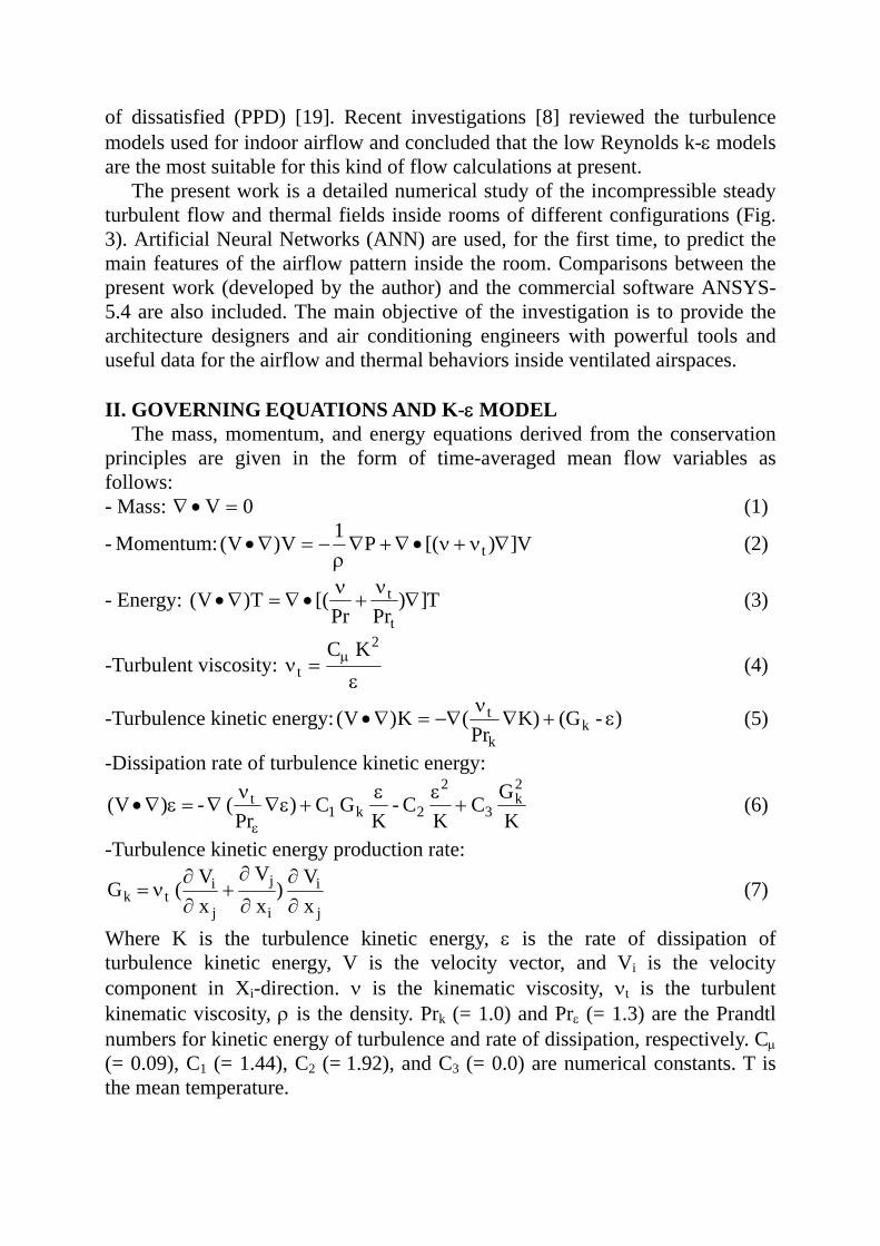
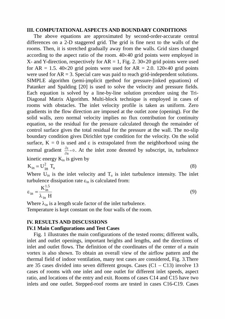
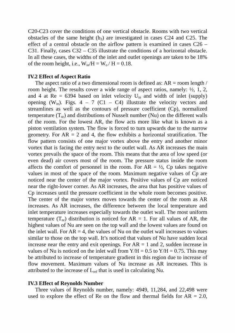
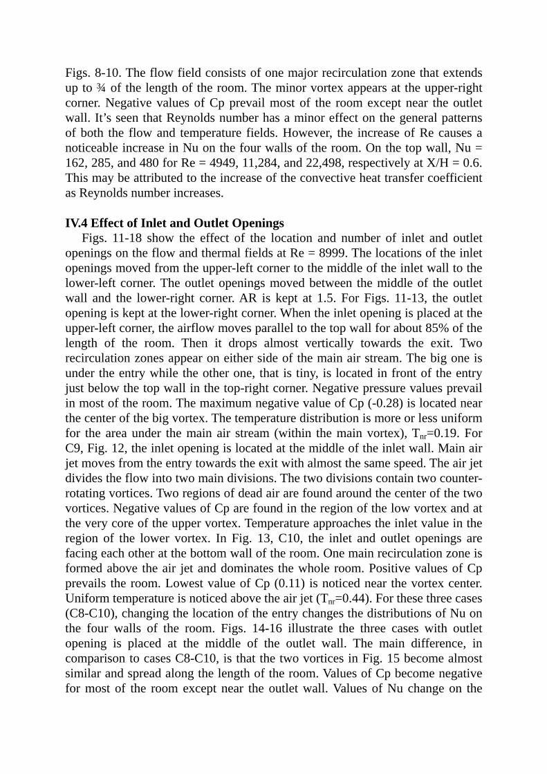
The aspect ratio of a two dimensional room is defined as: AR = room length / room height. The results cover a wide range of aspect ratios, namely: ½, 1, 2, and 4 at Re = 6394 based on inlet velocity Uin and width of inlet (supply) opening (Win). Figs. 4 – 7 (C1 – C4) illustrate the velocity vectors and streamlines as well as the contours of pressure coefficient (Cp), normalized temperature (Tnr) and distributions of Nusselt number (Nu) on the different walls of the room. For the lowest AR, the flow acts more like what is known as a piston ventilation system. The flow is forced to turn upwards due to the narrow geometry. For AR = 2 and 4, the flow exhibits a horizontal stratification. The flow pattern consists of one major vortex above the entry and another minor vortex that is facing the entry next to the outlet wall. As AR increases the main vortex prevails the space of the room. This means that the area of low speed (or even dead) air covers most of the room. The pressure status inside the room affects the comfort of personnel in the room. For AR = ½, Cp takes negative values in most of the space of the room. Maximum negative values of Cp are noticed near the center of the major vortex. Positive values of Cp are noticed near the right-lower corner. As AR increases, the area that has positive values of Cp increases until the pressure coefficient in the whole room becomes positive. The center of the major vortex moves towards the center of the room as AR increases. As AR increases, the difference between the local temperature and inlet temperature increases especially towards the outlet wall. The most uniform temperature (Tnr) distribution is noticed for AR = 1. For all values of AR, the highest values of Nu are seen on the top wall and the lowest values are found on the inlet wall. For AR = 4, the values of Nu on the outlet wall increases to values similar to those on the top wall. It’s noticed that values of Nu have sudden local increase near the entry and exit openings. For AR = 1 and 2, sudden increase in values of Nu is noticed on the inlet wall from Y/H = 0.5 to Y/H = 0.75. This may be attributed to increase of temperature gradient in this region due to increase of flow movement. Maximum values of Nu increase as AR increases. This is attributed to the increase of Lref that is used in calculating Nu.

IV.3 Effect of Reynolds Number

Three values of Reynolds number, namely: 4949, 11,284, and 22,498 were used to explore the effect of Re on the flow and thermal fields for AR = 2.0,

Figs. 8-10. The flow field consists of one major recirculation zone that extends up to ¾ of the length of the room. The minor vortex appears at the upper-right corner. Negative values of Cp prevail most of the room except near the outlet wall. It’s seen that Reynolds number has a minor effect on the general patterns of both the flow and temperature fields. However, the increase of Re causes a noticeable increase in Nu on the four walls of the room. On the top wall, Nu = 162, 285, and 480 for Re = 4949, 11,284, and 22,498, respectively at X/H = 0.6. This may be attributed to the increase of the convective heat transfer coefficient as Reynolds number increases.

IV.4 Effect of Inlet and Outlet Openings

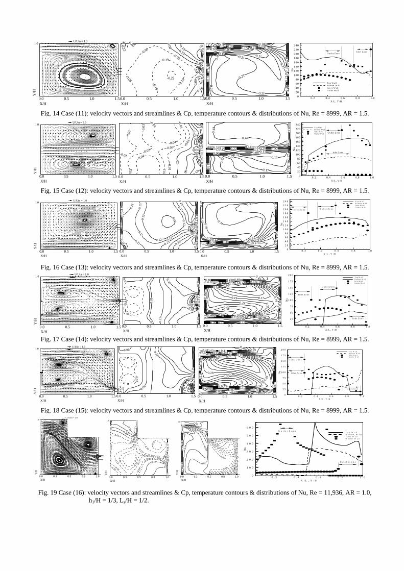
Figs. 11-18 show the effect of the location and number of inlet and outlet openings on the flow and thermal fields at Re = 8999. The locations of the inlet openings moved from the upper-left corner to the middle of the inlet wall to the lower-left corner. The outlet openings moved between the middle of the outlet wall and the lower-right corner. AR is kept at 1.5. For Figs. 11-13, the outlet opening is kept at the lower-right corner. When the inlet opening is placed at the upper-left corner, the airflow moves parallel to the top wall for about 85% of the length of the room. Then it drops almost vertically towards the exit. Two recirculation zones appear on either side of the main air stream. The big one is under the entry while the other one, that is tiny, is located in front of the entry just below the top wall in the top-right corner. Negative pressure values prevail in most of the room. The maximum negative value of Cp (-0.28) is located near the center of the big vortex. The temperature distribution is more or less uniform for the area under the main air stream (within the main vortex), Tnr=0.19. For C9, Fig. 12, the inlet opening is located at the middle of the inlet wall. Main air jet moves from the entry towards the exit with almost the same speed. The air jet divides the flow into two main divisions. The two divisions contain two counter-rotating vortices. Two regions of dead air are found around the center of the two vortices. Negative values of Cp are found in the region of the low vortex and at the very core of the upper vortex. Temperature approaches the inlet value in the region of the lower vortex. In Fig. 13, C10, the inlet and outlet openings are facing each other at the bottom wall of the room. One main recirculation zone is formed above the air jet and dominates the whole room. Positive values of Cp prevails the room. Lowest value of Cp (0.11) is noticed near the vortex center. Uniform temperature is noticed above the air jet (Tnr=0.44). For these three cases (C8-C10), changing the location of the entry changes the distributions of Nu on the four walls of the room. Figs. 14-16 illustrate the three cases with outlet opening is placed at the middle of the outlet wall. The main difference, in comparison to cases C8-C10, is that the two vortices in Fig. 15 become almost similar and spread along the length of the room. Values of Cp become negative for most of the room except near the outlet wall. Values of Nu change on the

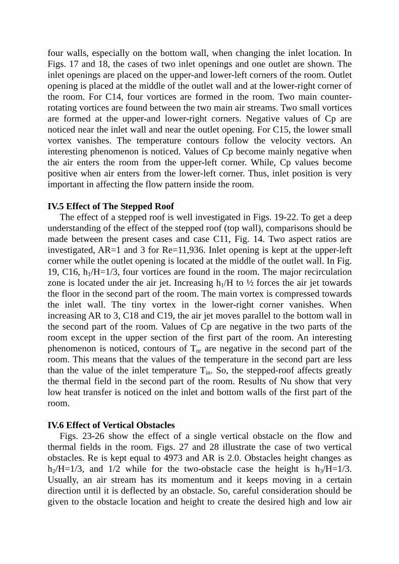
four walls, especially on the bottom wall, when changing the inlet location. In Figs. 17 and 18, the cases of two inlet openings and one outlet are shown. The inlet openings are placed on the upper-and lower-left corners of the room. Outlet opening is placed at the middle of the outlet wall and at the lower-right corner of the room. For C14, four vortices are formed in the room. Two main counter-rotating vortices are found between the two main air streams. Two small vortices are formed at the upper-and lower-right corners. Negative values of Cp are noticed near the inlet wall and near the outlet opening. For C15, the lower small vortex vanishes. The temperature contours follow the velocity vectors. An interesting phenomenon is noticed. Values of Cp become mainly negative when the air enters the room from the upper-left corner. While, Cp values become positive when air enters from the lower-left corner. Thus, inlet position is very important in affecting the flow pattern inside the room.

IV.5 Effect of The Stepped Roof

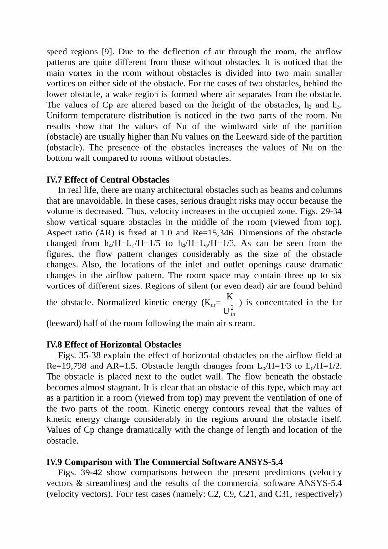
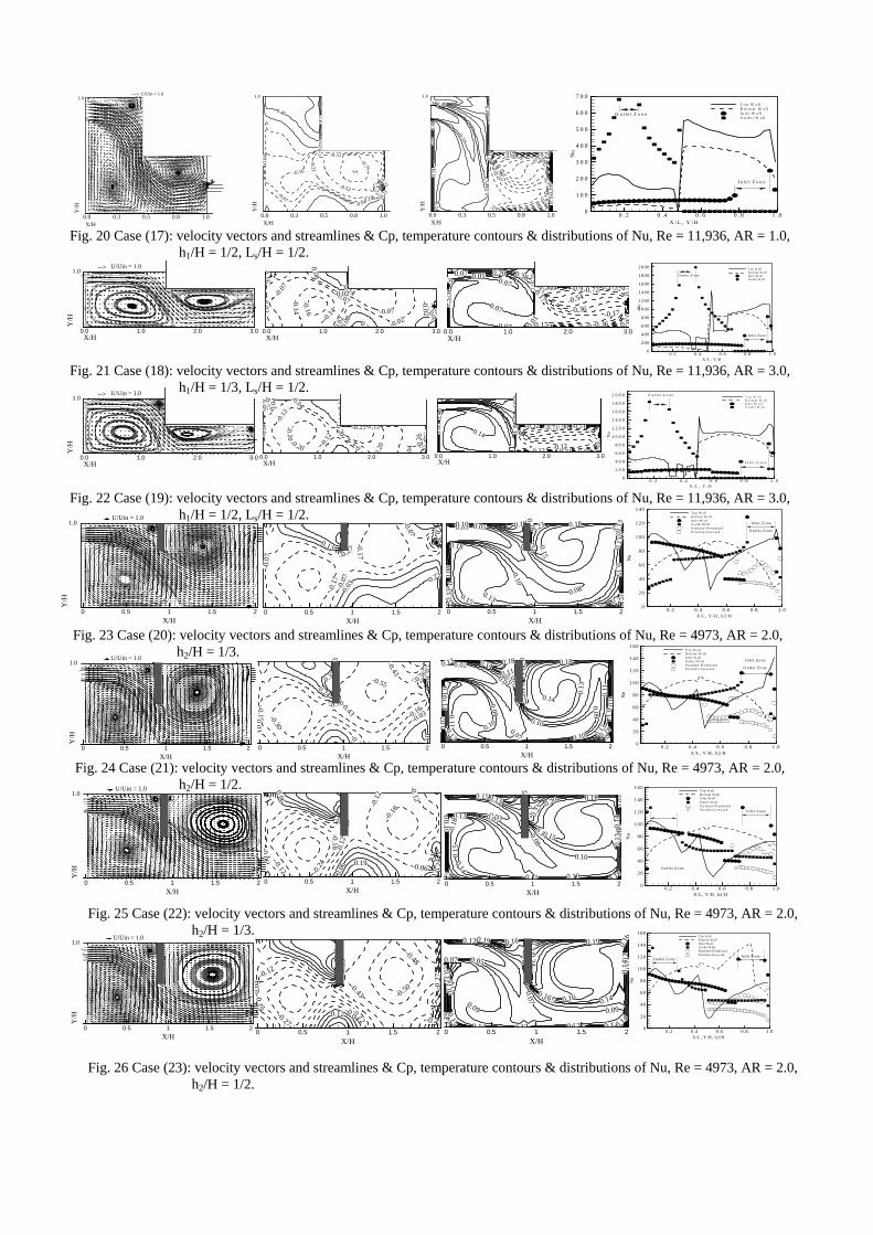
The effect of a stepped roof is well investigated in Figs. 19-22. To get a deep understanding of the effect of the stepped roof (top wall), comparisons should be made between the present cases and case C11, Fig. 14. Two aspect ratios are investigated, AR=1 and 3 for Re=11,936. Inlet opening is kept at the upper-left corner while the outlet opening is located at the middle of the outlet wall. In Fig. 19, C16, h1/H=1/3, four vortices are found in the room. The major recirculation zone is located under the air jet. Increasing h1/H to ½ forces the air jet towards the floor in the second part of the room. The main vortex is compressed towards the inlet wall. The tiny vortex in the lower-right corner vanishes. When increasing AR to 3, C18 and C19, the air jet moves parallel to the bottom wall in the second part of the room. Values of Cp are negative in the two parts of the room except in the upper section of the first part of the room. An interesting phenomenon is noticed, contours of Tnr are negative in the second part of the room. This means that the values of the temperature in the second part are less than the value of the inlet temperature Tin. So, the stepped-roof affects greatly the thermal field in the second part of the room. Results of Nu show that very low heat transfer is noticed on the inlet and bottom walls of the first part of the room. IV.6 Effect of Vertical Obstacles

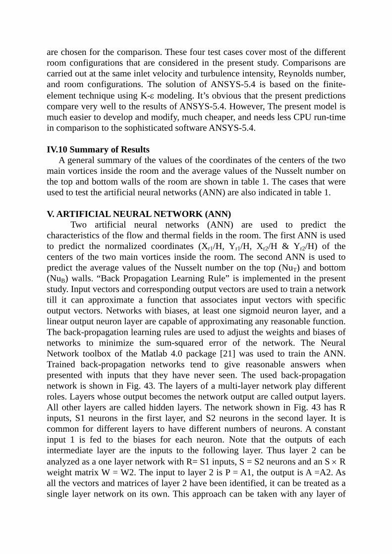
Figs. 23-26 show the effect of a single vertical obstacle on the flow and thermal fields in the room. Figs. 27 and 28 illustrate the case of two vertical obstacles. Re is kept equal to 4973 and AR is 2.0. Obstacles height changes as h2/H=1/3, and 1/2 while for the two-obstacle case the height is h3/H=1/3. Usually, an air stream has its momentum and it keeps moving in a certain direction until it is deflected by an obstacle. So, careful consideration should be given to the obstacle location and height to create the desired high and low air

speed regions [9]. Due to the deflection of air through the room, the airflow patterns are quite different from those without obstacles. It is noticed that the main vortex in the room without obstacles is divided into two main smaller vortices on either side of the obstacle. For the cases of two obstacles, behind the lower obstacle, a wake region is formed where air separates from the obstacle. The values of Cp are altered based on the height of the obstacles, h2 and h3. Uniform temperature distribution is noticed in the two parts of the room. Nu results show that the values of Nu of the windward side of the partition (obstacle) are usually higher than Nu values on the Leeward side of the partition (obstacle). The presence of the obstacles increases the values of Nu on the bottom wall compared to rooms without obstacles.

IV.7 Effect of Central Obstacles

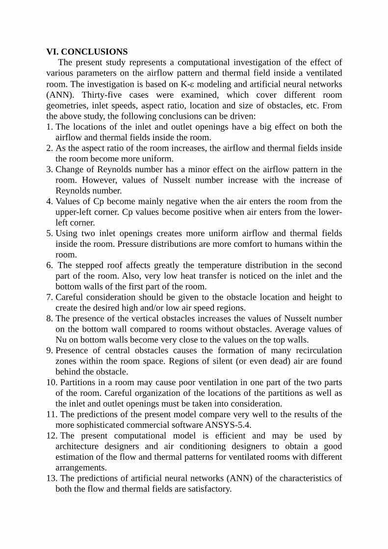
In real life, there are many architectural obstacles such as beams and columns that are unavoidable. In these cases, serious draught risks may occur because the volume is decreased. Thus, velocity increases in the occupied zone. Figs. 29-34 show vertical square obstacles in the middle of the room (viewed from top). Aspect ratio (AR) is fixed at 1.0 and Re=15,346. Dimensions of the obstacle changed from h4/H=Lo/H=1/5 to h4/H=Lo/H=1/3. As can be seen from the figures, the flow pattern changes considerably as the size of the obstacle changes. Also, the locations of the inlet and outlet openings cause dramatic changes in the airflow pattern. The room space may contain three up to six vortices of different sizes. Regions of silent (or even dead) air are found behind

the obstacle. Normalized kinetic energy (Knr= 2inU

K ) is concentrated in the far

(leeward) half of the room following the main air stream.

IV.8 Effect of Horizontal Obstacles Figs. 35-38 explain the effect of horizontal obstacles on the airflow field at

Re=19,798 and AR=1.5. Obstacle length changes from Lo/H=1/3 to Lo/H=1/2. The obstacle is placed next to the outlet wall. The flow beneath the obstacle becomes almost stagnant. It is clear that an obstacle of this type, which may act as a partition in a room (viewed from top) may prevent the ventilation of one of the two parts of the room. Kinetic energy contours reveal that the values of kinetic energy change considerably in the regions around the obstacle itself. Values of Cp change dramatically with the change of length and location of the obstacle. IV.9 Comparison with The Commercial Software ANSYS-5.4

Figs. 39-42 show comparisons between the present predictions (velocity vectors & streamlines) and the results of the commercial software ANSYS-5.4 (velocity vectors). Four test cases (namely: C2, C9, C21, and C31, respectively)

are chosen for the comparison. These four test cases cover most of the different room configurations that are considered in the present study. Comparisons are carried out at the same inlet velocity and turbulence intensity, Reynolds number, and room configurations. The solution of ANSYS-5.4 is based on the finite-element technique using K-ε modeling. It’s obvious that the present predictions compare very well to the results of ANSYS-5.4. However, The present model is much easier to develop and modify, much cheaper, and needs less CPU run-time in comparison to the sophisticated software ANSYS-5.4.

IV.10 Summary of Results

A general summary of the values of the coordinates of the centers of the two main vortices inside the room and the average values of the Nusselt number on the top and bottom walls of the room are shown in table 1. The cases that were used to test the artificial neural networks (ANN) are also indicated in table 1.

V. ARTIFICIAL NEURAL NETWORK (ANN)

Two artificial neural networks (ANN) are used to predict the characteristics of the flow and thermal fields in the room. The first ANN is used to predict the normalized coordinates (Xr1/H, Yr1/H, Xr2/H & Yr2/H) of the centers of the two main vortices inside the room. The second ANN is used to predict the average values of the Nusselt number on the top (NuT) and bottom (NuB) walls. “Back Propagation Learning Rule” is implemented in the present study. Input vectors and corresponding output vectors are used to train a network till it can approximate a function that associates input vectors with specific output vectors. Networks with biases, at least one sigmoid neuron layer, and a linear output neuron layer are capable of approximating any reasonable function. The back-propagation learning rules are used to adjust the weights and biases of networks to minimize the sum-squared error of the network. The Neural Network toolbox of the Matlab 4.0 package [21] was used to train the ANN. Trained back-propagation networks tend to give reasonable answers when presented with inputs that they have never seen. The used back-propagation network is shown in Fig. 43. The layers of a multi-layer network play different roles. Layers whose output becomes the network output are called output layers. All other layers are called hidden layers. The network shown in Fig. 43 has R inputs, S1 neurons in the first layer, and S2 neurons in the second layer. It is common for different layers to have different numbers of neurons. A constant input 1 is fed to the biases for each neuron. Note that the outputs of each intermediate layer are the inputs to the following layer. Thus layer 2 can be analyzed as a one layer network with R= S1 inputs, S = S2 neurons and an S × R weight matrix W = W2. The input to layer 2 is P = A1, the output is A =A2. As all the vectors and matrices of layer 2 have been identified, it can be treated as a single layer network on its own. This approach can be taken with any layer of

the network. It may be required to present a batch of Q input vectors to this network, at which time the matrix P will have the dimensions R × Q and the matrix A1 will have the dimensions S1 × Q. When a specific transfer function is to be used, the symbol for that transfer function will replace the ‘F’ shown in Fig. 43. The initial weights as well as the initial biases employed random values between 1 and -1. The nodes in the hidden layer were varied from 5 to 30 for every input pattern and the evaluation of the performance of the network in determining the optimum hidden nodes was carried out. Also, many training cases were operated to get the optimum transfer functions arrangement. The input to the neural network consists of the values of the aspect ratio (AR) as well as the main room configurations (hin/H, hout/H, h2/H & h3/H). This situation results in a neural network that consists of 5 input nodes and 4 output nodes for the flow field. As for the thermal field, the neural network consists of 5 input nodes and 2 output nodes. The neural network was trained for 14 different cases, namely: C1, C2, C3, C4, C5, C9, C11, C12, C13, C21, C22, C23, C24 & C25. After the ANN has been trained, a separate set of unseen test patterns is supplied as input to the ANN and its performance is evaluated. Fig. 44 shows a sample of the network error and its learning rate performance throughout the training for 11,134 epochs (epoch: the presentation of the set of training (input and/or target) vectors to a network and the calculation of new weights and biases). Results for many training cases that were operated to get the optimum number of neurons (S1) are presented in tables 2 and 3 for flow and thermal fields, respectively. Table 2 shows that best results are obtained for S1 = 200. For the thermal field, table 3, the best results are found for S1 = 1000. Considering the complexity of the flow pattern inside the rooms, the mentioned results are satisfactory for both the flow and thermal fields. The Author believes that the results will improve when more cases are considered for training the neural networks. However, the implementation of neural network is very promising for predicting the characteristics of the flow and thermal fields of complex flow patterns like those considered in the present study.

The use of neural networks has a major advantage over numerical predictions and experimental investigations. For neural networks, one can change any of the input vectors (room parameters) and predict the output vectors with minimum computational effort and run time. But, for numerical predictions, one has to change the room configurations, which requires considerably a lot of computational effort, and re-run the program. Then, the output is post-processed to obtain the required results. For experimental investigations, re-measuring the whole flow and thermal fields of the room is necessary when changing just one parameter of the room configuration.

VI. CONCLUSIONS The present study represents a computational investigation of the effect of

various parameters on the airflow pattern and thermal field inside a ventilated room. The investigation is based on K-ε modeling and artificial neural networks (ANN). Thirty-five cases were examined, which cover different room geometries, inlet speeds, aspect ratio, location and size of obstacles, etc. From the above study, the following conclusions can be driven: 1. The locations of the inlet and outlet openings have a big effect on both the

airflow and thermal fields inside the room. 2. As the aspect ratio of the room increases, the airflow and thermal fields inside

the room become more uniform. 3. Change of Reynolds number has a minor effect on the airflow pattern in the

room. However, values of Nusselt number increase with the increase of Reynolds number.

4. Values of Cp become mainly negative when the air enters the room from the upper-left corner. Cp values become positive when air enters from the lower-left corner.

5. Using two inlet openings creates more uniform airflow and thermal fields inside the room. Pressure distributions are more comfort to humans within the room.

6. The stepped roof affects greatly the temperature distribution in the second part of the room. Also, very low heat transfer is noticed on the inlet and the bottom walls of the first part of the room.

7. Careful consideration should be given to the obstacle location and height to create the desired high and/or low air speed regions.

8. The presence of the vertical obstacles increases the values of Nusselt number on the bottom wall compared to rooms without obstacles. Average values of Nu on bottom walls become very close to the values on the top walls.

9. Presence of central obstacles causes the formation of many recirculation zones within the room space. Regions of silent (or even dead) air are found behind the obstacle.

10. Partitions in a room may cause poor ventilation in one part of the two parts of the room. Careful organization of the locations of the partitions as well as the inlet and outlet openings must be taken into consideration.

11. The predictions of the present model compare very well to the results of the more sophisticated commercial software ANSYS-5.4.

12. The present computational model is efficient and may be used by architecture designers and air conditioning designers to obtain a good estimation of the flow and thermal patterns for ventilated rooms with different arrangements.

13. The predictions of artificial neural networks (ANN) of the characteristics of both the flow and thermal fields are satisfactory.

14. ANN is a very promising technique for predicting the complex flow and thermal fields inside a room especially when many cases are considered for training ANN.

REFERENCES [1] Lee, I.-B., and Short, T. H., 2000, “Two-Dimensional Numerical Simulation

of Natural Ventilation in a Multi-Span Greenhouse,” Transactions of the ASAE, Vol. 43(3), pp. 745-753.

[2] Lee, I.-B., and Short, T. H., 2001, “Verification of Computational Fluid Dynamic Temperature Simulations in a Full-Scale Naturally Ventilated Greenhouse,” Transactions of the ASAE, Vol. 44(1), pp. 119-127.

[3] Wu, B., and Gebremedhin, K. G., 2001, “CFD Development and Simulation of Flow Fields in Ventilated Spaces with Multiple Occupants,” Transactions of the ASAE, Vol. 44(6), pp. 1839-1850.

[4] Reichrath, S., and Davies, T. W., 2001, “CFD Modelling of the Internal Environment of Commercial Multi-Span Venlo-Type Glasshouse,” Paper# 014054, 2001 ASAE Annual Meeting, Sacramento, CA, USA, July 29 – Aug. 1, 2001.

[5] Reichrath, S., and Davies, T. W., 2002, “Computational Fluid Dynamics and Glasshouse Research,”Proceedings of the World Congress of Computers in Agriculture and Natural Resources, Iguacu Falls, Brazil, March 13-15 , 2002, pp. 175-182.

[6] Sun, H., Keener, H., Stowell, R. R., and Michel, F. C., 2001, “Three-Dimensional Numerical Simulation of Mechanical Ventilation,” Paper# 014049, 2001 ASAE Annual Meeting, Sacramento, CA, USA, July 29 – Aug. 1, 2001.

[7] Verboven, P., Datta, A. K., Scheerlinck, N., Nicolai, B. M., 2001, “Computation of Airflow Effects on Heat and Mass Transfer in a Microwave Oven,” Paper# 013013, 2001 ASAE Annual Meeting, Sacramento, CA, USA, July 29 – Aug. 1, 2001.

[8] Elhadidi, B., and Sherif, A., 2001, “Computational Study of Flow in Mechanically Ventilated Spaces,” Paper# 2001058, Proceedings of the Seventh International Conference of Fluid Dynamics and Propulsion, Cairo, Egypt, Dec. 18-20, 2001.

[9] Salman, A. A., 2001, “CFD Investigation of Airflow in a chamber under Different Air Speed, Aspect Ratio, and Outlet Location Using Explicit MacCormack Scheme,” Proceedings of the Nineth International Conference on Aerospace Sciences & Aviation Technology, Military Technical College, Cairo, Egypt, May 8-10, 2001.

[10] Salman, A. A., 2001, “Numerical Prediction of Airflow Patterns in a 2-D Room Model under Different Ceiling Shape with and without Passive Control,” Proceedings of the Seventh International Conference of Fluid Dynamics and Propulsion, Cairo, Egypt, Dec. 18-20, 2001.

[11] Zhao, L., Zhang, Y., Wang, X., Riskowski, G. L., and Charistianson, L. L., “Development of Particle Image Velocimetry Techniques for Measurement of Room Airflow Patterns in Ventilated Airspaces,” Web site: http://www.age.uiuc.edu/bee/research/piv/Pivpaper2.htm

[12] Zhao, L., Zhang, Y., Christianson, L. L., and Riskowski, G. L., 1998, “Measurement of Aerosol Concentration and Transportation in Ventilated Airspaces Using Particle Image Techniques,” Paper# 984064, 1998 ASAE Annual International Meeting, Orlando, Florida, USA, July 12 – 16, 1998.

[13] Zhao, L., Zhang, Y., Wang, X., Riskowski, G. L., and Christianson, L. L., 1999, “Measurement of Airflow Patterns in Ventilated Spaces Using Particle Image Velocimetry,” Paper# 994156, 1999 ASAE Annual International Meeting.

[14] Ginger, J. D., and Letchford, C. W., 1999, “Net Pressures on a Low-Rise Full-Scale Building,” J. Wind Eng. Ind. Aerodyn., Vol. 83, pp. 239-250.

[15] Bjerg, B., Svidt, K., Zhang, G., Morsing, S., and Jhonsen, J. O., 2001, “Numerical Simulation of Airflow in a Room with Multiple Wall Inlets,” Livestock Environment VI: Proceedings of the 6th International Symposium, May 21-23, 2001, Louisville, Kentucky, USA, ed. Stowell, R. R., Bucklin, R., and Bottcher, R. W, pp. 285-292.

[16] Kettlewell, P. J., Hoxey, R. P., Hartshorn, R. L., Meeks, I. R., and Twydell, P., 2001, “Controlled Ventilation System for Livestock Transport Vehicles,” Livestock Environment VI: Proceedings of the 6th International Symposium, May 21-23, 2001, Louisville, Kentucky, USA, ed. Stowell, R. R., Bucklin, R., and Bottcher, R. W, pp. 556-563.

[17] Reichrath, S., and Davis, T. W., 2001, “Experimental Analysis of the Internal Airflow in a Commercial Multi-span Venlo-Type Glasshouse,” Paper# 014057, 2001 ASAE Annual Meeting, Sacramento, CA, USA, July 29 – Aug. 1, 2001.

[18] Yu, H., 2001, “Experimental Determination of Airflow Performance in Ceiling Slot-Ventilated Enclosure under Isothermal Condition,” Paper# 014049, 2001 ASAE Annual Meeting, Sacramento, CA, USA, July 29 – Aug. 1, 2001.

[19] Hassan, M. A., Shaalan, M. R., and El-Shazly, K. M., 2002, “Energy Efficient Buildings: Investigation of Thermal Comfort,” Proceedings of the World Renewable Energy Congress VII, Cologne, Germany, June 29 – July 5, 2002.

[20] Patanker, S. V., and Spalding, D. B., 1972, “A Calculation Procedure for Heat, Mass and Momentum Transfer in Three-Dimensional Parabolic Flows,” Int. J. Heat and Mass Transfer, Vol. 15, pp. 1787-1806.

[21] Demuth, H., and Beale, M., 1992, Neural Network-Toolbox-for Use with Matlab, The Math Works, Inc.

NOMENCLATURE

ANN = artificial neural networks. AR = aspect ratio of the room =

height roomlength room = L / H.

CFD = computational fluid dynamics. Cp = static pressure coefficient =

qP P in− .

C1, C2, C3, Cμ: coefficients of turbulence modeling. GK = turbulence kinetic energy production rate. H = room height. h1 = height of the step in the stepped-room. h2 = height of the single vertical obstacle. h3 = height of each of the vertical obstacles for double-obstacle case. h4 = height of the central obstacle. hf = convection heat transfer coefficient. hi = height of the center of the main inlet (supply) opening (zone). his = height of the center of the secondary inlet (supply) opening (zone). ho = height of the center of the outlet (exit) opening (zone). IAQ = indoor air quality. K = turbulence kinetic energy. Kin = inlet turbulence kinetic energy. Knr = normalized kinetic energy =

2inU

K .

kf = conductive heat transfer coefficient of air. L = room length. Lref = reference length = room length (L). Ls = length of the step in the steped-room. Lo = length of both the central and horizontal obstacles. Nu = Nusselt number =

)T - (T kL h

fwf

reff××

NuB = average Nusselt number on the bottom wall. NuT = average Nusselt number on the top wall. P = static pressure. Pin = inlet static pressure. Pr = Prandtl number. Prt = turbulent Prandtl number. Prε and PrK = Prandtl numbers for ε and K, respectively. PMV = predicted mean vote (a thermal comfort index). PPD = predicted percentage of dis-satisfied (a thermal comfort index). q = inlet dynamic pressure. Re = Reynolds number =

νinin WU .

T = Mean temperature. Tf = flow temperature. Tin = inlet temperature. Tnr = normalized temperature =

in

inT

TT − .

Tu = inlet turbulence intensity. Tw = wall temperature. Uin = inlet (supply) velocity. V = velocity vector. Vi = velocity component in Xi-direction. u, v = velocity components in X- and Y-direction, respectively. Win = width of inlet (supply) opening (zone). Wo = width of outlet (exit) opening (zone). X, Y = coordinates in the horizontal and vertical directions, respectively. Xr1, Yr1 = coordinates of the center of the first main vortex, nearest to inlet

wall. Xr2, Yr2 = coordinates of the center of the second main vortex. ε = turbulence dissipation rate. εin = inlet turbulence dissipation rate. λin = length scale factor of the inlet turbulence. ν = kinematic viscosity of air. νt = turbulent kinematic viscosity. ρ = air density.

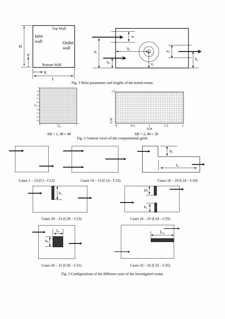
Fig. 1 Main parameters and lengths of the tested rooms.

AR = 1, 40 × 40 AR = 2, 40 × 20 Fig. 2 General views of the computational grids.

Cases 1 – 13 (C1 - C13) Cases 14 – 15 (C14 – C15) Cases 16 – 19 (C16 – C19)

Cases 20 – 23 (C20 – C23) Cases 24 – 25 (C24 – C25)

Cases 26 – 31 (C26 – C31) Cases 32 – 35 (C32 – C35)

Fig. 3 Configurations of the different cases of the investigated rooms.

H

Y

XL

Top Wall

Bottom Wall

Inlet wall Outlet

wall

Ls

h1

h2

h3

h3

Lo Lo

h4

hi

his

wi

ho

wo Xr

Yr

0 0.5 1 1.5 2X/H

Y/H

1.0

0 0.5 1X/H

0.1

0.2

0.3

0.4

0.5

0.6

0.7

0.8

0.9

1

Y/H

0.0 0.5 1.0X/H

0.1

0.2

0.3

0.4

0.5

0.6

0.7

0.8

0.9

1.0

Y/H U/U

in=

1.0

0.2 0.4 0.6 0.8 1.0X/L, Y/H

0

10

20

30

40

50

60

70

80

90

100

110

120

130

140

150

Nu

Top WallBottom WallInlet WallOutlet Wall

Inlet Zone

Outlet Zone

0.2 0.4 0.6 0.8 1.0X/L, Y/H

0

10

20

30

40

50

60

70

80

90

Nu

Top WallBottom WallInlet WallOutlet WallInlet Zone

Outlet Zone

X

0.1

0.2

0.3

0.4

0.5

0.6

0.7

0.8

0.9

1

0.50

U/U

in=

1

X

0.1

0.2

0.3

0.4

0.5

0.6

0.7

0.8

0.9

1

-1.91-1.74-0.84

-0.67

-0.65

-0.6

0

-0.67

-0.55

-0.55

-0.5 5- 0.49

-0.49

-0.49

-0.4

0-0.40

-0.4

0

-0.31 -0.31

-0.31

-0.1

3

-0.13

-0.1

3

0.05 0.05

0 22

0.22

0.50

X

0.1

0.2

0.3

0.4

0.5

0.6

0.7

0.8

0.9

1

0.02

0.02

0.060.06

0.10

0.10

0.10

0.14

0.14

.14

0.14

0.18

0.18

0.18

0 .1 8

0.22

0.22

0.22

0.26

0.26

0.26

0.3 00.

30

0.30

0.3 4

0.34

03 8

0.38

0.38

0. 3 8

0.50

0.0 0.5 1.0X/H

0.1

0.2

0.3

0.4

0.5

0.6

0.7

0.8

0.9

1.0

-1.2

3-0

.69-0.56

-0.42-0.15

-0.10

-0.10

-0.1 0

-0.02

-0.02 -0.02

-0.02

-0.0

2

0.12

0.12

0.12

0.120.

1 2

012 0.12

0.12

0.2

0.25

0.25

0.25

0.25

0.39

0.39

0.39

0.390.53

0.53

0.53

0.0 0.5 1.0X/H

0.1

0.2

0.3

0.4

0.5

0.6

0.7

0.8

0.9

1.0

0.0240.024

0.0710.071

0.071

0.071

0.07

1

0.118

0.118

0.11

8

0.118

0.118

0.118

0.1650.165

0.16

5

0.165

0.165

0.16

5

0.16 5

212 0.212

0.21

2

0.212

0.212

0 212

0.21

2

0.212

0.220

0.222

0.22

2

0.222

0.2220.222

0.22

2

0.222

0 222

0.22

2

0.2 220.220

0.2350.2350.235

0.235

0.235

0.23

50.

2 35

0.225

0.282

0.2820.282

0.28

2

0.282

03 2

0.329

0.329

0.329

0 .32

9

0.3290.306

376

0376

0.37

6

0.37

60.

376

0.0 0.5 1.0 1.5 2.0X/H

Y/H

1.0U/Uin = 1.0

0.0 0.5 1.0 1.5 2.0X/H

-0.120

05

0.05

0 .0 9

00 90 .

1 0

0.12

0.10

0 .1 2

0.12 0.12

0.120.14

0.14

0.14

0.14

0.1 8

0.18

0.18 0.18

0.18

0.1

0.14

0.22

0.22

0.22 0.22

0.31

0.31

0.31

0.39

0.390.48

0.57

0.0 0.5 1.0 1.5 2.0X/H

0 080

020.06 0.060.10 0.100.14 0.140.18 0.18

0.18

0.180 300.22

0.22

0.220.26 0.26

0.26

0.26

0.28 0.28

0.280.28

0.28

0.30 0.300.30

0.30

0.300.34

0.34

0.34

0.38

0.38

03 8

0.38

0.2 0.4 0.6 0.8 1.0X/L, Y/H

25

50

75

100

125

150

175

200

Nu


Inlet Zone

Outlet Zone

0.0 1.0 2.0 3.0 4.0X/H

Y/H

1.0

0.0 1.0 2.0 3.0 4.0X/H

Y/H

-0.27

0.09

0.17

0.17

0.19

0.19

0.21

0210.

24 0.24

0.31 0.310.39

0.39

0.46

0.53

1.0

0.0 1.0 2.0 3.0 4.0X/H

Y/H 0.04

0.04

0 2007 0 070.09 0.110.13 0 130.16 0.160.180.20 0.20

0 200.22 0.22

0.22

0 220.24

0.240.

24

0.27

0.27

0.27

0.29

0.29 029

0.3

0.310.31

031

0.330.36 036

0.38

038

1.0

0 .2 0 .4 0 . 6 0 . 8 1 . 0X /L , Y /H

0

1 0 0

2 0 0

3 0 0

4 0 0

5 0 0

Nu

T o p W a llB o tto m W a l lIn le t W a llO u tle t W a llI n le t Z o n e O u tle t Z o n e

Fig. 4 Case (1): velocity vectors and streamlines & Cp, temperature contours & distributions of Nu, Re = 6394, AR = ½.

Fig. 5 Case (2): velocity vectors and streamlines & Cp, temperature contours & distributions of Nu, Re = 6394, AR = 1.


Fig.7 Case (4): velocity vectors and streamlines & Cp, temperature contours & distributions of Nu, Re = 6349, AR = 4.

Y/H

/H /H /H

U/Uin = 1.0

Tnr - contours

Fig. 12 Case (9): velocity vectors and streamlines & Cp, temperature contours & distributions of Nu, Re = 8999, AR = 1.5. Fig. 13 Case (10): velocity vectors and streamlines & Cp, temperature contours & distributions of Nu, Re = 8999, AR = 1.5.

0 .2 0 .4 0 .6 0 .8 1 .0X /L , Y /H

0

5 0

1 0 0

1 5 0

2 0 0

2 5 0

3 0 0

Nu

T o p W a llB o tto m W a llIn le t W a llO u tle t W a ll

In le t Z o n eO u tle t Z o n e

0.0 0.5 1.0 1.5 2.0X/H

Y/H

-0.89-0.72-0

.46

-0.29

-0.15

-0.15

-0.15

-0.12

-0.12

-0.12

-0.07

0.07

-0.07

-0.07

-0.07

-0.0

3

0.07

-0.03

-0.03

-0.0

3

0.05

0.0 5

0.05

0.22

0.14

0.22

0.22

0.22

0.31

1.0

0.0 0.5 1.0 1.5 2.0X/H

Y/H

U/Uin = 1.01.0

0.0 0.5 1.0 1.5 2.0X/H

Y/H

0.020.09

0.09.09

0.0

0.16

0.160.16

0.16

0.16

0.22

0.22 0.22

0.22

0.29

0.29 0.29

0.29

036

0.3 6

1.0

0 . 2 0 . 4 0 . 6 0 . 8 1 . 0X /L , Y / H

0

2 5

5 0

7 5

1 0 0

1 2 5

1 5 0

1 7 5

2 0 0

Nu

T o p W a llB o t t o m W a llI n l e t W a l lO u t l e t W a l l

I n l e t Z o n e

O u t le t Z o n e

0.0 0.5 1.0 1.5 2.0X/H

Y/H

U/Uin = 1.01.0

0.0 0.5 1.0 1.5 2.0X/H

-0.1

6

-0.21

-0.1 2

-0.12

-0.12

-0.07

-0.07-0.0

7

-0.07

-0.0

7

-0.04

-0.0

4

-0.04

0.04

-0.07

0.05

0.05

0.05

0.14 0.22

0.31

1.0

0.0 0.5 1.0 1.5 2.0X/H

0.020.09

0.09.090.16

0.16

0.16

0.16 0.160.16

0.09

0.22

0.22 0.220.22

0.29

0.29 0.29

0.29

036

0 .361.0

0.0 0.5 1.0 1.5 2.0X/H

Y/H

U/Uin = 1.01.0

0.0 0.5 1.0 1.5 2.0X/H

-0.83-0.74-0.65-0.56

-0.2

1

-0.16

-0.16

-0.1

6

-0.13

-0.1

3

-0.13

-0.30

-0.09

-0.0

9

-0.09

009

-0.13

-0.0

4

-0.04

-0.09

0.05

0.05

0.05

0.14

0 23

0.23

0.23

0.311.0

0.0 0.5 1.0 1.5 2.0X/H

0.02 0.020.09

0.090.090.16

0.16

0 16

0.160.16

0.16

0.220.22 0.22

0.22

0 22

0.29

0.29 0.29

0.29

0.36

0.36

1.0

0.0 0.5 1.0 1.5X/H

Y/H

1.0U/Uin = 1.0

0.0 0.5 1.0 1.5X/H

-0.85

-0.28

-0.28

-0.2

4 -0.24

-0.50

0.1 5

-0.15

-0.15

-0.1

5-0.07

-0.07

-007

0.07

-0.07

-007

0.02

002

0.02

0.11

0.11

0.11

0.11

0.20

0.20

0.28

0.0 0.5 1.0 1.5X/H

0.030.09

0.09

0.09

0.15

0.15

0.15

0.19

0.19

0.190.19

0.19

0.190.19

0 24

0.24

0.24 0.24

0.24

0.29

0.29

0.29 0.29

0.29

0.35

0.35 0.35

0.350. 35

0 .41

0.41

0.41

047

0.47

0.47

0.2 0.4 0.6 0.8 1.0X/L, Y/H

020406080

100120140160180200220240

Nu

Top WallBottom W allInlet WallOutlet Wall

Inlet ZoneOutlet Zone

0 .2 0 .4 0 .6 0 .8 1 .0X /L , Y /H

05 0

1 0 01 5 02 0 02 5 03 0 03 5 04 0 04 5 05 0 05 5 06 0 0

Nu

T o p W allB otto m W allIn let W a llO u tlet W a ll

In le t Z o neO u tle t Z o ne

0.0 0.5 1.0 1.5X/H

Y/H

1.0U/Uin = 1.0

0.0 0.5 1.0 1.5X/H

-0.23

-0.19 -0.1

9

-0.15

0.15

-0.15

-0.11

-0.1

1

-0.06

-0.06

-0.0

2 -0.02

-0.02

002

0.02

0.02

0. 02

002

0.02

0.020.07

0.07

0.07

0.07

0.07

0.07

0.07

0 .1 1

0.11

0.11

0.11

0.110.

110.

11

0.15

0.15

0.15

0.150.

15

0.20

0.20

0.20

0.24

0.240.240.28 0.

32

0.0 0.5 1.0 1.5X/H

0.16

0.19

0.22

0.25

0.28

0.30

0.30

0.31

0.31

0.34

0.41

0.41

0.41

0.44

0. 44

0.47

0.2 0.4 0.6 0.8 1.0X/L, Y/H

020406080

100120140160180200220240

Nu


Inlet ZoneOutlet Zone

0.0 0.5 1.0 1.5X/H

Y/H

1.0U/Uin = 1.0

0.0 0.5 1.0 1.5X/H

0.00

000

0.00

0.03

003

003

003

0 .06

0.06

0 .0 9

0.0 9 0.100.10

0.11

0.10

0.11

0.06

0.10

0.11

0.12

0.12

0.12

0.12

0.120.15

0.15

0.15

0.15

0.15

0.15

0.15

0.15

0.1 8

0. 18

0.18

0.18

0.18

0.180.

18

0.210.21

0.2 1

0.21

0.21

0.21

0.24

0.24

0.24

0.24

0.24

0.27

0.27 0.3

0

0.33

0.330.

360.42

0.0 0.5 1.0 1.5X/H

0.03 0.08 0.080.08 0.00.14 0.14 0.080.19 0.19

0.170.25 0.25

0 250.31 0.31.36 0.36

0.360.42 0.42

0.42

.44 0.440.44

0.44

0.44

0.44

0.2 0.4 0.6 0.8 1.0X/L, Y/H

020406080

100120140160180200220240

Nu


Inlet Zone

Outlet Zone


Fig. 9 Case (6): velocity vectors and streamlines & Cp, temperature contours & distributions of Nu, Re = 11,248, AR = 2.

Fig.10 Case (7): velocity vectors and streamlines & Cp, temperature contours & distributions of Nu, Re = 22,498, AR = 2.

Fig.11 Case (8): velocity vectors and streamlines & Cp, temperature contours & distributions of Nu, Re = 8999, AR = 1.5.

0.0 0.5 1.0 1.5X/H

Y/H

1.0U/Uin = 1.0

0.0 0.5 1.0 1.5X/H

-0.47

-0.66

-0.28

-0.22

-0.22

-0.19

-0.19

-0.19

-0.09

-0.09-0.09

-0.0

9

0.00

0.00

0.00

0.00

0.10

0.10

0.10

0.10

0.19

0.19

0.19

0.29

0.0 0.5 1.0 1.5X/H

0.030.030.09

0.090.09

0.0

0.15 0.15

0.15

0.09

0.21

0.21

0.21

0.21

0.21 0.21

0.21

0.26

0.26

0.26 0.26

0.26

0 .32

0.32 0.32

0.32

0.38

0.38 0.38

0.38

0.40.44

044

0 .44

0 .2 0 .4 0 .6 0 .8 1 .0X /L , Y /H

02 04 06 08 0

10 012 014 016 018 020 022 024 0

Nu

T o p W allB o tto m W allIn le t v W allO u tle t W all

In le t Z o neO u tle t Z one

0.0 0.5 1.0 1.5X/H

Y/H

1.0U/Uin = 1.0

0.0 0.5 1.0 1.5X/H

-0.2

0-0

. 13-0.10-0.07

-0.04

-0.04

-0.04-0.10

0.03

-0.03

-0.0

3

0.03

-0.03

-0.03

-0.01

-0.0

1

-0.0 1

-0.0

1

-0.01

0.02

0. 02

002

002

0.06

0.06

0.06

0.06

0.09

0.12

0.12

0.15

0.150.18

0.0 0.5 1.0 1.5X/H

0.06 0.060.06

0.11 0.11

0.110.11

0.17

0.17

0.17

0.17 0.17

0.22

0.22 0.22

0.22

0.28

0.28 0.28

0.280 .33

0.33 0.33

0.33

0.39

0.39 0.39

0.39

.44 0.44

0.44

0.44

0. 44

0 .2 0 .4 0.6 0.8 1.0X /L , Y /H

020406080

100120140160180200220240

Nu

Top W allB ottom W allInlet W allO utlet W all

In let Z one

O utlet Z one

0.0 0.5 1.0 1.5X/H

Y/H

1.0U/Uin = 1.0

0.0 0.5 1.0 1.5X/H

-0.60-0.42

-0.060 .03

0.03

0.06

006

00 6

0.03

0.06

0.12

0 .12

0.12

0.12

0.12

0.1 20.1 2

0.150. 15

0.15

0.15

0.15

0.15

0.15

0.15

0.21 0.21

0.21

0.21

0.21

0.21

0.21

0.30

0.39

0.39 0.390.48

0.57

0.0 0.5 1.0 1.5X/H

0.060.28 0.080.11

0.14

0 14

0.170.190.22

0.220 36

0.250.280.31

0.310.33

0.33

0.34

0.34

0.36

0.36

0.36

0 44

0.390.42

0.42

0.42

0.44

0.47

0.4

0 . 2 0 . 4 0 . 6 0 . 8 1 . 0X /L , Y /H

02 04 06 08 0

1 0 01 2 01 4 01 6 01 8 02 0 02 2 02 4 0

Nu

T o p W a llB o tto m W a llI n l e t W a llO u t l e t W a l l

I n l e t Z o n e O u t l e t Z o n e

0.0 0.5 1.0 1.5X/H

Y/H

1.0U/Uin = 1.0

0.0 0.5 1.0 1.5X/H

-1.56 -1.0

3

-0.67

-0.49

-0.01

-0.0

1

-0.0

0.03

0.0

0.03

0.0 5

-0.13

0.15

0.15

0.220.30

0.30

0.40

0.40

0.0 0.5 1.0 1.5X/H

0.02

0.02

0.05

0.05

0.07

0.07

0.10

0.100.

10

0.12

0.12

0.12

0 14

0.14

0.140.14

0.17

0.17

0.17

0.19

0.19

0.19

0.19

0 21

0.21

0.21

.24

0.24

0.24

0 26

0.26

0.26

0.26

0.29

0.29

0.290.31

0.31

0.31

0.33

0.33

0.33

0.3 6

0.360.

36

0.38

0.38 0.38

0.40

0.40

0.43

0.430.45

0.48

0.48

0.48

0 .2 0 . 4 0 .6 0 .8 1 .0X /L , Y /H

2 5

5 0

7 5

1 0 0

1 2 5

1 5 0

1 7 5

2 0 0

Nu

T o p W a llB o tto m W a llIn le t W a llO u tle t W a ll

In le t Z o n e

O u tle t Z o n e

In le t Z o n e

0.0 0.5 1.0 1.5X/H

Y/H

1.0U/Uin = 1.0

0.0 0.5 1.0 1.5X/H

-0.1

1

-0.11

-0.03

-0. 02

0.06

0.06

0.06

0.23

0.23

0.35

0.0 0.5 1.0 1.5X/H

0.02 0.04

0.04

0.240.07

0.07

0.090.09

0.09

0.11

0.11

0 13

0.13

0 15

0.15

0.15

0 15

0.17

0.17

0.17

0.20

0.20

.20

0.22

0.22

0.24

0.30

0.24

0.26

0.26

0.26

0.28

.28

0.28

0.30

0.30

0.33

0.33

0.40.35

0.35

0.35

0.35

0.37

0.37

0 3

0.39

0.39

0.41

0.410.43

0.43

0.46

0.48

0.48

0.48

0 . 2 0 . 4 0 . 6 0 . 8 1 . 0X / L , Y / H

0

2 5

5 0

7 5

1 0 0

1 2 5

1 5 0

1 7 5

2 0 0

Nu

T o p W a l lB o t to m W a l lI n l e t W a l lO u t l e t W a l l

I n l e t Z o n e

O u t l e t Z o n e

I n l e t Z o n e

0.0 0.3 0.5 0.8 1.0X/H

Y/H

1.0U/Uin = 1.0--->

0.0 0.3 0.5 0.8 1.0X/H

Y/H

-1.53

-0.88-1.04

-0.55

-0.55

-0.55

-0.5

0

-0.39 -0. 3

9

-0.39

-0.23

-0.23

-0.2

3

-0.23

-0.1

8

-0.18

-0.55

-0.18-0.23

-0.16

-0.16

-0.1

6

-0.16

-0.1

6

-0.16

-0.13

-0.13

-0.13

-0.1

3

-0.13

-0.1

3

-0.06

-0.0

6

-0.06

-0.0

6-0

.06

-0.06

-0.0

6

-0.06

-0.02

-0. 0

2

-0.02 -0.0

2

-0.02

-0.0 2-0.02

010

0.10

0.10

0.1

0.26

0.26

0.26

0.43

0.4

0.59

0.5

0.75

1.0

0.0 0.3 0.5 0.8 1.0X/H

Y/H

0.91

-0.91 -0.91

-0.91

-0.75

-0.7 5-0.75

-0.7

5

-0.75

-0.58

-0.58

-0.58 -0.58

- 0.5

8-0.58

-0.41

-0.4

1

-0.41

-0.41

-0.41

-0.50

-0.25

-0.25

-0.25

-0.33

-0.25-0.41

-0.08

-0.08

-0.0

8 -0.33-0.16

0.02

0.02

0.02

0.02

.02

0.02

0.02

0.09

0.09

0.090.09

0.090.09

0.17

0.09

0 .25

0.25

0.25

0.25

0.25

0.25

0.4 2

0.4 2

0.42

0.420.42

0.42

0.42

0.58

0.58

0.58

0.58

0.580.67

0.58

1.0

0 . 2 0 . 4 0 . 6 0 . 8 1 . 0X / L , Y / H

0

1 0 0

2 0 0

3 0 0

4 0 0

5 0 0

6 0 0

Nu

T o p W a l lB o t t o m W a l lI n l e t W a l lO u t l e t W a l l

O u t l e t Z o n e

I n l e t Z o n e

Fig. 14 Case (11): velocity vectors and streamlines & Cp, temperature contours & distributions of Nu, Re = 8999, AR = 1.5.





Fig. 19 Case (16): velocity vectors and streamlines & Cp, temperature contours & distributions of Nu, Re = 11,936, AR = 1.0, h1/H = 1/3, Ls/H = 1/2.

0 .2 0 .4 0 .6 0 .8 1 .0X /L , Y /H , h 2 /H

0

2 0

4 0

6 0

8 0

1 0 0

1 2 0

1 4 0

Nu

T o p W allB otto m W allIn le t W allO utle t W allP artitio n -W in d w ardP artitio n -L eew ard O u tle t Z o ne

In le t Z on e

0 0.5 1 1.5 2X/H

-0.38

-0.27

-0.1

7

-0.17

-0.0

7

-0.0

7

-0.07

0.03

0.03

0.13

0.23

0.0 1.0 2.0 3.0X/H

-1.08-0.8

7

-0.4

025

-0.25-0.2

-0.20

-0.20

0.20

-0.20

-0.20

- 0.2

0

-0.12

-0.12

-0.12

-0.1

-0.12-0.12-0

.04

-0.0

4 -0.04 -0.0 4

.04

-0.040 .1 6

0.0 1.0 2.0 3.0X/H

Y/H

U/Uin = 1.0-->1.0

0.2 0 .4 0 .6 0 .8 1 .0X /L , Y /H

0

2 00

4 00

6 00

8 00

10 00

12 00

14 00

16 00

18 00

20 00

Nu

T o p W allB ottom W allIn let W allO u tlet W all

O u tlet Z o ne

In let Z o ne0.0 1.0 2.0 3.0X/H

-1.41-1.11-0

.5-0.3

-0.16

-0.22

-0.14

-0.14

016

-0.07

-0.07

-0.07

-0.14

-0.0

002

-0.02

0.02 -0.02

-0.02-0.02

0.08

0.08 0.23

0.0 0.3 0.5 0.8 1.0X/H

Y/H

-1.74

-0.75

-0.52

-0.52

-0.21

-0.21

-0.10

-0.10

-0.10

-0.0

7

-0.07

-0.21

-0.0

4

-0.0

7

-0.04

-0.040.1 0

0.40

1.0

0.0 0.3 0.5 0.8 1.0X/H

Y/H

1.0U/Uin = 1.0--->

0.0 0.3 0.5 0.8 1.0X/H

Y/H

-0.91

-0 74

-0.74

-0.5

6

-0.56

-0.39

-0.56

0.21

-0.21

-0.3

9

-0.04

0.10

0.10

0.10

0. 14

0.14

0.14

0 .31

0.31

0.31

0.4 9

0.49 0.49.49

0.49

0.66

.66

0.66 0.66

1.0

0 . 2 0 . 4 0 . 6 0 . 8 1 . 0X / L , Y /H

0

1 0 0

2 0 0

3 0 0

4 0 0

5 0 0

6 0 0

7 0 0

Nu

T o p W a l lB o t to m W a l lI n l e t W a l lO u t le t W a l l

O u t l e t Z o n e

I n le t Z o n e

0.0 1.0 2.0 3.0X/H

0 91

-0.91 -0.91-0.91

0 72 -0.72

-0.72 -0.72-0.82

-0 54

-0.54 -054-0.54

-0.36

-0.36

-0.3-0.36

-0.17-0.17

-0.17

-0.170.01

0.01

0.070.07

0 07

0.07

0.07

0.07

290.20

0.2

0 .38

0.38

0.57

0.57

0.0 1.0 2.0 3.0X/H

Y/H

U/Uin = 1.0-->1.0

0.0 1.0 2.0 3.0X/H

0 90

-0.90

-0 71

-0.71

-0.51

-0.51

-0 32

-0.32

-0.12

-0.120.07

0.14 0.14

0.1

0.26

0.46 0.4 6

0.65

0 .6 5

0 . 2 0 . 4 0 . 6 0 . 8 1 . 0X / L , Y / H

0

2 0 0

4 0 0

6 0 0

8 0 0

1 0 0 0

1 2 0 0

1 4 0 0

1 6 0 0

1 8 0 0

2 0 0 0

Nu

T o p W a l lB o t t o m W a l lI n l e t W a l lO u t l e t W a l l

O u t l e t Z o n e

I n le t Z o n e

0 0.5 1 1.5 2X/H

Y/H

U/Uin = 1.01.0

0 0.5 1 1.5 2X/H

0.03

0.03

0.05

0.05

0.05

0.08

0.08 0.08

0.10

0.10

0.10

0.13 0.13

0.13

0.13

0.13

15

0.15

0.15

0.15

0.18

0.18 0.18

0.20

0.23

0.230 25

0.28

0.350.38

0 0.5 1 1.5 2X/H

Y/H

U/Uin = 1.01.0

0 0.5 1 1.5 2X/H

-0.83

-0.70

-0.56-0.55

-0.43

-0.43

-0.3

0

-0.30

-0.30

-0.16 -0.16

003

-0.0

3

-0.0

-0.03

0.10

0.24

0.37

0 0.5 1 1.5 2X/H

0.02

0.02

0.04

0.04

0.0 7

0.07

0.07

0.070.09

0.09

0.09

0.10

0.10

0.10

0.11

0.11

0.11

0.11

0.13

0.13

0.13

0.13

0 .14

0.14

0.14

0 .14

0.14

0.16

0 .16

0.18 0.18

0.18

0.20

0.2

0.33

0 .2 0 .4 0 .6 0 .8 1 .0X /L , Y /H , h 2 /H

0

2 0

4 0

6 0

8 0

1 0 0

1 2 0

1 4 0

1 6 0

Nu

T o p W allB otto m W allIn le t W allO utle t W allP artitio n -W in d w ardP artitio n -L eew ard O u tle t Z o ne

In le t Z on e

0 0.5 1 1.5 2X/H

Y/H

U/Uin = 1.01.0

0 0.5 1 1.5 2X/H

-0.36

-0.24

-0.2

4

- 0.1 8

-0.18

-0.12

-0.1

2

-0.1

2

-0.12

-0.06

-0.06

0.06

0.06

12

0.19

0 0.5 1 1.5 2X/H

0.03

0.03 003

0.05

0.05

00 5

008

0.08 0.0 8

0.1 0

0.10

0.10

0.10

0.13

0.13

0.13

0.13

13

0.14

0.14

0.14

0 .15

0.15

0.15

0.18

0.18

0.18

0.20

0.23

0.25

0 .2 0 .4 0 .6 0.8 1.0X /L , Y /H , h2/H

0

20

40

60

80

100

120

140

160

Nu

T op W allB ottom W allIn let W allO utlet W allP artitio n-W indw ardP artitio n-L eew ard

O utlet Zone

In let Zone

0 0.5 1 1.5 2X/H

Y/H

U/Uin = 1.01.0

0 0.5 1 1.5 2X/H

-0.50

-0.48

-0.43

-0.3

5

-0.43-0.27

-0.2

7

-0.2

7

-0.19

-0.12

-0.12

-0.0

4

-0.04

0.12

0.12

0 0.5 1 1.5 2X/H

002

0.02

0.05

0.05

00 50.07

0.07

0.07

0.09

0.09 0.09

0.12

0 12

0.12

0 12

0.12 0.12

0.14 0 14 0.14

0.14

0.14

0.14

0.14

0.14

0.15

0.15

0.16

0.16

0.16

0 16

0.16

0.16

0.19 0.190.21 0.24

0 .2 0.4 0.6 0.8 1.0X/L, Y /H , h2/H

0

20

40

60

80

100

120

140

160

Nu

Top W allB ottom W allInlet W allO utlet W allPartition-W indw ardPartition-Leew ard

O utlet ZoneInlet Zone




Fig. 23 Case (20): velocity vectors and streamlines & Cp, temperature contours & distributions of Nu, Re = 4973, AR = 2.0, h2/H = 1/3.




0 0.5 1X/H

0.1

0.2

0.3

0.4

0.5

0.6

0.7

0.8

0.9

1

Y/H

-0.65

-0.30

-0.26

-0.26

-0.1

8

-0. 23

-0.1

8

-0.18

-0.1

8

-0. 14

-0.14-0.07 -0.23

0.05

0.05

0.16

0.21

0 .2 0 .4 0 .6 0 .8 1 .0X /L , Y /H , h 3 /H

0

2 0

4 0

6 0

8 0

1 0 0

1 2 0

1 4 0

1 6 0

Nu

T o p W allB o ttom W allIn le t W allO u tle t W allP ar titio n-W ind w ardP ar titio n-L eew ard

O u tlet Z o neIn le t Z on e

0 0.5 1 1.5 2X/H

Y/H

U/Uin = 1.01.0

0 0.5 1 1.5 2X/H

-0.31

-0.23

-0.22 -0.21

-0.21

-0.21

-0.17

-0.17-0.14 -0.14

-005

-0.05

-0.05

0.04

0.04

0.13

0.13

0 0.5 1 1.5 2X/H

0.02

0.02

0 .02

04

0.04

0.04

0.06

0.06

0.060 .0 6

0.08

0.08

0.08

0.08

0.08

08

0.100.10

0.10

10

0.11

0.11

0.11

0.1 1

0.13

0.13

0.13

13

0.13

0.15

0 15

0.15

0.1 7

0.17

0 17

0.17

0.19

0.21

0.21

0.23

0.29

0 0.5 1 1.5 2X/H

Y/H

U/Uin = 1.01.0

0 0.5 1 1.5 2X/H

-0.39

-0.29

-0.2

6

-0.19

-0.19 -0.1

9

-0.10

-0.10-0.10

-0.10

0.00

0.10

0.10

0.20

0.25

0.25

0 0.5 1 1.5 2X/H

0.02

0.02

0.04

0.040.07

0.07

0.070.07

0.07

0.09

0.07

0.09

0.09

0.09

0.0 9

0.10 0.10

0.10

0.24

0.11

0.11

0.11

0.10

0.1 10.11

0.13 0.13

0.13

0.13

0.16 0 16

0.16

0.18

0.180.18

0.18 0.20

0.220.24

0.36

0 .2 0 .4 0 .6 0 .8 1 .0X /L , Y /H , h 3 /H

0

2 0

4 0

6 0

8 0

1 0 0

1 2 0

1 4 0

1 6 0

Nu

T o p W allB o tto m W allIn le t W allO u tle t W allP ar titio n -W in d w a rdP ar titio n -L ee w a rd

O u tle t Z o n e

In le t Z o n e

0 0.5 1X/H

0.1

0.2

0.3

0.4

0.5

0.6

0.7

0.8

0.9

1

Y/H

0 .00

2

0 .00 2

0.002

0.00

50.0

05

0.00

5

0.005

0.005

0.010

0.010

0.010

0.010

0.010

0.010

0.010

0.01

0

0.010

0.01

0

0.010

0.010

0.010

0.015

0.015

0.015

0.01

5

0.015

0.015

0.020

0.020

0.0200.020

0.025

0.025

0.025

0.030

0.0300.035

0.035

0.03

5

0.044

0.0400.049

0.054

0.0740.0

840.099

0 0.5 1X/H

0.1

0.2

0.3

0.4

0.5

0.6

0.7

0.8

0.9

1

Y/H

0 504-0.4370 370

-0.236-0.169

-0.169

-0.101-0.034

0.033

0.033

0.033

0.100

0.100

0.100

0.100

0.167

0.167

0.100

0.1670.234

0234

0. 234

0.301

0.301

0.368

0.368

0.436

0.436

0.503

0.503

0.570

0.570

0.637

0.637

0.6370.704

0.771

0.838

0.838 0.905

0.973

0 0.5 1X/H

0.1

0.2

0.3

0.4

0.5

0.6

0.7

0.8

0.9

1

Y/H

0 0.5 1X/H

0.1

0.2

0.3

0.4

0.5

0.6

0.7

0.8

0.9

1

Y/H

U/Uin = 1.0---->

0 0.5 1X/H

0.1

0.2

0.3

0.4

0.5

0.6

0.7

0.8

0.9

1

Y/H

U/Uin = 1.0---->

0 0.5 1X/H

0.1

0.2

0.3

0.4

0.5

0.6

0.7

0.8

0.9

1

Y/H

0 0.5 1X/H

0.1

0.2

0.3

0.4

0.5

0.6

0.7

0.8

0.9

1

Y/H

-0.040

-0.008

-0.008

-0.00

8

0.048

0.048

0 488

0.048

0.13

6

0.136

0.136

0.136

0.224

0.224

0.312

0.312

0.400

0.400

0.488

0.488

0.577

0.577

0.665

0.6650.841

0.753

0.841

0.929

1.01

7

0 0.5 1X/H

0.1

0.2

0.3

0.4

0.5

0.6

0.7

0.8

0.9

1Y

/H

-0.4

21

-0.091-0.091 -0.070

-0. 070

-0.040

-0.070

-0.020

-0.0

20

-0.020-0.008

-0.008

-0. 0

08

-0.002

- 0. 0

0 2 -0.002

-0.002

0.019

0.01

9

0.129

0.239

0.2 39

0.349

0.459

0 0.5 1X/H

0.1

0.2

0.3

0.4

0.5

0.6

0.7

0.8

0.9

1

Y/H

0 .00

1

0.001

0.001

0.002

0.00

2

0.002

0.00

2

0.004

0.00

4 0 .0 0

4

0.0040.009

0.009

0.00

9

0.00

9

0.0090.009

0.013

0.013

0.01

3

0.013

0.018

0.022

0.022

0.01

8

0.018

0.022

0.022

0.02

2

0.022

0.026

0.022

0.031

0.0260.031

0.031

0.035

0.031

0.035

0.03

5

0.035

0.035

0.039

0.0390.044

0.031

0.048

0.048

0.053

0.048

0.061

0.05

7

0.066 0.0700.0790.083

0 0.5 1X/H

0.1

0.2

0.3

0.4

0.5

0.6

0.7

0.8

0.9

1

Y/H

U/Uin = 1.0---->

0 0.5 1X/H

0.1

0.2

0.3

0.4

0.5

0.6

0.7

0.8

0.9

1

Y/H

0 0.5 1X/H

0.1

0.2

0.3

0.4

0.5

0.6

0.7

0.8

0.9

1

Y/H -0.41

-0.108-0.007

-0.007

0.035

0035

0.035

0.035 0.094

0094

0.094

0.196

0.196

0.196

0.398

0.297

0.297

0.398

0.499

0.499

0.499

0.601

0.7020.8030.905

0.990

0 0.5 1X/H

0.1

0.2

0.3

0.4

0.5

0.6

0.7

0.8

0.9

1

Y/H

-0.4

71

-0.348-0.147

-0.147

-0.147

-0.13 2

-0.147

-0.101

-0.0

77

- 0.0

77

-0.07

7

-0.0

36-0.036

-0.036

-0.0

36

0.022

0.145

0.145

0.268

0.26

8

0.340

0.39

1

0 0.5 1X/H

0.1

0.2

0.3

0.4

0.5

0.6

0.7

0.8

0.9

1

Y/H

0.00

1

0.001

0.00

6

0 006

0.006

0.006

0.006

0.006

0.006

0.00

80.008

0.00

8

0.008

0.008

0.012

0.012

0.01

20.012

0.012

0.012

0.012

0.017

0.017

0.017

0.01

7

0.017

0.017

0.02

3

0.0230.023

0.029

0.023

0.029

0.029

0.029

0.035

0.035

0.03

5

0.040

0.040

0.040

0.040

0.04

6

0.052

0.0520.058

0.0630.069

0.081

0.081

0 0.5 1X/H

0.1

0.2

0.3

0.4

0.5

0.6

0.7

0.8

0.9

1

Y/H

U/Uin = 1.0---->

0 0.5 1X/H

0.1

0.2

0.3

0.4

0.5

0.6

0.7

0.8

0.9

1

Y/H

0 0.5 1X/H

0.1

0.2

0.3

0.4

0.5

0.6

0.7

0.8

0.9

1

Y/H

-0.053

-0.05

3

-0.0

16

-0.016

-0.016

-0.0160.003

0.0 03

0.031

0.003

0.031

0.031

0 530

0.031

0.114

0.114

0.114

0.197

0.197

0.197

0197

0.280

0.280

0.364

0.364

0.364

0.447

0.447

0.613

0.530

0.530

0.613

0.613

0.613

0.697

0.78

0

0.7800.863

0.946

0 0.5 1X/H

0.1

0.2

0.3

0.4

0.5

0.6

0.7

0.8

0.9

1

Y/H

-0.73

1-0.600-0.210

-0.0 79

-0.079

-0.028

-0.028

-0.028

-0.028-0. 010

-0.079

-0.010

-0010

0.012

0.012

0.01

2

-0.010

0.05

1

0.181

0.18

1

0.312

0.312

0.442

0.530

0.57

2

0.6 0 0

0 0.5 1X/H

0.1

0.2

0.3

0.4

0.5

0.6

0.7

0.8

0.9

1

Y/H

0. 004

0.004

0.004

0.004

0.004

0.006

0.006

0.006

0.00

6

0.004

0.00

6

006

0 009

0.0090.009

0.009

0.00 9

0.01

7

0.017

0.017

0.017

0.01

7

0.017

0.026

0.026

0.026

0.026

0.02

6

0.034

0.03

4

0.034

0.043

0.043

0.051

0.04

3

0.043

0.051

0.060

0.060

0.051

0.077

0.077

0.094

0 0.5 1X/H

0.1

0.2

0.3

0.4

0.5

0.6

0.7

0.8

0.9

Y/H

U/Uin = 1.0---->

0 0.5 1X/H

0.1

0.2

0.3

0.4

0.5

0.6

0.7

0.8

0.9

Y/H

0 0.5 1X/H

0.1

0.2

0.3

0.4

0.5

0.6

0.7

0.8

0.9

Y/H

-0.148-0.041

-0.041

0066

0.066

0.066

0.174

0174

0.174

0.174

0.281

0.281

0.28

1

0.389

0.389

0.3890.496

0.496

0.496

0.603

0.603

0.603

0.711

0.711

0.8180.925

0.99

0

0 0.5 1X/H

0.1

0.2

0.3

0.4

0.5

0.6

0.7

0.8

0.9

Y/H

-0.506

-0.2

63

-0.142-0.056

-0.0

5 6

-0.0

2 1

-0. 02 1 -0. 0

21

0001

0.001

0.001

001

0.001

0.001

0.001

0.101

0.10

0.136

0.13

6

.136

0.136

0.2 2 2

0. 22 2

0.344

0.46

5

0 0.5 1X/H

0.1

0.2

0.3

0.4

0.5

0.6

0.7

0.8

0.9

Y/H

0.008

0.008

0.008

0.008

0.008

0.008

0 017

0.017

0.017

0.01

7

0.017

0.02

5

0.025

0.025

0.02

5

0.025

0.033

0.033

0.0410.0410.050 0.050

0.05

8

0.083 0.08

30.1

08

0.124



Fig. 29 Case (26): velocity vectors & streamlines & u-velocity, Cp, kinetic energy contours, Re = 15,346, AR = 1.0, h4/H = Lo/H = 1/5.


Fig. 31 Case (28): velocity vectors & streamlines & u-velocity, Cp, kinetic energy contours, Re = 15,346, AR=1.0, h4/H = Lo/H = 1/5.



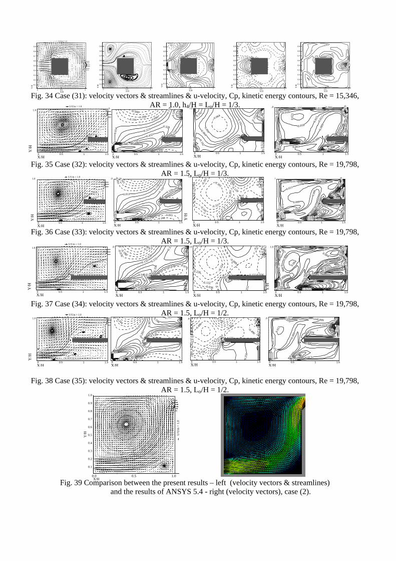
Fig. 39 Comparison between the present results – left (velocity vectors & streamlines) and the results of ANSYS 5.4 - right (velocity vectors), case (2).

0 0.5 1X/H

0.1

0.2

0.3

0.4

0.5

0.6

0.7

0.8

0.9

Y/H

U/Uin = 1.0---->

0 0.5 1X/H

0.1

0.2

0.3

0.4

0.5

0.6

0.7

0.8

0.9

Y/H

0 0.5 1X/H

0.1

0.2

0.3

0.4

0.5

0.6

0.7

0.8

0.9

Y/H

0.236

-0.133

-0.133

-0.133

-0.030

-0.030

0.073

0.073

0.073

-0.030

0.073

0.176

0.176

0.17

6

0.176

0279

0.279

0.279

0.279

0.382

0.382

0.3820.382

0.485

0.48

5

0.485

0.58

8

0.588

0.691

0.691 0.794

0.897

0.897

0 0.5 1X/H

0.1

0.2

0.3

0.4

0.5

0.6

0.7

0.8

0.9

Y/H

-0.6

87

-0.835

-0.194

-0.245

-0.24

5

-0.2

45

-0.392

-0.194

-0.194

-0.245

-0.0

9 7

-0.09

7

-0.0970.051

0.051

0.198

0.3460.493

0.78

8

0 0.5 1X/H

0.1

0.2

0.3

0.4

0.5

0.6

0.7

0.8

0.9

Y/H

0 008

0.013

0.008

0.008

0.013

0.013

0.013

0.013

0.01

3

0.013

026

0.026

0.02

6

0.026

0.026

0.039

0.0520.065

0.104 0.11

7

0.183

0.209

0 0.5 1 1.5X/H

Y/H

-0.508

-0.299-0.195

-0 195

-0.090

-0.090

-0.090

0.01

4

0.014

0.119

0.11

9

0 119

0.1190.223

0.223

0 328

0.328

0.32

8

0.328

0.432

0.53

7

0.5370.6410.746

0.851

1.0

0 0.5 1 1.5X/H

-0.320-0.128-0.064

0.00

00.000

000

0

0.06

40.064

0.06

4

0.128

0.12

8

0.192

0.192

0.192

0.19

0.256

0.25

60.

3 21

0.32

1

0.51

3

1.0

0 0.5 1 1.5X/H

Y/H

U/Uin = 1.01.0

0 0.5 1 1.5X/H

0.00

3

0.003

0.003

0.00

6

0.006

0.006

0.006

0.006

0.00

9 0.00

9

0.009

0 009

0.009

0.012 0.01

2

0.012

0.012

0.012

0.01

5

0.015

0.015

0.01

8 0.018

0.018

0.018

0.018

0.024

0.021

0.02

1

024

0.027

0.027

0.032

1.0

0 0.5 1 1.5X/H

Y/H

U/Uin = 1.01.0

0 0.5 1 1.5X/H

-0.303

-0.198-0.093

-0.093

-0.093

0.013

0.013

0.01

3

0.118

0 118

0.118

0.22

3

0.644

0.329

0.329

0.329

0.3290.434

0.4340.539

0.539

0.75

0.644

0.750

0.855

.0

0 0.5 1 1.5X/H

Y/H

-0.393

-0.393

-0.327

-0.327

-0.2

61

-0.2

6 1

-0.393

-0.195

-0.195

-0.1

29

-0.129

-0.129-0.0

64

-0. 064

-0.064

0.002

0.002

0.0680.13

0.18

00.180

0.265

1.0

0 0.5 1 1.5X/H003

0.003 0

003

0.00

6

0 006

0.006

0.006

0.007

0.00

7

0.00

6

0.007

0.007

0.009

0.009

0.009

0.009

0.009

0.009

0.011

0.011

0.009

0.011

0.011

0.012

0.01

2

0.012

0.012

0.012

.015

0.015

0.015

0.01

50.

018

0.018

0.018

0.021

0.027

0.0240.027

0.03

0

0.036 0.036

0.039 0.039

0

0 0.5 1 1.5X/H

Y/H

U/Uin = 1.01.0

0 0.5 1 1.5X/H

-0.387

-0.28

3

-0.180

-0.180

-0 076

-0.076

-0.076

0.028

0 028 028

0.0280.131

0.131

0.131

0.235

0.235

0.235

0.33

8

0.338

0.33

8

0.7530.546

0.64

0.546 0.5460.6490.753

0.856

.0

0 0.5 1 1.5X/H

Y/H

-1.092-0.996-0.900-0.708 -0.708-0.612-0.420

-0.3

24

-0.324

-0.3

24

-0.228 -0.708

-0.324

-0.132

-0.132

-0.036

-0.036-0.612

-0.009

-0.009

-0.00

006

0

0.156

252

1.0

0 0.5 1 1.5X/H

Y/H

0.0 02 0.00

2

0.002

0.004

0.004

0.004

0.0040.004

0.004

0.00

4

0.004 0.004

0.004

0.004

0.006

0.006

0.006

0.00

6

0 006

0.004

0.006

0.006

0.006

0.00

6

0 006

0.006

0.00

7

0.007

0 007

0.00

7

0.007

0.008

0.00

80.0

08

0.008

0.008

0.008

0.010

0.010

0.012

0.012

0.01

4

0.014

0.017

0.014

0.0210.021

0.023

1.0

0 0.5 1 1.5X/H

Y/H

U/Uin = 1.01.0

0 0.5 1 1.5X/H

-0.244

-0.139

-0.139

0 034

-0.034

0.071

0.071

0.071

0.177 0.177

0.177

0.28

2

0.282

0.282

0.38

7

0.3870.492

0.598

0.598

0.703

0.808

1.0

0 0.5 1 1.5X/H

-0.575

-0.496-0.496

-0.49

6-0. 416 -0.416-0.337

-0.258

-0.258

-0.1 79

-0.179

-0.100

-0.100

-0.100

0021 -0.021

0.058

0.137

0.217

0.25

0

0.250

.0

0 0.5 1 1.5X/H

0.006 0.006

0.006

0.006

0.006

0.00

9

0 009

0.00

6

0.009

0.009

0.006

0.013

0.01

3

0.013

0.013

0.013

0.01

3

0.019

0.01

9

0.019

0.02

6

0.026

0.026

0.032

1.0


Fig. 35 Case (32): velocity vectors & streamlines & u-velocity, Cp, kinetic energy contours, Re = 19,798, AR = 1.5, Lo/H = 1/3.




0.0 0.5 1.0X/H

0.1

0.2

0.3

0.4

0.5

0.6

0.7

0.8

0.9

1.0

Y/H U/U

in=

1.0

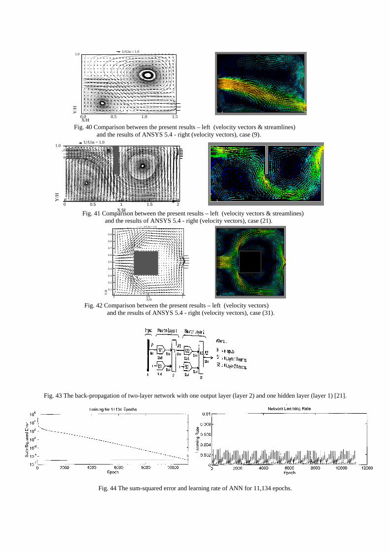
Fig. 43 The back-propagation of two-layer network with one output layer (layer 2) and one hidden layer (layer 1) [21].

Fig. 44 The sum-squared error and learning rate of ANN for 11,134 epochs.

0.0 0.5 1.0 1.5X/H

Y/H

1.0U/Uin = 1.0



Fig. 42 Comparison between the present results – left (velocity vectors) and the results of ANSYS 5.4 - right (velocity vectors), case (31).

0 0.5 1 1.5 2X/H

Y/H

U/Uin = 1.01.0

0 0.5 1X/H

0.1

0.2

0.3

0.4

0.5

0.6

0.7

0.8

0.9

Y/H

U/Uin = 1.0---->

Table 1. The values of the coordinates of the centers of the two main vortices and the average values of the Nusselt number on the top and bottom walls of the room.

No. Case AR hin/H hout/H h1/H-Ls/H h2/H h3/H h4/H Xr1/H Yr1/H Xr2/H Yr2/H NuT NuB 1 C1 0.5 0.11 0.89 ------- --- --- --- 0.183 0.702 --- --- 40.55 24.0 2 C2 1.0 0.11 0.89 ------- --- --- --- 0.4 0.632 --- --- 76.25 39 3 C3 2.0 0.11 0.91 ------- --- --- --- 1.136 0.6 --- --- 176 65 4 C4 4.0 0.1 0.93 ------- --- --- --- 1.619 0.55 --- --- 256 148 5 C5 2.0 0.91 0.11 ------- --- --- --- 1.143 0.368 --- --- 136.25 69.75 6 C6 2.0 0.91 0.11 ------- --- --- --- 1.171 0.368 --- --- 250 150 7 C7 2.0 0.91 0.11 ------ --- --- --- 1.136 0.4 --- --- 390 240 8 C8* 1.5 0.88 0.12 ------ --- --- --- 0.698 0.385 --- --- 150 105 9 C9 1.5 0.5 0.18 ------ --- --- --- 0.341 0.185 1.06 0.67 122 94 10 C10* 1.5 0.18 0.18 ------ --- --- --- 0.964 0.593 --- --- 155 52 11 C11 1.5 0.88 0.5 ------ --- --- --- 0.857 0.357 --- --- 156 106 12 C12 1.5 0.5 0.5 ------ --- --- --- 0.713 0.192 1.05 0.77 128 72 13 C13 1.5 0.18 0.5 ------ --- --- --- 0.878 0.6 --- --- 143 44 14 C14 1.5 0.11 0.5 ------ --- --- --- 0.214 0.346 0.262 0.654 56 40 15 C15 1.5 0.11 0.1 ------ --- --- --- 0.225 0.346 0.25 0.615 47.6 41 16 C16 1.0 0.88 0.3 0.333 – 0.5 --- --- --- 0.323 0.267 0.839 0.533 320 150 17 C17 1.0 0.88 0.3 0.5 – 0.5 --- --- ---- 0.233 0.232 0.767 0.357 330 180 18 C18 3.0 0.9 0.3 0.333 – 0.5 --- --- --- 0.857 0.357 2.143 0.429 720 460.5 19 C19 3.0 0.9 0.3 0.5 – 0.5 --- --- --- 0.224 0.37 0.6 0.37 800 560 20 C20* 2.0 0.88 0.88 ------ 0.33 --- --- 0.5 0.333 1.273 0.714 83 72 21 C21 2.0 0.88 0.88 ------ 0.5 --- --- 0.381 0.325 1.333 0.65 79 82 22 C22 2.0 0.88 0.18 ------ 0.33 --- --- 0.465 0.333 1.58 0.62 64 83 23 C23 2.0 0.88 0.18 ------ 0.5 --- --- 0.381 0.325 1.524 0.6 63 106 24 C24 2.0 0.88 0.5 ------ 0.33 0.33 --- 0.488 0.341 1.707 0.682 64 65 25 C25 2.0 0.88 0.88 ------ 0.33 0.33 --- 0.42 0.35 1.372 0.682 80 67 26 C26 1.0 0.88 0.5 ------ --- --- 0.2 0.673 0.25 --- --- ---- ---- 27 C27 1.0 0.88 0.5 ------ --- --- 0.33 0.192 0.612 0.808 0.163 ---- ---- 28 C28 1.0 0.88 0.12 ------ --- --- 0.2 0.558 0.184 ---- ---- ---- ---- 29 C29 1.0 0.88 0.12 ------ --- --- 0.33 0.167 0.529 0.463 0.157 ---- ---- 30 C30 1.0 0.5 0.5 ------ --- --- 0.2 0.245 0.163 0.34 0.816 ---- ---- 31 C31 1.0 0.5 0.5 ------ --- --- 0.33 0.148 0.12 0.519 0.22 ---- ---- 32 C32 1.5 0.12 0.9 ------ --- --- 0.33 0.538 0.625 ---- ---- ---- ---- 33 C33 1.5 0.12 0.9 ------ --- --- 0.33 0.466 0.652 ---- ---- ---- ---- 34 C34 1.5 0.12 0.9 ------ --- --- 0.5 0.4 0.66 ---- ---- ---- ---- 35 C35 1.5 0.12 0.9 ------ --- --- 0.5 0.308 0.667 ---- ---- ---- ----

(*) indicates the cases used to test the artificial neural network (ANN).

Table 2. Results of the test cases for the characteristics of the flow pattern.

No. Case S1 Desired output

(Xr1/H - Yr1/H - Xr2/H - Yr2/H) (Numerical results)

Actual output (Xr1/H - Yr1/H - Xr2/H - Yr2/H)

(ANN results) 1 C8 100 0.698 - 0.385 - 0.0 - 0.0 0.9153 - 0.1870 - 0.0 - 0.0 2 C10 100 0.964 - 0.593 - 0.0 -0.0 0.3795 - 0.7272 - 0.2074 - 0.056 3 C20 100 0.5 - 0.333 - 1.273 - 0.714 0.4908-0.3802-1.5456-0.7827 4 C8 200 0.698 - 0.385 - 0.0 - 0.0 0.6145 - 0.437 - 0.0 - 0.0 5 C10 200 0.964 - 0.593 - 0.0 -0.0 0.5190 - 0.7253 - 0.0 - 0.0 6 C20 200 0.5 - 0.333 - 1.273 - 0.714 0.7179-0.2432-1.3970-0.8116 7 C8 300 0.698 - 0.385 - 0.0 - 0.0 0.3188 - 0.2126 - 0.1109 - 0.0 8 C10 300 0.964 - 0.593 - 0.0 -0.0 0.6527 - 0.5980 - 0.0 - 0.0552 9 C20 300 0.5 - 0.333 - 1.273 - 0.714 0.4954 - 0.3901 - 1.4613 - 0.9348

10 C8 400 0.698 - 0.385 - 0.0 - 0.0 0.6400 - 0.1763 - 0.0 - 0.0 11 C10 400 0.964 - 0.593 - 0.0 -0.0 0.5817 - 0.5392 - 0.0706 - 0.0261 12 C20 400 0.5 - 0.333 - 1.273 - 0.714 0.5046 - 0.1100 - 1.3028 - 0.8538 13 C8 450 0.698 - 0.385 - 0.0 - 0.0 0.5767 - 0.168 - 0.0 - 0.4523 14 C10 450 0.964 - 0.593 - 0.0 -0.0 0.497 - 0.5362 - 0.1722 - 0.0 15 C20 450 0.5 – 0.333 - 1.273 - 0.714 0.3908 - 0.1784 -1.4384 - 0.5849 16 C8 500 0.698 - 0.385 - 0.0 - 0.0 1.1251 - 0.6031 - 0.0 - 0.0 17 C10 500 0.964 - 0.593 - 0.0 -0.0 0.1611 -0.3168 -0.1358 -0.0141 18 C20 500 0.5 – 0.333 - 1.273 - 0.714 0.3332-0.4315-1.4138-0.9481

Table 3. Results of the test cases for the thermal field.

No. Case S1 Desired output (NuT)

(Numerical results) Actual output (NuT)

(ANN results) Desired output (NuB) (Numerical results)

Actual output (NuB) (ANN results)

1 C8 100 150 136.9021 105 110.6129 2 C10 100 155 132.3253 52 61.2003 3 C20 100 83 111.5856 72 85.4637 4 C8 200 150 143.8706 105 125.3098 5 C10 200 155 137.2263 52 60.4204 6 C20 200 83 100.0459 72 80.9152 7 C8 300 150 146.4017 105 123.0694 8 C10 300 155 134.4982 52 60.7390 9 C20 300 83 96.3899 72 79.5001

10 C8 400 150 148.2182 105 131.0197 11 C10 400 155 136.5052 52 58.6440 12 C20 400 83 95.8816 72 79.3464 13 C8 500 150 151.2075 105 123.9144 14 C10 500 155 134.4290 52 60.2475 15 C20 500 83 94.5651 72 78.6101 16 C8 1000 150 151.3395 105 130.4269 17 C10 1000 155 136.2550 52 59.4992 18 C20 1000 83 93.7018 72 73.8633 19 C8 1500 150 152.1657 105 130.4320 20 C10 1500 155 135.1490 52 60.0479 21 C20 1500 83 93.2417 72 75.5530

Study of Both Airflow and Thermal Fields in a Room Using K-ε Modelling and Neural Networks

Documents

Transcript of Study of Both Airflow and Thermal Fields in a Room Using K-ε Modelling and Neural Networks