STRUCTURAL - Jonathan Ochshorn
356
Design of Columns, Beams, and Tension Elements in Wood, Steel, and Reinforced Concrete Third Edition STRUCTURAL JONATHAN OCHSHORN ELEMENTS FOR ARCHITECTS AND BUILDERS
-
Upload
khangminh22 -
Category
Documents
-
view
0 -
download
0
Transcript of STRUCTURAL - Jonathan Ochshorn

i
Design of Columns, Beams, and Tension Elementsin Wood, Steel, and Reinforced Concrete
Third Edition
STRUCTURAL
JONATHAN OCHSHORN
ELEMENTSFOR ARCHITECTS AND BUILDERS

ii

iii
Proudly and Indepedndently published 2020
Design of Columns, Beams, and Tension Elementsin Wood, Steel, and Reinforced Concrete
Third Edition
STRUCTURAL
JONATHAN OCHSHORN
ELEMENTSFOR ARCHITECTS AND BUILDERS

iv
Copyright © Jonathan Ochshorn 2020
All rights reserved. Apart from fair dealing for the purposes of study, research, criticism or review as permitted under the applicable copyright legislation, no part of this book may be reproduced by any process without written permission from the author.
Ochshorn, Jonathan, author. Structural elements for architects and builders : design of columns, beams, and tension elements in wood, steel, and reinforced concrete / Jonathan Ochshorn. — Third edition.
Disclaimer: The author assumes no liability for any injury and/or damage to persons or property arising from the use or application of the methods or instructions contained in this book: it is intended only for a preliminary understanding of structural behavior and design; a competent professional should be consulted for the design of actual structures.
Publishing history:1. First edition: Butterworth-Heinemann (an imprint of Elsevier Press), 2010, ISBN: 978-185617-771-92. Second edition: Common Ground Publishing LLC, 2015, ISBN: 978-1-61229-801-63. Third edition: Imprint: Proudly and independently published, 2020, ISBN: 979-8-68442-803-6 Version 3.0 September 2020 Version 3.1 November 2020 Version 3.2 December 2020 Version 3.3 February 2021
Cover image shows, schematically, contrasting structural strategies for supporting sculptural form: Alexandre-Gustave Eiffel’s structural design for the Statue of Liberty on the left and S.O.M. Chicago’s structural design for the Guggenheim Museum Bilbao on the right. Of course, these structural engineers worked with the actual designers of the external forms—Frédéric-Auguste Bartholdi for the famous statue and Frank Gehry for the museum. This image reappears as Figure 4.5 in the text (drawn by the author).
All drawings and figures were created by the author except for Figure 4.6 (Fair Store in Chicago by Jenney & Mundie), a public domain item in the collection of the Ryerson & Burnham Libraries at the The Art Institute of Chicago: RBA Digital File name: 000000_121127_016.jpg. All photographs were taken by the author, some screen captured from the author’s online video series on the construction of Milstein Hall at Cornell University: https://jonochshorn.com/scholarship/videos/milstein.
Free online structural calculators have been created for many examples in the book, enabling architects and builders to quickly find preliminary answers to structural design questions commonly encountered in school or in practice.
Visit https://jonochshorn.com/structuralelements for links to calculators and errata.

v
Table of Contents
Preface to first edition...................................................................................................................................................... viiPreface to second edition................................................................................................................................................ viiiPreface to the third edition............................................................................................................................................. viiiList of examples................................................................................................................................................................. ixList of appendices.............................................................................................................................................................. xi
Chapter 1........................................................................................................................................................................ 1Introduction to structural design....................................................................................................................................... 1 Statics....................................................................................................................................................................... 1 Tributary areas.......................................................................................................................................................... 1 Equilibrium............................................................................................................................................................... 5 Reactions.................................................................................................................................................................. 6 Internal forces and moments.................................................................................................................................. 13 Indeterminate structure......................................................................................................................................... 22 Material properties................................................................................................................................................. 24 Strength of materials.............................................................................................................................................. 26 Sectional properties................................................................................................................................................ 41 Construction systems.............................................................................................................................................. 41 Connections............................................................................................................................................................ 46 Chapter 1 Appendix................................................................................................................................................ 47 Chapter 2...................................................................................................................................................................... 49Loads ................................................................................................................................................................................ 49 Dead loads.............................................................................................................................................................. 49 Live loads................................................................................................................................................................ 50 Environmental loads............................................................................................................................................... 54 Design approaches................................................................................................................................................. 68 Chapter 2 Appendix................................................................................................................................................ 74
Chapter 3...................................................................................................................................................................... 85Wood................................................................................................................................................................................ 85 Material properties................................................................................................................................................. 85 Sectional properties................................................................................................................................................ 92 Design approaches.................................................................................................................................................. 93 Construction systems.............................................................................................................................................. 94 Tension elements.................................................................................................................................................... 96 Columns................................................................................................................................................................ 101 Beams................................................................................................................................................................... 107 Connections.......................................................................................................................................................... 117 Chapter 3 Appendix.............................................................................................................................................. 145
Contents

vi
Chapter 4.................................................................................................................................................................... 181Steel................................................................................................................................................................................ 181 Material properties............................................................................................................................................... 182 Sectional properties.............................................................................................................................................. 184 Design approaches................................................................................................................................................ 185 Construction systems............................................................................................................................................ 186 Tension elements.................................................................................................................................................. 191 Columns................................................................................................................................................................ 197 Beams................................................................................................................................................................... 201 Connections.......................................................................................................................................................... 213 Chapter 4 Appendix.............................................................................................................................................. 223
Chapter 5................................................................................................................................................................... 261Reinforced concrete....................................................................................................................................................... 261 Material properties............................................................................................................................................... 261 Sectional properties.............................................................................................................................................. 268 Design approaches................................................................................................................................................ 270 Construction systems............................................................................................................................................ 271 Tension elements.................................................................................................................................................. 276 Columns................................................................................................................................................................ 276 Beams and slabs................................................................................................................................................... 282 Connections.......................................................................................................................................................... 308 Chapter 5 Appendix.............................................................................................................................................. 316
Unit abbreviations and conversion................................................................................................................................. 329References...................................................................................................................................................................... 331Glossary.......................................................................................................................................................................... 333Index............................................................................................................................................................................... 341
Contents

vii
Preface to First Edition
As is well known, architects and builders rarely design the structural elements and systems within their buildings, in-stead engaging the services of (and, it is to be hoped, collaborating with) structural engineers, or relying upon standard practices sanctioned by building codes. Where architects or builders wish to be adventurous with their structures, some knowledge of structural behavior and the potential of structural materials is certainly useful. On the other hand, where they are content to employ generic structural systems — platform framing in wood, simple skeletal frames in steel or reinforced concrete — one can get by with little actual knowledge of structural design, relying instead on the expertise of structural consultants and the knowledge of common spans, heights, and cross-sectional dimensions around which many ordinary buildings can be planned.
The heroic stage of modernism, in which architects often sought to reconcile structural behavior and overall building form — some finding inspiration in the structural frame or the load-bearing wall — was also the heroic stage of struc-tural education for architects: it was hardly necessary, in that context, to explain why architects needed to learn about structures. Some of the same excitement about the potential of structure in architecture still remains, but it is also true that a “mannerist” tendency has emerged, interested not necessarily in renouncing the role of structure in architecture, but rather reveling in its potential to distort, twist, fragment, and otherwise subvert modernist conventions and the architectural forms they support.
Yet all structures, whether hidden from view or boldly expressed, follow the same laws of equilibrium, are exposed to the same types of forces, and are constrained by the same material properties and manufacturing practices. It is therefore appropriate for architects and builders to study structures in such a way that the basic principles underlying all structural form become clear. This can be accomplished in three phases: first, by studying the concepts of statics and strength of materials; second, by learning how these concepts are applied to the design of common structural elements fabricated from real materials; and third, by gaining insight into the design of structural systems comprised of structural elements interconnected in a coherent pattern.
Much of the material presented in this text can be found elsewhere; the basic conditions of equilibrium, historical insights into structural behavior that form the basis for structural design, and recommendations for design procedures incorporated into building codes, are all widely disseminated through industry-published manuals, government-sanc-tioned codes, and academic texts. Many excellent structures texts have been written specifically for architects and build-ers. The question therefore naturally arises: Why write another one?
The primary motivation for writing this text is to organize the material in a manner consistent with the structures curriculum developed within the Department of Architecture at Cornell University, based on the three sequential “phas-es” described above — structural concepts, elements, and systems. While this text does contain a concise introduction to structural concepts (statics), it is primarily concerned with the design and analysis of structural elements: columns, beams, and tension members, and their connections. This material is organized into a single volume that is concise, com-prehensive, and self-sufficient, including all necessary data for the preliminary design and analysis of these structural elements in wood, steel, and reinforced concrete.
A second motivation for writing this text is to present material in a manner consistent with my own priorities and sensibilities. Every chapter contains insight, speculation, or forms of presentation developed by the author and generally not found elsewhere. Additionally, the Appendices included at the end of the text contains numerous tables and graphs, based on material contained in industry publications, but reorganized and formatted especially for this text to improve clarity and simplicity — without sacrificing comprehensiveness.
Methods for designing structures and modeling loads are constantly being refined. Within the last several years, important changes have occurred in the design of wood, steel, and reinforced concrete structures, as well as in the mod-eling of loads. These changes include revised procedures for beam and column design in wood; the replacement of the standard specification for 36-ksi steel with a new standard based on 50-ksi steel for wide-flange sections; a major modi-fication in the load factors used in reinforced concrete design, aligning them with those recommended by SEI/ASCE 7 and already used in the design of wood and steel structures; and numerous refinements in the modeling of environmental loads. These changes have all been incorporated into this text.
Finally, a disclaimer: this text is intended to be used only for the preliminary (schematic) design and understanding of structural elements. For the design of an actual structure, a competent professional should be consulted.
Preface to First Edition

viii Preface to First Edition
Preface to Second Edition
Unlike laws of equilibrium, which remain unchanged year after year, the application of structural concepts to the design of actual structures using real materials and accepted methods changes on a fairly regular schedule. Material-centric institutes periodically revise their suggestions for building code language; these are referenced in model building codes, and the various states of the union eventually get around to adopting these model codes, turning them into legal man-dates that reflect evolving standards for structural design.
This fact alone would make it necessary to update the first edition of Structural Elements, and I have indeed incor-porated recommendations from the latest versions of all four primary references (i.e., from the AF&PA/AWC, AISC, ACI, and ASCE) into this second edition, including revised values for Southern Pine lumber that became effective in 2013.
In addition, I have reorganized the material in this second edition around the idea of materials rather than based on structural actions. In other words, while the first edition considered tension, compression, and bending as the primary “subjects” (with wood, steel, and reinforced concrete discussed for each of these structural behaviors), the second edi-tion organizes the content around wood, steel, and reinforced concrete (with the various structural actions — tension, compression, and bending — included within each “material” chapter). Doing so has allowed me to add new content concerning structural systems and material properties for each of the primary structural materials, and to integrate the discussion of connections within the particular material chapters to which they apply. In this way, the organization of the book reflects curricular changes within the building technology area of the architectural curriculum at Cornell.
J. Ochshorn, Ithaca, NYJanuary, 2015
Preface to Third Edition
This third edition has been updated to reflect the latest editions of all four primary references (i.e., those written by the AF&PA/AWC, AISC, ACI, and ASCE). The format has been enlarged, which helps accommodate more information in some of the appendices, and also reduces the page count. Most importantly, I have decided to self-publish this edition, in or-der to reduce its price and thereby make it more accessible to those who might find it useful.
J. Ochshorn, Ithaca, NYAugust, 2020

ix
List of Examples
Chapter 1: Introduction to structural design1.1 Find reactions for simply supported beam............................................................................................................... 61.2 Find reactions for three-hinged arch........................................................................................................................ 81.3 Find reactions for a cable........................................................................................................................................ 101.4 Find internal shear and bending moment for simply supported beam with “point” loads.................................... 131.5 Find internal shear and bending moments for a simply supported cantilever beam with distributed loads......... 161.6 Find internal axial forces in a truss (section method)............................................................................................. 201.7 Find internal axial forces in a three-hinged arch..................................................................................................... 211.8 Find internal axial forces in a cable......................................................................................................................... 221.9 Find elongation in tension element........................................................................................................................ 31
Chapter 2: Loads2.1 Calculate dead loads............................................................................................................................................... 492.2: Calculate live loads.................................................................................................................................................. 522.3 Calculate snow loads............................................................................................................................................... 562.4 Calculate wind loads............................................................................................................................................... 602.5 Calculate seismic loads........................................................................................................................................... 652.6 Load combinations (Part I)...................................................................................................................................... 702.7 Load combinations (Part II)..................................................................................................................................... 702.8 Load combinations (Part III).................................................................................................................................... 71
Chapter 3: Wood3.1 Analyze wood tension element............................................................................................................................... 983.2 Design wood tension element.............................................................................................................................. 1003.3 Analyze wood column........................................................................................................................................... 1023.4 Design wood column............................................................................................................................................ 1043.5 Analyze wood beam, dimension lumber............................................................................................................... 1083.6 Analyze wood beam, timbers................................................................................................................................ 1093.7 Design wood beam, glulam.................................................................................................................................. 1113.8 Design wood beam, dimension lumber................................................................................................................ 1143.9 Analyze wood single-shear connection using one bolt......................................................................................... 1233.10 Analyze wood single-shear connection using multiple bolts................................................................................ 1253.11 Analyze wood double-shear connection using multiple bolts.............................................................................. 1283.12 Analyze wood double-shear connection using multiple bolts and steel side plates............................................. 1303.13 Analyze wood single-shear connection using multiple lag screws........................................................................ 1323.14 Design wood single-shear connection using common nails.................................................................................. 1353.15 Analyze wood double-shear bolted connection using yield limit and group action equations............................. 1373.16 Design wood connection in withdrawal, using lag screws.................................................................................... 1413.17 Analyze wood connection in withdrawal, using common nails............................................................................ 1423.18 Check wood connection in bearing....................................................................................................................... 143
List of Examples

x
Chapter 4: Steel4.1 Analyze steel tension element.............................................................................................................................. 1934.2 Design steel tension element................................................................................................................................ 1954.3 Analyze steel column............................................................................................................................................ 1994.4 Design steel column.............................................................................................................................................. 2004.5 Find capacity of beam web based on block shear................................................................................................. 2084.6 Design steel beam................................................................................................................................................. 2094.7 Analyze rectangular HSS (hollow structural section)............................................................................................ 2124.8 Design bolted connection for steel tension element............................................................................................ 2164.9 Find capacity of welded connectors with transverse or longitudinal welds......................................................... 2194.10 Find capacity of welded connector with angled load........................................................................................... 2204.11 Design a welded connector with both longitudinal and transverse welds........................................................... 221
Chapter 5: Reinforced Concrete5.1 Analyze axially-loaded reinforced concrete column............................................................................................. 2795.2 Design axially-loaded reinforced concrete column with cross-sectional dimensions assumed............................ 2805.3 Design axially-loaded reinforced concrete column with reinforcement ratio assumed....................................... 2805.4 Analyze reinforced concrete beam....................................................................................................................... 2855.5 Design reinforced concrete beam, with steel ratio assumed................................................................................ 2935.6 Design reinforced concrete slab with slab thickness assumed............................................................................. 2945.7 Design reinforced concrete slab and T-beam, with cross-sectional dimensions assumed................................... 2965.8 Design shear reinforcement (stirrups) for reinforced concrete beam.................................................................. 3045.9 Find required development length for straight bar and 90-degree hook in reinforced concrete structure......... 3115.10 Find required length of compression column splice in reinforced concrete structure......................................... 315
List of Examples

xi
List of Appendices
Appendix 1: Introduction to structural design................................................................................................... 47A-1.1 Derivation of rules for drawing shear and moment diagrams................................................................................ 47A-1.2 Effective length coefficient, K, for wood and steel columns.................................................................................... 48A-1.3 Allowable deflection for span, L.............................................................................................................................. 48
Appendix 2: Loads...................................................................................................................................................... 74A-2.1 Dead loads.............................................................................................................................................................. 74A-2.2 Live loads................................................................................................................................................................ 74A-2.3 Environmental loads............................................................................................................................................... 75A-2.4 Snow load Importance factor, Is.............................................................................................................................. 75A-2.5 Wind coefficients.................................................................................................................................................... 76A-2-6 Seismic coefficients................................................................................................................................................ 79A-2.7 Combined load factors........................................................................................................................................... 83
Appendix 3: Wood................................................................................................................................................... 145A-3.1 Design values for tension, Ft (psi) for visually graded lumber and glued laminated timber.................................. 145A-3.2 Adjustments to allowable stress in tension, Ft, for visually-graded lumber and glued laminated softwood timber..................................................................................................... 146A-3.3 Design values for compression (psi), parallel to grain (Fc) and perpendicular to grain (Fc-per) for visually-graded lumber and glued laminated softwood timber.................................................... 147A-3.4 Adjustments to allowable stress in compression, Fc , for visually-graded lumber and glued-laminated softwood timber..................................................................................................... 149A-3.5 Design values for bending, Fb (psi) for visually-graded lumber and glued laminated softwood timber................ 150A-3.6 Adjustments to allowable stress in bending, Fb, for visually-graded lumber and glued laminated softwood timber..................................................................................................... 152A-3.7 Design values for shear, Fv (psi) for visually-graded lumber and glued laminated softwood timber..................... 154A-3.8 Adjustments to allowable stress in shear, Fv, for visually-graded lumber and glued laminated softwood timber.................................................................................................................. 156A-3.9 Design values for modulus of elasticity, E and Emin (psi) for visually-graded lumber and glued laminated softwood timber (values and adjustments)............................................................ 156A-3.10 Use of load duration factor, CD, for wood elements............................................................................................ 159A-3.11 Specific gravity for selected wood species (based on oven-dry weight and volume)......................................... 159A-3.12 Dimensions and properties of lumber................................................................................................................ 160A-3.13 Dimensions of typical glulam posts and beams (in.)........................................................................................... 161A-3.14 Allowable force (lb) based on row and group tear-out....................................................................................... 162A-3.15 Maximum (actual) deflection in a beam............................................................................................................. 162A-3.16 “Adjusted” section modulus (CFSx) values for wood sections in bending............................................................ 163A-3.17 Selected lag screw (lag bolt) dimensions............................................................................................................ 164A-3.18 Selected common wire nail dimensions............................................................................................................. 164A-3.19 Penetration and dowel bearing length............................................................................................................... 165A-3.20 Duration of load adjustment factor, CD, for wood connectors............................................................................ 165A-3.21 Wet service adjustment factor, CM, for wood connectors................................................................................... 166A-3.22 Group action adjustment factor, Cg, for wood connectors.................................................................................. 166A-3.23 Geometry adjustment factor, CΔ, for wood connectors (bolts and lag screws)................................................... 170A-3.24 Toe-nail adjustment factor, Ctn, for nails............................................................................................................. 172A-3.25 Temperature factor, Ct, for wood fasteners......................................................................................................... 172A-3.26 Lateral design value, Z (lb) for bolts: single-shear connections, with 1½ in. side member thickness, both members same species (or same specific gravity)........................................................ 172
List of Appendices

xii
A-3.27 Lateral design value, Z (lb) for bolts: double-shear connections, with 1½ in. side member thickness, both members same species (or same specific gravity)................................................. 174A-3.28 Lateral design value, Z (lb) for bolts: double-shear connections, with two ¼ in. A36 steel side plates.............. 175A-3.29 Lateral design value, Z (lb) for lag screws: single-shear connections, both members same species (or same specific gravity)....................................................................................... 177A-3.30 Lateral design value, Z (lb) for common nails: single-shear connections, both members same species (or same specific gravity)........................................................................................ 178A-3.31 Method for determining lateral design value, Z, based on yield limit equations................................................ 179A-3.32 Withdrawal design value, W, per inch of penetration (lb) for lag screws........................................................... 180A-3.33 Withdrawal design value, W, per inch of penetration (lb) for nails.................................................................... 180
Appendix 4: Steel..................................................................................................................................................... 223A-4.1 Steel properties.................................................................................................................................................... 223A-4.2 Steel allowable stresses and available strengths.................................................................................................. 224A-4.3 Dimensions and properties of steel W sections................................................................................................... 225A-4.4 Dimensions and properties of steel C and MC channels...................................................................................... 233A-4.5 Dimensions and properties of selected steel L angles.......................................................................................... 235A-4.6 Dimensions and properties of selected steel rectangular and square hollow structural sections (HSS).............. 237A-4.7 Dimensions and properties of selected steel round hollow structural sections (HSS).......................................... 239A-4.8 Dimensions and properties of selected steel pipe................................................................................................ 240A-4.9 Shear lag coefficient, U, for bolted and welded steel connections in tension...................................................... 241A-4.10 Allowable axial loads (kips), A992 steel wide-flange columns (Fy = 50 ksi)......................................................... 242A-4.11 Allowable stresses for A992 steel columns (Fy = 50 ksi)...................................................................................... 245A-4.12 Allowable stresses for A500 Grade B HSS rectangular columns (Fy = 46 ksi)....................................................... 246A-4.13 Allowable stresses for A500 Grade B HSS round columns (Fy = 42 ksi)............................................................... 247A-4.14 Allowable stresses for A36 steel columns (Fy = 36 ksi)........................................................................................ 248A-4.15 Plastic section modulus (Zx) values: lightest laterally braced steel compact shapes for bending, Fy = 50 ksi...... 249A-4.16 Available moment for A992 wide-flange (W) shapes.......................................................................................... 250A-4.17 Maximum (actual) deflection in a beam............................................................................................................. 228A-4.18 Shear capacity, or available strength, for a high-strength bolt subjected to single shear with threads excluded from shear plane (kips)................................................................................ 259A-4.19 Bearing capacity, or available strength, for a high-strength bolt bearing on material 1 in. thick, with clear spacing between bolts (or edge) ≥ 2 in. (kips)...................................................... 259A-4.20 Minimum and maximum spacing and edge distance measured from bolt centerline for standard holes.......... 260A-4.21 Size limitations (leg size, w) for fillet welds (in.).................................................................................................. 260
Appendix 5: Reinforced Concrete........................................................................................................................ 316A-5.1 Dimensions of reinforced concrete beams, columns, and slabs........................................................................... 316A-5.2 Steel reinforcement — rebar — areas (in2) for groups of bars............................................................................. 316A-5.3 Reinforced concrete minimum width or diameter (in.) based on bar spacing..................................................... 317A-5.4 Specifications for steel ties and spirals in reinforced concrete columns............................................................... 318A-5.5 Reinforced concrete strength reduction factors, ϕ and α..................................................................................... 318A-5.6 “Shear” equations for reinforced concrete beams............................................................................................... 319A-5.7 Approximate moment values for continuous reinforced concrete beams and slabs............................................ 320A-5.8 Limits on steel ratio for “tension-controlled” reinforced concrete beams........................................................... 321A-5.9 Values of R and ρ for reinforced concrete beams, T-beams, and one-way slabs (using 60 ksi steel).................... 322A-5.10 Development length in inches, ld, for deformed bars in tension, uncoated, normalweight concrete, with adequate spacing and/or stirrups......................................................... 326A-5.11 Development length for standard hooks in inches, ldh, for uncoated bars, normalweight concrete................... 326A-5.12 Development length in inches, ldc, for deformed bars in compression............................................................... 327A-5.13 Recommended minimum thickness (in.) of reinforced concrete beams and slabs for deflection control.......... 327
List of Appendices

1Introduction to structural design
The study of structural behavior and structural design begins with the concept of load. We repre-sent loads with arrows indicating direction and magnitude. The magnitude is expressed in pounds (lb), kips (1 kip = 1000 lb), or appropriate SI units of force; the direction is usually vertical (gravity) or horizontal (wind, earthquake), although wind loads on pitched roofs can be modeled as acting perpendicular to the roof surface (Figure 1.1).
Where loads are distributed over a surface, we say, for example, 100 pounds per square foot, or 100 psf. Where loads are distributed over a linear element, like a beam, we say, for example, 2 kips per linear foot, or 2 kips per foot, or 2 kips/ft (Figure 1.2). Where loads are concentrated at a point, such as the vertical load transferred to a column, we say, for example, 10 kips or 10 k.
Statics
Finding out what the loads are that act on a structure and how these loads are supported is the pre-requisite to all structural design. There are two main reasons for this. First, the fact that a structural element is supported at all means that the supporting element is being stressed in some way. To find the magnitude of the reactions of an element is thus to simultaneously find the magnitude of the loads acting on the supporting element. Each action, or load, has an equal reaction; or, as Newton said in defense of this third law: “If you press a stone with your finger, the finger is also pressed by the stone.”
The second reason for finding reactions of the structural element is that doing so fa-cilitates the further analysis or design of the element itself. That is, determining reactions is the prerequisite to the calculation of inter-nal loads and internal stresses, values of which are central to the most fundamental questions of structural engineering: Is it strong enough? Is it safe?
Tributary Areas
When loads are evenly distributed over a sur-face, it is often possible to “assign” portions of the load to the various structural elements supporting that surface by subdividing the total
Chapter 1
Introduction to structural design
Figure 1.1: Direction of loads can be (a) vertical; (b) hori-zontal; or (c) inclined
(b) (c)(a)
Figure 1.2: Distributed loads on a beam
Resultant, or total load = 40 kips
2 kips/ft
20'

2 Structural Elements for Architects and Builders
area into tributary areas corresponding to each member. In Figure 1.3, half the load of the table goes to each lifter.
In Figure 1.4, half the 20-psf snow load on the cantilevered roof goes to each column; the tribu-tary area for each column is 10 ft × 10 ft, so the load on each column is 20(10 × 10) = 2000 lb = 2 kips.
Figure 1.5 shows a framing plan for a steel building. If the total floor load is 100 psf, the load acting on each of the structural elements com-prising the floor system can be found using ap-propriate tributary areas. Beam A supports a total load of 100(20 × 10) = 20,000 lb = 20 kips; but it is more useful to calculate the distributed load act-ing on any linear foot of the beam — this is shown by the shaded tributary area in Figure 1.6a and is 100(1 × 10) = 1000 lb = 1 kip. Since 1000 lb is act-ing on a 1-ft length of beam, we write 1000 lb/ft or 1.0 kip/ft, as shown in Figure 1.6b.
As shown in Figure 1.7a, Beam B (or Girder B) supports a total tributary area of 17.5 × 20 = 350 ft2. The load at point a is not included in the beam’s tributary area. Rather, it is assigned to the edge, or spandrel, beam where it goes directly into a column, having no effect on Beam B. Unlike Beam A, floor loads are transferred to Beam B at two points: each concentrated load corresponds to a tributary area of 17.5 × 10 = 175 ft2; there-
Figure 1.3: Tributary areas divide the load among the various supports
Figure 1.4: Distributed load on a floor carried by two columns
10’ 20’
20 psf
Figure 1.5: Framing plan showing tributary areas for beams and girders
30' 40' 30'
15'
20'
20'
Figure 1.6: Distributed load on a steel beam, with (a) one linear foot of its tributary area shown; and (b) load diagram showing distributed load in kips per foot
100 psf
10'-0"
20'-0"
1'-0"
20'-0"
(b)
(a)w = 1 kip/ft
A
B
C
30'-0" 30'-0"40'-0"
20'-0
"20
'-0"
15'-0
"

3Introduction to structural design
fore, the two loads each have a magnitude of 100 × 175 = 17,500 lb = 17.5 kips. The load dia-gram for Beam B is shown in Figure 1.7b.
Spandrel girders
Beam C (or spandrel girder C), shown in Figure 1.5, is similar to Beam B except that the tribu-tary area for each concentrated load is small-er, 7.5 × 10 = 75 ft2, as shown in Figure 1.8a. The two concentrated loads, therefore, have a magnitude of 100 × 75 = 7500 lb = 7.5 kips, and the load diagram is as shown in Figure 1.8b.
There are three reasons spandrel girders are often larger than otherwise similar gird-ers located in the interior of the building, even though the tributary areas they support are smaller. First, spandrel girders often support cladding of various kinds, in addition to the floor loads included in this example. Second, aside from the added weight to be supported, spandrels are often made bigger so that their deflection, or vertical movement, is reduced. This can be an important consideration where nonstructural cladding is sensitive to move-ment of the structural frame. Third, when the girders are designed to be part of a moment-resisting frame, their size might need to be in-creased to account for the stresses introduced by lateral forces such as wind and earthquake.
Columns
One way or another, all of the load acting on the floor must be carried by columns under that floor. For most structures, it is appropri-ate to subdivide the floor into tributary areas defined by the centerlines between columns so that every piece of the floor is assigned to a column.
It can be seen from Figure 1.9 that typi-cal interior columns (Column A) carry twice the load of typical exterior columns (Column B), and four times the load of corner columns (Column C). However, two of the conditions
Figure 1.7: Concentrated loads on a girder (a) derived from tributary areas on framing plan; and (b) shown on load diagram
(b)
(a)
15'
20'
10' 10' 10'
17.5
'
17.5 kips
30'
a b c
d
17.5 kips
Beam B
Figure 1.8: Concentrated loads on a spandrel girder (a) de-rived from tributary areas on framing plan; and (b) shown on load diagram
Beam C10' 10' 10'
7.5 kips 7.5 kips
(b)
(a)
30'
15'
30' 30' 30'
C
B
A
20'
20'
Figure 1.9: Framing plan showing tributary areas for columns (one floor only)

4 Structural Elements for Architects and Builders
described earlier with respect to the enlargement of spandrel girders can also increase the size of exterior and corner columns: the need to support additional weight of cladding and the possibility of resisting wind and earthquake forces through rigid connections to the spandrel girders.
Column A in Figure 1.9 supports a tribu-tary area of 30 × 20 = 600 ft2 so that the load transferred to Column A from the floor above is 100 × 600 = 60,000 lb = 60 kips, assuming that the floor above has the same shape and loads as the floor shown. But every floor and roof above also transfers a load to Column A. Obviously, columns at the bottom of buildings support more weight than columns at the top of buildings, since all the tributary areas of the floors and roof above are assigned to them. As an example, if there are nine floors and one roof above Column A, all with the same distributed load and tributary area, then the total load on Column A would be, not 60 k, but (9 + 1) × 60 = 600 kips.
In practice, the entire load as previously cal-culated is not assigned to columns or to other structural elements with large total tributary ar-eas. This is because it is unlikely that a large tribu-tary area will be fully loaded at any given time. For example, if the live load caused by people and other movable objects is set at 60 psf, and one person weighed 180 lb, then a tributary area of 600 × 9 = 5400 ft2 (as in the example of Column A, but discounting the roof area) would have to be populated by 1800 people, each occupying 3 ft2, in order to achieve the specified load. That many people crowded into that large a space is an unlikely occurrence in most occupancies, and a live load reduction is often allowed by building codes. As the tributary area gets smaller, however, the prob-ability of the full live load being present increases, and no such reduction is permitted. Permanent and immovable components of the building, or dead loads, have the same probability of being pres-ent over large tributary areas as small tributary areas, so they are never included in this type of prob-ability-based load reduction. Calculations for live load reduction are explained in the next chapter.
The path taken by a load depends on the ability of the structural elements to transfer loads in various directions. Given the choice of two competing load paths such as (1) and (2) in Figure 1.10, the load is divided between the two paths in proportion to the relative stiffness of each path. Since the corrugated steel deck shown in Figure 1.10 is much stiffer in the direction of load path (1), and, in fact, is designed to carry the entire load in that direction, we neglect the possibility of the load moving along path (2).
For “two-way” systems, generally only used in reinforced concrete (Figure 1.11), or for indeter-minate systems in general, the assignment of loads to beams and columns also becomes a function of the relative stiffness of the various components of the system. Stiffer elements “attract” more
Figure 1.10: Competing load paths on a corrugated steel deck
Figure 1.11: Competing load paths on a two-way slab

5Introduction to structural design
load to them, and the simplistic division into tributary areas becomes inappropriate, except in cer-tain symmetrical conditions.
Equilibrium
Where loads or structural geometries are not symmetrical, using tributary areas may not accurately predict the effects of loads placed on structures, and other methods must be used. We can determine the effects of loads placed on statically determinate structures by assuming that such structures re-main “at rest,” in a state of equilibrium. The implication of this condition, derived from Newton’s sec-ond law, is that the summation of all forces (or moments) acting on the structure along any given co-ordinate axis equals zero. For a plane structure — i.e., one whose shape and deflection under loads occurs on a planar surface — three equations uniquely define this condition of equilibrium: two for loads (forces) acting along either of the per-pendicular axes of the plane’s coordinate sys-tem and one for moments acting “about” the axis perpendicular to the structure’s plane. Some examples of plane structures are shown in Figure 1.12.
In words, the equations of equilibrium state that the sum of all “horizontal” forces is zero; the sum of all “vertical” forces is zero; and — take a deep breath here — the sum of all moments about any point, including those resulting from any force multiplied by its dis-tance (measured perpendicular to the “line of action” of the force) to the point about which moments are being taken, is zero.
“Horizontal” and “vertical” can be taken as any perpendicular set of coordinate axes. Where x is used for the horizontal axis and y for the vertical, moments in the plane of the struc-ture are acting about the z-axis. This conven-tional way of representing coordinate systems for the consideration of equilibrium is inconsis-tent with the labeling typically used to distin-guish between axes of bending. Compare the typical axes of bending shown in Figure 1.13 with the “equilibrium” coordinate axes in Fig-ure 1.12. Written symbolically, the equations are:
ΣFx = 0 ΣFy = 0 ΣMpt. = 0
(1.1)
Figure 1.12: Examples of plane structures: simply-support-ed beam, three-hinged arch, and rigid (moment-resisting) frame
x
x
x
y
y
y
z
Figure 1.13: Coordinate axes for a steel W-shape
y
x
y
x

6 Structural Elements for Architects and Builders
For any plane, rigid-body structure (just “structure” or “structural element” from now on) subjected to various loads, the three equations of equilibrium provide the mathematical basis for determining values for up to three unknown forces and moments — the reactions of the structure to the loads. Structural elements of this type are statically determinate because the magnitudes of the unknown reactions can be determined using only the equations of static equilibrium.
Free-body diagrams
Any structure (or part of a structure) so defined can be represented as a free-body diagram (FBD). All “external” loads acting on the FBD, all unknown “external” moments or forces at the points where the FBD is connected to other structural elements (i.e., all reactions), and all unknown “internal” moments or forces at points where a FBD is “cut” must be shown on the diagram.
Single or multiple reactions occurring at a given point are often represented by standard sym-bols. These pictures graphically indicate the types of forces and moments that can be developed (Figure 1.14). Other combinations of forces and moments can be represented graphically; the three symbols shown, however, cover most commonly encountered conditions.
Where an FBD is “cut” at a point other than at the reactions of the structural element, an internal moment as well as two perpendicular internal forces are typically present, unless an internal con-straint, such as a hinge, prevents one or more of those forces (or moments) from developing.
Where there are more reactions than equations of equilibrium, the structure is said to be stati-cally indeterminate (redundant), and equilibrium alone is insufficient to determine the values of the reactions; other techniques have been developed to find the reactions of indeterminate structures, but these are beyond the scope of this text.
Reactions
The following examples show how the equations of equilibrium can be used to find reactions of vari-ous common determinate structures. The procedures have been developed so that the equations need not be solved simultaneously. Alternatively, where determinate structures are symmetrical in their own geometry as well as in their loading (assumed to be vertical), reactions can be found by assigning half of the total external loads to each vertical reaction.
Example 1.1 Find reactions for simply supported beam
Problem definition. Find the three reactions for a simply supported beam supporting a distributed load of 100 kips/ft over a span of 20 ft. Simply supported means that the beam is supported by
Figure 1.14: Abstract symbols for reactions, including: (a) hinge or pin-end, (b) roller, (c) fixed, and (d) free end
(a) (b) (c) (d)
7Introduction to structural design
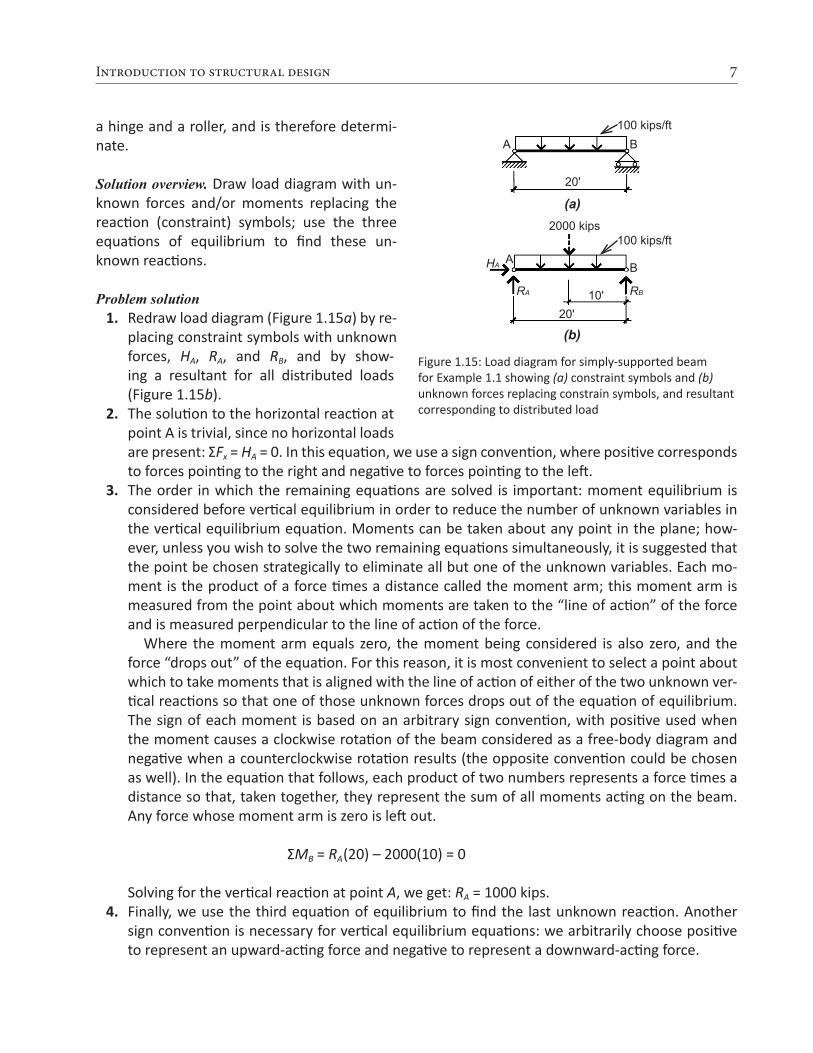
a hinge and a roller, and is therefore determi-nate.
Solution overview. Draw load diagram with un-known forces and/or moments replacing the reaction (constraint) symbols; use the three equations of equilibrium to find these un-known reactions.
Problem solution 1. Redraw load diagram (Figure 1.15a) by re-
placing constraint symbols with unknown forces, HA, RA, and RB, and by show-ing a resultant for all distributed loads (Figure 1.15b).
2. The solution to the horizontal reaction at point A is trivial, since no horizontal loads are present: ΣFx = HA = 0. In this equation, we use a sign convention, where positive corresponds to forces pointing to the right and negative to forces pointing to the left.
3. The order in which the remaining equations are solved is important: moment equilibrium is considered before vertical equilibrium in order to reduce the number of unknown variables in the vertical equilibrium equation. Moments can be taken about any point in the plane; how-ever, unless you wish to solve the two remaining equations simultaneously, it is suggested that the point be chosen strategically to eliminate all but one of the unknown variables. Each mo-ment is the product of a force times a distance called the moment arm; this moment arm is measured from the point about which moments are taken to the “line of action” of the force and is measured perpendicular to the line of action of the force.
Where the moment arm equals zero, the moment being considered is also zero, and the force “drops out” of the equation. For this reason, it is most convenient to select a point about which to take moments that is aligned with the line of action of either of the two unknown ver-tical reactions so that one of those unknown forces drops out of the equation of equilibrium. The sign of each moment is based on an arbitrary sign convention, with positive used when the moment causes a clockwise rotation of the beam considered as a free-body diagram and negative when a counterclockwise rotation results (the opposite convention could be chosen as well). In the equation that follows, each product of two numbers represents a force times a distance so that, taken together, they represent the sum of all moments acting on the beam. Any force whose moment arm is zero is left out.
ΣMB = RA(20) – 2000(10) = 0
Solving for the vertical reaction at point A, we get: RA = 1000 kips. 4. Finally, we use the third equation of equilibrium to find the last unknown reaction. Another
sign convention is necessary for vertical equilibrium equations: we arbitrarily choose positive to represent an upward-acting force and negative to represent a downward-acting force.
Figure 1.15: Load diagram for simply-supported beam for Example 1.1 showing (a) constraint symbols and (b) unknown forces replacing constrain symbols, and resultant corresponding to distributed load
100 kips/ftA B
(a)
(b)20'
HA
100 kips/ft2000 kips
AB
RA RB10'
20'

8 Structural Elements for Architects and Builders
ΣFy = RA + RB – 2000 = 0
or, substituting RA = 1000 kips:
1000 + RB – 2000 = 0
Solving for the vertical reaction at point B, we get RB = 1000 kips.
The two vertical reactions in this example are equal and could have been found by sim-ply dividing the total load in half, as we did when considering tributary areas. Doing this, however, is only appropriate when the struc-ture’s geometry and loads are symmetrical.
If the reactions represent other structural sup-ports such as columns or girders, then the “up-ward” support they give to the beam occurs simul-taneously with the beam’s “downward” weight on the supports: in other words, if the beam in Example 1.1 is supported on two columns, then those columns (at points A and B) would have load diagrams as shown in Figure 1.16a. The beam and columns, shown together, have reactions and loads as shown in Figure 1.16b. These pairs of equal and opposite forces are actually inseparable. In the Newtonian framework, each action, or load, has an equal reaction.
Example 1.2 Find reactions for three-hinged arch
Problem definition. Find the reactions for the three-hinged arch shown in Figure 1.17a.
Solution overview. Draw load diagram with un-known forces and/or moments replacing the re-action (constraint) symbols; use the three equa-tions of equilibrium, plus one additional equation found by considering the equilibrium of another free-body diagram, to find the four unknown re-actions.
Problem solution 1. The three-hinged arch shown in this ex-
ample appears to have too many unknown variables (four unknowns versus only three
Figure 1.16: Support for the beam from Example 1.1 showing (a) load on column supports and (b) reactions from beam corresponding to load on column supports
1000 kips
1000 kips
columns
A
(a)
1000 kips1000 kips1000 kips
1000 kips
B
(b)
columns
A B
Figure 1.17: Load diagram for 3-hinged arch for Example 1.2 showing (a) constraint symbols and (b) unknown forces replacing constrain symbols
20 kips
A
30' 30'
B20
'
(a)
20 kipsC
AHA
RA 30'(b)
30'RB
B HB
20'
C

9Introduction to structural design
equations of equilibrium); however, the internal hinge at point C prevents the structure from behaving as a rigid body, and a fourth equation can be developed out of this condition. The initial three equations of equilibrium can be written as follows:a. ΣMB = RA(60) – 20(30) = 0, from which RA = 10 kips.b. ΣFy = RA + RB – 20 = 0; then, substituting RA = 10 kips from the moment equilibrium equation
solved in step a, we get 10 + RB – 20 = 0, from which RB = 10 kips.c. ΣFx = HA – HB = 0.
Sign conventions are as described in Example 1.1. This last equation of horizontal equilibrium (step c) contains two unknown variables and cannot be solved at this point. To find HA, it is nec-essary to first cut a new FBD at the internal hinge (point C) in order to examine the equilibrium of the resulting partial structure shown in Figure 1.18.
2. With respect to this FBD, we show un-known internal forces HC and VC at the cut, but we show no bending moment at that point since none can exist at a hinge. This condition of zero moment is what al-lows us to write an equation that can be solved for the unknown, HA:
ΣMC = 10(30) – HA(20) = 0
from which HA = 15 kips. Then, going back to the “horizontal”
equilibrium equation shown in step c that was written for the entire structure (not just the cut FBD), we get:
ΣFx = HA – HB = 15 – HB = 0
from which HB = 15 kips.
While the moment equation written for the FBD can be taken about any point in the plane of the structure, it is easier to take mo-ments about point C, so that only HA appears in the equation as an unknown. Otherwise, it would be necessary to first solve for the internal unknown forces at point C, using “vertical” and “horizontal” equilibrium.
If there were no hinge at point C, we would need to add an unknown internal moment at C, in addition to the forces shown (Figure 1.19). The moment equation would then be ΣMC = 10(30) – HA(20) + MC = 0. With two unknown variables in the equation (HA and MC), we cannot solve for HA. In other words, unlike the three-hinged arch, this two-hinged arch is an indeterminate struc-ture.
A
C20
'
30'
20 kips
VC
HC
HA
MC
Figure 1.18: Free-body diagram cut at internal hinge at point C, for Example 1.2
A
C
20'
30'10 kips
20 kips
HA
VC
HC
Figure 1.19: Free-body diagram for a two-hinged arch (with internal moment at point C)

10 Structural Elements for Architects and Builders
Example 1.3 Find reactions for a cable
Problem definition. Find the reactions for the flexible cable structure shown in Figure 1.20a. The ac-tual shape of the cable is unknown: all that is specified is the maximum distance of the cable below the level of the supports (reactions): the cable’s sag.
Solution overview. Draw load diagram with unknown forces and/or moments replacing the reaction (constraint) symbols; use the three equations of equilibrium, plus one additional equation found by considering the equilibrium of another free-body diagram, to find the four unknown reactions.
Problem solution 1. The cable shown in this example appears to have too many unknown variables (four unknowns
versus only three equations of equilibrium); however, the cable’s flexibility prevents it from be-having as a rigid body, and a fourth equation can be developed out of this condition. The three equations of equilibrium can be written as follows:a. ΣMB = RA(80) – 10(65) – 20(40) = 0, from which RA = 18.125 kips.b. ΣFy = RA + RB – 10 – 20 = 0; then, substituting RA = 18.125 kips from the moment equilibrium
equation solved in step a, we get 18.125 + RB – 10 – 20 = 0, from which RB = 11.875 kips.
c. ΣFx = –HA + HB = 0. Sign conventions are as described in Example 1.1. This last equation of horizontal equilibrium
(step c) contains two unknown variables and cannot be solved at this point. By analogy to the three-hinged arch, we would expect to cut an FBD and develop a fourth equation. Like the in-ternal hinge in the arch, the entire cable, being flexible, is incapable of resisting any bending moments. But unlike the arch, the cable’s geometry is not predetermined; it is conditioned by the particular loads placed upon it. Before cutting the FBD, we need to figure out where the maximum specified sag of 10 ft occurs: without this information, we would be writing a mo-ment equilibrium equation of an FBD in which the moment arm of the horizontal reaction, HA, was unknown.
Figure 1.20: Load diagram for cable for Example 1.3 showing (a) constraint symbols and (b) unknown forces replacing constraint symbols
10 kips 20 kips
15' 25'
40'
(a)
(b)
10' s
ag10
' sag
10 kips 20 kips
15' 25'
40'
A B
C D
A B
C D
HA
RA
HB
RB

11Introduction to structural design
2. We find the location of the sag point by looking at internal vertical forces within the cable. When the direction of these internal vertical forces changes, the cable has reached its lowest point (Figure 1.21). Checking first at point C, we see that the internal vertical force does not change direction on either side of the external load of 10 kips (comparing Figure 1.22a and Figure 1.22b), so the sag point cannot be at point C.
However, when we check point D, we see that the direction of the internal vertical force does change, as shown in Figure 1.23. Thus, point D is the sag point of the cable (i.e., the low point), specified as being 10 ft below the support elevation.
Figure 1.22: Vertical component of cable force for Example 1.3 is found (a) just to the left of the external load at point C and (b) just to the right of the load
HA A
C
A
C
10 kips external load not included
18.125 kips
15'Vc
Hc
HA
10 kips
18.125 kips Hc
Vc15'
SFy = 18.125 – 10 – Vc = 0VC = 8.125 kips (downward)
SFy = 18.125 – Vc = 0VC = 18.125 kips (downward)
(a) (b)
Figure 1.21: Sag point occurs where the vertical component of internal cable forces changes direction (sign), for Example 1.3
V1
V2
sag point
Figure 1.23: Vertical component of cable force for Example 1.3 is found (a) just to the left of the external load at point D and (b) just to the right of the load
20 kips external load not included
A
C Hd
Vd
SFy = 18.125 - 10 - VD = 0VD = 8.125 kips (downward)
HA
25'
(b)
A
CDD
10 kips10 kips 20 kips
15'25'15'
Hd
Vd
HA
SFy = 18.125 - 10 - 20 - VD = 0VD = 11.875 kips (upwards)
(a)

12 Structural Elements for Architects and Builders
We can also find this sag point by constructing a diagram of cumulative vertical loads, begin-ning on the left side of the cable (Figure 1.24). The sag point then occurs where the “cumulative force line” crosses the baseline.
3. Having determined the sag point, we cut an FBD at that point (Figure 1.25a) and proceed as in the example of the three-hinged arch, taking moments about the sag point:
ΣMD = 18.125(40) – 10(25) – 10(HA) = 0, from which HA = 47.5 kips.
Once the location of the sag point is known, a more accurate sketch of the cable shape can be made, as shown in Figure 1.25b.
Then, going back to the “horizontal” equilibrium equation shown in step 1c that was written for the entire structure (not just the cut FBD), we get ΣFx = –HA + HB = –47.5 + HB = 0, from which HB = 47.5 kips. In this last equation, the value of HA is written with a minus sign since it acts toward the left (and our sign convention has positive going to the right).
We have thus far assumed particular directions for our unknown forces — for example, that HA acts toward the left. Doing so resulted in a positive answer of 47.5 kips, which confirmed that our guess of the force’s direction was correct. Had we initially assumed that HA acted toward the right, we would have gotten an answer of –47.5 kips, which is equally correct, but less satisfying. In other words, both ways of describing the force shown in Figure 1.26 are equivalent.
Figure 1.24: Diagram of cumulative vertical loads, for Example 1.3
18.125 kips
A BC D
10 kips
20 kips 11.875 kipssag point
Figure 1.25: Free-body diagram cut at the sag point for Example 1.3
10' s
ag
HA
15'
(a)
18.125 kips
10 kips
25'
10' s
ag
(b)
HA
15'
18.125 kips
10 kips
25' 40'
20 kips
HB
RB

13Introduction to structural design
Internal Forces and Moments
Finding internal forces and moments is no different than finding reactions; one need only cut an FBD at the cross section where the internal forces and moments are to be computed (after having found any unknown reactions that occur within the diagram). At any cut in a rigid element of a plane struc-ture, two perpendicular forces and one moment are potentially present. These internal forces and moments have names, depending on their orientation relative to the axis of the structural element where the cut is made (Figure 1.27). The force parallel to the axis of the member is called an axial force; the force perpendicular to the member is called a shear force; the moment about an axis perpendicular to the structure’s plane is called a bending moment.
In a three-dimensional environment with x-, y-, and z-axes as shown in Figure 1.27, three additional forces and moments may be pres-ent: another shear force (along the z-axis) and two other moments, one about the y-axis and one about the x-axis. Moments about the y-ax-is cause bending (but bending perpendicular to the two-dimensional plane); moments about the x-axis cause twisting or torsion. These types of three-dimensional structural behav-iors are beyond the scope of this discussion.
Internal shear forces and bending moments in beams
Where the only external forces acting on beams are perpendicular to a simply supported beam’s longitudinal axis, no axial forces can be present. The following examples show how internal shear forces and bending moments can be computed along the length of the beam.
Example 1.4 Find internal shear and bend-ing moment for simply supported beam with “point” loads
Problem definition. Find internal shear forces and bending moments at key points along the length of the beam shown in Figure 1.28, i.e., under each external load and reaction. Reac-tions have already been determined.
Figure 1.26: Negative and positive signs on force arrows going in opposite directions represent equivalent loads
47.5 kips – 47.5 kips
Figure 1.27: Internal shear and axial forces, and internal bending moment
Shear force
Bending moment
Axial force
x
z
y
Figure 1.28: Load diagram for Example 1.4
5 kips 5 kips
B
5 kips
8'8'8'
5 kips
ADC

14 Structural Elements for Architects and Builders
Solution overview. Cut free-body diagrams at each external load; use equations of equilibrium to compute the unknown internal forces and mo-ments at those cut points.
Problem solution 1. To find the internal shear force and bending moment at point A, first cut a free-body diagram
there, as shown in Figure 1.29. Using the equation of vertical equilibrium, ΣFy = 5 – VA = 0, from which the internal shear force
VA = 5 kips (downward). Moment equilibrium is used to confirm that the internal moment at the hinge is zero: ΣMA =
MA = 0. The two forces present (5 kips and VA = 5 kips) do not need to be included in this equa-tion of moment equilibrium since their moment arms are equal to zero. The potential internal moment, MA, is entered into the moment equilibrium equation as it is (without being multiplied by a moment arm) since it is already, by definition, a moment.
2. Shear forces must be computed on “both sides” of the external load at point C; the fact that this results in two different values for shear at this point is not a paradox: it simply reflects the discontinuity in the value of shear caused by the presence of a concentrated load. In fact, a truly concentrated load acting over an area of zero is impossible, since it would result in an infinitely high stress at the point of application; all concentrated loads are really distributed loads over small areas. However, there is only one value for bending moment at point C, whether or not the external load is included in the FBD. In other words, unlike shear force, there is no disconti-nuity in moment resulting from a concentrated load.a. Find internal shear force and bending moment at point C, just to the left of the external
load, by cutting an FBD at that point as shown in Figure 1.30a. Using the equation of verti-cal equilibrium: ΣFy = 5 – VC = 0, from which the internal shear force VC = 5 kips (downward). Using the equation of moment equilibrium, ΣMC = 5(8) – MC = 0, from which MC = 40 ft-kips (counterclockwise).
b. Find internal shear force and bending moment at point C, just to the right of the external load by cutting a FBD at that point, as shown in Figure 1.30b. Using the equation of vertical equilibrium: ΣFy = 5 – 5 – VC = 0, from which the internal shear force VC = 0 kips. Using the equation of moment equilibrium, ΣMC = 5(8) – MC = 0, from which MC = 40 ft-kips (counterclockwise), as before.
3. Find shear and moment at point D.a. Find internal shear force and bending
moment at point D, just to the left of the external load by cutting an FBD at that point, as shown in Figure 1.31a. Us-ing the equation of vertical equilibrium: ΣFy = 5 – 5 – VD = 0, from which the in-ternal shear force VD = 0 kips. Using the equation of moment equilibrium, ΣMD = 5(16) – 5(8) – MD = 0, from which MD = 40 ft-kips (counterclockwise).
5 kips8'(a)
C
Vc
Mc
5 kips
McC
Vc
A
5 kips8'(b)
A
Figure 1.30: Free-body diagram for Example 1.4 (a) cut just to the left of the external load at point C and (b) just to the right of the load
Figure 1.29: Free-body diagram cut at left reaction for Example 1.4
VA
A MA
5 kips

15Introduction to structural design
b. Find internal shear force and bending moment at point D, just to the right of the external load by cutting an FBD at that point, as shown in Figure 1.31b. Using the equation of vertical equilib-rium, ΣFy = 5 – 5 – 5 – VD = 0, from which the internal shear force VD = –5 kips (downward), which is equivalent to 5 kips (upward). Using the equation of moment equilibrium, ΣMD = 5(16) – 5(8) – MD = 0, from which MD = 40 ft-kips (counterclockwise), as before.
4. Find shear and moment at point B by cut-ting a free-body diagram just to the left of the reaction at point B, as shown in Figure 1.32. Using the equation of vertical equilibrium, ΣFy = 5 – 5 – 5 – VB = 0, from which the internal shear force VB = –5 kips (downward), which is equivalent to 5 kips (upward).
Moment equilibrium is used to confirm that the internal moment at the hinge is zero: ΣMB = 5(24) – 5(16) – 5(8) – MB = 0, from which MB = 0. The internal shear force, VB, does not need to be included in this equation of moment equilibrium since its moment arm is equal to zero.
The forces and moments can be graphically displayed as shown in Figure 1.33, by connecting the points found earlier.
Some important characteristics of internal shear forces and bending moments may now be sum-marized: (1) Internal axial forces are always zero in a horizontally oriented simply supported beam with only vertical loads. (2) Moments at hinges at the ends of structural members are zero. Only
Figure 1.31: Free-body diagram for Example 1.4 (a) cut just to the left of the external load at point D and (b) just to the right of the load
MD
VD
D
MD
VD
D
5 kips
5 kips
5 kips
5 kips
5 kips
8'
8'8'
8'
A C
A C
(a)
(b)
Figure 1.32: Free-body diagram cut just to the left of the reaction at point B for Example 1.4
A5 kips
C5 kipsD B
VB
MB
5 kips8' 8' 8'
Figure 1.33: Load, shear, and moment diagrams for Example 1.4
5 kips 5 kips
5 kips 5 kips
5 kips
-5 kips
40 ft-kips
8' 8'8'
Shear force diagram
Moment diagram

16 Structural Elements for Architects and Builders
when a continuous member passes over a hinge can the moment at a hinge be nonzero. (3) A shear force acting downward on the right side of an FBD is arbitrarily called “positive”; a bending moment acting counterclockwise on the right side of an FBD is arbitrarily called “positive.” Positive bending corresponds to “tension” on the bottom and “compression” on the top of a horizontal structural element.
General strategy for finding internal shear forces and bending moments
Shear and moment diagrams can also be drawn by noting the following rules: (1) At any point along the beam, the slope of the shear diagram equals the value of the load (the “infinite” slope of the shear diagram at concentrated loads can be seen as a shorthand approximation to the actual con-dition of the load being distributed over some finite length, rather than existing at a point). (2) Be-tween any two points along a beam, the change in the value of shear equals the total load (between those points). (3) The slope of the moment diagram at any point equals the value of the shear force at that point. (4) The change in the value of bending moment between any two points equals the “area of the shear diagram” between those points. These rules are derived by applying the equa-tions of equilibrium to an elemental slice of a beam, as shown in Appendix Table A-1.1.
Example 1.5 Find internal shear and bending moments for a simply supported cantilever beam with distributed loads
Problem definition. Find the distribution of internal shear forces and bending moments for the beam shown in Figure 1.34, first by using FBDs and then by applying the rules from Appendix Table A-1.1.
Solution overview. Find reactions using the equa-tions of equilibrium; find internal shear force and bending moment at key points (at reactions and at location of zero shear).
Problem solution 1. Find the resultant of the distributed load,
equal to 1 kip/ft × 25 ft = 25 kips. 2. To find reactions, first take moments about
either point A or point B; we choose point B: ΣMB = RA(20) – 25(12.5) = 0, from which RA = 15.625 kips. Next, use the equation of ver-tical equilibrium to find the other reaction: ΣFy = RA + RB – 25 = 15.625 + RB – 25 = 0, from which RB = 9.375 kips.
3. Find shear and moment at point A.a. Find internal shear force and bending
moment at point A, just to the left of the
Figure 1.34: Load diagram for Example 1.5
Figure 1.35: Free-body diagram for Example 1.5 (a) cut just to the left of the reaction at point A; and (b) just to the right of the reaction
5'
2.5'
VAA
5'
2.5'
VA
MA
A15.625 kips
(a)
(b)
1 kip/ft
1 kip/ftMA
Resultant of distributed load25 kips
B
w = 1 kip/ft
RA RB12.5'
20'5'
A

17Introduction to structural design
reaction by cutting an FBD at that point, as shown in Figure 1.35a. Using the equation of ver-tical equilibrium, ΣFy = –5 – VA = 0, from which the internal shear force, VA = –5 kips (down-ward) or 5 kips (upward). Using the equation of moment equilibrium, ΣMA = –5(2.5) – MA = 0, from which MA = –12.5 ft-kips (counterclockwise) or 12.5 ft-kips (clockwise).
b. Find internal shear force and bending moment at point A, just to the right of the reaction by cutting an FBD at that point, as shown in Figure 1.35b. Using the equation of vertical equilibrium, ΣFy = 15.625 – 5 – VA = 0, from which the internal shear force VA = 10.625 kips (downward). Using the equation of moment equilibrium, ΣMA = –5(2.5) – MA = 0, from which MA = –12.5 ft-kips (counterclockwise) or 12.5 ft-kips (clockwise), as before.
The moment at point A is not zero, even though there is a hinge at that point. The reason is that the beam itself is continuous over the hinge. This continuity is essential for the stabil-ity of the cantilevered portion of the beam.
4. Find shear and moment at point B by cut-ting a free-body diagram just to the left of the reaction at point B, as shown in Figure 1.36. Using the equation of verti-cal equilibrium, ΣFy = 15.625 – 25 – VB = 0, from which the internal shear force VB = – 9.375 kips (downward), which is equiv-alent to 9.375 kips (upward). Moment equilibrium is used to confirm that the in-ternal moment at the hinge is zero: ΣMB = 15.625(20) – 25(12.5) + MB = 0, from which MB = 0. The internal shear force, VB, does not need to be included in this equation of moment equilibrium since its moment arm is equal to zero.
5. The internal shear forces can be graphi-cally displayed as shown in Figure 1.37, by connecting the points found earlier. The slope of the shear diagram at any point equals the value of the load; since the load is uniformly distributed, or constant, the slope of the shear diagram is also con-stant.
The bending moment cannot be ade-quately diagrammed until one more point is determined and analyzed: the point somewhere between the two reactions where the shear is zero. Since the slope of the moment diagram at any point equals the value of the shear force, a change from positive to negative shear indicates at least a “local” minimum or maximum moment (Figure 1.38).
Figure 1.36: Free-body diagram cut just to the left of the reaction at point B for Example 1.5
Resultant of distributed load25 kips
1 kip/ft
MB
VB
12.5'
20'5'15.625 kips
A B
Figure 1.37: Load and shear diagrams for Example 1.5
B
1 kip/ft
5' 20'A
Shear diagram
10.6
25 k
ips
5.0
kips
9.37
5 ki
ps
equal slope
Figure 1.38: Relationship between value of shear diagram and slope of moment diagram
Negative value, getting smaller (more negative)
Positive value, getting smaller from left to right
Local maximumNegative slope
Positive slope, getting smaller from left to right
Moment
Shear

18 Structural Elements for Architects and Builders
This key point, labeled C in Figure 1.39, can be located by dividing the value of shear just to the right of the reaction at point A by the distributed load: the distance of point C from point A, then, is x = 10.625/1.0 = 10.625 ft.
The length, x, can also be found using similar triangles: x/10.625 = 20/20. Solving for x, we get the same value as earlier: x = 10.625 ft.
The moment at this point can be found by cutting an FBD at point C, as shown in Figure 1.40, and applying the equa-tion of moment equilibrium: ΣMC = 15.625(10.625) – 15.625(7.8125) – MC = 0, from which MC = 43.9 ft-kips (counterclock-wise).
6. Alternatively, shear and moment diagrams may be drawn based on the rules listed in Ap-pendix Table A-1.1, and illustrated in Figure 1.41. The critical points of the shear diagram are derived from the load diagram based on Rule 2: the “areas” of the load diagram (with concentrated loads or reactions counting as areas b and d) between any two points equal the change in shear between those points. These “area” values are summarized in the box between the load and shear diagrams. Con-necting the points established using Rule 2 is facilitated by reference to Rule 1: the slope of the shear diagram equals the value of the load at that point. Therefore, where the load diagram is “flat” (i.e., has constant value), the shear diagram has constant slope represented by a straight line that has positive slope for positive values of load, and negative slope corresponding to neg-ative values of load. Since almost all distributed loads are downward-acting (negative value), shear diagrams often have the characteristic pattern of negative slope shown in Figure 1.41.
Once the shear diagram has been completed, and any critical lengths have been found (see step 5), the moment diagram can be drawn based on Rules 3 and 4 of Appendix Table A-1.1. Critical moments are first found by examining the “areas” under the shear diagram, as de-scribed in Rule 4 of Appendix Table A-1.1. These “areas” — actually forces times distances, or moments — are shown in the box between the shear and moment diagrams in Figure 1.41 and represent the change in moment between the two points bracketed by the shear diagram ar-eas — not the value of the moments themselves. For example, the first “area e” of –12.5 ft-kips is added to the initial moment of zero at the free end of the cantilever, so that the actual mo-ment at point A is 0 + –12.5 = –12.5 ft-kips. The maximum moment (where the shear is zero), is found by adding “area f ” to the moment at point A: 56.45 + –12.5 = 43.95 ft-kips, as shown in Figure 1.41. Finally, slopes of the moment diagram curve can be determined based on Rule 3 of Appendix Table A-1.1: the slope of the moment diagram is equal to the value of the shear force at any point, as illustrated in Figure 1.38.
Figure 1.39: Shear diagram for Example 1.5, showing distance from reaction at point A to the point where the shear diagram crosses the baseline, going from positive to negative value
A BC
20'
x
20 k
ips
10.6
25 k
ips
9.37
5 ki
ps
Figure 1.40: Free-body diagram for Example 1.5, cut at the point of zero shear (where the shear diagram crosses the baseline, going from positive to negative value)
VC = 0
MCA C
15.625 kips1 kip/ft
15.625 kips 7.1825'
5' 10.625'15.625'

19Introduction to structural design
In drawing the moment diagram, it is important to emphasize the following: (1) The area under the shear diagram between any two points corresponds, not to the value of the moment, but to the change in moment between those two points. Therefore, the triangular shear diagram area, f, of 56.45 ft-kips in the Example 1.5 does not show up as a moment anywhere in the beam; in fact, the maximum moment turns out to be 43.95 ft-kips. (2) The particular curvature of the moment diagram can be found by relating the slope of the curve to the changing values of the shear diagram. (3) The moment and shear diagrams are created with respect to the actual distribution of loads on the beam, not the resultants of those loads, which may have been used in the calculation of reac-tions. The location of the maximum moment, therefore, has nothing to do with the location of any resultant load but occurs at the point of zero shear. (4) Moment diagrams can also be drawn in an alternate form, as shown at the bottom of Figure 1.41, by reversing the positions of negative and positive values. This form has the benefit of aligning the shape of the moment diagram more closely with the deflected shape of the beam (although it still remains significantly different from the de-flected shape), at the expense of being mathematically inconsistent. (5) Finally, it may be important in some cases to account for both positive and negative moments, and not just the maximum mo-ment. In this example, the maximum positive moment is 43.95 ft-kips, while the maximum negative moment is 12.5 ft-kips.
a
b = 15.625 kips
c
a c
d = 9.375 kips
b
Shear diagram
Moment diagram
Alternativemoment diagram
“Areas” (kips)
“Areas” (ft-kips)
AB
d5' 20'
5' 10.625' 9.375'
-5.0 -20.015.625 9.375
15.625 kips20 kips
10.625 kips
5.0 kips 9.375 kips
43.95 ft-kips12.5 ft-kips
56.45 ft-kips
-12.5 +56.45 -43.95
43.95 ft-kips12.5 ft-kips
56.45 ft-kips
e gf
e gf
Figure 1.41: Load, shear, and moment diagrams for Example 1.5, using load diagram “areas” to find shear values, and shear diagram “areas” to find moment values

20 Structural Elements for Architects and Builders
Internal axial forces in trusses, arches, and cables
There is a class of determinate structures that cannot sustain internal shear forces or bending mo-ments, either because their component elements are pinned together or because they are inher-ently flexible. We will examine three types of these axial-force structures. Trusses are made from individual elements organized in a triangular pattern and assumed to be pinned at the joints so that they may be analyzed using only equations of equilibrium. Reactions of trusses are found just like the reactions of beams, while the reactions of three-hinged arches and cables — the other two axial-force structures already examined — require special treatment. In general, the axial forces within trusses, three-hinged arches, and cables are found using the three equations of equilibrium. The following examples illustrate specific techniques and strategies.
Example 1.6 Find internal axial forces in a truss (section method)
Problem definition. Find the internal axial forces in truss bars C-F, C-E, and D-E for the truss shown in Figure 1.42. Assume pinned joints, as shown.
Solution overview. Find reactions; then, using the so-called section method, cut a free-body diagram through the bars for which internal forces are be-ing computed. As there are only three equations of equilibrium, no more than three bars may be cut (resulting in three unknown forces); use equa-tions of equilibrium to solve for the unknown forces.
Problem solution 1. Find reactions: by symmetry, RA = RB = (10 + 10 + 10)/2 = 15 kips. Alternatively, one could take
moments about point A or B, solve for the unknown reaction, and then use the equation of vertical equilibrium to find the other unknown reaction.
2. Cut a free-body diagram through the bars being evaluated (cutting through no more than three bars) as shown in Figure 1.43. Bar forces are labeled according to the nodes that are at either end of their bars, so, for example, FCF is the force between nodes C and F.a. Show unknown axial forces as tension
forces; a negative result indicates that the bar is actually in compression. Ten-sion means that the force is shown “pull-ing” on the bar or node within the free-body diagram.
b. Use equilibrium equations, chosen stra-tegically, to solve for unknown bar forces. To find FCF: ΣME = 15(16) – 10(8) + FCF(8) = 0; solving for the unknown bar force, we
Figure 1.42: Loading diagram for, and geometry of, truss, for Example 1.6
Figure 1.43: Free-body diagram cut through bars based on the section method, for Example 1.6
10 kips 10 kips10 kips
8'
8' 8' 8' 8'
B
C
DE
F G
A H
C
FDE
FCE
FCF F
E
10 kips
8' 8'
8'
15 kipsRA =
A
Component:0.707FCE
D

21Introduction to structural design
get FCF = –20 k (compression).c. To find FDE: ΣMC = 15(8) – FDE(8) = 0; solving for the unknown bar force, we get FDE = 15k (ten-
sion).d. Finally, to find FCE: find force “components” of inclined internal axial force FCE. The compo-
nents can be found using principles of trigonometry, based on the geometry of the triangle determined by the 8 ft × 8 ft truss panels. For example, the vertical (or horizontal) compo-nent equals FCE × sin 45° = 0.707FCE. We then use the equation of vertical equilibrium: ΣFy = 15 – 10 – 0.707FCE = 0; solving for the unknown bar force, we get FCE = 7.07 kips (tension).
The assumption that only axial forces exist within a truss is valid when the following conditions are met: (1) all bar joints are “pinned” (hinged), and (2) external loads and reactions are placed only at the joints or nodes. Under these circumstances, no internal shear forces or bending moments are possible. In practice, modern trusses are rarely pinned at each joint; nevertheless, the assumption is often used for preliminary design since it facilitates the calculation of internal forces. What is more, actual bar forces in indeterminate trusses (i.e., where the members are continuous rather than pinned) are often reasonably close to the approximate results obtained by assuming pinned joints.
Example 1.7 Find internal axial forces in a three-hinged arch
Problem definition. Find the internal axial force in bar AC of the three-hinged arch analyzed in Ex-ample 1.2.
Solution overview. Cut a free-body diagram through the bar in question, as shown in Figure 1.44a; label the unknown bar force as if in tension; use the equations of equilibrium to solve for the un-known force.
Problem Solution 1. Because the far force, FAC, is inclined, it is convenient to draw and label its horizontal and vertical
component forces, x and y. Using the equations of vertical and horizontal equilibrium, we can find these component forces directly: ΣFy = 10 + y = 0, from which y = –10 kips; ΣFx = 15 + x = 0, from which x = –15 kips. In both cases, the negative sign indicates that our initial assumption of tension was incorrect; the bar force is actually in compression, as one would expect in such an arch.
2. To find the actual bar force, FAC, the most direct approach is to use the Pythagorean theorem,
Figure 1.44: Internal bar force for Example 1.7 shown (a) in free-body diagram and (b) as a “force” triangle with com-ponents x and y
(a) (b)
15 kips10 kips
A
20'
C
30'
x
x
y
y
FAC
FAC
30.06'

22 Structural Elements for Architects and Builders
with the unknown force being the hypotenuse of a right triangle, as shown in Figure 1.44b. Therefore, FAC = √x2 + y2 = √152 + 102 = 8.03 kips. The signs of the forces are omitted in this cal-culation.
Example 1.8 Find internal axial forces in a cable
Problem definition. Find the internal axial force in segment AC of the cable analyzed in Example 1.3.
Solution overview. Cut a free-body diagram through the segment in question, as shown in Figure 1.45; label unknown cable force as if in tension; use the equations of equilibrium to solve for the un-known force.
Problem solution 1. Because the cable force, FAC, is inclined, it is convenient to draw and label its horizontal and
vertical component forces, x and y. Using the equations of vertical and horizontal equilibrium, we can find these component forces directly: ΣFy = 18.125 – y = 0, from which y = 18.125 kips; ΣFx = –47.5 + x = 0, from which x = 47.5 kips. In both cases, the positive sign indicates that our initial assumption of tension was correct, as one would expect in any cable structure.
2. To find the actual cable force, FAC, the most direct approach is to use the Pythagorean theorem, with the unknown force being the hypotenuse of a right triangle. Therefore, FAC = √x2 + y2 = √47.52 + 18.1252 = 50.84 kips. The signs of the forces are omitted in this calculation.
3. Since the cable is flexible, the height, h, is initially unknown and, in fact, will change if the loads are changed. To find h, we can use the fact that the “force triangle” and “geometry triangle” are similar; therefore, the ratio of their sides must be equal: h/15 = y/x = 18.125/47.5, from which h = 5.72 ft. Because the height will change if the loads change, the cable is an unstable structure.
Indeterminate Structures
Where there are more reactions, or constraints, than there are equations of equilibrium, a structure is said to be statically indeterminate or redundant. Each added constraint adds one degree of inde-terminacy or redundancy to the structure, making it that much more difficult to solve mathemati-cally. To understand the basis of the mathemati-cal solution to indeterminate structures, we will examine a simply supported beam with a single concentrated load that has been made 1-degree redundant (indeterminate) by adding a hanger at midspan: the structure now has four unknown re-actions (constraints), and only three equations of equilibrium are available, as shown in Figure 1.46.
The key to the solution is to find an addi-tional equation that includes one or more of the
Figure 1.46: Load diagram for a simply supported beam with an added hanger at midspan
HA
RA RB
A
P
DBC
RD
Figure 1.45: Bar force for Example 1.8 shown in free-body diagram with components x and y
47.5 kips
18.125 kips
15'
h
x
yFAC
A
C

23Introduction to structural design
structure’s constraint variables; that equation will not be concerned with equilibrium, but rather with the compatibility of structural de-formations or deflections. Looking at the simply supported beam and the tension hanger sepa-rately, it is possible to write equations relating the loads acting on them to their deflection. For now, we will simply note that Δ1 = P1S1, and Δ2 = P2 S2 as shown in Figure 1.47, where Δ1 and Δ2 are the deflections of the beam and hanger, respectively; P1 and P2 are the loads assumed to act separately on the beam and hanger; and S1 and S2 are deflection constants that include the length or span of the elements as well as their stiff-ness (i.e., their resistance to deformation).
These deflections, calculated separately for the beam and hanger, must actually be equal in the real structure, and the loads P1 and P2 that correspond to these equal deflections are actually only the parts of the total load, P, that the beam and hanger separately resist. In other words, Δ1 = Δ2; and P1 + P2 = P. This can be rewritten as follows:
P1S1 = P2S2
P1 = P – P2
Solving Equation 1.2 for P1 , and substituting the result into Equation 1.3, we get:
Solving for P2, we get:
Since the load P and coefficients S1 and S2 are all known, the force P2 can be determined from Equa-tion 1.5. Then, from Figure 1.47b, it can be seen that the vertical reaction, RD = P2. With this “fourth” reaction solved, the other vertical reactions at A and B can easily be determined using the equations of equilibrium.
Equation 1.5 also clarifies the relationship between the element load-deformation constants, represented by S1 and S2, and the overall behavior of the structure. For example, if the constants are equal, it can be seen that P2 = P/2; i.e., half the load is resisted by the hanger and half by the beam. On the other hand, if S1 is small compared to S2 (i.e., if the hanger is more effective in resist-ing deformation than the beam), then P2 approaches the value of P, and the hanger begins to resist virtually all of the total load, with the beam’s share approaching zero. This is of crucial importance in understanding the behavior of indeterminate structures: loads tend to follow the path of greatest stiffness, or, put another way, loads follow various competing load paths in proportion to the stiff-ness of those paths. In these formulations, “stiffness” is used as shorthand for the load-deformation relationship, which includes both the actual element stiffness (involving only material and cross-
(1.2)
(1.3)
(1.4)S1
P2S2 = P - P2
S1/S2 + 1P2 =
P (1.5)
Figure 1.47: Deflection diagrams for the two components of the structure shown in Figure 1.46: (a) a simply-support-ed beam with a concentrated load, P1, and (b) a tension hanger with load P2
HA
RA RB
A
P1
DC
RD
P2
A BΔ1 = P1S1
(a) (b)
Δ2 = P2S2
B

24 Structural Elements for Architects and Builders
sectional properties) as well as element length or span.For highly redundant structures, a greater number of equations, based on compatibility of de-
formations, needs to be solved simultaneously. While this becomes unwieldy if done by hand, struc-tural analysis software has been developed to solve such problems: the designer need only indicate the geometry of the structure (including lengths and spans), the nature of each constraint (hinged, fixed, etc.), and the relative stiffness of each element. This last requirement presents a bit of a dilem-ma, since relative member stiffnesses must be assumed before the structure can be designed. The stiffnesses assumed for the structure determine how the structure will respond to its loads, unlike determinate structures, whose internal forces and moments are independent of member cross sec-tions and material properties. For this reason, experience, trial and error, or a bit of both are crucial in the design of indeterminate structures.
Once internal forces and moments have been determined, however, the same strategies for the design of structural elements outlined in this book can be used, whether the structure is statically determinate or indeterminate.
Material Properties
Wood, steel and concrete are actually extraordinarily complex materials. Of the three, wood was used first as a structural material, and some of the otherwise inscrutable vocabulary of structural analysis derives from this fact: the notion of an “outer fiber” of a cross section, or even the concept of “horizontal shear” are rooted in the particular material structure of wood.
Only certain material properties are of interest to us here — specifically, those that have some bearing on the structural behavior of the elements under consideration. The most obvious, and im-portant, structural properties are those relating force to deformation, or stress to strain. Knowing how a material sample contracts or elongates as it is stressed up to failure provides a crucial model for its performance in an actual structure. Not only is its ultimate stress (or strength) indicated, but also a measure of its resistance to strain (modulus of elasticity), its linear (and presumably elastic) and/or nonlinear (plastic) behavior, and its ability to absorb energy without fracturing (ductility).
Ductility is important in a structural member because it allows concentrations of high stress to be absorbed and redistributed without causing sudden, catastrophic failure. Ductile failures are preferred to brittle failures, since the large strains possible with ductile materials give warning of col-lapse in advance of the actual failure. Glass, a non-ductile (i.e., brittle) material, is generally unsuit-able for use as a structural element, in spite of its high strength, because it is unable to absorb large amounts of energy, and could fail catastrophically as a result of local stress concentrations.
A linear relationship between stress and strain is an indicator of elastic behavior — the return of a material to its original shape after being stressed and then unstressed. Most structural materials are expected to behave elastically under normal “service” loads; but plastic behavior, character-ized by permanent deformations, needs to be considered when ultimate, or failure, loads are being computed. Typical stress-strain curves for wood, steel and concrete are shown in Figure 1.48. The modulus of elasticity, E, is the slope of the curve — i.e., the change in stress, σ, divided by the change in strain, ε. For linear materials:
E = σ/ε
The most striking aspect of these stress-strain curves shown in Figure 1.48 is the incredibly high
(1.6)

25Introduction to structural design
strength and modulus of elasticity (indicated by the slope of the curve) of steel relative to concrete and wood. Of equal importance is the information about the strength and duc-tility of the three materials in tension versus compression. For example, structural carbon steel, along with its high strength and modulus of elasticity, can be strained to a value 60 times greater than shown in Figure 1.48 in both ten-sion and compression, indicating a high degree of ductility. Concrete, on the other hand, has very little strength in tension, and fails in a brit-tle (nonductile) manner in both tension and compression. Wood has high tensile strength compared to concrete, but also fails in a brittle manner when stressed in tension; in compres-sion, however, wood shows ductile behavior.
Aside from this stress-strain data, mate-rial properties can also be affected by environ-mental conditions, manufacturing processes, or the way in which loads are applied. These material-dependent responses are discussed in the chapters that follow.
Sustainability
Sustainability is a notoriously inadequate term, as its use in both casual speech as well as in green building guidelines has no consistent relationship to the ongoing maintenance (or rather, degrada-tion) of human life and natural resources on planet Earth. Nevertheless, facts relating to at least one aspect of global environmental welfare — the production of greenhouse (global warming) gases — can be established for wood, steel, and concrete.
A tree, as is well known, extracts CO2 from the atmosphere as part of the photosynthesis process; carbon — formerly in the atmosphere — is sequestered in the material of the tree itself until the wood is left to decay, at which time it releases the carbon back into the atmosphere in the form of CO2. To the extent that trees are “farmed” on plantations, i.e., planted and harvested like any other agricultural crop, there is neither a net loss nor gain in greenhouse gases from the material itself. There are, however, greenhouse gases emitted from the cutting, transportation, and especially the drying of wood in kilns. Other greenhouse gases, e.g., formaldehyde, are associated with the glues used in various engineered wood products such as plywood. It is difficult, however, to find data about the overall impact of forest products on global warming.
Information is more readily available for steel and concrete, as both of these materials leave a significant mark on greenhouse gas emissions. The manufacture of steel releases CO2 at an average rate of 1.8 tonnes per tonne of steel produced (where 1 metric ton, or tonne, equals 1000 kilograms, which in turn equals 2205 lb or about 1.1 ton). This corresponds to about 6.7% of overall global CO2
Figure 1.48: Stress-strain curves for structural materials
Tens
ile s
tres
s (p
si)
Com
pres
sive
str
ess
(psi
)
Strain

26 Structural Elements for Architects and Builders
emissions generated by humans (and results from about 1.6 billion tonnes of steel being produced annually). Much of this CO2 is due to the persistence of less-efficient steel production technology in many parts of the world: old-fashioned and inefficient open hearth furnaces are still in use, for example, in Russia and Ukraine, while other inefficient technologies have been developed or persist because they exploit regionally available materials or expertise. In the U.S., steel is produced in elec-tric arc furnaces (having the least global warming impact) or basic oxygen furnaces (with the next least global warming impact).
Concrete’s large contribution to global warming comes about for two reasons. First, more con-crete is consumed than any other material on earth, discounting water. Second, it turns out that heating limestone to obtain calcium — a necessary ingredient in portland cement — releases quite a bit of CO2, as does the burning of fossil fuels to create the heat needed to drive this process of calcination. While “only” 1 tonne of CO2 is produced for every tonne of cement (compared with 1.8 tonnes of CO2 for every tonne of steel), the 2.35 billion tonnes of concrete produced annually result in about 5% of the world’s human-generated CO2. These statistics are, of course, subject to change, and reflect approximate values from the years 2010–2014.
Strength of Materials
The magnitude of internal forces and bending moments do not, by themselves, give any indication as to whether a particular structural element is safe or unsafe. Instead, the load or moment that an element can safely resist can only be determined when information about the element’s cross sec-tion and material properties is considered: clearly, a large cross section is stronger than a small one. But “large” in what way? The cross-sectional properties relevant to the determination of structural safety and serviceability are different for tension elements, columns, and beams and are, therefore, discussed more fully in their appropriate context. What follows is a brief overview and summary of the major cross-section properties encountered in structural analysis and design, followed by a dis-cussion of tension, compression, and bending.
Area
Cross-sectional areas are easily determined: for rectangles, the area A = B × H (Figure 1.49a) and for circles, A = πR2 (Figure 1.49c). What may not be as immediately clear is that the -shaped cross sec-tion (Figure 1.49b) has an area, A = (B × H) – (b × h), and the circular ring (Figure 1.49d) has an area, A = πR2 – πr 2, where R is the outer and r is the inner radius.
Moment of inertia
The moment of inertia, Ix, is defined as the sum of all elemental areas above or below the centroid (x-axis) of the cross section multiplied by the square of the distance from each of the individual el-emental centroids to the centroid of the cross section as a whole, or
∫Ix =
H/2
–H/2y2dA (1.7)
where y is the distance from each elemental area (the elemental areas being dA = width × dy) to the

27Introduction to structural design
centroid of the cross secti on, while H/2 and –H/2 represent the limits over which the integral is taken for the rectangle and -shaped secti on shown in Figure 1.49 (the same equati on holds for the circular secti ons as well, except with the integral taken from R/2 to –R/2).
This property is useful in understanding the sti ff ness of a cross secti on when bent. It can be seen that placing a good deal of the cross-secti onal material away from the centroid — as in the -shaped secti on or, to a lesser extent, in the circular ring — increases the moment of inerti a, and therefore the sti ff ness, since more “area” is multi plied by the square of a greater distance from the centroidal axis. Equati on 1.7 can be solved as follows for rectangular and circular shapes:
(1.8)
Moments of inerti a for the -shaped secti on and circular ring can be easily found by subtracti ng the smaller rectangle (or circle) from the larger one: for the -shaped secti on, Ix = BH3/12 – bh3/12; for the circular ring, Ix = πR4/4 – πr4/4.
For moments of inerti a taken about the y-axis, the equati ons for rectangles and circles are easily modifi ed:
Moments of inerti a for circular rings about the y-axis (Figure 1.49d) are determined as before: by subtracti ng the moment of inerti a of the smaller from that of the larger circle. For moments of iner-ti a of I-shaped secti ons about the y-axis, however, it is not possible to simply subtract the smaller rectangles from the larger, as was done when computi ng the moment of inerti a about the x-axis, since the centroids of the various parts being subtracted do not coincide. Instead, one must add the
Ix =BH3
12(rectangles); Ix =
πR4
4(circles)
Iy = HB3
12(rectangles); Iy =
πR4
4(circles) (1.9)
Figure 1.49: Cross secti ons typically encountered as structural elements include (a) rectangles, (b) -shaped secti ons, (c) circles, and (d) circular rings
(a) (b) (c) (d)

28 Structural Elements for Architects and Builders
three moments of inertia of the two flanges and web, as shown in Figure 1.50, each taken about the y-axis:
Section modulus
The elastic section modulus, Sx, is a single parameter that measures a cross section’s strength in bending. For symmetrical sections, such as those shown in Figures 1.49a and 1.49b:
For the circular shapes, Sx = Ix/R (Figures 1.49c and 1.49d). In each case, the moment of inertia is di-vided by half the cross-sectional height, or thickness. From Equations 1.8 and 1.11, it can be seen that the section modulus for a rectangular cross section is Sx = (BH 3/12)/(H/2) = BH 2/6.
Plastic section modulus
The plastic section modulus, Zx, is used to determine the limit state of steel beams, defined as the point when the entire cross section has yielded. This property is unique to steel, since neither of the other materials we are considering (wood and reinforced concrete) has the necessary ductility to reach this state. Unlike the elastic section modulus, Sx, the plastic section modulus has no fixed rela-tionship to the moment of inertia of the cross section. Rather, it is defined as the sum of all elemen-tal areas above or below the centroid (x-axis) of the cross section multiplied by the distance from each of the individual elemental centroids to the centroid of the cross section as a whole. The plastic section modulus for a rectangular cross section can be determined by multiplying each section half (e.g., the shaded area shown in Figure 1.51) by the distance from its centroid to the centroid for the whole section: Zx = B(H/2)(H/4) + B(H/2)(H/4) = BH 2/4.
(1.10)Iy =tf B3
12+
htw3
12tfB3
+12
Sx =Ix
(H/2) (1.11)
Figure 1.50: Dimensions of an -shaped section oriented about its y-axis, for the calculation of moment of inertia
Figure 1.51: Rectangular cross section showing shaded area and distance from centroid of shaded area to centroid of the whole cross section, for calculation of plastic section modulus, Zx

29Introduction to structural design
(b)
(a)
Radius of gyration
The radius of gyration of a cross section, r or ρ, is a distance — but one without any obvious physical meaning. It measures the cross section’s resistance to buckling, when compressed, and is defined as follows:
where Ix is the moment of inertia about the x-axis, and A is the cross-sectional area. Since buckling might occur about either of the cross-sectional axes, it is the cross section’s smaller radius of gyra-tion, taken about the y-axis (the weaker axis), that is often critical:
From Equation 1.9, the moment of inertia about the y-axis used to compute the minimum radius of gyration for a rectangular cross section is Iy = HB3/12, where H and B are as shown in Figure 1.49a.
Tension elements
Elements subjected to tension provide us with the simplest mathematical model relating internal force and stress:
axial stress =
forcearea
This equation is simple and straightforward because it corresponds to the simplest pattern of strain that can develop within the cross section of a structural element. As shown in Figure 1.52, this strain is assumed to be uniformly distributed across the entire cross section; for this reason, the stress can be defined as force per unit area. Classical “strength of materials” texts use the symbol, σ, for axial stress, so that we get:
where P is the internal force at a cross section with area, A. By axial stress, we mean stress “acting” parallel to the longitudinal axis of the structural element, or stress causing the ele-ment to strain in the direction of its longitudi-nal axis. Tension is an axial stress causing elon-gation; compression is an axial stress causing shortening or contraction.
(1.12)Ix
Arx =
√
(1.13)Iy
Ary =
√
(1.14)
(1.15)σ = PA
Figure 1.52: Illustrations of (a) tension element; and (b) free-body diagram cut at any cross-section with area, A.

30 Structural Elements for Architects and Builders
Where bolt holes reduce the cross-sectional area of a tension element, the remaining area at the cross section, An, is called the net area. Failure or “rupture” of an element stressed in tension occurs at a failure surface defined by the location and quantity of such bolt holes. Where the holes are ar-rayed in an orthogonal grid, as shown in Figure 1.53a, the failure surface is easily determined. For staggered rows of bolts, as shown in Figure 1.53b, more than one possible failure surface may exist: the net area in each case can be determined by multiplying the net width of the section by its thick-ness, t. This net width is found by subtracting from the gross width, W, the sum of hole diameters, dh, and then adding spacing-gage terms, s2/(4g), for each diagonal line in the failure surface. In these calculations, s is the spacing between bolt centerlines parallel to the direction of load, and g is the “gage,” or spacing between bolt centerlines perpendicular to the direction of load.
When we discuss particular structural materials, stresses are often represented by the letter F rather than σ, and capitalized when referring to allowable, yield or ultimate stresses in timber and steel. For example, Fy refers to the yield stress of steel; Fu refers to the ultimate stress of steel (the highest stress, or “strength,” of steel reached within the strain-hardening region); while Ft symbolizes allowable tensile stress in both timber and steel. Lowercase f, with appropriate subscripts, is often used to refer to the actual stress being computed. An exception to this convention occurs in rein-forced concrete strength design, where the yield stress of reinforcing steel (Fy in steel design) is given a lowercase designation, fy (as is the cylinder strength of concrete, fc' ) In any case, for axial tension in steel and wood, allowable stress design requires that:
The elongation of an element in tension can be computed based on the definition of modulus of elasticity given in Equation 1.6; since E = σ/ε, and substituting P/A for σ and (elongation)/(original length) for ε, we get:
Solving for elongation, and letting L = original length, the equation becomes:
(1.16)ft ≤ Ft
(1.17)E =(P × original length)
(A × elongation)
(1.18)elongation = PLAE
Figure 1.53: Net area of a cross section, shown in black, with (a) one possible failure surface when bolt holes are ar-rayed in orthogonal grid; and (b) multiple possible failure surfaces when bolt holes are staggered
(a) (b)

31Introduction to structural design
Example 1.9 Find elongation in tension elementProblem definition. Compute the elongation, or change in length, for a steel bar with a cross-sectional area of 4 in2, 3 ft in length, with E = 29,000,000 psi, subjected to a tensile load of 10 kips.
Solution overview. Find elongation = (PL)/(AE). Units must be consistent.
Problem solutionFrom Equation 1.18, elongation = (PL)/(AE) = (10 kips × 36 in.)/(4 in2 × 29,000 ksi) = 0.0031 in.
Columns
Columns are vertical elements subjected to compressive stress; nothing, however, prevents us from applying the same design and analysis methods to any compressive element, whether vertical, hori-zontal or inclined. Only axially-loaded compression elements (with no bending moments present) will be considered here.
Compression is similar to tension, since both types of structural action result in a uniform dis-tribution of axial stress over a cross section taken through the element. But allowable stress in compression is often limited by the phenomenon of buckling, in which the element deforms out of its axial alignment at a stress that may be significantly lower than the stress causing compressive crushing.
To understand why an axially-loaded col-umn will buckle rather than simply compress, consider the case of an eccentrically-loaded column, as shown in Figure 1.54. Unlike a beam whose internal bending moments are not influenced by load-induced deflections (Figure 1.55), the eccentrically-loaded col-umn will deflect more than might be expected if only the initial moment, M1, is considered, since the “initial deflections” increase bend-ing moments throughout the column, in turn causing further deflection, as shown in Fig-ure 1.54b. What the mathematician Leonard Euler (1707–1783) figured out was that these deflections increase rapidly in the vicinity of a particular (“critical”) load, at which point the column is assumed to fail, and that the value of this load is independent of the initial eccen-tricity. In other words, even with the smallest imaginable deviation from axiality, a column is assumed to buckle at some critical load. Since no perfectly axial columns (or loads) can exist, all columns behaving elastically are assumed to buckle at the critical buckling stress derived by Euler:
Figure 1.54: Increase of bending moment in a column due to load-induced deflection
Figure 1.55: No increase of bending moment in a beam due to load-induced deflection
M1
(b)
Pe1
M1 = Pe1
P P P P
e1 e2 e2
(a)M2 = Pe2 > M1
M2
P P
P/2P/2 P/2P/2
P/2 P/2M1 M2
P/2 P/2
(b)M1 = (P/2)(L)
(a)M2 = (P/2)(L) = M1
L L
e

32 Structural Elements for Architects and Builders
where E = the modulus of elasticityK = a coefficient that depends on the column’s end constraints (see Appendix Table A-1.2)L = the unbraced length of the columnr = the radius of gyration with respect to the unbraced length (sometimes given the symbol,
ρ), equal to √I/A, where I is the least moment of inertia and A is area of the cross section
For the typical case in which the unbraced length is the same for both axes of the column, r (or I) is taken as the smaller of the two possible values, i.e., rmin (or Imin). The term L/r, or KL/r, is called the column’s slenderness ratio. Although this formulation for buckling is widely used, it is actually an ap-proximation of a more accurate equation derived by Euler which does not indicate any catastrophic buckling point at all. Instead, as may be confirmed by physically buckling a slender piece of wood or other material, the initiation of buckling (at a stress approximated by Equation 1.19) leads to a grad-ually increasing lateral deflection up until the point of failure, which is initiated when the stresses in the material exceed the material’s strength. Certainly, the capacity of such a column is thereby reduced (compared with a hypothetical case in which the column remains perfectly straight), and Euler’s approximate formula does give a conservative value for the point at which such failure oc-curs; however, it is incorrect to imagine the actual behavior of a compression element as failing catastrophically and suddenly at a precise “critical buckling” point.
The strength of wood and steel columns is limited in two ways: either they will crush at their maximum compressive stress, or buckle at some critical stress that is different from, and indepen-dent of, their strength in compression. Euler’s equation for critical buckling stress works well for slen-der columns, but gives increasingly inaccurate results as the slenderness of columns decreases and the effects of crushing begin to interact with the idealized conditions from which Euler’s equation was derived. Figure 1.56 shows schematically the relationship between Euler critical buckling stress, crushing strength, and test results for columns with different slenderness ratios. It can be seen that only for slender columns can the Euler curve be used as a basis for design.
(1.19)σcr =π2E
(KL/r)2
Figure 1.56: Schematic relationship between critical stress and column slenderness
Stre
ss
Slenderness

33Introduction to structural design
Beams
Like all structural elements, beams are both stressed and subject to deformations when loaded. Both of these considerations must be accounted for in the design of beams.
Deflection. While the elongation or contraction of axially-loaded members along their longitudi-nal axes is usually of little consequence, beams may experience excessive deflection perpendicular to their longitudinal axes, making them unserviceable. Limits on deflection are based on several considerations, including minimizing vibrations, thereby improving occupant comfort; preventing cracking of ceiling materials, partitions, or cladding supported by the beams; and promoting positive drainage (for roof beams) in order to avoid ponding of water at midspan. These limits are generally expressed as a fraction of the span, L (Appendix Table A-1.3). Formulas for the calculation of maxi-mum deflection are included in the appendices for the wood and steel chapters, while values for recommended minimum beam depth are included in the appendix for reinforced concrete. The max-imum (midspan) deflection, Δ, of a uniformly loaded simple span can also be found from the equa-tion:
where w = distributed load (lb/in. or kips/in.); L = span (in.); E = modulus of elasticity (psi or ksi); and I = moment of inertia (in4). When using Equation 1.20 with L in feet, w in lb/ft or kips/ft, E in psi or ksi (compatible with load, w), and I in in4, as is most commonly done, multiply the expression by 123 to make the units consistent.
Bending stress. Beams are stressed when they bend because the action of bending causes an elongation on one side, resulting in tension, and a shortening on the other side, resulting in compression. By exaggerating the curvature of the beam as it bends, this elon-gation and shortening can be visualized. Ex-actly where the tension and compression are depends on how the beam is loaded and how it is supported.
For simply-supported beams with down-ward-acting loads (i.e., with gravity loads), the beam is stretched on the bottom (tension) and shortened on the top (compression) as shown in Figure 1.57.
For cantilevered beams fixed at one end, with downward-acting loads, the beam is stretched on the top and shortened on the bottom (Figure 1.58).
For continuous beams spanning over sev-eral supports, the changing curvature causes
(1.20)Δ = 5wL4
384EI
Figure 1.57: Behavior of a simply supported beam
Figure 1.58: Behavior of a cantilevered beam
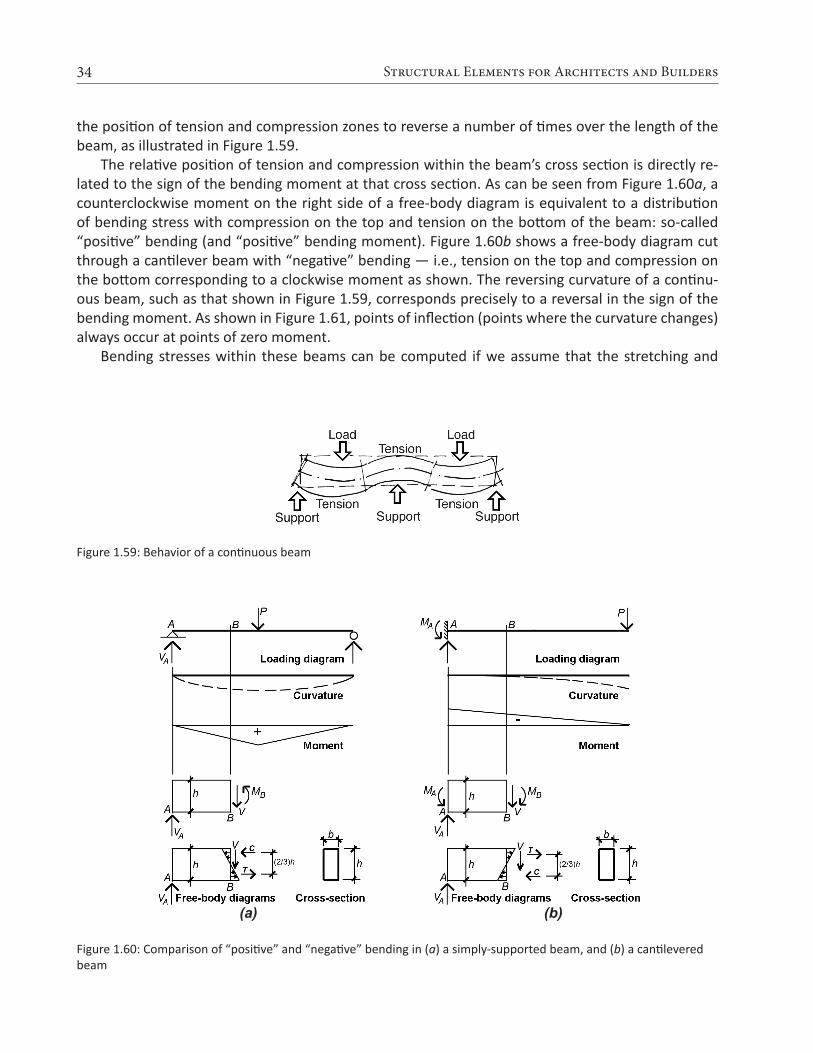
34 Structural Elements for Architects and Builders
the position of tension and compression zones to reverse a number of times over the length of the beam, as illustrated in Figure 1.59.
The relative position of tension and compression within the beam’s cross section is directly re-lated to the sign of the bending moment at that cross section. As can be seen from Figure 1.60a, a counterclockwise moment on the right side of a free-body diagram is equivalent to a distribution of bending stress with compression on the top and tension on the bottom of the beam: so-called “positive” bending (and “positive” bending moment). Figure 1.60b shows a free-body diagram cut through a cantilever beam with “negative” bending — i.e., tension on the top and compression on the bottom corresponding to a clockwise moment as shown. The reversing curvature of a continu-ous beam, such as that shown in Figure 1.59, corresponds precisely to a reversal in the sign of the bending moment. As shown in Figure 1.61, points of inflection (points where the curvature changes) always occur at points of zero moment.
Bending stresses within these beams can be computed if we assume that the stretching and
Figure 1.59: Behavior of a continuous beam
Figure 1.60: Comparison of “positive” and “negative” bending in (a) a simply-supported beam, and (b) a cantilevered beam
(a) (b)

35Introduction to structural design
shortening that take place at any cross section are linear; i.e., a straight line connecting a stretched point with a shortened point on any cross-sectional cut will accurately describe the shape of the beam throughout the entire cross section (Figure 1.62).
Three observations can be made, once this assumption is accepted: (1) maximum elongation and shortening occur at the top and bottom of the beam (the “extreme fibers”); (2) a surface exists somewhere between the extreme fibers that is neither elongated nor shortened — this “plane” is called the “neutral axis” or “neutral surface”; and (3) strain can be defined as the elongation or shortening of any portion of the beam, divided by its original (unloaded) length. Since the original length is a constant, a strain diagram has the same shape as an “elongation-shortening diagram.” For materials with linear stress-strain relationships (where stress equals strain times a constant modulus of elasticity), a stress diagram will also have the same shape as the strain or “elongation-shortening diagram.” Figure 1.63 compares these diagram shapes for materials with linear stress-strain relation-ships.
Figure 1.61: Continuous beam showing correspondence of points of inflection (change from positive to negative curva-ture) and points of zero moment
Figure 1.62: Shortening and stretching (compression and tension) at a typical beam cross-section
Shortening
ElongationOriginal (unloaded)position of beam
Figure 1.63: Elongation, strain, and stress diagrams for a linear, elastic material
Shortening
Elongation Strain Stress
Neutral axis (n.a.)

36 Structural Elements for Architects and Builders
For materials with nonlinear stress-strain relationships, a stress diagram can be pieced together by plotting points from a stress-strain curve for the material. Thus, a steel beam stressed beyond its elastic region would have stress and strain distributions as shown in Figure 1.64. The elongation and shortening, shown in Figure 1.64a, and therefore the strain, shown in Figure 1.64b, is assumed to remain linear even when the stress, shown in Figure 1.64d through Figure 1.64f, becomes nonlinear. In Figure 1.64c, the stress at the extreme fibers of the cross section just reaches the limit of elastic behavior (with stress, σy) which corresponds to the so-called elastic moment, Me. In Figure 1.64f, the strain at the outer fiber is extremely large (theoretically infinite), and the entire cross section is assumed to have yielded at the stress σy, i.e., moved past the linear-elastic yield strain labeled “1” in Figure 1.64g. This condition represents the limit state for a steel beam, and corresponds to the so-called plastic moment, Mp. For reinforced concrete, a nonlinear stress-strain relationship is most often assumed for design; special procedures have been developed to simplify the construction of these stress diagrams.
The shape of the stress diagram is a key element in determining the magnitudes of stresses with-in the beam: when combined with the cross-sectional shape, the requirements of equilibrium can be used to find the magnitudes of the stresses. Typical stress diagrams are shown in Figure 1.65 cor-responding to the allowable moment for wood and the limit states for steel and reinforced concrete.
Allowable stress design. As an example of how the stress-moment relationship is computed using the allowable stress design method, consider a free-body diagram cut from a rectangular cross section of width, b, and height, h (assuming a linear stress-strain relationship resulting in a linear stress dia-gram), as shown in Figure 1.65a. From the requirements of horizontal equilibrium, the total com-pressive force, C, must equal the total tension force, T. For this to occur, the neutral axis must be at the center of the beam, and the maximum compressive stress must equal the maximum tension
Figure 1.64: Elongation, strain, and stress diagrams for an elastic-plastic material such as steel showing (a) elongation and shortening of the actual material; (b) strain diagrams; (c) stress diagram at the point where the outer fiber has just yielded; (d) stress diagram corresponding to strain just beyond the elastic limit; (e) stress diagram corresponding to continued strain beyond the elastic limit; (f) stress diagram corresponding to the plastic moment (where the entire cross-section has yielded); and (g) stress-strain diagram
(a) (b) (c) (d) (e) (f)
(g)

37Introduction to structural design
stress. Any other linear distribution of stresses would be inconsistent with these requirements of equilibrium. The couple of equal and opposite forces represented by C and T, multiplied by the mo-ment arm between them, must equal the bending moment, M, caused by the loads acting on the beam. The basic bending stress equation derives from this simple fact: M equals C (or T) times the moment arm, τ; that is:
Accounting for beam width, b, C = (½)(Fb)(h/2)(b) and τ = (⅔)(h); substituting these values into Equa-tion 1.21, we get:
Defining “bh2/6” as the section modulus, S, and “bh3/12” as the moment of inertia, I, for a rectangu-lar cross section, and solving for the maximum allowable stress, Fb, we get the basic bending stress equations for allowable stress design:
where Fb is the allowable bending stress for the material (psi or ksi), M is the bending moment (in-lb or in-kips), S is the required section modulus (in3); I is the required moment of inertia (in4), and c = h/2 is the distance from the neutral axis to the extreme fiber (in.).
Stress-moment relationships. Equation 1.23 shows the relationship between bending stress, bending moment, and section modulus for a material stressed within its linear-elastic range. It is the basis for wood beam design. Steel and reinforced concrete, however, are no longer designed on the basis of assumed linear-elastic behavior. Even so, the basic relationship between moment, stress, and some sort of section modulus property remains essentially the same for all three materials, as can be seen by comparing the stress and resultant force diagrams shown in Figure 1.65. While specific deriva-tions will be covered in the chapters that follow, the requirements of horizontal equilibrium (C = T) and rotational equilibrium (M = C × τ = T × τ) lead to design equations with essentially the same form
(1.21)M = C × τ
(1.22)M = Fbbh2
6= Fb
bh3/12h/2
(1.23)Fb = MS
= McI
Figure 1.65: Bending stresses acting on rectangular cross sections corresponding to the (a) allowable moment for wood; and the limit states (maximum moment at failure) for (b) steel; and (c) reinforced concrete
C
h
Fb
C
TT
Fb Fy
Fy
C
T
0.85fc'
a/2
a
= d
– a/
2
fy
(a) (b) (c)

38 Structural Elements for Architects and Builders
for all three materials: Equation 1.24 (solving for the required section modulus, S, in Equation 1.23) applies to allowable stress design in wood; Equation 1.25 to allowable strength design in steel; and Equation 1.26 to strength design in reinforced concrete.
In each case, the section modulus term (S, Z, or bd2) must be greater or equal to the bending moment divided by a bending stress term. The stress terms in Equations 1.24, 1.25, and 1.26 vary: for wood, an adjusted allowable stress, Fb', is used directly; for steel, the yield stress, Fy, is used; for reinforced concrete, the stress term, R, is more complex as it must account for the limit state of both concrete (in compression) and steel (in tension), as well as the ratio of steel to gross area within the beam cross section. Factors of safety are also handled differently for the three materials: in wood “allowable stress” design, the factor of safety is hidden within the stress term, Fb'; in steel “allowable strength” design, the factor of safety, Ω (normally 1.67 for bending), is applied, not to the stress, but to the plastic moment capacity of the cross section in order to determine its “available strength”; in reinforced concrete “strength” design, the factor of safety, ϕ (normally 0.9 for bending), is a strength reduction factor applied to the moment capacity of the section. Load safety factors are also included within the reinforced concrete design moment, Mu.
The triangular stress distribution in allowable stress design for wood corresponds to the elastic section modulus, S = bd 2/6, defined in Equation 1.22 for rectangular cross sections. For steel, the plastic section modulus, Z, is used, and is equal to bd 2/4 for a rectangular section — this is easily derived from the equilibrium of stresses shown in Figure 1.65b, although it should be noted that rectangular solid shapes are virtually nonexistent in steel beams. The term, bd2, used in reinforced concrete Equation 1.26, has no official status as a “section modulus,” yet it consists of the same basic variables and has the same units as wood’s S and steel’s Z.
Bending design methods. Equations 1.24, 1.25, and 1.26 are “design” equations, since they provide guidance for the size and shape of bending elements that are capable of resisting a given bending moment. In practice, after bending moments are determined (for example, by the construction of load, shear, and moment diagrams; from moment value tables; or with the use of structural analysis software), the required section modulus term is calculated, and a cross section is then selected. In the case of wood and steel, tables of standard cross sections and their corresponding section moduli facilitate the direct selection of appropriate shapes. The design of a reinforced concrete beam is less direct, since the ratio of steel to concrete may vary, producing a range of acceptable bd2 terms, each of which may sponsor a range of choices for cross-sectional dimensions b and d.
Shear stress. Internal forces perpendicular to the longitudinal axis of beams may also exist along with bending moments at any cross section, consistent with the requirements of equilibrium (see, for example, the force V shown in the free-body diagrams within Figure 1.60). These shear forces are
bd2 ≥ Mu /(φR)
Sreq = M/Fb' (1.24)
Zreq = Ma Ω/Fy (1.25)
(1.26)

39Introduction to structural design
distributed over the cross-sectional surface according to the equation:
where τ = shear stress at a distance, y, from the extreme fiber (psi or ksi); V is the total shear force at the cross section (lb or kips); Q is the “static moment” of the partial cross-sectional area (from the extreme fiber to the distance, y) about the neutral axis of the cross section (in3); I is the moment of inertia of the cross section (in4); and b is the width of the cross section at a distance, y, from the extreme fiber (in.).
Rectangular sections. For rectangular cross sections, the maximum shear stress, which occurs at the neutral axis, becomes:
where h is the height of the rectangular cross section; all other variables are as defined above for Equation 1.27. Alternatively, one can solve for the required cross-sectional area, Areq = bh (in2) as the basis for designing or analyzing a rectangular beam for shear, corresponding to an allowable shear stress, τallow (psi or ksi) for maximum shear force, V (lb or kips). In this case, one gets:
Areq =
1.5Vτallow
This is the basis for checking shear in timber beams, which are almost always rectangular (Figure 1.66). Reinforced concrete beams be-have in a more complex manner, and special procedures for dealing with shear, or diagonal tension, have been developed.
In the vicinity of supports, loads are trans-ferred by compression directly to those sup-ports (Figure 1.67), and the maximum shear force is therefore somewhat less than the computed maximum value. In the design of wood and reinforced concrete beams, the shear force within a distance, d, of the face of the supports can be considered equal to the value of the shear force at that distance, d. For wood beams, d is the total beam height; for reinforced concrete, it represents the effective
(1.27)τ = VQIb
(1.28)τmax =1.5Vbh
(1.29)
Figure 1.66: Distribution of shear stress on a rectangular cross-section
Figure 1.67: Reduction of shear force, Vmax, in the vicinity of the beam’s reaction (support)
Cross section Shear stress
Partial shear diagram
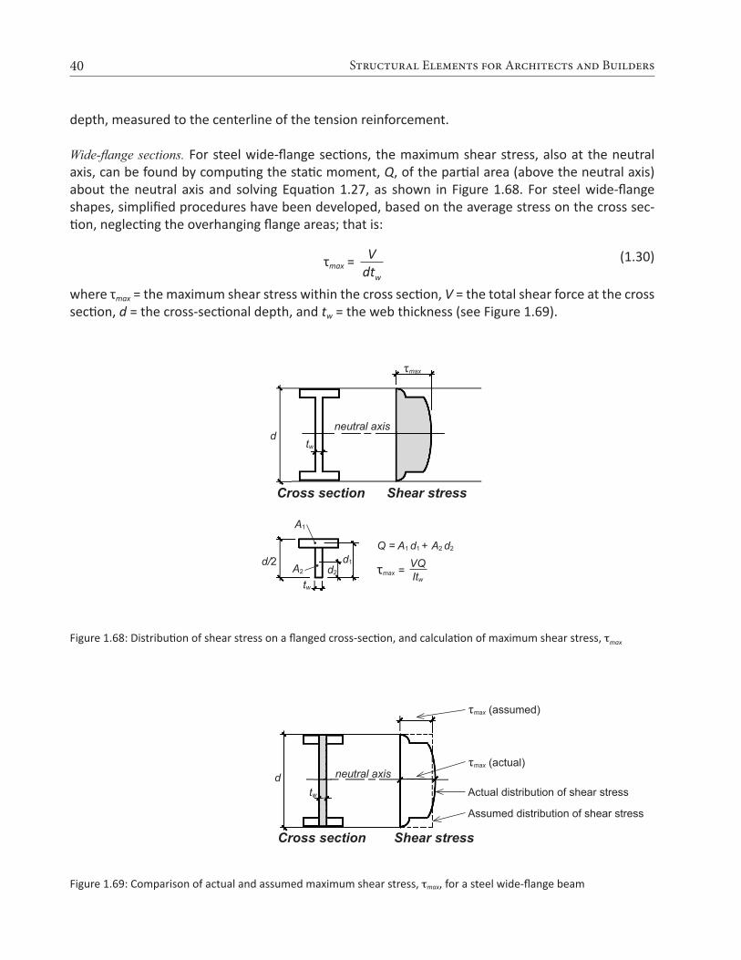
40 Structural Elements for Architects and Builders
depth, measured to the centerline of the tension reinforcement.
Wide-flange sections. For steel wide-flange sections, the maximum shear stress, also at the neutral axis, can be found by computing the static moment, Q, of the partial area (above the neutral axis) about the neutral axis and solving Equation 1.27, as shown in Figure 1.68. For steel wide-flange shapes, simplified procedures have been developed, based on the average stress on the cross sec-tion, neglecting the overhanging flange areas; that is:
where τmax = the maximum shear stress within the cross section, V = the total shear force at the cross section, d = the cross-sectional depth, and tw = the web thickness (see Figure 1.69).
(1.30)τmax =V
dtw
Figure 1.68: Distribution of shear stress on a flanged cross-section, and calculation of maximum shear stress, tmax
Figure 1.69: Comparison of actual and assumed maximum shear stress, tmax, for a steel wide-flange beam
Cross section Shear stress
dtw
τmax (assumed)
neutral axisτmax (actual)
Actual distribution of shear stress
Assumed distribution of shear stress
Cross section Shear stress
d
d/2
tw
τmax
A1
Q = A1 d1 + A2 d2
A2
d1d2 τmax = VQ
Itwtw
neutral axis

41Introduction to structural design
Sectional Properties
The behavior of structural elements is conditioned by the particular shapes into which these materi-als are formed, as well as the particular material qualities selected. Wood, steel and reinforced con-crete structures can be fabricated from elements having an enormous range of strength, stiffness, size and geometric configurations, subject only to the constraints imposed by manufacturing tech-nologies, transportation and handling, and the requirements of safety and serviceability.
In practice, though, the usual range is smaller, limited to standard shapes and sizes endorsed by industry associations. Typical standards for wood, steel, and reinforced concrete elements are de-scribed in the chapters that follow, but a few general observations can be made. For wood and steel, standard cross-sectional shapes are promulgated by industry associations for two primary reasons. First, especially for steel, there is a huge infrastructural investment in the machinery that creates particular shapes and sizes and — in spite of advances in numerical controlled manufacturing pro-cesses — it remains impractical to routinely produce custom designs. Second, properties of standard cross-sectional shapes can be easily complied and tabulated, facilitating structural design. Not only that, a whole assortment of subtle structural requirements can be verified in advance by controlling the proportions of these cross sections.
In the case of site-cast reinforced concrete, only reinforcing bars are manufactured in standard sizes. However, even in this case, the concrete must still be cast within forms, and these forms tend to be deployed in standard increments for a variety of reasons. Of course, it is always possible to create custom designed structural shapes, and some notable instances of this practice can be found. Such instances are beyond the scope of this book. Specific requirements for wood, steel, and rein-forced concrete are discussed in the chapters that follow.
Construction Systems
Structural systems can be extremely complex, and their behavior and design can be incredibly nu-anced and sophisticated. However, at a basic level, there are really only two relevant aspects to the design of structural systems: with respect to floors, the structure must accommodate the human need for horizontal surfaces upon which to walk, sit, sleep, and so on; with respect to roofs — in particular, long-span roofs where there is no such requirement for horizontal walking surfaces — an efficient structure must “find a form” that prioritizes axial stresses, reduces bending stresses, and maximizes the overall depth (height) of the spanning geometry. This last point bears repeating. To the extent that the structural system is made “deep” in the direction of applied loads, internal stress-es will be reduced, making constituent structural elements that comprise the system that much smaller. This is true not only of long-span roof structures (Figure 1.70a), but also of tall buildings or towers subjected to lateral (wind or seismic) loads. For such tall buildings, the “depth” is really the building width where the building itself is modeled as a vertical span cantilevered out of the ground, subjected to lateral forces (Figure 1.70b).
Floor structures are inherently inefficient because it rarely makes sense to increase the depth of the floor in order to increase structural efficiency — doing so might reduce stresses in the floor, but would create enormous inefficiencies in the overall building form. We therefore typically use ordinary beams, girders, slabs, and decks to make floors, rather than using deeper, and potentially more efficient, spanning elements. For long-span roofs or tall buildings, however, efficiency becomes paramount, especially because deflections increase proportionally with the fourth power of the span (Equation 1.20).

42 Structural Elements for Architects and Builders
The structural elements described in this book — tension elements or hangers, columns, and beams — are assembled into structural systems that must provide strength, stiffness, and stability. Strength refers to the ability to resist internal stresses up to a limit state modified (reduced) by a fac-tor of safety. Stiffness refers to the resistance to movement, whether axial deformation in the case of tension elements and columns, or deflection in the case of beams. Stability is required in com-pressive elements so that they don’t buckle, but more generally in structural systems as a whole so that they maintain their intended geometry even when loaded. Because vertical loads (live and dead “gravity” loads) can most often be transferred to a building’s foundation without adversely affecting the stability of the building as a whole, whereas horizontal (“lateral”) loads originating with wind or
Span
Dep
th o
f st
ruct
ure
Depth of structure
Can
tilev
ered
“spa
n”
(a) (b)
Figure 1.70: Increasing the “depth” of a structure, whether of a long-span roof (a) or of a tall building (b), reduces internal stresses
Figure 1.71: Lateral-force-resisting systems can consist of (a) shear walls, (b) triangulated elements, or (c) rigid (mo-ment-resisting) frames
(a) (b) (c)

43Introduction to structural design
seismic events can often challenge a building’s stability (think of a house of cards), a lateral-force-resisting system not only must be part of every structural system but is the key to the structure’s stability.
Aside from the design of innovative long-span or tall-building geometries, this last requirement is actually what makes structural design most interesting: whereas adequate strength and stiffness can be achieved simply by making structural elements as large as required — by calculating their size — the stability of a structural system must be adequately conceptualized before any calcula-tions are made. Fortunately, there really are only three alternative strategies for the design of such lateral-force-resisting systems: shear walls, triangulation (trusses, braces, buttresses, etc.), or rigid (moment-resisting) joints (Figure 1.71).
Masonry and reinforced concrete walls can serve as shear walls, as can wood “diaphragms” con-sisting of vertical studs, horizontal plates, and sheathing boards (Figure 1.71a). To the extent that such “solid” surfaces resist deformation, they keep a building stable. Where such systems are already used to support the live and dead loads of floors and roofs, it usually makes sense to take advantage of their inherent lateral stability as well.
Placing diagonal elements within the rectangular geometry of framed structures (i.e., structures otherwise consisting of columns and beams, rather than walls) is probably the most efficient way to achieve stability (Figure 1.71b). Triangles are inherently stable forms, in that they cannot be de-formed without changing the length of their bounding elements in both compression and tension. In contrast, rectangular frames can be deformed into parallelograms without changing the length of any of their bounding elements, especially when the joints between these elements offer little or no resistance to rotation.
In fact, where the joints between columns and beams in a rectangular geometry are made rigid (moment-resisting) so that rotation is prevented, we get the third, and least-efficient, strategy for stability: the rigid, or moment-resisting, frame (Figure 1.71c). The reason for the relative inefficiency of such rigid frames can best be understood by comparing a triangulated and rigid frame structure, each modeled as a 1-story, 1-bay building subjected to a single 2000 kip horizontal load at the “roof” and consisting of rectangular 10 in. × 20 in. vertical and horizontal structural elements (Figure 1.72). Using truss analysis (see Example 1.6, section method), it can be seen that the maximum axial force in the triangulated structure is 2000 kips (in the horizontal “roof” element closest to the load). Since the cross-sectional area of that horizontal element is assumed to be 10 × 20 = 200 in2, the axial com-pressive stress (Equation 1.15) = force/area = 2000/200 = 10 ksi.
(a) (b)
2000 k 2000 k
A
B C
D A
B C
D
Figure 1.72: Simplified 1-story, 1-bay buildings with (a) triangulated and (b) rigid (moment-resisting) frame lateral-force-resisting systems

44 Structural Elements for Architects and Builders
Now let’s examine the stress within the rigid frame, subject to the same 2000 kip horizontal load. Because this is an indeterminate structure, we will make some simplifying assumptions so that it can be analyzed using only the three equations of equilibrium: first, that points of inflection (with zero bending moment) occur at the midpoints of all elements as the rigid frame deforms under the load; second, that the two horizontal shear forces at these inflection points split the 2000 kip external load equally between them; and third, that the frame dimensions are 10 ft high and 20 ft across. With these assumptions, we can cut the frame into four free-body diagrams and solve for the unknown axial and shear forces, starting with the top, left section (Figure 1.73). The bending moment at the top-left corner, point B, is therefore 500 × 10 = 5000 ft-k or, multiplying by twelve, 60,000 in-k. The section modulus (see the derivation for rectangular sections immediately after Equation 1.11) of the 10 × 20 cross section is 10 × 20 2/6 = 666.67 in3. The bending stress (Equation 1.23) is therefore equal to M/S = 60,000/666.67 = 90 ksi. The axial stress in the horizontal member = force/area = 1000/200 = 5 ksi, so the total maximum stress is actually 95 ksi.
In other words (even ignoring the axial component), stresses in the rigid frame (90 ksi) are nine times greater than stresses in the triangulated structure (10 ksi) in this admittedly simplified ex-ample. Looked at in another way, the horizontal and vertical elements would need to have a section modulus nine times greater than the required section modulus of the structural elements in the triangulated structure in order to keep internal stresses at the same levels — resulting in cross-sectional dimensions of about 20 in. × 40 in. instead of 10 in. × 20 in. Not only that, lateral move-ment (deflection) in the more flexible rigid frame will also be much greater than in the triangulated structure. The rigid frame is inefficient as a lateral-force-resisting system because the magnitude of its internal stresses and its tendency to deflect are primarily determined by the “depth” (actually the section modulus, or moment of inertia in the case of deflection) of individual framing elements, rather than by the “depth” of the structural system as a whole.
A final point about lateral-force-resisting systems: they are typically deployed along two struc-tural lines in each of two orthogonal directions. Two lateral-force-resisting elements are used in each orthogonal direction because a single element would have difficulty dealing with torsional (twisting) movements of the structure as a whole if the resultant of the applied load were not perfectly aligned with it. Such pairs of lateral-force-resisting elements are placed in each of two orthogonal directions since lateral forces (wind or seismic) can come from any direction. If such a lateral force arrives at an
Figure 1.73: The rigid frame shown in Figure 1.72b is cut into four free-body diagrams at assumed inflection points, al-lowing for the calculation of internal shears and axial forces
2000 k
500 k
1000 k 1000 k
1000 k
1000 k 1000 k
1000 k 1000 k
500 k
500 k
5 ft
500 k500 k
500 k
10 ftC
B
A D

45Introduction to structural design
angle different from either of the two orthogo-nal axes, that force can be resolved into two orthogonal components aligned with the lat-eral-force-resisting elements — such compo-nents will always be smaller than the original force, so that a design based on the assump-tion that lateral forces may arrive in either of the two orthogonal directions is generally safe.
However, just providing a lateral-force-re-sisting system is not enough: somehow, all the other structural elements in the building must be adequately connected to the lateral-force-resisting system so that they, too, remain sta-ble. This is often accomplished by considering the floor structures, consisting of beams, gird-ers, slabs, and decks, as rigid (or semi-rigid) di-aphragms that — because they are attached to the lateral-force-resisting system — keep the rest of the structure in its intended alignment (Figure 1.74).
For long-span structures, the concept of a funicular shape — one that resolves all external loads into internal axial forces — is useful, since we have already seen in the case of the rigid frame that a strategy of resisting internal bending moments is inherently inefficient. A cable will always find its funicular shape, since it is incapable of resisting anything other than internal axial tension forces; therefore, optimal compressive shapes can be visualized by literally modeling them in tension and then “flipping them” over into compressive forms. Such idealized axial forms can then be used to gain insight into non-ideal geometries, since any geometric deviation from the ideal form corre-sponds to the magnitude of internal bending moments that would result, and therefore to the re-quirement for an increased section modulus in proportion to the geometric deviation (Figure 1.75).
The concept of the funicular curve also explains why floor structures are almost always structur-ally inefficient: the idealized form under a floor’s uniformly distributed load, as in the curve shown in Figure 1.75a, would be a parabolic vault or arch (think of the cable shape supporting the horizontal roadway of a suspension bridge), a shape not at all consistent with the efficient stacking of habitable space in multi-story buildings.
Figure 1.75: (a) The ideal funicular curve under a uniformly distributed load is a parabola; (b) a 3-hinged arch formed out of straight segments deviates from this ideal form; (c) to accommodate bending moments in this non-ideal form, the cross-section must become “deeper” in proportion to the deviation of the real from the ideal at all point along its length
(c)(a) (b)
(a)
(c)(b) (a)
(b)
(c)
Figure 1.74: Shear walls, or triangulated braces, are typi-cally organized into two orthogonal pairs, (a) and (b); their stability is extended throughout the structure by the rigid or semi-rigid diaphragm action of floors slabs or decks (c)

46 Structural Elements for Architects and Builders
In spite of the potential complexity of structural systems — especially indeterminate systems subject to, and designed to account for, dynamic loads such as those caused by wind or seismic events, or geometrically complex 3-dimensional structures like hyperbolic paraboloids, whose be-havior cannot easily be translated into 2-dimensional diagrams — the discussion of simple structural elements remains relevant. In the final analysis, even the most complex systems are often com-posed of structural elements subject to tension, compression, and bending moments, and so the procedures developed in this book are, in principle, applicable to the design of individual elements comprising more complex systems. Of course, the actual design and analysis of such complex sys-tems, typically accomplished with structural analysis software, is beyond the scope of this book, but insights gained into the behavior and design of the simpler elements from which they are assembled is a useful first step.
Connections
Structural elements are connected to form structural systems; the connections thus constitute an intermediate condition between elements and systems, and are not, strictly speaking, part of the elements themselves. Such connections, however, do have a direct bearing on the types of assump-tions made when the individual elements (or systems) are analyzed. Specifically, when the various elements of structure — columns, beams, and so on — are considered individually, we show them either as constrained by hinges and rollers, free to translate and rotate, or fixed in such a way that all relative movement is prevented.
These abstract constraints are models of the actual conditions encountered by such elements when they are connected within actual structural systems. For example, beams are attached to gird-ers, walls, or columns; columns are attached to foundations, transfer girders, or other columns; and tension elements are hung from beams, or inserted within truss systems. It may seem surprising that the conventional means of attaching structural elements to each other with nails, screws, bolts, welds, and reinforcing bars corresponds to the abstract hinges, rollers, or fixed constraints that will be encountered in the discussion of individual elements of wood, steel, or reinforced concrete (or as discussed earlier in this chapter): we rarely see connections in typical building structures that look anything like the diagrammatic representation of the constraints shown in Figure 1.14.
In fact, the relationship between the reality of a connection and the abstract modeling of it as hinge, roller, etc. is quite interesting. On the one hand, it is possible to design a real connection so that it both appears and behaves just like the abstract model. More commonly, however, one starts with a convenient means for connecting real materials, and then chooses a constraint model that approximates the behavior of this connection. Of course, such typical and “convenient” connections have evolved over time so that their behavior is in line with the assumptions we make about the types of movement, and the magnitude of forces and moments transmitted, between the elements being connected.
It is the latter group of typical connection strategies that will be discussed in the chapters about wood, steel, and reinforced concrete. These connections must resist the same sort of forces already encountered in the design of the structural elements themselves: direct compression and tension, as well as shear. Bending does not often show up directly in the design of fasteners, as it can usually be resolved into the other forces already mentioned.

47Introduction to structural design
Chapter 1 Appendix
Table A-1.1: Derivation of rules for drawing shear and moment diagrams1
Take any beam with variable load, as shown at left (diagram a). Then take an elemental slice of the beam with length, dx, and average load, w, over that length (diagram b). There is a shear force and moment on the left face of the element (V and M), and, because the load, w, is assumed to act in an upward direction (positive), there is a slightly smaller shear and moment on the right face (diagram c).
Rules 1 and 2 derive from the vertical equilibrium of that elemental slice, while Rules 3 and 4 derive from the rotational equilibrium of the same element.
From vertical equilibrium:ΣFy = wdx – V + V – dV = 0Solving for w, we get Rule 1 (at right):
Rule 1: w = dV/dxSolving for dv, we get: dv = wdx, or, integrating, we get Rule 2:
Rule 2:
From rotational (moment) equilibrium:ΣMB = –Vdx + wdx(dx/2) + M – (M – dM) = 0We can omit the dx2 term, because it it so small, and, solving for V, get Rule 3 (at right):
Rule 3: V = dM/dxSolving for dM, we get: dM = Vdx, or, integrating, we get Rule 4:
Rule 4:
Note:1. The four rules are expressed mathematically in the Table A-1.1; they may also be expressed in words, as follows:Rule 1: At any point along a beam, the slope of the shear diagram equals the value of the load (the “infinite” slope of the shear diagram at concentrated loads can be seen as a shorthand approximation to the actual condition of the load being distributed over some finite length, rather than existing at a point).Rule 2: Between any two points along a beam, the change in the value of shear equals the total load (between those points).Rule 3: The slope of the moment diagram at any point equals the value of the shear force at that point.Rule 4: The change in the value of bending moment between any two points equals the “area of the shear diagram” between those points.
(a)
(b)
(c)
∫=B
AwdxDV B
A
∫=B
AVdxDM B
A

48 Structural Elements for Architects and Builders
Table A-1.2: Effective length coefficient, K, for wood and steel columns
Description Pinned at both ends
Fixed at one end; pinned at the other
Fixed at one end; only horizontal translation allowed at the other end
Fixed at both ends
Fixed at one end; free at the other end (cantilever)
Pinned at one end; only horizontal translation allowed at the other end
"Ideal" K 1.0 0.7 1.0 0.5 2.0 2.0
"Code" K 1.0 0.8 1.2 0.65 2.1 12.0 - 2.4
Note:1. Use 2.0 for steel columns; 2.4 for wood columns
Table A-1.3: Allowable deflection for span, L1
A. Live, snow, or wind load onlyFloor beams Roof beamsBasic: L /360 No ceiling: L /180
Non-plaster ceiling: L /240Plaster ceiling: L /360
B. Combined live and dead loadFloor beams Roof beamsBasic: L /240 No ceiling: L /120
Non-plaster ceiling: L /180Plaster ceiling: L /240
Note:1. Use span, L, in inch units for allowable deflection in inch units; for cantilevers, use twice the actual cantilevered span for L.

49Loads
Chapter 2
Loads
There are three broad categories of loads on building structures: dead loads, live loads and “envi-ronmental” loads.
Dead Loads
Dead loads consist of the weight of the building itself, including structure, partitions, cladding, roof-ing materials and permanent interior finishes such as carpet, ceiling systems, etc. These gravity loads are always downward-acting, and can be calculated with a reasonable degree of accuracy, being the summation of various building material weights, which are easily determined and quite predictable. That being said, it is sometimes prudent to anticipate unpredictable scenarios which call for addi-tional dead load, so that future building modifications (such as the addition of a heavy tile floor, or a change from a mechanically attached to a ballasted roof) can be made without major structural modifications.
Dead loads are calculated by multiplying the unit weight of the materials by their quantity. Weights of some common materials and assemblies are listed in Appendix Table A-2.1.
Example 2.1 Calculate dead loads
Problem definition. Assume a typical steel structure with corrugated steel deck and concrete slab, tile floor, suspended ceiling system, and allowances for partitions and mechanical ducts, as shown in Fig-ure 2.1. The spandrel girders carry an additional cladding load consisting of a brick and block cavity wall, 12-ft high from floor to floor. Find the dead load distribution on beam A and spandrel girder B.
Solution overview. Find weights of building elements; compute total dead load on beams and girders.
Problem solutionBeam A
1. From Appendix Table A-2.1, find weights of building elements: a. steel deck, finish floor, ducts and ceiling
system = 47 psf.b. partitions = 8 psf.c. subtotal = 55 psf.
2. Compute weight per linear foot of beam by multiplying unit weight by tributary area on Figure 2.1: Framing plan for Example 2.1
30'-0" 30'-0"
30'-0
"30
'-0"

50 Structural Elements for Architects and Builders
one linear foot of the beam: 55 × 10 = 550 lb/ft.
3. From Appendix Table A-2.1, assume weight of beam: 40 lb/ft.
4. Add beam weight to superimposed dead load to get total dead load, D = 550 + 40 = 590 lb/ft, as shown in Figure 2.2.
Girder B
1. Find concentrated dead loads at third points caused by typical beam reactions, equal to the distributed load on the beam times the beam span divided by two: P = 590(30)/2 = 8850 lb.
2. From Appendix Table A-2.1, find weight of cladding = 1000 lb/ft.
3. From Appendix Table A-2.1, assume weight of girder: 80 lb/ft.
4. Add girder weight to cladding weight = 80 + 1000 = 1080 lb/ft.
5. The dead load on the girder consists of the distributed load in addition to the concen-trated loads transferred by typical beams, as shown in Figure 2.3.
Dead loads also figure prominently in the evaluation of various environmental loads, such as those caused by wind and earthquakes. Seismic loads, for example, are directly proportional to the inertial mass of the building, so that large dead loads are associated with large seismic forces. The effects of wind, on the other hand, can often be mitigated by the addition of dead load, since over-turning and uplift — tendencies that act opposite to the force of gravity — are reduced as the build-ing’s weight increases.
Live Loads
Live loads are nonpermanent, or movable, loads within buildings caused by the weight of people, furnishings, storage of objects, etc. They are relatively unpredictable, vary over time, and are often dynamic, rather than static, in their application. Since it is not possible to measure these loads ab-solutely, a probabilistic approach is used: values are assigned to various types of occupancies based on “worse case” expectations, taking into consideration actual observed loading conditions and the historical record of structural failures.
Since these determinations are generic to various occupancy classifications, and are not unique to each structure, the problem of determining live loads is taken out of the hands of building design-ers altogether, and appears as a mandate of government in the form of building codes. Within these codes, the actual complex behavior of live loads is reduced to an array of uniformly distributed val-
Figure 2.2: Beam A load diagram for Example 2.1
Figure 2.3: Girder B load diagram for Example 2.1
30'-0"
590 lb/ft dead load
30'-0"
8850 lb 8850 lb
1080 lb/ft dead load

51Loads
ues, one for each type of occupancy. Examples of these live load values are listed in Appendix Table A-2.2.
As floor areas become larger, it becomes increasingly improbable that the full live load will ever be present; therefore, a reduction in live load is generally permitted for structural elements “influ-enced” by relatively large floor areas. These so-called influence areas are different from the tributary areas used to compute “unreduced” loads — they are, in fact, four times larger for columns and two times larger for beams (Figure 2.4). For this reason, a single reduction equation based on tributary areas cannot be derived for both columns and beams; instead, such a formula is written in terms of what used to be called the influence area, AI, but is now defined in terms of the tributary area, AT (ft2), times a “live load element factor,” KLL:
Live loads are thus calculated by multiplying the tabulated values from Appendix Table A-2.2 by the area-dependent reduction coefficients (Equation 2.1), where KLL is defined in Appendix Table A-2.2, but equals 2.0 for most beams and 4.0 for most columns. The reduction coefficient is subject to the following limitations: (1) no reduction is allowed for values of KLLAT smaller than 400 ft2; (2) no live load reduction is permit-ted for elements supporting a single floor with live loads greater than 100 psf (and for elements supporting more than one floor with live loads greater than 100 psf, no reduction greater than 20% is permitted); (3) no reduction coefficient smaller than 0.5 is allowed for ordinary beams or columns supporting one level only; and (4) no reduction coefficient smaller than 0.4 is al-lowed for any other condition, i.e., for columns or beams supporting more than one level.
Live load reduction coefficients are plotted in Figure 2.5 for various tributary areas, shown separately for beams and columns. Notice that as the tributary area gets larger (and the likeli-hood of the full live load being present decreas-es), the live load reduction increases — i.e., the reduction coefficient decreases.
There are a few obvious exceptions to the rules governing live load reductions, most im-portantly for structural elements supporting large areas which are expected to be fully load-ed. In such cases, for example in places of public
(2.1)live load reduction coefficient = 0.25 + 15√KLLAT
Figure 2.4: “Influence areas” for beams and columns
Figure 2.5: Live load reduction coefficient graph
Tributary area (ft 2)
Live
load
redu
ctio
n co
effic
ient

52 Structural Elements for Architects and Builders
assembly or in garages, no live load reduction is allowed. Additionally, reductions are restricted for one- and two-way slabs since the failure mode of such slabs is not directly a function of tributary area, but rather corresponds more closely to the pattern of reinforcing bars. These are minimum val-ues for live loads: other than exposing oneself to the potential wrath of developers, owners, project managers and contractors, nothing prevents a designer from using larger, or unreduced, values if warranted by the particular conditions of the project.
Example 2.2 Calculate live loads
Problem definition. Find the live loads for typical Beam A and Girder B in the 6-story office building shown in Figure 2.6. What is the live load on first floor interior column C (ignoring roof loads)?
Solution overview. Find unreduced live loads; apply live load reduction coefficient where applicable.Problem solutionBeam A
1. From Appendix Table A-2.2, the unreduced live load for office occupancy = 50 psf. The load on a linear foot of the beam, found by multiplying the unit load by the tributary area on 1 linear foot of the beam, is 50(8) = 400 lb/ft (as shown in the shaded region of Figure 2.7).
2. From Appendix Table A-2.2, consider live load reduction, based on the beam’s tributary area, AT = 8 × 20 = 160 ft2 and a live load element factor, KLL = 2. Since KLLAT = 2(160) = 320 ft2 ≤ 400 ft2, no reduction is allowed, and the loading diagram remains as shown in Figure 2.8.
Girder B
1. Find the unreduced live load on the girder, applied at the quarter-points by the reactions of the beams, each of which equals the unit load on the beam times its span divided by two, or 400(20)/2 = 4000 lb. Since two beams frame into the girder at each point, the unreduced live load is 4000(2) = 8000 lb at each of the quarter-points.
2. Consider live load reduction:a. Find KLLAT = 2(20 × 32) = 1280 ft2. The tributary area is taken as 20 ft × 32 ft rather than 20
ft × 24 ft since the loads placed outside the middle 24 ft will have a structural effect on the girder.
Figure 2.6: Framing plan for Example 2.2
20'-0
"20
'-0"
20'-0
"
32'-0" 32'-0" 32'-0" 32'-0"

53Loads
b. From Equation 2.1, apply a reduction coefficient of: 0.25 + 15/√1280 = 0.67. The concen-trated live loads at each quarter-point become: 0.67 × 8000 = 5354 lb = 5.4 kips as shown in Figure 2.9.
Column C, 1st floor
1. Find the unreduced live load on the column: Since the 1st-floor column of a 6-story building supports 5 floors (not including the roof), and the tributary area of each floor is 32 × 20 = 640 ft2, the total tributary area supported by the column is 5 × 640 = 3200 ft2. This results in an un-reduced live load of 50 × 3200 = 160,000 lb.
2. Consider live load reduction:a. Find KLLAT = 4(3200) = 12,800 ft2.b. From Equation 2.1, apply a reduction coefficient of: 0.25 + 15/√12,800 = 0.38. Since the
minimum reduction coefficient for columns supporting more than one level is 0.4, we use a total live load of 0.4(160,000) = 64,000 lb = 64 kips.
Figure 2.7: Tributary area for live load on one linear foot of beam for Example 2.2, with shaded “stress block” volume of 50 × 8 × 1 = 400 lb/ft being the unreduced live load on one linear foot of the beam
Figure 2.8: Beam A load diagram for Example 2.2
20'-0"
400 lb/ft
32'-0"
5.4 kips5.4 kips5.4 kips
Figure 2.9: Girder B load diagram for Example 2.2

54 Structural Elements for Architects and Builders
Environmental Loads
Environmental loads are those due to snow, wind, rain, soil (and hydrostatic pressure) and earth-quake. Unlike live loads, which are assumed to act on all floor surfaces equally, independent of the geometry or material properties of the structure, most of these environmental loads depend not only upon the environmental processes responsible for producing the loads, but upon the geometry or weight of the building itself. For snow, wind and earthquake loads, the “global” environmental considerations can be summarized by location-dependent numbers for each phenomenon: ground snow load for snow, basic wind speed for wind, and maximum ground motion (acceleration) for earthquake (Appendix Table A-2.3). Considerations specific to each building are then combined with these “global” environmental numbers to establish the magnitude and direction of forces expected to act on the building. Like live loads, the actual procedures for calculating environmental loads are not derived independently for each building, but are mandated by local building codes. For the ac-tual design of real buildings in real places, the governing building code must be consulted; for the preliminary design of real or imaginary buildings, the following guidelines will do.
Snow loads
Determining the weight of snow that might fall on a structure starts with a ground snow load map, or a ground snow load value determined by a local building code official. These values range from zero to 100 psf for most regions, although weights of up to 300 psf are possible in locations such as Whittier, Alaska. Some typical ground snow load values are listed in Appendix Table A-2.3. Flat roof snow loads are generally considered to be about 30% less than these ground snow load values, and both wind and thermal effects — as well as the “importance” of the structure — are accounted for in further modifying this roof load. A thermal factor, Ct = 1.2, is included in the flat roof load for unheated structures (Ct= 1.0 for heated structures and 1.1 for heated structures with ventilated roofs protected with at least R-25 insulation below the ventilated plenum or attic); we will assume a nominal value of 1.0 for both wind (“exposure”) and “importance.” Other possible values for the snow load importance factor, Is, are listed in Appendix Table A-2.4. However, the major parameter in determining snow loads is the slope of the surface expected to carry the load. As the slope increases, more snow can be expected to slide off the roof surface, especially if the surface is slippery, and if the space immediately below the surface is heated. The slope-reduction factor, CS, which is multi-plied by the flat roof snow load to obtain the actual roof snow load, takes these factors into account:
a. CS = 1.0 for roof angles from 0° to A°.
c. CS = 0 for roof angles greater or equal to 70°.
The parameter A (degrees Fahrenheit) depends on how slippery the roof surface is, and whether that surface is allowed to become warm or cold: A = 5° for warm, slippery roofs (where the R-value must be at least 30 for unventilated roofs, and at least 20 for ventilated roofs); 30° for warm, not
(2.2)for roof angles from A° to 70°.b. CS = 1.0 –70°– A°
roof angle – A°

55Loads
slippery roofs (or for slippery roofs not meeting the R-value criteria); 15° for cold, slippery roofs; 45° for cold, not slippery roofs; and, for the intermediate condition where a roof remains somewhat cold because it is ventilated (with at least R-25 insulation below the ventilated space), A = 10° for slippery roofs; and 37.5° for not slippery roofs. Neglecting variations due to exposure, the snow load can be written as:
0.7CSCtIs(ground snow load)
For low-slope roofs (i.e., hip, gable, or monoslope roofs with slopes less than 15°), the roof snow load cannot be taken less than Is × ground snow load or Is × 20 lb/ft2, whichever is less.
As an example, for “ordinary” buildings (Is = 1.0) with nonslippery (e.g., asphalt shingle) roofs having slopes no greater than 37.5°, kept cold by proper ventilation (with at least R-25 insulation below the ventilated space), the sloped roof snow load, deployed on the horizontal projection of the inclined structural roof members, becomes:
0.7(1.0)(1.1)(1.0)(ground snow load)
Judgment should be used where the building geometry provides opportunities for drifting snow to accumulate on lower roofs, or when sliding snow from higher roofs might fall on lower roofs. Most building codes provide guidelines for these situations.
To account for the effects of wind acting simultaneously with snow on hip- or gable-type roofs, it is necessary to also check a so-called unbalanced snow load, caused by wind blowing snow from the windward to the leeward portion of the roof. In old building codes, this unbalanced load was computed by taking 1.5 times the snow load acting on the leeward side of the gable, with zero snow load on the windward side. Contemporary codes have a more complex strategy for computing such loads, but only applicable to hip and gable roofs with slopes between 2.38° (i.e., 1/2:12) and 30.26° (i.e., 7:12). Steeper or shallower roofs are not affected by wind-blown snow in the same way and so the calculation of such unbalanced loads is not required in these cases. For residential-scale build-ings — i.e., where the horizontal distance from ridge to eave is not greater than 20 ft — the unbal-anced snow load is taken as Is × ground snow load on the leeward side, with zero snow load on the windward side.
For larger buildings with ridge-to-eave horizontal distances greater than 20 ft, the unbalanced snow load calculations are more easily performed using a spreadsheet or other software. A load is first computed for the windward side, taken as 0.3 × roof snow load. In addition, there are two loads computed for the leeward side: the first is just the roof snow load taken over the entire lee-ward surface; the second has a magnitude of hdγ/√S , but is placed on only part of the leeward roof, specifically, that rectangular portion on the leeward side extending from the ridge a distance, measured horizontally, of (8/3)hd√S . In these calculations, hd (ft) is the height of a snow drift = 0.43(lu
1/3)(ground snow load +10)1/4 – 1.5; lu is the length of the roof upwind of the drift (ft), taken here as the horizontal distance from ridge to eave measured on the windward part of the roof; γ = the so-called snow density, taken as (0.13 × ground snow load) + 14 but no greater than 30 pcf; and S is a measure of the roof slope, taken as the horizontal run for a rise of 1.
Two other circumstances may be of importance and require special consideration. First, where snow load is calculated on roofs or decks that are below the depth of the ground snow, the bal-anced snow load is taken as Is × ground snow load. Second, where a roof surface is adjacent to but
(2.3)
(2.4)

56 Structural Elements for Architects and Builders
below another roof surface, both the leeward and windward conditions must be considered, since either could create snow drifts on the low-er roof, as shown schematically in Figure 2.10. Such calculations are rather complex and are not included here.
Example 2.3 Calculate snow loads
Problem definition. Find the snow load on a house in Portland, ME with a conventional roof with a 7:12 slope, i.e., with an angle = tan-1 (7/12) = 30.26°. The roof is kept cold by having a ventilated attic, with R-30 insulation separating the ventilated attic space from the heated house below. Calculate for both asphalt shingles and metal roofing.
Solution overview. Find ground snow load; compute roof snow load.
Problem solution. 1. From Appendix Table A-2.3, the ground snow load = 50 psf. 2. Find the roof snow load:
a. Nonslippery surface (asphalt shingles): From Equation 2.4, for this condition only, the snow load = 0.7(1.1)(1.0)(ground snow load) = 0.7(1.1)(1.0)(50) = 38.5 psf.
b. Slippery surface (metal roofing): From Equation 2.2, find the coefficient, CS for roof angles from A° to 70°, where A = 10° for cold, slippery roofs (kept cold by ventilation). In this case, CS = 1.0 – (roof angle – A°)/(70° – A°) = 1.0 – (30.26 – 10)/(70 – 10) = 0.66. From Equation 2.3, the snow load = 0.7CSCt (ground snow load) = 0.7(0.66)(1.1)(50) = 25.41 psf.
3. For rafters (sloped roof beams) spaced at 16 in. on center, the snow load on each rafter be-comes:a. 38.5(16/12) = 51 lb/ft for the non-slippery roof.
Figure 2.10: Effect of wind direction on snow drifts on lower roofs
SnowWinddirection
Windward drift Leeward drift
(a)
(b)
1'-0"
16"
38.5 or 25.41 psf
51 or 34 lb/ft
30.26°
30.26°
Figure 2.11: Snow load diagram with (a) distributed snow load; and (b) snow load on a typical rafter, for Example 2.3

57Loads
b. 25.41(16/12) = 34 lb/ft for the slippery roof.
4. Both of these loading diagrams are shown in Figure 2.11.
5. To account for the effects of wind acting simultaneously with snow on gable-type roofs, we also check the unbalanced snow load. Since the 30.26° slope of this roof falls between 2.38° and 30.26°, the unbalanced snow load on the leeward side must be computed. For residential-scale buildings — i.e., where the horizontal distance from ridge to eave is not greater than 20 ft — the unbalanced snow load is taken as Is × ground snow load, with zero snow load on the windward side. For this example, the unbalanced snow load diagram is shown in Figure 2.12.
Wind loads
Building codes take one of two approaches to the mathematical calculation of wind pressure on building surfaces: either these pressures are simply given as a function of height, or they are cal-culated as a function of the basic wind speed, modified by numerous environmental and building-specific factors.
The Building Code of the City of New York historically took the first approach, specifying a 30 psf horizontal wind pressure on the surfaces of buildings over 100 ft tall. This number was actually reduced to 20 psf in the 1930s and 1940s. Then, as buildings grew consistently taller and more data was assembled about wind speed at various elevations above grade, wind pressure began to be
30.26°
(1.0)(50) = 50 psfWind
Figure 2.12: Unbalanced snow load for Example 2.3
Figure 2.13: Historic values for wind loads, based on 1969 – 1981 New York City Building Codes

58 Structural Elements for Architects and Builders
modeled as a discontinuous function, increasing from 20 psf below 100 feet to 40 psf above 1000 feet (Figure 2.13).
In contrast to this approach, wind pressure can also be calculated directly from wind speed: the relationship between the velocity or “stagnation” pressure, q, and the basic wind speed, V, is derived from Bernoulli’s equation for streamline flow:
q = 0.5pV 2
where p is the mass density of air. Making some assumptions about air temperature to calculate p, defining qz as the velocity pressure at height z above ground, and converting the units to pounds per square foot (psf) for qz and miles per hour (mph) for V, we get:
qz = 0.00256Kz Kz t Kd Ke V 2
where Kz accounts for heights above ground different from the 10 m above ground used to deter-mine nominal wind speeds as well as different “boundary layer” conditions, or exposures, at the site of the structure; Kz t is a factor used only in special cases of increased wind speeds caused by hills, ridges, escarpments, and similar topographic features; the wind directionality factor, Kd , can be tak-en as 0.85 in most cases and accounts for the fact that the direction of a worst-case wind event may not coincide with the building’s weakest aerodynamic profile, although more conservative values for Kd are suggested for chimneys and other similar roof-top structures; and Ke is a ground elevation factor that can be taken conservatively as 1.0 for all buildings, but which — alternatively — can be reduced by as much as 80 percent when the ground level is 6,000 feet or more above sea level (ac-counting for the impact of reduced air density on velocity pressure). The importance factor, formerly included in this equation to account for relative hazards to life and property associated with various types of occupancies, is now incorporated directly into wind speed maps — that is, it shows up as part of V.
For a building close to sea level with normal occupancy at a height of 10 meters above grade in open terrain, i.e., with Kz = Kd = Kz t = Ke = 1.0, a wind speed of 115 mph corresponds to a velocity pressure equal to:
qz = 0.00256(1.0)(1.0)(1.0)(1.0)(1152) = 33.0 psf
The external design wind pressure, pe, can be found at any height, and for various environmental and building conditions, by multiplying the velocity pressure, qz, by a series of coefficients corresponding to those conditions:
pe = qzGCp
where qz is the velocity pressure as defined in Equation 2.6; G accounts for height-dependent gusti-ness; and Cp is a pressure coefficient accounting for variations in pressure and suction on vertical, horizontal and inclined surfaces. Combining Equations 2.6 and 2.8, we get:
(2.5)
(2.6)
(2.7)
(2.8)

59Loads
pe = 0.00256Kz Kz t Kd Ke GCpV 2 where:
pe = the external design wind pressure (psf)V = the basic wind speed (mph)Kz = the velocity pressure exposure coefficientKd = 0.85 is a wind directionality factor (for use only when computing load combinations)Kzt = a topography factor (can be taken as 1.0 unless the building is situated on a hill, ridge,
escarpment, etc.)Ke = a ground elevation factorG = a coefficient accounting for height-dependent gustinessCp = a pressure coefficient accounting for variations in pressure and suction on vertical, hori-
zontal and inclined surfaces
Some values for these coefficients — for buildings in various terrains (exposure categories) — are given in Appendix Table A-2.5 (except that wind velocities, V, for various cities and risk categories, are found in Appendix Table A-2.3). The resulting distribution of wind pressures on all exposed sur-faces of a generic rectangular building (with a sloped roof) is shown in Figure 2.14.
Only on the windward wall of the building does the wind pressure vary with height above ground. On all other surfaces, the coefficient Kz is taken at mean roof height for the entire surface, resulting in a uniform distribution of wind pressure (whereas for the windward wall, the coefficient Kz is taken at the height at which the pressure is being computed). This is consistent with the results of wind tunnel tests, which show a much greater variability (related to height) on the windward wall than on any other surface.
Changes in the building’s internal pressure as a result of high winds can increase or decrease the
(2.9)
Figure 2.14: Wind pressure on buildings

60 Structural Elements for Architects and Builders
total pressure on portions of a structure’s exterior “envelope.” This internal pressure, pi, is normally taken as 18% of the roof-height velocity pressure for enclosed buildings, but can be as high as 55% of the roof-height velocity pressure for partially-enclosed buildings The total design pressure, p, is therefore:
p = pe + pi
The actual behavior of wind is influenced not only by the surface (or boundary layer) conditions of the earth, but also by the geometry of the building. All sorts of turbulent effects occur, especially at building corners, edges, roof eaves, cornices, and ridges. Some of these effects are accounted for by the pressure coefficient Cp, which effectively increases the wind pressure at critical regions of the building envelope. Increasing attention is also being given to localized areas of extremely high pres-sure, which are averaged into the total design pressures used when considering a structure’s “main wind-force resisting system” (MWFRS). These high pressures need to be considered explicitly when examining the forces acting on relatively small surface areas, such as mullions and glazing, plywood sheathing panels, or roofing shingles. Building codes either stipulate higher wind pressures for small surface elements like glass and wall panels, or provide separate “component and cladding” values for the external pressure coefficients and gust response factors.
Since both external and internal pressures can be either positive (i.e., with the direction of force pushing on the building surface), or negative (i.e., with a suction-type force pulling away from the building surface), the total design pressure on any component or cladding element is always in-creased by the consideration of both external and internal pressures. For certain MWFRS calcula-tions, however, the internal pressures on opposite walls cancel each other so that only external pressures on these walls need to be considered.
As an alternative to the analytic methods described above, three other methods are also permit-ted: a simplified tabular method for certain buildings no more than 160 ft high, a simplified analytic procedure for enclosed, more-or-less symmetrical low-rise (no more than 60-feet high) buildings; and physical testing of models within wind-tunnels to determine the magnitudes and directions of wind-induced pressures.
Example 2.4 Calculate wind loads
Problem definition. Find the distribution of wind load on the windward and leeward surfaces of a 5-story office building located in the suburbs of Chicago. We will assume typical “suburban” terrain, or Exposure Category B. The wind di-rectionality factor Kd = 0.85 for main wind force resisting systems; and the ground elevation fac-tor, Ke = 1.0. The topography factor, Kzt = 1.0, since no peculiar topographic features are pres-ent, and wind speed is found based on a “risk category” of II corresponding to normal occu-pancy. A typical building section is shown in Fig-ure 2.15. Plan dimensions are 100 ft × 100 ft.
(2.10)
Figure 2.15: Schematic section through building for Example 2.4
100'-0"
4 @
12'
= 4
8'16
'
64'-0
"
Wind

61Loads
Neglect internal pressure.
Solution overview. Find basic wind speed; compute external design wind pressures.
Problem solution 1. From Appendix Table A-2.3, the basic (ultimate) wind speed, V = 115 mph. 2. Windward wall: From Equation 2.9, we find the external design wind pressure:
pe = 0.00256Kz Kz t Kd Ke GCpV 2
where values for Kz , G, and Cp are found in Appendix Table A-2.5 (Kzt, Kd ,and Ke are given in the problem statement). It is convenient to organize the solution in tabular form, as shown below in Table 2.1. The value of Kz at mean roof height (64 ft) is found by interpolation between the value at 60 ft and the value at 70 ft:
from which Kz = 0.87. The values for Kzt = Ke = 1.0.
Table 2.1: Calculation of external design windward wall pressure for Example 2.4Height 0.00256 Kz Kzt Kd Ke G Cp V 2 (mph) pe (psf)70 0.00256 0.89 1.0 0.85 1.0 0.85 0.8 115 x 115 17.42
64 0.00256 0.87 1.0 0.85 1.0 0.85 0.8 115 x 115 17.02
60 0.00256 0.85 1.0 0.85 1.0 0.85 0.8 115 x 115 16.63
50 0.00256 0.81 1.0 0.85 1.0 0.85 0.8 115 x 115 15.85
40 0.00256 0.76 1.0 0.85 1.0 0.85 0.8 115 x 115 14.87
30 0.00256 0.70 1.0 0.85 1.0 0.85 0.8 115 x 115 13.70
20 0.00256 0.62 1.0 0.85 1.0 0.85 0.8 115 x 115 12.13
0 – 15 0.00256 0.57 1.0 0.85 1.0 0.85 0.8 115 x 115 11.15
3. Leeward wall: From Equation 2.9, the external design wind pressure for the leeward wall can be found (there is only one value for the entire leeward wall, based on Kz at the mean roof height). From Appendix Table A-2.5, Cp = –0.5 (since the ratio L/B = 100/100 = 1.0); Kz = 0.87 (at mean roof height: see step 2); G = 0.85; Kd = 0.85; and Kzt = Ke = 1.0. The external wind pressure on the leeward side of the building is therefore:
pe = (0.00256)(0.87)(1.0)(1.0)(0.85)(0.85)(–0.5)(1152) = –10.64 psf
The negative sign indicates that this leeward pressure is acting in “suction,” pulling away from the leeward surface.
4. The distribution of wind pressure on the building section is shown in Figure 2.16. The direction of the arrows indicate positive pressure (pushing) on the windward side and negative pres-sure (suction) on the leeward side. Rather than connecting the points at which pressures are
(2.9)
Kz – 0.85 =0.89 – 0.85
64 – 6070 – 60

62 Structural Elements for Architects and Builders
computed with straight lines (which would result in triangular stress blocks over the surface of the building), it is common to use the more conservative assumption of con-stant pressure from level to level, which re-sults in a discontinuous, or stepped, pattern of wind pressure, as shown in Figure 2.16.
When computing the magnitude of wind loads that must be resisted by a building’s later-al-force-resisting system, internal pressures can be neglected (as they act in opposite directions on the two interior faces of the building, cancel-ing out), leaving only the windward and leeward pressures to be considered for each orthogonal plan direction.
Seismic loads
A building riding an earthquake is like a cowboy riding a bull in a rodeo: as the ground moves in a complex and dynamic pattern of horizontal and vertical displacements, the building sways back and forth like an inverted pendulum. The horizontal components of this dynamic ground motion, com-bined with the inertial tendencies of the building, effectively subject the building structure to lateral forces that are proportional to its weight. In fact, the earliest seismic codes related these seismic forces, F, to building weight, W, with a single coefficient:
where C was taken as 0.1.
What this simple equation doesn’t consider are the effects of the building’s geometry, stiffness and ductility, as well as the characteristics of the soil, on the magnitude and distribution of these equivalent static forces. In particular, the building’s fundamental period of vibration, related to its height and type of construction, is a critical factor. For example, the periods of short, stiff buildings tend to be similar to the periodic variation in ground acceleration characteristic of seismic motion, causing a dynamic amplification of the forces acting on those buildings. This is not the case with tall, slender buildings having periods of vibration substantially longer than those associated with the ground motion. For this reason, tall flexible buildings tend to perform well (structurally) in earth-quakes, compared to short, squat and stiff buildings.
But stiffness can also be beneficial since the large deformations associated with flexible buildings tend to cause substantial nonstructural damage. The “ideal” earthquake-resistant structure must therefore balance the two contradictory imperatives of stiffness and flexibility.
In modern building codes, the force F has been replaced with a “design base shear,” V, equal to the total lateral seismic force assumed to act on the building. Additionally, the single coefficient re-lating this shear force to the building’s weight (“seismic dead load”) has been replaced by a series of
F = CW (2.11)
Figure 2.16: Distribution of wind pressure on windward and leeward surfaces for Example 2.4

63Loads
coefficients, each corresponding to a particular characteristic of the building or site that affects the building’s response to ground motion. Thus, the base shear can be related to the building’s weight with the following coefficients, using an “equivalent lateral force procedure” for seismic design:
where:
V = the design base shear Cs = the seismic response coefficient equal to SDS/(R/Ie) W = the effective seismic weight (including dead load, permanent equipment, a percentage of
storage and warehouse live loads, partition loads, and certain snow loads) SDS = the design elastic response acceleration at short periods R = a response modification factor (relating the building’s lateral-force-resisting system to its
performance under seismic loads) Ie = the seismic importance factor (with somewhat different values than the equivalent factors
for wind or snow)
The coefficient Cs has upper and lower bounds that are described in Appendix Table A-2.6 part H, so it will only correspond to the value defined in Equation 2.12 when it falls between the two bounding values. The response modification factor, R, is assigned to specific lateral-force-resisting systems — not all of which can be used in every seismic region or for every type of occupancy; Ap-pendix Table A-2.6, part D, indicates which structural systems are either not permitted, or limited in height, within specific seismic design categories.
To approximate the structural effects that seismic ground motion produces at various story heights, seismic forces, Fx , are assigned to each level of the building structure in proportion to their weight times height (or height raised to a power no greater than two) above grade:
where: V = the design base shear, as defined above in Equation 2.12wi and wx = the portions of weight W at, or assigned to, a given level, i or xhi and hx = the heights from the building’s base to level i or x k = 1 for periods ≤ 0.5 s and 2 for periods ≥ 2.5 s (with linear interpolation permitted for
periods between 0.5 s and 2.5 s) and accounts for the more complex effect of longer periods of vibration (defined in Appendix Table A-2.6, part E) on the distribution of forces
The Σ symbol in Equation 2.13 indicates the sum of the product of (wi hik) for i ranging from 1 to
n, where n is the number of levels at which seismic forces are applied.
(2.12)V = CsW =
SDS
(R/Ie)W
V = CsW =SDS
(R/Ie)W (2.12)
Fx =Vwx hk
x
Σwihki
(2.13)

64 Structural Elements for Architects and Builders
A typical distribution of lateral seismic forc-es resulting from the application of this equa-tion is shown in Figure 2.17. It can be seen that Equation 2.13 for Fx guarantees that these story forces are in equilibrium with the design base shear, V.
By considering both a building’s occupancy category (see Appendix Table A-2.6, part F ) and the expected ground motion at the build-ing’s site, a Seismic Design Category, or SDC, can be determined. Criteria for a building’s SDC are found in Appendix Table A-2.6, part G. For structures that are in the lowest-risk SDC A, it is not necessary to consider the design of nonstruc-tural components for seismic resistance. On the other hand, for the highest-risk SDCs C, D, E, and F, increased scrutiny is required: issues of slope instability, liquifaction, settlement, surface displace-ment, and — for SDCs D, E, and F only — lateral pressure on basements must be considered. Such issues are beyond the scope of this chapter. Buildings with the most extreme SDCs E and F are not permitted where the ground surface might be ruptured by a known active fault.
Building codes require that larger seismic forces be used for the design of individual building elements, and for the design of floor “diaphragms.” The rationale for the separate calculation of these forces is similar to the logic behind the calculation of larger “component and cladding” loads in wind design: because the actual distribution of seismic forces is nonuniform, complex, and con-stantly changing, the average force expected to act upon the entire lateral-force-resisting structural system is less than the maximum force expected to occur at any one level, or upon any one building element.
While we tend to think of seismic forces as acting in the horizontal direction, there are also vertical forces associated with earthquake-induced ground motion. For any structural element, the effects of the horizontal story forces, or Eh, must be combined with the effects of these vertical ground motions, which can be approximated as Ev = 0.2SDSD. In this equation, values for SDS, the de-sign elastic response acceleration at short period described above, can be found in Appendix Table A-2.6, part C; while D represents the effect of the dead load on the particular structural element be-ing analyzed. Dead loads are taken as positive when acting downward, and therefore the same sign convention applies to the effect of the vertical component of seismic ground motion, Ev. The effects of both horizontal and (downward-acting) vertical earthquake forces must be added together when considering the overall effect when earthquake loads, E, are used in combination with live loads, dead loads, and snow loads. On the other hand, the vertical component of earthquake loads must be subtracted from the horizontal component when only the effects of dead load and earthquake load are considered. This is because the worst-case scenario represented by this load combination is triggered by uplift, i.e., by a negative value of Ev combined with a reduced value of the dead load effect, D. Load combinations are discussed in more detail later in this chapter. In any case, Ev can be ignored for buildings in Seismic Design Category B.
The determination of the effect that horizontal story forces have on any structural element, i.e., the determination of Eh, presumes that the structure has adequate redundancy to avoid failure due to extreme torsional irregularity or other conditions that might reduce the shear capacity at any par-ticular story level. Where this redundancy cannot be taken for granted — in particular for structures
Figure 2.17: Typical distribution of equivalent seismic story forces on a building

65Loads
in Seismic Design Categories D, E, and F — Eh must be multiplied by a redundancy factor, ρ = 1.3. This redundancy factor can be eliminated, i.e, ρ can be taken as 1.0, for structures in Seismic Design Category D without extreme torsional irregularities; or, for stories in Seismic Design Categories E and F — already prohibited from having extreme torsional irregularities — where no more than 35% of the base shear, V, must be resisted (typically only for the top stories of tall buildings).
The “equivalent lateral force analysis” method described above is but one of several alternate procedures developed for seismic force calculations. In addition to a “simplified analysis” method for most non-hazardous and nonessential low-rise structures, more sophisticated alternate meth-ods have been developed that can be used for any structure in any seismic region. These methods include modal response spectrum analysis as well as both linear and nonlinear response history analysis, all beyond the scope of this text.
Whatever the method of analysis, designers in seismically-active regions should carefully con-sider the structural ramifications of their “architectural” design decisions, and provide for ductile and continuous load paths from roof to foundation. Following are some guidelines:
1. Avoid “irregularities” in plan and section. In section, these irregularities include soft stories and weak stories that are significantly less stiff or less strong than the stories above; and geometric irregularities and discontinuities (offsets) within the structure. Plan irregularities include asym-metries, reentrant corners, discontinuities and offsets that can result in twisting of the struc-ture (leading to additional torsional stresses) and other stress amplifications. Buildings articu-lated as multiple masses can be either literally separated (in which case the distance between building masses must be greater than the maximum anticipated lateral drift, or movement), or structurally integrated (in which case the plan and/or sectional irregularities must be taken into account).
2. Provide tie-downs and anchors for all structural elements, even those that seem secured by the force of gravity: the vertical component of seismic ground acceleration can “lift” buildings off their foundations, roofs off of walls, and walls off of framing elements unless they are explicitly and continuously interconnected. Nonstructural items such as suspended ceilings, mechanical and plumbing equipment must also be adequately secured to the structural frame.
The explicit connection of all structural elements is also necessary for buildings subjected to high wind loads, since uplift and overturning moments due to wind loads can pull apart connec-tions designed on the basis of gravity loads only. But unlike seismic forces, which are triggered by the inertial mass of all objects and elements within the building, wind pressures act primarily on the exposed surfaces of buildings, so that the stability of interior nonstructural elements is not as much of a concern.
3. Avoid unreinforced masonry or other stiff and brittle structural systems. Ductile framing sys-tems can deform inelastically, absorbing large quantities of energy without fracturing.
Example 2.5 Calculate seismic loads
Problem definition. Find the distribution of seismic story loads on a 5-story office building located in San Francisco. Plan dimensions are 60 ft × 80 ft; assume that an “effective seismic weight” of 75 psf can be used for all story levels above grade, including the roof (primarily due to the dead load). The structure is a steel special moment-resisting frame and is built upon dense soil. The typical building

66 Structural Elements for Architects and Builders
section is shown in Figure 2.18.
Solution overview. Find the effective seismic weight, W and the seismic response coefficient, Cs; compute the base shear, V, and the story forces, Fx.
Problem solution 1. Find W: The effective seismic weight for
each story is the unit weight times the floor area = 75(60 × 80) = 360,000 lb = 360 kips per floor; the total weight, W, for the en-tire building (floors 2 – 5 plus roof) is therefore 5 × 360 = 1800 kips.
2. Find V:a. From Appendix Table A-2.3, find Ss, S1 (maximum considered earthquake ground motion at
short and long periods, respectively), and TL (long-period transition period) for San Fran-cisco: Ss = 1.50; S1 = 0.60; TL = 12.
b. From Appendix Table A-2.6 parts A and B, find site coefficients Fa and Fv: using dense soil (corresponding to Site Class C) and the values of Ss and S1 found in step a, we find that Fa = 1.2 and Fv = 1.4.
c. From Appendix Table A-2.6 part C, find the design elastic response accelerations: SDS = (2/3)(Fa Ss) = (2/3)(1.2)(1.5) = 1.2; SD1 = (2/3)(Fv S1) = (2/3)(1.4)(0.60) = 0.56.
d. From Appendix Table A-2.6 part D, the response modification factor, R = 8 (for special steel moment frames). There are no height limits or other restrictions for this structural sys-tem category; otherwise, it would be necessary to check which seismic design category the building falls under, from Appendix Table A-2.6 part G.
e. From Appendix Table A-2.6 part E, the fundamental period of vibration, T, can be taken as CT hn
x = 0.028(640.8) = 0.78 second, where hn = 64 ft is the building height; and the values used for CT and x, taken from Appendix Table A-2.6 part E, correspond to steel moment-resisting frames.
f. From Appendix Table A-2.6 part F, the importance factor, Ie equals 1.0 for ordinary buildings.g. It is now possible to find the seismic response factor, Cs. From Appendix Table A-2.6 part
H, the provisional value for Cs = SDS /(R/Ie) = 1.2/(8/1.0) = 0.15. However, this must be checked against the upper and lower limits shown in the table: since S1 = 0.60 ≥ 0.6 and T = 0.78 < TL = 12, the lower limit for Cs is the greater value of 0.044SDS Ie = 0.044(1.2 × 1.0) = 0.0528, or 0.01; or 0.5S1 /(R/Ie) = 0.5(0.60)/(8/1.0) = 0.0375; i.e., the lower limit is 0.0528 and the upper limit is Cs = SD1/(TR/Ie ) = 0.56/(0.78 × 8/1.0) = 0.090. The upper limit governs in this case, so we use Cs = 0.090.
h. From Equation 2.12, the base shear, V = CsW = 0.090(1800) = 162 kips. 3. From Equation 2.13, the story forces can be determined as follows:
In this equation, since the period, T = 0.78 seconds, is between 0.5 and 2.5, and the limiting
Fx =Vwx hk
x
Σwihki
Figure 2.18: Schematic section through building, show-ing story heights, for Example 2.5
64'-0
"
16'
4 @
12'
= 4
8'
28'
40'
52'
80'-0"

67Loads
values of the exponent, k, are set at 1.0 for T ≤ 0.5 and 2.0 for T ≥ 2.5, our value of k is found by linear interpolation:
from which k = 1.14. The seismic weight at each story, wi = 360 kips (see step 1), and the various
story heights can be most easily computed in tabular form (as shown below in Table 2.2).
Table 2.2: Calculation of story forces for Example 2.5Story level Story height, hx (ft) hx
1.14 Fx = 0.476hx1.14 (kips)
Roof 64 114.56 54.55
5 52 90.42 43.05
4 40 67.04 31.92
3 28 44.64 21.26
2 16 23.59 11.23
Sum of story forces, Fx = base shear V =
Once the values for hx1.14 have been determined for each story level, Equation 2.13 can be re-
written as:
and values for Fx = 0.476hx
1.14 can then be added to the table. Finally, their distribution on the building can be sketched, as shown in Figure 2.19. The sum of all the story forces, Fx, equals the design base shear, V, as it must to maintain horizontal equilibrium.
k – 1.02.0 – 1.0
=0.78 – 0.52.5 – 0.5
162
Fx =(162)(360)hx
1.14
(360)(23.59 + 44.64 + 67.04 + 90.42 + 114.56)= 0.476hx
1.14
Figure 2.19: Distribution of story forces, Fx, for Example 2.5

68 Structural Elements for Architects and Builders
Design Approaches
Structural engineering prescriptions tend to be written in the form of unambiguous mathematical relationships. In fact, the seeming authority of these formulations masks a rather different reality: the entire subject area of structures is littered with fundamental uncertainties. These uncertainties include not only the nature of loads and the strength and stiffness of structural materials in resisting these loads; but also the appropriateness of mathematical models used in design and analysis, and the degree to which actual built structures conform to the plans and specifications produced by their designers. The basic requirements of safety, serviceability and economy depend on how well design-ers maneuver within this probabilistic environment.
Allowable Stress Design
Structural design approaches can be characterized by the extent to which these uncertainties are made explicit. The simplest approach to designing structures uses a single factor of safety to define allowable stresses for a particular material. If actual (i.e., calculated) stresses do not exceed these allowable stresses, the structure is considered to be safe. Rather than using allowable stress, it is also possible to use allowable strength, measured in moment or force units. The allowable, or “available,” strength is defined by applying a safety factor to the structural element’s so-called “limit state,” i.e., to the maximum moment or force it can sustain. Then, the element is designed such that its available strength (the limit state divided by a safety factor) is greater or equal to its required strength (the computed force or moment resulting from the application of loads).
In some cases, the factor of safety is actually given. In steel design, for example, the available strength is determined by dividing the limit-state moment or force by a safety factor. In other cases, for example in timber design, the allowable stress is simply presented as a property of the material, and the degree of safety is hidden from the designer. In all cases, however, it is not possible to “fine tune” the structure’s design by considering the relative uncertainty of various load types.
In allowable stress (or allowable strength) design, dead and live loads are simply added together, in spite of the fact that dead loads can be predicted with a higher degree of certainty than live loads. Thus, if two structures carry the same total load, but one structure has a higher percentage of dead load, the structures will have different degrees of safety if designed using the allowable stress method. In fact, the structure with more dead load will be statistically safer, since the actual dead load acting on the structure is more likely to correspond to the calculated dead load than is the case with live load. Allowable stress design is sometimes called working stress design, since the loads used in the method (“service loads”) represent what we expect to actually “work” with during the life of the structure.
Load combinations in allowable stress design. To account for the improbability of multiple loads simul-taneously acting on a structure at their maximum intensity, most codes provide load reduction fac-tors for various combinations of load types. For example, where several loads are being considered, the “non-dead” loads may be multiplied by 0.75, as long as the total thus calculated does not exceed

69Loads
the dead load together with the largest single additional load considered in the calculations (earth-quake loads are sometimes excluded from this provision). The reduction of live loads on relatively large influence areas was discussed previously in this chapter.
Strength Design
A more recent approach to the design of structures explicitly considers the probabilistic nature of loads and the resistance of structural materials to those loads. Instead of regulating the design of structural elements by defining an upper limit to their “working stresses,” strength design considers both the limit state of the structural element — typically the strength at which the element fails or otherwise becomes structurally useless — as well as the relative uncertainty of the various loads acting on that element.
Using this method, the required strength of a structural element, calculated using loads multi-plied by load factors (that correspond to their respective uncertainties), must not exceed the de-sign strength of that element, calculated by multiplying the strength of the structural element by resistance factors (that account for the variability of stresses, and the consequences of failure). If Q represents the loads and their effects on a structural element, and R represents the resistance, or strength, of that element, then strength design can be schematically represented as follows:
λΣ(γiQi) ≤ φRn
where γi are the load factors (mostly greater than 1.0); φ is the strength reduction factor (smaller than 1.0); and λ is an additional factor (smaller than 1.0) that can be used when multiple load types are assumed to act simultaneously, in which case the likelihood of all loads being present at their maximum intensities is reduced.
Load combinations in strength design. For reinforced concrete designed with the strength method, some commonly used factored load combinations are listed in Appendix Table A-2.7. Multiple com-binations of loads are less likely to occur simultaneously at full magnitude; the load factors listed in Appendix Table A-2.7 account for these variable probabilities. The load factor for dead load is some-times less than zero, since this can represent the more dangerous condition (i.e., the more conserva-tive assumption) where wind or earthquake forces cause overturning or uplift.
Strength design is similar to Load and Resistance Factor Design (LRFD in wood or steel), or “limit state design.” In the U.S., strength design is now used almost exclusively in reinforced concrete de-sign; beginning to be widely used in steel design; and not yet commonly used in timber design. In this text, we will use strength design for reinforced concrete, allowable stress design for timber and allowable strength design for steel.
(2.14)

70 Structural Elements for Architects and Builders
Example 2.6 Load combinations (Part I)
Problem definition. For the “light manufactur-ing” structure shown in Figure 2.20, assume that the dead load consists of the reinforced concrete floor structure. The weight of the re-inforced concrete can be taken as 150 pcf. Find the distributed “design” load on a typical beam for both strength design and allowable stress design.
Solution overview. Find dead and live loads; add loads together for allowable stress design; apply load factors for strength design (strength design is used almost exclusively for the design of rein-forced concrete structures).
Problem solution 1. From Appendix Table A-2.2, find live load:
L = 125 psf; or, considering the distributed load on a typical beam, L = 125 × 10 = 1250 lb/ft.
2. Find dead load.a. Slab: (150)(6/12)(10) = 750 lb/ft.b. Beam: (150)(12/12)(12/12) = 150 lb/ft.c. Total dead load = 750 + 150 = 900 lb/ft.
3. Allowable stress design: Total load = D + L = 900 + 1250 = 2150 lb/ft (Figure 2.21a). 4. Strength design: From Appendix Table A-2.7, the total load = 1.2D + 1.6L = 1.2(900) + 1.6(1250) =
3080 lb/ft (Figure 2.21b).
Example 2.7 Load combinations (Part II)
Problem definition. Now, repeat Example 2.6, except change the occupancy to that of a restaurant, and add ceramic tile (weighing 25 psf) to the surface of the slab.
Solution overview. Find dead and live loads; add loads together for allowable stress design; apply load factors for strength design.
Figure 2.21 Load diagrams for Example 2.6 using (a) allowable stress design; and (b) strength design
(a) (b)
20'-0" 20'-0"
2150 lb/ft 3080 lb/ft
Allowable stress design Strength design
Figure 2.20: (a) Framing plan and (b) section for Example 2.6
(a) Plan
(b) Section
Tributary area for beam
30'-0
"30
'-0"
20'-0"20'-0" 20'-0"
10'-0"10'-0"
12"
12"
6"

71Loads
Problem solution 1. From Appendix Table A-2.2, find live load: L = 100 psf; or, considering the distributed load on a
typical beam, L = 100 × 10 = 1000 lb/ft. 2. Find dead load.
a. Slab: concrete + tile = (6/12)(150)(10) + 25(10) = 1000 lb/ft.b. Beam: (12/12)(12/12)(150) = 150 lb/ft.c. Total dead load = 1000 + 150 = 1150 lb/ft.
3. Allowable stress design: Total load = D + L = 1150 + 1000 = 2150 lb/ft (Figure 2.22a). 4. Strength design: From Appendix Table A-2.7, the total load = 1.2D + 1.6L = 1.2(1150) + 1.6(1000) =
2980 lb/ft (Figure 2.22b).
Examples 2.6 and 2.7 were admittedly rigged to make a point: even though the total unfactored loads are the same in both cases, the factored loads used in strength design are different, since the proportion of live to dead loads has changed. The allowable stress procedure would result in exactly the same beam design in both cases, whereas the strength method would permit a smaller beam for the restaurant in Example 2.7 (since the total design loads are smaller). However, according to the probabilistic logic of strength design, even though the restaurant beams are smaller than the beams for light manufacturing, the degree of safety would be the same for both beams.
Example 2.8 Load combinations (Part III)
Problem definition. Assuming strength design, find the various combinations of load acting on the 9th- and 10th-floor columns shown in Figure 2.23. Assume that the dead load for each floor level is 40 psf, the live load for the 10th floor is 60 psf, the roof live load, Lr (maintenance, etc.), is 20 psf, and the wind load acting on the roof is 30 psf (acting upward). The tributary area is 25 × 10 = 250 ft2 per floor, as shown in Figure 2.23.
Solution overview. Find loads (including live load reduction coefficient); compute load combinations; identify critical (governing) combinations.
Problem solution10th-floor column:
1. Find loads:a. D = 250(40) = 10,000 lb = 10 kips.b. Lr = 250(20) = 250(20) = 5000 lb = 5.0 kips.c. W = 250(–30) = –7500 lb = –7.5 kips.
Figure 2.22: Load diagrams for Example 2.7 using (a) allowable stress design; and (b) strength design
(a) (b)
20'-0" 20'-0"
2150 lb/ft 2980 lb/ft
Allowable stress design Strength design

72 Structural Elements for Architects and Builders
2. From Table A-2.7 (strength design), compute load combinations:a. 1.4D = 1.4(10) = 14 kips.b. 1.2D + 1.6L + 0.5(Lr or S) = 1.2(10) + 0 + 0.5(5) = 14.5 kips.c. 1.2D + 1.6(Lr or S) + (0.5L or 0.8W) = 1.2(10) + 1.6(5) + 0.8(–7.5) = 14 kips.d. 1.2D + 1.6W + 0.5L + 0.5(Lr or S) = 1.2(10) + 1.6(–7.5) + 0 + 0.5(5) = 2.5 kips.e. 1.2D + 1.0E + 0.5L + 0.2S = 1.2(10) + 0 + 0 + 0 = 12 kips.f. 0.9D + 1.6W = 0.9(10) + 1.6(–7.5) = –3 kips.g. 0.9D + 1.0E = 0.9(10) + 0 = 9 kips.
3. Conclusions: For the 10th-floor column, the critical load combinations are 14.5 kips from live and dead load plus roof live load (combination b); and –3 kips from dead and wind load (com-bination f). The negative force due to wind uplift must be considered since it places the upper level column in tension. In equations c, d, and e, the live load factor is taken as 0.5 (see Note 2 in Appendix Table A-2.7).
9th-floor column:
1. Find loads:a. D = 250 (40) × 2 floors = 20,000 lb = 20 kips.b. Lr = 250(20) = 250(20) = 5000 lb = 5.0 kips.c. The live load reduction coefficient can be found from Appendix Table A-2.2 and is equal to:
0.25 + 15/√4 × 250 = 0.72.d. L = (250 × 60)(reduction coefficient) = (250 × 60)(0.72) = 10,800 lb = 10.8 kips.e. W = 250(–30) = –7500 lb = –7.5 kips.
2. From Appendix Table A-2.7 (strength design), compute load combinations:a. 1.4D = 1.4(20) = 28 kips.b. 1.2D + 1.6L + 0.5(Lr or S) = 1.2(20) + 1.6(10.8) + 0.5(5) = 43.78 kips.
10'-0"
25'-0"
Figure 2.23 Tributary floor areas for Example 2.8

73Loads
c. There are two choices here: (1) using W: 1.2D + 1.6(Lr or S) + (0.5L or 0.8W) = 1.2(20) + 1.6(5) + 0.8(–7.5) = 26.0 kips; or (2) using L: 1.2D + 1.6(Lr or S) + (0.5L or 0.8W) = 1.2(20) + 1.6(5) + 0.5(10.8) = 37.4 kips.d. 1.2D + 1.6W + 0.5L + 0.5(Lr or S) = 1.2(20) + 1.6(–7.5) + 0.5(10.8) + 0.5(5) = 19.9 kips.e. 1.2D + 1.0E + 0.5L + 0.2S = 1.2(20) + 0 + 0.5(10.8) + 0 = 29.4 kips.f. 0.9D + 1.6W = 0.9(20) + 1.6(–7.5) = 6 kips.g. 0.9D + 1.0E = 0.9(20) + 0 = 18 kips.
3. Conclusions: For the 9th-floor column, the critical load combination is 43.78 kips from live and dead load plus roof live load (combination b). No combination of loads places the column in tension. In equations c, d, and e, the live load factor is taken as 0.5 (see Note 2 in Appendix Table A-2.7).
In a reinforced concrete structure, columns typically are also subjected to bending moments due to their continuity with beams, girders or slabs. Where the combined effects of axial loads and bending moments are accounted for — something that is beyond the scope of this book — the axial loads computed from other load combinations (together with the bending moments associated with them) might turn out to be critical.

74 Structural Elements for Architects and Builders
Table A-2.1: Dead loadsA. Basic volumetric weights in pounds per cubit foot (pcf)Stone:
SandstoneGraniteMarble
144165173
Brick/CMU/concreteNormal-weight reinforced concrete
100 – 145150
Metals:AluminumSteelLead
165492710
Glass 160
Wood 25 – 50
Water 64
Earth:Dry claySilt, moist and packedWet sand and gravel
6396120
Insulation:Glass fiber battsExpanded polystyrene boardsExtruded polystyrene boaardsPolyisocyanurate boardsFiberboard
0.80.9 – 1.82.22.01.5
B. Distributed loads in pounds per square feet (psf)Wood floor system: 2 × 10 joists at 16 in. on center, wood finish floor and subfloor, gypsum board ceiling
10.5
Steel floor system: 4½ in. corrugated steel deck with concrete slab, tile floor, mechanical ducts, suspended tile ceiling
47
Concrete floor system: 6 in. reinforced concrete slab, tile floor, mechanical ducts, suspended tile ceiling
80
Floor-ceiling components:Harwood finish floor, ⅞ in.Wood subfloor, ¾ in.Acoustical tile with suspended steel channelsMechanical duct allowanceSteel stud partition allowance
4.02.53.0
4.08.0
Sheathing:Plywood, per ⅛ in. thicknessGypsum board, per ⅛ in. thickness
0.400.55
C. Linear loads in pounds per foot (lb/ft)Steel beam, ordinary span and spacing 30 – 50
Steel girder, ordinary span and spacing 60 – 100
Wood joist, 2 × 10 4.0
Brick-CMU cavity wall, 12 ft high 1000
Table A-2.2: Live loadsA. Typical live loads based on occupancy (psf)Assembly areas with fixed seats 60
Assembly areas with movable seats 100
Lobbies, corridors (first floor) 100
Dining rooms and restaurants 100
Garages for passenger cars 40
Libraries, reading rooms 60
Libraries, stack areas (not less than) 150
Manufacturing, light 125
Manufacturing, heavy 250
Office buildings 50
Dwellings and hotels (except as noted below) 40
Note: Residential sleeping areas 30
Schools (classrooms) 40
Schools (corridors above first floor) 80
Stadium and arena bleachers 100
Stairs and exitways 100
Stores, retail (first floor) 100
Stores, retail (upper floors) 75
Stores, wholesale (all floors) 125
B. Live load reduction coefficient1,2,3,4
Notes for Part B:1. KLL is the live load element factor and is defined as follows for selected common beam and column configurations: KLL = 4 for columns without cantilever slabs KLL = 3 for edge columns with cantilever slabs KLL = 2 for corner columns with cantilever slabs KLL = 2 for beams (except as noted below) KLL = 1 for one-way and two-way slabs, edge beams with cantilever slabs, and anything else not previously mentioned — and note that AT for one-way slabs cannot be taken as more than 1.5 × (slab span)2
2. AT is the tributary area of the element being considered (ft2)3. No live load reduction applies when KLLAT ≤ 400 ft2 or when the element supports a single floor with live load > 100 psf (for an element supporting more than one floor with live loads > 100 psf, a reduction no greater than 20% is permitted)4. Reduction coefficient cannot be taken greater than 1.0; nor can it be smaller than 0.5 for elements supporting a single floor level; or smaller than 0.4 for all other conditions.
Live load reduction coefficient = 0.25 + 15√KLLAT
Chapter 2 Appendix

75Loads
Table A-2.3: Environmental loads1
City, State Ground Snow Load (psf)
Basic (Ultimate) Wind Speed, V (mph) Seismic Ground Motion2
RiskCategory I
RiskCategory II
RiskCategory III
RiskCategory IV
Ss S1 TL
Boston, MA 40 110 120 128 133 0.270 0.065 6
Chicago, IL 25 100 107 114 119 0.116 0.063 12
Little Rock, AR 10 98 105 111 115 0.387 0.150 12
Houston, TX 0 128 136 145 150 0.068 0.039 12
Ithaca, NY 40 100 110 116 122 0.119 0.045 6
Miami, FL 0 157 169 182 189 0.040 0.020 8
New York, NY 20 106 115 125 129 0.288 0.060 6
Philadelphia, PA 25 105 112 123 125 0.180 0.047 6
Phoenix, AZ 0 95 101 108 112 0.179 0.065 6
Portland, ME 50 103 112 119 125 0.281 0.072 6
San Francisco, CA 0 86 91 98 102 1.500 0.600 12
Notes:1. Approximate values taken from snow, wind, and seismic maps. Various web-based applications are available to find environmental loads at specific locations in the U.S. See, for example: SNOW, WIND, and SEISMIC: https://hazards.atcouncil.org/ [Applied Technology Council (ATC)] SEISMIC (disaggregated): https://seismicmaps.org/ [California’s Office of Statewide Health Planning and Development (OSHPD)]2. Ss and S1 are, respectively, the maximum considered earthquake ground motions of 0.2 s (short) and 1 s (long) spectral response acceleration (5% of critical damping) for site class B, measured as a fraction of the acceleration due to gravity. TL is the so-called “long-period transition period” (seconds).
Table A-2.4: Snow load Importance factor, Is
Category Description FactorI Low hazard (minor storage, etc.) 0.8
II Regular (ordinary buildings) 1.0
III Substantial hazard (schools, jails, places of assembly with no fewer than 300 occupants) 1.1
IV Essential facilities (hospitals, fire stations, etc.) 1.2

76 Structural Elements for Architects and Builders
Table A-2.5: Wind coefficientsA. Velocity pressure coefficient, Kz
1
Height above grade2, z (ft)
Exposure B 3
Exposure C4
Exposure D5
500 1.57 1.78 1.90
400 1.47 1.69 1.82
300 1.35 1.59 1.73
200 1.20 1.46 1.62
100 0.99 1.27 1.43
90 0.96 1.24 1.41
80 0.93 1.21 1.38
70 0.89 1.17 1.35
60 0.85 1.14 1.31
50 0.81 1.09 1.27
45 0.79 1.07 1.25
40 0.76 1.04 1.22
35 0.73 1.01 1.19
30 0.70 0.98 1.16
25 0.67 0.95 1.13
20 0.62 0.90 1.08
0 – 15 0.57 0.85 1.03
Notes for Part A:1. Values of Kz are based on the following equation, where z is the height above grade (ft); α = 7.0 for Exposure B; 9.5 for Exposure C, and 11.5 for Exposure D; and zg = 1200 for Exposure B; 900 for Exposure C; and 700 for Exposure D:
When using tabular values for K, linear interpolation between values is permitted.2. When computing pressures on windward surfaces, use height z corresponding to height for which pressure is being computed; for all other surfaces, use z = h (mean roof height: i.e., use this single value of z for the entire surface). See Table A-2.5 Part H for graphic explanation of building geometry parameters.3. Exposure B refers to urban or suburban areas, wooded areas, etc.4. Exposure C refers to open terrain with scattered obstructions, excluding water surfaces in hurricane regions.5. Exposure D refers to flat, unobstructed areas like mud flats, salt flats, or water, both inside or outside of hurricane regions.
B. External pressure coefficient for walls, Cp1
Orientation 0 < L/B ≤ 1 L/B = 2 L/B ≥ 4Windward 0.8 0.8 0.8
Leeward – 0.5 – 0.3 – 0.2
Side – 0.7 – 0.7 – 0.7Note for Part B:1. L and B are the plan dimensions of the rectangular building, with B being the dimension of the windward and leeward walls, and L the dimension of the side walls. See Table A-2.5 Part H for graphic explanation of building geometry parameters.
Kz = 2.01 zzg
2/α
C. External pressure coefficient on windward slope of roof, Cp, for wind direction normal to ridge1,2,7
Roof angle, θ (deg)
h/ L ≤ 0.25 h/ L = 0.50 h/ L ≥ 1.0
6θ < 10 0 < D ≤ h /2
h /2 < D ≤ h h < D ≤ 2h 2h < D
–0.9, -0.18–0.9, -0.18–0.5, -0.18–0.3, -0.18
–0.9, -0.18–0.9, -0.18–0.5, -0.18–0.3, -0.18
3–1.3, -0.18–0.7, -0.18–0.7, -0.18–0.7, -0.18
6θ = 10 –0.7, -0.18 –0.9, -0.18 3–1.3, -0.18
θ = 15 –0.5, 40.0 –0.7, -0.18 –1.0, -0.18
θ = 20 –0.3, 0.2 –0.4, 40.0 –0.7, -0.18
θ = 25 –0.2, 0.3 –0.3, 0.2 –0.5, 40.0
θ = 30 –0.2, 0.3 –0.2, 0.2 –0.3, 0.2
θ = 35 40.0, 0.4 –0.2, 0.3 –0.2, 0.2
θ = 45 0.4 40.0, 0.4 40.0, 0.35θ ≥ 60 0.01θ 0.01θ 0.01θ
Notes for Part C:1. Where two values are given, either may apply, and both must be considered. Interpolation between adjacent values is permit-ted, but must be between numbers of the same sign; where no number of the same sign exists, use 0.0.2. Values are used with Kz taken at mean roof height. Units of length for D, h, and L must be consistent with each other. For roof angles less than 10°, D refers to the range of horizontal distances from the windward eave (edge) for which the value of Cp applies; h is the height of the eave above grade for roof angles no greater than 10°, otherwise, h is the mean roof height above grade; L is the horizontal length of the building parallel to the wind direction. See Table A-2.5 Part H for graphic explanation of building geometry parameters.3. Value of –1.3 may be reduced depending on the area it is act-ing on: for areas no greater than 100 ft2, no reduction; for areas of 200 ft2, multiply by 0.9; for areas no smaller than 1000 ft2, multiply by 0.8; interpolate between given values.4. Values of 0.0 are used only to interpolate between adjacent fields.5. Roof angles over 80° are treated as windward walls, with Cp = 0.8.6. See Note 2 for roof height, h, where roof angle is no greater than 10°.7. Negative numbers indicate “suction,” i.e., forces acting away from the building surface; positive numbers indicate forces “push-ing” against the building surface.
(continued)

77Loads
D. External pressure coefficient on leeward slope of roof, Cp, for wind direction normal to ridge1,2,3
Roof angle, Θ (deg)
h/ L ≤ 0.25 h/ L = 0.50 h/ L ≥ 1.0
q = 10 –0.3 –0.5 –0.7
q = 15 –0.5 –0.5 –0.6
q ≥ 20 –0.6 –0.6 –0.6
Notes for Part D:1. The height h is measured to the eave for roof angles equal to 10°, otherwise, h is the mean roof height above grade; L is the horizontal length of the building parallel to the wind direction. See Table A-2.5 Part H for graphic explanation of building geometry parameters.2. For roof angles less than 10°, the roof is considered to be flat, and no leeward pressures are computed. Instead, use the values in Table A.2.4 Part C for the entire roof.3. Interpolation is permitted between values.4. Negative numbers indicate “suction,” i.e., forces acting away from the building surface; positive numbers indicate forces “push-ing” against the building surface.
E. External pressure coefficient roof, Cp, for wind direction parallel to ridge, for all roof angles1,2,4,5
Applicable Roof Area
h/ L ≤ 0.25 h/ L = 0.50 h/ L ≥ 1.0
0 < D ≤ h / 2 –0.9, –0.18 -0.9, –0.18 3-1.3, –0.18
h / 2 < D ≤ h –0.9, –0.18 -0.9, –0.18 –0.7, –0.18
h < D ≤ 2h –0.5, –0.18 -0.5, –0.18 –0.7, –0.18
2h < D –0.3, –0.18 -0.3, –0.18 –0.7, –0.18
Notes for Part E:1. Where two values are given, either may apply, and both must be considered. Interpolation between adjacent values is permit-ted, but must be between numbers of the same sign.2. Values are used with K taken at mean roof height. Units of length for D, h, and L must be consistent with each other. For all roof angles, D refers to the range of horizontal distances from the windward eave (edge) for which the value of Cp applies; h is the height of the eave above grade for roof angles no greater than 10°, otherwise, h is the mean roof height above grade; L is the horizontal length of the building parallel to the wind direction. See Table A-2.5 Part H for graphic explanation of building geometry parameters.3. Value of –1.3 may be reduced depending on the area it is act-ing on: for areas no greater than 100 ft2, no reduction; for areas of 200 ft2, multiply by 0.9; for areas no smaller than 1000 ft2, multiply by 0.8; interpolate between given values.4. Roof angles over 80° are treated as windward walls, with Cp = 0.8.5. Negative numbers indicate “suction,” i.e., forces acting away from the building surface; positive numbers indicate forces “push-ing” against the building surface.
F. Gust effect factor, GIn lieu of more complex calculations, use G = 0.85 for so-called “rigid” buildings: such buildings are in most cases no more than 4 times taller than their minimum width, and have a fundamen-tal frequency of at least 1 Hz (1 cycle per second).
G. Importance factor, Iw
Category Description Factor1
I Low hazard (minor storage, etc.) —
II Regular (ordinary buildings) —
III Substantial risk to human life or ma-jor economic impact, with or without significant disruption of daily life
—
IV Essential facilities (hospitals, fire stations, etc.)
—
Note for Part G:1. Importance factors for wind are no longer used directly in cal-culations; instead, consideration of importance (risk) has been in-corporated within basic wind speed maps and wind speed values.
H. Graphic definition of building parameters1
For Table 2.5 Parts B, C, and D
For Table 2.5, Part ENote for Part H:1. When using Table A-2.5 Parts C, D, and E, the roof height, h, is measured to the mean roof elevation, except for roof angles less than or equal to 10°, in which case h is measured to the eave, as indicated by the dotted line.
Table A-2.5: Wind coefficients (continued)
(continued)

78 Structural Elements for Architects and Builders
I. Ground elevation factor
Notes for Part I:1. The ground elevation factor is permitted to be taken, conservatively, as 1.0 for all buildings at or above sea level; or, nonconserva-tively, as 1.0 for buildings below sea level.2. Alternatively, values for buildings at ground level elevations between 0 and 6,000 feet can be interpolated from the values shown in the graph above.3. The values in the graph are based on the equation, Ke = e–0.0000362kg; this equation — with kg being the ground elevation above sea level in feet — can be used in lieu of the values shown above and, in fact, for any elevation, whether below sea level or greater than 6,000 feet above sea level. In this equation, e is the base of the natural logarithms ("Euler's number") and is approximately equal to 2.718. In many common spreadsheet programs — with the elevation above sea level (feet) in cell A1 — the equation for Ke would be written as: =EXP(-0.0000362 * A1).
Ground elevation above sea level, zg (feet)
Gro
und
elev
atio
n fa
ctor
, Ke
5,0001,000 2,000 3,000 4,000 6,000
0.8
0
1.0
0.9
0.83
0.96
0.93
0.90
0.86
0.80
Table A-2.5: Wind coefficients (continued)

79Loads
Table A-2-6: Seismic coefficientsA. Site coefficient, Fa
Ss ≤ 0.25 Ss = 0.5 Ss = 0.75 Ss = 1.0 Ss = 1.25 Ss ≥ 1.5A = hard rock 0.8 0.8 0.8 0.8 0.8 0.8
B = rock 0.9 0.9 0.9 0.9 0.9 0.9
C = dense soil or soft rock 1.3 1.3 1.2 1.2 1.2 1.2
D = stiff soil 1.6 1.4 1.2 1.1 1.0 1.0
E = soft soil 2.4 1.7 1.3 Need site-specific investigation
F = liquifiable soils, etc. Need site-specific investigation
B. Site coefficient, Fv
S1 ≤ 0.1 S1 = 0.2 S1 = 0.3 S1 = 0.4 S1 = 0.5 S1 ≥ 0.6A = hard rock 0.8 0.8 0.8 0.8 0.8 0.8
B = rock 0.8 0.8 0.8 0.8 0.8 0.8
C = dense soil or soft rock 1.5 1.5 1.5 1.5 1.5 1.4
D = stiff soil 2.4 12.2 12.0 11.9 11.8 11.7
E = soft soil 4.2 Need site-specific investigation
F = liquifiable soils, etc. Need site-specific investigation
Note for Part B:1. Site-specific investigation may be required in certain cases where S1 ≥ 0.2 in Site Class D.
C. Design elastic response acceleration, SDS and SD1
1,2SDS = ⅔(Fa)(Ss) 1SD1 = ⅔(Fa)(S1)
Note for Part C:1. See Table A-2.3 for selected values of Ss and S1. See Table A-2.5, Parts A and B for Fa and Fv respectively.2. In certain circumstances, the value of SDS used in the calculation of Cs and Ev can be taken as the larger of 1.0 and 0.7SDS. In particu-lar, the structure must be no higher than five stories, must have no irregularities, must be Risk Category I or II and Site Class A through D. There are additional requirements involving a so-called redundancy factor, ρ, that would need to be checked for Site Class D; this examination is beyond the scope of this book.
(continued)

80 Structural Elements for Architects and Builders
D. Response modification coefficient, R (includ-ing height and other limitations based on seismic design category1)
Bearing wall systems01. Special reinforced concrete shear walls (1,2catego-ries D, E limited to 160 ft; F limited to 100 ft)
5
02. Ordinary reinforced concrete shear walls (1not permitted in categories D – F)
4
03. Detailed plain concrete shear walls (1not permitted in categories C – F)
2
04. Ordinary plain concrete shear walls (1not permitted in categories C – F)
1.5
05. Intermediate precast shear walls (1,2categories D – F limited to 40 ft)
4
06. Ordinary precast shear walls (1not permitted in categories C – F)
3
07. Special reinforced masonry shear walls (1catego-ries D, E limited to 160 ft; F limited to 100 ft)
5
08. Intermediate reinforced masonry shear walls (1not permitted in categories D – F)
3.5
09. Ordinary reinforced masonry shear walls (1not permitted in categories D – F; C limited to 160 ft)
2
10. Detailed plain masonry shear walls (1not permitted in categories C – F)
2
11. Ordinary plain masonry shear walls (1not permitted in categories C – F)
1.5
12. Prestressed masonry shear walls (1not permitted in categories C – F)
1.5
13. Ordinary reinforced AAC [Autoclaved Aerated Concrete] masonry shear walls (1category C limited to 35 ft; not permitted in categories D – F)
2
14. Ordinary plain AAC [Autoclaved Aerated Concrete] masonry shear walls (1not permitted in categories C – F)
1.5
15. Light-frame (wood) walls sheathed with wood structural panels rated for shear resistance, or steel sheets (1categories D – F limited to 65 ft)
6.5
16. Light-frame (cold-formed steel) walls sheathed with wood structural panels rated for shear resistance, or steel sheets (1categories D – F limited to 65 ft)
6.5
17. Light-frame walls with shear panels of all other materials (1category D limited to 35 ft; not permitted in categories E, F)
2
18. Light-frame (cold-formed steel) wall systems using flat strap bracing (1categories D – F limited to 65 ft)
4
Building frame systems01. Steel eccentrically braced frames (1,2categories D, E limited to 160 ft; F limited to 100 ft)
8
02. Steel special concentrically braced frames (1,2cat-egories D, E limited to 160 ft; F limited to 100 ft)
6
03. Steel ordinary concentrically braced frames (1cat-egories D, E limited to 35 ft; category F not permitted)
3.25
04. Special reinforced concrete shear walls (1,2catego-ries D, E limited to 160 ft; F limited to 100 ft)
6(continued)
Table A-2.6 continued (Part D)
D. Response modification coefficient, R (includ-ing height and other limitations based on seismic design category1)05. Ordinary reinforced concrete shear walls (1not permitted in categories D – F)
5
06. Detailed plain concrete shear walls (1not permitted in categories C – F)
2
07. Ordinary plain concrete shear walls (1not permitted in categories C – F)
1.5
08. Intermediate precast shear walls (1,2categories D – F limited to 40 ft)
5
09. Ordinary precast shear walls (1not permitted in categories C – F)
4
10. Composite steel and concrete eccentrically braced frames (1categories D, E limited to 160 ft; F limited to 100 ft)
8
11. Steel and concrete composite special concentri-cally braced frames (1categories D, E limited to 160 ft; F limited to 100 ft)
5
12. Ordinary composite steel and concrete braced frames (1not permitted in categories D – F)
3
13. Steel and concrete composite plate shear walls (1categories D, E limited to 160 ft; F limited to 100 ft)
6.5
14. Steel and concrete composite special shear walls (1categories D, E limited to 160 ft; F limited to 100 ft)
6
15. Steel and concrete composite ordinary shear walls (1not permitted in categories D – F)
5
16. Special reinforced masonry shear walls (1catego-ries D, E limited to 160 ft; F limited to 100 ft)
5.5
17. Intermediate reinforced masonry shear walls (1not permitted in categories D – F)
4
18. Ordinary reinforced masonry shear walls (1catego-ry C limited to 160 ft; not permitted in categories D – F)
2
19. Detailed plain masonry shear walls (1not permitted in categories C – F)
2
20. Ordinary plain masonry shear walls (1not permitted in categories C – F)
1.5
21. Prestressed masonry shear walls (1not permitted in categories C – F)
1.5
22. Light-frame (wood) walls sheathed with wood structural panels rated for shear resistance (1catego-ries D – F limited to 65 ft)
7
23. Light-frame (cold-formed steel) walls sheathed with wood structural panels rated for shear resistance, or steel sheets (1categories D – F limited to 65 ft)
7
24. Light framed walls with shear panels — all other materials (1not permitted in categories E– F; D limited to 35 ft)
2.5
25. Buckling-restrained braced frames (1,2categories D, E limited to 160 ft; F limited to 100 ft)
8
26. Steel special plate shear walls (1,2categories D, E limited to 160 ft; F limited to 100 ft)
7

81Loads
D. Response modification coefficient, R (includ-ing height and other limitations based on seismic design category1)
Moment-resisting frame systems01. Special steel moment frames (no limits) 8
02. Special steel truss moment frames (1category D limited to 160 ft; E limited to 100 ft; not permitted in category F )
7
03. Intermediate steel moment frames (1,2category D limited to 35 ft; not permitted in categories E – F)
4.5
04. Ordinary steel moment frames (1,2not permitted in categories D – F )
3.5
05. Special reinforced concrete moment frames (no limits)
8
06. Intermediate reinforced concrete moment frames (1not permitted in categories D – F )
5
07. Ordinary reinforced concrete moment frames (1not permitted in categories C – F )
3
08. Special composite steel and concrete moment frames (no limits)
8
09. Steel and concrete composite intermediate mo-ment frames (1not permitted in categories D – F)
5
10. Steel and concrete composite partially restrained moment frames (1categories B, C limited to 160 ft; D limited to 100 ft; not permitted in categories E, F)
6
11. Steel and concrete composite ordinary moment frames (1not permitted in categories C – F)
3
12. Cold-formed steel – special bolted moment frame (1limited to 35 ft in all categories)
3.5
Dual systems with special moment frames that resist at least 25% of seismic forces01. Steel eccentrically braced frames (no limits) 8
02. Special steel concentrically braced frames (no limits)
7
03. Special reinforced concrete shear walls (no limits) 7
04. Ordinary reinforced concrete shear walls (1not permitted in categories D – F)
6
05. Composite steel and concrete eccentrically braced frames (no limits)
8
06. Composite steel and concrete special concentri-cally braced frames (no limits)
6
07. Steel and concrete composite plate shear walls (no limits)
7.5
08. Steel and concrete composite special shear walls with steel elements (no limits)
7
09. Steel and concrete composite ordinary shear walls with steel elements (1not permitted in categories D – F)
6
10. Special reinforced masonry shear walls (no limits) 5.5
11. Intermediate reinforced masonry shear walls (1not permitted in categories D – F )
4
12. Buckling-restrained braced frame (no limits) 8
Table A-2.6 continued (Part D)
D. Response modification coefficient, R (includ-ing height and other limitations based on seismic design category1)13. Special steel plate shear walls (no limits) 8
Dual systems with intermediate moment frames that resist at least 25% of seismic forces01. Special steel concentrically braced frames (1not permitted in categories E – F; D limited to 35 ft)
6
02. Special reinforced concrete shear walls (1category D limited to 160 ft; E – F limited to 100 ft)
6.5
03. Ordinary reinforced masonry shear walls (1catego-ry C limited to 160 ft; not permitted in categories D - F)
3
04. Intermediate reinforced masonry shear walls (1not permitted in categories D – F )
3.5
05. Steel and concrete composite special concentri-cally braced frames (1not permitted in category F; D limited to 160 ft; E limited to 100 ft)
5.5
06. Steel and concrete composite ordinary braced frames (1not permitted in categories D – F )
3.5
07. Steel and concrete composite ordinary shear walls (1not permitted in categories D – F )
5
08. Ordinary reinforced concrete shear walls (1not permitted in categories D – F )
5.5
Cantilevered column systems detailed to conform with:01. Steel special cantilever column systems (1catego-ries B – F limited to 35 ft)
2.5
02. Steel ordinary cantilever column systems (1not permitted in categories D – F; B,C limited to 35 ft)
1.25
03. Special reinforced concrete moment frames (1cat-egories B – F limited to 35 ft)
2.5
04. Intermediate concrete moment frames (1categories B, C limited to 35 ft; not permitted in categories D – F)
1.5
05. Ordinary concrete moment frames (1category B limited to 35 ft; not permitted in categories C – F )
1
06. Timber frames (1categories B – D limited to 35 ft; not permitted in categories E, F)
1.5
Miscellaneous other systemsSteel systems not specifically detailed for seismic re-sistance, excluding cantilevered column systems (1not permitted in categories D – F )
3
Shear wall-frame interactive system with ordinary reinforced concrete moment frames and ordinary reinforced concrete shear walls (1not permitted in categories C – F )
4.5
Notes for Part D:1. Seismic design categories are described in Table A-2.6 Part G, and range from A (least severe) to F (most severe).2. Height limits may be increased in certain cases, and buildings may be permitted in certain cases for this seismic force-resisting system (refer to building codes).
(continued)

82 Structural Elements for Architects and Builders
E. Fundamental period of vibration, T (seconds) — approximate value, and exponent2, k 1T Structure CT xT = CThn
x Steel moment-resisting frameConcrete moment-resisting frameSteel eccentrically-braced frame and buckling-restrained braced framesAll other structural types
0.0280.0160.0300.020
0.80.90.750.75
Notes for Part E:1. hn is the building height (ft).2. k accounts for the more complex effect of longer periods of vibration on the distribution of story forces, and equals 1 for periods ≤ 0.5 seconds; and 2 for periods ≥ 2.5 seconds (with linear interpolation permitted for periods between 0.5 and 2.5 seconds)
F. Importance factor, Ie
Occupancy category
Description Factor
I Low hazard (minor storage, etc.) 1.0
II Regular (ordinary buildings) 1.0
III Substantial risk to human life or major economic impact, with or without significant disruption of daily life 1.25
IV Essential facilities (hospitals, fire stations, etc.) 1.50
G. Seismic design category1
Occupancy category
20 ≤ SDS < 0.167or0 ≤ SD1 < 0.067
20.167 ≤ SDS < 0.33or0.067 ≤ SD1 < 0.133
20.33 ≤ SDS < 0.50or1.33 ≤ SD1 < 0.02
20.50 ≤ SDS
or0.20 ≤ SD1
S1 ≥ 0.75
I A B C D E
II A B C D E
III A B C D E
IV A C D D F
Notes for Part G:1. Where more than one category applies, use the more severe category (i.e., B before A; C before B, etc.)2. For buildings with S1 < 0.75, it is permissible to use only the SDS criteria (i.e., one need not consider the criteria involving SD1), but only where all of the following apply:
a) T < 0.8SD1 /SDS where the period T is found in Table A-2.5 Part E; and SD1 and SDS are found in Table A-2.6 Part C.b) Floor-roof systems (acting as structural “diaphragms”) are concrete slabs or metal decks with concrete infill; or lateral-force-resisting vertical elements (such as shear walls or trusses) are no more than 40 ft apart.
H. Seismic response coefficient, Cs1
T Upper limit for Cs Lower limit for Cs2Provisional Cs
T ≤ TL Use the greater value of 0.044SDSIe or 0.01 or, for S1 ≥ 0.6, 0.5S1 / (R / Ie)
T > TL
Notes for Part H:1. Values for S1 and TL for selected cities can be found in Table A-2.3; values for SDS and SD1 are found in Table A-2.6 Part C; values for R are found in Table A-2.6 Part D; approximate values for T are found in Table A-2.6 Part E; and values for Ie are found in Table A-2.6 Part F.2. Use the “provisional” value for Cs when it falls between the lower and upper limits; otherwise use the lower limit (when the provisional value is below the lower limit) or the upper limit (when the provisional value is above the upper limit).
SD1
(TR / Ie)SDS
(R / Ie)SD1TL
(T2R / Ie)
Table A-2.6 continued (Part E)

83Loads
Table A-2.7: Combined load factors1
A. Strength DesignLoad Combinations Combined Loads and FactorsDead load 1.4D
Dead, live, and roof or snow 1.2D + 1.6L + 0.5(Lr or S)
Dead, roof or snow, and live2 or wind 1.2D + 1.6(Lr or S) + (L or 0.5W)
Dead, wind, live,2 and roof or snow 1.2D + 1.0W + L + 0.5(Lr or S)
Dead, earthquake3, live,2 and snow 1.2D + 1.0E + L + 0.2S
Dead and wind 0.9D + 1.0W
Dead and earthquake3 0.9D + 1.0E
B. Allowable stress designLoad Combinations Combined Loads and FactorsDead load D
Dead and live D + L
Dead and roof or snow D + (Lr or S)
Dead, live, and roof or snow D + 0.75L + 0.75(Lr or S)
Dead and wind or earthquake D + (0.6W or 0.7E)
Dead, live, wind, and roof or snow D + 0.75L + 0.75(0.6W) + 0.75(Lr or S)
Dead, live, earthquake3, and snow D + 0.75L + 0.75(0.7E) + 0.75S
Dead and wind 0.6D + 0.6W
Dead and earthquake3 0.6D + 0.7E
Where only D, L, S, and Lr are present the allowable stress load combinations are com-monly reduced to the following:Dead and live D + L
Dead and roof or snow D + (Lr or S)
Dead, live, and roof or snow D + 0.75L + 0.75(Lr or S)
Notes:1. Only the following loads are considered in this table:D = dead load; L = live load; Lr = roof live load (construction, maintenance); W = wind load; S = snow load; E = earthquake load (omitted are fluid, flood, lateral earth pressure, rain, and self-straining forces).2. The load factor for L in these three cases only can be taken as 0.5 when L ≤ 100 psf (except for garages or places of public assem-bly).3. The earthquake load effect, E, actually consists of a horizontal and vertical component, Eh and Ev respectively, although the effect of the vertical component can be ignored for buildings in Seismic Design Category B. Where dead, earthquake, live, and snow loads are all combined, the vertical component effect is added to the horizontal component effect, so that E = Eh + Ev. However, it is important to note that for combinations including only dead and earthquake loads, it is the possibility of uplift that must be considered, so that not only is the load factor for the dead load less than 1.0, but the effect of the vertical component of ground motion (earthquake load) is taken to be upwards. In other words, E = Eh – Ev. The vertical component can be taken as Ev = 0.2SDSD, where values of SDS can be found in Ap-pendix Table A-2.6 part C; and D is the effect of the dead load on the structural element being analyzed.

84 Structural Elements for Architects and Builders

85Wood
Chapter 3
Wood
Wood is the stuff inside trees; timber is wood suitable for (or prepared for) use in structures; lumber is timber cut into standard-sized planks. Since we build with lumber (which is also timber, which is also wood), all three of these terms are used, depending on the context.
Material Properties
The basic structure of wood can be understood by examining its situation within the tree: the trunk consists of a bundle of cellulose tubes, or fibers, that serve the dual purpose of carrying water and nutrients from the ground to the leaves while providing a cellular geometry (“structure”) capable of supporting those leaves and the necessary infrastructure of branches.
Trees have a more-or-less circular cross section, shown schematically in Figure 3.1. The primary structural element of the wood consists of long strands of cellulose, running longitudinally up the tree: C6H10O5. These “straw-like” cellular structures are cemented together by lignin. Wood is stron-gest in the direction of these cells (longitudinally), and relatively weak perpendicular to this “grain.” The rings evident in the cross section correspond to alternating periods of rapid (spring) and slower (summer) growth.
Wood is classified into two main types: soft-woods, or gymnosperms (of which the most important family members are the conifers, i.e., cone bearing trees like pine, fir, and spruce but also including yews, i.e., fleshy fruit trees such as cherry) and hardwoods, or angiosperms, which are deciduous (having broad leaves which turn color in the fall — elm, maple, and oak are examples). In the U.S., softwoods are most commonly used as structural lumber. Common species include Douglas Fir, Southern Pine, or combinations with similar structural properties such as Spruce-Pine-Fir.
Various loads stress the tree trunk in axial compression (dead load and snow load) and in bending (wind load, eccentric dead and snow load). When we cut lumber from the tree, we do so in a way that allows it to be stressed with-in building structures in the same manner that
Bark
Cambium (growth layer)
Sapwood
Heartwood
Pith (medula)
Figure 3.1: Schematic cross section through a tree

86 Structural Elements for Architects and Builders
it was stressed while in the tree. Thus, saw cuts are made parallel to the longitudinal fibers of the wood, since it is the continuity of these fibers that give the wood strength.
Cutting
Lumber cut from a tree immediately has three structural defects, compared to wood in the tree it-self: First, it is virtually impossible to cut every piece of lumber so that the orientation of the fibers, or grain, is exactly parallel to the edges of the wood planks. This means that the full potential of the wood’s strength is rarely achieved.
Second, the continuous path of those fibers leading from trunk to branch — a functional and structural necessity within the tree — becomes a liability when the tree is cut, as it results in knots and other imperfections which weaken the boards. Wood is graded to account for these and other imperfections.
Third, the shear strength of the wood — i.e., its ability to resist sliding of the cellular fibers rela-tive to each other — is much lower than its strength in tension or compression parallel to those fibers. While a low shear strength is perfectly adapted to a tree’s circular cross section, it is not necessarily appropriate for the rectangular cross sections characteristic of lumber. Why this is so can be seen by comparing the two cross-sectional shapes: with a circle, a great deal of material is avail-able at the neutral axis (where shear stresses are highest) so the “glue” or lignin holding the fibers together can be relatively weak; but when the tree is cut into rectangular cross sections, relatively less material is present at the neutral axis, and shear stresses are therefore higher. For this reason, the structural efficiency of lumber with a rectangular cross section, i.e., all lumber, is compromised by a disproportionate weakness in shear.
Seasoning
A dead tree begins losing its internal water until its moisture content reaches equilibrium with the surrounding air. Two things then happen: the wood shrinks, especially perpendicular to the grain, and the wood gets stronger. As atmospheric humidity changes, the wood responds by gaining or los-ing moisture, expanding or shrinking, and becoming weaker or stronger. Moisture content (MC) is defined as the weight of water in the wood divided by the dry weight of the wood and is expressed as a percentage. Anything less than MC = 19% constitutes “dry” lumber, i.e., lumber that has been seasoned through air- or kiln-drying. Air drying takes several months (and results in an MC of 15-18%) versus kiln drying which only takes several days (and results in an MC of 8-11%). Moisture is often added during kiln drying to control the rate of evaporation, in order to reduce the splitting, check-ing, etc. that would otherwise occur under rapid, uncontrolled drying. Moisture content greater or equal to 19% constitutes “green” lumber. In ordinary applications, it is unwise to use green lumber, as it will shrink, and possibly warp, as it accommodates itself to the ambient humidity characteristic of normal occupancies. For most modern construction, kiln-dried lumber is used.
For structural design, the issue of strength versus moisture content is handled by assuming one of two conditions: either the wood is indoors, where the humidity is controlled and the moisture content of the wood is expected not to exceed 19% (for glued-laminated timber, this condition is met when the moisture content is less than 16%); or outdoors, where the potential exists for the wood to take on added moisture and lose some strength. The wood’s moisture content at the time of fabrication also has an impact on its in-service performance, especially for the design of connec-tions between structural elements.

87Wood
Shrinkage and Warping
Wood is most stable parallel to grain, i.e., along the longitudinal axis corresponding to the verti-cal orientation of the living tree trunk. It is least dimensionally stable along its so-called tangen-tial axis, i.e., parallel to the circular growth rings. Radial shrinkage is about half that of shrinkage in the tangential direction. These three axes are shown in Figure 3.2. All such shrinkage (and expansion) corresponds to the loss (or gain) of moisture. Rectangular cross sections are likely to to warp, or “cup,” when ambient humidity levels change if, and to the extent that, two opposite faces have different orientations with respect to the tangential direction. As a board loses mois-ture, for example, the face of the board that is more closely aligned with the growth ring, and therefore more oriented along the tangential axis, will shrink more than the opposite face — in such cases, the side of the board that cups will be closer to the bark (Figure 3.3, cross sec-tion a). Warping in cross sections with similar orientations to the tangential axis (Figure 3.3, cross section b) will be much less.
Lumber can be cut in such a way to reduce this warping tendency by orienting its long fac-es along the radial, rather than the tangential, axis. Such quartersawn lumber is used primarily for fine cabinetry, since it is more expensive to produce than plain-sawn, or flat-sawn lumber (Figure 3.4).
Figure 3.2: Longitudinal, tangential, and radial axes
LongitudinalRadial
Tangential
Figure 3.4: Plain-sawn or flat-sawn lumber (left) is less expensive to produce, and is used for most structural applica-tions; quartersawn lumber (right) is more difficult to cut and therefore more expensive
Figure 3.3: Warping, or “cupping,” is more pronounced when (a) the two wide faces of a board are oriented dif-ferently with respect to the tangential axis; such warping is minimized when (b) the two wide faces are parallel to the radial axis
(a)
(b)
Plain-sawn Quartersawn

88 Structural Elements for Architects and Builders
Because wood shrinks or expands more perpendicular to its grain, wooden buildings should be configured so that all lines of structure have more-or-less equal amounts of shrinkage (i.e., equal dimensions of wood perpendicular to grain). In Figure 3.5, the mezzanine intersects one line of struc-ture with elements (joists, plates, and sills) oriented perpendicular to the vertical lines of force. This side of the building would be expected to shrink, or expand, more than the other side, resulting in an unintended slope to the floor or roof above.
Volume
Lumber contains both hidden and visible pockets of low strength, due to imperfections within or between the cellular fibers of the material and larger cracks or knots often visible on the surface. It is impossible to know where all these defects might be in any particular piece of lumber, but one can safely surmise that there will be more of them as the volume of the piece increases. As the number of defects increases, the probability that larger, or more damaging, defects will exist within criti-cal regions of the structural element also increases. Since these regions of low strength can trigger brittle failure (wood is brittle when stressed in tension), large pieces of lumber will statistically fail at lower levels of stress than small pieces. This does not mean that large beams hold less load than small beams; it simply means that the average stress causing failure will be lower in larger beams.
Interestingly, the theory is validated by test results for all categories of beams and tension
Figure 3.5: Section through a wooden building with the potential for unequal shrinkage, or expansion, in the two en-closing walls (A and B) due to the joists, plates, and sills — shown shaded — that interrupt wall (A)
Wall (A) Wall (B)
Potential unintended slope

89Wood
elements, with one exception: increases in cross-sectional width seem to make beams stronger (but not tension members), opposite to what the theory of brittle failure predicts. The reason for this anomaly remains unclear, but may have to do with the fact that local failures at regions of low strength are more likely to cascade across the entire width of relatively thin cross sections, and more likely to be contained as cross-sectional width increases. A horizontal break corresponding to a complete discontinuity between the lower and upper parts of a cross section drastically reduces the cross section’s ability to resist bending moments, but has no effect on the section’s ability to resist axial tension. This would explain why beams, but not tension members, seem to get stronger with increased width. On the other hand, increasing the depth of a structural element has no such ben-eficial effect, since even a complete vertical break within a cross section neither increases nor de-creases a member’s bending or tensile strength. Because wide beams seem to be relatively stronger than narrow ones, the allowable stress in beams used flat (stressed about their weak axes) is higher than when they are used in their normal orientation, even though their total volume hasn’t changed.
Duration of load
Wood fails at a lower stress the longer it is loaded. This phenomenon is similar to the “fatigue” of metals, except that where metal fatigue is brought on by repeated cycling or reversals of stress, loss of strength in wood is purely time dependent and will occur even under a constant load. Thus, wood can sustain a higher stress caused by a short-duration impact load then by a longer-duration wind, snow or live load.
Species and grade
Many species of wood can be used as lumber. Within each species, different grades are identified, depending on such things as overall density, knots, checks and other imperfections. Grading can be done by visual inspection (for “visually graded lumber”) or with the aid of machines (for “machine stress rated lumber”). Since each species of wood is subdivided into numerous grades, the result is a multitude of possible material types, each with different structural properties. Practically speaking, the choices in any given geographical region are limited to what is locally available. For that reason, the material properties assumed when designing in timber are not arbitrarily selected from the lists produced by wood industry organizations, but are selected from the much shorter list of regionally-available species and grades. Several common species and grades of wood are listed in Appendix Tables A-3.1, A-3-3, A-3.5, A-3.7, and A-3.9 along with their “allowable stresses” in tension, compres-sion, bending, and shear, and their modulus of elasticity. Adjustments to these values, accounting for the effects of such things as moisture, volume, and duration of load, are listed in Appendix Tables A-3.2, A-3.4, A-3.6, A-3.8, and A-3.10.
Decay
Wood may decay in the presence of wood-eating organisms (fungi) which require the following things in order to operate: water, air (actually oxygen), suitable temperature, and food (i.e., the wood itself). Of course, it is also necessary that the fungi be present, but given their incredible ability to multiply and to disperse through the medium of air, or to be present within soil, it is a rather safe bet that this condition will be met.

90 Structural Elements for Architects and Builders
It is also possible to use species of wood that are more resistant to fungal attack, but no wood is entirely safe. Pressure-treated wood, like the more naturally decay-resistant species, contains substances that are toxic to fungi.
Water is necessary; however, the low mois-ture content of wood used indoors (anything below about 20% MC) is unsuitable for fungal growth. The issue, then, is restricted to wood subjected to outside conditions, or to unintend-ed water intrusion that raises its moisture con-tent. Paradoxically, wood submerged entirely in water, like some wooden piles, is not subject to fungal decay, as the water deprives the fungus of oxygen.
A typical fungus’s notion of “suitable temperature” pretty much coincides with human prefer-ences — somewhere between about 65°F and 95°F.
Given the difficulty of altering prevailing temperatures, or eliminating oxygen, it is usually easi-est to remove the water from the wood, and thereby protect it from decay. This is done primarily through good detailing practice (e.g., sloping all nearly-horizontal surfaces, using washes and drips, so the water doesn’t remain in contact with the wood as shown schematically in Figure 3.6; sloping the grade away from the building on all sides; covering soil under crawl spaces with a moisture bar-rier; using pressure-treated (PT) lumber where it is within about 18 in. of the soil; and protecting the surface of the wood with coatings such as paint.
Fire
Wood elements are combustible and are therefore not permitted to be used as structure in certain types of construction. Specifically, it is the combination of building height and number of stories above grade, combined with the nature of the building’s occupancy, that determine when wood structural elements are, or are not, allowed. Building codes establish a matrix of construction types (some of which exclude wooden structural elements) and occupancy classifications — Tables 504.3, 504.4, and 506.2 in the 2018 International Building Code are the primary U.S. examples — which set limits not only on the structural material, building height, and number of stories, but also on floor area.
Fire-retardant chemicals can be injected into the wood, allowing it to be used in certain structur-al and nonstructural applications, even in some construction types which otherwise exclude wood. Heavy timber construction, studied and developed in the 19th century for factories and mill build-ings, but still viable today, has a greater resistance to fire damage because of the thickness of indi-vidual members: a “char” layer forms on the outside of such heavy wooden cross sections when ex-posed to fire; this layer then protects the inner part of the wooden elements from further damage.
Mass timber building is an emerging form of “heavy timber” gaining increasing attention, in part because of its relatively low carbon footprint (compared to steel or reinforced concrete). It typically consists of thick wall and floor panels of cross-laminated timber (along with laminated strand lumber and laminated veneer lumber plus some steel and reinforced concrete) to reach potential heights of
Figure 3.6: Schematic wash and drip
Wash
Drip

91Wood
30 or even 40 stories, although current U.S. code revisions for the 2021 International Building Code will only permit up to 18 stories (or 180 feet; 55 meters) when sprinklered. See the following section on “related products” for more information on cross-laminated timber.
Related products
Several wood-based products have been developed with structural applications:
Glued-laminated (glulam) lumber is made by gluing together flat boards, typically 1⅜ or 1½ in. thick (half that for curved members) to create large cross sections of virtually unlimited length. Ma-terial properties can be controlled to some extent within the cross section — poorer-quality grades may be placed near the neutral axis, while higher-strength boards are reserved for the extreme fibers. A typical cross section is shown in Figure 3.7 (left).
Laminated veneer lumber (LVL) is similar to glulam except that the laminations are much thinner, being sliced off a log like paper pulled off a roll, rather than being sawn; and the glued joints between laminations are vertical, rather than horizontal. The grain in each lamination is ori-ented along the longitudinal axis of the member so that, like glulam, it mimics the anisotropic fibrous structure of an ordinary piece of lumber. LVL is used for beams and girders only, and is manufactured in standard sizes consistent with the sizes of sawn lumber, while glulam can be custom-fabricated in an unlimited variety of sizes and geometries. A typical LVL cross section is shown in Figure 3.7 (right).
Parallel strand lumber (PSL) is similar to LVL, except that strips of veneer are used instead of whole veneers.
Laminated strand lumber (LSL) is similar to PSL, except that somewhat more random strips of veneer, similar to those used in OSB (and still parallel to the longitudinal axis of the member,) are used instead of rectangular veneer strips.
Plywood is similar to LVL except that alternate laminations (plies) are oriented perpendicular to each other, creating a dimensionally-stable structural membrane, used typically as a substrate (sheathing) for roofs and exterior walls; and as a subfloor over joists in wood-frame construc-tion. Plywood typically contains an odd number of plies, except when the middle two plies are “doubled up” as in 4-ply plywood; in either case, the top and bottom fibers point in the same direction (parallel to the long dimension of the plywood sheet). For this reason, plywood is
Figure 3.7: Glulam beam cross section (left) and LVL beam cross section (right)

92 Structural Elements for Architects and Builders
typically oriented so that it spans in the di-rection of its long dimension (Figure 3.8). Where this doesn’t occur, for example, in certain panelized roof systems, the lower bending strength of the plywood spanning in its short direction needs to be consid-ered.
Cross-laminated timber (CLT) is similar to glulam lumber, except that it is typically config-ured into wide panels used as floor “slabs” or walls, with each layer of flat boards ori-ented perpendicular to the next, improv-ing dimensional stability. These alternating boards, typically consisting of 1⅜ in. (35 mm) laminations, are shown in Figure 3.9.
Oriented strand board (OSB) is similar to ply-wood, except that the various alternating layers consist of strands of wood glued to-gether.
I-joists are manufactured from various combina-tions of flange and web materials, and can be used in place of sawn lumber beams. Flange material can be ordinary sawn lum-ber or LVL; web material is typically ply-wood or particle board. Cold-formed metal can also be used as a “web” material, cre-ating a composite “truss-joist” consisting of wooden chords and metal diagonals. A typical I-joist cross section is shown in Fig-ure 3.10.
Prefabricated trusses consisting typically of sawn 2 × 4 or 2 × 6 members joined by metal connector plates can be used for both pitched roofs and flat floors. These products can be custom-fabri-cated, and are often structurally designed (engineered) by the manufacturer.
Sectional Properties
Within each species, lumber is further classified by its size. Various grades of lumber are then identi-fied for each size classification. The actual (“dressed”) sizes of lumber, which are currently 1/2 in., 3/4 in., or 1 in. smaller than their nominal dimensions, are shown in Appendix Table A-3.12, together with some important cross-sectional properties.
Following are the current rules (but be aware that older — even currently available — lumber
Figure 3.9: Cross-laminated timber (CLT)
Figure 3.10: I-joist
Figure 3.8: Plywood subfloor
8 ft
4 ft
Joist
Plywood subfloor

93Wood
may follow older rules) that establish the actual cross-sectional dimensions of lumber: (1) subtract 1/2 in. from any nominal dimension of 6 in. or less; (2) subtract 3/4 in. from any nominal dimension greater than 6 in. and less than 16 in. (for dimension lumber only, subtract 3/4 in. from a nominal dimension of 16 in.); (3) for timbers only, subtract 1 in. from any nominal dimension of 16 in. or greater. Thus, a 2 × 4 is really 11/2 in. × 31/2 in.; a 4 × 10 is really 31/2 in. × 91/4 in.; and a 12 × 20 is really 111/4 in. × 19 in. Because so much older lumber is still in circulation, the prior rules governing lumber sizes may well be encountered: (1) subtract 1/2 in. from all nominal dimensions except, for dimension lumber only, subtract 3/4 in. where the nominal dimension is greater than 6 in. It is possible, even likely, that you will encounter even older dimensioning rules if you are dealing with renovations of wooden structures from the 1960s or earlier.
Although the 2012 National Design Specification for Wood Construction (NDS) reduced the dry dressed sizes of certain timbers by subtracting 3/4 in. or 1 in. from nominal dimensions, the green minimum sizes remained the same, with only 1/2 in. subtracted from the nominal dimensions. For such timbers, all structural calculations use the green sizes, even when the dry minimum dressed dimensions are smaller. The appendix sizes show the appropriate dimensions that are to be used for structural calculations.
When describing wooden elements, the standard nomenclature used in timber design can be quite confusing: the smaller dimension, or thickness, is what we ordinarily call “width”; the longer dimension, or width, is what we usually call depth. Thus, the section modulus of a timber beam, described later in this chapter, is not “width” times “depth” squared, divided by 6 (as it would be in a strength of materials text); rather, it is thickness times width squared, divided by 6. Got that?
Standard glulam posts and beams come in depths that are multiples of the lamination size; and in an assortment of widths whose finished dimensions are different from those of dimension lum-ber. Some typical cross-sectional dimensions are shown in Appendix Table A-3.13.
Design Approaches
The simplest way to model loads and their supporting elements is to simply add the loads together and make sure that the stresses in the elements that support them are less than the stresses that would cause the elements to fail. These stresses that are allowed to be present within a given struc-tural element — allowable stresses — are simply the stresses that would cause failure multiplied by a factor of safety that is less than 1 (or divided by a factor of safety that is greater than 1). More sophisticated design methods have been developed (see Chapter 2), but there are still two reasons for continuing to use allowable stress design (ASD) for wood structures.
First, much of the engineering profession in the U.S. still uses this method, in spite of the fact that both ASD and LRFD (Load and Resistance Factor Design was described in Chapter 2) are available and sanctioned by industry groups such as the American Wood Council (AWC) and the American Forest & Paper Association (AFPA). The second reason has more relevance to an academic text than to practi-cal applications in the field: even though ASD does not provide the same nuanced approach to risk as does LRFD, it has the great advantage of utilizing section properties that are part of the canonical repertoire derived within strength of materials texts. In particular, ASD uses the moment of inertia or section modulus (see Chapter 1) in the computation of bending stresses, since all “working” stresses within the wood cross section are assumed to be linear.
Even though the section modulus is retained within LRFD for wood beams (unlike LRFD in steel or strength design in reinforced concrete, where nonlinear stress-strain relationships at the limit

94 Structural Elements for Architects and Builders
state are made explicit and therefore preclude the use of the section modulus), much of the naive elegance of the ASD method is lost, especially since allowable stress design values, already tabulated and widely distributed, are retained within the wood LRFD procedures by multiplying them by a “format conversion factor” rather than explicitly tabulating limit state stresses as is done in steel and reinforced concrete.
Construction Systems
Timber framing systems using large wooden cross sections were prevalent in both Western and East-ern cultures up until the invention of balloon framing (subsequently modified into “platform fram-ing”) in the mid-nineteenth century. A typical timber framing joint characteristic of such traditional framing involved a high degree of skill and craftsmanship; today, connections of large, or even small, cross sections often rely on metal fasteners (Figure 3.11).
Balloon framing was invented in the U.S. in the mid-nineteenth century and consists of wood elements with small cross sections (what we now call “dimension lumber”) configured in the wall as plates (horizontal) and studs (vertical); and in the floors and roofs and joists and rafters respectively. The strength and stiffness of such systems relies on diaphragm action in the walls and floors, cre-ated by nailing sheathing (walls) and subfloors (floors) to the studs and joists. In traditional balloon framing, diagonal wood members were “let into” the walls to provide lateral stability; in modern construction, plywood (or OSB) sheathing creates so-called “shear walls” without any diagonal ele-ments required.
Platform framing is a modification of balloon framing and is the prevalent mode of light wood framing today. The main difference between the two systems is that in balloon framing, vertical studs are continuous from foundation to roof, whereas in platform framing, studs are interrupted at each floor level by the floor construction. Platform framing has two advantages over balloon fram-ing: studs are only one story high, so long pieces of lumber are not required, and wall sections can be fabricated on the floor platforms in a horizontal position, and then easily lifted (or tilted) in place.
The main disadvantage of platform framing compared to balloon framing is that platform fram-ing interrupts the continuity of vertical studs with joists and plates oriented with their grain perpen-dicular to the direction of loads, so that expansion or contraction along the exterior wall surface may be greater at those points. This issue was discussed earlier (see Figure 3.5) in relation to unintended sloping of floor joists; it also should be considered when relatively rigid siding materials, such as brick veneer, are fastened to exterior studs. In such cases, the differential movement where floors
MortiseTenon
Metal beam hanger
(a) (b)
Figure 3.11: Traditional timber framing (a) utilized complex mortise and tenon joints; modern timber framing (b) tends to rely on metal fastening devices

95Wood
intersect the vertical studs should be accommodated with “soft” joints in the brick veneer.U.S. building with dimension lumber is based on a 4-foot (48-in.) structural module, subdivided
either into 16-in. or 24-in. on-center (o.c.) spacing of studs, joists, and rafters. So-called advanced framing, actually developed in the 1970s as optimum value engineering (OVE) framing, uses the mini-mum amount of lumber consistent with structural strength and stability: studs, joists, and rafters are spaced at 24-in. o.c.; double plates are eliminated, with discontinuities in single plates bridged with metal straps or overlapping, but short, wooden plates; 2 × 6 studs replace 2 × 4 studs; all joists, raf-ters, and studs align vertically, so that loads find consistent paths down to the foundation; windows and doors are framed with single, rather than double, studs, and so on. The contemporary interest in such optimized framing is driven by energy concerns: all of the wood that has been eliminated from the exterior walls is replaced with insulation, minimizing thermal bridging through the wood. The use of 2 × 6 exterior wall studs increases space for insulation and still results in a net savings of wood, compared with traditional 2 × 4 studs with double plates at 16 in. o.c. Traditional platform framing is illustrated in Figure 3.12, with only the basic structural elements shown. An advanced framing
Roof sheathing
Wall sheathing
Foundation wall
Sole plateStud
Double top plate
Attic joist
Rafter
Sill plate
Footing (footer)
Header
Subfloor
Joist
Sole plateStud
Double top plate
Subfloor
Joist
Threaded rod
Header
Figure 3.12: Classic platform framing in a two-story structure (showing only the main structural elements, and not including basement slabs)

96 Structural Elements for Architects and Builders
section would appear almost the same, except that single instead of double top plates would be used under the joists. However, many of the “reforms” embodied in advanced framing — including the elimination of numerous studs at corners, doors or windows, and the increased spacing and alignment of studs, joists, and rafters at 24 in. o.c. — do not appear in this type of drawing.
Tension Elements
Basic tabular values of allowable stresses in tension are shown in Appendix Table A-3.1 for some common species and grades of visually-graded lumber. The allowable stress in tension (parallel to the grain) for timber elements needs to be modified, or adjusted, to account for the variations in material properties discussed earlier in this chapter. The three most important adjustment factors, corresponding to these material properties, are as follows: CM for wood structural elements exposed to wet service conditions; CF for certain cross sections larger or smaller than 2 × 12; and CD for timber elements exposed to a total cumulative “duration of load” different from the time period associated with normal “occupancy” live loads. This adjusted stress, Ft' is computed by multiplying the basic tabular value, Ft, by the appropriate adjustment factors, CD, CM, and CF (see Appendix Table A-3.2). For an explanation of how the duration of load factor, CD, is used, see Appendix Table A-3.10.
The actual tension stress within the structural element is computed by dividing the internal ten-sion force by the cross-sectional area available to resist that force. Where bolt holes are present, the gross area, Ag, of the cross section is reduced by the nominal hole area, as shown in Figure 1.53a. The resulting net area, An, is therefore:
where Dh is the bolt hole diameter, taken somewhat larger than the bolt diameter; and t is the thick-ness of the cross section. Timber industry specifications recommend that the bolt hole diameter be 1/32 in. to 1/16 in. larger than the bolt diameter; in the examples that follow, a 1/16 in. increase will be assumed. The actual stress, ft, is therefore:
where no bolt holes are used; and
where bolt holes are present. These equations can be rewritten to solve for the capacity (allowable load), using the adjusted allowable stress, Ft', instead of the actual stress. Where tension elements are nailed rather than bolted, no reduction for nail holes is made; the full gross area is assumed to be available to resist the internal forces:
Where bolt holes are used:
Where wood elements are loaded in tension parallel to grain, another potential mode of failure must be checked where closely-spaced groups of bolts (or lag screws that fully penetrate the main member) are used as fasteners — this phenomenon does not apply to small-diameter nailed
An = Ag – (no. of holes × Dh × t) (3.1)
ft = P/Ag (3.2)
ft = P/An(3.3)
(3.4)Pallow = Ft' × Ag
Pallow = Ft' × An (3.5 )

97Wood
connections. As shown in Figure 3.13, the forces transmitted through a fastener group could cause entire “slots” of wood — either within each row of fasteners or for the entire fastener group taken as a whole — to tear out under the load. To prevent failure in the first case (“row tear-out,” Figure 3.13b), and in spite of the fact that the forces acting on the element itself are tensile, the external force acting on the connection must be no greater than the total allowable shear force that can be developed on all the potential failure planes along the rows of fasteners. In the second case (“group tear-out,” Figure 3.13c), the external force must be no greater than the allowable shear and tension forces that can be safely resisted by the three surfaces forming the boundary failure planes for the group of fasteners as a whole. Of these three surfaces, the resistance of the top and bottom parallel planes, stressed in shear, is equivalent to a single row subjected to row tear-out; the third surface, labeled At in Figure 3.13c, is stressed in tension.
In calculating row and group tear-out, adjusted allowable stresses for shear and tension are used that correspond to the species and grade of the wood elements being checked. The total length of the surface assumed to be resisting shear stress along a given row of fasteners is taken as the small-est distance between fasteners (or between the end of the wood member and the first fastener) multiplied by the number of fasteners in that row. This accounts for the fact that shear stress along the potential failure planes defined by fastener rows is not uniform, but is higher where the area between fasteners along the shear plane is smallest. Additionally, this shear stress is not uniformly distributed between fasteners, but is assumed to step up and down in a triangular pattern, from maximum to zero, so that the average value of shear stress is actually half of its maximum value
Figure 3.13: Forces on a wood member (a) loaded parallel to grain can cause (b) row tear-out or (c) group tear-out.
(a)
(b)
(c) scrit
At
t

98 Structural Elements for Architects and Builders
(corresponding to the average height of such a triangle).Taking all these caveats into consideration, the allowable maximum force at a connection using
bolts or lag screws — where the load is parallel to grain — is limited by the smaller of the following values for row and group tear-out:
a. For row tear-out: multiply the force safely resisted by the two shear planes at each row of fasteners by the number of rows (or, if not all rows of fasteners are the same, add the values for each row computed separately). The force resisted by a single row (arbitrarily called row 1) is equal to:
where n1 = the number of fasteners in row 1; Fv' = the adjusted allowable shear stress for the wood element; scrit = the minimum spacing between fasteners in row 1 (or the distance of the first fastener to the end of the member, if smaller); and t = the member thickness.
The force resisted by all fasteners, assuming that all rows are identical, is therefore the force resisted by a single row multiplied by the number of rows, rn, or:
b. For group tear-out: add the shear force resisted at the parallel planes defined by the top and bottom fastener rows (in typical cases where the top and bottom fastener rows have the same geometry, this is equal to the value of Z'RT-1 computed above for single row tear-out; otherwise, add Z'RT-1 /2 for the top and bottom rows) plus the tension force resisted by the plane surface joining, and perpendicular to, these shear planes. For At representing the area subjected to tension stress between the top and bottom rows of fasteners (see Figure 3.13c), and Ft' being the adjusted allowable tensile stress for the wood, the force resisted, in terms of group tear-out, is:
These limitations based on row and group tear-out are summarized in Appendix Table A-3.14.
Example 3.1 Analyze wood tension element
Problem definition. Find the maximum load that can be applied to a 2 × 8 tension element con-nected with six ½ in. diameter bolts. The wood used is Hem-Fir No. 1. Assume live, dead, and wind loads only, dry conditions, and spacing as shown in Figure 3.14.
Solution overview. Find gross area and net area; compute adjusted allowable stress; find capac-ity, P = Ft' An, with the net area as shown in Figure
(3.6)Z'RT-1 = 2n1(Fv'/2)scrit (t) = n1(Fv' )scrit (t)
(3.7)Z'RT = rn(Z'RT-1) = rnn1(Fv' )scrit (t)
(3.8)Z'GT = Z'RT-1 + Ft' At
Figure 3.14: Bolted 2 × 8 cross sections for Example 3.1

99Wood
3.15a. Check row tear-out, based on the shear failure planes shown in Figure 3.15b, and group tear-out, based on the shear and tension failure planes shown in Figure 3.15c. Adjust capacity based on tear-out calculations if necessary.
Problem solution 1. From Appendix Table A-3.12 the cross-sec-
tional area, Ag = 10.875 in2. 2. Use Equation 3.1 to find the net area, An:
Notice that even though there are six bolt holes, only two of them are subtracted from the gross area in calculating the net area, since the “failure plane” passes through only two holes. The hole diameter is taken as 1/16 in. larger than the bolt diam-eter, so Dh = 9/16 = 0.5625 in. Therefore, An = Ag – (no. of holes × Dh × t) = 10.875 – (2 × 0.5625 × 1.5) = 9.19 in2.
3. From Appendix Table A-3.1 find the tabular value of allowable tension stress, Ft = 625 psi.
4. Compute adjusted allowable tension stress:a. From Appendix Table A-3.2, find adjustments to tabular value: CD = 1.6; CM = 1.0; CF = 1.2.b. Ft' = FtCDCMCF = 625(1.6)(1.0)(1.2) = 1200 psi.
5. Using Equation 3.5, find capacity (allowable load) based on failure through the net area: P = Ft' An = 1200 × 9.19 = 11,028 lb.
6. From Appendix Table A-3.14, check capacity based on row and group tear-out, since the orien-tation of the load is parallel to grain and the member is in tension. The adjusted allowable stress in shear is found from Appendix Tables A-3.7 and A-3.8: Fv = 150 psi and the relevant adjust-ments are for wet service (CM = 1.0) and duration of load (CD = 1.6), so Fv' = 150(1.0)(1.6) = 240 psi. The adjusted allowable tension stress is as found above: Ft' = 1,200 psi. Other parameters needed for this step are as follows: the number of rows, rn = 2; the number of fasteners in a typical row, n1 = 3; the area subjected to tension stress (measured between the top and bottom rows of fasteners), At = (3.25)(1.5) = 4.875 in2; the minimum spacing between fasteners (or the end distance, if smaller), scrit = 2 in.; and the member thickness, t = 1.5 in.
The capacities based on row and group tear-out can now be determined:a. Z'RT = rnn1(Fv' )scrit(t) = (2)(3)(240)(2)(1.5) = 4320 lb.b. Z'GT = n1(Fv' )scrit(t) + Ft' At = (3)(240)(2)(1.5) + (1200)(4.875) = 8010 lb.
Because the smaller of these two values (4320 lb) is smaller than the capacity found in step 4, row tear-out governs the connection design, and the total adjusted connection capacity, P = 4320 lb.
7. Conclusion: the capacity of the 2 × 8 tension element, P = 4320 lb. The capacity of the bolts themselves has not been checked; the design and analysis of such fasteners is discussed later in this chapter.
Figure 3.15: Possible failure modes for Example 3.1 include (a) tension failure on net area; (b) row tear-out; and (c) group tear-out
(b)
(a)
(c)

100 Structural Elements for Architects and Builders
Example 3.2 Design wood tension element
Problem definition. Find an appropriate 2× cross section (Hem-Fir No. 2) to support a tensile load of 5 kips consisting only of live and dead loads in normal proportions. Use two lines of three 3/8 in. diameter bolts, as shown in Figure 3.16, to connect the wood element to another part of the structure. The bolt hole diameter = bolt diameter + 1/16 in. = 7/16 in. = 0.4375 in.
Solution overview. Compute provisional adjusted allowable stress; find required net area; find re-quired gross area; select provisional cross sec-tion; check cross section by finding adjusted al-lowable stress, required net area, and required gross area. Check row and group tear-out.
Problem solution 1. From Appendix Table 3.1, find the tabular value of the allowable tension stress, Ft = 525 psi (use
“dimension lumber” for 2× element). 2. Compute provisional adjusted allowable tension stress:
a. From Appendix Table A-3.2 find adjustments to tabular value: CD = 1.0; CM = 1.0; assume CF = 1.0 (the actual value is unknown at this time).
b. Ft' = FtCDCMCF = 525(1.0)(1.0)(1.0) = 525 psi. 3. Find required net area, An = load/stress = 5000/525 = 9.52 in2. 4. Using Equation 3.1 (but solving for Ag), and referring to Figure 3.16, find the required gross area,
Ag = An + (no. of holes × Dh × t ) = 9.52 + (2 × 0.4375 × 1.5) = 10.83 in2. 5. We need a provisional 2× cross section with Ag ≥ 10.83 in2; from Appendix Table A-3.12, select
a 2 × 8 with Ag = 10.88 in2. Not only must this cross section be analyzed (using the actual value of CF) but also the next smaller section (since it has a larger value of CF).
Trial 1: 2x8
Because the actual value of the size factor for a 2 × 8, CF = 1.2, is larger than the value initially as-sumed, the adjusted allowable stress will be higher than assumed, and therefore a 2 × 8 cross sec-tion will certainly work. However, it is necessary to analyze (check) the next smaller cross section, since this cross section has an even larger size factor than does the 2 × 8, and so has an even higher adjusted allowable stress.
Trial 2: 2x6
1. From Appendix Table A-3.12 the cross-sectional area of a 2 × 6, Ag = 8.25 in2. 2. Use Equation 3.1 to find the net area, An = Ag – (no. of holes × Dh × t ) = 8.25 – 2(0.4375 × 1.5) =
6.94 in2.
Figure 3.16: Bolted 2× cross section for Example 3.2

101Wood
3. As before, find the tabular value of allowable tension stress, Ft = 525 psi. 4. Compute adjusted allowable tension stress:
a. From Appendix Table A-3.2, find adjustments to tabular value: CD = 1.0; CM = 1.0; CF = 1.3.b. Ft' = FtCDCMCF = 525(1.0)(1.0)(1.3) = 682.5 psi.
5. Using Equation 3.5, find capacity (allowable load), P = Ft' An = 682.5 x 6.94 = 4737 lb. This is insuf-ficient capacity to support a load of 5000 lb: the 2 × 6 is too small. Therefore, the 2 × 8 must be provisionally selected, pending a check of row and group tear-out.
Check row and group tear-out
1. From Appendix Table A-3.14, check capacity based on row and group tear-out, since the orien-tation of the load is parallel to grain and the member is in tension. The adjusted allowable stress in shear is found from Appendix Tables A-3.7 and A-3.8: Fv = 150 psi and the relevant adjust-ments are for wet service (CM = 1.0) and duration of load (CD = 1.0), so Fv' = 150(1.0)(1.0) = 150 psi. The adjusted allowable tension stress for the 2 × 8 was never actually determined above; with a size factor, CF = 1.2, it is: Ft' = 525(1.2) = 630 psi. Other parameters needed for this step are as follows: the number of rows, rn = 2; the number of fasteners in a typical row, n1 = 3. Based on the provisional selection of a 2 × 8, let the spacing between bolts in a row, and the distance from the last bolt to the end of the wood element, equal 4 in., and the distance between rows of bolts equal 3½ in. Then, the area subjected to tension stress (measured between the left and right rows of fasteners), At = (3.5)(1.5) = 5.25 in2; the minimum spacing between fasteners (or the end distance, if smaller), scrit = 4 in.; and the member thickness, t = 1.5 in.
The capacities based on row and group tear-out can now be determined:a. Z'RT = rnn1(Fv' )scrit(t) = (2)(3)(150)(4)(1.5) = 5400 lb.b. Z'GT = n1(Fv' )scrit(t) + Ft' At = (3)(150)(4)(1.5) + (630)(5.25) = 6007 lb.
2. Conclusion: Because the smaller of the capacities for row and group tear-out (5400 lb) is larger than the actual load of 5000 lb, neither row nor group tear-out governs the connection design, and the 2 × 8 provisionally selected above may be used.
Columns
The reduction in allowable compressive stress, Fc , to account for buckling is accomplished by multi-plying Fc* by the column stability factor, CP . The value, Fc*, is the tabular value of compressive stress found in Appendix Table A-3.3, Fc , modified by all of the adjustment factors found in Appendix Table A-3.4 except CP . If all columns behaved according to the idealized model analyzed by Euler, the stabil-ity factor would be unnecessary, and σcr modified by some factor of safety would simply replace Fc as the allowable stress. That is, we would have:
In practice, given the pattern of column failure represented in Figure 1.56, the Euler equation must be modified to account for crushing and non-elastic behavior, especially at low slenderness ratios. The column stability factor, CP , does just that and more, replacing σcr with FcE (basically Euler's for-mula with a safety factor); adding a coefficient, c, to account for the non-ideal condition of various
(3.9)“Idealized CP” = σcr (safety factor)/Fc

102 Structural Elements for Architects and Builders
wood materials; and using statistical curve-fitting methods to match the empirical data. The slender-ness ratio is simplified for a rectangular section, as only one cross-sectional dimension remains when values of Imin = HB3/12 (see Equation 1.9) and A = BH are inserted into the equation for radius of gyration (see Equation 1.13): r = √Imin/A = √(HB3/12)/(BH ) =√B2/12 = 0.289B. Replacing the generic width term, B, with the wood industry’s d, one can still see the Euler buckling equation struggling to assert itself within FcE = 0.822E'min/(le/d)2, which appears in both of the terms A and B within this opaque formulation for the column stability factor:
In Equation 3.10, A = [1 + (FcE /Fc*)]/(2c) and B = (FcE /Fc*)/c.A full description of CP can be found in Appendix Table A-3.4, along with other adjustments to the
allowable compressive stress.For non-pin-ended columns, the unbraced length, le, is multiplied by an effective length coeffi-
cient (Appendix Table A-1.2) to account for the change in critical buckling stress resulting from more or less restraint at the column ends.
Example 3.3 Analyze wood column
Problem definition. Check the capacity (allowable load) of a 10 × 10 Douglas Fir-Larch Select Structural column 8.5 ft high, used indoors, supporting live load (L), roof live load (i.e., construction live load, Lr), dead load (D) and snow load (S) as follows:
L = 40 kips; Lr = 20 kips; D = 50 kips; and S = 20 kips.
Solution overview. Find relevant material properties and adjustment factors; compute adjusted allow-able stress; find capacity by multiplying cross-sectional area by adjusted allowable stress; compare capacity to governing load combination.
Problem solution 1. From Tables A-3.3 and A-3.9, find material properties Fc and Emin; the tabular (unadjusted) values
are: Fc = 1150 psi, and Emin = 580,000 psi. These values are taken from “posts and timbers” since the cross section being analyzed is larger than 5 × 5 and the larger of the two cross-sectional dimensions is less than 4 in. greater than the smaller dimension.
2. Find adjustment factors for Fc:a. From Appendix Table A-3.4 Part B, CM = 1.0.b. From Appendix Table A-3.4 Part A, CF = 1.0.c. Find load duration factor, CD , and the governing load combination: Two load combinations
from Appendix Table A-2.7 (for allowable stress design) should be considered: D + L; and also D + 0.75L + 0.75(Lr or S). Wind and earthquake forces are not included, as they do not appear in the problem definition. The other listed load combinations in Appendix Table A-2.7 need not be considered, since it is evident that their effect will not be as severe. For
(3.10)CP = A – √A2 - B

103Wood
the two selections, we divide each possible load combination by the load duration factor corresponding to the shortest load duration within that combination, as explained in Ap-pendix Table A-3.10. The roof construction live load and snow load are not considered to act simultaneously. Starting with D + L, we get:
(D + L)/CD = (50 + 40)/1.0 = 90.0. Then, looking at D + 0.75L + 0.75(Lr or S), we get either:
D + 0.75L + 0.75(S)/CD = (50 + 30 + 15)/1.15 = 82.61 or D + 0.75L + 0.75(Lr)/CD = (50 + 30 + 15)/1.25 = 76.0
Dead plus live load (D + L) governs, so CD = 1.00, and the load used to design (or analyze) the column is (D + L) = (50 + 40) = 90 kips. The duration of load factor, used to determine the governing condition, does not appear in the governing load itself. Rather, it will be applied to the allowable stress. It was not necessary to include the load combination consisting only of dead plus roof construction live load (D + Lr) since not only is the sum of these loads less than the combination of dead plus live load, but the duration of load factor (CD = 1.25) ef-fectively makes the wood stronger for this combination.
d. From Appendix Table A-3.4, find the column stability factor, CP (to account for buckling):
From Appendix Table A-3.9, find E'min = Emin × CM . Since CM = 1.0 for timbers (do not confuse this adjustment with the value for CM applied to the allowable compressive stress, Fc), we get:
Emin = 580,000 psi; E'min = 580,000 × 1.0 = 580,000 psi. le = 8.5 ft = 102 in. d = 9.5 in. FcE = 0.822E'min / (le / d)2 = 0.822 (580,000)/(102/9.5)2 = 4135.7 psi. Fc* = FcCDCMCF = 1150(1.00)(1.0)(1.0) = 1150 psi. c = 0.8 for sawn lumber. A = [1 + (FcE /Fc*)]/(2c) = [1 + (3920.9/1150)]/1.6 = 2.87. B = (FcE /Fc*)/c = (3920.9/1150)/0.8 = 4.50. CP = A – √A2 – B = 2.87 – √2.872 – 4.50 = 0.934.
3. Compute adjusted allowable stress in compression: from step 2, Fc* = 1150 psi and CP= 0.934; so Fc' = Fc*(CP) = 1150(0.934) = 1075 psi.
4. Find capacity, P = Fc' × A: From Appendix Table A-3.12 the cross-sectional area for a 10 × 10, A = 90.25 in2; therefore, P = 1075(90.25) = 96,679 lb = 96.7 kips.
5. Check capacity: since the capacity of 96.7 kips ≥ governing load combination of 90 kips, the column is OK.
The value of CP = 0.934 indicates that buckling has reduced the column's allowable compressive stress to 93.4% of its “crushing” strength.

104 Structural Elements for Architects and Builders
Example 3.4 Design wood column
Problem definition. Find the lightest cross section for a wood column (Douglas Fir-Larch Select Structural) that is 8.5 ft high, used indoors, on the second floor of the 3-story building shown in Figure 3.17, supporting live load (L), roof live load (i.e., construction live load, Lr), dead load (D) and snow load (S) as follows: L = 40 psf; Lr = 20 psf; D = 25 psf; and S = 30 psf.
Solution overview. Find relevant material properties and adjustment factors (assuming a provisional value for CP); compute adjusted allowable stress; find cross-sectional area by dividing load by ad-justed allowable stress; select provisional cross section and analyze; repeat this step by selecting new cross section until capacity is just larger than load.
Problem solution 1. Using Appendix Tables A-3.3 and A-3.9, find material properties Fc and Emin; as in the last ex-
ample, the tabular (unadjusted) value of Fc is 1150 psi, and the minimum modulus of elasticity, Emin = 580,000 psi. The value of Fc assumes a “post and timber” size.
2. Find adjustment factors for Fc, except for CP:a. From Appendix Table A-3.4 part B, CM = 1.0.b. From Appendix Table A-3.4 Part A, CF = 1.0 (assuming that “dimension lumber” will not be
used).c. From Appendix Tables A-3.10 and A-2.7, CD depends on which load combination proves to
be critical. To find CD, divide each possible load combination by the load duration factor cor-responding to the shortest load duration within each combination. The roof construction live load and snow load are not considered to act simultaneously. The tributary area for the typical column is 15 × 20 = 300 ft2 per floor for both the third floor live and dead load, and for the roof construction live load (or snow load) and dead load. Referring to Appendix Table A-2.2, part B, live load reduction for the third floor live load is appropriate since KLL times its tributary area of 300 ft2, or 1200 ft2, is greater than 400 ft2. For such an “influence area,” the live load reduction coefficient is 0.25 + 15/√4 × 300 = 0.68, so the reduced live load is 0.68(40) = 27.2 psf. Roof construction/maintenance live loads are not reduced. The dura-tion of load factor, CD, is found by dividing the various load combinations by the appropriate load duration factors (where loads are computed by multiplying each square foot value by the corresponding tributary area). Only two load combinations from Appendix Table A-2.7 need be considered, since the others evidently will not produce effects as severe. These combinations are: D + L and also D + 0.75L + 0.75(Lr or S). In the latter combination, wind and earthquake forces are not included, as they do not appear in the problem definition. We divide each possible load combination by the load duration factor corresponding to the shortest load duration within that combination, as explained in Appendix Table A-3.10. The roof construction live load and snow load are not considered to act simultaneously. Starting with D + L, we get:
Figure 3.17: Framing plan and building section for Ex-ample 3.4
Framing plan Section

105Wood
(D + L)/CD = [25(600) + 27.2(300)]/1.0 = 23,160 lb
Then, looking at D + 0.75L + 0.75(Lr or S), we get:
(D + .75L +.75S)/CD = [25(600) +.75(27.2)(300) +.75(30)(300)]/1.15 = 24,235 lb or
(D + .75L +.75Lr)/CD = [25(600) +.75(27.2)(300) + .75(20)(300)]/1.25 = 20,496 lb.
The first case of the second load combination governs (using dead, live, and snow load), so CD = 1.15, and the load used to design the column is (D + .75L +.75S), or:
25(600) + 0.75(27.2)(300) + 0.75(30)(300) = 27,870 lb.
3. Select cross section by trial. The stability factor, CP, cannot be determined directly, since it de-pends upon the cross-sectional dimensions of the column which haven’t yet been found. De-sign therefore turns into an iterative process, repeatedly making and testing assumptions about the column’s stability until the tests (i.e., column analyses) confirm the assumptions. To begin the iterative process:a. Assume a value for CP, for example, CP = 0.8.b. Compute Fc* = Fc CD CM CF = 1150(1.15)(1.0)(1.0) = 1322.5 psi.c. Compute Fc' = Fc* × CP = 1322.5(0.80) = 1058 psi.d. Compute the provisional required cross-sectional area, Areq:
Areq = axial load / stress = 27,870/1058 = 26.3 in2.
Trial 1:
1. From Appendix Table A-3.12, select trial cross section based on provisional required area of 26.3 in2: A 6 × 6 has an area of 30.25 in2, but since the provisional required area of 26.3 in2 was based on an assumption about the column's stability (CP = 0.8), it is not immediately clear whether the choice is correct: what we must enter into at this point is the first step of an itera-tive process. We start by checking the 6 × 6 for its actual capacity and comparing this capacity to the applied load. This process is identical to the timber column analysis method illustrated in Example 3.3.
2. From Appendix Table A-3.4, find the actual column stability factor, CP, for the 6 × 6 column:
From Appendix Table A-3.9, find E'min = the adjusted minimum modulus of elasticity = Emin × CM; since CM = 1.0 for timbers, E'min = 580,000 psi.
le = 8.5 ft = 102 in. d = 5.5 in.

106 Structural Elements for Architects and Builders
FcE = 0.822E'min /(le / d)2 = 0.822(580,000)/(102/5.5)2 = 1386.2 psi. Fc* = Fc CD CM CF = 1150(1.15)(1.0)(1.0) = 1322.5 psi (unchanged from above). c = 0.8 for sawn lumber. A = [1 + (FcE /Fc*)]/(2c) = [1 + (1386.2/1322.5)]/1.6 = 1.28. B = (FcE /Fc*)/c = (1386.2/1322.5)/0.8 = 1.31. CP = A – √A2 – B = 1.28 – √1.282 – 1.31 = 0.71.
3. Compute the adjusted allowable stress in compression:
Fc' = Fc* × CP = 1322.5(0.71) = 939.0 psi.
4. Find capacity, P = Fc' × A: From Appendix Table A-3.12, find cross-sectional area for 6 × 6: A = 30.25 in2; then, P = 939.0(30.25) = 28,405 lb.
5. Check capacity: the capacity of 28,405 lb is greater than the actual load of 27,870 lb. In other words, analysis shows that the 6 × 6 column is acceptable. If the capacity of a 6 × 6 column were insufficient, we would try the next largest size, i.e., a 6 × 8; and then an 8 × 8, etc. until a cross section was found with adequate capacity. In this case, however, even though the 6 × 6 is ac-ceptable, it is possible that a smaller column size will also work, for two reasons: first, the next smaller size (a 4 × 6) falls under the dimension lumber size classification, which has a higher allowable compressive stress than what was assumed for posts and timbers. Second, allowable stresses for dimension lumber generally increase as the cross-sectional area gets smaller, due to the size factor adjustment. For these reasons, we now check a 4 × 6 column.
Trial 2:
1. From Appendix Table A-3.12, a 4 × 6 has an area of 19.25 in2. 2. From Appendix Table A-3.4, find the actual column stability factor, CP, for the 4 × 6 column:
From Appendix Table A-3.9, find E'min = the adjusted minimum modulus of elasticity = Emin × CM; since CM = 1.0 for any dry service condition, E'min = 690,000 psi.
le = 8.5 ft = 102 in. d = 3.5 in.; FcE = 0.822E'min /(le / d)2 = 0.822(690,000)/(102/3.5)2 = 667.8 psi; Fc* = Fc CD CM CF = 1700(1.15)(1.0)(1.0) = 1955 psi (with the allowable stress, Fc, taken for dimen-
sion lumber). c = 0.8 for sawn lumber. A = [1 + (FcE /Fc*)]/(2c) = [1 + (667.8/1955)]/1.6 = 0.84. B = (FcE /Fc*)/c = (667.8/1955)/0.8 = 0.43. CP = A – √A2 – B = 0.84 – √0.842 – 0.43 = 0.32.
3. Compute the adjusted allowable stress in compression:
Fc' = Fc* × CP = 1955(0.32) = 615.9 psi.

107Wood
4. Find capacity, P = Fc' × A: From Appendix Table A-3.12, find cross-sectional area for 4 × 6: A = 19.25 in2; then, P = 615.9(19.25) = 11,856 lb.
5. Check capacity: the capacity of 11,856 lb is less than the actual load of 27,870 lb. Therefore, the 4 × 6 column is not OK: select the 6 × 6 column from Trial 1.
Beams
Wood beams are generally designed for bending stress and then checked for shear and deflection. Using allowable stress design, the required section modulus is found by dividing the maximum bend-ing moment by the adjusted allowable bending stress, Fb' , as shown in Equation 1.24. This adjusted value is found by multiplying the tabular value, Fb (Appendix Table A-3.5), by various adjustment fac-tors. In addition to factors for load duration, wet service conditions, and size, three new adjustment factors are introduced for bending: a flat use factor, a repetitive member factor, and a beam stability factor (Appendix Table A-3.6).
The flat use factor, Cfu, accounts for the apparent increase in bending strength when beams are stressed about their weak axes. The repetitive member factor, Cr, accounts for the increased safety of joists and rafters made from dimension lumber when they are joined by floor or roof decks and spaced not more than 24 in. on center. Wood beams acting individually must be designed according to the most conservative assumptions regarding their actual strength; whereas closely-spaced joists or rafters enjoy an additional margin of safety — particularly heavy concentrated loads (or unusu-ally weak joists or rafters) are “helped out” by the adjacent members. The beam stability factor, CL, accounts for the possibility of lateral-torsional buckling when the compression edge of a beam is not adequately braced. For beams continuously braced by roof or floor decks, as is often the case with dimension lumber, CL = 1.0. Otherwise, an effective length is found by multiplying the distance between lateral braces (often determined by the location of concentrated loads) by a coefficient and applying the formulas found in Appendix Table A-3.6.
For glued-laminated (glulam) beams only, the size factor is replaced by a “volume” factor, CV. Like the size factor, the volume factor is designed to account for the increased probability of brittle tensile failure in larger structural elements. Because the beam stability factor, CL, accounts for com-pressive buckling, while the volume factor accounts for tensile failure, it is not necessary to combine both of these factors when adjusting the allowable bending stress. Instead, only the smaller value of CV or CL is used for glulam beams.
Because some adjustment factors cannot be determined until the cross-sectional dimensions of the beam are known, the design process may become an iterative one, based on the analysis of trial sections. In this process, tabular values of allowable bending stress and modulus of elasticity are found in Appendix Tables A-3.5 and A-3.9; values for allowable shear stress, Fv, are found in Appendix Table A-3.7. Shear stress is only adjusted for duration of load and wet service conditions (Appendix Table A-3.8). When computing deflections, the only adjustment to modulus of elasticity, E, is for wet service conditions (Appendix Table A-3.9). The average modulus of elasticity (E), and not the mini-mum modulus of elasticity (Emin), is used in deflection calculations.
In the examples that follow, the maximum shear force, V, could have been reduced by consider-ing the value at a distance, d, from the face of the supports, as illustrated in Figure 1.67. Where shear does not appear to be a critical factor in the design of the beam, this reduction is usually unneces-sary; however, if shear appears to govern the beam design, it may be beneficial to use the reduced

108 Structural Elements for Architects and Builders
value of V in the calculation of actual shear stress. Example 3.5 Analyze wood beam, dimension lumber
Problem definition. Can a 2 × 8 Hem-Fir No. 2 joist, spaced 16 in. on center, be used in a residential application, spanning 12 ft? Assume a dead load corresponding to that listed in Appendix Table A-2.1 for wood floor systems with 2 × 10 joists.
Solution overview. Find loads; check bending stress (or required section modulus); check shear stress (or required cross-sectional area); check deflection.
Problem solution 1. Find loads:
a. From Appendix Table A-2.2, the live load, L = 40 psf; the live load distributed on 1 linear foot of the joist is L = 40(16/12) = 53.33 lb/ft. Live load reduction does not apply since AT KLL (the tributary area multiplied by the live load element factor — see Appendix Table A-2.2, part B — is less than 400 ft2.
b. From Appendix Table A-2.1, the dead load, D = 10.5 psf; the dead load distributed on 1 linear foot of the joist is D = 10.5 (16/12) = 14 lb/ft.
c. The total distributed load, w = 53.33 + 14.0 = 67.33 lb/ft. 2. Create load, shear and moment diagrams as shown in Figure 3.18 to determine critical (i.e.,
maximum) shear force and bending moment. 3. Find adjusted allowable bending stress:
a. From Appendix Table A-3.5, find the tabular allowable bending stress: Fb = 850 psi.b. From Appendix Table A-3.6, find all relevant adjustments: CF = 1.2; Cr = 1.15; CM = CD = 1.0.c. Multiply the tabular stress value by the adjustments to get the adjusted allowable stress:
Fb' = 850(1.2)(1.15) = 1173 psi. 4. From Equation 1.24, compute the required section modulus: Sreq = M/Fb' = 14,543/1173 =
12.4 in3. 5. From Appendix Table A-3.12, check the actual section modulus for a 2 × 8, bent about its strong
(x) axis: Sx = 13.14 in3; since actual Sx = 13.14 in3 ≥ required Sx = 12.4 in3, the 2 × 8 section is OK for bending.
6. Find adjusted allowable shear stress:a. From Appendix Table A-3.7, the tabular
allowable shear stress, Fv = 150 psi.b. From Appendix Table A-3.8, find all rel-
evant adjustments: CM = 1.0; CD = 1.0.c. Multiply the tabular stress value by the
adjustments to get the adjusted allow-able stress: Fv' = 150(1.0)(1.0) = 150 psi.
7. From Equation 1.29, compute the re-quired area, Areq = 1.5V/Fv' = 1.5(404)/150 = 4.04 in2.
8. From Appendix Table A-3.12, check the actual area of the cross section: Aact = 10.88 in2; since Aact = 10.88 in2 ≥ Areq =
Figure 3.18: Load, shear, and moment diagrams for Example 3.5

109Wood
4.04 in2, the 2 × 8 section is OK for shear. 9. From Appendix Table A-1.3, find the allowable total-load deflection for a floor joist: Δ T
allow = span/240 = (12 × 12)/240 = 0.6 in.; and the allowable live-load deflection for a floor joist: Δ L
allow = span/360 = (12 × 12)/360 = 0.4 in.
10. Using Appendix Table A-3.15, check the actual total-load deflection. ΔTact = CP(L/12)3/(EI) where:
C = 22.46. L = 12 × 12 = 144 in. (We are using the same symbol, L, for span and “live load”; the meaning
should be clear from the context). P = w(L/12) = 67.33(144/12) = 808 lb. E = 1,300,000 psi (Appendix Table A-3.9). Ix = 47.63 in4 (Appendix Table A-3.12). ΔT
act = 22.46(808)(144/12)3/(1,300,000 × 47.63) = 0.5 in. Since ΔT
act = 0.5 in. ≤ Δ Tallow = 0.6 in., the beam is OK for total-load deflection.
11. Using Appendix Table A-3.15, check the actual live-load deflection. ΔLact = CP(L/12)3/(EI) where:
C = 22.46. L = 12 × 12 = 144 in. (We are using the same symbol, L, for span and “live load”; the meaning
should be clear from context). P = w(L/12) = 53.33(144/12) = 640 lb (Use live load only!). E = 1,300,000 psi (Appendix Table A-3.9). Ix = 47.63 in4 (Appendix Table A-3.12).
ΔLact = 22.46(640)(144/12)3/(1,300,000 × 47.63) = 0.4 in.
Since ΔLact = 0.4 in. ≤ Δ L
allow = 0.4 in., the beam is OK for live-load deflection. 12. Conclusion: The 2 × 8 is OK for bending, shear and deflection. Therefore it is acceptable.
Example 3.6 Analyze wood beam, timbers
Problem definition. Can a 14 × 20 Hem-Fir No. 2 girder be used in a “heavy timber” office building application, as shown in Figure 3.19? Assume that only the beams framing into the girder provide lateral bracing at the third points. Assume a total dead load of 18 psf and a live load corresponding to office occupancy.
Solution overview. Find loads; check bending stress (or required section modulus); check shear stress (or required cross-sectional area); check deflection.
Figure 3.19: Framing plan and view of girder for Example 3.6
Framing plan View from below24'-0"
10'-0"10'-0"
10'-0"10'-0"

110 Structural Elements for Architects and Builders
Problem solution 1. Find loads:
a. From Appendix Table A-2.2, the live load for office occupancy, L = 50 psf; with live load reduction, we get: L = 50(0.25 + 15/√2 × 24 × 10) = 50(0.935) = 46.7 psf.
b. The dead load, D = 18 psf (given).c. A total concentrated load, P, acts on a
tributary area of 10 × 8 = 80 ft2, so P = (D + L)(80) = (18 + 46.7)(80) = 5176 lb.
2. Create load, shear and moment diagrams as shown in Figure 3.20 to determine criti-cal (i.e., maximum) shear force and bend-ing moment.
3. From Appendix Table A-3.5, the tabular value is Fb = 675 psi. 4. Find the adjustments to the allowable bending stress:
a. From Appendix Table A-3.6: CF = (12/19.5)1/9 = 0.95.b. From Appendix Table A-3.6: Cr = 1.0.c. From Appendix Table A-3.6: CM = 1.0.d. From Appendix Table A-3.6: CD = 1.0. e. In addition, the beam stability factor must be computed: CL = A – √A2 – B where:
le = 1.68lu = (1.68)(8 × 12) = 161 in. (for concentrated loads providing lateral support at the third points)
E'min = 400,000 psi (from Appendix Table A-3.9) b = 13.5 in.; d = 19.5 in. (“green” dimensions of a 14 × 20 from Appendix Table A-3.12) Fb* = FbCMCDCF = 675(1.0)(1.0)(0.95) = 640 psi FbE = 1.20(13.52)(400,000)/(161 × 19.5) = 27,864 A = (1 + 27,864/640)/1.9 = 23.44 B = (27,864/640)/0.95 = 45.83
f. CL = A – √A2 – B = 23.44 – √23.442 – 45.83 = 0.999. 5. The adjusted allowable stress, FB' = Fb*CL = 640(0.999) = 639 psi. 6. From Equation 1.24, compute the required section modulus: Sreq = M/Fb' = 496,896/639 = 778 in3. 7. From Appendix Table A-3.12, check the actual section modulus about the strong (x) axis: Sx =
855.6 in3; since the actual Sx = 855.6 in3 ≥ the required Sx = 778 in3, the section is OK for bending. 8. Find the adjusted allowable shear stress:
a. From Appendix Table A-3.7, the tabular allowable shear stress, Fv = 140 psi.b. From Appendix Table A-3.8, find all relevant adjustments: CM = 1.0; CD = 1.0.c. The adjusted allowable shear stress, Fv' = 140(1.0)(1.0) = 140 psi.
9. From Equation 1.29, compute the required area, Areq = 1.5V/Fv' = 1.5(5176)/140 = 55.5 in2.
Figure 3.20: Load, shear, and moment diagrams for Example 3.6

111Wood
10. From Appendix Table A-3.12, check the actual area of a 14 × 20 cross section: Aact = 263.3 in2. Since Aact = 263.3 in2 ≥ Areq = 55.5 in2, the section is OK for shear.
11. From Appendix Table A-1.3, find the allowable total-load deflection for a floor beam: ΔTallow =
span/240 = (24 × 12)/240 = 1.2 in.; and the allowable live-load deflection for a floor joist: ΔTallow =
span/360 = (24 × 12)/360 = 0.8 in. 12. From Appendix Table A-1.3, check the actual total-load deflection: ΔT
act = CP(L/12)3/(EI) where: C = 61.34. L = 24 × 12 = 288 in. P = (46.7 + 18)(10 × 8) = 5176 lb. E = 1,100,000 psi (from Appendix Table A-3.9). I = 8342 in4 (from Appendix Table A-3.12). ΔT
act = 61.34(5176)(288/12)3/(1,100,000 × 8342) = 0.48 in. Since ΔT
act = 0.48 in. ≤ ΔTallow = 1.2 in., the girder is OK for total-load deflection.
13. From Appendix Table A-3.15, check the actual live-load deflection: ΔLact = CP(L/12)3/(EI) where:
C = 61.34. L = 24 × 12 = 288 in. P = 46.7(10 × 8) = 3736 lb (Use live load only!) E = 1,100,000 psi (from Appendix Table A-3.9). I = 8342 in4 (from Appendix Table A-3.12). ΔL
act = 61.34(3736)(288/12)3/(1,100,000 × 8342) = 0.35 in. Since ΔL
act = 0.35 in. ≤ ΔLallow = 0.8 in., the girder is OK for live-load deflection.
14. Conclusion: The 14 × 20 is OK for bending, shear and deflection. Therefore it is acceptable.
Example 3.7 Design wood beam, glulam
Problem definition. Design a 32 ft-long glulam roof girder of stress class 20F-1.5E for the one-story in-dustrial building shown in the framing plan (Figure 3.21). Assume a snow load, S = 30 psf and a dead load, D = 20 psf. Use a beam width of 8¾ in., with 1½ in. laminations (i.e., assume that “Western Spe-cies” will be used). Beams framing into the girder provide lateral bracing only at the quarter points. Use snow load only in computing “live load” deflection, and assume that the deflection criteria will be based on a roof structure with no ceiling.
Solution overview. Find loads; begin iterative design process by assuming unknown adjustments to allowable stresses; then check bending stress (required section modulus), shear stress (required cross-sectional area) and deflection, as in analysis examples. Recompute if necessary with bigger (or smaller) cross section until bending, shear and deflection are OK.
Problem solution 1. Find loads: S = 30 psf (given). D = 20 psf (given). From Appendix Table A-2.7, it can be seen
by examining the various load combina-tions that the most severe effects occur with the combination: dead load plus snow Figure 3.21: Framing plan for Example 3.7
28'
28'
24' 24'32'
Girder

112 Structural Elements for Architects and Builders
load, or D + S. Using D + S, the total concentrated load, P, acts on tributary area of 28 × 8 = 224 ft2, so:
P = (D + S) × (tributary area) = (20 + 30)(224) = 11,200 lb. 2. Create load, shear and moment diagrams as shown in Figure 3.22 to determine critical (i.e.,
maximum) shear force and bending moment. 3. Find provisional adjusted allowable bending stress:
a. From Appendix Table A-3.5 part D, the design (tabular) value for bending is: Fb = 2000 psi.b. From Appendix Table A-3.6, the relevant adjustments are as follows: Cr = 1.0; CM = 1.0;
CD = 1.15; CL and CV cannot yet be determined, since they depend on the actual cross section size; for now, choose any reasonable value for the smaller of CL or CV; for example, assume that the smaller of CL or CV = 0.9.
c. The adjusted value for allowable bending stress, Fb' = 2000(1.15)(0.9) = 2070 psi. 4. From Equation 1.24, compute the required section modulus: Sreq = M/Fb' = 2,150,400/2070 =
1039 in3. 5. Compute the required depth, d, based on the section modulus for a rectangular cross sec-
tion, S = bd 2/6 = 1039 in3 and b = 8.75 in. (given). In this case, 8.75d 2/6 = 1039, from which d = 26.7 in. Rounding up to the first multiple of 1.5 in. (the depth of an individual lamination), we get: d = 27 in.
Trial 1: 8-3/4 in. x 27 in. cross section
1. Find allowable bending stress: as before, Fb = 2000 psi. 2. Find adjustments to allowable bending stress (Appendix Table A-3.6): Cr = 1.0. CM = 1.0. CD = 1.15. CL or CV (the smaller value still needs to be determined). CV = (21/ 32)1/10(12/27)1/10(5.125/8.75)1/10 = 0.84. CL = A – √A2 – B where: le = 1.54 lu = (1.54)(8 × 12) = 148 in. E'min = 780,000 psi, from Appendix Table A-3.9 parts B and C. b = 8.75 in.; d = 27 in.
Figure 3.22: Load, shear, and moment diagrams for Example 3.7

113Wood
Fb* = FbCD = 2000(1.15) = 2300 psi. FbE = 1.20(8.752)(780,000)/(148 × 27) = 17,934. A = (1 + 17,934/2300)/1.9 = 4.63. B = (17,934/2300)/0.95 = 8.21. CL = A – √A2 – B = 4.63 – √4.632 – 8.21 = 0.99. Since CV = 0.84 < CL = 0.99, use CV only. 3. The adjusted design value for bending is Fb' = Fb*CV = 2300(0.84) = 1932 psi. 4. From Equation 1.24, compute the required section modulus: Sreq = M/Fb' = 2,150,400/1932 =
1113 in3. 5. Check that actual section modulus is greater or equal to required section modulus: actual Sx =
bd 2/6 = 8.75(272)/6 = 1063 in3; since actual Sx = 1063 in3 < required Sx = 1113 in3, the section is not OK for bending. Try next larger section (increase depth, not width!).
Trial 2: 8-3/4 in. x 28-1/2 in. cross section (Figure 3.23)
1. Find allowable bending stress: as before, Fb = 2000 psi. 2. Find adjustments to allowable bending stress (Appendix Table A-3.6): Cr = 1.0. CM = 1.0. CD = 1.15. CL or CV (the smaller value still needs to be determined). CV = (21/ 32)1/10(12/28.5)1/10(5.125/8.75)1/10 = 0.83. CL = A – √A2 – B where: le = 1.54 lu = (1.54)(8 × 12) = 148 in. E'min = 780,000 psi, from Appendix Table A-3.9 parts B and C. b = 8.75 in.; d = 28.5 in. Fb* = FbCD = 2000(1.15) = 2300 psi. FbE = 1.20(8.752)(780,000)/(148 × 28.5) = 16,990. A = (1 + 16,990/2300)/1.9 = 4.41. B = (16,990/2300)/0.95 = 7.78. CL = A – √A2 – B = 4.41 – √4.412 – 7.78 = 0.99. Since CV = 0.83 < CL = 0.99, use CV only. 3. The adjusted design value for bending is Fb' = Fb*CV = 2300(0.83) = 1909 psi. 4. From Equation 1.24, compute the re-
quired section modulus: Sreq = M/Fb' = 2,150,400/1909 = 1126 in3.
5. Check that actual section modulus is great-er or equal to required section modulus: actual Sx = bd 2/6 = 8.75(28.52)/6 = 1185 in3; since actual Sx = 1185 in3 ≥ required Sx = 1126 in3, the section is OK for bending.
6. Find adjusted allowable shear stress:a. From Appendix Table A-3.7 part C, the
design value for shear, Fv = 195 psi.b. From Appendix Table A-3.8, the
Figure 3.23: Glued laminated cross section for trial 2, Example 3.7

114 Structural Elements for Architects and Builders
relevant adjustments are as follows: CM = 1.0; CD = 1.15.c. The adjusted allowable stress for shear, Fv' = 195(1.15) = 224.25 psi.
7. Based on Equation 1.29, the required cross-sectional area to resist shear, Areq = 1.5V/Fv' = 1.5(16,800)/224.25 = 112.4 in2.
8. Check actual cross-sectional area = 8.75 × 28.5 = 249.4 in2; since the actual area, Aact = 249.4 in2 ≥ Areq = 112.4 in2, section is OK for shear.
9. From Appendix Table A-1.3, the allowable total load deflection for a roof with no ceiling, ΔTallow =
span/120 = 32(12)/120 = 3.20 in.; and the allowable live load (actually snow load in this case) deflection for a roof with no ceiling, ΔL
allow = span/180 = 32(12)/180 = 2.13 in. 10. From Appendix Table A-3.15, the actual total load deflection is ΔT
act = CP(L/12)3/(EI) where: C = 85.54. P = (S + D)(tributary area) = (30 + 20)(28 × 8) = 11,200 lb. L = 32 × 12 = 384 in. E' = 1,500,000 psi, from Table A-3.9 parts A and C. The “average” adjusted modulus of elastic-
ity, E', is used for deflection calculations, whereas the adjusted minimum modulus of elasticity, E'min, is used in buckling or stability calculations.
I = bd 3/12 = (8.75)(28.53)/12 = 16,879.6 in4 (Equation 1.8). ΔT
act = 85.54(11,200)(384/12)3/(1,500,000 × 16,880) = 1.24 in. Since ΔTact = 1.24 in. ≤ ΔT
allow = 3.20 in., the beam is OK for total-load deflection.
11. From Appendix Table A-3.15, the actual live (snow) load deflection is ΔLact = CP(L/12)3/(EI) where:
C = 85.54. P = (S)(tributary area) = (30)(28 × 8) = 6720 lb (Use snow load only!). L = 32 × 12 = 384 in. E' = 1,500,000 psi, from Table A-3.9 parts A and C. The “average” adjusted modulus of elastic-
ity, E', is used for deflection calculations, whereas the adjusted minimum modulus of elasticity, E'min, is used in buckling or stability calculations.
I = bd 3/12 = (8.75)(28.53)/12 = 16,879.6 in4. ΔL
act = 85.54(6720)(384/12)3/(1,500,000 × 16,880) = 0.74 in. Since ΔLact = 0.74 in. ≤ ΔL
allow = 2.13 in., the beam is OK for live load (snow load) deflection.
12. Conclusion: The 8¾ in. × 28½ in. section is OK for bending, shear and deflection. Therefore it is acceptable.
Example 3.8 Design wood beam, dimension lumber
Problem definition. Design a Douglas Fir-Larch (North) No.1/No.2 girder using 4× lumber to support a residential live load as shown in Figure 3.24. Assume 10.5 psf for dead load. Loads on the girder can be modeled as being uniformly distributed since joists are spaced closely together.
Solution overview. Find loads; find known adjustments to allowable bending stress; use Appendix Table A-3.16 to directly compute lightest cross section for bending; check for shear and deflection. Alternatively, begin iterative design process by assuming unknown adjustments to allowable stress-es; then check bending stress (required section modulus), shear stress (required cross-sectional area) and deflection, as in analysis examples. Recompute if necessary with bigger (or smaller) cross

115Wood
section until bending, shear and deflection are OK.Problem solution 1. Find loads:
a. From Appendix Table A-2.2, the live load for a residential occupancy, L = 40 psf.b. The dead load, D = 10.5 psf (given).c. The total distributed load, w = (D + L)(tributary area) = (10.5 + 40)(6) = 303 lb/ft. Live load
reduction does not apply since KLL times the tributary area is less than 400 ft2. The tributary area for w is measured along one linear foot of the girder, in the direction of its span, as shown in the framing plan (Figure 3.24).
2. Create load, shear and moment diagrams as shown in Figure 3.25 to determine critical (i.e., maximum) shear force and bending moment.
3. Find partially-adjusted allowable bending stress:a. From Appendix Table A-3.5, the design (tabular) value for bending stress, Fb = 850 psi.b. From Appendix Table A-3.6, the following adjustments can be determined: Cr = 1.0; CM = 1.0;
CD = 1.0; CL = 1.0 (assume continuous bracing by floor deck). The size factor, CF, need not, and cannot, be determined at this point.
c. The adjusted value for bending stress, with all adjustments known except for CF, is Fb'' = 850CF psi (the double “prime” distinguishes this value from the fully adjusted value, Fb').
4. From Equation 1.24, compute the required section modulus: Sreq = M/Fb' = M /(850CF) =
Figure 3.24: Framing plan for Example 3.8
Figure 3.25: Load, shear, and moment diagrams for Example 3.8
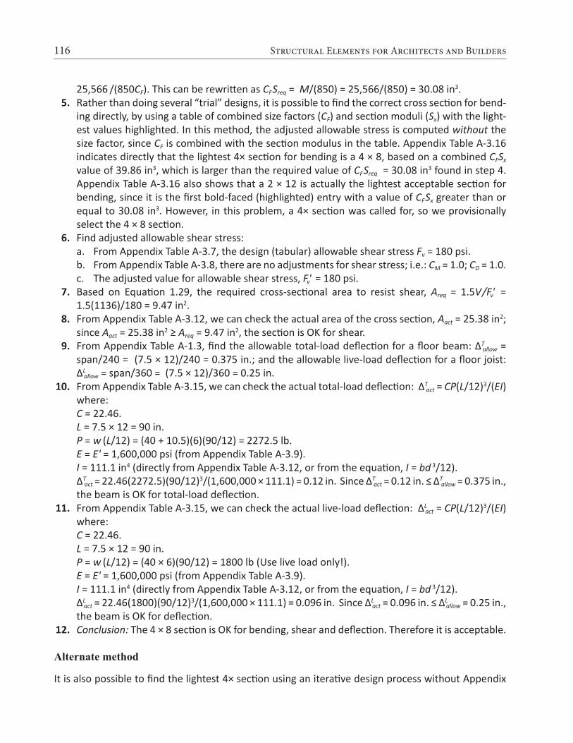
116 Structural Elements for Architects and Builders
25,566 /(850CF). This can be rewritten as CFSreq = M/(850) = 25,566/(850) = 30.08 in3. 5. Rather than doing several “trial” designs, it is possible to find the correct cross section for bend-
ing directly, by using a table of combined size factors (CF) and section moduli (Sx) with the light-est values highlighted. In this method, the adjusted allowable stress is computed without the size factor, since CF is combined with the section modulus in the table. Appendix Table A-3.16 indicates directly that the lightest 4× section for bending is a 4 × 8, based on a combined CFSx value of 39.86 in3, which is larger than the required value of CFSreq = 30.08 in3 found in step 4. Appendix Table A-3.16 also shows that a 2 × 12 is actually the lightest acceptable section for bending, since it is the first bold-faced (highlighted) entry with a value of CFSx greater than or equal to 30.08 in3. However, in this problem, a 4× section was called for, so we provisionally select the 4 × 8 section.
6. Find adjusted allowable shear stress:a. From Appendix Table A-3.7, the design (tabular) allowable shear stress Fv = 180 psi.b. From Appendix Table A-3.8, there are no adjustments for shear stress; i.e.: CM = 1.0; CD = 1.0.c. The adjusted value for allowable shear stress, Fv' = 180 psi.
7. Based on Equation 1.29, the required cross-sectional area to resist shear, Areq = 1.5V/Fv' = 1.5(1136)/180 = 9.47 in2.
8. From Appendix Table A-3.12, we can check the actual area of the cross section, Aact = 25.38 in2; since Aact = 25.38 in2 ≥ Areq = 9.47 in2, the section is OK for shear.
9. From Appendix Table A-1.3, find the allowable total-load deflection for a floor beam: ΔTallow =
span/240 = (7.5 × 12)/240 = 0.375 in.; and the allowable live-load deflection for a floor joist: ΔL
allow = span/360 = (7.5 × 12)/360 = 0.25 in. 10. From Appendix Table A-3.15, we can check the actual total-load deflection: ΔT
act = CP(L/12)3/(EI) where:
C = 22.46. L = 7.5 × 12 = 90 in. P = w (L/12) = (40 + 10.5)(6)(90/12) = 2272.5 lb. E = E' = 1,600,000 psi (from Appendix Table A-3.9). I = 111.1 in4 (directly from Appendix Table A-3.12, or from the equation, I = bd 3/12). ΔT
act = 22.46(2272.5)(90/12)3/(1,600,000 × 111.1) = 0.12 in. Since ΔTact = 0.12 in. ≤ ΔT
allow = 0.375 in., the beam is OK for total-load deflection.
11. From Appendix Table A-3.15, we can check the actual live-load deflection: ΔLact = CP(L/12)3/(EI)
where: C = 22.46. L = 7.5 × 12 = 90 in. P = w (L/12) = (40 × 6)(90/12) = 1800 lb (Use live load only!). E = E' = 1,600,000 psi (from Appendix Table A-3.9). I = 111.1 in4 (directly from Appendix Table A-3.12, or from the equation, I = bd 3/12). ΔL
act = 22.46(1800)(90/12)3/(1,600,000 × 111.1) = 0.096 in. Since ΔLact = 0.096 in. ≤ ΔL
allow = 0.25 in., the beam is OK for deflection.
12. Conclusion: The 4 × 8 section is OK for bending, shear and deflection. Therefore it is acceptable.
Alternate method
It is also possible to find the lightest 4× section using an iterative design process without Appendix
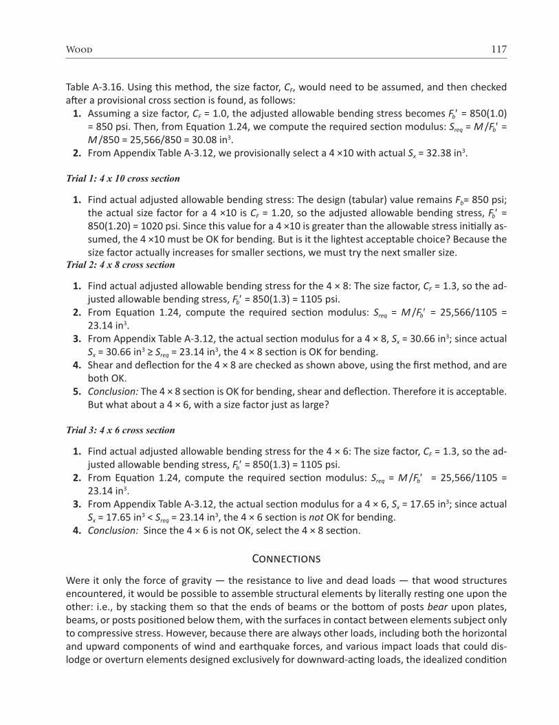
117Wood
Table A-3.16. Using this method, the size factor, CF, would need to be assumed, and then checked after a provisional cross section is found, as follows: 1. Assuming a size factor, CF = 1.0, the adjusted allowable bending stress becomes Fb' = 850(1.0)
= 850 psi. Then, from Equation 1.24, we compute the required section modulus: Sreq = M /Fb' = M /850 = 25,566/850 = 30.08 in3.
2. From Appendix Table A-3.12, we provisionally select a 4 ×10 with actual Sx = 32.38 in3.
Trial 1: 4 x 10 cross section
1. Find actual adjusted allowable bending stress: The design (tabular) value remains Fb= 850 psi; the actual size factor for a 4 ×10 is CF = 1.20, so the adjusted allowable bending stress, Fb' = 850(1.20) = 1020 psi. Since this value for a 4 ×10 is greater than the allowable stress initially as-sumed, the 4 ×10 must be OK for bending. But is it the lightest acceptable choice? Because the size factor actually increases for smaller sections, we must try the next smaller size.
Trial 2: 4 x 8 cross section
1. Find actual adjusted allowable bending stress for the 4 × 8: The size factor, CF = 1.3, so the ad-justed allowable bending stress, Fb' = 850(1.3) = 1105 psi.
2. From Equation 1.24, compute the required section modulus: Sreq = M /Fb' = 25,566/1105 = 23.14 in3.
3. From Appendix Table A-3.12, the actual section modulus for a 4 × 8, Sx = 30.66 in3; since actual Sx = 30.66 in3 ≥ Sreq = 23.14 in3, the 4 × 8 section is OK for bending.
4. Shear and deflection for the 4 × 8 are checked as shown above, using the first method, and are both OK.
5. Conclusion: The 4 × 8 section is OK for bending, shear and deflection. Therefore it is acceptable. But what about a 4 × 6, with a size factor just as large?
Trial 3: 4 x 6 cross section
1. Find actual adjusted allowable bending stress for the 4 × 6: The size factor, CF = 1.3, so the ad-justed allowable bending stress, Fb' = 850(1.3) = 1105 psi.
2. From Equation 1.24, compute the required section modulus: Sreq = M /Fb' = 25,566/1105 = 23.14 in3.
3. From Appendix Table A-3.12, the actual section modulus for a 4 × 6, Sx = 17.65 in3; since actual Sx = 17.65 in3 < Sreq = 23.14 in3, the 4 × 6 section is not OK for bending.
4. Conclusion: Since the 4 × 6 is not OK, select the 4 × 8 section.
Connections
Were it only the force of gravity — the resistance to live and dead loads — that wood structures encountered, it would be possible to assemble structural elements by literally resting one upon the other: i.e., by stacking them so that the ends of beams or the bottom of posts bear upon plates, beams, or posts positioned below them, with the surfaces in contact between elements subject only to compressive stress. However, because there are always other loads, including both the horizontal and upward components of wind and earthquake forces, and various impact loads that could dis-lodge or overturn elements designed exclusively for downward-acting loads, the idealized condition

118 Structural Elements for Architects and Builders
represented by this model must be adjusted by using fasteners that respond to those non-gravity forces as well. That being said, the basic idea of stacking one wood element on top of the other re-mains an important strategy for assembling many wood structures, as can be seen by examining a typical light wood framing system (Figure 3.26): in such cases, the necessary resistance to lateral and upward loads, from foundation to roof, is often accomplished by superimposing metal straps and other fasteners at key joints.
Aside from the use of metal straps, plates, and other more complex hangers and brackets, wood elements are typically connected using nails, bolts, and screws (of the screws, we will be consid-ering only lag screws, sometimes referred to as “lag bolts,” here). These fasteners can be used in two distinct ways: primarily as dowels inserted perpendicular to the direction of load; but also in withdrawal, i.e., subject to tension forces parallel to the direction of load. The designation for the capacity of a dowel-type fastener (i.e., a fastener stressed in shear) is Z; the capacity of a fastener used in withdrawal is designated as W, as shown in Figure 3.27. In both cases, the capacity must be multiplied by adjustment factors; the adjusted capacities are designated Z' and W' respectively.
Where the head of a lag screw or bolt, or the nut of a bolt, comes in contact with a wood mem-ber, a circular or square washer is inserted between the metal and wood surfaces in order to distrib-ute the load imparted by the metal fastener over a greater surface area of wood. This is a require-ment for bolts and lag screws subjected to either shear or tension.
Figure 3.26: Platform framing showing joists bearing on plates; plates bearing on studs; and studs bearing on plates (siding, building paper, insulation, vapor retarder, and interior finishes not shown)
Stud
Sole plate
Joist
Subfloor
Top plates
Sheathing
Header

119Wood
Shear
With respect to dowel-type action, nails and screws typically connect only two members (the side member being the piece into which the nail is first hammered or the screw is first inserted; the main member being the piece connected behind the side member). Such connections are in “single shear,” since there is only a single shear plane between the side and main member (Figure 3.28a). Bolts can connect two members in single shear, but also can connect three members in “double shear.” In the latter case, the “main member” is in the center, with the two outside members defined as “side members,” as shown in Figure 3.28b. Where bolts are used in single shear, the main member is defined as the thicker piece (if any), since either side could serve as the point of insertion without altering the behavior of the connection.
Figure 3.27: Wood fasteners with (a) dowel action; or (b) in withdrawal
(a) Dowel action (b) Withdrawal
Figure 3.28: Examples of (a) single shear and (b) double shear. "S" indicates side member; "M" indicates main member
(a) Single shear (b) Double shear

120 Structural Elements for Architects and Builders
Typical idealized diagrams representing the forces on dowel-type fasteners in single shear are often misleading, since neither the struc-ture (Figure 3.29a) nor the fasteners themselves (Figure 3.29b) would be in rotational equilibri-um with only a single force couple.
The actual pattern of forces acting on such fasteners is more complex, since these forces must satisfy all three equations of equilibrium. Several possibilities exist for the arrangement of forces on the fasteners that are consistent with the requirements for equilibrium. For example, as shown in Figure 3.30a, the force acting down-ward on the left-hand member can be “bal-anced” by two forces in the right-hand member; critical stress patterns applied to the wood by the fasteners are shown schematically in Figure 3.30b, assuming that only stresses in the left-hand member have reached critical values. This pattern of stress is designated Mode I.
Several other patterns of force and stress can develop in the wood connection. Figure 3.31 illustrates Mode II, in which critical stresses de-velop in both members. The inclination of the fastener (Figure 3.31b) is exaggerated to show how the pattern of critical stresses develops al-ternately on opposite sides of the fastener.
All together, researchers have identified four behavioral modes with dowel-type fasten-ers. For Modes III and IV (not illustrated), yield-ing of the fastener itself is presumed to have occurred; in these two latter cases, not only is the resistance of the wood to the pressure ex-erted by the fastener considered, but also the strength of the steel fastener itself. With these four modes, plus two variations each for Modes I and III (where critical stresses might occur ei-ther in the main or side member), there are six possible ways in which stress can develop in a single-shear connection, resulting in six possible values for the force that a single fastener can safely develop. Clearly, it is the smallest of these six allowable forces that governs the connec-tion design. For members connected in double shear, two of the modes are not considered, as
Figure 3.29: Simple single shear model with two equal and opposite forces, but rotational equilibrium unaccounted for: (a) forces acting on wood members; (b) forces acting on dowel-type fastener
Figure 3.30: Mode I behavior of fastener in single shear, showing (a) pattern of forces on fastener; and (b) corre-sponding critical stresses on wood member
Figure 3.31: Mode II behavior of fastener in single shear, showing (a) pattern of forces on fastener; and (b) corre-sponding critical stresses on wood member
(a) (b)
(a) (b)
(a) (b)

121Wood
they are incompatible with the geometry of elements in double-shear. Thus, only four equations need to be checked for double-shear connections.
Because the equations that have been developed for these six behavioral modes (four for double shear) acknowledge possible yielding of the steel fasteners, they are known as “yield limit” equa-tions. They can be used for bolts, lag screws, or nails — and not only for wood-to-wood connections, but also where steel plates are used for the side member(s). They are really not intended to be solved by hand: instead, three alternative strategies are commonly employed to design wood fasten-ers: (1) the use of spreadsheets or structural analysis software to solve the equations, (2) the use of tables containing commonly encountered fastener capacities, and (3) the use of “rules of thumb” in the form of tables and figures showing fastener details sanctioned by building codes. In most of the examples that follow, tables are used to find lateral design values. For a more detailed look at the use of yield limit equations, see Example 3.15 and Appendix Table A-3.31.
In general, fasteners should be placed in wood connections in such a way that the lines of force in the members being joined are aligned; a misaligned force is just another word for a force couple, which results in bending at the joint. Single-shear connections, as shown in Figure 3.28a, are inher-ently subject to such bending; whereas double-shear connections, as shown in Figure 3.28b, are inherently symmetrical, and therefore less likely to be subject to unanticipated bending stresses. On the other hand, many single-shear connections are embedded within, and attached to, a matrix of structural elements — sheathing, transverse members, and so on — that effectively relieve the fas-teners themselves of the burden of resisting stresses arising out of the misalignment. In the single-shear examples that follow, it is assumed that such additional structural elements (not shown in the examples) are actually present.
Aside from material properties for wood and steel, two other relationships between fastener and wood member must be accounted for: the penetration of lag screws and nails into the main member of the connection, as described in Appendix Table A-3.19; and the grain orientation of the various members being connected, with respect to the direction of load, as shown in Figure 3.32. To obtain full lateral design values, lag screw penetration must be at least equal to 8D, and nail penetra-tion must be at least equal to 10D (where D is the fastener diameter).
Just as the allowable stresses for wood structural elements in tension, compression, or bending
(a) (b) (c)
Figure 3.32: For dowel-type fasteners, three orientations of load to wood grain are possible, shown with their com-monly-used designations and equivalent keyboard-friendly designations, Zpar, Zs-per, and Zm-per. The latter designations are used in this text: (a) Zpar is the fastener capacity where both the side and main members are loaded parallel to grain; (b) Zs-per is the fastener capacity where the side member is loaded perpendicular to grain while the main mem-ber is loaded parallel to grain; and (c) Zm-per is the fastener capacity where the main member is loaded perpendicular to grain while the side member is loaded parallel to grain. The case where both members are loaded perpendicular to grain is uncommon, and is therefore not considered here.

122 Structural Elements for Architects and Builders
are adjusted to account for the actual behavioral properties of wood, the design values for wood fasteners are also adjusted in several ways. Two of these adjustments have already been discussed under the heading, material properties, although there are subtle differences in their application to fasteners. The duration of load factor (CD) accounts for changes in the strength of wood connec-tions based on the length of time (duration) that the load is applied. However, because the yield limit equations used to analyze single- and double-shear connections can also be used where steel side members are combined with wood main members, the allowable stress for such steel members has been reduced by a factor of 1.6, corresponding to the maximum duration-of-load adjustment for wood members under wind or seismic loading. In this way, CD may be applied to the entire con-nection design (so that the steel stress, already reduced, is increased up to its actual value in cases where the load combination includes wind or seismic forces), simplifying the design process, al-though making the steel side-member design conservative for load combinations that do not include wind or seismic forces (since in those cases, the steel stress is still initially reduced, but not increased by the same amount).
The wet service factor (CM) accounts for the increased strength of wood when used “dry.” For connection design, it is also important to consider the moisture content of the wood when it was first fabricated, since a change from an initial “wet” fabrication condition to a “dry” service condition can weaken the connection in some cases.
Two additional adjustments apply to dowel-type fasteners only, and only when the fastener di-ameter is greater or equal to ¼ in. (i.e., for bolts and lag screws). The group action adjustment (Cg) accounts for reductions in strength that may occur when comparing the behavior of a single fastener to that of a group of fasteners; the geometry factor (CΔ) includes a series of possible reductions that come into play when fasteners are closely spaced, or are placed too close to the edge or end of a wood member, as shown in Figure 3.33. The orientation of the wood grain determines the “edge” and “end” of the members, irrespective of the load direction; whereas “row spacing” parameters are measured with respect to the direction of the load (a “row of fasteners” being parallel to the direction of load).
Figure 3.33: Geometry factor parameters: (a) a 3-member connection is illustrated, with the grain represented by parallel lines on the surface of the members; (b) a free-body diagram shows how the geometry factor parameters are measured on the middle member
(a)
(b)

123Wood
For nails only, a toe-nail factor adjustment, Ctn, is used for lateral or withdrawal design values (see Appendix Table A-3.24) when the side and main members are fastened with nails driven at a 30° angle to the face of the side member.
The general strategy for designing wood connections is to first find the capacity of a single fas-tener, using one of the strategies discussed (i.e., using yield limit equations, or various tabular design aids), and then to multiply that capacity by the number of fasteners comprising the connection. As already suggested, this total capacity for multiple fasteners is explicitly modified using the group action adjustment factor Cg; the other adjustments — CD, CM, and CΔ — can be applied to either the entire connection or just a single fastener, but should only be applied once each per connection. A temperature factor, Ct , should be applied to wood elements subjected to sustained high tempera-tures: see Appendix Table A-3.25.
The complete dowel-type fastener design process for wood elements is summarized below; this summary constitutes the “Solution overview” within the examples that follow (with steps 4 and 5 eliminated where the connection consists of a single fastener only):
1. Find the capacity for a single fastener, Z.
2. For lag screws and nails, check that penetration into the main member is at least 4D (for lag screws) or 6D (for nails), and adjust capacity, Z, accordingly.
3. Adjust for duration of load, wet service conditions, and geometry.
4. For multiple-fastener connections only, adjust for group action, and then multiply the adjusted single-fastener capacity by the number of fasteners in the connection.
5. Remember that in addition to the fasteners, the element itself must be designed in a man-ner that accounts for the presence of bolt or lag screw holes (nail holes are not considered in structural element design). For multiple-fastener connections only, and only where forces are parallel to grain and in tension, also check the element for row and group tear-out (discussed earlier under the heading, tension).
Tables for computing fastener capacity are included in the appendix at the end of this chapter; specific guidelines for the use of these tables are provided in the examples that follow.
Example 3.9 Analyze wood single-shear con-nection using one bolt
Problem definition. Find the capacity of a connec-tion (single shear) consisting of a 2 × 10 beam connected to a 6 × 6 post using one ¾ in. di-ameter bolt, as shown in Figure 3.34. The wood used is Hem-Fir, and the bolts are fabricated from ordinary, low-strength, A307 steel, as is
Figure 3.34: Single-shear bolted connection with a single fastener, for Example 3.9

124 Structural Elements for Architects and Builders
typical for wood connections. Assume live and dead loads only, dry fabrication and service condi-tions, and spacing as shown.
Solution overview 1. Find the capacity for a single fastener, Z. 2. For lag screws and nails, check that penetration into the main member is at least 4D (for lag
screws) or 6D (for nails), and reduce capacity, Z, if necessary. 3. Adjust for duration of load, moisture, and geometry. 4. Adjust for group action (not applicable for single fastener connections). 5. Check that the element itself is designed in a manner that accounts for the presence of bolt or
lag screw holes (not included in this example).
Problem solution 1. From Appendix Table A-3.26, the lateral design value, Zs-per , is 460 lb. The value of Z chosen cor-
responds to the following condition: the side member (for bolted connections in single shear, the side member is defined as the thinner of the two members) is oriented so that the load is perpendicular to the direction of grain, while the main member is oriented so that the load is parallel to the direction of grain. This corresponds to Zs-per , as defined in Figure 3.32.
2. From Appendix Table A-3.19 (Note 4), penetration is only an issue with lag screws and nails, since bolts must always fully penetrate the members being connected. Therefore, no reduction of the tabular lateral design value is necessary, and it remains equal to Zs-per = 460 lb.
3. Adjustments are as follows: CD for typical values of live and dead load is 1.0 (Appendix Table A-3.20). CM for members fabricated and used “dry” is 1.0 (Appendix Table A-3.21). Cg does not apply to single-fastener connections. CΔ is found by testing four separate criteria (Appendix Table A-3.23): spacing between fasteners
in a row (not applicable where only one fastener is used); spacing between rows of fasteners (not applicable where only one fastener is used); end distance; and edge distance. It is some-times useful to sketch the members separately, showing dimensions for the relevant geometry factor parameters (Figure 3.35). In the calculations that follow, the fastener diameter is: D = ¾ in. = 0.75 in.
Figure 3.35: Geometry factor parameters for Example 3.9
Unspecified
Edge distanceEnd distance (compression)
Loaded edge distanceUnloaded eoaded edge distance
Unspecified
End distance (tension)
End distance

125Wood
Spacing criteria: For a single fastener connection, the spacing criteria (for spacing between rows and spacing of fasteners within a row) do not apply.
End distance: Adjustment criteria for end distance appear in Appendix Table A-3.23, part C. For the horizontal member, the loading direction is perpendicular to grain, so the minimum end distance for full value (i.e., for CΔ = 1.0) is 4D = 4 × 0.75 = 3 in. Since the actual end distance of 4 in. exceeds this value (and the other, unspecified, end distance is clearly larger), the geometry factor, CΔ = 1.0 for horizontal member end distance. For the vertical member, the loading direc-tion is parallel to grain and the specified wood is a “softwood,” so the minimum end distance for full value for “tension” (i.e., for CΔ = 1.0) is 7D = 7 × 0.75 = 5.25 in. Since the actual end distance, although unspecified, clearly exceeds this, the geometry factor, CΔ = 1.0 for vertical member end distance (tension). For the full value in “compression,” we need a minimum end distance of 4D = 4 × 0.75 = 3 in., which the actual end distance of 4¼ in. exceeds. The geometry factor therefore is also CΔ = 1.0 for vertical member end distance (compression).
Edge distance: Adjustment criteria for edge distance appear in Appendix Table A-3.23, part D. For the horizontal member, the loading direction is perpendicular to grain, so the loaded and unloaded edges must be determined separately. The minimum distance for the loaded edge (i.e., the edge towards which the fastener itself is bearing) is 4D = 4 × 0.75 = 3 in., which the ac-tual loaded edge distance of 4¼ in. exceeds. The minimum distance for the unloaded edge (i.e., the opposite edge away from which the fastener itself is bearing) is 1.5D = 1.5 × 0.75 = 1.125 in., which the actual unloaded edge distance of 5 in. exceeds. For the vertical member, the loading direction is parallel to grain, so the minimum edge distance is determined from the so-called slenderness ratio of the fastener, l /D. The length of the fastener, l , within the main member is 5½ in., so l /D = 5.5/0.75 = 7.33. Since this value is greater than 6, the minimum edge distance is 1.5D = 1.5 × 0.75 = 1.125 in., which the actual edge distance of 2.75 in. exceeds. Since all the criteria for full value are met, the geometry factor for edge distance is CΔ = 1.0.
The geometry factor for the entire connection is found by using the smallest of the geometry factors found for any of the four conditions tested above (end, edge, and the two spacing condi-tions where applicable): therefore, we use CΔ = 1.0.
The adjusted lateral design value for the single fastener in the connection is found by multi-plying the lateral design value from step 2 by the various adjustment factors determined in step 3: Z' = Z(CD)(CM)(CΔ) = 460(1.0)(1.0)(1.0) = 460 lb.
4. The group action factor, Cg, is 1.0 for all single-fastener connections (since only multiple fasten-er connections can have “group action”). Therefore, the connection capacity is equal to Z' (Cg) = 460(1.0) = 460 lb.
5. We are not considering the design of the structural elements themselves in this example. 6. Conclusion: The total capacity of the connection (consisting of a single 3/4 in. diameter bolt) is
460 lb.
Example 3.10 Analyze wood single-shear connection using multiple bolts
Problem definition. Find the capacity of a connection (single shear) consisting of two 2 × 8 tension ele-ments connected by a 2 × 8 member using six ½ in. diameter bolts in each member. The wood used is Hem-Fir No. 1, and the bolts are fabricated from ordinary, low-strength, A307 steel, as is typical for wood connections. Assume live, dead, and wind loads only, dry fabrication and service conditions, and spacing as shown in Figure 3.36.

126 Structural Elements for Architects and Builders
Solution overview 1. Find the capacity for a single fastener, Z. 2. For lag screws and nails, check that penetration into the main member is at least 4D (for lag
screws) or 6D (for nails), and reduce capacity, Z, if necessary. 3. Adjust for duration of load, moisture, and geometry. 4. Adjust for group action, and then multiply the adjusted single-fastener capacity by the number
of fasteners in the connection. 5. Check that the element itself is designed in a manner that accounts for the presence of bolt or
lag screw holes (not included in this example).
Problem solution 1. From Appendix Table A-3.26, the lateral design value, Zpar, is 410 lb. The value of Z chosen cor-
responds to the following condition: both the side and main member are oriented so that the load is parallel to the direction of grain, as defined in Figure 3.32.
2. From Appendix Table A-3.19 (Note 4), penetration is only an issue with lag screws and nails, since bolts must always fully penetrate the members being connected. Therefore, no reduction of the tabular lateral design value is necessary, and it remains equal to Zpar = 410 lb.
3. Adjustments are as follows: CD for live, dead, and wind load is 1.6 (Appendix Table A-3.20); CM for members fabricated and used “dry” is 1.0 (Appendix Table A-3.21); CΔ is found by testing four separate criteria (Appendix Table A-3.23): spacing between fasteners
in a row; spacing between rows of fasteners; end distance; and edge distance. It is sometimes useful to sketch the members separately, showing dimensions for the relevant geometry factor parameters (Figure 3.37):
In the calculations that follow, D is the fastener diameter of 1/2 in. Spacing criteria: Adjustment criteria for spacing appear in Appendix Table A-3.23, parts A and
B. For spacing between fasteners in a row, where the loading direction is parallel to grain, the minimum spacing for full value is 4D = 4 × 0.5 = 2 in. Since the actual spacing is 2 in., the full value applies, and CΔ = 1.0 for spacing between fasteners in a row. For spacing between rows of fasteners, again with the loading direction parallel to grain, the minimum required spacing is 1.5D = 1.5 × 0.5 = 0.75 in. Since the actual spacing (between rows) of 3.25 in. exceeds this
Figure 3.36: Single-shear bolted connection with multiple fasteners, for Example 3.10

127Wood
value, and is no greater than 5 in. (the maximum distance allowed between the outer rows of fasteners), the geometry factor is CΔ = 1.0 for spacing between rows of fasteners.
End distance: Adjustment criteria for end distance appear in Appendix Table A-3.23, part C. For all the members, the loading direction is parallel to grain. Where the fasteners are bearing towards the member end (in “tension”) and where the wood is “softwood,” the minimum end distance for full value (i.e., for CΔ = 1.0) is 7D = 7 × 0.5 = 3.5 in. For the primary members, the ac-tual end distance of 3.5 in. is no less than this, so the geometry factor, CΔ = 1.0. However, for the connecting member, shown to the right in Figure 3.37, the actual distance of 2 in. is between the absolute minimum (3.5D = 1.75 in.) and the required distance for full value (7D = 3.5 in.); therefore the geometry factor is taken as the actual end distance divided by the minimum dis-tance for full value, or CΔ = 2/3.5 = 0.571.
Edge distance: Adjustment criteria for edge distance appear in Appendix Table A-3.23, part D. For all the members, the loading direction is parallel to grain, so the minimum edge distance is determined from the so-called slenderness ratio of the fastener, l /D. The length of the fastener, l , within all members is 1½ in., so l /D = 1.5/0.5 = 3.0. Since this value is less than or equal to 6, the minimum edge distance is 1.5D = 1.5 × 0.5 = 0.75 in., which the actual edge distance of 2.0 in. exceeds. The geometry factor for edge distance is therefore CΔ = 1.0.
The geometry factor for the entire connection is found by using the smallest of the geometry factors found for any of the four conditions tested above (end, edge, and the two spacing condi-tions where applicable): therefore, we use CΔ = 0.571, which was computed for the end distance of the connecting member.
The adjusted lateral design value for a single bolt in the connection is found by multiplying the lateral design value from step 2 by the various adjustment factors determined in step 3: Z' = Z(CD)(CM)(CΔ) = 410(1.6)(1.0)(0.571) = 374.6 lb.
4. From Appendix Table A-3.22, the group action factor, Cg, is 0.993, a conservative value based on 2 × 8 main and side members (Am = As = approximately 11 in2), with three fasteners in a single row. The actual modulus of elasticity (Appendix Table A-3.9) for Hem-Fir No.1 is E = 1,500,000 psi, which is larger than the nominal value of 1,400,000 psi assumed in Appendix Table A-3.22; the actual fastener spacing, s = 2 in., is smaller than the value, s = 3 in., assumed in the table, and the actual fastener diameter, D = ½ in., is smaller than the value, D = ¾ in., assumed in the table. Therefore, the tabular value, Cg = 0.993, is conservative and can be used. Alternatively, a more
Figure 3.37: Geometry factor parameters for Example 3.10
Spacing between fasteners in a row
Spacing between rowsEdge distance
End distance (tension)Spacing between fasteners in a row

128 Structural Elements for Architects and Builders
accurate value for Cg can be found, based on the method described in Note 3 of Appendix Table A-3.22, and illustrated in Example 3.15.
Adjusting for group action and multiplying the single-fastener value for Z' found in step 3 by the number of fasteners in the connection, we get a total adjusted connection capacity equal to 374.6(0.993)(6) = 2232 lb.
5. We are not considering the design of the structural elements themselves in this example. Ten-sion, row and group tear-out are considered in Example 3.1.
6. Conclusion: The total capacity of the connection (consisting of a six ½ in. diameter bolts) is 2232 lb.
Example 3.11 Analyze wood double-shear connection using multiple bolts
Problem definition. Find the capacity of a connection (double shear) consisting of two 2 × 8 tension elements connected by two shorter 2 × 8 members, using six ½ in. diameter bolts in each member. The wood used is Hem-Fir No.1, and the bolts are fabricated from ordinary, low-strength, A307 steel, as is typical for wood connections. Assume live, dead, and wind loads only, dry fabrication and ser-vice conditions, and spacing as shown in Figure 3.38.
Solution overview 1. Find the capacity for a single fastener, Z. 2. For lag screws and nails, check that penetration into the main member is at least 4D (for lag
screws) or 6D (for nails), and reduce capacity, Z, if necessary. 3. Adjust for duration of load, moisture, and geometry. 4. Adjust for group action, and then multiply the adjusted single-fastener capacity by the number
of fasteners in the connection. 5. Not included in this example (check that the element itself is designed in a manner that ac-
counts for the presence of bolt or lag screw holes).
Problem solution 1. From Appendix Table A-3.27, the lateral design value, Zpar, is 900 lb. The value of Z chosen
corresponds to the following condition: both the side and main member are oriented so that the load is parallel to the direction of grain, as defined in Figure 3.32.
2. From Appendix Table A-3.19 (Note 4), penetration is only an issue with lag screws and nails, since bolts must always fully penetrate the members being connected. Therefore, no reduction
Figure 3.38: Double-shear bolted connection with multiple fasteners, for Example 3.11

129Wood
of the tabular lateral design value is necessary, and it remains equal to Zpar= 900 lb. 3. Adjustments are as follows: CD for live, dead, and wind load is 1.6 (Appendix Table A-3.20); CM for members fabricated and used “dry” is 1.0 (Appendix Table A-3.21); CΔ is found by testing four separate criteria (Appendix Table A-3.23): spacing between fasteners
in a row; spacing between rows of fasteners; end distance; and edge distance. It is sometimes useful to sketch the members separately, showing dimensions for the relevant geometry factor parameters (Figure 3.39).
In the calculations that follow, D is the fastener diameter of ½ in. Spacing criteria: Adjustment criteria for spacing appear in Appendix Table A-3.23, parts A
and B. For spacing between fasteners in a row, where the loading direction is parallel to grain, the minimum spacing for full value is 4D = 4 × 0.5 = 2 in. Since the actual spacing is 2 in., the full value applies, and CΔ = 1.0. For spacing between rows of fasteners, again with the loading direction parallel to grain, the minimum required spacing is 1.5D = 1.5 × 0.5 = 0.75 in. Since the actual spacing (between rows) of 3.25 in. exceeds this value, and is no greater than 5 in. (the maximum distance allowed between the outer rows of fasteners), the geometry factor is CΔ = 1.0.
End distance: Adjustment criteria for end distance appear in Appendix Table A-3.23, part C. For all the members, the loading direction is parallel to grain. Where the fasteners are bearing towards the member end, i.e., in “tension” and for “softwood,” the minimum end distance for full value (i.e., for CΔ = 1.0) is 7D = 7 × 0.5 = 3.5 in. For the main members, the actual end dis-tance of 3.5 in. is no less than this, so the geometry factor, CΔ = 1.0. However, for the connecting member, shown to the right in Figure 3.39, the actual distance of 2 in. is between the absolute minimum (3.5D = 1.75 in.) and the required distance for full value (7D = 3.5 in.); therefore the geometry factor is taken as the actual end distance divided by the minimum distance for full value, or CΔ = 2/3.5 = 0.571.
Edge distance: Adjustment criteria for edge distance appear in Appendix Table A-3.23, part D. For all the members, the loading direction is parallel to grain, so the minimum edge distance is determined from the so-called slenderness ratio of the fastener, l /D. The fastener length, l , within all members is 1½ in., so l /D = 1.5/0.5 = 3.0. Since this value is less than or equal to 6, the minimum edge distance is 1.5D = 1.5 × 0.5 = 0.75 in., which the actual edge distance of 2.0 in. exceeds. The geometry factor therefore is CΔ = 1.0.
The geometry factor for the entire connection is found by using the smallest of the geometry factors found for any of the four conditions tested above (end, edge, and the two spacing condi-
Figure 3.39: Geometry factor parameters for Example 3.11
Spacing between fasteners in a row
Spacing between rows
Spacing between fasteners in a rowEnd distance (tension)
Edge distance

130 Structural Elements for Architects and Builders
tions where applicable): therefore, we use CΔ = 0.571, which was computed for the end distance of the connecting member.
The adjusted lateral design value for a single bolt in the connection is found by multiplying the lateral design value from step 2 by the various adjustment factors determined in step 3: Z' = Z(CD)(CM)(CΔ) = 900(1.6)(1.0)(0.571) = 822.2 lb.
4. From Appendix Table A-3.22, the group action factor, Cg , is 0.983, a conservative value based on a single 2 × 8 main member and two 2 × 8 side members (Am = approximately 11 in2; As = approximately 17 in2), with three fasteners in a single row. The actual modulus of elasticity (Ap-pendix Table A-3.9) for Hem-Fir No.1 is E = 1,500,000 psi, which is larger than the nominal value of 1,400,000 psi assumed in the table; the actual fastener spacing, s = 2 in., is smaller than the value, s = 3 in., assumed in the table, and the actual fastener diameter, D = ½ in., is smaller than the value, D = ¾ in., assumed in the table; therefore, the tabular value, Cg = 0.983, is conserva-tive and can be used. Alternatively, a more accurate value for Cg can be found, based on the method described in Note 3 of Appendix Table A-3.22, and illustrated in Example 3.15.
Adjusting for group action and multiplying the single-fastener value for Z' found in step 3 by the number of fasteners in the connection, we get a total adjusted connection capacity equal to 822.2(0.983)(6) = 4849 lb.
5. We are not considering the design of the structural elements themselves in this example. Ten-sion, row and group tear-out are considered in Example 3.1.
6. Conclusion: The total capacity of the connection (consisting of a six ½ in. diameter bolts) is 4849 lb.
Example 3.12 Analyze wood double-shear connection using multiple bolts and steel side plates
Problem definition. Find the capacity of a connection (double shear) consisting of a 6 × 6 tension member connected by two ¼ in. steel side plates, using four ⅝ in. diameter bolts. The wood used is Douglas Fir-Larch (North) No. 1, the steel plates are ASTM A36 steel, and the bolts are fabricated from ordinary, low-strength, A307 steel, as is typical for wood connections. Assume live and dead loads only, dry fabrication and service conditions, and spacing as shown in Figure 3.40.
Solution overview 1. Find the capacity for a single fastener, Z. 2. For lag screws and nails, check that pene-
tration into the main member is at least 4D (for lag screws) or 6D (for nails), and reduce capacity, Z, if necessary.
3. Adjust for duration of load, moisture, and geometry.
4. Adjust for group action, and then multiply the adjusted single-fastener capacity by the number of fasteners in the connection.
5. Not included in this example (check that the element itself is designed in a manner that accounts for the presence of bolt or lag screw holes).
Figure 3.40: Double-shear bolted connection with mul-tiple fasteners and steel side plates, for Example 3.12

131Wood
Problem solution 1. From Appendix Table A-3.28, the lateral design value, Zpar, is 2390 lb. The value of Z chosen cor-
responds to the following condition: the main member is oriented so that the load is parallel to the direction of grain, as defined in Figure 3.32. The orientation of the steel side plates to the direction of load is not relevant, since there is no “grain” in the steel plates that influences its strength.
2. From Appendix Table A-3.19 (Note 4), penetration is only an issue with lag screws and nails, since bolts must always fully penetrate the members being connected. Therefore, no reduction of the tabular lateral design value is necessary, and it remains equal to Zpar = 2390 lb.
3. Adjustments are as follows: CD for typical values of live and dead load is 1.0 (Appendix Table A-3.20); CM for members fabricated and used “dry” is 1.0 (Appendix Table A-3.21); CΔ is found by testing four separate criteria (Appendix Table A-3.23): spacing between fasteners
in a row; spacing between rows of fasteners; end distance; and edge distance. It is sometimes useful to sketch the members separately, showing dimensions for the relevant geometry factor parameters (Figure 3.41). Only the wood main member is considered here; the tension capacity and bolt spacing in the steel plate must be considered separately (see Chapter 4 for discussion of steel subjected to tension and for discussion of bolt spacing).
In the calculations that follow, D is the fastener diameter of ⅝ in. = 0.625 in. Spacing criteria: Adjustment criteria for spacing appear in Appendix Table A-3.23, parts A
and B. For spacing between fasteners in a row, where the loading direction is parallel to grain, the minimum spacing for full value is 4D = 4 × 0.625 = 2.5 in. Since the actual spacing is 2.5 in., the full value applies, and CΔ = 1.0. For spacing between rows of fasteners, again with the load-ing direction parallel to grain, the minimum required spacing is 1.5D = 1.5 × 0.625 = 0.9375 in. Since the actual spacing (between rows) of 2.5 in. exceeds this value, and is no greater than 5 in. (the maximum distance allowed between the outer rows of fasteners), the geometry factor is CΔ = 1.0.
End distance: Adjustment criteria for end distance appear in Appendix Table A-3.23, part C. For the main member, the loading direction is parallel to grain. Where the fasteners are bearing toward the member end (in “tension”) and where the wood is “softwood,” the minimum end distance for full value (i.e., for CΔ = 1.0) is 7D = 7 × 0.625 = 4.375 in. The actual end distance of 5 in. is greater than this, so the geometry factor, CΔ = 1.0.
Edge distance: Adjustment criteria for edge distance appear in Appendix Table A-3.23, part D. For the main member, the loading direction is parallel to grain, so the minimum edge distance is deter-mined from the so-called slenderness ratio of the fastener, l /D. The fastener length, l , within the main member is 5½ in., so l /D = 5.5/0.625 = 8.8. Since this value is greater than 6, the minimum edge distance is ei-ther 1.5D = 1.5 × 0.625 = 0.9375 in., or one half of the spacing between rows = 0.5 × 2.5 = 1.25 in., whichever is greater: the
Figure 3.41: Geometry factor parameters for Example 3.12
Edge distanceSpacing between rows
End distance (tension)Spacing between fasteners in a row

132 Structural Elements for Architects and Builders
minimum edge distance is therefore 1.25 in., which the actual edge distance of 1.5 in. exceeds. The geometry factor therefore is CΔ = 1.0.
The geometry factor for the entire connection is found by using the smallest of the geometry factors found for any of the four conditions tested above (end, edge, and the two spacing condi-tions where applicable): therefore, we use CΔ = 1.0.
The adjusted lateral design value for a single bolt in the connection is found by multiplying the lateral design value from step 2 by the various adjustment factors determined in step 3: Z' = Z(CD)(CM)(CΔ) = 2390(1.0)(1.0)(1.0) = 2390 lb.
4. From Appendix Table A-3.22 (part B for steel side members) the group action factor, Cg, is 0.997, a conservative value based on a 6 × 6 main member and two ¼ in. steel side plates (Am = approx-imately 30 in2; As = approximately 3 in2), with two fasteners in a single row. The actual modulus of elasticity (Appendix Table A-3.9) for Douglas Fir-Larch (North) No.1 is E = 1,600,000 psi (for “posts and timbers”), which is larger than the nominal value of 1,400,000 psi assumed in the table; the actual fastener spacing, s = 2.5 in., is smaller than the value, s = 3 in., assumed in the table, and the actual fastener diameter, D = ⅝ in., is smaller than the value, D = ¾ in., assumed in the table; therefore, the tabular value, Cg = 0.997, is conservative and can be used. Alternatively, a more accurate value for Cg can be found, based on the method described in Note 3 of Appen-dix Table A-3.22, and illustrated in Example 3.15.
Adjusting for group action and multiplying the single-fastener value for Z' found in step 3 by the number of fasteners in the connection, we get a total adjusted connection capacity equal to 2390(0.997)(4) = 9531 lb.
5. We are not considering the design of the structural elements themselves in this example. Ten-sion, row and group tear-out are considered in Example 3.1.
6. Conclusion: The total capacity of the connection (consisting of a four ⅝ in. diameter bolts) is 9531 lb.
Example 3.13 Analyze wood single-shear connection using multiple lag screws
Problem definition. Find the capacity of a connection (single shear) consisting of a 4 × 10 beam con-nected to an 8 × 8 post using six 6-in.-long, ½-in.-diameter lag screws. The wood used is Douglas Fir-Larch No.2, and the lag screws are fabricated from ordinary, low-strength, A307 steel. Assume live and dead loads only, dry fabrication and service conditions, and spacing as shown in Figure 3.42.
Solution overview 1. Find the capacity for a single fastener, Z. 2. For lag screws and nails, check that penetration into the main member is at least 4D (for lag
screws) or 6D (for nails), and reduce capacity, Z, if necessary. 3. Adjust for duration of load, moisture, and geometry. 4. Adjust for group action, and then multiply the adjusted single-fastener capacity by the number
of fasteners in the connection. 5. Not included in this example (check that the element itself is designed in a manner that accounts
for the presence of bolt or lag screw holes).

133Wood
Problem solution 1. From Appendix Table A-3.29, the lateral
design value, Zs-per, is 270 lb. The value of Z chosen corresponds to the following condi-tion: the side member is oriented so that the load is perpendicular to the direction of grain, while the main member is orient-ed so that the load is parallel to its grain, as defined in Figure 3.32.
2. Penetration must be checked for lag screws (see Appendix Table A-3.19 for notes on penetration; lag screw dimensions can be found in Appendix Table A-3.17). The actu-al penetration, p = 2.1875 in., can be found by first subtracting the side member thick-ness of 3.5 in. from the lag screw length, L = 6 in., to get 2.5 in.; and then subtracting the length of the tapered tip, E = 0.3125 in., from the 2.5 in. length within the main member, as illustrated in Figure 3.43.
This actual penetration is then compared to the minimum lengths for lag screw pen-etration in Appendix Table A-3.19: the ab-solute minimum is 4D = 4 × 0.5 = 2 in.; the minimum penetration to obtain the full value of Z is 8D = 8 × 0.5 = 4 in. Since the ac-tual penetration is between these two val-ues, the lateral design value, Z, is reduced by multiplying it by p /(8D) = 2.1875/4 = 0.547. Therefore, we use a lateral design value of 270 × 0.547 = 148 lb.
3. Adjustments are as follows: CD for typical values of live and dead load is
1.0 (Appendix Table A-3.20); CM for members fabricated and used “dry”
is 1.0 (Appendix Table A-3.21); CΔ is found by testing four separate criteria
(Appendix Table A-3.23): spacing between fasteners in a row; spacing between rows of fasten-ers; end distance; and edge distance. It is sometimes useful to sketch the members separately, showing dimensions for the relevant geometry factor parameters (Figure 3.44):
In the calculations that follow, D is the fastener diameter of ½ in. (however, for lag screws, the so-called reduced body diameter, Dr = 0.371 in., is used to calculate lateral design values).
Spacing criteria: Adjustment criteria for spacing appear in Appendix Table A-3.23, parts A and B. For spacing between fasteners in a row for the horizontal member, where the loading direction is perpendicular to grain, the minimum spacing for full value is determined by the
Figure 3.42: Single-shear lag screw connection with mul-tiple fasteners, for Example 3.13
Figure 3.43: Penetration of lag screw into main member, for Example 3.13
3.5" 7.5"
6"
p = 2.1875"E = 0.3125"
Side member
Main member

134 Structural Elements for Architects and Builders
required values for the attached member (i.e., for the vertical member with loading parallel to grain). For spacing between rows of fasteners, again with the loading direction perpendicular to grain, the minimum required spacing is determined from the so-called slenderness ratio of the fastener, l /D. For lag screws, the dowel bearing length equals the penetration within the main member found in step 2, as noted in Appendix Table A.3.19. Therefore, the dowel bearing length, l , equals 2.1875 in., and l /D = 2.1875/0.5 = 4.375. Since this value is between 2 and 6, the minimum spacing between rows of fasteners is (5l + 10D)/8 = (5 × 2.1875 + 10 × 0.5) /8 = 1.992 in., which the actual spacing between rows of 3.5 in. exceeds. Therefore, the geometry factor is CΔ = 1.0.
For spacing between fasteners in a row, where the loading direction is parallel to grain, the minimum spacing for full value is 4D = 4 × 0.5 = 2 in. Since the actual spacing is 2⅛ in., the full value applies here (and also to the horizontal member), and CΔ = 1.0. For spacing between rows of fasteners, again with the loading direction parallel to grain, the minimum required spacing is 1.5D = 1.5 × 0.5 = 0.75 in. Since the actual spacing (between rows) of 3.5 in. exceeds this value, and is no greater than 5 in. (the maximum distance allowed between the outer rows of fasten-ers), the geometry factor is CΔ = 1.0.
End distance: Adjustment criteria for end distance appear in Appendix Table A-3.23, part C. For the horizontal member, the loading direction is perpendicular to grain, so the minimum end distance for full value (i.e., for CΔ = 1.0) is 4D = 4 × 0.5 = 2 in. Since the actual end distance of 2 in. equals this value (and the other, unspecified, end distance is clearly larger), the geometry factor, CΔ = 1.0. For the vertical member, the loading direction is parallel to grain and the speci-fied wood is a “softwood,” so the minimum end distance for full value for “tension” (i.e., for CΔ = 1.0) is 7D = 7 × 0.5 = 3.5 in. Since the actual end distance, although unspecified, clearly exceeds this, the geometry factor, CΔ = 1.0. For the full value in “compression,” we need a minimum end distance of 4D = 4 × 0.5 = 2 in., which the actual end distance of 2½ in. exceeds. The geometry factor therefore is also CΔ = 1.0.
Edge distance: Adjustment criteria for edge distance appear in Appendix Table A-3.23, part D. For the horizontal member, the loading direction is perpendicular to grain, so the loaded and unloaded edges must be determined separately. The minimum distance for the loaded edge (i.e., the edge towards which the fastener itself is bearing) is 4D = 4 × 0.5 = 2 in., which the actual loaded edge distance of 2½ in. exceeds. The minimum distance for the unloaded edge (i.e., the opposite edge away from which the fastener itself is bearing) is 1.5D = 1.5 × 0.5 =
Figure 3.44: Geometry factor parameters for Example 3.13
End distanceSpacing between rows
Unloaded edge distanceSpacing between fasteners in a row
Edge distanceEnd distance (compression)
Loaded edge distance

135Wood
0.75 in., which the actual unloaded edge distance of 2½ in. exceeds. For the vertical member, the loading direction is parallel to grain, so the minimum edge distance is determined from the so-called slenderness ratio of the fastener, l /D. The dowel bearing length, l , within the main member is 2.1875 in., so l /D = 2.1875/0.5 = 4.375. Since this value is less than or equal to 6, the minimum edge distance is 1.5D = 1.5 × 0.5 = 0.75 in., which the actual edge distance of 2.0 in. exceeds. The geometry factor therefore is CΔ = 1.0.
The geometry factor for the entire connection is found by using the smallest of the geometry factors found for any of the four conditions tested above (end, edge, and the two spacing condi-tions where applicable): therefore, we use CΔ = 1.0.
The adjusted lateral design value for a single lag screw in the connection is found by multiply-ing the lateral design value from step 2 by the various adjustment factors determined in step 3: Z' = Z(CD)(CM)(CΔ) = 148(1.0)(1.0)(1.0) = 148 lb.
4. From Appendix Table A-3.22, the group action factor, Cg , is 0.970, a conservative value based on an 8 × 8 main member and a side member with an effective area of 12.25 in2 (because the side member is loaded perpendicular to grain, its effective area is taken as its thickness of 3.5 in. multiplied by the distance between the outer rows of fasteners, also 3.5 in.). For use in Appendix Table A-3.22, these areas are rounded as follows: Am = 56 in2 and As = 11 in2. The actual modulus of elasticity (Appendix Table A-3.9) for Hem-Fir No.1 is E = 1,500,000 psi, which is larger than the nominal value of 1,400,000 psi assumed in the table; the actual fastener spac-ing, s = 2 in., is smaller than the value, s = 3 in., assumed in the table, and the actual fastener diameter, D = ½ in., is smaller than the value, D = ¾ in., assumed in the table; therefore, the tabular value, Cg = 0.970, is conservative and can be used. Alternatively, a more accurate value for Cg can be found, based on the method described in Note 3 of Appendix Table A-3.22, and illustrated in Example 3.15.
Adjusting for group action (using Cg = 0.970), and multiplying the single-fastener value for Z' found in step 3 by the number of fasteners in the connection, we get a total adjusted connec-tion capacity equal to 148(0.970)(6) = 861 lb.
5. We are not considering the design of the structural elements themselves in this example. 6. Conclusion: The total capacity of the connection (consisting of a six ½ × 6 in. lag screws) is
861 lb.
Example 3.14 Design wood single-shear connection using common nails
Problem definition. Determine the number of 10d common nails needed to connect a typical 2 × 10 floor joist, spanning 11.5 ft and spaced at 16 in. on center, to a 2 × 6 stud, as shown in Figure 3.45. The wood used is Spruce-Pine-Fir No.1/No.2, the distributed loads on the floor consist of 40 psf live load and 10.5 psf dead load, and the wood is fabricated and used “dry.”
Solution overview 1. Find the capacity for a single fastener, Z. 2. For lag screws and nails, check that penetration into the main member is at least 4D (for lag
screws) or 6D (for nails), and reduce capacity, Z, if necessary. 3. Adjust for duration of load, moisture, and geometry. 4. Group action does not apply to nailed connections.

136 Structural Elements for Architects and Builders
5. Check that the element itself is designed in a manner that accounts for the presence of bolt or lag screw holes (not applicable).
6. Find the total force acting on the connection and divide by the adjusted capacity for a single fastener to find the number of fasteners required.
Problem solution 1. From Appendix Table A-3.30, the lateral design value, Z, is 100 lb, for a 10d nail and a 1½ in. side
member. 2. In general, penetration must be checked for nails (see Appendix Table A-3.19): however, tabular
values in Appendix Table A-3.30 already include reductions for penetration, so this step is only necessary when lateral design values are computed using other means. We can confirm that a penetration reduction is not necessary by computing the actual penetration, p = 1½ in., as shown in Figure 3.46. First, subtract the side member thickness of 1½ in. from the nail length of 3 in., to get 1½ in. (nail dimensions can be found in Appendix Table A-3.18).
Next, the actual penetration is compared to the minimum requirements for nail penetration in Appendix Table A-3.19. Since p = 1.5 in. ≥ 10D = 10 × 0.148 = 1.48 in., we can use the full lat-eral design value. For values of p < 10D, lateral capacity would need to be reduced by p/(10d). In all cases where yield limit equations are used for nails, the dowel bearing length in the main member, lm, is taken as the penetration minus half the length of the tapered tip, so that tabular lateral design values, which do not consider this reduced dowel bearing length, may be slightly nonconservative in some cases (specifically, they may differ in cases where the governing yield limit equation includes the dowel bearing length parameter).
The lateral design value, Z, remains 100 lb. 3. Adjustments are as follows: CD for live and dead load is 1.0 (Appendix Table A-3.20); CM for members fabricated and used “dry” is 1.0 (Appendix Table A-3.21); CΔ = 1.0 for dowel-type fasteners with D < ¼ in. This applies to virtually all nails, certainly for 10d
nails with D = 0.148 in. (see Appendix Table A-3.18). While no specific numerical requirements are given for nail spacing, and edge or end distances, nails should be configured so that splitting
Figure 3.45: Single-shear nailed connection for Example 3.14
Framing plan
Connection detail
Tributary area for joist reaction
2 x 6 stud
2 x 10 joist
5'-9"
11'-6"
16" o.c.
16"
2 x 10 joist
Figure 3.46: Penetration of nail into main member, for Example 3.14
Side member
Main member
1.5" p = 1.5"
3"

137Wood
of the wood members does not occur. The adjusted lateral design value for the connection is found by multiplying the lateral design
value from step 2 by the various adjustment factors determined in step 3: Z' = Z(CD)(CM)(CΔ) = 100(1.0)(1.0)(1.0) = 100 lb.
4. The group action factor, Cg = 1.0, for fasteners with diameter, D < ¼ in., i.e., for most nailed con-nections.
5. We are not considering the design of the structural elements themselves in this example. 6. To determine the number of nails needed, we first find the total force acting at the connection,
i.e., the reaction of a typical joist, by multiplying the floor loads by the tributary area for half of a single joist: (40 + 10.5)(5.75 × 1.33) = 387.2 lb. Dividing this total force by 100 lb (the capacity of a single fastener), we get the required number of fasteners, n = 387.2/100 = 3.87; i.e., we need four 10d nails.
Example 3.15 Analyze wood double-shear bolted connection using yield limit and group action equations
Problem definition. Find the capacity of a connection (double shear) consisting of a 6 × 6 tension member connected by two ¼ in. steel side plates, using four ⅝ in. diameter bolts. The wood used is Douglas Fir-Larch (North) No. 1, the side plates are ASTM A36 steel, and the bolts are fabricated from ordinary, low-strength, A307 steel, as is typical for wood connections. Assume live and dead loads only, dry fabrication and service conditions, and spacing as shown in Figure 3.47. Use yield limit and group action equations, rather than tabular values (see Example 3.12 for solution using tabular values).
Solution overview 1. Find the capacity for a single fastener, Z,
using yield limit equations. 2. For lag screws and nails, check that pen-
etration into the main member is at least 4D (for lag screws) or 6D (for nails), and re-duce capacity, Z, if necessary.
3. Adjust for duration of load, moisture, and geometry.
4. Adjust for group action using group action factor equations, and then multiply the adjusted single-fastener capacity by the number of fasteners in the connection.
5. Check that the element itself is designed in a manner that accounts for the presence of bolt or lag screw holes (not included in this example).
Figure 3.47: Double-shear bolted connection with mul-tiple fasteners and steel side plates, for Example 3.15 (same as Figure 3.40 for Example 3.12)
6 × 6 tension member
1/4" A36 steel side plates

138 Structural Elements for Architects and Builders
Problem solution 1. To find the lateral design value, Z, for a single fastener using yield limit equations, follow the
step-by-step method outlined in Appendix Table A-3.31. The main member is oriented so that the load is parallel to the direction of grain, as defined in Figure 3.32. The orientation of the steel side plates to the direction of load is not relevant, since there is no “grain” in a steel plate that influences its strength.a. From Appendix Table A-3.11, G = 0.49 for Douglas Fir-Larch (North).b. D = ⅝ in. = 0.625 in.c. Main member (D > 0.25 in., wood, loaded parallel to grain): Fem = 11,200G = 11,200 × 0.49 = 5488 psi. Side member (A36 steel): Fes = 87,000 psi. It is common to round these values to the nearest 50 psi, so we will use
Fem = 5500 psi.d. Fyb = 45,000 psi for bolts.e. Dowel bearing lengths are l m = 5.5 in. and l s = 0.25 in.f. Compute the terms Re = Fem/Fes = 5500/87,000 = 0.06322; and Rt = l m /l s = 5.5/0.25 = 22.0.g. Rd = 4Kθ = 4(1.0) = 4 (for yield modes Im and Is); Rd = 3.6Kθ = 3.6(1.0) = 3.6 (for yield
mode II); and Rd = 3.2Kθ =3.2(1.0) = 3.2 (for yield modes IIIm , IIIs , IV). In these equations, Kθ = 1 + 0.25(θ/90) = 1.0, since θ = 0°.
h. Compute the following coefficients:
i. Compute Z for all applicable yield modes (four applicable modes for double shear): For yield mode Im, Z = DlmFem /Rd = 0.625(5.5)(5500)/4 = 4726.6 lb. For yield mode Is, Z = 2DlsFes /Rd = 2(0.625)(0.25)(87,000)/4 = 6796.9 lb for double shear. Yield mode II does not apply to double shear connections.
k1 = √Re + 2Re
2(1 + Rt + Rt2) + Rt
2Re3 – Re(1 + Rt)
(1 + Re)
k2 = –1 + 2(1 + Re) +2Fyb(1 + 2Re)D2
3Femlm2√
k3 = –1 +2(1 + Re) 2Fyb(2 + Re)D2
3Femls2√ Re
+
2(1 + 0.06322) + 2(45,000)(1 + 2 x 0.06322)(0.625)2
3(5500)(5.5)2√
= –1 + = 0.4852
= √0.06322 + 2(0.06322)2(1 + 22 + 222) + 222(0.06322)3 – 0.06322(1 + 22)(1 + 0.06322)
= 0.5687
2(1 + 0.06322) 2(45,000)(2 + 0.06322)(0.625)2
3(5500)(0.25)2√
= –1 + = 9.19670.06322) +

139Wood
Yield mode IIIm does not apply to double shear connections.
The smallest of the various yield mode values is then selected: Z = 2394.1 lb based on yield mode IIIs.
2. Penetration is only an issue with lag screws and nails, since bolts must always fully penetrate the members being connected. Therefore, no reduction of the lateral design value is necessary, and it remains equal to Z = 2394.1 lb.
3. Adjustments are as follows (same as for Example 3.12): CD for typical values of live and dead load is 1.0 (Appendix Table A-3.20); CM for members fabricated and used “dry” is 1.0 (Appendix Table A-3.21); CΔ is found by testing four separate criteria (Appendix Table A-3.23): spacing between fasteners
in a row; spacing between rows of fasteners; end distance; and edge distance. It is sometimes useful to sketch the members separately, showing dimensions for the relevant geometry factor parameters (Figure 3.48). Only the wood main member is considered here; the tension capacity and bolt spacing in the steel plate must be considered separately (see Chapter 4 for discussion of tension and bolt spacing in steel):
In the calculations that follow, D is the fastener diameter of ⅝ in. = 0.625 in. Spacing criteria: Adjustment criteria for spacing appear in Appendix Table A-3.23, parts A and
B. For spacing between fasteners in a row, where the loading direction is parallel to grain, the minimum spacing for full value is 4D = 4 × 0.625 = 2.5 in. Since the actual spacing is 2.5 in., the full value applies, and CΔ = 1.0. For spacing between rows of fasteners, again with the loading direction parallel to grain, the mini-mum required spacing is 1.5D = 1.5 × 0.625 = 0.9375 in. Since the actual spacing (be-tween rows) of 2.5 in. exceeds this value, and is no greater than 5 in. (the maximum distance allowed between the outer rows of fasteners), the geometry factor is CΔ = 1.0.
End distance: Adjustment criteria for end distance appear in Appendix Table A-3.23, part C. For the main member, the loading direction is parallel to grain. Where the fas-teners are bearing towards the member end (in “tension”) and for "softwood," the minimum end distance for full value (i.e.,
For Yield Mode IV, Z = 2D2 2FemFyb
Rd 3(1 + Re)= 2(0.625)2
3.22(5500)(45,000)3(1 + 0.06322)√ √
= 3041.4 lb.
For Yield Mode IIIs, Z =2k3DlsFem
(2 + Re)Rd= 2(9.1967)(0.625)(0.25)(5500)
(2 + 0.06322)(3.2)= 2394.1 lb.
Figure 3.48: Geometry factor parameters for Example 3.15 (same as Figure 3.31 for Example 3.12)
Edge distanceSpacing between rows
End distance (tension)Spacing between fasteners in a row

140 Structural Elements for Architects and Builders
for CΔ = 1.0) is 7D = 7 × 0.625 = 4.375 in. The actual end distance of 5 in. is greater than this, so the geometry factor, CΔ = 1.0.
Edge distance: Adjustment criteria for edge distance appear in Appendix Table A-3.23, part D. For the main member, the loading direction is parallel to grain, so the minimum edge distance is determined from the so-called slenderness ratio of the fastener, l /D. The fastener length, l , within the main member is 5½ in., so l /D = 5.5/0.625 = 8.8. Since this value is greater than 6, the minimum edge distance is either 1.5D = 1.5 × 0.625 = 0.9375 in., or one half of the spacing between rows = 0.5 × 2.5 = 1.25 in., whichever is greater: the minimum edge distance is there-fore 1.25 in., which the actual edge distance of 1.5 in. exceeds. The geometry factor therefore is CΔ = 1.0.
The geometry factor for the entire connection is found by using the smallest of the geometry factors found for any of the four conditions tested above (end, edge, and the two spacing condi-tions where applicable): therefore, we use CΔ = 1.0.
The adjusted lateral design value for a single bolt in the connection is found by multiplying the lateral design value from step 2 by the various adjustment factors determined in step 3: CD, CM, and CΔ: Z' = Z(CD)(CM)(CΔ) = 2394.1(1.0)(1.0)(1.0) = 2394.1 lb.
4. The group action factor, Cg, can be found based on the method described in Note 3 of Appendix Table A-3.22:
D = 0.625 in. γ = 270,000(D1.5) = 270,000(0.6251.5) = 133,409. s = 2.5 in. Em = 1,600,000 psi (see Appendix Table A-3.9). Es = 29,000,000 psi (see Chapter 4 for the modulus of elasticity of steel). Am = 30.25 in2; As = 2(0.25 × 5.5) = 2.75 in2 (Appendix Table A-3.12).
Adjusting for group action and multiplying the single-fastener value for Z' found in step 3 by the number of fasteners in the connection, we get a total adjusted connection capacity equal to 2394.1(0.999)(4) = 9567 lb.
5. We are not considering the design of the structural elements themselves in this example. Ten-sion, row and group tear-out are considered in Example 3.1.
6. Conclusion: The total capacity of the connection (consisting of a six ½ in. diameter bolts) is 9567 lb.
REA = (1,600,000)(30.25)(29,000,000)(2.75) = 0.607.
m = 1.0055 – √1.00552 – 1 = 0.900.
n = 2.
Cg =0.900(1 – 0.9002(2)
2[(1 + 0.607 × 0.9002)(1 + 0.900) – 1 + 0.9002(2)]1 + 0.6071 – 0.900
= 0.999.
u = 1 + (133,409) 2.52
1 1(1,600.000)(30.25) (29,000,000)(2.75)
= 1.0055+

141Wood
Withdrawal
Where a fastener is itself stressed in tension, it is considered to be loaded in “withdrawal,” as a fail-ure of the connection would cause it to “withdraw” — pull out — from the member into which it was inserted. For lag screws and nails, selected withdrawal design values, designated W to distinguish them from lateral design values, Z, are tabulated in Appendix Tables A-3.32 and A-3.33. These tabu-lar values increase with higher wood specific gravity, G, and larger shaft diameter, D, and are based on the following empirical equations: for lag screws, W = 1800G 3/2D 3/4; for nails, W = 1380G 5/2D. In these equations, W is the withdrawal design value per inch of penetration (lb); G is the specific grav-ity of the wood; and D is the fastener diameter (in.). While it is permitted to use nails in withdrawal, it is advisable to alter the connection geometry, if possible, so that such unthreaded fasteners are stressed in shear, rather than in tension. Unlike the penetration length of lag screws stressed in shear (laterally), the penetration of lag screws in withdrawal only includes that portion of the shank length that is both embedded in the main member, and threaded (excluding the tapered tip).
Lag screw withdrawal values must be reduced by 75% when the lag screws are inserted into the end grain of a wood member; nails are not permitted to be loaded in withdrawal from the end grain of wood members. Aside from computing the capacity of a connection based on computed with-drawal values, W, the tensile strength of lag screws loaded in withdrawal must also be checked, and, where the head (or washer) of the lag screw is in contact with a wood member, the bearing stress of the washer on this member must also be checked. Finally, the adjusted withdrawal capacity per inch of penetration, W', is computed by multiplying W by the appropriate adjustment factors: where in-service temperatures are no more than 100°F, only duration of load and wet service factors apply to fasteners in withdrawal (see Appendix Tables A-3.20 and A-3.21).
For bolted connections, “withdrawal” is not possible; instead, where bolts are placed in tension, the tensile strength of the bolt itself, as well as the bearing of the bolt (or washer) on the surface of the wood member, must be checked.
Example 3.16 Design wood connection in withdrawal, using lag screws
Problem definition. Determine the number of 3-in.-long, ½-in.-diameter, lag screws needed to con-nect a ¼ in. steel plate holding a 2800 lb load to a 4 × 10 wood beam, as shown in Figure 3.49. The wood used is Spruce-Pine-Fir No.1/No.2, the loads are dead and live only (so that CD = 1.0), and the wood is fabricated and used dry. Assume that the steel plate capacity is adequate.
Figure 3.49: Withdrawal load on lag screws for Example 3.16
2800 lb 1/4"-thick plate
T – E = 1.6875"
4 x 10
L =
3"
T =
2"
E = 0.3125"
D
(a) (b)

142 Structural Elements for Architects and Builders
Solution overview. Find the capacity of a single lag screw in withdrawal; divide the total load by this value to determine the required number of lag screws.
Problem solution 1. From Appendix Table A-3.32, the withdrawal design value, W, per inch of penetration, is 291 lb,
for a 3-in.-long, ½-in.-diameter lag screw. The adjusted value, W' = W(CD)(CM) = 291(1.0)(1.0) = 291 lb.
2. From Appendix Table A-3.17, it can be seen that the actual penetration into the main member (i.e., the length of the threaded portion of the lag screw that engages the main member, not including the tapered tip, or T – E) = 1.6875 in. Therefore, each lag screw resists (291)(1.6875) = 491 lb in withdrawal.
3. Since the total load to be resisted is 2800 lb, the required number of lag screws = 2800/491 = 5.7. Round up and use six 3-in.-long, ½-in.-diameter, lag screws.
Example 3.17 Analyze wood connection in withdrawal, using common nails
Problem definition. A steel bracket designed to hold heavy items is fastened to the floor joist above it using four 16d common nails, as shown in Figure 3.50. These nails must go through a ½ in. drywall ceiling, as well as the ⅛ in.-thick steel bracket itself, before reaching the wood joist, fabricated from Douglas Fir-Larch. How much load can the bracket carry, based on the capacity of the fasteners (and assuming that the strength of the bracket itself is adequate)?
Solution overview. Find the capacity of a single nail in withdrawal; multiply the single-nail capacity by the number of nails to find the capacity of the bracket.
Problem solution 1. From Appendix Table A-3.33, the withdrawal design value for a single 16d nail, W, per inch of
penetration, is 40 lb. The adjusted value, W' = W (CD)(CM) = 40(0.9)(1.0) = 36 lb. The decision to use a value of CD = 0.9 is based on an evaluation of the loads, which are essentially of a perma-nent nature (i.e., dead loads).
2. The actual penetration into the main member is the total nail length minus the drywall and steel thickness; from Appendix Table A-3.18, we see that p = 3.5 – (1/2 + 1/8) = 2.875 in. Therefore,
Wood joist
Nails
Drywall ceiling
Steel bracket
1/2"1/8"
PP
Section through bracket Cut-away viewFigure 3.50: Withdrawal load on nailed bracket for Example 3.17

143Wood
each nail resists (36)(2.875) = 103.5 lb in withdrawal. 3. Since there are four nails, the total capacity of the rack, P = 4(103.5) = 414 lb. However, it would
be wiser to use a threaded connector (such as a screw or lag screw) instead of a nail in this situ-ation.
Bearing
Where a wooden column or beam bears on another structural element, a compressive stress acts on the bearing surfaces. The use of the plural (“surfaces”) indicates that bearing always acts in two directions, so that, for example, a joist bearing on a plate implies that the plate is also bearing on the joist. In theory, the bearing stress is the same on both surfaces; in practice, the effective bearing area in some cases may be increased by adding ⅜ in. in the direction of the bearing length — measured in the direction parallel to the grain of the wood — to account for the ability of the wood grain to distribute the load across a larger area. For the beam and post shown in Figure 3.51, the bearing stress of the post on the beam, or the beam on the post, is equal to the load, P, divided by the bear-ing area, W × T. Since wood is weaker when stressed perpendicular to its grain, the critical bearing stress will almost always occur acting downward on the surface of the beam, rather than upward on the post. If the distance, D, measured from the edge of the post to the end of the beam, is greater than three inches, and the bearing length, W, of the post is less than six inches, we can reduce the effective bearing stress of the post on the beam by dividing the load, P, by the larger effective bear-ing area, T × (W + ⅜ in.). This stress is then compared to the adjusted allowable compressive stress (perpendicular to grain). For joists and other beams, the allowable stress is in compression, per-pendicular to the grain of the wood, whereas when considering the bearing stress on columns, the allowable stress value is taken for compression parallel to grain (but without including the ad-justment factor for stability, since buckling is not relevant at the surface where bearing stresses are being measured).
For compressive stresses parallel to grain, a steel plate must be used at the point of bearing to distribute such stresses more evenly across the surfaces in contact, but only in cases when these stresses exceed 75% of Fc*. See Appendix Table A-3.4 for adjustments to allowable com-pressive stresses.
Example 3.18 Check wood connection in bear-ing
Problem definition. A 4 × 4 post bears at the mid-point of a 4 × 10 girder. The 5000 lb load trans-ferred to the girder through the post consists of live, dead, and wind loads. Check whether the bearing capacity is adequate, assuming that both members are Hem-Fir No.2.
Figure 3.51: Bearing of post on beam: the direction of grain is indicated by the parallel lines on each surface
P
W
D
W + 3/8"
T

144 Structural Elements for Architects and Builders
Solution overview. Find the effective bearing area of the post on the girder; find the actual “effective” bearing stress on the girder; compare this stress to the allowable compressive stress perpendicular to grain.
Problem solution 1. Because the post has a bearing length less than six inches, and is more than three inches from
the end of the girder, we can use an effective bearing length ⅜ in. greater than its actual bear-ing length of 3.5 in. (see Appendix Table A-3.12 for cross-sectional dimensions). The effective bearing area is therefore = T × (W + ⅜) = 3.5(3.5 + 0.375) = 13.56 in2. The actual bearing stress on surface of the girder = 5000/13.56 = 369 psi.
2. This value is compared with the adjusted allowable bearing stress, F'c-per. From Appendix Table A-3.3, the design value for compression perpendicular to grain for the Hem-Fir girder is Fc-per = 405 psi.
3. Assuming that the members are used indoors, the only potentially relevant adjustment factor, for wet service, doesn’t apply. CM is taken as 0.67 only when the moisture content is greater than 19% for long periods of time — i.e., when used outdoors — but can be taken as 1.0 when used indoors; the size and duration of load factors do not apply to compression perpendicular to grain. Therefore, F'c-per = 405(1.0) = 405 psi, which is greater than the actual effective bearing stress. The connection is satisfactory with respect to bearing.
4. The 4 × 4 post need not be directly checked for bearing stress (since its allowable stress in compression parallel to grain will be greater than the girder’s allowable stress perpendicular to grain). However, we check to see whether the actual stress on the post exceeds 75% of Fc*, the allowable compressive stress parallel to grain with all adjustments except for the column stability factor; if it does, a steel bearing plate should be specified. The actual stress is the load divided by the post area, or 5000/(3.5 × 3.5) = 408 psi, where the cross-sectional dimensions can be found in Appendix Table A-3.12. From Appendix Tables A-3.3 and A-3.4, the adjusted al-lowable stress (without Cp) multiplied by 75% is (0.75)1300(1.15)(1.0) = 1121 psi (the size factor, CF = 1.15, for the 4 × 4 post). Since this value is greater than the actual stress, no bearing plates are required between the post and girder.
In the design of such a connection, it must not be assumed that gravity will hold the post firmly against the girder under all conditions; the two members must also be mechanically con-nected to guard against unintended movement.

145Wood
Chapter 3 AppendixTable A-3.1: Design values for tension, Ft (psi) for visually graded lumber and glued-laminated timberA. Dimension lumber (2 in. – 4 in. thick)Species Select Structural No. 1 No. 2 No. 3 MiscellaneousDouglas Fir-Larch 1000 675 575 325 1800
Douglas Fir-Larch (North) 825 n/a n/a 300 2500
Douglas Fir-South 900 600 525 300
Hem-Fir 925 625 525 300 1725
Hem-Fir (North) 775 n/a n/a 325 2575
Spruce-Pine-Fir 700 n/a n/a 250 2450
Spruce-Pine-Fir (South) 575 400 350 200
Southern Pine3 1000 650 525 300
B. Beams and stringers4
Species Select Structural No. 1 No. 2 No. 3 MiscellaneousDouglas Fir-Larch 950 675 425 n/a
Douglas Fir-Larch (North) 950 675 425 n/a
Douglas Fir-South 900 625 425 n/a
Hem-Fir 750 525 350 n/a
Hem-Fir (North) 725 500 325 n/a
Spruce-Pine-Fir 650 450 300 n/a
Spruce-Pine-Fir (South) 625 450 300 n/a
Southern Pine5 1000 900 550 n/a
C. Posts and timbers6
Species Select Structural No. 1 No. 2 No. 3 MiscellaneousDouglas Fir-Larch 1000 825 475 n/a
Douglas Fir-Larch (North) 1000 825 475 n/a
Douglas Fir-South 950 775 450 n/a
Hem-Fir 800 650 375 n/a
Hem-Fir (North) 775 625 375 n/a
Spruce-Pine-Fir 700 550 325 n/a
Spruce-Pine-Fir (South) 675 550 325 n/a
Southern Pine5 1000 900 550 n/a
D. Glued-laminated softwood timberSpecies Grade (and Identification No.)Douglas Fir-Larch (DF) L3 (ID#1)
950L2 (ID#2)
1250L2D (ID#3)
1450L1D L1 (ID#5)
1650
Softwood Species (SW) L3 (ID#22) 525
Alaska Cedar (AC) L3 (ID#69)725
L2 (ID#70)975
L1D (ID#71)1250
L1S (ID#72)1250
Southern Pine (SP) N2M14 N2M12 (ID#47) 1200
N2D14 N2D12 (ID#48) 1400
N1M16 (ID#49)1350
N1D14 (ID#50)1550
(continued)

146 Structural Elements for Architects and Builders
Table A-3.1 (continued)
Notes:1. No.1 & better2. No.1/No.23. Values for Southern Pine for dimension lumber are approximate: typical published values include the size factor and therefore list dif-ferent values for each lumber width; whereas the values in this table have been normalized (i.e., do not include the size factor) and have been rounded down to values that may be slightly conservative.4. Beams and stringers are a subset of the "timbers" size category, 5 in. x 5 in. or larger, where the width is at least 4 in. bigger than the thickness.5. Southern Pine values for timbers (beams and stringers; and posts and timbers) are for wet service conditions.6. Posts and timbers are a subset of the "timbers" size category, 5 in. x 5 in. or larger, where the width is equal to, or no more than 2 in. bigger than, the thickness.
Table A-3.2: Adjustments to allowable stress in tension, Ft, for visually-graded lumber and glued-laminated softwood timberA. Size factorSize factor, CF = 1.0 for tension stress, except for the following sizes of dimension lumber:
Size CF Size CF Size CF Size CF
22 × 2 1.5 42 × 8 1.2 1,42 × 14, 4 × 14 0.9 44 × 8 1.222 × 4 1.5 42 × 10 1.1 24 × 4 1.5 44 × 10 1.132 × 6 1.3 42 × 12 1.0 34 × 6 1.3 44 × 12 1.0
B. Wet service factorWet service factor, CM = 1.0, except for glulam with a moisture content of at least 16% (e.g., used outdoors), in which case CM = 0.8. In any dry service condition, CM = 1.0.
C. Load duration factorLoad duration factor, CD, is as follows:
Load type Duration CD Load type Duration CD
Dead load, D Permanent 0.90 Construction load, Lr 1 week 1.25
Live load, L 10 years 1.00 Wind or seismic load, W or E 10 minutes 1.60
Snow load, S 2 months 1.15 Impact load, I Instant 2.00
D. Temperature factor, Ct
Temperature, T (° F) Ct
T ≤ 100° F 1.0
100° F < T ≤ 150° F 0.9
Notes:1. CF = 0.9 for all 2× or 4× dimension lumber having nominal width greater or equal to 14.2. Exceptions: CF = 1.1 for stud grade 2 × 2, 2 × 4, and 4 × 4 lumber; CF = 1.0 for construction and standard 2 × 2, 2 × 4, and 4 × 4 lum-ber; and CF = 0.4 for utility grade 2 × 2 lumber3. Exceptions: CF = 1.0 for stud grade 2 × 6 and 4 × 6 lumber4. Exceptions: For stud grade lumber with nominal width of 8 or higher, use No.3 grade values for Ft and CF

147Wood
Table A-3.3: Design values for compression (psi), parallel to grain (Fc) and perpendicular to grain (Fc-per) for visually-grad-ed lumber and glued-laminated softwood timberA. Dimension lumber (2 in. – 4 in. thick)Species Fc
(parallel to grain)Fc-per
(perpendicular to grain)Select Structural No. 1 No. 2 No. 3 Misc. All grades7
Douglas Fir-Larch 1700 1500 1350 775 11550 625
Douglas Fir-Larch (North) 1900 n/a n/a 825 21400 625
Douglas Fir-South 1600 1450 1450 775 520
Hem-Fir 1500 1350 1300 725 11350 405
Hem-Fir (North) 1700 n/a n/a 850 21450 405
Spruce-Pine-Fir 1400 n/a n/a 650 21150 425
Spruce-Pine-Fir (South) 1200 1050 1000 575 335
Southern Pine3 1800 1575 1425 825 565
B. Beams and stringers4
Species Fc
(parallel to grain)Fc-per
(perpendicular to grain)Select Structural No. 1 No. 2 No. 3 Misc. All grades7
Douglas Fir-Larch 1100 925 600 n/a 625
Douglas Fir-Larch (North) 1100 925 600 n/a 625
Douglas Fir-South 1000 850 550 n/a 520
Hem-Fir 925 750 500 n/a 405
Hem-Fir (North) 900 750 475 n/a 405
Spruce-Pine-Fir 775 625 425 n/a 425
Spruce-Pine-Fir (South) 675 550 375 n/a 335
Southern Pine5 950 825 525 n/a 375
C. Posts and timbers6
Species Fc
(parallel to grain)Fc-per
(perpendicular to grain)Select Structural No. 1 No. 2 No. 3 Misc. All grades7
Douglas Fir-Larch 1150 1000 700 n/a 625
Douglas Fir-Larch (North) 1150 1000 700 n/a 625
Douglas Fir-South 1050 925 650 n/a 520
Hem-Fir 975 850 575 n/a 405
Hem-Fir (North) 950 850 575 n/a 405
Spruce-Pine-Fir 800 700 500 n/a 425
Spruce-Pine-Fir (South) 700 625 425 n/a 335
Southern Pine5 950 825 525 n/a 375
(continued)

148 Structural Elements for Architects and Builders
Table A-3.3 (continued)
D. Glued-laminated softwood timberSpecies Grade (and Identification No.)
Fc (parallel to grain) Fc-per (perpendicular to grain)
Douglas Fir-Larch8 (DF)(less than 4 laminations)
L3 (ID#1)15501250
L2 (ID#2)19501600
L2D (ID#3)23001900
L1 (ID#5)24002100
L3 (ID#1)560560
L2 (ID#2)560560
L2D (ID#3)650650
L1 (ID#5)650650
Softwood Species8 (SW)(less than 4 laminations)
L3 (ID#22)850525
L3 (ID#22)315315
Alaska Cedar8 (AC)(less than 4 laminations)
L3(ID#69)
11501100
L2(ID#70)14501450
L1D (ID#71)19001900
L1S (ID#72)19001900
L3(ID#69)
470470
L2(ID#70)
470470
L1D (ID#71)
560560
L1S (ID#72)
560560
Southern Pine8 (SP)(less than 4 laminations)
N2M12 (ID#47)19001150
N2D12 (ID#48)22001350
N1M16 (ID#49)21001450
N1D14 (ID#50)23001700
N2M12 (ID#47)
650650
N2D12 (ID#48)
740740
N1M16 (ID#49)
650650
N1D14 (ID#50)
740740
Species Combination SymbolFc (parallel to grain) Fc-per (perpendicular to grain)
Various species9 16F-1.3E925
20F-1.5E925
24F-1.7E1000
24F-1.8E1600
16F-1.3E315
20F-1.5E425
24F-1.7E500
24F-1.8E650
Notes:1. No.1 & better2. No.1/No.23. Values for Southern Pine for dimension lumber are approximate: typical published values include the size factor and therefore list dif-ferent values for each lumber width; whereas the values in this table have been normalized (i.e., do not include the size factor) and have been rounded down to values that may be slightly conservative.4. Beams and stringers are a subset of the "timbers" size category, 5 in. × 5 in. or larger, where the width is at least 4 in. bigger than the thickness.5. Southern Pine values for timbers (beams and stringers; posts and timbers) are for wet service conditions.6. Posts and timbers are a subset of the "timbers" size category, 5 in. × 5 in. or larger, where the width is equal to, or no more than 2 in. bigger than, the thickness.7. Values for compression perpendicular to grain apply to all the size categories listed in this table (i.e., listed under compression parallel to grain). However, "dense" variations of Douglas Fir-Larch and Southern Pine, not listed here, have higher values.8. These species designations are designed primarily for axially-loaded elements (compression and tension).9. These combination designations are designed primarily for bending elements, although they can be used in axial compression or ten-sion with the values that appear in this table. Values for Fc-per (compression perpendicular to grain) are based on loading perpendicular to the wide face of the laminations.

149Wood
Table A-3.4: Adjustments to allowable stress in compression, Fc , for visually-graded lumber and glued-laminated soft-wood timberA. Size factor3
Size factor, CF = 1.0 for compression stress, except for the following sizes of dimension lumber:
Size CF Size CF Size CF Size CF
62 × 2 1.15 82 × 8 1.05 1,82 × 14, 4 × 14 0.9 84 × 8 1.0562 × 4 1.15 82 × 10 1.00 64 × 4 1.15 84 × 10 1.0072 × 6 1.10 82 × 12 1.00 74 × 6 1.10 84 × 12 1.00
B. Wet service factorWet service factor, CM, is as follows: for dimension lumber2, CM = 0.8; for timbers, CM = 0.91; for glulam, CM = 0.73. In any dry service condition, CM = 1.0.
C. Load duration factor4
Load duration factor, CD, is as follows:
Load type Duration CD Load type Duration CD
Dead load, D Permanent 0.90 Construction load, Lr 1 week 1.25
Live load, L 10 years 1.00 Wind or seismic load, W or E 10 minutes 1.60
Snow load, S 2 months 1.15 Impact load, I Instant 2.00
D. Column stability factor5
The column stability factor, CP, is as follows:where:
E'min = EminCM (see Appendix Table A-3.9 for adjustments to E and Emin) d =
le = c = 0.8 for sawn lumber, and 0.9 for glulam
E. Temperature factor, Ct
Temperature, T (° F) Ct (used dry) Ct (used wet)T ≤ 100° F 1.0 1.0
100° F < T ≤ 125° F 0.8 0.7
125° F < T ≤ 150° F 0.7 0.5
Notes:1. CF = 0.9 for all 2× or 4× dimension lumber having nominal width greater or equal to 14.2. CM = 1.0 for dimension lumber when FcCF ≤ 750 psi.3. Size factor adjustments are not used for compression perpendicular to grain.4. Load duration adjustments are not used for compression perpendicular to grain.5. Column stability factor adjustments are not used for compression perpendicular to grain.6. Exceptions: CF = 1.05 for stud grade 2 × 2, 2 × 4, and 4 × 4 lumber; CF = 1.0 for construction and standard 2 × 2, 2 × 4, and 4 × 4 lumber; and CF = 0.6 for utility grade 2 × 2 lumber7. Exceptions: CF = 1.0 for stud grade 2 × 6 and 4 × 6 lumber8. Exceptions: For stud grade lumber with nominal width of 8 or higher, use No.3 grade values for Fc and CF
the unbraced length corresponding to the cross-sectional dimension, d
cross-sectional dimension (in.) corresponding to the unbraced length, le. Where the unbraced length is the same for both axes of the cross section, d should be taken as the smaller cross-sectional dimension; otherwise, use the larger value of le /d
A =
FcE
Fc*1 +
2cand B =
FcE
Fc*c
FcE =0.822E'min
(le/d)2and Fc* = FcCDCMCF
CP = A - √A2 - B

150 Structural Elements for Architects and Builders
Table A-3.5: Design values for bending, Fb (psi) for visually-graded lumber and glued-laminated softwood timberA. Dimension lumber (2 in. – 4 in. thick)Species Select Structural No. 1 No. 2 No. 3 MiscellaneousDouglas Fir-Larch 1500 1000 900 525 11200
Douglas Fir-Larch (North) 1350 n/a n/a 475 2850
Douglas Fir-South 1350 925 850 500
Hem-Fir 1400 975 850 500 11100
Hem-Fir (North) 1300 n/a n/a 575 21000
Spruce-Pine-Fir 1250 n/a n/a 500 2875
Spruce-Pine-Fir (South) 1300 875 775 450
Southern Pine3 1850 1175 950 550
B. Beams and stringers4
Species Select Structural No. 1 No. 2 No. 3 MiscellaneousDouglas Fir-Larch 1600 1350 875 n/a
Douglas Fir-Larch (North) 1600 1300 875 n/a
Douglas Fir-South 1550 1300 825 n/a
Hem-Fir 1300 1050 675 n/a
Hem-Fir (North) 1250 1000 675 n/a
Spruce-Pine-Fir 1100 900 600 n/a
Spruce-Pine-Fir (South) 1050 900 575 n/a
Southern Pine5 1500 1350 850 n/a
C. Posts and timbers6
Species Select Structural No. 1 No. 2 No. 3 MiscellaneousDouglas Fir-Larch 1500 1200 750 n/a
Douglas Fir-Larch (North) 1500 1200 725 n/a
Douglas Fir-South 1450 1150 675 n/a
Hem-Fir 1200 975 575 n/a
Hem-Fir (North) 1150 925 550 n/a
Spruce-Pine-Fir 1050 850 500 n/a
Spruce-Pine-Fir (South) 1000 800 475 n/a
Southern Pine5 1500 1350 850 n/a
(continued)

151Wood
D. Glued-laminated softwood timberSpecies Grade (and Identification No.)
Fb (for beams with d > 15 in.) Fb (for beams with d ≤ 15 in.)
Douglas Fir-Larch7 (DF)L3 (ID#1)
1100L2 (ID#2)
1496L2D (ID#3)
1760L1 (ID#5)
1936L3 (ID#1)
1250L2 (ID#2)
1700L2D (ID#3)
2000L1 (ID#5)
2200
Softwood Species7 (SW)L3 (ID#22)
638L3 (ID#22)
725
Alaska Cedar7 (AC)
L3(ID#69)
880
L2(ID#70)
1188
L1D (ID#71)1540
L1S (ID#72)1672
L3(ID#69)1000
L2(ID#70)1350
L1D (ID#71)1750
L1S (ID#72)1900
Southern Pine7 (SP)
N2M12 (ID#47)1232
N2D12 (ID#48)1408
N1M16 (ID#49)1584
N1D14 (ID#50)1848
N2M12 (ID#47)1400
N2D12 (ID#48)1600
N1M16 (ID#49)1800
N1D14 (ID#50)2100
Various species8 Combination Symbols for Stress ClassesFb (for positive bending9) Fb (for negative bending9)
16F-1.3E1600
20F-1.5E2000
24F-1.7E2400
24F-1.8E2400
16F-1.3E925
20F-1.5E1100
24F-1.7E1450
24F-1.8E1450
E. Glued-laminated softwood timber bent about y-axis (loaded parallel to wide face of laminations)Species Grade (and Identification No.)
Fb (for 4 or more laminations) Fb (for 3 laminations)
Douglas Fir-Larch7 (DF)
L3 (ID#1)1450
L2 (ID#2)1800
L2D (ID#3)2100
L1 (ID#5)2400
L3 (ID#1)1250
L2 (ID#2)1600
L2D (ID#3)1850
L1 (ID#5)2100
Softwood Species7 (SW)L3 (ID#22)
800L3 (ID#22)
700
Alaska Cedar7 (AC)
L3 (ID#69)1100
L2 (ID#70)1400
L1D (ID#71)1850
L1S (ID#72)1850
L3 (ID#69)975
L2 (ID#70)1250
L1D (ID#71)1650
L1S (ID#72)1650
Southern Pine7 (SP)
N2M12 (ID#47)1750
N2D12 (ID#48)2000
N1M16 (ID#49)1950
N1D14 (ID#50)2300
N2M12 (ID#47)1550
N2D12 (ID#48)1800
N1M16 (ID#49)1750
N1D14 (ID#50)2100
Species Combination Symbols for Stress ClassesFb (all cases)
Various species8 16F-1.3E800
20F-1.5E800
24F-1.7E1050
24F-1.8E1450
Notes:1. No.1 & better2. No.1/No.23. Values for Southern Pine for dimension lumber are approximate: typical published values include the size factor and therefore list dif-ferent values for each lumber width; whereas the values in this table have been normalized (i.e., do not include the size factor) and have been rounded down to values that may be slightly conservative.4. Beams and stringers are a subset of the "timbers" size category, 5 in. × 5 in. or larger, where the width is at least 4 in. bigger than the thickness.5. Southern Pine values for timbers (beams and stringers; and posts and timbers) are for wet service conditions.6. Posts and timbers are a subset of the "timbers" size category, 5 in. × 5 in. or larger, where the width is equal to, or no more than 2 in. bigger than, the thickness.
Table A-3.5 (continued)
(continued)

152 Structural Elements for Architects and Builders
7. These species designations are designed primarily for axially-loaded elements (compression and tension), although they can be used for bending with the values that appear in this table. For bending about the x-axis only, these elements are assumed to have no special tension laminations; such special tension laminations would increase the bending design values (for all cross-section sizes bent about the x-axis) to the values shown for d ≤ 15 in. multiplied by a factor of 1.18.8. These combination designations are designed primarily for simply-supported bending elements (i.e., for beams with only positive bending moments), and are manufactured with higher strength grades of wood used in the extreme fibers (for bending about the x-axis) where bending stresses are greatest.9. The combination symbols in this table refer to cross sections that are "unbalanced"; i.e., they are manufactured to optimize the behavior of simply-supported beams with only positive curvature. Where such unbalanced combinations are used for beams subjected to negative bending moments — i.e., for continuous or cantilevered beams — lower values for Fb must be used at those cross sections with negative moment. For beams subjected to reversals of curvature (and therefore both positive and negative bending), "balanced" (symmetrical) combinations can be specified where Fb is the same for both positive and negative bending, for example: combination symbols 16F-V6 with Fb = 1600 psi; 20F-V7 with Fb = 2000 psi; and 24F-V8 with Fb = 2400 psi.
Table A-3.6: Adjustments to allowable stress in bending, Fb, for visually-graded lumber and glued-laminated softwood timber A. Size factor3
Size factor, CF. (1) For glulam, size factor does not apply (use smaller of CV and CL — see Table A-3.6 Parts C and F below). (2) For timbers (beams and stringers; posts and timbers): when d > 12 in., CF = (12/d)1/9 ≤ 1; when loaded on the wide face, CF = 0.86 (select structural), 0.74 (No.1), or 1.00 (No.2); otherwise, CF = 1.00. (3) For dimension lumber, CF is as shown here:
Size CF Size CF Size CF Size CF
32 × 2 1.5 52 × 8 1.2 1,52 × 14 0.9 54 × 8 1.332 × 4 1.5 52 × 10 1.1 34 × 4 1.5 54 × 10 1.242 × 6 1.3 1,52 × 12, 4 × 14 1.0 44 × 6 1.3 1,54 × 12 1.1
B. Flat use factorFlat use factor, Cfu, is used only when dimension lumber (or glulam) is oriented about its weak axis:
(1) For dimension lumber:
Size Cfu Size Cfu Size Cfu Size Cfu
2 × 4 1.10 2 × 10 1.20 4 × 6 1.05 4 × 12 1.10
2 × 6 1.15 2 × 12 1.20 4 × 8 1.05 4 × 14 1.10
2 × 8 1.15 2 × 14 1.20 4 × 10 1.10 4 × 16 1.10
(2) For glulam:For glulam beams bent about their weak (y) axis, and where the depth, d < 12 in.:
Cfu = (12/d)1/9
The approximate values shown below can be used as an alternative:
Depth, d (in.) Cfu Depth, d (in.) Cfu
2½ 1.19 6¾ 1.07
3 or 3⅛ 1.16 8½ or 8¾ 1.04
5 or 5⅛ 1.10 10½ or 10¾ 1.01
Load direction on beam
d <
12"
y
Table A-3.5 Notes (continued)
(continued)

153Wood
C. Volume factorThe volume factor, CV, is used only for glulam beams loaded about their strong axes, and only if smaller than CL (see below). For these conditions:
where
L = the length of the simply-supported beam, or, for other beam types the distance between points of zero moment (ft)
d = beam depth (in.)
b = beam width (in.)
x = 10 (except x = 20 for Southern Pine only)
D. Wet service factorWet service factor, CM is as follows: for 2dimension lumber, CM = 0.85; for timbers, CM = 1.0; for glulam, CM = 0.8. In any dry service condition, CM = 1.0.
E. Repetitive member factorRepetitive member factor, Cr = 1.15, is used only for dimension lumber spaced 24 in. on center or less (typically the case with joists and rafters).
F. Beam stability factorThe beam stability factor, CL, may apply to glulam and timber beams, but not ordinarily to dimension lumber, and only when the compression edge of the beam is unbraced by a roof or floor deck. For continuously braced beams, i.e., when le = 0, CL = 0. For glulam, use only the smaller value of CL or CV. For timbers, combine CL with the size factor, CF. Use only when the beam depth is greater than its width. For these conditions, the beam stability factor, CL, is as follows: CL = A - √A2 - Bwhere:
E'min = EminCM (see Appendix Table A-3.9 for adjustments to E and Emin) d = beam depth (in.) and b = beam width (in.) lu = the unsupported (unbraced) length (in.), i.e., the greatest distance between lateral braces, including bridging or blocking, along the length of the beam le = the effective unsupported length (in.) where continuous lateral support is not provided as shown in these selected loading patterns:
Load arrangement Effective length, le Load arrangement Effective length, le
Uniform load: no lateralsupport except at ends.
Concentrated loads at third points:lateral support under loads and ends only.
Single concentrated load at midspan:no lateral support except at ends.
Concentrated loads at quarter points:lateral support under loads and ends only.
Single concentrated load at midspan:lateral support under load and ends only.
CV =21L
1/x 1/x 1/x12d
5.125b
≤ 1.0
FcE =1.20b2E'min
(led)
A =
FbE
Fb*1 +
1.9and B =
FbE
Fb*0.95
le = 1.63lu + 3d for lu /d ≥ 7
le = 2.06lu for lu /d < 7
le = 1.80lu for lu /d < 7
le = 1.37lu + 3d for lu /d ≥ 7
le = 1.11lu
le = 1.68lu
le = 1.54lu
Table A-3.6 (continued)
(continued)

154 Structural Elements for Architects and Builders
G. Load duration factorLoad duration factor, CD, is as follows:
Load type Duration CD Load type Duration CD
Dead load, D Permanent 0.90 Construction load, Lr 1 week 1.25
Live load, L 10 years 1.00 Wind or seismic load, W or E 10 minutes 1.60
Snow load, S 2 months 1.15 Impact load, I Instant 2.00
H. Temperature factor, Ct
Temperature, T (° F) Ct (used dry) Ct (used wet)T ≤ 100° F 1.0 1.0
100° F < T ≤ 125° F 0.8 0.7
125° F < T ≤ 150° F 0.7 0.5
Notes:
1. CF = 0.9 for all 2× dimension lumber having nominal width greater or equal to 14. CF = 1.0 for all 4× dimension lum-ber having nominal width greater or equal to 14. 2. CM = 1.0 for dimension lumber when FbCF ≤ 1150 psi.3. Exceptions: CF = 1.1 for stud grade 2 × 2, 2 × 4, and 4 × 4 lumber; CF = 1.0 for construction and standard 2 × 2, 2 × 4, and 4 × 4 lumber; and CF = 0.4 for utility grade 2 × 2 lumber4. Exceptions: CF = 1.0 for stud grade 2 × 6 and 4 × 6 lumber5. Exceptions: For stud grade lumber with nominal width of 8 in. or higher, use No.3 grade values for Fb and CF
Table A-3.7: Design values for shear, Fv (psi) for visually-graded lumber and glued-laminated softwood timberA. Dimension lumber (2 in. – 4 in. thick)Species Select Structural No. 1 No. 2 No. 3 MiscellaneousDouglas Fir-Larch 180 180 180 180 1180
Douglas Fir-Larch (North) 180 n/a n/a 180 2180
Douglas Fir-South 180 180 180 180
Hem-Fir 150 150 150 150 1150
Hem-Fir (North) 145 n/a n/a 145 2145
Spruce-Pine-Fir 135 n/a n/a 135 2135
Spruce-Pine-Fir (South) 135 135 135 135
Southern Pine3 175 175 175 175
B. Timbers3
Species Select Structural No. 1 No. 2 No. 3 MiscellaneousDouglas Fir-Larch 170 170 170 n/a
Douglas Fir-Larch (North) 170 170 170 n/a
Douglas Fir-South 165 165 165 n/a
Hem-Fir 140 140 140 n/a
Hem-Fir (North) 135 135 135 n/a
Spruce-Pine-Fir 125 125 125 n/a
Spruce-Pine-Fir (South) 125 125 125 n/a
Southern Pine5 165 165 165 n/a
Table A-3.6 (continued)
(continued)

155Wood
C. Glued-laminated softwood timber bent about x-axis (loaded perpendicular to wide face of laminations)Species Grade (and Identification No.)
Fv (for bending about x-axis7)Douglas Fir-Larch5 (DF) L3 (ID#1)
265L2 (ID#2)
265L2D (ID#3)
265L1D L1 (ID#5)
265
Softwood Species5, 8 (SW) L3 (ID#22) 195
Alaska Cedar5 (AC) L3 (ID#69)265
L2 (ID#70)265
L1D (ID#71)265
L1S (ID#72)265
Southern Pine5 (SP) N2M14 N2M12 (ID#47) 300
N2D14 N2D12 (ID#48) 300
N1M16 (ID#49)300
N1D14 (ID#50)300
Species Combination Symbols for Stress ClassesFv (for bending about x-axis7)
Various species6 16F-1.3E195
20F-1.5E195
24F-1.7E210
24F-1.8E265
D. Glued-laminated softwood timber bent about y-axis (loaded parallel to wide face of laminations)Species Grade (and Identification No.)
Fv (for bending about x-axis7)Douglas Fir-Larch5 (DF) L3 (ID#1)
230L2 (ID#2)
230L2D (ID#3)
230L1D L1 (ID#5)
230
Softwood Species5, 8 (SW) L3 (ID#22) 170
Alaska Cedar5 (AC) L3 (ID#69)230
L2 (ID#70)230
L1D (ID#71)230
L1S (ID#72)230
Southern Pine5 (SP) N2M14 N2M12 (ID#47) 260
N2D14 N2D12 (ID#48) 260
N1M16 (ID#49)260
N1D14 (ID#50)260
Species Combination Symbols for Stress ClassesFv (for bending about x-axis7)
Various species6 16F-1.3E170
20F-1.5E170
24F-1.7E185
24F-1.8E230
Notes:1. No.1 & better2. No.1/No.23. Timbers include "beams and stringers" and "posts and timbers," i.e., all cross sections 5 in. × 5 in. or larger.4. Southern Pine values for timbers (beams and stringers; and posts and timbers) are for wet service conditions.5. These species designations are designed primarily for axially-loaded elements (compression and tension), although they can be used for bending with the shear values that appear in this table.6. These combination designations are designed primarily for bending elements, and are manufactured with higher strength grades of wood used in the extreme fibers where bending stresses are greatest when bent about the x-axis.7. These values for horizontal shear must be reduced by a factor of 0.72 when used in the design of mechanical connections.8. The design values for Fv shown for "softwood species" must be reduced by 10 psi (before adjustments are considered) when the fol-lowing species are used in combination: Coast Sitka Spruce, Coast Species, Western White Pine, and Eastern White Pine.
Table A-3.7 (continued)

156 Structural Elements for Architects and Builders
Table A-3.8: Adjustments to allowable stress in shear, Fv, for visually-graded lumber and glued-laminated softwood timberA. Wet service factorWet service factor, CM, is as follows: for dimension lumber, CM = 0.97; for timbers, CM = 1.0; for glulam, CM = 0.875. In any dry service condition, CM = 1.0.
B. Load duration factorLoad duration factor, CD, is as follows:
Load type Duration CD Load type Duration CD
Dead load, D Permanent 0.90 Construction load, Lr 1 week 1.25
Live load, L 10 years 1.00 Wind or seismic load, W or E 10 minutes 1.60
Snow load, S 2 months 1.15 Impact load, I Instant 2.00
C. Temperature factor, Ct
Temperature, T (° F) Ct (used dry) Ct (used wet)T ≤ 100° F 1.0 1.0
100° F < T ≤ 125° F 0.8 0.7
125° F < T ≤ 150° F 0.7 0.5
Table A-3.9: Design values for modulus of elasticity, E and Emin (psi) for visually-graded lumber and glued-laminated softwood timber (values and adjustments)A. Modulus of elasticity, E (psi)5
Dimension lumber(2 in. - 4 in. thick)
Select Structural No. 1 No. 2 No. 3 Miscellaneous
Douglas Fir-Larch 1,900,000 1,700,000 1,600,000 1,400,000 11,800,000
Douglas Fir-Larch (North) 1,900,000 n/a n/a 1,400,000 21,600,000
Douglas Fir-South 1,400,000 1,300,000 1,200,000 1,100,000
Hem-Fir 1,600,000 1,500,000 1,300,000 1,200,000 11,500,000
Hem-Fir (North) 1,700,000 n/a n/a 1,400,000 21,600,000
Spruce-Pine-Fir 1,500,000 n/a n/a 1,200,000 21,400,000
Spruce-Pine-Fir (South) 1,300,000 1,200,000 1,100,000 1,000,000
Southern Pine 1,800,000 1,700,000 1,600,000 1,400,000
Timbers3 Select Structural No. 1 No. 2 No. 3 MiscellaneousDouglas Fir-Larch 1,600,000 1,600,000 1,300,000 n/a
Douglas Fir-Larch (North) 1,600,000 1,600,000 1,300,000 n/a
Douglas Fir-South 1,200,000 1,200,000 1,000,000 n/a
Hem-Fir 1,300,000 1,300,000 1,100,000 n/a
Hem-Fir (North) 1,300,000 1,300,000 1,100,000 n/a
Spruce-Pine-Fir 1,300,000 1,300,000 1,100,000 n/a
Spruce-Pine-Fir (South) 1,200,000 1,200,000 1,000,000 n/a
Southern Pine4 1,500,000 1,500,000 1,200,000 n/a
(continued)

157Wood
Glued-Laminated Software Timber
Grade (and Identification No.)
Douglas Fir-Larch7 (DF) L3 (ID#1)1,500,000
L2 (ID#2)1,600,000
L2D (ID#3)1,900,000
L1 (ID#5)2,000,000
Softwood Species7,9 (SW) L3 (ID#22) 1,000,000
Alaska Cedar7 (AC) L3 (ID#69)1,200,000
L2 (ID#70)1,300,000
L1D (ID#71)1,600,000
L1S (ID#72)1,600,000
Southern Pine7 (SP) N2M12 (ID#47)1,400,000
N2D12 (ID#48)1,700,000
N1M16 (ID#49)1,700,000
N1D14 (ID#50)1,900,000
Combination Symbols for Stress ClassesVarious species (bending about x-axis)8
16F-1.3E1,300,000
20F-1.5E1,500,000
24F-1.7E1,700,000
24F-1.8E1,800,000
Various species (bending about y-axis)8
16F-1.3E1,100,000
20F-1.5E1,200,000
24F-1.7E1,300,000
24F-1.8E1,600,000
B. Minimum modulus of elasticity, Emin (psi)6
Dimension lumber(2 in. - 4 in. thick)
Select Structural No. 1 No. 2 No. 3 Miscellaneous
Douglas Fir-Larch 690,000 620,000 580,000 510,000 1660,000
Douglas Fir-Larch (North) 690,000 n/a n/a 510,000 2580,000
Douglas Fir-South 510,000 470,000 440,000 400,000
Hem-Fir 580,000 550,000 470,000 440,000 1550,000
Hem-Fir (North) 620,000 n/a n/a 510,000 2580,000
Spruce-Pine-Fir 550,000 n/a n/a 440,000 2510,000
Spruce-Pine-Fir (South) 470,000 440,000 400,000 370,000
Southern Pine 660,000 620,000 580,000 510,000
Timbers3 Select Structural No. 1 No. 2 No. 3 MiscellaneousDouglas Fir-Larch 580,000 580,000 470,000 n/a
Douglas Fir-Larch (North) 580,000 580,000 470,000 n/a
Douglas Fir-South 440,000 440,000 370,000 n/a
Hem-Fir 470,000 470,000 400,000 n/a
Hem-Fir (North) 470,000 470,000 400,000 n/a
Spruce-Pine-Fir 470,000 470,000 370,000 n/a
Spruce-Pine-Fir (South) 440,000 440,000 370,000 n/a
Southern Pine4 550,000 550,000 440,000 n/a
Table A-3.9 (continued)
(continued)

158 Structural Elements for Architects and Builders
Glued-Laminated Software Timber
Grade (and Identification No.)
Douglas Fir-Larch7 (DF)L3 (ID#1)790,000
L2 (ID#2)850,000
L2D (ID#3)1,000,000
L1 (ID#5)1,060,000
Softwood Species7,10 (SW) L3 (ID#22) 530,000
Alaska Cedar7 (AC)L3 (ID#69)
630,000L2 (ID#70)
690,000L1D (ID#71)
850,000L1S (ID#72)
850,000
Southern Pine7 (SP)N2M12 (ID#47)
740,000N2D12 (ID#48)
900,000N1M16 (ID#49)
900,000N1D14 (ID#50)
1,000,000
Combination Symbols for Stress ClassesVarious species (bending about x-axis)8
16F-1.3E690,000
20F-1.5E790,000
24F-1.7E900,000
24F-1.8E1,000,000
Various species (bending about y-axis)8
16F-1.3E580,000
20F-1.5E630,000
24F-1.7E690,000
24F-1.8E850,000
C. Wet service adjustment (CM) to E and Emin
Wet service factor, where applicable, is as follows: for dimension lumber, CM = 0.9; for glulam, CM = 0.833; for any other condition, CM = 1.0. In any dry service condition, CM = 1.0.
D. Temperature factor adjustment (Ct) to E and Emin
Temperature, T (° F) Ct
T ≤ 100° F 1.0
100° F < T ≤ 150° F 0.9
Notes:1. No.1 & better2. No.1/No.23. Timbers include "beams and stringers" and "posts and timbers," i.e., all cross sections 5 in. × 5 in. or larger.4. Southern Pine values for timbers (beams and stringers; and posts and timbers) are for wet service conditions.5. The modulus of elasticity, E, is an average value, used in the calculation of beam deflections, but not for column or beam stability calculations.6. The minimum modulus of elasticity, Emin, is a conservative (low) value, based on statistical analyses of moduli for tested samples, and is used in calculations of column buckling (CP) and beam stability (CL).7. These species designations are designed primarily for axially-loaded elements (compression and tension), although they can be used in any context with the values that appear in this table.8. These combination designations are designed primarily for bending elements, although they can be used in any context with the values that appear in this table.9. The design values for E shown for "softwood species" must be reduced from 1,000,000 psi to 900,000 psi when the following species are used in combination: Western Cedars, Western Cedars (North), Western Woods, and Redwood (open grain).10. The design values for Emin shown for "softwood species" must be reduced from 530,000 psi to 477,200 psi when the following spe-cies are used in combination: Western Cedars, Western Cedars (North), Western Woods, and Redwood (open grain).
Table A-3.9 part B (continued)

159Wood
Table A-3.10: Use of load duration factor, CD, for wood elementsWhere more than one load type acts on a wood structural element, CD corresponds to the load of shortest duration. Values of CD for tension, compression, bending, and shear can be found in Appendix Tables A-3.2, A-3.4, A-3.6, and A-3.8 respectively. It is sometimes necessary to check various combinations of loads (where the corresponding value of CD changes) to determine the critical loading condition. Since the strength of lumber depends on the duration of loading, it is possible that a smaller load, with a longer duration, will be more critical than a larger load that acts on the element for less time.
For example, consider a wooden column supporting the following loads:
• a "construction" or roof live load, Lr = 6000 lb.• a live load, L = 20,000 lb.• a dead load, D = 15,000 lb.• a snow load, S = 16,000 lb. Lr and S are not considered simultaneously since it is unlikely that roof maintenance or construction will occur during a major snow storm.
Several load combinations should be analyzed, per Chapter 2 Appendix Table A-2.7 (using Allowable Stress Design for wood):
1. D + L with CD = 1.0 (corresponding to the live load).2. D + S with CD = 1.15 (corresponding to the snow load).3. D + 0.75L + 0.75S with CD = 1.15 (corresponding to the snow load).
It is usually unnecessary to go through the entire design procedure for each load combination; instead, divide the loads in each case by the corresponding load duration factor to get a measure of the relative "load effects;" that is:
1. (15,000 + 20,000)/1.00 = 35,000/1.0 = 35,000 lb; 2. (15,000 + 8,000)/1.15 = 23,000/1.15 = 20,000 lb; 3. (15,000 + 0.75 x 20,000 + 0.75 x 16,000)/1.15 = 42,000/1.15 = 36,522 lb.
The third load combination is the critical one in this case, based on the underlined value being largest of the three choices. However, the structural element should be designed for the bold-faced value of 42,000 lb, and not the underlined value of 36,522 lb which is used only to determine the governing load value. The governing duration of load factor, CD = 1.15, will then be applied, not to the loads, but to the allowable stress.
Where only "occupancy" live loads and dead loads are present, CD can almost always be taken as 1.0 (corresponding to the load duration factor for live loads). The case of dead load acting alone, with CD = 0.9, is critical only when more than 90% of the total load is dead load.
Table A-3.11: Specific gravity for selected wood species ((based on oven-dry weight and volume)Species or Species Combination Specific Gravity Species or Species Combination Specific GravityDouglas Fir-Larch 0.50 Hem-Fir (North) 0.46
Douglas Fir-Larch (North) 0.49 Spruce-Pine-Fir 0.42
Douglas Fir-South 0.46 Spruce-Pine-Fir (South) 0.36
Hem-Fir 0.43 Southern Pine 0.55

160 Structural Elements for Architects and Builders
Table A-3.12: Dimensions and properties of lumber1
Properties of rectangular cross sections: Cross-sectional area, A = bd Section modulus, Sx = bd 2/6 Moment of inertia, Ix = bd 3/12 Moment of inertia, Iy = db3/12
A. Dimension lumberDimension lumber nominal size Actual size, b × d (in.) Area (in2) Sx (in3) Ix (in4) Iy (in4)2 × 32 × 42 × 6 2 × 8 2 × 102 × 122 × 14
1.5 × 2.51.5 × 3.51.5 × 5.51.5 × 7.251.5 × 9.251.5 × 11.251.5 × 13.25
3.75 5.25 8.25 10.88 13.88 16.88 19.88
1.563 3.063 7.563 13.14 21.39 31.64 43.89
1.953 5.359 20.80 47.63 98.93 178.0 290.8
0.7030.9841.5472.0392.6023.1643.727
4 × 4 4 × 6 4 × 8 4 × 104 × 124 × 144 × 16
3.5 × 3.53.5 × 5.53.5 × 7.253.5 × 9.253.5 × 11.253.5 × 13.253.5 × 15.25
12.2519.2525.3832.3839.3846.3853.38
7.146 17.65 30.66 49.91 73.83 102.4 135.7
12.51 48.53 111.1 230.8 415.3 678.5 1034.4
12.51 19.65 25.90 33.05 40.20 47.34 54.49
B. Beams and stringersBeams + Stringers nominal size Actual size1, b × d (in.) Area (in2) Sx (in3) Ix (in4) Iy (in4)6 × 106 × 126 × 146 × 166 × 186 × 206 × 22
5.5 × 9.55.5 × 11.55.5 × 13.55.5 × 15.55.5 × 17.55.5 × 19.55.5 × 21.5
52.25 63.25 74.25 85.25 96.25 107.3 118.3
82.73 121.2 187.1 220.2 280.7 348.6 423.7
393.0 697.1 1128 1707 2456 3398 4555
131.7 159.4 187.2 214.9 242.6 270.4 298.1
8 × 128 × 148 × 168 × 188 × 208 × 228 × 24
7.5 × 11.57.5 × 13.57.5 × 15.57.5 × 17.57.5 × 19.57.5 × 21.57.5 × 23.5
86.3 101.3 116.3 131.3 146.3 161.3 176.3
165.3 227.8 300.3 382.8 475.3 577.8 690.3
950.5 1538 2327 3350 4634 6211 8111
404.3 474.6 544.9 615.2 685.5 755.9 826.2
10 × 1410 × 1610 × 1810 × 2010 × 2210 × 24
9.5 × 13.59.5 × 15.59.5 × 17.59.5 × 19.59.5 × 21.59.5 × 23.5
128.3 147.3 166.3 185.3 204.3 270.3
288.6 380.4 484.9 728.8 731.9 874.4
1948 2948 4243 5870 7868 10274
964.5 1107 1250 1393 1536 1679
12 × 1612 × 1812 × 2012 × 2212 × 24
11.5 × 15.511.5 × 17.511.5 × 19.511.5 × 21.511.5 × 23.5
178.3 201.3 224.3 247.3 270.3
460.5 587.0 728.8 886.0 1058
3569 5136 7106 9524 12437
1964 2218 2471 2725 2978
14 × 1814 × 2014 × 2214 × 24
13.5 × 17.513.5 × 19.513.5 × 21.513.5 × 23.5
236.3 263.3 290.3 317.3
689.1 855.6 1040 1243
6029 8342 11181 14600
3588 3998 4408 4818
16 × 2016 × 2216 × 24
15.5 × 19.515.5 × 21.515.5 × 23.5
302.3 333.3 364.3
982.3 1194 1427
9578 12837 16763
6051 6872 7293
b
dx
y
xy
(continued)

161Wood
C. Posts and timbersPosts + Timbers nominal size Actual size1, b × d (in.) Area (in2) Sx (in3) Ix (in4) Iy (in4) 6 × 6 6 × 8
5.5 × 5.55.5 × 7.5
30.25 41.25
27.73 51.56
76.26 193.4
76.26 104.0
8 × 88 × 10
7.5 × 7.57.5 × 9.5
56.25 71.25
70.31 112.8
263.7 535.9
263.7 334.0
10 × 1010 × 12
9.5 × 9.59.5 × 11.5
90.25 109.3
142.9 209.4
678.8 1204
678.8 821.7
12 × 1212 × 14
11.5 × 11.511.5 × 13.5
132.3 155.3
253.5 349.3
1458 2358
1458 1711
14 × 1414 × 16
13.5 × 13.513.5 × 15.5
182.3 209.3
410.1 540.6
2768 4189
2768 3178
16 × 1616 × 18
15.5 × 15.515.5 × 17.5
240.3 271.3
620.6 791.1
4810 6923
4810 5431
18 × 1818 × 20
17.5 × 17.517.5 × 19.5
306.3 341.3
893.2 1109
7816 10813
7816 8709
Notes:1. Actual sizes shown for “beams and stringers” and “posts and timbers” are minimum green dimensions—used for calculating the sec-tion properties listed in this table. For minimum dry sizes of these timbers, subtract ½ inch for 6-inch nominal dimensions, ¾ inch for nominal dimensions greater than 6 and less than 16, and 1 inch for nominal dimensions 16 inches or greater.
Table A-3.13: Dimensions of typical glulam posts and beams1 (in.)Southern Pine (1⅜ in. laminations) Western Species2 (1½ in. laminations)Width (in.) Depth (in.) Width (in.) Depth (in.)2⅛ 5½ to 24¾ 2⅛ 6 to 27
3 or 3⅛ 5½ to 24¾ 3⅛ 6 to 27
5 or 5⅛ 5½ to 35¾ 5⅛ 6 to 36
6¾ 6⅞ to 48⅛ 6¾ 7½ to 48
8½ 8¼ to 63¼ 8¾ 9 to 63
10½ 9⅝ to 77 10¾ 10½ to 81
12 11 to 86⅝ 12¼ 12 to 88½
14 13¾ to 100⅜ 14¼ 13½ to 102
Notes:1. Values are for premium, architectural, and industrial appearance grades; framing appearance grades are generally surfaced less so that they match standard lumber widths, e.g., 2½ in., 3½ in., 5½ in., and 7¼ in.2. Western Species (WS) consists of numerous species groups, not all of which are produced in the western US, including: Alaska Cedar (AC); Douglas Fir-Larch (DF) and Douglas Fir South (DFS); Eastern Spruce (ES), Hem-Fir (HF); Softwood Species (SW); and Spruce Pine Fir (SPF).
Table A-3.12 (continued)

162 Structural Elements for Architects and Builders
Table A-3.14: Allowable force (lb) based on row and group tear-out1,2
Row tear-out Group tear-outZ'RT = rnn1(Fv' )scrit(t ) Z'GT = n1(Fv' )scrit(t ) + Ft' At
Notes:1. The terms in the equations for Z'RT and Z'GT are defined as follows: Z'RT = the maximum force that can be safely resisted by all fasteners subjected to row tear-out (lb) Z'GT = the maximum force that can be safely resisted by all fasteners subjected to group tear-out (lb) rn = the number of rows of fasteners n1 = the number of fasteners in a typical row Fv' = the adjusted allowable shear stress for the wood element (psi) Ft' = the adjusted allowable tension stress for the wood element (psi) At = the area subjected to tension stress between the top and bottom rows of fasteners (in2) scrit = the minimum spacing between fasteners, or the distance of the first fastener to the end of the member, if smaller (inches) t = the member thickness (inches).2. Row and group tear-out apply to wood tension members when the following conditions are met: (a) the direction of the tension force is parallel to the grain of the tension element; (b) the fasteners consist of bolts or lag screws; and (c) the connection consists of multiple fasteners in a row for row tear-out; and multiple rows of fasteners for group tear-out.
Table A-3.15: Maximum (actual) deflection in a beam1,2,3
22.46 9.33 4.49 216
35.94 16.07 8.99 n/a
61.34 26.27 13.31 n/a
85.54 36.12 17.97 n/a
n/a n/a n/a 576
Notes:1. Beam diagram symbols in top row of tables represent the following conditions (from left to right): simply-supported; one end pinned and one end continuous; both ends continuous; and cantilever.2. Units for the maximum (actual) deflection equation are as follows: Δ = maximum (actual) deflection (in.) C = deflection coefficient L = span (in.): The quantity (L /12) that appears in the deflection equation is therefore the span in feet E = modulus of elasticity (psi when load is in lb; or ksi when load is in kips) Ix = moment of inertia about axis of bending (in4) P = concentrated load or resultant of uniformly-distributed load (lb or kips) w = uniformly-distributed load (lb/ft or kips/ft)3. Allowable deflections (from Appendix Table A-1.3) are as follows: For live load only (or snow or wind only), the typical basic floor beam limit is L /360 while typical roof beam limits are L /180, L /240, or L /360 (for no ceiling, nonplaster ceiling, or plaster ceiling respectively). For total loads (combined live and dead), the typical basic floor beam limit is L /240 while typical roof beam limits are L /120, L /180, or L /240 (for no ceiling, nonplaster ceiling, or plaster ceiling respectively).
Deflection coefficient, C, for maximum (actual) deflection, Δ (in.), where Δ =CP(L/12)3
EIx

163Wood
Table A-3.16: "Adjusted" section modulus (CFSx) values for wood sections in bending (lightest shown in bold face)1,2
Shape CFSx (in3) Shape CFSx (in3) Shape CFSx (in3)2 × 4 4.594 6 × 10 82.73 8 × 22 541.6Double 2 × 4 9.188 Triple 2 × 12 94.92 12 × 18 562.9
2 × 6 9.831 4 × 14 102.4 10 × 20 570.4
Triple 2 × 4 13.78 Triple 2 × 14 118.5 8 × 24 640.62 × 8 15.77 6 × 12 121.2 14 × 18 660.8
Double 2 × 6 19.66 4 × 16 135.7 10 × 22 686.04 × 6 22.94 6 × 14 164.9 12 × 20 690.5
2 × 10 25.53 8 × 12 165.3 14 × 20 810.6
Triple 2 × 6 29.49 6 × 16 214.1 10 × 24 811.5Double 2 × 8 31.54 8 × 14 224.9 12 × 22 830.42 × 12 31.64 6 × 18 269.2 16 × 20 930.7
2 × 14 39.50 10 × 14 284.8 14 × 22 974.8
4 × 8 39.86 8 × 16 291.9 12 × 24 982.3Double 2 × 10 47.06 6 × 20 330.3 16 × 22 1119
Triple 2 × 8 47.31 8 × 18 367.1 14 × 24 11534 × 10 59.89 10 × 16 369.7 18 × 22 1264
Double 2 × 12 63.28 6 × 22 397.1 16 × 24 1324Triple 2 × 10 70.59 12 × 16 447.6 20 × 22 1408 Double 2 × 14 79.00 8 × 20 450.4 18 × 24 1495 4 × 12 81.21 10 × 18 465.0 20 × 24 1666
Notes:1. "Double" or "triple" indicates that two or three sections, respectively, are nailed together to create a single bending element.2. The "adjusted" section modulus consists of the size factor, CF, multiplied by the section modulus, Sx.

164 Structural Elements for Architects and Builders
Table A-3.17: Selected lag screw (lag bolt) dimensions
L (in.) D (in.) Dr (in.) T (in.) T – E (in.) E (in.)3 0.250 0.173 2.0 1.8438 0.1562
3 0.375 0.265 2.0 1.7813 0.2187
3 0.500 0.371 2.0 1.6875 0.3125
3 0.625 0.471 2.0 1.5938 0.4062
4 0.250 0.173 2.5 2.3438 0.1562
4 0.375 0.265 2.5 2.2813 0.2187
4 0.500 0.371 2.5 2.1875 0.3125
4 0.625 0.471 2.5 2.0938 0.4062
5 0.250 0.173 3.0 2.8438 0.1562
5 0.375 0.265 3.0 2.7813 0.2187
5 0.500 0.371 3.0 2.6875 0.3125
5 0.625 0.471 3.0 2.5938 0.4062
6 0.250 0.173 3.5 3.3438 0.1562
6 0.375 0.265 3.5 3.2813 0.2187
6 0.500 0.371 3.5 3.1875 0.3125
6 0.625 0.471 3.5 3.0938 0.4062
Table A-3.18: Selected common wire nail dimensions
Designation1 L (in.) D (in.) 2 E (in.)6d 2.00 0.113 0.226
8d 2.50 0.131 0.262
10d 3.00 0.148 0.296
12d 3.25 0.148 0.296
16d 3.50 0.162 0.324
20d 4.00 0.192 0.384
30d 4.50 0.207 0.414
40d 5.00 0.225 0.450
50d 5.50 0.244 0.488
L
S T – E E
Reduced body diameterFull body diameter
D Dr
T
L
D
E
(continued)
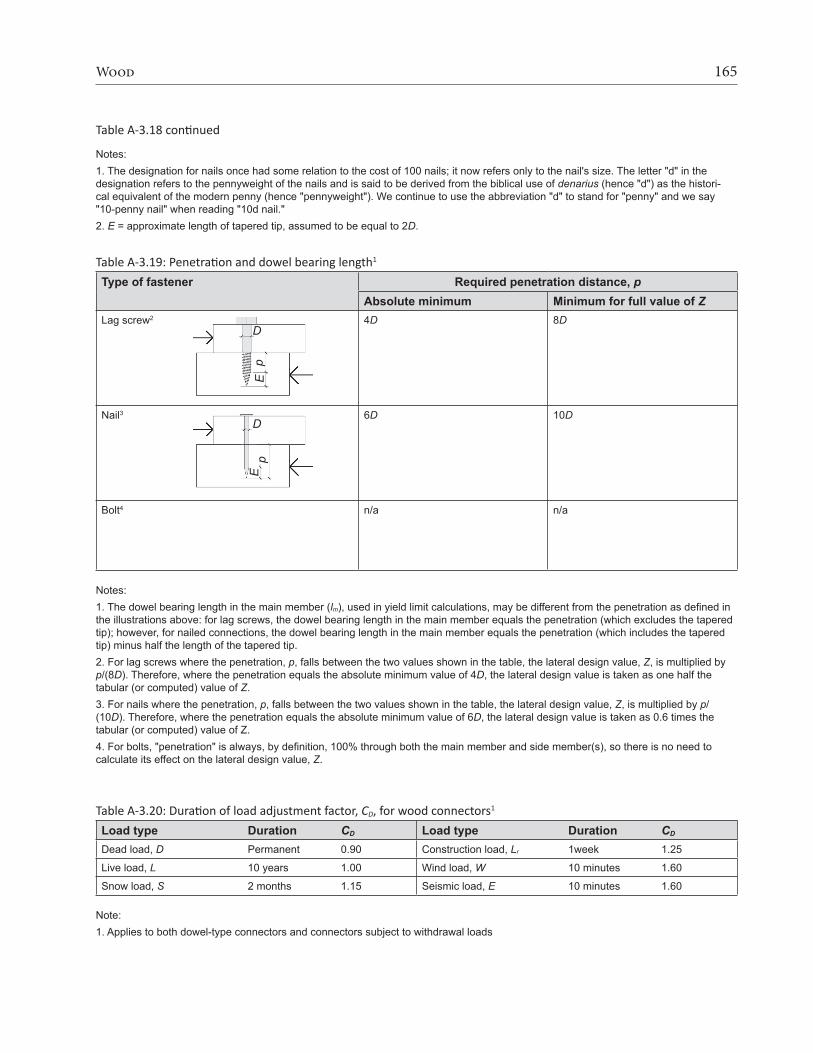
165Wood
Notes:1. The designation for nails once had some relation to the cost of 100 nails; it now refers only to the nail's size. The letter "d" in the designation refers to the pennyweight of the nails and is said to be derived from the biblical use of denarius (hence "d") as the histori-cal equivalent of the modern penny (hence "pennyweight"). We continue to use the abbreviation "d" to stand for "penny" and we say "10-penny nail" when reading "10d nail." 2. E = approximate length of tapered tip, assumed to be equal to 2D.
Table A-3.19: Penetration and dowel bearing length1
Type of fastener Required penetration distance, pAbsolute minimum Minimum for full value of Z
Lag screw2 4D 8D
Nail3 6D 10D
Bolt4 n/a n/a
Notes:1. The dowel bearing length in the main member (lm), used in yield limit calculations, may be different from the penetration as defined in the illustrations above: for lag screws, the dowel bearing length in the main member equals the penetration (which excludes the tapered tip); however, for nailed connections, the dowel bearing length in the main member equals the penetration (which includes the tapered tip) minus half the length of the tapered tip. 2. For lag screws where the penetration, p, falls between the two values shown in the table, the lateral design value, Z, is multiplied by p/(8D). Therefore, where the penetration equals the absolute minimum value of 4D, the lateral design value is taken as one half the tabular (or computed) value of Z.3. For nails where the penetration, p, falls between the two values shown in the table, the lateral design value, Z, is multiplied by p/(10D). Therefore, where the penetration equals the absolute minimum value of 6D, the lateral design value is taken as 0.6 times the tabular (or computed) value of Z.4. For bolts, "penetration" is always, by definition, 100% through both the main member and side member(s), so there is no need to calculate its effect on the lateral design value, Z.
Table A-3.20: Duration of load adjustment factor, CD, for wood connectors1
Load type Duration CD Load type Duration CD
Dead load, D Permanent 0.90 Construction load, Lr 1week 1.25
Live load, L 10 years 1.00 Wind load, W 10 minutes 1.60
Snow load, S 2 months 1.15 Seismic load, E 10 minutes 1.60
Note:1. Applies to both dowel-type connectors and connectors subject to withdrawal loads
D
pE
E
D
p
Table A-3.18 continued

166 Structural Elements for Architects and Builders
Table A-3.21: Wet service adjustment factor, CM, for wood connectors1,2
Fastener type with lateral load CM
"Dowel-type," wet when made, dry in-service:
• 1 fastener only
• 2 or more fasteners in single row parallel to grain
• Multiple rows of fasteners parallel to grain, separate splice plate each row
• Fastener with diameter < ¼ in.
• Multiple rows of fasteners with diameter ≥ ¼ in., without separate splice plates
"Dowel-type," wet when used (in-service)
varies as follows:
1.00
1.00
1.00
0.70
0.40
0.70
Fastener type with withdrawal load CM
Nails, wet when made, dry in-service
Nails, dry when made, wet in-service
Nails, wet when made, wet in-service
Lag screws and wood screws, wet in-service
0.25
0.25
1.00
0.70
Notes:1. Applies to both dowel-type connectors and connectors subject to withdrawal loads.2. CM = 1.0 for fasteners that are dry when fabricated and when used (in-service).
Table A-3.22: Group action adjustment factor, Cg, for wood connectors1,2,3,4
A. Cg, bolt (or lag screw) connections, wood members with same properties: E = 1,400,000 psi; bolt or lag screw diameter, D = 3/4 in.; spacing between fasteners in a row, s = 3 in.Am = Area of main member, in2
number fastenersin row
As = Area of side member(s), in2
5 8 11 14 17 30 40 56 64 5 2
3 4 5 6 7 8 9 10
1.0000.9840.9540.9140.8670.8170.7660.7160.669
0.9910.9620.9180.8660.8090.7520.6980.6470.601
0.9870.9520.9020.8440.7830.7230.6670.6160.570
0.9850.9470.8930.8310.7680.7070.6500.5980.552
0.9830.9430.8870.8230.7580.6960.6380.5870.540
0.9800.9360.8750.8070.7390.6750.6160.5630.517
0.9790.9330.8710.8020.7330.6880.6080.5560.510
0.9780.9310.8680.7980.7280.6620.6020.5490.503
0.9780.9310.8670.7960.7260.6600.6000.5470.501
8 2 3 4 5 6 7 8 9 10
0.9910.9620.9180.8660.8090.7520.6980.6470.601
1.0000.9900.9710.9430.9100.8730.8330.7920.751
0.9960.9790.9530.9180.8770.8340.7900.7460.704
0.9930.9730.9420.9030.8590.8120.7660.7200.677
0.9920.9700.9360.8940.8470.7980.7500.7030.659
0.9890.9620.9220.8750.8230.7700.7190.6700.624
0.9880.9590.9180.8690.8150.7610.7080.6590.613
0.9870.9570.9140.8630.8090.7530.7000.6500.603
0.9870.9560.9130.8620.8060.7510.6970.6470.600
11 2 3 4 5 6 7 8 9 10
0.9870.9520.9020.8440.7830.7230.6670.6160.570
0.9960.9790.9530.9180.8770.8340.7900.7460.704
1.0000.9930.9780.9580.9320.9030.8700.8360.801
0.9980.9860.9670.9420.9110.8770.8410.8040.766
0.9960.9830.9610.9320.8980.8610.8220.7830.744
0.9930.9750.9470.9110.8710.8280.7850.7410.700
0.9920.9720.9420.9050.8620.8180.7720.7280.685
0.9910.9700.9380.8990.8550.8090.7620.7170.673
0.9910.9690.9370.8970.8530.8060.7590.7130.669
(continued)

167Wood
A. Cg, bolt (or lag screw) connections, wood members with same properties: E = 1,400,000 psi; bolt or lag screw diameter, D = 3/4 in.; spacing between fasteners in a row, s = 3 in.Am = Area of main member, in2
number fastenersin row
As = Area of side member(s), in2
5 8 11 14 17 30 40 56 64 14 2
3 4 5 6 7 8 9 10
0.9850.9470.8930.8310.7680.7070.6500.5980.552
0.9930.9730.9420.9030.8590.8120.7660.7200.677
0.9980.9860.9670.9420.9110.8770.8410.8040.766
1.0000.9940.9830.9660.9450.9210.8940.8640.834
0.9980.9900.9760.9560.9310.9030.8730.8410.808
0.9950.9820.9610.9340.9020.8670.8310.7930.756
0.9940.9790.9560.9270.8930.8560.8170.7780.739
0.9930.9770.9520.9210.8850.8460.8050.7650.725
0.9930.9760.9510.9190.8830.8430.8020.7610.721
17 2 3 4 5 6 7 8 9 10
0.9830.9430.8870.8230.7580.6960.6380.5870.540
0.9920.9700.9360.8940.8470.7980.7500.7030.659
0.9960.9830.9610.9320.8980.8610.8220.7830.744
0.9980.9900.9760.9560.9310.9030.8730.8410.808
1.0000.9950.9860.9720.9540.9340.9100.8850.858
0.9970.9870.9710.9500.9240.8950.8640.8320.799
0.9960.9840.9660.9430.9140.8830.8500.8150.781
0.9950.9820.9620.9360.9060.8730.8370.8010.765
0.9950.9810.9610.9340.9040.8690.8330.7970.760
30 2 3 4 5 6 7 8 9 10
0.9800.9360.8750.8070.7390.6750.6160.5630.517
0.9890.9620.9220.8750.8230.7700.7190.6700.624
0.9930.9750.9470.9110.8710.8280.7850.7410.700
0.9950.9820.9610.9340.9020.8670.8310.7930.756
0.9970.9870.9710.9500.9240.8950.8640.8320.799
1.0000.9970.9920.9840.9730.9610.9460.9300.912
0.9990.9950.9870.9760.9630.9470.9290.9090.888
0.9980.9920.9830.9690.9530.9350.9140.8910.867
0.9980.9910.9810.9670.9500.9310.9090.8860.861
40 2 3 4 5 6 7 8 9 10
0.9790.9330.8710.8020.7330.6680.6080.5560.510
0.9880.9590.9180.8690.8150.7610.7080.6590.613
0.9920.9720.9420.9050.8620.8180.7720.7280.685
0.9940.9790.9560.9270.8930.8560.8170.7780.739
0.9960.9840.9660.9430.9140.8830.8500.8150.781
0.9990.9950.9870.9760.9630.9470.9290.9090.888
1.0000.9980.9940.9880.9800.9700.9590.9460.932
0.9990.9960.9890.9810.9700.9570.9430.9270.909
0.9990.9950.9880.9790.9670.9540.9380.9210.902
56 2 3 4 5 6 7 8 9 10
0.9780.9310.8680.7980.7280.6620.6020.5490.503
0.9870.9570.9140.8630.8090.7530.7000.6500.603
0.9910.9700.9380.8990.8550.8090.7620.7170.673
0.9930.9770.9520.9210.8850.8460.8050.7650.725
0.9950.9820.9620.9360.9060.8730.8370.8010.765
0.9980.9920.9830.9690.9530.9350.9140.8910.867
0.9990.9960.9890.9810.9700.9570.9430.9270.909
1.0000.9990.9960.9910.9850.9780.9700.9610.950
1.0000.9980.9940.9890.9820.9740.9650.9540.942
64 2 3 4 5 6 7 8 9 10
0.9780.9310.8670.7960.7260.6600.6000.5470.501
0.9870.9560.9130.8620.8060.7510.6970.6470.600
0.9910.9690.9370.8970.8530.8060.7590.7130.669
0.9930.9760.9510.9190.8830.8430.8020.7610.721
0.9950.9810.9610.9340.9040.8690.8330.7970.760
0.9980.9910.9810.9670.9500.9310.9090.8860.861
0.9990.9950.9880.9790.9670.9540.9380.9210.902
1.0000.9980.9940.9890.9820.9740.9650.9540.942
1.0000.9990.9960.9920.9870.9810.9740.9650.956
Table A-3.22 continued
(continued)

168 Structural Elements for Architects and Builders
B. Cg, bolt (or lag screw) connections, wood main member with E = 1,400,000 psi; steel side member(s) with E = 29,000,000 psi; bolt or lag screw diameter, D = 3/4 in.; spacing between fasteners in a row, s = 3 in.Am = Area of main member, in2
number fastenersin row
As = Area of steel side member(s), in2
1 2 3 4 5 7 10 12 15 5 2
3 4 5 6 7 8 9 10
0.9730.9150.8380.7580.6820.6130.5540.5020.458
0.9690.9050.8240.7390.6600.5910.5310.4800.436
0.9680.9020.8190.7330.6530.5830.5230.4720.429
0.9670.9000.8160.730.6500.5790.5190.4680.425
0.9670.8990.8150.7280.6480.5770.5170.4660.423
0.9660.8980.8130.7260.6450.5750.5140.4630.420
0.9660.8970.8120.7240.6430.5730.5120.4610.419
0.9660.8970.8110.7240.6430.5720.5120.4610.418
0.9660.8960.8110.7230.6420.5710.5110.4600.417
8 2 3 4 5 6 7 8 9 10
0.9860.9510.9010.8430.7820.7220.6660.6150.569
0.9820.9410.8840.8190.7540.6910.6330.5800.534
0.9800.9370.8780.8120.7440.6800.6210.5690.522
0.9800.9350.8750.8080.7400.6750.6160.5630.517
0.9790.9340.8740.8060.7370.6720.6120.5600.513
0.9790.9330.8720.8030.7340.6680.6090.5560.509
0.9780.9320.8700.8010.7310.6660.6060.5530.506
0.9780.9320.8700.8000.7300.6640.6050.5520.505
0.9780.9320.8690.7990.7290.6630.6040.5500.504
11 2 3 4 5 6 7 8 9 10
0.9920.9700.9350.8920.8440.7940.7450.6980.654
0.9880.9590.9160.8660.8110.7560.7030.6530.608
0.9860.9550.9100.8570.8000.7430.6890.6390.592
0.9860.9530.9070.8530.7950.7370.6820.6310.585
0.9850.9520.9050.8500.7920.7330.6780.6270.580
0.9850.9510.9030.8470.7880.7290.6730.6220.575
0.9840.9500.9020.8450.7850.7260.6700.6180.571
0.9840.9500.9010.8440.7840.7250.6680.6160.569
0.9840.9490.9000.8430.7830.7230.6670.6150.568
14 2 3 4 5 6 7 8 9 10
0.9960.9810.9560.9240.8860.8460.8040.7620.721
0.9910.9690.9360.8960.8500.8020.7550.7090.665
0.9900.9660.9300.8860.8380.7880.7390.6910.647
0.9890.9640.9270.8820.8320.7810.7310.6830.638
0.9890.9630.9250.8790.8290.7770.7260.6770.632
0.9880.9610.9230.8760.8250.7720.7210.6710.626
0.9880.9600.9210.8730.8220.7680.7160.6670.621
0.9880.9600.9200.8730.8200.7670.7150.6650.619
0.9880.9600.9200.8720.8190.7660.7130.6640.617
17 2 3 4 5 6 7 8 9 10
0.9980.9880.9700.9460.9170.8840.8490.8130.777
0.9940.9760.9500.9170.8780.8370.7950.7530.712
0.9920.9730.9430.9070.8650.8220.7770.7330.691
0.9910.9710.9400.9020.8590.8140.7680.7230.680
0.9910.9700.9380.8990.8550.8090.7630.7170.674
0.9900.9680.9360.8960.8510.8040.7570.7110.667
0.9900.9670.9340.8930.8480.8000.7520.7060.661
0.9900.9670.9340.8920.8470.7990.7500.7040.659
0.9900.9670.9330.8920.8450.7970.7490.7020.657
30 2 3 4 5 6 7 8 9 10
0.9970.9870.9700.9470.9190.8880.8550.8210.786
0.9980.9910.9800.9649.9440.9210.8960.8690.841
0.9970.9880.9730.9530.9290.9020.8730.8430.812
0.9960.9860.9690.9480.9220.8930.8620.8300.797
0.9960.9840.9670.9450.9180.8880.8560.8220.788
0.9950.9830.9650.9410.9130.8810.8480.8130.779
0.9950.9820.9630.9380.9090.8770.8420.8070.771
0.9950.9820.9620.9370.9080.8750.8400.8040.768
0.9940.9810.9620.9360.9060.8730.8380.8020.765
(continued)
Table A-3.22 continued

169Wood
B. Cg, bolt (or lag screw) connections, wood main member with E = 1,400,000 psi; steel side member(s) with E = 29,000,000 psi; bolt or lag screw diameter, D = 3/4 in.; spacing between fasteners in a row, s = 3 in.Am = Area of main member, in2
number fastenersin row
As = Area of steel side member(s), in2
1 2 3 4 5 7 10 12 15 40 2
3 4 5 6 7 8 9 10
0.9960.9830.9630.9360.9050.8710.8350.7980.761
1.0000.9960.9900.9810.9680.9540.9370.9190.899
0.9980.9930.9830.9700.9530.9340.9130.8900.865
0.9980.9910.9790.9640.9450.9240.9000.8750.849
0.9970.9890.9770.9610.9410.9180.8930.8670.839
0.9970.9880.9750.9570.9360.9110.8850.8570.828
0.9960.9870.9730.9540.9320.9060.8790.8490.819
0.9960.9870.9720.9530.9300.9040.8760.8470.816
0.9960.9860.9710.9520.9290.9020.8740.8440.813
56 2 3 4 5 6 7 8 9 10
0.9940.9800.9570.9270.8930.8560.8170.7780.740
0.9990.9940.9850.9740.9590.9420.9220.9010.879
1.0000.9970.9920.9840.9750.9630.9500.9350.919
0.9990.9950.9880.9790.9670.9530.9370.9190.901
0.9980.9940.9860.9750.9620.9470.9290.9100.890
0.9980.9920.9830.9710.9570.9390.9200.8990.877
0.9980.9910.9820.9690.9530.9340.9140.8910.868
0.9970.9910.9810.9670.9510.9320.9110.8880.864
0.9970.9910.9800.9660.9490.9300.9080.8850.860
64 2 3 4 5 6 7 8 9 10
0.9940.9790.9550.9250.8900.8520.8120.7720.733
0.9980.9930.9830.9710.9550.9360.9160.8930.869
1.0000.9980.9940.9870.9800.9700.9590.9460.932
0.9990.9960.9910.9830.9740.9620.9490.9350.919
0.9990.9950.9890.9800.9690.9560.9410.9250.907
0.9980.9940.9860.9760.9630.9490.9320.9140.894
0.9980.9930.9840.9730.9590.9430.9250.9050.884
0.9980.9920.9840.9720.9580.9410.9220.9020.881
0.9980.9920.9830.9710.9560.9390.9200.8990.877
Notes:1. Values are conservative when using smaller fastener diameter, smaller fastener spacing, and greater modulus of elasticity.2. For both the table and the exact method shown below, cross-sectional areas are used for Am and As when the member is loaded parallel to grain; when loaded perpendicular to grain, an equivalent area is used for Am or As, based on the member thickness (measured in a direction parallel to the fastener) multiplied by an equivalent member width. This equivalent width is taken as the distance between the outer rows of fasteners or, where there is only one row of fasteners, as the minimum spacing between rows that would be computed if there were multiple rows of fasteners.3. Cg = 1.0 for dowel-type fasteners with diameter, D < 0.25 in. Other values for Cg can be determined exactly (for fastener diameters greater than 0.25 in. and less than or equal to 1.0 in.) based on the following method:
a. Find the bolt or lag screw diameter, D; then find the so-called load/slip modulus, γ, as follows:
γ = 180,000(D1.5) for dowel-type fasteners in wood-wood connection; γ = 270,000(D1.5) for dowel-type fasteners in wood-metal connection b. Find s, the spacing (center-to-center) between fasteners in a row; c. Find Em and Es, the moduli of elasticity (psi) for the main and secondary members, respectively; d. Find Am and As, the cross-sectional areas (in2) for the main member and for the side member (or the sum of the areas of the side members, if there are more than one), respectively;
g. Find n = the number of fasteners in a row.
4. Applies to dowel-type connectors only.
f. Find REA =EsAs
EmAmor
EmAm
EsAs, whichever is smaller.
e. Find u = 1 + γ s2
and m = u – √u2 – 11 1EmAm EsAs
+
h. Find Cg =m (1 – m2n)
n [ (1 + REAmn)(1 + m) – 1 + m2n]1 + REA
1 – m×
Table A-3.22 continued

170 Structural Elements for Architects and Builders
Table A-3.23: Geometry adjustment factor, CΔ, for wood connectors (bolts and lag screws)A. Spacing (in.) between fasteners in a rowa,b,d
Loading direction Absolute minimum Minimum for full valueParallel to grain 3D 4D
Perpendicular to grain 3D Whatever is required for attached membersc
Notes for Part A:a. Required spacing (in.) is a multiple of the fastener diameter, D (in.).b. A distance below the absolute minimum is, of course, not permitted — in that case, the geometry factor, CΔ = 0. For any distance equal to or greater than the "minimum for full value," the geometry factor, CΔ = 1.0. For spacing between the two values shown in the table, the geometry factor, CΔ, is taken as the actual spacing divided by the minimum spacing for full value. For example, if the actual spacing between fasteners in a row, where the load was parallel to grain, is 3.5D, the geometry factor, CΔ = 3.5D/(4D) = 0.875. If the spacing in this case equaled the absolute minimum of 3D, the geometry factor, CΔ = 3D/(4D) = 0.75.c. For fasteners in a row, where the loading is perpendicular to grain, the minimum spacing necessary to obtain the full value of the geometry factor, i.e., CΔ = 1.0, is based on meeting the requirements for the member to which it is attached — i.e., the member whose load is parallel to grain — as long as this distance is no less than the absolute minimum value of 3D (assuming that both members in the connection are not oriented so that the load is perpendicular to grain).d. See general notes below.
B. Spacing (in.) between rows of fastenersa,b,d
Loading direction Condition Minimum spacingParallel to grain All conditions 1.5D
Perpendicular to grainc l /D ≤ 22 < l /D < 6l /D ≥ 6
2.5D(5l + 10D) / 85D
Notes for Part B:a. Required spacing (in.) is a multiple of the fastener diameter, D (in.).b. Where the minimum spacing between rows of fasteners is met, the geometry factor, CΔ = 1.0. Otherwise, where the spacing is below the minimum allowed, the connection is not permitted — i.e., CΔ = 0. Interestingly, the maximum spacing between rows of fasteners is also limited in the following way: a 5 in. maximum limit is placed on the spacing between the outer rows of fasteners, in cases where the rows are parallel to the grain of the wood. This reduces the possibility of splitting as the wood member shrinks or expands (due to changes in its moisture content) perpendicular to the grain, while the bolts are fixed in place by a connecting member.c. The fastener length, l (in.), is defined as the length of the fastener that is actually embedded within either the main member (the dowel bearing length — see Appendix Table A-3.27), or the total length within one or more secondary members, whichever is smaller. D is the fastener diameter (in.).d. See general notes below.
C. End distance (in.)a,b,c
Loading direction Absolute minimum Minimum for full valueParallel to grain: Compression Tension – softwood Tension – hardwood
2D 3.5D 2.5D
4D 7D 5D
Perpendicular to grain 2D 4D Notes for Part C:a. Required end distance (in.) is a multiple of the fastener diameter, D (in.).b. A distance below the absolute minimum is, of course, not permitted — in that case, the geometry factor, CΔ = 0; for any distance equal to or greater than the "minimum for full value," the geometry factor, CΔ = 1.0. For end distances between the two values shown in the table, the geometry factor, CΔ, is taken as the actual end distance divided by the minimum distance for full value. For example, if the end distance of a fastener loaded parallel to grain in compression is 3D, the geometry factor, CΔ = 3D/(4D) = 0.75. If the end distance in this case equaled the absolute minimum of 2D, the geometry factor, CΔ = 2D/(4D) = 0.50.c. See general notes below.
(continued)
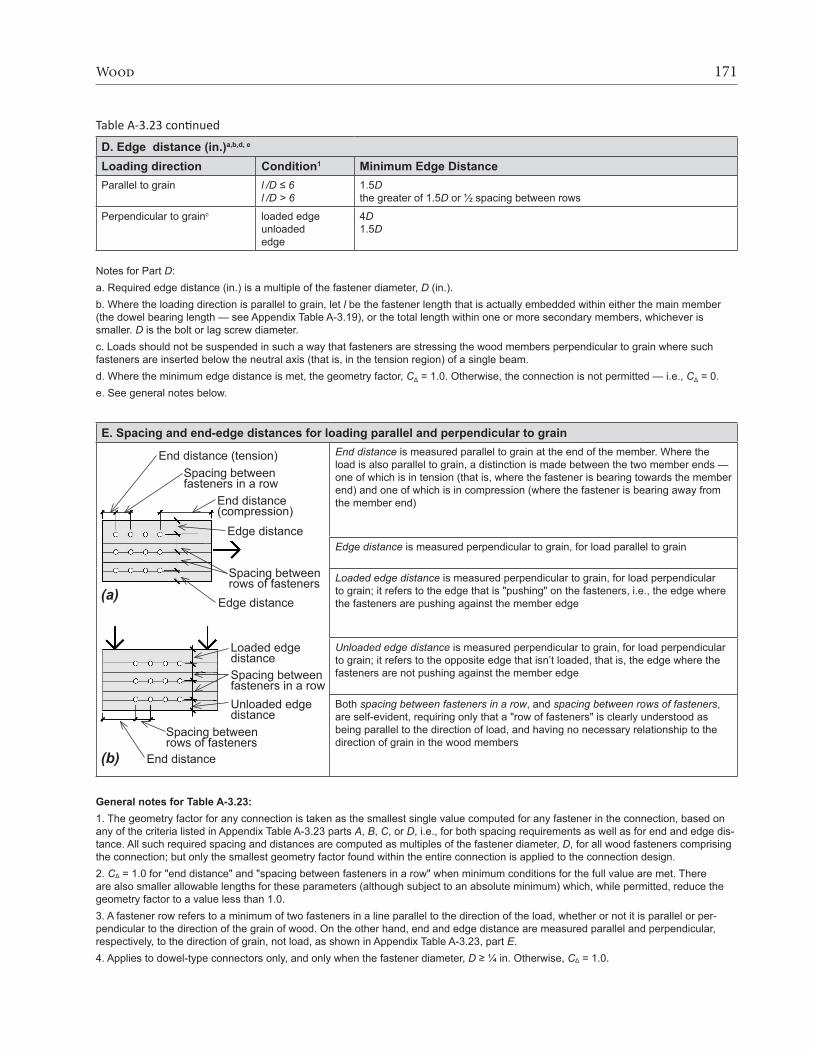
171Wood
D. Edge distance (in.)a,b,d, e
Loading direction Condition1 Minimum Edge DistanceParallel to grain l /D ≤ 6
l /D > 61.5Dthe greater of 1.5D or ½ spacing between rows
Perpendicular to grainc loaded edgeunloaded edge
4D1.5D
Notes for Part D:a. Required edge distance (in.) is a multiple of the fastener diameter, D (in.).b. Where the loading direction is parallel to grain, let l be the fastener length that is actually embedded within either the main member (the dowel bearing length — see Appendix Table A-3.19), or the total length within one or more secondary members, whichever is smaller. D is the bolt or lag screw diameter.c. Loads should not be suspended in such a way that fasteners are stressing the wood members perpendicular to grain where such fasteners are inserted below the neutral axis (that is, in the tension region) of a single beam.d. Where the minimum edge distance is met, the geometry factor, CΔ = 1.0. Otherwise, the connection is not permitted — i.e., CΔ = 0.e. See general notes below.
E. Spacing and end-edge distances for loading parallel and perpendicular to grainEnd distance is measured parallel to grain at the end of the member. Where the load is also parallel to grain, a distinction is made between the two member ends — one of which is in tension (that is, where the fastener is bearing towards the member end) and one of which is in compression (where the fastener is bearing away from the member end)
Edge distance is measured perpendicular to grain, for load parallel to grain
Loaded edge distance is measured perpendicular to grain, for load perpendicular to grain; it refers to the edge that is "pushing" on the fasteners, i.e., the edge where the fasteners are pushing against the member edge
Unloaded edge distance is measured perpendicular to grain, for load perpendicular to grain; it refers to the opposite edge that isn’t loaded, that is, the edge where the fasteners are not pushing against the member edge
Both spacing between fasteners in a row, and spacing between rows of fasteners, are self-evident, requiring only that a "row of fasteners" is clearly understood as being parallel to the direction of load, and having no necessary relationship to the direction of grain in the wood members
General notes for Table A-3.23:1. The geometry factor for any connection is taken as the smallest single value computed for any fastener in the connection, based on any of the criteria listed in Appendix Table A-3.23 parts A, B, C, or D, i.e., for both spacing requirements as well as for end and edge dis-tance. All such required spacing and distances are computed as multiples of the fastener diameter, D, for all wood fasteners comprising the connection; but only the smallest geometry factor found within the entire connection is applied to the connection design.2. CΔ = 1.0 for "end distance" and "spacing between fasteners in a row" when minimum conditions for the full value are met. There are also smaller allowable lengths for these parameters (although subject to an absolute minimum) which, while permitted, reduce the geometry factor to a value less than 1.0.3. A fastener row refers to a minimum of two fasteners in a line parallel to the direction of the load, whether or not it is parallel or per-pendicular to the direction of the grain of wood. On the other hand, end and edge distance are measured parallel and perpendicular, respectively, to the direction of grain, not load, as shown in Appendix Table A-3.23, part E.4. Applies to dowel-type connectors only, and only when the fastener diameter, D ≥ ¼ in. Otherwise, CΔ = 1.0.
Spacing between fasteners in a row
Loaded edge distance
Unloaded edge distance
Spacing between rows of fasteners
End distance(b)
End distance (tension)Spacing between fasteners in a row
End distance (compression)
Edge distance
Spacing between rows of fasteners
Edge distance(a)
Table A-3.23 continued

172 Structural Elements for Architects and Builders
Table A-3.24: Toe-nail adjustment factor, Ctn, for nails1
Diagram Direction of Applied Force Ctn
For lateral design values, Z, bearing lengths are as follows: • ln main member: lm = ln cos 30° – ln /3 • In side member: ls = ln /3where ln = length of nail
0.83
For withdrawal design values, W, depth of penetration, pw is actual length of nail in main member.
0.67
Note:1. Toe-nailing values are based on two assumptions: a. That the nail is driven at an angle of approximately 30° to the face of the side member. b. That the nail insertion point is ⅓ of the nail length (ln /3) above the end of the side member
Table A-3.25: Temperature factor, Ct, for wood fastenersTemperature, T (° F) Ct (used dry) Ct (used wet)T ≤ 100° F 1.0 1.0
100° F < T ≤ 125° F 0.8 0.7
125° F < T ≤ 150° F 0.7 0.5
Table A-3.26: Lateral design value, Z (lb) for bolts: single-shear connections, with 1½ in. side member thickness, both members same species (or same specific gravity)1
A. Designation for single-shear lateral design values according to direction of grain2
B. 1½ in. main member thicknessSpecies or Species Combination
½ in. diameter Bolts ¾ in. diameter Bolts 1 in. diameter BoltsZpar Zs-per Zm-per Zpar Zs-per Zm-per Zpar Zs-per Zm-per
Douglas Fir-Larch 480 300 300 720 420 420 970 530 530
Douglas Fir-Larch (North) 470 290 290 710 400 400 950 510 510
Douglas Fir-South 440 270 270 670 380 380 890 480 480
Hem-Fir 410 250 250 620 350 350 830 440 440
Hem-Fir (North) 440 270 270 670 380 380 890 480 480
Spruce-Pine-Fir 410 240 240 610 340 340 810 430 430
Spruce-Pine-Fir (South) 350 200 200 520 280 280 700 360 360
Southern Pine 530 330 330 800 460 460 1060 580 580
(continued)

173Wood
C. 3½ in. main member thicknessSpecies or Species Combination
½ in. diameter Bolts ¾ in. diameter Bolts 1 in. diameter BoltsZpar Zs-per Zm-per Zpar Zs-per Zm-per Zpar Zs-per Zm-per
Douglas Fir-Larch 610 370 430 1200 590 610 1830 680 740
Douglas Fir-Larch (North) 610 360 420 1190 560 490 1790 650 710
Douglas Fir-South 580 340 400 1140 520 550 1680 600 660
Hem-Fir 550 320 380 1100 460 500 1570 540 600
Hem-Fir (North) 580 340 400 1140 520 550 1680 600 660
Spruce-Pine-Fir 540 320 370 1080 450 480 1530 530 590
Spruce-Pine-Fir (South) 490 280 300 990 360 400 1320 420 480
Southern Pine 660 400 470 1270 660 690 2010 770 830
D. 5½ in. main member thicknessSpecies or Species Combination
⅝ in. diameter Bolts ¾ in. diameter Bolts 1 in. diameter BoltsZpar Zs-per Zm-per Zpar Zs-per Zm-per Zpar Zs-per Zm-per
Douglas Fir-Larch 610 370 430 1200 590 790 2050 680 1060
Douglas Fir-Larch (North) 610 360 420 1190 560 780 2030 650 1010
Douglas Fir-South 580 340 400 1140 520 740 1930 600 940
Hem-Fir 550 320 380 1100 460 700 1800 540 860
Hem-Fir (North) 580 340 400 1140 520 740 1930 600 940
Spruce-Pine-Fir 540 320 370 1080 450 690 1760 530 830
Spruce-Pine-Fir (South) 490 280 330 990 360 570 1520 420 680
Southern Pine 660 400 470 1270 660 850 2150 770 1190
Notes:1. Member thickness is measured parallel to the axis of the fastener.2. Designations for lateral design values are as illustrated: (a) Zpar for both members with direction of grain parallel to load; (b) Zs-per for side member with grain perpendicular to load and main member with grain parallel to load; and (c) Zm-per for main member with grain perpendicular to load and side member with grain parallel to load. A fourth possibility, with both members having grain perpendicular to the direction of load, is rarely encountered and not included here. The official designations also shown below the illustrations contain "parallel" and "perpendicular" symbols instead of the abbreviations, "par" and "per" used in these tables and text.
Table A-3.26 continued

174 Structural Elements for Architects and Builders
Table A-3.27: Lateral design value, Z (lb) for bolts: double-shear connections, with 1½ in. side member thickness, both members same species (or same specific gravity)1
A. Designation for double-shear lateral design values according to direction of grain2
B. 1½ in. main member thicknessSpecies or Species Combination
½ in. diameter Bolts ¾ in. diameter Bolts 1 in. diameter BoltsZpar Zs-per Zm-per Zpar Zs-per Zm-per Zpar Zs-per Zm-per
Douglas Fir-Larch 1050 730 470 1580 1170 590 2100 1350 680
Douglas Fir-Larch (North) 1030 720 460 1550 1130 560 2060 1290 650
Douglas Fir-South 970 680 420 1450 1040 520 1930 1200 600
Hem-Fir 900 650 380 1350 920 460 1800 1080 540
Hem-Fir (North) 970 680 420 1450 1040 520 1930 1200 600
Spruce-Pine-Fir 880 640 370 1320 900 450 1760 1050 530
Spruce-Pine-Fir (South) 760 560 290 1140 720 360 1520 840 420
Southern Pine 1150 800 550 1730 1330 660 2310 1530 770
C. 3½ in. main member thicknessSpecies or Species Combination
½ in. diameter Bolts ¾ in. diameter Bolts 1 in. diameter BoltsZpar Zs-per Zm-per Zpar Zs-per Zm-per Zpar Zs-per Zm-per
Douglas Fir-Larch 1230 730 860 2400 1170 1370 4090 1350 1580
Douglas Fir-Larch (North) 1210 720 850 2380 1130 1310 4050 1290 1510
Douglas Fir-South 1160 680 810 2280 1040 1210 3860 1200 1400
Hem-Fir 1100 650 760 2190 920 1080 3600 1080 1260
Hem-Fir (North) 1160 680 810 2280 1040 1210 3860 1200 1400
Spruce-Pine-Fir 1080 640 740 2160 900 1050 3530 1050 1230
Spruce-Pine-Fir (South) 980 560 660 1990 720 840 3040 840 980
Southern Pine 1320 800 940 2550 1330 1550 4310 1530 1790
(continued)

175Wood
D. 5½ in. main member thicknessSpecies or Species Combination
⅝ in. diameter Bolts ¾ in. diameter Bolts 1 in. diameter BoltsZpar Zs-per Zm-per Zpar Zs-per Zm-per Zpar Zs-per Zm-per
Douglas Fir-Larch 1760 1040 1190 2400 1170 1580 4090 1350 2480
Douglas Fir-Larch (North) 1740 1030 1170 2380 1130 1550 4050 1290 2370
Douglas Fir-South 1660 940 1110 2280 1040 1480 3860 1200 2200
Hem-Fir 1590 840 1050 2190 920 1400 3600 1080 1980
Hem-Fir (North) 1660 940 1110 2280 1040 1480 3860 1200 2200
Spruce-Pine-Fir 1570 830 1040 2160 900 1380 3530 1050 1930
Spruce-Pine-Fir (South) 1430 660 920 1990 720 1230 3040 840 1540
Southern Pine 1870 1130 1290 2550 1330 1690 4310 1530 2700
Notes:1. Member thickness is measured parallel to the axis of the fastener.2. Designations for lateral design values are as illustrated: (a) Zpar for both members with direction of grain parallel to load; (b) Zs-per for side member with grain perpendicular to load and main member with grain parallel to load; and (c) Zm-per for main member with grain perpendicular to load and side member with grain parallel to load. A fourth possibility, with both members having grain perpendicular to the direction of load, is rarely encountered and not included here. The official designations also shown below the illustrations contain "parallel" and "perpendicular" symbols instead of the abbreviations, "par" and "per" used in these tables and text.
Table A-3.28: Lateral design value, Z (lb) for bolts: double-shear connections, with two ¼ in. A36 steel side plates1
A. Designation for double-shear lateral design values according to direction of grain2
B. 1½ in. main member thicknessSpecies or Species Combination
½ in. diameter Bolts ¾ in. diameter Bolts 1 in. diameter BoltsZpar Zper Zpar Zper Zpar Zper
Douglas Fir-Larch 1050 470 1580 590 2100 680
Douglas Fir-Larch (North) 1030 460 1550 560 2060 650
Douglas Fir-South 970 420 1450 520 1930 600
Hem-Fir 900 380 1350 460 1800 540
Hem-Fir (North) 970 420 1450 520 1930 600
Spruce-Pine-Fir 880 370 1320 450 1760 530
Spruce-Pine-Fir (South) 760 290 1140 360 1520 420
Southern Pine 1150 550 1730 660 2310 770
Table A-3.27 continued
(continued)

176 Structural Elements for Architects and Builders
C. 3½ in. main member thicknessSpecies or Species Combination
½ in. diameter Bolts ¾ in. diameter Bolts 1 in. diameter BoltsZpar Zper Zpar Zper Zpar Zper
Douglas Fir-Larch 1650 1030 3340 1370 4090 1580
Douglas Fir-Larch (North) 1640 1010 3320 1310 4810 1510
Douglas Fir-South 1590 970 3220 1210 4510 1400
Hem-Fir 1540 890 3120 1080 4200 1260
Hem-Fir (North) 1590 970 3220 1210 4510 1400
Spruce-Pine-Fir 1530 860 3080 1050 4110 1230
Spruce-Pine-Fir (South) 1430 680 2660 840 3540 980
Southern Pine 1720 1100 3480 1550 5380 1790
D. 5½ in. main member thicknessSpecies or Species Combination
⅝ in. diameter Bolts ¾ in. diameter Bolts 1 in. diameter BoltsZpar Zper Zpar Zper Zpar Zper
Douglas Fir-Larch 2410 1420 3340 1890 5720 2480
Douglas Fir-Larch (North) 2390 1400 3320 1850 5670 2370
Douglas Fir-South 2330 1340 3220 1780 5510 2200
Hem-Fir 2260 1280 3120 1690 5330 1980
Hem-Fir (North) 2330 1340 3220 1780 5510 2200
Spruce-Pine-Fir 2230 1270 3090 1650 5280 1930
Spruce-Pine-Fir (South) 2090 1140 2890 1320 4930 1540
Southern Pine 2510 1510 3480 2000 5960 2810
Notes:1. Member thickness is measured parallel to the axis of the fastener.2. Designations for lateral design values are as illustrated: (a) Zpar for main member with direction of grain parallel to load; and (b) Zper for main member with grain perpendicular to load. The official designations also shown below the illustrations contain "parallel" and "perpendicular" symbols instead of the abbreviations, "par" and "per" used in these tables and text.
Table A-3.28 continued

177Wood
Table A-3.29: Lateral design value, Z (lb) for lag screws: single-shear connections, both members same species (or same specific gravity)1,2,3,4
A. Designation for single-shear lateral design values according to direction of grain2
B. 1½ in. side member thicknessSpecies or Species Combination
½ in. diameter Lag Screws ¾ in. diameter Lag Screws 1 in. diameter Lag ScrewsZpar Zs-per Zm-per Zpar Zs-per Zm-per Zpar Zs-per Zm-per
Douglas Fir-Larch 390 220 270 770 440 510 1290 530 810
Douglas Fir-Larch (North) 390 220 260 760 430 510 1280 500 790
Douglas Fir-South 370 210 250 730 400 480 1230 470 760
Hem-Fir 350 190 240 700 360 450 1180 420 720
Hem-Fir (North) 370 210 250 730 400 480 1230 470 760
Spruce-Pine-Fir 350 190 240 690 350 440 1160 410 710
Spruce-Pine-Fir (South) 310 160 210 620 280 390 1070 330 630
Southern Pine 410 250 290 830 470 560 1360 600 870
C. 3½ in. side member thicknessSpecies or Species Combination
½ in. diameter Lag Screws ¾ in. diameter Lag Screws 1 in. diameter Lag ScrewsZpar Zs-per Zm-per Zpar Zs-per Zm-per Zpar Zs-per Zm-per
Douglas Fir-Larch 390 270 270 960 600 610 1740 850 1060
Douglas Fir-Larch (North) 390 260 260 950 580 600 1730 830 1040
Douglas Fir-South 380 250 250 920 550 580 1670 790 1000
Hem-Fir 360 240 240 890 500 550 1610 740 950
Hem-Fir (North) 380 250 250 920 550 580 1670 790 1000
Spruce-Pine-Fir 360 240 240 880 490 540 1600 720 940
Spruce-Pine-Fir (South) 340 220 220 820 420 490 1450 630 850
Southern Pine 410 290 290 1010 650 650 1830 930 1120
Notes:1. Member thickness is measured parallel to the axis of the fastener.2. Designations for lateral design values are as illustrated: (a) Zpar for both members with direction of grain parallel to load; (b) Zs-per for side member with grain perpendicular to load and main member with grain parallel to load; and (c) Zm-per for main member with grain perpendicular to load and side member with grain parallel to load. A fourth possibility, with both members having grain perpendicular to the direction of load, is rarely encountered and not included here. The official designations also shown below the illustrations contain "parallel" and "perpendicular" symbols instead of the abbreviations, "par" and "per" used in these tables and text.3. Tabular values are based on full value minimum penetration, p, into main member. For penetration into main member between 4D and 8D, multiply tabular values by p /(8D).4. The reduced body diameter, Dr, is used in yield limit calculations for these lag screw lateral design values, except in the calculation of the dowel bearing strength for loading perpendicular to grain, Fe-perp, in which case the nominal diameter, D, is used.

178 Structural Elements for Architects and Builders
Table A-3.30: Lateral design value, Z (lb) for common nails: single-shear connections, both members same species (or same specific gravity)1,2,4
A. ¾ in. side member thicknessSpecies or Species Combination
Nail Size (pennyweight)6d 8d 10d 12d 16d 20d 30d 40d 50d
Douglas Fir-Larch 72 90 105 105 121 138 147 158 162
Douglas Fir-Larch (North) 71 87 102 102 117 134 143 154 158
Douglas Fir-South 65 80 94 94 108 125 133 144 147
Hem-Fir 58 73 85 85 99 114 122 132 136
Hem-Fir (North) 65 80 94 94 108 125 133 144 147
Spruce-Pine-Fir 57 70 83 83 96 111 119 129 132
Spruce-Pine-Fir (South) 46 58 69 69 80 93 101 110 113
Southern Pine 79 104 121 121 138 157 166 178 182
B. 1½ in. side member thicknessSpecies or Species Combination
Nail Size (pennyweight)6d 8d 10d 12d 16d 20d 30d 40d 50d
Douglas Fir-Larch — 397 118 118 141 170 186 205 211
Douglas Fir-Larch (North) — 395 115 115 138 166 182 201 206
Douglas Fir-South — 390 109 109 131 157 172 190 196
Hem-Fir — 384 102 102 122 147 161 178 181
Hem-Fir (North) — 390 109 109 131 157 172 190 196
Spruce-Pine-Fir — 382 100 100 120 144 158 172 175
Spruce-Pine-Fir (South) — 372 87 87 104 126 131 138 141
Southern Pine — 3106 128 128 154 185 203 224 230
Notes:1. Member thickness is measured parallel to the axis of the fastener.2. Where values are not indicated, nail penetration into main member does not satisfy minimum requirements. Otherwise, except as indi-cated in Note 3, it is assumed that the minimum penetration of the nail into the main member is equal to 10D (see Appendix Table A-3.19 for notes on penetration).3. These values must be reduced according to Note 3 in Appendix Table A-3.19, since the penetration falls below the minimum for full value. Nail dimensions can be found in Appendix Table A-3.18.4. In all cases where yield limit equations are used to compute lateral design values for nails, the dowel bearing length in the main mem-ber, lm, is taken as the penetration minus half the length of the tapered tip. Because these tabular lateral design values do not consider this reduced dowel bearing length, they may be slightly non-conservative in some cases (specifically, they may differ in cases where the governing yield limit equation includes the dowel bearing length parameter).

179Wood
Table A-3.31: Method for determining lateral design value, Z, based on yield limit equationsFor wood-wood or wood-metal connections that do not correspond to the parameters listed in the various Appendix tables, lateral design values may be determined using yield limit equations.
1. Using Appendix Table A-3.11 (specific gravity for wood members), find the specific gravity (G) for wood main and side member(s).
2. Find fastener diameter: use diameter, D, for bolts and nails (unthreaded shanks in contact with members) and reduced body diam-eter, Dr, for lag screws (in either case, designated as “D” in what follows);
3. Find dowel bearing strength, Fe, for main (Fem) and side (Fes) member(s), in psi units, using the appropriate specific gravity value for each wood member:a. For D > 0.25 in. and wood members loaded parallel to grain, Fe = 11,200G.
b. For D > 0.25 in. and wood members loaded perpendicular to grain, .
c. For D ≤ 0.25 in. and wood members, Fe = 16,600G1.84.d. For A36 steel, Fe = 87,000.e. For A653 GR33 steel (used in certain die-formed galvanized connector plates), Fe = 61,850.
4. Find the dowel bending yield strength, Fyb, in psi units:a. For bolts, use Fyb = 45,000.b. For lag screws with D = ¼ in., use Fyb = 70,000; with D = 5/16 in., use Fyb = 60,000; for D ≥ ⅜ in., use Fyb = 45,000.c. For nails with 0.099 in. ≤ D ≤ 0.142 in., use Fyb = 100,000; with 0.142 in. < D ≤ 0.177 in., use Fyb = 90,000; with 0.177 in. < D ≤
0.236 in., use Fyb = 80,000; with 0.236 in. < D ≤ 0.273 in., use Fyb = 70,000;
5. Find the main member and side member dowel bearing lengths, lm and ls, in inches (see Appendix Table A-3.19 for guidance). Even where there are two side members, the side member bearing length only includes the bearing length in a single side member.
6. Compute the terms Re = ; and Rt = .
7. Compute the “reduction term,” Rd, which varies according to yield mode and fastener diameter, as follows:a. For D ≤ 0.17 in. (i.e., for nails 16d or smaller), Rd = 2.2.b. For 0.17 in. < D < 0.25 in. (i.e., for most nails larger than 16d), Rd = 10D + 0.5.c. For 0.25 in. ≤ D ≤ 1 in. (i.e., for most bolts and lag screws), Rd = 4Kθ (for yield modes Im and Is); Rd = 3.6Kθ (for yield mode II); and
Rd = 3.2Kθ (for yield modes IIIm, IIIs, and IV). In these equations, Kθ = 1 + 0.25(θ/90), where θ = the maximum angle (degrees) between the load and the direction of grain for either member: for example, where the load is parallel to the direction of grain in all members, θ = 0 degrees, and Kθ = 1.0; where one or more member’s grain is perpendicular to the load, θ = 90°, and Kθ = 1.25. For angles other than 0 or 90°, θ is always measured in such a way that it falls between 0 and 90 (i.e., instead of using θ = 120°, or θ = –45°, use θ = 60° or θ = 45°, respectively).
8. Compute the coefficients k1, k2, and k3, as follows:
9. Compute the lateral design value, Z, for all applicable yield modes (i.e., for all six modes in single shear, and for all modes except II and IIIm in double shear), and select the smallest value:
Fe =6100G1.45
√D
Fem
Fes
lmls
a. k1 =√Re + 2Re
2(1 + Rt +Rt2) + Rt
2Re3 – Re(1 + Rt)
1 + Re
b. k2 = –1 +√
2(1 + Re) +2Fyb(1 + 2Re)D2
3Fem lm2
c. k3 = –1 +√
2(1 + Re) 2Fyb(2 + Re)D2
3Fem ls2+
Re
e. For Yield Mode IIIs, Z =k3DlsFem
(2 + Re)Rd
for single shear and Z =2k3DlsFem
(2 + Re)Rd
for double shear.
d. For Yield Mode IIIm (single shear only), Z =k2DlmFem
(1 + 2Re)Rd
b. For Yield Mode Is, Z =DlsFes
Rdfor single shear and Z =
2DlsFes
Rd
for double shear.
a. For Yield Mode Im, Z =DlmFem
Rd
c. For Yield Mode II (single shear only), Z =k1DlsFes
Rd
f. For Yield Mode IV, Z =D2
Rd√2FemFyb
3(1 + Re)for single shear and Z =
2D2
Rd √2FemFyb
3(1 + Re)for double shear.

180 Structural Elements for Architects and Builders
Table A-3.32: Withdrawal design value, W, per inch of penetration (lb) for lag screws1,2
Species or Species Combination
Unthreaded shank diameter, D (in.)1/4 5/16 3/8 7/16 1/2 5/8 3/4 7/8 1
Douglas Fir-Larch 225 266 305 342 378 447 513 576 636
Douglas Fir-Larch (North) 218 258 296 332 367 434 498 559 617
Douglas Fir-South 199 235 269 302 334 395 453 508 562
Hem-Fir 179 212 243 273 302 357 409 459 508
Hem-Fir (North) 199 235 269 302 334 395 453 508 562
Spruce-Pine-Fir 173 205 235 264 291 344 395 443 490
Spruce-Pine-Fir (South) 137 163 186 209 231 273 313 352 389
Southern Pine 260 307 352 395 437 516 592 664 734
Notes:1. Penetration length for lag screws excludes tapered tip; see Appendix Table A-3.17 for dimensions, and Appendix Table A-3.19 for notes on penetration.2. Withdrawal design values assume penetration into side grain of wood member, and must be reduced by 75% when inserted into end grain.
Table A-3.33: Withdrawal design value, W, per inch of penetration (lb) for nails1,2
Species or Species Combination
Nail size (pennyweight)6d 8d 10d 12d 16d 20d 30d 40d 50d
Douglas Fir-Larch 28 32 36 36 40 47 50 55 60
Douglas Fir-Larch (North) 26 30 34 34 38 45 48 52 57
Douglas Fir-South 22 26 29 29 32 38 41 45 48
Hem-Fir 19 22 25 25 27 32 35 38 41
Hem-Fir (North) 22 26 29 29 32 38 41 45 48
Spruce-Pine-Fir 18 21 23 23 26 30 33 35 38
Spruce-Pine-Fir (South) 12 14 16 16 17 21 22 24 26
Southern Pine 35 41 46 46 50 59 64 70 76
Notes:1. Penetration length for nails includes tapered tip; see Appendix Table A-3.18 for dimensions, and Appendix Table A-3.19 for notes on penetration.2. Withdrawal design values assume penetration into side grain of wood member. Nails subject to withdrawal are not permitted to be inserted into end grain of wood member.

181Steel
Chapter 4
Steel
Steel is one of several products derived from iron ore, traditionally made in a blast furnace by com-bining the iron ore with carbon (originally in the form of charcoal, then refined coal or coke), which acts as a “reducing agent” by drawing off oxygen from the iron oxides of the ore; and limestone, which removes impurities by forming a slag of lighter density which can be scraped off the top as the ingredients are heated to a molten mix.
The product of such a process is pig iron which contains quite a large percentage of carbon, and can be reheated and formed directly into cast iron. But cast iron, while strong in compression, is hard and brittle, especially in tension, and therefore not suitable for use as a modern structural material. Wrought iron is made by driving virtually all the carbon from the iron mix, which results in a material that is more ductile than cast iron, and can be safely stressed in tension. However, it is softer, more malleable, and less strong, making it also less suitable for structural use, especially when an alterna-tive (mild carbon steel) became available at or about the beginning of the twentieth century which combined some of the hardness and compressive strength of cast iron with the ductility and tensile strength of wrought iron. While all three of these materials — cast iron, wrought iron, and steel — were still in use in 1900, mild carbon steel soon became the de facto standard and is now the only iron-based (ferrous) structural material in use (the other two remain in use primarily as ornamental materials and railings, or as pipes in the case of cast iron). A summary of the three iron-based (fer-rous) metals follows:
1. Wrought iron contains 0.05-0.1% carbon. It is soft, malleable, and resists corrosion. 2. Plain carbon steel contains less than 2% carbon (while mild carbon steel contains less than 0.3%
carbon); it is strong, stiff, and ductile in both compression and tension. 3. Cast iron contains more than 1.71% carbon. It is hard, brittle, strong in compression, but weak
in tension. It is used in pipes and for ornamental metal applications.
Note that carbon is the most important ingredient in terms of the structural properties that re-sult. Alloys of steel can be made by adding other ingredients into the mix; two examples are weath-ering steel (Cor-ten is one proprietary brand name) and stainless steel (which contains chromium and/or nickel).
In the U.S., wide-flange (W) shapes are no longer commonly manufactured from iron ore in a “basic oxygen” process, but are made almost entirely from recycled cars in an “electric arc” furnace, a continuous casting process that takes approximately three hours from car to W-shape.

182 Structural Elements for Architects and Builders
Material Properties
Steel is subject to corrosion if not protected, and loss of strength and stiffness at high temperatures if not fireproofed (except that, as noted above, weathering and stainless steels resist corrosion). While these are extremely important material properties, the structural design of steel elements presupposes that these issues have been addressed within the architectural design process.
Stress-strain
Steel has a distinct elastic region in which stresses are proportional to strains, and a plastic region that begins with the yielding of the material and continues until a so-called strain-hardening region is reached (Figure 4.1). The yield stress defines the limit of elastic behavior, and can be taken as 36 ksi for ASTM A36, or 50 ksi for what is becoming the de facto standard, at least for wide-flange (W) shapes: ASTM A992.
Within the plastic range, yielded material strains considerably under constant stress (the yield stress), but does not rupture. In fact, rupture only occurs at the end of the strain-hardening region, at an ultimate or failure stress (strength) much higher than the yield stress. Bending cold-formed steel to create structural shapes out of flat sheet steel stretches the material at the outer edges of these bends beyond both the elastic and plastic regions, and into the strain-hardening region. This actually increases the strength of these structural elements, even though the direction of stretching is perpendicular to the longitudinal axis of the element.
High-strength steels (with yield stresses up to 100 ksi) are available, but their utility is limited in the following two ways: First, the modulus of elasticity of steel does not increase as strength in-creases, but is virtually the same for all steel (29,000 ksi). Reducing the size of structural elements because they are stronger makes it more likely that problems with serviceability (i.e., deflections
Figure 4.1: Schematic representation of a stress-strain curve for steel showing elastic, plastic, and strain hardening regions
ening regionPlasticElastic
Failure (ultimate) stress
Yield stress
regionStrain-hard-
Stress
Strainregion

183Steel
and vibrations) will surface since these effects are related, not to strength, but to the modulus of elasticity.
Second, increased strength is correlated with decreased ductility, and a greater susceptibility to fatigue failure. Therefore, where dynamic and cyclic loading is expected, high-strength steel is not recommended; where dead load dominates, and the load history of the structural element is expect-ed to be relatively stable, high-strength steel may be appropriate, as long as the first criteria relating to stiffness (modulus of elasticity) is met. The most commonly used steels, along with their yield and ultimate stresses, are listed in Appendix Table A-4.1. Allowable stresses and available strengths are found in Appendix Table A-4.2.
Residual stress
Hot-rolled steel shapes contain residual stresses even before they are loaded. These are caused by the uneven cooling of the shapes after they are rolled at temperatures of about 2000° F. The exposed flanges and webs cool and contract sooner than the web-flange intersections; the contraction of these junction points is then inhibited by the adjacent areas which have already cooled, so they are forced into tension as they simultaneously compress the areas that cooled first. The typical pattern of residual stresses within a wide-flange cross section is shown in Figure 4.2. Residual stresses have an impact on the inelastic buckling of steel columns, since partial yielding of the cross section occurs at a lower compressive stress than would be the case if the residual compressive stresses “locked” into the column were not present.
Related products
Aside from standard rolled structural shapes, several other structural applications of steel should be noted:
Cold-formed steel is made by bending steel sheet (typically with 90° bends) into vari-ous cross-sectional shapes, used primar-ily as studs (closely-spaced vertical com-pression elements), joists (closely-spaced beams), or elements comprising light-weight trusses. Manufacturers provide ta-bles for these products containing section properties and allowable loads, or stresses.
Hollow structural sections (HSS) are closed tu-bular steel shapes that can be formed and welded in various ways from flat sheets or plates; these shapes can be circular, square, or rectangular. Circular pipes are similar to round HSS, except that they are fabricated with a different grade of steel.
Open-web steel joists (OWSJ) are lightweight prefabricated trusses made from steel an-gles and rods. Spans of up to 144 feet are
Figure 4.2: Residual stresses in steel rolled section, with “+” indicating tension and “-” indicating compression
Web
Flange

184 Structural Elements for Architects and Builders
possible with “deep longspan” or DLH-series joists; regular “longspan” (LH-series) joists span up to 96 feet, while ordinary H-series joists span up to 60 feet. These products are relatively flex-ible, subject to vibration, and are most often used to support roof structures in large one-story commercial or industrial buildings.
Space-frame (actually “space-truss”) systems consist of linear elements and connecting nodes based on various geometries, most commonly tetrahedral or pyramid shaped.
Corrugated steel decks constitute the floor and roof system for almost all steel-framed buildings. For floor systems, they are often designed compositely with concrete fill, effectively creating a reinforced concrete floor system in which the reinforcement (and formwork) consists of the steel deck itself.
Cables and rods can be used as structural elements where the only expected stresses are tension, or where the element is prestressed into tension: the flexibility of these elements prevents them from sustaining any compressive or bending stresses. Applications include elements within trusses, bridges, and membrane structures.
Section Properties
Wide-flange shapes are commonly used for both beams and columns within steel-framed structures. They are designated by a capital W, followed by the cross section’s nominal depth (in.) and weight per linear foot (lb). For example, a W14 × 38 has a nominal depth of 14 in. and weighs 38 lb per linear foot (see Figure 4.3). Unlike standard “I-beam” (S) sections, whose flange surfaces are not parallel — the inner surface slopes about 16% relative to the outer surface — wide-flange (W) sections have parallel flange surfaces, mak-ing it somewhat easier to make connections to other structural elements. Wide-flange sec-tions are manufactured in groups with a com-mon set of inner rollers. Within each of these groups, the dimensions and properties are var-ied by increasing the overall depth of the sec-tion (thereby increasing the flange thickness) and letting the web thickness increase as well. For this reason, actual depths may differ consid-erably from the nominal depths given to each group of shapes. On the other hand, traditional standard I-beam (S) sections are still manufac-tured with fixed outer rollers and variable inner rollers, so that actual depths are fixed for each group, and can therefore be configured with exact integer dimensions ranging from 3 to 24 inches (whereas wide-flange nominal depths range from 4 to 44 inches). A schematic illustra-
Figure 4.3: Cross-section of a typical steel wide-flange (W) section
b = 6.77 in.
tw = 0.310 in.
d =
14.1
in.
t f =
0.51
5 in
.
x
y
W14 x 38
x
y

185Steel
tion of roller positions for wide-flange shapes within a group is shown in Figure 4.4.
Dimensions of commonly available W shapes are listed in Appendix Table A-4.3. Oth-er shapes, such as channels (C or MC), angles (L), pipes, and hollow structural sections (HSS) also have many structural applications; stan-dard dimensions for some of these shapes are listed in Appendix Tables A-4.4 through A-4.8. The designation for channels (C and MC) follows that for wide-flange sections, with the nomi-nal depth in inches followed by the weight in pounds per linear foot. For angles, three num-bers are given after the symbol, L: the first two are the overall lengths of the two legs; the third is the leg thickness (always the same for both legs). Hollow structural sections (HSS) are des-ignated with either two or three numbers corresponding to the diameter and nominal thickness (for round sections), or the two outside dimensions and nominal thickness (for rectangular sec-tions). Steel pipe, similar in shape to round HSS, is designated by nominal outside diameter in three “weights”: standard, extra strong, and double-extra strong.
Design Approaches
Earlier versions of the Steel Construction Manual published by the American Institute of Steel Con-struction (AISC) contained design procedures based on the allowable stress design (ASD) method. In 1986, the first edition of a “Load & Resistance Factor Design” (LRFD) Steel Construction Manual became available as an alternative to the traditional ASD Manual. More recent AISC Manuals have discarded the Allowable Stress Design concept in favor of an Allowable Strength Design method (still ASD); in both cases (allowable stress and allowable strength), determination of loads and load combinations is the same (see Appendix Table A-2.7 Part B). What changes are the limit states and factors of safety: whereas the allowable stress method defines the limit state as the moment when any part of the cross section yields, the newer allowable strength method defines the limit state as the point where all available strength is exhausted — i.e., the moment when the entire cross section has yielded.
Of course, the LRFD method is still published as an alternative to ASD, but one that will not be used in this text. In fact, the two methods (ASD and LRFD) yield identical results for structural ele-ments for which the magnitude of live loads is exactly three times that of dead loads — safety fac-tors for ASD and LRDF have been calibrated to achieve that result. However, because the LRFD safety factor for live load is greater than that for dead load, structural elements designed with the ASD method and with a live-to-dead load ratio greater than three will be slightly conservative compared with the same elements designed with LRDF; conversely, elements designed with the ASD method and with a live-to-dead load ratio less than three will end up smaller (and therefore slightly less strong) than elements designed with LRFD. For most structures, these differences are small and will not compromise the safety of buildings designed using either method.
Figure 4.4: Schematic illustration of a wide-flange cross section (solid line) and another member of its "family" or group (dotted line) manufactured with the same set of rollers
Fixed roller position maintains consistent inner dimension of web, although curved fillet radius between web and flange increases as sections get bigger
Variable roller position creates increased flange thickness by increasing overall depth of cross section

186 Structural Elements for Architects and Builders
Construction Systems
Steel-framed structures often consist of columns, girders, beams, and corrugated steel decks (with concrete fill when used for floors and for some roofs), stabilized with some sort of lateral-force-resisting system. In fact, it is common for all major steel elements in a building structure to consist of a single cross-sectional type: the wide-flange (W) shape. These shapes are remarkably versatile and efficient, especially for bending (beams), but also for columns. Such “open” cross sections facilitate making connections with clip angles, bolts, and welds. “Closed” sections, such as round or rectangu-lar hollow structural sections (HSS), cannot be as easily bolted together, since their insides are inac-cessible — how would you tighten the nut on a bolt, or even get the nut inside such a cross section? On the other hand, it is fairly easy to overcome this problem by welding small plates to the closed sections in the steel fabrication shop; these plates, being open, can be easily bolted to adjacent ele-ments. Alternatively, but with somewhat more difficulty and expense, closed structural elements can be directly welded to each other in the field, as can open cross sections.
There really are no limits to the ways in which steel can be configured as structure; numerous ex-amples can be found that illustrate creative and unusual applications utilizing assemblages of cables, rods, and plates, along with standard rolled sections and even one-of-a-kind steel castings (while not particularly common, steel can be cast as well as hot-rolled). Sections can be bent and curved; plates can be cut; and all sorts of composite elements can be configured by welding or bolting the various pieces together. Yet, in spite of this potential, most steel-framed buildings are far more conventional in their choices of elements and connections. Even buildings whose “architectural” qualities are highly idiosyncratic may hide rather conventional skeletal structures beneath their expressive outer forms; the Statue of Liberty, while not exactly a “building,” nevertheless illustrates this strategy (Fig-ure 4.5a). On the other hand, as demonstrated in the Guggenheim Museum Bilbao, it is possible to twist and distort the structure itself so that it directly follows the contours of the architectural form (Figure 4.5b).
Most steel-framed buildings are neither defined by complex doubly curved forms nor supported by inventive or unusual structural systems. Instead, they most often have “skeletal” steel frames consisting of wide-flange columns, girders, and beams. This hierarchical pattern of steel structural el-ements really hasn't changed much since the late nineteenth century (Figure 4.6), except that spans have increased as steel as gotten stronger, floor systems no longer rely on short masonry arches spanning between closely-spaced beams to provide fire protection, and riveted connections have been superseded by bolts and welds. Columns are still typically aligned on an orthogonal grid with girders spanning between columns in one direction only and beams spanning between girders (but with some beams aligning with — and therefore supported by — the columns) approximately 10 feet apart, more or less. This spacing between beams, which is actually quite variable, corresponds to the allowable span of corrugated steel decks (often designed to act compositely with concrete fill, in which case they really behave more like reinforced concrete slabs than steel decks).
Span tables are provided by steel deck manufacturers and are easily found online. Variables in these span tables include the gauge (thickness) of the sheet steel used to fabricate the corru-gated deck, the centerline spacing of beams between which the deck is spanning, the thickness of the deck (or the deck “type”), the total thickness of the composite deck (including the concrete fill), and the weight of the concrete (normalweight concrete is stronger than lightweight concrete). Concrete fill is always used in corrugated deck floor systems, at a minimum to provide a horizontal surface to support human occupation directly, or to support a so-called finish floor — carpet, tile,

187Steel
Figure 4.5: Alexandre-Gustave Eiffel's structural design for the Statue of Liberty (a), completed in 1883, consists of a wrought iron skeletal framework in stark contrast to the more famous and sculptural copper skin, designed by Fré-déric-Auguste Bartholdi, that it supports; the Chicago office of Skidmore Owings & Merrill's structural design for the Guggenheim Museum Bilbao (b), designed by Frank Gehry, consists of a complex and idiosyncratic steel framework that closely follows the doubly-curved surface of the titanium skin, leaving the interior spaces largely free of conven-tional columns and beams.
Figure 4.6: The Fair Store in Chicago, designed by Jenney & Mundie in 1892, has one of the first all-steel skeletal frames (prior "iron" buildings often employed combinations of cast iron columns and wrought iron beams), and illustrates the hierarchical pattern of column-girder-beam that remains typical for modern steel-framed buildings.
(a) (b)
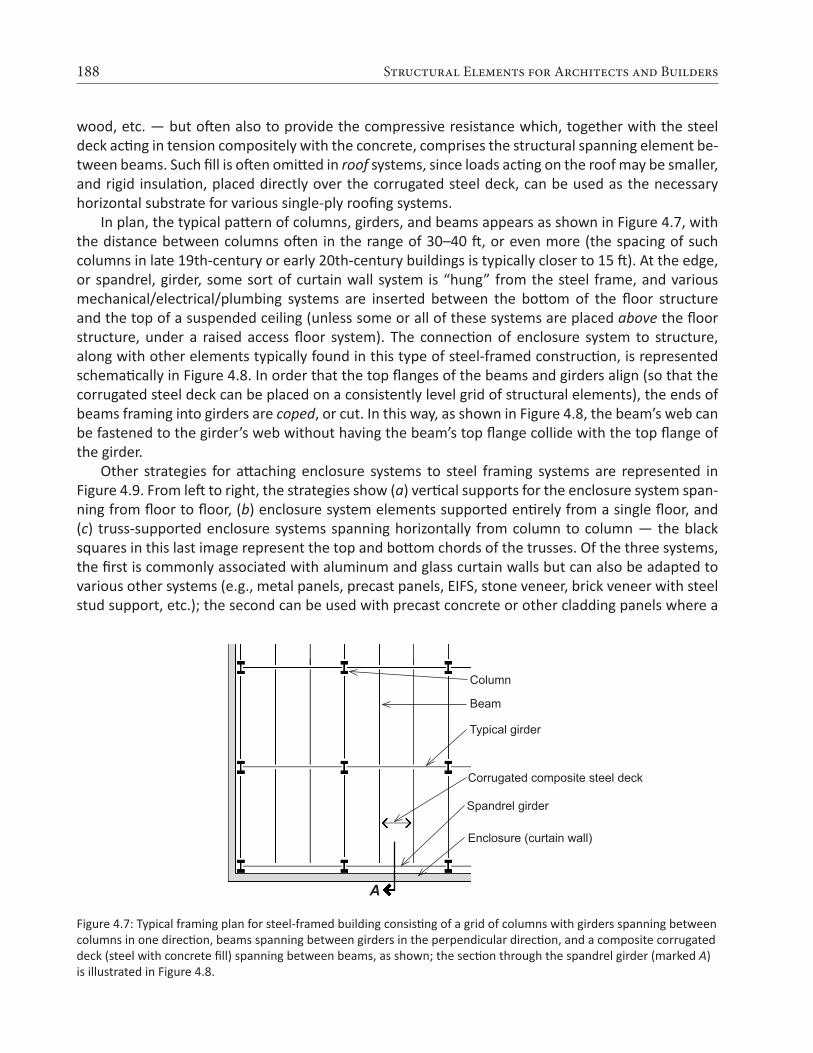
188 Structural Elements for Architects and Builders
wood, etc. — but often also to provide the compressive resistance which, together with the steel deck acting in tension compositely with the concrete, comprises the structural spanning element be-tween beams. Such fill is often omitted in roof systems, since loads acting on the roof may be smaller, and rigid insulation, placed directly over the corrugated steel deck, can be used as the necessary horizontal substrate for various single-ply roofing systems.
In plan, the typical pattern of columns, girders, and beams appears as shown in Figure 4.7, with the distance between columns often in the range of 30–40 ft, or even more (the spacing of such columns in late 19th-century or early 20th-century buildings is typically closer to 15 ft). At the edge, or spandrel, girder, some sort of curtain wall system is “hung” from the steel frame, and various mechanical/electrical/plumbing systems are inserted between the bottom of the floor structure and the top of a suspended ceiling (unless some or all of these systems are placed above the floor structure, under a raised access floor system). The connection of enclosure system to structure, along with other elements typically found in this type of steel-framed construction, is represented schematically in Figure 4.8. In order that the top flanges of the beams and girders align (so that the corrugated steel deck can be placed on a consistently level grid of structural elements), the ends of beams framing into girders are coped, or cut. In this way, as shown in Figure 4.8, the beam’s web can be fastened to the girder’s web without having the beam’s top flange collide with the top flange of the girder.
Other strategies for attaching enclosure systems to steel framing systems are represented in Figure 4.9. From left to right, the strategies show (a) vertical supports for the enclosure system span-ning from floor to floor, (b) enclosure system elements supported entirely from a single floor, and (c) truss-supported enclosure systems spanning horizontally from column to column — the black squares in this last image represent the top and bottom chords of the trusses. Of the three systems, the first is commonly associated with aluminum and glass curtain walls but can also be adapted to various other systems (e.g., metal panels, precast panels, EIFS, stone veneer, brick veneer with steel stud support, etc.); the second can be used with precast concrete or other cladding panels where a
Figure 4.7: Typical framing plan for steel-framed building consisting of a grid of columns with girders spanning between columns in one direction, beams spanning between girders in the perpendicular direction, and a composite corrugated deck (steel with concrete fill) spanning between beams, as shown; the section through the spandrel girder (marked A) is illustrated in Figure 4.8.
Corrugated composite steel deck
Column
Spandrel girder
Typical girder
Beam
A
Enclosure (curtain wall)

189Steel
Figure 4.8: Schematic section through spandrel (edge) girder in steel-framed building; the mechanical unit at the build-ing perimeter is increasingly omitted as glazing systems become more efficient, thereby reducing heat loss or heat gain through the curtain wall
Suspended ceiling system
Enclosure or curtain wall
Firestop system ("fire safing")
Cei
ling-
to-fl
oor d
imen
sion
appr
oxim
atel
y 4
ft.
Glazing system (part of
Spandrel girder Clip angle
Composite corrugated steel deck
Steel beam
Mechanical ventilation duct
Schematic representation offastening device to attach enclosure (cladding) to structure
enclosure or curtain wall)Mechanical unit for heating/cooling
Line of finish floor
Figure 4.9: Schematic sections showing three strategies for attaching enclosure systems to steel structural framing using (a) vertical elements spanning from floor to floor, (b) two points of support at each floor, leaving a structure-free space for glazing, and (c) trusses supporting cladding panels, fabricated off-site, spanning horizontally from column to column.
(a) (b) (c)

190 Structural Elements for Architects and Builders
continuous band of horizontal glazing is desired, and the third — less commonly encountered than the other strategies — can be used where off-site fabrication of large enclosure panels is desired.
Columns in multi-story steel-framed buildings must be spliced together from smaller lengths. In general, the largest lengths compatible with transport and erection constraints are used in order to minimize the work needed on-site to make such connections. This typically results in two- or three-story column lengths that are connected above the finish floor levels, as shown in Figure 4.10a. Small inefficiencies come about from this strategy, since the upper part of a typical two- or three-story section is stronger than it would otherwise need to be (its strength being governed by the heavier loads supported on the lower part of the section), but such inefficiencies are justified by savings in fabrication and erection costs. Steel cap and base plates may or may not be used where steel column sections are joined together; the simplest connections omit such plates in favor of “filler” or “pack-ing” plates that account for misalignment of flange and web surfaces (where adjacent columns are not the same size) so that splice plates can tie the separate elements together (Figure 4.10b).
Where columns meet the foundation, and therefore must be connected to the building’s rein-forced concrete substructure, base plates are always used. These plates, which are typically shop-welded or bolted to the bottom of the lowest steel columns, do not actually touch the top surface of the concrete substructure, but are designed to be “suspended” about an inch or less above the top surface of the concrete. Such tolerances are always required, since as-built conditions of both steel and concrete systems cannot be assumed to have the precision of, for example, factory-made com-ponents like windows or doors. The vertical alignment of steel columns is then carefully adjusted in the field, using shims or leveling bolts under the base plate, and the space between base plate and footing is filled with non-shrink grout so that compressive loads may be transferred from the column to the foundation (Figure 4.10c). Threaded rods, already positioned in the concrete substructure so that they align with bolt holes in the column base plate, are designed to prevent both lateral and vertical movement of the column when nuts are screwed onto the rods and tightened against the top of the base plates.
Figure 4.10: (a) Elevation of column in multi-story building spliced at 2-story increments; (b) detail at column splice, with gray tones representing locations of filler, or packing, plates behind splice plates; and (c) detail at column base plate with non-shrink grout filling space between base plate and footing subsequent to alignment of column.
Base plate
Column
2-st
ory
colu
mn
heig
ht
Column
Footing
Base plate
spliceSplice plate
(a) (b) (c)
Non-shrinkgrout
Footing

191Steel
Tension Elements
Unlike tension elements designed in timber, two modes of failure are considered when designing ten-sion members in steel. First, the element might become functionally useless if yielding occurs across its gross area, at the yield stress, Fy . Since internal tensile forces are generally uniform throughout the entire length of the element, yielding would result in extremely large deformations. On the other hand, if yielding commenced on the net area (where bolt holes reduce the gross area), the part of the element subjected to yield strains would be limited to the local area around the bolts, and ex-cessive deformations would not occur. However, a second mode of failure might occur at these bolt holes: rupture of the element could occur if, after yielding, the stresses across the net area reached the ultimate stress, Fu . As in wood design, typical bolt hole diameters are 1/16 in. larger than the actual bolt diameter (except that for bolts with diameters greater or equal to 1 in., the bolt hole diameter is made ⅛ in. larger). However, because a small amount of material surrounding the bolt hole is damaged as the hole is punched, an additional 1/16 in. is added to the hole diameter for the purpose of calculating net area, resulting in a bolt hole diameter taken as 1/8 in. larger than the nominal bolt diameter for steel elements (or 3/16 in. larger for bolts with diameters of 1 in. or larger).
Another difference in the design of wood and steel tension elements occurs because nonrectan-gular cross sections are often used in steel. If connections are made through only certain parts of the cross section, as illustrated in Figure 4.11, the net area in the vicinity of the connection will be effec-tively reduced, depending on the geometry of the elements being joined, and the number of bolts being used. This effective net area, Ae, is obtained by multiplying the net area, An, by a coefficient, U, defined in Appendix Table A-4.9.
Where all parts (i.e., flanges, webs, etc.) of a cross section are connected, and the so-called shear lag effect described above cannot occur, the coefficient U is taken as 1.0, and the effective net area equals the net area, just as in timber design. For short connection fittings like splice plates and gusset plates, U is also taken as 1.0, but Ae = An cannot exceed 0.85 times the gross area. These short con-necting elements may have an effective width less than their actual width to account for the shear lag effect, based on what is known as the “Whitmore section,” shown in Figure 4.12. For a length, L, of the fastener group measured in the direction of load, and a distance, W, between the outer rows of bolts or welds, the effective width is computed by extending a 30° line out from both sides of the fastener group; it can be seen that the effective width, lw , is equal to 2Ltan 30° + W.
Figure 4.11: Shear lag in steel tension element showing unstressed or under-stressed areas
Unstressed or under-stressed area
P
P

192 Structural Elements for Architects and Builders
Finally, the lengths of tension members, other than rods and cables, are recommended, but not required to have, a slenderness ratio — defined as the ratio of effective length to least radius of gy-ration — of 300, to prevent excessive vibrations and protect against damage during transportation and erection. The radius of gyration, a property of the cross section, is equal to √I/A, where I is the moment of inertia and A is the cross-sectional area of the element.
From the preceding discussion, it can be seen that two values for available strength, or allow-able stress, in tension need to be determined: one for yielding of the gross area and one for failure (rupture) of the effective net area. These two values are:
Ftgross = 0.6Fy
and Ft
net = 0.5Fu
where Ft gross and Ft net are the allowable tensile stresses for steel corresponding to the two modes of failure, or limit states: Fy is the yield stress and Fu is the ultimate stress for steel (Appendix Table A-4.1). The tensile stress is computed on the gross area in the same manner as for wood (see Equation 3.2). Rupture on a failure surface through bolted or welded connections, however, is determined using the effective net area rather than the net area, so Equation 3.3 (for wood) must be modified for steel connections as follows:
ft = P/Ae
When computing the capacity based on yielding, the full gross area is available to resist the internal forces:
Pallow = Ft gross × Ag
When computing the capacity on the effective net area:
Pallow = Ft net × Ae
(4.1)
(4.2)
(4.3)
(4.4)
(4.5)
Figure 4.12: The Whitmore section for connecting plates limits the effective width of the plate to 2L tan 30° + W for both (a) welded connections; and (b) bolted connections
(a) Welds (b) Bolts

193Steel
The “available strength” limit states listed in Appendix Table A-4.2 are equivalent to these formula-tions based on allowable stress.
The following example illustrates the application of these principles to a steel tension problem. Different procedures are used for cables, eyebars, threaded rods, and pin-connected plates.
Example 4.1 Analyze steel tension element
Problem definition. Find the maximum tension load, P, that can be applied to a W8 × 24 element con-nected to gusset plates within a truss with ¾-in.-diameter bolts, as shown in Figure 4.13. Use A36 steel. Find the required thickness of the gusset plates so that their capacity is no smaller than that
(a) Section at gross area
(b) Section at net area
(c) Truss elevation with 3-dimensional view
tp
3"
3"
W8x24
W8x24
Figure 4.13: Connection detail at gusset plate, with (a) section at gross area, (b) section at net area, and (c) truss eleva-tion with 3-dimensional view for Example 4.1

194 Structural Elements for Architects and Builders
of the W8 × 24 tension element. The bolt hole diameter = bolt diameter + 1/8 in. = 7/8 in. = 0.875 in.
Solution overview. Find cross-sectional dimensions and material properties; find gross area capacity; find effective net area capacity; the governing capacity is the lower of these two values. For gusset plate thickness, find effective width based on Whitmore section; apply equations for gross and net area capacity to determine required plate thickness.
Problem solution 1. From Appendix Table A-4.3, find cross-sectional dimensions (Figure 4.14):
Ag = 7.08 in2
d = 7.93 in. bf = 6.50 in. tf = 0.400 in.
2. From Appendix Table A-4.1, find Fy = 36 ksi and Fu = 58 ksi. 3. Gross area: find capacity, P:
a. Using Equation 4.1 (or Appendix Table A-4.2) find Ft gross = 0.6Fy = 0.6(36) = 22 ksi.b. Using Equation 4.4, P = Ft gross × Ag = 22(7.08) = 156 kips.
4. Effective net area: find capacity, P:a. From Appendix Table A-4.9, find the shear lag coefficient, U: U = 0.90 since the following criteria are met: • Bolts connect wide-flange (W) shape?
Yes. • Flange width, bf is no less than 0.67d?
In other words, 6.5 ≥ 0.67(7.93) = 5.3? Yes.
• Flange is connected with at least 3 bolts per line? Yes.
b. Find the net area, An (same as Equation 3.1 for wood). As shown in Figure 4.15:
An = Ag – (number of holes)(Dh × t) =
7.08 – 4(0.875 × 0.400) = 5.68 in2.
c. Ae = U(An) = 0.9(5.68) = 5.11 in2.d. Using Equation 4.2, find Ft net = 0.5Fu =
0.5(58) = 29 ksi.e. Using Equation 4.5, find P = Ft net × Ae =
29(5.11) = 148 kips. 5. Conclusion: failure on the effective net
area governs since 148 kips < 156 kips. The capacity (allowable load) is 148 kips.
6. We now can determine the thickness of the gusset plate, stressed in tension, with
Figure 4.14: Cross-sectional dimensions of W8 × 24 for Example 4.1
bf = 6.50"
tf = 0.400"
d =
7.93
"
x
y
Figure 4.15: Net area diagram for Example 4.1
tf = 0.400"
Dh = ¾ + ⅛ = ⅞"

195Steel
two lines of bolt holes per plate, using the Whitmore section to determine the effective width of the plate. As can be seen in Figure 4.12, the effective width, lw = 2(6)(tan 30°) + 3 = 9.9 in. The tensile capacity of the gusset plates may be based on either yielding of the gross area or rupture of the net area. First, the capacity based on yielding of the gross area of both plates is Ft Ag = 0.6(36)(2)(9.9tp) = 428tp kips. Next, the effective net area Ae = (2)(9.9 – 2 × ⅞)tp = 16.3tp in2, which cannot exceed 85% of the gross area for small gusset plates; i.e., it must be no larger than 0.85(2)(9.9tp) = 16.8tp in2. Therefore, the capacity based on rupture is 0.5(58)(16.3tp) = 473tp. Yielding governs, so the required thickness of the plate can be found by setting the required tensile capacity, 428tp equal to the governing load of 148 kips, from which tp = 0.35 in. Rounding up, we select a ⅜-in. thick gusset plate with tp = 0.375 in.
Example 4.2 Design steel tension element
Problem definition. Select a W section bolted as shown in Figure 4.16 with ⅝ in. diameter bolts, and 3 bolts per line, to resist a tension force of 100 kips. Assume A36 steel. The effective bolt hole diameter = bolt diameter + 1/8 in. = 5/8 + 1/8 = 3/4 in. = 0.75 in.
Solution overview. Find the required area based on net area capacity, assuming values for shear lag coefficient, U, and flange thickness, tf ; find required area based on gross area capacity; use the larger of the two area values to provisionally select a W section; check using “analysis” method if either U is smaller or tf is larger than assumed values. The area of the selected W section can be somewhat smaller than the “required” area if either U is larger or tf is smaller than assumed values — check using “analysis” method.
Problem solution 1. Gross area: find required gross area based on yielding. From Equation 4.4, the required gross
area, Ag = P/Ft gross = 100/(0.6 × 36) = 4.63 in2. 2. Effective net area: find required gross area after determining effective net area based on rup-
ture through failure surface (assume U = 0.9 and tf = 0.4 in.):a. From Equation 4.5, the required effective net area, Ae = P/Ft net = 100/(0.5 × 58) = 3.45 in2.b. Working backwards, the required net area, An = Ae /U = 3.45/0.9 = 3.83 in2.c. Finally, the required gross area can be computed: Ag = An + (bolt hole area) = 3.83 + 4(0.75 × 0.4) =
5.03 in2. 3. Since 5.03 in2 > 4.63 in2, the calculation
based on effective net area governs, and a W section must be selected with Ag ≥ 5.03 in2. Many wide-flange shapes could be se-lected. From Appendix Table A-4.3, the fol-lowing candidates are among those that could be considered:a. Check a W8 × 18 with Ag = 5.26 in2.
Two assumptions need to be test-ed: that U = 0.9, and that tf ≤ 0.4 in. From Appendix Table A-4.3, bf = 5.25 in., d = 8.14 in. and tf = 0.330 in. From
⅝" bolts, 3 bolts per line
100 kips
W section
Figure 4.16: Net area diagram for Example 4.2

196 Structural Elements for Architects and Builders
Appendix Table A-4.9, the criteria for U = 0.9 requires that bf = 5.25 ≥ 0.67d = 0.67(8.14) = 5.45 in. Since this condition is not met, we must use U = 0.85. Additionally, the flange thick-ness is different from our assumed value of 0.40 in., so that the calculation of net and effec-tive area will change: An = Ag – (bolt hole area) = 5.26 – 4(0.75 × 0.330) = 4.27 in2 and Ae = U × An = 0.85(4.27) = 3.63 in2. The capacity based on rupture through the effective net area is P = Ft net × Ae = (0.5 × 58)(3.63) = 105 k. The capacity based on yielding on the gross area has already been found satisfactory (since the gross area of the W8 × 18 is greater or equal to the required gross area computed above). Therefore, the W8 × 18 is acceptable.
b. Check a W6 × 20 with Ag = 5.87 in2. The same two assumptions need to be tested: that U = 0.9, and that tf ≤ 0.4. From Appendix Table A-4.3, bf = 6.02 in., d = 6.20 in. and tf = 0.365 in. From Appendix Table A-4.9, the criteria for U = 0.9 requires that bf = 6.02 ≥ 0.67d = 0.67(6.20) = 4.15 in. Since this condition is met, and since its net area is greater than as-sumed (this is so because its flange thickness, tf , is less that the value assumed, so that the bolt hole area is less than assumed, and therefore the net area is greater than assumed), the W6 × 20 is acceptable.
Both the W8 ×18 and the W6 × 20 would work, as would many other wide-flange shapes. Of the two sections considered, the W8 × 18 is lighter (based on the second number in the W-designation that refers to beam weight in pounds per linear foot), and therefore would be less expensive.
Steel threaded rods
Threaded rods are designed using an allowable tensile stress, Ft = 0.375Fu , which is assumed to be resisted by the gross area of the unthreaded part of the rod. This value for the allowable stress is found by dividing the nominal rod tensile strength of 0.75Fu by a safety factor, Ω = 2.00. While there are no limits on slenderness, diameters are normally at least 1/500 of the length, and the minimum diameter rod for structural applications is usually set at ⅝ in. Assuming A36 steel, with Fu = 58 ksi (Appendix Table A-4.1), the smallest acceptable rod with area, A = π(5/16)2 can support a tensile load, P = Ft × A = 0.375Fu × π(5/16)2 = 21.75 × 0.3068 = 6.67 kips.
Pin-connected plates
Where plates are connected with a single pin, as shown in Figure 4.17, the net area, An, is defined, not by the length, b, on either side of the pin hole, but rather by an effective length, be = 2t + 0.63 ≤ b, where t is the thickness of the plate (Figure 4.17b):
An = 2t × be
The plate capacity in tension is governed by either yielding on the gross area or rupture on the net area, whichever is smaller (there is no effective net area in this case), with Pgross = 0.6Fy × Ag and Pnet = 0.5Fu × An as before. It is possible to cut the plate at a 45° angle as shown in Figure 4.17, as long as length c is greater or equal to length a, which in turn must be greater or equal to 1.33be.
Aside from failure in tensile rupture or yielding, a third limit state for pin-connected plates is shear failure, or the relative sliding of areas Asf as illustrated in Figure 4.17c. In this case, the allow-able shear stress is taken as 0.3Fu so that Pshear = 0.3Fu × Asf.
(4.6)

197Steel
A fourth limit state for pin-connected plates is bearing, or compressive stress caused by the pin itself in direct contact with the adjacent plate. Here, the allowable stress on the projected area (Apb) of the pin that bears on the plate is 0.9Fy so that the allowable bearing strength is 0.9Fy Apb.
All four limit states must be checked, with the capacity of the pin-connected plate determined by the lowest of the four limits. Values for yield and ultimate stress used in these calculations, Fy and Fu , are listed in Appendix Table A-4.1.
For such pin-connected plates, as well as for all other bolted connections, the fasteners them-selves, and not only the stresses they produce on the elements being joined, must also be checked. This aspect of structural element design is discussed more thoroughly in the section of this chapter dealing with steel connections.
Columns
Steel columns with high slenderness ratios are designed using the Euler buckling equation, while “fatter” columns, which buckle inelastically or crush without buckling, are designed according to formulas corresponding to test results. Residual compressive stresses within hot-rolled steel sec-tions precipitate this inelastic buckling, as they cause local yielding to occur sooner than might oth-erwise be expected. Unlike timber column design, the two design equations corresponding to elastic and inelastic buckling have not been integrated into a single unified formula, so the underlying
Figure 4.17: (a) Overview of pin-connected plates; (b) rupture on net area and (c) shear failure
bDh
ta
b
Dh/2
Asf
Anc
P
P
P a + Dh
/2t
t
Dh
b
b
c
An
Asf
(a)
(b) (c)
b
b
Dhbe
be
Dh/2
a

198 Structural Elements for Architects and Builders
rationale remains more apparent. The slenderness ratio dividing elastic from inelastic buckling is set, somewhat arbitrarily, at the point where the Euler critical buckling stress equals 0.444 times the yield stress; i.e., at the stress:
This particular slenderness ratio separating elastic from inelastic buckling is found by solving for (KL /r) in Equation 4.7:
For Fy = 50 ksi, the value of KL /r is 113; for Fy = 36 ksi, the value is 134. For a slender column with a slenderness ratio greater than this separating value, elastic buckling is assumed, and the allowable (“available”) axial compressive stress, based on Euler’s equation (multiplied by a factor of 0.877, and divided by a safety factor, Ω = 1.67), is:
The coefficient, 0.525, in Equation 4.9 corresponds to the safety factor of 12/23 previously used for elastic buckling of steel columns.
Where KL /r is less than the value separating elastic from inelastic buckling, inelastic buckling governs, and the allowable (“available”) axial compressive stress is found by dividing the critical stress for inelastic buckling by the same factor of safety, Ω = 1.67:
In this equation, Fe is the elastic buckling stress shown in Equation 1.19; that is:
The slenderness ratio, KL /r, should not exceed 200 for steel axial compression elements. Values for K are shown in Appendix Table A-1.2. We are also assuming that compression elements are proportioned so that local buckling of their flanges or web does not occur; this requires that the compression element (typically a column) is not defined as slender. Wide-flange elements that are determined to be slender for compression are noted in Appendix Table A-4.3. Their design, involving calculations that effectively reduce the load they can safely carry, is beyond the scope of this discus-sion.
The two curves representing allowable stresses for elastic and inelastic buckling make a smooth transition at the slenderness ratio separating them, as shown in Figure 4.18. Rather than apply these equations to the solution of axial compression problems in steel, allowable stress tables (for analy-sis, Appendix Tables A-4.11 through A-4.14) or allowable load tables (for design, Appendix Table
(4.7)σcr =π2E
(KL /r)2 = 0.444Fy
(4.8)KL /r = 4.71 EFy√
(4.9)π2E(KL /r)2
π2E(KL /r)2Fc = 0.877
1.67 = 0.525
(4.10)Fc =0.658(Fy/Fe)Fy
1.67
(4.11)Fe =π2E
(KL /r)2

199Steel
A-4.10) are more often used. If values for allowable load are plotted instead of tabulated, the curves have the same pattern schematically represented in Figure 4.18. Examples of these axial column load curves are shown in Figure 4.19.
Example 4.3 Analyze steel column
Problem definition. Find the capacity (allowable load) of a W14 × 61 pin-ended column with an effec-tive length of 10 ft. Assume A36 steel.
Solution overview. Find relevant section properties; compute slenderness ratio; find allowable stress and capacity.
Problem solution 1. From Appendix Table A-4.3, rmin = 2.45 in. 2. Compute slenderness ratio:
a. From Appendix Table A-1.2, the effec-tive length coefficient, K = 1.0.
b. The effective length, L = 10.0 × 12 = 120 in.
c. KL/rmin = (1.0)(120)/2.45 = 48.98. Round up to 49.
3. From Appendix Table A-4.14, the allowable stress: Fc = 19.0 ksi.
4. Find capacity: From Appendix Table A-4.3, the area of the steel column, A = 17.9 in2. The capacity, P = Fc × A = 19.0(17.9) = 340 kips.
From Equation 4.8, the slenderness ratio separating elastic and inelastic column behav-ior is 134 for A36 steel. The column analyzed in Example 4.3 has a slenderness ratio of 48.98, which is less than this separating value; there-fore, it fails inelastically. Using Equation 4.10 to determine the “inelastic” allowable stress, we get the same result as was obtained in the example. The calculations are as follows, using Fy = 36 ksi:
From Equation 4.11, Fe = π2(29,000)/(48.982) = 119.3. Then, from Equation 4.10:
It can be seen that this is the same allowable stress as was obtained in Example 4.3.
Fc =0.658(Fy/Fe)Fy
1.67= 0.658(36/119.3)36
1.67= 19.0 ksi
Figure 4.18: Inelastic and elastic critical stress curves for column buckling
Stress
Transition point at 0.44Fy
"Euler" (elastic) curve
Allowable stress0.44Fy
Fy
Inelastic buckling curve
KL /r
Figure 4.19: Allowable axial column load plotted against effective length
Effective length, KL (feet)
Allo
wab
le lo
ad (k
ips)

200 Structural Elements for Architects and Builders
Example 4.4 Design steel column
Problem definition. Select the lightest (most economical) wide-flange section for the first-floor col-umn shown in Figure 4.20. Assume office occupancy; a roof (construction) live load of 20 psf; a typical steel floor system; and an allowance for steel stud partitions. Assume pin-ended (simple) connections. Use A992 steel.
Solution overview. Find total load on column; find effective length; select lightest section.
Problem solution 1. Find total column load:
a. From Appendix Table 2.2, the live load (L) for office occupancy = 50 psf.b. From Appendix Table 2.1, the typical dead load (D) = 47 psf (steel floor system, etc.) + 8 psf
(steel stud partition allowance) = 55 psf.c. The roof construction live load (Lr) = 20 psf, according to the Problem Definition.d. Find tributary area (see Figure 1.5): The column's tributary area is 25 ft × 40 ft = 1000 ft2 per
floor, or 5000 ft2 for the five levels on which occupancy live loads are computed (excluding the roof).
e. Using Appendix Table A-2.2, compute the reduced live load; the live load reduction factor is: 0.25 + 15/√4 × 5000 = 0.36, but no reduction less than 0.40 is permitted. Therefore, the live load can be reduced to 0.40 × 50 = 20 psf for the first-floor column under consideration.
f. Using Appendix Table A-2.7 for allowable stress design, find the total column load, account-ing for reductions due to load combinations:
L = (25 ft × 40 ft) × (20 psf) × 5 floors = 100,000 lb
D = (25ft × 40 ft) × (55 psf) × 6 floors = 330,000 lb
Lr = (25ft × 40 ft) × (20 psf) × 1 floor = 20,000 lb
For the three loads potentially pres-ent, only two load combinations need be considered (the others listed will produce less severe effects). For the second load combination, wind or seis-mic effects on the column may also be considered. However, in this example, we assume that the column is not part of the lateral force-resisting system for wind or seismic, and that any negative (uplift) wind load on the roof can be conservatively ignored. The two rele-vant load combinations to consider are as follows:
Figure 4.20: Framing plan and building section for Example 4.4
Framing plan
Building section

201Steel
D + L = 330,000 + 100,000 = 430,000 lb D + 0.75L + 0.75Lr = 330,000 + 0.75(100,000) + 0.75(20,000) = 330,000 + 75,000 + 15,000 = 420,000 lb.
The first case governs; therefore the total column load = 430,000 lb = 430 kips.
2. Using Appendix Table A-1.2, find the effective length: KL = (1.0)(14) = 14 ft. 3. Select the most economical section:
a. Using Appendix Table A-4.10, pick the lightest acceptable section from each “nominal depth” group (i.e., one W8, one W10, one W12, and so on), to assemble a group of “likely candidates.” Some columns are clearly either to small or too large; the three possible can-didates for a load of 430 kips and an effective length of 14 ft. are:
• W10 × 68 can support 440 kips • W12 × 65 can support 456 kips • W14 × 74 can support 466 kips
b. Choose lightest section: The W12 × 65 is the most economical since its weight per linear foot (65 pounds) is smallest.
To check the result in Example 4.4, first determine the slenderness ratio of the W12 × 65, find-ing the minimum (y-axis) radius of gyration, r = 3.02 in., from Appendix Table A-4.3. Then, KL /r = (1.0)(14 × 12)/3.02 = 55.63. From Equation 4.8, the slenderness ratio separating elastic from inelastic behavior for A992 steel is 113, so the column fails inelastically. Using Equation 4.10 to determine the “inelastic” allowable stress, we get the same result as was obtained in the example. The calculations are as follows, using Fy = 50 ksi:
From Equation 4.11, Fe = π2(29,000)/(55.632) = 92.5. Then, from Equation 4.10:
From Appendix Table A-4.3, the area of the W12 × 65, A = 19.1 in2. Therefore, the capacity, P = Fc × A = 23.9 × 19.1 = 456 kips, the same value found in Example 4.4.
Beams
The design of steel wide-flange beams using the “allowable strength design” method is quite similar to the procedures used to design timber beams (see Chapter 3). Cross sections are selected based on their strength in bending, and then checked for shear and deflection.
Bending of laterally-braced and compact beams
Unlike wood beams, however, steel beams are designed based on their “available” strength, rather than on the more convention notion of an “allowable” stress. Whereas the strength of a wood beam corresponds to its outer fibers reaching a failure stress, steel beams do not fail when their outer
Fc =0.658(Fy/Fe)Fy
1.67=
0.658(50/92.5)501.67
= 23.9 ksi

202 Structural Elements for Architects and Builders
fi bers fi rst begin to yield at the stress, Fy . A steel cross secti on is able to carry increased loads beyond the so-called elasti c moment, shown in Figure 4.21a, up unti l the enti re cross secti on has yielded, as shown in Figure 4.21b. The plasti c secti on modulus corresponds to this so-called plasti c moment, reached when the strain at a cross secti on is of suffi cient magnitude so that virtually the enti re sec-ti on has yielded.
Figure 4.21: Bending stresses acti ng on steel wide-fl ange ( -shaped) cross secti on corresponding to the (a) elasti c mo-ment and (b) plasti c moment, with three examples: (c) and (d) illustrate elasti c and plasti c moments for a hypotheti cal secti on with all its area at the extreme fi bers; (e) and (f) illustrate elasti c and plasti c moments for a typical W30 × 90 secti on; while (g) and (h) illustrate elasti c and plasti c moments for a rectangular secti on.
(a) (b)
(c) (d)
(e) (f)
(g) (h)

203Steel
Previously, steel used an “allowable stress” method based on a limit state corresponding to the elastic moment; and if the plastic moment were always stronger than the elastic moment to the same extent for all cross sections, one could simply adjust the factor of safety for allowable strength (plastic moment) design so that the method corresponded precisely to allowable stress (elastic mo-ment) design. However, it can be shown that the extra margin of safety gained by moving beyond the elastic, to the plastic moment (i.e., from the condition of Figure 4.21a to Figure 4.21b), is not the same for all cross sections, so that allowable stress design for steel does not provide a consistent margin of safety against the limit state of complete yielding.
For wide-flange ( -shaped) sections, the extremes can be represented by a hypothetical sec-tion with no web (i.e., consisting entirely of flanges of infinite density, or no thickness, as shown in Figures 4.21c and 4.21d ); and, at the other extreme, a section whose flanges merge together at the neutral axis (i.e., a rectangular section, as shown in Figures 4.21g and 4.21h). In the first case, it is clear that the elastic moment and plastic moment coincide, and the so-called “shape factor” defin-ing the ratio of plastic to elastic section modulus, Zx /Sx, equals 1.0. In the second case, the elastic section modulus can be computed by examining the rotational equilibrium of the force resultants shown in Figure 4.21g. Since the moment arm between them equals (2/3)h, and the resultant force, C, equals (1/2)(h/2)(b)(Fy), the moment, M, equals (2/3)(h)(1/2)(h/2)(b)(Fy) and, solving for the section modulus, Sx = M/Fy , we get Sx = bh2/6. Performing the same equilibrium calculation on Figure 4.21h (with a moment arm equal to h/2), and solving for the plastic section modulus, Zx = M/Fy , we get Zx = bh2/4. The shape factor in this case is Zx/Sx = 1.5.
Clearly, all -shaped sections must have a shape factor between these two extremes, i.e., be-tween 1.0 and 1.5. The shape factor for a typical W-shape (W30 × 90), shown in Figures 4.21e and 4.21f, can be determined in the same manner, abstracting from the complexities of the actual shape by considering only perfectly rectangular flange and web areas. Using the dimensions shown, and performing the same equilibrium calculations as in the cases above, we get Sx = 240 in3 and Zx = 277 in3, so the shape factor, Zx/Sx = 277/240 = 1.15. The actual values for elastic and plastic section modu-lus are found in Appendix Table A-4.3, and it can be seen that the approximate calculations are both conservative and reasonably accurate: the correct values are actually Sx = 245 in3 and Zx = 283 in3, so the real shape factor, Zx/Sx = 283/245 = 1.16.
The equation for plastic section modulus, Zx = M/Fy , presumes that the cross section is able to reach a state of complete yielding before one of two types of buckling occurs: either lateral-torsional buckling within any unbraced segment along the length of the span or local flange or web buckling. Therefore, to use this equation in design, based on the maximum moment encountered, the beam must be protected from both of these buckling modes, in the first case by limiting the effective length and, in the second case, by regulating the proportions of the beam flange and web (i.e., using a so-called compact section). Then, rewriting this equation in the form most useful for steel design, we get:
Zreq = ΩMmax /Fy
where Mmax = the maximum bending moment (in-kips), Fy is the yield stress of the steel (ksi), and Ω is a safety factor equal to 1.67 for bending. The units of the required plastic section modulus are in3.
We found earlier that the shape factor for a W30 × 90 section equals 1.16. By looking at the ratio of plastic to elastic section modulus for all wide-flange shapes, it can be seen that these shape fac-tors fall between 1.098 (for a W14 × 90), and 1.297 (for a W14 × 730). One could therefore conser-vatively create a safety factor for elastic allowable stress design by assuming a shape factor of 1.10,
(4.12)

204 Structural Elements for Architects and Builders
and by multiplying this value by the safety factor for allowable strength design, 1/Ω = 1/1.67 = 0.60 (inverted to be consistent with the conventions for allowable stress safety factors). Equation 4.12 would then become Sreq = Mmax /(1.1 × 0.6 × Fy) = Mmax / (0.66Fy). This, in fact, is the design equation for what used to be called “allowable stress design” in steel. It may still be used, but will give slightly conservative values compared with the available stress method using the plastic section modulus, Zx.
Choosing the lightest (i.e., most economical) laterally-braced, compact section is facilitated by the use of tables in which steel cross sections are ranked, first in terms of plastic section modulus, and then by least weight. Appendix Table A-4.15 is an example of such a list, in which only the light-est sections appear. Thus, a W30 × 191 (with a plastic section modulus of 675 in3) is not listed, since a lighter section, W40 × 167, has a higher plastic section modulus (693 in3).
Bending of laterally-unsupported or noncompact beams
When the compression flange of a beam is not continuously braced, lateral-torsional buckling can reduce the available bending moment below the value of Mp/Ω assumed earlier for laterally braced beams. How much this stress is reduced depends on whether the beam buckles before or after the cross section begins to yield, and how bending stresses vary over the beam’s effective length. Figure 4.22 shows several possible stress stages for a cross-sectional shape as the bending moment increases. At Figure 4.22c, the outer fibers begin to yield, and the elastic moment, My, is reached. At Figure 4.22d and Figure 4.22e, yielding progresses further into the cross section, as the moment increases. Finally, at Figure 4.22f, the entire cross section has yielded at the maximum plastic mo-ment that the section can sustain.
Being able to resist the full plastic moment represents an extra margin of safety: if a beam can
(a) (b) (c) (d) (e) (f)
(g)
Figure 4.22: Elongation, strain, and stress diagrams for an elastic-plastic material such as steel showing (a ) elongation and shortening of the actual material; (b ) strain diagrams; (c ) stress diagram at the point where the outer fiber has just yielded; (d) stress diagram corresponding to strain just beyond the elastic limit; (e ) stress diagram corresponding to continued strain beyond the elastic limit; (f ) stress diagram corresponding to the plastic moment (where the entire cross section has yielded); and (g ) stress-strain diagram. [Diagram reproduced from fig. 1.64]

205Steel
develop this plasti c moment without buckling, the maximum available bending moment of Mp/Ω is used, as shown in Equati on 4.12. In addi-ti on to lateral-torsional buckling (Figure 4.23a), various types of local fl ange and web buckling must also be prevented from occurring before the plasti c moment is reached (Figure 4.23b). Local buckling is prevented by limiti ng the rati o of fl ange width to fl ange thickness, as well as web width to web thickness. Secti ons propor-ti oned so that local buckling will not occur are called compact secti ons; these secti ons must be used to qualify for the full available moment of Mp/Ω. As it turns out, all but one of the wide-fl ange shapes listed in Appendix Table A-4.3 are compact secti ons when made from A36 steel (the excepti on being W6 × 15). For 50 ksi steel, all but ten (W6 × 8.5, W6 × 9, W6 × 15, W8 × 10, W8 × 31, W10 × 12, W12 × 65, W14 × 90, W14 × 99, and W21 × 48) are compact.
For secti ons that are compact and later-ally braced, Equati on 4.12 applies, and the full strength of the beam is uti lized. However, as shown in Figure 4.24, this available strength must be reduced if either local fl ange buckling (where the secti on is not compact) or lateral-torsional buckling (where the secti on is not ad-equately braced) occurs before the plasti c mo-ment is reached.
Lateral-torsional buckling
For beams with an unbraced length, Lb, that falls within the “middle zone” illustrated in Figure 4.24a (i.e., where the onset of buckling occurs before a full plasti c moment, but aft er the elas-ti c moment, is reached), the nominal bending strength is linearly reduced from the full plas-ti c moment, Mp = FyZx, to 70% of the elasti c mo-ment, or 0.7FySx. The two boundaries (unbraced lengths) that bracket this conditi on of inelasti c lateral-torsional buckling are called Lp and Lr . For an unbraced length, Lb, less than Lp, lateral-tor-sional buckling is not an issue, as the full plasti c moment can be reached. For an unbraced length greater than Lr, the onset of lateral-torsional
Figure 4.23: Two modes of buckling limiti ng the strength of a wide-fl ange ( -shaped) beam: (a) lateral-torsional buckling; and (b) local fl ange buckling
(b)(a)
Figure 4.24: Infl uence of lateral-torsional buckling and fl ange slenderness on available moment: three zones are defi ned for (a) lateral torsional buckling, with the bound-aries established by the laterally unbraced length, Lp (the greatest unbraced length where the secti on can reach a plasti c moment without lateral torsional buckling) and Lr (the greatest unbraced length where the secti on will buckle inelasti cally before reaching the plasti c moment); and for (b) fl ange slenderness, with the boundaries established by the rati o of half the fl ange width to fl ange thickness, λ = bf /(2tf ), set equal to λp (the greatest fl ange slenderness where the secti on can reach a plasti c mo-ment without local fl ange buckling) and λr (the greatest fl ange slenderness where the fl ange will buckle locally in an inelasti c manner before reaching the plasti c moment)
Mp = FyZx
Plastic moment
Strength × Zx
0.7FySx
Inelastic buckling
Elastic bucklingB
endi
ng s
tren
gth,
Mn
Lp Lr(a) Laterally unbraced length, Lb
Plastic moment (compact)
Inelastic buckling (noncompact)
Elastic buckling (slender)B
endi
ng s
tren
gth,
Mn
λrλp
Mp = FyZx
0.7FySx
λ = bf /(2tf )(b) Compressive fl ange slenderness,

206 Structural Elements for Architects and Builders
buckling is characterized entirely by elastic behavior, and the nominal bending strength must be re-duced even further. These boundaries are defined as follows: Lp is set at 1.76ry√E/Fy , where E is the modulus of elasticity (29,000 ksi for all steel), Fy is the yield stress (50 ksi for A992 steel, and 36 ksi for A36 steel), and ry is the minimum radius of gyration about the y-axis (see Table A-4.3 for wide-flange shapes). The other boundary, Lr , can be conservatively approximated as πrts√E/(0.7Fy) , where rts may itself be approximated as the radius of gyration for the compression flange and part of the web; i.e., rts = bf /√12 + 2htw/(bf/tf). In this equation, bf and tf are the flange width and thickness, respectively, and h is the length of the “straight” part of the web (i.e., the clear distance between flanges, minus the radii at the web-flange intersections).
However, all these equations are based on the assumption that the beam is subject to a uniform bending moment along its entire length; where the moment varies, as is almost always the case, this assumption is overly conservative, since lateral-torsional buckling is less likely to be triggered where bending stresses are not entirely at their maximum value along the whole length of an unbraced segment. For this reason, a coefficient, Cb, should be applied to the available strength of each un-braced segment of the beam, based on the distribution and magnitude of bending moments along that segment’s length. This “lateral-torsional buckling modifier” is defined as follows for doubly-symmetric bending elements such as wide-flange beams:
where Mmax is the greatest moment within the unbraced segment; and MA, MB, and MC are the bend-ing moments at the quarter point, midpoint, and three-quarters point, respectively, along the seg-ment. Where a segment is not braced at its endpoint (for example, where the end of a cantilevered beam is not braced), Cb should be taken as 1.0. Of course, Cb is not used where a beam is laterally braced and, in any case, can never increase the nominal bending strength beyond the plastic mo-ment, Mp, as shown in Figure 4.24a.
Local flange buckling
Compact sections are proportioned so that neither the flange nor the web will buckle locally before the onset of a plastic moment. Since all wide-flange webs meet the standards for compact sections, only the flange slenderness, defined as λ = bf /(2tf ), is at issue (where bf and tf are the flange width and thickness, respectively). In much the same way that boundaries are established for unbraced length that define the reduction in the bending strength due to lateral-torsional buckling (Figure 4.24a), similar boundaries are established for flange slenderness, with similar consequences for beam strength (Figure 4.24b). The limit for compact behavior — i.e., the maximum flange slender-ness for which beams are still able to reach the plastic moment without local flange buckling — is defined by λ p = 0.38√E/Fy. The other boundary (i.e., the maximum flange slenderness for which in-elastic behavior characterizes the onset of local flange buckling) is defined by λ r = 1.0√E/Fy. In these equations, E is the modulus of elasticity of steel (29,000 ksi) and Fy is the material’s yield stress (50 ksi for A992 steel, and 36 ksi for A36 steel).
As with reductions for lateral-torsional buckling, the nominal bending strength begins with the plastic moment, Mp = FyZx, for compact sections, and is linearly reduced to 70% of the elastic mo-ment, or 0.7FySx, between λ p and λ r, with further reductions beyond λ r.
(4.13)Cb =12.5Mmax
2.5Mmax + 3MA + 4MB + 3MC

207Steel
Where a beam is both noncompact and laterally unbraced, both criteria illustrated in Figure 4.24 are tested, and the smaller capacity governs. For beams that are both compact and laterally braced, Appendix Table A-4.15 can be used to select the lightest W-shape for bending. For A992 wide-flange beams that are not adequately braced laterally (i.e, where Lb > Lp), Appendix Table A-4.16 can be used to select the lightest beam. Of course, by setting the unbraced length to zero, Appendix Table A-4.16 can be used for laterally-braced beams as well.
Shear
Once a selection is made based on bending stress, the section is then checked for shear and deflec-tion. The nominal shear strength, Vn , equals 0.6FyAw, where Fy is the yield stress of the steel and Aw is the web area (equal to the beam depth times the web thickness, d × tw). For most cross sections, the safety factor can be taken as Ω = 1.5, so that the available strength is Vn /Ω = 0.6/Ω(FyAw) = 0.4FyAw. This can be converted into an “allowable stress” equation by defining the allowable shear stress, Fv = 0.4Fy , and solving for the required web area for a given shear force, V:
required Aw = V/Fv
For a small group of wide-flange beams with slender webs, the safety factor for shear is in-creased from 1.5 to 1.67, and so the allowable shear stress becomes Fv = (0.6/1.67)Fy = 0.36Fy . These sections are listed in Appendix Table A-4.3 (see Note 3).
Block shear
Where the top flange of a steel beam is coped (so that it may be fastened to the web of a gird-er while keeping the top surfaces of girder and beam flanges aligned), a mode of failure com-bining both shear and tension stresses in the beam web must be checked, with the shear and tension failure planes assumed to occur at the surface defined by the bolt centerline, as shown in Figure 4.25.
The nominal capacity of such a connection is found by adding the capacity of the net shear area subject to rupture (or the gross shear area subject to yielding) to the capacity of the net tension area subject to rupture. Where both net areas are subject to rupture, the capacity is defined as: Rn = 0.6Fu Anv + Ubs Fu Ant. Where yield-ing governs the failure of the shear area, the capacity is defined as: Rn = 0.6Fy Agv + Ubs Fu Ant. The smaller of these two values determines the capacity of the connection for resisting block shear. In these equations, Fu is the minimum
(4.14)
Net area subjected to shear
Net area subjected to tension
Ubs = 1.0(a)
(b)Ubs = 0.5
Figure 4.25: Block shear at coped beam with (a) coef-ficient Ubs =1.0 where tension stress is uniform (single line of bolts); and (b) Ubs = 0.5 where tension stress has a triangular distribution (double line of bolts)

208 Structural Elements for Architects and Builders
tension strength of the material (equal to 58 ksi for A36 steel, and 65 ksi for A992 steel); Anv and Ant are the net areas for shear and tension, respectively; Agv is the gross shear area; and Ubs equals 1.0 for conditions that correspond to uniform tension stress, as in the coped beam with a single line of bolts shown in Figure 4.25a, while Ubs equals 0.5 for conditions that lead to a triangular (non-uniform) tension stress, as in the coped beam with a two lines of bolts shown in Figure 4.25b. The available strength is then found by dividing the nominal capacity by the safety factor, Ω = 2.00.
It is also possible that a mode of shear failure alone, with no tension component, could govern the connection design. In such a case, both yielding on the gross area of the cross section and rup-ture on the net area need to be checked. For yielding, the nominal capacity, Rn, equals 0.60Fy Agv, and the available strength, ΩRn , is determined using a safety factor, Ω = 1.50 (not Ω =2.00). For rupture on the net area, Rn equals 0.60Fu Anv , and the available strength, ΩRn , is determined using a safety factor, Ω = 2.00. All the parameters are as defined above for block shear. The lower safety factor for yielding reflects the relative safety of a yielding mode of failure compared with the more sudden and catastrophic type of failure associated with rupture.
Example 4.5 Find capacity of beam web based on block shear
Problem definition. Find the capacity of a bolted double-angle connection to the web of a coped W18 × 86 wide-flange beam, considering only block shear in the web. Assume A992 steel (Fy = 50 ksi and Fu = 65 ksi) for the beam, and 3/4-in.-diameter bolts. The bolt spacing, s = 3 in., the vertical edge distance, Lev = 1.5 in., and the horizontal edge distance, Leh = 1.5 in. as defined in Figure 4.26.
Solution overview. Find the smaller of the capacities based on rupture and yielding of shear area, rupture of tension area, and bolt bearing on the web.
Problem solution 1. Find capacity based on net areas subject
to rupture. Lengths along net areas are found by subtracting the lengths of bolt hole diameters from the total (gross) di-mension. The net area for shear, Anv = tw (4s + Lev – 4.5Dh) = 0.480(4 × 3 + 1.5 – 4.5 × 0.875) = 4.59 in2, where tw is the web thickness (from Appendix Table A-4.3), s is the bolt spacing of 3 in., Lev is the verti-cal edge distance of 1.5 in., and Dh is the bolt hole diameter (found by adding ⅛ in. to the bolt diameter of ¾ in.). The net area for tension, Ant = tw (Leh – 0.5Dh) = 0.480(1.5 – 0.5 × 0.875) = 0.51 in2, where Leh is the horizontal edge spacing and Dh is the bolt hole diameter.
The capacity based on rupture of these net areas is defined as: Rn = 0.6FuAnv + Ubs Fu Ant , where Ubs = 1.0 for a single line of bolt Figure 4.26: Block shear in a coped beam, for Example 4.5
Net area, shear
s
s
s
s
Net area, tension
Leh
Lev Dh

209Steel
holes. Using the material properties defined above, we get: Rn = 0.6(65)(4.59) + (1.0)(65)(0.51) = 212.2 kips.
2. Find capacity based on gross area (yielding) for shear and net area (rupture) for tension. The gross area for shear, Agv = tw (4s + Lev) = 0.480(4 × 3 + 1.5) = 6.48 in2, where tw is the web thick-ness (from Appendix Table A-4.3); s is the bolt spacing of 3 in., and Lev is the vertical edge dis-tance of 1.5 in. The net area for tension, as in step 1, is 0.51 in2.
The capacity based on yielding of the shear area and rupture of the tension area is defined as: Rn = 0.6FyAgv + Ubs Fu Ant , where Ubs = 1.0 as before. Using the material properties defined above, we get: Rn = 0.6(50)(6.48) + (1.0)(65)(0.51) = 227.6 kips.
3. The governing capacity is the smaller value from steps 1 and 2: Rn = 212.2 kips based on rupture of the net areas.
Deflection
Deflection is based on the same criteria discussed in Chapter 3 for wood beams and involves a comparison of an allowable deflection, typically set at span/240 for total loads and span/360 for live loads on floor beams, to the actual computed deflection. Actual deflections can be computed based on the coefficients in Appendix Table A-4.17 (which are the same coefficients used for wood in Appendix Table A-3.15). Allowable deflection guidelines can be found in Appendix Table A-1.3 (also summarized in Appendix Table A-4.17).
Example 4.6 Design steel beam
Problem definition. Using A992 steel, design the typical beam and girder for the library stack area shown in Figure 4.27. Use the generic dead load for steel floor systems. Assume that the beams are continuously braced by the floor deck, and that the girders are braced only by the beams framing into them.
Solution overview. Find loads; compute maxi-mum bending moment and shear force; use ap-propriate tables to select beams for bending; then check for shear and deflection.
Problem solution Find loads: From Appendix Table A-2.1, the
dead load, D = 47 psf. From Appendix Table A-2.2, the live load,
L = 150 psf.
Beam design
1. Create load, shear and moment diagrams as shown in Figure 4.28 to determine
Figure 4.27: Framing plan for Example 4.6
Beam
Girder
15' 15' 15'
6' 24'
Framing plan
Figure 4.28: Load, shear, and moment diagrams for beam in Example 4.6
= 1.18 kips/ftw = (150 + 47)6 = 1182 lb/ft
8. 86 kips 8. 86 kips
8. 86 kips
15'
7.5' Shear
Moment
Mmax = 0.5(8.86 × 7.5)
= 399 in-kips= 33.24 ft-kips

210 Structural Elements for Architects and Builders
critical (i.e., maximum) shear force and bending moment. The total distributed load, w = (dead + live)(tributary area for 1 linear foot) = (47 + 150)(6) = 1182 lb/ft = 1.18 kips/ft. Live load re-duction would not apply even if the “influence” area was not less than 400 ft2, because of the library stack occupancy (i.e., the probability of full loading makes live load reduction a danger-ous assumption).
2. Find allowable bending stress: since the beam is laterally braced by the floor deck and the cross section is assumed to be compact, use Equation 4.12 to find Zreq = ΩMmax /Fy = 1.67Mmax /Fy . From Appendix Table A-4.1, Fy = 50 ksi for A992 steel, so Zreq = 1.67(399)/50 = 13.33 in3.
3. From Appendix Table A-4.15, select a W12 × 14 with actual Zx = 17.4 in3 ≥ Zreq. This section is, by definition, OK for bending.
4. Check section for shear: from Table A-4.3, the actual web area, Aw = d × tw = 11.9 × 0.20 = 2.38 in2.
5. From Equation 4.14, the required Aw = V/Fv = 8.86/(0.36 × 50) = 0.49 in2 where, from Appen-dix Table A-4.2, the allowable shear stress, Fv = 0.36Fy (and not the usual value of Fv = 0.40Fy) because the beam web is unusually slender. Beams requiring such reduced allowable shear stresses are noted in Appendix Table A-4.3. Since the actual web area is greater than the re-quired web area, the beam is OK for shear.
6. From Appendix Table A-1.3 (also summarized in Appendix Table A-4.17), find the allowable total-load deflection for a floor beam: ΔT
allow = span/240 = 12(15)/240 = 0.75 in. and the allow-able live-load deflection for a floor joist: ΔL
allow = span/360 = 12(15)/360 = 0.5 in. 7. From Appendix Table A-4.17, the actual total load deflection, ΔT
act = CP(L/12)3/(EI) where: C = 22.46. L = 15 × 12 = 180 in. (the term, L, is used for both span and live load). P = w (L/12) = (150 + 47)(6)(180/12) = 17,730 lb = 17.73 kips. E = 29,000 ksi (Appendix Table A-4.1, Note 1). I = 88.6 in4 (Appendix Table A-4.3). ΔT
act = 22.46(17.73)(180/12)3/(29,000 × 88.6) = 0.523 in. Since ΔT
act = 0.523 in. ≤ ΔTallow = 0.75 in., the beam is OK for total-load deflection.
8. From Appendix Table A-4.17, the actual live load deflection, ΔLact = CP(L/12)3/(EI) where:
C = 22.46. L = 15 × 12 = 180 in. P = w (L/12) = (150 × 6)(180/12) = 13500 lb = 13.5 kips (Use live load only!). E = 29,000 ksi (Appendix Table A-4.1, Note 1). I = 88.6 in4 (Appendix Table A-4.3). ΔL
act = 22.46(13.5)(180/12)3/(29,000 × 88.6) = 0.398 in. Since ΔL
act = 0.398 in. ≤ ΔLallow = 0.5 in., the beam is OK for live-load deflection.
9. Conclusion: The W12 × 14 section is OK for bending, shear and deflection. Therefore it is accept-able.
Girder design
1. Create load, shear and moment diagrams as shown in Figure 4.29 to determine the critical (i.e., maximum) shear force and bending moment. Each concentrated load is twice the typi-cal beam reaction, or 17.73 kips. Alternatively, compute using tributary areas; that is, P = (47 + 150)(15 × 6) = 17,730 lb = 17.73 kips. Live load reduction does not apply even though the

211Steel
“influence” area is greater than 400 ft2, because of the library stack occupancy (i.e., the prob-ability of full loading makes live load reduction a dangerous assumption).
2. Find allowable bending stress: The girder is not continuously braced by the floor deck; rather, it is braced every 6 ft by the beams framing into it, so the unbraced length, Lb = 6 ft. Use Appen-dix Table A-4.16 to directly find the lightest cross section for bending, based on Mmax = 212.76 ft-kips, Lb = 6 ft, and assuming (conservatively) that the “lateral-torsional buckling modifier,” Cb = 1.0. Find the intersection of moment and unbraced length (follow the dotted lines shown in Figure 4.30) and then move up or to the right to the first solid line representing the available moment capacity of wide-flange beams. Select a W21 × 44.
3. Check section for shear: from Appendix Table A-4.3, the actual web area, Aw = d × tw = 20.7 × 0.35 = 7.25 in2.
4. From Equation 4.14, the required Aw = V/Fv = 26.595/(0.40 × 50) = 1.33 in2 where, from Appen-dix Table A-4.2, the allowable shear stress, Fv = 0.40Fy (the usual value of Fv = 0.40Fy applies in this case). Since the actual web area is greater than the required web area, the beam is OK for shear.
5. From Appendix Table A-1.3 (also summa-rized in Appendix Table A-4.17), find the allowable total-load deflection for a floor beam, ΔT
allow = span/240 = 12(24)/240 = 1.2 in., and the allowable live-load deflec-tion for a floor joist, ΔL
allow = span/360 = 12(24)/360 = 0.8 in.
6. From Appendix Table A-4.17, the actual total-load deflection, ΔT
act = CP(L/12)3/(EI) where:
C = 85.54. L = 24 × 12 = 288 in. P = (47 + 150)(15 × 6) = 17,730 lb = 17.73
kips. E = 29,000 ksi (Appendix Table A-4.1,
Note 1). I = 843 in4 (Appendix Table A-4.3). ΔT
act = 85.54(17.73)(288/12)3/(29,000 × 843) = 0.86 in.
Since ΔTact = 0.86 in. ≤ ΔT
allow = 1.2 in., beam is OK for total-load deflection.
7. From Appendix Table A-4.17, the actual live-load deflection, ΔL
act = CP(L/12)3/(EI)where:
C = 85.54. L = 24 × 12 = 288 in. P = 150(15 × 6) = 13,500 lb = 13.5 kips
(Use live load only!). E = 29,000 ksi (Appendix Table A-4.1,
Note 1).
17.73 kips24'
6'6'
Mmax = 26.595(6) + 8.865(6) + 212.76 ft-kips
8.865 kipsShear
Moment
P = 17.73 kips
26.595 kips 26.595 kips
26.595 kips
P P
Figure 4.30: Selection of W21x44 beam based on available moment graphs (Appendix Table A-4.16) for Example 4.6
Unbraced length, Lb (ft)
Avai
labl
e m
omen
t, M
n / Ω
(ft-k
ips)
Figure 4.29: Load, shear, and moment diagrams for girder in Example 4.6

212 Structural Elements for Architects and Builders
I = 843 in4 (Appendix Table A-4.3). ΔL
act = 85.54(13.5)(288/12)3/(29,000 × 843) = 0.65 in. Since ΔL
act = 0.65 in. ≤ ΔLallow = 0.80 in., beam is OK for live-load deflection.
8. Conclusion: The W21 × 44 section is OK for bending, shear and deflection. Therefore it is accept-able.
Example 4.7 Analyze rectangular HSS (hollow structural section)
Problem definition. Determine whether an HSS12 × 4 × 1/4 can be used as a typical beam for the library stack area shown in Example 4.6.
Solution overview. Find loads; compute maximum bending moment and shear force; check beam for bending, shear, and deflection.
Problem solution 1. Find loads and moment (same as Example 4.6): The dead load, D = 47 psf. The live load, L = 150 psf Maximum moment, Mmax = 399 in-kips 2. Find allowable bending stress: Since the beam is laterally braced by the floor deck and the
cross section is assumed to be compact, use Equation 4.12 to find Zreq = ΩMmax/Fy = 1.67Mmax/Fy. From Appendix Table A-4.1, Fy = 46 ksi for HSS rectangular shapes (A500 grade B), so Zreq = 1.67(399)/46 = 14.49 in3.
3. From Appendix Table A-4.6, the actual plastic section modulus for an HSS12 × 4 × 1/4, Zx = 25.6 in3. Since the actual Zx is greater than Zreq, this HSS section is OK for bending.
4. Check section for shear: from Appendix Table A-4.2 (Note 3), the web area, Aw is taken as 2ht (where t is the wall thickness of the web and h can be assumed to equal the nominal depth mi-nus 3t). From Appendix Table A-4.4, this web area, Aw = 2ht = 2(12 – 3 × 0.233)(0.233) = 5.27 in2.
5. From Equation 4.14, the required Aw = V/Fv = 8.86/(0.36 × 50) = 0.49 in2 where, from Appendix Table A-4.2, the allowable shear stress, Fv = 0.36Fy (and not the value of Fv = 0.40Fy used for most wide-flange beams). Since the actual web area is greater than the required web area, the HSS beam is OK for shear.
6. From Appendix Table A-1.3 (also summarized in Appendix Table A-4.17), find the allowable total-load deflection for a floor beam: ΔT
allow = span/240 = 12(15)/240 = 0.75 in.; and the allow-able live-load deflection for a floor joist: ΔL
allow = span/360 = 12(15)/360 = 0.5 in. 7. From Appendix Table A-4.17, the actual total-load deflection, ΔT
act = CP(L/12)3/(EI) where: C = 22.46. L = 15 × 12 = 180 in. P = w (L/12) = (47 + 150)(6)(180/12) = 17,730 lb = 17.73 kips. E = 29,000 ksi (Appendix Table A-4.1, Note 1). I = 119 in4 (Appendix Table A-4.6). ΔT
act = 22.46(17.73)(180/12)3/(29,000 × 119) = 0.389 in. Since ΔT
act = 0.389 in. ≤ ΔTallow = 0.75 in., the HSS beam is OK for total-load deflection.

213Steel
8. From Appendix Table A-4.17, the actual live-load deflection, ΔLact = CP(L/12)3/(EI) where:
C = 22.46. L = 15 × 12 = 180 in. P = w (L/12) = (150 × 6)(180/12) = 13500 lb = 13.5 kips (Use live load only!). E = 29,000 ksi (Appendix Table A-4.1, Note 1). I = 119 in4 (Appendix Table A-4.6). ΔT
act = 22.46(13.5)(180/12)3/(29,000 × 119) = 0.300 in. Since ΔL
act = 0.300 in. ≤ ΔLallow = 0.5 in., the HSS beam is OK for live-load deflection.
9. Conclusion: The HSS12 × 4 × 1/4 section is OK for bending, shear and deflection. Therefore it is acceptable.
Connections
Steel structural elements are typically connected to each other using high-strength bolts or welds. Especially in so-called field connections — those that take place at the construction site — bolts are preferred, as they are easier, and generally less expensive, to execute in such contexts (outdoors, with unpredictable weather conditions, and without convenient access to welding equipment). Of-ten, when welding is found to be either necessary or expedient, it occurs at the fabricating shop, although field welding is sometimes unavoidable.
Steel connections are designated according to the types of forces and/or bending moments that are intended to be resisted, and that are symbolized by the hinges, rollers, or fixed constraints that populate load diagrams in statics texts (see Figure 1.14). In practice (see Figure 4.31), hinges and rollers become simple connections (previously designated as Type 2); fixed joints become fully restrained, or FR, connections (previously designated as Type 1); and the intermediate conditions between simple and fully restrained, become partially restrained, or PR, connections (previously designated as Type 3).
Bolted connections
High-strength bolts typically used to connect steel elements are stronger than the bolts most often used to connect wood elements: the two most commonly specified bolts used in steel structures in the U.S. are designated Group A (including A325 bolts with an ultimate strength, Fu = 120 ksi) and Group B (including A490 bolts with Fu = 150 ksi). A third type of high-strength bolt, developed in Japan, has more recently been designated as Group C (including F3043 bolts with Fu = 200 ksi). In contrast, A307 bolts typically used in wood connections have an ulti-mate strength, Fu = 60 ksi. Bolts used to connect steel elements are stressed most commonly in shear, tension, or a combination of shear and
Figure 4.31: Typical bolted connections for steel mem-bers: (a) simple column-beam connection (formerly Type 2); (b) simple beam-girder connection (formerly Type 2); and (c) fully restrained, rigid frame connection between column and girder (formerly Type 1)
(c)
(b)(a)

214 Structural Elements for Architects and Builders
tension, as illustrated in Figure 4.32. For shear connections, most bolts are designed so that they “bear” against the edge of the
bolt holes into which they are inserted. These are bearing-type, or “snug-tightened” joints, and a small amount of slip of the bolt within the slightly-larger bolt hole is permitted. In the less common cases where no slip is desired — for example, in structures subjected to repeated stress reversals — so-called slip-critical connections are designed on the basis of the clamping force that the bolts place on the steel elements being joined, so that friction between the surfaces clamped together resists the tendency of the bolts to slip within the bolt holes. In either case (bearing or slip-critical bolt de-sign), two separate strength criteria must be satisfied: (1) the shear strength of the bolt itself; and (2) the compressive capacity of the elements being joined, as the bolts “bear” on the inside surface of the bolt holes.
Shear capacity. The nominal bolt shear stress can be taken as 68 ksi for Group A (A325) bolts and 84 ksi for Group B (A490) bolts: when divided by the safety factor for bolt shear, Ω = 2.00, the allow-able stresses become 34 ksi for Group A and 42 ksi for Group B bolts. These values assume that the threaded part of the bolt shaft does not penetrate as far as the actual shear planes (designated as condition X, for threads “eXcluded” from the shear planes); in cases where the threaded portions of the shaft penetrate, or are included within, the shear planes (condition N for “iNcluded”), these available strengths are reduced by 80% to 27 ksi for Group A bolts and 34 ksi for Group B bolts. The capacity of a single bolt in shear is found by multiplying the appropriate available stress by the nominal bolt area, and then by the number of shear planes in the connection (typically either one or two corresponding to single or double shear). Typical values for the available shear strength of bolts can be found in Appendix Table A-4.18. While these values no longer include an implicit allowance (factor of safety) to account for unequal force distribution or eccentricities that may occur when groups of bolts are subjected to shear, we will assume in the examples that follow that all bolts are stressed equally. In such cases, the shear capacity of the connection is the sum of the capacities of the individual bolts, that is, the single-bolt capacity times the number of bolts in the connection. Slip-critical bolts are given a lower nominal shear stress, effectively requiring more bolts per connec-tion, thereby ensuring that no slip will occur.
Bearing capacity. The nominal bearing capacity of a bolt, Rn = 3.0dbtFu, depends on the strength of the material being bolted, measured by its minimum tensile strength, Fu, but may be reduced if the
Figure 4.32: Bolts stressed in (a) shear; (b) tension; and (c) shear and tension
(a) (b) (c)

215Steel
bolt holes are too closely spaced, or too close to the edge of the material being connected (when such clear spacing between bolt holes, or between a hole and the material edge, is less than 2 in., multiply Rn by Lc /2, where Lc is the smallest clear distance measured in the direction of the applied force). In this equation, db is the nominal bolt diameter and t is the thickness of the material upon which the bolt is bearing. The lowercase d in the abbreviation for bolt diameter, db, is consistent with steel industry practice, while the wood industry uses capital D to represent the diameter of nails and bolts (see Chapter 3). For bolts in single shear, the governing thickness is the thickness of the thinner element being joined. For bolts in double shear, the relevant thickness is either that of the middle piece, or the combined thicknesses of the two outer (side) pieces, whichever is less (assuming that all elements being joined are made from the same material). For connections made from different types of steel, bearing capacity should be computed for each element, based on its own thickness and material properties, with the smaller capacity governing the connection design for bearing.
Dividing the nominal bearing capacity by the safety factor for bearing, Ω = 2.0, we get the avail-able strength for a bolt in bearing, Rn /Ω = 1.5dbtFu, multiplied by Lc/2 as before, where the clear bolt hole spacing (or distance to the edge) is less than 2 in. The available strength is reduced by 80% for cases where the small deformations associated with bolt bearing, at ordinary service loads, are con-sidered to be a design issue. Typical values for the available bearing strength of bolts can be found in Appendix Table A-4.19. The bearing capacity of the connection is the sum of the capacities of the individual bolts, that is, the single-bolt capacity times the number of bolts in the connection. The bolt hole diameter (assuming standard holes) used in the calculation of bolt hole spacing can be taken as 1/16 in. greater (or ⅛ in. greater for bolts with diameters of 1 in. or larger) than the nominal bolt diameter, rather than increasing this bolt hole diameter by 1/16 in. as is required in the calculation of net area for steel tension elements. For example, the clear bolt hole spacing for ¾-in.-diameter bolts spaced 3 in. on center in the direction of the force, Lc = 23/16 in., is found by subtracting the bolt hole diameter (3/4 + 1/16 = 13/16 in.) from the centerline spacing (3 in.).
Minimum and maximum spacing. Bolts that are used to connect steel elements are also subjected to minimum and maximum spacing rules. The basic suggested minimum centerline spacing between bolts is 3 times the nominal bolt diameter, db , although a spacing no greater than 22/3 times db is per-mitted. In either case, the clear distance between bolt holes cannot be less than db . The minimum centerline distance to any edge varies, depending on the bolt diameter. Minimum spacing and edge distance requirements are given in Appendix Table A-4.20 for typical bolt sizes.
In addition to these minimum spacing requirements, bolts are also subjected to maximum spac-ing rules, with 12 in. being the maximum centerline bolt spacing, in the direction of the applied load, permitted for plates bolted to another element (for example, to another plate, or to a rolled section). Where either element being joined is less than 1/2 in. thick, this maximum spacing may be reduced to 24 times the thickness of the thinner element. Similarly, the maximum edge distance, measured from the bolt centerline, is 6 in., which may be reduced for elements less than 1/2 in. thick to 12 times the element thickness. These requirements can be found in Appendix Table A-4.20 part C, for typical member thicknesses.
Tension, shear and block shear. Where bolt holes reduce the cross-sectional area of a tension ele-ment, the design of the tension element itself must account for this reduced net, or effective net, area, as described previously for steel tension elements. For coped beams bolted to the webs of girders, block shear must be checked, as described previously for steel beams.

216 Structural Elements for Architects and Builders
Example 4.8 Design bolted connection for steel tension element
Problem definition. Examine the W8 × 24 wide-flange shape used as a tension element in a steel truss (the section's capacity was determined to be 148 kips in Example 4.1 when using two lines of 3/4 in. diameter bolts). Find the required num-ber of bolts so that their available strength is no less than the beam’s tension capacity (Figure 4.33). Assume A36 steel for the W8 × 24 sec-tion, and A490 high-strength bearing-type bolts (threads included in the shear plane).
Solution overview. Find the required number of bolts based on bolt shear; check for bolt bearing.
Problem solution 1. Required number of bolts (design based on shear): From Appendix Table A-4.18 part A, for
A490 bolts and 3/4 in. bolt diameter, the shear capacity per bolt is 18.6 kips, assuming threads excluded from the single shear plane. Based on Note 1 (for threads included in shear plane), this value is reduced by 80%, so the capacity per bolt becomes 0.80 × 18.6 = 14.88 kips per bolt. The required number of bolts is equal to the total capacity divided by the capacity per bolt, or 148/14.88 = 9.95 bolts. Clearly, this number must be rounded up to an integer that is divisible by 4, so that the four lines of bolts distributed on the two flanges all have the same number: therefore, we provisionally select 12 bolts, as shown in Figure 4.33.
2. Check required number of bolts (based on bearing capacity): From Appendix Table A-4.19, the bearing capacity per bolt, per inch of A36 material thickness, is 65.3 kips. As can be seen from Table A-4.3, the flange thickness of a W8 × 24 section is 0.40 in. Therefore, the capacity of a single bolt, based on bearing on the flange thickness, is 0.40 × 65.3 = 26.12 kips. The total ca-pacity of the 12-bolt connection, again based on bearing, is 12 × 26.12 = 313 kips. Since this capacity is no smaller than the capacity determined in step 1 for shear, the provisional selection of 12 bolts is satisfactory. For a bearing capacity less than that determined for shear, the num-ber of bolts would need to be increased accordingly, and the bolt design would be governed by bearing instead of shear.
Welded connections
Two pieces of steel may be welded together, not by directly melting one piece into the other, but rather by depositing melted steel contained in a separate electrode along the surfaces of the two steel pieces to be joined. Naturally, some melting of the joined pieces occurs as the “weld” steel is deposited; however, the weld and adjacent surfaces rapidly cool and harden as the electrode moves along the weld line, effectively connecting the pieces together. While there are numerous types of weld geometries — including groove welds, plug welds, and slot welds — the most common is the triangular fillet weld (pronounced fill-it). In what follows, we will discuss the strength of fillet welds subjected to loads parallel, perpendicular, or angled to the weld line.
tp
tf = 0.40"
P = 148 kips
3"
3"
W8 x 24
3"
Figure 4.33: Connection of W8 × 24 tension element using two lines per flange of high-strength bolts for Example 4.8

217Steel
As can be seen in Figure 4.34, a fillet weld is assumed to fail along the surface defined by its throat, labeled t in Figure 4.34a, whether the weld itself is stressed in tension, compression, or shear. With symmetrical welds angled at 45° to the surfaces being joined, it can be seen that the throat dimension, t, equals 0.707w (where w is the hypotenuse of a 45° right triangle with both legs equal to t). For a weld of length, L, the surface area resisting either tension, compression, or shear is therefore Aw = tL = 0.707wL. A typical one-inch length of weld (that is, with L = 1), therefore has a fail-ure surface area of Aw1 = 0.707w. The nominal strength (capacity) of a weld loaded “longitudinally” — that is, as shown in Figure 4.34c — is found by multiplying this surface area by the weld strength, taken as 0.6FEXX , where FEXX depends on the strength of the electrode used. For A36 (Fy = 36 ksi) and A992 (Fy = 50 ksi) steel, an electrode is typically specified with FEXX = 70 ksi, designated generically as E70XX. Putting this all together, we can compute the nominal strength of a 1-in.-long longitudinal weld: Rwl = 0.707(0.6 × 70)(w) = 29.69w kips per inch of weld length. The available strength is found by dividing this nominal capacity by the safety factor, Ω = 2.0, so that Rwl /Ω = 14.85w kips per inch of weld.
The general equation for all fillet welds, loaded longitudinally as shown in Figure 4.34c, trans-versely as shown in Figure 4.34b, or at any angle in between, is:
Rn/Ω = 14.85w (1.0 + 0.50 sin1.5 θ)
where Rn/Ω = the available strength of a one-inch-long weld (kips). θ = the angle (from 0° to 90°) between the weld line and the direction of load. w = the weld size, or leg length (in.).
It can be seen that for longitudinal welds, with θ = 0°, the parenthetical term drops out, and Equation 4.15 is as derived earlier. For θ = 90° (a transverse weld), the capacity increases by a factor of (1.0 + 0.50 sin1.5 90°) = 1.5. The available strengths for longitudinal and transverse welds are therefore as follows: for a one-inch-long longitudinal weld, we get
Rwl /Ω = 14.85w
(4.15)
(4.16)
Weld
Root
t45°
w
(a) (b) (c)
w
Figure 4.34: Three views of a typical fillet weld illustrating (a) the root, size (leg length), w, and throat dimension, t, as well as two modes of failure on the throat surface, based on either (b) tension or (c) shear

218 Structural Elements for Architects and Builders
while the available strength for a one-inch-long transverse weld is
Rwt /Ω = 1.5(14.85w) = 22.27w
In these equations, Rwl /Ω and Rwt /Ω are the available strengths (kips) of a one-inch-long weld orient-ed, respectively, longitudinally or transversely to the load, and w is the weld size, or leg length (in.). Where both longitudinal and transverse welds occur in the same connection, the available strength is taken as either (Rwl /Ω + Rwt /Ω) or (0.85Rwl /Ω + 1.5Rwt /Ω), whichever is greater. Other constraints on fillet weld design are discussed below.
Weld size limits. Weld sizes cannot simply be determined on the basis of Equations 4.16 or 4.17 in order to satisfy the requirements for available strength of a connection. Rather, they are also constrained by the dimensions of the material welded together. Minimum weld sizes must be pro-portioned according to the thickness of the materials being joined; while maximum weld sizes must be no larger than the edge along which the weld is deposited or, where the edge is 1/4 in. or more thick, must be at least 1/16 in. smaller than any such edge (these size constraints are summarized in Appendix Table A-4.21). For this reason, it is more common to first establish a provisional weld size according to these minimum and maximum limits, and then determine the required total weld length. For connections with combinations of longitudinal and transverse welds, the design process is necessarily iterative, unless one of the weld lengths, either for the longitudinal or transverse por-tion, can be initially determined from the connection geometry.
The minimum length of a fillet weld is required to be at least four times its leg size. Otherwise the effective size of the weld, used in calculations, must be taken as no more than one-fourth of the weld length. For example, the minimum weld length for a 1/2 in. leg size is 4 × 1/2 = 2 in. If a 1/2 in. weld size is used with a shorter weld length — say 1 in. — the effective weld size used in calculating the available strength of the weld would be no more than the actual length (1 in.) divided by 4, or 1/4 in, even though the actual weld size is 1/2 in.
Longitudinal welds. For symmetrical and parallel longitudinal welds, the weld length, L, must be no smaller than the distance between the two weld lines, W, as shown in Figure 4.35.
Where such welds transmit force to the “end” of an element subject to tension or compression (that is, through an “end-loaded” weld), an effective length Le = βL is used to com-pute the weld capacity, where β is defined as follows:
0.6 ≤ β = 1.2 – 0.002(L /w) ≤ 1.0
In other words, where the ratio of weld length to weld size, L /w ≤ 100, β = 1.0, and the effective length equals the actual weld length. Otherwise, β = 1.2 – 0.002(L /w), with a lower limit of β = 0.60 where the ratio of weld length to weld size, L /w ≥ 300.
(4.17)
(4.18)
Figure 4.35: Parallel, longitudinal welds
L
W
w = size

219Steel
Fillet weld terminations. In certain cases, fillet welds should be terminated before reaching the edge of the steel elements they are connecting, to prevent damage (notching, gouging) of the element's edge. Figure 4.36a illustrates a con-dition where the fillet weld at the underside of a plate (shown as a dotted line) is interrupted at the corners before turning 90° and being de-posited on the opposite side of the same plate. Figure 4.36b illustrates a lap joint that extends beyond a tension element: in such cases, it is ac-cepted practice for the fillet weld to terminate a distance equal to the weld size, w, from the edge of the tension element.
Shear strength of connecting elements. Where welded connecting elements such as gussets, angles, or other plates are subjected to shear, the required thickness, t, of such elements can be found by equating the available shear strength of the connector, per unit length, to the available longitudinal weld strength, again per unit length. The available shear strength of the connector is 0.6Fut/Ω, while that of a single longitudinal weld, from Equation 4.16, is Rwl /Ω = 14.85w. For a connector welded on both sides of the plate, the available strength of the weld doubles to 2 × 14.85w = 29.69w. Equating these strengths using a safety factor, Ω = 2.00 and a tensile strength, Fu = 58 ksi (corresponding to a connector fabricated from A36 steel), we get the following required connector thickness, tmin (in.) for a given weld size, w (in.), where the connector plate is welded on both sides:
tmin = 29.69w(2.0)/(0.6 × 58) = 1.71w
Example 4.9 Find capacity of welded connectors with transverse or longitudinal welds
Problem definition. Find the capacities of the 6-in.-wide, ⅞-in.-thick plates shown in Figure 4.37, welded to (a) a wide-flange shape with transverse welds, and (b) an 8-in.-deep chan-nel shape with longitudinal welds. In each case, assume that the plates are fabricated from A36 steel, and that the weld size is 3/8 in. Use an E70XX electrode with Fu = 70 ksi.
Solution overview. Find the capacity of the welds; confirm that the tensile capacity of the plates is no smaller than the weld capacity.
Problem solution 1. Based on Equations 4.16 and 4.17, we can
express the capacity of the transverse and
(4.19)
Figure 4.36: Termination of fillet welds where (a) welds occur on opposite sides of a common plane; and (b) a lap joint extends beyond a tension element
w
(a) (b)
Figure 4.37: Connector plate capacity for Example 4.9 using (a) transverse welds and (b) longitudinal welds
8"
6"
6"
P
(a) (b)
P

220 Structural Elements for Architects and Builders
longitudinal welds as follows: For the transverse weld, the unit capacity, Rwt /Ω = 1.5(14.85w) = 1.5(14.85)(3/8) = 8.35 kips
per inch of weld. There is a total of 6 × 2 = 12 in. of transverse weld on the two plates (since the plate width, W = 6 in.), so the total capacity for the transverse welds, Pt = 8.35(12) = 100.2 kips.
For the longitudinal weld, the unit capacity, Rwl /Ω = 14.85w = 14.85(3/8) = 5.57 kips per inch of weld. Since this is an “end-loaded” condition, the ratio of weld length to weld size must be checked: L /w = 8/(3/8) = 21.3 is no greater than 100, so the effective weld length equals the ac-tual length, which is 8 in. There is a total of 8 × 2 = 16 in. of longitudinal weld on the plate, so the total capacity for the longitudinal welds, Pl = 5.57(16) = 89.1 kips. The weld length, L = 8 in. cannot be smaller than the distance between the two weld lines, in this case equal to the plate width of 6 in.
2. The tensile capacity of both plates is based on the smaller of the following: either the capac-ity to resist tensile yielding on the gross area or to resist rupture on the net area. The capacity based on yielding (see previous section in this chapter) is 0.6Fy Ag = 0.6(36)(7/8 × 6) = 113.4 kips. The capacity based on rupture is 0.5FuAn = 0.5(58)(7/8 × 6) = 152.2 kips. The governing tensile ca-pacity, 113.4 kips, is larger than the actual capacity of either weld condition, so the strength of the welds governs both designs. For short gusset plates, the effective net area is taken as equal to the net area, so long as it is no bigger than 85% of the gross area.
3. Conclusion: the capacity of Plate a, Pt , equals 100.2 kips; and the capacity of Plate b, Pl , equals 89.1 kips.
Example 4.10 Find capacity of welded connector with angled load
Problem definition. Find the capacity of the 1/2-in.-thick plate shown in Figure 4.38, welded to a wide-flange column shape. Assume that the plate is fabricated from A36 steel, and that the weld size is 3/16 in., on both sides of the plate. Use an E70XX electrode with Fu = 70 ksi.
(a)
6"P
(b) (c)
3/16"
1/2"
Gusset plateFillet weld
Gusset plate
60°
w = 3/16"
t = 1/2"
Shear plane in plate
Shear plane in weld
Figure 4.38: Connector plate capacity for Example 4.10: a gusset plate welded to a W-shape is shown (a) in elevation; (b) in section; and (c) in a schematic "cut-away" view showing the potential shear failure planes for the plate and fillet welds

221Steel
Solution overview. Confirm that the shear capacity of the plate is greater than the capacity of the weld; compute the available strength of the weld.
Problem solution 1. From Equation 4.19, the required thickness of the plate (that is, the plate thickness consistent
with the maximum available shear strength of a weld on both sides of a connector plate) is tmin = 1.71w = 1.71(3/16) = 0.32 in. In this calculation, we have compared the weld and plate shear strength as if the load were parallel to the weld, even though the actual load on the connector is oriented at a 60° angle to the weld line.
2. Since the actual plate thickness of ½ in. is larger than the required thickness, tmin = 0.32 in., the weld will fail in shear before the plate does. For this reason, we can find the capacity (available strength) of the connector by determining the available strength of the weld, per inch of length, according to Equation 4.15:
Rn /Ω = 14.85w (1.0 + 0.50 sin1.5 θ) = 14.85(3/16)(1.0 + 0.50 sin1.5 60) = 3.91 kips per inch of weld. 3. The total weld length is 6 × 2 = 12 in., so the total available strength of the connector, P =
12(3.91) = 46.9 kips.
Example 4.11 Design a welded connector with both longitudinal and transverse welds
Problem definition. Find the required longitudinal weld length, L, on the two 1/2-in.-thick plates shown in Figure 4.39, to resist a load, P = 80 kips. Assume that the plate is fabricated from A36 steel. Use an E70XX electrode with Fu = 70 ksi.
Solution overview. Confirm that capacity of both plates is no less than 80 kips; find the required lon-gitudinal weld length so that the total weld capacity is no less than 80 kips.
Problem solution 1. The tensile capacity of both plates is based on the smaller of the following: either the capac-
ity to resist tensile yielding on the gross area or to resist rupture on the net area. The capacity based on yielding (see previous section in this chapter) is 0.6Fy Ag = 0.6(36)(½ × 4 × 2) = 86.4 kips. The capacity based on rupture is 0.5Fu An = 0.5(58)(½ × 4 × 2) = 116 kips. The govern-ing tensile capacity, 86.4 kips, is larger than the actual load of 80 kips, so the plates are satisfactory. For short gusset plates, the ef-fective net area is taken as equal to the net area, so long as it is no bigger than 85% of the gross area.
2. From Appendix Table A-4.21, for a ½-in.-thick plate, the minimum weld size is 3/16 in., and the maximum weld size is 1/2 – 1/16 = 7/16 in. For this example, we will choose a weld size of w = 3/16 in.
3. Based on Equations 4.16 and 4.17, we can express the capacity of the longitudinal
Figure 4.39: View of welded plate connectors for Example 4.11
P = 80 kips
1/2"
4"L

222 Structural Elements for Architects and Builders
and transverse welds as follows: For the longitudinal weld, the unit capacity, Rwl /Ω = 14.85w = 14.85(3/16) = 2.784 kips per inch
of weld. There is a total of 4L in. of longitudinal weld on the two plates (where L is the length of each longitudinal segment), so the total capacity for the longitudinal welds, Pl = 2.784(4L) = 11.138L kips.
For the transverse weld, the unit capacity, Rwt /Ω = 1.5(14.85w) = 1.5(14.85)(3/16) = 4.177 kips per inch of weld. There is a total of 4 × 2 = 8 in. of transverse weld on the two plates (since the plate width, W = 4 in.), so the total capacity for the transverse welds, Pt = 4.177(8) = 33.413 kips.
4. Where both longitudinal and transverse welds occur in the same connection, the available strength is taken as either (a) Rwl /Ω + Rwt /Ω; or (b) 0.85Rwl /Ω + 1.5Rwt /Ω, whichever is greater. The terms Rwl /Ω and Rwt /Ω refer to the available strengths (capacities) of the longitudinal and transverse welds, respectively; therefore, we must test both alternatives, setting the capacities equal to the load, P = 80 kips and solving for the required length, L:
Rwl /Ω + Rwt /Ω = 11.138L + 33.413 = 80; from which L = 4.18 in. 0.85Rwl /Ω + 1.5Rwt /Ω = 0.85(11.138L) + 1.5(33.413) = 80; from which L = 3.16 in. 5. Since the greater capacity of the two alternatives may be used, the smaller length, L = 3.16 in.
is acceptable. Looked at another way, if the length for both alternatives were set at L = 3.16 in., case (a) would have a capacity smaller than 80 kips, while case (b) would have a capacity exactly equal to 80 kips; it can be seen that case (b) has the greater capacity and therefore would gov-ern the design. Increasing the length to 4.18 in. found in case (a) is not required. We round up the required length for the longitudinal weld to 31/2 in.

223Steel
Chapter 4 Appendix
Table A-4.1: Steel properties1
Category ASTMdesignation
Yield stress,Fy (ksi)
(Ultimate) tensile stress, Fu (ksi)
Preferred for these shapes
Carbon A36A500 Gr. BA500 Gr. BA53 Gr. B
364246235
58585860
M, S, C, MC, L, plates4 and barsHSS round5
HSS rectangular5
Pipe
High-strength, low-alloy A992A572 Gr. 50
5050
6565
3WHP
Corrosion resistant, high-strength, low-alloy
A588A242
5042-50
7063-70
Low alloy reinforcing bars
A615 406075
6090100
Rebar
Bolts F3125 A325 n/a 120 High-strength bolts, 0.5 – 1.5 in. diameter
A490 n/a 150 High-strength bolts, 0.5 – 1.5 in. diameter
F3043 n/a 200 Check availability for these bolts, 1 – 1.25 in. diameter
A307 Gr. A n/a 60 Common bolts
Cold-formed A653 Gr. 33 33 45 Connector plates4 in wood con-struction
Notes:1. The modulus of elasticity, E, for these steels can be taken as 29,000 ksi.2. Steel with Fy =35 ksi may be designed as if the yield stress is Fy = 36 ksi.3. W-shapes have formerly been specified in A36; current practice in the U.S. is to use A992 with Fy = 50 ksi.4. In wood fastener design, the dowel bearing strength of connector plates, Fe equals 1.5Fu (for A36 hot-rolled steel) and 1.375Fu (for A653 GR 33 cold-formed steel). These values are 1.6 times less than those permitted in steel structures so that they can be used in yield limit equations for wood members that have load duration adjustments (adjustments that may be as high as 1.6 for wind or seis-mic).5. HSS can also be specified by ASTM A1085 and A1065, which follow somewhat different rules and are not considered in this text.

224 Structural Elements for Architects and Builders
Table A-4.2: Steel allowable stresses and available strengthsType of structural action Allowable stress1 (same units as Fy
or Fu)Available strength limit states (with safety factor, Ω) 4
Tension
Compression See Tables A-4.11 through A-4.14 (analysis) or A-4.10 (design)
Bending2, assuminglaterally braced, compact section
Fb = 0.60Fy (used with plastic section modulus, Zx) orFb = 0.66Fy (used with elastic section modulus, Sx)
The available strength method has no of-ficial limit state for the elastic moment
Shear3
Fv = 0.40Fy
Notes:1. Allowable stresses, although no longer officially sanctioned by the American Institute of Steel Construction, result in the same values that are obtained when considering available strength, except in the case of bending. For bending, the limit state defined by the elastic moment, formerly the basis of allowable stress design, is no longer applicable, although it can still be used with somewhat conservative results for laterally-braced, compact sections. On the other hand, an allowable stress equation can be formulated based on the plastic section modulus that is equivalent to the available strength equation for laterally-braced, compact sections. 2. The allowable stress for bending, 0.66Fb, used with the elastic section modulus, Sx, gives a generally conservative value compared with using Ω = 1.67 and the plastic section modulus, Zx. To reconcile these two different safety factors, it is necessary to approximate the ratio of Zx/Sx, which varies depending upon the cross section. This ratio can be taken conservatively as 1.1 for W shapes; therefore, Zx = 1.1Sx, and the allowable moment, Mp /Ω = FyZx/Ω = 1.1FySx/Ω = 1.1FySx/1.67 = 0.66FbSx, which corresponds to the assumptions used for an allowable bending stress.3. Both the allowable stress and available strength values for shear assume -shaped rolled members meeting the slenderness criteria for beam webs. For beam webs that do not meet slenderness criteria for shear, a reduced allowable shear stress, Fv = 0.36Fy, is used. This is equivalent to using an increased allowable strength design safety factor, Ω = 1.67, and applies to the following W-shapes: W12 × 14, W16 × 26, W24 × 55, W30 × 90, W33 × 118, W36 × 135, W40 × 149, and W44 × 230. For the rectangular HSS listed in Appendix Table A-4.6, the reduced shear stress, Fv = 0.36Fy, is also used, with a web area, Aw, equal to 2ht (where t is the wall thickness of the web and h can be assumed to equal the nominal depth minus 3t). The value for the coefficient Cv is equal to 1.0 for all W-shapes, and is not included in the shear equations. For cross sections with very thin webs, this coefficient needs to be considered.4. In these equations for various limit states, the subscript a refers to the available strength of the cross section, that is, the strength that is considered safe. The subscript n refers to the nominal strength of the cross section, that is, the actual limit state of the material. In other words, Pa is equivalent to the maximum tension force that the cross section can safely sustain; Ma is equivalent to the maximum bending moment that the cross section can safely sustain; and Va is equivalent to the maximum shear force that the cross section can safely sustain.
[rupture]
[yielding]Ftgross = 0.60Fy (yielding)
Ftnet = 0.50Fu (rupture)
Fy Ag
2.00ΩPa ≤Pn =
Fy Ag
1.67ΩPa ≤Pn =
Fy Zx
1.67ΩMa ≤Mn =
0.6Fy Aw
1.5ΩVa ≤Vn =

225Steel
Table A-4.3: Dimensions and properties of steel W sections5
Cross-sectional area = A Moment of inertia = I Section modulus, Sx = 2Ix /d Sectional modulus, Sy = 2Ix /bf
Radius of gyration, rx = √ Ix /A Radius of gyration, ry = √ Iy /A
Designa-tion
A(in2)
d(in.)
tw
(in.)bf
(in.)tf
(in.)Sx
(in3)Zx
(in3)Ix
(in4)Iy
(in4)ry
(in.)W4 × 13 3.83 4.16 0.280 4.06 0.345 5.46 6.28 11.3 3.86 1.00
W5 × 16 4.71 5.01 0.240 5.00 0.360 8.55 9.63 21.4 7.51 1.26
W5 × 19 5.56 5.15 0.270 5.03 0.430 10.2 11.6 26.3 9.13 1.28
W6 × 8.52 2.52 5.83 0.170 3.94 0.195 5.10 5.73 14.9 1.99 0.890
W6 × 92 2.68 5.90 0.170 3.94 0.215 5.56 6.23 16.4 2.20 0.905
W6 × 12 3.55 6.03 0.230 4.00 0.280 7.31 8.30 22.1 2.99 0.918
W6 × 16 4.74 6.28 0.260 4.03 0.405 10.2 11.7 32.1 4.43 0.967
W6 × 151 4.43 5.99 0.230 5.99 0.260 9.72 10.8 29.1 9.32 1.45
W6 × 20 5.87 6.20 0.260 6.02 0.365 13.4 14.9 41.4 13.3 1.50
W6 × 25 7.34 6.38 0.320 6.08 0.455 16.7 18.9 53.4 17.1 1.52
W8 × 102,4 2.96 7.89 0.170 3.94 0.205 7.81 8.87 30.8 2.09 0.841
W8 × 13 3.84 7.99 0.230 4.00 0.255 9.91 11.4 39.6 2.73 0.843
W8 × 15 4.44 8.11 0.245 4.02 0.315 11.8 13.6 48.0 3.41 0.876
W8 × 18 5.26 8.14 0.230 5.250 0.330 15.2 17.0 61.9 7.97 1.23
W8 × 21 6.16 8.28 0.250 5.270 0.400 18.2 20.4 75.3 9.77 1.26
W8 × 24 7.08 7.93 0.245 6.50 0.400 20.9 23.1 82.7 18.3 1.61
W8 × 28 8.25 8.06 0.285 6.54 0.465 24.3 27.2 98.0 21.7 1.62
W8 × 312 9.13 8.00 0.285 8.00 0.435 27.5 30.4 110 37.1 2.02
W8 × 35 10.3 8.12 0.310 8.02 0.495 31.2 34.7 127 42.6 2.03
W8 × 40 11.7 8.25 0.360 8.07 0.560 35.5 39.8 146 49.1 2.04
W8 × 48 14.1 8.50 0.400 8.11 0.685 43.2 49.0 184 60.9 2.08
W8 × 58 17.1 8.75 0.510 8.22 0.810 52.0 59.8 228 75.1 2.10
W8 × 67 19.7 9.00 0.570 8.28 0.935 60.4 70.1 272 88.6 2.12
W10 × 122,4 3.54 9.87 0.190 3.96 0.210 10.9 12.6 53.8 2.18 0.785
W10 × 154 4.41 10.0 0.230 4.00 0.270 13.8 16.0 68.9 2.89 0.810
W10 × 174 4.99 10.1 0.240 4.01 0.330 16.2 18.7 81.9 3.56 0.845
W10 × 19 5.62 10.2 0.250 4.02 0.395 18.8 21.6 96.3 4.29 0.874
W10 × 224 6.49 10.2 0.240 5.75 0.360 23.2 26.0 118 11.4 1.33
W10 × 26 7.61 10.3 0.260 5.77 0.440 27.9 31.3 144 14.1 1.36
W10 × 30 8.84 10.5 0.300 5.81 0.510 32.4 36.6 170 16.7 1.37
W10 × 33 9.71 9.73 0.290 7.96 0.435 35.0 38.8 171 36.6 1.94
W10 × 39 11.5 9.92 0.315 7.99 0.530 42.1 46.8 209 45.0 1.98
W10 × 45 13.3 10.10 0.350 8.02 0.620 49.1 54.9 248 53.4 2.01
W10 × 49 14.4 10.0 0.340 10.0 0.560 54.6 60.4 272 93.4 2.54
W10 × 54 15.8 10.1 0.370 10.0 0.615 60.0 66.6 303 103 2.56
W10 × 60 17.7 10.2 0.420 10.1 0.680 66.7 74.6 341 116 2.57
W10 × 68 19.9 10.4 0.470 10.1 0.770 75.7 85.3 394 134 2.59
Flange thickness, tf
Web thickness, tw
Flange width, bf
Dep
th, d
y
x
(continued)

226 Structural Elements for Architects and Builders
Designa-tion
A(in2)
d(in.)
tw
(in.)bf
(in.)tf
(in.)Sx
(in3)Zx
(in3)Ix
(in4)Iy
(in4)ry
(in.)W10 × 77 22.7 10.6 0.530 10.2 0.870 85.9 97.6 455 154 2.60
W10 × 88 26.0 10.8 0.605 10.3 0.990 98.5 113 534 179 2.63
W10 × 100 29.3 11.1 0.680 10.3 1.120 112 130 623 207 2.65
W10 × 112 32.9 11.4 0.755 10.4 1.250 126 147 716 236 2.68
W12 × 143,4 4.16 11.9 0.200 3.97 0.225 14.9 17.4 88.6 2.36 0.753
W12 × 164 4.71 12.0 0.220 3.99 0.265 17.1 20.1 103 2.82 0.773
W12 × 194 5.57 12.2 0.235 4.01 0.350 21.3 24.7 130 3.76 0.822
W12 × 224 6.48 12.3 0.260 4.03 0.425 25.4 29.3 156 4.66 0.848
W12 × 264 7.65 12.2 0.230 6.49 0.380 33.4 37.2 204 17.3 1.51
W12 × 304 8.79 12.3 0.260 6.52 0.440 38.6 43.1 238 20.3 1.52
W12 × 354 10.3 12.5 0.300 6.56 0.520 45.6 51.2 285 24.5 1.54
W12 × 40 11.7 11.9 0.295 8.01 0.515 51.5 57.0 307 44.1 1.94
W12 × 45 13.1 12.1 0.335 8.05 0.575 57.7 64.2 348 50.0 1.95
W12 × 50 14.6 12.2 0.370 8.08 0.640 64.2 71.9 391 56.3 1.96
W12 × 53 15.6 12.1 0.345 10.0 0.575 70.6 77.9 425 95.8 2.48
W12 × 58 17.0 12.2 0.360 10.0 0.640 78.0 86.4 475 107 2.51
W12 × 652 19.1 12.1 0.390 12.0 0.605 87.9 96.8 533 174 3.02
W12 × 72 21.1 12.3 0.430 12.0 0.670 97.4 108 597 195 3.04
W12 × 79 23.2 12.4 0.470 12.1 0.735 107 119 662 216 3.05
W12 × 87 25.6 12.5 0.515 12.1 0.810 118 132 740 241 3.07
W12 × 96 28.2 12.7 0.550 12.2 0.900 131 147 833 270 3.09
W12 × 106 31.2 12.9 0.610 12.2 0.990 145 164 933 301 3.11
W12 × 120 35.2 13.1 0.710 12.3 1.11 163 186 1070 345 3.13
W12 × 136 39.9 13.4 0.790 12.4 1.25 186 214 1240 398 3.16
W12 × 152 44.7 13.7 0.870 12.5 1.40 209 243 1430 454 3.19
W12 × 170 50.0 14.0 0.960 12.6 1.56 235 275 1650 517 3.22
W12 × 190 56.0 14.4 1.06 12.7 1.74 263 311 1890 589 3.25
W12 × 210 61.8 14.7 1.18 12.8 1.90 292 348 2140 664 3.28
W12 × 230 67.7 15.1 1.29 12.9 2.07 321 386 2420 742 3.31
W12 × 252 74.1 15.4 1.40 13.0 2.25 353 428 2720 828 3.34
W12 × 279 81.9 15.9 1.53 13.1 2.47 393 481 3110 937 3.38
W12 × 305 89.5 16.3 1.63 13.2 2.71 435 537 3550 1050 3.42
W12 × 336 98.9 16.8 1.78 13.4 2.96 483 603 4060 1190 3.47
W14 × 224 6.49 13.7 0.230 5.00 0.335 29.0 33.2 199 7.00 1.04
W14 × 264 7.69 13.9 0.255 5.03 0.420 35.3 40.2 245 8.91 1.08
W14 × 304 8.85 13.8 0.270 6.73 0.385 42.0 47.3 291 19.6 1.49
W14 × 344 10.0 14.0 0.285 6.75 0.455 48.6 54.6 340 23.3 1.53
W14 × 384 11.2 14.1 0.310 6.77 0.515 54.6 61.5 385 26.7 1.55
W14 × 434 12.6 13.7 0.305 8.00 0.530 62.6 69.6 428 45.2 1.89
W14 × 48 14.1 13.8 0.340 8.03 0.595 70.2 78.4 484 51.4 1.91
W14 × 53 15.6 13.9 0.370 8.06 0.660 77.8 87.1 541 57.7 1.92
Table A-4.3 continued
(continued)
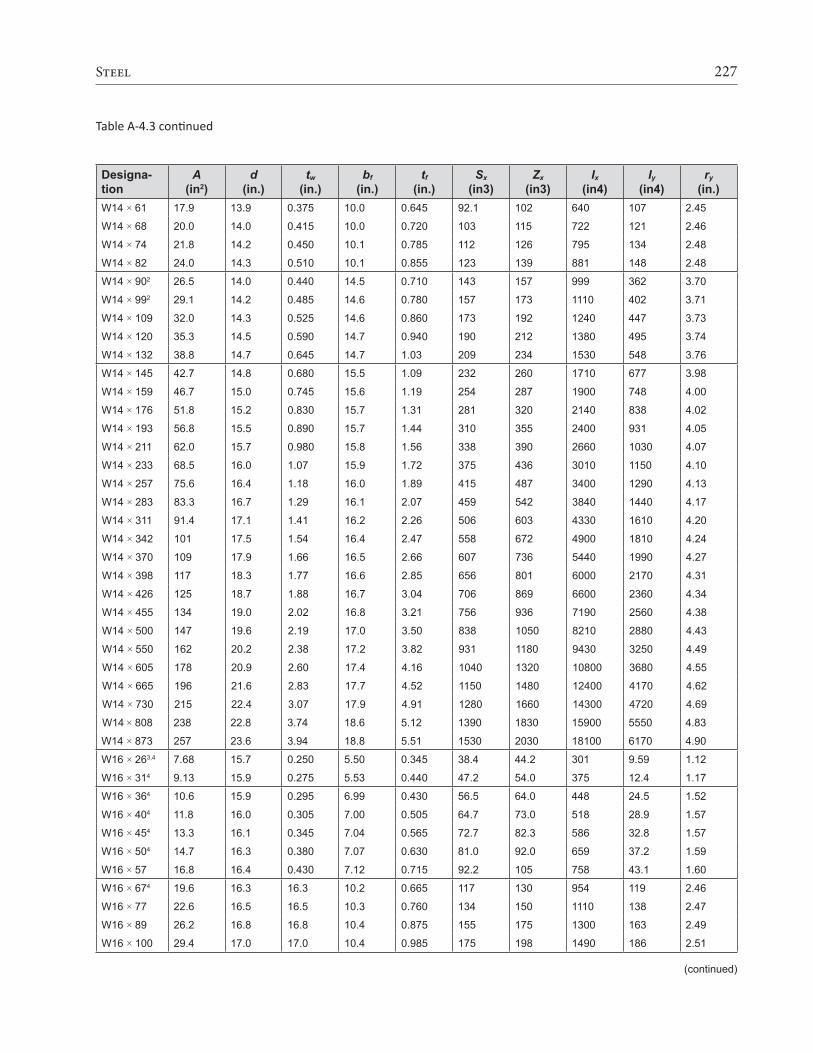
227Steel
Designa-tion
A(in2)
d(in.)
tw
(in.)bf
(in.)tf
(in.)Sx
(in3)Zx
(in3)Ix
(in4)Iy
(in4)ry
(in.)W14 × 61 17.9 13.9 0.375 10.0 0.645 92.1 102 640 107 2.45
W14 × 68 20.0 14.0 0.415 10.0 0.720 103 115 722 121 2.46
W14 × 74 21.8 14.2 0.450 10.1 0.785 112 126 795 134 2.48
W14 × 82 24.0 14.3 0.510 10.1 0.855 123 139 881 148 2.48
W14 × 902 26.5 14.0 0.440 14.5 0.710 143 157 999 362 3.70
W14 × 992 29.1 14.2 0.485 14.6 0.780 157 173 1110 402 3.71
W14 × 109 32.0 14.3 0.525 14.6 0.860 173 192 1240 447 3.73
W14 × 120 35.3 14.5 0.590 14.7 0.940 190 212 1380 495 3.74
W14 × 132 38.8 14.7 0.645 14.7 1.03 209 234 1530 548 3.76
W14 × 145 42.7 14.8 0.680 15.5 1.09 232 260 1710 677 3.98
W14 × 159 46.7 15.0 0.745 15.6 1.19 254 287 1900 748 4.00
W14 × 176 51.8 15.2 0.830 15.7 1.31 281 320 2140 838 4.02
W14 × 193 56.8 15.5 0.890 15.7 1.44 310 355 2400 931 4.05
W14 × 211 62.0 15.7 0.980 15.8 1.56 338 390 2660 1030 4.07
W14 × 233 68.5 16.0 1.07 15.9 1.72 375 436 3010 1150 4.10
W14 × 257 75.6 16.4 1.18 16.0 1.89 415 487 3400 1290 4.13
W14 × 283 83.3 16.7 1.29 16.1 2.07 459 542 3840 1440 4.17
W14 × 311 91.4 17.1 1.41 16.2 2.26 506 603 4330 1610 4.20
W14 × 342 101 17.5 1.54 16.4 2.47 558 672 4900 1810 4.24
W14 × 370 109 17.9 1.66 16.5 2.66 607 736 5440 1990 4.27
W14 × 398 117 18.3 1.77 16.6 2.85 656 801 6000 2170 4.31
W14 × 426 125 18.7 1.88 16.7 3.04 706 869 6600 2360 4.34
W14 × 455 134 19.0 2.02 16.8 3.21 756 936 7190 2560 4.38
W14 × 500 147 19.6 2.19 17.0 3.50 838 1050 8210 2880 4.43
W14 × 550 162 20.2 2.38 17.2 3.82 931 1180 9430 3250 4.49
W14 × 605 178 20.9 2.60 17.4 4.16 1040 1320 10800 3680 4.55
W14 × 665 196 21.6 2.83 17.7 4.52 1150 1480 12400 4170 4.62
W14 × 730 215 22.4 3.07 17.9 4.91 1280 1660 14300 4720 4.69
W14 × 808 238 22.8 3.74 18.6 5.12 1390 1830 15900 5550 4.83
W14 × 873 257 23.6 3.94 18.8 5.51 1530 2030 18100 6170 4.90
W16 × 263,4 7.68 15.7 0.250 5.50 0.345 38.4 44.2 301 9.59 1.12
W16 × 314 9.13 15.9 0.275 5.53 0.440 47.2 54.0 375 12.4 1.17
W16 × 364 10.6 15.9 0.295 6.99 0.430 56.5 64.0 448 24.5 1.52
W16 × 404 11.8 16.0 0.305 7.00 0.505 64.7 73.0 518 28.9 1.57
W16 × 454 13.3 16.1 0.345 7.04 0.565 72.7 82.3 586 32.8 1.57
W16 × 504 14.7 16.3 0.380 7.07 0.630 81.0 92.0 659 37.2 1.59
W16 × 57 16.8 16.4 0.430 7.12 0.715 92.2 105 758 43.1 1.60
W16 × 674 19.6 16.3 16.3 10.2 0.665 117 130 954 119 2.46
W16 × 77 22.6 16.5 16.5 10.3 0.760 134 150 1110 138 2.47
W16 × 89 26.2 16.8 16.8 10.4 0.875 155 175 1300 163 2.49
W16 × 100 29.4 17.0 17.0 10.4 0.985 175 198 1490 186 2.51
Table A-4.3 continued
(continued)

228 Structural Elements for Architects and Builders
Designa-tion
A(in2)
d(in.)
tw
(in.)bf
(in.)tf
(in.)Sx
(in3)Zx
(in3)Ix
(in4)Iy
(in4)ry
(in.)W18 × 354 10.3 17.7 0.300 6.00 0.425 57.6 66.5 510 15.3 1.22
W18 × 404 11.8 17.9 0.315 6.02 0.525 68.4 78.4 612 19.1 1.27
W18 × 464 13.5 18.1 0.360 6.06 0.605 78.8 90.7 712 22.5 1.29
W18 × 504 14.7 18.0 0.355 7.50 0.570 88.9 101 800 40.1 1.65
W18 × 554 16.2 18.1 0.390 7.53 0.630 98.3 112 890 44.9 1.67
W18 × 604 17.6 18.2 0.415 7.56 0.695 108 123 984 50.1 1.68
W18 × 65 19.1 18.4 0.450 7.59 0.750 117 133 1070 54.8 1.69
W18 × 71 20.9 18.5 0.495 7.64 0.810 127 146 1170 60.3 1.70
W18 × 764 22.3 18.2 0.425 11.0 0.680 146 163 1330 152 2.61
W18 × 86 25.3 18.4 0.480 11.1 0.770 166 186 1530 175 2.63
W18 × 97 28.5 18.6 0.535 11.1 0.870 188 211 1750 201 2.65
W18 × 106 31.1 18.7 0.590 11.2 0.940 204 230 1910 220 2.66
W18 × 119 35.1 19.0 0.655 11.3 1.06 231 262 2190 253 2.69
W18 × 130 38.3 19.3 0.670 11.2 1.20 256 290 2460 278 2.70
W18 × 143 42.0 19.5 0.730 11.2 1.32 282 322 2750 311 2.72
W18 × 158 46.3 19.7 0.810 11.3 1.44 310 356 3060 347 2.74
W18 × 175 51.4 20.0 0.890 11.4 1.59 344 398 3450 391 2.76
W18 × 192 56.2 20.4 0.960 11.5 1.75 380 442 3870 440 2.79
W18 × 211 62.3 20.7 1.06 11.6 1.91 419 490 4330 493 2.82
W18 × 234 68.8 21.1 1.16 11.7 2.11 466 549 4900 558 2.85
W18 × 258 76.0 21.5 1.28 11.8 2.30 514 611 5510 628 2.88
W18 × 283 83.3 21.9 1.40 11.9 2.50 565 676 6170 704 2.91
W18 × 311 91.6 22.3 1.52 12.0 2.74 624 754 6970 795 2.95
W21 × 444 13.0 20.7 0.350 6.50 0.450 81.6 95.4 843 20.7 1.26
W21 × 504 14.7 20.8 0.380 6.53 0.535 94.5 110 984 24.9 1.30
W21 × 574 16.7 21.1 0.405 6.56 0.650 111 129 1170 30.6 1.35
W21 × 482,4 14.1 20.6 0.350 8.14 0.430 93.0 107 959 38.7 1.66
W21 × 554 16.2 20.8 0.375 8.22 0.522 110 126 1140 48.4 1.73
W21 × 624 18.3 21.0 0.400 8.24 0.615 127 144 1330 57.5 1.77
W21 × 684 20.0 21.1 0.430 8.27 0.685 140 160 1480 64.7 1.80
W21 × 734 21.5 21.2 0.455 8.30 0.740 151 172 1600 70.6 1.81
W21 × 834 24.4 21.4 0.515 8.36 0.835 171 196 1830 81.4 1.83
W21 × 93 27.3 21.6 0.580 8.42 0.930 192 221 2070 92.9 1.84
W21 × 1014 29.8 21.4 0.500 12.3 0.800 227 253 2420 248 2.89
W21 × 111 32.6 21.5 0.550 12.3 0.875 249 279 2670 274 2.90
W21 × 122 35.9 21.7 0.600 12.4 0.960 273 307 2960 305 2.92
W21 × 132 38.8 21.8 0.650 12.4 1.04 295 333 3220 333 2.93
W21 × 147 43.2 22.1 0.720 12.5 1.15 329 373 3630 376 2.95
W21 × 166 48.8 22.5 0.750 12.4 1.36 380 432 4280 435 2.99
W21 × 182 53.6 22.7 0.830 12.5 1.48 417 476 4730 483 3.00
W21 × 201 59.3 23.0 0.910 12.6 1.63 461 530 5310 542 3.02
Table A-4.3 continued
(continued)

229Steel
Designa-tion
A(in2)
d(in.)
tw
(in.)bf
(in.)tf
(in.)Sx
(in3)Zx
(in3)Ix
(in4)Iy
(in4)ry
(in.)W21 × 223 66.5 23.4 1.00 12.7 1.79 520 601 6080 614 3.04
W21 × 248 73.8 23.7 1.10 12.8 1.99 576 671 6830 699 3.08
W21 × 275 81.8 24.1 1.22 12.9 2.19 638 749 7690 787 3.10
W24 × 553,4 16.2 23.6 0.395 7.01 0.505 114 134 1350 29.1 1.34
W24 × 624 18.2 23.7 0.430 7.04 0.590 131 153 1550 34.5 1.38
W24 × 684 20.1 23.7 0.415 8.97 0.585 154 177 1830 70.4 1.87
W24 × 764 22.4 23.9 0.440 8.99 0.680 176 200 2100 82.5 1.92
W24 × 844 24.7 24.1 0.470 9.02 0.770 196 224 2370 94.4 1.95
W24 × 944 27.7 24.3 0.515 9.07 0.875 222 254 2700 109 1.98
W24 × 1034 30.3 24.5 0.550 9.00 0.980 245 280 3000 119 1.99
W24 × 1044 30.7 24.1 0.500 12.8 0.750 258 289 3100 259 2.91
W24 × 1174 34.4 24.3 0.550 12.8 0.850 291 327 3540 297 2.94
W24 × 131 38.6 24.5 0.605 12.9 0.960 329 370 4020 340 2.97
W24 × 146 43.0 24.7 0.650 12.9 1.09 371 418 4580 391 3.01
W24 × 162 47.8 25.0 0.705 13.0 1.22 414 468 5170 443 3.05
W24 × 176 51.7 25.2 0.750 12.9 1.34 450 511 5680 479 3.04
W24 × 192 56.5 25.5 0.810 13.0 1.46 491 559 6260 530 3.07
W24 × 207 60.7 25.7 0.870 13.0 1.57 531 606 6820 578 3.08
W24 × 229 67.2 26.0 0.960 13.1 1.73 588 675 7650 651 3.11
W24 × 250 73.5 26.3 1.04 13.2 1.89 644 744 8490 724 3.14
W24 × 279 81.9 26.7 1.16 13.3 2.09 718 835 9600 823 3.17
W24 × 306 89.7 27.1 1.26 13.4 2.28 789 922 10700 919 3.20
W24 × 335 98.3 27.5 1.38 13.5 2.48 864 1020 11900 1030 3.23
W24 × 370 109 28.0 1.52 13.7 2.72 957 1130 13400 1160 3.27
W27 × 844 24.7 26.7 0.460 10.0 0.640 213 244 2850 106 2.07
W27 × 944 27.6 26.9 0.490 10.0 0.745 243 278 3270 124 2.12
W27 × 1024 30.0 27.1 0.515 10.0 0.830 267 305 3620 139 2.15
W27 × 1144 33.6 27.3 0.570 10.1 0.930 299 343 4080 159 2.18
W27 × 1294 37.8 27.6 0.610 10.0 1.10 345 395 4760 184 2.21
W27 × 1464 43.2 27.4 0.605 14.0 0.975 414 464 5660 443 3.20
W27 × 1614 47.6 27.6 0.660 14.0 1.08 458 515 6310 497 3.23
W27 × 178 52.5 27.8 0.725 14.1 1.19 505 570 7020 555 3.25
W27 × 194 57.1 28.1 0.750 14.0 1.34 559 631 7860 619 3.29
W27 × 217 63.9 28.4 0.830 14.1 1.50 627 711 8910 704 3.32
W27 × 235 69.4 28.7 0.910 14.2 1.61 677 772 9700 769 3.33
W27 × 258 76.1 29.0 0.980 14.3 1.77 745 852 10800 859 3.36
W27 × 281 83.1 29.3 1.06 14.4 1.93 814 936 11900 953 3.39
W27 × 307 90.2 29.6 1.16 14.4 2.09 887 1030 13100 1050 3.41
W27 × 336 99.2 30.0 1.26 14.6 2.28 972 1130 14600 1180 3.45
W27 × 368 109 30.4 1.38 14.7 2.48 1060 1240 16200 1310 3.48
W27 × 539 159 32.5 1.97 15.3 3.54 1570 1890 25600 2110 3.65
(continued)
Table A-4.3 continued

230 Structural Elements for Architects and Builders
Designa-tion
A(in2)
d(in.)
tw
(in.)bf
(in.)tf
(in.)Sx
(in3)Zx
(in3)Ix
(in4)Iy
(in4)ry
(in.)W30 × 903,4 26.3 29.5 0.470 10.4 0.610 245 283 3610 115 2.09
W30 × 994 29.0 29.7 0.520 10.5 0.670 269 312 3990 128 2.10
W30 × 1084 31.7 29.8 0.545 10.5 0.760 299 346 4470 146 2.15
W30 × 1164 34.2 30.0 0.565 10.5 0.850 329 378 4930 164 2.19
W30 × 1244 36.5 30.2 0.585 10.5 0.930 355 408 5360 181 2.23
W30 × 1324 38.8 30.3 0.615 10.5 1.00 380 437 5770 196 2.25
W30 × 1484 43.6 30.7 0.650 10.5 1.18 436 500 6680 227 2.28
W30 × 1734 50.9 30.4 0.655 15.0 1.07 541 607 8230 598 3.42
W30 × 1914 56.1 30.7 0.710 15.0 1.19 600 675 9200 673 3.46
W30 × 211 62.3 30.9 0.775 15.1 1.32 665 751 10300 757 3.49
W30 × 235 69.3 31.3 0.830 15.1 1.50 748 847 11700 855 3.51
W30 × 261 77.0 31.6 0.930 15.2 1.65 829 943 13100 959 3.53
W30 × 292 86.0 32.0 1.02 15.3 1.85 930 1060 14900 1100 3.58
W30 × 326 95.9 32.4 1.14 15.4 2.05 1040 1190 16800 1240 3.60
W30 × 357 105 32.8 1.24 15.5 2.24 1140 1320 18700 1390 3.64
W30 × 391 115 33.2 1.36 15.6 2.44 1250 1450 20700 1550 3.67
W33 × 1183,4 34.7 32.9 0.550 11.5 0.740 359 415 5900 187 2.32
W33 × 1304 38.3 33.1 0.580 11.5 0.855 406 467 6710 218 2.39
W33 × 1414 41.5 33.3 0.605 11.5 0.960 448 514 7450 246 2.43
W33 × 1524 44.9 33.5 0.635 11.6 1.06 487 559 8160 273 2.47
W33 × 1694 49.5 33.8 0.670 11.5 1.22 549 629 9290 310 2.50
W33 × 2014 59.1 33.7 0.715 15.7 1.15 686 773 11600 749 3.56
W33 × 2214 65.3 33.9 0.775 15.8 1.28 759 857 12900 840 3.59
W33 × 2414 71.1 34.2 0.830 15.9 1.40 831 940 14200 933 3.62
W33 × 263 77.4 34.5 0.870 15.8 1.57 919 1040 15900 1040 3.66
W33 × 291 85.6 34.8 0.960 15.9 1.73 1020 1160 17700 1160 3.68
W33 × 318 93.7 35.2 1.04 16.0 1.89 1110 1270 19500 1290 3.71
W33 × 354 104 35.6 1.16 16.1 2.09 1240 1420 22000 1460 3.74
W33 × 387 114 36.0 1.26 16.2 2.28 1350 1560 24300 1620 3.77
W36 × 1353,4 39.9 35.6 0.600 12.0 0.790 439 509 7800 225 2.38
W36 × 1504 44.3 35.9 0.625 12.0 0.940 504 581 9040 270 2.47
W36 × 1604 47.0 36.0 0.650 12.0 1.02 542 624 9760 295 2.50
W36 × 1704 50.0 36.2 0.680 12.0 1.10 581 668 10500 320 2.53
W36 × 1824 53.6 36.3 0.725 12.1 1.18 623 718 11300 347 2.55
W36 × 1944 57.0 36.5 0.765 12.1 1.26 664 767 12100 375 2.56
W36 × 2104 61.9 36.7 0.830 12.2 1.36 719 833 13200 411 2.58
W36 × 2324 68.0 37.1 0.870 12.1 1.57 809 936 15000 468 2.62
W36 × 256 75.3 37.4 0.960 12.2 1.73 895 1040 16800 528 2.65
(continued)
Table A-4.3 continued

231Steel
Designa-tion
A(in2)
d(in.)
tw
(in.)bf
(in.)tf
(in.)Sx
(in3)Zx
(in3)Ix
(in4)Iy
(in4)ry
(in.)W36 × 2314 68.2 36.5 0.760 16.5 1.26 854 963 15600 940 3.71
W36 × 2474 72.5 36.7 0.800 16.5 1.35 913 1030 16700 1010 3.74
W36 × 2624 77.2 36.9 0.840 16.6 1.44 972 1100 17900 1090 3.76
W36 × 2824 82.9 37.1 0.885 16.6 1.57 1050 1190 19600 1200 3.80
W36 × 302 89.0 37.3 0.945 16.7 1.68 1130 1280 21100 1300 3.82
W36 × 330 96.9 37.7 1.02 16.6 1.85 1240 1410 23300 1420 3.83
W36 × 361 106 38.0 1.12 16.7 2.01 1350 1550 25700 1570 3.85
W36 × 395 116 38.4 1.22 16.8 2.20 1490 1710 28500 1750 3.88
W36 × 441 130 38.9 1.36 17.0 2.44 1650 1910 32100 1990 3.92
W36 × 487 143 39.3 1.50 17.1 2.68 1830 2130 36000 2250 3.96
W36 × 529 156 39.8 1.61 17.2 2.91 1990 2330 39600 2490 4.00
W36 × 652 192 41.1 1.97 17.6 3.54 2460 2910 50600 3230 4.10
W36 × 723 213 41.8 2.17 17.8 3.90 2740 3270 57300 3700 4.17
W36 × 802 236 42.6 2.38 18.0 4.29 3040 3660 64800 4210 4.22
W36 × 853 251 43.1 2.52 18.2 4.53 3250 3920 70000 4600 4.28
W36 × 925 272 43.1 3.02 18.6 4.53 3390 4130 73000 4940 4.26
W40 × 1493,4 43.8 38.2 0.630 11.8 0.830 513 598 9800 229 2.29
W40 × 1674 49.3 38.6 0.650 11.8 1.03 600 693 11600 283 2.40
W40 × 1834 53.3 39.0 0.650 11.8 1.20 675 774 13200 331 2.49
W40 × 2114 62.1 39.4 0.750 11.8 1.42 786 906 15500 390 2.51
W40 × 2354 69.1 39.7 0.830 11.9 1.58 875 1010 17400 444 2.54
W40 × 264 77.4 40.0 0.960 11.9 1.73 971 1130 19400 493 2.52
W40 × 278 82.3 40.2 1.03 12.0 1.81 1020 1190 20500 521 2.52
W40 × 294 86.2 40.4 1.06 12.0 1.93 1080 1270 21900 562 2.55
W40 × 327 95.9 40.8 1.18 12.1 2.13 1200 1410 24500 640 2.58
W40 × 331 97.7 40.8 1.22 12.2 2.13 1210 1430 24700 644 2.57
W40 × 392 116 41.6 1.42 12.4 2.52 1440 1710 29900 803 2.64
W40 × 1994 58.8 38.7 0.650 15.8 1.07 770 869 14900 695 3.45
W40 × 2154 63.5 39.0 0.650 15.8 1.22 859 964 16700 796 3.54
W40 × 2494 73.5 39.4 0.750 15.8 1.42 993 1120 19600 926 3.55
W40 × 2774 81.5 39.7 0.830 15.8 1.58 1100 1250 21900 1040 3.58
W40 × 2974 87.3 39.8 0.930 15.8 1.65 1170 1330 23200 1090 3.54
W40 × 324 95.3 40.2 1.00 15.9 1.81 1280 1460 25600 1220 3.58
W40 × 362 106 40.6 1.12 16.0 2.01 1420 1640 28900 1380 3.60
W40 × 372 110 40.6 1.16 16.1 2.05 1460 1680 29600 1420 3.60
W40 × 397 117 41.0 1.22 16.1 2.20 1560 1800 32000 1540 3.64
W40 × 431 127 41.3 1.34 16.2 2.36 1690 1960 34800 1690 3.65
W40 × 503 148 42.1 1.54 16.4 2.76 1980 2320 41600 2040 3.72
W40 × 593 174 43.0 1.79 16.7 3.23 2340 2760 50400 2520 3.80
W40 × 655 193 43.6 1.97 16.9 3.54 2590 3080 56500 2870 3.86
Table A-4.3 continued
(continued)

232 Structural Elements for Architects and Builders
Designa-tion
A(in2)
d(in.)
tw
(in.)bf
(in.)tf
(in.)Sx
(in3)Zx
(in3)Ix
(in4)Iy
(in4)ry
(in.)W44 × 2303,4 67.8 42.9 0.710 15.8 1.22 971 1100 20800 796 3.43
W44 × 2624 77.2 43.3 0.785 15.8 1.42 1110 1270 24100 923 3.47
W44 × 2904 85.4 43.6 0.865 15.8 1.58 1240 1410 27000 1040 3.49
W44 × 3354 98.5 44.0 1.03 15.9 1.77 1410 1620 31100 1200 3.49
Notes:1. Section not compact for steel with Fy = 36 ksi or Fy = 50 ksi.2. Section compact for steel with Fy = 36 ksi, but not compact for steel with Fy = 50 ksi.3. Section webs do not meet slenderness criteria for shear for which the allowable stress can be taken as Fv = 0.4Fy; instead, use a reduced allowable shear stress, Fv = 0.36Fy.4. Section is slender for compression with Fy = 50 ksi.5. W-shapes are grouped together with common inner roller dimensions (i.e., web "lengths" excluding fillets)
Table A-4.3 continued

233Steel
Table A-4.4: Dimensions and properties of steel C and MC channels Cross-sectional area = A Dimension to y-axis = x Moment of inertia = I Section modulus, Sx = 2Ix /d Radius of gyration, rx = √ Ix /A Radius of gyration, ry = √ Iy /A
Designation A (in2) d (in.) tw (in.) bf (in.) x (in.) Ix (in4) Iy (in4)C3 × 3.5 1.09 3.00 0.132 1.37 0.443 1.57 0.169
C3 × 4.1 1.20 3.00 0.170 1.41 0.437 1.65 0.191
C3 × 5 1.47 3.00 0.258 1.50 0.439 1.85 0.241
C3 × 6 1.76 3.00 0.356 1.60 0.455 2.07 0.300
C4 × 4.5 1.38 4.00 0.125 1.58 0.493 3.65 0.289
C4 × 5.4 1.58 4.00 0.184 1.58 0.457 3.85 0.312
C4 × 6.25 1.77 4.00 0.247 1.65 0.435 4.00 0.345
C4 × 7.25 2.13 4.00 0.321 1.72 0.459 4.58 0.425
C5 × 6.7 1.97 5.00 0.190 1.75 0.484 7.48 0.470
C5 × 9 2.64 5.00 0.325 1.89 0.478 8.89 0.624
C6 × 8.2 2.39 6.00 0.200 1.92 0.512 13.1 0.687
C6 × 10.5 3.08 6.00 0.314 2.03 0.500 15.1 0.860
C6 × 13 3.81 6.00 0.437 2.16 0.514 17.3 1.05
C7 × 9.8 2.87 7.00 0.210 2.09 0.541 21.2 0.957
C7 × 12.25 3.59 7.00 0.314 2.19 0.525 24.2 1.16
C7 × 14.75 4.33 7.00 0.419 2.30 0.532 27.2 1.37
C8 × 11.5 3.37 8.00 0.220 2.26 0.572 32.5 1.31
C8 × 13.75 4.03 8.00 0.303 2.34 0.554 36.1 1.52
C8 × 18.75 5.51 8.00 0.487 2.53 0.565 43.9 1.97
C9 × 13.4 3.94 9.00 0.233 2.43 0.601 47.8 1.75
C9 × 15 4.41 9.00 0.285 2.49 0.586 51.0 1.91
C9 × 20 5.87 9.00 0.448 2.65 0.583 60.9 2.41
C10 × 15.3 4.48 10.0 0.240 2.60 0.634 67.3 2.27
C10 × 20 5.87 10.0 0.379 2.74 0.606 78.9 2.80
C10 × 25 7.34 10.0 0.526 2.89 0.617 91.1 3.34
C10 × 30 8.81 10.0 0.673 3.03 0.649 103 3.93
C12 × 20.7 6.08 12.0 0.282 2.94 0.698 129 3.86
C12 × 25 7.34 12.0 0.387 3.05 0.674 144 4.45
C12 × 30 8.81 12.0 0.510 3.17 0.674 162 5.12
C15 × 33.9 10.0 15.0 0.400 3.40 0.788 315 8.07
C15 × 40 11.8 15.0 0.520 3.52 0.778 348 9.17
C15 × 50 14.7 15.0 0.716 3.72 0.799 404 11.0
Dep
th, d
Flange width, bf
y
x
Web thickness, tw
x
(continued)

234 Structural Elements for Architects and Builders
Designation A (in2) d (in.) tw (in.) bf (in.) x (in.) Ix (in4) Iy (in4)MC3 × 7.1 2.11 3.00 0.312 1.94 0.653 2.72 0.666
MC4 × 13.8 4.03 4.00 0.500 2.50 0.849 8.85 2.13
MC6 × 6.5 1.95 6.00 0.155 1.85 0.513 11.0 0.565
MC6 × 7 2.09 6.00 0.179 1.88 0.501 11.4 0.603
MC6 × 12 3.53 6.00 0.310 2.50 0.704 18.7 1.85
MC6 × 15.1 4.44 6.00 0.316 2.94 0.940 24.9 3.46
MC6 × 16.3 4.79 6.00 0.375 3.00 0.927 26.0 3.77
MC6 × 15.3 4.49 6.00 0.340 3.50 1.05 25.3 4.91
MC6 × 18 5.29 6.00 0.379 3.50 1.12 29.7 5.88
MC7 × 19.1 5.61 7.00 0.352 3.45 1.08 43.1 6.06
MC7 × 22.7 6.67 7.00 0.503 3.60 1.04 47.4 7.24
MC8 × 8.5 2.50 8.00 0.179 1.87 0.428 23.3 0.624
MC8 × 18.7 5.50 8.00 0.353 2.98 0.849 52.4 4.15
MC8 × 20 5.88 8.00 0.400 3.03 0.840 54.4 4.42
MC8 × 21.4 6.28 8.00 0.375 3.45 1.02 61.5 6.58
MC8 × 22.8 6.70 8.00 0.427 3.50 1.01 63.8 7.01
MC9 × 23.9 7.02 9.00 0.400 3.45 0.981 84.9 7.14
MC9 × 25.4 7.47 9.00 0.450 3.50 0.970 87.9 7.57
MC10 × 6.51 1.95 10.0 0.152 1.17 0.194 22.9 0.133
MC10 × 8.41 2.46 10.0 0.170 1.50 0.284 31.9 0.326
MC10 × 22 6.45 10.00 0.290 3.32 0.990 102 6.40
MC10 × 25 7.35 10.0 0.380 3.41 0.953 110 7.25
MC10 × 28.5 8.37 10.0 0.425 3.95 1.12 126 11.3
MC10 × 33.6 9.87 10.0 0.575 4.10 1.09 139 13.1
MC10 × 41.1 12.1 10.0 0.796 4.32 1.09 157 15.7
MC12 × 10.61 3.10 12.0 0.190 1.50 0.269 55.3 0.378
MC12 × 14.3 4.18 12.0 0.250 2.12 0.377 76.1 1.00
MC12 × 31 9.12 12.0 0.370 3.67 1.08 202 11.3
MC12 × 35 10.3 12.0 0.465 3.77 1.05 216 12.6
MC12 × 40 11.8 12.0 0.590 3.89 1.04 234 14.2
MC12 × 45 13.2 12.0 0.710 4.01 1.04 251 15.8
MC12 × 50 14.7 12.0 0.835 4.14 1.05 269 17.4
MC13 × 31.8 9.35 13.0 0.375 4.00 1.00 239 11.4
MC13 × 35 10.3 13.0 0.447 4.07 0.980 252 12.3
MC13 × 40 11.8 13.0 0.560 4.19 0.963 273 13.7
MC13 × 50 14.7 13.0 0.787 4.41 0.974 314 16.4
MC18 × 42.7 12.6 18.0 0.450 3.95 0.877 554 14.3
MC18 × 45.8 13.5 18.0 0.500 4.00 0.866 578 14.9
MC18 × 51.9 15.3 18.0 0.600 4.10 0.858 627 16.3
MC18 × 58 17.1 18.0 0.700 4.20 0.862 675 17.6
Note:1. Section is slender for compression with Fy = 36 ksi.
Table A-4.4 continued

235Steel
Table A-4.5: Dimensions and properties of selected steel L anglesA. Angles with equal legs Cross-sectional area = A Dimension to x- or y-axis = x Moment of inertia = I Radius of gyration, rx = ry = √ Ix /A Radius of gyration, rz = √ Iz /A
Designation A (in2) d (in.) tw (in.) x (in.) Ix or Iy (in4) Iz (in4)L2 × 2 × 1/81,2 0.491 2.00 0.1250 0.534 0.189 0.0751
L2 × 2 × 1/4 0.944 2.00 0.2500 0.586 0.346 0.141
L2 × 2 × 5/16 1.16 2.00 0.3125 0.609 0.414 0.173
L2 × 2 × 3/8 1.37 2.00 0.3750 0.632 0.476 0.203
L3 × 3 × 3/161,2 1.09 3.00 0.1875 0.812 0.948 0.374
L3 × 3 × 1/4 1.44 3.00 0.2500 0.836 1.23 0.491
L3 × 3 × 3/8 2.11 3.00 0.3750 0.884 1.75 0.712
L3 × 3 × 1/2 2.76 3.00 0.5000 0.929 2.20 0.924
L4 × 4 × 1/41,2 1.93 4.00 0.2500 1.08 3.00 1.18
L4 × 4 × 3/8 2.86 4.00 0.3750 1.13 4.32 1.73
L4 × 4 × 1/2 3.75 4.00 0.5000 1.18 5.52 2.25
L4 × 4 × 3/4 5.44 4.00 0.7500 1.27 7.62 3.25
L5 × 5 × 5/161,2 3.07 5.00 0.3125 1.35 7.44 3.01
L5 × 5 × 7/16 4.22 5.00 0.4375 1.40 10.0 4.08
L5 × 5 × 5/8 5.90 5.00 0.6250 1.47 13.6 5.61
L5 × 5 × 7/8 8.00 5.00 0.8750 1.56 17.8 7.56
L6 × 6 × 5/161,2 3.67 6.00 0.3125 1.60 13.0 5.20
L6 × 6 × 1/2 5.77 6.00 0.5000 1.67 19.9 8.04
L6 × 6 × 3/4 8.46 6.00 0.7500 1.77 28.1 11.6
L6 × 6 × 1 11.0 6.00 1.0000 1.86 35.4 15.0
L8 × 8 × 1/21,2 7.84 8.00 0.5000 2.17 48.8 19.7
L8 × 8 × 5/8 9.69 8.00 0.6250 2.21 59.6 24.2
L8 × 8 × 7/8 13.3 8.00 0.8750 2.31 79.7 32.7
L8 × 8 × 1⅛ 16.8 8.00 1.1250 2.40 98.1 40.9
tw
x
yd
d
y
zx
t w
(continued)

236 Structural Elements for Architects and Builders
B. Angles with unequal legs Cross-sectional area = A Dimension to y-axis = x Dimension to x-axis = y Moment of inertia = I Radius of gyration, rx = √ Ix /A Radius of gyration, ry = √ Iy /A Radius of gyration, rz = √ Iz /A
Designation A (in2) d(in.)
b(in.)
tw (in.) x(in.)
y(in.)
Ix
(in4)Iy
(in4)Iz
(in4)α(°)
L3 × 2 × 1/4 1.20 3.00 2.00 0.2500 0.487 0.980 1.09 0.390 0.223 23.6
L3 × 2 × 5/16 1.48 3.00 2.00 0.3125 0.511 1.01 1.32 0.467 0.271 23.4
L3 × 2 × 3/8 1.75 3.00 2.00 0.3750 0.535 1.03 1.54 0.539 0.318 23.1
L3 × 2 × 1/2 2.26 3.00 2.00 0.5000 0.580 1.08 1.92 0.667 0.409 22.4
L3 × 2½ × 1/4 1.32 3.00 2.50 0.2500 0.653 0.900 1.16 0.734 0.356 34.3
L3 × 2½ × 5/16 1.63 3.00 2.50 0.3125 0.677 0.925 1.41 0.888 0.437 34.2
L3 × 2½ × 3/8 1.93 3.00 2.50 0.3750 0.701 0.949 1.65 1.03 0.514 34.0
L3 × 2½ × 1/2 2.50 3.00 2.50 0.5000 0.746 0.995 2.07 1.29 0.666 33.7
L3½ × 2½ × 1/42 1.45 3.50 2.50 0.2500 0.607 1.10 1.81 0.775 0.425 26.7
L3½ × 2½ × 5/16 1.79 3.50 2.50 0.3125 0.632 1.13 2.20 0.937 0.518 26.6
L3½ × 2½ × 3/8 2.12 3.50 2.50 0.3750 0.655 1.15 2.56 1.09 0.608 26.3
L3-½ × 2½ × 1/2 2.77 3.50 2.50 0.5000 0.701 1.20 3.24 1.36 0.782 25.9
L4 × 3 × 1/41,2 1.69 4.00 3.00 0.2500 0.725 1.22 2.75 1.33 0.691 29.2
L4 × 3 × 3/8 2.49 4.00 3.00 0.3750 0.775 1.27 3.94 1.89 1.01 28.9
L4 × 3 × 1/2 3.25 4.00 3.00 0.5000 0.822 1.32 5.02 2.40 1.30 28.5
L4 × 3 × 5/8 3.99 4.00 3.00 0.6250 0.867 1.37 6.01 2.85 1.59 28.1
L4 × 3½ × 1/41,2 1.82 4.00 3.50 0.2500 0.897 1.14 2.89 2.07 0.950 37.2
L4 × 3½ × 5/16 2.25 4.00 3.50 0.3125 0.923 1.17 3.53 2.52 1.17 37.1
L4 × 3½ × 3/8 2.68 4.00 3.50 0.3750 0.947 1.20 4.15 2.96 1.38 37.1
L4 × 3½ × 1/2 3.50 4.00 3.50 0.5000 0.994 1.24 5.30 3.76 1.808 36.9
L5 × 3 × 1/41,2 1.94 5.00 3.00 0.2500 0.648 1.64 5.09 1.41 0.825 20.4
L5 × 3 × 5/161,2 2.41 5.00 3.00 0.3125 0.673 1.67 6.24 1.72 1.01 20.2
L5 × 3 × 3/82 2.86 5.00 3.00 0.3750 0.698 1.69 7.35 2.01 1.20 20.0
L5 × 3 × 1/2 3.75 5.00 3.00 0.5000 0.746 1.74 9.43 2.55 1.55 19.6
L5 × 3½ × 1/41,2 2.07 5.00 3.50 0.2500 0.804 1.55 5.36 2.20 1.19 26.1
L5 × 3½ × 3/82 3.05 5.00 3.50 0.3750 0.854 1.60 7.75 3.15 1.74 25.9
L5 × 3½ × 1/2 4.00 5.00 3.50 0.5000 0.901 1.65 9.96 4.02 2.25 25.6
L5 × 3½ × 3/4 5.85 5.00 3.50 0.7500 0.993 1.74 13.9 5.52 3.22 24.9
L6 × 3½ × 5/161,2 2.89 6.00 3.50 0.3125 0.756 2.00 10.9 2.84 1.70 19.4
L6 × 3½ × 3/81,2 3.44 6.00 3.50 0.3750 0.781 2.02 12.9 3.33 2.00 19.2
L6 × 3½ × 1/2 4.50 6.00 3.50 0.5000 0.829 2.07 16.6 4.24 2.58 18.9
tw
x
yd
b
y
zx
t w
Table A-4.5 continued
(continued)

237Steel
Designation A (in2) d(in.)
b(in.)
tw (in.) x(in.)
y(in.)
Ix
(in4)Iy
(in4)Iz
(in4)α(°)
L6 × 4 × 3/81,2 3.61 6.00 4.00 0.3750 0.933 1.93 13.4 4.86 2.73 24.0
L6 × 4 × 1/2 4.75 6.00 4.00 0.5000 0.981 1.98 17.3 6.22 3.55 23.7
L6 × 4 × 5/8 5.86 6.00 4.00 0.6250 1.03 2.03 21.0 7.48 4.32 23.5
L6 × 4 × 7/8 8.00 6.00 4.00 0.8750 1.12 2.12 27.7 9.70 5.82 22.8
L7 × 4 × 3/81,2 4.00 7.00 4.00 0.3750 0.861 2.35 20.5 5.06 3.05 18.7
L7 × 4 × 1/22 5.26 7.00 4.00 0.5000 0.910 2.40 26.6 6.48 3.95 18.5
L7 × 4 × 5/8 6.50 7.00 4.00 0.6250 0.958 2.45 32.4 7.79 4.80 18.2
L7 × 4 × 3/4 7.74 7.00 4.00 0.7500 1.00 2.50 37.8 9.00 5.64 18.0
L8 × 4 × 1/21,2 5.80 8.00 4.00 0.5000 0.854 2.84 38.6 6.75 4.32 14.9
L8 × 4 × 5/8 7.16 8.00 4.00 0.6250 0.902 2.89 47.0 8.11 5.24 14.7
L8 × 4 × 3/4 8.49 8.00 4.00 0.7500 0.949 2.94 55.0 9.37 6.13 14.4
L8 × 4 × 1 11.1 8.00 4.00 1.0000 1.04 3.03 69.7 11.6 7.87 13.9
L8 × 6 × 1/21,2 6.80 8.00 6.00 0.5000 1.46 2.46 44.4 21.7 11.5 29.1
L8 × 6 × 5/8 8.41 8.00 6.00 0.6250 1.51 2.50 54.2 26.4 14.1 29.0
L8 × 6 × 7/8 11.5 8.00 6.00 0.8750 1.60 2.60 72.4 34.9 18.9 28.6
L8 × 6 × 1 13.1 8.00 6.00 1.0000 1.65 2.65 80.9 38.8 21.3 28.5
Notes:1. Section not compact for steel with Fy = 36 ksi.2. Section slender for steel with Fy = 36 ksi.
Table A-4.6: Dimensions and properties of selected steel rectangular and square hollow structural sections (HSS) Cross-sectional area = A Cross-sectional dimensions appear in designation as HSS H × B × t, where: Larger dimension (in.) = H Smaller dimension (in.) = B Nominal wall thickness (in.)1 = t Moment of inertia = I Section modulus, Sx = 2Ix /H Section modulus, Sy = 2Iy /B Radius of gyration, rx = √Ix /A Radius of gyration, ry = √Iy /A
Designation A(in2)
Design wall thickness,
t (in.)1
Sx
(in3)Zx
(in3)Ix
(in4)Iy
(in4)ry
(in.)
HSS2 × 2 × 3/16 1.19 0.174 0.641 0.797 0.641 0.641 0.733
HSS2 × 2 × 1/4 1.51 0.233 0.747 0.964 0.747 0.747 0.704
HSS2½ × 2½ × 3/16 1.54 1.54 1.08 1.32 1.35 1.35 0.937
HSS2½ × 2½ × 5/16 2.35 2.35 1.46 1.88 1.82 1.82 0.880
HSS3 × 3 × 3/16 1.89 0.174 1.64 1.97 2.46 2.46 1.14
HSS3 × 3 × 3/8 3.39 0.349 2.52 3.25 3.78 3.78 1.06
HSS3½ × 3½ × 3/16 2.24 0.174 2.31 2.76 4.05 4.05 1.35
HSS3½ × 3½ × 3/8 4.09 0.349 3.71 4.69 6.49 6.49 1.26
B
H
t
x
y
(continued)
Table A-4.5 continued

238 Structural Elements for Architects and Builders
Designation A(in2)
Design wall thickness,
t (in.)1
Sx
(in3)Zx
(in3)Ix
(in4)Iy
(in4)ry
(in.)
HSS4 × 3 × 3/16 2.24 0.174 2.47 3.00 4.93 3.16 1.19
HSS4 × 3 × 3/8 4.09 0.349 3.97 5.12 7.93 5.01 1.11
HSS4 × 4 × 1/4 3.37 0.233 3.90 4.69 7.80 7.80 1.52
HSS4 × 4 × 1/2 6.02 0.465 5.97 7.70 11.9 11.9 1.41
HSS6 × 4 × 1/4 4.30 0.233 6.96 8.53 20.9 11.1 1.61
HSS6 × 4 × 1/2 7.88 0.465 11.3 14.6 34.0 17.8 1.50
HSS6 × 6 × 1/4 5.24 0.233 9.54 11.2 28.6 28.6 2.34
HSS6 × 6 × 5/8 11.7 0.581 18.4 23.2 55.2 55.2 2.17
HSS8 × 4 × 1/4 5.24 0.233 10.6 13.3 42.5 14.4 1.66
HSS8 × 4 × 5/8 11.7 0.581 20.5 27.4 82.0 26.6 1.51
HSS8 × 8 × 1/42 7.10 0.233 17.7 20.5 70.7 70.7 3.15
HSS8 × 8 × 5/8 16.4 0.581 36.5 44.7 146 146 2.99
HSS12 × 4 × 1/4 7.10 0.233 19.9 25.6 119 21.0 1.72
HSS12 × 4 × 5/8 16.4 0.581 40.8 55.5 245 40.4 1.57
HSS12 × 8 × 1/42 8.96 0.233 30.6 36.6 184 98.8 3.32
HSS12 × 8 × 5/8 21.0 0.581 66.1 82.1 397 210 3.16
HSS12 × 12 × 1/42 10.8 0.233 41.4 47.6 248 248 4.79
HSS12 × 12 × 5/8 25.7 0.581 91.4 109 548 548 4.62
HSS16 × 4 × 5/16 11.1 0.291 38.5 51.1 308 33.2 1.73
HSS16 × 4 × 5/8 21.0 0.581 67.3 92.9 539 54.1 1.60
HSS16 × 8 × 5/16 13.4 0.291 56.4 69.4 451 155 3.40
HSS16 × 8 × 5/8 25.7 0.581 102 129 815 274 3.27
HSS16 × 12 × 5/162 15.7 0.291 74.4 87.7 595 384 4.94
HSS16 × 12 × 5/8 30.3 0.581 136 165 1090 700 4.80
HSS16 × 16 × 3/8 21.5 0.349 109 126 873 873 6.37
HSS16 × 16 × 5/8 35.0 0.581 171 200 1370 1370 6.25
HSS20 × 4 × 3/8 16.0 0.349 65.7 89.3 657 47.6 1.73
HSS20 × 4 × 1/2 20.9 0.465 83.8 115 838 58.7 1.68
HSS20 × 8 × 3/8 18.7 0.349 92.6 117 926 222 3.44
HSS20 × 8 × 5/8 30.3 0.581 144 185 1440 338 3.34
HSS20 × 12 × 3/82 21.5 0.349 120 144 1200 547 5.04
HSS20 × 12 × 5/8 35.0 0.581 188 230 1880 851 4.93
Notes:1. The nominal wall thickness, t, in the designation for an HSS shape (for example, ½ in. or ¼ in.) is different from the "design wall thick-ness," t, which is tabulated for each section and which is permitted to be smaller than the nominal value.2. Section is not compact, based on flange slenderness: use reduced nominal bending strength, Mn, as follows:
Mn = Mp – (Mp – FyS) 3.57bt
Fy
√ E– 4.0 ≤ Mp
Table A-4.6 continued

239Steel
Table A-4.7: Dimensions and properties of selected steel round hollow structural sections (HSS) Cross-sectional area = A Cross-sectional dimensions appear in designation as HSS H × t, where: Diameter (in.) = H Nominal wall thickness (in.)1 = t Moment of inertia = I Section modulus, S = 2I/H Radius of gyration, r = √I/A
Designation A (in2) Design wall thickness, t (in.)1 I (in4) r (in.)HSS1.660 × 0.140 0.625 0.130 0.184 0.543
HSS1.990 × 0.120 0.624 0.111 0.251 0.634
HSS1.990 × 0.188 0.943 0.174 0.355 0.613
HSS2.375 × 0.125 0.823 0.116 0.527 0.800
HSS2.375 × 0.250 1.57 0.233 0.910 0.762
HSS2.500 × 0.125 0.869 0.116 0.619 0.844
HSS2.500 × 0.250 1.66 0.233 1.08 0.806
HSS3.000 × 0.125 1.05 0.116 1.09 1.02
HSS3.000 × 0.250 2.03 0.233 1.95 0.982
HSS3.500 × 0.125 1.23 0.116 1.77 1.20
HSS3.500 × 0.313 2.93 0.291 3.81 1.14
HSS4.000 × 0.125 1.42 0.116 2.67 1.37
HSS4.000 × 0.313 3.39 0.291 5.87 1.32
HSS6.000 × 0.250 4.22 0.233 17.6 2.04
HSS6.000 × 0.500 8.09 0.465 31.2 1.96
HSS8.625 × 0.250 6.14 0.233 54.1 2.97
HSS8.625 × 0.625 14.7 0.581 119 2.85
HSS10.000 × 0.250 7.15 0.233 85.3 3.45
HSS10.000 × 0.625 17.2 0.581 191 3.34
HSS12.750 × 0.375 13.6 0.349 262 4.39
HSS12.750 × 0.500 17.9 0.465 339 4.35
HSS14.000 × 0.375 15.0 0.349 349 4.83
HSS14.000 × 0.625 24.5 0.581 552 4.75
HSS16.000 × 0.375 17.2 0.349 526 5.53
HSS16.000 × 0.625 28.1 0.581 838 5.46
HSS18.000 × 0.500 25.6 0.465 985 6.20
HSS20.000 × 0.500 28.5 0.465 1360 6.91
Note:1. The nominal wall thickness, t, in the designation for an HSS shape (e.g., 0.500 in. or 0.250 in.) is different from the "design wall thick-ness," t, which is tabulated for each section and which is permitted to be smaller than the nominal value.
H
t
x
y

240 Structural Elements for Architects and Builders
Table A-4.8: Dimensions and properties of selected steel pipe Cross-sectional area = A Diameter (in.) = H Moment of inertia = I Section modulus, S = 2I/H Radius of gyration, r = √I/A
Designation A (in2) Design wall thickness, t (in.) Diameter (in.) I (in4) r (in.)Standard weight steel pipe
Pipe 2 Std. 1.02 0.143 2.38 0.627 0.791
Pipe 2½ Std. 1.61 0.189 2.88 1.45 0.952
Pipe 3 Std. 2.07 0.201 3.50 2.85 1.17
Pipe 3½ Std. 2.50 0.211 4.00 4.52 1.34
Pipe 4 Std. 2.96 0.221 4.50 6.82 1.51
Pipe 5 Std. 4.01 0.241 5.56 14.3 1.88
Pipe 6 Std. 5.20 0.261 6.63 26.5 2.25
Pipe 8 Std. 7.85 0.300 8.63 68.1 2.95
Pipe 10 Std. 11.5 0.340 10.8 151 3.68
Pipe 12 Std. 13.7 0.349 12.8 262 4.39
Extra strong steel pipe
Pipe 2 x-Strong 1.40 0.204 2.38 0.827 0.771
Pipe 2½ x-Strong 2.10 0.257 2.88 1.83 0.930
Pipe 3 x-Strong 2.83 0.280 3.50 3.70 1.14
Pipe 3½ x-Strong 3.43 0.296 4.00 5.94 1.31
Pipe 4 x-Strong 4.14 0.315 4.50 9.12 1.48
Pipe 5 x-Strong 5.73 0.349 5.56 19.5 1.85
Pipe 6 x-Strong 7.83 0.403 6.63 38.3 2.20
Pipe 8 x-Strong 11.9 0.465 8.63 100 2.89
Pipe 10 x-Strong 15.1 0.465 10.8 199 3.64
Pipe 12 x-Strong 17.5 0.465 12.8 339 4.35
Double-extra strong steel pipe
Pipe 2 xx-Strong 2.51 0.406 2.38 1.27 0.711
Pipe 2½ xx-Strong 3.83 0.514 2.88 2.78 0.854
Pipe 3 xx-Strong 5.17 0.559 3.50 5.79 1.06
Pipe 4 xx-Strong 7.66 0.628 4.50 14.7 1.39
Pipe 5 xx-Strong 10.7 0.699 5.56 32.2 1.74
Pipe 6 xx-Strong 14.7 0.805 6.63 63.5 2.08
Pipe 8 xx-Strong 20.0 0.816 8.63 154 2.78
H
t
x
y

241Steel
Table A-4.9: Shear lag coefficient, U, for bolted and welded steel connections in tension1
Condition Shear lag coefficient, U DiagramAll parts of the element (e.g., web, flanges, legs) are connected by bolts or welds.
U = 1.0
Transverse welds connecting some, but not all, of the cross-sectional "parts."
U = 1.0, but the net area, An, is taken as only that portion of the element cross section (consisting of flanges, webs, legs, and so on) that is directly connected by the transverse welds.
Longitudinal welds connecting steel plates or other shapes. U = 3l2
3l2 + w2 1 –lx( )
where l = (l1 + l2) / 2 and l1 and l2 are at least 4 times the weld size; and x is the distance measured from the connec-tion plane to the centroid of the member.
Bolts connecting wide-flange (W) shapes; or M, S, HP shapes; or Tees made from any of those sections.
U = 0.90 where bf ≥ 0.67d and flange is connected with at least 3 bolts per line.U = 0.85 where bf < 0.67d and flange is connected with at least 3 bolts per line.U = 0.70 where only the web is connected with at least 4 bolts per line.
Bolts connecting single and double angles (L).
U = 0.80 where one leg of the angle is connected with at least 4 bolts per line.U = 0.60 where one leg of the angle is connected with 3 bolts per line. (See note 1 for angles connected with less than 3 bolts per line.)
Note: 1. The shear lag coefficient, U, for all tension members except plates and HSS, can be taken as U = 1 – x /l, where x is the distance measured from the connection plane to the centroid of the member and l is the length of the connection, measured either along the weld or measured from the first to the last bolt, in either case parallel to the direction of the tension force. For wide-flange shapes bolted through the flanges, the centroid is taken for half of the cross section, i.e., for the "tee" (WT shape), rather than for the whole W shape. Alternatively, the values for U listed in this table can be used in lieu of this equation.
An
w
l1
l2
Flange width, bf
Dep
th, d
x
y

242 Structural Elements for Architects and Builders
Table A-4.10: Allowable axial loads1, 2, 3 (kips), A992 steel wide-flange columns (Fy = 50 ksi)Designa-tion
Effective length, KL (ft)10 12 14 16 18 20 22 24 26 28 30 32 34 36 38 40
W4 × 13 39 27 20 15 12 9 8 6 5 5 4 3 3 3 2 2
W5 × 16 72 54 39 30 24 19 16 13 11 9 8 7 6 6 5 4
W5 × 19 87 65 48 37 29 23 19 16 14 12 10 9 8 7 6 5
W6 × 9 22 15 11 8 7 5 4 3 3 2 2 2 1 1 1 1
W6 × 12 31 21 15 12 9 7 6 5 4 3 3 3 2 2 2 1
W6 × 16 46 32 23 18 14 11 9 8 6 5 5 4 4 3 3 2
W6 × 15 80 64 49 37 29 24 20 16 14 12 10 9 8 7 6 6
W6 × 20 110 89 70 53 42 34 28 23 20 17 15 13 11 10 9 8
W6 × 25 139 114 89 69 54 44 36 30 26 22 19 17 15 13 12 11
W8 × 13 28 19 14 11 8 7 5 4 4 3 3 2 2 2 1 1
W8 × 15 35 24 18 13 10 8 7 6 5 4 3 3 3 2 2 2
W8 × 18 78 57 42 32 25 20 17 14 12 10 9 8 7 6 5 5
W8 × 21 95 70 52 39 31 25 21 17 15 13 11 9 8 7 7 6
W8 × 24 141 118 95 74 59 47 39 33 28 24 21 18 16 14 13 11
W8 × 28 165 138 112 88 69 56 46 39 33 28 25 22 19 17 15 14
W8 × 31 211 188 164 141 118 97 80 67 57 49 43 37 33 29 26 24
W8 × 35 238 213 186 160 134 110 91 76 65 56 49 43 38 34 30 27
W8 × 40 271 243 213 183 154 127 104 88 75 64 56 49 43 39 35 31
W8 × 48 330 297 262 226 191 159 131 110 94 81 70 62 55 49 44 39
W8 × 58 403 363 320 277 236 196 162 136 116 100 87 76 68 60 54 49
W8 × 67 466 420 372 323 276 230 190 160 136 117 102 90 79 71 63 57
W10 × 15 30 20 15 11 9 7 6 5 4 3 3 2 2 2 2 1
W10 × 19 44 31 22 17 13 11 9 7 6 5 4 4 3 3 3 2
W10 × 26 128 100 74 57 45 36 30 25 21 18 16 14 12 11 10 9
W10 × 30 151 118 88 67 53 43 35 30 25 22 19 16 14 13 11 10
W10 × 33 219 194 168 142 117 95 78 66 56 48 42 37 32 29 26 23
W10 × 39 263 233 203 173 144 117 97 81 69 60 52 45 40 36 32 29
W10 × 45 306 273 238 204 171 140 115 97 82 71 62 54 48 43 38 35
W10 × 49 366 340 313 283 254 224 195 168 143 123 107 94 83 74 67 60
W10 × 54 402 375 345 313 281 248 217 187 159 137 120 105 93 83 74 67
W10 × 60 451 421 387 352 316 280 244 211 180 155 135 119 105 94 84 76
W10 × 68 509 475 438 398 358 318 278 241 206 177 154 136 120 107 96 87
W10 × 77 581 543 500 456 410 364 319 277 236 204 177 156 138 123 110 100
W10 × 88 668 625 577 527 475 423 372 323 277 239 208 183 162 144 129 117
W10 × 100 755 706 653 597 539 481 424 369 317 273 238 209 185 165 148 134
W10 × 112 850 797 739 676 612 548 484 423 364 314 273 240 213 190 170 154
(continued)

243Steel
Designa-tion
Effective length, KL (ft)10 12 14 16 18 20 22 24 26 28 30 32 34 36 38 40
W12 × 40 264 234 202 171 141 114 94 79 67 58 51 44 39 35 31 28
W12 × 45 297 263 227 193 159 129 107 90 76 66 57 50 44 40 35 32
W12 × 50 332 294 255 216 179 146 120 101 86 74 65 57 50 45 40 36
W12 × 53 393 365 333 301 268 235 203 173 148 127 111 97 86 77 69 62
W12 × 58 430 400 366 331 296 260 226 194 165 142 124 109 96 86 77 69
W12 × 65 509 484 456 425 393 360 327 294 262 231 201 177 157 140 125 113
W12 × 72 563 536 505 471 436 400 363 327 292 258 226 198 176 157 140 127
W12 × 79 620 590 556 519 481 441 401 361 323 286 250 219 194 173 155 140
W12 × 87 685 652 615 575 533 490 446 402 360 319 279 245 217 194 174 157
W12 × 96 756 720 680 636 590 543 495 447 400 355 312 274 243 216 194 175
W12 × 106 837 798 754 706 656 604 551 498 447 397 349 307 272 242 218 196
W12 × 120 946 902 853 800 743 685 626 567 509 453 399 351 311 277 249 224
W12 × 136 1075 1026 971 912 848 783 717 650 585 522 461 406 359 320 287 259
W12 × 152 1206 1153 1092 1026 957 884 811 737 664 594 527 463 410 366 328 296
W12 × 170 1352 1293 1226 1154 1077 997 915 834 753 675 600 528 467 417 374 338
W12 × 190 1517 1452 1379 1299 1213 1125 1034 944 854 767 683 602 533 476 427 385
W12 × 210 1677 1607 1527 1440 1347 1250 1152 1052 954 859 766 677 600 535 480 433
W12 × 230 1841 1764 1678 1584 1484 1380 1273 1165 1058 954 853 755 669 597 536 483
W12 × 252 2018 1936 1843 1742 1634 1520 1405 1288 1172 1058 948 842 746 665 597 539
W12 × 279 2236 2147 2046 1936 1819 1696 1569 1442 1315 1190 1069 953 844 753 676 610
W12 × 305 2448 2353 2246 2128 2001 1869 1733 1595 1458 1323 1191 1065 944 842 756 682
W12 × 336 2713 2610 2494 2367 2230 2087 1939 1789 1639 1491 1347 1209 1074 958 860 776
Table A-4.10 continued
(continued)

244 Structural Elements for Architects and Builders
Designa-tion
Effective length, KL (ft)10 12 14 16 18 20 22 24 26 28 30 32 34 36 38 40
W14 × 433 281 247 212 177 145 117 97 82 70 60 52 — — — — —
W14 × 48 316 278 239 201 165 134 110 93 79 68 59 52 46 41 37 33
W14 × 53 351 309 266 224 185 150 123 104 88 76 66 58 51 46 41 37
W14 × 61 449 416 380 342 303 265 229 194 165 143 124 109 96 86 77 70
W14 × 68 503 466 425 383 340 298 257 219 186 161 140 123 109 97 87 78
W14 × 74 550 510 466 421 374 329 285 242 206 178 155 136 121 107 96 87
W14 × 82 605 561 513 463 412 362 313 267 227 196 171 150 133 118 106 96
W14 × 90 734 710 682 651 618 583 546 509 471 434 397 360 326 292 262 236
W14 × 99 807 780 749 716 680 641 601 560 519 478 437 398 359 322 289 261
W14 × 109 888 859 826 789 749 707 664 619 574 529 484 441 399 358 321 290
W14 × 120 980 948 911 871 828 782 734 685 635 585 536 488 442 397 356 322
W14 × 132 1078 1043 1003 960 912 862 810 756 702 647 594 541 491 441 396 357
W14 × 145 1196 1161 1122 1078 1030 979 926 871 815 759 702 647 592 540 488 441
W14 × 159 1309 1271 1229 1181 1129 1074 1016 957 896 834 773 712 653 595 539 487
W14 × 176 1453 1412 1364 1312 1255 1195 1131 1065 998 930 862 795 730 666 604 545
W14 × 193 1594 1550 1499 1442 1381 1315 1246 1174 1101 1028 954 881 809 740 673 607
W14 × 211 1741 1693 1638 1577 1510 1439 1364 1287 1207 1127 1047 968 890 814 741 669
W14 × 233 1926 1874 1813 1747 1674 1596 1514 1429 1342 1255 1167 1079 994 910 830 750
W14 × 257 2127 2070 2005 1932 1853 1768 1678 1586 1491 1395 1298 1202 1108 1017 928 841
W14 × 283 2347 2285 2214 2135 2049 1957 1860 1759 1656 1551 1446 1341 1238 1137 1040 944
W14 × 311 2577 2511 2434 2348 2255 2155 2049 1940 1827 1713 1599 1485 1372 1262 1155 1051
W14 × 342 2851 2779 2696 2602 2501 2392 2277 2158 2035 1910 1785 1660 1536 1415 1298 1184
W14 × 370 3080 3003 2914 2814 2706 2590 2467 2340 2208 2075 1940 1806 1674 1544 1417 1295
W14 × 398 3309 3228 3134 3029 2915 2792 2662 2527 2388 2246 2103 1960 1819 1680 1545 1414
W14 × 426 3539 3453 3354 3243 3122 2992 2855 2712 2564 2414 2262 2111 1961 1813 1669 1530
W14 × 455 3797 3707 3602 3486 3358 3221 3076 2924 2768 2609 2448 2287 2127 1969 1816 1667
W14 × 500 4171 4073 3961 3836 3698 3551 3394 3231 3062 2889 2715 2540 2367 2195 2028 1865
W14 × 550 4603 4498 4378 4243 4095 3935 3766 3590 3407 3220 3031 2841 2651 2464 2281 2103
W14 × 605 5065 4952 4823 4678 4519 4348 4166 3976 3778 3576 3371 3165 2960 2756 2557 2361
W14 × 665 5585 5465 5327 5172 5001 4817 4621 4416 4204 3986 3764 3541 3317 3096 2878 2665
W14 × 730 6136 6008 5860 5694 5512 5315 5105 4885 4657 4422 4184 3942 3701 3461 3224 2992
W14 × 808 6811 6677 6522 6348 6156 5948 5727 5494 5252 5002 4747 4488 4229 3970 3713 3461
W14 × 873 7364 7223 7060 6877 6675 6456 6223 5977 5720 5456 5185 4910 4634 4358 4084 3814
Notes:1. Slenderness ratio, KL/r > 200, for table cells shown with light tone: such slender columns are permitted but not recommended.2. Interpolation can be used to find approximate values for allowable axial loads for effective lengths not shown in the table (i.e., for odd numbers between 10 ft and 40 ft).3. Section is "slender" for compression; values have been appropriately lowered.
Table A-4.10 continued

245Steel
Table A-4.11: Allowable stresses for A992 steel columns (Fy = 50 ksi)KL/r Fc (ksi) KL/r Fc (ksi) KL/r Fc (ksi) KL/r Fc (ksi) KL/r Fc (ksi)
1 29.9 41 26.5 81 18.5 121 10.3 161 5.80
2 29.9 42 26.3 82 18.3 122 10.1 162 5.73
3 29.9 43 26.2 83 18.1 123 9.93 163 5.66
4 29.9 44 26.0 84 17.9 124 9.77 164 5.59
5 29.9 45 25.8 85 17.7 125 9.62 165 5.52
6 29.9 46 25.6 86 17.4 126 9.46 166 5.45
7 29.8 47 25.5 87 17.2 127 9.32 167 5.39
8 29.8 48 25.3 88 17.0 128 9.17 168 5.32
9 29.8 49 25.1 89 16.8 129 9.03 169 5.26
10 29.7 50 24.9 90 16.6 130 8.89 170 5.20
11 29.7 51 24.8 91 16.3 131 8.76 171 5.14
12 29.6 52 24.6 92 16.1 132 8.62 172 5.08
13 29.6 53 24.4 93 15.9 133 8.49 173 5.02
14 29.5 54 24.2 94 15.7 134 8.37 174 4.96
15 29.5 55 24.0 95 15.5 135 8.24 175 4.91
16 29.4 56 23.8 96 15.3 136 8.12 176 4.85
17 29.3 57 23.6 97 15.0 137 8.01 177 4.80
18 29.2 58 23.4 98 14.8 138 7.89 178 4.74
19 29.2 59 23.2 99 14.6 139 7.78 179 4.69
20 29.1 60 23.0 100 14.4 140 7.67 180 4.64
21 29.0 61 22.8 101 14.2 141 7.56 181 4.59
22 28.9 62 22.6 102 14.0 142 7.45 182 4.54
23 28.8 63 22.4 103 13.8 143 7.35 183 4.49
24 28.7 64 22.2 104 13.6 144 7.25 184 4.44
25 28.6 65 22.0 105 13.4 145 7.15 185 4.39
26 28.5 66 21.8 106 13.2 146 7.05 186 4.34
27 28.4 67 21.6 107 13.0 147 6.95 186 4.34
28 28.3 68 21.4 108 12.8 148 6.86 188 4.25
29 28.2 69 21.1 109 12.6 149 6.77 189 4.21
30 28.0 70 20.9 110 12.4 150 6.68 190 4.16
31 27.9 71 20.7 111 12.2 151 6.59 191 4.12
32 27.8 72 20.5 112 12.0 152 6.50 192 4.08
33 27.6 73 20.3 113 11.8 153 6.42 193 4.03
34 27.5 74 20.1 114 11.6 154 6.34 194 3.99
35 27.4 75 19.8 115 11.4 155 6.25 195 3.95
36 27.2 76 19.6 116 11.2 156 6.17 196 3.91
37 27.1 77 19.4 117 11.0 157 6.10 197 3.87
38 26.9 78 19.2 118 10.8 158 6.02 198 3.83
39 26.8 79 19.0 119 10.6 159 5.94 199 3.79
40 26.6 80 18.8 120 10.4 160 5.87 200 3.76

246 Structural Elements for Architects and Builders
Table A-4.12: Allowable stresses for A500 Grade B HSS rectangular columns (Fy = 46 ksi)KL/r Fc (ksi) KL/r Fc (ksi) KL/r Fc (ksi) KL/r Fc (ksi) KL/r Fc (ksi)
1 27.5 41 24.6 81 17.7 121 10.3 161 5.80
2 27.5 42 24.5 82 17.5 122 10.1 162 5.73
3 27.5 43 24.3 83 17.3 123 9.93 163 5.66
4 27.5 44 24.2 84 17.1 124 9.77 164 5.59
5 27.5 45 24.0 85 16.9 125 9.62 165 5.52
6 27.5 46 23.9 86 16.7 126 9.46 166 5.45
7 27.5 47 23.7 87 16.6 127 9.32 167 5.39
8 27.4 48 23.6 88 16.4 128 9.17 168 5.32
9 27.4 49 23.4 89 16.2 129 9.03 169 5.26
10 27.4 50 23.3 90 16.0 130 8.89 170 5.20
11 27.3 51 23.1 91 15.8 131 8.76 171 5.14
12 27.3 52 23.0 92 15.6 132 8.62 172 5.08
13 27.2 53 22.8 93 15.4 133 8.49 173 5.02
14 27.2 54 22.6 94 15.2 134 8.37 174 4.96
15 27.1 55 22.5 95 15.0 135 8.24 175 4.91
16 27.1 56 22.3 96 14.8 136 8.12 176 4.85
17 27.0 57 22.1 97 14.6 137 8.01 177 4.80
18 27.0 58 22.0 98 14.4 138 7.89 178 4.74
19 26.9 59 21.8 99 14.2 139 7.78 179 4.69
20 26.8 60 21.6 100 14.1 140 7.67 180 4.64
21 26.7 61 21.4 101 13.9 141 7.56 181 4.59
22 26.7 62 21.3 102 13.7 142 7.45 182 4.54
23 26.6 63 21.1 103 13.5 143 7.35 183 4.49
24 26.5 64 20.9 104 13.3 144 7.25 184 4.44
25 26.4 65 20.7 105 13.1 145 7.15 185 4.39
26 26.3 66 20.5 106 12.9 146 7.05 186 4.34
27 26.2 67 20.4 107 12.8 147 6.95 186 4.34
28 26.1 68 20.2 108 12.6 148 6.86 188 4.25
29 26.0 69 20.0 109 12.4 149 6.77 189 4.21
30 25.9 70 19.8 110 12.2 150 6.68 190 4.16
31 25.8 71 19.6 111 12.0 151 6.59 191 4.12
32 25.7 72 19.4 112 11.8 152 6.50 192 4.08
33 25.6 73 19.2 113 11.7 153 6.42 193 4.03
34 25.5 74 19.1 114 11.5 154 6.34 194 3.99
35 25.4 75 18.9 115 11.3 155 6.25 195 3.95
36 25.2 76 18.7 116 11.1 156 6.17 196 3.91
37 25.1 77 18.5 117 11.0 157 6.10 197 3.87
38 25.0 78 18.3 118 10.8 158 6.02 198 3.83
39 24.9 79 18.1 119 10.6 159 5.94 199 3.79
40 24.7 80 17.9 120 10.4 160 5.87 200 3.76

247Steel
Table A-4.13: Allowable stresses for A500 Grade B HSS round columns (Fy = 42 ksi)KL/r Fc (ksi) KL/r Fc (ksi) KL/r Fc (ksi) KL/r Fc (ksi) KL/r Fc (ksi)
1 25.1 41 22.7 81 16.8 121 10.2 161 5.80
2 25.1 42 22.6 82 16.6 122 10.1 162 5.73
3 25.1 43 22.4 83 16.5 123 9.93 163 5.66
4 25.1 44 22.3 84 16.3 124 9.77 164 5.59
5 25.1 45 22.2 85 16.1 125 9.62 165 5.52
6 25.1 46 22.1 86 16.0 126 9.46 166 5.45
7 25.1 47 22.0 87 15.8 127 9.32 167 5.39
8 25.1 48 21.8 88 15.6 128 9.17 168 5.32
9 25.0 49 21.7 89 15.5 129 9.03 169 5.26
10 25.0 50 21.6 90 15.3 130 8.89 170 5.20
11 25.0 51 21.4 91 15.1 131 8.76 171 5.14
12 24.9 52 21.3 92 15.0 132 8.62 172 5.08
13 24.9 53 21.2 93 14.8 133 8.49 173 5.02
14 24.8 54 21.0 94 14.6 134 8.37 174 4.96
15 24.8 55 20.9 95 14.4 135 8.24 175 4.91
16 24.8 56 20.7 96 14.3 136 8.12 176 4.85
17 24.7 57 20.6 97 14.1 137 8.01 177 4.80
18 24.7 58 20.5 98 13.9 138 7.89 178 4.74
19 24.6 59 20.3 99 13.8 139 7.78 179 4.69
20 24.5 60 20.2 100 13.6 140 7.67 180 4.64
21 24.5 61 20.0 101 13.4 141 7.56 181 4.59
22 24.4 62 19.9 102 13.3 142 7.45 182 4.54
23 24.3 63 19.7 103 13.1 143 7.35 183 4.49
24 24.3 64 19.6 104 12.9 144 7.25 184 4.44
25 24.2 65 19.4 105 12.8 145 7.15 185 4.39
26 24.1 66 19.2 106 12.6 146 7.05 186 4.34
27 24.0 67 19.1 107 12.4 147 6.95 186 4.34
28 24.0 68 18.9 108 12.3 148 6.86 188 4.25
29 23.9 69 18.8 109 12.1 149 6.77 189 4.21
30 23.8 70 18.6 110 12.0 150 6.68 190 4.16
31 23.7 71 18.5 111 11.8 151 6.59 191 4.12
32 23.6 72 18.3 112 11.6 152 6.50 192 4.08
33 23.5 73 18.1 113 11.5 153 6.42 193 4.03
34 23.4 74 18.0 114 11.3 154 6.34 194 3.99
35 23.3 75 17.8 115 11.2 155 6.25 195 3.95
36 23.2 76 17.6 116 11.0 156 6.17 196 3.91
37 23.1 77 17.5 117 10.8 157 6.10 197 3.87
38 23.0 78 17.3 118 10.7 158 6.02 198 3.83
39 22.9 79 17.1 119 10.5 159 5.94 199 3.79
40 22.8 80 17.0 120 10.4 160 5.87 200 3.76

248 Structural Elements for Architects and Builders
Table A-4.14: Allowable stresses for A361 steel columns (Fy = 36 ksi)KL/r Fc (ksi) KL/r Fc (ksi) KL/r Fc (ksi) KL/r Fc (ksi) KL/r Fc (ksi)
1 21.6 41 19.7 81 15.3 121 10.0 161 5.80
2 21.6 42 19.6 82 15.1 122 9.85 162 5.73
3 21.5 43 19.6 83 15.0 123 9.72 163 5.66
4 21.5 44 19.5 84 14.9 124 9.59 164 5.59
5 21.5 45 19.4 85 14.7 125 9.47 165 5.52
6 21.5 46 19.3 86 14.6 126 9.35 166 5.45
7 21.5 47 19.2 87 14.5 127 9.22 167 5.39
8 21.5 48 19.1 88 14.3 128 9.10 168 5.32
9 21.5 49 19.0 89 14.2 129 8.98 169 5.26
10 21.4 50 18.9 90 14.1 130 8.86 170 5.20
11 21.4 51 18.8 91 13.9 131 8.73 171 5.14
12 21.4 52 18.7 92 13.8 132 8.61 172 5.08
13 21.4 53 18.6 93 13.7 133 8.49 173 5.02
14 21.3 54 18.5 94 13.5 134 8.37 174 4.96
15 21.3 55 18.4 95 13.4 135 8.24 175 4.91
16 21.3 56 18.3 96 13.3 136 8.12 176 4.85
17 21.2 57 18.2 97 13.1 137 8.01 177 4.80
18 21.2 58 18.1 98 13.0 138 7.89 178 4.74
19 21.2 59 17.9 99 12.9 139 7.78 179 4.69
20 21.1 60 17.8 100 12.7 140 7.67 180 4.64
21 21.1 61 17.7 101 12.6 141 7.56 181 4.59
22 21.0 62 17.6 102 12.5 142 7.45 182 4.54
23 21.0 63 17.5 103 12.3 143 7.35 183 4.49
24 20.9 64 17.4 104 12.2 144 7.25 184 4.44
25 20.9 65 17.3 105 12.1 145 7.15 185 4.39
26 20.8 66 17.1 106 11.9 146 7.05 186 4.34
27 20.7 67 17.0 107 11.8 147 6.95 186 4.34
28 20.7 68 16.9 108 11.7 148 6.86 188 4.25
29 20.6 69 16.8 109 11.5 149 6.77 189 4.21
30 20.6 70 16.7 110 11.4 150 6.68 190 4.16
31 20.5 71 16.5 111 11.3 151 6.59 191 4.12
32 20.4 72 16.4 112 11.1 152 6.50 192 4.08
33 20.4 73 16.3 113 11.0 153 6.42 193 4.03
34 20.3 74 16.2 114 10.9 154 6.34 194 3.99
35 20.2 75 16.0 115 10.7 155 6.25 195 3.95
36 20.1 76 15.9 116 10.6 156 6.17 196 3.91
37 20.1 77 15.8 117 10.5 157 6.10 197 3.87
38 20.0 78 15.6 118 10.4 158 6.02 198 3.83
39 19.9 79 15.5 119 10.2 159 5.94 199 3.79
40 19.8 80 15.4 120 10.1 160 5.87 200 3.76
Note:1. Steel pipe fabricated with A53 Grade B steel and Fy = 35 ksi may be analyzed using this table for Fy = 36 ksi.

249Steel
Table A-4.15: Plastic section modulus (Zx) values: lightest laterally braced steel compact shapes for bending, Fy = 50 ksiShape Zx (in3) 2Lp (ft) Shape Zx (in3) 2Lp (ft) Shape Zx (in3) 2Lp (ft)W6 × 8.51 5.59 3.14 W21 × 55 126 6.11 W40 × 211 906 8.87
W6 × 91 6.23 3.20 W24 × 55 134 4.73 W40 × 215 964 12.5
W8 × 101 8.77 3.14 W21 × 62 144 6.25 W44 × 230 1100 12.1
W10 × 121 12.5 2.87 W24 × 62 153 4.87 W40 × 249 1120 12.5
W12 × 14 17.4 2.66 W21 × 68 160 6.36 W44 × 262 1270 12.3
W12 × 16 20.1 2.73 W24 × 68 177 6.61 W44 × 290 1410 12.3
W10 × 19 21.6 3.09 W24 × 76 200 6.78 W40 × 324 1460 12.6
W12 × 19 24.7 2.90 W24 × 84 224 6.89 W44 × 335 1620 12.3
W10 × 22 26.0 4.70 W27 × 84 244 7.31 W40 × 362 1640 12.7
W12 × 22 29.3 3.00 W30 × 90 283 7.38 W40 × 372 1680 12.7
W14 × 22 33.2 3.67 W30 × 99 312 7.42 W40 × 392 1710 9.33
W12 × 26 37.2 5.33 W30 × 108 346 7.59 W40 × 397 1800 12.9
W14 × 26 40.2 3.81 W30 × 116 378 7.74 W40 × 431 1960 12.9
W16 × 26 44.2 3.96 W33 × 118 415 8.19 W36 × 487 2130 14.0
W14 × 30 47.3 5.26 W33 × 130 467 8.44 W40 × 503 2320 13.1
W16 × 31 54.0 4.13 W36 × 135 509 8.41 W36 × 529 2330 14.1
W14 × 34 54.6 5.40 W33 × 141 514 8.58 W40 × 593 2760 13.4
W18 × 35 66.5 4.31 W40 × 149 598 8.09 W36 × 652 2910 14.5
W16 × 40 73.0 5.55 W36 × 160 624 8.83 W36 × 655 3080 13.6
W18 × 40 78.4 4.49 W40 × 167 693 8.48 W36 × 723 3270 14.7
W21 × 44 95.4 4.45 W36 × 182 718 9.01 W36 × 802 3660 14.9
W21 × 48 107 6.09 W40 × 183 774 8.80 W36 × 853 3920 15.1
W21 × 50 110 4.59 W40 × 199 869 12.2 W36 × 925 4130 15.0
W18 × 55 112 5.90
Notes:1. Section is just out of range to qualify as compact for Fy = 50 ksi steel. Because the nominal flexural strength of the section must be reduced a small percentage to account for slenderness of the noncompact flanges, the value for plastic section modulus has been reduced by the same percentage, so that it may be used, as is, in the bending strength equation: Zreq = ΩMmax /Fy.2. Lp, the largest unbraced length for which the section can be considered compact, is computed for Fy = 50 ksi steel. The comparable unbraced length for A36 steel is larger, and is equal to 4.16ry (ft), where ry is the section's radius of gyration about the y-axis (in.) — see Appendix Table A-4.3.

250 Structural Elements for Architects and Builders
Table A-4.16: Available moment for A992 wide-flange (W) shapes1,2
A. Available moments from 0 to 100 ft-kips
Avai
labl
e m
omen
t, M
n/Ω
(ft-k
ips)
Unbraced length, Lb (ft)
(continued)

251Steel
Table A-4.16 continued
B. Available moments from 100 to 200 ft-kips
Avai
labl
e m
omen
t, M
n/Ω
(ft-k
ips)
Unbraced length, Lb (ft)
(continued)

252 Structural Elements for Architects and Builders
Table A-4.16 continued
C. Available moments from 200 to 400 ft-kips
Avai
labl
e m
omen
t, M
n/Ω
(ft-k
ips)
Unbraced length, Lb (ft)
(continued)

253Steel
Table A-4.16 continued
D. Available moments from 400 to 600 ft-kips
(continued)
Unbraced length, Lb (ft)
Avai
labl
e m
omen
t, M
n/Ω
(ft-k
ips)

254 Structural Elements for Architects and Builders
Table A-4.16 continued
E. Available moments from 600 to 1000 ft-kips
Avai
labl
e m
omen
t, M
n/Ω
(ft-k
ips)
Unbraced length, Lb (ft)
(continued)

255Steel
Table A-4.16 continued
F. Available moments from 1000 to 2000 ft-kips
(continued)
Avai
labl
e m
omen
t, M
n/Ω
(ft-k
ips)
Unbraced length, Lb (ft)

256 Structural Elements for Architects and Builders
Table A-4.16 continued
G. Available moments from 2000 to 5000 ft-kips
Avai
labl
e m
omen
t, M
n/Ω
(ft-k
ips)
Unbraced length, Lb (ft)
(continued)

257Steel
Table A-4.16 continued
H. Available moments from 5000 to 8000 ft-kips
Notes:1. Values are based on the conservative assumption that the "lateral-torsional buckling modifier," Cb = 1.0. This conservative value of Cb = 1.0 is quite close to the actual value for simply-supported beams with equally spaced point loads of equal weight, where the beam is braced at those points only, except for the special case of a single point load at midspan, in which case Cb = 1.364. Actual values for Cb can be found for each unbraced beam segment by calculating the bending moments at the quarter-points along each segment (MA, MB, and MC, with MB being the moment at the midpoint of the segment), as well as the maximum moment, Mmax, within each segment, and then inserting these values into Equation 4.13, reproduced as follows:
In any case, the available moment cannot exceed Mp/Ω, the value for braced, compact sections given in Appendix Table A-4.15.2. Solid circles represent the maximum unbraced length, Lp, for which a plastic moment can be achieved before the onset of lateral-tor-sional buckling; open circles represent the maximum unbraced length, Lr, for which an elastic moment can be achieved before the onset of lateral-torsional buckling (see Figure 4.24).
Avai
labl
e m
omen
t, M
n/Ω
(ft-k
ips)
Unbraced length, Lb (ft)
Cb =12.5Mmax
2.5Mmax + 3MA + 4MB + 3MC

258 Structural Elements for Architects and Builders
Table A-4.17: Maximum (actual) deflection in a beam1,2,3
22.46 9.33 4.49 216
35.94 16.07 8.99 n/a
61.34 26.27 13.31 n/a
85.54 36.12 17.97 n/a
n/a n/a n/a 576
Notes:1. Beam diagram symbols in top row of tables represent the following conditions (from left to right): simply-supported; one end pinned and one end continuous; both ends continuous; and cantilever.2. Units for the maximum (actual) deflection equation are as follows: Δ = maximum (actual) deflection (in.) C = deflection coefficient L = span (in.): The quantity (L /12) that appears in the deflection equation is therefore the span in feet E = modulus of elasticity (psi when load is in lb; or ksi when load is in kips) Ix = moment of inertia about axis of bending (in4) P = concentrated load or resultant of uniformly-distributed load (lb or kips) w = uniformly-distributed load (lb/ft or kips/ft)3. Allowable deflections (from Appendix Table A-1.3) are as follows: For live load only (or snow or wind only), the typical basic floor beam limit is L /360 while typical roof beam limits are L /180, L /240, or L /360 (for no ceiling, nonplaster ceiling, or plaster ceiling respectively). For total loads (combined live and dead), the typical basic floor beam limit is L /240 while typical roof beam limits are L /120, L /180, or L /240 (for no ceiling, nonplaster ceiling, or plaster ceiling respectively).
Deflection coefficient, C, for maximum (actual) deflection, Δ (in.), where Δ =CP(L/12)3
EIx

259Steel
Table A-4.18: Shear capacity, or available strength, for a high-strength bolt subjected to single shear with threads ex-cluded from shear plane (kips)A. Bearing-type connections1
Bolt type Nominal bolt diameter (in.)5/8 3/4 7/8 1 1⅛ 1¼ 1⅜ 1½
Group A (A325) 10.4 15.0 20.4 26.7 33.8 41.8 50.3 60.2
Group B (A490) 12.9 18.6 25.2 33.0 41.7 51.7 62.2 74.3
Group C (F3043) — — — 44.4 56.2 69.5 — — B. Slip-critical connections (based on strength rather than serviceability)2
Bolt type Nominal bolt diameter (in.)5/8 3/4 7/8 1 1⅛ 1¼ 1⅜ 1½
Group A (A325) 4.29 6.33 8.81 11.5 12..7 16.0 19.2 23.3
Group B (A490) 5.42 7.91 11.1 14.5 18.1 23.1 27.3 33.4
Group C (F3043) — — — 20.3 25.5 32.3 — —
Notes:1. Capacities are tabulated for single-shear connections, with bolt threads excluded from all shear planes (condition X). For double-shear, multiply values by 2; for threads included within shear planes (condition N), multiply values by 0.8. For double-shear and threads included, multiply by 2 × 0.8 = 1.6.2. Slip-critical capacities are based on standard holes and single-shear. For double shear, multiply values by 2. Slip-critical bolts must also satisfy bearing capacity values in Appendix Table A-4.19.
Table A-4.19: Bearing capacity, or available strength, for a high-strength bolt bearing on material 1 in. thick, with clear spacing between bolts (or edge) ≥ 2 in. (kips)1
Material beingconnected
Nominal bolt diameter (in.)5/8 3/4 7/8 1 1⅛ 1¼ 1⅜ 1½
A36, Fu = 58 ksi 54.4 65.3 76.1 87.0 97.9 109 120 131
A992, Fu = 65 ksi 60.9 73.1 85.3 97.5 110 122 134 146
Note:1. Capacity (available strength) is tabulated assuming that the bolt hole clear spacing (or clear spacing between bolt hole and material edge) in direction of force is no less than 2 in. For clear spacing less than 2 in., multiply capacity by Lc/2, where Lc is the actual clear spacing (in.). For cases where the small deformations associated with bolt bearing, at ordinary service loads, are considered to be a design issue, multiply capacity by 0.8. Where the thickness, t, of the material is other than 1 in., multiply the capacity by the thickness, t (in.). These multiplications are cumulative so that, for example, the capacity of a material with t = ⅝ in., clear spacing between bolts of 1.75 in., and consideration of bearing deformations, would be equal to the tabular value multiplied by (⅝)(1.75/2)(0.8) = (tabular value × 0.4375).

260 Structural Elements for Architects and Builders
Table A-4.20: Minimum and maximum spacing and edge distance measured from bolt centerline for standard holesA. Minimum bolt spacing (in.)
Nominal bolt diameter (in.)5/8 3/4 7/8 1 1⅛ 1¼ 1⅜ 1½
Suggested 1⅞ 2¼ 2⅝ 3 3⅜ 3¾ 4⅛ 4½
Required 1⅔ 2 2⅓ 2⅔ 3 3⅓ 3⅔ 4
B. Minimum edge distance (in.)1
Type of edge Nominal bolt diameter (in.)5/8 3/4 7/8 1 1⅛ 1¼ 1⅜ 1½
All edges 7/8 1 1⅛ 1¼ 1½ 1⅝ 123/32 1⅞
C. Maximum bolt spacing and edge distance (in.)Member thickness (in.)
1/4 3/8 1/2 5/8 3/4 7/8 1 1⅛Centerline spacing2 6 9 12 12 12 12 12 12
Edge distance 3 4½ 6 6 6 6 6 6
Notes:1. Minimum edge distances, measured in the direction of force, may be reduced below these values, as long as bearing capacity is ap-propriately reduced (see Note 1 in Appendix Table A-4.19). Bearing and tearout limits must also be met.2. Maximum centerline spacing is measured in the direction of the applied load (longitudinally), and is valid for members not subject to corrosion, whether painted or not. For unpainted weathering steel, the maximum spacing is 7 in. or, where the thinner member is less than ½ in., 14 times that member's thickness.
Table A-4.21 Size limitations (leg size, w) for fillet welds (in.)
Thickness, T, of material being joined (in.)1
T < 1/4 in. T = 1/4 in. 1/4 < T ≤ 1/2 in. 1/2 < T ≤ 3/4 in. 3/4 < TMinimum weld size, w 1/8 1/8 3/16 1/4 5/16
Maximum weld size, w T 3/16 T – 1/16 in.
Note:1. For minimum weld size, the thickness, T, is the thinner of the two plate thicknesses being joined (either T1 or T2); for maximum weld size, the thickness, T, is the smallest thickness (edge) that the weld leg actually comes into contact with (i.e., T1).

261Reinforced Concrete
Chapter 5
Reinforced concrete
Reinforced concrete is plain concrete in which steel bars have been strategically placed so that they compensate for the low tensile strength of the concrete. This allows concrete — historically (i.e., before the late nineteenth century) a material that was, like masonry, stressed primarily in compres-sion — to become quite a bit more versatile. This versatility comes about not because reinforcing concrete with steel makes the concrete suitable for use in pure tension members, but rather be-cause it opens up the possibility of using concrete where either bending, or other combinations of compression and tension are expected: not only in all sorts of slabs, beams, girders, and columns, but also in more exotic shell structures such as hyperbolic paraboloids.
For the record, it should be noted that steel bars added to concrete bending and compression elements may also be placed where compression, and not only tension, is expected. In columns, for example, buckling can cause bending in either of two directions about a column’s weak axis, so the location of added tension and compression stresses is unknown. Therefore, reinforcing bars must be placed to resist tension on both sides of the column, even though one side will not be subjected to tension stress. In beams, compression steel is often provided for two reasons. First, it is conve-nient to provide at least a nominal amount of steel in all four corners of a rectangular concrete cross section, and not only in the tension zone. Doing so provides a framework (or cage) that enables the whole ensemble of necessary reinforcement to be tied together and lifted in one piece into formwork before the concrete is cast. Second, compression steel is often desired because it reduces deflection of beams, especially those with long spans and relatively narrow depths.
Material Properties
Concrete consists of aggregate (course aggregate, or gravel, and fine aggregate, or sand) that is bound together with hydraulic cement. “Hydraulic” refers to the fact that the cement reacts with and hardens (cures) in the presence of water. Water is therefore the third necessary ingredient in plain concrete.
Aggregate
While the Romans used all sorts of aggregate in their 2000-year-old plain concrete structures — in-cluding recycled brick rubble, tile, and relatively large hunks of rock — modern aggregate consists almost exclusively of stone and sand that are combined in precise proportions, using various sizes or grades to minimize voids between the aggregate particles.
The logic of grading can be understood by imagining a container filled with spherical stones, all

262 Structural Elements for Architects and Builders
of the same size (Figure 5.1a). Clearly the voids left between the spheres can be filled using smaller stones (Figure 5.1b); and the voids between those smaller stones can be filled with even smaller stones, or sands. The goal is to minimize such voids for two primary reasons. First, cement — which fills the voids and binds the aggregate together — is far more expensive than gravel and sand. Sec-ond, cement tends to shrink as it cures, so that large quantities of cement would result in unaccept-ably large amounts of shrinkage and cracking. Using only large stones is clearly less effective than adding a variety of smaller aggregate to a mix that includes large stones. On the other hand, using only small aggregate is also less effective, since a larger stone could displace not only a great deal of the smaller aggregate but also eliminate the voids (cement) between the small aggregate pieces that have been displaced.
So why not use really large rocks as aggregate, thereby displacing the most voids? In fact, the largest aggregate size used in any given mix is limited both by the spacing between bars of reinforc-ing steel (since the aggregate must be able to easily pass through the matrix of steel bars) and by the smallest dimension of the formwork or slab thickness. For this reason, maximum aggregate sizes of 3/4 in. or 1 in. are fairly common. Aggregates graded in this way typically comprise about 60 to 80 percent of the volume (and 70 to 85 percent of the weight) of plain concrete, and consist of several grades of fine aggregate (sand) and several grades of course aggregate (gravel), as represented in Figure 5.1c.
Cement
Modern cements — at least since 1824 when Joseph Aspdin patented a hydraulic mix whose color was similar to that of a stone found on the Isle of Portland in the English Channel (hence, portland cement) — contain a number of ingredients (calcium, silicon, aluminum and iron) which are ground, blended, and heated in a kiln to create a cement clicker which, in turn, is blended with gypsum and ground again into a fine powder. Cement ingredients come from rather commonplace materials such as limestone, shells, shale, clay, sand and iron ore.
Blended cements combine portland cement with other hydraulic materials including industrial by-products such as fly ash, blast furnace slag, and silica fume. These products can actually increase the durability and strength of concrete by reducing the amount of water necessary for the workabil-ity of the concrete mix. It turns out that more water is used in concrete than is needed for the chemi-cal reaction between water and cement that results in the hardening of the cement; this “extra”
Figure 5.1: Schematic representation of (a) container filled with only large, spherical aggregate, (b) the same container with smaller, spherical aggregate partially filling the voids between the large aggregate and (c) the container with a more realistic representation of continuously graded aggregate; in all images, the gray tone represents the cement
(a) (b) (c)

263Reinforced Concrete
water is required so that the concrete can be mixed and placed into forms; otherwise, it would be too stiff. When this extra water eventually evaporates, it leaves pores in the concrete that reduce the strength of the concrete (since a void cannot resist tensile or compressive forces) while provid-ing a pathway for salts or other unwanted elements into the concrete, leading to various forms of damage or distress. Certain materials, such as fly ash — a by-product of coal-fired electric generating plants — are unusually smooth and spherical. For that reason, they act like ball bearings within the concrete mix, facilitating mixing and placing with reduced quantities of water.
The strength of concrete is quite sensitive to the water-cement (w/c) ratio: too little water makes the concrete hard to place, and encourages honeycombing — i.e., the appearance of voids when the formwork is stripped because the concrete was too stiff to fill the form properly, thereby reducing its strength. On the other hand, too much water leads to loss of strength and durability as described earlier. For ordinary concrete, a w/c ratio of about 0.6 (comparing the weights of the two materials) is typical, although in corrosive environments, the w/c ratio should be reduced to 0.5 or even 0.4. By using blended cements, the w/c ratio can be lowered — reducing voids and increasing both strength and durability — without compromising the workability of the mix. One also scores points with green building rating systems, since the use of recycled materials such as fly ash is considered beneficial. Implicitly acknowledging the impact of concrete on the production of global warming gases, the ACI, beginning in 2014 and continuing in 2019, has included a short, and rather passive-aggressive, sec-tion on sustainability in their Building Code Requirements for Structural Concrete and Commentary. After stating that “the licensed design professional shall be permitted to specify in the construction documents sustainability requirements in addition to strength, serviceability, and durability require-ments of this Code,” the next section gratuitously reminds us that “strength, serviceability, and du-rability requirements of this Code shall take precedence over sustainability considerations.”
There are some downsides to the use of such recycled material to replace a portion of the port-land cement. In general, concrete cures faster when only portland cement is used, as blended ce-ments slow down the curing process: this slower cure time could result in substantial losses (since time = money), especially in multistory buildings where each floor is cast sequentially only after the prior floor structure has cured sufficiently. Additionally, some of these recycled ingredients, such as silica fume, have actually become more expensive than standard cement; and some of the lower-priced options may contain unwanted ingredients (e.g., sulfur) that could increase the risk of crack-ing or corrosion of steel reinforcement.
Table 5.1: Types of portland cementType Name Common applicationsType I General purpose For ordinary construction of buildings, pavement, etc.
Type II Moderate sulfate resistance For concrete exposed to sulfate ions in soil or water
Type III High early strength For use in cold weather, or where rapid construction is desired
Type IV Low heat of hydration Rarely used; formerly used in massive structures like dams
Type V High sulfate resistance For concrete exposed to high levels of sulfate ions in soil or water
Five types of portland cement are manufactured, as shown in Table 5.1. In practice, Types I and II are often combined into a single product (Type I/II). Type III is more finely ground, which tends to accelerate the mostly exothermic chemical reactions associated with curing, providing more heat to keep these reactions going in cold weather. Type IV is no longer commonly used, but was designed to slow down the exothermic reactions associated with curing in order to minimize temperature

264 Structural Elements for Architects and Builders
differentials in massive structures like dams (Type II cement is now more commonly used for such purposes, as its moderate heat of hydration has proven to be acceptable in massive concrete con-struction). Type V is like Type II, but with even more resistance to sulfate attack.
Water
Water used in reinforced concrete should be free of organic matter and salts. Ordinary municipal wa-ter works well and is commonly used, but some forms of recycled water are also acceptable. When concrete is cast in either extremely hot or extremely cold conditions, ice may be added to the water, or the water may be heated, to compensate for these environmental conditions. This adds some expense to the process, but otherwise helps maintain an appropriate rate of curing.
Admixtures
Aside from the three main constituents of concrete — aggregate, cement, and water — other in-gredients, called admixtures, are sometimes added to the concrete mix. The most commonly used are air-entraining agents. These admixtures increase the amount of air in concrete by forming tiny bubbles that are spread throughout the mix, allowing freezing water to expand (into these bubbles) without cracking the concrete. For this reason, air entrainment is almost always specified when concrete may be subject to freezing conditions. In fact, most cement types are available with such air-entraining agents already included.
Water reducers constitute a second class of admixtures that includes both mid-range and high-range variants, the latter also known as plasticizers or superplasticizers. These admixtures create workable, and in some cases highly “flowable,” concrete at lower w/c ratios, thereby increasing the concrete’s strength and durability. Some of these admixtures, such as fly ash, are precisely the ingre-dients used to create blended cements.
Corrosion inhibitors are a third type of admixture. These are designed to protect reinforcing steel from rusting in particularly corrosive environments; otherwise the inherently alkaline nature of con-crete protects steel bars from corrosion without requiring any added ingredients.
Brittleness
Lack of ductility is an undesirable property for a structural material, and is associated with low tensile strength. This is because small cracks or imperfections in a brittle material tend to propagate when pulled apart under tension, leading to a characteristic type of brittle failure. To prevent sudden, cata-strophic failure of reinforced concrete beams, for example, the amount of reinforcement must be kept small enough so that the steel will yield (in a ductile manner) before the concrete crushes (in a sudden, catastrophic, brittle manner). Where this is not possible — in structural elements controlled by compression — safety factors must be adjusted accordingly.
Mixing and testing
Concrete mixes are designed to achieve a desired compressive strength with the minimum amount of cement compatible with adequate workability. The primary variable in determining strength is the ratio of water to cement (w/c), where this ratio is based on the relative weight, not volume, of the two materials. A methodology for proportioning the constituent ingredients in concrete promulgated

265Reinforced Concrete
by the American Concrete Institute (ACI) is widely used in practice. Concrete, however, poses unique challenges as a material because the constituent ingredients
are often stored and put together at a batching plant, and then delivered to the job site in special trucks containing rotating drums in which the ingredients are mixed in transit. When the concrete is then cast (not “poured”) into forms, there is no way to validate the strength of the mix unless por-tions of the mix are set aside and tested. Some tests can be performed immediately on the job site: for example, the percentage of entrained air in the mix can be measured with an air entrainment meter (Figure 5.2a) and the consistency of the mix — and by implication the workability — can be evaluated with a slump test (Figure 5.2b). The first of these tests is based on Boyle’s law, with air pressure and volume being inversely proportional. The second test relies less on scientific equations and more on low-tech empirical evidence — when fresh concrete is placed in an inverted 12-in.-high cone and the cone is quickly removed, the concrete will “slump” down to an extent that can be cor-related with its consistency and workability (which is, to some extent, related to the w/c ratio). A more accurate w/c measurement can be obtained by conducting a microwave oven test that deter-mines this ratio by essentially heating a cylinder of fresh concrete until the water evaporates and then comparing the weight of evaporated water to that of the cement.
A test that is specified by the American Concrete Institute (ACI) and often mandated by building codes is a compressive strength cylinder test. At least two 6 × 12 cylinders — or three 4 × 8 cylinders — are filled with fresh concrete at the job site and cured in a testing lab for 28 days (Figure 5.2c). At that time, they are crushed in a testing machine and their compressive strength is measured. Two cylinders are filled for every 150 cubic yards of concrete (or for every 5,000 ft2 of slab surface) and, after 28 days of controlled curing, the average strength of any three consecutively tested cylinders must be greater or equal to the specified cylinder strength of the concrete. Alternatively, the con-crete is considered acceptable — even if this first criterion is not met — as long as all tested cylinders are no more than 500 psi weaker than the specified cylinder strength.
Figure 5.2: Three tests commonly performed on concrete are (a) an air entrainment test to measure the percentage of entrained air, (b) a slump test to approximately measure the consistency, or workability, of the concrete, and (c) a cylinder test to measure the 28-day compressive strength (all images first screen-captured from the Construction of Milstein Hall Part 4 Concrete video by the author at https://jonochshorn.com/scholarship/videos/milstein/ and then photo-edited; the cylinders shown have not yet been filled with fresh concrete)
(a) (b) (c)

266 Structural Elements for Architects and Builders
Strength of concrete
Aside from concrete’s relatively high compres-sive strength, the material properties that are most significant in terms of its structural be-havior are low tensile strength, brittleness, and shrinkage.
The specified compressive strength of con-crete, f 'c , is generally in the range of 3000 – 5000 psi for ordinary projects (Figure 5.3), although much higher values can be obtained, at greater expense, especially for high-rise applications. This compressive strength is not achieved im-mediately after the concrete is mixed, but only after 28 days of curing. Of course, if 28 days of waiting were required before a story could be cast on top of the story immediately below, completing the structure for a 12-story cast-in-place reinforced concrete building would take more than a year. In fact, concrete typically reaches more than half its specified strength after a week; at this time, formwork can be stripped and the next floor can be cast, even though the specified concrete strength has not yet been achieved. Con-crete continues to get stronger for several years after the initial 28-day curing period, but this added strength is not considered explicitly in the design process.
Low tensile strength makes plain concrete unsuitable for most structural applications, since even elements subjected to compressive stresses generally need sufficient tensile strength to inhibit buckling. For this reason, and to extend the range of its applications to beams and slabs as well as columns, concrete is reinforced with steel reinforcing bars, or “rebars,” in regions of the cross section where tension is expected to occur.
Shrinkage
Concrete — actually cement within the concrete mix — shrinks as part of the curing process. Expan-sion and contraction due to temperature changes can also cause differential movement between concrete and adjacent materials. To reduce and control cracking in slabs where this movement is restrained, for example by perimeter beams containing steel reinforcement, additional temperature and shrinkage reinforcement is added to 1-way slabs. These are slabs where the concrete spans and is structurally reinforced in one direction only, so that temperature and shrinkage reinforcement must be placed perpendicular to this spanning direction. In beams, columns, or two-way slabs, no temperature and shrinkage reinforcement is needed since reinforcement is already present where cracking might otherwise occur.
Creep is a form of inelastic shrinkage of concrete. As opposed to elastic deformations, which are proportional to loads and reversible (i.e., the deformation goes away when the load is removed), creep is neither proportional to the load, nor is it entirely reversible. Instead, it represents an ad-ditional, and ongoing, shrinkage of concrete under load above and beyond the chemically-induced curing shrinkage mentioned earlier, or the elastic deformation under load described in Equation
Figure 5.3: Compressive stress-strain curves are shown for 3000, 4000, and 5000 psi (3, 4, and 5 ksi) concrete
1
3
6
5
4
2
0.001
fc' = 4 ksi
fc' = 3 ksi
fc' = 5 ksi
0.002 0.003 0.004
Stre
ss (k
si)
Strain (in./in.)

267Reinforced Concrete
1.18. For most beams and slabs, this phenomenon can be safely ignored; for multi-story buildings, however, the effects of creep can become important, especially when adjacent lower-story columns or shear walls experience different amounts of creep owing to different loading or reinforcement conditions. Such analysis is, however, beyond the scope of this book.
Long-term problems
In an ideal environment, the alkaline nature of concrete protects the steel reinforcing bars within from corrosion. In real environments, several problems may affect the durability of reinforced con-crete structures.
Chloride-induced corrosion of reinforcing bars may occur for various reasons. The most obvious causal agents are de-icing salts that could get onto the surface of concrete slabs, e.g., in parking garages, and work their way into the concrete through cracks or pores. Remarkably, some older con-crete has experienced this type of corrosion because of agents deliberately added to the concrete — either as “accelerating admixtures” to speed up the curing process or “etching agents” to remove cement at the surface of the concrete in order to reveal a more textured aggregate pattern.
Carbonation is a chemical process that occurs when cement reacts with “acid rain,” causing the concrete to lose some of its alkalinity — this reduces the protection that the concrete ordinarily pro-vides to reinforcing steel, and could lead to corrosion where concrete surfaces are exposed to such environmental conditions.
Sulfate attack is to some extent mitigated by the use of appropriate cements (Types II or V). Otherwise, where concrete comes into contact with sulfates in ground water or from ingredients in the concrete mix — e.g., some types of blast furnace slab or pulverized fuel ash — not only is alkalin-ity reduced (as in carbonation), but chemical reactions involving sulfates and concrete ingredients cause a volume increase that can lead to spalling of the concrete.
Alkali-silica reaction (ASR) occurs when alkalis in portland cement (or from other sources) react with certain aggregate in the concrete mix, forming an alkali-silica gel that expands — leading to cracking.
Related products
Precast concrete is reinforced concrete that is cast away from the building site, and assembled on site. Some (but not all) precast concrete is available in standard shapes and dimensions: floor and roof planks, tees and double-tees are examples. Otherwise, precast concrete may be fabri-cated in any shape and size consistent with the laws of statics, the strength and stiffness of the materials, and the constraints imposed by formwork, transportation, handling, and erection.
Precasting may imply a loss of structural continuity if connections are made with steel inserts bolted or welded together to create simple supports. On the other hand, it is possible, through emulative detailing, to design precast systems whose behavior is identical to that of site-cast systems. This is done by maintaining the continuity of steel reinforcement from element to ele-ment. Special products are available to connect rebars that have been left exposed at the ends of the concrete pieces; non-shrinking grouts are then used to fill in the voids and complete the structural connection.
Precast concrete is also widely used as “nonstructural” cladding in addition to being used as primary structure, especially in the US. The quotation marks around nonstructural hint at the

268 Structural Elements for Architects and Builders
inadequacy of the term: in fact, all cladding is structural since it must resist wind, seismic, and impact loads and transfer these loads to the primary lateral-force resisting structural system of the building.
Autoclaved aerated concrete (AAC) has some of the ingredients characteristic of plain concrete — ce-ment, fine aggregate, and water — but also contains aluminum powder that reacts chemically to release hydrogen gas. This gas creates a kind of foam out of the concrete mix, which is easily cut into blocks or other shapes and then hardened within a pressurized autoclave chamber. The resulting product is lightweight, the entrapped air makes it highly insulative, and the units can be stacked and mortared much like more conventional concrete unit masonry.
Shotcrete is a modified mixture of concrete or mortar that is pneumatically “shot” from a hose at high velocity directly onto a surface, requiring no formwork (other than the surface onto which it adheres) or consolidation. There are two primary variants: a wet-mix where the dry ingredi-ents are already mixed with water, and a dry-mix, where water is combined with the dry ingre-dients at the nozzle (sometimes called gunite).
Sectional Properties
Because cast-in-place, or site-cast, concrete is literally made at the building site, the only real con-straint on the sizes and shapes of concrete structural elements is the willingness of architects, engi-neers, owners, and contractors to design the structure, and assemble the formwork into which the concrete and reinforcement is placed. The history of reinforced concrete structures is thus filled with elaborate, structurally-expressive, one-of-a-kind projects in which the “plasticity” of the material is exploited. The costs of formwork can be significant, though, and many reinforced concrete struc-tures are designed to minimize these costs by rationalizing the dimensions of the various concrete elements, in part by reusing standardized forms where possible. For these structures, the outside dimensions of beams, slabs and columns are often rounded up to the nearest ½ in., 1 in. or even-numbered inch, depending on how big the element is. Slabs 6 in. thick or less are rounded up to the nearest ½ in.; thicker slabs are rounded up to the nearest inch. The cross-sectional dimensions of beams and columns are rounded up to the nearest 1 in. or even-numbered inch (see Appendix Table A-5.1).
Reinforcing bar (rebar) spacing in reinforced concrete beams and columns is constrained by sev-eral factors. First, bars must be far enough apart so that aggregate in the concrete mix can pass freely between them — in general the largest aggregate size must be no more than 3/4 the minimum distance between bars. Looked at from the opposite point of view (that is, with the maximum ag-gregate size set), the minimum space between bars must be 1⅓ times greater than the largest ag-gregate. For 1 in. aggregate, the minimum clear bar spacing would be 1⅓ in., or approximately 1½ in. Additional requirements relate bar spacing to bar size: for beams, the spacing must be not less than the nominal bar diameter, or 1 in.; for columns, the spacing must be not less than 1½ times the nominal bar diameter, or 1½ in.
In the U.S., rebars were designated and marked by a number corresponding to the bar’s nominal diameter multiplied by eight: for example, a bar with a nominal diameter of ½ in. would be desig-nated as a No. 4 bar (since ½ × 8 = 4). In an increasingly international marketplace, these designa-tions have been replaced with SI (international system) units, so the old No. 4 bar is now designated with the number 13 (since ½ in. = 12.7 mm, or approximately 13 mm). Even so, the old U.S. system

269Reinforced Concrete
of bar numbering is still used by the American Concrete Institute (ACI) in its structural concrete codes and commentaries, and will be used in this text. Side-by-side listings of new and old designations can be found in Appendix Tables A-5.2 and A-5.3.
For all commonly used beam reinforcing (No. 11 bars or smaller) and with aggregate no larger than 1 in., the minimum bar clear spacing requirement can be set at 1½ in. for beams. For column reinforcing of No. 8 bars or smaller (that is, 1 in. diameter or smaller) and with aggregate no larger than 1 in., the minimum spacing re-quirement can also be set at 1½ in. for columns. However, for bar sizes larger than No. 8, the spacing requirement increases to 1½ times the nominal bar diameter.
The implications for minimum width or di-ameter of reinforced concrete columns and beams are shown in Figure 5.4 and summarized below, assuming 1½ in. cover and ½ in. diam-eter ties, stirrups, or spiral reinforcement. The specific function of these reinforcement types is explained later in this chapter (ties and spirals for columns; stirrups for beams).
Rectangular columns or beams
1. For beams (with bar size of No. 11 or smaller) and for columns with bar size of No. 8 or smaller, with two bars along the beam or column face: the minimum width (in.) = 5.5 + 2D, where D is the bar diameter (in.). For beams or columns with more than two bars in a line, add 11/2 in. + D for each additional bar.
2. For columns with bar size larger than No. 8, with two bars along the column face, the minimum width (in.) = 4 + 3.5D, where D is the bar diameter (in.). For columns with more than two bars in a line, add 2.5D for each additional bar.
Spiral columns
1. For spiral columns with six bars, No. 8 or smaller: the minimum column diameter (in.) = 7 + 3D, where D is the bar diameter (in.). For columns with bar sizes larger than No. 8: the minimum diameter = 4 + 6D.
2. Minimum widths for rectangular beams and columns, and minimum diameters for spiral col-umns, are given in Appendix Table A-5.3.
Figure 5.4: Minimum beam and column width (or diam-eter) based on bar spacing: (a) for tied column or beam; and (b) for spiral column. The bar nominal bar diameter is D, the required clear distance between bars is s and, for an angle, θ, between longitudinal bars in a spiral column, the distance, A = (D + s) / [2(sin θ/2)]
(b)(a)

270 Structural Elements for Architects and Builders
Design Approaches
The so-called strength design method (originally called “ultimate strength design”) was pioneered by the American Concrete Institute (ACI), which adopted a methodology in 1956 that both incorpo-rated load factors and considered the ultimate (failure) stress, rather than an allowable stress, as an alternate and more rational strategy for design. A working (allowable) stress design method re-mained the dominant methodology, however, for many years. This latter method did not distinguish between uncertainties inherent in various load types (e.g., dead vs. live loads), and did not consider the actual strength of a structural element subjected to these loads. Instead, it accounted for risk us-ing a single factor of safety based on an assumed elastic limit state. This is problematic for concrete on two counts: first, because the material itself does not exhibit clearly defined elastic behavior (see Figure 5.3) and second, because — in general and not just for concrete — the simple addition of load values without consideration of the probabilistic nature of their distribution within a structure is not entirely consistent with a risk-based approach to structural design.
By the early 1960s, strength design for reinforced concrete structures had matured to the point where both loads and resistances were given their own, independent sets of safety factors that were equivalent, at least in theory, to current versions of “Load & Resistance Factor Design” (LRFD) used for wood and steel. While the traditional working stress design method was, at that time, still the featured methodology for the design of reinforced concrete elements, strength design gradu-ally began to displace the older method. The first incarnation of strength design did not yet have explicit strength reduction (resistance) factors and was presented somewhat tentatively in the 1956 edition of ACI 318, the “Building Code Requirements for Reinforced Concrete” that is updated by ACI every few years. A short note referred those willing to try this new method to the appendix, which contained a concise description of the requirements for “ultimate strength design.” In 1963, working stress and strength methods achieved separate but equal status within the body of ACI 318. By 1971, strength design had become the featured method, with working stress design still included, but only as an “alternate design method.” In 1989, working stress design no longer appeared in the main text of ACI 318 at all, but was moved to the appendix, where it remained as an alternate method for an-other decade: by the time ACI 318 was updated in 2002, working stress design had been consigned to a small note in the manual’s Commentary stating that anyone still interested in it would need to consult the appendix of the 1999 edition, where it had last appeared.
Remarkably, it took 30 years after strength design was first presented in the ACI Code before the steel industry adopted its own version, called load and resistance factor design (LRFD), in 1986. Up until quite recently, however, load factors differed between steel and reinforced concrete. Those ad-opted by ACI had been calculated on the basis of “engineering judgment” rather than on more solid empirical studies and probabilistic research. Initial values from 1963, for example, included load factors of 1.5 and 1.8 for dead and live loads respectively; these were “adjusted” to 1.4 and 1.7 in 1971, where they remained for more than 30 years. Meanwhile, dead and live load factors for steel structures were set at 1.2 and 1.6 respectively, values that appeared in the very first LRFD edition of the American Institute of Steel Construction’s (AISC) Manual of Steel Construction in 1986, and that have been sanctioned by the American Society of Civil Engineers (ASCE) in their Minimum Design Loads for Buildings and Other Structures since 1988 and by the American National Standards Insti-tute (ANSI) in the precursor to this standard dating from 1982. Since safety factors for loads ought to be completely independent of particular material properties, it was something of an embarrassment for the concrete and steel institutes to be seen arguing in this way, and something of a relief when

271Reinforced Concrete
the ACI finally reconciled their strength design load factors with those of the AISC and ASCE in the 2002 edition of ACI 318. In order to maintain a comparable level of safety with these newly reduced, and therefore less conservative, load factors, ACI 318-02 also adjusted its strength reduction factors — i.e., made them more conservative.
While LRFD, even today, is not universally used for steel design — and certainly not for wood design — strength design has almost completely superseded older working stress methods used to design reinforced concrete elements and is therefore the design method that will be considered exclusively in this chapter.
Construction Systems
Reinforced concrete buildings are built twice: first as an “inverse” building in which the desired con-tent is made void and the space around this content is actually constructed; and then again as the real, intended structure consisting of concrete reinforced with deformed steel rods. Of course, the first building is not really a building at all, but rather the formwork in which the reinforced concrete building is cast. Still, the construction of extensive formwork as the inverse condition of the intended concrete structure has significant ramifications, not only in terms of structural costs but also in terms of formal constraints that are imposed on the concrete design by the necessity of first constructing the inverse forms from some other material.
Formwork
Historically, lumber was the primary material used to create forms into which concrete is placed, or cast. Now, other materials are also used, especially metal (reusable) forms and plywood (rather than boards), but also plastics and fiberglass. Formwork must be structurally able to withstand the lateral pressure of the “wet” concrete before it cures (hardens). Metal formwork ties are often provided for this purpose, leaving small circular marks in the surface of the concrete that may be organized and detailed for aesthetic purposes in so-called “architectural” concrete (i.e., concrete where the architect and client care about the surface qualities as in Figure 5.5a), or simply filled with grout in more utilitarian applications (or where the sloppiness of the finish is actually consistent with the aes-thetic intentions as in Figure 5.5b). These ties can be configured so that they simultaneously support
Figure 5.5: The pattern of formwork tie holes (a) can be considered as part of the architectural expression, as in the Johnson Museum, designed by I.M. Pei & Partners, or (b) can be filled solid in a utilitarian manner as in this stair adja-cent to Gates Hall, designed by Morphosis Architects (photos at Cornell University by the author, Sept. 2014)
(a) (b)
Typical formwork tie hole

272 Structural Elements for Architects and Builders
reinforcing bars, which are placed in the forms before the concrete is cast (Figure 5.6). Traditional formwork structures consist of ordinary dimension lumber arrayed in a gridded pattern of soldiers (vertical elements) and wailers (horizontal elements) that support two wooden surfaces (boards or plywood) between which a concrete wall is cast (Figure 5.7). Reusable metal forms are also com-monly employed (Figure 5.8) and, in applications where concrete walls need to be insulated in any case, insulating concrete forms (ICFs) — consisting only of rigid insulation held together with metal ribs instead of formwork ties — can be used instead of wood- or metal-based systems of formwork (Figure 5.9). In such systems, the insulation-as-formwork remains in place permanently.
When reinforced concrete elements are exposed, the surface quality of the concrete may be
Figure 5.6: Formwork ties are inserted through the formwork to keep the two form surfaces aligned properly, to keep them from deforming due to the lateral pressure exerted by the concrete before it has cured, and to support reinforc-ing bars; these ties are shown (a) from the side and (b) from the top of a form before the concrete has been placed (all images screen-captured from the Construction of Milstein Hall Part 2 Substructure video by the author at https://jonochshorn.com/scholarship/videos/milstein/)
(b)(a)
Figure 5.7: Typical formwork for reinforced concrete wall consists of soldiers and wailers supporting plywood surfaces, with formwork ties providing resistance to lateral pressure of the “wet” concrete
Concrete
Soldiers
Plywood
Wailers
Formwork tie

273Reinforced Concrete
problematic, since it is the cement — the least visually interesting component of the concrete — that rises to the surface. Many compensatory strategies have been employed to turn concrete into something more visually compelling. To remove the mottled gray surface of cement and expose aggregate, the surface can be sandblasted or acid etched; or the materials comprising the formwork itself can be carefully chosen to impart on the cement a mirror image of whatever the forms were made from — examples include the carefully spaced wooden boards shown in Figure 5.5a, or a rougher, “brutalist” aesthetic deriving from the use of construction-grade lumber, plywood, or even metal forms. Alternatively, form liners can be inserted into formwork to impart a texture or pattern onto the concrete that is independent of the formwork material itself (Figure 5.10).
Figure 5.8: Reusable metal forms, these based on a 2-foot module, are assembled for a residential foundation wall (photos by the author)
Figure 5.9: Insulating concrete forms (ICFs) consist of rigid insulation tied together with metal ribs (photo by the author)
Figure 5.10: Form liner is peeled away to reveal ribbed concrete surface, Milstein Hall, Cornell University, de-signed by Rem Koolhaas-OMA (from the Construction of Milstein Hall Part 2 Substructure video by the author at https://jonochshorn.com/scholarship/videos/milstein/)

274 Structural Elements for Architects and Builders
Conveying and placing concrete
Concrete is moved from mixer to formwork by various means, including wheelbarrows, buckets, pumping, or mere gravity (Figures 5.11 and 5.12). A danger in such movement is segregation, where heavier aggregate settles and water rises. Concrete is placed or cast rather than poured, although the latter term has insinuated itself into common construction vocabularies, and cannot be entirely avoided. In any case, try to say “cast-in-place” instead of “poured-in-place.” To make sure that con-crete has reached all parts of the formwork, it is often vibrated with special tools (yes, vibrators are used — see Figure 5.13). This prevents honeycombing (where voids appear after the formwork is removed). Concrete should be protected from moisture loss (evaporation) for at least 7 days, by sprinkling water on its surface, or by covering it with sheets such as polyethylene.
Figure 5.11: Concrete can be placed in many ways including (a) by wheel barrow, (b) using pumps, and (c) down a chute directly from the ready mix truck (photo a by author; other images b and c screen-captured from construction video by the author — see https://jonochshorn.com/scholarship/videos/milstein/)
(a) (b) (c)
Figure 5.12: Concrete for a slab is pumped from a remote vehicle
Figure 5.13: A vibrator is inserted into con-crete from the top of the formwork

275Reinforced Concrete
Frames and slabs
Reinforced concrete can be cast into an infinite variety of shapes, subject only to the laws of statics and the difficulty (expense) of creating the forms into which the concrete is cast. At one extreme can be found reinforced concrete structures whose forms are entirely unique, idiosyncratic, and ex-pressive; at the other extreme are concrete structures made entirely from rationalized and reusable forms organized to produce buildings with relatively simple and repetitive geometries. In the latter category are framed structures consisting of columns and slabs, either with or without the hierarchi-cally intermediate girders and beams characteristic of wood and steel structures. Reinforced con-crete girders are never really omitted in such systems, but they can be subsumed within the thick-ness of floor or roof slabs so that the structure appears to consist only of a slab resting directly on columns. Figure 5.14 shows common structural slab systems for reinforced concrete-framed struc-tures. Examples of one-way slab systems and grid (waffle) slab systems can be seen in Figure 5.15. Procedures for the design of reinforced concrete columns, one-way slabs, beams, and girders will be discussed later in this chapter.
Figure 5.14: Reinforced concrete slabs take many forms including (a) 1-way slabs spanning between beams supported by girders, (b) 2-way flat plates in which all beams or girders are subsumed within the slab thickness, (c) 2-way flat slabs with articulated drop panels and/or column capitals to improve resistance to punching shear, and (d) 2-way grid (waffle) slabs created with reusable formwork with a pre-determined module (arrows indicate the direction of slab reinforcement)
(a) (b) (c) (d)
Figure 5.15: (a) One-way slabs span directly between reinforced concrete girders supported on square columns, Teagle Hall, Cornell University, photo by the author; (b) two-way grid slabs are supported on cantilevered girders, Robert Pur-cell Community Center, Cornell University, photo by the author
(a) (b)

276 Structural Elements for Architects and Builders
Tension Elements
Concrete, having very little tensile stress, is ordinarily not used for tension elements. Where it is used, its strength in tension can be taken as approximately 10% of its compressive strength, or 0.1fc'. The cylinder strength of concrete, fc', is the ultimate (highest) compressive stress reached by a 4 in. × 8 in. or 6 in. × 12 in. cylinder of concrete after 28 days of curing. Reinforced concrete, consist-ing of steel bars imbedded within a concrete element, would not normally be a good choice for a pure tension element, since the steel reinforcement would be doing all the work. In this case, one might wonder what would justify the added expense of casting concrete around the steel. In fact, two justifications are possible: first, in a reinforced concrete building consisting largely of compres-sive and bending elements, the use of reinforced concrete for occasional tension elements would allow a similar mode of expression and of detailing throughout the building; second, where the steel in tension requires fireproofing, the use of reinforced concrete in tension (where the concrete cover provides the fireproofing) might prove advantageous, compared to other solutions.
Columns
Concrete columns are cast into forms containing a matrix of steel reinforcement. This reinforcement is distributed just inside the perimeter of the forms in a pattern designed to confine the concrete, much like sand would be confined when placed into a steel drum. In both cases (sand in a steel drum; concrete in a steel “cage”), the ability of the material to sustain an axial compressive stress is enormously increased by the presence of the confining steel, whether or not the steel contributes directly to the support of the external load.
Ties and spirals
Two patterns of steel reinforcement are commonly used for columns: a series of square or rectan-gular ties (Figure 5.16a) placed horizontally around a minimum of four longitudinal steel bars; or a
Figure 5.16: Containment of longitudinal bars using (a) ties; and (b) spiral reinforcement(a) (b)

277Reinforced Concrete
continuous circular spiral wire (Figure 5.16b) wrapped around a minimum of six longitudinal bars. Tied columns are usually rectangular and spiral columns are usually circular, but either pattern of reinforcement can be used for any column cross section. In general, spiral reinforcement provides more reliable confinement of the concrete, and a more ductile type of failure than tied columns; strength reduction factors for spiral versus tied columns take this relative safety into account. The actual design of ties and spirals is based on fairly straight-forward guidelines, summarized in Appen-dix Table A-5.4. The design and analysis examples that follow do not include the calculation of tie or spiral spacing and size.
Design of concrete and longitudinal steel
The amount of longitudinal steel in reinforced concrete columns, measured according to the ratio of steel area to gross column area (reinforcement ratio), must fall between two limiting values. The lower limit of 1% provides a minimum amount of steel to protect against tension failures due to un-anticipated bending moments; the upper limit of 8% prevents overcrowding of steel bars within the concrete formwork. Because longitudinal column reinforcement is typically spliced — and therefore doubled in area — where an upper column is cast above a lower column (see Figure 5.53), it is com-mon to limit the maximum reinforcement ratio to 4%. The reinforcement ratio is defined as:
where ρg = the reinforcement ratio of longitudinal steel area to gross area; As = the cross-sectional area of longitudinal reinforcement; and Ag = the gross cross-sectional area of the concrete column, whether the column is rectangular or circular in section. It is also possible that for columns of a given cross-sectional area with relatively small loads, even the minimum steel area (1% of the gross column area) might be greater than required to resist the load. In such cases, it is permitted to com-pute the required and minimum steel area on the basis of the portion of the concrete area that is required, rather than the entire concrete area actually provided—as long as this “required” area is no less than one half of the actual area. In other words, for such columns with relatively small loads, the reinforcement ratio, computed on the basis of the actual area, can be as low as 0.5%, but only when the applied loads can be resisted using only half the concrete area.
It is assumed in this chapter that reinforced concrete column stability is not a factor in the col-umn’s strength; that is, the column is not slender enough for buckling to be a problem. As a general rule of thumb, concrete columns braced against lateral misalignment (“sidesway”), with a slender-ness ratio, KL/r, no greater than 40, are rarely influenced by stability considerations. Taking the ra-dius of gyration of a rectangular column as approximately equal to 0.3 times the smaller cross-sec-tional column dimension, h (that is, assuming r = 0.3h), and taking the effective length coefficient, K = 1.0, we get KL/r = 1.0L/ (0.3h) ≤ 40. Solving for the ratio of unbraced length, L, to minimum cross-sectional dimension, h, we find that slenderness effects may typically be neglected in axially-loaded reinforced concrete columns when L/h ≤ 12. For slender concrete columns, other techniques must be used to account for the possibility of buckling.
For columns, at least 1½ in. of concrete is left outside the matrix of reinforcement to protect it from corrosion and to provide fire resistance (2 in. for No. 6 or larger bars if the concrete is exposed to the weather, or the earth; 3 in. for all bars if the concrete is cast directly against the earth — see Appendix Table A-5.1). For typical reinforcement sizes, the distance from the outside of the concrete
(5.1)ρg =As
Ag

278 Structural Elements for Architects and Builders
column to the centerline of the longitudinal re-inforcement can be taken as about 2½ in. or 3 in. (Figure 5.17).
For a reinforced concrete column subjected to pure axial compression, the ultimate load at failure is simply the concrete strength (failure stress) times its area, plus the yield stress of the longitudinal steel rebars times their area (Figure 5.18). The failure strength of concrete is taken as 85% of its cylinder strength, fc', since the more rapid rate of loading of the test cylinders (Figure 5.19, curve a), compared to loading of actual structural columns (Figure 5.19, curve b), results in a higher measured strength than can be ex-pected for real structures. The strain at which steel longitudinal reinforcement bars yield de-pends on their yield stress. For grade 60 rebars ( fy = 60 ksi), the yield strain (stress divided by modulus of elasticity) is 60/29,000 = 0.002. For grade 40 ( fy = 40 ksi), the yield strain is 40/29,000 = 0.001. In either case, the failure stress of the steel can be taken as its yield stress, fy , since yielding would have already occurred when the concrete reaches its crushing strain (precipitating column failure) of about 0.003. Combining the failure stresses for concrete and steel, we get an ultimate failure load for an axi-ally-loaded column of:
Pn = 0.85fc' (Ac) + fy As where As is the longitudinal steel area, and Ac is the net area of concrete, that is, the gross cross-sectional area minus the steel area.
There are two strength reduction safety fac-tors for axially-loaded reinforced concrete col-umns: ϕ is the ordinary factor, while α accounts for the possibility of non-axial loading. Both fac-tors depend on whether the column is tied or spiral (see Appendix Table A-5.5). Combining these strength reduction factors with factored loads (typically 1.2D + 1.6L where live and dead load govern, per Appendix Table A-2.7a), we get equations for the design and analysis of axially-loaded reinforced concrete columns. An example
(5.2)
Figure 5.17: Detail of reinforced concrete element show-ing approximate distance from centerline of rebar to outside face of concrete
Approximately 2½ in. or 3 in. from face of concrete to centerline of reinforcement
1½ in. cover
1½ in. cover
Figure 5.18: Nominal stresses at failure of axially loaded reinforced concrete column
P
fy
Concrete
Steel rebar
0.85fc'
Figure 5.19: Stress-strain diagrams for plain concrete showing (a) fast loading characteristic of test cylinders; and (b) slow loading characteristic of actual structures
0.85fc'
Stre
ss
Strain
(a) (b)
0 0.001 0.002 0.003
fc'

279Reinforced Concrete
of such an equation for dead load (D) and live load (L) only, where Pu is the factored or “design” load, is:
Pu = 1.2D + 1.6L ≤ ϕα(0.85fc' Ac + fy As) Example 5.1 Analyze axially-loaded reinforced concrete column
Problem definition. Assuming fc' = 4 ksi and fy = 60 ksi, find the nominal failure capacity of a 10 in. × 10 in. axially-loaded tied rectangular column with 4 No. 9 bars, as shown in Figure 5.20. Can this column support a live load of 100 kips and a dead load of 100 kips?
Solution overview. Find concrete and steel areas; multiply by failure stresses for concrete and steel and add together for ultimate capacity. Multiply ultimate capacity by strength reduction factors and compare with factored loads to determine whether capacity is adequate for given loads.
Problem solution 1. From Appendix Table A-5.2, the steel area
for 4 No. 9 bars, As = 4.00 in2. 2. The concrete area, Ac = Ag – As =
10 × 10 – 4.00 = 96 in2. 3. From Equation 5.2, the nominal capac-
ity or failure load, Pn = 0.85fc'Ac + fyAs = 0.85(4)(96) + 60(4.00) = 566.4 kips.
4. From Appendix Table A-5.2, strength re-duction factors for a tied column are: ϕ = 0.65 and α = 0.80.
5. Based on Equation 5.3, check whether Pu = 1.2D + 1.6L ≤ ϕα(Pn). We get: Pu = 1.2D + 1.6L = 1.2(100) + 1.6(100) = 280 kips; and ϕα(Pn) = (0.65)(0.80)(566.4) = 294.5 kips. Therefore, since Pu ≤ ϕα(Pn), the ca-pacity is adequate and the column is OK.
6. In this example, all column parameters were given. However, we can still check that the column has an acceptable rein-forcement ratio and that the bars fit within the cross section. Using Equation 5.1, we check that the reinforcement ratio is be-tween 1% and 8% (that is, between 0.01 and 0.08): ρg = As /Ag = 4.00/100 = 0.040, so the reinforcement ratio is OK. Using Ap-pendix Table A-5.3, we find that, for 2 No.9 bars in one line, we need 7.94 in. Since we actually have 10 in., the bars fit.
(5.3)
Figure 5.20: Column cross-section for Example 5.1
10"
10"
4 No. 9 bars

280 Structural Elements for Architects and Builders
Example 5.2 Design axially-loaded reinforced concrete column with cross-sectional dimensions assumed
Problem definition. Assuming fc' = 3 ksi and fy = 60 ksi, find the required steel area for an axially-loaded 12-in.-square tied reinforced concrete column supporting a dead load (D) of 150 kips and a live load (L) of 100 kips. Select bar size.
Solution overview. Use Equation 5.3 relating reduced strength to factored loads and solve for steel area. The area of concrete within the column cross section is found by subtracting the steel area from the gross cross-sectional dimensions; that is, Ac = Ag – As. Check reinforcement ratio limits and bar fit.
Problem solution 1. From Equation 5.3: Pu = 1.2D + 1.6L ≤ ϕα(0.85fc' Ac + fy As). Finding strength reduction factors, ϕ
and α, from Table A-5.5, we get:
1.2(150) + 1.6(100) ≤ (.65)(.80)[0.85(3)(144 – As) + 60As]. 340 ≤ (0.52)[367.2 – 2.55As + 60As]. 653.85 ≤ 367.2 + 57.45As. 57.45As ≥ 286.65. As ≥ 4.99 in2. This is the required steel area for longitudinal bars. 2. From Appendix Table A-5.2, choose 4 No. 10 bars with actual As = 5.08 in2. For symmetry, the
number of bars is limited to 4, 6, 8, and so on. 3. Using Equation 5.1, check that the reinforcement ratio is between 1% and 8% (that is, between
0.01 and 0.08): ρg = As /Ag = 5.08/144 = 0.035, so the reinforcement ratio is OK. Using Appendix Table A-5.3, we find that for two No. 10 bars in one line, we need 8.38 in. Since we actually have 12 in., the bars fit.
Example 5.3 Design axially-loaded reinforced concrete column with reinforcement ratio as-sumed
Problem definition. Assuming fc' = 5 ksi and fy = 60 ksi, select a diameter and find the required steel area for an axially-loaded spirally-reinforced circular reinforced concrete column supporting a dead load (D) of 150 kips and a live load (L) of 125 kips. Select bar size. Check reinforcement ratio and bar fit.
Solution overview. Use Equation 5.3 relating reduced strength to factored loads and solve for gross area. With the reinforcement ratio, ρg, assumed, the area of concrete within the column cross sec-tion, Ac = (1.00 – ρg)Ag and the steel area, As = ρg Ag. Find the required gross area, select column di-mensions (in this case, the column diameter), and proceed as in Example 5.2 with gross area known. Check reinforcement ratio limits and bar fit.

281Reinforced Concrete
Problem solution 1. From Equation 5.3: Pu = 1.2D + 1.6L ≤ ϕα(0.85fc'Ac + fy As). Since Ac = (1.00 – ρg)Ag and the steel
area, As = ρg Ag, we get:
Pu = 1.2D + 1.6L ≤ ϕα[0.85fc' (1.00 – ρg)Ag + fy ρg Ag]
The choice of a reinforcement ratio is somewhat arbitrary; we select ρg = 0.04; then, with strength reduction factors, ϕ and α, found from Appendix Table A-5.5, we get:
1.2(150) + 1.6(125) ≤ (.75)(.85)[0.85(5)(1.00 – 0.04)Ag + 60(0.04)Ag]. 380 ≤ (0.6375)[4.08Ag + 2.40Ag]. 596.1 ≤ 6.48Ag. Ag ≥ 91.99 in2; since Ag = π r2, the required radius for the concrete column, r = √91.11/π =
5.41 in. Therefore, the required diameter, d = 2r = 2(5.41) = 10.8 in. The actual diameter that we select may be either bigger or smaller than this “required” diam-
eter, since it was computed on the basis of a desired reinforcement ratio, which need not be — and cannot be — matched precisely in practice (since the actual bar area selected typically exceeds the required area, and since the actual diameter of the column is rounded to the near-est inch or “even” inch. We therefore select a column diameter close to the required value, say 10 in., and proceed as in Example 5.2, with the gross column area given.
2. From Equation 5.3: Pu = 1.2D + 1.6L ≤ ϕα(0.85fc' Ac + fy As). The strength reduction factors, ϕ and α, from Appendix Table A-5.5, have already been found, the gross area of a circular column with a 10 in. diameter is π r2 = π 52 = 78.54 in2, and we get:
1.2(150) + 1.6(125) ≤ (.75)(.85)[0.85(5)(78.54 – As) + 60As]. 380 ≤ (0.6375)[333.8 – 4.25As + 60As]. 596.1 ≤ 333.8 + 55.75As. 55.75As ≥ 262.3. As ≥ 4.71 in2. This is the required steel area for longitudinal bars. 3. From Appendix Table A-5.2, choose 6 No. 8 bars with actual As = 4.74 in2. For spiral columns, the
number of bars must be at least 6. 4. Using Equation 5.1, check that the reinforcement ratio is between 1% and 8% (that is, between
0.01 and 0.08): ρg = As /Ag = 4.74/78.54 = 0.060, so the reinforcement ratio is OK. Using Appendix Table A-5.3, we find that for 6 No.8 bars in the column, we need a 10.00 in. diameter. Since we actually have a 10 in. diameter, the bars fit.
The actual reinforcement ratio, ρg = 0.060, is much higher than our initial assumed value of ρg = 0.04. Had we selected a 12 in. diameter column instead of a 10 in. diameter column at the end of step 1, the actual steel ratio would have been much lower than 0.04. In other words, the practical require-ment to use whole even numbers for column diameter, together with the need to select bar areas corresponding to actual rebar sizes, often makes it difficult to precisely define the reinforcement ratio in advance. This method does, however, lead to a reasonable size for the column in cases where a range of reasonable sizes is not initially known.

282 Structural Elements for Architects and Builders
Beams and Slabs
Concrete beams are reinforced with steel rods (reinforcing bars) in order to resist internal tension forces within the cross section. Unlike wood and steel, which can withstand substantial tension stress, concrete may be safely stressed only in compression. The pattern of steel reinforcement thus corresponds to the pattern of positive and negative bending moments within the beam: in regions of positive bending, steel is placed at the bottom of the cross section; in regions of negative bending, steel is placed at the top (Figure 5.21). Like concrete columns, 2½ in. to 3 in. of cover, measured from the outside face of the beam to the centerline of the reinforcing steel, is used to protect the steel from corrosion, provide fire resistance, and insure adequate bond between the steel and concrete (see Figure 5.17).
The strength, or capacity, of a reinforced concrete beam can be determined by considering the equilibrium of tensile and compressive forces at any cross section. Failure of the beam occurs either with crushing of the concrete within the compression region; or yielding of the tension steel, fol-lowed by compressive crushing of the concrete. Since tension yielding is the required mode of fail-ure — compressive crushing of the concrete would be sudden and catastrophic, whereas yielding of the steel provides warning signs of collapse — concrete beams are deliberately under-reinforced to guarantee that, in the case of failure, the steel reinforcing bars begin to yield before the concrete in the compressive zone crushes.
At the point of failure, the stresses in a reinforced concrete cross section are as shown in Figure 5.22. The curved distribution of stresses within the compressive zone (above the neutral axis for “positive” bending) corresponds to the nonlinear stress-strain curves characteristic of plain con-crete, with a value of 0.85fc' taken for the strength of concrete corresponding to its behavior in an actual structure (Figure 5.19, curve b). Testing of many reinforced concrete beams has shown that
Figure 5.21: Relationship of bending moment and position of tension steel reinforcement with (a) simply-supported single-span beam and (b) multi-span beam
(a) (b)
Loads
MomentSteel reinforcement
Loads
MomentSteel reinforcement
Figure 5.22: Strain and stress diagrams for tension-reinforced concrete beam at point of failure
StressC
T = Asfy
bStrain
Steel bars with area, As
d
c
Neutral axis

283Reinforced Concrete
the average stress within the compressive zone is 0.85β1 fc' , and the resultant location is β1 c/2 from the face of the concrete beam, as shown in Figure 5.23a. The coefficient β1 ranges from 0.85 for fc' ≤ 4000 psi, to 0.65 for fc' ≥ 8000 psi (Figure 5.24). Thus, for a cross section of width, b, the total compressive force, C, is
C = 0.85β1 fc' bc Since the steel yields before the concrete crushes (assuming that the beam has been designed to be under-reinforced), the steel stress is fy and the total tensile force, T, is:
T = As fy where As is the steel area. (As the steel is now used in the context of concrete design, the designation for its yield stress changes from Fy to fy.)
Alternatively, a different, but equivalent, rectangular stress distribution can be used in place of the actual nonlinear distribution, as shown in Figure 5.23b. In this version, first formulated by C. S. Whitney and known as the “Whitney stress block,” the dimensions of the rectangle are adjusted so as to be consistent with the empirically-determined resultant location. The definition of β1 remains the same, as does the total compressive force, C.
Referring to the Whitney stress block diagram in Figure 5.23b, we can write equations of hori-zontal and moment equilibrium to determine the section’s capacity. From horizontal equilibrium,
(5.4)
(5.5)
Figure 5.23: Comparison of (a) actual stresses in reinforced concrete beam with (b) equivalent rectangular (“Whitney”) stress block
Figure 5.24: Relationship of coefficient β1 to concrete cylinder strength, fc'
0.85β1fc'
C
T = Asfy
d
β1c/2
(a)
c
Neutral axis
0.85fc'
dc
Whitney stress block
C
T = Asfy
a
(b)
Neutral axis
β1c/2β1c/2
0.85
0.75
0.65
4000 6000 8000
β1
fc' (psi)

284 Structural Elements for Architects and Builders
the resultants of the compressive and tensile stresses must be equal in magnitude; that is: T = C, or:
As fy = 0.85fc' ab Solving for the stress block depth, a, we get:
a =
From moment equilibrium, the resisting moment within the cross section must equal the force T (or C) times the moment arm between T and C. This moment arm equals d – a/2, so we can write the moment at failure, Mn = T (moment arm); or:
Mn = As fy (d – a/2) Substituting the expression for a from Equation 5.7, we get:
Mn = As fy
We define a steel ratio, ρ = As /(bd), so that
As = ρbd Then, substituting this expression for As into Equation (5.9), we get:
Mn = ρfy bd2[1 - 0.59ρfy /fc' ]
This moment represents the nominal strength of the cross section when it fails. In the strength design method used for the design of reinforced concrete elements, we reduce this moment by a strength reduction factor, ϕ, so that the useful capacity of the section becomes:
ϕMn = ϕbd 2R or Mu ≤ ϕbd 2R where
ϕ = capacity reduction factor, 0.9 for bending Mn = the nominal strength of the cross section (in-kips) Mu = the “design moment” based on factored loads (in-kips) b = the width of the cross section (in.) d = the effective depth of the cross section measured to the centerline of the steel reinforce-
ment (in.)
R is “assembled” from terms in Equation 5.11 and defined in Equation 5.13, as follows:
R = ρfy (1 – 0.5882ρfy /fc' )
(5.6)
0.85fc' bAs fy
(5.7)
(5.8)
As fy
(2)(0.85) fc' bd – (5.9)
(5.10)
(5.11)
(5.12)
(5.13)

285Reinforced Concrete
where fy = the yield stress of the steel reinforcement (we will use 60 ksi in all examples) fc' = the compressive cylinder strength of the concrete (ksi) ρ = the steel ratio, As /(bd)
For given values of fy and fc' , the relationship between R and ρ can be computed from Equation 5.13. Appendix Table A-5.9 gives typical values of R and ρ for fy = 60 ksi, and fc' ranging from 3000 psi to 5000 psi. Requirements for reinforcing bar cover and typical overall dimensions are the same as for reinforced concrete columns (see Table A-5.1).
Example 5.4 Analyze reinforced concrete beam
Problem definition. Check the capacity of the reinforced concrete cross section shown in Figure 5.25. Can it be safely used for the “service” (that is, unfactored) live load shown in Figure 5.25? Assume that the dead load, D, equals only the weight of the beam (assume 150 pcf for reinforced concrete, neglecting any other dead load); fy = 60 ksi; and fc' = 3000 psi. Reinforcing steel areas are listed in Appendix Table A-5.2; for minimum beam widths consistent with the number of bars selected, see Appendix Table A-5.3.
Solution overview. Find factored loads and maximum moment; compute bending capacity.
Problem solution 1. From Appendix Table 2.7, the typical fac-
tored load combination for a floor beam is 1.2D + 1.6L. The factored dead load consists of 1.2 times the beam weight, and is ex-pressed in weight per linear foot of beam: D = 1.2(150)(12/12)(28/12) = 420 lb/ft = 0.42 kips/ft. The factored live load, L = 1.6(20) = 32 kips.
2. Create load and moment diagrams as shown in Figure 5.26 to determine critical
14' 14'
12"25
”3”
4 No. 8 bars
20 kips (service live load)
(a) (b)
Figure 5.25: Reinforced concrete beam showing (a) loading diagram; and (b) cross section through beam for Example 5.4
a
5.88 kips
Mu
ΣMc = 21.88(14) – 6.88(7) – Mu = 0
bc
32 kips
Mu = 3098 in-kips
14'14’
0.42 kips/ft
21.88 kips 21.88 kipsa c
0.42 kips/ft
14'
Mu = 258.2 ft-kips = 3098 in-kips
(a) (b)
Figure 5.26: To find maximum moment for Example 5.4, draw (a) loading and moment diagram; or (b) free-body dia-gram cut at midpoint with equation of moment equilibrium

286 Structural Elements for Architects and Builders
(i.e., maximum) bending moment. One can find the maximum moment for the concentrated and distributed loads separately, and then add them together (since they both occur at the beam’s midpoint); or, as is shown in Figure 5.26b, the maximum moment may be computed di-rectly by applying the equation of moment equilibrium to a free-body diagram cut at midspan.
3. Compute (bending) capacity of beam: From Appendix Table A-5.5, ϕ = 0.9 for bending. From Appendix Table A-5.2, the area of four No. 8 bars is As = 3.16 in2. The steel ratio, ρ = As /(bd) = 3.16/(12 × 25) = 0.0105. From Appendix Table A-5.9 or from Equation 5.13, R = 0.552 ksi (this is obtained directly from
Equation 5.13; when using Appendix Table A-5.9, interpolate between values for ρ, or, conser-vatively, use the closest but smaller value of ρ to find R).
From Equation 5.12, ϕMn = ϕbd2R = 0.9(12)(252)(0.552) = 3726 in-kips 4. Check actual design moment: since the actual design moment = 3098 in-kips ≤ ϕMn = 3726 in-
kips (the available moment capacity of the beam), the section is OK for bending.
Continuous beams and T-beams
For simply-supported, determinate beams, no special guidelines are required for the calculation of shear and moment. In reality, though, reinforced concrete beams are rarely simply supported. Instead, concrete floor and roof structures are most often cast monolithically, and designed as inde-terminate, continuous structures. As an aid in computing the maximum negative and positive bend-ing moments characteristic of such structures (e.g., see Figure 1.61), approximate “moment values” have been tabulated for various support conditions. These can be used for uniformly-loaded floor structures with at least two more-or-less equal spans (differing in length by no more than 20%), as long as the dead load is greater or equal to one third of the live load (Appendix Table A-5.7).
Where slabs are cast monolithically with beams, as is most often the case (the use of precast ele-ments being the most common exception), the beam thickness is measured to the top of the slab, as shown in Figure 5.27a. Where negative moments are being computed, corresponding to tension at the top, the beam width is not influenced by the presence of the slab (which is entirely in tension) and the capacity of the cross section is equivalent to that of a “pure” rectangular shape, as shown in Figure 5.27b. With positive bending, however, the compression zone is not limited by the web or stem of the beam, but extends out into the slab, as shown in Figure 5.27c. The effective width, b, of such a T-beam is considered to be the smaller of the following:
Figure 5.27: The total thickness of a T-beam (a) extends into the slab; such beams subjected to negative bending (b) can be designed as ordinary rectangular beams, while positive-moment T-beams (c) have a greater compressive “flange” width
Beam thickness, h
(a)
b = bw
d
neutral axis
d
b
had
bw
(b) Negative bending (c) Positive bending
b = bw
neutral axis

287Reinforced Concrete
b = web width + 1/4 beam span; or b = centerline distance between beams; or b = web width + 16 times slab thickness.
Positive moments can thus be resisted with a much greater effective cross-sectional width than can negative moments, by taking advantage of the concrete already present within the slab. As long as the entire compression zone (or the equivalent stress block depth, a) is within the slab, the design of such a “T-beam” is quite similar to the design of a rectangular beam of width, b. Whether the com-pressive stress block is, in fact, within the slab can be checked by computing the stress block depth, a (from Equation 5.7), substituting ρ = As /(bd), and comparing a to the slab thickness, as follows:
For a ≤ slab thickness, the effective beam width, b, can be used. Otherwise, the design of T-beams is somewhat more complex, since the compression zone extends into the web (Figure 5.28). The design of such beams is not considered in this text.
Where both positive and negative moments occur over the span of a beam, it is most common to first design the beam for negative moment (where only the beam web width is available to resist compression stresses), thereby establishing the cross-sectional dimensions for the entire span. The beam is then designed for positive moment as a T-beam with all cross-sectional dimensions given. Proceeding from the opposite direction, that is, positive moment first, would lead to a much smaller effective depth (since the T-beam is designed with a much larger effective width, b), which in turn could result in an inordinately high steel ratio within the regions of negative moment.
The question of whether a T-beam can be designed as a simple rectangular beam with effective width, b, is influenced to a considerable extent by the reinforcement ratio, ρ. Equation 5.15 for stress block depth shows that, for given values of fy and fc' , the ratio of effective beam depth to stress block depth is inversely proportional to the steel ratio, ρ. That is, dividing both sides of Equation 5.15 by d, we get:
For the very low steel ratios characteristic of real-world positive moment T-beam design, the stress block remains within the slab thickness for all but the most extreme proportions. For example, using the steel ratio ρ = 0.000769 that we will encounter later in Example 5.7, with fy = 60 ksi and fc’ = 5 ksi, the ratio d/a (from Equa-tion 5.16) would be 92. In other words, with an effective depth, d = 21 in, the depth of the stress block, a, would be 21/92, or slightly less than ¼ in. Clearly, this is well within any reasonable slab thickness—which in this example happens
(5.14)
(5.15)a =As fy
0.85fc' b 0.85fc'=
ρfyd
(5.16)=0.85fc'
=ρfy
da
; orad 0.85fc'
ρfy
Figure 5.28: The compressive zone in a positive-moment T-beam rarely extends into the “web” of the beam
d
bw
Neutral axis
b

288 Structural Elements for Architects and Builders
to be 6 in.—so that the assumption that T-beams can be designed as simple rectangular beams is confirmed.
Minimum and maximum steel ratios for under-reinforced beams
To create under-reinforced beams, where yielding of the tension steel precedes crushing of the con-crete in the event of failure, current code guidelines stipulate that the strain in the reinforcing steel be no less than 0.005. This results in so-called tension-controlled members, allowing a simple and uniform strength reduction factor, ϕ = 0.9. A tension-controlled steel strain of 0.005 is far greater than 0.002, the strain at which 60 ksi steel yields — a number found by dividing this yield stress (60 ksi) by the modulus of elasticity (29,000 ksi) — thus providing a safety factor guaranteeing that the steel has already yielded when the concrete begins to crush.
The maximum steel ratio (ρmax), derived from the lowest permissible steel strain of 0.005, sets an upper limit for the amount of steel in a reinforced concrete beam where failure, should it occur, is initiated by yielding of the tensile reinforcement. By comparing the stress and strain diagrams for this condition (Figure 5.29), ρmax (the steel ratio corresponding to a steel strain of 0.005) can be found:
1. Equating similar triangles from the strain diagram in Figure 5.29, we get c/0.003 = d/0.008 from which c = 0.375d.
2. Substituting c = a/β1 into the equation above and solving for a, we get a = 0.375 β1 d.3. From horizontal equilibrium, As fy = (ab)0.85fc’ .4. Substituting a = 0.375 β1 d into the equation above and solving for the steel ratio, we get
As /bd = ρmax = 0.31875β1 (fc’ /fy ).With β1 = 0.85 for 3000 psi or 4000 psi concrete, and β1 = 0.8 for 5000 psi concrete (see Figure
5.24), values for ρmax can easily be computed, and have been tabulated in Appendix Table A-5.8. These limits can also be found in Appendix Table A-5.9, since the tabulated values of ρ end at the maximum value, which has been computed for concrete strengths of 3, 4, and 5 ksi.
Figure 5.29: Tensioned-controlled reinforced concrete beam
0.85fc'
d
c
Whitney stress block
C
T = Asfy
a
Strain
Neutral axis
β1c/2β1c/2
Stress
0.003
0.005
0.008

289Reinforced Concrete
For beams, a lower limit for the steel ratio (ρmin) is also prudent, and is set at the larger of 200/fy and 3√fc'/fy (where fc' and fy are in psi units). A minimum slab steel ratio is set at 0.0018(h/d), con-sistent with slab requirements for minimum temperature and shrinkage reinforcement perpendicu-lar to the direction of span, where h is the slab thickness and d is the effective depth. These lower bounds protect against a type of sudden failure that might otherwise occur in very lightly reinforced beams if the redistribution of stresses brought about by the initial cracking of concrete in the tension zone exceeds the capacity of the “cracked” cross section assumed in the calculation of steel area. For beams with relatively light loads, where even the minimum amount of steel provides greater capac-ity than required, it is permitted to reduce the amount of steel below the “minimum steel” limits, as long as the area of steel provided is at least one-third larger than what would otherwise be required by analysis. Typical minimum and maximum values for the steel ratio, ρ, are shown in Appendix Table A-5.8 and A-5.9.
There is a subtle, but important, difference between positive-moment T-beam design (with ef-fective “flange” width, b, and web or stem width, bw) and rectangular beam design (with constant width, b): the minimum steel ratio, ρmin, is much lower for the T-beam when expressed in terms of width, b. This is because ρmin, derived from a consideration of the beam’s moment capacity before tensile cracking of the concrete, is defined in terms of the beam “web” width in the tension zone, bw, and not the effective “flange” width, b. When using steel ratios expressed in terms of the effec-tive width, b, the minimum steel ratio values computed with bw must be divided by the ratio b/bw. To account for these lower minimum steel ratios in T-beam design, the R-ρ table provided (Appendix Table A-5.9) includes additional steel ratio values below those that would ordinarily be listed for rectangular beam design. Depending on the ratio of the effective width, b, to the web width, bw, the minimum steel ratio, written in terms of b, can easily be determined; and the design can proceed as it would for a rectangular cross section.
It is permissible to design minimum steel areas for T-beams subjected to negative bending as if they were rectangular beams with b = bw in spite of the large area of concrete in the tension flange that could, in fact, sustain a much larger “uncracked” moment. The reason for this appears to have something to do with the redundancy of continuous (indeterminate) T-beam floor systems: redistri-bution of moments from supports to midspan is possible if failure at the negative-moment supports renders them incapable of sustaining bending stress, essentially turning the system into a series of simply-supported spans with positive moment only. This logic does not apply in the following two situations. First, for statically determinate T-beams (such as precast cantilevered tees) where redis-tribution of moments is not possible, the minimum negative steel is calculated based on the flange width or twice the web (stem) width, whichever is smaller (see Appendix Table A-5.9d). Second, for any other negative moment where a T-beam cantilever occurs (i.e., where moment redistribution cannot occur), the minimum steel should be increased as it is for determinate T-beams.
Reinforced concrete beams can be safely designed within a range of sizes bracketed by these minimum and maximum steel ratios. Using ρmax results in the smallest under-reinforced cross sec-tion; while ρmin corresponds to the largest. Unlike wood and steel design, where the smallest, or lightest, cross section can usually be taken as the most economical, the best choice for a reinforced concrete beam is not necessarily the smallest cross section: the higher cost of steel relative to con-crete, the potential difficulty of placing many steel reinforcing bars within a small cross-sectional area, and the reduced stiffness of a smaller cross section often suggest some intermediate steel ratio as the best choice. For example, steel ratios in the range of 0.5ρmax seem to produce reasonably proportioned beams.

290 Structural Elements for Architects and Builders
Steel ratio given
If the design of a reinforced concrete beam starts with the selection of a steel ratio, such as 0.5ρmax, we can solve for bd2 in Equation 5.12 to get:
bd2 ≥
whereb = the width (in.) of the cross sectiond = the effective depth (in.) of the cross sectionMu = the design moment found using factored loads (in-kips)ϕ = 0.9 for bendingR = ρfy (1 - 0.5882ρfy /fc' ), as defined in Equation 5.13 (ksi units; values can also be found in
Appendix Table A-5.9)
While any values of width, b, and effective depth, d, consistent with the above equation are accept-able in principle, these cross-sectional dimensions are often constrained by three practical consider-ations. First, beam widths must be consistent with requirements for clear space between reinforcing bars and for concrete cover, as shown in Appendix Table A-5.3. Second, beam widths and depths are often made to align with other structural elements, such as column cross sections, other beams, or different sections of the same beam. Third, the actual depth of the cross section may be chosen to prevent excessive deflection, as indicated in Appendix Table A-5.13. It can be seen that one, but not both, of the cross-sectional dimensions must be assumed before the other dimension can be found. If the effective depth, d, is assumed as given, then:
b ≥
If the width, b, is assumed as given, then:
d ≥
Given a steel ratio, and knowing both cross-sectional beam dimensions, the required steel area can then be found from Equation 5.10 — that is, As = ρbd.
Cross-sectional dimensions given
Where both cross-sectional dimensions b and d are assumed as given, the steel ratio cannot also be selected, but must be calculated. From Equation 5.19, we found that: bd2 ≥ Mu/(ϕR). We can find the steel ratio, ρ, by first solving for R as follows:
R ≥
Mu
ϕR(5.19)
Mu
ϕRd2 (5.20)
Mu
√ ϕRb (5.21)
Mu
ϕbd2 (5.22)

291Reinforced Concrete
Then, the corresponding steel ratio can be determined from Appendix Table A-5.9. If the value of R does not appear in the table, two things are possible. Either the value is too low, corresponding to a required steel ratio, ρ < ρmin; or the value is too high, corresponding to a required steel ratio, ρ > ρmax. In the latter case, the cross-sectional dimensions must be changed and R recomputed. Where ρ < ρmin, one can either adjust the cross-sectional dimensions, or simply use the larger quantity of steel corresponding to ρmin. Alternatively, an acceptable steel ratio can be assumed, along with one cross-sectional dimension, and the procedures outlined earlier for “steel ratio given” can be followed.
Slabs
Reinforced concrete slabs, at least those designed to span in one direction, are no different con-ceptually from any other beams, with the following four caveats. First, only ¾ in. concrete cov-er is required (see Appendix Table A-5.1), so that the effective depth, d, measured to the cen-terline of the reinforcing steel, can generally be taken as the slab thickness minus one inch. Second, special shear reinforcement is rarely needed. Third, rather than computing the steel area for a slab, the required spacing of reinforcing bars is computed based on an assumed steel bar area. Finally, the minimum steel area is based on the gross slab dimensions (using the thick-ness, h, instead of the effective depth, d), so the minimum steel area, As,min = 0.0018(h × s), where s is the slab rebar spacing, and the minimum steel ratio, ρmin = 0.00180(h/d).
The calculation of rebar spacing for a one-way slab is facilitated by considering a typical 12-in.-wide strip of slab. Just as for a beam, the design moment, Mu, is found (or moment values are used), and R is computed based on Equation 5.22, with b set equal to 12 in. From Appendix Table A-5.9, ρ is found, and the required steel area for this 12-in. strip is computed just as for a beam: As = ρbd (where b = 12 in.). At this point, the design method for slabs diverges from that for beams, since the required steel area for a 12-in. wide strip is not, in itself, a useful piece of information. Instead, we prefer to find the required spacing for a selected rebar size, often choosing a No. 3, No. 4, or No. 5 bar size with a cross-sectional area of 0.11 in2, 0.20 in2, or 0.31 in2 respectively (see Appendix Table A-5.2). Since the ratio of steel area per width of slab is now known (As /12 in.), we can establish the required width of slab — i.e., the required bar spacing — for any steel area. For example, choosing a No. 3 bar, we can equate the ratio of As /12 in. to the ratio of the No. 3 bar area to its required spacing, s: As /12 in. = 0.11/s, as shown in Figure 5.30. If a No. 4 bar were selected, the equation would be: As /12 in. = 0.20/s; for a No. 5 bar size, the equation would be As /12 in. = 0.31/s. For any of these cases, we solve for the spacing, s = 12 × (selected bar area)/As .
This reinforcement spacing can alternatively be determined more directly by substituting ρbd for As (where b = 12 in.) in this last equation. Do-ing so, we get: s = 12 × (selected bar area)/(12ρd),
Figure 5.30: Steel in one-way slabs showing (a) equiva-lent steel area, As, for a given width, b = 12 in.; and (b) spacing, s, for a slab with a selected bar area (corre-sponding, typically, to a No. 3, No.4, or No. 5 rebar)
12"As
s
Selected bar area
(a)s s s
d
(b)
d

292 Structural Elements for Architects and Builders
or:
s =
where the “selected bar area” is typically that of a No. 3, No. 4, or No. 5 bar, and
s = the centerline spacing between bars ρ = the computed steel reinforcing ratiod = the effective slab depth
The spacing, s, must not exceed 18 in. nor 3 times the slab thickness, in any case. It is also common practice to choose a bar size so that the bar spacing ends up being at least 1½ times greater than the slab thickness; bars that are more closely spaced may satisfy “code” requirements, but end up being more costly to put in place.
Reinforcement may be required perpendicular to the main longitudinal slab reinforcement (i.e., perpendicular to the reinforcement placed parallel to the span) for two reasons. First, a minimum amount of perpendicular steel — with minimum steel area, As,min = 0.0018(h × s) — is required to protect against cracking due to shrinkage of the concrete or thermal (temperature) expansion. The spacing of such shrinkage-temperature steel cannot exceed 18 in. or 5h, where h is the slab thick-ness. Second, in cases where a T-beam is oriented so that it is parallel to the main slab reinforce-ment (for example, where a T-beam girder is supporting T-beams that in turn are supporting slabs, as shown in Figure 5.31), the overhanging flanges of the T-beam girder must be reinforced as if they were negative-moment cantilevers, with a design moment, Mu = wu(b – bw)2/8. This reinforcement is not designed to improve the spanning capability of the slab itself, but rather to ensure that the effective width of the T-beam can function as assumed.
selected bar areaρd
(5.23)
Figure 5.31: Slab steel for T-beams parallel to main slab reinforcement: (a) calculation of design moment, Mu = resul-tant force × distance = [wu(b – bw)/2] × [(b – bw)/4] = wu(b – bw)2/8; and (b) view of T-beam with effective width, b, and web width, bw
(a)
(b)

293Reinforced Concrete
Deflection
The rigorous calculation of reinforced concrete beam or slab deflection is complicated by the dif-ficulty of determining the stiffness, EI, of such bending elements that would be required in any deflection equation: in particular, the moment of inertia of a cracked section (cracked in the tension zone) containing two very different types of materials (steel and concrete) is complex and uncertain. While such procedures exist, we can control deflection — for preliminary design — by establishing minimum thicknesses for beam and slab elements based on their clear span, as shown in Appendix Table A-5.13. For example, the minimum thickness for a continuous reinforced concrete beam is set equal to its clear span divided by 21; while the minimum thickness for a continuous slab is set equal to its clear span divided by 28.
Example 5.5 Design reinforced concrete beam, with steel ratio assumed
Problem definition. Assuming a steel ratio, ρ = 0.5ρmax, design a continuous rectangular concrete beam with a clear span of 36 ft to resist a positive design moment, Mu = 350 ft-kips. Assume fy = 60 ksi; and fc' = 3000 psi. The beam width is set at 16 in. to align with rectangular columns. Assume 3 in. cover, measured to the centerline of reinforcement, and use even numbers for both cross-sectional dimen-sions. Check thickness for deflection control.
Solution overview. Find R; compute unknown cross-sectional dimension; recompute steel ratio; com-pute steel area; select reinforcement.
Problem solution 1. From Appendix Table A-5.8, find steel ratio:
ρmax = 0.0135.ρ = 0.5ρmax = 0.00675.
2. From Appendix Table A-5.9c, find R = 0.3728 based on ρ = 0.00675. Alternatively, use Equation 5.13 directly to obtain R = ρfy(1 - 0.5882ρfy/fc' ) = 0.00675(60)[1 - 0.5882(0.00675)(60)/3)] = 0.3728.
3. From Equation 5.21, compute cross-sectional dimensions: since b = 16 in., we get:
d ≥ 4. Adjust the effective depth, d, so that the total thickness of the cross section is an even number.
Since the assumed cover is 3 in., we can select an effective depth of either 27 in. (for a total thickness of 30 in.), or an effective depth of 29 in. (for a total thickness of 32 in.). Either choice is potentially correct, since even if the depth is less than what is required based on Equation 5.21, a revised steel ratio will be computed in the next step: a smaller depth will result in a larger steel ratio (more steel and less concrete), while a larger depth will result in a smaller steel ratio (less steel and more concrete). We will choose an effective depth, d = 29 in.
5. Find R using the actual cross-sectional dimensions, b = 16 in. and d = 29 in. From Equation 5.22, we get:
Mu 350 × 12√ ϕRb √ 0.9(0.3728)(16)
= = 28 in.

294 Structural Elements for Architects and Builders
R ≥ 6. From Appendix Table A-5.9c, we can either use R = 0.3474 and a corresponding value of
ρ = 0.00625; or we can interpolate between R = 0.3346 and R = 0.3474 to get:
from which ρ = 0.00624. We will use the more accurate value of ρ = 0.00624. Using the value of 0.00625 would certainly work (and for preliminary design might save a few minutes of calcula-tion time) and, at least in this case, is virtually the same.
7. From Equation 5.10, compute steel area: As = ρbd = 0.00624(16)(29) = 2.90 in2. 8. From Appendix Table A-5.2, select reinforcement that will fit in the beam, as shown in Figure
5.32: two No. 11 bars (with actual As = 3.12 in2) or three No. 9 bars (with actual As = 3.00 in2). 9. From Appendix Table A-5.3, check whether either choice fits within the beam width of 16 in.
Two No. 11 bars require 8.13 in. and three No. 9 bars require 10.04 in., so either choice works in a 16 in.-wide beam.
10. It is unlikely that our steel ratio will fall outside the limits for ρmin and ρmax, since our starting point was the selection of a steel ratio positioned between these two extremes. However, since the actual steel ratio being used is somewhat different from what we started with, a quick check is prudent. From Appendix Table A-5.8, the range of acceptable steel ratios is 0.0033 – 0.0135. This is also the range of values shown in Appendix Table A-5.9c for 3 ksi concrete. For two No. 11 bars, the steel ratio, ρ = As /bd = 3.12/(16 × 29) = 0.0067, which falls between the two limiting values (the steel ratio for three No. 9 bars, ρ = 3.00/(16 × 29) = 0.0065, is also acceptable).
11. Check beam thickness for deflection control: from Appendix Table A-5.13, the minimum thick-ness for a continuous beam with clear span, L (in.), is L/21 = (36 × 12)/21 = 20.6 in. This is no greater than the actual thickness of the beam, h = d + 3 = 29 + 3 = 32 in., so the beam is acceptable for deflection control.
Example 5.6 Design reinforced concrete slab with slab thickness assumed
Problem definition. Design a continuous 6 in.-thick reinforced concrete slab supporting a live load of 100 psf (and no live load reduction) with a clear span between supports of 14 ft. Assume fy = 60 ksi; and fc’ = 4000 psi. Consider both negative and positive moment values on typical interior spans (Appendix Table A-5.7). Assume that the dead load consists of the reinforced concrete weight (150 pcf). Span dimensions are measured from the inside face of supporting elements, rather than from their centerlines, when computing shear and moment. Assume a 1 in. cover for slabs (mea-sured to centerline of reinforcement).
Solution overview. Find factored loads; compute design moment; compute R; find ρ; compute rebar spacing. Check rebar spacing and deflection control.
Mu
ϕbd2
350 × 120.9(16)(292)
= 0.3468=
0.3474 – 0.34680.3474 – 0.3346
0.00600 – ρ0.00625 – 0.00600
=
Figure 5.32: Alternate bar selection for Example 5.5
2 No. 11 bars 3 No. 9 bars
16"16"
29"
3"
29"
3"

295Reinforced Concrete
Problem solutionFind loads: From Appendix Table A-2.1 (and as given in problem definition), the dead load, D = 150 pcf. The live load is given as L = 100 psf.
Slab design, negative moment 1. Find loads on 12-in-wide strip of slab: The live load, L = 100 psf = 100 lb/ft (for 1 linear foot of a 12-in.-wide strip of slab). Live load
reduction is not being considered. The dead load, D (for 1 linear foot of a 12-in.-wide strip of slab) = 150(6/12) = 75.0 lb/ft. From Appendix Table A-5.4, the factored (design) load, wu = 1.2 D + 1.6 L = 1.2(75) + 1.6(100) =
250 lb/ft = 0.250 kips/ft. 2. Using moment values from Appendix Table A-5.7, compute the negative design moment for
a typical interior span. Because the clear span of the slab is greater than 10 ft (see Note 2, Appendix Table A-5.7), the moment value is Mu = wu ln
2 /11 = 0.250 × 142/11 = 4.455 ft-kips = 53.455 in-kips. The initial calculation used kips/ft units for wu and foot units for ln, with the resulting moment value in ft-kips units. This value was then multiplied by 12 to convert the mo-ment value to in-kips units.
3. From Equation 5.22, R ≥ Mu/(ϕbd2) = 53.455/(0.9 × 12 × 52 ) = 0.198. In this equation, the effec-tive slab depth, d , is taken as 1 in. less than the given slab thickness, h = 6 in., consistent with typical requirements for slab cover.
4. From Appendix Table A-5.9b, we can either use R = 0.2058 and a corresponding value of ρ = 0.00354, or we can interpolate between R = 0.1939 and R = 0.2058. A value for ρ will be found by interpolation:
from which ρ = 0.00340. 5. From Appendix Table A-5.2, we select a value for As: assuming No. 4 reinforcing bars for the
slab, As = 0.20 in2. 6. From Equation 5.23, find rebar spacing: s = As /(ρd) = 0.20/(0.00340 × 5) = 11.76 in. The maximum permitted bar spacing for a slab is the smaller of 18 in. or three times the slab
thickness, 3h = 18 in. Rounding down, negative slab moments are resisted by No. 4 bars at 11 in. on center (a value that is also greater than the “practical” minimum of 1½ times the slab thick-ness). In this case, the same answer would have been obtained without interpolation, using the more conservative value of ρ = 0.00354.
7. Checking the steel ratio, we find the limits from Appendix Table A-5.9b to be ρmin = 0.00180(h/d) = 0.00180(6/5) = 0.002160 (this value can also be found directly in Appendix Table A-5.9d) and ρmax = 0.01810. The actual steel ratio can be found by dividing a single bar area by the gross concrete area determined by its spacing, s, and effective depth, d:
ρ = 0.20/(11 × 5) = 0.00364, which falls between these limiting values. 8. Deflection control can be checked using Appendix Table A-5.13: for a continuous slab, the mini-
mum thickness equals the clear span divided by 28, or (14 × 12)/28 = 6.00 in. The actual slab thickness, h = 6 in., corresponds exactly to this minimum, so the slab is thick enough for deflec-tion control.
0.2058 – 0.19800.2058 – 0.1939
0.00354 – ρ0.00354 – 0.00333
=

296 Structural Elements for Architects and Builders
Slab design, positive moment
1. Find loads: same as for negative moment: wu = 0.250 kips/ft. 2. From Appendix Table A-5.7, compute the positive design moment value, Mu = wu ln
2 /16 = 0.250 × 142/16 = 3.063 ft-kips = 36.75 in-kips. The initial calculation used kips/ft units for wu and foot units for ln, with the resulting moment value in ft-kips units. This value was then multiplied by 12 to convert the moment value to in-kips units.
3. From Equation 5.22, R ≥ Mu/(ϕbd2) = 36.75/(0.9 × 12 × 52 ) = 0.1361. In this equation, the effec-tive slab depth, d , is taken as 1 in. less than the given slab thickness, h = 6 in., consistent with typical requirements for slab cover.
4. From Appendix Table A-5.9b, we can either use R = 0.1410 and a corresponding value of ρ = 0.002400, or we can interpolate between R = 0.1360 and R = 0.1410. A value for ρ will be found by interpolation:
from which ρ = 0.002316. 5. From Appendix Table A-5.2, we select a value for As: assuming No. 4 reinforcing bars for the
slab, As = 0.20 in2. 6. From Equation 5.23, find rebar spacing: s = As /(ρd) = 0.20/(0.002316 × 5) = 17.3 in. The maximum permitted bar spacing for a slab is the smaller of 18 in. or three times the slab
thickness, 3h = 18 in. Rounding down, negative slab moments are resisted by No. 4 bars at 17 in. on center (a value that is also greater than the “practical” minimum of 1½ times the slab thick-ness). In this case, the same answer would not have been obtained without interpolation, using the more conservative value of ρ = 0.002664. Instead, a more conservative spacing of 15 in. on center would have been found.
7. Checking the steel ratio, we find the limits from Appendix Table A-5.9b to be ρmin = 0.00180(h/d) = 0.00180(6/5) = 0.002160 (this value can also be found directly in Appendix Table A-5.9d) and ρmax = 0.01810. The actual steel ratio can be found by dividing a single bar area by the gross concrete area determined by its spacing, s, and effective depth, d:
ρ = 0.20/(17 × 5) = 0.00235, which falls between these limiting values. 8. Deflection control need not be checked again, as it proved acceptable in the calculations for
negative steel.
Example 5.7 Design reinforced concrete slab and T-beam, with cross-sectional dimensions as-sumed
Problem definition. Design a continuous rein-forced concrete slab and typical beam to accom-modate light manufacturing, as shown in Figure 5.33. Assume fy = 60 ksi; and fc' = 5000 psi. Con-sider both negative and positive moment values on typical interior spans (Appendix Table A-5.7). Assume a beam width of 12 in., and a slab thick-ness of 6 in. as shown. The beams have a clear
0.1410 – 0.13610.1410 – 0.1360
0.002400 – ρ0.002400 – 0.002314
=
Figure 5.33: Cross section through slab and T-beam for Example 5.7
d = 21"3"
12" 12"84"
18"
6"

297Reinforced Concrete
span of 30 ft. Assume that the dead load consists of the reinforced concrete weight (150 pcf). Span dimensions are measured from the inside face of supporting elements, rather than from their center-lines, when computing shear and moment. Design beam and slab for typical interior spans. Assume 3-in. cover for beams, and 1 in. for slabs (measured to centerline of reinforcement).
Solution overview. For slab: find factored loads; compute design moment; compute R; find ρ; com-pute rebar spacing. For beam: find factored loads; compute design moment; compute R; find ρ; compute steel area, As; select reinforcement. Check bar fit for beam and deflection control for both beam and slab.
Problem solutionFind loads: From Appendix Table A-2.1 (and as given in problem definition), the dead load, D = 150 pcf. From Appendix Table A-2.2, the live load, L = 125 psf (light manufacturing).
Slab design, negative moment
1. Find loads on 12-in-wide strip of slab: The live load, L = 125 psf = 125 lb/ft (for 12-in.-wide strip of slab). Live load reduction does not
apply for live loads greater than 100 psf. The dead load, D (for 12-in.-wide strip of slab) = 150(6/12) = 75.0 lb/ft (see Figure 5.34). From Appendix Table A-5.4, the factored (design) load, wu = 1.2 D + 1.6 L = 1.2(75) + 1.6(125) =
290 lb/ft = 0.290 kips/ft. 2. Using moment values from Appendix Table A-5.7, compute the negative design moment for
a typical interior span. Because the clear span of the slab is no greater than 10 ft (see Note 2, Appendix Table A-5.7), the moment value is Mu = wu ln
2 /12 = 0.290 × 72/12 = 1.184 ft-kips = 14.21 in-kips. The initial calculation used kips/ft units for wu and foot units for ln, with the result-ing moment value in ft-kips units. This value was then multiplied by 12 to convert the moment value to in-kips units.
3. From Equation 5.22, R ≥ Mu/(ϕbd2) = 14.21/(0.9 × 12 × 52 ) = 0.0526. In this equation, the effec-tive slab depth, d , is taken as 1 in. less than the given slab thickness, h = 6 in., consistent with typical requirements for slab cover.
4. From Appendix Table A-5.9a, we can either use R = 0.0528 and a corresponding value of ρ = 0.000885, or we can interpolate between R = 0.0497 and R = 0.0528. In this case, the minimum steel ratio for a slab with thickness, h = 6 in., ρmin = 0.00180(6/5) = 0.002160, so there is no point interpolating: the result — as can be seen by examining Appendix Table A-5.9a — will be less than ρmin. Therefore, we use the minimum value, ρ = 0.002160.
5. From Appendix Table A-5.2, we select a val-ue for As: assuming No. 3 reinforcing bars for the slab, As = 0.11 in2.
6. From Equation 5.23, find rebar spacing: s = As /(ρd) = 0.11/(0.002160 × 5) = 10.19 in.
The maximum permitted bar spacing for a slab is the smaller of 18 in. or three times
Figure 5.34: Tributary area for calculation of slab weight, Example 5.7
12"
12"
6"
Slab

298 Structural Elements for Architects and Builders
the slab thickness, 3h = 18 in. Rounding down, negative slab moments are resisted by No. 3 bars at 10 in. on center (a value that is also greater than the “practical” minimum of 1½ times the slab thickness).
7. Checking the steel ratio, we find the limits from Appendix Table A-5.9 to be ρmin = 0.002160 (see Appendix Table A-5.9a or A-5.9d) and ρmax = 0.02130. The actual steel ratio can be found by dividing a single bar area by the gross concrete area determined by its spacing, s, and effective depth, d:
ρ = 0.11/(10 × 5) = 0.00220, which falls between these limiting values. 8. Deflection control can be checked using Appendix Table A-5.13: for a continuous slab, the mini-
mum thickness equals the clear span divided by 28, or (7 × 12)/28 = 3.00 in. The actual slab thickness, h = 6 in., exceeds this minimum, so the slab is thick enough for deflection control.
Slab design, positive moment
1. Find loads: same as for negative moment: wu = 0.290 kips/ft. 2. From Appendix Table A-5.7, compute the positive design moment value, Mu = wu ln
2 /16. Rather than going through the computation process, notice that the positive moment is smaller than the negative moment already computed; since the negative moment in this case was governed by the minimum steel ratio, the positive moment (which is even smaller) will have the same re-sult. Therefore, use the same bars and spacing computed for the negative moment: No. 3 bars at 10 in. on center.
Beam design, negative moment
1. Find distributed load on beam: We found that the live load, L = 125 psf, so the distributed load per foot of beam = 125 × tribu-
tary area = 125(8) = 1000 lb/ft. Live load reduction does not apply since the live load is greater than 100 psf.
The dead load can be found by adding the slab and beam-stem weight as shown in Figure 5.35: D = slab weight + beam-stem weight = 150(6/12)(8) + 150(18/12)(12/12) = 600 + 225 = 825 lb/ft.
From Appendix Table A-5.4, the fac-tored (design) load = 1.2 D + 1.6 L = 1.2(825) + 1.6(1000) = 2590 lb/ft = 2.59 kips/ft.
2. Using moment values from Appendix Ta-ble A-5.7, compute the negative design moment for a typical interior span: Mu = wu ln
2 /11 = 2.59 × 302/11 = 211.9 ft-kips = 2542.91 in-kips.
3. From Equation 5.22, R ≥ Mu /(ϕbd2) = 2542.91/(0.9 × 12 × 212) = 0.5339. In this equation, the effective beam depth, d, is
Figure 5.35: Tributary area for calculation of slab and beam stem weight, Example 5.7
6"
8'-0"
12"18"
12"
Slab
Beam stem

299Reinforced Concrete
taken as 3 in. less than the total beam thickness, h = 24 in., measured from the bottom of the beam “web” or “stem” to the top of the slab.
4. From Appendix Table A-5.9a, we can either use R = 0.5447 and a corresponding value of ρ = 0.00975, or we can interpolate between R = 0.5318 and R = 0.5447 to get:
from which ρ = 0.00954. We will use the more accurate value of ρ = 0.00954. 5. From Equation 5.10, compute steel area: As = ρbd = 0.00954(12)(21) = 2.40 in2. 6. From Appendix Table A-5.2, select reinforcement that will fit in the beam, as shown in Figure
5.36: two No. 10 bars (with actual As = 2.54 in2) or three No. 9 bars (with actual As = 3.00 in2). 7. From Appendix Table A-5.3, check whether either choice fits within the beam web (or stem)
width of 12 in. Two No. 10 bars require 7.83 in. and three No. 9 bars require 10.04 in., so either choice works in a 12-in.-wide beam.
8. Checking the steel ratio, we find the limits from Appendix Table A-5.9d to be ρmin = 0.00354 (see Appendix Table A-5.9d for negative-moment T-beams) and ρmax = 0.02130. The actual steel ratio can be found by dividing the bar area by the gross concrete area determined by width and ef-fective depth: for the two No. 10 bars, ρ = 2.54/(12 × 21) = 0.0101, which falls between these limiting values (the steel ratio for three No. 9 bars, ρ = 3.00/(12 × 21) = 0.0119, is also accept-able).
9. Deflection control can be checked using Appendix Table A-5.13: for a continuous beam, the minimum thickness equals the clear span divided by 21, or (30 × 12)/21 = 17.14 in. The actual beam thickness, h = 24 in., is greater than this minimum, so the beam is thick enough for deflec-tion control.
Beam design, positive moment (T-beam design)
1. Find distributed load on beam: same as for negative-moment design. 2. Using moment values from Appendix Table A-5.7, compute positive design moment for a typical
interior span: Mu = wu ln2 /16 = 2.59(302)/16 = 145.69 ft-kips = 1748.3 in-kips.
0.5447 – 0.53390.5447 – 0.5318
0.00975 – ρ0.00975 – 0.00950
=
Figure 5.36: Bar selection options for negative moment in T-beam, Example 5.7
3"21
"
2 No. 10 bars 3 No. 9 bars
12"12"
3"21
"

300 Structural Elements for Architects and Builders
3. From Equation 5.14, the effective width, b is the smaller of the following: b = web width + 1/4 span = 12 + (30 × 12)/4 = 102 in. b = centerline distance between beams = 96 in. b = web width + 16 times slab thickness = 12 + (16 × 6) = 108 in. The effective width, b = 96 in. 4. From Equation 5.22, R ≥ Mu /(ϕbd2) = 1748.3/(0.9 × 96 × 212) = 0.0459. In this equation, the
effective beam depth, d, is taken as 3 in. less than the total beam thickness, h = 24 in., measured from the bottom of the beam web or stem to the top of the slab.
5. From Appendix Table A-5.9a, we can either use R = 0.0470 and a corresponding value of ρ = 0.000787, or we can interpolate between R = 0.0445 and R = 0.0470 to get:
from which ρ = 0.000769. We will use the more accurate value of ρ = 0.000769. For positive moment T-beams, the minimum steel ratio is determined by dividing 0.00354
by the ratio b/bw = 96/12 = 8, from which ρmin = 0.00354/8 = 0.000443 (see Appendix Table A-5-9a or A-5-9d). Our value of ρ is not smaller than ρmin, so it is acceptable. Because a value for ρ was actually found in Appendix Table A-5.9a (no values greater than ρmax are listed in that table) and because steel ratios for positive moment T-beams tend to be quite small, the maximum steel ratio need not be checked.
6. From Equation 5.15, check that the stress block depth, a, falls within slab thickness: a = ρfyd /(0.85fc' ) = 0.000769(60)(21)/(0.85 × 5) = 0.23 in. ≤ slab thickness = 6 in., so T-beam
assumptions are valid. 7. From Equation 5.10, compute steel area: As = ρbd = 0.0007697(96)(21) = 1.55 in2. 8. From Appendix Table A-5.2, steel reinforcement is selected, as shown in Figure 5.37: two No. 8
bars with As = 1.58 in2. 9. From Table A-5.3, check whether this choice fits within the beam web (or stem) width of bw =
12 in. Two No. 8 bars require 7.33 in., so the choice works in a 12-in.-wide beam. 10. The steel ratio has already been checked (step 5). The check for deflection control is the same
as for negative moment and need not be repeated.
0.0470 – 0.04590.0470 – 0.0445
0.000787 – ρ0.000787 – 0.000745
=
Figure 5.37: Bar selection for positive moment in T-beam, Example 5.7
Effective width, b = 90"
a =
0.24
"h
= 6"
21"
3"
2 No. 8 bars
bw = 12"

301Reinforced Concrete
Shear
Wood and steel beams are generally designed for bending and checked for shear. If a beam selected for bending cannot safely resist the shear stresses, a larger section must be used. Reinforced con-crete beams are almost never acceptable for shear after they are designed for bending, because shear stresses, combined with bending stresses, produce diagonal tension within the beam. Since concrete is so weak in tension, excessive shear (really diagonal tension) would cause the beam to fail catastrophically. Rather than increase the size of the cross section to the point where the concrete can safely resist all diagonal tension stresses, shear (web) reinforcement is used where the shear stress exceeds the capacity of the concrete.
Web reinforcement, consisting of U- or rectangular-shaped steel stirrups, is generally made from No. 3 or No. 4 bars, bent as shown in Figure 5.38. The force resisted by each stirrup is based on an area twice the size of the bent bar, or Av = 2As, where As is the bar area and Av is the total area of shear reinforcement provided by a single stirrup. This value is double the area of the bar since two prongs of each stirrup are present at any diagonal tension crack (Figure 5.39). Thus, assuming that diagonal tension cracks form at a 45° angle, the number of stirrups resisting tension within each crack is d/s, where d = the effective depth of the beam and s = the stirrup spacing.
Figure 5.38: Typical web steel (stirrups) to resist diagonal tension associated with shear stress in beams
Figure 5.39: Assumed crack geometry for calculation of web steel capacity to resist shear forces (at diagonal tension cracks)
45° Bar area, 2As
s
d
sd
Assumed crack geometry

302 Structural Elements for Architects and Builders
At failure, corresponding to yielding of the stirrups, the total force resisted by the steel web reinforcement is therefore equal to the number of stirrups times the force resisted by each; that is: Vs = (d/s)(Av fy) or:
Vs = Av fy d/s
where Vs = the total force resisted by web reinforcement, which can be no larger than 4 × Vc (see
Equation 5.26 for definition of Vc) d = the effective depth of the beam s = the stirrup spacing Av = the area of shear reinforcement, equal to twice the area of the bar from which the stirrup
is made fy = the yield stress of the reinforcing bar, 60 ksi in all text examples.
Solving for the stirrup spacing, we get:
s = Av fy d/Vs
The concrete itself also inhibits the formation of diagonal tension cracks; its contribution can be taken as:
Vc = 2√fc' bd
where Vc = the total force resisted by the concrete (lb) fc' = the cylinder strength of the concrete (psi) b = the width of the beam, or “web” width for T-beams (in.) d = the effective depth of the beam (in.)
The value for concrete capacity shown in Equation 5.26 presumes concrete of normal weight (“normalweight” is one word in the ACI 318 reference). For lightweight concrete, this value can be multiplied by 0.85 (sand-lightweight concrete) or 0.75 (all-lightweight concrete). This value for concrete capacity can be increased by 10 percent for 1-way joist systems, but only when they meet certain criteria governing geometry (e.g., the width of the joist “ribs” must never be less than 4 in. and the clear spacing between ribs cannot be greater than 30 in.) and continuity of reinforcement in the joists.
The strength design method for shear in concrete beams stipulates that the design shear force, Vu , at any section (produced by factored loads) not exceed the available capacity of the concrete and web steel combined. When the strength reduction factor for shear, ϕ, is included, we get:
(5.24)
(5.25)
(5.26)

303Reinforced Concrete
Vu ≤ ϕ(Vc + Vs)
where Vu = the design shear force. ϕ = capacity reduction factor = 0.75 for shear (Appendix Table A-5.5)Vs and Vc = the values defined in Equations 5.24 and 5.26
There are several limitations that affect the deployment of web steel, as follows:
The closest practical stirrup spacing is 3 to 4 in.
The first stirrup is generally placed at a distance s/2 from the face of the support.
A minimum amount of web steel is required when Vu > 0.5ϕVc, even if the calculated shear force to be resisted by web steel is less than or equal to zero, i.e., for Vu ≤ ϕVc. This required minimum web steel can be written in terms of a required maximum stirrup spacing: s = Av fy /(0.75b × √fc') ≤ Av fy /(50b). For certain beams with small total depth or thickness, this requirement is waived, in which case stirrups are only needed when Vu > ϕVc. Both fy and fc' are expressed in psi units; b (in.) is the beam “stem” width in this case and d is the effec-tive depth (in.). This minimum amount of web steel is required, even if Vu < ϕVc; only when Vu < 0.5ϕVc can shear reinforcement be discontinued.
When Vs ≤ 2Vc, stirrup spacing cannot exceed the smaller of d/2, 24 in., or the maximum spacing governed by the requirement for minimum web steel. When Vs > 2Vc, the first two criteria are reduced by half (to the smaller of d/4 or 12 in.). Starting with ACI 318-19, limits are also placed on stirrup spacing across the beam width, perpendicular to the longitudinal direc-tion: when Vs ≤ 2Vc, the distance between stirrup legs cannot exceed d, and when Vs > 2Vc, the distance between stirrup legs cannot exceed d/2.
A single stirrup size is used throughout a given beam; the spacing of these stirrups varies to ac-count for changing values of shear along the span of the beam. For uniformly loaded spans, except as noted below, the maximum shear force at the face of the support is:
Vu = wulu / 2
where wu is the uniformly distributed and factored design load (lb/ft or kips/ft); and lu is the clear span (ft). This applies to plan geometries with relatively equal spans and unfactored live loads that are no more than 3 times the unfactored dead loads, just as for the moment values listed in Appen-dix Table A-5.7. The one exception is at the “interior” support of end spans in continuous structures, for which the design shear should be taken as 1.15 times the value in Equation 5.28. Since the point of critical (maximum) shear is actually measured at a distance d from the face of the beam’s sup-port — whether that support consists of wall, column, or girder — it makes no difference if the span used in Equation 5.28 is measured from face of support or support centerline. In either case, the
(5.27)
(5.28)

304 Structural Elements for Architects and Builders
“theoretical” value shown in Equation 5.28 must be reduced to the value computed at the critical section. Figure 5.40b shows such a critical sec-tion measured from the face of support as well as a typical pattern of shear force and web rein-forcement for a uniformly-loaded beam (Figure 5.40c). The stirrup spacing is symmetrical; only half is shown. Equations for web steel are repro-duced in Appendix Table A-5.6.
Example 5.8 Design shear reinforcement (stirrups) for reinforced concrete beam
Problem definition. Design the distribution of web steel (use No. 3 bars) for the cross section shown in Figure 5.41, assuming a factored de-sign load, wu = 6 kips/ft on a clear interior span, lu = 30 ft. Use fc' = 4000 psi and fy = 60 ksi.
Solution overview. Compute concrete capacity; find minimum, maximum and intermediate (op-tional) spacing for stirrups; sketch distribution of stirrups along length of beam.
Problem solutionAll equations can be found in Appendix Table A-5.6 with lb or psi units; these have been con-verted to kips or ksi units in what follows, except where lb or psi units are specifically required (Appendix Table A-5.6 parts C and F). 1. Compute concrete shear capacity (Appen-
dix Table A-5.6 part C):
Vc = 2bd√fc' = 2(12 × 24)√4000 = 36,429 lbs = 36.43 kips
Figure 5.40: Shear diagram (a) for a uniformly loaded beam; with (b) half of the shear diagram enlarged; and (c) beam elevation showing typical stirrup spacing
(a)
(b)
(c)
Figure 5.41: Cross section, load, and shear diagrams for Example 5.8
90 kips
15' = 180"12"
90 kips
6 kips/ft
d =
24"
3"
90 kips30'
Shear
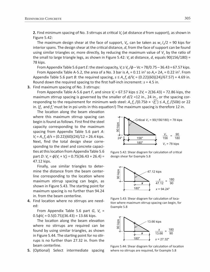
305Reinforced Concrete
2. Find minimum spacing of No. 3 stirrups at critical Vu (at distance d from support), as shown in Figure 5.42:
The maximum design shear at the face of support, Vu, can be taken as wu lu/2 = 90 kips for interior spans. The design shear at the critical distance, d, from the face of support can be found using similar triangles or, more directly, by reducing the maximum value of Vu by the ratio of the small to large triangle legs, as shown in Figure 5.42: Vu at distance, d, equals 90(156/180) = 78 kips.
From Appendix Table 5.6 part E: the steel capacity, Vs ≥ Vu /ϕ – Vc = 78/0.75 – 36.43 = 67.57 kips. From Appendix Table A-5.2, the area of a No. 3 bar is As = 0.11 in2 so Av= 2As = 0.22 in2. From
Appendix Table 5.6 part B: the required spacing, s ≤ Av fy d/Vs = (0.22)(60)(24)/67.57) = 4.69 in. Round down the required spacing to the first half-inch increment: s = 4.5 in.
3. Find maximum spacing of No. 3 stirrups: From Appendix Table A-5.6 part F, and since Vs = 67.57 kips ≤ 2Vc = 2(36.43) = 72.86 kips, the
maximum stirrup spacing is governed by the smaller of d/2 =12 in., 24 in., or the spacing cor-responding to the requirement for minimum web steel: Av fy /(0.75b × √fc') ≤ Av fy /(50b) or 22 in. (fy and fc' must be in psi units in this equation!) The maximum spacing is therefore 12 in.
The location along the beam elevation where this maximum stirrup spacing can begin is found as follows. First find the steel capacity corresponding to the maximum spacing from Appendix Table 5.6 part A: Vs = Av fy d/s = (0.22)(60)(24)/12 = 26.4 kips. Next, find the total design shear corre-sponding to the steel and concrete capaci-ties at this location from Appendix Table 5.6 part D: Vu = ϕ(Vc + Vs) = 0.75(36.43 + 26.4) = 47.12 kips.
Finally, use similar triangles to deter-mine the distance from the beam center-line corresponding to the location where maximum stirrup spacing can begin, as shown in Figure 5.43. The starting point for maximum spacing is no further than 94.24 in. from the beam centerline.
4. Find location where no stirrups are need-ed:
From Appendix Table 5.6 part G, Vu = 0.5ϕVc = 0.5(0.75)(36.43) = 13.66 kips.
The location along the beam elevation where no stirrups are required can be found by using similar triangles, as shown in Figure 5.44. The starting point for no stir-rups is no further than 27.32 in. from the beam centerline.
5. (Optional) Select intermediate spacing
Figure 5.42: Shear diagram for calculation of critical design shear for Example 5.8
Critical Vu = 90(156/180) = 78 kips
156"180"
24"
90 k
ips
Vu
15690
180
Vu = 78 kips
=
Figure 5.43: Shear diagram for calculation of loca-tion where maximum stirrup spacing can begin, for Example 5.8
90 k
ips 47.12 kips
x180"
x47.12
18090
x = 94.24"
=
Figure 5.44: Shear diagram for calculation of location where no stirrups are required, for Example 5.8
90 k
ips 13.66 kips
x180"
x13.66
18090
x = 27.32"
=

306 Structural Elements for Architects and Builders
between minimum and maximum values determined earlier:
Choose a spacing between the smallest required at the support (4.5 in.) and the maximum (12 in.), for example, s = 8 in.
Determine starting point for intermedi-ate spacing as follows. First, find the steel capacity corresponding to the chosen spac-ing: from Appendix Table A-5.6 part A, Vs = Av fy d/s = (0.22)(60)(24)/8 = 39.6 kips. Next, find the total design shear corre-sponding to the steel and concrete capacities at this location from Appendix Table 5.6 part D: Vu = ϕ(Vc + Vs) = 0.75(36.43 + 39.6) = 57.02 kips. Finally, use similar triangles to determine the distance from the beam centerline corresponding to the location where this intermediate stir-rup spacing can begin, as shown in Figure 5.45. The starting point for intermediate spacing, s = 8 in., is no further than 114 in. from the beam centerline.
6. Sketch the distribution of web steel (stirrups) for one half of the beam. The first stirrup is gen-erally placed at a distance s/2 = 4.5/2 = 2.25 in. from the face of the support (round down to 2 in.). The remaining stirrups are arranged within the zones of minimum, intermediate (optional) and maximum spacing, as shown in Figure 5.46. In this example, the middle 38 inches (that is, twice 19 in.) of the beam are not required to have stirrups.
Figure 5.45: Shear diagram for calculation of location where intermediate stirrup spacing may begin, for Ex-ample 5.7
90 k
ips 57.02 kips
x180"
x57.02
18090
x = 114"
=
Face of support Beam centerline180"
66" 19" 67" 28"
28"95"
114"
Maximum 12" o.c.Int.8" o.c.
Stirrups
2" 14 @ 4½" = 63" 19"
Minimum 4½" o.c.
6 @ 12" = 72"3 @ 8" = 24"
Figure 5.46: Elevation of beam showing spacing of stirrups for Example 5.8

307Reinforced Concrete
Depending on the beam’s cross-sectional dimensions, span, load, and material properties, the distribution of stirrup spacing can sometimes become even more complex for uniformly loaded beams with a triangular shear force pattern. As can be seen in Figure 5.47, there are four possible zones where the maximum shear force might occur, these zones bounded by values of Vu /ϕ equal to 0, 0.5Vc , Vc , 3Vc , and 4Vc . These bounded areas are significant since they define four zones with different criteria for stirrup spacing. In zone I, no stirrups are needed; in zone II, only minimum web steel is needed; in zone III, stirrup spacing cannot exceed the limits of “regular” maximum spacing (the smaller of d/2, 24 in., or the value determined by minimum web steel); and in zone IV, stirrup spacing cannot exceed the limits of “reduced” maximum spacing (the smaller of d/4, 12 in., or the value determined by minimum web steel). The upper limit of 5Vc corresponds to the maximum ac-ceptable value of Vu /ϕ — beyond that point, the shear force resisted by web steel is considered too high, and is not permitted.
Aside from the added cost and inefficiency of using too much steel, nothing prevents a designer from deploying stirrups at the minimum spacing, corresponding to the largest shear force, through-out the length of the beam. And there is also no prohibition against creating a greater number of spacing conditions, using any number of “intermediate” spacings, to minimize the amount of steel used in the beam. Finally, stirrup spacing over regions with constant shear force, Vu — commonly encountered in girders with concentrated loads — can be found with the same equations used in Example 5.7 and summarized in Appendix Table A-5.6.
Figure 5.47: Shear force diagram showing four zones where the maximum shear force might occur; the shear force, Vu is divided by the strength reduction factor, ϕ, in order to more clearly show the concrete and web steel contributions in relation to the total shear force at any point: Vu /ϕ = Vc + Vs

308 Structural Elements for Architects and Builders
Connections
Reinforced concrete elements are not ordinarily “connected” in the usual sense of the term; rather, they are most often cast together into a monolithic assembly. Of course, there are construction joints between sections of the structure cast separately, but even at such joints, opposite faces of concrete brought together in compression bear against each other just as if they had been mono-lithically cast; and steel reinforcement in tension is made to extend through each construction joint so that tensile forces in the bars continue from one side of the joint to the other.
The following discussion therefore does not include any reference to the types of welds, bolts, screws, or nails commonly found in wood or steel construction, where discrete structural elements subjected to tension, compression, or bending must be explicitly connected in order to function to-gether as a coherent structural system. Instead, two “quasi-connections,” both typical of reinforced concrete construction, shall be examined: the end condition of a continuous beam, and the lapped splicing of reinforcing bars where the bottom of one column is cast against the top of another col-umn.
Development length, tension
The fact that much reinforcing steel is subjected to tension raises an important question: what prevents such steel bars from being pulled out of, or slipping within, the concrete into which they have been placed? As can be seem in Fig-ure 5.48, any bending of a structural element literally stretches the tension region while the compression region shortens.
If the surface between the reinforcing bars and adjacent concrete were smooth and fric-tionless, the bars would remain “unstretched” as the beam bent; in general, it is the bond be-tween the steel bars and concrete that guaran-tees that such slippage will not occur. This bond is primarily a result of bumps, or deformations, placed on the surface of the reinforcement that create a mechanical interlocking of the steel and concrete surfaces, as shown schematically in Figure 5.49.
The strength of this bond, per unit of bar length, has been measured experimentally, so the total necessary bar length required to resist any tendency for the bar to be pulled through the concrete can be determined for any given tension stress. This required bar length is called the development length, ld, and is shown in Equation 5.29 for No. 7 or larger uncoated bars
Figure 5.48: Extension of rebar in tension zone of rein-forced concrete element
Original bar length
Reinforcing bar
Extension
Shortening
Figure 5.49: Schematic representation of a deformed reinforcing bar (rebar)

309Reinforced Concrete
with normalweight concrete and adequate bar spacing, or adequate spacing plus confinement with ties or stirrups, to prevent splitting of the concrete. Specifically, as illustrated in Figure 5.50, the bars must have a clear space between them at least equal to twice the bar diameter, that is, at least equal to 2db, and clear cover at least equal to the bar diameter, db. Alternatively, if adequate stirrups or ties are used throughout the development length region to confine the bars and prevent splitting of the concrete, the minimum clear spacing requirement may be reduced to db.
In Equation 5.29, ld is the development length for tension (in.), fy is the yield stress of the steel rein-forcement (psi), fc' is the compressive strength of the concrete (psi), ψt is a coefficient equal to 1.0 except when there is at least 12 in. of freshly cast concrete below the steel bars, in which case ψt = 1.3 (accounting for the negative impact on the bond between steel and concrete caused by rising air and water within a large mass of freshly-cast concrete), and db is the reinforcing bar diameter (in.). Some disclaimers: Where fy is greater than 60 ksi, the development length increases by 15 percent or 30 percent for Grade 80 and Grade 100 reinforcement respectively. The square root of fc’ in the equation cannot be taken greater than 100, an upper limit that only applies to concrete strengths greater than 10,000 psi. Equation 5.29 is often conservative, and a more complex version in the ACI Code might allow development lengths that are as much as 67% shorter under certain circumstances. On the other hand, using the simplified equation, but where the minimum conditions for spacing and stirrups (or ties) described above are not met, the development length in Equation 5.29 must be increased by a factor of 1.5. Where the bar size is smaller than No. 7, the development length is multiplied by 0.8. In no case may the development length be less than 12 in. Typical values for devel-opment length are tabulated in Appendix Table A-5.10 for common bar sizes.
Development length is influenced primar-ily by three factors: assuming adequate bar spacing and/or ties to prevent splitting of the concrete, the required development length be-comes larger if the tensile strength of the con-crete decreases (concrete’s tensile strength is proportional to the square root of its compres-sive strength); the required development length also increases if the stress in the bar increases (that stress being at most equal to the yield stress of the steel); and the development length increases as well if the surface area of the bar decreases (the surface area being proportional to the bar diameter). These three parameters can all be found in Equation 5.29.
If we imagine an isolated and discrete con-crete beam within a continuous concrete struc-ture, it is easier to see where and how the con-cept of development length becomes important.
(5.29)ld =fyψt
20√fc'db
Figure 5.50: Clear cover and spacing requirements for reinforced concrete beams
Clear cover
Bar diameter
Amount of fresh concrete below reinforcement
Clear spacing
Bar diameter
Clear cover

310 Structural Elements for Architects and Builders
As can be seen in Figure 5.51, a typical reinforced concrete beam-girder “connection” must resist the shear force and bending moment that occur at the surface where they come together. The shear force is resisted through the shear resistance of the concrete itself, the longitudinal steel bars, and the steel ties or stirrups provided for that purpose (the latter not shown in Figure 5.51 for clarity). The bending moment, in turn, is resolved into a compressive force (the resultant of the stress dis-tribution shown below the neutral axis for “negative” bending) and a tensile force (carried by the longitudinal steel reinforcement shown above the neutral axis). The compressive force presents no particular problems, as the concrete in the beam “pushes” against the concrete in the girder. The tensile force, however, could pull the bars out of the girder and beam, unless those bars develop
Girder Beam
ldh ld
12db Girder Beam
(b)
(c)
Column
Slab
Girder
Beam(a)
Figure 5.51: Development length of straight bars and standard hook: (a) section through typical slab and girder; (b) ex-ploded view showing "connection" between beam and girder (with slab omitted for clarity); and (c) required develop-ment length of hook (in girder) and straight bar (in beam)

311Reinforced Concrete
sufficient bond with the concrete to resist that tendency or are otherwise anchored into the con-crete. In the case of the beam, sufficient space is available to develop that bond strength by making sure that the bars extend into the beam for a distance at least as great as the required development length, ld (see Equation 5.29). For an exterior girder, however, it is likely that sufficient space is not available, and a 90° or 180° hook is often required.
As shown in Figure 5.51c, a 90° hook must be extended a distance of 12db below the bent portion of the bar, which in turn is defined by an inner radius that cannot be less than 3db for bars smaller than No. 9; 4db for No. 9, No. 10, and No. 11 bars; and 5db for No. 14 and No. 18 bars. In these guide-lines, db refers to the bar diameter. The required development length for such hooks, ldh, is given by the following equation for uncoated bars and normalweight concrete, with the most conservative assumptions regarding confinement and cover for the hooked bars:
In this equation, ldh is the development length for hooks (in.), fy = the yield stress of the steel rein-forcement (psi); fc' is the compressive strength of the concrete (psi); and db is the bar diameter (in.). In no case may the development length for a hook be less than 8db or 6 in. Typical values are tabu-lated in Appendix Table A-5.11 for common bar sizes.
It is possible to reduce this length if certain requirements are met that increase the level of con-finement of the hook or provide more concrete cover, making it less likely to split the concrete: First, the tabular values for development length can be divided by 1.6 if the centerline spacing between hooked bars is at least 6db or if the total area of ties or stirrups confining the hooked bars is not less than 0.4 times the total area of the hooked bars. Second, the tabular values for development length can be divided by 1.25 if the cover on the side of the hooked bars (i.e., perpendicular to their longitu-dinal direction) is at least equal to 6db or if the hooked bars are inside a column core with side cover at least equal to 2.5 in. Both of these modifications to development length for hooked bars can be taken if both criteria are met.
Example 5.9 Find required development length for straight bar and 90-degree hook in rein-forced concrete structure
Problem definition. A reinforced concrete beam frames into an exterior girder, as shown in Fig-ure 5.52, and the negative moment at the con-nection is resisted using No. 8 bars with 6 in. clear spacing between them. The required area for each bar = 0.74 in2. As the beam frames into a girder, it can be assumed that there is at least 6 in. of cover on the side of the hooked bars. Assume fc' = 4000 psi and fy = 60,000 psi. Find the required development length, ld, of the bars within the beam, the hook development length, ldh, and hook extension beyond the bend, within the girder.
(5.30)ldh =fy(fc’ /15,000+ 0.60) db
1.5
27.5√fc'
Figure 5.52: Required rebar development length for Example 5.9
3"
17"
ldh ld
No. 8 barr + db
12db
Beam
2"
Girder
r
312 Structural Elements for Architects and Builders
Solution overview. Find the nominal development lengths for a No. 8 bar, using 4000-psi concrete, in Appendix Table A-5.10 (for the beam) and Appendix Table A-5.11 (for the hook in the girder). Multi-ply these base values by the appropriate factors shown in the notes below each table.
Problem solution 1. The nominal development length required for the No. 8 bar in the beam is 62 in. (Appendix
Table A-5.10). This value is not divided by 1.3 (see Note 2) and also can be reduced by the ratio of required steel bar area to provided steel bar area = 0.74/0.79 = 0.937 (see Note 3), so that the final value for the required development length, ld = 62(0.937) = 58.1 in. or, rounded up to the nearest inch, 59 in. The required area for each bar = 0.74 in2 was given (or otherwise would be computed); the value for the provided steel bar area is simply the actual area of a No. 8 bar (see Appendix Table A-5.2). The computed development length exceeds the absolute minimum of 12 in. (see Note 5 in the table).
2. The nominal development length for the 90-degree hook in the beam is 30 in. (Appendix Table A-5.11). This value can be modified as follows: it can be divided by 1.6 since the 6 in. centerline spacing of the hooked bars is no less than 6db = 6 in. (see Note 4 in Appendix Table A-5.11); and it can be divided by 1.25 since the side cover is no less than 6db (see Note 5 in Appendix Table A-5.11). These reductions are cumulative, so the required development length for the hooked bar = 30 / (1.6 × 1.25) = 15 in. The actual dimensions of the girder would need to be able to ac-commodate this required length. The computed development length for hooks exceeds the two absolute minimums (see Note 8 in Appendix Table A-5.11): 8db = 8(1.0) = 8 in., or 6 in. Check-ing the minimum radius and minimum length of the “vertical” portion of the hook (see Note 5 in the table), we see that the required extension of the bar below the bend is 12db = 12(1.0) = 12 in. and the minimum inner radius for a No. 8 bar is 3db = 3(1.0) = 3 in.
There are two other requirements for tension reinforcement in continuous beams. First, for so-called positive-moment reinforcement — where tension occurs at the bottom of reinforced concrete beams — one-fourth of the rebars need to be extended at least 6 in. into the supports at each end of the beam. Second, for negative-moment reinforcement — where tension occurs at the top of the beam, typically in the vicinity of supports — at least one-third of the rebars need to extend beyond the point of inflection (where the negative moment becomes zero and the curvature changes from negative to positive) a distance of either d, 12db, or ln /16, whichever is greater: d is the effective depth of the beam; db is the rebar diameter; and ln is the clear span, measured between the faces of supports.
Development length, compression
For a steel reinforcing bar in compression, much of the stress in the steel can be transferred to the concrete through direct bearing of the bar end on the concrete. For that reason, the required devel-opment length in compression, ldc, is smaller than that required when bars are stressed in tension, and is given by the greater of the following values:
ldc = db and ldc = 0.0003fy db (5.31)0.02fy
√fc'

313Reinforced Concrete
In these equations, ldc is the development length (in.) for normalweight concrete in compression; fy = the yield stress of the steel reinforcement (psi); fc' is the compressive strength of the concrete (psi); and db is the bar diameter (in.). If lightweight concrete is used, the values for development length must be multiplied by 1.333. As with bars in tension, it is possible to reduce this required length by multiplying the greater value found in Equation 5.31 by the ratio of required steel bar area to provided steel bar area. In addition, the required development length may be multiplied by 0.75 in columns with adequate spirals or ties (specifically, with a minimum ¼ in. spiral at no more than a 4 in. pitch; or with No. 4 ties spaced at no more than 4 in. on center). In no case can the development length for compression be less than 8 in. Typical values are tabulated in Appendix Table A-5.12 for common bar sizes.
Bar splices in tension
Since the length of reinforcing bars is limited by manufacturing and transportation constraints, it is often necessary to splice them together, at least in cases where the continuity assumed in design indicates lengths greater than those available from a single bar. While it is possible to weld bars to-gether, or to use special mechanical splicing devices, the most common method for creating continu-ity between two bars in tension is by lapping them a sufficient distance so that tensile stresses can be transferred through the bond developed between the steel bars and adjacent concrete. For virtually all tension splices, the required lap distance is taken as 1.3ld, where the development length, ld, is defined as in Equation 5.29 (or as tabulated in Appendix Table A-5.10), except that the 12 in. mini-mum length for ld does not apply (but there is still a minimum splice length of 12 in.), and a reduction of the development length based on the ratio of provided to required steel area is not permitted. There are some limits placed on larger bar sizes: No. 14 and No. 18 bars cannot be lap spliced in ten-sion.
Bar splices in compression
Columns are almost always cast floor by floor, with longitudinal reinforcement left extending verti-cally beyond the current floor level, so that it can be spliced into the column steel for the next floor being cast. For fy ≤ 60 ksi and fc' ≥ 3000 psi, the required lap distance for compression is taken as:
required compressive lap distance = 0.0005fy db
This required lap distance equals 30db for 60 ksi steel bars, with an absolute minimum lap dis-tance of 12 in. For rebars with fy > 60 ksi, the required compressive lap distance is increased to (0.0009fy – 24)db or, only for rebars with fy > 80 ksi, to the larger of (0.0009fy – 24)db and the re-quired tension lap splice distance described above. In all these equations, fy is the yield stress of the steel reinforcement (psi); fc' is the compressive strength of the concrete (psi); and db is the bar diam-eter (in.). It should be emphasized that in many reinforced concrete columns, especially those ex-plicitly designed to resist bending moment as well as compressive force, a given lap splice may need to resist tension, compression, or both tension and compression, under different loading scenarios. For bars that resist only compression, and where confinement is provided by ties or spirals, it is pos-sible to create splices, not by lapping the bars, but instead by placing their ends in contact so that they bear directly upon each other. However, even in such cases where no tension is anticipated, all
(5.32)

314 Structural Elements for Architects and Builders
columns must maintain some ability to resist unexpected tension forces, so that either additional “tension” steel must be provided in such cases, or else compressive lap splices must be used (since compressive lap splices provide sufficient resistance to unexpected tension forces in the bars). The required length of column lap splices in compression may be reduced where sufficient confinement, in the form of ties or spirals, is provided. Specifically, where the bar area of a tie (taken as the total tie area cut in section, as shown in Figure 5.53) is greater or equal to 0.0015(h × s) — where h is the greater column cross-sectional thickness in inches, and s is the tie spacing in inches — the required lap distance may be multiplied by 0.83; with spirals, the required lap length may be multiplied by 0.75. In any case, the lap length can never be taken less than 12 in. Limits placed on larger bars are relaxed somewhat for lap splices in compression: No. 14 and No. 18 bars cannot be lap spliced to each other, but may be lap spliced to No. 11 and smaller bars. In cases where two different bar sizes are lap spliced together in compression, the required splice length is found by (1) computing the required development length for the larger bar, (2) computing the required lap splice length for the smaller bar, and (3) using the larger of these two values.
Figure 5.53: Column lap splice parameters
Tieh
(a) Plan view
(b) Sectional view
Tie area
Tie
spac
ing,
s
Lap
splic
e le
ngth
Beam and slab reinforcement not shown

315Reinforced Concrete
For a column resisting only compressive forces, the required lap length is determined for the bars originating in the upper column; the bars extended upwards from the lower column that terminate in the upper column must satisfy the requirements for compressive development length (Equation 5.31). In practice, the larger of these two criteria (compressive development length for the lower bars and required lap splice length for the upper bars) determines the minimum splice length. Since loads typically are smaller in upper-level columns, it is possible that smaller bars sizes can be used in the upper columns; these smaller bars can be spliced with larger bars extending upward from the lower column. In such cases, different bar diameters, db, must be used in determining lap splice length and development length.
Example 5.10 Find required length of compression column splice in reinforced concrete struc-ture
Problem definition. A 12 in. × 16 in. reinforced concrete column is configured as shown in Figure 5.53. The longitudinal (vertical) bars in the lower column consist of four No. 9 bars, which extend into the upper column. Four No. 8 bars originate in the upper column, and are spliced to the lower column bars as shown. The longitudinal steel is confined by No. 3 ties spaced at 9 in. on center. Assuming only compressive stress in the column, with fy = 60 ksi and fc' = 3000 psi, what is the required splice length?
Solution overview. Find the compressive lap splice length based on the diameter of the No. 8 bars in the upper column. Find the required compressive development length based on the No. 9 bars extended into the upper column. Use the larger of these two values for the column splice length.
Problem solution 1. Lap splice. From Equation 5.32, the minimum lap splice length for the No. 8 bars = 0.0005fy db =
0.0005(60,000 × 1.0) = 30 in. To check whether the 0.83 reduction factor may be used, it is nec-essary to see if the No. 3 bar area for the ties is greater than or equal to 0.0015(h × s), where h = 16 in. (the larger of the overall column dimensions) and s = 9 in. (the tie spacing). Using twice the area of a single tie (Appendix Table A-5.2), we find that 2(0.11) = 0.22 ≥ 0.0015(16 × 9) = 0.216, so the lap splice length may be reduced to 30 × 0.83 = 24.9 in. or, rounding up, 25 in.
2. Development length. From Equation 5.31, we get:
ldc = (1.128) = 21.9 in. and
ldc = 0.0003(60,000 × 1.128) = 20.3 in.
The bar diameter, db, is found in Appendix Table A-5.2. Using the larger value and rounding up, the minimum development length, ldc = 22 in. Because the tie spacing is greater than 4 in. on center, no reduction in development length may be taken.
3. Comparing the requirements for lap splice length and development length, the larger of the two values will be used: 25 in.
0.2 × 60,000√3000

316 Structural Elements for Architects and Builders
Chapter 5 Appendix
Table A-5.1: Dimensions of reinforced concrete beams, columns, and slabsA. Cover requirements (from outside face of concrete to face of closest rebar)Interior 1½ in. (or ¾ in. for slabs)
Exterior or exposed to ground 2 in. (or 1½ in. for No.5 bars or smaller)
Formed directly to ground 3 in.
B. Typical gross dimensionsBeams and columns Round to the nearest inch, or 2 in. increment, for all outside (gross) dimensions
Slabs Round to ½ in. increment (or 1 in. increment if over 6 in. thick)
Table A-5.2: Steel reinforcement — rebar — areas (in2) for groups of barsDesignation and diameter
Number of bars
Bar No.1
SI Bar No.2
Dia. (in.)
1 2 3 4 5 6 7 8 9 10 11 12 14 16
3 10 0.375 0.11 No. 3 (10) bars are used primarily for ties and in slabs
4 13 0.500 0.20 0.40 0.60 0.80 1.00 1.20 1.40 1.60 1.80 2.00 2.20 2.40 2.80 3.20
5 16 0.625 0.31 0.62 0.93 1.24 1.55 1.86 2.17 2.48 2.79 3.10 3.41 3.72 4.34 4.96
6 19 0.750 0.44 0.88 1.32 1.76 2.20 2.64 3.08 3.52 3.96 4.40 4.84 5.28 6.16 7.04
7 22 0.875 0.60 1.20 1.80 2.40 3.00 3.60 4.20 4.80 5.40 6.00 6.60 7.20 8.40 9.60
8 25 1.000 0.79 1.58 2.37 3.16 3.95 4.74 5.53 6.32 7.11 7.90 8.69 9.48 11.06 12.64
9 29 1.128 1.00 2.00 3.00 4.00 5.00 6.00 7.00 8.00 9.00 10.00 11.00 12.00 14.00 16.00
10 32 1.270 1.27 2.54 3.81 5.08 6.35 7.62 8.89 10.16 11.43 12.70 13.97 15.24 17.78 20.32
11 36 1.410 1.56 3.12 4.68 6.24 7.80 9.36 10.92 12.48 14.04 15.60 17.16 18.72 21.84 24.96314 43 1.693 2.25 4.50 6.75 9.00 11.25 13.50 15.75 18.00 20.25 22.50 24.75 27.00 31.50 36.00318 57 2.257 4.00 8.00 12.00 16.00 20.00 24.00 28.00 32.00 36.00 40.00 44.00 48.00 56.00 64.00
Notes:1. Rebars in the US were traditionally designated by the nominal diameter (in.) multiplied by eight, so that a No. 3 bar, for example, has a nominal diameter of ⅜ in. Rebars are no longer marked using this designation (see Note 2).2. Rebars are currently marked by the approximate number of millimeters in their diameter (SI units), although designation by nominal diameter (in.) multiplied by eight is still widely used in the US.3. No. 14 and No. 18 bars are used primarily in columns.

317Reinforced Concrete
Table A-5.3: Reinforced concrete minimum width or diameter (in.) based on bar spacingA. Minimum width (in.) for beams3
Designation Number of bars in one lineBar No.1
SI Bar No.2
2 3 4 5 6
4 13 6.33 8.17 10.00 11.83 13.67
5 16 6.58 8.54 10.50 12.46 14.42
6 19 6.83 8.92 11.00 13.08 15.17
7 22 7.08 9.29 11.50 13.71 15.92
8 25 7.33 9.67 12.00 14.33 16.67
9 29 7.58 10.04 12.50 14.96 17.42
10 32 7.83 10.42 13.00 15.58 18.17
11 36 8.13 10.88 13.63 16.38 19.13
B. Minimum width (in.) for tied columns3
Designation Number of bars in one lineBar No.1
SI Bar No.2
2 3 4 5 6
4 13 6.50 8.50 10.50 12.50 14.50
5 16 6.75 8.88 11.00 13.13 15.25
6 19 7.00 9.25 11.50 13.75 16.00
7 22 7.25 9.63 12.00 14.38 16.75
8 25 7.50 10.00 12.50 15.00 17.50
9 29 7.94 10.75 13.56 16.38 19.19
10 32 8.38 11.50 14.63 17.75 20.88
11 36 8.81 12.25 15.69 19.13 22.56
14 43 10.13 14.50 18.88 23.25 27.63
18 57 11.88 17.50 23.13 28.75 34.38
C. Minimum diameter (in.) for spiral columns3
Designation Total number of bars in columnBar No.1
SI Bar No.2
6 8 10 12 14
4 13 8.50 9.73 10.97 12.23 13.49
5 16 8.88 10.18 11.50 12.84 14.17
6 19 9.25 10.63 12.03 13.44 14.86
7 22 9.63 11.08 12.56 14.05 15.55
8 25 10.00 11.53 13.09 14.66 16.23
9 29 10.75 12.47 14.23 15.99 17.76
10 32 11.50 13.42 15.36 17.32 19.29
11 36 12.25 14.36 16.50 18.66 20.82
14 43 14.50 17.18 19.91 22.65 25.41
18 57 17.50 20.95 24.45 27.98 31.53
Notes:1. Rebars in the United States were traditionally designated by the nominal diameter (in.) divided by eight. Rebars are no longer marked using this designation.
Cover
Width
No. of bars in one line
No. of bars in one line
Cover
Width
Diameter
Cover
(continued)

318 Structural Elements for Architects and Builders
2. Rebars are currently designated (and marked) by the approximate number of millimeters (SI units) in their diameter.3. These minimum dimensions assume 1 in. maximum aggregate; 1½ in. cover (measured from outside face of rebar or spiral to face of concrete); and ½ in.-diameter stirrups, ties, or spiral. Minimum widths or diameters are typically rounded up to nearest inch, or to the nearest even inch. The amount of column steel is also limited by the required reinforcement ratio, ρg, between 0.01 and 0.08.
Table A-5.4: Specifications for steel ties and spirals in reinforced concrete columnsTiesUse minimum No. 3 bars to confine longitudinal steel up to No. 10; use minimum No. 4 bars for No. 11, 14, and 18 longitudinal steel.Center-to-center spacing of ties is the smaller of:• 16 × longitudinal bar diameter• 48 × tie bar diameter• Smallest column dimensionClear spacing of ties cannot be less than 4/3 of maximum aggregate size.
Ties must be arranged so that corner bars are bounded by a tie bent at a 90° angle, and alternate longitudinal bars (between the corners) are restrained by a tie bent to at least 135°. No unsupported longitudinal bar shall be farther than 6 in. clear on either side of a laterally supported bar.
SpiralsUse a continuous bar or wire of at least ⅜-in. diameter, with the clear space measured between turns of the spiral no more than 3 in. and no less than 1 in or 4/3 of maximum aggregate size. A minimum ratio, ρs, of the volume of spiral steel to the volume of concrete inside the spiral (the "core") is also specified: ρs = 0.45(Ag /Ac – 1)(fc' /fy) with fy ≤ 60 ksi, Ag being the gross concrete area, and Ac being the area of the "core" within the spiral.
Table A-5.5: Reinforced concrete strength reduction factors, ϕ and αType of behavior ϕ α1
Bending 20.9 n/a
Axial tension 0.9 n/a
Axial compression: spiral columns 30.75 0.85
Axial compression: tied columns 30.65 0.80
Shear 0.75 n/a
Notes:1. α accounts for unintended eccentricity or bending moment.2. ϕ decreases linearly from value listed above at εt = 0.005 to 0.65 or 0.75 (for tied or spiral lateral reinforcement respectively) at εt = 0.002, where εt is the net tensile strain in the extreme tension steel (we assume "tension-controlled" sections in this text, with values of ϕ = 0.9 as shown).3. ϕ increases linearly from value listed above at εt = 0.002 to 0.9 at εt = 0.005, where εt is the net tensile strain in the extreme tension steel for elements with combined compression and bending (this type of combined loading is beyond the scope of this book; in the prob-lems considered herein, with only compressive stresses, the value of ϕ is as shown).
Table A-5.3 continued (Notes)

319Reinforced Concrete
Table A-5.6: "Shear" equations for reinforced concrete beams1
EquationA. Capacity of steel stirrups2 (lb)
B. Required stirrup spacing2 (in.)
C. Capacity of concrete (lb)3 Vc = 2bd√fc'
D. Strength design equation2 Vu ≤ ϕ(Vc + Vs)
E. Required steel capacity (lb) from strength design equation2
F. Maximum stirrup spacing3 (in.) For Vs ≤ 2Vc, the smaller of:• d/2• 24 in.• Avfy /(0.75b × √fc' ) < Avfy /(50b) [see note 4]For Vs > 2Vc, the smaller of:• d/4• 12 in.• Avfy /(0.75b × √fc' ) < Avfy /(50b) [see note 4]
G. Design shear where no stirrups are needed2 (lb) Vu = 0.5ϕVc
Notes:1. Units are as follows: b = cross section width, or “web” width for T-beams (in.) d = cross section effective depth (in.) s = stirrup spacing (in.) Av = total stirrup bar area, equal to 2As, including both "prongs" (in2) fy = yield stress of steel stirrup (psi) fc' = cylinder strength of concrete (psi) Vu = design (factored) shear force (lb) Vc = capacity of concrete to resist shear (lb) Vs = capacity of steel stirrups to resist shear (lb) ϕ = 0.75 for shear (see Appendix Table A-5.5)2. Pound (lb) and pound per square inch (psi) units specified according to Note 1 may be changed to kips and ksi in these equations only. 3. The concrete cylinder strength fc' must be in psi units in Appendix Table 5.6 part C (with the resulting value of Vc in lb units) and both the steel yield stress fy and the concrete cylinder strength fc' must be psi units in part F (with in. units resulting).4. This limiting value for maximum spacing corresponds to the minimum amount of web steel required when Vu > 0.5ϕVc, except that it does not apply when the total beam depth (thickness, h) is less than 10 in. or, for T-beams, when the total beam depth is less than 24 in. and is also less than the larger of 2.5 × flange depth or 0.5 × the beam stem width.
Vs =Avfy d
s
Vs
Avfy ds ≤
Vs ≥Vu – Vcϕ

320 Structural Elements for Architects and Builders
Table A-5.7: Approximate moment values for continuous reinforced concrete beams and slabs1
End restraints for two spans Positive moment Negative momentEnd span End span
At interior support2
At exterior support2
Discontinuous end unrestrained
wuln2/11 n/a n/a
Discontinuous end restrained by spandrel girder wuln2/14 wuln2/9 wuln2/24
Discontinuous end restrained by column wuln2/14 wuln2/9 wuln2/16
End restraints for three or more spans Positive moment Negative momentInterior span
End span Typical interior support2
End spanAt interior support2
At exterior support2
Discontinuous end unrestrained wuln2/16 wuln2/11 n/a n/a n/a
Discontinuous end restrained by spandrel girder wuln2/16 wuln2/14 wuln2/11 wuln2/10 wuln2/24
Discontinuous end restrained by column wuln2/16 wuln2/14 wuln2/11 wuln2/10 wuln2/16
Notes:1. The units for uniformly distributed design load, wu, are typically lb/ft or kips/ft; the units for clear span, ln, are feet; and the resulting moment value, Mu is in ft-lb or ft-kips depending on the units chosen for the distributed load. These moment values are valid only for continuous reinforced concrete beams or slabs when the following conditions are met: a. Lengths of adjacent spans do not differ by more than 20%. b. The unfactored live load is less than or equal to 3 times the unfactored dead load.2. The negative moment (at the face of support) can be taken as wuln2/12 for slabs with clear spans no greater than 10 ft, and for beams framing into relatively stiff columns (specifically, the sum of column stiffness divided by the sum of beam stiffness at each end of the beam must be greater than 8). Stiffness is the product of modulus of elasticity and moment of inertia, neither of which are straightfor-ward quantities for structural elements consisting of two materials bonded together. For normalweight concrete, the modulus of elasticity, Ec (psi), may be taken as 57,000√fc' , where the cylinder strength of concrete, fc', is in psi units. The calculation of moment of inertia is left to the designer, with the American Concrete Institute (ACI) permitting any “reasonable and consistent assumptions." One suggestion is to use gross EcI values for both beams and columns. Where Ec is the same for all members, a typical joint with columns and beams at all four orthogonal points, and constant width for column and beam sections, would qualify for the wuln2/12 negative beam moment only when the column thickness at that joint becomes more than twice the beam thickness.
Numbers on beams refer to moment value coefficient, x, in the equation: Mu =wulu
2
x
Integral with column
UnrestrainedIntegral with spandrel

321Reinforced Concrete
Table A-5.8: Limits on steel ratio for "tension-controlled" reinforced concrete beams1,2,3
fc' (psi) Limits on steel ratio, ρmin – ρmax
3000 0.00333 – 0.01350
4000 0.00333 – 0.01810
5000 0.00354 – 0.02130
Notes:1. Values are for fy = 60 ksi, ϕ = 0.9, and steel strain, εt = 0.005 for ρmax.2. Values for maximum steel ratio apply to all beams and one-way slabs; values for minimum steel ratio apply only to rectangu-lar beams and negative-moment indeterminate T-beams; the minimum steel ratio for positive moment T-beams is ρmin = 0.00333/(b/bw) for f’c = 3000 psi and 4000 psi, and 0.00354/(b/bw) for f’c = 5000 psi; and the minimum steel ratio for one-way slabs is ρmin = 0.00180/(h/d). For details, see Appendix Table A-5.9 Part d.3. It is permitted to reduce the amount of steel below the minimum values stipulated for beams, as long as the steel area provided is at least one-third greater than the steel area required by analysis.

322 Structural Elements for Architects and Builders
Table A-5.9: Values of R and ρ for reinforced concrete beams, T-beams, and one-way slabs (using 60 ksi steel)1,2
a) fc’ = 5 ksi and fy = 60 ksiR and ρ for positive-moment T-beams and slabs R and ρ
ρmin defined as As / (bd)
ρmin for pos.-moment T-beam with b/bw = 11.50 0.0184 0.000308 0.2071 0.00354 0.7449 0.01375
ρmin for pos.-moment T-beam with b/bw = 11.00 0.0193 0.000322 0.2190 0.00375 0.7570 0.01400
ρmin for pos.-moment T-beam with b/bw = 10.50 0.0202 0.000337 0.2332 0.00400 0.7690 0.01425
ρmin for pos.-moment T-beam with b/bw = 10.00 0.0212 0.000354 0.2474 0.00425 0.7810 0.01450
ρmin for pos.-moment T-beam with b/bw = 9.50 0.0223 0.000373 0.2614 0.00450 0.7929 0.01475
ρmin for pos.-moment T-beam with b/bw = 9.00 0.0235 0.000393 0.2754 0.00475 0.8047 0.01500
ρmin for pos.-moment T-beam with b/bw = 8.50 0.0249 0.000416 0.2894 0.00500 0.8165 0.01525
ρmin for pos.-moment T-beam with b/bw = 8.00 0.0265 0.000443 0.3033 0.00525 0.8282 0.01550
ρmin for pos.-moment T-beam with b/bw = 7.50 0.0282 0.000472 0.3172 0.00550 0.8399 0.01575
ρmin for pos.-moment T-beam with b/bw = 7.00 0.0303 0.000506 0.3310 0.00575 0.8516 0.01600
ρmin for pos.-moment T-beam with b/bw = 6.50 0.0326 0.000545 0.3448 0.00600 0.8632 0.01625
ρmin for pos.-moment T-beam with b/bw = 6.00 0.0353 0.000590 0.3585 0.00625 0.8747 0.01650
ρmin for pos.-moment T-beam with b/bw = 5.75 0.0368 0.000616 0.3721 0.00650 0.8862 0.01675
ρmin for pos.-moment T-beam with b/bw = 5.50 0.0385 0.000644 0.3857 0.00675 0.8976 0.01700
ρmin for pos.-moment T-beam with b/bw = 5.25 0.0402 0.000674 0.3992 0.00700 0.9090 0.01725
ρmin for pos.-moment T-beam with b/bw = 5.00 0.0423 0.000708 0.4127 0.00725 0.9203 0.01750
ρmin for pos.-moment T-beam with b/bw = 4.75 0.0445 0.000745 0.4262 0.00750 0.9316 0.01775
ρmin for pos.-moment T-beam with b/bw = 4.50 0.0470 0.000787 0.4396 0.00775 0.9428 0.01800
ρmin for pos.-moment T-beam with b/bw = 4.25 0.0497 0.000833 0.4529 0.00800 0.9472 0.01810
ρmin for pos.-moment T-beam with b/bw = 4.00 0.0528 0.000885 0.4662 0.00825 0.9539 0.01825
ρmin for pos.-moment T-beam with b/bw = 3.75 0.0563 0.000944 0.4794 0.00850 0.9650 0.01850
ρmin for pos.-moment T-beam with b/bw = 3.50 0.0602 0.001011 0.4926 0.00875 0.9761 0.01875
ρmin for pos.-moment T-beam with b/bw = 3.25 0.0648 0.001089 0.5057 0.00900 0.9871 0.01900
ρmin for pos.-moment T-beam with b/bw = 3.00 0.0702 0.001180 0.5188 0.00925 0.9981 0.01925
ρmin for pos.-moment T-beam with b/bw = 2.75 0.0765 0.001287 0.5318 0.00950 1.0090 0.01950
ρmin for pos.-moment T-beam with b/bw = 2.50 0.0841 0.001416 0.5447 0.00975 1.0198 0.01975
ρmin for pos.-moment T-beam with b/bw = 2.25 0.0933 0.001573 0.5576 0.01000 1.0306 0.02000
ρmin for pos.-moment T-beam with b/bw = 2.00 0.1049 0.001770 0.5705 0.01025 1.0413 0.02025
ρmin for slabs with thickness, h = 12 0.1162 0.001964 0.5833 0.01050 1.0520 0.02050
ρmin for slabs with thickness, h = 11 0.1171 0.00198 0.5961 0.01075 1.0626 0.02075
ρmin for slabs with thickness, h = 10 0.1183 0.002 0.6088 0.01100 1.0732 0.02100
ρmin for slabs with thickness, h = 9 0.1198 0.002025 0.6214 0.01125 1.0838 0.02125
ρmin for slabs with thickness, h = 8 0.1216 0.002057 0.6340 0.01150 1.0858 0.02130
ρmin for slabs with thickness, h = 7 0.1241 0.0021 0.6465 0.01175 — —
ρmin for slabs with thickness, h = 6 0.1276 0.00216 0.6590 0.01200 — —
ρmin for slabs with thickness, h = 5.5 0.1300 0.0022 0.6714 0.01225 — —
ρmin for slabs with thickness, h = 5 0.1329 0.00225 0.6838 0.01250 — —
ρmin for slabs with thickness, h = 4.5 0.1366 0.002314 0.6962 0.01275 — —
ρmin for slabs with thickness, h = 4 0.1416 0.0024 0.7084 0.01300 — —
ρmin for slabs with thickness, h = 3.5 0.1485 0.00252 0.7206 0.01325 — —
ρmin for slabs with thickness, h = 3 0.1589 0.0027 0.7328 0.01350 — —
R ρ R ρ R ρ
(continued)

323Reinforced Concrete
Table A-5.9 (continued) b) fc’ = 4 ksi and fy = 60 ksi
R and ρ for positive-moment T-beams and slabs R and ρ
ρmin defined as As / (bd)
ρmin for pos.-moment T-beam with b/bw = 11.50 0.0174 0.000290 0.1939 0.00333 0.7135 0.01350
ρmin for pos.-moment T-beam with b/bw = 11.00 0.0181 0.000303 0.2058 0.00354 0.7249 0.01375
ρmin for pos.-moment T-beam with b/bw = 10.50 0.0190 0.000317 0.2176 0.00375 0.7362 0.01400
ρmin for pos.-moment T-beam with b/bw = 10.00 0.0199 0.000333 0.2315 0.00400 0.7475 0.01425
ρmin for pos.-moment T-beam with b/bw = 9.50 0.0210 0.000351 0.2454 0.00425 0.7587 0.01450
ρmin for pos.-moment T-beam with b/bw = 9.00 0.0221 0.000370 0.2593 0.00450 0.7698 0.01475
ρmin for pos.-moment T-beam with b/bw = 8.50 0.0234 0.000392 0.2731 0.00475 0.7809 0.01500
ρmin for pos.-moment T-beam with b/bw = 8.00 0.0249 0.000416 0.2868 0.00500 0.7919 0.01525
ρmin for pos.-moment T-beam with b/bw = 7.50 0.0265 0.000444 0.3004 0.00525 0.8028 0.01550
ρmin for pos.-moment T-beam with b/bw = 7.00 0.0284 0.000476 0.3140 0.00550 0.8137 0.01575
ρmin for pos.-moment T-beam with b/bw = 6.50 0.0306 0.000512 0.3275 0.00575 0.8245 0.01600
ρmin for pos.-moment T-beam with b/bw = 6.00 0.0331 0.000555 0.3409 0.00600 0.8352 0.01625
ρmin for pos.-moment T-beam with b/bw = 5.75 0.0346 0.000579 0.3543 0.00625 0.8459 0.01650
ρmin for pos.-moment T-beam with b/bw = 5.50 0.0361 0.000605 0.3676 0.00650 0.8565 0.01675
ρmin for pos.-moment T-beam with b/bw = 5.25 0.0378 0.000634 0.3809 0.00675 0.8670 0.01700
ρmin for pos.-moment T-beam with b/bw = 5.00 0.0397 0.000666 0.3941 0.00700 0.8775 0.01725
ρmin for pos.-moment T-beam with b/bw = 4.75 0.0418 0.000701 0.4072 0.00725 0.8879 0.01750
ρmin for pos.-moment T-beam with b/bw = 4.50 0.0441 0.000740 0.4202 0.00750 0.8982 0.01775
ρmin for pos.-moment T-beam with b/bw = 4.25 0.0467 0.000784 0.4332 0.00775 0.9085 0.01800
ρmin for pos.-moment T-beam with b/bw = 4.00 0.0496 0.000833 0.4461 0.00800 0.9126 0.01810
ρmin for pos.-moment T-beam with b/bw = 3.75 0.0529 0.000888 0.4590 0.00825 — —
ρmin for pos.-moment T-beam with b/bw = 3.50 0.0566 0.000951 0.4718 0.00850 — —
ρmin for pos.-moment T-beam with b/bw = 3.25 0.0609 0.001025 0.4845 0.00875 — —
ρmin for pos.-moment T-beam with b/bw = 3.00 0.0659 0.001110 0.4971 0.00900 — —
ρmin for pos.-moment T-beam with b/bw = 2.75 0.0719 0.001211 0.5097 0.00925 — —
ρmin for pos.-moment T-beam with b/bw = 2.50 0.0790 0.001332 0.5222 0.00950 — —
ρmin for pos.-moment T-beam with b/bw = 2.25 0.0876 0.001480 0.5347 0.00975 — —
ρmin for pos.-moment T-beam with b/bw = 2.00 0.0984 0.001665 0.5471 0.01000 — —
ρmin for slabs with thickness, h = 12 0.1158 0.001964 0.5594 0.01025 — —
ρmin for slabs with thickness, h = 11 0.1167 0.001980 0.5716 0.01050 — —
ρmin for slabs with thickness, h = 10 0.1179 0.002000 0.5838 0.01075 — —
ρmin for slabs with thickness, h = 9 0.1193 0.002025 0.5959 0.01100 — —
ρmin for slabs with thickness, h = 8 0.1212 0.002057 0.6080 0.01125 — —
ρmin for slabs with thickness, h = 7 0.1237 0.002100 0.6200 0.01150 — —
ρmin for slabs with thickness, h = 6 0.1271 0.002160 0.6319 0.01175 — —
ρmin for slabs with thickness, h = 5.5 0.1294 0.002200 0.6438 0.01200 — —
ρmin for slabs with thickness, h = 5 0.1323 0.002250 0.6556 0.01225 — —
ρmin for slabs with thickness, h = 4.5 0.1360 0.002314 0.6673 0.01250 — —
ρmin for slabs with thickness, h = 4 0.1410 0.002400 0.6789 0.01275 — —
ρmin for slabs with thickness, h = 3.5 0.1478 0.002520 0.6905 0.01300 — —
ρmin for slabs with thickness, h = 3 0.1581 0.002700 0.7021 0.01325 — —
R ρ R ρ R ρR ρ R ρ R ρ
(continued)

324 Structural Elements for Architects and Builders
Table A-5.9 (continued) c) fc’ = 3 ksi and fy = 60 ksi
R and ρ for positive-moment T-beams and slabs R and ρ
ρmin defined as As / (bd)
ρmin for pos.-moment T-beam with b/bw = 11.50 0.0173 0.000290 0.1920 0.00333
ρmin for pos.-moment T-beam with b/bw = 11.00 0.0181 0.000303 0.2151 0.00375
ρmin for pos.-moment T-beam with b/bw = 10.50 0.0189 0.000317 0.2287 0.00400
ρmin for pos.-moment T-beam with b/bw = 10.00 0.0199 0.000333 0.2423 0.00425
ρmin for pos.-moment T-beam with b/bw = 9.50 0.0210 0.000351 0.2557 0.00450
ρmin for pos.-moment T-beam with b/bw = 9.00 0.0221 0.000370 0.2691 0.00475
ρmin for pos.-moment T-beam with b/bw = 8.50 0.0234 0.000392 0.2824 0.00500
ρmin for pos.-moment T-beam with b/bw = 8.00 0.0248 0.000416 0.2955 0.00525
ρmin for pos.-moment T-beam with b/bw = 7.50 0.0265 0.000444 0.3086 0.00550
ρmin for pos.-moment T-beam with b/bw = 7.00 0.0284 0.000476 0.3217 0.00575
ρmin for pos.-moment T-beam with b/bw = 6.50 0.0305 0.000512 0.3346 0.00600
ρmin for pos.-moment T-beam with b/bw = 6.00 0.0331 0.000555 0.3474 0.00625
ρmin for pos.-moment T-beam with b/bw = 5.75 0.0345 0.000579 0.3602 0.00650
ρmin for pos.-moment T-beam with b/bw = 5.50 0.0360 0.000605 0.3728 0.00675
ρmin for pos.-moment T-beam with b/bw = 5.25 0.0378 0.000634 0.3854 0.00700
ρmin for pos.-moment T-beam with b/bw = 5.00 0.0396 0.000666 0.3979 0.00725
ρmin for pos.-moment T-beam with b/bw = 4.75 0.0417 0.000701 0.4103 0.00750
ρmin for pos.-moment T-beam with b/bw = 4.50 0.0440 0.000740 0.4226 0.00775
ρmin for pos.-moment T-beam with b/bw = 4.25 0.0466 0.000784 0.4348 0.00800
ρmin for pos.-moment T-beam with b/bw = 4.00 0.0495 0.000833 0.4470 0.00825
ρmin for pos.-moment T-beam with b/bw = 3.75 0.0527 0.000888 0.4590 0.00850
ρmin for pos.-moment T-beam with b/bw = 3.50 0.0564 0.000951 0.4710 0.00875
ρmin for pos.-moment T-beam with b/bw = 3.25 0.0608 0.001025 0.4828 0.00900
ρmin for pos.-moment T-beam with b/bw = 3.00 0.0657 0.001110 0.4946 0.00925
ρmin for pos.-moment T-beam with b/bw = 2.75 0.0716 0.001211 0.5063 0.00950
ρmin for pos.-moment T-beam with b/bw = 2.50 0.0787 0.001332 0.5179 0.00975
ρmin for pos.-moment T-beam with b/bw = 2.25 0.0873 0.001480 0.5294 0.01000
ρmin for pos.-moment T-beam with b/bw = 2.00 0.0979 0.001665 0.5408 0.01025
ρmin for slabs with thickness, h = 12 0.1151 0.001964 0.5522 0.01050
ρmin for slabs with thickness, h = 11 0.1160 0.001980 0.5634 0.01075
ρmin for slabs with thickness, h = 10 0.1172 0.002000 0.5746 0.01100
ρmin for slabs with thickness, h = 9 0.1186 0.002025 0.5857 0.01125
ρmin for slabs with thickness, h = 8 0.1204 0.002057 0.5966 0.01150
ρmin for slabs with thickness, h = 7 0.1229 0.002100 0.6075 0.01175
ρmin for slabs with thickness, h = 6 0.1263 0.002160 0.6184 0.01200
ρmin for slabs with thickness, h = 5.5 0.1286 0.002200 0.6291 0.01225
ρmin for slabs with thickness, h = 5 0.1314 0.002250 0.6397 0.01250
ρmin for slabs with thickness, h = 4.5 0.1351 0.002314 0.6503 0.01275
ρmin for slabs with thickness, h = 4 0.1399 0.002400 0.6607 0.01300
ρmin for slabs with thickness, h = 3.5 0.1467 0.002520 0.6711 0.01325
ρmin for slabs with thickness, h = 3 0.1569 0.002700 0.6814 0.01350
R ρR ρ R ρ
(continued)

325Reinforced Concrete
Table A-5.9 (continued)d) Notes for minimum and maximum steel ratio, ρmin and ρmax
Minimum steel ratio for rectangular beams and negative-moment, indeterminate T-beams: b/bw = 1.0 For fc' = 3 or 4 ksi, ρmin = 0.00333For fc' = 5 ksi, ρmin = 0.00354
Minimum steel ratio for positive-moment T-beams:
For fc' = 3 or 4 ksi ρmin =
For fc' = 5 ksi, ρmin =
The effective width, b, of a positive-moment T-beam is smaller of the following: b = web width + ¼ clear beam span b = centerline distance between beams b = web width + 16 times slab thickness
Minimum steel ratio for negative-moment determinate T-beams(e.g., precast sections and cantilevers):
For b/bw > 2, ρmin = 0.00667(bw/b) for fc’ = 3 or 4 ksi; and ρmin = 0.00708 (bw/b) for fc’ = 5 ksi.
For b/bw < 2, ρmin = 0.00333 for fc’ = 3 or 4 ksi; and ρmin = 0.00354 for fc’ = 5 ksi.
Minimum steel ratio for 1-way slabs:ρmin = 0.00180(h/d) for slabs; the same steel ratio applies to shrinkage and temperaturecontrol steel perpendicular to slab longitudinal bar.
Maximum steel ratio: ρmax = 0.01350 for fc' = 3 ksi ρmax = 0.01810 for fc' = 4 ksi ρmax = 0.02130 for fc' = 5 ksi
Note:1. Mu ≤ ϕbd 2R, where ϕ = 0.9, R = ρfy (1 - 0.5882ρfy / fc' ), and ρ = As /bd. When using this table, R, fy, and fc' are in ksi units; b is the effective flange width (or effective width); bw is the beam stem or web width; and d is the effective depth, all in inch units. For positive-moment T-beams, results are valid only when the compressive stress block depth, a = ρfy d/(0.85fc' ) ≤ slab thickness, h. Steel strain at failure, εt = 0.005 for ρmax (that is, only tension-controlled sections are considered).2. The values for ρmin tabulated for slabs assume that the slab effective depth, d, is equal to the slab thickness, h – 1 (inch units).
b = bw
d
Positive moment rectangular beam
d d
b = bwb = bw
Negative moment rectangular beam
Negative moment indetermiate T-beam
b
bw
a h
d
0.00333b/bw
0.00354b/bw
bw
b
dd h

326 Structural Elements for Architects and Builders
Table A-5.10: Development length in inches, ld, for 60 ksi deformed bars in tension, uncoated, normalweight concrete, with adequate spacing and/or stirrups and at least 12 in. of fresh concrete below the tension bars 1,2,3,4,5
fc' (psi) Bar number [“in-lb” designation, with nominal diameter (in.) = bar number/8]3 4 5 6 7 8 9 10 11 14 18
3000 27 36 45 53 62 71 80 90 100 121 161
4000 23 31 39 46 54 62 70 78 87 104 139
5000 21 28 34 41 48 55 62 70 78 93 124
Notes:1. Bars must have a clear space between them at least equal to twice the bar diameter, that is, at least equal to 2db, and a clear cover at least equal to the bar diameter, db. Alternatively, if adequate stirrups or ties are used throughout the development length region to con-fine the bars and prevent splitting of the concrete, the minimum clear spacing requirement may be reduced to db. For bars not meeting these conditions, multiply values by 1.5.2. Values assume “top” bars in tension with at least 12 in. of freshly-placed concrete below them; for “bottom” bars in tension (that is, bars placed for positive moment in beams), divide values by 1.3.3. The development length may be reduced if the steel bar area provided is greater than the bar area required by multiplying the tabular value by the ratio of bar area required to bar area provided.4. All of the modifications mentioned in Notes 1 and 2 are cumulative; that is, a value may be multiplied by one or more of the applicable modification factors.5. In any case, the development length, ld, cannot be less than 12 in.
Table A-5.11: Development length for 60 ksi standard hooks in inches, ldh, for uncoated bars, normalweight concrete1,2,3,4,5,6,7,8
fc' (psi) Bar number [“in-lb” designation, with nominal diameter (in.) = bar number/8]3 4 5 6 7 8 9 10 11 14 18
3000 7 11 16 21 26 32 38 46 53 70 108
4000 7 11 15 19 24 30 36 43 50 66 101
5000 7 10 14 19 24 29 35 41 48 63 98
Notes:1. Development lengths must be multiplied by 1.333 where lightweight concrete is used.2. Development lengths must be multiplied by 1.20 where epoxy-coated or zinc and epoxy dual-coated reinforcement is used.3. Unlike the case for deformed bars in tension (Appendix Table A-5.10), the development length may not be reduced if the steel bar area provided is greater than the bar area required.4. For hooked bars no greater in size than No. 11, the development length may be divided by 1.6 if the centerline spacing between hooked bars is at least 6db or if the total area of ties or stirrups confining the hooked bars is not less than 0.4 times the total area of the hooked bars5. For hooked bars no greater in size than No. 11, the development length can be divided by 1.25 if the cover on the side of the hooked bars (i.e., perpendicular to their longitudinal direction) is at least equal to 6db or if the hooked bars are inside a column core with side cover at least equal to 2.5 in.6. All of the modifications mentioned in Notes 1 and 2 are cumulative; that is, a value may be multiplied by one or more of the applicable modification factors.7. A 90° hook must be extended a distance of 12db below the bent portion of the bar, which in turn is defined by an inner radius that can-not be less than 3db for bars smaller than No. 9; 4db for No. 9, No. 10, and No. 11 bars; and 5db for No. 14 and No. 18 bars.8. In any case, the development length for hooks, ldh, cannot be less than 8db or 6 in.

327Reinforced Concrete
Table A-5.12: Development length in inches, ldc, for 60 ksi deformed bars in compression1,2,3,4
fc' (psi) Bar number [“in-lb” designation, with nominal diameter (in.) = bar number/8]3 4 5 6 7 8 9 10 11 14 18
3000 9 11 14 17 20 22 25 28 31 38 50
4000 8 10 12 15 17 19 22 25 27 33 43
5000 8 9 12 14 16 18 21 23 26 31 41
Notes:1. Values may be multiplied by 0.75 where adequately confined by a spiral or ties (specifically, with a minimum ¼ in. spiral at no more than a 4 in. pitch; or with No. 4 ties spaced at no more than 4 in. on center).2. Values may be multiplied by the ratio of required steel bar area to provided steel bar area, except in cases where the anchorage is required to reach the yield stress, fy, or in certain high-risk seismic zones.3. All of the modifications mentioned in Notes 1and 2 are cumulative; that is, a value may be multiplied by one or both of the applicable modification factors.4. In any case, the development length for compression, ldc, cannot be less than 8 in.
Table A-5.13: Recommended minimum thickness (in.) of reinforced concrete beams and slabs for deflection control1,2
Beams L / 16 L / 18.5 L / 21 L / 8
Slabs L / 20 L / 24 L / 28 L / 10
Notes:1. Beam diagram symbols in top row of tables represent the following conditions (from left to right): simply-supported; one end pinned and one end continuous; both ends continuous; and cantilever.2. L = span (in.)

328 Structural Elements for Architects and Builders

329
Unit abbreviations and conversionUnit abbreviationsSI (international system) units Inch-pound unitsm = metermm = millimeterMPa = megapascalN = newtonkN = kilonewtonkg = kilogramkm/h = kilometers per hour
in. = inchft = footkip is unabbreviatedlb = poundpsi = pounds per square inchksi = kips per square inchpsf = pounds per square footpcf = pounds per cubic footmph = miles per hour
Conversions from SI (international system) to inch-pound unitsLength, area, volume,section modulus, andmoment of inertia
Weight, moment, and speed Pressure, load per unit length, and density
1 m = 3.2808 ft1 mm = 0.03934 in.1 mm2 = 0.00155 in2
1 m2 = 10.7639 ft2
1 m3 = 35.3147 ft3
1 mm3 = 6.1024 x 10⁻⁵ in3
1 mm4 = 2.4025 x 10⁻⁶ in4
1 N = 0.2248 lb1 kN = 0.2248 kips1 N-m = 0.738 ft-lb1 kN-m = 0.738 ft-kips1 N-m = 8.850 in-lb1 kN-m = 8.850 in-kips1 km/h = 0.6214 mph
1 MPa = 145.0377 psi1 MPa = 0.1450 ksi1 kN/m = 0.0685 kips/ft1 kN/m2 = 20.8854 psf1 kg/m3 = 0.0624 pcf
Conversions from inch-pound to SI (international system) unitsLength, area, volume,section modulus, andmoment of inertia
Weight, moment, and speed Pressure, load per unit length, and density
1 ft = 0.3048 m1 in = 25.40 mm1 in2 = 645.16 mm2
1 ft2 = 0.0929 m2
1 ft3 = 0.0283 m3
1 in3 = 16,387 mm3
1 in4 = 416,231 mm4
1 lb = 4.4482 N1 kip = 4.4482 kN1 ft-lb = 1.3558 N-m1 ft-kip = 1.3558 kN-m1 in-lb = 0.11298 N-m1 in-kip = 0.11298 kN-m1 mph = 1.609 km/h
1 psi = 0.006895 MPa1 ksi = 6.895 MPa1 kip/ft = 14.59 kN/m1 psf = 0.0479 kN/m2
1 pcf = 16.03 kg/m3

Structural Elements for Architects and Builders

331
ReferencesAmerican Concrete Institute, Building Code Requirements for Structural Concrete (ACI 318-19), 2019
American Forest & Paper Association and American Wood Council, National Design Specification for Wood Construction, 2018 Edition, ANSI/AWC NDS-2018
American Institute of Steel Construction, Steel Construction Manual, Fifteenth Edition, 2017
American Society of Civil Engineers, Minimum Design Loads for Buildings and Other Structures (ASCE/SEI 7-16), 2016


333Glossary
Glossaryabout [as in: compute moment about the neutral axis] prep. the term “about” is equivalent to saying: “by measuring
moment arms perpendicularly from each force to.”
aggregate n. Stone selected for use in concrete, consisting of various grades, or sizes, from course (gravel) to fine (sand).
axial force n. A force parallel to the longitudinal axis of a structural element.
balloon frame n. A type of light wood-frame construction characterized by the use of dimension lumber for continu-ous vertical studs (2x4 or 2x6 at 16 in. or 24 in. on center) and closely spaced joists and rafters; largely superseded by platform frame construction.
beams and stringers n. A subcategory of “timbers,” refers to lumber whose smaller nominal cross-sectional dimen-sion exceeds 4 in. and whose larger nominal cross-sectional dimension is at least 4 in. bigger than the smaller dimen-sion, thereby forming a rectangular shape appropriate for use as a beam, but not limited to that use.
bearing ger. The force exerted, in compression, by the surface of a structural element in contact with (that is, pressing against) the surface of another element.
bending moment n. An effect on a structural element caused by the action of at least two parallel force components that are not co-linear, and resulting in a distribution of stress within the element’s cross section characterized by maximum stress at the “extreme fibers” (opposite edges) and zero stress at the neutral axis.
bolt n. A type of fastener used in both wood and steel construction consisting of a head and threaded shank, onto which is placed a nut; bolts are first inserted into a bolt hole before being tightened.
brittle adj. Lacking ductility, that is, lacking the ability to absorb energy, therefore being susceptible to catastrophic and sudden failure, especially under dynamic loading.
cantilevered beam n. A beam which extends beyond one or both of its supports.
cast iron n. An alloy of iron with very high carbon content; used most famously in the nineteenth century for structural columns, but largely superseded by steel in the early twentieth century.
cellulose n. An organic compound consisting of hundreds of linked and linear glucose units comprising about half the content of wood.
compact section n. Steel shapes proportioned so that, when used in bending, the strength and reserve capacity of the element will not be compromised by local flange or web buckling within those portions of the cross section sub-jected to compressive stress; this is primarily a function of the relative thickness of flanges and webs; for noncompact shapes, the available strength is reduced.
conifer n. A type of cone-bearing tree, one of the gymnosperms, including the most common structural lumbers: firs, pines, hemlocks, redwoods, larches, etc.
continuous beam n. Any beam that extends over more than two supports, and is therefore statically indeterminate.
couple [of equal and opposite forces on a cross section in bending] n. Two equal and opposite forces, F, separated by a moment arm, τ (that is., two such forces that are not co-linear), and therefore causing a moment, M = F × τ.

334 Glossary
curing [of concrete] ger. The chemical process by which concrete hardens; the reaction of portland cement and water within the concrete mix.
cylinder strength [of concrete] n. The compressive stress at which a 6 in. × 12 in. cylinder of concrete, which has cured for 28 days, fractures.
decay n. The deterioration of wood caused by fungi; occurs when wood is wet or moist, temperatures are suitable, and oxygen (air) is available.
deflection n. The movement measured perpendicular to the longitudinal axis of a structural element under load, typi-cally a beam; the term usually refers to the maximum deflection, often at midspan.
determinate adj. Pertaining to a class of structures whose reactions can be determined using only equations of equi-librium; includes simply-supported beams, cables, three-hinged arches, and pinned trusses formed from simple triangles.
development length n. For reinforcement in reinforced concrete structures, the minimum bar length such that any tendency for the bar to slip relative to the concrete is counteracted.
dimension lumber n. Lumber whose smaller nominal cross-sectional dimension is 4 in. or less; used extensively in light wood framing.
ductile adj. Having the capacity to absorb energy without fracturing; a quality of steel, but not of cast iron; of wood (in compression), but not of unreinforced concrete or masonry; see brittle.
effective length n. The length of a compressive element with simple (pinned) constraints whose strength is identical to an otherwise similar compressive element with at least one non-pinned constraint.
elastic [behavior of material] adj. A material property characterized by a return to the initial shape after a load is first applied and then removed; associated with linear stress-strain behavior.
elastic moment n. The largest bending moment that can be sustained by a structural element such that all stresses
within a given cross section are within the elastic range; in steel, the distribution of stresses coinciding with an elastic moment are linear, with a maximum value equal to the yield stress, Fy.
equilibrium n. A state of “rest,” or balance, characterized by the sum of all forces in any direction being zero and the sum of all moments about any axis being zero; in a “plane” (two-dimensional) structure, conditions of static equilib-rium are met when all forces in the x- and y-directions (that is, those axes that define the plane in which the structural element exists) equal zero, and all moments about the z-axis equal zero.
free-body diagram n. [FBD] A diagram of a structural element (or portion thereof) abstracted from its context, togeth-er with all forces and moment acting on the element, both externally (ordinary loads and reactions) and internally (at cross sections where the element has been “cut,” representing internal shears, axial forces, and bending moments).
force n. A vector with magnitude and direction represented by an arrow, ordinarily described as a load or weight, and measured in units of pounds or kips.
graded [lumber] adj. Having a mark that describes the quality of a given piece of lumber; typical grades include select structural, No. 1, No. 2, No. 3, stud, construction, standard, and utility.
grain [of lumber] n. The directional pattern observed on the surface of lumber (or manufactured products such as plywood) corresponding to the groups of cellulose fibers originally running longitudinally up the trunk of the tree.

335Glossary
hardwood n. Wood from broad-leafed, deciduous angiosperm trees, such as oak, elm, and maple; not necessarily harder than “softwoods.”
hydraulic adj. Referring to cement, having the ability to harden due to a chemical reaction with water.
indeterminate adj. Pertaining to a class of structures whose reactions cannot be determined using only equations of equilibrium; analysis of such structures requires, in addition to equilibrium, consideration of compatibility of displace-ments, and therefore of the relative stiffness of structural elements; such structures are also described as redundant, in that they contain elements, or constraints, beyond what is required for equilibrium.
influence area n. The area in plan within which a load will have an effect upon (that is, influence) a structural element, formerly used in the calculation of live load reduction; not to be confused with tributary area, but rather equal to the tributary area times the live load element factor, KLL.
internal hinge n. A connecting device within a structural form that prevents translation (vertical or horizontal moment) of one side relative to the other, but allows rotation; present in three-hinged arches and multi-span determinate beams.
joist [steel or wood] n. One of a series of closely spaced and parallel beams supporting a floor; in wood-frame construc-tion, joists are commonly made from dimension lumber and spaced at 16 in. or 24 in. on center.
knot [in lumber] n. A defect in a piece of lumber characterized by the interruption of the board’s parallel grain by circular rings corresponding to the former position of a branch.
lag screw n. A type of fastener used in wood construction consisting of a head, shank, and tapered tip; part of the shank and tapered tip are threaded; sometimes called lag bolts.
leeward adj. Referring to the side of a building on the far side relative to the direction of the wind; see windward.
lignin n. The “glue” binding cellulose fibers together within a wood cross section.
linear [for example, stretching and shortening on a cross section subjected to bending] adj. In a straight line; referring to the straight-line stress-strain (or load-deformation) curves of certain materials, within their elastic ranges.
live load reduction n. The permitted reduction of live loads assumed to be present on relatively large areas, justified by the probabilistic argument that the worse-case live load values found in building codes (determined for relatively small areas) are increasingly less likely to be valid as the areas being considered get larger; calculations for live load reduction were formerly based on the so-called influence area, but now are based on the tributary area multiplied by a live load element factor, KLL.
live load element factor [see influence area]
main member n. Where two structural elements are connected using nails or lag screws, the member into which the fastener end terminates; with bolts, the thicker of the two members, if any; or the middle member in three-member (usually bolted) connections.
modulus of elasticity n. A material property defined as the change in stress divided by the change in strain; therefore, the slope of a stress-strain curve; implicated in the “stiffness,” but not the strength, of a material.
moisture content n. A measure of the water within a piece of wood, defined as the weight of water divided by the dry weight of the wood and expressed as a percentage; the moisture content (m.c.) separating dry (“seasoned”) and wet (“green”) lumber is about 19%.

336 Glossary
moment of inertia n. For structural elements subjected to bending, a cross-sectional property indicating the section’s contribution to stiffness; calculated by finding the sum of the products of areas and the square of their distances to the centroidal axis of the section.
nail n. A type of fastener used to connect two pieces of wood consisting of a head, shank, and tapered tip; typically driven into the wood by means of a hammer or pneumatic device.
penetration n. For nails and lag screws, the length of the fastener within the main member.
plane structure n. A structure or structural element that can be modeled as existing, and moving under the application of loads, on a two-dimensional (plane) surface.
plastic [behavior of material] adj. A material property characterized by a failure to return to the initial shape after a load is first applied and then removed; steel, for example, has a distinct plastic range beyond its elastic range.
plastic moment n. In steel, the bending moment at a cross section within a structural element corresponding to a stress distribution in which all stresses are assumed to be equal to the yield stress, Fy, half in tension and half in com-pression.
platform frame n. A type of light wood-frame construction characterized by the use of dimension lumber for 1-story-high vertical studs (2x4 or 2x6 at 16 in. or 24 in. on center) and closely spaced joists and rafters which, after a subfloor has been installed, provide a “platform” for the construction of additional stories; derived from, but has largely su-perseded balloon frame construction.
point of inflection n. A point along a structural element subject to bending marking the transition from positive to negative moment; a point of zero moment between regions of bending with opposite curvature.
ponding ger. A phenomenon associated with flat or low-slope roofs in which rain water, collecting in the deflected areas at the midspan of roof beams, causes increased deflection as it accumulates, leading to progressively large deflec-tions and, potentially, structural failure; can be prevented by providing adequate slope, proper drainage, and camber for large spans.
portland cement n. The most commonly used cement used to make concrete.
posts and timbers n. A subcategory of “timbers,” refers to lumber whose smaller nominal cross-sectional dimension exceeds 4 in. and whose other nominal cross-sectional dimension is the same or no more than 2 in. bigger than the smaller dimension, thereby forming a relatively square shape appropriate for use as a column (post), but not limited to that use.
reaction n. For any structural element, the forces and moments at its supports necessary to resist the action of applied loads, thereby maintaining a condition of equilibrium.
redundant [see indeterminate]
reinforcement (steel) ratio [in reinforced concrete] n. The ratio of the area of reinforcing steel to the gross area, for columns; for beams, the ratio of the area of reinforcing steel to the area defined by the beam width times the beam depth measured from the face of concrete in the compression zone to the centerline of tensile steel reinforcement.
relative stiffness n. The stiffness of one element (stiffness defined for elements subjected to bending as the modulus of elasticity times the moment of inertia; for elements subjected to axial force, as the modulus of elasticity times the cross-sectional area) compared to that of another; where two or more elements combine to resist the same loads, those loads are resisted by each element in proportion to its relative stiffness. Stiffness is sometimes used as a

337Glossary
convenient shorthand to describe a load-deformation relationship which includes both the actual element stiffness (involving only material and cross-sectional properties) as well as element length or span.
residual stress n. Stress “locked in” to a structural element, usually as an unintended but unavoidable result of heating and cooling during the manufacturing process (for example, hot-rolled steel sections), but sometimes as a deliberate technique for improving material qualities (for example, tempered glass).
sag [of a cable] n. The vertical distance measured from the low-point of a cable to the level of the supports.
sag point n. The position along the length of a gable corresponding to the lowest point; see sag.
seasoning ger. The process of drying out wood after it has been cut into boards (lumber); both air-drying or kiln-drying are used.
section modulus n. A cross-sectional property indicating that section’s relative strength in bending; equals the mo-ment of inertia divided by half the height of the section (for symmetrical sections).
shear force n. An internal force within a cross section perpendicular to the longitudinal axis of the structural element.
shear lag n. A phenomenon encountered when a connection is made to only a portion of a steel element in tension, so that the cross section in the vicinity of that connection is only partially, and incompletely, stressed.
side member n. Where two structural elements are connected using nails or lag screws, the member into which the fastener is first inserted; with bolts, the thinner of the two members, if any; or the two outside members in three-member (usually bolted) connections.
sign [of a bending moment or shear force] n. An arbitrary assignment of “positive” or “negative” corresponding to rotational direction (for a bending moment), or vertical direction (for shear in a beam); for beams, positive bending corresponds to tension on the bottom and compression on the top of the cross section, with a counterclockwise mo-ment acting on the right side of a free-body diagram; while positive shear corresponds to an downward-acting force on the same free-body diagram.
simply supported beam n. A beam supported by a hinge and a roller, the hinge preventing all translation but allow-ing rotation, and the roller preventing translation perpendicular to the longitudinal axis of the beam while allowing “horizontal” translation and rotation; such a model is commonly applied to ordinary steel and wood beams and joists, which both approximates their actual behavior, and allows them to be analyzed as statically determinate structures.
slenderness ratio n. A dimensional property of a structural element subjected to axial compression indicating its sus-ceptibility to buckling, and defined as the effective length divided by the radius of gyration; the more “slender” the element, the greater the tendency to buckle.
softwood n. Wood from cone-bearing gymnosperm trees, such as pines, firs, larches, etc., and comprising the majority of structural lumber; not necessarily softer than “hardwoods.”
spandrel [beam or girder] adj. At the outside face of a building.
specific gravity n. A material property equal to the relative density of the material compared to that of water.
spiral [in a reinforced concrete column] n. A continuous steel wire in the shape of a spiral used to confine both longitu-dinal reinforcing steel and concrete within a round cross section.
stagnation pressure [see velocity pressure]

338 Glossary
statically determinate [see determinate]
statically indeterminate [see indeterminate]
stud [steel or wood] n. One of a series of closely-spaced and parallel posts comprising a wall; in wood-frame construc-tion, studs are commonly made from dimension lumber and spaced at 16 in. or 24 in. on center.
tension-controlled member n. A reinforced concrete element in which failure is initiated by yielding of reinforcing steel in tension, rather than by crushing of concrete in compression.
thickness [of wood cross section] n. The smaller dimension of a wood cross section.
tie [in a reinforced concrete column] n. One of a series of steel reinforcing bars placed around the perimeter of rein-forced concrete columns and used to confine both longitudinal reinforcing steel and concrete within rectangular cross sections.
timbers n. Lumber whose smaller nominal cross-sectional dimension is greater than 4 in.
torsion n. An effect on a structural element caused by the action of a moment about the element’s longitudinal axis; also referred to as torque or twisting.
tributary area n. The area in plan assigned to each structural element, measured from the centerlines between those elements; used to determine the distribution of loads; results in accurate load values only in special cases without cantilevers or continuous (indeterminate) elements, and with symmetrical placement of loads; otherwise still useful as an approximate means for assigning loads.
unbraced length [between lateral supports on a beam] n. The distance between lateral supports on a beam, used to determine the beam’s susceptibility to lateral-torsional buckling, and therefore the reduction in allowable bending stress.
under-reinforced [concrete beams] adj. Having the desirable property that failure is initiated by yielding of reinforc-ing steel in tension rather than by crushing of concrete in compression; such behavior is implemented by requiring a minimum steel strain at failure of 0.004 (or 0.005 to take advantage of the highest “strength reduction” factor for bending).
uniformly distributed [load] adj. Spread out evenly over a floor or roof (in which case it is measured in units of pounds per square foot), or over a linear element such as a beam (in which case it is measured in units of pounds or kips per linear foot).
unserviceable adj. Not useful or adequate for its intended purpose, due to such things as excessive vibration or deflec-tion under normal loads.
velocity (or stagnation) pressure n. The pressure (uniformly distributed load) assumed to act on the surface of a building, caused by the force of a constant wind; proportional to the square of the wind’s speed.
weld n. A type of fastening used in steel construction in which molten steel deposited by an electrode cools and joins two structural steel elements together. v. To engage in the activity of depositing such electrode-steel in order to con-nect two steel structural elements together.
width [of wood cross section] n. The larger dimension of a wood cross section.
windward adj. Referring to the side of a building directly in the path of the wind; see leeward.

339Glossary
withdrawal n. The capacity of a nail or lag screw to remain in place when subjected to a tension force that would oth-erwise pull it out.
workability [of concrete] n. Being of a consistency that permits proper mixing and placement; not too stiff.
wrought iron n. An alloy of iron with very low carbon content; in many ways a precursor to modern steel, but no longer commonly used.
yielding [of steel] ger. A characteristic property of steel in the plastic range in which the material is able to strain with-out any increase in stress, that is, deformations can increase at a constant load; the stress at which yielding occurs, marking the end of the elastic range, is called the yield stress.

340 Glossary

341Index
Glossary entries shown in italicsAAdjustment factor
beam stability, 107, 110, 112, 113, 115, 152, 153, 158column stability, 101–106, 144, 149, 158duration of load, 89, 96, 99–106, 108, 110, 112, 113, 115, 116,
122–127, 129, 130–133, 135–137, 139–142, 146, 149, 154, 156, 159, 165
flat use, 107, 152geometry, 122–137, 139, 140, 170, 171group action, 122–128, 130, 132, 135, 136, 137, 140, 166, 167–169repetitive member, 107, 108, 110, 115, 153size, 96, 99, 100, 102–108, 110, 115–117, 144, 146, 152–154, 163temperature, 123, 141, 146, 149, 154, 156, 158, 172toe-nail, 123, 172volume, 88–89, 107, 112, 113, 152, 153wet service, 96, 99–108, 110, 112, 113, 115, 116, 122–124,
129–133, 135–137, 139, 140–142, 144, 146, 149, 151, 153–156, 158, 166
Admixture, 264, 267Advanced framing, see Framing, advancedAggregate, 261–264, 267–269, 273, 274, 318, 333Air entrainment, 264, 265Allowable strength design, 38, 68, 69, 185, 201, 203, 204, 224Allowable stress design, 30, 31, 36–38, 68–71, 83, 89, 93, 94, 96–104,
106–108, 110, 111, 114, 116, 117, 121, 122, 143, 144, 146, 149, 152, 156, 159, 185, 192, 193, 196–201, 203, 204, 207, 214, 245–248, 270
Arch, three-hinged, 5, 8–10, 12, 20, 21Arch, two-hinged, 9Area, effective net, 191, 192, 194–196, 198, 215, 220, 221Area, gross, 38, 96, 98–100, 191–199, 220, 221, 277, 278, 280, 281,
291, 295, 296, 298, 299, 318Area, influence, 51, 69, 104, 210, 211Area, net, 29, 30, 96, 98–100, 191, 193–197, 207–209, 215, 220, 221,
278Area, tributary, 1–5, 8, 49, 51–53, 70–72, 74, 104, 108, 110, 112, 114,
115, 136, 137, 200, 210, 297, 298, 338
BBalloon framing, see Framing, balloonBeam, 1–4, 6–8, 13, 15–17, 19, 20, 22, 23, 26, 28, 31, 33–39, 41–43, 45,
45–52, 56, 70, 71, 73, 74, 88, 89, 91–93, 107–111, 114, 116, 117, 123, 132, 141, 143, 145–153, 155, 158, 160–162, 171, 183, 184, 186–189, 196, 201, 203–213, 215, 216, 224, 257, 258, 261, 264, 266–269, 275, 282, 283, 285–294, 296–312, 316, 317, 319, 320, 321, 322–325, 327
Beam, continuous, 15, 17, 33–35, 152, 162, 258, 286, 289, 293–296, 298, 299, 303, 308, 309, 312, 320, 327, 333
Beam, simply-supported, 5–7, 13, 15, 16, 22, 23, 33, 34, 152, 153, 162, 257, 258, 282, 286, 289, 327, 337
Beams and stringers, 145–148, 150–152, 155, 158, 160, 161, 333Bending, 5, 13, 16, 28, 33, 34, 37, 38, 41, 44, 46, 85, 89, 92, 93,
107–117, 121, 148, 150–152, 155, 157–159, 162, 163, 179, 182–184, 186, 201, 203–207, 209–213, 224, 238, 249, 261, 276, 282, 284–286, 289, 290, 293, 301, 308, 310, 318
Bending moment, see MomentBernoulli, Daniel, 58Bolt, 29, 30, 46, 81, 96, 98–101, 118, 119, 121–133, 136–141, 162,
164–166, 168–176, 179, 186, 190–197, 207–209, 213–216, 223, 241, 267, 308, 333
Bond, 282, 308, 309, 311, 313, 320Boundary layer, 58, 60Brittleness, 24, 25, 65, 88, 89, 181, 264, 266, 333Buckling, 28, 31, 32, 42, 80–82, 101–103, 107, 114, 143, 158, 183,
197–199, 203–206, 211, 257, 261, 266, 277
CCable, 10–12, 20, 22, 45, 184, 186, 192, 193Cantilever, 2, 16–18, 33, 34, 41, 42, 48, 74, 81, 152, 162, 206, 258, 275,
289, 292, 325, 327, 333Cast iron, 181, 187, 333Cellulose, 85, 333Cement, 261–268, 273, 336Column, 1–4, 8, 26, 31, 32, 42, 43, 46, 48, 51–53, 71–74, 81, 101–107,
143, 144, 149, 158, 159, 183, 184, 186–190, 197–201, 213, 220, 242, 244–248, 261, 266–269, 275–282, 285, 290, 293, 303, 308, 310, 311, 313–318, 320, 326
Compact section, 201, 203–207, 210, 212, 224, 232, 237, 238, 249, 333Compression, 16, 20, 21, 25, 26, 29, 31–35, 38, 39, 43, 46, 85, 86, 89,
103, 106, 107, 121, 124, 125, 134, 143, 144, 147–149, 152, 153, 155, 158, 159, 170, 171, 181, 183, 198, 204, 206, 217, 218, 224, 232, 234, 244, 261, 264, 278, 282, 286, 287, 308, 312–315, 318, 327
Concrete, 4, 24–26, 28, 30, 33, 36–39, 41, 43, 46, 49, 69–71, 73, 74, 80, 81, 82, 90, 93, 94, 184, 186, 188, 190, 261–327
Confinement, 276, 277, 309, 311, 313–315, 318, 326, 327Conifer, 85, 333Connection, 94, 96–99, 101, 117–144, 155, 162, 166, 168–172, 174,
175–179, 184,186, 188–194, 196, 197, 200, 207, 208, 213–223, 241, 259, 267, 308–311
Constraint, 6–8, 10, 22–24, 32, 41, 46, 213Corrosion, 181, 182, 223, 260, 263, 264, 267, 277, 282Couple, see Couple under forceCover, 269, 276, 278, 282, 285, 290, 291, 293–297, 309, 311, 312,
316–318, 326Creep, 266, 267Cross-laminated timber, 90–92Curing, 261–267, 271, 272, 276, 334Cylinder strength, see Strength, cylinder
DDecay, 25, 89, 334Deflection, 3, 5, 23, 31–33, 41, 42, 44, 48, 107–109, 111, 114, 116, 117,
158, 162, 182, 201, 207, 209–213, 258, 261, 290, 293–300, 327, 334Deformation, 23, 24, 33, 42, 43, 62, 191, 259, 266, 308Determinate, 4–7, 9, 20–24, 44, 286, 289, 325, 334Development length, 308, 309, 311–315, 326, 327, 334Diagram, free-body, 6–10, 12, 14–18, 20–22, 29, 34, 36, 38, 44, 122,
285, 286, 334Dimension lumber, see Lumber, dimensionDuctility, 24, 25, 28, 62, 65, 181, 183, 264, 277, 334
Index

Index342
EEarthquake, 1, 3, 4, 41, 43, 44 ,46, 50, 54, 62–67, 69, 75, 79, 80, 82,
102, 104, 117, 122, 146, 154, 156, 165, 200, 223, 268, 327Eiffel, Alexandre-Gustave, 187Elastic, 24, 28 ,31, 35–38, 63–66, 79, 101, 182, 183, 197–199, 201–206,
224, 257, 266, 270, 334Elongation, 24, 29, 30, 31, 33, 35, 36, 204Equilibrium, 5–10, 12, 14–18, 20–23, 36–38, 44, 47, 64, 67, 86, 120,
203, 282–286, 288, 334Euler, Leonard, 31, 32, 78, 101, 102, 197–199Exposure, 54, 55, 58–60, 76
FFair Store, Chicago, 187Fastener, see ConnectionFatigue, 89, 183Fireproofing, 182, 276Flexure, see BendingForce, 334 axial, 13, 20–22, 43–45, 96, 98, 118, 191, 195, 224, 241, 263,
282–284, 314, 315, 333 clamping, 214 couple, 37, 120, 121, 333 in connections, 46, 97, 98, 118, 120, 121, 123, 136, 137, 162 and deformation, 24 earthquake (lateral), 3, 4, 41, 43–45, 50, 54, 62, 63–67, 69, 102,
104, 122, 136, 200, 268 environmental, 54 equal and opposite, 8, 37 in equlibrium equations, 5–24, 36, 64, 203 equivalent lateral, 63, 65 of gravity, 50, 65, 117 internal, 11, 13–24, 26, 38–40, 44, 45, 47, 88, 96, 191, 192 resultant, 37, 203, 283, 284, 310 shear, 13–17, 38–40, 44, 47, 62, 97, 98, 107, 108, 110, 112, 115,
207, 209, 210, 212, 224, 301–304, 307, 310 and stress, 29, 43, 44 units of, 1, 68 wind (lateral), 3, 4, 41, 43–45, 54, 60, 62, 69, 72, 76, 77, 102, 122,
186, 200, 268Formwork, 184, 261–263, 266–268, 271–275, 277Framing advanced, 95, 96 balloon, 94. 333 platform, 94, 95, 118, 336Framing plan, 2, 3, 49, 52, 70, 104, 109, 115Free-body diagram, see Diagram, free bodyFundamental period of vibration, 62, 66
GGage, 30Gehry, Frank, 187Girder, 2–4, 8, 41, 45, 46, 49, 50, 52, 53, 73, 74, 91, 109, 111, 114, 115,
143, 144, 186–189, 207, 209–211, 213, 215, 261, 275, 292, 303, 307, 310–312, 320
Glued-laminated (glulam) lumber, 86, 91–93, 107. 111. 145–158, 161Grain, 85–88, 91, 94, 96, 98, 99, 101, 121–127, 129, 131, 133–135,
138–141, 143, 144, 147–149, 158, 162, 166, 169–177, 179, 180, 334Guggenheim Museum Bilbao, 186, 187Gust factor, 58–60, 77
HHardwood, 85, 170, 335Hinge, 5–10, 12, 145, 15, 17, 20, 21, 24, 45, 46, 213Hinge, internal, 9, 10, 335
Hollow structural section (HSS), 183, 185, 186. 212. 213. 223. 224. 237–239, 241, 246, 247
Hook, 310–312, 326
II-joist, 92Importance factor, 54, 58, 63, 66, 75, 77, 82Indeterminate (redundant), 4, 6, 9, 21–24, 44, 46, 286, 289, 321, 325,
335Inelastic, 65, 183, 197–199, 201, 205, 206, 266Inflection, point of, 34, 35, 44, 312, 336
JJenney & Mundie, 187Joist, 74, 88, 91, 92, 94–96, 107–109, 111, 114, 116, 118, 135–137, 142,
143, 153, 183, 184, 210–212, 302, 335
KKnot, 86, 88, 89, 335
LLag screw, 96, 98, 118, 121–124, 126, 128–137, 139, 141–143, 162,
164–166, 168–171, 177, 179, 180, 335Laminated strand lumber, 90, 91Laminated veneer lumber, 90, 91Lap splice, see SpliceLeeward, 55–57, 60–62, 76, 77, 335Length, effective, 48, 102, 107, 153, 192, 199–201, 204, 218, 242, 244,
277, 334Length, unbraced, 32, 102, 149, 205–207, 211, 249–257, 277, 338Lignin, 85, 86, 335Line of action, 5, 7Live load, see Load, liveLive load element factor, 51, 52, 74, 108, 335Live load reduction, 4, 51–53, 68, 71, 72, 74, 104, 108, 115, 200, 210,
211, 294, 295, 297, 298, 335Load factor, 69, 70, 72, 73, 83, 270, 271Load path, 4, 23, 65Load and resistance factor design, 69, 93, 94, 185, 270, 271Load, concentrated, 1, 2, 3, 14, 16, 18, 22, 23, 47, 50, 107, 112, 153,
162, 210, 258, 307Load, dead, 4, 43, 48–50, 62–65, 68–74, 85, 100, 102, 104, 108–111,
114, 115, 117, 124, 130–133, 135–137, 139, 142, 146, 149, 154, 156, 159, 165, 183, 185, 200, 2009, 212, 279, 280, 285, 286, 294, 295, 297, 298, 303, 320
Load, uniformly distributed, 2, 4, 6, 7, 14, 16, 18, 33, 45, 50, 70, 71, 74, 108, 115, 135, 162, 210, 258, 286, 298, 299, 320, 338
Load, earthquake, see Earthquake under forceLoad, environmental, see Environmental under forceLoad, live, 4, 49–54, 63, 64, 68–74, 89, 96, 102–104, 108–111, 114–116,
135, 146, 149, 154, 156, 159, 162, 165, 185, 200, 2009–213, 270, 279, 280, 285, 286, 294, 295, 297, 298, 303, 320
Load, seismic, see Load, earthquakeLoad, snow, 2, 54–57, 63, 64, 75, 85, 89, 102–105, 111, 114, 146, 149,
154, 156, 159, 162, 165Load, wind, 1, 3, 4, 41, 42, 44, 46, 48, 50, 54, 55, 57–62, 65, 69, 71, 72,
200LRFD, see Load & resistance factor designLumber, dimension, 93–95, 100, 104, 106–108, 114, 145–154, 156–158,
160, 272, 334
MMain member, 96, 119, 121–126, 128–142, 165, 166, 168–179, 335Mass timber buildings, 90Method of sections, see Section method

343Index
Modulus of elasticity, 24, 25, 30, 32, 33, 35, 89, 104–107, 114, 127, 130, 132, 135, 140, 156–158, 162, 169, 182, 183, 206, 223, 258, 278, 288, 320, 335
Moisture content, 86, 90, 122, 144, 146, 170, 335Moment (bending), 3, 5–10, 12–21, 24, 26, 31, 34, 36–38, 43–47, 65,
66, 68, 73, 81, 82, 89, 107, 108, 110, 112, 115, 152, 153, 202–206, 209–213, 224, 250–257, 277–287, 289–300, 303, 310–313, 318, 320–326, 333
Moment arm, 7, 10, 14, 15, 17, 37, 203, 284Moment diagram, 15–19, 38, 47, 108, 110, 112, 115, 209–211, 285Moment (rotational) equilibrium, 7, 9, 10, 14, 15, 17, 18, 37, 47, 120,
203, 283–286Moment of inertia, 26–29, 32, 33, 37, 39, 44, 93, 160, 162, 192, 225,
233, 235–237, 239, 240, 258, 293, 320, 336Moment-resisting frame, 3, 5, 42, 43, 66, 81, 82Moment, elastic, 36, 202–206, 224, 257, 334Moment, internal, see MomentMoment, overturning, 65Moment, plastic, 36, 38, 202–206, 257Moment, static, 39, 40Moment value, 38, 286, 291, 294–299, 303, 320Mortise, 94
NNail, 46, 94, 96, 118, 119, 121, 1123, 124, 126, 128–132, 135–137, 139,
141–143, 163–166, 172, 178–180, 215, 308, 336Neutral axis, 35–37, 39, 40, 86, 91, 171, 203, 282, 283, 286–288, 310Newton, Isaac, 1, 5, 8Nonlinear, 24, 36, 65, 93, 282, 283
OOpen-web steel joist, 183Optimum value engineering, see Framing, advancedOriented strand board, 92
PParallel strand lumber, 91Period, see Fundamental period of vibrationPlastic behavior, 24, 336 in formwork, 271 moment, 36, 38, 202–206 region (steel), 182 section modulus, 28, 38, 202–204, 212, 224, 249 Plate metal connector (in wood construction), 92, 118, 121, 130–132,
137–139, 141, 143, 144, 166, 175, 179 steel, 183, 186, 190, 191, 193–197, 215, 219–223, 241 in wood framing (horizontal “stud”), 43, 88, 94–96, 117, 143 Plate, gusset, 191, 193–195, 219–221Plate, pin-connected, 193, 196, 197Platform framing, see Framing, platformPlywood, 25, 74, 91, 92, 94, 271–273Ponding, 33, 336Portland cement, see CementPosts and timbers, 102, 106, 132, 145–148, 150–152, 155, 158, 161,
336Pressure, velocity, 58–60, 76, 338
RR-value, 54,55Radius of gyration, 28, 29, 32, 102, 192, 201, 206, 225, 233, 235–237,
239, 240, 249, 277Reaction alkali-silica, 267
chemical (cement), 262, 263, 267 forces, 1, 6–8, 10, 13, 15–23, 50, 52, 137, 210, 336Rebar, see Reinforcing barRedundant, see IndeterminateReinforcement ratio, 277, 279–281, 287, 318, 336Reinforcing bar (rebar), 41, 46, 52, 223, 261, 266–268, 272, 278, 281,
282, 285, 289–291, 294–297, 302, 308, 309, 311–313, 316–318Response modification factor, 63, 66, 80, 81Roof, 1, 2, 4, 33, 41–43, 48, 49, 52–61, 65–67, 71–73, 76, 77, 88, 91, 92,
94, 102–104, 107, 111, 114, 118, 153, 159, 162, 184, 186, 188, 200, 267, 275, 276, 286
Rupture, 29, 182, 191, 192, 195, 196, 207–209, 220, 221
SSag, 10–12, 337Seasoning, 86, 337Section method, 20, 43Section modulus, 28, 37, 38. 44. 45. 93. 94, 107–117, 160, 163,
202–204, 212, 224, 225, 233, 237, 239, 240, 249, 337Seismic, see EarthquakeSeismic design category, 63–66, 80–83Seismic load, see Earthquake under forceSeismic response coefficient, 63, 66, 82Seismic weight, see Weight, seismicShear, 13–21, 24, 38–40, 42–47, 62–67, 80–82, 86, 89, 94, 97–99, 101,
107–126, 128, 130, 132, 133, 135–139, 141, 154–156, 159, 162, 172, 174, 175, 177–179, 191, 194–197, 201, 207–217, 219–221, 224, 232, 241, 259, 267, 275, 286, 291, 294, 297, 301–307, 310, 318, 319, 337
Shear, base, 62–67Shear, block, 207, 208, 215Shear lag, 191, 194, 195, 241, 337Shear, double, 119–121, 128, 130, 137–139, 179, 214, 215, 259Shear, punching, 275Shear, single, 119, 120, 123–125, 132, 179, 215, 216, 259Shear wall, 42, 43, 45, 80–82, 94, 267Shrinkage (of wood or concrete), 87, 88, 262, 266, 289, 292, 325Side member, 119–124, 127, 130, 132, 133, 135, 136, 138, 165, 166,
168, 169, 172–175, 177–179, 337Sign convention, 7, 9, 10, 12, 337Slenderness ratio, 32, 101, 102, 125, 127, 129, 132, 134, 135, 140, 192,
197–199, 201, 244, 277, 337Slump, 265Softwood, 85, 125, 127, 129, 131, 134, 139, 145–152, 154–158, 161,
170, 337Soldier, 272Spandrel, 2–4, 49, 188, 189, 320, 337Spiral, 269, 276–278, 280, 281, 313, 314, 317, 318, 327, 337Splice, 166, 190, 191, 277, 313–315Stability, 17, 42, 43, 45, 65, 92, 94, 95, 101–103, 105–107, 110, 114,
143, 144, 149, 153, 158, 277Stability factor, see Adjustment factor, column stabilityStagnation pressure, see Pressure, velocityStatic moment, see Moment, staticStatics, 1, 213, 267, 275Statue of Liberty, 186, 187Steel ratio, see Reinforcement ratioStiffness, 34, 25, 56, 58, 83, 84, 90, 123, 234, 235, 239, 367, 371, 406.
420, 421Stiffness, relative, 4,24, 336Stirrup, 269, 301–307, 309–311, 318, 319, 326Story, soft, 65Story, weak, 65Strain, 6, 24, 25, 29, 30, 35, 36, 93, 182, 191, 202, 204, 266, 278, 282,
288, 318, 321, 325Strain hardening, 30, 182Strength design, 30, 38, 69–72, 83, 93, 270, 271, 284, 302, 319

Index344
Strength reduction factor, 38, 69, 270, 271, 277–281, 284, 288, 302, 307, 318
Strength, cylinder, 30, 265, 276, 278, 283, 285, 302, 319, 320, 334Stress block, 53, 61, 283, 284, 287, 288, 300, 325Stress, residual, 183, 337Stringers — see beams and stringersStructure, axial-force, 20Structure, plane, 5, 13, 336Structure, rigid-body, 6Stud, 43, 74, 94–96, 118, 135, 136, 146, 149, 154, 183, 188, 200, 338Symmetry, 20, 280
TTear-out, group, 97–101, 123, 128, 130, 132, 140, 162Tear-out, row, 97–99, 162Tenon, 94Tension-controlled, 288, 318, 321, 325, 338Ties, 269, 271, 272, 276, 277, 309–311, 313–316, 318, 326, 327, 338Timbers, 338 (see also Posts and timbers)Truss, 20, 21, 43, 46, 81, 82, 92, 183, 184, 188, 189, 193, 216
UUltimate strength design, see Strength designUnder-reinforced beam, 282, 283, 288, 289, 338Unserviceable, 33, 338
VVelocity pressure, see Pressure, velocity
WWailer, 272Weight, seismic, 63, 65–67Weld, 46, 183, 186, 190–192, 213, 216–222, 241, 260, 267, 308, 313,
338Whitmore section, 191, 192, 194, 195Whitney, C.S., 283Windward, 55–57, 59, 60–62, 76, 77, 338Workability, 262–265, 339Wrought iron, 181, 187, 339
YYield limit equations, 121–123, 136–138, 165, 177–179, 223Yielding, 120, 121, 182, 183, 191, 192, 195–197, 203, 204, 207–209,
220, 221, 224, 278, 282, 288, 302, 339