Structural Diversity of Biological Ligands

and their Binding Sites in Proteins

Gareth Rhys Stockwell

European Bioinformatics Institute

Hinxton, Cambridge

and

Biomolecular Structure and Modelling Unit

Department of Biochemistry and Molecular Biology

University College London

A thesis submitted to the University of London

in the Faculty of Science for the degree of Doctor of Philosophy

August 2005

UMI Number: U602759

All rights reserved

INFORMATION TO ALL USERS The quality of this reproduction is dependent upon the quality of the copy submitted.

In the unlikely event that the author did not send a complete manuscript and there are missing pages, these will be noted. Also, if material had to be removed,

a note will indicate the deletion.

Dissertation Publishing

UMI U602759Published by ProQuest LLC 2014. Copyright in the Dissertation held by the Author.

Microform Edition © ProQuest LLC.All rights reserved. This work is protected against

unauthorized copying under Title 17, United States Code.

ProQuest LLC 789 East Eisenhower Parkway

P.O. Box 1346 Ann Arbor, Ml 48106-1346

This document was prepared using the typesetting system (Lamport, 1985).

Molecular graphics were generated using the PyMOL program (DeLano, 2002).

The Dia package (http://www.gnome.org/projects/dia) was used to generate

many of the diagrams, and statistical analysis and charting was performed using

R (Ihaka and Gentleman, 1996), GnuPlot (http://www.gnuplot.info) and

OpenOffice (http: //www. openof f ice. org).

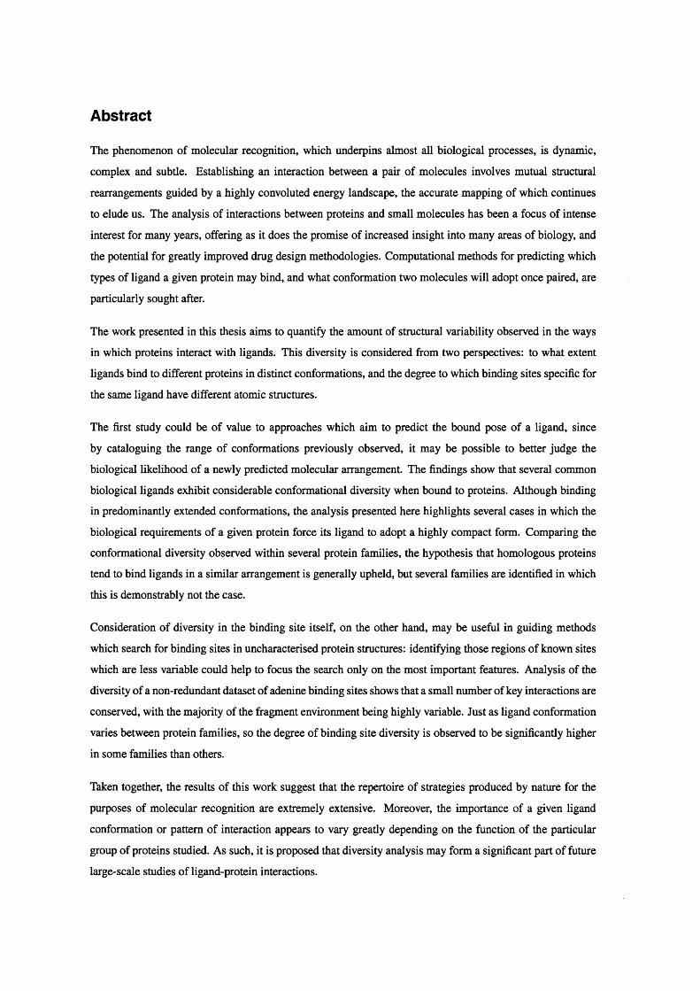
Abstract

The phenomenon of molecular recognition, which underpins almost all biological processes, is dynamic,

complex and subtle. Establishing an interaction between a pair of molecules involves mutual structural

rearrangements guided by a highly convoluted energy landscape, the accurate mapping of which continues

to elude us. The analysis of interactions between proteins and small molecules has been a focus of intense

interest for many years, offering as it does the promise of increased insight into many areas of biology, and

the potential for greatly improved drug design methodologies. Computational methods for predicting which

types of ligand a given protein may bind, and what conformation two molecules will adopt once paired, are

particularly sought after.

The work presented in this thesis aims to quantify the amount of structural variability observed in the ways

in which proteins interact with ligands. This diversity is considered from two perspectives: to what extent

ligands bind to different proteins in distinct conformations, and the degree to which binding sites specific for

the same ligand have different atomic structures.

The first study could be of value to approaches which aim to predict the bound pose of a ligand, since

by cataloguing the range of conformations previously observed, it may be possible to better judge the

biological likelihood of a newly predicted molecular arrangement. The findings show that several common

biological ligands exhibit considerable conformational diversity when bound to proteins. Although binding

in predominantly extended conformations, the analysis presented here highlights several cases in which the

biological requirements of a given protein force its ligand to adopt a highly compact form. Comparing the

conformational diversity observed within several protein families, the hypothesis that homologous proteins

tend to bind ligands in a similar arrangement is generally upheld, but several families are identified in which

this is demonstrably not the case.

Consideration of diversity in the binding site itself, on the other hand, may be useful in guiding methods

which search for binding sites in uncharacterised protein structures: identifying those regions of known sites

which are less variable could help to focus the search only on the most important features. Analysis of the

diversity of a non-redundant dataset of adenine binding sites shows that a small number of key interactions are

conserved, with the majority of the fragment environment being highly variable. Just as ligand conformation

varies between protein families, so the degree of binding site diversity is observed to be significantly higher

in some families than others.

Taken together, the results of this work suggest that the repertoire of strategies produced by nature for the

purposes of molecular recognition are extremely extensive. Moreover, the importance of a given ligand

conformation or pattern of interaction appears to vary greatly depending on the function of the particular

group of proteins studied. As such, it is proposed that diversity analysis may form a significant part of future

large-scale studies of ligand-protein interactions.

Acknowledgements

It is a great pleasure to be able to offer my gratitude to all those whose friendship, advice and support has

made this thesis possible.

Firstly I would like to thank my primary supervisor, Janet Thornton, for her unfaltering enthusiasm and

encouragement throughout the course of this project. She has been a source of outstanding inspiration,

without whom I would never have reached this point. Thanks are also due to my second supervisor Richard

Jackson, and my mentor Christine Orengo, both of whom maintained an active interest in this work. The

administrative burden of undertaking a Ph.D. was lightened significantly by Gillian Adams, who has been

immensely helpful in dealing with forms, contracts, manuscripts and a variety of other issues - always with

a smile on her face! This work was funded mainly by the BBSRC, with additional support from EMBL and

Inpharmatica.

My time at the EBI has been very enjoyable thanks to members of the Thornton group past and present, many

of whom have become good friends as well as colleagues. In particular I wish to thank: Jonathan Barker, for

ensuring that our office was always anything but dull; Gail Bartlett, for ensuring that the pranks stayed (at

least mostly) on the right side of good taste and decency; Matthew Bashton, for his amusing stories on all

topics imaginable; Alex Gutteridge, for being a model of Zen calm to aspire to, both in the office and on the

ski slope; Kevin Murray, for teaching me that the light at the end of the tunnel might just be a train; Richard

Morris and Rafael Najmanovich, for sharing my view that the Flying Pig is as good a place as any to talk

science (and much else besides); James Torrance, for his inimitably dry humour; and Gordon Whamond, for

being a friend and housemate for almost three years.

I have benefitted greatly over the last few years from the knowledge and expertise of other members of

the group; those to whom I am particularly indebted for numerous enlightening scientific discussions include

Tom Funkhouser, Fabian Glaser, Roman Laskowski, Tim Massingham, Richard Morris, Rafael Najmanovich,

Irilenia Nobeli, Hannes Ponstingl and Hugh Shanahan. In addition, I thank the other members of the group

for contributing to the social atmosphere and always being ready to go to coffee: notably Eric Blanc, Shiri

Freilich, Abdullah Kahraman, Marialuisa Pellegrini-Calace, Eugene Schuster, Mike Stevens and (our own)

James Watson.

The support of my friends has been invaluable throughout my Ph.D. Although I cannot thank them all here,

I would especially like to mention the following people: Daniel Bassett, Rick Muir, Liam O’Flynn, Sam

Weatherill and Ed Wood, for some truly momentous nights out; James Howarth and Annabelle Lewis, for

regular games of tennis when weather allowed, and trips to the pub when it didn’t; Ollie Redfem, for sharing

the pain; Andy Pick, for persuading me to abandon common sense and buy the MR2; Ella Hinton, for being

such a great and cheery housemate; and Alice Carr, Fred Goldberg, Sam Gray and Barney Jopson, for making

my trip to Sri Lanka so memorable. Above all, my thanks go to Debora Lucarelli, for being there for me.

Finally, I wish to thank my parents, Helen and Ian. The importance to me of their love, understanding and

support in every circumstance cannot be overstated. Mum and Dad, this is for you.

5

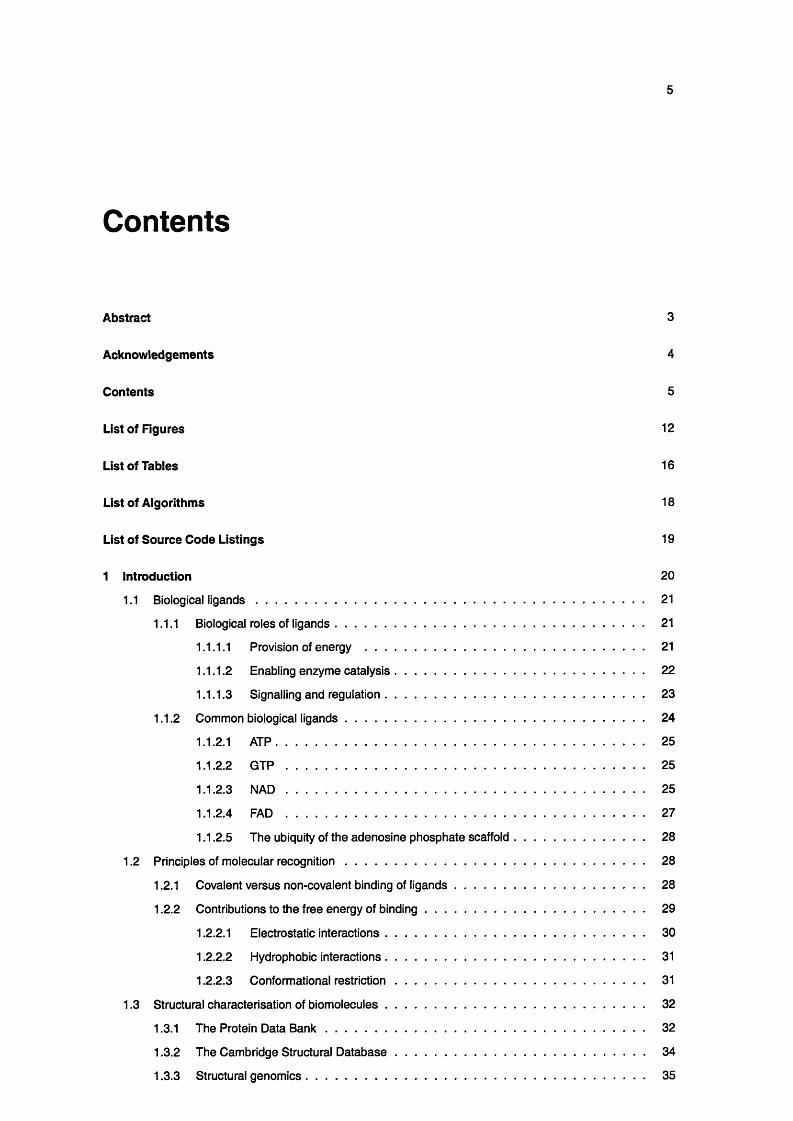
Contents

Abstract 3

Acknowledgements 4

Contents 5

List of Figures 12

List of Tables 16

List of Algorithms 18

List of Source Code Listings 19

1 Introduction 20

1.1 Biological l ig a n d s .................................................................................................................................. 21

1.1.1 Biological roles of ligands....................................................................................................... 21

1.1.1.1 Provision of energy .............................................................................................. 21

1.1.1.2 Enabling enzyme catalysis .................................................................................... 22

1.1.1.3 Signalling and regulation....................................................................................... 23

1.1.2 Common biological lig an d s .................................................................................................... 24

1.1.2.1 ATP............................................................................................................................ 25

1.1.2.2 G T P ......................................................................................................................... 25

1.1.2.3 N A D ......................................................................................................................... 25

1.1.2.4 FAD ......................................................................................................................... 27

1.1.2.5 The ubiquity of the adenosine phosphate scaffold............................................ 28

1.2 Principles of molecular recogn ition .................................................................................................... 28

1.2.1 Covalent versus non-covalent binding of lig an d s .................................................................. 28

1.2.2 Contributions to the free energy of b ind ing ........................................................................... 29

1.2.2.1 Electrostatic interactions........................................................................................ 30

1.2.2.2 Hydrophobic interactions........................................................................................ 31

1.2.2.3 Conformational restric tion .................................................................................... 31

1.3 Structural characterisation of biom olecules....................................................................................... 32

1.3.1 The Protein Data B a n k ............................................................................................................ 32

1.3.2 The Cambridge Structural D a ta b a s e .................................................................................... 34

1.3.3 Structural genom ics................................................................................................................... 35

1.3.4 Structure quality ..................................................................................................................... 35

1.3.5 Non-cognate l ig a n d s ............................................................................................................... 36

1.3.6 Chemical compound d a t a s e t s .............................................................................................. 37

1.4 Protein structure and ev o lu tio n ........................................................................................................... 38

1.5 Computational studies of ligand binding ........................................................................................... 42

1.5.1 Locating the binding s i t e ........................................................................................................ 43

1.5.2 D ocking...................................................................................................................................... 43

1.5.3 Knowledge-based ligand prediction........................................................................................ 44

1.5.3.1 Similarity-based approaches................................................................................ 45

1.5.3.2 Propensity approaches ....................................................................................... 45

1.5.4 The relationship between ligand specificity and protein function ...................................... 46

1.6 Overview of the T h e s i s ......................................................................................................................... 47

2 The GAMUT library 49

2.1 A brief history of computational biology.............................................................................................. 49

2.1.1 Methodological c h a n g e s ........................................................................................................ 51

2.1.2 Technological c h a n g e s ............................................................................................................ 51

2.2 Other projects related to GAM UT........................................................................................................ 52

2.3 Design of GAMUT.................................................................................................................................. 55

2.3.1 Design p rin c ip les...................................................................................................................... 55

2.3.1.1 M odularity .............................................................................................................. 55

2.3.1.2 Ease of use ........................................................................................................... 55

2.3.2 R o b u stn ess ................................................................................................................................ 56

2.3.3 Choice of la n g u a g e .................................................................................................................. 56

2.3.4 Architecture of the lib rary ........................................................................................................ 57

2.3.4.1 Generic com ponents.............................................................................................. 58

2.3.4.2 Macromolecular structure c o m p o n e n ts ............................................................. 63

2.3.4.3 Chemical structure com ponen ts.......................................................................... 64

2.3.4.4 Ligand binding site com ponen ts.......................................................................... 67

2.3.4.5 Density map c o m p o n e n ts .................................................................................... 68

2.4 Documentation ...................................................................................................................................... 68

2.4.1 Installation g u i d e ...................................................................................................................... 69

2.4.2 Tutorials...................................................................................................................................... 69

2.4.3 API re fe ren ce ............................................................................................................................ 70

2.5 S u m m a ry ................................................................................................................................................ 70

3 Methods 72

3.1 Graph m atch in g ...................................................................................................................................... 72

3.1.1 Vertex and edge compatibility.................................................................................................. 73

3.1.2 Available methods .................................................................................................................. 74

3.1.2.1 Clique d e te c tio n ..................................................................................................... 74

3.1.2.2 Backtracking s e a r c h ............................................................................................. 74

3.1.3 Match size m e t r ic s ................................................................................................................. 80

3.2 C lu ste rin g ............................................................................................................................................... 80

3.2.1 Dissimilarity matrices, measures and metrics .................................................................... 81

3.2.2 Hierarchical clustering te c h n iq u e s ....................................................................................... 81

3.2.2.1 Agglomerative a lg o rith m s................................................................................... 81

3.2.2.2 Divisive algorithm s................................................................................................. 82

3.2.3 Problems with hierarchical clustering.................................................................................... 82

3.2.4 V alidation.................................................................................................................................. 84

3.2.5 Stopping criteria ..................................................................................................................... 84

3.3 Analysis of multidimensional data s e t s ............................................................................................... 85

3.3.1 Principal components a n a ly s is .............................................................................................. 85

3.3.2 Multidimensional s c a l in g ........................................................................................................ 86

3.3.3 Choice of the number of dimensions to r e t a i n ................................................................... 87

3.4 Geometric range querying..................................................................................................................... 88

3.4.1 The bricking algorithm ........................................................................................................... 88

3.4.2 k d -tre e s ...................................................................................................................................... 88

3.5 Sequence alignment ............................................................................................................................ 90

3.5.1 Pairwise alignment a lg o rith m s.............................................................................................. 91

3.5.1.1 Dynamic programming.......................................................................................... 91

3.5.1.2 Hidden Markov Models ....................................................................................... 94

3.6 Coordinate su perposition ..................................................................................................................... 94

3.6.1 Available methods .................................................................................................................. 95

3.6.2 The planarity problem .............................................................................................................. 95

3.7 Analysis of ligand conform ation........................................................................................................... 96

3.7.1 Radius of gyration..................................................................................................................... 96

3.7.2 Torsion angles ........................................................................................................................ 96

3.7.2.1 Definition.................................................................................................................. 97

3.7.2.2 N om encla tu re ........................................................................................................ 98

3.8 Calculation of solvent-accessible surface a r e a .................................................................................... 101

3.8.1 Molecular surface defin itions..................................................................................................... 101

3.8.2 kd-tree algorithm for neighbour detection................................................................................. 101

3.8.3 Generation of uniformly distributed surface p o in ts .................................................................102

3.8.3.1 Uniform distribution of points on the unit sp h e re ................................................... 102

3.8.3.2 Surface triangulation..................................................................................................103

3.8.3.3 Spherical t-designs ..................................................................................................104

3.8.4 C a v e a ts ......................................................................................................................................... 105

3.8.4.1 Structural water m olecules........................................................................................105

3.8.4.2 Internal c a v i t i e s ........................................................................................................ 105

3.8.5 Degree of burial........................................................................................................................ 106

4 Generation of d a tase ts 107

4.1 Protocol for validation of ligand iden tity ................................................................................................. 108

4.1.1 The need for ligand validation ................................................................................................. 108

4.1.2 The algorithm ............................................................................................................................... 109

4.1.3 W e a k n e s s e s ............................................................................................................................... 113

4.2 Protocol for comparing and clustering ligand binding s i t e s ................................................................ 113

4.2.1 A im s................................................................................................................................................113

4.2.2 Multi-domain binding s i t e s ........................................................................................................ 114

4.2.3 The algorithm ............................................................................................................................... 115

4.3 Architecture of the processing p ip e lin e ................................................................................................. 117

4.3.1 Obtaining the chemical compound data set .......................................................................... 120

4.3.2 Representation of mappings from molecular structures to reference compounds . . . 122

4.3.3 Representation of ligand-domain c o n ta c ts ..............................................................................123

4.3.4 Generation of the ligand d a t a s e t .............................................................................................. 123

4.3.5 Maintainance of in teg rity ............................................................................................................124

4.3.6 Improving performance through parallelisation....................................................................... 125

4.4 Ligands in the P D B .................................................................................................................................. 126

4.4.1 Results of the validation p rocedure ........................................................................................... 126

4.4.1.1 Bound state of potential ligand m olecu les ............................................................. 126

4.4.1.2 Results of graph m atch ing........................................................................................128

4.4.1.3 Examples of automatic identification of problems in ligand d a ta ...................... 130

4.4.1.4 The most common ligand t y p e s ............................................................................. 131

4.4.2 Distribution of ligand types with respect to sequence and structure fam ilies......................132

4.4.2.1 Evolutionary diversity of proteins binding each ligand t y p e .................................132

4.4.2.2 Diversity of ligands binding each protein f o l d .......................................................134

4.4.2.3 Occurrence of multi-domain binding s i t e s ............................................................. 139

4.4.3 Distribution of ligand types with respect to enzyme fu n c tio n ................................................ 140

4.5 Datasets of ligands of particular biological in te re s t ..............................................................................142

4.5.1 Analysis of the c lu stering ............................................................................................................142

4.5.2 Distribution of folds and superfamilies binding each ligand t y p e ..........................................142

4.5.3 Distribution of enzyme functions among proteins binding each ligand t y p e ....................... 147

4.6 S u m m a ry ................................................................................................................................................... 147

5 Conformational variability of bound ligands 149

5.1 Rationale for studying ligand conform ation...........................................................................................149

5.2 Chemical theory pertinent to small molecule conform ation................................................................ 151

5.2.1 Electron-pair re p u ls io n ............................................................................................................... 151

5.2.2 Electrostatic interaction............................................................................................................... 152

5.2.3 Steric h inderance ......................................................................................................................... 152

5.3 Previous work on ligand conformation ..................................................................................................153

5.4 Methodology................................................................................................................................................156

5.5 Overall shape of bound lig a n d s ............................................................................................................... 157

5.5.1 S u p erp o sitio n s ............................................................................................................................157

5.5.1.1 ATP.............................................................................................................................. 157

5.5.1.2 G T P .............................................................................................................................. 160

5.5.1.3 N A D .............................................................................................................................. 160

5.5.1.4 FAD .............................................................................................................................. 164

5.5.2 Radii of gyration............................................................................................................................ 166

5.5.3 General observations.............................................................................................................. 171

5.6 Conformational differences between and within c lu s te r s .................................................................... 174

5.6.1 Hierarchical clustering of ligand conformations....................................................................... 174

5.6.2 Multidimensional scaling of ligand conformational d iffe rences.............................................179

5.7 Relationship between protein sequence and ligand con fo rm atio n ....................................................186

5.7.1 General t r e n d s ............................................................................................................................ 186

5.7.2 Ligand conformation and sequence similarities in the ‘twilight zone’ ...............................190

5.8 Analysis of torsion a n g le s ......................................................................................................................... 194

5.9 Concluding rem ark s...................................................................................................................................200

6 Structural and chemical variability in ligand environments 204

6.1 Qualitative observations of binding site d iv e rs ity ................................................................................. 205

6.2 Previous work on adenylate recognition..................................................................................................207

6.3 Methodology................................................................................................................................................ 211

6.3.1 Definition of the binding site .....................................................................................................211

6.3.2 Atom t y p e s .................................................................................................................................. 212

6.3.3 Generation of property m a p s .....................................................................................................217

6.3.4 Generation of environment m a s k s ...........................................................................................219

6.3.5 Mapping environment properties onto the fragment s u r f a c e .............................................. 219

6.4 Characterisation and comparison of fragment environm ents........................................................... 221

6.4.1 Localised contact p ro p en sitie s ..................................................................................................222

6.5 Diversity of fragment environm ents.........................................................................................................228

6.5.1 Measures of d iversity .................................................................................................................. 229

6.5.1.1 Entropy......................................................................................................................... 229

6.5.1.2 Chemical d iversity ..................................................................................................... 231

6.5.1.3 A combined diversity score .....................................................................................233

6.5.2 Diversity of unrelated adenine-binding s i t e s .........................................................................234

6.5.3 Diversity of related adenine binding s i te s ............................................................................... 238

6.5.4 Diversity of environments for different fragment t y p e s ........................................................ 245

6.6 Concluding rem ark s ................................................................................................................................... 246

7 Discussion 249

A Graph theory 254

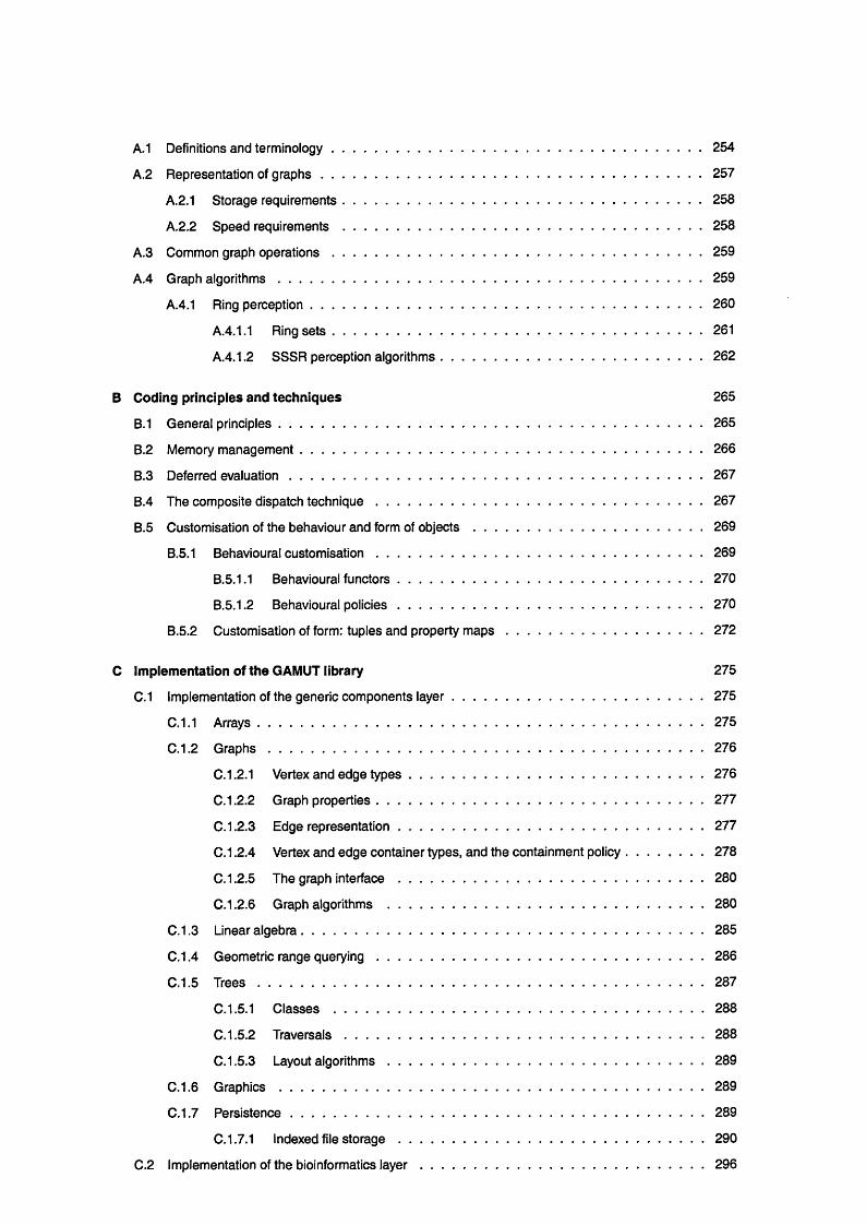
A.1 Definitions and term inology.....................................................................................................................254

A.2 Representation of g r a p h s ........................................................................................................................ 257

A.2.1 Storage requirem ents..................................................................................................................258

A.2.2 Speed requirements ..................................................................................................................258

A.3 Common graph o p e ra t io n s .....................................................................................................................259

A.4 Graph a lg o rith m s..................................................................................................................................... 259

A.4.1 Ring perception ............................................................................................................................260

A.4.1.1 R in g s e ts ..................................................................................................................261

A.4.1.2 SSSR perception algorithm s....................................................................................262

B Coding principles and techn iques 265

B.1 General principles......................................................................................................................................265

B.2 Memory m anagem ent............................................................................................................................... 266

B.3 Deferred ev a lu a tio n .................................................................................................................................. 267

B.4 The composite dispatch te c h n iq u e ........................................................................................................267

B.5 Customisation of the behaviour and form of o b j e c t s ..........................................................................269

B.5.1 Behavioural cu sto m isa tio n ........................................................................................................ 269

B.5.1.1 Behavioural fu n c to rs ................................................................................................. 270

B.5.1.2 Behavioural p o lic ie s ................................................................................................. 270

B.5.2 Customisation of form: tuples and property m a p s ..................................................................272

C Implementation of the GAMUT library 275

C.1 Implementation of the generic components la y e r .................................................................................275

C.1.1 A rrays............................................................................................................................................ 275

C.1.2 G r a p h s ......................................................................................................................................... 276

C.1.2.1 Vertex and edge ty p e s .............................................................................................. 276

C.1.2.2 Graph properties........................................................................................................ 277

C. 1.2.3 Edge represen tation ..................................................................................................277

C.1.2.4 Vertex and edge container types, and the containment policy............................278

C. 1.2.5 The graph interface ..................................................................................................280

C.1.2.6 Graph algorithms ..................................................................................................... 280

C.1.3 Linear a lgebra ................................................................................................................................285

C.1.4 Geometric range q u e ry in g ........................................................................................................ 286

C.1.5 T r e e s ............................................................................................................................................ 287

C.1.5.1 Classes ......................................................................................................................288

C.1.5.2 T ra v e rsa ls .................................................................................................................. 288

C.1.5.3 Layout a lg o rith m s ..................................................................................................... 289

C.1.6 Graphics ...................................................................................................................................... 289

C.1.7 P e rs is te n c e ...................................................................................................................................289

C.1.7.1 Indexed file s t o r a g e ..................................................................................................290

C.2 Implementation of the bioinformatics l a y e r ............................................................................................296

C.2.1 Macromolecular structu re .......................................................................................................... 296

C.2.1.1 Nodes of the molecular t r e e .................................................................................... 296

C.2.1.2 Molecule as a manager c l a s s .................................................................................296

C.2.1.3 File I /O .........................................................................................................................303

C.2.2 Chemical s t ru c tu re .....................................................................................................................303

C.2.2.1 The chemical graph c l a s s ....................................................................................... 303

C.2.2.2 The chemical compound archive class ................................................................ 303

C.2.2.3 Structure diagram g e n e ra tio n ................................................................................. 304

C.3 Ligand binding s i t e s ..................................................................................................................................305

C.4 Density m a p s ............................................................................................................................................307

D Ligand datasets 309

E CATH superfamily names 331

Abbreviations and nomenclature 335

References 337

12

List of Figures

1.1 Magnesium coordination inducing strain in the ATP phosphate linkage .................................... 22

1.2 The four ligands chosen for detailed an a ly s is ................................................................................... 24

1.3 Proximity of nicotinamide ring to a s u b s t r a te ................................................................................... 26

1.4 The oxidised and reduced forms of nicotinam ide............................................................................ 26

1.5 The oxidised and reduced forms of riboflavin................................................................................... 27

1.6 “Butterfly bending” in the isoalloxine r i n g ......................................................................................... 28

1.7 Hydrogen bond g eo m e try .................................................................................................................... 30

1.8 Growth in PDB holdings....................................................................................................................... 32

1.9 Types of PDB e n t r y .............................................................................................................................. 33

1.10 Resolution of deposited X-ray s tru c tu re s ......................................................................................... 36

2.1 Timeline showing key advances in computational b io lo g y ........................................................... 50

2.2 Architecture of the GAMUT library ................................................................................................... 58

2.3 Hierarchy of objects which makes up the representation of macromolecular s tru c tu re 63

2.4 The process of mapping coordinates of a ligand molecule against a reference compound . . . 65

2.5 Chemical structure diagram showing an adenine fragm ent............................................................ 66

2.6 Example of the definition of a ratable b o n d ...................................................................................... 67

2.7 A screenshot of the on-line GAMUT d o cu m en ta tio n ..................................................................... 69

2.8 Screenshot of part of an on-line GAMUT tu to r ia l............................................................................ 70

2.9 The graphical class hierarchy d ia g r a m ............................................................................................ 71

2.10 Summary of member functions in on-line docum entation............................................................... 71

3.1 Types of graph isomorphism ............................................................................................................. 73

3.2 Example g ra p h s ..................................................................................................................................... 74

3.3 Graph matching by clique detection................................................................................................... 75

3.4 Progression of Ullman’s algorithm....................................................................................................... 76

3.5 An example clustering dendrogram ................................................................................................... 82

3.6 Agglomerative clustering methods ................................................................................................... 83

3.7 Geometric range querying.................................................................................................................... 88

3.8 kd-tree range q u e ry in g ....................................................................................................................... 89

3.9 Population of the dynamic programming m atrix ............................................................................... 93

3.10 Traceback of the dynamic programming m a trix ............................................................................... 94

3.11 Definition of a torsion a n g le ................................................................................................................ 97

3.12 The Klyne-Prelog system for angle range n o m en cla tu re .............................................................. 98

3.13 Torsion angles defined for nucleotide triphosphates ...................................................................... 99

3.14 Torsion angles defined for the nucleotide derivatives NAD and F A D ...............................................100

3.15 Molecular surface representations ....................................................................................................... 102

3.16 Spherical t-designs in three dimensions ............................................................................................. 104

3.17 Searching for potentially solvent-excluding neighbours...................................................................... 105

3.18 Calculation of per-atom solvent accessible su rfa c e .............................................................................106

4.1 The NAD molecule from PDB entry 1B I 9 ..........................................................................................111

4.2 Example of two isomeric co m p o u n d s....................................................................................................112

4.3 Convention for referring to the handedness of chiral stereocen tres.................................................. 113

4.4 Multidomain binding s i t e s ........................................................................................................................114

4.5 Example of binding site domain com position .......................................................................................116

4.6 Dataset generation p ipe line .....................................................................................................................119

4.7 Number of compounds in MSD reference dictionary, broken down by RCSB_HETTYPE . . . . 121

4.8 UML diagram of classes which represent ligand id e n tity ...................................................................122

4.9 Generation of the ligand d a t a s e t ...........................................................................................................124

4.10 UML diagram of master/slave c la s se s ................................................................................................ 126

4.11 Distribution of the bound state .............................................................................................................. 127

4.12 Distribution of matching r e s u l t s .............................................................................................................. 129

4.13 Bound ligand m a tc h in g ........................................................................................................................... 129

4.14 Most commonly-occurring hetgroups in the P D B ................................................................................ 131

4.15 Distribution of numbers of distinct folds binding each ligand ty p e ......................................................133

4.16 Ligands which bind to the most evolutionary diverse proteins ......................................................... 133

4.17 Most promiscuous fo ld s ........................................................................................................................... 135

4.18 Most promiscuous folds compared with distribution of folds in protein s p a c e ..............................136

4.19 Fraction of binding sites for each ligand type composed of more than one dom ain........................139

4.20 Fraction of proteins binding each ligand type which are annotated with enzyme functions . . . 141

4.21 Ligands whose binding proteins have the widest range of enzyme functions..................................141

4.22 CATH wheels for the four ligands which were analysed in d e t a i l ......................................................144

4.23 EC wheels for the four ligands which were analysed in detail............................................................ 145

4.24 EC wheels for the CATH S35 representatives.......................................................................................146

5.1 Newman projections of eclipsed and staggered conformations of e t h a n e ..................................... 152

5.2 1,2-dibromoethane in an anti staggered con fo rm ation ...................................................................... 152

5.3 Lennard-Jones potential........................................................................................................................... 153

5.4 Superposition of ATP cluster represen tatives.......................................................................................158

5.5 Conformation of ATP molecules bound to tRNA synthetase e n z y m e s ........................................159

5.6 The syn and anti conformations of A T P ............................................................................................. 159

5.7 Superposition of GTP cluster representatives.......................................................................................161

5.8 Superposition of NAD cluster representatives ....................................................................................162

5.9 Folded conformations of NAD in flavin re d u c ta se ................................................................................ 163

5.10 NAD binding by ADP-ribosylating p r o te in s .......................................................................................... 164

5.11 Superposition of FAD cluster representatives.......................................................................................165

5.12 FAD binding sites in the glutathione reductase family......................................................................... 166

5.13 Generated ligand conformations .......................................................................................................... 169

5.14 Distribution of radii of gyration................................................................................................................. 172

5.15 Comparison of ATP conformations with cluster assig n m en ts ............................................................ 175

5.16 Comparison of GTP conformations with cluster assignm ents............................................................ 176

5.17 Comparison of NAD conformations with cluster assignments .........................................................177

5.18 Comparison of FAD conformations with cluster assignm ents............................................................ 178

5.19 Multidimensional scaling of ligand conformational d iffe re n c es .........................................................180

5.19 Multidimensional scaling of ligand conformational d iffe re n c es .........................................................181

5.20 Hypothetical conformational energy la n d sc a p e ................................................................................... 182

5.21 Significance testing of within-cluster mean pairwise RMSD ....................................... 183

5.22 Variation in FAD conformation within the flavin reductase fa m ily ......................................................185

5.23 Variation in FAD conformation within the flavin reductase fa m ily ......................................................186

5.24 Sequence identity of ATP binding domains versus ligand conformational d istance ........................187

5.25 Sequence identity of GTP binding domains versus ligand conformational d i s t a n c e ..................... 187

5.26 Sequence identity of NAD binding domains versus ligand conformational d i s ta n c e ......................188

5.27 Sequence identity of FAD binding domains versus ligand conformational distance ......................188

5.28 Sequence identity of P-loop hydrolase domains versus ATP RMSD v a l u e s ..................................192

5.29 Sequence identity of Rossmann fold domains versus NAD RMSD v a lu e s ................................. 192

5.30 Sequence identity of Rossmann fold domains versus NAD conformational d is tan ce .................193

5.31 Coordinates of NAD molecules modelled into density maps at different re so lu tio n s.....................195

5.32 Variation in ATP torsion a n g l e s .............................................................................................................. 196

5.33 Variation in GTP torsion a n g le s .............................................................................................................. 197

5.34 Variation in NAD torsion a n g le s .......................................................................................................... 198

5.35 Variation in FAD torsion a n g le s .............................................................................................................. 199

5.36 Conformational change of NAD in transhydrogenase......................................................................... 201

6.1 Examples of diversity in adenine binding s i t e s ................................................................................... 206

6.2 The adenylate m o ie ty .............................................................................................................................. 207

6.3 The adenine recognition motif described by Kobayashi and Go ..................................................... 209

6.4 Definition of the ligand binding s i t e ....................................................................................................... 212

6.5 Dissimilarity between the atom types of Rantanen e t a l . ...................................................................216

6.6 Convolution of atom coordinates with a Gaussian function ............................................................... 218

6.7 Precomputation of the 3-dimensional Gaussian fu n c tio n .................................................................. 218

6.8 ‘Smearing’ effect of the Gaussian density convo lu tio n ......................................................................219

6.9 Creation of environment m a s k s ..............................................................................................................220

6.10 Mapping properties onto an atomic su rfa c e ..........................................................................................221

6.11 Spatial distribution of atom types contacting a d e n in e ......................................................................... 222

6.12 Spatial distribution of polar atoms contacting a d e n in e ......................................................................224

6.13 Distribution of immobilised water molecules around a d e n in e .......................................................... 225

6.14 Spatial distribution of non-polar atoms contacting a d e n in e ..............................................................226

6.15 A composite picture of the adenine environments ...........................................................................227

6.16 Example of entropy sc o r in g ............................................................................................................... 231

6.17 Example of chemical diversity scoring ...............................................................................................233

6.18 Effect of exponential parameters on components of the combined s c o re .......................................234

6.19 Depiction of entropy scores for adenine env ironm en ts.................................................................... 235

6.20 Depiction of chemical diversity scores for adenine environm ents....................................................236

6.21 Depiction of combined diversity scores for adenine env iro n m en ts.................................................237

6.22 Combined diversity scores mapped onto adenine s u r f a c e ..............................................................239

6.23 Sample size-dependence of the binding site diversity indices for a d e n in e .................................... 240

6.24 Diversity in adenine-binding site structure within superfam ilies....................................................... 242

6.25 Diversity scores for adenine clusters compared to results of random sampling ......................... 245

A.1 The Konigsberg bridge problem ............................................................................................................ 255

A.2 Types of graphs, organised in terms of connectivity...........................................................................256

A.3 An example of an induced s u b g r a p h .................................................................................................. 256

A.4 Types of graph isomorphism ............................................................................................................... 257

A.5 An example g ra p h ................................................................................................................................... 257

A.6 Cycles in a complex ring s e t ...................................................................................................................261

A.7 Ring perception by breadth-first s e a r c h ............................................................................................... 264

C.1 UML diagram of the inheritance hierarchy of the Graph c la s s ...........................................................279

C.2 UML diagram of the inheritance hierarchy of two graph algorithm c l a s s e s .....................................284

C.3 Tree layout algorithm s.............................................................................................................................289

C.4 Organisation of an ISAM a r c h iv e ......................................................................................................... 291

C.5 Pointer swizzling....................................................................................................................................... 293

C.6 Separation of the ‘object manager1 roles of the Molecule c la s s ........................................................297

C.7 Different types of iteration through nodes of the molecular t r e e ........................................................298

C.8 Classes which constitute the selection fra m e w o rk ........................................................................... 299

C.9 Selection bitmasks .................................................................................................................................300

C.10 Concise storage of atom properties using a bit-masking ap p ro ach .................................................303

C.11 Example of the chemical structure layout algorithm........................................................................... 304

16

List of Tables

1.1 Description of the levels of the CATH and SCOP hierarchies.......................................................... 40

2.1 Software development projects related to G A M U T.......................................................................... 54

3.1 Range of target graph sizes which can potentially provide a sufficiently good m atch .................. 79

3.2 Agglomerative clustering methods .................................................................................................... 82

3.3 Definition of torsion angles for nucleotide derivatives...........................................................................101

4.1 Clustering steps used to generate ligand d a t a s e t s ..............................................................................117

4.2 Summary of ligand validation p ro c e d u re .............................................................................................. 127

4.3 Common names corresponding to selected RCSB compound identifiers ....................................... 132

4.4 Levels of the Enzyme Commission h ierarchy ........................................................................................140

4.5 Summary of the ligand d a ta se ts ...............................................................................................................143

5.1 Definition of torsion angles and associated minima for nucleotide d e riv a tiv es ........................... 167

5.2 Definition of torsion angles and associated minima for N A D ............................................................. 167

5.3 Definition of torsion angles and associated minima for F A D ............................................................. 167

5.4 Results of conformation generation experim ent.....................................................................................168

5.5 Radii of gyration ..........................................................................................................................................170

5.6 Comparison of conformational variance within and between clusters .............................................184

5.7 Number of predominantly single-domain binding sites for each l ig a n d .............................................186

5.8 Linear regression between domain sequence identity and ligand conformation distance . . . 189

5.9 x2 analysis of ligand conformation distance versus domain sequence identity ............................... 190

6.1 GAMUT atom c la s s e s ............................................................................................................................... 214

6.2 Dissimilarity between GAMUT atom c l a s s e s ........................................................................................217

6.3 Summary of the adenine binding site clusters .................................................................................... 241

6.4 Comparison of environment diversity within and between clusters of adenine binding sites . . 244

6.5 Comparison of environment diversity scores of three different fragments ......................................246

A.1 Average orders of complexity for common graph o p e ra tio n s .............................................................259

C.1 Vertex-related functions in the graph in te r f a c e .................................................................................... 281

C.2 Edge-related functions in the graph in te rface ....................................................................................... 282

C.3 Graph algorithms currently implemented in G A M U T.......................................................................... 283

C.4 Types of tree ite ra to rs ............................................................................................................................... 288

C.5 Examples of diagrams generated by chemical graph layout a lg o rith m ........................................... 308

D.1 Summary of the ATP d a t a s e t ..................................................................................................................310

D.2 Summary of the GTP d a ta s e t ..................................................................................................................317

D.3 Summary of the NAD d a ta s e t .............................................................................................................. 319

D.4 Summary of the FAD d a t a s e t ..................................................................................................................326

E.1 Mapping from CATH codes to superfamily names .............................................................................331

18

List of Algorithms

3.1 Ullman’s backtracking search algorithm for exact subgraph isomorphism d e te c tio n 77

4.1 Validation of ligand identity ........................................................................................................... 110

A. 1 Breadth-first search in an undirected graph ................................................................................ 260

A.2 Depth-first search in an undirected graph........................................................................................260

A.3 Ring perception by breadth-first search...........................................................................................263

C. 1 Chemical structure diagram generation a lg o rith m ....................................................................306

19

List of Source Code Listings

B.l The deferred evaluation te ch n iq u e ................................................................................................. 268

B.2 The composite dispatch tech n iq u e ................................................................................................. 269

B.3 An example functo r...........................................................................................................................270

B.4 A sketch of code for a simulated annealing a lgorithm .............................................................. 271

B.5 Design of a simulated annealing algorithm using policy c lasses...............................................271

B.6 Naieve design for a generic tree node c la ss .....................................................................................272

B.7 Property m ap s .................................................................................................................................... 274

C.1 Syntax for definition of a GAMUT graph ty p e ...............................................................................277

C.2 Population of a graph object with d a t a ........................................................................................... 283

C.3 Graph layout example........................................................................................................................285

C.4 Classes defined in the linear algebra com ponent........................................................................... 286

C.5 An outline of the framework for describing geometric regions . ...............................................287

C.6 Implementation of serialisation functions for a GAMUT o b jec t.................................................. 291

C.7 Example of using selection functions to pick out a ligand binding site ......................................302

20

Chapter 1

Introduction

The binding of small molecules to proteins lies at the heart of almost all biological processes. Molecular

recognition is a vital part of enzyme catalysis, signal transduction and DNA replication to name but three;

without it, life could not be sustained. Viewed from a physical perspective, the specific binding of one

molecule to another is the result of precise geometric and chemical complementarity between them.

Developing a coherent picture of the principles which underlie intermolecular interactions is therefore of

central importance to unravelling the complexities of biological systems. One ultimate aim of computational

biology - to be able to accurately model all aspects of a cell - can only be realised if we are able to predict, with

atomic-scale precision, the ways in which molecules interact. Since the actions of drugs are determined by

the same forces which govern natural protein-ligand interactions, deepening our understanding of molecular

recognition may also lead to cheaper, more effective theraputic agents - and perhaps most importantly, fewer

undesirable side-effects.

The way in which ligands bind to proteins has been an area of intense interest for many years, with recent

innovations in computing technology, allied with increasing availability of biological data, having brought

significant advances in our understanding of the subject. The problems of how to predict which ligands

a given protein may bind, and the structure of the resulting complex, however, remain unsolved. Despite

increasing levels of sophistication in the physical models used to represent protein-ligand interactions, it

appears that they are insufficiently accurate to distinguish correct modes of binding from incorrect solutions.

Therefore many studies take a more knowledge-based approach, using common patterns of binding observed

in protein-ligand complexes to predict putative interactions with new, uncharacterised proteins.

This thesis does not set out to develop a predictive method, but rather to describe and quantify the degree of

variation observed in the interactions between a given ligand and the proteins which bind it. The objective of

this study is to provide information which can inform future development of predictive methods in this field.

This chapter addresses some questions fundamental to the analysis which follows: What biological roles do

ligands play? What is our current understanding of the physical principles underlying molecular recognition?

What is the nature of the available structural information on protein-ligand binding? What computational

methods have previously been developed? At this stage, the connections between some of these topics are

not explicitly spelled out, but will become apparent in later sections of the thesis. The chapter concludes with

an outline of the remainder of the thesis.

1. Introduction 21

1.1 Biological ligands

The word ligand derives from the Latin ligare (to bind). In chemistry, it usually refers to ions, atoms or

functional groups which are covalently bonded to one or more partners. In biochemistry, however, the use of

the word is somewhat broader, being applied to any molecule which interacts with a large macromolecule, the

type of interaction being either covalent or non-covalent. As a consequence, the term ‘ligand’ in a biological

context comprises an extremely diverse set of molecules, playing a wide range of biological roles.

1.1.1 Biological roles of ligands

1.1.1.1 Provision of energy

Energy is required by biological systems for three main purposes: the performance of mechanical work in

muscle contraction and for other cellular movements, the active transport of molecules between cellular

compartments, and to power enzymatic reactions involved in biosynthesis. This energy is obtained by

chemotrophs through the metabolic breakdown of fuel molecules, and in phototrophs by harvesting free

energy from light. In both types of organism, the energy is then stored in the form of chemical bonds. These

bonds are made in molecules whose chemical structure is such as to make them convenient stores of energy:

that is, which are stable in the absence of a catalyst, but which can be easily persuaded to release their latent

energy when it is required.

Adenosine triphosphate (ATP) - see figure 1.2a - is the molecule which universally plays this energy storage

role. Its ability to store and release energy derives from the fact that its triphosphate unit contains two

phosphoanhydride bonds. These can be hydrolysed to produce ADP and pyrophosphate (P;), while liberating

energy. Although the triphosphate group is thermodynamically unstable - which is to say the free energy

of hydrolysis is relatively high (Stryer (1995) cites a value of around 12 kJ mol-1 under physiological

conditions) - it is kinetically stable, meaning that in the absence of a catalyst, ATP is only slowly hydrolysed.

The choice of ATP as the universal energy carrier can be rationalised in part by considering the following

contributions to its free energy of hydrolysis:

• Electrostatic repulsion. At physiological pH, the triphosphate group is deprotonated, meaning that

several negative charges are in close proximity. The electrostatic repulsion between them is relieved

when ATP is hydrolysed.

• Resonance. The bonding electrons in pyrophosphate are highly delocalised, but less so when the

moiety is bonded to ADP. Hydrolysis therefore causes an increase in entropy.

• Strain. ATP is often bound along with Mg2+. The divalent coordination of the ion with two

of the phosphate groups induces strain in the phosphodiester linkage, thus promoting hydrolysis

(see figure 1.1).

There are, however, other biological compounds which possess a phosphodiester linkage to which

these arguments would equally apply; why is ATP preferred? One reason that molecules such as

phosphoenolpyruvate and creatine are not used as the universal energy carrier is that they actually have a

higher phosphoryl potential than ATP, due in part to the ability of the dephosphorylated product to adopt

1. Introduction 22

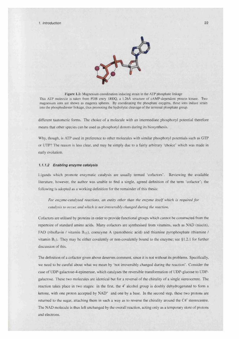
Figure 1.1: Magnesium coordination inducing strain in the ATP phosphate linkage This ATP molecule is taken from PDB entry 1RDQ, a 1.26A structure of cAMP-dependent protein kinase. Two magnesium ions are shown as magenta spheres. By coordinating the phosphate oxygens, these ions induce strain into the phosphodiester linkage, thus promoting the hydrolytic cleavage of the terminal phosphate group.

different tautomeric forms. The choice of a molecule with an intermediate phosphoryl potential therefore

means that other species can be used as phosphoryl donors during its biosynthesis.

Why, though, is ATP used in preference to other molecules with similar phosphoryl potentials such as GTP

or UTP? The reason is less clear, and may be simply due to a fairly arbitrary ‘choice’ which was made in

early evolution.

1.1.1.2 Enabling enzyme catalysis

Ligands which promote enzymatic catalysis are usually termed ‘cofactors’. Reviewing the available

literature, however, the author was unable to find a single, agreed definition of the term ‘cofactor’; the

following is adopted as a working definition for the remainder of this thesis:

For enzyme-catalysed reactions, an entity other than the enzyme itself which is required for

catalysis to occur, and which is not irreversibly changed during the reaction.

Cofactors are utilised by proteins in order to provide functional groups which cannot be constructed from the

repertoire of standard amino acids. Many cofactors are synthesised from vitamins, such as NAD (niacin),

FAD (riboflavin / vitamin B 12), coenzyme A (pantothenic acid) and thiamine pyrophosphate (thiamine /

vitamin Bi). They may be either covalently or non-covalently bound to the enzyme; see §1.2.1 for further

discussion of this.

The definition of a cofactor given above deserves comment, since it is not without its problems. Specifically,

we need to be careful about what we mean by ‘not irreversibly changed during the reaction’. Consider the

case of UDP-galactose-4-epimerase, which catalyses the reversible transformation of UDP-glucose to UDP-

galactose. These two molecules are identical but for a reversal of the chirality of a single stereocentre. The

reaction takes place in two stages: in the first, the 4' alcohol group is doubly dehydrogenated to form a

ketone, with one proton accepted by NAD+ and one by a base. In the second step, these two protons are

returned to the sugar, attaching them in such a way as to reverse the chirality around the C4' stereocentre.

The NAD molecule is thus left unchanged by the overall reaction, acting only as a temporary store of protons

and electrons.

1. Introduction 23

Compare this to the reaction catalysed by alcohol dehydrogenase:

alcohol+ NAD+ acetaldehyde + NADH + H+

After each cycle of this reaction, the cofactor is released from the enzyme in a reduced form, and therefore

cannot be said to be unchanged. However, the NAD+ may be regenerated by other pathways and returned to

the enzyme for further enzymatic cycles to take place. Partly by convention, NAD is classified as a cofactor

even in cases where the molecule is changed during the reaction.

The problem with making exceptions in this way is knowing where to stop. Do we, for example, classify

ATP as a cofactor in cases where it is used an an energy source (and is therefore hydrolysed), but does not

react directly with a substrate? Here, the ATP, leaving the enzyme as ADP and P,-, then being regenerated

via other pathways, is acting similarly to NAD in alcohol dehydrogenase. Again, we fall back to convention,

and designate ATP here, and in all reactions in which it is hydrolysed, as a substrate.

Another problematic example is that of coenzyme A. This molecule acts as a ubiquitous scaffold to which

other moieties are attached for transportation between compartments, and between pathways. The reactions

in which it participates therefore often modify the coenzyme by adding, removing or exchanging its molecular

cargo. Nonetheless, it is not usually classified as a substrate.

Here, no distinction is made between the terms ‘cofactor’ and ‘coenzyme’. Some definitions of the former

include non-organic entities such as metal ions, reserving ‘coenzyme’ for organic cofactors. The author

prefers not to describe metal ions as cofactors, and all cofactors mentioned here can be assumed to be organic

molecules.

1.1.1.3 Signalling and regulation

In many situations, the binding of a ligand plays a communicatory role. This communication may occur

between cells, between cellular compartments within a cell, or within a cellular compartment. In the latter

case, the communication often forms part of a regulatory circuit.

Binding of Cyclic AMP (cAMP) to the regulatory domain of protein kinase A induces a conformational

change which releases the catalytic domain, thus relieving inhibition and allowing it to phosphorylate

its target proteins (Krebs, 1989). When GTP binds to G-proteins such as ras, its hydrolysis causes a

conformational change which releases a catalytic unit which initiates the MAP kinase cascade (Bhattacharya

etal., 2004).

In many cases, the product of a given step within a reaction pathway inhibits the activity of an enzyme

catalysing an earlier step. This type of feedback inhibition regulates the cellular quantity of the ultimate

product of the pathway. An example of this is inhibition of aspartate transcarbamoylase by CTP. Binding

of this nucleotide causes an allosteric shift in the hexameric enzyme, which in turn decreases the reaction

velocity. Moreover, ATP competes with CTP for occupation of the regulatory sites, and acts as an activator

of the enzyme. The overall effect is that the pathway is active when ATP is abundant, and hence energy

is available for DNA replication, but when the level of CTP is high, the pathway is suppressed in order to

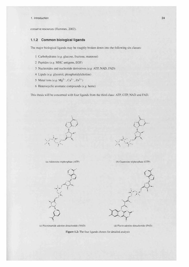
1. Introduction

conserve resources (Hammes, 2002).

1.1.2 Common biological ligands

The major biological ligands may be roughly broken down into the following six classes:

1 Carbohydrates (e.g. glucose, fructose, mannose)

2 Peptides (e.g. MHC antigens, EGF)

3 Nucleotides and nucleotide derivatives (e.g. ATP, NAD, FAD)

4 Lipids (e.g. glycerol, phosphatidylcholine)

5 Metal ions (e.g. Mg2+, Ca2+, Zn2+)

6 Heterocyclic aromatic compounds (e.g. heme)

This thesis will be concerned with four ligands from the third class: ATP, GTP, NAD and FAD.

(a) Adenosine triphosphate (ATP) (b) Guanosine triphosphate (GTP)

r r

/.o\ /

I

;:o(c) Nicotinamide adenine dinucleotide (NAD)

*‘4 ° n ,%\ci y \

(d) Flavin adenine dinucleotide (FAD)

Figure 1.2: The four ligands chosen for detailed analysis

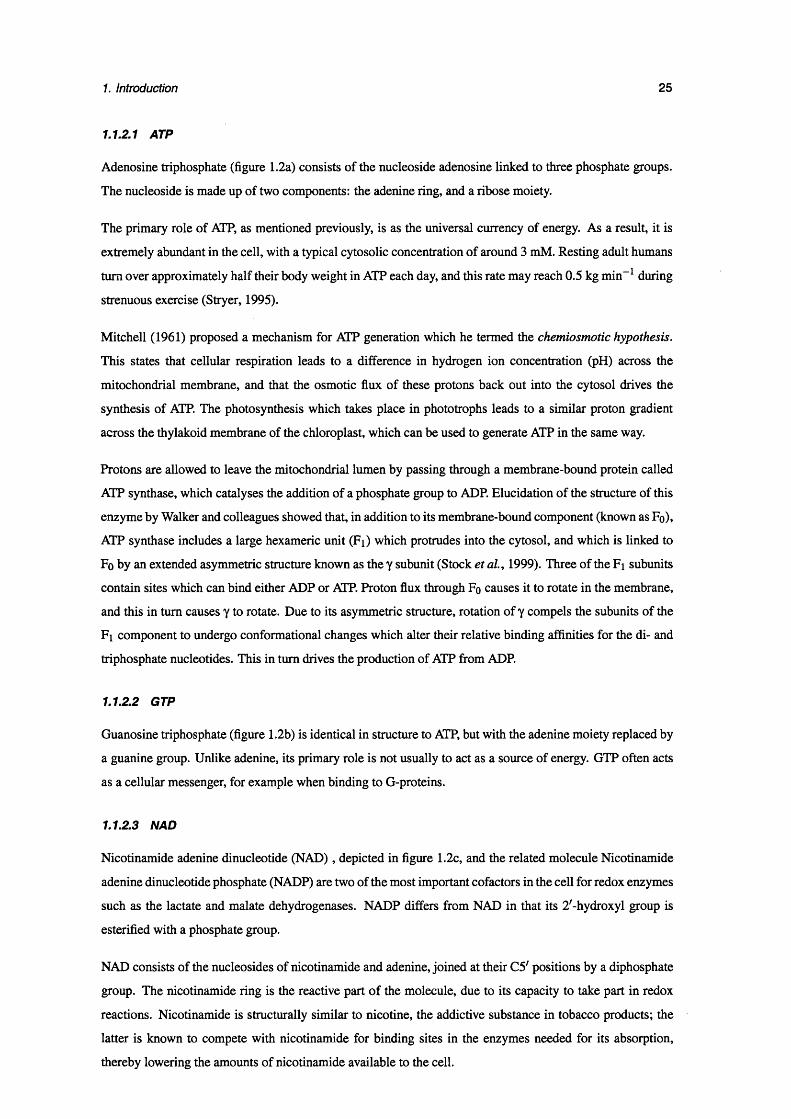
1. Introduction 25

1.1.2.1 ATP

Adenosine triphosphate (figure 1.2a) consists of the nucleoside adenosine linked to three phosphate groups.

The nucleoside is made up of two components: the adenine ring, and a ribose moiety.

The primary role of ATP, as mentioned previously, is as the universal currency of energy. As a result, it is

extremely abundant in the cell, with a typical cytosolic concentration of around 3 mM. Resting adult humans

turn over approximately half their body weight in ATP each day, and this rate may reach 0.5 kg min-1 during

strenuous exercise (Stryer, 1995).

Mitchell (1961) proposed a mechanism for ATP generation which he termed the chemiosmotic hypothesis.

This states that cellular respiration leads to a difference in hydrogen ion concentration (pH) across the

mitochondrial membrane, and that the osmotic flux of these protons back out into the cytosol drives the

synthesis of ATP. The photosynthesis which takes place in phototrophs leads to a similar proton gradient

across the thylakoid membrane of the chloroplast, which can be used to generate ATP in the same way.

Protons are allowed to leave the mitochondrial lumen by passing through a membrane-bound protein called

ATP synthase, which catalyses the addition of a phosphate group to ADP. Elucidation of the structure of this

enzyme by Walker and colleagues showed that, in addition to its membrane-bound component (known as Fo),

ATP synthase includes a large hexameric unit (Fi) which protrudes into the cytosol, and which is linked to

Fo by an extended asymmetric structure known as the y subunit (Stock et al., 1999). Three of the Fi subunits

contain sites which can bind either ADP or ATP. Proton flux through Fo causes it to rotate in the membrane,

and this in turn causes y to rotate. Due to its asymmetric structure, rotation of y compels the subunits of the

Fi component to undergo conformational changes which alter their relative binding affinities for the di- and

triphosphate nucleotides. This in turn drives the production of ATP from ADP.

1.1.2.2 GTP

Guanosine triphosphate (figure 1.2b) is identical in structure to ATP, but with the adenine moiety replaced by

a guanine group. Unlike adenine, its primary role is not usually to act as a source of energy. GTP often acts

as a cellular messenger, for example when binding to G-proteins.

1.1.2.3 NAD

Nicotinamide adenine dinucleotide (NAD), depicted in figure 1.2c, and the related molecule Nicotinamide

adenine dinucleotide phosphate (NADP) are two of the most important cofactors in the cell for redox enzymes

such as the lactate and malate dehydrogenases. NADP differs from NAD in that its 2'-hydroxyl group is

esterified with a phosphate group.

NAD consists of the nucleosides of nicotinamide and adenine, joined at their C5' positions by a diphosphate

group. The nicotinamide ring is the reactive part of the molecule, due to its capacity to take part in redox

reactions. Nicotinamide is structurally similar to nicotine, the addictive substance in tobacco products; the

latter is known to compete with nicotinamide for binding sites in the enzymes needed for its absorption,

thereby lowering the amounts of nicotinamide available to the cell.

1. Introduction 26

Figure 1.3: Proximity of nicotinamide ring to a substrate The protein shown here is a UDP-galactose 4-epimerase mutant; PDB entry 1A9Y. The NAD molecule (ball and stick) is shown bound by a canonical Rossmann fold domain (yellow). The substrate (shown with sticks) is bound largely by the catalytic domain (green), which brings it into close proximity with the reactive nicotinamide ring; this is a typical arrangement in NAD(P)-dependent oxidoreductases.

Because their nicotinamide groups are positively charged, the oxidised forms of NAD and NADP are often

written NAD+ and NADP+ respectively. Both cofactors can accept two electrons at a time, in the following

reaction

NAD+ + H+ + 2e“ *=* NADH

They may therefore act as oxidising agents in reactions such as the following, in which a secondary alcohol

is oxidised to form a ketone

NAD+ + R -C H O H -R ' *=* NADH + R -C O -R ' + H+

The oxidised and reduced forms of nicotinamide are shown in figures 1.4a and 1.4b.

O NH2 G .

CH CH CH C ,

N CH N .CH

(a) Oxidised form (NAD+) (b) Reduced form (NADH)

Figure 1.4: The oxidised and reduced forms of nicotinamide

NAD+ is the major electron acceptor in the oxidation of fuel molecules, which occurs in glycolysis and the

1. Introduction 27

citric acid cycle of cellular respiration. NADP is used almost exclusively for reductive biosynthesis, such as

in fatty acid synthesis, and also appears as a reducing agent in the later Calvin cycle of photosynthesis. Like

ATP, the reduced forms of NAD and NADP are quite stable in the absence of a catalyst.

1.1.2.4 FAD

Although it is the most common and best-known hydrogen acceptor, nicotinamide is not the only functional

group which plays this role - other moieties frequently involved in redox chemistry include the flavin and

quinone groups. Approximately 90% of cellular flavin is in the form of Flavin adenine dinucleotide (FAD)

(figure 1.2d), in which it is conjugated with an adenine diphosphate moiety. Another relatively common

flavin-containing compound is Flavin mononucleotide (FMN) , which is simply a phosphorylated form of

flavin. It should be mentioned that neither FAD nor FMN are actually nucleotides, despite their names, since

in both cases, the alloxazine ring is bound not to a sugar residue but to an alcohol (ribitol) instead.

C . N CH CH3 C N ^ C H CHS

'"'X X ^ X<̂ XX

X ° X ^ cX / X x ° X .H

CH2 OH CH2 OHxx xxCH OH CH OH

X X X x

(a) Oxidised form (FAD) (b) Reduced form (FADH2)

Figure 1.5: The oxidised and reduced forms of riboflavin

Like NAD, FAD can also accept 2 electrons. Unlike NAD, it also takes up a proton as well as a hydride ion,

as shown in the following reaction

+H+ +e~ -t-H+ +e~FAD v ■■ x FADH , FADH2

oxidised - yellow semiquinone - blue reduced. colourless

The oxidised form of flavin (figure 1.5a) is associated with a vivid yellow colour, which accounts for its name

(derived from the Latin flavus for yellow). Upon reduction (figure 1.5b), resonance effects in the flavin group

are lost, causing the colour to disappear. This loss of resonance means that the redox potential of flavin-

containing compounds is affected by factors which stabilise the reduced form. A structural consequence of

flavin reduction is that the planarity of the oxidised form tends to be lost (see figure 1.6).

FAD appears as an oxidising agent in a number diverse biological contexts including DNA repair (in the

photolyase protein (Weber, 2005)) and control of folding (in oxidoreductin, found in the endoplasmic

reticulum). The fact that flavin is a stronger oxidising agent than nicotinamide makes it suitable for its

1. Introduction 28

(a) (b)

Figure 1.6: “Butterfly bending” in the isoalloxine ring The coordinates of the isoalloxine ring taken from two FAD molecules are shown, (a) The straight form of isoalloxine, from PDB entry 1N62 (carbon monoxide dehydrogenase at 1.09A). (b) A butterfly form of the isoalloxine group, as observed in PDB entry 1CL0 (thiodoxin reductase at 2.50A), in which it is in the reduced form. The degree of flavin bending observed in this structure (34° relative to the oxidised form) was found to be the largest in the PDB (Lennon etal., 1999).

role in the electron transport chain, in which FMN mediates electron transfer between carriers that transfer

two electrons (e.g. NADH) and carriers that can only accept single electrons, such as Fe111.

Common enzymes which utilise FAD as a cofactor include D-amino acid oxidase, glucose oxidase, and

xanthine oxidase. FMN is the cofactor for NADH dehydrogenase, an example which illustrates the high

oxidative potential of flavin compared to nicotinamide.

1.1.2.5 The ubiquity o f the adenosine phosphate scaffold

It is apparent that adenosine phosphate units form a key part of the biochemical repertoire. It has been

proposed that their ubiquity may hark back to the ancient origins of life, in which, in addition to their current

role as carriers of genetic information, the nucleic acids were also used as catalysts. Prior to the emergence

of proteins, RNA enzymes (also known as ribozymes) may have been the dominant type of biocatalyst in

primordial life. As stated above, cofactors, and in particular their respective reactive groups, are recruited

by enzymes to perform functions which cannot be fulfilled using polypeptides alone. If this recruitment

originally occurred before the advent of proteins, it is not surprising that the scaffolds to which many reactive

functional groups are attached would be derived from nucleotides.

1.2 Principles of molecular recognition

1.2.1 Covalent versus non-covalent binding of ligands

The interactions between proteins and ligands may be either covalent or non-covalent in nature. This thesis

is concerned only with non-covalent interactions, which may be either permanent or transient. If a ligand is

permanently bound to a protein, it is sometimes referred to as a ‘prosthetic group’; the term ‘tightly bound’

typically refers to a non-covalently bound prosthetic group.

Heme molecules are the most common prosthetic groups, and may be either covalently bound, as in the

c-type cytochromes (Barker and Ferguson, 1999), or non-covalently bound, as in hemoglobin. In the case

of cytochrome c, the heme molecule is also a cofactor, since the oxidation state of its iron atom changes

as it accepts and releases electrons. Another example of a cofactor which is also a prosthetic group is the

1. Introduction 29

FAD molecule in glutathione reductase, which is irreversibly bound and largely buried. As discussed in

the previous section, however, not all cofactors are prosthetic groups - those which leave their enzymes to

undergo a ‘recycling’ step between catalytic cycles are clearly not irreversibly bound.

Regulatory molecules and substrates interact only transiently with their protein partners. The catalytic

constant, or turnover number (kcat) for enzymes varies over the range 103 — 107 s_1, meaning that for the

most efficient enzymes such as catalases, each substrate molecule interacts with the protein for less than 1/ts

on average (Fersht, 1999). At the other end of the spectrum, the rate of intrinsic GTPase hydrolysis by the G-

protein ras is approximately 1 hr-1 . This rate is significantly increased by the binding of GTPase-activating

proteins (GAPs) which therefore promote the inactivation of the G-protein.

The nature of ligand binding has several implications which should be borne in mind when looking at the

structure of ligand-protein complexes determined by crystallography. Where a ligand is non-covalently

bound to a protein, it is normally secured by several hydrogen-bonding or electrostatic interactions. Since

the strength of a covalent bond is roughly ten times that of a hydrogen bond (Jeffrey and Saenger, 1991),

covalent attachment of a ligand obviates the need for so many non-covalent interactions.

Another consideration is the temporal relationship of ligand binding to protein folding. In several cases,

cofactors have been shown to interact with unfolded polypeptides in vitro. By forming specific interactions

with parts of the denatured chain, some cofactors can dramatically reduce the entropy of the unfolded state,

and therefore speed up the conformational search for the native fold (Higgins et a l, 2005). Despite their

supposed role in accelerating protein folding, however, not all tightly-bound cofactors are strictly required

for stabilising the folded protein. In the case of flavoproteins1, for example, a variety of techniques are

available for extracting the flavin-containing cofactor, and then restoring the apoprotein to its native state

(Hefti et a l, 2003).

The distinction between early and late binding of cofactors is an important one to bear in mind, since the

structural rearrangements which can take place during folding imply that the interactions we see in a co­

crystallised structure of an early-binding molecule may not necessarily be those which facilitated its initial

recognition. Equally, however, extensive side-chain rearrangements are known to occur when ligands bind

to fully-folded proteins (Najmanovich et a l, 2000). To an extent, therefore, the caveat that experimental

observation may not accurately represent the complete biological picture applies to all studies of molecular

recognition carried out using X-ray crystallography.

1.2.2 Contributions to the free energy of binding

The non-covalent binding of a protein to a ligand encompasses a range of processes, including the desolvation

of parts of the two molecules, conformational rearrangements and the establishment of a variety of different

interactions. This section discusses these changes, considering the contribution of each to the binding affinity

of the complex.

l i.e. those which rely on an FAD or FMN cofactor

1. Introduction 30

1.2.2.1 Electrostatic interactions

Types of electrostatic interactions implicated in molecular recognition include salt bridges, hydrogen bonds,

dipole-dipole interactions and the interaction with metal ions. Of these, hydrogen bonds are generally

recognised to be one of the most important factors. Hydrogen bonds result from an electrostatic attraction

between a hydrogen atom bonded to an electronegative atom (such as oxygen or nitrogen), and a lone pair or

7i-electron system. The electron-withdrawing effect of the hydrogen atom causes the proton of the hydrogen

to be de-shielded, thus exposing its positive charge.

AA

DD

Figure 1.7: Hydrogen bond geometry The critical distances |HA| and |DA|, and angles ZHA AA and ZD HA are shown. Thresholds applied to these measurements are used to determine whether a given interaction consututes a valid hydrogen bond.

Establishing a hydrogen bond requires that the geometry of the hydrogen-bonded atoms and their covalent

partners obeys fairly strict rules. By analysing hydrogen-bonding interactions in high-resolution protein

structures, Baker and Hubbard (1984) stated these as follows (refer to figure 1.7 for the definition of the

atoms involved):

• |HA| < 2.5 A

• |DA| < 3.9 A

• ZH A AA > 90 °

• ZD HA ~ 180 ^

These criteria mean that hydrogen bonds are strongly directional, and that consequently, establishing a strong

hydrogen bonding network between two molecules depends upon their precise orientation relative to one

another.

The strength of a hydrogen bond is strongly affected by its environment: the extent to which the two opposing

charges are shielded depends on the local dielectric constant. Proximity to polar groups results in an increase

in the dielectric constant and therefore a decrease in hydrogen bond strength. This means that hydrogen

bonds which are buried within the protein - or in the interface between a protein and its ligand - tend to be

stronger than those which occur in solvent-exposed regions.

1. Introduction 31

1.2.2.2 Hydrophobic interactions

When a ligand binds to a protein, some parts of both molecules must be desolvated. This involves rupturing

hydrogen bonds between each molecule and the bulk solvent, followed by a reorganisation of water molecules

at the interface. The enthalpic cost of breaking protein-solvent and ligand-solvent hydrogen bonds is

compensated for by the water molecules which previously formed solvation shells around the two molecules

adopting a more structured, clathrate-like arrangement, in which the total number of hydrogen bonds is

reduced, but the strength of individual bonds becomes greatej, thus yielding an entropic benefit.

This description of desolvation highlights the two main energetic components of the so-called “hydrophobic

effect”, which describes the unfavourability of exposing a non-polar molecular surface to water. During

ligand binding, the hydrophobic effect resulting from unfolding the solvated ligand molecule, and from

exclusion of water from the binding pocket, is compensated for by the hydrophobic portions of the two

molecules coming into contact with one another. This ‘hydrophobic collapse’ is thought to be one of the

driving forces behind the ‘induced fit’ which is observed upon ligand binding, and is due to the same physical

principles which compel the rapid condensation of the core of many proteins during folding.

Another important type of non-polar interaction is Van der Waals attraction. When atoms are

separated by more than a few angstroms, they experience a weak mutual attractive force known as

Van der Waals attraction2. This force originates from the instantaneous dipoles which are set up in each

individual atom as a result of the mobility of the electrons which surround their nuclei. When atoms approach

one another, the instantaneous dipole in one of them induces a polarity in the other, such that the parts of

the two atoms which are juxtaposed have temporary opposite charges. As long as the two atoms remain in

proximity, electronic fluctuations in the electron shell of one atom causes corresponding charge redistribution

in the other, thus maintaining the attraction. The strength of this attractive force varies with the size of the

atoms involved, but is several orders of magnitude less than that of a covalent bond. An example from nature

illustrates that Van der Waals interactions can nonetheless be a significant force: remarkably, the unique

ability of geckos to cling to smooth surfaces is attributed solely to Van der Waals interactions, rather than to

any special chemical properties of the surfaces of their toes (Autumn et al., 2002). Van der Waals attraction

between two molecules is related to the degree to which their surfaces have complementary shapes. Shape

complementarity is therefore thought to be an important factor in protein-ligand recognition.

1.2.2.3 Conformational restriction

Upon binding, a protein and a ligand each lose three degrees of translational freedom and three degrees of

rotational freedom relative to one another. In addition, the ratable bonds in the ligand and in the residues

which comprise the binding site are, to some extent, restrained. This entropic cost can in some cases be

mitigated against by pre-organisation of the ligand molecule while still in solution.

2Van der Waals attraction is also sometimes referred to as the “London force”, or as “dispersion forces”.

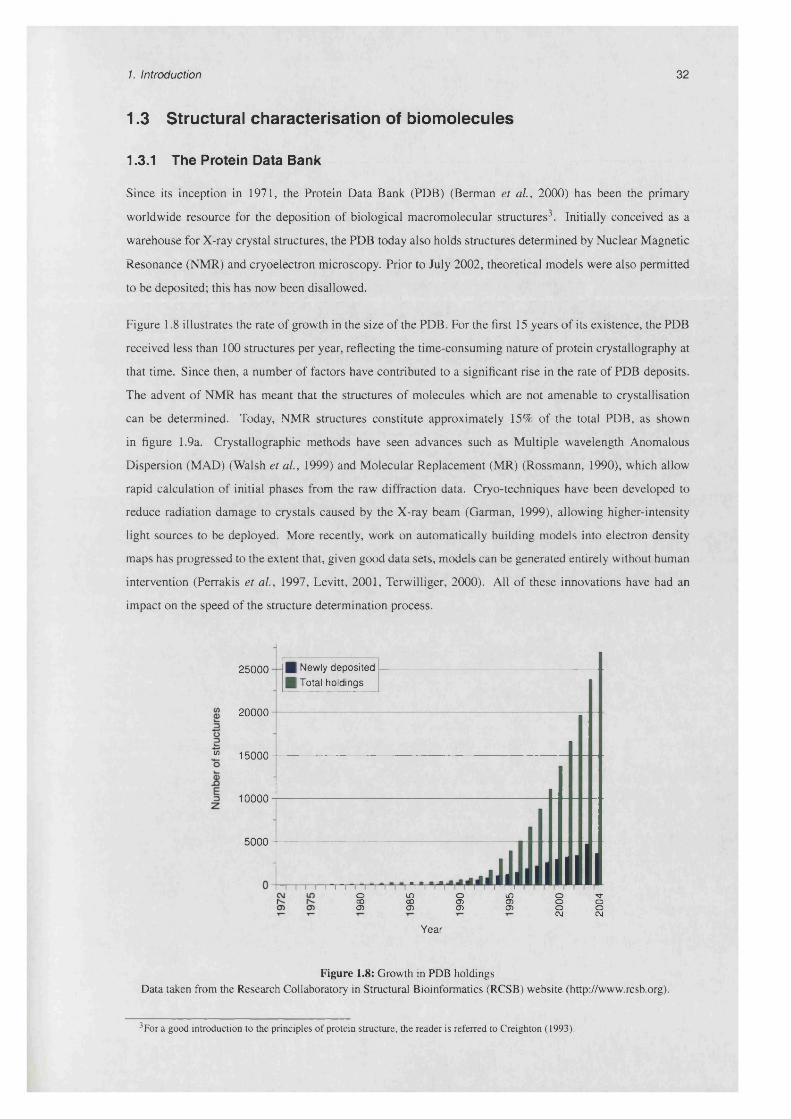
1. Introduction 32

1.3 Structural characterisation of biomolecules

1.3.1 The Protein Data Bank

Since its inception in 1971, the Protein Data Bank (PDB) (Berman et al., 2000) has been the primary

worldwide resource for the deposition of biological macromolecular structures3. Initially conceived as a

warehouse for X-ray crystal structures, the PDB today also holds structures determined by Nuclear Magnetic

Resonance (NMR) and cryoelectron microscopy. Prior to July 2002, theoretical models were also permitted

to be deposited; this has now been disallowed.

Figure 1.8 illustrates the rate of growth in the size of the PDB. For the first 15 years of its existence, the PDB

received less than 100 structures per year, reflecting the time-consuming nature of protein crystallography at

that time. Since then, a number of factors have contributed to a significant rise in the rate of PDB deposits.

The advent of NMR has meant that the structures of molecules which are not amenable to crystallisation

can be determined. Today, NMR structures constitute approximately 15% of the total PDB, as shown

in figure 1.9a. Crystallographic methods have seen advances such as Multiple wavelength Anomalous

Dispersion (MAD) (Walsh et al., 1999) and Molecular Replacement (MR) (Rossmann, 1990), which allow

rapid calculation of initial phases from the raw diffraction data. Cryo-techniques have been developed to

reduce radiation damage to crystals caused by the X-ray beam (Garman, 1999), allowing higher-intensity

light sources to be deployed. More recently, work on automatically building models into electron density

maps has progressed to the extent that, given good data sets, models can be generated entirely without human

intervention (Perrakis et al., 1997, Levitt, 2001, Terwilliger, 2000). All of these innovations have had an

impact on the speed of the structure determination process.

25000 | New ly deposited

| Total holdings

20000

“ 15000

10000

5000

■i 1iJjoCOO )

in o mCO CD CD0) 0) 0)

Y ear

oooCM

•<3-OOCM

Figure 1.8: Growth in PDB holdings Data taken from the Research Collaboratory in Structural Bioinformatics (RCSB) website (http://www.rcsb.org).

3For a good introduction to the principles of protein structure, the reader is referred to Creighton (1993).

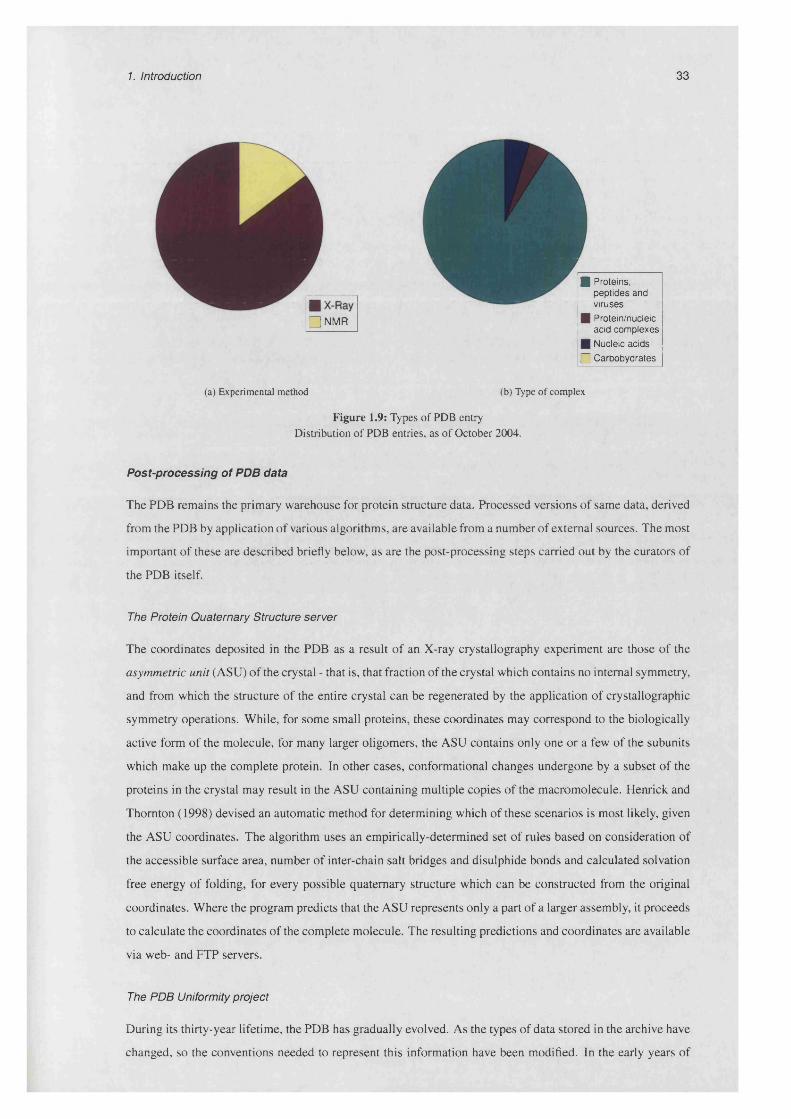
1. Introduction 33

■ Proteins,peptides and viruses

□ NMR ■ Protein/nucleic acid complexes

■ Nucleic acids

□ Carbohydrates

(a) Experimental method (b) Type of complex

Figure 1.9: Types of PDB entry Distribution of PDB entries, as of October 2004.

Post-processing o f PDB data

The PDB remains the primary warehouse for protein structure data. Processed versions of same data, derived

from the PDB by application of various algorithms, are available from a number of external sources. The most

important of these are described briefly below, as are the post-processing steps carried out by the curators of

the PDB itself.

The Protein Quaternary Structure server

The coordinates deposited in the PDB as a result of an X-ray crystallography experiment are those of the

asymmetric unit (ASU) of the crystal - that is, that fraction of the crystal which contains no internal symmetry,

and from which the structure of the entire crystal can be regenerated by the application of crystallographic

symmetry operations. While, for some small proteins, these coordinates may correspond to the biologically

active form of the molecule, for many larger oligomers, the ASU contains only one or a few of the subunits

which make up the complete protein. In other cases, conformational changes undergone by a subset of the

proteins in the crystal may result in the ASU containing multiple copies of the macromolecule. Henrick and

Thornton (1998) devised an automatic method for determining which of these scenarios is most likely, given

the ASU coordinates. The algorithm uses an empirically-determined set of rules based on consideration of

the accessible surface area, number of inter-chain salt bridges and disulphide bonds and calculated solvation

free energy of folding, for every possible quaternary structure which can be constructed from the original

coordinates. Where the program predicts that the ASU represents only a part of a larger assembly, it proceeds

to calculate the coordinates of the complete molecule. The resulting predictions and coordinates are available

via web- and FTP servers.

The PDB Uniformity project

During its thirty-year lifetime, the PDB has gradually evolved. As the types of data stored in the archive have

changed, so the conventions needed to represent this information have been modified. In the early years of

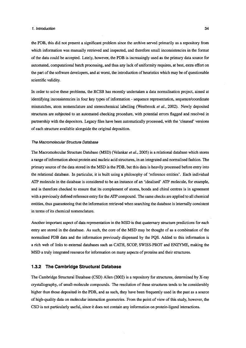
1. Introduction 34

the PDB, this did not present a significant problem since the archive served primarily as a repository from

which information was manually retrieved and inspected, and therefore small inconsistencies in the format

of the data could be accepted. Lately, however, the PDB is increasingly used as the primary data source for

automated, computational batch processing, and thus any lack of uniformity requires, at best, extra effort on

the part of the software developers, and at worst, the introduction of heuristics which may be of questionable

scientific validity.

In order to solve these problems, the RCSB has recently undertaken a data normalisation project, aimed at

identifying inconsistencies in four key types of information - sequence representation, sequence/coordinate

mismatches, atom nomenclature and stereochemical labelling (Westbrook et a l, 2002). Newly deposited

structures are subjected to an automated checking procedure, with potential errors flagged and resolved in

partnership with the depositors. Legacy files have been automatically processed, with the ‘cleaned’ versions

of each structure available alongside the original deposition.

The Macromolecular Structure Database

The Macromolecular Structure Database (MSD) (Velankar et al., 2005) is a relational database which stores

a range of information about protein and nucleic acid structures, in an integrated and normalised fashion. The

primary source of the data stored in the MSD is the PDB, but this data is heavily processed before entry into

the relational database. In particular, it is built using a philosophy of ‘reference entities’. Each individual

ATP molecule in the database is considered to be an instance of an ‘idealised’ ATP molecule, for example,

and is therefore checked to ensure that its complement of atoms, bonds and chiral centres is in agreement

with a previously defined reference entry for the ATP compound. The same checks are applied to all chemical

entities, thus guaranteeing that the information retrieved when searching the database is internally consistent

in terms of its chemical nomenclature.

Another important aspect of data representation in the MSD is that quaternary structure predictions for each

entry are stored in the database. As such, the core of the MSD may be thought of as a combination of the

normalised PDB data and the information previously dispensed by the PQS. Added to this information is

a rich web of links to external databases such as CATH, SCOP, SWISS-PROT and ENZYME, making the

MSD a truly integrated resource for information on many aspects of proteins and their structures.

1.3.2 The Cambridge Structural Database

The Cambridge Structural Database (CSD) Allen (2002) is a repository for structures, determined by X-ray

crystallography, of small-molecule compounds. The resolution of these structures tends to be considerably

higher than those deposited in the PDB, and as such, they have been frequently used in the past as a source

of high-quality data on molecular interaction geometries. From the point of view of this study, however, the

CSD is not particularly useful, since it does not contain any information on protein-ligand interactions.

1. Introduction 35

1.3.3 Structural genomics

In addition to the technological changes outlined above, the past five years have also seen changes in the

approach to structure determination. Until recently, structures tended to be solved by researchers who had

a particular interest in the protein concerned, and had therefore expended considerable time and effort to

characterise it biochemically. The individual focus was therefore on obtaining insight into the function of

particular proteins, by solving their structures. Viewed from a global perspective, however, this has meant

that the choice of which proteins to solve has largely been an ad hoc one, based on the intrinsic value of each

particular structure, rather than on its contribution to our understanding of protein structure, function and

evolution on a more general level. Increasingly, researchers from a number of fields have come to the view

that obtaining a more uniform sampling of ‘protein structure space’ would yield many benefits.

Perhaps the most obvious potential benefit of a more systematic approach to structure determination would

be an increased understanding of protein evolution. Given that molecular evolution at the sequence level

is generally considered to be fairly well understood, the ability to relate changes in protein sequence to

modifications of the resulting structure will further illuminate the selective pressures which have caused the

evolutionary changes which we can observe today. This endeavour would be greatly assisted by a more

rational choice of protein targets.

On a more pragmatic note, having access to the structure of a relatively close neighbour of any protein one

may choose, would allow the structure of the new protein to be modelled to reasonable accuracy. In the

pharmaceutical industry, there is currently great interest in the feasibility of applying rational drug design to

modelled structures; a more uniform coverage of protein space would allow this idea to be explored more

thoroughly.

These considerations have led to the initiation of a worldwide program of systematic structure determination,

known as Structural Genomics (Burley, 2000). The overall aim of this initiative is to determine the structure

of at least one representative protein from each family. In order to achieve this, crystallographers and NMR

spectroscopists are altering the way they work, effectively postponing traditional analyses in favour of a

high-throughput mode of structure solution.

1.3.4 Structure quality

When assessing the quality of protein structures, one measure which is often used for structures resulting

from X-ray crystallography experiments is the resolution. The resolution of a crystallographic structure is

determined by the extent of the reflection data which can be collected during the structure determination.

The 2-dimensional diffraction pattern which results from the experiment shows concentric rings of scattering

peaks, each of which corresponds to a different interplanar distance in the real lattice. The resolution which is

quoted is the interplanar spacing for the outermost scattering ring for which data can be reliably collected. It

is directly related to the optical definition of resolution - that is, the minimum distance by which two objects

may be separated, and may still be visible as two separate objects. The uncertainty in the position of an

atom depends both on the resolution of the structure, and the R-factor; on average, the uncertainty in each

atomic coordinate in a high-quality structure (R-factor of 0.2 or less) is roughly one fifth to one tenth of the

1. Introduction 36

resolution (Rhodes, 2000). The distribution of reported resolution values for PDB structures determined by

X-ray crystallography is shown in figure 1.10.

6000

5000

w 4000

*5 3000

1llII, ,

-lllllII I I I .__2000

1000

w in w in m inc- cy| ,_• m m in m m in

1 in I in 1 in 1 inp c i i i n h - p c N i i n r -N W N N n r i r i r i

Resolution /A

Figure 1.10: Resolution of deposited X-ray structures This graph shows the distribution of the resolution of PDB entries which were solved by X-ray crystallography, as of October 2004.

Crystals for which data extended beyond about 1.2A can yield structures in which some of the hydrogen

positions can be determined based on the X-ray data alone. Where the resolution is poorer than this,

their positions cannot be directly observed; this means that the chemical identity of the terminal side-chain

atoms is uncertain for aspartic acid, glutamine and threonine residues, and must be inferred from the protein

environment of the side chain. Similarly, the orientation of the imidazole ring of histidine residues cannot

be unambiguously determined. These uncertainties can lead to errors in crystal structures, the possibility of

which cannot be discounted during studies which depend on precise determination of protein geometry at the

atomic level. In recent years, the number of crystal structures being determined to very high-resolution has

increased, largely due to the advent of synchotrons which offer very high-intensity light sources.

1.3.5 Non-cognate ligands

Analogues of cognate ligands are routinely used when performing biochemical characterisation of proteins,

or when determining their structures. Compounds whose overall structure is similar to a natural ligand, but

which are inert, are valuable in obtaining a ‘snapshot’ of a reaction, halted at a particular step. For example,

the ATP analogue ATPyS, in which one oxygen atom on the terminal phosphate group has been replaced

by a sulphur atom, hydrolyses much more slowly than the natural ligand. Another example of a substrate

analogue which has been used in crystallisation experiments is methotrexate, a folic acid mimic. This binds

to dihydrofolate reductase, an enzyme which catalyses the production of an intermediate in the biosynthesis

of amino acids and purine nucleotides.

Sometimes, the ligand present in a crystal structure may not even be an analogue of the natural substrate.

During crystallisation experiments, many different small molecules are routinely screened to determine

1. Introduction 37

whether any of them encourages the formation of crystals. Some of the ligands thus discovered are only

‘structural ligands’ - that is, molecules whose binding stabilises the crystal lattice, but which are not thought

to be of functional importance to the protein being crystallised.

It is therefore important when analysing protein-ligand interactions obtained from the PDB, to attempt to

determine whether the observed complex is likely to be cognate: that is, whether the ligand used in the

structure determination experiment is the true biological partner for that protein. Achieving this reliably

in an automated manner is challenging, although efforts are currently underway to compile a database of

cognate ligands associated with certain proteins (I. Nobeli, personal communication). The work described

in this thesis focusses on analysis of interactions between proteins and fairly ubiquitous biological ligands.

Therefore in most cases discussed here, we can be fairly confident that the interactions observed are likely to

be biologically relevant.

1.3.6 Chemical compound datasets

When working with crystallographic structures of ligands, access to a reference set of chemical compounds

can often be of use. Given any chemical compound, we may think of it in terms of several distinct ‘levels of

abstraction’. The most fundamental of these is a single, idealised representation of the molecule. This

corresponds to the diagram of the molecule which a chemist may draw. In other words, the idealised

representation contains information about the atoms and bonds which make up the molecule - including

the atomic number of each atom, the location of any formal charges, and the location and handedness of any

chiral stereocentres which may be present. In addition, this representation should contain information about

the connectivity of the molecule, including the order of each chemical bond. Additional annotation such as

the presence of delocalised or aromatic systems may also be included.

At the other end of the spectrum, we may think of a particular, real instance of the molecule, existing in a

physical environment. In order to describe such an instance, we should specify additional information such as

three-dimensional coordinates of each of its atoms and the distribution of electron density across the volume

occupied by the molecule. Of course even this enriched description of the molecule falls short of what would

be considered a realistic representation in terms of quantum physics.

The representations of molecular species whose structure has been determined by crystallographic or

spectroscopic methods lie at a point intermediate between these two extremes. An X-ray model is a static

snapshot of what in reality is a dynamic system; therefore information about molecular motion is to a large

extent lost during the structure determination process. Indirectly, the evidence of motion can still be seen

in disorded regions, which manifest themselves as blurring of the corresponding electron density. NMR

experiments on the other hand yield not one but an ensemble of valid structural solutions. Here, mobile parts

of the molecule appear in different conformations among different members of the ensemble.

Given a set of atomic coordinates obtained from X-ray crystallography, building a model into it requires

that the chemical identity of the molecule(s) present be identified. This procedure is performed prior to

deposition of a structure in the PDB, with the assigned identities being recorded in the PDB residue name

fields. For small molecules, however, this assignment is sometimes done inconsistently; therefore it is

1. Introduction 38

desirable to be able to verify the chemical identity of the molecule automatically. Given only the atomic

coordinates of a molecule in this frozen state, each labelled with the corresponding chemical element, it is

possible to deduce the connectivity of the molecule by reference to a table of standard covalent radii. The

resulting topological representation of the molecule is amenable to comparison against a reference dictionary

of chemical compounds using graph theoretic methods (see appendix A).

Any number of reference sets of chemical compounds are available, ranging from catalogues of available

reagents, through metabolite dictionaries (e.g. KEGG COMPOUND, http://www.genome.jp/ligand; ChEBI,

http://www.ebi.ac.uk/chebi), to databases of xenobiotic compounds, for example drug molecules (e.g. the

National Cancer Institute’s drug dictionary, http://www.nci.nih.gov). The reference set of chemical

compounds used in this work was taken from the MSD, which contains a comprehensive record for each

chemical entity found in the PDB. This record contains, along with other data, all the information required

for the validation procedure, including in vacuo energy-minimised coordinates generated using the CORINA

program, which is distributed as part of the CACTVS tool set (Ihlenfeldt et al., 1994).

1.4 Protein structure and evolution

The process of evolution is driven by natural selection acting on variation. Within a population of organisms,

those which are best adapted to their environment and circumstances stand a better chance of survival than

their peers. Molecular biology has shown us that the source of variations at the level of the organism can be

traced to microscopic changes in the molecules which constitute them, which are derived from mutations in

the molecules which carry their genetic information. Where mutations occur in the coding regions of genes,

they may cause corresponding changes in the proteins encoded by those genes. This change in a protein’s

primary sequence can, in turn, affect its structure, and hence impact upon the function which it plays within

the organism. The cumulative effect of many such changes, occurring over vast timespans, eventually leads to

the evolution of proteins with entirely novel structures and functions. This expansion of the protein repertoire

is thought to be ultimately responsible for most, if not all of the evolutionary diversity which we see in the

living things that surround us.

Proteins which have descended from a common ancestral protein are said to be homologous, and may retain

similarities in terms of sequence, structure and function. As mutations are accumulated by a protein, these

similarities become increasingly hard to detect. It is generally accepted that, in more distant proteins,

structure is more conserved than sequence (Chothia, 1984). As a result, while comparison of protein

sequences can reveal fairly close evolutionary relationships, taking into account structural information allows

the identification of more distant relatives. Specifically, the gross arrangement of secondary structures in

a protein - the fold - appears to be particularly well conserved, and therefore proteins with similar folds

are often evolutionarily related. Care must be taken in equating structural similarity with evolutionary

relatedness, however, since unrelated proteins may converge to a similar fold for functional or physico­

chemical reasons.

An examination of pairs of homologous proteins from SCOP showed that some had quite different functions

- either two different enzymatic functions, as determined by the enzyme classification (EC) number (IUPAC-

1. Introduction 39

IUB, 1983) - or one enzyme and one non-enzyme (Hegyi and Gerstein, 1999). Russell et al. (1998) showed,

in a comprehensive analysis of the location of binding sites within structurally superposed SCOP superfamily

members, that in approximately 10% of cases, the location was not conserved, suggesting a complete change

in function. A comparison of pairs of SCOP domains in conjunction with their EC numbers, (or against

FlyBase annotations, in the case of non-enzymes), suggested that precise function is usually only conserved

when the sequence identity is above a 40% threshold (Wilson et al., 2000).

Functional congruity between proteins often appears to indicate a common ancestor, but this too can be

misleading. A well-known example is the evolution of so-called ‘antifreeze proteins’ by fish living in very

cold waters. These proteins, which prevent the growth of ice crystals in the fishes’ bloodstreams, are found

in fish indigenous to both the north and south poles. The simplest explanation initially appeared to be

that both groups of species inherited the gene for these proteins from a common ancestor prior to their

geographical dispersion. In fact, genome analyses have shown that the two populations split long before they

developed the antifreeze protein (Chen et a l, 1997). This ‘reinvention of the wheel’ by nature is known as

convergent evolution, and has been demonstrated several times in diverse systems.

Because of these phenomena, a combination of structural and functional likeness is usually taken to be

necessary for robust identification of relatedness between proteins whose sequences have diverged beyond

detectable levels of similarity. A number of algorithms are now available for the automatic detection of

structural similarity between proteins (e.g. SSAP (Orengo and Taylor, 1996), DALI (Holm and Sander, 1995),

VAST (Madej etal., 1995) and CE (Shindyalov and Bourne, 1998)).

Protein domains and structure classification

Many large proteins can be separated into a number of (semi-)independent units known as domains. There

is no single, universally-agreed definition of exactly what constitutes a domain. Biochemists may define a

domain as a functional unit of a protein, mediating a certain aspect of a protein’s role (e.g. “the ligand-binding

domain”). Those with a more structural bent tend to talk about domains as being “independent folding units”,

possessing their own hydrophobic core, and hence often being more amenable to protein crystallography in

cases where the structural complexity of a large protein poses experimental difficulties. Those whose focus is

more towards the evolutionary aspects of proteins prefer to describe domains as “units of evolution”, pointing

towards the tendency of new protein functions to be generated not by incremental point mutation, but often

by recombination of large ‘blocks’ of sequence at a time (Patthy, 1991, Baron et a l, 1991, Sonnhammer and

Kahn, 1994).

In fact, domains often appear to be all of these things at the same time. Any apparent conflict in the definitions

given above is due to the intimate inter-relationship of protein sequence, structure and function. Because of

the significance of protein domains in evolution, proteins are often compared at the individual domain - rather

than whole polypeptide chain - level. Several databases of domains, defined either in terms of their sequence

or structure, are available. Here, the focus is on protein structure, and therefore the two pre-eminent structure-

based databases of protein domains, CATH (Pearl et a l, 2005) and SCOP (Murzin et a l, 1995, Andreeva

et a l, 2004), will be described.

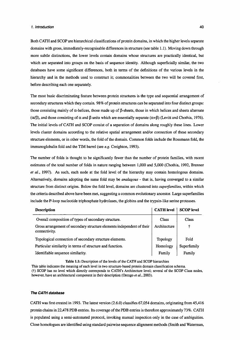
1. Introduction 40

Both CATH and SCOP are hierarchical classifications of protein domains, in which the higher levels separate

domains with gross, immediately-recognisable differences in structure (see table 1.1). Moving down through

more subtle distinctions, the lower levels contain domains whose structures are practically identical, but

which are separated into groups on the basis of sequence identity. Although superficially similar, the two

databases have some significant differences, both in terms of the definitions of the various levels in the

hierarchy and in the methods used to construct it; commonalities between the two will be covered first,

before describing each one separately.

The most basic discriminating feature between protein structures is the type and sequential arrangement of

secondary structures which they contain. 98% of protein structures can be separated into four distinct groups:

those consisting mainly of a-helices, those made up of (3-sheets, those in which helices and sheets alternate

(ot/P), and those consisting of a and P units which are essentially separate (a+P) (Levitt and Chothia, 1976).

The initial levels of CATH and SCOP consist of a separation of domains along roughly these lines. Lower

levels cluster domains according to the relative spatial arrangement and/or connection of these secondary

structure elements, or in other words, the fold of the domain. Common folds include the Rossmann fold, the

immunoglobulin fold and the TIM barrel (see e.g. Creighton, 1993).

The number of folds is thought to be significantly fewer than the number of protein families, with recent

estimates of the total number of folds in nature ranging between 1,000 and 5,000 (Chothia, 1992, Brenner

et al., 1997). As such, each node at the fold level of the hierarchy may contain homologous domains.

Alternatively, domains adopting the same fold may be analogous - that is, having converged to a similar

structure from distinct origins. Below the fold level, domains are clustered into superfamilies, within which

the criteria described above have been met, suggesting a common evolutionary ancestor. Large superfamilies

include the P-loop nucleotide triphosphate hydrolases, the globins and the trypsin-like serine proteases.

Description CATH level SCOP level

Overall composition of types of secondary structure. Class Class

Gross arrangement of secondary structure elements independent of their connectivity.

Architecture t

Topological connection of secondary structure elements. Topology Fold

Particular similarity in terms of structure and function. Homology Superfamily

Identifiable sequence similarity. Family Family

Table 1.1: Description of the levels of the CATH and SCOP hierarchies This table indicates the meaning o f each level in two structure-based protein domain classification schema.(t) SCOP has no level which directly corresponds to CATH’s Architecture level; several o f the SCOP Class nodes, however, have an architectural component in their description (Orengo et al., 2003).

The CATH database

CATH was first created in 1993. The latest version (2.6.0) classifies 67,054 domains, originating from 45,416

protein chains in 22,478 PDB entries. Its coverage of the PDB entries is therefore approximately 73%. CATH

is populated using a semi-automated protocol, invoking manual inspection only in the case of ambiguities.

Close homologues are identified using standard pairwise sequence alignment methods (Smith and Waterman,

1. Introduction 41

1981), requiring a match of at least 35% sequence identity over 80% of the length of the longer sequence in

order to infer that a pair of domains belong in the same family.

More distant homologues are identified using a profile-based search whereby the new sequence is queried

against a library of profiles previously generated for each CATH family using the IMPALA protocol (Schaffer

et al., 1999). Any matches found using this approach are then validated using the SSAP program, a dynamic

programming method which compares the residue environments of a pair of proteins, and which has been

shown to be a robust method for structural comparison (Orengo and Taylor, 1996). Where no homologues are

found using the profile search, the input is checked to determine whether it may be a multi-domain protein.

This is done using a consensus of three different domain boundary prediction algorithms (Jones et a l, 1998);

any domains thus found are resubmitted separately to the sequence searches.

For around 15% of new structures, the sequence similarity to existing members of the database is too low

to detect. In order to find more distant relatives, the tertiary structures of the domains are compared using

a graph-based algorithm (Harrison et al., 2003). Any matches found by this method are then assigned to

a superfamily by scanning the protein against a set of superfamily templates generated using the CORA

program (Orengo, 1999). If, on the other hand, no match is found (which occurs in about 7% of cases), the

domain is compared against all structures in the appropriate class using the more sensitive but slower SSAP

program. The domains which are still uncharacterised following this step are manually assigned.

The CATH hierarchy itself differs slightly from the general classification scheme described above. Firstly,

CATH does not distinguish between ot/(3 and a+0 domains. More significantly, the definition of fold is

shared across two levels in CATH. The first of these, the ‘Architecture’ level, describes the overall relative

arrangement of secondary structure elements in space, independent of the order of the connecting loops

between them. Below this, the ‘Topology’ level distinguishes between the different ways of connecting up

the secondary structure elements.

The SCOP database

SCOP originated in 1994. The latest release (1.67) contains 65,122 domains in 50,285 chains from 24,037

PDB entries (a coverage of 78%). A key difference between CATH and SCOP is that the latter is constructed

almost entirely by manual inspection of each new protein structure. A second difference is that the top SCOP

level contains a further seven classes (“multi-domain”, “membrane and cell surface”, “small”, “coiled coil”,

“low resolution”, “peptides” and “designed proteins”) in addition to those described above.

Proteins are first separated into domains, using a structural definition based on the presence of a independent

hydrophobic core and limited contacts to the rest of the structure (Reddy and Bourne, 2003). Class, fold and

superfamily are then assigned manually. The clustering of proteins into families is then done principally on

the basis of sequence identity (with a 30% cutoff), but in some cases proteins which exhibit structural and

functional similarity despite low sequence identity (e.g. globins) are placed in the same superfamily.

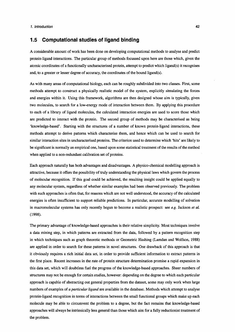
1. Introduction 42

1.5 Computational studies of ligand binding

A considerable amount of work has been done on developing computational methods to analyse and predict

protein-ligand interactions. The particular group of methods focussed upon here are those which, given the

atomic coordinates of a functionally uncharacterised protein, attempt to predict which ligand(s) it recognises

and, to a greater or lesser degree of accuracy, the coordinates of the bound ligand(s).

As with many areas of computational biology, each can be roughly subdivided into two classes. First, some

methods attempt to construct a physically realistic model of the system, explicitly simulating the forces

and energies within it. Using this framework, algorithms are then designed whose aim is typically, given

two molecules, to search for a low-energy mode of interaction between them. By applying this procedure

to each of a library of ligand molecules, the calculated interaction energies are used to score those which

are predicted to interact with the protein. The second group of methods may be characterised as being

‘knowledge-based’. Starting with the structures of a number of known protein-ligand interactions, these

methods attempt to derive patterns which characterise them, and hence which can be used to search for

similar interaction sites in uncharacterised proteins. The criterion used to determine which ‘hits’ are likely to

be significant is normally an empirical one, based upon some statistical treatment of the results of the method

when applied to a non-redundant calibration set of proteins.

Each approach naturally has both advantages and disadvantages. A physico-chemical modelling approach is

attractive, because it offers the possibility of truly understanding the physical laws which govern the process

of molecular recognition. If this goal could be achieved, the resulting insight could be applied equally to

any molecular system, regardless of whether similar examples had been observed previously. The problem

with such approaches is often that, for reasons which are not well understood, the accuracy of the calculated

energies is often insufficient to support reliable predictions. In particular, accurate modelling of solvation

in macromolecular systems has only recently begun to become a realistic prospect: see e.g. Jackson et al.

(1998).

The primary advantage of knowledge-based approaches is their relative simplicity. Most techniques involve

a data mining step, in which patterns are extracted from the data, followed by a pattern recognition step

in which techniques such as graph theoretic methods or Geometric Hashing (Lamdan and Wolfson, 1988)

are applied in order to search for these patterns in novel structures. One drawback of this approach is that

it obviously requires a rich initial data set, in order to provide sufficient information to extract patterns in

the first place. Recent increases in the rate of protein structure determination promise a rapid expansion in

this data set, which will doubtless fuel the progress of the knowledge-based approaches. Sheer numbers of

structures may not be enough for certain studies, however: depending on the degree to which each particular

approach is capable of abstracting out general properties from the dataset, some may only work when large

numbers of examples of a particular ligand are available in the database. Methods which attempt to analyse

protein-ligand recognition in terms of interactions between the small functional groups which make up each

molecule may be able to circumvent the problem to a degree, but the fact remains that knowledge-based

approaches will always be intrinsically less general than those which aim for a fully reductionist treatment of

the problem.

1. Introduction 43

1.5.1 Locating the binding site

While in principle, any method capable of searching for favourable interactions between a pair of molecules

could simply be applied to the two structures in their entirety, in practice, it is often desirable (and sometimes

necessary) to reduce the computational complexity of the problem by first identifying regions of the protein

which are likely to contain binding sites.

One common approach is to analyse the geometry of the protein structure in order to find clefts or depressions

in its surface. The author of one of the earliest such method, SURFNET (Laskowski, 1995), validated the

program by applying it to a set of enzyme structures in which the location of the active site was known. It was

reported that, in around 80% of cases, the active site is located in the largest cleft. As such, cleft detection

is an effective tool for determining likely binding sites. Although useful, this method is not universally

applicable: while some types of compounds are bound in deep clefts, others - for instance carbohydrates

(Taroni et a l, 2000) - tend to bind to shallow grooves on the protein surface, which cannot be identified using

cleft detection. A wide range of algorithms for pocket finding have now been published (Ho and Marshall,

1990, Levitt and Banaszak, 1992, Kleywegt and Jones, 1994, Hendlich e ta l, 1997, Brady and Stouten, 2000,

Binkowski et a l, 2003); each has its own technical innovations, but the results produced are broadly similar

regardless of the specific method chosen.

An alternative group of methods involve calculating the energy between simple organic probes and the

protein, at all points across the surface. Clusters of low-energy points are taken to delineate likely binding

pockets. A number of studies involving this type of algorithm have been published (Ringe and Mattos,

1999, Silberstein et a l, 2003, Laurie and Jackson, 2005). They report better results that those obtained using

geometric approaches; however, the latter are currently the method of choice in high-throughput binding site

search applications (Laskowski et a l, 2003).

1.5.2 Docking

Docking is a term for computational schemes which attempt to find the ‘best’ relative positioning of two

molecules. Docking has been very thoroughly discussed in a recent review (Halperin et a l, 2002); here,

those aspects relating to the problem of protein-ligand docking are briefly outlined.

Docking programs attempt to match ligands to proteins based on two criteria: geometric complementarity,

and energetic minimisation. These two criteria require quite different representations of the system, and

also different search methodologies. Geometry-based docking approaches typically represent the surface of

the two molecules using a set of sparse critical points, and then use these representations to compute rigid

transformations of the two surfaces which maximise shape complementarity, while penalising penetration of

one surface into the other. The transformations are often computed using the Geometric Hashing algorithm,

which was originally developed for computer vision applications (Lamdan and Wolfson, 1988). This

algorithm achieves high performance through an offline pre-processing step which converts the set of points

into a translation- and rotation-invariant representation. From this, closely-matching regions between the two

surfaces can be quickly identified. Following the translation, scores are calculated on the basis of overlap

checks, counts of hydrogen bonds, counts of unsatisfied buried charges, and measures of buried surface area.

1. Introduction 44

Both protein-protein docking and docking of small molecules require an accurate treatment of the energetics

of the system, in addition to the geometry. Effective scoring functions for docking must combine treatments

of electrostatics, solvation, entropy and van der Waals forces; commonly-used examples include the

CHARMM (Brooks et a l, 1983) and AMBER (Weiner et a l, 1984) force fields. Unlike geometric matching,

finding energetically-favourable matches is computationally expensive; the conformational possibilities

within even a small spatial region are vast due to the degrees of freedom available to the system4. While some

components of the energy f unction - notably the van der Waals term due to the protein - can be calculated

in advance and stored on a grid overlaying the system, the need to re-evaluate many potentials at every

orientation searched means that even fairly limited docking experiments on small systems can take hours or

even days of CPU time. Force field docking methods may either (i) perform an exhaustive scan of solution

space in a systematic manner, or (ii) follow a guided progression through some subset of solution space.

While docking can be carried out on bound forms of the two molecules (where co-ordinates of the two

components from a co-crystallised complex are the starting point), a more realistic approach is to attempt to

dock ‘native’ or unbound forms of the molecules. This is referred to as ‘unbound docking’. The main problem

which this poses is how to model the flexibility necessary to take one or both molecules from their ‘native’

to ‘bound’ states. Proteins undergo two main types of conformational changes on ligand binding: (i) side

chain re-arrangements, which contribute to the entropic component of the binding energy and (ii) backbone

movements, which may accompany ‘induced fit’ (Koshland, 1958). The magnitudes of such changes have

been measured by examining cases where proteins are available in both apo and holo forms. One such study,

involving 31 apo-holo pairs (Betts and Sternberg, 1999), found that half of the pairs exhibited no more Ca and

side-chain movement than was observed between different unbound structures of the same protein. However,

the greatest movements were seen in the interface residues. In a different study, Najmanovich et a l (2000)

analysed 353 apo-holo pairs of protein-ligand interactions, representing 154 unique protein sequences, and

showed that in most cases, only a few residues in the binding pocket underwent significant conformational

change on binding.

In de novo ligand design methods, the aim is to try to identify favourable interaction sites for fragments of

molecules using methods such as GRID (Goodford, 1985), rather than attempting to dock entire ligands.

Once a set of probable interactions have been collected, these methods attempt to find molecules with

appropriately-positioned functional groups. The most widely used method is the Multiple Copy Simultaneous

Search (MCSS) (Miranker and Karplus, 1991), which searches for energetically favourable orientations and

positions of functional groups based on the CHARMM energy function. The resulting functionality maps

can be used to predict probable ligands by using the HOOK program (Eisen et a l, 1994), which generates

molecular skeletons by making bonds between the predicted functional groups, screening out unfavourable

conformations using a simple van der Waals function.

1.5.3 Knowledge-based ligand prediction

In many cases, a protein’s function may be determined by the spatial arrangement of just a few residues or

atoms, which mediate ligand binding or catalysis. As such, computational methods which attempt to discover

4Three degrees of translational freedom, three axes of rotation, and rotation of bonds in both the protein and the ligand

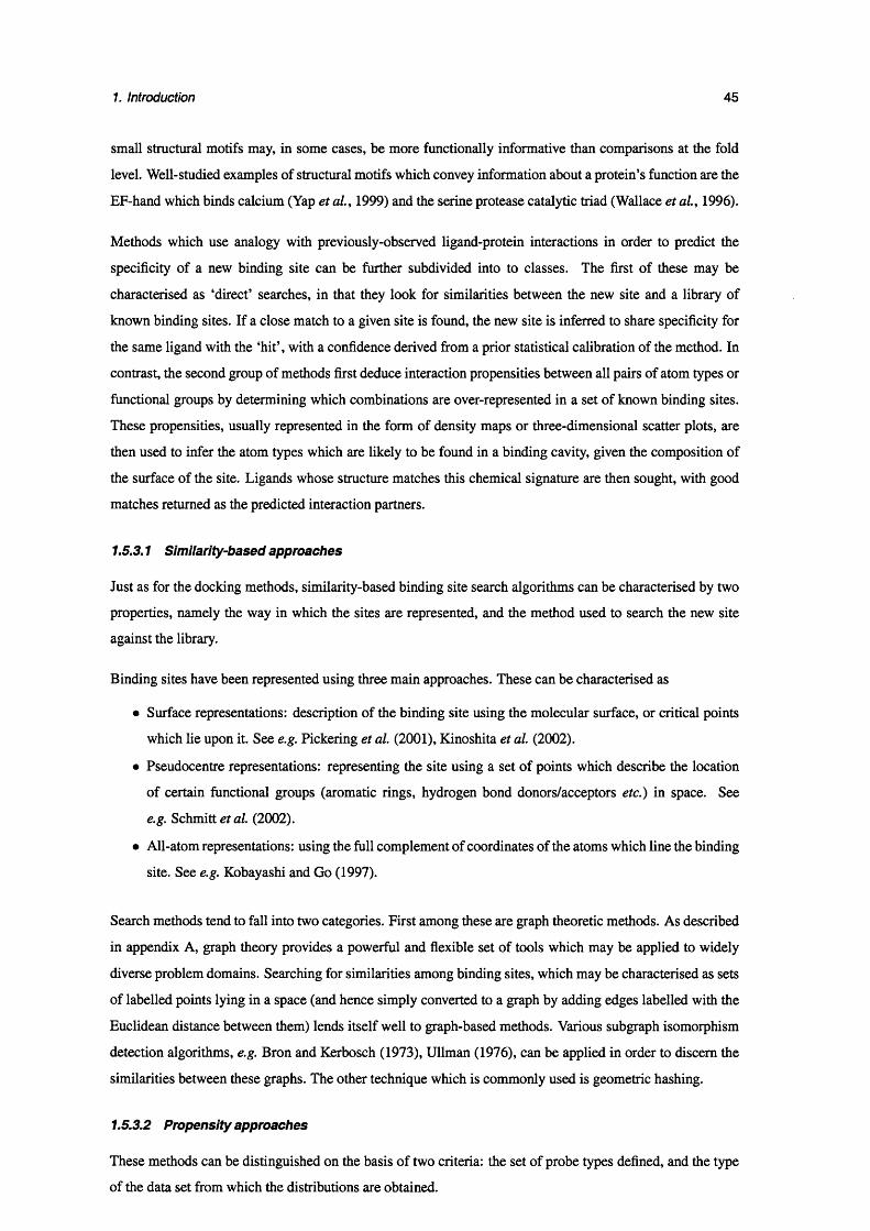
1. Introduction 45

small structural motifs may, in some cases, be more functionally informative than comparisons at the fold

level. Well-studied examples of structural motifs which convey information about a protein’s function are the

EF-hand which binds calcium (Yap et a l, 1999) and the serine protease catalytic triad (Wallace et a l, 1996).

Methods which use analogy with previously-observed ligand-protein interactions in order to predict the

specificity of a new binding site can be further subdivided into to classes. The first of these may be

characterised as ‘direct’ searches, in that they look for similarities between the new site and a library of

known binding sites. If a close match to a given site is found, the new site is inferred to share specificity for

the same ligand with the ‘hit’, with a confidence derived from a prior statistical calibration of the method. In

contrast, the second group of methods first deduce interaction propensities between all pairs of atom types or

functional groups by determining which combinations are over-represented in a set of known binding sites.

These propensities, usually represented in the form of density maps or three-dimensional scatter plots, are

then used to infer the atom types which are likely to be found in a binding cavity, given the composition of

the surface of the site. Ligands whose structure matches this chemical signature are then sought, with good

matches returned as the predicted interaction partners.

1.5.3.1 Similarity-based approaches

Just as for the docking methods, similarity-based binding site search algorithms can be characterised by two

properties, namely the way in which the sites are represented, and the method used to search the new site

against the library.

Binding sites have been represented using three main approaches. These can be characterised as

• Surface representations: description of the binding site using the molecular surface, or critical points

which lie upon it. See e.g. Pickering et al. (2001), Kinoshita et al. (2002).

• Pseudocentre representations: representing the site using a set of points which describe the location

of certain functional groups (aromatic rings, hydrogen bond donors/acceptors etc.) in space. See

e.g. Schmitt etal. (2002).

• All-atom representations: using the full complement of coordinates of the atoms which line the binding

site. See e.g. Kobayashi and Go (1997).

Search methods tend to fall into two categories. First among these are graph theoretic methods. As described

in appendix A, graph theory provides a powerful and flexible set of tools which may be applied to widely

diverse problem domains. Searching for similarities among binding sites, which may be characterised as sets

of labelled points lying in a space (and hence simply converted to a graph by adding edges labelled with the

Euclidean distance between them) lends itself well to graph-based methods. Various subgraph isomorphism

detection algorithms, e.g. Bron and Kerbosch (1973), Ullman (1976), can be applied in order to discern the

similarities between these graphs. The other technique which is commonly used is geometric hashing.

1.5.3.2 Propensity approaches

These methods can be distinguished on the basis of two criteria: the set of probe types defined, and the type

of the data set from which the distributions are obtained.

1. Introduction 46

In the case of X-SITE (Laskowski et a l, 1996), 26 atomic probes are defined, based on a previously published

list of atom types (Engh and Huber, 1991). Contact preferences are defined relative to 163 three-atom

fragments5, each of which occurs in one or more of the standard amino acid side chains, and which define a

coordinate frame. By analysing a set of high-resolution, non-homologous protein structures taken from the

PDB, three-dimensional density maps are constructed for each probe/reference-frame pair, which describe the

distribution of probe atoms relative to the fragment. Validation on a set of 5 known protein-ligand complexes

resulted in correctly predicted atom types for 54-78% of ligand atoms.

The source of the original data for IsoStar (Bruno et al., 1997) is a combination of PDB structures, and

coordinates taken from the CSD. It contains distributions constructed in a similar way to those found in X-

SITE, except that the probe types in this case are not individual atoms, but rather small functional groups

such as hydroxyl moieties or methyl groups. This library is utilised by the SuperStar program to produce

contoured propensity maps for putative binding sites. SuperStar was validated on a set of 122 protein-ligand

complexes from the PDB. For 80% of the ligand atoms in the test set, the density of the correct probe type at

that position was found greater than expected by chance (Verdonk et al., 1999, 2001).

1.5.4 The relationship between ligand specificity and protein function

Identification of the ligand or ligands which bind to a new protein is often cited as an important clue to

predicting its function. It is therefore instructive to clarify something of what we mean by the word ‘function’.

The inability of this word to encapsulate the many aspects of the role played by one protein in an organism,

has been recognised by Skolnick and Fetrow (2000) and Moult and Melamud (2000); meanwhile, the ever-

increasing body of knowledge relating to gene and protein function has highlighted a need to explicitly define

the vocabulary we use to express this information (Ashbumer et al., 2000). A synthesis of the schemes

previously presented for the description of protein function leads to the following four complementary

classes:

• Physiological function (In which biological processes is the protein involved in the organism?)

• Cellular component (i.e. cellular location - is the protein membrane-bound, cytosolic etc.)

• Biological process (e.g. translation, metabolism)

• Biochemical function (e.g. enzyme, transporter)

Of these, protein structure - and in particular, protein-ligand interaction information - allows us access most

directly to molecular (or biochemical) function. Moult and Melamud suggested breaking this class further

into more fine-grained descriptors:

1 Class (e.g. enzyme, DNA-binding protein)

2 Type (e.g. protease, transcriptional repressor)

3 Specificity (e.g. trypsin-specific protease, lac repressor)

A reliable method for the prediction of protein-ligand interactions would give us access to the last of these

descriptors. The value of this information would depend in part on the particular ligand predicted: knowing

sThe X-SITE data set has since been updated to include a wider range of probe types (R.A. Laskowski, personal communication).

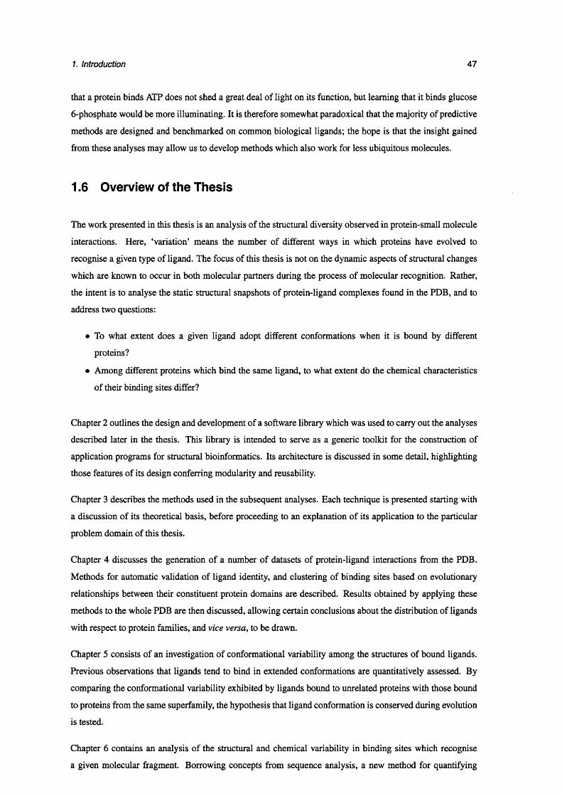
1. Introduction 47

that a protein binds ATP does not shed a great deal of light on its function, but learning that it binds glucose

6-phosphate would be more illuminating. It is therefore somewhat paradoxical that the majority of predictive

methods are designed and benchmarked on common biological ligands; the hope is that the insight gained

from these analyses may allow us to develop methods which also work for less ubiquitous molecules.

1.6 Overview of the Thesis

The work presented in this thesis is an analysis of the structural diversity observed in protein-small molecule

interactions. Here, ‘variation’ means the number of different ways in which proteins have evolved to

recognise a given type of ligand. The focus of this thesis is not on the dynamic aspects of structural changes

which are known to occur in both molecular partners during the process of molecular recognition. Rather,

the intent is to analyse the static structural snapshots of protein-ligand complexes found in the PDB, and to

address two questions:

• To what extent does a given ligand adopt different conformations when it is bound by different

proteins?

• Among different proteins which bind the same ligand, to what extent do the chemical characteristics

of their binding sites differ?

Chapter 2 outlines the design and development of a software library which was used to carry out the analyses

described later in the thesis. This library is intended to serve as a generic toolkit for the construction of

application programs for structural bioinformatics. Its architecture is discussed in some detail, highlighting

those features of its design conferring modularity and reusability.

Chapter 3 describes the methods used in the subsequent analyses. Each technique is presented starting with

a discussion of its theoretical basis, before proceeding to an explanation of its application to the particular

problem domain of this thesis.

Chapter 4 discusses the generation of a number of datasets of protein-ligand interactions from the PDB.

Methods for automatic validation of ligand identity, and clustering of binding sites based on evolutionary

relationships between their constituent protein domains are described. Results obtained by applying these

methods to the whole PDB are then discussed, allowing certain conclusions about the distribution of ligands

with respect to protein families, and vice versa, to be drawn.

Chapter 5 consists of an investigation of conformational variability among the structures of bound ligands.

Previous observations that ligands tend to bind in extended conformations are quantitatively assessed. By

comparing the conformational variability exhibited by ligands bound to unrelated proteins with those bound

to proteins from the same superfamily, the hypothesis that ligand conformation is conserved during evolution

is tested.

Chapter 6 contains an analysis of the structural and chemical variability in binding sites which recognise

a given molecular fragment. Borrowing concepts from sequence analysis, a new method for quantifying

1. Introduction 48

binding site diversity is proposed. This is then applied to binding sites for a number of common ligand

fragments, with the aim of determining whether the degree of variation in binding sites is similar among

different protein families, and for sites recognising different fragments. Potential applications of this method

in knowledge-based binding site prediction are discussed.

Chapter 7 discusses the implications of the findings from the previous chapters, presents the conclusions

which can be drawn from them, and suggests future work which could be undertaken.

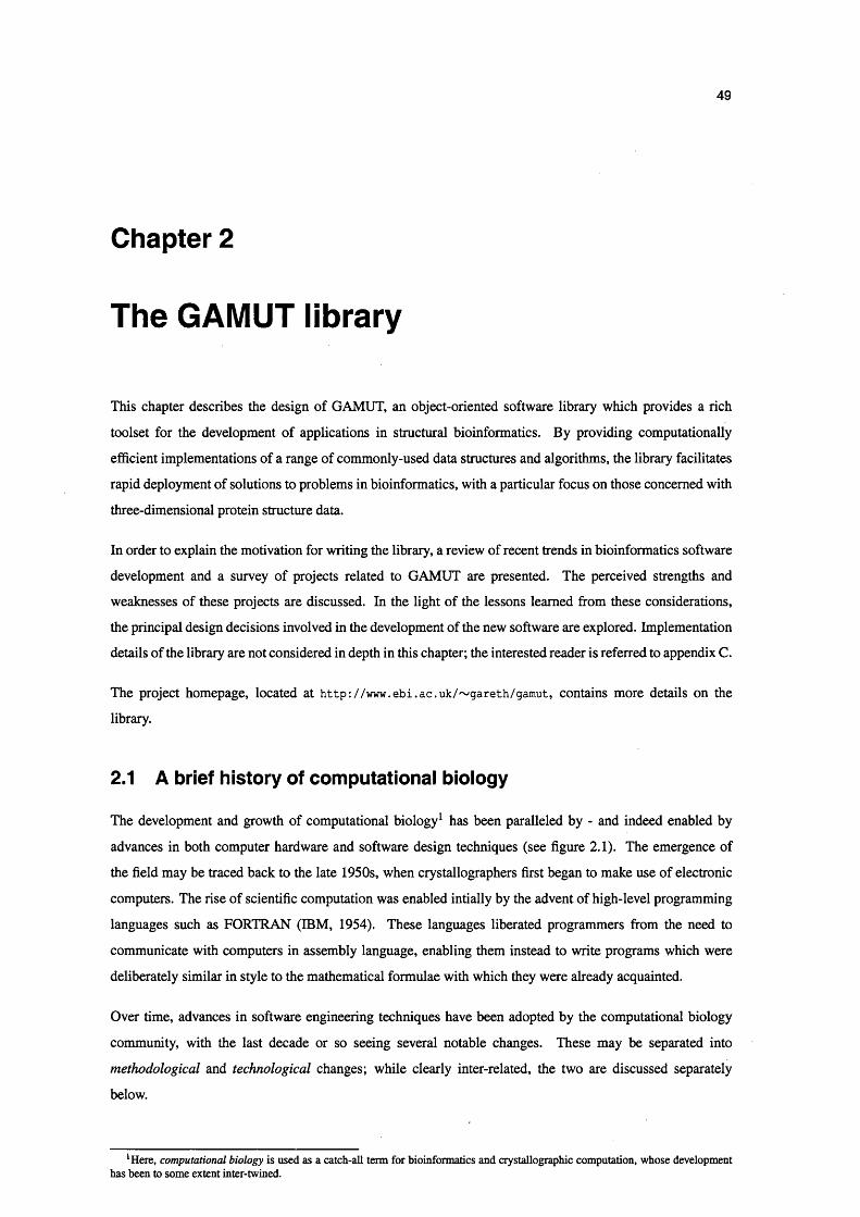
49

Chapter 2

The GAMUT library

This chapter describes the design of GAMUT, an object-oriented software library which provides a rich

toolset for the development of applications in structural bioinformatics. By providing computationally

efficient implementations of a range of commonly-used data structures and algorithms, the library facilitates

rapid deployment of solutions to problems in bioinformatics, with a particular focus on those concerned with

three-dimensional protein structure data.

In order to explain the motivation for writing the library, a review of recent trends in bioinformatics software

development and a survey of projects related to GAMUT are presented. The perceived strengths and

weaknesses of these projects are discussed. In the light of the lessons learned from these considerations,

the principal design decisions involved in the development of the new software are explored. Implementation

details of the library are not considered in depth in this chapter; the interested reader is referred to appendix C.

The project homepage, located at http://www.ebi.ac.uk/~gareth/gamut, contains more details on the

library.

2.1 A brief history of computational biology

The development and growth of computational biology1 has been paralleled by - and indeed enabled by

advances in both computer hardware and software design techniques (see figure 2.1). The emergence of

the field may be traced back to the late 1950s, when crystallographers first began to make use of electronic

computers. The rise of scientific computation was enabled intially by the advent of high-level programming

languages such as FORTRAN (IBM, 1954). These languages liberated programmers from the need to

communicate with computers in assembly language, enabling them instead to write programs which were

deliberately similar in style to the mathematical formulae with which they were already acquainted.

Over time, advances in software engineering techniques have been adopted by the computational biology

community, with the last decade or so seeing several notable changes. These may be separated into

methodological and technological changes; while clearly inter-related, the two are discussed separately

below.

1 Here, computational biology is used as a catch-all term for bioinformatics and crystallographic computation, whose development has been to some extent inter-twined.

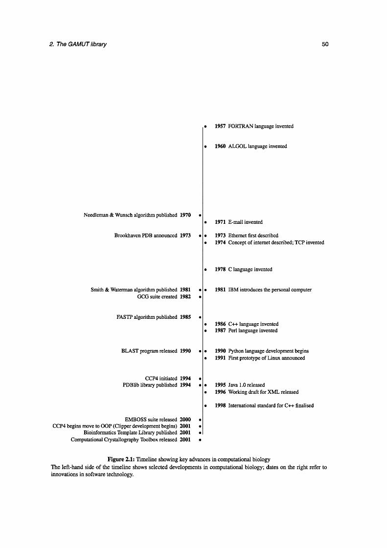
2. The GAMUT library 50

• 1957 FORTRAN language invented

• 1960 ALGOL language invented

Needleman & Wunsch algorithm published 1970

Brookhaven PDB announced 1973

1971 E-mail invented

1973 Ethernet first described1974 Concept of internet described; TCP invented

• 1978 C language invented

Smith & Waterman algorithm published 1981 GCG suite created 1982

FASTP algorithm published 1985

BLAST program released 1990

CCP4 initiated 1994 PDBlib library published 1994

EMBOSS suite released 2000 CCP4 begins move to OOP (Clipper development begins) 2001

Bioinformatics Template Library published 2001 Computational Crystallography Toolbox released 2001

1981 IBM introduces the personal computer

1986 C++ language invented1987 Perl language invented

1990 Python language development begins1991 First prototype of Linux announced

1995 Java 1.0 released1996 Working draft for XML released

1998 International standard for C++ finalised

Figure 2.1: Timeline showing key advances in computational biology The left-hand side of the timeline shows selected developments in computational biology; dates on the right refer to innovations in software technology.

2. The GAMUT library 51

2.1.1 Methodological changes

Early software development in computational biology was very much focussed on a specific, individual

problems: e.g. writing a program to perform the calculation of a Patterson map from reflection amplitudes. As

such, the only constraint on the program design was that it should perform its one job adequately. However, as

the use of computers in crystallography became more ubiquitous, the need to develop complete tool chains

which would work in synchrony with one another became apparent. This need was normally met by the

definition of file formats, through which each program in the chain could ‘talk’ to the next.

The obvious problem with such an approach is that code is redundantly repeated from one tool to the next; if

programs X and Y perform two different transformations on electron density maps then, while the code for

the transformation itself will differ between the programs, the two are likely to share a lot of ‘housekeeping’

code for constructing an in-memory representation of the density map, converting between reciprocal- and

real-space coordinates, and so forth.

The means for eliminating such redundancy lies in the development of libraries of re-usable code. Software

libraries may be described as collections of subprograms, which are used to help develop software. Libraries

are distinguished from executables in that they are not standalone programs; rather, they consist of ‘helper

code’ which provides services to another independent program or programs. As such, commonly-used

routines may be collected into a library, and then employed by any number of application programs. The

key requirements in library design, therefore, are that - in addition to performing a particular set of tasks -

the library must provide a well-defined interface through which applications may utilise its features. More

formally, a software library should satisfy the following requirements:

• Functionality: the library must provide a wide enough spectrum of capabilities to make it useful, such

that the client2 is motivated to utilise the library rather than writing custom code.

• Reusability: the functionality provided by the library should be flexible enough to be applicable to

a range of related problems; without this constraint, a library becomes simply a bespoke software

component designed for a single application.

• Ease of use: the library should be as user-friendly as possible, meaning that it should provide a clearly

documented interface, whose style conforms with existing conventions in the programming language

in which it is written.

• Robustness: the library should be tolerant to both heavy usage conditions, and to errors in input data.

A good example of a widely-used body of code for computational biology is the CCP4 library (Collaborative

Computational Project Number 4,1994) for crystallographic map manipulation and model building.

2.1.2 Technological changes

Historically, scientific programs have been composed of comparatively simple data structures such as arrays

and matrices, with the most commonly required operations being floating-point arithmetic computations.

Program structure is also often found to be fairly simple, consisting largely of counting loops and selections.

2Throughout this thesis, the term client will be used to refer to either the application or the programmer who utilises a library

2. The GAMUT library 52

The prime concern in much scientific programming is efficiency; as such, the languages which initially

found favour in the area were those which could offer speed comparable to assembly language programming.

However, they were not necessarily the most sophisticated in terms of their control and data structures.

From early, unstructured languages, through structured programming and lately into object-oriented

languages, language developments have allowed scientific programmers to model biological data with

increasing accuracy and clarity. The programming paradigm currently enjoying the highest profile in

computational biology is that of Object-Oriented Programming (OOP) (Meyer, 1997). While, in traditional

programming models, data and process are separate parts of a program, the object-oriented approach merges

the two together. There are many definitions of an object’, technically, an object is a software entity which

bundles data variables together with the methods which act on this data. More poetically, Meyer characterises

the concept of an object using the motto “Ask not first what the system does: As what it does it to!”.

Conceptually, software objects are able to closely model real-world objects, since they possess the ability

to represent both the state and behaviour of an entity. The object-oriented programming paradigm was

adopted for the design of GAMUT.

2.2 Other projects related to GAMUT

At the outset of the work presented in this thesis, it was clear that software posessing a number of capabilities

would be required. These capabilities included:

• Coordinate handling: the ability to import, represent and manipulate three-dimensional macromolec-

ular coordinate data, including calculations of rigid-body superpositions; methods for classifying

atoms into groups according to specified schemas

• Chemical structure manipulation: the ability to represent chemical structures, including facilities for

detecting common substructures shared by a pair of compounds, identifying rotable bonds, computing

graph invariants, and the generation of 2D chemical structure diagrams

• 3D density mapping: a framework for handling 3D scalar fields, including features such as calculating

convolutions, comparing groups of maps and computing isosurface contours

• Representation of protein structure classifications: the ability to assign domain identities to

individual residues in proteins based on existing structure classification schemes such as CATH and

SCOP

• Miscellaneous utilities: clustering, database access, linear algebra, computational geometry

It was necessary, therefore, to determine whether libraries providing these features were already available.

Several programming libraries for computational biology have recently been described, including a number

of object-oriented libraries. These libraries are summarised in table 2.1.

The suitability of the available libraries for the project was assessed in each case according to two main

criteria:

2. The GAMUT library 53

• Ease of use: Does the library provide an intuitive, well-documented interface? How easily can it be

integrated with other systems?

• Functionality: Does the library provide the required features?

Predictably, most of the available libraries provided a subset of the required functionality, in addition to

other features which were not required. For example, the Clipper library contains very powerful density-map

handling facilities, including coordinate transforms, file import/export for several common data formats and

comparison of multiple maps. However, at the the outset of the project, Clipper did not have any ability to

represent models of macromolecular structure. This pattern was common to all of the libraries surveyed;

ultimately, it was felt that developing a new library which provided a full set of the features required would

be preferable to attempting to marry several disparate systems.

An additional major motivation for the design and implementation of GAMUT was the percieved educational

benefit to the author of undertaking the project. In particular, it was felt that writing a system like GAMUT

from scratch would allow the author to gain an understanding of both software design methodologies and

algortihmics, which could not be gleaned by simply ‘patching together’ existing components.

Name Reference Description Language Active"

PDBlib (Chang et a/., 1994) A class library for modelling structural features of biomolecules at the level which can be parsed from PDB files.

C++ No

MMTK (Hinsen, 2000) The Molecular Modelling Toolkit. Provides features including rigid-body fitting, force field minimizations, molecular dynamics, surface calculations.

Python Yes

BALL (Kohlbacher and Lenhof, 2000) Biochemical ALgorithms Library. Extensive collection of data structures and algorithms for development of molecular modelling and simulation applications.

C++ Yes

Clipper (Cowtan, 2000) A set of libraries for crystallographic computing. Aimed at aiding the transition of CCP4 developers to object-oriented programming. Provides classes for representation of electron density maps, and frameworks for developing crystallographic phase estimation and model refinement methods.

C++ Yes

BTL (Pitt et al., 2001) The Bioinformatics Template Library. Library of components for biocomputing, designed with a strong emphasis on generic programming. Consists largely of generic algorithms in the mould of the Standard Template Library, along with a few specialised data structures.

C++ No

MMDB (Krissinel, 2002) The CCP4 coordinate library project. A library intended to help CCP4 developers in working with coordinate files. Provides various high-level tools for working with coordinate files such as orthogonal-fractional coordinate transforms, generation of symmetry mates, and editing molecular structures.

C++ Yes

CACTVS (Ihlenfeldt etal., 1994) A research project aiming to change the ways of doing computational chemistry. The functionality of the toolkit is exposed via a scripting layer, but source code for the underlying library is not freely available.

C/Tk Yes

OpenBabel (The OpenBabel Team, 2001) A cross-platform program and library designed to interconvert between many file formats used in molecular modeling and computational chemistry.

C++ Yes

CDK (Dortu et al. , 2000) Java utitility classes for Chemolnformatics and Computational chemistry. Java Yes

Table 2.1: Software development projects related to GAMUT

“Whether the project was undergoing active development at the time of writing, to the best of the author’s knowledge

2. The GAMUT library 55

2.3 Design of GAMUT

This section describes the overall design of GAMUT, with only limited reference to details of the

implementation, which are treated separately in appendix C. The focus of the discussion here is upon the

requirements which the library was designed to satisfy.

2.3.1 Design principles

2.3.1.1 Modularity

As described above, GAMUT was conceived as a general-purpose framework for developing structural

bioinformatics applications, and as such, provides a wide range of functionality in several distinct areas.

It is clear, however, that for any one application, only a subset of this functionality may be required. A

key requirement in GAMUT, therefore, is the ability for a client to utilise only the components which are

required; this was realised through the following:

• Object-orientation: by implementing each data structure and algorithm as an object, each of which is

designed with the principle of abstraction in mind, independent software components, each fulfilling a

distinct and well-defined role, are made available to the client.

• Library organisation: related GAMUT classes, such as the chemistry classes, or density map classes,

are collected together in independent modules. This allows the client to utilise only those groups

of components which will be required for application development in the area(s) in which he/she is

interested.

2.3.1.2 Ease of use

In order to make GAMUT as user-friendly as possible, the following principles were adopted (see also

appendix B.l):

• Consistent, intuitive interface: functions and variable names are chosen in order to make their use as

intuitive as possible. Moreover, naming conventions are used throughout the library, such that functions

with the same name in different classes should have the same or comparable effects. The interface is

thoroughly documented, as described in §2.4.

• Idiomatic interface: the GAMUT interface makes use of numerous design patterns which are in

common use in other software components, and are therefore likely to be familiar to potential clients.

For example, collections of objects are stored inside container classes, and access to them is typically

granted through iterators, which prevent array bounds over-runs, and also allow the design of generic

algorithms which may operate on a variety of different containers.

• Simple installation procedure: to enable portability of the library, standard methods of distribution

and installation of the library have been employed: the GNU build tools (Vaughan, 2000), familiar to

most UNIX users, are used to configure, compile and install the library.

2. The GAMUT library 56

2.3.2 Robustness

A library will only be utilised if it can be relied upon; therefore a great deal of effort has been spent in making

GAMUT as error-free as possible. The key points of this enterprise are:

• E rro r tolerance: where errors may occur during execution of library functions, for example due to

erroneous input data, they are checked for, and reported using a system of runtime exceptions.

• Protecting the programmer: programming errors are made less likely by removing from the client

the burden of memory management: all dynamic memory allocation and deallocation is done within

the library itself (see appendix B.2).

• Self-testing: a suite of test programs is provided with the library, which should be run once the library

itself has been installed. This test suite checks the behaviour of the library in a range of different

situations, including several which deliberately invoke errors in order to check GAMUT’S exception-

handling mechanism. In addition to reassuring the client that his/her installation of the library is

working correctly, the testsuite is invaluable during library development, both in checking that recent

changes have not inadvertantly introduced bugs into the library, and in evaluating the portability of the

system to a number of different platforms.

2.3.3 Choice of language

Once the decision had been taken to design GAMUT in an object-oriented manner, the choice of languages

could be substantially narrowed. The three major object-oriented languages currently available are Java (Inc.,

1995), C++ (Stroustrup, 1995) and Python (Python Software Foundation, 1990). Each language naturally has

its own advantages and disadvantages.

Of the three, Python was the least well-suited to the task: being an interpreted language, its execution speed is

typically much slower than that of either of C++ or Java. As such, Python is not suitable for implementation

of the numerically-intensive parts of the library, for which efficiency was identified as a priority.

Java was designed from the outset as a cross-platform object-oriented language, and therefore benefits from a

clean design, excellent portability and robustness. In addition, there are a large number of high-quality third

party Java libraries available. However, certain attractive language features, notably operator overloading

and generics (see below) are currently missing from Java. An even more serious impediment to using the

language is that the virtual machine architecture needed to provide the ability to run the same program on

any platform incurs a significant performance penalty.

C++ was originally conceived as a “C with classes”, and as such, owes both good and bad features to C.

On the good side, C++ programs can be made to run extremely quickly since the language retains the

pointer-manipulation capability of C. This can lead to coding errors, however, and porting C++ code between

platforms is recognised to often be troublesome. The mosaic heritage of C++ is often criticised as having led

to a language which, although powerful, has become somewhat baroque in its design3.

3 An unattributed comment found on the world-wide web describes the language as being “An octopus made by nailing extra legs onto a dog”I

2. The GAMUT library 57

C++ provides an extremely high degree of expressivity, due to its support for multiple programming

paradigms: in addition to its object-orientation capabilities, C++ allows powerful generic programming

techniques to be leveraged, thanks to its template framework. A template class is one in which the type

of one or more data members is replaced by a ‘dummy’ or placeholder type. In order to use a template class,

it is ‘instantiated’ by specifying the type(s), which are substituted for the placeholders.

The simplest application of templates is the design of generic objects: for example, one may wish to design a

type-safe array object. The array may be implemented as a template class with a single parameter, namely the

type of object to be stored in the array. Using this single template, a client is able to instantiate any number

of array types, each of which stores a different type of data.

Although the idea of templates is fairly simple, and the number of syntactic rules governing their use

within the language is small, templates enable a range of particularly powerful programming techniques

to be leveraged using C++. The most exotic of these fall into a group known as ‘metaprogramming’. By

employing template specialisation and recursion, the compiler can be made to act as an iterpreter, such that

parts of C++ programs are effectively executed at compile-time, rather than at run-time, as is normally the

case. Alternatively, template metaprogramming can be used to simplify the interface of a complex class using

policies and/or typelists. Both of these aspects of metaprogramming were employed in the implementation

of GAMUT, and will be discussed further later in this chapter, and in appendices B.4 and B.5.

Since the recent finalisation of an ISO standard for C++ (ISO/IEC Information Technology Task Force,

1998), compiler designers have had a concrete specification to work to, greatly reducing portability problems.

One final advantage of C++ is the availability of powerful tools for interfacing with the Python language

(Abrahams, 2003), allowing an easy-to-use scripting layer to be wrapped around a C++ library. These

features taken together motivated the decision to implement GAMUT in C++.

2.3.4 Architecture of the library

The evolution of a piece of software can often be viewed as a Popperian process. It begins with an initial

design, in which the software engineer does his or her best to capture the essence of the problem. This initial

conception allows a prototype of the system to be constructed, which fulfils the main requirements identified

during the design stage. Inevitably, however, flaws in the design are discovered during the implementation

and testing of the software; many design flaws are easily corrected, but every so often, a radical change

in the overall design of the system is required. This process of iterative re-design, often involves, in OOP

terminology, several refactoring steps: elements common to two or more existing classes are abstracted away

into a common base class, thereby improving modularity and promoting code re-use. Eventually, the system

reaches maturity when all of the features specified in the original design are present, and the system is able

to perform the task(s) for which it was designed.

GAMUT has undergone such an evolution of design; a sketch of its final architecture is presented in figure

2.2. It may be seen as consisting of several layers; each of which performs a more specific function than

the one before. Within each layer, components which are conceptually related are grouped together into

semi-independent modules.

2 . The GAMUT library 58

GAMUT applications

GAMUT bioinformatics layer

MSD interface LigandsDomain

ArchitectureDensityMaps

BiologicalSequencesDatabase

InterfaceMacromolecular

CoordinatesChemicalStructure

Third Party Libraries GAMUT generic components layer

i| Database APIs IAlgorithms | | Data structures | lA D ^ ^ G r a p h ic s |

Standard Template Library (STL)

Figure 2.2: Architecture of the GAMUT library GAMUT consists of several layers, which, reading from the bottom of the picture upwards, are in order of increasingly specialised function.

The lowest layer consists of the C++ Standard Template Library (STL) (Inc., 1994). This is a collection

of fundamental data structures such as sets, maps and arrays, an implementation of which is provided with

most C++ compilers, and can therefore be assumed to be present on all target platforms for GAMUT. While

not strictly part of the GAMUT library, the STL data structures are used as the atomic building blocks from

which many of the classes in the higher levels of the library are composed.

2.3.4.1 Generic components

Moving in the direction of increasing specialisation of function, the next layer contains generic data

structures, algorithms and utilities. This layer does not contain anything specifically related to biological data;

as such, it provides components which are potentially also of use in application areas outside computational

biology.

The existence of the generic components layer is largely due to the refactoring process described above, with

many classes having begun life as part of the bioinformatics layer, before it was realised that common factors

could be abstracted away. A good example of this phenomenon is the tree data. In the first implementation

of the macromolecular structure module, the atom, residue and chain classes were designed such that the

parent-child relationships between them was explicitly coded into each class. A residue object, for example,

contained a pointer to its parent chain, and an array of pointers to its constituent atoms. This meant that

code for common tree operations such as adding a child node, or iterating through all children of a given

node, were repeated through the atom, residue and polymer classes. In addition, ‘housekeeping’ code was

also repeated: when a residue object is destroyed, it must make sure that the atom objects to which it holds

pointers are also destroyed. The chain object holds the same responsibility towards its child residues.

By abstracting the tree concept into its own class, this redundancy was removed: a single node class, which

manages the lifetime of, and provides functions for access to its child nodes, now can serve as a base class

for the atom, residue and chain classes. This type of abstraction is an example of the Composite design

pattern (Gamma et al., 1995). Once code for a generic tree is in place, it becomes possible to quickly develop

other tree-based data structures - such as those which represent protein domain classification hierarchies like

2. The GAMUT library 59

CATH or SCOP - without re-inventing the wheel.

The key components present in the generic layer are briefly outlined here with a focus upon the aims which

were in mind during the design of each one. It should be noted that components similar to several of those

provided in GAMUT’S generic component layer are now freely available in a third-party C++ library called

Boost (The Boost Committee, 1998). These include a generic graph library, linear algebra components, and

support for functional programming. Although utilisation of this existing code could have replaced some

which was written for GAMUT, the architecture of Boost is such that it is difficult to separate just a few

components from the library as a whole4. Employing Boost components in GAMUT would have required

either distribution of the entire Boost source tree along with GAMUT, or requiring that the user already had

Boost installed before downloading GAMUT. Neither of these alternatives was viable.

2.3.4.1.1 Arrays

Classes for representing arrays of objects whose size is fixed at compile-time were required in GAMUT, due

to their current absence from the C++ standard. While the language has good support for dynamic arrays,

through the std:: vector class, these are not ideal when dealing with arrays whose length is known not to be

changeable, for example, when implementing a 3-dimensional vector object. Conversely, the fixed-size array

types present in C++ are due to the language’s C heritage, and do not provide any of the convenient OOP

features of the STL containers. As such, the requirements for the fixed-size array class were that it should

be a wrapper for static C arrays, providing an interface as close as possible to that exposed by std::vector

while maintaining the computational efficiency of the native array types.

In addition to a class for fixed-sized one-dimensional arrays, a three-dimensional array class was required

for GAMUT. It should be noted that the author draws a distinction between three-dimensional arrays, and

three-dimensional fields. While both are three-dimensional grids of values, only fields are associated with

coordinates in three-dimensional space. A field therefore should be thought of as an array which has been

embedded in a space. The array class should provide the following capabilities:

• Intuitive indexing: the client should be able to access data within the array by either providing a three-

dimensional address within the grid, or by specifying an index value. The array class should provide

means for translating between these two forms of look-up.

• Views: by specifying a pair of bounding addresses, the client should be able to identify a block within

the array, upon which further operations may be performed. For example, the client must be able to

identify a view of the array, and then iterate through all values in that view.

• Arithmetic operations: where the type of data stored in the grid supports arithmetic operators, the

client should be able to apply these operators to pairs of arrays with compatible dimensions, thereby

effecting a cell-by-cell addition, subtraction or multiplication of values. In addition, it should be

possible to apply these operations to pairs of arrays with different sizes, as long as the smaller array

can be placed somewhere within the larger. This type of operation could be used to update a large

scalar field by incrementing a small region using a function stored as an precomputed array of values.

4Since the development of GAMUT, a more recent release of Boost which provides a mechanism for installing library components independently has become available.

2. The GAMUT library 60

2.3.4.1.2 Graphs

Graphs, which are discussed in appendix A, are one of the most fundamental data structures in computer

science, and are particularly important within GAMUT. Their primary application is in the representation of

the atomic connectivity of chemical compounds.

In designing the graph framework for GAMUT, the principal requirements were:

• A flexible, generic data structure: the data structure should be able to represent graphs in the same

variety of ways that mathematicians use when thinking about them. That is to say, the library should

allow one to construct graphs which are directed or undirected, whose connectivity information is

stored using adjacency list, edge list or edge matrix, whose edges and vertices may be labelled or

unlabelled, etc.

• An intuitive interface: typical patterns of accessing graph information include iteration through all

vertices in a graph, iteration over out-edges of a given vertex, depth-first and breadth-first searches.

Mechanisms for performing these should be provided by the library.

• A consistent interface: as far as possible, the graph interface should be invariant over the different

types of graph described above. That is to say, whether the client is referring to an edge list graph or

an adjacency matrix graph, he/she should be able to perform any given operation in the same manner.

• An extensible algorithm framework: efficient implementations of commonly-used graph algorithms

such as shortest-path methods, cycle perception and isomorphism detection, should be provided. They

should be implemented in such a way that, should a client wish to add a new isomorphism algorithm

for example, the means for doing so are clear.

• Graphical representations: it is often difficult to interpret the results of graph operations without

reference to a diagrammatic depiction of the graph. Many graph layout algorithms are available; it was

decided that several should be implemented in GAMUT.

2.3.4.1.3 Trees

As described above, a generic tree component was required. The design requirements for the tree classes

were as follows:

• An expressive interface: clients should be access the data held in the tree by iterating through children

of a given node, traversing the tree using depth-first and breadth-first searches, and so on.

• Automatic lifetime management of nodes: as described above, parent nodes should take responsibil­

ity for the management of the lifetime of their child nodes, in order to avoid memory leaks. A corollary

of this is that, when a node n is copied, the copying operation must be deep: that is to say, all nodes in

the subtree below n must be recursively copied to form a new, independent subtree.

• Ability to represent different types of trees: just as the graph framework was designed in order to

provide a similar interface, to data structures which internally, may be represented in quite different

ways, different types of trees (e.g. binary - balanced or unbalanced, N-ary) should expose similar

interfaces to the client. Another distinction which may be drawn is between polymorphic trees, where

the nodes may be of different types (such as the tree of a macromolecular structure, where some nodes

2. The GAMUT library 61

represent residues, others atoms etc.), and monomorphic trees, such as trees generated by hierarchical

clustering algorithms, where each node represents the same type of object, namely a branch in the

clustering hierarchy.

2.3.4.1.4 Persistence

A key requirement when developing application programs is the ability to save the state of objects within the

program to disk, such that the objects can later be reconstructed from the disk file. This ability to interconvert

between volatile, in-memory representations of data, and non-volatile representations such as disk files is

known as persistence; the actual operation of writing objects to disk is sometimes referred to as serialisation.

The main issues at hand when designing GAMUT’S persistence mechanism were:

• Platform independence: files written by a GAMUT application running on one machine should be

readable by a GAMUT application running on a different type of platform. The format of the file

must not, therefore, be dependent on the features of any particular machine. This is relatively easy to

achieve if data is written to text-based files using a common standard such as American Standard Code

for Information Interchange (ASCII). By utilising a text-based file format such as Extensible Markup

Language (XML) , complex data can be stored in files which, in addition to being readable on any

platform, may also be understood by any application which can parse XML.

The parsing of a text-based file, however, incurs an overhead on the data recovery process. The

alternative is to store data in a binary file format, which can be read in much more rapidly, since

the on-disk representation of the data is essentially identical to that held in memory. The disadvantage

of using a binary format are that the data is less accessible: whereas an XML file can be inspected

using any text editor, and may be parsed by any application which understands XML conventions, a

binary file typically can only be interpreted by the program which created it. In addition, storing data in

binary files requires consideration of issues such as endianness, whereby different types of computer

store the bytes of their data in different orders. Transferring files between machines with different

endianness requires swapping the byte order within the data.

At present, the persistence mechanism in GAMUT is binary, for reasons of speed; however, an XML

persistence mechanism could be added fairly simply; this would improve the ability of GAMUT

applications to communicate with other programs.

• Versioning: the information content of a class may change as the software is developed; as such, the

information written to disk when an object of that class is serialised, may also change. In order to

prevent errors when reading files, it is important to record the version number of the software which

created the file, at the start of the data written to disk. On reading the file, this number must be

checked against the version of the software performing the read. A mismatch in version number may

necessitate an error being generated; on the other hand, newer versions of the software should be

backwards-compatible with older file versions.

• Identity verification: an additional check which may be added to a persistence mechanism is to verify

that the file being read does in fact contain data of the correct type. This means that, in addition to

2. The GAMUT library 62

storing the version number at the head of a data block, each object should write an identifier which

specifies that it is of type X\ if a Y object later attempts to read the file, an error will be generated to

report the mistake.

• Indexing: at an early stage of GAMUT development, it was realised that a means for storing large

quantities of data in a form from which specific data items could be rapidly recovered would be

advantageous. This data typically takes the form of a large number of objects, each of which can

be identified by a small number of ‘keys’ (e.g. numeric indices, or text labels). Third-party database

engines could perform this function; however, for such simple data relationships, full relational

database capabilities are often not required. Instead, an Indexed Sequential Access Management

(ISAM) system was conceived for GAMUT. ISAM storage works by serialising the data objects into

one large file, while maintaining a separate file which maps from the keys, to a number which records

the location of the appopriate data object in the main data file. In order to access a particular data

object, the client needs simply to look up the file offset in the index, and then read from the appropriate

position in the archive (see appendix C. 1.7.1 for more details).

2.3.4.1.5 Linear algebra

Facilities for basic linear algebra operations, primarily (but not limited to) manipulation of three-dimensional

coordinates and transforms, were required for many parts of the library. Many libraries for linear algebra,

written in, or compatible with C++, already existed (e.g. LAPACK (Anderson et al., 1999) and LEDA

(Algorithmic Solutions Software, 2001)). However, these libraries provide capabilities far beyond those

required; GAMUT’S linear algebra module was designed as lightweight components providing the following

features:

• Vectors and matrices: classes for the fundamental objects used in linear algebra were designed,

including basic operations such as matrix algebra, scalar and cross products etc.

• M atrix decomposition: singular value decomposition and diagonalisation algorithms

2.3.4.1.6 Computational geometry

Certain geometric operations are common in structural bioinformatics applications; the following were

identified as necessary for implementation in GAMUT:

• Geometric range queries: structures and algorithms for rapidly determining the set of objects, located

in space, which fall inside a given geometric region, such as kd-trees and brick maps. For example,

determining the set of residues in contact with a ligand molecule begins with identifying those residues

which are in proximity to the ligand; this can be done using a geometric query map.

• Triangulation: means for computing and representing triangular meshes, including algorithms for

calculating isocontours through scalar fields.

2.3.4.1.7 Graphics

A basic 2D graphics toolkit was designed for GAMUT, in order to allow applications to generate diagrams

by providing objects corresponding to geometric primitives such as squares, lines and circles. The graphics

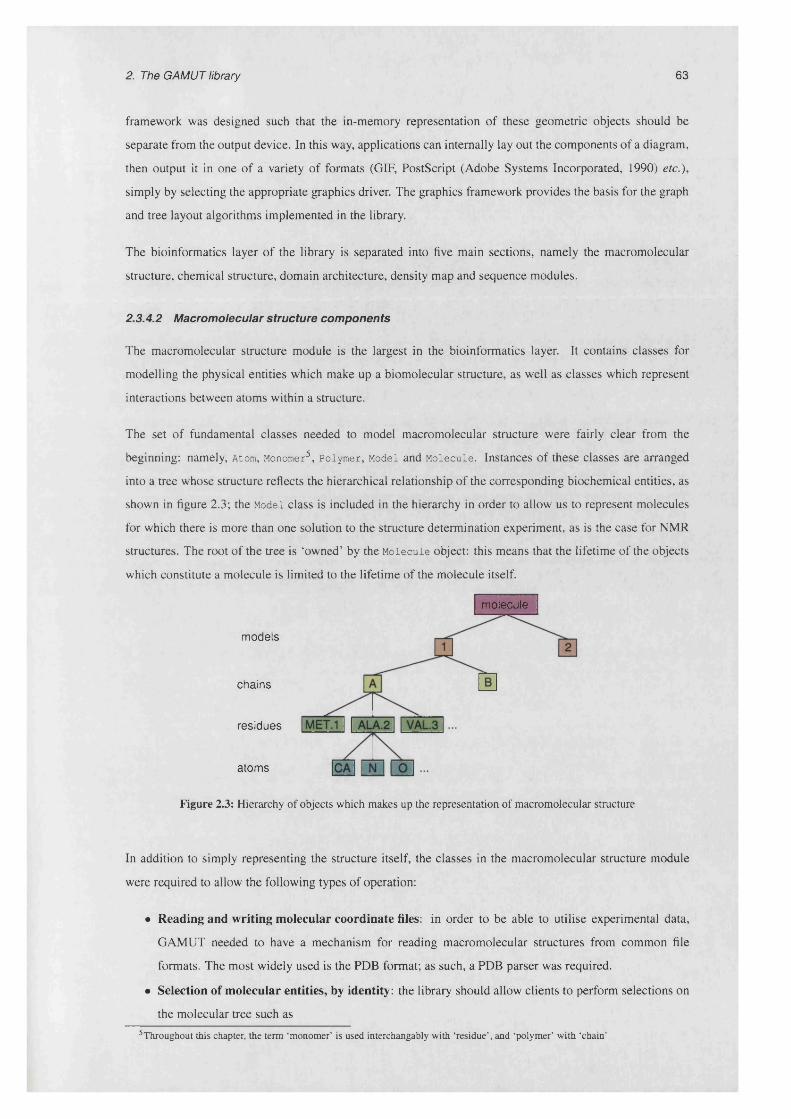
2. The GAMUT library 63

framework was designed such that the in-memory representation of these geometric objects should be

separate from the output device. In this way, applications can internally lay out the components of a diagram,

then output it in one of a variety of formats (GIF, PostScript (Adobe Systems Incorporated, 1990) etc.),

simply by selecting the appropriate graphics driver. The graphics framework provides the basis for the graph

and tree layout algorithms implemented in the library.

The bioinformatics layer of the library is separated into five main sections, namely the macromolecular

structure, chemical structure, domain architecture, density map and sequence modules.

2.3.4.2 Macromolecular structure components

The macromolecular structure module is the largest in the bioinformatics layer. It contains classes for

modelling the physical entities which make up a biomolecular structure, as well as classes which represent

interactions between atoms within a structure.

The set of fundamental classes needed to model macromolecular structure were fairly clear from the

beginning: namely, Atom, Monomer5, Polymer, Model and Molecule. Instances of these classes are arranged

into a tree whose structure reflects the hierarchical relationship of the corresponding biochemical entities, as

shown in figure 2.3; the Model class is included in the hierarchy in order to allow us to represent molecules

for which there is more than one solution to the structure determination experiment, as is the case for NMR

structures. The root of the tree is ‘owned’ by the Molecule object: this means that the lifetime of the objects

which constitute a molecule is limited to the lifetime of the molecule itself.

models

chains

residues

atoms

Figure 2.3: Hierarchy of objects which makes up the representation of macromolecular structure

In addition to simply representing the structure itself, the classes in the macromolecular structure module

were required to allow the following types of operation:

• Reading and writing molecular coordinate files: in order to be able to utilise experimental data,

GAMUT needed to have a mechanism for reading macromolecular structures from common file

formats. The most widely used is the PDB format; as such, a PDB parser was required.

• Selection of molecular entities, by identity: the library should allow clients to perform selections on

the molecular tree such as

5Throughout this chapter, the term ‘monomer’ is used interchangably with ‘residue’, and ‘polymer’ with ‘chain’

molecule

2. The GAMUT library 64

- select all residues named ALA. in chain A

- select all C“ atoms except those in glycine residues

• Selection of molecular entities, by geometry: selections should also be possible using geometric

criteria, e.g.

- select all atoms within 4A o f a fixed point, P

- select all residues with at least one atom within 4k o f a fixed point, P

- select all atoms which are within 4k o f a predefined set o f atoms, S

• Classification of atom or residue types: the client should be able to specify a scheme for

classification of atoms or residues into a number of types. After applying such a classification, it

should be possible to easily access all atoms/residues of a particular type, e.g. all aliphatic residues.

• Computation and application of coordinate transforms: the library should provide the facility for

applying coordinate transformations (i.e. translations and rigid rotations) to a molecule, or to a subset

of its atoms, residues or chains. In addition, it should be able to calculate transformations which

perform a least-squares superposition of one set of points (i.e. atomic coordinates) onto another.

• Editing the molecular tree: clients should be able to edit the molecular tree by adding or removing

atoms, residues, chains or models. For example, it should be possible to take a molecule, identify a

region of interest (say, a ligand binding site), and then strip away all other parts of the molecule.

2.3.4.3 Chemical structure components

The second module in the bioinformatics layer is concerned with the representation and comparison of

chemical structures, primarily their topological connectivity. In order to do this, the chemistry module

was designed around a labelled, undirected graph data structure in which this information could be easily

stored. The primary use of chemical graphs in the library is to serve as reference structures against which

other graphs may be compared in order to determine the identity of the compound which they represent. In

order to perform such a comparison, the ability to derive a chemical graph from the atomic coordinates of a

monomer, taken from a crystallographic structure, is required. This allows a dictionary of chemical graphs to

be used as a resource for validating the identity of compounds found within, or bound to, protein structures.

This process is illustrated schematically in figure 2.4, and is discussed further in chapter 4.

Each vertex in the graph represents an atom, and the following properties were deemed sufficient to describe

the characteristics of the atom:

• Atomic number

• Chirality

• Valence

• Number of hydrogens bonded to it

• Formal charge

• Number of ‘missing’ neighbours

• A string label

2. The GAMUT library 65

O •

(a) (b)

(c)

Figure 2.4: The process of mapping coordinates of a ligand molecule against a reference compound The ligand molecule is represented in a crystallographic data file only by its coordinates (a). By referring to a table of standard atomic radii, connectivity information can be added to the molecule (b). This representation of the molecule can then be compared against a reference graph by using a subgraph isomorphism algorithm, thus generating a set of atom-vertex mappings (c).

While the meanings of most of these properties are self-explanatory, the record of missing neighbours should

be explained. This field was added in order to better represent molecular fragments. Here, it is desirable

to be able to ‘mark’ the atoms which have incompletely satisfied valence, and which therefore constitute

‘attachment points’ to which other groups may be bonded. This is illustrated for the case of an adenine

moiety in figure 2.5.

In addition to the properties listed above, it was decided that each atom should be optionally associated with

a coordinate in 3-dimensional space. This allows the graph object to store energy-minimised coordinates,

upon which superpositions can be performed.

Edges in the graph represent chemical bonds; their properties are the type of the bond (single, double, or

triple), and an aromaticity flag. Aromatic systems are modelled in GAMUT as alternating single and double

bonds, each of which is marked as aromatic.

A system for storing dictionaries of graphs, which may represent idealised conformations of reference

compounds, or chemical fragments, was designed using the generic ISAM table component described above.

2. The GAMUT library 66

H

H

Figure 2.5: Chemical structure diagram showing an adenine fragment The ‘attachment point’ at N3 is shown with a green circle.

These dictionaries are named ChemBase archives.

Since the chemical graph class is derived from the generic graph template, any algorithm which is

implemented to act on generic graphs, is also applicable to chemical graphs. Therefore, the isomorphism

detection and cycle perception algortihms mentioned in §2.3.4.1.2 can be applied to chemical compounds.

In addition, a number of algorithms specifically applicable to chemical structures were also designed as part

of the chemistry component. These were required to do the following:

• Structure diagram generation: generation of a 2-dimensional image of a chemical structure, given

only the graph object. Note that this layout should not require any 3-dimensional coordinates to begin

with; in other words, it should be a true graph layout algorithm rather than an ‘unrolling’ algorithm

such as that utilised in the LIGPLOT program (Wallace et a l, 1995).

• Rotable bond detection: the ability to identify rotable bonds, allowing compounds to be automatically

partitioned into rigid molecular fragments.

• Torsion angle calculation: given a rotable bond in a reference graph, facilities for calculating the

torsion angle around it.

• Reading and writing small-molecule structure files: the ability to parse and write MDL MOL2 files

(Dalby etal., 1992).

2.3.4.3.1 Rotable bond detection

For the purposes of the work described in this thesis, rotable bonds are defined as single, acyclic bonds. A

ring perception algorithm (see appendix A) had already been implemented, so implementation of the rotable

bond detection class was straightforward.

In this thesis, a rotable bond is defined as a bond which

• is single

• is not in a ring

• if broken, yields two fragments consisting of at least two atoms each

The last of these conditions means that only those single, acyclic bonds about which we can observe the

result of rotation, are considered rotable. For example, neither of the two covalent bonds of a water molecule

2. The GAMUT library 67

are considered rotable, but the carbon-oxygen bond of methanol is.

In order to illustrate the definition of a rotable bond, consider the example shown in figure 2.6. An important

point to make regarding the use of rotable bonds in this thesis relates to the effect of hiding hydrogen atoms.

Due to the third condition above, certain rotable bonds - specifically, bonds whose rotation does not produce

any new conformation of heavy atoms - become non-rotable when hydrogen atoms are neglected. Examples

of this type of bond are those to a terminal CH3 , NH2 or OH group. Since hydrogen atoms are not normally

resolved in macromolecular crystal structures, the effect of manipulating these rotors cannot be see in the

atomic coordinates.

o

(b)

Figure 2.6: Example of the definition of a rotable bond Rotable bonds are coloured in red. When hydrogens are hidden, several bonds which would previously have been considered rotable, are no longer.

2.3.4.4 Ligand binding site components

The chemical structure and macromolecular coordinate components described above provide the basic tools

necessary for working with ligands and their binding sites. In order to be able to carry out large-scale surveys

of ligand binding across data resources such as the PDB, components for storing information about ligand

binding sites were required. In particular, the following three pieces of information about any given ligand

should be accessible:

• Identity: the location of the ligand molecule in the database; in other words, the identifier of the

database entry in which it was found, and the chain and residue codes which uniquely identify the

monomer of interest.

• Reference compound: the identity of the reference compound to which the coordinate-derived graph

was matched.

• Atom mappings: mappings from each atom in the ligand as it was found in the PDB, to the

corresponding atom of the reference compound.

In addition, we need to store this information in such a way as to enable queries such as the following to be

answered:

• “Find all ligands bound to PDB entry Ixyz”

• “Find all ligand molecules called ABC in PDB”

2. The GAMUT library 68

• “Find all ligand molecules which matched reference compound graph XYZ”

As such, three classes were designed: one to store the unique identity of a ligand molecule as it appears in

the PDB, one to map PDB atoms onto reference graph vertices, and one to organise this data in an accessible

fashion. The latter was designed as an ISAM archive in a similar way to the dictionary of reference graphs.

Further to dealing with the identity of ligand molecules and their correspondance with reference compounds,

the ability to conveniently manipulate the atomic coordinates of ligands and their environments was required.

In particular, a class which performs the following functions was designed:

• Given the structure of a complete molecule, isolate just the ligand of interest and the residues which

constitute its environment, given the ligand identity as described above.

• Compute a transformation which superposes the ligand onto the coordinates of its idealised reference

compound.

• Compute a subgraph isomorphism between a part of the ligand molecule and a specified chemical

fragment, allowing the calculation of a transformation which superposes just that part of the ligand

onto the reference fragment.

2.3.4.5 Density map components

The third part of the bioinformatics layer is concerned with the manipulation of 3-dimensional scalar fields,

or density maps. This module is very simple, since a density map is essentially a scalar field. The

only added functionality over the generic scalar field classes is the ability to read and write CCP4 format

(Collaborative Computational Project Number 4, 1994) density map files, which allow GAMUT density

maps to be visualised using standard molecular graphics programs.

2.4 Documentation

A key requirement in library design is that the interface should be well documented. Ideally, the

documentation should be stratified, providing several views of the system with varying levels of detail, in

order to cater for users with different levels of expertise. In other words, a programmer with a basic working

knowledge of both the language and the problem domain should be able to quickly build simple applications,

by making use of example code and tutorials. On the other hand, developers with in-depth understanding of

the language should be able to access detailed information on the structure of the library, while those with

expertise in the methods utilised in the library may wish to know algorithmic details.

An accessible documentation system is provided, primarily in the form of web pages (see figure 2.7. These

have largely been generated using the Doxygen documentation system (van Heesch, 1997), which processes

a list of annotated source code files to generate a set of hyperlinked HTML pages, UNIX manual pages or

DTgX documents.

The on-line documentation contains the following sections:

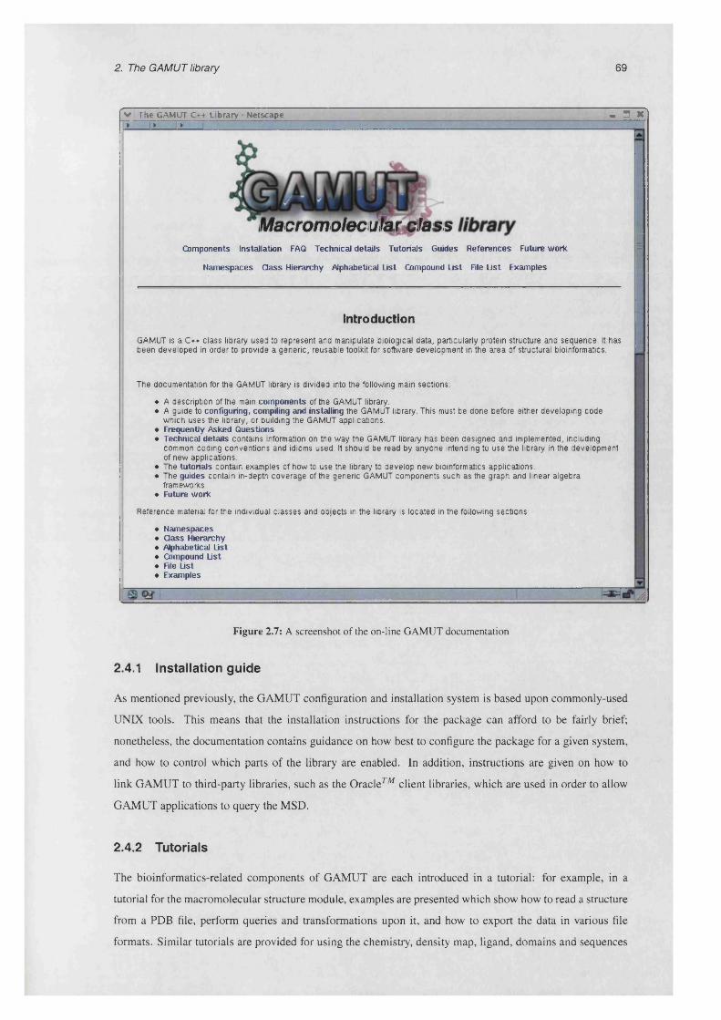
2. The GAMUT library 69

v The GAMUT C++ L ibrary N e tscap e m n n► I ►____J> '

Macromolecular classC om ponents Installation FAQ Technical de ta ils Tutorials G uides R eferen ces Future w ork

N am esp aces C lass H ierarchy Alphabetical List Compound List File List Exam ples

Introduction

GAMUT is a C++ class library used to represent and manipulate biological data, particularly protein structure and sequence. It has been developed in order to provide a generic, reusable toolkit for software development in the a rea of structural bioinformatics.

The documentation for the GAMUT library is divided into the following main sections:

♦ A description of the main com ponen ts of the GAMUT library.♦ A guide to configuring, compiling and installing the GAMUT library. This must be done before either developing code

which uses the library, or building the GAMUT applications.♦ Frequently A sked Q uestions♦ Technical de ta ils contains information on the way the GAMUT library has been designed and implemented, including

common coding conventions and idioms used. It should be read by anyone intending to use the library in the development of new applications.

♦ The tu to ria ls contain examples of how to use the library to develop new bioinformatics applications.♦ The guides contain in-depth coverage of the generic GAMUT components such as the graph and linear algebra

frameworks.♦ Future w ork

Reference material for the individual c lasses and objects in the library is located in the following sections:

♦ N am espaces♦ Class H ierarchy♦ Alphabetical List♦ Compound List♦ File List♦ Exam ples

A

Figure 2.7: A screenshot of the on-line GAMUT documentation

2.4.1 Installation guide

As mentioned previously, the GAMUT configuration and installation system is based upon commonly-used

UNIX tools. This means that the installation instructions for the package can afford to be fairly brief;

nonetheless, the documentation contains guidance on how best to configure the package for a given system,

and how to control which parts of the library are enabled. In addition, instructions are given on how to

link GAMUT to third-party libraries, such as the Oracle™ client libraries, which are used in order to allow

GAMUT applications to query the MSD.

2.4.2 Tutorials

The bioinformatics-related components of GAMUT are each introduced in a tutorial: for example, in a

tutorial for the macromolecular structure module, examples are presented which show how to read a structure

from a PDB file, perform queries and transformations upon it, and how to export the data in various file

formats. Similar tutorials are provided for using the chemistry, density map, ligand, domains and sequences

2. The GAMUT library 70

components.

V The GAMUT C++ Library N etscape 1 X► !> f i !

Finding the maximum common substructure between two compoundsA very common operation in cheminformalics is the determination of common substructures between compounds. Most often, we want to know if structure S contains chemical motif M (say, an adenine ring); but this is just a general case of the question “What is the maximum common substructure between X and Y“. All we do to determine if S completely contains the motif M (assuming that 5 has at least as many atoms as M) is to find the maximum common substructure of 5 and M which is of size M.

Translating all this into mathematics (graph theory), the problem becomes finding the maximum common subgraph of grapghs G and H This Is done by computing a subgraph isomorphism, or vertex-vertex mapping between the two graphs. GAMUT contains an implementation of a maximum common subgraph detection algorithm, originally designed by Dr. Eugene Krissinel (EBI, personal communication). Its usage is quite simple, and is demonstrated in the following code:

/ / Let g and h be a p a ir of cfcea: Graph ob jec ts

/ / Create an o b jec t vhich rep resen ts the subgraph isomorphism algorithm , and i n i t i a l i s e i t withgraph: : MCS_Krissinel<cheiti: : Graph> algo (g, h) ;

our two graphs

/ / L e t 's say we want to discover common subgraphs v i th a t le a s t S atomsalgo. min_match() ■ 5;

/ / Take bond order in to account when matching (so a s ing le bond cannot match a double bond)algo. use_bond_order() * f a lse ;

/ / Run the algorithmalgo. ru n () ;

/ / R etrieve the matches, i f th e re are anysiz e t n iso = a lg o .n is o ( ) ;i f (n_iso7)) {

f (s iz e _ t i=0; i<n_iso; ++i) (

const graph::Isomorphism<chem::Graph>& iso = a lg o .is o ( i ) ; s t d . :cout << "Isomorphism #" « i+1 << s td : :e n d l << iso ;

})

std : cout << “No matches found" << s td : e n d l .

© Done

Figure 2.8: Screenshot of part of an on-line GAMUT tutorial

In addition to the tutorials, technical guides are available, which describe in more detail the structure of the

generic library components such as the graph, tree, vector and matrix data structures.

2.4.3 API reference

The bulk of the GAMUT documentation consists of a complete reference guide for tha GAMUT Application

Programming Interface (A P I). For every class in the library, there is a page containing the following:

• A brief description of the role of the class

• A collaboration diagram illustrating the relationship between this and other classes. This is

hyperlinked, so that the user can browse around the class hierarchy of the library. A portion of the

global class hierarchy diagram is shown in figure 2.9.

• A list of all member functions, including full function signatures and explanation of the usage of the

function (see figure 2 .1 0 ).

• For certain classes, links to example code which demonstrates their use are included

2.5 Summary

The development of a new object-oriented software library for structural bioinformatics has been motivated

by outlining the requirements not only of the research project described in this thesis, but of structural

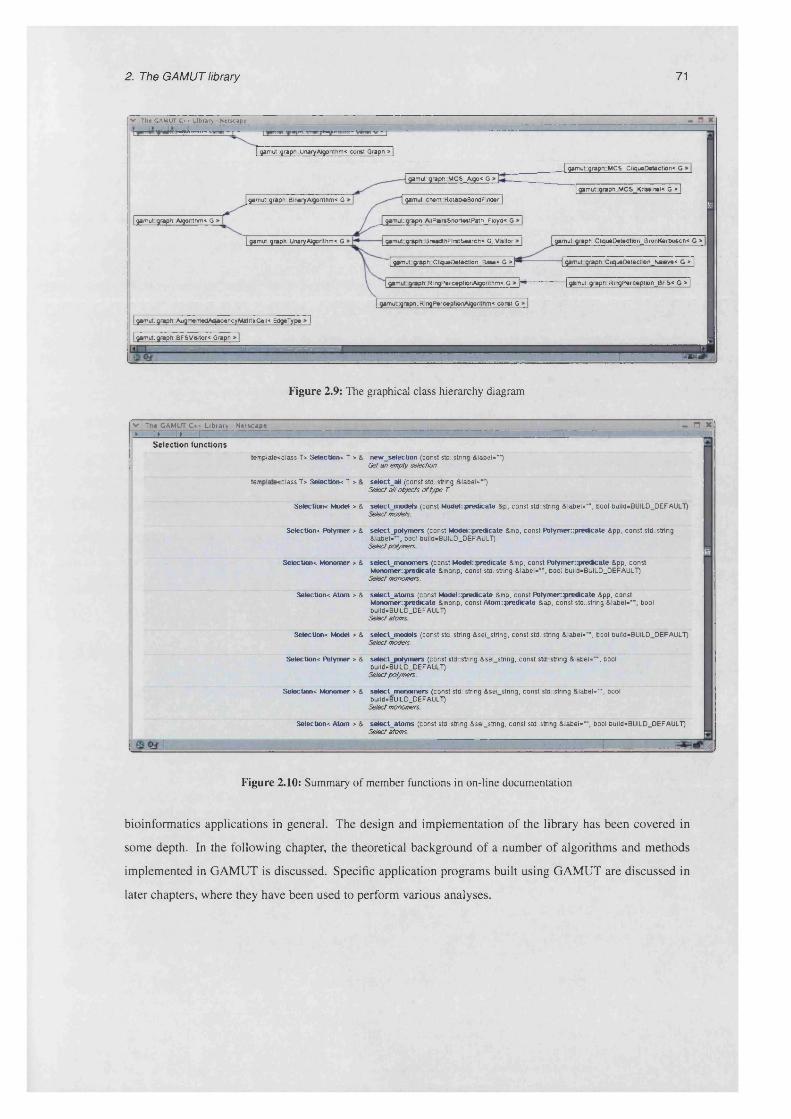
2. The GAMUT library 71

v The GAMUT C++ L ibrary N etscape

gamut::qraph::UnaryAiqorilhm* const Graph >

J gam u tq rap n M C S C Iiq u o O aU c tto n * G

I gamut: qraph::MCS_Kri»sin«l< G > |

gamut::qraph: MCS_Algo* G

qam utq iap lrB inaryA lgorlthm * G qam ut::chem Rotable Bo ndFinder

q»mut::qf»ph:: Algorithm* G gam ut::qrsph::AIIP»lrs5HorlttP»th Floyd* G

qamut::qr«pti:;CliquoDetection_BronK»r6o«ch« G >gamut::qraph::UnaryAlgonthm< G | g am u tq rap h B reaflthF in tSearch* G. Visitor

I q»mut::graph:CliquoD«toction_Ba»o* G > I gam ut graph .C liqueO oloctionN aiove* G »~|

H gamut::qrapri:Rinq P e rc e p t ion BFS< G » |gam ut graph RinqPerceptionAlqoritnm* G

gamut::qraph::RinqPercoptionAlgontnm* co n tt G

qamut::qtaph::AijqmentadAdaconcyM alriaCell< EdqeType

qamut::qraph::BFSVttitor< Graph

Figure 2.9: The graphical class hierarchy diagram

v The GAM UT C++ L ib ra ry - N e ts c a p e . H Xn r* r> i

Selection functionstemplate<clas$ T> S e le c t io n * T > & n e w s e ie c t io n (const std::string & label-‘“)

Get an empty selection.

A1A1Es

s e l e c t aM (const substring & label-“") Select all objects of type T.

S e le c t io n * M odel > & s e l e c t m o d e ls (const M o d e l::p re d ic a te &p, const std::sthng &label«'“ , bool build-BUILD_DEFAUL7) Select models

S e le c tio n * P o ly m e r > & s e l e c t j o l y m e r s (const M o d e l::p re d ic a te &mp, const P o ly m e r : :p r e d ic a te &pp, const std::strlng & lab e l-" , bool build-BUILD_DEFAULT)Select polymers

S e le c tio n * M o n o m e r > & s e l e c t m o n o m e rs (const M o d e l::p re d ic a te &mp, const P o ly m e r : :p r e d lc a te &pp, const M o n o m e r ::p re d ic a te &monp, const std::strlng &label«*“, bool build-BUILD_DEFAULT)

Select monomers.

S e le c t io n * A to m > & s e le c t_ a to m s (const M o d e l :p re d ic a te &mp, const P o ly m e r :p r e d ic a te &pp, const M o n o m er: :p re d ic a te &monp, const A to m p r e d i c a t e &ap, const std::string &label»'", bool build»BUILD_DEFAULT)Select atoms

S e le c t io n * M odel > & s e l e c t m o d e ls (const std::string &sel string, const std::strtng &label»"', bool build-BUILD DEFAULT) Select models.

S e le c t io n * P o ly m e r > & s e l e c t j m l y m e r s (const std::string &sel string, const std.:string &label«'"‘, bool build»BUILD_DEFAULT)Select polymers.

S e le c t io n * M o n o m e r > & s e l e c t m o n o m e rs (const std::$tring &sei string, const std::$tring &iabel="“, bool build-BUILD_DEFAULT)Select monomers

S e le c tio n * A to m > & s e l e c t a to m s (const stdr.string 8.sel_string, const std::string &label='"', bool bulld-BUILD_DEFAULT) Select atoms

Figure 2.10: Summary of member functions in on-line documentation

bioinformatics applications in general. The design and implementation of the library has been covered in

some depth. In the following chapter, the theoretical background of a number of algorithms and methods

implemented in GAMUT is discussed. Specific application programs built using GAMUT are discussed in

later chapters, where they have been used to perform various analyses.

72

Chapter 3

Methods

This chapter contains details of the main methods used in the analysis presented subsequently. This

discussion will be from a fairly abstract perspective, which is to say that the focus will be upon explaining

the theoretical background to each group of methods, and where applicable, examining the advantages and

disadvantages of different approaches to a problem. The following chapter will build upon this one by

discussing how the methods outlined here were used to construct a pipeline for the generation and analysis

of datasets of ligand binding sites. As such, all details of the implementation of the methods are deferred to

the following chapter.

3.1 Graph matching

Many problems in bioinformatics can be formulated in terms of graph theory1, with a common requirement

being to compare pairs of graphs in order to determine the degree of similarity between them. Graph matching

techniques have been applied to a fairly diverse range of problems in computational biology and chemistry,

including automatic chemical reaction mechanism generation (Ratkiewicz and Truong, 2003), chemical

database searching (Raymond and Willet, 2002), protein-protein docking (Gardiner et al., 2000), and protein

structure comparison (Krissinel and Henrick, 2004b). These, along with numerous other applications, serve

to illustrate the power of this particular abstraction.

Graph matching techniques aim to discover subgraph isomorphisms between pairs of graphs. Three types

of isomorphism which will be referred to here, are illustrated in 3.1. Isomorphism detection algorithms can

typically be broken down into two stages:

1 Determine all pairs of vertices from the two input graphs which may be matched

2 Starting with one such pair of compatible vertices, build up the isomorphism by adding new pairs,

checking at each stage that the relationship of the first vertex to the first subgraph is equivalent to the

relationship of the second vertex to the second graph

The following sections elaborate on these two steps, and provide several illustrative examples.

1 Readers unfamiliar with graph theory are referred to appendix A, in which some fundamental concepts are outlined.

3. Methods 73

(a) A full graph isomorphism

(b) An exact subgraph isomorphism (c) A common subgraph isomorphism

Figure 3.1: Types of graph isomorphism

3.1.1 Vertex and edge compatibility

Before considering the details of graph matching methods, it is necessary to introduce the concept of vertex

and edge compatibility functions. Graph matching algorithms need to test whether particular pairs of vertices

or edges from the two input graphs may potentially be matched in the resulting isomorphism. This is

done according to predefined criteria for vertex/edge compatibility. For example, when matching graphs

representing chemical structures, the criteria for vertex matching may be that the vertex labels representing

atomic number are identical. Alternatively, atoms may be labelled with additional information such as

chirality; in this case, the vertex compatibility function can be modified in order to take into account this

information during matching.

The boolean functions p and v will be used henceforth to represent the vertex and edge compatibility

functions respectively. It should be noted here that the function v by convention matches the absence of

an edge with any other absent edge. The importance of this will become apparent in the discussion of the

construction of association graphs which follows.

Using these functions, our working definition of a common subgraph isomorphism can be stated as follows:

For graphs G = (V,£) and H = (W,F) 2, a subgraph ismorphism of size k is defined as / C V x W, where X

and Y are enumerations of a subset of vertices in V and W respectively, satisfying

The problem of finding common subgraphs can be reformulated as that of finding the enumerations

K vXjiwyi) A VfexjXj> fytyj) V i , j . (3.1)

X = {jc/}*=1 and Y = {y/}f=1 which satisfy 3.1.

2 As described in appendix A, G = (V,E) indicates that a graph G is defined as a pair of finite sets: the vertices, V, and the edges, £ . £ is a binary relation on V.

3. Methods 74

3.1.2 Available methods

The problem of determining the Maximum Common Subgraph (MCS) between two or more graphs is known

to be NP-complete (Garey and Johnson, 1979). That is, no algorithm is known which can guarantee to find

the MCS between any pair of graphs in polynomial time. The two pre-eminent solutions to the problem are

the clique-detection approach, and the backtracking search.

3.1.2.1 Clique detection

Common Subgraph Isomorphism (CSI) discovery by clique detection (Bron and Kerbosch, 1973) is carried

out by first constructing an association graph A between the input graphs G and H. For every pair of vertices

(v ,w ): v G V,w G W, for which /t(v,w) is true, a vertex a is added to the association graph. Once this process

is complete, every pair of vertices (a, a') G A is checked for edge compatibility. Specifically, if there exist a

pair o f edges e = (v,v') G E and / = (w, vi/) G F such that v (e ,/) is true, then an edge b = {a, a!) is added to

A. It can easily be seen that a clique in A corresponds bijectively3 to an isomorphism between G and H, and

therefore that determination of the largest clique in the association graph leads to the definition of the MCS

between the input graphs.

As a simple example, consider the two graphs in figure 3.2. The association graph formed by comparing

these graphs is shown in figure 3.3a, and the cliques within it are shown in figure 3.3b. The equivalence

between the two largest cliques in the association graph, and the largest isomorphisms between the input

graphs, is clear.

(a) G (b) H

Figure 3.2: Example graphs The colours represent the vertex properties; numbers are simply indices which are used to refer to each vertex.

3.1.2.2 Backtracking search

The Bron-Kerbosch algorithm is the most efficient available for CSI detection, with a worst-case complexity

of 0((mn)m), where n and m are the numbers of vertices in the input graphs (m < n). When an Exact

Subgraph Isomorphism (ESI) is sought, a more efficient algorithm is the backtracking search method

(Ullman, 1976).

3FormaIly, a mapping which is both injective, i.e. one-to-one, and surjective. A surjective (or ‘onto’) mapping is one in which all members of the target set are mapped to.

3. Methods 75

3:1

6:3

5:3 4:2

2:2

3:1

6:3

5:3 4:2

r * n(a) Association graph formed from the example graphs in figure 3.2. Pairs of indices refer to the corresponding vertices of G and H respectively.

(b) The two 3-vertex cliques in the association graph

Figure 3.3: Graph matching by clique detection Each clique in the association graph corresponds to an isomorphism between the original two graphs. The two 3-vertex isomorphisms are therefore {(3,1), (4,2), (6,3)} and {(3,1), (4,2), (5,3)}

3.1.2.2.1 Uliman's method

The backtracking search method begins by identifying a single vertex-vertex mapping,

vi !-»• wi :ji(v i,w 1)

The algorithm then proceeds by extending the mapping by adding another pair of vertices such that the

resulting match still describes a valid isomorphism according to equation 3.1. Given an existing isomorphism

consisting of i matched vertex pairs

/ = { (v i, Wi) • • • (Vj,Wj)}

the match can be extended by mapping v;+i i—► wXi+l if the following conditions are satisfied:

K vi+uwi+i) (3.2)

\ / k < i e = (v*,v,+ i) £ E <=> f = ( x v k,W i+i )e F A v(e , f ) (3.3)

Condition 3.2 merely requires that the new vertex pair satisfy the vertex compatibility function; condition

3.3 stipulates that, for every edge incident on the newly mapped vertex from graph G, there must be a

corresponding edge incident on the mapped vertex from H, satisfying the edge compatibility constraint.

Once the mapping I contain: m )airs of vertices, the exact subgraph isomorphism has been determined and

the algorithm stops. If, on the other hand, the vertex v,- cannot be mapped onto any vertex w,-, the algorithm

backtracks by matching the last mapped vertex v;_i onto a vertex from H which has not yet been tried. The

progression of Ullman’s algorithm applied to the example graphs of figure 3.2 is shown in figure 3.4.

The algorithm described thus far is capable of detecting the exact subgraph isomorphism, but a further

optimisation, known as the ‘forward checking’ procedure, is described in Ullman (1976). The idea is that, for

3. Methods 76

H2 3

__ —

“-_

3:1

1 2 3

1 11

2 1

✓3

4 11

5 1

611

0 4:2r

1 2 3

1

2

3 ✓4 .... ✓ ....

5

6

1 2 3

2:2

| compatible ^ mapped- - mapped to another vertex X incompatible

Figure 3.4: Progression of Ullman’s algorithm Diagrammatic representation of the progression of Ullman’s algorithm on the example graphs shown in figure 3.2. The algorithm is initiated by identifying all pairs of compatible vertices, shown as green cells in the matrix, (a) vertex G3 is mapped to HI. (b) vertex G2 is mapped to H2. All other mappings to H2 are thus rendered incompatible, as shown by the dotted red lines. Mappings 5:3 and 6:3 are determined incompatible by the forward checking procedure, since H3 is a neighbour of H2, but neither G5 nor G6 are adjacent to H2. (c) no further mappings can be made, so the algorithm backtracks, (d) G4 is mapped to G2. The two ESIs can now be found by mapping either G5 or G6 to H2.

each mapping v, w,-, a check is made to see whether there exists at least one mapping for each remaining

vertex vj : j = i+ 1 ,. . . , w which satisfies equation 3.1. If the forward checking fails, the algorithm backtracks

immediately, thus eliminating the exploration of unproductive branches of the search tree. This is exemplified

by step (c) of figure 3.4.

Ullman’s method is described formally in algorithm 3.1. In this version of the algorithm, the conditions of

subgraph isomorphism are tested in the ‘forward checking’ procedure, and are stored in an m x n binary

matrix (P), which records whether the Ith and 7 th vertices of G and H respectively are still compatible at each

stage of the search.

It can be shown that the worst-case complexity of Ullman’s algorithm is 0(m nn2). However, this only occurs

in practice when graphs with high degrees of connectivity and redundancy of labels are used as the input.

Chemical graphs have low connectivity, and only moderate label redundancy; as such, the Ullman algorithm

tends to exhibit good performance for the purposes for which it has been used in this thesis.

3.1.2.2.2 Krissinel’s improved backtracking search

The Ullman algorithm described here searches for exact subgraph isomorphisms, with search branches

potentially leading to common subgraph ismorphisms being discarded by the forward checking routine.

Recently, improvements to the Ullman method have been described which allow searching for common

3. Methods 77

Main function o f the algorithm, called with input graphs G and H Function U llm a n ( G = (V,E),H = (W,F)) :

m +— |V|, n <— \W\ assert m < n

Initialise the vertex matching candidate matrix P

p = (P,j) ■■ Pij = { o V < = 1, . . . ,m ;; = 1, . . .

Initialise set o f matched vertex indices to empty I <— Q

Start the recursive part B a c k t r a c k (P ,7)

Recursive part o f the algorithmP is the current vertex mapping candidate matrix; I contains the current match Function BACKTRACK(P,m,7) :

»<- |/ |if i > m then

An exact subgraph has been detected - return it return (I)

for each j = l , . . . , n : if Pi, = 1 then

Add the newly matched pair o f vertices to the isomorphism /< -/U (v ,- ,w ;)

Update the candidate matrix P '«_ /> , p'kj = 0 V k > i if FORW ARDCHECK(PV,m,n,7) = true then

B a c k t r a c k ^ , / )

Remove the pair o f vertices which failed to match I < - I - { { v » W ] ) }

No match was found - return an empty isomorphism

return (0)

Function which checks whether a match can potentially be extended Function F o r w a r d C h e c k (P , i, m, n, I) :

for each k = / + l , . . . , n , Z = :if Pki = 1 then

for each (v, w) e l :ifv(e = (v * ,v ) ,/= ([wi,w)) = false then

Pki <— 0Check whether each remaining vertex vj : j — i+ 1,.. . ,n has at least one mapping to H for each k = i+ 1 , . . . ,n :

for each I = :if Pki = 1 then

Found a mapping for v*; go to next vertex next k

Vk has no potential mappings - forward checking failed

return false

Algorithm 3.1: Ullman’s backtracking search algorithm for exact subgraph isomorphism detection

3. Methods 78

subgraph ismorphisms, and which also improve the performance of the algorithm (Krissinel and Henrick,

2004a).

The ability to detect common subgraph isomorphisms, as opposed to exact subgraph isomorphisms, is easily

achieved simply by altering the number of potential mappings which we require to be identified at the

forward checking stage. Whereas the original Ullman method requires all unmapped vertices from G to

have at least one potential mapping to a vertex in H, the Krissinel method simply requires that the maximum

achievable match at any point is at least equal to a minimum match parameter, no (and is greater than the

largest isomorphism yet found). Varying no allows the user to specify the minimum size of match which is

considered to be meaningful in any particular problem. Branches which cannot lead to a match of at least no

vertices are not explored.

The Krissinel algorithm achieves performance improvements over the Ullman method via several

modifications. The first is to represent the potential vertex mappings, contained in the matrix P in the

original algorithm, using a representation which is more efficient given the frequently sparse nature of P.

The Krissinel Vertex Mapping Matrix (VMM) consists of a matrix M and a vector L. My gives the index of

the vertex in H which is mappable onto v,- from G, j = 1 ,... L stores the length of each row of M (i.e. the

number of vertices mappable onto each vertex of G). This representation reduces the time required to obtain

the list of vertices mappable onto v; when extending the match.

In the example shown previously, each vertex in graph G maps to only one potential candidate in H, so the

initial states of M and L are

M =

( 2

2

1

2

3

\ 3

\

, L = (1 1 1 1 1 1)

In addition, Krissinel et al. show that the selection of the next vertex from G to be added to the match, has an

impact on performance. Specifically, picking the vertex which has the fewest number of potential mappings

reduces the runtime of the algorithm to the extent that, on the type of graphs used in their study, it outperforms

both the clique detection approach for CSI detection and the original backtracking search for finding ESIs.

Match metric Condition Minimum r t j Maximum n r Minimum match size

1 Tanimoto coefficient ^ — train y/'tmiri'ftQn Q

y/tm in/ ^min / 2 i 2 \

V i + w ( n e + " r )2

3

Percentage match

Mismatch of smaller graph

P ^ Pmin

Msmaller — flmax

Pmin-KQ

1

n Q

Pminoo

Pmin • max (wq , /Z7’)

max( 1, min(ng> ) - Umax)

4 Mismatch of query graph flquery — flmax m ax(l,/ig Umax) oo HQ fimax

5 Mismatch of larger graph larger — Umax max( 1, flQ Umax) n Q ”1“ f^max max( 1 ,max(/2g ,n r ) - fimax)

6 Mismatch of target graph ptarget — t^max max( 1, tlQ l^max) nQ + lbiax n r —Umax

Table 3.1: Range of target graph sizes which can potentially provide a sufficiently good match In each expression, hq is the size of the query graph, and nj the size of the target graph. The sizes of the smallest and largest target graphs which can potentially provide a match which satisfies the condition are shown. In practice, the maximum value of nr for metrics 3 and 4 is the size of the largest target graph in the database. The last column shows the size of the smallest match between the target and a given query graph, which would satisfy the condition.

co

3. Methods

3. Methods 80

3.1.3 Match size metrics

When using graph matching methods to identify those members of a database of graphs which exhibit some

degree of similarity to a query graph, it is necessary to define a similarity metric. That is, a function which,

given the maximum common subgraph isomorphism between a pair of graphs, calculates a scalar value

indicating their degree of mutual (dis)similarity.

The following simple functions (where I stands for the number of vertices matched; m and n are the sizes of

the two graphs), are commonly used for this purpose:

1 Tanimoto (or Jaccard) coefficient. This is a score between 0 and 1, where 1 indicates identity, and 0

indicates no similarity.I2

m2 + n2 — I2

2 Percentage identity. This is also bounded by [0,1].

IP = ------ rmax(m,n)

3 Mismatch. The number of vertices from either the smaller or larger of the two graphs, which are not

included in the match, may be used as a dissimilarity measure. This obviously has the disadvantage

that the size of only one graph is taken into account in the metric.

Msmaller = min(lW, 7l) I [ l̂arger = max(#W, w) I

Alternatively, we may require that the number of mismatched with respect to either the query or target

graphs, regardless of which is the smaller, is below a specified threshold.

Any of these metrics may be used as the basis for a condition for accepting or rejecting a match, for example,

only matches for which x > 0.75 may be of interest. Given a particular query graph G q , it is then possible

to compute the range of target graph sizes which could potentially provide a sufficiently good match. These

ranges are shown, for each of the match metrics outlined above, in table 3.1. Any target graph whose size

falls outside this range can then be immediately excluded from the search, thereby improving its efficiency.

3.2 Clustering

Cluster analysis is concerned with inspecting a set of data to determine whether it contains any underlying

structure, in the form of groupings into distinct subsets. Formally, we wish to partition an initial data set of

n objects, X, into m clusters C, such that each member of X belongs to exactly one cluster, and so that the

union of all clusters is equal to the original set:

3. Methods 81

X = {xu x2, . . . , x n}

C = {ci,C2 , . . . , c m} wherec,- C X andc/flcy = 0Vi , j =

ci U C2 U • • • U cm = X

The choice of the value m is often not straightforward, and is discussed further below. The use of any

clustering method tends to involve several compromises.

3.2.1 Dissimilarity matrices, measures and metrics

The input to most clustering algorithms is a distance matrix D, where the element dy expressed a measure

of the dissimilarity between objects x,- and xj in the original set. The procedure used to calculate D from X

varies depending on the type of objects being clustered. If the elements of X are vectors of real numbers, for

example, the familiar Euclidean distance is often used to populate the dissimilarity matrix:

In most cases, the distance measure is required to be a metric. A metric d on X is a mapping, d(x,y) R,

which must satisfy the following conditions for all x,y,z E X:

• Non-negativity: d(x,y) > 0

• Symmetry: d(x,y) — d(y,x)

• Triangle inequality: d (x ,y) < d (x, z)+ d(y, z)

• Reflexivity: d(x,x) = 0

3.2.2 Hierarchical clustering techniques

In hierarchical clustering approaches, a series of consecutive partitions is applied to the data set. These

partitions are typically represented in the form of a dendrogram or tree diagram4. In order to obtain

distinct groupings, a threshold must be specified, the value of which corresponds to physically ‘cutting’

the dendrogram at that height (see figure 3.5).

Hierarchical clustering methods may be divided into two classes of iterative procedures: agglomerative and

divisive.

3.2.2.1 Agglomerative algorithms

As the name suggests, agglomerative algorithms start with n distinct groups, each containing one data

point. Each iteration involves fusing a pair of groups, with the end of the process being reached when

all data points are in a single group. At each stage of this process, the algorithm must therefore determine

which pair of groups are ‘closest’ to one another; the definition of this inter-group distance is the main

technically, a rooted, terminally-labelled, weighted tree.

X ~ xJk)2 where x/>xj e R pk=l

3. Methods 82

V

o J

root

M rn Hnrh r n l r nJ L U

Figure 3.5: An example clustering dendrogram The value of h corresponding to a chosen pair of data points ( i , j ) is represented by the height at which the branches of i and j first join. The red dotted line shows an arbitrarily chosen tree cutting threshold; the clusters which would result from this cut are indicated with red braces.

distinguishing characteristic of different agglomerative methods. Common methods are summarised in table

3.2 and illustrated in figure 3.6. When a pair of groups is chosen for fusion, the distance describing their

separation is stored, and it is this distance which is represented in the dendrogram as the height of the node

which corresponds to the fusion event.

Method Definition of the distance between two clusters c, and cj

Single linkage The minimum distance among pairs consisting of one data point from ci and one from cj

Complete linkage The maximum distance among pairs consisting of one data point from Ci and one from cj

Group-average The average of all distances among pairs consisting of one data point from ci and one from cj

Centroid Distance between the centroids of c,- and cj

Ward’s The increase in the sum of squared distances which would be brought about by the fusion of c,- and cj

Table 3.2: Agglomerative clustering methods

3.2.2.2 Divisive algorithms

Beginning with a group containing all of the data points, each step of a divisive clustering algorithm involves

dividing an existing group into two. As such, two decisions must be made: which cluster to divide, and

how best to perform that division. Such algorithms are much more rarely used than agglomerative methods,

chiefly because finding the optimal division of a set is computationally demanding. They are not considered

further here.

3.2.3 Problems with hierarchical clustering

No clustering method is perfect; indeed some have conspicuous flaws. The simplest hierarchical clustering

method, single linkage clustering, is well known to suffer from the problem of chaining; that is, the tendency

to cluster together, at a relatively low level, groups which are linked by a series of isolated intermediates.

3. Methods 83

This makes it unsuitable in many cases. Often, methods such as complete linkage are preferred, as they

result in compact, globular clusters which agree more closely with our intuitive notion of how the data

should be grouped.

Despite the practical problems resulting from its application, single linkage clustering is held by some to be

the method with the greatest mathematical appeal. Let us denote the height of the node at which data points

i and j join the same cluster with hij. This value is not the same as the dissimilarity dij between these two

points. The heights are clearly symmetric, and obey the relation

hij < max{h it, hjk)

which is known as the ultrametric inequality. Even if the distance measure is a metric, the metric inequality

shown in §3.2.1 is clearly a weaker condition than the ultrametric inequality. The clustering operation

therefore can be viewed as a transformation which imposes a constraint that was not satisfied by the original

data. It has been shown that, if we require certain properties of a clustering method, including that it should

be continuous, single linkage clustering is the only method which satisfies the conditions (Jardine and Sibson,

1971). On the basis of empirical studies which compare the clusters returned by various clustering methods

to previously known structure in the data, however, other authors have recommended almost every known

method. The conclusion to be drawn is that no one method is ultimately superior; the choice of which to use

should be made in the light of each particular problem.

(a) Single linkage (b) Complete linkage

(c) Centroid (d) Group average

Figure 3.6: Agglomerative clustering methods For each method, the method of calculating inter-cluster distance is illustrated with an arrow. For (d), the distance value is the average of all the arrow lengths.

3. Methods 84

3.2.4 Validation

A key problem when using clustering is that it is often unclear whether the results obtained by using any one

method truly represents any underlying structure in the data. After all, even randomly generated input data

will result in a clustering hierarchy - so how does one know if structure has been discovered in, or imposed

upon a data set? One way is to try to assess the degree of distortion caused by the clustering method, by

comparing the dendrogram heights to the original dissimilarity matrix. This can be done by computing the

cophenetic correlation coefficient, which is the product-moment correlation coefficient between the lower

half of the distance matrix and the corresponding terms in the cophenetic matrix, H, which contains the

heights at which each pair of data points first occur in the same cluster:

p _ ssdh SSddSShh

This leaves us with the problem of deciding upon a threshold for r above which the dendrogram is deemed

to represent the data set with sufficient accuracy. Various values from 0.8 upwards have been suggested

(Romesburg, 1984).

More empirical methods for validating clustering results draw on the idea that a clustering solution should be

stable. In order to test this, error terms are added to the dissimilarity matrix, or subsets of the original data are

excluded (Lanyon, 1985). Comparing the dendrogram thus obtained can provide an indication of the quality

of the solution. An example of this type of approach is the bootstrap (Felsenstein, 1985), a non-parametric

resampling approach.

3.2.5 Stopping criteria

Assuming that it is valid, the dendrogram in itself provides a valuable insight into the structure of the data

set. Sometimes, however, obtaining the tree is only an intermediate step towards dividing the objects

into discrete clusters. In order to produce clusters, a threshold height must be specified, as mentioned

previously; equivalently, this value may be used as a stopping criterion during the agglomeration procedure.

As mentioned previously, the choice of this value is not trivial.

Qualitatively, inspection of the dendrogram for large changes in height can indicate a sensible value for the

‘best’ partition. Several attempts have been made to formalise this decision. One such study suggests that

the cut should be made at h + kOh, where & is a constant in the range (2.75,3.50) (Mojena, 1977); other

approaches are reviewed in (Milligan and Cooper, 1985).

In summary, clustering methods should be applied with care, and their results interpreted while bearing in

mind the caveats discussed above.

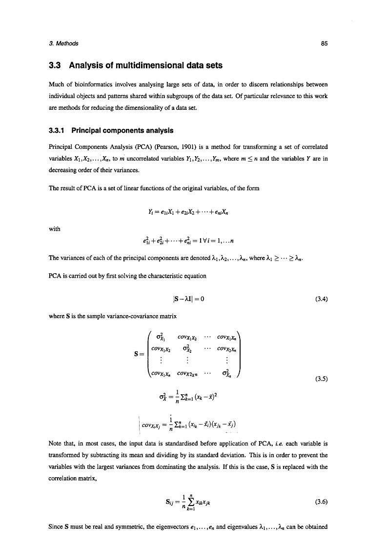
3. Methods 85

3.3 Analysis of multidimensional data sets

Much of bioinformatics involves analysing large sets of data, in order to discern relationships between

individual objects and patterns shared within subgroups of the data set. Of particular relevance to this work

are methods for reducing the dimensionality of a data set.

3.3.1 Principal components analysis

Principal Components Analysis (PCA) (Pearson, 1901) is a method for transforming a set of correlated

variables X \,X 2, . . . ,Xn, to m uncorrelated variables Yi,Y2, .. . ,Y m, where m < n and the variables Y are in

decreasing order of their variances.

The result of PCA is a set of linear functions of the original variables, of the form

Yi = euXi + e2iX2 H 1- eniXn

with

e li + e2H ̂eni = 1 V / = 1 , . . .11

The variances of each of the principal components are denoted A,i, X2, . . . , X„, where > • • • > X„.

PCA is carried out by first solving the characteristic equation

| S - M | = 0

where S is the sample variance-covariance matrix

( o2Xi covXlx2 •••

(3.4)

S =covXlx2 yx2

covXlxn

covx2xn

\C O V X lX n COVX 2 x n • • • a zXn /

cx — ~ £jfc=i (** ~ *Y

(3.5)

j covXiXj = - X / U i ( * / * - * « ) ( * / * — J0' )

Note that, in most cases, the input data is standardised before application of PCA, i.e. each variable is

transformed by subtracting its mean and dividing by its standard deviation. This is in order to prevent the

variables with the largest variances from dominating the analysis. If this is the case, S is replaced with the

correlation matrix,

1 nSjj — ~ %ikXjk

n k= 1(3.6)

Since S must be real and symmetric, the eigenvectors e \ , . . . ,e n and eigenvalues , . . . , X„ can be obtained

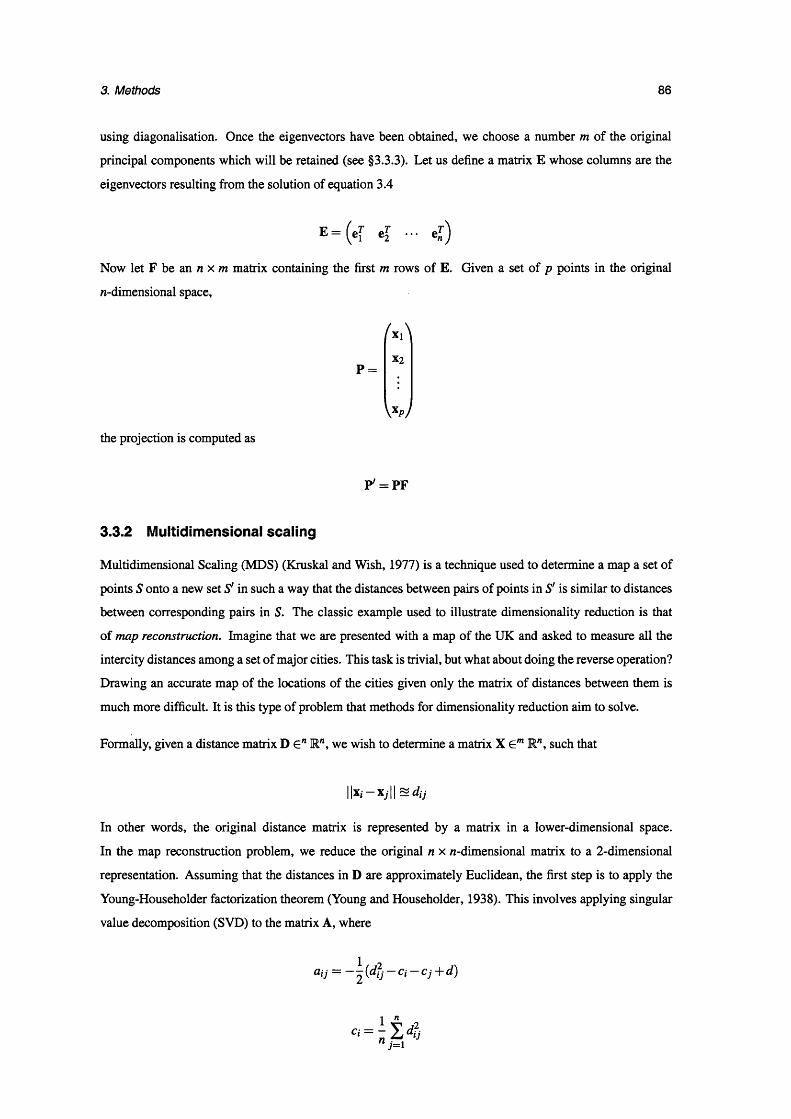
3. Methods 86

using diagonalisation. Once the eigenvectors have been obtained, we choose a number m of the original

principal components which will be retained (see §3.3.3). Let us define a matrix E whose columns are the

eigenvectors resulting from the solution of equation 3.4

E “ (• r ■0Now let F be an n x m matrix containing the first m rows of E. Given a set of p points in the original

n-dimensional space,

the projection is computed as

P =X2

\ XPJ

P/ = PF

3.3.2 Multidimensional scaling

Multidimensional Scaling (MDS) (Kruskal and Wish, 1977) is a technique used to determine a map a set of

points S onto a new set S' in such a way that the distances between pairs of points in S' is similar to distances

between corresponding pairs in S. The classic example used to illustrate dimensionality reduction is that

of map reconstruction. Imagine that we are presented with a map of the UK and asked to measure all the

intercity distances among a set of major cities. This task is trivial, but what about doing the reverse operation?

Drawing an accurate map of the locations of the cities given only the matrix of distances between them is

much more difficult. It is this type of problem that methods for dimensionality reduction aim to solve.

Formally, given a distance matrix D € ” R", we wish to determine a matrix X e m R", such that

\\xi-XjW~dij

In other words, the original distance matrix is represented by a matrix in a lower-dimensional space.

In the map reconstruction problem, we reduce the original n x n-dimensional matrix to a 2-dimensional

representation. Assuming that the distances in D are approximately Euclidean, the first step is to apply the

Young-Householder factorization theorem (Young and Householder, 1938). This involves applying singular

value decomposition (SVD) to the matrix A, where

a ij = - ^ { d f j - C i - C j + d )

n j=i

3. Methods 87

d = 7 l l ‘%ij=l

The SVD method decomposes A as follows:

A = U.W.Vr

U and V are each n x n column-orthogonal matrices, and W is a diagonal matrix. The columns of U give

the eigenvectors of the decomposition, and the diagonal values of W are the corresponding eigenvalues. If

the eigenvalues of the decomposition are arranged in order of magnitude so that Xi > X2 > X3 • • • and the

corresponding eigenvectors, scaled to the length of a unit vector, are denoted e;, then the matrix X is given

by

/v ^ T e [ \

X =

V :By selecting the first m eigenvectors, where m < n, the dimensionality of the original space is reduced.

3.3.3 Choice of the number of dimensions to retain

A key question which must be addressed when performing dimensionality reduction is how to determine

the number of dimensions to retain. More specifically, how many dimensions are required to adequately

represent any patterns in the original data set? The choice of how many components to retain is usually

based on the proportion of the total variance of the original data set which is explained by the combination of

these components. The total variance of the original data set is given by the trace of the correlation covariance

matrix S; therefore, the variance explained by the first m principal components is given by

(Xi H------ \-Xm)/T r{S)

As for the case of determining clustering thresholds, there are many semi-heuristic rules for determining the

proportion of total variance which we wish to capture in the set of m principal components. These include

• Retain all components required to explain at least 80% of the total variance.

• The scree test. Typically, the first few eigenvalues of a PCA are of similar magnitude, then there is a

sudden drop. The scree test involves plotting the series of eigenvalues and looking for the point of the

decrease.

• Broken stick test. Retain all components whose proportion of the total variance is greater than would

be expected if the components had been chosen at random.

For some of the analyses presented in this thesis, the aim of PCA/MDS is to project the original data into

exactly two dimensions, so they can be plotted in a diagram. When this is the case, a measure of the amount

of variance captured by the 2D plot is always provided.

3. Methods 88

3.4 Geometric range querying

Many applications require the ability to perform geometric range queries. These are, in general, problems of

the following form: given a set P of N points in a ^-dimensional space 5, build a data structure such that the

set of points which lie inside an arbitrary region R G 5 may be quickly determined (see figure 3.7).

Figure 3.7: Geometric range querying The set of points which fall inside a region R of the space S, are shown in red.

Two approaches for geometric range querying were assessed: ‘brick maps’ and kd-trees. The principle

behind both methods is to precompute a division of 5 into a set of smaller partitions T such that one can

rapidly compute which members of T are intersected by R. Only points which lie in this subset of T need

then be inspected to determine whether they fall inside the region R.

3.4.1 The bricking algorithm

The subdivision procedure used in the bricking algorithm is simple: as the name suggests, the pre-processing

step consists of partitioning S into a set of cuboids (bricks). Each brick contains a list of pointers to the

objects which fall inside it. In order to quickly process the range query, it is fairly trivial to calculate the set

of bricks T which intersect R.

3.4.2 kd-trees

The kd-tree method is somewhat more sophisticated than the bricking algorithm. The subdivision of S is

represented as a binary tree, the root node of which consists of the whole initial space. Each node in the rest

of the tree is defined by placing a plane through one of the k dimensions, which partitions the set of points

in the parent node such that each of its two children receives an equal number of points. The partitioning

continues until each leaf node in the tree contains just a single point; this occurs after logiiN) divisions.

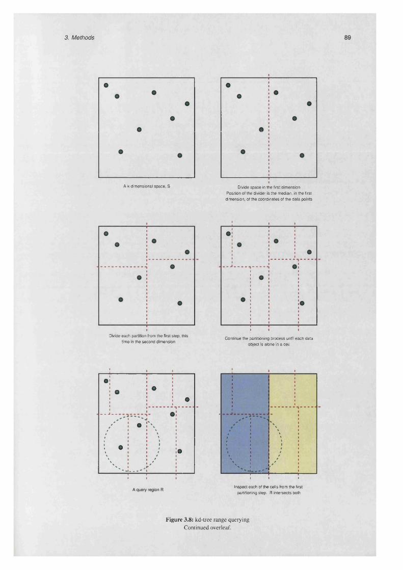
3. Methods

Divide space in the first dimensionA k-dimensional space, S

Position of the divider is the median, in the first dimension, of the coordinates of the data points

Divide each partition from the first step, this „ .. . ... . . . .r Continue the partitioning process until each datatime in the second dimension object is alone in a cell

® :•11

iii

I1•o 1

11

i■■

111

: • ii

I1

: 1 i■......

i■ " I

I' l I * ■ / ■ l: • : \ ■

i ! % 1/ i i % ■ / 1 \ ii i • * i i • % l

# § i % ■ i 1 % Ii i i i ■ i i i i

i O I #■ i i

1 i1i

l1

% i t # 0 % I # I\ i i i i % i $ 1

\ i i / i \ a i I\ , / % *

% ■ ■ / i \ 1 I* ^ 1 i * I>%I»l1»t

■^ „

i >I I I 1i i i

Inspect each of the cells from the first partitioning step. R intersects both

Figure 3.8: kd-tree range querying Continued overleaf.

3. Methods 90

■ i ■ ■ ■

For each of the two partitions retained in At the final step, one of the cellsthe previous step, inspect the next step of is discarded,

the partitioning. In both cases, R intersects only one of the two segments.

Figure 3.8: kd-tree range querying (continued)

A query on the kd-tree is processed by starting at the root node, and asking whether R intersects the region

represented by that node. If so, the same question is asked of the two child nodes, and so forth down the

tree. The search down any one branch of the tree is terminated as soon as a node is found whose region does

not intersect R. In this way, the search quickly homes in on the regions of 5 which are intersected by R\ the

limited set of points in these partitions may then be inspected in turn. The kd-tree method is illustrated in

figure 3.8.

It may be seen from the descriptions of the two geometric query methods above, that any region may be used

as a query, as long as we may ask of it the following questions:

• Does the region contain a point PI

• Does the region intersect the k-dimensional hypercuboid C? (This is necessary in order to process the

query on a kd-tree)

• What is the geometric centre of the region, and what is the distance of its furthest extremity from the

centre? (This is the requirement for computing which cells of a brick map we need to inspect)

3.5 Sequence alignment

As discussed in §1.4, identification of overall sequence similarity is a powerful method for inferring

structural and functional relationships between proteins based on their primary structure alone. In addition,

where several sequences are available for comparison, identification of regions which are particularly well-

conserved across all of them can be valuable indicators of functional sites within the proteins.

Achievement of either of these goals involves sequence alignment; that is, identification of equivalent

positions between the input sequences. In order to do so, an evolutionary model must first be provided which

describes the likelihood of the mutational changes described in §1.4. The aim of any sequence alignment

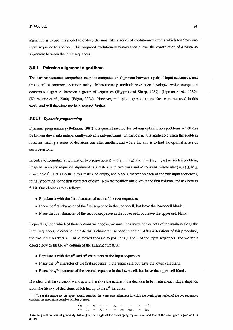
3. Methods 91

algorithm is to use this model to deduce the most likely series of evolutionary events which led from one

input sequence to another. This proposed evolutionary history then allows the construction of a pairwise

alignment between the input sequences.

3.5.1 Pairwise alignment algorithms

The earliest sequence comparison methods computed an alignment between a pair of input sequences, and

this is still a common operation today. More recently, methods have been developed which compute a

consensus alignment between a group of sequences (Higgins and Sharp, 1989), (Lipman et al., 1989),

(Notredame et a l, 2000), (Edgar, 2004). However, multiple alignment approaches were not used in this

work, and will therefore not be discussed further.

3.5.1.1 Dynamic programming

Dynamic programming (Bellman, 1984) is a general method for solving optimisation problems which can

be broken down into independently-solvable sub-problems. In particular, it is applicable when the problem

involves making a series of decisions one after another, and where the aim is to find the optimal series of

such decisions.

In order to formulate alignment of two sequences X = (jci , . . . ,xm) and Y = (yi, . . . ,yn) as such a problem,

imagine an empty sequence alignment as a matrix with two rows and N columns, where max(m, n) < N <

m + n holds5 . Let all cells in this matrix be empty, and place a marker on each of the two input sequences,

initially pointing to the first character of each. Now we position ourselves at the first column, and ask how to

fill it. Our choices are as follows:

• Populate it with the first character of each of the two sequences.

• Place the first character of the first sequence in the upper cell, but leave the lower cell blank.

• Place the first character of the second sequence in the lower cell, but leave the upper cell blank.

Depending upon which of these options we choose, we must then move one or both of the markers along the

input sequences, in order to indicate that a character has been ‘used up’. After n iterations of this procedure,

the two input markers will have moved forward to positions p and q of the input sequences, and we must

choose how to fill the 71th column of the alignment matrix:

• Populate it with the and 4 th characters of the input sequences.

• Place the /7th character of the first sequence in the upper cell, but leave the lower cell blank.

• Place the character of the second sequence in the lower cell, but leave the upper cell blank.

It is clear that the values of p and q, and therefore the nature of the decision to be made at each stage, depends

upon the history of decisions which led up to the /2th iteration.

5 To see the reason for the upper bound, consider the worst-case alignment in which the overlapping region of the two sequences contains the maximum possible number of gaps:

Ixi - x2 - ■■■ xm - -V~ yi - n ■■■ - ym ym+i ••• yn)

Assuming without loss of generality that m < n, the length of the overlapping region is 2m and that of the un-aligned region of Y is n — m.

3. Methods 92

To solve the problem, we need to define a scoring scheme which measures the quality of an alignment, based

ideally on the biological likelihood of the evolutionary history which it implies. The essential components

of this score are a substitution matrix M = (/x,j) which provides a score for each amino acid type mutating

to every other type, and a function which penalises the introduction of gaps into the alignment6. The power

of dynamic programming derives from noting that the value of the scoring function is local to each column

of the alignment, meaning that parts of the alignment can be independently optimised and then concatenated

to give the solution. More specifically, we can define the score of a given alignment in terms of the score for

the optimal alignment up to the penultimate position, plus the score for the final position alone.

If the score for the optimal alignment up to positions p and q in the two input sequences is denoted Ap, and

the gap penalty by y, then we can write

7-1

Aqp = max <

^ p - i + ^xpyq

A"p_ i+ Y (3-7)

/ r ‘ +Y

By setting p = m,q = n, equation 3.7 provides a recursive solution to finding the optimal global alignment,

but this is not the most efficient approach, since doing so would likely involve finding the same optimal

subalignments multiple times.

Dynamic programming circumvents this problem by systematically computing each subalignment exactly

once. Consider the problem of aligning the subsequences Xp = (x \ , . .. ,xp) and Yq = (y i,... ,yq). There are

clearly many possible such alignments, but they all have in common the fact that they end with a column

containing xp and yq. This seems like a trivial observation, but by creating a m x n matrix populated

with the score of the optimal alignment for each value p = 1, . . . , m, q — 1, . . . ,n, we produce an organised

representation of all the sub-problems which comprise the recursive equation 3.7.

3 .5 .1.1.1 The Needleman-Wunsch algorithm

The dynamic programming matrix S, consists of m rows, corresponding to the positions of sequence X, and

n columns, corresponding to Y. Applying the method of (Needleman and Wunsch, 1970), it is populated as

follows:

1 The first row and column are populated with the scores for aligning the appropriate characters.

sn = H x iy iV i=

J l j = f i x iy j y J = 1 »•••}**

2 The remaining cells are populated by first calculating three scores corresponding to aligning the

appropriate characters, or to inserting a gap into either of the two sequences:

• an corresponds to inserting a gap into sequence X. It is calculated by adding the gap penalty y to

6Here the regular gap model, in which extension of existing gaps is not preferred over opening new ones, is assumed. The method may be simply modified to prefer the reverse, by the use of a gap extension penalty.

3. Methods 93

the score from the cell immediately above.

aij — $i— 1 j+ Y

• bij corresponds to inserting a gap into sequence Y. It is calculated by adding the gap penalty y to

the score from the cell immediately to the left.

bij = s y - 1 +Y

• Cij corresponds to aligning jc,- with xj. It is calculated by adding mj to the score from the cell

diagonally to the left and above.

cij = Si—i j — i + [Lij

The largest of these three values is then stored in the (/, cell

Sij = max(aij,bij,Cij)

This procedure for populating S can be illustrated by consideration of the following (slightly contrived)

simple example. Let X = (A,B,C,D,C) and Y = (B,D,B,A), where we are using an imaginary four-letter

alphabet. Now let us suppose that we have the following substitution matrix.

A B C DA 1 0 -5 5 -5B 1 0 -5 -7C 1 0 -5D 1 0

The matrix S thus obtained is shown in figure 3.9.

B D B A

A-5 -5 -5 10

-6 -1 6 -1

B -1 -12 -610 -1 2 5 -1 0

-12 -6 10

C -1 6 -6 -1 7

-5 5 -6 10

-6 -1 7 -1

D -1 8 -6 -13

-7 5 -2 -11

-6 -1 3 -1

C -16 -1 7 -11

-5 -12 0 3

Figure 3.9: Population of the dynamic programming matrix The first sequence, X, is arranged down the left-hand side of the matrix; Y is along the top. Within each cell, the upper score (aij) is the score for inserting a gap into X, the left-hand score (bij) is for inserting a gap into Y and the bottom- right score (c^) is for aligning the two sequence characters. The highest score(s) in each cell (s^) are highlighted.

In order to obtain the alignment itself, one must ‘trace back’ through the dynamic programming matrix to

find the particular series of ‘best decisions’ which make up the alignment (see figure 3.10).

3. Methods 94

B D B A

A -5 -5 -5 10

B 10 -1 5 -1

C -5 5

4-6 10

D -7 5n

-2 -1

%C -5 -6 o -4j - 3

Figure 3.10: Traceback of the dynamic programming matrix The optimal alignment is found by moving back through the matrix, at each step choosing the highest-scoring subalignment which preceded the current state. This is found by considering the highest-scoring of the left, upper and diagonal neighbouring cells.

The alignment resulting from the traceback of our example matrix is

A B C D - CI I +

B - D B A

3.5.1.2 Hidden Markov Models

A more recent family of methods for sequence alignment are based on the concept of the Hidden Markov

Model (HMM) . An HMM is a state machine, whose output is a series of symbols. The inner workings of

an HMM are hidden, but can be inferred using several well-studied algorithms. If an HMM is constructed

whose output consists of the two sequences to be aligned, then the inference of the hidden states within it

corresponds to finding the most likely series of mutations which would change the first sequence into the

second. HMMs were not used in this work, so they are not discussed further.

3.6 Coordinate superposition

Given two sets of coordinates, with a list of correspondances between them, it is common to require a

transformation which superposes one coordinate set onto the other. Formally, the requirement for such a

transformation is that is should minimise the average squared distance between pairs of corresponding atoms.

This quantity, normally referred to as the Root Mean Squared Deviation (RMSD), is defined for two sets of

coordinates P and Q as follows:

rmsd(P,Q) = i / - £ IIP* <3-8)V n i = l

The superposition problem can be split into two parts: a rotation around the geometric centre of the coordinate

set which brings it into the correct orientation, and a translation which superposes the centres of the sets. Let

us define the two sets of coordinates X and Y, and require that they are ordered such that the coordinate pair

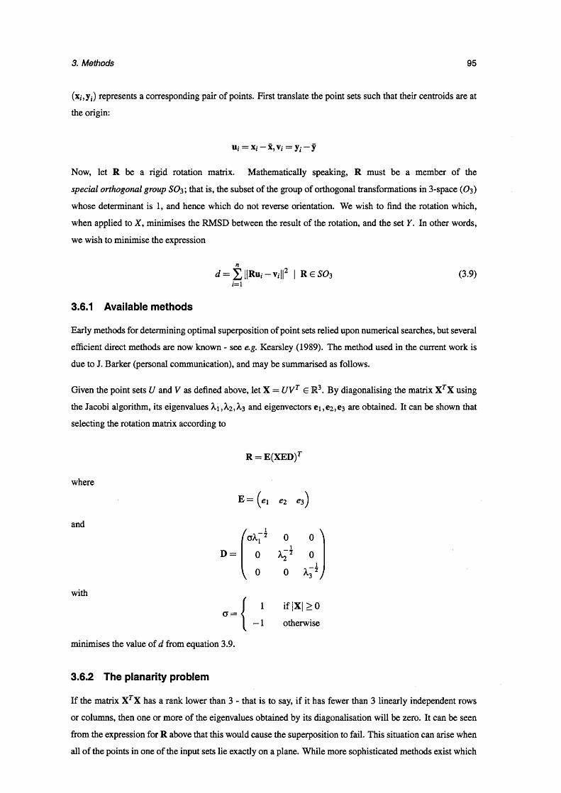
3. Methods 95

(xj,y,) represents a corresponding pair of points. First translate the point sets such that their centroids are at

the origin:

Now, let R be a rigid rotation matrix. Mathematically speaking, R must be a member of the

special orthogonal group SO3 ; that is, the subset of the group of orthogonal transformations in 3-space (O3 )

whose determinant is 1, and hence which do not reverse orientation. We wish to find the rotation which,

when applied to X , minimises the RMSD between the result of the rotation, and the set Y. In other words,

we wish to minimise the expression

3.6.1 Available methods

Early methods for determining optimal superposition of point sets relied upon numerical searches, but several

efficient direct methods are now known - see e.g. Kearsley (1989). The method used in the current work is

due to J. Barker (personal communication), and may be summarised as follows.

Given the point sets U and V as defined above, let X = UVT e R3. By diagonalising the matrix Xr X using

the Jacobi algorithm, its eigenvalues A. 1 , ^ 2 > ^ 3 and eigenvectors ei ,e2 ,e3 are obtained. It can be shown that

selecting the rotation matrix according to

or columns, then one or more of the eigenvalues obtained by its diagonalisation will be zero. It can be seen

from the expression for R above that this would cause the superposition to fail. This situation can arise when

all of the points in one of the input sets lie exactly on a plane. While more sophisticated methods exist which

U; = x,- - X, V; = y,- - y

nd = S l | R u i - v 1||2 I R e s o 3 (3.9)

i= l

R = E(XED)r

where

and

with

— 1 otherwise

1 if |X| > 0

minimises the value of d from equation 3.9.

3.6.2 The planarity problem

If the matrix X TX has a rank lower than 3 - that is to say, if it has fewer than 3 linearly independent rows

3. Methods 96

are able to handle these cases gracefully, it was found to be sufficient for the current work merely to test for

planarity prior to computing the superposition, and either to report an error if it was detected, or to perturb

the points slightly away from the plane.

3.7 Analysis of ligand conformation

The conformation of small molecules - in this case, biological ligands - was studied using several different

techniques. The first two, radius of gyration and planarity, provide a general overview of molecular shape,

while the calculation of the torsion angles around individual rotable bonds allow the local conformation of

individual parts of the molecule to be studied in more detail.

3.7.1 Radius of gyration

The radius of gyration rg of a solid body is defined by the equation

I = mR\

where I is the moment of inertia of the body and m is its mass. For a collection of atoms with individual

masses m \ , . . . , mn and coordinates x i , . . . , x„, we can therefore write the radius of gyration as

'S-Urn/H xf —x [| 2

E " = i m= " (3.10)

Note that this formula is simply a mass-weighted version of the RMSD given in equation 3.8. It is commonly

calculated for proteins using experimental techniques such as Small-angle X-ray Scattering (SAXS) in order

to obtain a rough measure of the sphericity of the molecule. For ligands, rg provides a first approximation

of the degree to which the molecule is in an extended or a bent conformation. For an ideal polymer, it can

be shown that the mean radius of gyration is linearly related to the mean end-to-end separation (Atkins and

de Paula, 2001).

Although the end-to-end distance of a polymer is perhaps a more intuitive way of representing its degree of

‘bentness’, the radius of gyration is a more general form. Specifically, the definition of end-to-end distance

is unambiguous only for simple polymers; where the molecule is branched or cyclic, this quantity no longer

has a clear meaning. We could perhaps define the ‘ends’ of a modestly-branched molecule using an all­

pairs shortest path graph algorithm such as Floyd (1962), but the justification for such a measurement would

necessarily break down for many of the molecules we would be interested in. The radius of gyration, on the

other hand, is calculable for any topology of molecule, and is therefore taken as the preferred method for

representing conformational compactness at the gross level.

3.7.2 Torsion angles

The approaches so far in this section have been concerned with representing molecular shape in fairly crude

terms; for describing local conformation in detail, torsion angles are a simple but effective tool.

3. Methods 97

3.7.2.1 Definition

Given four atoms A,B ,C and D, where each atom is bonded to the previous one (see figure 3.11), the torsion

or dihedral angle represents the relative orientations of the A — B and C — D bonds.

Formally, we define the torsion angle with respect to the four atoms A,B,C and D, xa b c d as follows

e = BC x BA

f =CD x CB e f

t =

'tA B C D = <

|e||f|cos- 1 (f) i f e - C D > 0

271 — cos- 1 {t) otherwise

Mnemonically, if one imagines looking along the B — C bond, with B closest and oriented such that B — A

points vertically upwards, the torsion angle is the clockwise deflection of C — D from 12 o’clock.

c

e

Figure 3.11: Definition of a torsion angle The torsion angle xa b c d represents the clockwise deflection of p{CD) from p{BA), where the transformation p represents projection into a plane normal to CB. The vectors e and f are constructions used in the calculation of Ta b c d > a s described in the text.

Torsion angles are routinely used to describe the conformation of proteins. The shape of the backbone can

be completely defined by specifying two torsion angles for each peptide unit. The conventional definitions

of these angles are

<)>: defined by atoms C1 - 1 — N1 — C„ — C1

\ |/ : defined by atoms N' — — C' — NI+ 1

where the superscripts indicate to which peptide unit each atom belongs. The combination of the <|>

and \]/ angles for one or more residues is commonly displayed on a two-dimensional Ramachandran plot

(Ramachandran and Sasisekharan, 1968). Low-energy orientations of these bonds correspond to the common

secondary structure conformations of protein backbones, primarily right-handed a-helices and (3-sheets.

Comparison of the torsion angles calculated from the coordinate model built into an electron density map

with those most statistically favoured for each residue type (Morris et al., 1992) can be used to validate the

model building and refinement procedures (Laskowski et a l, 1993).

3. Methods 98

3.7.2.2 Nomenclature

3.7.2.2.1 Angular range nomenclature

The system of Klyne and Prelog (1960) was used for naming angle ranges, with definitions for torsion angles

taken from the IUPAC Commission (1974). This system breaks torsion angles firstly into two halves, and

then into three equal segments per semicircle, as shown in figure 3.12. Angles in the range [—90°,90°) are

referred to as syn, and the rest are called anti. The term periplanar is applied to angles within [—30°,30°]

and [150°, —150°], while clinal refers to angles which fall outside those ranges. Combinations of these terms

are used to generate unique names for each of the six segments in the Klyne-Prelog system. The names cis,

trans, +gauche and -gauche are also sometimes used to refer to angles 0°, 180°, +30° and —30° respectively.

syn

cis-30

-gauche +gauche

-sc +SC

-90

-ac +ac

-150 150trans

anti

Figure 3.12: The Klyne-Prelog system for angle range nomenclature Combination of the terms syn, anti, clinal and periplanar, defined in the text, lead to the names of the six segments: synperiplanar (sc), +synclinal (+sc), +anticlinal (+ac), antiperiplanar (ap), -anticlinal (-ac) and -synclinal (-sc).

3.7.2.2.2 Bond definitions

When referring to torsion angles of nucleotide derivatives, IUPAC-IUB naming conventions (IUPAC-IUB,

1983) are generally adopted. Figure 3.13 shows two nucleotide triphosphate molecules, ATP and GTP. The

angles defined with respect to the standard atom names are listed in table 3.3. The application of these angle

definitions to the nucleotide derivatives NAD and FAD is covered in chapter 5.

The torsion angle around the N-glycosidic bond is denoted %. The atoms which define it depend upon whether

the nucletoide is a purine or a pyrimidine, as shown in table 3.3. These are chosen such that the definitions

of syn and anti conformations (§3.7.2.2.1) are consistent with accepted chemical conventions.

One angle for which the definition diverges from IUPAC conventions is Here, we use this symbol to refer to

a P-0 bond in the pyrophosphate moiety, with a subscript applied to denote the number of phosphate groups

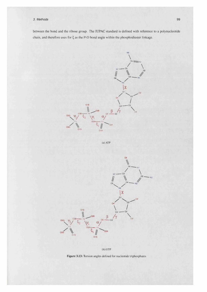
3. Methods 99

between the bond and the ribose group. The IUPAC standard is defined with reference to a polynucleotide

chain, and therefore uses for £ as the P-0 bond angle within the phosphodiester linkage.

\\0 3 B --------- PB '

\^ C6== :n i

N 7 - -------- 0 5 \

ll \✓N9

\x/ C, \ ^ • ° 2'

0 4 ' f\

C 4-------------< *

A 0 3

\ V ^ \V, < yPG-------------------------- 03A -------- PA

/ \ ^ “#01G 01A

P h0 5 ’ — —— C5'

(a) ATP

01B

\0 3 B p b ‘

w/ N,\

C 5 \

II I / 0 8 ^ ^ C4 -

■ N2

. 02 '

\0 4 ' - C3'

P A \ ,?G VI/ / t . 1

V 2/ ^ y , « /PG 0 3 A p ,

Q 1G H

0 5 ’ ----------C5'

(b) GTP

Figure 3.13: Torsion angles defined for nucleotide triphosphates

3. Methods 100

? a /

r vN3_A I

\ ^S.A C4_^ \N7 A

*A N9V /04 '_ 4 / ^ t 8 _ A' TM 1 A

v, C5_N—05_NV P.

C3'J*---C4'-N

I \Cg N « -N

I x„

eNN7

"^7 N

NN1W / \ n

.-w / V \ a .' — 0 5 A C 3 '_A "^ \

V ~ /“I 02 N °3'-A5n\ . /

v\„

(a) NAD

CSM

J* '-V N<J T \

W £S »\

V N9 A 'Kpy1* A

\ C 8 C 9 - ------- ---------------t \V \C7ht— C 7 C9A— — N10 0 2 '

\ / \C e = C 5 A 0 1 0 =\ / \NS = C 4 4 C 2 = 0 2

\ /C 4 --------* 3

/

e /e >C 5 ' ^ ° 5 1 0 1 ^ \ A

\C 3" .

8 , / 8 \6 ca' 5

02P Ya / \u „ B cL

”03P\^ A / R C3'_A ^>2'_A> ^ a Pa i

(b) FAD

Figure 3.14: Torsion angles defined for the nucleotide derivatives NAD and FAD

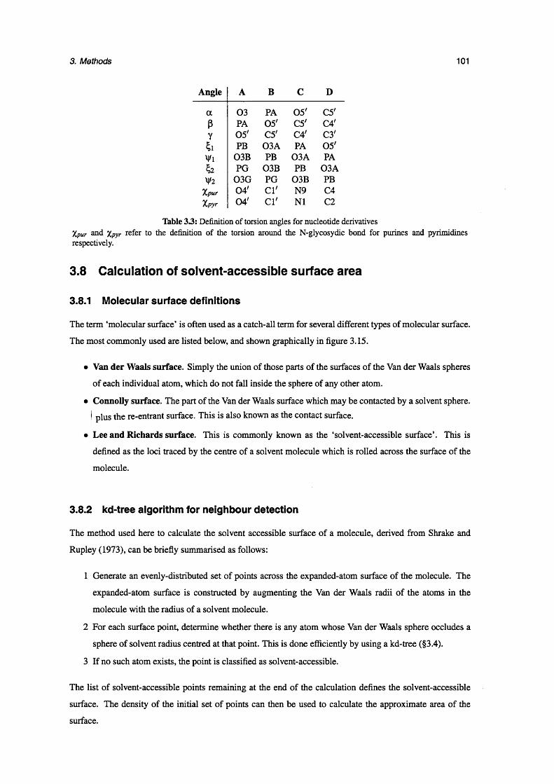
3. Methods 101

Angle A B c D

a 03 PA 0 5 ' C5'P PA 05 ' C5' C4'Y 0 5 ' C5' C4' C3'Si PB 03A PA 0 5 'Vi 03B PB 03A PA

PG 03B PB 03AV2 03G PG 03B PB

Xpur 04 ' C l' N9 C4X pyr 04 ' C l' N1 C2

Table 33: Definition of torsion angles for nucleotide derivatives Xpur and Xpyr refer to the definition of the torsion around the N-glycosydic bond for purines and pyrimidines respectively.

3.8 Calculation of solvent-accessible surface area

3.8.1 Molecular surface definitions

The term ‘molecular surface’ is often used as a catch-all term for several different types of molecular surface.

The most commonly used are listed below, and shown graphically in figure 3.15.

• Van der Waals surface. Simply the union of those parts of the surfaces of the Van der Waals spheres

of each individual atom, which do not fall inside the sphere of any other atom.

• Connolly surface. The part of the Van der Waals surface which may be contacted by a solvent sphere.

| plus the re-entrant surface. This is also known as the contact surface.

• Lee and Richards surface. This is commonly known as the ‘solvent-accessible surface’. This is

defined as the loci traced by the centre of a solvent molecule which is rolled across the surface of the

molecule.

3.8.2 kd-tree algorithm for neighbour detection

The method used here to calculate the solvent accessible surface of a molecule, derived from Shrake and

Rupley (1973), can be briefly summarised as follows:

1 Generate an evenly-distributed set of points across the expanded-atom surface of the molecule. The

expanded-atom surface is constructed by augmenting the Van der Waals radii of the atoms in the

molecule with the radius of a solvent molecule.

2 For each surface point, determine whether there is any atom whose Van der Waals sphere occludes a

sphere of solvent radius centred at that point. This is done efficiently by using a kd-tree (§3.4).

3 If no such atom exists, the point is classified as solvent-accessible.

The list of solvent-accessible points remaining at the end of the calculation defines the solvent-accessible

surface. The density of the initial set of points can then be used to calculate the approximate area of the

surface.

3. Methods 102

(a) Circles representing the Van der Waals radii of a set of atoms

(b) Connolly surface

(c) Conceptual method used to construct the Lee & (d) The complete Lee & Richards surfaceRichards surface

Figure 3.15: Molecular surface representations

3.8.3 Generation of uniformly distributed surface points

A number of methods for generating the initial set of evenly distributed surface points were considered. Since

each of these approaches has its drawbacks, the choice of which to use was to some extent a pragmatic one.

In order to distribute points evenly on the molecular surface, we may first distribute points evenly on the

surface of each atom, and then prune away those points which which fall inside the sphere of any other atom.

3.8.3.1 Uniform distribution o f points on the unit sphere

A naive approach to randomly distributing points on the unit sphere would be to select the spherical polar

coordinates 0 and <(> from the uniform distributions 0 G [0,2n) and <\> G [0,7t]. However, we note that the area

element

dQ. = sin<|)<i0 d(j) (3.11)

3. Methods 103

is a function of <{>, and that therefore points picked in this way will be more dense towards the poles, and less

so at the equator of the sphere.

One solution to this problem is to follow the initial placement step with an iterative refinement which attempts

to even out the point density across the surface of the sphere. This can be done by modelling each point as

a charged particle; if all points have the same charge, they repel one another, and if their movement is

constrained to the spherical surface, this repulsion will lead to a uniform distribution of points. In order

to avoid oscillatory motion, a viscosity term is usually added. The problem with such an approach is its

computational complexity: each step of the refinement process requires the solution of a differential equation,

and depending upon the number of points involved, several hundred iterations may be required to achieve a

stable conformation.

Alternatively, direct methods can be used. Inspection of the area element given in equation 3.11 leads to a

simple way of eliminating the bias described above. First, we rewrite dQ, as follows:

dQ = sin<)) dQd§

= //0/f(cOS<J>)

Evenly distributing points on the surface of the sphere is equivalent to ensuring that any small area upon

it is expected to contain the same number of points. In other words, we need to choose distributions for 0

and <|> for which the differentials dQ and /f(cos<J>) are constant at all values. It is clear that, choosing random

variables U and V on (0,1), the following expressions for 0 and <J) satisfy this condition:

0 = 2711/

<1> = cos_ 1 (2 v — 1 )

3.8.3.2 Surface triangulation

An alternative approach is to triangulate the molecular surface, taking either the set of triangular vertices, or

the centroids of each triangle as the set of surface points. Such a triangulation can be easily constructed by

first representing the occluded volume of the molecule using a regular three-dimensional grid: all points

which lie outside the molecule are set to zero, and those inside to unity. Application of an isosurface

generation method such as the Marching Cubes algorithm (Lorensen and Cline, 1997) then produces triangles

which lie approximately on the molecular surface.

A problem with this approach is that the triangles produced are not guaranteed to be equal in size; deriving

a uniformly distributed set of points therefore requires an additional refinement step similar to that described

above, in order to make the vertices more evenly distributed. While triangulation is a powerful method for

approximating volumetric data of arbitrary shapes therefore, it is not ideally suited to the current problem.

3. Methods 104

3.8.3.3 Spherical t-designs

A set of N points on the sphere is called a spherical t-design if the integral of any polynomial of degree

at most t is equal to the average value of that polynomial over the set of N points. Sets of such designs

for different values of N and t have been precomputed (Hardin and Sloane, 1996) and are available on the

world-wide web from http://www.research.att.com/~njas/sphdesigns. Examples of 3-dimensional spherical

designs are shown in figure 3.8.3.3.

(e) t=21, n=240

Figure 3.16: Spherical t-designs in three dimensions For each design, the values of the parameter t and n - the number of points in the design - are given. (Figure courtesy of J. Barker)

The problem of calculating solvent accessible surface area can be formulated as an integral. Let / be a

function defined on the expanded-atom-radius surface S of the molecule, whose value is zero at regions of

the surface inaccessible to solvent, and unity at solvent-exposed points. Now the total solvent-accessible

surface area is given by

3. Methods 105

SsfdA

3.8.3.3.1 Determination of surface point accessibility

In order to determine whether a given point is accessible to solvent, we need to determine whether any atom

A is within a distance d = 2rso[vent + r& from the point as shown in figure 3.17. Here, this is done using a

kd-tree based search.

1+ 2rs

Figure 3.17: Searching for potentially solvent-excluding neighbours The green circle indicates the volume which must be searched in order to find atoms which may potentially exclude solvent from the surface of atom A.

3.8.4 Caveats

3.8.4.1 Structural water molecules

Before determining the solvent-accessible surface of a molecule whose coordinates have been determined by

X-ray crystallography, it is customary first to remove all water molecules from the structure. The implicit

assumption here is that these molecules, although immobilised in the crystal (and hence visible in the

diffraction pattern), would revert to being part of the bulk solvent were the compound to be returned to its

in vivo state. This is not always the case, however; some proteins contain structural water molecules which

do not interchange with bulk solvent. Marking the parts of the protein contacted by these waters as solvent

accessible could therefore be said to be erroneous. Automatic discrimination between physiologically-

immobilised waters and water of crystallisation is, however, not possible in practice.

3.8.4.2 Internal cavities

The method described above does not distinguish between the external surface of a protein, and that of any

internal cavities which it may have. Some proteins, for example the lipocalins (Flower, 1996), many of

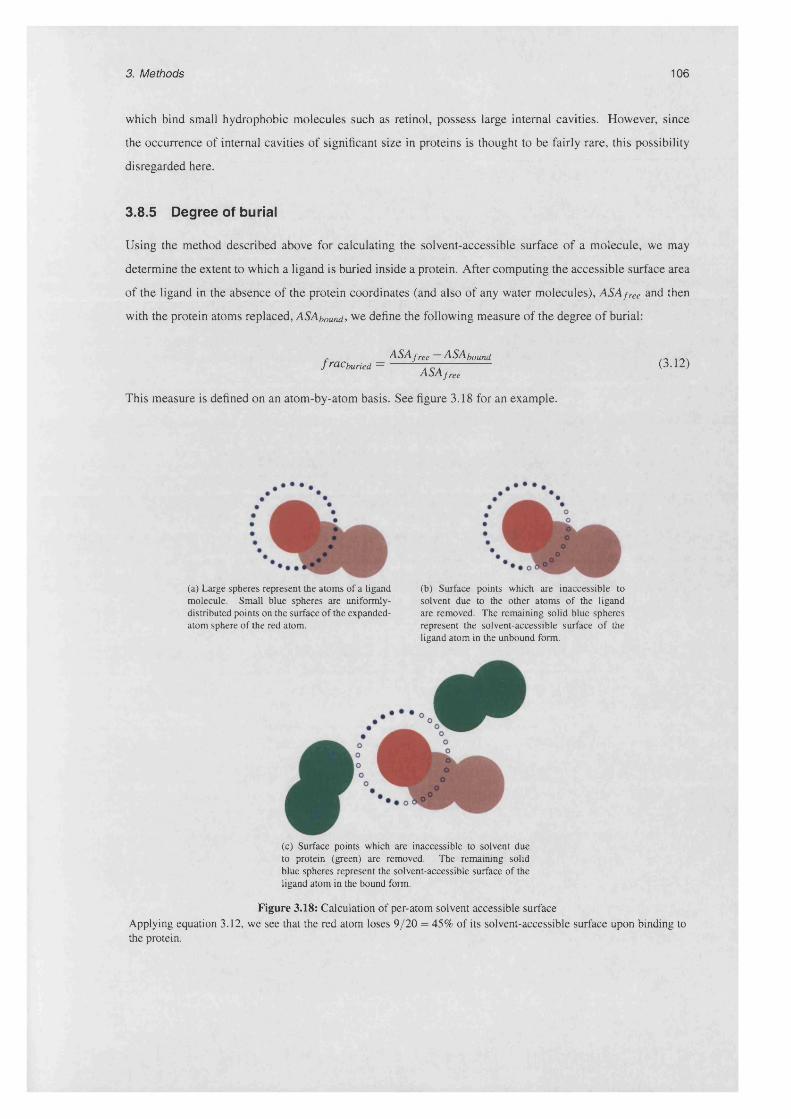
3. Methods 106

which bind small hydrophobic molecules such as retinol, possess large internal cavities. However, since

the occurrence of internal cavities of significant size in proteins is thought to be fairly rare, this possibility

disregarded here.

3.8.5 Degree of burial

Using the method described above for calculating the solvent-accessible surface of a molecule, we may

determine the extent to which a ligand is buried inside a protein. After computing the accessible surface area

of the ligand in the absence of the protein coordinates (and also of any water molecules), ASAfree and then

with the protein atoms replaced, ASAbound, we define the following measure of the degree of burial:

ASA f ree ASAboundfracburied = tt t;------------ (3.12)ASA free

This measure is defined on an atom-by-atom basis. See figure 3.18 for an example.

(a) Large spheres represent the atoms of a ligand molecule. Small blue spheres are uniformly- distributed points on the surface of the expanded- atom sphere of the red atom.

(b) Surface points which are inaccessible to solvent due to the other atoms of the ligand are removed. The remaining solid blue spheres represent the solvent-accessible surface of the ligand atom in the unbound form.

(c) Surface points which are inaccessible to solvent due to protein (green) are removed. The remaining solid blue spheres represent the solvent-accessible surface of the ligand atom in the bound form.

Figure 3.18: Calculation of per-atom solvent accessible surface Applying equation 3.12, we see that the red atom loses 9/20 = 45% of its solvent-accessible surface upon binding to the protein.

107

Chapter 4

Generation of datasets

This chapter describes the protocols which were developed in order to generate robust, high-quality data sets

for the subsequent analyses presented in this thesis.

The aims are, for each ligand compound of interest:

1 Identify all instances of that compound co-crystallised with protein, which are present in a coordinate

repository such as the PDB.

2 Extract the coordinates of each ligand along with its binding site, transforming them such that all ligand

molecules lie in a common coordinate frame.

3 Cluster the binding sites based on the evolutionary relatedness of the proteins which comprise them.

Each resulting cluster should contain those sites which are from non-identical members of the same

homologous superfamily.

The main sections of this chapter, therefore, are as follows. Firstly, the problems involved in the automated

creation of good-quality, non-redundant data sets of ligand binding sites are discussed. Secondly, the

protocols used to address these problems are described. Thirdly, the architecture of the computational

pipeline which implements these protocols is outlined. By applying this procedure to all ligands in the

PDB, an overview of the distribution of ligand types with respect to both protein superfamilies and enzyme

function is obtained. Finally, datasets for four ligands of particular biological importance,

• ATP

• GTP

• NAD

• FAD

are discussed in more detail. These datasets form the basis of the analyses which follow.

4. Generation of datasets 108

4.1 Protocol for validation of ligand identity

4.1.1 The need for ligand validation

In order to perform a systematic study of ligand binding sites, using co-crystal structures as the data source,

an automatic method of identifying ligand molecules is required. In particular, this method should have the

following capabilities:

1 Given a crystal structure, identify all ligand molecules.

2 For each ligand, determine its identity; in other words, identify it as being an instance of a particular

chemical compound (see §1.3.6).

3 Compute a mapping between each atom in the ligand molecule, as seen in the crystal structure, and the

corresponding atom in the reference compound.

A naive approach to achieving this would be simply to parse the PDB file for the structure, then perform the

three steps listed above by

1 Finding ligand molecules by looking for HETATM records.

2 For each ligand, reading the residue name, and assigning chemical identity by looking up this name in

the RCSB hetgroup dictionary.

3 Mapping each ligand atom to an atom in the reference compound, based on the PDB atom name.

The problem with this simple method is that steps 2 and 3 would frequently fail due to well-known

inconsistencies in the data which can be retrieved from the PDB files. Problems may also arise from the fact

that this data is the result of an experimental procedure, and therefore contains unavoidable error. Specifically,

the following difficulties may be encountered:

• Inconsistency in naming of compounds. While PDB files deposited from October 1998 onwards

are subject to data uniformity checking (Westbrook et al., 2002), older ‘legacy’ files may contain

compounds whose residue name does not agree with the standard nomenclature.

• Inconsistency in atom names. Similarly, atom names are not applied in a uniform manner across

entries, so we cannot assume that an atom named ‘A’ in one instance of compound XYZ refers to the

same chemical entity as another atom with the same descriptor.

• Stereochemical errors. A chiral stereocentre can be defined by specifying four atoms and their

‘handedness’. Where distinct stereoisomers of a compound are found in complex with proteins, those

stereoisomers should each have a unique hetgroup identity. Cases can often be found in the PDB,

however, in which either the atom labelling or the name of a residue is incorrect, resulting in its

chirality, as determined from its coordinates, being inconsistent with that specified for the reference

compound.

• Missing atoms due to insufficient resolution. Parts of the structure which are mobile, or which

exhibit crystal mosaicity, may not produce sufficiently well-defined electron density for reliable model

building in that region. This is manifested as missing atoms in the coordinate file. If we later wish

to use those atoms as the basis for a coordinate frame, in order to compare different sites binding this

molecule, we must first ensure that all atoms in the molecule have well-defined positions.

4. Generation of datasets 109

All of these problems may be circumvented by systematically checking the coordinates of every ligand

molecule against a set of reference chemical structures, as described below. It should be noted that, during

the time in which this work was carried out, the MSD, which is a ‘cleaned up’ version of the PDB in which

many of the issues discussed above have been alleviated, was released. The reason why it was not used in

this study is partly due to issues of time: by the time the database became publicly available, the validation

scheme described here had already been implemented. In addition, however, the aims of the MSD’s data

validation protocols, with respect to ligands, are somewhat different to those of this work, and the author has

found examples where the ligand identity assigned by the MSD does not agree either with that provided by

this pipeline, nor with that which would be applied on visual inspection. Some of these cases are discussed

further below.

4.1.2 The algorithm

The protocol used to identify all ligands in the PDB is outlined as pseudocode in algorithm 4.1. The algorithm

attempts to assign a chemical identity to every monomer which is not an amino acid, part of a nucleotide

chain, or a solvent molecule. These conditions are tested using a simple screen based on the residue name

present in the PDB file; those monomers which remain are identified using a graph-matching procedure.

The procedure is applied to all X-ray crystal structures within the PDB. It should be noted at this point that,

where the resolution of the compound is particularly poor, or the crystallographic temperature factors of the

ligand atoms are high, the results of this procedure may be suspect. At this stage, however, all ligands are

treated equally; a decision can be made later on whether to process only those ligands identified from good

quality structures, as determined by, for example, a minimum resolution threshold.

The coordinates of each ligand molecule L are converted into a graph by deducing the connectivity between

atoms. This is done by calculating the distances between all pairs of atoms in the monomer. A pair of atoms

a\ and d2 are considered to be covalently bonded if the separation of their centres d, as calculated from the

coordinates in the PDB file, satisfies

d < r\ + r2 + t

where r\ and r2 are the standard covalent radii of the two atoms, according to a reference table, and t is a

tolerance value, which has been set here to 0 . 2 A. Each atom in the molecule is represented by a vertex whose

label corresponds to the atomic number of the atom. Edges are added between vertices whose atoms satisfy

the distance cutoff. These edges are unlabelled, since reliable deduction of bond valences and aromaticity

from atomic coordinates alone is not a trivial problem: see e.g. Labute (2005). The result of this procedure

is a graph, G l, consisting of N l vertices.

In order to determine the chemical identity of the ligand, G l must be compared against the database of

reference structures (D. This search can be made faster by first identifying the subset S C (D which can

potentially provide a sufficiently good match against G l , as described in §3.1.3. Using the expressions

shown in table 3.1, it is possible to calculate the range of reference graph sizes (in terms of numbers of

vertices) Nmin and Nmox, which could potentially provide an acceptable match; the set S is then given by

4. Generation of datasets 110

Function V a lid a t e P D B L ig a n d s (P D B P, ChemBase C, MatchCriteria M, MatchSize 5) :Ligands <— 0 for each Entry E e P :

for each Monomer m e E :if not m.ls_AMiNO_ACiD() and not m.iS_SOLVENT() then

Ligands <— Ligands + lDENTlFYMONOMER(m,C,M ,S)

Compare connectivity o f a given monomer against reference graphsFunction lDENTiFYMONOMER(Monomer m, ChemBase C, MatchCriteria M, MatchSize 5) :

Matches <— 0

Convert the coordinates o f monomer m into a graph using tables o f standard covalent radii G l < - COMPUTEGRAPH(m)N <— G1.n _v e r t ic e s()

Compute the range o f target graph sizes which can potentially provide a match against a query o f size N, satisfying size criterion S(Lower, Upper) <— COMPUTETARGETRANGE(N,5)

Compare the monomer graph against all reference graphs within the target range M specifies the criteria for identifying pairs o f atoms and bonds which can be matched

for Target Size <— Lower to U pper : for each Graph G2 € C: G2.n _v e r t ic e s() = Target Size :

M atches«- Matches U MATCHGRAPHS(G1, G2,M , S)

if Matches = 0 then return NoMalch

elsereturn GetBestMATCU(Matches)

Function C o m pareM atch es(X ,F ) : if X .NStereocentreMismalches = Y.NStereocentreMismatches then

return X.Gl.name = X.Gl.name else

return X.NStereoCentreMismatches < Y.NStereoCentreMismatches

Function Ge tB e st M atch(Matches) :X < - 0for each Match G Matches :

X *- X + (Match, Ch e c k s t e r e o c e n t r e s(Match))Sort the list X, using the comparison function CompareMatches

return X[0]

Check correspondence o f stereocentre chiralities between monomer and reference graphs Function C h ec k S t er eo c e n t r e s(M) :

MisMatches <— 0for each Stereocentre 52 G M.G2 :

Map atoms from reference stereocentre onto the monomer graph Stereocentre 5 1 4- M a p C h ira lC en tre (5 2 ,M .G 2 ,M .G 1 ,M )Chirality2 <- COMPUTECHIRALITY(51)Chirality2 4- 52.CHIRALITY() if Chirality I 7 ̂Chirality2 then

MisMatches <— MisMatches + 1 return MisMatches

Algorithm 4.1: Validation of ligand identity

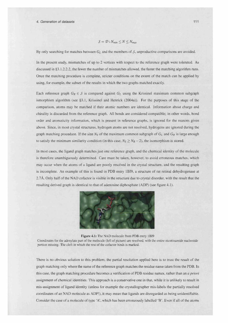
4. Generation of datasets 111

S = <D:Nmin< N < N max

By only searching for matches between Gl and the members of S , unproductive comparisons are avoided.

In the present study, mismatches of up to 2 vertices with respect to the reference graph were tolerated. As

discussed in §3.1.2.2.2, the fewer the number of mismatches allowed, the faster the matching algorithm runs.

Once the matching procedure is complete, stricter conditions on the extent of the match can be applied by

using, for example, the subset of the results in which the two graphs matched exactly.

Each reference graph G r € S is compared against G l using the Krissinel maximum common subgraph

ismorphism algorithm (see §3.1, Krissinel and Henrick (2004a)). For the purposes of this stage of the

comparison, atoms may be matched if their atomic numbers are identical. Information about charge and

chirality is discarded from the reference graph. All bonds are considered compatible; in other words, bond

order and aromaticity information, which is present in reference graphs, is ignored for the reasons given

above. Since, in most crystal structures, hydrogen atoms are not resolved, hydrogens are ignored during the

graph matching procedure. If the size N s of the maximum common subgraph of G l and G r is large enough

to satisfy the minimum similarity condition (in this case, N s > N r — 2), the isomorphism is stored.

In most cases, the ligand graph matches just one reference graph, and the chemical identity of the molecule

is therefore unambiguously determined. Care must be taken, however, to avoid erroneous matches, which

may occur when the atoms of a ligand are poorly resolved in the crystal structure, and the resulting graph

is incomplete. An example of this is found in PDB entry 1BI9, a structure of rat retinal dehydrogenase at

2.7A. Only half of the NAD cofactor is visible in the structure due to crystal disorder, with the result that the

resulting derived graph is identical to that of adenosine diphosphate (ADP) (see figure 4.1).

Figure 4.1: The NAD molecule from PDB entry 1BI9 Coordinates for the adenylate part of the molecule (left of picture) are resolved, with the entire nicotinamide nucleotide portion missing. The cleft in which the rest of the cofactor binds is marked.

There is no obvious solution to this problem; the partial resolution applied here is to trust the result of the

graph matching only where the name of the reference graph matches the residue name taken from the PDB. In

this case, the graph matching procedure becomes a verification of PDB residue names, rather than an a priori

assignment of chemical identities. This approach is a conservative one in that, while it is unlikely to result in

mis-assignment of ligand identity (unless for example the crystallographer mis-labels the partially resolved

coordinates of an NAD molecule as ADP!), it may mean that ligands are disregarded as being unidentifiable.

Consider the case of a molecule of type ‘A’, which has been erroneously labelled ‘B \ Even if all of the atoms

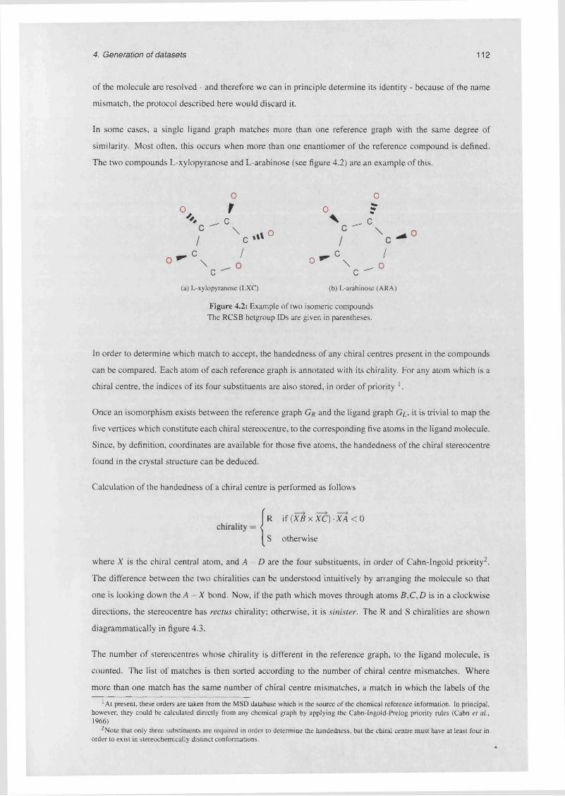
4 . Generation of datasets 112

of the molecule are resolved - and therefore we can in principle determine its identity - because of the name

mismatch, the protocol described here would discard it.

In some cases, a single ligand graph matches more than one reference graph with the same degree of

similarity. Most often, this occurs when more than one enantiomer of the reference compound is defined.

The two compounds L-xylopyranose and L-arabinose (see figure 4.2) are an example of this.

O 0

% J ° ' J

i\ » > °—* C / _ C /

\ 0 \ ^ 0 c ^ c "(a) L-xylopyranose (LXC) (b) L-arabinose (ARA)

Figure 4.2: Example of two isomeric compounds The RCSB hetgroup IDs are given in parentheses.

In order to determine which match to accept, the handedness of any chiral centres present in the compounds

can be compared. Each atom of each reference graph is annotated with its chirality. For any atom which is a

chiral centre, the indices of its four substituents are also stored, in order of priority 1.

Once an isomorphism exists between the reference graph G r and the ligand graph G l , it is trivial to map the

five vertices which constitute each chiral stereocentre, to the corresponding five atoms in the ligand molecule.

Since, by definition, coordinates are available for those five atoms, the handedness of the chiral stereocentre

found in the crystal structure can be deduced.

Calculation of the handedness of a chiral centre is performed as follows

{R if {XB x XC) • XA < 0

S otherwise

where X is the chiral central atom, and A - D are the four substituents, in order of Cahn-Ingold priority2.

The difference between the two chiralities can be understood intuitively by arranging the molecule so that

one is looking down the A —X bond. Now, if the path which moves through atoms B,C,D is in a clockwise

directions, the stereocentre has rectus chirality; otherwise, it is sinister. The R and S chiralities are shown

diagrammatically in figure 4.3.

The number of stereocentres whose chirality is different in the reference graph, to the ligand molecule, is

counted. The list of matches is then sorted according to the number of chiral centre mismatches. Where

more than one match has the same number of chiral centre mismatches, a match in which the labels of the

1 At present, these orders are taken from the MSD database which is the source of the chemical reference information. In principal, however, they could be calculated directly from any chemical graph by applying the Cahn-Ingold-Prelog priority rules (Cahn et al., 1966)

2Note that only three substituents are required in order to determine the handedness, but the chiral centre must have at least four in order to exist in stereochemically distinct conformations.

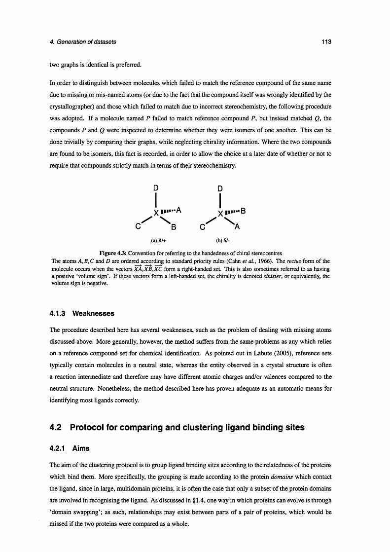
4. Generation of datasets 113

two graphs is identical is preferred.

In order to distinguish between molecules which failed to match the reference compound of the same name

due to missing or mis-named atoms (or due to the fact that the compound itself was wrongly identified by the

crystallographer) and those which failed to match due to incorrect stereochemistry, the following procedure

was adopted. If a molecule named P failed to match reference compound P, but instead matched Q, the

compounds P and Q were inspected to determine whether they were isomers of one another. This can be

done trivially by comparing their graphs, while neglecting chirality information. Where the two compounds

are found to be isomers, this fact is recorded, in order to allow the choice at a later date of whether or not to

require that compounds strictly match in terms of their stereochemistry.

D D

(a) R/+ (b) S/-

Figure 43: Convention for referring to the handedness of chiral stereocentres The atoms A,B,C and D are ordered according to standard priority rules (Cahn et al., 1966). The rectus form of the molecule occurs when the vectors XA,XB,XC form a right-handed set This is also sometimes referred to as having a positive ‘volume sign’. If these vectors form a left-handed set, the chirality is denoted sinister, or equivalently, the volume sign is negative.

4.1.3 W eaknesses

The procedure described here has several weaknesses, such as the problem of dealing with missing atoms

discussed above. More generally, however, the method suffers from the same problems as any which relies

on a reference compound set for chemical identification. As pointed out in Labute (2005), reference sets

typically contain molecules in a neutral state, whereas the entity observed in a crystal structure is often

a reaction intermediate and therefore may have different atomic charges and/or valences compared to the

neutral structure. Nonetheless, the method described here has proven adequate as an automatic means for

identifying most ligands correctly.

4.2 Protocol for comparing and clustering ligand binding sites

4.2.1 Aims

The aim of the clustering protocol is to group ligand binding sites according to the relatedness of the proteins

which bind them. More specifically, the grouping is made according to the protein domains which contact

the ligand, since in large, multidomain proteins, it is often the case that only a subset of the protein domains

are involved in recognising the ligand. As discussed in § 1.4, one way in which proteins can evolve is through

‘domain swapping’; as such, relationships may exist between parts of a pair of proteins, which would be

missed if the two proteins were compared as a whole.

4. Generation of datasets 114

We wish to obtain several levels of clustering. In order of increasingly coarse-grained groupings, these are:

1 Group together all identical binding sites.

2 Group together all binding sites whose domains could be identified as being related on the basis of

sequence similarity alone (that is, whose sequences are more than 35% identical).

3 Group together all binding sites whose domains, although having low sequence identity, have been

identified as being evolutionarily related on the basis of conserved structure and/or function.

From here on, these three levels of clustering will be referred to as the first-, second- and third-level

clusterings respectively.

4.2.2 Multi-domain binding sites

A common problem which is encountered when performing this type of grouping of functional sites in

proteins, be they catalytic sites or ligand binding sites, is how to handle cases where a site is situated at the

interface of two or more domains.

To illustrate the problem, consider the two binding sites represented in figure 4.4. Although the majority of

each site is contributed by domains which belong to the same homologous superfamily (the ‘blue’ domain),

each ligand also contacts another domain, and this domain comes from a different superfamily in each case.

Do we wish to cluster such sites together based on the relatedness of their shared domain, or do we judge

the replacement of the red domain with the green one to be a sufficiently large evolutionary step to warrant

placing the site in a new cluster?

i / r U /• A m m m y * A h <Jftv

Figure 4.4: Multidomain binding sites Two binding sites for a given compound are shown; in each, the ligand is represented schematically as a black rectangle. The colour of the residues which contact the ligand indicate the homologous superfamily to which they belong. Note that the domain may mutate so that it presents different chemical groups to the ligand, or so that the position of residues relative to it change. The binding site clustering protocol ignores these local changes and is only concerned with the identity of the domain as a whole.

This type of situation commonly occurs where the ligand in question is an enzymatic cofactor. Here, we often

find that a certain conserved cofactor-binding domain is paired with a different catalytic domain in different

proteins. An example of this is the Rossmann fold NAD-binding domain found in many oxidoreductases.

This domain is found together with a variety of different catalytic domains (Bashton and Chothia, 2002). By

interchanging the catalytic units, evolution has been able to generate proteins with new enzymatic activities

without needing to re-evolve the capability to recognise and bind the cofactor.

4. Generation of datasets 115

Given that we seek an automatic binding site clustering method, there appears to be no clear-cut solution to

the multidomain problem; here, a simple heuristic which gives mostly reasonable clusters is adopted.

4.2.3 The algorithm

Let us define a dissimilarity function, d, which returns a value bounded by [0,1] for each pair of binding sites

considered, where higher values indicate that the domain compositions of the two sites are more dissimilar.

This function can then be used to populate a distance matrix, to which the clustering methods discussed in

§3.2 can be applied.

The steps of the clustering protocol used here are as follows

1 For each site to be clustered, identify the set of residues which contact the ligand. This is done using a

simple distance threshold - any residue which has at least one atom within 4A of any atom of the ligand

is considered to be part of the binding site. Note that we do not require that the residue must make

an attractive contact with the ligand. This is partly a pragmatic choice, since to do so would be more

computationally demanding. It is also motivated by the idea that even residues which do not directly

contact the ligand may play an important structural role within the binding site. Ultimately, however,

these details are unlikely to significantly affect the clustering result.

2 Annotate all amino acid residues in the binding site according to the domain to which they belong.

Here, CATH version 2.6.0 was used, but this annotation could in principle be done according to any

other hierarchical domain classification scheme, such as SCOP. Residues which are not annotated as

belonging to any domain are marked as unclassified.

3 Decide upon a level, L at which the clustering will be performed. This level must be one of the levels

in the domain classification hierarchy. For example, if we want all binding sites composed of domains

with similar sequences (to 35% identity) to be grouped together, we should choose the S35 level. If, on

the other hand, we want all binding sites composed of domains in the same homologous superfamily

to be grouped together (a more coarse-grained clustering), we would choose the H level.

4 For each domain in the binding site, obtain its ancestor within the domain hierarchy, at the level chosen

above. In this way, produce a list of all L-level nodes which contribute to the binding site, each one

associated with the fraction of the binding site residues which it contributes. Consider the following

example.

Let us imagine a binding site, X, composed of three domains a,b,c, which contribute 2, 3 and 4

residues to the site respectively. In addition, the site contains one residue which is not classified as

belonging to a domain (see figure 4.5). We wish to cluster sites at the homologous superfamily level,

so the CATH codes for each domain are retrieved, to the fourth level. These are a: 1.2.3.4, b : 1.2.3.4

a n d c : 5.6.7.8.

Since domains a and b belong to the same homologous superfamily, their fractional contributions of

0.2 and 0.3 are summed to obtain the total contribution of the 1.2.3.4 family to this site. We can

therefore write the composition of X, in terms of homologous superfamilies, as follows

4. Generation of datasets 116

Family 1.2.3.4 provides 5 /10 residues

a (1 .2 .3 .4 ) ______b ( 1 .2.3.4)

unclassifiedo• • • •

c (5 .6 .7 .8 )

Family 5 .6 .7 .8 provides 4 /10 residues

Figure 4.5: Example of binding site domain composition Binding site residues are represented as circles, with the colour of each one indicating the CATH superfamily of each domain.

X = 0.1, {(1.2.3.4,0.5), (5.6.7.8,0.4)}

where the 0.1 represents the fraction of binding site residues which were unclassified. In general, the

binding site composition is represented by

mX = u ,{(xu p i) , . . . , ( x m,pm)} : '£ (p i) + u = 1 (4.1)

;=1

where the jc,s stand for the L-level ancestors of domains in the binding site, the p i for their fractional

contributions, and where u is the fraction of residues in the binding site which were not classified as

being part of any domain.

5 For each pair of binding sites, compute the dissimilarity between their domain compositions, as

represented by expression 4.1. The dissimilarity value is calculated as follows. Start with a value

of 1. For each L-level node which occurs in both sites, subtract from the current dissimilarity value,

the smaller of the two fractional contribution values associated with this node. The result is therefore

a number bounded by [0,1],

Algorithmically,

d(X ,Y) = I -

min (pi,qj) if X i= yjOn

0 otherwise

For example, if we imagine that we have two sites X =0.1,{(1.2.3.4,0.5),(5.6.7.8,0.4)} and

Y = 0.2, {(1.1.1.1,0.2), (5.6.7.8,0.6)}, the only node shared is 5.6.7.8. The smaller contribution of this

node (0.4, to site X) is subtracted from 1, resulting in a dissimilarity value of 0.6.

In order to generate a ligand dataset, firstly any site for which less than 80% of its residues are classified

in CATH, is discarded. Then, the groupings (1-3) listed previously are obtained by applying the clustering

protocol three times. Firstly, the sites are clustered based on their S95-level annotation. By applying a cutoff

4. Generation of datasets 117

threshold, distinct clusters are obtained. A representative is then chosen from each cluster.

The choice of representative is made on two criteria: firstly, structures which are thought to represent the

true biological unit are preferred. This is to prevent the dataset being contaminated by binding sites which,

although in reality occurring at a subunit interface, only have half of their coordinates present in the ASU

due to crystallographic symmetry. All structures in PQS are annotated according to whether the algorithm

predicts that the inter-subunit contacts in the proposed assembly is likely to be biologically relevant, as

opposed to simply being crystal packing artefacts. Sites are then ordered according to the resolution of the

structure.

Stage CATH level Clustering algorithm Dissimilarity cutoff

A S95 single linkage 0.4B S35 complete linkage 0.4C H complete linkage 0.4

Table 4.1: Clustering steps used to generate ligand datasets The first stage is done using single-linkage clustering for reasons of efficiency. For certain ligands (e.g. HEM), there are many examples in the structure database, meaning that application of complete linkage clustering would be very slow. The choice of clustering algorithm has little influence on the results of this stage. The choice of the dissimilarity threshold of 0.4 was heuristic, being based on visual inspection of the clusters obtained, and assessment of their biological significance.

The representatives from this first stage of clustering are then clustered on their S35-level annotation, and the

representatives from this stage are grouped based on H-level annotation. These three stages are summarised

in table 4.2.3.

It should be stressed that this protocol clusters binding sites only on the basis of the complement of

domains which actually contact the ligand; it does not attempt to cluster proteins as a whole. As such, it

is quite possible that binding sites which come from related proteins are placed into separate clusters by this

procedure, if the evolution of the protein family has changed the composition of the binding site. Therefore,

when reference is made to ligands in the same cluster, this should be read as “ligands contacted by the same

combination of related domains”.

A caveat to this automated procedure is that ligands may also be placed in separate clusters if they bind in a

different sites within the same protein, or if two ligands bind in the same site, but in a sufficiently different

orientation that the set of domains contacting it are changed.

4.3 Architecture of the processing pipeline

The aim of the pipeline, as stated previously, is to generate, for any specified ligand type, a list of all instances

of that compound co-crystallised with proteins, and then to provide a hierarchical grouping of that list based

upon the evolutionary relationships between the binding sites. For instance, the pipeline can generate a

dataset consisting of all ATP ligands found during the validation process.

While this chapter focusses on whole ligands, at this point, it should be pointed out that the dataset generation

pipeline can also be used to collect sets of ligands which share a common fragment. For example, one may

4. Generation of datasets 118

be interested in adenine recognition in general, with the identity of the adenine-containing ligand being

unimportant. In this case, a list of all instances of every adenine-containing molecule (e.g. AMP, ADP, ATP,

NAD, FAD, etc.) can be generated. This set of molecules is then clustered using the same domain-based

procedure just described, but only those residues which contact the adenine moiety of each molecule are

taken into account. Fragment-centric analyses of ligand recognition feature heavily in chapter 6, and will be

discussed further at that point.

An overview of the architecture of the pipeline used to generate ligand datasets is shown in figure 4.6. The

main stages of the process are as follows:

1 Populate an archive of reference compounds. The source of the reference compounds can either

be a local instance of the MSDchem database, or otherwise, the user can supply any arbitrary set of

compounds in the form of MOL2-format files. In this study, the set of compounds used for ligand

validation were obtained from MSDchem. A list of molecular fragments of particular interest were

built by hand and used to populate a separate ChemBase archive; this set was used for the the analysis

presented in chapter 6.

2 Build a domain tree. The hierarchical relationships between nodes in either the CATH or SCOP

domain classification schema are stored as a GAMUT binary file. This is for two reasons: firstly,

efficiency, since it means that the CATH or SCOP flat-files need only be parsed once, and secondly, to

abstract away the differences between the two classifications. Once either CATH or SCOP has been

converted into a GAMUT domain tree object, the applications which use it are able to be agnostic as

to its original origin.

3 Perform ligand validation. Using the archive of reference compounds generated above, and a source

of coordinate data, all ligand molecules found in the input structures have their identity determined

and recorded by the build-match.table program, using the protocol described in §4.1. The source of

coordinate data used in this study is the PQS archive; due to the modular nature of the pipeline, any

other source of structural data (e.g. PDB, MSD) could be in principal be substituted here.

4 Determine ligand-domain contacts. For each ligand molecule in the list generated above, the

build_contact_table program determines the set of protein residues which contact it, by inspection

of the coordinates. The domain to which each residue belongs (if it is classified) is found by reference

to the domain tree, and the list of domains contacting the ligand is then stored.

5 Generate ligand dataset. The dataset produced by the generate.].igand_dataset program is in the

form of a number of formatted text files which unambiguously identify the ligand molecules matching

the description provided, and which indicate to which cluster each ligand belongs at each of the three

clustering stages (§4.2). In addition, a file is generated which lists several types of data for each ligand,

including the resolution of the structure, its EC number if present, and a summary of the domain

composition of the binding site.

Stages 1-4 above need only be carried out once for any given set of structures, and, when the coordinate

database is updated, need only be performed on new structures. Since the computationally expensive

calculations have then already been carried out, generation of the dataset for a given query is a relatively

fast operation. The following sections expand on the details of several of the steps listed above.

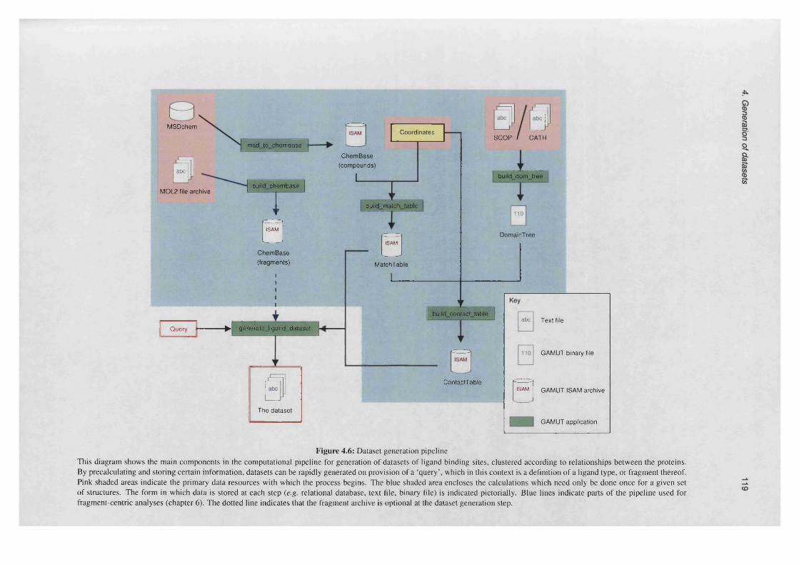
MSDchem

m sd to chem base

abc

MOL2 file archivebuild chem base

ISAM

Chem Base(fragments)

Query |I * riAnorato linsinH HntacAt1 *

yt/i mi die?_nycuiu_uaiabci

The dataset

Chem Base(compounds)

I

CoordinatesSCOP I CATH

build dom tree

build match table

DomainTreei ,M.I

MatchTable

I

build contact tableabc Text file

GAMUT binary file

ContactTableISAM GAMUT ISAM archive

GAMUT application

Figure 4.6: Dataset generation pipelineThis diagram shows the main components in the computational pipeline for generation of datasets of ligand binding sites, clustered according to relationships between the proteins. By precalculating and storing certain information, datasets can be rapidly generated on provision of a ‘query’, which in this context is a definition o f a ligand type, or fragment thereof. Pink shaded areas indicate the primary data resources with which the process begins. The blue shaded area encloses the calculations which need only be done once for a given set of structures. The form in which data is stored at each step (e.g. relational database, text file, binary file) is indicated pictorially. Blue lines indicate parts of the pipeline used for fragment-centric analyses (chapter 6). The dotted line indicates that the fragment archive is optional at the dataset generation step.

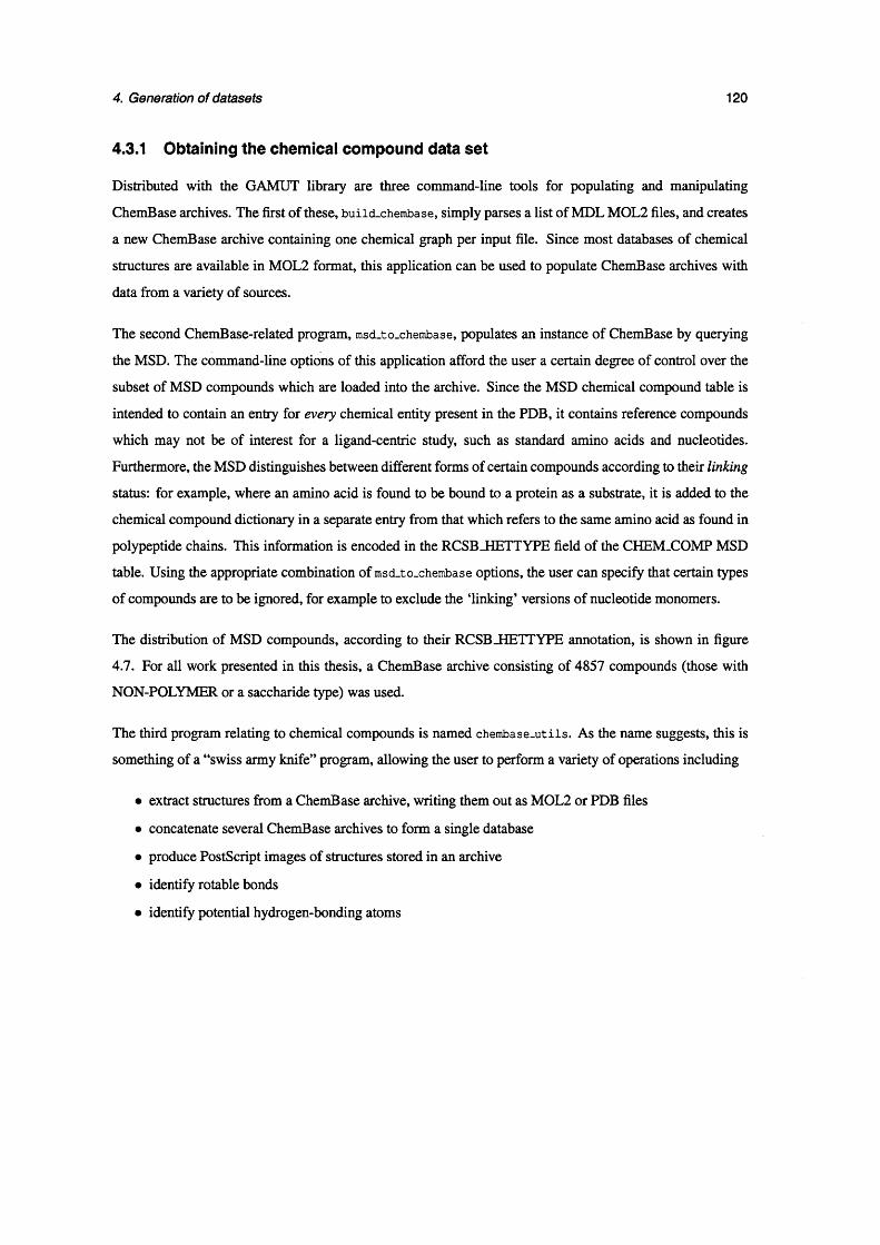
4. Generation of datasets 120

4.3.1 Obtaining the chemical compound data set

Distributed with the GAMUT library are three command-line tools for populating and manipulating

ChemBase archives. The first of these, build-chembase, simply parses a list of MDL MOL2 files, and creates

a new ChemBase archive containing one chemical graph per input file. Since most databases of chemical

structures are available in MOL2 format, this application can be used to populate ChemBase archives with

data from a variety of sources.

The second ChemBase-related program, msd_to_chembase, populates an instance of ChemBase by querying

the MSD. The command-line options of this application afford the user a certain degree of control over the

subset of MSD compounds which are loaded into the archive. Since the MSD chemical compound table is

intended to contain an entry for every chemical entity present in the PDB, it contains reference compounds

which may not be of interest for a ligand-centric study, such as standard amino acids and nucleotides.

Furthermore, the MSD distinguishes between different forms of certain compounds according to their linking

status: for example, where an amino acid is found to be bound to a protein as a substrate, it is added to the

chemical compound dictionary in a separate entry from that which refers to the same amino acid as found in

polypeptide chains. This information is encoded in the RCSB_HETTYPE field of the CHEM.COMP MSD

table. Using the appropriate combination of msd_to_chembase options, the user can specify that certain types

of compounds are to be ignored, for example to exclude the ‘linking’ versions of nucleotide monomers.

The distribution of MSD compounds, according to their RCSB_HETTYPE annotation, is shown in figure

4.7. For all work presented in this thesis, a ChemBase archive consisting of 4857 compounds (those with

NON-POLYMER or a saccharide type) was used.

The third program relating to chemical compounds is named chembase-utils. As the name suggests, this is

something of a “swiss army knife” program, allowing the user to perform a variety of operations including

• extract structures from a ChemBase archive, writing them out as MOL2 or PDB files

• concatenate several ChemBase archives to form a single database

• produce PostScript images of structures stored in an archive

• identify ratable bonds

• identify potential hydrogen-bonding atoms

4. Generation of datasets 121

RCSBJHETTYPE Number of compounds

D-PEPTIDE LINKING 27L-PEPTIDE LINKING 439

D-SACCHARIDE * 126L-SACCHARIDE * 15SACCHARIDE* 263

DNA LINKING 139RNA LINKING 94

NON-POLYMER * 4594

Null 258

5955

| D-peptide linking

■ L-peptide linking

■ D-saccharide

■ L-saccharide

□ Saccharide

^ DNA linking

□ RNA linking

■ Non-polymer

■ Unclassified

Figure 4.7: Number of compounds in MSD reference dictionary, broken down by RCSB.HETTYPE Asterisks indicate those classes of compound which were included in the ChemBase archive used for PDB ligand validation

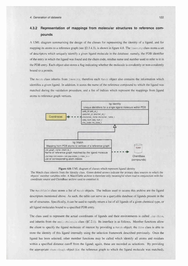
4. Generation of datasets 122

4.3.2 Representation of mappings from molecular structures to reference com­

pounds

A UML diagram summarising the design of the classes for representing the identity of a ligand, and for

mapping its atoms to a reference graph (see §2.3.4.3), is shown in figure 4.8. The id en tity class stores a set

of descriptors which uniquely identify a given ligand molecule in the database: namely, the PDB identifier

of the entry in which the ligand was found and the chain code, residue name and number used to refer to it in

the PDB entry. Each object also stores a flag indicating whether the molecule is covalently or non-covalently

bound to a protein.

The Match class inherits from identity, therefore each Match object also contains the information which

identifies a given ligand. In addition, it stores the name of the reference compound to which the ligand was

matched during the validation procedure, and a list of indices which represent the mappings from ligand

atoms to reference graph vertices.

C h em B ase

(com pounds)

ISAM

Coordinates

+ref_graph_name: chem::id_tN am e of reference graph m atched by the ligand m olecule

+corresp: std:vector< std::pair<index_t, index_t> >List of corresponding atom indices

lig::Match

M apping from P D B atom s to vertices of a reference graph

+pdb_id: pdb_id_t +polymer_id: polymer_id_t +monomer_name: monomer_name_t +seq_num: seq_num_t +ins_code: ins_code_t

lig::ldentity

Unique identifiers for a single ligand m olecule within P D B

Figure 4.8: UML diagram of classes which represent ligand identity The Match class inherits from the Identity class. Green dotted arrows indicate the primary data sources to which the objects’ member variables refer. A MatchTable archive is therefore only meaningful when read in conjunction with the coordinate source and ChemBase archive used to construct it.

The MatchTable class stores a list of Match objects. The indices used to access this archive are the ligand

descriptors mentioned above. As such, the table can serve as a queryable database of ligands present in the

set of structures. Specifically, it can be used to rapidly return a list of all ligands of a given chemical type, or

all ligand molecules bound to a specified PDB entry.

The class used to represent the actual coordinates of ligands and their environments is called lig: .-Site,

and inherits from the mmol::Molecule class (§C.2.1). Its interface is as follows. Member functions allow

the client to specify the ligand molecule of interest by providing a Match object; the Site class is able to

store the identity of this ligand internally using the selection framework described previously. Once the

ligand has been selected, other member functions may be called which identify all atoms and residues

within a specified distance cutoff from the ligand; again, these are recorded as selections. By providing

the appropriate chem:: Graph object (i.e. the reference graph to which the ligand molecule was matched),

4. Generation of datasets 123

a transformation may be computed which superposes the ligand, or a fragment of it, onto the reference

structure. This transformation is recorded inside the Site object, allowing the client at a later date to invert it,

transforming the coordinates of the binding site back to the coordinate frame used in the original structure.

Finally, a member function is defined which removes all parts of the original structure, save for the selected

ligand and binding site region. Given a MatchTable archive and the original source of coordinate data which

was used to build it, the lig: :Site class provides a convenient framework which applications can use to

manipulate the ligand(s) of interest.

4.3.3 Representation of ligand-domain contacts

For each atom of a ligand molecule, the residues which contact it are identified by the build_contact_table

program. In order to store this information in a compact manner, the record for each ligand molecule contains

the following data:

• A list of the domain identifiers which contact the ligand, stored as text {e.g. { lhShD2, lh$hD3})

• For each atom of the ligand, a list of pairs of indices {(di,jci),. . . , (dn,xn)} where each di is the index

of a domain which contacts this atom, and the xi is the sequential offset into that domain. For example,

if the tenth residue of domain 1/i8/zD2 contacts a given atom, its contact list would contain the index

pair (0,9).

Storing the data this way allows different types of questions to be asked about the ligand’s contacts later on,

specifically:

• Which domains contact the ligand?

• How many residues from each domain contact the ligand?

• Which parts of the ligand are contacted by a given domain?

Since no coordinate data need be queried in order to answer these questions, they can be processed very

quickly.

Contact records are archived in an ISAM table in the same way used to store Match objects. As a

consequence, once a list of the ligand molecules of interest has been generated, obtaining domain contact

information for each one is a simple matter of querying the archive object.

4.3.4 Generation of the ligand dataset

Once the MatchTable archive has been constructed, generation of the dataset of all instances of a given ligand

(or of ligands containing a given fragment) is a simple matter of querying the ISAM table. This is done by

providing the name of either a ligand or a fragment to the generate_ligand_dataset program.

The generate_ligand_dataset program performs either one or both of the following roles:

1 Generate a list of the identities of either all ligands of a given type, or all ligands containing a given

fragment, from the MatchTable archive.

4. Generation of datasets 124

2 For a list of ligands, apply the clustering protocol (§4.2), for a given level in the domain hierarchy and

with a given dissimilarity threshold.

In order to perform the three-stage clustering described previously, the program is simply run three times,

as shown in figure 4.9. The first time, the input is a ligand/fragment definition. The subsequent steps each

consist of clustering the list of representatives obtained from the previous step.

Ligand / fragm ent

definition “ “ I “ “

Stage 1 clusters S tage 2 clusters Stage 3 clusters

S tage 2 cluster

representatives

Stage 3 cluster

representatives

Stage 1 cluster

representatives

S 9 5 , 0 .4 , single

generate_ligand_datasetS 3 5 , 0 .4 , com plete H, 0 .4 , com plete

Figure 4.9: Generation of the ligand dataset The generate_ligand_dataset program is used to generate, and then iteratively cluster, a list of validated instances of the required ligand or molecular fragment. At each stage, representatives from each cluster form the input to the subsequent stage. Parameters used for each clustering step are shown in the green box (see §4.2).

4.3.5 Maintainance of integrity

The data archives described above are intended primarily as read-only structures, and as such, they do not

require the type of integrity checking mechanisms used in traditional databases (Silberschatz et al., 1997).

However, since different archives reference one another, a minimal check is needed to make sure that the

correct version of an archive is being used.

Since GAMUT data archives are stored as normal files rather than being marshalled by a data management

system of some kind, a timestamping mechanism is used in the pipeline. Whenever a binary file (such as a

DomainTree object, or an ISAM archive) is generated, the time of creation is stored within it. When this file

is then used in the generation of a second data file (such as when a MatchTable archive is used to build a

ContactTable) the first file becomes a dependency of the second. In other words, it must be guaranteed that,

at a later date, when the ContactTable and MatchTable archives are queried together, the correct instances of

those archives are used. To do this, the timestamp of the dependency is stored within the dependent; here,

the timestamp of the MatchTable archive is recorded within the ContactTable. By cross-referencing these

numbers whenever the files are accessed, consistency is guaranteed.

4. Generation of datasets 125

The choice to construct much of the pipeline around binary file formats was taken for reasons of

computational efficiency, as discussed in §2.3.4.1.4. However, this is obtained at the cost of transparency: the

user cannot directly inspect the content of files generated at different steps of the pipeline. In addition, since

these files are only readable by GAMUT applications, the data cannot directly be used by other programs.

Both of these concerns are addressed by providing utility programs which can be used to query and extract

data from all of the binary file formats used in the pipeline. Command-line tools are available which allow

either interactive querying or batch processing of each type of data archive. These can be used to generate

human-readable reports of the data, column-separated files for import into spreadsheets or processing by other

programs, and, where applicable, to export data in commonly-used file formats such as PDB or MOL2. The

latter means that, although conceived and designed as a complete processing pipeline, individual modules

from the schema shown in figure 4.6 may be used in isolation, with their output then being passed on for

processing by other third-party tools.

A possible future development for the pipeline would be to replace some of the binary data files with a more

portable format such as XML. The binary serialisation mechanism used in GAMUT is already abstracted

to a significant degree from individual objects, so it could be extended fairly trivially to support XML

serialisation.

4.3.6 Improving performance through parallelisation

The early stages of the pipeline described above are relatively time-consuming (ligand validation on ~20,000

PDB structures takes more than 24 hours on a single 2.4GHz workstation). Particularly during development

and refinement of the method itself, the duration of these calculations were found to be prohibitive, so the

programs buiId-match_table and build_contact_table were parallelised.

Both of these programs simply apply a single operation (in the first case graph matching, and in the second,

geometric range querying) sequentially to a large number of ligand molecules. They are therefore ideal

candidates for parallelisation. The strategy adopted here is based on a master-slave architecture. Given N -)-1

processes, we designate one to be the master, and the remaining N are the slaves. The master process reads

the list of molecules to be processed, and then iterates through the list. At each step, it polls the group of

slave processes to determine whether any are idle; if all slaves are busy, the master waits until one becomes

free. The next molecule is then dispatched to a free slave, and the master progresses down the list.

Object-oriented programming techniques (§2.1.2) may be leveraged to simplify the process of parallelising

an application. The first step is to encapsulate the ‘driver’ functionality (reading the list of inputs; iterating

through it) and the ‘worker’ role (processing each entity in the list) each in a separate class. Once this is done,

implementation of the serial version of the application is a simple matter of creating an instance of each of

these classes, and then writing a couple of loops.

Writing the parallel version of the code requires only slightly more work: all that needs to be done is to

augment the driver and worker classes by adding functions which allow them to communicate with one

another. Specifically, the Master class, which inherits from Driver, needs a function to send the next entry

4. Generation of datasets 126

to a given slave, and a function to receive the results of that slave’s processing. The Slave class requires

corresponding functions which mediate its end of these communications (see figure 4.10). By isolating

the data processing code from that which handles master-slave communication, the resulting program is

considerably easier to understand.

+process(const DaiaObject&): void

Worker

+receiveJob(const DataObject&): void +send_results_to_master(): void

Slave

+read_input_data(): void +have_more_data(): bool +get_next_object(): DataObject

Driver

+send_nextJob_to_slave(slave_id): void +receive_results_from_slave(slaveJd): void

Master

Figure 4.10: UML diagram of master/slave classes

Inter-process communication was performed using the Local Area Multicomputer (LAM) (Burns et a l,

1994) implementation of the Message Passing Interface (MPI) standard (Message Passing Interface Forum,

1998). Processing was carried out on a homogeneous Linux cluster providing up to 120 nodes. The speed

increase upon parallelisation is roughly linear with respect to the number of processors used (results not

shown). Utilising ~100 nodes, ligand validation can therefore be performed on all structures in the PDB in

approximately 30 minutes.

4.4 Ligands in the PDB

The ligand validation procedure described in §4.1 was applied to all structures in the PQS database as

of January 2005. This consisted of assemblies derived from 24,933 PDB entries. The dataset of 4857

compounds discussed in the previous section was used as the reference compound set. Molecules with fewer

than 3 or more than 60 atoms were skipped. The remainder, a total of 110,988 molecules, were matched

against the reference dictionary, allowing up to 2 mismatches per comparison. This is summarised in table

4.2.

4.4.1 Results of the validation procedure

4.4.1.1 Bound state of potential ligand molecules

Figure 4.11 shows the distribution of ‘bound states’ for all molecules inspected. The environment of

each molecule was inspected to determine whether it was non-covalently or covalently bound to any

other molecule. Where the ligand was more than 4A away from any other molecule, it was classified as

‘free’. Where it was within 4A of a protein molecule, the ligand was classified as ‘non-covalently bound’.

Approximately a third of molecules inspected were covalently bonded to another residue; these cases were

separated into those where the ligand is attached to a protein, and those where it is attached to another

hetgroup molecule.

4. Generation of datasets 127

Source data

Number of compounds in MSDchem (January 2005)Number of compounds in reference compound set Source of coordinate data Number of structures processed

5,955

4,857 PQS (January 2005)

24,933

Pre-processingNumber of molecules inspected Number of molecules too small (< 3 atoms) Number of molecules too large (> 60 atoms)

164,72752,820

919

Number of molecules checked Number of mismatched atoms tolerated

110,9882

Graph matching Graph properties ignored chirality, charge, aromaticity, bond order

Graph properties retained Bond tolerance

atom type, valence0 .2 A

Number of non-covalently bound ligands with validated identities

56,231 (from 12,629 entries)

Table 4.2: Summary of ligand validation procedure This table summarises the key parameters used when applying the ligand identity validation procedure to generate the datasets used in the current study.

The 9% of molecules which were classified as ‘free’ almost exclusively consist of ions (mostly Ca2+, Mg2+

and Na2+), and other ingredients commonly found in crystallisation liquors, such as glycerol (compound

name GOL) and acetate (ACT). Several are structures of intercalating agents crystallised with segments

of nucleic acid chains (e.g. daunomycin in PDB entry 1O0K), or of prosthetic groups from low-resolution

structures of membrane proteins in which the polypeptide chains were poorly resolved and therefore have

missing coordinates (e.g. the light-harvesting complex in PDB entry 1VCR).

Approximately 19% of molecules surveyed were found to be covalently bonded to proteins. A large

proportion of these molecules (around 1 1 % of the total) are actually non-standard amino acids such as

Free

Non-covalently

■ C ovalent to protein

□ C ovalent to another hetgroup

Figure 4.11: Distribution of the bound state Distribution of bound states for all 110,988 molecules inspected during the validation procedure. ‘Free’ indicates that the molecule was more than 4A away from any other molecule. ‘Bound’ indicates that the molecule was within 4A of a protein. Where molecules were found to be covalently bonded to another molecule, a distinction is drawn between hetgroups bonded to protein, and hetgroups bonded to other hetgroups.

4. Generation of datasets 128

selenomethionine (MSE) and N-dimethyl-lysine (MLY), which were not recognised as protein constituents

and therefore treated as potential ligands by the validation procedure. Unsurprisingly, the remainder consists

overwhelmingly of post-translational modifications such as N-acetyl-glucosamine (NAG) and myristic

acid (MYR). Attachment of these and other carbohydrates is one of the most common post-translational

modifications applied to eukaryotic proteins, particularly those which are secreted or inserted into the

membrane. Although there is no single function associated with these adornments, in many cases, they

seem to lengthen the lifetime of secreted proteins by slowing their rate of clearance from the serum (Chitlaru

et al., 1998). In the case of membrane-bound proteins, these sugars are frequently involved in interactions

with other proteins, including those which mediate cell-cell communication (Alberts et a l , 1994).

Also found in this group are 78 FAD molecules, which are known to be covalently attached in certain protein

families (Dym and Eisenberg, 2001). In addition, 496 heme molecules were found to be covalently attached

to proteins. These come from structures of c-type cytochromes which, for reasons which are not fully

understood (Barker and Ferguson, 1999), appear to be unique among heme-utilising proteins in forming

covalent bonds to the cofactor.

13% of the molecules checked were found to be covalently bonded to other hetero-group molecules. This set

is quite diverse, containing substantial numbers of saccharide units such as NAG and mannose (MAN), and

various small chemical groups such as methyl, phosphate, iodide and sialic acid. Several structures in which

heme is bound to carbon monoxide (e.g. 1MZ0, 1VRE) are also found in this group.

The majority of the molecules studied, however (57%), and the set with which the remainder of this thesis

will be concerned, are those which are non-covalently bound by protein.

4.4.1.2 Results of graph matching

Figure 4.12 shows the distribution of validation results for all molecules checked. The first thing to note is

the large number of molecules (around 31%) discarded due to being too small (fewer than 3 non-hydrogen

atoms). The size threshold was implemented specifically to exclude ions, and crystallisation solvents often

found in crystal structures. Only a small proportion of molecules (0.5%) were excluded due to being too

large (more than 60 atoms). These molecules, particularly cyclic compounds such as siroheme (SRM) and

cyclodextrin (ACX) were found to significantly slow down the graph-matching procedure, and were therefore

excluded from validation for purely pragmatic reasons.

In order to focus on ‘true’ ligands, rather than post-translational modifications and other covalently attached

groups, in figure 4.13, the same data is re-plotted, this time omitting those molecules excluded from validation

on the basis of their size, and only showing those molecules classified as non-covalently bound.

The majority of molecules in this set (84%) match the reference compound with the same name as the PDB

residue name. A further 8% match to compounds which are stereochemical variants of the molecule named

in the PDB entry. Only 8% of molecules either matched a different compound, or failed to match to any

reference compound altogether. Taking those molecules which matched with 100% identity to the same

isomer of the compound named in the PDB file, this gives a total set of 56,231 ligand molecules from 12,629

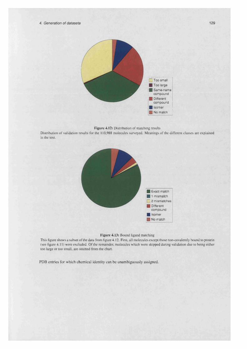
4. Generation of datasets 129

I

□ Too small

| Too large

| S a m e -n a m e com pound

| D ifferent com pound

| Isom er

I N o m atch

Figure 4.12: Distribution of matching results Distribution of validation results for the 110,988 molecules surveyed. Meanings of the different classes are explained in the text.

■ Exact m atch

■ 1 m ism atch

□ 2 m ism atches

■ D ifferent com pound

■ Isom er

■ No m atch

Figure 4.13: Bound ligand matching This figure shows a subset of the data from figure 4.12. First, all molecules except those non-covalently bound to protein (see figure 4.11) were excluded. Of the remainder, molecules which were skipped during validation due to being either too large or too small, are omitted from the chart.

PDB entries for which chemical identity can be unambiguously assigned.

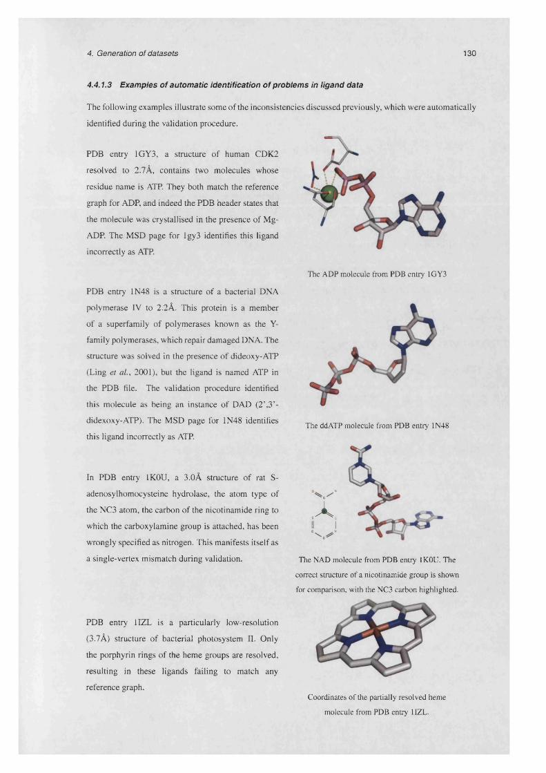
4. Generation of datasets 130

4.4.1.3 Examples o f automatic identification o f problems in ligand data

The following examples illustrate some of the inconsistencies discussed previously, which were automatically

identified during the validation procedure.

PDB entry 1GY3, a structure of human CDK2

resolved to 2.7A, contains two molecules whose

residue name is ATP. They both match the reference

graph for ADP, and indeed the PDB header states that

the molecule was crystallised in the presence of Mg-

ADP. The MSD page for lgy3 identifies this ligand

incorrectly as ATP.

The ADP molecule from PDB entry 1GY3

PDB entry 1N48 is a structure of a bacterial DNA

polymerase IV to 2.2A. This protein is a member

of a superfamily of polymerases known as the Y-

family polymerases, which repair damaged DNA. The

structure was solved in the presence of dideoxy-ATP

(Ling et al., 2001), but the ligand is named ATP in

the PDB file. The validation procedure identified

this molecule as being an instance of DAD (2’,3’-

didexoxy-ATP). The MSD page for 1N48 identifies

this ligand incorrectly as ATP.

In PDB entry 1K0U, a 3.0A structure of rat S-

adenosylhomocysteine hydrolase, the atom type of

the NC3 atom, the carbon of the nicotinamide ring to

which the carboxylamine group is attached, has been

wrongly specified as nitrogen. This manifests itself as

a single-vertex mismatch during validation.

PDB entry 1IZL is a particularly low-resolution

(3.1 A) structure of bacterial photosystem II. Only

the porphyrin rings of the heme groups are resolved,

resulting in these ligands failing to match any

reference graph.Coordinates of the partially resolved heme

molecule from PDB entry 1IZL.

A.II I

The NAD molecule from PDB entry 1K0U. The

correct structure of a nicotinamide group is shown

for comparison, with the NC3 carbon highlighted.

The ddATP molecule from PDB entry 1N48

4. Generation of datasets 131

Of the four examples shown above, three come from structures of fairly poor quality, and could therefore

be excluded by simply applying a threshold to the resolution of structures which are accepted for further

analysis. However, the method shown here is more generic, and is capable of detecting problems, for example

due to human error, which may still occur even where the crystallographic data itself is of a high standard.

4.4.1.4 The most common ligand types

The compounds which are most commonly found in complex with proteins are shown in figure 4.14. For

each compound, the number of validated instances in the PDB are shown, along with the number of distinct

PDB entries in which those instances were observed. The 20 most frequently observed molecules essentially

consist of the most common biological cofactors (HEM, NAD(P), ADP, ATP, FAD, FMN) and widely used

crystallisation buffer ingredients (P04, DMS, EDO, FMT, TRS). Other molecules of biological interest are

less frequently found, for example the guanosine nucleotides GDP (235 instances in 143 PDB entries), acetyl

co-enzyme A (180/58) and GTP (122/46).

It should be remembered, however, that these counts simply reflect the number of times in which a given

molecule has been co-crystallised with a protein. As such, they are influenced by the non-uniformity in the

number of structures for a given protein family which have been deposited in the PDB. The prevalence of

heme structures is an illustration of this: partly as a result of its historical status, myoglobin and the related

protein hemoglobin have been heavily studied, resulting in a somewhat disproportionate number of their

structures being present in the database.

2500

2000

» 1500o c CD 3S' 1000

LL

500

0

Blue bars indicate the number of instances of molecules which matched exactly to the reference graphs shown. Green bars represent the number of distinct PDB entries in which the matching molecules were found. The common names corresponding to the RCSB compound identifiers shown here are given in table 4.3. Note that the top two most commonly-occurring molecules, S04 (sulphate ion, 11,867 instances) and GOL (glycerol, 3692 instances) have been omitted for clarity.

In s ta n c e s

P D B en tries

uO I “ O C L > - Q O Q - l -q O < Q O C L < | - 2l u < Z < < ^ Lj- < u _

R C S B c o m p o u n d iden tifie r

Figure 4.14: Most commonly-occurring hetgroups in the PDB

4. Generation of datasets 132

RCSB identifier Common name_________________________ Likely biological ligand?

ACT Acetate ion ★ACY Acetic acid *ADP Adenosine diphosphateANP Phosphoaminophosphonic acid-adenylate ester /ATP Adenosine triphosphate SCOA Coenzyme A SDMS Dimethyl sulfoxide X

EDO 1,2-ethanediol X

FAD Flavin adenine dinucleotide SFMN Flavin mononucleotide SFMT Formic acid X

GDP Guanosine diphosphate SGTP Guanosine triphosphate SGLC Glucose SHEC Heme c SHEM Hemeb sMPD 2-methyl-2,4-pentanediol X

NAD Nicotinamide adenine dinucleotide SNAP Nicotinamide adenine dinucleotide phosphate SP04 Phosphate ion ★TRS 2-amino-2-hydroxymethy 1-propane-1,3-diol X

Table 43: Common names corresponding to selected RCSB compound identifiers Molecules most likely to be biological ligands were identified by manual inspection, and are indicated using the following symbols:(x) most instances in crystal structures are probably experimental artefacts.(*) some instances may be biologically relevant; others are probably due to crystallisation conditions.(vO most instances are likely to be the true biological ligand, or at least a close analogue of it.

4.4.2 Distribution of ligand types with respect to sequence and structure families

In order to gain a fairer picture of the distribution of different ligand types for which we have structural

information, it is useful to enumerate the different protein folds, superfamilies and sequence families which

interact with each type of compound. This is not intended to give a definitive picture of the relative occurrence

of different molecules in metabolism, physiology or biological catalysis. Rather, it simply aims to provide a

measure of the diversity, in evolutionary terms, of the structural data currently available for studies of ligand

binding.

A ContactTable archive was built using CATH version 2.6.0; the data presented here were obtained simply by

querying the MatchTable and ContactTable archives, and processing the results with Perl (Wall et al., 2000)

scripts in order to generate summary statistics.

4.4.2.1 Evolutionary diversity of proteins binding each iigand type

Figure 4.15 shows the distribution of the number of different protein folds which interact with each type

of ligand. These counts represent the number of distinct CATH numbers, up to the topology level, among

domains which contact the ligands. The majority of ligands (77%) bind either to just one fold (33% of all

compounds), or two different folds3 (40%). The number of compounds which are found in partnership with

a large number of folds is very restricted: 107 compounds (2.2%) bind to more than 10 folds, 40 compounds

3To clarify, this is based simply on an enumeration of the number of different folds among all domains which contact the ligand in different structures; therefore these counts may represent ligands which are bound at a domain interface, or may be due to ligands which interact with one fold in one protein, and a different fold in another.

4. Generation of datasets

(0.8%) to more than 20 folds and only 25 compounds (0.5%) to more than 30.

133

2000

1 5 0 0

COO)0 10001E

5 0 0

5 6 7N u m b e r of folds

10 11 +

Figure 4.15: Distribution of numbers of distinct folds binding each ligand type The chart shows the distribution of the number of distinct ligand types bound to each fold (Le. to domains belonging to each CATH topology).

This is not a surprising result, since many of the compounds in the reference set are substrates specific to one

or just a few enzymes, and hence would only be expected to bind to a limited number of folds. Conversely,

the ubiquitous cofactors - which we expect to interact with a diverse set of proteins - make up only a small

subset of the compound set. In order to quantify the degree of promiscuity of these common ligands, the

number of protein families, superfamilies and folds with which each compound interacts was determined.

This data is shown in figure 4.16. Compounds which were deemed by manual inspection unlikely to be

biologically relevant ligands (see table 4.3) were excluded from the plot.

1 80■ S 3 5

■ H

□ T

160

w 140Q3| 120ca> 100a)T3O

CD-QE=3z

CLa o<

a<LL

CLI— CLZ

CL<

o a.QLU

R C S B co m p o u n d identifier

Figure 4.16: Ligands which bind to the most evolutionary diverse proteins The twelve biological ligands which bind to the largest number of sequence families (CATH S35 families) are plotted. Also shown for each ligand is the number of distinct folds and homologous superfamilies to which it binds.

4. Generation of datasets 134

Comparing figures 4.14 and 4.16, it is unsurprising to see the compounds which ranked highest in terms of

the raw counts of their occurrences in the PDB, also appear near the top of the list of compounds ordered by

the number of protein families with which they interact. The adenosine nucleotides all rank much higher in

terms of numbers of families which bind them, however, than in the list of occurrences (figure 4.14). The

fact that the top-ranking compound in the non-redundant list (figure 4.16) is an adenosine nucleotide reflects

the key role of ATP as the universal energy carrier in the cell. Similarly, the guanosine nucleotides, which

also play a wide variety of cellular roles, are promoted once the redundancy present among PDB proteins is

eliminated.

For both the adenosine and guanosine nucleotides, the diphosphate compound is more common than the

triphosphate. This may not be an accurate reflection of the distribution of proteins for which the cognate

ligand is, for example, ADP rather than ATP. Rather, it is likely that, during crystallisation of a protein which

naturally recognises ATP, ADP has been supplied in the crystallisation liqor for experimental reasons.

Overall, the ratios of the numbers of families, superfamilies and folds which bind each compound are roughly

constant over the common ligands shown here. The ratio between numbers of superfamilies and numbers

of folds per ligand ranges between 1.05 (for HEM) and 1.44 (FMN). The ratio between numbers of families

and numbers of superfamilies, on the other hand, is more variable; this is to be expected, since the number

of families within each CATH superfamily varies considerably. The ligand with the minimum value of this

ratio is AMP (1.7), while the three ligands with the highest value for this ratio are the redox cofactors NAD

(4.15), NADP (3.45) and FAD (3.53).

The fact that these three cofactors bind proteins which exhibit the greatest sequence diversity per superfamily

may be rationalised on the basis that the biological role of these ligands - namely, facilitating the

oxidation/dehydrogenation of substrates - is fairly limited. The range of substrates which are modified by

NAD(P) or FAD-dependent oxidoreductases, on the other hand, is extremely broad. We know that evolution

of new substrate specificity while conserving the reaction often occurs through sequence divergence up

to, but not beyond the point where fold also changes: see e.g. Hegyi and Gerstein (1999), Wilson et al.

(2000), Todd et al. (2001). It is not surprising, therefore, that while relatively few folds have evolved to bind

these cofactors, the diversity in terms of the number of sequence families within each of the fold groups is

considerably larger.

4.4.2.2 Diversity of ligands binding each protein fold

Having assessed the evolutionary diversity of proteins binding each ligand, we now consider the inverse

question: how many different types of ligand are bound by each fold? Figure 4.17 shows the protein folds

which are most promiscuous in terms of the number of compounds with which they are partnered.

The first observation to make is that the numbers of small-molecule species found to interact with each

fold type are surprisingly high. There are two reasons for this. Firstly, these counts include all compounds

from the set of 56,231 molecules described in §4.4.1.2, and hence contain crystallisation artefacts as well as

cognate ligands. As a result, a proportion of the counts shown here are due to a given fold being crystallised

in the presence of different solvents, rather than due to it interacting with different ligands in vivo.

4. Generation of datasets 135

800

T 3CcuO)

<DjQE=3z

Ii ■IIl l l m n

o■M-d

occCDEinC/3OCC

o oCM T—

o oCM •M-

co CM

"(D CLq

CD E_o o-C

1- H

CM

CD

_ooO)oc3EE

o•M-CM,Qc

'</>ClCD£00O

OC*5CO

JDCLffl1_Q

CO.cQ.<

OCDCM

Oino

= </)

OK «® Ccoo£5.COo-C0.

ooCMdCOCO

COcjcCDco

JO

£*o

oJZ0.

ocod'D'CO

CDco2CD

ECO0)■cCOCL

Figure 4.17: Most promiscuous folds The protein folds which bind to the largest number of distinct ligand types are shown. For each, the CATH code up to the third level is given in parentheses.

The second reason is that the set of molecules which comprise the reference compound dictionary are not

uniformly distributed in chemical space. That is to say, the compound set contains molecules which are

very similar to one another (stereoisomers, and compounds which differ by minor substitutions of functional

groups), as well as molecules which are very dissimilar. As a result, the fact that a given fold binds many

different compounds does not necessarily imply a capability to interact with ligands which are chemically

diverse. While these caveats diminish the meaning of the absolute values of the counts plotted here, it is still

useful to discuss their relative magnitudes. It should be stressed, however, that what follows is a discussion of

the relative occurrence of particular domain-ligand interactions in the PDB rather than in biology as a whole.

Considering the ten folds shown in figure 4.17, we see that five of them (the Rossmann fold, the TIM barrel,

the immunoglobulin-like proteins, the a(3-plaits, and the jelly rolls) belong to the set of nine ‘superfolds’

which were identified more than a decade ago (Orengo et al., 1994). Superfolds are defined as those which

recur in proteins having neither sequence nor functional similarity4.

4Since the publication of the original paper, the OB (oligonucleotide binding) fold has been added to this list, with eleven other CATH topologies currently proposed as potential superfolds (Orengo et al., 1997).

1.10.510Phosphotransferase (1:144)

3.40.640Aspartate aminotransferase (1:95)

3.40.50Rossmann (doubly wound) fold (92:775)

3.30.200 Phosphorylase kinase (1:143)

3.30.Alpha/beta plait (47:155)

2.40.10Thrombin (3:300)

2.40.70Cathepsin D (1:189)

2.60.40Immunoglobulin (64:260)

3.20.20 TIM barrel (21:403)

SRffc 2'60-120Jelly roll (21:150)

11. mainly alpha |2 . mainly beta 3. alpha / beta

14. few secondary structures

Figure 4.18: Most promiscuous folds compared with distribution of folds in protein space The ten most promiscuous folds, in term of the number of compounds which they bind, are shown. The CATH wheel shows the relative populations of the first three levels (class, architecture, topology) of version 2.6.0 of the hierarchy: the size of the segment for each topology (in the outermost ring) is proportional to the number of homologous superfamilies which adopt that fold. Folds whose name is shown in red are those which have been identified as superfolds. Numbers in parentheses indicate, respectively the number of homologous superfamilies which adopt each fold, and the number of distinct ligands which are bound to domains with this fold. The colour of each segment corresponds to the CATH class, as shown in the key.

4. Generation of datasets

136

4. Generation of datasets 137

The evolutionary reasons for such widespread occurrence of certain folds in nature has been discussed

extensively in the literature. The prevailing view is that, in most cases, proteins which share a common

fold originated from a common ancestor; those structures which are for some reason particularly resilient

to mutational changes without loss of stability therefore allow functional divergence to occur, whilst

maintaining the same fold. An alternative hypothesis is that of convergent evolution - that is, the evolution of

disparate sequences with no common ancestor to arrive at the same structure and/or function. If this were the

case, then we may expect structural motifs which fold via fairly simply pathways, to occur more frequently.

In either case, intrinsic structural stability would appear to be one likely explanation for the prevalence of the

superfolds.

Figure 4.18 illustrates the relative occurrences in the CATH database of the ten folds which bind the largest

numbers of compounds. The biological reasons for this promiscuity can be understood in some cases by

considering the roles which proteins adopting each of these folds tend to play.

The Rossmann fold is the most highly populated of the a /3 folds. It functions as a nucleotide binding

domain, and is utilised in many oxidoreductases for recognition of the cofactor. Although it does not perform

any catalysis, the fact that the NAD cofactor is bound quite deeply within it, with only the nicotinamide

portion protruding to meet the catalytic partner domain (Bashton and Chothia, 2002), means that substrate

molecules frequently contact the Rossmann domain as well as the catalytic unit. Since dehydrogenases act on

a wide range of substrates, this accounts for the large number of molecules which are classified as interacting

with Rossmann fold domains.

The TIM barrel fold is the most widely observed of all in crystal structures, the third most populous a /3

fold, and it has been estimated that around 10% of all enzymes adopt it (Copley and Bork, 2000). Its

usefulness as an enzymatic scaffold is illustrated by the fact that TIM barrels are associated with some

16 different EC numbers (Nagano et al., 1999). Furthermore, several experiments have demonstrated that

the catalytic function of enzymes with this fold can be successfully altered using directed evolution (Jurgens

et a l, 2000, Altamirano et al., 2000). It is therefore not surprising that it is found in complex with such a

large number of ligand types.

The thrombin fold is named after the protein in which it was first discovered, a serine protease which initiates

blood clotting in response to wound signals by cleaving the fibrinogen protein to release a rapidly aggregating

peptide (Creighton, 1993). Several other common serine proteases, including the digestive enzymes trypsin,

chymotrypsin and elastase share this fold. Each of these, although catalysing a similar endopeptidase

reaction, has a different substrate specificity, with chymotrypsin cleaving peptide bonds flanked by bulky

hydrophobic residues, trypsin cleaving bonds flanked with positively charged amino acids and elastase acting

on peptide bonds between small, neutral residues (Hedstrom, 2002). Besides these preferences, however,

these enzymes are not specific for particular peptide sequences; this is a necessary characteristic given their

role in breaking down a wide range of foodstuffs, and indeed necessitates the protection of the enzyme from

autodigestion, by producing it as an inactive precursor which is only set in action once it reaches the stomach.

A number of proteins with thrombin folds are drug targets, explaining their high prevalence in the PDB.

4. Generation of datasets 138

The immunoglobulin fold was initially identified in proteins involved in the immune system, has since

been observed in extracellular domains recognising a wide variety of ligands including small molecules

(in the case of Fab proteins), peptides (MHC/HLA), DNA (the p53 DNA-binding domain) and other

proteins (components of the extracellular matrix) (Bork et al., 1994, and references therein). Among

P folds, it contains the highest number of homologous superfamilies (64). Despite their broad-ranging

substrate specificity, immunoglobulin-like domains do not appear to be directly involved in catalysis; no

immunoglobulin fold domain is known to contain a naturally-present enzymatic active site. In the classical

immunoglobulin G protein, ligand binding is mediated by loops which, due to high levels of recombination in

the gene which encodes them (Tonegawa, 1983), exhibit a large amount of structural diversity. The majority

of immunoglobulin-like domains, on the other hand, tend to interact with ligands via their (3-sheets (Bork

etal., 1994).

The cathepsin D fold contains only one superfamily of aspartic proteases. These enzymes, involved in the

catabolism of cartilage and connective tissue, have a similar substrate specificity to chymotrypsin (Barrett,

1977). As with the other proteases, cathepsin D folds are found in complex with a large number of different

small peptides, which are classified as ligands in the MSD compound set. Like thrombin, several cathepsin

D proteins are of particular pharmaceutical interest, meaning that they have been crystallised repeatedly with

subtly different substrates.

a/(3-plaits perform nucleotide binding functions in a wide variety of proteins ranging from the RNA-

binding domains of various ribonucleoproteins, through viral DNA-binding proteins to ribosomal protein

L3, which binds the 23S rRNA and may participate in the formation of the peptidyltransferase center of the

ribosome (Orengo and Thornton, 1993). It is the third-most highly populated fold in CATH, following the

Rossmann and TIM barrel folds. Inspection of the list of ligands which it binds shows that a large fraction

are nucleotides, or nucleotide derivatives.

The jelly roll fold consists of two ‘greek key’ motifs linked by two connecting loops. It is found in a

wide variety of proteins, including carbohydrate binding proteins, spherical virus coat proteins, influenza

hemagluttinin and tumour necrotic factor. These are found in 21 distinct superfamilies. The ligands to which

it is bound in the PDB are primarily carbohydrates.

The phosphotransferase and aspartate aminotransferase folds, like the cathepsin D proteins, are both

singlets, i.e. they each consist of just one large superfamily. In the case of the phosphotransferase domain, it

is partnered with a phosphorylase kinase domain. Aspartate aminotransferases catalyse the reversible transfer

of the amino group from an amino acid to a 2-keto acid, using pyridoxal 5’-phosphate as a cofactor (Stryer,

1995). In contrast to many enzymes such as the proteases discussed previously, the aminotransferases react

with both acidic substrates such as aspartate and glutamate, and neutral amino acids.

Overall, therefore, there appear to be three main reasons for ligand promiscuity in protein folds. The first

is that certain folds are utilised by proteins with very diverse functions. This is the case for TIM barrels,

and to a lesser extent, immunoglobulin folds and jelly rolls. In such cases, large evolutionary expansion of

the superfamily has provided numerous opportunities for functional diversification. The reasons why this is

4. Generation of datasets 139

observed to such a large extent for some folds, and less so for others, are still not fully understood.

Another reason may be that the substrate specificity for a given protein is quite broad, resulting in many

structures being present in the PDB, each crystallised with a slightly different partner. This is the case

for many proteins which act on biopolymers, e.g. proteases and enzymes which catalyse modifications to

DNA or RNA. The third reason is that protein families which are of particular biological interest are often

deliberately crystallised many times with different substrates. This is particularly the case for drug targets.

The over-representation of a particular fold in the PDB may be to one or a combination of these reasons: for

example, the cathepsin D proteins are present in high numbers, probably due to both the second and third

reasons given here.

4.4.2.3 Occurrence o f multi-domain binding sites

In order to assess the frequency with which binding sites occur at domain interfaces, the number of domains

contacting each ligand in the dataset was counted. Overall, 74% of binding sites were composed entirely

from a single domain, with the remaining 26% consisting of residues from two or more domains. It is

interesting to compare the proportion of multi-domain binding sites with the results of a previous study of a

non-homologous set of 178 catalytic sites, which found that in all but 35 cases (20%), the entire complement

of catalytic residues belongs to just a single domain (Bartlett et al., 2002). The fact that the fraction of multi­

domain binding sites is slightly larger than the fraction of multi-domain active sites is largely a product of

the strict criteria which the authors used to define catalytic residues; this results in active sites consisting of a

small number of closely-positioned residues.

» 0.3

S 0.1

A*P G*P COA GLC FAD FMN NAD NAP HEM

RCSB compound identifier

Figure 4.19: Fraction of binding sites for each ligand type composed of more than one domain For each of the most common ligand types, the fraction of all binding sites which are comprised of more than one CATH domain is shown. Ligands ATP, ADP and AMP are collected together and plotted as A*T; guanosine nucleotides are similarly grouped as G*P.

4. Generation of datasets 140

Given both the differing sizes and diverse biological roles of different ligand types, however, this distribution

would not be expected to be uniform across all compounds. Figure 4.19 shows the distribution of single-

and multi-domain binding sites for several common ligands. The high frequency of multidomain binding

sites for the redox cofactors NAD and FAD is not surprising given the tendency of proteins which bind them

to have independent cofactor recognition and catalytic domains. Conversely, the common heme-binding

proteins (hemoglobin, myoglobin, the cytochromes, and catalase) all bind the cofactor entirely within a

single domain. The tendency of guanosine nucleotides to interact with only one domain is to be expected

given their common role as signalling molecules that often bind to a single receptor domain, which in turn

conveys the message to other effector domains within the protein. As the smallest molecule in this set, it

is not surprising that glucose tends to interact with only one domain at a time. The reason for the striking

difference between the fraction of FAD binding sites which contain more than one domain, and those for

FMN, may simply be the difference in size between the two molecules.

4.4.3 Distribution of ligand types with respect to enzyme function

In order to obtain a general picture of the functional diversity of proteins which bind each type of compound,

the fraction of each set which are annotated as enzymes was calculated. This was done by querying the

MSD to obtain Enzyme Commission (EC) numbers for each protein chain which forms part of an enzyme.

The MSD acquires this information by first searching each protein chain against the SWISS-PROT protein

sequence database (Boeckmann et a l, 2003). The latter is a manually curated database which, for many

proteins, contains extensive biological annotation including enzyme function. For every match to a SWISS-

PROT sequence which is annotated with an EC number, this annotation can be transferred to the appropriate

PDB chain(s), and hence to PDB entries. The SQL statement used to perform this query was as follows:

SELECT UNIQUE pdb.accession_code, swiss.chain_pdb_code, ec.ec_number FROM entry pdb, swiss_prot_mapping swiss, ec_mapping ec WHERE swiss.entry_id = pdb.entry_id AND ec.molecule_id = swiss.molecule_id;

The EC classification is a hierarchical system consisting of four levels; the meaning of each of these levels is

shown in table 4.4. The level up to which two EC numbers are identical represents, to a first approximation,

the degree of similarity between the two reactions concerned.

First digit (class) Reaction type Second digit Third digit

1 (Oxidoreductases)

2 (Transferases)

3 (Hydrolases)

4 (Lyases)

5 (Isomerases)

6 (Ligases)

Oxidation / ReductionTransfer of a group between substrates

Bond cleavage by hydrolysis

Bond cleavage by elimination Transfer of groups within a moleculeBond formation coupled to ATP hydrolysis

Substrate acted upon Description of the transferred group

Bond type being hydrolysed

Bond type being broken TVpe of isomerism

Bond type being formed

Type of AcceptorMore information about the group

Type of substrate

Type of group eliminated Type of substrate

Type of compound formed

Table 4.4: Levels of the Enzyme Commission hierarchy The meanings of the second and third digits of the EC classification vary according to the reaction class (the first digit). The fourth digit indicates a particular reaction.

4. Generation of datasets 141

Figure 4.20 shows the fraction of proteins binding each of the common ligands which were annotated with

one or more EC number. The one unusual result is the low proportion of coenzyme A-binding proteins which

were associated with an EC number. Manual inspection of several such proteins which were clearly enzymes

- including some annotated as such in the PDB header records - showed that the MSD enzyme annotation

protocol did not assign EC numbers to these proteins. As a result, the numbers shown here may underestimate

the true number of enzymes which bind each ligand.

O <D

CD Q

A*P G*P COA GLC FAD FMN NAD NAP HEM

RCSB compound identifier

Figure 4.20: Fraction of proteins binding each ligand type which are annotated with enzyme functions Enzyme function annotations were obtained from the MSD as described in the text. Ligands ATP, ADP and AMP are collected together and plotted as A*T; guanosine nucleotides are similarly grouped as G*P.

NAD ADP FAD ATP NAP AMP NDP HEM FMN COA

RCSB compound identifier

Figure 4.21: Ligands whose binding proteins have the widest range of enzyme functions The ten ligands which bind to proteins with the largest range of EC numbers to the third level are plotted. Also shown for each ligand is the number of distinct EC numbers to the second and third levels, among the proteins to which it binds.

4. Generation of datasets 142

The range of functions catalysed by the enzymes discovered in the previous step was assessed by plotting

the number of distinct EC numbers associated with each ligand, up to the second, third and fourth levels

(see figure 4.21). Once again, the compounds whose proteins have the widest range of enzyme functions are

the expected common biological ligands. It is interesting to note that while there is a considerable range in

diversity at the fourth EC position among the ten ligands shown, the range of different numbers to the second

and third levels is significantly less pronounced. This suggests that, for cofactors such as NAD, ATP and

FAD, there are numerous enzymes which catalyse very similar reactions, whereas for coenzyme A, where

the number of distinct EC numbers to the fourth level is only just over twice the number to the third level, the

number of enzymes which have evolved to perform similar functions is much fewer. A more detailed analysis

of the particular EC numbers associated with several key ligands is presented in the following section.

4.5 Datasets of ligands of particular biological interest

The ligands ATP, GTP, NAD and FAD were chosen for further analysis (see figure 1.2); for each, non-

homologous datasets were generated using the clustering protocol described in §4.2. Details of the results of

this clustering are tabulated in appendix D. Henceforth, the list of sites presented in tables D.1-D.4 will be

referred to simply as ‘the ligand dataset’, and the numbers shown in the first column of those tables will be

used to refer to the different third-level clusters for each ligand type. The domain composition of the binding

sites in the largest clusters, and the functions of the associated proteins, are summarised in table 4.5.

There is large variance in the amount of functional diversity found among proteins within each cluster: the

group with the widest range of functions are the ATP-binding proteins in the first cluster (P-loop containing

NTP-hydrolyase domains), which are associated with four different primary EC numbers (IUPAC-IUB,

1983). The group of Rossmann-fold NAD-binding oxidoreductases, on the other hand, all catalyse similar

types of reaction, but act on a wide range of substrates. Moving to smaller clusters, we find some which

perform extremely specialised functions, such as the tRNA synthetases in ATP cluster 4, all of which

catalyse the transfer of a particular amino acid onto the appropriate tRNA molecule. This group contains

five members, each of which acts on a different amino acid type, and which, while sharing the same overall

fold, exhibit only very low sequence similarity to one another.

4.5.1 Analysis of the clustering

4.5.2 Distribution of folds and superfamilies binding each ligand type

Figure 4.22 shows CATH wheels representing the distribution of different folds and superfamilies which

interact with each of the four ligands considered here. For each site in the ligand dataset, the domain which

contributes the largest fraction of the binding residues is determined. For example, site 1RDQ/a /a t p . 600/b,

the representative for cluster 2 in the ATP dataset, consists of two domains - a phosphotransferase domain

(CATH code 1.10.510.10) which contributes about a third of the binding residues, and a phosphorylase kinase

domain (3.30.200.20) making up the remaining two thirds. In this case, the phosphorylase kinase domain is

identified as the majority partner.

4. Generation of datasets 143

Ligand Cluster Size Rep Domains Functions

1 22 1E2Q 3.40.50.300 P-loop containing nucleotide triphosphate hydrolases

Various

ATP 2 9 1RDQ3.30.200.20

1.10.510.10

Phosphorylase Kinase domain 1Transferase (Phosphotransferase) domain 1

Kinases

3 9 1MJH 3.40.50.620 Rossman fold ligase domain Ligases; transferases

4 5 1B8A 3.30.930.10 Bira Bifunctional Protein domain 2 tRNA synthetases

5 3 1KJ83.30.470.20

3.30.1490.20

ATP grasp fold domain B Formyltransferase; synapsin 1; biotin carboxylase

6 3 1GZ4 3.40.50.720 NAD(P)-binding Rossmann-like Malic enzyme; molybdopterin synthesis

GTP 1 6 1QRA 3.40.50.300 P-loop containing nucleotide triphosphate hydrolases

Signal proteins

NAD

1 54 1T2D 3.40.50.720* Rossmann Various oxidoreductases; UDP-glucose 4-epimerase

2 4 10043.40.605.10

3.40.309.10

Aldehyde Dehydrogenase domain 1

Aldehyde Dehydrogenase domain 2

Aldehyde dehydrogenase; Glyceraldehyde 3-phosphate dehydrogenase

3 4 1NUU 3.40.50.620 Rossmann fold ligase domain Adenylyltransferases

4 4 1LW7 3.50.50.60 FAD/NAD(P)-binding domainGlutathione reductase; ferredoxin reductase; NADH peroxidase; Dihydrolipamide reductase

5 4 1GIQ 2.30.100.10 Toxin ADP-ribosyltransferase ADP-ribosyltransferases

1 19 3GRS 3.50.50.60 FAD/NAD(P)-binding domain Various oxidoreductases

FAD2 9 1GAW

2.40.30.10

3.40.50.80

Translation factors

Nucleotide-binding domain

Ferredoxin-NADP+ reductase; cytochrome reductase; nitric oxide synthase

3 5 1N623.30.465.10

3.30.43.10

UridineDiphospho-n-acetylenolpyruvylglucosamine Reductase domains

Carbon monoxide dehydrogenase; nucleotide metabolism oxidoreductases

4 5 1LQT 3.40.50.720 RossmannFPRA;dihyropyrimidine dehydrogenase; D-amino acid oxidase

5 3 1E8G3.30.465.20

3.30.43.10

UridineDiphospho-n-acetylenolpyruvylglucosamine Reductase domains

Vanillyl-alcohol oxidase; cholesterol oxidase; D-lactate dehydrogenase

6 3 1IQR1.10.579.10

1.25.40.80

DNA Cyclobutane Dipyrimidine Photolyase domain 3

DNA photolyase

Table 4.5: Summary of the ligand datasets For each cluster with three or more members, ‘size’ indicates the number of members, and ‘rep’ is the PDB entry ID of the cluster representative. The homologous superfamily level annotations of domains making up the binding sites in each cluster are shown along with their associated CATH numbers. Where the proteins in a cluster have a small range of functions, these are listed; in other cases, the range of functions is too large to list here. See appendix D for a more detailed version of this table.(*) this domain binds the cofactor in partnership with other domains.

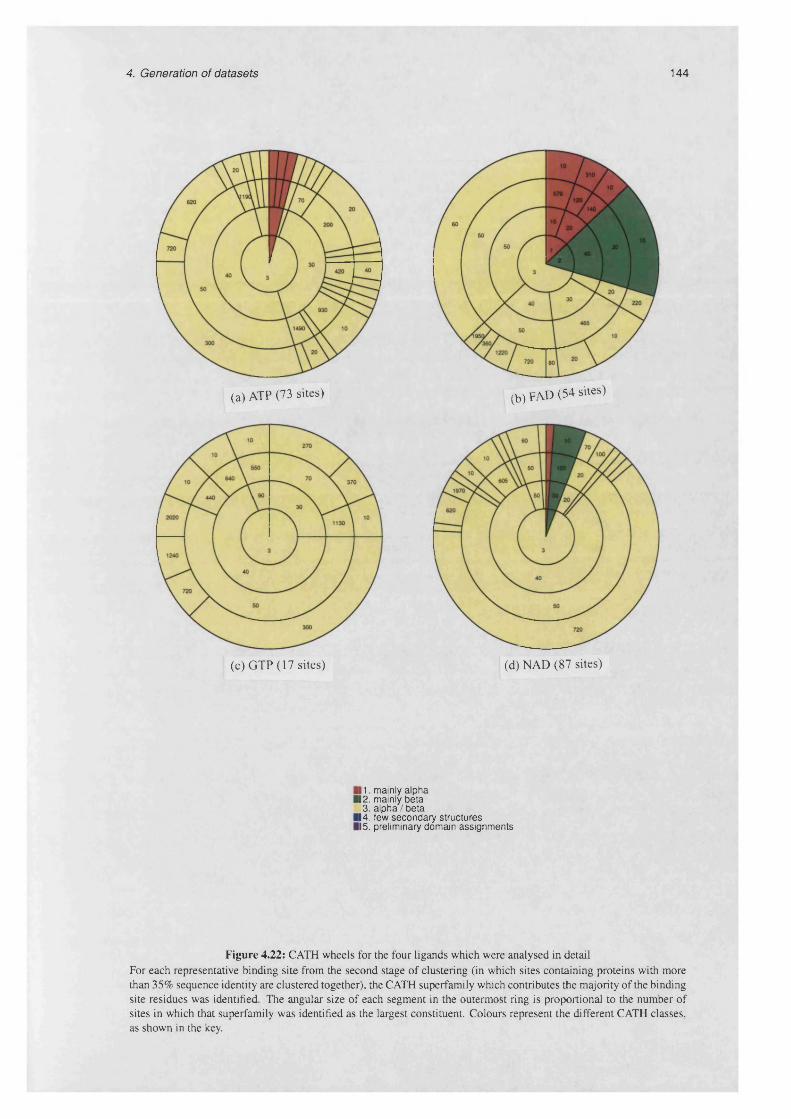
4. Generation of datasets 144

(a) ATP (73 sites) (b) F A D (54 sites)

(c) GTP (17 sites) (d) NAD (87 sites)

11. m ainly a lpha12. mainly b e ta 3. a lp h a / b e ta

14. few seco n d a ry s tru c tu res15. prelim inary dom ain a ss ig n m en ts

Figure 4.22: CATH wheels for the four ligands which were analysed in detail For each representative binding site from the second stage of clustering (in which sites containing proteins with more than 35% sequence identity are clustered together), the CATH superfamily which contributes the majority of the binding site residues was identified. The angular size of each segment in the outermost ring is proportional to the number of sites in which that superfamily was identified as the largest constituent. Colours represent the different CATH classes, as shown in the key.

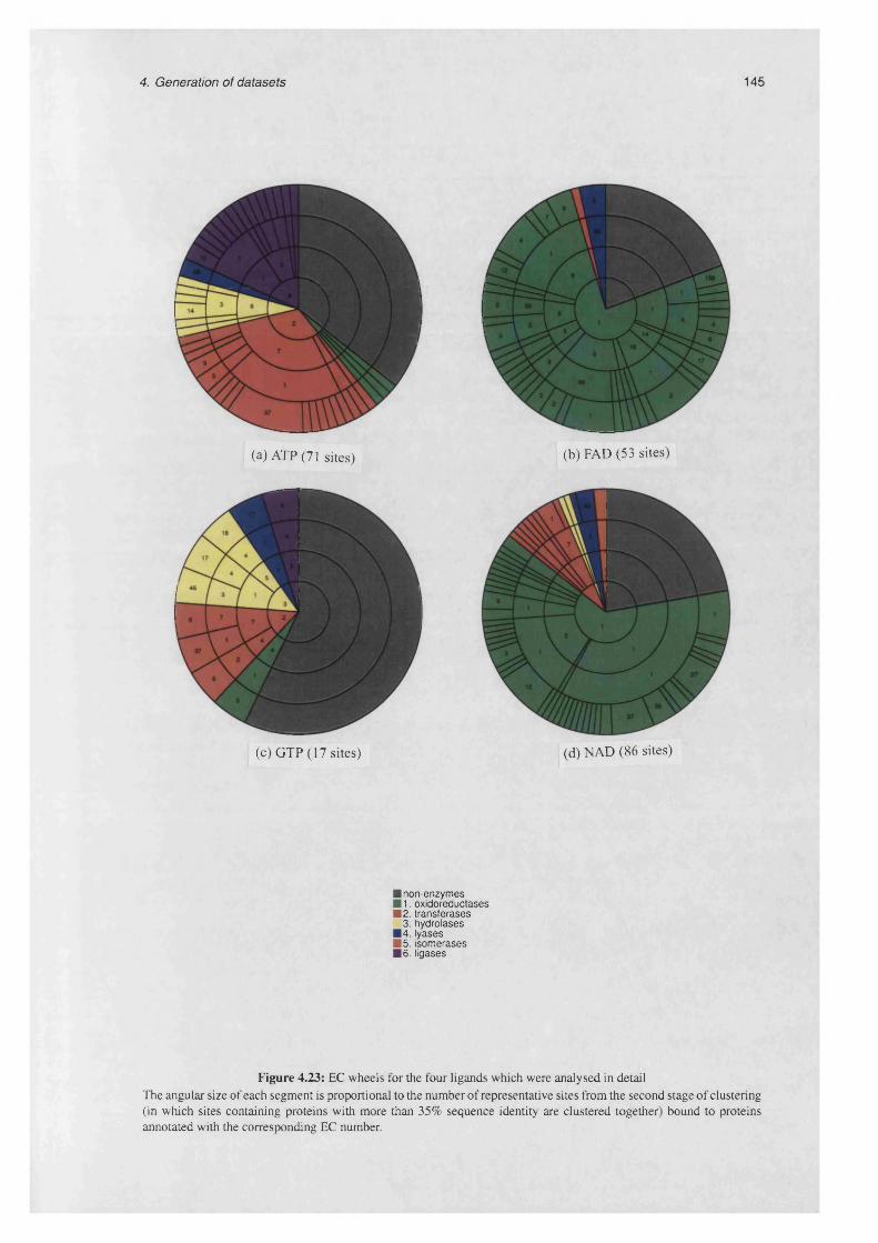
4. Generation of datasets 145

(a) ATP (71 sites) (b) FAD (53 sites)

(c) GTP (17 sites) (d) NAD (86 sites)

■ non-enzym es■ 1. oxidoreductases ■ 2 . transferases

3. hydrolases■ 4. lyases ■ 5 . isom erases ■ 6 . ligases

Figure 4.23: EC wheels for the four ligands which were analysed in detail The angular size of each segment is proportional to the number of representative sites from the second stage of clustering (in which sites containing proteins with more than 35% sequence identity are clustered together) bound to proteins annotated with the corresponding EC number.

4. Generation of datasets 146

■ non-enzymes■ 1. oxidoreductases■ 2. transferases

3. hydrolases■ 4. lyases■ 5. isomerases■ 6. ligases

(a) All CATH S35 representatives (b) CATH S35 representatives with EC numbers

Figure 4.24: EC wheels for the CATH S35 representatives

The CATH wheels represent the frequency of occurrence of each superfamily, counted in this way across all

sites in each ligand dataset. Most of the binding sites are composed of a /P fold domains; exceptions to these

patterns are quite rare: all GTP binding sites are composed of a /P domains, and for ATP, only two families

adopt an a-helical fold. These are the GroEL proteins (cluster 10) and the ribonucleotide reductases (cluster

24). Both of these clusters are singlets.

Of the four nucleotide derivatives, FAD exhibits the widest diversity in the fold types which bind it. Although

chiefly recognised by a /P domains, three FAD clusters belong to other classes. Sites in cluster 2, a diverse

group originating from cytochromes and various oxidoreductases, bind the cofactor inside P-sheet domains

belonging to the ‘translation factor’ superfamily (2.40.30.10). Two smaller clusters recognise FAD using

a-helical folds: cluster 6, which contains three families of photolyase enzymes; and cluster 7, containing two

short-chain dehydrogenases.

The degree of fold diversity in NAD binding sites is intermediate between those in the ATP and FAD datasets.

The canonical NAD recognition motif is a P-sheet sandwiched between pairs of a-helices. The NAD

molecule binds in a crevice formed at the ‘switch point’ of the P-sheet, where it is stabilised by interactions

with the a-helical dipoles (Lesk, 1995). There are, however, other a /P folds which bind NAD, notably the

a /P barrels (CATH architecture 3.20) found in the inosine-monophosphate dehydrogenases (cluster 7) and

reductases acting on monosaccharides and the acids which are formed by their oxidation (cluster 8). There are

two exceptions to the dominance of the a /P domains in the NAD dataset. Cluster 5 contains four families of

ribosyltransferases, in which the NAD-binding domain is a P-sheet structure (2.30.100.10). Citrate synthase

proteins (cluster 18), which fall into a single family, utilise an all-a-helical fold (1.10.580.10) for cofactor

binding.

4. Generation of datasets 147

4.5.3 Distribution of enzyme functions among proteins binding each ligand type

Figure 4.23 shows EC wheels for each of the four ligand types. For each site in the dataset, annotation of

enzyme function, where available, was obtained for its parent protein using the procedure described in §4.4.3.

The angular size of each segment of the EC wheel indicates the number of sites which belong to enzymes

catalysing the relevant reaction. In a few cases, the protein was assigned more than one EC number, for

example site 1K87/c/f a d .2001 is from a bifunctional protein which can catalyse both pyrroline-carboxylate

decarboxylation (EC number 1.5.1.12) and proline dehydrogenation (EC 1.5.99.8) reactions. These cases

are extremely rare (2, 0, 1 and 1 examples for ATP, GTP, NAD and FAD respectively), and therefore were

excluded from the analysis.

Figure 4.24 shows the distribution of enzyme functions among a non-homologous set of proteins. This set

was generated by first taking the representative domains for each CATH S35 family. The EC number(s)

associated with the parent protein of each domain were then plotted in the same way described above.

The most common enzyme functions for ATP-binding proteins reflect the chemistry most often performed

upon it, namely hydrolysis of diphosphate esters. The most common EC numbers are 2.7.- (transferases

transferring phosphate-containing groups), 6.1.- (ligases acting on C—O bonds), 3.6- (hydrolases acting on

acid anhydrides) and 6.3- (ligases acting on C—N bonds).

Unsurprisingly, the wheels for FAD and NAD are dominated by oxidoreductase functions. The overall range

of enzyme functions associated with GTP- and particularly ATP-binding proteins, on the other hand, is far

broader, with ATP-binding proteins catalysing several transferase, hydrolase and ligase reactions, as well as

a small number of oxidoreductase and lyase reactions.

4.6 Summary

In this chapter, automatic protocols for generating datasets of ligand binding sites have been described.

These protocols include methods for determining the chemical identity of ligand molecules from their atomic

coordinates, and a procedure for clustering binding sites based on relationships between the domains which

constitute each of them.

The ligand identification/validation procedure has been applied to all structures in the PDB. The results show

that several common biological ligands and cofactors are present in a large number of entries. The usefulness

of the graph matching methodology for checking ligand identities is demonstrated by several cases in which

ligands are mis-named in the PDB.

Analysis of the pairings of different protein folds and different ligand types shows that several of the folds

which are most promiscuous in terms of the set of compounds with which they interact, are those which have

been previously identified as occurring in many different protein superfamilies. Several promiscuous folds,

however, correspond to only a small number of families; in these cases, arguments based on the specific

functions of the proteins in these families can be invoked in order to explain their gregarious behaviour.

Due to biases affecting the selection of candidate proteins for crystallisation, as well as the compounds co­

4. Generation of datasets 148

crystallised with them, the data shown here should not be viewed as a direct reflection of the distribution

of cognate ligands with respect to different protein folds. A more careful analysis in which ligand-

protein interactions are checked for their biological relevance is currently under way (I. Nobeli, personal

communication), and should clarify the extent to which the findings here can be extrapolated to biology

as a whole. However, the fact that certain folds are capable of binding to such a large diversity of

compounds, albeit sometimes under unphysiological conditions, does suggest that broadly similar patterns

will be observed by more detailed analyses.

While the majority of ligand binding sites are composed of a single domain, the fraction of multi-domain

binding sites among ligands and cofactors of interest, which tend to be among the larger compounds

considered, is typically higher than average. This presents challenges for automated binding site clustering

based on domain annotation. The method described here overcomes these methods using heuristics which

appear to give reasonable clustering results.

Finally, datasets of binding sites for four ligands of particular interest were generated, and analysed both

in terms of the domains which contribute to them, and in terms of the enzymatic functions of the proteins

concerned. In the following two chapters, the structural properties of these binding sites will be investigated

in detail, firstly from the point of view of ligand conformation, and then focussing on the diversity of their

micro-environments.

149

Chapter 5

Conformational variability of bound

ligands

The shape of a molecule depends on two factors. The first is, naturally, the chemical structure of the

compound; that is, its complement of atoms and covalent bonds. As long as the molecule does not participate

in any chemical reactions, this remains unchanged, while the second - the set of torsion angles around each of

its ratable bonds - may vary dynamically through random thermal fluctuations, and as the molecule finds itself

in different physical environments. This chapter is concerned with analysing the different conformations

adopted by biological ligands. The variation in conformation is analysed first among ligands bound to

evolutionarily unrelated binding sites, and secondly among ligands whose sites are composed of domains

belonging to the same superfamily - that is, first between and then within the clusters defined as per §4.2.

The aims of this study are to understand whether a given pair of interacting molecules (protein and ligand)

always interact in the same way, and to what extent the different conformational states of the ligand are

accessible when interacting with evolutionarily unrelated proteins.

5.1 Rationale for studying ligand conformation

Although small in comparison to proteins, many biological ligands are capable of considerable

conformational variability. In the most abstract sense, the free energy landscape of a molecule with n ratable

bonds may be considered to be an n-dimensional function, which may be replete with peaks (energy barriers),

valleys (energy minima), and passes (saddle points). If we discretise this space by assuming that the Ith

bond may exist in just one of a small number jc,- of distinct, stable orientations, then the number of possible

conformations of the molecule as a whole is given by the product x\ x X2 x . .. x xn.

It is clear that the combinatorial effect of varying just a few ratable bonds leads to a large number of

possibilities: if we assume that any one ratable bond can exist in three distinct rotational states, then a

molecule with only ten such bonds can theoretically adopt 310 = 59,049 different conformations. Of course,

many of these will be physically impossible due to steric clashes between atoms. Still others may be strongly

disfavoured energetically, but a large number may have an energy not too distant from the global minimum,

meaning that a considerable region of conformational space is potentially available for exploration by small

organic molecules.

5. Conformational variability of bound ligands 150

Upon binding to a protein, the conformational freedom of a ligand is typically restricted to a small number of

states, which are often distinct from the optimum conformation of the solvated molecule, and in many cases

may not even be close to a local energy minimum (Nicklaus et al., 1995, Bostrom et a l, 1998). In some

cases however, ligands retain considerable mobility even when complexed with proteins. Crystallographic

and thermodynamic studies of natural and synthetic strepdavidin inhibitors showed that the ligand with the

highest binding affinity also exhibited the greatest conformational variability in the binding site (Weber et a l,

1995). It must be remembered that while molecular recognition is thought to be driven in part by enthalpic

change, and therefore characterised by the formation of specific interactions between the protein and the

immobilised ligand, the favourable entropic effect of maintaining some ligand flexibility can in some cases

compensate for weaker interactions between the two molecules.

Appreciation of the energetic constraints acting on bound ligands can shed light on how they perform their

particular biological functions, be these as enzymatic cofactors, signalling molecules or labile substrates. In

particular, strain induced in a ligand as a consequence of the shape which it is forced to adopt may promote its

participation in chemical reactions. Alternatively, conformational change upon binding may expose a reactive

atom or functional group which would otherwise be inacessible to other reactants. This is seen, for example,

in the mechanism of DNA glycosylases, enzymes which catalyse the excision of damaged nucleotides from

stretches of DNA. In order for catalysis to occur, the damaged base must be everted from the double helix to

expose its C l ' atom to the enzymatic active site (Stivers and Jiang, 2003).

From a practical standpoint, the investigation of bound ligand conformations may prove valuable in the

development of docking methods, where libraries of rotamers derived from bound ligand structures could be

used to speed up conformational searches by a priori elimination of some of the large number of possible

conformations mentioned previously. Furthermore, knowledge of the degree of conformational variation

exhibited by bound ligands, both within and between protein families, should be useful in assessing the

likely biological relevance of a proposed bound ligand pose. In particular, as high-throughput structure

determination programmes begin to bear the promised fruit of complete coverage of the protein structure

universe (Burley, 2000), we may be able to enumerate - at least for common ligands - the range of ligand

conformations which occur in complex with proteins. This would be useful as a benchmark for in silico

ligand binding prediction methods, for which the similarity between the predicted ligand pose with the set of

conformations previously observed may be of use in judging its likelihood of being correct.

A slightly different application area where studies of small molecule conformation may be valuable is that

of crystallographic refinement. Here, the comparative paucity of data on favoured ligand conformations, in

comparison to those available for proteins themselves, can hamper the structure determination process, often

leading to small molecule coordinates which are poorly refined. Although this is clearly something of a

circular problem, increased understanding of the regions of conformational space which are most frequently

explored by bound ligands, and particularly of the torsional deviations from theoretically stable states which

may be tolerated when a ligand is in a protein environment (rather than an aqueous one), may lead to more

robust assignments of ligand coordinates within complexes.

5. Conformational variability of bound ligands 151

In summary, the primary motivations for the work presented in this chapter are as follows:

• To quantify the degree of conformational diversity of bound ligands, with a view to:

1 Assessing the scale of the problem of predicting the cognate ligand for an uncharacterised

structure: can searching be restricted to a small number of common conformations? Similar

considerations apply during refinement of ligand coordinates during structure determination.

2 Considering the advisibility of methods which attempt to predict ligand binding site specificity

by comparison with databases of known sites: are ligands so flexible that fragment-based

comparison methods are likely to meet with more success?

3 Comparing ligand conformation variation within homologous superfamilies to that observed in

ligands bound to unrelated proteins.

• To determine the extent to which ligand/cofactor conformation is correlated with protein function. In

the cases where such correlation is observed, to investigate reasons why this should be so.

• To investigate whether ligands tend to bind with their bonds in the expected, low-energy orientations,

or whether they are found in strained conformations.

5.2 Chemical theory pertinent to small molecule conformation

In §1.2, some contributions to the free energy of protein-ligand binding were discussed. The question of the

internal strain energy of the ligand was previously omitted; since this is relevant to the current chapter, it is

discussed briefly here.

5.2.1 Electron-pair repulsion

Let us consider the energy involved in rotating the carbon-carbon bond in an ethane molecule. The distance

between the two carbon atoms in unchanged, but the distance between hydrogen atoms bonded to the two

carbon atoms varies. It is simple to show that the minimum distance between a pair of hydrogen atoms is

about 2.3A, occurring when the molecule is in the conformation shown in figure 5.1a. The maximum distance

is around 2.5A (figure 5.1b). Since the distance of closest approach is only just less than twice the Van der

Waals radius of hydrogen (1.2A), the Van der Waals repulsion caused by the eclipsed conformation is small.

However, measurements of the energy of this conformation show that it is in fact significantly higher than

would be expected on the basis of steric hinderance alone.

This may be explained in part to repulsion between the electron pairs which constitute the C-H bonds.

This type of repulsion is sometimes referred to as “eclipsing strain” or “torsional strain”. The magnitude

of this repulsion varies sinusoidally with respect to the torsion angle around the bond; the peaks of this

energy function are known as the rotational barriers and its minima represent favoured conformations of the

molecule. In the case of ethane the three minima are equally favourable, but this is not the case if the three

substituents attached to each carbon atom are different.

5. Conformational variability of bound ligands 152

(b) Staggered(a) Eclipsed

Figure 5.1: Newman projections of eclipsed and staggered conformations of ethane

5.2.2 Electrostatic interaction

Where electronegative atoms are found in compounds, their negative charge-withdrawing effect induces

dipoles within the molecule. These dipoles, in contrast to those discussed in §1.2.2.2 in relation to Van

der Waals attraction, are permanent. Electrostatic interactions between these partial charges can cause some

rotational states to be more stable than others. For example, consider 1,2-dibromoethane, which is an ethane

molecule in which one hydrogen attached to each carbon atom has been replaced with a bromine atom. Each

C-Br bond is polarised such that the bromine atom carries a partial negative charge. While the positively

charged carbon atoms are covalently bonded, and thus cannot move away from one another, the negatively

charged bromines can rotate to move as far apart as possible; the staggered conformation which places them

on opposite sides of the C-C bond is known as the anti arrangement, and is shown in figure 5.2.

Br

Br

Figure 5.2:1,2-dibromoethane in an anti staggered conformation This is the most stable staggered conformation, since it provides maximal separation of the negatively charged bromine atoms. The other two staggered conformations are known as gauche.

5.2.3 Steric hinderance

The origin of Van der Waals attraction was discussed previously. As two atoms become closer, the Van

der Waals attraction becomes balanced by a repulsive force due to the overlapping of their electronic orbits.

This repulsive force is sometimes known as Van der Waals repulsion. The point at which the attractive and

repulsive forces balance is the sum of the Van der Waals radii of the two atoms; the Van der Waals radius can

therefore be seen as a measure of the size of an atom, including its electron cloud.

5 . Conformational variability of bound ligands 153

The sum of the attractive and repulsive Van der Waals forces is often approximated using a “Lennard-Jones

potential” which takes the form

where s is the depth of the potential well and a is the hard-sphere radius (see figure 5.3). The (y )6 term

describes the attractive force and the (®)12 term describes the repulsive force. This is often referred to as a

6-12 potential.

V(r)

r

Figure 5.3: Lennard-Jones potential The energy minimum occurs when the inter-atom separation r is equal to the sum of the two Van der Waals radii. As the two atoms move closer than this, the repulsive force increases very rapidly.

Ligand conformation has been analysed previously from a number of different perspectives. As is the case

in many areas of structural bioinformatics, these can be roughly divided into those originating from first-

principles consideration of the forces and energies acting on small molecules, and those take a ‘knowledge-

based’ approach, focussing on comparisons of ligand conformations in complex with different proteins.

One of the earliest large-scale analyses of ligand conformation (Moodie and Thornton, 1993) compared

the coordinates of protein-bound nucleotides to those in an unbound dataset obtained from the CSD. The

latter consisted of crystal structures of deoxyribo- and ribonucleosides, nucleotides, dinucleotides and paired

dinucleotides. The main finding was that few torsion angles were observed to undergo significant changes,

and that these rotations tended to result in the nucleotides changing from folded to extended conformations

upon binding to proteins. In addition, the authors found that the glycosidic bond within adenosine nucleotides

had an overwhelming preference for adopting an anti orientation. At the time of the study, the available

structural data for bound pyrimidine nucleotides was too scarce to allow the corresponding torsion angle in

guanine nucleotides to be analysed.

The observations of pronounced ligand extension and the preference for an anti glycosidic bond were

interpreted as being indicative of the need for ligands to expose as much of their surface area as possible,

thereby facilitating more sensitive recognition. The authors suggest that the relatively small number of

torsional changes which occur upon ligand binding are evidence that bound ligands exist predominantly

5.3 Previous work on ligand conformation

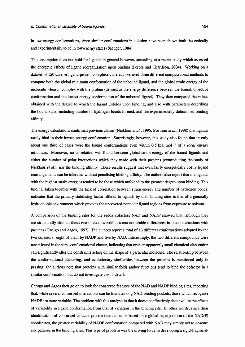
5. Conformational variability of bound ligands 154

in low-energy conformations, since similar conformations in solution have been shown both theoretically

and experimentally to be in low-energy states (Saenger, 1984).

This assumption does not hold for ligands in general however, according to a recent study which assessed

the energetic effects of ligand reorganisation upon binding (Perola and Charifson, 2004). Working on a

dataset of 150 diverse ligand-protein complexes, the authors used three different computational methods to

compute both the global minimum conformation of the unbound ligand, and the global strain energy of the

molecule when in complex with the protein (defined as the energy difference between the bound, bioactive

conformation and the lowest energy conformation of the unbound ligand). They then compared the values

obtained with the degree to which the ligand unfolds upon binding, and also with parameters describing

the bound state, including number of hydrogen bonds formed, and the experimentally-determined binding

affinity.

The energy calculations confirmed previous claims (Nicklaus et al., 1995, Bostrom et a l, 1998) that ligands

rarely bind in their lowest-energy conformation. Surprisingly, however, this study also found that in only

about one third of cases were the bound conformations even within 0.5 kcal mol-1 of a local energy

minimum. Moreover, no correlation was found between global strain energy of the bound ligands and

either the number of polar interactions which they made with their proteins (contradicting the study of

Nicklaus etal.), nor the binding affinity. These results suggest that even fairly energetically costly ligand

rearrangements can be tolerated without penalising binding affinity. The authors also report that the ligands

with the highest strain energies tended to be those which unfolded to the greatest degree upon binding. This

finding, taken together with the lack of correlation between strain energy and number of hydrogen bonds,

indicates that the primary stabilising factor offered to ligands by their binding sites is that of a generally

hydrophobic environment which protects the uncovered nonpolar ligand regions from exposure to solvent.

A comparison of the binding sites for the redox cofactors NAD and NADP showed that, although they

are structurally similar, these two molecules exhibit some noticeable differences in their interactions with

proteins (Carugo and Argos, 1997). The authors report a total of 13 different conformations adopted by the

two cofactors: eight of them by NADP and five by NAD. Interestingly, the two different compounds were

never found in the same conformational cluster, indicating that even an apparently small chemical elaboration

can significantly alter the constraints acting on the shape of a particular molecule. The relationship between

the conformational clustering, and evolutionary similarities between the proteins is mentioned only in

passing; the authors note that proteins with similar folds and/or functions tend to bind the cofactor in a

similar conformation, but do not investigate this in detail.

Carugo and Argos then go on to look for conserved features of the NAD and NADP binding sites, reporting

that, while several conserved interactions can be found among NAD-binding pockets, those which recognise

NADP are more variable. The problem with this analysis is that it does not effectively deconvolute the effects

of variability in ligand conformation from that of variation in the binding site. In other words, since their

identification of conserved cofactor-protein interactions is based on a global superposition of the NAD(P)

coordinates, the greater variability of NADP conformation compared with NAD may simply act to obscure

any patterns in the binding sites. This type of problem was the driving force in developing a rigid-fragment-

5. Conformational variability of bound ligands 155

centric protocol for binding site analysis, which will be discussed in the following chapter.

An interesting analysis of the sequence and structure of 32 families of FAD-binding proteins has been

reported (Dym and Eisenberg, 2001). While the main stated aim of this study was the identification of

sequence motifs diagnostic of the main fold groups within their dataset, the authors also comment on the

conformation of the cofactors bound to each protein. They find that, while in some structural families (namely

the p-cresol methylhydroxylase and pyruvate oxidase proteins), the cofactor conformation is essentially fixed,

other groups (the glutathione reductase (GR) and ferredoxin reductase (FR) families) contain proteins which

bind FAD in quite varied arrangements. Another interesting distinction of the FR family which they note is

that it is the only one among the families studied in which the FAD is oriented with its isoalloxine ring, rather

than the adenine ring, pointing towards the FAD-binding domain.

A structural basis for the variation of FR cofactor conformation is proposed in the paper: these proteins

consist of two domains which are ‘bridged’ by the FAD molecule. Since, in different members of this family,

the relative orientations of these two domains can vary, so the conformation of the cofactor must change in

order to maintain its contacts. No explanation is given of the wide range in GR cofactor shapes, however;

nor is the conformational variance of FAD within families compared to that observed between families.

Hansen and coworkers published a study of the relationship between protein sequence similarity and NAD

cofactor conformation (Kho et al., 2003). They obtained sequences of NAD(P)-utilising enzymes from

SWISS-PROT, and then clustered them using a method which they term protein keys. These keys are strings

of scores which represent the similarity of a given protein to every other sequence in the database, and hence

describe the protein as a function of its sequence neighbourhood. Distances between these keys are used

to generate sequence clusters, although since the authors fail to report the clustering thresholds used, it is

difficult to estimate the sequence identity shared by proteins which fall into the same group. The authors

then compare the sequence clusters obtained with a clustering based on the pairwise RMSDs between bound

NAD(P) molecules retrieved from the PDB.

The main result reported in the paper is that each sequence family binds NAD(P) molecules in conformations

which cluster together. This is not surprising, since the identification of protein relationships from sequence

alone implies that more than 30% of their residues are identical, which in turn implies that function is

conserved - and hence the cofactor should be expected to bind in the same way. Although relationships

between higher-level protein similarities {i.e. superfamily or fold groupings) and cofactor conformation

are not discussed at length, the overall finding is that members of the large structural families (Rossmann

fold oxidoreductases and flavin-NAD(P)-coupled enzymes) both bind their cofactors in several different

conformations, while the smaller families each map to just a single conformational cluster.

Intramolecular hydrogen bonding can be important in stabilising the conformation of small molecules.

In an ab initio conformational analysis of the adenosine moiety for instance, it was found that hydrogen

bonding between the adenine and ribose fragments was an important contributor to the stability of certain

conformations (Lau etal., 2003).

5 . Conformational variability of bound ligands 156

5.4 Methodology

In light of the existing corpus of literature on ligand conformation, the author felt that one area which has until

now been insufficiently studied is the question of the extent to which homologous proteins may bind their

ligands or cofactors in different conformations. As discussed previously, such a study would have value both

in deepening understanding of the evolutionary constraints acting on molecular recognition, and in providing

guidance on the permitted ranges of ligand conformation within any given family.

To gain an overall picture of the degree of ligand conformational variability between clusters for each

ligand type, molecular superpositions were performed of the representatives of the third-level clustering.

The reader will recall that each third-level cluster contains binding sites whose composition in terms of

domains is similar up to the CATH H level (§4.2). For example, for ATP, this superposition consists of the

27 representative molecules (see table D.l).

A quantitative measure of overall conformational variation was obtained by calculating the radius of gyration

(rg) for each molecule. As discussed in §3.7.1, this parameter provides a crude measure of the extent to which

a molecule is in an extended conformation, and is related to the measurement of its end-to-end distance.

It is interesting to compare similarities between the observed conformations of the bound ligands against

relationships between the proteins which bind them. Firstly, we wished to compare the extent to which

ligand conformations vary within and between families. Specifically, we wished to answer the following

questions:

• What is the extent of conformation variation among ligands in the same cluster?

• Where variation is found within a cluster, it is manifested as a continuum, or are a number of distinct

conformations preferred?

• How often do unrelated binding sites (i.e. those in different clusters) bind the ligand in the same

conformation?

To approach these questions, we computed similarities between the shapes of all ligands in each dataset

by performing least-squares superposition of all atoms in the molecule (see §3.6) to obtain RMSD values

between each pair. These dissimilarities were then compared against the level-3 clustering assignment of

the site to which each molecule is bound. In order to investigate the relationship between protein sequence

similarity and ligand conformation, pairwise sequence identity values between ligand-binding domains were

compared against the RMSD between their bound ligands.

Having investigated general trends in ligand shape, conformational differences were analysed in more detail

by calculating torsion angles for several ratable bonds in each molecule. The objective of doing this was to

establish which parts of each ligand type are the most flexible, and to identify molecules which are bound

in particularly unusual conformations (as evidenced by torsion angles which lie outside preferred angular

ranges). Where these outlying local conformations occur, they may simply be due to poor crystallographic

refinement, or alternatively may reflect special structural or functional contraints acting on the bound ligand.

The occurrences of both these contingencies are discussed later in the chapter.

5. Conformational variability of bound ligands 157

5.5 Overall shape of bound ligands

5.5.1 Superpositions

Superpositions were performed using the method described in §3.6, which has been implemented in the

GAMUT library. In order to show more clearly the conformational differences between individual molecules,

the superpositions were performed on rigid fragments at their termini, rather than globally across the whole

molecule, since the latter type of alignment tends to be very difficult to interpret visually. For ATP, the adenine

ring was used; for GTP, the guanine ring; for NAD, the nicotinamide moiety; and for FAD, the isoalloxine

group. Figures 5.4, 5.7, 5.8 and 5.11 show coordinate superpositions of all cluster representatives, for each

ligand type studied. The initial observations which can be drawn from these plots are described for each

ligand type in turn.

5.5.1.1 ATP

Visual inspection of figure 5.4 provokes three immediate reactions. The first is that the conformational

diversity exhibited by ATP is considerable. Indeed, it is clear that the amount of variation in the shapes

which this molecule can adopt - particularly in its triphosphate tail - are likely to preclude attempts to define

a unique pharmacophore describing its recognition. The second is that, in agreement with previous studies,

ATP is observed to adopt a generally fairly extended conformation. Thirdly, we note that the N-glycosidic

bond is most often found in the anti orientation.

Although most bound ATP molecules are extended, this is not universally true: two representatives (1B8A

and 3R1R) are seen to be bent to such a degree that the terminal phosphate atoms are almost in Van der Waals

contact with the adenine ring. IB8A is a structure of aspartyl-tRNA synthase. tRNA synthase enzymes,

which catalyse the specific esterification of a given amino acid to the 3' end of its corresponding tRNA, can

be divided into two classes on the basis of sequence motifs (Eriani et al., 1990). These classes each adopt

different structural folds - class I enzymes adopt a Rossmann fold, while class II enzymes bind ATP using

an antiparallel (3-sheet motif. The conformations of ATP bound to these two classes (clusters 9 and 4 in the

ATP dataset respectively) are shared, from the adenine moiety to the alpha phosphate (figure 5.5), with the

beta phosphate bent back towards the adenine. This bending allows access to the alpha phosphate to which

the tRNA molecule is esterified, as discussed in the paper describing PDB entry 1B8A (Schmitt et a l, 1998).

It appears, then, that the subsequent bending of the gamma phosphate even closer to the adenine ring, which

occurs only in class II enzymes, does not have a direct significance; Schmitt et a l report that, in structure

IB 8A, this conformation is stabilised by a water molecule which forms bridging hydrogen bonds between

the N7 atom and a magnesium ion coordinated by the triphosphate tail.

In the case of 3R1R, a structure of ribonucleotide reductase, the bent ATP conformation may be an

experimental artefact. The authors report that ATP was not co-crystallised with the protein, but was soaked

in afterwards, and that the soaking time may not have been sufficient for conformational changes to occur,

which would accommodate the ligand in a more native conformation (Eriksson et a l , 1997).

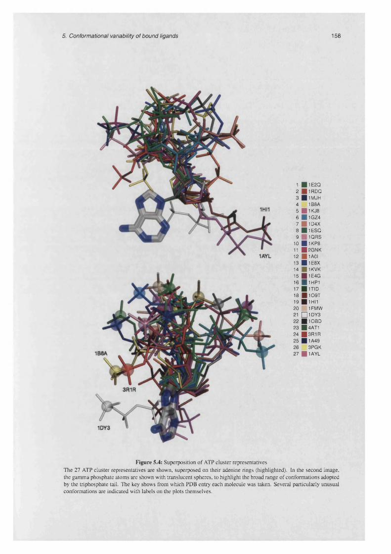
5. Conformational variability of bound ligands 158

1 ■ 1E2Q2 ■ 1RDQ3 ■ 1MJH4 1B8A5 ■ 1KJ86 ■ 1GZ47 1D4X8 H 1 ESQ9 1QRS

10 ■ 1KP811 ■ 2G NK12 ■ 1A0I13 H 1E8X14 ■ 1KVK15 ■ 1E4G16 ■ 1HP117 ■ 1TID18 1 1 0 9 T19 1 1HI120 1FM W21 □ 1DY322 ■ 10B D23 ■ 4AT124 ■ 3R1R25 ■ 1A4926 3PG K27 ■ 1AYL

Figure 5.4: Superposition of ATP cluster representatives The 27 ATP cluster representatives are shown, superposed on their adenine rings (highlighted). In the second image, the gamma phosphate atoms are shown with translucent spheres, to highlight the broad range of conformations adopted by the triphosphate tail. The key shows from which PDB entry each molecule was taken. Several particularly unusual conformations are indicated with labels on the plots themselves.

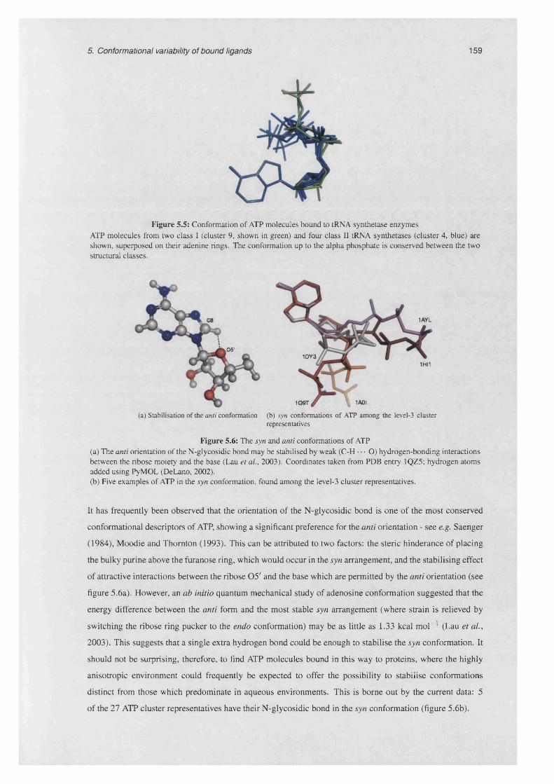
5. Conformational variability of bound ligands 159

Figure 5.5: Conformation of ATP molecules bound to tRNA synthetase enzymes ATP molecules from two class I (cluster 9, shown in green) and four class II tRNA synthetases (cluster 4, blue) are shown, superposed on their adenine rings. The conformation up to the alpha phosphate is conserved between the two structural classes.

1AYL

1DY31HI1

1A0I109T

.05'

(a) Stabilisation of the anti conformation (b) syn conformations of ATP among the level-3 clusterrepresentatives

Figure 5.6: The syn and anti conformations of ATP(a) The anti orientation of the N-glycosidic bond may be stabilised by weak (C-H • • • O) hydrogen-bonding interactions between the ribose moiety and the base (Lau et al., 2003). Coordinates taken from PDB entry 1QZ5; hydrogen atoms added using PyMOL (DeLano, 2002).(b) Five examples of ATP in the syn conformation, found among the level-3 cluster representatives.

It has frequently been observed that the orientation of the N-glycosidic bond is one of the most conserved

conformational descriptors of ATP, showing a significant preference for the anti orientation - see e.g. Saenger

(1984), Moodie and Thornton (1993). This can be attributed to two factors: the steric hinderance of placing

the bulky purine above the furanose ring, which would occur in the syn arrangement, and the stabilising effect

of attractive interactions between the ribose 05 ' and the base which are permitted by the anti orientation (see

figure 5.6a). However, an ab initio quantum mechanical study of adenosine conformation suggested that the

energy difference between the anti form and the most stable syn arrangement (where strain is relieved by

switching the ribose ring pucker to the endo conformation) may be as little as 1.33 kcal mol-1 (Lau et al.,

2003). This suggests that a single extra hydrogen bond could be enough to stabilise the syn conformation. It

should not be surprising, therefore, to find ATP molecules bound in this way to proteins, where the highly

anisotropic environment could frequently be expected to offer the possibility to stabilise conformations

distinct from those which predominate in aqueous environments. This is borne out by the current data: 5

of the 27 ATP cluster representatives have their N-glycosidic bond in the syn conformation (figure 5.6b).

5. Conformational variability of bound ligands 160

Since these five proteins have quite diverse functions, it is not possible to posit any functional reason why

they should bind ATP in this way; in all cases, upon visual inspection of the individual structures, interactions

between the protein and the ligand can be identified which may contribute extra stability. These include

hydrogen-bonding between the adenine ring and waters coordinating magnesium ions (1DY3), hydrophobic

residues stacking against the face of the adenine ring (1AYL, 1A0I) and the fact that, for two proteins (1A0I

and 1H31), the catalytic mechanism involves the ATP becoming covalently attached to the protein via its

ribose moiety.

It is interesting to note that, in all five of these cases (1A0I, 109T, 1HI1, 1DY3 and 1AYL), the level-3

clusters concerned (clusters 12, 18, 19, 21 and 27 respectively) are singlets. In other words, none of these

five proteins has a relative which is distinct in sequence, but which belongs to the same superfamily. This

may suggest that syn binding of ATP is an elaboration with fairly limited utility, and which has not therefore

been propagated into other sequence families. This result may, on the other hand, simply reflect the current

lack of structural data.

5.5.1.2 GTP

The conformations adopted by GTP bound to proteins are broadly similar to those of ATP (see figure 5.7).

The syn conformation of the N-glycosidic bond seems to be more disfavoured when the base is guanine

compared to adenine - only one GTP molecule (1JLR) has its N-glycosidic bond in the syn conformation.

This is not surprising, given the presence of a bulky amine group attached to the C2 position of the guanine

base, and the fact that the C8 atom in the guanine ring can make a weak hydrogen bond to ribose, similarly

to the corresponding interaction in adenine.

5.5.1.3 NAD

Figure 5.8 shows the 19 representative NAD molecules, superposed on their nicotinamide rings. While

most NAD molecules adopt a fairly extended shape, in agreement with previous studies, the degree of

conformational diversity apparently permitted to the cofactor is striking. Two obvious exceptions to the

tendency of NAD molecules to bind in extended forms are those from PDB entries 2BKJ and 1LW7.

2BKJ is a structure of flavin reductase from the luminous bacterium Vibrio harvey, with both NAD and FMN

bound at one of its active sites. Flavin reductase enzymes catalyse the reduction of flavin using NAD(P)H

as a cofactor. The substrate and cofactor are in close proximity in this structure, but the NAD molecule

approaches FMN via its pyrophosphate moiety, with the adenine and nicotinamide rings stacked and pointing

out of the binding cavity (figure 5.9a). This arrangement is not amenable to hydride transfer between the

two bound molecules. In their paper describing the structure, the authors suggest that this arrangement

is evidence for a mechanism whereby the NAD first binds in this folded conformation, then unfolding to

its active conformation inside the binding site. Following reduction of the flavin, electrostatic repulsion

between the protein and the positively charged nicotinamide ring may promote the return of the cofactor

to its bent conformation and subsequent expulsion from the active site (Tanner et a l, 1999). The observed

coordinates of NAD therefore could represent an intermediate between the solution structure and the fully

bound, extended form.

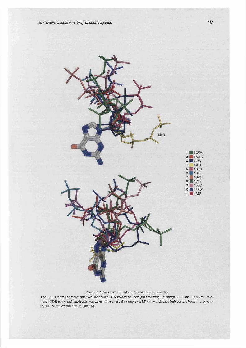
5. Conformational variability of bound ligands 161

1 B i q r a2 ■ 1 H W X3 1 1 0 8 04 1JLR5 ■ i Q L N6 ■ 1 H I 07 1 1UVN8 ■ 1C4K9 J 1 L O O

10 1 1FRW11 H 1A8R

Figure 5.7: Superposition of GTP cluster representatives The 11 GTP cluster representatives are shown, superposed on their guanine rings (highlighted). The key shows from which PDB entry each molecule was taken. One unusual example (1JLR), in which the N-glycosidic bond is unique in taking the syn orientation, is labelled.

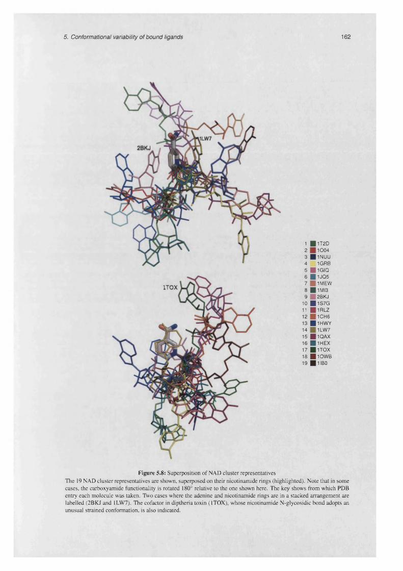
5. Conformational variability of bound ligands 162

1 ■ 1T2D2 1 0 0 43 ■ 1NUU4 1GRB5 ■ 1GIQ6 ■ 1JQ57 1M EW8 ■ 1MI39 2BKJ

10 ■ 1S7G11 ■ 1RLZ12 1CH613 ■ 1HW Y14 1LW 715 ■ 1QAX16 ■ 1HEX17 ■ 1TO X18 ■ 1 0W B19 ■ 1IB0

Figure 5.8: Superposition of NAD cluster representatives The 19 NAD cluster representatives are shown, superposed on their nicotinamide rings (highlighted). Note that in some cases, the carboxyamide functionality is rotated 180° relative to the one shown here. The key shows from which PDB entry each molecule was taken. Two cases where the adenine and nicotinamide rings are in a stacked arrangement are labelled (2BKJ and 1LW7). The cofactor in diptheria toxin (1TOX), whose nicotinamide N-glycosidic bond adopts an unusual strained conformation, is also indicated.

1TOX

5. Conformational variability of bound ligands 163

(a) Unproductive complex of folded NAD and FMN in PDB (b) Productive complex of folded NAD and FAD in PDBentry 2BKJ (2.1 A resolution) entry 1RZ1 (2.1 A resolution)

Figure 5.9: Folded conformations of NAD in flavin reductase

Recent structural studies on another flavin reductase enzyme, however, cast doubt on this hypothesis. PDB

entry 1RZ11 is a structure of flavin reductase PheA2 from Bacillus thermoglucosidasius, which displays no

amino acid sequence similarity with the family of enzymes to which the Vibrio harvey belongs. It contains an

NAD molecule, bound in a ring-stacked conformation, with the nicotinamide ring positioned close to an FAD

molecule (see figure 5.9b). The authors report bleaching of the crystals upon addition of NAD, indicating

that flavin reduction occurs, and therefore that the folded conformation of NAD persists during the reaction

(van den Heuvel et al., 2004).

1LW7 is a structure of the H. influenzae NadR protein. This is a bifunctional enzyme possessing both NMN

adenylyltransferase and ribosylnicotinamide kinase activities (Singh et al., 2002). The NAD molecule in the

dataset, however, is not bound at an active site, and while it makes a number of specific contacts with the

protein, its biological significance, if any, is unclear.

Another unusually-shaped NAD molecule is not as conspicuous as the ring-stacked examples - 1TOX, a

structure of diptheria toxin (DT), binds NAD with the N-glycosidic bond of its nicotinamide nucleotide in an

unusual conformation. This has been previously noted, and attributed to the particular catalytic mechanism

of the toxin (Bell et al., 1997). DT is an ADP-ribosyltransferase (ART) enzyme which catalyses the cleavage

of the nicotinamide N-glycosidic bond followed by the transfer of the resulting ADP-ribose moiety to a post-

translationally modified histidine residue of EF-2. By covalently linking the ADP-ribose to the elongation

factor, protein synthesis is inhibited, resulting in cell death. The unusual strained conformation of the cofactor

is thought to promote this reaction by exposing the reactive atom of NAD when bound within the active site.

Diptheria toxin is only one of a number of known ADP-ribosyltransferase enzymes. These include

three other groups of prokaryotic toxins, each of which ADP-ribosylates a different type of target. One

group, including cholera toxin, modifies heterotrimeric GTP-binding proteins (Fishman, 1990); another,

1 These molecules are missing from the main datasets used here since 1RZ1 is not classified in CATH release 2.6.0.

5. Conformational variability of bound ligands 164

including C.botulinum C3 exoenzyme, targets small GTP-binding proteins (Aktories et al., 1988). A

fourth group contains a number of toxins which ADP-ribosylate actin, with slightly different specificities

- C.botulinum C2 toxin is restricted to modifying non-muscle actin, whereas C.perfringens iota toxin also

causes depolymerisation of skeletal muscle actin (Tsuge et al., 2003). In addition, two eukaryotic proteins

with structural similarity to these bacterial toxins are known. These are the poly(ADP-ribsosyl)polymerase

and ecto-ADP-ribosyltransferase families (Ruf et al., 1996, Mueller-Dieckmann et al., 2002). Each of these

performs post-translational modifications on a wide range of targets.

In addition to that found in the DT structure, the NAD dataset contains four other molecules originating

from ART enzymes. These are an iota toxin, two C3 exoenzyme-like toxins, and a rat ecto-ART. Inspection

of the clustering revealed an error in the CATH database: whereas the NAD-binding domain from DT is

classified as an a /p structure (CATH code 3.90.175.10), the domains which comprise the other four ART

NAD-binding sites are classified as mostly P-sheet (2.30.100.10), and hence are placed in a separate cluster

(cluster 5). These two domains share a common NAD-binding region consisting of a greek key motif, as

shown in figure 5.10a and in SCOP, all five domains are classified as belonging to the same family. Figure

5.10b shows that all five ADP-ribosylating enzymes bind NAD in a similar conformation, with the torsion

around the N-glycosidic bond being particularly well-conserved. Upon being notified of this problem, the

CATH curators reclassified the NAD-binding domain of 1TOX: although it did not meet their criteria for

being classified as homologous to the other ART domains, it has now been assigned to the same fold group,

with a CATH number of 3.90.176.10.

(a) Comparison of NAD-binding domains from diptheria toxin (1TOX, green) and C.botulinum iota toxin (1GIQ, pink). Superposition is based upon the coordinates of the protein backbones, and was performed using SSM (Krissinel and Henrick, 2004b).

(b) Comparison of conformation of NAD in diptheria toxin (1TOX, green) and the four P-sheet ADP-ribosylating proteins from cluster 5 (1GIQ, pink; 1GZF, blue; 10JZ, yellow; 10G3, grey), superposed on the nicotinamide moiety. The shared orientation of the nicotinamide N-glycosidic bond is clearly visible.

Figure 5.10: NAD binding by ADP-ribosylating proteins

5.5.1.4 FAD

Superpositions of the 14 FAD cluster representatives, aligned upon their isoalloxine rings, are shown in figure

5.11. Visual inspection of the plots shows the conformations of FAD to be somewhat more homogeneous than

those of NAD, with the main variation occurring around the ribitol-isoalloxine bond. The adenine nucleotide

part of the molecule tends to be fairly extended, and FAD is the only molecule of the four studied here in

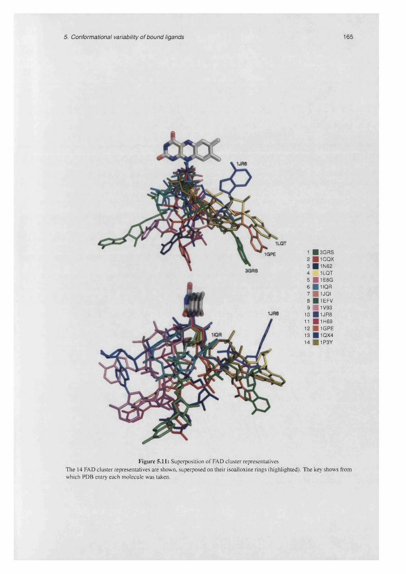
5. Conformational variability of bound ligands 165

1GPE 1 ■ 3G R S2 | 1 C Q X

3 ■ 1N624 1LQ T5 ■ 1E8G6 ■ 1IQ R7 1JQI8 H 1E FV

9 | 1V9310 ■ 1JR811 ■ 1H6912 f f i 1G PE

13 ■ 1Q X 414 ■ 1P 3Y

Figure 5.11: Superposition of FAD cluster representatives The 14 FAD cluster representatives are shown, superposed on their isoalloxine rings (highlighted). The key shows from which PDB entry each molecule was taken.

5. Conformational variability of bound ligands 166

which the adenosine N-glycosidic bond seems to adopt the anti conformation exclusively.

In contrast to NAD, no examples of FAD are seen where the molecule is bent enough to allow adenine-

isoalloxine stacking interactions. The most bent conformation is that from PDB entry 1IQR (DNA photolyase

from Thermus thermophilus), in which the centroids of the adenine and isoalloxine groups are separated by

around 6.3A, compared with 3.6A and 4.0A for the inter-ring distances in the NAD molecules from 2BKJ

and 1LW7 respectively. There is no clear functional reason why the FAD in this enzyme should adopt such a

compact conformation.

Three FAD molecules which have clearly similar conformations are 3GRS, 1LQT and 1GPE, which are the

representatives from clusters 1, 4 and 12 respectively. Inspection of the clustering results shows that in all

three cases, the FAD molecule is bound by a Rossmann fold domain (CATH code 3.50.50.60), but whereas in

3GRS (glutathione reductase), the FAD binding site is formed by two Rossmann fold domains, in both 1LQT

(FprA, a mycobacterial oxidoreductase) and 1GPE (glucose oxidase), a single Rossmann domain binding

the adenine is partnered with a second domain of a different type (see figure 5.12). The resulting change in

the fraction of residue contributed by the Rossmann fold domain causes each site to be placed in a different

cluster, although a human expert would classify them all as belonging to the glutathione reductase family

(Dym and Eisenberg, 2001).

(a) Glutathione reductase (3GRS) (b) FprA (1LQT) (c) Glucose oxidase (1GPE)

Figure 5.12: FAD binding sites in the glutathione reductase family In each case, the Rossmann fold domain which binds the adenine end of the FAD molecule is coloured red. Other colours indicate the following domains: green, Rossmann fold; yellow, enolase-like; blue, FAD/NAD(P)-binding; purple, glucose oxidase domain.

5.5.2 Radii of gyration

Having discussed several qualitative aspects of the bound conformations of the four ligands, we now proceed

to analyse the degree of molecular compactness of each molecule, in order to quantify to what extent the

general principal of ligand extension upon binding is realised in each case. Before looking at the radii of

gyration calculated for each bound ligand in the dataset, it is instructive to explore the range of the possible

values which this parameter could potentially take for each molecule. To estimate this, a set of artificially-

generated conformations of each ligand were compiled, sampling the full extent of conformational space.

5. Conformational variability of bound ligands 167

This was done by specifying a list of ratable bonds for each ligand, and a set of allowed rotamers for each

bond. These ratable bonds were selected according to the criteria outlined in §2.3.4.3.1 and are shown

diagrammatically in figures 3.13 and 3.14. For each bond, preferred angular ranges have been assigned by

consideration of the hybridisation states of the pairs of bonded atoms, and by consulting previous literature

on the subject. The atoms which define all ratable bonds used here, along with the preferred orientations, are

shown in tables 5.1 - 5.3.

Angle A B C D Preferred orientations

Xpur 04' Cl' N9 C4 + j c , 180°-300°Xpyr 04' Cl' N1 C2 +sc, 180° -300°

Y 05' C5' C4' C3' ±sc, ap3 PA 05' C5' C4' ±sc, apa 03 PA 05' C5' ±sc, apSi PB 03A PA 05' ±sc, apVi 03B PB 03A PA ± 5C , aph PG 03B PB 03A ± 5C , apV2 03G PG 03B PB ± 5C , ap

Table 5.1: Definition of torsion angles and associated minima for nucleotide derivatives Torsion angles are ordered from the adenine end of the molecule to the triphosphate tail. Xpur and %pyr refer to the definition of the torsion around the N-glycosydic bond for purines and pyrimidines respectively. See figure 3.13.

Angle A B C D Preferred orientations

Xa 04'_A C1'_A N9_A C4_A +sc, 180° — 300°YA 05'_A C5'_A C4'_A C3'_A ap

Adenine nucleotide 3a P_A 05'_A CS'Ji C4'_A ±sc, apOLa 03 P_A 05'_A C5'_A ±sc, ap'U P_N 03 PJS. 05'_A ±sc, ap

Sv PJ^ 03 P_N 05'_N ±sc, apa v 03 PJS1 05'_N C5'_N ±sc, ap

Nicotinamide fW P_N 05'JM C5'_N C4'_N ±5C, apnucleotide YN 05'_N C5'_N C4'_N C3'_N ± 5C , ap

X v 04'_N Cl'JSf N9_N C4_N +sc, 180° - 300°0AT C2_N C3_N C7_N NN7 sp,ap

Table 5.2: Definition of torsion angles and associated minima for NAD Torsion angles are ordered from the adenine end of the molecule to the nucleotide moiety. See figure 3.14a.

Adenine nucleotide

Ribitol phosphate

Angle A B C D Preferred orientations

X 04'_A C1'_A N9.A C4_A +sc, 180° — 300°Y 05'_A C5'_A C4'_A C3'_A ±sc, apP P_A 05 '_A C5'_A C4'_A ±sc, apa 03 P_A 05'_A C5'_A isc , apSa P 03P P_A 05'_A ±5C, ap

s» P_A 03P P 05' ± 5C , ap01 03P P 05' C5' dbsc, ap02 P 05' C5' C4' ±sc, ap03 05' C5' C4' C4' ±sc, ap04 C5' C4' C3' C2' ±sc, ap05 C4' C3' C2' Cl' ±sc, ap06 C3' C2' Cl' N10 ±sc, ap07 C2' C l' N10 CIO sp,ap

Table S3: Definition of torsion angles and associated minima for FAD Torsion angles are ordered from the adenine end of the molecule to the riboflavin moiety. See figure 3.14b.

5. Conformational variability of bound ligands 168

A program was then written which generates all possible conformations of the molecule by systematically

setting the rotable bonds to each combination of the allowed rotameric states. Each arrangement is then

tested for steric clashes by checking whether any pair of non-bonded atoms approaches closer than the sum

of their Van der Waals radii (values taken from Bondi (1964)). Atoms in the same ring system are excluded

from this check. Since the restrictive definition of rotable bonds used here does not include bonds such as

C—OH , it is possible that atoms which were found to clash in the conformations generated here would

actually be free to rotate away from one another, were a more complete simulation of the molecule to be

carried out. For this reason, clashes due to this type of atom (such as a hydroxyl hydrogen) were ignored.

The set of arrangements which were found to be free of atomic clashes was taken to represent the extent

of conformational space which may be explored by the molecule. No energy calculations were performed;

therefore this set consists of those conformations which need satisfy only fairly liberal constraints.

The initial coordinates of each molecule used were the idealised coordinates retrieved from the MSD. These

coordinates were originally generated using the CORINA program (Gasteiger et al., 1990) (D. Dimitropoulis

personal communication). Hydrogen atoms were included for the purposes of the steric hinderance check,

but were excluded from the calculations of radius of gyration, to allow direct comparison of these values with

those calculated from ligand coordinates taken from crystal structures. The allowed rotameric states for each

bond were defined as the median values of each of the preferred angular ranges shown in tables 5.1 - 5.3.

The results of the conformation generation experiment are summarised in table 5.4. Figure 5.13 shows a

number of the artificially-generated ligand conformations which exemplify the extrema and average values

of rg for each population.

Ligand Number of rotable bonds*

Total number of possible

conformations

Number of conformations

free of steric clashes

ATP 8 4374 830GTP 8 4374 826NAD 11 52488 3054FAD 13 1062882 4992

Table 5.4: Results of conformation generation experiment (*) This is the number of bonds which were allowed to rotate in the current experiment, which is a subset of the total number of rotable bonds. A C—NH2 bond, for instance, is not considered rotable for the purposes of this analysis. See §2.3.4.3.1 for more details. For each ligand, the total number of comformations resulting from all combinations of the rotamers defined previously is quoted. Following checks for steric clashes, a subset of these conformations is retained; these are taken to define the total conformational space of the molecule.

The generated conformations of ATP and GTP show that the syn orientation of the N-glycosidic bond is

necessary to fold the molecules into their most compact forms. Most molecules in the datasets presented

above, on the other hand, tend to adopt conformations intermediate between the median and extended forms.

For both FAD and NAD, in arrangements with an rg close to the median value, the two rings tend to be

separated from one another. The most compact NAD conformations are achieved by stacking the terminal

ring systems in parallel; in the folded FAD structures, the adenine and isoalloxine rings are in close proximity,

but do not lie in parallel. This suggests that the folded conformation of NAD in DNA photolyase (1IQR) is

5. Conformational variability of bound ligands 169

(a) ATP folded (rg= 3.6A)

(d) NAD folded (rg= 4.1 A)

(g) FAD folded (rg= 4.4A) (h) FAD average (rg= 6.5A) (i) FAD extended (rg= 8.4A)

Figure 5.13: Generated ligand conformations Artificially-generated ligand conformations which represent the minima, maxima and average values of rg for each ligand type are shown. GTP is omitted since its conformations are essentially analogous to those shown for ATP.

in fact fairly close to the most compact possible arrangement of the cofactor. Circular dichroism experiments

and molecular dynamics studies on NAD suggest that ring stacking occurs in this molecule when free

in solvent (Thornton and Bayley, 1977); we may therefore take the folded conformation shown in figure

5.13d as being at least partially populated in an aqueous environment. Several authors have observed that,

when in complex with proteins, the nicotinamide and adenine rings of NAD(P) tend to be approximately

perpendicular and separated by around 15A - see e.g. Stoddard et al. (1993). This corresponds to an

intermediate conformation between the median and extended forms (figures 5.13e and 5.13f).

Having established the range of radii of gyration available to each ligand type, we can ask quantitatively how

much of this range is explored by protein-bound ligand molecules. Table 5.5 shows statistics which describe

the distributions of rg for each ligand type, in both the ‘real’ (protein-bound) and artificially-generated

datasets. Figure 5.14 shows histograms of these distributions. Structures of molecules from the dataset

which illustrate the most compact and extended protein-bound forms of each ligand which were observed, as

well as an example of a molecule with average extension, are included in each plot.

(b) ATP average (rg= 4.7A) (c) ATP extended (rg= 5.6A)

(f) NAD extended (rg= 7.6k)

Radius of gyration (rg) /A Test of normality^p

Ligand Dataset* n Minimum Maximum M a W P (Wilcoxontest)A

ATP Artificial Level 3

83027

3.583.75

5.605.11

4.634.59

0.400.35

0.990.94

1.13 x 10-6 9.87 x 10~2 0.64

GTP Artificial Level 3

82611

3.603.95

5.735.07

4.714.59

0.420.36

0.990.93

1.06 x 10“ 5 4.49 x 10“ !

0.24

NAD Artificial Level 3

305419

4.084.21

7.596.53

5.865.63

0.590.66

1.000.92

1.39 x 10-8 1.28 x 10_l

0.17

FAD Artificial Level 3

499214

4.384.97

8.447.62

6.436.76

0.690.68

0.990.90

6.38 x 10~14 9.63 x 10"2

0.09

Table 5.5: Radii of gyration(★) ‘Artificial’ refers to the set o f generated ligand conformations; ‘level 3’ refers to die set of cluster representatives at the third level, (f) The Shapiro-Wilks test, as implemented in the R (?) package e l071 (?), was used.( A ) Wilcoxon 2-sample test, applied to determine whether the medians of the artifical and level-3 distributions differ significantly.

5. C

onformational variability

of bound ligands

170

5 . Conformational variability of bound ligands 171

Comparison of the ranges of rg values for the artificial and bound ligand conformations shows that, for all

four ligand types, there are instances of the molecule which bind proteins in almost a maximally compact

conformation. For ATP and GTP, the difference between the most tightly folded molecules in the generated

and observed datasets seems to be that in the former, the N-glycosidic bond is in the syn conformation.

While this does occur in the bound dataset, it tends to be accompanied by a fairly extended triphosphate tail

(figure 5.6b); it is likely that the combination of the syn arrangement with a tightly bent triphosphate tail is

energetically unfavourable, explaining its absence from the bound dataset.

At the other end of the distributions, there is a larger difference between the artificial and bound datasets,

particularly for NAD and FAD. It appears that, while ligands often bind in extended conformations, these are

not the most extended arrangements which they are capable of adopting. One explanation for this may be

that this fully extended arrangement prevents coordination of metal ions by consecutive phosphate moieties,

which is a commonly-observed motif in complexes of proteins with nucleotides and nucleotide derivatives.

Neither the rg values for the artificially-generated conformations nor those for the bound ligand conformations

are normally distributed, as shown by a Shapiro-Wilks test. This test measures the likelihood that the samples

are drawn from normally-distributed populations (Royston, 1982); the p-values shown in table 5.5 show

that, in most cases, this hypothesis is rejected with at least 90% confidence. This suggests that, rather than

comparing the means and standard deviations of the distributions, more instructive statistics would be the

measure of skewness.

Since the distributions are not normal, using a t-test to determine whether their means differ significantly is

not appropriate. Instead, a Wilcoxon 2-sample test (two-tailed) was applied. The results indicate that, for

all ligands except FAD, the medians of the two distributions are not significantly different - and therefore

conflicts with previous assertions that these ligands bind in predominantly extended conformations. Rather,

it seems that the bound conformations of ATP, GTP and NAD are drawn at random from the pool of

possible conformations available to these molecules. When interpreting these findings, however, it must

be remembered that the number of data points is quite small in all cases, and that increased amounts of data

would allow for more substantial conclusions to be drawn.

An interesting observation which arises from comparison of the radii of gyration for ATP and GTP with

those of NAD and FAD is that, for the latter pair of ligands, a slightly bimodal distribution is observed.

Again, this should be treated with caution in light of the sparsity of data, but it appears that the mmost folded

conformations of NAD and FAD are truly outliers, rather than being simply the lower extrema of smooth

distributions.

5.5.3 General observations

IIn summary of the analysis of the overall shape of bound ligands, we find that, in conflict with previous

studies, their degree o f extension is not significantly different to the average degree of extension of all possible

conformations. Indeed, rather than binding in exclusively extended arrangements, a small proportion of

5. Conformational variability of bound ligands 172

1G5T [1] (3.70)

□ Level 3 repsGenerated

Radius of gyration /A

(a) ATP

1C80 [3*] (3.95) 1A8R [11*] (4.72) 1NRJ [1] (5.09)

1KJ8 [5*] (4.53) 1A60 [2] (5.16)

□ Level 3 repsGenerated

Radius of gyration /A

(b) GTP

Figure 5.14: Distribution of radii of gyration The distribution of the radius of gyration among level-3 cluster representatives is compared against that obtained from the artificially generated conformations. Molecules from the dataset which represent the extrema and average of the distribution are shown. The level-3 cluster to which each molecule belongs is shown in square brackets; an asterisk indicates that the molecule is a cluster representative. The radius of gyration for each compound (in A) is given in parentheses. Continued overleaf.

5. Conformational variability of bound ligands 173

1LW7 [3] (4.21) 1S7G [10*] (5.54) 1EJ2 [3] (6.60)

□ Level 3 reps ■ G enerated

1DNP [6] (4.92)

0.4

□ Level 3 reps ■ G enerated

Radius of gyration /A

(d) FAD

Figure 5.14: Distribution of radii of gyration Continued from previous page.

Radius of gyration /A

(c) NAD

1JR8 [10*] (5.98) 1NG4 [1 ] (7.66)

5. Conformational variability of bound ligands 174

ligands appear to bind in very compact conformations; in some cases, these results may be due to biolog’ y

inactive complexes, but in others, genuine functional reasons can be posited to explain why this should

Here, several cases in which ligands bind with part of the molecule in a strained or unfavourable arrangement

have been identified. In some cases, this appears to promote catalysis, either by weakening a particular

covalent bond, or by relieving steric hinderance around a reactive centre. In others, such as the syn

conformations observed for the nucleoside moieties, the energetic impediment to adopting these orientations

is not particularly high, and thus their occurrence may be explained as allowing for slightly more favourable

protein-ligand interactions. Finally, the qualitative observation is made that the degree of variation between

the conformations of a given ligand when bound by unrelated proteins is significant. The following section

explores this finding in more detail.

5.6 Conformational differences between and within clusters

Having observed the large conformational variations between representative molecules of the level-3 clusters,

the next phase of the analysis was to quantify that variation, and compare it against the extent to which

molecules in the same cluster adopt different shapes.

5.6.1 Hierarchical clustering of ligand conformations

Similarities between the shapes of all level-2 representatives in each dataset were calculated by performing

least-squares superposition of all atoms in the molecule (see §3.6). The RMSD values thus obtained were

used to populate a distance matrix. This matrix was then analysed by applying complete-linkage clustering

(§3.2). The relationships between the shapes of the ligands in the dataset, and the evolutionary relationships

between the sites in which they are bound, were then compared by producing plots of the clustering

dendrograms, labelling each leaf node with the index of the level-3 cluster to which the corresponding

molecule belonged. In this way, clusters in which all members share a similar conformation are visible

as leaf labels which are grouped together on the dendrogram; conversely, clusters which contain members

with diverse conformations manifest themselves as labels which are scattered across the width of the tree.

Note that the absolute ordering of nodes along the tree is not significant in and of itself: this can be changed

arbitrarily by flipping a subtree around about its root node.

The clustering dendrograms are shown in figures 5.15 - 5.18. An initial comparison of these trees shows

that of the four ligand types, ATP appears to exhibit the greatest degree of conformational variation within

clusters. While, for GTP, NAD and FAD, most large clusters tend to have a large proportion of non-leaf nodes

below the 1A threshold, indicating that their members are similarly shaped, the two largest ATP clusters seem

to be more distantly spread in conformational space, and hence appear more widely scattered along the leaves

of the dendrogram (figure 5.15). Cluster 1 contains members which, although they all share a common

Rossmann-fold ATP-binding domain, are diverse in terms of the protein function. Cluster 2, on the other

hand, is composed almost exclusively of kinases (see table D.l). Qualitatively, the degree of conformational

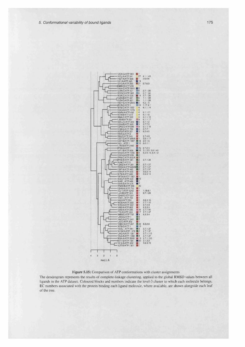
5. Conformational variability of bound ligands 175

Ir f f iDO0/G/ATP.900 | 1

■1AYL/A/ATP.541 271 NSF/A/ATP.858 | 1HI1/A/ATP.665 ■ 19

1 DY3/A/ATP.200 1 21NK/D/ATP.200 11

■1 MJH/C/ATP.2001 1 3 •1 LHR/C/ATP.401 B8

1 E SQ /D /A T P.300 B8 ------ 1 KVK/C/ATP.535 ■ 14•____r1 GZ4/8/ATP.601 > 6: *1 GZ4/D/ATP.601 B6

1 NSY/C/ATP.2000 B 3■3R1 R/C/ATP.1 B24 ■1 B76/C/ATP.1552 4•1H4Q/A/ATP. 1478 4■1 KM N/A/ATP .452 41 E24/B/ATP.512 41 B8A/C/ATP.500 41 J09/B/ATP.501 B9 ■1MAU/C/ATP.400 B 3

GN8/B/ATP.600 B 3 QRS/C/ATP.999 B 9

1 F9A/G/ATP.700 B3 1 KP3/F/ATP.301 B3 ■1 R0X/E/ATP.2 B 1•1 N5I/C/ATP.543 B1 •1 G5T/C/ATP.999/A B 1 ■109T/B/ATP.1397 B18 ■1AOI/_/ATP.1 B12•1 J7K/B/ATP.2060 B1 ■3PGK/A/ATP.1 B 26■1 HP 1/B/ATP .606 B161DV2/C/ATP. 1000 B 5 1 CSN/A/ATP.299 B 2 ■1 PK8/C/ATP.802/A B5

PHK/E/ATP.381 B■1KJ8/C/ATP.5 •1QMZ/A/ATP,1RDQ/A/ATP,

■------- 1 Q97/A/ATP.485j ------ 1 H8H/F/ATP.600 B 17*---- 1 E79/A/ATP.600 B1

•1W7A/A/ATP.1801 B 1 1 E 4G /T /A T P.500 ( 1 51K A Z /JA T P .486 B 7 1 D 4X /B/A TP.676 B 7

j ---------1 FMW/B/ATP.999 20- f t --------- 1 Q H G /E /A T P.700 B 1L------- 1G21 /1/ATP.5292 B 1

1JJ V/B/ATP.300 ■ 11QHX/E/ATP.501 B1 ■1 D9Z//ATP.700 B1■1 II0/C/ATP.591 fl11 KO5/A/ATP.302 B1•1E2Q/A/ATP.302 B1 '1A82/A/ATP .802 B11 A49/A/ATP.535 B25■1TID/E/ATP.200 B171MB9/C/ATP.702 B 3 1 JWA/E/ATP.1 B 6■1 A6O/A/ATP.340 B 21 JI0/C/ATP.302 B 1■1 OBD/A/ATP.307 B22■1KP8/G/ATP.1 B 101GOL/_/ATP.581 B2 •1H1 W/A/ATP.1373 B 2 •1 JAG/A/ATP. 1301 B1 •1OL6/A/ATP. 1388 B 2

E8X/A/ATP.2000 B13AT1/D/ATP.154 B23

-1Q12/A/ATP.302 ■ '-1 L2T/E/ATP.1301 B1

.381 B 2 5 B 5 >.381 B 2 >.600/BB2 .485 B 2

i - c a

4.1.1.493.6.4.6

2.7.1.35 2.7.1.502.7.1.361.1.1.381.1.1.386.3.1.51.17.4.1 6.1.1.14

6 .1 .1.216 . 1.1.6 6 .1 .1.126.1.1.17 6 .1 .1.22.7.7.36.1.1.182.7.7.16.3.4.5

2.7.4.92.5.1.172.5.1.66.5.1.1

2.7.2.33.1.3.5, 3.6.1.45 6.3.4.14,6.4.1.2

2.7.1.38

2.7.1.372.7.1.372.7.1.373.6.3.143.6.3.14

3.6.3.162.7.1.122.7.4.96.3.3.3 2.7.1.40 2.7.1.376.5.3.4

2.7.1.372.7.1.37 2.7.1.1132.7.1.37 2.7.1.153 2.1.3.2 3.6.3.19

1---- 1---- 14 3 2 1

r m s d /A

Figure 5.15: Comparison of ATP conformations with cluster assignments The dendrogram represents the results of complete-linkage clustering, applied to the global RMSD values between all ligands in the ATP dataset. Coloured blocks and numbers indicate the level-3 cluster to which each molecule belongs. EC numbers associated with the protein binding each ligand molecule, where available, are shown alongside each leaf of the tree.

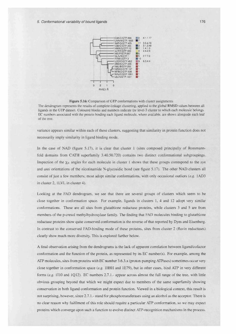
5. Conformational variability of bound ligands 176

RMSD /A

■1 C4K/C/GTP.999 ■ 8 4.1.1.17■1UVN/A/GTP. 1665 ■ 7■1 A8R/G/GTP.405 11 3.5.4.16■1 C80/C/GTP.355 ■ 3 3.1.3.46•1HWX/G/GTP.12 ■ 2 1.4.1.3■1JLR/E/GTP.300 4 2.4.2.9■1 HI0/P/GTP.667 ■ 6-1QLN/R/GTP.1 ■ 5 2.7.7.6■1 FRW/l/GTP.3 ■ 10■1 LOO/C/GTP.452 ■ 9 6.3.4.4-1ZBD/E/GTP.200 ■ 1■1 N6L/B/GTP.200 ■ 1■1QRA/C/GTP. 167 ■ 1-1 M7B/D/GTP.538 ■ 1■1 NRJ/C/GTP.1001 ■ 1-1 J2J/A/GTP.1001 ■ 1

Figure 5.16: Comparison of GTP conformations with cluster assignments The dendrogram represents the results of complete-linkage clustering, applied to the global RMSD values between all ligands in the GTP dataset. Coloured blocks and numbers indicate the level-3 cluster to which each molecule belongs. EC numbers associated with the protein binding each ligand molecule, where available, are shown alongside each leaf of the tree.

variance appears similar within each of these clusters, suggesting that similarity in protein function does not

necessarily imply similarity in ligand binding mode.

In the case of NAD (figure 5.17), it is clear that cluster 1 (sites composed principally of Rossmann-

fold domains from CATH superfamily 3.40.50.720) contains two distinct conformational subgroupings.

Inspection of the Xn angles for each molecule in cluster 1 shows that these groups correspond to the syn

and anti orientations of the nicotinamide N-glycosidic bond (see figure 5.17). The other NAD clusters all

consist of just a few members; most adopt similar conformations, with only occasional outliers (e.g. 1AD3

in cluster 2, 1LVL in cluster 4).

Looking at the FAD dendrogram, we see that there are several groups of clusters which seem to be

close together in conformation space. For example, ligands in clusters 1, 4 and 12 adopt very similar

conformations. These are all sites from glutathione reductase proteins, while clusters 3 and 5 are from

members of the p-cresol methylhydroxylase family. The finding that FAD molecules binding to glutathione

reductase proteins show quite conserved conformation is the reverse of that reported by Dym and Eisenberg.

In contrast to the conserved FAD-binding mode of these proteins, sites from cluster 2 (flavin reductases)

clearly show much more diversity. This is explored further below.

A final observation arising from the dendrograms is the lack of apparent correlation between ligand/cofactor

conformation and the function of the protein, as represented by its EC number(s). For example, among the

ATP molecules, sites from proteins with EC number 3.6.3.x (proton-pumping ATPases) sometimes occur very

close together in conformation space (e.g. 1H8H and 1E79), but in other cases, bind ATP in very different

forms (e.g. 1110 and 1Q12). EC numbers 2.7.1.- appear across almost the full range of the tree, with little

obvious grouping beyond that which we might expect due to members of the same superfamily showing

conservation in both ligand conformation and protein function. Viewed in a biological context, this result is

not surprising, however, since 2.7.1.- stand for phosphotransferases using an alcohol as the acceptor. There is

no clear reason why fulfilment of this role should require a particular ATP conformation, so we may expect

proteins which converge upon such a function to evolve distinct ATP-recognition mechanisms in the process.

5. Conformational variability of bound ligands 177

-1LW7/E/NAD.605 -1 HWY/G/NAD.31/A -2BKJ/B/NAD.243 -1 IBO/B/NAD. 1994 -1 S7G/F/NAD.701 -1OWB/C/N AD .3001

1 RLZ/E/NAD.700 1LVL/A/NAD.460i 1 DQS/A/NAD.4001----- 1JQ5/I/NAD.401

TOX/A/NAD.536 i GIQ/A/NAD.500 10G3/A/NAD. 1227 ■1 OJZ/A/NAD.500 •1 GZF/A/NAD.1248

i ■ ■

■ r-H_r—“1 :i ■

r G

1 M9H/B/NAD.300 1MI3/A/NAD.1350 1 F8G/E/NAD.2500 1 MEW/E/NAD.987 1LSS/I/NAD.1001 1 F3P/C/NAD.500 INPX/A/NAD.818

1 GRB/A/NAD.480 1 CH6/G/NAD.S62 1 AD3/A/NAD.600 1LW7/E/NAD.601 •1EJ2/L/NAD.1339 •1 K4M/D/NAD.601 1NUU/E/NAD.401 ■1QAX/G/NAD.1001 •1 EVJ/A/NAD.500 •1NFB/A/NAD.701 •1 H94/A/NAD.799 ■1IY8/A/NAD.1268 ■1B14/C/NAD.255 •1 FK8/C/NAD.800 •1 FDV/A/NAD.361 ■1D7O/E/NAD.501 ■1ENY/B/NAD .500 ■1QSG/B/NAD. 1304 •1NHW/I/NAD.450

I— 1QR R/A/N AD .401 1 EBF/C/NAD.2109 •1 BDB/A/NAD.300 ■1FMC/A/NAD .256 •1 NFF/F/NAD.2300 ■1 E6W/C/NAD.301 W u 1 GEE/D/NAD.2262

i T-10RR/A/NAD.1200 Jl_r-1KEW/C/NAD.1400

] MGEG/A/NAD.101h 1 DHR/B/NAD.241“ ---- 1I3L/C/NAD.400

■1 GR0/A/NAD.1000 •1 CH6/G/NAD.571 ■1 BXG/A/NAD.360 ■1 NVM/B/NAD.3501 •1 DU/C/NAD.403 •1GAD/0/NAD.336 •1 F0Y/C/NAD.750 1K6X/C/NAD.400 1BPW/A/NAD.4 1 UXT/A/NAD.1503 •1004/D/NAD.6504 •1EE9/C/NAD.10

|------1 D4F/E/NAD.502|t_i 1 ARZ/B/NAD.274

1P9L/E/NAD.301'------- 1 NPD/A/NAD.300I j — 1PJC/G/NAD.500 : Mi—1MX3/E/NAD.1000

rH 1 DXY/D/NAD.336i ' 2NAD/A/NAD.394

•1 R37/A/NAD.403 .DT/A/NAD.401

■1 K0L/A/NAD.1403 1T2D/E/NAD.316 1J5P/C/NAD.300 1 HYH/A/NAD.330 106Z/C/NAD.2003 1 BMD/A/NAD.334 1PJ3/E/NAD.2601 1 LLD/A/NAD.1 1 PSD/B/NAD.450 1 N8K/A/NAJ.377 •1EMD/A/NAD.314

r C *

A ■ 14A ■ 13 1.4.1.3A ■ 9S ■ 19 1.6.2.2A ■ 10A ■ 18 2.3.3.1

11 2.5.1.464 1.8.1.4

A ■ 6 1.1.1.25 2.A ■ 6 1.1.1.6

■ 17 2.4.2.36S ■ 5

■ 5 2.4.2.31■ 5

S ■ 5A ■ 16 1.1.1.85A ■ 8 1.1.1.274A ■ 8S ■ 1 1.6.1.2

■ 7 1.1.1.205A ■ 1

4A 4 1.11.1.1A 4 1.8.1.7

■ 12■ 2 1.2.1.5

A ■ 3A ■ 3 2.7.7.1A ■ 3 2.7.7.18A ■ 3 2.7.7.1

■ 15 1.1.1.88A ■ 1

■ 7 1.1.1.205■ 1 1.1.1.49

A ■ 1S ■ 1 1.1.1.1S ■ 1S ■ 1 1.1.1.62S ■ 1 1.3.1.9S ■ 1S ■ 1 1.3.1.9s ■ 1s ■ 1 3.13.1.1s ■ 1 1 .1 .14s ■ 1s ■ 1 1.1.1.159s ■ 1s ■ 1 1.1.1.35s ■ 1 1.1.1.47s ■ 1s ■ 1 4.2.1.46s ■ 1.1 .14s ■ 1 1.5.1.34s ■ 1 5 .1 4 4s ■ 1s ■ 1s ■ 1 1 .4.140s ■ 1s ■ 1 1 .1 .142s ■ 1 14.1.12s ■ 1 1.1.1.35s ■ 1A ■ 2 14.1 .8A ■ 2 1.2.1.9A ■ 2 1.2.1.3A ■ 1 1.5.1.15A ■ 1 3.3.1.1A ■ 1 1.3.1.26A ■ 1 1.3.1.26A ■ 1A ■ 1 1.4.1.1A ■ 1A ■ 1A ■ 1 1.2.1.2A ■ 1 1.1.1.1A ■ 1 1.1.1.27A ■ 1 1.2.1.46A ■ 1 1.1.1.27A ■ 1A ■ 1A ■ 1 1.1.1.37A ■ 1 1.1.1.37A ■ 1 1.1.1.38A ■ 1 1.1.1.27A ■ 1 1.1.1.95A ■ 1 1.1.1.1A ■ 1 1 .1 .147

I I I I I5 4 3 2 1

RMSD iK

Figure 5.17: Comparison of NAD conformations with cluster assignments The dendrogram represents the results of complete-linkage clustering, applied to the global RMSD values between all ligands in the NAD dataset. Coloured blocks and numbers indicate the level-3 cluster to which each molecule belongs. The orientation of the nicotinamide N-glycosidic bond is shown as S (syn), A (anti) or - (outside allowed ranges). EC numbers associated with the protein binding each ligand molecule, where available, are shown alongside each leaf of the tree.

5. Conformational variability of bound ligands 178

i—F =: 1 ■

■10QC/A/FAD.1 ■ 10-1 JR8/C/FAD.334 ■ 10■1 DNP/A/FAD.472 ■ 6 4.1.99.3-1 NP7/A/FAD.500 ■ 6■1 IQR/C/FAD.421 ■ 6 4.1.99.3-1ABP/ /FAD.259 ■ 2 1.18.1.2■1 KRH/A/FAD.501 ■ 2 1.18.1.3■1 GAW/E/FAD.320 ■ 2■1 EP3/E/FAD.502 ■ 2 1.3.3.1■1K87/C/FAD.2001 ■ 9 1.5.1.12 1.5.99.8■1 IVH/A/FAD.399 ■ 7 1.3.99.10■1 JQI/E/FAD.399 ■ 7 1.3.99.2-1DDI/ /FAD.600 ■ 2 1.8.1.2•117P/B/FAD.301 ■ 2 1.6.2.2■1F2Q/B/FAD. 1501 ■ 2 1.14.13.39-1 JA1/A/FAD.1750 ■ 2 1.6.2.4-1H69/C/FAD. 1274 11 1.6.99.2■1 E8G/B/FAD.600 ■ 5 1.1.3.38■1I19/A/FAD.700 ■ 5■2MBR/A/FAD.401 ■ 3 1.1.1.158■1 HSK/E/FAD.401 ■ 3 1.1.1.158■1 FOX/A/FAD.600 ■ 5 1.1.1.28■1 JRO/I/FAD.3005 ■ 3 1.1.1.204■1 FIQ/G/FAD.606 ■ 3 1.1.3.22■1 N62/F/FAD.4931 ■ 3 1.2.99.2■1 V93/C/FAD.300 ■ 9■1 POX/A/FAD.612 ■ 8 1.2.3.3■1 EFV/C/FAD.599 ■ 8■1 P3Y/L7FAD.259 ■ 14■1 QX4/A/FAD.301 ■ 13 1.6.2.2■1 CQX/A/FAD.405 ■ 2 1.14.12.17■1 GPE/A/FAD.600 ■ 12 1.1.3.4-1 GTE/A/FAD. 1031 4 1.3.1.2■1 HYU/C/FAD.700 ■ 1-1H82/A/FAD.579 ■ 1 1.5.3.11■1K0I/D/FAD.395 ■ 1 1.14.13.2-1N1P/B/FAD.510 ■ 1 1.1.3.6•1FEC/A/FAD. 499 ■ 1 1.8.1.12•1LQT/C/FAD.3457 4 1.18.1.2■1M09/C/FAD. 1013 ■ 1 1.8.1.5■1TRB/A/FAD. 500 ■ 1 1.8.1.9-3GRS/A/FAD.479 ■ 1 1.8.1.7■1FCD/A/FAD.699 ■ 1-1LVL7A/FAD.459 ■ 1 1.8.1.4■3LAD/A/FAD.480 ■ 1 1.8.1.4•1NHP/B/FAD.448 ■ 1 1.11.1.1■1 NG4/E/FAD.400 ■ 1 1.4.3.19■1 KNP/C/FAD.800 ■ 1 1.4.3.16■1QLA/H/FAD.6 ■ 1 1.3.99.1■1 QO8/A/FAD.605 ■ 1 1.3.99.1■1 AN9/B/FAD.351 4 1.4.3.3■1 EL5/A/FAD.400 ■ 1 1.5.3.1■1 PN0/C/FAD.6031 ■ 1■1 F3P/C/FAD.449 ■ 1

i i i I i i i

Figure 5.18: Comparison of FAD conformations with cluster assignments The dendrogram represents the results o f complete-linkage clustering, applied to the global RMSD values between all ligands in the FAD dataset. Coloured blocks and numbers indicate the level-3 cluster to which each molecule belongs. EC numbers associated with the protein binding each ligand molecule, where available, are shown alongside each leaf of the tree.

An exception is found in the tRNA synthetases. Cluster 9 contains two families o f class I tRNA synthetases,

which use a Rossmann fold to recognise the ATP molecule (Schmitt et al., 1998); cluster 3 also contains a

binding site from a class I tRNA synthetase (1MAU), as well as several other proteins of different functions

which recognise ATP using a related domain. Cluster 4 contains five families o f class II tRNA synthetases,

whose ATP recognition site is built around an antiparallel (3-sheet (Schmitt et al., 1998). While the two

classes of tRNA synthetase bind ATP in subtly distinct conformations, they still remain adjacent in the

clustering dendrogram, indicating that although evolutionarily unrelated, these two groups have converged

upon a similar ATP-recognition mode.

Among the NAD binding sites, the situation is slightly different. Stereospecificity in dehydrogenases has

been extensively studied, and the tendency for enzymes which accept the same substrates to adopt the same

cofactor stereospecificity previously noted (Glasfeld et al., 1990). Although the amount of data shown in

figure 5.17 is fairly small, we see that within cluster 1, where there are multiple families with the same

EC number, they tend to cluster closely in conformational space with the N-glycosidic bond in the same

orientation (e.g. 1D 70, 1QSG, 1F0Y; 1R37, 1N8K). An exception to this is the NAD binding site from

IB 14. Like 1R37 and 1N8K, this is a structure of an alcohol dehydrogenase, but unlike these two, in entry

5. Conformational variability of bound ligands 179

IB 14, the substrate is not present, and the nicotinamide ring has rotated around to sit in the substrate-binding

pocket.

For the FAD binding sites (figure 5.18), there is no clear pattern in the distribution of enzyme functions

relative to cofactor conformation. Here, the main functional requirement - namely that the electron

donor/acceptor group (flavin) be presented to the substrate - does not appear to impose any particular

conformational constraints on the rest of the molecule. Although the shape of the cofactor may have an

influence upon its redox potential, this is affected most by a bending of the flavin ring (Walsh and Miller,

2003), and less so by conformational rearrangements of the rest of the molecule. In any case, the redox

potential is likely to be dominated by the composition of the binding site around the reactive part of the

cofactor (Lostao et al., 1997).

5.6.2 Multidimensional scaling of ligand conformational differences

Another way of comparing ligand conformation with the assignment of binding site clusters is by applying

MDS to the RMSD matrices. As described in §3.3.1, this technique allows a set of data points to be projected

into a high-dimensional Euclidean space, given only the matrix of distances between the points. By viewing

only the the first two or three dimensions of this space, we can obtain an overview of relationships and patterns

within the data. Since the separation of points in the MDS plot directly corresponds to the dissimilarity of

the objects which they represent, this representation of the data may be easier to interpret than the clustering

dendrograms.

Plots of the first two dimensions of the projection space are shown, for ATP, NAD and FAD, in figure

5.19. The results of the multidimensional scaling reinforce the findings obtained by inspecting the clustering

dendrograms. The extent of variation within certain clusters is perhaps better highlighted in the MDS plots;

see for example ATP cluster 3 and FAD cluster 2. In addition, they allow us to address the question of whether

conformational variability is manifested continuously, or as distinct subgroups. The answer seems to be that

this varies in different clusters: the variation in ATP cluster 1 shows a tendency to be divided into a number of

groupings, while the conformations of ATP cluster 3 and FAD cluster 2 are fairly evenly distributed. Beyond

these observations, there is little more to be gained by mere visual inspection of the plots.

Quantitative analysis

Once the data has been embedded in a space in this way - the result of the MDS will be referred to here as the

‘projected space’ - standard geometric concepts can be applied. For instance, we can easily calculate points

which lie at the centroids of each cluster. This allows us to directly compare the spread of these points with the

spread found within each cluster. This type of comparison is not possible in the original conformation space,

since there is no robust way to define the ‘average conformation’ of an ensemble of molecules. We could of

course compare the conformational variance of cluster representatives against the distributions within each

cluster, but in this case, choice of an appropriate representative becomes problematic. Therefore the centroids

of clusters in projection space are used here for ‘between cluster’ comparisons.

5. Conformational variability of bound ligands 180

CO

<Doc03*c03>Oc0)caE8■oC8CD

CO

First component of variance (36%)

(a) ATP

oCM

CO

OcScaE8T3£8a>W

First com ponent of variance (20%)

(b) NAD. The two distinct conformational subgroups visible in cluster 1 correspond to the anti (A) and syn (S) conformations of the N-glycosidic bond.

Figure 5.19: Multidimensional scaling of ligand conformational differences Continued overleaf.

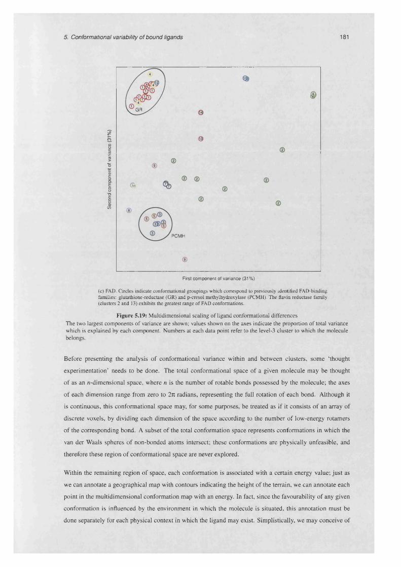
5. Conformational variability of bound ligands 181

GR

CO

§OJIOcoCaEoo~oc88

<Z>

PCMH

First component of variance (31%)

(c) FAD. Circles indicate conformational groupings which correspond to previously identified FAD-binding families: glutathione-reductase (GR) and p-cresol methylhydroxylase (PCMH). The flavin reductase family (clusters 2 and 13) exhibits the greatest range of FAD conformations.

Figure 5.19: Multidimensional scaling of ligand conformational differences The two largest components of variance are shown; values shown on the axes indicate the proportion of total variance which is explained by each component. Numbers at each data point refer to the level-3 cluster to which the molecule belongs.

Before presenting the analysis of conformational variance within and between clusters, some ‘thought

experimentation’ needs to be done. The total conformational space of a given molecule may be thought

of as an n-dimensional space, where n is the number of rotable bonds possessed by the molecule; the axes

of each dimension range from zero to 2n radians, representing the full rotation of each bond. Although it

is continuous, this conformational space may, for some purposes, be treated as if it consists of an array of

discrete voxels, by dividing each dimension of the space according to the number of low-energy rotamers

of the corresponding bond. A subset of the total conformation space represents conformations in which the

van der Waals spheres of non-bonded atoms intersect; these conformations are physically unfeasible, and

therefore these region of conformational space are never explored.

Within the remaining region of space, each conformation is associated with a certain energy value; just as

we can annotate a geographical map with contours indicating the height of the terrain, we can annotate each

point in the multidimensional conformation map with an energy. In fact, since the favourability of any given

conformation is influenced by the environment in which the molecule is situated, this annotation must be

done separately for each physical context in which the ligand may exist. Simplistically, we may conceive of

5. Conformational variability of bound ligands 182

two energy landscapes - one for the molecule in an aqueous context, and one when bound to protein. Now,

by setting a hypothetical energy threshold, we obtain the set of ligand conformations which may exist stably

when bound to protein (see figure 5.20).

Figure 5.20: Hypothetical conformational energy landscape The outer box represents all possible molecular conformations, with grid lines showing the discretisation according to bond rotamers. Grey shading shows the volume of conformation space which is inaccessible due to steric clashes. The blue region represents the conformational space explored by the molecule when in solvent; the red boundary encompasses conformations which are permitted when bound to protein. Red shading stands for the energy of each (discretised) conformation, with darker colours being more favourable. The set of allowed protein-bound conformations, according to some hypothetical energy cut-off, are marked with crosses.

Let us assume that the variance among the energies of these conformations is low - in other words that, to

a first approximation, all of the allowed bound conformations are equally stable. Since non-homologous

proteins have by definition evolved independently, we may assume that the ‘choice’ of which ligand

conformation to bind is also independent for each, and hence that they are effectively sampling from

the population of stable bound ligand conformations at random. This implies that the variance of ligand

conformations among a randomly selected set of binding sites from evolutionarily unrelated proteins is an

unbiased estimator of the variance of conformation among all stable, protein-bound arrangements of that

particular ligand.

It is clear that the fact of being bound to a protein imposes certain constraints on ligand conformation;

this is evidenced by the previously reported differences between solvent-exposed and protein-bound forms

of certain molecules (Moodie and Thornton, 1993). One way of looking at conformational differences

within and between clusters of related binding sites is to ask the question: does being bound to a protein

from a particular superfamily impose any further constraints over and above the general requirements for

being stable in a protein environment in general? In other words, are binding sites in domains belonging to

the same superfamily sampling from the same pool of stable conformations as are unrelated sites, or do they

‘pick’ from a more restricted subset?

To test this, let us propose the following null and alternative hypotheses, noting that distance in projection

space is equivalent to RMSD between conformations2:

2Note that, while in figure 5.19, only the first two components of variance are shown, for the distance calculations, all dimensions of projection space are used.

5. Conformational variability of bound ligands 183

Ho: The average pairwise RMSD between ligands in the same cluster is the same as the average

distance between cluster centroids in projection space.

H i: The average pairwise RMSD between ligands in the same cluster is less than the average

distance between cluster centroids in projection space.

Biological intuition tells us that Hi is likely to be true: we expect that molecules bound to proteins belonging

to the same superfamily should tend to adopt similar conformations. Therefore any clusters for which we

fail to disprove the null hypothesis represent interesting cases, in which proteins within a single superfamily

bind their ligands in very diverse ways.

0.15

0.05

M ean pairw ise RMSD /A

Figure 5.21: Significance testing of within-cluster mean pairwise RMSD The distribution shown is that of the average ATP inter-centroid distance, from 10,000 samples of 7 centroids at a time. The red line indicates the value of the average within-cluster RMSD value for ATP cluster 3. This leads to a p-value for the significance test of 0.07.

We take the mean distance between all points (in projection space) belonging to a cluster as the statistic

which measures the spread of that cluster. For a given cluster, let this quantity be denoted /z, and the number

of members in the cluster by s. Were Ho to be true, the observed value of n would be the result of random

sampling of s points from the pool of allowed protein-bound conformations. Since we assume that unrelated

binding sites ‘choose’ their ligand conformations by random sampling from this pool, we can obtain the

expected distribution of /z by repeatedly computing the mean pairwise distance between s randomly sampled

centroids. The fraction of the resulting distribution which lies below /z is then the probability of observing

this value by chance, if Hq is true.

Between clusters Pairwise RMSD within cluster /A

Ligand No. of clusters

No. of centroid pairs*

Mean inter-centroid

RMSD/ACluster No. of

members No. of pairs* Minimum Maximum Mean PA

1 22 231 0.42 3.71 1.91 ±0.04 < io - 102 9 36 0.47 2.26 1.58 ±0.08 < IO"10

ATP 27 351 2.21 ±0.03 34

75

2110

1.010.77

2.451.39

1.90 ±0.08 1.12 ±0.06

6.69 x IO-2 < IO-10

5 3 6 0.88 1.04 0.95 ±0.03 3.00 x 10“46 3 6 0.07 2.86 1.93 ±0.51 2.25 x 10"1

GTP 11 55 2.51 ±0.07 1 6 15 0.17 0.83 0.47 ±0.06 0

1 54 1431 0.24 4.13 1.83 ±0.02 not calculated *2 4 6 0.39 2.45 1.47 ±0.41 < 10~10

NAD 19 171 3.58 ±0.08 3 4 6 0.99 2.00 1.69 ±0.18 < IO-104 4 6 0.63 3.88 2.38 ±0.64 6.00 x 10~35 4 6 0.77 2.51 1.82 ±0.27 < 10~10

1 19 171 0.29 1.54 0.87 ±0.02 not calculated t2 9 36 0.72 4.83 2.78 ±0.18 7.70 x 10“3

FAD 14 91 3.49 ±0.13 34

53

103

0.320.61

1.121.23

0.92 ±0.07 0.97 ±0.18

< IO"10 3.00 x 10~3

5 3 3 0.95 1.70 1.28 ±0.22 6.60 x 10~36 3 3 0.24 0.47 0.35 ±0.06 < IO"10

Table 5.6: Comparison of conformational variance within and between clusters This table shows statistics on the conformational variance within and between clusters for each ligand type. The variance was estimated using the mean pairwise distance between

points in the projection space (for the within-cluster spread) and mean pairwise distance between cluster centroids (for between-cluster spread). (*) ^ where n is the number of clusters.(t) insufficient number of cluster centroids available for sampling.( A ) probability of observing a within-cluster conformational variance this large or greater, if the hypothesis that sites within a given cluster sample ligand conformation space at random is true. This was calculated according to the method described in the text.

5. C

onformational variability

of bound ligands

184

5. Conformational variability of bound ligands 185

For example, ATP cluster 3 has 7 members, and a mean pairwise within-cluster RMSD of 1.90A. To estimate

the probability of observing a conformational spread of this size or less at random, 7 points are selected at

random from the 27 ATP cluster centroids, and the mean distance between the = 2 1 possible pairs

is calculated. Repeating this procedure 10,000-fold results in the distribution shown in figure 5.21. 7% of

this distribution lies below the value of 1.90A, meaning that for this cluster, we fail to reject Ho at the 5%

significance level or greater.

Two clusters (NAD cluster 1 and FAD cluster 1) were excluded from this analysis because they contained

more members than there were cluster centroids, thus rendering the sampling scheme described above

impossible. Inspection of the MDS plots shows that these two clusters are clearly highly localised in

projection space, indicating that Ho would likely be strongly rejected for both, were sufficient data available.

Of the remaining clusters, the null hypothesis is rejected with p < 0.01 for all but two cases - ATP cluster 3

(p = 0.07) and ATP cluster 6 (p — 0.23) - see table 5.6. The latter contains only three members, of which

two are highly similar, with one distant outlier; this result may not be particularly meaningful. There is no

clear functional reason why cluster 3 should be so conformationally diverse: although its members catalyse

a number of different functions, this is the case also for other clusters.

240.303012

2 4 0 .3 0 1 0 1

3 4 0 .5 0 .8 0 13040.50.80.7

(a) Nitric oxide synthase (1F20,1.9A resolution) (b) Benzoate 1,2-dioxygenase reductase(1KRH, 1.5A resolution)

Figure 5.22: Variation in FAD conformation within the flavin reductase family Small changes in the relative positions and structures of the two domains which interact with FAD cause concomitant changes in the cofactor conformation.

Although the spread within FAD cluster 2 was not found to be statistically significant, it is clearly the largest

among all the FAD clusters. As pointed out by Dym and Eisenberg, this spread can be understood by

inspecting the structure of the binding sites within the cluster. Each site in the flavin reductase family is

composed principally of two domains - a nucleotide-binding domain with a Rossmann fold (CATH code

3.40.50.80) which binds the flavin end of the cofactor, and a (3-sheet domain (CATH code 2.40.30.10)

which interacts with the adenosine nucleotide part. The relative orientation of these two domains varies

between different members of the FR family (see figure 5.22 for examples), resulting in differences in the

conformation of the FAD which forms a bridge between them (figure 5.23).

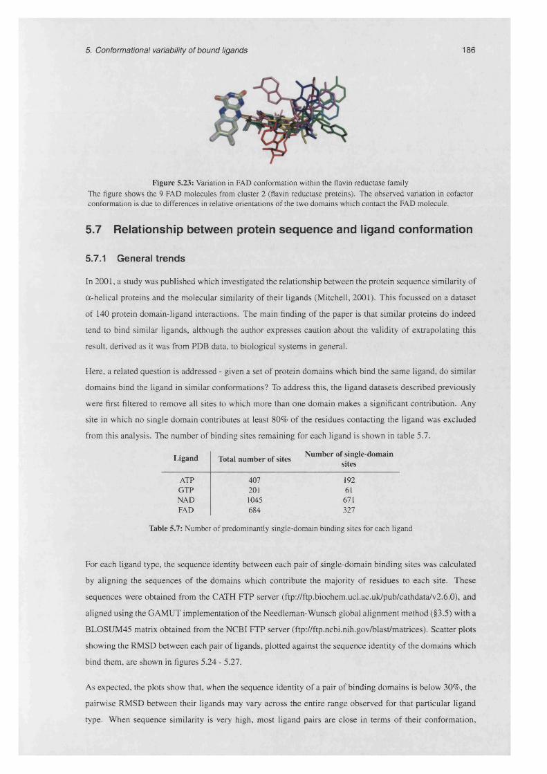
5. Conformational variability of bound ligands 186

Figure 5.23: Variation in FAD conformation within the flavin reductase family The figure shows the 9 FAD molecules from cluster 2 (flavin reductase proteins). The observed variation in cofactor conformation is due to differences in relative orientations of the two domains which contact the FAD molecule.

5.7 Relationship between protein sequence and ligand conformation

5.7.1 General trends

In 2001, a study was published which investigated the relationship between the protein sequence similarity of

a-helical proteins and the molecular similarity of their ligands (Mitchell, 2001). This focussed on a dataset

of 140 protein domain-ligand interactions. The main finding of the paper is that similar proteins do indeed

tend to bind similar ligands, although the author expresses caution about the validity of extrapolating this

result, derived as it was from PDB data, to biological systems in general.

Here, a related question is addressed - given a set of protein domains which bind the same ligand, do similar

domains bind the ligand in similar conformations? To address this, the ligand datasets described previously

were first filtered to remove all sites to which more than one domain makes a significant contribution. Any

site in which no single domain contributes at least 80% of the residues contacting the ligand was excluded

from this analysis. The number of binding sites remaining for each ligand is shown in table 5.7.

Ligand Total number of sites Number of single-domain sites

ATP 407 192GTP 201 61NAD 1045 671FAD 684 327

Table 5.7: Number of predominantly single-domain binding sites for each ligand

For each ligand type, the sequence identity between each pair of single-domain binding sites was calculated

by aligning the sequences of the domains which contribute the majority of residues to each site. These

sequences were obtained from the CATH FTP server (ftp://ftp.biochem.ucl.ac.Uk/pub/cathdata/v2.6.0), and

aligned using the GAMUT implementation of the Needleman-Wunsch global alignment method (§3.5) with a

BLOSUM45 matrix obtained from the NCBI FTP server (ftp://ftp.ncbi.nih.gov/blast/matrices). Scatter plots

showing the RMSD between each pair of ligands, plotted against the sequence identity of the domains which

bind them, are shown in figures 5.24 - 5.27.

As expected, the plots show that, when the sequence identity of a pair of binding domains is below 30%, the

pairwise RMSD between their ligands may vary across the entire range observed for that particular ligand

type. When sequence similarity is very high, most ligand pairs are close in terms of their conformation,

Liga

nd

RMSD

/A

Liga

nd

RMSD

/A

5. Conformational variability of bound ligands 187

4.5 ------------ 1------------ 1------------ 1------------1------------1------------ 1------------ 1------------ 1------------ r

Domain seq u en c e identity /%

Figure 5.24: Sequence identity of ATP binding domains versus ligand conformational distance Result of linear regression (calculated using R) is shown as a red line (r2 = 0.29).

3.5

2.5

0.5

V

0 10 20 30 40 50 60 70 80 90 100Domain seq u en c e identity /%

Figure 5.25: Sequence identity of GTP binding domains versus ligand conformational distance Result of linear regression (calculated using R) is shown as a red line (r2 = 0.14).

Liga

nd

RMSD

/A

Liga

nd

RMSD

/A

5. Conformational variability of bound ligands 188

7 -------------- 1-------------- 1-------------- 1-------------- 1-------------- 1-------------- 1-------------- 1-------------- 1-------------- r

0 10 20 30 40 50 60 70 80 90 100Domain seq u en ce identity /%

Figure 5.26: Sequence identity of NAD binding domains versus ligand conformational distance Result of linear regression (calculated using R) is shown as a red line (r2 = 0.14).

6 ------------ 1------------ 1------------ 1------------ 1------------ 1------------ 1------------ 1------------ 1------------ r

0 10 20 30 40 50 60 70 80 90 100Domain seq u en c e identity /%

Figure 5.27: Sequence identity of FAD binding domains versus ligand conformational distance Result of linear regression (calculated using R) is shown as a red line (r2 = 0.19).

5. Conformational variability of bound ligands 189

but for all ligands except FAD, there are several outlying pairs in which practically identical domains bind

ligands in very disparate shapes. This may be due to conformational changes undergone at different stages

of a reaction cycle. For example, in PDB entry 1PJ3, a 2.10A structure of human malic enzyme, NAD

molecules are bound to identical subunits of the protein in radically different arrangements.

The general trend, however, is for more similar domains to bind ligands in a more similar conformation. To

quantify this, we can compute the standard linear regression coefficient. The nature of the data, however,

means that the value obtained will necessarily be small. Firstly, there is a large variance in RMSD values

corresponding to low sequence identities. Secondly, the inhomogeneous composition of the PDB means that

there is a relative paucity of sequence pairs with identities in the range 50-80%, somewhat obscuring the

general trend obeyed by these two variables. Table 5.8 shows the results of the linear regression, which in all

cases indicates only weak correlation between the two variables; visual inspection of the plots suggests that

an exponential or polynomial function may provide a better fit.

LigandLinear regression (y = a b

a + bx) r2

ATP 2.43 -0.02 0.29GTP 2.34 -0.01 0.14NAD 2.88 -0.03 0.14FAD 2.52 -0.03 0.19

Table 5.8: Linear regression between domain sequence identity and ligand conformation distance Calculations were performed using R (Ihaka and Gentleman, 1996). r2 is the linear regression correlation coefficient.

The data were then analysed by dividing the plots into discrete regions, and using a %2 test to determine

whether the distributions observed are significantly different to what would be expected by chance. In doing

so, we assume that the domain sequence identity and ligand RMSD variables are independent. The sequence

identity values were divided into two ranges - low and high - using 45% as the cutoff value. This value is

the same as that used in the analysis of Mitchell. It is generally held that pairs of proteins with this degree of

sequence identity or greater are likely to be closely related in both evolutionary and structural terms (Orengo

et al., 1993). The RMSD values were divided using a cutoff of 1.5A for ATP and GTP, and 2.0A for NAD

and FAD. These values were determined manually, and were chosen such that pairs of molecules with an

RMSD below the threshold can be seen visibly to be in a very similar conformation; the larger value for

NAD and FAD reflects the dependence of the RMSD value on the number of points used to calculate it.

The proportions of binding site pairs whose sequence similarity is high are 4%, 15%, 3% and 7% for ATP,

GTP, NAD and FAD respectively. The corresponding proportions of pairs whose ligand RMSD is below the

threshold are 8%, 30%, 35% and 56%. Making the assumption that these two variables are independent,

we can construct a 2 x 2 contingency table as shown in table 5.9. Applying a %2 test to the values in

these tables, with 1 degree of freedom, shows that in all cases, the hypothesis of independence is rejected

with p <C 0.005 (critical value = 7.879). The tendency for similar domains to bind the ligand in a similar

conformation is expressed by the enrichment factor for the (high sequence similarity, low ligand RMSD) cell

of the contingency table. This factor is the ratio between the number of observations in this cell compared

to that which would be expected under the assumption of independence. Of the four ligand types, ATP has

5. Conformational variability of bound ligands 190

ATP

Sequence i<45%

Observed Expected

dentity>45%

Observed Expected Total

RM

SD

A IV

In ui

>o >. 16,704 16,028.77

757 1,432.23128 803.23 747 71.77

16,832 (0.92) 1,504 (0.08)

x2 = 7259 f

GTP

17,461 (0.96)

Sequence i<45%

Observed Expected

875 (0.04)

dentity>45%

Observed Expected

18,336

Total

£ > 1-5A g < 1.5A

1,212 1,089.65 341 463.35

72 194.35 205 82.65

1,284 (0.70) 546 (0.30)

X2 = 3041

NAD

1,553 (0.85)

Sequence i<45%

Observed Expected

277 (0.15)

dentity>45%

Observed Expected

1,830

TotalA| > 2.0A 2 < 2.0A

146,262 141,907.31 71,120 75,474.69

478 4,832.69 6,925 2,570.31

146,740 (0.65) 78,045 (0.35)

x2 = 11687 f

FAD

217,382 (0.97)

Sequence i<45%

Observed Expected

7,403 (0.03)

identity>45%

Observed Expected

224,785

Totald£ > 2.0A 2 < 2.0A

23,151 21,622.71 26,492 28,020.29

65 1,593.29 3,593 2,064.71

23,216 (0.44) 30,085 (0.56)

x2 = 27891- 49,643 (0.93) 3,658 (0.07) 53,301

Table 5.9: x2 analysis of ligand conformation distance versus domain sequence identity Numbers in parentheses show the fraction of total pairs for each ligand which fall into each row or column.(t) The critical level for %2 at the 0.1% significance level, with one degree of freedom, is 10.83. Therefore the deviation from random is highly significant in all cases.

the highest enrichment factor (10.41), indicating that the relationship between sequence similarity and ligand

conformations is strongest for this ligand.

The results of this analysis must be interpreted with caution, due to the degree of non-uniformity in the

distribution of pairwise sequence similarities. Although the x2 analysis indicates a relationship between

domain sequence similarity and bound ligand RMSD, the weak linear regression results, coupled with visual

inspection of the scatter plots, show that this relation only really holds when sequence similarity is above

around 30%.

5.7.2 Ligand conformation and sequence similarities in the ‘twilight zone’

We know that, within homologous superfamilies, the overall structure of proteins tend to be conserved

even though their primary sequences may diverge beyond the point at which their relatedness is detectable

using standard sequence analysis methods. Pairs of sequences which lie below this similarity threshold,

5. Conformational variability of bound ligands 191

commonly taken to be around 35% identity, are said to be ‘in the twilight zone’. Here we ask whether

pairs of domains towards the upper boundary of this sequence similarity interval tend to bind ligands in

more similar conformations, or whether, once sequences have diverged so far, any relationship between

evolutionary distance and ligand conformational similarity has been obscured to the point where it can no

longer be observed.

In order to address this question, binding site clusters which satisfy the following three criteria were sought:

• Contain binding sites which are predominantly single-domain, such that sequence similarities between

sites can be calculated in a straightforward manner;

• Contain several members (at least 10);

• Exhibit a reasonable degree of conformational diversity: must contain pairs of molecules which differ

by at least 3A

The only two clusters which satisfied all three of these requirements were ATP cluster 1 (P-loop hydrolase

domains) and NAD cluster 1 (classical Rossmann-fold domain dehydrogenases). For each, pairwise sequence

similarities and ligand conformational distances were calculated as above; scatter plots of the results are

shown in figures 5.7.2 and 5.7.2 respectively. Visual inspection suggests that, for the ATP cluster, the two

variables are uncorrelated below the 35% sequence identity threshold, while for NAD cluster 1, there is a

weak correlation, with more similar domains tending to bind the cofactor in more similar conformations.

This is confirmed by least squares linear regression analysis, which returns r2 values for the two clusters of

0.004 and 0.15 respectively.

In order to better understand the relationship between pairwise domain sequence identity and NAD

conformation among the Rossmann-fold domain dehydrogenases, a ‘heat map’ was constructed, in which

a square matrix was plotted, with rows and columns corresponding to each site within the cluster. Each cell

is coloured according to the sequence identity between the appropriate pair of domains, and the rows and

columns are ordered according to a dendrogram obtained by clustering the cofactor conformations (figure

5.7.2).

The pattern which clearly emerges is that sequence identity, even within the ‘twilight zone’, is correlated

with the stereospecificity of the cofactor conformation. This suggests that cofactor stereospecificity is non-

random, but is in fact an evolutionary conserved trait; this is in agreement with previous studies (Glasfeld

et al., 1990, and references therein). Moreover, it appears that altering dehydrogenase substrate specificity

may require fewer mutational changes than those which are needed in order to permit the cofactor to bind

with its nicotinamide ring positioned in the opposite direction. This is to be expected, since the latter may

involve significant structural rearrangements, while facilitating recognition of a new substrate may simply be

a matter of subtly changing the shape or electrostatic properties of the binding site.

Liga

nd

RMSD

/A

Liga

nd

RMSD

/A

5. Conformational variability of bound ligands 192

3.5

+ +

2.5*+++ +

+ +++-f*i4.+ +++

f++

0.5

0 5 10 20 25 30 35 4015Domain seq u en ce identity /%

Figure 5.28: Sequence identity of P-loop hydrolase domains versus ATP RMSD values Result of linear regression is shown as a red line (r2 = 0.004).

4.5

3.5 ++Z+ T+ r + ■'+' + ?

J t % *

2.5 r + +

+ +

+ + + +^ - t L + + ^ + * + + + + +

0.5

0 10 205 15 25 30 35 40 45Domain seq u e n ce identity /%

Figure 5.29: Sequence identity of Rossmann fold domains versus NAD RMSD values Result of linear regression is shown as a red line (r2 = 0.15).

5. Conformational variability of bound ligands 193

RMSD /A r 4- 3- 2- 1 L 0

'F8G-1-E-NAD-2500iLSS-i+NAD-1001irY*-1-A-NAD-12*61H#4-1-A-NAD-7BB1T2D-1-E-NAD-3161KOL-1 -A-NAD-1403SLOT *1 -A-NAD-4011R37-1-A-NAD-4031J5P-1-C-NAD-300iBMD-i-A-NAD-334106Z-1-C-NAD-20031HYW-1-A-NAD-3301PJ3-1 -£-NAD-26011 N6K-1 -A-NAJ-3771PSO-1-&-NAD-4601UD-1-A-NAO-11EMD-1-A-NAD-3141DXY-1 -O-NAD-336iMX3-l-€-NAD-1000i PJC-1 -G-NAD-5002NAD-1-A-NAD-3841NPD-1-A-NAD-300lP*.-1-£-NADa0l1ARZ-1 -ft-NAD-274 1D4F-1-6-NAD6M 1EE8-1-C-NAD-10 lNHW-l-t-NAD-450 1D70-1-E-NAD-601 1O8O-1-DNAD-1304 1 ENV-l -&-NAD-500 i POV-1 -A-NAD-361 iFtflM -C-NAD-600 1B14.1-C-NAD-6S6 1I3L-1-C-NAD-400 lDMR-1 -&-NAD-241 10AR-l-A-NAD-1200 lGEE-l-O-NAD-2262 ' ESW-1 -C-NAD-301 1NFF-1-F-NAD-2300 1FMC-1 -A-NAD-256 1 BOB-1 • A-NAD-300 1OEO-1-A-NAD-101 1KEW-1-C-NAD-1400 iEBf-1-C-NAD-210#10AR-l-A-NAD-401 1K6X-1-C-NAD-400 1OA0-1-A-NAD-1000 1FOY-1 -C-NAD- 750 i GAD-1-O-NAD-336 iDU-i-C-NAD-403 1NVU-1-8-NAD-3501 1BXG-1 -A-NAD-360 1CH6-1-G-NAD-671 1EVJ-1-A-NAD-500

Figure 5.30: Sequence identity of Rossmann fold domains versus NAD conformational distance Rossman fold domains within the same superfamily, but with sequence identities of less than 30%, and which bind NAD, were analysed. Cells of the matrix are coloured according to the sequence identity between the appropriate pair of domains, and the rows and columns are ordered according to a dendrogram obtained by clustering the NAD conformations. NAD molecules are distinguished according to the orientation of the nicotinamide N-glycosidic bond, as shown by the braces at the bottom of the plot.

5. Conformational variability of bound ligands 194

5.8 Analysis of torsion angles

Another way of looking at ligand conformation is to measure the torsion angles of each rotable bond in the

molecule. Comparison of the distribution of angles for each bond among a group of ligands can provide an

overview of which parts of the molecule are the most variable.

As with all studies of ligand-protein interaction, the quality of the structural data used is of key importance

when interpreting the results of this analysis. Torsion angles are particularly sensitive to experimental

uncertainties - since the error in atomic coordinates in a structure resolved to 2.0A is typically around 0.4A,

accurate calculation of bond torsions really requires data of at least this quality or better. In their discussion of

the NAD(P) torsion angles, Carugo and Argos point out that, in many cases, these may be biased by restraints

applied during crystallographic refinement (Carugo and Argos, 1997). Figure 5.31 shows the coordinates

of NAD molecules taken from four structures of different resolutions, compared with the electron density

observed in each crystallisation experiment. It is clear that, for data sets with resolutions of 2.5A or worse,

atomic positions cannot be unambiguously assigned from the electron density map alone.

An analysis of several hundred PDB structures (Morris et al., 1992) found a clear dependency between the

resolution of the structure and the standard deviations of the <|>, \y, %i and %2 torsion angles. Even at the best

resolutions of 1.3 A, standard deviations of the order 10-15° remained, and extrapolation of the best fit line to

a hypothetical resolution of 0A suggested that a residual deviation of between 2.9° and 9.3° would remain.

From these results, it is clear that torsion angles should be regarded as a fairly approximate measure.

Figures 5.32 - 5.35 show the distribution of torsion angles for each rotable bond of ATP, GTP, NAD and

FAD. These values were calculated using all level-3 cluster representatives as the input data. As such, they

represent the conformations of all molecules bound to sites composed of non-homologous domains. For the

reasons outlined above, the spokes of each torsion wheel are colour-coded according to the resolution of the

structure from which the corresponding torsion angle was calculated.

The first observation which is prompted by inspection of these plots is that, among the four ligand types,

ATP appears to exhibit the greatest spread in torsion angles, with a considerable number falling outside the

theoretically favourable ranges. This is due in part to the structures in the ATP dataset being resolved to a

lower resolution in general than those for the other three ligands. It is notable that the ATP bonds with the

greatest variation, and which have the greatest proportion of examples in supposedly disfavoured regions, are

those towards the phosphate tail of the molecule. This is the case even in structures of quite high resolution.

This can be attributed to two factors. Firstly, since the adenine part of the molecule is that which tends to

be bound by the protein, the phosphate moieties are often more exposed to solvent, and therefore can retain

greater mobility when the ligand is bound. As a result, electron density for the y and, to a lesser extent,

(3-phosphates is likely to be less well defined than for the adenine-ribose group. Secondly, the orientation

of each phosphate is determined solely by the position of its four oxygen atoms. Since these are large,

electronegative atoms which share a partial negative charge at physiological pH, they possess considerable

electron density, which tends to blur out around the phosphate atom, thus presenting problems for accurate

modelling of this part of the ligand coordinates.

5. Conformational variability of bound ligands 195

(b) 1BT0. 2.0A, R=0.174

(c) 1E3L. 2.5A, R=0.218 (d) 1AGN. 3.0A, R=0.223

Figure 5.31: Coordinates of NAD molecules modelled into density maps at different resolutions Each figure shows the coordinates of an NAD molecule, along with the electron density, contoured at 2a (green chicken wire). The NAD molecules were arbitrarily chosen, from structures with a spread of different resolutions. They are from three structures of alcohol dehydrogenase (1BTO, 1E3L and 1AGN) and one of UDP-galactose 4-epimerase (1HZJ). Electron density maps were obtained from the Uppsala Electron Density Server (http://eds.bmc.uu.se). The density contours illustrate that, at a resolution of 2A, robust assignment of coordinates is fairly straightforward, with the positions of most atoms clearly resolved. The 1.5 A map allows for completely unambiguous modelling, with even the holes in ring structures clearly visible. At resolutions of 2.5 A or poorer, coordinates can only be built by application of strict restraints, and therefore cannot be completely trusted. The maps in figures (c) and (d) show that the accuracy of torsion angles in particular may be limited.

It should be stressed that a wider range in the local orientations about a number of bonds does not necessarily

lead to a similarly more diverse set of overall conformations. It is known that nearby torsion angles are

correlated; therefore a change in one may be compensated for by another bond near to it in the molecule also

being rotated. The combination of these two transformations may return the molecule to a global arrangement

close to the original one.

Since ATP, NAD and FAD share a common adenosine nucleotide portion, we can directly compare the

distributions of bonds 1-6 between these ligands. The general preferences of each bond are broadly similar

for each ligand type. The % and (3 angles (bonds 1 and 3 respectively) are particularly well-conserved, with

all three ligands showing strong preferences for the anti orientation of the % bond, and for the ap orientation

of the 3 bond. These trends are to be expected given the steric hinderance caused by the other rotamers of

each of these bonds.

Ml 1 :0 4 -C 1' -N 9 -C 4 2 :0 5 ' • C5' - C4' - C3' 3 : PA - 0 5 ' - C5' - C4

4 : 03A - PA - 0 5 ' - C5 5 : PB - 03A - PA - 0 5 ' 6 : 03B - PB - 03A • PA

7 : PG - 03B - PB - 03A 8 : 03G - PG - 03B - PB

Figure 5.32: Variation in ATP torsion anglesFor each of the rotable bonds, a wheel diagram showing the distribution of torsion angles among the 27 level-3 cluster representatives is plotted. The colours of the spokes represent the resolution of the structure from which the coordinates were taken, according to the scale bar shown (values in A). Theoretically favourable angular ranges for each bond (see table5.1) are shaded.

5. Conformational variability

of bound ligands

196

o. /01B ,

7 II ̂ /0 2 0 03B._____1 1 ______ 02B „ C 4 '-------- -C3'

\ V ' \ 7 « / \V l 4/ “0 3 0 \ \ ---------------------------------—

° ' Q H ^ O Z A

01A

4 : 03A - PA - 05' - C5' 6 : 03B - PB - 03A - PA

7 : PG - 0 3 B • PB - 0 3 A 8 : 0 3 G - PG - 0 3 B - PB

Figure 5.33: Variation in GTP torsion anglesFor each of the rotable bonds, a wheel diagram showing the distribution of torsion angles among the 11 level-3 cluster representatives is plotted. The colours of the spokes represent the resolution of the structure from which the coordinates were taken, according to the scale bar shown (values in A). Theoretically favourable angular ranges for each bond (see table5.1) are shaded.

5 : PB - 03A - PA - 05'

197

"N3_A I

\

° ! - 1 C 6 J , -------C* A

14 8/ \*P A— 0 5 A

5/0 3

\ V “

1 N9

X V A

j VS02_A

\C5_N— 0 5 _ N

A 8/ 7 \ n

I \C2'_N « ' - N

N v /

I 10NN1*.

« / >

' S / S a/ ' "IT) CM i n CO COT-‘ ’ csi ' AV in . in

3 : P_A - 05'_A - C5'_A - C4'_A

03 - P_A - 05'_A - C5 _A 5 : P_N - 03 - P_A • 05'_A 6 : P_A - 0 3 - P_N - Q5’_N

7 0 3 - P_N - 05'_N - C5'_N 8 : P_N - 05 _N - C5*_N - C4 _N 9 : 0 5 _N - C5_N - C4 _N - C3*_N

1 0 :0 4 N-CV N-NN1 -C2 N 11 : C2 N - C3 N -C 7 N - NN7

Figure 5.34: Variation in NAD torsion anglesFor each of the rotable bonds, a wheel diagram showing the distribution of torsion angles among the 19 level-3 cluster representatives is plotted. The colours of the spokes represent the resolution of the structure from which the coordinates were taken, according to the scale bar shown (values in A). Theoretically favourable angular ranges for each bond (see table 5.2) are shaded.

5. Conformational variability

of bound ligands

198

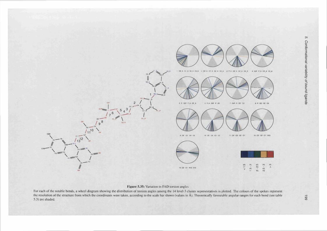
y s yII I3 * C5_A

\ H 7J

.04' i /

or a

02P 2 / \I orjr-«*± '

03P 5 A 9 / cxjr \ »

I// 8

\ ' 9> _ HA'

6 V 4

7 „ y \ 03* A

02_A

\C8

//

/ t C2*

C l - — v

» / . _12 \ \ _ i 13 °

1° \1 «■

\ / CtO==-— v

XC6-ss:c=4 / \“ ■ \ / c

' ^ —C4A /

N5̂ \ /\ — N3//

1 : 0 4 _A - C1'_A - N9_A • C4_A 2 :0 5_ A - C5 _A • C4_A - C3 _A 3 : P_A - 0 5 _A - C5_A • C4 _A 4 : 0 3P - P_A 05_A - C5_A

5 : P • 0 3P • P_A - 0 6 ’_A 6 : P_A - Q3P - P - 0 6 ‘ 7 : 0 3P P 0 5 - C51

9 : 0 5 ’ • C5‘ - C4‘ - C3* 10 : C5* • C4‘ - C3‘ • CZ9 : 0 5 ’ • C5‘ - C4' - C3' 10 : C5 ‘ - C4 ' - C3 * - C2’

lo cv in co co T-’ • cvi Av io . in

f - cm cvi

Figure 5.35: Variation in FAD torsion anglesFor each of the rotable bonds, a wheel diagram showing the distribution of torsion angles among the 14 level-3 cluster representatives is plotted. The colours of the spokes represent the resolution of the structure from which the coordinates were taken, according to the scale bar shown (values in A). Theoretically favourable angular ranges for each bond (see table 5.3) are shaded. coco

5. C

onformational variability

of bound ligands

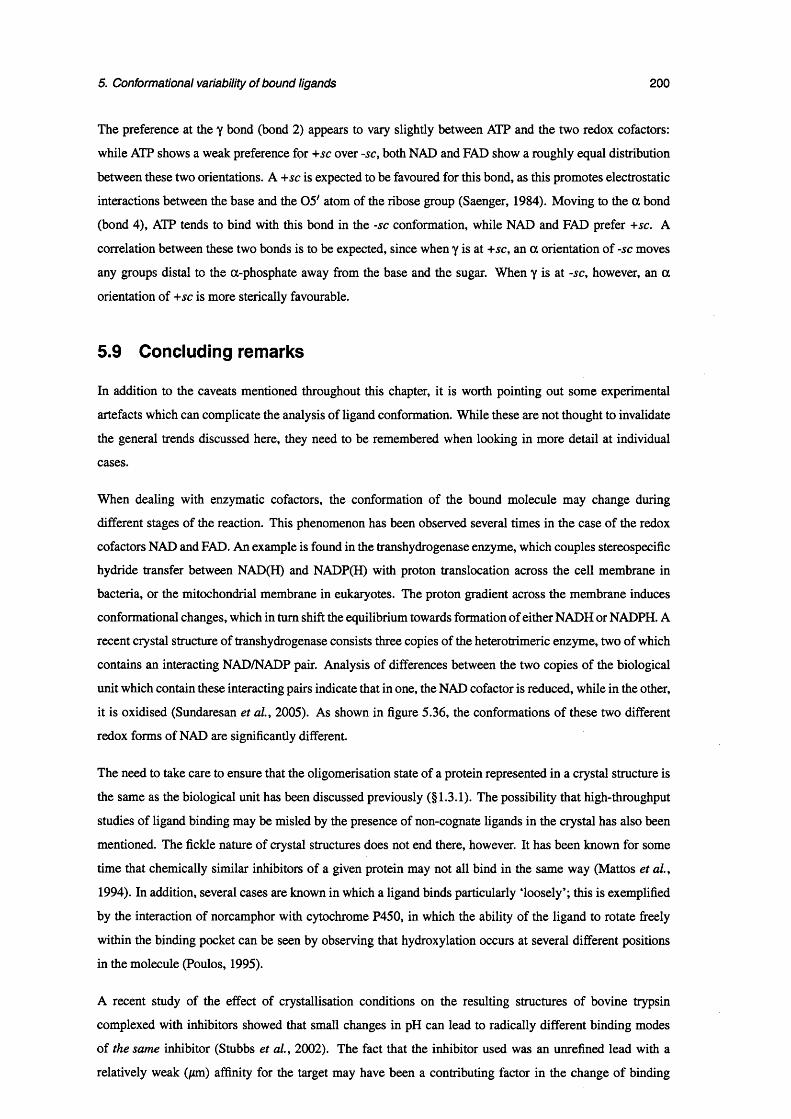
5. Conformational variability of bound ligands 200

The preference at the y bond (bond 2) appears to vary slightly between ATP and the two redox cofactors:

while ATP shows a weak preference for +jc over -sc, both NAD and FAD show a roughly equal distribution

between these two orientations. A +sc is expected to be favoured for this bond, as this promotes electrostatic

interactions between the base and the 0 5 ' atom of the ribose group (Saenger, 1984). Moving to the a bond

(bond 4), ATP tends to bind with this bond in the -sc conformation, while NAD and FAD prefer +sc. A

correlation between these two bonds is to be expected, since when y is at +sc, an a orientation of -sc moves

any groups distal to the cs-phosphate away from the base and the sugar. When y is at -sc, however, an a

orientation of +sc is more sterically favourable.

5.9 Concluding remarks

In addition to the caveats mentioned throughout this chapter, it is worth pointing out some experimental

artefacts which can complicate the analysis of ligand conformation. While these are not thought to invalidate

the general trends discussed here, they need to be remembered when looking in more detail at individual

cases.

When dealing with enzymatic cofactors, the conformation of the bound molecule may change during

different stages of the reaction. This phenomenon has been observed several times in the case of the redox

cofactors NAD and FAD. An example is found in the transhydrogenase enzyme, which couples stereospecific

hydride transfer between NAD(H) and NADP(H) with proton translocation across the cell membrane in

bacteria, or the mitochondrial membrane in eukaryotes. The proton gradient across the membrane induces

conformational changes, which in turn shift the equilibrium towards formation of either NADH or NADPH. A

recent crystal structure of transhydrogenase consists three copies of the heterotrimeric enzyme, two of which

contains an interacting NAD/NADP pair. Analysis of differences between the two copies of the biological

unit which contain these interacting pairs indicate that in one, the NAD cofactor is reduced, while in the other,

it is oxidised (Sundaresan et al., 2005). As shown in figure 5.36, the conformations of these two different

redox forms of NAD are significantly different.

The need to take care to ensure that the oligomerisation state of a protein represented in a crystal structure is

the same as the biological unit has been discussed previously (§1.3.1). The possibility that high-throughput

studies of ligand binding may be misled by the presence of non-cognate ligands in the crystal has also been

mentioned. The fickle nature of crystal structures does not end there, however. It has been known for some

time that chemically similar inhibitors of a given protein may not all bind in the same way (Mattos et a l,

1994). In addition, several cases are known in which a ligand binds particularly ‘loosely’; this is exemplified

by the interaction of norcamphor with cytochrome P450, in which the ability of the ligand to rotate freely

within the binding pocket can be seen by observing that hydroxylation occurs at several different positions

in the molecule (Poulos, 1995).

A recent study of the effect of crystallisation conditions on the resulting structures of bovine trypsin

complexed with inhibitors showed that small changes in pH can lead to radically different binding modes

of the same inhibitor (Stubbs et al., 2002). The fact that the inhibitor used was an unrefined lead with a

relatively weak (jtim) affinity for the target may have been a contributing factor in the change of binding

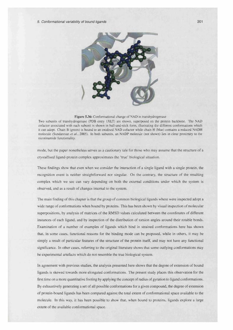
5. Conformational variability of bound ligands 201

Figure 5.36: Conformational change of NAD in transhydrogenase Two subunits of transhydrogenase (PDB entry 1XLT) are shown, superposed on the protein backbone. The NAD cofactor associated with each subunit is shown in ball-and-stick form, illustrating the different conformations which it can adopt. Chain B (green) is bound to an oxidised NAD cofactor while chain H (blue) contains a reduced NADH molecule (Sundaresan et al., 2005). In both subunits, an NADP molecule (not shown) lies in close proximity to the nicotinamide functionality.

mode, but the paper nonetheless serves as a cautionary tale for those who may assume that the structure of a

crystallised ligand-protein complex approximates the ‘true’ biological situation.

These findings show that even when we consider the interaction of a single ligand with a single protein, the

recognition event is neither straightforward nor singular. On the contrary, the structure of the resulting

complex which we see can vary depending on both the external conditions under which the system is

observed, and as a result of changes internal to the system.

The main finding of this chapter is that the group of common biological ligands where were inspected adopt a

wide range of conformations when bound by proteins. This has been shown by visual inspection of molecular

superpositions, by analysis of matrices of the RMSD values calculated between the coordinates of different

instances of each ligand, and by inspection of the distribution of torsion angles around their rotable bonds.

Examination of a number of examples of ligands which bind in strained conformations here has shown

that, in some cases, functional reasons for the binding mode can be proposed, while in others, it may be

simply a result of particular features of the structure of the protein itself, and may not have any functional

significance. In other cases, referring to the original literature shows that some outlying conformations may

be experimental artefacts which do not resemble the true biological system.

In agreement with previous studies, the analysis presented here shows that the degree of extension of bound

ligands is skewed towards more elongated conformations. The present study places this observation for the

first time on a more quantitative footing by applying the concept of radius of gyration to ligand conformations.

By exhaustively generating a set of all possible conformations for a given compound, the degree of extension

of protein-bound ligands has been compared against the total extent of conformational space available to the

molecule. In this way, it has been possible to show that, when bound to proteins, ligands explore a large

extent of the available conformational space.

5 . Conformational variability of bound iigands 202

Among homologous proteins, the degree of conformational variation is not the same for all superfamilies.

While most bind the ligand or cofactor in a reasonably conserved manner, several, notably the FAD-binding

flavin reductase proteins, and proteins which contain a Rossmann-fold ATP-recognition domain, exhibit

considerable variation in the binding mode. Statistical analysis shows that, for the latter family, the degree of

ATP conformational variation is as great as that observed between homologous superfamilies.

Analysis of the relationship between the sequence similarity of protein domains binding a given ligand,

and the similarities between the bound ligand conformations, shows that in general the correlation between

these two variables is weak. Just as protein sequences with more than about 35% identity tend to fold into

similar structures, domains above this threshold tend to bind ligands in fairly similar conformations. Below

this sequence similarity cutoff, little correlation is evident. Next, the sequence similarity-ligand conformation

relationship was explored among domains which are in the same superfamily but have less than 35% sequence

identity. The two superfamilies examined showed quite different behaviour, with the ATP-binding P-loop

hydrolase family showing no correlation, whereas the NAD-binding Rossmann-fold domains showed a clear

relationship between primary sequence and cofactor stereospecificity.

Besides constraints of space and time, one reason why the current study was limited to the four molecules

studied, was that a limitation of the automatic method for dataset generation used here is that it does not

guarantee that the binding sites obtained are in complex with their cognate ligands. This is not too great a

problem for the compounds studied here, where we can be reasonably confident that most of the interactions

which they make are biologically relevant. Extending the study to more esoteric molecules, however,

increases the risk that analogues, xenobiotic compounds and experimental artefacts will pollute the results. A

resource which rectifies this problem by cataloguing the cognate ligands associated with each protein domain

should soon be available (I. Nobeli, personal communication); application of the generic analytical methods

presented here to a ‘clean’ dataset containing greater diversity of ligands would likely yield many interesting

findings. In conclusion, the work presented in this chapter is intended as a ‘pathfinding’ report, which the

author hopes will stimulate increased interest in the complex area of ligand conformational diversity, and

which will encourage other researchers to explore its many ramifications across biology.

This work raises numerous questions which could be addressed in future studies. In particular, the

relationship between protein evolution and ligand/cofactor conformation needs to be investigated in more

detail. The findings shown here indicate that this relationship is complex, with no simple mapping between

the similarity (in sequence or structure) of protein domains and the similarity of the shape of the bound ligand.

This is most likely a product of the fact that the evolutionary pressure acting upon functional sites such as

ligand binding pockets is not necessarily the same as that on the domain as a whole. By performing multiple

sequence alignents and conservation analysis using previously published methods (Valdar and Thornton,

2001a), it would be possible to study the relationship between the evolutionary divergence of just the ligand-

binding region, and the conformation of the ligand.

Another area which has been touched upon here, but which deserves further study, is the connection of

cofactor conformation to enzymatic function. The results presented in this chapter suggest that this is

weak at best, but this conclusion is drawn from a very small data set, and should therefore be more

5. Conformational variability of bound ligands 203

thoroughly validated. It may be that more sensitive methods of ligand structure comparison than the

superposition/RMSD approach taken here could uncover subtle relationships between conformation and

function. The development of a method which attempts to predict the function of an enzyme based on the

shape of its cofactor, using sophisticated spherical-harmonics based shape matching, is currently underway

(T. Funkhouser, personal communication), and may go some way to addressing this point.

As stated previously, the main aim of the work in this thesis was to analyse the diversity of binding sites for a

given ligand, as observed in structures retrieved from the PDB. In the light of the conformational variability so

dramatically illustrated by the molecular superpositions shown here, it is clear that any attempts to compare

binding sites simply by superposing the ligands as a whole will founder. As a result, it was decided to

analyse the environments of rigid fragments of each ligand in turn, thus circumventing the problem of

molecular flexibility. The following chapter describes a semi-automatic, generic method for identifying these

rigid fragments, extracting and superposing their protein environments, and discusses several approaches for

quantifying the structural and chemical diversity among these binding sites.

204

Chapter 6

Structural and chemical variability in

ligand environments

The previous chapter established that the amount of conformational diversity shown by several common

ligands when bound to different proteins is considerable. This has the effect of making patterns of interaction

between ligands and proteins hard to detect, both visually and algorithmically. A natural response to this

difficulty is to attempt to look for commonalities in those regions of ligand binding sites which surround

rigid fragments of the ligand. In this way, ligand flexibility is eliminated, allowing comparatively simple

approaches for binding site comparison to be designed.

A number of studies analysing interactions between rigid ligand fragments and proteins have been published.

In several cases, structural motifs for fragment recognition have been identified which occur in unrelated

proteins, suggesting that evolution may have converged upon a similar solution on a number of different

occasions. Such cases of well-defined motifs, however, are the exception rather than the rule; despite

extensive study, it appears that distilling the essential features of binding sites for a given ligand into a

single structural ‘template’ - or even a manageable number of such templates - may prove intractable. Visual

inspection of proteins interacting with several common ligand fragments suggests that, in terms of gross

structural features such as sheets, helices and loops, and even in terms of local arrangements of amino acid

residues, these sites exhibit almost limitless variability.

Trends can be identified, however, particularly when the binding sites are considered from the point of the

view of the ligand - that is to say, when they are represented in terms of what the ligand ‘sees’ (i.e. a particular

disposition of chemical properties), rather than what the crystallographer sees (that is, three-dimensional

arrangements of amino acid residues). The first of part of this chapter describes a simple method for analysing

groups of fragment environments in order to identify patterns of interaction. This is applied to a dataset of

adenine binding sites, allowing a ‘fuzzy template’ - one which expresses the consensus pattern of interactions

while also implicitly retaining information about binding site variation - to be defined.

The second part of the chapter is concerned with the development of a quantitative measure for binding site

diversity. If elucidation of the common features of a group of binding sites may be considered analagous to

finding the mean of a group of numbers, then measuring their diversity of the sites corresponds to calculating

the variance. When comparing groups of biological sequences, tertiary structures, or very well-conserved

6. Structural and chemical variability in ligand environments 205

motifs such as catalytic sites, established methods exist for measuring the degree to which they are conserved

(i.e. are lacking in diversity), both on the whole and locally. No such measure currently exists for binding

sites. Such a quantity could be extremely useful, for example, in guiding computational searches for putative

binding sites, in which a knowledge not only of which regions of known sites tend to show similarities, but

also which exhibit significant levels of variation, would allow appropriate up- and down-weighting of the

importance of those regions to the search. Here, the basis for such a method, defined by borrowing concepts

from biological sequence analysis, is described, and examples of its application are shown.

6.1 Qualitative observations of binding site diversity

In order to demonstrate the degree of diversity found in the structure of ligand binding sites, consider the

three ATP-binding proteins shown in figure 6.1. cAMP-dependent protein kinase (cAPK) is a member of a

large superfamily of proteins which catalyse the transfer of the y-phosphate from ATP onto serine, threonine

or tyrosine residues on substrate proteins. This phosphorylation controls the activity, localization and overall

function of many proteins, and plays a central role in many cellular processes, including signal transduction

and regulation of the cell cycle. cAPK consists of two domains joined by a loop; the ATP-binding site is

located between them, with the loop forming several specific polar interactions with the Watson-Crick edge

of the adenine ring (figure 6.1a). The faces of the ring, on the other hand, are packed between a number of

hydrophobic residues.

Lysyl-tRNA synthetase is one of a family of enzymes, each of which catalyses the ‘charging’ of a specific

tRNA molecule with the appropriate amino acid. tRNA synthetases can be separated into two classes,

which differ in both structure and mechanistic detail. Class I enzymes are normally monomeric, with the

ATP molecule being bound by a classical Rossmann fold domain. Class II enzymes, of which lysyl-tRNA

synthetase is an example, function as monomers, with the ATP being bound by a central antiparallel (3-sheet

motif. The amino acid transfer reaction proceeds in two steps. In the first step, the amino acid is activated

by formation of an aminoacyl-adenylate, in which the carboxyl group of the amino acid is linked in to the

alpha-phosphate of ATP, releasing pyrophosphate. When the correct tRNA is bound, the aminoacyl group

of the aminoacyl-adenylate is transferred onto either the 2' OH of the tRNA (in class I enzymes) or onto

the y OH (in most class II enzymes). Around the adenine moiety, the pattern of interactions in lysyl-tRNA

synthetase is quite different to that seen in cAPK (see figure 6.1b). A phenylalanine ring lies across one face

of adenine, and the only polar atom which is hydrogen bonded to the protein is N6, which donates two bonds.

Finally, we consider phosphoribosylgyclinamide formyltransferase. This enzyme catalyses the second step in

the pathway of de novo purine biosynthesis, in which a formyl group is added to glycinamide ribonucleotide

(‘activated ribose’). This reaction also results in the terminal pyrophosphate bond of ATP being cleaved.

As in cAPK, the ATP molecule is bound between two domains, with a connecting loop interacting with the

Watson-Crick edge of adenine. However, in this case, an additional hydrogen bond is also formed at the trans

position of N6, and N7 is unsatisfied (figure 6.1c). In this protein, N3 is exposed to solvent, with the position

of an immobilised water molecule resolved nearby (not shown).

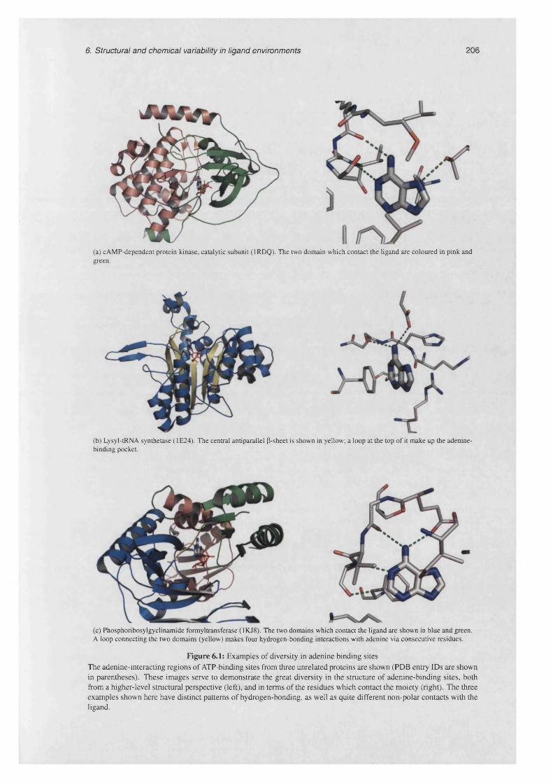
6. Structural and chemical variability in ligand environments 206

(a) cAMP-dependent protein kinase, catalytic subunit (1RDQ). The two domain which contact the ligand are coloured in pink andgreen.

(b) Lysyl-tRNA synthetase (1E24). The central antiparallel P-sheet is shown in yellow; a loop at the top of it make up the adenine- binding pocket.

(c) Phosphoribosylgyclinamide formyltransferase (1KJ8). The two domains which contact the ligand are shown in blue and green.A loop connecting the two domains (yellow) makes four hydrogen-bonding interactions with adenine via consecutive residues.

Figure 6.1: Examples of diversity in adenine binding sites The adenine-interacting regions of ATP-binding sites from three unrelated proteins are shown (PDB entry IDs are shown in parentheses). These images serve to demonstrate the great diversity in the structure of adenine-binding sites, both from a higher-level structural perspective (left), and in terms of the residues which contact the moiety (right). The three examples shown here have distinct patterns of hydrogen-bonding, as well as quite different non-polar contacts with the ligand.

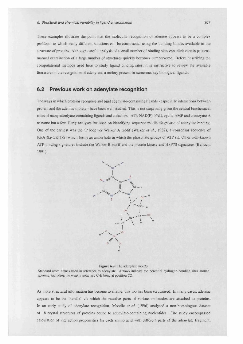
6. Structural and chemical variability in ligand environments 207

These examples illustrate the point that the molecular recognition of adenine appears to be a complex

problem, to which many different solutions can be constructed using the building blocks available in the

structure of proteins. Although careful analysis of a small number of binding sites can elicit certain patterns,

manual examination of a large number of structures quickly becomes cumbersome. Before describing the

computational methods used here to study ligand binding sites, it is instructive to review the available

literature on the recognition of adenylate, a moiety present in numerous key biological ligands.

6.2 Previous work on adenylate recognition

The ways in which proteins recognise and bind adenylate-containing ligands - especially interactions between

protein and the adenine moiety - have been well studied. This is not surprising given the central biochemical

roles o f many adenlyate-containing ligands and cofactors - ATP, NAD(P), FAD, cyclic AMP and coenzyme A

to name but a few. Early analyses focussed on identifying sequence motifs diagnostic o f adenylate binding.

One o f the earliest was the ‘P loop’ or Walker A motif (Walker et al., 1982), a consensus sequence o f

[G/A]X4 -GK[T/S] which forms an anion hole in which the phosphate groups o f ATP sit. Other well-known

ATP-binding signatures include the Walker B motif and the protein kinase and HSP70 signatures (Bairoch,

1991).

N6

C6 /

I || N C 8 - H

t \ / 7C1' /

/ ^ C 2 '_ h04 J

H \ C3--------°3 ’\ J * \ \' / \ ' H

u — C 5‘ ' HH

. O 05’

/ / O oIH

Figure 6.2: The adenylate moiety Standard atom names used in reference to adenylate. Arrows indicate the potential hydrogen-bonding sites around adenine, including the weakly polarised C-H bond at position C2.

As more structural information has become available, this too has been scrutinised. In many cases, adenine

appears to be the ‘handle’ via which the reactive parts of various molecules are attached to proteins.

In an early study of adenylate recognition, Moodie et a l (1996) analysed a non-homologous dataset

of 18 crystal structures of proteins bound to adenylate-containing nucleotides. The study encompassed

calculation of interaction propensities for each amino acid with different parts of the adenylate fragment,

6. Structural and chemical variability in ligand environments 208

analysis of hydrogen bonding patterns and energy calculations. The authors found that hydrophobic and

aromatic residues are particularly preferred in the adenine environment, in agreement with a previous study

(Chakrabarti and Samanta, 1995). These residues tend to sandwich the adenine ring in a predominantly

hydrophobic environment: interestingly, in addition to these non-polar residues, the basic side-chain of

arginine is also noted to frequently lie across the face of the adenine ring.

From their analysis of the hydrogen bonding interactions between protein and adenylate, Moodie and

coworkers conclude that there is no common motif for recognition of adenylate. Overall, fewer than one

third of the theoretical total number of hydrogen bonds are formed to protein; some of the remainder of

polar atoms in the ligands may interact with bulk solvent, but given the generally high degree to which

adenylate tends to be buried in the protein (83.6% of adenine solvent accessible area is lost on average

upon binding), the authors suggest that some hydrogen bonding sites may be completely occluded and hence

remain unsatisfied. Of the four potential hydrogen bonding positions of adenine, the N6 donor make the

most frequent interactions, while the N3 acceptor is reported to be involved in the least number of hydrogen

bonds.

Moodie et al. conclude their paper by proposing the notion of a ‘fuzzy template’ for adenylate recognition,

whereby different types of interactions may be described in broad geometric terms with respect to the ligand,

but where precise templates of the form previously described for catalytic sites (Wallace et a l, 1996) may not

be applicable. This type of approach to analysis of ligand recognition has proved enduringly popular: similar

thinking can be seen to have motivated a number of studies including those based on the ‘fuzzy functional

forms’ concept (Fetrow and Skolnick, 1998), investigations into recognition of heme (Taroni etal., 2000) and

sugars (Karmirantzou and Thornton, 1998), and the grid-based methods for the description of intermolecular

interactions, X-SITE and IsoStar, which were described previously (§1.5.3.2).

One such analysis is that of Nobeli et al. (2001), which investigated the structural basis for the discrimination

between the similarly shaped purine bases, adenine and guanine. They looked at a set of 97 adenine-

protein complexes and 28 guanine-protein complexes to determine whether there were any salient differences

between the two in terms of residue preference, burial or hydrogen bonding pattern. The paper as a whole

serves to reinforce the fuzzy template concept since, while there are differences in the overall composition

of binding sites for the two moieties, no clear patterns emerge which are characteristic of either one or the

other. Experiments in which one base is substituted for the other within a structure in silico showed that the

two key discriminating factors are (i) shape, with the added bulk of guanine’s N2 amine group preventing it

from fitting in some adenine binding sites and (ii) hydrogen bonds to the positions which differ between the

two fragments (N6/06, N1 and C2/N2).

Other studies have found particular structural motifs which are implicated in adenine/adenylate recognition.

Kobayashi and Go (1997) described a geometrical method for comparing the environments of ligands wih the

aim of finding common structural patterns. After applying their method to the set of all structures of adenine

environments at that time, they reported that two unrelated protein families, cAMP-dependent protein kinase

and D-Ala:D-Ala ligase (which has an ATP-grasp fold) bind adenine using a similar local arrangment of

residues. Specifically, they describe a shared four-residue segment which makes two specific interactions

6. Structural and chemical variability in ligand environments 209

with the ligand: the carboxyl oxygen of the second residue accepts a hydrogen bond from the N6 amine

group, while the backbone nitrogen of the fourth residue donates a hydrogen bond to the N 1 atom (see figure

6.3).

i \::

Figure 63: The adenine recognition motif described by Kobayashi and Go This was described in Kobayashi and Go (1997). Red dashed lines represent hydrogen bond interactions between the adenine ring and the protein.

Denessiouk and Johnson (2000) generalised this finding somewhat by first noting that both groups of proteins

identified by Kinoshita and Go shared a larger region of supersecondary structure around the adenine binding

site, which they were then able to show was also present in the structure of ribonucleotide reductase R1 (RNR

Rl). Upon closer inspection of all three structures, the authors report an extended version of the original

motif, in which the two hydrogen bonds to adenine are augmented with a hydrogen bond to the 02 ' atom

of the ribose, from the carboxy-terminal residue of the adenine-binding loop, and an invariant lysine residue

which interacts with the a phosphate. Finally, they show that a total of 12 distinct ATP-binding folds exhibit

the original adenine recognition motif, 8 of which also have the additional adenylate-interaction features

which they newly define.

In a subsequent paper, the authors address the question of whether these ATP-recognition motifs are similarly

found in sites which bind other adenylate-containing ligands (Denessiouk et al., 2001). This issue is key to

our understanding of molecular recognition: does the available data justify the application of a reductionist

approach to the problem, whereby different parts of a ligand may be treated quasi-independently - or is the

nature of protein-ligand recognition such that binding sites can only be appreciated when viewed in their

entirety? The findings of this paper seem to suggest that, at least from a pattem-recognition perspective,

the situation tends towards the former. In addition to the ATP-binding proteins previously reported, the

authors find occurrences of similar adenine recognition motifs in numerous proteins which bind a range of

ligands including coenzyme A, NAD, NADP and FAD. While this is striking, it must be pointed out that the

6. Structural and chemical variability in ligand environments 210

complement of protein-ligand complexes thus grouped together only accounts for less than a third of the total

number of adenine environments in the PDB, meaning that many more ways of binding the moiety remain to

be described.

More recently, the same authors noted that the donor-acceptor-donor (DAD) pattern along the Watson-Crick

edge of the adenine group, which is recognised by the motif just described, is also present along two more

edges of the base - the Hoogsteen (major groove) edge, and the sugar (shallow groove) edge (Denessiouk and

Johnson, 2003). A thorough analysis of all protein-adenine complexes in the PDB shows that similar motifs

exist to recognise these edges. Although the authors make no claim that these findings facilitate prediction of

adenine binding sites, it should be pointed out that the notion of a structural motif has by this point become

rather more abstract than the one originally identified by Kobayashi and Go, and could not be used to define

a rigid structural template, for example, in the spirit of Wallace et al. (1996).

Cappello et a l (2002) take a slightly different approach, aiming not to discover particular motifs which bind

adenine, but rather to describe the extent of diversity in the ways which evolution has produced to recognise

it. By denoting each of the six potential hydrogen-bonding sites in adenine (five polar atoms plus the weak C-

H donor of C2) as either satisfied or unsatisfied, they represent each protein-ligand complex using a six-digit

binary string. Of the 64 possible combinations of interactions, the authors report that 33 are never observed.

The most common situation is for no hydrogen bonds to be formed between adenine and the protein (around

40% of cases), with around 95% of structures belonging to one of 13 patterns. Of these, the most frequent

combination is a pair of interactions with N6 and N l, as described by Denessiouk and Johnson. Capello

et al. state in addition that in these cases, it is the cis hydrogen of N6 which is donated. Interestingly, C2 is

found to be more often involved in hydrogen bonding than either N3 or N7, showing that even presumably

weak donors can contribute significant interactions to the binding site.

A recent paper points out that, since previous studies have broadly agreed that many protein-ligand

interactions are mediated via backbone atoms, defining the binding site in terms of atomic contacts, rather

than the amino acid residues to which they belong, is a sensible starting point (Kuttner et al., 2003). Given

this premise, they describe a procedure for detecting spatial clusters containing atoms of similar types, in

a coordinate frame defined by superposition of adenine. Applying this method to a non-redundant dataset

of protein-adenine complexes, they define a number of clusters, most of which are in agreement with the

distributions which would be expected given the chemical structure of the ligand. They then use these clusters

as a search template to look for putative adenine binding sites in a test set of known adenine-binding proteins.

The method suffers from a high false positive rate, but a number of post-search filters are described which

reduce this considerably. However, the authors admit that their method is unlikely to be able to distinguish

between proteins which bind adenine and those which do not.

The overall picture which emerges from these studies is that, in contrast to enzymatic active sites, well-

conserved structural templates do not exist for ligand recognition. Rather, a given molecule may be

recognised by interacting with one of a number of sites on its surface. Some of these interactions are more

common than others, leading to regions of the binding sites which are more conserved. However, visual

inspection tells us that, on the whole, the sites are extremely variable. The aim of this work is to quantify that

6. Structural and chemical variability in ligand environments 211

statement: how variable are ligand binding sites? Is this variability uniform among different families binding

a given ligand?

6.3 Methodology

This section describes the methodological framework which is used to represent the fragment environments

in a way which is amenable to the analyses which follow.

6.3.1 Definition of the binding site

When discussing protein-ligand interactions, the ‘binding site’ - that is, the parts of the protein which interact

with the ligand molecule - may be defined in various different ways. Using one of the surfaces described

in §3.8.1, the binding site may be defined as the region of the protein surface which is in proximity to, or

accessible to the ligand. Note that this assumes that the coordinates of the ligand are known, an assumption

which is made throughout this chapter. Alternatively, the binding site may be defined as the set of atoms or

residues which lie within a given distance threshold of any part of the ligand. This definition of the binding

site has the advantage that it is simple to compute, but brings the drawback that a distance cutoff large enough

to include atoms interacting with the ligand via hydrogen bonds (around 3.5A between atomic centres) also

includes atoms in the second ‘shell’ around the ligand. In other words, atoms may be close to the ligand but

occluded from being in direct contact with it, and hence should not be considered to form a functional part

of the binding site.

Here, the binding site is defined as the set of atoms which expose a significant part of their Van der Waals

surface to the ligand (or to the fragment of the ligand in which we are interested). In this way, atoms

which cannot physically interact with the ligand are excluded. There is no requirement, however, that the

atoms defined as comprising the binding site actually make attractive contacts with the ligand. The aim

here was to obtain a purely knowledge-based description of the binding site, and therefore no detection of

hydrogen bonding interactions or consideration of 7t-stacking geometries was applied. If we aim to map the

distribution of interactions with respect to a ligand, as opposed to atom-type contacts, then the results will

depend upon the particular model of interactions used. The present study aims to obtain a model-independent

representation of the distribution of atomic contacts to a given ligand.

In detail, the algorithm used to define the binding site is as follows. Firstly, all atoms whose centres are within

3.5A of the centre of any ligand atom are found using a kd-tree search (§3.4.2). Points are then distributed

on the Van der Waals surface of each atom - from both the ligand and its neighbourhood - using the spherical

design method described in §3.8.3.3. From each point on the ligand surface in turn, a ray-tracing method

is then used to determine the set of environment surface points which are visible. This consists of a kd-tree

search using a hemisphere of 2.5A radius, projected from the ligand surface point, to obtain all potentially

visible environment atom surface points. Each of these is then tested to determine whether the line of sight

from ligand surface to environment atom surface is occluded by any other atom. If the line of sight is clear,

the environment atom surface point is marked as visible.

6. Structural and chemical variability in ligand environments 212

Once this procedure is completed, each environment atom is inspected to determine the fraction of its surface

points which were marked as visible from the ligand surface. Atoms exposing more than 10% of their

Van der Waals surface to the ligand (equivalent to approximately 3.6A2 for a carbon atom) are considered

to be making significant contacts with it. Using optimisations such as the kd-tree search and eliminating

environment atom surface points once they have been marked as visible, means that this method is suitably

efficient, at least on the relatively small number of atoms which need to be considered during ligand binding

site analysis.

(a) A large portion of the surface of the nearer (b) Most of the rays to the further atom areatom (green) is visible to the ligand surface occluded (shown in red).point.

Figure 6.4: Definition of the ligand binding site Illustration of the ray-tracing method used to determining environment atom visibility.

6.3.2 Atom types

The atoms which make up each binding site are then classified into a set of predefined types. A number of

atom type schemas have been previously described. One of the best-known is due to Engh and Huber (Engh

and Huber, 1991), who extended a set of atom types originally used in the XPLOR refinement package to a

total of 31 groupings. These types discriminate between atoms firstly on the basis of their chemical element,

then according to the chemical context in which the atom is found, and finally depending on whether or

not the atom is charged. For example, 18 types of carbon atoms are defined, with aliphatic carbons being

separated from aromatic atoms, and both charged and uncharged states defined for carbon atoms liable to

protonation (e.g. histidine Cel).

In a study of covalent radii derived from protein crystal structures, Li and Nussinov defined 25 atom types,

discriminating atoms firstly according to their chemical element and then by the number of hydrogen atoms

to which they are bonded (Li and Nussinov, 1998). This results in a slightly different classification from

that of Engh and Huber: for example, while in the older paper, histidine Cs and Ce are placed in separate

classes, Li and Nussinov consider them chemically equivalent. Also, some atom types are missing from their

classification altogether (e.g. arginine (5 , histidine CY and proline backbone nitrogen), since insufficient

examples of them were found in their dataset.

6. Structural and chemical variability in ligand environments 213

Mitchell et a l (1999) generalise the concept of atom typing by describing a system (SATIS) for classifying

any atom according to its element and those of its covalent partners. This does not require a previously

defined set of atom types, and therefore can be applied automatically to any compound. However, for the

purposes of this study, classification of atoms based on some accepted chemical notions are required, and

therefore SATIS is not particularly useful here.

The atom classification schema used in the LPC software (Sobolev et a l, 1999) is attractive due to its

simplicity. In this approach, atoms are defined according to whether they can donate or accept hydrogen

bonds, and for non-polar atoms, whether they are part of aromatic systems and whether they are bonded to

polar atoms.

The LPC schema forms the basis of the atom classification used in the present study, which is shown in table

6.1. It consists of six types, three polar and three primarily non-polar. Potential hydrogen bond acceptors and

donors make up two types, with those atoms which can potentially both accept and donate hydrogen bonds

{e.g. side-chain hydroxyl groups) belonging to a third class named ‘hydrophilic’. The ‘hydrophobic’ atom

type is composed of aliphatic side-chain carbon atoms, and aromatic side chain carbons belong to a fifth

class. The final class, named ‘neutral’ contains carbon atoms which are covalently bonded to polar atoms,

and which may therefore carry a small partial charge.

No atom typing system is perfect; indeed most suffer from two conspicuous drawbacks. The first is that, in

specifying a rigid classification of atoms in this way, we are necessarily grouping atoms according to their

identity rather than by the role which they play in a particular context. For example, although the atoms

in the ‘acceptor’ class are all capable of accepting hydrogen bonds, this potential is no means realised in

every instance of their occurrence. Depending on the local environment, a carboxyl oxygen atom making no

hydrogen bonding interactions may not be particularly unfavourable.

The second drawback is that, even leaving aside the effects of different environments on the behaviour of

certain chemical groups, it is clear that the properties (however they may be defined) of different functional

groups - and therefore of individual atoms within them - form a continuum. A strict atom classification

scheme is to some extent quite an unrealistic proposal. For instance, the aromatic atom type is clearly

more similar to the hydrophilic class than, say, the acceptor type is to the hydrophobic class. Being able to

enshrine these similarities in some type of quantitative measure would add greatly to the value of the atom

classification model. In particular, it would allow us to compare two binding sites, and to determine in which

regions of space they expose similar chemical properties to the ligand.

The difficulty of measuring similarities between a number of discrete classes also applies when considering

proteins in terms of amino acids: of the twenty amino acids commonly found in proteins, some share more

similar characteristics than others. One way of expressing these similarities is by dividing amino acids into

a number of classes according to their phyisco-chemical properties. For instance, we may identify each

amino acid type as being either ‘aliphatic’ (AGDLPV), ‘basic’ (RHK), ‘acidic’ (DE), ‘polar’ (STCMNQ) or

‘aromatic’ (FWY)1. Taylor (1986) suggested a more complex classification in which he defined a number

1 Amino acids belonging to each type are given parenthetically, using the standard one-letter code.

6. Structural and chemical variability in ligand environments

Atom type Included atoms

214

Backbone carboxyl oxygenCarboxylate oxygens of acidic sidechains (Asp O51, O52; Glu Oel, Oe2) Carboxyl oxygen of asparagine and glutamine (Asn O51; Gin 0 £l)

Backbone nitrogenNitrogens of basic sidechains (His Ne2+; Lys N ;̂ Arg NE, N^1, N112)Amine nitrogen of asparagine and glutamine (Asp N52; Gin Ne2)Trytophan sidechain amine nitrogen (Trp Nel)

Sidechain hydroxyl groups (Ser 0 Y; Thr 0Yl; Tyr)His N8lt

Backbone C“ atomsAll CP atoms except Cys, Ser, ThrAll C1 atoms except Asp, Asn, Phe, tyrAliphatic sidechain carbons (lie C*1, O 2, C81; Leu C81, C82; Lys C8; Thr C?2; Val O K O 2)

Sidechain carbons of Phe (C81, C82, C£l, Ce2, CY, (S)Sidechain carbons of Trp except C81 (C82, Ce2, Ce3, C^2, (S3, C111)Sidechain carbons of Tyr (C81, C82, Cel, Ce2, CY, (5)

Backbone carbonyl carbon atoms atoms of Cys, Ser and Thr

Sidechain carbons bonded to polar atoms(Arg C8, Arg <5, Asn C ,̂ Asp O , Glu C8, Gin C8, His C£l, His C82, Lys C£,

Met C£, Pro C8, Pro N, Trp C81)Sulphur atoms (Met S8; Cys SY)

Table 6.1: GAMUT atom classes This table shows the six categories into which protein atoms are classified for the purposes of representing ligand binding sites in this study. Coloured boxes illustrate the colour-coding scheme used in diagrams throughout the chapter, (t) note that the distinction between histidine N81 and N£2 atoms assumes a particular tautomeric state and therefore may be a source of some errors.(*) atoms in this class can potentially both donate and accept hydrogen bonds.

of physical and chemical properties which were not mutually exclusive {e.g. small, charged, negative, polar,

etc.), thereby constructing a Venn diagram in which each amino acid is classified according to the set of

properties which it possesses. This has the advantage that the similarity of a pair of amino acids may be

judged according to the number of properties which they share. A similar, if slightly simpler, classification

was used by Zvelebil et al. (1987), in which amino acid properties are presented in the form of a truth table.

While these classifications are useful ways in which our understanding of the chemical properties of amino

acids can be embodied, they are all somewhat ad hoc, and therefore not particularly suitable for statistical

analysis of protein sequence and structure. By inspecting multiple alignments of protein sequences, the

frequency with which each type of amino acid is observed to mutate to every other type can be calculated.

This type of analysis, pioneered by Dayhoff et al. (1978) and later refined by Henikoff and Henikoff (1992),

results in a 20 x 20 matrix of scores. Although they are actually mutation frequencies, the values in such

matrices are often taken to represent amino acid similarity. This is rationalised on the basis that amino acids

with more similar properties are more likely to be substituted for one another. Of course, mutation frequency

also depends on other factors such as codon bias and secondary structural context - see e.g. Shi etal. (2001)

- but to a first approximation, the inference of similarity from replaceability is generally considered to be

Acceptor

Donor

Hydrophilic*

Hydrophobic

Aromatic

Neutral

6. Structural and chemical variability in ligand environments 215

acceptable.

No such evolution-based model exists from which we can derive atom type similarities, but several studies

have attempted to do so by analysing the frequency with which different atoms or functional groups are

seen to play similar chemical roles. This phenomenon - specifically the observation of functional groups or

molecules which have chemical and/or physical similarities producing broadly similar biological properties -

is commonly referred to as bioisosterism. From a structural perspective, bioisosteres have been described as

“molecules or functional groups that are structurally different but form similar intermolecular interactions”.

Watson et al. (2001) set out to quantify the degree of bioisosterism which exists between pairs of functional

groups by comparing their spatial distributions with respect to various ‘central group’ fragments. In a similar

study by Verdonk and coworkers, distributions obtained from the IsoStar database (Bruno et al., 1997) are

approximated by fitting three-dimensional Gaussian functions to peaks found in the density maps. For each

pair of functional groups, a number of different similarity indices are then calculated, and averaged over all

central fragments to give an indication of the frequency with which the contacting fragments form similar

interactions. The authors show, by comparing their results against a curated database of bioisosteres, that their

method is able to automatically identify functionally similar fragments. They point out, however, that the

robust definition of threshold values on their scores, above which the degree of bioisosterism is significant,

remains an unresolved problem.

In a similar study, Rantanen et al. (2001) obtain contact information obtained from the PDB, using ligand

fragments as the central groups. While the study of Verdonk and coworkers analysed the distribution of

chemical fragments around a reference group, in this paper, the contact distributions are calculated for a set

of 25 atom types, adopted from Li and Nussinov (1998).These distributions are then approximated by a linear

combination of Gaussian functions, using an expectation-minimisation algorithm to compute the fitting. In

a subsequent paper (Rantanen et a l, 2002), each pair of Gaussian mixture models is compared to yield a

dissimilarity matrix for the set of atom types. Their results suggest that many of the 25 atom types show

distinct spatial distributions with respect to ligand fragments, with only a small number showing significant

levels of similarity, therefore implying that they should be merged.

The results of Rantanen et al. were used to determine whether the GAMUT atom classification schema is

a sensible one2. The dissimilarity matrix published in their paper was analysed using multidimensional

scaling (§3.3.2); figure 6.5 shows a plot of the first two dimensions of the results, with each of the 25 atom

types colour-coded according to which GAMUT class it belongs. The results shown here agree broadly with

our intuition of the relationships between the atom types: there is a clear separation between polar atom

types (acceptor, donor, hydrophilic) and non-polar types (hydrophobic, aromatic). Interestingly, atoms in the

‘neutral’ class, rather than being intermediate between the polar and non-polar atoms, occupy a quite distinct

third section of the plot.

When the GAMUT atom classification was first devised, cysteine thiol (type 13) and methionine sulphide

(type 14) sulphur atoms were classified in the hydrophilic and acceptor classes respectively. This was done

2Herein, the atom groupings of Rantanen et al.will be referred to as ‘atom types’, while the GAMUT classification will be referred to as ‘atom classes’, for clarity.

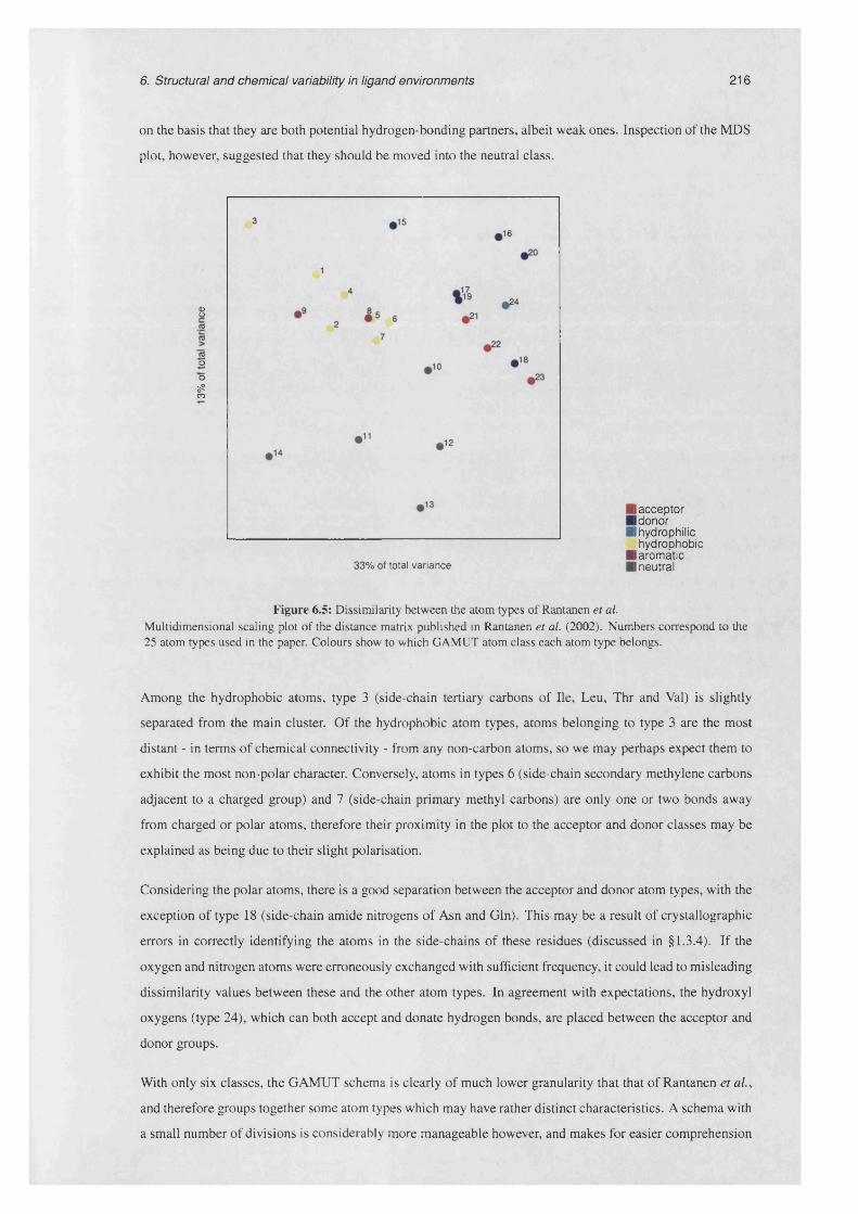
6. Structural and chemical variability in ligand environments 216

on the basis that they are both potential hydrogen-bonding partners, albeit weak ones. Inspection of the MDS

plot, however, suggested that they should be moved into the neutral class.

8

o

o

a?CO

33% of total variance

I a cc e p to r I do nor I hydrophilic h ydrop hob ic

I a ro m a tic I neutra l

Figure 6.5: Dissimilarity between the atom types of Rantanen et al.Multidimensional scaling plot of the distance matrix published in Rantanen et al. (2002). Numbers correspond to the 25 atom types used in the paper. Colours show to which GAMUT atom class each atom type belongs.

Among the hydrophobic atoms, type 3 (side-chain tertiary carbons of lie, Leu, Thr and Val) is slightly

separated from the main cluster. Of the hydrophobic atom types, atoms belonging to type 3 are the most

distant - in terms of chemical connectivity - from any non-carbon atoms, so we may perhaps expect them to

exhibit the most non-polar character. Conversely, atoms in types 6 (side-chain secondary methylene carbons

adjacent to a charged group) and 7 (side-chain primary methyl carbons) are only one or two bonds away

from charged or polar atoms, therefore their proximity in the plot to the acceptor and donor classes may be

explained as being due to their slight polarisation.

Considering the polar atoms, there is a good separation between the acceptor and donor atom types, with the

exception of type 18 (side-chain amide nitrogens of Asn and Gin). This may be a result of crystallographic

errors in correctly identifying the atoms in the side-chains of these residues (discussed in §1.3.4). If the

oxygen and nitrogen atoms were erroneously exchanged with sufficient frequency, it could lead to misleading

dissimilarity values between these and the other atom types. In agreement with expectations, the hydroxyl

oxygens (type 24), which can both accept and donate hydrogen bonds, are placed between the acceptor and

donor groups.

With only six classes, the GAMUT schema is clearly of much lower granularity that that of Rantanen et al.,

and therefore groups together some atom types which may have rather distinct characteristics. A schema with

a small number of divisions is considerably more manageable however, and makes for easier comprehension

6. Structural and chemical variability in ligand environments 217

acceptor donor hydrophilic hydrophobic aromatic neutral

acceptor 0 0.59 0.49 0.90 0.94 0.82donor 0.59 0 0.40 0.71 0.81 0.76

hydrophilic 0.49 0.40 0 0.91 1.00 0.86hydrophobic 0.90 0.71 0.91 0 0.38 0.58

aromatic 0.94 0.81 1.00 0.38 0 0.64neutral 0.82 0.76 0.86 0.58 0.64 0

Table 6.2: Dissimilarity between GAMUT atom classes Distance matrix obtained by ‘compressing’ that published by Rantanen etal., in order to group together those atom types which belong to each GAMUT atom class.

of the analyses later in this chapter. The atom classification used here may therefore be seen as a prototype

for later, more sophisticated studies; here, for the purposes of exploring the analysis of binding site diversity,

this schema is considered adequate.

We can now calculate a new distance matrix between the six GAMUT atom classes. In the projected space

obtained by MDS analysis of the 25 x 25 distance matrix of Rantanen et al., a point which represents each

of the GAMUT atom classes can be calculated simply by computing the centroid of the atom types which

constitute it. For example, the aromatic class is represented by a point located - in 25-dimensional space -

mid-way between atom types 8 and 9. Thus we can obtain dissimilarity values between the GAMUT atom

classes by calculating pairwise distances between the centroids. In this way the original 25 x 25 matrix

is effectively compressed to a 6 x 6 matrix by grouping certain rows and columns. The resulting distance

matrix, scaled so that the maximum distance is 1.0, is shown in table 6.2.

6.3.3 Generation of property maps

Once the set of atoms in contact with the ligand or fragment has been classified according to a specified

schema, a density map is computed for each atom class. This is done by convoluting the coordinates of all

atoms belonging to that class (e.g. hydrophobic, acceptor etc.) with a 3-dimensional Gaussian function, using

a method similar to that used in, among others, the X-SITE program (Laskowski et al., 1996).

The standard Gaussian function has the form

f ( x ) = a e - ^

For generation of the property maps, the variable x represents the distance from the atomic centre; the

parameter b is chosen such that the value of the function on the surface of the Van der Waals sphere of

the atom is half that at its centre: in other words,

, ln2 r2v d w

Although the function is defined over an infinite domain, it is evaluated only up to two Van der Waals radii

away from the centre. The parameter a is chosen such that the sum of the function over all gridpoints within

this range is 100 - this ensures that the total contribution of each atom to the density map is the same (figure

6.6).

6. Structural and chemical variability in ligand environments 218

V_ _ -a/O

-r

•r

(a) The standard deviation of the normal curve is chosen such that the value of the function is half of its maximum value (p) at one Van der Waals radius (r) away from the centre of the atom. The magnitude of the function is set in order that the integral of the function sums to 100.0 .

(b) A 2-dimensional analogue of the previous function. Extension to 3 dimensions is conceptually simple but cannot easily be represented on the page.

Figure 6.6: Convolution of atom coordinates with a Gaussian function

For reasons of computational efficiency, the values of this Gaussian function are not calculated exactly for

every atom in every binding site. Rather, a ‘mask function’ is precomputed for each chemical element on

a 3-dimensional grid large enough to accommodate a sphere of twice its Van der Waals radius (figure 6.7).

When updating a property map with density due to a given atom, rather than evaluating the Gaussian function

at each gridpoint in its vicinity, the precomputed mask is simply added to the map, positioning it so that its

centre lies at the gridpoint closest to the atom centre. A small systematic error is thus introduced, due to

the finite size of the grid spacing, but since the spacing used here (0.375A) is significantly smaller than the

atomic radii - and typically comparable to the experimental error in atom positions - this is not considered

to be overly problematic. Other grid spacings were experimented with; the one used here was chosen as a

compromise between granularity and computational cost.

Figure 6.7: Precomputation of the 3-dimensional Gaussian function The Van der Waals sphere of the atom is shown in pink. The Gaussian function is evaluated on all gridpoints lying within the green circle. As shown, the value of the function declines by one half at one Van der Waals radius from the centre of the atom.

The result of this procedure is a map for each atom type whose value, at all gridpoints inside the Van der

6. Structural and chemical variability in ligand environments 219

Waals sphere of an atom of that type, is ^ or greater. Therefore, if a pair of atoms of the same class are

covalently bonded, a contour at level ^ envelops both atoms together (figure 6.8). Taking the set of maps for

all k atom classes, we then obtain, at each gridpoint, a vectorial description of the composition of the binding

site at that point: in regions of void space, the binding site is represented by the null vector, and in regions

close to one or more atoms, the values in the vector represent the relative proximity of the point to nearby

atoms of the k different classes.

Figure 6.8: ‘Smearing’ effect of the Gaussian density convolution Two covalently bonded atoms are shown as Van der Waals spheres. The mesh shows the contour of the resulting property map, calculated at half the peak value.

6.3.4 Generation of environment masks

The property maps are defined within a box enclosing the ligand molecule, but much of the volume inside

the map is not of interest since it is too far away from the ligand. In addition, the volume occupied by the

ligand itself must be excluded from analysis of the property maps, since this will necessarily be void. The

method used to achieve this is to define an ‘environment mask’, which is simply a density map defined over

the same region as the property maps, in which high values indicate those grid points which are considered

as part of the environment of the ligand or fragment.

Construction of the environment mask consists of three stages (see figure 6.9). In the first, a map which

marks the volume occupied by the ligand molecule itself is generated. Every point in the grid is tested to

determine whether any ligand atoms lie in proximity to it, using a cutoff of 5.5A. If so, the grid point is

assigned a value by evaluating the Gaussian function with the distance to the nearest ligand atom.

Next, another map is created in which any point within 4A of a ligand atom is set to 1.0. This map therefore

contains non-zero values both within the volume occupied by the ligand, and in the space adjacent to it. In

the third stage, the values in the first map are subtracted from those in the second. The result is a density map

in which the only non-zero values are at grid points surrounding the fragment of interest, excluding the part

of space at which the rest of the ligand is attached.

6.3.5 Mapping environment properties onto the fragment surface

For some analyses, it is desirable to map values from a density map onto a molecular surface. By so doing,

the focus is changed from looking at the distribution of a certain property in space around a ligand, to the

values of the property which the ligand ‘sees’, from each point on its surface. The specific advantages of

mapping properties onto the surface are twofold:

6. Structural and chemical variability in ligand environments 220

(a) Schematic representation of a ligand (green), (b) Volume occupied by the ligand is marked out with the fragment of interest marked in red

(c) Volume enclosing the fragment and its environ- (d) Subtraction of the first map from the secondment is defined using the approximate Gaussian leaves a mask defining the fragment environmentconvolution method

Figure 6.9: Creation of environment masks Note that these figures are not to scale.

1 Visualising and interpreting three-dimensional scalar fields can be difficult, even with the aid of a

graphics terminal and isocontouring tools. Conveying the same information comprehensibly on the

printed page, however, is even more challenging. By mapping property values onto the surface, and

showing these surfaces using a colour code to indicate different ranges of values, the essential features

of the property map can be illustrated more simply.

2 Once the property has been mapped onto the surface, we can integrate it to obtain an average value.

This enables the values of a certain property to be compared between different fragments, even if they

are of differing shapes and sizes (for example adenine and nicotinamide).

The method used here to achieve this is simple, and is illustrated in figure 6.10. First, the molecular surface

is calculated by computing a triangulated isosurface over the fragment (Lorensen and Cline, 1997). Then,

normal vectors are calculated for each triangular facet on the surface. Normals from neighbouring facets are

averaged in order to mitigate against the effects of local deformations in the surface. For every facet, the

value of the density map at a point located a specified distance normal to it is obtained by first-order linear

interpolation. Thus the values of the density map at points surrounding the fragment are projected onto its

surface.

6. Structural and chemical variability in ligand environments 221

Figure 6.10: Mapping properties onto an atomic surface The triangulated surface over an adenine moiety is shown. The surface normal of one facet is shown in green; in the example shown here, this facet would be assigned a high value, since the region of space which it is sampling falls inside a density isocontour.

6.4 Characterisation and comparison of fragment environments

Figure 6.11 shows the distribution of different atom types in contact with adenine. The dataset from which

this image was generated contains a non-redundant subset of all adenine environments found in the PDB,

regardless of the particular ligand in which the adenine moiety occurs. The dataset was generated using the

method described in §4.2, counting only the residues in contact with the adenine part of each ligand when

calculating their domain composition. This was done in order to allow the construction of a dataset of adenine

binding sites, irrespective of the ligand type to which each adenine fragment belongs. This procedure resulted

in 120 clusters; representatives of these clusters were used to generate the contact distributions shown here.

Certain patterns are evident from these images, notably two fairly distinct clusters of potential hydrogen

bond acceptors proximal to the N6 hydrogen atoms, and a cluster of potential donors to the left of the picture,

adjacent to Nl. Less clear is a general preference for hydrophobic and aromatic contacts to occur above and

below the plane of the ring rather than around its rim. Weaker preferences for donor and acceptor types which

complement the other polar atoms of the fragment can also be discerned. Appreciating details of the patterns,

however, such as comparing the shapes, spreads and intensities of localised enrichments for particular atom

types, is almost impossible.

Identification of all but the most obvious patterns from this data by eye is difficult, partly because the sheer

amount of information in each image is somewhat overwhelming, and also because the relative frequencies

of occurrence of each type of atom in proteins as a whole are not equal. Picking out those interactions which

are more than simply what would be expected by chance, therefore, is challenging. To overcome the first

difficulty, the distributions of atomic positions were converted into density maps using the method described

earlier. Isocontours of these maps can then be used to identify preferred interaction geometries; however, the

choice of contouring level presents a new problem. To address this, the relative abundance of each atom type

in a representative set of protein surfaces was computed, and these were used to convert raw density values

into propensities, as described below.

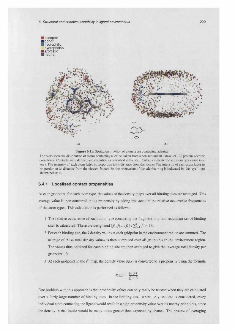
6. Structural and chemical variability in ligand environments 222

■ acceptor ■ donor■ hydrophilic

hydrophobic■ aromatic■ neutral

ee~o<sf fi * *At O* •

f t ̂o *. & _cA - ^ &, * 0 .0°^ V® . s

• - W w f -«• e','% Vco*0

W ’ *

(a)

« > e • • •s£**A.0*V S6 * .

<z>(b)

Figure 6.11: Spatial distribution of atom types contacting adenine The plots show the distribution of atoms contacting adenine, taken from a non-redundant dataset of 120 protein-adenine complexes. Contacts were defined and classified as described in the text. Colours indicate the six atom types used (see key). The intensity of each atom fades in proportion to its distance from the viewer The intensity of each atom fades in proportion to its distance from the viewer. In part (b), the orientation of the adenine ring is indicated by the ‘eye’ logo shown below it.

6.4.1 Localised contact propensities

At each gridpoint, for each atom type, the values of the density maps over all binding sites are averaged. This

average value is then converted into a propensity by taking into account the relative occurrence frequencies

of the atom types. This calculation is performed as follows:

1 The relative occurrence of each atom type contacting the fragment in a non-redundant set of binding

sites is calculated. These are designated fk ) - E*=i f i = 1 -0.

2 For each binding site, the k density values at each gridpoint in the environment region are summed. The

average of these total density values is then computed over all gridpoints in the environment region.

The values thus obtained for each binding site are then averaged to give the ‘average total density per

gridpoint’, p.

3 At each gridpoint in the I th map, the density value p, (.x:) is converted to a propensity using the formula

« i ( * ) =P i ( * )

f i * P

One problem with this approach is that propensity values can only really be trusted when they are calculated

over a fairly large number of binding sites. In the limiting case, where only one site is considered, every

individual atom contacting the ligand would result in a high propensity value over its nearby gridpoints, since

the density in that locale would be many times greater than expected by chance. The process of averaging

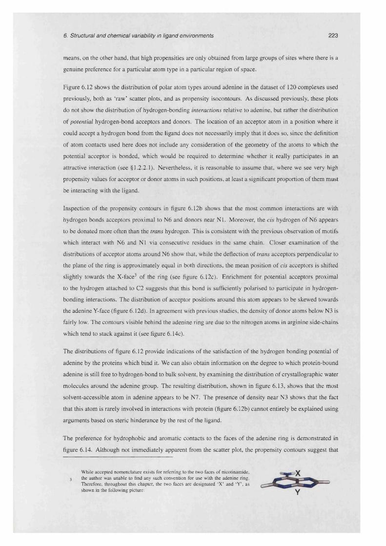
6. Structural and chemical variability in ligand environments 223

means, on the other hand, that high propensities are only obtained from large groups of sites where there is a

genuine preference for a particular atom type in a particular region of space.

Figure 6.12 shows the distribution of polar atom types around adenine in the dataset of 120 complexes used

previously, both as ‘raw’ scatter plots, and as propensity isocontours. As discussed previously, these plots

do not show the distribution of hydrogen-bonding interactions relative to adenine, but rather the distribution

of potential hydrogen-bond acceptors and donors. The location of an acceptor atom in a position where it

could accept a hydrogen bond from the ligand does not necessarily imply that it does so, since the definition

of atom contacts used here does not include any consideration of the geometry of the atoms to which the

potential acceptor is bonded, which would be required to determine whether it really participates in an

attractive interaction (see § 1.2.2.1). Nevertheless, it is reasonable to assume that, where we see very high

propensity values for acceptor or donor atoms in such positions, at least a significant proportion of them must

be interacting with the ligand.

Inspection of the propensity contours in figure 6.12b shows that the most common interactions are with

hydrogen bonds acceptors proximal to N6 and donors near Nl. Moreover, the cis hydrogen of N6 appears

to be donated more often than the trans hydrogen. This is consistent with the previous observation of motifs

which interact with N6 and Nl via consecutive residues in the same chain. Closer examination of the

distributions of acceptor atoms around N6 show that, while the deflection of trans acceptors perpendicular to

the plane of the ring is approximately equal in both directions, the mean position of cis acceptors is shifted

slightly towards the X-face3 of the ring (see figure 6.12c). Enrichment for potential acceptors proximal

to the hydrogen attached to C2 suggests that this bond is sufficiently polarised to participate in hydrogen-

bonding interactions. The distribution of acceptor positions around this atom appears to be skewed towards

the adenine Y-face (figure 6.12d). In agreement with previous studies, the density of donor atoms below N3 is

fairly low. The contours visible behind the adenine ring are due to the nitrogen atoms in arginine side-chains

which tend to stack against it (see figure 6.14c).

The distributions of figure 6.12 provide indications of the satisfaction of the hydrogen bonding potential of

adenine by the proteins which bind it. We can also obtain information on the degree to which protein-bound

adenine is still free to hydrogen-bond to bulk solvent, by examining the distribution of crystallographic water

molecules around the adenine group. The resulting distribution, shown in figure 6.13, shows that the most

solvent-accessible atom in adenine appears to be N7. The presence of density near N3 shows that the fact

that this atom is rarely involved in interactions with protein (figure 6.12b) cannot entirely be explained using

arguments based on steric hinderance by the rest of the ligand.

The preference for hydrophobic and aromatic contacts to the faces of the adenine ring is demonstrated in

figure 6.14. Although not immediately apparent from the scatter plot, the propensity contours suggest that

While accepted nomenclature exists for referring to the two faces of nicotinamide, the author was unable to find any such convention for use with the adenine ring. Therefore, throughout this chapter, the two faces are designated ‘X’ and *Y\ as shown in the following picture:

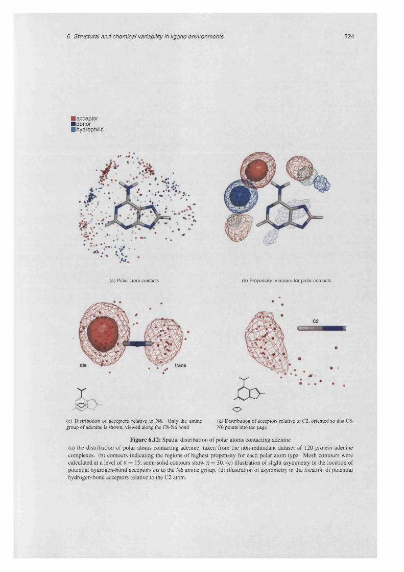
6. Structural and chemical variability in ligand environments 224

■ acceptor ■donor■ hydrophilic

I* •#

(a) Polar atom contacts (b) Propensity contours for polar contacts

trans

(c) Distribution of acceptors relative to N6. Only the amine group of adenine is shown, viewed along the C8-N6 bond

C2

<3>(d) Distribution of acceptors relative to C2, oriented so that C8- N6 points into the page

Figure 6.12: Spatial distribution of polar atoms contacting adenine (a) the distribution of polar atoms contacting adenine, taken from the non-redundant dataset of 120 protein-adenine complexes, (b) contours indicating the regions of highest propensity for each polar atom type. Mesh contours were calculated at a level of n = 15; semi-solid contours show 7t = 30. (c) illustration of slight asymmetry in the location of potential hydrogen-bond acceptors cis to the N6 amine group, (d) illustration of asymmetry in the location of potential hydrogen-bond acceptors relative to the C2 atom.

6. Structural and chemical variability in ligand environments 225

t*

(a) Distribution of water oxygen atoms (b) Density contours for water oxygen

Figure 6.13: Distribution of immobilised water molecules around adenine (a) scatter plot of oxygen atoms from water molecules crystallographically visible around adenine in the 120 complexes analysed, (b) density contours showing most preferred regions: propensity values cannot be calculated for the water maps, so mesh contours are shown at a = 3 and semi-solid contours at a = 5 where a is the standard deviation of values in the map.

this preference is not completely symmetrical with respect to the two faces of the ring. Aromatic contacts

appear to be slightly more favoured on the X-face than the Y-face; conversely, there is a slightly greater

density of hydrophobic/aliphatic contacts to the Y-face.

The distribution of arginine side-chains around arginine, which have been previously noted to frequently be

found stacking in parallel against it, is shown in figure 6.14c. This demonstrates a striking asymmetry, with

contacts to the Y-face being around four times more likely than those to the X-face (12 and 3 occurrences

respectively). Figure 6 .14d shows the distribution of aromatic side-chains around arginine. Phenylalanine

and tyrosine are approximately equally likely to contact adenine (35 and 34 occurrences respectively), with

tryptophan being less common (8 residues). Instances in which aromatic side-chains were oriented in parallel

to, and stacked on the face of the adenine ring were identified by visual inspection. Counting the frequency

of stacking interactions shows that contacts to the X-face are approximately twice as likely as those to the

Y-face (14 versus 7 instances), with the majority of aromatic side-chains (56 residues) contacting adenine at

an oblique angle.

Combining these propensity maps allows us to define the consensus binding site - or pharmacophore - for

adenine, as shown in figure 6.15. This description, which is a realisation of the fuzzy template concept

defined by Moodie and Thornton, is at the same time a feature-rich and easily comprehensible representation

of the geometry of interactions made between proteins and this moiety.

6. Structural and chemical variability in ligand environments 226

hydrophobic I aromatic I neutral

“‘‘S' <•*«*»% • o.r c±=a

o • * c a

4-'* o o «* ( £ • : i \ %

O(a) Non-polar atom contacts

;^x

O(b) Propensity contours for non-polar contacts

<3> <3>

(c) Arginine side-chain contacts (d) Aromatic side-chain contacts. Tyrosine residues are coloured yellow, tryptophan in blue and phenylalanine in magenta.

Figure 6.14: Spatial distribution of non-polar atoms contacting adenine (a) the distribution of non-polar atoms contacting adenine, taken from a non-redundant dataset of 120 protein-adenine complexes, (b) contours indicating the regions of highest propensity for each polar atom type. Mesh contours were calculated at a level of n = 15; semi-solid contours show n = 30. (c) distribution of arginine side chain contacts, showing the tendency for arginine to stack against one side of the ring, (d) distribution of aromatic side chain contacts.

6. Structural and chemical variability in ligand environments 227

■acceptor■ donor■ hydrophilic

hydrophobic■arom atic■ neutral

Figure 6.15: A composite picture of the adenine environments Contours indicating the regions of highest propensity for each atom type, in a non-redundant dataset of 120 protein- adenine complexes. Mesh contours were calculated at a level of n = 15; semi-solid contours show n = 30.

6. Structural and chemical variability in ligand environments 228

6.5 Diversity of fragment environments

The concept of conservation has long been applied in the realm of sequence analysis (see Valdar (2002)

and references therein), where analyses of multiple alignments of sequences belonging to a protein family is

commonly used to delineate functionally important regions, or to identify sequence signatures diagnostic of

the particular family being studied.

Several recent studies have combined conservation information from sequence and structure. A methodology

known as ‘evolutionary trace’, was described by Lichtarge et a l (1996), and later refined by Pupko et al.

(2002). These studies, while they also aim to produce a mapping of sequence position-specific conservation

scores onto three-dimensional structure, may be distinguished from those mentioned above in that they derive

their scores from a consideration of the phylogenetic relationships between the sequences. The paper of

Ben-Tal and co-workers describes the application of their method to the SH2 domain, a component of an

intracellular signalling cascade which is found in many proteins, and which recognises tyrosine-containing

polypeptide fragments. They show that, in addition to the region of the domain surface which is involved in

dimerisation, higher-than-average conservation scores are also found in the peptide-binding groove. The

extent to which this is generally true for ligand-binding sites is still unclear. As mentioned previously,

functional regions of proteins are often located in clefts which may be defined using purely geometric criteria.

A problem which is encountered when applying cleft-detection methods is that the region of interest, if it

is included in one of the resulting cavities at all, is typically restricted to a small fraction of its volume.

Investigations are currently underway, therefore, to determine whether conservation scores can be used to

‘zoom in’ on the potential interaction sites within a cleft (F. Glaser, personal communication).

Valdar and Thornton describe a method of mapping residue conservation scores obtained from a multiple

sequence alignment onto the three-dimensional structure of a representative protein from the family. They

show that, considering residues on the surface of the protein, appropriately defined conservation scores are

able to discriminate those regions which participate in subunit dimerisation (Valdar and Thornton, 2001a).

In a later study (Valdar and Thornton, 2001b), the same authors report that conservation can also be used to

distinguish between those subunit contacts in a crystal which are biologically important, and those which are

merely due to crystal packing.

A slightly different approach involves mapping just the evolutionarily invariant polar residues onto a

reference structure, then applying a spatial clustering procedure (Aloy et a l, 2001). The conserved clusters

defined using this method were found to correctly identify the functional site of a protein (as defined by the

SITE records in the PDB file) in around 80% of cases.

Local structural conservation has been studied in some detail for catalytic active sites. For many enzymes,

a small number of residues can be identified as being responsible for the enzymatic function. By comparing

the relative location of these residues in space, the extent to which their functional role places constraints on

the local structure can be understood. A study of Ser-His-Asp catalytic triads among several convergently

evolved groups of hydrolases, for example, found that the distances between the functional atoms of the

Ser and Asp residues was within 1.4A of the consensus distance over all examples analysed (Wallace et a l,

6. Structural and chemical variability in ligand environments 229

1996). A more recent study (Torrance et al., 2005) showed that within most homologous enzyme families,

the corresponding figure is below 1 A.

Similar studies of structural conservation of ligand-binding sites are more difficult. In enzymes, the same

small number of residues are often clearly identifiable as being responsible for catalysing a particular reaction

among proteins within - and sometimes between - homologous families. This permits residue equivalences

to be unambiguously established between functional sites in different enzymes, thereby allowing them to be

compared using standard geometrical measures such as RMSD. As has been previously stated, the situation

is considerably less clear-cut for sites whose shared feature is not catalysis of a chemical reaction, but

recognition of a particular chemical entity. Visual inspection of binding sites quickly reveals that there

are far more ways to bind a given ligand than there appear to be for delivering efficient catalysis. The rest of

this section is devoted to the development of a method for quantifying the extent to which this is so, and for

visualising the regions of binding sites which tend to be the most variable.

6.5.1 Measures of diversity

6.5.1.1 Entropy

The concept of entropy was first introduced in 1865, and was defined as the amount of energy in a system

which cannot be used to do work. During the course of studying thermodynamic transformations, Rudolf

Clausius found that the introduction of this new quantity was required to explain why some transformations

are reversible, and some are not: only those which do not result in an increase of entropy may be reversed.

In 1877, Boltzmann looked at entropy from the standpoint of statistical mechanics, and redefined it in

terms of the number of ‘microstates’ which a system may adopt, and which are consistent with its gross

thermodynamic properties. Specifically, he defined entropy as

S = fclnQ

where k is Boltzmann’s constant and Q is the number of microstates for the system (Atkins and de Paula,

2001). This leads to the idea of entropy as a measure of the amount of disorder within a system.

More recently, Shannon (1948) proposed a new definition of entropy for use in the analysis of information

coding and transmission systems. The motivation for this new definition was to obtain a formula which,

when applied to a source of information, would calculate the minimum channel capacity required to reliably

transfer the data as a series of binary digits. The definition of information entropy of a discrete random event

(as opposed to the thermodynamic entropy of a system discussed above) is

k

h (*) = - X PiloZlPi (6.1)i= 1

where k is the number of possible outcomes for the event, and pi is the probability of the Ith outcome.

For instance, given a passage of text written in English, one could calculate the channel capacity necessary

to transmit it by counting the occurrence within it of each letter of the alphabet. Assuming that the only

punctuation in the text are spaces and full stops, we may then calculate its entropy as

6. Structural and chemical variability in ligand environments 230

H = - ( p a lOg,2 P a + P b l o & P b + • • • + P z l 0 g 2 P z + P . l o g 2P . + P s p a c e ^ g 2P space)

where pa is the frequency of occurrence of the letter ‘a’ divided by the length of the passage.

Although originally defined for a particular purpose, Shannon’s entropy measure tells us something about the

nature of the signal - its information content. More specifically, it is a measure of the amount of information

in a signal, over and above that which is strictly determined by - and hence predictable from - its inherent

structure. Returning to the example of text, imagine an alphabet with only one letter, ‘a’. The message ‘aaaaa’

written in this alphabet conveys no information, since we could have predicted its content perfectly prior to

receiving it. Any message written in English, on the other hand, is more informative (in an information

theoretic sense), since we cannot anticipate it from the relative frequencies of the different letters of the

alphabet. It should be clear from the mathematical definition of information entropy given above that, for

an alphabet with a given number of letters, the maximum entropy is reached when all are equally probable,

and that, adding extra letters (with none-zero occurrence frequencies) to the alphabet will always increase its

information content.

It is interesting to note that, although at first sight all that is shared by the information theoretic and

thermodynamic formulations of entropy is a name, in fact the connection is much deeper. Given a uniformly

distributed discrete random variable X with k possible values, let us ask what is the probability, after p

observations of X, of seeing the distribution (/i , f 2 ... /*), where f is the number of occurrences of outcome

jc,-. This probability follows a multinomial distribution

where Q is the number of combinations of outcomes fitting the observed distribution

piQ = - ------------------

/ i ! £ ! . . .A!

and N is the number of all possible outcomes, N = kp. Applying the statistical mechanical formulation, the

entropy of the system is given by the logarithm of the number of states, Q. As the number of observations p

tends towards infinity, pi can be approximated by Stirling’s approximation

ln£! ~ k\nk — k

Taking the logarithm of Q, we thus obtain

kln£2= - p ^ p i l n p i

i= 1

which is linearly related to the definition of H given in equation 6.1.

Entropy-based scores have been used previously to quantify the degree of conservation at each position of a

multiple sequence alignment (Sander and Schneider, 1991, Gerstein and Altman, 1995). In the present study,

a gridpoint in the space surrounding the ligand may be thought of as analagous to a column in the sequence

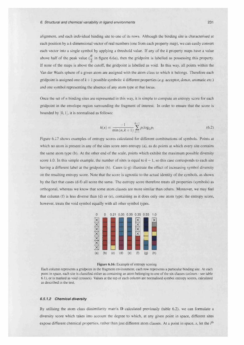
6. Structural and chemical variability in ligand environments 231

alignment, and each individual binding site to one of its rows. Although the binding site is characterised at

each position by a ^-dimensional vector of real numbers (one from each property map), we can easily convert

each vector into a single symbol by applying a threshold value. If any of the k property maps have a value

above half of the peak value in figure 6.6a), then the gridpoint is labelled as possessing this property.

If none of the maps is above the cutoff, the gridpoint is labelled as void. In this way, all points within the

Van der Waals sphere of a given atom are assigned with the atom class to which it belongs. Therefore each

gridpoint is assigned one of k + 1 possible symbols: k different properties {e.g. acceptor, donor, aromatic etc.)

and one symbol representing the absence of any atom type at that locus.

Once the set of n binding sites are represented in this way, it is simple to compute an entropy score for each

gridpoint in the envelope region surrounding the fragment of interest. In order to ensure that the score is

bounded by [0,1], it is normalised as follows:

2 fc+i

',W = min(»;t + l ) i§ Pil082/,i (6'2)

Figure 6.17 shows examples of entropy scores calculated for different combinations of symbols. Points at

which no atom is present in any of the sites score zero entropy (a), as do points at which every site contains

the same atom type (b). At the other end of the scale, points which exhibit the maximum possible diversity

score 1.0. In this simple example, the number of sites is equal to k+ 1, so this case corresponds to each site

having a different label at the gridpoint (h). Cases (c-g) illustrate the effect of increasing symbol diversity

on the resulting entropy score. Note that the score is agnostic to the actual identity of the symbols, as shown

by the fact that cases (d-f) all score the same. The entropy score therefore treats all properties (symbols) as

orthogonal, whereas we know that some atom classes are more similar than others. Moreover, we may feel

that column (f) is less diverse than (d) or (e), containing as it does only one atom type; the entropy score,

however, treats the void symbol equally with all other symbol types.

0 0 0.21 0.35 0.35 0.35 0.55 1.0

(a) (b) (c) (d) (e) (f) (g) (h)

Figure 6.16: Example of entropy scoring Each column represents a gridpoint in the fragment environment; each row represents a particular binding site. At each point in space, each site is classified either as containing an atom belonging to one of the six classes (colours - see table 6.1), or is marked as void (crosses). Values at the top of each column are normalised symbol entropy scores, calculated as described in the text.

6.5.1.2 Chemical d iversity

By utilising the atom class dissimilarity matrix D calculated previously (table 6.2), we can formulate a

diversity score which takes into account the degree to which, at any given point in space, different sites

expose different chemical properties, rather than just different atom classes. At a point in space, x, let the Ith

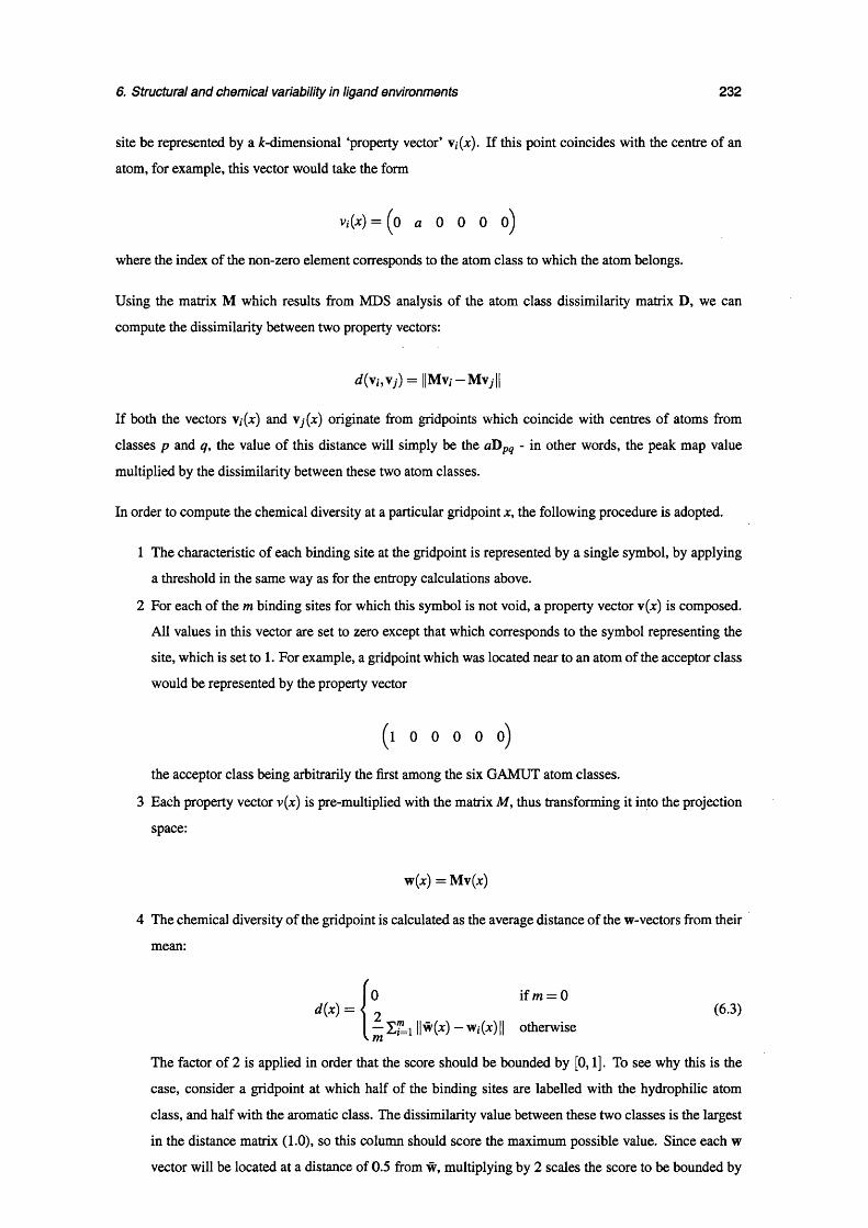
6. Structural and chemical variability in ligand environments 232

site be represented by a ^-dimensional ‘property vector’ v,(jc). If this point coincides with the centre of an

atom, for example, this vector would take the form

V i(*) = (o a 0 0 0 o)

where the index of the non-zero element corresponds to the atom class to which the atom belongs.

Using the matrix M which results from MDS analysis of the atom class dissimilarity matrix D, we can

compute the dissimilarity between two property vectors:

d ( \ i , \ j ) = \ \M \i-M \j\\

If both the vectors v,(x) and \j(x ) originate from gridpoints which coincide with centres of atoms from

classes p and q, the value of this distance will simply be the aDpq - in other words, the peak map value

multiplied by the dissimilarity between these two atom classes.

In order to compute the chemical diversity at a particular gridpoint x, the following procedure is adopted.

1 The characteristic of each binding site at the gridpoint is represented by a single symbol, by applying

a threshold in the same way as for the entropy calculations above.

2 For each of the m binding sites for which this symbol is not void, a property vector \(x) is composed.

All values in this vector are set to zero except that which corresponds to the symbol representing the

site, which is set to 1. For example, a gridpoint which was located near to an atom of the acceptor class

would be represented by the property vector

( l 0 0 0 0 o)

the acceptor class being arbitrarily the first among the six GAMUT atom classes.

3 Each property vector v ( jc ) is pre-multiplied with the matrix M, thus transforming it into the projection

space:

w (x) = M v (jc)

4 The chemical diversity of the gridpoint is calculated as the average distance of the w-vectors from their

mean:

d(x) = *0 if m = 02 (63) — YiLi ||w(jc) — wi(x) || otherwise

The factor of 2 is applied in order that the score should be bounded by [0,1]. To see why this is the

case, consider a gridpoint at which half of the binding sites are labelled with the hydrophilic atom

class, and half with the aromatic class. The dissimilarity value between these two classes is the largest

in the distance matrix (1.0), so this column should score the maximum possible value. Since each w

vector will be located at a distance of 0.5 from w, multiplying by 2 scales the score to be bounded by

6. Structural and chemical variability in ligand environments 233

[0 , 1].

Figure 6.17 shows chemical diversity scores calculated for a number of hypothetical environment gridpoints.

While it improves on the problems discussed in reference to the entropy score, the chemical diversity index

has its own problems. Conspicuously, being based on calculation of a mean value, it is sensitive to outlying

values, as shown by the value in column (c). Although this column is predominantly composed of acceptor

classes, one hydrophobic symbol is sufficient to increase the diversity score from zero to 0.44. In addition, it

is clear that, at gridpoints where most sites are devoid of atoms, the effect of a small number of atoms from

dissimilar classes will be amplified.

However, cases (d-f) are more reasonably distinguished by the diversity score. At position (d), the binding

sites have either hydrophilic or aromatic atoms, which are the most chemically dissimilar (table 6 .2 ), resulting

in a high diversity score. At (e), on the other hand, although the symbol diversity is the same, chemically the

sites are more similar, as reflected by the score. Position (f) illustrates the difference in the response of the

two scores to void values: here, the four void sites are ignored, and since all non-void sites have the same

atom type, the chemical diversity is zero.

0 0.44 0.89 0.48 0 0.72 0.96

§11(b) (c) (d) (e) (f) (g) (h)

Figure 6.17: Example of chemical diversity scoring Each column represents a gridpoint in the fragment environment; each row represents a particular binding site. At each point in space, each site is classified either as containing an atom belonging to one of the six classes (colours - see table 6.1), or is marked as void (crosses). Values at the top of each column are normalised chemical diversity scores, calculated as described in the text.

6.5.1.3 A combined diversity score

In order to play up the relative strengths of each score while compensating for their weaknesses, therefore,

we define a new index which combines the two. In so doing, we follow a similar approach to that described

by Valdar (2002). In this paper, the author was interested in comparing a range of scores for quantifying the

degree of conservation of each column in a multiple sequence alignment. He identified three components of

positional variability - namely symbol diversity, stereochemical diversity of the amino acids present, and the

number of gaps. Choosing an appropriate measure for each of these quantities, bounded by [0,1], the degree

of conservation of a given column is then defined as

CM H i -'(*))“( ! - 'M /a -* M )Y

where t, r and g represent the three quantities listed above, and where a , (3 and y are parameters used to

weight their relative importance.

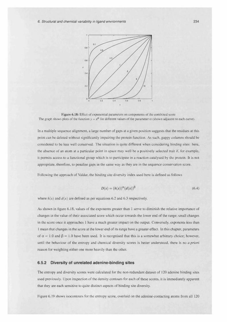
6. Structural and chemical variability in ligand environments 234

0 .2 ,

0.5

y

0.4

0.2

0 0.2 0.4 0.6 0.8 1

x

Figure 6.18: Effect of exponential parameters on components of the combined score The graph shows plots o f the function y = for different values of the parameter a (shown adjacent to each curve).

In a multiple sequence alignment, a large number of gaps at a given position suggests that the residues at this

point can be deleted without significantly impairing the protein function. As such, gappy columns should be

considered to be less well conserved. The situation is quite different when considering binding sites: here,

the absence of an atom at a particular point in space may well be a positively selected trait if, for example,

it permits access to a functional group which is to participate in a reaction catalysed by the protein. It is not

appropriate, therefore, to penalise gaps in the same way as they are in the sequence conservation score.

Following the approach of Valdar, the binding site diversity index used here is defined as follows

d(x) = mr(6.4)

where h{x) and d(x) are defined as per equations 6.2 and 6.3 respectively.

As shown in figure 6.18, values of the exponents greater than 1 serve to diminish the relative importance of

changes in the value of their associated score which occur towards the lower end of the range; small changes

in the score once it approaches 1 have a much greater impact on the output. Conversely, exponents less than

1 mean that changes in the score at the lower end of its range have a greater effect. In this chapter, parameters

of a = 1.0 and (3 = 1.0 have been used. It is recognised that this is a somewhat arbitrary choice; however,

until the behaviour of the entropy and chemical diversity scores is better understood, there is no a priori

reason for weighting either one more heavily than the other.

6.5.2 Diversity of unrelated adenine-binding sites

The entropy and diversity scores were calculated for the non-redundant dataset of 120 adenine binding sites

used previously. Upon inspection of the density contours for each of these scores, it is immediately apparent

that they are each sensitive to quite distinct aspects of binding site diversity.

Figure 6.19 shows isocontours for the entropy score, overlaid on the adenine-contacting atoms from all 120

6. Structural and chemical variability in ligand environments 235

sites. The first observation is that the entropy score is clearly dependent on the local ‘crowding’ of atoms: the

higher entropy values are restricted to regions of space which are more frequently populated with contacts.

This is to be expected given the way the the score is defined, since gridpoints where a high fraction of sites are

classified ‘void’ obtain a low entropy score. The most noticeable high-entropy regions are those contacting

the two faces of the adenine ring, with approximately equal degrees of disorder on both sides. In contrast,

the areas around the rim of the ring tend to have quite low entropy scores, with only a few localised regions

where the density values are above 0.3.

(a) (b)

Figure 6.19: Depiction of entropy scores for adenine environments Mesh isocontours were calculated at a level of 0.3; semi-solid contours at 0.4. Adenine-contacting atoms from the binding sites are shown as spheres, colour-coded according to the atom class to which they are assigned (table 6.1).

Contact density is not the sole determining factor of the entropy score, however. This is evidenced by

comparing the contours around the acceptor atoms cis to N6 and the donors proximal to Nl. These two

regions are similarly densely populated, but the latter has much higher atom type diversity. Inspection of the

clusters of atoms at these points reveals that this is a good reflection of the type of contacts which occur:

while around the N6 amine hydrogens, sites tend to be either void or occupied by acceptor atoms, next to N l,

while there is a high concentration of donor contacts, we also see considerable numbers of other atom types.

Figure 6.20 shows contours describing the distribution of chemical diversity scores for the same dataset of

adenine environments. It is immediately apparent that, in contrast to the entropy scores, the regions where

this index is highest are those around the rim of adenine, with the two faces scoring relatively low values.

Although it is difficult to see in figures 6.20a and 6.20b, interactive inspection of these distributions on a

graphics workstation shows that there are clear ‘holes’ in the diversity contours at locations where contacts

are made to the polar atoms of the adenine fragment. Most noticeable among these is a distinct region of

low diversity at the cis position of N6, with a less well-pronounced reduction in scores around donors to N1

(figure 6.20c).

We can rationalise these findings by considering the nature of the interactions which are made to the face and

the edges of adenine. Contacts to the faces can be characterised as being non-specific and diffuse: that is, the

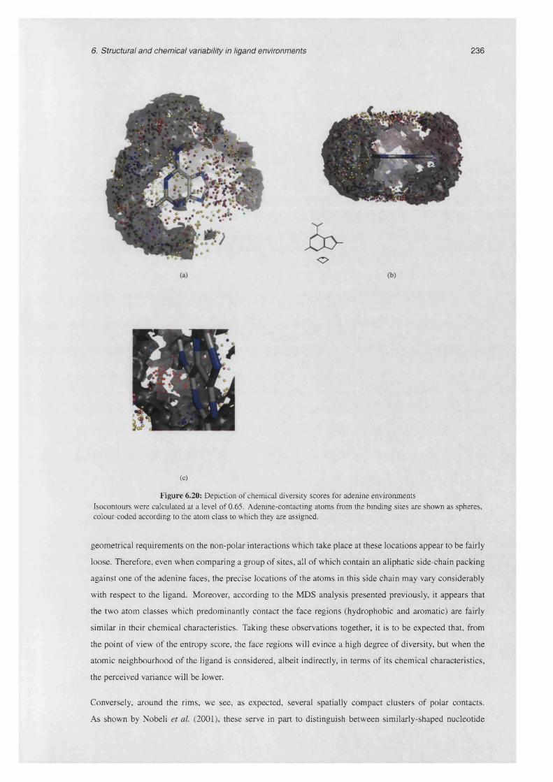
6. Structural and chemical variability in ligand environments 236

(c)

Figure 6.20: Depiction of chemical diversity scores for adenine environments Isocontours were calculated at a level of 0.65. Adenine-contacting atoms from the binding sites are shown as spheres, colour-coded according to the atom class to which they are assigned.

geometrical requirements on the non-polar interactions which take place at these locations appear to be fairly

loose. Therefore, even when comparing a group of sites, all of which contain an aliphatic side-chain packing

against one of the adenine faces, the precise locations of the atoms in this side chain may vary considerably

with respect to the ligand. Moreover, according to the MDS analysis presented previously, it appears that

the two atom classes which predominantly contact the face regions (hydrophobic and aromatic) are fairly

similar in their chemical characteristics. Taking these observations together, it is to be expected that, from

the point of view of the entropy score, the face regions will evince a high degree of diversity, but when the

atomic neighbourhood of the ligand is considered, albeit indirectly, in terms of its chemical characteristics,

the perceived variance will be lower.

Conversely, around the rims, we see, as expected, several spatially compact clusters of polar contacts.

As shown by Nobeli et al. (2001), these serve in part to distinguish between similarly-shaped nucleotide

6. Structural and chemical variability in ligand environments 237

bases during molecular recognition, and therefore should be both specific and accurate. The distribution of

chemical diversity scores around the rim of the adenine ring suggests that, while there is a high degree of

apparent variability in general, there are distinct regions where contacts to the ligand, if they are made, are

of a particular type, with little tolerance for non-specific interactions.

Next we consider the effect of combining the entropy and diversity scores according to equation 6.4. A

difficulty faced in doing so is that, while the relative simplicity of the two separate scores means that they can

be understood in isolation, gaining an intuitive feel for what a particular value of the combined score means

is more difficult. In addition, it is clear that the behaviour of the combined score will be quite sensitive to the

choice of the two parameters a and (3. Contour plots obtained from the combined score (with a = (3 = 1.0)

are shown in figure 6.21.

(c)

Figure 6.21: Depiction of combined diversity scores for adenine environments Mesh isocontours were calculated at a level of 0.15, light semi-solid contours at 0.20 and dark semi-solid contours at 0.25. Adenine-contacting atoms from the binding sites are shown as spheres, colour-coded according to the atom class to which they are assigned.

6. Structural and chemical variability in ligand environments 238

Overall, the entropy score appears to dominate the combined results; interactive exploration of the density

contours suggest that the variance in entropy scores is somewhat higher that in the diversity values.

Nevertheless, the addition of the chemical diversity information has had some noticeable effects on the

contour plots. Combined scores around the cis N6 acceptors are the lowest among the densely populated

regions of the binding sites, reinforcing the intuitive impression that this interaction is among the most

conserved. Conversely, while the areas around the C2 hydrogen atom have fairly low entropy scores, the

presence in this region of several chemically diverse atom classes results in a relatively high combined

diversity score.

Looking at the contours around adenine face contacts, we see that, although the two faces were fairly equal

in terms of entropy scores, regions which abut the Y face have considerably higher combined diversity scores

than those on the X face. This may be explained in part due to the previously noted high propensity for

aromatic rings to stack against the X face, with a lower tendency in this region for aliphatic contacts. It

appears that apolar contacts to the X face are slightly more homogeneous in nature, although inspection of

the ‘raw’ coordinate superpositions of the binding sites shows that this is only a weak distinction.

In order to better understand the distribution of combined diversity scores around adenine, it is useful to map

these values onto the fragment surface using the method described in §6.3.5. Plots of the surfaces, with each

facet colour-coded according to the diversity score of its neighbourhood, are shown in figure 6.22. The most

striking observation is the disparity in diversity scores between the two faces of the ring, with the Y face

(figure 6.22a) being annotated with values peaking at around 0.4; values on the X face (figure 6.22b) are all

below 0.3.

These plots recapitulate the result that the rim environment is less diverse than the regions which contact

the ring faces. It is possible to see some slight differences between different regions around the rim, such

as the higher scores around the trans N6 hydrogen than around the cis hydrogen, and the elevated values

on the surface of the N l atom (figure 6.22c). However, this type of visual analysis is hampered both by

the difficulty of capturing the gradations of a score using only colour-coding, and by the fact that the more

directional nature of polar interactions means that differences in diversity scores around the rim are projected

onto relatively smaller surface areas than are those across the faces. In summary, it is extremely difficult to

capture this type of three-dimensional information on the page, although the graphical techniques used here

are considered to be sufficiently informative to convey at least the most important points.

6.5.3 Diversity of related adenine binding sites

Just as, in the previous chapter, the question “Do ligands bound to related proteins adopt more similar

conformations than those bound to unrelated proteins?”, here we ask whether the environments of adenine in

related proteins are significantly more similar than those found in the non-redundant dataset.

The method used to do this is simple: the combined diversity scores mapped onto the fragment surface as

in the previous section, are simply integrated across the adenine moiety to give an overall diversity score

for any given collection of binding sites. Comparison of this value obtained from the non-redundant dataset

described above, with those obtained by comparing binding sites in the same cluster, will be used to address

6. Structural and chemical variability in ligand environments 239

J | |-

■

m m

(a) (b)

0

0.00

0.05

0.10

0.15

0.20

0.25

0.30

0.35

0.40

(C )

Figure 6.22: Combined diversity scores mapped onto adenine surface In figures (a) and (b), the orientation of the ligand surface is shown by faintly overlaying a stick representation of adenine.

the question posed above. Before so doing, however, we must determine whether there is any dependence of

this overall diversity score on the number of binding sites used to calculate it, since the number of sites in

any one cluster is significantly fewer than the number of cluster representatives.

To do this, a random sampling procedure was devised. From the set of 120 binding sites in the non-redundant

dataset, a subset of n sites was chosen at random, where n ranges from 2 to 120. The overall diversity

measure was calculated for this subset of binding sites, and this was repeated 25 times. From these 25 values,

the mean and variance of the overall diversity score was calculated for each n. In addition, the entropy

and chemical diversity scores were integrated over the fragment surface independently, allowing any sample

size dependence in the combined score to be deconvolved into its two component parts. The results of this

experiment are plotted in figure 6.23.

Both the entropy and diversity measures decline as decreasing numbers of binding sites are sampled. As this

number drops below 7, the entropy score climbs once again, due to the effect of the min(«,£ + 1) term in the

denominator of its correction factor (see equation 6.2). The monotonic decrease of the combined score as the

sample size is reduced, is not a particularly desirable characteristic for a descriptive statistic: we would prefer

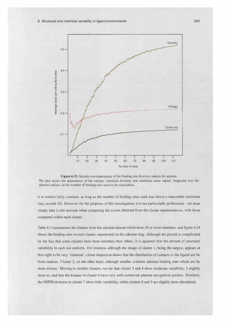
6. Structural and chemical variability in ligand environments 240

Diversity

0.5 —

0.4 —coo03<Do03

30)c3

0 . 3 -<5CLOi<DO)03I< 0 .2 -

Entropy

Com bined

0.1 -

40 50 60 70 80 90 100 11010 20 30

N um ber of sites

Figure 6.23: Sample size-dependence of the binding site diversity indices for adenine The plot shows the dependence of the entropy, chemical diversity and combined score values, integrated over the adenine surface, on the number of binding sites used in the calculation.

it to remain fairly constant, as long as the number of binding sites used was above a reasonable minimum

(say, around 10). However, for the purposes of this investigation, it is not particularly problematic - we must

simply take it into account when comparing the scores obtained from the cluster representatives, with those

computed within each cluster.

Table 6.3 summarises the clusters from the adenine dataset which have 10 or more members, and figure 6.24

shows the binding sites in each cluster, superposed on the adenine ring. Although the picture is complicated

by the fact that some clusters have more members than others, it is apparent that the amount of structural

variability in each not uniform. For instance, although the image of cluster 1, being the largest, appears at

first sight to be very ‘cluttered’, closer inspection shows that the distribution of contacts to the ligand are far

from random. Cluster 2, on the other hand, although smaller, contains adenine binding sites which are far

more diverse. Moving to smaller clusters, we see that cluster 3 and 4 show moderate variability, 5 slightly

more so, and that the kinases in cluster 6 have very well-conserved adenine recognition pockets. Similarly,

the HSP90 domains in cluster 7 show little variability, while clusters 8 and 9 are slightly more disordered.

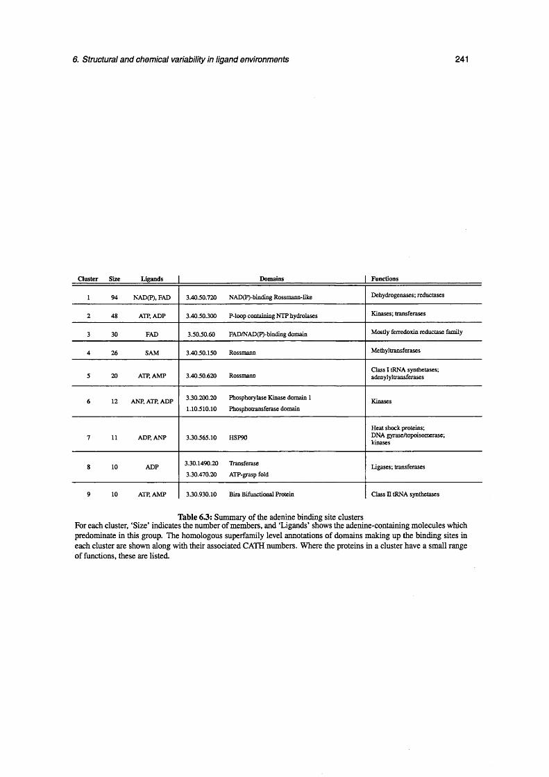
6. Structural and chemical variability in ligand environments 241

Cluster Size Ligands Domains Functions

1 94 NAD(P), FAD 3.40.50.720 NAD(P)-binding Rossmann-like Dehydrogenases; reductases

2 48 ATP, ADP 3.40.50.300 P-loop containing NTP hydrolases Kinases; transferases

3 30 FAD 3.50.50.60 FAD/NAD(F)-binding domain Mostly ferredoxin reductase family

4 26 SAM 3.40.50.150 Rossmann Methyltransferases

5 20 ATP, AMP 3.40.50.620 RossmannClass I tRNA synthetases; adenylyltransferases

6 12 ANP, ATP, ADP 3.30.200.201.10.510.10

Phosphorylase Kinase domain 1 Phosphotransferase domain

Kinases

7 11 ADP, ANP 3.30.565.10 HSP90Heat shock proteins;DNA gyrase/topoisomerase; kinases

8 10 ADP 3.30.1490.203.30.470.20

Transferase ATP-grasp fold

Ligases; transferases

9 10 ATP, AMP 3.30.930.10 Bira Bifunctional Protein Class II tRNA synthetases

Table 63: Summary of the adenine binding site clusters For each cluster, ‘Size’ indicates the number of members, and ‘Ligands’ shows the adenine-containing molecules which predominate in this group. The homologous superfamily level annotations of domains making up the binding sites in each cluster are shown along with their associated CATH numbers. Where the proteins in a cluster have a small range of functions, these are listed.

6. Structural and chemical variability in ligand environments 242

(b) Cluster 2 (48 members)(a) Cluster 1 (94 members)

(c) Cluster 3 (30 members) (d) Cluster 4 (26 members)

(e) Cluster 5 (20 members) (f) Cluster 6(12 members)

Figure 6.24: Diversity in adenine-binding site structure within superfamilies The adenine-contacting residues from five sites randomly selected from the nine adenine-binding site clusters in table 6.4 are shown, demonstrating the different degrees of structural variability seen in adenine-binding sites from different superfamilies.

6. Structural and chemical variability in ligand environments 243

(g) Cluster 7(11 members) (h) Cluster 8(11 members)

(i) Cluster 9 (10 members)

Figure 6.24: Diversity in adenine-binding site structure within superfamilies (continued)

Values of each of the three scores (entropy, chemical diversity and combined) calculated for each of these

clusters are shown in table 6.4, alongside the mean and variance from the sampling experiment with the

appropriate value of n. Figure 6.25 shows these scores plotted onto the graph illustrating the sample size

dependency for each score type during random sampling. Making the assumption that the diversity values

obtained in the sampling experiment follow a normal distribution, a Z-value is calculated for each score, for

each cluster.

Looking first at the combined diversity scores, we see that they are in broad agreement with our intuitive

notion of the degree of variation in each cluster. In all but two cases, the Z-score is negative, indicating

that the binding sites in these clusters are significantly less variable than would be expected by sampling the

same number of sites from the non-redundant dataset. The largest negative Z-score is for cluster 1, indicating

that, although it is not immediately apparent by looking at the superposition plots, this cluster has the least

diversity in the adenine binding pocket. Next are the scores for clusters 6 and 7, which were identified

visually as bein particularly well conserved.

6. Structural and chemical variability in ligand environments 244

Cluster No. of sites Score usedAverage score per unit area

(A)

Random sampling. Standard Mean (ji) error (SE) Z*

entropy 0.2062 0.2165 8.36xl0-4 -12.3 * * *1 94 diversity 0.3670 0.5019 1.23 xl0~4 -1023.6 * * *

combined 0.0907 0.1175 4.22 xlO-4 -63.5 •kick

entropy 0.2244 0.2047 1.61 x l0 “3 12.2 ***2 48 diversity 0.3655 0.4068 3.14xl0"3 -13.2

combined 0.1086 0.1011 1.09 xlO-3 6.88 * * *

entropy 0.1927 0.1960 2.35 xlO-3 -1.43 30 diversity 0.1890 0.3140 3.92 xlO-3 -31.9 irkk

combined 0.0614 0.0846 1.85 xlO-3 -12.6 ***

entropy 0.2036 0.1910 1.98 xl0~3 6.4 * ★ *

4 26 diversity 0.1791 0.2797 4.92 xlO-3 -20.4 * * *

combined 0.0543 0.0800 1.50xl0-3 -17.1 * * *

entropy 0.1906 0.1801 1.87 xlO"3 5.65 20 diversity 0.2260 0.2326 4.09 xlO"3 -1.6

combined 0.0810 0.0710 1.69 xlO-3 5.92 •kirk

entropy 0.1198 0.1590 3.70xl0-3 -10.6 •kick

6 12 diversity 0.0118 0.1317 4.56xl0“3 -26.3combined 0.0040 0.0490 1.48 xlO"3 -30.4 * * *

entropy 0.1005 0.1544 2.90xl0-3 -18.6 * * *

7 11 diversity 0.0303 0.1238 3.14xl0-3 -29.8 irirk

combined 0.0128 0.0464 1.26xl0-3 -26.7 ★ *-*

entropy 0.1653 0.1544 2.90 x l0 “3 3.76 * *

8 11 diversity 0.0576 0.1238 3.14xl0-3 -21.1 ***combined 0.0248 0.0464 1.26xl0-3 -13.3 ★**

entropy 0.1340 0.1523 3.08 xl0~3 -5.9 irk*

9 10 diversity 0.0406 0.1079 3.95 xlO"3 -17.0 kirk

combined 0.0156 0.0408 1.77 xl0~3 -14.2 kick

Table 6.4: Comparison of environment diversity within and between clusters of adenine binding sites

In two cases, however (2 and 5), the Z-score is positive, indicating that the binding sites are significantly

more diverse than groups of sites randomly sampled from the non-redundant set. It is interesting to note

that adenine cluster 5, consisting primarily of ATP/AMP molecules bound to class I tRNA synthetases and

adenylyltransferases, corresponds roughly to cluster 3 from the ATP dataset. In the previous chapter, it

was shown in §5.6.2 that this cluster showed significantly high levels of variation in the ATP conformation.

Proteins belonging to these families, therefore, can be considered to be among the most variable in terms of

their ATP binding sites, from both a ligand conformation perspective and when comparing the binding sites

themselves.

Cluster 2, on the other hand, corresponds to ATP cluster 1. The conformational diversity shown by this

group of ligands, although high, was not found to be statistically significant. Therefore we find that this

group of proteins tends to bind the ligand in the same overall conformation, but stabilises it using a different

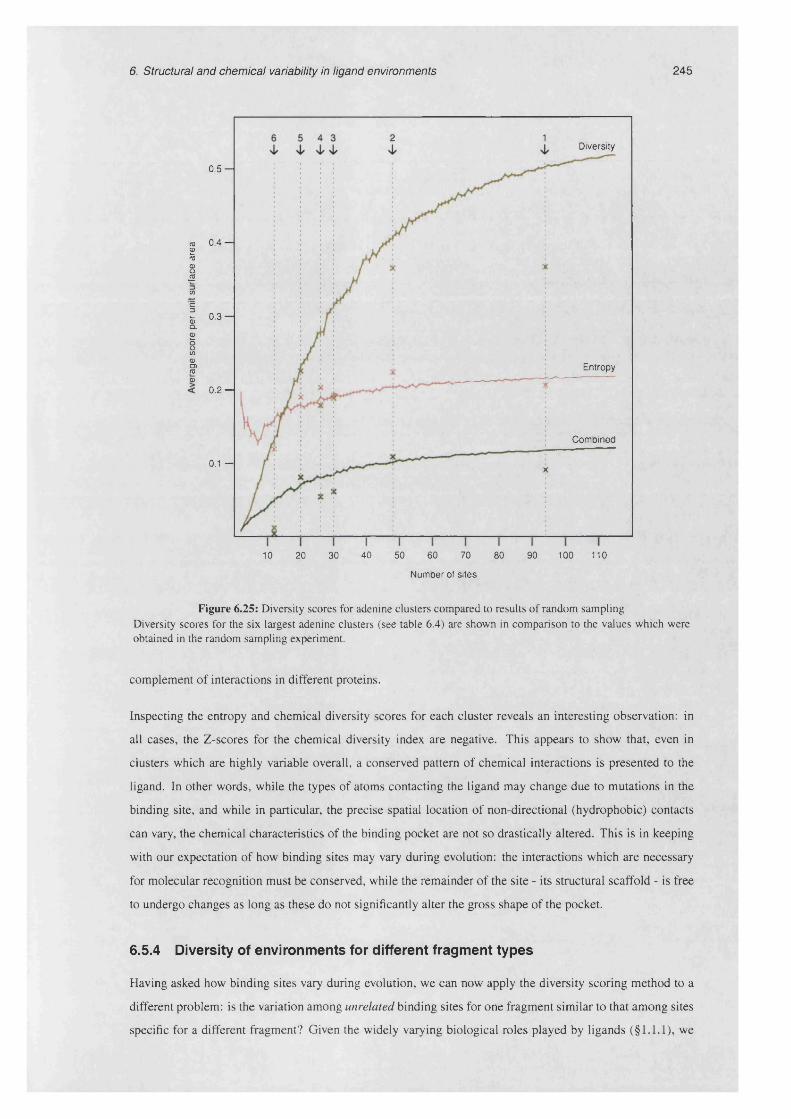
6. Structural and chemical variability in ligand environments 245

Diversity

0 .5 -

m 0 . 4 -2?(01€CO

c3I<1)I

0 . 3 -

C/)<DO)<5CD

0.2 -

Entropy

C om bined

0.1 -

10 20 30 40 50 60 70 80 90 100 110

N um ber of s ite s

Figure 6.25: Diversity scores for adenine clusters compared to results of random sampling Diversity scores for the six largest adenine clusters (see table 6.4) are shown in comparison to the values which were obtained in the random sampling experiment.

complement of interactions in different proteins.

Inspecting the entropy and chemical diversity scores for each cluster reveals an interesting observation: in

all cases, the Z-scores for the chemical diversity index are negative. This appears to show that, even in

clusters which are highly variable overall, a conserved pattern of chemical interactions is presented to the

ligand. In other words, while the types of atoms contacting the ligand may change due to mutations in the

binding site, and while in particular, the precise spatial location of non-directional (hydrophobic) contacts

can vary, the chemical characteristics of the binding pocket are not so drastically altered. This is in keeping

with our expectation of how binding sites may vary during evolution: the interactions which are necessary

for molecular recognition must be conserved, while the remainder of the site - its structural scaffold - is free

to undergo changes as long as these do not significantly alter the gross shape of the pocket.

6.5.4 Diversity of environments for different fragment types

Having asked how binding sites vary during evolution, we can now apply the diversity scoring method to a

different problem: is the variation among unrelated binding sites for one fragment similar to that among sites

specific for a different fragment? Given the widely varying biological roles played by ligands (§1.1.1), we

6. Structural and chemical variability in ligand environments 246

would expect their recognition pockets to be under quite different constraints. Where a fragment is usually

used as a binding ‘anchor’, for example, its binding sites may be fairly similar, having evolved under one

primary constraint - to recognise and bind the fragment tightly. On the other hand, those cofactor fragments

which frequently play an active role in enzymatic catalysis would be expected to be found in quite diverse

environments, according to which substrate was bound by any one protein.

To investigate this, the same procedure used to generate the adenine binding site dataset (see §4.2) was

applied to create datasets of environments of guanine, nicotinamide and isoalloxine. This resulted in 35, 27

and 26 clusters respectively. Using the same protocol as described above for the adenine binding site clusters,

the overall diversity scores obtained from the cluster representatives of each fragment was compared to that

calculated from randomly selected groups of the same number of adenine sites. The resulting Z-scores

therefore show whether the binding sites for each fragment are more or less variable overall than those for

adenine. The results are shown in table 6.5.

Fragment No. of sitesAverage score per unit area

(A)

Random sampling( . Standard Mean (/z) error (SE)

Guanine 35 0.0987 0.0947 1.55 xlO"3 2.58**Nicotinamide 27 0.1052 0.0814 1.56x 10-3 15.3***Isoalloxine 26 0.1314 0.0800 1.50xl0-3 24.3***

Table 6.5: Comparison of environment diversity scores of three different fragments Combined diversity scores are compared against those calculated for adenine using the method described in the text

A — u(t) Z = ---- -SE(*★) p < 0.01, two-tailed (★*★) p < 0.001, two-tailed

The environments of all three fragments are found to be more diverse than those of adenine. Of the three,

guanine shows only slightly more variability in its binding sites than adenine, while nicotinamide and

isoalloxine are significantly more diverse. This is in agreement with the expectations outlined above - we

may expect that a relatively small number of recognition strategies for binding adenine or guanine may have

been selected during evolution, whereas the need to bind a variety of substrates in proximity to the redox

group would necessitate greater binding site diversity around nicotinamide or isoalloxine.

These results suggest that knowledge-based binding site prediction methods may have more success with

some ligand types than others. Moreover, their applicability in terms of function prediction may well be

limited to fairly broad proclamations: while we might reasonably expect to be able to predict that a given

protein binds, say, an NAD cofactor, and therefore is likely to be a redox enzyme, determination of its

particular substrate specificity may be more difficult, and may well be better approached using docking

methods.

6.6 Concluding remarks

This chapter has considered the structural and chemical variability exhibited by the regions of ligand binding

sites which interact with rigid molecular fragments. By showing examples of the broad range of ways in

6. Structural and chemical variability in ligand environments 247

which proteins can apparently recognise a given moiety, the need for a score which quantifies binding site

variability has been demonstrated.

A problem faced when designing this study was how to strike a balance between a purely knowledge-based

approach to binding site representation, and one which is imbued with more chemical realism. Calculating the

distribution of different functional groups or atom types around ligands is relatively simple to do, but suffers

from the problem that some pairs of functionalities or atom types are more similar in their chemical properties

than others. On the other hand, methods which attempt to analyse binding site similarities or differences by

comparing various forcefields calculated over their volumes (see e.g. Kastenholz et al. (2000), Sheridan

et a l (2002)), while potentially more realistic, are heavily dependent upon the reliability of the particular

interaction mapping method used, which often cannot be easily assessed. The approach presented here,

in which mixtures of atom-class densities are compared using empirically-determined atom-type similarity

values, offers a simple and powerful means of taking into account chemical information when analysing

structural data. While the set of atom classes used here may be criticised as being too coarse-grained, the

modular analytical framework can allow different atom classification schema and dissimilarity to be ‘plugged

in’ in a straightforward manner.

By representing each locus of a binding site in terms of a mixture of different atom types, and applying

multidimensional scaling techniques to the atom type dissimilarity matrix, a simple method for comparing the

chemical composition of a binding site at each point in space was described. Although its use was restricted

here to a multi-way assessment of chemical diversity, it may also have applications in pairwise binding

site comparison. Instead of the graph-matching approaches which are commonly employed to compute

similarity between a pair of sites, we could represent each of them using the density mapping approach,

and then compute a similarity index by applying the chemical diversity score discussed in this chapter. This

would clearly be more computationally expensive, but may offer a more sensitive method of binding site

comparison.

The main innovation of this chapter has been the prototyping of a novel diversity measure for application

to ligand binding sites. Concepts previously applied in the analysis of protein sequence conservation - a

one-dimensional problem - have been adapted in order that they could be leveraged on the three-dimensional

information present in a collection of aligned ligand binding sites. The method which has been developed

allows interactive exploration of the spatial distribution of binding site diversity, as well as calculation of

an overall diversity metric which can be used to compare the variability of binding sites in different protein

families and/or specific for different ligand fragments. Qualitative analysis of the score distributions obtained

using this method suggest that it is capable of replicating our intuitive notions of what constitutes a variable

- or conserved region of a binding site. Although more thorough validation would be necessary first, it is

possible that this method could be used to help ‘focus’ binding site search methods, weighting the relative

importance of different regions of the binding site according to the observed level of diversity.

Applying the diversity scoring method to a non-redundant set of adenine binding sites has shown that their

variability can be roughly divided into two types, which are manifested in different regions of the ligand

environment. The faces of the adenine rings are dominated by non-specific, non-polar contacts, which are

6. Structural and chemical variability in ligand environments 248

variable in terms of their precise spatial location and in terms of the atom types which are involved. The

chemical characteristics of the binding sites in these regions, however, tends to be fairly homogeneous.

Around the rim of the adenine fragment, however, we see a far greater diversity of chemical groups, with

small islands of conserved interactions floating in a sea of variability. It appears, then, that these few specific

interactions - with the N6 cis acceptor position being most prevalent - are capable of standing out sufficiently

to ensure reliable recognition of the correct nucleotide.

As with the analysis of ligand conformational diversity, it appears that not all protein families are equal

when we consider the conservation of their adenine binding sites. Comparison of the overall diversity scores

for 9 clusters of adenine-binding sites showed that, while most are significantly well conserved, two families

exhibited approximately the same level of diversity as we would expect by randomly sampling from unrelated

sites. The biological reasons for this are not clear, and require further analysis.

The work presented in this chapter is by no means a definitive analysis of binding site variability, but it

serves to illustrate an important point which should be heeded when designing any method for binding site

comparison or prediction. The degree of variability varies greatly both between different regions of a binding

site, and between the sites of different protein families. Therefore appropriate weighting should be applied

when searching for geometric patterns in binding sites. Moreover, it should be appreciated that no single

approach can be expected to work well when applied to all proteins: the fact that some families appear to

be able to tolerate far greater diversity in their ligand-binding sites may mean that they will prove to be

stumbling blocks for predictive methods.

249

Chapter 7

Discussion

This project set out to address two questions: comparing ligands bound to unrelated proteins (domains

belonging to different superfamilies) with those bound to related proteins (non-identical domains from the

same superfamily),

1 How much do the conformations of the ligand vary?

2 How much do the structure and properties of the binding sites vary?

In the course of providing answers to these problems, new software and methods were developed, and several

novel insights into the phenomenon of molecular recognition were gained. This chapter draws together some

of the main points from the body of the thesis, and suggests several areas in which further work could be

done.

The GAMUT library

In addition to seeking answers to the biological questions stated above, the author took this doctoral research

project as an opportunity to pursue an abiding interest in scientific programming techniques. The outcome

of this part of the work was a software library called GAMUT, the details of which were covered in chapter

2. Besides providing the platform upon which all of the programs used for the analyses presented here were

built, the design and implementation of GAMUT highlighted several important aspects of successful software

development.

Perhaps the clearest of these is the need to strike a balance between expressivity and useability when

designing software libraries. The former allows the library to fulfil a wide range of tasks, allowing it to serve

as the main codebase for application development, thus reducing dependencies and simplifying the project.

Expressivity is, however, often achieved at the expense of comprehensibility, since generic components

tend to be less easily accessible to the programmer, requiring more time to understand how to access the

required functionality. This can be particularly true in a language such as C++, where genericity is usually

implemented using templates, which are burdensome both in terms of syntax and as a cause of ‘code bloat’

(both problems are covered extensively in the literature - see e.g. Alexandrescu (2001)). By using a range of

techniques including template metaprogramming, much of the complexity inherent in the generic features of

GAMUT has been hidden, such that, for example, clients may use the chemical graph class without needing

to know that it inherits from a highly generic graph template class. Users with more complex needs, however,

are free to employ the more powerful aspects of the library which come from harnessing these generic classes.

7. Discussion 250

If the author were writing the library again from scratch, some design decisions would be taken differently.

The implementation of GAMUT was seen not only as a means to an end (in terms of providing the

tools necessary to perform certain analyses), but also as a educational vehicle for improving the author’s

programming skills. As such, some aspects of the library are overly complex, having been written in part

to help understand the workings of a particular language feature. This is clearly not an ideal way to design

software; nevertheless, the modular design of the library means that, while some parts should be re-written,

such re-designs would not affect the overall structure of the system.

Diversity of structure and function of proteins binding a given ligand

The analysis presented in §4.4 provides a summary of the extent of macroscopic diversity - that is, diversity

at the level of the whole protein - shown by proteins which contact ligands in the PDB. These must be viewed

with caution since they include non-cognate interactions, and are adversely affected by biases present in the

database, but nevertheless constitute a useful overview.

In terms of protein structure, most ligands tend to interact with only a small number of fairly similar

proteins: over three quarters of ligands interact with only one or two folds (figure 4.15), and there are only

11 compounds which are bound by domains from more than 20 homologous superfamilies (figure 4.16).

Considering function, only 9 ligands are bound by proteins with EC numbers distinct up to the second level

(figure 4.21).

Conformational diversity of of bound ligands

In chapter 5, the considerable diversity in conformation of several common biological ligands was

demonstrated, first pictorially, and then by application of a measure of compactness, the molecular radius

of gyration. This showed that, while ligands often bind in an extended conformation, this is not always

the case, and even when ligands do unfold upon binding, they are still free to explore a large region of

conformational space.

Interestingly, the assumption that homologous proteins bind ligands in similar conformations was found not

to hold universally. Indeed, the conformations of ligands bound to some families were found to be statistically

as diverse as we would expect by sampling randomly from unrelated binding sites. This was demonstrated

by application of a newly-developed technique for multi-way analysis of ligand conformation. The findings

suggests that, firstly, the biological constraints on ligand conformation are not equal in all proteins, and

secondly, that in many cases, ligands are likely to be only partially immobilised upon binding.

Structural and chemical diversity of ligand environments

Having established the high degree of ligand conformational variability, attention was turned in chapter 6

to assessing diversity in the ligand binding sites. Due to the findings of the previous chapter, this was done

by concentrating on rigid fragments of ligands, primarily the adenine moiety. Here, binding sites were

also shown to be highly diverse; conserved interactions were highlighted by using a propensity mapping

approach to identify regions of space in which particular types of contacts to the ligand are statistically over­

7. Discussion 251

represented. This method is a realisation of the ‘fuzzy template’ approach proposed previously (Moodie

et al., 1996), and may be a useful starting point for development of new binding site search techniques

(discussed further below).

The remainder of chapter 6 describes a new method for quantifying binding site diversity. It should be

stressed that this approach is currently only at a preliminary stage, but it appears that it is capable of providing

a reasonable objective measure of the variance at each locus of a group of binding sites, which is in keeping

with our own intuitive assessment.

Future work

Active development on GAMUT is likely to end with the completion of this thesis. However, were it to

continue, the main threads would probably be the addition of a scripting layer, allowing the power of the

library to be accessed from an interpreted library such as Python (Python Software Foundation, 1990), and

the design of a web interface to the application programs, allowing users to perform analyses similar to those

presented here on their own datasets.

Several aspects of the methodology used to generate the binding site datasets are worthy of further comment.

The method used to validate ligand identities offered a simple and automatic means of guaranteeing that

all instances of molecules identified as being of a particular type have a chemical structure which agrees

with our notion of what that compound should be. It is somewhat stricter than the ligand validation applied

in, for instance, the MSD, because ligands which are poorly resolved in the crystallography experiment are

automatically excluded. From a biological perspective, however, it is less than ideal, since no checks are

made on whether or not the ligand is cognate to the protein. In order to be more sure that findings from the

type of high-throughput analysis described here are biologically relevant, this should be remedied in future

work, particularly if more esoteric ligands are analysed.

The binding site clustering approach is similarly well-suited to large-scale analysis, but perhaps less reliable

than it could be. The heuristic of clustering binding sites on the basis of their domain composition appears to

be fairly effective, but may be misleading in that, for example, two binding sites which appear on homologous

domains, but in different locations on the surface of those domains, would be clustered together. This means

that conclusions drawn about the binding sites in this cluster may be the result of comparing sites which

are, in truth, not directly comparable. This issue is not thought to be a particularly common problem, and

therefore does not invalidate the general findings of this thesis, but could be rectified fairly simply in future

work.

Finally, the overall architecture of the analytical pipeline described in chapter 4 could be improved by

reducing its reliance on proprietary file formats.

The torsion angles of ligands in the four datasets in chapter 5 were treated only in passing; these deserve

somewhat deeper analysis. In particular, the question of why so many torsion angles are observed to lie

well outside preferred angular ranges - even in relatively high-resolution structures - needs to be addressed.

It may be that, in some of these structures, although of generally high quality, the density into which the

7. Discussion 252

ligands were fitted is less well-defined. Another explanation, stemming from anecdotal reports of structure

determination practices, is that the refinement of ligand coordinates may in some cases not be as rigourously

checked as that of the protein backbone. Thirdly, some of the strained angles will be the result of a particular

conformation imposed on the ligand by the protein. An analysis which reveals the relative prevalence of

each of these scenarios would be illuminating. In the first instance, this could be undertaken by a thorough

analysis of temperature factors for all ligand coordinates in the datasets. An interesting experiment which

could then be performed would be to obtain structure factors, where available, for each structure, and then

systematically re-refine the coordinates of the ligand molecules using the same parameters for each, and then

compare the results with the coordinates deposited in the PDB entry.

Another aspect of ligand conformational diversity which could be explored is the relationship between ligand

conformation and binding site shape. Work is currently underway to develop methods for comparing the

shape of binding pockets, with a view to predicting the ligand - or ligands - which may bind to a new

protein (T. Funkhouser, personal communication). An interesting question which arises from this is, where

we find domains which bind ligands in diverse conformations, does the shape of the binding pocket undergo

concommittant deformations, or is it simply large enough to permit certain parts of the ligand to flex within

an essentially rigid binding site?

In chapter 6, it was stated that the diversity scores could be used to focus geometric searches for potential

binding sites. One way in which this proposal could be tested is as follows. For each fragment, templates

could be constructed from the location of peak values in the propensity maps of each atom class. These

templates could then be used to search for binding sites in a test set of structures (using appropriate cross-

validation procedures), using an existing algorithm such as that recently described by Barker and Thornton

(2003). This type of search would be expected to return a large number of false-positives; the utility of the

diversity maps could then be tested by using them to calculate weights on each component of the template,

and determining whether the extra information improved the specificity of the search.

Another avenue which could be explored using the diversity index is the relationship between sequence

evolution and the increase in binding site diversity. Given a large, diverse protein family, one could

sample groups of binding sites, of approximately equal size, gradually allowing more evolutionarily diverse

sequences to join. By computing the binding site diversity for each group, one could begin to explore the

effects of divergence on ligand binding sites.

Concluding remarks

In summary, the work presented in this thesis highlights the extremely high level of diversity among

ligand binding sites. This goes some way to explaining the difficulties encountered by many researchers

in developing ligand binding site prediction methods: the success of pattern-matching approaches is dictated

by the signal-to-noise ratio of the data, which in this case is demonstrably low. Docking approaches offer an

alternative which does not depend on analogy to previous examples, but instead is based on physico-chemical

principles. Although these techniques allow us to build attractively realistic models of the forces involved in

molecular recognition, the current level of accuracy in the free energy calculations based on these models is

7. Discussion 253

too low to allow for robust predictions.

Ultimately, we must retain hope that reliable methods for predicting molecular interactions can and will be

developed. All the information required for recognition is present in the atomic structures of the molecules

involved; the correct partners are bound in vivo, so it should be possible for us to model the same processes

in silico. Whether the most successful approach to this problem turns out to be knowledge-based, rooted in

first principles, or a combination of the two remains to be seen. What we can say is that at present, there are

some conspicuous gaps in our understanding of the process of molecular recognition, which will most likely

be filled only after detailed inspection of many more experimentally studied interactions.

254

Appendix A

Graph theory

Graphs are mathematical abstractions useful for solving a wide range of problems. A thorough review of the

whole field of graph theory is beyond the scope of this chapter; here, elementary graph theory is summarised,

and some key algorithms are described in pseudocode.

The first modem application of graph theory is attributed to the Swiss mathematician Leonhard Euler, and

was published in 1736. Euler wished to mathematically prove a widely held belief among residents of his

town, Konigsberg in East Prussia. The proposition was that it is impossible to cross each of the town’s

seven bridges (shown schematically in figure A. la) exactly once during a single walk. Euler reformulated

the problem by drawing a graph (figure A. lb) which represented the essential elements of the problem: the

vertices correspond to the distinct land masses in the town, and its edges symbolise the bridges which join

those land masses. Euler noted that, in the course of a walk around the town, the act of ‘visiting’ a new vertex

corresponded to the use of two bridges (edges) - one used to arrive, and another to leave. It follows that, in

order to avoid using the same bridge twice, the vertex must have an even number of incident edges. In order

to carry out the type of walk described above, this condition must hold for all but at most two of the vertices

in the graph - the remaining two being the vertices at which the path starts and ends. (Note that the starting

and ending vertices may be the same, in which case the order of every vertex must be even.) It is clear that

the Konigsberg graph does not satisfy the constraint; whether this proof put an end to Sisyphean wandering

on the part of Euler’s fellow townsfolk is more difficult to say.

Graph theory has been applied in areas as diverse as chemistry, social sciences and computer networking.

In this appendix, a basic review of graph theory is presented, in order to provide a foundation for the graph

theoretic techniques applied to chemical structures in the rest of this thesis.

A.1 Definitions and terminology

Firstly, it is necessary to explain what is meant by the term ’graph’, in a mathematical sense, and to define

some terms commonly used in graph theory. More information and examples explaining the definitions given

here may be found in Gibbons (1985).

A graph may be defined as a set of vertices, and a set of edges, where an edge is a connection between

a pair of vertices within the graph. More precicely, a graph is a pair, G = (V,E), where V is a finite set

and £ is a binary relation on V. The contents of the set V = {v,-}^ are the graph vertices; we introduce

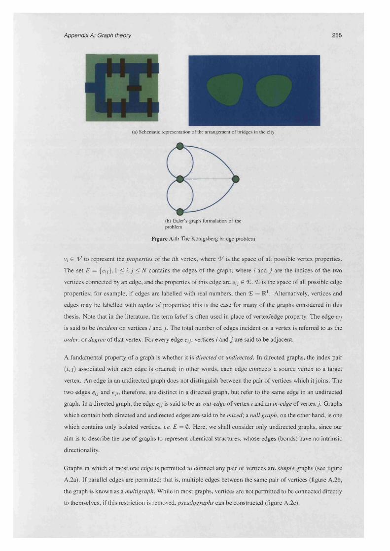
Appendix A: Graph theory 255

(a) Schematic representation of the arrangement of bridges in the city

(b) Euler’s graph formulation of the problem

Figure A.l: The Konigsberg bridge problem

v; e V to represent the properties of the z'th vertex, where V is the space of all possible vertex properties.

The set E = {«/_/}, 1 < i , j < N contains the edges of the graph, where i and j are the indices of the two

vertices connected by an edge, and the properties of this edge are ey e £ . £ is the space of all possible edge

properties; for example, if edges are labelled with real numbers, then £ = R 1. Alternatively, vertices and

edges may be labelled with tuples of properties; this is the case for many of the graphs considered in this

thesis. Note that in the literature, the term label is often used in place of vertex/edge property. The edge eij

is said to be incident on vertices i and j. The total number of edges incident on a vertex is referred to as the

order, or degree of that vertex. For every edge eij, vertices i and j are said to be adjacent.

A fundamental property of a graph is whether it is directed or undirected. In directed graphs, the index pair

(z, j ) associated with each edge is ordered; in other words, each edge connects a source vertex to a target

vertex. An edge in an undirected graph does not distinguish between the pair of vertices which it joins. The

two edges ey and eji, therefore, are distinct in a directed graph, but refer to the same edge in an undirected

graph. In a directed graph, the edge eij is said to be an out-edge of vertex i and an in-edge of vertex j . Graphs

which contain both directed and undirected edges are said to be mixed; a null graph, on the other hand, is one

which contains only isolated vertices, i.e. E = 0. Here, we shall consider only undirected graphs, since our

aim is to describe the use of graphs to represent chemical structures, whose edges (bonds) have no intrinsic

directionality.

Graphs in which at most one edge is permitted to connect any pair of vertices are simple graphs (see figure

A.2a). If parallel edges are permitted; that is, multiple edges between the same pair of vertices (figure A.2b,

the graph is known as a multigraph. While in most graphs, vertices are not permitted to be connected directly

to themselves, if this restriction is removed, pseudographs can be constructed (figure A.2c).

Appendix A: Graph theory 256

*st* T #(a) A simple graph (b) A multigraph (c) A pseudograph

Figure A.2: Types of graphs, organised in terms of connectivity

Graphs in which every vertex is directly or indirectly connected to every other; that is, in which one can

construct a walk along one or more edges from any vertex to any other, are said to be connected. Once again,

as we focus on chemical graphs, the following discussions consider only simple connected graphs.

A path on a graph is defined as a set of vertices {vi,V2 ,- • • ,v„} which are sequentially connected; in other

words, the edge set {e\2 , ej3 , • • •, en- i n} is a subset of the edges in the graph. A path in which the first vertex

is also the last, is called a cycle, or, with particular reference to chemical graphs, a ring Downs (2003).

If the vertex and edge sets of a graph H are subsets of the vertex and edge sets respectively of another graph

G, then H is a subgraph of G. Given a subset V' of the vertices G, an induced subgraph can be constructed

by selecting a set E' from the edge set of G such that both endpoints of each edge in E' are in V'. The pair

I = {V',E') then constitutes the subgraph of G induced by the vertex set V '. This is illustrated in figure A.3

• *(a) A graph (b) Subgraph induced by the

vertex set {1,2,5}

Figure A.3: An example of an induced subgraph

An ismorphism between two graphs is a one-to-one mapping between their two sets of vertices. If just some

parts of a pair of graphs can be mapped onto one another, we may define a subgraph isomorphism. Strictly, a

subgraph isomorphism between a pair of graphs G,H is an isomorphism between subgraphs G',H' of G and

H. If, however, one of these subgraphs is in fact equal to its parent graph {i.e. G' = G), then a special case

exists in which one graph, G, can be entirely mapped to a subgraph of H. For clarity, this type of subgraph

isomorphism shall be referred to as an Exact Subgraph Isomorphism. This is shown schematically in figure

A.4b. The term Common Subgraph Isomorphism will be used to describe the case where both G' and H' are

subsets of the parent graphs G and H, as shown in figure A.4c. Note that common subgraph isomorphisms

can be distinguished according to whether or not they are connected in each graph. An isomorphism is

connected within one of the two graphs if each vertex within the subgraph is connected to every other by a

path. A connected subgraph is also known as a clique. Finally, figure A.4a depicts an isomorphism in which

all vertices from both graphs are mapped; this will be referred to as a full graph ismorphism.

Appendix A: Graph theory 257

(a) A full graph isomorphism

0 00(b) An exact subgraph isomorphism (c) A common subgraph isomor­

phism

Figure A.4: Types of graph isomorphism

A.2 Representation of graphs

We may conceive of a number of ways of representing the structure of graphs. Consider the graph in figure

A.5.

Figure A.5: An example graph The vertex properties v, are the colours of the circles. Edges do not have any properties in this graph.

The simplest representation is the edge list, which is simply the set E. In the case presented here, edges are

unlabelled, so each member in the set E is simply an unordered pair of indices indicating the pair of vertices

which are connected by the edge. The edge list for the graph in figure A.5 is as follows:

(1,2) (2,3) (2,4) (2,5) (5,6) (5,7)

An alternative is the adjacency list, in which a list of adjacent vertices is stored for each vertex in the graph.

For instance, vertex 2 has adjacent vertices 1, 3,4 and 5; the complete adjacency list is:

21,3,4,5 2 22,6,755

The adjacency matrix is a third representation. Since edges are unlabelled, the adjacency matrix in this case

is a boolean matrix; that is, a matrix in which each cell M\j simply indicates the presence or absence of an

edge connecting the ith and jth vertices. The values stored in the |Vj x | V | boolean matrix M are given by

Mi j =

1 e ij £ E

otherwiseM y

otherwise

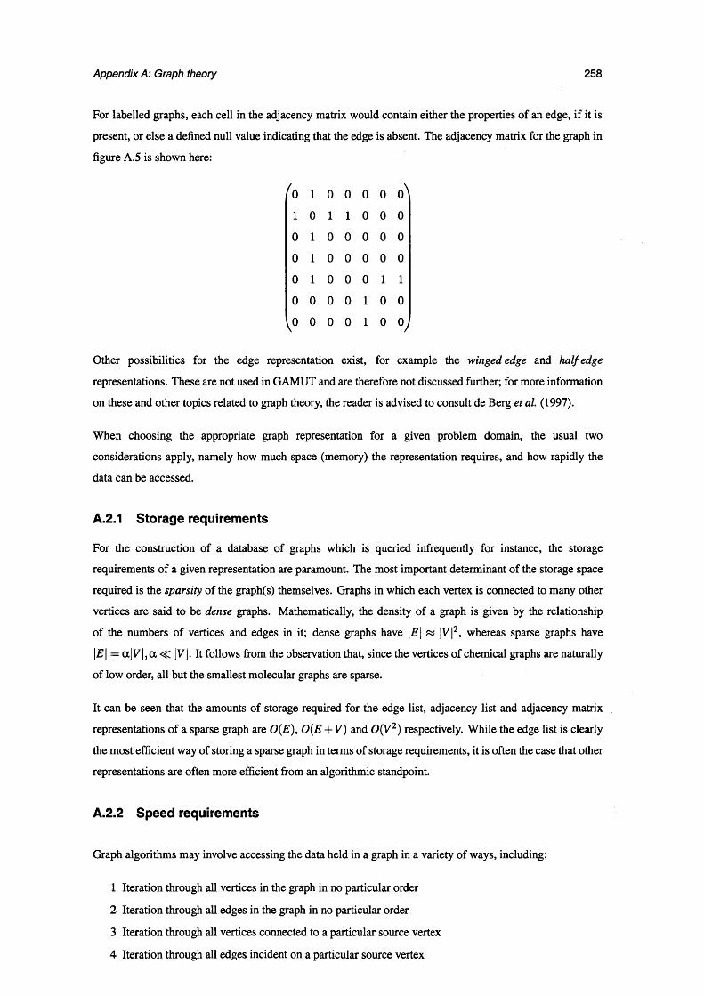
Appendix A: Graph theory 258

For labelled graphs, each cell in the adjacency matrix would contain either the properties of an edge, if it is

present, or else a defined null value indicating that the edge is absent. The adjacency matrix for the graph in

figure A.5 is shown here:

0 1 0 0 0 0 0

1 0 1 1 0 0 0

0 1 0 0 0 0 0

0 1 0 0 0 0 0

0 1 0 0 0 1 1

0 0 0 0 1 0 0

0 0 0 0 1 0 0

Other possibilities for the edge representation exist, for example the winged edge and half edge

representations. These are not used in GAMUT and are therefore not discussed further; for more information

on these and other topics related to graph theory, the reader is advised to consult de Berg et al. (1997).

When choosing the appropriate graph representation for a given problem domain, the usual two

considerations apply, namely how much space (memory) the representation requires, and how rapidly the

data can be accessed.

A.2.1 Storage requirements

For the construction of a database of graphs which is queried infrequently for instance, the storage

requirements of a given representation are paramount. The most important determinant of the storage space

required is the sparsity of the graph(s) themselves. Graphs in which each vertex is connected to many other

vertices are said to be dense graphs. Mathematically, the density of a graph is given by the relationship

of the numbers of vertices and edges in it; dense graphs have |2?| « |Vj2, whereas sparse graphs have

\E\ = a |V |,a < |Vj. It follows from the observation that, since the vertices of chemical graphs are naturally

of low order, all but the smallest molecular graphs are sparse.

It can be seen that the amounts of storage required for the edge list, adjacency list and adjacency matrix

representations of a sparse graph are 0(E ), 0 (E + V) and 0 (V 2) respectively. While the edge list is clearly

the most efficient way of storing a sparse graph in terms of storage requirements, it is often the case that other

representations are often more efficient from an algorithmic standpoint.

A.2.2 Speed requirements

Graph algorithms may involve accessing the data held in a graph in a variety of ways, including:

1 Iteration through all vertices in the graph in no particular order

2 Iteration through all edges in the graph in no particular order

3 Iteration through all vertices connected to a particular source vertex

4 Iteration through all edges incident on a particular source vertex

Appendix A: Graph theory 259

5 Asking whether a particular pair of vertices are connected by an edge

For a graph with V vertices and E edges, we can derive orders of complexity for these operations, using each

of the representations described above. These orders are shown in table A.I.

Clearly, no one representation is optimal for all possible operations; rather, the choice of representation used

by a given algorithm is often a heuristic one, based largely on the types of graphs which are expected to be

processed.

Representation All vertices iteration

All edges iteration

Adjacent vertices iteration

Incident edges iteration

Edge existence test

Edge list 0(V ) 0(E ) 0(E ) 0(E ) 0(E)Adjacency list 0(V ) 0(E ) 0 ( f ) 0 ( f ) 0 ( f )Edge matrix 0(V ) 0 ($ V 2) 0(V ) 0 (V ) constant

Table A.1: Average orders of complexity for common graph operations

A.3 Common graph operations

Two fundamental types of graph iteration are the Depth-first search (DFS) and Breadth-first search (BFS)

. They are described briefly here; the following, more in-depth discussion of several graph algorithms will

refer to these traversal methods. Both DFS and BFS are methods for visiting all vertices in a graph G which

are reachable from a given source vertex v5; in a connected graph, this means that all vertices are visited

eventually.

In BFS, the search proceeds by first visiting all neighbours of - that is, vertices adjacent to - the current vertex.

Next, the vertices adjacent to those neighbours are visited, and so on. In this way, the search propagates

outwards from the initial vertex, until all vertices have been visited. A formal description of the BFS is

presented in algorithm A. 1.

In DFS, by contrast, the search moves forward, deeper into the graph, as soon as it reaches a new vertex.

That is, it will pick the next adjacent unvisited vertex until reaching a vertex that has no unvisited adjacent

vertices. The algorithm will then backtrack to the previous vertex and continue along any as-yet unexplored

edges from that vertex. DFS is formalised in algorithm A.2.

A.4 Graph algorithms

There are many types of graph algorithms, reflecting the widespread applicability of graph theory to

different problem domains. Among them are methods for detecting cycles in graphs (e.g. Figueras (1996)),

determining minimum path lengths between pairs of vertices, and generating 2-dimensional depictions of

graphs. The family of graph theoretic algorithms most used in the current study are those for matching pairs

of graphs; two such algorithms are discussed in detail in §3.1.

Appendix A: Graph theory 260

Recursive breadth-first search on an undirected graph G = (V,E), starting at vertex vsThe VlSITfj function may be a user-defined event which should occur as each new vertex is discovered

Function B r e a d t h F ir stS ea r c h (G, vs) :Initialise the set o f unvisited vertices R ^ V - v s

Visit the initial vertex V isit (vs)B FS-R ec u r s iv e (vs,R ,£ )

Function BFS JRe c u r siv e (vc,R ,F ) :Get the set o f unvisited vertices adjacent to the current vertex vc N <— {vi e R I 3 eci € E}

Visit neighbours o f the current vertex for each v € N :

VlSIT(v)

Recursively call the function to visit neighbours-of-neighbours for each v € N :

R * - R - vBFS_R e c u r siv e (v, R , E)

Algorithm A.l: Breadth-first search in an undirected graph

Recursive depth-first search on an undirected graph G = (V,E ), starting at vertex v5The VlSITO function may be a user-defined event which should occur as each new vertex is discovered

Function D epth F ir stS e a r c h (G, v5) :Initialise the set o f unvisited vertices R ^ V - v s

Visit the initial vertex VlSIT(Vi)DFS_RECURSIVE(Vi, R, E)

Function DFS_Re c u r s iv e (vc,R ,F ) :Get the set o f unvisited vertices adjacent to the current vertex vc N <— {v; € R I 3 eci e E}

Visit neighbours o f the current vertex; proceed forward from each new vertex immediately for each v e N :

VlSIT(v)R ^ R - vDFS_Re c u r s iv e (v,R ,£ )

Algorithm A.2: Depth-first search in an undirected graph

A.4.1 Ring perception

Firstly, let us elaborate on the definition of a graph cycle presented previously. If no pair of vertices in a cycle

is joined by an edge which is not part of the cycle, it is a simple cycle; other cycles are complex. Since all

chemical graphs are simple graphs, all cycles found in them are by definition simple.

Given a graph with v vertices and e edges, consisting of n connected components 1, the number of rings

which make up a fundamental basis set is given by the Cauchy formula:

/i = e — v + n

^ere, n is always equal to 1, since we are only considering graphs which represent individual molecules, and hence contain only one connected component

Appendix A: Graph theory 261

A fundamental basis set is a set o f rings from which all others, in a non-trivial ring system , can be produced

by com bining subsets o f them.

A.4.1.1 Ring sets

For com plex ring system s, a range o f cycles can be perceived. Figure A .6 show s the seven possible cycles

in a com plex ring system consisting o f three fused simple cycles. A com m on problem is how to select a set

o f rings which is in som e way optimal for the given graph. For instance, if w e require that a ring set should

satisfy the criterion that it contains each vertex in the ring system at least once, then w e may enumerate the

follow ing possible combinations:

{a,b ,c}-,{a ,e}\{b ,dy,{c,f}

(c)(a) (b)

(e)(d) (f)

(g)

Figure A.6: Cycles in a complex ring set

For m ost applications in cheminformatics, the most useful type o f ring set is the sm allest set o f sm allest rings,

otherwise known as the minimal cycle basis. Definition o f the SSSR is a preliminary step in the identification

o f rigid molecular fragments, which can be created by removing all acyclic single bonds from a m olecule.

For certain applications however, other types o f ring sets may be more applicable. For exam ple, a ring set

known as the Essential Set o f Essential R ings (ESER) has been used in analysis o f changes in catalytic sites

Appendix A: Graph theory 262

during enzymatic reactions. Further details on different types of ring sets are available in Gibbons (1985).

A.4.1.2 SSSR perception algorithms

Several algorithms for perceiving the SSSR have been published (Qian et al. (1990), Fan et al. (1993),

Balducci and Pearlman (1994), Figueras (1996)).

Figureas’ method is summarised in pseudocode as algorithm A.3. The essence of the algorithm is as follows:

1 Remove all vertices whose degree is less than 2.

2 Determine the smallest degree of the remaining vertices. If it is greater than 2, temporarily remove

edges from the lowest-degree vertex to reduce its degree to 2.

3 Select a vertex of degree 2, and perform a breadth-first search to find the smallest ring which contains

this vertex.

4 Remove a degree-2 vertex from the ring just found, thus breaking it.

5 Repeat from step 3 until all nodes of degree 2 have been eliminated.

In order to illustrate the breadth-first search method, consider the graph shown in figure A.7. The algorithm

begins by assigning intial values to the paths leading from the source vertex (1) to its neighbouring vertices,

2 and 5.

path[ 2] = [1,2]

path[5\ = [1,5]

The search progresses by moving from vertex 2 on to vertex 3. First, a check is made to determine whether

path[3] is empty. It is, so a closed path has not been found; the value of path[3] is then updated:

path[3] = path[2] + 3 = [1,2,3]

This procedure progresses until a non-empty path is encountered. Referring to step figure A.7b, we see that

extending the path from vertex 4 to vertex 3 will meet a non-empty path. At this stage, the intersection of the

two paths is computed; here:

intersection = path[4] x path[3] = [1,5,4] x [1,2,3] = [1]

The fact that the intersection contains just a single vertex indicates that the closed path is a valid ring. Contrast

this with the situation when the path leading around the four-membered ring is extended from vertex 6 to

vertex 4:

intersection = path[6\ x path[4\ = [1,5,7,6] x [1,5,4] = [1,5]

This indicates that the target vertex, 4, can be reached by more than one path from the source. The ring

{1,5,7,6,4,3,2} is not therefore a member of the SSSR.

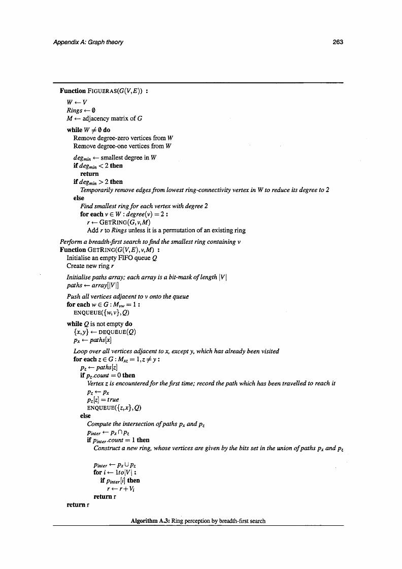
Appendix A: Graph theory 263

Function F ig u e r a s (G (V ,£ )) :

W ^ V Rings <— 0M <— adjacency matrix of G

while W 7̂ 0 doRemove degree-zero vertices from W Remove degree-one vertices from W

degmin *— smallest degree in W if degm in < 2 then

return if degmin > 2 then

Temporarily remove edges from lowest ring-connectivity vertex in W to reduce its degree to 2 else

Find smallest ring for each vertex with degree 2 for each v £ l V : degree(v) — 2 :

r «- GETRlNG( G , v , M )Add r to Rings unless it is a permutation of an existing ring

Perform a breadth-first search to find the smallest ring containing v Function G e t R I N G ( G ( V , E ) , v , M ) :

Initialise an empty FIFO queue Q Create new ring r

Initialise paths array; each array is a bit-mask o f length |Vj paths <— array[|V|]

Push all vertices adjacent to v onto the queue for each w G G : Afw = 1 :

ENQUEUE({w,v},0

while Q is not empty do {x ,y } 4 - DEQUEUE(G)Px <- paths[x\

Loop over all vertices adjacent to x, except y, which has already been visited for each z € G : Mxz = 1 , z ^ y :

Pz <- paths[z] if pz.count — 0 then

Vertex z is encountered for the first time; record the path which has been travelled to reach itPz+~Px Pz[z] = true EN Q UEUE({z,*},0

elseCompute the intersection o f paths px and pzPinter * Px^Pzif Pinter-count = 1 then

Construct a new ring, whose vertices are given by the bits set in the union o f paths px and pz

Pinter * Px U Pzfor i <— lfo|Vj :

if Pinter[i\ then r ^ r + V i

return rreturn r

Algorithm A3: Ring perception by breadth-first search

Appendix A: Graph theory 264

7

1

[1 .2 ][1,5]

(b)

[1,5,7,6]

[1,5,4] [1,2,3]

[1,5,7]

[1,2][1,5]

(d)

[1,5,4] [1,2,3]

[1,5,7]

[1,2][1,5]

(c)

Figure A.7: Ring perception by breadth-first search

265

Appendix B

Coding principles and techniques

This appendix describes, first, the conventions which were adhered to while writing the library. An

appreciation of these principles, particularly those which relate to names, should aid the reader when he/she

reads the GAMUT code. The rest of the appendix details several programming techniques which were used

in various points of the library.

B.1 General principles

• Pointers are avoided in the public interfaces of classes; references are preferred.

• Objects are passed by const reference rather than by value wherever possible.

• C-style casts are not used; the new C++ casting operators are used instead.

• static.casto is only used where there is a strong advantage to doing so, either from a performance

or simplicity standpoint.

• The const keyword is used wherever possible.

• const-ness is respected within classes; const.casto is avoided.

• Macros are used in the following reasons only:

- Header inclusion guards

- Control of conditional compilation, e.g. debugging code

- For recursive metaprogramming (e.g. typelists)

- To throw GAMUT exceptions, which report the file and line number where they originated

- In certain special cases where their use improves readability of the code e.g. for initialisation of

static class members used by the I/O system

The source code for the library was organised using the following guidelines:

• Header files have the suffix .h

• Source code files have the suffix .cpp

• Template function definitions are in files with suffix .hxx

• Inline function definitions are in files with suffix .ini. Inlining of member functions is controlled by a

macro which is set during library configuration. The macros look like this:

Appendix B: Coding principles and techniques 266

#ifdef GAMUT_INLINING ♦define GAMUT_INLINE inlin*♦ else♦define GAMUT_INLINE ♦endif

The body of potentially inlined member functions in the .ini file is written as follows:

GAMUT_INLINE void MyClass::myfunc() { / * . . , * / }

If inlining is enabled, this file is included in the appropriate header, making the implementation of the

function visible to all callers of it. If inlining is disabled, the file is appended to the .cpp file, meaning

that the functions are compiled into the library itself.

• All header files are protected with macros which prevent multiple inclusion.

• The hierarchy of namespaces is reflected in the directory structure of the library code. For example, a

class which is in the gamut: :mmol namespace would be found in the gamut/mmol/ subdirectory of the

source tree.

Names for classes and functions were chosen according to the following rules:

• Class names are capitalised, and multiple words concatenated, e.g. ScalarField.

• Functions are named in lower case, with multiple words joined by underscores, e.g. read_data.

• Private and protected class members are named with a trailing underscore (e.g. data_).

• Private and protected class functions are named with a trailing underscore (e.g. void init_();).

• Typedef names are given the _t (for type) suffix (e.g. matrix.t).

• Macros and static class constants are named all in upper case.

• Everything in the GAMUT library belongs to the gamut namespace. Subcomponents of the library lie

in nested namespaces (e.g. the chemistry components are all defined in namespace gamut:: chem).

B.2 Memory management

GAMUT is designed in such a way that clients should rarely need to use the new and delete keywords

to create and dispose of library objects. This is achieved primarily by having complex objects (e.g. the

macromolecular structure and graph classes) manage the lifetime of their constituent components internally

(here, e.g. atoms and vertices respectively), allowing clients access to those objects by passing references

to them. Where the copy constructor and assigment operator (operator=) of a class are public, they should

perform deep copying. For example, copying the root node of a tree will also cause the subtree of that node

to be copied recursively. For some classes, copying is explicitly prevented by making these operators private.

This is typically for those objects whose existence is managed by other objects; for example, macromolecule

selection objects are managed by a selection manager, which provides functions for creating, copying and

disposing of them.

Appendix B: Coding principles and techniques 267

B.3 Deferred evaluation

A problem which recurs in the design of complex classes is how best to maintain the integrity of internal

class data, with minimal computational cost. As an example, consider a hypothetical class c which stores a

list L of some kind of object. In addition, c is required to maintain several indices, through which the client

may perform look-ups into L. For example, l may be a list of graph objects, and the indices may be derived

properties of those graphs, such as the number of cycles in each.

These indices are derived from the objects stored in l. N o w assume that, whenever objects are added

to, or removed from l, the indices become invalidated, and must be rebuilt. The problem is that this

rebuilding process may be relatively computationally expensive, and, until a look-up is requested, is not

strictly necessary. The technique of deferred evaluation1 is used to address this problem, by postponing

rebuilding of the indices until access to them is needed. This is typically achieved by storing a flag which

indicates whether, at any time, a given internal data field is up to date. Operations on l in this example would

clear the up-to-date flag; look-up operations would first check this flag to see whether to rebuild the indices,

before accessing them. Deferred evaluation is utilised in many of the GAMUT classes.

The implementation of deferred evaluation typically relies upon mutable data, members, i.e. those which are

permitted to be modified by even those class member functions which are qualified with the const keyword.

The reason for using the mutable keyword is related to the definition of const-ness as applied to an object.

To return to the example above, rebuilding of the indices certainly violates the physical const-ness of c; that

is, the bits and bytes which constitute the c object are altered by the re-indexing operation. However, this

operation should not violate the object’s logical const-ness. That is, it should not change the contents of

the object as seen by an outside observer. Since the index stored by c is not really a part of the data which

defines the object, but rather a peripheral data member which only exists to facilitate proper operation of its

parent object, it may be altered even by functions which are defined to be non-mutating, or const.

The example code presented in listing B.l illustrates the use of this technique.

B.4 The composite dispatch technique

At various stages while writing the library, the following problem was encountered: I have a class, C, which,

under certain circumstances, should use A as its base class, and under others, should used B. For example, let

us say that we are writing a container class c, templated on the value stored within it (let this type be named

t). If that data type is numeric, a certain set of interface functions should be exposed; if it is non-numeric,

another set should be. The obvious way to do this is somehow to define the numerical-values interface in

one class (a), and the non-numerical interface in another (b). N o w , it is trivial to write a mechanism which

determines whether or not t is numeric by using the type traits pattern. But how should we change the base

class of c depending upon the result?

The author has invented a technique for doing this, and has named it ‘composite dispatch’. The use of

1The name is chosen in analogy to the technique o f lazy evaluation which is employed in functional programming paradigms to delay evaluation of a functional argument until its value is required.

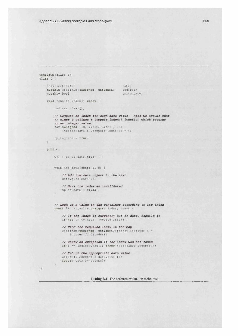
Appendix B: Coding principles and techniques 268

template<class T>class C {

std::vector <T>mutable std::map<unsigned, unsigned> mutable bool

data; indices; up_to_date;

void rebuild_index () const {

indices.clear ();

// C o m p u te an i n d e x f o r e a c h d a t a v a l u e . H e r e w e a s s u m e t h a t / / c l a s s T d e f i n e s a c o m p u te _ in d e x ( ) f u n c t i o n w h ic h r e t u r n s / / an i n t e g e r v a l u e .for(unsigned i=0; i<data.size() ; ++i)

indices[data[i].compute_index() ] = i;

up_to_date = true;

CO : up_to_date (true) { }

void add_data(const T& x) {

// A d d t h e d a t a o b j e c t t o t h e l i s tdata.push_back(x);

// M ark t h e i n d e x a s i n v a l i d a t e dup_to_date = false;

}

// L o o k up a v a l u e i n t h e c o n t a i n e r a c c o r d i n g t o i t s i n d e xconst T S get_value(unsigned index) const {

// I f t h e i n d e x i s c u r r e n t l y o u t o f d a t e , r e b u i l d i tif(not up_to_date) rebuild_index ();

// F in d t h e r e q u i r e d in d e x i n t h e map std::map<unsigned, unsigned>::const_iterator i =

indices.find(index);

// T h ro w an e x c e p t i o n i f t h e i n d e x w a s n o t f o u n dif(i == indices.end()) throw std::range_exception;

// Return the a p p r o p r i a t e d a t a v a l u eassert(i->second < data.size()); return data[i->second];

public:

};

Listing B .l: The deferred evaluation technique

Appendix B: Coding principles and techniques 269

different base classes to contribute parts of the functionality of a derived class is known as the Composite

design pattern (Gamma et al., 1995), and the compile-time selection of different parts of code via the template

mechanism is commonly referred to as ‘compile-time dispatch’.

The code in listing B.2 illustrates how the technique works.

// S e l e c t o r c l a s s e s - t h e s e a r e t y p i c a l l y j u s t empty s t r u c t sstruct A_Tag { }; struct B_Tag { };

// Two p o t e n t i a l b a s e c l a s s e s ; o n e o f t h e s e w i l l b e i n h e r i t e d fro m // b y t h e c l a s s C, d e f i n e d b e lo w class A { / * ... */ }; class B { /* ... V };

// D e f i n i t i o n o f t h e c l a s s w h ic h s e l e c t s t h e a p p r o p r i a t e b a s e f o r C template<class Tag> struct Selector { };

// S p e c i a l i s a t i o n s o f th e s e l e c t o r m ap t a g s o n to b a s e c l a s s e s templateo struct Selector<A_Tag> { typedef A base_t; }; template<> struct Selector<B_Tag> { typedef B base_t; };

// T he c l a s s w h ic h w e a c t u a l l y i n s t a n t i a t e template<class T a g>class C : public Selector<Tag>::base_t { / * . . . * / } ;

// Two e x a m p le i n s t a n t i a t i o n s u s i n g d i f f e r e n t b a s e c l a s s s e l e c t o r sC<A_Tag> c_inheriting_from_A;C<B_Tag> c_inheriting_from_B;

Listing B.2: The composite dispatch technique This idiom allows the programmer to define a class whose base class is determined by passing a template ‘selector’ parameter.

B.5 Customisation of the behaviour and form of objects

In several places through the GAMUT library, the problem of how to permit customisation of objects was

encountered. Specifically, how best to allow a client to modify the way an object behaves, within the bounds

of the definition of the role of that class, using simple and intutive programming techniques? This object

customisation came in two flavours, which are discussed separately below: customisation of behaviour and

customisation of form.

B.5.1 Behavioural customisation

Consider the design of a class which implements a particular algorithm. The client instantiates an object of

this class, provides the input data, and then instructs it to execute the algorithm. Finally, the client can request

the result of the algorithm from this object.

Most algorithms, however, allow some degree of parameterisation. In some cases, this may be simple -

for example, a clustering algorithm may require the client to supply some kind of threshold value; clearly

this can be easily implemented with a single member function of the algorithm object. However, suppose

the algorithm permits some more complex adjustment of its behaviour. For example, a simulated annealing

algorithm may allow the client to alter the mathematical function which controls the way the system ‘cools’.

Appendix B: Coding principles and techniques 270

It is not so immediately obvious how this should be implemented: whereas before we simply needed to pass

a value, now it seems that we require a function into which we can pass a piece o f code. In fact this is not so

far-fetched, and there are several ways to achieve it. GAMUT utilises two, which shall be described here.

B.5.1.1 Behavioural functors

The first approach is to use a functor (or “function object”). This is an object which defines the application

operator, operator (), as a member function, and hence may be thought of as a free function which has been

‘wrapped’ inside an object. By passing a functor to our algorithm object, we are effectively passing it a piece

of code, and can therefore alter its behaviour at runtime. Function objects used in this context are referred to

as behavioural functors in order to distinguish them from the many other uses of functors in C++.

Let us look more closely at the anatomy of a simple functor. The code snippet in listing B.3 shows how we

might write a base class for functors which express a cooling function for a simulated annealing algorithm.

struct CoolingFunctor {

// C lo n in g f u n c t i o n - r e t u r n s a c o p y o f t h e c o o l i n g f u n c t o r ,// d y n a m i c a l l y c r e a t e d on t h e h e a p .virtual CoolingFunctor* clone() const = 0;

// The c o o l i n g f u n c t i o n . G iv e n p r e v i o u s t e m p e r a tu r e a n d t im e // e l a p s e d , i t r e t u r n s t h e n ew , c o o l e r t e m p e r a tu r e . virtual float operator()(float temp, float time) const = 0;

};

Listing B.3: An example functor

This abstract base class mandates that any cooling functor provide at least two functions: one which

dynamically creates a copy of itself, returned in the form of a base class pointer, and one which computes the

new, cooled temperature which results after a given time lapse. A sketch of part of the annealing algorithm

object may now look as shown in listing B.4.

Note that the use of function objects to customise the behaviour of an object is potentially very powerful.

While the functor demonstrated above is very simple, a functor may in fact be quite complex, containing its

own data, and exposing any number of member functions. The only requirement is that functors used in this

way should be derived from an abstract base class which defines a cloning function, and in which all member

functions required by the algorithm object are also virtual.

B.5.1.2 Behavioural policies

Another design methodology which has some similarities with the functor technique is that of policies.

As with behavioural functors, policies Alexandrescu (2001) are small classes which are used to specify a

behavioural or structural part o f a larger class. The key difference between functors and policies as they

are used in GAMUT is that while functors are used for run-time customisation, policies must be specified at

compile-time, as template parameters of a template class or template member function.

Suppose that we wished to rewrite the algorithm class outlined above, using policies rather than functors to

specify the cooling function. This would be the result of a design decision that execution speed was more

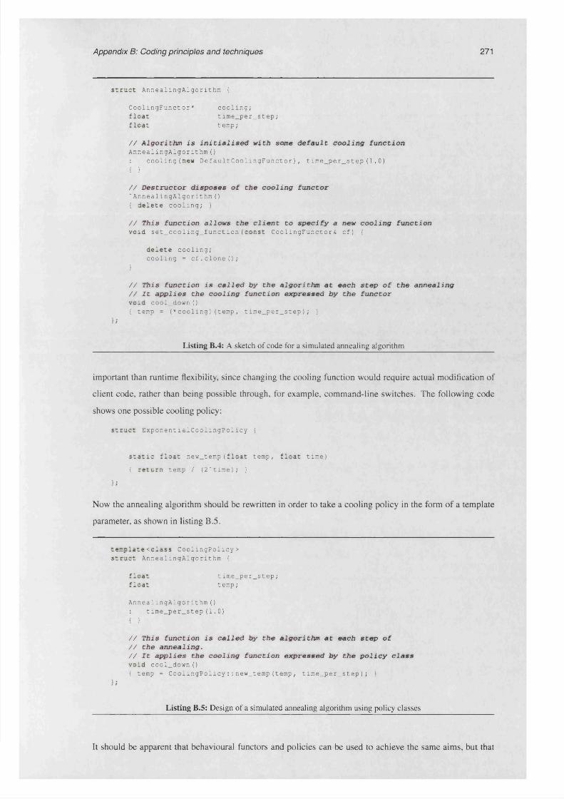
Appendix B: Coding principles and techniques 271

struct AnnealingAlgorithm {

CoolingFunctor* cooling;float time_per_step;float temp;

// A l g o r i t h m i s i n i t i a l i s e d w i t h som e d e f a u l t c o o l i n g f u n c t i o nAnnealingAlgorithm(): cooling(new DefaultCoolingFunctor), time_per_step (1.0){ )

// D e s t r u c t o r d i s p o s e s o f t h e c o o l i n g f u n c t o r‘AnnealingAlgorithm(){ delete cooling; }

// T h is f u n c t i o n a l l o w s t h e c l i e n t t o s p e c i f y a n e w c o o l i n g f u n c t i o nvoid set_cooling_function(const CoolingFunctor& cf) {

delete cooling; cooling = cf.clone ();

}

// T h is f u n c t i o n i s c a l l e d b y t h e a l g o r i t h m a t e a c h s t e p o f t h e a n n e a l in g / / I t a p p l i e s t h e c o o l i n g f u n c t i o n e x p r e s s e d b y t h e f u n c t o rvoid cool_down(){ temp = (*cooling) (temp, time_per_step); }

Listing B.4: A sketch of code for a simulated annealing algorithm

important than runtime flexibility, since changing the cooling function would require actual modification of

client code, rather than being possible through, for example, command-line switches. The following code

shows one possible cooling policy:

struct ExponentialCoolingPolicy {

static float new_temp(float temp, float time){ return temp / (2‘time); }

Now the annealing algorithm should be rewritten in order to take a cooling policy in the form of a template

parameter, as shown in listing B.5.

templatecclass CoolingPolicy> struct AnnealingAlgorithm {

float time_per_step;float temp;

AnnealingAlgorithm (): time_per_step (1.0){ }

// T h is f u n c t i o n i s c a l l e d b y t h e a l g o r i t h m at e a c h s t e p o f / / t h e a n n e a l i n g ./ / I t a p p l i e s t h e c o o l i n g f u n c t i o n e x p r e s s e d b y t h e p o l i c y c l a s svoid cool_down()( temp = CoolingPolicy::new_temp(temp, time_per_step); )

Listing B.5; Design of a simulated annealing algorithm using policy classes

It should be apparent that behavioural functors and policies can be used to achieve the same aims, but that

Appendix B: Coding principles and techniques 272

the design of the object which is to be parameterised, is significantly different in each case. So, in what

circumstances is each of these approaches desirable? Since functors are passed using references or pointers

to an abstract base class which defines the functor interface, their interfaces must consist of virtual functions,

thereby incurring the usual penalties of runtime polymorphism. Policy classes, on the other hand, can be

written using normal member functions, and can therefore provide greater efficiency of execution. On the

other hand, the runtime flexibility afforded by the use of functors can in certain circumstances make them

more useful than policy classes.

8.5.2 Customisation of form: tuples and property maps

While, in the previous section, we were concerned with how to alter the behaviour of a class, another similar

(and yet orthogonal, in OOP terms) problem is how to alter the contents of a class. That is, how to design a

generic class to which we can easily add data members. As an example, consider the design of a graph vertex

class. For some applications, there may be no information stored at each vertex; for others, each vertex may

be given a label in the form of the string. For still other applications, the client may wish to associate a colour,

or a more complex data structure with each vertex. A similar situation exists in the design of a generic tree

node class.

The problem, therefore, is how to enable the client to customise the type of information which is stored at

each node in a tree, or at each vertex and each edge in a graph. The ‘classical’ OOP solution to this problem

would be to define an unlabelled graph or tree node as the base class, then to inherit from it, adding labels

as member variables of the derived class, as shown in listing B.6. This approach has several drawbacks,

notably that, for every type of node class derived firom the generic base, code for various functions such as

serialising the data, or printing it to the screen, has to be specially written. A far better approach would be to

parameterise the base class on the type of data stored in it.

// G e n e r ic b a s e n o d e class Node {

// C o n ta in s c o d e f o r i t e r a t i n g th r o u g h c h i l d n o d e s , m a n a g in g l i f e t i m e o f // c h i l d r e n , e t c .

};

// D e r i v e d n o d e t y p e - we w is h t o l a b e l e a c h n o d e w i t h a n u m b er class LabelledNode : public Node {

// L a b e l i s a m em ber v a r i a b l e o f t h e d e r i v e d c l a s sint label;

// Now w e m u s t w r i t e c o d e f o r s e r i a l i s i n g t h e l a b e l , e t c .};

Listing B.6: Naieve design for a generic tree node class

C++ provides the capability for parameterising a class through the use of templates, which are orthogonal to

inheritance. The STL defines several container templates, which may be instantiated by the client to allow

any type of object to be stored inside them. One limitation of templates, however, is that one must specify

the number of template parameters which a class should take; in other words, a naive parameterisation of the

Appendix B: Coding principles and techniques 273

base class allows us only to change the types of a fixed number of labels. For example, specifying the type of

a generic graph vertex class as

template<class Labell, class Label2> class Vertex

states that each vertex is labelled with exactly two variables. We cannot specify an instantiation of the vertex

template which has one, three or four labels.

Let us define the vertex template as taking just one parameter, then. Now, if we wish to instantiate a vertex

type with three labels, we simply define a ‘label object’, and specify that as the template parameter:

template<class Label> class Vertex;struct MyLabels { int i; float f; std::string s; };typedef Vertex<MyLabels> MyVertex;

The problem with this approach is that we now need to write a set of member functions for MyLabels, which

take care of I/O operations and the like. This means that some of the genericity of the Vertex template is lost,

and the use of templates has gained us little over simply inheriting from an unlabelled base and adding the

label data to the derived class.

The solution used in GAMUT is to use property maps. The first step of their implementation is to define a

tuple class, that is, a fixed-size, heterogeneous collection of elements. Each node, vertex or edge contains a

tuple, whose number and type of elements is determined at compile time by providing a type list. Typelists

(Czamecki and Eisenecker, 2000, Alexandrescu, 2002) are lists of types which a recursively defined: a

typelist is a type, followed by a typelist, as shown below. The end of a typelist is marked by the presence of

a ‘null typelist’ in the second position.

template<class Head, class Tail> struct TypeList {

typedef Head head; typedef Tail tail;

};

Just as we may recursively build up a list of types, a tuple is constructed by recursively building a list of

variables, the type of each one being obtained from a typelist. This ‘construction’ occurs at compile-time;

the run-time overhead of constructing a tuple is identical to that which would be incurred for construction of

a normal structure containing the same variable types. The advantage of using tuples over structures is that

generic code for serialising the tuple data, for printing the list of tuple elements to the screen and so forth,

may be written just once, in the tuple template. This code is then valid for all combinations of types for

the elements contained in the tuple; as such, the tuple class represents a truly generic software component.

Moreover, an empty tuple may be optimised by the compiler to take up no storage space, and little or no

runtime overhead. Using tuples to store the label data, we may define the generic node class as shown below.

Appendix B: Coding principles and techniques 274

// T he L a b e lT y p e s parameter s h o u ld he a t y p e l i s t , c o n t a i n i n g t h e t y p e s

/ / o f l a b e l ( s ) w h ic h are s t o r e d a t e a c h n o d e i n t h e t r e e . T h e t y p e l i s t m ay

/ / b e e m p ty , i n w h ic h c a s e t h e n o d e s a r e u n l a b e l l e d

template<class LabelTypes> class Node {

// A t u p l e o f l a b e l s i s a g g r e g a te d i n t o t h e v e r t e x

Tuple<LabelTypes> labels;

};

Accessing specific elements of a tuple by their index in the complete list of elements can be fairly easily

implemented, but this is not very convenient for accessing the labels of a vertex, node or edge. For example,

when defining a graph in which vertices each have a name (stored as a string), and a colour (stored as an

integer), the vertex type would be defined using code something like the following:

typadaf Vertex<TYPELIST(std::string, int)> vertex_type;

Now, when we wish to access the colour of a vertex, we must remember that it is in the second position

within the list of labels. Given a vertex which has many different labels, this could be burdensome; a system

in which we could refer to a specific label using its name, rather than its index, would be preferable, and

closer in spirit to the usual situation in OOP, whereby member variables are accessed through getter and

setter methods whose names are similar to that of the variable being referred to.

The provision of a more intuitive look-up system is the final step in the property map implementation. A

property map is an extension of the tuple concept, whereby each element in the tuple is associated with a

name, or key. The key is itself a C++ type, and a property map is defined by passing two typelists: the first

specifies a list of key types, and the second specified the list of elements stored in the tuple. Elements may

then be referred to using either their indices, or their keys, as shown in listing B.7. Now, we may simply

inherit from the PropertyMap class when designing the vertex or node classes. In this way, the vertex and

node classes become customisable in just the way described above.

// F i r s t , d e f i n e t y p e s u s e d a s p r o p e r t y k e y s - t h e s e a r e s i m p l y e m p ty s t r u c t u r e s struct name_key { }; struct colour_key { };

// D e f i n i t i o n o f a p r o p e r t y map t y p e/ / H e re , TYPELIST i s a m a c ro w h ic h r e c u r s i v e l y c o n s t r u c t s a l i s t o f t y p e stypedef PropertyMap<

TYPELIST(name_key, colour_key), // L i s t o f k e y t y p e sTYPELIST(std::string, int) // L i s t o f e le m e n t t y p e s

> property_map_type;

// Create an i n s t a n c e o f t h e p r o p e r t y map t y p eproperty_map_type P ( '' joebloggs'', 5);

// A c c e s s e le m e n ts o f t h e p r o p e r t y map u s i n g t u p l e i n d i c e sstd::string name = P.elem<0>(); // R e tu r n s " j o e b l o g g s ’ 'P.elem<l>() =10; // S e t s c o lo u r t o 10

// A c c e s s e le m e n ts o f t h e p r o p e r t y map u s i n g p r o p e r t y k e y sstd::string name2 = P .property<name_key>(); // Returns *•j o e b l o g g s * 'int colour2 = P .property<colour_key>(); // Returns 10

Listing B.7: Property maps

275

Appendix C

Implementation of the GAMUT library

This appendix is concerned with the technical details of the implementation of the GAMUT library. It aims

to show how the design of the library delivers both efficiency of execution and ease of use to the programmer.

C.1 Implementation of the generic components layer

In this and the next section, the implementation of each component of GAMUT is discussed in more detail.

Here, we focus upon the generic component layer upon which more complex classes are built. Where

possible, the inter-relationships between different classes in the library are illustrated using Unified Modelling

Language (UML) diagrams (Object Management Group, 1995). The description presented here is, at times,

necessarily quite technical in nature; as such, a working knowledge of the C++ language will be necessary

to fully understand certain salient points. For a summary of the general coding principles adhered to when

writing the library, the reader is referred to appendix B .l; the appendices which follow it discuss some more

specialised programming issues which relate to the design and implementation of certain parts of the library.

Short sections of GAMUT code are included here where necessary in order to illustrate a particular concept.

In order to fully understand all details of the library, however, interested readers are advised to inspect the

library home page.

C.1.1 Arrays

As described in §2.3.4.1.1, the two main types of array class defined in GAMUT are fixed-size, one­

dimensional arrays, and a three-dimensional array class with associated indexing and addressing features.

The fixed-size array class is a template class, which is simply a wrapper around a standard C array. Its

function is to endow arrays with the object-oriented features (such as iterators, proper copy semantics, etc.)

expected of data types in C++, which are missing from the C array type. Since the only data member of the

class is the aggregated C array, and since almost all member functions are inline, the array class nonetheless

offers performance comparable to the C array type.

The implementation of the three-dimensional array class is broken into two pieces: a dimension class, and

the array class itself, which holds the data values. The dimension class is responsible for index-address

conversions, and for determining whether a given index or address is within bounds. The array class proper

is responsible for managing and providing access to the data values (the latter being possible using iterators,

Appendix C: Implementation of GAMUT 276

views or random access). The array class inherits from the dimension class, thus exposing the indexing

functions of the latter to the client.

The array class is naturally templated on the type of value being stored within it. Where this type is numerical,

a composite dispatch technique1 is used to add arithmetical operators to the array interface, as described in

the design section.

C.1.2 Graphs

The graph components within GAMUT were originally written to facilitate the representation and

comparison of chemical structures. In their original incarnation, they were heavily based on the graph

components in the CCP4 Coordinate Library (Krissinel, 2002). Since then, the graph objects have been

substantially redesigned, with much inspiration taken from the Boost Graph Library (The Boost Committee,

1998).

The fundamental components of the GAMUT graph framework are the Graph, Vertex and Edge class

templates. Of these, the only class of which users create objects directly is Graph; Vertex and Edge objects

are created and ‘owned’ by the Graph class, with users gaining access to vertices and edges via references

returned from Graph methods.

GAMUT graphs are parameterised on seven characteristics, namely:

1 Vertex type

2 Edge type

3 Properties attached to the graph itself

4 Edge representation

5 Vertex container type

6 Edge container type

7 Containment policy

These are explained below.

C. 1.2.1 Vertex and edge types

The vertex and edge classes used in GAMUT graphs are parameterised on the type of data stored in each.

This data is stored and accessed using a technique called ‘property maps’; more details on this are available

in appendix B.5.2. A graph type is defined by first defining the types of its vertices and edges, and then

instantiating the Graph template with these parameters. All three of the class templates Vertex, Edge and

Graph may be assigned labels using the property map framework. The whole process is illustrated in listing

C. l .

*See appendix B.4 for a description of the composite dispatch technique.

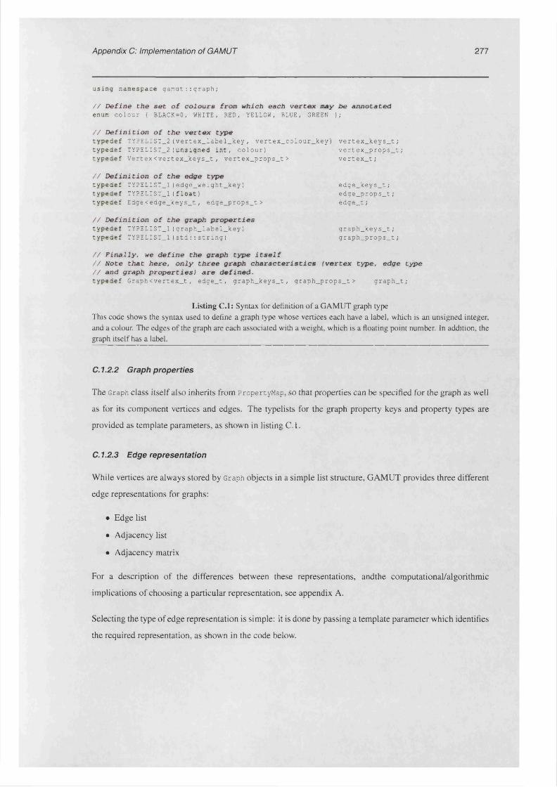
Appendix C: Implementation of GAMUT 277

using namespace gamut::graph;

// D e f i n e t h e s e t o f c o l o u r s f ro m w h ic h e a c h v e r t e x m a y b e e m n o ta te denum colour { BLACK=0, WHITE, RED, YELLOW, BLUE, GREEN };

// D e f i n i t i o n o f t h e v e r t e x t y p etypedef TYPELIST_2(vertex_label_key, vertex_colour_key) vertex_keys_t; typedef TYPELIST_2(unsigned int, colour) vertex_props_t;typedef Vertex<vertex_keys_t, vertex_props_t> vertex_t;

// D e f i n i t i o n o f t h e e d g e t y p etypedef TYPELIST_1(edge_weight_key) edge_keys_t;typedef TYPELIST_1(float) edge_props_t;typedef Edge<edge_keys_t, edge_props_t> edge_t;

// D e f i n i t i o n o f t h e g r a p h p r o p e r t i e stypedef TYPELIST_1(graph_label_key) graph_keys_t;typedef TYPELIST_1(std::string) graph_props_t;

// F i n a l l y , we d e f i n e t h e g r a p h t y p e i t s e l f// N o te t h a t h e r e , o n l y t h r e e g r a p h c h a r a c t e r i s t i c s ( v e r t e x t y p e , e d g e t y p e / / a n d g ra p h p r o p e r t i e s ) a r e d e f i n e d .typedef Graph<vertex_t, edge_t, graph_keys_t, graph_props_t> graph_t;

Listing C .l: Syntax for definition of a GAMUT graph type This code shows the syntax used to define a graph type whose vertices each have a label, which is an unsigned integer, and a colour. The edges o f the graph are each associated with a weight, which is a floating point number. In addition, the graph itself has a label.

C. 1.2.2 Graph properties

The Graph class itself also inherits from PropertyMap, so that properties can be specified for the graph as well

as for its component vertices and edges. The typelists for the graph property keys and property types are

provided as template parameters, as shown in listing C.l.

C. 1.2.3 Edge representation

While vertices are always stored by Graph objects in a simple list structure, GAMUT provides three different

edge representations for graphs:

• Edge list

• Adjacency list

• Adjacency matrix

For a description of the differences between these representations, andthe computational/algorithmic

implications of choosing a particular representation, see appendix A.

Selecting the type of edge representation is simple: it is done by passing a template parameter which identifies

the required representation, as shown in the code below.

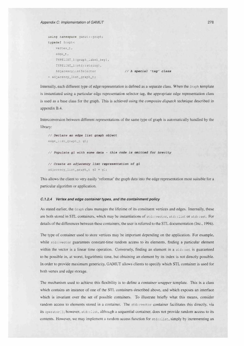
Appendix C: Implementation of GAMUT 278

using namespace gamut::graph; typ ed ef Graph<

vertex_t, edge_t,TYPELIST_1(graph_label_key) ,TYPELIST_1(std::string),AdjacencyListSelector // A s p e c i a l ' t a g ' c l a s s

> adjacency_list_graph_t;

Internally, each different type of edge representation is defined as a separate class. When the Graph template

is instantiated using a particular edge representation selector tag, the appropriate edge representation class

is used as a base class for the graph. This is achieved using the composite dispatch technique described in

appendix B.4.

Interconversion between different representations of the same type of graph is automatically handled by the

library:

// D e c l a r e an e d g e l i s t g ra p h o b j e c t

edge_list_graph_t gl;

// P o p u l a t e g l w i t h so m e d a ta - t h i s c o d e i s o m i t t e d f o r b r e v i t y

/ / C r e a t e an a d j a c e n c y l i s t r e p r e s e n t a t i o n o f g l

adjacency_list_graph_t g2 = gl;

This allows the client to very easily ‘reformat’ the graph data into the edge representation most suitable for a

particular algorithm or application.

C. 1.2.4 Vertex and edge container types, and the containment policy

As stated earlier, the Graph class manages the lifetime of its consituent vertices and edges. Internally, these

are both stored in STL containers, which may be instantiations of std:: vector, std: :list or std: :set. For

details of the differences between these containers, the user is referred to the STL documentation (Inc., 1994).

The type of container used to store vertices may be important depending on the application. For example,

while std::vector guarantees constant-time random access to its elements, finding a particular element

within the vector is a linear time operation. Conversely, finding an element in a std: :set is guaranteed

to be possible in, at worst, logarithmic time, but obtaining an element by its index is not directly possible.

In order to provide maximum genericity, GAMUT allows clients to specify which STL container is used for

both vertex and edge storage.

The mechanism used to achieve this flexibility is to define a container wrapper template. This is a class

which contains an instance of one of the STL containers described above, and which exposes an interface

which is invariant over the set of possible containers. To illustrate briefly what this means, consider

random access to elements stored in a container. The std::vector container facilitates this directly, via

its operator!]; however, std: :list, although a sequential container, does not provide random access to its

contents. However, we may implement a random access function for std: :list, simply by incrementing an

Appendix C: Implementation of GAMUT 279

iterator from the beginning of the list, by the required number of steps. Clearly this is a linear-time operation,

compared with the constant-time amortization of std:: vector::operator [ ].

The ContainerWrapper template class exposes a number of member functions, including operator!], each

of which may either be a forwarding function to the aggregated STL container, if a suitable function exists,

or may be implemented within ContainerWrapper using member functions of the STL container. In this way,

we may create containers which, although internally implemented using different STL components, expose

a common interface, and which therefore may be used interchangably inside other classes such as Graph.

The inheritance hierarchy of the Graph class is illustrated in figure C.l.

J EdgeType: [ , EdgeContainerType: t

EdgeList♦ edgejist: ContainerWrapper<EdgeType. EdgeContainerType, ContainmentPolicy*List of ail edge objects in the graph

Exactly one of these inheritance relations is chosen by the compile-time dispatch mechanism.

This is realised by partially specialising the EdgeRepresentation class on Its

EdgeRepresentationSeiector parameter.

J Edge Type:, EdgeContainerType I ContainmentPolicy:

AdjacencyList.e cp e iisi ContamerWrappercEdgeType. EdgeContainerType. ContainmentPolicy*List ot all edge objects in the graph.adjacency taoie stc vector, std vector<unsigned> >A list of indices for each vertex, containing the indices of its neighbouring vertices

] EdgeType , EdgeContainerType

_J ContainmentPolicy

AdjacencyMatrix♦edge_iist: ContainerWrapper<EdgeType, EdgeContainerType. ContainmentPo(icy>List of all edge objects in the graph.adjacency_.matnx SouareMatnx<edgeJist_iterator>The adjacency matrix contains iterators into the master edge list, so each edge is only stored once

• EdgeType:I EdgeRepresentalionSsieclor i EdgeContainerType:

J ContainmentPolicy

EdgeRepresentationThis class is a compile-time dispatcher which selects the appropriate edge representation

, VenexType: i VertexContainerType * ContainmentPolicy:

VertexListThis class manages the lifetime of the vertex obiects in the graph

.v e rtex jist: ContamerWrapper<VertexType. VertexContainerType, ContammentPolicy> List of all vertex objects in the graph

---------------------- Z-----------

» KeyList:‘ PropertyUst:

PropertyMap♦data: Tupie< Property List>

s —

The property map framework is employed to customise data stored at each vertex and edge In the graph, and also to customise overall graph properties. As such, PropertyMap is an ancestor of Vertex, Edge and Graph classes.

[ VertexType:I EdgeType:■ KeyList:] PropertyUst: i VertexContainerType:• EdgeContainerType:J EdgeRepresentationSeiector:

_ j ContainmentPolicy

| G rap h * f.................. ...

The client instantiates an instance of the Graph template

■ KeyList:‘ PropertyUsl:

I Vertex*

Vertex and edge types are defined by the client, but instances of them are not created directly; this is done by ancestors of the graph class, via member functions of class Graph.

Figure C .l: UML diagram of the inheritance hierarchy of the Graph class

Appendix C: Implementation of GAMUT 280

C. 1.2.5 The graph interface

As mentioned in §2.3.4.1.2, one requirement of the graph framework was that is should expose an intutive

interface which should be, as far as possible, invariant over different combinations of the graph parameters.

In other words, the client should be able to manipulate a coloured, edge-list graph in much the same was

as he/she would interact with an uncoloured, adjacency-matrix graph. To achieve this, a set of interface

functions which should be available for any vertex and edge representations was mandated during the design

phase; this is summarised in tables C.l and C.2. A use of the graph interface, to populate a graph with data,

is illustrated in listing C.2.

C.1.2.6 Graph algorithms

In the GAMUT graph framework, each type of graph algorithm is implemented as a template class,

parameterised on the type of graph which it processes. In order to run an algorithm on a given graph,

the client creates an instance of the algorithm object, passes it a reference to the graph, and then calls the run

member function of the algorithm. The results of the algorithm may then be accessed through other member

functions of the algorithm object.

Graph algorithms are divided into unary algorithms, which operate on one graph at a time (such as a ring

perception algorithm), and binary algorithms, which operate upon a pair of graphs (such as a maximum

common subgraph detection algorithm). Every unary algorithm class inherits from the unaryAlgorithm

class, which holds a pointer to the subject graph, and has responsibility for logging functions. A similar

BinaryAlgorithm base class is also defined. Figure C.2 shows part of the inheritance hierarchy of the graph

algorithm classes. It should be noted that this hierarchy was consciously designed in such a way as to

facilitate the easy addition of more than one algorithm of the same type. For example, should the client

wish to implement a new subgraph isomorphism algorithm, he/she should do so by inheriting from the

MCSAlgorithm class. In this way, two benefits are realised: firstly, much of the ‘housekeeping code’ necessary

for the algorithm is inherited from the base class, and secondly, the new algorithm object can be substituted

for any other subgraph isomorphism object in client code, since they share the same interface.

Function Return type Description

n_vertices() const size.t Number of vertices in the graphvertex(size.t n) vertex_type& Get reference to the nth vertexvertex(size.t n) const vertex_type& Get const reference to the nth vertexn_visible_vertices() const size.t Number of vertices in the graph which are not hidden. Each vertex can

be temporarily hidden, which means that it is ignored by any algorithms which operate on the graph.

visible.vertex(size.t n) vertex_type& Get reference to the nth visible vertexvisible.vertex(size.t n) const vertex_type& Get const reference to the nth visible vertexvertex.begin() vertex_iterator Get iterator to the first vertex in the graphvertex_end() vertex.iterator Get iterator past the last vertex in the graphvertex.begin() const const.vertex.iterator Get iterator to the first vertex in the graphvertex_end() const const.vertex.iterator Get iterator past the last vertex in the graphvisible_vertex_begin() visible.vertex.iterator Get iterator to the first visible vertex in the graphvisible.vertex.end() visible.vertex.iterator Get iterator past the last visible vertex in the graphvisible_vertex_begin() const const.visible.vertex.iterator Get iterator to the first visible vertex in the graphvisible.vertex.end() const const.visible.vertex.iterator Get iterator past the last visible vertex in the grapherase.vertex(vertex.iterator) vertex.iterator Erase a vertex from the graphadd_vertex(const vertex_properties_t&) vertex.iterator Add a vertex to the graph, and give it the specified properties

Table C.l: Vertex-related functions in the graph interface

Appendix C: Im

plementation

of GA

MU

T

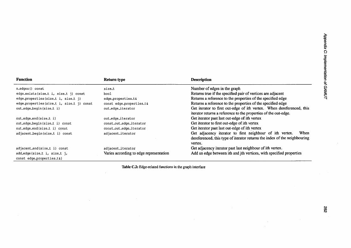
Function Return type Description

n_edges() const size.t Number of edges in the graphedge.exists(size.t i, size.t j) const bool Returns true if the specified pair of vertices are adjacentedge_properties(size.t i, size.t j) edge_properties_t& Returns a reference to the properties of the specified edgeedge.properties(size.t i, size.t j) const const edge.properties.tS Returns a reference to the properties of the specified edgeout_edge_begin(size.t i) out.edge.iterator Get iterator to first out-edge of ith vertex. When dereferenced, this

iterator returns a reference to the properties of the out-edge.out_edge_end(size.t i) out.edge.iterator Get iterator past last out-edge of ith vertexout_edge_begin (size.t i) const const.out.edge.iterator Get iterator to first out-edge of ith vertexout.edge.end(size.t i) const const_out_edge_iterator Get iterator past last out-edge of ith vertexadjacent±»egin(size.t i) const adjacent.iterator Get adjacency iterator to first neighbour of ith vertex. When

dereferenced, this type of iterator returns the index of the neighbouring vertex.

adjacent.end(size.t i) const adjacent_iterator Get adjacency iterator past last neighbour of ith vertex.add_edge(size.t i, size.t j, Varies according to edge representation Add an edge between ith and jth vertices, with specified propertiesconst edge_properties_t&)

Table C.2: Edge-related functions in the graph interface

Appendix C: Im

plementation

of GAM

UT 282

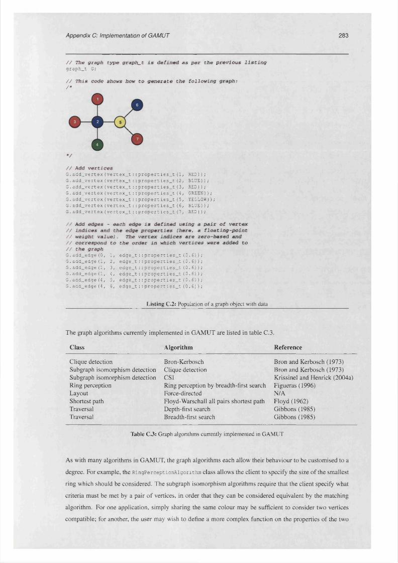
Appendix C: Implementation of GAMUT 283

// The g r a p h t y p e g r a p h ^ t i s d e f i n e d a s p e r t h e p r e v i o u s l i s t i n ggraph_t G;

// T h is c o d e sh o w s h ow t o g e n e r a t e t h e f o l l o w i n g g r a p h :/ *

/ / A d d v e r t i c e sG.add_vertex(vertex_t::properties_t(1, RED));G.add_vertex(vertex_t::properties_t(2, BLUE));G.add_vertex(vertex_t::properties_t(3, RED));G.add_vertex(vertex_t::properties_t(4, GREEN));G.add_vertex(vertex_t::properties_t( 5 , YELLOW));G.add_vertex(vertex_t::properties_t(6, BLUE));G.add_vertex(vertex_t::properties_t(7, RED));

// Add e d g e s - e a c h e d g e i s d e f i n e d u s in g a p a i r o f v e r t e x / / i n d i c e s a n d t h e e d g e p r o p e r t i e s ( h e r e , a f l o a t i n g - p o i n t // w e ig h t v a l u e ). T he v e r t e x i n d i c e s a r e z e r o - b a s e d a n d / / c o r r e s p o n d t o t h e o r d e r i n w h ic h v e r t i c e s w e r e a d d e d t o / / t h e g r a p hG.add_edge(0, 1, edge_t::properties_t(0.6));G.add_edge(1, 2, edge_t::properties_t(0.6));G.add_edge(1, 3, edge_t::properties_t(0.6));G.add_edge(1, 4, edge_t::properties_t (0.6));G.add_edge(4, 5 , edge_t::properties_t(0.6));G.add_edge(4, 6, edge_t::properties_t (0.6));

Listing C.2: Population of a graph object with data

The graph algorithms currently implemented in GAMUT are listed in table C.3.

Class Algorithm Reference

Clique detection Bron-Kerbosch Bron and Kerbosch (1973)Subgraph isomorphism detection Clique detection Bron and Kerbosch (1973)Subgraph isomorphism detection CSI Krissinel and Henrick (2004a)Ring perception Ring perception by breadth-first search Figueras (1996)Layout Force-directed N/AShortest path Floyd-Warschall all pairs shortest path Floyd (1962)Traversal Depth-first search Gibbons(1985)Traversal Breadth-first search Gibbons(1985)

Table C 3: Graph algorithms currently implemented in GAMUT

As with many algorithms in GAMUT, the graph algorithms each allow their behaviour to be customised to a

degree. For example, the RingPerceptionAlgorithm class allows the client to specify the size of the smallest

ring which should be considered. The subgraph isomorphism algorithms require that the client specify what

criteria must be met by a pair of vertices, in order that they can be considered equivalent by the matching

algorithm. For one application, simply sharing the same colour may be sufficient to consider two vertices

compatible; for another, the user may wish to define a more complex function on the properties of the two

Appendix C: Implementation of GAMUT 284

■ Graph: i

Algorithm+set_log(log:std ::ostream&): voidSet the stream to which logging information is written

T1 ftranh- | 1 firanh-

UnaryAlgorithm BinaryAlgorithm+graph_: Graph*Pointer to subject graph

+graph1_: Graph*Pointer to subject graph

+graph(): G raphs +set_graph(GraphS): void

+graph2_: Graph*Pointer to subject graph

L +graph1(): G raphs +graph2(): G raphs +set_graph1 (GraphS): void +set_graph2(GraphS): void

IRingPerceptionAlgorithm

i

MCSAlgorithmBase class for ring perception algorithms Base class for subgraph isomorphism algorithms

+n_rings(): size_t const +n_iso(): size_t constReturn number of rings found Return number of isomorphisms found+ring(n:unsigned): ring_tS +iso(n:unsigned): iso_tSGet reference to nth ring Get reference to nth isomorphism

* f t r a n h - 1

Ri ng Pe rceptio n Algo rith m_B FS Ring perception by breadth-first search

MCSAIgorithm_Krissinel Subgraph isomorphism detection by method of Krissinel

+run(): void +run(): void

Figure C.2: UML diagram of the inheritance hierarchy of two graph algorithm classes

vertices.

These two examples of behavioural parameterisation fall into distinct classes: the first is easily achieved by a

member function which modifies a scalar value in the algorithm object, while the second essentially requires

that the client be able to effectively pass a bundle of code into the algorithm. As in several places through the

library, the latter type of parameterisation is implemented using behavioural functors2. The vertex matching

criteria discussed above may be encapsulated in a functor of the following form:

template<class VertexType> struct VerticesMatch {

bool operator()(const VertexType& u, const VertexType& v) const;};

This functor takes as its arguments a pair of vertex references, and returns a boolean value indicating whether

they are compatible, and hence, may form part of a graph isomorphism. The MCSAlgorithm class allows the

client to register a vertex-matching functor of this type, and a corresponding functor for the edge-matching

criteria, before running the algorithm.

2See appendix B.5 for a discussion of behavioural customisation using function objects.

Appendix C: Implementation of GAMUT 285

C. 1.2.6.1 Layout algorithms

For the case of graph layout methods, the algorithm in question calculates the 2D coordinates of each vertex

in the layout, but does not ‘know’ how to draw the vertices and edges onto a graphics device. Again, functors

are used; this time, the functors are vertex and edge ‘depiction generators’, each of which returns a graphics

object for a given vertex or edge. In this way, the client is free to write a functor which represents each vertex

as a circle, a triangle, or any other depiction of arbitrary complexity. The usefulness of this approach is

exemplified in the implementation of the chemical structure diagram generation class (described in detail in

§C.2.2.3). In order to produce diagrams with a standardised apperance, each atom in the structure should be

represented in the appropriate way (i.e . the atomic symbol, with a superscript indicating its formal charge).

Implementing this is simple: a functor was written which generates the appropriate glyphs, and simply

‘plugged in’ to the layout framework.

The graph layout algorithm base class inherits directly from graphics::Collection, a container class for

graphics objects (see §C.1.6). This means that the, after the initial layout phase, the client can easily perform

various manipulations on the layout (e .g . rotations, scaling e tc .) in order to tailor it to the requirements of the

application. An example is presented in listing C.3.

// L e t g ra p h_t b e a t y p e d e f f o r t h e g ra p h t y p e we a r e u s i n ggraph_t G;

// P o p u la te g ra p h w i th d a ta - c o d e o m i t t e d h e r e

/ / D e c la r e a l a y o u t o b j e c t . T h i s i s an i n s t a n c e o f t h e random / / l a y o u t c l a s s , w h ic h s i m p l y a s s i g n s random 2D c o o r d i n a te s t o / / e a c h v e r t e x .graph::LayoutRandora<graph_t > layout(G);

// Run t h e a l g o r i th mlayout.layout ();

// S c a le t h e c o l l e c t i o n o f g r a p h i c s o b j e c t s t o f i t i n s i d e a / / g i v e n b o u n d in g b o x , w h i l e m a i n t a in i n g t h e a s p e c t r a t i o o f / / t h e o r i g i n a l l a y o u tlayout.fit_maintain_aspect(100, 100, 500, 500);

// Open a P o s t S c r i p t f i l e , a n d d ra w t h e g ra p h l a y o u t i n t o i tgraphics::PostScript out(''graph.ps''); layout.draw(out);

Listing C.3: Graph layout example

C.1.3 Linear algebra

The fundamental components of GAMUT’S linear algebra framework are classes for representing vectors

and matrices. Each of these may be divided into to two broad types: those whose size is fixed at compile­

time, and those which may be dynamically re-sized. Objects which can be dynamically re-sized incur an

extra overhead compared to those whose size is statically determined, both in terms of extra data members

which must be maintained (to store the current size of the object and the amount of memory which has been

allocated to it), and a runtime speed penalty. As such, fixed-size linear algebra components are preferred for

applications such as 3D geometry, in which the size of the vectors and matrices will always be the same.

Appendix C: Implementation of GAMUT 286

On the other hand, applications such as those which manipulate distance matrices for clustering or pricipal

component analysis require the ability to change the size of the linear algebra objects at runtime.

The implementation consequences of choosing whether a linear algebra component is statically or

dynamically sized are as follows:

• Storage: statically sized components may store their data by aggregating a statically C array; dynamic

components should aggregate an STL container instead. The container used in the dynamic component

implies extra overhead in terms of both required storage and runtime performance.

• Runtime checks: vector and matrix algebra operations can be carried out on statically sized objects

without any runtime checks to ensure that the operands are compatible in dimension.

• Construction: vectors and matrices which have a fixed size may have their elements initialised directly

by the constructor; since the length of the list elements required for a dynamic component is not known

a priori, it cannot be passed to the constructor. This means that statically sized components may be

constructed more efficiently.

The templates which are defined in the linear algebra module are listed in listing C.4. Elementary linear

algebra operations, for example matrix multiplication, are implemented as member functions of these classes.

More complex operations, such as matrix diagonalisation and singular value decomposition, are implemented

as classes in the same way as the graph algorithms described above.

// S t a t i c a l l y s i z e d c l a s s e stemplat*<typ«n*me T, size_t N> class Vector;templat#<typ«nama T, size_t N> class SquareMatrix;

// C l a s s e s w h o se s i z e may h e s p e c i f i e d a t r u n t im e tamplatactypanaraa T> class DynamicVector;tamplata<typ«name T> class DynamicMatrix;template<typenam8 T> class DynamicSquareMatrix;

Listing C.4: Classes defined in the linear algebra component

C.1.4 Geometric range querying

Geometric range querying (§3.4) is a common operation in structural bioinformatics applications. The

geometric range query framework implemented in GAMUT allows any type of data to be stored in the

query map, as long as each data object is associated with a k-dimensional coordinate. This allows it to be

used, for instance, to index the positions of atoms in space such that the set of atoms which fall inside a given

geometric region may be rapidly determined.

GAMUT defines an abstract base class named Region providing functions which answer these questions.

Region is templated on the dimensionality of the space, and on the type used to represent coordinates in

this space. A set of shapes including (hyper)spheres, (hyper)cubes and (hyper)annuli, which inherit from

Region are defined. Of course, the client is free to define other regions in a similar manner; in this way,

the geometric query framework is fully extensible. An outline of the classes which comprise the geometric

region framework is presented in listing C.5.

Appendix C: Implementation of GAMUT 287

// A b s t r a c t b a s e c l a s s f o r r e g i o n s i n D - d im e n s io n a l s p a c e / / C i s t h e t y p e o f c o o r d i n a t e u s e dtemplate<typename C , size_t D> class Region {

virtual bool contains_point(const Vector<C,D>&) const = 0;virtual bool intersects_box(const Vector<C,D>&, const Vector<C,D>&) const = 0;

// F u n c t io n s w h ic h r e t u r n t h e g e o m e t r i c c e n t r e o f t h e r e g i o n , a n d/ / t h e d i s t a n c e o f i t s f u r t h e s t e x t r e m i t y fro m t h i s p o i n tvirtual Vector<C,D> centre () const = 0;virtual C extent () const = 0;

};

// C o n c r e t e c l a s s e s w h ic h i n h e r i t fro m t h e e f o s t r a c t r e g i o ntemplatectypename C, size_t D> class Sphere : public Region<C,D> {/*... * / }; templatectypename C , size_t D> class Cube : public Region<C,D> { / * . . . * / }; templatectypename C , size_t D> class Annulus : public Region<C,D> { / * . . . * / };

Listing C.5: An outline o f the framework for describing geometric regions

C.1.5 Trees

A tree is mathematically equivalent to a Directed Acyclic Graph (DAG) ; as such, it would be possible to

implement a tree data structure directly using the graph template described above. However, certain features

of the graph template render it unsuitable for the types of uses to which trees are put within GAMUT As

such, a separate tree component was written from scratch.

Within GAMUT, types trees are distinguished on two primary criteria:

• Arity of children: binary trees, where each node has exactly two children, are distinguished from

N-ary trees, where each node may have any number of children (including zero). The former type is

used to represent data structures such as clustering hierarchies and kd-trees, while the second forms

the basis for molecular structure and domain classification hierarchies.

• Heterogeneity: in some trees, all nodes are of the same type, while other trees may be heterogeneous

in their composition. For example, in a clustering tree, every node in the tree represents a single

clustering division, and therefore each node stores the same type of data. Taking the example of a tree

representing a molecular structure, some nodes represent residues, others atoms etc.. This distinction

is important from an implementational standpoint, as is clear when one considers the operation of

copying a tree. Where the nodes are monomorphic, this is straightforward, but for a polymorphic tree,

it is necessary to store the children of each node using base-class pointers, with the concrete type of

each newly-created node being determined by inspecting the type of the source node.

In GAMUT, there is no such class as Tree; rather, a tree is created simply by declaring a node object, which

represents the root. Node objects ‘own’ their child nodes, such that when the destructor of a node is called,

it destroys all its children automatically. This leads to the recursive destruction of the entire subtree of that

node. It should be clear, therefore, that a node class should:

• contain its child nodes, either

- in the form of pointers to dynamically-allocated objects, which are explicitly deleted by the

parent’s destructor

Appendix C: Implementation of GAMUT 288

- directly, by aggregation: in this case, child nodes will be automatically disposed of when the

parent is destroyed

• contain a pointer to the parent node, which is null if the node is a root

C.l.5.1 Classes

Due to the quite different characteristics exhibited by each of the types of tree described above, they are

modelled using four different class templates, all defined in namespace gamut: rtree:

• BinaryNode

• PolymorphicBinaryNode

• NaryNode

• PolymorphicNaryNode

However, since all node types share the characteristic that they contain a pointer to their parent, each of these

classes inherits from a common base, Node. The binary node classes each contain a pair of pointers to their left

and right children. The N-ary nodes aggregate a container of child nodes, in the form of a ContainerWrapper

object, as described in §C. 1.2.4.

C.l.5.2 Traversals

Whereas, for the graph classes, traversals such as breadth-first and depth-first searches are implemented as

standalone classes, it was more convenient in the tree framework to implement these as different types of

iterators. There are five ‘flavours’ of iterators defined, as shown in table C.4.

Type Result of incrementing Result of decrementing Stopping condition

vertical Move to first child Move to parent Current node has no childrenhorizontal Move to next node at Move to previous node at Current node is last at

current depth current depth current depthdepth-first Move to next node in Move to previous node in Current node is last in

depth-first-search depth-first-search the treebreath-first Move to next node in Move to previous node in Current node is last in

breadth-first-search breadth-first-search the treechildren Move to next child of Move to previous child of Already at last child of

current node current node current node

Table C.4: Types of tree iterators The five flavours of tree iterator are described. Each one defines the increment and decrement operators ++ and —; the effect of calling each of these is described. As with all types of iterators, there must be a means of determining when the iteration should be stopped; this is described as the ‘stopping condition’.

The interface for performing tree iterations is common across all types of tree; for example, in order to iterate

through all children of a particular node, one would write code with the following form:

SomeNodeType n;for(SomeNodeType::child_iterator i = n.child_begin();

i != n .child_end (); ++i) const SomeNodeTypeS child = *i;

The syntax for performing other types of iteration is similar to this.

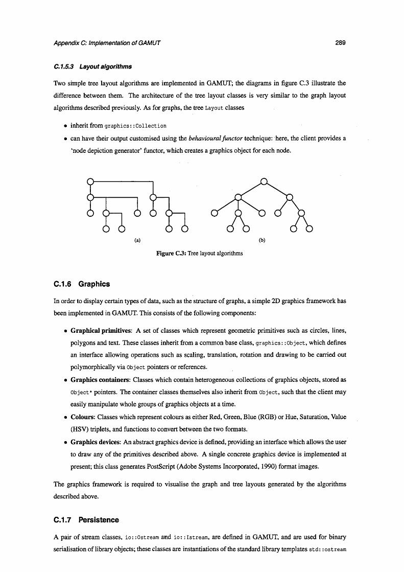
Appendix C: Implementation of GAMUT 289

C. 1.5.3 Layout algorithms

Two simple tree layout algorithms are implemented in GAMUT; the diagrams in figure C.3 illustrate the

difference between them. The architecture of the tree layout classes is very similar to the graph layout

algorithms described previously. As for graphs, the tree Layout classes

• inherit from graphics::Collection

• can have their output customised using the behavioural functor technique: here, the client provides a

‘node depiction generator’ functor, which creates a graphics object for each node.

(b)(a)

Figure C.3: Tree layout algorithms

C.1.6 Graphics

In order to display certain types of data, such as the structure of graphs, a simple 2D graphics framework has

been implemented in GAMUT. This consists of the following components:

• Graphical primitives: A set of classes which represent geometric primitives such as circles, lines,

polygons and text. These classes inherit from a common base class, graphics: :0b ject, which defines

an interface allowing operations such as scaling, translation, rotation and drawing to be carried out

polymorphically via Object pointers or references.

• Graphics containers: Classes which contain heterogeneous collections of graphics objects, stored as

Object* pointers. The container classes themselves also inherit from object, such that the client may

easily manipulate whole groups of graphics objects at a time.

• Colours: Classes which represent colours as either Red, Green, Blue (RGB) or Hue, Saturation, Value

(HSV) triplets, and functions to convert between the two formats.

• Graphics devices: An abstract graphics device is defined, providing an interface which allows the user

to draw any of the primitives described above. A single concrete graphics device is implemented at

present; this class generates PostScript (Adobe Systems Incorporated, 1990) format images.

The graphics framework is required to visualise the graph and tree layouts generated by the algorithms

described above.

C.1.7 Persistence

A pair of stream classes, io: :0stream and io: :istream, are defined in GAMUT, and are used for binary

serialisation of library objects; these classes are instantiations of the standard library templates std:: ostream

Appendix C: Implementation of GAMUT 290

and std: :istream. T he interface to the stream objects consists o f a pair o f functions nam ed gwrite and

gread, for “generic write” and “generic read”:

template<typ«nam« T> Ostream& Ostream::gwrite(const T& x); templatectypename T> Istreams Istream::gread(T& x) ;

T hese functions are described as generic in the sense that they are capable o f writing or reading any type o f

object, as long as it is either

• A G A M U T object

• A P O D (plain o ld data) type, such as char, int, float, etc.

The w ay these functions work is as fo llow s. If the object x passed to the gwrite function is a P O D type, a

specialised version o f gwrite is called (a specialised version o f the function exists for every P O D type). This

function writes x to the stream using the standard library function std::ostream::write. B y convention,

G A M U T objects are stored in little-endian format. W hen perform ing binary I/O on floating point values,

is is required that the machine represents floating point numbers internally using the IEEE 754 standard

(Institute o f Electrical and Electronic Engineers, 1987); on all platforms inspected to date, this has been

found to be the case.

I f the object is not a PO D type, it cannot match the signature o f any o f the specialised form s o f gwrite, so

the generic (nonspecialised) version o f the function is called. This version attempts to call x. write (*this).

A ll G A M U T objects define a pair o f functions w hich im plem ent its serialisation; these functions have the

signatures

void write (io :: OstreamS) const; void read(io::IstreamS);

The call to the nonspecialised gwrite function can only com pile i f the com piler can find an appropriate write

function defined in the t class - in other words, i f x is a G A M U T object.

To sum marise, the G A M U T Ostream class facilitates the writing o f any type o f object (PO D or G A M U T)

to the stream using the sam e function call (gwrite), with the appropriate im plem entation o f this function

being chosen by the rules o f C ++ tem plate instantiation, and endianness being autom atically accounted for.

Sym m etrically, any type o f PO D or G A M U T object m ay be read from an istream using the gread function.

The result o f this is that the im plem entation o f the serialisation functions w ithin each G A M U T class becom es

very sim ple, as show n in listing C .6.

C. 1.7.1 Indexed file storage

In addition to sim ple serialisation, G A M U T provides the capability to create indexed files. Indexed files

are useful w hen a large number o f objects o f the sam e type need to be stored, and accessed efficiently. B y

indexing the archive file, on ly those item s o f data to w hich the client requests access, need be read into

memory.

The indexed file m echanism im plem ented in G A M U T is based on the ISA M principle. T he idea is that two

disk files are created. The first, known as the data file, sim ply contains data objects serialised one after

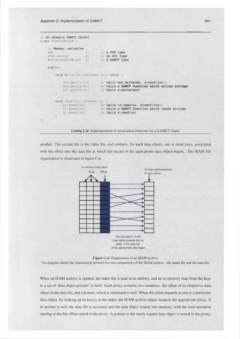
Appendix C: Implementation of GAMUT 291

// An example GAMUT o b j e c tclass AGamutObject {

// M ember v a r i a b l e sint i; / / A POD t y p estd::string s; //An STL t y p eAnotherGamutObject o; // A GAMUT t y p e

public:

void write(io::Ostreamfi out) const {

out.gwrite (i); // C a l l sout.gwrite (s); // C a l l sout.gwrite (o) ; // C a l l s

s i z e o f ( i n t ) )

void read(io::IstreamS in) {in.gread(i); // C a l l s i n . r e a d ( H i , s i z e o f ( i n t ) )in.gread(s); // C a l l s a GAMUT f u n c t i o n w h i c h r e a d s s t r i n g sin.gread(o); // C a l l s o . r e a d ( i n )

);

Listing C.6 : Implementation of serialisation functions for a GAMUT object

another. The second file is the index file, and contains, for each data object, one or more keys, associated

with the offset into the data file at which the record of the appropriate data object begins. The ISAM file

organisation is illustrated in figure C.4.

In-memory index table

Keys OffsetOn-disk representations of d a ta values

The last column in the index table contains the file

offset, in the da ta file, of the appropriate d a ta object

Figure C.4: Organisation of an ISAM archive The diagram shows the relationship between the two components of the ISAM archive - the index file and the data file.

When an ISAM archive is opened, the index file is read in its entirety, and an in-memory map from the keys

to a set of ‘data object proxies’ is built. Each proxy contains two members: the offset of its respective data

object in the data file, and a pointer, which is initialised to null. When the client requests access to a particular

data object, by looking up its key(s) in the index, the ISAM archive object inspects the appropriate proxy. If

its pointer is null, the data file is accessed, and the data object loaded into memory, with the read operation

starting at the file offset stored in the proxy. A pointer to the newly loaded data object is stored in the proxy,

Appendix C: Implementation of GAMUT 292

and a reference to the sam e object returned to the client.

If, w hen a proxy is inspected, its pointer is found to be non-null, this m eans that the data object has already

been loaded into memory, and a reference to it can be returned im m ediately, w ithout further disk access. This

schem e, w hich is known as pointer swizzling, therefore m inim ises the amount o f access w hich needs to be

m ade to the data file, which is typically large in size.

The description o f ISA M behaviour thus far has assumed that the archive is a read-only object. G A M U T does

indeed allow an ISA M archive to be opened read-only, but it m ay also be opened w ith write access enabled.

In this case, the library must keep track o f changes w hich have been m ade to the archive. The archive may be

changed by adding, deleting, or m odifying data objects held in it. Changes are only m ade to the in-m em ory

representation o f the archive data; the client m ust explicitly call a commit function in order to com m it these

changes to disk. A t this point, the index and data files are reorganised to bring them into syncrony with the

in-m em ory data. A ll o f the steps described above are illustrated in figure C .5.

The im plem entation o f the ISA M archive class in G A M U T consists o f three parts. The first o f these is the

definition o f a class w hich handles the mapping from a tuple o f keys, to the file offset. G A M U T contains

a template class, TupleMap, w hich maps a tuple onto a single data value. Internally, TupleMap contains N

separate maps, where N is the number o f elem ents in the key tuple. This allow s queries to be performed

either on a single key elem ent, or on a com bination o f several key elem ents.

The second com ponent o f the ISA M archive is the proxy class. A s described above, the proxy contains the

file offset o f the data object w hich it represents, as w ell as a pointer to that object. In addition, each proxy

contains a pointer to a file stream w hich is connected to the data file. This allow s the definition o f a mem ber

function in the proxy, Proxy:: operator* () w hich autom atically loads the data object, i f required, and returns

a reference to it. A s such, the proxy represents an autonom ous pointer sw izzler, transparently returning its

data object w hen required, leaving the client unaware whether or not disk access has taken place. In addition,

the Proxy class contains a record o f the status o f its data object, w hich records whether the object is new,

m odified, or still synchronised with the on-disk representation.

The third part o f the ISA M im plem entation is the class w hich clients actually utilise, nam ed isam::Table.

The table class contains a TupleMap from tuple keys to Proxy objects, and provides the m em ber functions

necessary to allow the client to access data in the archive. The Table class is responsible for orchestrating

all disk access to the ISA M files, in particular maintaining the integrity betw een the index and data files, and

reorganising data objects such that no gaps are created in the data file by removal or m odification o f data

values.

Appendix C: Implementation of GAMUT 293

On-disk representations of data values

In-memory index table

Index table read into memory

V A » A Proxies store tile offset | of each value In the

Keys Proxies datafile

(a)

1. Client accesses a particular value by looking up a key in

the index

2. Offset into data file is looked up

In-memory value

4. Client is returned a reference to the in-memory value transparently; no explicit call to read any file is made

3. Value is automatically read from data file

(b)

Pointer to newly-loaded object is stored in the proxy

In-memory value

Offset into data file is maintained in the proxy: at this point, the on-disk

representation of the value is still up to date

(C )

Figure C.5: Pointer swizzling (a) Index is loaded into memory; (b,c) swizzling occurs when data values are requested by the client. Continued overleaf.

Appendix C: Implementation of GAMUT 294

Several more values are loaded into memory

file

(d)

1. Client accesses a particular value by looking up a key in

Datafile

2. Value has already been read into memory. Client is returned a reference to the value; nofile access is required

(e)

1. Client changes one of the values

Data file

2. Proxy for this value is marked as having been changed. On-disk version of the valueis no longer up to date.

(f)

Figure C.5: Pointer swizzling (continued)(d) swizzling occurs when data values are requested by the client; (e) cached values can be returned immediately without file access; (f) altered values are marked. Continued overleaf.

Appendix C: Implementation of GAMUT 295

Index file

4. Modified index 2. Obsolete value is removed fromtable is written

to index filedisk file and replaced by copying values which are still up to date

1. Client instructs changes to

be committedData file

3. Changed value is written to disk, and file offset of the new record is stored in the appropriate proxy

(g)

Figure C.5: Pointer swizzling (continued)(g) changes are committed to disk.

Appendix C: Implementation of GAMUT 296

C.2 Implementation of the bioinformatics layer

C.2.1 Macromolecular structure

C lasses for representing m acrom olecular coordinate data are defined in nam espace gamut: :mmol.

C.2.1.1 Nodes of the molecular tree

Each o f the levels in the m olecular tree is populated with objects o f a different type, nam ely, Model, Polymer,

Monomer and Atom objects. Each o f these classes inherits from an instance o f the PolymorphicNaryNode

tem plate described in §C .1.5, allow ing them to be part o f a polym orphic tree.

C.2.1.2 Molecule as a manager class

Internally, Molecule is required to perform m ultiple housekeeping roles. Its primary purpose is to act as

the root o f the m olecular tree: as such, it ‘ow ns’ each Model o f the m olecu le, and therefore indirectly, also

ow ns all o f the Polymer, Monomer and Atom objects. In addition to being the ultimate ow ner o f all nodes in

the m olecular tree, a Molecule object is also the owner o f all selections m ade upon it, as w ell as all bonds

betw een its atoms.

Each o f these ‘object manager’ roles is separated in the im plem entation o f Molecule, through the use o f

inheritance. M anagem ent o f each type o f objects (node, selection and bond) is undertaken by one o f the base

classes o f Molecule, as illustrated in figure C.6.

C.2.1.2.1 The coordinate manager

The coordinate manager is responsible for the lifetim e o f the objects w hich constitute the m olecular hierarchy.

Each CoordinateManager object stores by aggregation the root node o f this hierarchy, through w hich all nodes

in the tree m ay be accessed. For exam ple, in order to iterate through all nodes in the second level dow n from

the tree, the client w ould recursively iterate through the children o f the root, and the children o f those nodes

in turn.

For many applications, the ancestry o f each node may not be important; if, for exam ple, the client sim ply

w ishes to iterate through each m onom er in the m olecule, doing so by traversing the tree w ould be quite

inefficient (see figure C .l). For this reason, the CoordinateManager class also stores a list o f pointers to the

objects at each lebel o f the m olecular tree (atoms, residues, chains and m odels). C lients m ay iterate through

these lists using m em ber functions o f the manager. It is evidently important that the coordinate manager

should ensure that these lists are consistent at all tim es w ith the nodes present in the tree; this is done using

the deferred evaluation technique described above.

Another responsibility o f the coordinate manager class is to maintain a geometric query map (see §3.4) o f

atom ic positions. This allow s the client to rapidly perform queries w hich return the set o f atom s lying in

any given region o f space; the interface through w hich these queries are actually perform ed is defined in the

selection manager class described below. O nce again, deferred evaluation is used to keep the query map up

Appendix C: Implementation of GAMUT 297

CoordinateManager

+root_: node_tRoot node of the molecular tree +atom _map_: atom _geom _m ap_tGeometric query map containing pointers to atom objects

+n_models(): intGet number of models for this structure +model(n:int): Model&Get a reference to the nth model+erase_model(n:int): void - -Erase the nth model from the tree+add_model(id:int): Model&Add a new model to the tree, and return a reference to it _

SelectionManager

#selections_:std::vector<Selection_Base*>Array of pointers to selection objects owned by the manager #sel_label_m ap: std::map<std::string, Selection_Base*>Map from selection labels to selection objects owned by the manager

+new _selection(label:const std:string&): Selection&Create new selection, and return reference to it+discard_selection(selection:Selection&): voidDestroy a selection object; does not destroy selected objects+erase_selection(selection :Selection&): voidRemove all selected objects from the molecule tree +propagate_selection(selection:Selection&):Selection&Propagate a selection from its current level to a new level (e.g. Residue->Atom) +find_selection(label:const std::string&): Selection_Base*Find the selection with the given label (if it exists)+select_atom s(sel_string:const std::string&,label:const std::string&): Selection<Atom>&Create a selection of atoms which satisfy the provided selection string +select_m onom ers(sel_string:const std:string&,label:const std::string&): Selection<Monomer>& Create a selection of monomers which satisfy the provided selection string

A

BondManager

#cbond_v_: std::vector<CBond*>Array of pointers to covalent bond objects owned by the manager #hbond_v_: std::vector<HBond*>Array of pointers to hydrogen bond objects owned by the manager

+ « c o n s t » are_cbonded(a1 :const Atom&,a2:const Atom&): bool Determine whether a pair of atoms are covalently bonded + « c o n s t » are_hbonded(a1 :const Atom&,a2:const Atom&): bool Determine whether a pair of atoms are hydrogen bonded

J

Molecule

Figure C.6: Separation of the ‘object manager’ roles o f the Molecule class Almost all of the functionality of Molecule is inherited from its base classes, each o f which takes responsibility for managing a different type of information. The lists of class attributes and methods shown here is incomplete, and is intended to serve as an illustration o f the function of each base class.

Appendix C: Implementation of GAMUT 298

Root

Models

Polymers

Monomers

Atoms

Figure C.l: Different types of iteration through nodes of the molecular tree The green arrows indicate the process of iterating through all atoms of a given polymer, by recursively traversing the tree using member functions of its nodes. The red arrows indicate the process of iterating through all atoms in a molecule, using the lists stored by the CoordinateManager class. Clearly the latter represents a more efficient means for traversal of all nodes at a particular level.

to date. Finally, the coordinate manager provides the ability for the client to perform certain operations to all

objects in the tree en masse, such as rotations and translations.

C.2.1.2.2 The selection manager

GAMUT allows the client to construct selections at any level of the molecular tree, and provides a mechanism

conferring persistence upon the selections. The classes which constitute the selection framework are

illustrated in figure C.8 . Each selection is represented by a Selection<T> object, where T is a template

parameter determining the type of objects in the selection; the selection object contains a list of pointers to

the objects which constitute it. Clients are granted access to the selected objects via member functions of the

selection class.

The mechanism used to keep the list of selected objects up to date is a deferred evaluation3 approach based

on bit-masks. Each selection object is associated with a bit-mask, in which all bits except one are set to

zero. Similarly, every node in the molecular tree has a bit-mask of the same length. Any number of bits in

the masks associated with node objects may be set; each bit which is set indicates membership of that node

in a given selection; see figure C.9. In order to rebuild the list of selected objects therefore, a Selection

object needs simply to query its associated CoordinateManager object (to which a pointer is held), iterating

through all nodes in the appropriate level of the tree and checking the bit mask of each. Whenever a node

is encountered in whose bit-mask the bit corresponding to the selection object is set, a pointer to the node is

added to the list of selected objects. This procedure is carried out whenever a Selection member function is

called which requires access to the list of selected objects, and when that list is found to have been marked

out-of-date.

Creation and disposal of Selection objects is orchestrated by the SelectionManager class. When the client

requests creation of a new selection, the first task of the selection manager is to generate a bit-mask which

is orthogonal to all masks currently in use. This is done by maintaining a count of the number of masks

generated to date: if, for example, 3 selections have already been made, the newly-generated mask would be

<000100. . . >. When a client no longer requires a given selection, the SelectionManager::discard_selection

3see appendix B.3 for a brief discussion of the deferred evaluation technique.

Appendix C: Implementation of GAMUT 299

Each selection Is identified by a bit-mask consisting of a string ot zeroes, and a single one. Any object in the tree in which that bit is also set, is part of the selection.

All objects which constitute the molecular tree are labelled with a bit-mask indicating which selectlon(s) they a re part of

j T:Type ot selected objects

Selection

These functions invalidate the objects, vector, and set a flag Indicating that it should be rebuilt next time access to it is required.

These functions check the u p .to .date . flag when called; if it is false, the update, function

The u p d a te , function queries the molecular tree held in the CoordinateM anager object pointed to by the m an ag e r, pointer, In order to retrieve all objects w hose

Atom ModelPolymerMonomer

MaskFixed-length bit mask class

+selections.: std::vector<Selection_Base'»List of pointers to all selection objects ♦ labe l.m ap .: std::map<std::stringt S e lec tion .B ase’>Map allowing clients to retrieve selections by their label

SelectionManager

+manager_: CoordinateM anager’Pointer to the manager of the molecular tree♦label.: std::string♦ u p .to .d a te .Flag indicating the list of objects is up to date

+clone(): Selection .B ase’ constAbstract function which clones a selection of a given type+rotate(matrix:const mat33_t&): void+translate(vector:const vec3_t&): void const+w ritejxfb(fnam e:const std::string&): void const♦label!): const std::string& const♦update.!): voidRebuild the internal list of selected objects

Selection_Base Abstract base selection class

♦objects.: std::vector<T*>List of pointers to selected objects

+add_object(obj:T&): void +remove_object(obj:T&): void + |-(s:const Selection<T>&): Selection<T>&Add all objects selected in s, to this selection♦&*(s:const Selection<T>&): Selection<T>&Restrict this selection to only objects which are also in s+begin(): iteratorGet iterator to the first selected object +end(): iteratorGet iterator past the last selected object ♦clone!): Selection .B ase’ const ♦rotate! matrix:const mat33_tS): void ♦translate(vector:const vec3_t&): void ♦update .!): voidRebuild the internal list of selected objects

bit-masks contain the appropriate bit tor this selection.

Figure C.8: Classes which constitute the selection framework The member data and functions listed here do not fully describe the classes, but serve to illustrate the relationship between the selection objects and the selection manager. The SelectionManager functions which are used to create selections are described elsewhere.

function may be called. This has three effects: firstly, the selection mask is subtracted bitwise from the

mask of every selected object. Secondly, the mask is added to a pool of ‘recycled’ masks maintained by the

selection manager object. These masks may now be re-used for new selections, thus allowing any number of

selections to be created on a given molecule, as long as no more that n are in use at any time, where n is the

length of the bit-masks (128 in the current implementation). Finally, the Selection object itself is destroyed.

In order to create selections based on object identities, such as atom name, or residue sequence number,

a system of selection predicates is used. Each of the molecular node classes (Atom, Monomer, Polymer and

Model) define a nested type called predicate, which is in fact a unary functor returning either true or false.

For example, the atom predicate class has the following form:

struct predicate{ bool operator () (const Atoms) const; };

Each node class also defines static member functions which generate predicate objects representing certain

criteria. For example, the Atom::metal function creates a predicate object which returns true when presented

with a metal atom, and false otherwise. Similar functions exist to create predicates which return true if the

atom has a certain name, if the residue sequence number lies within a given range, and so forth. Now, let us

Appendix C: Implementation of GAMUT 300

00011

00110

00010

00001

00100

00100

Selection 1 O • 00001

Selection 2 O • O 00010

Selection3 O O O 00100

Figure C.9: Selection bitmasks A section of the molecular tree is shown, with the bit masks associated with each leaf node. The objects which constitute each selection are illustrated below the tree.

say we wish to select all residues in chain ‘A’ of the first model of a molecule, whose sequence number is

within the range 10 to 20. The SelectionManager class defines a function with the following signature:

Selection<Monomer>& select_monomers( const Model::predicate&, const Polymer::predicate&, const Monomer::predicates, const std::strings label

) ;

In order to create the selection described above, we simply need to provide three predicate objects which

define the selection criteria at the model, polymer and monomer levels, as follows:

Selection<Monomer>s my_selection = my_molecule.select_monomers(Model::id_equals(1) , / / M o d e l p r e d i c a t e

Polymer::id_equals('A'), // P o l y m e r p r e d i c a t e

Monomer::seq_num_in_range(10, 20), // M onomer p r e d i c a t e

' 'some_informative_name'' // L a b e l

);

Similar functions exist for selections at each level of the tree, with the number of predicate arguments required

corresponding to the depth of that level from the root node.

The selection object is populated by performing a depth-first search of the molecular tree. When each new

node is discovered by the search, it is checked against the appropriate predicate to determine whether it

matches; if not, the search down that branch of the tree is terminated. When an object at the last level (here,

the monomer level) is encountered, which matches its predicate, a pointer to it is added to the selection list,

the mask of the object is bitwise-OR’ed with that of the selection object, and the search moves back up the

tree.

Appendix C: Implementation of GAMUT 301

Rather than using predicate objects, the client m ay make the sam e selection by providing a selection string,

com plying w ith a predefined format. Without going into the details o f this format, the selection string

corresponding to the exam ple given here is /1 /A / . 10-20; internally, this is parsed by the selection manager

and converted into a series o f predicate objects w hich are passed to the function above. The power o f the

predicate-based approach, however is its flexibility: any number and com bination o f predicates m ay be

supplied to the selection function, as long as they can be expressed in the form o f unary boolean functors.

The standard logical operations A N D , OR and NOT are defined on the predicate classes, such that the client

can write predicate expressions such as

Selection<Monomer>& my_selection = my_molecule.select_monomers(Model::any(),not Polymer::id_equals('A'),Monomer::name_equals{''GLY''} and Monomer::seq_num_in_range(1,50)

) ;

A s discussed previously, in addition to selections based on object identity, geom etrically-defined selections

w ere also required. T hese w ere divided into tw o types: selection o f all objects ly ing in an arbitrary geom etric

region, and those w hich are defined by proxim ity to objects in an existing selection.

W hen specifying a region-based selection, it is necessary to clarify exactly what qualifies a particular entity

as being ‘inside’ a given region. For exam ple, considering an am ino acid residue, do w e sim ply require any

atom o f the residue to fall inside the region, or do w e want the stricter criterion that the centre (geom etric,

or centre o f m ass) o f the residue be within the query region? In GA M U T, these ‘insideness criteria’ are

specified using policies4.

The available insideness criteria po lic ies are:

• GeometricCentre.insidenessCriterion - object is inside the region i f its geom etric centre is inside the

region.

• MassCentre.insidenessCriterion - object is inside the region i f its centre o f m ass is inside the region.

• GeometricCentreOf Children_lnsidenessCriterion - object is inside the region i f the geom etric centre

o f any o f its child nodes is inside the region.

The fo llow ing statements illustrate the creation o f selections in w hich, in the first case, any atom o f a

m onom er inside a given sphere qualifies the m onom er as ‘se lected ’, then the geom etric centre and centre

o f m ass o f each m onom er m ust be inside the sphere. The first statement show s how to create selections in

w hich any atom o f a m onom er inside a given sphere qualifies the m onom er as ‘selected ’:

select_region < GeometricCentreOfChildren_Insidenes sCriterion>( s p h e r e _ t ( v e c 3 _ t (0,0,0), 5));

If, on the other hand, the geom etric centre or centre o f m ass o f each m onom er m ust be inside the sphere in

order to qualify it as selected, the follow ing statements should be used:

4See appendix B.S for a discussion of the use of policy classes for behavioural parameterisation.

Appendix C: Implementation of GAMUT 302

s e l e c t _ r e g i o n <Geomet r i c C e n t r e _ I n s i d e n e s s C r i t e r i o n >

( s p h e r e _ t (v e c 3 _ t ( 0 , 0 , 0 ) , 5 ) ) ;

s e l e c t _ r e g i o n <M a s s C e n t r e _ I n s i d e n e s s C r i t e r i o n >

( s p h e r e _ t (v e c 3 _ t ( 0 , 0 , 0 ) , 5 ) ) ;

W hen defining a new selection by proxim ity to an existing selection, another criterion m ust b e specified,

nam ely from w hich part(s) o f the existing selection distances should be measured. That is , do w e w ish to

select objects near to the geom etric centre o f the existing selection, or c lo se to any object in that selection?

T his choice is expressed using a ‘relative selection origin’ policy. The available relative selection origin

p olicies are:

• GeometricCentreOf S e le c t ion .O rig in C riter ion - distances are measured from the geom etric centre o f

the existing selection.

• G eom etricCentreO fEachElem ent-OriginCriterion - the distance o f a given point from the selection is

taken as the distance from that point to the nearest m em ber o f the existing selection.

• GeometricCentreOfEachChildOfEachElement_OriginCriterion - the distance o f a g iven point from the

selection is taken as the distance from that point to the nearest child o f any mem ber o f the selection.

In order to illustrate the use o f the selection policies, consider the cod e snippet in listing C.7, w hich show s

the selection o f a ligand based upon its identity, fo llow ed by geom etric selection o f all residues w hich have

at least one atom in proxim ity to any atom o f the ligand.

// S e l e c t i o n o f t h e l i g a n d m o le c u le .S e l e c t i o n < M o n o m e r > l i g a n d =

M . s e l e c t _ m o n o m e r s ( ' ' / 1 / A / A T P . 1 ' ' , ' ' l i g a n d ' ' ) ;

/ / S e l e c t i o n o f a l l r e a i d u e e w h ic h c o n t a c t t h e l i g a n dSelection<Monomer> environment =

M. s e l e c t _ r e l a t i v e <GeometricCentreOfChildren_InsidenessCriterion,G e o m e t r i c C e n t r e O f E a c h C h i l d O f E a c h E l e m e n t _ O r i g i n C r i t e r i o n

>

Listing C.7: Example o f using selection functions to pick out a ligand binding site

C.2.1.2.3 The bond manager

B y default, bonds betw een atoms in a m olecular structure are not explicitly stored in a Molecule object.

H owever, facilities are provided for representing both covalent and hydrogen bonds. B oth types o f bond

inherit from a com m on Bond base class, w hich contains pointers to the tw o bonded atom s. A ll bond objects

are m anaged by the BondManager class, w hich, like the SelectionManager maintains a list o f all bonds.

B y referring to a table o f standard covalent radii for each elem ent, the bond manager c lass is able to

infer covalent bonds betw een atoms within and betw een residues. This allow s the atom ic coordinates o f

a m onom er (protein residue, or ligand) to be converted into a graph w hich represents the connectivity o f the

m olecule.

Appendix C: Implementation of GAMUT 303

C.2.1.3 File I/O

In order to read coordinate data into Molecule objects, a parser for P D B format files w as im plem ented. In

addition to extracting coordinate data, the parser may also obtain sequence data and additional annotations

such as EC number from the P D B file, although the latter is often recorded in a non-standard fashion, and

therefore cannot be reliably retrieved. The inconsistencies present in PD B files are w ell-know n, and the

G A M U T parser attempts to check for som e o f these as it reads the file. For exam ple, the parser can be

instructed to throw an exception if it encounters tw o atoms with identical nam e and alternative location

fields, belonging to the sam e residue. A variety o f other checks m ay be optionally enabled or disabled by

the client depending upon the level o f strictness required. PD B form at files m ay be also written by G AM UT

objects, in order to export data for use in other programs.

C.2.2 Chemical structure

N am espace gamut:: chem contains the classes w hich deal with chem ical connectivity data.

C.2.2.1 The chemical graph class

Im plementation o f the chem ical graph class was fairly straightforward given the generic graph template

described above. A s m entioned earlier, chem:: Graph is not in fact sim ply an instantiation o f the generic

Graph template; rather, it is derived from such an instantiation. T he reason for doing this is to add extra

member functions to the graph object, w hich perform functions such as com puting the valence o f each atom

o f the com pound, from the connectivity information stored w ithin the graph.

One point worthy o f discussion is the representation o f atom properties. The atom ic properties o f atom ic

number, chirality, valence, number o f hydrogens and charge m ay all be represented as integer values; since

the upper bound on each value is sm all, it is possible to store them con cise ly as a single 32-bit integer using

a bit-m asking system , as illustrated in figure C .10. The advantage o f doing this is realised w hen chem ical

structures are compared using graph isom orphism algorithms. If, for a given application, the chirality o f an

atom is not considered relevant for the graph-matching procedure, it can trivially be hidden by m asking out

the appropriate bits from the com posite atom property value.

atomic number chirality valence num ber of hydrogens formal charge

1 9 12 16 24 32

Figure C.10: Concise storage of atom properties using a bit-masking approach The 32 bits of the integer value are partitioned into ‘chunks’, each of which represents one o f the properties o f the atom.

C.2.2.2 The chemical compound archive class

A s described above, an archive was required in w hich collections o f chem ical structures (in the form o f

graph objects) could be persistently stored, and from w hich those structures could be easily retrieved. The

im plem entation o f this archive class, called ChemBase, w as based upon the generic ISA M table class described

previously, and was therefore trivial.

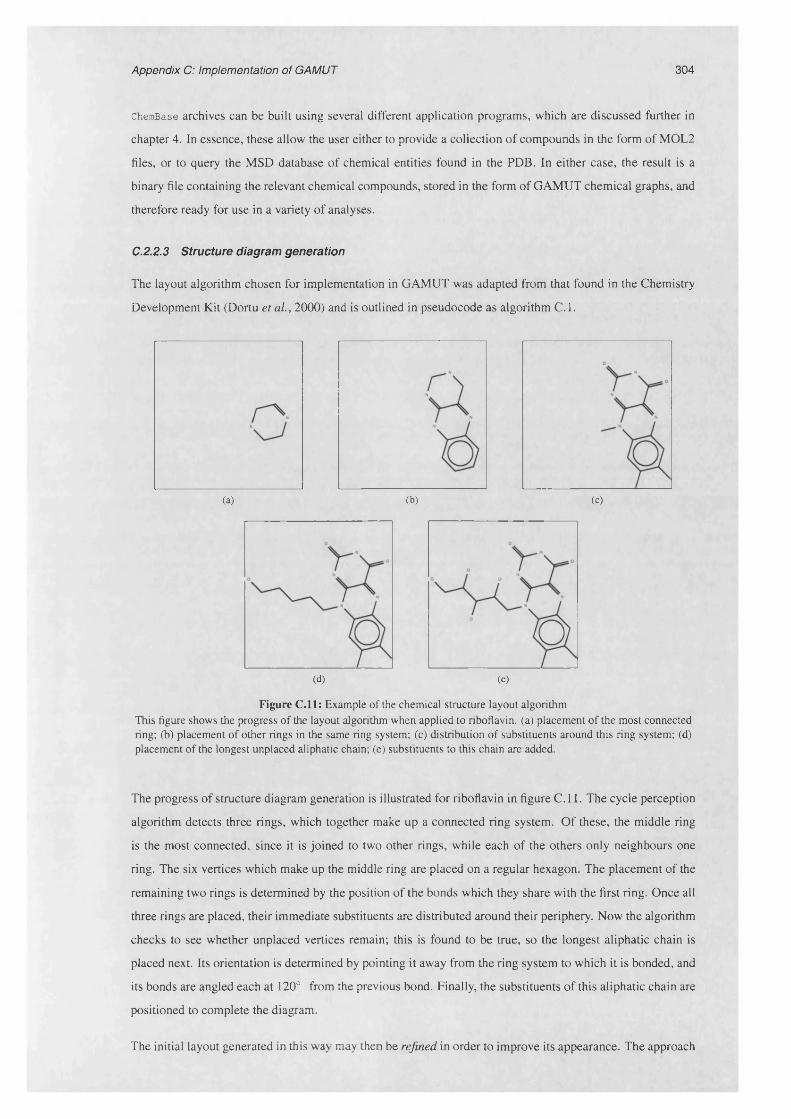
Appendix C: Implementation of GAMUT 304

ChemBase archives can be built using several different application programs, which are discussed further in

chapter 4. In essence, these allow the user either to provide a collection o f com pounds in the form o f MOL2

files, or to query the M SD database o f chemical entities found in the PDB. In either case, the result is a

binary file containing the relevant chem ical compounds, stored in the form o f G A M U T chem ical graphs, and

therefore ready for use in a variety o f analyses.

C.2.2.3 Structure diagram generation

The layout algorithm chosen for implementation in GAM UT was adapted from that found in the Chemistry

Developm ent Kit (Dortu et al., 2000) and is outlined in pseudocode as algorithm C .l.

(b)(a) (c)

(d) (e)

Figure C .ll: Example of the chemical structure layout algorithm This figure shows the progress of the layout algorithm when applied to riboflavin, (a) placement of the most connected ring; (b) placement of other rings in the same ring system; (c) distribution of substituents around this ring system; (d) placement of the longest unplaced aliphatic chain; (e) substituents to this chain are added.

The progress o f structure diagram generation is illustrated for riboflavin in figure C .l 1. The cycle perception

algorithm detects three rings, which together make up a connected ring system. O f these, the middle ring

is the most connected, since it is joined to two other rings, w hile each o f the others only neighbours one

ring. The six vertices which make up the middle ring are placed on a regular hexagon. The placem ent o f the

remaining two rings is determined by the position o f the bonds which they share with the first ring. O nce all

three rings are placed, their immediate substituents are distributed around their periphery. N ow the algorithm

checks to see whether unplaced vertices remain; this is found to be true, so the longest aliphatic chain is

placed next. Its orientation is determined by pointing it away from the ring system to w hich it is bonded, and

its bonds are angled each at 120° from the previous bond. Finally, the substituents o f this aliphatic chain are

positioned to com plete the diagram.

The initial layout generated in this way may then be refined in order to improve its appearance. The approach

Appendix C: Implementation of GAMUT 305

used here is to ‘flip’ single acyclic bonds with the aim o f reducing clashes betw een atoms in the diagram.

This is done by com puting a penalty function based on the proxim ity o f all pairs o f non-covalently-bonded

atom s in the structure. Each single acyclic is inspected to determ ine whether flipping it w ould decrease the

value o f this function; i f so , the change is accepted, otherwise it is ignored. B y applying this to each flippable

bond, and then repeating the w hole cycle a number o f tim es, the appearance o f the layout m ay be improved.

Several other exam ples o f diagrams generated by the layout algorithm are show n in table C.5.

The pow er o f having this algorithm im plem ented internally w ithin the library, rather than sim ply writing a

M O L2 file for the com pound, and depicting it using an external program, is that it allow s the details o f the

diagram to b e programm atically m odified. For exam ple, in order to illustrate the parts o f tw o com pounds

w hich are m atched in a subgraph isom orphism , the programmer can easily ‘instruct’ the layout object to

highlight the m atched atom s in a different colour.

C.3 Ligand binding sites

Im plem entation o f the ligand binding site components described in §2 .3 .4 .4 consists o f three core classes,

defined in nam espace gamut:: lig:

• Identity: this class contains all information needed to unam biguously identify a single ligand

m olecu le within the PD B archive, namely:

- P D B entry

- chain identifier

- residue name

- sequence number

- insertion code

In addition, where the m olecu le was observed to ex ist in m ore than one location w ithin the crystal,

the identity class also records the alternative location indicator for the conform ation seen to have the

highest occupancy.

• Match: this class inherits from Identity; in addition to the fields listed above, it also contains:

- nam e o f the reference com pound to w hich the ligand w as matched

- correspondances betw een the atoms o f the ligand m olecule, and the vertices o f the reference

graph. T hese are stored as pairs o f indices, where the first refers to the index o f the reference

vertex, and the second to the index o f the ligand atom.

- whether the ligand is covalently or non-covalently bound to protein within the P D B entry

• MatchTable: this is an ISA M archive w hich stores Match objects. Its indices allow clients to look

up ligand matches by PD B entry, residue name, reference com pound nam e, bound state, or any

com bination o f the above.

In addition to these classes, the ligand binding site com ponent contains numerous utilities for perform ing

functions including

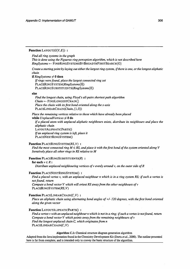
Appendix C: Implementation of GAMUT 306

Function L a y o u t (G (V ,£ ) ) :

F in d a l l r in g s y s te m s in th e g r a p h

T h is i s d o n e u s in g th e F ig u e r a s r in g p e r c e p t io n a lg o r i th m , w h ic h i s n o t d e s c r i b e d h e r e

R i n g S y s t e m s «- F in d R in g S y s t e m s B y B r e a d t h F ir s t S e a r c h ( G )

C r e a te a s ta r t in g p o in t b y la y in g o u t e i th e r th e la r g e s t r in g s y s te m , i f th e r e i s o n e , o r th e lo n g e s t a l ip h a t ic

c h a in

if RingSystems ^ 0 then I f rings were found, place the largest connected ring set PhACERlNGSYSlEM(RingSystems[0])FLACERlNGSVBSTlTUEms(RingSystems[0])

elseF in d th e lo n g e s t c h a in , u s in g F l o y d ’s a l l - p a i r s s h o r te s t p a th a lg o r i th m

C h a in <— F in d L o n g e s t C h a in ( )P la c e th e c h a in w ith i t s f i r s t b o n d o r ie n te d a lo n g th e x -a x is

P la c e L in e a r C h AIN {C h a in , (1 ,0 ))

P la c e th e r e m a in in g v e r t i c e s r e la t iv e to th o s e w h ic h h a v e a l r e a d y b e e n p l a c e d

while U n p la c e d V e r t i c e s ^ 0 do I f a p l a c e d a to m w ith u n p la c e d a l ip h a t ic n e ig h b o u r s e x is ts , d i s t r ib u te i t s n e ig h b o u r s a n d p l a c e th e

a l ip h a t ic c h a in

L a y o u t A l ip h a t i c P a r t s ( )I f a n u n p la c e d r in g s y s te m is le f t, p l a c e i t

P l a c e N e x t R in g S y s t e m ()

Function P la c e R in g S y s t e m ( R S ,V ) :F in d th e m o s t c o n n e c te d r in g M € R S , a n d p l a c e i t w i th th e f i r s t b o n d o f th e s y s te m o r i e n te d a lo n g V

I te r a t i v e ly p l a c e a l l o th e r r in g s in R S r e la t iv e to M

Function P la c e R in g S u b s t i t u e n t s ( R ) : for each v e R :

D is t r ib u te u n p la c e d n e ig h b o u r in g v e r t i c e s o f v e v e n ly a r o u n d v, o n th e o u te r s id e o f R

Function P la c e N e x t R in g S y s t e m ( ) :F in d a p l a c e d v e r te x v , w i th a n u n p la c e d n e ig h b o u r n w h ic h is in a r in g s y s te m R S ; i f s u c h a v e r te x is

n o t fo u n d , re tu r n

C o m p u te a b o n d v e c to r V w h ic h w i l l o r ie n t R S a w a y f r o m th e o th e r n e ig h b o u r s o f v

P la c e R in g S y s te m (R 5 , V )

Function P la c e L in e a r C h a in ( C ,V ) :P la c e a n a l ip h a t ic c h a in u s in g a l te r n a t in g b o n d a n g le s o f + / ~ 1 2 0 d e g r e e s , w i th th e f i r s t b o n d o r ie n te d

a lo n g th e g iv e n v e c to r

Function L a y o u t A l ip h a t i c P a r t s ( ) :F in d a v e r te x v w ith a n u n p la c e d n e ig h b o u r n w h ic h is n o t in a r in g ; i f s u c h a v e r te x i s n o t fo u n d , re tu r n

C o m p u te a b o n d v e c to r V w h ic h p o in t s a w a y f r o m th e r e m a in in g n e ig h b o u r s o f v

F in d th e lo n g e s t u n p la c e d c h a in C , w h ic h o r ig in a te s f r o m n

P la c e L in e a r C h a in ( C , V )

Algorithm C .l: Chemical structure diagram generation algorithm Adapted from the Java implentation found in the Chemistry Development Kit (Dortu et a l, 2000). The outline presented here is far from complete, and is intended only to convey the basic structure o f the algorithm.

Appendix C: Implementation of GAMUT 307

• D eriving a chem ical graph from the atom ic coordinates o f a ligand m olecu le

• Computing a least-squares rigid superposition o f one m olecu le onto another, given a list o f atom-atom

correspondances

• Computing torsion angles from atom ic coordinates o f a m olecule

• Determ ining the handedness o f the chiral stereocentres o f a m olecu le from its coordinates

The details o f how these operations are carried out are discussed further in chapter 4.

C.4 Density maps

A s stated above, the density map class is sim ply an instantiation o f the generic scalar field tem plate, w ith the

added capability o f reading and writing C C P4 format map files. S ince G A M U T maps are alw ays defined as

orthonormal grids, the library w ill generate an error w hen reading a CCP4 map unless it has been saved in

m ode 2, w ill all cell skew angles equal to 90°.

Appendix C: Implementation of GAMUT 308

Name

C yclic AM P

Estradiol

Indinavir

Riboflavin

N -acetyl serotonin

PDB HET code Diagram

CMP

EST

MK1

RBF

ASE

ATable C.5: Examples of diagrams generated by chemical graph layout algorithm

309

Appendix D

Ligand datasets

T his appendix contains tabulated sum maries o f the datasets for the four ligands (ATP, GTP, N A D and FAD)

w h ose analysis form s the main body o f the thesis. The information contained in each colum n is as follow s:

• Cluster: the number o f each third-level cluster (see §4.2), w hich is used to refer to it in the rest o f the

thesis. Clusters are ordered by size.

• Ligand: the identity o f each ligand, as found in the PQS database. This has the fo llow ing form:

PDB ID /chain ID / residue ID.

• Protein: the nam e o f the protein, as recorded in the PD B file header.

• Family size: the number o f non-identical sites w hich belong to each second-level cluster; in other

words, the number o f first-level representatives w hich belong to this cluster.

• Resolution: the resolution o f the structure in w hich each m olecu le w as found. W here the structure was

solved by X -ray crystallography, this is the crystallographic resolution in angstroms; N M R structures

are denoted ‘N M R ’.

• EC: the EC number(s) associated w ith the protein to w hich each ligand is bound (see §4 .4.3).

• Domain: this colum n contains the CATH numbers for each superfam ily w hich contacts the ligand.

T he nam es o f each o f these superfam ilies can be obtained by consulting the table in appendix E.

• Fraction: the fractional contribution o f each superfam ily to the binding site (see §4.2 .3).

Table D.l: Summary of the ATP dataset

Cluster Ligand Protein Family size Resolution EC Domain Fraction

1 E2Q/A/ATP.302/ Thymidylate kinase 1 1.7 2.7.4.9 3.40.50.300 1.00

1 G5T/C/ATP.999/A Cobalamin adenosyltransferase 1 1.8 2.5.1.17 3.40.50.300 0.86

1 A82/A/ATP.802/ Dethiobiotin synthetase 1 1.8 6.3.3.3 3.40.50.300 1.00

1 N5I/C/ATP.543/ Thymidylate kinase 1 1.9 2.7.4.9 3.40.50.300 1.00

1L2T/E/ATP. 1301/ Hypothetical ABC transporter ATP-binding protein MJ0796 1.9 3.40.50.300 1.00

1NSF/A/ATP.858/ N-ethylmaleimide sensitive factor 1 1.9 3.6.4.61.10.8.60

3.40.50.300

0.14

0.86

1R0X/E/ATP.2/ Cystic fibrosis transmembrane conductance regulator 1 2.2 3.40.50.300 1.00

1W7 A/A/ATP. 1801/ DNA mismatch repair protein (MutS) 1 2.3 3.40.50.300 1.00

1 KO5/A/ATP.302/ Gluconate kinase 1 2.3 2.7.1.12 3.40.50.300 1.00

1II0/C/ATP.591/ Arsenical pump-driving ATPase 1 2.4 3.6.3.16 3.40.50.300 1.00

1E79/A/ATP.600/ ATP synthase, a chain heart isoform 1 2.4 3.6.3.141.10.1140.10

3.40.50.300

0.07

0.80

1 1QHX/E/ATP.501/ Chloramphenicol phosphotransferase 1 2.5 3.40.50.300 1.00

1Q12/A/ATP.302/ Maltose/maltodextrin transport ATP-binding protein (MalK) 1 2.6 3.6.3.19 3.40.50.300 1.00

1 JAG/A/ATP. 1301/ Deoxyguanosine kinase 1 2.8 2.7.1.113 3.40.50.300 1.00

1H8H/F/ATP.600/ Bovine mitochondrial FI-ATPase 1 2.9 3.6.3.141.10.1140.10

3.40.50.300

0.22

0.78

1 DO0/G/ATP.900/ Heat shock locus U 2 3.01.10.8.60

3.40.50.300

0.25

0.75

1G21/I/ATP.5292/ Nitrogenase molybdenum-iron protein, a chain 1 3.0 1.18.6.1 3.40.50.300 1.00

1J7K/B/ATP.2060/ Holliday junction DNA helicase (RuvB) 1 1.81.10.8.60 0.22

Appendix D: Ligand

datasets 310

Table D .l : Summary of the ATP dataset (continued from previous page)

Cluster Ligand Protein Family size Resolution EC Domain Fraction

3.40.50.300 0.78

1JI0/C/ATP.302/ ABC transporter 1 2.0 3.40.50.300 1.00

1JJV/B/ATP.300/ Dephospho-CoA kinase 1 2.0 2.7.1.24 3.40.50.300 1.00

1 QHG/E/ATP.700/ ATP-dependent helicase (PcrA) 1 2.5 3.40.50.300 1.00

1D9Z//ATP.700/ Excinuclease UvrABC component (UvrB) 1 3.1 3.40.50.300 1.00

1 RDQ/A/ATP.600/B cAMP-dependent protein kinase, a-catalytic subunit 2 1.3 2.7.1.371.10.510.10

3.30.200.20

0.31

0.62

1CSN/A/ATP.299/ Casein kinase-1 1 2.01.10.510.10

3.30.200.20

0.35

0.65

1H1W/A/ATP.1373/ 3-phosphoinositide dependent protein kinase-1 1 2.0 2.7.1.371.10.510.10

3.30.200.20

0.24

0.76

1 QMZ/A/ATP.381/ Cell division protein kinase 2 1 2.2 2.7.1.371.10.510.10

3.30.200.20

0.30

0.60

2 2PHK/E/ATP.381/ Phosphorylase kinase 1 2.6 2.7.1.381.10.510.10

3.30.200.20

0.36

0.50

1A60/A/ATP.340/ Protein kinase CK2, a-subunit 1 2.11.10.510.10

3.30.200.20

0.44

0.56

1 Q97/A/ATP.485/ SR protein kinase 1 2.3 2.7.1.371.10.510.10

3.30.200.20

0.37

0.63

1OL6/A/ATP. 1388/ Serine/threonine kinase 6 1 3.0 2.7.1.371.10.510.10

3.30.200.20

0.21

0.79

Appendix D: Ligand

datasets

Table D .l : Summary of the ATP dataset (continued from previous page)

Cluster Ligand Protein Family size Resolution EC Domain Fraction

1GOL//ATP.581/ Transferase 1 NMR 2.7.1.371.10.510.10

3.30.200.20

0.55

0.45

1MJH/C/ATP.2001/ ATP-binding domain o f protein MJ0577 1 1.7 3.40.50.620 1.00

1 GN8/B/ATP.600/ Phosphopantetheine adenylyltransferase 1 1.8 2.1.13 3.40.50.620 1.00

1KP3/F/ATP. 301/ Argininosuccinate synthetase 1 2.0 6.3.4.5 3.40.50.620 0.89

31 F9A/G/ATP.700/ Hypothetical protein MJ0541 1 2.0 2.1.1.1 3.40.50.620 1.00

1NSY/C/ATP.2000/ NAD synthetase 1 2.0 6.3.1.5 3.40.50.620 1.00

1 MB9/C/ATP.702/ 3-lactam synthetase 1 2.1 6.3.3.4 3.40.50.620 1.00

1 MAU/C/ATP.400/ Tryptophan-tRNA ligase 1 2.1 6.1.1.21.10.240.10

3.40.50.620

0.27

0.73

1B 8 A/C/ATP.500/ Aspartyl-tRNA synthetase 2 1.9 6.1.1.12 3.30.930.10 1.00

1E24/B/ATP.512/ Lysyl-tRNA synthetase 1 2.4 6.1.1.6 3.30.930.10 0.82

4 1 KMN/A/ATP.452/ Histidyl-tRNA synthetase 1 2.8 6.1.1.21 3.30.930.10 0.94

1H4Q/A/ATP. 1478/ Prolyl-tRNA synthetase 1 3.0 3.30.930.10 1.00

1B76/C/ATP. 1552/ Glycyl-tRNA synthetase 1 3.4 6.1.1.14 3.30.930.10 1.00

3.30.470.20 0.441KJ8/C/ATP.5/ Phosphoribosylglycinamide formyltransferase 2 1 1.6

3.30.1490.20 0.50

5

Appendix D: Ligand

datasets 312

Table D .l : Summary of the ATP dataset (continued from previous page)

Cluster Ligand Protein Family size Resolution EC Domain Fraction

1 PK8/C/ATP.802/A Rat synapsin 1 2 2.13.30.470.20

3.30.1490.20

0.43

0.43

1DV2/C/ATP. 1000/ Biotin carboxylase 1 2.56.3.4.14

6.4.1.2

3.30.470.20

3.30.1490.20

0.47

0.53

1 GZ4/D/ATP.601 / NAD-dependent malic enzyme 1 2.2 1.1.1.38 3.40.50.720 0.88

6 1 GZ4/B/ATP.601/ NAD-dependent malic enzyme 1 2.2 1.1.1.38 3.40.50.720 0.81

1JWA/E/ATP.1/ Molybdopterin biosynthesis protein (MoeB) 1 2.9 3.40.50.720 0.95

7

1 D4X/B/ATP.676/ Actin 6 1.83.30.420.40

3.90.640.10

0.76

0.24

1 KAZ//ATP.486/ Hydrolase 1 NMR3.30.420.40

3.90.640.10

0.70

0.30

81 ESQ/D/ATP.300/ Hydroxyethylthiazole kinase 1 2.5 2.7.1.50 3.40.1190.20 1.00

1 LHR/C/ATP.401/ Pyridoxal kinase 1 2.6 2.7.1.35 3.40.1190.20 1.00

o

1 QRS/C/ATP.999/ Glutaminyl-tRNA synthetase 1 2.6 6.1.1.181.10.1160.10

3.40.50.620

0.25

0.75

Appendix D: Ligand

datasets 313

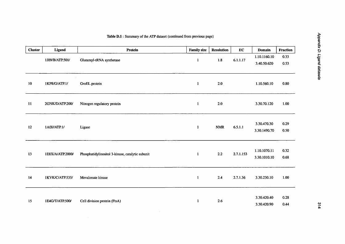
Table D .l : Summary of the ATP dataset (continued from previous page)

Cluster Ligand Protein Family size Resolution EC Domain Fraction

1J09/B/ATP.501/ Glutamyl-tRNA synthetase 1 1.8 6.1.1.171.10.1160.10

3.40.50.620

0.33

0.53

10 1KP8/G/ATP.1/ GroEL protein 1 2.0 1.10.560.10 0.80

11 2GNK/D/ATP.200/ Nitrogen regulatory protein 1 2.0 3.30.70.120 1.00

12 1A0I//ATP.1/ Ligase 1 NMR 6.5.1.13.30.470.30

3.30.1490.70

0.29

0.50

13 1E8X/A/ATP.2000/ Phosphatidylinositol 3-kinase, catalytic subunit 1 2.2 2.7.1.1531.10.1070.11

3.30.1010.10

0.32

0.68

14 1KVK/C/ATP.535/ Mevalonate kinase 1 2.4 2.7.1.36 3.30.230.10 1.00

15 1 E4G/T/ATP.500/ Cell division protein (FtsA) 1 2.63.30.420.40

3.30.420.90

0.28

0.44

Appendix D: Ligand

datasets 314

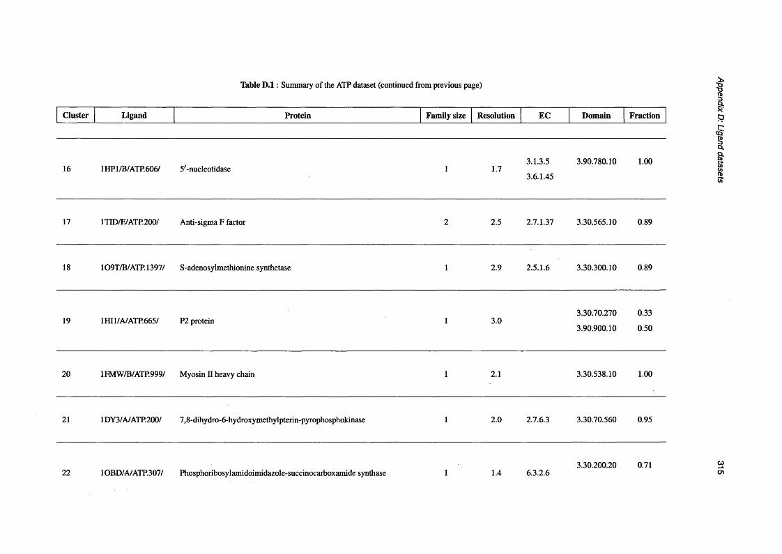
Table D . l : Summary of the ATP dataset (continued from previous page)

Cluster Ligand Protein Family size Resolution EC Domain Fraction

16 1HP1/B/ATP.606/ 5'-nucleotidase 1 1.73.1.3.5

3.6.1.45

3.90.780.10 1.00

17 1TTD/E/ATP.200/ Anti-sigma F factor 2 2.5 2.7.1.37 3.30.565.10 0.89

18 109T/B/ATP. 1397/ S-adenosylmethionine synthetase 1 2.9 2.5.1.6 3.30.300.10 0.89

19 1 HI 1/A/ATP.665/ P2 protein 1 3.03.30.70.270

3.90.900.10

0.33

0.50

20 1 FMW/B/ATP.999/ Myosin II heavy chain 1 2.1 3.30.538.10 1.00

21 1 DY3/A/ATP.200/ 7,8-dihydro-6-hydroxymethylpterin-pyrophosphokinase 1 2.0 2.7.6.3 3.30.70.560 0.95

22 1 OBD/A/ATP.307/ Phosphoribosylamidoimidazole-succinocarboxamide synthase 1 1.4 6.3.2.63.30.200.20 0.71

Appendix D: Ligand

datasets 315

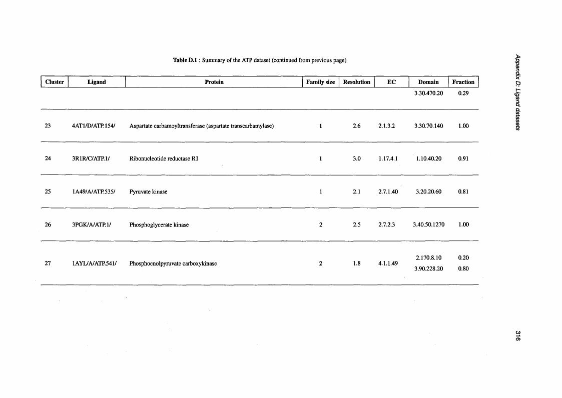
Table D . l : Summary of the ATP dataset (continued from previous page)

Cluster Ligand Protein Family size Resolution EC Domain Fraction

3.30.470.20 0.29

23 4AT1/D/ATP. 154/ Aspartate carbamoyltransferase (aspartate transcarbamylase) 1 2.6 2.1.3.2 3.30.70.140 1.00

24 3R1R/C/ATP.1/ Ribonucleotide reductase R1 1 3.0 1.17.4.1 1.10.40.20 0.91

25 1A49/A/ATP.535/ Pyruvate kinase 1 2.1 2.7.1.40 3.20.20.60 0.81

26 3PGK/A/ATP.1/ Phosphoglycerate kinase 2 2.5 2.1.23 3.40.50.1270 1.00

27 1AYL/A/ATP.541/ Phosphoenolpyruvate carboxykinase 2 1.8 4.1.1.492.170.8.10

3.90.228.20

0.20

0.80

Appendix D: Ligand

datasets 316

Table D.2: Summary of the GTP dataset

Cluster Ligand Protein Family size Resolution EC Domain Fraction

1QR A/C/GTP. 167/ Transforming protein p21/h-ras-l 3 1.6 3.40.50.300 1.00

1J2J/A/GTP. 1001/ ADP-ribosylation factor 1 3 1.6 3.40.50.300 1.00

11NRJ/C/GTP. 1001/ Signal recognition particle receptor, a subunit homolog 1 1.7 3.40.50.300 1.00

1M7B/D/GTP.538/ Rnd3/rhoe small GTP-binding protein 2 2.0 3.40.50.300 1.00

1ZBD/E/GTP.200/ Rab-3a 1 2.6 3.40.50.300 1.00

1 N6L/B/GTP.200/ Ras-related protein rab-5a 1 1.6 3.40.50.300 1.00

2 1HWX/G/GTP. 12/ Glutamate dehydrogenase 1 2.5 1.4.1.3 3.40.50.720 1.00

3 1C80/C/GTP.355/ Fructose-2,6-bisphosphatase 1 2.2 3.1.3.46 3.40.50.1240 1.00

4 1JLR/E/GTP.300/ Uracil phosphoribosyltransferase 1 2.5 2.4.2.9 3.40.50.2020 1.00

5 1QLN/R/GTP.1/ Bacteriophage T7 RNA polymerase 1 2.4 2.7.7.6 3.30.70.370 1.00

6 1 HI0/P/GTP.667/ P2 protein 1 3.03.30.70.270

3.90.900.10

0.64

0.36

Appendix D: Ligand

datasets 317

Table D .2: Summary of the GTP dataset (continued from previous page)

Cluster Ligand Protein Family size Resolution EC Domain Fraction

7 1UVN/A/GTP. 1665/ RNA-dependent RNA polymerase 1 3.01.10.1360.10

3.30.70.270

0.36

0.55

8 1 C4K/C/GTP.999/ Ornithine decarboxylase 1 2.7 4.1.1.17 3.40.640.10 1.00

9 1 LOO/C/GTP.452/ Adenylosuccinate synthetase 1 2.2 6.3.4.43.40.440.10

3.90.170.10

0.56

0.44

10 1FRW/I/GTP.3/ Molybdopterin-guanine dinucleotide biosynthesis protein 1 1.8 3.90.550.10 1.00

11 1 A8R/G/GTP.405/ GTP cyclohydrolase 1 1 2.1 3.5.4.16 3.30.1130.10 0.90

Appendix D: Ligand

datasets 318

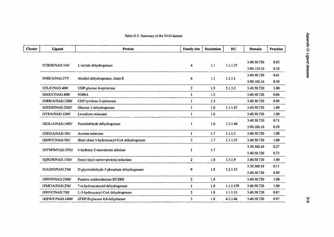
Table D.3: Summary of the NAD dataset

Cluster Ligand Protein Family size Resolution EC Domain Fraction

1T2D/E/NAD.316/ L-lactate dehydrogenase 4 1.1 1.1.1.273.40.50.720

3.90.110.10

0.82

0.18

1N8K/A/NAJ.377/ Alcohol dehydrogenase, chain E 6 1.1 1.1.1.13.40.50.720

3.90.180.10

0.61

0.39

113L/C/NAD.400/ UDP-glucose 4-epimerase 2 1.5 5.1.3.2 3.40.50.720 1.00

1 K6X/C/NAD.400/ NMRA 1 1.5 3.40.50.720 0.86

1ORR/A/NAD. 1200/ CDP-tyvelose-2-epimerase 1 1.5 3.40.50.720 0.89

1GEE/D/NAD.2262/ Glucose 1-dehydrogenase 1 1.6 1.1.1.47 3.40.50.720 1.00

1IY8/A/NAD. 1268/ Levodione reductase 1 1.6 3.40.50.720 1.00

1KOL/A/NAD. 1403/ Formaldehyde dehydrogenase 1 1.6 1.2.1.463.40.50.720

3.90.180.10

0.71

0.29

1GEG/A/NAD. 101/ Acetoin reductase 1 1.7 1.1.1.5 3.40.50.720 1.00

1E6W/C/NAD.301/ Short chain 3-hydroxyacyl-CoA dehydrogenase 2 1.7 1.1.1.35 3.40.50.720 1.00

1NVM/B/NAD.3501/ 4-hydroxy-2-oxovalerate aldolase 1 1.73.30.360.10

3.40.50.720

0.27

0.73

1QSG/B/NAD. 1304/ Enoyl- [acyl-carrier-protein] reductase 2 1.8 1.3.1.9 3.40.50.720 1.00

1G AD/O/NAD.336/ D-glyceraldehyde-3-phosphate dehydrogenase 9 1.8 1.2.1.123.30.360.10

3.40.50.720

0.11

0.89

1NFF/F/NAD.2300/ Putative oxidoreductase RV2002 2 1.8 3.40.50.720 1.00

1FMC/A/NAD.256/ 7 a-hydroxysteroid dehydrogenase 1 1.8 1.1.1.159 3.40.50.720 1.00

1F0Y/C/NAD.750/ L-3-hydroxyacyl-CoA dehydrogenase 2 1.8 1.1.1.35 3.40.50.720 0.87

1KEW/C/NAD. 1400/ dTDP-D-glucose 4,6-dehydratase 3 1.8 4.2.1.46 3.40.50.720 0.97

Appendix D: Ligand

datasets 319

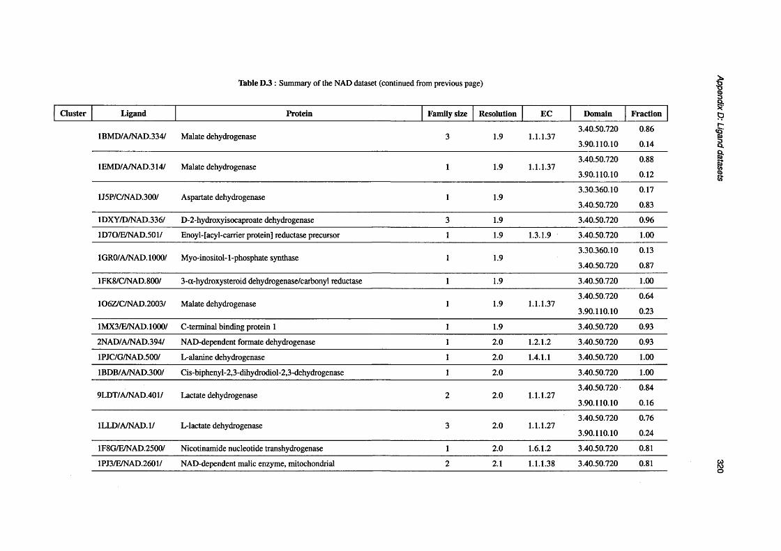
Table D.3 : Summary of the NAD dataset (continued from previous page)

Cluster Ligand Protein Family size Resolution EC Domain Fraction

1BMD/A/NAD.334/ Malate dehydrogenase 3 1.9 1.1.1.373.40.50.720

3.90.110.10

0.86

0.14

1EMD/A/NAD.314/ Malate dehydrogenase 1 1.9 1.1.1.373.40.50.720

3.90.110.10

0.88

0.12

1J5P/C/NAD.300/ Aspartate dehydrogenase 1 1.93.30.360.10

3.40.50.720

0.17

0.83

1DXY/D/NAD.336/ D-2-hydroxyisocaproate dehydrogenase 3 1.9 3.40.50.720 0.96

1D7O/E/NAD. 501/ Enoyl-[acy 1-carrier protein] reductase precursor 1 1.9 1.3.1.9 3.40.50.720 1.00

1GRO/A/NAD. 1000/ Myo-inositol-1-phosphate synthase 1 1.93.30.360.10

3.40.50.720

0.13

0.87

1FK8/C/NAD.800/ 3-a-hydroxysteroid dehydrogenase/carbonyl reductase 1 1.9 3.40.50.720 1.00

106Z/C/NAD.2003/ Malate dehydrogenase 1 1.9 1.1.1.373.40.50.720

3.90.110.10

0.64

0.23

1 MX 3/E/NAD. 1000/ C-terminal binding protein 1 1 1.9 3.40.50.720 0.93

2NAD/A/NAD.394/ NAD-dependent formate dehydrogenase 1 2.0 1.2.1.2 3.40.50.720 0.93

1PJC/G/NAD.500/ L-alanine dehydrogenase 1 2.0 1.4.1.1 3.40.50.720 1.00

1BDB/A/NAD.300/ Cis-biphenyl-2,3-dihydrodiol-2,3-dehydrogenase 1 2.0 3.40.50.720 1.00

9LDT/A/NAD.401/ Lactate dehydrogenase 2 2.0 1.1.1.273.40.50.720

3.90.110.10

0.84

0.16

1LLD/A/NAD.1/ L-lactate dehydrogenase 3 2.0 1.1.1.273.40.50.720

3.90.110.10

0.76

0.24

1F8G/E/NAD.2500/ Nicotinamide nucleotide transhydrogenase 1 2.0 1.6.1.2 3.40.50.720 0.81

1PJ3/E/NAD.2601/ NAD-dependent malic enzyme, mitochondrial 2 2.1 1.1.1.38 3.40.50.720 0.81

Appendix D: Ligand

datasets 320

Table D .3 : Summary of the NAD dataset (continued from previous page)

Cluster Ligand Protein Family size Resolution EC Domain Fraction

1ENY/B/NAD.500/ Enoyl-acyl carrier protein reductase 1 2.2 3.40.50.720 1.00

1HYH/A/NAD.330/ L-2-hydroxyisocaproate dehydrogenase 1 2.23.40.50.720

3.90.110.10

0.85

0.15

1EBF/C/NAD.2109/ Homoserine dehydrogenase 1 2.3 1.1.1.3 3.40.50.720 1.00

1BXG/A/NAD.360/ Phenylalanine dehydrogenase 1 2.3 1.4.1.20 3.40.50.720 1.00

1DHR/B/NAD.241/ Dihydropteridine reductase 1 2.3 1.5.1.34 3.40.50.720 1.00

1LSS/I/NAD.1001/ Trk system potassium uptake protein TrkA homolog 1 2.3 3.40.50.720 1.00

1 R37/A/NAD.403/ NAD-dependent alcohol dehydrogenase 1 2.3 1.1.1.13.40.50.720

3.90.180.10

0.66

0.34

1 P9L/E/NAD.301/ Dihydrodipicolinate reductase 1 2.3 1.3.1.263.30.360.10

3.40.50.720

0.05

0.90

1NPD/A/NAD.300/ Hypothetical shikimate 5-dehydrogenase-like protein YdiB 1 2.3 3.40.50.720 0.91

1 DLI/C/NAD.403/ UDP-glucose dehydrogenase 1 2.3 1.1.1.22 3.40.50.720 0.85

1 NHW/I/NAD.450/ Enoyl-acyl carrier reductase 1 2.4 3.40.50.720 0.92

1B14/C/NAD.255/ Alcohol dehydrogenase 1 2.4 l.l .l . l 3.40.50.720 1.00

1H94/A/NAD.799/ Glucose 6-phosphate 1-dehydrogenase 1 2.5 1.1.1.493.30.360.10

3.40.50.720

0.06

0.94

1ARZ/B/NAD.274/ Dihydrodipicolinate reductase 1 2.6 1.3.1.263.30.360.10

3.40.50.720

0.05

0.95

1EVJ/A/NAD.500/ Glucose-fructose oxidoreductase 1 2.73.30.360.10

3.40.50.720

0.19

0.81

1 PSD/B/NAD.450/ D-3-phosphoglycerate dehydrogenase 1 2.8 1.1.1.95 3.40.50.720 0.92

1 D4F/E/NAD.502/(phosphoglvcerate dehydrogenase) S-adenosylnomocysteine hydrolase 1 2.8 3.3.1.1

3.40.50.720 0.60

Table D.3 : Summary of the NAD dataset (continued from previous page)

Cluster Ligand Protein Family size Resolution EC Domain Fraction

3.40.50.1480 0.20

1CH6/G/NAD.571/ Glutamate dehydrogenase 1 2.9 3.40.50.720 0.71

1EE9/C/NAD. 10/ 5,10-methylenetetrahydrofolate dehydrogenase 1 3.0 1.5.1.15 3.40.50.720 0.95

1FDV/A/NAD.361/ 17 - (3-hydroxy steroid dehydrogenase 1 3.1 1.1.1.62 3.40.50.720 1.00

1 QRR/A/NAD.401 / Sulfolipid biosynthesis protein 1 1.6 3.13.1.1 3.40.50.720 0.88

1004/D/NAD.6504/ Aldehyde dehydrogenase, mitochondrial precursor 4 1.4 1.2.1.33.40.309.10

3.40.605.10

0.14

0.86

2

1UXT/A/NAD. 1503/ Glyceraldehyde-3-phosphate dehydrogenase 1 2.2 1.2.1.93.40.309.10

3.40.605.10

0.18

0.68

1AD3/A/NAD.600/ Aldehyde dehydrogenase (class 3) 1 2.6 1.2.1.53.40.309.10

3.40.605.10

0.32

0.68

1BPW/A/NAD.4/ Aldehyde dehydrogenase 1 2.8 1.2.1.83.40.309.10

3.40.605.10

0.15

0.81

1 NUU/E/NAD.401/ FKSG76 (NMN adenylyltransferase) 2 1.9 2.7.7.1 3.40.50.620 1.00

1EJ2/L/NAD. 1339/ Nicotinamide mononucleotide adenylyltransferase 1 1.9 2.7.7.1 3.40.50.620 1.00D

1K4M/D/NAD.601/ NAMN adenylyltransferase 1 1.9 2.7.7.18 3.40.50.620 1.00

1LW7/E/NAD.601/ Transcriptional regulator NADR 1 2.9 3.40.50.620 1.00

Appendix D: Ligand

datasets 322

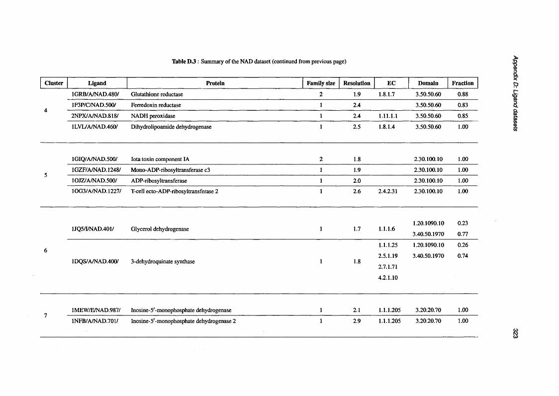
Table D.3 : Summary of the NAD dataset (continued from previous page)

Cluster Ligand Protein Family size Resolution EC Domain Fraction

1GRB/A/NAD.480/ Glutathione reductase 2 1.9 1.8.1.7 3.50.50.60 0.88

A 1F3P/C/NAD.500/ Ferredoxin reductase 1 2.4 3.50.50.60 0.83

2NPX/A/NAD.818/ NADH peroxidase 1 2.4 1.11.1.1 3.50.50.60 0.85

1 LVL/A/NAD.460/ Dihydrolipoamide dehydrogenase 1 2.5 1.8.1.4 3.50.50.60 1.00

1GIQ/A/NAD.500/ Iota toxin component IA 2 1.8 2.30.100.10 1.00

C1GZF/A/NAD. 1248/ Mono-ADP-ribosyltransferase c3 1 1.9 2.30.100.10 1.00

J

1OJZ/A/NAD.500/ ADP-ribosyltransferase 1 2.0 2.30.100.10 1.00

10G3/A/NAD. 1227/ T-cell ecto-ADP-ribosyltransferase 2 1 2.6 2.4.2.31 2.30.100.10 1.00

1JQ5/I/NAD.401/ Glycerol dehydrogenase 1 1.7 1.1.1.61.20.1090.10

3.40.50.1970

0.23

0.77

£ 1.1.1.25 1.20.1090.10 0.26O

1 DQS/A/NAD.400/ 3-dehydroquinate synthase 1 1.82.5.1.19

2.7.1.71

4.2.1.10

3.40.50.1970 0.74

1MEW/E/NAD.987/ Inosine-5'-monophosphate dehydrogenase 1 2.1 1.1.1.205 3.20.20.70 1.00/

1NFB/A/NAD.701/ Inosine-5'-monophosphate dehydrogenase 2 1 2.9 1.1.1.205 3.20.20.70 1.00

Appendix D: Ligand

datasets 323

Table D.3 : Summary of the NAD dataset (continued from previous page)

Cluster Ligand Protein Family size Resolution EC Domain Fraction

81MI3/A/NAD. 1350/ Xylose reductase 1 1.8 3.20.20.100 1.00

1M9H/B/NAD.300/ 2,5-diketo-D-gluconic acid reductase A 1 2.0 1.1.1.274 3.20.20.100 1.00

9 2BKJ/B/NAD.243/ Flavin reductase 1 2.1 3.40.109.10 1.00

10 1S7G/F/NAD.701/ NAD-dependent deacetylase 2 1 2.3 3.40.50.1220 0.85

11 1RLZ/E/NAD.700/ Deoxyhypusine synthase 1 2.1 2.5.1.46 3.40.910.10 0.97

12 1CH6/G/NAD.562/ Glutamate dehydrogenase 1 2.9 3.40.192.10 1.00

13 1HWY/G/NAD.31/A Glutamate dehydrogenase 1 3.2 1.4.1.33.40.50.720

3.40.192.10

0.40

0.44

14 1 LW7/E/NAD.605/ Transcriptional regulator NADR 1 2.93.40.50.300

3.40.50.620

0.75

0.25

Appendix D: Ligand

datasets 324

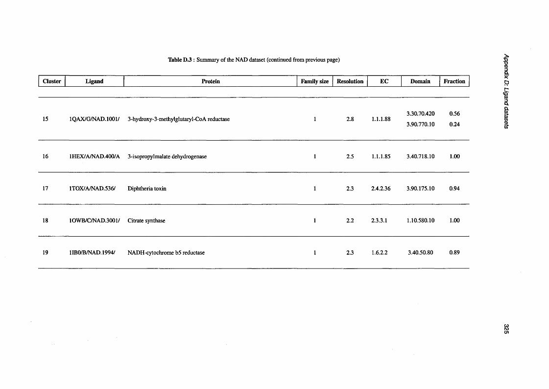
Table D.3 : Summary of the NAD dataset (continued from previous page)

Cluster Ligand Protein Family size Resolution EC Domain Fraction

15 1QAX/G/NAD. 1001/ 3-hydroxy-3-methylglutaryl-CoA reductase 1 2.8 1.1.1.883.30.70.420

3.90.770.10

0.56

0.24

16 1 HEX/A/NAD.400/A 3-isopropylmalate dehydrogenase 1 2.5 1.1.1.85 3.40.718.10 1.00

17 1TOX/A/NAD.536/ Diphtheria toxin 1 2.3 2.4.2.36 3.90.175.10 0.94

18 1OWB/C/NAD.3001/ Citrate synthase 1 2.2 2.3.3.1 1.10.580.10 1.00

19 1IB0/B/NAD. 1994/ NADH-cytochrome b5 reductase 1 2.3 1.6.2.2 3.40.50.80 0.89

Appendix D: Ligand

datasets 325

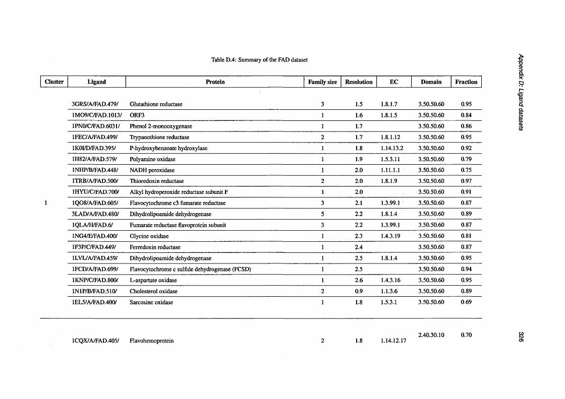
Table D.4: Summary of the FAD dataset

Cluster Ligand Protein Family size Resolution EC Domain Fraction

3GRS/A/FAD.479/ Glutathione reductase 3 1.5 1.8.1.7 3.50.50.60 0.95

1M09/C/FAD. 1013/ ORF3 1 1.6 1.8.1.5 3.50.50.60 0.84

1PN0/C/FAD.6031/ Phenol 2-monooxygenase 1 1.7 3.50.50.60 0.86

1 FEC/A/FAD.499/ Trypanothione reductase 2 1.7 1.8.1.12 3.50.50.60 0.95

1K0I/D/FAD.395/ P-hydroxybenzoate hydroxylase 1 1.8 1.14.13.2 3.50.50.60 0.92

1H82/A/FAD.579/ Polyamine oxidase 1 1.9 1.5.3.11 3.50.50.60 0.79

1 NHP/B/FAD.448/ NADH peroxidase 1 2.0 1.11.1.1 3.50.50.60 0.75

1TRB/A/FAD.500/ Thioredoxin reductase 2 2.0 1.8.1.9 3.50.50.60 0.97

1H YU/C/FAD.700/ Alkyl hydroperoxide reductase subunit F 1 2.0 3.50.50.60 0.91

1 1QO8/A/FAD.605/ Flavocytochrome c3 fumarate reductase 3 2.1 1.3.99.1 3.50.50.60 0.87

3LAD/A/FAD.480/ Dihydrolipoamide dehydrogenase 5 2.2 1.8.1.4 3.50.50.60 0.89

1QLA/H/FAD.6/ Fumarate reductase flavoprotein subunit 3 2.2 1.3.99.1 3.50.50.60 0.87

1 NG4/E/FAD.400/ Glycine oxidase 1 2.3 1.4.3.19 3.50.50.60 0.81

1F3P/C/FAD.449/ Ferredoxin reductase 1 2.4 3.50.50.60 0.87

1LVL/A/FAD.459/ Dihydrolipoamide dehydrogenase 1 2.5 1.8.1.4 3.50.50.60 0.95

1FCD/A/FAD.699/ Flavocytochrome c sulfide dehydrogenase (FCSD) 1 2.5 3.50.50.60 0.94

1KNP/C/FAD.800/ L-aspartate oxidase 1 2.6 1.4.3.16 3.50.50.60 0.95

1N1P/B/FAD.510/ Cholesterol oxidase 2 0.9 1.1.3.6 3.50.50.60 0.89

1EL5/A/FAD.400/ Sarcosine oxidase 1 1.8 1.5.3.1 3.50.50.60 0.69

1CQX/A/FAD.405/ Flavohemoprotein 2 1.8 1.14.12.172.40.30.10 0.70

Appendix D: Ligand

datasets 326

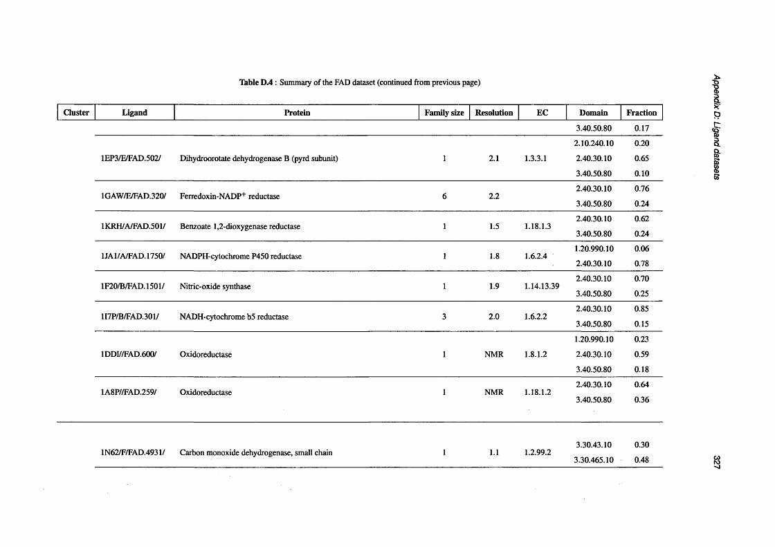
Table D .4 : Summary of the FAD dataset (continued from previous page)

Cluster Ligand Protein Family size Resolution EC Domain Fraction

3.40.50.80 0.17

2.10.240.10 0.20

1EP3/E/FAD.502/ Dihydroorotate dehydrogenase B (pyrd subunit) 1 2.1 1.3.3.1 2.40.30.10

3.40.50.80

0.65

0.10

1GAW/E/FAD.320/ Ferredoxin-NADP+ reductase 6 2.22.40.30.10

3.40.50.80

0.76

0.24

1KRH/A/FAD.501/ Benzoate 1,2-dioxygenase reductase 1 1.5 1.18.1.32.40.30.10

3.40.50.80

0.62

0.24

1JA1/A/FAD.1750/ NADPH-cytochrome P450 reductase 1 1.8 1.6.2.41.20.990.10

2.40.30.10

0.06

0.78

1F20/B/FAD. 1501/ Nitric-oxide synthase 1 1.9 1.14.13.392.40.30.10

3.40.50.80

0.70

0.25

1I7P/B/FAD.301/ NADH-cytochrome b5 reductase 3 2.0 1.6.2.22.40.30.10

3.40.50.80

0.85

0.15

1.20.990.10 0.23

1DDI//FAD.600/ Oxidoreductase 1 NMR 1.8.1.2 2.40.30.10

3.40.50.80

0.59

0.18

1A8P//FAD.259/ Oxidoreductase 1 NMR 1.18.1.22.40.30.10

3.40.50.80

0.64

0.36

1N62/F/FAD.4931/ Carbon monoxide dehydrogenase, small chain 1 1.1 1.2.99.23.30.43.10

3.30.465.10

0.30

0.48

Appendix D: Ligand

datasets 327

Table D .4 : Summary of the FAD dataset (continued from previous page)

Cluster Ligand Protein Family size Resolution EC Domain Fraction

1HSK/E/FAD.401/ UDP-N-acetylenolpyruvoylglucosamine reductase 1 2.3 1.1.1.1583.30.43.10

3.30.465.10

0.29

0.57

1FIQ/G/FAD.606/ Xanthine oxidase 1 2.5 1.1.3.223.30.43.10

3.30.465.10

0.29

0.58

1JRO/I/FAD.3005/ Xanthine dehydrogenase, chain A 1 2.7 1.1.1.2043.30.43.10

3.30.465.10

0.31

0.47

2MBR/A/FAD.401/ Uridine diphospho-N-acetylenolpyruvylglucosamine reductase 1 1.8 1.1.1.1583.30.43.10

3.30.465.10

0.37

0.47

1LQT/C/FAD.3457/ FPRA 2 1.1 1.18.1.23.40.50.720

3.50.50.60

0.61

0.26

41GTE/A/FAD. 1031/ Dihydropyrimidine dehydrogenase 1 1.6 1.3.1.2

3.40.50.720

3.50.50.60

0.79

0.12

1 AN9/B/FAD.351/ D-amino acid oxidase 1 2.5 1.4.3.3 3.40.50.720 0.84

1E8G/B/FAD.600/ Vanillyl-alcohol oxidase 1 2.1 1.1.3.383.30.43.10

3.30.465.20

0.28

0.50

5 111 9/A/FAD.700/ Cholesterol oxidase 1 1.73.30.43.10

3.30.465.20

0.34

0.59

1 F0X/A/FAD.600/ D-lactate dehydrogenase 1 1.9 1.1.1.283.30.43.10

3.30.465.20

0.44

0.53

Appendix D: Ligand

datasets 328

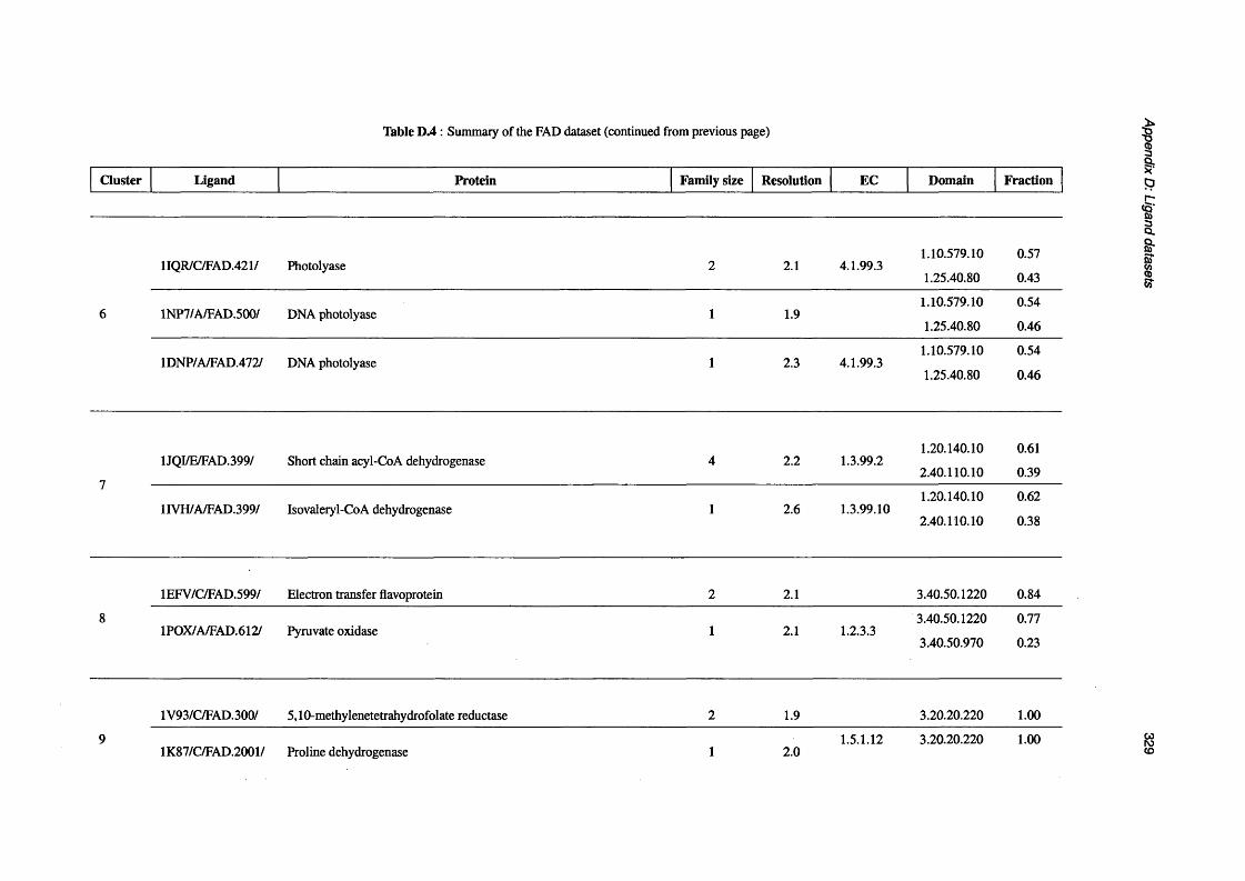
Table D.4 : Summary of the FAD dataset (continued from previous page)

Cluster Ligand Protein Family size Resolution EC Domain Fraction

1IQR/C/FAD.421/ Photolyase 2 2.1 4.1.99.31.10.579.10

1.25.40.80

0.57

0.43

6 1NP7/A/FAD.500/ DNA photolyase 1 1.91.10.579.10

1.25.40.80

0.54

0.46

1DNP/A/FAD.472/ DNA photolyase 1 2.3 4.1.99.31.10.579.10

1.25.40.80

0.54

0.46

7

1JQI/E/FAD.399/ Short chain acyl-CoA dehydrogenase 4 2.2 1.3.99.21.20.140.10

2.40.110.10

0.61

0.39

HVH/A/FAD.399/ Isovaleryl-CoA dehydrogenase 1 2.6 1.3.99.101.20.140.10

2.40.110.10

0.62

0.38

1EFV/C/FAD.599/ Electron transfer flavoprotein 2 2.1 3.40.50.1220 0.84

81POX/A/FAD.612/ Pyruvate oxidase 1 2.1 1.2.3.3

3.40.50.1220

3.40.50.970

0.77

0.23

1V93/C/FAD.300/ 5,10-methylenetetrahydrofolate reductase 2 1.9 3.20.20.220 1.00

91K87/C/FAD.2001/ Proline dehydrogenase 1 2.0

1.5.1.12 3.20.20.220 1.00

Appendix D: Ligand

datasets 329

Table D .4 : Summary of the FAD dataset (continued from previous page)

Cluster Ligand Protein Family size Resolution EC Domain Fraction

1.5.99.8

101JR8/C/FAD.334/ Erv2 protein, mitochondrial 1 1.5 1.20.120.310 1.00

10QC/A/FAD. 1/ Augmenter of liver regeneration 1 1.8 1.20.120.310 1.00

11 1H69/C/FAD. 1274/ NAD(P)H dehydrogenase 1 4 1.9 1.6.99.2 3.40.50.360 1.00

12 1 GPE/A/FAD.600/ Glucose oxidase 2 1.8 1.1.3.43.50.50.60

4.10.450.10

0.44

0.34

13 1QX4/A/FAD.301/ NADH-cytochrome b5 reductase 1 1.8 1.6.2.22.40.30.10

3.40.50.80

0.31

0.69

14 1P3Y/L/FAD.259/ MRSD protein 1 2.5 3.40.50.1950 0.92

Appendix D: Ligand

datasets 330

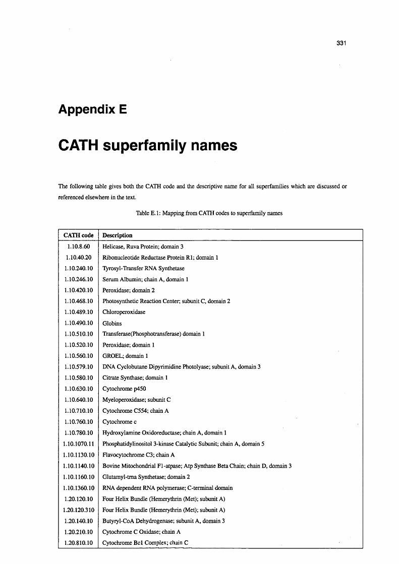
331

Appendix E

CATH superfamily names

The following table gives both the CATH code and the descriptive name for all superfamilies which are discussed or

referenced elsewhere in the text.

Table E.l: Mapping from CATH codes to superfamily names

CATH code Description

1.10.8.60 Helicase, Ruva Protein; domain 3

1.10.40.20 Ribonucleotide Reductase Protein Rl; domain 1

1.10.240.10 Tyrosyl-Transfer RNA Synthetase

1.10.246.10 Serum Albumin; chain A, domain 1

1.10.420.10 Peroxidase; domain 2

1.10.468.10 Photosynthetic Reaction Center; subunit C, domain 2

1.10.489.10 Chloroperoxidase

1.10.490.10 Globins1.10.510.10 Transferase(Phosphotransferase) domain 1

1.10.520.10 Peroxidase; domain 1

1.10.560.10 GROEL; domain 1

1.10.579.10 DNA Cyclobutane Dipyrimidine Photolyase; subunit A, domain 3

1.10.580.10 Citrate Synthase; domain 1

1.10.630.10 Cytochrome p450

1.10.640.10 Myeloperoxidase; subunit C

1.10.710.10 Cytochrome C554; chain A

1.10.760.10 Cytochrome c

1.10.780.10 Hydroxylamine Oxidoreductase; chain A, domain 1

1.10.1070.11 Phosphatidylinositol 3-kinase Catalytic Subunit; chain A, domain 5

1.10.1130.10 Flavocytochrome C3; chain A

1.10.1140.10 Bovine Mitochondrial Fl-atpase; Atp Synthase Beta Chain; chain D, domain 3

1.10.1160.10 Glutamyl-tma Synthetase; domain 2

1.10.1360.10 RNA dependent RNA polymerase; C-terminal domain

1.20.120.10 Four Helix Bundle (Hemerythrin (Met); subunit A)

1.20.120.310 Four Helix Bundle (Hemerythrin (Met); subunit A)

1.20.140.10 Butyiyl-CoA Dehydrogenase; subunit A, domain 3

1.20.210.10 Cytochrome C Oxidase; chain A

1.20.810.10 Cytochrome Bel Complex; chain C

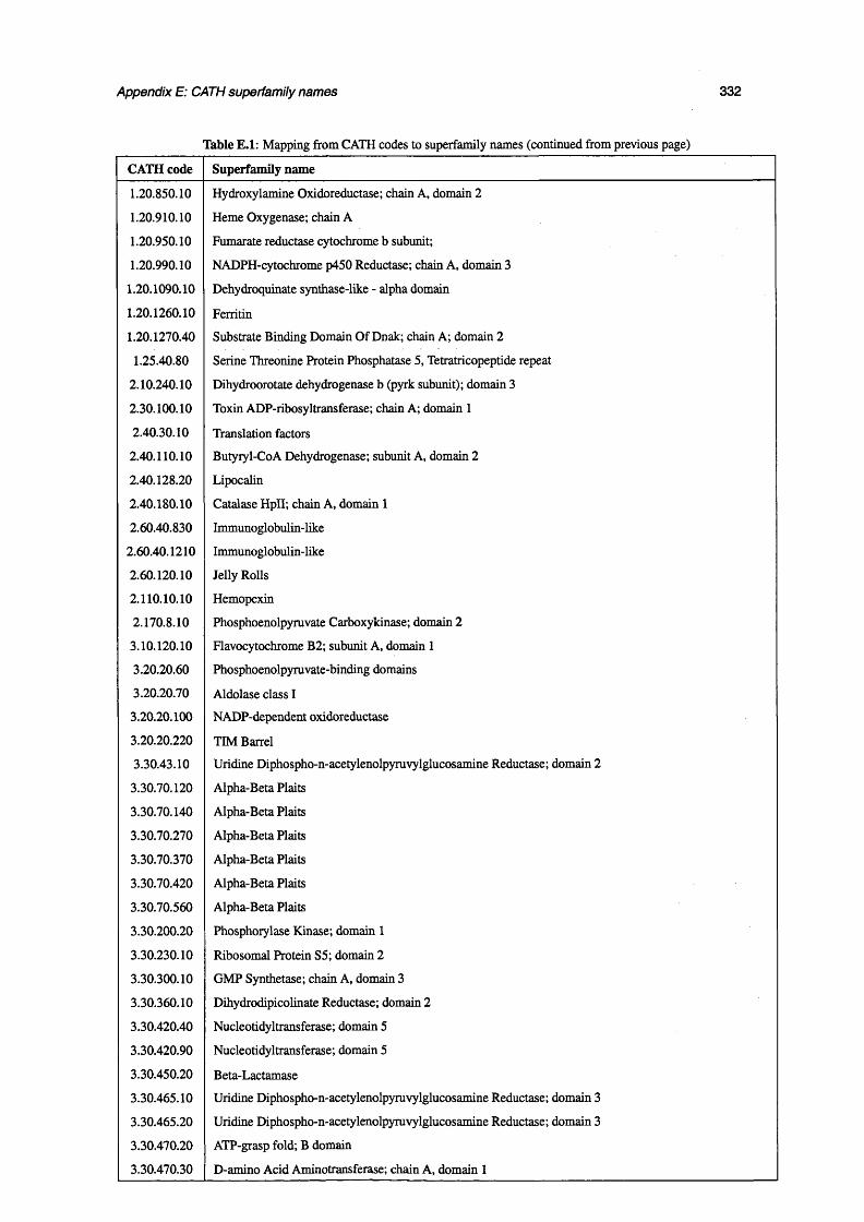
Appendix E: CATH superfamily names 332

Table E.1: Mapping from CATH codes to superfamily names (continued from previous page)

CATH code Superfamily name

1.20.850.10 Hydroxylamine Oxidoreductase; chain A, domain 2

1.20.910.10 Heme Oxygenase; chain A

1.20.950.10 Fumarate reductase cytochrome b subunit;

1.20.990.10 NADPH-cytochrome p450 Reductase; chain A, domain 3

1.20.1090.10 Dehydroquinate synthase-like - alpha domain

1.20.1260.10 Ferritin

1.20.1270.40 Substrate Binding Domain Of Dnak; chain A; domain 2

1.25.40.80 Serine Threonine Protein Phosphatase 5, Tetratricopeptide repeat

2.10.240.10 Dihydroorotate dehydrogenase b (pyrk subunit); domain 3

2.30.100.10 Toxin ADP-ribosyltransferase; chain A; domain 1

2.40.30.10 Translation factors

2.40.110.10 Butyryl-CoA Dehydrogenase; subunit A, domain 2

2.40.128.20 Lipocalin

2.40.180.10 Catalase HpII; chain A, domain 1

2.60.40.830 Immunoglobulin-like

2.60.40.1210 Immunoglobulin-like

2.60.120.10 Jelly Rolls

2.110.10.10 Hemopexin

2.170.8.10 Phosphoenolpyruvate Carboxykinase; domain 2

3.10.120.10 Flavocytochrome B2; subunit A, domain 1

3.20.20.60 Phosphoenolpyruvate-binding domains

3.20.20.70 Aldolase class I3.20.20.100 NADP-dependent oxidoreductase

3.20.20.220 TIM Barrel

3.30.43.10 Uridine Diphospho-n-acetylenolpyruvylglucosamine Reductase; domain 2

3.30.70.120 Alpha-Beta Plaits

3.30.70.140 Alpha-Beta Plaits

3.30.70.270 Alpha-Beta Plaits

3.30.70.370 Alpha-Beta Plaits

3.30.70.420 Alpha-Beta Plaits

3.30.70.560 Alpha-Beta Plaits

3.30.200.20 Phosphorylase Kinase; domain 1

3.30.230.10 Ribosomal Protein S5; domain 2

3.30.300.10 GMP Synthetase; chain A, domain 3

3.30.360.10 Dihydrodipicolinate Reductase; domain 2

3.30.420.40 Nucleotidyltransferase; domain 5

3.30.420.90 Nucleotidyltransferase; domain 5

3.30.450.20 Beta-Lactamase3.30.465.10 Uridine Diphospho-n-acetylenolpyruvylglucosamine Reductase; domain 3

3.30.465.20 Uridine Diphospho-n-acetylenolpyruvylglucosamine Reductase; domain 3

3.30.470.20 ATP-grasp fold; B domain

3.30.470.30 D-amino Acid Aminotransferase; chain A, domain 1

Appendix E: CATH superfamily names 333

Table E.1: Mapping from CATH codes to superfamily names (continued from previous page)

CATH code Superfamily name

3.30.538.10 Myosin fragment; domain 2

3.30.565.10 Heat Shock Protein 90

3.30.930.10 Bira Bifunctional Protein; domain 2

3.30.1010.10 Phosphatidylinositol 3-kinase Catalytic Subunit; chain A, domain 4

3.30.1130.10 GTP Cyclohydrolase I; domain 2

3.30.1490.20 Dna Ligase; domain 1

3.30.1490.70 Dna Ligase; domain 1

3.30.1500.10 Heme-binding Protein A; chain A;

3.40.50.80 Nucleotide-binding domain of ferredoxin-NADP reductase (FNR) module

3.40.50.300 P-loop containing nucleotide triphosphate hydrolases

3.40.50.360 Rossmann fold

3.40.50.620 Rossmann fold

3.40.50.720 NAD(P)-binding Rossmann-like domain

3.40.50.970 Rossmann fold

3.40.50.1220 TPP-binding domain

3.40.50.1240 Phosphoglycerate mutase-like

3.40.50.1270 Rossmann fold

3.40.50.1480 Rossmann fold

3.40.50.1950 Rossmann fold

3.40.50.1970 Rossmann fold

3.40.50.2020 Rossmann fold

3.40.109.10 NADH Oxidase

3.40.192.10 Leucine Dehydrogenase; chain A, domain 1

3.40.309.10 Aldehyde Dehydrogenase; chain A, domain 2

3.40.440.10 Adenylosuccinate Synthetase; subunit A, domain 1

3.40.605.10 Aldehyde Dehydrogenase; chain A, domain 1

3.40.640.10 Type I PLP-dependent aspartate aminotransferase-like (Major domain)

3.40.718.10 Isopropylmalate Dehydrogenase

3.40.910.10 Deoxyhypusine Synthase

3.40.1190.20 UDP-N-acetylmuramoyl-L-alanine:D-glutamate ligase

3.50.50.60 FAD/NAD(P)-binding domain

3.90.10.10 Cytochrome C3

3.90.110.10 L-2-Hydroxyisocaproate Dehydrogenase; subunit A, domain 2

3.90.170.10 Adenylosuccinate Synthetase; subunit A, domain 3

3.90.175.10 Diphtheria Toxin; domain 1

3.90.180.10 Medium-chain alcohol dehydrogenases; catalytic domain

3.90.228.20 Phosphoenolpyruvate Carboxykinase; domain 3

3.90.340.10 Nitric Oxide Synthase; chain A, domain 1

3.90.550.10 Spore Coat Polysaccharide Biosynthesis Protein SpsA; chain A

3.90.640.10 Actin; chain A, domain 4

3.90.770.10 3-hydroxy-3-methylglutaryl-coenzyme A Reductase; chain A, domain 2

3.90.780.10 5’-nucleotidase; domain 2

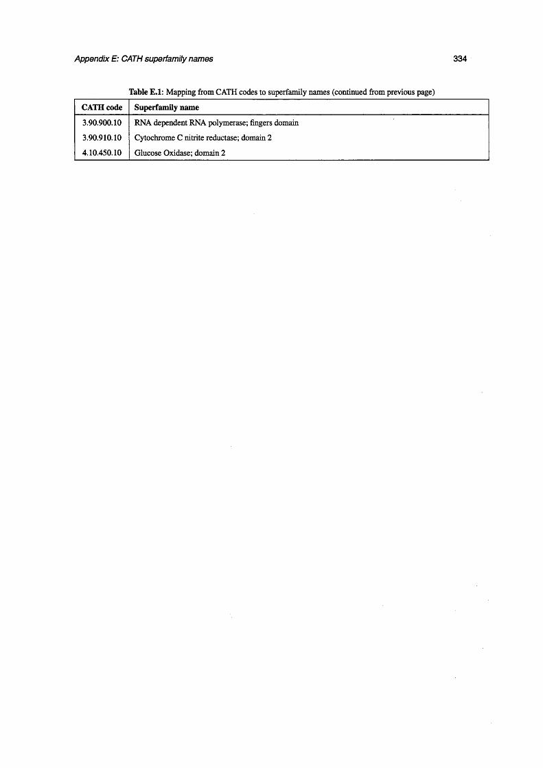
Appendix E: CATH superfamily names 334

Table E.1: Mapping from CATH codes to superfamily names (continued from previous page)

CATH code Superfamily name

3.90.900.10

3.90.910.10

4.10.450.10

RNA dependent RNA polymerase; fingers domain

Cytochrome C nitrite reductase; domain 2

Glucose Oxidase; domain 2

Abbreviations and nomenclature

API Application Programming Interface

ART ADP-ribosyltransferase

ASCII American Standard Code for Information Interchange

ATP Adenosine triphosphate

BBSRC Biotechnology and Biological Sciences Research Council

BFS Breadth-first search

BLOSUM Block Substitution Matrix

cAMP Cyclic AMP

CSD Cambridge Structural Database

CSI Common Subgraph Isomorphism

DAG Directed Acyclic Graph

DFS Depth-first search

DHFR Dihydrofolate reductase

EBI European Bioinformatics Institute

EC Enzyme Commission

EMBL European Molecular Biology Laboratory

ESER Essential Set of Essential Rings

ESI Exact Subgraph Isomorphism

FAD Flavin adenine dinucleotide

FMN Flavin mononucleotide

FTP File Transfer Protocol

GAMUT Gareth’s Macromolecular Utility Toolkit

HMM Hidden Markov Model

HSV Hue, Saturation, Value

HTML Hypertext Markup Language

References

ISAM Indexed Sequential Access Management

LAM Local Area Multicomputer

MAD Multiple wavelength Anomalous Dispersion

MCS Maximum Common Subgraph

MDS Multidimensional Scaling

MPI Message Passing Interface

MR Molecular Replacement

MSD Macromolecular Structure Database

NAD Nicotinamide adenine dinucleotide

NADP Nicotinamide adenine dinucleotide phosphate

NCBI National Center for Biotechnology Information

NMR Nuclear Magnetic Resonance

OOP Object-Oriented Programming

PCA Principal Components Analysis

PDB Protein Data Bank

PQS Protein Quaternary Structure

RCSB Research Collaboratory in Structural Bioinformatics

RGB Red, Green, Blue

RMSD Root Mean Squared Deviation

SAXS Small-angle X-ray Scattering

SCOP Structural Classification of Proteins

STL C++ Standard Template Library

SVD singular value decomposition

UCL University College London

UML Unified Modelling Language

VMM Vertex Mapping Matrix

XML Extensible Markup Language

336

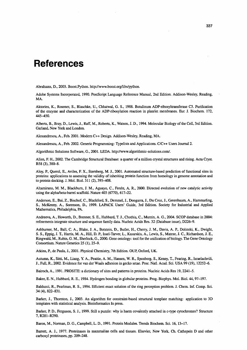
337

References

Abrahams, D., 2003. Boost.Python. http://www.boost.org/libs/python.

Adobe Systems Incorporated, 1990. PostScript Language Reference Manual, 2nd Edition. Addison-Wesley, Reading, MA.

Aktories, K., Rosener, S., Blaschke, U., Chhatwal, G. S., 1988. Botulinum ADP-ribosyltransferase C3. Purification of the enzyme and characterization of the ADP-ribosylation reaction in platelet membranes. Eur. J. Biochem. 172, 445-450.

Alberts, B., Bray, D., Lewis, J., Raff, M., Roberts, K., Watson, J. D., 1994. Molecular Biology of the Cell, 3rd Edition. Garland, New York and London.

Alexandrescu, A., Feb. 2001. Modem C++ Design. Addison-Wesley, Reading, MA.

Alexandrescu, A., Feb. 2002. Generic Programming: Typelists and Applications. C/C++ Users Journal 2.

Algorithmic Solutions Software, G., 2001. LEDA. http://www.algorithmic-solutions.com/.

Allen, F. H., 2002. The Cambridge Structural Database: a quarter of a million crystal structures and rising. Acta Cryst. B58 (3), 380-8.

Aloy, P., Querol, E., Aviles, F. X., Sternberg, M. J., 2001. Automated structure-based prediction of functional sites in proteins: applications to assessing the validity of inheriting protein function from homology in genome annotation and to protein docking. J. Mol. Biol. 311 (2), 395-408.

Altamirano, M. M., Blackburn, J. M., Aguayo, C., Fersht, A. R., 2000. Directed evolution of new catalytic activity using the alpha/beta-barrel scaffold. Nature 403 (6770), 617-22.

Anderson, E., Bai, Z., Bischof, C., Blackford, S., Demmel, J., Dongarra, J., Du Croz, J., Greenbaum, A., Hammarling,S., McKenny, A., Sorenson, D., 1999. LAPACK Users’ Guide, 3rd Edition. Society for Industrial and Applied Mathematics, Philadelphia, PA.

Andreeva, A., Howorth, D., Brenner, S. E., Hubbard, T. J., Chothia, C., Murzin, A. G., 2004. SCOP database in 2004: refinements integrate structure and sequence family data. Nucleic Acids Res. 32 (Database issue), D226-9.

Ashbumer, M., Ball, C. A., Blake, J. A., Botstein, D., Butler, H., Cherry, J. M., Davis, A. P., Dolinski, K., Dwight, S. S., Eppig, J. T., Harris, M. A., Hill, D. P., Issel-Tarver, L., Kasarskis, A., Lewis, S., Matese, J. C., Richardson, J. E., Ringwald, M., Rubin, G. M., Sherlock, G., 2000. Gene ontology: tool for the unification of biology. The Gene Ontology Consortium. Nature Genetics 25 (1), 25-9.

Atkins, P., de Paula, J., 2001. Physical Chemistry, 7th Edition. OUP, Oxford, UK.

Autumn, K., Sitti, M., Liang, Y. A., Peattie, A. M., Hansen, W. R., Sponberg, S., Kenny, T., Fearing, R., Israelachvili, J., Full, R., 2002. Evidence for van der Waals adhesion in gecko setae. Proc. Natl. Acad. Sci. USA 99 (19), 12252-6.

Bairoch, A., 1991. PROSITE: a dictionary of sites and patterns in proteins. Nucleic Acids Res 19,2241-5.

Baker, E. N., Hubbard, R. E., 1984. Hydrogen bonding in globular proteins. Prog. Biophys. Mol. Biol. 44, 97-197.

Balducci, R., Pearlman, R. S., 1994. Efficient exact solution of the ring perception problem. J. Chem. Inf. Comp. Sci. 34 (4), 822-831.

Barker, J., Thornton, J., 2003. An algorithm for constraint-based structural template matching: application to 3D templates with statistical analysis. Bioinformatics In press.

Barker, P. D., Ferguson, S. J., 1999. Still a puzzle: why is haem covalently attached in c-type cytochromes? Structure 7, R281-R290.

Baron, M., Norman, D. G., Campbell, L. D., 1991. Protein Modules. Trends Biochem. Sci. 16,13-17.

Barrett, A. J., 1977. Proteinases in mammalian cells and tissues. Elsevier, New York, Ch. Cathepsin D and other carboxyl proteinases, pp. 209-248.

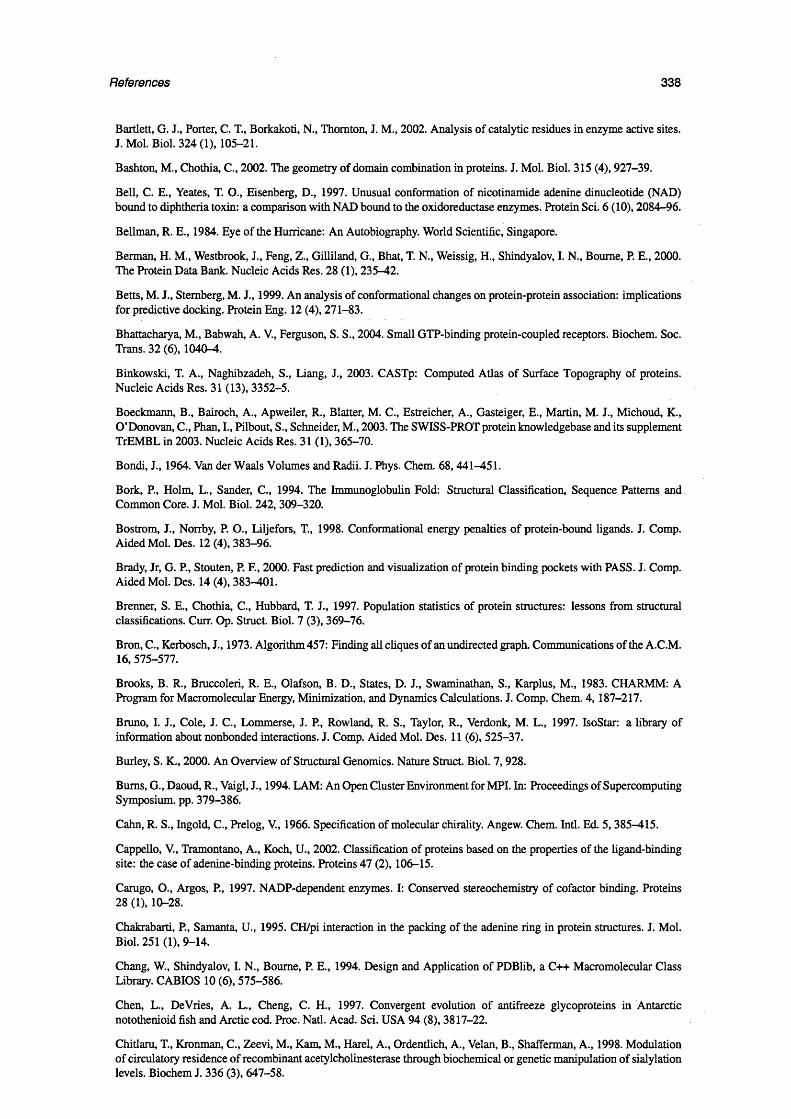
References 338

Bartlett, G. J., Porter, C. T., Borkakoti, N., Thornton, J. M., 2002. Analysis of catalytic residues in enzyme active sites. J. Mol. Biol. 324 (1), 105-21.

Bashton, M., Chothia, C., 2002. The geometry of domain combination in proteins. J. Mol. Biol. 315 (4), 927-39.

Bell, C. E., Yeates, T. O., Eisenberg, D., 1997. Unusual conformation of nicotinamide adenine dinucleotide (NAD) bound to diphtheria toxin: a comparison with NAD bound to the oxidoreductase enzymes. Protein Sci. 6 (10), 2084-96.

Bellman, R. E., 1984. Eye of the Hurricane: An Autobiography. World Scientific, Singapore.

Berman, H. M., Westbrook, J., Feng, Z., Gilliland, G., Bhat, T. N., Weissig, H., Shindyalov, I. N., Bourne, P. E., 2000. The Protein Data Bank. Nucleic Acids Res. 28 (1), 235-42.

Betts, M. J., Sternberg, M. J., 1999. An analysis of conformational changes on protein-protein association: implications for predictive docking. Protein Eng. 12 (4), 271-83.

Bhattacharya, M., Babwah, A. V., Ferguson, S. S., 2004. Small GTP-binding protein-coupled receptors. Biochem. Soc. Trans. 32 (6), 1040-4.

Binkowski, T. A., Naghibzadeh, S., Liang, J., 2003. CASTp: Computed Atlas of Surface Topography of proteins. Nucleic Acids Res. 31 (13), 3352-5.

Boeckmann, B., Bairoch, A., Apweiler, R., Blatter, M. C., Estreicher, A., Gasteiger, E., Martin, M. J., Michoud, K., O’Donovan, C., Phan, I., Pilbout, S., Schneider, M., 2003. The SWISS-PROT protein knowledgebase and its supplement TrEMBL in 2003. Nucleic Acids Res. 31 (1), 365-70.

Bondi, J., 1964. Van der Waals Volumes and Radii. J. Phys. Chem. 68,441-451.

Bork, P., Holm, L., Sander, C., 1994. The Immunoglobulin Fold: Structural Classification, Sequence Patterns and Common Core. J. Mol. Biol. 242, 309-320.

Bostrom, J., Norrby, P. O., Liljefors, T., 1998. Conformational energy penalties of protein-bound ligands. J. Comp. Aided Mol. Des. 12 (4), 383-96.

Brady, Jr, G. P., Stouten, P. F., 2000. Fast prediction and visualization of protein binding pockets with PASS. J. Comp. Aided Mol. Des. 14 (4), 383-401.

Brenner, S. E., Chothia, C., Hubbard, T. J., 1997. Population statistics of protein structures: lessons from structural classifications. Curr. Op. Struct. Biol. 7 (3), 369-76.

Bron, C., Kerbosch, J., 1973. Algorithm 457: Finding all cliques of an undirected graph. Communications of the A.C.M. 16, 575-577.

Brooks, B. R., Bruccoleri, R. E., Olafson, B. D., States, D. J., Swaminathan, S., Karplus, M., 1983. CHARMM: A Program for Macromolecular Energy, Minimization, and Dynamics Calculations. J. Comp. Chem. 4,187-217.

Bruno, I. J., Cole, J. C., Lommerse, J. P., Rowland, R. S., Taylor, R., Verdonk, M. L., 1997. IsoStar: a library of information about nonbonded interactions. J. Comp. Aided Mol. Des. 11 (6), 525-37.

Burley, S. K., 2000. An Overview of Structural Genomics. Nature Struct. Biol. 7,928.

Bums, G., Daoud, R., Vaigl, J., 1994. LAM: An Open Cluster Environment for MPI. In: Proceedings of Supercomputing Symposium, pp. 379-386.

Cahn, R. S., Ingold, C., Prelog, V., 1966. Specification of molecular chirality. Angew. Chem. Intl. Ed. 5, 385-415.

Cappello, V., Tramontano, A., Koch, U., 2002. Classification of proteins based on the properties of the ligand-binding site: the case of adenine-binding proteins. Proteins 47 (2), 106-15.

Carugo, O., Argos, P., 1997. NADP-dependent enzymes. I: Conserved stereochemistry of cofactor binding. Proteins 28 (1), 10-28.

Chakrabarti, P., Samanta, U., 1995. CH/pi interaction in the packing of the adenine ring in protein structures. J. Mol. Biol. 251 (1), 9-14.

Chang, W., Shindyalov, I. N., Bourne, P. E., 1994. Design and Application of PDBlib, a C++ Macromolecular Class Library. CABIOS 10 (6), 575-586.

Chen, L., DeVries, A. L., Cheng, C. H., 1997. Convergent evolution of antifreeze glycoproteins in Antarctic notothenioid fish and Arctic cod. Proc. Natl. Acad. Sci. USA 94 (8), 3817-22.

Chitlaru, T., Kronman, C., Zeevi, M., Kam, M., Harel, A., Ordentlich, A., Velan, B., Shafferman, A., 1998. Modulation of circulatory residence of recombinant acetylcholinesterase through biochemical or genetic manipulation of sialylation levels. Biochem J. 336 (3), 647-58.

References 339

Chothia, C., 1984. Principles that determine the structure of proteins. Ann. Rev. Biochem. 53, 537-72.

Chothia, C., 1992. Proteins. One thousand families for the molecular biologist. Nature 357 (6379), 543-4.

Collaborative Computational Project Number 4,1994. The CCP suite: Programs for protein crystallography. Acta Cryst. D50,760-763.

Copley, R. R., Bork, P., 2000. Homology among (betaalpha)(8) barrels: implications for the evolution of metabolic pathways. J. Mol. Biol. 303 (4), 627-41.

Cowtan, K., 2000. The Clipper Project. http://http://www.ysbl.york.ac.uk/~cowtan/clipper/clipper.html.

CRAN, 1996. The Comprehensive R Archive Network. http://lib.stat.cmu.edu/R/CRAN.

Creighton, T. E., 1993. Proteins: Structure and Molecular Properties, 2nd Edition. W.H. Freeman, New York.

Czamecki, K., Eisenecker, U., 2000. Generative Programming: Methods, Tools, and Applications. Addison-Wesley, Reading, MA.

Dalby, A., Nourse, J. G., Hounshell, W. D., Gushurst, A. K. I., Grier, D. L., Leland, B. A., Laufer, J., 1992. Description of several chemical structure file formats used by computer programs developed at Molecular Design Limited. J. Chem. Inf. Comp. Sci. 32 (3), 244-255.

Dayhoff, M., Schwartz, R., Orcutt, B., 1978. Atlas of Protein Sequence and Structure. Vol. 5. National Biomedical Research Foundation, Washington, D.C., Ch. A model of evolutionary change in proteins, pp. 345-352.

de Berg, M., van Kreveld, M., Overmars, M., Schwarzkopf, O., 1997. Computational Geometry (Algorithms and Applications). Springer-Verlag, Berlin Heidelberg.

DeLano, W. L., 2002. The PyMOL molecular graphics program, http://www.pymol.org.

Denessiouk, K., Johnson, M., 2000. When fold is not important: a common structural framework for adenine and AMP binding in 12 unrelated protein families. Proteins 38 (3), 310-26.

Denessiouk, K., Johnson, M., 2003. ’’Acceptor-donor-acceptor” motifs recognize the Watson-Crick, Hoogsteen and Sugar ”donor-acceptor-donor” edges of adenine and adenosine-containing ligands. J. Mol. Biol. 333 (5), 1025-43.

Denessiouk, K., Rantanen, V., Johnson, M., 2001. Adenine recognition: a motif present in ATP-, CoA-, NAD-, NADP-, and FAD-dependent proteins. Proteins 44 (3), 282-91.

Dortu, F., Gezelter, D., Guha, R., Han, Y., Hartmann, K., Horlacher, O., Howard, M., Josten, G., Krassavine, A., Kuhn,S., Luttmann, E., Mazuir, N., Michels, S., Murray-Rust, P., Pudney, C., Rienstra-Kiracofe, J., Robinson, D., Sandhu, B., Senecal, J.-S., Sild, S., Smith, B., Steinbeck, C., Tomkinson, S., Wegner, J., Wemer, S., Willighagen, E., Zhang, Y., 2000. The Chemistry Development Kit. http://cdk.sourceforge.net.

Downs, G. M., 2003. Handbook of Cheminformatics: From Data to Knowledge. Vol. 1. Wiley-VCH, Weinheim, Ch. Ring Perception, pp.161-177.

Dym, O., Eisenberg, D., 2001. Sequence-structure analysis of FAD-containing proteins. Protein Sci. 10 (9), 1712-28.

Edgar, R. C., 2004. MUSCLE: multiple sequence alignment with high accuracy and high throughput. Nucleic Acids Res. 32 (5), 1792-7.

Eisen, M. B., Wiley, D. C., Karplus, M., Hubbard, R. E., 1994. HOOK: a program for finding novel molecular architectures that satisfy the chemical and steric requirements of a macromolecule binding site. Proteins 19 (3), 199- 221 .

Engh, R. A., Huber, R., 1991. Accurate bond and angle parameters for X-ray protein structure refinement. Acta Cryst. A47, 392-400.

Eriani, G., Delarue, M., Poch, O., Gangloff, J., Moras, D., 1990. Partition of tRNA synthetases into two classes based on mutually exclusive sets of sequence motifs. Nature 347 (6289), 203-6.

Eriksson, M., Uhlin, U., Ramaswamy, S., Ekberg, M., Regnstrom, K., Sjoberg, B. M., Eklund, H., 1997. Binding of allosteric effectors to ribonucleotide reductase protein Rl: reduction of active-site cysteines promotes substrate binding. Structure 5 (8), 1077-92.

Fan, B. T., Panaye, A., Doucet, J. P., Barbu, A., 1993. Ring perception. A new algorithm for directly finding the smallest set of smallest rings from a connection table. J. Chem. Inf. Comp. Sci. 33 (5), 657-662.

Felsenstein, J., 1985. Confidence limits on phylogenies - an approach using the bootstrap. Evolution 39 (4), 783-791.

Fersht, A. R., 1999. Structure and Mechanism in Protein Science. W.H. Freeman, New York.

References 340

Fetrow, J., Skolnick, J., 1998. Method for prediction of protein function from sequence using the sequence-to-structure- to-fimction paradigm with application to glutaredoxins/thioredoxins and T1 ribonucleases. J. Mol. Biol. 281 (5), 949- 68 .

Figueras, J., 1996. Ring Perception Using Breadth-First Search. J. Chem. Inf. Comp. Sci. 36 (5), 986-991.

Fishman, P. H., 1990. ADP-ribosylating Toxins and G Proteins. American Society of Microbiology, Washington, DC, Ch. Mechanism of action of cholera toxin, pp. 127-140.

Flower, D. R., 1996. The lipocalin protein family: structure and function. Biochem. J. 318 (1), 1-14.

Floyd, R. W., 1962. Algorithm 97: Shortest path. Communications of the A.C.M. 5 (6), 345.

Gamma, E., Helm, R., Johnson, R., Vlissides, J., 1995. Design patterns: elements of reusable software. Addison-Wesley, Reading, MA.

Gardiner, E. J., Willett, P., Artymiuk, P. J., 2000. Graph-theoretic techniques for macromolecular docking. J. Chem. Inf. Comp. Sci. 40 (2), 273-9.

Garey, M., Johnson, D., 1979. Computers and Intractability; A Guide to the Theory of NP-Completeness. Freeman, New York.

Garman, E., 1999. Cool data: quantity AND quality. Acta Cryst. D55 (10), 1641-53.

Gasteiger, J., Rudolph, C., Sadowski, J., 1990. Automatic Generation of 3D-Atomic Coordinates for Organic Molecules. Tetrahedron Comput. Methodol. 3, 537-547.

Gerstein, M., Altman, R., 1995. Average core structures and variability measures for protein families: application to the immunoglobulins. J. Mol. Biol. 251 (1), 161-75.

Gibbons, A., 1985. Algorithmic Graph Theory. Cambridge University Press, Cambridge, UK.

Glasfeld, A., Leanz, G. F., Benner, S. A., 1990. The stereospecificities of seven dehydrogenases from Acholeplasma laidlawii. The simplest historical model that explains dehydrogenase stereospecificity. J. Biol. Chem. 265 (20), 11692-9.

Goodford, P., 1985. A computational procedure for determining energetically favorable binding sites on biologically important macromolecules. J. Med. Chem. 28 (7), 849-57.

Halperin, I., Ma, B., Wolfson, H., Nussinov, R., 2002. Principles of docking: An overview of search algorithms and a guide to scoring functions. Proteins 47 (4), 409-43.

Hammes, G. G., 2002. Multiple conformational changes in enzyme catalysis. Biochemistry 41 (26), 8221-8.

Hardin, N. H., Sloane, N. J. A., 1996. McLaren’s Improved Snub Cube and Other New Spherical Designs in Three Dimensions. Discrete and Computational Geometry 15,429-441.

Harrison, A., Pearl, F., Sillitoe, I., Slidel, T., Mott, R., Thornton, J., Orengo, C., 2003. Recognizing the fold of a protein structure. Bioinformatics 19 (14), 1748-59.

Hedstrom, L., 2002. Serine protease mechanism and specificity. Chem. Rev. 102 (12), 4501-24.

Hefti, M. H., Vervoort, J., van Berkel, W. J., 2003. Deflavination and reconstitution of flavoproteins. Eur. J. Biochem. 270 (21), 4227-42.

Hegyi, H., Gerstein, M., 1999. The relationship between protein structure and function: a comprehensive survey with application to the yeast genome. J. Mol. Biol. 288 (1), 147-64.

Hendlich, M., Rippmann, F., Bamickel, G., 1997. LIGSITE: automatic and efficient detection of potential small molecule-binding sites in proteins. J. Mol. Graph. Model. 15 (6), 359-63.

Henikoff, S., Henikoff, J., 1992. Amino acid substitution matrices from protein blocks. Proc. Nad. Acad. Sci. U SA 89 (22), 10915-9.

Henrick, K., Thornton, J., 1998. PQS: a protein quaternary structure file server. Trends Biochem. Sci. 23 (9), 358-61.

Higgins, C. L., Muralidhara, B. K., Wittung-Stafshede, P., 2005. How do cofactors modulate protein folding? Protein Pept. Lett. 12 (2), 165-70.

Higgins, D. G., Sharp, P. M., 1989. Fast and sensitive multiple sequence alignments on a microcomputer. Comp. Appl. Biosci. 5 (2), 151-3.

Hinsen, K., 2000. The molecular modeling toolkit: A new approach to molecular simulations. J. Comp. Chem. 21 (2), 79-85.

References 341

Ho, C. M., Marshall, G. R., 1990. Cavity search: an algorithm for the isolation and display of cavity-like binding regions. J. Comp. Aided Mol. Des. 4 (4), 337-54.

Holm, L., Sander, C., 1995. Dali: a network tool for protein structure comparison. Trends Biochem. Sci. 20 (11), 478-80.

IBM, 1954. Preliminary Report, Specifications for the IBM Mathematical FORmula TRANslation System, FORTRAN. Tech. rep., IBM Corporation, New York.

Ihaka, R., Gentleman, R., 1996. R: A language for data analysis and graphics. Journal of Computational and Graphical Statistics 5 (3), 299-314.

Ihlenfeldt, W. D., Takahashi, Y., Abe, H., Sasaki, S., 1994. Computation and Management of Chemical Properties in CACTVS: An extensible Networked Approach toward Modularity and Flexibility. J. Chem. Inf. Comp. Sci. 34, 109- 116. . . . . . .

Inc., S. M., 1994. Standard Template Library, http://www.sgi.com/tech/stl/.

Inc., S. M„ 1995. Java programming language, http://java.sun.com.

Institute of Electrical and Electronic Engineers, 1987. IEEE standard 754. Tech. rep., Institute of Electrical and Electronic Engineers.

ISO/IEC Information Technology Task Force, 1998. Programming Language C++. Tech. Rep. 14882:1998, International Organization for Standardization.

IUPAC Commission, 1974. Rules for the nomenclature of organic chemistry, Section E: Stereochemistry, Recommendations. Pure Appl. Chem. 45,11-30.

IUPAC-IUB, 1983. Nomenclature Committee of IUB (NC-IUB) and IUB-IUPAC Joint Commission on Biochemical Nomenclature (JCBN): Newsletter 1983. Biochem J 209 (1), I-IV.

Jackson, R. M., Gabb, H. A., Sternberg, M. J., 1998. Rapid refinement of protein interfaces incorporating solvation: application to the docking problem. J. Mol. Biol. 276 (1), 265-85.

Jardine, N., Sibson, R., 1971. Mathematical Taxonomy. Wiley, London.

Jeffrey, G. A., Saenger, W., 1991. Hydrogen Bonding in Biological Structures. Springer-Verlag, Berlin.

Jones, S., Stewart, M., Michie, A., Swindells, M. B., Orengo, C., Thornton, J. M., 1998. Domain assignment for protein structures using a consensus approach: characterization and analysis. Protein Sci. 7 (2), 233-42.

Jurgens, C., Strom, A., Wegener, D., Hettwer, S., Wilmans, M., Sterner, R., 2000. Directed evolution of a (beta alpha)8- barrel enzyme to catalyze related reactions in two different metabolic pathways. Proc. Natl. Acad. Sci. USA 97 (18), 9925-30.

Karmirantzou, M., Thornton, J., 1998. Rational Molecular Design in Drug Research. Alfred Benzon Symposium 42, Munksgaard, Copenhagen, Denmark, Ch. Computational approaches to protein ligand interactions: protein-heme complexes, pp. 264—279.

Kastenholz, M., Pastor, M., Cruciani, G., Haaksma, E., Fox, T., 2000. GRID/CPCA: a new computational tool to design selective ligands. J. Med. Chem. 43 (16), 3033-44.

Kearsley, S. K., 1989. On the orthogonal transformation used for structural comparisons. Acta Cryst. A45,208-210.

Kho, R., Baker, B. L., Newman, J. V., Jack, R. M., Sem, D. S., Villar, H. O., Hansen, M. R., 2003. A path from primary protein sequence to ligand recognition. Proteins 50 (4), 589-99.

Kinoshita, K., Furui, J., Nakamura, H., 2002. Identification of protein functions from a molecular surface database, eF-site. J. Struct. Funct. Genomics. 2 (1), 9-22.

Kleywegt, G. J., Jones, T. A., 1994. Detection, delineation, measurement and display of cavities in macromolecular structures. Acta Cryst. D50 (2), 178-85.

Klyne, W., Prelog, V., 1960. Experientia 16,521-523.

Kobayashi, N., Go, N., 1997. A method to search for similar protein local structures at ligand binding sites and its application to adenine recognition. Eur. Biophys. J. 26 (2), 135-414.

Kohlbacher, O., Lenhof, H., 2000. BALL - Rapid Software Prototyping in Computational Molecular Biology. Bioinformatics 16 (9), 815-824.

References 342

Koshland, D. E., 1958. Application of a theory of enzyme specificity to protein synthesis. Proc. Natl. Acad. Sci. USA 44,98-123.

Krebs, E. G., 1989. Role of the cyclic AMP-dependent protein kinase in signal transduction. JAMA 262,1815-1818.

Krissinel, E. B., 2002. CCP4 Coordinate Library Project, http://www.ebi.ac.uk/keb/cldoc/.

Krissinel, E. B., Henrick, K., 2004a. Common subgraph isomorphism detection by backtracking search. Softw. Pract. Exper. 34 (6), 591-607.

Krissinel, E. B., Henrick, K., 2004b. Secondary Structure Matching (SSM), a new tool for fast protein structure alignment in 3D. Acta Cryst. D60 (12), 2256-68.

Kruskal, J. B., Wish, M., 1977. Multidimensional scaling. Sage Publications, Beverly Hills, CA.

Kuttner, Y., Sobolev, V., Raskind, A., Edelman, M., 2003. A consensus-binding structure for adenine at the atomic level permits searching for the ligand site in a wide spectrum of adenine-containing complexes. Proteins 52 (3), 400-11.

Labute, P., 2005. On the perception of molecules from 3D Atomic Coordinates. J. Chem. Inf. Model. 45 (2), 215-21.

Lamdan, Y., Wolfson, H., 1988. Geometric hashing: A general and efficient model-based recognition scheme. In: Proceedings of the International Conference of Computer Vision.

Lamport, L., 1985. LaTeX: A Document Preparation System Addison Wesley.

Lanyon, S. M., 1985. Detecting internal inconsistencies in distance data. Systematic Zoology 34 (4), 397-403.

Laskowski, R. A., 1995. SURFNET: a program for visualizing molecular surfaces, cavities, and intermolecular interactions. J. Mol. Graph. 13 (5), 323-30,307-8.

Laskowski, R. A., MacArthur, M. W., Moss, D. S., Thornton, J. M., 1993. PROCHECK: A program to check the stereochemical quality of protein structures. J. Appl. Cryst. 26,283-291.

Laskowski, R. A., Thornton, J. M., Humblet, C., Singh, J., 1996. X-SITE: use of empirically derived atomic packing preferences to identify favourable interaction regions in the binding sites of proteins. J. Mol. Biol. 259 (1), 175-201.

Laskowski, R. A., Watson, J. D., Thornton, J. M., 2003. From protein structure to biochemical function? J. Struct. Funct. Genomics 4 (2-3), 167-77.

Lau, S. K., Chass, G. A., Lovas, S., Penke, B., Csizmadia, I. G., 2003. An exploratory ab initio conformational analysis of selected fragments of nicotinamide adenine dinucleotide (NAD+). Part II: adenosine. J. Mol. Struct. (THEOCHEM) 666,431-437.

Laurie, A. T., Jackson, R. M., 2005. Q-SiteFinder: an energy-based method for the prediction of protein-ligand binding sites. Bioinformatics 21 (9), 1908-16.

Lennon, B. W., Wiliams, C. H. J., Ludwig, M. L., 1999. Crystal structure of reduced thioredoxin reductase from Escherichia coli: Structural flexibility in the isoalloxine ring of the flavin adenine dinucleotide cofactor. Protein Sci. 8, 2366-2379.

Lesk, A. M., 1995. NAD-binding domains of dehydrogenases. Curr. Op. Struct. Biol. 5 (6), 775-83.

Levitt, D. G., 2001. A new software routine that automates the fitting of protein X-ray crystallographic electron-density maps. Acta Cryst. D57 (7), 1013-9.

Levitt, D. G., Banaszak, L. J., 1992. POCKET: a computer graphics method for identifying and displaying protein cavities and their surrounding amino acids. J. Mol. Graph. 10 (4), 229-34.

Levitt, M., Chothia, C., 1976. Structural patterns in globular proteins. Nature 261 (5561), 552-8.

Li, A., Nussinov, R., 1998. A set of van der Waals and coulombic radii of protein atoms for molecular and solvent- accessible surface calculation, packing evaluation, and docking. Proteins 32 (1), 111-27.

Lichtarge, O., Bourne, H. R., Cohen, F. E., 1996. An evolutionary trace method defines binding surfaces common to protein families. J. Mol. Biol. 257 (2), 342-58.

Ling, H., Boudsocq, F., Woodgate, R., Yang, W., 2001. Crystal structure of a Y-family DNA polymerase in action: a mechanism for error-prone and lesion-bypass replication. Cell 107 (11), 91-102.

Lipman, D. J., Altschul, S. F., Kececioglu, J. D., 1989. A tool for multiple sequence alignment. Proc. Natl. Acad. Sci. USA 86 (12), 4412-5.

Lorensen, W. E., Cline, H. E., 1997. Marching Cubes: A High iResolution 3D, Surface Construction Algorithm. Proceedings of SIGGRAPH ’87 21 (4), 163-169.

References 343

Lostao, A., Gomez-Moreno, C., Mayhew, S. G., Sancho, J., 1997. Differential stabilization of the three FMN redox forms by tyrosine 94 and tryptophan 57 in flavodoxin from Anabaena and its influence on the redox potentials. Biochemistry 36 (47), 14334—44.

Madej, T., Gibrat, J. F., Bryant, S. H., 1995. Threading a database of protein cores. Proteins 23 (3), 356-69.

Mattos, C., Rasmussen, B., Ding, X., Pestko, G. A., Ringe, D., 1994. Analagous inhibitors of elastase do not always bind analagously. Nature Struct. Biol. 1,55-58.

Message Passing Interface Forum, 1998. MPI: A Message-Passing Interface Standard (version 1.2). http://www. mpi-forum.org.

Meyer, B., 1997. Object-Oriented Software Construction. Prentice Hall PTR, New Jersey.

Milligan, G. W., Cooper, M. C., 1985. An examination of procedures for determining the number of clusters in a data set. Psychometrika 50,159-179.

Miranker, A., Karplus, M., 1991. Functionality maps of binding sites: a multiple copy simultaneous search method. Proteins 11 (1), 29-34.

Mitchell, J., Alex, A., Snarey, M., 1999. SATIS; Atom Typing from Chemical Connectivity. J. Chem Inf. Comp. Sci. 39, 751-757.

Mitchell, J. B., 2001. The relationship between the sequence identities of alpha helical proteins in the PDB and the molecular similarities of their ligands. J. Chem. Inf. Comp. Sci. 41 (6), 1617-22.

Mitchell, P., 1961. Coupling of Phosphorylation to Electron and Hydrogen Transfer by a Chemiosmotic Type of Mechanism. Nature 191,144—148.

Mojena, R., 1977. Hierarchical grouping methods and stopping rules: an evaluation. Computer Journal 20,359-363.

Moodie, S. L., Mitchell, J. B., Thornton, J. M., 1996. Protein recognition of adenylate: an example of a fuzzy recognition template. J. Mol. Biol. 263 (3), 486-500.

Moodie, S. L., Thornton, J. M., 1993. A study into the effects of protein binding on nucleotide conformation. Nucleic Acids Res. 21 (6), 1369-80.

Morris, A. L., MacArthur, M. W., Hutchison, E. G., Thorton, J. M., 1992. Assessing the Accuracy of Protein Structural Coordinates. Proteins 12, 345-364.

Moult, J., Melamud, E., 2000. From fold to function. Curr. Op. Struct. Biol. 10 (3), 384—9.

Mueller-Dieckmann, C., Ritter, H., Haag, F., Koch-Nolte, F„ Schulz, G. E., 2002. Structure of the ecto-ADP-ribosyl transferase ART2.2 from rat. J. Mol. Biol. 322 (4), 687-96.

Murzin, A. G., Brenner, S. E., Hubbard, T., Chothia, C., 1995. SCOP: a structural classification of proteins database for the investigation of sequences and structures. J. Mol. Biol. 247 (4), 536-40.

Nagano, N., Hutchison, E. G., Thornton, J. M., 1999. Barrel structures in proteins: automatic identification and classification including a sequence analysis of TIM barrels. Protein Sci. 8,2072-2084.

Najmanovich, R., Kuttner, J., Sobolev, V., Edelman, M., 2000. Side-chain flexibility in proteins upon ligand binding. Proteins 39 (3), 261-8.

Needleman, S. B., Wunsch, C. D., 1970. A general method applicable to the search for similarities in the amino acid sequence of two proteins. J. Mol. Biol. 48 (3), 443-53.

Nicklaus, M. C., Wang, S., Driscoll, J. S., Milne, G. W., 1995. Conformational changes of small molecules binding to proteins. Bioorg. Med. Chem. 3 (4), 411-28.

Nobeli, I., Laskowski, R., Valdar, W., Thornton, J., 2001. On the molecular discrimination between adenine and guanine by proteins. Nucleic Acids Res 29 (21), 4294-309.

Notredame, C., Higgins, D. G., Heringa, J., 2000. T-Coffee: A nov/el method for fast and accurate multiple sequence alignment. J. Mol. Biol. 302 (1), 205-17.

Object Management Group, 1995. Unified Modelling Language. htt{p://www.uml.org.

Orengo, C. A., 1999. CORA-topological fingerprints for protein stnactural families. Protein Sci. 8 (4), 699-715.

Orengo, C. A., Flores, T. P., Taylor, W. R., Thornton, J. M., 199J3. Identification and classification of protein fold families. Protein Eng. 6 (5), 485-500.

References 344

Orengo, C. A., Jones, D. T., Thornton, J. M., 1994. Protein superfamilies and domain superfolds. Nature 372 (6507), 631-4.

Orengo, C. A., Michie, A. D., Jones, S., Jones, D. T., Swindells, M. B., Thornton, J. M., 1997. CATH-a hierarchic classification of protein domain structures. Structure 5 (8), 1093-108.

Orengo, C. A., Pearl, F. M. G., Thornton, J. M., 2003. Structural Bioinformatics. Wiley-Liss, Hobocken, NJ, Ch. The CATH Domain Structure Database, pp. 249-272.

Orengo, C. A., Taylor, W. R., 1996. SSAP: sequential structure alignment program for protein structure comparison. Methods Enzymol. 266,617-35.

Orengo, C. A., Thornton, J. M., 1993. Alpha plus beta folds revisited: some favoured motifs. Structure 1 (2), 105-20.

Patthy, L., 1991. Modular exchange principles in proteins. Curr. Op. Struct. Biol. 1, 351-361.

Pearl, F., Todd, A., Sillitoe, I., Dibley, M., Redfem, O., Lewis, T., Bennett, C., Marsden, R., Grant, A., Lee, D., Akpor, A., Maibaum, M., Harrison, A., Dallman, T., Reeves, G., Diboun, I., Addou, S., Lise, S., Johnston, C., Sillero, A., Thornton, J., Orengo, C., 2005. The CATH Domain Structure Database and related resources Gene3D and DHS provide comprehensive domain family information for genome analysis. Nucleic Acids Res. 33 (Database issue), D247-51.

Pearson, K., 1901. On lines and planes of closest fit to systems of points in space. Phil. Mag. 2,559-72.

Perola, E., Charifson, P. S., 2004. Conformational analysis of drug-like molecules bound to proteins: an extensive study of ligand reorganization upon binding. J. Med. Chem. 47 (10), 2499-510.

Perrakis, A., Sixma, T. K., Wilson, K. S., Lamzin, V. S., 1997. wARP: improvement and extension of crystallographic phases by weighted averaging of multiple-refined dummy atomic models. Acta Cryst. D53 (Pt 4), 448-55.

Pickering, S., Bulpitt, A., Efford, N., Gold, N., Westhead, D., 2001. Al-based algorithms for protein surface comparisons. Comput. Chem. 26 (1), 79-84.

Pitt, W. R., Williams, M. A., Steven, M., Sweeney, B., Bleasby, A. J., Moss, D. S., 2001. The Bioinformatics Template Library - generic components for biocomputing. Bioinformatics 17 (8), 729-737.

Poulos, T. L., 1995. Cytochrome P450. Curr. Op. Struct. Biol. 5, 767-774.

Pupko, T., Bell, R., Mayrose, I., Glaser, F., Ben-Tal, N., 2002. Rate4Site: an algorithmic tool for the identification of functional regions in proteins by surface mapping of evolutionary determinants within their homologues. Bioinformatics 18 (Suppl 1), S71-7.

Python Software Foundation, 1990. Python programming language, http://www.python.org.

Qian, C., Fisanick, W., Hartzler, D. E., Chapman, S. W., 1990. Enhanced algorithm for finding the smallest set of smallest rings. J. Chem. Inf. Comp. Sci. 30 (2), 105-110.

Ramachandran, G. N., Sasisekharan, V., 1968. Conformation of polypeptides and proteins. Adv. Protein. Chem. 23, 283-438.

Rantanen, V., Denessiouk, K., Gyllenbeig, M., Koski, T., Johnson* M., 2001. A fragment library based on Gaussian mixtures predicting favorable molecular interactions. J. Mol. Biol. 313 (1), 197-214.

Rantanen, V. V., Gyllenberg, M., Koski, T., Johnson, M. S., 2002. A dissimilarity matrix between protein atom classes based on Gaussian mixtures. Bioinformatics 18 (9), 1257-63.

Ratkiewicz, A., Truong, T. N., 2003. Application of chemical graph theory for automated mechanism generation. J. Chem. Inf. Comp. Sci. 43 (1), 36-44.

Raymond, J. W., Willet, P., 2002. Effectiveness of graph-based and fingerprint-based similarity measures for virtual screening of 2D, chemical structure databases. J. Comp. Aided Mol.. Des. 16 (1), 59-71.

Reddy, B. V. B., Bourne, P. E., 2003. Structural Bioinformatics. Wiley-Liss, Hobocken, NJ, Ch. Protein Structure Evolution and the SCOP Database, pp. 239-248.

Rhodes, G., 2000. Crystallography Made Crystal Clear, 2nd Edition. Elsevier, New York.

Ringe, D., Mattos, C., 1999. Analysis of the binding surfaces of proiteins. Med. Res. Rev. 19 (4), 321-31.

Romesburg, H. C., 1984. Cluster Analysis for Researchers. Lifetime Learning Publications, Belmont, CA.

Rossmann, M. G., 1990. The molecular replacement method. Acta Cryst. A46 (2), 73-82.

Royston, P., 1982. Algorithm AS 181: The W Test for Normality. Applied Statistics 31,176-180.

References 345

Ruf, A., Mennissier de Murcia, J., de Murcia, G., Schulz, G. E., 1996. Structure of the catalytic fragment of poly(AD- ribose) polymerase from chicken. Proc. Natl. Acad. Sci. USA 93 (15), 7481-5.

Russell, R. B., Sasieni, P. D., Sternberg, M. J., 1998. Supersites within superfolds. Binding site similarity in the absence of homology. J. Mol. Biol. 282 (4), 903-18.

Saenger, W., 1984. Principles of Nucleic Acid Structure. Springer-Verlaf, New York.

Sander, C., Schneider, R., 1991. Database of homology-derived protein structures and the structural meaning of sequence alignment. Proteins 9 (1), 56-68.

Schaffer, A. A., Wolf, Y. I., Ponting, C. P., Koonin, E. V., Aravind, L., Altschul, S. E, 1999. IMPALA: matching a protein sequence against a collection of PSI-BLAST-constructed position-specific score matrices. Bioinformatics 15(12), 1000-11.

Schmitt, E., Moulinier, L., Fujiwara, S., Imanaka, T., Thierry, J. C., Moras, D., 1998. Crystal structure of aspartyl-tRNA synthetase from Pyrococcus kodakaraensis KOD: archaeon specificity and catalytic mechanism of adenylate formation. EMBO J. 17 (17), 5227-37.

Schmitt, S., Kuhn, D., Klebe, G., 2002. A new method to detect related function among proteins independent ofsequence and fold homology. J. Mol. Biol. 323 (2), 387-406.

Shannon, C., 1948. A mathematical theory of communication. Bell System Tech. J. 27, 379-423.

Sheridan, R., Holloway, M., McGaughey, G., Mosley, R., Singh, S., 2002. A simple method for visualizing thedifferences between related receptor sites. J. Mol. Graph. Model. 21 (1), 71-9.

Shi, J., Blundell, T., Mizuguchi, K., 2001. FUGUE: sequence-structure homology recognition using environment- specific substitution tables and structure-dependent gap penalties. J. Mol. Biol. 310 (1), 243-57.

Shindyalov, I. N., Bourne, P. E., 1998. Protein structure alignment by incremental combinatorial extension (CE) of the optimal path. Protein Eng. 11 (9), 739-47.

Shrake, A., Rupley, J. A., 1973. Environment and exposure to solvent of protein atoms. Lysozyme and insulin. J. Mol. Biol. 79 (2), 351-71.

Silberschatz, A., Korth, H. F., Sudarshan, S., 1997. Database System Concepts, 3rd Edition. McGraw-Hill, Maidenhead, Berkshire.

Silberstein, M., Dennis, S., Brown, L., Kortvelyesi, T., Clodfelter, K., Vajda, S., 2003. Identification of substrate binding sites in enzymes by computational solvent mapping. J. Mol. Biol. 332 (5), 1095-113.

Singh, S. K., Kumasov, O. V., Chen, B., Robinson, H., Grishin, N. V., Osterman, A. L., Zhang, H., 2002. Crystalstructure of Haemophilus influenzae NadR, protein. A bifunctional enzyme endowed with NMN, adenyltransferase and ribosylnicotinimide kinase activities. J. Biol. Chem. 277 (36), 33291-9.

Skolnick, J., Fetrow, J. S., 2000. From genes to protein structure and function: novel applications of computational approaches in the genomic era. Trends Biotech. 18 (1), 34-9.

Smith, T. F., Waterman, M. S., 1981. Identification of common molecular subsequences. J. Mol. Biol. 147 (1), 195-7.

Sobolev, V., Sorokine, A., Prilusky, J., Abola, E., Edelman, M., 1999. Automated analysis of interatomic contacts in proteins. Bioinformatics 15 (4), 327-32.

Sokal, R. R., Rohlf, F. J., 2003. Biometry, 3rd Edition. WH Freeman, New York.

Sonnhammer, E. L., Kahn, D., 1994. Modular arrangement of proteins as inferred from analysis of homology. ProteinSci. 3 (3), 482-92.

Stivers, J. T., Jiang, Y. L., 2003. A mechanistic perspective on the chemistry of DNA, repair glycosylases. Chem Rev. 103 (7), 2729-59.

Stock, D., Leslie, A. G., Walker, J. E., 1999. Molecular architecture of the rotary motor in ATP, synthase. Science 286 (5445), 1700-5.

Stoddard, B. L., Dean, A., Koshland, Jr, D. E., 1993. Structure of isocitrate dehydrogenase with isocitrate, nicotinamide adenine dinucleotide phosphate, and calcium at 2.5-A resolution: a pseudo-Michaelis ternary complex. Biochemistry 32 (36), 9310-6.

Stroustrup, B., 1995. The C++ Programming Language, 1st Edition. Addison-Wesley, Reading, MA.

Stryer, L., 1995. Biochemistry, 4th Edition. W.H. Freeman, New York.

References 346

Stubbs, M. T., Reyda, S., DuUweber, F., Moller, M., Klebe, G., Dorsch, D., Mederski, W. W., Wurziger, H., 2002. pH- dependent binding modes observed in trypsin crystals: lessons for structure-based drug design. Chembiochem 3 (2-3), 246-9.

Sundaresan, V., Chartron, J., Yamaguchi, M., Stout, C., 2005. Conformational diversity in NAD(H) and interacting transhydrogenase nicotinamide nucleotide binding domains. J. Mol. Biol. 346 (2), 617-29.

Tanner, J. J., Tu, S. C., Barbour, L. J., Bames, C. L., Krause, K. L., 1999. Unusual folded conformation of nicotinamide adenine dinucleotide bound to flavin reductase P. Protein Sci. 8 (9), 1725-32.

Taroni, C., Jones, S., Thornton, J. M., 2000. Analysis and prediction of carbohydrate binding sites. Protein Eng. 13 (2), 89-98.

Taylor, W., 1986. The classification of amino acid conservation. J. Theor. Biol. 119 (2), 205-18.

Terwilliger, T. C., 2000. Maximum-likelihood density modification. Acta Cryst. D56 (8), 965-72.

The Boost Committee, 1998. C++Boost. http://www.boost.org/.

The OpenBabel Team, 2001. OpenBabel. http://sourceforge.net/projects/openbabel/.

Thornton, J. M., Bayley, P. M., 1977. Conformational energy calculations for dinucleotide molecules: a study of the nucleotide coenzyme nicotinamide adenine dinucleotide (NAD+). Biopolymers 16 (9), 1971-86.

Todd, A. E., Orengo, C. A., Thornton, J. M., 2001. Evolution of function in protein superfamilies, from a structural perspective. J. Mol. Biol. 307 (4), 1113-43.

Tonegawa, S., 1983. Somatic generation of antibody diversity. Nature 302 (5909), 575-81.

Torrance, J. W., Bartlett, G. J., Porter, C. T., Thornton, J. M., 2005. Using a library of structural templates to recognise catalytic sites and explore their evolution in homologous families. J. Mol. Biol. 347 (3), 565-81.

Tsuge, H., Nagahama, M., Nishimura, H., Hisatsune, J., Sakaguchi, Y., Itogawa, Y., Katunuma, N., Sakurai, J., 2003. Crystal structure and site-directed mutagenesis of enzymatic components from Clostridium perfringens iota-toxin. J. Mol. Biol. 325 (3), 471-83.

Ullman, J. R., 1976. An algorithm for subgraph isomorphism. Journal of the Association for Computing Machinery 23, 31-42.

Valdar, W., 2002. Scoring residue conservation. Proteins 48 (2), 227-41.

Valdar, W., Thornton, J., 2001a. Protein-protein interfaces: analysis of amino acid conservation in homodimers. Proteins 42 (1), 108-24.

Valdar, W. S., Thornton, J. M., 2001b. Protein-protein interfaces: analysis of amino acid conservation in homodimers. Proteins 42 (1), 108-24.

van den Heuvel, R. H., Westphal, A. H., Heck, A. J., Walsh, M. A., Rovida, S., van Berkel, W. J., Mattevi, A., 2004. Structural studies on flavin reductase PheA2 reveal binding of NAD in an unusual folded conformation and support novel mechanism of action. J. Biol. Chem. 279 (13), 12860-7.

van Heesch, D., 1997. Doxygen. http://http://www.stack.nl/~dimitri/doxygen/.

Vaughan, G. V., 2000. GNU Autoconf, Automake and Libtool. Macmillan, Indianapolis, PA.

Velankar, S., McNeil, P., Mittard-Runte, V., Suarez, A., Barrell, D., Apweiler, R., Henrick, K., 2005. E-MSD: an integrated data resource for bioinformatics. Nucleic Acids Res. 33 (Database issue), D262-5.

Verdonk, M. L., Cole, J. C., Taylor, R., 1999. SuperStar: a knowledge-based approach for identifying interaction sites in proteins. J. Mol. Biol. 289 (4), 1093-108.

Verdonk, M. L., Cole, J. C., Watson, P., Gillet, V., Willett, P., 2001. SuperStar: improved knowledge-based interaction fields for protein binding sites. J. Mol. Biol. 307 (3), 841-59.

Walker, J., Saraste, M., Runswick, M., Gay, N., 1982. Distantly related sequences in the alpha- and beta-subunits of ATP synthase, myosin, kinases and other ATP-requiring enzymes and a common nucleotide binding fold. EMBO J 1 (8), 945-51.

Wall, L., Christiansen, T., Orwant, J., 2000. Programming Perl, 3rd Edition. O’Reilly, Sebastopol, CA.

Wallace, A. C., Laskowski, R. A., Thornton, J. M., Feb. 1995. LIGPLOT: a program to generate schematic diagrams of protein-ligand interactions. Protein Eng. 8 (2), 127-34.

References 347

Wallace, A. C., Laskowski, R. A., Thornton, J. M., 1996. Derivation of 3D coordinate templates for searching structural databases: application to Ser-His-Asp catalytic triads in the serine proteinases and lipases. Protein Sci. 5 (6), 1001-13.

Walsh, J. D., Miller, A.-F., 2003. Flavin reduction potential tuning by substitution and bending. J. Mol. Struct. (THEOCHEM) 623,185-195.

Walsh, M. A., Evans, G., Sanishvili, R., Dementieva, I., Joachimiak, A., 1999. MAD data collection - current trends. Acta Cryst. D55 (10), 1726-32.

Watson, P., Willett, P., Gillet, V., Verdonk, M., 2001. Calculating the knowledge-based similarity of functional groups using crystallographic data. J. Comput. Aided. Mol. Des. 15 (9), 835-57.

Weber, P. C., Pantoliano, M. W., Salemme, F. R., 1995. Crystallographic and thermodynamic comparison of structurally diverse molecules binding to streptavidin. Acta Cryst. D51 (4), 590-596.

Weber, S., 2005. Light-driven enzymatic catalysis of DNA repair: a review of recent biophysical studies on photolyase. Biochim. Biophys. Acta. 1707 (1), 1-23.

Weiner, S. J., Kollman, P. A., Case, D. A., Singh, U. C., Ghio, C., Alagona, G., Profeta, S., Weiner, P., 1984. A new force field for molecular mechanical simulation of nucleic acids and proteins. J. Am. Chem. Soc. 106,765-784.

Westbrook, J., Feng, Z., Jain, S., Bhat, T. N., Thanki, N., Ravichandran, V., Gilliland, G. L., Bluhm, W., Weissig, H., Greer, D. S., Bourne, P. E., Berman, H. M., 2002. The Protein Data Bank: unifying the archive. Nucleic Acids Res. 30 (1), 245-8.

Wilson, C. A., Kreychman, J., Gerstein, M., 2000. Assessing annotation transfer for genomics: quantifying the relations between protein sequence, structure and function through traditional and probabilistic scores. J. Mol. Biol. 297 (1), 233- 49.

Yap, K. L., Ames, J. B., Swindells, M. B., Ikura, M., 1999. Diversity of conformational states and changes within the EF-hand protein superfamily. Proteins 37 (3), 499-507.

Young, G., Householder, A., 1938. Discussion of a set of points in terms of their mutual distances. Psychometrika 3, 19-22.

Zvelebil, M., Barton, G., Taylor, W., Sternberg, M., 1987. Prediction of protein secondary structure and active sites using the alignment of homologous sequences. J. Mol. Biol. 195 (4), 957-61.