Citation: Cohen, M.; Wang, X. Stress

Intensity Factors and T-Stress

Solutions for 3D Asymmetric

Four-Point Shear Specimens. Metals

2022, 12, 1068. https://doi.org/

10.3390/met12071068

Academic Editor:

Alberto Campagnolo

Received: 20 May 2022

Accepted: 20 June 2022

Published: 22 June 2022

Publisher’s Note: MDPI stays neutral

with regard to jurisdictional claims in

published maps and institutional affil-

iations.

Copyright: © 2022 by the authors.

Licensee MDPI, Basel, Switzerland.

This article is an open access article

distributed under the terms and

conditions of the Creative Commons

Attribution (CC BY) license (https://

creativecommons.org/licenses/by/

4.0/).

metals

Article

Stress Intensity Factors and T-Stress Solutions for 3DAsymmetric Four-Point Shear SpecimensMark Cohen and Xin Wang *

Department of Mechanical and Aerospace Engineering, Carleton University, Ottawa, ON K1S 5B6, Canada;mark.e.cohen@outlook.com* Correspondence: xin.wang@carleton.ca

Abstract: In this paper, extensive three-dimensional finite element analysis is conducted to study anasymmetric four-point shear (AFPS) specimen: a widely used mixed-mode I/II fracture test specimen.Complete solutions of fracture mechanics parameters KI, KII, KIII, T11, and T33 have been obtainedfor a wide range of a/W and t/W geometry combinations. It is demonstrated that the thickness ofthe specimen has a significant effect on the variation of fracture parameter values. Their effects onthe crack tip plastic zone are also investigated. The results presented here will be very useful for thetoughness testing of materials under mixed-mode loading conditions.

Keywords: fracture toughness; mixed-mode loading; stress intensity factor; T-stress; asymmetricfour-point shear specimen

1. Introduction

The critical value of stress intensity factor, known as KIC or fracture toughness, pro-vides a means to test materials and geometric predisposition to resist fracture. The mostcommon test specimens to determine KIC are specimens loaded by pure mode I loading,such as single-edge notch beam and compact tension specimens. These specimens are oftenused to represent idealized cases of plane strain fracture under pure mode I loading. Acracked body can, however, be loaded in any number of combinations of three primaryloading directions, or modes. In order to determine the onset of fracture for the othermodes of loading, and combinations thereof, fracture specimens for mixed-mode loadingcases have been developed.

One such specimen, and the focus of this work, is the asymmetric four-point shear(AFPS) specimen described by He, Cao, and Evans [1] (see Figure 1). Note that the distancebetween crack line and the loading points is defined as offset c; the case of c = 0 is shown inFigure 1. This specimen is used to test fracture behaviour under pure mode II (also calledantisymmetric four-point shear, or simply four-point shear (FPS) specimen), when theoffset c = 0 and mixed-mode I/II (called AFPS specimen) loading when the offset c is notzero. Different mixed-mode I/II loading is achieved by varying offset value c. Figure 2a,billustrated these two cases, respectively.

The AFPS specimen has since been used to test fracture behaviour for mixed mode I/IIloading, and 2D solutions were provided by He, Cao, and Evans [1] and later refined byHe and Hutchinson [2]. The fracture cases considered by these researchers are simplifiedby either plane stress or plane strain conditions, where the values of KI and KII are used asthe critical fracture parameters. In all these analyses, the effect of KIII is neglected.

In recent studies, 3D finite element analysis has been used to study the effects of finitethickness on fracture behaviour. In order to account for specimen thickness in the inter-pretation of fracture testing results, comprehensive stress intensity factor (SIF) solutionsfor varying specimen thicknesses are needed. Researchers such as Jin and Wang [3], Kwonand Sun [4], and Nakamura and Parks [5] have looked at the finite-thickness effect for

Metals 2022, 12, 1068. https://doi.org/10.3390/met12071068 https://www.mdpi.com/journal/metals

Metals 2022, 12, 1068 2 of 17

pure mode I or mode II fracture specimens. Recently, Jin et al. [6] studied the mixed-modecompact-tension-shear (CTS) specimen, and the finite thickness effect was also studied.When considering specimens such as AFPS in 3D, it is therefore expected that all threemodes of stress intensity factors, KI, KII and KIII, will be present. No detailed analysis wasavailable until recently.

Metals 2022, 12, x FOR PEER REVIEW 2 of 18

Figure 1. The asymmetric four-point-shear (AFPS) specimen.

Figure 2. Asymmetric four-point-shear (AFPS) specimen: (a) c = 0 (b) c ≠ 0.

The AFPS specimen has since been used to test fracture behaviour for mixed mode I/II loading, and 2D solutions were provided by He, Cao, and Evans [1] and later refined by He and Hutchinson [2]. The fracture cases considered by these researchers are simpli-fied by either plane stress or plane strain conditions, where the values of KI and KII are used as the critical fracture parameters. In all these analyses, the effect of KIII is neglected.

In recent studies, 3D finite element analysis has been used to study the effects of finite thickness on fracture behaviour. In order to account for specimen thickness in the inter-pretation of fracture testing results, comprehensive stress intensity factor (SIF) solutions for varying specimen thicknesses are needed. Researchers such as Jin and Wang [3], Kwon and Sun [4], and Nakamura and Parks [5] have looked at the finite-thickness effect for pure mode I or mode II fracture specimens. Recently, Jin et al. [6] studied the mixed-mode compact-tension-shear (CTS) specimen, and the finite thickness effect was also studied. When considering specimens such as AFPS in 3D, it is therefore expected that all three modes of stress intensity factors, KI, KII and KIII, will be present. No detailed analysis was available until recently.

To help better understand the stress field surrounding the crack tip, the plastic zone can be calculated for given K values. This type of plastic zone analysis determines the plastic zone shape and size for different mixed-mode cases, and is a useful indicator of

Figure 1. The asymmetric four-point-shear (AFPS) specimen.

Metals 2022, 12, x FOR PEER REVIEW 2 of 18

Figure 1. The asymmetric four-point-shear (AFPS) specimen.

Figure 2. Asymmetric four-point-shear (AFPS) specimen: (a) c = 0 (b) c ≠ 0.

The AFPS specimen has since been used to test fracture behaviour for mixed mode I/II loading, and 2D solutions were provided by He, Cao, and Evans [1] and later refined by He and Hutchinson [2]. The fracture cases considered by these researchers are simpli-fied by either plane stress or plane strain conditions, where the values of KI and KII are used as the critical fracture parameters. In all these analyses, the effect of KIII is neglected.

In recent studies, 3D finite element analysis has been used to study the effects of finite thickness on fracture behaviour. In order to account for specimen thickness in the inter-pretation of fracture testing results, comprehensive stress intensity factor (SIF) solutions for varying specimen thicknesses are needed. Researchers such as Jin and Wang [3], Kwon and Sun [4], and Nakamura and Parks [5] have looked at the finite-thickness effect for pure mode I or mode II fracture specimens. Recently, Jin et al. [6] studied the mixed-mode compact-tension-shear (CTS) specimen, and the finite thickness effect was also studied. When considering specimens such as AFPS in 3D, it is therefore expected that all three modes of stress intensity factors, KI, KII and KIII, will be present. No detailed analysis was available until recently.

To help better understand the stress field surrounding the crack tip, the plastic zone can be calculated for given K values. This type of plastic zone analysis determines the plastic zone shape and size for different mixed-mode cases, and is a useful indicator of

Figure 2. Asymmetric four-point-shear (AFPS) specimen: (a) c = 0 (b) c 6= 0.

To help better understand the stress field surrounding the crack tip, the plastic zonecan be calculated for given K values. This type of plastic zone analysis determines theplastic zone shape and size for different mixed-mode cases, and is a useful indicator ofcrack tip stress. By considering specimens in 3D, any variation of the plastic zone along thecrack front can be seen.

Traditional fracture testing of mode I specimens yields a value of KIC that is applicablefor situations of high crack tip constraint, which may be overly conservative. A numberof researchers have shown that it is necessary to include an additional non-singular termin the Williams expansion to adequately describe the stress state surrounding the crack.This non-singular term is known as the T-stress, and forms the basis of the two-parameterfracture mechanics approach, see Betegon and Hancock [7], O’Dowd and Shih [8], andWang [9], for example. Recently, it has been demonstrated that both in-plane T-stress T11and out-of-plane T33 are required to quantify the in-plane and out-of-plane constrainteffect [10–12].

Metals 2022, 12, 1068 3 of 17

In addition, researchers have investigated the effects of T-stress magnitude on theplastic zone, for various mixed-mode cases [13]. The T-stress values for mode I testspecimens have been studied, but calculated values for the mixed-mode AFPS specimenare not readily available.

In this paper, AFPS specimens are studied for a wide variety of plate thicknesses andcrack depths. The resulting fracture parameter solutions are presented and used to predictthe size and shape of the plastic zone at various locations through the specimen’s thickness.

2. Finite Element Model of AFPS Specimen

In this section, the FEA of 3D AFPS specimens is presented.

2.1. 3D FEA Model

The mixed-mode specimen, the AFPS, combines mode II in-plane shear loadingwith mode I opening (or bending) loading by offsetting the crack location, setting upasymmetric loading. The amount of mode I contribution is controlled by the value of c/W,or the crack offset ratio. Figure 1 depicts the AFPS specimen. In the present paper, theresults for c/W = 0 and 0.1 will be presented. In Figure 2a,b, the cases of different c valuesare illustrated.

Geometric parameters were varied in the models created for the mixed mode I/II case:crack length-to-width ratios of a/W = 0.1, 0.2, 0.3, 0.4, 0.5, 0.6, and 0.7; and thickness-to-width ratios of t/W = 0.1, 0.2, 0.5, 1.0, 2.0, and 4.0.

The material was considered to be perfectly elastic, with an elastic modulus of 207GPaand Poisson’s ratio (v) of 0.3, common values for typical engineering materials. An individ-ual case was performed for a value of v = 0 and a thickness ratio t/W = 4.0, to be used as arepresentative 2D case.

The mesh design was a constant 2D mesh across the face of the plate (in the x–y direction,see Figure 3), and was swept along the crack front (z direction). The mesh was refinedaround the loading and boundary condition locations, as well as at the crack tip. Theelement type throughout the model was a 20-noded quadratic element with reducedintegration (C3D20R). At the crack tip, one edge of the element was collapsed to form awedge with the point at the crack. The mesh refinement around the crack tip was doneusing 30 elements angularly around the crack tip (Dassault Systems/ SIMULIA, 2013) [14].Mid-side nodes on the element sides directly adjacent to the crack tip were moved to thequarter point, to better capture the singularity at the crack tip. A typical specimen meshfor a plate with t/W = 1.0 and a/W = 0.1 is shown in Figure 3, and the C3D20R schematic isshown in Figure 4. Through-thickness, between 20 and 50 elements were used to calculatefracture parameters.

Metals 2022, 12, x FOR PEER REVIEW 4 of 18

The mesh was refined in two ways: along the thickness direction, the mesh was re-fined towards the free edge (see Figure 4); and around the crack tip, the mesh was altered to meet the sizing recommended by Abaqus training documentation (Dassault Systems/ SIMULIA, 2013) [14]. Additionally, the mesh was refined around the loading and support points to minimize any potential impact on the crack tip elements.

Figure 3. Typical mesh for the AFPS specimen with a/W = 0.7, c/W = 0.1, and t/W = 1.0.

Figure 4. C3D20R element configuration (Dassault Systèmes/SIMULIA, 2013, data from ref. [14]).

2.2. Loads and Boundary Conditions As seen in Figure 3, load P was applied to the upper loading points while the lower

support points were restrained. The value of P was set, and the force was distributed two-thirds and one-third to the points as shown in the same figure. The load used for each was a function of the plate thickness, where force P was applied as force/unit length. The value of P selected was 525 N/mm, corresponding to 175 N/mm and 350 N/mm applied to each of the two loading points (on top), respectively. Static loading cases were studied here.

The lower support points were modeled as simple supports, and a single node at the bottom corner of the specimen was restrained from displacing along the length direction, preventing the specimen from having excessive displacement during the analysis.

Both the loading and support points were modeled by applying a pressure or re-straining a small strip. The additional mesh refinement helped distribute the stress and deformation across many elements, relieving some of the stress spikes that can occur due to local boundary conditions and loads.

Symmetry was used to simplify the calculation analysis. The midplane (z/t = 0) was chosen as the plane of symmetry, which had an insignificant effect on the results. All results were symmetric about the mid plane, with the exception of KIII, which was anti-symmetric.

2.3. Determination of SIF and T-Stress The FEA models were analyzed using Abaqus built-in contour integral calculation,

which modified the crack tip mesh with collapsed element edges, forming degenerate cube (wedge) elements. A diagram of the element design around the crack tip is shown in

Figure 3. Typical mesh for the AFPS specimen with a/W = 0.7, c/W = 0.1, and t/W = 1.0.

Metals 2022, 12, 1068 4 of 17

Metals 2022, 12, x FOR PEER REVIEW 4 of 18

The mesh was refined in two ways: along the thickness direction, the mesh was re-fined towards the free edge (see Figure 4); and around the crack tip, the mesh was altered to meet the sizing recommended by Abaqus training documentation (Dassault Systems/ SIMULIA, 2013) [14]. Additionally, the mesh was refined around the loading and support points to minimize any potential impact on the crack tip elements.

Figure 3. Typical mesh for the AFPS specimen with a/W = 0.7, c/W = 0.1, and t/W = 1.0.

Figure 4. C3D20R element configuration (Dassault Systèmes/SIMULIA, 2013, data from ref. [14]).

2.2. Loads and Boundary Conditions As seen in Figure 3, load P was applied to the upper loading points while the lower

support points were restrained. The value of P was set, and the force was distributed two-thirds and one-third to the points as shown in the same figure. The load used for each was a function of the plate thickness, where force P was applied as force/unit length. The value of P selected was 525 N/mm, corresponding to 175 N/mm and 350 N/mm applied to each of the two loading points (on top), respectively. Static loading cases were studied here.

The lower support points were modeled as simple supports, and a single node at the bottom corner of the specimen was restrained from displacing along the length direction, preventing the specimen from having excessive displacement during the analysis.

Both the loading and support points were modeled by applying a pressure or re-straining a small strip. The additional mesh refinement helped distribute the stress and deformation across many elements, relieving some of the stress spikes that can occur due to local boundary conditions and loads.

Symmetry was used to simplify the calculation analysis. The midplane (z/t = 0) was chosen as the plane of symmetry, which had an insignificant effect on the results. All results were symmetric about the mid plane, with the exception of KIII, which was anti-symmetric.

2.3. Determination of SIF and T-Stress The FEA models were analyzed using Abaqus built-in contour integral calculation,

which modified the crack tip mesh with collapsed element edges, forming degenerate cube (wedge) elements. A diagram of the element design around the crack tip is shown in

Figure 4. C3D20R element configuration (Dassault Systèmes/SIMULIA, 2013, data from ref. [14]).

Similar meshes were created for each geometric case considered. Many differentmodels were created, with varying numbers of elements from 10,000 to close to 500,000,depending on thickness and crack depth. Mesh convergence studies were performed toensure the FEA results had converged.

The mesh was refined in two ways: along the thickness direction, the mesh was refinedtowards the free edge (see Figure 4); and around the crack tip, the mesh was altered to meetthe sizing recommended by Abaqus training documentation (Dassault Systems/ SIMULIA,2013) [14]. Additionally, the mesh was refined around the loading and support points tominimize any potential impact on the crack tip elements.

2.2. Loads and Boundary Conditions

As seen in Figure 3, load P was applied to the upper loading points while the lowersupport points were restrained. The value of P was set, and the force was distributedtwo-thirds and one-third to the points as shown in the same figure. The load used for eachwas a function of the plate thickness, where force P was applied as force/unit length. Thevalue of P selected was 525 N/mm, corresponding to 175 N/mm and 350 N/mm applied toeach of the two loading points (on top), respectively. Static loading cases were studied here.

The lower support points were modeled as simple supports, and a single node at thebottom corner of the specimen was restrained from displacing along the length direction,preventing the specimen from having excessive displacement during the analysis.

Both the loading and support points were modeled by applying a pressure or re-straining a small strip. The additional mesh refinement helped distribute the stress anddeformation across many elements, relieving some of the stress spikes that can occur dueto local boundary conditions and loads.

Symmetry was used to simplify the calculation analysis. The midplane (z/t = 0) waschosen as the plane of symmetry, which had an insignificant effect on the results. All resultswere symmetric about the mid plane, with the exception of KIII, which was anti-symmetric.

2.3. Determination of SIF and T-Stress

The FEA models were analyzed using Abaqus built-in contour integral calculation,which modified the crack tip mesh with collapsed element edges, forming degeneratecube (wedge) elements. A diagram of the element design around the crack tip is shown inFigure 4. Abaqus calculated SIF values for each node along the crack tip. Five contourswere used for the calculation, and the average of the outer three is presented as the result.For all geometries, convergence of the contour integral indicated that adequate meshingrefinement was met, as values were stable after the first two contours.

These results were then extracted from the output files (.dat and .odb) and processedthrough the use of MATLAB scripts. Using scripted calculations, the results were organized,normalized, and plotted. The expressions used to normalize the results are described inSection 3.1.

Two-dimensional and 3D FEA models were created in Abaqus to reproduce the 2Dresults presented by He and Hutchinson [2] for the four-point shear specimen. Results

Metals 2022, 12, 1068 5 of 17

will be shown in Section 3. Verification of this kind served to confirm the modelling andcalculation techniques that were used to produce the results.

3. SIF and T-Stress Results

To provide a more generalized form of the SIF and T-stress solutions, the results ofthese parameters are normalized as functions of geometry and loading.

3.1. SIF Normalizing Functions

He and Hutchinson [2] provide the mode I and II stress intensity factors as functionsof crack and loading geometry. In a mixed-mode I/II case, KI can be described as a functionof crack and loading geometry:

KRI =

6cQW2

√πaFI(a/W) (1)

where FI is the normalized mode I SIF, a function of crack depth and geometry. KII and KIIIare defined as follows:

KRII =

Q

W12

(a/W)32

(1− a/W)12

FI I(a/W) (2)

KRII I =

Q

W12

(a/W)32

(1− a/W)12

FI I I(a/W) (3)

where FII and FIII are the normalized mode II and III SIFs, and Q is shear force, calculatedas follows:

Q = P(b2 − b1)/(b2 + b1) (4)

3.2. T-Stress Normalizing Functions

The first non-singular term in the Williams expansion is known as T-stress, and thenon-zero components can be described as:

T11 = T (5)

T33 = Ee33 + vT (6)

It is typical, in 2D and 3D cases, for T-stress to be normalized with respect to theloading, or far-field stress. In the case of the AFPS specimen, the loading stress associatedwith T-stress comes from the mode I bending stress. The normalizing factor for the T-stressis introduced as σnom, the nominal bending stress, and is calculated as follows:

σnom =6cQW2 (7)

The normalized T-stress values are presented as

T11 =T11

σnom (8)

T33 =T33

σnom (9)

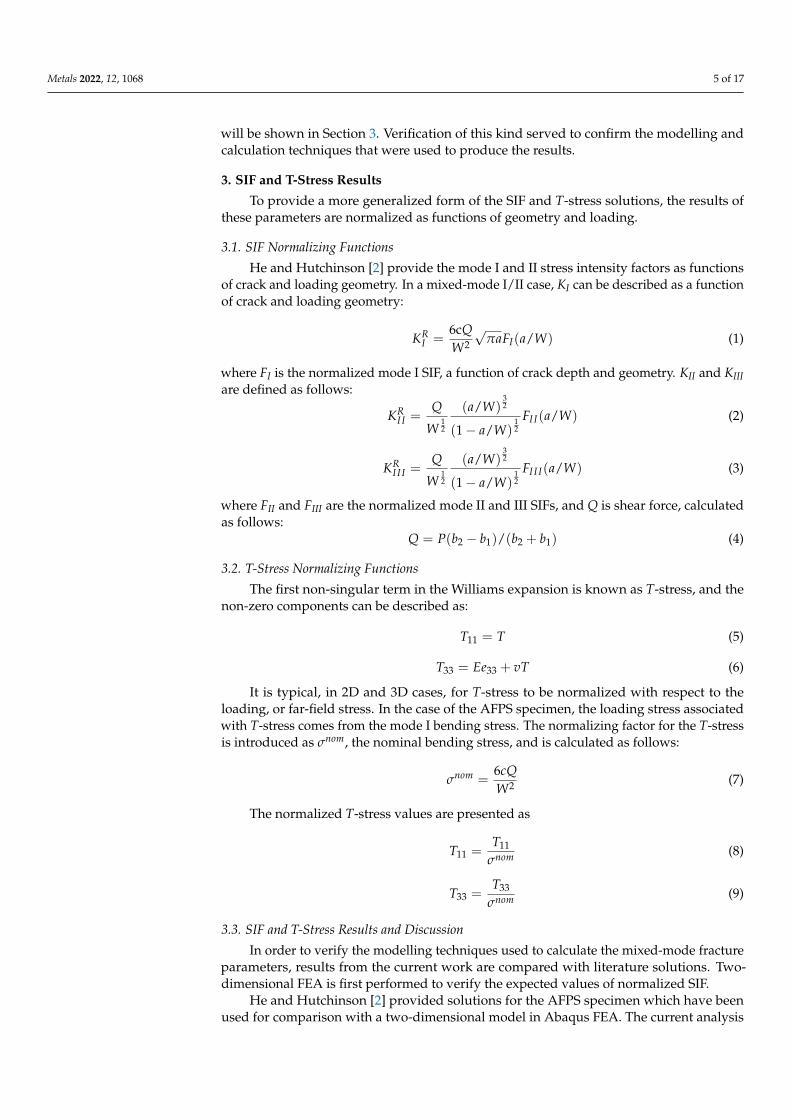
3.3. SIF and T-Stress Results and Discussion

In order to verify the modelling techniques used to calculate the mixed-mode fractureparameters, results from the current work are compared with literature solutions. Two-dimensional FEA is first performed to verify the expected values of normalized SIF.

He and Hutchinson [2] provided solutions for the AFPS specimen which have beenused for comparison with a two-dimensional model in Abaqus FEA. The current analysis

Metals 2022, 12, 1068 6 of 17

shows good agreement with the literature solutions over the full range of crack depthsconsidered. Figure 5 shows the current FEA results for various crack depths and crackoffset ratios (c/W). The percent differences are found to be small for all cases of a/W andc/W, within 1%.

Metals 2022, 12, x FOR PEER REVIEW 6 of 18

𝑇 = 𝑇𝜎 (8)

𝑇 = 𝑇𝜎 (9)

3.3. SIF and T-Stress Results and Discussion In order to verify the modelling techniques used to calculate the mixed-mode fracture

parameters, results from the current work are compared with literature solutions. Two-dimensional FEA is first performed to verify the expected values of normalized SIF.

He and Hutchinson [2] provided solutions for the AFPS specimen which have been used for comparison with a two-dimensional model in Abaqus FEA. The current analysis shows good agreement with the literature solutions over the full range of crack depths considered. Figure 5 shows the current FEA results for various crack depths and crack offset ratios (c/W). The percent differences are found to be small for all cases of a/W and c/W, within 1%.

Figure 5. 2D FEA comparison with literature results.

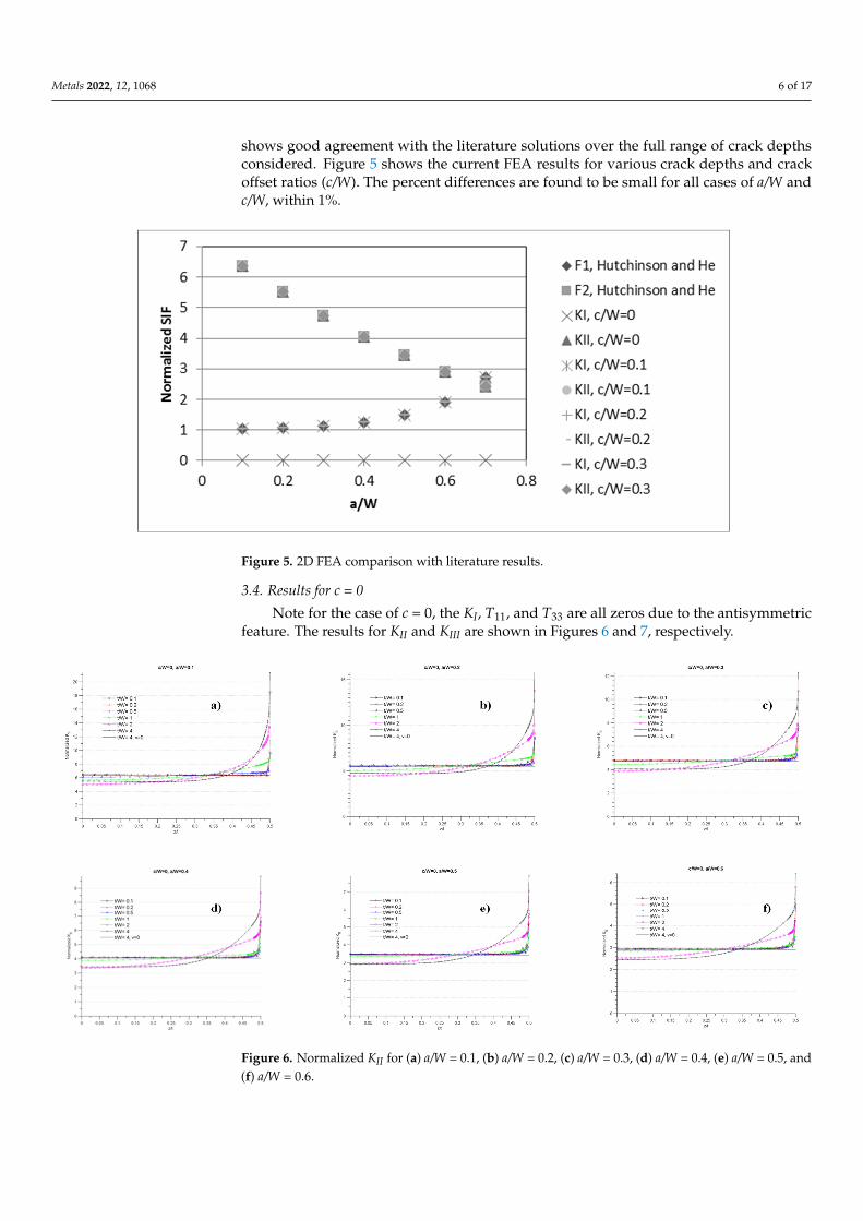
3.4. Results for c = 0 Note for the case of c = 0, the KI, T11, and T33 are all zeros due to the antisymmetric

feature. The results for KII and KIII are shown in Figures 6 and 7, respectively. Of the six thickness cases considered, the results can be split into two groups: thick

plates and thin plates. The cases of t/W = 0.1, 0.2, and 0.5, can be considered as thin plates, and show only minor variation in KII value through-thickness, corresponding well to the 2D literature solutions. From Figure 6a–f it can be seen that the thin plate cases are typi-cally only a few percent from the literature solution at the mid plane. The KII values of these thin plates are fairly constant and positive in value, through the thickness, with a steep increase very close to the free edge (z/t = 0.5).

Figure 5. 2D FEA comparison with literature results.

3.4. Results for c = 0

Note for the case of c = 0, the KI, T11, and T33 are all zeros due to the antisymmetricfeature. The results for KII and KIII are shown in Figures 6 and 7, respectively.

Metals 2022, 12, x FOR PEER REVIEW 7 of 18

Figure 6. Normalized KII for (a) a/W = 0.1, (b) a/W = 0.2, (c) a/W = 0.3, (d) a/W = 0.4, (e) a/W = 0.5, and (f) a/W = 0.6.

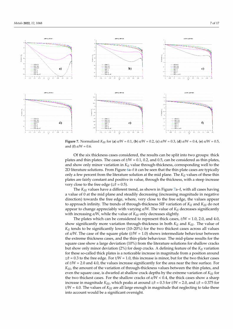
Figure 7. Normalized KIII for (a) a/W = 0.1, (b) a/W = 0.2, (c) a/W = 0.3, (d) a/W = 0.4, (e) a/W = 0.5, and (f) a/W = 0.6.

The KIII values have a different trend, as shown in Figure 7a–f, with all cases having a value of 0 at the mid plane and steadily decreasing (increasing magnitude in negative direction) towards the free edge, where, very close to the free edge, the values appear to approach infinity. The trends of through-thickness SIF variation of KII and KIII do not ap-pear to change appreciably with varying a/W. The value of KII decreases significantly with increasing a/W, while the value of KIII only decreases slightly.

Figure 6. Normalized KII for (a) a/W = 0.1, (b) a/W = 0.2, (c) a/W = 0.3, (d) a/W = 0.4, (e) a/W = 0.5, and(f) a/W = 0.6.

Metals 2022, 12, 1068 7 of 17

Metals 2022, 12, x FOR PEER REVIEW 7 of 18

Figure 6. Normalized KII for (a) a/W = 0.1, (b) a/W = 0.2, (c) a/W = 0.3, (d) a/W = 0.4, (e) a/W = 0.5, and (f) a/W = 0.6.

Figure 7. Normalized KIII for (a) a/W = 0.1, (b) a/W = 0.2, (c) a/W = 0.3, (d) a/W = 0.4, (e) a/W = 0.5, and (f) a/W = 0.6.

The KIII values have a different trend, as shown in Figure 7a–f, with all cases having a value of 0 at the mid plane and steadily decreasing (increasing magnitude in negative direction) towards the free edge, where, very close to the free edge, the values appear to approach infinity. The trends of through-thickness SIF variation of KII and KIII do not ap-pear to change appreciably with varying a/W. The value of KII decreases significantly with increasing a/W, while the value of KIII only decreases slightly.

Figure 7. Normalized KIII for (a) a/W = 0.1, (b) a/W = 0.2, (c) a/W = 0.3, (d) a/W = 0.4, (e) a/W = 0.5,and (f) a/W = 0.6.

Of the six thickness cases considered, the results can be split into two groups: thickplates and thin plates. The cases of t/W = 0.1, 0.2, and 0.5, can be considered as thin plates,and show only minor variation in KII value through-thickness, corresponding well to the2D literature solutions. From Figure 6a–f it can be seen that the thin plate cases are typicallyonly a few percent from the literature solution at the mid plane. The KII values of these thinplates are fairly constant and positive in value, through the thickness, with a steep increasevery close to the free edge (z/t = 0.5).

The KIII values have a different trend, as shown in Figure 7a–f, with all cases havinga value of 0 at the mid plane and steadily decreasing (increasing magnitude in negativedirection) towards the free edge, where, very close to the free edge, the values appearto approach infinity. The trends of through-thickness SIF variation of KII and KIII do notappear to change appreciably with varying a/W. The value of KII decreases significantlywith increasing a/W, while the value of KIII only decreases slightly.

The plates which can be considered to represent thick cases, t/W = 1.0, 2.0, and 4.0,show significantly more variation through-thickness in both KII and KIII. The value ofKII tends to be significantly lower (10–20%) for the two thickest cases across all valuesof a/W. The case of the square plate (t/W = 1.0) shows intermediate behaviour betweenthe extreme thickness cases, and the thin-plate behaviour. The mid-plane results for thesquare case show a large deviation (10%) from the literature solutions for shallow cracksbut show only minor deviation (2%) for deep cracks. A defining feature of the KII variationfor these so-called thick plates is a noticeable increase in magnitude from a position aroundz/t = 0.3 to the free edge. For t/W = 1.0, this increase is minor, but for the two thicker casesof t/W = 2.0 and 4.0, the values increase significantly for the area near the free surface. ForKIII, the amount of the variation of through-thickness values between the thin plates, andeven the square case, is dwarfed at shallow crack depths by the extreme variation of KIII forthe two thickest cases. For the shallow cracks of a/W < 0.4, the thick cases show a sharpincrease in magnitude KIII, which peaks at around z/t = 0.3 for t/W = 2.0, and z/t = 0.375 fort/W = 4.0. The values of KIII are all large enough in magnitude that neglecting to take theseinto account would be a significant oversight.

Metals 2022, 12, 1068 8 of 17

3.5. Results for c = 0.1

Next, typical results of fracture mechanics parameters for a/W = 0.1 and 0.5 withvarying t/W ratios of 0.1, 0.2, 0.5, 1, 2, and 4 are presented in this paper. Figure 8 showsthe results for KI, KII, KIII, and Figure 9 illustrates T11 and T33, respectively. In Figure 8a,d,the mode I SIF values show a general trend of decreasing values of KI as the positionthrough-thickness approaches the free surface. This trend of the KI value dropping towardsthe free surface appears for all thickness cases and for all considered crack depths. Forthe case of thin specimens (t/W < 1.0), the values of KI are all very close and show similarthrough-thickness variation. With increasing thickness appears to be a decreasing valueof KI, an effect that is most pronounced for the shallowest crack (a/W = 0.1) case. The twothickest cases (t/W = 2.0, 4.0) show significantly reduced values of KI located at positions ofz/t = 0.25 up to the free surface when compared with the values of the thinner cases. Theeffect of increasing thickness appears to be most significant at low values of a/W.

Metals 2022, 12, x FOR PEER REVIEW 9 of 18

singularity, different from the standard 1/√𝑟 singularity, which was not considered in the present work.

Figure 8. Results for a/W = 0.1, (a) KI, (b) KII (c) KIII, and a/W = 0.5, (d) KI, (e) KII, and (f) KIII. Figure 8. Results for a/W = 0.1, (a) KI, (b) KII (c) KIII, and a/W = 0.5, (d) KI, (e) KII, and (f) KIII.

In Figure 8b,c,e,f, the SIFs associated with the mode II loading, KII and KIII, are shown.Comparison with the previous results calculated in the pure mode II result (i.e., FPSspecimen, with c = 0), obtained in Section 3.4 is also made, and similar trends are observed.

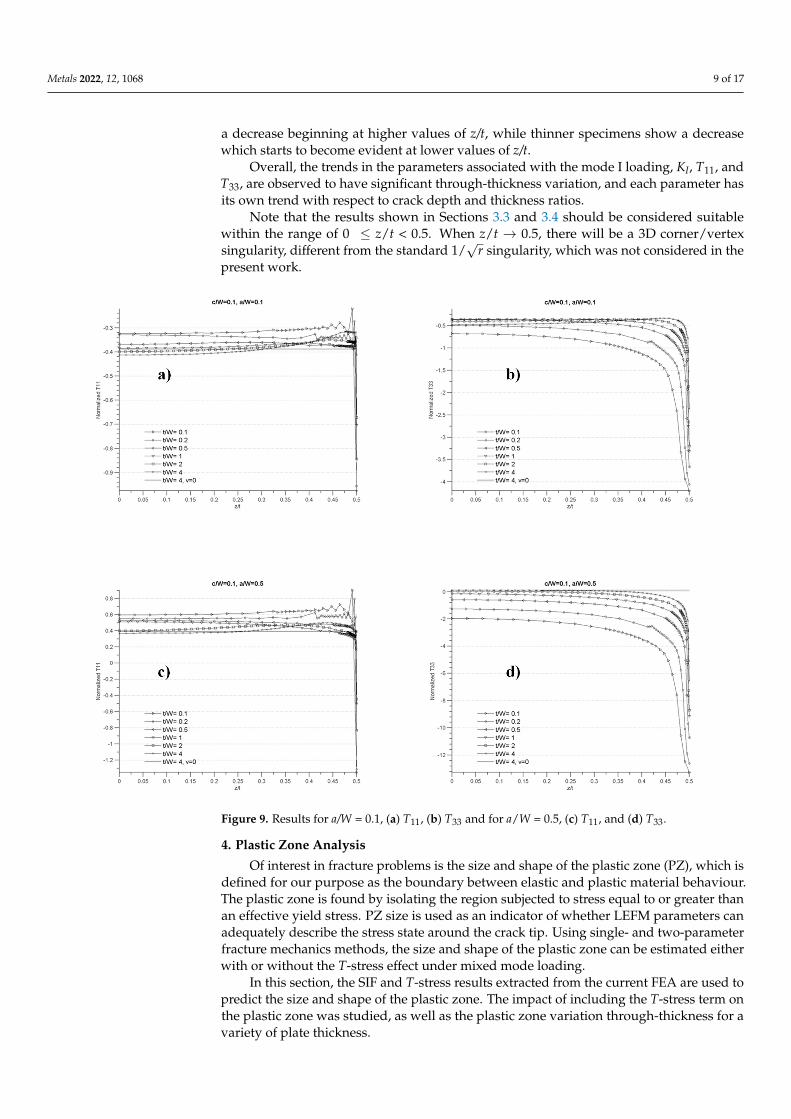
The T11 and T33 results are shown in Figure 9. The trends of T-stress variation through-thickness, and with respect to t/W ratio, are seen to be consistent with the trends identifiedin Jin and Wang [3]. The value of T11 is negative for a/W ≤ 0.3, and positive for thedeeper cracks where a/W > 0.3. The trends of variation through-thickness appear mostlyindependent of a/W, and the value of T11 is, for the most part, constant across the thickness.The values of T11 are observed to increase as thickness decreases, at the midplane andmost of the through-thickness locations. The cases of thicker specimens (t/W > 1.0) showincreasing values of T11 for the locations from z/t = 0.3 up to the free surface.

The plots of T33 show trends that can be described more easily. Thickness appears toinversely correlate to T33 value, where the thinner specimens have a larger magnitude ofT33. T33 increases with increasing a/W ratio, which could be attributed to the fact that thea/W ratio is not considered in the normalizing functions. The value of T33 is also observedto decrease as the position approaches the free surface, with the thicker specimens showing

Metals 2022, 12, 1068 9 of 17

a decrease beginning at higher values of z/t, while thinner specimens show a decreasewhich starts to become evident at lower values of z/t.

Overall, the trends in the parameters associated with the mode I loading, KI, T11, andT33, are observed to have significant through-thickness variation, and each parameter hasits own trend with respect to crack depth and thickness ratios.

Note that the results shown in Sections 3.3 and 3.4 should be considered suitablewithin the range of 0 ≤ z/t < 0.5. When z/t → 0.5, there will be a 3D corner/vertexsingularity, different from the standard 1/

√r singularity, which was not considered in the

present work.

Metals 2022, 12, x FOR PEER REVIEW 10 of 18

Figure 9. Results for a/W = 0.1, (a) T11, (b) T33 and for a/W = 0.5, (c) T11, and (d) T33.

4. Plastic Zone Analysis Of interest in fracture problems is the size and shape of the plastic zone (PZ), which

is defined for our purpose as the boundary between elastic and plastic material behaviour. The plastic zone is found by isolating the region subjected to stress equal to or greater than an effective yield stress. PZ size is used as an indicator of whether LEFM parameters can adequately describe the stress state around the crack tip. Using single- and two-parameter fracture mechanics methods, the size and shape of the plastic zone can be estimated either with or without the T-stress effect under mixed mode loading.

In this section, the SIF and T-stress results extracted from the current FEA are used to predict the size and shape of the plastic zone. The impact of including the T-stress term on the plastic zone was studied, as well as the plastic zone variation through-thickness for a variety of plate thickness.

A method for tracing the boundary of the plastic zone was created and verified against the previous methods of Nazarali and Wang [13]. Current FEA results were used to plot the plastic zone size and shape at various locations through the specimen’s thick-ness.

4.1. Calculating and Plotting the Plastic Zone from LEFM Parameters The William’s series expansion for the stress around a crack tip calculates the stress

components, in polar coordinates, at a distance r from the crack tip and at angle 𝜃. In mixed-mode loading, the mode I, mode II, and mode III stress contributions, together with

Figure 9. Results for a/W = 0.1, (a) T11, (b) T33 and for a/W = 0.5, (c) T11, and (d) T33.

4. Plastic Zone Analysis

Of interest in fracture problems is the size and shape of the plastic zone (PZ), which isdefined for our purpose as the boundary between elastic and plastic material behaviour.The plastic zone is found by isolating the region subjected to stress equal to or greater thanan effective yield stress. PZ size is used as an indicator of whether LEFM parameters canadequately describe the stress state around the crack tip. Using single- and two-parameterfracture mechanics methods, the size and shape of the plastic zone can be estimated eitherwith or without the T-stress effect under mixed mode loading.

In this section, the SIF and T-stress results extracted from the current FEA are used topredict the size and shape of the plastic zone. The impact of including the T-stress term onthe plastic zone was studied, as well as the plastic zone variation through-thickness for avariety of plate thickness.

Metals 2022, 12, 1068 10 of 17

A method for tracing the boundary of the plastic zone was created and verified againstthe previous methods of Nazarali and Wang [13]. Current FEA results were used to plotthe plastic zone size and shape at various locations through the specimen’s thickness.

4.1. Calculating and Plotting the Plastic Zone from LEFM Parameters

The William’s series expansion for the stress around a crack tip calculates the stresscomponents, in polar coordinates, at a distance r from the crack tip and at angle θ. Inmixed-mode loading, the mode I, mode II, and mode III stress contributions, together withT11 and T33, can be obtained from William’s series expansion. The contributions of mode Iloading are

σ11(r, θ) = KI√2πr

cos(

θ2

)[1− sin

(θ2

)sin(

3θ2

)]+ T11

σ22(r, θ) = KI√2πr

cos(

θ2

)[1 + sin

(θ2

)cos(

3θ2

)]σ12(r, θ) = KI√

2πrcos(

θ2

)sin(

θ2

)cos(

3θ2

)σ33(r, θ) = v

(KI√2πr

cos(

θ2

)[1− sin

(θ2

)sin(

3θ2

)]+ σ22

)+ T33

(10)

For mode II loading, the stress state can be described in polar coordinates by thefollowing [15]:

σ11(r, θ) = − KI I√2πr

sin(

θ2

)[2 + cos

(θ2

)cos(

3θ2

)]σ22(r, θ) = KI I√

2πrsin(

θ2

)[cos(

θ2

)cos(

3θ2

)]σ12(r, θ) = KI I√

2πrcos(

θ2

)[1− sin

(θ2

)sin(

3θ2

)]σ33(r, θ) = v(σ11 + σ22)

(11)

where v is Poisson’s ratio.For pure mode III, the stress state can be described as follows:

σ13(r, θ) = − KI I I√2πr

sin(

θ2

)σ23(r, θ) = KI I I√

2πrcos(

θ2

) (12)

Applying the principle of superposition for both modes, the total stress can be calculated:

σij(total) = σij

(I) + σij(I I) + σij

(I I I) (13)

The stress components from Equation (13) are substituted into von Mises’ yield cri-terion. The plastic zone radius is extracted using the process described in Cohen [16]; aneffective SIF, Keff, is used to normalize the plastic zone, and includes the mode I componentas follows:

Ke f f =√

K2I + K2

I I (14)

The plastic zone is normalized using the values only at the midplane; in this way, thethrough-thickness variation of the plastic zone can be clearly seen.

By using the components defined by the Williams’ expansion, a yield criterion can beapplied—in this case, von Mises’ yield criterion. The effective von Mises’ stress is given by:

σe =

√(σ11 − σ22)

2 + (σ22 − σ33)2 + (σ33 − σ11)

2 + 6(σ2

12 + σ223 + σ2

31)

2(15)

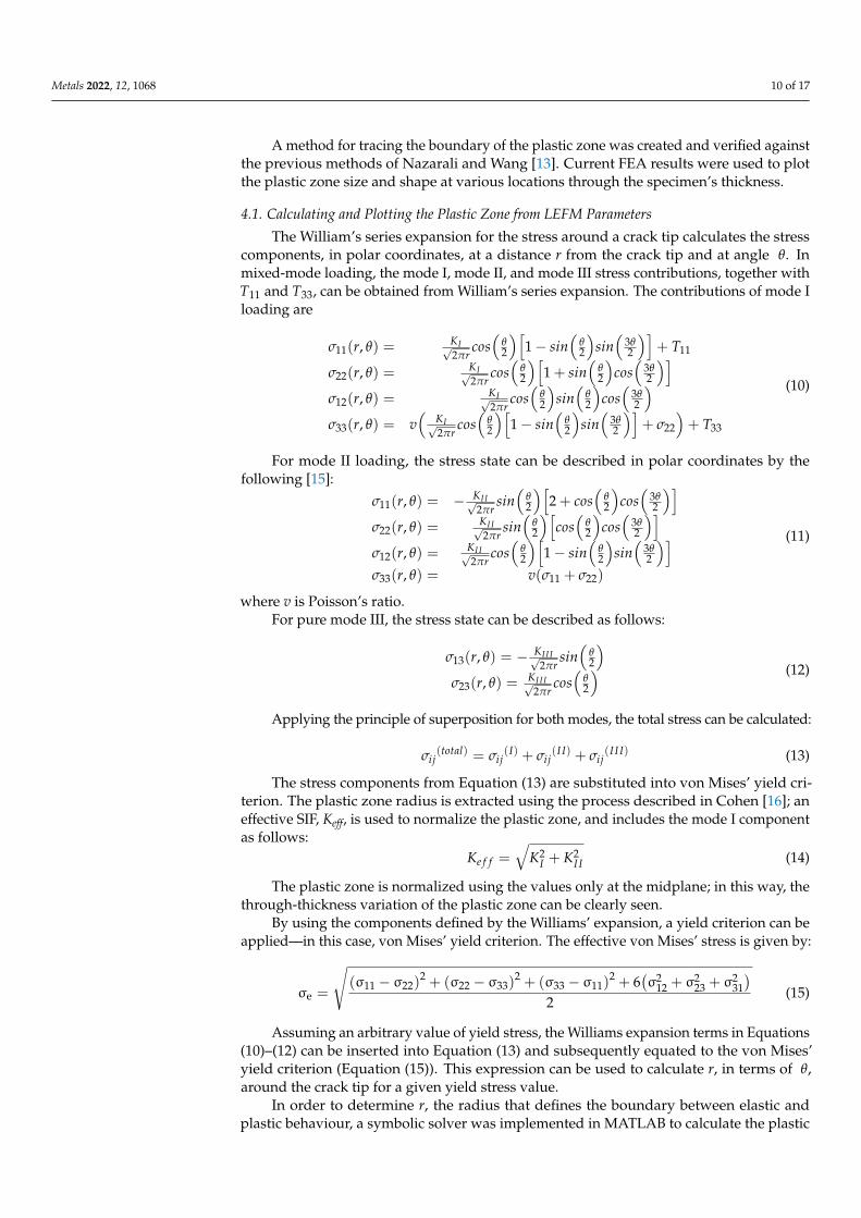
Assuming an arbitrary value of yield stress, the Williams expansion terms in Equations(10)–(12) can be inserted into Equation (13) and subsequently equated to the von Mises’yield criterion (Equation (15)). This expression can be used to calculate r, in terms of θ,around the crack tip for a given yield stress value.

In order to determine r, the radius that defines the boundary between elastic andplastic behaviour, a symbolic solver was implemented in MATLAB to calculate the plastic

Metals 2022, 12, 1068 11 of 17

zone for the FEA results previously presented. The function used in MATLAB was vpasolve,and the variable r, the radial distance from the crack tip in Equations (10)–(12), was assignedas a symbolic variable in MATLAB [17]. Non-normalized SIF values were substituted intoEquation (8), and r was found for the full range of θ at several locations through thethickness. For pure mode II loading, the plastic zone was normalized as a function of Kand yield stress:

Normalized plastic zone radius Rp =r

1π

[KI IσYS

]2 (16)

To show the relative size of the plastic zone at various locations through the specimen’sthickness, the value of KII at the mid plane was used to normalize all values of Rp for eachof the different through-thickness cases. The value of KIII was found to be zero at themid plane for all values of t/W, so the impact of its inclusion in calculating the PZ canbe clearly seen. On the first plastic zone plot, the location of the crack line is shown forillustration purposes.

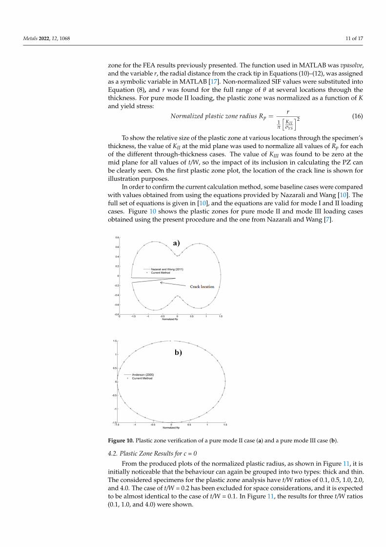
In order to confirm the current calculation method, some baseline cases were comparedwith values obtained from using the equations provided by Nazarali and Wang [10]. Thefull set of equations is given in [10], and the equations are valid for mode I and II loadingcases. Figure 10 shows the plastic zones for pure mode II and mode III loading casesobtained using the present procedure and the one from Nazarali and Wang [7].

Metals 2022, 12, x FOR PEER REVIEW 12 of 18

through the thickness. For pure mode II loading, the plastic zone was normalized as a function of K and yield stress: 𝑁𝑜𝑟𝑚𝑎𝑙𝑖𝑧𝑒𝑑 𝑝𝑙𝑎𝑠𝑡𝑖𝑐 𝑧𝑜𝑛𝑒 𝑟𝑎𝑑𝑖𝑢𝑠 𝑅 = 𝑟1𝜋 𝐾𝜎

(16)

To show the relative size of the plastic zone at various locations through the specimen’s thickness, the value of KII at the mid plane was used to normalize all values of Rp for each of the different through-thickness cases. The value of KIII was found to be zero at the mid plane for all values of t/W, so the impact of its inclusion in calculating the PZ can be clearly seen. On the first plastic zone plot, the location of the crack line is shown for illustration purposes.

In order to confirm the current calculation method, some baseline cases were com-pared with values obtained from using the equations provided by Nazarali and Wang [10]. The full set of equations is given in [10], and the equations are valid for mode I and II loading cases. Figure 10 shows the plastic zones for pure mode II and mode III loading cases obtained using the present procedure and the one from Nazarali and Wang [7].

Figure 10. Plastic zone verification of a pure mode II case (a) and a pure mode III case (b).

4.2. Plastic Zone Results for c = 0 From the produced plots of the normalized plastic radius, as shown in Figure 11, it

is initially noticeable that the behaviour can again be grouped into two types: thick and thin. The considered specimens for the plastic zone analysis have t/W ratios of 0.1, 0.5, 1.0, 2.0, and 4.0. The case of t/W = 0.2 has been excluded for space considerations, and it is expected to be almost identical to the case of t/W = 0.1. In Figure 11, the results for three t/W ratios (0.1, 1.0, and 4.0) were shown.

When comparing the plastic zones, for all cases, the smallest plastic zone (through-thickness) was located at the mid plane, and the plastic zone radius increased at all posi-tions towards the free surface. The value of KIII always reached zero at the mid plane, so

Figure 10. Plastic zone verification of a pure mode II case (a) and a pure mode III case (b).

4.2. Plastic Zone Results for c = 0

From the produced plots of the normalized plastic radius, as shown in Figure 11, it isinitially noticeable that the behaviour can again be grouped into two types: thick and thin.The considered specimens for the plastic zone analysis have t/W ratios of 0.1, 0.5, 1.0, 2.0,and 4.0. The case of t/W = 0.2 has been excluded for space considerations, and it is expectedto be almost identical to the case of t/W = 0.1. In Figure 11, the results for three t/W ratios(0.1, 1.0, and 4.0) were shown.

Metals 2022, 12, 1068 12 of 17Metals 2022, 12, x FOR PEER REVIEW 14 of 18

Figure 11. Plastic zone comparison for (a) t/W = 0.1, a/W = 0.1, (b) t/W = 0.1, a/W = 0.7, (c) t/W = 1.0, a/W = 0.1, (d) t/W = 1.0, a/W = 0.7, and (e) t/W = 4.0, a/W = 0.1, (f) t/W = 4.0, a/W = 0.7.

Figure 11. Plastic zone comparison for (a) t/W = 0.1, a/W = 0.1, (b) t/W = 0.1, a/W = 0.7, (c) t/W = 1.0, a/W = 0.1, (d) t/W = 1.0, a/W = 0.7, and (e) t/W = 4.0, a/W = 0.1,(f) t/W = 4.0, a/W = 0.7.

Metals 2022, 12, 1068 13 of 17

When comparing the plastic zones, for all cases, the smallest plastic zone (through-thickness) was located at the mid plane, and the plastic zone radius increased at all positionstowards the free surface. The value of KIII always reached zero at the mid plane, so theplastic zone in the middle of the plate can be expected to resemble that of pure modeII loading. The relative increase in plastic zone size was small for the thin (t/W = 0.1,0.5) plates considered, but was significant for the thicker cases. The thin plates showeda plastic zone which stayed at a fairly constant size in the shape expected of pure modeII loading. The case of t/W = 1.0 (see Figure 11c,d) showed an increased plastic zone atlocations approaching the free surface, still in the shape of pure mode II loading. The sizeincrease (from the mid plane) of the plastic zone at outer positions appeared to decreasewith increasing a/W, where shallower cracks had larger variations in plastic zone size thandeep cracks.

As might be expected from the significant KIII variations seen in Figure 7, the thickestcases had the largest plastic zone variations of through the specimen’s thickness. Fort/W = 4.0, Figure 11e,f shows an increased plastic zone size, with circular shape, at thelocation close to the free edge. This change in shape and increase in size corresponded withthe high value of KIII at that location through the specimen’s thickness. This effect is mostnoticeable in the shallow-crack case of the thickest plate considered, t/W = 4.0, where theplastic zone at the mid plane appeared to be just a fraction of that at the near-surface point(z/t = 0.375). At this near-surface point, the plastic zone appeared almost perfectly round,and represented a high amount of mode III contribution.

The calculated plastic zone sizes described using the William’s expansion and the vonMises’ yield criterion provided results showing large variations of plastic zone size andshape through-thickness. In order to verify that these predicted values were consistentwith the stress results from elastic FEA, the PZ shape and size were estimated from thestress contour and compared with the prediction for some typical cases.

Image analysis was used to gather data from the FEA stress contours. The FEA-extracted plastic zone data was normalized using the same method and values as used forthe predicted plastic zones. Some typical thickness cases were considered—t/W = 0.1,1.0,and 4.0—for the cases of crack depth extremes, a/W = 0.1 and 0.7. In these figures, thenumber of data points shown for the FEA-extracted results was reduced for clarity.

In the current analysis, for specimens with relatively small plastic zones, for example,mid-plane at shallow cracks, the plastic zone could be confined to be within a singleelement. This was not an ideal situation, as the built-in stress contour within Abaqus mustbe used to approximate the boundary. As seen in the comparison case, the plastic zoneestimated by the SIF solutions showed good agreement with the FEA images for all typicalcases. The thin case, t/W = 0.1, had little variation in through-thickness for both thick andthin cracks. The resulting plots, from Figure 11, show good correlation with size and shapeof the extracted and calculated plastic zones. There was some overlap of the FEA-extractedplastic zones for the two positions in each of the two thin cases, and this was attributed toinaccuracies in the extraction method and coarseness of the contour refinement.

The square (t/W = 1.0) specimen showed very good agreement between the calculatedand extracted values for both crack depth ratios considered. Similar agreement was seenwith the thick case of t/W = 4.0; however, it appeared that the FEA-extracted values wereslightly larger than the calculated values for the shallow crack (a/W = 0.1) case. Thisapparent difference could be attributed to contour coarseness or even mesh coarsenessin the area surrounding the crack. The deep-crack case showed better agreement withthe calculated values and supported the predicted values. Overall, the comparison casesshowed that the plastic zone size and shape, as predicted by the current calculation method,was consistent with results from the FEA stress contours.

4.3. Plastic Zone Results for c = 0.1

In the current analysis, two plastic zone size predictions are made, the first calculatedincluding the effects of only the three SIFs and the second including all SIF and T-stress

Metals 2022, 12, 1068 14 of 17

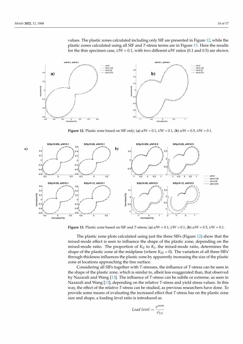
values. The plastic zones calculated including only SIF are presented in Figure 12, while theplastic zones calculated using all SIF and T-stress terms are in Figure 13. Here the resultsfor the thin specimen case, t/W = 0.1, with two different a/W ratios (0.1 and 0.5) are shown.

Metals 2022, 12, x FOR PEER REVIEW 15 of 18

The calculated plastic zone sizes described using the William’s expansion and the von Mises’ yield criterion provided results showing large variations of plastic zone size and shape through-thickness. In order to verify that these predicted values were con-sistent with the stress results from elastic FEA, the PZ shape and size were estimated from the stress contour and compared with the prediction for some typical cases.

Image analysis was used to gather data from the FEA stress contours. The FEA-ex-tracted plastic zone data was normalized using the same method and values as used for the predicted plastic zones. Some typical thickness cases were considered—t/W = 0.1,1.0, and 4.0—for the cases of crack depth extremes, a/W = 0.1 and 0.7. In these figures, the number of data points shown for the FEA-extracted results was reduced for clarity.

In the current analysis, for specimens with relatively small plastic zones, for example, mid-plane at shallow cracks, the plastic zone could be confined to be within a single ele-ment. This was not an ideal situation, as the built-in stress contour within Abaqus must be used to approximate the boundary. As seen in the comparison case, the plastic zone estimated by the SIF solutions showed good agreement with the FEA images for all typical cases. The thin case, t/W = 0.1, had little variation in through-thickness for both thick and thin cracks. The resulting plots, from Figure 11, show good correlation with size and shape of the extracted and calculated plastic zones. There was some overlap of the FEA-extracted plastic zones for the two positions in each of the two thin cases, and this was attributed to inaccuracies in the extraction method and coarseness of the contour refinement.

The square (t/W = 1.0) specimen showed very good agreement between the calculated and extracted values for both crack depth ratios considered. Similar agreement was seen with the thick case of t/W = 4.0; however, it appeared that the FEA-extracted values were slightly larger than the calculated values for the shallow crack (a/W = 0.1) case. This ap-parent difference could be attributed to contour coarseness or even mesh coarseness in the area surrounding the crack. The deep-crack case showed better agreement with the calculated values and supported the predicted values. Overall, the comparison cases showed that the plastic zone size and shape, as predicted by the current calculation method, was consistent with results from the FEA stress contours.

4.3. Plastic Zone Results for c = 0.1 In the current analysis, two plastic zone size predictions are made, the first calculated

including the effects of only the three SIFs and the second including all SIF and T-stress values. The plastic zones calculated including only SIF are presented in Figure 12, while the plastic zones calculated using all SIF and T-stress terms are in Figure 13. Here the results for the thin specimen case, t/W = 0.1, with two different a/W ratios (0.1 and 0.5) are shown.

Figure 12. Plastic zone based on SIF only; (a) a/W = 0.1, t/W = 0.1, (b) a/W = 0.5, t/W = 0.1. Figure 12. Plastic zone based on SIF only; (a) a/W = 0.1, t/W = 0.1, (b) a/W = 0.5, t/W = 0.1.

Metals 2022, 12, x FOR PEER REVIEW 16 of 18

Figure 13. Plastic zone based on SIF and T-stress; (a) a/W = 0.1, t/W = 0.1, (b) a/W = 0.5, t/W = 0.1.

The plastic zone plots calculated using just the three SIFs (Figure 12) show that the mixed-mode effect is seen to influence the shape of the plastic zone, depending on the mixed-mode ratio. The proportion of KII to KI, the mixed-mode ratio, determines the shape of the plastic zone at the midplane (where KIII = 0). The variation of all three SIFs’ through-thickness influences the plastic zone by apparently increasing the size of the plastic zone at locations approaching the free surface.

Considering all SIFs together with T-stresses, the influence of T-stress can be seen in the shape of the plastic zone, which is similar to, albeit less exaggerated than, that ob-served by Nazarali and Wang [13]. The influence of T-stress can be subtle or extreme, as seen in Nazarali and Wang [13], depending on the relative T-stress and yield stress values. In this way, the effect of the relative T-stress can be studied, as previous researchers have done. To provide some means of evaluating the increased effect that T-stress has on the plastic zone size and shape, a loading level ratio is introduced as 𝐿𝑜𝑎𝑑 𝑙𝑒𝑣𝑒𝑙 = 𝜎𝜎

In the current analysis, the values of load level considered are 0.006 (a low-loading scenario), 0.06, 0.09, and 0.12 (a high-loading case), providing a good range of T-stress effects that can be observed. The ratio S/Sy used in the plastic zone plots in Figure 13 refers to the load level ratio σnom/σYS.

By comparing the plastic zone predictions calculated with and without T-stress, the influence of T-stress can be shown. At low load levels, the value of T-stress, with respect to yield stress, is low, and the plastic zone contribution is small. The plastic zone plots for relatively low load levels (σnom/σYS = 0.006, 0.06) show plastic zones consistent with those predicted without T-stress effects. It is clear that for moderate- to larger-scale yielding, the T-stress effects need to be included.

5. Summary and Conclusions From the plots of the results, some key observations can be made about the inclusion

of KIII in the fracture analysis of the FPS specimen. Primarily, it can be seen that the KIII influence on pure mode II loading cannot be ignored and can influence PZ size and shape greatly. The coupling of KII and KIII is caused by Poisson’s ratio’s effects at the free surface, which can be significant for thick specimens. This is seen most easily in the exaggerated case shown in Figure 11e (t/W = 4.0, a/W = 0.1), where a large magnitude of KIII is seen to greatly affect the plastic zone size and shape, resembling a circular shape, similar to that expected of a pure mode III loading scenario. The trends seen in the results indicate that

Figure 13. Plastic zone based on SIF and T-stress; (a) a/W = 0.1, t/W = 0.1, (b) a/W = 0.5, t/W = 0.1.

The plastic zone plots calculated using just the three SIFs (Figure 12) show that themixed-mode effect is seen to influence the shape of the plastic zone, depending on themixed-mode ratio. The proportion of KII to KI, the mixed-mode ratio, determines theshape of the plastic zone at the midplane (where KIII = 0). The variation of all three SIFs’through-thickness influences the plastic zone by apparently increasing the size of the plasticzone at locations approaching the free surface.

Considering all SIFs together with T-stresses, the influence of T-stress can be seen inthe shape of the plastic zone, which is similar to, albeit less exaggerated than, that observedby Nazarali and Wang [13]. The influence of T-stress can be subtle or extreme, as seen inNazarali and Wang [13], depending on the relative T-stress and yield stress values. In thisway, the effect of the relative T-stress can be studied, as previous researchers have done. Toprovide some means of evaluating the increased effect that T-stress has on the plastic zonesize and shape, a loading level ratio is introduced as

Load level =σnom

σYS

Metals 2022, 12, 1068 15 of 17

In the current analysis, the values of load level considered are 0.006 (a low-loadingscenario), 0.06, 0.09, and 0.12 (a high-loading case), providing a good range of T-stresseffects that can be observed. The ratio S/Sy used in the plastic zone plots in Figure 13 refersto the load level ratio σnom/σYS.

By comparing the plastic zone predictions calculated with and without T-stress, theinfluence of T-stress can be shown. At low load levels, the value of T-stress, with respectto yield stress, is low, and the plastic zone contribution is small. The plastic zone plots forrelatively low load levels (σnom/σYS = 0.006, 0.06) show plastic zones consistent with thosepredicted without T-stress effects. It is clear that for moderate- to larger-scale yielding, theT-stress effects need to be included.

5. Summary and Conclusions

From the plots of the results, some key observations can be made about the inclusionof KIII in the fracture analysis of the FPS specimen. Primarily, it can be seen that the KIIIinfluence on pure mode II loading cannot be ignored and can influence PZ size and shapegreatly. The coupling of KII and KIII is caused by Poisson’s ratio’s effects at the free surface,which can be significant for thick specimens. This is seen most easily in the exaggeratedcase shown in Figure 11e (t/W = 4.0, a/W = 0.1), where a large magnitude of KIII is seento greatly affect the plastic zone size and shape, resembling a circular shape, similar tothat expected of a pure mode III loading scenario. The trends seen in the results indicatethat thick plates containing shallow cracks are most affected by the influence of KIII. Thethrough-thickness comparison of SIF variation also showed an interesting trend, with someextreme cases showing significant variation in plastic zone size and shape at differentlocations through the specimen’s thickness.

Another key observation is that the amount of through-thickness variation of KIIappeared to be a function of the thickness of the plate. The trends identified show anincreasing KII variation for increased plate thickness. For the thicker cases (t/W > 1.0), itwas observed that the value of KII at the mid plane was lower than the literature solutionbut increased to higher values closer to the free surface.

To see the total effect of finite-thickness considerations on the pure mode II loadingcase, the PZ size and shape were used as an indicator of crack tip stress state. It wasobserved that the through-thickness variation in the SIFs (increasing magnitude in positiveKII and negative KIII) had a tendency to increase PZ size. Inspection of the von Mises’ yieldcriterion showed that, in the absence of KI, the KIII stress contributions served to increasethe effective stress, which in turn increased the radius of the predicted plastic zone. Theproduced PZ plots show that, for relatively thick plates (t/W ≥ 1.0), the plastic zone is notof constant through the specimen’s thickness and enlarges at locations approaching thefree surface.

The main conclusion that can be drawn from the pure mode II analysis of the FPSspecimen is that the inclusion of 3D effects can have a very large effect on the plastic zoneand stress field surrounding a crack and must be considered. Of the cases consideredin this analysis, the relatively thick (t/W > 1.0) plate specimens were affected most whenshallow cracks were present, with the largest values of KIII and the biggest amount ofthrough-thickness variation. What this could mean, in practical terms, is that the criticalarea to consider in these shallow-crack thick-plate bodies is not necessarily located ateither the mid- or edge plane, but rather at some location between. This conclusion iscounter to the results for KI in pure mode I specimens [3], which showed thick plates ingood agreement with a plane strain 2D reference solution. The current results suggest thatapplying a similar assumption to mode II specimens, when considering mode III influence,would be incorrect.

The current analysis also suggests that for thin plates (t/W < 1.0), the variation ofthrough-thickness appears to be less significant than for thick plates, and the inclusion ofthe KIII term has a less pronounced effect. This conclusion is arrived at after inspection of theplastic zone plots, which can be used qualitatively to estimate the influence of each mode’s

Metals 2022, 12, 1068 16 of 17

SIF. Thin FPS fracture specimens appear to be consistent with the 2D reference solutions,and test results could be interpreted using these solutions with reasonable accuracy.

The fracture parameter solutions obtained in this work will be very useful for fracturetoughness testing of FPS specimens. The results of the plastic zone analysis performed inthis work provide a clear illustration of the 3D effects on fracture specimens of varyingthicknesses undergoing pure mode II loading.

From the analysis of the AFPS specimen, it is found that finite thickness effects havesignificant effect on the fracture mechanics parameters. For mixed-mode I/II loading, thefinite thickness effect is present at all thicknesses. For thin specimens, T-stress magnitudesare large approaching the free surface, enlarging the plastic zone greatly. At the other endof the spectrum, thick specimens do not see the same amount of T-stress effect, but largeKII and KIII values cause enlarged plastic zones at locations between the midplane and freeedge. The current findings show that the plastic zone is also affected by all three SIFs andtwo T-stresses.

The findings from the current analysis show that using 2D solutions to interpretfracture specimens undergoing mixed-mode loading will not adequately describe the stressat the crack. It is necessary to consider the finite thickness effects on the specimen, as wellas the crack tip constraint effect from the T-stress.

Author Contributions: Conceptualization, X.W.; methodology, M.C. and X.W.; software, M.C.;validation, M.C. and X.W.; formal analysis, M.C.; investigation, M.C.; resources, X.W.; data curation,M.C.; writing—original draft preparation, M.C.; writing—review and editing, X.W.; visualization,M.C.; supervision, X.W.; project administration, X.W.; funding acquisition, X.W. All authors haveread and agreed to the published version of the manuscript.

Funding: This research was funded by the Natural Science and Engineering Research Council(NSERC) of Canada grant number (RGPIN-2020-06550).

Institutional Review Board Statement: Not applicable.

Informed Consent Statement: Not applicable.

Data Availability Statement: Not applicable.

Conflicts of Interest: The authors declare no conflict of interest.

References1. He, M.Y.; Cao, H.C.; Evans, A.G. Mixed-mode fracture: The four-point shear specimen. Acta Metall. Mater. 1990, 38, 839–846.

[CrossRef]2. He, M.Y.; Hutchinson, J.W. Asymmetric four-point crack specimen. J. Appl. Mech. 2000, 67, 207–209. [CrossRef]3. Jin, Z.; Wang, X. Characteristics of crack front stress fields in three-dimensional single edge cracked plate specimens under

general loading conditions. Theor. Appl. Fract. Mech. 2015, 77, 14–34. [CrossRef]4. Kwon, S.W.; Sun, C.T. Characteristics of three-dimensional stress fields in plates with a through-the-thickness crack. Int. J. Fract.

2000, 104, 289–314. [CrossRef]5. Nakamura, T.; Parks, D.M. Antisymmetrical 3-D stress field near the crack front of a thin elastic plate. Int. J. Solids Struct. 1989, 25,

1411–1426. [CrossRef]6. Jin, P.; Liu, Z.; Wang, X.; Chen, X. Three-dimensional analysis of mixed mode compact-tension-shear (CTS) specimens: Stress

intensity factors, T-stresses and crack initiation angles. Theor. Appl. Fract. Mech. 2022, 118, 103218. [CrossRef]7. Betegon, C.; Hancock, J.W. Two-parameter characterization of elastic-plastic crack tip fields. ASME J. Appl. Mech. 1991, 58,

104–110. [CrossRef]8. O’Dowd, N.P.; Shih, C.F. Family of crack tip fields characterised by a triaxiality parameter—I, structure of fields. J. Mech. Phys.

Solids 1991, 39, 989–1015. [CrossRef]9. Wang, X. Elastic T-Stress for cracks in test specimens subjected to non-uniform stress distributions. Eng. Fract. Mech. 2002, 69,

1339–1352. [CrossRef]10. Liu, Z.; Wang, X.; Tang, J.; Deng, C.; Zhao, H.; Chen, X. The effects of in-plane and out-of-plane constraints on JR curves for X80

steel: A study using clamped SENT specimens. Eng. Fract. Mech. 2019, 206, 342–358. [CrossRef]11. Liu, Z.; Wang, X.; Miller, R.E.; Hu, J.; Chen, X. Ductile fracture properties of 16MND5 bainitic forging steel under different

in-plane and out-of-plane constraint conditions: Experiments and predictions. Eng. Fract. Mech. 2021, 241, 107359. [CrossRef]12. Liu, Z.; Wang, X.; Miller, R.E.; Jin, P.; Shen, Y.; Chen, X. Determination of R-curves for thermal aged 16MND5 bainitic forging steel

using 3D constraint-based fracture mechanics. Theor. Appl. Fract. Mech. 2021, 116, 103084. [CrossRef]

Metals 2022, 12, 1068 17 of 17

13. Nazarali, Q.; Wang, X. The effect of T-stress on crack-tip plastic zones under mixed-mode loading conditions. Fatigue Fract. Eng.Mater. Struct. 2011, 34, 792–803. [CrossRef]

14. Dassault Systèmes/SIMULIA Modeling Fracture and Failure with Abaqus; Dassault Systèmes: Providence, RI, USA, 2013.15. Anderson, T.L. Fracture Mechanics: Fundamentals and Applications, 3rd ed.; CRC Press: Boca Raton, FL, USA, 2005.16. Cohen, M. 3D Mixed-Mode Fracture of the 4-Point Shear Specimen. Master’s Thesis, Carleton University, Ottawa, ON, Canada, 2015.17. MathWorks. MATLAB User Manual; MathWorks: Natick, MA, USA, 2015.