Stochastic nonlinear time series forecasting using

time-delay reservoir computers: performance and

universality

Lyudmila Grigoryeva1, Julie Henriques2, Laurent Larger3, and Juan-Pablo Ortega4

Abstract

Reservoir computing is a recently introduced machine learning paradigm that has already shownexcellent performances in the processing of empirical data. We study a particular kind of reservoircomputers called time-delay reservoirs that are constructed out of the sampling of the solution of atime-delay differential equation and show their good performance in the forecasting of the conditionalcovariances associated to multivariate discrete-time nonlinear stochastic processes of VEC-GARCHtype as well as in the prediction of factual daily market realized volatilities computed with intradayquotes, using as training input daily log-return series of moderate size. We tackle some problemsassociated to the lack of task-universality for individually operating reservoirs and propose a solutionbased on the use of parallel arrays of time-delay reservoirs.

Key Words: Reservoir computing, echo state networks, neural computing, time-delay reservoir,time series forecasting, universality, VEC-GARCH model, volatility forecasting, realized volatility, par-allel reservoir computing.

1 Introduction

Reservoir computing (RC), also referred to in the literature as liquid state machines, echo state net-works, or nonlinear transient computing, is a recently introduced machine learning paradigm [Jaeg 01,Jaeg 04, Maas 02, Maas 11, Croo 07, Vers 07, Luko 09] that has already shown excellent performancesin the processing of empirical data. Examples of tasks that have already been explored are spokendigit recognition [Jaeg 07, Appe 11, Larg 12, Paqu 12, Brun 13], the NARMA model identificationtask [Atiy 00, Roda 11], and continuation of chaotic time series [Jaeg 04].

RC is a promising and fundamentally new approach to neural computing that can be seen as amodification of the traditional artificial recurrent neural networks (RNN) in which the architecture andthe neuron weights of the network are created using different static or dynamic procedures and remaininaccessible during the training stage; this out of reach RNN is called the reservoir. The output signalis obtained out of the RNN via a linear readout layer that is trained using the teaching signal via aridge regression.

1Laboratoire de Mathematiques de Besancon, Universite de Franche-Comte, UFR des Sciences et Techniques. 16, routede Gray. F-25030 Besancon cedex. France. Lyudmyla.Grygoryeva@univ-fcomte.fr

2Cegos Deployment. 11 rue Denis Papin. F-25000 Besancon. jhenriques@deployment.org3UMR CNRS FEMTO-ST 6174/Optics Department, Universite de Franche-Comte, UFR des Sciences et Techniques.

16, route de Gray. F-25030 Besancon cedex. France. Laurent.Larger@univ-fcomte.fr4Corresponding author. Centre National de la Recherche Scientifique, Laboratoire de Mathematiques de Besancon,

Universite de Franche-Comte, UFR des Sciences et Techniques. 16, route de Gray. F-25030 Besancon cedex. France.Juan-Pablo.Ortega@univ-fcomte.fr

1

Stochastic time series forecasting using TDRs: performance and universality 2

In this paper we concentrate on a specific class of reservoirs whose architecture is dynamically createdvia the sampling of the solutions of a forced time-delay differential equation of the form

x(t) = F (x(t), x(t− τ), I(t)), (1.1)

where τ > 0 is the delay, and the external forcing I(t) is used to insert the input signal that needs tobe processed into the reservoir. We will refer to reservoirs constructed this way as time-delay reservoirs(TDRs). As we will see in detail in the next section, this procedure yields reservoir topologies thatgeneralize the so called Simple Cycle Reservoirs (SCR) [Roda 11, Guti 12] that have already showngood performances in a variety of tasks. Moreover, as equations of the type (1.1) appear profuselyin the modeling of concrete phenomena, this leads to the possibility of building physical realizationsof the reservoir [Appe 11, Larg 12, Paqu 12, Dupo 12, Damb 12, Brun 13] which confers interestingpossibilities to this approach. A particularly impressive example related to this feature are the resultspresented in [Brun 13] where an optoelectronic implementation of a TDR is capable of achieving thelowest documented error in the speech recognition task as well as the highest classification speed in anexperiment design in which the setup carries out in parallel digit and speaker recognition.

Our work contains three main contributions:

• We show the pertinence of using TDRs in the forecasting of multivariate discrete time nonlinearstochastic processes, which is a non-deterministic extension of the frameworks where this techniquehas already proved to exhibit good performance. We carry out this assessment by exploringthe applicability of this approach in volatility forecasting both with synthetic data generatedusing VEC-GARCH type models, as well as with actual market daily realized volatility matricescomputed using intraday market price quotes. RC has already been used in the forecasting offactual time series from various origins (see for example [Ilie 07, Wyff 08, Wyff 10] and referencestherein); the underlying dynamics of the series chosen in most of these works exhibits significantseasonal and trend components that help in the forecasting. In contrast with these existing works,we will be dealing in our work with nonlinearly generated multidimensional white noise that lacksthose helping features.

• We evidence the lack of task-universality for an individually operating TDR; more specifically, areservoir that performs well in the forecasting of a stochastic dynamical model for a given horizondoes not reproduce the same performance when the parameter values are modified and, to alesser extent, when the prediction horizon changes. This observation has two serious negativeconsequences:

– Adapting the reservoir to different tasks, even when they are closely related (like the fore-casting of the same dynamical phenomenon at different horizons), requires the execution ofexpensive cross-validation based optimization routines.

– It prevents the use of TDRs in a multi-tasking regime, which is one of the major potentialadvantages of reservoir computing [Maas 11].

• We propose the use of parallel arrays of reservoir computers in order to limit the computationaleffort necessary to adapt the device to the task at hand, to improve the performance for smalltraining sample sizes, and to achieve robustness with respect to modifications in the task, hencemaking it more universal and appropriate for parallel reading. This approach is inspired by thetheoretical results in [Boyd 85, Maas 00, Maas 11] that use basis filters to secure the defining fea-tures of a functioning RC, namely, the fading memory, separation, and approximation properties.The use of several reservoirs, each running at different regimes, functionally enriches the output ofthe global device. A parallel approach similar to ours with only two reservoirs has been exploredin [Orti 12] where it is shown that the use of parallel nodes with different parameters is capableof providing memory capacity increases.

Stochastic time series forecasting using TDRs: performance and universality 3

The paper is structured as follows: Section 2 explains in detail the construction of TDR computersand how they are adapted for forecasting tasks. Section 3 presents the volatility forecasting task thatwe are interested in, introduces the parametric family that we will be using as data generating process,and reviews the standard forecasting approach in this context that we use as a performance benchmark;additionally we introduce the parallel reservoir architecture that helps us solve challenges having todo with universality issues and small training sizes. The empirical results are presented in detail inSection 4. Section 5 concludes the paper.

Acknowledgments: We thank Yanne Chembo, Stephane Chretien, Maxime Jacquot, Christine de Mol,and Luis Pesquera for various insights about this project that have significantly improved it. Realizedvolatility matrices computed using intraday data were generously made available to us by Luc Bauwens.We acknowledge partial financial support of the Region de Franche-Comte (Convention 2013C-5493),the European project PHOCUS (FP7 Grant No. 240763), the Labex ACTION program (Contract No.ANR-11-LABX-01-01), and Deployment S.L. LG acknowledges financial support from the Faculty forthe Future Program of the Schlumberger Foundation.

2 Construction of Time-Delay Reservoir (TDR) computers

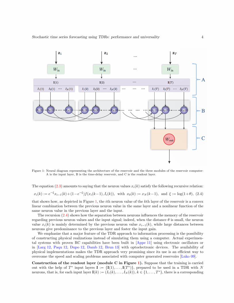
A reservoir computer is formed by three modules that are depicted in Figure 1: an input layer (moduleA in the figure) that feeds the signal to be treated, the reservoir (module B) that processes it, and areadout layer (module C) that uses the reservoir output to produce the information needed. The inputand readout layers are adapted to the specific features of the task under consideration; for example theconstruction of the input layer needs to take into consideration the dimensionality of the signal thatneeds to be processed; different ways to feed the signal can have an impact on the training speed of thesystem. Regarding the readout layer, we restrict to linear readings that are calibrated by minimizing themean square error committed when comparing the output with a teaching signal, via a ridge regression.In this work we consider exclusively an offline (batch) type of training.

Construction of the time-delay reservoir (module B in Figure 1). We start by describing theconstruction of the dynamical time-delay reservoir out of a solution x(t) of the differential equation (1.1).The state of the reservoir is labeled in time steps that are multiples of the delay τ and is characterized bythe values of N virtual neurons obtained out of the regular sampling of x(t) during a given time-delayinterval. We will denote by xi(k) the value of the ith neuron of the reservoir at time kτ defined by

xi(k) := x(kτ − (N − i)θ), i ∈ {1, . . . , N}, (2.1)

where τ := θN and θ is referred to as the separation between neurons. We will also say sometimesthat xi(k) is the ith neuron value of the kth layer of the reservoir.

Even though the justification for the TDR topology depicted in Figure 1 intuitively follows from theform of the differential equation (1.1), it can be also explained through its Euler time discretization asin [Appe 11, Guti 12]. More explicitly, consider the following special case of the time-delay differentialequation (1.1):

x(t) = −x(t) + f(x(t− τ), I(t)). (2.2)

Given an arbitrary natural number N , the Euler discretization of (2.2) with integration step θ := τ/Nis

x(t)− x(t− θ)θ

= −x(t) + f(x(t− τ), I(t)). (2.3)

We now construct a reservoir by using the same assignment of neuron values as in (2.1), that is, wedefine

xi(k) := x(kτ − (N − i)θ) and Ii(k) := I(kτ − (N − i)θ).

Stochastic time series forecasting using TDRs: performance and universality 4

Figure 1: Neural diagram representing the architecture of the reservoir and the three modules of the reservoir computer:A is the input layer, B is the time-delay reservoir, and C is the readout layer.

The equation (2.3) amounts to saying that the neuron values xi(k) satisfy the following recursive relation:

xi(k) := e−ξxi−1(k)+(1−e−ξ)f(xi(k−1), Ii(k)), with x0(k) := xN (k−1), and ξ := log(1+θ), (2.4)

that shows how, as depicted in Figure 1, the ith neuron value of the kth layer of the reservoir is a convexlinear combination between the previous neuron value in the same layer and a nonlinear function of thesame neuron value in the previous layer and the input.

The recursion (2.4) shows how the separation between neurons influences the memory of the reservoirregarding previous neuron values and the input signal; indeed, when the distance θ is small, the neuronvalue xi(k) is mainly determined by the previous neuron value xi−1(k), while large distances betweenneurons give predominance to the previous layer and foster the input gain.

We emphasize that a major feature of the TDR approach to information processing is the possibilityof constructing physical realizations instead of simulating them using a computer. Actual experimen-tal systems with proven RC capabilities have been built in [Appe 11] using electronic oscillators orin [Larg 12, Paqu 12, Dupo 12, Damb 12, Brun 13] with optoelectronic devices. The availability ofphysical implementations makes the TDR approach very promising since its use is an efficient way toovercome the speed and scaling problems associated with computer generated reservoirs [Luko 09].

Construction of the readout layer (module C in Figure 1). Suppose that the training is carriedout with the help of T ∗ input layers I := {I(1), . . . , I(T ∗)}, prepared to be used in a TDR with Nneurons, that is, for each input layer I(k) := (I1(k), . . . , IN (k)), k ∈ {1, . . . , T ∗}, there is a corresponding

Stochastic time series forecasting using TDRs: performance and universality 5

teaching signal y(k) ∈ Rn. As we already said, the construction of the input signal layers I is adaptedto each specific task and will be described in detail below for the stochastic time series forecasting task.Typically, the number of neurons N is taken much higher than the dimension n of the teaching signal.

Since we restrict ourselves to linear readouts, for each input signal I(k) and reservoir layer x(k) :=(x1(k), . . . , xN (k)), a n-dimensional output y(k)∗ ∈ Rn is obtained by using an output matrix Wout ∈Mat(N,n) and by setting y(k)∗ := x(k)T ·Wout. The training consists of finding the output matrixWout that minimizes the distance between this output and the teaching signal, measured via the L2

norm. This amounts to solving the following regularized optimization problem

Wout := arg minW∈Mat(N,n)

(T∗∑k=1

‖y(k)∗ − y(k)‖2 + λ‖W‖2Frob

)

= arg minW∈Mat(N,n)

(T∗∑k=1

‖x(k)T ·W − y(k)‖2 + λ‖W‖2Frob

), (2.5)

whose solution is given byWout = (XXT + λIN )−1Xy, (2.6)

where X ∈ Mat(N,T ∗) is the reservoir output given by Xi,j := xi(j) and y ∈ Mat(T ∗, n) is theteaching matrix containing the vectors y(k), k ∈ {1, . . . , T ∗}, organized by rows. The symbol ‖ · ‖Frobdenotes the Frobenius norm ‖W‖2Frob := trace

(WTW

)[Meye 00] and the ridge (or Tikhonov) penalty

term λ‖W‖2Frob [Tikh 43] is introduced in order to regularize the regression problem by limiting thenorm of the solution hence helping to avoid overfitting. This regularization requires introducing a newparameter λ that controls the intensity of the penalty and that needs to be optimized at training viacross-validation.

The linear RC training philosophy that we adopt in this work has a profound positive impact in itspractical implementation when compared to more traditional machine learning approaches like recur-sive neural networks because it allows us to replace convoluted and sometimes ill-defined optimizationalgorithms by simple regressions.

Construction of the input layer (module A in Figure 1) and the teaching signal for fore-casting tasks. Given a multivariate time series sample z = {z1, . . . , zTtrain

}, zi ∈ Rn, the goal ofthe forecasting task consists in training the RC so that it is capable of predicting the time series val-ues h time steps in advance in an out-of-sample configuration. The value h will be referred to as theforecasting horizon.

The first choice that has to be made in the construction of the input layer is the number NI of timeseries values that are assigned to each reservoir layer; this choice may have an impact on the trainingspeed of the system. We pick NI so that it divides the number of neurons N and we note KI := N/NI .

Before the sample is inserted in the reservoir, it is preprocessed using a random input mask Win ∈Mat(KI , n) that produces a new signal u = {u1, . . . ,uTtrain

}, defined by ui := Winzi ∈ RKI . Thisoperation has two main roles:

• It takes care of the temporal and dimensional multiplexing of the signal by distributing the infor-mation contained in the same time series value to among KI neurons.

• If the average of the mask values is zero then the preprocessed signal u has zero mean even if theoriginal signal z does not have this property; this is particularly convenient in order to eliminatethe need for an intercept in the ridge regression (2.5).

The choice of the input mask Win may have a major impact in the performance of the TDR computer andthe parameters that rule the working regime of the reservoir need, in general, to be optimized with respect

Stochastic time series forecasting using TDRs: performance and universality 6

to the particular Win selected. After the preprocessing, the input signal layers I = {I(1), . . . , I(T ∗)} areconstructed via the assignment

I(k) :=(uTNI(k−1)+1,u

TNI(k−1)+2, . . . ,uNI(k−1)+NI−1,u

TkNI

)T∈ RN ,

with k ∈ {1, . . . , T ∗}. In order to simplify the presentation, we will assume without loss of generalitythat the entire sample z is used for training and hence NIT

∗ = Ttrain.If the goal of the forecasting task is, for instance, guessing the value of the time series value h time

steps in advance it is natural to use as teaching signal

y(k) := zkNI+h ∈ Rn, k ∈ {1, . . . , T}. (2.7)

Another example is provided in Section 3.2 where we carry out a volatility forecasting exercise whoseteaching signal is specified in (3.5).

Once the system has been trained and the output matrix Wout(h) adapted to the forecasting horizonh has been computed using (2.6), actual forecasting can be carried out of a separate testing data set

z := {z1, . . . , zTtest} by generating a new reservoir output X ∈ Mat(N,Ttest/NI) out of it and by

setting y := XTWout(h); the rows of y contain the h-steps ahead forecasts for the elements of the form{zNI

, z2NI, . . . , zTtest

} in z (we assume that Ttest is a multiple of the number NI of time series valuesused for each input layer of the reservoir).

3 Stochastic nonlinear time series forecasting using time-delayreservoirs

In this section we explore the performance of RC in the forecasting of multidimensional nonlinearstochastic time series. Stochastic time series forecasting is a well established topic in statistical modelingwith major applications in a large spectrum of applied research fields: sociology, epidemiology, ecology,econometrics, medicine, finance, engineering, transportation, meteorology, or material sciences to namea few. Most of the research activity in this field takes place in the parametric statistics setup. Usingthis approach, various families of models developed over the years and adapted to different kinds oftemporal phenomena are fitted (estimated) to the available historical data and are subsequently usedfor forecasting via the minimization of different objective functions (usually the mean square error).Many textbooks explain this methodology, usually referred to as the Box-Jenkins approach [Box 76],at various levels and with different applications in mind; see [Broc 06, Broc 02, Lutk 05, Tsay 10]. Weemphasize that this strategy is intrinsically empirical in the sense that the observed data are used forthe selection and estimation of the models that are used later on for forecasting. Its implementationconsists in the following steps:

• Model selection: this stage requires the choice of a specific parametric family of models for theproblem at hand, hundreds of which have been developed over the years to account for manyphenomena arising in different contexts. In practice, there are not many theoretical results thatcan be used for the selection of a particular family and this choice usually involves much trialand error. Additionally, once a model has been picked, one needs to determine its order; thereexist asymptotic estimators for that purpose based on information theoretical arguments (AIC,BIC), forecasting efficiency (FPE, first prediction error), or others (Hannan-Quinn and Schwarzcriteria). See [Lutk 05] for a careful presentation of all these criteria.

• Model estimation: it provides the values of the model parameters that fit best the availablehistorical data. It is usually carried out via maximum likelihood estimation (MLE) which involvessometimes solving complicated, non-convex, high dimensional constrained optimization problems.

Stochastic time series forecasting using TDRs: performance and universality 7

• Diagnostic checking: it consists of testing the statistical properties of the estimation residuals inorder to asses the quality of the model choice. It usually involves using various tests of randomnessadapted to the specific problems at hand.

• Forecasting: carried out via the minimization of an objective function. When this function is themean square error, the solution of the optimization problem is provided by the conditional expec-tation of the time series value at the desired forecasting horizon with respect to the information setgenerated by the known history of the process. There are formulas available for most parametricfamilies that allow the construction of this conditional expectation. A more complicated task is theassessment of the quality of the forecast since the error associated with it involves aggregating theerrors committed not only at the forecasting stage but also at the model selection and estimationsteps. For linear models there are available results based on asymptotic theory that provide infor-mation in this context [Lutk 05, Grig 13] while in more general contexts bootstrapping providesgood answers (see [Pasc 01, Ruiz 02, Pasc 04, Pasc 05, Pasc 06, Rodr 09] and references therein).

The problems associated with parametric families, namely the intrinsic difficulties that go withmodel selection and estimation have motivated the use of alternative approaches, in particular neuralnetworks based techniques. Artificial neural networks (ANNs) are intrinsically nonparametric and theyhence provide an attractive solution in situations where there is a high danger of model misspecification,that is, they are capable of learning from examples and capturing subtle functional relationships amongthe data even when they are unknown or hard to describe. As a consequence, one finds ANNs in theforecasting of specific time series like airborne pollen, commodity prices, environmental temperature,helicopter component loads, international airline passenger traffic, macroeconomic indices, ozone level,personnel inventory, rainfall, river flow, student grade point averages, tool life, total industrial produc-tion, trajectories and transportation, and wind pressure profile, to name a few. The paper [Zhan 98]provides a good description of the state of the art and hundreds of references regarding the applicationof standard neural methods to forecasting.

Despite the plethora of studies having to do with the use ANNs for forecasting, there is no universalcriterion that describes the situations in which ANNs outperform the parametric approach; a work inthis direction is [Alme 91] which claims that for series with short memory, neural networks outperformthe Box-Jenkins methodology. A comprehensive review that evaluates the forecasting performance ofANNs in 48 studies is [Adya 98]. Most of these works evoke the design problem as the major difficulty inthe practical implementation of ANN based forecasting methods [Kaas 96, Balk 00, Cron 05] and eventhough many of these references present recipes for the conception of reasonable network architectures,it is clear that these rules are the outcome of trial and error analysis.

The objective of this section is proving that TDRs are capable of forecasting performances comparableto those attained using the Box-Jenkins approach when the nonlinear VEC-GARCH volatility modelsproposed by Bollerslev et al [Boll 88] are taken as data generating process (DGP).

The VEC-GARCH family is the straightforward multivariate extension of the one-dimensional gen-eralized autoregressive conditionally heteroscedastic (GARCH) models [Engl 82, Boll 86]. These modelsare widely used tools to forecast volatility due to their ability to capture most of the stylized empiricalfacts that can be observed in financial time series: leptokurticity, volatility clustering, and asymmetricresponse to volatility shocks. The main difficulty associated to the practical implementation of thesemodels is their lack of parsimony that, even in low dimensions, makes them extremely complicated tocalibrate. Indeed, in n dimensions the VEC(1,1) family requires n(n + 1)(n(n + 1) + 1)/2 parametersand hence it is rare to find these models at work beyond two or three dimensions and even then, ad-ditional limitations are imposed on the model to make it artificially parsimonious. See [Alta 03] for anillustration of the estimation of a three dimensional DVEC-GARCH model (VEC-GARCH model withdiagonal parameter matrices [Boll 88]) using constrained non-linear programming; in [Chre 13], Breg-man divergences based optimization methods are used to estimate VEC(1,1) models of dimensions up to

Stochastic time series forecasting using TDRs: performance and universality 8

eight with considerable computational effort. Another reason that makes these models good candidatesfor testing the performance of TDRs, is the availability of explicit expressions for the optimal volatilityforecasts whose associated errors can be subsequently used as a benchmark to asses the performance ofthe RC system.

As we will see in the following sections, the main mathematical difficulties that one encounters whenforecasting in the VEC-GARCH context with standard methods, namely, the need for the solution ofhigh dimensional nonconvex optimization problems, is replaced in the RC approach by topology selectionquestions. In that sense, time-delay reservoirs simplify the problem since they reduce it to the task oftuning the parameters of the nonlinear delay kernel. This intrinsic parameter set is parsimonious and, insome cases, the performance of the RC system is reasonably robust with respect to its values; moreover,we will show that it is possible to obtain additional parameter independence by using parallel pools ofTDRs. We emphasize that once the TDR has been designed, its training does not in principle need thesolution of sophisticated optimization problems and hence a good RC performance in the VEC-GARCHforecasting task is a nontrivial achievement that improves the state of the art technology.

3.1 The VEC-GARCH family and volatility forecasting

Consider the n-dimensional conditionally heteroscedastic discrete-time process {zt} determined by therelation

zt = H1/2t εt with {εt} ∼ IIDN(0, In).

The symbol IIDN(0, In) refers to the set of n-dimensional independent and identically distributed nor-mal variables with mean 0 and covariance matrix In. Additionally, in this expression {Ht} is assumed tobe a predictable positive semidefinite matrix process, that is, for each t ∈ N, the matrix random variableHt is Ft−1-measurable, with Ft−1 := σ (z0, . . . , zt−1) the information set (sigma algebra) generated by{z0, . . . , zt−1}. In these conditions it is easy to show that the conditional mean E[zt | Ft−1] = 0 andthat the conditional covariance matrix process of {zt} coincides with {Ht}.

Different specifications for the time evolution of the conditional covariance matrix {Ht} determinedifferent vector conditional heteroscedastic models. Here we focus on the VEC-GARCH model,introduced in [Boll 88] as the direct generalization of the univariate GARCH model [Boll 86] in thesense that every conditional variance and covariance is a function of all lagged conditional variances andcovariances as well as all squares and cross-products of the lagged time series values. More specifically,the VEC(q,p) model is determined by

ht = c +

q∑i=1

Aiηt−i +

p∑i=1

Biht−i,

where ht := vech(Ht), ηt := vech(ztzTt ), c is a N -dimensional vector, with N := n(n + 1)/2 and

Ai, Bi ∈ MN . The linear operator vech : Sn → RN stacks the lower triangular part of a symmetricmatrix including its main diagonal into a vector [Lutk 05]. We consider the case p = q = 1, that is:{

zt = H1/2t εt with {εt} ∼ IIDN(0, In),

ht = c +Aηt−1 +Bht−1.(3.1)

As we already mentioned, in this case the model needs N(2N + 1) = 12n(n+ 1)(n2 + n+ 1) parameters

for a complete specification.A major complication in the estimation of these models via maximum likelihood is that the general

prescription for the VEC-GARCH model spelled out in (3.1) does not guarantee that it has stationarysolutions or that the resulting conditional covariance matrices {Ht}t∈N are necessarily positive semidef-inite. These structural requirements call for constraints that should be imposed on the parameter

Stochastic time series forecasting using TDRs: performance and universality 9

matrices c, A, and B. Unlike the situation encountered in the one-dimensional case, only sufficientconditions for positivity and stationarity are available in the literature for the multidimensional setup.For example, [Gour 97] shows that (3.1) admits a unique second order stationary solution if all theeigenvalues of A + B lie strictly inside the unit circle. Regarding positive semidefiniteness of {Ht}t∈N,it can be shown that (see [Chre 13, Proposition 3.1]) this is ensured by the positive semidefiniteness ofmath(c),Σ(A), and Σ(B), where math : RN → Sn is the inverse of the vech operator and Σ is the linearoperator introduced in [Chre 13, Definition 2.2].

Volatility forecasting. The main use of the VEC(1,1) model (3.1) is the description and the forecastingof the volatility of financial time series. In that context, the process {zt} describes the dynamicalevolution of market log-returns and {Ht} are the associated conditional covariance matrices. The log-returns {zt} are observable but the covariance matrices {Ht} are not; nevertheless, the estimation andforecasting of these random variables is of paramount importance in portfolio and risk management, aswell as in scenarios generation. The volatility prediction task at time T with a horizon of h time steps

consists of providing the optimal forecast HT+h of the conditional covariance matrix HT+h based onthe information set FT generated by the log-returns up to time T , that is, FT := σ(z0, . . . , zT ). Thisestimate is produced by minimizing the mean square forecasting error (MSFE) defined as

MSFE(h) := E

[(hT+h − hT+h

)(hT+h − hT+h

)T],

where hT+h := vech(HT+h) is the vectorized conditional covariance matrix at time T +h, and hT+h :=

vech(HT+h). The MSFE(h) is a positive semidefinite matrix of dimension N := 12n(n+ 1) hence, given

two different forecasts of hT+h with associated errors MSFE(h) and MSFE(h), respectively, we will say

that MSFE(h) ≤ MSFE(h) when the difference MSFE(h)−MSFE(h) is a positive semidefinite matrix.A standard result [Hami 94, Chapter 4] shows that the optimal forecast of a random variable withrespect to the MSFE and a given information set is given by its conditional expectation with respect to

that information set. In particular, the optimal forecast hT+h for the covariance matrix hT+h knowingthe log-returns {z0, . . . , zT } is given by:

hT+h := arg min˜hT+h|FT

E

[(hT+h − ˜hT+h|FT

)(hT+h − ˜hT+h|FT

)T]= E [hT+h | FT ] . (3.2)

An important advantage of the VEC-GARCH family is the possibility of explicitly computing the

conditional expectation in (3.2) that yields the optimal forecast hT+h via the following recursion on thehorizon h:

hT+1 = hT+1 = c +AηT +BhT ,

hT+2 = c + (A+B)hT+1,

hT+3 = c + (A+B)hT+2,

... (3.3)

hT+i = c + (A+B)hT+i−1,

...

hT+h = c + (A+B)hT+h−1.

We emphasize that this recursion shows that the functional dependence of the forecast hT+h on theelements {z0, . . . , zT } that generate the information set FT is highly nonlinear. Since it is the series

Stochastic time series forecasting using TDRs: performance and universality 10

{z0, . . . , zT } that are used as an input in the TDR for the forecasting task, the performance of the RCscheme, if positive, cannot be exclusively associated to the linear readout layer that is estimated via aridge regression and requires the contribution of the nonlinear reservoir module.

3.2 TDR based volatility forecasting

The objective of this section is assessing the performance and challenges of TDRs in the forecastingof volatilities synthetically generated by VEC-GARCH models of the type introduced in the previoussubsection. We work in dimension n = 3 which requires the use of 78 different parameters in theconstruction of the model (3.1). The forecasting task will be carried out with a TDR of the type presentedin Section 2 using the same nonlinear function used in [Appe 11] for the design of an experimentalelectronics based reservoir computer, namely,

f(x(t− τ), u(t), η, γ, p) =η (x(t− τ) + γu(t))

1 + (x(t− τ) + γu(t))p , (3.4)

where γ, η, and p are real value parameters.We work with reservoirs made out of N neurons with each layer constructed using a single time series

value (NI = 1, T ∗ = Ttrain), that is, if z = {z1, . . . , zTtrain}, zi ∈ Rn, is the training sample generated

with a given three dimensional VEC-GARCH model, then the i-th input signal layer I(i) ∈ RN isobtained via the assignment I(i) := Winzi with Win ∈ Mat(N,n) a random input mask whose entriesare uniformly distributed in the centered interval [−a, a], a ∈ R.

We emphasize that the VEC-GARCH process (3.1) is a white noise, that is the series z = {z1, . . . , zTtrain}exhibits no serial autocorrelation. This makes pointless the forecasting of those time series values inthe sense described in Section 2. In exchange, as we already mentioned, the main use of VEC-GARCHtype models is the forecasting of conditional covariances and hence, in order to construct a readoutlayer adapted to this task, it suffices to use in (2.7) as teaching signal the h-shifted versions of theconditional covariance matrices {h1+h, . . . ,hTtrain} generated by the model together with the time seriesvalues {z1, . . . , zTtrain−h}, that is,

y(k) := hk+h ∈ Rn, k ∈ {1, . . . , Ttrain − h}. (3.5)

The regression (2.6) using this teaching signal and the reservoir output, yields an output matrix Wout

that is subsequently used for out-of-sample forecasting.

Reservoir design and parameter optimization. Given a reservoir architecture it is in generalchallenging to find a universal set of optimal parameters (θ, γ, η) that offers top performance for a largearray of tasks presented to it. A particularly detailed description of this phenomenon can be foundin [Damb 12] where a detailed quantitative analysis is carried out in which the dependence of the totalmemory capacity of a RC system is studied as a function of its design parameters. We have realized inour work that our particular task is not an exception and that tuning the reservoir parameters to adaptthem to it may have a major impact on the final performance of the method. In the particular case ofVEC-GARCH volatility forecasting, the empirical results in Section 4 show that this statement holdstrue when forecasting is carried out for different processes, that is, different sets of parameters c, A, andB, and to a lesser extent when the forecasting horizon changes. This observation has two importantimplications from the practical implementation point of view:

• Numerical cost: The parameter optimization is carried out via a computationally expensivecross validation procedure.

• Parallel reading (multi-tasking): one of the potential advantages of RC is the ability to carryout tasks in parallel (see for example the introduction in [Maas 11]); the strategy behind this

Stochastic time series forecasting using TDRs: performance and universality 11

observation consists of processing a single signal with the reservoir and consequently using itsoutput for different tasks via adapted readout matrices estimated with the pertinent teachingsignal. In other words, there is a single signal processing step but various tasks are simultaneouslyaccomplished with the output by adapting only the linear regression step to each of them. Thisis obviously only possible if the reservoir is functioning in a regime with good performance forall the tasks. In the particular case of forecasting problems, parallel reading can be useful atthe time of simultaneously predicting at various horizons out of a single input signal; however,we emphasize this is only feasible whenever there is a set of reservoir parameters for which theforecasting performance is acceptable for all the horizons of interest.

3.3 Parallel reservoir computing and universality

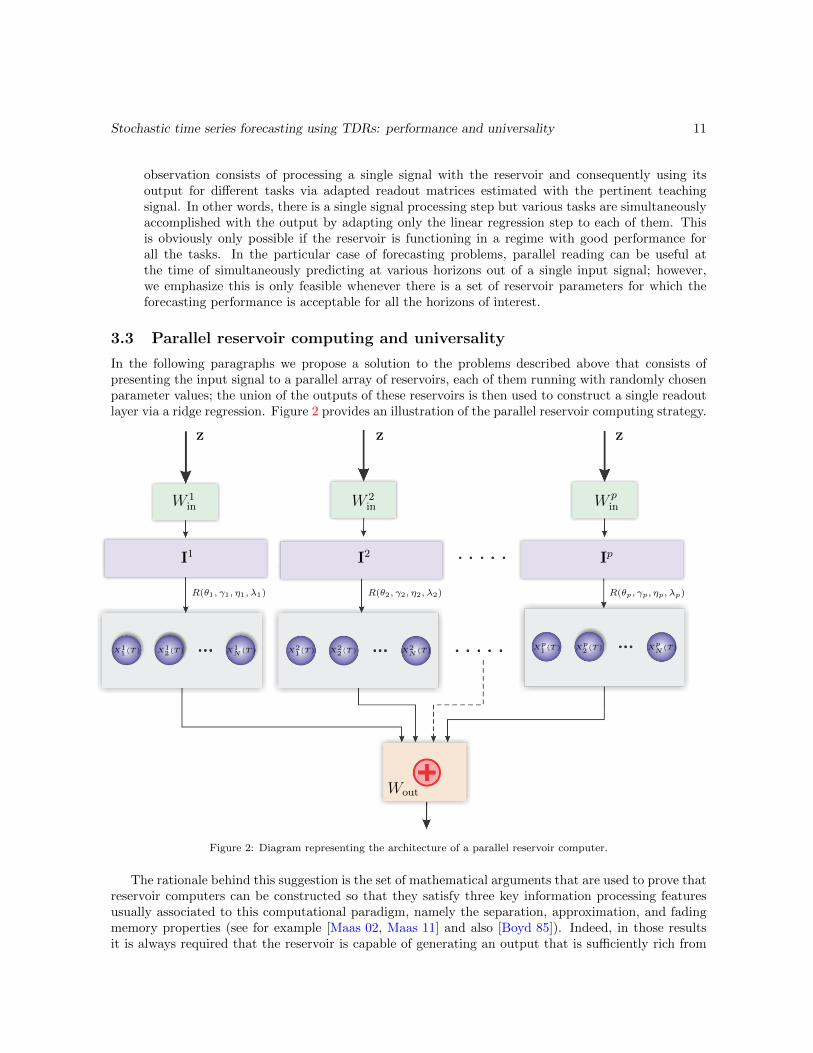
In the following paragraphs we propose a solution to the problems described above that consists ofpresenting the input signal to a parallel array of reservoirs, each of them running with randomly chosenparameter values; the union of the outputs of these reservoirs is then used to construct a single readoutlayer via a ridge regression. Figure 2 provides an illustration of the parallel reservoir computing strategy.

W 1in W 2

in W pin

X11(T ) X1

2(T ) X1N (T ) X2

1(T ) X22(T ) X2

N (T ) Xp1(T ) X

p2(T ) X

pN

(T )

R(θ1, γ1, η1, λ1) R(θ2, γ2, η2, λ2) R(θp, γp, ηp, λp)

Z Z Z

I1 I2 Ip

Wout

Figure 2: Diagram representing the architecture of a parallel reservoir computer.

The rationale behind this suggestion is the set of mathematical arguments that are used to prove thatreservoir computers can be constructed so that they satisfy three key information processing featuresusually associated to this computational paradigm, namely the separation, approximation, and fadingmemory properties (see for example [Maas 02, Maas 11] and also [Boyd 85]). Indeed, in those resultsit is always required that the reservoir is capable of generating an output that is sufficiently rich from

Stochastic time series forecasting using TDRs: performance and universality 12

the functional point of view so that standard approximation results like the Stone-Weierstrass theoremcan be applied. A more explicit statement is provided in [Boyd 85] where it is shown how to carry outapproximations using Volterra series generated by ensembles of delay operators. A parallel approachsimilar to ours with only two reservoirs has been explored in [Orti 12] where it is shown that the use ofparallel nodes with different parameters is capable of providing memory capacity increases.

As we empirically show in the next section, this approach presents several advantages when comparedto the use of a single optimized reservoir with the same total number of neurons, namely, limited com-putational effort for parameter optimization, better performance for smaller training sample sizes, andimproved universality with respect to changes in the forecasting horizon and in the model specification.

4 Empirical results

In this section we conduct two empirical experiments that show the good performance of TDRs in thevolatility forecasting task and substantiate the claims in the previous paragraphs as to the differentimplementation strategies. The tests will be conducted using both synthetic time series as well as realmarket data:

• Performance assessment with synthetic data: we consider a generic VEC(1,1) model asin (3.1) with parameters c, A, and B that satisfy the constraints spelled out in Section 3.1 andthat ensure that the model is stationary and produces positive semidefinite conditional covariancematrices. This model will be used as a data generating process for both the training and testingdatasets when forecasting using the TDRs. In order to test the volatility forecasting capabilitiesof the different TDR implementation strategies, we generate two pairs of VEC-GARCH time se-ries with their corresponding conditional covariance matrices, each of length 100 000 time steps.These pairs are subsequently used for the training and for the testing, respectively, noticing thatwe use the first 1 000 points in both as a washout period; the first pair will be used for param-eter optimization in the different configurations (see below) and the second one for performanceassessment.

• Performance assessment with market data. Realized volatility forecasting: the goal ofthis exercise is testing the ability of the TDR in the forecasting of market realized daily covariancematrices out of the observed corresponding market log-returns. The realized covariances arecomputed using intraday price quotes. The main challenge of this task when compared to theprevious one are the limitations in sample size since we only have 2 500 available time steps fortraining and testing.

The different forecasting performances will be measured using the scalar standardized mean squareforecasting error (sMSFE) defined as follows:

sMSFE(h) :=

E

[(hT+h − hT+h

)T (hT+h − hT+h

)]var (hT+h)

,

where hT+h is the vectorized covariance matrix that we are interested in and hT+h the correspondingforecast h time steps into the future. We will consider forecasting horizons of up to twenty time steps.

4.1 Reservoir configurations

The different devices whose performances will be compared are constructed according to the followingarchitectures:

Stochastic time series forecasting using TDRs: performance and universality 13

(i) TDR with 400 neurons and grid optimized parameters: a TDR is built according to theprescription in (2.1) using the nonlinear kernel in (3.4). A preliminary study showed that theforecasting performance of this device is much dependent on the parameter values θ := τ/N , γ,and η of the kernel (3.4). We hence carry out a grid search for the optimal parameters (θ, γ, η) byusing the first pair of series to conduct training/testing routines for each of the parameter com-binations in the grid that yields, for each forecasting horizon h, the triple (θ, γ, η) that minimizesthe corresponding sMSFE(h). The optimization grid is constructed according to the followingprescription: θ, γ ∈ [0.1, 2], η ∈ [0.1, 1.5] with a search step of 0.1.

(ii) TDR with 400 neurons and random optimized parameters: In this case we randomlysimulate one hundred different sets of parameters and keep for each forecasting horizon the onethat produces the smallest error in the testing phase. The parameters are randomly drawn fromthe uniform distribution on the intervals [0.01, 2] for θ and γ, and [0.01, 1.5] for η. For each ofthese parameter sets we simulate a new random input mask Win.

(iii) Parallel array of 40 TDRs of 10 neurons each with random optimized parameters: werandomly generate one hundred parallel TDRs containing 40 reservoirs each with 10 neurons. Theparameters of each TDR are generated using the same prescription as in the previous point andthe different random input masks Win are used for each draw.

(iv) Parallel array of 80 TDRs of 5 neurons each with random optimized parameters: theprocedure is identical to the one in the previous point but this time with 80 reservoirs with 5neurons each.

The choice of the total number of neurons for the individually operating TDR (configurations (i)and (ii)) has been made after several trials that show 400 nodes suffice to appropriately handle thecomplexity of the forecasting task at hand without incurring in overfitting. The size of this neural arrayalso allows the construction of the arrays in points (iii) and (iv) with a sizeable number of parallelunits, each of them with a reasonable number of neurons.

Concerning the parameter p in the nonlinear kernel (3.4), we explore the performances obtainedwith the values p = 1 and p = 2. The value p = 1 presents a potential difficulty due to the factthat there are non-generic combinations of reservoir inputs and outputs such that the denominator1 + (x(t− τ) +γu(t))p in (3.4) may become close to zero and cause a divergence. We avoid this problemin practice by using a random input mask Win ∈ Mat(N,n) that takes values in the interval [−a, a],with a sufficiently small; the use of this device amounts to a global normalization of the input/outputseries that makes the term x(t − τ) + γu(t) small with respect to 1 and hence makes the cancelling of1 +x(t− τ) +γu(t) very unlikely. In what follows we will consider random input masks Win with valuesuniformly distributed in the interval [−0.1, 0.1] for the kernel with p = 1; in the case p = 2 this intervalwill be replaced by [−1, 1].

4.2 Volatility forecasting with synthetic data

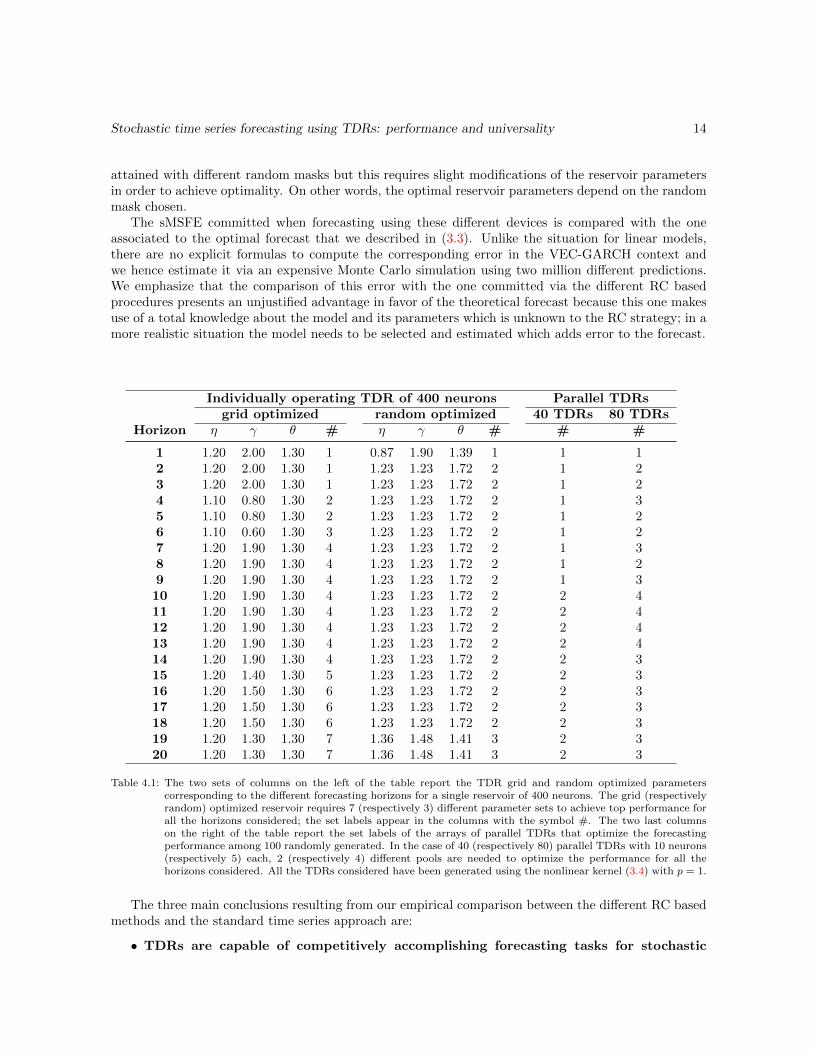
Using the generic VEC(1,1) model described above as data generating process for both time series andcovariance matrices, we construct the different optimized reservoir configurations that we just listed.Table 4.1 reports the sets of optimal parameters obtained for each horizon and for both the grid andthe random optimized individually operating TDR; additionally, the two last columns report the setlabels of the arrays of parallel TDRs that optimize the forecasting performance among 100 randomlygenerated. In the case of 40 (respectively 80) parallel TDRs with 10 neurons (respectively 5) each, 2(respectively 4) different pools are needed to optimize the performance for all the horizons considered.

We emphasize that the optimal parameters reported in Table 4.1 are related to a specific choice ofrandom input mask Win. Unreported simulations show that the same forecasting performances can be

Stochastic time series forecasting using TDRs: performance and universality 14

attained with different random masks but this requires slight modifications of the reservoir parametersin order to achieve optimality. On other words, the optimal reservoir parameters depend on the randommask chosen.

The sMSFE committed when forecasting using these different devices is compared with the oneassociated to the optimal forecast that we described in (3.3). Unlike the situation for linear models,there are no explicit formulas to compute the corresponding error in the VEC-GARCH context andwe hence estimate it via an expensive Monte Carlo simulation using two million different predictions.We emphasize that the comparison of this error with the one committed via the different RC basedprocedures presents an unjustified advantage in favor of the theoretical forecast because this one makesuse of a total knowledge about the model and its parameters which is unknown to the RC strategy; in amore realistic situation the model needs to be selected and estimated which adds error to the forecast.

Individually operating TDR of 400 neurons Parallel TDRsgrid optimized random optimized 40 TDRs 80 TDRs

Horizon η γ θ # η γ θ # # #

1 1.20 2.00 1.30 1 0.87 1.90 1.39 1 1 12 1.20 2.00 1.30 1 1.23 1.23 1.72 2 1 23 1.20 2.00 1.30 1 1.23 1.23 1.72 2 1 24 1.10 0.80 1.30 2 1.23 1.23 1.72 2 1 35 1.10 0.80 1.30 2 1.23 1.23 1.72 2 1 26 1.10 0.60 1.30 3 1.23 1.23 1.72 2 1 27 1.20 1.90 1.30 4 1.23 1.23 1.72 2 1 38 1.20 1.90 1.30 4 1.23 1.23 1.72 2 1 29 1.20 1.90 1.30 4 1.23 1.23 1.72 2 1 310 1.20 1.90 1.30 4 1.23 1.23 1.72 2 2 411 1.20 1.90 1.30 4 1.23 1.23 1.72 2 2 412 1.20 1.90 1.30 4 1.23 1.23 1.72 2 2 413 1.20 1.90 1.30 4 1.23 1.23 1.72 2 2 414 1.20 1.90 1.30 4 1.23 1.23 1.72 2 2 315 1.20 1.40 1.30 5 1.23 1.23 1.72 2 2 316 1.20 1.50 1.30 6 1.23 1.23 1.72 2 2 317 1.20 1.50 1.30 6 1.23 1.23 1.72 2 2 318 1.20 1.50 1.30 6 1.23 1.23 1.72 2 2 319 1.20 1.30 1.30 7 1.36 1.48 1.41 3 2 320 1.20 1.30 1.30 7 1.36 1.48 1.41 3 2 3

Table 4.1: The two sets of columns on the left of the table report the TDR grid and random optimized parameterscorresponding to the different forecasting horizons for a single reservoir of 400 neurons. The grid (respectivelyrandom) optimized reservoir requires 7 (respectively 3) different parameter sets to achieve top performance forall the horizons considered; the set labels appear in the columns with the symbol #. The two last columnson the right of the table report the set labels of the arrays of parallel TDRs that optimize the forecastingperformance among 100 randomly generated. In the case of 40 (respectively 80) parallel TDRs with 10 neurons(respectively 5) each, 2 (respectively 4) different pools are needed to optimize the performance for all thehorizons considered. All the TDRs considered have been generated using the nonlinear kernel (3.4) with p = 1.

The three main conclusions resulting from our empirical comparison between the different RC basedmethods and the standard time series approach are:

• TDRs are capable of competitively accomplishing forecasting tasks for stochastic

Stochastic time series forecasting using TDRs: performance and universality 15

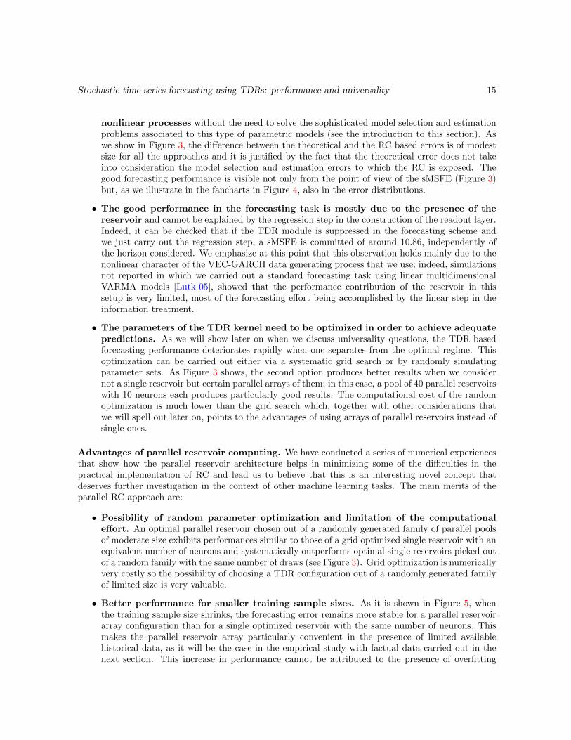
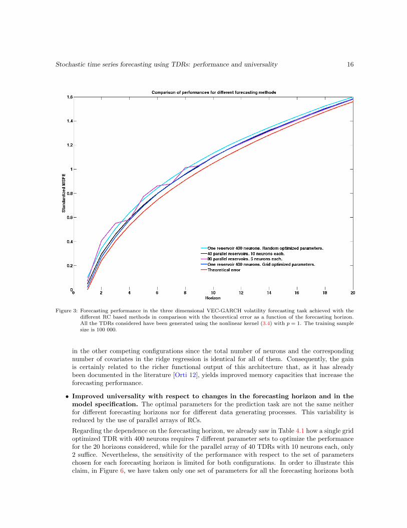
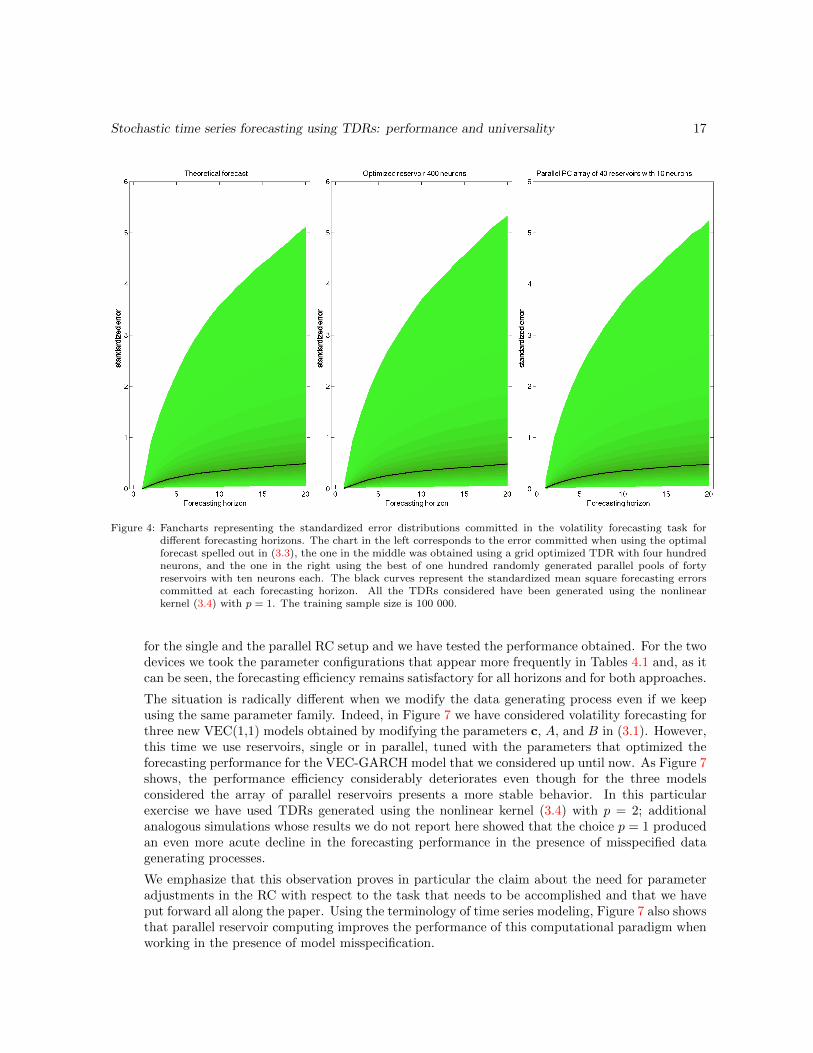
nonlinear processes without the need to solve the sophisticated model selection and estimationproblems associated to this type of parametric models (see the introduction to this section). Aswe show in Figure 3, the difference between the theoretical and the RC based errors is of modestsize for all the approaches and it is justified by the fact that the theoretical error does not takeinto consideration the model selection and estimation errors to which the RC is exposed. Thegood forecasting performance is visible not only from the point of view of the sMSFE (Figure 3)but, as we illustrate in the fancharts in Figure 4, also in the error distributions.

• The good performance in the forecasting task is mostly due to the presence of thereservoir and cannot be explained by the regression step in the construction of the readout layer.Indeed, it can be checked that if the TDR module is suppressed in the forecasting scheme andwe just carry out the regression step, a sMSFE is committed of around 10.86, independently ofthe horizon considered. We emphasize at this point that this observation holds mainly due to thenonlinear character of the VEC-GARCH data generating process that we use; indeed, simulationsnot reported in which we carried out a standard forecasting task using linear multidimensionalVARMA models [Lutk 05], showed that the performance contribution of the reservoir in thissetup is very limited, most of the forecasting effort being accomplished by the linear step in theinformation treatment.

• The parameters of the TDR kernel need to be optimized in order to achieve adequatepredictions. As we will show later on when we discuss universality questions, the TDR basedforecasting performance deteriorates rapidly when one separates from the optimal regime. Thisoptimization can be carried out either via a systematic grid search or by randomly simulatingparameter sets. As Figure 3 shows, the second option produces better results when we considernot a single reservoir but certain parallel arrays of them; in this case, a pool of 40 parallel reservoirswith 10 neurons each produces particularly good results. The computational cost of the randomoptimization is much lower than the grid search which, together with other considerations thatwe will spell out later on, points to the advantages of using arrays of parallel reservoirs instead ofsingle ones.

Advantages of parallel reservoir computing. We have conducted a series of numerical experiencesthat show how the parallel reservoir architecture helps in minimizing some of the difficulties in thepractical implementation of RC and lead us to believe that this is an interesting novel concept thatdeserves further investigation in the context of other machine learning tasks. The main merits of theparallel RC approach are:

• Possibility of random parameter optimization and limitation of the computationaleffort. An optimal parallel reservoir chosen out of a randomly generated family of parallel poolsof moderate size exhibits performances similar to those of a grid optimized single reservoir with anequivalent number of neurons and systematically outperforms optimal single reservoirs picked outof a random family with the same number of draws (see Figure 3). Grid optimization is numericallyvery costly so the possibility of choosing a TDR configuration out of a randomly generated familyof limited size is very valuable.

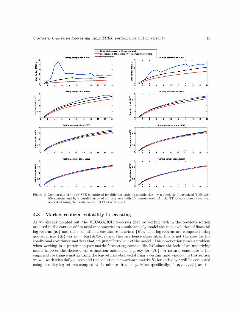
• Better performance for smaller training sample sizes. As it is shown in Figure 5, whenthe training sample size shrinks, the forecasting error remains more stable for a parallel reservoirarray configuration than for a single optimized reservoir with the same number of neurons. Thismakes the parallel reservoir array particularly convenient in the presence of limited availablehistorical data, as it will be the case in the empirical study with factual data carried out in thenext section. This increase in performance cannot be attributed to the presence of overfitting

Stochastic time series forecasting using TDRs: performance and universality 16

Figure 3: Forecasting performance in the three dimensional VEC-GARCH volatility forecasting task achieved with thedifferent RC based methods in comparison with the theoretical error as a function of the forecasting horizon.All the TDRs considered have been generated using the nonlinear kernel (3.4) with p = 1. The training samplesize is 100 000.

in the other competing configurations since the total number of neurons and the correspondingnumber of covariates in the ridge regression is identical for all of them. Consequently, the gainis certainly related to the richer functional output of this architecture that, as it has alreadybeen documented in the literature [Orti 12], yields improved memory capacities that increase theforecasting performance.

• Improved universality with respect to changes in the forecasting horizon and in themodel specification. The optimal parameters for the prediction task are not the same neitherfor different forecasting horizons nor for different data generating processes. This variability isreduced by the use of parallel arrays of RCs.

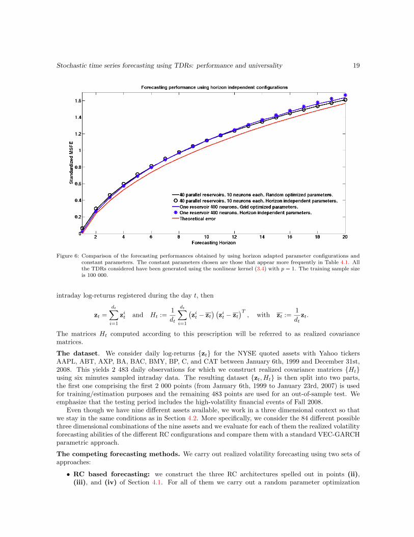
Regarding the dependence on the forecasting horizon, we already saw in Table 4.1 how a single gridoptimized TDR with 400 neurons requires 7 different parameter sets to optimize the performancefor the 20 horizons considered, while for the parallel array of 40 TDRs with 10 neurons each, only2 suffice. Nevertheless, the sensitivity of the performance with respect to the set of parameterschosen for each forecasting horizon is limited for both configurations. In order to illustrate thisclaim, in Figure 6, we have taken only one set of parameters for all the forecasting horizons both

Stochastic time series forecasting using TDRs: performance and universality 17

Figure 4: Fancharts representing the standardized error distributions committed in the volatility forecasting task fordifferent forecasting horizons. The chart in the left corresponds to the error committed when using the optimalforecast spelled out in (3.3), the one in the middle was obtained using a grid optimized TDR with four hundredneurons, and the one in the right using the best of one hundred randomly generated parallel pools of fortyreservoirs with ten neurons each. The black curves represent the standardized mean square forecasting errorscommitted at each forecasting horizon. All the TDRs considered have been generated using the nonlinearkernel (3.4) with p = 1. The training sample size is 100 000.

for the single and the parallel RC setup and we have tested the performance obtained. For the twodevices we took the parameter configurations that appear more frequently in Tables 4.1 and, as itcan be seen, the forecasting efficiency remains satisfactory for all horizons and for both approaches.

The situation is radically different when we modify the data generating process even if we keepusing the same parameter family. Indeed, in Figure 7 we have considered volatility forecasting forthree new VEC(1,1) models obtained by modifying the parameters c, A, and B in (3.1). However,this time we use reservoirs, single or in parallel, tuned with the parameters that optimized theforecasting performance for the VEC-GARCH model that we considered up until now. As Figure 7shows, the performance efficiency considerably deteriorates even though for the three modelsconsidered the array of parallel reservoirs presents a more stable behavior. In this particularexercise we have used TDRs generated using the nonlinear kernel (3.4) with p = 2; additionalanalogous simulations whose results we do not report here showed that the choice p = 1 producedan even more acute decline in the forecasting performance in the presence of misspecified datagenerating processes.

We emphasize that this observation proves in particular the claim about the need for parameteradjustments in the RC with respect to the task that needs to be accomplished and that we haveput forward all along the paper. Using the terminology of time series modeling, Figure 7 also showsthat parallel reservoir computing improves the performance of this computational paradigm whenworking in the presence of model misspecification.

Stochastic time series forecasting using TDRs: performance and universality 18

Figure 5: Comparison of the sMSFE committed for different training sample sizes by a single grid optimized TDR with400 neurons and by a parallel array of 40 reservoirs with 10 neurons each. All the TDRs considered have beengenerated using the nonlinear kernel (3.4) with p = 1.

4.3 Market realized volatility forecasting

As we already pointed out, the VEC-GARCH processes that we worked with in the previous sectionare used in the context of financial econometrics to simultaneously model the time evolution of financiallog-returns {zt} and their conditional covariance matrices {Ht}. The log-returns are computed usingquoted prices {St} via zt := log (St/St−1) and they are hence observable; this is not the case for theconditional covariance matrices that are just inferred out of the model. This observation poses a problemwhen working in a purely non-parametric forecasting context like RC since the lack of an underlyingmodel imposes the choice of an estimation method or a proxy for {Ht}. A natural candidate is theempirical covariance matrix using the log-returns observed during a certain time window; in this sectionwe will work with daily quotes and the conditional covariance matrix Ht for each day t will be computedusing intraday log-returns sampled at six minutes frequency. More specifically, if {z1t , . . . , z

dtt } are the

Stochastic time series forecasting using TDRs: performance and universality 19

Figure 6: Comparison of the forecasting performances obtained by using horizon adapted parameter configurations andconstant parameters. The constant parameters chosen are those that appear more frequently in Table 4.1. Allthe TDRs considered have been generated using the nonlinear kernel (3.4) with p = 1. The training sample sizeis 100 000.

intraday log-returns registered during the day t, then

zt =

dt∑i=1

zit and Ht :=1

dt

dt∑i=1

(zit − zt

) (zit − zt

)T, with zt :=

1

dtzt.

The matrices Ht computed according to this prescription will be referred to as realized covariancematrices.

The dataset. We consider daily log-returns {zt} for the NYSE quoted assets with Yahoo tickersAAPL, ABT, AXP, BA, BAC, BMY, BP, C, and CAT between January 6th, 1999 and December 31st,2008. This yields 2 483 daily observations for which we construct realized covariance matrices {Ht}using six minutes sampled intraday data. The resulting dataset {zt, Ht} is then split into two parts,the first one comprising the first 2 000 points (from January 6th, 1999 to January 23rd, 2007) is usedfor training/estimation purposes and the remaining 483 points are used for an out-of-sample test. Weemphasize that the testing period includes the high-volatility financial events of Fall 2008.

Even though we have nine different assets available, we work in a three dimensional context so thatwe stay in the same conditions as in Section 4.2. More specifically, we consider the 84 different possiblethree dimensional combinations of the nine assets and we evaluate for each of them the realized volatilityforecasting abilities of the different RC configurations and compare them with a standard VEC-GARCHparametric approach.

The competing forecasting methods. We carry out realized volatility forecasting using two sets ofapproaches:

• RC based forecasting: we construct the three RC architectures spelled out in points (ii),(iii), and (iv) of Section 4.1. For all of them we carry out a random parameter optimization

Stochastic time series forecasting using TDRs: performance and universality 20

Figure 7: Forecasting performance under model misspecification. All the TDRs considered have been generated using thenonlinear kernel (3.4) with p = 2. Unreported analogous simulations showed that the choice p = 1 produced aneven more acute decline in the forecasting performance in the presence of misspecified data generating processes.The training sample size is 100 000.

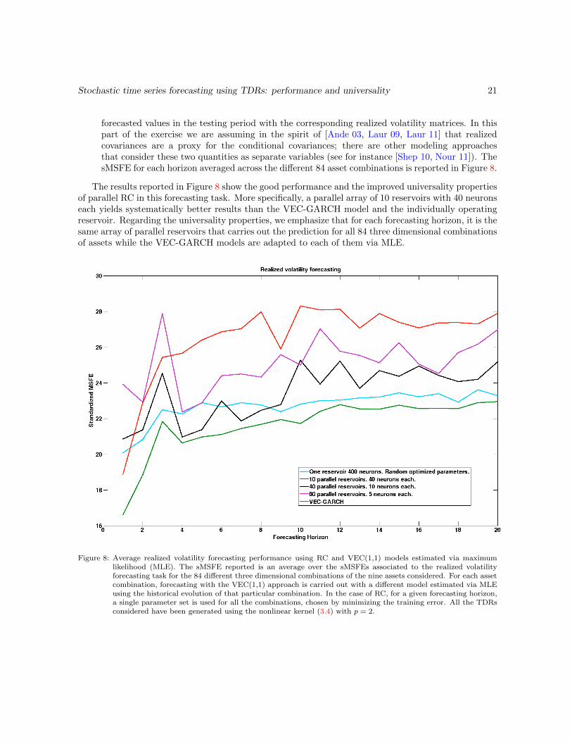
based on the in-sample forecasting performance within the 2 000 days long training period. Thisoptimization is carried out for each prediction horizon and for each of the different 84 threedimensional combinations of assets. For each different RC architecture and for each forecastinghorizon we select the reservoir parameters that yield the smallest training error among the 84combinations of assets and we use that same reservoir for the testing part of the exercise forall the asset combinations. The sMSFE for each horizon averaged across the different 84 assetcombinations is reported in Figure 8 only for the single operating reservoir with 400 neurons andfor the 40 parallel reservoirs with 10 neurons each since other configurations offer much worseperformances.

• VEC-GARCH based forecasting: for each three dimensional asset combination we estimatevia the constrained maximum likelihood estimation algorithm in [Chre 13] a VEC(1,1) model asin (3.1) with the log-returns data included in the 2 000 days long training period. These modelsare used to forecast conditional covariance matrices according to (3.3) and we then compare this

Stochastic time series forecasting using TDRs: performance and universality 21

forecasted values in the testing period with the corresponding realized volatility matrices. In thispart of the exercise we are assuming in the spirit of [Ande 03, Laur 09, Laur 11] that realizedcovariances are a proxy for the conditional covariances; there are other modeling approachesthat consider these two quantities as separate variables (see for instance [Shep 10, Nour 11]). ThesMSFE for each horizon averaged across the different 84 asset combinations is reported in Figure 8.

The results reported in Figure 8 show the good performance and the improved universality propertiesof parallel RC in this forecasting task. More specifically, a parallel array of 10 reservoirs with 40 neuronseach yields systematically better results than the VEC-GARCH model and the individually operatingreservoir. Regarding the universality properties, we emphasize that for each forecasting horizon, it is thesame array of parallel reservoirs that carries out the prediction for all 84 three dimensional combinationsof assets while the VEC-GARCH models are adapted to each of them via MLE.

Figure 8: Average realized volatility forecasting performance using RC and VEC(1,1) models estimated via maximumlikelihood (MLE). The sMSFE reported is an average over the sMSFEs associated to the realized volatilityforecasting task for the 84 different three dimensional combinations of the nine assets considered. For each assetcombination, forecasting with the VEC(1,1) approach is carried out with a different model estimated via MLEusing the historical evolution of that particular combination. In the case of RC, for a given forecasting horizon,a single parameter set is used for all the combinations, chosen by minimizing the training error. All the TDRsconsidered have been generated using the nonlinear kernel (3.4) with p = 2.

Stochastic time series forecasting using TDRs: performance and universality 22

5 Conclusions

We have shown that newly introduced parallel configurations of time-delay reservoirs (TDRs) are capableof good performances in the forecasting of the conditional covariances associated to multivariate discrete-time nonlinear stochastic processes of VEC-GARCH type as well as in the prediction of factual dailymarket realized volatilities computed with intraday quotes using as training input daily log-returnquotes.

Our study has shown that this type of reservoir computers does not exhibit task universality in thiscontext in the sense that reservoir parameter configurations that yield good results for a given modelor forecasting horizon do not for others (see Figures 7 and 6, and Table 4.1). This observation hasas negative consequences that TDRs need to be adapted for each task via a computational expensivecross validation procedure; additionally multi-tasking through parallel reading [Maas 11] is not availablesince it requires acceptable reservoir performance for each of the tasks that are being simultaneouslyprocessed via parallel read out.

We propose as a solution to these difficulties the use of parallel arrays of TDRs, each running at adifferent regime. This configuration reduces the computational effort necessary to adapt to the task athand by using random optimization. It presents a better performance for small training sample sizesand is less sensitive to modifications in the task hence making it more universal and appropriate formulti-tasking.

References

[Adya 98] M. Adya and F. Collopy. “How effective are neural networks at forecasting and prediction?A review and evaluation”. Journal of Forecasting, Vol. 17, pp. 481–495, 1998.

[Alme 91] C. de Almeida and P. A. Fishwick. “Time series forecasting using neural networks vs. Box-Jenkins methodology”. Simulation, Vol. 57, No. 5, pp. 303–310, Nov. 1991.

[Alta 03] A. Altay-Salih, M. c. Pinar, and S. Leyffer. “Constrained nonlinear programming for volatil-ity estimation with GARCH models”. SIAM Rev., Vol. 45, No. 3, pp. 485—-503 (electronic),2003.

[Ande 03] T. G. Andersen, T. Bollerslev, F. X. Diebold, and P. Labys. “Modeling and ForecastingRealized Volatility”. Econometrica, Vol. 71, No. 2, pp. 579–625, March 2003.

[Appe 11] L. Appeltant, M. C. Soriano, G. Van der Sande, J. Danckaert, S. Massar, J. Dambre,B. Schrauwen, C. R. Mirasso, and I. Fischer. “Information processing using a single dy-namical node as complex system.”. Nature communications, Vol. 2, p. 468, Jan. 2011.

[Atiy 00] A. F. Atiya and A. G. Parlos. “New results on recurrent network training: unifying the algo-rithms and accelerating convergence.”. IEEE transactions on neural networks / a publicationof the IEEE Neural Networks Council, Vol. 11, No. 3, pp. 697–709, Jan. 2000.

[Balk 00] S. D. Balkin and J. K. Ord. “Automatic neural network modeling for univariate time series”.International Journal of Forecasting, Vol. 16, No. 4, pp. 509–515, Oct. 2000.

[Boll 86] T. Bollerslev. “Generalized autoregressive conditional heteroskedasticity”. Journal of Econo-metrics, Vol. 31, No. 3, pp. 307–327, 1986.

[Boll 88] T. Bollerslev, R. F. Engle, and J. M. Wooldridge. “A capital asset pricing model with timevarying covariances”. Journal of Political Economy, Vol. 96, pp. 116–131, 1988.

Stochastic time series forecasting using TDRs: performance and universality 23

[Box 76] G. E. P. Box and G. M. Jenkins. Time Series Analysis: Forecasting and Control. Holden-Day,1976.

[Boyd 85] S. Boyd and L. Chua. “Fading memory and the problem of approximating nonlinear oper-ators with Volterra series”. IEEE Transactions on Circuits and Systems, Vol. 32, No. 11,pp. 1150–1161, Nov. 1985.

[Broc 02] P. J. Brockwell and R. A. Davis. Introduction to Time Series and Forecasting. Springer,2002.

[Broc 06] P. J. Brockwell and R. A. Davis. Time Series: Theory and Methods. Springer-Verlag, 2006.

[Brun 13] D. Brunner, M. C. Soriano, C. R. Mirasso, and I. Fischer. “Parallel photonic informationprocessing at gigabyte per second data rates using transient states”. Nature Communications,Vol. 4, No. 1364, 2013.

[Chre 13] S. Chretien and J.-P. Ortega. “Multivariate GARCH estimation via a Bregman-proximaltrust-region method”. Computational Statistics and Data Analysis, Vol. To appear, 2013.

[Cron 05] S. F. Crone. “Stepwise Selection of Artificial Neural Network Models for Time Series Pre-diction”. Journal of Intelligent Systems, Vol. 15, 2005.

[Croo 07] N. Crook. “Nonlinear transient computation”. Neurocomputing, Vol. 70, pp. 1167–1176,2007.

[Damb 12] J. Dambre, D. Verstraeten, B. Schrauwen, and S. Massar. “Information processing capacityof dynamical systems”. Scientific reports, Vol. 2, No. 514, 2012.

[Dupo 12] F. Duport, B. Schneider, A. Smerieri, M. Haelterman, and S. Massar. “All-optical reservoircomputing”. Optics Express, Vol. 20, No. 20, pp. 22783–95, 2012.

[Engl 82] R. F. Engle. “Autoregressive conditional heteroscedasticity with estimates of the varianceof United Kingdom inflation”. Econometrica, Vol. 50, No. 4, pp. 987–1007, 1982.

[Gour 97] C. Gourieroux. ARCH models and financial applications. Springer Series in Statistics,Springer-Verlag, New York, 1997.

[Grig 13] L. Grigoryeva and J.-P. Ortega. “Hybrid forecasting with estimated temporally aggregatedlinear processes”. http://papers.ssrn.com/sol3/papers.cfm?abstract id=2148895, 2013.

[Guti 12] J. M. Gutierrez, D. San-Martın, S. Ortın, and L. Pesquera. “Simple reservoirs with chaintopology based on a single time-delay nonlinear node”. In: 20th European Symposium onArtificial Neural Networks, Computational Intelligence and Machine Learning, pp. 13–18,2012.

[Hami 94] J. D. Hamilton. Time series analysis. Princeton University Press, Princeton, NJ, 1994.

[Ilie 07] I. Ilies, H. Jaeger, O. Kosuchinas, M. Rincon, V. Sakenas, and N. Vaskevicius. “Steppingforward through echoes of the past: forecasting with Echo State Networks”. Tech. Rep.,2007.

[Jaeg 01] H. Jaeger. “The ’echo state’ approach to analysing and training recurrent neural networks”.Tech. Rep., German National Research Center for Information Technology, 2001.

[Jaeg 04] H. Jaeger and H. Haas. “Harnessing Nonlinearity: Predicting Chaotic Systems and SavingEnergy in Wireless Communication”. Science, Vol. 304, No. 5667, pp. 78–80, 2004.

Stochastic time series forecasting using TDRs: performance and universality 24

[Jaeg 07] H. Jaeger, M. Lukosevicius, D. Popovici, and U. Siewert. “Optimization and applicationsof echo state networks with leaky-integrator neurons”. Neural networks, Vol. 20, No. 3,pp. 335–352, 2007.

[Kaas 96] I. Kaastra and M. Boyd. “Designing a neural network for forecasting financial and economictime series”. Neurocomputing, Vol. 10, pp. 215–236, 1996.

[Larg 12] L. Larger, M. C. Soriano, D. Brunner, L. Appeltant, J. M. Gutierrez, L. Pesquera, C. R.Mirasso, and I. Fischer. “Photonic information processing beyond Turing: an optoelectronicimplementation of reservoir computing”. Optics Express, Vol. 20, No. 3, p. 3241, Jan. 2012.

[Laur 09] S. Laurent and J. Rombouts. “On loss functions and ranking forecasting performances ofmultivariate volatility models”. Sciences-New York, 2009.

[Laur 11] S. Laurent, J. V. K. Rombouts, and F. Violante. “On the forecasting accuracy of multivariateGARCH models”. Journal of Applied Econometrics, pp. n/a–n/a, Apr. 2011.

[Luko 09] M. Lukosevicius and H. Jaeger. “Reservoir computing approaches to recurrent neural net-work training”. Computer Science Review, Vol. 3, No. 3, pp. 127–149, 2009.

[Lutk 05] H. Lutkepohl. New Introduction to Multiple Time Series Analysis. Springer-Verlag, Berlin,2005.

[Maas 00] W. Maass and E. D. Sontag. “Neural Systems as Nonlinear Filters”. Neural Computation,Vol. 12, No. 8, pp. 1743–1772, Aug. 2000.

[Maas 02] W. Maass, T. Natschlager, and H. Markram. “Real-time computing without stable states:a new framework for neural computation based on perturbations”. Neural Computation,Vol. 14, pp. 2531–2560, 2002.

[Maas 11] W. Maass. “Liquid state machines: motivation, theory, and applications”. In: S. S. BarryCooper and A. Sorbi, Eds., Computability In Context: Computation and Logic in the RealWorld, Chap. 8, pp. 275–296, 2011.

[Meye 00] C. Meyer. Matrix Analysis and Applied Linear Algebra Book and Solutions Manual. Societyfor Industrial and Applied Mathematics, 2000.

[Nour 11] D. Noureldin, N. Shephard, and K. K. Sheppard. “Multivariate high-frequency-based volatil-ity (HEAVY) models”. Journal of Applied Econometrics, pp. n/a–n/a, Aug. 2011.

[Orti 12] S. Ortin, L. Pesquera, and J. M. Gutierrez. “Memory and nonlinear mapping in reservoircomputing with two uncoupled nonlinear delay nodes”. In: Proceedings of the EuropeanConference on Complex Systems, pp. 895–899, 2012.

[Paqu 12] Y. Paquot, F. Duport, A. Smerieri, J. Dambre, B. Schrauwen, M. Haelterman, and S. Massar.“Optoelectronic reservoir computing”. Scientific reports, Vol. 2, p. 287, Jan. 2012.

[Pasc 01] L. Pascual, J. Romo, and E. Ruiz. “Effects of parameter estimation on prediction densities:a bootstrap approach”. International Journal of Forecasting, Vol. 17, No. 1, pp. 83–103,Jan. 2001.

[Pasc 04] L. Pascual, J. Romo, and E. Ruiz. “Bootstrap predictive inference for ARIMA processes”.Journal of Time Series Analysis, Vol. 25, No. 4, pp. 449–465, July 2004.

Stochastic time series forecasting using TDRs: performance and universality 25

[Pasc 05] L. Pascual, J. Romo, and E. Ruiz. “Bootstrap prediction intervals for power-transformedtime series”. International Journal of Forecasting, Vol. 21, No. 2, pp. 219–235, Apr. 2005.

[Pasc 06] L. Pascual, J. Romo, and E. Ruiz. “Bootstrap prediction for returns and volatilities inGARCH models”. Computational Statistics & Data Analysis, Vol. 50, No. 9, pp. 2293–2312,May 2006.

[Roda 11] A. Rodan and P. Tino. “Minimum complexity echo state network.”. IEEE transactionson neural networks / a publication of the IEEE Neural Networks Council, Vol. 22, No. 1,pp. 131–44, Jan. 2011.

[Rodr 09] A. Rodriguez and E. Ruiz. “Bootstrap prediction intervals in state-space models”. Journalof Time Series Analysis, Vol. 30, No. 2, pp. 167–178, March 2009.

[Ruiz 02] E. Ruiz and L. Pascual. “Bootstrapping Financial Time Series”. Journal of EconomicSurveys, Vol. 16, No. 3, pp. 271–300, July 2002.

[Shep 10] N. Shephard and K. Sheppard. “Realising the future: forecasting with high-frequency-basedvolatility (HEAVY) models”. Journal of Applied Econometrics, Vol. 25, No. 2, pp. 197–231,March 2010.

[Tikh 43] A. N. Tikhonov. “On the stability of inverse problems”. Dokl. Akad. Nauk SSSR, Vol. 39,No. 5, pp. 195–198, 1943.

[Tsay 10] R. S. Tsay. Analysis of Financial Time Series. Wiley, 2010.

[Vers 07] D. Verstraeten, B. Schrauwen, M. DHaene, and D. Stroobandt. “An experimental unificationof reservoir computing methods”. Neural Networks, Vol. 20, pp. 391–403, 2007.

[Wyff 08] F. Wyffels, B. Schrauwen, and D. Stroobandt. “Using reservoir computing in a decompositionapproach for time series prediction”. 2008.

[Wyff 10] F. Wyffels and B. Schrauwen. “A comparative study of Reservoir Computing strategies formonthly time series prediction”. Neurocomputing, Vol. 73, No. 10, pp. 1958–1964, 2010.

[Zhan 98] G. Zhang, B. Eddy Patuwo, and M. Y. Hu. “Forecasting with artificial neural networks:the state of the art”. International Journal of Forecasting, Vol. 14, No. 1, pp. 35–62, March1998.