STEPS - an Approach for Human MobilityModeling

Anh-Dung Nguyen12, Patrick Senac12, Victor Ramiro3, and Michel Diaz2

1 ISAE/University of Toulouse, Toulouse, France2 LAAS/CNRS, Toulouse, France

3 NIC Chile Research Labs, Santiago, Chile{anh-dung.nguyen, patrick.senac}@isae.fr, vramiro@niclabs.cl,

michel.diaz@laas.fr

Abstract. In this paper we introduce Spatio-TEmporal Parametric Step-ping (STEPS) - a simple parametric mobility model which can cover alarge spectrum of human mobility patterns. STEPS makes abstraction ofspatio-temporal preferences in human mobility by using a power law torule the nodes movement. Nodes in STEPS have preferential attachmentto favorite locations where they spend most of their time. Via simula-tions, we show that STEPS is able, not only to express the peer to peerproperties such as inter-contact/contact time and to reflect accurately re-alistic routing performance, but also to express the structural propertiesof the underlying interaction graph such as small-world phenomenon.Moreover, STEPS is easy to implement, flexible to configure and alsotheoretically tractable.

1 Introduction

Human mobility is known to have a significant impact on performance of net-works created by wireless portable devices e.g. MANET, DTN. Unfortunately,there is no model that is able to capture all the characteristics of human mobilitydue to its high complexity. In this paper we introduce Spatio-TEmporal Para-metric Stepping (STEPS) - a new powerful formal model for human mobility ormobility inside social/interaction networks. The introduction of this new modelis justified by the lack of modeling and expressive power, in the currently usedmodels, for the spatio-temporal correlation usually observed in human mobility.

We show that preferential location attachment and location attractors areinvariants properties, at the origin of the spatio-temporal correlation of mobility.Indeed, as observed in several real mobility traces, while few people have a highlynomadic mobility behavior the majority has a more sedentary one.

In this paper, we assess the expressive and modeling power of STEPS byshowing that this model successes in expressing easily several fundamental hu-man mobility properties observed in real traces of dynamic network:

1. The distribution of human traveled distance follows a truncated power law.2. The distribution of pause time between travels follows a truncated power

law.

3. The distribution of inter-contact/contact time follow a truncated power law.4. The underlying dynamic graph can emerge a small-world structure.

The rest of this paper is structured as follows. After an overview of the stateof the art in Section 2, we present the major idea behind the model in Section 3.Section 4 formally introduces STEPS as well as some implementation issues.Section 5 shows capacity of STEPS to capture salient features observed in realdynamic networks, going from inter-contact/contact time to epidemic routingperformance and small-world phenomenon. Finally we conclude the paper inSection 6.

2 Related works

Human mobility has attracted a lot of attention of not only computer scientistsbut also epidemiologists, physicists, etc because its deep understanding may leadto many other important discoveries in different fields. The lack of large scale realmobility traces made that research is initially based on simple abstract modelse.g. Random Waypoint, Random Walk (see [3] for a survey). These models whoseparameters are usually drawn from an uniform distribution, although are goodfor simulation, can not reflect the reality and even are considered harmful forresearch in some cases [14]. In these model, there is no notion of spatio-temporalpreferences.

Recently, available real data allows researchers to understand deeper the na-ture of human mobility. The power law distribution of the traveled distance wasinitially reported in [6] and [1] in which the authors study the spatial distributionof human movement based on mobile phone and bank note traces. The powerlaw distribution of the inter-contact time was initially studied by Chaintreau etal. in [4]. In [8], Karagiannis et al. confirm this and also suggest that the inter-contact time follows a power law up to a characteristic time (about 12 hours)and then cut-off by an exponential decay.

Based on these findings, some more sophisticated models have been proposed.In [5], the authors have proposed an universal model being able to capture manycharacteristics of human daily mobility by combining different sub-models. Witha lot of parameters to configure, the complexity of this type of model make themhard to use.

In [9], the authors propose SLAW - a Random Direction liked model, ex-cept that the traveled distance and the pause time distributions are ruled by apower law. An algorithm for trajectory planning was added to mimic the humanbehavior of always choosing the optimal path. Although being able to capturestatistical characteristics like inter-contact, contact time distribution, the no-tion of spatio-temporal preferential attachment is not expressed. Moreover, therouting protocol performance results have not been compared with real traces.

Another modeling stream is to integrating social behaviors in the model.In [10], a community based model was proposed in which the movement dependson the relationship between nodes. The network area is divided in zones and the

social attractivity of a zone is based on the number of friends in the same zone.The comparisons of this model with real traces show a difference for the contacttime distribution. Moreover, the routing performance has not been shown.

Time Varying Community [7] is another interesting model in which the au-thors try to model the spatio-temporal preferences of human mobility by creatingcommunity zones. Nodes have different probabilities to jump in different com-munities to capture the spatial preferences. Time structure was build on thebasis of night/day and days in a week to capture temporal preferences.

A recent research shows that some mobility model (including [7]), despiteof the capacity of capturing the spatio-temporal characteristics, deviate signifi-cantly the routing performances compared to ones obtained with real traces [12].This aspect that has not always been considered in existing models is indeed re-ally important because it shows how a model can confront the real dynamicnetworks.

3 Characterizing Human Mobility

STEPS is inspired by observable characteristics of the human mobility behaviour,specifically the spatio-temporal correlation. Indeed, people share their dailytime between some specific locations at some specific time (e.g. home/office,night/day). This spatio-temporal pattern repeats at different scales and has beenrecently observed on real traces [7].

On a short time basis (i.e. a day, a week), we can assume that one have afinite space of locations. We define two mobility principles :

• Preferential attachment : the probability for a node to move in a location isinverse proportional to the distance from his preferential location.• Attractor : when a node is outside of his preferential location, he has a higher

probability to move closer to this location than moving farther.

From this point of view, the human mobility can be modeled as a finite statespace Markov chain in which the transition probability distribution express amovement pattern. In the next section, we answer the question what exactlythis probability distribution. Figure 1(a) illustrates a Markov chain of 4 stateswhich corresponds to 4 locations: (A) House, (B) Office, (C) Shop and (D) Otherplaces.

4 Model description

In STEPS, a location is modeled as a zone in which a node can move freelyaccording to a random mobility model such as Random Waypoint. The displace-ment between zones and the staying duration in a zone are both drawn from apower law distribution whose the exponent value expresses the more or less lo-calized mobility. By simply tuning the power law exponent, we can cover a largespectrum of mobility patterns from purely random ones to highly localized ones.

A B

C D

(a)

A

111

1

111

1

2 2 2 2

2

2

2 2 2 2 2

2

2

2

2

2

2

(b)

Fig. 1. (a) Human mobility modeling under a markovian view: States represent differ-ent localities e.g. House, Office, Shop and Other places, and transitions represent themobility pattern. (b) 5 × 5 torus representing the distances from a location A to theother locations.

Moreover, complex heterogeneity can be described by combining nodes with dif-ferent mobility patterns as defined by their preferential zones and the relatedattraction power. Group mobility is also supported on our implementation.

4.1 The model

Assume that the network area is a square torus divided in N ×N square zones.The distance between theses zones is defined according to a metric (here we useChebyshev distance). Figure 1(b) illustrates an example of a 5×5 torus with thedistances from the zone A. One can imagine a zone as a geographic location (e.g.building, school, supermarket) or a logical location (i.e. a topic of interest suchas football, music, philosophy, etc). Therefore, we can use the model to studyhuman geographic mobility or human social behaviours. In this paper, we dealonly with the first case.

In the so structured space, each node is associated to a preferential zone Z0.For the sake of simplicity we assume is this paper that each node is attached toone zone, however this model can be extended by associating several preferentialzones to each node. The movement between zones is driven by a power lawsatisfying two mobility principles described above. The pdf of this power law isgiven by

P [D = d] =β

(1 + d)α, (1)

where d is the distance from Z0, α is the power law exponent that representsthe attractor power and β is a normalizing constant.

From (1) we can see that : the farther a zone is from the preferential zone, theless probability the node to move in (i.e. principle of preferential attachment).On the other hand, when a node is outside of its preferred zone he has a higherprobability to move closer to this one than moving farther (i.e. principle ofattraction).

Algorithm 1: STEPS algorithm

Input: Initial zone ← Z0

repeat- Select randomly a distance d from the probability distribution (1);- Select randomly a zone Zi among all zones that are d distance units awayfrom Z0;- Select randomly a point in Zi;- Go linearly to this point with a speed randomly chosen from[vmin, vmax] , 0 < vmin ≤ vmax < +∞;- Select randomly a staying time t from the probability distribution (2);while t has not elapsed do

Perform Random Waypoint movement in Zi ;end

until End of simulation;

The staying time in a zone is also driven by a power law

P [T = t] =ω

tτ, (2)

where τ is the temporal preference degree of node and ω is a normalizing con-stant.

From this small set of modeling parameters the model can cover a full spec-trum of mobility behaviours. Indeed, according to the value of the α exponenta node has a more or less nomadic behavior. For instance,

• when α < 0, nodes have a higher probability to choose a long distance thana short one and so the preferential zone plays the repulsion role instead of aattraction one,• when α > 0, nodes are more localized,• when α = 0, nodes move randomly towards any zone with a uniform proba-

bility.

We summarize the description of STEPS in Algorithm 1.

4.2 Markov chain modeling

In this section, we introduce the Markovian model behind STEPS. This analyt-ical analysis makes it possible to derive routing performance bounds when usingthe model. From a formal point of view STEPS can be modeled by a discrete-time Markov chain of N states where each state corresponds to one zone. Notethat the torus structure gives nodes the same spatial distribution wherever theirpreferential zones (i.e. they have the same number of zones with an equal dis-tances to their preferential zones). More specifically, for a distance d, we have8×d zones with equal distances from Z0. Consequently, the probability to chooseone among these zones is

P [Zi|dZiZ0= l] =

1

8lP [D = l] =

β

8l(1 + l)α. (3)

Because the probabilities for a node to jump to any zone do not depend onthe residing zone but only on the distance from Z0, the transition probabilities ofthe Markov chain is defined by a stochastic matrix with similar lines. Thereforethe resulting stochastic matrix is a idempotent matrix (i.e. the product of thematrix by itself gives the same matrix)

P =

p(Z0) p(Z1) . . . p(Zn−1)p(Z0) p(Z1) . . . p(Zn−1)

......

. . ....

p(Z0) p(Z1) . . . p(Zn−1)

.Hence it is straight-forward to deduce the stationary state of the Markov

chainΠ =

(p(Z0) p(Z1) . . . p(Zn−1)

). (4)

From this result, it is interesting to characterize the inter-contact time (i.e.the delay between two consecutive contacts of the same node pair) of STEPSbecause this characteristic is well known to have a great impact on routing indynamic networks. To simplify the problem, we assume that a contact occursif and only if two nodes are in the same zone. Let two nodes A and B moveaccording to the underlying STEPS Markov chain and initially start from thesame zone. Let assume that the movement of A and B are independent. For eachinstant, the probability that the two nodes are in the same zone is

pcontact = PA(Z0)PB(Z0) + . . .+ PA(Zn−1)PB(Zn−1)

=

n−1∑i=0

P (Zi)2 =

dMax∑i=0

1

8i

[β

(i+ 1)α

]2 ,

where dMax = b√N2 c is the maximum distance a node can attain in the torus.

Let ICT be the discrete random variable which represents the number ofinstants elapsed before A and B are in contact again. One can consider that ICTfollows a geometric distribution with the parameter pcontact, i.e. the number oftrials before the first success of an event with probability of success pcontact.Hence, the pdf of ICT is given by

P [ICT = t] = (1− pcontact)t−1pcontact. (5)

It is well known that the continuous analog of a geometric distribution is anexponential distribution. Therefore, the inter-contact time distribution for i.i.d.nodes can be approximated by an exponential distribution. This is true whenthe attractor power α is equals to 0 (i.e. nodes move uniformly) because there isno spatio-temporal correlation between nodes. But when α 6= 0, there is a highercorrelation in their movement and in consequence the exponential distributionis not a good approximation. Indeed, [2] reports this feature for the CorrelatedRandom Walk model where the correlation of nodes induces the emergence ofa power law in the inter-contact time distribution. A generalized closed formula

100

101

102

103

104

10−2

10−1

100

t

P(x

>t)

0 1000 2000 3000 4000 5000 6000 700010

−2

10−1

100

(a) α = 0

100

101

102

103

104

10−4

10−3

10−2

10−1

100

t

P(x

>t)

0 500 1000 1500 2000 2500 3000 350010

−4

10−3

10−2

10−1

100

(b) α > 0

Fig. 2. Theoretical Inter-Contact Time Distribution of STEPS

for STEPS inter-contact time is an on-going work. We provide here simulationresults related to this feature.

Figure 2 gives the linear-log plot of the complementary cumulative distribu-tion function (CCDF) of the inter-contact time that results from a simulationof the Markov chain described above when α = 0 and α > 0. In the first case,the inter-contact time distribution fits an exponential distribution (i.e. is repre-sented by a linear function the linear-log plot) while in the second case it fitsa power law distribution (i.e. is represented by a linear function in the log-logplot) with an exponential decay tail. This result confirms the relationship be-tween the spatio-temporal correlation of nodes and the emergence of a powerlaw in inter-contact time distribution.

5 Model properties

It is worth mentioning that a mobility model should express the fundamentalproperties observed in real dynamic networks. In this section, we show thatSTEPS can really capture the seminal characteristics of human mobility and thatwhen used for testing routing performance STEPS deliver the same performancesas the ones observed on top of real traces (this features is too often neglectedwhen introducing a new mobility model).

5.1 Inter-Contact Time vs Contact Time Distributions

Inter-Contact Time Distribution The inter-contact time is defined as thedelay between two encounters of a pair of nodes. Real trace analysis suggestthat the distribution of inter-contact time can be approximated by a power lawup to a characteristic time (i.e. about 12 hours) followed by an exponentialdecay [8]. In the following we will use the set of traces presented by Chaintreauet al. in [4] as base of comparison with STEPS mobility simulations. Figure 3(a)shows the aggregate CCDF of the inter-contact time (i.e. the CCDF of inter-contact time samples over all distinct pairs of nodes) for different traces. In orderto demonstrate the capacity of STEPS to reproduce this feature, we configured

100

101

102

103

104

105

106

10−6

10−5

10−4

10−3

10−2

10−1

100

t

P(x

>t)

0 0.5 1 1.5 2 2.5 3 3.5

x 105

10−6

10−4

10−2

100

Intel

Cambridge

Infocom06

Infocom05

(a) Real traces

102

103

104

105

106

10−6

10−5

10−4

10−3

10−2

10−1

100

t

P(x

>t)

0 0.5 1 1.5 2 2.5 3 3.5

x 105

10−6

10−4

10−2

100

STEPS

Infocom06

(b) STEPS vs Infocom06 trace

Fig. 3. CCDF of Inter-Contact Time

Table 1. Infocom 2006 trace

Number of nodes 98

Duration 4 days

Technology Bluetooth

Average inter-contact time 1.9 hours

Average contact duration 6 minutes

STEPS to exhibit the results observed in the Infocom 2006 conference trace.Table 1 summarizes the characteristics of this trace.

To simulate the conference environment, we create a 10 × 10 torus of size120 × 120m2 that mimics rooms in the conference. The radio range is set to10m which corresponds to Bluetooth technology. Figure 3(b) shows the CCDFof inter-contact time in log-log and lin-log plots. We observe that the resultinginter- contact time distribution as given by the STEPS simulations fits with theone given by the real trace.

Contact Time Distribution Because of the potential diversity of nodes be-havior it is more complicated to reproduce the contact duration given by realtraces. Indeed, the average time spent for each contact depends on the person(e.g. some people spend a lot of time to talk while the others just check hands).To the best of our knowledge, the abstract modeling of social behavior has notbeen studied precisely yet. We measured the average contact duration and thecelebrity (i.e. the global number of neighbor nodes) of the Infocom06 nodes andranked them according to their average contact duration. The result is plottedin Figure 4(a). According to this classification, it appears that the more/lesspopular the person is, the less/more time he spends for each contact. Becausethe contact duration of STEPS depends principally on the pause time of themovement inside zone (i.e. the pause time of RWP model), to mimic this behav-ior we divided nodes in four groups. Each group corresponds to a category ofmobility behavior: highly mobile nodes, mobile nodes, slightly mobile and rarelymobile. The pause time for each groups is summarized in Table 2

0 10 20 30 40 50 60 70 80 90 1000

0.1

0.2

0.3

0.4

0.5

0.6

0.7

0.8

0.9

1

Ranked nodes

No

rmaliz

ed v

alu

es

Contact Time

Celebrity

(a) Social Characteristic Observed in In-focom06

100

101

102

103

104

105

10−6

10−5

10−4

10−3

10−2

10−1

100

t

P(x

>t)

0 0.5 1 1.5 2 2.5 3 3.5 4 4.5

x 104

10−6

10−4

10−2

100

STEPS

Infocom06

(b) CCDF of Contact Time of STEPS vsInfocom06 Trace

Fig. 4. Contact Time Behavior of STEPS vs Real Trace

Table 2. Group categories

Dynamicity categories RWP pause time range (s) Number of nodes

Very high [0, 60] 65High [60, 900] 15Low [900, 3600] 10

Very low [3600, 43200] 8

With this configuration, we aim to mimic the behavior observed in Infocom06trace where a large percentage of nodes have short contacts and a few nodeshave long to very long contacts. The CCDFs of contact time of STEPS andInfocom06 trace as shown in Figure 4(b) show that STEPS can also capturewith high accuracy this mobility behavior.

5.2 Epidemic routing performance

A mobility model has not only to capture the salient features observed in realtraces but must also reproduce the performances given by routing protocolson top of real traces. In order to assess the capacity of STEPS to offer thisimportant property we ran Epidemic routing on STEPS and Infocom06 traceand compared the respective routing delays. For each trace, the average delayto spread a message to all the nodes is measured in function of the number ofnodes who received the message. Figure 5 shows that STEPS is able to reflect atthe simulation level the performance of Epidemic routing when applied on realtraces.

5.3 Human mobility structure studied with STEPS

A mobility model should allow not only to express faithfully peer-to-peer inter-actions properties such as inter-contact time and contact duration, but shouldbe able also to reproduce the fundamental structure of the underlying interac-tion graph as modeled by a temporal graph, i.e. graphs with time varying edges.

0 10 20 30 40 50 60 70 80 90 10010

0

101

102

103

104

105

Number of nodes that received the message (unit)

De

lay (

s)

Infocom06

STEPS

Fig. 5. Epidemic Routing Delay ofSTEPS vs Infocom06 Trace

0 0.1 0.2 0.3 0.4 0.5 0.6 0.7 0.8 0.9 10

0.1

0.2

0.3

0.4

0.5

0.6

0.7

0.8

0.9

1

Ratio of High Mobile Nodes to High Localized Nodes

normalized clutering coefficient

normalized shortest path length

Fig. 6. Small-World Structure inSTEPS

The structural properties of static interaction graphs have been studied lead-ing to the observation of numerous instances of real interaction graph with ahigh clustering and a low shortest path length [13]. Such a structure of graph iscalled small-world. With respect to routing, the small world structure inducesfast message spreading in the underlying network.

We extended the notions of clustering coefficient and shortest path lengthintroduced in [13] for dynamic graph. In this paper, we present only the mostimportant definitions due to the lack of space.

Let G(t) = (V(t), E(t)) be a temporal graph with a time varying set V(t) ofvertexes and with a time varying set E(t) of edges.

1. Temporal Clustering Coefficient : Let N (w, i) be the set of neighbors ofnode i in a time window w. The temporal clustering coefficient is defined asthe ratio of the actual number of connections between neighbors of i to thetheoretical number of connections between them during a time window w.Intuitively, it represents the cliquishness of a time varying friendship circle.Formally, that is

Ci =2∑j |N (w, j) ∩N (w, i)|

|N (w, i)| (|N (w, i)| − 1), (6)

where j is a neighbor of i and |X| denotes the cardinal of X.2. Temporal Shortest Path Length : Let Rij(t) ∈ {0, 1} denotes a direct or

indirect (i.e. via multiple connections at different times) connection betweennode i and node j at time t. The shortest path length between i and j isdefined as the earliest instant when there is a connection between them.That is

Lij = inf{t|Rij(t) = 1}. (7)

To visualize the phenomenon in STEPS, we create scenarios where thereare two categories of nodes with different attractor power. In the first category,nodes have a high mobile behaviour (i.e. α is small) while in the second one, theyare more localized (i.e. α is large). The idea is to “rewiring” a high clustereddynamic graph (i.e. with the population is in the second category) by introduc-ing high mobile nodes into the population. By tuning the ratio of number of

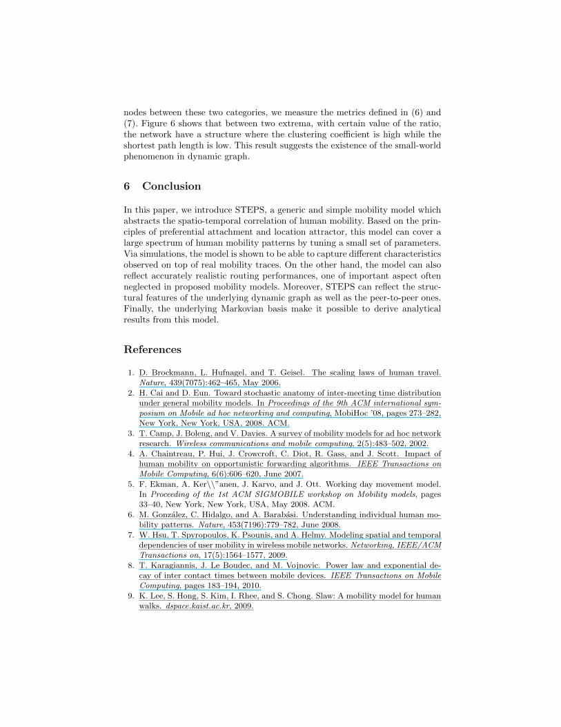
nodes between these two categories, we measure the metrics defined in (6) and(7). Figure 6 shows that between two extrema, with certain value of the ratio,the network have a structure where the clustering coefficient is high while theshortest path length is low. This result suggests the existence of the small-worldphenomenon in dynamic graph.

6 Conclusion

In this paper, we introduce STEPS, a generic and simple mobility model whichabstracts the spatio-temporal correlation of human mobility. Based on the prin-ciples of preferential attachment and location attractor, this model can cover alarge spectrum of human mobility patterns by tuning a small set of parameters.Via simulations, the model is shown to be able to capture different characteristicsobserved on top of real mobility traces. On the other hand, the model can alsoreflect accurately realistic routing performances, one of important aspect oftenneglected in proposed mobility models. Moreover, STEPS can reflect the struc-tural features of the underlying dynamic graph as well as the peer-to-peer ones.Finally, the underlying Markovian basis make it possible to derive analyticalresults from this model.

References

1. D. Brockmann, L. Hufnagel, and T. Geisel. The scaling laws of human travel.Nature, 439(7075):462–465, May 2006.

2. H. Cai and D. Eun. Toward stochastic anatomy of inter-meeting time distributionunder general mobility models. In Proceedings of the 9th ACM international sym-posium on Mobile ad hoc networking and computing, MobiHoc ’08, pages 273–282,New York, New York, USA, 2008. ACM.

3. T. Camp, J. Boleng, and V. Davies. A survey of mobility models for ad hoc networkresearch. Wireless communications and mobile computing, 2(5):483–502, 2002.

4. A. Chaintreau, P. Hui, J. Crowcroft, C. Diot, R. Gass, and J. Scott. Impact ofhuman mobility on opportunistic forwarding algorithms. IEEE Transactions onMobile Computing, 6(6):606–620, June 2007.

5. F. Ekman, A. Ker\\”anen, J. Karvo, and J. Ott. Working day movement model.In Proceeding of the 1st ACM SIGMOBILE workshop on Mobility models, pages33–40, New York, New York, USA, May 2008. ACM.

6. M. Gonzalez, C. Hidalgo, and A. Barabasi. Understanding individual human mo-bility patterns. Nature, 453(7196):779–782, June 2008.

7. W. Hsu, T. Spyropoulos, K. Psounis, and A. Helmy. Modeling spatial and temporaldependencies of user mobility in wireless mobile networks. Networking, IEEE/ACMTransactions on, 17(5):1564–1577, 2009.

8. T. Karagiannis, J. Le Boudec, and M. Vojnovic. Power law and exponential de-cay of inter contact times between mobile devices. IEEE Transactions on MobileComputing, pages 183–194, 2010.

9. K. Lee, S. Hong, S. Kim, I. Rhee, and S. Chong. Slaw: A mobility model for humanwalks. dspace.kaist.ac.kr, 2009.

10. M. Musolesi and C. Mascolo. A community based mobility model for ad hocnetwork research. In Proceedings of the 2nd international workshop on Multi-hopad hoc networks: from theory to reality, pages 31–38, New York, New York, USA,May 2006. ACM.

11. J. Tang, M. Musolesi, C. Mascolo, and V. Latora. Characterising temporal distanceand reachability in mobile and online social networks. ACM SIGCOMM ComputerCommunication Review, 40(1):118–124, 2010.

12. G. S. Thakur, U. Kumar, A. Helmy, and W.-J. Hsu. Analysis of Spatio-TemporalPreferences and Encounter Statistics for DTN Performance. July 2010.

13. D. Watts and S. Strogatz. Collective dynamics of ‘small-world’networks. Nature,393(6684):440–442, June 1998.

14. J. Yoon, M. Liu, and B. Noble. Random waypoint considered harmful. In IEEESocieties INFOCOM 2003. Twenty-Second Annual Joint Conference of the IEEEComputer and Communications, volume 2, 2003.