Statistical Tuning of Adaptive-Weight Depth

Map Algorithm

Alejandro Hoyos1, John Congote1,2, Inigo Barandiaran2,Diego Acosta3, and Oscar Ruiz1

1 CAD CAM CAE Laboratory, EAFIT University, Medellin, Colombia{ahoyossi,oruiz}@eafit.edu.co

2 Vicomtech Research Center, Donostia-San Sebastian, Spain{jcongote,ibarandiaran}@vicomtech.org

3 DDP Research Group, EAFIT University, Medellin, Colombiadacostam@eafit.edu.co

Abstract. In depth map generation, the settings of the algorithm pa-rameters to yield an accurate disparity estimation are usually chosenempirically or based on unplanned experiments. A systematic statisti-cal approach including classical and exploratory data analyses on over14000 images to measure the relative influence of the parameters allowstheir tuning based on the number of bad pixels. Our approach is sys-tematic in the sense that the heuristics used for parameter tuning aresupported by formal statistical methods. The implemented methodologyimproves the performance of dense depth map algorithms. As a resultof the statistical based tuning, the algorithm improves from 16.78% to14.48% bad pixels rising 7 spots as per the Middlebury Stereo Evalua-tion Ranking Table. The performance is measured based on the distanceof the algorithm results vs. the Ground Truth by Middlebury. Futurework aims to achieve the tuning by using significantly smaller data setson fractional factorial and surface-response designs of experiments.

Keywords: Stereo Image Processing, Parameter Estimation, DepthMap.

1 Introduction

Depth map calculation deals with the estimation of multiple object depths on ascene. It is useful for applications like vehicle navigation, automatic surveillance,aerial cartography, passive 3D scanning, automatic industrial inspection, or 3Dvideoconferencing [1]. These maps are constructed by generating, at each pixel,an estimation of the distance between the screen and the object surface (depth).

Disparity is commonly used to describe inverse depth in computer vision, andalso to measure the perceived spatial shift of a feature observed from close cameraviewpoints. Stereo correspondence techniques often calculate a disparity functiond (x, y) relating target and reference images, so that the (x, y) coordinates ofthe disparity space match the pixel coordinates of the reference image. Stereomethods commonly use a pair of images taken with known camera geometry to

A. Berciano et al. (Eds.): CAIP 2011, Part II, LNCS 6855, pp. 563–572, 2011.c© Springer-Verlag Berlin Heidelberg 2011

564 A. Hoyos et al.

generate a dense disparity map with estimates at each pixel. This dense outputis useful for applications requiring depth values even in difficult regions likeocclusions and textureless areas. The ambiguity of matching pixels in heavytextured or textureless zones tends to require complex and expensive overallimage processing or statistical correlations using color and proximity measuresin local support windows.

Most implementations of vision algorithms make assumptions about the vi-sual appearance of objects in the scene to ease the matching problem. The stepsgenerally taken to compute the depth maps may include: (i) matching cost com-putation, (ii) cost or support aggregation, (iii) disparity computation or opti-mization, and (iv) disparity refinement.

This article is based on work done in [1] where the principles of the stereocorrespondence techniques and the quantitative evaluator are discussed. The lit-erature review is presented in section 2, followed by section 3 describing thealgorithm, filters, statistical analysis and experimental set up. Results and dis-cussions are covered in section 4, and the article is concluded in section 5.

2 Literature Review

The algorithm and filters use several user-specified parameters to generate thedepth map of an image pair, and their settings are heavily influenced by theevaluated data sets [2]. Published works usually report the settings used for theirspecific case studies without describing the procedure followed to fine-tune them[3,4,5], and some explicitly state the empirical nature of these values [6]. Thevariation of the output as a function of several settings on selected parameters isbriefly discussed while not taking into account the effect of modifying them allsimultaneously [3,2,7]. Multiple stereo methods are compared choosing valuesbased on experiments, but only some algorithm parameters are changed notdetailing the complete rationale behind the value setting [1].

2.1 Conclusions of the Literature Review

Commonly used approaches in determining the settings of depth map algorithmparameters show all or some of the following shortcomings: (i) undocumentedprocedures for parameter setting, (ii) lack of planning when testing for the bestsettings, and (iii) failure to consider interactions of changing all the parameterssimultaneously.

As a response to these shortcomings, this article presents a methodology tofine-tune user-specified parameters on a depth map algorithm using a set ofimages from the adaptive weight implementation in [4]. Multiple settings are usedand evaluated on all parameters to measure the contribution of each parameterto the output variance. A quantitative accuracy evaluation allows using maineffects plots and analyses of variance on multi-variate linear regression modelsto select the best combination of settings for each data set. The initial resultsare improved by setting new values of the user-specified parameters, allowingthe algorithm to give much more accurate results on any rectified image pair.

Statistical Tuning of Adaptive-Weight Depth Map Algorithm 565

3 Methodology

3.1 Image Processing

In the adaptive weight algorithm ([3,4]), a window is moved over each pixel onevery image row, calculating a measurement based on the geometric proximityand color similarity of each pixel in the moving window to the pixel on its center.Pixels are matched on each row based on their support measurement with largerweights coming from similar pixel colors and closer pixels. The horizontal shift,or disparity, is recorded as the depth value, with higher values reflecting greatershifts and closer proximity to the camera.

The strength of grouping by color (fs (cp, cq)) for pixels p and q is defined asthe Euclidean distance between colors (Δcpq) by Equation (1). Similarly, group-ing strength by distance (fp (gp, gq)) is defined as the Euclidean distance betweenpixel image coordinates (Δgpq) by Equation (2). Where γc and γp are adjustablesettings used to scale the measured color delta and window size respectively.

(1)fs (cp, cq) = exp

(−Δcpq

γc

)

(2)fp (gp, gq) = exp

(−Δgpq

γp

)

The matching cost between pixels shown in Equation (3) is measured by ag-gregating raw matching costs, using the support weights defined by Equations (1)and (2), in support windows based on both the reference and target images.

(3)E (p, pd) =

∑q∈Np,qd∈Npd

w (p, q)w (pd, qd)∑

c∈{r,g,b} |Ic (q)− Ic (qd)|∑q∈Np,qd∈Npd

w (p, q)w (pd, qd)

where w (p, q) = fs (cp, cq) · fp (gp, gq), pd and qd are the target image pixelsat disparity d corresponding to pixels p and q in the reference image, Ic is theintensity on channels red (r), green (g), and blue (b), and Np is the windowcentered at p and containing all q pixels. The size of this movable window N isanother user-specified parameter. Increasing the window size reduces the chanceof bad matches at the expense of missing relevant scene features.

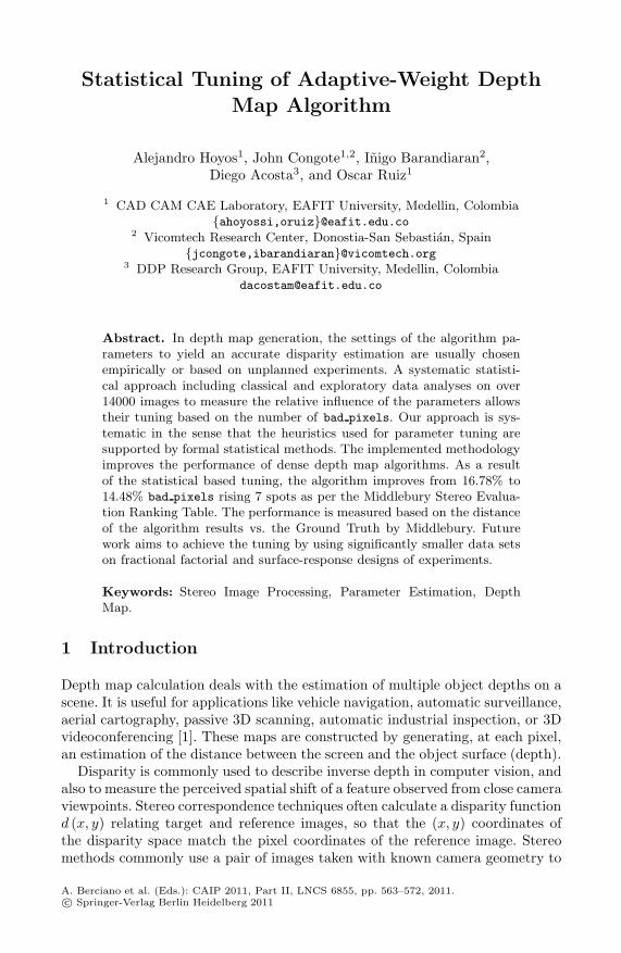
Post-Processing Filters. Algorithms based on correlations depend heavilyon finding similar textures at corresponding points in both reference and targetimages. Bad matches happen more frequently in textureless regions, occludedzones, and areas with high variation in disparity. The winner takes all approachenforces uniqueness of matches only for the reference image in such a way thatpoints on the target image may be matched more than once, creating the need tocheck the disparity estimates and fill any gaps with information from neighboringpixels using post-processing filters like the ones shown in Table 1.

566 A. Hoyos et al.

Table 1. User-specified parameters of the adaptive weight algorithm and filters

Filter Function User-specified parameter

AdaptiveWeight [3]

Disparity estimation andpixel matching

γaws: similarity factor, γawg: proximity factorrelated to the WAW pixel size of the supportwindow

Median Smoothing and incorrectmatch removal

WM : pixel size of the median window

Cross-check[8]

Validation of disparitymeasurement per pixel

Δd: allowed disparity difference

Bilateral[9] Intensity and proximityweighted smoothing withedge preservation

γbs: similarity factor, γbg: proximity factor re-lated to the WB pixel size of the bilateral win-dow

Median Filter. They are widely used in digital image processing to smoothsignals and to remove incorrect matches and holes by assigning neighboringdisparities at the expense of edge preservation. The median filter provides amechanism for reducing image noise, while preserving edges more effectively thana linear smoothing filter. It sorts the intensities of all the q pixels on a window ofsize M and selects the median value as the new intensity of the p central pixel.The size M of the window is another of the user-specified parameters.

Cross-check Filter. The correlation is performed twice by reversing the roles ofthe two images and considering valid only those matches having similar depthmeasures at corresponding points in both steps. The validity test is prone tofail in occluded areas where disparity estimates will be rejected. The alloweddifference in disparities is one more adjustable parameter.

Bilateral Filter. Is a non-iterative method of smoothing images while retain-ing edge detail. The intensity value at each pixel in an image is replaced by aweighted average of intensity values from nearby pixels. The weighting for eachpixel q is determined by the spatial distance from the center pixel p, as well asits relative difference in intensity, defined by Equation (4).

(4)Op =

∑q∈W fs (q − p) gi (Iq − Ip)Iq∑q∈W fs (q − p) gi (Iq − Ip)

where O is the output image, I the input image, W the weighting window, fsthe spatial weighing function, and gi the intensity weighting function. The sizeof the window W is yet another parameter specified by the user.

3.2 Statistical Analysis

The user-specified input parameters and output accuracy measurements datais statistically analyzed measuring the relations amongst inputs and outputswith correlation analyses, while box plots give insight on the influence of groups

Statistical Tuning of Adaptive-Weight Depth Map Algorithm 567

of settings on a given factor. A multi-variate linear regression model shown inEquation (5) relates the output variable as a function of all the parameters to findthe equation coefficients, correlation of determination, and allows the analysisof variance to measure the influence of each parameter on the output variance.Residual analyses are checked to validate the assumptions of the regression modellike constant error variance, and mean of errors equal to zero, and if necessary,the model is transformed. The parameters are normalized to fit the range (−1, 1)as shown in Table 2.

(5)y = β0 +

n∑i=1

βixi + ε

where y is the predicted variable, xi are the factors, and βi are the coefficients.

3.3 Experimental Set Up

The depth maps are calculated with an implementation developed for real timevideoconferencing in [4]. Using well-known rectified image sets: Cones from [1],Teddy and Venus from [10], and Tsukuba head and lamp from the University ofTsukuba. Other commonly used sets are also freely available [11,12]. The sampleused consists of 14688 depth maps, 3672 for each data set, like the ones shownin Figure 1.

Fig. 1. Depth Map Comparison. Top: best initial, bottom: new settings. (a) Cones, (b)Teddy, (c) Tsukuba, and (d) Venus data set.

Many recent stereo correspondence performance studies use the MiddleburyStereomatcher for their quantitative comparisons [2,7,13]. The evaluator code,sample scripts, and image data sets are available from the Middlebury stereovision site1, providing a flexible and standard platform for easy evaluation.

1 http://vision.middlebury.edu/stereo/

568 A. Hoyos et al.

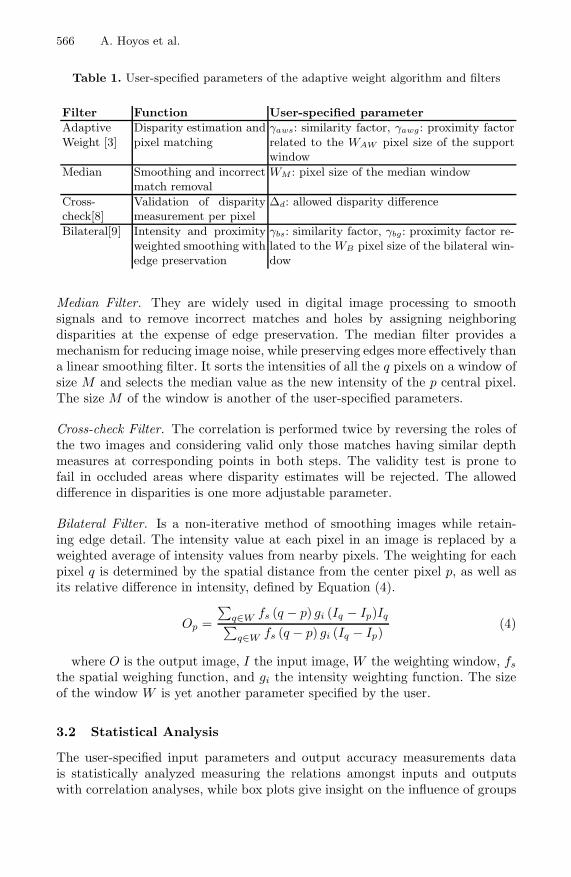
Table 2. User-specified parameters of the adaptive weight algorithm

Parameter Name Levels Values Coding

Adaptive Weights Window Size aw win 4 [1 3 5 7] [-1 -0.3 0.3 1]Adaptive Weights Color Factor aw col 6 [4 7 10 13 16 19] [-1 -0.6 -0.2 0.2 0.6 1]Median Window Size m win 3 [N/A 3 5] [N/A -1 0.2 1]Cross-Check Disparity Delta cc disp 4 [N/A 0 1 2] [N/A -1 0 1]Cross-Bilateral Window Size cb win 5 [N/A 1 3 5 7] [N/A -1 -0.3 0.3 1]Cross-Bilateral Color Factor cb col 7 [N/A 4 7 10 13 16 19] [N/A -1 -0.6 -0.2 0.2 0.6 1]

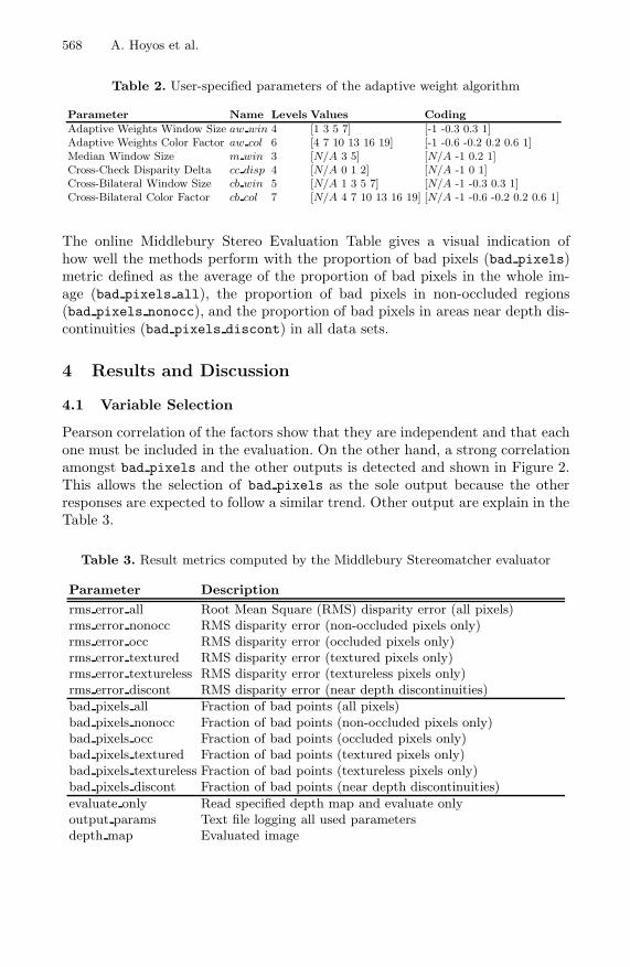
The online Middlebury Stereo Evaluation Table gives a visual indication ofhow well the methods perform with the proportion of bad pixels (bad pixels)metric defined as the average of the proportion of bad pixels in the whole im-age (bad pixels all), the proportion of bad pixels in non-occluded regions(bad pixels nonocc), and the proportion of bad pixels in areas near depth dis-continuities (bad pixels discont) in all data sets.

4 Results and Discussion

4.1 Variable Selection

Pearson correlation of the factors show that they are independent and that eachone must be included in the evaluation. On the other hand, a strong correlationamongst bad pixels and the other outputs is detected and shown in Figure 2.This allows the selection of bad pixels as the sole output because the otherresponses are expected to follow a similar trend. Other output are explain in theTable 3.

Table 3. Result metrics computed by the Middlebury Stereomatcher evaluator

Parameter Description

rms error all Root Mean Square (RMS) disparity error (all pixels)rms error nonocc RMS disparity error (non-occluded pixels only)rms error occ RMS disparity error (occluded pixels only)rms error textured RMS disparity error (textured pixels only)rms error textureless RMS disparity error (textureless pixels only)rms error discont RMS disparity error (near depth discontinuities)

bad pixels all Fraction of bad points (all pixels)bad pixels nonocc Fraction of bad points (non-occluded pixels only)bad pixels occ Fraction of bad points (occluded pixels only)bad pixels textured Fraction of bad points (textured pixels only)bad pixels textureless Fraction of bad points (textureless pixels only)bad pixels discont Fraction of bad points (near depth discontinuities)

evaluate only Read specified depth map and evaluate onlyoutput params Text file logging all used parametersdepth map Evaluated image

Statistical Tuning of Adaptive-Weight Depth Map Algorithm 569

Fig. 2. bad pixels and other output correlation

4.2 Exploratory Data Analysis

Box plots analysis of bad pixels presented in Figure 3(a) show lower outputvalues from using filters, relaxed cross-check disparity delta values, large adaptiveweight window sizes, and large adaptive weight color factor values. The medianwindow size, bilateral window size, and bilateral window color values do notshow a significant influence on the output at the studied levels.

The influence of the parameters is also shown on the slopes of the main effectsplots of Figure 4 and confirms the behavior found with the ANOVA of themulti-variate linear regression model. The settings to lower bad pixels fromthis analysis yields a result of 14.48%.

(a) Box Plots (b) ANOVA proportion of bad pixels

Fig. 3. (a) Box Plots of bad pixels. (b) Contribution to the bad pixels variance byparameter.

4.3 Multi-variate Linear Regression Model

The analysis of variance on a multi-variate linear regression (MVLR) over alldata sets using the most parsimonious model quantifies the parameters with themost influence as shown in Figure 3(b). cc disp is the most significant factoraccounting for a third to a half of the variance on every case.

570 A. Hoyos et al.

Interactions and higher order terms are included on the multi-variate linearregression models to improve the goodness of fit. Reducing the number of inputimages per dataset from 3456 to 1526 by excluding the worst performing casescorresponding to cc disp = 0 and aw col = [4, 7], allows using a cubic modelwith interactions and an R2 of 99.05%.

The residuals of the selected model fail to follow a normal distribution. Trans-forming the output variable or removing large residuals does not improve theresiduals distribution, and there are no reasons to exclude any outliers fromthe image data set. Nonetheless, improved algorithm performance settings arefound using the model to obtain lower bad pixels values comparable to theones obtained through the exploratory data analysis (14.66% vs. 14.48%).

In summary, the most noticeable influence on the output variable comes fromhaving a relaxed cross-check filter, accounting for nearly half the response vari-ance in all the study data sets. Window size is the next most influential factor,followed by color factor, and finally window size on the bilateral filter. Increasingthe window sizes on the main algorithm yield better overall results at the ex-pense of longer running times and some foreground loss of sharpness, while thesupport weights on each pixel have the chance of becoming more distinct andpotentially reduce disparity mismatches. Increasing the color factor on the mainalgorithm allows better results by reducing the color differences, and slightlycompensating minor variations in intensity from different viewpoints.

A small median smoothing filter window size is faster than a larger one, whilestill having a similar accuracy. Low settings on both the window size and thecolor factor on the bilateral filter seem to work best for a good balance betweenperformance and accuracy.

Fig. 4. Main Effects Plots of each factor level for all data sets. Steeper slopes relate tobigger influence on the variance of the bad pixels output measurement.

The optimal settings in the original data set are presented in Table 4 alongwith the proposed combinations. Low settings comprise the depth maps withall their parameter settings at each of their minimum tested values yielding67.62% bad pixels. High settings relates to depth maps with all their param-eter settings at each of their maximum tested values yielding 19.84% bad pixels.Best initial are the most accurate depth maps from the study data set yielding

Statistical Tuning of Adaptive-Weight Depth Map Algorithm 571

Table 4. Model comparison. Average bad pixels values over all data sets and theirparameter settings.

Run Type bad pixels aw win aw col m win cc disp cb win cb col

Low Settings 67.62% 1 4 3 0 1 4High Settings 19.84% 7 19 5 2 7 19Best Initial 16.78% 7 19 5 1 3 4Exploratory analysis 14.48% 9 22 5 1 3 4MVLR optimization 14.66% 11 22 5 3 3 18

16.78% bad pixels. Exploratory analysis corresponds to the settings deter-mined using the exploratory data analysis based on box plots and main effectsplots yielding 14.48% bad pixels. MVLR optimization is the extrapolationoptimization of the classical data analysis based on multi-variate linear regres-sion model, nested models, and ANOVA yielding 14.66% bad pixels.

The exploratory analysis estimation and the MVLR optimization tend toconverge at similar lower bad pixels values using the same image data set. Thebest initial and improved depth map outputs are shown in Figure 1.

5 Conclusions and Future Work

This work presents a systematic methodology to measure the relative influence ofthe inputs of a depth map algorithm on the output variance and the identificationof new settings to improve the results from 16.78% to 14.48% bad pixels. Themethodology is applicable on any group of depth map image sets generated withan algorithm where the relative influence of the user-specified parameters meritsto be assessed.

Using design of experiments reduces the number of depth maps needed tocarry out the study when a large image database is not available. Further analysison the input factors should be started with exploratory experimental fractionalfactorial designs comprising the full range on each factor, followed by a responsesurface experimental design and analysis. In selecting the factor levels, analyzingthe influence of each filter independently would be an interesting criterion.

Acknowledgments. This work has been partially supported by the SpanishAdministration Agency CDTI under project CENIT-VISION 2007-1007, theColombian Administrative Department of Science, Technology, and Innovation;and the Colombian National Learning Service (COLCIENCIAS-SENA) grantNo. 1216-479-22001.

References

1. Scharstein, D., Szeliski, R.: A taxonomy and evaluation of dense two-frame stereocorrespondence algorithms. Int. J. Comput. Vision 47(1-3), 7–42 (2002)

2. Gong, M., Yang, R., Wang, L., Gong, M.: A performance study on different cost ag-gregation approaches used in real-time stereo matching. Int. J. Comput. Vision 75,283–296 (2007)

572 A. Hoyos et al.

3. Yoon, K., Kweon, I.: Adaptive support-weight approach for correspondence search.IEEE Trans. Pattern Anal. Mach. Intell. 28(4), 650 (2006)

4. Congote, J., Barandiaran, I., Barandiaran, J., Montserrat, T., Quelen, J., Ferran,C., Mindan, P., Mur, O., Tarres, F., Ruiz, O.: Real-time depth map generationarchitecture for 3d videoconferencing. In: 3DTV-Conference: The True Vision-Capture, Transmission and Display of 3D Video (3DTV-CON), 2010, pp. 1–4(2010)

5. Gu, Z., Su, X., Liu, Y., Zhang, Q.: Local stereo matching with adaptive support-weight, rank transform and disparity calibration. Pattern Recogn. Lett. 29,1230–1235 (2008)

6. Hosni, A., Bleyer, M., Gelautz, M., Rhemann, C.: Local stereo matching usinggeodesic support weights. In: Proceedings of the 16th IEEE Int. Conf. on ImageProcessing (ICIP), pp. 2093–2096 (2009)

7. Wang, L., Gong, M., Gong, M., Yang, R.: How far can we go with local optimiza-tion in real-time stereo matching. In: Proceedings of the Third International Sym-posium on 3D Data Processing, Visualization, and Transmission (3DPVT 2006),pp. 129–136 (2006)

8. Fua, P.: A parallel stereo algorithm that produces dense depth maps and preservesimage features. Machine Vision and Applications 6(1), 35–49 (1993)

9. Weiss, B.: Fast median and bilateral filtering. ACM Trans. Graph. 25, 519–526(2006)

10. Scharstein, D., Szeliski, R.: High-accuracy stereo depth maps using structuredlight. In: IEEE Conference on Computer Vision and Pattern Recognition, vol. 1,pp. 195–202 (2003)

11. Scharstein, D., Pal, C.: Learning conditional random fields for stereo. In: IEEEConference on Computer Vision and Pattern Recognition, pp. 1–8 (2007)

12. Hirschmuller, H., Scharstein, D.: Evaluation of cost functions for stereo matching.In: IEEE Conference on Computer Vision and Pattern Recognition, pp. 1–8 (2007)

13. Tombari, F., Mattoccia, S., Di Stefano, L., Addimanda, E.: Classification and eval-uation of cost aggregation methods for stereo correspondence. In: IEEE Conferenceon Computer Vision and Pattern Recognition, pp. 1–8 (2008)