Deep-Sea Research II 88–89 (2013) 34–46

Contents lists available at SciVerse ScienceDirect

Deep-Sea Research II

0967-06

http://d

n Corr

E-m

journal homepage: www.elsevier.com/locate/dsr2

State-space models for bio-loggers: A methodological road map

I.D. Jonsen a,n, M. Basson b, S. Bestley a,e, M.V. Bravington c, T.A. Patterson b, M.W. Pedersen d,R. Thomson b, U.H. Thygesen d, S.J. Wotherspoon e,f

a Ocean Tracking Network, Department of Biology, Dalhousie University, Halifax, Nova Scotia, Canadab CSIRO Marine and Atmospheric Research, Wealth from Ocean Flagship, Castray Esplanade, Hobart, Tasmania, Australiac CSIRO Mathematics, Informatics and Statistics, Castray Esplanade, Hobart, Tasmania, Australiad National Institute of Aquatic Resources, Technical University of Denmark, Charlottenlund, Denmarke Institute for Marine and Antarctic Studies, University of Tasmania, Sandy Bay, Hobart, Tasmania, Australiaf Australian Antarctic Division, Kingston, Tasmania, Australia

a r t i c l e i n f o

Available online 17 July 2012

Keywords:

Animal movement

Bayesian statistics

Foraging behaviour

Frequentist statistics

Hidden Markov model

Migration

Telemetry

Time series analysis

45/$ - see front matter & 2012 Elsevier Ltd. A

x.doi.org/10.1016/j.dsr2.2012.07.008

esponding author. Tel.: þ1 902 494 3910.

ail address: ijonsen@dal.ca (I.D. Jonsen).

a b s t r a c t

Ecologists have an unprecedented array of bio-logging technologies available to conduct in situ studies

of horizontal and vertical movement patterns of marine animals. These tracking data provide key

information about foraging, migratory, and other behaviours that can be linked with bio-physical

datasets to understand physiological and ecological influences on habitat selection. In most cases,

however, the behavioural context is not directly observable and therefore, must be inferred. Animal

movement data are complex in structure, entailing a need for stochastic analysis methods. The recent

development of state-space modelling approaches for animal movement data provides statistical rigor

for inferring hidden behavioural states, relating these states to bio-physical data, and ultimately for

predicting the potential impacts of climate change. Despite the widespread utility, and current

popularity, of state-space models for analysis of animal tracking data, these tools are not simple and

require considerable care in their use. Here we develop a methodological ‘‘road map’’ for ecologists by

reviewing currently available state-space implementations. We discuss appropriate use of state-space

methods for location and/or behavioural state estimation from different tracking data types. Finally, we

outline key areas where the methodology is advancing, and where it needs further development.

& 2012 Elsevier Ltd. All rights reserved.

1. Introduction

Within marine ecology, a very general set of ecological ques-tions has emerged that researchers address using bio-loggingtechniques. For example, where and when do animals move?What are the physiological costs of these movements? How dothese movements relate to environmental variability and the everchanging distributions of heterogeneous resources? What are theimplications of individual movements at the population level?How might animal movements and population distribution beaffected by future environmental change in the ocean? Answeringthese important ecological questions becomes a challengingstatistical problem when using most bio-logging data.

Telemetry-based studies of animal movement ecology, phy-siology, and environmental interactions generally rely on acompartmentalized approach to analysis of tracking data. Thisapproach typically has three stages: (1) error correction; (2) cal-culation of summary movement metrics from corrected tracks;and (3) biological inference through statistical or non-statistical

ll rights reserved.

analysis (Patterson et al., 2008). There are three key drawbacks tothis approach. First, implicit assumptions, which may or may not bevalid, regarding an animal’s movements are required to removespurious location errors (e.g., Austin et al., 2003). Second, measure-ment error effects are not separated from the underlying movementprocesses that are of interest, which can bias analyses (Bradshawet al., 2007). Third, the analysis tools associated with this approachtend to be correlative, comparative (using simple hypothesis tests),or pattern-based; all of which are limited in their scope for directexamination of the ecological and physiological mechanisms thatunderpin animal movement. Adopting a stochastic, model-basedapproach that allows mechanistic models of the movement processto be fit directly to telemetry data, while accounting for measure-ment error when appropriate, is more rigorous and powerful butalso requires more complicated analysis tools.

Recent reviews (Patterson et al., 2008; Schick et al., 2008) havepublicized the notion of state-space model (SSM1) approaches forstudying animal movement and these tools are now being morewidely applied. We see signs within the bio-logging communitythat SSM approaches are making their way into analyses of many

1 See the Glossary for a definition of this and other technical terms.

I.D. Jonsen et al. / Deep-Sea Research II 88–89 (2013) 34–46 35

kinds of telemetry data. A total of 21 oral and poster presenta-tions at the Fourth International Symposium on Bio-logging(March 2011), held in Hobart, Tasmania, Australia, included someform of SSM analysis of telemetry data or further developed theirimplementation.2 In many cases, SSMs are used to filter error-prone Argos (2011) or light-based (Hill, 1994) location data and/or to estimate unobserved behavioural states of animals. Despitethese promising signs, we feel there is a gap to be bridged in thegeneral understanding of SSMs, both in the technical aspects oftheir application and in the interpretation of their results. It is,therefore, timely to build a methodological road map for bio-loggers outlining currently available methods and applicationsappropriate to particular problems in the study of animal move-ment and behaviour.

Here we explain SSMs in the context of marine animal trackingdata by providing the necessary background, technical details,and examples for field ecologists to appreciate the flexibility andpower of these statistical tools. We outline general considerationsfor fitting SSMs, for querying their fit to data, and for model selection.We highlight several previously published SSM approaches fortracking data and the situations in which one may be preferred overothers. Finally, we suggest areas where the methods are advancingand where further work is required.

Fig. 1. Structure of a SSM for estimation. The state variable evolves randomly

in time, starting at x0 and ending at xtN. At times t1 ,t2 , . . . ,tN , measurements

y1 , . . . ,yN are taken. In this graphical representation of the model, an arrow from

2. General explanation of state-space methods

State-space models encompass a range of time series methodsthat estimate the state of an unobservable process from anobserved data set. The earliest example of state-space methodsused for estimation purposes is the celebrated Kalman filter (KF)(Kalman, 1960, see also Section 5) which is now used in applica-tions from aerospace to finance, as well as for geolocation ofanimals from tagging data (Sibert et al., 2003). The state-spaceparadigm is not limited to time series analysis: it applies also topure analysis problems, one example from marine ecology beinglarval transport and growth (e.g., Christensen et al., 2008), and todynamic optimization problems, e.g., arising in behavioural ecology(Houston and McNamara, 1999). In ecology, state-space methodsare used to model single individuals, population dynamics (Brinchet al., 2011; de Valpine and Hastings, 2002), and marine ecosystemdynamics (Evensen, 2003).

The notion of the state is pivotal in SSMs, as the name suggests.In a bio-logging context, the most common state variables used (todate) are an animal’s position (Anderson-Sprecher and Ledolter,1991; Jonsen et al., 2003; Royer et al., 2005; Thygesen et al., 2009)and it’s behaviour, the latter is usually represented as a discretevariable with two or more nominal categories such as ‘‘foraging’’ and‘‘not foraging’’ or ‘‘migratory’’ and ‘‘resident’’ (Jonsen et al., 2005;Morales et al., 2004; Patterson et al., 2009; Pedersen et al., 2011b).Mathematically, a collection of variables constitute the state of adynamical system, if they summarize the previous history of thesystem, so that predictions about the future can be made solely fromthe current state. Choosing the right number of state variables todescribe a real system is a delicate balance between realism andfeasibility, and choosing the most important state variables requiresinsight into not just the biology of the animal, but also the dataquality and the nature of the statistical estimation problem.

The key ingredient in a stochastic SSM is the process model, anequation that describes how the state evolves randomly in time. Asimple example of a process model is a random walk, whichverbally can be formulated as follows: if the position of an animal

2 http://www.cmar.csiro.au/biologging4/documents/AbstractsandProgram_

final.pdf, last accessed on 25/05/2012.

at time t is known to be xt , then the position one day later isGaussian with mean xt and variance V. Here V is a parameter, thevariance of the daily move distance. A mathematical formulationof this is

xtþ19t �Nðxt ,VÞ ð2:1Þ

Note that the process model is written in terms of conditionalprobability distributions. If the state xt at time t is known, how isthe later state xtþ1 distributed? Mathematically, the notion of astate is formalized by the Markov property: given the currentvalue of the state, future state variables are statistically indepen-dent of past state variables. These conditional distributions, whichare known as transition probabilities, are sufficient to describe allstate dynamics. Note also that we distinguish between statesand parameters: states like xt evolve in time and describe theimmediate situation, while parameters like V are typically con-stant in time and describe the underlying properties of the animalor mechanism of the system.

In this example, the state variable is continuous, i.e. may takeany real value. In other cases, the state may be purely discrete, i.e.only a finite (or countable) number of different states are possible.In yet other examples, the state is composed of both continuousand discrete state variables. Similarly, the time variable may becontinuous or discrete. Even if, for example, the position of ananimal is defined at all times, we may choose to have the modelrepresent only the daily position.

The process model is written entirely without reference toavailable data. Of course, choosing a suitable process model requiresthought about available data, but the state of the system evolvesregardless of how or if we observe the system.

For estimation purposes, the process model is complementedby one or more equations, the observation model, which describethe link between each observed data point and the state of thesystem at the time of observation, or at regular time intervalswithin which observations may or may not occur. The observationmodel describes what happens at the time of observation, so doesnot make any reference to the dynamics in the underlying processmodel. This structure is depicted in Fig. 1. Also these equationsspecify conditional probability distributions: if the state at time t

were known to be xt , how is the measurement yt distributed? Itis important to appreciate the generality of this framework: themeasurement may be a state variable subject to measurementerror, for example, a position estimated with the Argos satellitesystem, but the measurement may also be any other quantitywhich holds some information about the state, for example, ananimal’s travel speed or sea surface temperature (SST). Theobservation model may specify several different types of mea-surements which may be taken simultaneously or at differentpoints of time. Like the process model, the observation model

one variable (say, xti) to another (say, yi) indicates that the model is written in

terms of the conditional distribution of yi given xti, and furthermore that

conditional on xti, yi is statistically independent of all other variables since they

are not connected with arrows.

I.D. Jonsen et al. / Deep-Sea Research II 88–89 (2013) 34–4636

may contain unknown parameters, for example, the bias orvariance of a measurement error.

For our purpose, the most important use of the stochastic SSMis to draw inference from actual observations about how the stateevolves through time, and about associated parameters thatrepresent biological mechanisms underlying the state evolutionand/or parameters that represent important features of the datacollection process. A suite of different algorithms exist for thispurpose, and the applicability of these depends on the specifics ofthe SSM. Although they share the underlying principle, thealgorithms appear quite distinct. For example, if the conditionaldistributions in both the process model and the observationmodel are all Gaussian, then the state estimation problem canbe written in terms of means and variances; this is the KF.Similarly, in the discrete case where the state may attain only afinite number of different values (and this number is not exceed-ingly large), it is possible to compute the exact probability ofbeing in each state at each point in time. This leads to theframework of hidden Markov models (HMM) (Rabiner, 1989;Zucchini and MacDonald, 2009). In both cases, a by-product ofestimating the state for a given parameter is the likelihood of theparameter, so an outer loop can maximize the likelihood andthereby provide parameter estimates. In the general case onlyMonte Carlo methods (Gelman et al., 2004) are feasible, and evenwithin this class a large variability of algorithms exists. We willdiscuss algorithms for estimation further in Section 5.

Finally, an SSM may be an element in an hierarchical modelstructure (Jonsen et al., 2003, 2006; Mills Flemming et al., 2010).For example, in a tagging study that includes a number of animals,we may assume that all animals move according to a random walk,but that each animal is characterized by a different diffusivity,and that these diffusivities are random variables drawn from anunknown distribution. Then, the focus of the modelling shifts fromthe single animal to the population, and to the variability betweenanimals in the population.

3. Process models: behaviour and movement

In a bio-logging context, the process model formally describesthe biological process of interest and predicts the state of thisprocess through time. This is a model of some combination ofmovement, behaviour, or perhaps the physiological response ofan individual animal. Here we outline in simple terms someexamples of process models commonly applied to bio-loggingdata. It is important to realise that an SSM does not necessarilyhave to be a movement model—something we feel is a commonmisconception in the bio-logging community at the moment.

3.1. Stochastic models of animal behaviour

The fact that behaviours tend to persist through time in bouts,and that animals do not jump randomly in space means thattemporal dependence in bio-logging data is almost guaranteed.An animal is more likely to be doing the same thing at some timeclose to the present, than it is to switch to another activity.Certainly its current location will be near to its recent previouslocation. From a statistical perspective, these obvious truismshave an important effect in that they lead to data which arehighly auto-correlated. This has large implications for how bio-logging data of movement and behaviour ought to be modelledand mandates that we employ process models which can capturethis time dependence.

Perhaps the simplest process model which described suchbouts of behaviour is a Markov chain describing the evolution ofan animal’s behaviour through time. Consider an animal assumed

to be in one of two possible states at time t; which we labelforaging ðFtÞ or not-foraging ðNFtÞ. In this simple case, the ‘‘state-space’’ of the model is the finite set made up of these two possiblestates. The Markov chain is specified by the probability of switch-ing states from F at time t to NF at time tþ1. The model is writtenin terms of a transition matrix:

P¼PrðFtþ19FtÞ PrðNFtþ19FtÞ

PrðFtþ19NFtÞ PrðNFtþ19NFtÞ

!ð3:1Þ

and a state variable St, which probabilistically describes the stateof the animal at any time: St ¼ ½PrðFtÞ PrðNFtÞ�. The probability ofeach behavioural state through time is updated by Stþ1 ¼ St � P.Despite its simplicity, this is a useful process model and can alsobe coupled with spatial movement models (see below), formingthe basis of more complicated spatial description of individualmovement (see below). Greater complexity can be built into thisMarkovian model by, for example, specifying the probability ofswitching between F and NF as a function of local environmentalconditions (Morales et al., 2004; Patterson, 2009). The Markovchain approach would be straightforward if we could observe thebehaviours directly.

Despite advances in telemetry, an animal’s behavioural statetypically is unobservable, but the great advantage of SSMs is theability to posit a reasonable model of behaviour and fit it totelemetry data related to the hidden behaviour. For example, wemight expect that travel speeds when in mode F tend to be slowercompared to NF. We can use a HMM in this situation. Typically,HMMs applied to bio-logging data take the position of the animalto be known without error and are fit to derived metrics from themovement path such as speed and turning angle (e.g., Moraleset al., 2004; Patterson et al., 2009). These metrics constitute thedata to the HMM and enable inference about the underlyinghidden Markov process—the animal’s behaviour. As a generalrule, these data should be observed with minimal error, e.g., GPSdata, but HMMs have been usefully applied to geolocationestimates (Patterson, 2009). Model predictions of behaviour canoften be usefully mapped to show geographical areas of likelyimportance for a species (Patterson, 2009), though inferencesdrawn from such maps should consider the accuracy of locationdata. The assumption here is that areas with high-residence arelikely to be important for foraging, breeding or some otherbiological imperative. This assumption is grounded in ecologicaltheory (Charnov, 1976) but may not always hold when real dataare examined (e.g., Bestley et al., 2010).

3.2. Individual movement models

In order to explicitly model the movement of an individualanimal, we require a model of the trajectory of the animal throughspace as opposed to solely categorising pre-calculated movementmetrics into behaviours. Behavioural categorization can be carriedout simultaneously with characterization of individual movement.For spatial process models, the state variable St usually includes atleast the location of the animal at time t, St ¼ ðLongt ,LattÞ but couldalso include auxiliary variables such as the animal’s speed.

One of the simplest movement models is a diffusion model:given the position xt , a later position xtþdt follows a Gaussiandistribution with mean xt and variance 2D dt. Here dt is anypositive time step and D is the diffusion rate. Many movementmodels can be seen as extensions or modifications of the diffusionmodel (Turchin, 1998). Although animal movement is a contin-uous-time phenomenon, the model may be solely in discretetime, for example, in terms of a daily position. In that case wewould only consider integer dt. The resulting model is a randomwalk in discrete time with Gaussian displacements.

I.D. Jonsen et al. / Deep-Sea Research II 88–89 (2013) 34–46 37

The diffusion model states that the mean displacement overany time interval is 0, but this often does not adequately reflectanimal movement behaviours. A simple extension of the diffusionmodel is to add a systematic bias or advection so that themovements tend to ‘‘drift’’ in a particular direction. The resultingadvection–diffusion model, or biased random walk, has a dis-placement which still has variance 2D dt, but now mean dis-placement udt rather than 0. The drift u may be a constant, time-varying (e.g., to reflect seasonal changes in directed movements),or it may depend on space (e.g., Brillinger et al., 2002) to reflectattraction to or repulsion from specific regions in space (i.e.movements within a home range). If the animal moves randomlyaccording to a diffusion or advection–diffusion model, then theprobability density of the animal’s position evolves according to apartial differential equation known as the advection–diffusionequation (see Okubo and Levin, 2001, for background material).These partial differential equations can only be solved in specialsituations, for example, the linear cases which lead to the KF.Without such simple structure, one must resort to numericalsolutions; this is computationally demanding and effectivelyrestricts the state variables to latitude, longitude, and possibly afew discrete behavioural states. A large number of computa-tional methods for partial differential equations can in principlebe applied. Finite volume or finite element methods have theadvantage that irregular geometries such as coastlines can betaken into account (Pedersen et al., 2011a), and that standardalgorithms and software have been developed for engineeringapplications. Finite volume methods essentially divide space intodiscrete grid cells, which the animal moves between, and there-fore, corresponds to approximating the dynamics of the animalwith a Markov chain.

Although the advection–diffusion model allows the animal adirectional preference, it has no room for directional persistence:the displacements in two consecutive time steps are statisticallyindependent. In reality, the velocity of an animal will almostinvariably display some correlation in time. To take this intoaccount, one may introduce a discrete behavioural state which isassociated with a specific value of the drift u, or one may extendthe random walk to a correlated random walk. This may beachieved by adding the velocity as a state variable, or, in adiscrete-time setting, by amending to the state variable theposition at previous time step (e.g., Jonsen et al., 2005). Goingfrom a random walk to a correlated random walk increases thefidelity of small-scale features in the estimated track, providedthat the data quality is sufficient to resolve these features.

3.2.1. Continuous and discrete state-space representations

The details of specifying the process model differ slightly depend-ing on how space and time are treated. For example, a diffusionmodel can be expressed in continuous space but often tends to benumerically calculated using finite-difference schemes or otherapproximations.

It is often convenient to treat space as a discrete quantity andapproximate the continuous situation with a finite set of loca-tions. Doing so has the advantages of being able to restrict animalsfrom moving to implausible locations. Additionally, treating spaceas a discrete quantity can render the SSM updating to be tract-able without recourse to computationally demanding simulation(Pedersen et al., 2011b). Likewise, time may be viewed as contin-uous (e.g., Johnson et al., 2008; Patterson et al., 2010) or discrete(e.g., Jonsen et al., 2003, 2005) in SSM process models. Typically,dealing with discrete time is mathematically more straightforwardand some models may only be posited if discrete times are assumed.However, much telemetry data is more naturally modelled withcontinuous time models. For example, telemetry data collected

when marine mammals surface will be truly irregular. Light-levelgeolocation estimates of position however, are truly regular, beingcollected at dawn and dusk, however, data obtained from PSAT tagscan be highly irregular due to transmission issues after tag pop-off.

3.3. Spatial switching models

The final class of models we consider here are what we termspatial switching models, which include both location and beha-viour in the state vector. These models are relevant in the casewhere movement and behaviour are of interest but observationerror is non-negligible. These are a combination of the modelsdiscussed in Sections 3.1 and 3.2.

Spatial switching models were introduced to the bio-loggingcommunity in Jonsen et al. (2005). In this paper, a correlatedrandom walk (CRW) process model is outlined but also includesthe possibility of switching between two different CRW’s. Theswitching process is governed by a Markov chain model of thesort given in Eq. (3.1). The motivation behind construction ofthese models is that they offer the possibility of location errorcorrection as well as simultaneous behavioural state estimation.The process model described in Jonsen et al. (2005) assumes thatthe two CRW models, and the behavioural states they describe,differ only in their values of y and g, the mean turn angle andmove persistence parameters (see Jonsen et al., 2005 for fulldetails). Thus the process model gains the subscript bt, denotingthe behavioural state, on ybt

and gbt:

dtþ1 ¼ gbtTðybtÞdtþZt ð3:2Þ

where dtþ1 and dt are the differences between positions xtþ1, xt

and xt , xt�1, respectively, TðybtÞ is a matrix describing the

behavioural state-specific mean turn angle required to move fromdt to dtþ1, and Zt is a bi-variate Gaussian random variabledescribing the stochastic part of the movement process.

Switches between behavioural states are modelled by assum-ing that an animal can change from its current behaviour toanother one with a fixed probability given by the Markov chain:

Prðbtþ1 ¼ i9bt ¼ jÞ ¼ aij ð3:3Þ

where aij is the probability of an animal being in behavioural statei at time tþ1 given that it was in behavioural state j at time t. Weestimate a11, the probability of remaining in state 1, and a12, theprobability of switching from state 2 to state 1.

So far, few studies have considered models where the beha-vioural state of an animal is continuous (but see Breed et al.,2012; Dowd and Joy, 2010; Forester et al., 2007) and for many ofthe general distinctions in animal behaviour (e.g., searching/foraging, resident/migrant) discrete states may suffice.

Finally, we emphasize the multiple types of models that arediscussed here. The process model is a subcomponent of theoverall SSM. As such, process models employed in bio-loggingsituations tend to be well-known movement models which have along history in ecology (Okubo and Levin, 2001; Turchin, 1998).The advance brought by SSMs to this problem is the ability to takethese movement models, meld them with stochastic descriptionsof behaviour (e.g., the Markov behavioural model Eq. (3.1)), andfit them to empirical data.

As we will see in Section 5, it is important to recognize that thechoices about the type of model that often stem from the specificsof the available data lead naturally toward one or anotherestimation framework.

4. The observation model

The observation model describes the statistical distributionsgenerating the observations conditional on the state. In terms of

I.D. Jonsen et al. / Deep-Sea Research II 88–89 (2013) 34–4638

Fig. 1, the observation model relates to the arrows that link eachxt to a yt . Exactly what constitutes the ‘‘observations’’ is a choicewhich should relate to the questions being asked and the relevanttime- and spatial scales of interest. For example, if daily move-ments at the scale of kilometers is of interest, it would beinappropriate (and unnecessary) to use data recorded at 2 sintervals in the observation model. Instead, summaries of the‘‘raw’’ data (e.g., mean, median, variance, counts) should be used.Some metrics will more obviously relate to specific statisticaldistributions than others, e.g., Poisson distributions are a naturalchoice for count data. There are many potential options fordistributions (e.g., McLachlan and Peel, 2000), and the choiceshould be informed by the data characteristics. One shouldconsider: are the data continuous (e.g., travel speed) or discrete(e.g., counts of dives to a certain depth)? Are all observationspositive, or both positive and negative? Mixture distributions canbe hard to fit when using heavy-tailed distributions (McLachlanand Peel, 2000), so it is advisable to start with lighter-taileddistributions (e.g., Gaussian or Poisson) and only use heaviertailed distributions (e.g., t-distribution) if residuals and otherdiagnostics indicate the need (see Section 6). Examples fromapplications in the literature include: exponential distributionsfor movement distance (Patterson et al., 2009); Weibull distribu-tions for speed (Morales et al., 2004); t-distributions for Argoslocations (Jonsen et al., 2005); Gaussian distributions for geoloca-tions (Sibert et al., 2003). More complicated formulations are alsopossible, including bias terms, fitting to multiple types of datasimultaneously (e.g., Nielsen et al., 2006), and estimating obser-vation model parameters as function of covariates. However, westress that care should be taken as to the biological meaning ofsuch formulations and to determine whether increased modelcomplexity really is warranted. Observation model parametersare estimated together with the process model parameters asdiscussed in the next section.

3 R Development Core Team; http://www.r-project.org, last accessed on

25/05/2012.4 The Mathworks, Inc; http://www.mathworks.com/products/matlab, last accessed

on 25/05/2012.5 AD Model Builder; http://admb-project.org, last accessed on 25/05/2012.

5. Model fitting approaches

Procedures for fitting SSMs to data (estimating parameters andhidden states) are varied and often highly complex. Our aim inthis section is to provide a brief overview of the fitting approachesavailable. Interested readers should consult the references forfurther details on implementation of the various approaches andavailable software.

State space models and their variants can be fitted by max-imum likelihood or Bayesian methods. The common difficulty ofboth approaches is the evaluation of the likelihood. The specifica-tion of the process and observation models determines the jointdistribution of the observations and the underlying latent states, butparameter estimation relies on the likelihood of the observations—

the joint density averaged over the latent states. In general, theevaluation of the marginal likelihood can be extremely computa-tionally demanding.

5.1. Maximum likelihood approaches

There are some cases for which the marginal likelihood can beevaluated directly. In HMMs, the states are entirely discrete andthe likelihood is calculated in a straightforward manner bysumming over these discrete states. The marginal likelihood andthe optimal state can be calculated efficiently with a two passrecursive algorithm (Scott, 2002; Zucchini and MacDonald, 2009).The first or forward pass computes the marginal likelihood, whilethe reverse pass computes the probability the system is ineach state at each time interval. Given the marginal likelihood,maximum likelihood (or Bayesian methods, see ‘‘Simulation

approaches’’) can be applied to derive parameter estimates byplugging the likelihood function into a numerical optimizer suchas optim in R3 or fminunc in Matlab.4 These functions providethe optimal parameter values and the covariance of these para-meters (via the Hessian matrix). An alternative to direct optimi-zation is the expectation-maximisation (EM) algorithm, which inthe context of HMMs is also known as the Baum–Welch algorithm(Rabiner, 1989). The EM-algorithm is attractive because it isguaranteed to improve the likelihood in each iteration. However,it does not take advantage of built-in optimizers and thereforerequires additional coding effort, and it does not provide theparameter covariance matrix so uncertainty of parameter esti-mates cannot be directly assessed (for further discussion of directlikelihood optimization versus the EM algorithm see Zucchini andMacDonald, 2009, p. 72). Given the optimal parameter values themost likely state in each time step is provided by the recursivealgorithm, but the most likely sequence of states must bedetermined by the Viterbi (2006) algorithm.

For linear SSMs with continuous states and Gaussian observationerrors, the joint distribution of the observations and the state isGaussian, and the marginal likelihood can be easily calculated. TheKalman smoother is a two pass recursive algorithm that efficientlyaccomplishes this. The KF, the first or forward pass of this algorithm,calculates the marginal likelihood and the filtered states—theoptimal estimates of the state for each time interval given onlythe observations preceding that time. The second or backwardpass of the Kalman smoother calculates the smoothed states—theoptimal estimates of the states given all the observations. Again,given a method of evaluating the marginal likelihood, parameterestimates can be derived by maximum likelihood or Bayesianmethods.

The extended and unscented KFs generalize the KF to the caseof mildly nonlinear (but differentiable) SSMs. These apply localapproximations in each time interval to generate approximateparameter estimates.

The primary advantages of the aforementioned methods aretheir speed and availability. Because these methods evaluate themarginal likelihood directly they are comparatively fast. Packagesfor fitting HMMs and linear SSMs in C/Cþþ, Fortran, Matlab and Rare readily available, typically the user need only provide code tospecify the process and observation models. Alternately, ADMB5

uses automatic differentiation to facilitate efficient maximizationof the likelihood, but the user must provide code in a C-likesyntax to evaluate the likelihood.

5.2. Bayesian/simulation approaches

Strongly nonlinear models, models with non-Gaussian errors,and models with a mixture of continuous and discrete states aretypically fitted with simulation based Bayesian techniques (butsee Breed et al., 2012; Dowd and Joy, 2010). In the Bayesianparadigm, the model parameters are viewed as random andinference is based on the posterior distribution of the parametersand states—the joint distribution of the parameters and statesconditional on the observed data (Ellison, 2004). Unfortunately,even for comparatively simple problems direct calculation of theposterior is often intractable.

Markov Chain Monte Carlo (MCMC) techniques approximatethe posterior by simulating samples from the posterior dis-tribution. Any property of the posterior is approximated by the

I.D. Jonsen et al. / Deep-Sea Research II 88–89 (2013) 34–46 39

corresponding property of the samples in the same way that asample mean approximates a population mean. Theory guaran-tees that an infinite MCMC sample will be representative of theposterior, but in practice only finite samples can be drawn andconsiderable care must be exercised to ensure that these arerepresentative of the posterior (see ‘‘Model checking and selec-tion’’). MCMC samplers can be temperamental, and often requiresome tuning. When a sampler is performing poorly it can beextremely difficult to ascertain why; even different representa-tions of the same model may yield vastly different performances(Lunn et al., 2000).

Software such as WinBUGs (Lunn et al., 2000), OpenBUGs(Lunn et al., 2009), JAGs6 and PyMC (Patil et al., 2010) have madeMCMC highly accessible. The major advantage of these packagesis their flexibility and ease of use—a vast variety of models can becatered for, and typically the user need only provide code tospecify the model structure and the software automaticallydevises a scheme to sample from the posterior. A potentialdisadvantage is that there is little scope to connect these sophis-ticated packages to large-scale environmental databases, limitingthe capacity to include environmental covariates in the model.

Particle filter (PF), or sequential Monte Carlo (SMC), methods arespecifically designed for simulating the states of an SSM (Doucetet al., 2001). These methods sequentially simulate a sample of‘‘particles’’ that follow ‘‘trajectories’’ defined by the model. At eachtime step the particles are resampled so that particles that followunlikely trajectories are down-weighted and those that follow likelytrajectories are up-weighted in the sample (e.g., Royer et al., 2005).Particle filters sample only the model states, and so model para-meters must be estimated by incorporating an MCMC step, or by theprocess of ‘‘state augmentation’’ in which parameters are viewed asa component of the state that can either remain constant or varyover time (e.g., Breed et al., 2012; Dowd and Joy, 2010). Althoughpackages implementing particle filters exist in C/Cþþ, Fortran,Matlab and R, typically these methods require a high level ofstatistical and programming sophistication from the user.

6. Model checking and selection

All SSMs fit to data must be checked to determine how wellthey fit the data. In the context of generalized linear models,diagnostics and model selection are well-defined and understood,so inferences can be made with confidence. In the context ofSSMs, however, model checking and selection remain areas ofactive statistical research. This is also the case even in the simplerbut related context of fitting independent mixture distributions todata (McLachlan and Peel, 2000).

Diagnostics based on the notion of residuals are becomingreasonably well-established for HMMs. But for all types of SSMsthe tools for formal model selection (e.g., Akaike’s Informationcriterion – AIC, Bayesian information criterion – BIC) are generallyunreliable for reasons given below. Here we provide guidance forgood practice given the statistical tools currently available, andunder the three mains aspects of model checking: (1) technicalissues of fitting; (2) diagnostics and goodness of fit checks;(3) model selection and inference.

6.1. Technical issues of fitting

The first checks of model fit should be aimed at trappingproblems in fitting and/or weeding out models that do not make

6 Martyn Plummer, http://mcmc-jags.sourceforge.net/, last accessed on

25/05/2012.

biological or ecological sense, e.g., because parameter estimatesare unrealistic for the study animal or system.

Two potential problems when fitting by maximising the like-lihood are lack of convergence and convergence at a local ratherthan global maximum. Optimisation routines (e.g., nlminb andoptim in R) indicate whether convergence was achieved; if it hasfailed, different starting values or optimisation control para-meters can be tried. It is also good practice to use a range ofstarting values to see whether the same maximum is identified ineach case.

Related checks should be applied to models fitted by Bayesianmeans (see Appendix A for examples of convergence diagnosticsapplied to MCMC chains). One potentially serious implementationproblem is a label-switching issue which HMMs share with finitemixture models. The labels associated with the states in an HMMare arbitrary and the model is invariant under permutation of thelabels. This is irrelevant to maximum likelihood estimation, butis a problem in the context of MCMC estimation of posteriordistributions, regardless of which sampling strategy is being used.This problem is usually resolved by imposing constraints on theparameters that would be violated by permuting the state labels(Scott, 2002; Zucchini and MacDonald, 2009).

There is a large body of literature on checking the convergenceof MCMC chains (e.g., Cowles and Carlin, 1996; Mengersen et al.,1999), and Robert et al. (1999) deal specifically with HMMs.Celeux et al. (2000) made a comment (echoed by Chopin, 2007;Zucchini and MacDonald, 2009) regarding lack of convergence ofMCMCs: ‘‘[y] we consider that almost the entirety of MCMCsamplers implemented for mixture models has failed to con-verge!’’. Although this statement was made of independentmixture models, it is presumably also applicable to HMMs.

For more general SSMs, the technical assessment of fit isstraightforward only if the model was fit using a KF. As onemoves further from vanilla KFs, fitting and assessing goodness offit escalates rapidly in difficulty.

Even if there are no fitting problems, it is important to checkwhether the parameter estimates make intuitive and biologicalsense. Unrealistic, even ludicrous, parameters can result from anover-parameterised model, often due to too many states. It isinformative to plot estimated functional relationships betweenparameters and covariates. Fitting SSMs to simulated data,including fitting clearly ‘‘wrong’’ models, can be very useful fordeveloping intuition for model behaviour and hence modelformulation. Simulations can also illustrate sensitivity to startingvalues and how well you might expect to estimate parameterswith actual data series of different lengths (e.g., Jonsen et al.,2003; Patterson et al., 2009).

6.2. Diagnostics and goodness of fit

Assessing goodness of fit and identifying outliers for HMMs fittedby maximum likelihood can be done via pseudo-residuals which areeasily calculated. Zucchini and MacDonald (2009) provide details forcalculating and assessing two types of pseudo-residuals (ordinaryand forecast), for both continuous and discrete state distributions.Pseudo-residuals computed on the uniform scale are better forassessing general goodness of fit, and computed on the normalscale are better for identifying outliers and assessing time-series/autocorrelation characteristics (e.g., Peel and Good, 2011). If ahistogram of the pseudo-residuals (uniform scale) departs substan-tially from a uniform distribution, it indicates lack of fit. A well-fitting model should show no remaining autocorrelation in theforward pseudo-residuals at different lags (e.g., see Appendix B inPatterson et al., 2009).

Diagnostics based on run lengths and transition frequencieshave proved useful for Markov models, i.e. non-hidden MMs

I.D. Jonsen et al. / Deep-Sea Research II 88–89 (2013) 34–4640

(Foster and Bravington, 2011). Similar approaches are useful forHMMs, though computationally slightly more demanding. Recentapplications include modelling of caterpillar feeding behaviour(Zucchini and MacDonald, 2009) and elephant seal foraging trips(Patterson, 2009).

Model checking is as important when fitting by Bayesianapproaches as it is for fitting by maximum likelihood, and it doesnot stop at checking whether the MCMC chains have converged.Gelman et al. (2004) provide substantial detail on model checkingin Bayesian analyses. Essentially, this involves examining poster-ior distributions to see how they fail to fit reality and howsensitive the resulting posterior distributions are to arbitraryspecifications. Posterior predictive checks, to assess the fit of amodel to data, consists of drawing simulated values from theposterior predictive distribution of replicated data and comparingthese samples to the observed data. Potential failings of the modelare indicated by any systematic differences between the simula-tions and the data.

Irrespective of how the model was fitted, it is worth consider-ing additional ‘‘targeted’’ residual plots and explorations, parti-cularly with regard to the main quantities of interest. Scott (2002)provides an informative example in the Bayesian context.

The same general principles apply to models with continuousspace, but diagnostics are particularly well developed for KFs.Harvey (1993) provides details for diagnostic checking in uni-variate and multivariate KF models, including graphical proce-dures for residuals, tests of misspecification and measures ofgoodness of fit. Patterson et al. (2010) illustrate the value ofresiduals as a diagnostic tool in KFs applied to Argos data fromgrey seals, but more importantly, they calculate coverage prob-abilities on confidence intervals for locations. The coverageprobabilities were then used as a ‘‘diagnostic’’ to assess whichmodel estimated error in location most reliably.

With any statistical model, not just SSMs, the assessment ofdiagnostics is as much an art as a science. There is no precisecriterion for how bad is too bad, and the answer always involvesindividual judgment and consideration of the model purpose.Further, many definitions of residuals are possible and bothbiological and statistical insight are required in order to chooseappropriate definitions that will illuminate model inadequaciesthat are likely to affect inferences.

6.3. Model selection and inference

SSMs, including HMMs, exemplify some of the deep, unre-solved issues of model checking and selection that apply tocomplicated modern statistical methods. When fitting by max-imum likelihood, the standard tools for inference used withGaussian linear models (LM), i.e. likelihood ratio tests (LRT),information criteria (IC; e.g., Akaike Information Criterion – AIC,Bayesian Information Criterion – BIC), are not straightforwardlyapplicable to SSMs and are unlikely to be reliable for the followingreasons. First, the extent to which the addition of one parameterto the model would affect the likelihood is not well known forSSMs (it is known for LMs). This is relevant to the penalty term ininformation criteria and the degrees of freedom for the distribu-tion of the LRT (McLachlan and Peel, 2000, and references therein)(for HMMs see Celeux and Durand, 2008).

Second, with any type of statistical model, even Gaussian LMswhere there is a solid theoretical basis, it would be unwise toaccept just one model if the IC is only marginally better. The ICsare only assessments about which model is likely to be better. Ifdata were collected again under identical conditions the outcomebased on the same criterion might be different. With SSMs thesituation is even worse because the ICs are only approximations

of the ideal criterion, which is unknown and can not be computedexactly.

Third, the notion of which model is ‘‘best’’ is intimately tied tothe purpose of the model and robustness of inference to modelchoice is of utmost importance. For example, if two competingmodels have very different implications, but only slightly differ-ent AIC values, it would be unwise to consider the model withlower AIC as ‘‘best’’. It would only be reasonable to do so if thedifference in AIC is overwhelming. We echo the view that therelevant question is not ‘‘Is our model true or false?’’ but rather‘‘Do the model’s deficiencies have a noticeable effect on thesubstantive inferences?’’ (Gelman et al., 2004) .

Theoretical results and simulation studies have shown thatusing LRT, AIC or BIC does not generally lead to selection of themodel with the correct number of components (‘‘states’’) inindependent mixture models (e.g., McLachlan and Peel, 2000).Similar problems occur with HMMs, and Celeux and Durand(2008) suggest using cross-validated likelihood criteria whichare, however, complicated to implement and calculate. Fortu-nately, telemetry data are usually available for several indivi-duals. Provided there is reasonable homogeneity amongindividuals, using multiple data sequences would avoid one ofthe main computational difficulties that arises when only a singledata sequence is available.

Considerations of the ‘‘correct’’ number of states are only oneaspect of model selection when working with telemetry data.Other questions may relate to the dependence of parameters oncovariates, or it may be the unobserved states themselves that areof interest. In principle, these questions demand different modelselection criteria; in practice, no one has yet worked out what theappropriate criteria should be. This is, however, susceptible tosimulation (Celeux and Durand, 2008).

The LRT can be used in the usual way in the specific case ofcomparing nested stationary HMMs with a common, knownnumber of ‘‘states’’ (Giudici et al., 2000). Comparison of non-nested models (with possibly unknown number of states) is morechallenging. Altman (2004) proposed a graphical technique forassessing the goodness of fit of a stationary HMM. However, littleis known about the theoretical properties of non-stationaryHMMs. If model selection is critically important because infer-ences from the competing models are substantially different, theonly feasible resolution is likely to be found in a well-designedsimulation study, and this is a big task.

Model averaging provides a different perspective on modelselection: instead of trying to select the ‘‘best’’ model and makinginferences based on that, inferences are made on a collection ofmodels and then averaged, taking into account goodness of fit.Both frequentist approaches, e.g., ‘‘AIC weighting’’ (Burnham andAnderson, 2002) and frequentist model averaging (FMA; Hjortand Claeskens, 2003) and Bayesian approaches, e.g., reversiblejump MCMC (RJMCMC; e.g. Robert et al., 2000) exist. However,the theoretical basis for AIC weighting is unclear, the practicalimplementation of FMA is challenging and its performance hasnot been thoroughly tested, and RJMCMC is notoriously difficultto implement successfully. All these approaches can be seen asplacing some kind of prior on model complexity and it is notobvious that these priors would have good properties for theinferences that are being made.

In summary, new tools for inference in the context of HMMs(and SSMs in general) are being developed, but solutions are notstraightforward. It may be some time before the toolbox is as well-developed as it is for Gaussian (and General) linear models. In themeantime, we advise model selection based on satisfactory diag-nostics and model structure/results that concur with biologicalintuition. Most importantly, the robustness of inference should beof paramount importance, and model ‘‘selection’’ should be linked

I.D. Jonsen et al. / Deep-Sea Research II 88–89 (2013) 34–46 41

back to the implications they may have for the key questions beingasked of the data. If different models fit equally well, but have verydifferent implications then the data are essentially insufficient todistinguish between the models (irrespective of what AICs or BICsimply). A simulation study can then be attempted to try to resolvethe issue, but there is no guarantee that it will.

7. Example analyses of GPS, Argos and PSAT tracking data

When selecting an approach for analysing bio-logging data,one must identify the questions the analysis aims to answer whilekeeping in mind the available data (see Table 1). This sectionaddresses three common data types along with brief demonstra-tions of how each can be analysed to extract inferences aboutlikely behaviour, location or both.

We simulated a scenario where three different tag-types wereattached to the same free-ranging individual. Artificial data weregenerated using a switching CRW (Jonsen et al., 2005) at 10 minintervals for 90 days, giving turning angle, move persistence,and differences in consecutive locations (Eq. (3.2)). The data typesemulated were Fastloc GPS, Argos, and PSAT light-based longitudeand sea surface temperature (SST) summaries. Fastloc GPS data weregenerated by subsampling the true locations at 30 min intervals andadding small Gaussian noise (sd¼0.000391, see Costa et al., 2010).Argos data were subsampled at 60 min intervals and perturbed by t-distributed noise as per Jonsen et al. (2005). PSAT data were sampledat 12 h intervals, with latitudes derived from an artificial SST-fieldsampled with noise (sd¼0.71 1C, see Pedersen et al., 2011b), andlongitudes composed of the true longitude with Gaussian noiseadded (sd¼0.321, see Musyl et al., 2001). All parameter values canbe found in the programming code in the data.

7.1. Analyses

7.1.1. GPS data

Fastloc GPS error is low compared to even small movementranges so it is reasonable to assume that these data consist of‘‘true’’ locations. Under this assumption there is no need forlocation estimation, simplifying the analysis to focus on beha-viour. Here, the behaviour estimation is handled with an HMM asin Patterson et al. (2009), and reported as the probability of beingin the foraging state at a given time (Fig. 2). Note that GPS

Table 1Common bio-logging data types, analysis goal(s), and suitable existing SSM/HMM tools

filtering refers to estimating ‘‘true’’ locations while filtering out observation error; behavi

or summaries of an animals movement (e.g., turn angle or speed); covariates refer to t

relationship to the unobserved behaviours and/or movement parameters; hierarchical

animals. Publications listed under Examples point readers to some of the relevant liter

Goal of analysis Data type

GPS Argosa Light

Location filtering – KF KF

Bayes SSM Baye

Location filteringþbehaviour – Bayes SSM Spat

Spatial HMM Baye

Behaviour HMM – –

Behaviourþcovariates HMM – –

Location filteringþbehaviourþcovariates – Spatial HMM Spat

BayesSSMc Baye

Hierarchical analysis HMM Bayes SSM Baye

a Note: the changing implementation of Argos position estimates (Argos, 2011).b E.g., SST, tidal pressure.c Possible but not yet implemented.

tags (and Argos-based tags, see below) can only transmit whenan aquatic animal surfaces. This introduces extra complexityas the data are irregular and hence are ideally modelled incontinuous time (see Future directions). For known true locations,it is feasible to extend the simple analysis presented here toinclude environmental covariates by making movement para-meters functions of, e.g., SST or light. This might allow forinference of the response of the animal to potential environmen-tal changes.

7.1.2. Argos data

Transmitted Argos locations have varying uncertainty and areparticularly prone to outliers. It is, therefore, not appropriate toassume that they represent the true location. Instead the inherentlocation uncertainty must be accounted for in the SSM.

Kalman filters and variants have been used to filter Argos datain continuous time (Johnson et al., 2008; Patterson et al., 2010).The advantage of this approach is (1) the computational speed,(2) relative simplicity of the KF, and (3) the ability to naturallyhandle irregularly observed data. Kalman filters, however, assumethat the location errors can be modelled using Gaussian distribu-tions, which unfortunately renders the filter unable to capture thelong-tailed nature of the Argos error distributions. Outlier detec-tion and removal in a preprocessing step is a potential solutionif done using methodical and reproducible procedures (Pattersonet al., 2010), but this can sometimes lead to loss of a sizeableportion of the data (e.g., 450%). To date only a few studies haveempirically compared Kalman filtering with highly accurate GPSdata (Patterson et al., 2010). Service Argos now offer Kalman-filtered location estimates based on raw-Doppler data (Argos,2011). Further work is required to assess these new data typesand determine appropriate usage in SSMs with an ecologicalfocus. Ideally, Argos data should be analyzed with methods whichare robust to long-tailed error distributions (e.g., a t-distribution).Estimation methods that have this ability include Bayes SSM (e.g.,Jonsen et al., 2005), PF’s (e.g., Dowd and Joy, 2010), and spatialHMM (e.g., Pedersen et al., 2011b).

Here we present the results of a Bayes SSM analysis which alsoincludes behaviour in the state vector of the SSM (a spatial switchingmodel; Eqs. (3.2) and (3.3)). The analysis assumes a time-step of4-h, which is 1/4 the resolution of the simulated data (locationsare irregular in time but on average 1 h�1). The model is fit via

for analysis of animal movement and behaviour. Under ‘‘Goal of Analysis’’: location

our refers to estimating a sequence of behavioural states, given a series of locations

he linking of environmental, physiological or other measures via some functional

analysis refers to the estimation of (typically) behavioural states across multiple

ature.

Examples

/indirectb

Sibert et al. (2003), Nielsen et al. (2006), Johnson et al. (2008),

Lam et al. (2008), Patterson et al. (2010)

s SSM Jonsen et al. (2005), Block et al. (2011)

ial HMM Jonsen et al. (2005), Block et al. (2011), Pedersen et al. (2011b)

s SSM

Morales et al. (2004), Pedersen et al. (2008)

Morales et al. (2004), Patterson et al. (2009)

ial HMMc Pedersen et al. (2011b)

s SSMc

s SSM Jonsen et al. (2003), Morales et al. (2004), Jonsen et al. (2006),

Eckert and Moore (2008), Mills Flemming et al. (2010)

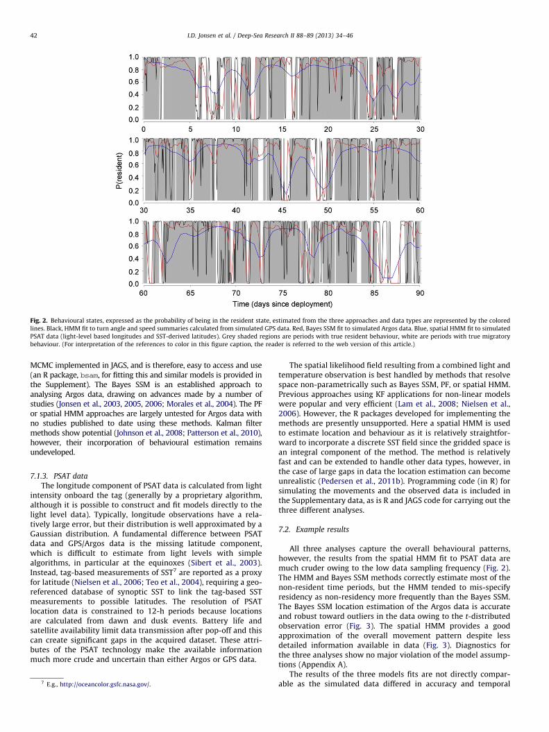
Fig. 2. Behavioural states, expressed as the probability of being in the resident state, estimated from the three approaches and data types are represented by the colored

lines. Black, HMM fit to turn angle and speed summaries calculated from simulated GPS data. Red, Bayes SSM fit to simulated Argos data. Blue, spatial HMM fit to simulated

PSAT data (light-level based longitudes and SST-derived latitudes). Grey shaded regions are periods with true resident behaviour, white are periods with true migratory

behaviour. (For interpretation of the references to color in this figure caption, the reader is referred to the web version of this article.)

I.D. Jonsen et al. / Deep-Sea Research II 88–89 (2013) 34–4642

MCMC implemented in JAGS, and is therefore, easy to access and use(an R package, bsam, for fitting this and similar models is provided inthe Supplement). The Bayes SSM is an established approach toanalysing Argos data, drawing on advances made by a number ofstudies (Jonsen et al., 2003, 2005, 2006; Morales et al., 2004). The PFor spatial HMM approaches are largely untested for Argos data withno studies published to date using these methods. Kalman filtermethods show potential (Johnson et al., 2008; Patterson et al., 2010),however, their incorporation of behavioural estimation remainsundeveloped.

7.1.3. PSAT data

The longitude component of PSAT data is calculated from lightintensity onboard the tag (generally by a proprietary algorithm,although it is possible to construct and fit models directly to thelight level data). Typically, longitude observations have a rela-tively large error, but their distribution is well approximated by aGaussian distribution. A fundamental difference between PSATdata and GPS/Argos data is the missing latitude component,which is difficult to estimate from light levels with simplealgorithms, in particular at the equinoxes (Sibert et al., 2003).Instead, tag-based measurements of SST7 are reported as a proxyfor latitude (Nielsen et al., 2006; Teo et al., 2004), requiring a geo-referenced database of synoptic SST to link the tag-based SSTmeasurements to possible latitudes. The resolution of PSATlocation data is constrained to 12-h periods because locationsare calculated from dawn and dusk events. Battery life andsatellite availability limit data transmission after pop-off and thiscan create significant gaps in the acquired dataset. These attri-butes of the PSAT technology make the available informationmuch more crude and uncertain than either Argos or GPS data.

7 E.g., http://oceancolor.gsfc.nasa.gov/.

The spatial likelihood field resulting from a combined light andtemperature observation is best handled by methods that resolvespace non-parametrically such as Bayes SSM, PF, or spatial HMM.Previous approaches using KF applications for non-linear modelswere popular and very efficient (Lam et al., 2008; Nielsen et al.,2006). However, the R packages developed for implementing themethods are presently unsupported. Here a spatial HMM is usedto estimate location and behaviour as it is relatively straightfor-ward to incorporate a discrete SST field since the gridded space isan integral component of the method. The method is relativelyfast and can be extended to handle other data types, however, inthe case of large gaps in data the location estimation can becomeunrealistic (Pedersen et al., 2011b). Programming code (in R) forsimulating the movements and the observed data is included inthe Supplementary data, as is R and JAGS code for carrying out thethree different analyses.

7.2. Example results

All three analyses capture the overall behavioural patterns,however, the results from the spatial HMM fit to PSAT data aremuch cruder owing to the low data sampling frequency (Fig. 2).The HMM and Bayes SSM methods correctly estimate most of thenon-resident time periods, but the HMM tended to mis-specifyresidency as non-residency more frequently than the Bayes SSM.The Bayes SSM location estimation of the Argos data is accurateand robust toward outliers in the data owing to the t-distributedobservation error (Fig. 3). The spatial HMM provides a goodapproximation of the overall movement pattern despite lessdetailed information available in data (Fig. 3). Diagnostics forthe three analyses show no major violation of the model assump-tions (Appendix A).

The results of the three models fits are not directly compar-able as the simulated data differed in accuracy and temporal

Fig. 3. True simulated locations (white line) with start and end locations (green and red circles, respectively). Left: ARGOS locations (magenta points) with Bayes SSM

estimated locations (black line). Right: estimated spatial HMM locations (black line). (For interpretation of the references to color in this figure caption, the reader is

referred to the web version of this article.)

I.D. Jonsen et al. / Deep-Sea Research II 88–89 (2013) 34–46 43

resolution. However, in comparison with the HMM results, theBayes SSM’s lower frequency of behavioural state mis-specifica-tion is not surprising given the data were simulated witheffectively the same process model (Eqs. (3.2) and (3.3)) as thatemployed in the Bayes SSM. The mis-specifications by the HMM,although somewhat numerous given the highly accurate simu-lated GPS data, are generally transient artefacts but they highlightthe importance of examining the plausibility of the behaviouralstate estimates.

7.2.1. Irregularly observed data

Irregularity in the timing of location observations and data gapsintroduced, for example, by an animal’s diving behaviour, satelliteavailability or transmission issues, cloud cover and/or strong lightattenuation at depth can render location data difficult to deal with.In cases where locations are observed irregularly but frequently, atime step may be selected that ensures at least one observationoccurs per step. When observations are highly irregular and tooinfrequent, a sufficiently long time step may become impractical. Inthis case a continuous time process model (e.g., the time elapsedbetween locations is modelled explicitly, and is the solutionemployed in the spatial HMM used here; Pedersen et al., 2011b)or an observation model with a regularization step (e.g., the BayesSSM used here; Jonsen et al., 2005) are viable solutions. In general,the continuous time approach is the more natural solution, but canbe more costly, in terms of computation time, to implement.

In some situations missing data is a signature of a change inbehaviour which should, in turn, affect the movement model. Forexample, for cod geolocated with a tidal method (Pedersen et al.,2008), individuals are in less contact with the bottom duringmigrations than during periods of residence, so migratory periodsare characterized by high mobility and few observations. Simi-larly, periodic crepuscular diving activity or extremely deep waterpreferences of animals tagged with PSATs or archival geolocatorscan produce light-level profiles that are either minimally or notinformative about horizontal location (Holdsworth et al., 2009). Incases where inference of movement behaviour is the goal, greatcare must be taken to determine how best to deal with minimallyinformative (highly imprecise) data or large data gaps so as not tounduly bias results.

8. Future directions

We have outlined how SSMs provide a general and highlyflexible statistical framework for modelling animal movementdata and highlighted three approaches for modelling commontypes of bio-logging data. Although statistical approaches (state-space or otherwise) for analysis of bio-logging data have prolif-erated in recent years (e.g., Horne et al., 2007; Gurarie et al., 2009;Polansky et al., 2010; Sumner et al., 2009, and other referencesherein), the toolbox is incomplete. As bio-logging datasets arebecoming more mature the focus of research is naturally shiftingfrom individual- to population-level questions. This shift in focuswill require a better understanding of the extent to whichindividual-level bio-logging data can inform population-levelpredictions (Morales et al., 2010). Enhancements in the theory(process models) of animal movements and a more completestatistical toolbox for fitting such models to bio-logging datasources will help achieve this understanding.

Despite a rich history of theoretical models of animal movementdeveloped around the notion of diffusion processes (Okubo andLevin, 2001; Turchin, 1998, and references therein), the applicationof these models to bio-logging data is relatively rare. Unlike fieldssuch as fisheries biology, where a comprehensive library of practicalmodels and estimation tools has been developed for fisheries orecosystem research and management purposes, animal movementecology lacks such a library. We agree with Cagnacci et al. (2010)that advances in bio-logging techniques are challenging ecologists todevelop more relevant theory and more powerful analytical tools.We must strive to develop and test more realistic models of animalmovement that can account for factors such as heterogeneous anddynamic environmental conditions (Grunbaum, 1998), physiologicalimperatives (Kareiva and Odell, 1987), memory and social interac-tions (Haydon et al., 2008).

Similarly, the statistical toolbox must be expanded so that newand more realistic movement models can be fit routinely to bio-logging data. A number of challenges exist. First, movement datausually are collected at finer temporal and spatial scales relativeto most independently collected environmental observationsor model output. This is likely to be a bigger issue in marineenvironments where animal habitat usually is more dynamicand less easily characterized than in terrestrial environments.

I.D. Jonsen et al. / Deep-Sea Research II 88–89 (2013) 34–4644

We are aware of few studies that assess the influence of thesemismatches in sampling scales on ecological inferences (seeBradshaw et al., 2002 for a partial assessment). However, sucheffects should not be ignored as they may bias inference ofunderlying relationships. This problem may be partly overcomeby relying on tag-deployed environmental sensors, which areincreasingly sophisticated and diverse (Bograd et al., 2010).

Second, the ability to process high-frequency, high volumetelemetry data, such as triaxial accelerometry data (e.g., Wilsonet al., 2008) is currently at or beyond the limits of commonlyavailable statistical tools. For example, Dowd and Joy (2010) fit aparticle filter SSM to 1-d accelerometry data (with a 2 s samplingfrequency) from a northern fur seal to assess diving behaviourduring a single day. It remains to be seen whether this approach isscalable to more ecologically relevant time scales, althoughrelated inertial navigation problems (e.g., dead reckoning) havebeen dealt with in engineering applications (Hide et al., 2003).

Third, analysis and inference across multiple individuals –hierarchical or mixed models – have been under-utilized inanimal movement modelling, but will be central to efforts atscaling up inferences from individuals to populations. The statis-tical theory for hierarchical SSMs is relatively simple, but theirestimation is difficult; model fitting becomes complex and com-putationally demanding as simultaneous estimation of locationand behavioural states across individuals is required. BayesianSSM approaches are ideally suited for fitting hierarchical SSMs(Eckert and Moore, 2008; Jonsen et al., 2003, 2006), but alternateestimation approaches (e.g., Altman, 2007) should be pursued.

Fourth, location uncertainty in movement data (e.g., Argos,geolocation data) should be better characterized. Currently, only afew double-tagging or fixed location studies have been used tocharacterize Argos location errors (e.g., Costa et al., 2010; Vincentet al., 2002). Further study is required to determine to what extentinference can be improved with better characterization of Argoslocation errors. Additionally, the new Argos location algorithm,which uses an ensemble of KFs, dispenses with location qualityclasses and provides new continuously distributed location errorestimates (Argos, 2011). Additional efforts are now required todetermine how best to model these location ‘‘data’’, which areestimates from a movement model and will therefore, have adifferent statistical structure compared to the previous Argos loca-tion data. Much work has focused on improving the precision oflight- or light and SST-based geolocation estimates (Nielsen et al.,2006; Sibert et al., 2003), but there is room for further improvement.For example, development of a full likelihood for light-level datacould allow geolocations to be routinely estimated by plugging thelikelihood into existing SSMs of animal movement. This wouldconsiderably ease the effort required to fit comparable SSMs todifferent kinds of tracking data (e.g., Block et al., 2011).

Bio-logging is approaching a golden age where telemetrytechnology is allowing us to peer further than ever before intothe oceans. The statistical tools already available add value andrigor to bio-logging datasets by allowing researchers to gaze intothe details of animal movement and behaviour, which are other-wise hidden to us. Ensuring that these tools meet the demands offuture bio-logging research avenues is a pressing challenge, butalso provides rich opportunities for enhancing theoretical andpractical approaches to the statistical analysis of animal move-ment and behavioural data.

Acknowledgments

The idea for this paper emerged at an informal workshop onquantitative approaches to animal movement modelling, orga-nized by TAP, during the Fourth International Science Symposium

on Bio-logging (14–18 March 2011 in Hobart, Tasmania, Austra-lia). IDJ thanks the Symposium organizers for the invitation togive a keynote talk; some of the themes of the talk are repre-sented in this paper, but the substance is very much a groupeffort. We thank two anonymous reviewers and Karen Evans forcomments that helped improve the clarity of the paper. IDJ wasfunded by the Natural Sciences and Engineering Research Councilof Canada (NSERC) and the Canadian Foundation for Innovation(CFI) through their support of the Ocean Tracking Network inCanada. MWP was funded by the Nordic Centre of Excellenceproject Climate Change on Marine Ecosystems and ResourceEconomics (NorMER) supported financially by the NordforskTop-Level Research Initiative (TFI), NordForsk Project number36800.

Appendix A. Supplementary material

Simulation and analysis code is provided in an accompanyingarchive file (ssmexamples.zip). All example analyses in themanuscript can be evaluated in R using the files provided in thearchive. Unzip the archive, and install the provided R librarybsam_0.21.tar.gz (for Linux and Mac OS X) or bsam_0.21.zip (for Windows). The bsam library is used to fit the Bayes SSM(MCMC) model to Argos tracking data, and requires the JAGSsoftware (version 3.1) for implementing the MCMC algorithms.JAGS is available for Windows and Mac, and can be built fromsource in Linux. It can be downloaded from here (last accessed 10June 2012): http://mcmc-jags.sourceforge.net/. Additionally, thebsam library depends on the following R libraries: dclone, snow,and rjags, also note that these libraries may in-turn haveadditional dependencies.

All analyses can be run by sourcing the script runall.R

into an R session. Note, it will take some time (approximately30–40 min, depending on your processor speed) to complete theanalyses. Additional required R libraries can be downloaded fromthe CRAN repository by typing install.packages{‘‘name_of_library’’} in an active R session. A README.txt file included inthe archive file provides more details on running the scripts,including a quick-start guide.

Supplementary data associated with this article can be found inthe online version at http://dx.doi.org/10.1016/j.dsr2.2012.07.008.

References

Altman, R.M., 2004. Assessing the goodness-of-fit of hidden Markov models.Biometrics 60, 444–450.

Altman, R.M., 2007. Mixed hidden Markov models. J. Am. Stat. Assoc. 477,201–210.

Anderson-Sprecher, R., Ledolter, J., 1991. State-space analysis of wildlife telemetrydata. J. Am. Stat. Assoc. 86, 596–602.

Argos, 2011. User’s Manual. CLS/Service Argos, Toulouse, France.Austin, D., McMillan, J.I., Bowen, W.D., 2003. A three-stage algorithm for filtering

erroneous Argos satellite locations. Mar. Mamm. Sci. 19, 371–383.Bestley, S., Patterson, T.A., Hindell, M.A., Gunn, J.S., 2010. Predicting feeding

success in a migratory predator: integrating telemetry, environment, andmodeling techniques. Ecology 91, 2373–2384.

Block, B.A., Jonsen, I.D., Jorgensen, S.J., Winship, A.J., Shaffer, S.A., Bograd, S.J.,Hazen, E.L., Foley, D.G., Breed, G.A., Harrison, A.L., Ganong, J.E., Swithenbank,A., Castleton, M., Dewar, H., Mate, B.R., Shillinger, G.L., Schaefer, M.K., Benson,S.R., Wiese, M.J., Henry, R.W., Costa, D.P., 2011. Tracking apex marine predatormovements in a dynamic ocean. Nature 475, 86–90.

Bograd, S.J., Block, B.A., Costa, D.P., Godley, B.J., 2010. Biologging technologies: newtools for conservation. Introduction. Endang. Species Res. 10, 1–7.

Bradshaw, C., Hindell, M., Michael, K., Sumner, M., 2002. The optimal spatial scalefor the analysis of elephant seal foraging as determined by geo-location inrelation to sea surface temperatures. ICES J. Mar. Sci. 59, 770–781.

Bradshaw, C.J.A., Sims, D.W., Hays, G.C., 2007. Measurement error causes scale-dependent threshold erosion of biological signals in animal movement data.Ecol. Appl. 17, 628–638.

I.D. Jonsen et al. / Deep-Sea Research II 88–89 (2013) 34–46 45

Breed, G.A., Costa, D.P., Jonsen, I.D., Robinson, P.W., Mills-Flemming, J., 2012. State-space methods for more completely capturing behavioral dynamics fromanimal tracks. Ecol. Model. 235–236, 49–58.

Brillinger, D.R., Preisler, H.K., Ager, A.A., Kie, J.G., Stewart, B.S., 2002. Employingstochastic differential equations to model wildlife motion. Bull. Braz. Math.Soc. 33, 385–408.

Brinch, C., Eikeset, A., Stenseth, N., Walters, C., 2011. Maximum likelihoodestimation in nonlinear structured fisheries models using survey and catch-at-age data. Can. J. Fish Aquat. Sci. 68, 1717–1731.

Burnham, K.P., Anderson, D.R., 2002. Model Selection and Multimodel Inference: APractical Information-Theoretic Approach. Springer-Verlag, New York.

Cagnacci, F., Boitani, L., Powell, R.A., Boyce, M.S., 2010. Animal ecology meets GPS-based radiotelemetry: a perfect storm of opportunities and challenges. Philos.Trans. R. Soc. B 365, 2157–2162.

Celeux, G., Durand, J.-B., 2008. Selecting hidden Markov model state number withcross-validated likelihood. Comput. Stat. 23, 541–564.

Celeux, G., Hurn, M., Robert, C.P., 2000. Computational and inferential difficultieswith mixture posterior distributions. J. Am. Stat. Assoc. 95, 957–970.

Charnov, E.L., 1976. Optimal foraging: the marginal value theorem. Theor. Popul.Biol. 9, 129–136.

Chopin, N., 2007. Inference and model choice for sequentially ordered hiddenMarkov models. J. R. Soc. Stat. B. 69, 269–284.

Christensen, A., Jensen, H., Mosegaard, H., John, M., Schrum, C., 2008. Sandeel(Ammodytes marinus) larval transport patterns in the north sea from anindividual-based hydrodynamic egg and larval model. Can. J. Fish. Aquat. Sci.65, 1498–1511.

Costa, D.P., Robinson, P.W., Arnould, J.P.Y., Harrison, A.L., Simmons, S.E., Hassrick,J.L., Hoskins, A.J., Kirkman, S.P., Oosthuizen, H., Villegas-Amtmann, S., Crocker,D.E., 2010. Accuracy of argos locations of pinnipeds at-sea estimated usingFastloc GPD. PLoS One 5, e8677, URL /http://dx.doi.org/10.1371%2Fjournal.pone.0008677S.

Cowles, M.K., Carlin, B.P., 1996. Markov chain Monte Carlo convergence diagnos-tics: a comparative review. J. Am. Stat. Assoc. 91, 882–904.

de Valpine, P., Hastings, A., 2002. Fitting population models incorporating processnoise and observation error. Ecol. Monogr. 72, 57–76.

Doucet, A., Freitas, N.D., Gordon, N.J. (Eds.), 2001. Sequential Monte Carlo Methodsin Practice. Springer-Verlag, New York.

Dowd, M., Joy, R., 2010. Estimating behavioral parameters in animal movementmodels using a state-augmented particle filter. Ecology 92, 568–575.

Eckert, S.A., Moore, J.E., 2008. Modeling loggerhead turtle movement in theMediterranean: importance of body size and oceanography. Ecol. Appl. 18,290–308.

Ellison, A.M., 2004. Bayesian inference in ecology. Ecol. Lett. 7, 509–520.Evensen, G., 2003. The ensemble Kalman filter: theoretical formulation and

practical implementation. Ocean Dyn. 53, 343–367.Forester, J.D., Ives, A.R., Turner, M.G., Anderson, D.P., Fortin, D., Beyer, H.L., Smith,

D.W., Boyce, M.S., 2007. State-space models link elk movement patterns tolandscape characteristics in Yellowstone National Park. Ecol. Monogr. 77,285–299.

Foster, S.D., Bravington, M.V., 2011. Graphical diagnostics for Markov models forcategorical data. J. Comput. Graph. Stat. 20, 355–374.

Gelman, A., Carlin, J.B., Stern, H.S., Rubin, D.B., 2004. Bayesian Data Analysis. CRCPress, Boca Raton.

Giudici, P., Ryden, T., Vandekerkhove, P., 2000. Likelihood-ratio tests for hiddenMarkov models. Biometrics 56, 742–747.

Grunbaum, D., 1998. Using spatially explicit models to characterize foragingperformance in heterogeneous landscapes. Am. Nat. 151, 97–115.

Gurarie, E., Andrews, R.D., Laidre, K.L., 2009. A novel method for identifyingbehavioural changes in animal movement data. Ecol. Lett. 12, 395–408.

Harvey, A.C., 1993. Time Series Models, second ed. The MIT Press, New York.Haydon, D.T., Morales, J.M., Yott, A., Jenkins, D.A., Rosatte, R., Fryxell, J.M., 2008.

Socially informed random walks: incorporating group dynamics into modelsof population spread and growth. Proc. R. Soc. B. 275, 1101–1109.

Hide, C., Moore, T., Smith, M., 2003. Adaptive Kalman filtering for low-cost INS/GPS. J. Navig. 56, 143–152.

Hill, R., 1994. Theory of geolocation by light levels. In: LeBoeuf, B.J., Laws, R.M.(Eds.), Elephant Seals: Population Ecology, Behaviour, and Physiology. Uni-versity of California Press, pp. 227–236.

Hjort, N.L., Claeskens, G., 2003. Frequentist model average estimators. J. Am. Stat.Assoc. 98, 879–899.

Holdsworth, J., Sippel, T., Block, B., 2009. Near real time satellite tracking of stripedmarlin (Kajikia audax) movements in the pacific ocean. Mar. Biol. 156,505–514.

Horne, J.S., Garton, E.O., Krone, S.M., Lewis, J.S., 2007. Analyzing animal move-ments using Brownian bridges. Ecology 88, 2354–2363.

Houston, A., McNamara, J.M., 1999. Models of Adaptive Behaviour. CambridgeUniversity Press, Cambridge.

Johnson, D.S., London, J.M., Lea, M.A., Durban, J.W., 2008. Continuous-time correlatedrandom walk model for animal telemetry data. Ecology 89, 1208–1215.

Jonsen, I.D., Flemming, J.M., Myers, R.A., 2005. Robust state-space modeling ofanimal movement data. Ecology 86, 2874–2880.

Jonsen, I.D., Myers, R.A., Flemming, J.M., 2003. Meta-analysis of animal movementusing state-space models. Ecology 84, 3055–3063.

Jonsen, I.D., Myers, R.A., James, M.C., 2006. Robust hierarchical state-space modelsreveal diel variation in travel rates of migrating leatherback turtles. J. Anim.Ecol. 75, 1046–1057.

Kalman, R., 1960. A new approach to linear filtering and prediction problems.J. Basic Eng. 82, 35–45.

Kareiva, P., Odell, G., 1987. Swarms of predators exhibit ‘‘prey taxis’’ if individualpredators use area-restricted search. Am. Nat. 130, 233–270.

Lam, C.H., Nielsen, A., Sibert, J.R., 2008. Improving light and temperature basedgeolocation by unscented Kalman filtering. Fish. Res. 91, 15–25.

Lunn, D., Spiegelhalter, D., Thomas, A., Best, N., 2009. The BUGS project: evolution,critique and future directions. Stat. Med. 28, 3049–3067.

Lunn, D.J., Thomas, A., Best, N., Spiegelhalter, D., 2000. WinBUGS – a Bayesianmodelling framework: concepts, structure, and extensibility. Stat. Comput. 10,325–337.

McLachlan, G.J., Peel, D., 2000. Finite Mixture Models. John Wiley and Sons, Ltd.,New York.

Mengersen, K.L., Robert, C.P., Guihenneuc-Jouyaux, C., 1999. MCMC convergencediagnostics: a review. In: Berger, J., Bernardo, J., Dawid, A.P., Smith, A.F.M.(Eds.), Bayesian Statistics, vol. 6. Oxford University Press, Oxford, pp. 415–440.

Mills Flemming, J., Jonsen, I.D., Myers, R.A., Field, C.A., 2010. Hierarchical state-space estimation of leatherback turtles navigation ability. PLoS One 5, e14245,http://dx.doi.org/10.1371/journal.pone.0014245.

Morales, J.M., Haydon, D.T., Frair, J., Holsinger, K.E., Fryxell, J.M., 2004. Extractingmore out of relocation data: building movement models as mixtures ofrandom walks. Ecology 85, 2436–2445.

Morales, J.M., Moorcroft, P.R., Matthiopoulos, J., Frair, J.L., Kie, J.G., Powell, R.A.,Merrill, E.H., Haydon, D.T., 2010. Building the bridge between animal move-ment and population dynamics. Philos. Trans. R. Soc. B 365, 2289–2301.

Musyl, M.K., Brill, R.W., Curran, D.S., Gunn, J.S., Hartog, J.R., Hill, R.D., Welch, D.W.,Eveson, J.P., Boggs, C.H., Brainard, R.E., 2001. Ability of archival tags to provideestimates of geographical position based on light intensity. In: Sibert, J.R.,Nielsen, J.L. (Eds.), Electronic Tagging and Tracking in Marine FisheriesReviews: Methods and Technologies in Fish Biology and Fisheries. KluwerAcademic Press, Dordrecht, pp. 343–368.

Nielsen, A., Bigelow, K.A., Musyl, M.K., Sibert, J.R., 2006. Improving light-basedgeolocation by including sea surface temperature. Fish. Oceanogr. 15, 314–325.

Okubo, A., Levin, S.A., 2001. Diffusion and Ecological Problems: Modern Perspec-tives. Springer-Verlag, New York.

Patil, A., Huard, D., Fonnesbeck, C., 2010. PyMC: Bayesian stochastic modelling inPython. J. Stat. Software 35, 1–81.

Patterson, T.A., 2009. State-Space Models of Animal Movement. Ph.D. thesis,University of Tasmania, School of Zoology.

Patterson, T.A., Basson, M., Bravington, M.V., Gunn, J.S., 2009. Classifying move-ment behaviour in relation to environmental conditions using hidden Markovmodels. J. Anim. Ecol. 78, 1113–1123.

Patterson, T.A., McConnell, B.J., Fedak, M.A., Bravington, M.V., Hindell, M.A., 2010.Using GPS data to evaluate the accuracy of state-space methods for correctionof Argos satellite telemetry error. Ecology 91, 273–285.

Patterson, T.A., Thomas, L., Wilcox, C., Ovaskainen, O., Matthiopoulos, J., 2008.State-space models of individual animal movement. Trends Ecol. Evol. 23,87–94.

Pedersen, M., Thygesen, U., Madsen, H., 2011a. Nonlinear tracking in a diffusionprocess with a Bayesian filter and the finite element method. Comput. Stat.Data Anal. 55, 280–290.

Pedersen, M.W., Patterson, T.A., Thygesen, U.H., Madsen, H., 2011b. Estimatinganimal behavior and residency from movement data. Oikos 120, 1281–1290.

Pedersen, M.W., Righton, D., Thygesen, U.H., Andersen, K.H., Madsen, H., 2008.Geolocation of North Sea cod (Gadus morhua) using hidden Markov modelsand behavioural switching. Can. J. Fish. Aquat. Sci. 65, 2367–2377.

Peel, D., Good, N.M., 2011. A hidden Markov model approach for determiningvessel activity from vessel monitoring system data. Can. J. Fish. Aquat. Sci. 68,1252–1264.

Polansky, L., Wittemyer, G., Cross, P.C., Tambling, G.J., Getz, W.M., 2010. Frommoonlight to movement and synchronized randomness: Fourier and waveletanalyses of animal location time series data. Ecology 91, 1506–1518.

Rabiner, L.R., 1989. A tutorial on Hidden Markov models and selected applicationsin speech recognition. Proc. IEEE 77, 257–286.

Robert, C.P., Ryden, T., Titterington, D., 1999. Convergence controls for MCMCalgorithms, with applications to hidden Markov chains. J. Stat. Comput.Simulation 64, 327–355.

Robert, C.P., Ryden, T., Titterington, D.M., 2000. Jump Markov chain Monte Carloalgorithms for Bayesian inference in hidden Markov models. J. R. Stat. Soc. B.62, 57–75.

Royer, F., Fromentin, J.M., Gaspar, P., 2005. A state-space model to derive bluefintuna movement and habitat from archival tags. Oikos 109, 473–484.

Schick, R.S., Loarie, S.R., Colchero, R., Best, B.D., Boustany, A., Conde, D.A., Halpin,P.N., Joppa, L.N., McClellan, C.M., Clark, J.S., 2008. Understanding movementdata and movement processes: current and emerging directions. Ecol. Lett. 11,1338–1350.

Scott, S.L., 2002. Bayesian methods for hidden Markov models. J. Am. Stat. Assoc.97, 337–351.

Sibert, J.R., Musyl, M.K., Brill, R.W., 2003. Horizontal movements of bigeye tunanear Hawaii from archival tagging data. Fish. Oceanogr. 12, 141–151.

Sumner, M.D., Wotherspoon, S.J., Hindell, M.A., 2009. Bayesian estimation ofanimal movement from archival and satellite tags. PLoS One 4, e7324, URL/http://dx.doi.org/10.1371%2Fjournal.pone.0007324S.

Teo, S.L.H., Boustany, A., Blackwell, S., Walli, A., Weng, K.C., Block, B.A., 2004.Validation of geolocation based on light level and sea surface temperaturefrom electronic tags. Mar. Ecol. Prog. Ser. 283, 81–98.

I.D. Jonsen et al. / Deep-Sea Research II 88–89 (2013) 34–4646

Thygesen, U.H., Pedersen, M.W., Madsen, H., 2009. Geolocating fish using hiddenMarkov models and data storage tags. In: Nielsen, J., Arrizabalaga, H., Fragoso,N., Hobday, A., Lutcavage, M., Sibert, J. (Eds.), Tagging and Tracking of MarineAnimals with Electronic Devices. Reviews: Methods and Technologies in FishBiology and Fisheries, vol. 9. Springer, New York, pp. 277–293.

Turchin, P., 1998. Quantitative Analysis of Movement: Measuring and ModelingPopulation Redistribution in Animals and Plants. Sinauer Associates,Sunderland.

Vincent, C., McConnell, B.J., Fedak, M.A., Ridoux, V., 2002. Assessment of ARGOSlocation accuracy from satellite tags deployed on captive grey seals. Mar.Mamm. Sci. 18, 301–322.

Viterbi, A.J., 2006. A personal history of the Viterbi algorithm. IEEE Signal Proc.Mag. 23, 120–142.

Wilson, R.P., Shepard, E.L.C., Liebsch, N., 2008. Prying into the intimate details ofanimal lives: use of a daily diary on animals. Endang. Species Res. 4, 123–137.

Zucchini, W., MacDonald, I.L., 2009. Hidden Markov Models for Time Series: AnIntroduction using R. Chapman and Hall/CRC, Boca Raton.

Glossary

Advection–diffusion: a transport mechanism where advection is directed andpredictable, while diffusion is undirected and random. Originally formulatedfor analysis of molecule movements, it is also used for analysis of animalmovements by analogy, and is the foundation of many process-based modelsdescribing animal movement;

Bayesian state-space model (Bayes SSM): a state-space model that employs arecursive algorithm that generates a probability estimate of an unobservedstate and then uses Bayes rule to update that estimate with an observation.Bayes SSMs can naturally accommodate nonlinear process models and non-Gaussian errors in data. These models are typically fit using MCMC algorithms,which can require considerably more computational effort compared to theKalman Filter;

Maximum likelihood (ML): principle for estimating parameters: One chooses theparameters so that the prior probability of the actual measurements is as largeas possible. The principle has a dominant role in statistics.;

Behavioural state: a particular manner of movement that is assumed to be relatedto a behaviour type. For example, an animal foraging intensively on aproductive patch of food might move slowly with much turning;

Hessian matrix: a matrix estimated by many optimization algorithms that givesthe curvature of the likelihood function at the maximum. This curvature isused to assess parameter uncertainty; estimates of parameter standard errorsare obtained from the diagonal elements of the inverse of the Hessian matrix;

Hidden Markov model (HMM): a SSM with discrete (i.e. discontinuous) hiddenstates. Examples include classifying movements as ‘‘foraging’’ or ‘‘not foraging’’and assigning spatial locations to discrete habitat patches. Typically, movement

HMMs do not consider observation error on location (but see spatial HMMbelow), but treat the data as the stochastic outcome of a particular unobser-vable behavioural state;

Kalman filter (KF): a recursive algorithm for estimating the unobserved state of asystem based on measurements of correlated variables. In its pure form, itapplies to a system whose dynamics are linear and subject to additiveGaussian noise; many variants and extensions exist to deal with mild formsof nonlinearity;

Markov chain Monte Carlo (MCMC): a class of algorithms that use a Markov chainapproach to sample from probability distributions. The Markov chain isconstructed so that it converges to the desired distribution. MCMC is typicallyused to numerically solve the multi-dimensional integrals that arise inBayesian statistics;

Markov process: a Markov process is a stochastic process in which the probabilitythat the system will be in a particular state in the next time unit is purely afunction of its current and past states. This is known as the Markov condition.First-order processes only depend on the current state, whereas higher-orderMarkov processes incorporate dependencies at greater time lags;

Movement metric: quantities that might be calculated directly from raw, uncor-rected and unprocessed movement data. These include step length (distancebetween successive locations), speed, the turning angle between locationsand so on;

Observation model: in SSMs, this refers to a probabilistic model of the samplingprocess. In movement data, this might refer to a model that describestelemetry precision or spatiotemporal variation in recapture effort.;

Process model: in movement SSMs, a model of the dynamics of the movementthrough time and space;

Random walk (RW): a mathematical description (often a Markov process) forgenerating a trajectory in space from a starting position;

Spatial hidden Markov model (Spatial HMM): the ‘‘spatial’’ prefix to HMM indicatesthat the unobserved state has a spatial component in addition to thebehavioural component of the HMM described above. To handle locationobservation error with arbitrary distribution, spatial HMMs rely on a dis-cretization of two-dimensional space. This provides the flexibility to handleany observation type, direct or indirect (e.g., light, temperature, pressure), andthe ability to exclude inaccessible spatial regions. The main cost is increasedcomputation time compared to the HMM;

State: a quantity that describes a true, but not necessarily known, attribute of asystem. For a movement SSM, this might be location, behavioural state,energetic or physiological condition. The variables are time-indexed andmight be collected together into a state-vector (e.g., location, behaviouralmode and energetic reserves could feasibly be grouped into a state vector);

State-space model (SSM): a time-series model that predicts the future state of asystem from its previous states probabilistically, via a process model. The SSMdescribes mathematically how observations of the system’s state are gener-ated via an observation model;