State-of-the-Art Sensors Technology in Spain 2015 - Open ...

Volume 1

State-of-the-Art Sensors Technology in Spain 2015

Gonzalo Pajares Martinsanz

www.mdpi.com/journal/sensors

Edited by

sensors

Printed Edition of the Special Issue Published in Sensors

State-of-the-Art Sensors Technology in Spain 2015

Volume 1

Special Issue Editor Gonzalo Pajares Martinsanz

http://www.mdpi.com/journal/sensors

http://creativecommons.org/licenses/by-nc-nd/4.0/

Special Issue Editor


Department Software Engineering and Artificial Intelligence

Faculty of Informatics

University Complutense of Madrid

Spain

Editorial Office

MDPI AG

St. Alban-Anlage 66

Basel, Switzerland

This edition is a reprint of the Special Issue published online in the open access

journal Sensors (ISSN 1424-8220) from 2015–2016 (available at:

http://www.mdpi.com/journal/sensors/special_issues/state-of-the-art-spain-2015).

For citation purposes, cite each article independently as indicated on the article

page online and as indicated below:

Author 1; Author 2; Author 3 etc. Article title. Journal Name. Year. Article

number/page range.

Vol 1 ISBN 978-3-03842-370-6 (Pbk) Vol 1-2 ISBN 978-3-03842-312-6 (Pbk)

Vol 1 ISBN 978-3-03842-371-3 (PDF) Vol 1-2 ISBN 978-3-03842-313-3 (PDF)

Articles in this volume are Open Access and distributed under the Creative Commons Attribution

license (CC BY), which allows users to download, copy and build upon published articles even for

commercial purposes, as long as the author and publisher are properly credited, which ensures

maximum dissemination and a wider impact of our publications. The book taken as a whole is © 2017

MDPI, Basel, Switzerland, distributed under the terms and conditions of the Creative Commons by

Attribution (CC BY-NC-ND) license (http://creativecommons.org/licenses/by-nc-nd/4.0/).

iii

Table of Contents

About the Guest Editor .............................................................................................................................. v

Preface to “State-of-the-Art Sensors Technology in Spain 2015” ......................................................... ix

Jorge Alfredo Ardila-Rey, Ricardo Albarracín, Fernando Álvarez and Aldo Barrueto

A Validation of the Spectral Power Clustering Technique (SPCT) by Using a Rogowski Coil in

Partial Discharge Measurements

Reprinted from: Sensors 2015, 15(10), 25898–25918; doi: 10.3390/s151025898

http://www.mdpi.com/1424-8220/15/10/25898 ....................................................................................... 1

Alonso Sánchez, José-Manuel Naranjo, Antonio Jiménez and Alfonso González

Analysis of Uncertainty in a Middle-Cost Device for 3D Measurements in BIM Perspective

Reprinted from: Sensors 2016, 16(10), 1557; doi: 10.3390/s16101557

http://www.mdpi.com/1424-8220/16/10/1557 ......................................................................................... 20

Ricardo Albarracín, Jorge Alfredo Ardila-Rey and Abdullahi Abubakar Mas’ud

On the Use of Monopole Antennas for Determining the Effect of the Enclosure of a Power

Transformer Tank in Partial Discharges Electromagnetic Propagation


http://www.mdpi.com/1424-8220/16/2/148 ............................................................................................. 37

Adrian Carrio, Carlos Sampedro, Jose Luis Sanchez-Lopez, Miguel Pimienta and Pascual Campoy

Automated Low-Cost Smartphone-Based Lateral Flow Saliva Test Reader for Drugs-of-Abuse

Detection


http://www.mdpi.com/1424-8220/15/11/29569 ....................................................................................... 55

Erik Aguirre, Santiago Led, Peio Lopez-Iturri, Leyre Azpilicueta, Luís Serrano and Francisco Falcone

Implementation of Context Aware e-Health Environments Based on Social Sensor Networks


http://www.mdpi.com/1424-8220/16/3/310 ............................................................................................. 76

Rafael Socas, Sebastián Dormido, Raquel Dormido and Ernesto Fabregas

Event-Based Control Strategy for Mobile Robots in Wireless Environments


http://www.mdpi.com/1424-8220/15/12/29796 ....................................................................................... 103

Arturo Bertomeu-Motos, Luis D. Lledó, Jorge A. Díez, Jose M. Catalan, Santiago Ezquerro, Francisco J. Badesa and Nicolas Garcia-Aracil

Estimation of Human Arm Joints Using Two Wireless Sensors in Robotic Rehabilitation Tasks


http://www.mdpi.com/1424-8220/15/12/29818 ....................................................................................... 120

Beatriz R. Mendoza, Silvestre Rodríguez, Rafael Pérez-Jiménez, Alejandro Ayala and Oswaldo González

Comparison of Three Non-Imaging Angle-Diversity Receivers as Input Sensors of Nodes for Indoor

Infrared Wireless Sensor Networks: Theory and Simulation


http://www.mdpi.com/1424-8220/16/7/1086 ........................................................................................... 132

iv

José Antonio Sánchez Alcón, Lourdes López, José-Fernán Martínez and Gregorio Rubio Cifuentes

Trust and Privacy Solutions Based on Holistic Service Requirements


http://www.mdpi.com/1424-8220/16/1/16 ............................................................................................... 150

Gregorio Rubio, José Fernán Martínez, David Gómez and Xin Li

Semantic Registration and Discovery System of Subsystems and Services within an Interoperable

Coordination Platform in Smart Cities


http://www.mdpi.com/1424-8220/16/7/955 ............................................................................................. 188

Antonio-Javier Garcia-Sanchez, Fernando Losilla, David Rodenas-Herraiz, Felipe Cruz-Martinez and Felipe Garcia-Sanchez

On the Feasibility of Wireless Multimedia Sensor Networks over IEEE 802.15.5 Mesh Topologies


http://www.mdpi.com/1424-8220/16/5/643 ............................................................................................. 214

Ramon Sanchez-Iborra and Maria-Dolores Cano

State of the Art in LP-WAN Solutions for Industrial IoT Services


http://www.mdpi.com/1424-8220/16/5/708 ............................................................................................. 241

Joaquín Luque, Diego F. Larios, Enrique Personal, Julio Barbancho and Carlos León

Evaluation of MPEG-7-Based Audio Descriptors for Animal Voice Recognition over Wireless

Acoustic Sensor Networks


http://www.mdpi.com/1424-8220/16/5/717 ............................................................................................. 255

Óscar Oballe-Peinado, Fernando Vidal-Verdú, José A. Sánchez-Durán, Julián Castellanos-Ramos and José A. Hidalgo-López

Accuracy and Resolution Analysis of a Direct Resistive Sensor Array to FPGA Interface


http://www.mdpi.com/1424-8220/16/2/181 ............................................................................................. 277

v

About the Guest Editor

Gonzalo Pajares received his Ph.D. degree in Physics from

the Distance University, Spain, in 1995, for a thesis on

stereovision. Since 1988 he has worked at Indra in critical

real-time software development. He has also worked at

Indra Space and INTA in advanced image processing for

remote sensing. He joined the University Complutense of

Madrid in 1995 on the Faculty of Informatics (Computer

Science) at the Department of Software Engineering and

Artificial intelligence. His current research interests include computer and machine visual perception,

artificial intelligence, decision-making, robotics and simulation and has written many publications,

including several books, on these topics. He is the co-director of the ISCAR Research Group. He is an

Associated Editor for the indexed online journal Remote Sensing and serves as a member of the

Editorial Board in the following journals: Sensors, EURASIP Journal of Image and Video Processing,

Pattern Analysis and Applications. He is also the Editor-in-Chief of the Journal of Imaging.

ix

Preface to “State-of-the-Art Sensors Technology in Spain 2015”

Since 2009, three Special Issues have been published on sensors and technologies in Spain,

where researchers have presented their successful progress. Thirty-one high quality papers

demonstrating significant achievements have been collected and reproduced in this book.

They are self-contained works addressing different sensor-based technologies, procedures and

applications in several areas, including measurement devices, wireless sensor networks, robotics,

imaging, optical systems or electrical/electronic devices among others.

Readers will find an excellent source of resources for the development of research, teaching or

industrial activity.

Although the book is focused on sensors and technologies in Spain, it describes worldwide

developments and references on the covered topics. Some works have been or come from

international collaborations.

Our society demands new technologies for data acquisition, processing and transmission for

immediate actuation or knowledge, and with important impact on one’s welfare when required.

The international, scientific and industrial communities worldwide will also be an indirect

beneficiary of these works. Indeed, the book provides insights and solutions for the varied problems

covered. Also, it lays the foundation for future advances toward new challenges and progress in many

areas. In this regard, new sensors will contribute to the solution of existing problems, and, where the

need arises for the development of new technologies or procedures, this book paves

the way.

We are grateful to all the people involved in the preparation of this book. Without the

invaluable contributions of the authors together with the excellent help of reviewers, this book would

not have reached fruition. More than 120 authors have contributed to this book.

Thanks also to the Sensors journal editorial team for their invaluable support and

encouragement.


Guest Editor

sensors

Article

A Validation of the Spectral Power ClusteringTechnique (SPCT) by Using a Rogowski Coil inPartial Discharge Measurements

Jorge Alfredo Ardila-Rey 1,*, Ricardo Albarracín 2, Fernando Álvarez 3 and Aldo Barrueto 1

1 Departamento de Ingeniería Eléctrica, Universidad Técnica Federico Santa María, Av. VicuñaMackenna 3939, Santiago de Chile 8940000, Chile; [email protected]

2 Generation and Distribution Network Area. Dept. Electrical Engineering. Innovation, Technology and R&D,Boslan S.A. Consulting and Engineering, Calle de la Isla Sicilia 1, Madrid 28034, Spain;[email protected]

3 Departamento de Ingeniería Eléctrica, Universidad Politécnica de Madrid, Ronda de Valencia 3,Madrid 28012, Spain; [email protected]

* Correspondence: [email protected]; Tel.: +56-22-303-7231; Fax: +56-22-303-6600.

Academic Editor: Gonzalo Pajares MartinsanzReceived: 4 September 2015; Accepted: 6 October 2015; Published: 13 October 2015

Abstract: Both in industrial as in controlled environments, such as high-voltage laboratories, pulsesfrom multiple sources, including partial discharges (PD) and electrical noise can be superimposed.These circumstances can modify and alter the results of PD measurements and, what is more, theycan lead to misinterpretation. The spectral power clustering technique (SPCT) allows separating PDsources and electrical noise through the two-dimensional representation (power ratio map or PRmap) of the relative spectral power in two intervals, high and low frequency, calculated for each pulsecaptured with broadband sensors. This method allows to clearly distinguishing each of the effectsof noise and PD, making it easy discrimination of all sources. In this paper, the separation abilityof the SPCT clustering technique when using a Rogowski coil for PD measurements is evaluated.Different parameters were studied in order to establish which of them could help for improving themanual selection of the separation intervals, thus enabling a better separation of clusters. The signalprocessing can be performed during the measurements or in a further analysis.

Keywords: partial discharges (PD); Rogowski coil; wideband PD measurements; clustering techniques;condition monitoring; electrical insulation condition; on-line PD measurements; pattern recognition;signal processing

1. Introduction

The electrical generation, transmission and, even distribution infrastructures require largefinancial investments, so their long-term profitability must be optimized. In this context, there hasbeen a growing interest on the one hand, to reduce maintenance cycles applied to electrical machineryand power cables when they are very aged and secondly, to adequately plan their replacement whenits operation becomes unreliable [1].

For these reasons, it is assumed that electrical equipment must be replaced every certain period oftime, close to 30–40 years [2,3], and that the maintenance cycles must be fixed in advance (preventivemaintenance). However, the progress made in basic electrical insulation research and the increasein the availability of historical failure data allows choosing new maintenance strategies. Throughthese strategies, it is possible to know the operation condition of the electrical assets by performing inservice (on-line) measurements in high-voltage installations. This procedure extends the lifespan of theequipment, as well as their periods of scheduled maintenance [4]. Thus, the lack of investment, that is

Sensors 2015, 15, 1–19 1 www.mdpi.com/journal/sensors

Sensors 2015, 15, 1–19

often required in the replacement of equipment [3], could be compensated with the implementationof a proper Condition-Based Maintenance (CBM) program [5]. For these reasons, PD measurementhas become a major diagnostic method used in the maintenance of electrical installations, in order toestablish the degradation of the insulation systems, since its lifetime is determined by the degree ofdegradation present [6].

In measurements made on-site or even in controlled environments, such as high-voltagelaboratories, the pulses from multiple PD sources and electrical noise may be overlapped, thuscreating complex phase-resolved PD (PRPD) patterns. In some cases, the noise signals can havemagnitudes greater than the PD pulses, so the raising the trigger level of the acquisition systems isnot a valid PD separation technique. This problem has increased due to the growing use of electronicpower converters in electrical systems (variable frequency drives, power supplies switching, rectifiers,inverters, converters, etc.). Consequently, source separation has become a fundamental requirementin obtaining an effective diagnostic, such that avoid erroneous assessments in the equipment orsystem insulation.

Many modern measuring instruments are equipped with pulse classification tools that are basedon characterization of the waveforms of the acquired pulses, inasmuch as noise and PD pulsesgenerated by different sources present different shapes.

The classification procedures require broadband sensors capable of detecting ranges up to tensof MHz [7,8]. Commonly, inductive sensors are used for PD measurements. These sensors arecapable of measuring according to the standard detection circuits. The most widely used are thehigh-frequency current transformers (HFCT), inductive loop sensors (ILS) and the Rogowski coils(RC) [9–14]. Recent studies have shown that the SPCT applied to the pulses obtained with HFCTand ILS sensors measuring in different test objects, have been successfully characterized and itseffectiveness to separate different PD sources and electrical noise has been proven, even when thesesources are simultaneously active [15].

In this paper, the ability of clustering by applying the SPCT to PD pulses and electrical noiseacquired with a RC for various test objects in two different environments is evaluated. The aim of thepaper is to show the benefits of SPTC technique, even when sensors with a poor transfer impedance areused. To this end, the RC was used, since it has an air-core of non-magnetic material, which provideslinearity and low self-inductance [13]. This type of core allows designing sensors with lower weights,cheap and more flexible, allowing more applicability and easy-to-use.

Additionally, the behaviour of the different frequency bands is studied when multiple sources arepresent during the acquisition. This is done, in order to establish some important indicators, that allowthe operator of the classification tool (based on SPCT), to evaluate whether the selected frequencyranges are the most appropriate, when it comes to separate the different sources that may be presentduring the measurement.

2. Rogowski Coil

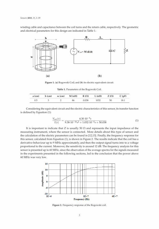
The RC, as well as the different inductive sensors commonly used for PD detection (HFCTor ILS) [9,15], operates on the basic principle of the Faraday’s Law and can be applied to measurePD [16]. Accordingly, the air-core coil is placed around the conductors through which the currentpulses associated to PD and electrical noise can be propagated. This variable current produces amagnetic field, which links the secondary of the coil and induces a voltage directly proportional tothe rate of change of the current in the conductor and the mutual inductance between the coil andthe conductor. The RC designed and used in this paper, is based on a toroidal transformer with anair-core of transversal rectangular section, made of 12 identical turns as on the geometry indicatedin Figure 1a. This configuration is modelled with the equivalent circuit shown in Figure 1b, withthe induced voltage represented by the source voltage Vcoil and the electrical effects of the windingrepresented by R, L and C parameters, which correspond with the resistance, self-inductance of the

2

Sensors 2015, 15, 1–19

winding cable and capacitance between the coil turns and the return cable, respectively. The geometricand electrical parameters for this design are indicated in Table 1.

(a) (b)

Figure 1. (a) Rogowski Coil; and (b) its electric equivalent circuit.

Table 1. Parameters of the Rogowski Coil.

a (cm) b (cm) w (cm) M (nH) R (Ω) L (nH) Z (Ω) C (pF)

0.5 3 2 86 0.038 1032 50 18.1

Considering the equivalent circuit and the electric characteristics of this sensor, its transfer functionis defined by Equation (1):

Vout(s)

I(s)=

4.30·10−6s

9.38·10−16s2 + 1.032·10−6s + 50.038(1)

It is important to indicate that Z is usually 50 Ω and represents the input impedance of themeasuring instrument, where the sensor is connected. More details about this type of sensor andthe calculation of the electric parameters can be found in [12,13]. Finally, the frequency response forthis sensor, calculated from Equation (1), is shown in Figure 2. The results indicate that the coil has aderivative behaviour up to 9 MHz approximately, and then the output signal turns into to a voltageproportional to the current. Moreover, the sensitivity is around 12 dB. The frequency analysis for thissensor is presented up to 60 MHz, since the observation of the average spectra for the signals measuredin the experiments presented in the following sections, led to the conclusion that the power above60 MHz was very low.

Figure 2. Frequency response of the Rogowski coil.

3

Sensors 2015, 15, 1–19

3. Experimental Setup and PD Sources Separation

3.1. Experimental Setup

Due to the importance of PD phenomenon to estimate the insulation lifetime, a procedureto measure PD including the circuits implemented for their detection is detailed in the standardIEC 60,270 [6]. Although the measured PD signals are different to the original signals originated inthe PD sources, due to the attenuation and dispersion effects until the sensor captures them, muchinformation of the pulse shape to distinguish their source type (internal, surface or corona) can beobtained [17–19].

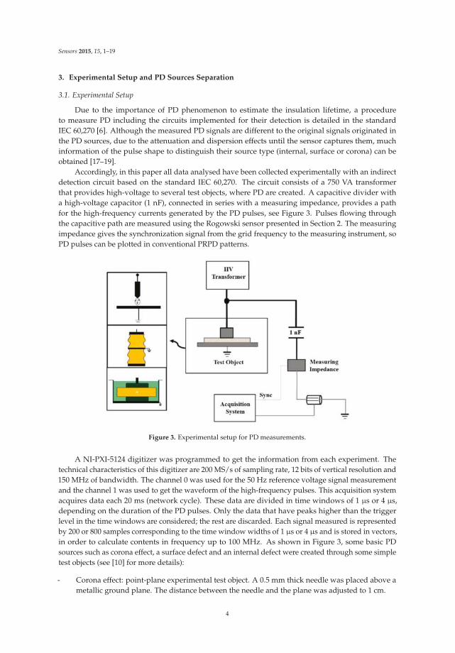
Accordingly, in this paper all data analysed have been collected experimentally with an indirectdetection circuit based on the standard IEC 60,270. The circuit consists of a 750 VA transformerthat provides high-voltage to several test objects, where PD are created. A capacitive divider witha high-voltage capacitor (1 nF), connected in series with a measuring impedance, provides a pathfor the high-frequency currents generated by the PD pulses, see Figure 3. Pulses flowing throughthe capacitive path are measured using the Rogowski sensor presented in Section 2. The measuringimpedance gives the synchronization signal from the grid frequency to the measuring instrument, soPD pulses can be plotted in conventional PRPD patterns.

Figure 3. Experimental setup for PD measurements.

A NI-PXI-5124 digitizer was programmed to get the information from each experiment. Thetechnical characteristics of this digitizer are 200 MS/s of sampling rate, 12 bits of vertical resolution and150 MHz of bandwidth. The channel 0 was used for the 50 Hz reference voltage signal measurementand the channel 1 was used to get the waveform of the high-frequency pulses. This acquisition systemacquires data each 20 ms (network cycle). These data are divided in time windows of 1 µs or 4 µs,depending on the duration of the PD pulses. Only the data that have peaks higher than the triggerlevel in the time windows are considered; the rest are discarded. Each signal measured is representedby 200 or 800 samples corresponding to the time window widths of 1 µs or 4 µs and is stored in vectors,in order to calculate contents in frequency up to 100 MHz. As shown in Figure 3, some basic PDsources such as corona effect, a surface defect and an internal defect were created through some simpletest objects (see [10] for more details):

- Corona effect: point-plane experimental test object. A 0.5 mm thick needle was placed above ametallic ground plane. The distance between the needle and the plane was adjusted to 1 cm.

4

Sensors 2015, 15, 1–19

- Surface defect: Contaminated ceramic bushing. A 15 kV ceramic bushing was contaminated byspraying a solution of salt in water to create ionization paths along the surface. In order to avoidunstable PD activity, the measurements are carried out once moisture has been disappeared.

- Internal defect: Insulating sheets immersed in mineral oil. This setup was designed to generateinternal discharges and consists of eleven insulating sheets of NOMEX paper (polyimide 0.35 mmthick film). The central paper sheet was pierced with a needle (1 mm in diameter) to create an airvoid inside this dielectric.

As it will be indicated later in the experimental results, the experimental setup was implementedidentically in two different high-voltage laboratories, one that is completely shielded and anotherthat is unshielded. This was done in order to characterize the ability of the PR maps to separate PDsources in two different environments measuring with the RC sensor. In the first laboratory, controlled,the noise signals present a low magnitude and in the second one, less controlled, the noise signalspresent similar characteristics to those found in industrial environments: high-levels of amplitude andhigh-spectral variability.

3.2. Spectral Power Clustering Technique (SPCT)

Separation and identification of PD sources are stages that must be approached sequentially, dueto separation is a prerequisite fundamental and obligatory for a successful and accurate identification.

When PD measurements are carried out with inductive sensors, such as the RC, the waveform ofthe carrying currents sensed as a result of PD activity cannot be universally identified with a particulartype of PD source (corona, surface or internal), due to the stochastic behaviour of PD phenomena anddue to the distortion caused in the pulse transmission from the source to the measuring point and inthe coupling system itself. However, PRPD patterns allow to successful identifying PD sources [19].Therefore, a generic solution widely used in most PD measuring instruments, is based on the analysisof the entire PRPD pattern containing all sources measured and on the separation of this patterninto sub-PRPD patterns, each corresponding to a specific source. The separation is accomplished byassuming that each PD source exhibits similar waveforms, while the signals produced by differentsources are different. Following this premise, this paper attempts to prove that the SPCT allowsseparating different PD and noise sources, mapping for each of the measured signals the value of therelative spectral power calculated for two intervals: PRL (power ratio for low-frequencies) and PRH(power ratio for high-frequencies).

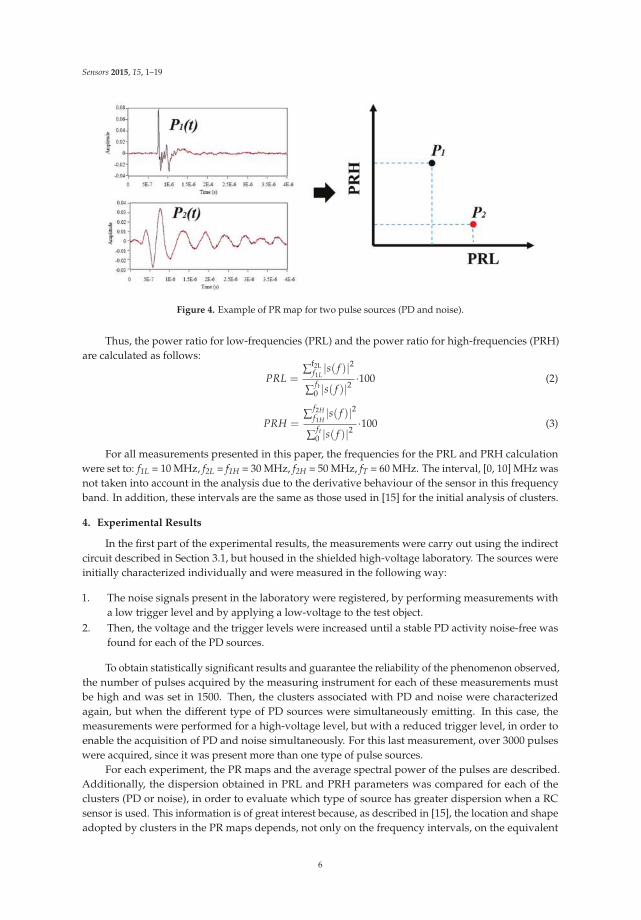
In this approach, the pulses are analysed in the frequency domain therefore, the fast Fouriertransform is applied to each detected pulse, obtaining its spectral magnitude distribution s(f ) [10].Then, the spectral power of each pulse is calculated in two frequency intervals, [f1L, f2L] and [f1H, f2H].Since the total spectral power or amplitude of the signals may influence the pulse characterization,these spectral powers are divided into the overall spectral power calculated up to the maximumanalysed frequency ft. The obtained quantities are defined as power ratios (%), one for the higherfrequency interval, PRH, and another for the lower frequency interval, PRL, as shown in Equations (2)and (3). These two parameters are represented in a two dimensional map, where each pulse sourceshowed a different cloud of points (clusters) with different positions, (see Figure 4).

For all measurements, the frequency analysis was made up to 100 MHz, however, the observationof the average spectra for all the experiments led to the conclusion that the power above 60 MHz wasvery low, so this last value was used as ft.

5

Sensors 2015, 15, 1–19

Figure 4. Example of PR map for two pulse sources (PD and noise).

Thus, the power ratio for low-frequencies (PRL) and the power ratio for high-frequencies (PRH)are calculated as follows:

PRL =∑

f2Lf1L|s( f )|2

∑ft

0 |s( f )|2·100 (2)

PRH =∑

f2H

f1H|s( f )|2

∑ft

0 |s( f )|2·100 (3)

For all measurements presented in this paper, the frequencies for the PRL and PRH calculationwere set to: f1L = 10 MHz, f2L = f1H = 30 MHz, f2H = 50 MHz, fT = 60 MHz. The interval, [0, 10] MHz wasnot taken into account in the analysis due to the derivative behaviour of the sensor in this frequencyband. In addition, these intervals are the same as those used in [15] for the initial analysis of clusters.

4. Experimental Results

In the first part of the experimental results, the measurements were carry out using the indirectcircuit described in Section 3.1, but housed in the shielded high-voltage laboratory. The sources wereinitially characterized individually and were measured in the following way:

1. The noise signals present in the laboratory were registered, by performing measurements witha low trigger level and by applying a low-voltage to the test object.

2. Then, the voltage and the trigger levels were increased until a stable PD activity noise-free wasfound for each of the PD sources.

To obtain statistically significant results and guarantee the reliability of the phenomenon observed,the number of pulses acquired by the measuring instrument for each of these measurements mustbe high and was set in 1500. Then, the clusters associated with PD and noise were characterizedagain, but when the different type of PD sources were simultaneously emitting. In this case, themeasurements were performed for a high-voltage level, but with a reduced trigger level, in order toenable the acquisition of PD and noise simultaneously. For this last measurement, over 3000 pulseswere acquired, since it was present more than one type of pulse sources.

For each experiment, the PR maps and the average spectral power of the pulses are described.Additionally, the dispersion obtained in PRL and PRH parameters was compared for each of theclusters (PD or noise), in order to evaluate which type of source has greater dispersion when a RCsensor is used. This information is of great interest because, as described in [15], the location and shapeadopted by clusters in the PR maps depends, not only on the frequency intervals, on the equivalent

6

Sensors 2015, 15, 1–19

capacitance of the test object, and on the pulse nature, but also on the type of sensor used. Therefore, themore homogeneous are the clusters associated with a particular source the better is its characterizationwhen different sources are detected, especially if there is a clear separation between them.

In the second part of the experimental results, the measurements were made using the sameindirect measurement circuit but in this case, this was housed in the unshielded laboratory. Again, theclusters associated to PD and electrical noise were characterized in these tests, when different types ofsources were present simultaneously.

4.1. Experimental Measurements Performed in the Shielded Laboratory

The measurements described below, were made, in order to obtain a controlled environment tominimize the influence of electrical noise, and to facilitate the characterization of the dispersion of theclusters of pulses for each type of PD source. However, as it will be indicated in Section 4.1.3, it is notpossible to completely minimize the influence of noise during the acquisitions, especially when themeasurements are performed with a RC sensor, whose signal-to-noise ratio (SNR) is low compared toother types of inductive sensors [20–22].

4.1.1. Noise Characterization

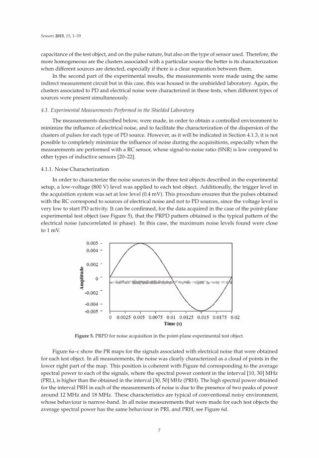
In order to characterize the noise sources in the three test objects described in the experimentalsetup, a low-voltage (800 V) level was applied to each test object. Additionally, the trigger level inthe acquisition system was set at low level (0.4 mV). This procedure ensures that the pulses obtainedwith the RC correspond to sources of electrical noise and not to PD sources, since the voltage level isvery low to start PD activity. It can be confirmed, for the data acquired in the case of the point-planeexperimental test object (see Figure 5), that the PRPD pattern obtained is the typical pattern of theelectrical noise (uncorrelated in phase). In this case, the maximum noise levels found were closeto 1 mV.

Figure 5. PRPD for noise acquisition in the point-plane experimental test object.

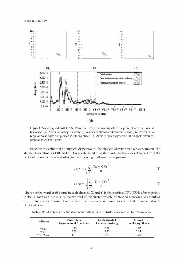
Figure 6a–c show the PR maps for the signals associated with electrical noise that were obtainedfor each test object. In all measurements, the noise was clearly characterized as a cloud of points in thelower right part of the map. This position is coherent with Figure 6d corresponding to the averagespectral power to each of the signals, where the spectral power content in the interval [10, 30] MHz(PRL), is higher than the obtained in the interval [30, 50] MHz (PRH). The high spectral power obtainedfor the interval PRH in each of the measurements of noise is due to the presence of two peaks of poweraround 12 MHz and 18 MHz. These characteristics are typical of conventional noisy environment,whose behaviour is narrow-band. In all noise measurements that were made for each test objects theaverage spectral power has the same behaviour in PRL and PRH, see Figure 6d.

7

Sensors 2015, 15, 1–19

(a) (b) (c)

(d)

Figure 6. Noise acquisition 800 V. (a) Power ratio map for noise signals in the point-plane experimentaltest object; (b) Power ratio map for noise signals in a contaminated ceramic bushing; (c) Power ratiomap for noise signals in pierced insulating sheets; (d) Average spectral power of the signals obtainedwith the three test objects.

In order to evaluate the statistical dispersion of the clusters obtained in each experiment, thestandard deviation for PRL and PRH was calculated. The standard deviation was obtained from thecentroid for each cluster according to the following mathematical expression:

σPRL =

√

√

√

√

n

∑i=1

(Xi − CX) 2

n(4)

σPRH =

√

√

√

√

n

∑i=1

(Yi − CY) 2

n(5)

where n is the number of points in each clusters, Xi and Yi is the position (PRL-PRH) of each point i

in the PR map and (CX, CY) is the centroid of the cluster, which is obtained according to describedin [15]. Table 2 summarizes the results of the dispersion obtained for each cluster associated withelectrical noise.

Table 2. Results obtained of the standard deviation for each cluster associated with electrical noise.

IndicatorPoint-Plane

Experimental SpecimenContaminated

Ceramic BushingPierced

Insulating Sheets

σPRL 3.15 3.10 3.02σPRH 2.23 2.52 2.35

σPRL/σPRH 1.41 1.23 1.28

8

Sensors 2015, 15, 1–19

Analysing the results in Table 2, the dispersion in PRL and PRH for each of the clusters has verysimilar values. When comparing the dispersion between PRL and PRH for each cluster, it is observedthat the dispersion in PRL is higher than that obtained by PRH, this last is most notable in the caseof the point-plane experimental test object, where the σPRL/σPRH ratio is higher than for other testobjects (1.41). This ratio will allow us to identify during the measurements in which axis of the PRmap, is more dispersed one cluster, i.e. if σPRL/σPRH > 1; PRL has a greater dispersion, otherwise ifσPRL/σPRH < 1 this means that PRH has the greater dispersion.

From the point of view of source separation, an ideal cluster is the one that has a ratioσPRL/σPRH ≈ 1 and a high homogeneity (low dispersion in PRL and PRH). Therefore, if the clusterslocated on the classification map are obtained with these characteristics (i.e., σPRL/σPRH ≈ 1, low σPRL

and low σPRH), it will be obtained a very homogeneous clouds of points that facilitates the applicationof any method of clusters identification (K-means, K-medians, Gaussian, etc.), after the application ofthe SPCT, so a better separation and identification of points associated with each cluster is achievedwhen multiple sources are present.

It is important, for the operator of the classification tool, to consider this information once each ofthe sources in the classification map have been characterized, as this can help to verify if the separationintervals manually selected should be modified slightly or completely changed in order to enhance theclusters separation. This will facilitate, in a later stage, the sources identification process, that can beperformed through visual inspections or applying automatic identification algorithms. Furthermore, itmust be emphasized that this information is only useful once the intervals of separation have beenselected, because these indicators alone cannot estimate the frequency bands where the separationintervals should be located. They only allow assessing homogeneity, dispersion and shape of theclusters for each of the previously demarcated intervals.

However, in Section 4.1.3, an additional graphic indicator is presented. This is based on thevariability of the spectral power of the captured signals, which does allow identifying areas of interestwhere the user must locate the separation intervals, in order to obtain an initial characterizationwhich may, or may not, be improved by modifying slightly the position of the separation intervals orevaluating the dispersion in PRL (σPRL), PRH (σPRH) and its ratio (σPRL/σPRH), for each case, up to abetter characterization of each source.

4.1.2. Partial Discharge Source Characterization

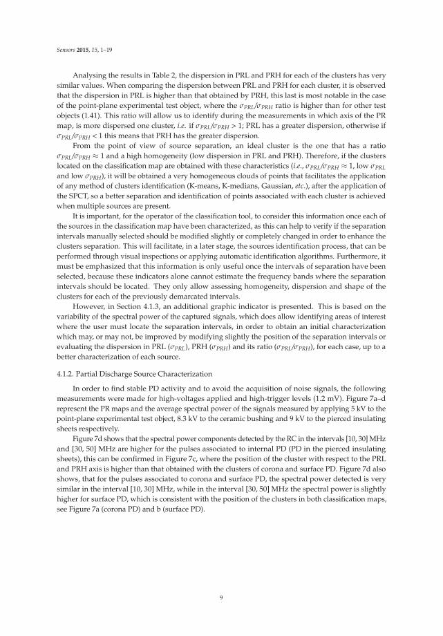
In order to find stable PD activity and to avoid the acquisition of noise signals, the followingmeasurements were made for high-voltages applied and high-trigger levels (1.2 mV). Figure 7a–drepresent the PR maps and the average spectral power of the signals measured by applying 5 kV to thepoint-plane experimental test object, 8.3 kV to the ceramic bushing and 9 kV to the pierced insulatingsheets respectively.

Figure 7d shows that the spectral power components detected by the RC in the intervals [10, 30] MHzand [30, 50] MHz are higher for the pulses associated to internal PD (PD in the pierced insulatingsheets), this can be confirmed in Figure 7c, where the position of the cluster with respect to the PRLand PRH axis is higher than that obtained with the clusters of corona and surface PD. Figure 7d alsoshows, that for the pulses associated to corona and surface PD, the spectral power detected is verysimilar in the interval [10, 30] MHz, while in the interval [30, 50] MHz the spectral power is slightlyhigher for surface PD, which is consistent with the position of the clusters in both classification maps,see Figure 7a (corona PD) and b (surface PD).

9

Sensors 2015, 15, 1–19

(a) (b) (c)

(d)

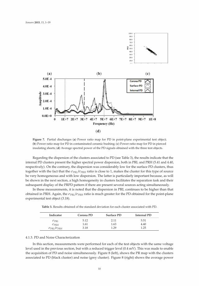
Figure 7. Partial discharges (a) Power ratio map for PD in point-plane experimental test object;(b) Power ratio map for PD in contaminated ceramic bushing; (c) Power ratio map for PD in piercedinsulating sheets; (d) Average spectral power of the PD signals obtained with the three test objects.

Regarding the dispersion of the clusters associated to PD (see Table 3), the results indicate that theinternal PD clusters present the higher spectral power dispersion, both in PRL and PRH (5.41 and 4.40,respectively). On the contrary, the dispersion was considerably low for the surface PD clusters, thustogether with the fact that the σPRL/σPRH ratio is close to 1, makes the cluster for this type of sourcebe very homogeneous and with low dispersion. The latter is particularly important because, as willbe shown in the next section, a high homogeneity in clusters facilitates the separation task and theirsubsequent display of the PRPD pattern if there are present several sources acting simultaneously.

In these measurements, it is noted that the dispersion in PRL continues to be higher than thatobtained in PRH. Again, the σPRL/σPRH ratio is much greater for the PD obtained for the point-planeexperimental test object (3.18).

Table 3. Results obtained of the standard deviation for each cluster associated with PD.

Indicator Corona PD Surface PD Internal PD

σPRL 5.12 2.11 5.51σPRH 1.61 1.63 4.40

σPRL/σPRH 3.18 1.29 1.25

4.1.3. PD and Noise Characterization

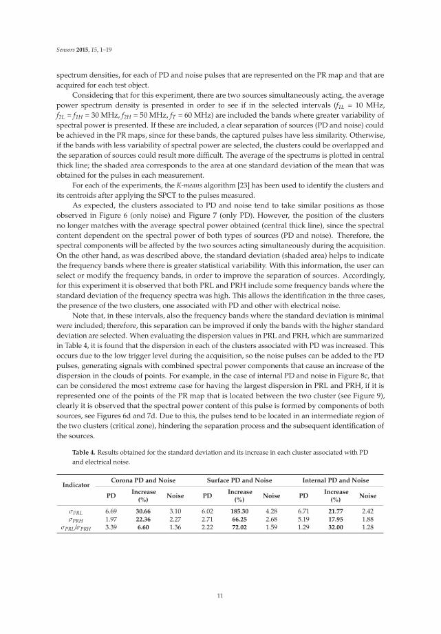
In this section, measurements were performed for each of the test objects with the same voltagelevel used in the previous section, but with a reduced trigger level (0.4 mV). This was made to enablethe acquisition of PD and noise simultaneously. Figure 8 (left), shows the PR map with the clustersassociated to PD (black cluster) and noise (grey cluster). Figure 8 (right) shows the average power

10

Sensors 2015, 15, 1–19

spectrum densities, for each of PD and noise pulses that are represented on the PR map and that areacquired for each test object.

Considering that for this experiment, there are two sources simultaneously acting, the averagepower spectrum density is presented in order to see if in the selected intervals (f1L = 10 MHz,f2L = f1H = 30 MHz, f2H = 50 MHz, fT = 60 MHz) are included the bands where greater variability ofspectral power is presented. If these are included, a clear separation of sources (PD and noise) couldbe achieved in the PR maps, since for these bands, the captured pulses have less similarity. Otherwise,if the bands with less variability of spectral power are selected, the clusters could be overlapped andthe separation of sources could result more difficult. The average of the spectrums is plotted in centralthick line; the shaded area corresponds to the area at one standard deviation of the mean that wasobtained for the pulses in each measurement.

For each of the experiments, the K-means algorithm [23] has been used to identify the clusters andits centroids after applying the SPCT to the pulses measured.

As expected, the clusters associated to PD and noise tend to take similar positions as thoseobserved in Figure 6 (only noise) and Figure 7 (only PD). However, the position of the clustersno longer matches with the average spectral power obtained (central thick line), since the spectralcontent dependent on the spectral power of both types of sources (PD and noise). Therefore, thespectral components will be affected by the two sources acting simultaneously during the acquisition.On the other hand, as was described above, the standard deviation (shaded area) helps to indicatethe frequency bands where there is greater statistical variability. With this information, the user canselect or modify the frequency bands, in order to improve the separation of sources. Accordingly,for this experiment it is observed that both PRL and PRH include some frequency bands where thestandard deviation of the frequency spectra was high. This allows the identification in the three cases,the presence of the two clusters, one associated with PD and other with electrical noise.

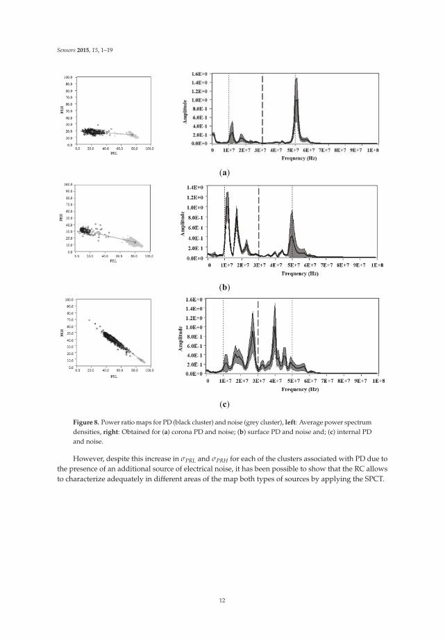
Note that, in these intervals, also the frequency bands where the standard deviation is minimalwere included; therefore, this separation can be improved if only the bands with the higher standarddeviation are selected. When evaluating the dispersion values in PRL and PRH, which are summarizedin Table 4, it is found that the dispersion in each of the clusters associated with PD was increased. Thisoccurs due to the low trigger level during the acquisition, so the noise pulses can be added to the PDpulses, generating signals with combined spectral power components that cause an increase of thedispersion in the clouds of points. For example, in the case of internal PD and noise in Figure 8c, thatcan be considered the most extreme case for having the largest dispersion in PRL and PRH, if it isrepresented one of the points of the PR map that is located between the two cluster (see Figure 9),clearly it is observed that the spectral power content of this pulse is formed by components of bothsources, see Figures 6d and 7d. Due to this, the pulses tend to be located in an intermediate region ofthe two clusters (critical zone), hindering the separation process and the subsequent identification ofthe sources.

Table 4. Results obtained for the standard deviation and its increase in each cluster associated with PDand electrical noise.

IndicatorCorona PD and Noise Surface PD and Noise Internal PD and Noise

PDIncrease

(%)Noise PD

Increase(%)

Noise PDIncrease

(%)Noise

σPRL 6.69 30.66 3.10 6.02 185.30 4.28 6.71 21.77 2.42σPRH 1.97 22.36 2.27 2.71 66.25 2.68 5.19 17.95 1.88

σPRL/σPRH 3.39 6.60 1.36 2.22 72.02 1.59 1.29 32.00 1.28

11

Sensors 2015, 15, 1–19

(a)

(b)

(c)

Figure 8. Power ratio maps for PD (black cluster) and noise (grey cluster), left: Average power spectrumdensities, right: Obtained for (a) corona PD and noise; (b) surface PD and noise and; (c) internal PDand noise.

However, despite this increase in σPRL and σPRH for each of the clusters associated with PD due tothe presence of an additional source of electrical noise, it has been possible to show that the RC allowsto characterize adequately in different areas of the map both types of sources by applying the SPCT.

12

Sensors 2015, 15, 1–19

Figure 9. Example of a pulse formed by components of PD and noise.

4.2. Experimental Measurements Performed in the Unshielded Laboratory

In order to evaluate the performance of the RC in a less controlled environment, where the noisepresent has completely different characteristics in time and frequency to those found in the previousexperiments, new measurements were carried out in a second high-voltage laboratory. In this secondemplacement, there is not any type of shielding that can minimize the presence of external noisesources generated. Additionally, the laboratory is in an area of industrial activity (surrounded byindustrial facilities), where the noise level can vary depending on the external activity during themeasurement process.

On the other hand, the experimental setup used in this section was prepared to simultaneouslygenerate three different sources: one associated with corona another to internal PD and the last oneassociated with electrical noise. Thus, the pulse sources were measured with the RC working in a verysimilar environment to that found in on-site measurements, where most of times it is necessary to detectand separate simultaneous PD and noise sources in order to identify the insulation defects involved.

For this purpose, the tests objects used for internal and corona PD were modified to obtain astable PD activity for the same voltage level on both test objects (5.2 kV). In this case, the separationfrom the needle to the ground in the point-plane configuration was 1.5 cm. For the internal defect, theinsulation system was composed by eleven insulating sheets of NOMEX where the five central sheetswere pierced. Then, an air cylinder with 5 × 0.35 mm in height inside the solid material is obtained.For this experiment, the trigger level was set at 1.3 mV (low), because the maximum noise levels foundwere close to 2.1 mV, this level of noise is greater than that in the laboratory shielded (1 mV).

Finally, both test objects were electrically connected in parallel and subjected to 5.2 kV, measuringthousands of PD and noise pulses waveforms. The resulting PR map for this experiment, maintainingthe same intervals of separation as previously (f1L = 10 MHz, f2L = f1H = 30 MHz, f2H = 50 MHz,fT = 60 MHz) is presented in Figure 10. For this case, three different clouds of points can be easilyselected (since they are clearly separated) to identify the PD source type through the PRPD patterns.

13

Sensors 2015, 15, 1–19

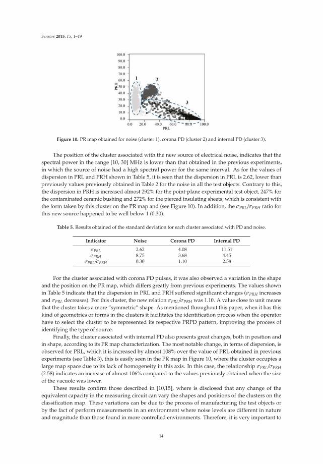
Figure 10. PR map obtained for noise (cluster 1), corona PD (cluster 2) and internal PD (cluster 3).

The position of the cluster associated with the new source of electrical noise, indicates that thespectral power in the range [10, 30] MHz is lower than that obtained in the previous experiments,in which the source of noise had a high spectral power for the same interval. As for the values ofdispersion in PRL and PRH shown in Table 5, it is seen that the dispersion in PRL is 2.62, lower thanpreviously values previously obtained in Table 2 for the noise in all the test objects. Contrary to this,the dispersion in PRH is increased almost 292% for the point-plane experimental test object, 247% forthe contaminated ceramic bushing and 272% for the pierced insulating sheets; which is consistent withthe form taken by this cluster on the PR map and (see Figure 10). In addition, the σPRL/σPRH ratio forthis new source happened to be well below 1 (0.30).

Table 5. Results obtained of the standard deviation for each cluster associated with PD and noise.

Indicator Noise Corona PD Internal PD

σPRL 2.62 4.08 11.51σPRH 8.75 3.68 4.45

σPRL/σPRH 0.30 1.10 2.58

For the cluster associated with corona PD pulses, it was also observed a variation in the shapeand the position on the PR map, which differs greatly from previous experiments. The values shownin Table 5 indicate that the dispersion in PRL and PRH suffered significant changes (σPRH increasesand σPRL decreases). For this cluster, the new relation σPRL/σPRH was 1.10. A value close to unit meansthat the cluster takes a more “symmetric” shape. As mentioned throughout this paper, when it has thiskind of geometries or forms in the clusters it facilitates the identification process when the operatorhave to select the cluster to be represented its respective PRPD pattern, improving the process ofidentifying the type of source.

Finally, the cluster associated with internal PD also presents great changes, both in position andin shape, according to its PR map characterization. The most notable change, in terms of dispersion, isobserved for PRL, which it is increased by almost 108% over the value of PRL obtained in previousexperiments (see Table 3), this is easily seen in the PR map in Figure 10, where the cluster occupies alarge map space due to its lack of homogeneity in this axis. In this case, the relationship σPRL/σPRH

(2.58) indicates an increase of almost 106% compared to the values previously obtained when the sizeof the vacuole was lower.

These results confirm those described in [10,15], where is disclosed that any change of theequivalent capacity in the measuring circuit can vary the shapes and positions of the clusters on theclassification map. These variations can be due to the process of manufacturing the test objects orby the fact of perform measurements in an environment where noise levels are different in natureand magnitude than those found in more controlled environments. Therefore, it is very important to

14

Sensors 2015, 15, 1–19

properly select the separation intervals depending on the scenario to obtain a clear characterization ofall sources present during the measurements.

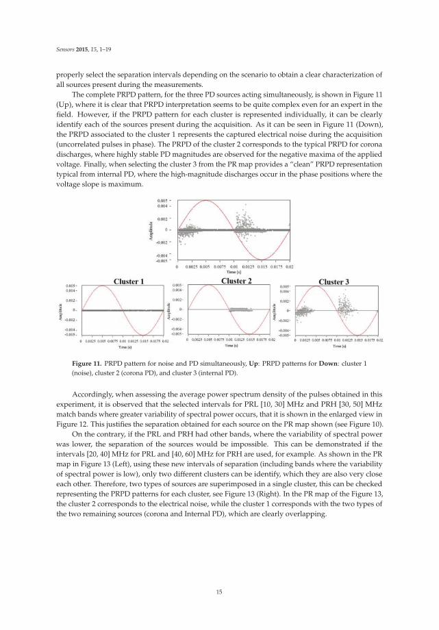
The complete PRPD pattern, for the three PD sources acting simultaneously, is shown in Figure 11(Up), where it is clear that PRPD interpretation seems to be quite complex even for an expert in thefield. However, if the PRPD pattern for each cluster is represented individually, it can be clearlyidentify each of the sources present during the acquisition. As it can be seen in Figure 11 (Down),the PRPD associated to the cluster 1 represents the captured electrical noise during the acquisition(uncorrelated pulses in phase). The PRPD of the cluster 2 corresponds to the typical PRPD for coronadischarges, where highly stable PD magnitudes are observed for the negative maxima of the appliedvoltage. Finally, when selecting the cluster 3 from the PR map provides a “clean” PRPD representationtypical from internal PD, where the high-magnitude discharges occur in the phase positions where thevoltage slope is maximum.

Figure 11. PRPD pattern for noise and PD simultaneously, Up: PRPD patterns for Down: cluster 1(noise), cluster 2 (corona PD), and cluster 3 (internal PD).

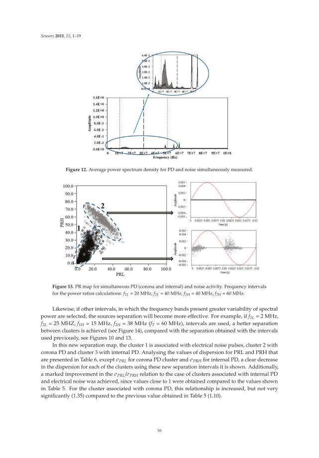
Accordingly, when assessing the average power spectrum density of the pulses obtained in thisexperiment, it is observed that the selected intervals for PRL [10, 30] MHz and PRH [30, 50] MHzmatch bands where greater variability of spectral power occurs, that it is shown in the enlarged view inFigure 12. This justifies the separation obtained for each source on the PR map shown (see Figure 10).

On the contrary, if the PRL and PRH had other bands, where the variability of spectral powerwas lower, the separation of the sources would be impossible. This can be demonstrated if theintervals [20, 40] MHz for PRL and [40, 60] MHz for PRH are used, for example. As shown in the PRmap in Figure 13 (Left), using these new intervals of separation (including bands where the variabilityof spectral power is low), only two different clusters can be identify, which they are also very closeeach other. Therefore, two types of sources are superimposed in a single cluster, this can be checkedrepresenting the PRPD patterns for each cluster, see Figure 13 (Right). In the PR map of the Figure 13,the cluster 2 corresponds to the electrical noise, while the cluster 1 corresponds with the two types ofthe two remaining sources (corona and Internal PD), which are clearly overlapping.

15

Sensors 2015, 15, 1–19

Figure 12. Average power spectrum density for PD and noise simultaneously measured.

Figure 13. PR map for simultaneous PD (corona and internal) and noise activity. Frequency intervalsfor the power ratios calculations: f1L = 20 MHz, f2L = 40 MHz, f1H = 40 MHz, f2H = 60 MHz.

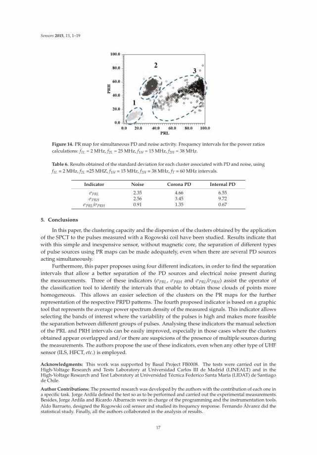
Likewise, if other intervals, in which the frequency bands present greater variability of spectralpower are selected, the sources separation will become more effective. For example, if f1L = 2 MHz,f2L = 25 MHZ, f1H = 15 MHz, f2H = 38 MHz (fT = 60 MHz), intervals are used, a better separationbetween clusters is achieved (see Figure 14), compared with the separation obtained with the intervalsused previously, see Figures 10 and 13.

In this new separation map, the cluster 1 is associated with electrical noise pulses, cluster 2 withcorona PD and cluster 3 with internal PD. Analysing the values of dispersion for PRL and PRH thatare presented in Table 6, except σPRL for corona PD cluster and σPRH for internal PD, a clear decreasein the dispersion for each of the clusters using these new separation intervals it is shown. Additionally,a marked improvement in the σPRL/σPRH relation to the case of clusters associated with internal PDand electrical noise was achieved, since values close to 1 were obtained compared to the values shownin Table 5. For the cluster associated with corona PD, this relationship is increased, but not verysignificantly (1.35) compared to the previous value obtained in Table 5 (1.10).

16

Sensors 2015, 15, 1–19

Figure 14. PR map for simultaneous PD and noise activity. Frequency intervals for the power ratioscalculations: f1L = 2 MHz, f2L = 25 MHz, f1H = 15 MHz, f2H = 38 MHz.

Table 6. Results obtained of the standard deviation for each cluster associated with PD and noise, usingf1L = 2 MHz, f2L =25 MHZ, f1H = 15 MHz, f2H = 38 MHz, fT = 60 MHz intervals.

Indicator Noise Corona PD Internal PD

σPRL 2.35 4.66 6.55σPRH 2.56 3.45 9.72

σPRL/σPRH 0.91 1.35 0.67

5. Conclusions

In this paper, the clustering capacity and the dispersion of the clusters obtained by the applicationof the SPCT to the pulses measured with a Rogowski coil have been studied. Results indicate thatwith this simple and inexpensive sensor, without magnetic core, the separation of different typesof pulse sources using PR maps can be made adequately, even when there are several PD sourcesacting simultaneously.

Furthermore, this paper proposes using four different indicators, in order to find the separationintervals that allow a better separation of the PD sources and electrical noise present duringthe measurements. Three of these indicators (σPRL, σPRH and σPRL/σPRH) assist the operator ofthe classification tool to identify the intervals that enable to obtain those clouds of points morehomogeneous. This allows an easier selection of the clusters on the PR maps for the furtherrepresentation of the respective PRPD patterns. The fourth proposed indicator is based on a graphictool that represents the average power spectrum density of the measured signals. This indicator allowsselecting the bands of interest where the variability of the pulses is high and makes more feasiblethe separation between different groups of pulses. Analysing these indicators the manual selectionof the PRL and PRH intervals can be easily improved, especially in those cases where the clustersobtained appear overlapped and/or there are suspicions of the presence of multiple sources duringthe measurements. The authors propose the use of these indicators, even when any other type of UHFsensor (ILS, HFCT, etc.) is employed.

Acknowledgments: This work was supported by Basal Project FB0008. The tests were carried out in theHigh-Voltage Research and Tests Laboratory at Universidad Carlos III de Madrid (LINEALT) and in theHigh-Voltage Research and Test Laboratory at Universidad Técnica Federico Santa Maria (LIDAT) de Santiagode Chile.

Author Contributions: The presented research was developed by the authors with the contribution of each one ina specific task. Jorge Ardila defined the test so as to be performed and carried out the experimental measurements.Besides, Jorge Ardila and Ricardo Albarracín were in charge of the programming and the instrumentation tools.Aldo Barrueto, designed the Rogowski coil sensor and studied its frequency response. Fernando Álvarez did thestatistical study. Finally, all the authors collaborated in the analysis of results.

17

Sensors 2015, 15, 1–19

Conflicts of Interest: The authors declare no conflict of interest.

References

1. Willis, H.; Schrieber, R. Aging Power Delivery Infrastructures, Second Edition; Power Engineering (Willis),Taylor & Francis: Boca Raton, FL, USA, 2013.

2. Ravi, S.; Ward, J. A Novel Approach for Prioritizing Maintenance of Underground Cables. Technical report, Power

Systems Engineering Research Center (PSERC); Arizona State University: Tempe, AZ, USA, 2006.3. Zhang, X.; Gockenbach, E.; Wasserberg, V.; Borsi, H. Estimation of the Lifetime of the Electrical Components

in Distribution Networks. IEEE Trans. Power Deliv. 2007, 22, 515–522. [CrossRef]4. James, R.; Su, Q. Condition Assessment of High Voltage Insulation in Power System Equipment; The Institution of

Engineering and Technology: London, UK, 2008.5. Jardine, A.K.; Lin, D.; Banjevic, D. A review on machinery diagnostics and prognostics implementing

condition-based maintenance. Mech. Syst. Signal Process. 2006, 20, 1483–1510. [CrossRef]6. IEC-60270. High-Voltage Test Techniques—Partial Discharge Measurements. Available online: https://

webstore.iec.ch/publication/1247 (accessed on 10 October 2015).7. Sahoo, N.; Salama, M.; Bartnikas, R. Trends in partial discharge pattern classification: A survey. IEEE Trans.

Dielectr. Electr. Insul. 2005, 12, 248–264. [CrossRef]8. Cavallini, A.; Montanari, G.; Puletti, F.; Contin, A. A new methodology for the identification of PD in

electrical apparatus: properties and applications. IEEE Trans. Dielectr. Electr. Insul 2005, 12, 203–215.[CrossRef]

9. Cavallini, A.; Montanari, G.; Contin, A.; Pulletti, F. A new approach to the diagnosis of solid insulationsystems based on PD signal inference. IEEE Electr. Insul. Mag. 2003, 19, 23–30. [CrossRef]

10. Ardila-Rey, J.; Martinez-Tarifa, J.; Robles, G.; Rojas-Moreno, M. Partial discharge and noise separation bymeans of spectral-power clustering techniques. IEEE Trans. Dielectr. Electr. Insul. 2013, 20, 1436–1443.[CrossRef]

11. Rojas-Moreno, M.V.; Robles, G.; Tellini, B.; Zappacosta, C.; Martinez-Tarifa, J.M.; Sanz-Feito, J. Study ofan inductive sensor for measuring high frequency current pulses. IEEE Trans. Instrum. Meas. 2011, 60,1893–1900. [CrossRef]

12. Argüeso, M.; Robles, G.; Sanz, J. Implementation of a Rogowski coil for the measurement of partial discharges.Rev. Sci. Instrum. 2005, 6, 065107. [CrossRef]

13. Robles, G.; Martinez, J.; Sanz, J.; Tellini, B.; Zappacosta, C.; Rojas, M. Designing and Tuning an Air-CoredCurrent Transformer for Partial Discharges Pulses Measurements. In Proceedings of the Instrumentationand Measurement Technology Conference, Victoria, BC, USA, 12–15 May 2008; pp. 2021–2025.

14. Álvarez, F.; Garnacho, F.; Ortego, J.; Sánchez-Urán, M. Application of HFCT and UHF sensors in on-linepartial discharge measurements for insulation diagnosis of high voltage equipment. Sensors 2015, 15,7360–7387. [CrossRef] [PubMed]

15. Ardila-Rey, J.A.; Rojas-Moreno, M.V.; Martínez-Tarifa, J.M.; Robles, G. Inductive sensor performance inpartial discharges and noise separation by means of spectral power ratios. Sensors 2014, 14, 3408–3427.[CrossRef] [PubMed]

16. Samimi, M.; Mahari, A.; Farahnakian, M.; Mohseni, H. The rogowski coil principles and applications:A review. IEEE Sens. J. 2015, 15, 651–658. [CrossRef]

17. Okubo, H.; Hayakawa, N. A novel technique for partial discharge and breakdown investigation based oncurrent pulse waveform analysis. IEEE Trans. Dielectr. Electr. Insul. 2005, 12, 736–744. [CrossRef]

18. Cavallini, A.; Montanari, G.; Tozzi, M.; Chen, X. Diagnostic of HVDC systems using partial discharges.IEEE Trans. Dielectr. Electr. Insul. 2011, 18, 275–284. [CrossRef]

19. IEC-TS-60034-27-2. Rotating Electrical Machines—Part 27-2: On-Line Partial Discharge Measurements onthe Stator Winding Insulation of Rotating Electrical machines. Available online: https://webstore.iec.ch/publication/131 (accessed on 10 October 2015).

20. Zhang, Z.; Xiao, D.; Li, Y. Rogowski air coil sensor technique for on-line partial discharge measurement ofpower cables. IET Sci. Meas. Technol. 2009, 3, 187–196. [CrossRef]

18

Sensors 2015, 15, 1–19

21. Hewson, C.; Ray, W. The Effect of Electrostatic Screening of Rogowski Coils Designed for Wide-BandwidthCurrent Measurement in Power Electronic Applications. In Proceedings of the 2004 IEEE 35th Annual PowerElectronics Specialists Conference, Aachen, Germany, 20–25 June 2004; pp. 1143–1148.

22. Hashmi, G.M. Partial Discharge Detection for Condition Monitoring of Covered-Conductor OverheadDistribution Networks Using Rogowski Coil. Ph.D. Thesis, Helsinki University of Technology, Helsinki,Finland, 22 August 2008.

23. Hastie, T.; Tibshirani, R.; Friedman, J. The Elements of Statistical Learning: Data Mining, Inference, and Prediction;

Springer Series in Statistics; Springer: New York, NY, USA, 2013.

© 2015 by the authors; licensee MDPI, Basel, Switzerland. This article is an open accessarticle distributed under the terms and conditions of the Creative Commons Attribution(CC-BY) license (http://creativecommons.org/licenses/by/4.0/).

19

sensors

Article

Analysis of Uncertainty in a Middle-Cost Device for3D Measurements in BIM Perspective

Alonso Sánchez 1,*, José-Manuel Naranjo 2, Antonio Jiménez 3 and Alfonso González 1

1 University Centre of Mérida, University of Extremadura, 06800 Mérida, Spain; [email protected] Polytechnic School, University of Extremadura, 10003 Cáceres, Spain; [email protected] Development Area, Provincial Council of Badajoz, 06071 Badajoz, Spain; [email protected]* Correspondence: [email protected]; Tel.: +34-924-289-300; Fax: +34-924-301-212

Academic Editor: Gonzalo Pajares MartinsanzReceived: 19 April 2016; Accepted: 19 September 2016; Published: 22 September 2016

Abstract: Medium-cost devices equipped with sensors are being developed to get 3D measurements.Some allow for generating geometric models and point clouds. Nevertheless, the accuracy of thesemeasurements should be evaluated, taking into account the requirements of the Building InformationModel (BIM). This paper analyzes the uncertainty in outdoor/indoor three-dimensional coordinatemeasures and point clouds (using Spherical Accuracy Standard (SAS) methods) for Eyes Map,a medium-cost tablet manufactured by e-Capture Research & Development Company, Mérida, Spain.To achieve it, in outdoor tests, by means of this device, the coordinates of targets were measured from1 to 6 m and cloud points were obtained. Subsequently, these were compared to the coordinates of thesame targets measured by a Total Station. The Euclidean average distance error was 0.005–0.027 mfor measurements by Photogrammetry and 0.013–0.021 m for the point clouds. All of them satisfy thetolerance for point cloud acquisition (0.051 m) according to the BIM Guide for 3D Imaging (GeneralServices Administration); similar results are obtained in the indoor tests, with values of 0.022 m.In this paper, we establish the optimal distances for the observations in both, Photogrammetry and3D Photomodeling modes (outdoor) and point out some working conditions to avoid in indoorenvironments. Finally, the authors discuss some recommendations for improving the performanceand working methods of the device.

Keywords: photogrammetry; point clouds; uncertainty; constrained least squares adjustment;middle-cost device

1. Introduction

The three-dimensional modeling of an object begins with the required data acquisition processfor the reconstruction of its geometry and ends with the formation of a virtual 3D model that canbe viewed interactively on a computer [1]. The information provided by the display of thesemodels makes its application possible for different uses [2], such as the inspection of elements,navigation, the identification of objects and animation, making them particularly useful in applicationssuch as artificial intelligence [3], criminology [4], forestry applications [5,6], the study of naturaldisasters [7,8], the analysis of structural deformation [9,10], geomorphology [11,12] or cultural heritageconservation [13,14].

In particular, the generation of point clouds and 3D models has important applications,especially in Building Information Modeling (BIM). This digital representation of the physical andfunctional characteristics of the buildings serves as an information repository for the processes ofdesign and construction, encouraging the use of 3D visualizations [15]. In the future, devices couldinclude different types of sensors to capture all kind of information for BIM applications. In addition,important technological advances in automated data acquisition has led to the production of more

Sensors 2016, 16, 1557 20 www.mdpi.com/journal/sensors

Sensors 2016, 16, 1557

specific models tailored to Historic Building Information Modeling (HBIM) for the preservation ofhistorical or artistic heritage [16,17].

In recent years, different techniques have been developed to acquire data [18]. On the onehand, there are active measurement techniques, carrying out modeling based on scans (range-basedmodeling), which uses instruments equipped with sensors that emit a light with a structure definedand known by another sensor that has to capture it [19]. On the other hand, there are passivemeasurement techniques, with modeling based on images (image-based modeling), which use opticalor optical-electronic capture systems for extracting geometric information in the construction of 3Dmodels [19]. The former uses different types of laser scanners, while the latter employs photogrammetricor simple conventional cameras. In each case, specific software for data processing is used.

One of the most important geometric aspects is the verification of the accuracy and reliabilityof measurements with which data are acquired and the resulting 3D models are obtained, since,according to the tolerances and maximum permissible errors required for the use of certain models,for example in BIM working environment, the final accuracy and reliability obtained with a specificdevice will determine its suitability for certain works [20]. Many studies have carried out such analysisfor active measurement techniques [21–23] as in the case of passive measurement techniques [4,24,25].These are deduced in the first case for objects of medium format, with the use of handheld laserscanners, where an accuracy up to 0.1 mm can be achieved [26]; in the second case, using techniquesof automated digital photogrammetry, precision is of the order of about 5 mm [27], but with theadvantage of a smaller economic cost.

There are instruments equipped with a low-cost sensor on the market: the David laser scanner [28],Microsoft Kinetic v1 and v2 sensors, and RGB-D cameras. These cameras are easy to manage andthey are being used for applications that require a precision of about 5 mm to a measured distanceof 2 m [29]. There are also middle-cost devices, based on structured light technology, such as the DPI-8Handheld Scanner (from DotProduct LLC, Boston, MA, USA) and the FARO Freestyle3D Scanner(FARO, Lake Mary, FL, USA).

Nowadays, there are new projects that are trying to enter the market using instruments basedon a smartphone or a tablet including a range imaging camera and special vision sensor, which areuser-friendly, affordable and offer accuracy for a wide range of applications. These include Google’sTango project from 2014, the Structure Sensor from Occipital from 2015 and EyesMap (EM) carried bye-Capture Research and Development from 2014.

Nonetheless, one of the main problems encountered when performing 3D modeling is todetermine the accuracies obtained with these devices, especially when taking into account the rate ofinformation uptake and the intended product. Normally, the two products we are trying to obtain aregeometric models and 3D point clouds. The first is used to describe the shape of an object, by meansof an analytical, mathematical and abstract model. The second produces very dense and elaboratecoordinate data points for the surfaces of a physical object [30,31]. For this reason, one objectiveof this paper is to perform an analysis of the accuracy of the EM, in two modes of data capture:(1) Photogrammetry to get 3D point coordinates; and (2) Photomodeling to get 3D point cloud and thecolor of the object observed.

This accuracy was evaluated by comparison with the EM measurements and the data acquired bya Total Station. On the other hand, operator error was estimated by comparison with the coordinatesof symmetrical target centers measured by EM and by a Scanstation. Additionally, to investigate thefeasibility of coordinates, measurements and point cloud acquisition from a BIM perspective, furtherevaluation was performed in reference to the guidelines of the GSA for BIM Guide for 3D Imaging [32].

2. Materials and Methods

This study was conducted with an EM tablet from e-capture Research & Development Company.It has dimensions of 303 × 194 × 56 mm3, a weight of 1.9 kg and a screen of 11.6 inches. The devicehas a processor Intel Core i7, 16 gigabytes of RAM and runs on the Windows 8 operating system.

21

Sensors 2016, 16, 1557

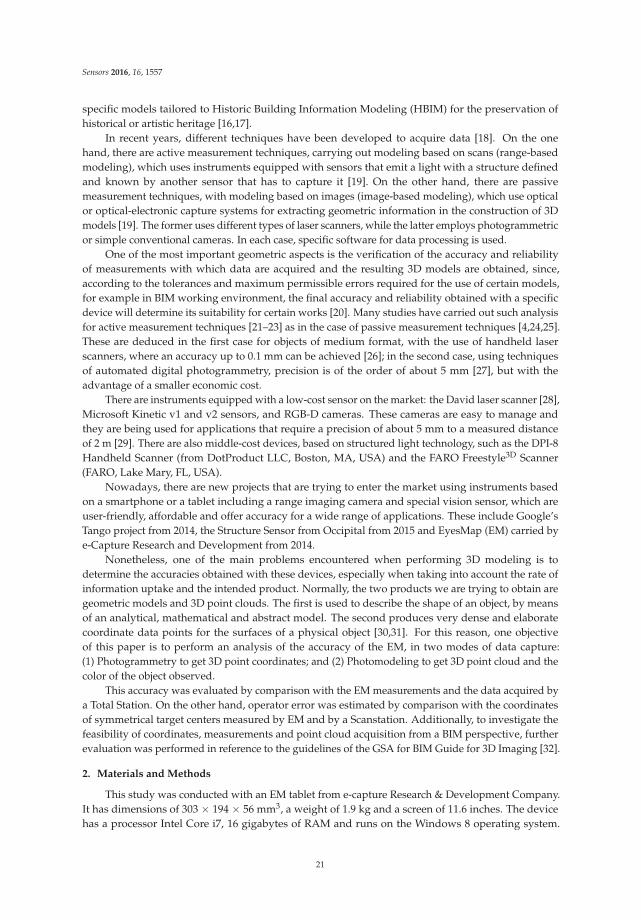
It has an Inertial Measurement Unit and a GNSS system, which allow for measuring speed, orientationand gravitational forces, as well as the positioning of the instrument in real time. To capture thethree-dimensional information, on the back of the tablet (Figure 1), there is a depth sensor and twocameras with a focal length of 2.8 mm and a 13 megapixel resolution, that form a base line of 230 mm,with a field of view up to 67.

(a) (b)

Figure 1. EyesMap (EM): (a) back; and (b) front.

The beta version of EM costs around €9500. The basic principle of operation is based onphotogrammetry techniques, which reconstruct a scene in real time. The precision indicated bythe manufacturer (Table 1) for both measurement modes are:

Table 1. EyesMap (EM) precision specified by the manufacturer.

Range Accuracy STD 1 Accuracy STD Optimized Scale

3 m 3 mm 2.6 mm15 m 15 mm 11 mm30 m 30 mm 23 mm

1 Standard deviation (STD).

Precisely in order to achieve the precisions expressed in the previous table, the recommendationsof the manufacturer for the Photogrammetry measurement are: (1) take at least 2 pictures;(2) 80% overlap/2 pictures; and (3) capture in parallel or convergent. In the case of measurement by3D Photomodeling, the same recommendations apply, but take at least five pictures instead of two.EM uses a computer vision approach based on general method of Photogrammetry [33].

In this sense, obtaining coordinates (XP, YP, ZP), is computed by Digital Image Correlation (DIC).In this way, 3D cloud points are achieved to a very high density from the surface of the studied object,moreover, storing color information (RGB). The calculation process of the coordinates of the points thatcompose the cloud, from a pair of oriented pictures is carried out by the method of triangulation [34].

The continuous evolution of algorithms that perform DIC has been reaching very high levelsof precision and automation. Currently, the most effective are Structure from Motion (SFM) and thealgorithms of Reconstruction in 3D in high density named Digital Multi-View 3D Reconstruction(DMVR) which produce 3D models of high precision and photorealistic quality from a collection ofdisorganized pictures of a scene or object, taken from different points of view [35].

2.1. EM Workflow

The processes of calibration and orientation of cameras are implemented in the EM software.The orientation of pictures can be done in three ways: (1) automatic orientation, matching homologouspoints that the system finds in both pictures; (2) manual orientation, in which the user chooses

22

Sensors 2016, 16, 1557

at least 9 points in common in both pictures; and (3) automatic orientation by means of targets,which require the existence of at least 9 asymmetrical targets in common. The latter one offersmajor precision and requires a major processing time. The information obtained can also beviewed in real dimension by means of the target named the Stereo target. EM offers the followingoptions: Photogrammetry, 3D Photomodeling, 3D Modeling with Depth Sensor and Orthophoto.Photogrammetry allows for measuring coordinates, distances and areas between points, as well asexporting its coordinates in different formats (*.txt and *.dxf) so other computer aided design programscan be used. 3D Photomodeling and 3D Modeling with Depth Sensor allow 3D point clouds with XYZand color information (PLY and RGB formats respectively), from an object. However, modeling withthe support of the depth sensor is restricted for indoor work, offering less precise results than the 3DPhotomodeling. The last gives an orthophotograph of the work area.

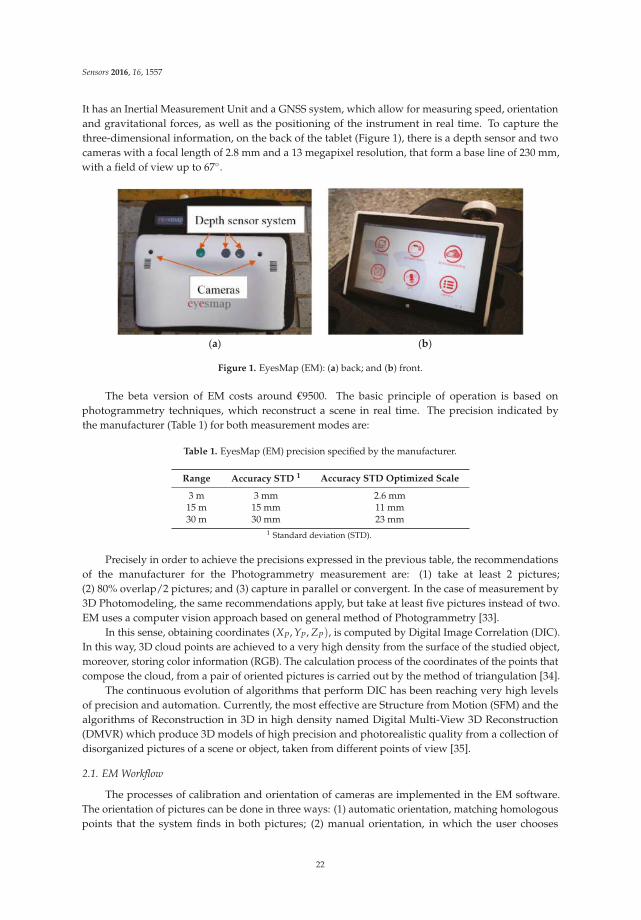
In Photogrammetry (Figure 2a), pictures can be either captured or loaded. Secondly, pictures haveto be managed and the desired pictures selected. Thirdly, we can choose: (1) automatic orientation;(2) manual orientation; or (3) automatic target orientation, in order to achieve the relative orientationof the pictures. In this regard, an automatic scale is made by means of automatic target orientation andthe Stereo target is used. After this, the following measurements can be obtained: (1) coordinates ofpoints; (2) distances; or (3) areas. Finally, the geometric model is obtained.

(a) (b)

Figure 2. Workflow of EM measurement: (a) Photogrammetry; and (b) 3D Photomodeling.

In 3D Photomodeling (Figure 2b), pictures are managed in the same way as Photogrammetry.Secondly, the object to be measured according to its size is selected: small if dimensions are lessthan one meter, medium-sized if the dimensions are below 10 m and large for all other dimensions.

23

Sensors 2016, 16, 1557

Consequently, high, medium or low resolution must be selected. The final model will be scaled orunscaled by means of the Stereo target. After this, the master picture can be selected.

In each of these four options, different working procedures are followed, depending on capturemethodology, shooting planning, and the size and characteristics of the object to measure. Figure 2shows the two options that were used in this study.

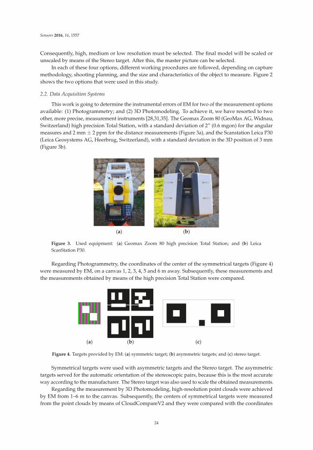
2.2. Data Acquisition Systems

This work is going to determine the instrumental errors of EM for two of the measurement optionsavailable: (1) Photogrammetry; and (2) 3D Photomodeling. To achieve it, we have resorted to twoother, more precise, measurement instruments [28,31,35]. The Geomax Zoom 80 (GeoMax AG, Widnau,Switzerland) high precision Total Station, with a standard deviation of 2” (0.6 mgon) for the angularmeasures and 2 mm ± 2 ppm for the distance measurements (Figure 3a), and the Scanstation Leica P30(Leica Geosystems AG, Heerbrug, Switzerland), with a standard deviation in the 3D position of 3 mm(Figure 3b).

(a) (b)

Figure 3. Used equipment: (a) Geomax Zoom 80 high precision Total Station; and (b) LeicaScanStation P30.

Regarding Photogrammetry, the coordinates of the center of the symmetrical targets (Figure 4)were measured by EM, on a canvas 1, 2, 3, 4, 5 and 6 m away. Subsequently, these measurements andthe measurements obtained by means of the high precision Total Station were compared.

(a) (b) (c)

Figure 4. Targets provided by EM: (a) symmetric target; (b) asymmetric targets; and (c) stereo target.

Symmetrical targets were used with asymmetric targets and the Stereo target. The asymmetrictargets served for the automatic orientation of the stereoscopic pairs, because this is the most accurateway according to the manufacturer. The Stereo target was also used to scale the obtained measurements.

Regarding the measurement by 3D Photomodeling, high-resolution point clouds were achievedby EM from 1–6 m to the canvas. Subsequently, the centers of symmetrical targets were measuredfrom the point clouds by means of CloudCompareV2 and they were compared with the coordinates

24

Sensors 2016, 16, 1557

obtained by the high precision Total Station. In any case, no point of the clouds obtained by EMcoincides exactly with the center of a target and it is necessary to locate and measure the closest pointto this center (not the real center) using CloudCompareV2. On the other hand, only the coordinates ofthe targets that could be correctly identified were measured.

2.3. Data Processing

The coordinates measured by EM (x, y, z); and those obtained by the Total Station and the Scanstation (X, Y, Z) are geo referenced on different coordinate systems. To be able to compare them,the coordinates obtained by EM were transformed to the coordinate system provided by the TotalStation. The transformation that was used was the so-called Helmert or 7 parameters. The three stepsof this transformation are: (1) three rotation angles (Ω, Φ, K); (2) three translations (Tx, Ty, Tz); and (3) achange of scale (λ), which except for the last step were calculated using the EM coordinates system.Both systems of coordinates were parallel. Through the translations, both systems would have thesame origin of coordinates. Finally, the scale factors of both systems of coordinates have the samemeasurement units. Nonetheless, the application of the scale factor may alter the measurements [36],which was not applied for this reason.

⎡

⎢

⎣

X

Y

Z

⎤

⎥

⎦=

⎡

⎢

⎣

a11 a12 a13

a21 a22 a23

a31 a32 a33

⎤

⎥

⎦

⎡

⎢

⎣

x

y

z

⎤

⎥

⎦+

⎡

⎢

⎣

TX

TY

TZ

⎤

⎥

⎦(1)

where:

a11 = cosΦcosK a12 = −cosΦsinK a13 = sinΦ

a21 = cosΩsinK + sinΩsinΦcosK a22 = cosΩcosK − sinΩsinΦsinK a23 = −sinΩcosΦ

a31 = sinΩsinK a32 = sinΩcosK + cosΩsinΦsinK a33 = cosΩcosΦ

(2)

The equations were linearized for a point P by means of the development in Taylor series to thefirst term:

XP = (XP)0 +

(

∂XP

∂Ω

)

0dΩ +

(

∂XP

∂Φ

)

0dΦ +

(

∂XP

∂K

)

0dK +

(

∂XP

∂TX

)

0+ dTX +

(

∂XP

∂TY

)

0dTY +

(

∂XP

∂TZ

)

0dTZ (3)

YP = (YP)0 +

(

∂YP

∂Ω

)

0dΩ +

(

∂YP

∂Φ

)

0dΦ +

(

∂YP

∂K

)

0dK +

(

∂YP

∂TX

)

0+ dTX +

(

∂YP

∂TY

)

0dTY +

(

∂YP

∂TZ

)

0dTZ (4)

ZP = (ZP)0 +

(

∂ZP

∂Ω

)

0dΩ +

(

∂ZP

∂Φ

)

0dΦ +

(

∂ZP

∂K

)

0dK +

(

∂ZP

∂TX

)

0+ dTX +

(

∂ZP

∂TY

)

0dTY +

(

∂ZP

∂TZ

)

0dTZ (5)

On the basis of the linearized equations of general expression and knowing the coordinates inboth systems of at least two points, the following equations were formed:

rn11dΩ + rn

12dΦ + rn13dK + rn

14dTX + rn15dTY + rn

16dTZ = Xn − (Xn)0 (6)

rn21dΩ + rn

22dΦ + rn23dK + rn


26dTZ = Yn − (Yn)0 (7)

rn31dΩ + rn

32dΦ + rn33dK + rn


36dTZ = Zn − (Zn)0 (8)

Expressing the system of equations in matrix form:

⎡

⎢

⎢

⎣

rn11 rn

12 rn13 rn

14 rn15 rn

16

rn21 rn

22 rn23 rn

24 rn25 rn

26

rn31 rn

32 rn33 rn

34 rn35 rn

36

⎤

⎥

⎥

⎦

⎡

⎢

⎢

⎢

⎢

⎢

⎢

⎢

⎢

⎢

⎢

⎢

⎢

⎣

dΩ

dΦ

dK

dTX

dTY

dTZ

⎤

⎥

⎥

⎥

⎥

⎥

⎥

⎥

⎥

⎥

⎥

⎥

⎥

⎦

−

⎡

⎢

⎢

⎣

Xn − (Xn)0

Yn − (Yn)0

Zn − (Zn)0

⎤

⎥

⎥

⎦

=

⎡

⎢

⎢

⎣

VXn

VYn

VZn

⎤

⎥

⎥

⎦

(9)

25

Sensors 2016, 16, 1557

Applying the adjustment by least squares, the system of equations is solved and 6 transformationparameters were obtained (Ω, Φ, K, Tx, Ty, and Tz). Nevertheless, half of the coordinates of thecenter of the symmetrical measured targets were used. These were called Transformation Points.Subsequently, with the transformation parameters obtained, the other half of the coordinates of thecenter of symmetrical targets measured were transformed from the system of coordinates of EM to thesystem of coordinates of Total Station. The resulting Validation Points have two sets of coordinates inthe coordinate system established by the Total Station: (1) coordinates transformed to the Total Stationcoordinate system; from the measured performed by EM; and (2) coordinates of reference directlymeasured by Total Station.

2.4. Uncertainty Assessment

The measurements were made at the Roman Bridge in Merida (Spain), on a canvas ofapproximately 6 × 5 m2 (Figures 5 and 6). This bridge, being of granite, presents an optimal texture forautomatic correlation of images. EM was evaluated according to how correctly it measured elementsplaced at different depth levels.

Figure 5. Used targets.

(a) (b)

Figure 6. Data capture using EM: (a) front view; and (b) back view.

The metric quality of measurements obtained by EM was evaluated using the method proposedby Hong et al. [31]. The three-dimensional coordinate measurements and point clouds obtained by EM(Figure 7) were compared to a set of Total Station point measurements used as reference points. In themapping accuracy assessment, comparisons were based on identifiable target centers. These targets

26

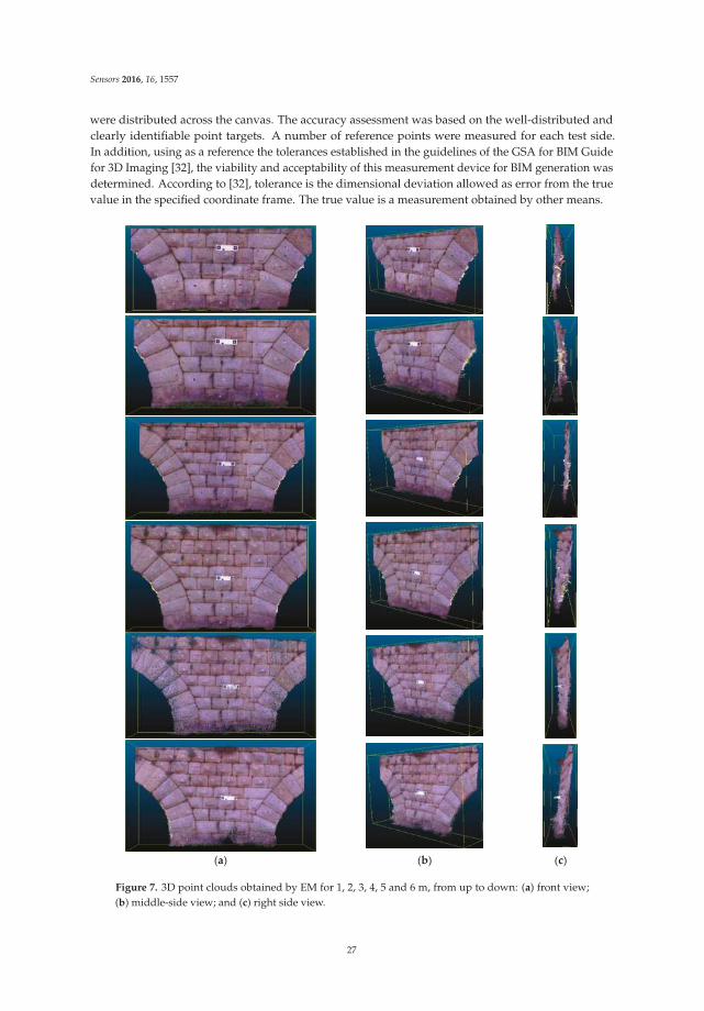
Sensors 2016, 16, 1557

were distributed across the canvas. The accuracy assessment was based on the well-distributed andclearly identifiable point targets. A number of reference points were measured for each test side.In addition, using as a reference the tolerances established in the guidelines of the GSA for BIM Guidefor 3D Imaging [32], the viability and acceptability of this measurement device for BIM generation wasdetermined. According to [32], tolerance is the dimensional deviation allowed as error from the truevalue in the specified coordinate frame. The true value is a measurement obtained by other means.

(a) (b) (c)

Figure 7. 3D point clouds obtained by EM for 1, 2, 3, 4, 5 and 6 m, from up to down: (a) front view;(b) middle-side view; and (c) right side view.

27

Sensors 2016, 16, 1557

Firstly, the precision of the measurements made by EM by Photogrammetry and 3DPhotomodeling are evaluated through the Euclidean average distance error (δavg).

δavg =1n

n

∑i=1

|Rai − T − bi| (10)

where ai corresponding to the measurement is carried out by EM for the i-th check point in one case byPhotogrammetry and in the other case by 3D Photomodeling and bi is the measurement made for thesame point by Total Station. In addition, the rotation and translation parameters of the 3D Helmerttransformation are R and T, respectively. Note that scale was not considered in this transformation [37].

Secondly, the corresponding average error is calculated, together with the error vectors in the x, y

and z directions. The Root Mean Square Error (RMSE) is then calculated to assess the quality of thepoints captured by EM and measured by means of photogrammetry and 3D Photomodeling.

RMSE =

√

√

√

√

1n

n

∑i=1

(

ati − bi

)

2

(11)

where ati shows the point transformed to the coordinates of the Total Station.

Thirdly, the quality of the points measured by EM is also assessed by calculating the SphericalAccuracy Standard (SAS). The SAS, which represents the spherical radius of a 90% probabilitysphere [38], is defined as

SAS = 2.5 × 0.3333 ×(

RMSEx + RMSEy + RMSEZ

)

(12)

This represents a positional accuracy of the coordinates obtained by Photogrammetry andthe point cloud obtained by 3D Photomodeling with a 90% confidence level. The calculation oferrors was repeated for the measurements carried out by EM from 1–6 m to the object measuredby Photogrammetry.

3. Results

Results were tabulated (Tables 2 and 3) and shown in graphs. Different points were chosen ineach case (3D Photomodeling and Photogrammetry modes) depending on the correct identification oftarget centers by the operator.

Table 2. Accuracy assessment result for photogrammetry data measured from 3 m to measured object(unit: mm).

Point ID Error Vector X Error Vector Y Error Vector Z Error

7 3 0 0 39 −10 0 −3 10

11 −9 0 −2 913 15 2 4 1616 −6 −4 −2 718 −14 3 −5 1520 −7 3 −2 822 −13 2 −3 1325 −15 1 −1 1527 12 −3 −4 1329 11 2 3 1231 12 1 3 1234 12 1 3 12

Average error 11

RMSE 11 2 3 12SAS 13

28

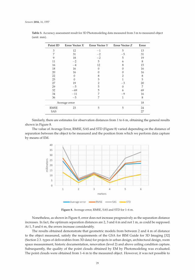
Sensors 2016, 16, 1557

Table 3. Accuracy assessment result for 3D Photomodeling data measured from 3 m to measured object(unit: mm).


3 12 −1 5 137 31 −2 −5 319 18 −2 5 19

11 −2 5 6 816 −4 12 8 1518 16 0 0 1620 16 0 0 1622 0 8 2 825 0 5 1 527 19 2 −3 2029 −5 5 0 732 −69 5 6 6934 −11 7 −9 1636 −5 7 1 8

Average error 18

RMSE 23 5 5 24SAS 27

Similarly, there are estimates for observation distances from 1 to 6 m, obtaining the general resultsshown in Figure 8.

The value of Average Error, RMSE, SAS and STD (Figure 8) varied depending on the distance ofseparation between the object to be measured and the position from which we perform data captureby means of EM.

Figure 8. Average error, RMSE, SAS and STD for 1–6 m.

Nonetheless, as shown in Figure 8, error does not increase progressively as the separation distanceincreases. In fact, the optimum separation distances are 2, 3 and 4 m and not 1 m, as could be supposed.At 1, 5 and 6 m, the errors increase considerably.

The results obtained demonstrate that geometric models from between 2 and 4 m of distanceto the object measured, satisfy the requirements of the GSA for BIM Guide for 3D Imaging [32](Section 2.3. types of deliverables from 3D data) for projects in urban design, architectural design, roomspace measurement, historic documentation, renovation (level 2) and above ceiling condition capture.Subsequently, the quality of the point clouds obtained by EM by Photomodeling was evaluated.The point clouds were obtained from 1–6 m to the measured object. However, it was not possible to

29

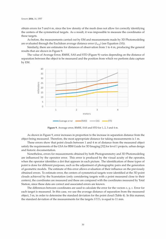
Sensors 2016, 16, 1557

obtain errors for 5 and 6 m, since the low density of the mesh does not allow for correctly identifyingthe centers of the symmetrical targets. As a result, it was impossible to measure the coordinates ofthese targets.

As before, the measurements carried out by EM and measurements made by 3D Photomodelingare evaluated through the Euclidean average distance error (δavg) (see Equation (10)).

Similarly, there are estimates for distances of observation from 1 to 4 m, producing the generalresults that are shown in Figure 9.

The value of Average Error, RMSE, SAS and STD (Figure 9) varies depending on the distance ofseparation between the object to be measured and the position from which we perform data captureby EM.

Figure 9. Average error, RMSE, SAS and STD for 1, 2, 3 and 4 m.

As shown in Figure 9, error increases in proportion to the increase in separation distance from theobject being measured. Therefore, the most appropriate distance for taking measurements is 1 m.

These errors show that point clouds between 1 and 4 m of distance from the measured objectsatisfy the requirements of the GSA for BIM Guide for 3D Imaging [32] for level 1 projects, urban designand historic documentation.

Nonetheless, errors for measurements obtained by both Photogrammetry and 3D Photomodelingare influenced by the operator error. This error is produced by the visual acuity of the operator,when the operator identifies a dot that appears in each picture. The identification of these types ofpoint is done for different purposes, such as the adjustment of photographic pairs and the generationof geometric models. The estimate of this error allows evaluation of their influence on the previouslyobtained errors. To estimate error, the centers of symmetrical targets were identified at the 3D pointclouds achieved by the Scanstation (only considering targets with a point measured close to theircenters), the coordinates are measured and these are compared with the coordinates measured by TotalStation, since these data are correct and associated errors are known.

The differences between coordinates are used to calculate the error for the vectors x, y, z. Error foreach target is measured. In this case, we use the average distance of separation from the measuredobject, 3 m, in order to determine the standard deviation for the point cloud (Table 4). In this manner,the standard deviation of the measurements for the targets STDT is equal to 11 mm.

30

Sensors 2016, 16, 1557

Table 4. Estimation of the standard deviation of the measurements for the targets. Distance: 3 m(unit: mm).


4 13 17 −4 255 45 −3 −16 487 16 −4 −11 198 6 −5 −3 9

11 12 2 −35 3812 25 4 −5 2613 41 6 −2 4118 25 17 −1 3020 39 20 5 4421 16 26 −6 3124 −26 25 2 3626 19 24 5 3128 9 47 2 4829 6 37 7 3830 9 39 2 4031 5 38 1 38

STDT 11

In addition, STDT is related to: (1) the standard deviation for the Scanner Station STDSC = ±3 mmin X, Y, Z coordinates; (2) the standard deviation for the Total Station STDST = 2 mm ± 2 ppm and 2”(0.6 mgon) also supplied by the manufacturer; and (3) the standard deviation of the operator STDOP

when the operator measure the targets:

STDT =√

STDSC2 + STDST

2 + STDOP2 (13)

The estimation of the error committed by the operator in the identification of the targets,in this case, is equal to 10 mm (Table 5). Likewise, if we take into account the standard deviation formeasurements by Photogrammetry STDPH and Photomodelling STDCP (Figures 8 and 9) and STDOP

estimated previously, it was observed (Table 5) that there is a huge influence for this error on themeasures carried out.

Table 5. Relation between errors of measurements by Photogrammetry, 3D Photomodeling and theestimated error of the operator (unit: mm).

Distance (Meters) STDPH STDCP STDOPSTDOP

STDPH

STDOP

STDCP

3 11 16 10 91% 62%

In this respect, the estimated error of the operator is roughly 91% of the total error measured byPhotogrammetry and 62% when we measure with 3D Photomodeling. Note that the color of targetsshould be in black and white, since when we carried out tests with red and green targets, the errorestimate for the operator was even higher.

4. 3D Modeling of Indoor Environments with EM

The instrument under study (EM) allows obtaining 3D models inside buildings and structures(indoor). For this, the manufacturer recommends using the option of working with the depth sensorsystem of the instrument (Figure 1), with which we can create a complete and scaled point cloud of anindoor environment in real time, with an object to device distance less than 4 m.

In order to perform the analysis of the accuracy of the EM in this mode of data capture, we havedesigned two experiments: the first, which was conducted inside a historic building that presents an

31

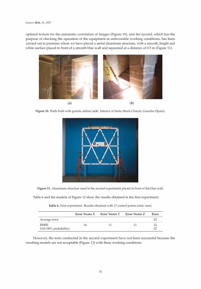
Sensors 2016, 16, 1557

optimal texture for the automatic correlation of images (Figure 10), and the second, which has thepurpose of checking the operation of the equipment in unfavorable working conditions, has beencarried out in premises where we have placed a metal aluminum structure, with a smooth, bright andwhite surface placed in front of a smooth blue wall and separated at a distance of 0.5 m (Figure 11).

(a) (b)

Figure 10. Walls built with granite ashlars (a,b). Interior of Santa María Church, Guareña (Spain).

Figure 11. Aluminum structure used in the second experiment placed in front of the blue wall.

Table 6 and the models of Figure 12 show the results obtained in the first experiment.

Table 6. First experiment. Results obtained with 17 control points (unit: mm).

Error Vector X Error Vector Y Error Vector Z Error

Average error 22

RMSE 16 11 11 22SAS (90% probability) 32

However, the tests conducted in the second experiment have not been successful because theresulting models are not acceptable (Figure 13) with these working conditions.

32

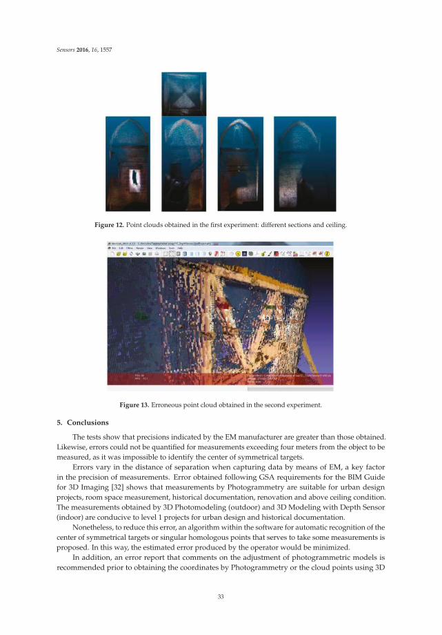
Sensors 2016, 16, 1557

Figure 12. Point clouds obtained in the first experiment: different sections and ceiling.

Figure 13. Erroneous point cloud obtained in the second experiment.

5. Conclusions

The tests show that precisions indicated by the EM manufacturer are greater than those obtained.Likewise, errors could not be quantified for measurements exceeding four meters from the object to bemeasured, as it was impossible to identify the center of symmetrical targets.

Errors vary in the distance of separation when capturing data by means of EM, a key factorin the precision of measurements. Error obtained following GSA requirements for the BIM Guidefor 3D Imaging [32] shows that measurements by Photogrammetry are suitable for urban designprojects, room space measurement, historical documentation, renovation and above ceiling condition.The measurements obtained by 3D Photomodeling (outdoor) and 3D Modeling with Depth Sensor(indoor) are conducive to level 1 projects for urban design and historical documentation.

Nonetheless, to reduce this error, an algorithm within the software for automatic recognition of thecenter of symmetrical targets or singular homologous points that serves to take some measurements isproposed. In this way, the estimated error produced by the operator would be minimized.

In addition, an error report that comments on the adjustment of photogrammetric models isrecommended prior to obtaining the coordinates by Photogrammetry or the cloud points using 3D

33

Sensors 2016, 16, 1557

Photomodeling. Thus, the user would know whether the dimension of error in the photogrammetricadjustment is acceptable when performing a particular task.

Furthermore, it would be convenient for EM to report on what parameter values were used forinternal, relative and absolute orientation for each picture once the adjustment has been made. In thissense, EM should also enter the precise value of these parameters. Thus, a user can resume a workingsession without having to start the entire process of adjusting each picture. Users could even workwith historical pictures where orientation parameters were known.

Finally, the convenient portability of EM and its calculation of error make it complementary tothe Scanstation, particularly with measurements difficult to obtain by the latter device.

Acknowledgments: The authors would like to acknowledge the delegation of Leica Geosystems in Seville for itsprovision of technical equipment. The anonymous reviewers are kindly acknowledged for their contribution tothe improvement of the paper with their valuable comments and suggestions.

Author Contributions: Alonso Sánchez Ríos conceived and designed the methodologies; Alonso Sánchez Ríos,José Manuel Naranjo Gómez, Antonio Jiménez Serrano and Alfonso González González performed theexperiments; Alonso Sánchez Ríos and José Manuel Naranjo Gómez analyzed the data; and all aforementionedauthored this paper.


References

1. Remondino, F.; El-Hakim, S. Image-based 3D modelling: A review. Photogramm. Rec. 2006, 21, 269–291.[CrossRef]

2. Remondino, F.; El-Hakim, S.; Mπαλτσαβιáς, E.; Picard, M.; Γαµµατικóπoυλoς, Λ. Image-Based 3DModeling of the Erechteion, Acropolis of Athens. Available online: http://hypatia.teiath.gr/xmlui/handle/11400/11019?locale-attribute=en (accessed on 20 September 2016).

3. Patil, H.; Kothari, A.; Bhurchandi, K. 3-D face recognition: Features, databases, algorithms and challenges.Artif. Intell. Rev. 2015, 44, 393–441. [CrossRef]

4. Zancajo-Blazquez, S.; Gonzalez-Aguilera, D.; Gonzalez-Jorge, H.; Hernandez-Lopez, D. An automaticimage-based modelling method applied to forensic infography. PLoS ONE 2015, 10, e0118719. [CrossRef][PubMed]

5. Liang, X.; Wang, Y.; Jaakkola, A.; Kukko, A.; Kaartinen, H.; Hyyppä, J.; Honkavaara, E.; Liu, J. Forest datacollection using terrestrial image-based point clouds from a handheld camera compared to terrestrial andpersonal laser scanning. IEEE Trans. Geosci. Remote Sens. 2015, 53, 5117–5132. [CrossRef]

6. Behmann, J.; Mahlein, A.K.; Paulus, S.; Kuhlmann, H.; Oerke, E.C.; Plümer, L. Calibration of hyperspectralclose-range pushbroom cameras for plant phenotyping. ISPRS J. Photogramm. Remote Sens. 2015, 106,172–182. [CrossRef]

7. Abellán, A.; Oppikofer, T.; Jaboyedoff, M.; Rosser, N.J.; Lim, M.; Lato, M.J. Terrestrial laser scanning of rockslope instabilities. Earth Surf. Process. Landf. 2014, 39, 80–97. [CrossRef]

8. Ghuffar, S.; Székely, B.; Roncat, A.; Pfeifer, N. Landslide displacement monitoring using 3D range flow onairborne and terrestrial lidar data. Remote Sens. 2013, 5, 2720–2745. [CrossRef]

9. Akavci, S.S.; Tanrikulu, A.H. Static and free vibration analysis of functionally graded plates based on a newquasi-3D and 2D shear deformation theories. Compos. Part B Eng. 2015, 83, 203–215. [CrossRef]

10. Cabaleiro, M.; Riveiro, B.; Arias, P.; Caamaño, J.C. Algorithm for beam deformation modeling from lidardata. Meas. J. Int. Meas. Confed. 2015, 76, 20–31. [CrossRef]

11. Lotsari, E.; Wang, Y.; Kaartinen, H.; Jaakkola, A.; Kukko, A.; Vaaja, M.; Hyyppä, H.; Hyyppä, J.; Alho, P.Gravel transport by ice in a subarctic river from accurate laser scanning. Geomorphology 2015, 246, 113–122.[CrossRef]

12. Harpold, A.A.; Marshall, J.A.; Lyon, S.W.; Barnhart, T.B.; Fisher, B.A.; Donovan, M.; Brubaker, K.M.;Crosby, C.J.; Glenn, N.F.; Glennie, C.L.; et al. Laser vision: Lidar as a transformative tool to advance criticalzone science. Hydrol. Earth Syst. Sci. 2015, 19, 2881–2897. [CrossRef]

13. Cacciari, I.; Nieri, P.; Siano, S. 3D digital microscopy for characterizing punchworks on medieval panelpaintings. J. Comput. Cult. Herit. 2015, 7. [CrossRef]

34

Sensors 2016, 16, 1557

14. Jaklic, A.; Eric, M.; Mihajlovic, I.; Stopinšek, Ž.; Solina, F. Volumetric models from 3D point clouds: The casestudy of sarcophagi cargo from a 2nd/3rd century ad roman shipwreck near sutivan on island brac, Croatia.J. Archaeol. Sci. 2015, 62, 143–152. [CrossRef]

15. Johansson, M.; Roupé, M.; Bosch-Sijtsema, P. Real-time visualization of building information models (bim).Autom. Constr. 2015, 54, 69–82. [CrossRef]

16. Brilakis, I.; Fathi, H.; Rashidi, A. Progressive 3D reconstruction of infrastructure with videogrammetry.Autom. Constr. 2011, 20, 884–895. [CrossRef]

17. Murphy, M.; McGovern, E.; Pavia, S. Historic building information modelling–adding intelligence to laserand image based surveys of european classical architecture. ISPRS J. Photogramm. Remote Sens. 2013, 76,89–102. [CrossRef]

18. Forlani, G.; Roncella, R.; Nardinocchi, C. Where is photogrammetry heading to? State of the art and trends.Rend. Lincei 2015, 26, 85–96. [CrossRef]

19. Guidi, G.; Russo, M.; Beraldin, J.-A. Acquisizione 3D e Modellazione Poligonale; McGraw-Hill: New York, NY,USA, 2010.

20. Remondino, F.; Spera, M.G.; Nocerino, E.; Menna, F.; Nex, F. State of the art in high density image matching.Photogramm. Rec. 2014, 29, 144–166. [CrossRef]

21. Muralikrishnan, B.; Ferrucci, M.; Sawyer, D.; Gerner, G.; Lee, V.; Blackburn, C.; Phillips, S.; Petrov, P.;Yakovlev, Y.; Astrelin, A.; et al. Volumetric performance evaluation of a laser scanner based on geometricerror model. Precis. Eng. 2015, 40, 139–150. [CrossRef]

22. Pejic, M.; Ogrizovic, V.; Božic, B.; Milovanovic, B.; Marošan, S. A simplified procedure of metrological testingof the terrestrial laser scanners. Measurement 2014, 53, 260–269. [CrossRef]

23. Polo, M.-E.; Felicísimo, Á.M. Analysis of uncertainty and repeatability of a low-cost 3D laser scanner. Sensors

2012, 12, 9046–9054. [CrossRef] [PubMed]24. He, F.; Habib, A.; Al-Rawabdehb, A. Planar constraints for an improved uav-image-based dense point cloud

generation. Int. Arch. Photogramm. Remote Sens. Spat. Inform. Sci. 2015, 40, 269–274. [CrossRef]25. Percoco, G.; Salmerón, A.J.S. Photogrammetric measurement of 3D freeform millimetre-sized objects with

micro features: An experimental validation of the close-range camera calibration model for narrow angles ofview. Meas. Sci. Technol. 2015, 26, 095203. [CrossRef]

26. Meetings: Laser Technik Journal 4/2015. Available online: http://onlinelibrary.wiley.com/doi/10.1002/latj.201590046/abstract (accessed on 20 September 2016).

27. Martínez Espejo Zaragoza, I. Precisiones Sobre el Levantamiento 3D Integrado con Herramientas Avanzadas,

Aplicado al Conocimiento y la Conservación del Patrimonio Arquitectónico; Universitat Politècnica de València:Valencia, Spain, 2014.

28. Dupuis, J.; Paulus, S.; Behmann, J.; Plümer, L.; Kuhlmann, H. A multi-resolution approach for an automatedfusion of different low-cost 3D sensors. Sensors 2014, 14, 7563–7579. [CrossRef] [PubMed]

29. Lachat, E.; Macher, H.; Landes, T.; Grussenmeyer, P. Assessment and calibration of a RGB-D camera(kinect v2 sensor) towards a potential use for close-range 3D modeling. Remote Sens. 2015, 7, 13070–13097.[CrossRef]

30. Anil, E.B.; Akinci, B.; Huber, D. Representation requirements of as-is building information models generatedfrom laser scanned point cloud data. In Proceedings of the International Symposium on Automation andRobotics in Construction (ISARC), Seoul, Korea, 29 June–2 July 2011.

31. Hong, S.; Jung, J.; Kim, S.; Cho, H.; Lee, J.; Heo, J. Semi-automated approach to indoor mapping for 3Das-built building information modeling. Comput. Environ. Urban Syst. 2015, 51, 34–46. [CrossRef]

32. General Services Administration. BIM Guide for 3D Imaging; Version 1.0; U.S. General Services Administration:Washington, DC, USA, 2009; p. 53.

33. Luhmann, T.; Robson, S.; Kyle, S.; Boehm, J. Close-Range Photogrammetry and 3D Imaging; De Gruyter: Vienna,Austria, 2013; p. 702.

34. Hartley, R.I.; Sturm, P. Triangulation. Comput. Vis. Image Underst. 1997, 68, 146–157. [CrossRef]35. Koutsoudis, A.; Vidmar, B.; Ioannakis, G.; Arnaoutoglou, F.; Pavlidis, G.; Chamzas, C. Multi-image 3D

reconstruction data evaluation. J. Cult. Herit. 2014, 15, 73–79. [CrossRef]36. Gordon, S.; Lichti, D.; Stewart, M.; Franke, J. Modelling point clouds for precise structural deformation

measurement. Int. Arch. Photogramm. Remote Sens. 2004, 35, B5.

35

Sensors 2016, 16, 1557

37. Reit, B. The 7-parameter transformation to a horizontal geodetic datum. Surv. Rev. 1998, 34, 400–404.[CrossRef]

38. Greenwalt, C.R.; Shultz, M.E. Principles of Error Theory and Cartographic Applications; ACIC Technical ReportNo. 96; Aeronautical Chart and Information Center, U.S. Air Force: St. Louis, MO, USA, 1968; pp. 46–49.


36

sensors

Article

On the Use of Monopole Antennas forDetermining the Effect of the Enclosure ofa Power Transformer Tank in Partial DischargesElectromagnetic Propagation

Ricardo Albarracín 1,*, Jorge Alfredo Ardila-Rey 2 and Abdullahi Abubakar Mas’ud 3

1 Generation and Distribution Network Area. Department of Electrical Engineering. Leader in Innovation,Technology and R&D, Boslan Engineering and Consulting S.A., Madrid 28034, Spain;[email protected]

2 Department of Electrical Engineering, Universidad Técnica Federico Santa María, Santiago de Chile 8940000,Chile; [email protected]

3 Department of Electrical and Electronic Engineering Technology, Jubail Industrial College, Road No. 6,8244 Al Huwailat, Al Jubail 35718, Saudi Arabia; [email protected]

* Correspondence: [email protected]; Tel.; +34-653-204-691; Fax: +56-22-303-6600

Academic Editor: Gonzalo Pajares MartinsanzReceived: 8 December 2015; Accepted: 21 January 2016; Published: 25 January 2016

Abstract: A well-defined condition-monitoring for power transformers is key to implementing acorrect condition-based maintenance (CBM). In this regard, partial discharges (PD) measurement andits analysis allows to carry out on-line maintenance following the standards IEC-60270 and IEC-60076.However, new PD measurements techniques, such as acoustics or electromagnetic (EM) acquisitionsusing ultra-high-frequency (UHF) sensors are being taken into account, IEC-62478. PD measurementswith antennas and the effect of their EM propagation in power transformer tanks is an open researchtopic that is considered in this paper. In this sense, an empty tank model is studied as a rectangularcavity and their resonances are calculated and compared with their measurement with a networkanalyser. Besides, two low cost improved monopole antennas deployed inside and outside of thetank model capture background noise and PD pulses in three different test objects (Nomex, twistedpair and insulator). The average spectrum of them are compared and can be found that mainly, theantenna frequency response, the frequency content distribution depending on the PD source andthe enclosure resonances modes are the main factors to be considered in PD acquisitions with thesesensors. Finally, with this set-up, it is possible to measure PD activity inside the tank from outside.

Keywords: power transformer tank; VHF and UHF sensors; monopole antennas; partial discharges;condition monitoring

1. Introduction

Measurement of partial discharges using very-high frequency (VHF), 30–300 MHz, and ultra-highfrequency, 300–3000 MHz, sensors has become an important tool when monitoring and assessing thestate of the insulation system on gas-insulated substations (GIS) and power transformers [1,2]. Thecurrent pulses that occur as a consequence of PD activity within this electrical equipment can generatethe presence of electromagnetic emissions with bandwidths ranging from MHz to several GHz [3].All information contained in these frequency bands can be captured and stored by using widebandsensors (antennas) which also does not require galvanic contact with any terminal of the equipmentunder test [4–7].

Besides, one of the main drawbacks when using externally such sensors in electrical equipmentwith self-shielding, according with its constructive nature, is that it may modify and/or mitigate the


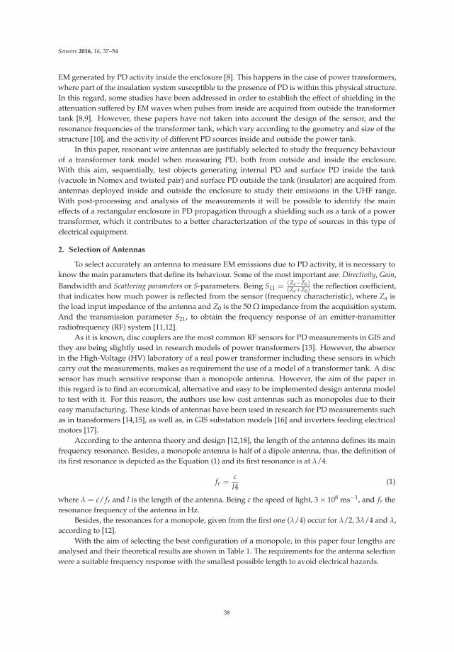
Sensors 2016, 16, 37–54

EM generated by PD activity inside the enclosure [8]. This happens in the case of power transformers,where part of the insulation system susceptible to the presence of PD is within this physical structure.In this regard, some studies have been addressed in order to establish the effect of shielding in theattenuation suffered by EM waves when pulses from inside are acquired from outside the transformertank [8,9]. However, these papers have not taken into account the design of the sensor, and theresonance frequencies of the transformer tank, which vary according to the geometry and size of thestructure [10], and the activity of different PD sources inside and outside the power tank.

In this paper, resonant wire antennas are justifiably selected to study the frequency behaviourof a transformer tank model when measuring PD, both from outside and inside the enclosure.With this aim, sequentially, test objects generating internal PD and surface PD inside the tank(vacuole in Nomex and twisted pair) and surface PD outside the tank (insulator) are acquired fromantennas deployed inside and outside the enclosure to study their emissions in the UHF range.With post-processing and analysis of the measurements it will be possible to identify the maineffects of a rectangular enclosure in PD propagation through a shielding such as a tank of a powertransformer, which it contributes to a better characterization of the type of sources in this type ofelectrical equipment.

2. Selection of Antennas

To select accurately an antenna to measure EM emissions due to PD activity, it is necessary toknow the main parameters that define its behaviour. Some of the most important are: Directivity, Gain,Bandwidth and Scattering parameters or S-parameters. Being S11 = (Za−Z0)

(Za+Z0)the reflection coefficient,

that indicates how much power is reflected from the sensor (frequency characteristic), where Za isthe load input impedance of the antenna and Z0 is the 50 Ω impedance from the acquisition system.And the transmission parameter S21, to obtain the frequency response of an emitter-transmitterradiofrequency (RF) system [11,12].

As it is known, disc couplers are the most common RF sensors for PD measurements in GIS andthey are being slightly used in research models of power transformers [13]. However, the absencein the High-Voltage (HV) laboratory of a real power transformer including these sensors in whichcarry out the measurements, makes as requirement the use of a model of a transformer tank. A discsensor has much sensitive response than a monopole antenna. However, the aim of the paper inthis regard is to find an economical, alternative and easy to be implemented design antenna modelto test with it. For this reason, the authors use low cost antennas such as monopoles due to theireasy manufacturing. These kinds of antennas have been used in research for PD measurements suchas in transformers [14,15], as well as, in GIS substation models [16] and inverters feeding electricalmotors [17].

According to the antenna theory and design [12,18], the length of the antenna defines its mainfrequency resonance. Besides, a monopole antenna is half of a dipole antenna, thus, the definition ofits first resonance is depicted as the Equation (1) and its first resonance is at λ/4.

fr =c

l4(1)

where λ = c/ fr and l is the length of the antenna. Being c the speed of light, 3 × 108 ms−1, and fr theresonance frequency of the antenna in Hz.

Besides, the resonances for a monopole, given from the first one (λ/4) occur for λ/2, 3λ/4 and λ,according to [12].

With the aim of selecting the best configuration of a monopole, in this paper four lengths areanalysed and their theoretical results are shown in Table 1. The requirements for the antenna selectionwere a suitable frequency response with the smallest possible length to avoid electrical hazards.

38

Sensors 2016, 16, 37–54

Table 1. Theoretical resonance frequencies for monopole antennas.

Monopole antenna fr(λ/4) (MHz) fr(λ/2) (MHz) fr(3λ/4) (MHz) fr(λ) (MHz)1 cm 7500 15000 22500 300005 cm 1500 3000 4500 600010 cm 750 1500 2250 300016.5 cm 454 910 1364 1820

As described in experimental setup (Section 5), the measurement equipment used can reach upto 2.5 GHz, so the resonances that can be measured are gray as marked in Table 1. The frequencyresonances for the 1 cm monopole cannot be measured, so its used is discarded. In addition, theoscilloscope only can represent the first resonance of the 5 cm monopole, thus this antenna is alsorejected. With respect to the 16.5 cm monopole, although it has their frequency resonances into theanalysed bandwidth, its high length can produce electric hazard due to contact with the feeding ofthe setup or with energized electrode of the test object. Moreover, this drawback can be increased inreal power transformers with the possibility of electrical contact with their windings, so this sensoris also discarded. Thus, the length of the monopole elected is 10 cm, even more, it has its three firstresonances below than 2.5 GHz band, so it could measure energy from PD with less risk of electrichazard than the 16.5 cm monopole.

An Agilent E8364B network analyser (NA) is used to measure the frequency response (S11

parameter) for the monopole antenna. Likewise, this kind of resonant antennas could be improvedby introducing a ground plane at its terminal so that it works as dipole antenna. Thus, to evaluatethe performance of the sensor, the measurements with the NA was carried out with and without aground plane. The main advantage of a dipole antenna is to have the double gain and directivity thana monopole antenna with the same length. Thus, for a λ/4 dipole its gain is G λ

4≃ ecd3.286 dB and

its directivity D λ4= 5.167 dB, only applicable for their resonance frequencies at λ/4, λ/2, 3λ/4 and

λ. Where ecd is the radiation efficiency of the antenna, being ecd ≃ 1 at the frequency resonances ofmonopoles and dipoles sensors [12,18].

In Table 2, it is shown the resonance frequency values for the 10 cm antenna with and without aground plane together with the relative error (RE) between the theoretical value and the experimentalmeasure. Note that a λ/4 monopole or dipole antenna has the same theoretical frequency resonances,so the comparison between the results of calculations for the monopole (dipole) can be carry out withthose obtained from measurements on dipole. Besides, it can be observed that the match betweenthe resonances calculated theoretically, Table 1, and the experimental results using a ground plane isbetter than those obtained without the ground plane, Table 2. In addition, when a monopole or dipoletype antenna is used, sometimes, the resonant frequencies are shifted with respect to the theoreticalones [11].

In this case, the dipole antenna has a better match of the frequency resonances with the theoreticalcalculation made in Table 2, with an error between [−15,+15]%. These results are contrasted with thoseobtained in [11], where the frequency response of a 10 cm monopole antenna with and without groundplane is quite similar, however the power spectrum is greater for the dipole antenna than that obtainedat their analogous resonant frequencies (approximately at 750 MHz and 1500 MHz) for the monopole.

Table 2. Experimental values of the resonance frequencies of the 10 cm antenna working as dipole ormonopole antenna for λ/4, λ/2, 3λ/4 and λ.

fr(λ/4) fr(λ/2) fr(3λ/4) fr(λ)

Antenna Monopole Dipole Monopole Dipole Monopole Dipole Monopole Dipole

10 cm MHz 530 640 1060 1730 1385 2150 2137 2600% 29 15 29 −15 38 4 29 13

39

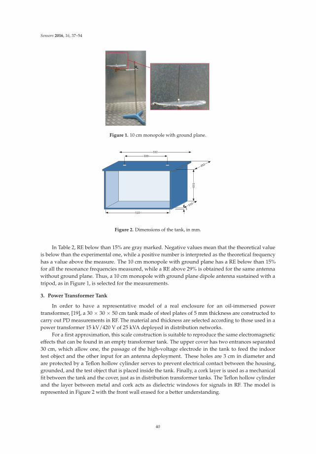
Sensors 2016, 16, 37–54

Figure 1. 10 cm monopole with ground plane.

592

392

310

300

510

5

310

Figure 2. Dimensions of the tank, in mm.

In Table 2, RE below than 15% are gray marked. Negative values mean that the theoretical valueis below than the experimental one, while a positive number is interpreted as the theoretical frequencyhas a value above the measure. The 10 cm monopole with ground plane has a RE below than 15%for all the resonance frequencies measured, while a RE above 29% is obtained for the same antennawithout ground plane. Thus, a 10 cm monopole with ground plane dipole antenna sustained with atripod, as in Figure 1, is selected for the measurements.

3. Power Transformer Tank

In order to have a representative model of a real enclosure for an oil-immersed powertransformer, [19], a 30 × 30 × 50 cm tank made of steel plates of 5 mm thickness are constructed tocarry out PD measurements in RF. The material and thickness are selected according to those used in apower transformer 15 kV/420 V of 25 kVA deployed in distribution networks.

For a first approximation, this scale construction is suitable to reproduce the same electromagneticeffects that can be found in an empty transformer tank. The upper cover has two entrances separated30 cm, which allow one, the passage of the high-voltage electrode in the tank to feed the indoortest object and the other input for an antenna deployment. These holes are 3 cm in diameter andare protected by a Teflon hollow cylinder serves to prevent electrical contact between the housing,grounded, and the test object that is placed inside the tank. Finally, a cork layer is used as a mechanicalfit between the tank and the cover, just as in distribution transformer tanks. The Teflon hollow cylinderand the layer between metal and cork acts as dielectric windows for signals in RF. The model isrepresented in Figure 2 with the front wall erased for a better understanding.

40

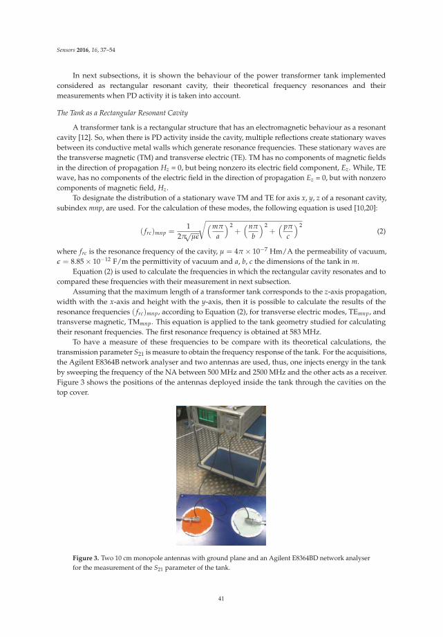
Sensors 2016, 16, 37–54

In next subsections, it is shown the behaviour of the power transformer tank implementedconsidered as rectangular resonant cavity, their theoretical frequency resonances and theirmeasurements when PD activity it is taken into account.

The Tank as a Rectangular Resonant Cavity

A transformer tank is a rectangular structure that has an electromagnetic behaviour as a resonantcavity [12]. So, when there is PD activity inside the cavity, multiple reflections create stationary wavesbetween its conductive metal walls which generate resonance frequencies. These stationary waves arethe transverse magnetic (TM) and transverse electric (TE). TM has no components of magnetic fieldsin the direction of propagation Hz = 0, but being nonzero its electric field component, Ez. While, TEwave, has no components of the electric field in the direction of propagation Ez = 0, but with nonzerocomponents of magnetic field, Hz.

To designate the distribution of a stationary wave TM and TE for axis x, y, z of a resonant cavity,subindex mnp, are used. For the calculation of these modes, the following equation is used [10,20]:

( frc)mnp =1

2π√

μǫ

√

(mπ

a

) 2+

(nπ

b

) 2+

( pπ

c

) 2(2)

where frc is the resonance frequency of the cavity, μ = 4π × 10−7 Hm/A the permeability of vacuum,ǫ = 8.85 × 10−12 F/m the permittivity of vacuum and a, b, c the dimensions of the tank in m.

Equation (2) is used to calculate the frequencies in which the rectangular cavity resonates and tocompared these frequencies with their measurement in next subsection.

Assuming that the maximum length of a transformer tank corresponds to the z-axis propagation,width with the x-axis and height with the y-axis, then it is possible to calculate the results of theresonance frequencies ( frc)mnp, according to Equation (2), for transverse electric modes, TEmnp, andtransverse magnetic, TMmnp. This equation is applied to the tank geometry studied for calculatingtheir resonant frequencies. The first resonance frequency is obtained at 583 MHz.

To have a measure of these frequencies to be compare with its theoretical calculations, thetransmission parameter S21 is measure to obtain the frequency response of the tank. For the acquisitions,the Agilent E8364B network analyser and two antennas are used, thus, one injects energy in the tankby sweeping the frequency of the NA between 500 MHz and 2500 MHz and the other acts as a receiver.Figure 3 shows the positions of the antennas deployed inside the tank through the cavities on thetop cover.

Figure 3. Two 10 cm monopole antennas with ground plane and an Agilent E8364BD network analyserfor the measurement of the S21 parameter of the tank.

41

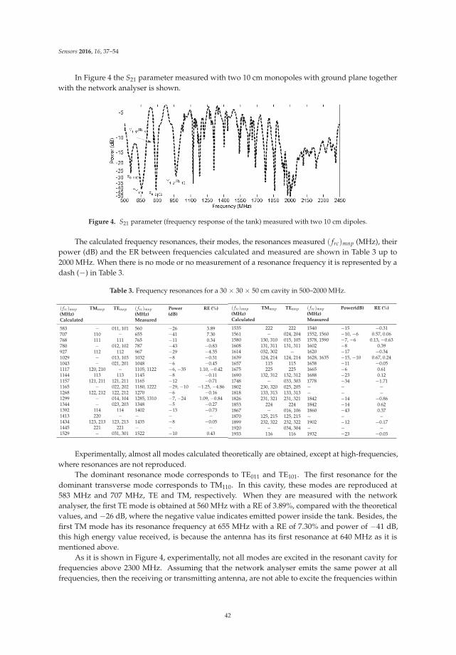
Sensors 2016, 16, 37–54

In Figure 4 the S21 parameter measured with two 10 cm monopoles with ground plane togetherwith the network analyser is shown.

Figure 4. S21 parameter (frequency response of the tank) measured with two 10 cm dipoles.

The calculated frequency resonances, their modes, the resonances measured ( frc)mnp (MHz), theirpower (dB) and the ER between frequencies calculated and measured are shown in Table 3 up to2000 MHz. When there is no mode or no measurement of a resonance frequency it is represented by adash (−) in Table 3.

Table 3. Frequency resonances for a 30 × 30 × 50 cm cavity in 500–2000 MHz.

( frc)mnp

(MHz)Calculated

TMmnp TEmnp ( frc)mnp

(MHz)Measured

Power(dB)

RE (%)

583 − 011, 101 560 −26 3.89707 110 − 655 −41 7.30768 111 111 765 −11 0.34780 − 012, 102 787 −43 −0.83927 112 112 967 −29 −4.351029 − 013, 103 1032 −8 −0.311043 − 021, 201 1048 −6 −0.451117 120, 210 − 1105, 1122 −6, −35 1.10, −0.421144 113 113 1145 −8 −0.111157 121, 211 121, 211 1165 −12 −0.711165 − 022, 202 1180, 1222 −29, −10 −1.25, −4.861268 122, 212 122, 212 1270 −6 −0.161299 − 014, 104 1285, 1310 −7, −24 1.09, −0.841344 − 023, 203 1348 −5 −0.271392 114 114 1402 −13 −0.731413 220 − − − −1434 123, 213 123, 213 1435 −8 −0.051445 221 221 − − −1529 − 031, 301 1522 −10 0.43

( frc)mnp

(MHz)Calculated

TMmnp TEmnp ( frc)mnp

(MHz)Measured

Power(dB) RE (%)

1535 222 222 1540 −15 −0.311561 − 024, 204 1552, 1560 −10, −6 0.57, 0.061580 130, 310 015, 105 1578, 1590 −7, −6 0.13, −0.631608 131, 311 131, 311 1602 −8 0.391614 032, 302 − 1620 −17 −0.341639 124, 214 124, 214 1628, 1635 −15, −10 0.67, 0.241657 115 115 1658 −11 −0.051675 225 225 1665 −6 0.611690 132, 312 132, 312 1688 −23 0.121748 − 033, 303 1778 −34 −1.711802 230, 320 025, 205 − − −1818 133, 313 133, 313 − − −1826 231, 321 231, 321 1842 −14 −0.861853 224 224 1842 −14 0.621867 − 016, 106 1860 −43 0.371870 125, 215 125, 215 − − −1899 232, 322 232, 322 1902 −12 −0.171920 − 034, 304 − − −1933 116 116 1932 −23 −0.03

Experimentally, almost all modes calculated theoretically are obtained, except at high-frequencies,where resonances are not reproduced.

The dominant resonance mode corresponds to TE011 and TE101. The first resonance for thedominant transverse mode corresponds to TM110. In this cavity, these modes are reproduced at583 MHz and 707 MHz, TE and TM, respectively. When they are measured with the networkanalyser, the first TE mode is obtained at 560 MHz with a RE of 3.89%, compared with the theoreticalvalues, and −26 dB, where the negative value indicates emitted power inside the tank. Besides, thefirst TM mode has its resonance frequency at 655 MHz with a RE of 7.30% and power of −41 dB,this high energy value received, is because the antenna has its first resonance at 640 MHz as it ismentioned above.

As it is shown in Figure 4, experimentally, not all modes are excited in the resonant cavity forfrequencies above 2300 MHz. Assuming that the network analyser emits the same power at allfrequencies, then the receiving or transmitting antenna, are not able to excite the frequencies within

42

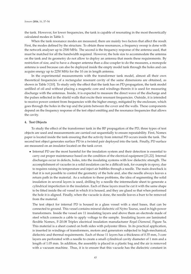
Sensors 2016, 16, 37–54

the tank. However, for lower frequencies, the tank is capable of resonating in the most theoreticallycalculated modes in Table 3.

When the tank resonance modes are measured, there are mainly two factors that affect the result.First, the modes defined by the structure. To obtain these resonances, a frequency sweep is done withthe network analyser up to 2500 MHz. The second is the frequency response of the antenna used, thatmust be matched for all the bandwidth required. However, the hole size to accommodate the antennaon the tank and its geometry do not allow to deploy an antenna that meets these requirements. Byrestriction of size, and to have a cheaper antenna than a disc-coupler to do the measures, a monopoleantenna is used because can also be deployed inside the empty model tank through the holes and canacquire energy up to 2250 MHz for the 10 cm in length antenna.

In the experimental measurements with the transformer tank model, almost all their owntheoretical frequencies of a rectangular resonant cavity of the same dimensions are obtained, asshown in Table 3 [10]. To study only the effect that the tank has on PD propagation, the tank modelunfilled of oil and without placing a magnetic core and windings therein it is used for measuringdischarge with the antennas. Inside, it is expected to measure the direct wave of the discharge andthe pulses reflected in the shield walls that excite their resonant frequencies. Outside, it is intendedto receive power content from frequencies with the higher energy, mitigated by the enclosure, whichgoes through the holes in the top and the joints between the cover and the walls. These componentsdepend on the frequency response of the test object emitting and the resonance frequencies that allowsthe cavity.

4. Test Objects

To study the effect of the transformer tank in the RF propagation of the PD, three types of testobjects are used and measurements are carried out sequentially to ensure repeatability. First, Nomexpaper is located inside the tank ensuring that the activity from internal PD occurs inside the tank. Thesecond test object generates surface PD in a twisted pair deployed into the tank. Finally, PD surfaceare measured on an insulator located on the tank cover.

• Internal PD are the most harmful for the insulation system and their detection is essential tocarry out proper maintenance based on the condition of the electrical equipment [21,22]. Internaldischarges occur in defects, holes, into the insulating systems with low dielectric strength. Theaccomplishment of vacuoles in a solid insulation can be a difficult task, for example in epoxy, dueto requires raising its temperature and inject air bubbles through a needle. The main drawback isthat it is not possible to control the geometry of the hole and, also the needle always leaves areturn path in the material. As a solution to these problems, the idea of segmenting the solidinsulation in several layers is used, drilling by a needle the intermediate sheet to generate acylindrical imperfection in the insulation. Each of these layers must be cut it with the same shapeto be fitted inside the oil vessel in which it is housed, and they are glued so that when performedthe hole it is aligned. Finally, when the vacuole is done, the needle leaves a burr to be removedfrom the material.

The test object for internal PD is housed in a glass vessel with a steel bases, that can beconnected to ground. This vessel contains mineral dielectric oil Nytro Taurus, used in high-powertransformers. Inside the vessel are 11 insulating layers and above them an electrode made ofsteel which connects a cable to apply voltage to the sample. Insulating layers are laminatedflexible Nomex, F-20.08 Triplex electrical insulation manufacturer Royal-Diamond, Figure 5a.This material is a sheet coated on both sides with polyester fibres. In its practical application,is inserted in windings of transformers, motors and generators subjected to high-mechanical,dielectric and thermal requirements. Each of those 11 layers has a thickness of 0.35 mm, 3 corelayers are perforated with a needle to create a small cylindrical cavity diameter of 1 mm and alength of 1.05 mm. In addition, the assembly is placed in a plastic bag and the air is removedwith a vacuum machine. Thus, it is to ensure that this vacuole has the dielectric constant in

43

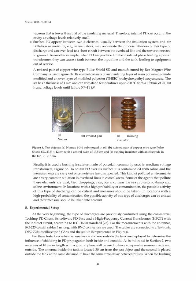
Sensors 2016, 16, 37–54

vacuum that is lower than that of the insulating material. Therefore, internal PD can occur in thecavity at voltage levels relatively small.

• Surface PD appear between two dielectrics, usually between the insulation system and air.Pollution or moisture, e.g., in insulators, may accelerate the process fetterless of this type ofdischarge and can even lead to a short-circuit between the overhead line and the tower connectedto ground. As another example, when PD are produced in the insulated phase feeding a powertransformer, they can cause a fault between the input line and the tank, leading to equipmentout of service.

A twisted pair of copper wire type Pulse Shield SD and manufactured by Rea Magnet WireCompany is used Figure 5b. Its enamel consists of an insulating layer of resin polyamide-imidemodified and an over layer of modified polyester (THEIC) trishydroxyethyl isocyanurate. Theset has a thickness of 1 mm and can withstand temperatures up to 220 C with a lifetime of 20,000h and voltage levels until failure 5.7–11 kV.

(a)Nomex

(b) Twisted pair (c) Bushinginsulator

Figure 5. Test objects: (a) Nomex 4-3-4 submerged in oil, (b) twisted pair of copper wire type PulseShield SD, 23.5 × 12 cm with a central twist of 13.5 cm and (c) bushing insulator with an electrode inthe top, 21 × 8 cm.

Finally, it is used a bushing insulator made of porcelain commonly used in medium voltagetransformers, Figure 5c. To obtain PD over its surface it is contaminated with saline and themeasurements are carry out once moisture has disappeared. This kind of polluted environmentsare a very common situation in overhead lines in coastal areas. Some of the agents that pollutethese elements are dust, bird droppings, rain, ice and, near the sea provisions, damp andsaline environment. In locations with a high probability of contamination, the possible activityof this type of discharge can be critical and measures should be taken. In locations with ahigh-probability of contamination, the possible activity of this type of discharges can be criticaland their measure should be taken into account.

5. Experimental Setup

At the very beginning, the type of discharges are previously confirmed using the commercialTechImp PD Check, its software PD Base and a High-Frequency Current Transformer (HFCT) withthe indirect circuit, according to IEC-60270 standard [23]. For the measurements with the antennas,RG-223 coaxial cables 5 m long, with BNC connectors are used. The cables are connected to a TektronixDPO 7254 oscilloscope 5 GS/s and the set-up is represented in Figure 6.

For these tests, two antennas, one inside and one outside the tank are deployed to determine theinfluence of shielding in PD propagation both inside and outside. As is indicated in Section 2, twoantennas of 10 cm in length with a ground plane will be used to have comparable sensors inside andoutside. The antenna inside the tank is located 30 cm from the test object and the second is placedoutside the tank at the same distance, to have the same time-delay between pulses. When the bushing

44

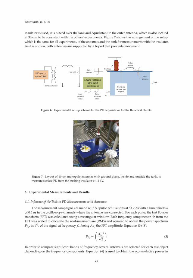
Sensors 2016, 16, 37–54

insulator is used, it is placed over the tank and equidistant to the outer antenna, which is also locatedat 30 cm, to be consistent with the others’ experiments. Figure 7 shows the arrangement of the setup,which is the same for all experiments, of the antennas and the tank for measurements with the insulator.As it is shown, both antennas are supported by a tripod that prevents movement.

Nomex or

twisted pair

objects

Inner

antenna

Tank

HV source

up to 15kV

HV transformer

100 kV 1 nF

Teflon

hollow

cylinders

5 GS/s Tektronix

DPO 7254

oscilloscope

Inner

antenna

input

Outer

antenna

input

BushingOuter

antenna

Figure 6. Experimental set-up scheme for the PD acquisitions for the three test objects.

BushingInner

10 cm

monopole

Outer

10 cm

monopole

Figure 7. Layout of 10 cm monopole antennas with ground plane, inside and outside the tank, tomeasure surface PD from the bushing insulator at 12 kV.

6. Experimental Measurements and Results

6.1. Influence of the Tank in PD Measurements with Antennas

The measurement campaigns are made with 50 pulse acquisitions at 5 GS/s with a time windowof 0.5 μs in the oscilloscope channels where the antennas are connected. For each pulse, the fast Fouriertransform (FFT) was calculated using a rectangular window. Each frequency component n-th from theFFT was scaled to calculate the root-mean-square (RMS) and squared to obtain the power spectrumPfn

, in V2, of the signal at frequency fn, being A fnthe FFT amplitude, Equation (3) [8].

Pfn=

(

A fn2

√2

)

(3)

In order to compare significant bands of frequency, several intervals are selected for each test objectdepending on the frequency components. Equation (4) is used to obtain the accumulative power in

45

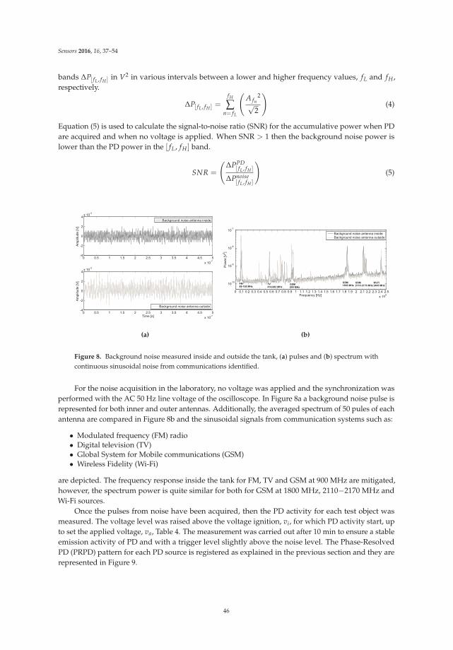
Sensors 2016, 16, 37–54

bands ΔP[ fL , fH ] in V2 in various intervals between a lower and higher frequency values, fL and fH ,respectively.

ΔP[ fL , fH ] =fH

∑n= fL

(

A fn2

√2

)

(4)

Equation (5) is used to calculate the signal-to-noise ratio (SNR) for the accumulative power when PDare acquired and when no voltage is applied. When SNR > 1 then the background noise power islower than the PD power in the [ fL, fH ] band.

SNR =

(

ΔPPD[ fL , fH ]

ΔPnoise[ fL , fH ]

)

(5)

0 0.5 1 1.5 2 2.5 3 3.5 4 4.5 5

x 10-7

-4

-2

0

2

4x 10

-3

Am

plit

ud

e [

V]

Background noise antenna inside

0 0.5 1 1.5 2 2.5 3 3.5 4 4.5 5

x 10-7

-4

-2

0

2

4x 10

-3

Time [s]

Am

plit

ud

e [

V]

Background noise antenna outside

(a)

0 0.1 0.2 0.3 0.4 0.5 0.6 0.7 0.8 0.9 1 1.1 1.2 1.3 1.4 1.5 1.6 1.7 1.8 1.9 2 2.1 2.2 2.3 2.4 2.5

x 109

10-10

10-9

10-8

10-7

Frequency [Hz]

Po

we

r [V

2]

Background noise antenna insideBackground noise antenna outside

FM

88-108 MHz

GSM

2110-2170 MHzTV

414-882 MHz

GSM

1800 MHzGSM

900 MHz

Wi-Fi

2400 MHz

(b)

Figure 8. Background noise measured inside and outside the tank, (a) pulses and (b) spectrum withcontinuous sinusoidal noise from communications identified.

For the noise acquisition in the laboratory, no voltage was applied and the synchronization wasperformed with the AC 50 Hz line voltage of the oscilloscope. In Figure 8a a background noise pulse isrepresented for both inner and outer antennas. Additionally, the averaged spectrum of 50 pules of eachantenna are compared in Figure 8b and the sinusoidal signals from communication systems such as:

• Modulated frequency (FM) radio• Digital television (TV)• Global System for Mobile communications (GSM)• Wireless Fidelity (Wi-Fi)

are depicted. The frequency response inside the tank for FM, TV and GSM at 900 MHz are mitigated,however, the spectrum power is quite similar for both for GSM at 1800 MHz, 2110−2170 MHz andWi-Fi sources.

Once the pulses from noise have been acquired, then the PD activity for each test object wasmeasured. The voltage level was raised above the voltage ignition, vi, for which PD activity start, upto set the applied voltage, va, Table 4. The measurement was carried out after 10 min to ensure a stableemission activity of PD and with a trigger level slightly above the noise level. The Phase-ResolvedPD (PRPD) pattern for each PD source is registered as explained in the previous section and they arerepresented in Figure 9.

46

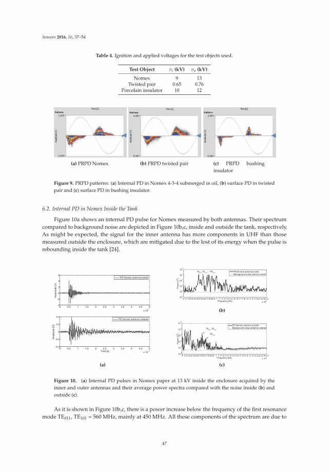
Sensors 2016, 16, 37–54

Table 4. Ignition and applied voltages for the test objects used.

Test Object vi (kV) va (kV)

Nomex 9 13Twisted pair 0.65 0.76

Porcelain insulator 10 12

(a) PRPD Nomex (b) PRPD twisted pair (c) PRPD bushinginsulator

Figure 9. PRPD patterns: (a) Internal PD in Nomex 4-3-4 submerged in oil, (b) surface PD in twistedpair and (c) surface PD in bushing insulator.

6.2. Internal PD in Nomex Inside the Tank

Figure 10a shows an internal PD pulse for Nomex measured by both antennas. Their spectrumcompared to background noise are depicted in Figure 10b,c, inside and outside the tank, respectively.As might be expected, the signal for the inner antenna has more components in UHF than thosemeasured outside the enclosure, which are mitigated due to the lost of its energy when the pulse isrebounding inside the tank [24].

0 0.5 1 1.5 2 2.5 3 3.5 4 4.5 5

x 10-7

-4

-2

0

2

4

6

Am

plit

ud

e [

V]

PD Nomex antenna inside

0 0.5 1 1.5 2 2.5 3 3.5 4 4.5 5

x 10-7

-0.4

-0.2

0

0.2

0.4

Time [s]

Am

plit

ud

e [

V]

PD Nomex antenna outside

(a)

0 0.1 0.20.3 0.4 0.50.6 0.7 0.80.9 1 1.11.2 1.31.4 1.5 1.61.7 1.8 1.9 2 2.1 2.22.3 2.4 2.5

x 109

10-7

10-6

10-5

10-4

10-3

10-2

Frequency [Hz]

Po

we

r [V

2]

PD Nomex antenna insideBackground noise antenna inside

TE011

,TE101

TM110

(b)

0 0.1 0.2 0.3 0.4 0.5 0.6 0.7 0.8 0.9 1 1.1 1.2 1.3 1.4 1.5 1.6 1.7 1.8 1.9 2 2.1 2.2 2.3 2.4 2.5

x 109

10-8

10-7

10-6

10-5

10-4

10-3

Frequency [Hz]

Po

we

r [V

2]

PD Nomex antenna outsideBackground noise antenna outsideTE

011,TE

101

TM110

(c)

Figure 10. (a) Internal PD pulses in Nomex paper at 13 kV inside the enclosure acquired by theinner and outer antennas and their average power spectra compared with the noise inside (b) andoutside (c).

As it is shown in Figure 10b,c, there is a power increase below the frequency of the first resonancemode TE011, TE101 = 560 MHz, mainly at 450 MHz. All these components of the spectrum are due to

47

Sensors 2016, 16, 37–54

the characteristics of the direct emission radiated of this type of internal PD at these frequencies [8],the frequency response of the antenna and the resonance characteristic of the enclosure.

For the power spectrum calculated for the pulses acquired with the antenna outside the tank, itcan be seen that no significant power is received from the PD above 1.2 GHz, so the tank acts as a lowpass filter. Furthermore, the content of power at 450 MHz is also received outside and mainly up to400 MHz. Indeed, more power below 400 MHz is received outside the tank than inside. This can bedue to the cable to ground of the enclosure which act as an antenna whose length radiate in thesefrequency ranges when the PD leave the cavity conductively through the ground path.

Finally, the first two resonance modes are marked, TE011, TE101 = 560 MHz and TM110 = 655 MHzin Figure 10b,c verifying that they can be measured from outside the tank under these circumstances.Table 5 compares the first resonance modes for Nomex inside and outside the tank. As can be expected,in both cases, the peak power values are greater inside than outside. To compare which has the highestmagnitude, the power inside is divided by the power outside (Ratio), so values greater than 1 meanthat the mode has higher power inside the tank and viceversa.

Table 5. Peak values for first TE and TM modes inside and outside the tank for internal PD in Nomex.

Modes Power (V2)

Inside Outside RatioTE011, TE101 = 560 MHz 8.1 × 10−4 5.9 × 10−4 1.4TM110 = 655 MHz 2.4 × 10−5 3.3 × 10−6 7.3

Table 6 presents the accumulated power measured with the inner and outer 10 cm monopoles.In this case, three bands are analysed with their SNR: up to 300 MHz where there is the maincontribution in power from the outer antenna; 300–1200 MHz, where there are the first resonance modesand; 1200–2500 MHz, where no PD radiation is received from outside. Focused on the 300–1200 MHzband, the ratio for the inner antenna is 166.5 while outside is 35.5, so it could be measured the theresonances inside the tank from outside with a high SNR. In Table 6, also the two first modes areincluded as example of comparison, with high values for the measure inside the tank. Up to 300 MHz,the ratio outside 214.3 is much greater than inside 2.6, so this components are not coming from insidethe enclosure. From 1200–2500, the power is greater inside with a ratio of 6.8 than outside, 1.1, thustheir low power can not come out the enclosure.

Table 6. Accumulated power and SNR for internal PD in Nomex inside the tank when measured withthe inner and outer monopoles of 10 cm.

Antenna Power (V2)

13 kV 0 V SNRInside ∼300 MHz 3.4 × 10−4 1.3 × 10−4 2.6Outside ∼300 MHz 1.4 × 10−3 6.3 × 10−6 214.3Inside 300–1200 MHz 6.6 × 10−2 4 × 10−4 166.5Outside 300–1200 MHz 8.3 × 10−4 2.3 × 10−5 35.5Inside 1200–2500 MHz 4.4 × 10−3 6.4 × 10−4 6.8Outside 1200–2500 MHz 5.4 × 10−5 4.9 × 10−6 1.1

6.3. Surface PD in a Twisted Pair Inside the Tank

In Figure 11a surface PD pulses with the twisted pair inside the tank are shown from inside andoutside. For the inner antenna, the pulse has high amplitude than outside the enclosure.

The spectrum of noise compare with PD obtained with both antennas are shown in Figure 11b,c.Inside the tank, the power is concentrated mainly between 500–1100 MHz with a maximum high-powerpeak value of 3 ×10−3 V2. First resonance modes are marked on figures for these frequencies. Besides,

48

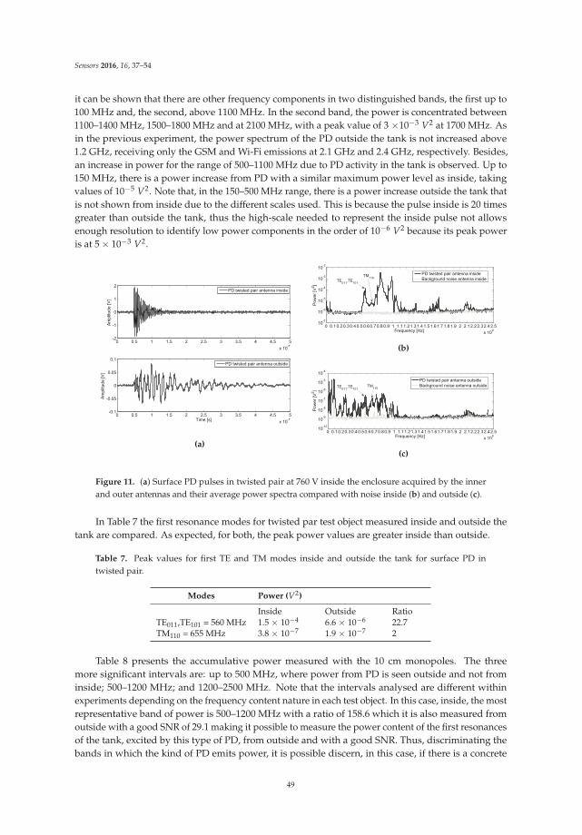
Sensors 2016, 16, 37–54

it can be shown that there are other frequency components in two distinguished bands, the first up to100 MHz and, the second, above 1100 MHz. In the second band, the power is concentrated between1100–1400 MHz, 1500–1800 MHz and at 2100 MHz, with a peak value of 3 ×10−3 V2 at 1700 MHz. Asin the previous experiment, the power spectrum of the PD outside the tank is not increased above1.2 GHz, receiving only the GSM and Wi-Fi emissions at 2.1 GHz and 2.4 GHz, respectively. Besides,an increase in power for the range of 500–1100 MHz due to PD activity in the tank is observed. Up to150 MHz, there is a power increase from PD with a similar maximum power level as inside, takingvalues of 10−5 V2. Note that, in the 150–500 MHz range, there is a power increase outside the tank thatis not shown from inside due to the different scales used. This is because the pulse inside is 20 timesgreater than outside the tank, thus the high-scale needed to represent the inside pulse not allowsenough resolution to identify low power components in the order of 10−6 V2 because its peak poweris at 5 × 10−3 V2.

0 0.5 1 1.5 2 2.5 3 3.5 4 4.5 5

x 10-7

-2

-1

0

1

2

Am

plit

ud

e [

V]

PD twisted pair antenna inside

0 0.5 1 1.5 2 2.5 3 3.5 4 4.5 5

x 10-7

-0.1

-0.05

0

0.05

0.1

Time [s]

Am

plit

ud

e [

V]

PD twisted pair antenna outside

(a)

0 0.10.2 0.30.4 0.50.60.7 0.80.9 1 1.11.2 1.31.4 1.51.61.7 1.81.9 2 2.12.2 2.32.4 2.5

x 109

10-7

10-6

10-5

10-4

10-3

10-2

Frequency [Hz]

Po

we

r [V

2]

PD twisted pair antenna inside

Background noise antenna insideTE011

,TE101

TM110

(b)

0 0.10.20.30.40.50.60.70.80.9 1 1.11.21.31.41.51.61.71.81.9 2 2.12.22.32.42.5

x 109

10-10

10-9

10-8

10-7

10-6

10-5

10-4

Frequency [Hz]

Po

we

r [V

2]

PD twisted pair antenna outside

Background noise antenna outsideTE011

,TE101

TM110

(c)

Figure 11. (a) Surface PD pulses in twisted pair at 760 V inside the enclosure acquired by the innerand outer antennas and their average power spectra compared with noise inside (b) and outside (c).

In Table 7 the first resonance modes for twisted par test object measured inside and outside thetank are compared. As expected, for both, the peak power values are greater inside than outside.

Table 7. Peak values for first TE and TM modes inside and outside the tank for surface PD intwisted pair.

Modes Power (V2)

Inside Outside RatioTE011,TE101 = 560 MHz 1.5 × 10−4 6.6 × 10−6 22.7TM110 = 655 MHz 3.8 × 10−7 1.9 × 10−7 2

Table 8 presents the accumulative power measured with the 10 cm monopoles. The threemore significant intervals are: up to 500 MHz, where power from PD is seen outside and not frominside; 500–1200 MHz; and 1200–2500 MHz. Note that the intervals analysed are different withinexperiments depending on the frequency content nature in each test object. In this case, inside, the mostrepresentative band of power is 500–1200 MHz with a ratio of 158.6 which it is also measured fromoutside with a good SNR of 29.1 making it possible to measure the power content of the first resonancesof the tank, excited by this type of PD, from outside and with a good SNR. Thus, discriminating thebands in which the kind of PD emits power, it is possible discern, in this case, if there is a concrete

49

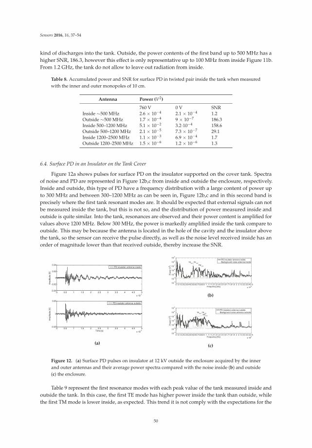
Sensors 2016, 16, 37–54

kind of discharges into the tank. Outside, the power contents of the first band up to 500 MHz has ahigher SNR, 186.3, however this effect is only representative up to 100 MHz from inside Figure 11b.From 1.2 GHz, the tank do not allow to leave out radiation from inside.

Table 8. Accumulated power and SNR for surface PD in twisted pair inside the tank when measuredwith the inner and outer monopoles of 10 cm.

Antenna Power (V2)

760 V 0 V SNRInside ∼500 MHz 2.6 × 10−4 2.1 × 10−4 1.2Outside ∼500 MHz 1.7 × 10−4 9 × 10−7 186.3Inside 500–1200 MHz 5.1 × 10−2 3.2·10−4 158.6Outside 500–1200 MHz 2.1 × 10−5 7.3 × 10−7 29.1Inside 1200–2500 MHz 1.1 × 10−3 6.9 × 10−4 1.7Outside 1200–2500 MHz 1.5 × 10−6 1.2 × 10−6 1.3

6.4. Surface PD in an Insulator on the Tank Cover

Figure 12a shows pulses for surface PD on the insulator supported on the cover tank. Spectraof noise and PD are represented in Figure 12b,c from inside and outside the enclosure, respectively.Inside and outside, this type of PD have a frequency distribution with a large content of power upto 300 MHz and between 300–1200 MHz as can be seen in, Figure 12b,c and in this second band isprecisely where the first tank resonant modes are. It should be expected that external signals can notbe measured inside the tank, but this is not so, and the distribution of power measured inside andoutside is quite similar. Into the tank, resonances are observed and their power content is amplified forvalues above 1200 MHz. Below 300 MHz, the power is markedly amplified inside the tank compare tooutside. This may be because the antenna is located in the hole of the cavity and the insulator abovethe tank, so the sensor can receive the pulse directly, as well as the noise level received inside has anorder of magnitude lower than that received outside, thereby increase the SNR.

0 0.5 1 1.5 2 2.5 3 3.5 4 4.5 5

x 10-7

-0.04

-0.02

0

0.02

0.04

Am

plit

ud

e [

V]

PD insulator antenna inside

0 0.5 1 1.5 2 2.5 3 3.5 4 4.5 5

x 10-7

-0.05

0

0.05

Time [s]

Am

plit

ud

e [

V]

PD insulator antenna outside

(a)

0 0.10.20.30.40.50.60.70.80.9 1 1.11.21.31.41.51.61.71.81.9 2 2.12.22.32.42.5

x 109

10-11

10-10

10-9

10-8

10-7

10-6

10-5

Frequency [Hz]

Po

we

r [V

2]

PD insulator antenna insideBackground noise antenna insideTE

011,TE

101

TM110

(b)

0 0.10.20.30.40.50.60.70.80.9 1 1.11.21.31.41.51.61.71.81.9 2 2.12.22.32.42.5

x 109

10-11

10-10

10-9

10-8

10-7

10-6

10-5

Frequency [Hz]

Po

we

r [V

2]

PD insulator antenna outsideBackground noise antenna outsideTE

011,TE

101TM

110

(c)

Figure 12. (a) Surface PD pulses on insulator at 12 kV outside the enclosure acquired by the innerand outer antennas and their average power spectra compared with the noise inside (b) and outside(c) the enclosure.

Table 9 represent the first resonance modes with each peak value of the tank measured inside andoutside the tank. In this case, the first TE mode has higher power inside the tank than outside, whilethe first TM mode is lower inside, as expected. This trend it is not comply with the expectations for the

50

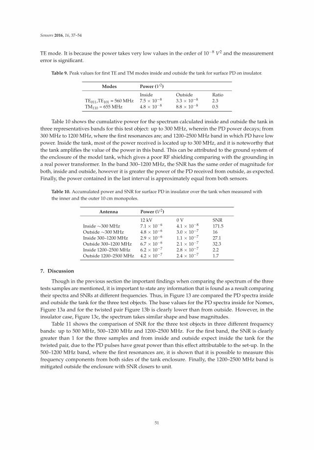
Sensors 2016, 16, 37–54

TE mode. It is because the power takes very low values in the order of 10−8 V2 and the measurementerror is significant.

Table 9. Peak values for first TE and TM modes inside and outside the tank for surface PD on insulator.

Modes Power (V2)

Inside Outside RatioTE011,TE101 = 560 MHz 7.5 × 10−8 3.3 × 10−8 2.3TM110 = 655 MHz 4.8 × 10−8 8.8 × 10−8 0.5

Table 10 shows the cumulative power for the spectrum calculated inside and outside the tank inthree representatives bands for this test object: up to 300 MHz, wherein the PD power decays; from300 MHz to 1200 MHz, where the first resonances are; and 1200–2500 MHz band in which PD have lowpower. Inside the tank, most of the power received is located up to 300 MHz, and it is noteworthy thatthe tank amplifies the value of the power in this band. This can be attributed to the ground system ofthe enclosure of the model tank, which gives a poor RF shielding comparing with the grounding ina real power transformer. In the band 300–1200 MHz, the SNR has the same order of magnitude forboth, inside and outside, however it is greater the power of the PD received from outside, as expected.Finally, the power contained in the last interval is approximately equal from both sensors.

Table 10. Accumulated power and SNR for surface PD in insulator over the tank when measured withthe inner and the outer 10 cm monopoles.

Antenna Power (V2)

12 kV 0 V SNRInside ∼300 MHz 7.1 × 10−6 4.1 × 10−8 171.5Outside ∼300 MHz 4.8 × 10−6 3.0 × 10−7 16Inside 300–1200 MHz 2.9 × 10−6 1.1 × 10−7 27.1Outside 300–1200 MHz 6.7 × 10−6 2.1 × 10−7 32.3Inside 1200–2500 MHz 6.2 × 10−7 2.8 × 10−7 2.2Outside 1200–2500 MHz 4.2 × 10−7 2.4 × 10−7 1.7

7. Discussion

Though in the previous section the important findings when comparing the spectrum of the threetests samples are mentioned, it is important to state any information that is found as a result comparingtheir spectra and SNRs at different frequencies. Thus, in Figure 13 are compared the PD spectra insideand outside the tank for the three test objects. The base values for the PD spectra inside for Nomex,Figure 13a and for the twisted pair Figure 13b is clearly lower than from outside. However, in theinsulator case, Figure 13c, the spectrum takes similar shape and base magnitudes.

Table 11 shows the comparison of SNR for the three test objects in three different frequencybands: up to 500 MHz, 500–1200 MHz and 1200–2500 MHz. For the first band, the SNR is clearlygreater than 1 for the three samples and from inside and outside expect inside the tank for thetwisted pair, due to the PD pulses have great power than this effect attributable to the set-up. In the500–1200 MHz band, where the first resonances are, it is shown that it is possible to measure thisfrequency components from both sides of the tank enclosure. Finally, the 1200–2500 MHz band ismitigated outside the enclosure with SNR closers to unit.

51

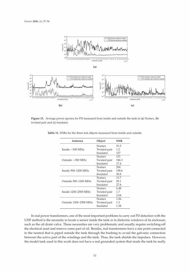
Sensors 2016, 16, 37–54

0 0.1 0.2 0.3 0.4 0.5 0.6 0.7 0.8 0.9 1 1.1 1.2 1.3 1.4 1.5 1.6 1.7 1.8 1.9 2 2.1 2.2 2.3 2.4 2.5

x 109

10-8

10-7

10-6

10-5

10-4

10-3

10-2

Frequency [Hz] P

ow

er

[V2]

PD Nomex antenna insidePD Nomex antenna outside

(a)

0 0.1 0.2 0.3 0.4 0.5 0.6 0.7 0.8 0.9 1 1.1 1.2 1.3 1.4 1.5 1.6 1.7 1.8 1.9 2 2.1 2.2 2.3 2.4 2.5

x 109

10-9

10-8

10-7

10-6

10-5

10-4

10-3

10-2

Frequency [Hz]

Po

we

r [V

2]

PD twisted pair antenna insidePD twisted pair antenna outside

(b)

0 0.1 0.2 0.3 0.4 0.5 0.6 0.7 0.8 0.9 1 1.1 1.2 1.3 1.4 1.5 1.6 1.7 1.8 1.9 2 2.1 2.2 2.3 2.4 2.5

x 109

10-10

10-9

10-8

10-7

10-6

10-5

Frequency [Hz] P

ow

er

[V2]

PD insulator antenna insidePD insulator pair antenna outside

(c)

Figure 13. Average power spectra for PD measured from inside and outside the tank in (a) Nomex, (b)twisted pair and (c) insulator.

Table 11. SNRs for the three test objects measured from inside and outside.

Antenna Object SNR

Nomex 51.5Inside ∼500 MHz Twisted pair 1.2

Insulator 127Nomex 131

Outside ∼500 MHz Twisted pair 186.3Insulator 17.4Nomex 204

Inside 500–1200 MHz Twisted pair 158.6Insulator 30.8Nomex 13.7

Outside 500–1200 MHz Twisted pair 29.1Insulator 27.8Nomex 6.48

Inside 1200–2500 MHz Twisted pair 1.7Insulator 2.04Nomex 1.06

Outside 1200–2500 MHz Twisted pair 1.3Insulator 1.38

In real power transformers, one of the most important problems to carry out PD detection with theUHF method is the necessity to locate a sensor inside the tank or in dielectric windows of its enclosure,such as the oil drain valve. These necessities are very problematic and usually require switching-offthe electrical asset and remove some part of oil. Besides, real transformers have a star point connectedto the neutral that is piped outside the tank through the bushing to avoid the galvanic connectionbetween the active part of the windings and the tank. Thus, the tank shields the impulses. However,the model tank used in this work does not have a real grounded system that made the tank be really

52

Sensors 2016, 16, 37–54

like a screen for the pulses. Thus, the model tank acts as an emitter at VHF and the outer antenna canregister its effect.

8. Conclusions

Partial discharge measurements performed inside the model of a transformer tank show thatthe spectrum of the received signals are influenced by several factors. The first is the cavity, whichdepending on its dimensions allowing a certain resonant modes that have power for certain frequencies.The second is the frequency response of the antenna. The third depends on the PD type. Whenthe EM emission comes out, the tank acts as a low-pass filter with a cut-off frequency of about1.2 GHz, so that the outer antenna is not able to receive power from the PD above this frequency.Furthermore, it was found that a higher power content may appear outside than inside, below300 MHz, and this is attributed to the ground cable of the enclosure which behaves as an antenna thatamplify the PD radiation below 300 MHz. When the insulator is located outside the tank, similar powerbelow 300 MHz is measured inside than outside, this could be due to the insufficient EM enclosure ofthe tank model. In this case, similarly than with the other test objects, resonance modes of the tankare excite and the cumulative power has the same order of magnitude both inside and outside in the500–1200 MHz range. These results suggest that taking into account only the power spectrum of thePD, it is not trivial to identify the kind of PD source and additional studies in future must be carriedout. In this sense, it will be intended to have a voltage reference to represent the PRPD pattern toidentify the type of source in each case. However, this requires the use of another hardware to carryout the measurements in order to capture both, fast pulses in the order of ns, such as PD, synchronizingwith the AC voltage reference in the order of ms, so a synchronized acquisition system with uncouplechannels, with different frequency sample will be required. In future research, it would be necessary todeploy artificial defects with similar PRPD distributions as those described in this work in a real powertransformer to measure its PD activity in UHF with various sensor arrangements. Future research willbe a step forward in this research area and will allow for applying the knowledge acquired in thispaper for application in the field.

Acknowledgments: This work was supported by Basal Project FB0008. The authors would like to thank theDepartment of Electrical Engineering at Universidad Carlos III de Madrid for all tests that were done inHigh-Voltage Research and Test Laboratory (LINEALT), as well as to the Department of Signal Theory andCommunications for the same institution by the support in the measurements with the network analyser.

Author Contributions: The presented research was developed by the authors with the contribution of eachone in a specific task. Ricardo Albarracín defined the tests to be performed and carried out the experimentalmeasurements. Besides, he did the post-processing and analysis of the results. Jorge Alfredo Ardila-Rey supportedRicardo Albarracín in test object design and PD measurements in the laboratory. Finally, Ricardo Albarracín,Jorge Alfredo Ardila-Rey and Abdullahi Mas’ud contribute in a brainstorming to the analysis of the results.


References

1. Judd, M.; Yang, L.; Hunter, I. Partial discharge monitoring of power transformers using UHF sensors. Part I:sensors and signal interpretation. IEEE Electri. Insul. Mag. 2005, 21, 5–14.

2. Markalous, S.; Tenbohlen, S.; Feser, K. Detection and location of partial discharges in power transformersusing acoustic and electromagnetic signals. IEEE Trans. Dielectr. Electr. Insul. 2008, 15, 1576–1583.

3. Robles, G.; Albarracín, R.; Vázquez, J.L. Antennas in Partial Discharge Sensing System. In Handbook of

Antenna Technologies; Chen, Z.N., Ed.; Springer Singapore: Singapore, 2015; pp. 1–47.4. IEC-62478. High-Voltage Test Techniques—Measurement of Partial Discharges by Electromagnetic and Acoustic

Methods. Proposed Horizontal Standard, 1st ed.; International Electrotechnical Commission (IEC): Geneva,Switzerland, 2016.(submitted)

5. Coenen, S.; Tenbohlen, S.; Markalous, S.; Strehl, T. Sensitivity of UHF PD measurements in powertransformers. IEEE Trans. Dielectr. Electr. Insul. 2008, 15, 1553–1558.

6. Robles, G.; Fresno, J.M.; Martínez-Tarifa, J.M. Separation of Radio-Frequency Sources and Localization ofPartial Discharges in Noisy Environments. Sensors 2015, 15, 9882–9898.

53

Sensors 2016, 16, 37–54

7. Albarracín, R.; Robles, G.; Martínez-Tarifa, J.; Ardila-Rey, J. Separation of sources in radiofrequencymeasurements of partial discharges using time-power ratio maps. ISA Trans. 2015, 58, 389–397.

8. Robles, G.; Albarracín, R.; Martínez-Tarifa, J. Shielding effect of power transformers tanks in theultra-high-frequency detection of partial discharges. IEEE Trans. Dielectr. Electr. Insul. 2013, 20, 678–684.

9. Mirzaei, H.; Akbari, A.; Zanjani, M.; Gockenbach, E.; Borsi, H. Investigating the partial dischargeelectromagnetic wave propagation in power transformers considering active part characteristics. InProceedings of the IEEE 2012 International Conference on Condition Monitoring and Diagnosis (CMD), Bali,India, 23–27 September 2012; pp. 442–445.

10. Balanis, C.A. Advanced Engineering Electromagnetics, 2nd ed.; Wiley: Hoboken, NJ, USA, 2012.11. Robles, G.; Sánchez-Fernández, M.; Albarracín-Sánchez, R.; Rojas-Moreno, M.; Rajo-Iglesias, E.;

Martínez-Tarifa, J. Antenna Parametrization for the Detection of Partial Discharges. IEEE Trans. Instrum. Meas.

2013, 62, 932–941.12. Balanis, C.A. Antenna Theory: Analysis and Design, 3rd ed.; Wiley-Interscience: Hoboken, NJ, USA, 2005.13. Judd, M.; Farish, O.; Hampton, B. Broadband couplers for UHF detection of partial discharge in gas-insulated

substations. IEE Proc. Sci. Meas. Technol. 1995, 142, 237–243.14. Tang, Z.; Li, C.; Cheng, X.; Wang, W.; Li, J.; Li, J. Partial discharge location in power transformers using

wideband RF detection. IEEE Trans. Dielectr. Electr. Insul. 2006, 13, 1193–1199.15. López-Roldán, J.; Tang, T.; Gaskin, M. Optimisation of a sensor for onsite detection of partial discharges in

power transformers by the UHF method. IEEE Trans. Dielectr. Electr. Insul. 2008, 15, 1634–1639.16. Kaneko, S.; Okabe, S.; Yoshimura, M.; Muto, H.; Nishida, C.; Kamei, M. Detecting characteristics of various

type antennas on partial discharge electromagnetic wave radiating through insulating spacer in gas insulatedswitchgear. IEEE Trans. Dielectr. Electr. Insul. 2009, 16, 1462–1472.

17. Fabiani, D.; Cavallini, A.; Montanari, G. A UHF Technique for Advanced PD Measurements on Inverter-FedMotors. IEEE Trans. Power Electron. 2008, 23, 2546–2556.

18. Stutzman, W.L.; Thiele, G. Antenna Theory and Design; Wiley: Hoboken, NJ, USA, 1998.19. Prevost, T.; Oommen, T.V. Cellulose insulation in oil-filled power transformers: Part I—History and

development. IEEE Electr. Insul. Mag. 2006, 22, 28–35.20. Cheng, D.K. Fundamentals of Electromagnetism Engineering; Addison Wesley Iberoamericana: Mexico DF,

Mexico, 1998.21. Jardine, A.K.; Lin, D.; Banjevic, D. A review on machinery diagnostics and prognostics implementing

condition-based maintenance. Mech. Syst. Signal Process. 2006, 20, 1483–1510.22. Gill, P. Electrical Power Equipment Maintenance and Testing, Second Edition; Power Engineering (Willis), Taylor

& Francis: Boca Raton, FL, USA, 2008.23. IEC-60270. High-Voltage Test Techniques—Partial Discharge Measurements, 3rd ed.; International

Electrotechnical Commission (IEC): New Delhi, India, 2000.24. Pozar, D. Microwave Engineering; Wiley: Hoboken, NJ, USA, 2005.

c© 2016 by the authors; licensee MDPI, Basel, Switzerland. This article is an open accessarticle distributed under the terms and conditions of the Creative Commons Attribution(CC-BY) license (http://creativecommons.org/licenses/by/4.0/).

54

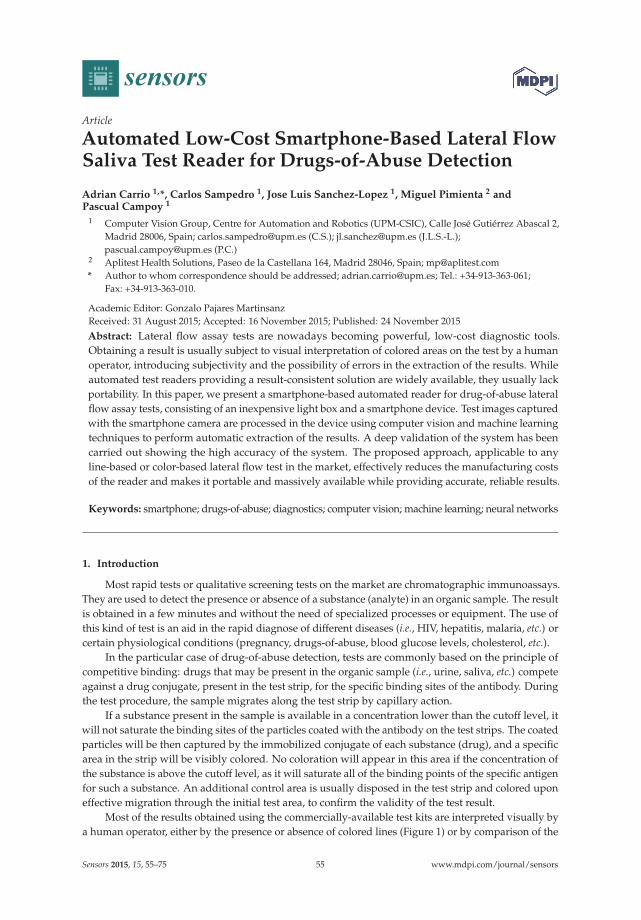
sensors

Article

Automated Low-Cost Smartphone-Based Lateral FlowSaliva Test Reader for Drugs-of-Abuse Detection

Adrian Carrio 1,*, Carlos Sampedro 1, Jose Luis Sanchez-Lopez 1, Miguel Pimienta 2 andPascual Campoy 1

1 Computer Vision Group, Centre for Automation and Robotics (UPM-CSIC), Calle José Gutiérrez Abascal 2,Madrid 28006, Spain; [email protected] (C.S.); [email protected] (J.L.S.-L.);[email protected] (P.C.)

2 Aplitest Health Solutions, Paseo de la Castellana 164, Madrid 28046, Spain; [email protected]* Author to whom correspondence should be addressed; [email protected]; Tel.: +34-913-363-061;

Fax: +34-913-363-010.

Academic Editor: Gonzalo Pajares MartinsanzReceived: 31 August 2015; Accepted: 16 November 2015; Published: 24 November 2015

Abstract: Lateral flow assay tests are nowadays becoming powerful, low-cost diagnostic tools.Obtaining a result is usually subject to visual interpretation of colored areas on the test by a humanoperator, introducing subjectivity and the possibility of errors in the extraction of the results. Whileautomated test readers providing a result-consistent solution are widely available, they usually lackportability. In this paper, we present a smartphone-based automated reader for drug-of-abuse lateralflow assay tests, consisting of an inexpensive light box and a smartphone device. Test images capturedwith the smartphone camera are processed in the device using computer vision and machine learningtechniques to perform automatic extraction of the results. A deep validation of the system has beencarried out showing the high accuracy of the system. The proposed approach, applicable to anyline-based or color-based lateral flow test in the market, effectively reduces the manufacturing costsof the reader and makes it portable and massively available while providing accurate, reliable results.

Keywords: smartphone; drugs-of-abuse; diagnostics; computer vision; machine learning; neural networks

1. Introduction

Most rapid tests or qualitative screening tests on the market are chromatographic immunoassays.They are used to detect the presence or absence of a substance (analyte) in an organic sample. The resultis obtained in a few minutes and without the need of specialized processes or equipment. The use ofthis kind of test is an aid in the rapid diagnose of different diseases (i.e., HIV, hepatitis, malaria, etc.) orcertain physiological conditions (pregnancy, drugs-of-abuse, blood glucose levels, cholesterol, etc.).

In the particular case of drug-of-abuse detection, tests are commonly based on the principle ofcompetitive binding: drugs that may be present in the organic sample (i.e., urine, saliva, etc.) competeagainst a drug conjugate, present in the test strip, for the specific binding sites of the antibody. Duringthe test procedure, the sample migrates along the test strip by capillary action.

If a substance present in the sample is available in a concentration lower than the cutoff level, itwill not saturate the binding sites of the particles coated with the antibody on the test strips. The coatedparticles will be then captured by the immobilized conjugate of each substance (drug), and a specificarea in the strip will be visibly colored. No coloration will appear in this area if the concentration ofthe substance is above the cutoff level, as it will saturate all of the binding points of the specific antigenfor such a substance. An additional control area is usually disposed in the test strip and colored uponeffective migration through the initial test area, to confirm the validity of the test result.

Most of the results obtained using the commercially-available test kits are interpreted visually bya human operator, either by the presence or absence of colored lines (Figure 1) or by comparison of the


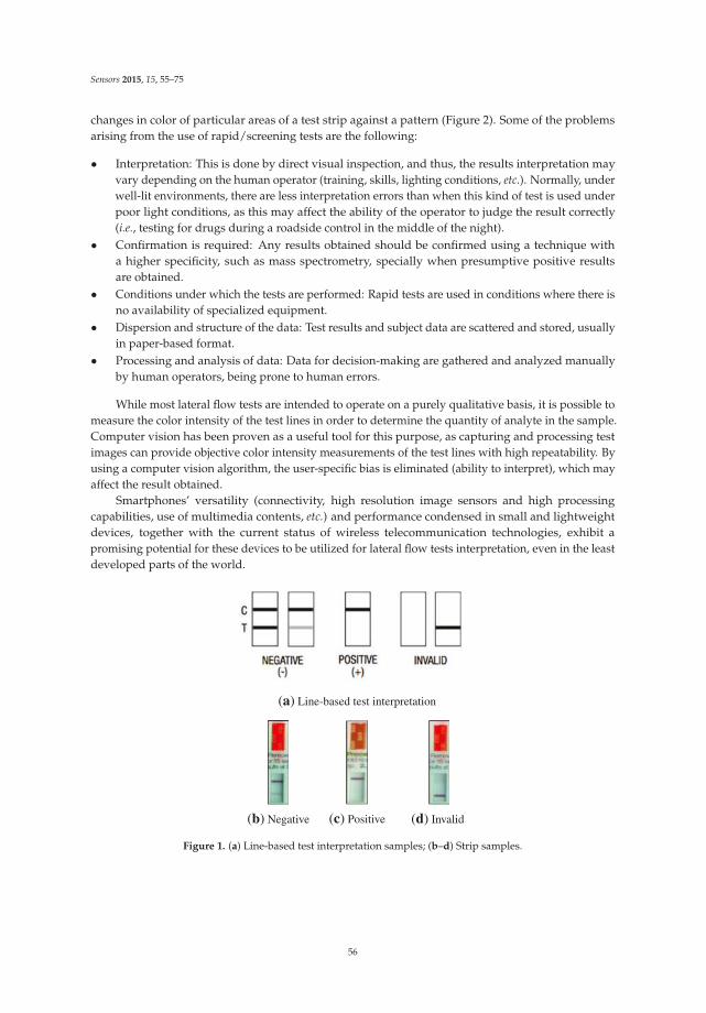
Sensors 2015, 15, 55–75

changes in color of particular areas of a test strip against a pattern (Figure 2). Some of the problemsarising from the use of rapid/screening tests are the following:

• Interpretation: This is done by direct visual inspection, and thus, the results interpretation mayvary depending on the human operator (training, skills, lighting conditions, etc.). Normally, underwell-lit environments, there are less interpretation errors than when this kind of test is used underpoor light conditions, as this may affect the ability of the operator to judge the result correctly(i.e., testing for drugs during a roadside control in the middle of the night).

• Confirmation is required: Any results obtained should be confirmed using a technique witha higher specificity, such as mass spectrometry, specially when presumptive positive resultsare obtained.

• Conditions under which the tests are performed: Rapid tests are used in conditions where there isno availability of specialized equipment.

• Dispersion and structure of the data: Test results and subject data are scattered and stored, usuallyin paper-based format.

• Processing and analysis of data: Data for decision-making are gathered and analyzed manuallyby human operators, being prone to human errors.

While most lateral flow tests are intended to operate on a purely qualitative basis, it is possible tomeasure the color intensity of the test lines in order to determine the quantity of analyte in the sample.Computer vision has been proven as a useful tool for this purpose, as capturing and processing testimages can provide objective color intensity measurements of the test lines with high repeatability. Byusing a computer vision algorithm, the user-specific bias is eliminated (ability to interpret), which mayaffect the result obtained.

Smartphones’ versatility (connectivity, high resolution image sensors and high processingcapabilities, use of multimedia contents, etc.) and performance condensed in small and lightweightdevices, together with the current status of wireless telecommunication technologies, exhibit apromising potential for these devices to be utilized for lateral flow tests interpretation, even in the leastdeveloped parts of the world.

(a) Line-based test interpretation

(b) Negative (c) Positive (d) Invalid

Figure 1. (a) Line-based test interpretation samples; (b–d) Strip samples.

56

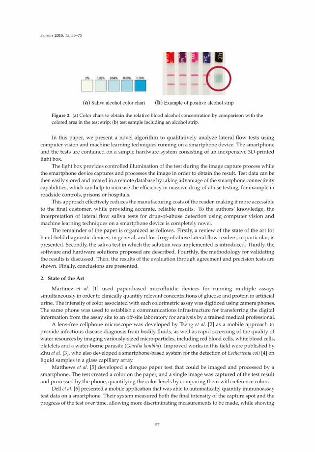
Sensors 2015, 15, 55–75

(a) Saliva alcohol color chart (b) Example of positive alcohol strip

Figure 2. (a) Color chart to obtain the relative blood alcohol concentration by comparison with thecolored area in the test strip; (b) test sample including an alcohol strip.

In this paper, we present a novel algorithm to qualitatively analyze lateral flow tests usingcomputer vision and machine learning techniques running on a smartphone device. The smartphoneand the tests are contained on a simple hardware system consisting of an inexpensive 3D-printedlight box.

The light box provides controlled illumination of the test during the image capture process whilethe smartphone device captures and processes the image in order to obtain the result. Test data can bethen easily stored and treated in a remote database by taking advantage of the smartphone connectivitycapabilities, which can help to increase the efficiency in massive drug-of-abuse testing, for example inroadside controls, prisons or hospitals.

This approach effectively reduces the manufacturing costs of the reader, making it more accessibleto the final customer, while providing accurate, reliable results. To the authors’ knowledge, theinterpretation of lateral flow saliva tests for drug-of-abuse detection using computer vision andmachine learning techniques on a smartphone device is completely novel.

The remainder of the paper is organized as follows. Firstly, a review of the state of the art forhand-held diagnostic devices, in general, and for drug-of-abuse lateral flow readers, in particular, ispresented. Secondly, the saliva test in which the solution was implemented is introduced. Thirdly, thesoftware and hardware solutions proposed are described. Fourthly, the methodology for validatingthe results is discussed. Then, the results of the evaluation through agreement and precision tests areshown. Finally, conclusions are presented.

2. State of the Art

Martinez et al. [1] used paper-based microfluidic devices for running multiple assayssimultaneously in order to clinically quantify relevant concentrations of glucose and protein in artificialurine. The intensity of color associated with each colorimetric assay was digitized using camera phones.The same phone was used to establish a communications infrastructure for transferring the digitalinformation from the assay site to an off-site laboratory for analysis by a trained medical professional.

A lens-free cellphone microscope was developed by Tseng et al. [2] as a mobile approach toprovide infectious disease diagnosis from bodily fluids, as well as rapid screening of the quality ofwater resources by imaging variously-sized micro-particles, including red blood cells, white blood cells,platelets and a water-borne parasite (Giardia lamblia). Improved works in this field were published byZhu et al. [3], who also developed a smartphone-based system for the detection of Escherichia coli [4] onliquid samples in a glass capillary array.

Matthews et al. [5] developed a dengue paper test that could be imaged and processed by asmartphone. The test created a color on the paper, and a single image was captured of the test resultand processed by the phone, quantifying the color levels by comparing them with reference colors.

Dell et al. [6] presented a mobile application that was able to automatically quantify immunoassaytest data on a smartphone. Their system measured both the final intensity of the capture spot and theprogress of the test over time, allowing more discriminating measurements to be made, while showing

57

Sensors 2015, 15, 55–75

great speed and accuracy. However, registration marks and an intensity calibration pattern had to beincluded in the test to correctly process the image, and also, the use of an additional lens was requiredfor image magnification.

Uses of rapid diagnostic test reader platforms for malaria, tuberculosis and HIV have beenreported by Mudanyali et al. [7,8]. Smartphone technology was also used to develop a quantitativerapid diagnostic test for multi-bacillary leprosy, which provided quantifiable and consistent data toassist in the diagnosis of MBleprosy.

A smartphone-based colorimetric detection system was developed by Shen et al. [9], togetherwith a calibration technique to compensate for measurement errors due to variability in ambient light.Oncescu et al. [10] proposed a similar system for the detection of biomarkers in sweat and saliva.Similar colorimetric methods for automatic extraction of the result in ELISA plates [11] and proteinuriain urine [12] have also been reported. However, none of those works presented developments oncolored line detection.

In the area of drug-of-abuse detection, accurate confirmatory results are nowadays obtained in alaboratory usually by means of mass spectrometry techniques. These laboratory-based solutions areexpensive and time consuming, as the organic sample has to be present in the laboratory in order toperform the analysis. In contrast, screening techniques provide in situ, low-cost, rapid presumptiveresults with a relatively low error rate, with immunoassay lateral flow tests currently being the mostcommon technique for this type of test. Nonetheless, as most lateral flow tests operate on a purelyqualitative basis, obtaining a result is usually subject to the visual interpretation of colored areas onthe test by a human operator, therefore introducing subjectivity and the possibility of human errors tothe test result. Hand-held diagnostic devices, known as lateral flow assay readers, are widely used toprovide automated extraction of the test result.

VeriCheck [13] is an example of an automated reader for lateral flow saliva tests consisting of theuse of a conventional image scanner and a laptop. However, this solution is far from portable, as itconsists of multiple devices and requires at least a power outlet for the scanner.

DrugRead [14] offers a portable automated reader solution on a hand-held device. However,our system offers a low-cost, massively available solution, as it has been implemented on a commonsmartphone device.

3. Saliva Test Description

The proposed image processing methodology can be applied to any line presence or absence-basedor color interpretation-based immunoassay tests on the market. For the results and validationpresented, the rapid oral fluid drug test DrugCheck SalivaScan [15], manufactured by ExpressDiagnostics Inc. (Minneapolis, MN, USA), was used. DrugCheck SalivaScan is an immunoassayfor rapid qualitative and presumptive detection of drugs-of-abuse in human oral fluid samples.

The device is made of one or several strips of membrane incorporated in a plastic holder, asshown in Figure 3. For sample collection, a swab with a sponge containing an inert substance thatreduces saliva viscosity is used. A saturation indicator is placed inside the collection swab to controlthe volume of saliva collected and to provide the indication to start the reaction (incubation) of therapid test. The test may contain any combination of the parameters/substances and cutoff levels aslisted in Table 1.

Additionally, the test may include a strip for the detection of the presence of alcohol (ethanol) inoral fluid, providing an approximation of the relative blood alcohol concentration. When in contactwith solutions of alcohol, the reactive pad in the strip will rapidly turn colors depending on theconcentration of alcohol present. The pad employs a solid-phase chemistry that uses a highly specificenzyme reaction. The detection levels of relative blood alcohol concentration range between 0.02%up to 0.30%.

58

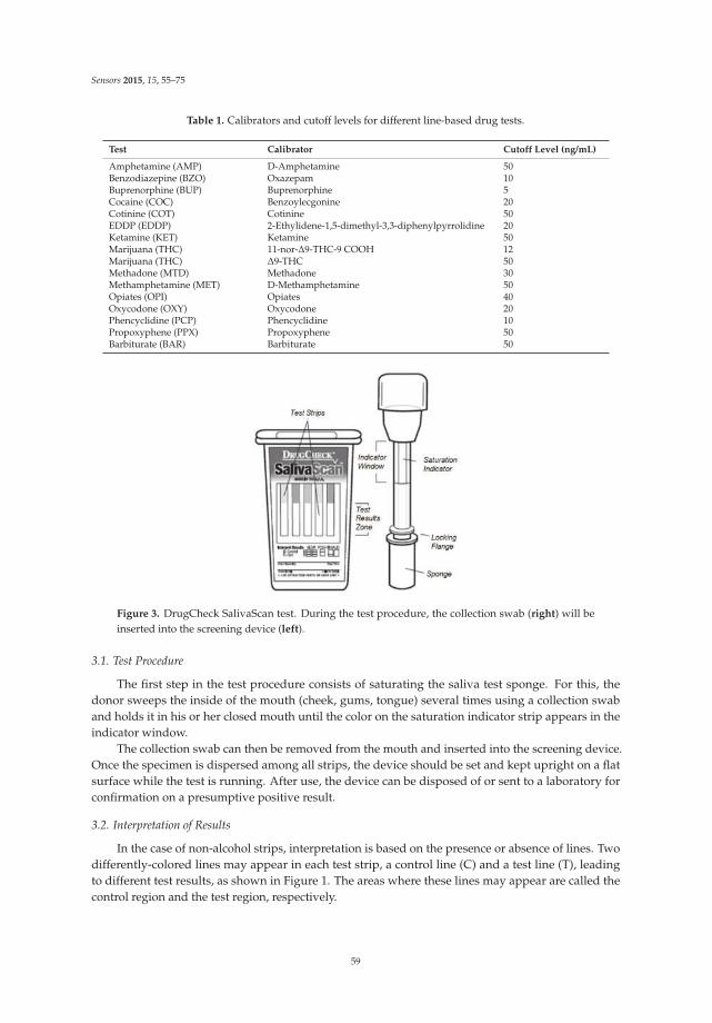
Sensors 2015, 15, 55–75

Table 1. Calibrators and cutoff levels for different line-based drug tests.

Test Calibrator Cutoff Level (ng/mL)

Amphetamine (AMP) D-Amphetamine 50Benzodiazepine (BZO) Oxazepam 10Buprenorphine (BUP) Buprenorphine 5Cocaine (COC) Benzoylecgonine 20Cotinine (COT) Cotinine 50EDDP (EDDP) 2-Ethylidene-1,5-dimethyl-3,3-diphenylpyrrolidine 20Ketamine (KET) Ketamine 50Marijuana (THC) 11-nor-Δ9-THC-9 COOH 12Marijuana (THC) Δ9-THC 50Methadone (MTD) Methadone 30Methamphetamine (MET) D-Methamphetamine 50Opiates (OPI) Opiates 40Oxycodone (OXY) Oxycodone 20Phencyclidine (PCP) Phencyclidine 10Propoxyphene (PPX) Propoxyphene 50Barbiturate (BAR) Barbiturate 50

Figure 3. DrugCheck SalivaScan test. During the test procedure, the collection swab (right) will beinserted into the screening device (left).

3.1. Test Procedure

The first step in the test procedure consists of saturating the saliva test sponge. For this, thedonor sweeps the inside of the mouth (cheek, gums, tongue) several times using a collection swaband holds it in his or her closed mouth until the color on the saturation indicator strip appears in theindicator window.

The collection swab can then be removed from the mouth and inserted into the screening device.Once the specimen is dispersed among all strips, the device should be set and kept upright on a flatsurface while the test is running. After use, the device can be disposed of or sent to a laboratory forconfirmation on a presumptive positive result.

3.2. Interpretation of Results

In the case of non-alcohol strips, interpretation is based on the presence or absence of lines. Twodifferently-colored lines may appear in each test strip, a control line (C) and a test line (T), leadingto different test results, as shown in Figure 1. The areas where these lines may appear are called thecontrol region and the test region, respectively.

59

Sensors 2015, 15, 55–75

Negative results can be read as soon as both lines appear on any test strip, which usually happenswithin 2 min. Presumptive positive results can be read after 10 min. Three possible results maybe obtained:

1. Positive: Only one colored line appears in the control region. No colored line is formed in the testregion for a particular substance. A positive result indicates that the concentration of the analytein the sample exceeds the cutoff level.

2. Negative: Two colored lines appear on the membrane. One line is formed in the control regionand another line in the test region for the corresponding substance. A negative result indicatesthat the analyte concentration is below the cutoff level.

3. Invalid result: No control line is formed. The result of any test in which there is no control lineduring the specified time should not be considered.

The intensity of the colored line in the test region may vary depending on the concentrationof the analyte present in the specimen. Therefore, any shade of color in the test region should beconsidered negative.

In the case of saliva alcohol strips, the interpretation of the results should be made by comparingthe color obtained in the reagent strip against a printed color pattern that is provided with the test(Figure 2). Alcohol strips must be read at 2 min, as pad color may change, and again, three possibleresults may be obtained:

1. Positive: The test will produce a color change in the presence of alcohol in the sample. The colorintensity will range, being light blue at a 0.02% relative blood alcohol concentration and darkblue near a 0.30% relative blood alcohol concentration. An approximation of the relative bloodalcohol concentration within this range can be obtained by comparison with the provided colorpattern (Figure 2).

2. Negative: If the test presents no color changes, this should be interpreted as a negative result,indicating that alcohol has not been detected in the sample.

3. Invalid: If the color pad is already colored in blue before applying the saliva sample, the testshould not be used.

4. System Description

In the following section, a description of the saliva test reader system is presented. Firstly, imageacquisition aspects are discussed, including a description of the light box device used for illuminationnormalization purposes. Secondly, the computer vision algorithms used in the image processingstage are described. Finally, the machine learning algorithms used for lateral histogram classificationare presented.

4.1. Image Acquisition

Image acquisition is an extremely important step in computer vision applications, as the qualityof the acquired image will condition all further image processing steps. Images must meet certainrequirements in terms of image quality (blur, contrast, illumination, etc.). The positions of the camera(a mobile device in our case) and the object to be captured (here, the test) should remain in a constantrelative position for the best results. However, contrary to traditional image processing applications, amobile device is hand-held and, therefore, does not have a fixed position with respect to the test, whichcan lead to motion blur artifacts. Furthermore, mobile devices are used in dynamic environments,implying that ambient illumination has to be considered in order to obtain repeatable results regardlessof the illumination conditions.

In order to minimize all image acquisition-related problems, a small light box was designedto keep the relative position between the smartphone and the test approximately constant, whileremoving external illumination and projecting white light onto the test with an embedded electronic

60

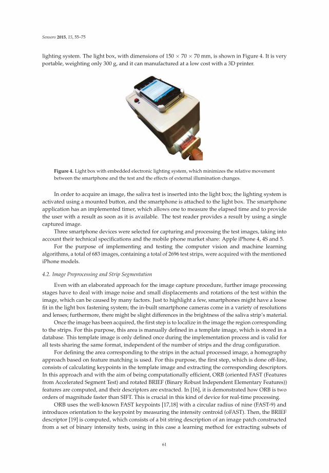
Sensors 2015, 15, 55–75

lighting system. The light box, with dimensions of 150 × 70 × 70 mm, is shown in Figure 4. It is veryportable, weighting only 300 g, and it can manufactured at a low cost with a 3D printer.

Figure 4. Light box with embedded electronic lighting system, which minimizes the relative movementbetween the smartphone and the test and the effects of external illumination changes.

In order to acquire an image, the saliva test is inserted into the light box; the lighting system isactivated using a mounted button, and the smartphone is attached to the light box. The smartphoneapplication has an implemented timer, which allows one to measure the elapsed time and to providethe user with a result as soon as it is available. The test reader provides a result by using a singlecaptured image.

Three smartphone devices were selected for capturing and processing the test images, taking intoaccount their technical specifications and the mobile phone market share: Apple iPhone 4, 4S and 5.

For the purpose of implementing and testing the computer vision and machine learningalgorithms, a total of 683 images, containing a total of 2696 test strips, were acquired with the mentionediPhone models.

4.2. Image Preprocessing and Strip Segmentation

Even with an elaborated approach for the image capture procedure, further image processingstages have to deal with image noise and small displacements and rotations of the test within theimage, which can be caused by many factors. Just to highlight a few, smartphones might have a loosefit in the light box fastening system; the in-built smartphone cameras come in a variety of resolutionsand lenses; furthermore, there might be slight differences in the brightness of the saliva strip’s material.

Once the image has been acquired, the first step is to localize in the image the region correspondingto the strips. For this purpose, this area is manually defined in a template image, which is stored in adatabase. This template image is only defined once during the implementation process and is valid forall tests sharing the same format, independent of the number of strips and the drug configuration.

For defining the area corresponding to the strips in the actual processed image, a homographyapproach based on feature matching is used. For this purpose, the first step, which is done off-line,consists of calculating keypoints in the template image and extracting the corresponding descriptors.In this approach and with the aim of being computationally efficient, ORB (oriented FAST (Featuresfrom Accelerated Segment Test) and rotated BRIEF (Binary Robust Independent Elementary Features))features are computed, and their descriptors are extracted. In [16], it is demonstrated how ORB is twoorders of magnitude faster than SIFT. This is crucial in this kind of device for real-time processing.

ORB uses the well-known FAST keypoints [17,18] with a circular radius of nine (FAST-9) andintroduces orientation to the keypoint by measuring the intensity centroid (oFAST). Then, the BRIEFdescriptor [19] is computed, which consists of a bit string description of an image patch constructedfrom a set of binary intensity tests, using in this case a learning method for extracting subsets of

61

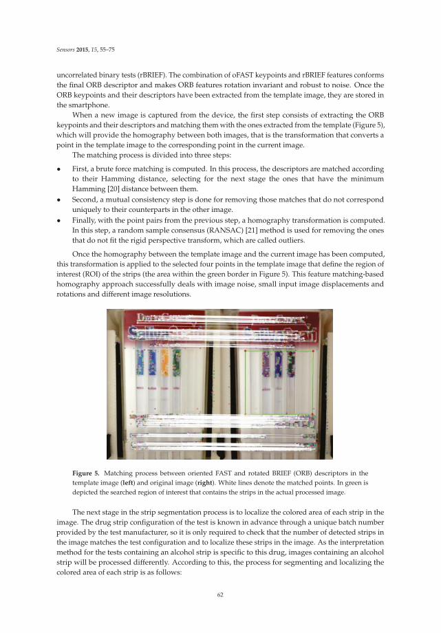
Sensors 2015, 15, 55–75

uncorrelated binary tests (rBRIEF). The combination of oFAST keypoints and rBRIEF features conformsthe final ORB descriptor and makes ORB features rotation invariant and robust to noise. Once theORB keypoints and their descriptors have been extracted from the template image, they are stored inthe smartphone.

When a new image is captured from the device, the first step consists of extracting the ORBkeypoints and their descriptors and matching them with the ones extracted from the template (Figure 5),which will provide the homography between both images, that is the transformation that converts apoint in the template image to the corresponding point in the current image.

The matching process is divided into three steps:

• First, a brute force matching is computed. In this process, the descriptors are matched accordingto their Hamming distance, selecting for the next stage the ones that have the minimumHamming [20] distance between them.

• Second, a mutual consistency step is done for removing those matches that do not corresponduniquely to their counterparts in the other image.

• Finally, with the point pairs from the previous step, a homography transformation is computed.In this step, a random sample consensus (RANSAC) [21] method is used for removing the onesthat do not fit the rigid perspective transform, which are called outliers.

Once the homography between the template image and the current image has been computed,this transformation is applied to the selected four points in the template image that define the region ofinterest (ROI) of the strips (the area within the green border in Figure 5). This feature matching-basedhomography approach successfully deals with image noise, small input image displacements androtations and different image resolutions.

Figure 5. Matching process between oriented FAST and rotated BRIEF (ORB) descriptors in thetemplate image (left) and original image (right). White lines denote the matched points. In green isdepicted the searched region of interest that contains the strips in the actual processed image.

The next stage in the strip segmentation process is to localize the colored area of each strip in theimage. The drug strip configuration of the test is known in advance through a unique batch numberprovided by the test manufacturer, so it is only required to check that the number of detected strips inthe image matches the test configuration and to localize these strips in the image. As the interpretationmethod for the tests containing an alcohol strip is specific to this drug, images containing an alcoholstrip will be processed differently. According to this, the process for segmenting and localizing thecolored area of each strip is as follows:

62

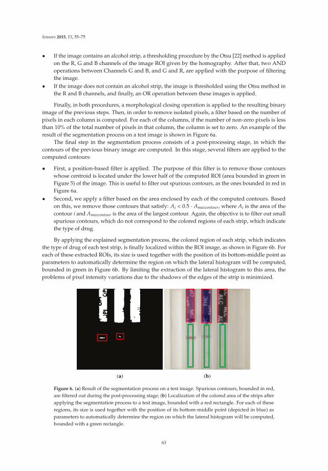
Sensors 2015, 15, 55–75

• If the image contains an alcohol strip, a thresholding procedure by the Otsu [22] method is appliedon the R, G and B channels of the image ROI given by the homography. After that, two ANDoperations between Channels G and B, and G and R, are applied with the purpose of filteringthe image.

• If the image does not contain an alcohol strip, the image is thresholded using the Otsu method inthe R and B channels, and finally, an OR operation between these images is applied.

Finally, in both procedures, a morphological closing operation is applied to the resulting binaryimage of the previous steps. Then, in order to remove isolated pixels, a filter based on the number ofpixels in each column is computed. For each of the columns, if the number of non-zero pixels is lessthan 10% of the total number of pixels in that column, the column is set to zero. An example of theresult of the segmentation process on a test image is shown in Figure 6a.

The final step in the segmentation process consists of a post-processing stage, in which thecontours of the previous binary image are computed. In this stage, several filters are applied to thecomputed contours:

• First, a position-based filter is applied. The purpose of this filter is to remove those contourswhose centroid is located under the lower half of the computed ROI (area bounded in green inFigure 5) of the image. This is useful to filter out spurious contours, as the ones bounded in red inFigure 6a.

• Second, we apply a filter based on the area enclosed by each of the computed contours. Basedon this, we remove those contours that satisfy: Ai < 0.5 · Amaxcontour, where Ai is the area of thecontour i and Amaxcontour is the area of the largest contour. Again, the objective is to filter out smallspurious contours, which do not correspond to the colored regions of each strip, which indicatethe type of drug.

By applying the explained segmentation process, the colored region of each strip, which indicatesthe type of drug of each test strip, is finally localized within the ROI image, as shown in Figure 6b. Foreach of these extracted ROIs, its size is used together with the position of its bottom-middle point asparameters to automatically determine the region on which the lateral histogram will be computed,bounded in green in Figure 6b. By limiting the extraction of the lateral histogram to this area, theproblems of pixel intensity variations due to the shadows of the edges of the strip is minimized.

(a) (b)

Figure 6. (a) Result of the segmentation process on a test image. Spurious contours, bounded in red,are filtered out during the post-processing stage; (b) Localization of the colored area of the strips afterapplying the segmentation process to a test image, bounded with a red rectangle. For each of theseregions, its size is used together with the position of its bottom-middle point (depicted in blue) asparameters to automatically determine the region on which the lateral histogram will be computed,bounded with a green rectangle.

63

Sensors 2015, 15, 55–75

4.3. Lateral Histogram Extraction and Preprocessing

The regions of interest that represent each segmented strip in the previous section need to beprocessed before the classification step takes place. Due to the different way in which alcohol andnon-alcohol strips should be interpreted, both require different preprocessing stages.

In the case of a non-alcohol strip, the preprocessing stage consists of four steps described below,whose mission is to simplify the information given to the classifier as much as possible to increase itsefficiency. All of these steps are done for each non-alcohol segmented strip.

The first step is the lateral histogram extraction from the area extracted during the segmentationstage. The lateral histogram is computed for each of these areas, where the average pixel intensityvalue for each image row (strip transversal direction) is computed according to:

xHG(i) =1n ∑

∀j

s(i, j) (1)

where xHG(i) is the lateral histogram extracted value in the i coordinate; s(i, j) is the (i, j) pixel intensityvalue; i are image rows (strip transversal direction); j are image columns (strip longitudinal direction);and n is the number of image columns inside the lateral histogram area.

Due to differences of image acquisition, raw lateral histograms do not usually have the sameamount of bins. Therefore, an adjustment in the lateral histogram number of bins is set to an arbitrarynumber nbin = 100 through the use of quadratic interpolation. With this step, we ensure that the lateralhistogram always has the same number of bins (set to nbin = 100), independent of the image used.

Then, to minimize the effect of the light intensity changes in the same segmented strip andbetween two different images, a RANSAC technique is applied. The proposed model to be fitted is alinear model y = a · i + b, where y is the lateral histogram value; i is the coordinate; and a and b are theestimated parameters. Then, the lateral histogram is recalculated:

xHR(i) = xHN(i)− (a·i + b) (2)

where xHN(i) is the lateral histogram value in the i coordinate after the adjustment to nbin = 100.As the lateral histogram peaks, which have the information of the test and control regions, are

clearly separated, the fourth and last pre-processing step tries to exploit this information by liningup these peaks. The histogram xHR is divided into two similar parts. The first part uses bins fromone to nbin

2 = 50, while the last part uses bins from nbin2 = 50 to nbin = 100. The minima for each part,

hmin1(i) and hmin2(i), respectively, are computed. The final lateral histogram hx is the conjunction ofboth minimum values with a range of 15 bins in each direction. That means the final lateral histogramhx has nbin−final = 62 bins. Note that the first 31 bins will correspond to the control line (C), and theremaining bins will correspond to the test line (T).

In the case of an alcohol strip, a different processing is done: the first and the second steps areanalogous, but with nbin = 62. Then, a third step to reduce the light intensity differences betweentwo different images is done. The average of only the first nav = 15 values of the lateral histogram iscalculated and then subtracted from the original lateral histogram.

hx(i) = xHN(i)−1

nav

nav

∑i=1

xHN(i) (3)

where hx is the lateral histogram value adjusted to nbin = 62 bins with no light intensity influencebetween two different images. This normalization is done only with respect to the first 15 values ofthe lateral histogram, because this part of the histogram has proven to account well for illuminationchanges along the strip. The normalization with respect to the mean of these 15 values helps tominimize the influence of differences in illumination along the strip.

64

Sensors 2015, 15, 55–75

4.4. Lateral Histogram Classification and Test Outcome

Three different supervised machine learning classifiers based on artificial neural networks (ANN)have been implemented for lateral histogram classification:

• A classifier for alcohol strip lateral histograms.• A classifier for control lines in non-alcohol strip lateral histograms.• A classifier for test lines in non-alcohol strip lateral histograms.

By dividing the classification task into three steps through the use of different classifiers, a betterperformance can be achieved due to its forced specialization. All three classifiers have the same kindof model, and only their structure (their size) and their parameters are different from one another.

Machine learning algorithms require a correct sample dataset in order to be trained. Supervisedalgorithms require examples of each of the desired classes to be learned in order to performclassification tasks.

The parameters of the classifier need to be set after the best structure is selected through across-validation algorithm. The available dataset is randomly, but uniformly divided into threesub-sets depending on its functionality. In our case, “training data” correspond to 70% of the availabledata and are used to adjust the parameters of the model; “validation data”, 15%, are used to checkthe model parameters, ensuring the correct training; finally, “test data”, 15%, test the performance ofthe classifier.

Five sequential algorithms have been considered for generating the classifiers. firstly, anunsupervised input data normalization is performed:

xnormalized(i) =hx(i)− xtrain(i)

std(xtrain (i))(4)

where hx(i) is the preprocessed lateral histogram value in the coordinate i; the subscript train indicatesthe “training data” set; xtrain(i) stands for the mean value; and std stands for the standard deviation.

Secondly, an unsupervised data mapping is done:

xmapped(i) = 2· xnormalized(i)− minm,t(i)

maxm,t(i)− minm,t(i)− 1 (5)

where minm,t(i) and maxm,t(i) are the minimum and maximum values used for the mapping in the i

coordinate and calculated with the “training data” set.Then, a supervised ANN, multi-layer perceptron (MLP) [23], is first trained and afterwards

executed to classify the data. This ANN is composed by several layers, called the “input layer”,“hidden layers” and the “output layer”, depicted in Figure 7. Each layer (except the “input layer”,which is only the input to the ANN) is formed by several neurons. Each neuron has a single output;multiple inputs (all of the outputs of the neurons of the previous layer); a weight value associated witheach input; and a bias value. The behavior of each neuron, i.e., how its output is computed based on itsinputs and internal parameters, is given by:

output = tansig

(

∑∀i

input(i)·weight(i) + bias

)

(6)

where tansig(x) is the hyperbolic tangent sigmoid function.After the input

→x NN =

→x mapped is introduced to the ANN, it generates an output vector

→y NN .

The number of neurons and its configuration (i.e., the structure of the classifier) and the weights andbiases of each neuron (i.e., the parameters of the classifier) are calculated using the “training data” set.

65

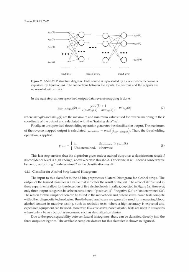
Sensors 2015, 15, 55–75

Figure 7. ANN-MLP structure diagram. Each neuron is represented by a circle, whose behavior isexplained by Equation (6). The connections between the inputs, the neurons and the outputs arerepresented with arrows.

In the next step, an unsupervised output data reverse mapping is done:

yrev−mapped(k) =yNN(k) + 1

2(maxr,t(k)− minr,t(k))+ minr,t(k) (7)

where maxr,t(k) and minr,t(k) are the maximum and minimum values used for reverse mapping in the k

coordinate of the output and calculated with the “training data” set.Finally, an unsupervised thresholding operation generates the classification output. The maximum

of the reverse mapped output is calculated: ycandidate = max(→

y rev−mapped

)

. Then, the thresholdingoperation is applied:

yclass =

k, ifycandidate ≥ ythres(k)

Undetermined, otherwise(8)

This last step ensures that the algorithm gives only a trained output as a classification result ifits confidence level is high enough, above a certain threshold. Otherwise, it will show a conservativebehavior, outputting “undetermined” as the classification result.

4.4.1. Classifier for Alcohol Strip Lateral Histograms

The input to this classifier is the 62-bin preprocessed lateral histogram for alcohol strips. Theoutput of the trained classifier is a value that indicates the result of the test. The alcohol strips used inthese experiments allow for the detection of five alcohol levels in saliva, depicted in Figure 2a. However,only three output categories have been considered: “positive (1)”, “negative (2)” or “undetermined (3)”.The reason for this simplification can be found in the market demand, where saliva-based tests competewith other diagnostic technologies. Breath-based analyzers are generally used for measuring bloodalcohol content in massive testing, such as roadside tests, where a high accuracy is expected andexpensive equipment can be used. However, low-cost saliva-based alcohol tests are used in situationswhere only a binary output is necessary, such as detoxification clinics.

Due to the good separability between lateral histograms, these can be classified directly into thethree output categories. The available complete dataset for this classifier is shown in Figure 8.

66

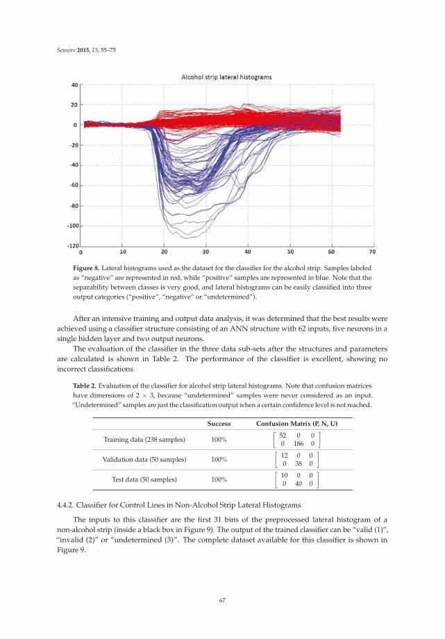
Sensors 2015, 15, 55–75

Figure 8. Lateral histograms used as the dataset for the classifier for the alcohol strip. Samples labeledas “negative” are represented in red, while “positive” samples are represented in blue. Note that theseparability between classes is very good, and lateral histograms can be easily classified into threeoutput categories (“positive”, “negative” or “undetermined”).

After an intensive training and output data analysis, it was determined that the best results wereachieved using a classifier structure consisting of an ANN structure with 62 inputs, five neurons in asingle hidden layer and two output neurons.

The evaluation of the classifier in the three data sub-sets after the structures and parametersare calculated is shown in Table 2. The performance of the classifier is excellent, showing noincorrect classifications.

Table 2. Evaluation of the classifier for alcohol strip lateral histograms. Note that confusion matriceshave dimensions of 2 × 3, because “undetermined” samples were never considered as an input.“Undetermined” samples are just the classification output when a certain confidence level is not reached.

Success Confusion Matrix (P, N, U)

Training data (238 samples) 100%[

52 0 00 186 0

]

Validation data (50 samples) 100%[

12 0 00 38 0

]

Test data (50 samples) 100%[

10 0 00 40 0

]

4.4.2. Classifier for Control Lines in Non-Alcohol Strip Lateral Histograms

The inputs to this classifier are the first 31 bins of the preprocessed lateral histogram of anon-alcohol strip (inside a black box in Figure 9). The output of the trained classifier can be “valid (1)”,“invalid (2)” or “undetermined (3)”. The complete dataset available for this classifier is shown inFigure 9.

67

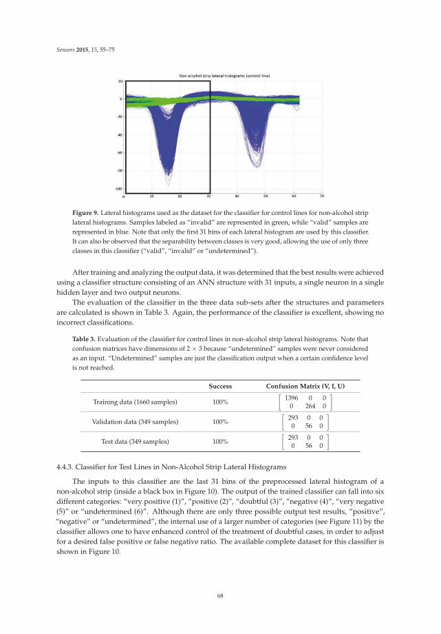
Sensors 2015, 15, 55–75

Figure 9. Lateral histograms used as the dataset for the classifier for control lines for non-alcohol striplateral histograms. Samples labeled as “invalid” are represented in green, while “valid” samples arerepresented in blue. Note that only the first 31 bins of each lateral histogram are used by this classifier.It can also be observed that the separability between classes is very good, allowing the use of only threeclasses in this classifier (“valid”, “invalid” or “undetermined”).

After training and analyzing the output data, it was determined that the best results were achievedusing a classifier structure consisting of an ANN structure with 31 inputs, a single neuron in a singlehidden layer and two output neurons.

The evaluation of the classifier in the three data sub-sets after the structures and parametersare calculated is shown in Table 3. Again, the performance of the classifier is excellent, showing noincorrect classifications.

Table 3. Evaluation of the classifier for control lines in non-alcohol strip lateral histograms. Note thatconfusion matrices have dimensions of 2 × 3 because “undetermined” samples were never consideredas an input. “Undetermined” samples are just the classification output when a certain confidence levelis not reached.

Success Confusion Matrix (V, I, U)

Training data (1660 samples) 100%[

1396 0 00 264 0

]

Validation data (349 samples) 100%[

293 0 00 56 0

]

Test data (349 samples) 100%[

293 0 00 56 0

]

4.4.3. Classifier for Test Lines in Non-Alcohol Strip Lateral Histograms

The inputs to this classifier are the last 31 bins of the preprocessed lateral histogram of anon-alcohol strip (inside a black box in Figure 10). The output of the trained classifier can fall into sixdifferent categories: “very positive (1)”, “positive (2)”, “doubtful (3)”, “negative (4)”, “very negative(5)” or “undetermined (6)”. Although there are only three possible output test results, “positive”,“negative” or “undetermined”, the internal use of a larger number of categories (see Figure 11) by theclassifier allows one to have enhanced control of the treatment of doubtful cases, in order to adjustfor a desired false positive or false negative ratio. The available complete dataset for this classifier isshown in Figure 10.

68

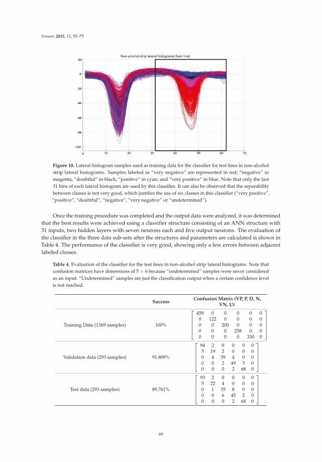
Sensors 2015, 15, 55–75

Figure 10. Lateral histogram samples used as training data for the classifier for test lines in non-alcoholstrip lateral histograms. Samples labeled as “very negative” are represented in red; “negative” inmagenta; “doubtful” in black; “positive” in cyan; and “very positive” in blue. Note that only the last31 bins of each lateral histogram are used by this classifier. It can also be observed that the separabilitybetween classes is not very good, which justifies the use of six classes in this classifier (“very positive”,“positive”, “doubtful”, “negative”, “very negative” or “undetermined”).

Once the training procedure was completed and the output data were analyzed, it was determinedthat the best results were achieved using a classifier structure consisting of an ANN structure with31 inputs, two hidden layers with seven neurons each and five output neurons. The evaluation ofthe classifier in the three data sub-sets after the structures and parameters are calculated is shown inTable 4. The performance of the classifier is very good, showing only a few errors between adjacentlabeled classes.

Table 4. Evaluation of the classifier for the test lines in non-alcohol strip lateral histograms. Note thatconfusion matrices have dimensions of 5 × 6 because “undetermined” samples were never consideredas an input. “Undetermined” samples are just the classification output when a certain confidence levelis not reached.

SuccessConfusion Matrix (VP, P, D, N,

VN, U)

Training Data (1369 samples) 100%

⎡

⎢

⎢

⎢

⎢

⎣

459 0 0 0 0 00 122 0 0 0 00 0 200 0 0 00 0 0 258 0 00 0 0 0 330 0

⎤

⎥

⎥

⎥

⎥

⎦

Validation data (293 samples) 91.809%

⎡

⎢

⎢

⎢

⎢

⎣

94 2 0 0 0 05 19 2 0 0 00 4 39 4 0 00 0 2 49 3 00 0 0 2 68 0

⎤

⎥

⎥

⎥

⎥

⎦

Test data (293 samples) 89.761%

⎡

⎢

⎢

⎢

⎢

⎣

93 2 0 0 0 05 22 4 0 0 00 1 35 8 0 00 0 6 45 2 00 0 0 2 68 0

⎤

⎥

⎥

⎥

⎥

⎦

69

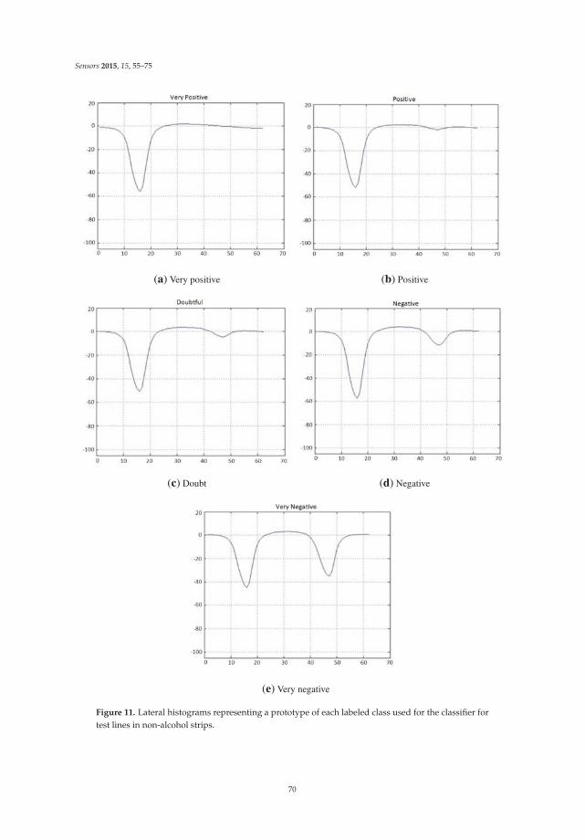
Sensors 2015, 15, 55–75

(a) Very positive (b) Positive

(c) Doubt (d) Negative

(e) Very negative

Figure 11. Lateral histograms representing a prototype of each labeled class used for the classifier fortest lines in non-alcohol strips.

70

Sensors 2015, 15, 55–75

5. System Evaluation Methodology

A study was conducted by an external company to verify the performance of the application withregards to the two following aspects:

• Verify the agreement between visual results obtained by human operators and those obtained bythe test reader (agreement).

• Check the repeatability of the results interpreted by the test reader (precision).

The following values should be established as an outcome of the testing:

1. Provide the number of cases (%) in which the results obtained by the test reader agreed with theinterpretation made by an operator by visual interpretation, on a given representative samplesize (N) (at least two or three independent operators should be considered, to minimize bias orthe impact of subjectivity).

2. Provide the number of cases (%) in which the test reader is able to repeat the same result (positive,negative or invalid) when interpreting any test, given a representative sample size (N).

Ninety SalivaScan double-sided tests were used (detection of six drugs + alcohol in oral fluid)with the following configuration: amphetamine, ketamine, cocaine and methamphetamine on one sideand opiates, marijuana and alcohol on the other side, with the cutoff levels indicated in Table 1. Threedetection levels were considered: negative, cutoff and 3× cutoff (saliva controls with three-times thecutoff concentration level).

In order to simulate the concentration on each detection level, positive and negative standardsaliva controls were used. Such controls were sourced from Synergent Biochem Inc. ( HawaiianGardens, CA, USA) [24].

The visual and automated results obtained for the alcohol (ALC) strip were not recorded, as theinterpretation for the results is made by comparison of the color changes in the reagent pad against apattern and not by the interpretation of the control and test lines.

The results interpreted by the test reader were extracted using an iPhone 4 (partial test) and aniPhone 4S (full test), both running iOS Version 6.1.3.

5.1. Agreement Test

In the agreement test, the results of 30 tests per detection level were considered. Two humanoperators made the visual interpretation of the results obtained on each test, and the second operatorobtained a result using the test reader in addition to his or her own interpretation. Each operatorwould log the results independently from each other. The detailed steps followed on each test werethe following:

1. The reaction on each test was started after adding the corresponding positive or negative controldepending on the cutoff level being tested.

2. Operator 1 waited 10 min for incubation of the result, interpreted it and logged the test outcome.3. Operator 2 interpreted the visual result, independently from Operator 1, and logged the

test outcome.4. Operator 2 interpreted the result using the test reader and logged the result.

A retest was performed at the negative and 3× detection levels, using a different lot. On eachlevel, 20 tests were performed.

5.2. Precision Test

Test devices from the agreement evaluation were randomly selected, three tests from eachdetection level (negative, cutoff, 3×). Test 1 corresponds to an (amphetamine (AMP), ketamine(KET), cocaine (COC), methamphetamine (MET)) configuration, while Tests 2 and 3 had an (opiates(OPI), THC, ALC) configuration. Each of these tests was processed 40 times repeatedly.

71

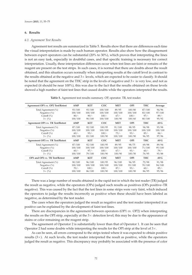
Sensors 2015, 15, 55–75

6. Results

6.1. Agreement Test Results

Agreement test results are summarized in Table 5. Results show that there are differences each timethe visual interpretation is made by each human operator. Results also show how the disagreementbetween expert operators can be substantial (20% to 30%), which proves that interpreting the linesis not an easy task, especially in doubtful cases, and that specific training is necessary for correctinterpretation. Usually, these interpretation differences occur when test lines are faint or remains of thereagent are present on the test strips. In such cases, it is normal that there are doubts about the resultobtained, and this situation occurs normally when interpreting results at the cutoff level in contrast tothe results obtained at the negative and 3× levels, which are expected to be easier to classify. It shouldbe noted that the agreement on the THC strip in the levels of negative and 3× is very low, and not asexpected (it should be near 100%), this was due to the fact that the results obtained on those levelsshowed a high number of faint test lines that caused doubts while the operators interpreted the results.

Table 5. Agreement test results summary. OP, operator. TR, test reader.

Agreement OP1 vs. OP2 Test/Retest AMP KET COC MET OPI THC Average

Total Agreement (%) 93/100 93/100 100/100 89/95 100/80 87/100 94/96Negative (%) 100/100 100/100 100/100 100/100 100/100 83/100 97/100

Cutoff (%) 80/- 90/- 100/- 67/- 100/- 97/- 89/-3× (%) 100/100 90/100 100/100 100/90 100/60 80/100 95/92

Agreement OP1 vs. TR Test/Retest AMP KET COC MET OPI THC AVG


Cutoff (%) 60/- 93/- 100/- 73/- 93/- 85/- 84/-3× (%) 100/100 83/100 100/90 100/100 100/90 96/95 97/96

Agreement OP2 vs. TR Test/Retest AMP KET COC MET OPI THC AVG


Cutoff (%) 60/- 97/- 100/- 67/- 93/- 60/- 79/-3× (%) 100/100 79/100 100/90 100/90 100/50 76/95 93/88

OP1 and OP2 vs. TR Test/Retest AMP KET COC MET OPI THC AVG


Cutoff (%) 70/- 100/- 100/- 87/- 93/- 60/- 85/-3× (%) 100/100 86/100 100/90 100/100 100/90 86/95 95/96

There was a large number of results obtained in the rapid test in which the test reader (TR) judgedthe result as negative, while the operators (OPs) judged such results as positives (OPs positive–TRnegative). This was caused by the fact that the test lines in some strips were very faint, which inducedthe operators to judge the results incorrectly as positive when these should have been labeled asnegative, as determined by the test reader.

The cases when the operators judged the result as negative and the test reader interpreted it aspositive can be explained by the development of faint test lines.

There are discrepancies in the agreement between operators (OP1 vs. OP2) when interpretingthe results on the OPI strip, especially at the 3× detection level; this may be due to the appearance ofstains or color remaining on the reagent strip.

The agreement of Operator 2 is substantially lower than that of Operator 1. It can be seen thatOperator 2 had some doubts while interpreting the results for the OPI strip at the level of 3×.

As can be seen, all errors correspond to the strips tested where it was expected to obtain positiveresults (3×). At such levels, the test reader interpreted the result as positive, while the operatorsjudged the result as negative. This discrepancy may probably be associated with the presence of color

72

Sensors 2015, 15, 55–75

remaining on the strip, which might give the impression to the operators of a test line, while such linesdid not have the typical characteristics to be considered as test lines.

The cases in which both operators did not agree on the results obtained by the test reader can beclassified in the categories shown in Table 6, as well as the results as a percentage of the total numberof strips evaluated.

Table 6. Disagreement and adjusted agreement test results summary.

Both Operators vs.Test Reader

AMP KET COC MET OPI THC Total

Disagreements OPsnegative–TR positive count

(%)/retest count (%)0 (0)/0 (0) 0 (0)/0 (0) 0 (0)/2 (5) 0 (0)/0 (0) 0 (0)/2 (5) 3 (3)/1 (3) 3 (1)/5 (2)

Disagreements OPspositive–TR negative count

(%)/retest count (%)9 (10)/0 (0) 4 (4)/0 (0) 0 (0)/0 (0) 4 (4)/0 (0) 2 (2)/0 (0)

20 (22)/0(0)

39 (7)/0 (0)

Disagreements TR error count(%)/retest count (%)

0 (0)/0 (0) 0 (0)/0 (0) 0 (0)/0 (0) 0 (0)/0 (0) 2 (2)/0 (0) 2 (2)/0 (0) 4 (1)/0 (0)

Total disagreementscount/retest count

9/0 4/0 0/2 4/0 4/2 25/1 46/5

Total adjusted agreement(%)/retest (%)

100/100 100/100 100/95 100/100 98/95 94/98 99/98

Total test count/retest count 89/40 89/40 89/40 89/40 89/40 89/40 534/240

Excluding the cases in which the operators indicated positive when the test reader indicatednegative and counting them as interpretation errors attributable to the operators, the total adjustedagreement (excluding cases when OPs positive and TR negative) has been computed and is shown inTable 6.

6.2. Precision Test Results

The results indicated in Table 7 were obtained once the tests were processed repeatedly usingthe test reader for each detection level. The cases in which the test reader interpreted the result as“negative” when the operator interpreted it as “positive” correspond to strips showing very faint testlines, especially at “cutoff Test 1” and “3× Test 1” on the strips KET and OPI.

Table 7. Precision test results.

Detection Level No. TestsNo. Strips per

SideTotal Strips 1

No. of Times That TRGave The Same Result

for a Given Strip 2Precision (%)

Negative test 1/2/3 40/40/40 4/2/2 156/78/78 156/78/78 100/100/100Precision for negative 312 312 100

Cutoff test 1/2/3 40/40/40 4/2/2 160/80/80 149/78/71 93/98/89Precision for cutoff 320 298 94

3× test 1/2/3 40/40/40 4/2/2 156/80/80 137/80/80 88/100/100Precision for 3× 316 297 94

Total 360 948 907 961 Total number of strips correctly interpreted; invalid strips or errors excluded; 2 in the case of different results,the maximum value was taken.

7. Conclusions

An innovative, low-cost, portable approach for the rapid interpretation of lateral flow salivatest results in drug-of-abuse detection based on the use of commonly-available smartphone deviceshas been presented and evaluated. A small inexpensive light box is used to control image qualityparameters during the acquisition. This solution reuses an existing smartphone, and there is no

73

Sensors 2015, 15, 55–75

additional equipment needed, besides the light box, which costs a fraction of the price for similarproducts on the market, with prices ranging around 3000 EUR/device. In order to segment thestrips, images are first pre-processed to correct for small displacements and/or rotations withan ORB feature-based matching and homography strategy, and the strips corresponding to thedifferent substances to be detected are segmented using color features and morphological operations.Finally, a lateral histogram containing the saliva test lines’ intensity profile is extracted. Lateralhistograms are then classified with a machine learning-based procedure, including unsupervised datanormalization and classification using a multilayer perceptron artificial neural network (MLP-ANN).The implemented solution can be adapted to any line-based or color-based lateral flow test onthe market. System agreement and precision tests were run for system evaluation, showing greatagreement between the visual results obtained by human operators and those obtained by the testreader app, while showing high repeatability. The objective of the work is to demonstrate that thetest reader is able to obtain the same result (or better) than a trained operator, therefore reducingthe subjectivity of the analysis by standardizing the test interpretation conditions (illumination, testto image sensor distance, etc.) and by using a deterministic algorithm to obtain the results. In thissense, any operator independent of his/her level of experience can rely on the results obtained bythe test reader. The system is automatic, allowing one to systematize the collection and analysis ofthe data in real time, removing the risks of manual results’ management and allowing for centralizedprocessing. The mentioned features can be very useful in places where there is no qualified staff andrapid detection is needed, such as on-site detection performed by a police officer or a first-aid operator.

Author Contributions: All authors have contributed to the development of the work presented in this paper, andthey are its sole intellectual authors, all collaborating tightly in several parts for the final success of the system.Carlos Sampedro has been responsible for the computer vision part. Jose Luis Sanchez-Lopez has been responsiblefor the machine learning algorithms. Adrian Carrio has been responsible for the software and system integration.Miguel Pimienta has staged the problem and final objectives of the system. He has developed the light box, alsoproviding the samples, and has been responsible for the external evaluation process. Pascual Campoy has actedas the general supervisor of the technical development of the project.

Conflicts of Interest: The system has been developed under a private contract between the company VincilabHealthcare S.L. (Madrid, Spain) and the Universidad Politécnica de Madrid (UPM). The resulting procedure andsystem are patent pending, and the exploitation of their results is shared by the two companies split from theoriginal one, named Vincilab Healthcare S.L. and Aplitest Solutions S.L. (Madrid, Spain), both retaining all of theindustrial rights.

References

1. Martinez, A.W.; Phillips, S.T.; Carrilho, E.; Thomas, S.W.; Sindi, H.; Whitesides, G.M. Simple telemedicine fordeveloping regions: Camera phones and paper-based microfluidic devices for real-time, off-site diagnosis.Anal. Chem. 2008, 80, 3699–3707. [CrossRef] [PubMed]

2. Tseng, D.; Mudanyali, O.; Oztoprak, C.; Isikman, S.O.; Sencan, I.; Yaglidere, O.; Ozcan, A. Lensfreemicroscopy on a cellphone. Lab Chip 2010, 10, 1787–1792. [CrossRef] [PubMed]

3. Zhu, H.; Yaglidere, O.; Su, T.W.; Tseng, D.; Ozcan, A. Cost-effective and compact wide-field fluorescentimaging on a cell-phone. Lab Chip 2011, 11, 315–322. [CrossRef] [PubMed]

4. Zhu, H.; Sikora, U.; Ozcan, A. Quantum dot enabled detection of Escherichia coli using a cell-phone. Analyst

2012, 137, 2541–2544. [CrossRef] [PubMed]5. Matthews, J.; Kulkarni, R.; Gerla, M.; Massey, T. Rapid dengue and outbreak detection with mobile systems

and social networks. Mob. Netw. Appl. 2012, 17, 178–191. [CrossRef]6. Dell, N.L.; Venkatachalam, S.; Stevens, D.; Yager, P.; Borriello, G. Towards a point-of-care diagnostic system:

Automated analysis of immunoassay test data on a cell phone. In Proceedings of the 5th ACM Workshop onNetworked Systems for Developing Regions, New York, NY, USA, 28 June 2011; pp. 3–8.

7. Mudanyali, O.; Dimitrov, S.; Sikora, U.; Padmanabhan, S.; Navruz, I.; Ozcan, A. Integratedrapid-diagnostic-test reader platform on a cellphone. Lab Chip 2012, 12, 2678–2686. [CrossRef] [PubMed]

74

Sensors 2015, 15, 55–75

8. Mudanyali, O.; Padmanabhan, S.; Dimitrov, S.; Navruz, I.; Sikora, U.; Ozcan, A. Smart rapid diagnosticstest reader running on a cell-phone for real-time mapping of epidemics. In Proceedings of the SecondACM Workshop on Mobile Systems, Applications, and Services for HealthCare, Toronto, ON, Canada,6–9 November 2012.

9. Shen, L.; Hagen, J.A.; Papautsky, I. Point-of-care colorimetric detection with a smartphone. Lab Chip 2012, 12,4240–4243. [CrossRef] [PubMed]

10. Oncescu, V.; O’Dell, D.; Erickson, D. Smartphone based health accessory for colorimetric detection ofbiomarkers in sweat and saliva. Lab Chip 2013, 13, 3232–3238. [CrossRef] [PubMed]

11. De la Fuente, J.B.; Garcia, M.P.; Cueli, J.G.; Cifuentes, D. A new low-cost reader system for ELISA plates basedon automated analysis of digital pictures. In Proceedings of the IEEE Instrumentation and MeasurementTechnology Conference, Sorrento, Italy, 24–27 April 2006; pp. 1792–1794.

12. Velikova, M.; Lucas, P.; Smeets, R.; van Scheltinga, J. Fully-automated interpretation of biochemical tests fordecision support by smartphones. In Proceedings of the 25th International Symposium on Computer-basedMedical Systems, Roma, Italy, 20–22 June 2012; pp. 1–6.

13. DrugCheck VeriCheck. Available online: http://www.drugcheck.com/dc_vericheck.html (accessed on22 November 2015).

14. Securetec DrugRead. Available online: http://www.securetec.net/en/products/drug-test/drugread-device.html (accessed on 22 November 2015).

15. DrugCheck SalivaScan. Available online: http://www.drugcheck.com/dc_salivascan.html (accessed on22 November 2015).

16. Rublee, E.; Rabaud, V.; Konolige, K.; Bradski, G. ORB: An efficient alternative to SIFT or SURF. In Proceedingsof the IEEE International Conference on Computer Vision, Barcelona, Spain, 6–13 November 2011;pp. 2564–2571.

17. Rosten, E.; Drummond, T. Machine Learning for High-Speed Corner Detection. In Computer Vision–ECCV

2006; Springer: Berlin, Germany, 2006; pp. 430–443.18. Rosten, E.; Porter, R.; Drummond, T. Faster and better: A machine learning approach to corner detection.

IEEE Trans. Pattern Anal. Mach. Intell. 2010, 32, 105–119. [CrossRef] [PubMed]19. Calonder, M.; Lepetit, V.; Strecha, C.; Fua, P. Brief: Binary Robust Independent Elementary Features.

In Computer Vision–ECCV 2010; Springer: Berlin, Germany, 2010; pp. 778–792.20. Hamming, R.W. Error detecting and error correcting codes. Bell Syst. Tech. J. 1950, 29, 147–160. [CrossRef]21. Fischler, M.A.; Bolles, R.C. Random sample consensus: A paradigm for model fitting with applications to

image analysis and automated cartography. Commun. ACM 1981, 24, 381–395. [CrossRef]22. Otsu, N. A threshold selection method from gray-level histograms. IEEE Trans. Systems Man Cybern. 1979, 9,

62–66.23. Cybenko, G. Approximation by superpositions of a sigmoidal function. Math. Control Signals Syst. 1989, 2,

303–314. [CrossRef]24. Synergent Biochem Inc. Homepage. Available online: http://www.synergentbiochem.com (accessed on 22

November 2015).


75

sensors

Article

Implementation of Context Aware e-HealthEnvironments Based on Social Sensor NetworksErik Aguirre 1, Santiago Led 1, Peio Lopez-Iturri 1, Leyre Azpilicueta 2, Luís Serrano 1

and Francisco Falcone 1,*1 Electrical and Electronic Engineering Department, Public University of Navarre, Pamplona 31006, Spain;

[email protected] (E.A.); [email protected] (S.L.); [email protected] (P.L.-I.);[email protected] (L.S.)

2 School of Engineering and Sciences, Tecnologico de Monterrey, Monterrey 64849, Mexico;[email protected]

* Correspondence: [email protected]; Tel.: +34-948-169-741; Fax: +34-948-169-720

Academic Editor: Gonzalo Pajares MartinsanzReceived: 23 December 2015; Accepted: 24 February 2016; Published: 1 March 2016

Abstract: In this work, context aware scenarios applied to e-Health and m-Health in the frameworkof typical households (urban and rural) by means of deploying Social Sensors will be described.Interaction with end-users and social/medical staff is achieved using a multi-signal input/outputdevice, capable of sensing and transmitting environmental, biomedical or activity signals andinformation with the aid of a combined Bluetooth and Mobile system platform. The devices, whichplay the role of Social Sensors, are implemented and tested in order to guarantee adequate servicelevels in terms of multiple signal processing tasks as well as robustness in relation with the usewireless transceivers and channel variability. Initial tests within a Living Lab environment have beenperformed in order to validate overall system operation. The results obtained show good acceptanceof the proposed system both by end users as well as by medical and social staff, increasing interaction,reducing overall response time and social inclusion levels, with a compact and moderate cost solutionthat can readily be largely deployed.

Keywords: social sensors; wireless body area networks; deterministic radio planning; back office

1. Introduction

Population ageing is unprecedented, without parallel in human history—and the twenty-firstcentury will witness even more rapid ageing than did the century just past [1]. This global phenomenonis affecting the whole world, although with different evolution rates of the process, depending onregions or countries. In any case, the main goal for the future is to ensure people everywhere will beageing actively, making possible their participation in social activities without any restrictions.

Hence, to reach the above challenge, an embedded Social-Health care action or strategy wherecitizen empowerment should be the solution’s central point is mandatory [2]. This strategy must takeinto account all personal and context factors such as personal health, work and economic situation,social networks, etc. that affect active aging and assisted living processes. This Social-Health carestrategy should be based on massive use of Information and Communication Technologies (ICT) formaking possible a service deployment with several main features as cost-effective, plug and playoperation, minimal user’s intervention, and helpful for the largest number of citizens.

Adopted ICT Social-Health care solutions could be included in two possible scenarios [3]. On theone hand, indoor monitoring scenarios, so-called home monitoring is defined where the user’s state iscontrolled at his or her own residence. These scenarios provide more real information about the userdue to the fact that the remote control process is achieved at a comfortable and regular environment.


Sensors 2016, 16, 310

On the other hand, outdoor monitoring scenarios that include all situations where the user is awayfrom home (office, walking on street, gym, etc.) and is also continuously monitored. These scenariosprovide mobility to the user while the control process is performed. In both scenarios, the devices(for medical or behavioral monitoring), are portable or wearable, general purpose, and user-friendly.Moreover, they are equipped with short range (Bluetooth, Zigbee, IrDA, etc.) and/or large range(GSM-GPRS, UMTS, etc.) wireless technologies.

Currently, the use of Wireless Sensor Networks (WSN) continues to grow in a wide variety ofapplication fields [4–6], such as agriculture and farming [7], infrastructure state monitoring [8], locationand guiding [9], vehicular communications [10] and healthcare monitoring [11,12], to name a few.The future trend seems to be the increase of the number of wireless nodes in order to collect moreinformation from the surrounding environment, bringing the Internet of Things (IoT) to our daily life.

Among WSNs, Mobile Ad-hoc Networks (MANET) have attracted the attention of many researchgroups around the world, becoming popular due to the unique characteristics they provide: wirelessmobile devices with limited resources that can exchange information with each other without any fixedinfrastructure. Thus, MANETs provide easier deployment, system maintenance and upgrade. Thesecharacteristics make MANETs an adequate solution to solve efficiently many applications, as is the caseof the telemedicine and healthcare system presented in this work. In fact, in the literature can be foundseveral works of MANETs applied to healthcare environments, such as hospital and big in-buildingenvironments [13], tele-emergency projects [14], tele-care and telemedicine systems [15,16], real timemedical data acquisition and patient monitoring systems [17–19], and more specific applications suchas tele-cardiology [20], emergency telemedicine system in disaster areas [21] and monitoring combatsoldiers [22].

In Spain, the Social-Sanitary System term (in Spanish “Sistema Socio-Sanitario”) makes reference tothe public or private healthcare system focused on guaranteeing the best population’ state regardinggeneral aspects as life quality, well-being, and social integration. Meanwhile, the Sanitary termmakes reference to the healthcare system part responsible for solving physiological and psychologicalproblems suffered by the population. The Social term includes all the aspects associated withpopulation social problems such as loneliness, integration into the society, energy poverty, populationageing, among others; problems that require specific healthcare professionals like social workers orassistants. The Social-Sanitary System concept is deeply adopted by Spanish population.

Social problems suffered by population can be detected and monitored in the same way asclinical diseases. Thus, it is required to know the user’s social state by means of specific devices andsensors responsible for acquiring outstanding parameters associated to daily activity, habits, and ingeneral any information that makes possible to work a social problem out. In this sense, environmentmeasurements are combined with information related with user behavior, providing additional insightinto the socio-sanitary context of the user; e.g., water consumption, electricity and gas consumption,operation time of HVAC (heating, ventilating and air conditioning) system, open/close status ofdoors and windows, among many others. Thus, water consumption can provide information aboutfrequency the user goes to the toilet or takes a shower. A very low consumption can indicate the usersuffers some degenerative disease or poverty situation. Electricity/gas consumption together withoperation time of HVAC system can indicate the user is in energy poverty situation; if the user doesnot have enough resources for operating HVAC system during a suitable time period, the consumptionvalues will be very low compared to average value. Because all these problems have a social natureand they must be treated by social workers and assistants, the sensors used to acquire their associatedinformation are called social sensors throughout this paper.

In general, social sensors are environmental acquisition devices that require minimum userintervention, and for this reason, they are placed at previously established locations; ceiling fortemperature/humidity sensors, doors and windows for open–close detection, sink pipe for waterconsumption sensors, etc. Social sensors exhibit reduced size, wireless communication capabilities,and minimum current consumption allowing them to be battery powered and highly operation

77

Sensors 2016, 16, 310

autonomous; this feature allows the reduction of maintenance service costs. Moreover, social sensorsmust ensure the lowest visual and structural impact when embedded within the planned servicescenario. Personal health devices show features similar to social sensors. However, they do have greatervariety concerning form factor and location within the monitoring scenario. Some health devices likeweigh scale, blood pressure monitor, and glucose meter could be used only a few times every dayand they do not require to be worn by the user all the time. Thus, these devices could be portablesensors always located at the same living space, mainly bathroom and bedroom; when a biomedicalmeasurement must be taken, the user goes to the living space where the medical device remains anduses it. Other health devices like electrocardiogram monitors require a real time monitoring processand they must be worn by the user. These devices must be wearable sensors and their location insidethe monitoring scenario is not fixed, but changes as the user moves.

With regards to ICT, there is no implementation difference between health and socialsensors because they require similar functional blocks: analog front-end (AFE), A/D conversion,microprocessor, power supply, and wireless communication. The resources provided by theseblocks are conveniently used according to the sensor type, intelligent-processing needs, autonomyrequirements, etc. This solution is currently being used for ICT Social-Health care service in Navarra (inSpanish “Navarra-ASISte-TIC”, NASISTIC) project deployment [22] as a proof of concept of an integralSocial-Healthcare system monitored by Red Cross in Navarra, and focused mainly on providinghigh-quality services to vulnerable citizens like the elderly or people suffering mental illnesses.Moreover, Navarra region shows an exceptional scenario for this deployment because it includespopulations living in a medium-size city, Pamplona, as well as sparse citizens living in rural andmountain surroundings.

The novelty of the proposal presented within this work is focused in the development of IntegratedSocio-Sanitary Services based on Information and Communication Technologies and with minimaluser interaction, providing integral user care given by inherent interdependence between Health andSocial Environment. In the context of elderly persons, a main target of the system (with elementssuch as dependence, loneliness, assisted living, etc.), this combined rollout is of particular importance,because degradation of health state can be caused by the degradation of the social context (energeticpoverty, poor nutrition, cleanliness, etc.) and vice versa. In this way, deployments such as NASISTICare of special interest in order to provide integral control of elderly people, people in risk of socialexclusion, chronic patients, among others.

In this work, the implementation of Social Sensor devices and their application to e-Healthmonitoring within the framework of an urban scenario, given by project NASISTIC in Navarra, Spain,will be analyzed. Different considerations of physical implementation of the devices, consideringmultiple signal capability as well as usability factors (such as ergonomics and power consumption)will be analyzed. The usability and performance of the devices are strongly dependent on thebehavior and influence of wireless transceivers, which are analyzed by deterministic techniques,providing assessment in the configuration of individual nodes as well as in the location and number oftransceivers as a function of the scenario. The developed sensors will then be tested in a living labconfiguration, which serves as the base for a future full-scale deployment.

The paper is structured as follows: Section 2 describes the architecture and functionality of theSocial Sensor Devices, based on a multi signal Input/Output controller in which different sensors canpotentially be implemented. Section 3 analyzes the impact of the wireless channel behavior, whichis a key parameter to evaluate overall performance of the Social Sensor devices in terms of mobility,security and quality of the exchanged information, as well as on the design of individual nodes andlayout of node network architecture. In Section 4, initial tests within a Living Lab framework aredescribed, providing insight in complete system operation and the potential full-scale deployment.Finally, Section 5 provides conclusions and final remarks of the work.

78

Sensors 2016, 16, 310

2. Related Work

Different solutions based on multiple sensor platforms and configurations have been proposedin order to implement remote health-monitoring, diagnostics and medical services, with specialinterest in the past decade [23–25], due to their capability of reducing overall costs and increasingquality of life metrics. Solutions have been provided in the context of application of Information andCommunication Technologies in order to allow system interoperability and enhance medical service,by means of solutions such as electronic patient records or digital image records, to name a few. A stepfurther is achieved by adding mobility to previous e-Health scenarios, by means of integration ofmobile terminals, connected to Public Land Mobile Networks (PLMN), allowing initial tele-monitoringcapabilities. Other solutions, such as advanced care and alert portable telemedical monitor (AMON)project [26] employed GSM transmission links to communicate a wrist wearable device, with capabilityof measuring multiple signals, such as Electrocardiograms (ECG), Electromyograms (EMG), locationor skin conductance. Cordless phones have also been employed as transmitter device, to which aspecialized sensor unit was connected, implementing a real time wireless physiological monitoringsystem [27]. Prior to the popularization of Smart Phones, several solutions employed PersonalDigital Assistants (PDA), with basic control functions of multiple sensor devices connected to sensorboards [28].

One of the main drivers in order to increase system interactivity is the use of compact sizebiomedical sensors, which can communicate in real time with medical specialists or social services,or can perform data-logging functions in order to store and send the relevant information later.In this sense, communication systems shift from PLMN based systems to Wireless Personal AreaNetwork/Body Area Network devices, with predominance in the use of 802.15.4 standards, such asBluetooth or ZigBee [23]. The main benefit in this approach is the inherent capability of connectingmultiple devices, small size and reduced energy consumption as compared with PLMN/WirelessLocal Area Network (WLAN) solutions.

Another relevant aspect in the adoption of remote health monitoring solutions is the advancein the implementation of sensors as well as the capability of embedding them in truly wearableconfigurations. In this sense, it is possible to measure multiple bio-physical parameters, such asglucose levels, blood pressure, oxygen saturation, respiration rate, ECG, and EMG, which can becombined with environmental parameters and user movement and location. The use of the combinedinformation of these multiple sensors and sources leads to truly context aware Ambient AssistedLiving (AAL) scenarios, with multiple solutions reported [23]. A following step in system integrationis embedding sensors in textiles within user garments, in order to increase ergonomics as well asin depth user monitorization. Different solutions have been proposed, such as the MagIC vest orthe MyHeart instrumented shirt, in which multiple sensor elements have been included within theclothing [29–33]. As a further step, specific software development frameworks, such as SPINE, havebeen proposed and multiple Body Sensor Network applications have also been proposed, such asrehabilitation, Gait analysis, emotional stress detection or handshake detection, to name a few [34].Table 1 presents a comparison of different remote health monitoring systems.

79

Sensors 2016, 16, 310

Tab

le1.

Hea

lth

mon

itor

ing

syst

emco

mp

aris

on.

Sys

tem

Tran

smis

sion

Sys

tem

Arc

hit

ectu

reA

pp

lica

tion

Sce

nar

ioD

etec

ted

Var

iab

les

Ref

eren

ce

Liv

eNE

TP

DA

Con

nect

ivit

yC

entr

aliz

edD

etec

tion

ofE

pile

psy

Seiz

ure

,P

arki

nson

sym

pto

md

etec

tion

,So

ldie

rH

ealt

hM

onit

orin

g

3DA

ccel

erom

eter

,EC

G,E

MG

,ga

lvan

icsk

inco

ndu

ctan

ce[2

5]

AM

ON

Wri

stbr

acel

et,G

SMO

per

ator

Bas

edE

stim

atio

nof

Pat

ient

Hea

lth

Con

dit

ions

Blo

odP

ress

ure

,Blo

odSa

tura

tion

,Ski

nTe

mp

erat

ure

,E

CG

[26]

Lif

eGu

ard

Blu

etoo

thto

aba

sest

atio

nC

entr

aliz

edM

ult

ipar

amet

erW

eara

ble

Mon

itor

ing

Syst

em

EC

G,r

esp

irat

ion

rate

,hea

rtra

te,o

xyge

nsa

tura

tion

,bod

yte

mp

erat

ure

,blo

odp

ress

ure

,bo

dy

mov

emen

t.

[28]

Rea

lTim

eW

irel

ess

Phy

siol

ogic

alM

onit

orin

gSy

stem

Low

Pow

erC

ord

less

Pho

neTo

Bas

eSt

atio

nC

entr

aliz

edSy

stem

Aid

inN

urs

ing

Cen

ters

and

Hos

pit

als

Blo

odP

ress

ure

,Hea

rtR

ate

and

Tem

per

atu

re[2

7]

Bra

inIn

jury

Mon

itor

ing

Syst

emB

luet

ooth

toH

ome

PC

Cen

tral

ized

Mon

itor

ing

ofB

rain

Inju

red

Infa

nts

Blo

odSa

tura

tion

,Hea

rtR

ate,

Res

pir

atio

n,B

ody

Mov

emen

t.[2

9]

MyH

eart

Com

mu

nica

tion

toD

ata

Log

ger

Off

-lin

e

Wea

rabl

eSy

stem

for

Hea

rtD

isea

seM

onit

orin

g.Se

nsor

skn

itte

dor

embe

dd

edin

garm

ent.

EC

G,A

ctiv

ity

Sens

or.

[30]

Wea

rabl

eH

ealt

hC

are

Syst

em(W

EA

LTH

Y)

Blu

etoo

th/

GP

RS

Cen

tral

ized

orD

atal

ogge

r

Ap

plic

atio

nto

clin

ical

pat

ient

sd

uri

ngre

habi

litat

ion,

eld

erly

peo

ple

,pat

ient

sw

ith

chro

nic

dis

ease

s

EC

G,E

MG

,tho

raci

can

dab

dom

inal

resp

irat

ion

rate

,bo

dy

pos

itio

n,m

ovem

ent

[31]

Mag

ICB

luet

ooth

Cen

tral

ized

Wov

ente

xtile

sens

ors

ina

was

habl

eve

stE

CG

,res

pir

atio

nra

te,

mot

ion

leve

l.[3

2]

Med

ical

Rem

ote

Mon

itor

ing

ofC

loth

es(M

ER

MO

TH

)R

FL

ink

toP

DA

Dat

aL

ogge

rW

eara

ble

and

Stre

tcha

ble

Sens

ing

Gar

men

t

EC

G,r

esp

irat

ory

ind

uct

ance

ple

thys

mog

rap

hy,s

kin

tem

per

atu

re,a

ctiv

ity.

[33]

NA

SIST

ICB

luet

ooth

/2G

-4G

Con

nect

ion

Loc

ally

Dis

trib

uted

/Cen

tral

ized

Soci

alSe

nsor

Nod

eD

eplo

ymen

tsC

ombi

nati

onof

Bio

phy

sica

lsi

gnal

s(E

CG

)wit

hu

ser

habi

ts.

80

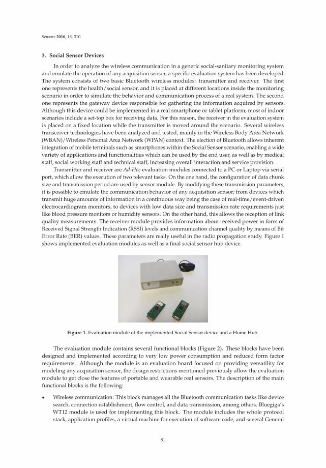
Sensors 2016, 16, 310

3. Social Sensor Devices

In order to analyze the wireless communication in a generic social-sanitary monitoring systemand emulate the operation of any acquisition sensor, a specific evaluation system has been developed.The system consists of two basic Bluetooth wireless modules: transmitter and receiver. The firstone represents the health/social sensor, and it is placed at different locations inside the monitoringscenario in order to simulate the behavior and communication process of a real system. The secondone represents the gateway device responsible for gathering the information acquired by sensors.Although this device could be implemented in a real smartphone or tablet platform, most of indoorscenarios include a set-top box for receiving data. For this reason, the receiver in the evaluation systemis placed on a fixed location while the transmitter is moved around the scenario. Several wirelesstransceiver technologies have been analyzed and tested, mainly in the Wireless Body Area Network(WBAN)/Wireless Personal Area Network (WPAN) context. The election of Bluetooth allows inherentintegration of mobile terminals such as smartphones within the Social Sensor scenario, enabling a widevariety of applications and functionalities which can be used by the end user, as well as by medicalstaff, social working staff and technical staff, increasing overall interaction and service provision.

Transmitter and receiver are Ad-Hoc evaluation modules connected to a PC or Laptop via serialport, which allow the execution of two relevant tasks. On the one hand, the configuration of data chunksize and transmission period are used by sensor module. By modifying these transmission parameters,it is possible to emulate the communication behavior of any acquisition sensor; from devices whichtransmit huge amounts of information in a continuous way being the case of real-time/event-drivenelectrocardiogram monitors, to devices with low data size and transmission rate requirements justlike blood pressure monitors or humidity sensors. On the other hand, this allows the reception of linkquality measurements. The receiver module provides information about received power in form ofReceived Signal Strength Indication (RSSI) levels and communication channel quality by means of BitError Rate (BER) values. These parameters are really useful in the radio propagation study. Figure 1shows implemented evaluation modules as well as a final social sensor hub device.

Figure 1. Evaluation module of the implemented Social Sensor device and a Home Hub.

The evaluation module contains several functional blocks (Figure 2). These blocks have beendesigned and implemented according to very low power consumption and reduced form factorrequirements. Although the module is an evaluation board focused on providing versatility formodeling any acquisition sensor, the design restrictions mentioned previously allow the evaluationmodule to get close the features of portable and wearable real sensors. The description of the mainfunctional blocks is the following:

‚ Wireless communication: This block manages all the Bluetooth communication tasks like devicesearch, connection establishment, flow control, and data transmission, among others. Bluegiga’sWT12 module is used for implementing this block. The module includes the whole protocolstack, application profiles, a virtual machine for execution of software code, and several General

81

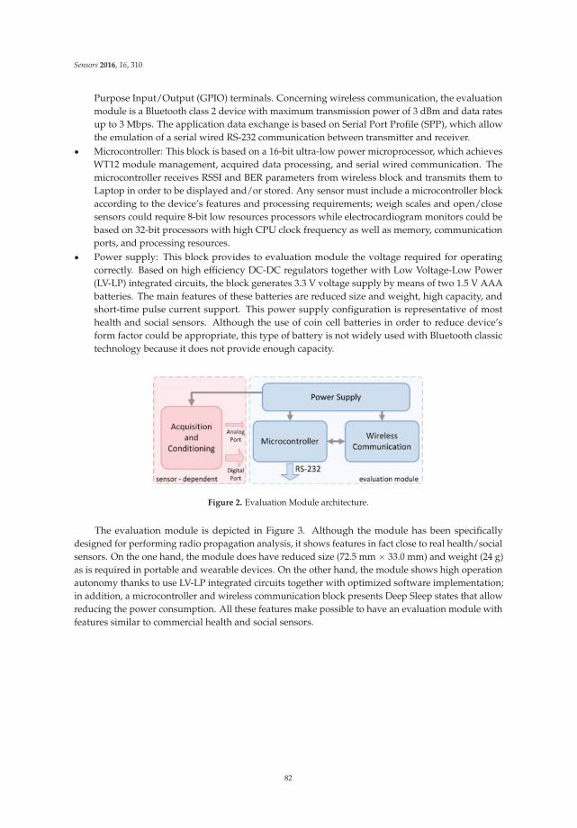
Sensors 2016, 16, 310

Purpose Input/Output (GPIO) terminals. Concerning wireless communication, the evaluationmodule is a Bluetooth class 2 device with maximum transmission power of 3 dBm and data ratesup to 3 Mbps. The application data exchange is based on Serial Port Profile (SPP), which allowthe emulation of a serial wired RS-232 communication between transmitter and receiver.

‚ Microcontroller: This block is based on a 16-bit ultra-low power microprocessor, which achievesWT12 module management, acquired data processing, and serial wired communication. Themicrocontroller receives RSSI and BER parameters from wireless block and transmits them toLaptop in order to be displayed and/or stored. Any sensor must include a microcontroller blockaccording to the device’s features and processing requirements; weigh scales and open/closesensors could require 8-bit low resources processors while electrocardiogram monitors could bebased on 32-bit processors with high CPU clock frequency as well as memory, communicationports, and processing resources.

‚ Power supply: This block provides to evaluation module the voltage required for operatingcorrectly. Based on high efficiency DC-DC regulators together with Low Voltage-Low Power(LV-LP) integrated circuits, the block generates 3.3 V voltage supply by means of two 1.5 V AAAbatteries. The main features of these batteries are reduced size and weight, high capacity, andshort-time pulse current support. This power supply configuration is representative of mosthealth and social sensors. Although the use of coin cell batteries in order to reduce device’sform factor could be appropriate, this type of battery is not widely used with Bluetooth classictechnology because it does not provide enough capacity.

Figure 2. Evaluation Module architecture.

The evaluation module is depicted in Figure 3. Although the module has been specificallydesigned for performing radio propagation analysis, it shows features in fact close to real health/socialsensors. On the one hand, the module does have reduced size (72.5 mm ˆ 33.0 mm) and weight (24 g)as is required in portable and wearable devices. On the other hand, the module shows high operationautonomy thanks to use LV-LP integrated circuits together with optimized software implementation;in addition, a microcontroller and wireless communication block presents Deep Sleep states that allowreducing the power consumption. All these features make possible to have an evaluation module withfeatures similar to commercial health and social sensors.

82

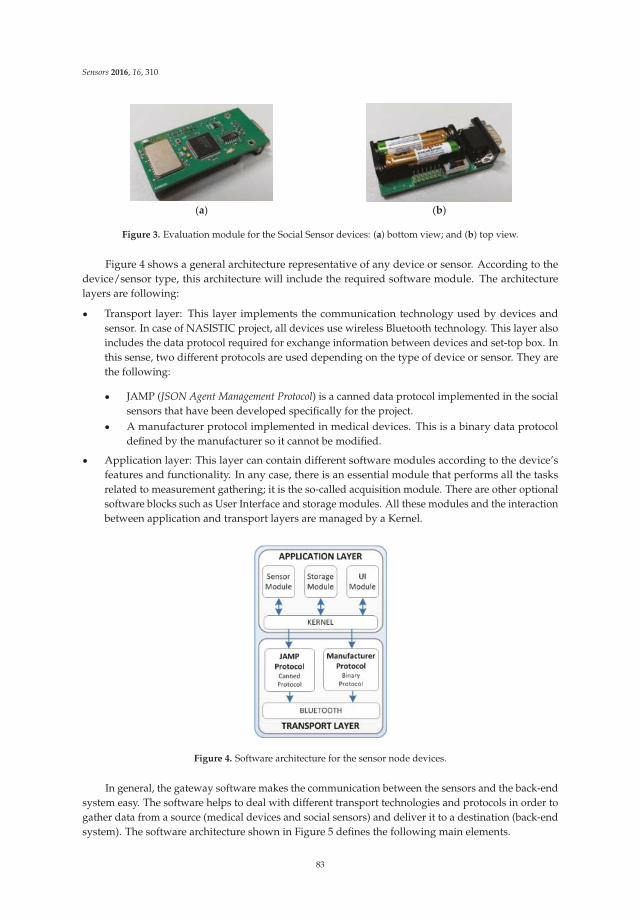
Sensors 2016, 16, 310

(a) (b)

Figure 3. Evaluation module for the Social Sensor devices: (a) bottom view; and (b) top view.

Figure 4 shows a general architecture representative of any device or sensor. According to thedevice/sensor type, this architecture will include the required software module. The architecturelayers are following:

‚ Transport layer: This layer implements the communication technology used by devices andsensor. In case of NASISTIC project, all devices use wireless Bluetooth technology. This layer alsoincludes the data protocol required for exchange information between devices and set-top box. Inthis sense, two different protocols are used depending on the type of device or sensor. They arethe following:

‚ JAMP (JSON Agent Management Protocol) is a canned data protocol implemented in the socialsensors that have been developed specifically for the project.

‚ A manufacturer protocol implemented in medical devices. This is a binary data protocoldefined by the manufacturer so it cannot be modified.

‚ Application layer: This layer can contain different software modules according to the device’sfeatures and functionality. In any case, there is an essential module that performs all the tasksrelated to measurement gathering; it is the so-called acquisition module. There are other optionalsoftware blocks such as User Interface and storage modules. All these modules and the interactionbetween application and transport layers are managed by a Kernel.

Figure 4. Software architecture for the sensor node devices.

In general, the gateway software makes the communication between the sensors and the back-endsystem easy. The software helps to deal with different transport technologies and protocols in order togather data from a source (medical devices and social sensors) and deliver it to a destination (back-endsystem). The software architecture shown in Figure 5 defines the following main elements.

83

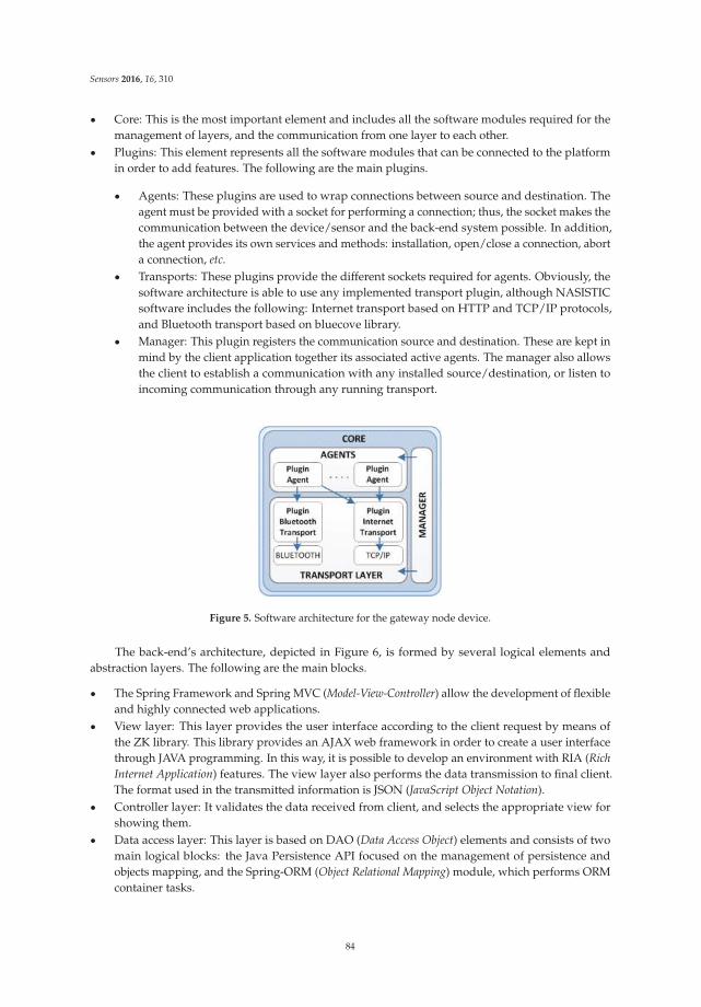
Sensors 2016, 16, 310

‚ Core: This is the most important element and includes all the software modules required for themanagement of layers, and the communication from one layer to each other.

‚ Plugins: This element represents all the software modules that can be connected to the platformin order to add features. The following are the main plugins.

‚ Agents: These plugins are used to wrap connections between source and destination. Theagent must be provided with a socket for performing a connection; thus, the socket makes thecommunication between the device/sensor and the back-end system possible. In addition,the agent provides its own services and methods: installation, open/close a connection, aborta connection, etc.

‚ Transports: These plugins provide the different sockets required for agents. Obviously, thesoftware architecture is able to use any implemented transport plugin, although NASISTICsoftware includes the following: Internet transport based on HTTP and TCP/IP protocols,and Bluetooth transport based on bluecove library.

‚ Manager: This plugin registers the communication source and destination. These are kept inmind by the client application together its associated active agents. The manager also allowsthe client to establish a communication with any installed source/destination, or listen toincoming communication through any running transport.

Figure 5. Software architecture for the gateway node device.

The back-end’s architecture, depicted in Figure 6, is formed by several logical elements andabstraction layers. The following are the main blocks.

‚ The Spring Framework and Spring MVC (Model-View-Controller) allow the development of flexibleand highly connected web applications.

‚ View layer: This layer provides the user interface according to the client request by means ofthe ZK library. This library provides an AJAX web framework in order to create a user interfacethrough JAVA programming. In this way, it is possible to develop an environment with RIA (Rich

Internet Application) features. The view layer also performs the data transmission to final client.The format used in the transmitted information is JSON (JavaScript Object Notation).

‚ Controller layer: It validates the data received from client, and selects the appropriate view forshowing them.

‚ Data access layer: This layer is based on DAO (Data Access Object) elements and consists of twomain logical blocks: the Java Persistence API focused on the management of persistence andobjects mapping, and the Spring-ORM (Object Relational Mapping) module, which performs ORMcontainer tasks.

84

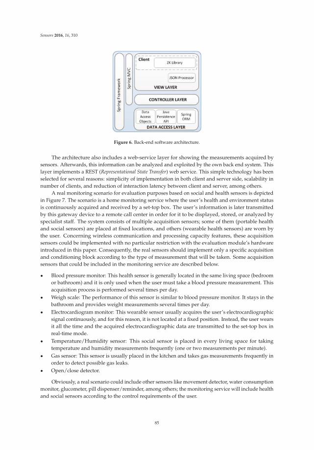
Sensors 2016, 16, 310

Figure 6. Back-end software architecture.

The architecture also includes a web-service layer for showing the measurements acquired bysensors. Afterwards, this information can be analyzed and exploited by the own back end system. Thislayer implements a REST (Representational State Transfer) web service. This simple technology has beenselected for several reasons: simplicity of implementation in both client and server side, scalability innumber of clients, and reduction of interaction latency between client and server, among others.

A real monitoring scenario for evaluation purposes based on social and health sensors is depictedin Figure 7. The scenario is a home monitoring service where the user’s health and environment statusis continuously acquired and received by a set-top box. The user’s information is later transmittedby this gateway device to a remote call center in order for it to be displayed, stored, or analyzed byspecialist staff. The system consists of multiple acquisition sensors; some of them (portable healthand social sensors) are placed at fixed locations, and others (wearable health sensors) are worn bythe user. Concerning wireless communication and processing capacity features, these acquisitionsensors could be implemented with no particular restriction with the evaluation module’s hardwareintroduced in this paper. Consequently, the real sensors should implement only a specific acquisitionand conditioning block according to the type of measurement that will be taken. Some acquisitionsensors that could be included in the monitoring service are described below.

‚ Blood pressure monitor: This health sensor is generally located in the same living space (bedroomor bathroom) and it is only used when the user must take a blood pressure measurement. Thisacquisition process is performed several times per day.

‚ Weigh scale: The performance of this sensor is similar to blood pressure monitor. It stays in thebathroom and provides weight measurements several times per day.

‚ Electrocardiogram monitor: This wearable sensor usually acquires the user’s electrocardiographicsignal continuously, and for this reason, it is not located at a fixed position. Instead, the user wearsit all the time and the acquired electrocardiographic data are transmitted to the set-top box inreal-time mode.

‚ Temperature/Humidity sensor: This social sensor is placed in every living space for takingtemperature and humidity measurements frequently (one or two measurements per minute).

‚ Gas sensor: This sensor is usually placed in the kitchen and takes gas measurements frequently inorder to detect possible gas leaks.

‚ Open/close detector.

Obviously, a real scenario could include other sensors like movement detector, water consumptionmonitor, glucometer, pill dispenser/reminder, among others; the monitoring service will include healthand social sensors according to the control requirements of the user.

85

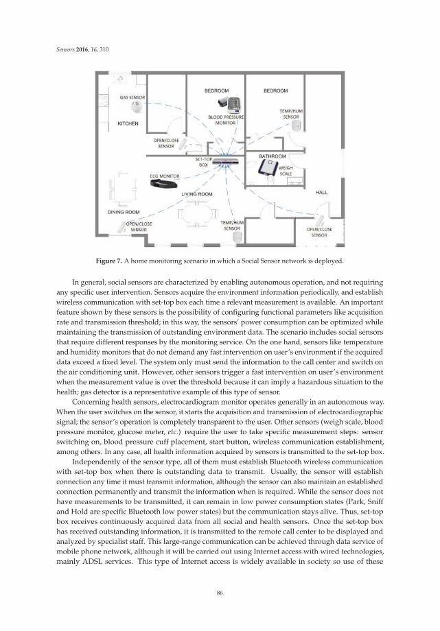
Sensors 2016, 16, 310

Figure 7. A home monitoring scenario in which a Social Sensor network is deployed.

In general, social sensors are characterized by enabling autonomous operation, and not requiringany specific user intervention. Sensors acquire the environment information periodically, and establishwireless communication with set-top box each time a relevant measurement is available. An importantfeature shown by these sensors is the possibility of configuring functional parameters like acquisitionrate and transmission threshold; in this way, the sensors’ power consumption can be optimized whilemaintaining the transmission of outstanding environment data. The scenario includes social sensorsthat require different responses by the monitoring service. On the one hand, sensors like temperatureand humidity monitors that do not demand any fast intervention on user’s environment if the acquireddata exceed a fixed level. The system only must send the information to the call center and switch onthe air conditioning unit. However, other sensors trigger a fast intervention on user’s environmentwhen the measurement value is over the threshold because it can imply a hazardous situation to thehealth; gas detector is a representative example of this type of sensor.

Concerning health sensors, electrocardiogram monitor operates generally in an autonomous way.When the user switches on the sensor, it starts the acquisition and transmission of electrocardiographicsignal; the sensor’s operation is completely transparent to the user. Other sensors (weigh scale, bloodpressure monitor, glucose meter, etc.) require the user to take specific measurement steps: sensorswitching on, blood pressure cuff placement, start button, wireless communication establishment,among others. In any case, all health information acquired by sensors is transmitted to the set-top box.

Independently of the sensor type, all of them must establish Bluetooth wireless communicationwith set-top box when there is outstanding data to transmit. Usually, the sensor will establishconnection any time it must transmit information, although the sensor can also maintain an establishedconnection permanently and transmit the information when is required. While the sensor does nothave measurements to be transmitted, it can remain in low power consumption states (Park, Sniffand Hold are specific Bluetooth low power states) but the communication stays alive. Thus, set-topbox receives continuously acquired data from all social and health sensors. Once the set-top boxhas received outstanding information, it is transmitted to the remote call center to be displayed andanalyzed by specialist staff. This large-range communication can be achieved through data service ofmobile phone network, although it will be carried out using Internet access with wired technologies,mainly ADSL services. This type of Internet access is widely available in society so use of these

86

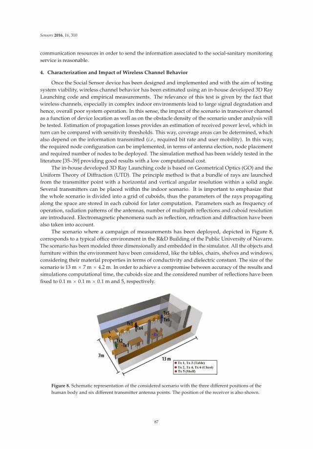
Sensors 2016, 16, 310

communication resources in order to send the information associated to the social-sanitary monitoringservice is reasonable.

4. Characterization and Impact of Wireless Channel Behavior

Once the Social Sensor device has been designed and implemented and with the aim of testingsystem viability, wireless channel behavior has been estimated using an in-house developed 3D RayLaunching code and empirical measurements. The relevance of this test is given by the fact thatwireless channels, especially in complex indoor environments lead to large signal degradation andhence, overall poor system operation. In this sense, the impact of the scenario in transceiver channelas a function of device location as well as on the obstacle density of the scenario under analysis willbe tested. Estimation of propagation losses provides an estimation of received power level, which inturn can be compared with sensitivity thresholds. This way, coverage areas can be determined, whichalso depend on the information transmitted (i.e., required bit rate and user mobility). In this way,the required node configuration can be implemented, in terms of antenna election, node placementand required number of nodes to be deployed. The simulation method has been widely tested in theliterature [35–39] providing good results with a low computational cost.

The in-house developed 3D Ray Launching code is based on Geometrical Optics (GO) and theUniform Theory of Diffraction (UTD). The principle method is that a bundle of rays are launchedfrom the transmitter point with a horizontal and vertical angular resolution within a solid angle.Several transmitters can be placed within the indoor scenario. It is important to emphasize thatthe whole scenario is divided into a grid of cuboids, thus the parameters of the rays propagatingalong the space are stored in each cuboid for later computation. Parameters such as frequency ofoperation, radiation patterns of the antennas, number of multipath reflections and cuboid resolutionare introduced. Electromagnetic phenomena such as reflection, refraction and diffraction have beenalso taken into account.

The scenario where a campaign of measurements has been deployed, depicted in Figure 8,corresponds to a typical office environment in the R&D Building of the Public University of Navarre.The scenario has been modeled three dimensionally and embedded in the simulator. All the objects andfurniture within the environment have been considered, like the tables, chairs, shelves and windows,considering their material properties in terms of conductivity and dielectric constant. The size of thescenario is 13 m ˆ 7 m ˆ 4.2 m. In order to achieve a compromise between accuracy of the results andsimulations computational time, the cuboids size and the considered number of reflections have beenfixed to 0.1 m ˆ 0.1 m ˆ 0.1 m and 5, respectively.

Figure 8. Schematic representation of the considered scenario with the three different positions of thehuman body and six different transmitter antenna points. The position of the receiver is also shown.

87

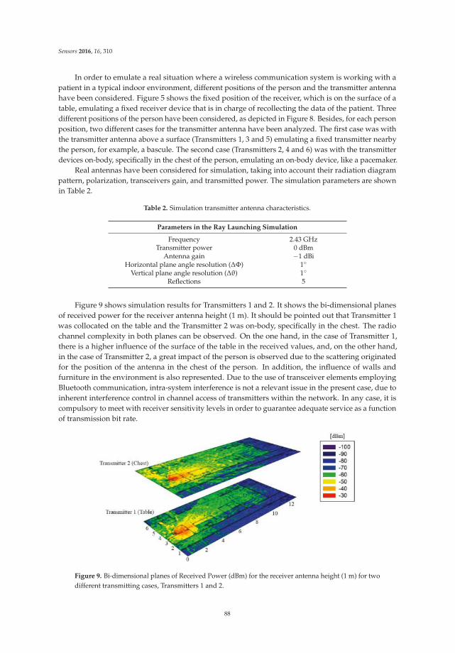
Sensors 2016, 16, 310

In order to emulate a real situation where a wireless communication system is working with apatient in a typical indoor environment, different positions of the person and the transmitter antennahave been considered. Figure 5 shows the fixed position of the receiver, which is on the surface of atable, emulating a fixed receiver device that is in charge of recollecting the data of the patient. Threedifferent positions of the person have been considered, as depicted in Figure 8. Besides, for each personposition, two different cases for the transmitter antenna have been analyzed. The first case was withthe transmitter antenna above a surface (Transmitters 1, 3 and 5) emulating a fixed transmitter nearbythe person, for example, a bascule. The second case (Transmitters 2, 4 and 6) was with the transmitterdevices on-body, specifically in the chest of the person, emulating an on-body device, like a pacemaker.

Real antennas have been considered for simulation, taking into account their radiation diagrampattern, polarization, transceivers gain, and transmitted power. The simulation parameters are shownin Table 2.

Table 2. Simulation transmitter antenna characteristics.

Parameters in the Ray Launching Simulation

Frequency 2.43 GHzTransmitter power 0 dBm

Antenna gain ´1 dBiHorizontal plane angle resolution (ΔΦ) 1˝

Vertical plane angle resolution (Δθ) 1˝

Reflections 5

Figure 9 shows simulation results for Transmitters 1 and 2. It shows the bi-dimensional planesof received power for the receiver antenna height (1 m). It should be pointed out that Transmitter 1was collocated on the table and the Transmitter 2 was on-body, specifically in the chest. The radiochannel complexity in both planes can be observed. On the one hand, in the case of Transmitter 1,there is a higher influence of the surface of the table in the received values, and, on the other hand,in the case of Transmitter 2, a great impact of the person is observed due to the scattering originatedfor the position of the antenna in the chest of the person. In addition, the influence of walls andfurniture in the environment is also represented. Due to the use of transceiver elements employingBluetooth communication, intra-system interference is not a relevant issue in the present case, due toinherent interference control in channel access of transmitters within the network. In any case, it iscompulsory to meet with receiver sensitivity levels in order to guarantee adequate service as a functionof transmission bit rate.

Figure 9. Bi-dimensional planes of Received Power (dBm) for the receiver antenna height (1 m) for twodifferent transmitting cases, Transmitters 1 and 2.

88

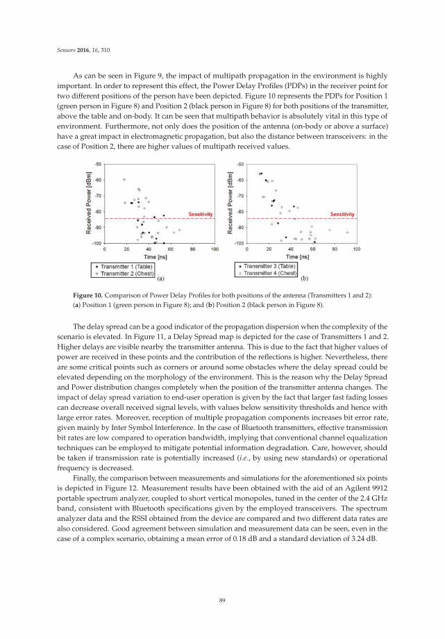
Sensors 2016, 16, 310

As can be seen in Figure 9, the impact of multipath propagation in the environment is highlyimportant. In order to represent this effect, the Power Delay Profiles (PDPs) in the receiver point fortwo different positions of the person have been depicted. Figure 10 represents the PDPs for Position 1(green person in Figure 8) and Position 2 (black person in Figure 8) for both positions of the transmitter,above the table and on-body. It can be seen that multipath behavior is absolutely vital in this type ofenvironment. Furthermore, not only does the position of the antenna (on-body or above a surface)have a great impact in electromagnetic propagation, but also the distance between transceivers: in thecase of Position 2, there are higher values of multipath received values.

Figure 10. Comparison of Power Delay Profiles for both positions of the antenna (Transmitters 1 and 2):(a) Position 1 (green person in Figure 8); and (b) Position 2 (black person in Figure 8).

The delay spread can be a good indicator of the propagation dispersion when the complexity of thescenario is elevated. In Figure 11, a Delay Spread map is depicted for the case of Transmitters 1 and 2.Higher delays are visible nearby the transmitter antenna. This is due to the fact that higher values ofpower are received in these points and the contribution of the reflections is higher. Nevertheless, thereare some critical points such as corners or around some obstacles where the delay spread could beelevated depending on the morphology of the environment. This is the reason why the Delay Spreadand Power distribution changes completely when the position of the transmitter antenna changes. Theimpact of delay spread variation to end-user operation is given by the fact that larger fast fading lossescan decrease overall received signal levels, with values below sensitivity thresholds and hence withlarge error rates. Moreover, reception of multiple propagation components increases bit error rate,given mainly by Inter Symbol Interference. In the case of Bluetooth transmitters, effective transmissionbit rates are low compared to operation bandwidth, implying that conventional channel equalizationtechniques can be employed to mitigate potential information degradation. Care, however, shouldbe taken if transmission rate is potentially increased (i.e., by using new standards) or operationalfrequency is decreased.

Finally, the comparison between measurements and simulations for the aforementioned six pointsis depicted in Figure 12. Measurement results have been obtained with the aid of an Agilent 9912portable spectrum analyzer, coupled to short vertical monopoles, tuned in the center of the 2.4 GHzband, consistent with Bluetooth specifications given by the employed transceivers. The spectrumanalyzer data and the RSSI obtained from the device are compared and two different data rates arealso considered. Good agreement between simulation and measurement data can be seen, even in thecase of a complex scenario, obtaining a mean error of 0.18 dB and a standard deviation of 3.24 dB.

89

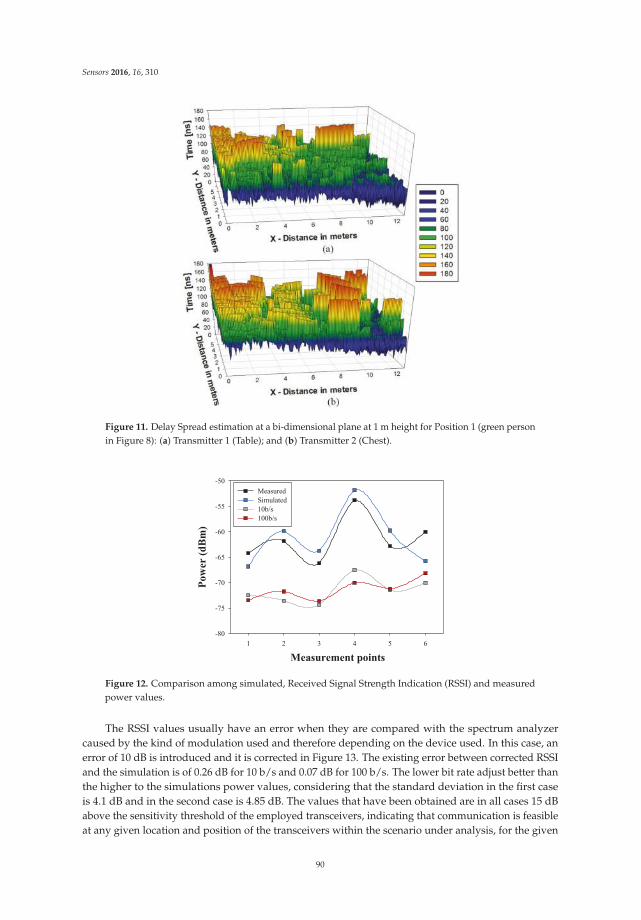
Sensors 2016, 16, 310

Figure 11. Delay Spread estimation at a bi-dimensional plane at 1 m height for Position 1 (green personin Figure 8): (a) Transmitter 1 (Table); and (b) Transmitter 2 (Chest).

Measurement points

1 2 3 4 5 6

Po

wer (

dB

m)

-80

-75

-70

-65

-60

-55

-50

Measured

Simulated

10b/s

100b/s

Figure 12. Comparison among simulated, Received Signal Strength Indication (RSSI) and measuredpower values.

The RSSI values usually have an error when they are compared with the spectrum analyzercaused by the kind of modulation used and therefore depending on the device used. In this case, anerror of 10 dB is introduced and it is corrected in Figure 13. The existing error between corrected RSSIand the simulation is of 0.26 dB for 10 b/s and 0.07 dB for 100 b/s. The lower bit rate adjust better thanthe higher to the simulations power values, considering that the standard deviation in the first caseis 4.1 dB and in the second case is 4.85 dB. The values that have been obtained are in all cases 15 dBabove the sensitivity threshold of the employed transceivers, indicating that communication is feasibleat any given location and position of the transceivers within the scenario under analysis, for the given

90

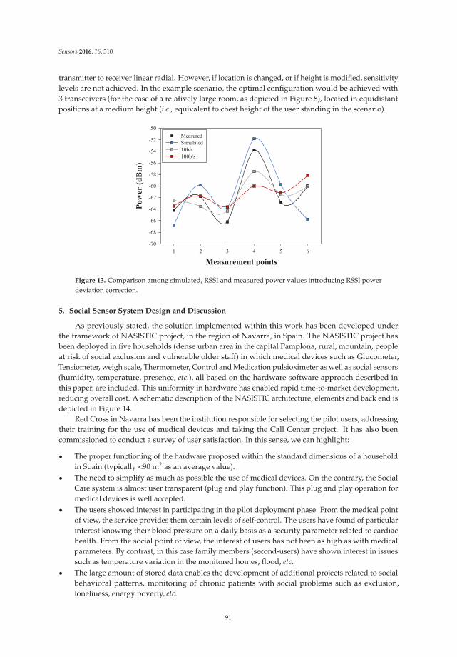
Sensors 2016, 16, 310

transmitter to receiver linear radial. However, if location is changed, or if height is modified, sensitivitylevels are not achieved. In the example scenario, the optimal configuration would be achieved with3 transceivers (for the case of a relatively large room, as depicted in Figure 8), located in equidistantpositions at a medium height (i.e., equivalent to chest height of the user standing in the scenario).

Measurement points

1 2 3 4 5 6

Po

wer (

dB

m)

-70

-68

-66

-64

-62

-60

-58

-56

-54

-52

-50

Measured

Simulated

10b/s

100b/s

Figure 13. Comparison among simulated, RSSI and measured power values introducing RSSI powerdeviation correction.

5. Social Sensor System Design and Discussion

As previously stated, the solution implemented within this work has been developed underthe framework of NASISTIC project, in the region of Navarra, in Spain. The NASISTIC project hasbeen deployed in five households (dense urban area in the capital Pamplona, rural, mountain, peopleat risk of social exclusion and vulnerable older staff) in which medical devices such as Glucometer,Tensiometer, weigh scale, Thermometer, Control and Medication pulsioximeter as well as social sensors(humidity, temperature, presence, etc.), all based on the hardware-software approach described inthis paper, are included. This uniformity in hardware has enabled rapid time-to-market development,reducing overall cost. A schematic description of the NASISTIC architecture, elements and back end isdepicted in Figure 14.

Red Cross in Navarra has been the institution responsible for selecting the pilot users, addressingtheir training for the use of medical devices and taking the Call Center project. It has also beencommissioned to conduct a survey of user satisfaction. In this sense, we can highlight:

‚ The proper functioning of the hardware proposed within the standard dimensions of a householdin Spain (typically <90 m2 as an average value).

‚ The need to simplify as much as possible the use of medical devices. On the contrary, the SocialCare system is almost user transparent (plug and play function). This plug and play operation formedical devices is well accepted.

‚ The users showed interest in participating in the pilot deployment phase. From the medical pointof view, the service provides them certain levels of self-control. The users have found of particularinterest knowing their blood pressure on a daily basis as a security parameter related to cardiachealth. From the social point of view, the interest of users has not been as high as with medicalparameters. By contrast, in this case family members (second-users) have shown interest in issuessuch as temperature variation in the monitored homes, flood, etc.

‚ The large amount of stored data enables the development of additional projects related to socialbehavioral patterns, monitoring of chronic patients with social problems such as exclusion,loneliness, energy poverty, etc.

91

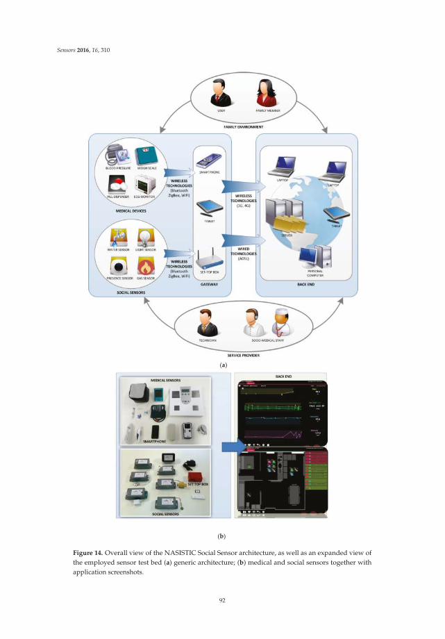
Sensors 2016, 16, 310

(a)

(b)

Figure 14. Overall view of the NASISTIC Social Sensor architecture, as well as an expanded view ofthe employed sensor test bed (a) generic architecture; (b) medical and social sensors together withapplication screenshots.

92

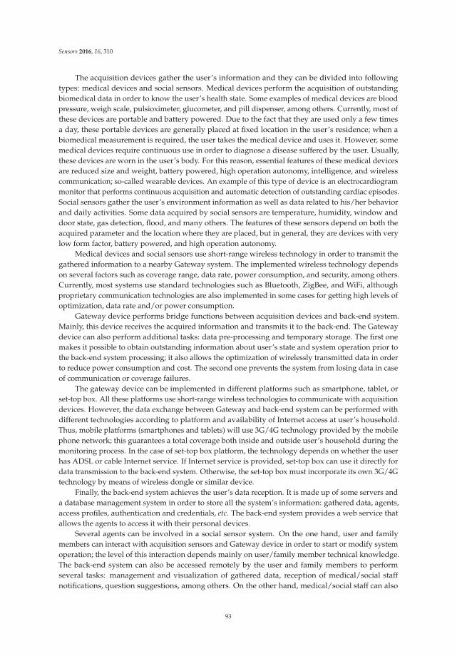
Sensors 2016, 16, 310

The acquisition devices gather the user’s information and they can be divided into followingtypes: medical devices and social sensors. Medical devices perform the acquisition of outstandingbiomedical data in order to know the user’s health state. Some examples of medical devices are bloodpressure, weigh scale, pulsioximeter, glucometer, and pill dispenser, among others. Currently, most ofthese devices are portable and battery powered. Due to the fact that they are used only a few timesa day, these portable devices are generally placed at fixed location in the user’s residence; when abiomedical measurement is required, the user takes the medical device and uses it. However, somemedical devices require continuous use in order to diagnose a disease suffered by the user. Usually,these devices are worn in the user’s body. For this reason, essential features of these medical devicesare reduced size and weight, battery powered, high operation autonomy, intelligence, and wirelesscommunication; so-called wearable devices. An example of this type of device is an electrocardiogrammonitor that performs continuous acquisition and automatic detection of outstanding cardiac episodes.Social sensors gather the user’s environment information as well as data related to his/her behaviorand daily activities. Some data acquired by social sensors are temperature, humidity, window anddoor state, gas detection, flood, and many others. The features of these sensors depend on both theacquired parameter and the location where they are placed, but in general, they are devices with verylow form factor, battery powered, and high operation autonomy.

Medical devices and social sensors use short-range wireless technology in order to transmit thegathered information to a nearby Gateway system. The implemented wireless technology dependson several factors such as coverage range, data rate, power consumption, and security, among others.Currently, most systems use standard technologies such as Bluetooth, ZigBee, and WiFi, althoughproprietary communication technologies are also implemented in some cases for getting high levels ofoptimization, data rate and/or power consumption.

Gateway device performs bridge functions between acquisition devices and back-end system.Mainly, this device receives the acquired information and transmits it to the back-end. The Gatewaydevice can also perform additional tasks: data pre-processing and temporary storage. The first onemakes it possible to obtain outstanding information about user’s state and system operation prior tothe back-end system processing; it also allows the optimization of wirelessly transmitted data in orderto reduce power consumption and cost. The second one prevents the system from losing data in caseof communication or coverage failures.

The gateway device can be implemented in different platforms such as smartphone, tablet, orset-top box. All these platforms use short-range wireless technologies to communicate with acquisitiondevices. However, the data exchange between Gateway and back-end system can be performed withdifferent technologies according to platform and availability of Internet access at user’s household.Thus, mobile platforms (smartphones and tablets) will use 3G/4G technology provided by the mobilephone network; this guarantees a total coverage both inside and outside user’s household during themonitoring process. In the case of set-top box platform, the technology depends on whether the userhas ADSL or cable Internet service. If Internet service is provided, set-top box can use it directly fordata transmission to the back-end system. Otherwise, the set-top box must incorporate its own 3G/4Gtechnology by means of wireless dongle or similar device.

Finally, the back-end system achieves the user’s data reception. It is made up of some servers anda database management system in order to store all the system’s information: gathered data, agents,access profiles, authentication and credentials, etc. The back-end system provides a web service thatallows the agents to access it with their personal devices.

Several agents can be involved in a social sensor system. On the one hand, user and familymembers can interact with acquisition sensors and Gateway device in order to start or modify systemoperation; the level of this interaction depends mainly on user/family member technical knowledge.The back-end system can also be accessed remotely by the user and family members to performseveral tasks: management and visualization of gathered data, reception of medical/social staffnotifications, question suggestions, among others. On the other hand, medical/social staff can also

93

Sensors 2016, 16, 310

access the back-end system in order to analyze and visualize the user’s information. Depending onthis information and automatic alerts generated by the own system, the agent can know the user’ stateand even determine behavioral patterns that must be corrected. In these cases, the medical/social staffwill make contact with the user or family member in order to notify behavioral advices, medicationprescription, etc. Finally, technical workers are in charge of installing and configuring the systemoperation. These agents also have maintenance functions when some system malfunction has occurred.There will be problems whose solution will be performed remotely from the service provider, butother ones will require the movement of technical worker to the user’s household; device malfunction,system configuration failure, and wrong device communication are common problems that cannot besolved by users or family members, so a technician must do it in person.

Centralized and secure management in the deployment of Socio-Sanitary services such asNASISTIC is a mandatory requirement. These back-end tools are designed for managing userswith different roles (end-users, family users or secondary users, stakeholder users, etc.) as well as themanagement of information received from all monitored houses. Obviously, the end-users and theirfamily users can access their own information. In the case of stakeholder users, access will be for allhomes or end-users of their institution. In any case, these tools provide a complete configurabilityof roles.

Furthermore, in order to ease as far as possible the service configuration, tools like NASISTICprovide graphical aids such as either 2D or 3D drawings of housing for sensor placement, whetherthey are social sensors or health sensors, and tools for viewing the received data (time graphs, etc.).Moreover, besides a user-friendly configuration wizard, tools for configuring alerts from the receivedmeasurements are also implemented. For example, for a user, maximum and minimum blood pressurelevels can be set (relative or absolute in %) or any other health sensor and alerts on social sensorslike temperature (energy poverty, etc.) or moisture. These alerts generate messages (SMS, emails,WhatsApp messages, etc.) or phone calls to those in charge of the user who previously have beenconfigured (family-users, physicians, stakeholder users or even end users).

In order to provide insight into the detailed operation of the system and to effectively testits suitability as an AAL system [40], examples of multiple signals available have been tested in aLiving Lab environment, within the Public University of Navarra. As was previously mentioned,the evaluation module could emulate the functional operation of any monitoring sensor, being onlyrequired the implementation of analogue acquisition block. In this way, it is possible to emulatethe home monitoring service’s operation as the system was implemented in a real scenario. Forthis emulation, we consider four sensors: temperature/humidity sensor, electrocardiogram monitor,weigh scale, and open/close detector. Table 3 shows the main emulated features of sensors. Thegateway device is also emulated with an evaluation module that gathers the acquired information andtransmits it to Laptop via RS-232 serial communication. Laptop does not implement a display softwareapplication, so the raw data are stored in a stream file for later analyze and graphic representation.

Table 3. Features of emulated health and social sensors.

Sensor Location AccuracyTransmission

RateRange

AcquisitionRate

Temperature/Humidity Living room ˘0.5 ˝C ˘1% RH 1 value/min 0 ˝C–65 ˝C 2 samples/sWeigh scale Bathroom ˘100 gr. 2 value/day 0 gr–150 gr 2 sample/d

Electrocardiogrammonitor

User’s body ˘45 µV/LSB Real-time ´1V–2V500

samples/sOpen/close Hall door - - 0V–1V -

As an example, Figure 15a,b shows measurements related to weigh scale and electrocardiogrammonitor devices, respectively. The first one shows the user’s weigh scale evolution throughout aweek. This evolution, if it were to continue for too long, could be representative of a poor diet in

94

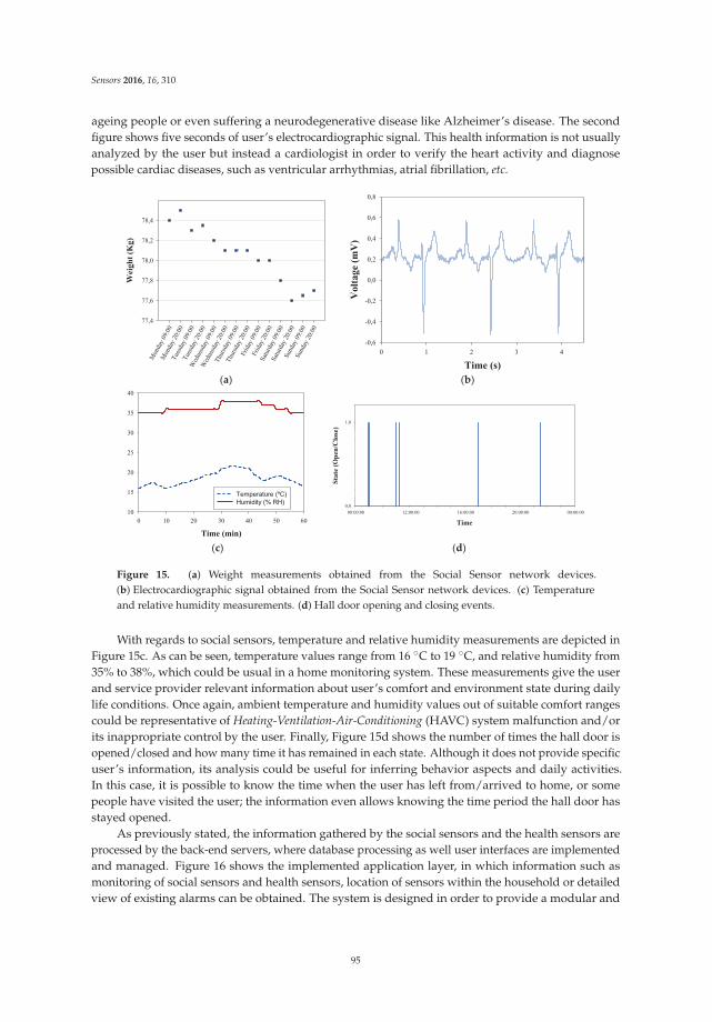
Sensors 2016, 16, 310

ageing people or even suffering a neurodegenerative disease like Alzheimer’s disease. The secondfigure shows five seconds of user’s electrocardiographic signal. This health information is not usuallyanalyzed by the user but instead a cardiologist in order to verify the heart activity and diagnosepossible cardiac diseases, such as ventricular arrhythmias, atrial fibrillation, etc.

(a) (b)

Mon

day

09:0

0M

onda

y 20

:00

Tue

sday

09:

00T

uesd

ay 2

0:00

Wed

nesd

ay 0

9:00

Wed

nesd

ay 2

0:00

Thu

rsda

y 09

:00

Thu

rsda

y 20

:00

Fri

day

09:0

0Fri

day

20:0

0Sat

urda

y 09

:00

Sat

urda

y 20

:00

Sun

day

09:0

0Sun

day

20:0

0

Wei

gh

t (K

g)

77,4

77,6

77,8

78,0

78,2

78,4

Time (s)

0 1 2 3 4V

olt

ag

e (m

V)

-0,6

-0,4

-0,2

0,0

0,2

0,4

0,6

0,8

(c) (d)

Time (min)

0 10 20 30 40 50 60

10

15

20

25

30

35

40

Temperature (ºC)

Humidity (% RH)

Time

08:00:00 12:00:00 16:00:00 20:00:00 00:00:00

Sta

te (

Op

en/C

lose

)

0,0

0,2

0,4

0,6

0,8

1,0

1,2

Figure 15. (a) Weight measurements obtained from the Social Sensor network devices.(b) Electrocardiographic signal obtained from the Social Sensor network devices. (c) Temperatureand relative humidity measurements. (d) Hall door opening and closing events.

With regards to social sensors, temperature and relative humidity measurements are depicted inFigure 15c. As can be seen, temperature values range from 16 ˝C to 19 ˝C, and relative humidity from35% to 38%, which could be usual in a home monitoring system. These measurements give the userand service provider relevant information about user’s comfort and environment state during dailylife conditions. Once again, ambient temperature and humidity values out of suitable comfort rangescould be representative of Heating-Ventilation-Air-Conditioning (HAVC) system malfunction and/orits inappropriate control by the user. Finally, Figure 15d shows the number of times the hall door isopened/closed and how many time it has remained in each state. Although it does not provide specificuser’s information, its analysis could be useful for inferring behavior aspects and daily activities.In this case, it is possible to know the time when the user has left from/arrived to home, or somepeople have visited the user; the information even allows knowing the time period the hall door hasstayed opened.

As previously stated, the information gathered by the social sensors and the health sensors areprocessed by the back-end servers, where database processing as well user interfaces are implementedand managed. Figure 16 shows the implemented application layer, in which information such asmonitoring of social sensors and health sensors, location of sensors within the household or detailedview of existing alarms can be obtained. The system is designed in order to provide a modular and

95

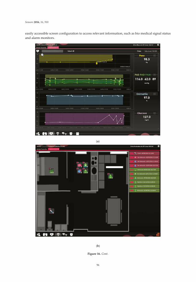
Sensors 2016, 16, 310

easily accessible screen configuration to access relevant information, such as bio medical signal statusand alarm monitors.

(a)

(b)

Figure 16. Cont.

96

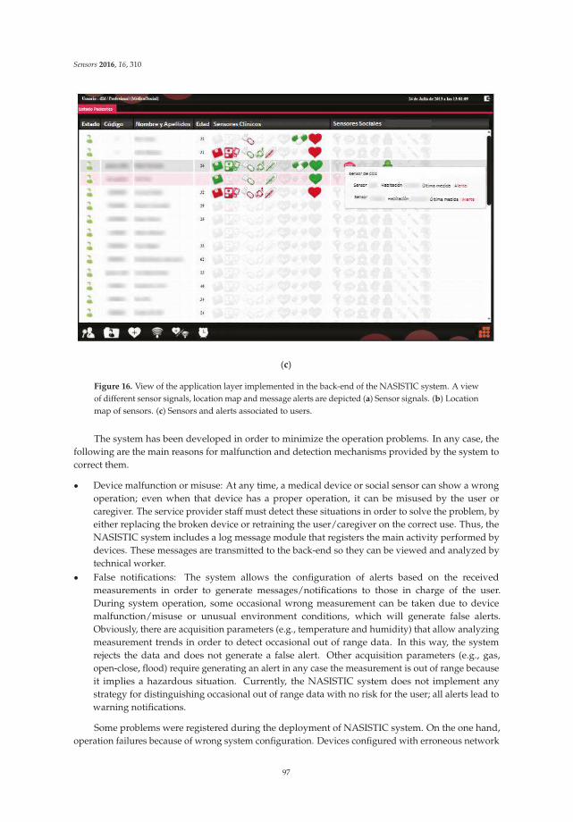
Sensors 2016, 16, 310

(c)

Figure 16. View of the application layer implemented in the back-end of the NASISTIC system. A viewof different sensor signals, location map and message alerts are depicted (a) Sensor signals. (b) Locationmap of sensors. (c) Sensors and alerts associated to users.

The system has been developed in order to minimize the operation problems. In any case, thefollowing are the main reasons for malfunction and detection mechanisms provided by the system tocorrect them.

‚ Device malfunction or misuse: At any time, a medical device or social sensor can show a wrongoperation; even when that device has a proper operation, it can be misused by the user orcaregiver. The service provider staff must detect these situations in order to solve the problem, byeither replacing the broken device or retraining the user/caregiver on the correct use. Thus, theNASISTIC system includes a log message module that registers the main activity performed bydevices. These messages are transmitted to the back-end so they can be viewed and analyzed bytechnical worker.

‚ False notifications: The system allows the configuration of alerts based on the receivedmeasurements in order to generate messages/notifications to those in charge of the user.During system operation, some occasional wrong measurement can be taken due to devicemalfunction/misuse or unusual environment conditions, which will generate false alerts.Obviously, there are acquisition parameters (e.g., temperature and humidity) that allow analyzingmeasurement trends in order to detect occasional out of range data. In this way, the systemrejects the data and does not generate a false alert. Other acquisition parameters (e.g., gas,open-close, flood) require generating an alert in any case the measurement is out of range becauseit implies a hazardous situation. Currently, the NASISTIC system does not implement anystrategy for distinguishing occasional out of range data with no risk for the user; all alerts lead towarning notifications.

Some problems were registered during the deployment of NASISTIC system. On the one hand,operation failures because of wrong system configuration. Devices configured with erroneous network

97

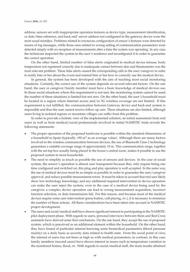
Sensors 2016, 16, 310

address, sensors set with inappropriate operation features as device type, measurement identification,or date/time reference, and back end’ server address not configured in the gateway device were themost usual mistakes. Problems related to erroneous configuration of sensor’s features were detected bymeans of log messages, while those ones related to wrong setting of communication parameters weredetected simply with no reception of measurements after a time the system was operating. In any case,the technician inspected the system in the user’s residence and reconfigured it in order to guaranteethe correct operation.

On the other hand, limited number of false alerts originated in medical device misuse; bodytemperature not registered correctly due to inadequate contact between skin and thermometer was themost relevant problem. These false alerts caused the corresponding calls to the user/caregiver in orderto notify him or her about the event and remind him or her how to correctly use the medical device.

In general, the system has been developed with the aim of reaching most social monitoringsituations. Certainly, the correct use of the system depends on several relevant factors. On the onehand, the user or caregiver/family member must have a basic knowledge of medical devices use.In those social situations where this requirement is not met, the monitoring system cannot be used;the number of these situations is limited but not zero. On the other hand, the user’s household mustbe located in a region where Internet access and/or 3G wireless coverage are not limited. If thisrequirement is not fulfilled, the communication between Gateway device and back-end system isimpossible and thus the user cannot receive follow up care. These situations are also limited, althoughusers living in isolated regions or mountain villages can suffer from this problem.

In order to provide a holistic view of the implemented solution, an initial assessment from endusers as well as from medical/social professionals involved in initial NASISTIC trials reveals thefollowing statements:

‚ The proper operation of the proposed hardware is possible within the standard dimensions ofa household in Spain (typically <90 m2 as an average value). Although there are many factorsinvolved in the wireless communication between devices, the use of Bluetooth Class 2 technologyguarantees a suitable coverage range of approximately 10 m. This communication range, togetherwith the set-top box usually being placed in the house’s central room, makes it possible to use theproposed system in most households.

‚ The need to simplify as much as possible the use of sensors and devices. In the case of socialsystem, the sensor’s operation is almost user transparent because they only require being onetime configured and switched on; this plug and play operation is well accepted. In the same way,the use of medical devices must be as simple as possible in order to guarantee the user/caregiverapproval, and reduce possible measurement errors. It must be taken in account that end user likelyshow low technology knowledge, and any additional required intervention in device operationcan make the user reject the system; even in the case of a medical device being used by thecaregiver, a complex device operation can lead to wrong measurement acquisition, incorrectfunction selection, or data transmission fail. For this reason, and because most of the medicaldevices require some user intervention (press button, cuff placing, etc.), it is necessary to minimizethe number of these actions. All these considerations have been taken into account in NASISTICproject development.

‚ The users and social/medical staff have shown significant interest in participating in the NASISTICpilot deployment phase. With regards to users, personal interviews between them and Red Crossassistants have derived some first conclusions. On the one hand, they accept the use of proposedsystem, which is perceived as an additional element within the household. On the other hand,they have found of particular interest knowing some biomedical parameters (blood pressuremainly) on a daily basis as security data related to health state. From the social point of view,the interest of users has not been as high as with medical parameters; in contrast, in this case,family members (second users) have shown interest in issues such as temperature variation inthe monitored homes, flood, etc. With regards to social/medical staff, the main results obtained

98

Sensors 2016, 16, 310

are the following: response times are reduced due to real time interaction capabilities offered bythe social sensors, and the general service provides them certain levels of self-control. Althoughspecific survey forms have not been implemented, the daily personal contact between users andsocial/medical staff during the project deployment has made obtaining these first satisfactiondata possible.

‚ The large amount of stored data enables the development of additional projects related to socialbehavioral patterns. Meanwhile, biomedical data allow the knowledge of user’s health state andmood, while other activity data, such as watching TV, use of HVAC system, water consumption,or length of phone calls, can provide information about user’s behavior and social relationships.All this information can be combined with user activity on the Internet and specific web socialnetworks like Facebook, Twitter, etc. This makes broader monitoring applications focused onfollowing up with users with chronic social problems such as exclusion, loneliness, energy poverty,etc. possible.

‚ Technical workers, engineers and architects involved in the deployment indicate that the proposedsystem is simple to integrate and maintain, reducing overall installation and operational costs.Thus, start-up system requires minimum intervention by technical worker because elements arepre-configured from factory or service provider; the worker only has to verify the correctness ofsystem operation the first installation time. In addition, the system maintenance neither demandsa great number of home interventions by engineers or technical workers unless some elementmust be repaired or replaced.

6. Conclusions

In this work, the implementation of Context Aware in order to aid in the assistance of end userswithin the framework of e-Health and m-Health scenarios has been described. A prototype of SocialSensor device has been designed and implemented in order to provide multiple-signal processingcapabilities, while exhibiting flexible, low complexity and moderate cost features. The Social Sensordevice is based on a Bluetooth transceiver, in which a dedicated microcontroller provides access toseveral signals, which can provide medical, environmental or behavioral information. In order toanalyze the robustness of the system, detailed wireless channel analysis has been performed, providinginsight on the behavior of the devices in real complex indoor scenarios, in which large signal variabilitycan severely degrade overall performance. Estimations of received power levels have been comparedwith experimental results, indicating that received power levels comply with receiver sensitivity levelsin the scenario for any potential transceiver location, implying adequate overall system service levels.Initial tests under Living Lab conditions, given by NASISTIC operational requirements have also beenperformed, showing the feasibility to successfully interchange multiple information within real timeregime. Trial runs have shown the feasibility in data acquisition of multiple bio-physical parameters aswell as user information, leading to a practical AAL platform. The proposed solution is currently beingprepared for large-scale deployment because of the ease in installation and maintenance, positiveadoption by end users and adequate results in terms of response time reduction and preventive actionsthat can be adopted.

The NASISTIC system is a remote health and behavior monitoring system, providing meansto health professionals as well as social services to provide increased quality of living to vulnerablepopulation segments, such as elderly people, and those suffering from some form of disability ormental illness. The difference between NASISTIC and other proposed systems is the integral approachin capturing biomedical signals as well as other signals that are related with user habits, such as usageof lights, heating, electrical appliances, water consumption or open/close indication of doors. In thisway, combined action of health specialists and social services can be provided in order to enable higherdegrees of autonomy to the users as well as increasing quality of life levels.

As future steps, complete system validation, integration of additional sensor elements, and theimplementation of a distributed system architecture based on cloud integration will be performed.

99

Sensors 2016, 16, 310

The current implementation of NASISTIC system uses a back-end server for information storage.Although this first version is based on a centralized solution, the system is not limited to it. Suitablemodifications on back-end element can lead to distributed implementations based on cloud solutions.

Additionally, complete user experience assessment will be obtained in order to identify usability,leading to further modifications and enhancements.

Acknowledgments: The authors wish to acknowledge funding of project NASISTIC, from the Government ofNavarra, Spain; Project TEC2013-45585-C2-1-R, funded by the Spanish Ministry of Economy and Competiveness;collaboration and support from Red Cross Navarra; and D2D, AH and ID corporations, in Spain.

Author Contributions: Erik Aguirre, Peio López-Iturri, Leyre Azpilicueta and Francisco Falcone conducted thecharacterization of wireless propagation mechanisms in the Living Lab scenarios. Santiago Led and Luis Serranoparticipated in the development of the NASISTIC architecture and back end.


References

1. UN Department of Economic and Social Affairs. Available online: http://www.un.org/esa/population/publications/worldageing19502050/ (accessed on 25 February 2016).

2. Monteagudo, J.L.; Moreno, O. eHealth for Patient Empowerment in Europe, 2009. Available Online:http://ec.europa.eu (accessed on 25 February 2016).

3. Led, S.; Serrano, L.; Galarraga, M. Wearable Wireless Monitoring System Based on Bluetooth Technology:A Tutorial. In Proceedings of the 3rd European Medical and Biological Engineering Conference EMBEC,Prague, Czech Republic, 20–25 November 2005.

4. Xiao, Y.; Pan, Y. Emerging Wireless LANs, Wireless PANs, and Wireless MANs; John Wiley & Sons: New York,NJ, USA, 2009.

5. Dargie, W.; Poella, B.C. Fundamentals of Wireless Sensor Networks Theory and Practice; John Wiley & Sons:Chichester, UK, 2010.

6. Kim, Y.; Evans, R.G.; Iversen, W.M. Remote sensing and control of an irrigation system using a distributedwireless sensor network. IEEE Trans. Instrum. Meas. 2008, 57, 1379–1387.

7. Grosse, C.U.; Glaser, S.D.; Kruger, M. Initial development of wireless acoustic emission sensor Motes forcivil infrastructure state monitoring. Smart Struct. Syst. 2010, 6, 197–209. [CrossRef]

8. Rahal, Y.; Pigot, H.; Mabilleau, P. Location estimation in a smart home: System implementation andevaluation using experimental data. Int. J. Telemed. Appl. 2008. [CrossRef] [PubMed]

9. Tayal, S.; Tripathy, M.R. VANET-Challenges in selection of Vehicular Mobility Model. In Second International

Conference on Advanced Computing & Communication Technologies (ACCT); IEEE: Rohtak, India, 2012;pp. 231–235.

10. Li, Y.Z.; Wang, L.; Wu, X.M.; Zhang, Y.T. Experimental analysis on radio transmission and localization of aZigBee based wireless healthcare monitoring platform. In Proceedings of the 5th International Conferenceon Information Technology and Applications in Biomedicine (ITAB’08), Nanjing, China, 30–31 May 2008;pp. 488–490.

11. Dagtas, S.; Pekhteryev, G.; Sahinoglu, Z.; Cam, H.; Challa, N. Real-time and secure wireless health monitoring.Int. J. Telemed. Appl. 2008. [CrossRef]

12. Villanueva, F.J.; de la Morena, J.; Barba, J.; Moya, F.; Lopez, J.C. Mobile Ad-Hoc Networks for Largein-Building Environments. In Proceedings of the International Conference on Wireless Networks,Communications and Mobile Computing, Maui, HI, USA, 13–16 June 2005.

13. Husni, E.M.; Heryadi, Y.; Arifianto, M.S. The Smart Tele-emergency Project: A Mobile Telemedicine UnitBased on Mobile IPv6 and Mobile Ad-HOC Network for Sabah Areas. In Proceedings of the RF andMicrowave Conference, RFM, Selangor, Malaysia, 5–6 October 2004.

14. Husni, E.M.; Heryadi, Y.; Woon, W.T.H.; Arifianto, M.S.; Viswacheda, D.V.; Barukang, L. Mobile Ad HocNetwork and Mobile IP for Future Mobile Telemedicine System. In Proceedings of the IFIP InternationalConference on Wireless and Optical Communications Networks, Bangalore, India, 11–13 April 2006.

15. Aziz, M.; Al-Akaidi, M. Security Issues in Wireless Ad Hoc Networks and the Application to the TelecareProject. In Proceedings of the 15th International Conference on Digital Signal. Processing, Cardiff, UK,1–4 July 2007.

100

Sensors 2016, 16, 310

16. Yang, S.H.; Song, K.T. An Adaptive Routing Protocol for Health Monitoring with a Sensor Network andMobile Robot. In Proceedings of the 36th Annual Conference on IEEE Industrial Electronics Society, IECON,Glendale, CA, USA, 7–10 November 2010.

17. Rashid, R.A.; Ch’ng, H.S.; Alias, M.A.; Fisal, N. Real time medical data acquisition over wireless Ad-Hocnetwork. In Proceedings of the Asia-Pacific Conference on Applied Electromagnetics, APACE, Johor Baru,Malaysia, 20–21 December 2005.

18. Singh, D.; Kew, H.-P.; Tiwary, U.S.; Lee, H.-J.; Chung, W.-Y. Global Patient Monitoring System UsingIP-Enabled Ubiquitous Sensor Network. In Proceedings of the WRI World Congress on Computer Scienceand Information Engineering, Los Angeles, CA, USA, 31 March–2 April 2009.

19. Hu, F.; Jiang, M.; Wagner, M.; Dong, D.C. Privacy-Preserving Telecardiology Sensor Networks: Toward aLow-Cost Portable Wireless Hardware/Software Codesign. IEEE Trans. Inf. Technol. Biomed. 2007, 11, 6–10.[CrossRef]

20. Kim, J.C.; Kim, D.Y.; Jung, S.M.; Lee, M.H.; Kim, K.S.; Lee, C.K.; Nah, J.Y.; Lee, S.H.; Kim, J.H.; Choi, W.J.;et al. Implementation and performance evaluation of mobile ad hoc network for Emergency TelemedicineSystem in disaster areas. In Proceedings of the Annual International Conference of the IEEE Engineering inMedicine and Biology Society, EMBC, Minneapolis, MN, USA, 2–6 September 2009.

21. Egbogah, E.E.; Fapojuwo, A.O.; Shi, L. An energy-efficient transmission scheme for monitoring of combatsoldier health in tactical mobile ad hoc networks. In Proceedings of the Military Communications Conference,MILCOM, Orlando, FL, USA, 29 October–1 November 2012.

22. NASISTIC Project Description. Available online: http://nasistic.com/index.php/nasistic (accessed on25 February 2016).

23. Soh, P.J.; Vandenbosch, G.A.E.; Mercuri, M.; Schreurs, D.M.M.-P. Wearable Wireless Health Monitoring:Current Developments, Challenges, and Future Trends. IEEE Microw. Mag. 2015, 16, 55–70. [CrossRef]

24. Pantelopoulos, A.; Bourbakis, N.G. A Survey on Wearable Sensor-Based Systems for Health Monitoring andPrognosis. IEEE Trans. Syst. Man Cybern. Part. C Appl. Rev. 2010, 40, 1–12. [CrossRef]

25. Sung, M.; Marci, C.; Pentland, A. Wearable feedback systems for rehabilitation. J. NeuroEng. Rehabil. 2005, 2,17–20. [CrossRef] [PubMed]

26. Anliker, U.; Ward, J.A.; Lukowicz, P.; Tr¨oster, G.; Dolveck, F.; Baer, M.; Keita, F.; Schenker, E.B.; Catarsi, F.;Coluccini, L.; et al. AMON: A Wearable Multiparameter Medical Monitoring and Alert System. IEEE Trans.

Inf. Technol. Biomed. 2004, 8, 415–427. [CrossRef] [PubMed]27. Lin, B.S.; Chou, N.K.; Chong, F.C.; Chen, S.J. RTWPMS: A Real-Time Wireless Physiological Monitoring

System. IEEE Trans. Inf. Technol. Biomed. 2006, 10, 647–656. [CrossRef] [PubMed]28. Mundt, C.W.; Montgomery, K.N.; Udoh, U.E.; Barker, V.N.; Thonier, G.C.; Tellier, A.M.; Ricks, R.D.;

Darling, R.B.; Cagle, Y.D.; Cabrol, N.A.; et al. A multiparameter wearable physiological monitoring systemfor space and terrestrial applications. IEEE Trans. Inf. Technol. Biomed. 2005, 9, 382–391. [CrossRef] [PubMed]

29. Tura, A.; Badanai, M.; Longo, D.; Quareni, L. A medical wearable device with wireless bluetooth-based datatransmission. Meas. Sci. Rev. 2003, 3, 1–4.

30. Habetha, J. The MyHeart project—Fighting cardiovascular diseases by prevention and early diagnosis. InProceedings of the 28th Annual International IEEE EMBS Conference, New York, NY, USA, 31 August–3September 2006; pp. 6746–6749.

31. Paradiso, R.; Loriga, G.; Taccini, N. A wearable health care system based on knitted integral sensors.IEEE Trans. Inf. Technol. Biomed. 2005, 9, 337–344. [CrossRef] [PubMed]

32. Di Rienzo, M.; Rizzo, F.; Parati, G.; Brambilla, G.; Ferratini, M.; Castiglioni, P. MagIC System: A NewTextile-Based Wearable Device for Biological Signalmonitoring Applicability in Daily Life and ClinicalSetting. In Proceedings of the 27th Annual International IEEE EMBS Conference, Shanghai, China,1–4 September 2005; pp. 7167–7169.

33. Luprano, J. European projects on Smart Fabrics, Interactive Textiles: Sharing Opportunities and Challenges;Workshop Wearable Technol. Intel.; Textiles: Helsinki, Finland, 2006.

34. Fortino, G.; Giannantonio, R.; Gravina, R.; Kuryloski, P.; Jafari, R. Enabling Effective Programming andFlexible Management of Efficient Body Sensor Network Applications. IEEE Trans. Hum. Mach. Syst. 2013, 43,115–133. [CrossRef]

101

Sensors 2016, 16, 310

35. Led, S.; Azpilicueta, L.; Aguirre, E.; Martínez de Espronceda, M.; Serrano, L.; Falcone, F. Analysis andDescription of HOLTIN Service Provision for AECG monitoring in Complex Indoor Environments. Sensors

2013, 13, 4947–4960. [CrossRef] [PubMed]36. Iturri, P.L.; Nazábal, J.A.; Azpilicueta, L.; Rodriguez, P.; Beruete, M.; Fernández-Valdivielso, C.; Falcone, F.

Impact of High Power Interference Sources in Planning and Deployment of Wireless Sensor Networks andDevices in the 2.4 GHz frequency band in Heterogeneous Environments. Sensors 2012, 12, 15689–15708.[CrossRef] [PubMed]

37. Aguirre, E.; Arpón, J.; Azpilicueta, L.; de Miguel, S.; Ramos, V.; Falcone, F. Evaluation of electromagneticdosimetry of wireless systems in complex indoor scenarios within body human interaction. Progr.

Electromagn. Res. B 2012, 43, 189–209. [CrossRef]38. Azpilicueta, L.; Falcone, F.; Astráin, J.J.; Villadangos, J.; García, Z.I.J.; Landaluce, H.; Angulo, I.; Perallos, A.

Measurement and modeling of a UHF-RFID system in a metallic closed vehicle. Microw. Opt. Technol. Lett.

2012, 54, 2126–2130. [CrossRef]39. Nazábal, J.A.; Iturri, P.L.; Azpilicueta, L.; Falcone, F.; Fernández-Valdivielso, C. Performance Analysis of

IEEE 802.15.4 Compliant Wireless Devices for Heterogeneous Indoor Home Automation Environments.Int. J. Antennas Propag. 2012, 2012. [CrossRef]

40. Lloret, J.; Canovas, A.; Sendra, S.; Parra, L. A smart communication architecture for ambient assisted living.IEEE Commun. Mag. 2015, 53, 26–33. [CrossRef]


102

Article

Event-Based Control Strategy for Mobile Robots inWireless EnvironmentsRafael Socas *, Sebastián Dormido, Raquel Dormido and Ernesto Fabregas

Departamento de Informática y Automática, Universidad Nacional de Educación a Distancia, Juan del Rosal 16,Madrid 28040, Spain; [email protected] (S.D.); [email protected] (R.D.); [email protected] (E.F.)* Correspondence: [email protected]; Tel.: +34-629-578-386

Academic Editor: Gonzalo Pajares MartinsanzReceived: 26 October 2015; Accepted: 27 November 2015; Published: 2 December 2015

Abstract: In this paper, a new event-based control strategy for mobile robots is presented. It hasbeen designed to work in wireless environments where a centralized controller has to interchangeinformation with the robots over an RF (radio frequency) interface. The event-based architectureshave been developed for differential wheeled robots, although they can be applied to other kindsof robots in a simple way. The solution has been checked over classical navigation algorithms,like wall following and obstacle avoidance, using scenarios with a unique or multiple robots.A comparison between the proposed architectures and the classical discrete-time strategy is alsocarried out. The experimental results shows that the proposed solution has a higher efficiency incommunication resource usage than the classical discrete-time strategy with the same accuracy.

Keywords: event-based control; navigation algorithms; mobile robots; wireless communication

1. Introduction

A distributed networked control system (NCS) is composed of numerous subsystems (fixedor mobile) called agents, which are geographically distributed. In such a system, the individualsubsystems exchange information over a communication network. The communication networkgenerally uses wireless technology, which has a limited bandwidth and constraints in throughputand delays. In practice, communication, especially in wireless networks, uses digital networkinfrastructures, where the information is transmitted in discrete packets. These packets may be lostduring communication. Moreover, the communication media are a resource that is usually accessed inan exclusive manner by the agents. This means that the throughput capacity of such networks andthe number of elements is limited. In this kind of network, there are effects of non-linearities andconstraints in closed loop control that may impact the performance and control stability of the system.Some effects are the loss of information when transmitting data, variable communication delays, signalsampling and quantization issues due to information packaging and constraints related to limitedbandwidth [1]. On the other hand, it is important to decrease the input traffic to the network in a shortperiod of time. This means that the input data to a network will be reduced. An important result ofthis kind of reduction is that the network can simply guarantee a predictable bandwidth to a controlloop, and furthermore, it simplifies the analysis of network delay, which affects the control loop [2].For these reasons, an important issue in the implementation of these systems is to define methodsthat use the limited network resources available for transmitting the state and control informationmore effectively.

To deal with this problem, the timing issue in NCS has been investigated by some researches [3].In traditional approaches, the controllers are used under the assumption of perfect communication, andthen, the maximum allowable transfer interval (MATI) between two subsequent message transmissionsthat ensures closed loop stability under a network protocol is determined. Examples of them are the


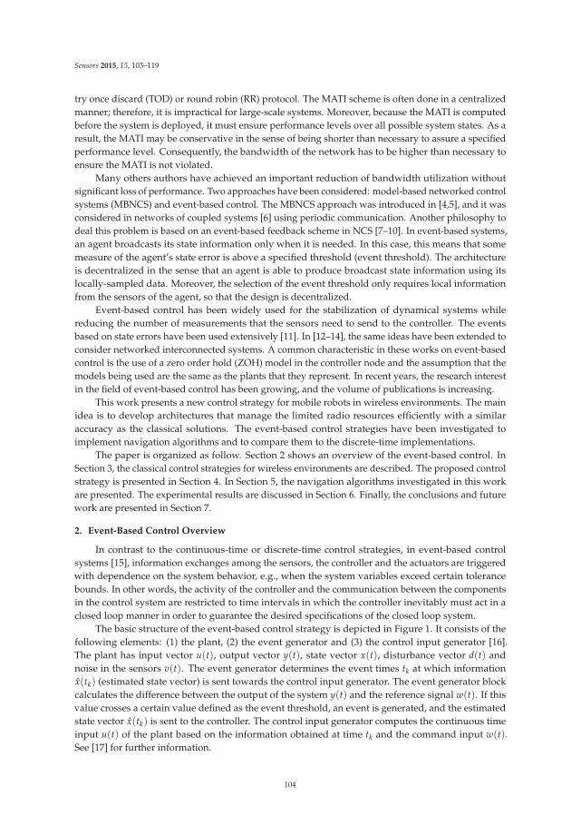
Sensors 2015, 15, 103–119

try once discard (TOD) or round robin (RR) protocol. The MATI scheme is often done in a centralizedmanner; therefore, it is impractical for large-scale systems. Moreover, because the MATI is computedbefore the system is deployed, it must ensure performance levels over all possible system states. As aresult, the MATI may be conservative in the sense of being shorter than necessary to assure a specifiedperformance level. Consequently, the bandwidth of the network has to be higher than necessary toensure the MATI is not violated.

Many others authors have achieved an important reduction of bandwidth utilization withoutsignificant loss of performance. Two approaches have been considered: model-based networked controlsystems (MBNCS) and event-based control. The MBNCS approach was introduced in [4,5], and it wasconsidered in networks of coupled systems [6] using periodic communication. Another philosophy todeal this problem is based on an event-based feedback scheme in NCS [7–10]. In event-based systems,an agent broadcasts its state information only when it is needed. In this case, this means that somemeasure of the agent’s state error is above a specified threshold (event threshold). The architectureis decentralized in the sense that an agent is able to produce broadcast state information using itslocally-sampled data. Moreover, the selection of the event threshold only requires local informationfrom the sensors of the agent, so that the design is decentralized.

Event-based control has been widely used for the stabilization of dynamical systems whilereducing the number of measurements that the sensors need to send to the controller. The eventsbased on state errors have been used extensively [11]. In [12–14], the same ideas have been extended toconsider networked interconnected systems. A common characteristic in these works on event-basedcontrol is the use of a zero order hold (ZOH) model in the controller node and the assumption that themodels being used are the same as the plants that they represent. In recent years, the research interestin the field of event-based control has been growing, and the volume of publications is increasing.

This work presents a new control strategy for mobile robots in wireless environments. The mainidea is to develop architectures that manage the limited radio resources efficiently with a similaraccuracy as the classical solutions. The event-based control strategies have been investigated toimplement navigation algorithms and to compare them to the discrete-time implementations.

The paper is organized as follow. Section 2 shows an overview of the event-based control. InSection 3, the classical control strategies for wireless environments are described. The proposed controlstrategy is presented in Section 4. In Section 5, the navigation algorithms investigated in this workare presented. The experimental results are discussed in Section 6. Finally, the conclusions and futurework are presented in Section 7.

2. Event-Based Control Overview

In contrast to the continuous-time or discrete-time control strategies, in event-based controlsystems [15], information exchanges among the sensors, the controller and the actuators are triggeredwith dependence on the system behavior, e.g., when the system variables exceed certain tolerancebounds. In other words, the activity of the controller and the communication between the componentsin the control system are restricted to time intervals in which the controller inevitably must act in aclosed loop manner in order to guarantee the desired specifications of the closed loop system.

The basic structure of the event-based control strategy is depicted in Figure 1. It consists of thefollowing elements: (1) the plant, (2) the event generator and (3) the control input generator [16].The plant has input vector u(t), output vector y(t), state vector x(t), disturbance vector d(t) andnoise in the sensors v(t). The event generator determines the event times tk at which informationx(tk) (estimated state vector) is sent towards the control input generator. The event generator blockcalculates the difference between the output of the system y(t) and the reference signal w(t). If thisvalue crosses a certain value defined as the event threshold, an event is generated, and the estimatedstate vector x(tk) is sent to the controller. The control input generator computes the continuous timeinput u(t) of the plant based on the information obtained at time tk and the command input w(t).See [17] for further information.

104

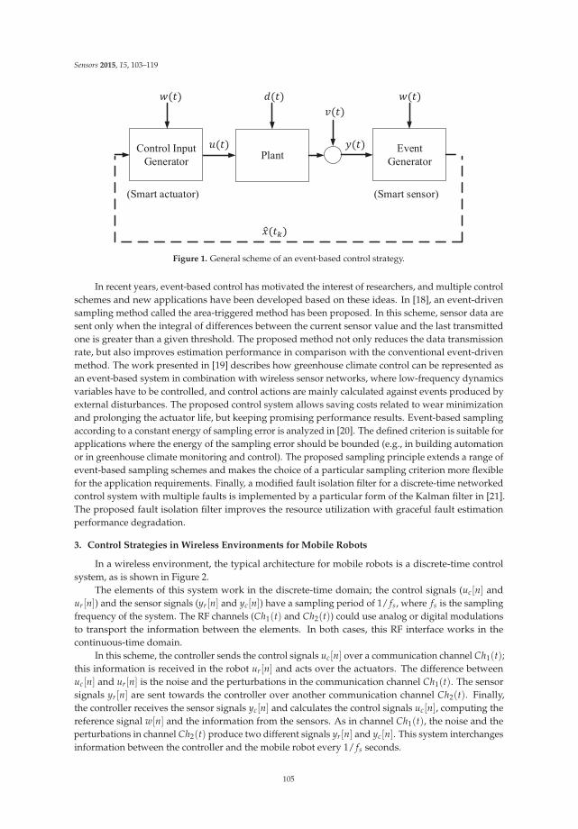
Sensors 2015, 15, 103–119

PlantEvent

Generator

Control Input

Generator

(Smart actuator) (Smart sensor)

Figure 1. General scheme of an event-based control strategy.

In recent years, event-based control has motivated the interest of researchers, and multiple controlschemes and new applications have been developed based on these ideas. In [18], an event-drivensampling method called the area-triggered method has been proposed. In this scheme, sensor data aresent only when the integral of differences between the current sensor value and the last transmittedone is greater than a given threshold. The proposed method not only reduces the data transmissionrate, but also improves estimation performance in comparison with the conventional event-drivenmethod. The work presented in [19] describes how greenhouse climate control can be represented asan event-based system in combination with wireless sensor networks, where low-frequency dynamicsvariables have to be controlled, and control actions are mainly calculated against events produced byexternal disturbances. The proposed control system allows saving costs related to wear minimizationand prolonging the actuator life, but keeping promising performance results. Event-based samplingaccording to a constant energy of sampling error is analyzed in [20]. The defined criterion is suitable forapplications where the energy of the sampling error should be bounded (e.g., in building automationor in greenhouse climate monitoring and control). The proposed sampling principle extends a range ofevent-based sampling schemes and makes the choice of a particular sampling criterion more flexiblefor the application requirements. Finally, a modified fault isolation filter for a discrete-time networkedcontrol system with multiple faults is implemented by a particular form of the Kalman filter in [21].The proposed fault isolation filter improves the resource utilization with graceful fault estimationperformance degradation.

3. Control Strategies in Wireless Environments for Mobile Robots

In a wireless environment, the typical architecture for mobile robots is a discrete-time controlsystem, as is shown in Figure 2.

The elements of this system work in the discrete-time domain; the control signals (uc[n] andur[n]) and the sensor signals (yr[n] and yc[n]) have a sampling period of 1/ fs, where fs is the samplingfrequency of the system. The RF channels (Ch1(t) and Ch2(t)) could use analog or digital modulationsto transport the information between the elements. In both cases, this RF interface works in thecontinuous-time domain.

In this scheme, the controller sends the control signals uc[n] over a communication channel Ch1(t);this information is received in the robot ur[n] and acts over the actuators. The difference betweenuc[n] and ur[n] is the noise and the perturbations in the communication channel Ch1(t). The sensorsignals yr[n] are sent towards the controller over another communication channel Ch2(t). Finally,the controller receives the sensor signals yc[n] and calculates the control signals uc[n], computing thereference signal w[n] and the information from the sensors. As in channel Ch1(t), the noise and theperturbations in channel Ch2(t) produce two different signals yr[n] and yc[n]. This system interchangesinformation between the controller and the mobile robot every 1/ fs seconds.

105

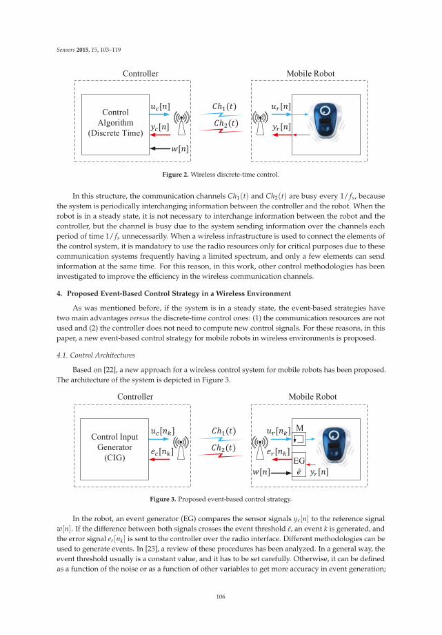
Sensors 2015, 15, 103–119

Control

Algorithm

(Discrete Time)

Mobile RobotController

Figure 2. Wireless discrete-time control.

In this structure, the communication channels Ch1(t) and Ch2(t) are busy every 1/ fs, becausethe system is periodically interchanging information between the controller and the robot. When therobot is in a steady state, it is not necessary to interchange information between the robot and thecontroller, but the channel is busy due to the system sending information over the channels eachperiod of time 1/ fs unnecessarily. When a wireless infrastructure is used to connect the elements ofthe control system, it is mandatory to use the radio resources only for critical purposes due to thesecommunication systems frequently having a limited spectrum, and only a few elements can sendinformation at the same time. For this reason, in this work, other control methodologies has beeninvestigated to improve the efficiency in the wireless communication channels.

4. Proposed Event-Based Control Strategy in a Wireless Environment

As was mentioned before, if the system is in a steady state, the event-based strategies havetwo main advantages versus the discrete-time control ones: (1) the communication resources are notused and (2) the controller does not need to compute new control signals. For these reasons, in thispaper, a new event-based control strategy for mobile robots in wireless environments is proposed.

4.1. Control Architectures

Based on [22], a new approach for a wireless control system for mobile robots has been proposed.The architecture of the system is depicted in Figure 3.

Control Input

Generator

(CIG)

Mobile Robot

EG

Controller

M

Figure 3. Proposed event-based control strategy.

In the robot, an event generator (EG) compares the sensor signals yr[n] to the reference signalw[n]. If the difference between both signals crosses the event threshold e, an event k is generated, andthe error signal er[nk] is sent to the controller over the radio interface. Different methodologies can beused to generate events. In [23], a review of these procedures has been analyzed. In a general way, theevent threshold usually is a constant value, and it has to be set carefully. Otherwise, it can be definedas a function of the noise or as a function of other variables to get more accuracy in event generation;

106

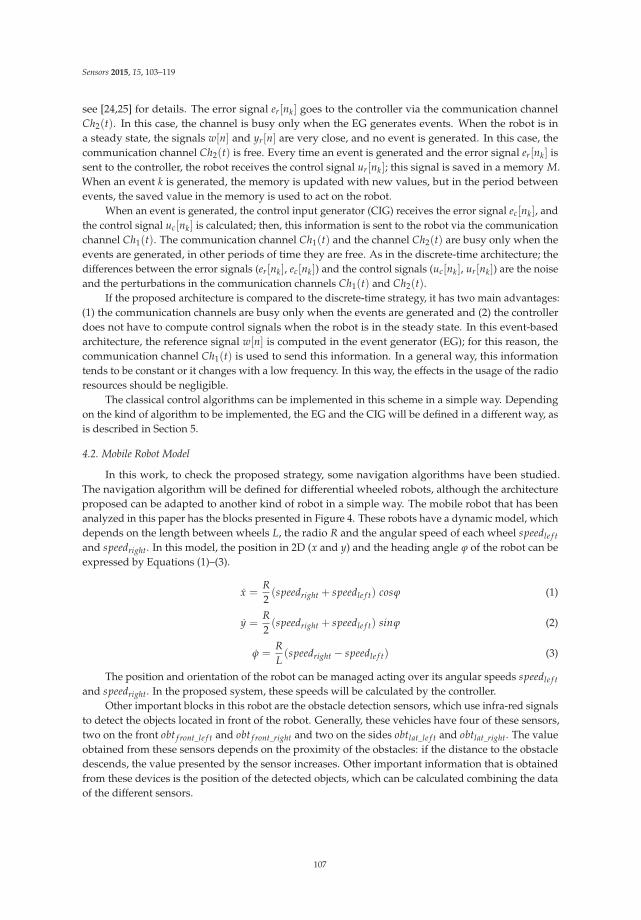
Sensors 2015, 15, 103–119

see [24,25] for details. The error signal er[nk] goes to the controller via the communication channelCh2(t). In this case, the channel is busy only when the EG generates events. When the robot is ina steady state, the signals w[n] and yr[n] are very close, and no event is generated. In this case, thecommunication channel Ch2(t) is free. Every time an event is generated and the error signal er[nk] issent to the controller, the robot receives the control signal ur[nk]; this signal is saved in a memory M.When an event k is generated, the memory is updated with new values, but in the period betweenevents, the saved value in the memory is used to act on the robot.

When an event is generated, the control input generator (CIG) receives the error signal ec[nk], andthe control signal uc[nk] is calculated; then, this information is sent to the robot via the communicationchannel Ch1(t). The communication channel Ch1(t) and the channel Ch2(t) are busy only when theevents are generated, in other periods of time they are free. As in the discrete-time architecture; thedifferences between the error signals (er[nk], ec[nk]) and the control signals (uc[nk], ur[nk]) are the noiseand the perturbations in the communication channels Ch1(t) and Ch2(t).

If the proposed architecture is compared to the discrete-time strategy, it has two main advantages:(1) the communication channels are busy only when the events are generated and (2) the controllerdoes not have to compute control signals when the robot is in the steady state. In this event-basedarchitecture, the reference signal w[n] is computed in the event generator (EG); for this reason, thecommunication channel Ch1(t) is used to send this information. In a general way, this informationtends to be constant or it changes with a low frequency. In this way, the effects in the usage of the radioresources should be negligible.

The classical control algorithms can be implemented in this scheme in a simple way. Dependingon the kind of algorithm to be implemented, the EG and the CIG will be defined in a different way, asis described in Section 5.

4.2. Mobile Robot Model

In this work, to check the proposed strategy, some navigation algorithms have been studied.The navigation algorithm will be defined for differential wheeled robots, although the architectureproposed can be adapted to another kind of robot in a simple way. The mobile robot that has beenanalyzed in this paper has the blocks presented in Figure 4. These robots have a dynamic model, whichdepends on the length between wheels L, the radio R and the angular speed of each wheel speedle f t

and speedright. In this model, the position in 2D (x and y) and the heading angle ϕ of the robot can beexpressed by Equations (1)–(3).

x =R

2(speedright + speedle f t) cosϕ (1)

y =R

2(speedright + speedle f t) sinϕ (2)

ϕ =R

L(speedright − speedle f t) (3)

The position and orientation of the robot can be managed acting over its angular speeds speedle f t

and speedright. In the proposed system, these speeds will be calculated by the controller.Other important blocks in this robot are the obstacle detection sensors, which use infra-red signals

to detect the objects located in front of the robot. Generally, these vehicles have four of these sensors,two on the front obt f ront_le f t and obt f ront_right and two on the sides obtlat_le f t and obtlat_right. The valueobtained from these sensors depends on the proximity of the obstacles: if the distance to the obstacledescends, the value presented by the sensor increases. Other important information that is obtainedfrom these devices is the position of the detected objects, which can be calculated combining the dataof the different sensors.

107

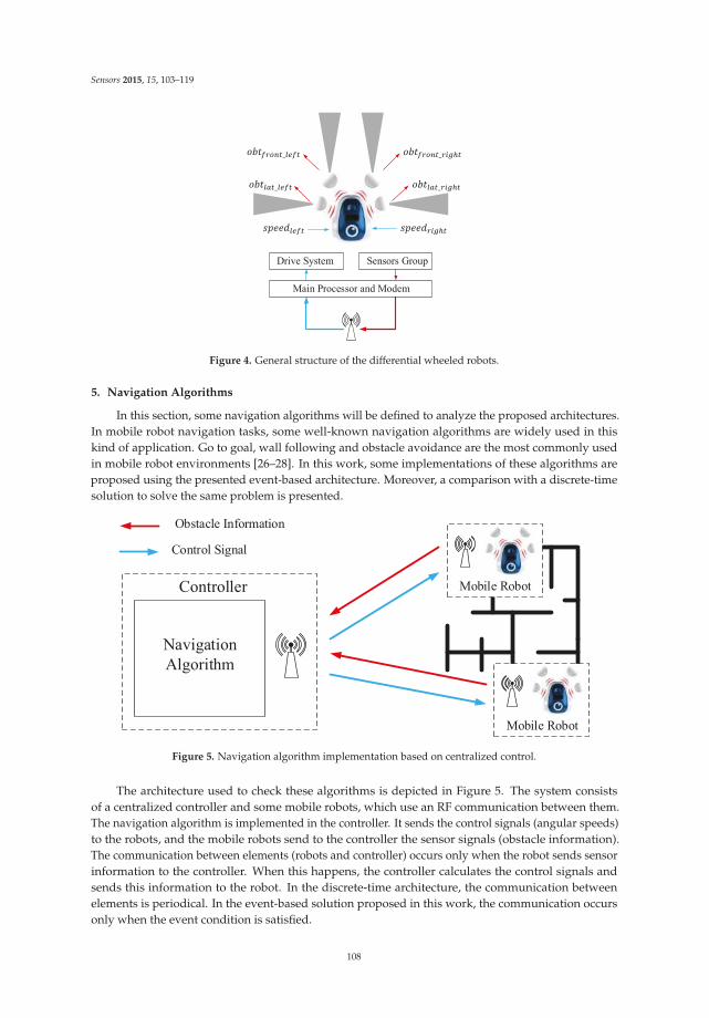
Sensors 2015, 15, 103–119

Drive System Sensors Group

Main Processor and Modem

Figure 4. General structure of the differential wheeled robots.

5. Navigation Algorithms

In this section, some navigation algorithms will be defined to analyze the proposed architectures.In mobile robot navigation tasks, some well-known navigation algorithms are widely used in thiskind of application. Go to goal, wall following and obstacle avoidance are the most commonly usedin mobile robot environments [26–28]. In this work, some implementations of these algorithms areproposed using the presented event-based architecture. Moreover, a comparison with a discrete-timesolution to solve the same problem is presented.

Navigation

Algorithm

Controller

Obstacle Information

Control Signal

Mobile Robot

Mobile Robot

Figure 5. Navigation algorithm implementation based on centralized control.

The architecture used to check these algorithms is depicted in Figure 5. The system consistsof a centralized controller and some mobile robots, which use an RF communication between them.The navigation algorithm is implemented in the controller. It sends the control signals (angular speeds)to the robots, and the mobile robots send to the controller the sensor signals (obstacle information).The communication between elements (robots and controller) occurs only when the robot sends sensorinformation to the controller. When this happens, the controller calculates the control signals andsends this information to the robot. In the discrete-time architecture, the communication betweenelements is periodical. In the event-based solution proposed in this work, the communication occursonly when the event condition is satisfied.

108

Sensors 2015, 15, 103–119

In the next sections, a wall following and an obstacle avoidance algorithms will be developed toanalyze the behavior of the proposed strategy and to compare to a classical discrete-time solution.

5.1. Wall Following Algorithm

A wall following algorithm is one of the most common process used in mobile robot navigation.The basic algorithm is as follows:

(1) Find the closest wall.(2) Move to a desired distance from the wall.(3) Turn and start moving along the wall, staying the desired distance away.

Wall following algorithms have two variants of implementation: clockwise or counter-clockwise;in this case, the second option is selected. To implement this algorithm in the controller, a simplecontrol law has been designed; it is presented in Equation (4).

if (obt f ront_le f t > 0) f ront_obstacle = 1

else f ront_obstacle = 0

scle f t(%) =(

obtlat_le f t−5040

)

· 40 + 50

scright(%) = 50 − ( f ront_obstacle) · 50

(4)

In this expression, obt f ront_le f t and obtlat_le f t are the values of the sensors, the range of whichgoes from 0% (obstacle is out of the range of the sensor) to 100% (the obstacle is touching the robot).The auxiliary variable f ront_obstacle is used to detect if an obstacle is in front of the robot. scle f t andscright are the angular speeds calculated in the controller, which have to be sent to the robot over theradio channel; the range of these speeds go from 0%–100%.

The control law in Equation (4) modifies the wheel speed of the robot to force it to stay at aconstant distance (50% of the lateral sensor’s range) from the wall with a constant speed (50% of therobot’s maximum speed).

This navigation algorithm is the same for the discrete-time solution and for the event-based one.In the mobile robot, when the discrete-time solution is used, every sampling time 1/ fs, the robot sendsthe sensor information (obt f ront_le f t, obt f ront_right, obtside_le f t and obtside_right) over the radio interface.After the controller receives this information, it computes the control signals (scle f t and scright), andthey are sent to the robot over the same radio interface. Finally, in the robot, the received controlsignals are assigned by the drive system to the wheels (speedle f t = scle f t and speedright = scright).

When the event-based proposal is considered, as was mentioned before, the algorithm in thecontroller is the same, but in the mobile robot, an event-based algorithm is implemented. The proposedevent-based system for the mobile robot is depicted in Figure 6. The event-based algorithm in therobot depends on the event condition, which is presented in Equation (5), where w represents thereference signal, which is 50% for this algorithm. The event threshold e is the parameter that definesthe accuracy of the system, the number of the events and its influence on the communication load inthe RF interface.

if ((obt f ront_le f t > 0) OR (abs(obtlat_le f t − w) > e)

event = trueelse event = f alse

(5)

When the event condition is satisfied, an event is generated, and the robot sends to the controllerthe sensor information. At the same time, the controller, after computing the control signals, returns tothe robot this information, which contains new speed values. Every time the event condition is true,

109

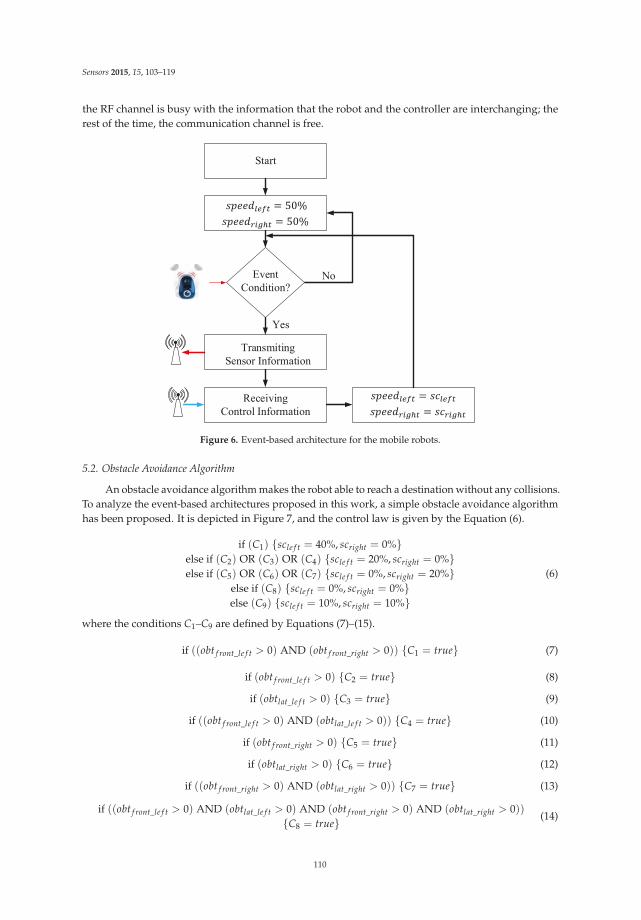
Sensors 2015, 15, 103–119

the RF channel is busy with the information that the robot and the controller are interchanging; therest of the time, the communication channel is free.

Start

NoEvent

Condition?

Transmiting

Sensor Information

Receiving

Control Information

Yes

Figure 6. Event-based architecture for the mobile robots.

5.2. Obstacle Avoidance Algorithm

An obstacle avoidance algorithm makes the robot able to reach a destination without any collisions.To analyze the event-based architectures proposed in this work, a simple obstacle avoidance algorithmhas been proposed. It is depicted in Figure 7, and the control law is given by the Equation (6).

if (C1) scle f t = 40%, scright = 0%else if (C2) OR (C3) OR (C4) scle f t = 20%, scright = 0%else if (C5) OR (C6) OR (C7) scle f t = 0%, scright = 20%

else if (C8) scle f t = 0%, scright = 0%else (C9) scle f t = 10%, scright = 10%

(6)

where the conditions C1–C9 are defined by Equations (7)–(15).

if ((obt f ront_le f t > 0) AND (obt f ront_right > 0)) C1 = true (7)

if (obt f ront_le f t > 0) C2 = true (8)

if (obtlat_le f t > 0) C3 = true (9)

if ((obt f ront_le f t > 0) AND (obtlat_le f t > 0)) C4 = true (10)

if (obt f ront_right > 0) C5 = true (11)

if (obtlat_right > 0) C6 = true (12)

if ((obt f ront_right > 0) AND (obtlat_right > 0)) C7 = true (13)

if ((obt f ront_le f t > 0) AND (obtlat_le f t > 0) AND (obt f ront_right > 0) AND (obtlat_right > 0))C8 = true (14)

110

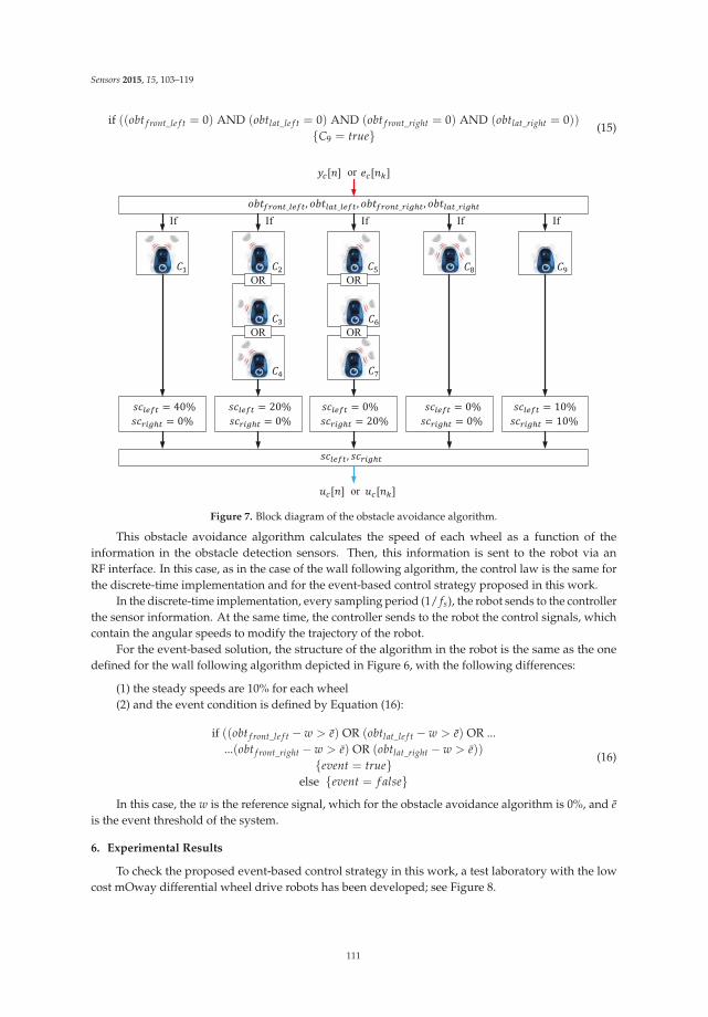
Sensors 2015, 15, 103–119

if ((obt f ront_le f t = 0) AND (obtlat_le f t = 0) AND (obt f ront_right = 0) AND (obtlat_right = 0))C9 = true (15)

If If If If If

or

or

OR

OR

OR

OR

Figure 7. Block diagram of the obstacle avoidance algorithm.

This obstacle avoidance algorithm calculates the speed of each wheel as a function of theinformation in the obstacle detection sensors. Then, this information is sent to the robot via anRF interface. In this case, as in the case of the wall following algorithm, the control law is the same forthe discrete-time implementation and for the event-based control strategy proposed in this work.

In the discrete-time implementation, every sampling period (1/ fs), the robot sends to the controllerthe sensor information. At the same time, the controller sends to the robot the control signals, whichcontain the angular speeds to modify the trajectory of the robot.

For the event-based solution, the structure of the algorithm in the robot is the same as the onedefined for the wall following algorithm depicted in Figure 6, with the following differences:

(1) the steady speeds are 10% for each wheel(2) and the event condition is defined by Equation (16):

if ((obt f ront_le f t − w > e) OR (obtlat_le f t − w > e) OR ......(obt f ront_right − w > e) OR (obtlat_right − w > e))

event = trueelse event = f alse

(16)

In this case, the w is the reference signal, which for the obstacle avoidance algorithm is 0%, and e

is the event threshold of the system.

6. Experimental Results

To check the proposed event-based control strategy in this work, a test laboratory with the lowcost mOway differential wheel drive robots has been developed; see Figure 8.

111

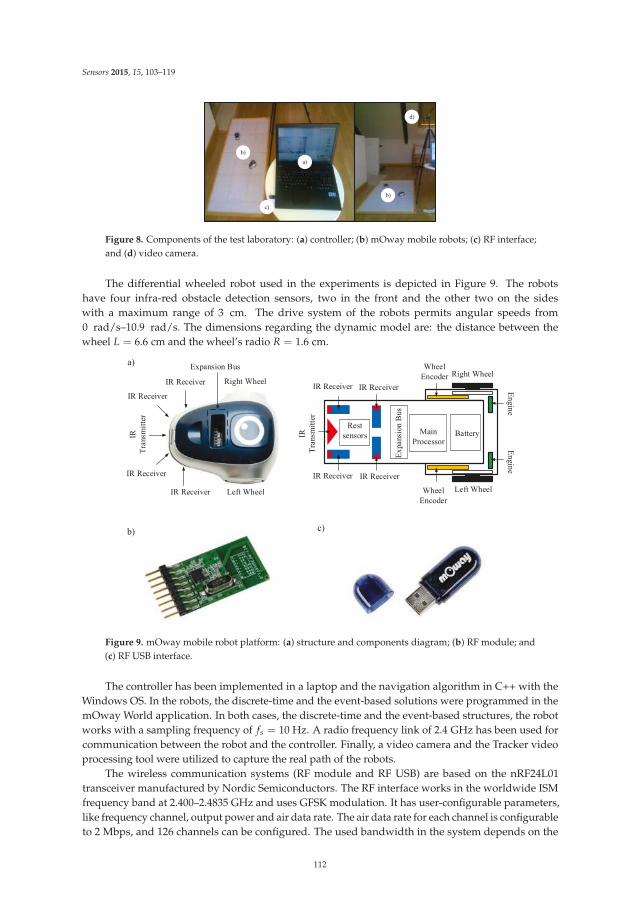
Sensors 2015, 15, 103–119

a)

b)

b)

c)

d)

Figure 8. Components of the test laboratory: (a) controller; (b) mOway mobile robots; (c) RF interface;and (d) video camera.

The differential wheeled robot used in the experiments is depicted in Figure 9. The robotshave four infra-red obstacle detection sensors, two in the front and the other two on the sideswith a maximum range of 3 cm. The drive system of the robots permits angular speeds from0 rad/s–10.9 rad/s. The dimensions regarding the dynamic model are: the distance between thewheel L = 6.6 cm and the wheel’s radio R = 1.6 cm.

a)

b) c)

Main

ProcessorBatteryIR

Tra

nsm

itte

r

IR Receiver IR Receiver

IR Receiver IR Receiver

Rest

sensors

Ex

pansi

on

Bus

Wheel

Encoder

Wheel

Encoder

En

gin

eE

ngin

e

Right Wheel

Left Wheel

IR

Tra

nsm

itte

r

IR Receiver

IR Receiver Right Wheel

Left Wheel

IR Receiver

IR Receiver

Expansion Bus

Figure 9. mOway mobile robot platform: (a) structure and components diagram; (b) RF module; and(c) RF USB interface.

The controller has been implemented in a laptop and the navigation algorithm in C++ with theWindows OS. In the robots, the discrete-time and the event-based solutions were programmed in themOway World application. In both cases, the discrete-time and the event-based structures, the robotworks with a sampling frequency of fs = 10 Hz. A radio frequency link of 2.4 GHz has been used forcommunication between the robot and the controller. Finally, a video camera and the Tracker videoprocessing tool were utilized to capture the real path of the robots.

The wireless communication systems (RF module and RF USB) are based on the nRF24L01transceiver manufactured by Nordic Semiconductors. The RF interface works in the worldwide ISMfrequency band at 2.400–2.4835 GHz and uses GFSK modulation. It has user-configurable parameters,like frequency channel, output power and air data rate. The air data rate for each channel is configurableto 2 Mbps, and 126 channels can be configured. The used bandwidth in the system depends on the

112

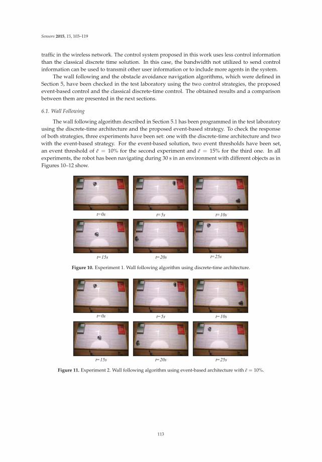
Sensors 2015, 15, 103–119

traffic in the wireless network. The control system proposed in this work uses less control informationthan the classical discrete time solution. In this case, the bandwidth not utilized to send controlinformation can be used to transmit other user information or to include more agents in the system.

The wall following and the obstacle avoidance navigation algorithms, which were defined inSection 5, have been checked in the test laboratory using the two control strategies, the proposedevent-based control and the classical discrete-time control. The obtained results and a comparisonbetween them are presented in the next sections.

6.1. Wall Following

The wall following algorithm described in Section 5.1 has been programmed in the test laboratoryusing the discrete-time architecture and the proposed event-based strategy. To check the responseof both strategies, three experiments have been set: one with the discrete-time architecture and twowith the event-based strategy. For the event-based solution, two event thresholds have been set,an event threshold of e = 10% for the second experiment and e = 15% for the third one. In allexperiments, the robot has been navigating during 30 s in an environment with different objects as inFigures 10–12 show.

t=0s t=5s t=10s

t=15s t=20s t=25s

Figure 10. Experiment 1. Wall following algorithm using discrete-time architecture.

t=0s t=5s t=10s

t=15s t=20s t=25s

Figure 11. Experiment 2. Wall following algorithm using event-based architecture with e = 10%.

113

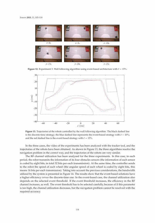
Sensors 2015, 15, 103–119

t=0s t=5s t=10s

t=15s t=20s t=25s

Figure 12. Experiment 3. Wall following algorithm using event-based architecture with e = 15%.

-60 -40 -20 0 20 40 60-40

-30

-20

-10

0

10

20

30

Figure 13. Trajectories of the robots controlled by the wall following algorithm. The black dashed lineis the discrete-time strategy; the blue dashed line represents the event-based strategy with e = 10%;and the red dashed line is the event-based strategy with e = 15%.

In the three cases, the video of the experiments has been analyzed with the tracker tool, and thetrajectories of the robots have been obtained. As shown in Figure 13, the three algorithms resolve thenavigation problem in the correct way, and the trajectories of the robots are very similar.

The RF channel utilization has been analyzed for the three experiments. In this case, in eachperiod, the robot transmits the information of its four obstacles sensors (the information of each sensoris coded by eight bits, in total 32 bits per each transmission). At the same time, the controller sendsto the robot the speed of each wheel (the angular speed of each wheel is coded by eight bits, thismeans 16 bits per each transmission). Taking into account the previous considerations, the bandwidthutilized by the system is presented in Figure 14. The results show that the event-based solutions havea higher efficiency versus the discrete-time one. In the event-based case, the channel utilization alsodepends on the selected event threshold. If the event threshold increases, the efficiency in the RFchannel increases, as well. The event threshold has to be selected carefully, because of if this parameteris too high, the channel utilization decreases, but the navigation problem cannot be resolved with therequired accuracy.

114

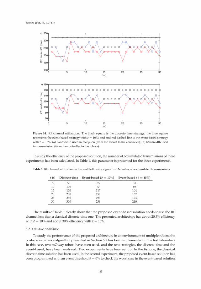
Sensors 2015, 15, 103–119

0 5 10 15 20 25 30100

150

200

250

300

350

0 5 10 15 20 25 30

60

80

100

120

140

160

180

a)

b)

Figure 14. RF channel utilization. The black square is the discrete-time strategy; the blue squarerepresents the event-based strategy with e = 10%; and and red dashed line is the event-based strategywith e = 15%. (a) Bandwidth used in reception (from the robots to the controller); (b) bandwidth usedin transmission (from the controller to the robots).

To study the efficiency of the proposed solution, the number of accumulated transmissions of theseexperiments has been calculated. In Table 1, this parameter is presented for the three experiments.

Table 1. RF channel utilization in the wall following algorithm. Number of accumulated transmissions.

t (s) Discrete-time Event-based (e = 10%) Event-based (e = 15%)

5 50 35 3110 100 77 6915 150 117 10420 200 158 13725 250 199 17430 300 239 210

The results of Table 1 clearly show that the proposed event-based solution needs to use the RFchannel less than a classical discrete-time one. The presented architecture has about 20.3% efficiencywith e = 10% and about 30% efficiency with e = 15%.

6.2. Obstacle Avoidance

To study the performance of the proposed architecture in an environment of multiple robots, theobstacle avoidance algorithm presented in Section 5.2 has been implemented in the test laboratory.In this case, two mOway robots have been used, and the two strategies, the discrete-time and theevent-based, have been analyzed. Two experiments have been set up. In the fist one, the classicaldiscrete-time solution has been used. In the second experiment, the proposed event-based solution hasbeen programmed with an event threshold e = 0% to check the worst case in the event-based solution.

115

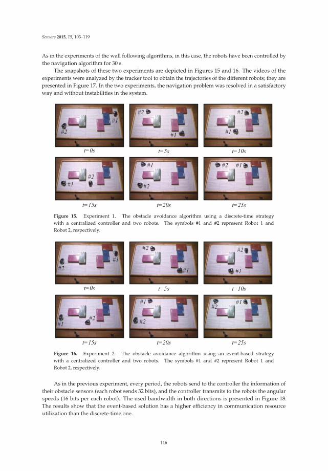
Sensors 2015, 15, 103–119

As in the experiments of the wall following algorithms, in this case, the robots have been controlled bythe navigation algorithm for 30 s.

The snapshots of these two experiments are depicted in Figures 15 and 16. The videos of theexperiments were analyzed by the tracker tool to obtain the trajectories of the different robots; they arepresented in Figure 17. In the two experiments, the navigation problem was resolved in a satisfactoryway and without instabilities in the system.

t=0s t=5s t=10s

t=15s t=20s t=25s

#1

#1#1

#1

#1 #1

#2

#2 #2

#2

#2

#2

Figure 15. Experiment 1. The obstacle avoidance algorithm using a discrete-time strategywith a centralized controller and two robots. The symbols #1 and #2 represent Robot 1 andRobot 2, respectively.

t=0s t=5s t=10s

t=15s t=20s t=25s

#1

#1 #1

#1

#1 #1

#2

#2 #2

#2#2

#2

Figure 16. Experiment 2. The obstacle avoidance algorithm using an event-based strategywith a centralized controller and two robots. The symbols #1 and #2 represent Robot 1 andRobot 2, respectively.

As in the previous experiment, every period, the robots send to the controller the information oftheir obstacle sensors (each robot sends 32 bits), and the controller transmits to the robots the angularspeeds (16 bits per each robot). The used bandwidth in both directions is presented in Figure 18.The results show that the event-based solution has a higher efficiency in communication resourceutilization than the discrete-time one.

116

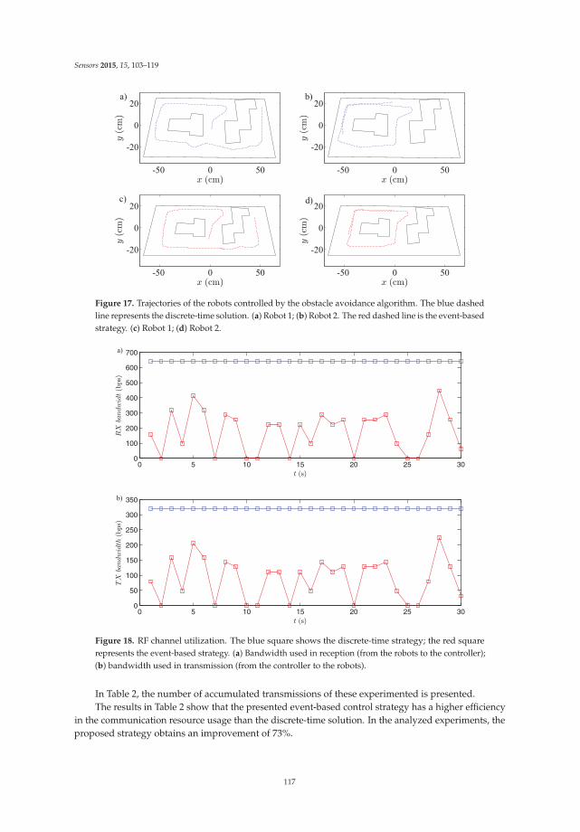
Sensors 2015, 15, 103–119

-50 0 50

-20

0

20

-50 0 50

-20

0

20

-50 0 50

-20

0

20

-50 0 50

-20

0

20

b)

d)

a)

c)

Figure 17. Trajectories of the robots controlled by the obstacle avoidance algorithm. The blue dashedline represents the discrete-time solution. (a) Robot 1; (b) Robot 2. The red dashed line is the event-basedstrategy. (c) Robot 1; (d) Robot 2.

0 5 10 15 20 25 300

100

200

300

400

500

600

700

0 5 10 15 20 25 300

50

100

150

200

250

300

350

a)

b)

Figure 18. RF channel utilization. The blue square shows the discrete-time strategy; the red squarerepresents the event-based strategy. (a) Bandwidth used in reception (from the robots to the controller);(b) bandwidth used in transmission (from the controller to the robots).

In Table 2, the number of accumulated transmissions of these experimented is presented.The results in Table 2 show that the presented event-based control strategy has a higher efficiency

in the communication resource usage than the discrete-time solution. In the analyzed experiments, theproposed strategy obtains an improvement of 73%.

117

Sensors 2015, 15, 103–119

Table 2. RF channel utilization. Number of accumulated transmissions.

t (s) Discrete-Time Event-Based

5 100 3110 200 5815 300 7920 400 10625 500 13430 600 163

7. Conclusions and Future Work

The proposed event-based control strategy can be implemented in mobile robot architectures ina simple way. In this work, these strategies are applied to the mOway mobile robots platform, butthis solution can be adapted to other kinds of robots following the same methodology. The controlstructures defined in the mobile robot only need to set one parameter, the event threshold e, whichdefines the accuracy of the system and the performance in the radio interface. In the navigationexperiments presented in this work, the proposed system has resolved the navigation problem inthe same way as the discrete-time solution. The event-based solution obtains higher efficienciesin communication resource usage than the classical discrete-time solution. In the wall followingalgorithm, an efficiency of 15% is obtained, and for the obstacle avoidance algorithm, it is 73%.

As future work, the system is now being checked with a hybrid system, which contains severalnavigation algorithms (go to goal, wall following in its two versions and obstacle avoidance) workingtogether using the architectures presented in this paper. Furthermore, the stability of the proposedsolution is going to be analyzed in a theoretical way.

Acknowledgments: This work has been funded by the National Plan Project DPI2012-31303 of the SpanishMinistry of Economy and Competitiveness and FEDER funds.

Author Contributions: Rafael Socas designed the system, performed the experiments, analysed the results andprepared the first draft of the manuscript. Sebastián Dormido performed the theoretical conception and planningof the system. The manuscript was revised and modified by Raquel Dormido. Ernesto Fabregas assisted in thedata acquisition and communications requirements.


References

1. Mansano, R.K.; Godoy, E.P.; Porto, A.J. The Benefits of Soft Sensor and Multi-Rate Control for theImplementation of Wireless Networked Control Systems. Sensors 2014, 14, 24441–24461.

2. Roohi, M.H.; Ghaisari, J.; Izadi, I.; Saidi, H. Discrete-time event-triggered control for wireless networks:Design and network calculus analysis. In Proceedings of the International Conference on Event-based Control,Communication, and Signal Processing (EBCCSP), Krakow, Poland, 17–19 June 2015; pp. 1–8.

3. Cloosterman, M.B.; Hetel, L.; van de Wouw, N.; Heemels, W.; Daafouz, J.; Nijmeijer, H. Controller synthesisfor networked control systems. Automatica 2010, 46, 1584–1594.

4. Montestruque, L.; Antsaklis, P.J. State and output feedback control in model-based networked control systems.In Proceedings of the 41st IEEE Conference on Decision and Control, Las Vegas, NV, USA, 10–13 December2002; Volume 2, pp. 1620–1625.

5. Montestruque, L.A.; Antsaklis, P.J. On the model-based control of networked systems. Automatica 2003,39, 1837–1843.

6. Sun, Y.; El-Farra, N.H. Quasi-decentralized model-based networked control of process systems.Comput. Chem. Eng. 2008, 32, 2016–2029.

7. Tabuada, P. Event-triggered real-time scheduling of stabilizing control tasks. IEEE Trans. Autom. Control

2007, 52, 1680–1685.8. Wang, X.; Lemmon, M.D. Event-triggering in distributed networked control systems. IEEE Trans.

Autom. Control 2011, 56, 586–601.

118

Sensors 2015, 15, 103–119

9. Garcia, E.; Antsaklis, P.J. Decentralized model-based event-triggered control of networked systems.In Proceedings of the American Control Conference (ACC), Montreal, QC, Canada, 27–29 June 2012;pp. 6485–6490.

10. Guinaldo, M.; Dimarogonas, D.V.; Johansson, K.H.; Sánchez, J.; Dormido, S. Distributed event-based controlfor interconnected linear systems. In Proceedings of the 50th IEEE Conference on Decision and Control andEuropean Control Conference (CDC-ECC), Orlando, FL, USA, 12–15 December 2011; pp. 2553–2558.

11. Anta, A.; Tabuada, P. To sample or not to sample: Self-triggered control for nonlinear systems. IEEE Trans.

Autom. Control 2010, 55, 2030–2042.12. Wang, X.; Lemmon, M.D. Event-Triggering in Distributed Networked Systems with Data Dropouts and

Delays. In Hybrid Systems: Computation and Control; Springer: Berlin, Germany, 2009; pp. 366–380.13. Mazo, M.; Tabuada, P. Decentralized event-triggered control over wireless sensor/actuator networks.

IEEE Trans. Autom. Control 2011, 56, 2456–2461.14. Dimarogonas, D.V.; Johansson, K.H. Event-triggered control for multi-agent systems. In Proceedings of

the 48th IEEE Conference on Decision and Control, 2009 Held Jointly with the 2009 28th Chinese ControlConference, Shanghai, China, 15–18 December 2009; pp. 7131–7136.

15. Sánchez, J.; Visioli, A.; Dormido, S. Event-based PID control. In PID Control in the Third Millennium; Springer:Berlin, Germany, 2012; pp. 495–526.

16. Aström, K.J. Event Based Control. In Analysis and Design of Nonlinear Control Systems; Springer: Berlin,Germany, 2008; pp. 127–147.

17. Lunze, J.; Lehmann, D. A state-feedback approach to event-based control. Automatica 2010, 46, 211–215.18. Nguyen, V.H.; Suh, Y.S. Networked estimation with an area-triggered transmission method. Sensors 2008,

8, 897–909.19. Pawlowski, A.; Guzman, J.L.; Rodríguez, F.; Berenguel, M.; Sánchez, J.; Dormido, S. Simulation of greenhouse

climate monitoring and control with wireless sensor network and event-based control. Sensors 2009,9, 232–252.

20. Miskowicz, M. Efficiency of event-based sampling according to error energy criterion. Sensors 2010,10, 2242–2261.

21. Li, S.; Sauter, D.; Xu, B. Fault isolation filter for networked control system with event-triggered samplingscheme. Sensors 2011, 11, 557–572.

22. Lehmann, D.; Lunze, J. Extension and experimental evaluation of an event-based state-feedback approach.Control Eng. Pract. 2011, 19, 101–112.

23. Dormido, S.; Sánchez, J.; Kofman, E. Muestreo, control y comunicación basados en eventos. Rev. Iberoam.

Autom. Inform. Ind. RIAI 2008, 5, 5–26.24. Socas, R.; Dormido, S.; Dormido, R. Event-based controller for noisy environments. In Proceedings

of the Second World Conference on Complex Systems (WCCS), Agadir, Morocco, 10–12 November 2014;pp. 280–285.

25. Romero, J.A.; Pascual, N.J.; Peñarrocha, I.; Sanchis, R. Event-Based PI controller with adaptive thresholds.In Proceedings of the 4th International Congress on Ultra Modern Telecommunications and Control Systemsand Workshops (ICUMT), St. Petersburg, Russia, 3–5 October 2012; pp. 219–226.

26. Siegwart, R.; Nourbakhsh, I.R.; Scaramuzza, D. Introduction to Autonomous Mobile Robots; MIT Press:Cambridge, MA, USA, 2011.

27. Nehmzow, U. Robot Behaviour: Design, Description, Analysis and Modelling; Springer Science & Business Media:Berlin, Germany, 2008.

28. Nehmzow, U. Mobile Robotics; Springer Science & Business Media: Berlin, Germany, 2003.


119

Article

Estimation of Human Arm Joints Using Two WirelessSensors in Robotic Rehabilitation TasksArturo Bertomeu-Motos *, Luis D. Lledó, Jorge A. Díez, Jose M. Catalan, Santiago Ezquerro,Francisco J. Badesa and Nicolas Garcia-Aracil

Neuro-Bioengineering Research Group, Miguel Hernandez University, Avda. de la Universidad W/N,03202 Elche, Spain; [email protected] (L.D.L.); [email protected] (J.A.D.); [email protected] (J.M.C.);[email protected] (S.E.); [email protected] (F.J.B.); [email protected] (N.G.-A.)* Correspondence: [email protected]; Tel.: +34-965-222-505; Fax: +34-966-658-979

Academic Editor: Gonzalo Pajares MartinsanzReceived: 27 October 2015; Accepted: 2 December 2015; Published: 4 December 2015

Abstract: This paper presents a novel kinematic reconstruction of the human arm chain with fivedegrees of freedom and the estimation of the shoulder location during rehabilitation therapy assistedby end-effector robotic devices. This algorithm is based on the pseudoinverse of the Jacobian throughthe acceleration of the upper arm, measured using an accelerometer, and the orientation of theshoulder, estimated with a magnetic angular rate and gravity (MARG) device. The results show ahigh accuracy in terms of arm joints and shoulder movement with respect to the real arm measuredthrough an optoelectronic system. Furthermore, the range of motion (ROM) of 50 healthy subjects isstudied from two different trials, one trying to avoid shoulder movements and the second one forcingthem. Moreover, the shoulder movement in the second trial is also estimated accurately. Besides thefact that the posture of the patient can be corrected during the exercise, the therapist could use thepresented algorithm as an objective assessment tool. In conclusion, the joints’ estimation enables abetter adjustment of the therapy, taking into account the needs of the patient, and consequently, thearm motion improves faster.

Keywords: kinematic reconstruction; neuro-rehabilitation; end-effector robots; upper limbs; MARG

1. Introduction

Robot-aided neuro-rehabilitation therapies have become an interesting field in the roboticsarea. There are several devices, such as exoskeletons, prosthesis or end-effector configuration robots,developed for this purpose [1,2]. They are able to help and assist the shortcomings of human beings.Post-stroke patients usually lose limb mobility due to the impairment in motor activity. Rehabilitationin this field takes an important role when it comes to improving the motor and proprioceptiveactivity [3,4]. In terms of the activities of daily living (ADL), the total or partial recovery of the upperlimbs is the most important part in early rehabilitation. End-effector configuration robots are the mostcommon devices used in these therapies. They are easily adapted to and easy to use by patients withdifferent diseases.

These robots provide objective information about the trajectory followed by the end effector andthe improvement in the motor recovery. However, they are not able to measure and control the armmovements. The progress in the arm joints, i.e., the range of motion (ROM), is an important parameterin these kinds of therapies. This estimation requires non-invasive wearable sensors, which must beeasy to place onto the patient’s arm and must be extended to a clinical environment. Visual feedbackof the arm configuration is studied in some rehabilitation therapies, though the arm joints cannot bemeasured [5,6]. This estimation can be accurately performed with optoelectronic systems based onmotion tracking, even though they cannot be adapted to a rehabilitation environment [7,8]. In 2006,


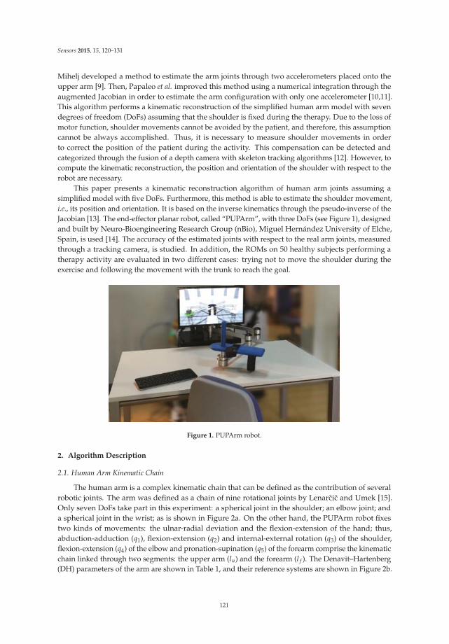
Sensors 2015, 15, 120–131

Mihelj developed a method to estimate the arm joints through two accelerometers placed onto theupper arm [9]. Then, Papaleo et al. improved this method using a numerical integration through theaugmented Jacobian in order to estimate the arm configuration with only one accelerometer [10,11].This algorithm performs a kinematic reconstruction of the simplified human arm model with sevendegrees of freedom (DoFs) assuming that the shoulder is fixed during the therapy. Due to the loss ofmotor function, shoulder movements cannot be avoided by the patient, and therefore, this assumptioncannot be always accomplished. Thus, it is necessary to measure shoulder movements in orderto correct the position of the patient during the activity. This compensation can be detected andcategorized through the fusion of a depth camera with skeleton tracking algorithms [12]. However, tocompute the kinematic reconstruction, the position and orientation of the shoulder with respect to therobot are necessary.

This paper presents a kinematic reconstruction algorithm of human arm joints assuming asimplified model with five DoFs. Furthermore, this method is able to estimate the shoulder movement,i.e., its position and orientation. It is based on the inverse kinematics through the pseudo-inverse of theJacobian [13]. The end-effector planar robot, called “PUPArm”, with three DoFs (see Figure 1), designedand built by Neuro-Bioengineering Research Group (nBio), Miguel Hernández University of Elche,Spain, is used [14]. The accuracy of the estimated joints with respect to the real arm joints, measuredthrough a tracking camera, is studied. In addition, the ROMs on 50 healthy subjects performing atherapy activity are evaluated in two different cases: trying not to move the shoulder during theexercise and following the movement with the trunk to reach the goal.

Figure 1. PUPArm robot.

2. Algorithm Description

2.1. Human Arm Kinematic Chain

The human arm is a complex kinematic chain that can be defined as the contribution of severalrobotic joints. The arm was defined as a chain of nine rotational joints by Lenarcic and Umek [15].Only seven DoFs take part in this experiment: a spherical joint in the shoulder; an elbow joint; anda spherical joint in the wrist; as is shown in Figure 2a. On the other hand, the PUPArm robot fixestwo kinds of movements: the ulnar-radial deviation and the flexion-extension of the hand; thus,abduction-adduction (q1), flexion-extension (q2) and internal-external rotation (q3) of the shoulder,flexion-extension (q4) of the elbow and pronation-supination (q5) of the forearm comprise the kinematicchain linked through two segments: the upper arm (lu) and the forearm (l f ). The Denavit–Hartenberg(DH) parameters of the arm are shown in Table 1, and their reference systems are shown in Figure 2b.

121

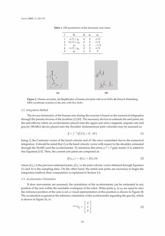
Sensors 2015, 15, 120–131

Table 1. DH parameters of the kinematic arm chain.

i θi di ai αi

1 π/2 + q1 0 0 π/22 3π/2 + q2 0 0 π/23 q3 lu 0 −π/24 π/2 + q4 0 0 π/25 q5 l f 0 0

(a) (b)

Figure 2. Human arm joints. (a) Simplification of human arm joints with seven DoFs; (b) Denavit–Hartenberg(DH) coordinate systems of the arm with five DoFs.

2.2. Integration Method

The inverse kinematics of the human arm during the exercise is based on the numerical integrationthrough the pseudo-inverse of the Jacobian (J) [10]. The necessary devices to estimate the arm joints are:the end-effector robot; an accelerometer placed onto the upper arm and a magnetic angular rate andgravity (MARG) device placed onto the shoulder. Instantaneous joint velocities may be assessed as:

q = J−1(q) vd + K · err (1)

being vd the Cartesian vector of the hand velocity and err the error committed due to the numericalintegration. It should be noted that vd is the hand velocity vector with respect to the shoulder, estimatedthrough the MARG and the accelerometer. To minimize this error, a 7 × 7 gain matrix K is added tothis Equation [13]. Then, the current arm joints are computed as:

q(tk+1) = q(tk) + q(tk)Δt (2)

whereq(tk) is the previous estimated joints, q(tk) is the joint velocity vector obtained through Equation(1) and Δt is the sampling time. On the other hand, the initial arm joints are necessary to begin theintegration method; their computation is explained in Section 2.6.

2.3. Accelerometer Orientation

If slow movements are assumed, the orientation of the accelerometer can be estimated in anyposition of the arm within the reachable workspace of the robot. When joints q1 to q5 are equal to zero,the reference position of the arm is set; a visual representation of this position is shown in Figure 2b.The acceleration acquired in the reference orientation of the accelerometer regarding the gravity, whichis shown in Figure 3a, is:

acc0 Vg =

⎡

⎢

⎣

010

⎤

⎥

⎦(3)

122

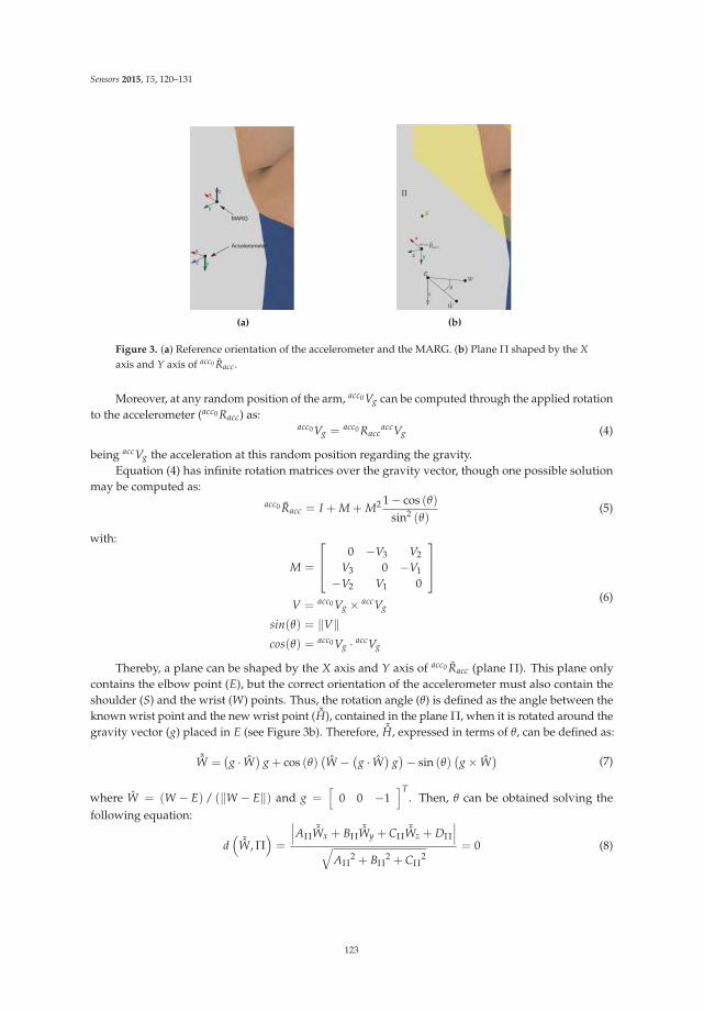
Sensors 2015, 15, 120–131

(a) (b)

Figure 3. (a) Reference orientation of the accelerometer and the MARG. (b) Plane Π shaped by the X

axis and Y axis of acc0 Racc.

Moreover, at any random position of the arm, acc0 Vg can be computed through the applied rotationto the accelerometer (acc0 Racc) as:

acc0 Vg = acc0 RaccaccVg (4)

being accVg the acceleration at this random position regarding the gravity.Equation (4) has infinite rotation matrices over the gravity vector, though one possible solution

may be computed as:acc0 Racc = I + M + M2 1 − cos (θ)

sin2 (θ)(5)

with:

M =

⎡

⎢

⎣

0 −V3 V2

V3 0 −V1

−V2 V1 0

⎤

⎥

⎦

V = acc0 Vg × accVg

sin(θ) = ‖V‖cos(θ) = acc0 Vg · accVg

(6)

Thereby, a plane can be shaped by the X axis and Y axis of acc0 Racc (plane Π). This plane onlycontains the elbow point (E), but the correct orientation of the accelerometer must also contain theshoulder (S) and the wrist (W) points. Thus, the rotation angle (θ) is defined as the angle between theknown wrist point and the new wrist point ( ˜H), contained in the plane Π, when it is rotated around thegravity vector (g) placed in E (see Figure 3b). Therefore, ˜H, expressed in terms of θ, can be defined as:

˜W =(

g · W)

g + cos (θ)(

W −(

g · W)

g)

− sin (θ)(

g × W)

(7)

where W = (W − E) / (‖W − E‖) and g =[

0 0 −1]T

. Then, θ can be obtained solving thefollowing equation:

d(

˜W, Π)

=

∣

∣

∣AΠ˜Wx + BΠ

˜Wy + CΠ˜Wz + DΠ

∣

∣

∣

√

AΠ2 + BΠ

2 + CΠ2

= 0 (8)

123

Sensors 2015, 15, 120–131

having the plane Π computed as follows:

Pxacc =

acc0 Racc

[

1 0 0]T

Pyacc =

acc0 Racc

[

0 1 0]T

SPyacc =

(

Pyacc − S

)

Pxacc P

yacc =

(

Pyacc − Px

acc

)

⎡

⎢

⎣

AΠ

BΠ

CΠ

⎤

⎥

⎦= SP

yacc × Px

acc Pyacc

DΠ =[

AΠ BΠ CΠ

]T· S

(9)

Two possible solutions are obtained through Equation (8) and, therefore, two values of acc0 Racc.The correct solution is one for which the Z axis is in the same direction as the cross product between theelbow-wrist segment and elbow-shoulder segment due to the reference position of the accelerometer.Finally, the rotation of the accelerometer regarding the robot is computed as:

rRacc =r Racc0 ·acc0 Racc (10)

being rRacc0 the reference orientation of the accelerometer concerning the robot (see Figure 3a). Thisorientation is required to estimate the elbow orientation and shoulder position during the exercise.

2.4. MARG Orientation

The orientation of magneto-inertial devices is usually based on Kalman filtering [16]; nevertheless,they can be quite complicated, and an extended Kalman filter is needed to linearize the problem. Theorientation filter to measure the rotation of the MARG of Madgwick et al. is used in this algorithm [17].The magnetic distortion that may be introduced by external sources, including metal furniture andmetal structures within a building, is performed in this filter [18]. Furthermore, the orientationalgorithm requires an adjustable parameter (β) that can be adjusted to the requirements of this exercise.Hence, the value of this parameter (β = 5) was established after a “trial and error” approach testedbefore the experiment, taking into account the features of the exercises.

This filter measures the reference quaternion of the device with respect to the Earth referencesystem, defined by the gravity vector and the Earth’s magnetic field lines. However, the rotation of theEarth concerning the robot is unknown. If the MARG is placed in a known orientation with respect tothe robot (R

M0q), the acquired transformation defines the Earth frame relative to the sensor frame (M0

E q),and therefore, the reference transformation between the robot and the Earth is known as:

RE q =R

M0q ⊗M0

E q (11)

Therefore, every rotation of the MARG is defined in the workspace as:

RMq =R

E q ⊗ME q∗ (12)

where ME q is the current value of the sensor. In this way, the shoulder orientation is estimated during

the exercise.

2.5. Elbow and Shoulder Location

The hand, as was said before, is tightly attached to the end effector of the robot, and theulnar-radial deviation and flexion-extension of the hand remain constant. Hence, the transformation

124

Sensors 2015, 15, 120–131

matrix between the hand and the end effector (rTw) is known, and therefore, the elbow position maybe obtained as:

rPe =r Tw ∗

[

0 0 −l f 1]T

(13)

The orientation of the elbow, since the rotation matrix between the elbow and the accelerometerorientation (acc0 Re) is known (see Figure 3a), may be calculated as:

rRe =r Racc ·acc0 Re (14)

with rRacc the rotation matrix computed through Equation (10). Thus, the transformation of the elbowrelative to the robot remains:

rTe =

[

rRerPe

0 0 0 1

]

(15)

On the other hand, one of the most important points of this algorithm is the ability to estimate theshoulder position and orientation during the exercise. The shoulder position can be processed easilythrough Equation (15) as:

rPs =r Te ∗

[

0 lu 0 1]T

(16)

Whilst the orientation of the MARG relative to the robot is known by Equation (12), its rotationmatrix rRM is directly obtained [19]. Thus, the shoulder orientation is estimated as:

rRs =r RM ·M0 Rs (17)

where rRM is the current rotation of the sensor with respect to the robot and M0 Rs the reference positionof the MARG relative to the shoulder (see Figure 3a). Hence, the transformation of the shoulder relativeto the robot remains:

rTs =

[

rRsrPs

0 0 0 1

]

(18)

Finally, since the elbow and the shoulder location are instantaneously known, the initial conditionsand the integration method can be performed.

2.6. Initial Conditions

In this algorithm, since it is based on a numerical integration, the initial conditions are required.The locations of the three main points, namely the shoulder (rTs), the elbow (rTs) and the wrist (rTs),are known. The shoulder joints (q1, q2 and q3) are directly related to the matrix sTe =r T−1

s ·r Te, definedin the previous section, and they can be acquired by the spherical joint method [13]. This matrix, interms of the corresponding joints, can be expressed by DH parameters shown in Table 1 as:

s0 Ts3 = s0 Ts1 · s1 Ts2 · s2 Ts3 =

⎡

⎢

⎢

⎢

⎣

c1s3 − c3s1s2 −c2s1 c1c3 + s1s2s3 luc2s1

s1s3 + c1c3s2 c1c2 c3s1 − c1s2s3 −luc1c2

−c2 c3 s2 c2 s3 −lus2

0 0 0 1

⎤

⎥

⎥

⎥

⎦

(19)

having si = sin (qi) and ci = cos (qi), i = 1, 2, 3. If the transformation matrix s0 Ts3 is defined as:

s0 Ts3 (q1,q2,q3) =

⎡

⎢

⎢

⎢

⎣

nx ny nz px

ox oy oz py

ax ay az pz

0 0 0 1

⎤

⎥

⎥

⎥

⎦

(20)

125

Sensors 2015, 15, 120–131

two possible solutions of the shoulder joints are obtained; if q2 ∈ [0 π]:

q1 = atan2(

−ny, oy

)

q2 = atan2(

ay,√

n2y + o2

y

)

q3 = atan2 (az,−ax)

(21)

and if q2 ∈ [−π 0]:q1 = atan2

(

ny,−oy

)

q2 = atan2(

ay,−√

n2y + o2

y

)

q3 = atan2 (−az, ax)

(22)

Thereby, the elbow joint (q4) is directly determined with the cosine law as:

q4 = arcsin

⎛

⎝

l2u + l2

f − ||H − S||2

2lul f

⎞

⎠ (23)

and its homogeneous matrix remains:

s3 Ts4 =

⎡

⎢

⎢

⎢

⎣

− sin (q4) 0 cos (q4) 0cos (q4) 0 sin (q4) 0

0 1 0 00 0 0 1

⎤

⎥

⎥

⎥

⎦

(24)

Thus, the transformation matrix between the systems s0 and s4 can be computed. The knownmatrix sTh =r T−

s 1 ·r Th defines the transformation between the system s0 and s5. On the other hand,the last joint, q5, is defined with the DH parameters as:

s4 Ts5 (q5) =

⎡

⎢

⎢

⎢

⎣

− sin (q5) cos (q5) 0 0cos (q5) sin (q5) 0 0

0 0 1 00 0 0 1

⎤

⎥

⎥

⎥

⎦

(25)

and therefore, q5 is estimated as:q5 = atan2 (−nx, ox) (26)

Finally, two possible configurations of the arm joints are found, even though only one solutionis possible. Due to the limits of the arm joints, [−π/2 π/2], only one solution accomplishes thisrestriction, and the initial position of the arm is assessed. This method can produce abrupt changesin the estimated arm joints caused by possible perturbations in the accelerometer that might leadto a non-anatomical position. Hence, since the new position depends on the latest position and thesample time, the integration method for real-time reconstruction is the best way to overcome theaforementioned drawbacks following Equations (1) and (2).

3. Results and Discussion

3.1. Experimental Exercises

With the aim of studying the arm joint estimation algorithm, with K = diag1.5, 1.5, ...1.5 N/ms(chosen by the “trial and error” approach tested before the experiment), two different experimentswere performed. The first exercise was to compute the algorithm accuracy in terms of the arm jointsand the position of the shoulder, performed by four healthy subjects. Then, a rehabilitation exercisewith two different trials was performed by 50 healthy subject (aged between 20 and 72) to test the

126

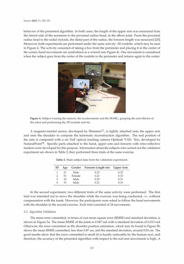
Sensors 2015, 15, 120–131

behavior of the presented algorithm. In both cases, the length of the upper arm was measured fromthe lateral side of the acromion to the proximal radius head, in the elbow joint. From the proximalradius head to the radial styloids, the distal part of the radius, the forearm length was measured [20].Moreover, both experiments are performed under the same activity: 3D roulette, which may be seenin Figure 4. The activity consisted of taking a box from the perimeter and placing it in the center ofthe screen; hand movements are symbolized as a wrench (see Figure 4). One movement is consideredwhen the subject goes from the center of the roulette to the perimeter and returns again to the center.

Figure 4. Subject wearing the sensors, the accelerometer and the MARG, grasping the end effector ofthe robot and performing the 3D roulette activity.

A magneto-inertial sensor, developed by Shimmer c©, is tightly attached onto the upper armand onto the shoulder to compute the kinematic reconstruction algorithm. The real position ofthe arm is computed with a six DoF optical tracking camera Optitrak V120: Trio, developed byNaturalPoint R©. Specific parts attached to the hand, upper arm and forearm with retro-reflectivemarkers were developed for this purpose. Information about the subjects who carried out the validationexperiment are shown in Table 2; they performed three trials of the same exercise.

Table 2. Main subject data from the validation experiment.

ID Age Gender Forearm Length (m) Upper Arm

1 21 Male 0.23 0.322 51 Female 0.21 0.333 32 Male 0.25 0.314 31 Male 0.21 0.33

In the second experiment, two different trials of the same activity were performed. The firsttrial was intended not to move the shoulder while the exercise was being conducted, i.e., withoutcompensation with the trunk. However, the participants were asked to follow the hand movementswith the shoulder in the second exercise. Each trial consisted of 24 movements.

3.2. Algorithm Validation

The mean error committed, in terms of root mean square error (RMSE) and standard deviation, isshown in Figure 5a. The mean RMSE of the joints is 0.047 rad with a standard deviation of 0.013 rad.Otherwise, the error committed on the shoulder position estimation, which may be found in Figure 5b,shows the mean RMSE committed, less than 0.87 cm, and the standard deviation, around 0.83 cm. Thegood results show that the error committed is small (it is hardly noticeable by the human eye), andtherefore, the accuracy of the presented algorithm with respect to the real arm movements is high. A

127

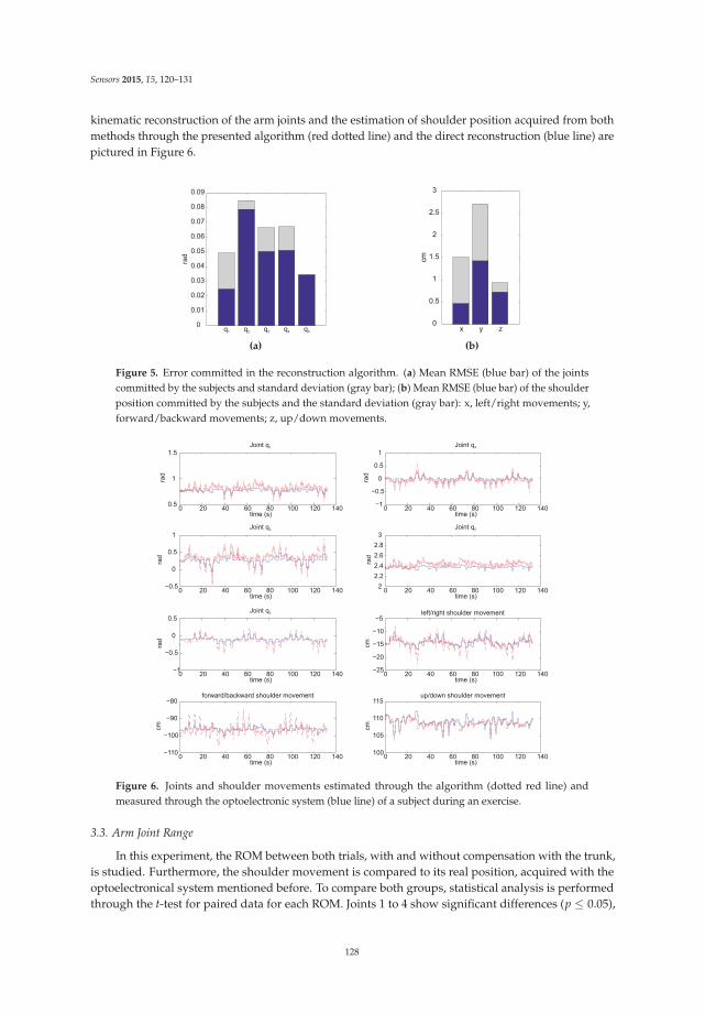
Sensors 2015, 15, 120–131

kinematic reconstruction of the arm joints and the estimation of shoulder position acquired from bothmethods through the presented algorithm (red dotted line) and the direct reconstruction (blue line) arepictured in Figure 6.

(a) (b)

Figure 5. Error committed in the reconstruction algorithm. (a) Mean RMSE (blue bar) of the jointscommitted by the subjects and standard deviation (gray bar); (b) Mean RMSE (blue bar) of the shoulderposition committed by the subjects and the standard deviation (gray bar): x, left/right movements; y,forward/backward movements; z, up/down movements.

Figure 6. Joints and shoulder movements estimated through the algorithm (dotted red line) andmeasured through the optoelectronic system (blue line) of a subject during an exercise.

3.3. Arm Joint Range

In this experiment, the ROM between both trials, with and without compensation with the trunk,is studied. Furthermore, the shoulder movement is compared to its real position, acquired with theoptoelectronical system mentioned before. To compare both groups, statistical analysis is performedthrough the t-test for paired data for each ROM. Joints 1 to 4 show significant differences (p ≤ 0.05),

128

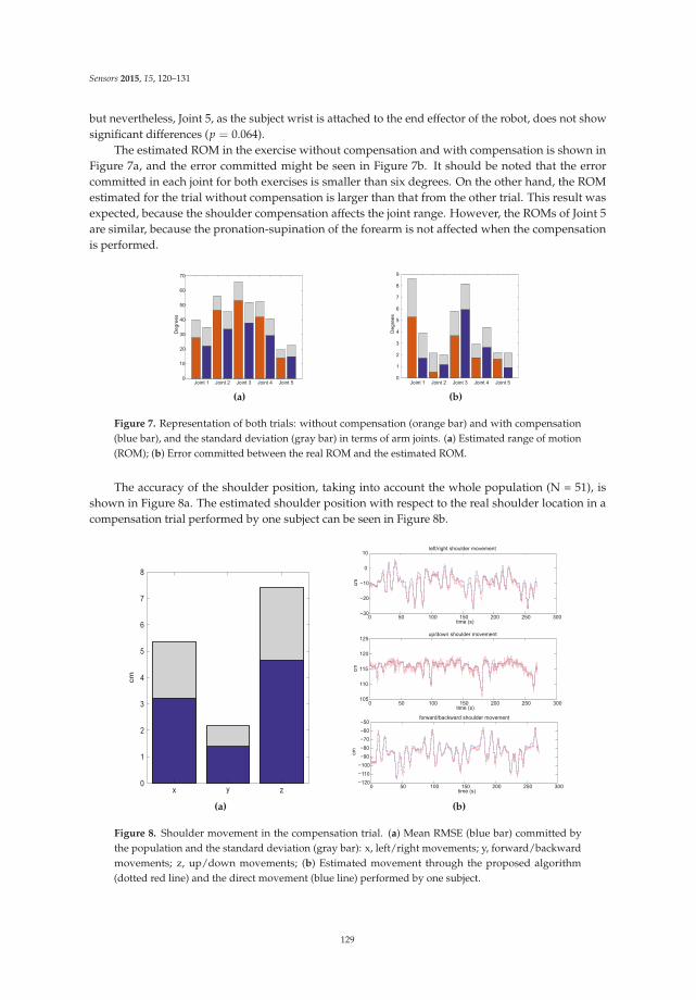
Sensors 2015, 15, 120–131

but nevertheless, Joint 5, as the subject wrist is attached to the end effector of the robot, does not showsignificant differences (p = 0.064).

The estimated ROM in the exercise without compensation and with compensation is shown inFigure 7a, and the error committed might be seen in Figure 7b. It should be noted that the errorcommitted in each joint for both exercises is smaller than six degrees. On the other hand, the ROMestimated for the trial without compensation is larger than that from the other trial. This result wasexpected, because the shoulder compensation affects the joint range. However, the ROMs of Joint 5are similar, because the pronation-supination of the forearm is not affected when the compensationis performed.

(a) (b)

Figure 7. Representation of both trials: without compensation (orange bar) and with compensation(blue bar), and the standard deviation (gray bar) in terms of arm joints. (a) Estimated range of motion(ROM); (b) Error committed between the real ROM and the estimated ROM.

The accuracy of the shoulder position, taking into account the whole population (N = 51), isshown in Figure 8a. The estimated shoulder position with respect to the real shoulder location in acompensation trial performed by one subject can be seen in Figure 8b.

(a) (b)

Figure 8. Shoulder movement in the compensation trial. (a) Mean RMSE (blue bar) committed bythe population and the standard deviation (gray bar): x, left/right movements; y, forward/backwardmovements; z, up/down movements; (b) Estimated movement through the proposed algorithm(dotted red line) and the direct movement (blue line) performed by one subject.

129

Sensors 2015, 15, 120–131

4. Conclusions

In this paper, a kinematic reconstruction of the upper limbs during robot-aided rehabilitationwith planar robots taking into account shoulder movements is presented. The estimated arm joints arevery accurate with respect to the real position of the arm. Thus, the arm joint improvements of thepatient can be measured objectively, and a better adaptation of the therapy to the patient needs can bealso performed.

The measurement of the shoulder movement can be also computed accurately. To the best of ourknowledge, this feature is not included in the previous algorithms where the shoulder is assumedto be fixed, even when little movements cannot be avoided during the exercise. This feature helpsthe therapist to correct the patient’s posture during exercise for faster improvement in terms ofarm mobility.

In summary, the arm joints’ improvement may be included as a new objective assessmentparameter in addition to the motor and proprioceptive activity and assessments scales, which are, bydefinition, subjective, as the Fugl–Meyer assessment [21].

Acknowledgments: This work was supported by the European Commission under FP7-ICT Contract 231143(ECHORD (European Clearing House for Open Robotics Development)).

Author Contributions: N.G.-A., F.J.B and L.D.L. conceived of and designed the experiments. A.B.-M. and S.E.performed the experiments. A.B.-M. drafted the paper. A.B.-M., J.M.C. and J.A.D. analyzed the data. All authorsread and approved the manuscript.


References

1. Nef, T.; Mihelj, M.; Colombo, G.; Riener, R. ARMin-robot for rehabilitation of the upper extremities.In Proceedings of the 2006 IEEE International Conference on Robotics and Automation, Orlando, FL, USA,15–19 May 2006.

2. Tang, Z.; Zhang, K.; Sun, S.; Gao, Z.; Zhang, L.; Yang, Z. An upper-limb power-assist exoskeleton usingproportional myoelectric control. Sensors 2014, doi:10.3390/s140406677.

3. Lum, P.S.; Burgar, C.G.; Shor, P.C.; Majmundar, M.; der Loos, M.V. Robot-assisted movement trainingcompared with conventional therapy techniques for the rehabilitation of upper-limb motor function afterstroke. Arch. Phys. Med. Rehabil. 2002, 83, 952 – 959.

4. Badesa, F.; Morales, R.; Garcia-Aracil, N.; Alfaro, A.; Bernabeu, A.; Fernandez, E.; Sabater, J. Robot-assistedrehabilitation treatment of a 65-year old woman with alien hand syndrome. Biomed. Robot. Biomech. 2002,doi:10.1109/BIOROB.2014.6913809.

5. Cameirao, M.; Badia, S.; Oller, E.; Verschure, P. Neurorehabilitation using the virtual reality basedRehabilitation Gaming System: methodology, design, psychometrics, usability and validation. J. NeuroEng.

Rehabil. 2010, doi:10.1186/1743-0003-7-48.6. Wittmann, F.; Lambercy, O.; Gonzenbach, R.R.; van Raai, M.A.; Hover, R.; Held, J.; Starkey, M.L.; Curt, A.;

Luft, A.; Gassert, R. Assessment-driven arm therapy at home using an IMU-based virtual reality system.Rehabil. Robot. 2015, doi:10.1109/ICORR.2015.7281284.

7. Klopcar, N.; Lenarcic, J. Kinematic model for determination of human arm reachable workspace. Meccanica

2005, 40, 203–219.8. Rab, G.; Petuskey, K.; Bagley, A. A method for determination of upper extremity kinematics. Gait Posture

2002, doi:10.1016/S0966-6362(01)00155-2.9. Mihelj, M. Human arm kinematics for robot based rehabilitation. Robotica 2006, 24, 377–383.10. Papaleo, E.; Zollo, L.; Garcia-Aracil, N.; Badesa, F.; Morales, R.; Mazzoleni, S.; Sterzi, S.; Guglielmelli, E.

Upper-limb kinematic reconstruction during stroke robot-aided therapy. Med. Biol. Eng. Comput. 2015,53, 815–828.

11. Kreutz-Delgado, K.; Long, M.; Seraji, H. Kinematic analysis of 7 DOF anthropomorphic arms. Robot. Autom.

1990, doi:10.1109/ROBOT.1990.126090.

130

Sensors 2015, 15, 120–131

12. Taati, B.; Wang, R.; Huq, R.; Snoek, J.; Mihailidis, A. Vision-based posture assessment to detectand categorize compensation during robotic rehabilitation therapy. Biomed. Robot. Biomech. 2012,doi:10.1109/BioRob.2012.6290668.

13. Siciliano, B.; Sciavicco, L.; Villani, L.; Oriolo, G. Robotics: Modelling, Planning and Control; Springer-VerlagLondon: London, UK, 2009.

14. Badesa, F.J.; Llinares, A.; Morales, R.; Garcia-Aracil, N.; Sabater, J.M.; Perez-Vidal, C. Pneumaticplanar rehabilitation robot for post-stroke patientes. Biomed. Eng. Appl. Basis Commun. 2014,doi:10.4015/S1016237214500252.

15. Lenarcic, J.; Umek, A. Simple model of human arm reachable workspace. IEEE Trans. Syst. Man. Cybern.

1994, 24, 1239–1246.16. Kalman, R.E. A new approach to linear filtering and prediction problems. J. Basic Eng. 1960, 82, 35–45.17. Madgwick, S.; Harrison, A.; Vaidyanathan, R. Estimation of IMU and MARG orientation using a gradient

descent algorithm. Rehabil. Robot. 2011, doi:10.1109/ICORR.2011.5975346.18. Bachmann, E.; Yun, X.; Peterson, C. An investigation of the effects of magnetic variations on inertial/magnetic

orientation sensors. Robot. Autom. 2004, doi:10.1109/ROBOT.2004.1307974.19. Kuipers, J.B. Quaternions and Rotation Sequences; Princeton University Press: Princeton, NJ, USA, 1999.20. Mazza, J.C. Mediciones antropométricas. Estandarización de las Técnicas de medición, Actualizada

según Parámetros Internacionales. Available online: http://g-se.com/es/journals/publice-standard/articulos/mediciones-antropometricas.-estandariza-cion-de-las-tecnicas-de-medicion-actualizada-segun-parametros-internacionales-197 (accessed on 9 October 2015).

21. McCrea, P.H.; Eng, J.J.; Hodgson, A.J. Biomechanics of reaching: Clinical implications for individuals withacquired brain injury. Disabil. Rehabil. 2002, 24, 534–541.


131

sensors

Article

Comparison of Three Non-Imaging Angle-DiversityReceivers as Input Sensors of Nodes for IndoorInfrared Wireless Sensor Networks: Theoryand SimulationBeatriz R. Mendoza 1, Silvestre Rodríguez 2,*, Rafael Pérez-Jiménez 2, Alejandro Ayala 1

and Oswaldo González 1

1 Departamento de Ingeniería Industrial, Universidad de La Laguna (ULL), 38203 La Laguna (Tenerife), Spain;[email protected] (B.R.M.); [email protected] (A.A.); [email protected] (O.G.)

2 Departamento de Señales y Comunicaciones, Universidad de Las Palmas de Gran Canaria (ULPGC),35017 Las Palmas (Gran Canaria), Spain; [email protected]

* Correspondence: [email protected]; Tel.: +34-922-845242

Academic Editor: Gonzalo Pajares MartinsanzReceived: 1 April 2016; Accepted: 7 July 2016; Published: 14 July 2016

Abstract: In general, the use of angle-diversity receivers makes it possible to reduce the impact ofambient light noise, path loss and multipath distortion, in part by exploiting the fact that they oftenreceive the desired signal from different directions. Angle-diversity detection can be performedusing a composite receiver with multiple detector elements looking in different directions. These arecalled non-imaging angle-diversity receivers. In this paper, a comparison of three non-imagingangle-diversity receivers as input sensors of nodes for an indoor infrared (IR) wireless sensor networkis presented. The receivers considered are the conventional angle-diversity receiver (CDR), thesectored angle-diversity receiver (SDR), and the self-orienting receiver (SOR), which have beenproposed or studied by research groups in Spain. To this end, the effective signal-collection area ofthe three receivers is modelled and a Monte-Carlo-based ray-tracing algorithm is implemented whichallows us to investigate the effect on the signal to noise ratio and main IR channel parameters, such aspath loss and rms delay spread, of using the three receivers in conjunction with different combinationtechniques in IR links operating at low bit rates. Based on the results of the simulations, we showthat the use of a conventional angle-diversity receiver in conjunction with the equal-gain combiningtechnique provides the solution with the best signal to noise ratio, the lowest computational capacityand the lowest transmitted power requirements, which comprise the main limitations for sensornodes in an indoor infrared wireless sensor network.

Keywords: angle-diversity; sensor network; infrared channel; simulation; signal to noise ratio

1. Introduction

Although most wireless sensor networks used are currently based on radio frequency (RF)systems [1,2], wireless optical communications are becoming an alternative to RF technology in somewell-defined indoor application scenarios, such as environments where RF emissions are forbiddenor restricted (health care, nuclear and chemical plants, etc.), video/audio transmission for in-homeapplications, secure network access or sensor networking [3]. Optical systems do not interfere with RFsystems, thus avoiding electromagnetic compatibility restrictions. Moreover, there are no current legalrestrictions involving bandwidth allocation and, since radiation is confined by walls, they produceintrinsically cellular networks, which are more secure against deliberate attempts to gain unauthorizedaccess than radio systems. Despite the recent development in the field of visible light communications(VLC), the non-directed non-line-of-sight (non-LOS) infrared (IR) radiation has also been considered


Sensors 2016, 16, 1086

as a very attractive alternative to RF waves for indoor wireless local area networks, and therefore forindoor wireless sensor networking.

Sensor networks represent a significant improvement over traditional sensors. A sensor networkcan range from a few sensor nodes to a few hundred nodes capable of collecting data and routingthem back to the sink. Data are routed back to the sink by a multihop infrastructureless architecturethrough the nodes. The sink node may communicate with the task manager, for example, via Internet.A sensor node consists of four basic components: a sensing unit, a processing unit, a transceiverunit, and a power unit, although they may also have additional application-dependent componentssuch as a location finding system, power generator and mobilizer. In a sensor network, the sensornodes are limited in power, computational capacities, and memory. Furthermore, the nodes shouldcommunicate untethered over short distances and mainly use broadcast communication. In a multihopsensor network, communicating nodes are linked by a wireless medium. As previously mentioned,most sensor networks are based on RF technology; however, another possible method for internodecommunication is by infrared, which enables the use of transceivers that are cheaper and easier tobuild. Current infrared-based sensor networks require a line-of-sight (LOS) between transmitter andreceiver [1–3]. There are two basic classification schemes for wireless IR links [4]. In the first approach,the link can be directed by employing a narrow-beam transmitter and a narrow field of view (FOV)receiver, or non-directed, with a broad-beam transmitter and a wide FOV receiver. The second schemeclassifies the links according to whether or not they rely on a line-of-sight (LOS) between the transmitterand the receiver (LOS and non-LOS configurations). The directed LOS IR method is the most efficientin terms of power consumption and can achieve very high bit rates. Its drawbacks are tight alignmentrequirement, immobility of the receiver, and interruptions in transmission caused by shadowing.These disadvantages are overcome in non-directed non-LOS methods (referred to as diffuse links),which utilize diffuse reflections from the ceiling and walls. These methods, however, suffer fromineffective power use and multipath dispersion, which tend to greatly limit the transmission rate.In an indoor wireless optical sensor network, it is not necessary to achieve high transmission rates, butit is necessary to limit power consumption, avoid blockage and shadowing, and reduce the impactof ambient light noise. In general, the use of angle-diversity detection makes it possible to reducethe impact of ambient light noise, path loss, and multipath distortion, in part by exploiting the factthat they often receive the desired signal received from different directions [4–13]. Angle-diversitydetection can be implemented in two main ways: using a composite receiver with several brancheslooking in different directions (non-imaging angle-diversity receiver), or using an imaging receiverconsisting of imaging optics and an array of photodetectors (imaging angle-diversity receiver).

The propagation characteristics of the indoor IR channel are fully described by the channel’simpulse response, which depends on multiple factors such as the room geometry, the reflection patternof surfaces, the emitter and receiver characteristics and their relative locations. Indoor optical channelsimulation can significantly enhance the study of optical wireless links. For this reason, in orderto estimate the impulse response in IR wireless indoor channels, several simulation methods havebeen put forth [14,15], but all of them share the same problem, namely, the intensive computationaleffort. However, we make use of a Monte Carlo ray-tracing algorithm [16–19], which offers a lowercomputational cost than previous methods, especially when a high temporal resolution and a largenumber of reflections are required. In this paper, we study by simulation those indoor IR links thatare characterised by the use of three non-imaging angle-diversity receivers as input sensor of nodesfor an indoor IR wireless sensor network. The receivers, which have been proposed or studied byresearch groups in Spain, are the conventional angle-diversity receiver (CDR) [7,8,13], the sectoredangle-diversity receiver (SDR) [11,12], and the self-orienting receiver (SOR) [20,21]. A conventionalangle-diversity receiver uses multiple receiving elements or branches that are oriented in differentdirections, where each element employs its own filter and non-imaging concentrator, such as acompound parabolic concentrator (CPC) or hemispheric lens; a sectored receiver is a hemispherewhere a set of parallels and meridians defines the photodetector boundaries; and finally, a self-oriented

133

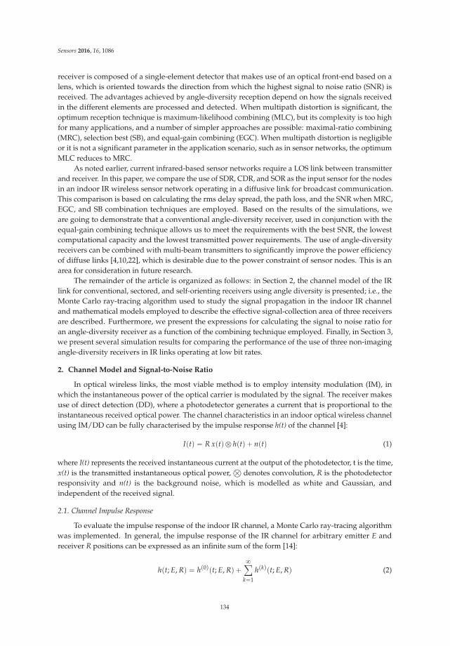
Sensors 2016, 16, 1086

receiver is composed of a single-element detector that makes use of an optical front-end based on alens, which is oriented towards the direction from which the highest signal to noise ratio (SNR) isreceived. The advantages achieved by angle-diversity reception depend on how the signals receivedin the different elements are processed and detected. When multipath distortion is significant, theoptimum reception technique is maximum-likelihood combining (MLC), but its complexity is too highfor many applications, and a number of simpler approaches are possible: maximal-ratio combining(MRC), selection best (SB), and equal-gain combining (EGC). When multipath distortion is negligibleor it is not a significant parameter in the application scenario, such as in sensor networks, the optimumMLC reduces to MRC.

As noted earlier, current infrared-based sensor networks require a LOS link between transmitterand receiver. In this paper, we compare the use of SDR, CDR, and SOR as the input sensor for the nodesin an indoor IR wireless sensor network operating in a diffusive link for broadcast communication.This comparison is based on calculating the rms delay spread, the path loss, and the SNR when MRC,EGC, and SB combination techniques are employed. Based on the results of the simulations, weare going to demonstrate that a conventional angle-diversity receiver, used in conjunction with theequal-gain combining technique allows us to meet the requirements with the best SNR, the lowestcomputational capacity and the lowest transmitted power requirements. The use of angle-diversityreceivers can be combined with multi-beam transmitters to significantly improve the power efficiencyof diffuse links [4,10,22], which is desirable due to the power constraint of sensor nodes. This is anarea for consideration in future research.

The remainder of the article is organized as follows: in Section 2, the channel model of the IRlink for conventional, sectored, and self-orienting receivers using angle diversity is presented; i.e., theMonte Carlo ray-tracing algorithm used to study the signal propagation in the indoor IR channeland mathematical models employed to describe the effective signal-collection area of three receiversare described. Furthermore, we present the expressions for calculating the signal to noise ratio foran angle-diversity receiver as a function of the combining technique employed. Finally, in Section 3,we present several simulation results for comparing the performance of the use of three non-imagingangle-diversity receivers in IR links operating at low bit rates.

2. Channel Model and Signal-to-Noise Ratio

In optical wireless links, the most viable method is to employ intensity modulation (IM), inwhich the instantaneous power of the optical carrier is modulated by the signal. The receiver makesuse of direct detection (DD), where a photodetector generates a current that is proportional to theinstantaneous received optical power. The channel characteristics in an indoor optical wireless channelusing IM/DD can be fully characterised by the impulse response h(t) of the channel [4]:

Iptq “ R xptq b hptq ` nptq (1)

where I(t) represents the received instantaneous current at the output of the photodetector, t is the time,x(t) is the transmitted instantaneous optical power,

Â

denotes convolution, R is the photodetectorresponsivity and n(t) is the background noise, which is modelled as white and Gaussian, andindependent of the received signal.

2.1. Channel Impulse Response

To evaluate the impulse response of the indoor IR channel, a Monte Carlo ray-tracing algorithmwas implemented. In general, the impulse response of the IR channel for arbitrary emitter E andreceiver R positions can be expressed as an infinite sum of the form [14]:

hpt; E, Rq “ hp0qpt; E, Rq `8ÿ

k“1

hpkqpt; E, Rq (2)

134

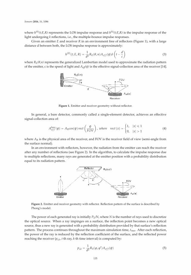
Sensors 2016, 16, 1086

where h(0)(t;E,R) represents the LOS impulse response and h(k)(t;E,R) is the impulse response of thelight undergoing k reflections, i.e., the multiple-bounce impulse responses.

Given an emitter E and receiver R in an environment free of reflectors (Figure 1), with a largedistance d between both, the LOS impulse response is approximately:

hp0qpt; E, Rq “ 1d2 REpθ, nqAe f f pψqδ

ˆ

t ´ d

c

˙

(3)

where RE(θ,n) represents the generalized Lambertian model used to approximate the radiation patternof the emitter, c is the speed of light and Aeff(ψ) is the effective signal-collection area of the receiver [14].

Figure 1. Emitter and receiver geometry without reflector.

In general, a bare detector, commonly called a single-element detector, achieves an effectivesignal-collection area of:

Abaree f f pψq “ ARcospψq rect

ˆ

ψ

FOV

˙

, where rect pxq “#

1, |x| ď 1

0, |x| ą 1(4)

where AR is the physical area of the receiver, and FOV is the receiver field of view (semi-angle fromthe surface normal).

In an environment with reflectors, however, the radiation from the emitter can reach the receiverafter any number of reflections (see Figure 2). In the algorithm, to calculate the impulse response dueto multiple reflections, many rays are generated at the emitter position with a probability distributionequal to its radiation pattern.

Figure 2. Emitter and receiver geometry with reflector. Reflection pattern of the surface is described byPhong’s model.

The power of each generated ray is initially PE/N, where N is the number of rays used to discretizethe optical source. When a ray impinges on a surface, the reflection point becomes a new opticalsource, thus a new ray is generated with a probability distribution provided by that surface’s reflectionpattern. The process continues throughout the maximum simulation time, tmax. After each reflection,the power of the ray is reduced by the reflection coefficient of the surface, and the reflected powerreaching the receiver (pi,k, i-th ray, k-th time interval) is computed by:

pi,k “ 1d2 RSpϕ, ϕ1qAe f f pψq (5)

135

Sensors 2016, 16, 1086

where RS(ϕ,ϕ’) is the model used to describe the reflection pattern. In this work, Phong’s model isused [17]. In this model, the surface characteristics are defined by three parameters: the reflectioncoefficient ρ, the percentage of incident signal that is reflected diffusely rd, and the directivity of thespecular component of the reflection m.

Therefore, the total received power in the k-th time interval (width Δt) is calculated as the sum ofthe power of the Nk rays that contribute in that interval:

pk “Nkÿ

i“1

pi,k “Nkÿ

i“1

1d2 RSpϕ, ϕ1qAe f f pψq (6)

Letting M = tmax/Δt, and assuming as the time origin the arrival of the LOS component, theimpulse response after multiple reflections is given by:

8ÿ

k“1

hpkqpt; E, Rq “M´1ÿ

j“0

pkδpt ´ jΔtq (7)

Replacing Equations (3) and (7) in Equation (2), the channel impulse response can be expressed as:

hpt; E, Rq “ 1d2 REpθ, nqAe f f pψqδptq `

M´1ÿ

j“1

pkδpt ´ jΔtq (8)

Once the impulse response h(t) is computed for a fixed emitter E and receiver R position, the mainparameters that characterise the IR channel—the path loss (PL) and the rms delay spread (D)—areeasily calculated as [4]:

PL “ ´10logHp0q H p f q “ş8´8 hptqe´j2πt f dt

D “„

ş

8

´8pt´μq2h2ptqdt

ş

8

´8h2ptqdt

j 12

μ “ş

8

´8th2ptqdt

ş

8

´8h2ptqdt

(9)

2.2. Effective Signal-Collection Area Model for Non-Imaging Angle-Diversity Receivers

In general, the use of angle-diversity receivers makes it possible to reduce the impact of ambientlight noise, path loss and multipath distortion, in part by exploiting the fact that they often receive thedesired signal from different directions. Another advantage of angle-diversity reception is that it allowsthe receiver to simultaneously achieve a high optical gain and a wide FOV. In this section we describethe models for the effective signal-collection area of three non-imaging angle-diversity receivers thathave been proposed or analysed by research groups in Spain. The receivers are called the conventionalangle-diversity receiver, the sectored angle-diversity receiver, and the self-orienting receiver.

2.2.1. Conventional Angle-Diversity Receiver

A conventional angle-diversity receiver uses multiple receiving elements or branches thatare oriented in different directions, where each element employs its own filter and non-imagingconcentrator, such as a compound parabolic concentrator or hemispherical lens (see Figure 3a).

By adding a filter and concentrator to a bare detector, the effective signal–collection area of thereceiver becomes:

Ac, fe f f pψq “ ARTSpψqgpψqcospψqrect

ˆ

ψ

π2

˙

(10)

136

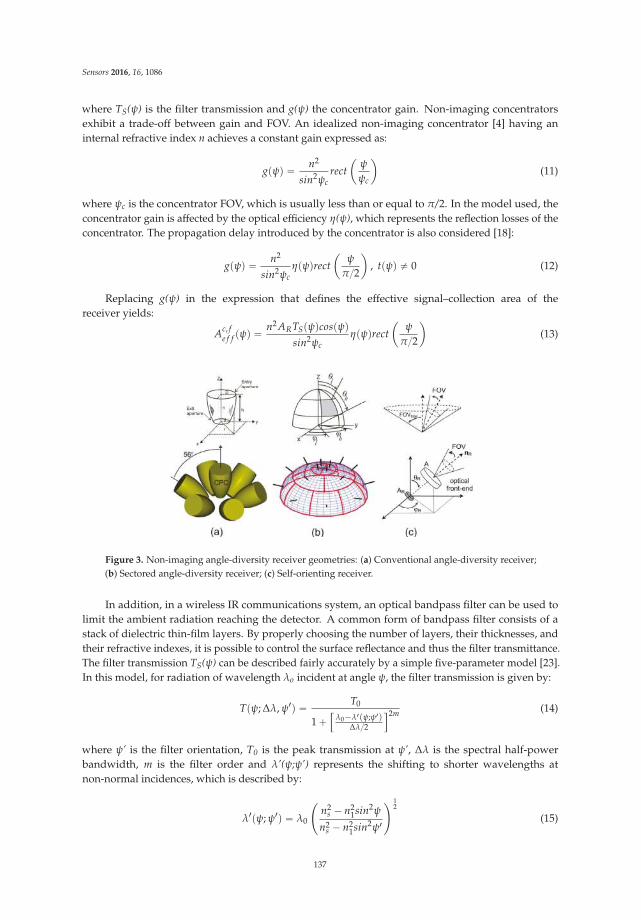
Sensors 2016, 16, 1086

where TS(ψ) is the filter transmission and g(ψ) the concentrator gain. Non-imaging concentratorsexhibit a trade-off between gain and FOV. An idealized non-imaging concentrator [4] having aninternal refractive index n achieves a constant gain expressed as:

gpψq “ n2

sin2ψc

rect

ˆ

ψ

ψc

˙

(11)

where ψc is the concentrator FOV, which is usually less than or equal to π/2. In the model used, theconcentrator gain is affected by the optical efficiency η(ψ), which represents the reflection losses of theconcentrator. The propagation delay introduced by the concentrator is also considered [18]:

gpψq “ n2

sin2ψc

ηpψqrect

ˆ

ψ

π2

˙

, tpψq ‰ 0 (12)

Replacing g(ψ) in the expression that defines the effective signal–collection area of thereceiver yields:

Ac, fe f f pψq “ n2 ARTSpψqcospψq

sin2ψc

ηpψqrect

ˆ

ψ

π2

˙

(13)

Figure 3. Non-imaging angle-diversity receiver geometries: (a) Conventional angle-diversity receiver;(b) Sectored angle-diversity receiver; (c) Self-orienting receiver.

In addition, in a wireless IR communications system, an optical bandpass filter can be used tolimit the ambient radiation reaching the detector. A common form of bandpass filter consists of astack of dielectric thin-film layers. By properly choosing the number of layers, their thicknesses, andtheir refractive indexes, it is possible to control the surface reflectance and thus the filter transmittance.The filter transmission TS(ψ) can be described fairly accurately by a simple five-parameter model [23].In this model, for radiation of wavelength λo incident at angle ψ, the filter transmission is given by:

Tpψ; Δλ, ψ1q “ T0

1 `”

λ0´λ1pψ;ψ1qΔλ2

ı2m(14)

where ψ’ is the filter orientation, T0 is the peak transmission at ψ’, Δλ is the spectral half-powerbandwidth, m is the filter order and λ’(ψ;ψ’) represents the shifting to shorter wavelengths atnon-normal incidences, which is described by:

λ1pψ; ψ1q “ λ0

˜

n2s ´ n2

1sin2ψ

n2s ´ n2

1sin2ψ1

¸ 12

(15)

137

Sensors 2016, 16, 1086

where n1 is the index of the input layer and ns is the effective index for the spacer layer. The design ofthe optical filter thus boils down to specifying the two parameters Δλ and ψ’.

The remaining three parameters (ns, m and T0) should be chosen to be as large possible, whileconsidering the constraints imposed by technology. In keeping with reference [23], we used ns = 2.293,m = 3, and T0 = 0.92. Furthermore, to provide the best utilization of the CPC and filter, the angularbandwidth Δψ should be equal to the concentrator FOV. Figure 3a shows a conventional angle-diversityreceiver composed of seven elements, one of them oriented vertically towards the ceiling and sixangled at a 56˝ elevation with a 60˝ separation in azimuth. Each element uses a bandpass optical filterand a CPC with a 50˝ field of view. The receiver structure resulted from a study focused on designingthe conventional angle-diversity receiver that offers the best performance with respect to the path lossand the rms delay spread [13].

2.2.2. Sectored Angle-Diversity Receiver

A sectored angle-diversity receiver consists of a set of photodetectors located on a hemisphere.The space of sectored receivers enclosed between two parallels is called a crown, and a sector is theregion of the crown enclosed between two equally spaced meridians. Every sector in each crown hasan equal azimuth aperture, and therefore the same limiting elevation angles. In summary, the sectoredreceiver is defined by a set of parameters [11], Ψ, which specifies, for each crown, its number of sectors,NS, the azimuth offset of its first sector, ε, and its limiting elevation angles, θl and θh. As an example,bottom illustration in Figure 3b shows the configuration of a sectored receiver with three crowns,which is defined by Ψ = (4, 0˝, 0˝, 24˝), (4, 20˝, 24˝, 53˝), (8, 0˝, 53˝, 9˝). As we can see, the first crownin the sectored receiver consists of 4 sectors (NS = 4). The azimuth offset of its first sector is ε = 0˝, andits limiting elevation angles are 0˝ and 24˝ (θl = 0˝ and θh = 24˝). Analogously to the conventionalangle-diversity receiver shown in Figure 3a, the configuration of the sectored receiver was the result ofa study focused on achieving the receiver structure that exhibits the minimum simultaneous rms delayspread and path loss [12].

As with a single-element detector, each sector of the sectored receiver is defined by its position,orientation, vertical and horizontal apertures, and effective signal-collection area. The region of asector is specified by the two limiting elevation angles, θl and θh, and the two limiting azimuth angles,φl and φh, where θl < θh and φl < φh (see top illustration in Figure 3b). Consequently, the verticalaperture is given by (θh ´ θl)/2, whereas the horizontal aperture is set by (φh ´ φl)/2. The orientationof each sector is defined by its azimuth and elevation angles (φS,θS), which are given by:

φS “ pφl ` φhq 2 and θS “ pθl ` θhq 2 (16)

except in the case of a polar crown with a single sector where θS = 0˝ (sector aimed vertically upward,φh ´ φl = 2π, θh any, θl = 0). Each sector in a sectored receiver has an effective signal-collection areagiven by:

Ae f f pψq “ ARTS pψq cospψqrect

ˆ

ψ

π2

˙

(17)

where TS(ψ) is the transmission characteristic of the filter used to limit the ambient radiation reachingeach photodetector, ψ is the incidence angle of radiation with respect to the sector orientation, and AR

represents the physical area of the detector, which is described by:

AR “ r2 ¨ pφh ´ φlq ¨ pcos θl ´ cos θhq (18)

where r is the radius of the hemisphere. In a sectored receiver, the optical filter should be deposited orbonded onto the outer surface of the sectored receiver, i.e., onto all the sectors or photodetectors thatcomprise the receiver. In this sense, a bandpass or interference optical filter cannot be used becausethe radiation that reaches each photodetector is incident upon the filter at any value of ψ between0˝ and 90˝, shifting the filter transmission to shorter wavelengths and minimizing its transmission.

138

Sensors 2016, 16, 1086

Therefore, the ambient light radiation and the desired signal striking the filter at wide incidence angleswill not be adequately filtered. However, in order to reject ambient light, longpass absorption opticalfilters could be used [4], which pass light at every wavelength beyond the cutoff wavelength. They areusually made of coloured glass or plastic and their transmission characteristics are constant andsubstantially independent of the incidence angle, i.e., TS(ψ) = T0 for all wavelengths longer than thecutoff wavelength. Since the silicon device does not respond to wavelengths beyond about 1100 nm,the filter-photodetector combination exhibits a bandpass optical response, whose bandwidth will rangefrom the filter cutoff wavelength to the longest wavelength at which the silicon responds. Although thesectored receiver may currently be regarded as a theoretical structure since no prototype has yetbeen implemented, we assume that a longpass absorption filter with a 780-nm cutoff wavelengthis employed, specifically the Schott RG-780 optical filter [24]. This filter exhibits an almost constanttransmission characteristic above 780 nm given by T0 = 0.99, and consequently, the spectral bandwidthresulting from the filter-photodetector combination is about Δλ = 320 nm.

2.2.3. Self-Orienting Receiver

The third angle-diversity receiver considered is called a self-orienting receiver (see Figure 3c).The self-orienting receiver consists of a single-element detector which employs an optical front-endbased on a lens [20,21]. The receiver is mounted on an electromechanical orienting system controlledby a digital signal processor (DSP). An SNR estimator and a maximum search algorithm, which isbased on a modified version of Simulated Annealing (SA), are used to automatically aim the receiver atthe area of the room with the highest SNR [20,21]. From the description above, we can deduce that thereceiver is actually a modified version of a select-best angle diversity receiver, which allows operatingwith very narrow FOV. In general, the self-orienting receiver can be represented by the parameters pR,nR, FOVtotal, A, AR, and FOV, i.e., its position, orientation, total FOV, aperture area of the lens, physicalarea of photodetector and the FOV of the system formed by the detector and the optical front-end.Therefore, its effective signal-collection area can be expressed as:

Ae f f pψq “ ARTSpψqgpψqcospψqrect

ˆ

ψ

π2

˙

(19)

where TS(ψ) is the filter transmission and g(ψ) = G represents the optical front-end gain. Replacing thegain G by A/AR in the expression, and assuming an ideal filter, the expression that defines the effectivesignal-collection area of the receiver can be expressed as:

Ae f f pψq “ AR G cospψqrect

ˆ

ψ

π2

˙

“ A cospψqrect

ˆ

ψ

π2

˙

(20)

In keeping with the proposal made in [20,21], we have assumed that the self-orienting receiveruses a positive lens system with an aperture diameter of 1.5 cm as an optical concentrator, along with acircular photodetector with area AR = 3.53 mm2 and responsivity R = 0.6 A/W to collect the signalsreceived. The concentrator provides a high optical gain (G = 50) at the expense of a narrow FOV, whichis only 3˝. This extremely narrow FOV allows us to use an ideal bandpass optical filter with a narrowspectral bandwidth (Δλ = 50 nm) for better optical noise rejection.

2.3. Signal to Noise Ratio

In general, the received signal-to-noise ratio can be expressed by:

SNR “ pR PSq2 σ2 (21)

139

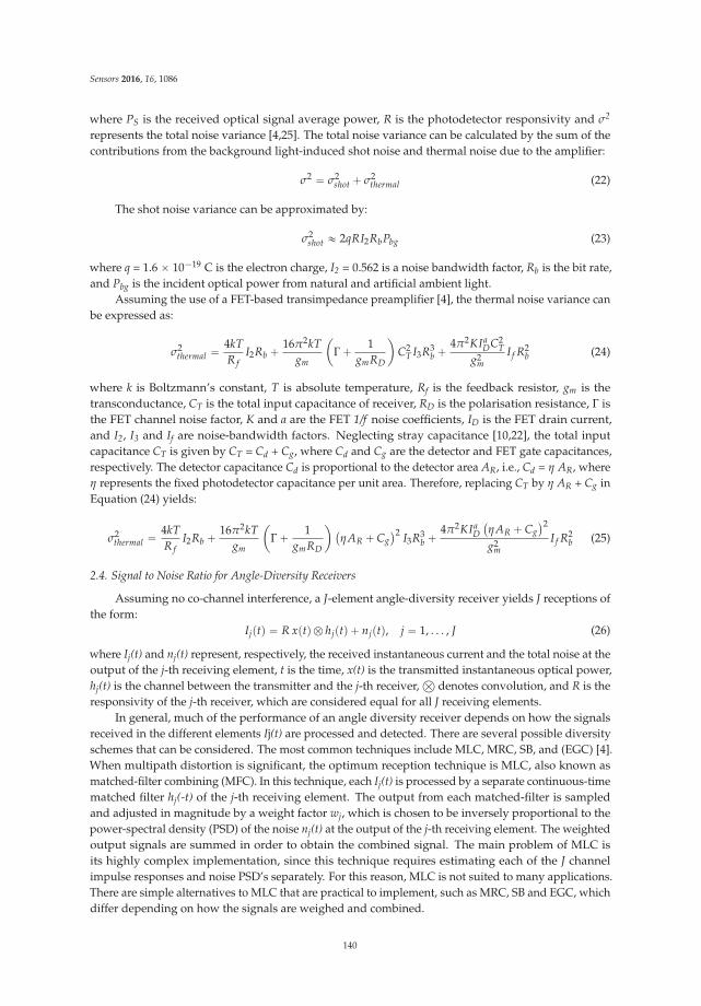
Sensors 2016, 16, 1086

where PS is the received optical signal average power, R is the photodetector responsivity and σ2

represents the total noise variance [4,25]. The total noise variance can be calculated by the sum of thecontributions from the background light-induced shot noise and thermal noise due to the amplifier:

σ2 “ σ2shot ` σ2

thermal (22)

The shot noise variance can be approximated by:

σ2shot « 2qRI2RbPbg (23)

where q = 1.6 ˆ 10´19 C is the electron charge, I2 = 0.562 is a noise bandwidth factor, Rb is the bit rate,and Pbg is the incident optical power from natural and artificial ambient light.

Assuming the use of a FET-based transimpedance preamplifier [4], the thermal noise variance canbe expressed as:

σ2thermal “ 4kT

R fI2Rb ` 16π2kT

gm

ˆ

Γ ` 1gmRD

˙

C2T I3R3

b ` 4π2KIaDC2

T

g2m

I f R2b (24)

where k is Boltzmann’s constant, T is absolute temperature, Rf is the feedback resistor, gm is thetransconductance, CT is the total input capacitance of receiver, RD is the polarisation resistance, Γ isthe FET channel noise factor, K and a are the FET 1/f noise coefficients, ID is the FET drain current,and I2, I3 and If are noise-bandwidth factors. Neglecting stray capacitance [10,22], the total inputcapacitance CT is given by CT = Cd + Cg, where Cd and Cg are the detector and FET gate capacitances,respectively. The detector capacitance Cd is proportional to the detector area AR, i.e., Cd = η AR, whereη represents the fixed photodetector capacitance per unit area. Therefore, replacing CT by η AR + Cg inEquation (24) yields:

σ2thermal “ 4kT

R fI2Rb ` 16π2kT

gm

ˆ

Γ ` 1gmRD

˙

`

ηAR ` Cg

˘2I3R3

b ` 4π2KIaD

`

ηAR ` Cg

˘2

g2m

I f R2b (25)

2.4. Signal to Noise Ratio for Angle-Diversity Receivers

Assuming no co-channel interference, a J-element angle-diversity receiver yields J receptions ofthe form:

Ijptq “ R xptq b hjptq ` njptq, j “ 1, . . . , J (26)

where Ij(t) and nj(t) represent, respectively, the received instantaneous current and the total noise at theoutput of the j-th receiving element, t is the time, x(t) is the transmitted instantaneous optical power,hj(t) is the channel between the transmitter and the j-th receiver,

Â

denotes convolution, and R is theresponsivity of the j-th receiver, which are considered equal for all J receiving elements.

In general, much of the performance of an angle diversity receiver depends on how the signalsreceived in the different elements Ij(t) are processed and detected. There are several possible diversityschemes that can be considered. The most common techniques include MLC, MRC, SB, and (EGC) [4].When multipath distortion is significant, the optimum reception technique is MLC, also known asmatched-filter combining (MFC). In this technique, each Ij(t) is processed by a separate continuous-timematched filter hj(-t) of the j-th receiving element. The output from each matched-filter is sampledand adjusted in magnitude by a weight factor wj, which is chosen to be inversely proportional to thepower-spectral density (PSD) of the noise nj(t) at the output of the j-th receiving element. The weightedoutput signals are summed in order to obtain the combined signal. The main problem of MLC isits highly complex implementation, since this technique requires estimating each of the J channelimpulse responses and noise PSD’s separately. For this reason, MLC is not suited to many applications.There are simple alternatives to MLC that are practical to implement, such as MRC, SB and EGC, whichdiffer depending on how the signals are weighed and combined.

140

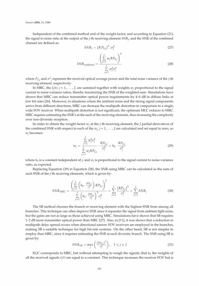
Sensors 2016, 16, 1086

Independent of the combined method and of the weight factor, and according to Equation (21),the signal to noise ratio at the output of the j-th receiving element SNRj, and the SNR of the combinedchannel are defined as:

SNRj “`

R PS,j˘2 σ2

j (27)

SNRcombined “

˜

Jř

j“1wjRPS,j

¸2

Jř

j“1w2

j σ2j

(28)

where PS,j and σ2j represent the received optical average power and the total noise variance of the j-th

receiving element, respectively.In MRC, the Ij(t), j = 1, . . . , J, are summed together with weights wj proportional to the signal

current to noise-variance ratios, thereby maximizing the SNR of the weighted sum. Simulations haveshown that MRC can reduce transmitter optical power requirements by 4–6 dB in diffuse links atlow bit rates [26]. Moreover, in situations where the ambient noise and the strong signal componentsarrive from different directions, MRC can decrease the multipath distortion in comparison to a single,wide FOV receiver. When multipath distortion is not significant, the optimum MLC reduces to MRC.MRC requires estimating the SNR’s at the each of the receiving elements, thus increasing the complexityover non-diversity reception.

In order to obtain the weight factor wj at the j-th receiving element, the J partial-derivatives ofthe combined SNR with respect to each of the wj, j = 1, . . . , J are calculated and set equal to zero, sowj becomes:

wj “

Jř

j“1w2

j σ2j

Jř

j“1wjRPS,j

¨RPS,j

σ2j

“ k0 ¨RPS,j

σ2j

(29)

where k0 is a constant independent of j, and wj is proportional to the signal current to noise-varianceratio, as expected.

Replacing Equation (29) in Equation (28), the SNR using MRC can be calculated as the sum ofeach SNR of the j-th receiving elements, which is given by:

SNRMRC “

˜

Jř

j“1

ˆ

k0 ¨ RPS,j

σ2j

˙

RPS,j

¸2

Jř

j“1

ˆ

k0 ¨ RPS,j

σ2j

˙2

σ2j

“J

ÿ

j“1

`

RPS,j˘2

σ2j

“J

ÿ

j“1

SNRj (30)

The SB method chooses the branch or receiving element with the highest SNR from among allbranches. This technique can often improve SNR since it separates the signal from ambient light noise,but the gains are not as large as those achieved using MRC. Simulations have shown that SB requires1–2 dB more transmitter optical power than MRC [27]. Also, in [11], it was shown that a reduction inmultipath delay spread occurs when directional narrow FOV receivers are employed in the branches,making SB a suitable technique for high bit-rate systems. On the other hand, SB is not simpler toemploy than MRC, since it requires estimating the SNR at each diversity branch. The SNR using SB isgiven by:

SNRSB “ maxj

ˆ

pRPS,jq2

σ2j

˙

, 1 ď j ď J (31)

EGC corresponds to MRC, but without attempting to weigh the signals; that is, the weights ofall the received signals Ij(t) are equal to a constant. This technique increases the receiver FOV but is

141

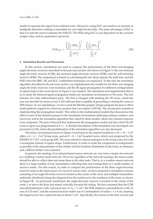
Sensors 2016, 16, 1086

unable to separate the signal from ambient noise. Moreover, using EGC can result in an increase inmultipath distortion, making it unsuitable for very high bit rate links. The main advantage of EGC isthat it avoids the need to estimate the SNR [7]. The SNR using EGC is not dependent on the constantweight value, and its expression is given by:

SNREGC “

˜

Jř

j“1wRPS,j

¸2

Jř

j“1w2σ2

j

“

˜

Jř

j“1RPS,j

¸2

Jř

j“1σ2

j

(32)

3. Simulation Results and Discussion

In this section, simulations are used to compare the performance of the three non-imagingangle-diversity receivers described in the previous section and shown in Figure 3: the conventionalangle-diversity receiver (CDR), the sectored angle-diversity receiver (SDR), and the self-orientingreceiver (SOR). The comparison is based on calculating the rms delay spread, the path loss, and theSNR when the MRC, SB, and EGC combination techniques are employed. To this end, the simulationalgorithm described in the previous section was implemented, the models for the three non-imagingangle-diversity receivers were included, and the IR signal propagation for different configurationsof optical links in the room shown in Figure 4 was studied. The simulation tool implemented allowsus to study the infrared signal propagation inside any simulation environment or 3D scene. The toolfeatures two fully differentiated parts. The first is charged with defining the 3D scene, which theuser can describe by means of any CAD software that is capable of generating or storing the scene in3DS format. In our simulations, we have used the Blender graphic design program because it offersmulti-platform support in a freeware product that can output a 3DS file. The second part consists ofimplementing the propagation model. This refers to the mathematical models that characterize theeffect of each of the elements present in the simulation environment (reflecting surfaces, emitters, andreceivers), and to the simulation algorithm that, aided by these models, allows the channel responseto be computed. The part of the tool that implements the propagation model and into which the 3Dscene is input was programmed in C++. A detailed description of the simulation tool developed waspresented in [19], where the parallelization of the simulation algorithm was also discussed.

The indoor environment shown in Figure 4 was based on the channel models for a 14 ˆ 14 ˆ 3 m3

office, a 6 ˆ 6 ˆ 3 m3 living room, and an 8 ˆ 8 ˆ 3 m3 hospital room, which were proposed by theIEEE802.15.7 VLC work group [28]. The room selected is almost analogous to the living room, but witha rectangular instead of square shape. Furthermore, in order to make the comparison as independentas possible of the characteristics of the emitter and the furniture distribution in the room, no obstaclesand a diffuse emitter were assumed.

In general, the topology of an infrared-based sensor network can vary from a simple star networkto a multihop wireless mesh network. However, regardless of the network topology, the sensor nodesshould be able to collect data and route them to the sink node. That is, in a wireless sensor networkthere is a large number of tiny transmitters collecting data and routing them to a small number ofreceiver nodes. For this reason, in order to compare the performance of the three angle-diversityreceivers used as the input sensor of a receiver sensor node, we have proposed a simulation scenarioconsisting of an angle-diversity receiver located in the centre of the room and multiple transmittersuniformly distributed along the diagonal from the northwest to the southeast of the room, as shownin Figure 4b. As previously mentioned, the angle-diversity receiver is located in the centre of theroom, 1 m above the floor and aimed vertically towards the ceiling. We have assumed that the CDRuses photodetectors with a physical area of AR = 1 cm2, the SOR employs a photodetector with anarea of 3.53 mm2, and the sectored receiver makes use of a hemisphere of radius r = 1.4 cm, meaningthe largest sector has a physical area of about 1 cm2. Specifically, the sectors in the first, second and

142

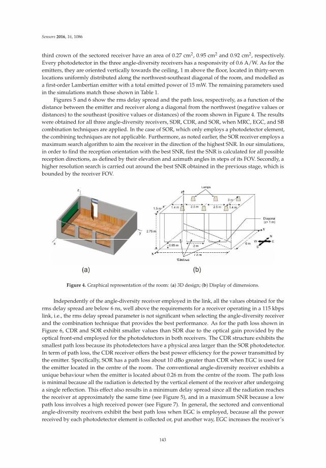
Sensors 2016, 16, 1086

third crown of the sectored receiver have an area of 0.27 cm2, 0.95 cm2 and 0.92 cm2, respectively.Every photodetector in the three angle-diversity receivers has a responsivity of 0.6 A/W. As for theemitters, they are oriented vertically towards the ceiling, 1 m above the floor, located in thirty-sevenlocations uniformly distributed along the northwest-southeast diagonal of the room, and modelled asa first-order Lambertian emitter with a total emitted power of 15 mW. The remaining parameters usedin the simulations match those shown in Table 1.

Figures 5 and 6 show the rms delay spread and the path loss, respectively, as a function of thedistance between the emitter and receiver along a diagonal from the northwest (negative values ordistances) to the southeast (positive values or distances) of the room shown in Figure 4. The resultswere obtained for all three angle-diversity receivers, SDR, CDR, and SOR, when MRC, EGC, and SBcombination techniques are applied. In the case of SOR, which only employs a photodetector element,the combining techniques are not applicable. Furthermore, as noted earlier, the SOR receiver employs amaximum search algorithm to aim the receiver in the direction of the highest SNR. In our simulations,in order to find the reception orientation with the best SNR, first the SNR is calculated for all possiblereception directions, as defined by their elevation and azimuth angles in steps of its FOV. Secondly, ahigher resolution search is carried out around the best SNR obtained in the previous stage, which isbounded by the receiver FOV.

Figure 4. Graphical representation of the room: (a) 3D design; (b) Display of dimensions.

Independently of the angle-diversity receiver employed in the link, all the values obtained for therms delay spread are below 6 ns, well above the requirements for a receiver operating in a 115 kbpslink, i.e., the rms delay spread parameter is not significant when selecting the angle-diversity receiverand the combination technique that provides the best performance. As for the path loss shown inFigure 6, CDR and SOR exhibit smaller values than SDR due to the optical gain provided by theoptical front-end employed for the photodetectors in both receivers. The CDR structure exhibits thesmallest path loss because its photodetectors have a physical area larger than the SOR photodetector.In term of path loss, the CDR receiver offers the best power efficiency for the power transmitted bythe emitter. Specifically, SOR has a path loss about 10 dBo greater than CDR when EGC is used forthe emitter located in the centre of the room. The conventional angle-diversity receiver exhibits aunique behaviour when the emitter is located about 0.26 m from the centre of the room. The path lossis minimal because all the radiation is detected by the vertical element of the receiver after undergoinga single reflection. This effect also results in a minimum delay spread since all the radiation reachesthe receiver at approximately the same time (see Figure 5), and in a maximum SNR because a lowpath loss involves a high received power (see Figure 7). In general, the sectored and conventionalangle-diversity receivers exhibit the best path loss when EGC is employed, because all the powerreceived by each photodetector element is collected or, put another way, EGC increases the receiver’s

143

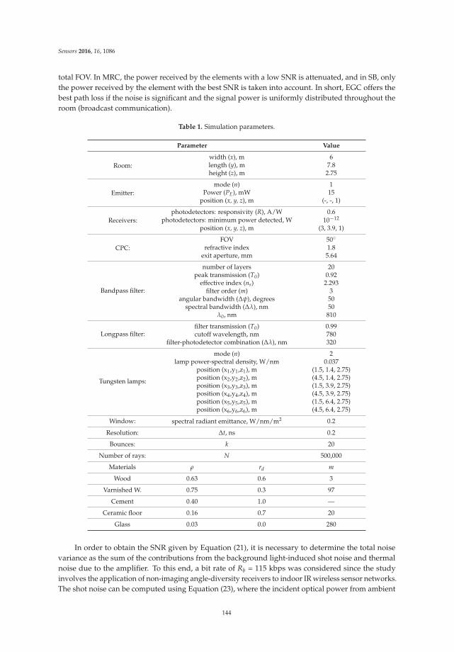
Sensors 2016, 16, 1086

total FOV. In MRC, the power received by the elements with a low SNR is attenuated, and in SB, onlythe power received by the element with the best SNR is taken into account. In short, EGC offers thebest path loss if the noise is significant and the signal power is uniformly distributed throughout theroom (broadcast communication).

Table 1. Simulation parameters.

Parameter Value

Room:width (x), m 6length (y), m 7.8height (z), m 2.75

Emitter:mode (n) 1

Power (PE), mW 15position (x, y, z), m (-, -, 1)

Receivers:photodetectors: responsivity (R), A/W 0.6

photodetectors: minimum power detected, W 10´12

position (x, y, z), m (3, 3.9, 1)

CPC:FOV 50˝

refractive index 1.8exit aperture, mm 5.64

Bandpass filter:

number of layers 20peak transmission (T0) 0.92

effective index (ns) 2.293filter order (m) 3

angular bandwidth (Δψ), degrees 50spectral bandwidth (Δλ), nm 50

λ0, nm 810

Longpass filter:filter transmission (T0) 0.99cutoff wavelength, nm 780

filter-photodetector combination (Δλ), nm 320

Tungsten lamps:

mode (n) 2lamp power-spectral density, W/nm 0.037

position (x1,y1,z1), m (1.5, 1.4, 2.75)position (x2,y2,z2), m (4.5, 1.4, 2.75)position (x3,y3,z3), m (1.5, 3.9, 2.75)position (x4,y4,z4), m (4.5, 3.9, 2.75)position (x5,y5,z5), m (1.5, 6.4, 2.75)position (x6,y6,z6), m (4.5, 6.4, 2.75)

Window: spectral radiant emittance, W/nm/m2 0.2

Resolution: Δt, ns 0.2

Bounces: k 20

Number of rays: N 500,000

Materials ρ rd m

Wood 0.63 0.6 3

Varnished W. 0.75 0.3 97

Cement 0.40 1.0 —

Ceramic floor 0.16 0.7 20

Glass 0.03 0.0 280

In order to obtain the SNR given by Equation (21), it is necessary to determine the total noisevariance as the sum of the contributions from the background light-induced shot noise and thermalnoise due to the amplifier. To this end, a bit rate of Rb = 115 kbps was considered since the studyinvolves the application of non-imaging angle-diversity receivers to indoor IR wireless sensor networks.The shot noise can be computed using Equation (23), where the incident optical power from ambient

144

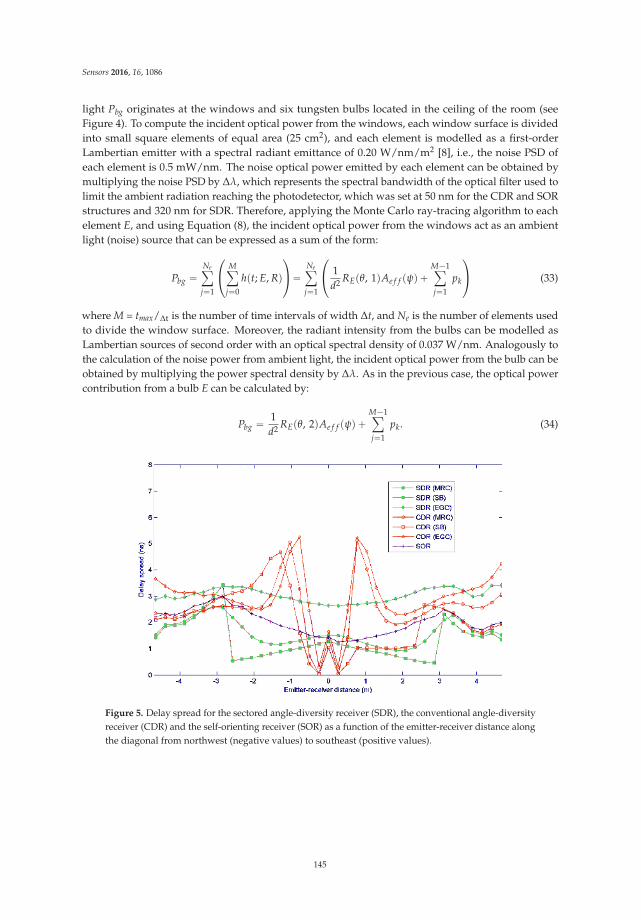
Sensors 2016, 16, 1086

light Pbg originates at the windows and six tungsten bulbs located in the ceiling of the room (seeFigure 4). To compute the incident optical power from the windows, each window surface is dividedinto small square elements of equal area (25 cm2), and each element is modelled as a first-orderLambertian emitter with a spectral radiant emittance of 0.20 W/nm/m2 [8], i.e., the noise PSD ofeach element is 0.5 mW/nm. The noise optical power emitted by each element can be obtained bymultiplying the noise PSD by Δλ, which represents the spectral bandwidth of the optical filter used tolimit the ambient radiation reaching the photodetector, which was set at 50 nm for the CDR and SORstructures and 320 nm for SDR. Therefore, applying the Monte Carlo ray-tracing algorithm to eachelement E, and using Equation (8), the incident optical power from the windows act as an ambientlight (noise) source that can be expressed as a sum of the form:

Pbg “Neÿ

j“1

¨

˝

Mÿ

j“0

hpt; E, Rq

˛

‚“Neÿ

j“1

¨

˝

1d2 REpθ, 1qAe f f pψq `

M´1ÿ

j“1

pk

˛

‚ (33)

where M = tmax/Δt is the number of time intervals of width Δt, and Ne is the number of elements usedto divide the window surface. Moreover, the radiant intensity from the bulbs can be modelled asLambertian sources of second order with an optical spectral density of 0.037 W/nm. Analogously tothe calculation of the noise power from ambient light, the incident optical power from the bulb can beobtained by multiplying the power spectral density by Δλ. As in the previous case, the optical powercontribution from a bulb E can be calculated by:

Pbg “ 1d2 REpθ, 2qAe f f pψq `

M´1ÿ

j“1

pk. (34)

Figure 5. Delay spread for the sectored angle-diversity receiver (SDR), the conventional angle-diversityreceiver (CDR) and the self-orienting receiver (SOR) as a function of the emitter-receiver distance alongthe diagonal from northwest (negative values) to southeast (positive values).

145

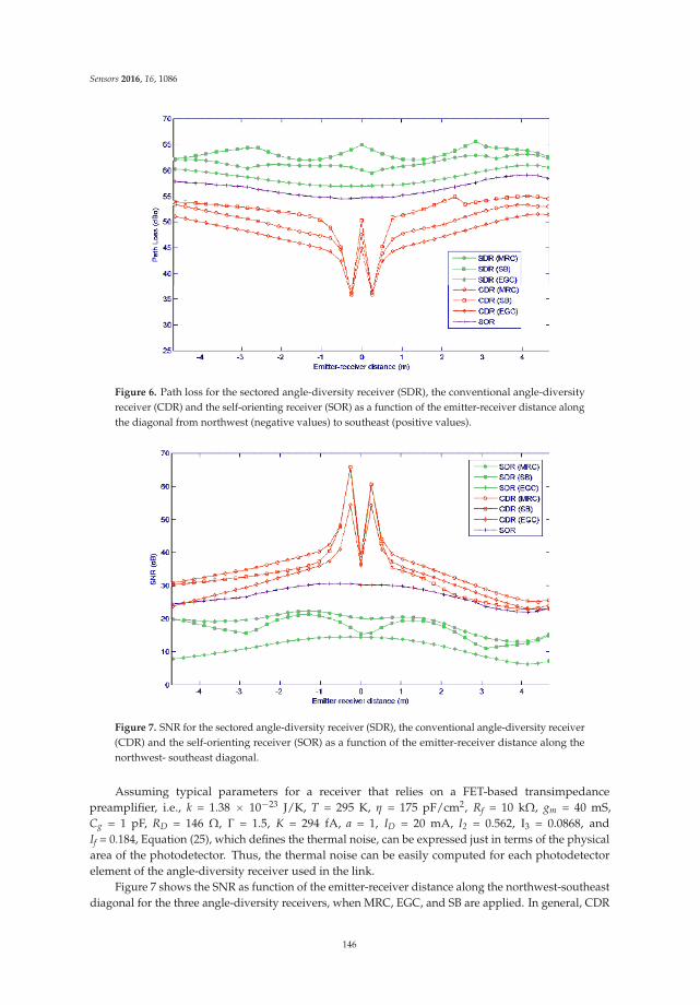
Sensors 2016, 16, 1086

Figure 6. Path loss for the sectored angle-diversity receiver (SDR), the conventional angle-diversityreceiver (CDR) and the self-orienting receiver (SOR) as a function of the emitter-receiver distance alongthe diagonal from northwest (negative values) to southeast (positive values).

Figure 7. SNR for the sectored angle-diversity receiver (SDR), the conventional angle-diversity receiver(CDR) and the self-orienting receiver (SOR) as a function of the emitter-receiver distance along thenorthwest- southeast diagonal.

Assuming typical parameters for a receiver that relies on a FET-based transimpedancepreamplifier, i.e., k = 1.38 ˆ 10´23 J/K, T = 295 K, η = 175 pF/cm2, Rf = 10 kΩ, gm = 40 mS,Cg = 1 pF, RD = 146 Ω, Γ = 1.5, K = 294 fA, a = 1, ID = 20 mA, I2 = 0.562, I3 = 0.0868, andIf = 0.184, Equation (25), which defines the thermal noise, can be expressed just in terms of the physicalarea of the photodetector. Thus, the thermal noise can be easily computed for each photodetectorelement of the angle-diversity receiver used in the link.

Figure 7 shows the SNR as function of the emitter-receiver distance along the northwest-southeastdiagonal for the three angle-diversity receivers, when MRC, EGC, and SB are applied. In general, CDR

146

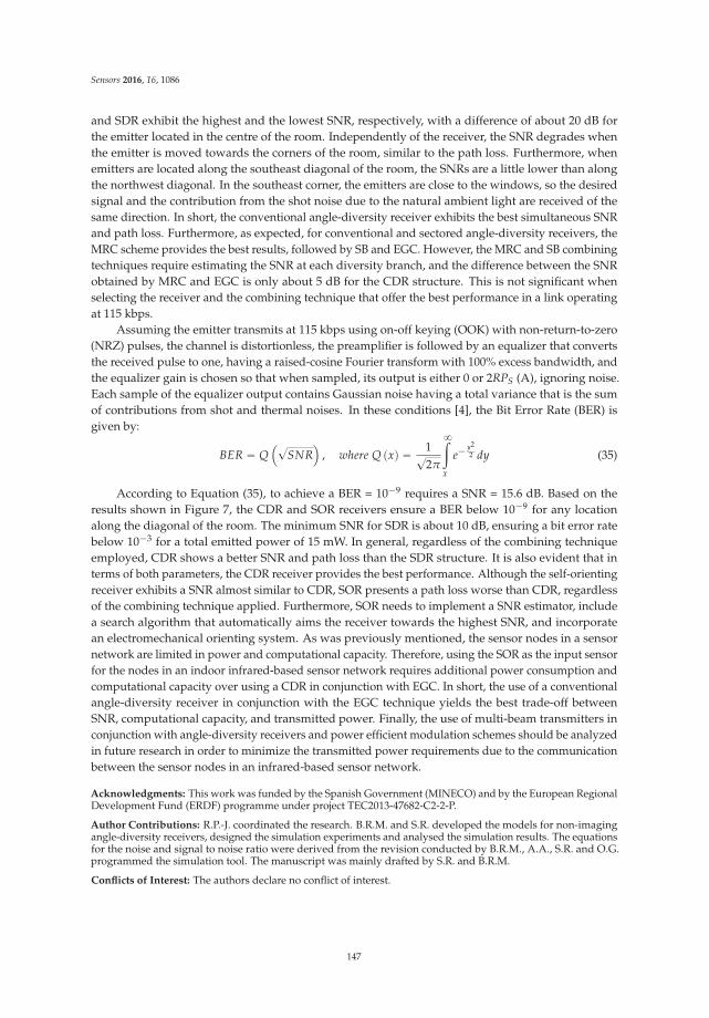
Sensors 2016, 16, 1086

and SDR exhibit the highest and the lowest SNR, respectively, with a difference of about 20 dB forthe emitter located in the centre of the room. Independently of the receiver, the SNR degrades whenthe emitter is moved towards the corners of the room, similar to the path loss. Furthermore, whenemitters are located along the southeast diagonal of the room, the SNRs are a little lower than alongthe northwest diagonal. In the southeast corner, the emitters are close to the windows, so the desiredsignal and the contribution from the shot noise due to the natural ambient light are received of thesame direction. In short, the conventional angle-diversity receiver exhibits the best simultaneous SNRand path loss. Furthermore, as expected, for conventional and sectored angle-diversity receivers, theMRC scheme provides the best results, followed by SB and EGC. However, the MRC and SB combiningtechniques require estimating the SNR at each diversity branch, and the difference between the SNRobtained by MRC and EGC is only about 5 dB for the CDR structure. This is not significant whenselecting the receiver and the combining technique that offer the best performance in a link operatingat 115 kbps.

Assuming the emitter transmits at 115 kbps using on-off keying (OOK) with non-return-to-zero(NRZ) pulses, the channel is distortionless, the preamplifier is followed by an equalizer that convertsthe received pulse to one, having a raised-cosine Fourier transform with 100% excess bandwidth, andthe equalizer gain is chosen so that when sampled, its output is either 0 or 2RPS (A), ignoring noise.Each sample of the equalizer output contains Gaussian noise having a total variance that is the sumof contributions from shot and thermal noises. In these conditions [4], the Bit Error Rate (BER) isgiven by:

BER “ Q´?

SNR¯

, where Q pxq “ 1?2π

8ż

x

e´ y22 dy (35)

According to Equation (35), to achieve a BER = 10´9 requires a SNR = 15.6 dB. Based on theresults shown in Figure 7, the CDR and SOR receivers ensure a BER below 10´9 for any locationalong the diagonal of the room. The minimum SNR for SDR is about 10 dB, ensuring a bit error ratebelow 10´3 for a total emitted power of 15 mW. In general, regardless of the combining techniqueemployed, CDR shows a better SNR and path loss than the SDR structure. It is also evident that interms of both parameters, the CDR receiver provides the best performance. Although the self-orientingreceiver exhibits a SNR almost similar to CDR, SOR presents a path loss worse than CDR, regardlessof the combining technique applied. Furthermore, SOR needs to implement a SNR estimator, includea search algorithm that automatically aims the receiver towards the highest SNR, and incorporatean electromechanical orienting system. As was previously mentioned, the sensor nodes in a sensornetwork are limited in power and computational capacity. Therefore, using the SOR as the input sensorfor the nodes in an indoor infrared-based sensor network requires additional power consumption andcomputational capacity over using a CDR in conjunction with EGC. In short, the use of a conventionalangle-diversity receiver in conjunction with the EGC technique yields the best trade-off betweenSNR, computational capacity, and transmitted power. Finally, the use of multi-beam transmitters inconjunction with angle-diversity receivers and power efficient modulation schemes should be analyzedin future research in order to minimize the transmitted power requirements due to the communicationbetween the sensor nodes in an infrared-based sensor network.

Acknowledgments: This work was funded by the Spanish Government (MINECO) and by the European RegionalDevelopment Fund (ERDF) programme under project TEC2013-47682-C2-2-P.

Author Contributions: R.P.-J. coordinated the research. B.R.M. and S.R. developed the models for non-imagingangle-diversity receivers, designed the simulation experiments and analysed the simulation results. The equationsfor the noise and signal to noise ratio were derived from the revision conducted by B.R.M., A.A., S.R. and O.G.programmed the simulation tool. The manuscript was mainly drafted by S.R. and B.R.M.


147

Sensors 2016, 16, 1086

References

1. Akyildiz, I.; Su, W.; Sankarasubramaniam, Y.; VCayirci, E. A survey on sensor networks. IEEE Commun. Mag.

2002, 40, 102–114. [CrossRef]2. Sharif, A.; Potdar, V.; Chang, E. Wireless multimedia sensor network technology: A survey. In Proceedings

of the 7th IEEE International Conference on Industrial Informatics, Cardiff, Wales, UK, 23–26 June 2009;pp. 606–613.

3. Agrawal, N.; Davis, C.; Milner, S. Design and performance of a directional media access control protocol foroptical wireless sensor networks. IEEE J. Opt. Commun. Netw. 2014, 6, 215–224. [CrossRef]

4. Kahn, J.M.; Barry, J.R. Wireless infrared communications. Proc. IEEE. 1997, 85, 367–379. [CrossRef]5. Alsaadi, F.E.; Elmirghani, J.M.H. Adaptive mobile line strip multibeam MC-CDMA optical wireless system

employing imaging detection in a real indoor environment. IEEE J. Sel. Areas Commun. 2009, 27, 1663–1675.[CrossRef]

6. Alsaadi, F.E.; Elmirghani, J.M.H. Adaptive mobile multicarrier code division multiple access optical wirelesssystems employing a beam clustering method and diversity detection. IET Optoelectron. 2010, 4, 95–112.[CrossRef]

7. Al-Ghamdi, A.G.; Elmirghani, J.M.H. Analysis of diffuse optical wireless channels employing spot-diffusingtechniques, diversity receivers, and combining schemes. IEEE Trans. Commun. 2004, 52, 1622–1631.[CrossRef]

8. Carruthers, J.B.; Kahn, J.M. Angle diversity for nondirected wireless infrared communication.IEEE Trans. Commun. 2000, 48, 906–969. [CrossRef]

9. Jivkova, S.; Hristov, B.A.; Kaverhrad, M. Power-efficient multispot-diffuse multiple-input-multiple-outputapproach to broad-band optical wireless communications. IEEE Trans. Veh. Technol. 2004, 53, 882–888.[CrossRef]

10. Djahani, P.; Kahn, J.M. Analysis of infrared wireless links employing multibeam transmitters and imagingdiversity receivers. IEEE Trans. Commun. 2000, 48, 2077–2088. [CrossRef]

11. Lomba, C.R.A.T.; Valadas, R.T.; De Oliveira Duarte, A.M. Sectored receivers to combat the multipathdispersion of the indoor optical channel. In Proceedings of the Sixth IEEE International Symposium onPersonal, Indoor and Mobile Communications (PIMRC’95), Toronto, ON, Canada, 27–29 September 1995;pp. 321–325.

12. Mendoza, B.R.; Rodríguez, S.; Pérez-Jiménez, R.; González, O.; Poves, E. Considerations on the designof sectored receivers for wireless optical channels using a Monte Carlo based ray tracing algorithm.IET Optoelectron. 2007, 1, 226–232. [CrossRef]

13. Rodríguez, S.; Mendoza, B.R.; Pérez-Jiménez, R.; González, O.; García-Viera, A. Design considerationsof conventional angle-diversity receivers for indoor optical wireless communications. EURASIP J. Wirel.

Commun. Netw. 2014, 221. [CrossRef]14. Barry, J.R.; Kahn, J.M.; Lee, E.A.; Messerschmitt, D.G. Simulation of multipath impulse response for indoor

wireless optical channels. IEEE J. Sel. Areas Commun. 1993, 11, 367–379. [CrossRef]15. López-Hernández, F.J.; Betancor, M.J. DUSTIN: A novel algorithm for the calculation of the impulse response

on IR wireless indoor channels. Electron. Lett. 1997, 33, 1804–1805. [CrossRef]16. López-Hernandez, F.J.; Pérez-Jiménez, R.; Santamaría, A. Ray-Tracing algorithms for fast calculation of the

channel impulse response on diffuse IR-wireless indoor channels. Opt. Eng. 2000, 39, 2775–2780.17. Rodríguez, S.; Pérez-Jiménez, R.; López-Hernádez, F.J.; González, O.; Ayala, A. Reflection model for

calculation of the impulse response on IR-wireless indoor channels using ray-tracing algorithm. Microw. Opt.

Technol. Lett. 2002, 32, 296–300. [CrossRef]18. Rodríguez, S.; Pérez-Jiménez, R.; González, O.; Rabadán, J.; Mendoza, B.R. Concentrator and lens models for

calculating the impulse response on IR-wireless indoor channels using a ray-tracing algorithm. Microw. Opt.

Technol. Lett. 2003, 36, 262–267. [CrossRef]19. Rodríguez, S.; Pérez-Jiménez, R.; Mendoza, B.R.; López-Hernádez, F.J.; Ayala, A. Simulation of impulse

response for indoor visible light communications using 3D CAD models. EURASIP J. Wirel. Commun. Netw.

2013, 7. [CrossRef]

148

Sensors 2016, 16, 1086

20. Castillo-Vazquez, M.; Puerta-Notario, A. Self-orienting receiver for indoor wireless infrared links at high bitrates. In Proceedings of the 57th IEEE Semiannual Vehicular Technology Conference, Orlando, FL, USA,22–25 April 2003.

21. Castillo-Vazquez, M.; García-Zambrana, A.; Puerta-Notario, A. Self-Orienting Receiver using Rate-AdaptiveTransmission based on OOK Formats with Memory for Optical Wireless Communications. In Proceedings ofthe IEEE Global Telecommunications Conference, Dallas, TX, USA, 29 November–3 December 2004.

22. Tang, A.P.; Kahn, J.M.; Ho, K.P. Wireless infrared communications links using multi-beam transmitters andimaging receivers. In Proceedings of the IEEE International Conference on Communications, Dallas, TX,USA, 23–27 June 1996.

23. Barry, J.R.; Kahn, J.M. Link design for nondirected wireless infrared communications. Appl. Opt. 1995, 34,3764–3776. [CrossRef] [PubMed]

24. SchottRG780 Longpass Filter Data Sheet. Available online: http://www.sydor.com/wp-content/uploads/SCHOTT-RG780-Longpass-Filter.pdf (accessed on 3 July 2016).

25. Franco, S. Design with Operational Amplifiers and Analog Integrated Circuits, 4th ed.; McGraw-Hill Education:Penn Plaza, NY, USA, 2015; pp. 357–360.

26. Tavares, A.M.R.; Valadas, R.J.M.T.; de Oliveira Duarte, A.M. Performance of an optical sectored receiver forindoor wireless communication systems in presence of artificial and natural noise sources. In Proceedings ofthe SPIE, Wireless Data Transmission, Philadelphia, PA, USA, 8 December 1995.

27. Valadas, R.T.; Duarte, A.M. Sectored receivers for indoor wireless optical communication systems.In Proceedings of the IEEE International Symposium on Personal, Indoor and Mobile Radio Communications,The Hague, The Netherlands, 18–23 September 1994.

28. LiFi Reference Channel Models: Office, Home and Hospital. Available online: https://mentor.ieee.org/802.15/dcn/15/15-15-0514-01-007a-lifi-reference (accessed on 14 June 2016).


149

Article

Trust and Privacy Solutions Based on HolisticService Requirements

José Antonio Sánchez Alcón *, Lourdes López †, José-Fernán Martínez † andGregorio Rubio Cifuentes †

Centro de Investigación en Tecnologías Software y Sistemas Multimedia para la Sostenibilidad (CITSEM),Campus Sur Universidad Politécnica de Madrid (UPM), Ctra. de Valencia, km. 7. 28031 Madrid, Spain;[email protected] (L.L.); [email protected] (J.-F.M.); [email protected] (G.R.C.)* Correspondence: [email protected]; Tel.: +34-914-524-900 (ext. 20791)† These authors contributed equally to this work.

Academic Editor: Dario BruneoReceived: 24 September 2015; Accepted: 17 December 2015; Published: 24 December 2015

Abstract: The products and services designed for Smart Cities provide the necessary tools to improvethe management of modern cities in a more efficient way. These tools need to gather citizens’information about their activity, preferences, habits, etc. opening up the possibility of tracking them.Thus, privacy and security policies must be developed in order to satisfy and manage the legislativeheterogeneity surrounding the services provided and comply with the laws of the country wherethey are provided. This paper presents one of the possible solutions to manage this heterogeneity,bearing in mind these types of networks, such as Wireless Sensor Networks, have important resourcelimitations. A knowledge and ontology management system is proposed to facilitate the collaborationbetween the business, legal and technological areas. This will ease the implementation of adequatespecific security and privacy policies for a given service. All these security and privacy policies arebased on the information provided by the deployed platforms and by expert system processing.

Keywords: Smart Cities; Smart Grid; Internet of Things; Wireless Sensor Network; security services;privacy; personal data protection; Utility Matrix

1. Introduction

A smart city represents a leap forward in increasing a city’s sustainable growth and strengtheningcity functions to provide a greater quality of life for citizens than a traditional city. It is predicted thatthere will be a great quantity of “objects” interacting continuously with citizens and which can be bothcollectors and distributors of information regarding their mobility, energy consumption, etc. As aresult, cyber and real worlds are strongly linked in a smart city. Thus those “objects” can act as sensorsand actuators to interact with the smart city [1,2]. New services based on information gathered andrecorded from multiple sources can be deployed when needed. The loss of trust and privacy of citizenscould be an obstacle in the interaction between smart city and citizens. Citizens with their mobilephones and other smart devices, such as wearable devices, can also act as sensors, and they can giveinformation about their movements, habits, preferences, etc. One of the most significant perceived risksfor citizens is the tracking of their movements and their activities through the information gathered bythe objects. They also fear being included in a list of personal profiles. Analyzing these data in order toidentify behaviors and habits of people, yields information that could be used in many areas, mainlyin marketing.

The set of services in a smart city can be viewed as a holistic compound service comprising allsingle services such as urban mobility, energy consumption, critical infrastructures, public safety,health etc. As a result, using the appropriate Smart City technologies, sustainable management of


Sensors 2016, 16, 16

the whole is made possible. There are many stakeholders in a Smart City, each one having their owninterests. Among the major stakeholders are sponsors, services operators, and the monitored entities(some of which may be citizens). Stakeholders’ interests may conflict with each other. The solution ofthese situations represents a challenge for legislative and regulatory entities. Therefore it is necessary toimplement coherent trust and privacy policies based on legislation, since they are able to reconcile therights and interests of all stakeholders and protect the citizens from infringements of their rights andinvasions of their privacy. Nevertheless, this new range of services also requires the development ofnew communication architectures to minimize their vulnerability and ensure the maximum protectionto citizens. Therefore it is necessary to develop and research about new mechanisms to provide safeand reliable environments. Concepts such as “Privacy by Design (PBD)” [3] and the mechanisms tofacilitate positive or negative consent are being researched in order to build confidence and allowthe users to choose. This idea also requires the participation of actors and stakeholders to protectagainst the possible chaos if a mass deployment of these technologies were to occur. Thus, for the PBD

seven principles are defined [3], these deal with proactivity; prevention; privacy settings configured bydefault and integrated into the design, etc. They also deal with the visibility, transparency and designsneeded to focus on the user and respect people’s privacy.

This paper proposes two goals: (1) A platform to integrate the functionalities and control of theservices to acquire enough capacity to generate new applications; (2) An expert system to solve thediverse legislation issues and provide options to generate a policy of trust and privacy mechanismsto apply.

Currently, several Interconnection and Cooperation Platforms (ICP) are being developed. Theseplatforms also have to allow management of trust and privacy policies. One of them is the “ACCUS

Project [4]”. The Adaptive Cooperative Control in Urban (sub)Systems (ACCUS) platform aimsto implement three innovations: (1) integration and coordination platform for urban systems;(2) new control architecture for urban subsystems and (3) general methodologies and tools forcreating applications.

This paper is organized in the following manner: Section 2 shows existing related work in thisresearch field, Section 3 shows an brief overview on ACCUS platform in the smart city, Section 4discusses the major challenges to privacy and trust in that environment. Section 5 shows the neededelements for privacy and trust policy implementation, and in Section 6 these are applied to an exampleof a Smart Service in a smart city. Section 7 concludes with a summary of the major contributions ofthis paper and future work.

2. Related Work

The 2012 during our investigation activities about security and privacy in the “Internet of Things”field we were able to verify the huge interdependence between the selection of the mechanisms andthe security and privacy countermeasures, the right legislation that must be applied to a determinedIoT service and the commercial need for the cost to be as low as reasonably possible.

After a study on the state of the art about this topic reported in previous publications [5,6],three different kinds of contributions were found: (1) state of the art regarding commercialproducts and businesses focused on the creation of new ideas and services to be commercialized;(2) technology-based state of the art, which provides better and more efficient solutions by its naturalprogress; (3) legislative state of the art, which is not always homogeneous for the different marketswhere it is expected to be used, and with a very significant impact on the companies related to thesectors where they perform their activities. The timing that is required for each of the groups is verydifferent and they do not always move at the same speed, thus resulting in potential risks for people,critical infrastructures, etc.

The study that was carried out started by analysing the selection process of the security andprivacy mechanisms that were made during the specification and design process of several productsand services made by two relevant companies of the sector. These companies, although unwilling to

151

Sensors 2016, 16, 16

be identified in this manuscript, nevertheless provided us their support. Mechanisms were selectedaccording to the technological solution suitable to the legal requirements that were obtained by meansof the counsel requested to consultancy companies regarded as leaders of legislative cases involvingInternet usage. In this process we have found a significant amount of issues. Several of them havebeen enumerated as follows:

1. Consultancy costs are high, both in economic and time-to-market terms.2. In some cases, costs associated to security made the product or the service unviable, resulting in

the cancellation of the service after significant resource expenses, or the redesign of the service,thus increasing the related costs.

3. Concern was manifested by the companies consulted with regards to the associated cost ofclaims, complaints, sanctions and corporative image deterioration that suppose the impacts tiedto security and privacy flaws.

4. Both companies pointed out the convenience of having a simulator to test new ideas for productsand services that could provide them with a forecast of the requirements for security and dataprotection in order to perform a cost evaluation prior to the start of the development phase.

5. Heterogeneity of legislative frameworks in the different countries those companies operate in is amajor issue for them.

6. This heterogeneous legislative framework also affects the same countries or even the sameservice, depending on how it is used [5,6]. This also happens when one product is designed as acombination of some others, when the same terminal is used to offer several services, etc.

7. Actions to be taken in a context of likely legislative changes, or when dealing with emergencylevel changes that may imply different features related to security and privacy.

8. Previous knowledge of the impact that a specific legislative change will have (in terms of securityand data protection on the IoT-based products and services already deployed) is prone to behelpful for the agents involved in legislation.

9. The user tends to recklessly offer his/her trust less often. What he/she really requests is beguaranteed that their information, intimacy, security and safety will not be jeopardized by themere fact of voluntarily using (or refusing to use) these new products and services.

After several months of study and consultations to the members of the “Internet Society” relatedto the legal area of knowledge, political parties, trade unions, etc., the idea of having these three areasof knowledge cooperating (business, law and technology) with each other started to build up. Thisconcept of channelling the requirements of security and privacy through a collaborative system amongthe areas of business, law and technology is an original contribution the authors of this manuscript(this idea has been contrasted and validated by the interlocutors previously mentioned).

This collaboration materializes itself in the collection of the entrepreneurial, legislative andtechnological knowledge that can be used by an expert system to provide an answer for the alreadymentioned main challenges.

We couldn´t find any system or integrated packet that would adapt to the automation that wewere looking for. The closest were the “Legal Expert Systems”, even though analysis and legislativeconflicts were their focus. The expert system proposed in this paper was inspired basically onCuadrado Gamarra´s book about expert systems in the legal field [7], and the articles of Stevens [8]and Venkateswarlu [9] as well as related references in these about “Legal Expert Systems”. Withinour paper the vision is a bit different; we do not try to solve legislative conflicts as is the case of thepreviously mentioned works [7–9], but rather what we want is to obtain the key legislative knowledgeneeded in a matter of security and privacy to be able to apply the needed legal imperatives, about aconcrete IoT service.

On the other hand and due to the large researcher activity about it, a lot of investigation studies areavailable (among them the major part of the bibliography in the previous publications [5,6] mentioned

152

Sensors 2016, 16, 16

before in this paper) providing mechanisms and technological countermeasures to act against thethreats and attacks to the security and privacy being able to provide solutions.

Therefore, knowing the details of the IoT service that is to be developed, the legal imperativesthat must be applied and a group of available technological solutions, it should be possible to managea solution tailored for each situation. This is the purpose of the proposed expert system.

The structure of the system relies on not hindering the independent evolution of each of thespheres, each of them with its own budget capabilities, Information Technologies systems and theirown route map for their own progress. The only adaptations that must be done are involving datacommunication, transfer and results storage; all the other actions can be performed in each of thespheres with their regular means of work.

This paper proposes an expert system to generate security and privacy policies for services inthe smart city. This policy is communicated to the ACCUS platform, which is able to deploy it to thenetwork and devices. The expert system proposed in this research has gone though various majorversions since its first design. The first version was presented at the “Third Intech Conference inLondon, 2013” [5]. The first version was designed to decide the security level that is needed for acertain use case for a specific service. It managed the behavior for different use cases using the sameWSN dedicated to health monitoring, but subjected to different legal frameworks. In that case theexpert system provided its security and privacy policies to a service platform called AWARE whichwas then able to configure the WSN remotely.

The second version was designed in 2014, when its functionalities were expanded and the modelwas modified to be able to work with more than one WSN in different technologies or IoT services [6].Thus, the expert system was improved to be able to manage the requirements of various services,taking into account the possibilities of different technologies. At the same time, the platform mentionedbefore was boosted to be able to communicate and configure the security mechanisms for variousWSN technologies.

Lastly, this paper wishes to further expand the model of the expert system to be capable ofselecting the different security and privacy levels for each one of the services in a smart city. Eachnewly generated services and created by combination of the existing ones must have a security leveladequate, maybe can be different than the ones being used. It also offers the possibility of changing thesecurity level in a city, depending on the possible states of alarm or emergency. In this environment,the mediating platform for the city’s services is ACCUS [4]. This research paper provides a way totackle the issues and challenges with regards to security and privacy in the Internet of Things withinthe framework of a smart city. These challenges have a major impact in the entrepreneurial, legislativeand technological environments, and while each of them offers only one part of the solution, the finalsolution must come from the collaboration among all three areas. Another important issue is that flawsin security and privacy may affect people´s rights.

This paper does not propose any legislation framework and no security mechanism, but rather itdescribes a method to choose and apply the security services based on the collaborative environmentamong the business, legal and technological areas.

3. Smart Cities Applications and Urban Systems Management Using ICP

3.1. Smart City Applications

Smart city applications are grouped into several areas. One classification is proposed in [10],based on the presence of six characteristics shown in Table 1. All these areas raise new challenges insecurity and privacy such as transnational authentication systems for citizens and businesses, agreedframeworks for data privacy, and the sharing and collection of individual and business data, in orderto make a more livable city for citizens, the performance of integrated services and urban systems (suchas manager of the traffic, energy, lighting, emergency systems, or information systems) must be taken

153

Sensors 2016, 16, 16

into account. This enables integrated management strengthened through mutual aid in situations thatrequire it.

Table 1. Smart City applications.

Applications Target

Smart EconomyInnovative spirit; Entrepreneurship; Economic image/trademarks;Productivity; Flexibility of labor market; International embeddedness.

Smart PeopleLevel of qualification; Affinity to lifelong learning; Social and ethnicplurality; Flexibility; Creativity; Cosmopolitanism/Open-mindedness;Participation in public life.

Smart GovernanceParticipation in decision-making; Public and social services; Transparentgovernance; Political strategies/perspectives

Smart MobilityLocal accessibility; Accessibility; Availability of ICT-infrastructure;Sustainable, innovative and safe transport systems

Smart EnvironmentNatural conditions; Pollution; Environmental protection; Sustainableresource management

Smart LivingCultural facilities; Health conditions; Individual safety; Housing quality;Education facilities; Social cohesion

For example, correct traffic management in emergency situations can contribute to emergencyservices arriving in the shortest possible time wherever they are required, and could also reinforce orrestrict other resources in the same area, etc. To obtain this range of new applications, it is necessaryto integrate both the performance and control of these autonomous systems. It should be noted thatthe systems providing specific services must continue to evolve independently and their integrationwith other systems must not impede their natural path of evolution, but must find a way that does notaffect their integration with others, in a scenario of an integration of “systems of systems”. Each systemhas its own internal evolution, which must not be affected by the integration process, so an integrationplatform that enables the possibility for each platform to maintain its functionality and control wouldbe necessary, and to obtain with the integration the additional advantage of having enough capacity toenable the generation of new applications.

3.2. ACCUS Project

The proposal in this paper has been deployed inside the European ACCUS project, but theproposed expert system is in fact adaptable to any other platform that can control, send and receivecommands and responses to/from network elements and perform the needed remote configurations.

As indicated in [4] the ACCUS project focuses on four innovations that are listed below:

‚ Provide an integration and coordination platform for urban systems to build new applicationsacross urban systems.

‚ Provide adaptive and cooperative control architectures and the corresponding algorithms forurban subsystems in order to optimize their combined performance.

‚ Provide general methodologies and tools for creating real-time collaborative applications for“systems of systems”.

‚ Seamless connectivity and semantic interoperability among all services and subsystems connected.ACCUS ICP must provide the necessary mechanisms and facilities so that present and futureapplications and services connected within the smart city can consult which other subsystemsand services exist and what is their functionality.

Currently, the platform has two types of components: (1) core components: the componentswhich allow the platform to provide its basic functionality such as registration, discovery, controlelements, security, etc. and (2) city customization components: in order to enable the adaptation of theICP platform to any city, it must have some plugins that allow this customization, e.g., event detection,location detection, data analytics, situation awareness . . . A main functionality of the ICP platform

154

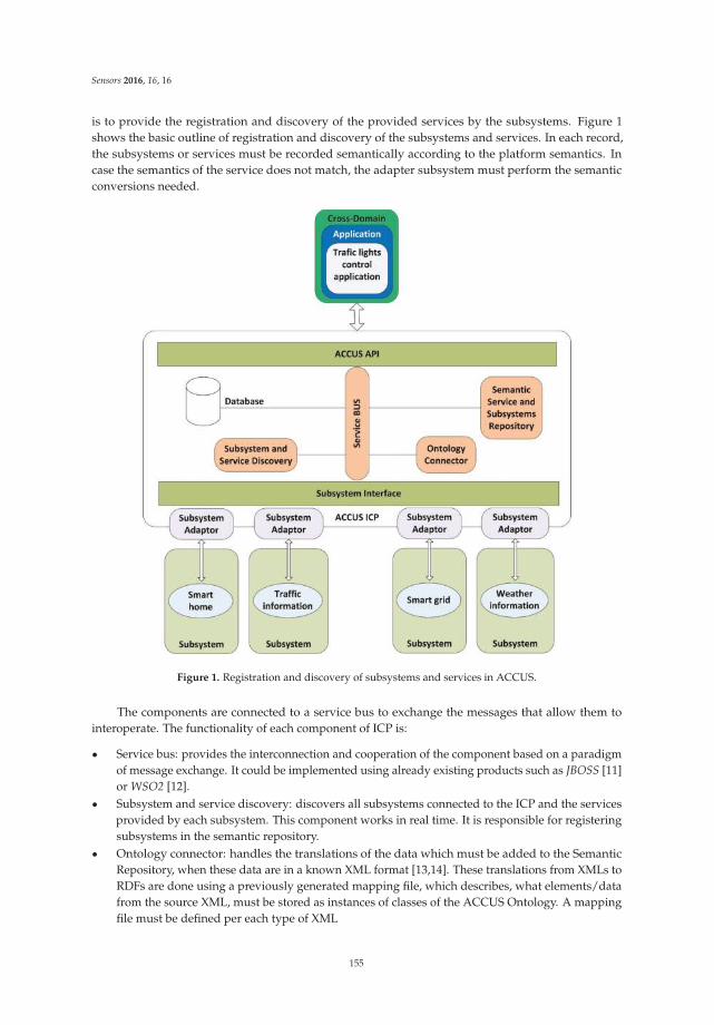
Sensors 2016, 16, 16

is to provide the registration and discovery of the provided services by the subsystems. Figure 1shows the basic outline of registration and discovery of the subsystems and services. In each record,the subsystems or services must be recorded semantically according to the platform semantics. Incase the semantics of the service does not match, the adapter subsystem must perform the semanticconversions needed.

Figure 1. Registration and discovery of subsystems and services in ACCUS.

The components are connected to a service bus to exchange the messages that allow them tointeroperate. The functionality of each component of ICP is:

‚ Service bus: provides the interconnection and cooperation of the component based on a paradigmof message exchange. It could be implemented using already existing products such as JBOSS [11]or WSO2 [12].

‚ Subsystem and service discovery: discovers all subsystems connected to the ICP and the servicesprovided by each subsystem. This component works in real time. It is responsible for registeringsubsystems in the semantic repository.

‚ Ontology connector: handles the translations of the data which must be added to the SemanticRepository, when these data are in a known XML format [13,14]. These translations from XMLs toRDFs are done using a previously generated mapping file, which describes, what elements/datafrom the source XML, must be stored as instances of classes of the ACCUS Ontology. A mappingfile must be defined per each type of XML

155

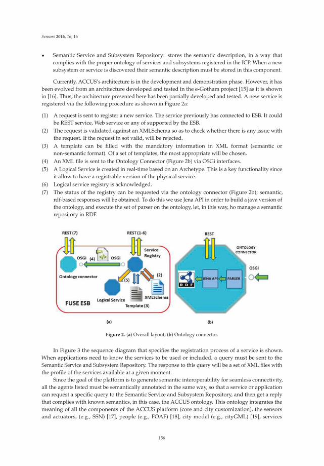
Sensors 2016, 16, 16

‚ Semantic Service and Subsystem Repository: stores the semantic description, in a way thatcomplies with the proper ontology of services and subsystems registered in the ICP. When a newsubsystem or service is discovered their semantic description must be stored in this component.

Currently, ACCUS’s architecture is in the development and demonstration phase. However, it hasbeen evolved from an architecture developed and tested in the e-Gotham project [15] as it is shownin [16]. Thus, the architecture presented here has been partially developed and tested. A new service isregistered via the following procedure as shown in Figure 2a:

(1) A request is sent to register a new service. The service previously has connected to ESB. It couldbe REST service, Web service or any of supported by the ESB.

(2) The request is validated against an XMLSchema so as to check whether there is any issue withthe request. If the request in sot valid, will be rejected.

(3) A template can be filled with the mandatory information in XML format (semantic ornon-semantic format). Of a set of templates, the most appropriate will be chosen.

(4) An XML file is sent to the Ontology Connector (Figure 2b) via OSGi interfaces.(5) A Logical Service is created in real-time based on an Archetype. This is a key functionality since

it allow to have a registrable version of the physical service.(6) Logical service registry is acknowledged.(7) The status of the registry can be requested via the ontology connector (Figure 2b); semantic,

rdf-based responses will be obtained. To do this we use Jena API in order to build a java version ofthe ontology, and execute the set of parser on the ontology, let, in this way, ho manage a semanticrepository in RDF.

Figure 2. (a) Overall layout; (b) Ontology connector.

In Figure 3 the sequence diagram that specifies the registration process of a service is shown.When applications need to know the services to be used or included, a query must be sent to theSemantic Service and Subsystem Repository. The response to this query will be a set of XML files withthe profile of the services available at a given moment.

Since the goal of the platform is to generate semantic interoperability for seamless connectivity,all the agents listed must be semantically annotated in the same way, so that a service or applicationcan request a specific query to the Semantic Service and Subsystem Repository, and then get a replythat complies with known semantics, in this case, the ACCUS ontology. This ontology integrates themeaning of all the components of the ACCUS platform (core and city customization), the sensorsand actuators, (e.g., SSN) [17], people (e.g., FOAF) [18], city model (e.g., cityGML) [19], services

156

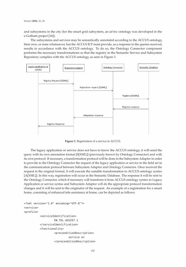
Sensors 2016, 16, 16

and subsystems in the city (for the smart grid subsystem, an ad-hoc ontology was developed in thee-Gotham project [16]).

The subsystems and services may be semantically annotated according to the ACCUS ontology,their own, or none whatsoever, but the ACCUS ICP must provide, as a response to the queries received,results in accordance with the ACCUS ontology. To do so, the Ontology Connector componentperforms the necessary transformations so that the registry in the Semantic Service and SubsystemRepository complies with the ACCUS ontology, as seen in Figure 3.

Figure 3. Registration of a service in ACCUS.

The legacy application or service does not have to know the ACCUS ontology, it will send thequery with its own annotation format [S[XML]] (previously known by Ontology Connector) and withits own protocol. If necessary, a transformation protocol will be done in the Subsystem Adaptor in orderto provide to the Ontology Connector the request of the legacy application or service in the field set inthe communication protocol between Subsystem Adaptor and Ontology Connector. Once received therequest in the original formal, it will execute the suitable transformation to ACCUS ontology syntax[A[XML]]. In this way, registration will occur in the Semantic Database. The response it will be sent tothe Ontology Connector, which if necessary will transform it from ACCUS ontology syntax to LegacyApplication or service syntax and Subsystem Adaptor will do the appropriate protocol transformationchanges and it will be sent to the originator of the request. An example of a registration for a smarthome, consisting of enhanced tele-assistance at home, can be depicted as follows:

<?xml version="1.0" encoding="UTF-8"?>

<service>

<profile>

<serviceIdentification>

EN_TEL_ASSIST_1

</serviceIdentification>

<functionality>

<preconditionDescription>

service on

</preconditionDescription>

157

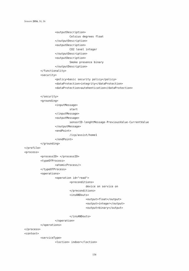
Sensors 2016, 16, 16

<outputDescription>

Celsius degrees float

</outputDescription>

<outputDescription>

CO2 level integer


<outputDescription>

Smoke presence binary


</functionality>

<security>

<policy>basic security policy</policy>

<dataProtection>integrity</dataProtection>

<dataProtection>autehentication</dataProtection>

</security>

<grounding>

<inputMessage>

start

</inputMessage>

<outputMessage>

sensorID-lenghtMessage-PreviousValue-CurrentValue

</outputMessage>

<endPoint>

/icp/assist/home1

</endPoint>

</grounding>

</profile>

<process>

<processID> </processID>

<typeOfProcess>

<atomicProcess/>

</typeOfProcess>

<operations>

<operation id="read">

<preconditions>

device on service on

</preconditions>

<insANDouts>

<output>float</output>

<output>integer</output>

<output>binary</output>

</insANDouts>

</operation>

</operations>

</process>

<context>

<serviceType>

<loction> indoor</loction>

158

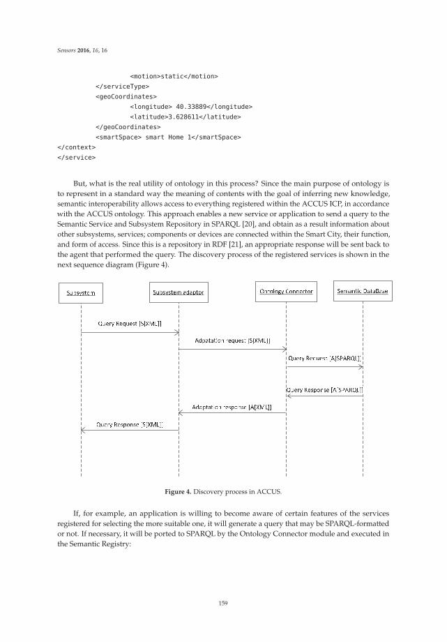
Sensors 2016, 16, 16

<motion>static</motion>

</serviceType>

<geoCoordinates>

<longitude> 40.33889</longitude>

<latitude>3.628611</latitude>

</geoCoordinates>

<smartSpace> smart Home 1</smartSpace>

</context>

</service>

But, what is the real utility of ontology in this process? Since the main purpose of ontology isto represent in a standard way the meaning of contents with the goal of inferring new knowledge,semantic interoperability allows access to everything registered within the ACCUS ICP, in accordancewith the ACCUS ontology. This approach enables a new service or application to send a query to theSemantic Service and Subsystem Repository in SPARQL [20], and obtain as a result information aboutother subsystems, services; components or devices are connected within the Smart City, their function,and form of access. Since this is a repository in RDF [21], an appropriate response will be sent back tothe agent that performed the query. The discovery process of the registered services is shown in thenext sequence diagram (Figure 4).

Figure 4. Discovery process in ACCUS.

If, for example, an application is willing to become aware of certain features of the servicesregistered for selecting the more suitable one, it will generate a query that may be SPARQL-formattedor not. If necessary, it will be ported to SPARQL by the Ontology Connector module and executed inthe Semantic Registry:

159

Sensors 2016, 16, 16

PREFIX ns:<http://www.semanticweb.org/ACCUS/1.1#>

SELECT ?ServiceIdentification ?inputDescription ?outputDescription ?policy ?data

Protection ?endPoint

WHERE

?service ns:hasProfile ?profile.

?profile ns:hasServiceIdentification ?serviceIdentification.

?profile ns:hasFunctionality ?functionality.

?profile ns:hasSecurity ?security.

?profile ns:hasGrounding ?grounding.

?functionality ns:hasInputDescription ?inputDescription.

?functionality ns:hasOutputDescription ?outputDescription.

?security ns:hasPolicy ?ns:policy.

?security ns:hasDataProtection ?dataProtection.

?grounding ns:hasEndPoinf ?endPoint.

Response will be in an XML-formatted message according to the ontology:


<services>

<service>

<profile>

<serviceIdentification>

EN_TEL_ASSIST_1

</serviceIdentification>

<functionality>

<preconditionDescription>

service on

</preconditionDescription>

<outputDescription>

Celsius degrees float


<outputDescription>

CO2 level integer


<outputDescription>

Smoke Presence binary


</functionality>

<security>

<policy>basic security policy</policy>

<dataProtection>integrity</dataProtection>

</security>

<grounding>

<endPoint>

/icp/assist/home1

</endPoint>

</grounding>

160

Sensors 2016, 16, 16

</profile>

</service>

<service>.....</service>

<service>.....</service>

</services>

With the information therein it will be capable of inferring new knowledge that, in the context of asmart city, consists of generating new cross-domain applications and services for the city and citizens,which then must also be registered in the ACCUS ICP, producing constant feedback. Furthermore,these new applications will already use the ACCUS ontology.

3.3. Security and Privacy in a Smart City

Studies performed some years ago such as [22] recognized the importance of data privacy andpersonal identity among the aspects to be dealt with, not only on technical grounds, but also concerninglegal frameworks:

E-Government: There are a number of technologies that will be required for the underlyinginfrastructure that is needed to help support this process. Fundamental technologies are key to thedevelopment of the Digital Single Market (such as authentication and privacy), and to the developmentof e-government in smart cities. The development of transnational authentication systems for citizensand businesses, the development of agreed frameworks for data privacy, and the sharing and collectionof individual and business data, must be considered.

Health, Inclusion and Assisted Living: The key technical requirements to be addressed in thisdomain are: security (encryption, authentication and authorization), service discovery, scalability andsurvivability, persistence, interworking, community-to-community application messaging propagation,auditing and logging, location information sharing, and application service migration.

The challenge related to ICT security aspects has to be ensured by a manageable access controlmanagement system, to ensure that only authorized persons are allowed to access the data, andensures that the data is protected to achieve confidentiality. Users should manage authorization.Dedicated authentication and logging mechanisms have to support the enforcement of access control.The challenge in this approach is that access control architecture has to enable both the decentralizedstorage of data, and the comprehensive access control mechanisms and enforcement that concern allparties that could have access to that data.

Intelligent Transportation Systems: the provisioning of flexible, scalable and self-optimized networks,dealing with heterogeneity, effectively exploiting location information, guaranteeing real-timeexchange of data where needed, and providing security, privacy and authentication mechanisms.

Smart Grids, Energy Efficiency, and the Environment: Other challenges include: newcommunication and networking ICT technologies, new affordable devices that gather environmentdata, new intelligent algorithms for smart ubiquitous environments, new light sources, new andfair regulations that enables the mass implementation of the Intelligent Street Lighting System ideaprovided by different vendors; new products for global markets that enable steady economic growth;and advanced products and services based on IP to foster innovations, and economic growth basedon an open innovation scheme. Recently, Sicari et al. presented in [23] a vision of the near futurein security, privacy and trust in IoT. Finally, Weber et al. presented in [24] the forthcoming issues inprivacy applied to IoT.

4. Challenges on Privacy and Trust

It is important to know how to classify data sources in a smart city and their relation to personalidentity. These sources are the following:

161

Sensors 2016, 16, 16

‚ Non personal sources: data, unrelated to specific people, gathered from devices (temperature orhumidity sensors, etc.)

‚ Personal sources: data, related to specific people, gathered from devices, unambiguously usinguser identity (social networks, etc.)

‚ Anonymous sources: data related to specific people gathered from devices, but which have beenpre-processed to mask their personal identity (covering faces in video camera images, etc.).

It may be possible to discover user information by processing data from several sources. Thesesituations must be considered. From a technological viewpoint the security and privacy problemscan be grouped as follows: (1) Problems related to computer security and communication systems;(2) Problems related to database security, user identities and communications; (3) Problems occurringwhen new subsystems are added to the smart city (increasing its complexity and vulnerabilities).

4.1. Problems Related to Computer Security and Communication Systems

These are the problems such as malware (viruses, trojans, worms, backdoors, spyware, etc.), orbots, loggers, rootkits, DDoS attacks, lack of updates [25,26], etc. They are prevented by installingsuitable antivirus, firewalls, honeypots, intrusion detection systems (IDS), security policies, updatingand implementing system authentication measures. When the devices are localized all around thecity and do not have a common control platform, updating or implementing the new policies ofauthentication or refusing the authorizations is difficult.

4.2. Problems Related to Database Security, User Identities and Communications

‚ Database security [27] The Statistical Disclosure Control (SDC) techniques consist of insertingnoise or aggregations to maintain privacy, while maintaining the significant value of the data.Private Information Retrieval (PIR) techniques are based on queries asking for more than thenecessary information in order to hide the specific information demanded by the user.

‚ To hide user identities accessing location-based services (LBS) techniques are used such as cloakingand using pseudonyms.

‚ Privacy in communications, advanced cryptography and access control can be used to preventeavesdropping on the data and prevent unauthorized connection nodes to the networks withdistributed devices in access public places [28].

4.3. Problems Occurring When New Subsystems Are Added to the Smart City

When new subsystems are added to the smart city the complexity and the number ofvulnerabilities grow [28], which can be exploited by malicious people to harm the most vulnerablesystems and enter into the other subsystems of the smart city.

‚ Increased interconnections among services increase the ways through which a virus can propagate.Hackers can move through the interconnections among the systems and take control.

‚ Dependencies among infrastructures. A failure in one of the nodes in the dependencies networkcould cause some cascade problems. Planning and management can alleviate the problem [29].

‚ The connection of the smart city with the other platforms and applications by middleware is astrategic element. Those connections must be secured, implementing confidentiality, integrity andauthenticity and they must also be interoperable.

‚ The fact that having a great quantity of services and data sources facilitates creating newapplications and services, but risks the availability of these services if a fault in any of themoccurs, which would cause malfunctions an application and even make it unusable.

‚ In an open data context with a great quantity of information sources (both real-time and historical),publishing new data makes it difficult to ensure that they cannot be used to infer the identity ofusers (using correlation techniques,...). To minimize the time of intrusions and attacks, solutionsthat implement active reactions in a crisis scenario to curb the anomaly [30] are used.

162

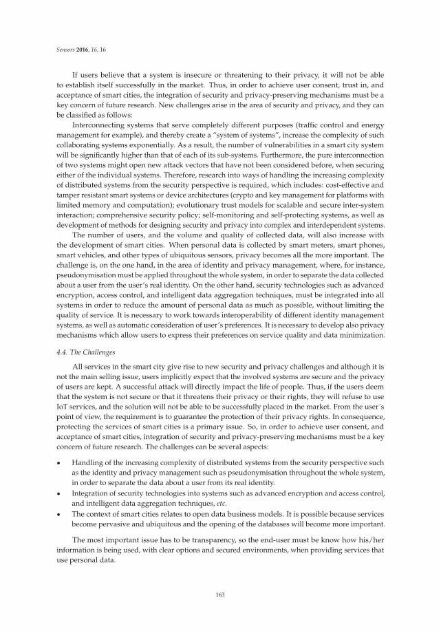
Sensors 2016, 16, 16

If users believe that a system is insecure or threatening to their privacy, it will not be ableto establish itself successfully in the market. Thus, in order to achieve user consent, trust in, andacceptance of smart cities, the integration of security and privacy-preserving mechanisms must be akey concern of future research. New challenges arise in the area of security and privacy, and they canbe classified as follows:

Interconnecting systems that serve completely different purposes (traffic control and energymanagement for example), and thereby create a “system of systems”, increase the complexity of suchcollaborating systems exponentially. As a result, the number of vulnerabilities in a smart city systemwill be significantly higher than that of each of its sub-systems. Furthermore, the pure interconnectionof two systems might open new attack vectors that have not been considered before, when securingeither of the individual systems. Therefore, research into ways of handling the increasing complexityof distributed systems from the security perspective is required, which includes: cost-effective andtamper resistant smart systems or device architectures (crypto and key management for platforms withlimited memory and computation); evolutionary trust models for scalable and secure inter-systeminteraction; comprehensive security policy; self-monitoring and self-protecting systems, as well asdevelopment of methods for designing security and privacy into complex and interdependent systems.

The number of users, and the volume and quality of collected data, will also increase withthe development of smart cities. When personal data is collected by smart meters, smart phones,smart vehicles, and other types of ubiquitous sensors, privacy becomes all the more important. Thechallenge is, on the one hand, in the area of identity and privacy management, where, for instance,pseudonymisation must be applied throughout the whole system, in order to separate the data collectedabout a user from the user’s real identity. On the other hand, security technologies such as advancedencryption, access control, and intelligent data aggregation techniques, must be integrated into allsystems in order to reduce the amount of personal data as much as possible, without limiting thequality of service. It is necessary to work towards interoperability of different identity managementsystems, as well as automatic consideration of user’s preferences. It is necessary to develop also privacymechanisms which allow users to express their preferences on service quality and data minimization.

4.4. The Challenges

All services in the smart city give rise to new security and privacy challenges and although it isnot the main selling issue, users implicitly expect that the involved systems are secure and the privacyof users are kept. A successful attack will directly impact the life of people. Thus, if the users deemthat the system is not secure or that it threatens their privacy or their rights, they will refuse to useIoT services, and the solution will not be able to be successfully placed in the market. From the user´spoint of view, the requirement is to guarantee the protection of their privacy rights. In consequence,protecting the services of smart cities is a primary issue. So, in order to achieve user consent, andacceptance of smart cities, integration of security and privacy-preserving mechanisms must be a keyconcern of future research. The challenges can be several aspects:

‚ Handling of the increasing complexity of distributed systems from the security perspective suchas the identity and privacy management such as pseudonymisation throughout the whole system,in order to separate the data about a user from its real identity.

‚ Integration of security technologies into systems such as advanced encryption and access control,and intelligent data aggregation techniques, etc.

‚ The context of smart cities relates to open data business models. It is possible because servicesbecome pervasive and ubiquitous and the opening of the databases will become more important.

The most important issue has to be transparency, so the end-user must be know how his/herinformation is being used, with clear options and secured environments, when providing services thatuse personal data.

163

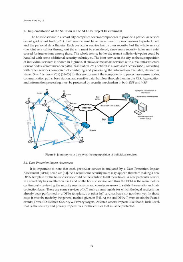
Sensors 2016, 16, 16

5. Implementation of the Solution in the ACCUS Project Environment

The holistic service in a smart city comprises several components to provide a particular service(smart grid, smart traffic, etc.). Each service must have its own security mechanisms to protect itselfand the personal data therein. Each particular service has its own security, but the whole service(the joint service) for throughout the city must be considered, since some security holes may existcaused for interactions among those. The whole service in the city from a holistic viewpoint could behandled with some additional security techniques. The joint service in the city as the superpositionof individual services is shown in Figure 5. It shows some smart services with a real infrastructure(sensor nodes, communication paths, base station, etc.) defined as a Real Smart Service (RSS), coexistingwith other services comprised of combining and processing the information available, defined asVirtual Smart Services (VSS) [31–33]. In this environment the components to protect are sensor nodes,communication paths, base station, and sensible data that flow through them in the RSS. Aggregationand information processing must be protected by security mechanism in both RSS and VSS.

Figure 5. Joint service in the city as the superposition of individual services.

5.1. Data Protection Impact Assessment

It is important to note that each particular service is analyzed by a Data Protection ImpactAssessment (DPIA) Template [34]. As a result some security holes may appear; therefore making a newDPIA Template for the holistic service could be the solution to fill these holes. A new particular servicein a smart city has an effect on itself and on the holistic service, and thus the DPIA is the main tool forcontinuously reviewing the security mechanisms and countermeasures to satisfy the security and dataprotection laws. There are some services of IoT such as smart grids for which the legal analysis hasalready been performed in a DPIA template, but other IoT services have not got them yet. In thosecases it must be made by the general method given in [34]. At the end DPIA-T must obtain the Fearedevents; Threat ID; Related Security & Privacy targets; Affected assets; Impact; Likelihood; Risk Level,that is, the security and privacy imperatives for the entities that must be protected.

164

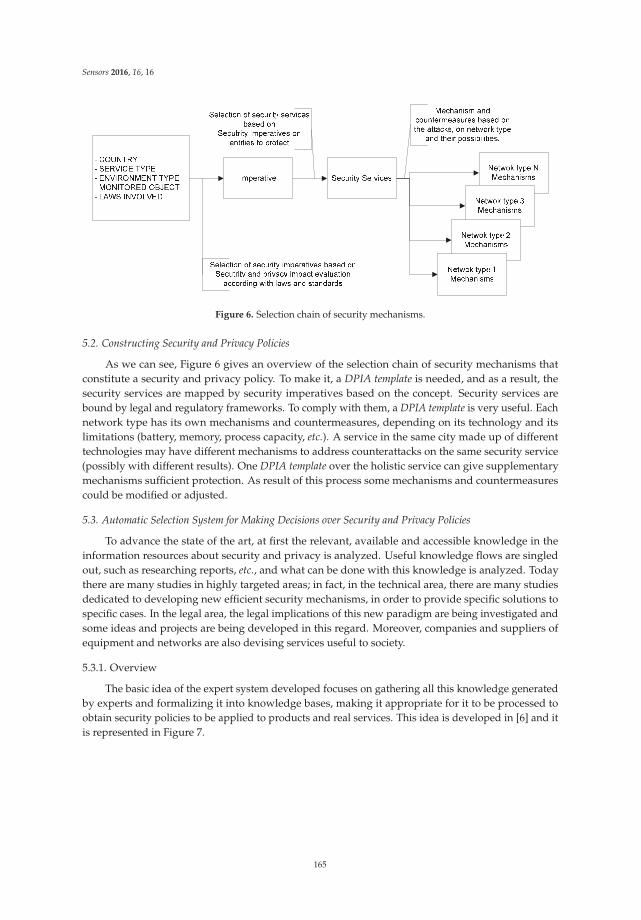
Sensors 2016, 16, 16

Figure 6. Selection chain of security mechanisms.

5.2. Constructing Security and Privacy Policies

As we can see, Figure 6 gives an overview of the selection chain of security mechanisms thatconstitute a security and privacy policy. To make it, a DPIA template is needed, and as a result, thesecurity services are mapped by security imperatives based on the concept. Security services arebound by legal and regulatory frameworks. To comply with them, a DPIA template is very useful. Eachnetwork type has its own mechanisms and countermeasures, depending on its technology and itslimitations (battery, memory, process capacity, etc.). A service in the same city made up of differenttechnologies may have different mechanisms to address counterattacks on the same security service(possibly with different results). One DPIA template over the holistic service can give supplementarymechanisms sufficient protection. As result of this process some mechanisms and countermeasurescould be modified or adjusted.

5.3. Automatic Selection System for Making Decisions over Security and Privacy Policies

To advance the state of the art, at first the relevant, available and accessible knowledge in theinformation resources about security and privacy is analyzed. Useful knowledge flows are singledout, such as researching reports, etc., and what can be done with this knowledge is analyzed. Todaythere are many studies in highly targeted areas; in fact, in the technical area, there are many studiesdedicated to developing new efficient security mechanisms, in order to provide specific solutions tospecific cases. In the legal area, the legal implications of this new paradigm are being investigated andsome ideas and projects are being developed in this regard. Moreover, companies and suppliers ofequipment and networks are also devising services useful to society.

5.3.1. Overview

The basic idea of the expert system developed focuses on gathering all this knowledge generatedby experts and formalizing it into knowledge bases, making it appropriate for it to be processed toobtain security policies to be applied to products and real services. This idea is developed in [6] and itis represented in Figure 7.

165

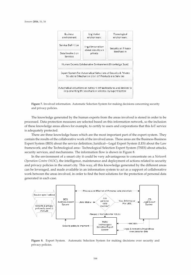
Sensors 2016, 16, 16

Figure 7. Involved information. Automatic Selection System for making decisions concerning securityand privacy policies.

The knowledge generated by the human experts from the areas involved is stored in order to beprocessed. Data protection measures are selected based on this information network, so the inclusionof these knowledge areas allows for example, to certify to users and corporations that this IoT serviceis adequately protected.

There are three knowledge bases which are the most important part of the expert system. Theycontain the results of the collaborative work of the involved areas. These areas are the Business-BusinessExpert System (BES) about the service definition; Juridical—Legal Expert System (LES) about the Lawframework; and the Technological area– Technological Selection Expert System (TSES) about attacks,security services, and mechanisms. The information flow is shown in Figure 8.

In the environment of a smart city it could be very advantageous to concentrate on a Network

Operation Centre (NOC), the intelligence, maintenance and deployment of actions related to securityand privacy policies in the smart city. This way, all this knowledge generated by the different areascan be leveraged, and made available in an information system to act as a support of collaborativework between the areas involved, in order to find the best solutions for the protection of personal datagenerated in each case.

Figure 8. Expert System. Automatic Selection System for making decisions over security andprivacy policies.

166

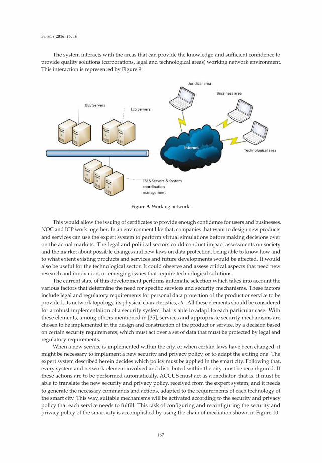
Sensors 2016, 16, 16

The system interacts with the areas that can provide the knowledge and sufficient confidence toprovide quality solutions (corporations, legal and technological areas) working network environment.This interaction is represented by Figure 9.

Figure 9. Working network.

This would allow the issuing of certificates to provide enough confidence for users and businesses.NOC and ICP work together. In an environment like that, companies that want to design new productsand services can use the expert system to perform virtual simulations before making decisions overon the actual markets. The legal and political sectors could conduct impact assessments on societyand the market about possible changes and new laws on data protection, being able to know how andto what extent existing products and services and future developments would be affected. It wouldalso be useful for the technological sector. It could observe and assess critical aspects that need newresearch and innovation, or emerging issues that require technological solutions.

The current state of this development performs automatic selection which takes into account thevarious factors that determine the need for specific services and security mechanisms. These factorsinclude legal and regulatory requirements for personal data protection of the product or service to beprovided, its network topology, its physical characteristics, etc. All these elements should be consideredfor a robust implementation of a security system that is able to adapt to each particular case. Withthese elements, among others mentioned in [35], services and appropriate security mechanisms arechosen to be implemented in the design and construction of the product or service, by a decision basedon certain security requirements, which must act over a set of data that must be protected by legal andregulatory requirements.

When a new service is implemented within the city, or when certain laws have been changed, itmight be necessary to implement a new security and privacy policy, or to adapt the exiting one. Theexpert system described herein decides which policy must be applied in the smart city. Following that,every system and network element involved and distributed within the city must be reconfigured. Ifthese actions are to be performed automatically, ACCUS must act as a mediator, that is, it must beable to translate the new security and privacy policy, received from the expert system, and it needsto generate the necessary commands and actions, adapted to the requirements of each technology ofthe smart city. This way, suitable mechanisms will be activated according to the security and privacypolicy that each service needs to fulfill. This task of configuring and reconfiguring the security andprivacy policy of the smart city is accomplished by using the chain of mediation shown in Figure 10.

167

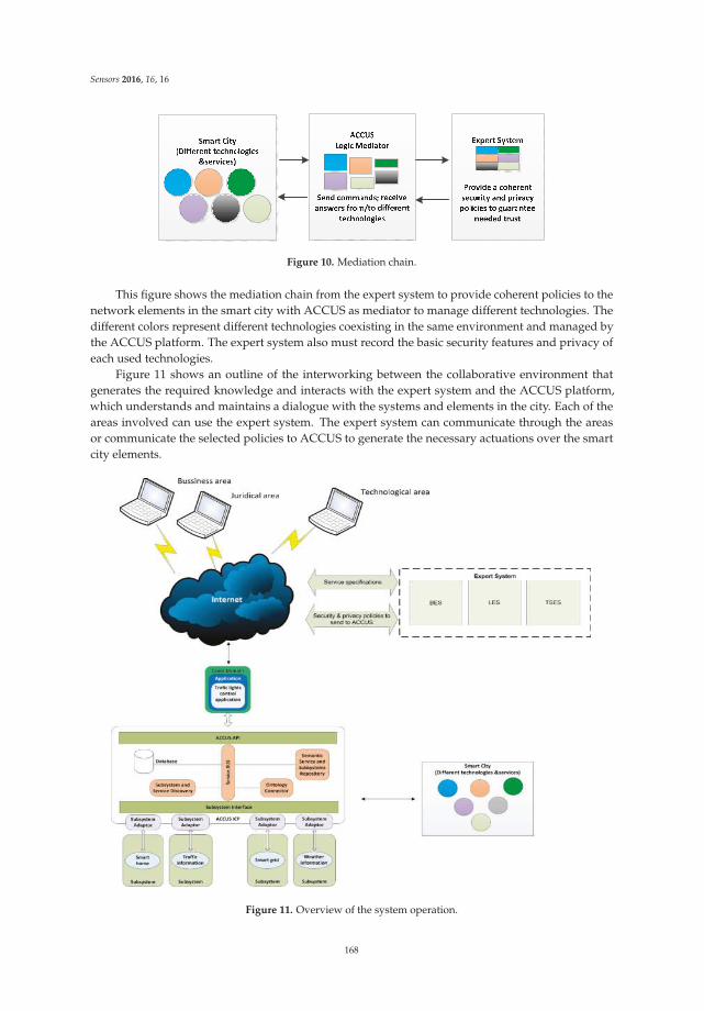
Sensors 2016, 16, 16

Figure 10. Mediation chain.

This figure shows the mediation chain from the expert system to provide coherent policies to thenetwork elements in the smart city with ACCUS as mediator to manage different technologies. Thedifferent colors represent different technologies coexisting in the same environment and managed bythe ACCUS platform. The expert system also must record the basic security features and privacy ofeach used technologies.

Figure 11 shows an outline of the interworking between the collaborative environment thatgenerates the required knowledge and interacts with the expert system and the ACCUS platform,which understands and maintains a dialogue with the systems and elements in the city. Each of theareas involved can use the expert system. The expert system can communicate through the areasor communicate the selected policies to ACCUS to generate the necessary actuations over the smartcity elements.

Figure 11. Overview of the system operation.

168

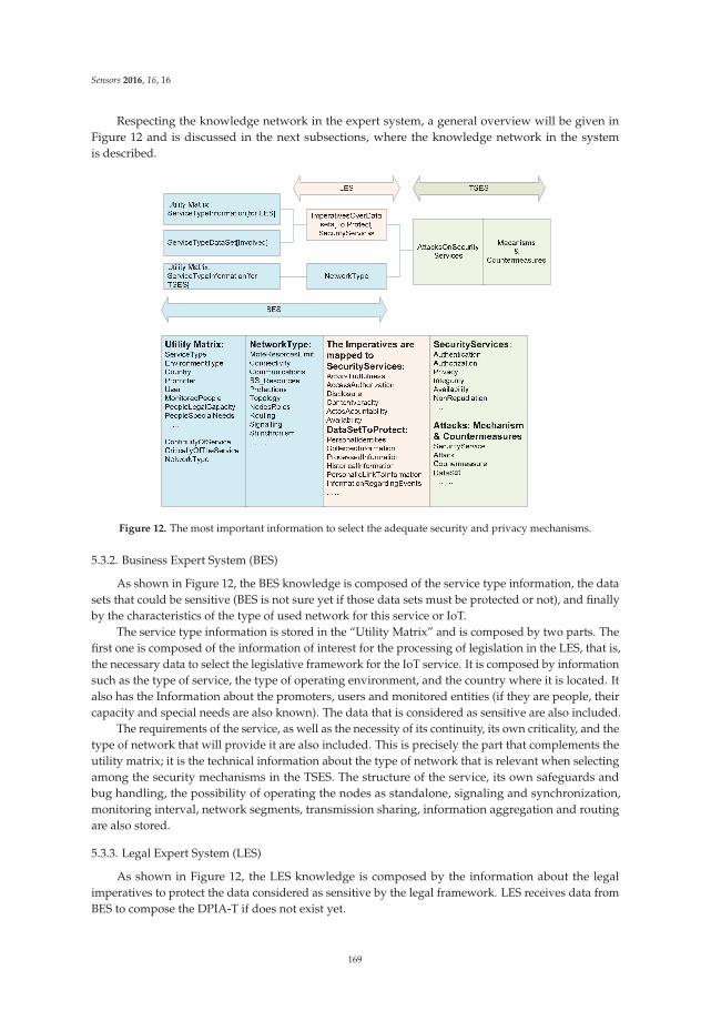
Sensors 2016, 16, 16

Respecting the knowledge network in the expert system, a general overview will be given inFigure 12 and is discussed in the next subsections, where the knowledge network in the systemis described.

Figure 12. The most important information to select the adequate security and privacy mechanisms.

5.3.2. Business Expert System (BES)

As shown in Figure 12, the BES knowledge is composed of the service type information, the datasets that could be sensitive (BES is not sure yet if those data sets must be protected or not), and finallyby the characteristics of the type of used network for this service or IoT.

The service type information is stored in the “Utility Matrix” and is composed by two parts. Thefirst one is composed of the information of interest for the processing of legislation in the LES, that is,the necessary data to select the legislative framework for the IoT service. It is composed by informationsuch as the type of service, the type of operating environment, and the country where it is located. Italso has the Information about the promoters, users and monitored entities (if they are people, theircapacity and special needs are also known). The data that is considered as sensitive are also included.

The requirements of the service, as well as the necessity of its continuity, its own criticality, and thetype of network that will provide it are also included. This is precisely the part that complements theutility matrix; it is the technical information about the type of network that is relevant when selectingamong the security mechanisms in the TSES. The structure of the service, its own safeguards andbug handling, the possibility of operating the nodes as standalone, signaling and synchronization,monitoring interval, network segments, transmission sharing, information aggregation and routingare also stored.

5.3.3. Legal Expert System (LES)

As shown in Figure 12, the LES knowledge is composed by the information about the legalimperatives to protect the data considered as sensitive by the legal framework. LES receives data fromBES to compose the DPIA-T if does not exist yet.

169

Sensors 2016, 16, 16

As the LES processes information, data sets are put together, grouping personal and other sensitivedata handled by the IoT service. A specific normative is applied to these data sets, assigning legalconstraints or a necessary level of protection for a certain service type.

The service type is a function of the environment, country, promoters, users and monitoredentities and their relevant legal characteristics. Actually, this information framing is coherent withthe legal analysis that the NIST as well as the European Union carry out in their DPIA-T impactassessment templates.

If there is a set, si, of services that possess infrastructures, and there is a set, sj, of joint servicescomposed by subsets of si, then there will be (i + j) impact assessment templates. It may also be thecase that new services can be generated from elements of sj, by themselves or by combining withother elements of si. In conclusion, the simplest approach is to have an impact assessment for eachindividual service, and one for each joint service, adapting the necessary mechanisms to each service.That way, services with an associated infrastructure are not hindered in regards to resources, achievinga tailored security. All data processing in LES is compatible with the “Data Protection Risk Assessment(DPIA)”.

5.3.4. Technological Selection Expert System (TSES)

As shown in Figure 12, the TSES knowledge is composed by the security service information, andthe information about the attacks, mechanism & countermeasures. The TSES processes informationby mapping the imperatives in security services that need to be applied to data sets. These securityservices for a certain network type (resources, connectivity, communications, resources in the basestation, topology, nodes, routing, signaling, and synchronism) are threatened by a list of attacks thataffect the IoT service. These attacks have countermeasures (security service, network type, attacks,mechanism & countermeasure).

Luckily, nowadays there are already securities and privacy mechanisms that make it possibleto use complex cryptographic mechanisms, supported by the rapidly advancing development of thehardware and operating systems of network elements. Currently, it is possible to cover the majority ofcases routinely presented, and luckily there is a lot of activity focused in the creation of new solutions.

For the purpose of this paper, the security and privacy policy is considered as the set ofmechanisms integrated within the services. The security policies and mechanisms’ suitability analysisis selected by the degree of coverage reached while having sufficient mechanisms, and by determiningthe best ones for the resources of the technology to which they are applied (delay, consumption, etc.). Ifnot enough mechanisms are found, a coverage alarm would be set off in the corresponding knowledgebase, urging the corresponding experts to solve the issue.

Attacks can be done by both outsider and insider attackers. Insiders, however, are able to performworst damaging actions since they used to have a higher level of permissions and system knowledge.

If an overview of insider attacks is done, it can be noticed that, for instance, SCADA systemsare used in many critical infrastructure applications that have important software components,such as Human Machine Interfaces, servers with historical data, Remote Terminal Units and thecommunication links between them. The latter include the units used to collect information andtransfer it back to the central site carrying out any necessary analysis and control, and displaying thatinformation on an operator screen afterwards. The operators use the Human Machine Interfaces data tomake supervisory decisions. Therefore, the Human Machine Interfaces, data historians, communicationlinks, sensors threshold values and actuator normal settings [36,37] can be attacked by an outsider(the attack can be initiated from outside, by unauthorized or illegitimate users; those usually areopportunistic, deliberate, and malicious) or by insider attackers (they happen when an authorizeduser misuses the permissions and damages the system by sending legitimate control commands witha great impact and higher success rate; these are difficult to predict and provide protection againstthem). With regards to users, not only engineers (responsible for managing object libraries and userinterfaces, setting grid topology, normal work condition states, setting parameters of devices, defining

170

Sensors 2016, 16, 16

process set points, writing automation scripts, etc.) have to be considered in a secure deployment, butalso operators (expected to monitor the system status in Human Machine Interfaces servers, react toalarms and some events so that the process will run correctly, execute operator commands that oftenprevent triggering new alarms, resolve incoming alarms, make decisions about changing topology,etc.). An engineer is a more powerful system user than an operator, but the transmission system iscontrolled by operators. Insider attacks [36,37] to be considered are:

- Unresolved alarms attacks, when alarms are not perfectly resolved (delaying or making incorrector incomplete actuations). These situations can provoke cascading failures of major consequencesif a critical security error is unnoticed. Malfunctions sometimes are a consequence of wrong,high-level management decisions, such as budget cuts, transforming the activity of humanoperators from one of specialized nature to a multifunctional one without enough training, etc.

- Misconfiguration attacks of differing nature: Overload attacks (wrong changes of topology andload transfers, which can cause overload or a power failure in a large area), Outage attacks(opening the output feeders), incorrect setting attacks (improper equipment settings which couldcause equipment incorrect operation).

The incident response can be a complicated matter because one minor mistake may result in theloss of the most critical pieces of evidence and make the whole case inadmissible for a trial or othercourt actions. Some mechanisms against insider attacks has been mentioned and referenced in [36–41],such as:

‚ Detect anomalous behavior in SCADA network traffic.‚ Detect anomalies based on validating protocol specifications‚ A real-time anomaly detection system for unknown attacks‚ Anomaly detection for insider attacks based on system logs of the SCADA system to be

periodically monitored to detect anomalous behavior (it is necessary to control time periods,parameter values, content of the command orders and many more variables).

‚ Detecting insider attacks in SCADA by data passing through the system and include a semanticmodule capable of understanding user actions.

‚ Statistical Anomaly Detection Method (SADM) is developed in some SCADA systems, byanalyzing statistical properties of alarms that will determine the normal system behavior. SADMuses statistical properties to determine whether “current behavior” deviate significantly fromthe “normal behavior” by using the mean and standard deviation parameters in order to setthresholds, which can be learned from observations (operator behavior).

‚ Reference [42] talk about any malicious behavior changes statistical properties of alarms and isidentified as an anomaly (experimental scenarios have been simulated by the proposed ColoredPetri Nets (CPN)-model for insider attacks).

5.4. Processing Stages

Table 2 shows the basic process of selection and the knowledge bases involved. This operationmode enables the cooperation between experts from the areas involved through knowledge generatedand formalized.

Simplicity was given a priority after numerous concept tests, so that the expert system is fast anduser friendly. But this is not free, the coverage and reliability of policies and security mechanisms aretransferred to the performance, coverage and reliability of the information in the knowledge bases ofeach of the three parts, BES, LES and TSES.

171

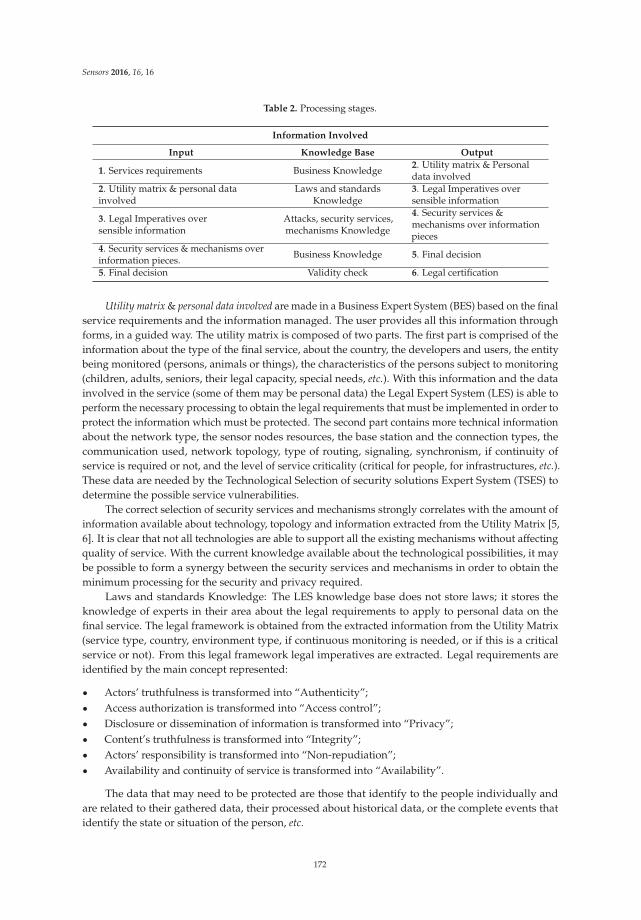
Sensors 2016, 16, 16

Table 2. Processing stages.

Information Involved

Input Knowledge Base Output

1. Services requirements Business Knowledge2. Utility matrix & Personaldata involved

2. Utility matrix & personal datainvolved

Laws and standardsKnowledge

3. Legal Imperatives oversensible information

3. Legal Imperatives oversensible information

Attacks, security services,mechanisms Knowledge

4. Security services &mechanisms over informationpieces

4. Security services & mechanisms overinformation pieces.

Business Knowledge 5. Final decision

5. Final decision Validity check 6. Legal certification

Utility matrix & personal data involved are made in a Business Expert System (BES) based on the finalservice requirements and the information managed. The user provides all this information throughforms, in a guided way. The utility matrix is composed of two parts. The first part is comprised of theinformation about the type of the final service, about the country, the developers and users, the entitybeing monitored (persons, animals or things), the characteristics of the persons subject to monitoring(children, adults, seniors, their legal capacity, special needs, etc.). With this information and the datainvolved in the service (some of them may be personal data) the Legal Expert System (LES) is able toperform the necessary processing to obtain the legal requirements that must be implemented in order toprotect the information which must be protected. The second part contains more technical informationabout the network type, the sensor nodes resources, the base station and the connection types, thecommunication used, network topology, type of routing, signaling, synchronism, if continuity ofservice is required or not, and the level of service criticality (critical for people, for infrastructures, etc.).These data are needed by the Technological Selection of security solutions Expert System (TSES) todetermine the possible service vulnerabilities.

The correct selection of security services and mechanisms strongly correlates with the amount ofinformation available about technology, topology and information extracted from the Utility Matrix [5,6]. It is clear that not all technologies are able to support all the existing mechanisms without affectingquality of service. With the current knowledge available about the technological possibilities, it maybe possible to form a synergy between the security services and mechanisms in order to obtain theminimum processing for the security and privacy required.

Laws and standards Knowledge: The LES knowledge base does not store laws; it stores theknowledge of experts in their area about the legal requirements to apply to personal data on thefinal service. The legal framework is obtained from the extracted information from the Utility Matrix(service type, country, environment type, if continuous monitoring is needed, or if this is a criticalservice or not). From this legal framework legal imperatives are extracted. Legal requirements areidentified by the main concept represented:

‚ Actors’ truthfulness is transformed into “Authenticity”;‚ Access authorization is transformed into “Access control”;‚ Disclosure or dissemination of information is transformed into “Privacy”;‚ Content’s truthfulness is transformed into “Integrity”;‚ Actors’ responsibility is transformed into “Non-repudiation”;‚ Availability and continuity of service is transformed into “Availability”.

The data that may need to be protected are those that identify to the people individually andare related to their gathered data, their processed about historical data, or the complete events thatidentify the state or situation of the person, etc.

172

Sensors 2016, 16, 16

The conceptual direct relationship is established between the LES legal imperatives obtainedand security services by Recommendation X.800 [43] in TSES. The attacks on the final service arecountered by the security services which comprise countermeasures and security mechanisms. In theTSES knowledge base the security services, and the countermeasures and the security mechanisms areassociated with the attacks. The obtained result is a set of mechanisms and countermeasures to achievethe security level needed. When the system is unable to find a solution for all requirements of securityand privacy, a warning of insufficiency of knowledge is thrown indicating the problem encountered.

One part of the assigned work to the technological human experts of TSES is to feed the knowledgedatabase with useful mechanisms that may be utilized. These mechanisms will be classified accordingto several features concerning the casuistry where they are successful when applied, their effectivenessagainst attacks (based both on a study made for this solution and past experience), an assessment ofeasiness of change and adjustment and the capacity of the each mechanism to be monitored.

The ACCUS platform directly supervises the involved security mechanisms, attack attemptsand the successful attacks, and once the attack has been mitigated, the involved mechanisms will berevised, and corresponding changes are made in the platform, in the service and in the expert system.

5.5. Performance Evaluation

The expert system is responsible for controlling the level of current legislation fulfilment regardingasset protection (that is, the level of fulfilment of legal obligations). The smart city offers a collectionof individual services prone to be attacked. Each of the services is subdued to some specific “legalobligations” that are implemented by means of “countermeasures and security mechanisms”. “Attacks”may cause an “impact” on the assets that must be protected, so the level of fulfilment regarding currentlegislation is assessed on the basis of the impact that has taken place (“0” = no impact registered,“1” = impact on non-legally protected assets, “2” = impact on legally protected assets). There arethree indicators:

‚ No legislation-based impact attacks: (Service; Attack; Impact (0 U 1)).‚ Seriousness of the impacts: (Service; Attack; Impact (0, 1, 2)).‚ Legislation-based impact: (Service; Attack; Impact (2)).

These indicators can be aggregated to the overall service or disaggregated in individual servicesfrom the values: Vn’, k’ (Indicator value for indicator k’, for the service n’). When impact is mentioned,it is referred to one value k’ P [1, k] depending on the specific service n’ P [1, n] it has been aggregatedto. Value V is the one corresponding to the impact.

Thus, the number of attacks without legal impact, the number of attacks with legal impact, and aquantitative measure of the seriousness of the occurring impacts can be known. It is also possible toknow which the most attacked services and the attacks that cause greater impact are, and thereforeassess the mechanisms against the attacks.

To find the main causes that lead to unwanted impacts, auxiliary measures must be obtainedto establish an improvement plan. These measures are obtained from the service platforms that cansend them, or logging in periodically and processing this information from their event logs. Theseindicators are basically two: (1) Effectiveness of the mechanisms and countermeasures against securityattacks and (2) Overhead introduced by those mechanisms in the system when these mechanisms areoperating and may affect the quality of the service (traffic, delays and excessive resource consumption),i.e., Overhead caused by defensive actions.

This performance control is executed by the expert system, based on an alarms system which isdescribed below:

‚ Security system states:

All Seem Well (ASW), no alarm condition. Alarm categorized as “Minor alarm”, “Major alarm” or “Critical alarm”.

173

Sensors 2016, 16, 16

An “Alarm Ceasing” condition appears when the alarm condition disappears.

‚ There is an alarm increasement-related category policy because of alarm accumulation andthe usage of an alarm decreasement category policy if there is no alarm repetition in a certaintime interval.

‚ When there is not any alarm the text ASW appears, and the Minor, Major and Critical alarmstext with green background. When alarms appear the Minor background is blue, the Majorbackground is yellow, and the Critical background is red. If we look at the panel and on the alarmbackground the number of detected alarms in each category appear highlighted. For example,supposing that in one moment there are 3 “Minor” alarms and 1 “Major” alarm, number “3” ishighlighted on the Minor alarm background and number “1” on the Major alarm background. Allthe data of the alarms, their activity, their start and the alarm ceasing, are stored in the alarmlog.Based on the alarmlog information the statistics about the alarms are established.

This concentration of alarm information gives the possibility of generating higher-level alarmsand proactive alarms. When an alarm is received, is categorized with an alarm level based on theknowledge base (Vn,k; LAlm). After that, its alarm level (An,k) may change according to the number ofrepeats and time interval. Each one of the attacks on a service is associated with a mechanism, alongwith the impact. Noting "the time until the alarm ceases", "the associated mechanism" and the "codeof completion of the action" for a mechanism, a general vision is obtained. The expert system alsoevaluates the features regarding the properties of the mechanisms which are:

‚ Flexibility: the simplicity (or complexity) degree of change and readjustment regarding securitymechanisms, either due to a change in legislation or an update in the smart city alert level(pre-emptive actions, natural disasters, etc.) is considered too. if because of one of these reasonssecurity levels in a smart city have to be modified, the ability of modifying them with ease (evenremotely if possible) will improve the efficiency of the smart city.

‚ Capability of being monitored: this parameter measures the capacity of one security mechanismto be monitored. Manufacturers may provide tools to supervise the procedures that they haveenabled for their equipment. If this is not the case, they must be developed by human experts anddescribed in TSES.

‚ There is also knowledge coverage control over the knowledge in the BES, LES and TSES, whichusually gives way to revisions and adjustments of the mechanisms.

All this information is analyzed and then enters the system improvement plan.As a conclusion of the performance evaluation, the main intangible benefit is to provide fast

answers to new legal risks about personal data protection in the IoT environment, and these answersare provided by the entity capable of doing so (juridical area) and control the results. Another benefitis to allow companies to conduct cost studies and test ideas for new products and services beforebeginning the development process.

The main tangible benefit is to provide a tailored security and privacy implies that use thenecessaries mechanisms only. It represents as results to obtain savings in resources for sensor nodes.In some cases these savings avoid to use heterogeneous sensor network, for example. If a promoterwant to provide the same service such as “health monitoring” for different user types (people, animals,or plants), each one has a different requirements on privacy. These savings can be calculated by thefollowing expression (Equation (1)):

X¨ Y “ Z;

¨

˚

˚

˚

˝

b11 . b1k

. . .

. . .bn1 . bnk

˛

‹

‹

‹

‚

¨

¨

˚

˝

SecService1.

SecServicek

˛

‹

‚“

¨

˚

˚

˚

˝

SecServices UserType p1q..

SecServices UserType pnq

˛

‹

‹

‹

‚

(1)

174

Sensors 2016, 16, 16

X represents the assign matrix; Y is the matrix that represents the possibilities to provide securityservices for one specific technology in the final service, finally Z is the set of services assigned to oneuser type.

Matrix X assign the security services to user type. Each row represents the services for one usertype and the each column enable “1” or disable “0”, the specific security services, so b[nk] is the enableo disable value for the security service “k” for the user type “n”, SecServices UserType(k) is the set ofsecurity services assigned to the user type(K).

All users have to belong to the defined user types, and each user type has a certain percentage ofusers inside. For example, suppose that 25% of users belong to each of the four groups; SecServicesUserType(1): cows; SecServices UserType(2): horses; SecServices UserType(3): footballers; SecServicesUserType(4): firefighters, according with [6], the expression is Equation (2):

¨

˚

˚

˚

˝

0 0 0 01 1 0 01 1 1 01 1 1 1

˛

‹

‹

‹

‚

¨

¨

˚

˚

˚

˝

Authenticity

Privacy

Integrity

Availability

˛

‹

‹

‹

‚

“

¨

˚

˚

˚

˝

No Sec

Aut ` Priv

Aut ` Priv ` Int

Aut ` Priv ` Int ` Avail

˛

‹

‹

‹

‚

(2)

25% of users do not have any security services, and the others save some services. Each servicecan be quantified in spent of resources in terms of energy, delay, dollars, etc. Another tangible benefit isthat by concentrating the intelligence in a NOC, not only leads to greater specialization, the manpowercosts are rationalized in a coherent dimension.

6. Application Scenario for a Smart Service Providing Security, Privacy and Trust: “Living atHome Longer, Autonomously and Safely”

The goal was to develop a service for elderly people named “Living at home longer, autonomouslyand safely“. This service is composed of one service called “Enhanced tele-assistance at home” andanother one called “Safe home”. The next paragraphs describe the security and privacy requirements,as well as the solutions proposed and the performance evaluation.

The first service, named “Enhanced tele-assistance at home” has been designed to specificallyaddress the requirements of the elderly. It is composed by a gateway at home connected using landand mobile lines. It supports several protocols, such as TT21 (dual tone multi-frequency signalingor DTMF, and the sequential/single tone multi-frequency (STMF) protocol for mobile GSM/NextGeneration Networks (NGN) and Telecare Home Units), TT92 (DTMF and STMF), BS8521 (DTMF),TTNEW (DTMF) so as to send/receive calls to/from the assistance center. In the home subsystem, thegateway is connected through the sink to a wearable body sensor network (ZigBee) in order to retrievethe body temperature, heart rate, and fall detector events. The system has been designed to monitorseveral concurrent users in the same home; all these data are sent to the assistance center throughthe Internet.

The second service is named “safe home” and it is addressed to a wide range of users. This serviceis composed by a gateway at home connected to the assistance service through the Internet. In thehome subsystem, the gateway is connected through the sink to several sensors deployed throughoutthe house (ZigBee) providing security alarms related to the indoor temperature, CO, smoke, gas,water flood, as well as events related with open doors or windows. Those alarms can be audible andaddressed to an attention center to receive assistance. When a CO, smoke or gas alarm is triggered, theactuators close the corresponding latch and open the windows.

The composite service: “Living at home longer, autonomously and safely” is basically composedof both mentioned services, with some changes in several sensors, bearing in mind that this compositeservice is designed for elderly people. The person’s health and the living environment must bemonitored. It is composed by the same gateway mentioned in the first service, with the capacity toalso manage the second service using the same gateway and sink.

175

Sensors 2016, 16, 16

6.1. DPIA-T for This Service

Since there is no Data Protection Impact Assessment-Template (DPIA-T) related with this service,the expert system has to do the processing stages mentioned in Table 2. As said before, a compositeservice has its own security and privacy requirements, and can have substantial differences regardingthe individual services. Let us see the utility matrix in order to obtain the security and privacyrequirements (Tables 3 and 4).

Table 3. Utility Matrix: Service.

Utility Matrix: Description

Service name Living at home longer autonomously and safely.Service Type Health-care; Safety

Environment Type HomeCountry SpainPromoter Joint venture: Health care and Home insurance companies

User Elder peopleMonitored person People and rooms at home.

Legal capacity of person Full legal capacitySpecial needs person Elder people with logical limitations, without special needs

Continuity of servicePush button, critical sensors for life: CO, smoke, gas, presence sensorand outside door and windows open and critical sensor for service.

Critically of the service highNetwork type NW_Type1

The network type must be defined also.

Table 4. Utility Matrix: Network type for the service.

Network Type: Living at Home Longer Autonomously and Safely

Network Type Name NW_Type1Mote resources limit Wearable mote: Memory to store data on standalone operationConnectivity Radio

Communications

Wearable mote—Gateway, via radio when push button is pressed to callwith assistant center. ZigBee connection between wearable node andsink for send data via internet to the assistant center.

The home sensors—sync via ZigBee and connection via internet fromgateway to service provider. In case of CO, gas or smoke alarm, iscommunicated to actuators to shut down the problem and open outsidewindow and send alarm to the person.

BS Resources LimitNone, when power is down, it has batteries and connections via GSM,3G. In home there is an emergency battery for four hours (emergencylight and sensors power).

Topology Star

Nodes Roles

The wearable node has collected basically function

All nodes has collected basically function except window sensor node; ithas an actuator function to open outside window directly when CO, gasor smoke are detected.

Routing Routing is unicast for all sensors to Gateway.

Security imperatives in DPIA-T Format, according to the Spanish (and European) legislation onpersonal data protections are as follows [6]:

‚ Data related health must be protected or at least unlinked from the personal identity.‚ Data must be fresh and true.‚ The data related to the intimacy at home must be protected.

176

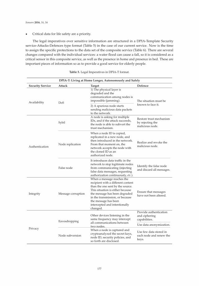
Sensors 2016, 16, 16

‚ Critical data for life safety are a priority.

The legal imperatives over sensitive information are structured in a DPIA-Template Securityservice-Attacks-Defences type format (Table 5) in the case of our current service. Now is the timeto assign the specific protections to the data set of the composite service (Table 6). There are severalchanges compared with the individual services: a water flood can cause a fall, so it is considered as acritical sensor in this composite service, as well as the presence in home and presence in bed. These areimportant pieces of information so as to provide a good service for elderly people.

Table 5. Legal Imperatives in DPIA-T format.

DPIA-T: Living at Home Longer, Autonomously and Safely

Security Service Attack Target Defence

Availability DoS

1) The physical layer isdegraded and thecommunication among nodes isimpossible (jamming). The situation must be

known to face it.2) A spurious node startssending malicious data packetsto the network.

Authentication

Sybil

A node is asking for multipleIDs, and if the attack succeeds,the node is able to subvert thetrust mechanism.

Restore trust mechanismby rejecting themalicious node.

Node replication

When a node ID is copied,replicated in a new node, andthen introduced in the network.From that moment on, thenetwork accepts the node withthe cloned ID as anauthorized node.

Realize and revoke themalicious node.

False node

It introduces data traffic in thenetwork to stop legitimate nodesfrom communicating (injectingfalse data messages, requestingauthorization continuously, etc.).

Identify the false nodeand discard all messages.

Integrity Message corruption

When a message reaches therecipient with a different contentthan the one sent by the source.This situation is either becausethe message has been degradedin the transmission, or becausethe message has beenintercepted and intentionallychanged.

Ensure that messageshave not been altered.

Privacy

Eavesdropping

Other devices listening in thesame frequency may interceptall communications betweentwo nodes.

Provide authenticationand cipheringcapabilities.

Use data anonymization.

Node subversion

When a node is captured andcryptoanalyzed the secret keys,node ID, security policies, andso forth are disclosed.

Use few data stored ineach node and renew thekeys.

177

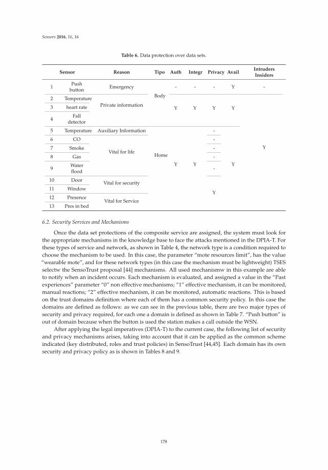
Sensors 2016, 16, 16

Table 6. Data protection over data sets.

Sensor Reason Tipo Auth Integr Privacy AvailIntrudersInsiders

1Push

buttonEmergency

Body

- - - Y -

2 TemperaturePrivate information

Y Y Y Y

Y

3 heart rate

4Fall

detector

5 Temperature Auxiliary Information

Home

Y Y

-

Y

6 CO

Vital for life

-

7 Smoke -

8 Gas -

9Waterflood

-

10 Door Vital for security

Y11 Window

12 PresenceVital for Service

13 Pres in bed

6.2. Security Services and Mechanisms

Once the data set protections of the composite service are assigned, the system must look forthe appropriate mechanisms in the knowledge base to face the attacks mentioned in the DPIA-T. Forthese types of service and network, as shown in Table 4, the network type is a condition required tochoose the mechanism to be used. In this case, the parameter “mote resources limit”, has the value“wearable mote”, and for these network types (in this case the mechanism must be lightweight) TSESselectw the SensoTrust proposal [44] mechanisms. All used mechanismw in this example are ableto notify when an incident occurs. Each mechanism is evaluated, and assigned a value in the “Pastexperiences” parameter “0” non effective mechanisms; “1” effective mechanism, it can be monitored,manual reactions; “2” effective mechanism, it can be monitored, automatic reactions. This is basedon the trust domains definition where each of them has a common security policy. In this case thedomains are defined as follows: as we can see in the previous table, there are two major types ofsecurity and privacy required, for each one a domain is defined as shown in Table 7. “Push button” isout of domain because when the button is used the station makes a call outside the WSN.

After applying the legal imperatives (DPIA-T) to the current case, the following list of securityand privacy mechanisms arises, taking into account that it can be applied as the common schemeindicated (key distributed, roles and trust policies) in SensoTrust [44,45]. Each domain has its ownsecurity and privacy policy as is shown in Tables 8 and 9.

178

Sensors 2016, 16, 16

Table 7. Trust domains defined.

Sensor Trust Domain Sensor Type

1 Push button Out of domains

Wearable2 Temperature

Domain 1 Policy3 heart rate4 Fall detector5 Temperature

Domain 2 Policy

Home

6 CO7 Smoke8 Gas9 Water flood

10 Door

Domain 1 Policy11 window12 Presence13 Presence in bed

Table 8. Trust domain 1 policies.

Domain 1 Policy

Security Service Attack Countermeasure

Availability DoSMech_DoS_1: One alarm is triggered in the Security Managerinforming about the situation

Authentication

Sybil

Mech_Sybil_1: In the security scheme, every node ID ispreconfigured for each node and only the Security Manager(out of the WSN) has the complete list of the IDs. In extremis, itis possible to perform a node revocation.

Node replication

It provides two mechanisms to avoid this attack.Mech_N_Repl_1: The Node ID is stored in an external entity(SM) that controls all the IDs working in the network.Mech_N_Repl_2: Security policy, if the SM detects that twonodes are operating with the same ID, a node revocationprotocol is issued, and the node is dropped from the network.

False node

Mech_N_False_1: Using the node ID, the schema is able toidentify the false node and, using the domain key renewalfunctionality, all the messages sent by this node will bediscarded.

Integrity Message corruptionMech_Msg_Corrupt_1: To avoid both issues, security schemaincludes the ciphering suite functionality, which allowsperforming a message hash (using MD5, SHA1, etc.).

Privacy

Eavesdropping

Mech_Eavers_1: To avoid data disclosure, it provides bothsymmetric and PKI ciphering capabilities.Mech_Eavers_2: Anonymization, unlinking the personalidentification and his/her measure data

Node subversionMech_N_Subv_1: To avoid it is to minimize thecryptographic and security information stored in each node.Nevertheless, all the keys in the network can be renewed.

Table 9. Trust domain 2 policies.

Domain 2 Policy

Availability DoS Mech_DoS_1

Authentication

Sybil Mech_Sybil_1

Node replication Mech_N_Repl_1Mech_N_Repl_2

False node Mech_N_False_1Integrity Message corruption Mech_Msg_Corrupt_1

179

Sensors 2016, 16, 16

Countermeasures against outsider attacks are based on authentication, and the countermeasuresagainst insider attacks are based on the security policies and the trust domains.

6.3. Performance Evaluation

To preserve the Quality of Service (QoS) it is necessary to know the limitations (Table 10). In thesensor nodes used for the testing purposes, the maximum power computation was limited below 20%,since it was considered that 20% of this maximum value is able to ensure proper operation. With Sybiland False node, the node load is keeping below the maximum limit defined.

Table 10. Restrictions and limitations.

SensorCritical RequirementBattery Delay

1 Push button

Y

N2 Body Temperature

Y3 Heart rate4 Fall detector5 Home Temperature

N

N6 CO

Y7 Gas8 Smoke9 Water flood

10 Outside door

N11 window12 Presence at home13 Presence in bed

The battery life is only important in case of Wearable devices, because gateway, sink and devicesin home have battery for emergency light and sensors with enough autonomy when the electric poweris fell down. The results have been obtained in laboratory for the policy more restrictive (Figures 13and 14). Finally, it is necessary that the system is designed to provide reports about both the anomaliesfound (true + and ´, false + and ´) as their reactions.

Reporting to BES and TSES:

‚ No legislation-based impact attacks.‚ Seriousness of the impacts.‚ Legislation-based impact.‚ Alarm report

Reporting to LES:

‚ Legislation-based impact.‚ Improvement plan.

180

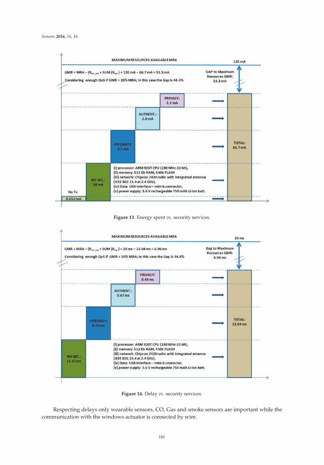
Sensors 2016, 16, 16

Figure 13. Energy spent vs. security services.

Figure 14. Delay vs. security services.

Respecting delays only wearable sensors, CO, Gas and smoke sensors are important while thecommunication with the windows actuator is connected by wire.

181

Sensors 2016, 16, 16

Some indicators can be [46]:

‚ Percentile 90: The time until to solve the faults.‚ Considering MTBF: Mean Time Between Failures (true positives + false negatives) and MTTR:

Mean Time To Repair (true positives + false negatives + false positives).‚ MTTR over false positives represents the resources spent on inefficient results.‚ The actuations on false negatives represent the impact when a problem is not detected on time.‚ Coef (no attacks) ě MTBF/(MTBF + MTTR).‚ Regarding the system behavior, it has obtained the following results (Tables 11 and 12).

Table 11. Citizen protection impact and reaction.

Impact and Reaction:Security Service Incidences Impact Resolution Time Pending

Authentication 7 1 Manually 0Integrity 7 1 Manually 0Privacy 7 2 Manually 0

Other incidences -

These used mechanisms in the application scenario only notify about the problem, and thecorrective actions are manual. Resolution time only appear for automatic actions. Respect to theoperation of the entire system, the results were as follows.

Table 12. System parts behavior.

BES: Users Perspective. Forms ValidationBES-USER interactionValidated Rejected Validation time

10 4 70 msBES: Making Utility Matrix 1st Part (Service)

Process and BES-LES interactionLES validations LES rejections Process time6 0 4.2 s

BES: Making Utility Matrix 2nd Part (Network Type for the Service)Process and BES-TSES

interactionTSES validation TSES rejections Process time

6 0 3.2 sLES: Validation Utility Matrix 1st Part

Internal Process onlyValidated Rejected Validation time6 0 120 ms

LES: Making DPIA-TProcess and LES-TSES

interactionTSES validations TSES rejections Process time

6 0 3.5 sTSES: Validation DPIA-T

Internal Process onlyValidated Rejected Validation time6 0 30 ms

TSES: Validation Utility Matrix 2nd PartInternal Process onlyValidated Rejected Validation time

6 0 50 msTSES: Making Policies

Process and TSES-BESinteraction

BES validation Rejected Process time6 0 7.8 s

TSES: Making PoliciesProcess and TSES-ACCUS

interactionACCUS validation Rejected Process time

6 0 12.1 sService Platform: Policy Validation

Accepted Rejected Validation time Internal process. is possible to doit with the information received?6 0 340 ms

Service Platform: Actions GeneratedActuations completed Time to complete Generate the actuations and configure the testing nodes.

6 18.21 min

182

Sensors 2016, 16, 16

Ten services have been perfomed for this test, four of them had bad data, and the other six werewell done. Times are measured on viable services, because rejections are much faster. Interactionsinclude processing and the information transfer between them.

6.4. Providing the Obtained Results to the ACCUS Platform

Once the mechanisms have been selected, they must be provided to ACCUS platform in order tocontinue the process and configure the service. The following lines present the process to communicatethe policy corresponding to trusted domain number 2.

The selection criteria of security mechanisms are as follow for trust domain 2. The input andoutput xml can be:

/*Input Model*/


<in:input xmlns:in="http://www.grys.org/securityServicesIN">

<in:contextOfProtection>Smart Home Trust Domain 2</in:contextOfProtection>

<in:facestToProtect>

<in:facet> Temperature </in:facet>

<in:facet> CO </in:facet>

<in:facet> Smoke </in:facet>

<in:facet> Gas </in:facet>

<in:facet> Water Flood </in:facet>

</in:facestToProtect>

</in:input>

/*Output Model*/


<out:recommendations xmlns:out="http://www.grys.org/securityServicesOUT">

<out:services>

<out:service>

<out:name id=”av”>Availabilitu</out:name>

<out:mechanism>

Mech_DoS_1

</out:mechanism>

</out:service>

<out:service>

<out:name id=”auth”>Authentication</out:name>

<out:mechanism>

Mech_Sybil_1

</out:mechanism>

<out:mechanism>

Mech_N_Repl_1

Mech_N_Repl_2

</out:mechanism>

<out:mechanism>

Mech_N_False_1

</out:mechanism>

</out:service>

<out:service>

<out:name id=”int”>Integrity</out:name>

<out:mechanism>

Mech_Msg_Corrupt_1

183

Sensors 2016, 16, 16

</out:mechanism>

</out:service>

</out:services>

<out:attacks>

<out:context> Smart Home</out:context>

<out:attack refTo=”av”>

<out:description> DoS </out:description>

</out:attack>

<out:attack refTo=”auth”>

<out:description> Sybil </out:description>

<out:description> Node replication </out:description>

<out:description> False Node </out:description>

</out:attack>

<out:attack refTo=”int”>

<out:description> Message corruption </out:description>

</out:attack>

<out:secSerToImplement>

Availability Authentication Integrity

</out:secSerToImplement>

</out:attacks>

</out:recommendations>

All of this effort has secured only one smart service in the city. However, this process should beiterated for all possible service combinations.


Collaboration between multiple areas (business, legal and technological) is critical in order toprovide users with the necessary trust in the security of the service and protection of their personaldata. The limitation of resources of wireless sensor networks for products and services makes itnecessary to implement a tailored security schema to avoid the risk of poor quality of service whenresources are exhausted. In this way, the intelligent combination of security mechanisms availablecould increase the service’s efficiency.

In an environment where several services and technologies coexist, the intelligence of thedecision-making on security policies could be integrated into the officially recognized and certifiednetwork operations centre which would provide a large capacity of management, updating thedeployed security measures. Since there is no legislative uniformity, it is necessary to develop toolsand methods that permit a transition period with minimal risk to people and their rights.

When citizens’ quality of life greatly depends on the correct performance of smart cities, which,in turn, depend on the correct performance of systems and services (and the networks in which theyare set up), it might be required to configure and reconfigure privacy and security policies. It maybe due to changes in states of emergency, alarm, etc. Or, they may be necessary because of dynamicchanges within the city. Therefore, it is important to know timely and in due form the security policiesthat must be implemented in each case, in a reliable way, by the expert system described. It wouldalso be convenient to deploy and perform the actions needed on the elements of the city, fast andefficiently (decreasing human intervention to a minimum), using the mediation chain described. Thekey lies in the cooperative environment between the three main knowledge areas described, and in

184

Sensors 2016, 16, 16

a common management, even if the systems are technically duplicated or diversified to augmentsecurity and availability.

It must be considered that, in an uncertain future, a failure in the performance of a smart city maybe disastrous and could have serious consequences; far from just a mild annoyance, it could resultin the endangerment of people and infrastructure. A service under attack or functioning incorrectlymay activate an alarm, with no emergency triggering it. Therefore, investing in security, privacy andreliability in the performance of systems in a smart city may be worthwhile.

In the future, we will point in different directions according to the road map. On the expert systemside knowledge bases should be enhanced to make possible interactions between IoT platforms andseveral technologies. Also is will be necessary to make life easier for the human experts providingthem nice tools to manage the information. ACCUS must go on with its road map, to improve thefunctionalities to create new services in the smart city environment. Those new services representgood opportunities for both systems to work together to face new issues.

Acknowledgments: ACCUS (Adaptive Cooperative Control in Urban Systems) project has been partially fundedby the Spanish Ministry of Industry, Energy and Tourism (Ref. ART-010000-2013-2) and by the Artemis JU (GAnumber 333020-1). LifeWear (Mobilized Lifestyle with Wearables) project has been funded by the Spanish Ministryof Industry, Energy and Tourism (Ref. TSI-010400-2010-100) by the Avanza Competitividad I+D+I program. Theauthors would like to thank CITSEM (Research Center on Software Technologies and Multimedia Systems forSustainability, Centro de Investigación en Tecnologías Software y Sistemas Multimedia para la Sostenibilidad)from the UPM.

Author Contributions: The work presented in this paper is a collaborative effort participated by all of the authors.Jose Antonio Sánchez and Jose-Fernán Martínez have studied, defined and developed the collaborative modelto solve the problem dealing with collaboration on the business, legal and technological areas. Lourdes Lópezhas defined the research theme with the purpose of solving the challenges associated to the trust and privacyproblem. Gregorio Rubio Cifuentes has defined the communication between expert system the urban systems. Allthe authors have made written contributions to the paper, and Lourdes Lopez has reviewed the whole manuscript.All of the authors have read and approved the manuscript. The research group named Next-Generation Networksand Services (GRyS), which the authors belong to, is developing the prototypes. GRyS research group is integratedwithin the Technical University of Madrid (UPM) and as part of CITSEM.


References

1. Kanter, R.M.; Litow, S.S. Informed and Interconnected: A Manifesto for Smarter Cities; Working Paper 09-141;Harvard Business School: Boston, MA, USA, 2009.

2. Caragliu, A.; del Bo, C.; Nijkamp, P. Smart Cities in Europe. J. Urban Technol. 2011, 18, 65–82. [CrossRef]3. Cavoukian, Ann (2011) Privacy by Design—The 7 Foundational Principles. Available online:

http://www.ipc.on.ca/english/privacy/introduction-to-pbd (accessed on 24 March 2015).4. The ACCUS (Adaptive Cooperative Control in Urban (sub)Sytems). Available online: http://projectaccus.eu/

(accessed on 24 March 2015).5. Sánchez-Alcón, J.-A.; López, L.; Martínez-Ortega, J.-F.; Castillejo, P. Automated determination of security

services to ensure personal data protection in the internet of things applications. In Proceedings of the 3rdInternational Conference on Innovative Computing Technology (Intech), London, UK, 29–31 August 2013;pp. 71–76. [CrossRef]

6. Sánchez-Alcón, J.-A.; López-Santidrián, L.; Martínez, J.-F. Solución para garantizar la privacidad en internetde las cosas. Prof. Inf. 2014, 24, 62–70. [CrossRef]

7. Cuadrado, N. Aplicación de los Sistemas Expertos al Campo del Derecho; Servicio de Publicaciones de laUniversidad Complutense de Madrid: Madrid, Spain, 2004. (In Spanish)

8. Stevens, C.; Barot, V.; Carter, J. The Next Generation of Legal Expert Systems—New Dawn or False Dawn? InResearch and Development in Intelligent Systems XXVII; Springer: London, UK, 2011; pp. 439–452. [CrossRef]

9. Venkateswarlu, N.M.; Sushant, L. Building a Legal Expert System for Legal Reasoning in Specific Domain-ASurvey. Int. J. Comput. Sci. Inf. Technol. 2012, 4, 175–184. [CrossRef]

185

Sensors 2016, 16, 16

10. Giffinger, R.; Fertner, C.; Kramar, H.; Kalasek, R.; Pichler-Milanovic, N.; Meijers, E. Smart Cities—Ranking

of European Medium-Sized Cities; Research Report; Vienna University of Technology: Vienna, Austria,2007; Available online: http://www.smart-cities.eu/download/smart_cities_final_report.pdf (accessedon 24 March 2015).

11. JBossDeveloper 2012. Available online: http://www.jboss.org/products/fuse/overview/ (accessed on3 December 2014).

12. Open Platform for Your Connected Business 2011. Available online: http://wso2.com/ (accessed on3 December 2014).

13. Stoimenov, L.; Stanimirovic, A.; Djordjevic-Kajan, S. Semantic Interoperability using multiple ontologies.In Proceedings of the 8th AGILE Conference on GIScience, Estoril, Portugal, 26–28 May 2005; pp. 261–270.Available online: http://plone.itc.nl/agile_old/Conference/estoril/papers/88_Leonid%20Stoimenov.pdf(accessed on 12 January 2014).

14. Zang, M.A.; Pohl, J.G. Ontological Approaches for Semantic Interoperability. In Proceedings ofthe 5th Annual ONR Workshop on Collaborative Decision-Support Systems, San Luis Obispo, CA,USA, 10–11 September 2003; pp. 1–10. Available online: http://digitalcommons.calpoly.edu/cgi/viewcontent.cgi?article=1078 (accessed on 12 January 2014).

15. Sustainable Smart Grid Open System for the Aggregated Control, Monitoring and Management of Energy(e-Gotham) Project. Available online: http://www.e-gotham.eu/ (accessed on 22 May 2015).

16. De Diego, R.; Martínez, J.-F.; Rodríguez-Molina, J.; Cuerva, A. A Semantic Middleware Architecture Focusedon Data and Heterogeneity Management within the Smart Grid. Energies 2014, 7, 5953–5994. [CrossRef]

17. W3C Semantic Sensor Network Incubator Group. Semantic Sensor Network Ontology. 2011. Availableonline: http://www.w3.org/2005/Incubator/ssn/ssnx/ssn (accessed on 21 May 2015).

18. Brickley, D.; Miller, L. FOAF Vocabulary Specification 0.99. Namespace Document 14 January 2014-Paddington Edition. Available online: http://xmlns.com/foaf/spec (accessed on 20 May 2015).

19. CityGML. Available online: http://www.opengeospatial.org/standards/citygml (acceessed on 22 May 2015).20. Prud’hommeaux, E.; Seaborne, A. SPARQL Query Lenguaje for RDF, W3C Recommendation 15 January

2008. Available online: http://www.w3.org/TR/rdf-sparql-query (acceessed on 3 April 2015).21. Gandon, F.; Schreiber, G. RDF 1.1 XML Syntax. W3C recommendation. 25 February 2014. Available online:

http://www.w3.org/TR/rdf-syntax-grammar/ (acceessed on 23 May 2015).22. Codagnone, C.; Wimmer, M.A. Roadmapping eGovernment Research—Visions and Measures towards

Innovative Governments in 2020; European Commission FP6 Project eGovRTD2020, Final Report;Guerinoni Marco: Clusone, Italy, 2007; Available online: https://air.unimi.it/retrieve/handle/2434/171379/176506/FinalBook.pdf (accessed on 12 January 2015).

23. Sicari, S.; Rizzardi, A.; Grieco, L.A.; Coen-Porisini, A. Security, privacy and trust in Internet of Things:The road ahead. Comput. Netw. 2015, 76, 146–164. [CrossRef]

24. Weber, R.H. Internet of things: Privacy issues revisited. Comput. Law Secur. Rev. 2015, 31, 618–627. [CrossRef]25. Ten, C.-W.; Manimaran, G.; Liu, C.-C. Cybersecurity for Critical Infrastructures: Attack and Defense

Modeling. In Systems, Man and Cybernetics, Part A: Systems and Humans; IEEE: Piscataway, NJ, USA, 2010;Volume 40, pp. 853–865. [CrossRef]

26. Daryabar, F.; Dehghantanha, A.; Udzir, N.I.; Sani, N.F.B.M.; Bin-Shamsuddin, S. Towards secure model forscada systems. In Proceedings of the 2012 International Conference on Cyber Security, Cyber Warfare andDigital Forensic, CyberSec 2012, Kuala Lumpur, Malaysia, 26–28 June 2012; pp. 60–64. [CrossRef]

27. Martinez-Balleste, A.; Perez-Martínez, P.A.; Solanas, A. The pursuit of citizens’ privacy: A privacy-awaresmart city is possible. IEEE Commu. Mag. 2013, 51, 136–141. Available online: http://ieeexplore.ieee.org/stamp/stamp.jsp?tp=&arnumber=6525606&isnumber=6525582 (accessed on 7 January 2015). [CrossRef]

28. Bartoli, A.; Hernández-Serrano, J.; Soriano, M.; Dohler, M.; Kountouris, A.; Barthel, D. Securityand privacy in your smart city. In Proceedings of the Barcelona Smart Cities Congress, Barcelona,Spain, 29 November–2 December 2011; pp. 1–6. Available online: http://smartcitiescouncil.com/sites/default/files/public_resources/Smart%20city%20security.pdf (accessed on 8 February 2015).

29. Rinaldi, S.M. Modeling and simulating critical infrastructures and their interdependencies. In SystemSciences, Proceedings of the 37th Annual Hawaii International Conference, Big Island, HI, USA,5–8 January 2004; IEEE: Big Island, HI, USA, 2004; p. 8. Available online: http://ieeexplore.ieee.org/stamp/stamp.jsp?tp=&arnumber=1265180&isnumber=28293 (accessed on 12 January 2015). [CrossRef]

186

Sensors 2016, 16, 16

30. Cazorla, L.; Alcaraz, C.; Lopez, J. Towards automatic critical infrastructure protection through machinelearning. In Proceedings of 8th International Conference on Critical Information InfrastructuresSecurity, Amsterdam, The Netherlands, 16–18 September 2013; pp. 197–203. Available online:http://link.springer.com/chapter/10.1007%2F978-3-319-03964-0_18#page-1 (accessed on 12 January 2015).[CrossRef]

31. Islam, M.M.; Hassan, M.M.; Lee, G.; Huh, E. A Survey on Virtualization of Wireless Sensor Networks. Sensors

2012, 12, 2175–2207. [CrossRef] [PubMed]32. Islam, M.M.; Huh, E. Virtualization in Wireless Sensor Network: Challenges and Opportunities. J. Netw.

2012, 7, 412–418. [CrossRef]33. Lucas Martínez, N.; Martínez, J.F.; Hernández, V. Virtualization of Event Sources in Wireless Sensor Networks

for the Internet of Things. Sensors 2014, 14, 22737–22753. [CrossRef] [PubMed]34. Data Protection Impact Assessment Template for Smart Grid and Smart Metering systems, Smart Grid

Task Force 2012-14, Expert Group 2: Regulatory Recommendations for Privacy, Data Protection andCyber-Security in the Smart Grid Environment, 18.03.2014. Available online: https://ec.europa.eu/energy/sites/ener/files/documents/2014_dpia_smart_grids_forces.pdf (accessed on 24 March 2015).

35. Lopez, J.; Roman, R.; Alcaraz, C. Analysis of Security Threats, Requirements, Technologies and Standardsin Wireless Sensor Networks. In Foundations of Security Analysis and Design; Springer: Berlin/Heidelberg,Germany, 2009; Volume 5705, pp. 289–338.

36. Nasr, P.M.; Varjani, A.Y. Alarm based anomaly detection of insider attacks in SCADA system. In Proceedingsof the Smart Grid Conference (SGC), Tehran, Iran, 9–10 December 2014; pp. 1–6. [CrossRef]

37. Zhu, B.; Sastry, S. SCADA-Specific Intrusion Detection/Prevention Systems: A Survey and Taxonomy.In Proceedings of the 1st Workshop on Secure Control Systems (SCS’10), Stockholm, Sweden, 12 April 2010.

38. Vieira, K.; Schulter, A.; Westphall, C.B.; Westphall, C.M. Intrusion Detection for Grid and CloudComputing. IT Prof. 2010, 12, 38–43. Available online: http://ieeexplore.ieee.org/stamp/stamp.jsp?tp=&arnumber=5232794&isnumber=5512497 (accessed on 2 September 2015). [CrossRef]

39. De Chaves, S.A.; Uriarte, R.B.; Westphall, C.B. Toward an architecture for monitoring private clouds. IEEE

Commun. Mag. 2011, 49, 130–137. Available online: http://ieeexplore.ieee.org/stamp/stamp.jsp?tp=&arnumber=6094017&isnumber=6093994 (accessed on 5 September 2015). [CrossRef]

40. De Chaves, S.A.; Westphall, C.B.; Lamin, F.R. SLA Perspective in Security Management for CloudComputing. In Proceedings of the Sixth International Conference of Networking and Services (ICNS),Cancun, Mexico, 7–13 March 2010; pp. 212–217. Available online: http://ieeexplore.ieee.org/stamp/stamp.jsp?tp=&arnumber=5460645&isnumber=5460618 (accessed on 5 September 2015). [CrossRef]

41. Farooq, A.; Petros, M. Security for Wireless Ad Hoc Networks; Wiley-Interscience, Cop.: Hoboken, NJ, USA,2007; p. 247.

42. Nasr, P.M.; Varjani, A.Y. Petri net model of insider attacks in SCADA system. In Proceedings of the Conferenceon Information Security and Cryptology (ISCISC) (11th International ISC), Tehran, Iran, 3–4 September 2014;pp. 55–60. [CrossRef]

43. International Telecommunications Union. Recommendation X.800: Security Architecture for OpenSystems Interconnection for CCITT Applications. Available online: http://www.itu.int/rec/T-REC-X.800-199103-I/en (accessed on 12 January 2015).

44. Pedro Castillejo, P.; Martínez-Ortega, J.F.; López, L.; Sánchez Alcón, J.A. SensoTrust: Trustworthy Domainsin Wireless Sensor Networks. IJDSN 2015. [CrossRef]

45. Rolim, C.O.; Koch, F.L.; Westphall, C.B.; Werner, J.; Fracalossi, A.; Salvador, G.S. A Cloud ComputingSolution for Patient’s Data Collection in Health Care Institutions. In eHealth, Telemedicine, and SocialMedicine 2010, Proceedings of the Second International Conference ETELEMED ‘10, St. Maarten,The Netherlands, 10–16 February 2010; pp. 95–99. Available online: http://ieeexplore.ieee.org/stamp/stamp.jsp?tp=&arnumber=5432853&isnumber=5432832 (accessed on 5 September 2015). [CrossRef]

46. Herrmann, D.S. Complete Guide to Security and Privacy Metrics: Measuring Regulatory Compliance, Operational

Resilience, and ROI; Auerbach Publications: Boca Raton, FL, USA, 2007; p. 824.


187

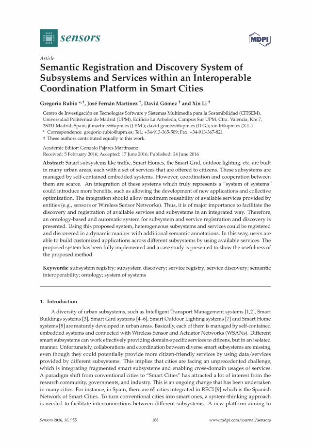
sensors

Article

Semantic Registration and Discovery System ofSubsystems and Services within an InteroperableCoordination Platform in Smart CitiesGregorio Rubio *,†, José Fernán Martínez †, David Gómez † and Xin Li †

Centro de Investigación en Tecnologías Software y Sistemas Multimedia para la Sostenibilidad (CITSEM),Universidad Politécnica de Madrid (UPM), Edificio La Arboleda, Campus Sur UPM. Ctra. Valencia, Km 7,28031 Madrid, Spain; [email protected] (J.F.M.); [email protected] (D.G.); [email protected] (X.L.)* Correspondence: [email protected]; Tel.: +34-913-365-509; Fax: +34-913-367-821† These authors contributed equally to this work.

Academic Editor: Gonzalo Pajares MartinsanzReceived: 5 February 2016; Accepted: 17 June 2016; Published: 24 June 2016

Abstract: Smart subsystems like traffic, Smart Homes, the Smart Grid, outdoor lighting, etc. are builtin many urban areas, each with a set of services that are offered to citizens. These subsystems aremanaged by self-contained embedded systems. However, coordination and cooperation betweenthem are scarce. An integration of these systems which truly represents a “system of systems”could introduce more benefits, such as allowing the development of new applications and collectiveoptimization. The integration should allow maximum reusability of available services provided byentities (e.g., sensors or Wireless Sensor Networks). Thus, it is of major importance to facilitate thediscovery and registration of available services and subsystems in an integrated way. Therefore,an ontology-based and automatic system for subsystem and service registration and discovery ispresented. Using this proposed system, heterogeneous subsystems and services could be registeredand discovered in a dynamic manner with additional semantic annotations. In this way, users areable to build customized applications across different subsystems by using available services. Theproposed system has been fully implemented and a case study is presented to show the usefulness ofthe proposed method.

Keywords: subsystem registry; subsystem discovery; service registry; service discovery; semanticinteroperability; ontology; system of systems

1. Introduction

A diversity of urban subsystems, such as Intelligent Transport Management systems [1,2], SmartBuildings systems [3], Smart Gird systems [4–6], Smart Outdoor Lighting systems [7] and Smart Homesystems [8] are maturely developed in urban areas. Basically, each of them is managed by self-containedembedded systems and connected with Wireless Sensor and Actuator Networks (WSANs). Differentsmart subsystems can work effectively providing domain-specific services to citizens, but in an isolatedmanner. Unfortunately, collaborations and coordination between diverse smart subsystems are missing,even though they could potentially provide more citizen-friendly services by using data/servicesprovided by different subsystems. This implies that cities are facing an unprecedented challenge,which is integrating fragmented smart subsystems and enabling cross-domain usages of services.A paradigm shift from conventional cities to “Smart Cities” has attracted a lot of interest from theresearch community, governments, and industry. This is an ongoing change that has been undertakenin many cities. For instance, in Spain, there are 65 cities integrated in RECI [9] which is the SpanishNetwork of Smart Cities. To turn conventional cities into smart ones, a system-thinking approachis needed to facilitate interconnections between different subsystems. A new platform aiming to


Sensors 2016, 16, 955

connect different subsystems and represent a true “system of systems” integration has been developedin the Adaptive Cooperative Control in Urban (sub)Systems (ACCUS) project [10]. This platform,called Integration and Coordination Platform (ICP), emphasizes how to integrate different subsystemsand enables the development of new applications across subsystems without interfering individualupdates and internal policies.

The ICP is capable of providing a variety of functionalities in order to optimize combinedperformance of different subsystems, thus achieving more flexible, more efficient and more robustintegrated urban systems and managing different emergent behaviors. The platform is conceived as adistributed and layered architecture which offers three main groups of functions:

‚ Core functions: they are referred to generic platform functionalities which are offered bythe Runtime Environment of the ICP. Core functions are provided by the following softwarecomponents: applications servers, service broker, service repository, service bus, data broker andmanagement, policy management, security management, workflow engine, security managementand message broker and database.

‚ Extension functions: they are referred to ICP specific functionalities that can be used by otherservices and applications. Extension functions are offered by info broker, control broker, subsystemmonitoring, subsystems adaptors, ontology connector, programming API and ICP ontology.

‚ City configurations functions: these are city specific generic functionalities available for other ICPservices and applications. They are provided by event detection, location detection, data analytics,situation awareness, and reasoning.

To ensure that the ICP could fulfill the aforementioned capabilities, a key premise is to addressthe heterogeneity (e.g., data formats and protocols) inherent to subsystems and services provided bydifferent subsystems and provide a unified interface of reference for available subsystems and serviceswithin the ICP. With this reference, maximum reusability of available services provided by entities (e.g.,sensors, or Wireless Sensor Networks) could be enabled so as to develop new cross-domain applications.Thus, an ontology-based and automatic system for registering and discovering subsystems and servicesis presented in this paper. This proposed system can be embedded into the ICP in order to discover andregister available heterogeneous services and subsystems in a dynamic manner. The proposed systemfor subsystems and services registration and discovery is able to adapt to any change that occursin subsystems and services. Additionally, in order to abstract the heterogeneity of subsystems andservices and provide a common understanding to the ICP, this proposed system employs an ontologicalapproach to provide a formalized model, named new Subsystem and Service Oriented Ontology (nSSOO),for the registry and discovery process. Thus, different subsystems and services could be semanticallyannotated and understood by the ICP and users as well. The proposed system for subsystem andservice registration and discovery is playing an important role in ICP to enable the creation of real-timecollaborative applications across subsystems by employing services available in the city. The proposedsystem is completely implemented and validated by using a traffic light control application use case.

This paper is organized as follows: Section 2 presents related work on existing platforms forSmart Cities and their solutions to register and discover subsystems and services within them. Theproposed system for registry and discovery of subsystems and services within the ICP is shown inSection 3. Specifically, Section 3.1 highlights the main contributions that are provided by this paper.Section 3.2 shows system integration regarding Semantic Interoperability right afterwards. The newlyproposed nSSOO ontology used to model the registry and discovery information base is introducedin Section 3.3. Section 3.4 provides a holistic view of the system and elaborates the specific softwarecomponents that are involved. Workflow for the subsystem and service discovery and registrationprocedures is detailed in Section 3.5. Section 4 presents a use case about the traffic light control tovalidate the proposed system. Finally, in Section 5, conclusions are given and future work is pointedout as well.

189

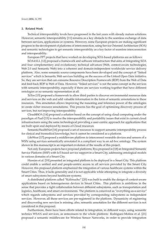
Sensors 2016, 16, 955

2. Related Work

Technical interoperability levels have progressed in the last years with already mature solutions.However, semantic interoperability [11] remains as a key obstacle to the seamless exchange of databetween services, applications or systems. However, some European projects are making significantprogress in the development of platforms of interconnection, using Service Oriented Architecture (SOA)and semantic technologies to get semantic interoperability as a key factor of seamless interconnectionand interoperability.

European FP7 projects that have worked on developing SOA-based platforms are as follows:SOA4ALL [12] proposed a framework and software infrastructure that aims at integrating SOA

and four complementary and evolutionary technical advances (Web, context-aware technologies,Web 2.0 and Semantic Web) into a coherent and domain-independent worldwide service deliveryplatform. Also, some semantic source components have been developed and the concept of “linkedservices” which is Semantic Web services building on the success of the Linked Open Data initiative.So, they are services that can consume Resource Description Framework (RDF) from the Web of Dataand feed-back RDF to Web of Data. However, “linked services” is not the same concept as the serviceswith semantic interoperability, especially if there are services working together that have differentontologies or no semantic representation at all.

TaToo [13] proposed a framework to allow third parties to discover environmental resources dataand services on the web and add valuable information in the form of semantic annotations to theseresources. This annotation allows improving the reasoning and inference power of the ontologiesto create richer resource annotations. This process has the goal of optimizing discovery process ofservices, but not improving interoperability.

Cloud4SOA [14] proposed a solution based on the concept of using cloud computing under theparadigm of PaaS [15] to resolve the interoperability and portability issues that exist in current cloudinfrastructures using the same technological providing a user-centric approach for applications thatare built upon and deployed by means of Cloud resources.

SemanticHealthNet [16] proposed a set of resources to support semantic interoperability processfor clinical and biomedical knowledge, but it cannot be considered as a platform.

LifeWear [17] proposed a middleware platform to interconnect wearable devices and sensors of aWSN using services semantically annotated in a compliant way to an ad-hoc ontology. The systemshown in this manuscript is an important evolution of the results of this project.

Not only European projects have proposed platforms; Ryu proposed in [18] an Integrated SemanticService Platform (ISSP) with IoT-based service support in a Smart City, addressing ontological modelsin various domains of a Smart City.

Hussian et al. [19] presented an integrated platform to be deployed in a Smart City. This platformcould enable a unified and and people-centric access to all services provided by the Smart City.However, this proposed platform emphasized the integration of various healthcare systems within theSmart Cities. Thus, it lacks generality and it is not applicable while attempting to integrate a diversityof smart subsystems beyond healthcare systems.

A distributed platform called “Kalimucho” [20] was built to enable the design of context-awareapplications based on heterogeneous devices in Smart Cities. This platform is ambitious in thesense that provides a tight collaboration between different subsystems, such as transportation andlogistics, healthcare, and smart environments. The platform is conceived as “everything-as-a-service”which regards subsystems and services provided by corresponding subsystems as independentservices. However, all those services are pre-registered in the platform. Dynamicity of registeringand discovering new services is missing; also, semantic annotation for the different services is notconsidered in this proposal.

Furthermore, there have been efforts related to integration, in different ways, using semantictechnics WSAN and services, as antecessors to the whole platform: Rodriguez-Molina et al. [21]proposed a semantic middleware for Wireless Sensor Networks, in order to provide integration

190

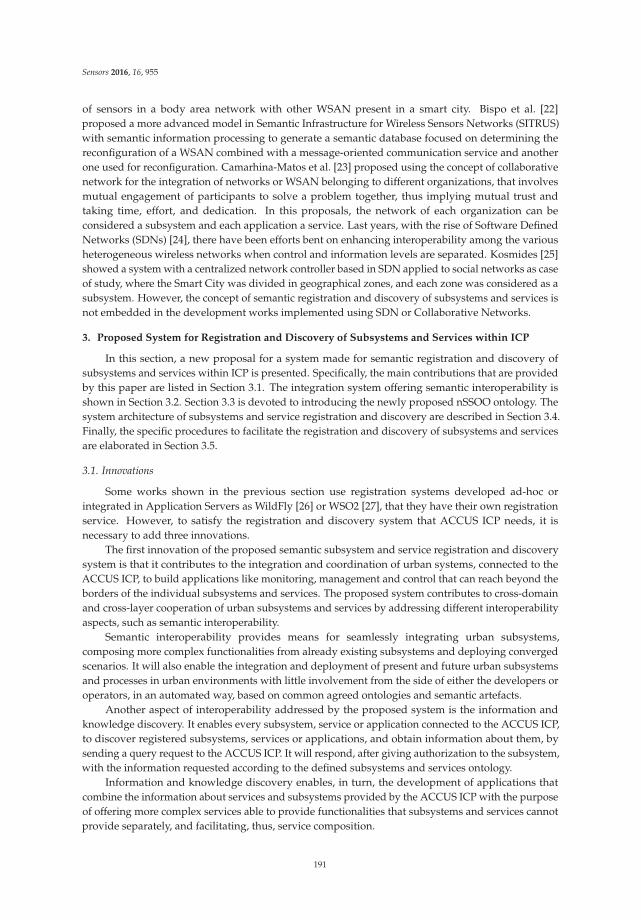
Sensors 2016, 16, 955

of sensors in a body area network with other WSAN present in a smart city. Bispo et al. [22]proposed a more advanced model in Semantic Infrastructure for Wireless Sensors Networks (SITRUS)with semantic information processing to generate a semantic database focused on determining thereconfiguration of a WSAN combined with a message-oriented communication service and anotherone used for reconfiguration. Camarhina-Matos et al. [23] proposed using the concept of collaborativenetwork for the integration of networks or WSAN belonging to different organizations, that involvesmutual engagement of participants to solve a problem together, thus implying mutual trust andtaking time, effort, and dedication. In this proposals, the network of each organization can beconsidered a subsystem and each application a service. Last years, with the rise of Software DefinedNetworks (SDNs) [24], there have been efforts bent on enhancing interoperability among the variousheterogeneous wireless networks when control and information levels are separated. Kosmides [25]showed a system with a centralized network controller based in SDN applied to social networks as caseof study, where the Smart City was divided in geographical zones, and each zone was considered as asubsystem. However, the concept of semantic registration and discovery of subsystems and services isnot embedded in the development works implemented using SDN or Collaborative Networks.

3. Proposed System for Registration and Discovery of Subsystems and Services within ICP

In this section, a new proposal for a system made for semantic registration and discovery ofsubsystems and services within ICP is presented. Specifically, the main contributions that are providedby this paper are listed in Section 3.1. The integration system offering semantic interoperability isshown in Section 3.2. Section 3.3 is devoted to introducing the newly proposed nSSOO ontology. Thesystem architecture of subsystems and service registration and discovery are described in Section 3.4.Finally, the specific procedures to facilitate the registration and discovery of subsystems and servicesare elaborated in Section 3.5.

3.1. Innovations

Some works shown in the previous section use registration systems developed ad-hoc orintegrated in Application Servers as WildFly [26] or WSO2 [27], that they have their own registrationservice. However, to satisfy the registration and discovery system that ACCUS ICP needs, it isnecessary to add three innovations.

The first innovation of the proposed semantic subsystem and service registration and discoverysystem is that it contributes to the integration and coordination of urban systems, connected to theACCUS ICP, to build applications like monitoring, management and control that can reach beyond theborders of the individual subsystems and services. The proposed system contributes to cross-domainand cross-layer cooperation of urban subsystems and services by addressing different interoperabilityaspects, such as semantic interoperability.

Semantic interoperability provides means for seamlessly integrating urban subsystems,composing more complex functionalities from already existing subsystems and deploying convergedscenarios. It will also enable the integration and deployment of present and future urban subsystemsand processes in urban environments with little involvement from the side of either the developers oroperators, in an automated way, based on common agreed ontologies and semantic artefacts.

Another aspect of interoperability addressed by the proposed system is the information andknowledge discovery. It enables every subsystem, service or application connected to the ACCUS ICP,to discover registered subsystems, services or applications, and obtain information about them, bysending a query request to the ACCUS ICP. It will respond, after giving authorization to the subsystem,with the information requested according to the defined subsystems and services ontology.

Information and knowledge discovery enables, in turn, the development of applications thatcombine the information about services and subsystems provided by the ACCUS ICP with the purposeof offering more complex services able to provide functionalities that subsystems and services cannotprovide separately, and facilitating, thus, service composition.

191

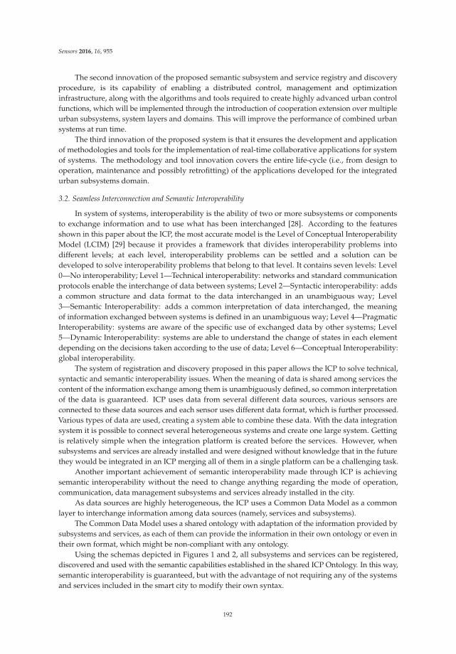
Sensors 2016, 16, 955

The second innovation of the proposed semantic subsystem and service registry and discoveryprocedure, is its capability of enabling a distributed control, management and optimizationinfrastructure, along with the algorithms and tools required to create highly advanced urban controlfunctions, which will be implemented through the introduction of cooperation extension over multipleurban subsystems, system layers and domains. This will improve the performance of combined urbansystems at run time.

The third innovation of the proposed system is that it ensures the development and applicationof methodologies and tools for the implementation of real-time collaborative applications for systemof systems. The methodology and tool innovation covers the entire life-cycle (i.e., from design tooperation, maintenance and possibly retrofitting) of the applications developed for the integratedurban subsystems domain.

3.2. Seamless Interconnection and Semantic Interoperability

In system of systems, interoperability is the ability of two or more subsystems or componentsto exchange information and to use what has been interchanged [28]. According to the featuresshown in this paper about the ICP, the most accurate model is the Level of Conceptual InteroperabilityModel (LCIM) [29] because it provides a framework that divides interoperability problems intodifferent levels; at each level, interoperability problems can be settled and a solution can bedeveloped to solve interoperability problems that belong to that level. It contains seven levels: Level0—No interoperability; Level 1—Technical interoperability: networks and standard communicationprotocols enable the interchange of data between systems; Level 2—Syntactic interoperability: addsa common structure and data format to the data interchanged in an unambiguous way; Level3—Semantic Interoperability: adds a common interpretation of data interchanged, the meaningof information exchanged between systems is defined in an unambiguous way; Level 4—PragmaticInteroperability: systems are aware of the specific use of exchanged data by other systems; Level5—Dynamic Interoperability: systems are able to understand the change of states in each elementdepending on the decisions taken according to the use of data; Level 6—Conceptual Interoperability:global interoperability.

The system of registration and discovery proposed in this paper allows the ICP to solve technical,syntactic and semantic interoperability issues. When the meaning of data is shared among services thecontent of the information exchange among them is unambiguously defined, so common interpretationof the data is guaranteed. ICP uses data from several different data sources, various sensors areconnected to these data sources and each sensor uses different data format, which is further processed.Various types of data are used, creating a system able to combine these data. With the data integrationsystem it is possible to connect several heterogeneous systems and create one large system. Gettingis relatively simple when the integration platform is created before the services. However, whensubsystems and services are already installed and were designed without knowledge that in the futurethey would be integrated in an ICP merging all of them in a single platform can be a challenging task.

Another important achievement of semantic interoperability made through ICP is achievingsemantic interoperability without the need to change anything regarding the mode of operation,communication, data management subsystems and services already installed in the city.

As data sources are highly heterogeneous, the ICP uses a Common Data Model as a commonlayer to interchange information among data sources (namely, services and subsystems).

The Common Data Model uses a shared ontology with adaptation of the information provided bysubsystems and services, as each of them can provide the information in their own ontology or even intheir own format, which might be non-compliant with any ontology.

Using the schemas depicted in Figures 1 and 2, all subsystems and services can be registered,discovered and used with the semantic capabilities established in the shared ICP Ontology. In this way,semantic interoperability is guaranteed, but with the advantage of not requiring any of the systemsand services included in the smart city to modify their own syntax.

192

Sensors 2016, 16, 955

This shared ICP Ontology has a part specifically developed to register and discover subsystemsand services in the ICP. It is specified in the next section.

Figure 1. Common data model.

Figure 2. Integration system regarding Semantic Interoperability.

3.3. Ontology Specifications

When attempting to provide an interoperable and formalized knowledge model for subsystem,service registration and discovery processes, the new Subsystem and Service Oriented Ontology(nSSOO) is proposed. The nSSOO is conceived to comprehensively and semantically describe a varietyof features about subsystems and services owned by the complex urban system. This proposedontology makes possible the integration and registration of information provided by sensors orsubsystems. Originally thought for services offered by low capability devices (sensors, PDAs, RFIDtags, etc.), this ontology can also be applied to services based on normal devices or subsystems (SmartHome subsystem, Smart Traffic subsystem, etc.), as in the ACCUS project.

Figure 3. Proposal of nSSOO.

193

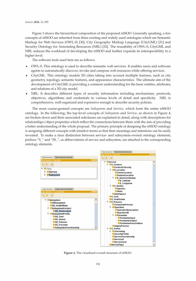
Sensors 2016, 16, 955

Figure 3 shows the hierarchical composition of the proposed nSSOO. Generally speaking, a fewconcepts of nSSOO are inherited from three existing and widely used ontologies which are SemanticMarkup for Web Services (OWL-S) [30], City Geography Markup Language (CityGML) [31] andSecurity Ontology for Annotating Resources (NRL) [32]. The reusability of OWL-S, CityGML andNRL reduces the workload of developing the nSSOO and further expands its interoperability to ahigher level.

The software tools used here are as follows:

‚ OWL-S. This ontology is used to describe semantic web services. It enables users and softwareagents to automatically discover, invoke and compose web resources while offering services.

‚ CityGML. This ontology models 3D cities taking into account multiple features, such as citygeometry, topology, semantic features, and appearance characteristics. The ultimate aim of thedevelopment of CityGML is providing a common understanding for the basic entities, attributes,and relations of a 3D city model.

‚ NRL. It describes different types of security information including mechanisms, protocols,objectives, algorithms and credentials in various levels of detail and specificity. NRL iscomprehensive, well-organized and expressive enough to describe security policies.

The most coarse-grained concepts are Subsystem and Service, which form the entire nSSOOontology. In the following, the top-level concepts of Subsystem and Service, as shown in Figure 4,are broken down and their associated subclasses are explained in detail, along with descriptions forrelationships/object properties which reflect the connections between them with the aim of providinga better understanding of the whole proposal. The primary principle of designing the nSSOO ontologyis assigning different concepts with intuitive terms so that their meanings and intentions can be easilyrevealed. To make a clear distinction between service- and subsystem-owned ontology elements,prefixes “S_” and “SS_”, as abbreviations of service and subsystem, are attached to the correspondingontology elements.

Figure 4. The visualized overall structure of nSSOO.

194

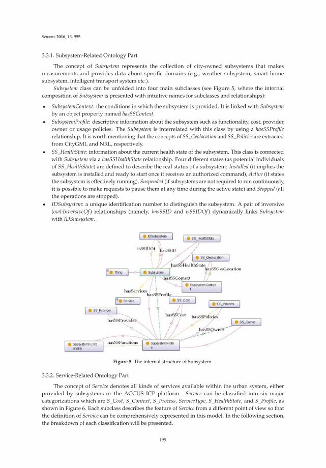
Sensors 2016, 16, 955

3.3.1. Subsystem-Related Ontology Part

The concept of Subsystem represents the collection of city-owned subsystems that makesmeasurements and provides data about specific domains (e.g., weather subsystem, smart homesubsystem, intelligent transport system etc.).

Subsystem class can be unfolded into four main subclasses (see Figure 5, where the internalcomposition of Subsystem is presented with intuitive names for subclasses and relationships):

‚ SubsystemContext: the conditions in which the subsystem is provided. It is linked with Subsystem

by an object property named hasSSContext.‚ SubsystemProfile: descriptive information about the subsystem such as functionality, cost, provider,

owner or usage policies. The Subsystem is interrelated with this class by using a hasSSProfile

relationship. It is worth mentioning that the concepts of SS_Geolocation and SS_Policies are extractedfrom CityGML and NRL, respectively.

‚ SS_HealthState: information about the current health state of the subsystem. This class is connectedwith Subsystem via a hasSSHealthState relationship. Four different states (as potential individualsof SS_HealthState) are defined to describe the real status of a subsystem: Installed (it implies thesubsystem is installed and ready to start once it receives an authorized command), Active (it statesthe subsystem is effectively running), Suspended (if subsystems are not required to run continuously,it is possible to make requests to pause them at any time during the active state) and Stopped (allthe operations are stopped).

‚ IDSubsystem: a unique identification number to distinguish the subsystem. A pair of inversive(owl:InversiveOf ) relationships (namely, hasSSID and isSSIDOf ) dynamically links Subsystem

with IDSubsystem.

Figure 5. The internal structure of Subsystem.

3.3.2. Service-Related Ontology Part

The concept of Service denotes all kinds of services available within the urban system, eitherprovided by subsystems or the ACCUS ICP platform. Service can be classified into six majorcategorizations which are S_Cost, S_Context, S_Process, ServiceType, S_HealthState, and S_Profile, asshown in Figure 6. Each subclass describes the feature of Service from a different point of view so thatthe definition of Service can be comprehensively represented in this model. In the following section,the breakdown of each classification will be presented.

195

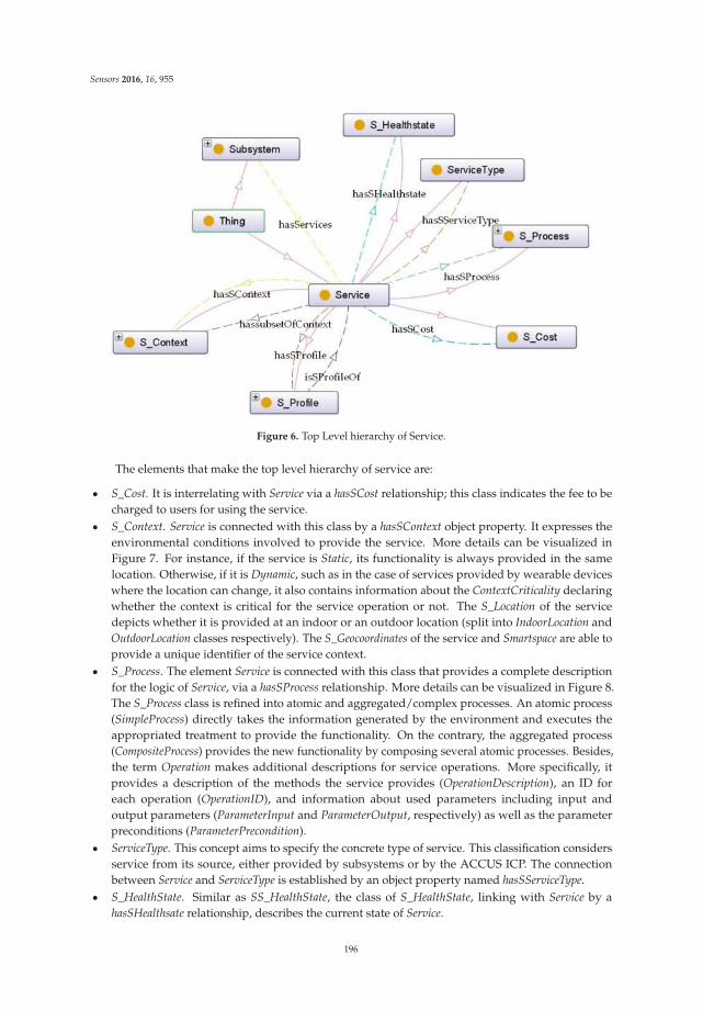
Sensors 2016, 16, 955

Figure 6. Top Level hierarchy of Service.

The elements that make the top level hierarchy of service are:

‚ S_Cost. It is interrelating with Service via a hasSCost relationship; this class indicates the fee to becharged to users for using the service.

‚ S_Context. Service is connected with this class by a hasSContext object property. It expresses theenvironmental conditions involved to provide the service. More details can be visualized inFigure 7. For instance, if the service is Static, its functionality is always provided in the samelocation. Otherwise, if it is Dynamic, such as in the case of services provided by wearable deviceswhere the location can change, it also contains information about the ContextCriticality declaringwhether the context is critical for the service operation or not. The S_Location of the servicedepicts whether it is provided at an indoor or an outdoor location (split into IndoorLocation andOutdoorLocation classes respectively). The S_Geocoordinates of the service and Smartspace are able toprovide a unique identifier of the service context.

‚ S_Process. The element Service is connected with this class that provides a complete descriptionfor the logic of Service, via a hasSProcess relationship. More details can be visualized in Figure 8.The S_Process class is refined into atomic and aggregated/complex processes. An atomic process(SimpleProcess) directly takes the information generated by the environment and executes theappropriated treatment to provide the functionality. On the contrary, the aggregated process(CompositeProcess) provides the new functionality by composing several atomic processes. Besides,the term Operation makes additional descriptions for service operations. More specifically, itprovides a description of the methods the service provides (OperationDescription), an ID foreach operation (OperationID), and information about used parameters including input andoutput parameters (ParameterInput and ParameterOutput, respectively) as well as the parameterpreconditions (ParameterPrecondition).

‚ ServiceType. This concept aims to specify the concrete type of service. This classification considersservice from its source, either provided by subsystems or by the ACCUS ICP. The connectionbetween Service and ServiceType is established by an object property named hasSServiceType.

‚ S_HealthState. Similar as SS_HealthState, the class of S_HealthState, linking with Service by ahasSHealthsate relationship, describes the current state of Service.

196

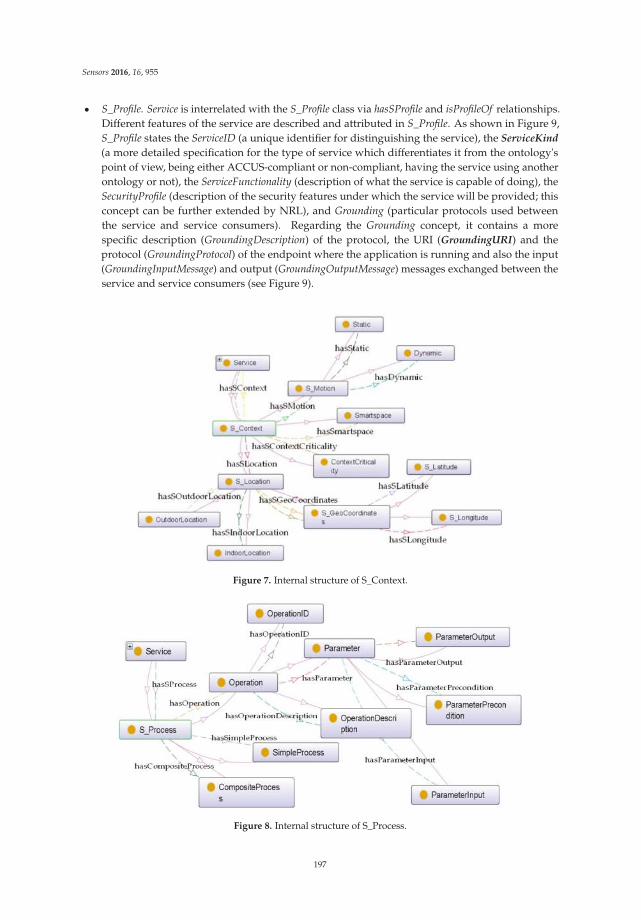
Sensors 2016, 16, 955

‚ S_Profile. Service is interrelated with the S_Profile class via hasSProfile and isProfileOf relationships.Different features of the service are described and attributed in S_Profile. As shown in Figure 9,S_Profile states the ServiceID (a unique identifier for distinguishing the service), the ServiceKind

(a more detailed specification for the type of service which differentiates it from the ontology'spoint of view, being either ACCUS-compliant or non-compliant, having the service using anotherontology or not), the ServiceFunctionality (description of what the service is capable of doing), theSecurityProfile (description of the security features under which the service will be provided; thisconcept can be further extended by NRL), and Grounding (particular protocols used betweenthe service and service consumers). Regarding the Grounding concept, it contains a morespecific description (GroundingDescription) of the protocol, the URI (GroundingURI) and theprotocol (GroundingProtocol) of the endpoint where the application is running and also the input(GroundingInputMessage) and output (GroundingOutputMessage) messages exchanged between theservice and service consumers (see Figure 9).

Figure 7. Internal structure of S_Context.

Figure 8. Internal structure of S_Process.

197

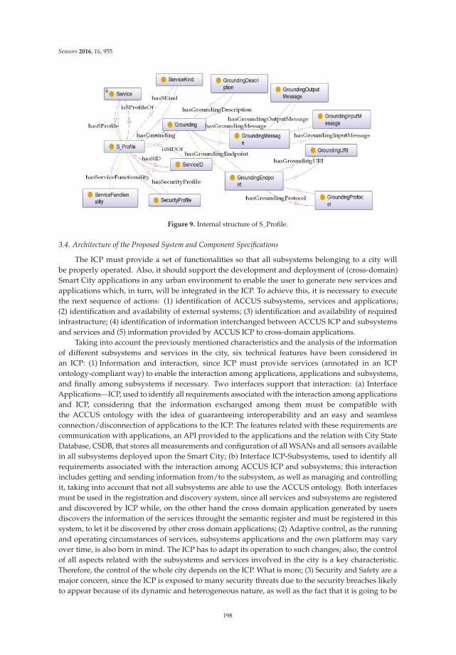
Sensors 2016, 16, 955

Figure 9. Internal structure of S_Profile.

3.4. Architecture of the Proposed System and Component Specifications

The ICP must provide a set of functionalities so that all subsystems belonging to a city willbe properly operated. Also, it should support the development and deployment of (cross-domain)Smart City applications in any urban environment to enable the user to generate new services andapplications which, in turn, will be integrated in the ICP. To achieve this, it is necessary to executethe next sequence of actions: (1) identification of ACCUS subsystems, services and applications;(2) identification and availability of external systems; (3) identification and availability of requiredinfrastructure; (4) identification of information interchanged between ACCUS ICP and subsystemsand services and (5) information provided by ACCUS ICP to cross-domain applications.

Taking into account the previously mentioned characteristics and the analysis of the informationof different subsystems and services in the city, six technical features have been considered inan ICP: (1) Information and interaction, since ICP must provide services (annotated in an ICPontology-compliant way) to enable the interaction among applications, applications and subsystems,and finally among subsystems if necessary. Two interfaces support that interaction: (a) InterfaceApplications—ICP, used to identify all requirements associated with the interaction among applicationsand ICP, considering that the information exchanged among them must be compatible withthe ACCUS ontology with the idea of guaranteeing interoperability and an easy and seamlessconnection/disconnection of applications to the ICP. The features related with these requirements arecommunication with applications, an API provided to the applications and the relation with City StateDatabase, CSDB, that stores all measurements and configuration of all WSANs and all sensors availablein all subsystems deployed upon the Smart City; (b) Interface ICP-Subsystems, used to identify allrequirements associated with the interaction among ACCUS ICP and subsystems; this interactionincludes getting and sending information from/to the subsystem, as well as managing and controllingit, taking into account that not all subsystems are able to use the ACCUS ontology. Both interfacesmust be used in the registration and discovery system, since all services and subsystems are registeredand discovered by ICP while, on the other hand the cross domain application generated by usersdiscovers the information of the services throught the semantic register and must be registered in thissystem, to let it be discovered by other cross domain applications; (2) Adaptive control, as the runningand operating circumstances of services, subsystems applications and the own platform may varyover time, is also born in mind. The ICP has to adapt its operation to such changes; also, the controlof all aspects related with the subsystems and services involved in the city is a key characteristic.Therefore, the control of the whole city depends on the ICP. What is more; (3) Security and Safety are amajor concern, since the ICP is exposed to many security threats due to the security breaches likelyto appear because of its dynamic and heterogeneous nature, as well as the fact that it is going to be

198

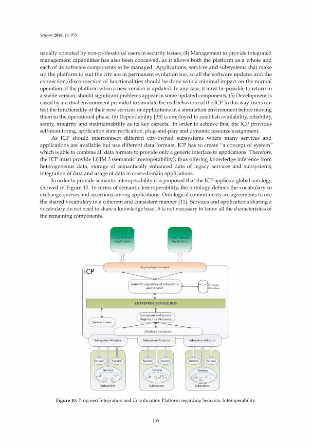
Sensors 2016, 16, 955

usually operated by non-professional users in security issues; (4) Management to provide integratedmanagement capabilities has also been conceived, as it allows both the platform as a whole andeach of its software components to be managed. Applications, services and subsystems that makeup the platform to suit the city are in permanent evolution too, so all the software updates and theconnection/disconnection of functionalities should be done with a minimal impact on the normaloperation of the platform when a new version is updated. In any case, it must be possible to return toa stable version, should significant problems appear in some updated components; (5) Development iseased by a virtual environment provided to simulate the real behaviour of the ICP. In this way, users cantest the functionality of their new services or applications in a simulation environment before movingthem to the operational phase; (6) Dependability [33] is employed to establish availability, reliability,safety, integrity and maintainability as its key aspects. In order to achieve this, the ICP providesself-monitoring, application state replication, plug-and-play and dynamic resource assignment.

As ICP should interconnect different city-owned subsystems where many services andapplications are available but use different data formats, ICP has to create “a concept of system”which is able to combine all data formats to provide only a generic interface to applications. Therefore,the ICP must provide LCIM 3 (semantic interoperability), thus offering knowledge inference fromheterogeneous data, storage of semantically enhanced data of legacy services and subsystems,integration of data and usage of data in cross-domain applications.

In order to provide semantic interoperability it is proposed that the ICP applies a global ontology,showed in Figure 10. In terms of semantic interoperability, the ontology defines the vocabulary toexchange queries and assertions among applications. Ontological commitments are agreements to usethe shared vocabulary in a coherent and consistent manner [11]. Services and applications sharing avocabulary do not need to share a knowledge base. It is not necessary to know all the characteristics ofthe remaining components.

Figure 10. Proposed Integration and Coordination Platform regarding Semantic Interoperability.

199

Sensors 2016, 16, 955

If all the functions described above are to be performed, the first action to be taken is ensuringinteroperability among all the Smart City systems and applications. It is strictly necessary, first ofall, that the ICP itself has its own complete system of registration and discovery of subsystems andservices, which it is proposed in this paper. Figure 10 shows the architecture of the whole system ofICP related to registry and discovery.

The first step to discover all subsystems connected to ICP and the services provided by eachsubsystem is taken by the component Subsystem and Service Registry and Discovery through InterfaceICP—Subsystems. A key point is that this component works in real time. Later, each service orsubsystem will provide their own description in a compliant way to nSSOO or not. Regardlessof what is used, ICP provides semantic interoperability and seamless interconnection betweenapplications and services embedded in subsystems. In order to perform semantic mapping fordata interoperability enabling the transparent sharing of information among subsystems in the smartcity, the mail requirement is the translation of the output of subsystems and services that are goingto interchange information among them. The translations of this service are used for the registrationand discovery of services and subsystems in the service repository. This fact can be achieved byparsing XML data to RDF. This way, semantic experts can define the XML to RDF mapping andnon-semantic experts can work with XML files avoiding the effort of analysing ontologies for eachsubsystem. The service is provided by the components Subsystem adaptor and Ontology Connector.The first one facilitates the connection of subsystems and their services, and provides all necessaryfunctions of adaptation and coordination. It is a very relevant component since it is in charge ofthe transformation of the information provided by services and subsystems to the ICP. The secondone handles the translations of the data format which will be added to the Semantic Repository,when data are delivered in a known XML-like format [34]. These translations from XMLs to OWL orRDFs will be made using a mapping file which describes the transformation between the elementsof source XML to an instance of the global ontology. A mapping file must be defined for each typeof XML instance. When the description of the service or subsystem is available for the Subsystemand Service Registry and Discovery, it will establish a connection trough the Enterprise Service Buswith the component Semantic Subsystem and Service Repository to store the semantic description ofservices and subsystems registered in the ICP, according to the global ontology defined for the system.When a new subsystem or service is discovered by the Subsystem and Service Discovery component,its semantic description (profile) will be stored in this repository. Enterprise Service Bus providesinterconnection and cooperation of the components based on a paradigm of message interchange;the ESB selected in ACCUS ICP is JBoss [35], which was preferred over two competitive alternatives:WSO2 and MULE [36]. Obviously, the component Service broker is necessary to orchestrate servicesand mediate between different software protocols if necessary.

Once all services and subsystems are registered, the Cross-domain Applications through theInterface Applications-ICP can execute SPARQL [37] queries and get their needed results in order togenerate new applications or services, that, at the same time, will be registered.

This mode of operation allows the permanent update of all services, subsystems and applicationsof the Smart City.

3.5. Procedure Specifications: The Specific Workflow of Registering and Discovering Services and Subsystems

In this section, the specific process to register and discover subsystems and services is introduced.

3.5.1. Subsystems Registration

Once all subsystems and ACCUS ICP are up, subsystems must start with the registrationprocedure one by one. As shown in Figure 11, first, each subsystem sends a registration requestto the ACCUS ICP which includes the subsystem profile in an XML document. The subsystem profilecontains information to identify itself, such as functionality, geolocation, health state, provider or inputand output parameters. This information is not compliant with the ACCUS ontology and therefore, it

200

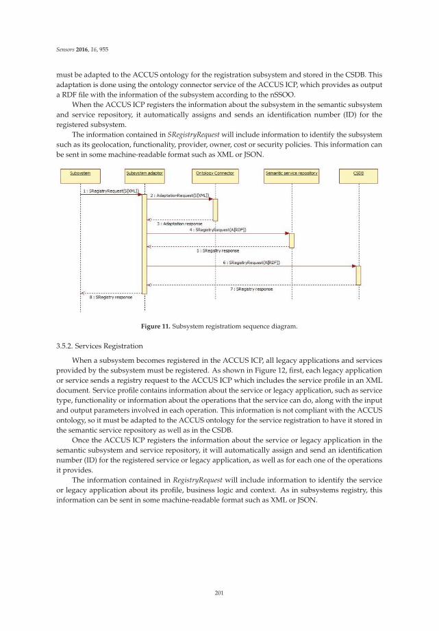
Sensors 2016, 16, 955

must be adapted to the ACCUS ontology for the registration subsystem and stored in the CSDB. Thisadaptation is done using the ontology connector service of the ACCUS ICP, which provides as outputa RDF file with the information of the subsystem according to the nSSOO.

When the ACCUS ICP registers the information about the subsystem in the semantic subsystemand service repository, it automatically assigns and sends an identification number (ID) for theregistered subsystem.

The information contained in SRegistryRequest will include information to identify the subsystemsuch as its geolocation, functionality, provider, owner, cost or security policies. This information canbe sent in some machine-readable format such as XML or JSON.

Figure 11. Subsystem registratiom sequence diagram.

3.5.2. Services Registration

When a subsystem becomes registered in the ACCUS ICP, all legacy applications and servicesprovided by the subsystem must be registered. As shown in Figure 12, first, each legacy applicationor service sends a registry request to the ACCUS ICP which includes the service profile in an XMLdocument. Service profile contains information about the service or legacy application, such as servicetype, functionality or information about the operations that the service can do, along with the inputand output parameters involved in each operation. This information is not compliant with the ACCUSontology, so it must be adapted to the ACCUS ontology for the service registration to have it stored inthe semantic service repository as well as in the CSDB.

Once the ACCUS ICP registers the information about the service or legacy application in thesemantic subsystem and service repository, it will automatically assign and send an identificationnumber (ID) for the registered service or legacy application, as well as for each one of the operationsit provides.

The information contained in RegistryRequest will include information to identify the serviceor legacy application about its profile, business logic and context. As in subsystems registry, thisinformation can be sent in some machine-readable format such as XML or JSON.

201

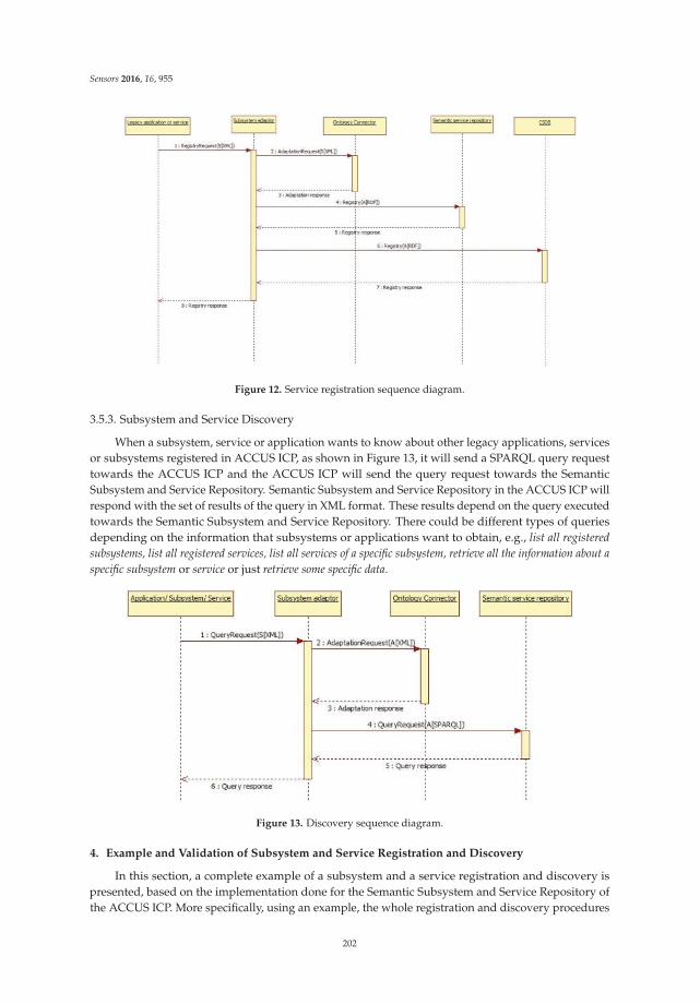
Sensors 2016, 16, 955

Figure 12. Service registration sequence diagram.

3.5.3. Subsystem and Service Discovery

When a subsystem, service or application wants to know about other legacy applications, servicesor subsystems registered in ACCUS ICP, as shown in Figure 13, it will send a SPARQL query requesttowards the ACCUS ICP and the ACCUS ICP will send the query request towards the SemanticSubsystem and Service Repository. Semantic Subsystem and Service Repository in the ACCUS ICP willrespond with the set of results of the query in XML format. These results depend on the query executedtowards the Semantic Subsystem and Service Repository. There could be different types of queriesdepending on the information that subsystems or applications want to obtain, e.g., list all registered

subsystems, list all registered services, list all services of a specific subsystem, retrieve all the information about a

specific subsystem or service or just retrieve some specific data.

Figure 13. Discovery sequence diagram.

4. Example and Validation of Subsystem and Service Registration and Discovery

In this section, a complete example of a subsystem and a service registration and discovery ispresented, based on the implementation done for the Semantic Subsystem and Service Repository ofthe ACCUS ICP. More specifically, using an example, the whole registration and discovery procedures

202

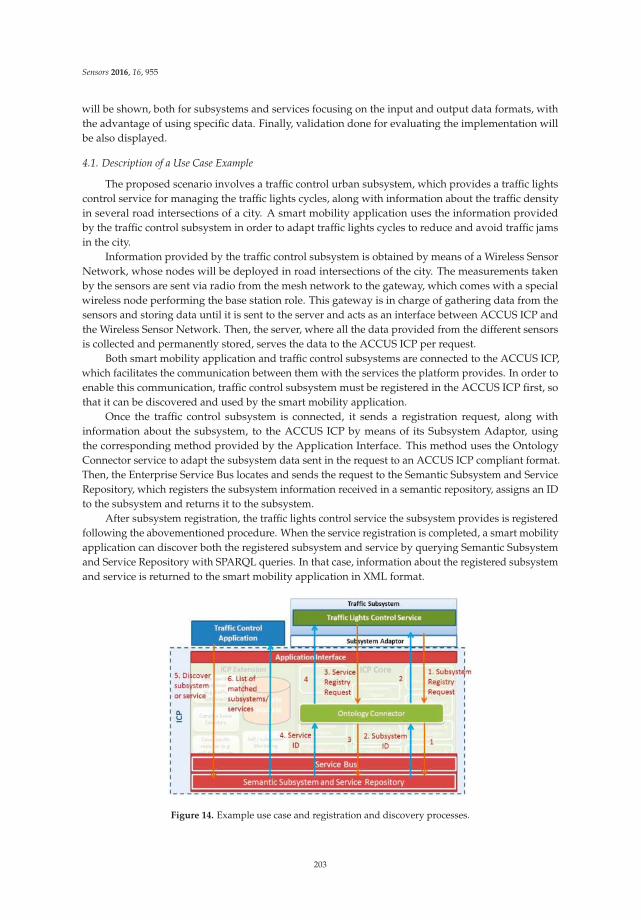
Sensors 2016, 16, 955

will be shown, both for subsystems and services focusing on the input and output data formats, withthe advantage of using specific data. Finally, validation done for evaluating the implementation willbe also displayed.

4.1. Description of a Use Case Example

The proposed scenario involves a traffic control urban subsystem, which provides a traffic lightscontrol service for managing the traffic lights cycles, along with information about the traffic densityin several road intersections of a city. A smart mobility application uses the information providedby the traffic control subsystem in order to adapt traffic lights cycles to reduce and avoid traffic jamsin the city.

Information provided by the traffic control subsystem is obtained by means of a Wireless SensorNetwork, whose nodes will be deployed in road intersections of the city. The measurements takenby the sensors are sent via radio from the mesh network to the gateway, which comes with a specialwireless node performing the base station role. This gateway is in charge of gathering data from thesensors and storing data until it is sent to the server and acts as an interface between ACCUS ICP andthe Wireless Sensor Network. Then, the server, where all the data provided from the different sensorsis collected and permanently stored, serves the data to the ACCUS ICP per request.

Both smart mobility application and traffic control subsystems are connected to the ACCUS ICP,which facilitates the communication between them with the services the platform provides. In order toenable this communication, traffic control subsystem must be registered in the ACCUS ICP first, sothat it can be discovered and used by the smart mobility application.

Once the traffic control subsystem is connected, it sends a registration request, along withinformation about the subsystem, to the ACCUS ICP by means of its Subsystem Adaptor, usingthe corresponding method provided by the Application Interface. This method uses the OntologyConnector service to adapt the subsystem data sent in the request to an ACCUS ICP compliant format.Then, the Enterprise Service Bus locates and sends the request to the Semantic Subsystem and ServiceRepository, which registers the subsystem information received in a semantic repository, assigns an IDto the subsystem and returns it to the subsystem.

After subsystem registration, the traffic lights control service the subsystem provides is registeredfollowing the abovementioned procedure. When the service registration is completed, a smart mobilityapplication can discover both the registered subsystem and service by querying Semantic Subsystemand Service Repository with SPARQL queries. In that case, information about the registered subsystemand service is returned to the smart mobility application in XML format.

Figure 14. Example use case and registration and discovery processes.

203

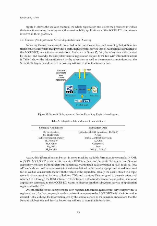
Sensors 2016, 16, 955

Figure 14 shows the use case example, the whole registration and discovery processes as well asthe interactions among the subsystem, the smart mobility application and the ACCUS ICP componentsinvolved in these processes.

4.2. Example of Subsystem and Service Registration and Discovery

Following the use case example presented in the previous section, and assuming that a) there is atraffic control subsystem that provides a traffic lights control service that b) has been just connected tothe ACCUS ICP, two actions are carried out. As shown in Figure 15, first, the subsystem is discoveredby the ICP and secondly, the subsystem sends a registration request to the ICP with information aboutit. Table 1 shows the information sent by the subsystem as well as the semantic annotations that theSemantic Subsystem and Service Repository will use to store that information.

Figure 15. Semantic Subsystem and Service Repository Registration diagram.

Table 1. Subsystem data and semantic annotations.

Semantic Annotations Subsystem Data

SS_Geolocation Latitude: 54.3521 Longitude: 18.64637SS_HealthState Active

SubsystemFunctionality Traffic Control SubsystemSS_Provider ACCUSSS_Owner Company1

SS_Cost FreeSS_Policies Policy1, Policy2

Again, this information can be sent in some machine readable format as, for example, in XMLor JSON. ACCUS ICP receives this data via a REST interface, and Semantic Subsystem and ServiceRepository converts the input data into semantically annotated data formatted in RDF. To do so, JenaAPI methods are used in order to obtain the classes defined in the ontology graph and stored in an .owlfile, as well as to instantiate them with the values of the input data. Finally, the data is stored in a triplestore database provided by Jena, called Jena TDB, and a unique ID is assigned to the subsystem andreturned to it through the REST interface. This interface is also used whenever a subsystem, service orapplication connected to the ACCUS ICP wants to discover another subsystem, service or applicationregistered in the ICP.

Once the traffic control subsystem has been registered, the traffic lights control service it provides isregistered and, for that purpose, it sends a registration request to the ACCUS ICP with the informationabout it. Table 2 shows the information sent by the service as well as the semantic annotations that theSemantic Subsystem and Service Repository will use to store that information.

204

Sensors 2016, 16, 955

Table 2. Subsystem data and semantic annotations.

Semantic Annotations Service Data Semantic Annotations Service Data

ServiceType Subsystem service OperationDescriptionchangeState: provides

the change and durationof the new state

S_HealthState Active ParameterPrecondition initialState

S_Cost Free ParameterInput dataTimeInterval

ServiceKind ACCUS compliant ParameterOutput lightValue

ServiceFunctionality Traffic lights control Static Static

SecurityProfile securityProfile1 Dynamic Non dynamic

GroundingDescription change state IndoorLocation Non indoor

GroundingInputMessage none OutdoorLocation Outdoor

GroundingOutputMessage changes done ContextCriticality Critical

GroundingURI ACCUS/trafficLightsControl Smartspace SS2

GroundingProtocol REST S_Latitude 54.3521

SimpleProcess Simple S_Longitude 18.64637

Then, when the ACCUS ICP receives the data, Semantic Subsystem and Service Repositoryregisters the service, following the same procedure as for the subsystem, and finally an ID is assignedto the subsystem’s service.

As soon as the subsystem and the service it provides have been registered, they can be discoveredby any subsystem, service or application connected to the ACCUS ICP, thus obtaining informationabout them. To do so, they can query the Semantic Subsystem and Service Repository, using one of themethods that this service API provides. The results will be output in a document XML.

For example, if the smart mobility application wants to discover the traffic control subsystempreviously registered, it can call listAllSubsystems method, which returns a list of all registeredsubsystems, or also it can call subsystemInfo method, which returns the information about thesubsystem whose ID matches the one passed as an input parameter.

Therefore, calling, for example, the latter method using the traffic control subsystem ID, thefollowing SPARQL query is executed:

PREFIX ns: <http://www.semanticweb.org/ACCUS/1.1#>

SELECT ?subsystemID ?subsystemFunctionality ?subsystemHealthState ?subsystemGeolocation

?subsystemProvider ?subsystemOwner ?subsystemCost ?subsystemPolicies

WHERE ns:@id@ ns:isSSIDOf ?subsystem.

?subsystem ns:hasSSID ?subsystemID.

?subsystem ns:hasSSHealthState ?subsystemHealthState.

?subsystem ns:hasSSContext ?subsystemContext.

?subsystemContext ns:hasSSGeoLocation ?subsystemGeolocation.

?subsystem ns:hasSSProfile ?subsystemProfile.

?subsystemProfile ns:hasSSFunctions ?subsystemFunctionality.

?subsystemProfile ns:hasSSCost ?subsystemCost.

?subsystemProfile ns:hasSSPolicies ?subsystemPolicies.

?subsystemProfile ns:hasSSOwner ?subsystemOwner.

?subsystemProfile ns:hasSSProvider ?subsystemProvider.

And the following output will be returned:

205

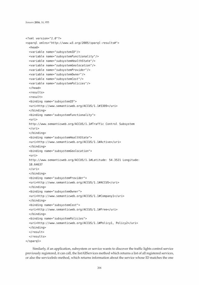
Sensors 2016, 16, 955

<?xml version="1.0"?>

<sparql xmlns="http://www.w3.org/2005/sparql-results#">

<head>

<variable name="subsystemID"/>

<variable name="subsystemFunctionality"/>

<variable name="subsystemHealthState"/>

<variable name="subsystemGeolocation"/>

<variable name="subsystemProvider"/>

<variable name="subsystemOwner"/>

<variable name="subsystemCost"/>

<variable name="subsystemPolicies"/>

</head>

<results>

<result>

<binding name="subsystemID">

<uri>http://www.semanticweb.org/ACCUS/1.1#3309</uri>

</binding>

<binding name="subsystemFunctionality">

<uri>

http://www.semanticweb.org/ACCUS/1.1#Traffic Control Subsystem

</uri>

</binding>

<binding name="subsystemHealthState">

<uri>http://www.semanticweb.org/ACCUS/1.1#Active</uri>

</binding>

<binding name="subsystemGeolocation">

<uri>

http://www.semanticweb.org/ACCUS/1.1#Latitude: 54.3521 Longitude:

18.64637

</uri>

</binding>

<binding name="subsystemProvider">

<uri>http://www.semanticweb.org/ACCUS/1.1#ACCUS</uri>

</binding>

<binding name="subsystemOwner">

<uri>http://www.semanticweb.org/ACCUS/1.1#Company1</uri>

</binding>

<binding name="subsystemCost">

<uri>http://www.semanticweb.org/ACCUS/1.1#Free</uri>

</binding>

<binding name="subsystemPolicies">

<uri>http://www.semanticweb.org/ACCUS/1.1#Policy1, Policy2</uri>

</binding>

</result>

</results>

</sparql>

Similarly, if an application, subsystem or service wants to discover the traffic lights control servicepreviously registered, it can call, the listAllServices method which returns a list of all registered services,or also the serviceInfo method, which returns information about the service whose ID matches the one

206

Sensors 2016, 16, 955

passed as an input parameter. In the first case, the SPARQL query executed for listing all the registeredservices is the following:

PREFIX ns: <http://www.semanticweb.org/ACCUS/1.1#>

SELECT ?serviceID ?serviceFunctionality ?serviceType ?serviceHealthState ?serviceKind ?

serviceCost ?securityProfile

WHERE ?Resource ns:hasSServiceType ?serviceType.

?Resource ns:hasSCost ?serviceCost.

?Resource ns:hasSHealthstate ?serviceHealthState.

?Resource ns:hasSProfile ?serviceProfile.

?serviceProfile ns:hasSID ?serviceID.

?serviceProfile ns:hasServiceFunctionality ?serviceFunctionality.

?serviceProfile ns:hasSKind ?serviceKind.

?serviceProfile ns:hasSecurityProfile ?securityProfile.

and the information returned will be the following:

<?xml version="1.0"?>

<sparql xmlns="http://www.w3.org/2005/sparql-results#">

<head>

<variable name="serviceID"/>

<variable name="serviceFunctionality"/>

<variable name="serviceType"/>

<variable name="serviceHealthState"/>

<variable name="serviceKind"/>

<variable name="serviceCost"/>

<variable name="securityProfile"/>

</head>

<results>

<result>

<binding name="serviceID">


</binding>

<binding name="serviceFunctionality">

<uri>http://www.semanticweb.org/ACCUS/1.1#Subsystem and Service

Repository: an ontology translator for ACCUS ICP data treatment,

whenever the nSSOO ontology is required, that will be storing semantic

information related with subsystems and services connected to the ICP.

</uri>

</binding>

<binding name="serviceType">

<uri>http://www.semanticweb.org/ACCUS/1.1#ACCUS ICP service</uri>

</binding>

<binding name="serviceHealthState">


</binding>

<binding name="serviceKind">

<uri>http://www.semanticweb.org/ACCUS/1.1#ACCUS compliant</uri>

</binding>

<binding name="serviceCost">


</binding>

207

Sensors 2016, 16, 955

<binding name="securityProfile">

<uri>http://www.semanticweb.org/ACCUS/1.1#ACCUS security profile</uri>

</binding>

</result>

<result>

<binding name="serviceID">


</binding>

<binding name="serviceFunctionality">

<uri>http://www.semanticweb.org/ACCUS/1.1#Traffic lights control </uri>

</binding>

<binding name="serviceType">

<uri>http://www.semanticweb.org/ACCUS/1.1#Subsystem service</uri>

</binding>

<binding name="serviceHealthState">


</binding>

<binding name="serviceKind">

<uri>http://www.semanticweb.org/ACCUS/1.1#Not ACCUS compliant</uri>

</binding>

<binding name="serviceCost">


</binding>

<binding name="securityProfile">

<uri>http://www.semanticweb.org/ACCUS/1.1#securityProfile1</uri>

</binding>

</result>

</result>......</result>

</result>......</result>

</results>

</sparql>

Note that, when listing all services, information about Semantic Subsystem and Service Repositoryis also shown because internal ACCUS ICP active services are also registered in the semantic repositoryonce the ICP is up.

4.3. Validation

In order to validate the practical performance of the Semantic Subsystem and Service Repositoryimplementation, both the response time and the registration rate of the service have been tested. Inorder to test the response time, the timespan used for the different operations that the service providesto be executed has been measured. For each measurement, three samples have been taken in orderto obtain an average value of the response time. On the other hand, the registration rate refers tothe percentage of subsystems and services registered with regards to a certain number of registryrequests done.

Tests have been done using an Intel(R) Core(TM)2 Quad CPU Q6600 processor @ 2.40 GHzequipped with 2.39 GHz and a RAM memory of 4 GB in a machine operating under the 64-bitWindows 7 Professional operating system.

208

Sensors 2016, 16, 955

4.3.1. Response Time

When a request is done to the Semantic Subsystem and Service Repository for the first time, thisservice must be initialized, so it takes more time than usual to execute the request. So, to begin with,the response time required when a request is done to the semantic repository for the first time has beenmeasured. Results obtained are shown in Table 3.

Table 3. Response time when the first request is done to the semantic repository.

Operation T1 (ms) T2 (ms) T3 (ms) Average Time Elapsed (ms)

registerSubsystem 130 29 56 71.67registerService 142 142 92 125.33

listAll 469 530 532 510.33listAllSubsystems 450 447 463 453.33

listAllServices 476 490 460 475.33getSubsystemInfo 464 498 476 479.33

getServiceInfo 815 578 564 652.33

Now, considering that the service has been initialized, the response time of the semantic repositoryoperations has been measured in three different cases: when the repository has 100, 500 and 1000of subsystems and services registered. The purpose is to test the normal operation of the semanticrepository for different amounts of registered data. The results obtained are shown in Tables 4–6.

Table 4. Response time when there are 100 subsystems and services registered.




listAllServices 20 17 18 18.33getSubsystemInfo 8 5 5 6

getServiceInfo 99 42 27 56



registerSubsystem 67 66 28 53.67registerService 76 75 41 64


listAllServices 73 63 62 66getSubsystemInfo 6 3 5 4.67





listAll 398 368 771 512.33listAllSubsystems 195 500 367 354

listAllServices 138 107 111 118.67getSubsystemInfo 6 4 5 5


209

Sensors 2016, 16, 955

Analyzing the results obtained, several conclusions can be drawn. Besides the fact that theresponse time is higher when the first request is done due to the initialization of the semantic repository,it can also be appreciated that the response time increases with the amount of subsystems andservices stored.

Comparing the time response between the different operations, it can be seen that the timeresponse of listAll operation is considerably higher than in the other operations due to the higheramount of data that must be retrieved, which are all the subsystems and services stored in the semanticrepository, while, for example, in listAllSubsystems and listAllServices only operation subsystems in thefirst case, and services in the second case are shown. Regarding the last two operations mentioned, thetime response of listAllSubsystems is higher than the time response of listAllServices because in the firstoperation more information is shown than in the second operation. For the same reason, time responsein registerService and getServiceInfo operations is higher than in registerSubsystem and getSubsystemInfo.Finally, it can be appreciated that the time response of registerSubsystem, registerService, getSubsystemInfo,getServiceInfo does not change significantly with the amount of data registered, because in theseoperations just one subsystem or service is registered or queried so they are not affected by the amountof data registered.

4.3.2. Registration Rate

For testing the registration rate, 5000 subsystem and service registry requests were done towardsthe Semantic Subsystem and Service Repository, and all the requests were successfully executed,registering the 100% of subsystems and services that requested registration.


This paper has presented an ontology-based and automatic system for subsystem and serviceregistry and discovery within the context of the ACCUS project. This proposed system, embedded inACCUS ICP, is able to dynamically register and discover heterogeneous subsystems and servicesprovided by subsystems within a Smart City so that cross-domain applications and collectiveoptimization can be built upon the ICP by using existing services. To address the heterogeneity(e.g., data formats and protocols) of subsystems and services, a new ontology, named nSSOO, hasbeen proposed and employed by the system to provide a formalized vocabulary for the registrationand discovery processes. The nSSOO has been developed on the basis of three existing ontologies,including OWL-S, CityGML, and NRL. By complying with this ontology, heterogeneous subsystemsand services provided by individual subsystems can share a same understanding which results ina formal and homogeneous appearance of the ICP. The proposed ontology, from a global point ofview, is an important contribution to achieve semantic interoperability in the ICP and it has beenpresented with detailed explanations for inner composition. In addition to that, different softwarecomponents which form the whole system have been shown with their main functionalities explained.The proposed ontology-based scheme for subsystem and service discovery and registry has beenelaborated with a set of sequence diagrams that present the specific workflow of inner componentsinvolved in this scheme. Furthermore, after presenting the specific procedures to ease the subsystemand service discovery and registry, a complete example about discovering and registering a trafficcontrol system and a traffic lights control service has been provided to show the performance of theproposed scheme. Different kinds of queries for information stored in ICP have also been introduced.

The system proposed to register and discover subsystems and services has been proven tobe useful to interconnect different subsystems and services. What is more, it could abstract theheterogeneity of different subsystems and services so as to provide a homogeneous interface forapplications or other services inside the ICP. Though this scheme aims to create an accurate referenceframework for available information (e.g., subsystems, services, and applications) within the SmartCities, it could be also possible to adapt it to other domains, such as underwater robotics. Developerscan become aware of the services that are working in the Smart city, which are their features and how

210

Sensors 2016, 16, 955

can be accessed, to design their applications by making use of those services provided by subsystems.Also, developers are isolated of the problem of transforming data protocols.

Future work could be focused on the following aspects:

‚ The proposed subsystem and service discovery and registry scheme should be tested in morescenarios in a real city. In ACCUS project, the city that has been chosen to deploy the pilot isGdansk, in Poland.

‚ The relationships among different services are a crucial factor for application developers whenthey design brand new applications. Future work should focus on examining the similaritydegree of different services. For instance, services able to provide similar functionalities can bealternatives if the ideal service to be used is not available. A potential solution could be includinginformation about relationships of different services in relevant service profiles.

‚ The nSSOO ontology should evolve to richly describe more features of subsystems and services.For example, it is possible to extend nSSOO with some new classes using FOAF [38] to includeadditional aspects of information about people, such as roles like provider or owner. Anotherpotential extension of the ontology could be including concepts about event-driven services.

‚ Future emphasis can also be put on including decision-making related algorithms in the nSSOOontology. e.g., MADISE [39] ontology can be reused and integrated with the nSSOO ontology.

Acknowledgments: This paper is a result of research made by the authors in the Adaptive and CooperativeControl in Urban Subsystems (ACCUS) project, ARTEMIS 2012-1. SP1-JT1-ARTEMIS-2012-ASP7-EmbeddedSystem supporting sustainable urban life, SP1-JT1-ARTEMIS-2012-ASP3: Embedded systems in Smartenvironments. The authors would like to thank CITSEM (Research Center on Software Technologies andMultimedia Systems for Sustainability, Centro de Investigación en Tecnologías Software y Sistemas Multimediapara la Sostenibilidad) from the Technical University of Madrid (UPM).

Author Contributions: The research result presented in this article is a collaborative work of all authors. Rubiohas prepared the architecture of the ICP. Rubio, Gómez and Li have defined the ontology. Li has implemented theontology. Rubio and Gómez have defined the sequence of registering and discovering subsystems and service.Gómez has prepared and implemented the SPARQL queries. Martínez has given technical and conceptual supportfor the entire article. All authors have participated in writing this article. All of the authors have reviewed andfinally approved the manuscript.


References

1. Nellore, K.; Hancke, G. A Survey on Urban Traffic Management System Using Wireless Sensor Networks.Sensors 2016, 16, 157. [CrossRef] [PubMed]

2. Moreno, A.; Perallos, A.; López-de-Ipiña, D.; Onieva, E.; Salaberria, I.; Masegosa, A. A Novel SoftwareArchitecture for the Provision of Context-Aware Semantic Transport Information. Sensors 2015, 15,12299–12322. [CrossRef] [PubMed]

3. Ghayvat, H.; Mukhopadhyay, S.; Gui, X.; Suryadevara, N. WSN- and IOT-Based Smart Homes and TheirExtension to Smart Buildings. Sensors 2015, 15, 10350–10379. [CrossRef] [PubMed]

4. Rodríguez-Molina, J.; Martínez, J.-F.; Castillejo, P.; de Diego, R. SMArc: A Proposal for a Smart, SemanticMiddleware Architecture Focused on Smart City Energy Management. Int. J. Distrib. Sens. Netw. 2013, 2013,1–17. [CrossRef]

5. Zhou, L.; Rodrigues, J.J.P.C. Service-oriented middleware for smart grid: Principle, infrastructure,and application. IEEE Commun. Mag. 2013, 51, 84–89. [CrossRef]

6. Hernandez, L.; Baladrón, C.; Aguiar, J.M.; Calavia, L.; Carro, B.; Sanchez-Esguevillas, A.; Cook, D.J.;Chinarro, D.; Gómez, J. A Study of the Relationship between Weather Variables and Electric Power Demandinside a Smart Grid/Smart World Framework. Sensors 2012, 12, 11571–11591. [CrossRef]

7. Sung, W.-T.; Lin, J.-S. Design and Implementation of a Smart LED Lighting System Using a Self AdaptiveWeighted Data Fusion Algorithm. Sensors 2013, 13, 16915–16939. [CrossRef]

8. Warriach, E.U.; Kaldeli, E.; Lazovik, A.; Aiello, M. An Interplatform Service-Oriented Middleware for theSmart Home. Int. J. Smart Home 2013, 7, 115–142.

211

Sensors 2016, 16, 955

9. RECI. Red Española de Ciudades Inteligentes. Available online: http://www.redciudadesinteligentes.es(accessed on 28 March 2016).

10. The ACCUS (Adaptive Cooperative Control in Urban (sub)Systems) Project. Available online: http://projectaccus.eu/ (accessed on 31 March 2016).

11. Zang, M.A. Ontological Approaches for Semantic Interoperability. In Proceedings of the 5th Annual ONRWorkshop on Collaborative Decision-Support Systems, San Luis Obispo, CA, USA, 10–11 September 2003.

12. Services Oriented Architecture for All. Available online: http://www.soa4all.ue (accessed on 10 April 2016).13. Tagging Tool Based on a Semantic Discovery Framework. Available online: www.tatoo-fp7.eu (accessed on

11 March 2016).14. Cloud4SOA. Available online: http://www.cloud4soa.com (accessed on 10 March 2016).15. Butler, B. PaaS Primer: What Is Platform as Services and Why Does It Matter?; Network World: Framingham,

MA, USA, 2013.16. Semantichealthnet. Available online: http://www.semantichealthnet.eu (accessed on 27 March 2016).17. Mobilized Lifestyle with Wearables (LifeWear). Available online: https://itea3.org/project/lifeware.html

(accesed 21 June 2016).18. Ryu, M.; Kim, J.; Yun, J. Integrated semantics services platform for the internet of things: A case study of a

smart office. Sensors 2015, 15, 2137–2160. [CrossRef] [PubMed]19. Hussain, A.; Wenbi, R.; da Silva, A.L.; Nadher, M.; Mudhish, M. Health and emergency-care platform for the

elderly and disabled people in the Smart City. J. Syst. Softw. 2015, 110, 253–263. [CrossRef]20. Benhaourech, A.; Aaroud, A.; Roose, P.; Zine-Dine, K. Study and comparison of smart city dedicated

platforms: Case of the Kalimucho platform. In Proceedings of the 2014 5th Workshop on Codes,Cryptography and Communication Systems (WCCCS), El Jadida, Morocco, 27–28 November 2014;pp. 161–166.

21. Rodriguez-Molina, J.; Martinez, J.F.; Castillejo, P.; López, L. Combining Wireless Sensors networks anssemantic middleware for an internet of things-based sportman/woman monitoring application. Sensors

2013, 13, 1787–1835. [CrossRef] [PubMed]22. Bispo, K.A.; Rosa, N.S.; Cunha, P.R. SITRUS: Semantic Infraestructure for Wireless Sensor Networks. Sensors

2015, 15, 27436–27469. [CrossRef] [PubMed]23. Camarinha-Matos, L.M.; Afsarmanesh, H.; Galeano, N.; Molina, A. Collaborative networked

organizations—Concepts and practice in manufacturing entreprises. Comput. Ind. Eng. 2009, 57, 46–60.[CrossRef]

24. Li, C.-S.; Liao, W. Software Defined Networks. IEEE Commun. Mag. 2013, 51, 113–114. [CrossRef]25. Kosmides, P.; Adamopoulo, E.; Demestichas, K.; Theologou, M.; Anagnostou, M.; Rouskas, A. Socially Aware

Heterogeneous Wirelees Networks. Sensors 2015, 15, 13705–13724. [CrossRef] [PubMed]26. WildFly. Available online: http://www.wildfly.org (accessed on 25 May 2016).27. WSO2: Open platform for your connected Bussiness. Available online: http://wso2.com (accessed on 25

May 2016).28. Abel, D.J.; Ooi, B.C.; Tan, K.L.; Tan, S.H. Towards integrated geographical information processing. J. Geogr.

Inf. Sci. 1998, 12, 353–371. [CrossRef]29. Turnitsa, C.D. Extending the levels of conceptual interoperability model. In Proceedings of the IEEE Summer

Computer Simulation Conference, Philadelphia, PA, USA, 24–28 July 2005.30. Martin, D.; Burstein, M.; Hobbs, J.; Lassila, O.; McDermott, D.; McIlraith, S.; Narayanan, S.; Paolucci, M.;

Parsia, B.; Payne, T.; et al. OWL-S: Semantic Markup for Web Services. W3C Member Submission 22November 2004. Available online: http://www.w3.org/Submission/OWL-S (acceessed on 15 April 2015).

31. CityGML. Available online: http://www.opengeospatial.org/standards/citygml (accessed on 25 May 2016).32. Kim, A.; Luo, J.; Kang, M. Security Ontology for Annotating Resources. In Proceedings of the 5th

International Conference on Ontology, Databases and Applications on Semantics (ODBASE; 05), Agia Napa,Cyprus, 31 October–4 November 2005; pp. 1483–1499.

33. Avizienis, A.; Laprie, J.; Randell, B.; Landwehr, C. Basic concepts and taxonomy of dependable and securecomputing. IEEE Trans. Dependable Secur. Comput. 2004, 1, 11–33. [CrossRef]

34. Stoimenov, L.; Stanimirovic, A.; Dordevic-Kajan, S. Semantic interoperability using multiples ontologies.In Proceedings of the AGILE 2005 8th AGILE Conference on GIScience, Estoril, Portugal, 26–28 May 2005;pp. 261–270.

212

Sensors 2016, 16, 955

35. Jbossdeveloper. Available online: http://www.jboss.org/products/fuse/overview (accessed on25 May 2016).

36. Mulesoft. Available online: http://www.mulesoft.com/platform/soa/mule-esb-open-source-esb(accessed on 25 May 2016).

37. Prud’hommeaux, E.; Seaborne, A. SPARQL Query Lenguaje for RDF, W3C Recommendation 15 January2008. Available online: http://www.w3.org/TR/rdf-sparql-query (acceessed on 25 March 2016).

38. Brickley, D.; Miller, L. FOAF Vocabulary Specification 0.99. Namespace Document 14 January2014—Paddington Edition. Available online: http://xmlns.com/foaf/spec (accessed on 25 March 2016).

39. Kornyshova, E.; Denecker, R. Decision making method family madise: Validations within the RequirementsEngineering Domain. In Proceedings of the 6th International Conference on Research Challenges inInformation Science RCIS, Valencia, Spain, 1–10 May 2012; pp. 1–10.


213

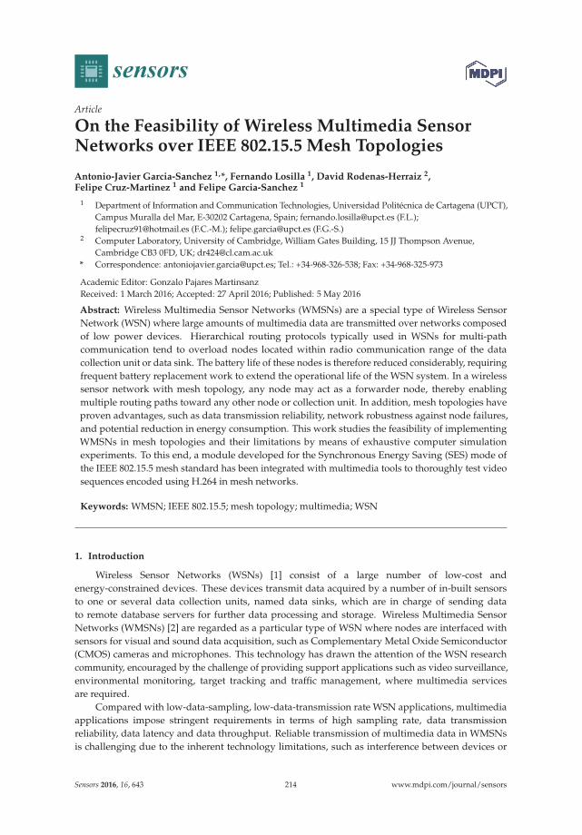
sensors

Article

On the Feasibility of Wireless Multimedia SensorNetworks over IEEE 802.15.5 Mesh Topologies

Antonio-Javier Garcia-Sanchez 1,*, Fernando Losilla 1, David Rodenas-Herraiz 2,Felipe Cruz-Martinez 1 and Felipe Garcia-Sanchez 1

1 Department of Information and Communication Technologies, Universidad Politécnica de Cartagena (UPCT),Campus Muralla del Mar, E-30202 Cartagena, Spain; [email protected] (F.L.);[email protected] (F.C.-M.); [email protected] (F.G.-S.)

2 Computer Laboratory, University of Cambridge, William Gates Building, 15 JJ Thompson Avenue,Cambridge CB3 0FD, UK; [email protected]

* Correspondence: [email protected]; Tel.: +34-968-326-538; Fax: +34-968-325-973

Academic Editor: Gonzalo Pajares MartinsanzReceived: 1 March 2016; Accepted: 27 April 2016; Published: 5 May 2016

Abstract: Wireless Multimedia Sensor Networks (WMSNs) are a special type of Wireless SensorNetwork (WSN) where large amounts of multimedia data are transmitted over networks composedof low power devices. Hierarchical routing protocols typically used in WSNs for multi-pathcommunication tend to overload nodes located within radio communication range of the datacollection unit or data sink. The battery life of these nodes is therefore reduced considerably, requiringfrequent battery replacement work to extend the operational life of the WSN system. In a wirelesssensor network with mesh topology, any node may act as a forwarder node, thereby enablingmultiple routing paths toward any other node or collection unit. In addition, mesh topologies haveproven advantages, such as data transmission reliability, network robustness against node failures,and potential reduction in energy consumption. This work studies the feasibility of implementingWMSNs in mesh topologies and their limitations by means of exhaustive computer simulationexperiments. To this end, a module developed for the Synchronous Energy Saving (SES) mode ofthe IEEE 802.15.5 mesh standard has been integrated with multimedia tools to thoroughly test videosequences encoded using H.264 in mesh networks.

Keywords: WMSN; IEEE 802.15.5; mesh topology; multimedia; WSN

1. Introduction

Wireless Sensor Networks (WSNs) [1] consist of a large number of low-cost andenergy-constrained devices. These devices transmit data acquired by a number of in-built sensorsto one or several data collection units, named data sinks, which are in charge of sending datato remote database servers for further data processing and storage. Wireless Multimedia SensorNetworks (WMSNs) [2] are regarded as a particular type of WSN where nodes are interfaced withsensors for visual and sound data acquisition, such as Complementary Metal Oxide Semiconductor(CMOS) cameras and microphones. This technology has drawn the attention of the WSN researchcommunity, encouraged by the challenge of providing support applications such as video surveillance,environmental monitoring, target tracking and traffic management, where multimedia servicesare required.

Compared with low-data-sampling, low-data-transmission rate WSN applications, multimediaapplications impose stringent requirements in terms of high sampling rate, data transmissionreliability, data latency and data throughput. Reliable transmission of multimedia data in WMSNsis challenging due to the inherent technology limitations, such as interference between devices or


Sensors 2016, 16, 643

limited data transmission bandwidth. Multimedia communications also require a high utilization ofthe transmission channel, increasing communication activity within the network and considerablydecreasing the operational lifetime of battery-powered nodes. This clearly contrasts with the traditionalWSN/WMSN requirements imposed by, on the one hand, the use of short-range communications overlow-bandwidth links (maximum bitrate of 250 kbps at 2.4 GHz) and, on the other hand, the energyconstraints of sensor devices.

Traditional routing in WSNs is also a problem in WMSNs. Many state-of-the-art multi-hopproposals for WSNs consider tree-based topological configurations where only a few number of nodesare likely to forward all the data traffic. Because of the intensive use of these nodes, the network maynot fulfil the Quality of Service (QoS) required by the multimedia application and, more importantly, itwill lead to the overuse and depletion of the batteries of nodes in the path. In addition, traditionalrouting mechanisms usually only deal with the transmission to a sink node and not to any arbitrarynode of the network, which hampers the development of collaborative applications or the use ofmultiple sinks.

Mesh topologies, in addition to enabling multiple routing paths between two nodes outsideof radio communication range with each other, have proven advantages against other topologicalconfigurations, such as tree-based or cluster-based topologies, which include data transmissionreliability, network robustness against node failures, and potential reduction in energy consumption [3].Nodes arranged in a mesh topology are generally easier to deploy and potentially easier to maintain asthey are able to reconfigure themselves in order to adapt to the conditions brought by the deploymentenvironment. Among the different mesh solutions available for low-power wireless networks, thelow-rate part of the IEEE 802.15.5 (hereafter IEEE 802.15.5) [4] offers suitable functionalities forenabling multimedia applications compared with other state-of-the-art network/MAC layer standards.This standard assures that any node is able to communicate with any other node of the networkthrough different routes, enhancing data transmission reliability and robustness against node failures.It also emphasizes simplicity, adding, for low-rate WPAN, a thin mesh sublayer on top of the IEEE802.15.4 MAC sublayer, the most widely adopted point-to-point communication standard for low-ratewireless personal area networks (LR-WPANs). This results in an easy migration of applications usingthe 802.15.4 standard and in a greater scalability, enabling large-scale deployments. In addition, thestandard provides two radio duty-cycle mechanisms, named Asynchronous Energy Saving (ASES)and Synchronous Energy Saving (SES). These mechanisms are intended to make efficient use of theavailable battery energy for, respectively, asynchronous and synchronous communications, therebyprolonging the battery life. For all the aforementioned reasons, IEEE 802.15.5 can be, a priori, a suitableand representative WMSN solution for the transmission of video in mesh topologies.

However, according to our knowledge, there are very few studies in the scientific literaturecombining mesh topologies with multimedia applications for low power devices. Under thesecircumstances, the purpose of this paper is to contribute to the development of multimedia applicationsin the WMSN arena, fulfilling the WSN/WMSN specific requirements, assuring the QoS of themultimedia service and achieving a reasonable performance of the network in terms of, for instance,lifetime and data transmission reliability. To achieve these goals, we have designed a novel tool,available for download, that evaluates, by means of computer simulation, the performance of videotransmissions using the SES energy-saving mechanism of IEEE 802.15.5. For the evaluation of thestandard, Quarter Common Intermediate Format (QCIF) video sequences are encoded using theH.264/AVC compression standard and transmitted through WMSN mesh networks of different sizes.The main results will be discussed, highlighting the most important metrics such as latency, jitter, timebetween packets, message delivery ratio, power consumption, lifetime and Peak Signal-to-Noise Ratio(PSNR). The rest of this paper is organized as follows: Section 2 introduces related work in the field ofWMSNs. Section 3 provides the necessary technological background about video encoding with H.264as well as WMSN operation based on the IEEE 802.15.5 standard. Section 4 describes the simulation

215

Sensors 2016, 16, 643

tool and simulation environment. Section 5 shows and analyzes simulation results, which are furtherdiscussed in Section 6. Section 7 concludes this work.

2. Related Work

In spite of the proven advantages arising from the use of the IEEE 802.15.5 standard, to theknowledge of the authors, there is no other work that makes use of this technology in WMSNs. Thereare however a number of proposals that use mesh communication for transmitting multimedia flows [5].However, they do not consider Wireless Sensor Networks but rather focus on less energy-constrainedstandards such as 802.11. In this regard, the purpose of this work is twofold: first, to carry out a firstevaluation of the performance of a mesh standard, the IEEE 802.15.5, for video transmission; second,to provide simulation tools to help evaluate further improvements for multimedia transmission madeto the original standard.

The performance of WSNs and WMSNs should be assessed using real WSN/WMSN hardwarebefore actual deployment, for example, using a test bed in the laboratory. However, it is best practiceto make sure that no software/hardware errors are introduced before test-bed experiments are carriedout. Finding and correcting these errors is usually a tedious and time-consuming task, and simulationis a powerful tool that helps do this in a much faster and easier way than dealing directly withhardware. In this regard, Pham [6] studied the communication performance of the most popular WSNcommercial platforms to date in data-intensive applications. Results showed significant delays limitingthe maximum data throughput at both the sender and the receiver. The best results were obtainedusing MicaZ devices [7]. Pham also showed that more effort should be made on the developmentof new hardware platforms, but also that more realistic simulation models are needed to considerthe constraints of these commercial devices. Farooq et al. [8] studied the feasibility of performingthe evaluation of new multimedia proposals in large WSN testbeds available for research usage.They concluded that, despite the existence of powerful hardware platforms for multimedia applications,there has been little work yet to integrate them into testbeds. Consequently, simulations are the mostcost-effective solution for evaluating WMSN proposals.

Some researches focused on comparing the performance of data-intensive WMSN applicationsusing different MAC and network protocols for diverse layouts. Ammar et al. [9] compared theperformance obtained in WMSN by using two well-known WSN MAC protocols, S-MAC and 802.15.4,and two routing protocols, Ad hoc On-Demand Distance Vector (AODV) routing and its extensionAd hoc On-demand Multipath Distance Vector (AOMDV) routing. They remarked on the importanceof optimizing the network layer protocols. In addition, their simulation results showed a betterperformance of the IEEE 802.15.4 standard in terms of network lifetime, which is supported by thelarge number of WMSN proposals based on this standard. Andrea et al. [10] studied this standard inone-hop data-intensive networks with star topology. They simulated a video surveillance system bycontinuously transmitting images to a sink node. Among other outcomes, their study determinedthat the Packet Error Rate for this kind of traffic, where packets have the maximum size allowedby the IEEE 802.15.4 standard, presents a significant increase as the network grows in comparisonwith typical WSNs with scalar sensors and short packets. In the same line, Pekhteryev et al. [11]performed a similar research in ZigBee networks that showed the difficulties in transmitting imagesover multi-hop networks. Although they only compared one-hop and two-hop schemes, they observedan important decrease in the percentage of recoverable images at the receiver for the two-hop scenario(from 2.6% to 20.5% using JPEG images, while for JPEG 2000 images the tests for the two-hop scenariocould not completed due to interferences from other nodes).

There are other studies that focus on optimizing wireless performance communication inWMSNs in different ways. One of them considers cross-layer approaches to improve QoS.García-Sánchez et al. [12] used application-level QoS parameters to tune the MAC and physical layersof the popular IEEE 802.15.4 standard. An important increase in the maximum throughput for one-hopmultimedia transmissions was achieved by means of a series of optimizations which maximized the

216

Sensors 2016, 16, 643

amount of data transmitted and avoided collisions due to imperfect synchronization and other issues.In addition, the proposed solution remained compliant with the original standard. Farooq et al. [13]proposed another cross-layer architecture for multi-hop clustered networks where, upon congestion,nodes are requested to reduce the data transmission rate to avoid congestion. The authors useda differentiated services approach that classifies data traffic according to six different classes andwhere nodes producing less data and low priority data are penalized more than those producing highvolumes of data and high priority data. Alanazi et al. [14] evaluated other QoS routing protocols forreal-time WMSN applications, among which the Pheromone Termite (PT) protocol [15] offered betterperformance. The protocol, though, relies on both ad-hoc MAC and, more importantly, physical layers,which makes its implementation on real devices very difficult.

In video transmission, the importance of each video frame can be used to select different QoSprofiles. Kandris et al. [16] developed a video distortion model that made it possible to predict the effecton video quality of dropping each packet. In case of congestion, typically found when transmittingmultimedia flows, this model is used to selectively drop less significant packets prior to transmission,therefore improving performance at the expense of additional computing load. The authors also useda hierarchical routing protocol with asymmetrical communications, where the sink is able to transmitdirectly to all nodes, with no intermediary hops. Zaidi et al. [17] developed a multipath protocol thatobtained three different paths toward a sink node and, based on Bit Error Rate and delay, selectedthe best of them for the transmission of the most important video frames (the I frames, explainedin Section 3).

In general, multipath communication has traditionally been used to increase robustness orreliability in WMSNs. For example, the MMSPEED protocol [18] uses probabilistic multipathforwarding to control the number of paths based on the required delivery probability. In this way,depending on the packet loss rate and QoS requirements, it can send multiple copies of a same packetto ensure the delivery of data. In WMSNs, multipath can also be used to increase the throughput indata-intensive flows. Teo et al. [19] proposed a routing protocol, I2MR, that transmits simultaneouslythrough two paths. In order to avoid interference between them, the protocol uses the shortestpath between source and destination as the primary path and marks one- and two-hop neighborsof nodes in the primary path as the interference zone. A secondary path as well as a backup pathare then constructed using nodes outside the interference zone. This protocol is intended for lessenergy-constrained 802.11 networks, but there are similar proposals using more energy-constrainedstandards. Maimour [20] developed the MR2 protocol. This protocol, which is better suited for denseWSN deployments, is also interference-aware, and constructs paths incrementally. After obtaininga new path, all of the nodes neighboring to the path, which potentially may cause interference, arenotified and put in a passive mode and cannot be used for new paths. Therefore, avoiding interferenceand saving energy. Li et al. [21] proposed GEAM, a Geographic Energy-Aware Multipath routingscheme that divides the network into what the authors named “districts”. The distance between themis sufficiently large to avoid transmission interference. To send a packet, GEAM assigns the packetto a district and forwards it to the sink using the greedy algorithm. Consequently, it is necessarythat each node is aware of its location. Bidai et al. [22] developed another multipath routing schemefor video transmission that combines proactive routing, which provides fast response to events ofinterest, with reactive routing. In this way, upon the detection of an event, the transmission of datapackets to the sink starts immediately and, simultaneously, a route discovery phase begins wherenew paths to the sink are discovered. These paths are selected according to a metric defined by theauthors that estimates their amount of interference. Simulation results demonstrate that selecting theless interfering path can increase throughput and decrease packet loss.

Table 1 shows the main contributions of the abovementioned proposals, as well as other features.As it can be observed, many of the proposals use either the IEEE 802.11 standard or the non-beaconmode of the IEEE 802.15.4 standard, which does not define how duty-cycling should be carried out.The 802.11 standard allows higher data transmission bit rates, therefore allowing for higher data

217

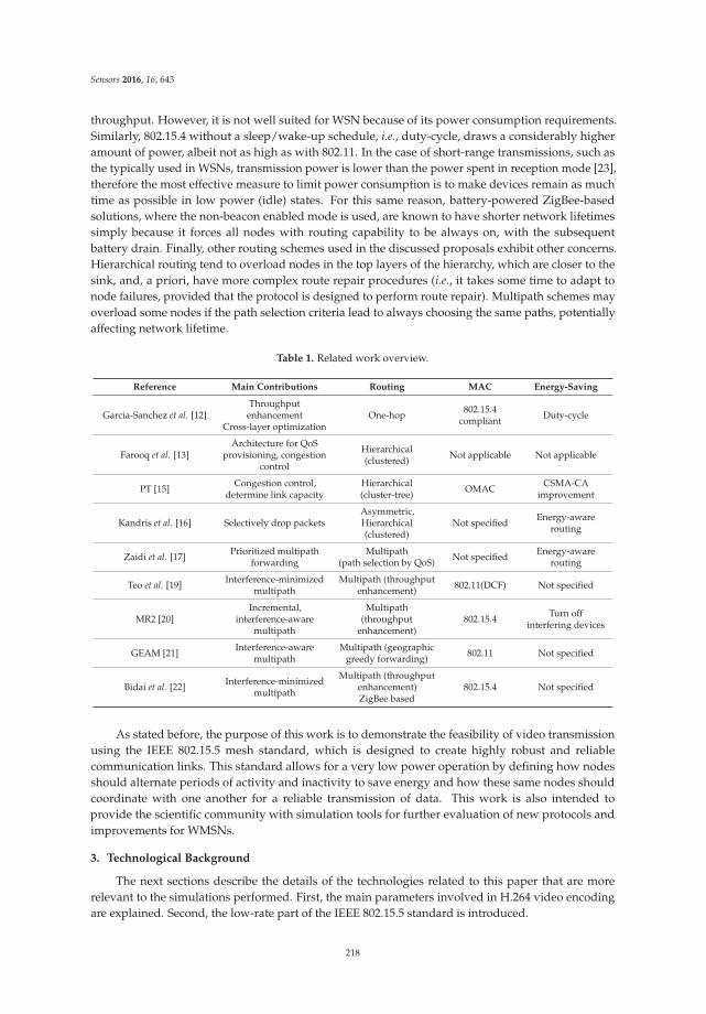
Sensors 2016, 16, 643

throughput. However, it is not well suited for WSN because of its power consumption requirements.Similarly, 802.15.4 without a sleep/wake-up schedule, i.e., duty-cycle, draws a considerably higheramount of power, albeit not as high as with 802.11. In the case of short-range transmissions, such asthe typically used in WSNs, transmission power is lower than the power spent in reception mode [23],therefore the most effective measure to limit power consumption is to make devices remain as muchtime as possible in low power (idle) states. For this same reason, battery-powered ZigBee-basedsolutions, where the non-beacon enabled mode is used, are known to have shorter network lifetimessimply because it forces all nodes with routing capability to be always on, with the subsequentbattery drain. Finally, other routing schemes used in the discussed proposals exhibit other concerns.Hierarchical routing tend to overload nodes in the top layers of the hierarchy, which are closer to thesink, and, a priori, have more complex route repair procedures (i.e., it takes some time to adapt tonode failures, provided that the protocol is designed to perform route repair). Multipath schemes mayoverload some nodes if the path selection criteria lead to always choosing the same paths, potentiallyaffecting network lifetime.

Table 1. Related work overview.

Reference Main Contributions Routing MAC Energy-Saving

Garcia-Sanchez et al. [12]Throughput

enhancementCross-layer optimization

One-hop802.15.4

compliantDuty-cycle

Farooq et al. [13]Architecture for QoS

provisioning, congestioncontrol

Hierarchical(clustered)

Not applicable Not applicable

PT [15]Congestion control,

determine link capacityHierarchical(cluster-tree)

OMACCSMA-CA

improvement

Kandris et al. [16] Selectively drop packetsAsymmetric,Hierarchical(clustered)

Not specifiedEnergy-aware

routing

Zaidi et al. [17]Prioritized multipath

forwardingMultipath

(path selection by QoS)Not specified

Energy-awarerouting

Teo et al. [19]Interference-minimized

multipathMultipath (throughput

enhancement)802.11(DCF) Not specified

MR2 [20]Incremental,

interference-awaremultipath

Multipath(throughput

enhancement)802.15.4

Turn offinterfering devices

GEAM [21]Interference-aware

multipathMultipath (geographic

greedy forwarding)802.11 Not specified

Bidai et al. [22]Interference-minimized

multipath

Multipath (throughputenhancement)ZigBee based

802.15.4 Not specified

As stated before, the purpose of this work is to demonstrate the feasibility of video transmissionusing the IEEE 802.15.5 mesh standard, which is designed to create highly robust and reliablecommunication links. This standard allows for a very low power operation by defining how nodesshould alternate periods of activity and inactivity to save energy and how these same nodes shouldcoordinate with one another for a reliable transmission of data. This work is also intended toprovide the scientific community with simulation tools for further evaluation of new protocols andimprovements for WMSNs.

3. Technological Background

The next sections describe the details of the technologies related to this paper that are morerelevant to the simulations performed. First, the main parameters involved in H.264 video encodingare explained. Second, the low-rate part of the IEEE 802.15.5 standard is introduced.

218

Sensors 2016, 16, 643

3.1. H.264 Video Encoding

As already stated, the transmission of video in low-power WSNs is challenging due to theirinherent constraints. The transmission of large amounts of data poses additional problems such ascontention for medium access, which increases jitter and further decreases throughput. It is clearthat in order to cope with these restrictions video compression is needed. As an example, a typicalQCIF sequence (176 ˆ 144 pixels) at 30 frames per second requires almost 6 Mbps to be transmitteduncompressed via streaming. However, the nominal transmission rate of IEEE 802.15.4-compliantdevices, such as MICAz [7] or TelosB [24], is 250 kbps when operating in the 2.4 GHz ISM band.

H.264 [25], also known as MPEG-4 Part 10 or MPEG-4 Advanced Video Coding (AVC), is one ofthe most popular standards for video encoding. It is about 1.5 to 2 times more efficient than MPEG-4(Part 2) encoding, resulting in smaller compressed files. This is crucial for WMSNs, which are severelyconstrained by the transmission rate and energy consumption of nodes. The main benefit arising fromthe use of H.264 in WMSNs is the reduction in the number of data messages necessary for transmittinga video frame. This further helps reduce the network congestion and prolong the nodes lifetime.As a drawback, H.264 encoding requires more energy at the source node. However, according to [26],the use of H.264 results in a better lifetime in networks with at least five hops between the sensornodes and the data sink and also in smaller networks with more complex video contents or morestringent video quality requirements. A more detailed study about energy spent in video encodingcan be found in [27].

Several encoding parameters used by H.264 (GOP size, Quantization Parameter and CRF mode),which will be referred to subsequently, are described next.

The Group of Pictures (GOP) structure specifies the order in which different types of frames arearranged in inter-frame encoding techniques. H.264 uses three different types of frames:

- I-frames (intra-coded frames). I-frames are encoded independently of all other frames. They arethe largest frames and provide the best quality, but they are also the least efficient froma compression perspective.

- P-frames (predictive-coded frames). P-frames reference redundant information contained inprevious frames (I or P frames). Therefore, they contain a lesser amount of information.

- B-frames (bidirectional predictive-coded frames). B-frames can reference both previous and futureframes. From a compression perspective, they are the most efficient frames.

Encoders usually require the GOP size as a parameter, which is the number of frames in a GOPstructure. Since a GOP only contains an I-frame at the beginning of the structure, this parameter setsthe separation between two I-frames.

For each frame, the Quantization Parameter (QP) regulates how much spatial detail is saved ordiscarded. In this paper, rather than using a fixed QP for each frame, the Constant Rate Factor (CRF)mode is used instead. With this mode, the encoder tries to achieve a constant perceptual quality levelfor all frames by adjusting the QP according to the characteristics of each frame. That is, it uses highercompression rates for frames with high motion, as the loss of detail is harder to notice in movingobjects. A CRF parameter, ranging from 0 to 51, is defined to control the desired quality of the video,where lower values result in better quality and higher values in more compressed video sequences.

In this work, the value of the CRF has been set to 24 since this offers a balance between videoquality and compression. In Table 2 different metrics are compared for CRF values of 10 and 24 usingthe same video sequence. It can be observed that a value of 24 decreases the bitrate of the compressedvideo and, consequently, the transmission time over a 6 ˆ 6 grid mesh network. The drop in quality ofthe video is very small, as can be observed by comparing Figure 1.

219

Sensors 2016, 16, 643

Table 2. Comparison of bitrate, latency (Latency, see Section 5.1) and PSNR (Peak Signal-to-Noise Ratio(PSNR), objective video (or signal) quality metric, analyzed in Section 5.6) according to CRF.

CRF Bitrate (kbps) Latency (s) Mean PSNR (dB)

10 (medium-lowcompression level)

247 356.704 50.936

24 (medium-highcompression level)

53 84.042 41.730

Figure 1. (a) Akiyo QCIF, CRF = 10; (b) Akiyo QCIF, CRF = 24.

3.2. IEEE 802.15.5 Low Rate

IEEE 802.15.4 standard defines Physical (PHY) and Medium Access Control (MAC) specificationsfor Low-Rate Wireless Personal Networks (LR-WPAN). This standard does not define the network layerand, therefore, does not offer routing capabilities by itself. Consequently, with the aim of providingan efficient multi-hop scheme, the IEEE 802.15.5 standard emerged in 2009. This new standard hasa low-rate part, which will be the focus of the paper, consisting of a set of recommendations, which,according to the standard, provide an architectural framework that enables low-power, low-rate WPANdevices to promote interoperable, stable, and scalable wireless mesh topologies [28].

The objective of the standard is to support features such as unicast, multicast and reliable broadcastover multi-hop mesh links, synchronous and asynchronous communication for power saving, traceroute functionality and portability of end devices [28]. In addition, being a mesh standard, it providesroute redundancy, which enhances network reliability. Another key feature of the standard is thatit fosters simplicity. There is no need for route discovery, reducing communication overhead, orfor storing routing tables for all possible destinations. One of its main advantages over other meshnetworking approaches is that it has a very similar set of service access points to the 802.15.4 MACsublayer and, therefore, migration from non-mesh IEEE 802.15.4 networks to mesh networks isa straightforward process. In this regard, IEEE 802.15.5 aims at standardizing mesh networking overIEEE 802.15.4.

Figure 2 shows a comparison of the topologies of an IEEE 802.15.5 network with a cluster-treeIEEE 802.15.4 network. The main difference lies in the mesh links (represented by dashed lines), whichconnect any node with any neighbor node within communication range. The types of device defined inan IEEE 802.15.5 network are also shown in the Figure. A mesh coordinator is the root of the logical treeof the mesh network. It creates and manages the mesh network, and may also serve as the referenceclock when network-wide synchronization is required. Mesh devices are responsible for intelligentlyrelaying sensor data toward their intended destination. Finally, end devices are generally nodes within-built sensors and do not include mesh routing capability.

The establishment of the network topology is key to the operation of IEEE 802.15.5. During thisprocess, logic addresses are assigned to nodes according to their position in the network. By bindinglogic addresses to the network topology, the Tunneled Direct Link Setup (TDLS) routing protocol [29]suggested by the IEEE 802.15.5 standard can forward packets without performing route discovery,

220

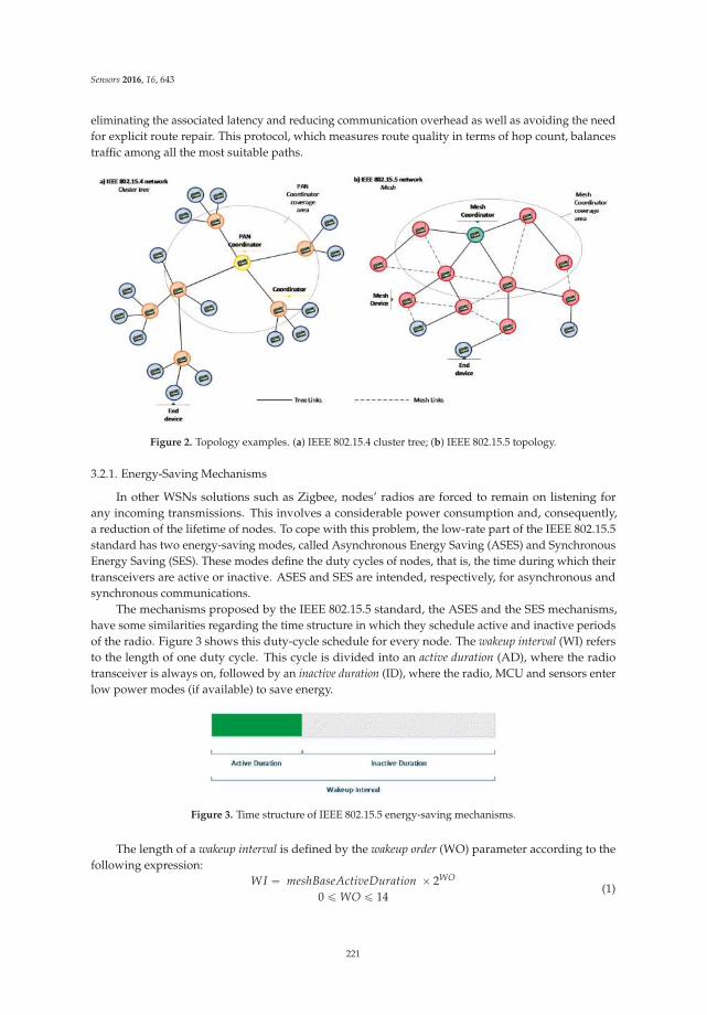
Sensors 2016, 16, 643

eliminating the associated latency and reducing communication overhead as well as avoiding the needfor explicit route repair. This protocol, which measures route quality in terms of hop count, balancestraffic among all the most suitable paths.

Figure 2. Topology examples. (a) IEEE 802.15.4 cluster tree; (b) IEEE 802.15.5 topology.

3.2.1. Energy-Saving Mechanisms

In other WSNs solutions such as Zigbee, nodes’ radios are forced to remain on listening forany incoming transmissions. This involves a considerable power consumption and, consequently,a reduction of the lifetime of nodes. To cope with this problem, the low-rate part of the IEEE 802.15.5standard has two energy-saving modes, called Asynchronous Energy Saving (ASES) and SynchronousEnergy Saving (SES). These modes define the duty cycles of nodes, that is, the time during which theirtransceivers are active or inactive. ASES and SES are intended, respectively, for asynchronous andsynchronous communications.

The mechanisms proposed by the IEEE 802.15.5 standard, the ASES and the SES mechanisms,have some similarities regarding the time structure in which they schedule active and inactive periodsof the radio. Figure 3 shows this duty-cycle schedule for every node. The wakeup interval (WI) refersto the length of one duty cycle. This cycle is divided into an active duration (AD), where the radiotransceiver is always on, followed by an inactive duration (ID), where the radio, MCU and sensors enterlow power modes (if available) to save energy.

Figure 3. Time structure of IEEE 802.15.5 energy-saving mechanisms.

The length of a wakeup interval is defined by the wakeup order (WO) parameter according to thefollowing expression:

WI “ meshBaseActiveDuration ˆ 2WO

0 ď WO ď 14(1)

221

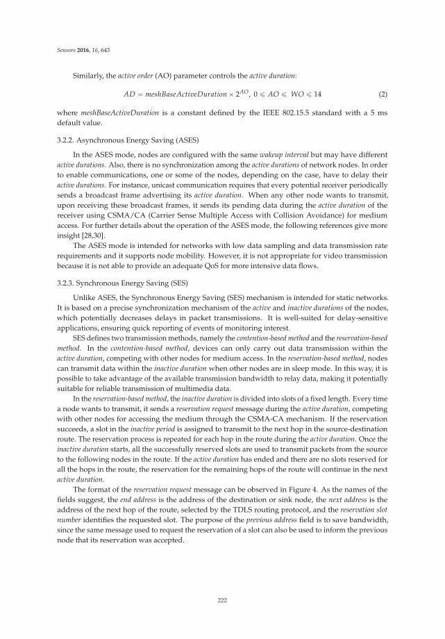
Sensors 2016, 16, 643

Similarly, the active order (AO) parameter controls the active duration:

AD “ meshBaseActiveDuration ˆ 2AO, 0 ď AO ď WO ď 14 (2)

where meshBaseActiveDuration is a constant defined by the IEEE 802.15.5 standard with a 5 msdefault value.

3.2.2. Asynchronous Energy Saving (ASES)

In the ASES mode, nodes are configured with the same wakeup interval but may have differentactive durations. Also, there is no synchronization among the active durations of network nodes. In orderto enable communications, one or some of the nodes, depending on the case, have to delay theiractive durations. For instance, unicast communication requires that every potential receiver periodicallysends a broadcast frame advertising its active duration. When any other node wants to transmit,upon receiving these broadcast frames, it sends its pending data during the active duration of thereceiver using CSMA/CA (Carrier Sense Multiple Access with Collision Avoidance) for mediumaccess. For further details about the operation of the ASES mode, the following references give moreinsight [28,30].

The ASES mode is intended for networks with low data sampling and data transmission raterequirements and it supports node mobility. However, it is not appropriate for video transmissionbecause it is not able to provide an adequate QoS for more intensive data flows.

3.2.3. Synchronous Energy Saving (SES)

Unlike ASES, the Synchronous Energy Saving (SES) mechanism is intended for static networks.It is based on a precise synchronization mechanism of the active and inactive durations of the nodes,which potentially decreases delays in packet transmissions. It is well-suited for delay-sensitiveapplications, ensuring quick reporting of events of monitoring interest.

SES defines two transmission methods, namely the contention-based method and the reservation-based

method. In the contention-based method, devices can only carry out data transmission within theactive duration, competing with other nodes for medium access. In the reservation-based method, nodescan transmit data within the inactive duration when other nodes are in sleep mode. In this way, it ispossible to take advantage of the available transmission bandwidth to relay data, making it potentiallysuitable for reliable transmission of multimedia data.

In the reservation-based method, the inactive duration is divided into slots of a fixed length. Every timea node wants to transmit, it sends a reservation request message during the active duration, competingwith other nodes for accessing the medium through the CSMA-CA mechanism. If the reservationsucceeds, a slot in the inactive period is assigned to transmit to the next hop in the source-destinationroute. The reservation process is repeated for each hop in the route during the active duration. Once theinactive duration starts, all the successfully reserved slots are used to transmit packets from the sourceto the following nodes in the route. If the active duration has ended and there are no slots reserved forall the hops in the route, the reservation for the remaining hops of the route will continue in the nextactive duration.

The format of the reservation request message can be observed in Figure 4. As the names of thefields suggest, the end address is the address of the destination or sink node, the next address is theaddress of the next hop of the route, selected by the TDLS routing protocol, and the reservation slot

number identifies the requested slot. The purpose of the previous address field is to save bandwidth,since the same message used to request the reservation of a slot can also be used to inform the previousnode that its reservation was accepted.

222

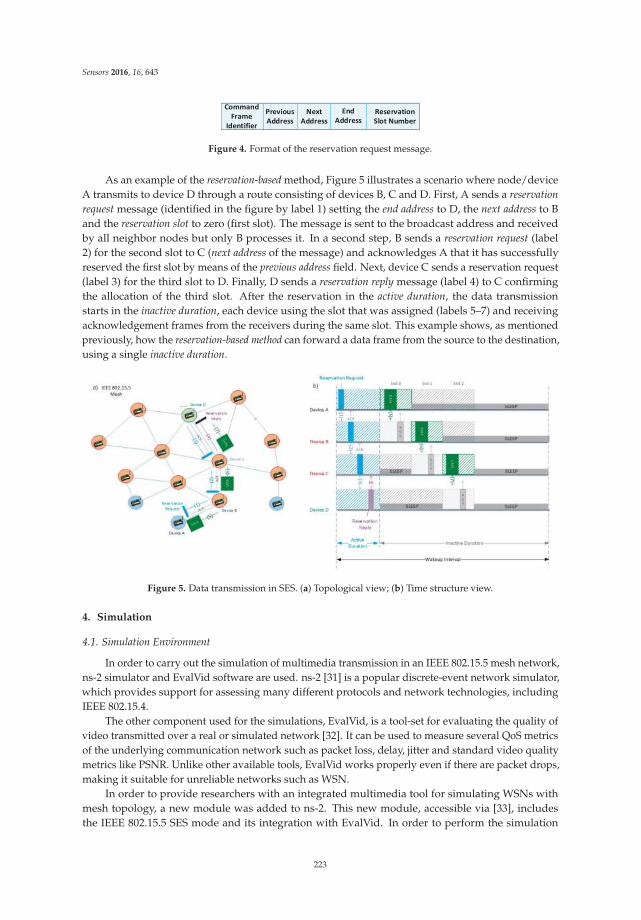
Sensors 2016, 16, 643

Command

Frame

Identifier

Previous

Address

Next

Address

Reservation

Slot Number

End

Address

Figure 4. Format of the reservation request message.

As an example of the reservation-based method, Figure 5 illustrates a scenario where node/deviceA transmits to device D through a route consisting of devices B, C and D. First, A sends a reservation

request message (identified in the figure by label 1) setting the end address to D, the next address to Band the reservation slot to zero (first slot). The message is sent to the broadcast address and receivedby all neighbor nodes but only B processes it. In a second step, B sends a reservation request (label2) for the second slot to C (next address of the message) and acknowledges A that it has successfullyreserved the first slot by means of the previous address field. Next, device C sends a reservation request(label 3) for the third slot to D. Finally, D sends a reservation reply message (label 4) to C confirmingthe allocation of the third slot. After the reservation in the active duration, the data transmissionstarts in the inactive duration, each device using the slot that was assigned (labels 5–7) and receivingacknowledgement frames from the receivers during the same slot. This example shows, as mentionedpreviously, how the reservation-based method can forward a data frame from the source to the destination,using a single inactive duration.

Figure 5. Data transmission in SES. (a) Topological view; (b) Time structure view.

4. Simulation

4.1. Simulation Environment

In order to carry out the simulation of multimedia transmission in an IEEE 802.15.5 mesh network,ns-2 simulator and EvalVid software are used. ns-2 [31] is a popular discrete-event network simulator,which provides support for assessing many different protocols and network technologies, includingIEEE 802.15.4.

The other component used for the simulations, EvalVid, is a tool-set for evaluating the quality ofvideo transmitted over a real or simulated network [32]. It can be used to measure several QoS metricsof the underlying communication network such as packet loss, delay, jitter and standard video qualitymetrics like PSNR. Unlike other available tools, EvalVid works properly even if there are packet drops,making it suitable for unreliable networks such as WSN.

In order to provide researchers with an integrated multimedia tool for simulating WSNs withmesh topology, a new module was added to ns-2. This new module, accessible via [33], includesthe IEEE 802.15.5 SES mode and its integration with EvalVid. In order to perform the simulation

223

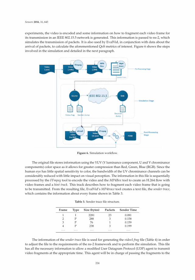
Sensors 2016, 16, 643

experiments, the video is encoded and some information on how to fragment each video frame forits transmission in an IEEE 802.15.5 network is generated. This information is passed to ns-2, whichsimulates the transmission of packets. It is also used by EvalVid, in conjunction with data about thearrival of packets, to calculate the aforementioned QoS metrics of interest. Figure 6 shows the stepsinvolved in the simulation and detailed in the next paragraph.

Figure 6. Simulation workflow.

The original file stores information using the YUV (Y luminance component, U and V chrominancecomponents) color space as it allows for greater compression than Red, Green, Blue (RGB). Since thehuman eye has little spatial sensitivity to color, the bandwidth of the UV chrominance channels can beconsiderably reduced with little impact on visual perception. The information in this file is sequentiallyprocessed by the FFmpeg tool to encode the video and the MP4Box tool to create an H.264 flow withvideo frames and a hint track. This track describes how to fragment each video frame that is goingto be transmitted. From the resulting file, EvalVid’s MP4trace tool creates a text file, the sender trace,which contains the information about every frame shown in Table 3.

Table 3. Sender trace file structure.

Frame Type Size (bytes) Packets Sender Time

1 I 2281 23 0.0812 P 288 3 0.1583 P 76 1 0.1594 P 238 3 0.199

. . . . . . . . . . . . . . .

The information of the sender trace file is used for generating the video1.frag file (Table 4) in orderto adjust the file to the requirements of the ns-2 framework and to perform the simulation. This filehas all the necessary information to allow a modified User Datagram Protocol (UDP) agent to transmitvideo fragments at the appropriate time. This agent will be in charge of passing the fragments to the

224

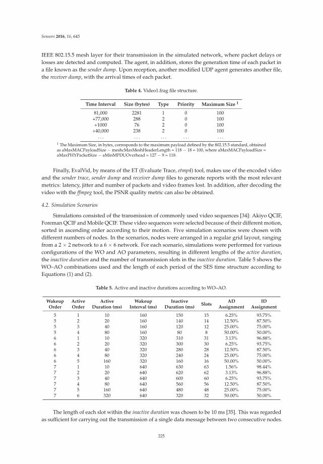
Sensors 2016, 16, 643

IEEE 802.15.5 mesh layer for their transmission in the simulated network, where packet delays orlosses are detected and computed. The agent, in addition, stores the generation time of each packet ina file known as the sender dump. Upon reception, another modified UDP agent generates another file,the receiver dump, with the arrival times of each packet.

Table 4. Video1.frag file structure.

Time Interval Size (bytes) Type Priority Maximum Size 1

81,000 2281 1 0 100+77,000 288 2 0 100+1000 76 2 0 100

+40,000 238 2 0 100. . . . . . . . . . . . . . .

1 The Maximum Size, in bytes, corresponds to the maximum payload defined by the 802.15.5 standard, obtainedas aMaxMACPayloadSize ´ meshcMaxMeshHeaderLength = 118 ´ 18 = 100, where aMaxMACPayloadSize =aMaxPHYPacketSize ´ aMinMPDUOverhead = 127 ´ 9 = 118.

Finally, EvalVid, by means of the ET (Evaluate Trace, etmp4) tool, makes use of the encoded videoand the sender trace, sender dump and receiver dump files to generate reports with the most relevantmetrics: latency, jitter and number of packets and video frames lost. In addition, after decoding thevideo with the ffmpeg tool, the PSNR quality metric can also be obtained.

4.2. Simulation Scenarios

Simulations consisted of the transmission of commonly used video sequences [34]: Akiyo QCIF,Foreman QCIF and Mobile QCIF. These video sequences were selected because of their different motion,sorted in ascending order according to their motion. Five simulation scenarios were chosen withdifferent numbers of nodes. In the scenarios, nodes were arranged in a regular grid layout, rangingfrom a 2 ˆ 2 network to a 6 ˆ 6 network. For each scenario, simulations were performed for variousconfigurations of the WO and AO parameters, resulting in different lengths of the active duration,the inactive duration and the number of transmission slots in the inactive duration. Table 5 shows theWO–AO combinations used and the length of each period of the SES time structure according toEquations (1) and (2).

Table 5. Active and inactive durations according to WO–AO.

WakeupOrder

ActiveOrder

ActiveDuration (ms)

WakeupInterval (ms)

InactiveDuration (ms)

SlotsAD

AssignmentID

Assignment

5 1 10 160 150 15 6.25% 93.75%5 2 20 160 140 14 12.50% 87.50%5 3 40 160 120 12 25.00% 75.00%5 4 80 160 80 8 50.00% 50.00%6 1 10 320 310 31 3.13% 96.88%6 2 20 320 300 30 6.25% 93.75%6 3 40 320 280 28 12.50% 87.50%6 4 80 320 240 24 25.00% 75.00%6 5 160 320 160 16 50.00% 50.00%7 1 10 640 630 63 1.56% 98.44%7 2 20 640 620 62 3.13% 96.88%7 3 40 640 600 60 6.25% 93.75%7 4 80 640 560 56 12.50% 87.50%7 5 160 640 480 48 25.00% 75.00%7 6 320 640 320 32 50.00% 50.00%

The length of each slot within the inactive duration was chosen to be 10 ms [35]. This was regardedas sufficient for carrying out the transmission of a single data message between two consecutive nodes.

225

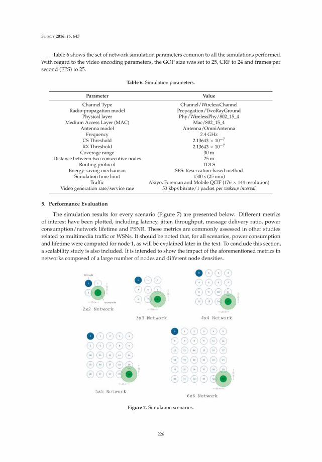
Sensors 2016, 16, 643

Table 6 shows the set of network simulation parameters common to all the simulations performed.With regard to the video encoding parameters, the GOP size was set to 25, CRF to 24 and frames persecond (FPS) to 25.

Table 6. Simulation parameters.

Parameter Value

Channel Type Channel/WirelessChannelRadio-propagation model Propagation/TwoRayGround

Physical layer Phy/WirelessPhy/802_15_4Medium Access Layer (MAC) Mac/802_15_4

Antenna model Antenna/OmniAntennaFrequency 2.4 GHz

CS Threshold 2.13643 ˆ 10´7

RX Threshold 2.13643 ˆ 10´7

Coverage range 30 mDistance between two consecutive nodes 25 m

Routing protocol TDLSEnergy-saving mechanism SES: Reservation-based method

Simulation time limit 1500 s (25 min)Traffic Akiyo, Foreman and Mobile QCIF (176 ˆ 144 resolution)

Video generation rate/service rate 53 kbps bitrate/1 packet per wakeup interval

5. Performance Evaluation

The simulation results for every scenario (Figure 7) are presented below. Different metricsof interest have been plotted, including latency, jitter, throughput, message delivery ratio, powerconsumption/network lifetime and PSNR. These metrics are commonly assessed in other studiesrelated to multimedia traffic or WSNs. It should be noted that, for all scenarios, power consumptionand lifetime were computed for node 1, as will be explained later in the text. To conclude this section,a scalability study is also included. It is intended to show the impact of the aforementioned metrics innetworks composed of a large number of nodes and different node densities.

Figure 7. Simulation scenarios.

226

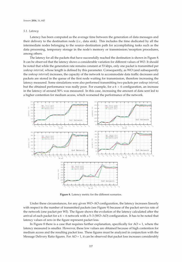
Sensors 2016, 16, 643

5.1. Latency

Latency has been computed as the average time between the generation of data messages andtheir delivery to the destination node (i.e., data sink). This includes the time dedicated by all theintermediate nodes belonging to the source–destination path for accomplishing tasks such as thedata processing, temporary storage in the node's memory or transmission/reception procedures,among others.

The latency for all the packets that have successfully reached the destination is shown in Figure 8.It can be observed that the latency shows a considerable variation for different values of WO. It shouldbe noted that while the generation rate remains constant at 53 kbps, only one packet is transmitted perwakeup interval, whose length is defined by this parameter. Consequently, as WO (and subsequentlythe wakeup interval) increases, the capacity of the network to accommodate data traffic decreases andpackets are stored in the queue of the first node waiting for transmission, therefore increasing thelatency measured. Some simulations were also performed transmitting two packets per wakeup interval,but the obtained performance was really poor. For example, for a 6 ˆ 6 configuration, an increasein the latency of around 50% was measured. In this case, increasing the amount of data sent led toa higher contention for medium access, which worsened the performance of the network.

Figure 8. Latency metric for the different scenarios.

Under these circumstances, for any given WO–AO configuration, the latency increases linearlywith respect to the number of transmitted packets (see Figure 9) because of the packet service rate ofthe network (one packet per WI). The figure shows the evolution of the latency calculated after thearrival of each packet for a 6 ˆ 6 network with a 5–3 (WO–AO) configuration. It has to be noted thatlatency values of zero in the figure represent packet loss.

In Figure 8 there is a case that requires further explanation, specifically for AO = 1, where thelatency measured is smaller. However, these low values are obtained because of high contention formedium access and the resulting packet loss. These figures must be analyzed in conjunction with theMessage Delivery Ratio figures. For AO = 1, it can be observed that packet loss increases considerably

227

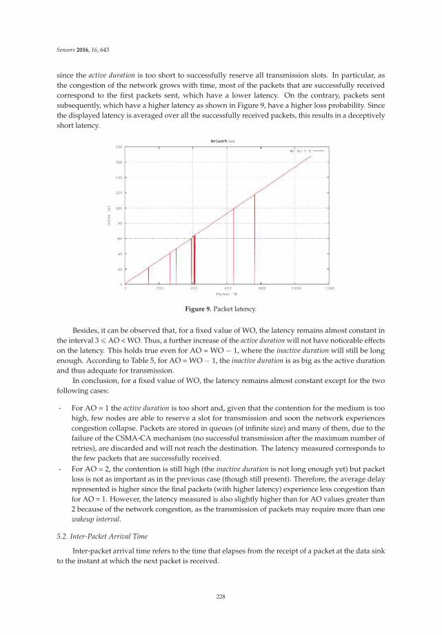
Sensors 2016, 16, 643

since the active duration is too short to successfully reserve all transmission slots. In particular, asthe congestion of the network grows with time, most of the packets that are successfully receivedcorrespond to the first packets sent, which have a lower latency. On the contrary, packets sentsubsequently, which have a higher latency as shown in Figure 9, have a higher loss probability. Sincethe displayed latency is averaged over all the successfully received packets, this results in a deceptivelyshort latency.

Figure 9. Packet latency.

Besides, it can be observed that, for a fixed value of WO, the latency remains almost constant inthe interval 3 ď AO < WO. Thus, a further increase of the active duration will not have noticeable effectson the latency. This holds true even for AO = WO ´ 1, where the inactive duration will still be longenough. According to Table 5, for AO = WO ´ 1, the inactive duration is as big as the active durationand thus adequate for transmission.

In conclusion, for a fixed value of WO, the latency remains almost constant except for the twofollowing cases:

- For AO = 1 the active duration is too short and, given that the contention for the medium is toohigh, few nodes are able to reserve a slot for transmission and soon the network experiencescongestion collapse. Packets are stored in queues (of infinite size) and many of them, due to thefailure of the CSMA-CA mechanism (no successful transmission after the maximum number ofretries), are discarded and will not reach the destination. The latency measured corresponds tothe few packets that are successfully received.

- For AO = 2, the contention is still high (the inactive duration is not long enough yet) but packetloss is not as important as in the previous case (though still present). Therefore, the average delayrepresented is higher since the final packets (with higher latency) experience less congestion thanfor AO = 1. However, the latency measured is also slightly higher than for AO values greater than2 because of the network congestion, as the transmission of packets may require more than onewakeup interval.

5.2. Inter-Packet Arrival Time

Inter-packet arrival time refers to the time that elapses from the receipt of a packet at the data sinkto the instant at which the next packet is received.

228

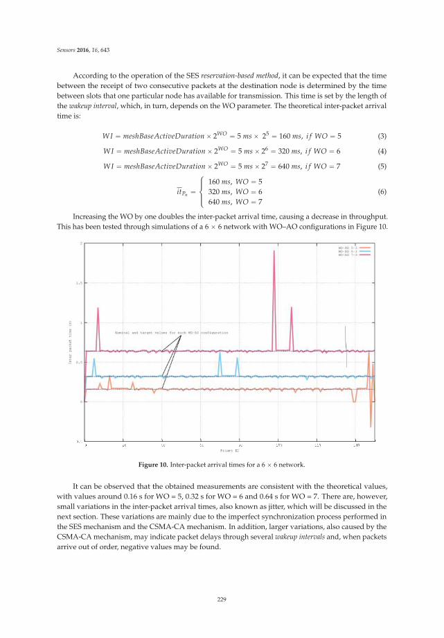
Sensors 2016, 16, 643

According to the operation of the SES reservation-based method, it can be expected that the timebetween the receipt of two consecutive packets at the destination node is determined by the timebetween slots that one particular node has available for transmission. This time is set by the length ofthe wakeup interval, which, in turn, depends on the WO parameter. The theoretical inter-packet arrivaltime is:

WI “ meshBaseActiveDuration ˆ 2WO “ 5 ms ˆ 25 “ 160 ms, i f WO “ 5 (3)



itPn “

$

’

&

’

%

160 ms, WO “ 5320 ms, WO “ 6640 ms, WO “ 7

(6)

Increasing the WO by one doubles the inter-packet arrival time, causing a decrease in throughput.This has been tested through simulations of a 6 ˆ 6 network with WO–AO configurations in Figure 10.

Figure 10. Inter-packet arrival times for a 6 ˆ 6 network.

It can be observed that the obtained measurements are consistent with the theoretical values,with values around 0.16 s for WO = 5, 0.32 s for WO = 6 and 0.64 s for WO = 7. There are, however,small variations in the inter-packet arrival times, also known as jitter, which will be discussed in thenext section. These variations are mainly due to the imperfect synchronization process performed inthe SES mechanism and the CSMA-CA mechanism. In addition, larger variations, also caused by theCSMA-CA mechanism, may indicate packet delays through several wakeup intervals and, when packetsarrive out of order, negative values may be found.

229

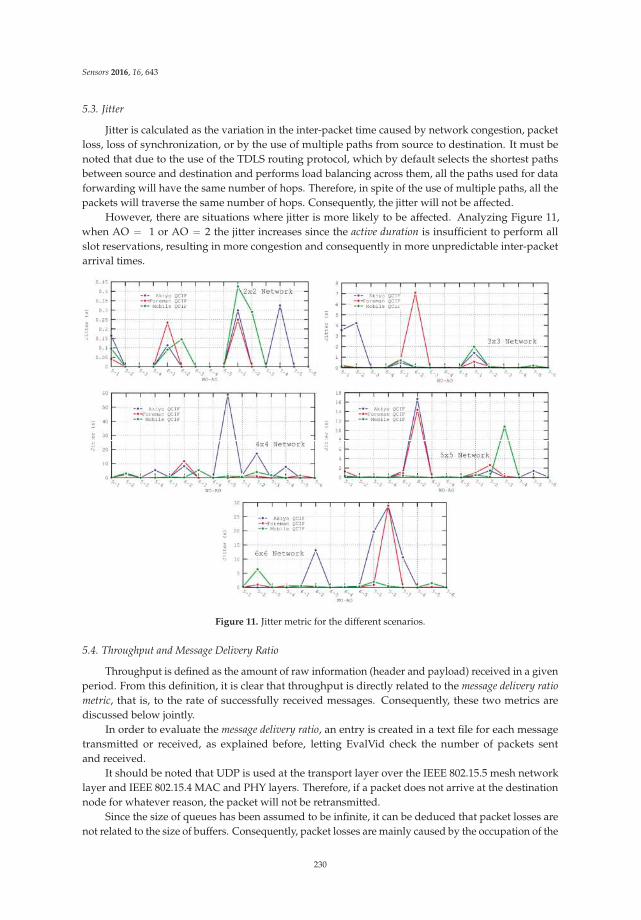
Sensors 2016, 16, 643

5.3. Jitter

Jitter is calculated as the variation in the inter-packet time caused by network congestion, packetloss, loss of synchronization, or by the use of multiple paths from source to destination. It must benoted that due to the use of the TDLS routing protocol, which by default selects the shortest pathsbetween source and destination and performs load balancing across them, all the paths used for dataforwarding will have the same number of hops. Therefore, in spite of the use of multiple paths, all thepackets will traverse the same number of hops. Consequently, the jitter will not be affected.

However, there are situations where jitter is more likely to be affected. Analyzing Figure 11,when AO “ 1 or AO “ 2 the jitter increases since the active duration is insufficient to perform allslot reservations, resulting in more congestion and consequently in more unpredictable inter-packetarrival times.

Figure 11. Jitter metric for the different scenarios.

5.4. Throughput and Message Delivery Ratio

Throughput is defined as the amount of raw information (header and payload) received in a givenperiod. From this definition, it is clear that throughput is directly related to the message delivery ratio

metric, that is, to the rate of successfully received messages. Consequently, these two metrics arediscussed below jointly.

In order to evaluate the message delivery ratio, an entry is created in a text file for each messagetransmitted or received, as explained before, letting EvalVid check the number of packets sentand received.

It should be noted that UDP is used at the transport layer over the IEEE 802.15.5 mesh networklayer and IEEE 802.15.4 MAC and PHY layers. Therefore, if a packet does not arrive at the destinationnode for whatever reason, the packet will not be retransmitted.

Since the size of queues has been assumed to be infinite, it can be deduced that packet losses arenot related to the size of buffers. Consequently, packet losses are mainly caused by the occupation of the

230

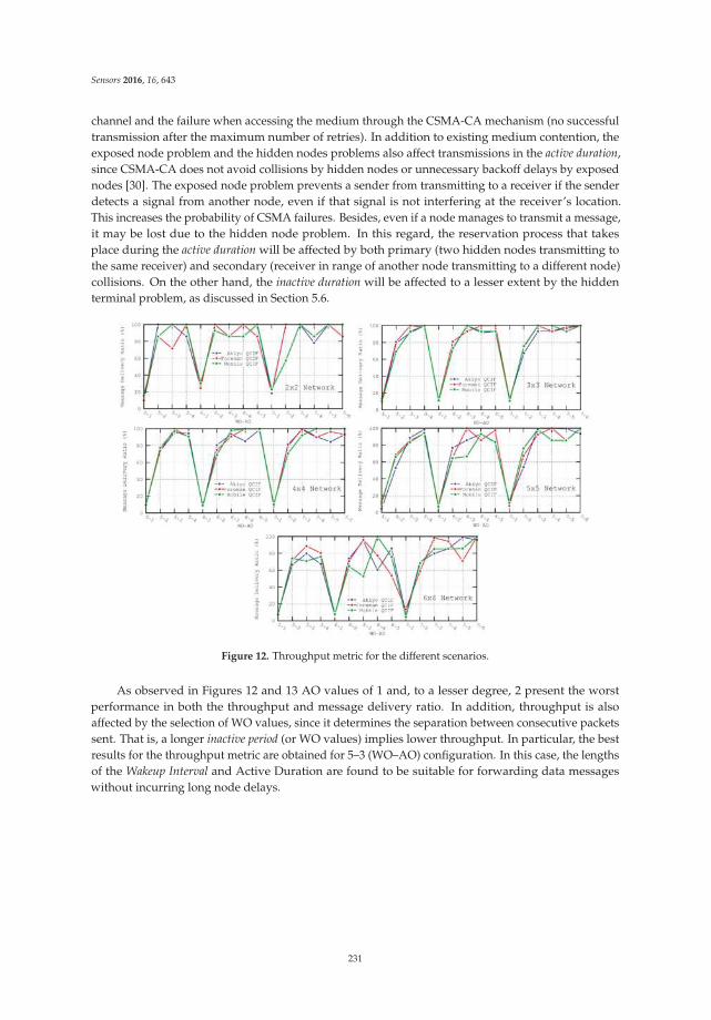
Sensors 2016, 16, 643

channel and the failure when accessing the medium through the CSMA-CA mechanism (no successfultransmission after the maximum number of retries). In addition to existing medium contention, theexposed node problem and the hidden nodes problems also affect transmissions in the active duration,since CSMA-CA does not avoid collisions by hidden nodes or unnecessary backoff delays by exposednodes [30]. The exposed node problem prevents a sender from transmitting to a receiver if the senderdetects a signal from another node, even if that signal is not interfering at the receiver’s location.This increases the probability of CSMA failures. Besides, even if a node manages to transmit a message,it may be lost due to the hidden node problem. In this regard, the reservation process that takesplace during the active duration will be affected by both primary (two hidden nodes transmitting tothe same receiver) and secondary (receiver in range of another node transmitting to a different node)collisions. On the other hand, the inactive duration will be affected to a lesser extent by the hiddenterminal problem, as discussed in Section 5.6.

Figure 12. Throughput metric for the different scenarios.

As observed in Figures 12 and 13 AO values of 1 and, to a lesser degree, 2 present the worstperformance in both the throughput and message delivery ratio. In addition, throughput is alsoaffected by the selection of WO values, since it determines the separation between consecutive packetssent. That is, a longer inactive period (or WO values) implies lower throughput. In particular, the bestresults for the throughput metric are obtained for 5–3 (WO–AO) configuration. In this case, the lengthsof the Wakeup Interval and Active Duration are found to be suitable for forwarding data messageswithout incurring long node delays.

231

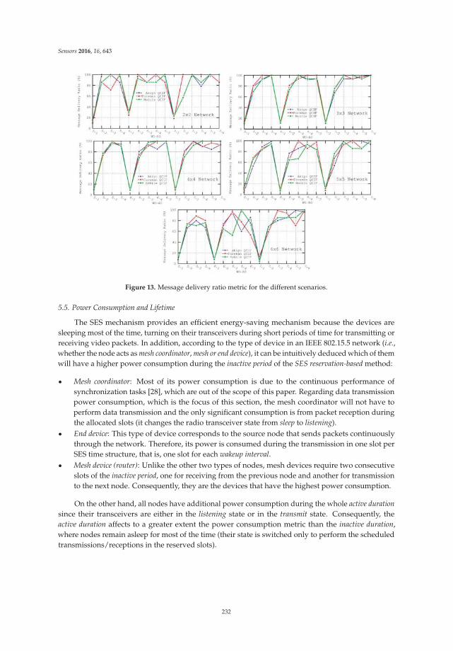
Sensors 2016, 16, 643

Figure 13. Message delivery ratio metric for the different scenarios.

5.5. Power Consumption and Lifetime

The SES mechanism provides an efficient energy-saving mechanism because the devices aresleeping most of the time, turning on their transceivers during short periods of time for transmitting orreceiving video packets. In addition, according to the type of device in an IEEE 802.15.5 network (i.e.,whether the node acts as mesh coordinator, mesh or end device), it can be intuitively deduced which of themwill have a higher power consumption during the inactive period of the SES reservation-based method:

‚ Mesh coordinator: Most of its power consumption is due to the continuous performance ofsynchronization tasks [28], which are out of the scope of this paper. Regarding data transmissionpower consumption, which is the focus of this section, the mesh coordinator will not have toperform data transmission and the only significant consumption is from packet reception duringthe allocated slots (it changes the radio transceiver state from sleep to listening).

‚ End device: This type of device corresponds to the source node that sends packets continuouslythrough the network. Therefore, its power is consumed during the transmission in one slot perSES time structure, that is, one slot for each wakeup interval.

‚ Mesh device (router): Unlike the other two types of nodes, mesh devices require two consecutiveslots of the inactive period, one for receiving from the previous node and another for transmissionto the next node. Consequently, they are the devices that have the highest power consumption.

On the other hand, all nodes have additional power consumption during the whole active duration

since their transceivers are either in the listening state or in the transmit state. Consequently, theactive duration affects to a greater extent the power consumption metric than the inactive duration,where nodes remain asleep for most of the time (their state is switched only to perform the scheduledtransmissions/receptions in the reserved slots).

232

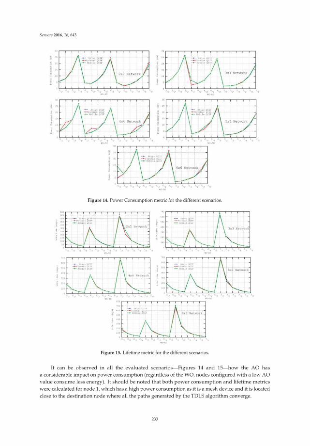
Sensors 2016, 16, 643

Figure 14. Power Consumption metric for the different scenarios.

Figure 15. Lifetime metric for the different scenarios.

It can be observed in all the evaluated scenarios—Figures 14 and 15—how the AO hasa considerable impact on power consumption (regardless of the WO, nodes configured with a low AOvalue consume less energy). It should be noted that both power consumption and lifetime metricswere calculated for node 1, which has a high power consumption as it is a mesh device and it is locatedclose to the destination node where all the paths generated by the TDLS algorithm converge.

233

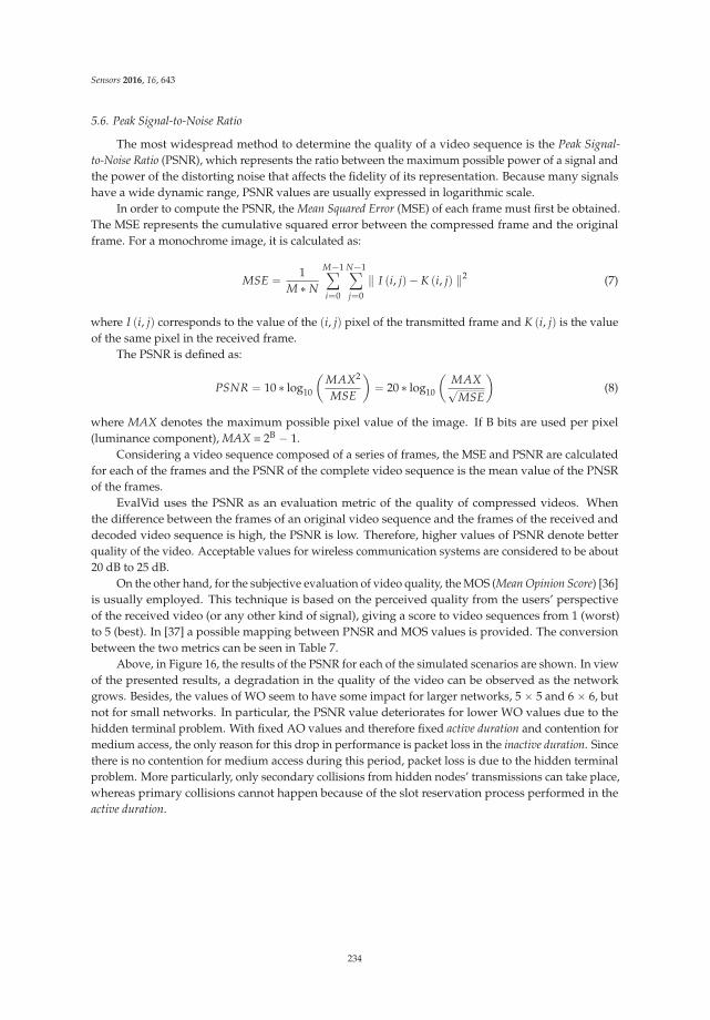
Sensors 2016, 16, 643

5.6. Peak Signal-to-Noise Ratio

The most widespread method to determine the quality of a video sequence is the Peak Signal-

to-Noise Ratio (PSNR), which represents the ratio between the maximum possible power of a signal andthe power of the distorting noise that affects the fidelity of its representation. Because many signalshave a wide dynamic range, PSNR values are usually expressed in logarithmic scale.

In order to compute the PSNR, the Mean Squared Error (MSE) of each frame must first be obtained.The MSE represents the cumulative squared error between the compressed frame and the originalframe. For a monochrome image, it is calculated as:

MSE “ 1M ˚ N

M´1ÿ

i“0

N´1ÿ

j“0

‖ I pi, jq ´ K pi, jq ‖2 (7)

where I pi, jq corresponds to the value of the pi, jq pixel of the transmitted frame and K pi, jq is the valueof the same pixel in the received frame.

The PSNR is defined as:

PSNR “ 10 ˚ log10

ˆ

MAX2

MSE

˙

“ 20 ˚ log10

ˆ

MAX?MSE

˙

(8)

where MAX denotes the maximum possible pixel value of the image. If B bits are used per pixel(luminance component), MAX = 2B ´ 1.

Considering a video sequence composed of a series of frames, the MSE and PSNR are calculatedfor each of the frames and the PSNR of the complete video sequence is the mean value of the PNSRof the frames.

EvalVid uses the PSNR as an evaluation metric of the quality of compressed videos. Whenthe difference between the frames of an original video sequence and the frames of the received anddecoded video sequence is high, the PSNR is low. Therefore, higher values of PSNR denote betterquality of the video. Acceptable values for wireless communication systems are considered to be about20 dB to 25 dB.

On the other hand, for the subjective evaluation of video quality, the MOS (Mean Opinion Score) [36]is usually employed. This technique is based on the perceived quality from the users’ perspectiveof the received video (or any other kind of signal), giving a score to video sequences from 1 (worst)to 5 (best). In [37] a possible mapping between PNSR and MOS values is provided. The conversionbetween the two metrics can be seen in Table 7.

Above, in Figure 16, the results of the PSNR for each of the simulated scenarios are shown. In viewof the presented results, a degradation in the quality of the video can be observed as the networkgrows. Besides, the values of WO seem to have some impact for larger networks, 5 ˆ 5 and 6 ˆ 6, butnot for small networks. In particular, the PSNR value deteriorates for lower WO values due to thehidden terminal problem. With fixed AO values and therefore fixed active duration and contention formedium access, the only reason for this drop in performance is packet loss in the inactive duration. Sincethere is no contention for medium access during this period, packet loss is due to the hidden terminalproblem. More particularly, only secondary collisions from hidden nodes’ transmissions can take place,whereas primary collisions cannot happen because of the slot reservation process performed in theactive duration.

234

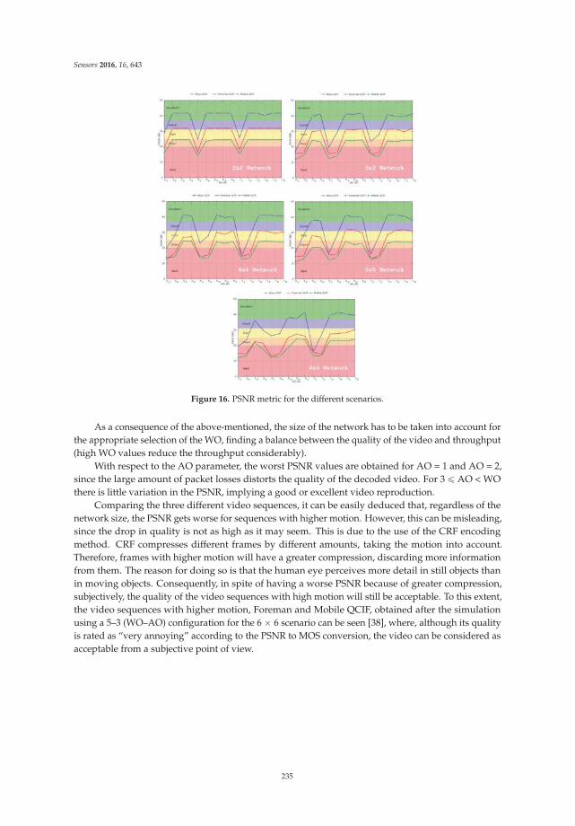
Sensors 2016, 16, 643

Figure 16. PSNR metric for the different scenarios.

As a consequence of the above-mentioned, the size of the network has to be taken into account forthe appropriate selection of the WO, finding a balance between the quality of the video and throughput(high WO values reduce the throughput considerably).

With respect to the AO parameter, the worst PSNR values are obtained for AO = 1 and AO = 2,since the large amount of packet losses distorts the quality of the decoded video. For 3 ď AO < WOthere is little variation in the PSNR, implying a good or excellent video reproduction.

Comparing the three different video sequences, it can be easily deduced that, regardless of thenetwork size, the PSNR gets worse for sequences with higher motion. However, this can be misleading,since the drop in quality is not as high as it may seem. This is due to the use of the CRF encodingmethod. CRF compresses different frames by different amounts, taking the motion into account.Therefore, frames with higher motion will have a greater compression, discarding more informationfrom them. The reason for doing so is that the human eye perceives more detail in still objects thanin moving objects. Consequently, in spite of having a worse PSNR because of greater compression,subjectively, the quality of the video sequences with high motion will still be acceptable. To this extent,the video sequences with higher motion, Foreman and Mobile QCIF, obtained after the simulationusing a 5–3 (WO–AO) configuration for the 6 ˆ 6 scenario can be seen [38], where, although its qualityis rated as “very annoying” according to the PSNR to MOS conversion, the video can be considered asacceptable from a subjective point of view.

235

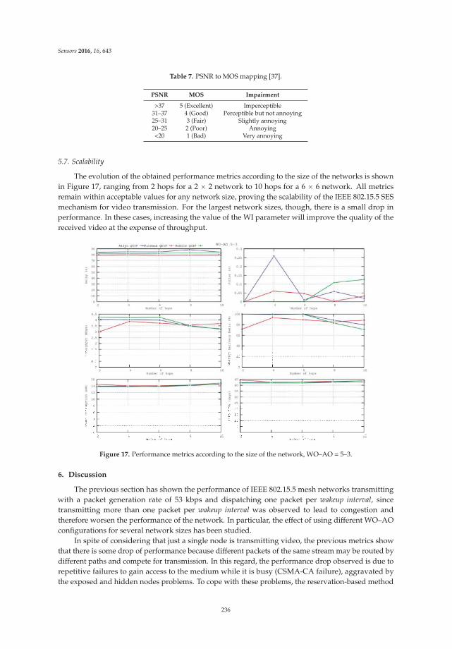
Sensors 2016, 16, 643

Table 7. PSNR to MOS mapping [37].

PSNR MOS Impairment

>37 5 (Excellent) Imperceptible31–37 4 (Good) Perceptible but not annoying25–31 3 (Fair) Slightly annoying20–25 2 (Poor) Annoying<20 1 (Bad) Very annoying

5.7. Scalability

The evolution of the obtained performance metrics according to the size of the networks is shownin Figure 17, ranging from 2 hops for a 2 ˆ 2 network to 10 hops for a 6 ˆ 6 network. All metricsremain within acceptable values for any network size, proving the scalability of the IEEE 802.15.5 SESmechanism for video transmission. For the largest network sizes, though, there is a small drop inperformance. In these cases, increasing the value of the WI parameter will improve the quality of thereceived video at the expense of throughput.

Figure 17. Performance metrics according to the size of the network, WO–AO = 5–3.

6. Discussion

The previous section has shown the performance of IEEE 802.15.5 mesh networks transmittingwith a packet generation rate of 53 kbps and dispatching one packet per wakeup interval, sincetransmitting more than one packet per wakeup interval was observed to lead to congestion andtherefore worsen the performance of the network. In particular, the effect of using different WO–AOconfigurations for several network sizes has been studied.

In spite of considering that just a single node is transmitting video, the previous metrics showthat there is some drop of performance because different packets of the same stream may be routed bydifferent paths and compete for transmission. In this regard, the performance drop observed is due torepetitive failures to gain access to the medium while it is busy (CSMA-CA failure), aggravated bythe exposed and hidden nodes problems. To cope with these problems, the reservation-based method

236

Sensors 2016, 16, 643

of the SES mode proposes the use of a relatively short active duration period, where all contentionfor reserving transmission slots takes place, and the inactive duration, where nodes have slots wheretransmission is guaranteed. In data-intensive applications, though, this inactive period can also beaffected by the hidden node problem to some degree, as mentioned.

During the active period, nodes have the opportunity to reserve slots for subsequent transmissionsin the inactive period. Since the active duration of all neighbor nodes is synchronized, it is likelythat several nodes will try to perform simultaneous reservations. In order to avoid collisions, theCSMA-CA scheme allows that, if some reservation message cannot be sent because the channel isbusy, several subsequent retransmission attempts (up to a configurable maximum number in theIEEE 802.15.4 standard, macMaxCSMABackoff, 4 by default) can be performed. However, accordingto the simulations, AO values of 1 and 2 result in active durations not long enough to perform allCSMA-CA retries. For example, the maximum delay (in a worst case scenario) due to the CSMA-CA

backoff is 36.8 ms (calculated asř backo f f “4

backo f f “0p2BE ´ 1q ˚ aUnitBackoffPeriod ˚ symbol _time whereBE “ minpmacMinBE ` backoff, macMaxBEq) using the IEEE 802.15.4 default values at 2.4 GHz,whereas for AO = 1 the active duration is only 10 ms long. This implies that several active durationsmay be necessary in order to reserve one transmission slot. However, during that time, new packetswould also require to be transmitted, increasing the contention for medium access (if the packetsare received by neighbor nodes) or the queue size of the node, and therefore the performance of thenetwork would get worse as time goes on.

Given all the factors that affect negatively the transmissions during the active duration, it is clearthat it is very important to select an AO value that allows transmission with an appropriate QoS.It has been observed for all the previous QoS metrics that for AO values equal to or greater than 3, theperformance has been quite satisfactory. Taking into account that the AO parameter is detrimental topower consumption and network lifetime, a value of 3 can be used for the scenarios studied withoutaffecting latency, jitter, throughput and message delivery ratio.

Regarding the selection of the wakeup interval length, and consequently the WO parameter, it isimportant to find a balance between power consumption (which improves with high WO values) andthroughput (which improves with low WO values). In addition, it has also been observed that thesize of the network may affect the quality of the received video due to the hidden terminal problem,and more particularly secondary collisions. Other negative factors such as contention for mediumaccess, the exposed node problem or primary collisions due to the hidden node problem are avoidedby the use of transmission in reserved slots of the inactive period. Thanks to this fact, the drop ofperformance in the inactive duration is not important and it is only noticeable for networks of size 5 ˆ 5and greater. As the size of the networks grows, the number of packet retransmissions in the meshnetwork increases, and therefore the probability of secondary collisions. For the scenarios studied,a WO value of 5 has shown to provide good video quality without worsening the throughput. Thiscan be better observed by watching the received videos since, as mentioned in the previous section,values of PSNR values may be misleading for videos with high motion. It has to be noted that, dueto the tendency of worsening PSNR and packet loss with network size, for networks larger than thestudied ones, higher values of WO should be considered. In this case, increasing the WO by oneimplies a more than twofold increase of the inactive duration and the number of slots (see Table 5).Therefore transmissions in the inactive duration are sparser and the probability of collision decreases.

In view of the simulation results, it can be affirmed that it is feasible to transmit video using theIEEE 802.15.5 standard. Using appropriate WO–AO values, it can achieve the necessary reliabilityfor a satisfactory video quality. On the other hand, the main drawback of the standard is that it doesnot achieve high throughput values, which hinders its applicability to real-time video applications,although this is anyway very challenging for multi-hop networks. In order to improve throughput,some enhancements are necessary that allow more than one packet per wakeup interval to be reliablysent. This can be achieved by tackling the diverse problems that have been discussed in this section inorder to arrange transmissions so that multimedia flows can use more than one slot per wakeup interval,

237

Sensors 2016, 16, 643

but also by applying enhancements in the directions given in the Related Work section. In this line, thestandard has an important feature, the possibility of allowing transmissions to any other node of thenetwork, which facilitates the development of collaborative or multi-sink applications.

7. Conclusions

In this paper, the transmission of video sequences using the low rate part of the IEEE 802.15.5standard has been evaluated by means of a new simulation tool which is available in [33]. This toolimplements the SES reservation-based method as energy-saving mechanism, following faithfully thestandard specification. Furthermore, the simulation framework integrates the SES method and theEvalVid software, which generates compressed QCIF video sequences with different motion, encodedusing H.264/AVC. These sequences are transmitted through mesh networks of different sizes. Themain results of the simulations have been presented and discussed, highlighting the most importantmetrics such as latency, jitter, time between packets, message delivery ratio, power consumption,lifetime and PSNR. The importance of the selection of appropriate values for the active order andwakeup order parameters has been emphasized, observing that for 3 ď AO ă WO video transmissionis feasible. A 5–3 (WO–AO) configuration has been found to be the best for the scenarios studied,although, for larger networks, higher WO values can be considered. The video sequence obtained afterthe simulation of 5–3 and 7–2 (WO–AO) configurations for Akiyo, Foreman and Mobile QCIF can befound at [38–43].

In addition, the developed tool can be used to evaluate different enhancements over the IEEE802.15.5 standard. In spite of the advantages of this standard reported in this work, such asfault tolerance or the possibility that any node transmits to any other node, there is still room forimprovement for data-intensive applications and, more particularly, WMSN applications. In thisregard, it is possible to introduce enhancements to the original standard, with no detriment to theinteroperability with other IEEE 802.15.5 devices, which take into account the particularities of WMSNand increase its performance for this type of application.

Acknowledgments: This research has been supported by the MINECO/FEDER project grantTEC2013-47016-C2-2-R (COINS).

Author Contributions: Antonio-Javier Garcia-Sanchez and Felipe García-Sánchez conceived the idea andparticipated in the elaboration of the manuscript and in the analysis of results. Fernando Losilla was involvedin the writing of the manuscript and in the analysis of the results. David Rodenas-Herraiz developed the SESmodule of the simulation tool. Felipe Cruz-Martínez took part in the elaboration of the simulation tool and theexecution of simulations. All authors revised the paper.


References

1. Akyildiz, I.F.; Su, W.; Sankarasubramaniam, Y.; Cayirci, E. Wireless sensor networks: A survey. Comput. Netw.

2002, 38, 393–422. [CrossRef]2. Akyildiz, I.F.; Melodia, T.; Chowdhury, K.R. A survey on wireless multimedia sensor networks. Comput. Netw.

2007, 51, 921–960. [CrossRef]3. Rodenas-Herraiz, D.; Garcia-Sanchez, A.-J.; Garcia-Sanchez, F.; Garcia-Haro, J. Current trends in wireless

mesh sensor networks: A review of competing approaches. Sensors 2013, 13, 5958–5995. [CrossRef] [PubMed]4. Lee, M.; Zhang, R.; Zhu, C.; Park, T.R.; Shin, C.-S.; Jeon, Y.; Lee, S.-H.; Choi, S.-S.; Liu, E.Y.; Park, S.-W.

Meshing wireless personal area networks: Introducing IEEE 802.15. 5. IEEE Commun. Mag. 2010, 48, 54–61.[CrossRef]

5. Ali, A.; Ahmed, M.E.; Piran, M.J.; Suh, D.Y. Resource Optimization Scheme for Multimedia-Enabled WirelessMesh Networks. Sensors 2014, 14, 14500–14525. [CrossRef] [PubMed]

6. Pham, C. Communication performances of IEEE 802.15. 4 wireless sensor motes for data-intensiveapplications: A comparison of WaspMote, Arduino MEGA, TelosB, MicaZ and iMote2 for image surveillance.J. Netw. Comput. Appl. 2014, 46, 48–59. [CrossRef]

238

Sensors 2016, 16, 643

7. MICAz Datasheet. Available online: http://www.memsic.com/userfiles/files/Datasheets/WSN/micaz_datasheet-t.pdf (accessed on 3 February 2016).

8. Farooq, M.O.; Kunz, T. Wireless sensor networks testbeds and state-of-the-art multimedia sensor nodes.Appl. Math. Inf. Sci. 2014, 8, 935–940. [CrossRef]

9. Ben Ammar, A.; Bouattay, O.; Dziri, A.; Terre, M.; Youssef, H. Performance analysis of AODV and AOMDVover SMAC and IEEE 802.15. 4 in Wireless Multimedia Sensor Network. In Proceedings of the 2015International Wireless Communications and Mobile Computing Conference (IWCMC 2015), Dubrovnik,Croatia, 24–28 August 2015.

10. Andrea, P.; Scavongelli, C.; Orcioni, S.; Conti, M. Performance analysis of JPEG 2000 over 802.15. 4 wirelessimage sensor network. In Proceedings of the 2010 8th Workshop on Intelligent Solutions in EmbeddedSystems, Heraklion, Greece, 8–9 July 2010.

11. Pekhteryev, G.; Sahinoglu, Z.; Orlik, P.; Bhatti, G. Image transmission over IEEE 802.15. 4 and ZigBeenetworks. In Proceedings of the 2005 IEEE International Symposium on Circuits and Systems (ISCAS 2005),Kobe, Japan, 23–26 May 2005.

12. Garcia-Sanchez, A.-J.; Garcia-Sanchez, F.; Garcia-Haro, J.; Losilla, F. A cross-layer solution for enablingreal-time video transmission over IEEE 802.15. 4 networks. Multimed. Tools Appl. 2011, 51, 1069–1104.[CrossRef]

13. Farooq, M.O.; St-Hilaire, M.; Kunz, T. Cross-layer architecture for QoS provisioning in wireless multimediasensor networks. KSII Trans. Internet Inf. Syst. 2012, 6, 176–200.

14. Alanazi, A.; Elleithy, K. Real-Time QoS Routing Protocols in Wireless Multimedia Sensor Networks: Studyand Analysis. Sensors 2015, 15, 22209–22233. [CrossRef] [PubMed]

15. Razaque, A.; Elleithy, K. Modular energy-efficient and robust paradigms for a disaster-recovery process overwireless sensor networks. Sensors 2015, 15, 16162–16195. [CrossRef] [PubMed]

16. Kandris, D.; Tsagkaropoulos, M.; Politis, I.; Tzes, A.; Kotsopoulos, S. Energy efficient and perceived QoSaware video routing over wireless multimedia sensor networks. Ad Hoc Netw. 2011, 9, 591–607. [CrossRef]

17. Zaidi, S.M.A.; Song, B. Prioritized Multipath Video Forwarding in WSN. J. Inf. Process. Syst. 2014, 10,176–192. [CrossRef]

18. Felemban, E.; Lee, C.-G.; Ekici, E. MMSPEED: Multipath Multi-SPEED Protocol for QoS Guarantee ofReliability and Timeliness in Wireless Sensor Networks. IEEE Trans. Mob. Comput. 2006, 5, 738–754.[CrossRef]

19. Teo, J.-Y.; Ha, Y.; Tham, C.-K. Interference-minimized multipath routing with congestion control in wirelesssensor network for high-rate streaming. IEEE Trans. Mob. Comput. 2008, 7, 1124–1137.

20. Maimour, M. Maximally radio-disjoint multipath routing for wireless multimedia sensor networks.In Proceedings of the 4th ACM Workshop on Wireless Multimedia Networking and Performance Modeling,Vancouver, BC, Canada, 27–31 October 2008; pp. 26–31.

21. Li, B.-Y.; Chuang, P.-J. Geographic energy-aware non-interfering multipath routing for multimediatransmission in wireless sensor networks. Inf. Sci. 2013, 249, 24–37. [CrossRef]

22. Bidai, Z.; Maimour, M. Interference-aware multipath routing protocol for video transmission over ZigBeewireless sensor networks. In Proceedings of the 2014 International Conference on Multimedia Computingand Systems (ICMCS 2014), Marrakech, Morocco, 14–16 April 2014; pp. 837–842.

23. Haenggi, M.; Puccinelli, D. Routing in ad hoc networks: A case for long hops. IEEE Commun. Mag. 2005, 43,93–101. [CrossRef]

24. Memsic. TelosB Datasheet; Crossbow Technology, Inc.: San Jose, CA, USA, 2011.25. Wiegand, T.; Sullivan, G.J.; Bjontegaard, G.; Luthra, A. Overview of the H. 264/AVC video coding standard.

IEEE Trans. Circuits Syst. Video Technol. 2003, 13, 560–576. [CrossRef]26. Ullah, S.; Ahmad, J.J.; Khalid, J.; Khayam, S.A. Energy and distortion analysis of video compression schemes

for Wireless Video Sensor Networks. In Proceedings of the 2011 Military Communications Conference(MILCOM 2011), Baltimore, MD, USA, 7–10 November 2011; pp. 822–827.

27. Jung, D.; Teixeira, T.; Savvides, A. Sensor node lifetime analysis: Models and tools. ACM Trans. Sens. Netw.

2009, 5, 3. [CrossRef]28. IEEE Std 802.15.5™-2009: Mesh Topology Capability in Wireless Personal Area Networks (WPANs); IEEE Computer

Society: Washington, DC, USA, 2009.

239

Sensors 2016, 16, 643

29. Zheng, J.; Lee, M.J. A resource-efficient and scalable wireless mesh routing protocol. Ad Hoc Netw. 2007, 5,704–718. [CrossRef]

30. Rodenas-Herraiz, D.; Garcia-Sanchez, F.; Garcia-Sanchez, A.-J.; Garcia-Haro, J. On the influence of the hiddenand exposed terminal problems on asynchronous IEEE 802.15. 5 networks. Comput. Stand. Interfaces 2015, 42,53–70. [CrossRef]

31. The Network Simulator (ns-2). Available online: http://www.isi.edu/nsnam/ns (accessed on 3 May 2016).32. Klaue, J.; Rathke, B.; Wolisz, A. Evalvid—A framework for video transmission and quality evaluation.

In Computer Performance Evaluation: Modelling Techniques and Tools; Springer: Berlin, Germany, 2003;pp. 255–272.

33. IEEE 802.15.5 Video Simulation Tool. Available online: http://labit501.upct.es/~agarcia/Project/ (accessedon 18 February 2016).

34. YUV Video Sequences. Available online: http://trace.eas.asu.edu/yuv/ (accessed on 18 February 2016).35. Garcia-Sanchez, A.-J.; Garcia-Sanchez, F.; Rodenas-Herraiz, D.; Garcia-Haro, J. On the synchronization of

IEEE 802.15. 5 wireless mesh sensor networks: Shortcomings and improvements. EURASIP J. Wireless

Commun. Netw. 2012, 2012, 1–23. [CrossRef]36. Mean Opinion Score. Available online: https://www.itu.int/rec/T-REC-P.800.2-201305-I/en (accessed on

18 February 2016).37. Ohm, J.-R. Bildsignalverarbeitung Fuer Multimedia-Systeme; Skript Institut für Nachrichtentechnik und

theoretische Elektrotechnik der TU: Berlin, Germany, 1999.38. Mobile QCIF WO-AO 5-3. Available online: https://www.youtube.com/watch?v=KVWEtJbNfoM (accessed

on 18 February 2016).39. Akiyo QCIF WO-AO 5-3. Available online: https://www.youtube.com/watch?v=UMYEFdpfRXY (accessed

on 18 February 2016).40. Akiyo QCIF WO-AO 7-2. Available online: https://www.youtube.com/watch?v=31avC1TEFo0 (accessed

on 18 February 2016).41. Foreman QCIF WO-AO 5-3. Available online: https://www.youtube.com/watch?v=rU-83jD8rDI (accessed

on 18 February 2016).42. Foreman QCIF WO-AO 7-2. Available online: https://www.youtube.com/watch?v=neM4w04LyNY

(accessed on 18 February 2016).43. Mobile QCIF WO-AO 7-2. Available online: https://www.youtube.com/watch?v=CdgpNBUzFhQ (accessed

on 18 February 2016).


240

sensors

Review

State of the Art in LP-WAN Solutions for IndustrialIoT ServicesRamon Sanchez-Iborra * and Maria-Dolores Cano

Departamento de Tecnologías de la Información y las Comunicaciones, Universidad Politécnica de Cartagena,Cartagena 30202, Spain; [email protected]* Correspondence: [email protected]; Tel.: +34-968-325-953

Academic Editor: Gonzalo Pajares MartinsanzReceived: 25 February 2016; Accepted: 9 May 2016; Published: 17 May 2016

Abstract: The emergence of low-cost connected devices is enabling a new wave of sensorizationservices. These services can be highly leveraged in industrial applications. However, the technologiesemployed so far for managing this kind of system do not fully cover the strict requirements ofindustrial networks, especially those regarding energy efficiency. In this article a novel paradigm,called Low-Power Wide Area Networking (LP-WAN), is explored. By means of a cellular-typearchitecture, LP-WAN–based solutions aim at fulfilling the reliability and efficiency challenges posedby long-term industrial networks. Thus, the most prominent LP-WAN solutions are reviewed,identifying and discussing the pros and cons of each of them. The focus is also on examiningthe current deployment state of these platforms in Spain. Although LP-WAN systems are at earlystages of development, they represent a promising alternative for boosting future industrial IIoT(Industrial Internet of Things) networks and services.

Keywords: Low-Power Wide Area Networks (LP-WAN); Machine-to-Machine (M2M) communications;Industrial Internet of Things (IIoT); Internet of Things (IoT); wireless sensor networks

1. Introduction

Machine-to-Machine (M2M) networks and Industrial Internet of Things (IIoT) services are two keyenabling approaches for future industrial networking [1]. As reflected from the forecast investmentspredicted in the IIoT field [2], the advent of low-cost, always-connected devices opens new and excitingopportunities involving many stakeholders from a wide range of sectors. Deploying well-structuredand easily-accessible M2M networks will facilitate having a precise control over the production orcompany’s installations, which could be translated into a smart strategy for saving logistic costs [3].As an example, new services such as real-time event processing or 24/7 access to tracking informationwill be introduced into the supply chain. Having a thorough monitoring system deployed all along themanufacturing and supply chain allows enriching the complete value chain with precious information,minimizing losses against unexpected events, and hence improving both business processes and theinformation exchange among stakeholders (Business-to-Business (B2B) networks) [4]. In this case,smart metering (water, oil, etc.), goods and facilities monitoring, or smart farming are good examplesof areas of activity for M2M/B2B networks.

M2M networks can be seen as a revamp of the widely-deployed Wireless Sensor Networks(WSN); we could also think that most of the aforementioned applications are already covered bythis well-studied approach. It is true that we have survived so far with the existing WSN classic

solutions such as ZigBee, Bluetooth, or even WiFi (short-range technologies), but the main point ofindustrial M2M networks is the huge increase in the number of devices composing them and thenotable widening of the covered areas. Global device connections are estimated to be about 28 billionby 2020 (Figure 1) [5]. This enormous growth requires (i) minimized cost per unit; (ii) optimized


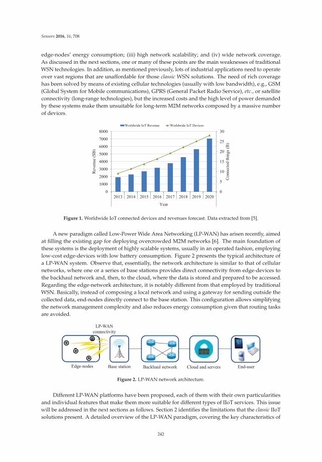
Sensors 2016, 16, 708

edge-nodes’ energy consumption; (iii) high network scalability; and (iv) wide network coverage.As discussed in the next sections, one or many of these points are the main weaknesses of traditionalWSN technologies. In addition, as mentioned previously, lots of industrial applications need to operateover vast regions that are unaffordable for those classic WSN solutions. The need of rich coveragehas been solved by means of existing cellular technologies (usually with low bandwidth), e.g., GSM(Global System for Mobile communications), GPRS (General Packet Radio Service), etc., or satelliteconnectivity (long-range technologies), but the increased costs and the high level of power demandedby these systems make them unsuitable for long-term M2M networks composed by a massive numberof devices.

0

5

10

15

20

25

30

0

1000

2000

3000

4000

5000

6000

7000

8000

2013 2014 2015 2016 2017 2018 2019 2020

Year

Co

nn

ecte

d t

hin

gs

(B)

Rev

enu

e ($

B)

Worldwide IoT Revenue Worldwide IoT Devices

Figure 1. Worldwide IoT connected devices and revenues forecast. Data extracted from [5].

A new paradigm called Low-Power Wide Area Networking (LP-WAN) has arisen recently, aimedat filling the existing gap for deploying overcrowded M2M networks [6]. The main foundation ofthese systems is the deployment of highly scalable systems, usually in an operated fashion, employinglow-cost edge-devices with low battery consumption. Figure 2 presents the typical architecture ofa LP-WAN system. Observe that, essentially, the network architecture is similar to that of cellularnetworks, where one or a series of base stations provides direct connectivity from edge-devices tothe backhaul network and, then, to the cloud, where the data is stored and prepared to be accessed.Regarding the edge-network architecture, it is notably different from that employed by traditionalWSN. Basically, instead of composing a local network and using a gateway for sending outside thecollected data, end-nodes directly connect to the base station. This configuration allows simplifyingthe network management complexity and also reduces energy consumption given that routing tasksare avoided.

Edge-nodes Base station Backhaul network Cloud and servers

LP-WAN

connectivity

End-user

Figure 2. LP-WAN network architecture.

Different LP-WAN platforms have been proposed, each of them with their own particularitiesand individual features that make them more suitable for different types of IIoT services. This issuewill be addressed in the next sections as follows. Section 2 identifies the limitations that the classic IIoTsolutions present. A detailed overview of the LP-WAN paradigm, covering the key characteristics of

242

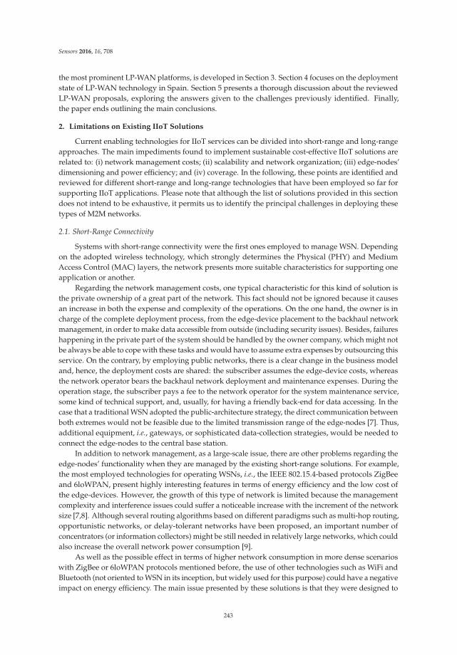
Sensors 2016, 16, 708

the most prominent LP-WAN platforms, is developed in Section 3. Section 4 focuses on the deploymentstate of LP-WAN technology in Spain. Section 5 presents a thorough discussion about the reviewedLP-WAN proposals, exploring the answers given to the challenges previously identified. Finally,the paper ends outlining the main conclusions.

2. Limitations on Existing IIoT Solutions

Current enabling technologies for IIoT services can be divided into short-range and long-rangeapproaches. The main impediments found to implement sustainable cost-effective IIoT solutions arerelated to: (i) network management costs; (ii) scalability and network organization; (iii) edge-nodes’dimensioning and power efficiency; and (iv) coverage. In the following, these points are identified andreviewed for different short-range and long-range technologies that have been employed so far forsupporting IIoT applications. Please note that although the list of solutions provided in this sectiondoes not intend to be exhaustive, it permits us to identify the principal challenges in deploying thesetypes of M2M networks.

2.1. Short-Range Connectivity

Systems with short-range connectivity were the first ones employed to manage WSN. Dependingon the adopted wireless technology, which strongly determines the Physical (PHY) and MediumAccess Control (MAC) layers, the network presents more suitable characteristics for supporting oneapplication or another.

Regarding the network management costs, one typical characteristic for this kind of solution isthe private ownership of a great part of the network. This fact should not be ignored because it causesan increase in both the expense and complexity of the operations. On the one hand, the owner is incharge of the complete deployment process, from the edge-device placement to the backhaul networkmanagement, in order to make data accessible from outside (including security issues). Besides, failureshappening in the private part of the system should be handled by the owner company, which might notbe always be able to cope with these tasks and would have to assume extra expenses by outsourcing thisservice. On the contrary, by employing public networks, there is a clear change in the business modeland, hence, the deployment costs are shared: the subscriber assumes the edge-device costs, whereasthe network operator bears the backhaul network deployment and maintenance expenses. During theoperation stage, the subscriber pays a fee to the network operator for the system maintenance service,some kind of technical support, and, usually, for having a friendly back-end for data accessing. In thecase that a traditional WSN adopted the public-architecture strategy, the direct communication betweenboth extremes would not be feasible due to the limited transmission range of the edge-nodes [7]. Thus,additional equipment, i.e., gateways, or sophisticated data-collection strategies, would be needed toconnect the edge-nodes to the central base station.

In addition to network management, as a large-scale issue, there are other problems regarding theedge-nodes’ functionality when they are managed by the existing short-range solutions. For example,the most employed technologies for operating WSNs, i.e., the IEEE 802.15.4-based protocols ZigBeeand 6loWPAN, present highly interesting features in terms of energy efficiency and the low cost ofthe edge-devices. However, the growth of this type of network is limited because the managementcomplexity and interference issues could suffer a noticeable increase with the increment of the networksize [7,8]. Although several routing algorithms based on different paradigms such as multi-hop routing,opportunistic networks, or delay-tolerant networks have been proposed, an important number ofconcentrators (or information collectors) might be still needed in relatively large networks, which couldalso increase the overall network power consumption [9].

As well as the possible effect in terms of higher network consumption in more dense scenarioswith ZigBee or 6loWPAN protocols mentioned before, the use of other technologies such as WiFi andBluetooth (not oriented to WSN in its inception, but widely used for this purpose) could have a negativeimpact on energy efficiency. The main issue presented by these solutions is that they were designed to

243

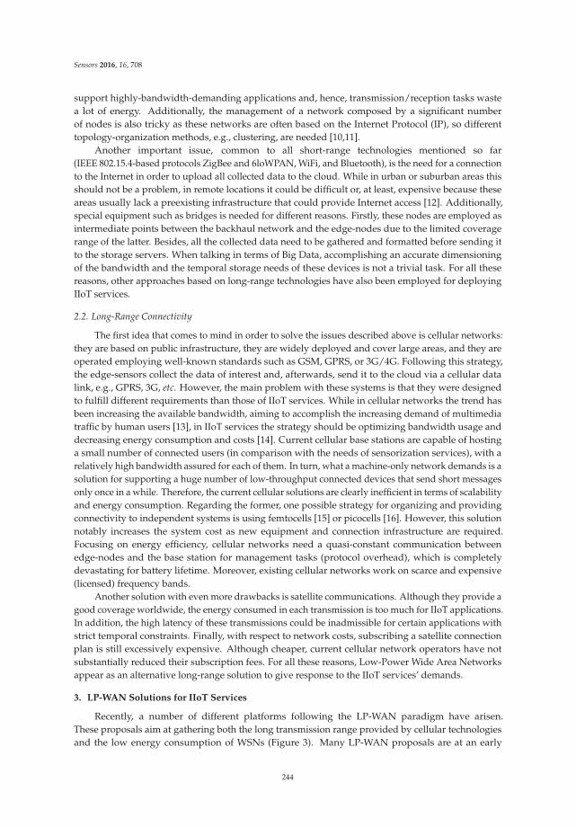
Sensors 2016, 16, 708

support highly-bandwidth-demanding applications and, hence, transmission/reception tasks wastea lot of energy. Additionally, the management of a network composed by a significant numberof nodes is also tricky as these networks are often based on the Internet Protocol (IP), so differenttopology-organization methods, e.g., clustering, are needed [10,11].

Another important issue, common to all short-range technologies mentioned so far(IEEE 802.15.4-based protocols ZigBee and 6loWPAN, WiFi, and Bluetooth), is the need for a connectionto the Internet in order to upload all collected data to the cloud. While in urban or suburban areas thisshould not be a problem, in remote locations it could be difficult or, at least, expensive because theseareas usually lack a preexisting infrastructure that could provide Internet access [12]. Additionally,special equipment such as bridges is needed for different reasons. Firstly, these nodes are employed asintermediate points between the backhaul network and the edge-nodes due to the limited coveragerange of the latter. Besides, all the collected data need to be gathered and formatted before sending itto the storage servers. When talking in terms of Big Data, accomplishing an accurate dimensioningof the bandwidth and the temporal storage needs of these devices is not a trivial task. For all thesereasons, other approaches based on long-range technologies have also been employed for deployingIIoT services.

2.2. Long-Range Connectivity

The first idea that comes to mind in order to solve the issues described above is cellular networks:they are based on public infrastructure, they are widely deployed and cover large areas, and they areoperated employing well-known standards such as GSM, GPRS, or 3G/4G. Following this strategy,the edge-sensors collect the data of interest and, afterwards, send it to the cloud via a cellular datalink, e.g., GPRS, 3G, etc. However, the main problem with these systems is that they were designedto fulfill different requirements than those of IIoT services. While in cellular networks the trend hasbeen increasing the available bandwidth, aiming to accomplish the increasing demand of multimediatraffic by human users [13], in IIoT services the strategy should be optimizing bandwidth usage anddecreasing energy consumption and costs [14]. Current cellular base stations are capable of hostinga small number of connected users (in comparison with the needs of sensorization services), with arelatively high bandwidth assured for each of them. In turn, what a machine-only network demands is asolution for supporting a huge number of low-throughput connected devices that send short messagesonly once in a while. Therefore, the current cellular solutions are clearly inefficient in terms of scalabilityand energy consumption. Regarding the former, one possible strategy for organizing and providingconnectivity to independent systems is using femtocells [15] or picocells [16]. However, this solutionnotably increases the system cost as new equipment and connection infrastructure are required.Focusing on energy efficiency, cellular networks need a quasi-constant communication betweenedge-nodes and the base station for management tasks (protocol overhead), which is completelydevastating for battery lifetime. Moreover, existing cellular networks work on scarce and expensive(licensed) frequency bands.

Another solution with even more drawbacks is satellite communications. Although they provide agood coverage worldwide, the energy consumed in each transmission is too much for IIoT applications.In addition, the high latency of these transmissions could be inadmissible for certain applications withstrict temporal constraints. Finally, with respect to network costs, subscribing a satellite connectionplan is still excessively expensive. Although cheaper, current cellular network operators have notsubstantially reduced their subscription fees. For all these reasons, Low-Power Wide Area Networksappear as an alternative long-range solution to give response to the IIoT services’ demands.

3. LP-WAN Solutions for IIoT Services

Recently, a number of different platforms following the LP-WAN paradigm have arisen.These proposals aim at gathering both the long transmission range provided by cellular technologiesand the low energy consumption of WSNs (Figure 3). Many LP-WAN proposals are at an early

244

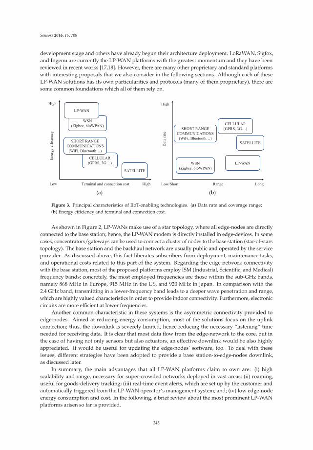
Sensors 2016, 16, 708

development stage and others have already begun their architecture deployment. LoRaWAN, Sigfox,and Ingenu are currently the LP-WAN platforms with the greatest momentum and they have beenreviewed in recent works [17,18]. However, there are many other proprietary and standard platformswith interesting proposals that we also consider in the following sections. Although each of theseLP-WAN solutions has its own particularities and protocols (many of them proprietary), there aresome common foundations which all of them rely on.

(a) (b)

High

High

Low Terminal and connection cost

CELLULAR

(GPRS, 3G…)

WSN

(Zigbee, 6loWPAN)

En

erg

yef

fici

ency

SATELLITE

LP-WAN

SHORT RANGE

COMMUNICATIONS

(WiFi, Bluetooth…)

LP-WAN

Long

High

Low/Short Range

CELLULAR

(GPRS, 3G…)

WSN

(Zigbee, 6loWPAN) D

ata

rate

SATELLITE

SHORT RANGE

COMMUNICATIONS

(WiFi, Bluetooth…)

Figure 3. Principal characteristics of IIoT-enabling technologies. (a) Data rate and coverage range;(b) Energy efficiency and terminal and connection cost.

As shown in Figure 2, LP-WANs make use of a star topology, where all edge-nodes are directlyconnected to the base station; hence, the LP-WAN modem is directly installed in edge-devices. In somecases, concentrators/gateways can be used to connect a cluster of nodes to the base station (star-of-starstopology). The base station and the backhaul network are usually public and operated by the serviceprovider. As discussed above, this fact liberates subscribers from deployment, maintenance tasks,and operational costs related to this part of the system. Regarding the edge-network connectivitywith the base station, most of the proposed platforms employ ISM (Industrial, Scientific, and Medical)frequency bands; concretely, the most employed frequencies are those within the sub-GHz bands,namely 868 MHz in Europe, 915 MHz in the US, and 920 MHz in Japan. In comparison with the2.4 GHz band, transmitting in a lower-frequency band leads to a deeper wave penetration and range,which are highly valued characteristics in order to provide indoor connectivity. Furthermore, electroniccircuits are more efficient at lower frequencies.

Another common characteristic in these systems is the asymmetric connectivity provided toedge-nodes. Aimed at reducing energy consumption, most of the solutions focus on the uplinkconnection; thus, the downlink is severely limited, hence reducing the necessary “listening” timeneeded for receiving data. It is clear that most data flow from the edge-network to the core, but inthe case of having not only sensors but also actuators, an effective downlink would be also highlyappreciated. It would be useful for updating the edge-nodes’ software, too. To deal with theseissues, different strategies have been adopted to provide a base station-to-edge-nodes downlink,as discussed later.

In summary, the main advantages that all LP-WAN platforms claim to own are: (i) highscalability and range, necessary for super-crowded networks deployed in vast areas; (ii) roaming,useful for goods-delivery tracking; (iii) real-time event alerts, which are set up by the customer andautomatically triggered from the LP-WAN operator’s management system; and; (iv) low edge-nodeenergy consumption and cost. In the following, a brief review about the most prominent LP-WANplatforms arisen so far is provided.

245

Sensors 2016, 16, 708

3.1. LoRaWAN

This platform is promoted by the LoRa Alliance [19], composed by IBM, Semtech, and Actility,among others. It proposes a star-of-stars topology with dedicated gateways serving as transparentbridges between edge-nodes and the central network, where the data is stored and made availableto the subscriber. The edge-nodes connect to the access points via one-hop links by using the LoRa(Long Range) modulation. This is Semtech’s proprietary Chirp Spread Spectrum (CSS) radio schemethat employs a wide channel of up to 250/500 kHz (Europe/North America) and provides adaptivedata rate capabilities by means of a variable processing gain. Please note that this concept representsthe ratio between the chip rate and the baseband information rate, and is usually known as theSpreading Factor (SF). LoRaWAN presents a SF from 7 to 12. Using this last characteristic, edge-nodescan tune the transmission power and bitrate to the real network conditions, allowing a reduction inenergy consumption. Moreover, LoRaWAN defines three types of edge-devices depending on theirdownloading needs: Class A devices have a scheduled downloading window just after each uplinkconnection (Receiver-Initiated Transmission strategy, low power consumption), Class B devices haveadditional scheduled downlink windows (Coordinated Sampled Listening strategy, medium powerconsumption), and Class C devices can receive messages almost at any time (Continuous Listeningstrategy, large power consumption). In its specification sheets, LoRaWAN claims a Class A edge-node’sbattery lifetime is over five years.

Originally, LoRaWAN was designed to work in ISM bands but it can be also adapted forsupporting the licensed spectrum. Under these conditions, LoRaWAN claims to demodulate signals19.5 dB below the noise floor, hence achieving greater ranges than those provided by cellular basestations. In both communication directions, the adaptive data-rate ranges from 0.25 kbps (0.98 kbps inNorth America due to FCC (Federal Communications Commission) limitations) up to 50 kbps, with amaximum payload length of 256 bytes. Finally, security issues have been thoroughly considered,so that end-to-end AES (Advanced Encryption Standard) encryption security, including the use ofa unique network, application, and device keys for encrypting data at different OSI (Open SystemsInterconnection) levels, is provided.

3.2. Sigfox

This is the platform in the most advanced deployment state in Europe. By means of agreementswith local cellular network operators, Sigfox [20] claims to have covered most of the territory ofFrance, Russia, and Spain, among others. Technically speaking, this solution is quite different fromthe LoRaWAN approach. Instead of using bidirectional spread spectrum channels, Sigfox employsproprietary ultra-narrow band modulation (Differential Binary Phase Shift Keying, DBPSK) with aheavily limited uplink connection. Using this modulation, a maximum data rate of 100 bps can beachieved by transmitting messages with a maximum payload length of 12 bytes. Meanwhile, using thislow bitrate permits large ranges of 10 km and beyond with very low transmission power, which allowssaving energy at edge-nodes. Sigfox’s technical sheets claim a typical stand-by time of 20 years witha 2.5 Ah battery.

Sigfox’s star topology is similar to a cellular architecture, with a wide deployment of base stationsaimed at covering entire countries by employing ISM bands. This base station structure permitsedge-nodes to upload the gathered data directly to Sigfox servers, which makes it accessible tosubscribers through a web-based API (Application Programming Interface). The use of ISM bandstogether with Sigfox’s medium access strategy, namely without collision-avoidance techniques, leadsto a stringent bandwidth-occupancy limitation suffered by edge-nodes. For example, a duty cycleof 1% is established in the Europe regulations; hence, a maximum of 140 messages per edge-nodeper day are allowed. In the case of the USA regulations, Sigfox’s limited data rate of 100 bps showsthat transmitting single messages usually takes 2–3 s, which is outside the FCC’s maximum messagetransmission time in ISM bands of 0.4 s. Although originally designed as a unidirectional system,

246

Sensors 2016, 16, 708

Sigfox has lately included a limited downlink window (four messages of eight bytes per edge-node perday) similar to the strategy adopted by LoRaWAN’s Class A devices (please see previous sub-section).

Regarding security issues, Sigfox implements frequency-hopping and anti-replay mechanisms intheir servers, but no encryption techniques are used between end-nodes and base stations. Additionally,the payload format is undefined. Therefore, Sigfox’s security strategy relies on the fact that anintercepted message cannot be interpreted unless the attacker is able to understand the particularsubscriber’s system.

3.3. Weightless

Weightless is the alliance name for a set of three LP-WAN open standards: Weightless-W,Weightless-N, and Weightless-P [21]. The three Weightless flavors work in sub-GHz bands, but each ofthem has its own particularities.

The original Weightless-W standard makes use of the TV whitespace spectrum and provides awide range of modulation schemes, spreading factors, and packet sizes. Considering all these features,and depending on the link budget, Weightless-W claims to achieve two-way data rates from 1 kbpsto 10 Mbps with very low overhead. Due to the extensive feature set provided by Weightless-W,the edge-node’s battery lifetime is limited to three years and the terminal cost is higher than that ofits competitors. The communication between the edge-nodes and the base station can be establishedalong 5 km, depending on the environmental conditions.

In turn, Weightless-N uses a class of low-cost technology, very similar to that employed by Sigfox.Thereby, ultra-narrow band (DBPSK) modulation is adopted in order to provide unidirectional-onlyconnectivity of up to 100 bps, exploiting ISM bands. This scheme is based on nWave’s technology [22],which was donated as a template for the Weightless-N standard. Because of the simplicity of thissolution, Weightless-N allows a battery duration of up to 10 years, very low cost terminals, and a longconnection range similar to that reached by Weightless-W.

Finally, the newest Weightless-P open standard is derived from the M2Communication’s Platanusprotocol [23]. This version gathers together the most proper characteristics of the previous standards,and it claims to be specifically focused on the industrial sector. Using a narrow-band modulationscheme (Gaussian Minimum Shift Keying, GMSK, and Offset Quadrature Phase Shift Keying, OQPSK)operating in 12.5 kHz channels, Weightless-P implements bi-directional communication with anadaptive data rate from 200 bps to 100 kbps. It supports both ISM and licensed spectrum operation.Aimed at providing the reliability demanded by some industrial applications, Weightless-P includes,by default, valued characteristics such as acknowledged transmissions, auto-retransmission, frequencyand time synchronization, and channel coding, among others. Compared with the other Weightlessstandards, Weightless-P provides a more limited range of 2 km and its advanced features in comparisonwith Weightless-N permit a shorter battery lifetime of three years.

Regarding security, the three Weightless versions provide end-to-end network authentication and128 bit AES encryption.

3.4. Other Alternatives

Besides the three solutions mentioned so far, there are other alternatives that, up to the date ofpreparing this article, either are in a less advanced deployment state or their technical insights are notyet available. For example, Ingenu (formerly known as On-Ramp) is a LP-WAN platform currentlybeginning its deployment in the USA. It is based on its proprietary RPMA (Random Phase MultipleAccess) technology, which has the particularity of working in the 2.4 GHz band. In addition, it permitsboth star and tree topologies by using different network hardware. Although Ingenu has raisedhigh expectations regarding the range, edge-device’s battery lifetime, and available bandwidth [24],these promising figures should be confirmed in real deployments as they have been extracted so faronly from simulation studies.

247

Sensors 2016, 16, 708

Mostly focused in the Smart Cities market, Telensa [25] has also developed its own bi-directionalultra-narrow-band technology. Telensa’s PLANet (Public Lighting Active Network) and PARKet arefocused on street lighting control and smart parking enhancement, respectively. Both of them aredefined as end-to-end systems, from edge-nodes (telecells) to the end-user interface, including basestations. By using their proprietary technology, Telensa claims to reach 2–3 km (urban) and 5–8 km(rural) real ranges. They have already deployed their solutions in different big cities worldwide.

In turn, Dash7 is an open standard promoted by the Dash7 Alliance [26], which has its origin inthe ISO/IEC 18000-7. Unlike the afore-reviewed solutions, Dash7 proposes a two-hops tree topologycomposed by hierarchized devices, namely endpoints, sub-controllers, and gateways. Notice that thistopology is similar to the traditional WSN architecture instead of the long-range systems described inthis article. The main advantages provided by the Dash7 protocol are the extended range in comparisonwith other pure-WSN solutions due to the use of sub-GHz bands (433 MHz and 868/915 MHz),the possibility of direct device-to-device communication, which is not currently available in any ofthe LP-WAN platforms described above, and its compatibility with Near Field Communication (NFC)radio devices. However, this proposal has not been widely adopted yet, and only some pilot projectshave been carried out so far [27].

Finally, it is worth mentioning other solutions such as those proposed by Helium [28], M2MSpectrum Networks [29] (recently joined the LoRa Alliance), or Amber Wireless [30] which, althoughless expanded, could bring more competence to this growing market in the future.

3.5. Standardization Bodies’ Efforts

Besides the platforms reviewed above, there are different solutions proposed by well-recognizedstandardization bodies that are currently under study. For example, the IEEE has proposed theP802.11ah [31] and 802.15.4k [32] standards. The former presents a series of modifications at the802.11 PHY and MAC layers aimed at adapting them to sub-GHz bands (excluding TV white space).Using the well-studied Orthogonal Frequency Division Multiplexing (OFDM), it is intended to reacha minimum data rate of 100 kbps and a transmission range up to 1 km [33]. In this standard,the co-existence with other technologies, such as all those based on the IEEE 802.15.4 PHY-layerspecifications, is being considered. In turn, the IEEE 802.15.4k standard presents MAC and PHYlayer specifications to facilitate Low Energy Critical Infrastructure Monitoring (LECIM) applications.This standard defines two PHY modes: Direct-Sequence Spread Spectrum (DSSS) and Frequency ShiftKeying (FSK). The former permits links of up to 20 km in line of sight (5 km in non–line of sight) withdata rates of up to 125 kbps. The proposed architecture is a point-to-multipoint network by means of astar topology composed by two types of nodes, namely a PAN (Personal Area Network) coordinatorand the edge-devices. The communication between the collector and the sensors is asymmetric, aimedat limiting the “listening” time of the battery-powered sensors. This standard permits employing bothsub-GHz and 2.4 GHz bands using Binary Phase Shift Keying (BPSK) and OQPSK modulations.

In turn, the 3GPP group (3rd Generation Partnership Project) is working on the developmentof the LTE-MTC (Long Term Evolution-Machine-Type Communications) standard [34]. In the LTERelease 12, the Cat 0 speed of 1 Mbps was defined, but in order to reduce the chipset’s complexityand power consumption, there is a plan to define an even lower speed of about 200 kbps (referred toas Cat M) in the next release, Release 13. Although the standard is still being developed, it has beendecided to make use of 1.4 MHz channels within the cellular band (450 MHz) in order to providebi-directional connectivity between edge-nodes and the base station. Finally, aimed at presenting acomprehensive comparison among all the reviewed LP-WAN platforms,tab:sensors-16-00708-t001 shows their most relevant characteristics. Please note that the presentedvalues have been extracted from the platform’s specification sheets and some of them could beprovisional figures due to the ongoing evolution of the different solutions.

248

Sensors 2016, 16, 708

Tab

le1.

LP

-WA

Np

latf

orm

ssu

mm

ary.

LoR

aWA

NS

igfo

xW

eigh

tles

sIn

gen

uTe

len

saD

ash

7IE

EE

802.

15.4

k(D

SS

S)

IEE

EP

802.

11ah

LTE

-MT

C-W

-N-P

Ban

d43

3/86

8/78

0/91

5M

Hz

868/

915

MH

zT

Vw

hite

spac

eSu

b-G

Hz

Sub-

GH

z2.

4G

Hz

Sub-

GH

zSu

b-G

Hz

Sub-

GH

z/2.

4G

Hz

Sub-

GH

zC

ellu

lar

Max

.d

ata-

rate

50kb

ps

100

bps

10M

bps

100

bps

100

kbp

s19

kbp

s/M

Hz

346

Mbp

s-

125

kbp

s34

6M

bps

200

kbp

s

Ran

ge(u

rban

)5

km10

km5

km5

km2

km15

km1

km3

km5

km1

km5

km

Pack

et-s

ize

Max

.256

B12

BM

in.1

0B

Max

.20

BM

in.1

0B

Max

.10

kBM

ax.6

5kB

.-

Max

32B

Max

.65

kB.

-

Dow

nlin

kYe

s.D

iffe

rent

pla

nsYe

s(n

otsy

m.)

Yes

(sym

.)N

oYe

s(s

ym.)

Yes

(not

sym

.)Ye

s(s

ym.)

Yes

(sym

.)Ye

s(n

otsy

m.)

Yes

(sym

.)Ye

s(s

ym.)

Top

olog

ySt

ar-o

f-st

ars

Star

Star

Star

Star

Star

/Tr

eeSt

ar/

Tree

Star

Star

Star

/Tr

eeSt

ar

Roa

min

gYe

sYe

sYe

sYe

sYe

sYe

sYe

sYe

s-

Yes

Yes

Secu

rity

Fully

add

ress

edP

arti

ally

add

ress

edFu

llyad

dre

ssed

Fully

add

ress

edFu

llyad

dre

ssed

Fully

add

ress

edIn

dev

elop

men

t-

Par

tial

lyad

dre

ssed

Ind

evel

opm

ent

Ind

evel

opm

ent

Pro

toco

low

ners

hip

Par

tial

lyp

rop

riet

ary

Pro

pri

etar

ySt

and

ard

Stan

dar

dSt

and

ard

Pro

pri

etar

ySt

and

ard

Pro

pri

etar

ySt

and

ard

Stan

dar

dSt

and

ard

249

Sensors 2016, 16, 708

4. Current Deployment State of LP-WAN Solutions in Spain

As in the rest of the world, the rollout of LP-WAN platforms in Spain is in its beginning stages.Currently, there is one solution with a clear advantage over the rest: Sigfox. After reaching anagreement with the network operator Cellnex Telecom [35,36], Sigfox has reached a count of morethan 1300 base stations covering the Spanish territory. Thus, Sigfox employs the already-deployedCellnex (previously known as Abertis Telecom) infrastructure. This strategy of partnering with a bignetwork operator has been also adopted by Sigfox in other countries such as France (TDF [37]) andthe Netherlands (Aerea [38]). Regarding the Spanish case, Sigfox has focused on security services(e.g., to connect alarm systems to the cloud) and is beginning its expansion to other niche markets(e.g., in smart farming and precision agriculture).

Although far from the Sigfox network’s deployment state, other platforms have begun theirlanding in Spain, too. For example, a LoRaWAN pilot network is planned to be deployed in thecity of Malaga by the Swiss company iSPHER [39,40]. Therefore, by rolling out their SPHER NET,an operational end-to-end LoRa IoT network solution, the full city territory will be covered. Up to thedate of writing this article, this project is still at an early stage of development.

Regarding the standard solutions, the deployment of the LTE-MTC technology will permit currentcellular carriers to take advantage of their deployed infrastructure. LTE-MTC will be compatible withthe normal construct of LTE networks, so the network operators only will have to update their systems’software. In Spain, several cellular carriers have already deployed their own infrastructure; thus,more competitors will arise with the advent of this promising standard.

Aimed at providing a specific scenario of applicability for LP-WAN solutions, in the followingthe case of irrigation water smart metering is discussed; this is a greatly valued good in the southernregions of Spain [41,42]. Due to the shortage of water and its expensive price, both water companiesand farmer associations are highly interested on having a thorough control of water consumption [43].The main obstacle found until now is the remote location of the fields, which in many cases lack of anykind of connectivity or even electricity. Therefore, having a centralized control of water consumptionis greatly challenging in this scenario. Due to the great distances among fields, it is not feasible todeploy an interconnected WSN with the aim of routing the collected to data to a gateway connected tothe Internet. Even more, as explained in previous sections, the gateway’s Internet connection wouldbe difficult and expensive to establish. In such remote locations, it is usual to not have GSM/GPRScoverage, so employing cellular networks is not a valid strategy either. Therefore, this is a good exampleof the applicability of LP-WAN solutions. Given the great coverage range of base stations, especially infree space, one of these stations can provide connectivity to several water meters, which can directlysubmit their readings to the base station, making them accessible almost in real time. Thus, abusiveconsumption, water theft, or pipe losses can be easily detected, increasing the whole system’s efficiencywith an inexpensive investment [44].

5. Discussion (All that Glitters Is Not Gold)

We are witnessing the dawn of LP-WAN solutions for wide and overcrowded M2M networksand IIoT services. There are differentiating characteristics such as the data rate, power consumption,or cost that work against each other. Consequently, none of the existing platforms provides the bestperformance for all of these requirements. Thus, once the needs of the service to be deployed arespecified, the LP-WAN solution that matches best will be chosen. For that reason, there is not a cleardominant platform yet among all the arisen platforms that could completely fulfill the key challengesidentified in Section 2:

‚ Focusing on management costs, most platforms offer the same model to their customers:the subscriber assumes the expenses of deploying the edge-network and pays a fee to theLP-WAN operator for managing and making all the collected data accessible. This is an adequate

250

Sensors 2016, 16, 708

solution, as the issues and expenses related to the information management process are avoidedby the subscriber.

‚ In terms of network organization and the edge-nodes’ dimensioning, it seems that the star topologyallows an easy and straight connection from each end-node to the base station. However, althoughall the cited solutions claim high system scalability with base station capacities of thousands ofsimultaneously connected nodes, other topologies such as star-of-stars or tree architectures couldimprove this scalability at the expense of employing special nodes (concentrators) and increasingthe edge-network complexity.

‚ Regarding power efficiency, every reviewed platform ensures edge-node lifetimes of some years.Of course, these figures depend on the number of messages transmitted per day, the transmissionbitrate, and other factors such as the edge-node’s downlink strategy.

‚ Concerning the area covered by the system, the explored solutions claim connectivity rangesof at least 1 km from the base station. Those platforms operating at the sub-GHz band takeadvantage of greater transmission distances and wave penetration in comparison with thosesystems employing the 2.4 GHz band. In addition, solutions adopting a hierarchized architecture,e.g., Dash7, could also extend the network coverage at the expense of needing more hops betweenthe edge-nodes and the backhaul network.

Furthermore, there are other points regarding the service reliability and security that seemimportant for the proper operation of IIoT applications and represent challenges not fully coveredyet. Focusing on reliability, it is clear that outdoor or industrial environment conditions are notthe most favorable for sensor (edge-device) deployment. They are sometimes installed in extremetemperature and moisture conditions, near potential noise (acoustic and electromagnetic) sources,or under other hostile scenarios. Considering that M2M networks are self-regulated and that oneunheard or non-transmitted message could provoke loss of revenues, the reliability of these systemsshould be heavily ensured. In addition, most of the cited platforms avoid using the 2.4 GHz bandbecause of its “current saturation” [45]. However, in the near future the forecasted billions of connectedthings will be transmitting in the sub-GHz band; hence, the impact of the interferences among allthe co-existing technologies will not be negligible either. As another relevant point, the sendingand processing time for each transmission should not be ignored in applications with severe timingconstraints or in the case of messaging between sensors and actuators. Besides, an effective downlinkshould be ready to transmit the proper message back to the edge-network if necessary. In architectureswhere direct device-to-device communication is allowed, e.g., Dash7, this issue could be easilysolved, but in the more common star topology, messages should be firstly processed by the LP-WANoperator’s systems.

Regarding security, for mission-critical or high-security applications, the use of private datastorage or servers would be more convenient than using third-party (e.g., LoRaWAN, Sigfox, etc.)servers. In the last case, the data owner could lose control of the information management process;this could be risky or even unacceptable in certain applications. Additionally, as the ISM bandsare freely accessible, they are vulnerable to a broad range of security threats; therefore, includingextra functionality to support the functions of confidentiality, authentication, authorization, or evenaccounting would be very welcome. Of course, all these new features would be against theedge-device’s power consumption, so a balance between the edge-nodes; functionality and energy usewould be necessary.

Besides these important issues more focused on the network’s technical insights, the businessmodel emerges as another key challenge for taking advantage against the competitors. Havingthe best technological solution does not always lead to success. For example, we have seen thatultra-narrow-band technology presents a series of drawbacks in comparison with other modulationschemes that offer better connectivity. However, Sigfox seems to be very attractive to potentialcustomers due to its simplicity and its higher degree of deployment. It is on this last point whereLP-WAN companies have to make the biggest economical effort and some of them have focused

251

Sensors 2016, 16, 708

on different specific regions. While Sigfox seems to be more focused, for the moment, in Europe,with several countries fully covered, LoRa-WAN and Ingenu are focused on the North Americanmarket. Regarding territory coverage plans, they are commonly designed regarding the territory’spopulation; thus, the major urban areas are usually mostly covered but there is often a lack ofconnectivity in rural sites. Precisely, many big factories and farms are isolated in these emplacements,so quasi-dedicated base stations will be needed to provide services to these customers.

To sum up, we are currently in a highly dynamic scenario, with all the different platformspositioning themselves in the market. The diverse technological and business solutions offered byeach of them will determine their success or failure, but there is no doubt that the LP-WAN is a risingtechnology that will play an important role in the forthcoming expansion of IIoT services.

6. Conclusions

This article discussed different enabling solutions for the imminent IIoT era. Taking advantageof these technologies will make companies ready to tackle future large-scale challenges, improvingbusiness productivity at several levels. In addition, the new networking solutions presented here arealso focused on reducing power consumption in order to construct more efficient and sustainablearchitectures. The LP-WAN paradigm seems to be a promising response to the limitations showed bycurrent technologies, but we are just at the very beginning of the IIoT explosion, so it will be necessaryto remain vigilant to the new challenges that the upcoming M2M-based services will pose.

Acknowledgments: This work was supported by the MINECO/FEDER project grant TEC2013-47016-C2-2-R(COINS).


Abbreviations

The following abbreviations are used in this manuscript:

LP-WAN Low-Power Wide Area NetworkingM2M Machine-to-MachineIIoT Industrial Internet of ThingsB2B Business-to-BusinessWSN Wireless Sensor NetworksGSM Global System for Mobile communications)GPRS General Packet Radio ServiceMAC Medium Access ControlISM Industrial, Scientific, and MedicalCSS Chirp Spread SpectrumSP Spreading FactorFCC Federal Communications CommissionDBPSK Differential Binary Phase Shift KeyingGMSK Gaussian Minimum Shift KeyingOQPSK Offset Quadrature Phase shift KeyingRPMA Random Phase Multiple AccessLECIM Low Energy Critical Infrastructure Monitoring3GPP 3rd Generation Partnership ProjectLTE-MTC Long Term Evolution-Machine-Type Communications

References

1. Anton-Haro, C.; Dohler, M. Machine-to-Machine (M2M) Communications. Architecture, Performance and

Applications; Elsevier: Waltham, MA, USA, 2015.2. Manyika, J. The Internet of Things: Mapping the Value Beyond the Value; McKinsey Global Institute:

San Francisco, CA, USA, 2015.

252

Sensors 2016, 16, 708

3. McFarlane, D.; Giannikas, V.; Lu, W. Intelligent logistics: Involving the customer. Comput. Ind. 2016. in press.[CrossRef]

4. Stock, T.; Seliger, G. Opportunities of sustainable manufacturing in Industry 4.0. Procedia CIRP 2016,40, 536–541. [CrossRef]

5. Worldwide and Regional Internet of Things (IoT) 2014–2020 Forecast: A Virtuous Circle of Proven Valueand Demand. Available online: https://www.business.att.com/content/article/IoT-worldwide_regional_2014-2020-forecast.pdf (accessed on 10 May 2016).

6. Xiong, X.; Zheng, K.; Xu, R.; Xiang, W.; Chatzimisios, P. Low power wide area machine-to-machine networks:Key techniques and prototype. IEEE Commun. Mag. 2015, 53, 64–71. [CrossRef]

7. Wang, F.; Liu, J. Networked wireless sensor data collection: Issues, challenges, and approaches.IEEE Commun. Surv. Tutor. 2011, 13, 673–687. [CrossRef]

8. Chen, D.; Brown, J.; Khan, J.Y. An interference mitigation approach for a dense heterogeneous wireless sensornetwork. In Proceedings of the 9th International Conference on Signal Processing and CommunicationSystems (ICSPCS), Cairns, Australia, 14–16 December 2015; pp. 1–7.

9. Mekikis, P.-V.; Antonopoulos, A.; Kartsakli, E.; Lalos, A.S.; Alonso, L.; Verikoukis, C. Information Exchange inRandomly Deployed Dense WSNs With Wireless Energy Harvesting Capabilities. IEEE Trans. Wirel. Commun.

2016, 15, 3008–3018. [CrossRef]10. Vambase, S.V.; Mangalwede, S.R. Cooperative clustering protocol for mobile devices with bluetooth and

Wi-Fi interface in mLearning. In Proceedings of the 3rd IEEE International Advance Computing Conference(IACC), Ghaziabad, India, 22–23 February 2013; pp. 505–510.

11. Younis, O.; Krunz, M.; Ramasubramanian, S. Node clustering in wireless sensor networks: Recentdevelopments and deployment challenges. IEEE Netw. 2006, 20, 20–25. [CrossRef]

12. Wolff, R.; Andrews, E. Broadband access, citizen enfranchisement, and telecommunications servicesin rural and remote areas: A report from the american frontier (Topics in Wireless Communications).IEEE Commun. Mag. 2010, 48, 128–135. [CrossRef]

13. Nasralla, M.M.; Ognenoski, O.; Martini, M.G. Bandwidth scalability and efficient 2D and 3D videotransmission over LTE networks. In Proceedings of the IEEE International Conference on CommunicationsWorkshops (ICC), Budapest, Hungary, 9–13 June 2013; pp. 617–621.

14. Lin, F.; Liu, Q.; Zhou, X.; Chen, Y.; Huang, D. Cooperative differential game for model energy-bandwidthefficiency tradeoff in the Internet of Things. China Commun. 2014, 11, 92–102.

15. Zhang, H.; Jiang, C.; Mao, X.; Chen, H.-H. Interference-limited resource optimization in cognitive femtocellswith fairness and imperfect spectrum sensing. IEEE Trans. Veh. Technol. 2016, 65, 1761–1771. [CrossRef]

16. Zhang, H.; Liu, H.; Jiang, C.; Chu, X.; Nallanathan, A.; Wen, X. A practical semidynamic clustering schemeusing affinity propagation in cooperative picocells. IEEE Trans. Veh. Technol. 2015, 64, 4372–4377. [CrossRef]

17. Centenaro, M.; Vangelista, L.; Zanella, A.; Zorzi, M. Long-range communications in unlicensed bands:The rising stars in the IoT and smart city scenarios. Available online: http://arxiv.org/pdf/1510.00620v1.pdf(accessed on 16 May 2016).

18. Margelis, G.; Piechocki, R.; Kaleshi, D.; Thomas, P. Low throughput networks for the IoT: Lessons learnedfrom industrial implementations. In Proceedings of the 2015 IEEE 2nd World Forum on Internet of Things(WF-IoT), Milan, Italy, 14–16 December 2015; pp. 181–186.

19. LoRa-Alliance. A Technical Overview of LoRa and LoRaWAN; LoRa-Alliance: San Ramon, CA, USA, 2015.20. Sigfox M2M and IoT Redefined through Cost Effective and Energy Optimized Connectivity; CBS Interactive Inc.:

San Francisco, CA, USA, 2014; Available online: https://lafibre.info/images/3g/201302_sigfox_whitepaper.pdf (accessed on 16 May 2016).

21. Poole, I. Weightless Wireless M2M White Space Communications. Available online: http://www.radio-electronics.com (accessed on 10 May 2016).

22. nWave. Available online: http://www.nwave.io (accessed on 10 May 2016).23. M2Communication. A Cellular-Type Protocol Innovation for the Internet of Things. Available

online: http://www.theinternetofthings.eu/sites/default/files/%5Buser-name%5D/M2C%20Whitepaper%20for%20IoT%20Connectivity.pdf (accessed on 10 May 2016).

24. An educational guide. How RPMA Works; Ingenu: San Diego, CA, USA, 2015.25. Public Lighting Active Network; Telensa Ltd.: Essex, UK, 2015.

253

Sensors 2016, 16, 708

26. Alliance, D. DASH7 Alliance Protocol Specification v1.0. Available online: http://95.85.41.106/wp-content/uploads/2014/08/005-Dash7-Alliance-Mode-technical-presentation.pdf (accessed on 16 May 2016).

27. Cetinkaya, O.; Akan, O.B. A DASH7-based power metering system. In Proceedings of the 12th Annual IEEEConsumer Communications and Networking Conference (CCNC), Las Vegas, NV, USA, 9–12 January 2015;pp. 406–411.

28. Helium. Available online: https://helium.com (accessed on 10 May 2016).29. M2M Spectrum Networks. Available online: http://m2mspectrum.com (accessed on 10 May 2016).30. Amber Wireless. Available online: https://www.amber-wireless.de (accessed on 10 May 2016).31. IEEE P802.11ah/D5.0—IEEE Draft Standard for Information Technology-Telecommunications and Information

Exchange Between Systems-Local and Metropolitan Area Networks-Specific Requirements-Part 11: Wireless LAN

Medium Access Control and Physical Layer Specification; IEEE: New York, NY, USA, 2015.32. IEEE 802.15.4k—IEEE Standard for Local and metropolitan area networks—Part 15.4: Low-Rate Wireless Personal

Area Networks (LR-WPANs). Amendment 5: Physical Layer Specifications for Low Energy, Critical Infrastructure

Monitoring Networks; IEEE: New York, NY, USA, 2013.33. Khorov, E.; Lyakhov, A.; Krotov, A.; Guschin, A. A survey on IEEE 802.11ah: An enabling networking

technology for smart cities. Comput. Commun. 2015, 58, 53–69. [CrossRef]34. Flore, D. Evolution of LTE in Release 13. Available online: http://www.3gpp.org (accessed on 10 May 2016).35. Cellnex Telecom. Available online: https://www.cellnextelecom.com/noticia-8 (accessed on 10 May 2016).36. eSMARTCITY. Available online: https://www.esmartcity.es/noticias/abertis-y-sigfox-lanzaran-en-espana-

una-red-de-internet-de-las-cosas (accessed on 10 May 2016).37. TDF. Available online: http://www.tdf.fr (accessed on 28 December 2015).38. Aerea. Available online: http://www.aerea.nl (accessed on 31 January 2016).39. iSPHER. Available online: http://www.ispher.com (accessed on 20 December 2015).40. Europa Press. Available online: http://www.europapress.es/andalucia/malaga-00356/noticia-sostenible-

ayuntamiento-malaga-estudia-implantacion-proyecto-internet-cosas-20151025122230.html (accessed on10 May 2016).

41. Martínez-Alvarez, V.; García-Bastida, P.A.; Martin-Gorriz, B.; Soto-García, M. Adaptive strategies of on-farmwater management under water supply constraints in south-eastern Spain. Agric. Water Manag. 2014,136, 59–67. [CrossRef]

42. Navarro-Hellín, H.; Martínez-del-Rincon, J.; Domingo-Miguel, R.; Soto-Valles, F.; Torres-Sánchez, R. Adecision support system for managing irrigation in agriculture. Comput. Electron. Agric. 2016, 124, 121–131.[CrossRef]

43. Lopez-Gunn, E.; Zorrilla, P.; Prieto, F.; Llamas, M.R. Lost in translation? Water efficiency in Spanishagriculture. Agric. Water Manag. 2012, 108, 83–95. [CrossRef]

44. Hsia, S.-C.; Chang, Y.-J.; Hsu, S.-W. Remote monitoring and smart sensing for water meter system andleakage detection. IET Wirel. Sens. Syst. 2012, 2, 402–408. [CrossRef]

45. Zhang, H.; Chu, X.; Guo, W.; Wang, S. Coexistence of Wi-Fi and heterogeneous small cell networks sharingunlicensed spectrum. IEEE Commun. Mag. 2015, 53, 158–164. [CrossRef]


254

sensors

Article

Evaluation of MPEG-7-Based Audio Descriptors forAnimal Voice Recognition over Wireless AcousticSensor NetworksJoaquín Luque *, Diego F. Larios, Enrique Personal, Julio Barbancho and Carlos León

Department of Electronic Technology, University of Seville, Seville 41011, Spain; [email protected] (D.F.L.);[email protected] (E.P.); [email protected] (J.B.); [email protected] (C.L.)* Correspondence: [email protected]; Tel.: +349-545-528-38; Fax: +349-545-528-33

Academic Editor: Gonzalo Pajares MartinsanzReceived: 7 March 2016; Accepted: 12 May 2016; Published: 18 May 2016

Abstract: Environmental audio monitoring is a huge area of interest for biologists all over the world.This is why some audio monitoring system have been proposed in the literature, which can beclassified into two different approaches: acquirement and compression of all audio patterns inorder to send them as raw data to a main server; or specific recognition systems based on audiopatterns. The first approach presents the drawback of a high amount of information to be stored ina main server. Moreover, this information requires a considerable amount of effort to be analyzed.The second approach has the drawback of its lack of scalability when new patterns need to bedetected. To overcome these limitations, this paper proposes an environmental Wireless AcousticSensor Network architecture focused on use of generic descriptors based on an MPEG-7 standard.These descriptors demonstrate it to be suitable to be used in the recognition of different patterns,allowing a high scalability. The proposed parameters have been tested to recognize different behaviorsof two anuran species that live in Spanish natural parks; the Epidalea calamita and the Alytes obstetricans

toads, demonstrating to have a high classification performance.

Keywords: sensor network; habitat monitoring; audio monitoring

1. Introduction

Nowadays, there is a growing interest in studying the evolution of certain environmentalparameters associated with climate change. The scientific studies of the evidence of climate changethrough animals is done through phenology [1]. A clear example of these effects can be observed inanimal behavior [2].

One of the most common methods to evaluate animal behavior is using an acoustic study.It consists of recording and analyzing animal voices in an area of interest. These studies can help us tounderstand key issues in ecology, such as the health status of an animal colony. Consequently, this isan important research area in ethology.

With the purpose of acquiring animal sound patterns, ethologists have traditionally deployedaudio recording systems over the natural environment where their research was being developed.However this procedure requires human presence in the area of interest at certain moments. To avoidthese events, some data loggers have been proposed in the literature [3,4]. Although they reducethe monitoring effort, they still require collecting the acquired information in-situ. In this regard,Banerjee et al. [5], Dutta et al. [6] and Diaz et al. [7] proposed different remotely accessible systems inorder to minimize the impact of the presence of human beings in the habitat that is being monitored.

Once the data is collected through any of the described systems, several audio processingtechniques have to be developed in order to extract useful information about the animals’ behavior.This task represents a heavy workload for biologists. Therefore, automated techniques have to be


Sensors 2016, 16, 717

considered. In this sense, some processing systems have been proposed in the literature. There aremany strategies that can be followed in order to extract features from the audio records. Some examplesare [8,9] where automatic audio detection and localization systems are described. Other examplesare [10,11], where the authors presented an automatic acoustic recognition system for frog classification;Chunh et al. [12] proposes an automatic detection and recognition system for pig diseases, based on theevaluation of Mel Frequency Cepstrum Coefficients; and Kim et al. [13] details an automatic acousticlocalization system that detect events using direct waveform comparison with acoustic patterns.

Automatic acoustic recognition systems in natural environments are not used only for animaldetection. There are other applications that are based on this scheme of information extraction. This isthe case of [14], which describes a detection and location system for an illegal presence in a naturalpark. This system is based on the calculation of the differences between the time of arrival of thesound waves emitted by multiple microphones. However, all of these ad-hoc solutions are specificfor an application. Consequently, they cannot be scaled well to study other phenomena, such as therecognition of a new animal or a new behavior.

To overcome these limitations, this paper proposes a different approach based on the use of theMPEG-7 descriptors. MPEG-7 [15] is a multimedia content description standardized by ISO and IECas the ISO/IEC 15938 standard. MPEG-7 was designed initially to propose a family of multimediadescriptors that allow a fast and efficient search for material that is of interest to the user.

In this paper, the MPEG-7 low level audio descriptors [16] are called primary descriptors. There aresome studies that have demonstrated that these audio descriptors are suitable to be used to detectaudio patterns over not well defined or variable scenarios [17], such as music identification [18], voicediseases [19], speech emotion recognition [20] or bird detection [21].

One important audio characteristic of animal voices is reverberation which can be used in animaldetection and recognition. However, the basic primary descriptors do not depict these characteristicswell. Due to that and taking into account applications for animal monitoring, we propose the additionof other parameters to characterize reverberations. These parameters are called secondary descriptorsand are based on long-term analysis of the variations of primary descriptors.

Therefore, we propose the use of a Wireless Acoustic Sensor Network (WASN) to monitoranimals’ voices. In the proposed architecture, primary descriptors are only sent through the networks,reducing the required bandwidth. Thanks to that, it is possible to use Low-Power Wireless radiocommunication devices, improving the network lifetime. Furthermore, the base station only requiresstoring primary and secondary descriptors, saving a high amount of dedicated storage space for longterm environmental analysis. This information is usually enough to solve animals’ song recognitionproblem, as is described in Section 3.

The proposed recognition algorithm allows us to search and detect animal voices, even for animalsnot initially considered. In this regard, an adequate classifier must be selected and used.

The proposed distributed monitoring architecture has been mainly designed to be spread outin Spanish natural parks. This is the case of Doñana Natural Park, a park that is internationally wellknown for its research in the application of novel sensor technologies for environmental monitoring [22].In this way, the proposed descriptors have been tested using a Spanish anuran audio database,obtaining promising results in the detection of common anuran species that live in these environments.This fact makes the work of the biologists easier, letting them avoid tedious tasks such as audiocollection and analysis of large sets of audio patterns.

This work has been done in collaboration with the Doñana Biological Station and the NationalMuseum of Natural Sciences in Madrid, Spain. According to our results, the proposed classifier cannot only be used to distinguish an individual of Spanish species among other ones, it even detectsdifferent behaviors of the same species with accuracy. These results can be even obtained only using asmall group of descriptors.

The rest of the paper is organized as follows: Sections 2 and 3 describe the architecture ofthe proposed system for audio monitoring and its audio descriptors. These descriptors have been

256

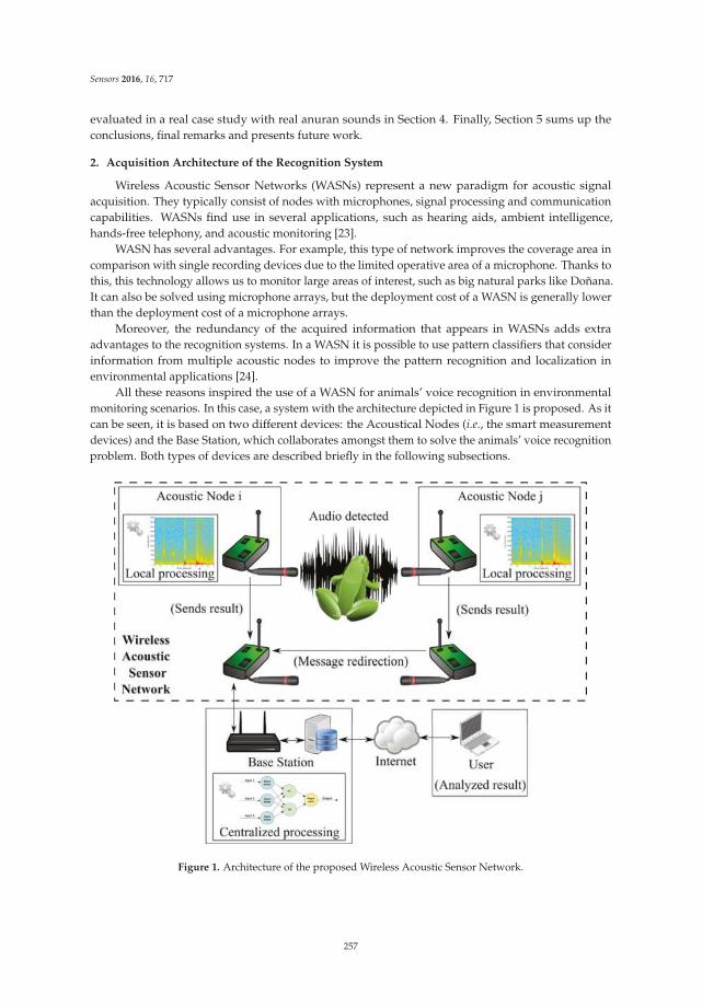
Sensors 2016, 16, 717

evaluated in a real case study with real anuran sounds in Section 4. Finally, Section 5 sums up theconclusions, final remarks and presents future work.

2. Acquisition Architecture of the Recognition System

Wireless Acoustic Sensor Networks (WASNs) represent a new paradigm for acoustic signalacquisition. They typically consist of nodes with microphones, signal processing and communicationcapabilities. WASNs find use in several applications, such as hearing aids, ambient intelligence,hands-free telephony, and acoustic monitoring [23].

WASN has several advantages. For example, this type of network improves the coverage area incomparison with single recording devices due to the limited operative area of a microphone. Thanks tothis, this technology allows us to monitor large areas of interest, such as big natural parks like Doñana.It can also be solved using microphone arrays, but the deployment cost of a WASN is generally lowerthan the deployment cost of a microphone arrays.

Moreover, the redundancy of the acquired information that appears in WASNs adds extraadvantages to the recognition systems. In a WASN it is possible to use pattern classifiers that considerinformation from multiple acoustic nodes to improve the pattern recognition and localization inenvironmental applications [24].

All these reasons inspired the use of a WASN for animals’ voice recognition in environmentalmonitoring scenarios. In this case, a system with the architecture depicted in Figure 1 is proposed. As itcan be seen, it is based on two different devices: the Acoustical Nodes (i.e., the smart measurementdevices) and the Base Station, which collaborates amongst them to solve the animals’ voice recognitionproblem. Both types of devices are described briefly in the following subsections.

Figure 1. Architecture of the proposed Wireless Acoustic Sensor Network.

257

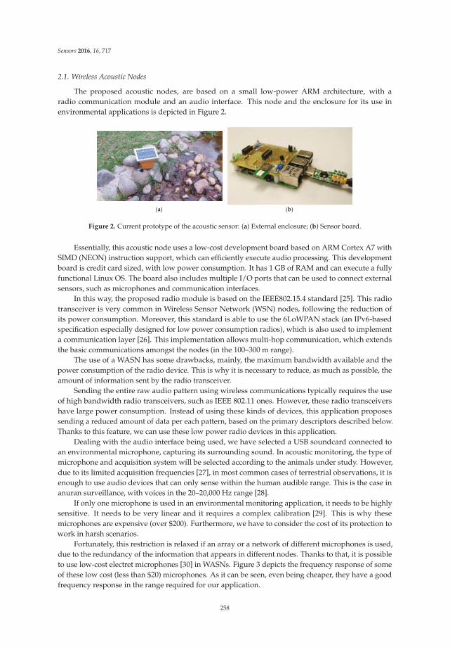
Sensors 2016, 16, 717

2.1. Wireless Acoustic Nodes

The proposed acoustic nodes, are based on a small low-power ARM architecture, with aradio communication module and an audio interface. This node and the enclosure for its use inenvironmental applications is depicted in Figure 2.

(a) (b)

Figure 2. Current prototype of the acoustic sensor: (a) External enclosure; (b) Sensor board.

Essentially, this acoustic node uses a low-cost development board based on ARM Cortex A7 withSIMD (NEON) instruction support, which can efficiently execute audio processing. This developmentboard is credit card sized, with low power consumption. It has 1 GB of RAM and can execute a fullyfunctional Linux OS. The board also includes multiple I/O ports that can be used to connect externalsensors, such as microphones and communication interfaces.

In this way, the proposed radio module is based on the IEEE802.15.4 standard [25]. This radiotransceiver is very common in Wireless Sensor Network (WSN) nodes, following the reduction ofits power consumption. Moreover, this standard is able to use the 6LoWPAN stack (an IPv6-basedspecification especially designed for low power consumption radios), which is also used to implementa communication layer [26]. This implementation allows multi-hop communication, which extendsthe basic communications amongst the nodes (in the 100–300 m range).

The use of a WASN has some drawbacks, mainly, the maximum bandwidth available and thepower consumption of the radio device. This is why it is necessary to reduce, as much as possible, theamount of information sent by the radio transceiver.

Sending the entire raw audio pattern using wireless communications typically requires the useof high bandwidth radio transceivers, such as IEEE 802.11 ones. However, these radio transceivershave large power consumption. Instead of using these kinds of devices, this application proposessending a reduced amount of data per each pattern, based on the primary descriptors described below.Thanks to this feature, we can use these low power radio devices in this application.

Dealing with the audio interface being used, we have selected a USB soundcard connected toan environmental microphone, capturing its surrounding sound. In acoustic monitoring, the type ofmicrophone and acquisition system will be selected according to the animals under study. However,due to its limited acquisition frequencies [27], in most common cases of terrestrial observations, it isenough to use audio devices that can only sense within the human audible range. This is the case inanuran surveillance, with voices in the 20–20,000 Hz range [28].

If only one microphone is used in an environmental monitoring application, it needs to be highlysensitive. It needs to be very linear and it requires a complex calibration [29]. This is why thesemicrophones are expensive (over $200). Furthermore, we have to consider the cost of its protection towork in harsh scenarios.

Fortunately, this restriction is relaxed if an array or a network of different microphones is used,due to the redundancy of the information that appears in different nodes. Thanks to that, it is possibleto use low-cost electret microphones [30] in WASNs. Figure 3 depicts the frequency response of someof these low cost (less than $20) microphones. As it can be seen, even being cheaper, they have a goodfrequency response in the range required for our application.

258

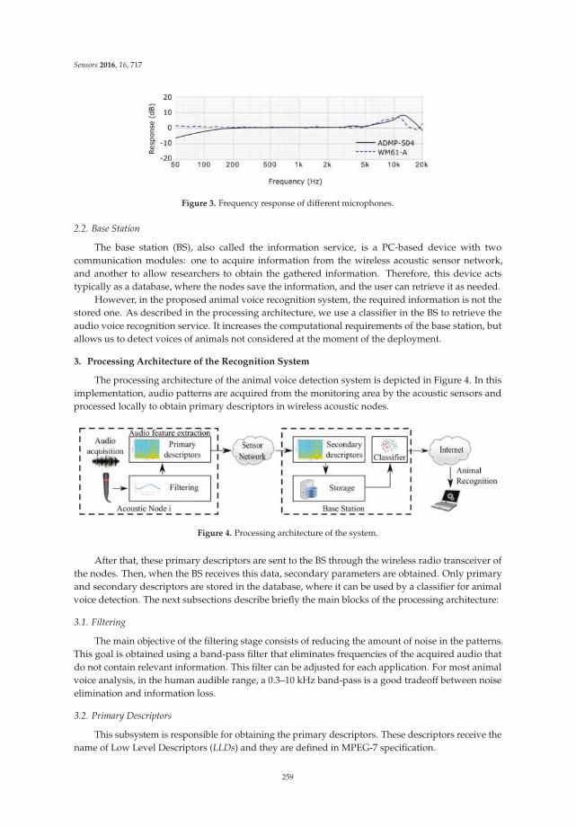
Sensors 2016, 16, 717

Figure 3. Frequency response of different microphones.

2.2. Base Station

The base station (BS), also called the information service, is a PC-based device with twocommunication modules: one to acquire information from the wireless acoustic sensor network,and another to allow researchers to obtain the gathered information. Therefore, this device actstypically as a database, where the nodes save the information, and the user can retrieve it as needed.

However, in the proposed animal voice recognition system, the required information is not thestored one. As described in the processing architecture, we use a classifier in the BS to retrieve theaudio voice recognition service. It increases the computational requirements of the base station, butallows us to detect voices of animals not considered at the moment of the deployment.

3. Processing Architecture of the Recognition System

The processing architecture of the animal voice detection system is depicted in Figure 4. In thisimplementation, audio patterns are acquired from the monitoring area by the acoustic sensors andprocessed locally to obtain primary descriptors in wireless acoustic nodes.

Figure 4. Processing architecture of the system.

After that, these primary descriptors are sent to the BS through the wireless radio transceiver ofthe nodes. Then, when the BS receives this data, secondary parameters are obtained. Only primaryand secondary descriptors are stored in the database, where it can be used by a classifier for animalvoice detection. The next subsections describe briefly the main blocks of the processing architecture:

3.1. Filtering

The main objective of the filtering stage consists of reducing the amount of noise in the patterns.This goal is obtained using a band-pass filter that eliminates frequencies of the acquired audio thatdo not contain relevant information. This filter can be adjusted for each application. For most animalvoice analysis, in the human audible range, a 0.3–10 kHz band-pass is a good tradeoff between noiseelimination and information loss.

3.2. Primary Descriptors

This subsystem is responsible for obtaining the primary descriptors. These descriptors receive thename of Low Level Descriptors (LLDs) and they are defined in MPEG-7 specification.

259

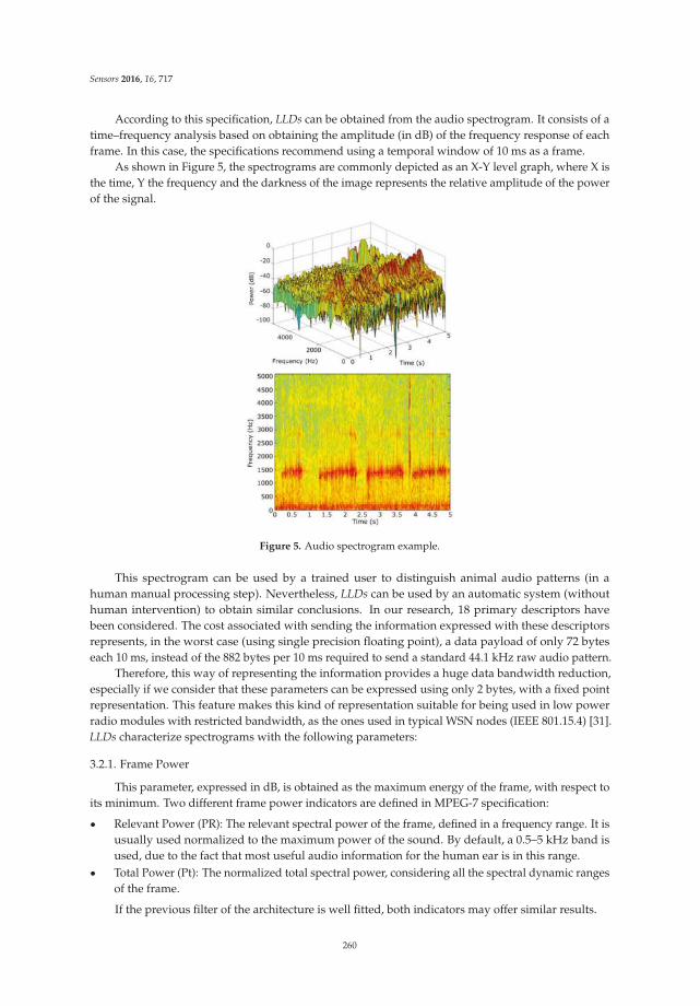
Sensors 2016, 16, 717

According to this specification, LLDs can be obtained from the audio spectrogram. It consists of atime–frequency analysis based on obtaining the amplitude (in dB) of the frequency response of eachframe. In this case, the specifications recommend using a temporal window of 10 ms as a frame.

As shown in Figure 5, the spectrograms are commonly depicted as an X-Y level graph, where X isthe time, Y the frequency and the darkness of the image represents the relative amplitude of the powerof the signal.

Figure 5. Audio spectrogram example.

This spectrogram can be used by a trained user to distinguish animal audio patterns (in ahuman manual processing step). Nevertheless, LLDs can be used by an automatic system (withouthuman intervention) to obtain similar conclusions. In our research, 18 primary descriptors havebeen considered. The cost associated with sending the information expressed with these descriptorsrepresents, in the worst case (using single precision floating point), a data payload of only 72 byteseach 10 ms, instead of the 882 bytes per 10 ms required to send a standard 44.1 kHz raw audio pattern.

Therefore, this way of representing the information provides a huge data bandwidth reduction,especially if we consider that these parameters can be expressed using only 2 bytes, with a fixed pointrepresentation. This feature makes this kind of representation suitable for being used in low powerradio modules with restricted bandwidth, as the ones used in typical WSN nodes (IEEE 801.15.4) [31].LLDs characterize spectrograms with the following parameters:

3.2.1. Frame Power

This parameter, expressed in dB, is obtained as the maximum energy of the frame, with respect toits minimum. Two different frame power indicators are defined in MPEG-7 specification:

‚ Relevant Power (PR): The relevant spectral power of the frame, defined in a frequency range. It isusually used normalized to the maximum power of the sound. By default, a 0.5–5 kHz band isused, due to the fact that most useful audio information for the human ear is in this range.

‚ Total Power (Pt): The normalized total spectral power, considering all the spectral dynamic rangesof the frame.

If the previous filter of the architecture is well fitted, both indicators may offer similar results.

260

Sensors 2016, 16, 717

3.2.2. Frame Power Centroid (CP)

In a particular frame, the power centroid briefly represents the shape of the frequency spectrum.The centroid offers information about the frequencies where most of the energy of the frame isdistributed. It can be obtained as shown in Equation (1):

CP “ř

i r fi¨ Pisř

i Pi(1)

where fi is the frequency of the spectrogram, and Pi the acoustic power of the associated frequency.

3.2.3. Spectral Dispersion (DE)

It represents approximately the shape of the frequency spectrum of a frame. It can be obtained asshown in Equation (2):

DE “

g

f

f

e

ř

i

”

`

fi ´ Cp

˘2 ¨ Pi

ı

ř

i Pi(2)

3.2.4. Spectrum Flatness (Pl)

It represents the deviation of the audio spectrum in relation to a flat spectrum (i.e., a white noise).It can be obtained with Equation (3):

Pl “a

ś

i Pi1n

ř

i Pi

(3)

3.2.5. Harmonicity Ratio (Ra)

Ra is the ratio of harmonic power to total power. According to MPEG-7 specifications, it can beobtained from the autocorrelation of the audio signal s pnq into the frame, as expressed in Equation (4):

Ra “ maxk

¨

˝

ř

j s pjq ¨ pj ´ kqb

ř

j s pjq2 ¨ ř

j s pj ´ kq2

˛

‚ (4)

where k is the length of the frame.

3.2.6. Fundamental Frequency (Pitch)

The fundamental frequency (or sound pitch) is the frequency that best describes the periodicity ofa signal. It can be obtained with the Linear Prediction Coding (LPC) algorithm [32]. LPC, models thespectral power as sum of the polynomial A pzq defined by Equation (5):

A pzq “ 1 ´ÿp

k“1

”

ak¨ z´kı

(5)

where the polynomial degree p represents the model precision. The coefficients ak representthe formants of the audio signal, i.e., the spectral maximum produces by the audio resonances.According to [32], these coefficients can be obtained reducing the error between the polynomialprediction and the spectral power of the audio frame using a minimum least squares estimation.

For the sound s pnq the error function ε pnq is obtained according to Equation (6):

ε pnq “ s pnq ´ÿp

k“1aks pn ´ kq (6)

For ε pnq, the autocorrelation function is obtained by Equation (7):

ϕ pkq “ÿ`8

m“´8ε pmq ε pm ` kq (7)

261

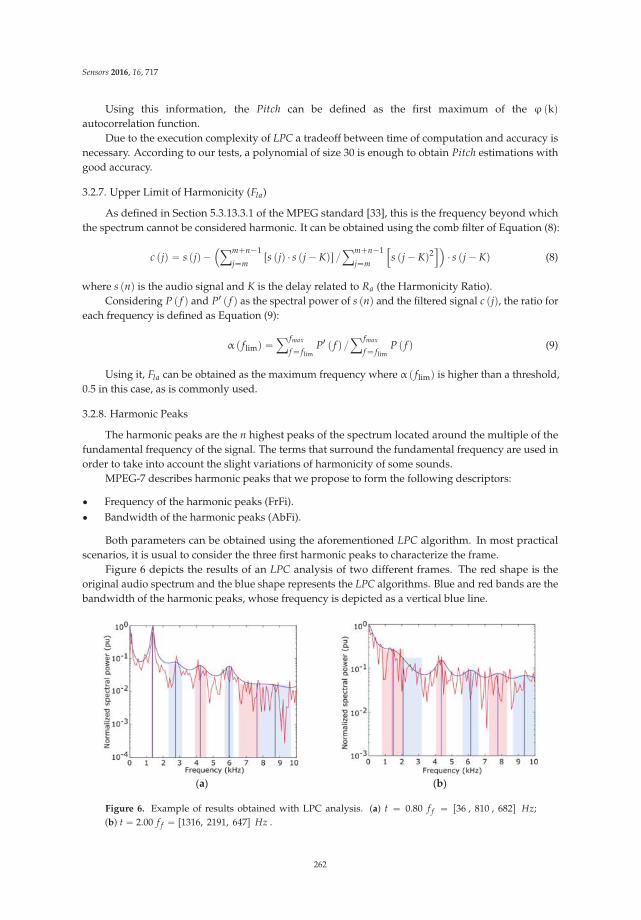
Sensors 2016, 16, 717

Using this information, the Pitch can be defined as the first maximum of the ϕ pkqautocorrelation function.

Due to the execution complexity of LPC a tradeoff between time of computation and accuracy isnecessary. According to our tests, a polynomial of size 30 is enough to obtain Pitch estimations withgood accuracy.

3.2.7. Upper Limit of Harmonicity (Fla)

As defined in Section 5.3.13.3.1 of the MPEG standard [33], this is the frequency beyond whichthe spectrum cannot be considered harmonic. It can be obtained using the comb filter of Equation (8):

c pjq “ s pjq ´´

ÿm`n´1

j“mrs pjq ¨ s pj ´ Kqs

ÿm`n´1

j“m

”

s pj ´ Kq2ı¯

¨ s pj ´ Kq (8)

where s pnq is the audio signal and K is the delay related to Ra (the Harmonicity Ratio).Considering P p f q and P1 p f q as the spectral power of s pnq and the filtered signal c pjq, the ratio for

each frequency is defined as Equation (9):

α p flimq “ÿ fmax

f “ flimP1 p f q

ÿ fmax

f “ flimP p f q (9)

Using it, Fla can be obtained as the maximum frequency where α p flimq is higher than a threshold,0.5 in this case, as is commonly used.

3.2.8. Harmonic Peaks

The harmonic peaks are the n highest peaks of the spectrum located around the multiple of thefundamental frequency of the signal. The terms that surround the fundamental frequency are used inorder to take into account the slight variations of harmonicity of some sounds.

MPEG-7 describes harmonic peaks that we propose to form the following descriptors:

‚ Frequency of the harmonic peaks (FrFi).‚ Bandwidth of the harmonic peaks (AbFi).

Both parameters can be obtained using the aforementioned LPC algorithm. In most practicalscenarios, it is usual to consider the three first harmonic peaks to characterize the frame.

Figure 6 depicts the results of an LPC analysis of two different frames. The red shape is theoriginal audio spectrum and the blue shape represents the LPC algorithms. Blue and red bands are thebandwidth of the harmonic peaks, whose frequency is depicted as a vertical blue line.

(a) (b)

Figure 6. Example of results obtained with LPC analysis. (a) t “ 0.80 f f “ r36 , 810 , 682s Hz;(b) t “ 2.00 f f “ r1316, 2191, 647s Hz .

262

Sensors 2016, 16, 717

3.2.9. Harmonic Centroid (CA)

It is a weighted average that selects a frequency that represents the harmonic peaks of the frame.It can be obtained with Equation (10):

CH “řn f

i“1 r fi¨ visřn f

i“1 vi

(10)

where fi is the ith frequency of the harmonic peak and vi its peak value.

3.2.10. Harmonic Spectral Deviation (DeA)

It is computed as the deviation between harmonic peaks and the signal spectrum of the frame.It can be obtained with Equation (11):

DeA “ maxk

¨

˝

řn f

i“1

ˇ

ˇ

ˇlog pviq ´ log

´

13 ¨ ř1

k“´1 rvi ` ks¯ˇ

ˇ

ˇ

řn f

i“1 log pviq

˛

‚ (11)

3.2.11. Harmonic Spectral Spread (DiA)

It is computed as the typical deviation between harmonics peaks and the harmonic centroid.It can be obtained with Equation (12):

DiA “ 1Ca

¨

g

f

f

f

e

řn f

i“1

”

vi2¨ p fi ´ Caq2

ı

řn f

i“1 vi2

(12)

3.2.12. Harmonic Spectral Variation (VA)

It is obtained as a normalized correlation between the harmonic peaks of two adjacent frames.It can be obtained with Equation (13):

VA “ 1 ´řn f

i“1

“

vi,j¨ vi,j´1‰

řn f

i“1

b

vi,j2¨ řn f

i“1

b

vi,j´12

(13)

where vi,j is the amplitude of the ith harmonic of the frame j.

3.3. Secondary Descriptors

One shortcoming in the use of MPEG-7 LLDs for animal voice detection is that they do notconsider reverberation effects. This is due to the reduced size of the frame (only 10 ms), which issmaller than the duration of these effects. However, many animal characteristic acoustic patterns havean important reverberation component, which can be used to distinguish between species.

To describe these effects we propose the use of secondary descriptors. These descriptors areobtained with a methodology based on the same methodology used with the primary descriptors.The dispersion between longer time frames is analyzed. These time frames are called micro-segmentsand have a duration of 100 ms (i.e., 10 frames). This time is chosen considering that, audio delayshigher than 100 ms are identified by human being as echo, instead of a reverberation.

We define these secondary descriptors as the interquartile range of each one of the primaryparameters, in a 100 ms micro-segment.

According this procedure, we obtained the next secondary parameters:

‚ Dispersion of relevant Power (PR~).‚ Dispersion of total Power (Pt~).

263

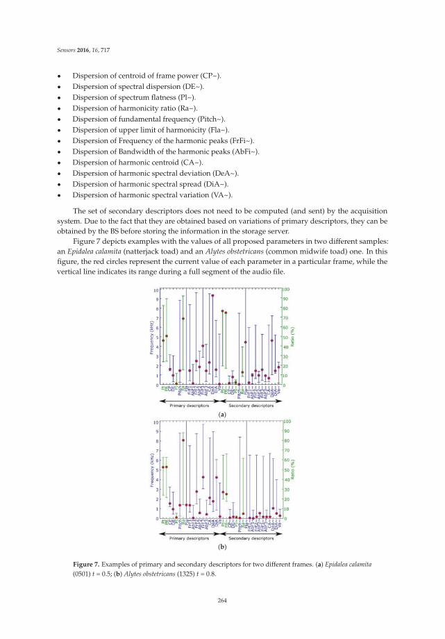
Sensors 2016, 16, 717

‚ Dispersion of centroid of frame power (CP~).‚ Dispersion of spectral dispersion (DE~).‚ Dispersion of spectrum flatness (Pl~).‚ Dispersion of harmonicity ratio (Ra~).‚ Dispersion of fundamental frequency (Pitch~).‚ Dispersion of upper limit of harmonicity (Fla~).‚ Dispersion of Frequency of the harmonic peaks (FrFi~).‚ Dispersion of Bandwidth of the harmonic peaks (AbFi~).‚ Dispersion of harmonic centroid (CA~).‚ Dispersion of harmonic spectral deviation (DeA~).‚ Dispersion of harmonic spectral spread (DiA~).‚ Dispersion of harmonic spectral variation (VA~).

The set of secondary descriptors does not need to be computed (and sent) by the acquisitionsystem. Due to the fact that they are obtained based on variations of primary descriptors, they can beobtained by the BS before storing the information in the storage server.

Figure 7 depicts examples with the values of all proposed parameters in two different samples:an Epidalea calamita (natterjack toad) and an Alytes obstetricans (common midwife toad) one. In thisfigure, the red circles represent the current value of each parameter in a particular frame, while thevertical line indicates its range during a full segment of the audio file.

(a)

(b)

Figure 7. Examples of primary and secondary descriptors for two different frames. (a) Epidalea calamita

(0501) t = 0.5; (b) Alytes obstetricans (1325) t = 0.8.

264

Sensors 2016, 16, 717

On the other hand, the color of the axis indicates the units of the parameters. As it can be seen,red ones are defined in Hertz, while green ones are in percentages.

This example graphically shows that the proposed parameters have very different range andvalues for different audio samples. Therefore, they can be effectively used by an automatic classificationsystem in order to distinguish different patterns.

3.4. Data Storage

This subsystem is dedicated to storing the primary and secondary descriptors. This informationmust be tagged with a timestamp, and can be stored in a regular SQL database.

3.5. Classifier

This subsystem plays an important role in the whole system. It is responsible for theimplementation of the classification method. Its main goal is to classify the audio patterns (i.e.,its descriptors) into one of the proposed classes. In this sense, hundreds of supervised classifiers havebeen proposed in the literature. The selection for the best method is a decision that has to be doneconsidering the characteristics of the problem to solve [34]. However, in our real case analysis, evensimple classifiers offer good class separations using the aforementioned descriptors.

4. A Case Study: Anuran classification system

The proposed animal audio detection descriptors have been evaluated considering the differentbehavior of two anuran species: Alytes obstetricans (Figure 8a) and Epidalea calamita (Figure 8b).

(a) (b)

Figure 8. Two specific anuran species: (a) Alytes obstetricans toad, carrying egg strings [35];(b) Epidalea calamita toad [36]. Photographs by Ursina Tobler.

Ethology studies focused on the anuran species, such as the described ones, are especiallyinteresting for the biologist. The reason for this interest is based on the fact that in some amphibianspecies, climate change and UV radiation have important effects on their population (largelydetermined by their habitat) [1,37]. More concretely, an interesting phenomenon can be observed inanurans (frogs and toads). These kinds of amphibians present peaks in the timing of reproductivecalling (songs), depending on each species and temperature evolution [38]. This is why an anuranclassifier is used as a case study of the proposed descriptors.

4.1. Sound Database Information

In order to analyze the performance of the proposed descriptors, this research has based itsevaluation on a relevant database of anuran songs. This database is composed by a set of audiosamples of Alytes obstetricans and Epidalea calamita provided by “Fonozoo: Fonoteca Zoológica del Museo

Nacional de Ciencias Naturales”, a Spanish phonotheque based on recordings of animal sounds [39].

265

Sensors 2016, 16, 717

This organization provided a scientific collection of animal sounds. Fonozoo was created with the aimof supporting the study of acoustic communication in animals.

The collection includes more than 45,000 sound recordings belonging to more than 12,000 differentspecies, all of which makes Fonozoo a valuable tool in the systematic study of animal behavior.The main goal of using a public audio database is that these files can be used by other researchers allover the world for comparative performance analysis. In the case of the studied anurans, the collectionis composed of 63 audio samples, according to the characteristics described in Table 1.

Table 1. Analysis of the sound collections.

Caption Vocalization Files

Epidalea calamitastandard 20chorus 3

oviposit 10

Alytes obstetricansstandard 29

distress call 1

This collection of anuran audio files offers a total of 6053 s of recorded sounds, with a meanduration of 96 s and a median of 53 s. Therefore, our test collection has 605,300 frames, where eachframe has a total amount of 36 associated values that are its primary and secondary descriptors.

As can be seen, the number of chorus vocalization samples of Epidalea calamita toads is not enoughto train a system. Moreover, it sounds similar to the standard vocalization. Due to this, both cases aregoing to be considered as the same classification category.

In the case of the Alytes obstetricans toads, there are not enough distress call vocalization samplesto train a system. Due to this, in the test of the proposed descriptor, we have considered the nextnumber of samples by categories:

‚ Type 1: 23 samples of Epidalea calamita toad with standard or chorus vocalization.‚ Type 2: 10 samples of Epidalea calamita toad with oviposit vocalization.‚ Type 3: 30 samples of Alytes obstetricans toad with standard or distress call vocalization.

Due to the fact that the samples have been obtained from environmental scenarios, not onlyanimal vocalization is recorded. In fact, there is a high percentage of background sound, composed ofwind, rain, traffic, human voices, and so forth. Therefore, there are intervals of time in each samplethat do not correspond with animal vocalization, and which need to be detected and rejected by theclassification system. With this purpose, a fourth type of audio has been considered, that correspondswith noise, i.e., sounds in which we are not interested in.

4.2. Classification Results

Supervised classifier techniques require the use of sound models for each class. These models arerequired in the training and adjusting phase of the classifier. In this case, two files have been chosen asa pattern from both Epidalea calamita and Alytes obstetricans toads with standard vocalization, and onefile for Epidalea calamita toad with oviposit vocalization. These models have been selected empirically,looking for files in which the sound is easily distinguishable. In this case, files “0501” and “0707” fromFonozoo collection are chosen as type 1 pattern, “0503” as type 2, and “1325” and “1330” as type 3.

Once the classification criterion has been selected, it is necessary to evaluate its value. In thissense, a classification can only offer good accuracy if there exists a surface in the input parameters(i.e., the descriptors) space, where the different classes can be isolated completely or with a reducederror. This feature can be observed in Figure 9, where the value of each parameter (centroid anddispersion versus power in this example) for each frame is summarized. A color code has been chosento indicate its class type. Blue for type 1 (Epidalea calamita toad with standard or chorus vocalization),

266

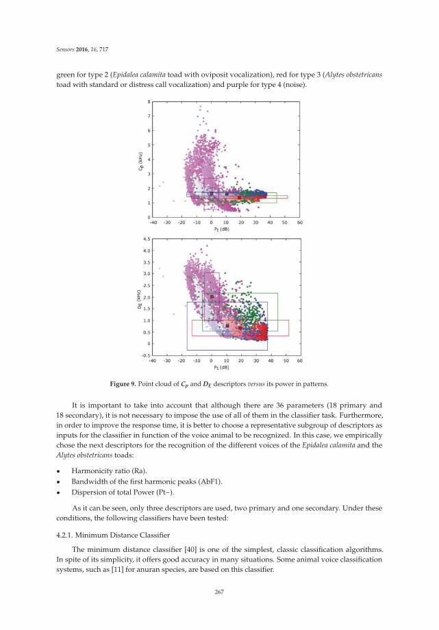
Sensors 2016, 16, 717

green for type 2 (Epidalea calamita toad with oviposit vocalization), red for type 3 (Alytes obstetricans

toad with standard or distress call vocalization) and purple for type 4 (noise).

Figure 9. Point cloud of Cp and DE descriptors versus its power in patterns.

It is important to take into account that although there are 36 parameters (18 primary and18 secondary), it is not necessary to impose the use of all of them in the classifier task. Furthermore,in order to improve the response time, it is better to choose a representative subgroup of descriptors asinputs for the classifier in function of the voice animal to be recognized. In this case, we empiricallychose the next descriptors for the recognition of the different voices of the Epidalea calamita and theAlytes obstetricans toads:

‚ Harmonicity ratio (Ra).‚ Bandwidth of the first harmonic peaks (AbF1).‚ Dispersion of total Power (Pt~).

As it can be seen, only three descriptors are used, two primary and one secondary. Under theseconditions, the following classifiers have been tested:

4.2.1. Minimum Distance Classifier

The minimum distance classifier [40] is one of the simplest, classic classification algorithms.In spite of its simplicity, it offers good accuracy in many situations. Some animal voice classificationsystems, such as [11] for anuran species, are based on this classifier.

267

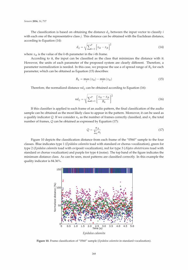
Sensors 2016, 16, 717

The classification is based on obtaining the distance dij between the input vector to classify i

with each one of the representative class j. This distance can be obtained with the Euclidean distance,according to Equation (14):

dij “c

ÿP

k“1

”

xik ´ xjk

ı2(14)

where xik is the value of the k-th parameter in the i-th frame.According to it, the input can be classified as the class that minimizes the distance with it.

However, the units of each parameter of the proposed system are clearly different. Therefore, aparameter normalization is needed. In this case, we propose the use a of spread range of Rk for eachparameter, which can be obtained as Equation (15) describes:

Rk “ maxi

pxikq ´ mini

pxikq (15)

Therefore, the normalized distance ndij can be obtained according to Equation (16):

ndij “

d

ÿP

k“1

„

xik ´ xjk

Rk

j2

(16)

If this classifier is applied to each frame of an audio pattern, the final classification of the audiosample can be obtained as the most likely class to appear in the pattern. Moreover, it can be used asa qualify indicator Q. If we consider na as the number of frames correctly classified, and nj the totalnumber of frames, Q can be obtained as expressed by Equation (17):

Q “ nAř

j nj(17)

Figure 10 depicts the classification distance from each frame of the “0560” sample to the fourclasses. Blue indicates type 1 (Epidalea calamita toad with standard or chorus vocalization), green fortype 2 (Epidalea calamita toad with oviposit vocalization), red for type 3 (Alytes obstetricans toad withstandard or chorus vocalization) and purple for type 4 (noise). The top band of the figure indicates theminimum distance class. As can be seen, most patterns are classified correctly. In this example thequality indicator is 84.36%.

Epidalea calamita

Figure 10. Frame classification of “0560” sample (Epidalea calamita in standard vocalization).

268

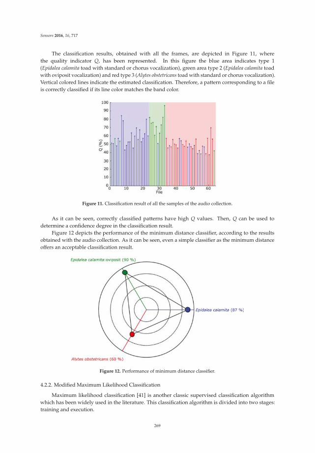
Sensors 2016, 16, 717

The classification results, obtained with all the frames, are depicted in Figure 11, wherethe quality indicator Q, has been represented. In this figure the blue area indicates type 1(Epidalea calamita toad with standard or chorus vocalization), green area type 2 (Epidalea calamita toadwith oviposit vocalization) and red type 3 (Alytes obstetricans toad with standard or chorus vocalization).Vertical colored lines indicate the estimated classification. Therefore, a pattern corresponding to a fileis correctly classified if its line color matches the band color.

Figure 11. Classification result of all the samples of the audio collection.

As it can be seen, correctly classified patterns have high Q values. Then, Q can be used todetermine a confidence degree in the classification result.

Figure 12 depicts the performance of the minimum distance classifier, according to the resultsobtained with the audio collection. As it can be seen, even a simple classifier as the minimum distanceoffers an acceptable classification result.

Figure 12. Performance of minimum distance classifier.

4.2.2. Modified Maximum Likelihood Classification

Maximum likelihood classification [41] is another classic supervised classification algorithmwhich has been widely used in the literature. This classification algorithm is divided into two stages:training and execution.

269

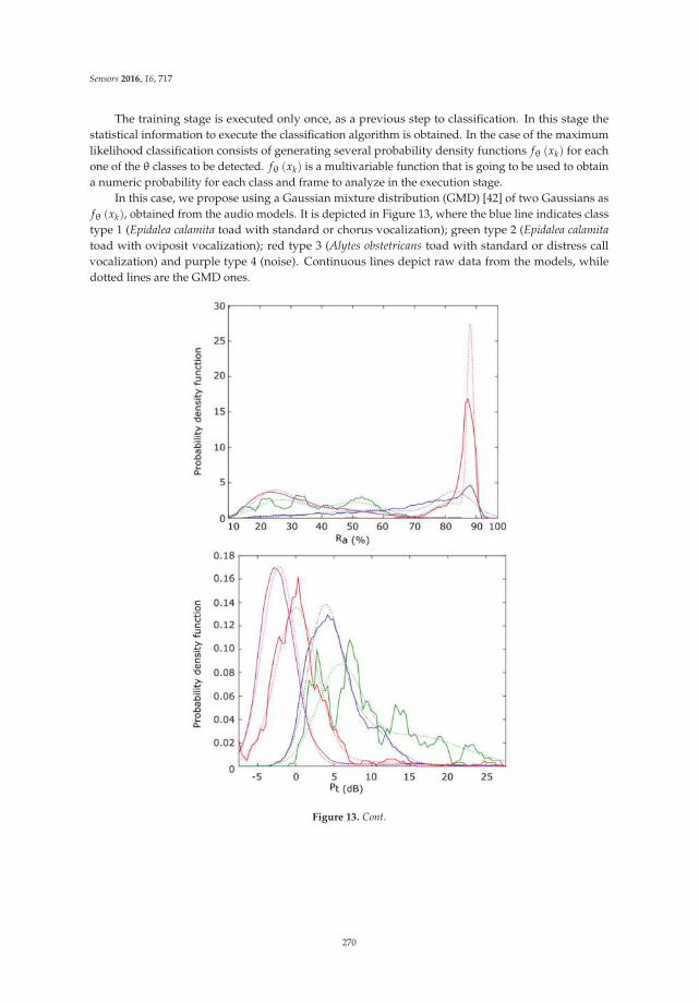
Sensors 2016, 16, 717

The training stage is executed only once, as a previous step to classification. In this stage thestatistical information to execute the classification algorithm is obtained. In the case of the maximumlikelihood classification consists of generating several probability density functions fθ pxkq for eachone of the θ classes to be detected. fθ pxkq is a multivariable function that is going to be used to obtaina numeric probability for each class and frame to analyze in the execution stage.

In this case, we propose using a Gaussian mixture distribution (GMD) [42] of two Gaussians asfθ pxkq, obtained from the audio models. It is depicted in Figure 13, where the blue line indicates classtype 1 (Epidalea calamita toad with standard or chorus vocalization); green type 2 (Epidalea calamita

toad with oviposit vocalization); red type 3 (Alytes obstetricans toad with standard or distress callvocalization) and purple type 4 (noise). Continuous lines depict raw data from the models, whiledotted lines are the GMD ones.

Figure 13. Cont.

270

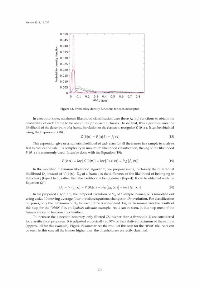
Sensors 2016, 16, 717

Figure 13. Probability density functions for each descriptor.

In execution time, maximum likelihood classification uses these fθ pxkq functions to obtain theprobability of each frame to be one of the proposed θ classes. To do that, this algorithm uses thelikelihood of the descriptors of a frame, in relation to the classes to recognize L pθ |x q. It can be obtainedusing the Expression (18):

L pθ |x q “ P px| θq “ fθ pxq (18)

This expression give us a numeric likelihood of each class for all the frames in a sample to analyze.But to reduce the calculus complexity in maximum likelihood classification, the log of the likelihoodV pθ |x q is commonly used. It can be done with the Equation (19):

V pθ |x q “ log rL pθ |x qs “ log rP px| θqs “ log r fθ pxqs (19)

In the modified maximum likelihood algorithm, we propose using to classify the differentiallikelihood Dij instead of V pθ |x q. Dij of a frame i is the difference of the likelihood of belonging tothat class j (type 1 to 3), rather than the likelihood it being noise r (type 4). It can be obtained with theEquation (20):

Dij ” V`

θj

ˇ

ˇxi

˘

´ V pθr|xiq “ log“

fθj pxiq‰

´ log r fθr pxiqs (20)

In the proposed algorithm, the temporal evolution of Dij of a sample to analyze is smoothed outusing a size 10 moving average filter to reduce spurious changes in Dij evolution. For classificationpurposes, only the maximum of Dij for each frame is considered. Figure 14 summarizes the results ofthis step for the “0560” file, an Epidalea calamita example. As it can be seen, in this step most of theframes are yet to be correctly classified.

To increase the detection accuracy, only filtered Dij higher than a threshold β are consideredfor classification proposes. β is adjusted empirically at 30% of the relative maximum of the sample(approx. 0.5 for this example). Figure 15 summarizes the result of this step for the “0560” file. As it canbe seen, in this case all the frames higher than the threshold are correctly classified.

271

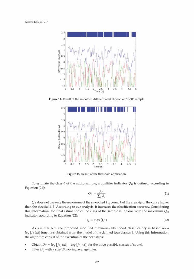
Sensors 2016, 16, 717

Figure 14. Result of the smoothed differential likelihood of “0560” sample.

Figure 15. Result of the threshold application.

To estimate the class θ of the audio sample, a qualifier indicator Qθ is defined, according toEquation (21):

Qθ “ Aθř

j Aj(21)

Qθ does not use only the maximum of the smoothed Dij count, but the area Aθ of the curve higherthan the threshold β, According to our analysis, it increases the classification accuracy. Consideringthis information, the final estimation of the class of the sample is the one with the maximum Qm

indicator, according to Equation (22):Q “ max

j

`

Qj

˘

(22)

As summarized, the proposed modified maximum likelihood classificatory is based on alog r fθ pxqs functions obtained from the model of the defined four classes θ. Using this information,the algorithm consist of the execution of the next steps:

‚ Obtain Dij “ log“

fθj pxq‰

´ log r fθr pxqs for the three possible classes of sound.‚ Filter Dij with a size 10 moving average filter.

272

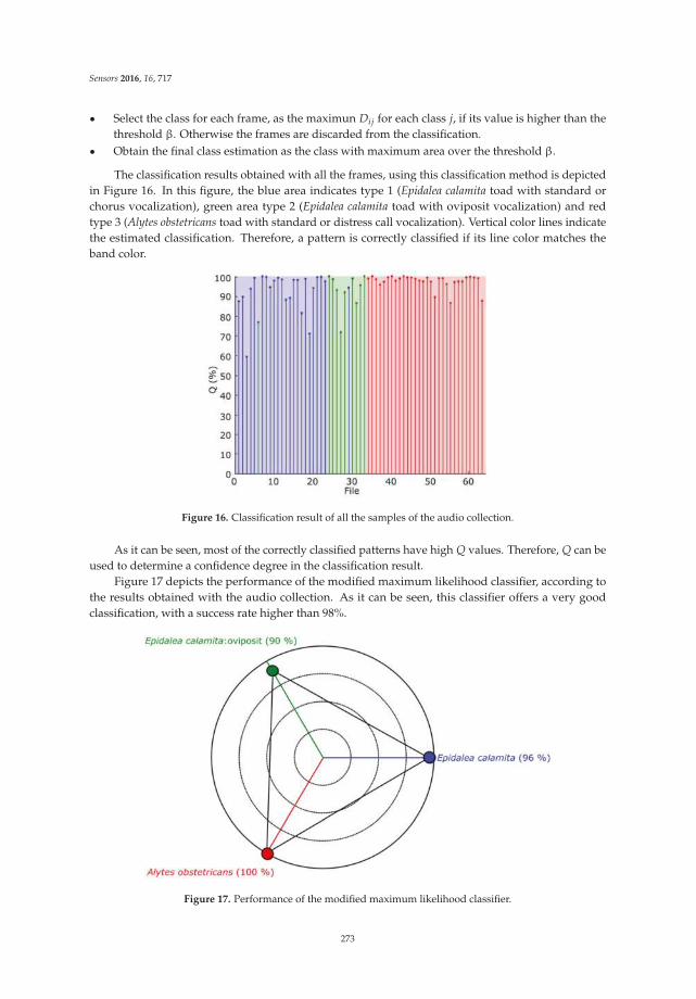
Sensors 2016, 16, 717

‚ Select the class for each frame, as the maximun Dij for each class j, if its value is higher than thethreshold β. Otherwise the frames are discarded from the classification.

‚ Obtain the final class estimation as the class with maximum area over the threshold β.

The classification results obtained with all the frames, using this classification method is depictedin Figure 16. In this figure, the blue area indicates type 1 (Epidalea calamita toad with standard orchorus vocalization), green area type 2 (Epidalea calamita toad with oviposit vocalization) and redtype 3 (Alytes obstetricans toad with standard or distress call vocalization). Vertical color lines indicatethe estimated classification. Therefore, a pattern is correctly classified if its line color matches theband color.

Figure 16. Classification result of all the samples of the audio collection.

As it can be seen, most of the correctly classified patterns have high Q values. Therefore, Q can beused to determine a confidence degree in the classification result.

Figure 17 depicts the performance of the modified maximum likelihood classifier, according tothe results obtained with the audio collection. As it can be seen, this classifier offers a very goodclassification, with a success rate higher than 98%.

Figure 17. Performance of the modified maximum likelihood classifier.

273

Sensors 2016, 16, 717


This paper describes a classification architecture for animal voice recognition. The main goalof the proposed architecture is first to reduce biologists’ effort to manually classify audio patterns,and second, to provide a method that can be used to classify classes not previously considered.This classification architecture is based on the use of MPEG-7 low level descriptors, plus a family ofderived descriptors used to detect animal voice reverberations. These descriptors have been tested inreal scenarios detecting anuran voices stored in a public sound database.

The obtained results allow us to conclude that the proposed generic descriptors, using adequateclassifiers, can be used to classify animal voices with a high degree of accuracy. In addition, theproposed architecture does not have the most common drawbacks of audio classification architectures.

The future work that is being considered by the authors focuses on two strategies: first, thedeployment of this animal voice detection system in several natural environments; and secondly, thedevelopment of other classifiers using the proposed descriptors.

Acknowledgments: This work has been supported by the Consejería de Innovación, Ciencia y Empresa,Junta de Andalucía, Spain, through the excellence eSAPIENS (reference number TIC-5705). The authors wouldlike to thank Rafael Ignacio Marquez Martinez de Orense (Museo Nacional de Ciencias Naturales) andJuan Francisco Beltrán Gala (Faculty of Biology, University of Seville) for their collaboration and support.

Author Contributions: Joaquín Luque conceived and designed the experiments; Joaquín Luque, Diego F. Larios,Enrique Personal, Julio Barbancho and Carlos León performed the experiments, analyzed the data and wrotethe paper.


References

1. Walls, S.; Barichivich, W.; Brown, M. Drought, deluge and declines: The impact of precipitation extremes onamphibians in a changing climate. Biology 2013, 2, 399–418. [CrossRef] [PubMed]

2. Parmesan, C.; Yohe, G. A globally coherent fingerprint of climate change impacts across natural systems.Nature 2003, 421, 37–42. [CrossRef] [PubMed]

3. Cambron, M.; Bowker, R. An automated digital sound recording system: The amphibulator. In Proceedingsof the Eighth IEEE International Symposium on Multimedia (ISM’06), San Diego, CA, USA, 11–13December 2006.

4. Cambron, M.E.; Emberton, A.C. Amphibulator II. In Proceedings of the IEEE Southeastcon, Jacksonville, FL,USA, 4–7 April 2013.

5. Banerjee, R.; Mobashir, M.; Bit, S.D. Partial DCT-based energy efficient compression algorithm for wirelessmultimedia sensor network. In Proceedings of the 2014 IEEE International Conference on Electronics,Computing and Communication Technologies (CONECCT), Bangalore, India, 6–7 January 2014.

6. Dutta, I.; Banerjee, R.; Bit, S.D. Energy efficient audio compression scheme based on red black wavelet liftingfor wireless multimedia sensor network. In Proceedings of the 2013 International Conference on Advancesin Computing, Communications and Informatics (ICACCI), Mysore, India, 22–25 August 2013.

7. Diaz, J.J.M.; Nakamura, E.F.; Yehia, H.C.; Salles, J.; Loureiro, A.A.F. On the use of compressive sensing for thereconstruction of anuran sounds in a wireless sensor network. In Proceedings of the 2012 IEEE InternationalConference on Green Computing and Communications, Besancon, France, 20–23 November 2012.

8. Salomons, E.; Havinga, P. A survey on the feasibility of sound classification on wireless sensor nodes. Sensors

2015, 15, 7462–7498. [CrossRef] [PubMed]9. Okuyucu, C.; Sert, M.; Yazici, A. Audio feature and classifier analysis for efficient recognition of

environmental sounds. In Proceedings of the 2013 IEEE International Symposium on Multimedia, Anaheim,CA, USA, 9–11 December 2013.

10. Croker, B.; Kottege, N. Using feature vectors to detect frog calls in wireless sensor networks. J. Acoust.

Soc. Am. 2012, 131, EL400. [CrossRef] [PubMed]11. Huang, C.J.; Yang, Y.J.; Yang, D.X.; Chen, Y.J. Frog classification using machine learning techniques.

Expert Syst. Appl. 2009, 36, 3737–3743. [CrossRef]

274

Sensors 2016, 16, 717

12. Chung, Y.; Oh, S.; Lee, J.; Park, D.; Chang, H.H.; Kim, S. Automatic detection and recognition of pig wastingdiseases using sound data in audio surveillance systems. Sensors 2013, 13, 12929–12942. [CrossRef] [PubMed]

13. Kim, Y.; Ahn, J.; Cha, H. Locating acoustic events based on large-scale sensor networks. Sensors 2009, 9,9925–9944. [CrossRef] [PubMed]

14. González-Castaño, F.J.; Alonso, J.V.; Costa-Montenegro, E.; López-Matencio, P.; Vicente-Carrasco, F.;Parrado-García, F.J.; Gil-Castiñeira, F.; Costas-Rodríguez, S. Acoustic sensor planning for gunshot location innational parks: A pareto front approach. Sensors 2009, 9, 9493–9512. [CrossRef] [PubMed]

15. Quackenbush, S.; Lindsay, A. Overview of MPEG-7 audio. IEEE Trans. Circuits Syst. Video Technol. 2001, 11,725–729. [CrossRef]

16. You, S.D.; Chen, W.H. Comparative study of methods for reducing dimensionality of MPEG-7 audiosignature descriptors. Multimed. Tools Appl. 2013, 74, 3579–3598. [CrossRef]

17. Lin, C.H.; Tu, M.C.; Chin, Y.H.; Liao, W.J.; Hsu, C.S.; Lin, S.H.; Wang, J.C.; Wang, J.F. SVM-based soundclassification based on MPEG-7 audio LLDs and related enhanced features. In Convergence and Hybrid

Information Technology; Springer Science + Business Media: Berlin, Germany, 2012; pp. 536–543.18. You, S.D.; Chen, W.H.; Chen, W.K. Music Identification system using MPEG-7 audio signature descriptors.

Sci. World J. 2013, 2013, 1–11. [CrossRef] [PubMed]19. Muhammad, G.; Melhem, M. Pathological voice detection and binary classification using MPEG-7 audio

features. Biomed. Signal Process. Control 2014, 11, 1–9. [CrossRef]20. Lampropoulos, A.S.; Tsihrintzis, G.A. Evaluation of MPEG-7 descriptors for speech emotional recognition.

In Proceedings of the 2012 Eighth International Conference on Intelligent Information Hiding and MultimediaSignal Processing, Piraeus, Greece, 18–20 July 2012.

21. Tyburek, K.; Prokopowicz, P.; Kotlarz, P. Fuzzy system for the classification of sounds of birds based on theaudio descriptors. In Artificial Intelligence and Soft Computing; Springer Science + Business Media: Berlin,Germany, 2014; pp. 700–709.

22. Larios, D.; Barbancho, J.; Sevillano, J.; Rodríguez, G.; Molina, F.; Gasull, V.; Mora-Merchan, J.; León, C.Five years of designing wireless sensor networks in the doñana biological reserve (Spain): An applicationsapproach. Sensors 2013, 13, 12044–12069. [CrossRef] [PubMed]

23. Bertrand, A. Applications and trends in wireless acoustic sensor networks: A signal processing perspective.In Proceedings of the 2011 18th IEEE Symposium on Communications and Vehicular Technology in theBenelux (SCVT), Ghent, Belgium, 22–23 November 2011.

24. Wang, H.; Chen, C.E.; Ali, A.; Asgari, S.; Hudson, R.E.; Yao, K.; Estrin, D.; Taylor, C. Acoustic sensor networksfor woodpecker localization. In Proceedings of the Advanced Signal Processing Algorithms, Architectures,and Implementations XV, San Diego, CA, USA, 2–4 August 2005.

25. The Institute of Electrical and Electronics Engineers (IEEE). IEEE Standard for Local and metropolitan area

networks. Part 15.4: Low-Rate Wireless Personal Area Networks (LR-WPANs); IEEE Standards Association:New York, NY, USA, 2011.

26. Ko, J.; Terzis, A.; Dawson-Haggerty, S.; Culler, D.E.; Hui, J.W.; Levis, P. Connecting low-power and lossynetworks to the internet. IEEE Commun. Mag. 2011, 49, 96–101.

27. Blumstein, D.T.; Mennill, D.J.; Clemins, P.; Girod, L.; Yao, K.; Patricelli, G.; Deppe, J.L.; Krakauer, A.H.;Clark, C.; Cortopassi, K.A.; et al. Acoustic monitoring in terrestrial environments using microphone arrays:Applications, technological considerations and prospectus. J. Appl. Ecol. 2011, 48, 758–767. [CrossRef]

28. Acevedo, M.A.; Corrada-Bravo, C.J.; Corrada-Bravo, H.; Villanueva-Rivera, L.J.; Aide, T.M. Automatedclassification of bird and amphibian calls using machine learning: A comparison of methods. Ecol. Inform.

2009, 4, 206–214. [CrossRef]29. Müller, G.; Möser, M. Handbook of Engineering Acoustics; Springer: Berlin/Heidelberg, Germany, 2012.30. Fristrup, K.M.; Mennitt, D. Bioacoustical monitoring in terrestrial environments. Acoust. Today 2012, 8, 16.

[CrossRef]31. Akyildiz, I.F.; Melodia, T.; Chowdhury, K.R. A survey on wireless multimedia sensor networks. Comput. Netw.

2007, 51, 921–960. [CrossRef]32. Rabiner, L.R.; Schafer, R.W. Introduction to Digital Speech Processing; Foundations and Trends in Signal

Processing: Hanover, MA, USA, 2007; Volume 1, pp. 1–194.

275

Sensors 2016, 16, 717

33. International Organization for Standardization (ISO)/International Electrotechnical Commission (IEC).Information Technology—Multimedia Content Description Interface—Part 4: Audio; ISO/IEC FDIS 15938-4:2002;ISO/IEC Association: Geneva, Switzerland, 2002.

34. Fernández-Delgado, M.; Cernadas, E.; Barro, S.; Amorim, D. Do we need hundreds of classifiers to solve realworld classification problems? J. Mach. Learn. Res. 2014, 15, 3133–3181.

35. Tobler, U.; Garner, T.W.J.; Schmidt, B.R. Genetic attributes of midwife toad (Alytes obstetricans) populationsdo not correlate with degree of species decline. Ecol. Evol. 2013, 3, 2806–2819. [CrossRef] [PubMed]

36. Oromi, N.; Richter-Boix, A.; Sanuy, D.; Fibla, J. Genetic variability in geographic populations of the natterjacktoad (Bufo calamita). Ecol. Evol. 2012, 2, 2018–2026. [CrossRef] [PubMed]

37. Blaustein, A.R.; Walls, S.C.; Bancroft, B.A.; Lawler, J.J.; Searle, C.L.; Gervasi, S.S. Direct and indirect effects ofclimate change on amphibian populations. Diversity 2010, 2, 281–313. [CrossRef]

38. Walpole, A.A.; Bowman, J.; Tozer, D.C.; Badzinski, D.S. Community-level response to climate change: Shiftsin anuran calling phenology. Herpetol. Conserv. Biol. 2012, 7, 249–257.

39. Solís, G.; Eekhout, X.; Márquez, R. FonoZoo.com a New Resource in the Web for the Study of Animal Sounds;Razprave IV. Razreda Sazu; Slovenska Akademija Znanosti in Umetnosti: Ljubljana, Slovenia, 2006;Volume XLVII, pp. 145–154.

40. Rudrapatna, M.; Sowmya, A. Feature weighted minimum distance classifier with multi-class confidenceestimation. In Lecture Notes in Computer Science; Springer Science + Business Media: Berlin, Germany, 2006;pp. 253–263.

41. Beel, J.; Gipp, B. Academic search engine spam and google scholar’s resilience against it. J. Electron. Publ.

2010, 13. [CrossRef]42. Roweis, S.; Ghahramani, Z. A unifying review of linear gaussian models. Neural Comput. 1999, 11, 305–345.

[CrossRef] [PubMed]


276

sensors

Article

Accuracy and Resolution Analysis of a DirectResistive Sensor Array to FPGA Interface

Óscar Oballe-Peinado 1,2, Fernando Vidal-Verdú 1,2,*, José A. Sánchez-Durán 1,2,Julián Castellanos-Ramos 1,2 and José A. Hidalgo-López 1,2

1 Departamento de Electrónica, Universidad de Málaga, Andalucía Tech, Campus de Teatinos, Málaga 29071,Spain; [email protected] (O.O.-P.); [email protected] (J.A.S.-D.); [email protected] (J.C.-R.);[email protected] (J.A.H.-L.)

2 Instituto de Investigación Biomédica de Málaga (IBIMA), Málaga 29010, Spain* Correspondence: [email protected]; Tel.: +34-952-133-325; Fax: +34-952-133-324

Academic Editor: Gonzalo Pajares MartinsanzReceived: 27 December 2015; Accepted: 29 January 2016; Published: 1 February 2016

Abstract: Resistive sensor arrays are formed by a large number of individual sensors which aredistributed in different ways. This paper proposes a direct connection between an FPGA and aresistive array distributed in M rows and N columns, without the need of analog-to-digital convertersto obtain resistance values in the sensor and where the conditioning circuit is reduced to the use ofa capacitor in each of the columns of the matrix. The circuit allows parallel measurements of theN resistors which form each of the rows of the array, eliminating the resistive crosstalk which istypical of these circuits. This is achieved by an addressing technique which does not require externalelements to the FPGA. Although the typical resistive crosstalk between resistors which are measuredsimultaneously is eliminated, other elements that have an impact on the measurement of dischargetimes appear in the proposed architecture and, therefore, affect the uncertainty in resistance valuemeasurements; these elements need to be studied. Finally, the performance of different calibrationtechniques is assessed experimentally on a discrete resistor array, obtaining for a new model ofcalibration, a maximum relative error of 0.066% in a range of resistor values which correspond to atactile sensor.

Keywords: resistive sensor arrays; direct sensor-to-digital device interface; FPGAs; parallel analoguedata acquisition

1. Introduction

An important number of sensors are based on the variation of resistance values shown dueto the passage of an electric current, depending on a physical magnitude which is measured.These are resistive sensors, which can be classified according to their applications. They can betactile sensors [1–10], temperature sensors [11,12], gas detectors [13–15] or for other substances [16,17].In order to obtain the desired information, sometimes a single sensor can be enough. Several sensors arenecessary in other occasions. For example, tactile sensors used in applications such as skin emulationor robotic hands (where large surfaces need to be scanned) are usually formed by an array with alarge number of individual sensors. Substance detectors are also usually formed by a large numberof sensors.

One of the main problems of resistive sensor arrays is that they need a large number of componentsand complicated wiring for the circuits which measure the different resistances. There are alsonumerous circuits carrying out signal conditioning and analog-to-digital conversion of the informationfor its subsequent processing. In principle, for a single access (SA) configuration 2¨ M¨ N cables fromthe sensor to the circuit are needed, although one of them is normally shared by all sensors [10] so they


Sensors 2016, 16, 181

are reduced to M¨ N + 1. The time needed to extract the information of the whole array is practicallythe time needed to extract the information of a single sensor. However, each sensor needs its owncircuit for conditioning and AD conversion. For this reason, for large size arrays this configuration canbe very costly in terms of area and energy consumption.

With the aim of alleviating this problem, a resistive sensor array can be distributed in the shape ofa two-dimensional matrix of M rows and N columns. There are several sensors sharing the rows andcolumns in this array access (AA) configuration, but in such a way that the information of a singlesensor can be accessed by selecting a row and a column. Therefore, the number of cables from thearray is reduced to M + N and the number of necessary circuits to scan the information would beM or N depending on the type of array. In addition to this, additional circuits are needed to carryout sensor addressing. On the other hand, the time needed to extract the information of the wholearray is the result of multiplying the time used in scanning a sensor by the number of N columns orM rows of the array plus the time required in multiplexing. This same solution has to be used if theconstruction of the sensor already has a structure of rows and columns and its output comes throughM + N wires, as in [2,4]. A second possibility to further reduce the circuitry which carries out ADconversion is the increase of the multiplexing of the information of the array in such a way that onlyone element is scanned at a time. This solution is obviously slower and the multiplexing circuits aremore complicated.

The last two strategies to scan a resistive sensor array show, in addition to the increase of thetime needed to access the information, the so-called crosstalk effect [11,18–23]. This effect happenswhen the resistance values of other elements of the array have an impact on the measurement of theresistance of the element which is being scanned. Because of this effect, resistance measurements showa certain degree of error when the structures mentioned above are used. For instance, errors of 30%are obtained for a 4 ˆ 4 array with resistors in a range between 100 Ω and 1000 Ω (using buffers withinternal resistance of 10 Ω to address the rows) [24], despite the use of four operational amplifiersto reduce crosstalk. This error can be reduced with more complex circuits including calibrationtechniques to improve the readout accuracy [25] or including analog switches and an additionalOA [24]. Therefore, for accurate and fast readings without these complex circuits, the only solution isaccessing each of the elements of the array individually and without multiplexing.

The solution used in this paper avoids resistive crosstalk, providing accuracy in the measurementas in a SA configuration, while having the intermediate speed and intermediate hardware cost ofan AA configuration. The structure of the array is divided into rows and columns, but now, in eachcolumn, all sensors share a terminal while the other is individual (row access configuration, RA).Therefore, the sensor would have (M + 1)¨ N cables and the information of N sensors will be accessedsimultaneously. The signal conditioning circuit is only one capacitor in each column, which is also partof the circuit for AD conversion (for our case a time-to-digital conversion). This is carried out by usingan FPGA as in [26] instead of microcontrollers [27]. This configuration, with some modifications, canbe applied to other sensors (capacitive or inductive) that provide a time-modulated signal that can bedirectly measured in the digital domain [28,29].

Another reason to use this array configuration lies in the need of calibrating the measurementof resistive sensors. There is extensive literature on calibration of single sensors [26,30–33], but noton calibration of resistive sensor arrays. In general, calibration is necessary to avoid errors in themeasurement of parameters which are used in the determination of resistance values. In an AA typesensor, for best accuracy, M¨ N calibration resistors would also be needed, as the values of the capacitorswhich are used by each resistor of the array have to be calibrated as well. Calibrating the thresholdvoltage which makes digital devices go from detecting a 1-logic to a 0-logic would also be necessary ifmicrocontrollers or FPGAs are used for AD conversion. This greatly complicates the total hardware ofthe system. However, only N calibration elements are necessary if an array with an RA configurationis used.

278

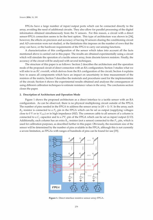
Sensors 2016, 16, 181

FPGAs have a large number of input/output ports which can be connected directly to thearray, avoiding the need of additional circuits. They also allow for parallel processing of the digitalinformation obtained simultaneously from the N sensors. For this reason, a circuit with a directsensor-FPGA connection seems to be the best option. This type of architecture was shown in [34],however, the effects on precision and accuracy of having M sensors sharing the conditioning circuitand AD conversion were not studied, or the limitations this imposes on the number of rows that thearray can have, or the hardware requirements of the FPGA to carry out sensing functions.

A characterization of this configuration of the sensor which takes into account all the factsmentioned above is carried out in this paper. The results are obtained experimentally using a circuitwhich will simulate the operation of a tactile sensor array, from discrete known resistors. Finally, theaccuracy of the circuit will be analyzed with several techniques.

The structure of this paper is as follows: Section 2 describes the architecture and the operationmode of the proposed circuit of direct connection with an RA configuration; Section 3 studies what wewill refer to as RC crosstalk, which derives from the RA configuration of the circuit; Section 4 explainshow to assess all components which have an impact on uncertainty in time measurement of theresistors of the matrix; Section 5 describes the materials and procedures used for the implementationof the circuit; Section 6 shows the experimental results obtained and analyses the consequences ofusing different calibration techniques to estimate resistance values in the array. The conclusions sectioncloses the paper.

2. Description of Architecture and Operation Mode

Figure 1 shows the proposed architecture as a direct interface to a tactile sensor with an RAconfiguration. As can be observed, there is no physical multiplexing circuit outside of the FPGA.The number of pins needed in the FPGA to address the sensor array is (M + 1)¨ N. In the array, eachRij resistor is connected to a Pij pin in the FPGA which can be set as output (supplying voltagesclose to 0 V or to VDD) or in high impedance (HZ). The common cable to all sensors of a column isconnected to a Cj capacitor and to a PVj pin of the FPGA which can be set as input/output (I/O).Additionally, each column has an extra Rcj resistor (not a sensor) connected to the Pcj pin, which isused for calibration purposes, as described further in this paper. Obviously, the maximum size of thesensor will be determined by the number of pins available in the FPGA, although this is not currentlya severe limitation, as FPGAs with ranges of hundreds of pins can be found for use [35].

Figure 1. Direct interface resistive sensor array-FPGA.

279

Sensors 2016, 16, 181

The reading process of each row of the array has two phases. Firstly, in the charge phase, Cj

capacitors are charged by setting PVj pins as output to a ‘1’ level while all Pij pins are kept in HZ.Then, in the discharge phase, a whole row is selected by setting its corresponding I/O pins to ‘0’.For instance, pins Pk1, . . . PkN are set to ‘0’ while the remaining Pij pins, are kept in HZ. Simultaneously,all PVj pins are selected as input to be able to measure the Vj voltage of the Cj capacitor which is beingdischarged. A set of timers are started in the FPGA at the beginning of this discharging phase andtheir counts are stopped when the low threshold (VTj) is reached at the related column pins. VTj isthe voltage in which the FPGA detects a ‘0’ logic in PVj. Therefore, a whole row is read in parallel.The process is repeated for the M rows of the array and the calibration row.

The purpose of the calibration resistor is to avoid having to know the Cj, VTj and VDD values,because these are normally difficult to measure. In addition, Cj and VTj depend on power voltagesupply or temperature and they can drift with time. As there is only one calibration resistor, itwould seem that the method used is what is known in the literature as a single-point calibration [27].According to this method, if when row i is selected, the discharge time measured for the Cj capacitoris Δtij, and when the calibration row is selected, the time is Δtcj, then the Rij resistance value isdetermined by:

Rij “Δtij

ΔtcjRcj (1)

where Rcj is a value decided by the designer. However, this calibration method does not take intoaccount the output resistance RBj of the FPGA buffers (around 10 Ω for the FPGA of this paper) whichare connected in series to Rij and Rcj. For this reason, if Equation (1) is used, a mistake is made in theestimation of resistance value. More accuracy could be obtained if the two-point calibration method isused [27]. However, adding an additional row of calibration is then necessary, resulting in an increaseof hardware in the circuit.

A calibration solution which takes into account RBi resistances, and uses a single calibrationresistor is proposed in [36]. The method consists on using off-time calibration (outside of the normaloperation of the sensor) where, by using different resistors and measuring their discharge time, arelationship can be established between Rij and Rcj. It is shown that the adjustment of the experimentaldata using a linear function is sufficiently accurate, resulting in the following relationship:

Rij “ α ¨ Δt1ij ` B (2)

with α and B as constants and where Δt1ij would be the time used for discharging Cj through Rij during

off-time calibration. Δt1cj must also be measured during off-time calibration. This is the time used in

the discharge through Rcj (calibration resistor which will be used during the normal operation of thesensor). By using this time value, Equation (2) Rij can be calculated as follows:

Rij “ A ¨Δt1

ij

Δt1cj

` B (3)

where A = Rcj ´ B. Using Equation (3), during the normal operation of the circuit, the value of Rij canbe calculated by measuring the Δtij and Δtcj times:

Rij “ A ¨Δtij

Δtcj` B (4)

This way of obtaining Rij is similar to that of a single-point calibration but taking the RBi bufferresistances into account and, therefore, with an accuracy which is similar to that of a two-pointcalibration. We will refer to this procedure as the off-on time method. This technique has the drawback ofrequiring prior pre-calibration, although the hardware is simpler, so the cost is reduced. Moreover, the

280

Sensors 2016, 16, 181

time required to scan the array decreases when compared with that of the two-point calibration method,and the power consumption is also lower.

Although in principle there is no crosstalk in Equation (4), it must be noted that this expressiondoes not take stray capacitors which appear in the FPGA pins into account, which are in HZ statewhen an array row is read. This originates what will be referred to as RC crosstalk in this paper, whichwill be studied in detail in the following section.

3. RC Crosstalk

Figure 2 shows the detail of the j column of the circuit when the discharge of Cj is being measuredthrough the Rij resistor. Cpkj with k ‰ i are the capacitors which group all stray capacitors connectedto Pij pins in HZ state in the FPGA. By analyzing Figure 2, it can be observed how all stray capacitorshave an impact on the discharge process of Cj. Moreover, the impact is not always the same, as theresistors which link them to Cj also vary. In Figure 2, it has been assumed that the discharge of the Cpij

capacitor is very fast compared to that of Cj, (and it is true, as RBi << Rij and Cpij << Cj).

Figure 2. Detail of the j column of the circuit, showing the stray capacitors.

Vj(s) is the voltage of Cj in the Laplace variable, during the discharge process. Its value isdetermined by:

Vjpsq “ ´IL

Cjs` VDD

s(5)

where IL is the current which discharges the capacitor and VDD is its initial charging voltage. On theother hand, for each IK with k ‰ i:

Vjpsq “ Ik

˜

Rk j ` 1Cpk j

¸

` VDD

s(6)

while:

Ii “VjpsqRij

(7)

Solving for IL in Equation (5), Ik in Equation (6) and taking into account that:

IL “M`1ÿ

k“1

Ik (8)

where k = M + 1 indicates the calibration row, the equation is:

´ VjpsqCjs ` CjVDD “VjpsqRij

`M`1ÿ

k “ 1k ‰ i

1Rk j

sVjpsq ´ VDD

s ` 1Rk jCpk j

(9)

281

Sensors 2016, 16, 181

solving for Vj(s):

Vjpsq “ VDD ¨

Cj `M`1ř

k “ 1k ‰ i

1Rk j

1

s ` 1Rk jCpk j

Cjs ` 1Ri j

`M`1ř

k “ 1k ‰ i

1Rk j

1

s ` 1Rk jCpk j

(10)

and finally:

Vjpsq “ VDD ¨

1 `M`1ř

k “ 1k ‰ i

Cpk j

Cj

1Rk jCpk js ` 1

s

¨

˚

˚

˚

˚

˚

˝

1 `M`1ř

k “ 1k ‰ i

Cpk j

Cj

1Rk jCpk js ` 1

˛

‹

‹

‹

‹

‹

‚

` 1Ri jCj

(11)

Some facts are clear from Equation (11). Firstly, Vj(s) is not only the discharge voltage of acapacitor with a single pole; it has M + 1 poles and M zeros. Equation (11) also shows crosstalkappearance, as Vj(s) is not only a function of Rij and Cj; it also depends on the rest of the resistors ofthe column (Rkj) and on the Cpkj stray capacitors associated to each pin in the column (this is wherethe name RC crosstalk comes from).

Secondly, if Cpkj << Cj, Equation (11) is reduced to:

Vjpsq « VDD

s ` 1Ri jCj

(12)

which is the discharge equation through an only capacitor. Therefore, the higher Cj is, compared toCpkj, the lower the crosstalk will be. Reducing Cpkj implies making a good design of the sensor and ofthe control circuit. However, there are terms composing Cpkj which cannot be reduced, such as FPGApin capacitance or that of their contacts with the wiring of the sensors (once the PCB technology of thesensors has been selected). The dependency with Rkj can also be observed in Equation (11). But thisterm cannot be varied as it is the resistance of the sensors themselves.

Although RC crosstalk has been analyzed in a sensor array, it will also appear if any of thecalibration techniques mentioned in Section 2 are used. This situation occurs even when a single sensoris calibrated. Figure 3 shows a circuit for the measurement of an RX resistor, with two calibrationresistors, RC1 and RC2. As shown in the figure, RC1 and RC2 resistors are associated with two parasiticcapacitors, CpC1 and CpC2.

282

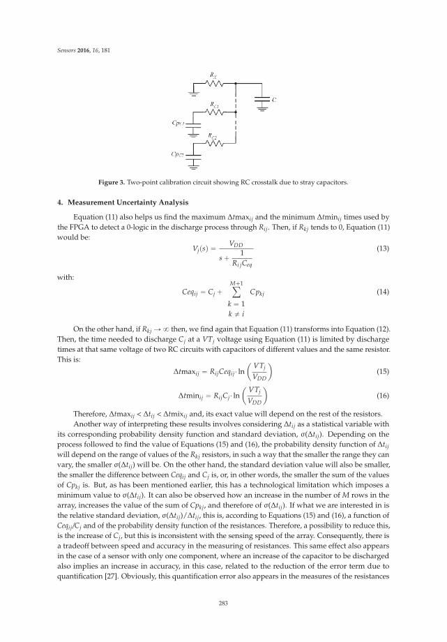
Sensors 2016, 16, 181

Figure 3. Two-point calibration circuit showing RC crosstalk due to stray capacitors.

4. Measurement Uncertainty Analysis

Equation (11) also helps us find the maximum Δtmaxij and the minimum Δtminij times used bythe FPGA to detect a 0-logic in the discharge process through Rij. Then, if Rkj tends to 0, Equation (11)would be:

Vjpsq “ VDD

s ` 1Ri jCeq

(13)

with:

Ceqij “ Cj `M`1ÿ

k “ 1k ‰ i

Cpkj (14)

On the other hand, if Rkj Ñ 8 then, we find again that Equation (11) transforms into Equation (12).Then, the time needed to discharge Cj at a VTj voltage using Equation (11) is limited by dischargetimes at that same voltage of two RC circuits with capacitors of different values and the same resistor.This is:

Δtmaxij “ RijCeqij¨ lnˆ

VTj

VDD

˙

(15)

Δtminij “ RijCj¨ lnˆ

VTj

VDD

˙

(16)

Therefore, Δtmaxij < Δtij < Δtmixij and, its exact value will depend on the rest of the resistors.Another way of interpreting these results involves considering Δtij as a statistical variable with

its corresponding probability density function and standard deviation, σ(Δtij). Depending on theprocess followed to find the value of Equations (15) and (16), the probability density function of Δtij

will depend on the range of values of the Rkj resistors, in such a way that the smaller the range they canvary, the smaller σ(Δtij) will be. On the other hand, the standard deviation value will also be smaller,the smaller the difference between Ceqij and Cj is, or, in other words, the smaller the sum of the valuesof Cpkj is. But, as has been mentioned earlier, this has a technological limitation which imposes aminimum value to σ(Δtij). It can also be observed how an increase in the number of M rows in thearray, increases the value of the sum of Cpkj, and therefore of σ(Δtij). If what we are interested in isthe relative standard deviation, σ(Δtij)/Δtij, this is, according to Equations (15) and (16), a function ofCeqij/Cj and of the probability density function of the resistances. Therefore, a possibility to reduce this,is the increase of Cj, but this is inconsistent with the sensing speed of the array. Consequently, there isa tradeoff between speed and accuracy in the measuring of resistances. This same effect also appearsin the case of a sensor with only one component, where an increase of the capacitor to be dischargedalso implies an increase in accuracy, in this case, related to the reduction of the error term due toquantification [27]. Obviously, this quantification error also appears in the measures of the resistances

283

Sensors 2016, 16, 181

of the array. Therefore, and in sum, the measuring of the Δtij time, corresponding to a specific resistorof the array, has as uncertainty resources related to other sensors: the values of the other resistorsof the array and the existence of Cpkj capacitors. This causes a first source of uncertainty, crosstalkuncertainty, σcrosstalk(Δtij). The other sources of uncertainty that a single sensor which is not part of anarray would have, must be added to this: u(z) quantification noise and the noise in VDD, VTj and Cj,which generate what we will refer to as trigger noise uncertainty, σtrigger(Δtij).

The same procedure can be followed if the aim is to measure the time needed to get a 0-logicfor the calibration resistor (Δtcj). This time value will also be a random variable with extreme valuesdetermined by:

Δtmaxcj “ RcjCeqcj ¨ lnˆ

VTj

VDD

˙

(17)

Δtmincj “ RcjCj ¨ lnˆ

VTj

VDD

˙

(18)

where:

Ceqcj “ Cj `Mÿ

k“1

Cpk j (19)

and therefore, with its own standard deviation, σ(Δtcj). It must be noted that the differences betweenthe Δtij and Δtcj values are not only determined by the different Rij and Rcj resistance values, but alsobecause, in general, Ceqcj ‰ Ceqij with i ‰ c, due to the different capacitors associated to the wiringwhich links each sensor with its corresponding pin in the FPGA (these differences can become verysmall with a careful design and adequate technology, although they will always exist). This also showsthat if the position of the resistors in a column was changed (with the exception of that for calibration)variations in their values would appear. Then, as it has been shown with Rcj, there is a third source ofuncertainty associated to the difference between the capacitances of the nodes in a column. This willoriginate a standard deviation in time measurement which will be referred to as σcolumn(Δtij).

It could also be argued that there is noise due to the position in the same row but in differentcolumns. However, assuming that the distribution of resistance values is independent of the rows andthat the variation in the Cpij capacitors is identical in all columns, this noise would only be due to thevariations in Cj. This is compensated through the calibration circuit of each column, so it is consideredas insignificant. Therefore, uncertainty in Δtij measurement, can be expressed by:

σ`

Δtij

˘

“b

σ2crosstalk

`

Δtij

˘

` σ2trigger

`

Δtij

˘

` σ2column

`

Δtij

˘

(20)

as the three terms inside the root are independent of each other.Noise due to quantification, upzq “ Ts

?12, should be added to this deviation [37], where Ts is

the period of time of the counter which measures discharge time. Although uncertainty in VDD, VTj

and Cj values can be compensated using Equation (4) (reducing then the values of all terms inside theroot), there is still uncertainty in measurement due to RC crosstalk. According to Equations (15) and(16), there are three possibilities to reduce the relative impact of crosstalk: the first one is in the increaseof Cj, but, as we have mentioned before, this reduces the scanning speed of the array. The secondpossibility is the reduction of the Cpij terms, but this (once a careful design of the system has beencarried out) is limited by technology and the number of rows in the array. The third possibility is thelimitation in the range of values of the resistors of the array, but obviously, this can only be achieved insome very specific sensors. Therefore, although the RA structure of the sensor array does not show thetypical resistive crosstalk, there exists what has been referred to as RC crosstalk and which, therefore,has to be assessed.

284

Sensors 2016, 16, 181

Assessment Method of Uncertainty in Measurement

A naive method for uncertainty assessment in Δtij measurement would be to perform a set ofmeasurements for each of the sensors of the array, varying the resistors of the remaining sensors ineach of the measurements, obtaining then the maximum ranges of variation. However, the use of thismethod of characterization is a difficult task to undertake, as the number of sensors in an array is notusually a small number, even in our case where a “reduced” 7 ˆ 8 sensor array has been used.

The aim of this paper is to propose the assessment of total uncertainty in the measurement of anyresistor of the array based on the independency of uncertainties due to crosstalk, column and triggerby using Equation (20).

For this reason, a circuit simulating by means of resistors the different values which can be readfrom all positions of an array with RA configuration has been designed. The circuit, obviously, includesan FPGA and the necessary capacitors for time-to-digital conversion.

The assessment method of uncertainty in measurement comprises the following steps: firstly, aset of sufficient resistor values which approximately divide the range of the sensor in uniform sectionsis selected (8 in our case). Each of these resistors is placed in successive tests in the M rows of a columnof the array selected for characterization. The remaining resistors of the column take the mean valuein the range. Then, a set of Q time measurements are carried out (Δtij). The process is repeated M

times changing the position of the resistor in a circular manner, in such a way that M¨ Q time measuresare obtained for each resistor. This set of times has a standard deviation which is due both to triggeruncertainty and to position uncertainty in the column, with variance σ2

trigger`column.

To get the value of each of these terms σ2trigger and σ2

column (for each resistor), the following

procedure is proposed. From a set of Q measurements carried out in each row, M σ2trigger values

are obtained. These values should be very similar for all rows, and the mean of these values isthe final estimation of σ2

trigger. Because they are independent sources of uncertainty, its variance is

σ2trigger ` column “ σ2

trigger ` σ2column and therefore σ2

column could be calculated as:

σ2column “ σ2

trigger ` column ´ σ2trigger (21)

σcrosstalk can be found with the following procedure: a row in the column used for the set ofprevious measurements is selected. Each of the eight resistors will be placed in this position of the array.Two sets of Q measurements will be carried out for each resistor. In the first set of Q measurements,the minimum value resistor in the sensor is added to the selected resistor in the remaining positionsof the column. In the second set of Q measurements, minimum value resistors are replaced by thosewith maximum values. Then we find the Δtmax maximum and Δtmin minimum time values for the2¨ Q measures, and their difference Δtmax ´ Δtmin, will be the estimator used to find the range of Δtij

values for each resistor due to RC crosstalk. Finally, assuming that the values of the sensor resistorshave a uniform distribution and, therefore, Δtij as well, for each resistor, the σcrosstalk value can becalculated as:

σtrigger`crosstalk “ Δtmax ´ Δtmin?12

(22)

where again we can solve for σcrosstalk:

σ2crosstalk “ σ2

trigger`crosstalk ´ σ2trigger (23)

Therefore, the value of σ(Δtij) can be obtained for each resistor by using Equation (20).Quantification uncertainty, u(z), should be added to this, obtaining then a total uncertainty value, σT

(Δtij), determined by:

σT

`

Δtij

˘

“b

σ2`

Δtij

˘

` u2pzq (24)

Uncertainty in the whole range will be the maximum value of all uncertainties obtained.

285

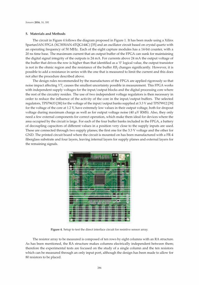
Sensors 2016, 16, 181

5. Materials and Methods

The circuit in Figure 4 follows the diagram proposed in Figure 1. It has been made using a XilinxSpartan3AN FPGA (XC3S50AN-4TQG144C) [35] and an oscillator circuit based on crystal quartz withan operating frequency of 50 MHz. Each of the eight capture modules has a 14-bit counter, with a20 ns time base. The maximum current that an output buffer of the FPGA can sunk for maintainingthe digital signal integrity of the outputs is 24 mA. For currents above 24 mA the output voltage ofthe buffer that drives the row is higher than that identified as a ‘0’ logical value, the output transistoris not in the ohmic region and the resistance of the buffer RBj changes significantly. However, it ispossible to add a resistance in series with the one that is measured to limit the current and this doesnot alter the procedure described above.

The design rules recommended by the manufactures of the FPGA are applied rigorously so thatnoise impact affecting VTj causes the smallest uncertainty possible in measurement. This FPGA workswith independent supply voltages for the input/output blocks and the digital processing core wherethe rest of the circuitry resides. The use of two independent voltage regulators is then necessary inorder to reduce the influence of the activity of the core in the input/output buffers. The selectedregulators, TPS79633 [38] for the voltage of the input/output banks supplied at 3.3 V and TPS79912 [39]for the voltage of the core at 1.2 V, have extremely low values in their output voltage, both for dropoutvoltage during maximum charge as well as for output voltage noise (40 µV RMS). Also, they onlyneed a few external components for correct operation, which make them ideal for devices where thearea occupied by the circuit is large. For each of the four buffer banks included in the FPGA, a batteryof decoupling capacitors of different values in a position very close to the supply inputs are used.These are connected through two supply planes; the first one for the 3.3 V voltage and the other forGND. The printed circuit board where the circuit is mounted on has been manufactured with a FR-4fiberglass substrate and four layers, leaving internal layers for supply planes and external layers forthe remaining signals.

Figure 4. Setup to test the direct interface circuit for resistive sensor array.

The resistor array to be measured is composed of ten rows by eight columns with an RA structure.As has been mentioned, the RA structure makes columns electrically independent between them;therefore the experimental tests are focused on the study of a single column and the ten resistorswhich can be measured through an only input port, although the design has been made to allow for80 resistors to be placed.

286

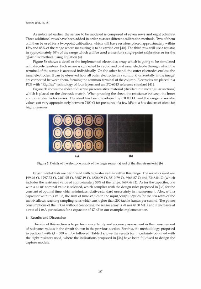
Sensors 2016, 16, 181

As indicated earlier, the sensor to be modeled is composed of seven rows and eight columns.Three additional rows have been added in order to asses different calibration methods. Two of themwill then be used for a two-point calibration, which will have resistors placed approximately within15% and 85% of the range where measuring is to be carried out [40]. The third row will use a resistorin approximately 50% of the range which will be used either for a single-point calibration or for theoff-on time method, using Equation (4).

Figure 5a shows a detail of the implemented electrodes array which is going to be simulatedwith discrete resistors. Each sensor is connected to a solid and oval inner electrode through which theterminal of the sensor is accessed individually. On the other hand, the outer electrodes enclose theinner electrodes. It can be observed how all outer electrodes in a column (horizontally in the image)are connected between them, forming the common terminal of the column. Electrodes are placed in aPCB with “Rigiflex” technology of four layers and an IPC-6013 reference standard [41].

Figure 5b shows the sheet of discrete piezoresistive material (divided into rectangular sections)which is placed on the electrode matrix. When pressing the sheet, the resistance between the innerand outer electrodes varies. The sheet has been developed by CIDETEC and the range or resistorvalues can vary approximately between 7400 Ω for pressures of a few kPa to a few dozens of ohms forhigh pressures.

Figure 5. Details of the electrode matrix of the finger sensor (a) and of the discrete material (b).

Experimental tests are performed with 8 resistor values within this range. The resistors used are:199.96 Ω, 1297.73 Ω, 2401.95 Ω, 3687.49 Ω, 4836.09 Ω, 5810.79 Ω, 6966.87 Ω and 7348.84 Ω (whichincludes the resistance value of approximately 50% of the range, 3687.49 Ω). As for the capacitor, onewith a 47 nF nominal value is selected, which complies with the design rules proposed in [33] for theconstant of optimal time which minimizes relative standard uncertainty in measurement. Also, with acapacitor with this value, the sum of time values in the input/output cycles for the ten rows of thematrix allows reaching sampling rates which are higher than 200 tactile frames per second. The powerconsumptions of the FPGA without connecting the sensor array is 78 mA @ 50 MHz and it increases ata rate of 1 mA per column for a capacitor of 47 nF in our example implementation.

6. Results and Discussion

The aim of this section is to perform uncertainty and accuracy assessment in the measurementof resistance values in the circuit shown in the previous section. For this, the methodology proposedin Section 3 with Q = 500 will be followed. Table 1 shows the results for uncertainty obtained withthe eight resistors used, where the indications proposed in [36] have been followed to design thecapture module.

287

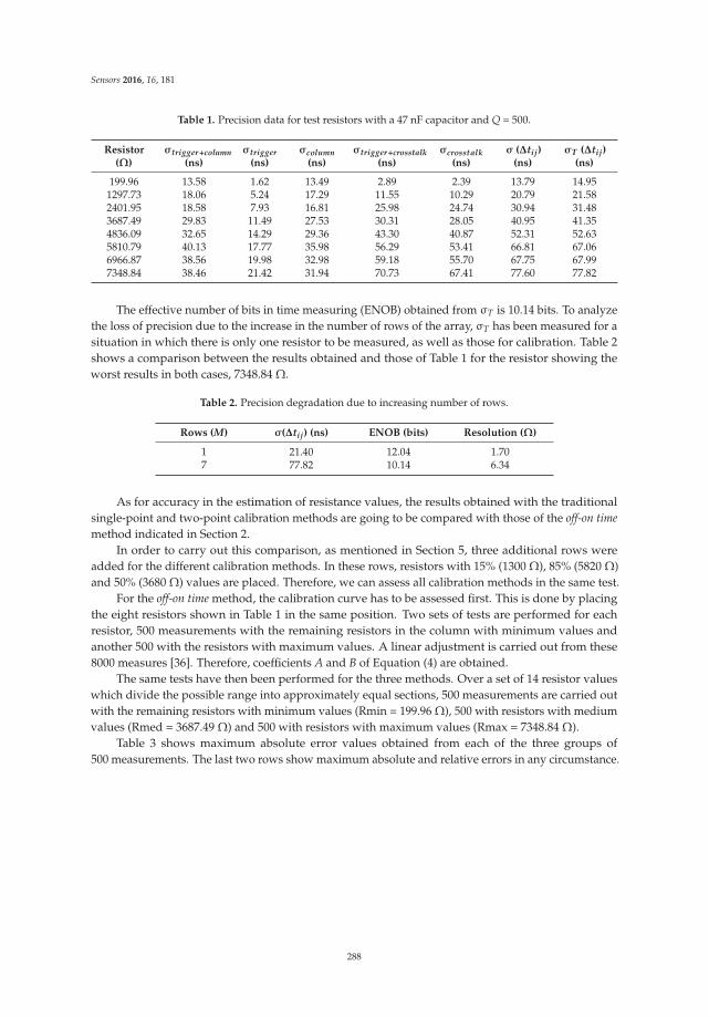
Sensors 2016, 16, 181

Table 1. Precision data for test resistors with a 47 nF capacitor and Q = 500.

Resistor(Ω)

σtrigger+column

(ns)σtrigger

(ns)σcolumn

(ns)σtrigger+crosstalk

(ns)σcrosstalk

(ns)σ (∆tij)

(ns)σT (∆tij)

(ns)

199.96 13.58 1.62 13.49 2.89 2.39 13.79 14.951297.73 18.06 5.24 17.29 11.55 10.29 20.79 21.582401.95 18.58 7.93 16.81 25.98 24.74 30.94 31.483687.49 29.83 11.49 27.53 30.31 28.05 40.95 41.354836.09 32.65 14.29 29.36 43.30 40.87 52.31 52.635810.79 40.13 17.77 35.98 56.29 53.41 66.81 67.066966.87 38.56 19.98 32.98 59.18 55.70 67.75 67.997348.84 38.46 21.42 31.94 70.73 67.41 77.60 77.82

The effective number of bits in time measuring (ENOB) obtained from σT is 10.14 bits. To analyzethe loss of precision due to the increase in the number of rows of the array, σT has been measured for asituation in which there is only one resistor to be measured, as well as those for calibration. Table 2shows a comparison between the results obtained and those of Table 1 for the resistor showing theworst results in both cases, 7348.84 Ω.

Table 2. Precision degradation due to increasing number of rows.

Rows (M) σ(∆tij) (ns) ENOB (bits) Resolution (Ω)

1 21.40 12.04 1.707 77.82 10.14 6.34

As for accuracy in the estimation of resistance values, the results obtained with the traditionalsingle-point and two-point calibration methods are going to be compared with those of the off-on time

method indicated in Section 2.In order to carry out this comparison, as mentioned in Section 5, three additional rows were

added for the different calibration methods. In these rows, resistors with 15% (1300 Ω), 85% (5820 Ω)and 50% (3680 Ω) values are placed. Therefore, we can assess all calibration methods in the same test.

For the off-on time method, the calibration curve has to be assessed first. This is done by placingthe eight resistors shown in Table 1 in the same position. Two sets of tests are performed for eachresistor, 500 measurements with the remaining resistors in the column with minimum values andanother 500 with the resistors with maximum values. A linear adjustment is carried out from these8000 measures [36]. Therefore, coefficients A and B of Equation (4) are obtained.

The same tests have then been performed for the three methods. Over a set of 14 resistor valueswhich divide the possible range into approximately equal sections, 500 measurements are carried outwith the remaining resistors with minimum values (Rmin = 199.96 Ω), 500 with resistors with mediumvalues (Rmed = 3687.49 Ω) and 500 with resistors with maximum values (Rmax = 7348.84 Ω).

Table 3 shows maximum absolute error values obtained from each of the three groups of500 measurements. The last two rows show maximum absolute and relative errors in any circumstance.

288

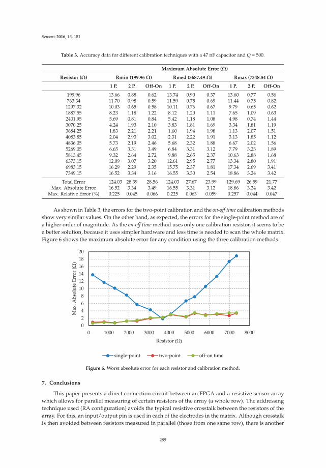
Sensors 2016, 16, 181

Table 3. Accuracy data for different calibration techniques with a 47 nF capacitor and Q = 500.

Maximum Absolute Error (Ω)

Resistor (Ω) Rmin (199.96 Ω) Rmed (3687.49 Ω) Rmax (7348.84 Ω)

1 P. 2 P. Off-On 1 P. 2 P. Off-On 1 P. 2 P. Off-On

199.96 13.66 0.88 0.62 13.74 0.90 0.37 13.60 0.77 0.56763.34 11.70 0.98 0.59 11.59 0.75 0.69 11.44 0.75 0.821297.32 10.03 0.65 0.58 10.11 0.76 0.67 9.79 0.65 0.621887.55 8.23 1.18 1.22 8.12 1.20 1.11 7.65 1.09 0.632401.95 5.69 0.81 0.84 5.42 1.18 1.08 4.98 0.74 1.443070.25 4.24 1.93 2.10 3.83 1.81 1.69 3.34 1.81 1.193684.25 1.83 2.21 2.21 1.60 1.94 1.98 1.13 2.07 1.514083.85 2.04 2.93 3.02 2.31 2.22 1.91 3.13 1.85 1.124836.05 5.73 2.19 2.46 5.68 2.32 1.88 6.67 2.02 1.565269.05 6.65 3.31 3.49 6.84 3.31 3.12 7.79 3.23 1.895813.45 9.32 2.64 2.72 9.88 2.65 2.37 10.63 2.88 1.686373.15 12.09 3.07 3.20 12.61 2.95 2.77 13.34 2.80 1.916983.15 16.29 2.29 2.35 15.75 2.37 1.81 17.34 2.69 3.417349.15 16.52 3.34 3.16 16.55 3.30 2.54 18.86 3.24 3.42

Total Error 124.03 28.39 28.56 124.03 27.67 23.99 129.69 26.59 21.77Max. Absolute Error 16.52 3.34 3.49 16.55 3.31 3.12 18.86 3.24 3.42

Max. Relative Error (%) 0.225 0.045 0.066 0.225 0.063 0.059 0.257 0.044 0.047

As shown in Table 3, the errors for the two-point calibration and the on-off time calibration methodsshow very similar values. On the other hand, as expected, the errors for the single-point method are ofa higher order of magnitude. As the on-off time method uses only one calibration resistor, it seems to bea better solution, because it uses simpler hardware and less time is needed to scan the whole matrix.Figure 6 shows the maximum absolute error for any condition using the three calibration methods.

0

2

4

6

8

10

12

14

16

18

20

0 1000 2000 3000 4000 5000 6000 7000 8000

Max

. Ab

solu

te E

rro

r (

)

Resistor ( )

single-point two-point off-on time

Figure 6. Worst absolute error for each resistor and calibration method.

7. Conclusions

This paper presents a direct connection circuit between an FPGA and a resistive sensor arraywhich allows for parallel measuring of certain resistors of the array (a whole row). The addressingtechnique used (RA configuration) avoids the typical resistive crosstalk between the resistors of thearray. For this, an input/output pin is used in each of the electrodes in the matrix. Although crosstalkis then avoided between resistors measured in parallel (those from one same row), there is another

289

Sensors 2016, 16, 181

element, RC crosstalk, which affects uncertainty when measuring discharge time in capacitors (andwhich is used to estimate resistance) causing a reduction in the effective number of bits in time-digitalconversion (ENOB).

The implementation of a circuit to perform a set of tests has been carried out. These tests simulate,with discrete resistors of known values, the behavior of a specific tactile sensor. The range of resistorvalues which has been assessed goes from 200 Ω to 7350 Ω.

In this case, the total uncertainty which includes all studied components (σtrigger, σcrosstalk andσcolumn) and also quantification noise, results in an ENOB of 10.14 bits. Besides the precision inthe estimation of the resistance values, a study of accuracy has been performed by using differentcalibration techniques avoiding having to know certain values which are difficult to measure (Cj, VTj

and VDD), which could change with time and temperature.From the calibration methods analyzed, the off-on time method, based on an adjustment to a linear

function from data obtained in an operation mode previous to the normal mode, provides similarresults to those of the two-point calibration technique, but only with the need of a reference resistor.Therefore both the hardware and the sampling time of the whole matrix are reduced. The maximumrelative error obtained with this method has been 0.066%

Acknowledgments: This work has been funded by the Spanish Government and by the European ERDF programfunds under contract TEC2012-38653.

Author Contributions: This paper is part of the PhD Thesis of Oscar Oballe-Peinado and he is the maincontributor. Fernando Vidal-Verdú and José Antonio Hidalgo-López are co-advisors of his PhD Thesis, so bothhave oriented the work and have helped in the writing and revision of the text. José A. Sánchez-Durán and JuliánCastellanos-Ramos have assisted in testing and characterization tasks.


References

1. Tise, B. A compact high resolution piezoresistive digital tactile sensor. In Proceedings of the 1988 IEEEInternational Conference on Robotics and Automation, Philadelphia, PA, USA, 24–29 April 1988.

2. Castellanos-Ramos, J.; Navas-González, R.; Macicior, H.; Sikora, T.; Ochoteco, E.; Vidal-Verdú, F. Tactilesensors based on conductive polymers. Microsyst. Technol. 2010, 16, 765–776. [CrossRef]

3. Dahiya, R.S.; Metta, G.; Valle, M.; Adami, A.; Lorenzelli, L. Piezoelectric oxide semiconductor field effecttransistor touch sensing devices. Appl. Phys. Lett. 2009. [CrossRef]

4. Drimus, A.; Kootstra, G.; Bilberg, A.; Kragic, D. Design of a flexible tactile sensor for classification of rigidand deformable objects. Robot. Auton. Syst. 2014, 62, 3–15. [CrossRef]

5. Kane, B.J.; Cutkosky, M.R.; Kovacs, G.T.A. A traction stress sensor array for use in high-resolution robotictactile imaging. J. Microelectromechanical Syst. 2000, 9, 425–434. [CrossRef]

6. Kim, M.-S.; Shin, H.-J.; Park, Y.-K. Design concept of high-performance flexible tactile sensors with a robuststructure. Int. J. Precis. Eng. Manuf. 2012, 13, 1941–1947. [CrossRef]

7. Shimojo, M.; Namiki, A.; Ishikawa, M.; Makino, R.; Mabuchi, K. A tactile sensor sheet using pressureconductive rubber with electrical-wires stitched method. IEEE Sens. J. 2004, 4, 589–596. [CrossRef]

8. Speeter, T.H. A Tactile Sensing System for Robotic Manipulation. Int. J. Robot. Res. 1990, 9, 25–36. [CrossRef]9. Zhang, X.; Zhao, Y.; Zhang, X. Design and fabrication of a thin and soft tactile force sensor array based on

conductive rubber. Sens. Rev. 2012, 32, 273–279. [CrossRef]10. Weiss, K.; Worn, H. Resistive tactile sensor matrices using inter-electrode sampling. In Proceedings

of the IECON 2005-31st Annual Conference of IEEE Industrial Electronics Society, Raleigh, NC, USA,6–10 November 2005.

11. Wu, J.; Wang, L.; Li, J.; Yu, Z. A small size device using temperature sensor array. Chin. J. Sens. Actuators

2011, 24, 1649–1652.12. Yang, Y.-J.; Cheng, M.-Y.; Shih, S.-C.; Huang, X.-H.; Tsao, C.-M.; Chang, F.-Y.; Fan, K.-C. A 32 ˆ 32 temperature

and tactile sensing array using PI-copper films. Int. J. Adv. Manuf. Technol. 2010, 46, 945–956. [CrossRef]13. Fratoddi, I.; Venditti, I.; Cametti, C.; Russo, M.V. Chemiresistive polyaniline-based gas sensors: A mini

review. Sens. Actuators B Chem. 2015, 220, 534–548. [CrossRef]

290

Sensors 2016, 16, 181

14. Wang, J.; Chan, S.; Carlson, R.R.; Luo, Y.; Ge, G.; Ries, R.S.; Heath, J.R.; Tseng, H.-R. Electrochemicallyfabricated polyaniline nanoframework electrode junctions that function as resistive sensors. Nano Lett. 2004,4, 1693–1697. [CrossRef]

15. Depari, A.; Falasconi, M.; Flammini, A.; Marioli, D.; Rosa, S.; Sberveglieri, G.; Taroni, A. A new low-costelectronic system to manage resistive sensors for gas detection. IEEE Sens. J. 2007, 7, 1073–1077. [CrossRef]

16. Lilly, R.V.; Devaki, S.J.; Narayanan, R.K.; Sadanandhan, N.K. Design of a nanostructured electromagneticpolyaniline–keggin iron–clay composite modified electrochemical sensor for the nanomolar detection ofascorbic acid. J. Appl. Polym. Sci. 2014. [CrossRef]

17. Song, E.; Choi, J.-W. Multi-analyte detection of chemical species using a conducting polymer nanowire-basedsensor array platform. Sens. Actuators B Chem. 2015, 215, 99–106. [CrossRef]

18. Wu, J.; Wang, L.; Li, J. VF-NSE method measurement error analysis of networked resistive sensor array.Sens. Actuators Phys. 2014, 211, 45–50. [CrossRef]

19. Wu, J.; Wang, L.; Li, J. Design and Crosstalk Error Analysis of the Circuit for the 2-D Networked ResistiveSensor Array. IEEE Sens. J. 2015, 15, 1020–1026. [CrossRef]

20. Saxena, R.S.; Bhan, R.K.; Saini, N.K.; Muralidharan, R. Virtual Ground Technique for Crosstalk Suppressionin Networked Resistive Sensors. IEEE Sens. J. 2011, 11, 432–433. [CrossRef]

21. Saxena, R.S.; Saini, N.K.; Bhan, R.K. Analysis of Crosstalk in Networked Arrays of Resistive Sensors.IEEE Sens. J. 2011, 11, 920–924. [CrossRef]

22. Liu, H.; Zhang, Y.-F.; Liu, Y.-W.; Jin, M.-H. Measurement errors in the scanning of resistive sensor arrays.Sens. Actuators Phys. 2010, 163, 198–204. [CrossRef]

23. D’Alessio, T. Measurement errors in the scanning of piezoresistive sensors arrays. Sens. Actuators Phys. 1999,72, 71–76. [CrossRef]

24. Kim, J.-S.; Kwon, D.-Y.; Choi, B.-D. High-Accuracy, Compact Scanning Method and Circuit for ResistiveSensor Arrays. Sensors 2016. [CrossRef] [PubMed]

25. Oballe-Peinado, Ó.; Vidal-Verdú, F.; Sánchez-Durán, J.A.; Castellanos-Ramos, J.; Hidalgo-López, J.A.Improved Circuits with Capacitive Feedback for Readout Resistive Sensor Arrays. Sensors 2016. [CrossRef][PubMed]

26. Ares, L.; Rodriguez-Andina, J.J.; Farina, J. FPGA-based direct resistance and capacitance measurements. InProceedings of the 35th Annual Conference of IEEE Industrial Electronics (IECON 2009), Porto, Portugal,3–5 November 2009.

27. Reverter, F.; Jordana, J.; Gasulla, M.; Pallàs-Areny, R. Accuracy and resolution of direct resistivesensor-to-microcontroller interfaces. Sens. Actuators Phys. 2005, 121, 78–87. [CrossRef]

28. Reverter, F. The Art of Directly Interfacing Sensors to Microcontrollers. J. Low Power Electron. Appl. 2012, 2,265–281. [CrossRef]

29. Kokolanski, Z.; Jordana, J.; Gasulla, M.; Dimcev, V.; Reverter, F. Direct inductive sensor-to-microcontrollerinterface circuit. Sens. Actuators Phys. 2015, 224, 185–191. [CrossRef]

30. Reverter, F. Direct interface circuits for sensors. In Smart Sensors and MEMS: Intelligent Devices and

Microsystems for Industrial Applications; Nihtianov, S., Luque, A., Eds.; Woodhead Publishing: Oxford,UK, 2014.

31. Custodio, A.; Pallas-Areny, R.; Bragos, R. Error analysis and reduction for a simple sensor-microcontrollerinterface. IEEE Trans. Instrum. Meas. 2001, 50, 1644–1647. [CrossRef]

32. Bengtsson, L.E. Analysis of direct sensor-to-embedded systems interfacing: A comparison of targets’performance. Int. J. Intell. Mechatron. Robot. 2012, 2, 41–46. [CrossRef]

33. Reverter, F.; Pallàs-Areny, R. Effective number of resolution bits in direct sensor-to-microcontroller interfaces.Meas. Sci. Technol. 2004. [CrossRef]

34. Vidal-Verdú, F.; Oballe-Peinado, Ó.; Sánchez-Durán, J.A.; Castellanos-Ramos, J.; Navas-González, R. ThreeRealizations and Comparison of Hardware for Piezoresistive Tactile. Sensors 2011, 11, 3249–3266. [CrossRef][PubMed]

35. Xilinx, Inc. Spartan-3AN FPGA Family Data Sheet. Available online: http://www.xilinx.com/support/documentation/data_sheets/ds557.pdf (accessed on 6 November 2015).

291

Sensors 2016, 16, 181

36. Oballe-Peinado, Ó.; Vidal-Verdú, F.; Sánchez-Durán, J.A.; Castellanos-Ramos, J.; Hidalgo-López, J.A. SmartCapture Modules for Direct Sensor-to-FPGA Interfaces. Sensors 2015, 15, 31762–31780. [CrossRef] [PubMed]

37. ISO Guide to the Expression of Uncertainty in Measurement (GUM:1995). Availble online:http://www.iso.org/iso/home/store/catalogue_ics/catalogue_detail_ics.htm?csnumber=50461 (accessedon 13 September 2015).

38. Texas Instruments, Inc. TPS795 Ultralow-Noise, High-PSRR, Fast, RF, 500-mA Low-Dropout LinearRegulators Datasheet. Available online: http://www.ti.com/lit/ds/symlink/tps795.pdf (accessed on6 November 2015).

39. Texas Instruments, Inc. TPS799 200-mA, Low-Quiescent Current, Ultralow Noise, High-PSRR Low-DropoutLinear Regulator Datasheet. Available online: http://www.ti.com/lit/ds/symlink/tps799.pdf (accessed on6 November 2015).

40. Pallàs-Areny, R.; Jordana, J.; Casas, Ó. Optimal two-point static calibration of measurement systems withquadratic response. Rev. Sci. Instrum. 2004, 75, 5106–5111. [CrossRef]

41. IPC IPC-6013 Specification for Printed Wiring, Flexible and Rigid-Flex. Available online:http://www.ipc.org/ (accessed on 8 December 2015).


292

MDPI AG

St. Alban-Anlage 66

4052 Basel, Switzerland

Tel. +41 61 683 77 34

Fax +41 61 302 89 18

http://www.mdpi.com

Sensors Editorial Office

E-mail: [email protected]





MDPI AG

St. Alban-Anlage 66

4052 Basel

Switzerland

Tel: +41 61 683 77 34

Fax: +41 61 302 89 18

www.mdpi.com ISBN 978-3-03842-371-3

State-of-the-Art Sensors Technology in Spain 2015 - Open ...

Documents

Transcript of State-of-the-Art Sensors Technology in Spain 2015 - Open ...