Standard Partial Molar Heat Capacities and Volumes of ...

Standard Partial Molar Heat Capacities and Volumes of Aqueous

Dimethylethanolamine and 3-Methoxypropylamine from 283 to 393 K, and

Thermodynamic Functions for Their Ionization Equilibria to 598 K and 20 MPa

by

Samantha Binkley

A Thesis

presented to

The University of Guelph

In partial fulfilment of requirements

for the degree of

Master of Science

in

Chemistry

Guelph, Ontario, Canada

© Samantha Binkley, January, 2021

ABSTRACT

STANDARD PARTIAL MOLAR HEAT CAPACITIES AND VOLUMES OF

AQUEOUS DIMETHYLETHANOLAMINE AND 3-METHOXYPROPYLAMINE

FROM 283 TO 393 K, AND THERMODYNAMIC FUNCTIONS FOR THEIR

IONIZATION EQUILIBRIA TO 598 K AND 20 MPa

Samantha Binkley Advisor:

University of Guelph, 2021 Peter Tremaine

Densities for dilute aqueous solutions of N,N-dimethylethanolamine (DMEA), 3-

methoxypropylamine (3-MPA), and their protonated salts were measured relative to water at

283.15 K ≤ T ≤ 363.15 K and 0.1 MPa using vibrating tube densimeters. Volumetric heat

capacities of the same solutions were measured at 283.15 K ≤ T ≤ 393.15 K and 0.4 MPa using

twin fixed-cell, power compensation, differential temperature scanning nano calorimeters.

From these measurements apparent molar volumes, Vϕ, and heat capacities, Cp,ϕ, were

calculated and corrected for speciation to obtain standard partial molar properties Vo and Cpo,

for the species DMEA(aq), DMEAH+Cl-(aq), 3-MPA(aq) and 3-MPA+Cl-(aq). The

experimental values for Vo and Cpo, measured in this work were combined with high

temperature values reported by Bulemela and Tremaine (J. Phys. Chem. B 2008, 112, 5626-

5645) over the range 423.15 to 598.15 K to derive parameters for the semi-empirical “density”

model that expresses the standard partial molar thermodynamic properties of aqueous species

as a function of temperature and solvent density. The fitted parameters were used with

critically evaluated literature values for the standard partial molar Gibbs energy and enthalpy

of reaction at 298.15 K to obtain values for the ionization constant of N,N-

dimethylethanolamine and 3-methoxypropylamine from 283.15 to 598.15 K.

iii

ACKNOWLEDGEMENTS

Thank you to Professor Peter Tremaine; first for the opportunity to complete

research and learn from you, but also for your guidance, time, and dedication as this thesis

would not exist and I would not be a better student without them.

Jenny Cox and Olivia Fandiño Torres, thank you for being co-supervisors and

ensuring my success. Every sample I prepared, measurement I made, and instrument I

attempted to fix, was done following your guidance and insight. Your willingness to share

your experience has been greatly appreciated throughout this project.

To the Tremaine Research Group; Hugues Arcis, Swaroop Sasidharanpillai, Matt

Wolf, Chris Alcorn, Jane Ferguson, Avinaash Persaud, Jacy Conrad, Jason Sylvester, and

Matt McLeod, thank you for making time to double check my math, for coffee breaks, and

for supporting me.

Thank you to Farnood Pakravan for your technical expertise; my research has been

greatly aided through your time and I am very grateful.

I would also like to thank the members of my advisory committee, Professor

Dmitriy Soldatov and Professor Khashayar Ghandi for their guidance over my program

and project.

Thank you to my friends and family: my parents, my siblings, my Bethany

professors, and my friends. You all deserve credit for helping me complete this work.

Thank you for your guidance, support and encouragement.

iv

TABLE OF CONTENTS Abstract .......................................................................................................................... ii

Acknowledgements ....................................................................................................... iii

Table of Contents .......................................................................................................... iv

List of Tables................................................................................................................ vii

List of Figures ............................................................................................................... ix

List of Abbreviations and Symbols ............................................................................... xii

Chapter 1 Introduction .....................................................................................................1

1.1 Amines and Alkanolamines ...................................................................................1

1.2 Nuclear Applications.............................................................................................2

1.2.1 Secondary Steam Circuit Overview ............................................................3

1.2.2 Secondary Steam Circuit Chemistry ...........................................................3

1.3 Thermodynamic Properties of Solutions .............................................................. 11

1.4 Apparent and Standard Partial Molar Properties .................................................. 14

1.5 Equations of State ............................................................................................... 15

1.5.1 Hydration Effects ..................................................................................... 15

1.5.2 The Born Equation ................................................................................... 17

1.5.3 Helgeson-Kirkham-Flowers Model ........................................................... 18

1.5.4 The “Density” Model ............................................................................... 21

1.5.5 Functional Group Additivity Models ........................................................ 23

1.6 Instrumentation ................................................................................................... 24

1.6.1 Vibrating Tube Densimeter ...................................................................... 24

1.6.2 The Picker Calorimeter ............................................................................. 26

1.6.3 DSC Type Calorimeters ............................................................................ 29

1.7 Thesis Objectives ................................................................................................ 31

1.8 Contributions to Thesis ....................................................................................... 33

Chapter 2 Standard Partial Molar Heat Capacities and Volumes of Aqueous N,N-

Dimethylethanolamine and N,N-Dimethylethanolammonium Chloride from 283 K to 393

K ................................................................................................................................... 35

2.1 Introduction ........................................................................................................ 36

2.2 Experimental ....................................................................................................... 38

2.2.1 Materials and Solution Preparation ........................................................... 38

v

2.2.2 Densimetry ............................................................................................... 38

2.2.3 Calorimetry .............................................................................................. 41

2.3 Results ................................................................................................................ 43

2.3.1 Apparent Molar Volumes and Heat Capacities.......................................... 43

2.3.2 Single-Ion Properties ................................................................................ 53

2.3.3 Thermodynamic Functions for the Ionization of DMEAH+ at Elevated T

and p 61

2.4 Discussion .......................................................................................................... 62

2.4.1 Comparison with Literature Results .......................................................... 62

2.4.2 Density Model .......................................................................................... 69

2.5 Acknowledgements ............................................................................................. 70

Chapter 3 Standard Partial Molar Heat Capacities and Volumes of Aqueous 3-

Methoxypropylamine and 3-Methoxypropylammonium Chloride from 283 K to 393 K . 71

3.1 Introduction ........................................................................................................ 72

3.2 Experimental ....................................................................................................... 73

3.2.1 Materials and Solution Preparation ........................................................... 73

3.2.2 Densimetry ............................................................................................... 75

3.2.3 Calorimetry .............................................................................................. 76

3.3 Results ................................................................................................................ 78

3.3.1 Apparent Molar Volumes and Heat Capacities.......................................... 78

3.3.2 Speciation Corrections .............................................................................. 78

3.3.3 Single-Ion Properties ................................................................................ 87

3.4 Discussion .......................................................................................................... 98

3.4.1 Comparison with Literature Results .......................................................... 98

3.4.2 Density Model ........................................................................................ 102

3.5 Acknowledgements ........................................................................................... 102

Chapter 4 Conclusions and Future Work ...................................................................... 103

References ................................................................................................................... 106

Supplementary Information ......................................................................................... 111

Appendix A- Properties of Water ................................................................................. 112

Appendix B- Density Model Derivations ..................................................................... 114

Appendix C- Data Treatment ....................................................................................... 117

4.1 Apparent Molar Volume ................................................................................... 117

vi

4.2 Apparent Molar Heat Capacity .......................................................................... 118

4.3 Standard Partial Molar Volume ......................................................................... 119

4.4 Standard Partial Molar Heat Capacity ............................................................... 121

4.5 Single- Ion Properties........................................................................................ 122

4.6 Thermodynamic Functions for the Ionization of BH+ at Elevated T and p.......... 124

vii

LIST OF TABLES

Table 1 Amines listed as pH control alternatives [1; 2; 5; 6] .......................................... 10

Table 2 List of the chemicals used in this work (DMEA), including purities as listed by

the supplier. ....................................................................................................... 39

Table 3 Experimental densities relative to water (ρs - ρw) of DMEA (aq) and DMEAH+Cl-

(aq) as a function of temperature T at p = 0.10 MPa, for each stoichiometric

molality, mst, with standard uncertainties, u.a, b ................................................... 44

Table 4 Experimental volumetric heat capacities relative to water (cp,s·ρs – cp,w·ρw) of

DMEA (aq) at stoichiometric, “st”, molalities, mst, at temperature T and pressure p

= 0.40 MPa with standard uncertainties, u.a, b, c ................................................... 45

Table 5 Experimental volumetric heat capacities relative to water (cp,s·ρs – cp,w·ρw) of

DMEAH+Cl- (aq) at stoichiometric, “st”, molalities, mst, at temperature T and

pressure p = 0.40 MPa with standard uncertainties, u.a, b, c .................................. 47

Table 6 Mean values of experimental, ‘exp’, apparent and standard partial molar volumes

and heat capacities of DMEA(aq), (Vφexp, V°) and (Cp,φ

exp, Cp°) at p = 0.40 MPa and

their standard uncertainties, u (±).a,b ................................................................... 49


and heat capacities of DMEAH+Cl-(aq), (Vφexp, V°) and (Cp,φ

exp, Cp°) at p = 0.40

MPa and their standard uncertainties, u (±).a, b .................................................... 50

Table 8a-c Fitting parameters for the temperature dependence of the standard partial molar

volume of reaction for DMEA, DMEAH+Cl-, H+Cl- and ΔV°ion for reaction 2.13

with standard uncertainties of the parameters, u (±), and relative uncertainties of

the fit ur. ............................................................................................................ 57

Table 9 Standard partial molar volumes, V°, and standard partial molar heat capacities, Cp°, of DMEA and DMEAH+Cl- and the pKa for the ionization reaction, Δion DMEA, at

p = 0.4 MPa calculated from eqs 2.19 and 2.20, and the fitting parameters in Tables

8a and 8b, with their standard uncertainties, u (±). .............................................. 63

Table 10 Standard partial molar volumes, V°, and standard partial molar heat capacities,

Cp°, of DMEA and DMEAH+Cl- and the pKa for the ionization reaction, Δion

DMEA, at p = 15 MPa calculated from eqs 2.19 and 2.20, and the fitting parameters

in Tables 8a and 8b, with their standard uncertainties, u (±). .............................. 64

Table 11 Standard partial molar heat capacities, ΔionCp°, enthalpies, ΔionH°, and values of

pKa for reaction 2.13, at 10, 15, and 20 MPa with standard relative uncertainties of

the fit ur. ............................................................................................................ 65

viii

Table 12 List of the chemicals used in this work (3-MPA), including purities as listed by

the supplier. ....................................................................................................... 74

Table 13 Experimental densities relative to water (ρs - ρw) of 3-MPA (aq) and 3-MPAH+Cl-

(aq) as a function of temperature T at p = 0.10 MPa, for each stoichiometric

molality, mst, with standard uncertainties, u.a, b ................................................... 78

Table 14 Experimental volumetric heat capacities relative to water (cp,s·ρs – cp,w·ρw) of 3-

MPA (aq) at stoichiometric, “st”, molalities, mst, at temperature T and pressure p =

0.40 MPa with standard uncertainties, u.a, b, c ...................................................... 80

Table 15 Experimental volumetric heat capacities relative to water (cp,s·ρs – cp,w·ρw) of 3-

MPAH+Cl- (aq) at stoichiometric, “st”, molalities, mst, at temperature T and

pressure p = 0.40 MPa with standard uncertainties, u.a, b, c .................................. 82


and heat capacities of 3-MPA(aq), (Vφexp, V°) and (Cp,φ

exp, Cp°) at p = 0.40 MPa and

their standard uncertainties, u (±).a,b ................................................................... 84


and heat capacities of 3-MPAH+Cl-(aq), (Vφexp, V°) and (Cp,φ

exp, Cp°) at p = 0.40

MPa and their standard uncertainties, u (±).a, b .................................................... 85

Table 18a-c Fitting parameters for the temperature dependence of the standard partial

molar volume of reaction for 3-MPA, 3-MPAH+Cl-, H+Cl- and ΔV°ion for reaction

3.8 with standard uncertainties of the parameters, u (±), and relative uncertainties

of the fit ur. ........................................................................................................ 94


Cp°, of 3-MPA and 3-MPAH+Cl- and the pKa for the ionization reaction, Δion 3-

MPA, at p = 0.4 MPa calculated from eqs 3.16 and 3.17, and the fitting parameters

in Tables 18a and 18b, with their standard uncertainties, u (±). ........................... 94


Cp°, of 3-MPA and 3-MPAH+Cl- and the pKa for the ionization reaction, Δion 3-

MPA, at p = 15 MPa calculated from eqs 3.16 and 3.17, and the fitting parameters

in Tables 18a and 18b, with their standard uncertainties, u (±). ........................... 97

Table 21 Standard partial molar heat capacities, ΔionCp°, enthalpies, ΔionH°, and values of

pKa for reaction 3.8, at 10, 15, and 20 MPa with their standard relative uncertainties,

ur........................................................................................................................ 98

Table 22 Thermodynamic properties of water from Hill (1990) [61], Archer and Wang

(1990) [73], NIST [74], and Marshall and Frank (1981) [34]. ........................... 112

ix

LIST OF FIGURES

Figure 1. A schematic of the steam generator for a CANDU reactor from Essential

CANDU: A Textbook on the CANDU Nuclear Power Plant Technology [3]........ 4

Figure 2. A schematic of the secondary steam system for a CANDU reactor from Essential

CANDU: A Textbook on the CANDU Nuclear Power Plant Technology [3]........ 5

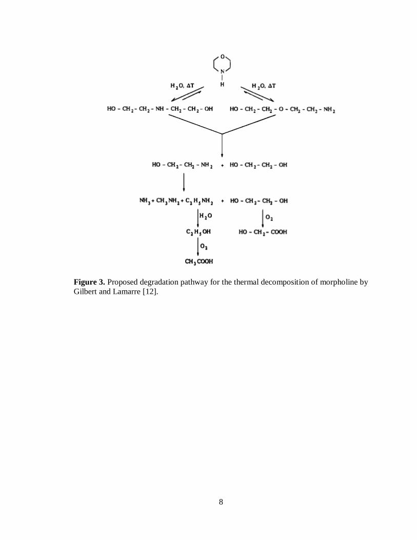
Figure 3. Proposed degradation pathway for the thermal decomposition of morpholine by

Gilbert and Lamarre [12]. ..................................................................................... 8

Figure 4. A schematic of the solvation model proposed by Frank and Evans (1945). The

schematic shows first and second hydration spheres for a cation, and bulk water

where long range polarization can be described by the Born equation [19]. ........ 16

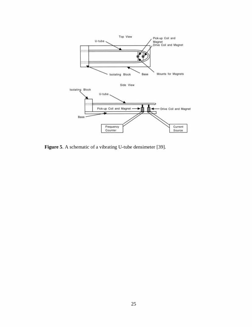
Figure 5. A schematic of a vibrating U-tube densimeter [38]. ........................................ 25

Figure 6: The conceptual design of a twin cell Picker flow heat-capacity microflow

calorimeter [19].................................................................................................. 28

Figure 7. Twin platinum capillary cells within the Nano DSC 6300 by TA instruments

[46]. ................................................................................................................... 30

Figure 8. Twin gold batch cells from the Nano power compensation DSC 60200 by the

Calorimetry Science Corporation taken in the Tremaine Lab at the University of

Guelph. .............................................................................................................. 32

Figure 9. Standard partial molar volumes for DMEA(aq) with density model fit from

283.15 to 363.15 K: ●, this work; ▽, Lebrette et al. (2002) [58]; ⬛, Collins et al.

(2000) [47]; ▬, density model (eq 2.20, Table 8a). ............................................ 54

Figure 10. Standard partial molar volumes for DMEAH+Cl-(aq) with density model fit

from 283.15 to 363.15 K: ●, this work; ○, Collins et al. (2000) [47]; ▬, density

model (eq 2.20, Table 8a). .................................................................................. 54

Figure 11. Standard partial molar heat capacities for DMEA(aq) with density model fit

from 283.15 to 410.15 K at 0.4 MPa: ●, this work; ○, and Collins et al. (2000) [47];

▬, density model (eq 2.19, Table 8c). ................................................................ 55

Figure 13. Standard partial molar heat capacities for DMEAH+Cl-(aq) with density model

fit from 283.15 to 410.15 K at 0.4 MPa: ●, this work; ○, Collins et al. (2000) [47];

▬, density model (eq 2.19, Table 8c). ................................................................ 55


283.15 to 598.15 K: ●, this work; ▼, Lebrette et al. (2002) [58]; ○, Collins et al.

(2000) [47]; Δ, Bulemela and Tremaine (2008) [48]; ▬, density model (eq 2.20,

Table 8a). ........................................................................................................... 59

x


from 283.15 to 598.15 K: ▼, this work; ●, Collins et al. (2000) [47]; ○, Bulemela

and Tremaine (2008) [48]; ▬, density model (eq 2.20, Table 8a). ...................... 59


from 283.15 to 598.15 K: ●, this work; ○, Collins et al. (2000) [47]; ▬, density

model (eq 2.19, Table 8c). .................................................................................. 60


fit from 283.15 to 598.15 K: ●, this work; ○, Collins et al. (2000) [47]; ▬, density

model (eq 2.19, Table 8c). .................................................................................. 60

Figure 18. Literature pKa values with the density model used in this work for the ionization

of DMEA(aq), reaction 2.13, from 283.15 to 393.15 K at p = 0.4 MPa: ●, Hamborg

and Versteeg (2009) [54]; ○, Littel et al. (1990) [55]; ▼, Christensen et al. (1969)

[52]; Δ, Fernandes et al. (2012) [53]; ▬, density model (eq 2.24, Table 8c). ...... 66


of DMEA(aq), reaction 2.13, from 283.15 to 598.15 K at p = 15 MPa: ●, Hamborg

and Versteeg (2009) [54]; ○, Littel et al. (1990) [55]; ▼, Christensen et al. (1969)

[52]; Δ, Fernandes et al. (2012) [53]; ▬, density model (eq 2.24, Table 8c). ...... 67

Figure 20. Standard partial molar volumes for 3-MPA(aq) with density model fit from

283.15 to 363.15 K: ●, this work; ▬, fit to the density model (eq 3.17, Table

18a). ................................................................................................................... 88

Figure 21. Standard partial molar volumes for 3-MPAH+Cl-(aq) with density model from

283.15 to 363.15 K: ●, this work; ▬, fit to the density model (eq 3.17, Table

18a). ................................................................................................................... 88

Figure 22. Standard partial molar heat capacities for 3-MPA(aq) from 283.15 to 393.15 K

at 0.4 MPa: ●, this work; ▬, fit to the density model (eq 3.16, Table 18c). ........ 89

Figure 23. Standard partial molar heat capacities for 3-MPAH+Cl-(aq) from 283.15 to

393.15 K at 0.4 MPa: ●, this work; ▬, fit to the density model (eq 3.16, Table 18c).

.......................................................................................................................... 89

Figure 24. Standard partial molar volumes for 3-MPA(aq) with density model from 283.15

to 613.15 K: ●, this work; ○, Bulemela and Tremaine (2008) [48]; ▬, fit to the

density model (eq 3.17, Table 18a). .................................................................... 91

Figure 25. Standard partial molar volumes for 3-MPAH+Cl-(aq) with density model fit

from 283.15 to 598.15 K: ●, this work; ○, Bulemela and Tremaine (2008) [48]; ▬,

fit to the density model (eq 3.17, Table 18a). ...................................................... 91

xi

Figure 26. Standard partial molar heat capacities for 3-MPA(aq) with density model from

283.15 to 598.15 K: ●, this work; ▬, fit to the density model (eq 3.16, Table 18c).

.......................................................................................................................... 93

Figure 27. Standard partial molar heat capacities for 3-MPAH+Cl-(aq) with density model

fit from 283.15 to 598.15 K: ●, this work; ▬, fit to the density model (eq 3.16,

Table 18c). ......................................................................................................... 93


of 3-MPA(aq), reaction 3.8, from 283.15 to 573.15 K at p = 15 MPa: ●,

Balakrishnan (1988) [1]; ○, Cabani et al. (1977) [68]; ▼, Lobo and Robertson

(1976) [69]; ▬, fit to the density model (eq 3.20, Table 18c). ......................... 100

xii

LIST OF ABBREVIATIONS AND SYMBOLS

ABBREVIATIONS

3-MPA 3-methoxypropylamine

3-MPAH+Cl- 3-methoxypropylammonium chloride

AMP 2-amino-2-methylpropanol

AVT all-volatile treatment

CANDU CANadian Deuterium Uranium

DEA diethylamine

DEAE N,N-diethylaminoethanol

DIPA diisopropylamine

DMA dimethylamine

DMAMP 2-dimethylamino-2-methylpropan-1-ol

DMEA N,N-dimethylethanolamine

DMEAH+Cl- N,N-dimethylethanolammonium chloride

DSC differential scanning calorimeter

EAE 2-ethylaminoethanol

EPRI Electric Power Research Institute

ETA monoethanolamine

FAC flow accelerated corrosion

HKF Helgeson – Kirkham – Flowers

MPH morpholine

PHWR Pressurised Heavy Water Reactor

PIP piperidine

PYR pyrrolidine

QUI quinuclidine

xiii

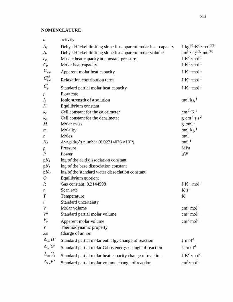
NOMENCLATURE

a activity

Ac Debye-Hückel limiting slope for apparent molar heat capacity J·kg1/2·K-1·mol-3/2

Av Debye-Hückel limiting slope for apparent molar volume cm3 ·kg3/2·mol-3/2

cp Massic heat capacity at constant pressure J·K-1·mol-1

Cp Molar heat capacity J·K-1·mol-1

,pC Apparent molar heat capacity J·K-1·mol-1 rel

,pC Relaxation contribution term J·K-1·mol-1

pC Standard partial molar heat capacity J·K-1·mol-1

f Flow rate

Is Ionic strength of a solution mol·kg-1

K Equilibrium constant

kc Cell constant for the calorimeter cm-3·K-1

kρ Cell constant for the densimeter g·cm-3·μs-2

M Molar mass g·mol-1

m Molality mol·kg-1

n Moles mol

NA Avagadro’s number (6.02214076 ×10²³) mol-1

p Pressure MPa

P Power μW

pKa log of the acid dissociation constant

pKb log of the base dissociation constant

pKw log of the standard water dissociation constant

Q Equilibrium quotient

R Gas constant, 8.3144598 J·K-1·mol-1

r Scan rate K·s-1

T Temperature K

u Standard uncertainty

V Molar volume cm3·mol-1

V° Standard partial molar volume cm3·mol-1

V Apparent molar volume cm3·mol-1

Y Thermodynamic property

Ze Charge of an ion

ion H Standard partial molar enthalpy change of reaction J·mol-1

ionG Standard partial molar Gibbs energy change of reaction kJ·mol-1

ion pC Standard partial molar heat capacity change of reaction J·K-1·mol-1

ionV Standard partial molar volume change of reaction cm3·mol-1

xiv

GREEK LETTERS

Degree of chemical dissociation

1 Thermal expansivity of water K-1

βw Isothermal compressibility of water MPa-1

Activity coefficient

r Relative permittivity

0 Permittivity of free space F·m-1

Density g·cm-3

Period of vibration µs

Resonant frequency Hz-1

SUBSCRIPT SUPERSCRIPT

a Acid ex Excess molality

b Base exp Experimental property

ion Ionization Standard state

r Reaction st Stoichiometric molality

s Sample

w Water

Apparent molar property

1 Properties of water

1

Chapter 1 Introduction

1.1 Amines and Alkanolamines

Amines are often used as pH control additives in steam generators to prevent

corrosion. Alkanolamines, an important family of amines, contain properties of both

amines and alcohols and are used in many industrial processes; such as natural gas

processing and oil refining. Alkanolamines are also used in the removal of acidic gases,

like carbon dioxide and hydrogen sulfide from gas streams in natural gas and petroleum

processing [1; 2]. Amines used in the power and gas industries are of interest for basic

research due to their thermal stability at high temperatures, and because amines allow for

the measurement of both neutral and ionized species.

The most common amines used for pH control in power generation are

monoethanolamine (ETA), morpholine (MPH), and ammonia [3; 4]. Other less common

additives include 2-amino-2-methylpropanol (AMP), cyclohexylamine, and 3-

methoxypropylamine (3-MPA) [2; 5; 6]. Amines, or a combination of amines, are the main

component in all-volatile treatment (AVT) for corrosion control in steam generating

systems. The use of AVT allows for corrosion control throughout the entirety of the steam

generating system, providing the necessary alkalinity to both steam and condensed phases

within the system [3].

Selection of an adequate pH control amine requires an understanding of each amines

distribution between steam and water phases, equilibrium constants at operating

conditions, and their thermal stability in water at operating temperatures. These

requirements can be fulfilled by scientific measurements at operating conditions or through

2

the use of extrapolation and predictive models for amine properties. Most higher molecular

weight amine additives undergo thermal decomposition at reactor temperatures, about

573.15 K; many degrading to form acids which can cause local corrosion. In order to

understand the complete system chemistry at reactor temperatures, the thermal

decomposition products of the pH control additives must also be measured and modeled.

Amines and alkanolamines being considered as pH control additives are model

systems for probing high temperature and solvation phenomena due to their inherent high

thermal stability. Measurement and modeling of amines and their functional groups will

aid in the development of predictive models for all organic species, improving existing

models of functional group additivity.

There are few data at elevated temperature and pressure for amine species to develop

these predictive models from. This thesis aims to contribute experimental high temperature

thermodynamic data of amine species for the future development of predictive models.

1.2 Nuclear Applications

The nuclear industry relies heavily on experimental data at high temperature and

pressures as well as extrapolations from ambient temperatures when literature gaps exist.

An area of interest to the industry at present is closing the existing literature gaps for amines

that have the potential to be used as pH control agents in the secondary system of nuclear

reactors.

3

1.2.1 Secondary Steam Circuit Overview

CANadian Deuterium Uranium (CANDU) nuclear reactors are a type of Pressurised

Heavy Water Reactor (PHWR) and utilise a primary coolant circuit and a secondary steam

circuit with a steam generator to produce electricity [3; 7].

The steam generator primarily supplies the turbines with energy for the production

of electricity. Visible in the schematic in Figure 1, the primary coolant enters the inverted

U-tubes of the steam generator at high velocity allowing for high heat transfer into the

metal containing the secondary coolant [3; 8]. The secondary coolant is at lower pressure

causing it to boil very quickly, inducing a strong upward convection current. This current

creates efficient recirculation and heat transfer in the steam generating system while the

steam produced is separated and piped into a high pressure turbine at 533 K, where it

produces some power, followed by a series of three low pressure turbines [3]. The steam

is then condensed and pumped through low pressure feedwater to be reheated. After

passing through a deaerator and high pressure heaters for further preheating, the coolant

re-enters the steam generator at a temperature of 453 K to begin the process again [3]. A

schematic of the steam system, from the Essential CANDU textbook, is available in Figure

2.

1.2.2 Secondary Steam Circuit Chemistry

Many failures of nuclear systems involve the degradation of materials as they interact

with their environments, indicating that chemistry control within systems should be

considered as materials are selected [3]. The exact materials and configuration of the

secondary system is unique to each PHWR, but can be generally categorized as either all-

copper or all-ferrous containing [3].

4

Figure 1. A schematic of the steam generator for a CANDU reactor from Essential

CANDU: A Textbook on the CANDU Nuclear Power Plant Technology [3].

5

Figure 2. A schematic of the secondary steam system for a CANDU reactor from Essential

CANDU: A Textbook on the CANDU Nuclear Power Plant Technology [3].

6

Protection from corrosion becomes especially important in the steam generator, the

barrier between the nuclear and non-nuclear regions of the plant. Impurities and corrosion

products, that are often non-volatile species like iron, copper, sodium, and chlorides, from

the feedwater and pipes will accumulate in the steam generator in a process called fouling

[3; 5]. These impurities can concentrate in the physical crevices between boiler tubes and

support plates that lead to chemical imbalances in the boiler crevices and promote either

localized acidic or alkaline pH’s, both of which are detrimental to the boiler tubes from a

general corrosion perspective [3].

Stress corrosion cracking produces a marked loss of mechanical strength with very

little metal loss, resulting in damage that is not visible with casual inspection but can result

in a catastrophic failure [3; 9]. The corrosion may occur by a number of mechanisms;

hydrogen embrittlement, season cracking (describing the cracking of brass in an ammonia

containing environment), and caustic cracking (the cracking of steel in a strongly alkaline

environment) [9]. Impurities in the steam generator cause hide-out, where species like

chlorides, sulphates, and sodium are absorbed and retained in crevices or deposited in

sludge piles, which can lead to aggressive acidic or alkaline chemistry conditions for the

boiler tubes [3]. Alloy-600, 72% nickel, and alloy-800, 32% nickel and approximately 50%

iron, are currently employed in nuclear power plants [3]. Alloy-800 is the choice material

for recent CANDU reactor boiler tubes based on its superior corrosion resistance and

limited stress corrosion cracking over a wide range of chemistry conditions. However, high

nickel alloys can undergo stress corrosion cracking in environments containing high-purity

steam and both steel and nickel alloys are susceptible to highly acidic or alkaline conditions

[3; 10].

7

All-ferrous containing systems are more susceptible to flow accelerated corrosion

(FAC) in the steam generating system [3]. The basic mechanism of FAC is the dissolution

and “wearing” of the thin, protective layer of magnetite, Fe3O4, that develops on steel in

high-temperature water. The solubility of magnetite depends on both pH and redox

conditions at hydrothermal conditions and its dissolution can result in deposition elsewhere

in the system [3; 11]. The equilibrium of magnetite with aqueous Fe(II) and Fe(III) are as

follows;

2

3 4 2 2

1 1 4Fe O 2 H H Fe OH H O

3 3 3

b

bb b

(1.1)

3

3 4 2 2

1 1 4Fe O 3 H H Fe OH H O

3 6 3

b

bb b

(1.2)

where b = 0, 1, 2, 3, or 4 and increases with increasing solution pH [3; 11]. The solubility

of the magnetite film is at its highest between 403-423 K and lowest at a 298 KpH of

approximately 9.5 [3; 11]. Maintaining low solubility conditions throughout the entirety of

the steam generating system is desirable to limit pipe wall thinning by FAC.

The most common amines used for pH control in power generation are

monoethanolamine (ETA), morpholine (MPH), cyclohexylamine, and ammonia [1; 3].

Ammonia is becoming less commonly used because of its high volatility that can leave

condensed phases of the steam generating system unprotected. Ammonia is also known to

considerably accelerate corrosion, especially when oxygen is present, in systems that

contain copper [3; 5]. At temperatures above 533.15 K morpholine undergoes thermal

decomposition to form ammonia, ethanolamine, 2-(2-aminoethoxy) ethanol, methylamine,

ethylamine, ethylene glycol, and acetic and glycolic acids [12]. A proposed route for the

degradation of morpholine into these products is available in Figure 3. The ammonia,

8

Figure 3. Proposed degradation pathway for the thermal decomposition of morpholine by

Gilbert and Lamarre [12].

9

glycolic and acetic acids produced in the thermal decomposition of morpholine could be

detrimental to the material components of the steam system morpholine is meant to protect.

Although cyclohexylamine is more thermally stable than morpholine, it has still been found

to undergo thermolysis at reactor conditions producing organic acids; acetate, formate, and

propionate [4]. Ethanolamine has been found by Klimas et al. (2003) [5] to increase

fouling, and therefore increase crevice corrosion in steam systems. As a result, several

alternative pH control agents are being investigated.

Alternative pH control amines being considered include 2-amino-2-methylpropanol

(AMP), dimethylamine (DMA), and 3-methoxypropylamine (3-MPA), cyclohexamine,

piperidine (PIP), N,N-diethylaminoethanol (DEAE) and 2-dimethylamino-2-

methylpropan-1-ol (DMAMP) [2; 5; 6]. An additional list of alternatives not yet listed here

is given by Balakrishnan (1988); diethanolamine (DEA), diisopropylamine (DIPA), N,N-

dimethylethanolamine (DMEA), 2-ethylaminoethanol (EAE), pyrrolidine (PYR), and

quinuclidine (QUI) [1]. These amines and their structures are listed in Table 1. A more

extensive list of over 70 alternative amines has been created by the Electric Power Research

Institute (EPRI).

The selection of a more optimal pH control agent has begun with the consideration

of many parameters; reaction to secondary system materials, cost, stability, and

decomposition products. This optimization includes gathering high temperature data of

the aqueous species so the amines can be modeled under reactor conditions using chemical

equilibrium modeling software like MULTEQ [13] and OLI [14]. Experimental

thermodynamic measurements for all alternative amines and their decomposition products

is not feasible as a result of the time and cost required.

10

Table 1 Amines listed as pH control alternatives [1; 2; 5; 6]

2-amino-2-methylpropanol (AMP) dimethylamine (DMA)

3-methoxypropylamine (3-MPA) cyclohexamine

piperidine (PIP) N,N-diethylaminoethanol (DEAE)

2-dimethylamino-2-methylpropan-1-ol

(DMAMP)

diethanolamine (DEA)

diisopropylamine (DIPA) N,N-dimethylethanolamine (DMEA)

2-ethylaminoethanol (EAE) pyrrolidine (PYR)

quinuclidine (QUI)

11

Therefore, the development of theoretical models that can be used to correlate,

extrapolate, and eventually predict experimental data becomes necessary. Amines being

considered for use in the PWRs are ideal model systems for the development of such

predictive models because of their high thermal stability and wide variety of functional

groups. The experimental measurements of alternative pH control amines can be used to

develop functional group additivity models that will limit the need to measure each amine

species individually.

1.3 Thermodynamic Properties of Solutions

Chemical reactions are driven by changes in the Gibbs energy. In terms of

equilibrium, these changes are related to concentration and can be represented by

lnG RT K (1.3)

where G is the change in Gibbs free energy; R is the gas constant (8.3145 J·K-1mol-1);

T is the temperature in K; and K is the equilibrium constant [15; 16]. For a general

ionization reaction,

HA H Aaq aq aq (1.4)

the equilibrium constant can be written as

H A A H A H

HA HA HA

a a m mK

a m

(1.5)

where H

a , A

a , and HAa are activities with units of molality; H

m , A

m , and HAm are

concentrations with units of molality; and H ,

A , and HA are activity coefficients [17].

An equilibrium constant is defined as

12

H A

HA

ln ln lnK Q

(1.6)

where the equilibrium quotient, Q, is

A H

HA

m mQ

m

(1.7)

The van’t Hoff equation is an expression for the slope of a plot of the equilibrium

constant, specifically ln K, as a function of temperature. An equation from the

differentiation of eq 1.1, with respect to temperature, is given

ln 1

rGdTd K

dT R dT

(1.8)

The Gibbs-Helmholtz equation,

2

r r

p

G Hd

dT T T

(1.9)

where ΔrH° is the standard enthalpy of reaction and can be combined with eq 1.8 [16; 17;

18]. Equations 1.8 and 1.9 result in the relation

ln

1r HK

R

T

(1.10)

which can be integrated over two temperatures to obtain values for ln K at temperature T

if the value of ΔrH° is assumed to change only slightly within the temperature range. This

form of the van’t Hoff equation does not give an accurate value for ln K at high

13

temperatures and does not include a term for the pressure dependence of the equilibrium

constant [16; 19].

Temperature and pressure dependence can be derived using two fundamental

thermodynamic expressions

G H T S (1.11)

dG V dp S dT (1.12)

where S° is the standard molar entropy, V° is the standard molar volume, and p is pressure.

From the relationships, p

GS

T

,

T

GV

p

, and

p

p

SC T

T

,

where pC is the change in heat capacity, the direct differential equation, expressed as

p T

G Gd G dT dp

T p

(1.13)

is obtained. The expression can be integrated to form

,, ,

1 1 1 1ln ln

r r T pr r

p

T p T p p

r

C VK K H dT C dT dp

R T T T T T

(1.14)

where the integration occurs from the reference state (Tr, pr) to the state of interest (T, p).

The heat capacity and volume terms can be used to represent the temperature and pressure

dependence of the equilibrium constant if the values are measured as functions of

temperature and pressure themselves [17; 19].

14

1.4 Apparent and Standard Partial Molar Properties

Experimental values can be measured as apparent molar properties and extrapolated

to infinite dilution to obtain standard molar properties. Meaningful comparisons in

thermodynamics require measurements to made at the same concentration or mole fraction

[15]. The use of an infinite dilution, or hypothetical 1 mol·kg-1 state, allows for these

meaningful comparisons.

Apparent molar properties, Yϕ, are the change in a property, when adding solute to

pure solvent, per mole of solute, ni, added in dilute solutions

ln,

so solvent solventi

i

Y n YY

n

(1.15)

and Y is used to describe any thermodynamic property [15; 16; 19]. At infinite dilution,

apparent molar properties and partial molar properties are the same, as both are describing

the contribution of solute surrounded by solvent [15; 16]. This is referred to the standard

partial molar property, Y◦,

0

limm

Y Y

(1.16)

Measurements of standard partial molar properties are as a sensitive indicator of

the solvent solvation effects, and can be used to extrapolate measurements under

hydrothermal conditions.

15

1.5 Equations of State

1.5.1 Hydration Effects

Solvation is defined as the interaction between a solvent and dissolved species,

which leads to the stabilization of the solute in solution. In a solvated state the solute is

surrounded or complexed by the solvent through intramolecular forces such as hydrogen

bonding, dipole-dipole, dipole-induced dipole interactions, or van der Waals forces.

Hydration is a specific case of solvation where the solvent is water. In 1945 a hydration

model was presented by Frank and Evan (1945) [20] that proposes three regions, or “co-

spheres” around an ion. Figure 4, from Tremaine and Arcis [19], gives a schematic showing

the proposed co-spheres surrounding a cation. For small ions the primary hydration sphere

is composed of highly coordinated water molecules bound to the ion through ion-dipole

interactions and, in some cases, covalent bonding. For large ions and non-polar non-

electrolytes, the primary hydration shell is described as a loosely bound clathrate cage

surrounding the molecule. This is caused by hydrophobic effects where water-water

hydrogen bonding is stronger than any solute-solvent effects causing the water to bond

around the molecule creating a clathrate-type structure [19].

The secondary hydration shell consists of water molecules with mismatched

hydrogen bonds acting as an intermediate between the highly structured first hydration

sphere and bulk water where the solvent may have higher or lower entropy than the bulk

solvent [19]. As an example, the hydrogen bonding of water molecules in the second

hydration sphere surrounding a cation is highly disrupted, decreasing the volume, and

increasing the entropy of the second hydration shell when compared to bulk water.

16

Figure 4. A schematic of the solvation model proposed by Frank and Evans (1945). The

schematic shows first and second hydration spheres for a cation, and bulk water where long

range polarization, caused by charge-dipole interactions between the ion and bulk water,

can be described by the Born equation [19].

17

At ambient conditions water favours an approximately tetrahedral lattice geometry

that varies slightly depending on the vibrational and rotational state of the molecules and

their surroundings [21]. At higher temperatures the thermal energy causes disruptions to

the tetrahedral orientation, producing more random configurations in the form of dimers,

trimers, and longer hydrogen bonded chains [21]. “Bulk water” refers to water in its normal

equilibrium hydrogen-bonded structure far enough from the solute that the effects of long

range charge-solvent polarization can be described by the Born model of hydration [19].

At temperatures above ~500 K at steam saturation pressure, hydrogen bonding is disrupted,

the compressibility of water increases, and long-range polarization effects begin to

dominate. Ions attract more water molecules as temperature increases resulting in a

decrease of their standard partial molar volume, V°, and heat capacity, Cp°, which will

approach negative infinity [19]. Non-polar non-electrolyte species repel water molecules

and show an increase in their standard partial molar volume and heat capacity, which will

approach positive infinity as temperature increases. At temperatures below ~400 K species

specific hydration effects dominate. A combination of hydrogen bonding and long-range

charge-dipole effects occurs as temperatures increase, giving unknown variability to

extrapolations from ambient temperatures or using the Born model [19].

1.5.2 The Born Equation

The Born model gives the simplest way of calculating the Gibbs energy of

hydration for an ion and has been the foundation of many semi-empirical equations to

model hydration [22]. The model describes a charged sphere, of radius re, in a vacuum

entering a cavity in a dielectric medium, εr. Interactions between the ion and the solvent

are assumed to be electrostatic where the charge, Ze, is removed from the sphere prior to

18

entering the cavity and then returned after the sphere is immersed in the dielectric medium

[19; 22; 23]. The free energy is given

Born Born

11

r

G

(1.17)

2

Born

( )

8

A

o e

N Ze

r

(1.18)

where 0 is the permittivity of free space; and Avagadro’s number is NA [19; 22; 23; 24].

This model effectively describes long-range ion solvent interactions, which dominate at

high temperatures where hydrogen bonding breaks down and the solvent resembles the

dielectric medium described in the theory. By itself, the Born equation does not account

for hydrogen bonding or the short-range effects of solute-solvent interactions that dominate

at low temperature and pressure [22; 23]. The Born equation does not include the

compressibility effects of water and fails as the solvent approaches its critical point [23].

1.5.3 Helgeson-Kirkham-Flowers Model

In an attempt to better predict the thermodynamic properties of solutes, several

models or “equations of state” have been developed. These models are typically based on

long-range solute-solvent interactions that dominate at high temperatures with additional

adjustable parameters for short range effects that dominate at ambient temperatures. The

Helgeson – Kirkham – Flowers (HKF) equation of state is a semi-empirical model designed

to predict the standard partial molar properties of aqueous species at hydrothermal

conditions [24; 25; 26; 27]. The equation uses a combination of non-electrostatic terms,

adjustable parameters that dominate at low temperatures, and an electrostatic, long range

polarization term based on the Born equation that dominates at high temperatures. The

19

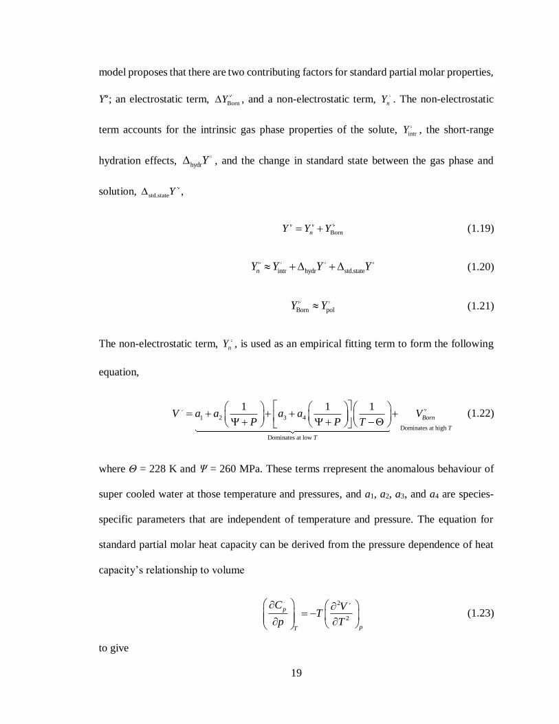
model proposes that there are two contributing factors for standard partial molar properties,

Y°; an electrostatic term, BornY , and a non-electrostatic term, nY . The non-electrostatic

term accounts for the intrinsic gas phase properties of the solute, intrY , the short-range

hydration effects, hydrY , and the change in standard state between the gas phase and

solution, std.stateY ,

BornnY Y Y (1.19)

intr hydr std.statenY Y Y Y (1.20)

Born polY Y (1.21)

The non-electrostatic term, nY , is used as an empirical fitting term to form the following

equation,

1 2 3 4

Dominates at high

Dominates at low

1 1 1Born

T

T

V a a a a VP P T

(1.22)

where Θ = 228 K and Ψ = 260 MPa. These terms rrepresent the anomalous behaviour of

super cooled water at those temperature and pressures, and a1, a2, a3, and a4 are species-

specific parameters that are independent of temperature and pressure. The equation for

standard partial molar heat capacity can be derived from the pressure dependence of heat

capacity’s relationship to volume

2

2

p

pT

C VT

p T

(1.23)

to give

20

2 3

1 2 3 4 ,

Dominates at high

Dominates at low

1 12 ( ) lnp r p Born

rT

T

pC c c T a p p a C

T T p

(1.24)

where c1 and c2 are temperature and pressure independent species specific parameters; pr

is the reference pressure (1 bar), and the terms a3, and a4 are from fitting to V°. The terms

in the HKF model have been set so the non-electrostatic terms dominate at low temperature

and the electrostatic contributions dominate at high temperatures, where the Born model is

most similar to solvation behaviour. The Born terms for the temperature and pressure

dependence of standard partial molar volume and heat capacity are described as

Born

1 ln 11

T T

Vp p

(1.25)

2

,Born 2

12 1p

T p

C TX TY TT T

(1.26)

where, for the standard partial molar heat capacity

22

2

1 ln ln

pp

XT T

(1.27)

1 ln

p

YT

(1.28)

The ω term is identical for the standard partial molar volume and standard partial molar

heat capacity. This means the electrostatic term from one property can be used to determine

the electrostatic term for the other, or in other words, the high temperature behaviour of

one property can be used to extrapolate the high temperature behaviour of the other [19].

Parameters for the HKF model were obtained for many electrolytes through the

regression of experimental heat capacity and volume measurements made over a range of

21

temperatures and pressures [24; 26]. Although a physical interpretation of the non-

electrostatic terms contributions to experimental quantities has not been clearly defined,

the HKF model has been able to reproduce standard state properties of electrolytes

effectively.

The extension of the HKF model to neutral species is not justified from a theoretical

view. Without the charge component for the Born coefficient the Born term becomes a

fitting parameter. On a purely empirical basis the model can be used to correlate

thermodynamic properties for uncharged species over a variety of temperatures. The

correlations obtained for neutral species when used to predict parameters have been

effective in some cases [28; 29], and failed in others [30; 31; 32; 33].

1.5.4 The “Density” Model

The density model is a semi-empirical fitting function reported by Marshall and

Frank (1981), and used experimentally by some authors [18; 34; 35]. The model contains

a combination of temperature and pressure dependent fitting terms for equilibrium

constants. The model is given

12 3

Dominates at high

Dominates at low

2

log log

T

T

b c dK a k

T T T

f gk e

T T

(1.29)

where the terms a-g are adjustable fitting parameters, independent of temperature and

pressure, and ρ1 is the density of the solvent in units of g·cm-3. The adjustable terms a, b,

c, and d dominate at ambient temperature and describe the intrinsic, or species specific

properties, and short-range hydrogen bonding effects. The fitting terms e, f, and g dominate

22

at high temperature and are associated with long range polarization effects. This model

makes the determination of other thermodynamic properties simple, continuing the use of

the same parameters. Gibbs energy can be determined through the relation in eq 1.3 as

12 3 2ln10 log

b c d f gG RT a e

T T T T T

(1.30)

Many other thermodynamic properties can be determined from the equilibrium

constant; the enthalpy of ionization can be determined using the relationship in eq 1.7,

2

1 12

2 3 2ln10 log

c d gH R b f RT k

T T T

(1.31)

where a1 is the thermal expansion of water in the form

11

1

1

pT

(1.32)

With the derivations given in full in Appendix B, the other thermodynamic quantities can

be determined from the model with the following equations [18];

1 12 3 2

2ln10 log

c d gS R a e RTk

T T T

(1.33)

2 11 12 3 2

2 6 2 2ln10 log 2p

p

c d g gC Ra eT RT k

T T T T T

(1.34)

1V RTk (1.35)

where the compressibility of water, β1, is described as

23

11

1

1

Tp

(1.36)

A more simplified version of this model has been reported by Anderson et al. where

only the a, b, and f terms are used, written as [34]

321 1ln ln

ppK p

T T

(1.37)

and has been shown by Mesmer et al. (1988) [18] to accurately predict thermodynamic

values to temperatures of approximately 573.15 K. This simplified model greatly effects

the simplicity of the standard partial heat capacity when fitting data to the model while still

maintaining its predictive ability [34].

1.5.5 Functional Group Additivity Models

Predictive methods could replace experimental measurements if they provide

sufficiently good estimates. A functional group additivity model would be capable of

predicting thermodynamic properties of pure and mixed solutions using the properties of

atoms or functional groups. This method has the ability to drastically limit the quantity of

experimental data required; instead of measuring the properties of thousands or millions of

compounds individually, a predictive method might only require data for a few dozen or

hundred groups to be known to determine the properties of thousands.

The general equation used to describe standard molar thermodynamic properties for

functional group additivity models is given as

'2 2,1

1N

ss i ii

Y Ze Y nY

(1.38)

24

where N is the total number of functional groups, ni is the number if occurrences of each

specific group, 2Y is the thermodynamic property, '2,iY is the property contribution of each

functional group, and Ze is the charge (Yezdimer et al., 2000). The term Yss represents the

standard state measurement of the thermodynamic property. This work is currently limited

for amines by the availability of experimental data above 523.15 K for some functional

groups, and 323.15 K for others [36]. Some development of functional group additivity

models has been successfully completed using mostly C and H group types [36; 37; 38].

1.6 Instrumentation

1.6.1 Vibrating Tube Densimeter

The measurement of apparent molar volumes was revolutionized by the invention

of the vibrating-tube densimeter by Kratky et al. (1969) [19]. This densimeter operates by

accurately measuring changes in resonant frequency of a vibrating tube, created by the

differences in mass as the contents of the tube is changed between calibration and sample

materials. A typical design for a vibrating-tube densimeter is shown in Figure 5. The

densimeter consists of a thin walled glassed tube in the shape of a ‘U’ that is fixed to a

mass so the tube is isolated from any mechanical disturbances in the densimeter [39]. Two

sets of electromagnetic assemblies, composed of permanent magnets and wire coils

(termed the “pick-up” and “drive”), are used to make the tube vibrate so a frequency can

be measured [39]. To create a measureable disturbance an alternating electric current is run

through the drive and generates stationary oscillations. These oscillations induce an

electrical signal at the pick-up, which is connected to a frequency counter that measures

the cycles of oscillation, or pulses per second, in an electronic signal. Both circuits are

25

Figure 5. A schematic of a vibrating U-tube densimeter [39].

26

connected to create a continuous resonant frequency through the assistance of a phase lock

loop [19; 39]. The reciprocal of the measured resonant frequency, ω, is the period, τ,

1

(1.39)

and can be directly related to density of the sample

2 2

1 1( );s p sk (1.40)

where and ρs, ρ1, τs, and τ1 are the densities (g·cm-3) and periods of vibration (μs),

respectively. The term kρ is the cell constant and is determined using a calibration method

developed by the Woolley research group and others [39; 40; 41; 42]. If the period of

vibration is known for a volume of solution, it is possible to determine the relative density

of an unknown solution to a standard reference solution; and, therefore, determine the

density of the unknown solution.

The DMA 5000 manufactured by Anton Paar Ltd., is a vibrating tube densimeter

and is capable of making relative density measurements from 273.15 to 363.15 K with a

precision of ± 2x10-6 g·cm-3. These high precision density measurements are required for

precise measurements of apparent molar properties.

1.6.2 The Picker Calorimeter

The development of the Picker calorimeter in 1971 is noted as a major development

in aqueous heat capacity calorimetry. The flow design of the calorimeter allows for the

volumetric heat capacities of two solutions to be measured with a temperature range of 275

to 340 K and a relative uncertainty as low as ± 0.00002 J·mol-1·K-1 [43]. This uncertainty

gave researchers the ability to make measurements of solutions with concentrations as low

27

as 0.02 mol·kg-1 while maintaining an acceptable calorimetric uncertainty of ± 4 J·mol-1·K-

1. The development of the Picker calorimeter has also greatly reduced the quantity of

solutions required for measurements, requiring only 30 cm3 to complete multiple

measurements at a single temperature [19].

The Picker flow microcalorimeter consists of two parallel, tubular cells insulated

from one another and their surroundings by a vacuum [19; 44]. The inlet of both cells is

temperature controlled by a single bath, ensuring the temperature of the solution entering

each cell is identical. The conceptual design is shown in Figure 6. The difference in heat

capacity of each cell is measured by power compensation; power is applied to cell 1, the

sample cell, so it maintains identical temperature to cell 2, the reference cell [19]. Since

the values for ΔT are identical between the two cells, the ratio of heat capacities can be

described using the ratio of power required to maintain identical cell temperature and the

flow rate,

1 2

2 1

1

2

p m

p m

C fP

C P f (1.41)

where Cp1/Cp2 is the heat capacity ratio of the two cells, P1/P2 is the power ratio and ƒm2/ƒm1

is the ratio of mass flow rates [19]. While power can be accurately measured, the flow rate

could not be accurately measured or controlled until the Picker flow microcalorimeter

solved this problem by adding a delay line, which is a long length of tubing that connects

the two cells [19; 44]. Using the delay line, water is run through both cells, followed by the

experimental solution. Measurements are taken when there is only sample remaining in the

first cell, only water in the second cell, and the interface is in the delay line [19].

28

Figure 6: The conceptual design of a twin cell Picker flow heat-capacity microflow

calorimeter [19].

29

Through the use of density, the mass flow rate can be related to the

volumetric flow rate as described by

1

2

1 2

2 1

p

p

C P

C P

(1.42)

where ρ2/ρ1 is the ratio of densities of the solutions in the delay line.

1.6.3 DSC Type Calorimeters

Another advance in heat capacity calorimetry occurred in 1995 with the

development of a twin fixed cell power compensation calorimeter by the Privalov research

group [45]. The differential scanning calorimeter (DSC) is characterized by twin fixed cells

used to directly measure the differences in heat capacities of two aqueous solutions with a

high level of precision. A nano DSC, based on the Privalov design, was used by Woolley

(2007) to create a calibration method and complete measurements of NaCl [42; 43].

Woolley (1997, 2007) found the calorimeter was able to measure aqueous solution heat

capacities with comparable, and in some cases better, precision than that of the Picker

calorimeter over an extended temperature range [41; 42; 43]. A fixed cell DSC require

sample sizes between 0.3 and 1.0 cm3 and can achieve pressures of 0.6 MPa within a 273

to 420 K temperature range. The relative precision given across most models is >±

0.000005 with a sensitivity of 50 nW.

A nano power compensating DSC measures the difference in power required to

maintain an equal temperature between the sample cell, reference cell, and the thermal

jacket as the instrument completes scans that increase and decrease in temperature. The

difference in power applied to the two cells is proportional to the difference in heat capacity

30

Figure 7. Twin platinum capillary cells within the Nano DSC 6300 by TA instruments

[46].

31

of the two cells and their contents [19; 42; 43; 47]. The equations used to calculate heat

capacity from the measurements of the difference in power are available in the

experimental section of Chapter 2. As visible in Figure 7 from TA Instruments, the twin

cells are fixed to avoid changes in response from cell placement. Material and design of

the cells changes between versions of the calorimeter; the more current model in Figure 7

contains platinum capillary cells, meant to aide in the aggregation of proteins these

calorimeters are commonly used to measure. Figure 8 displays twin gold batch cells found

in a traditional DSC. In both figures semiconductor batteries are visible between the twin

cells, and are used to sense the temperature difference between the two cells so the

appropriate amount of power can be distributed to each cell. This power distribution is

completed by individual electric heaters located on the outside of each cell. A thermal

jacket contains both cells as well as a platinum thermometer and heating and cooling Peltier

elements. The thermal jacket ensures no heat transfer occurs between the cells and their

surroundings by maintaining a temperature difference of zero between the cells and their

surroundings [42; 47]. A piston maintains constant pressure in the manostat directly

connected to the cells and is monitored by a piezoelectric sensor.

Density is used to compensate for the expansion and the changes in mass of the

solutions with temperature so the heat capacity values measured are accurate for the

volume of fluid inside the cell at the specific time and temperature of the measurement

[42].

1.7 Thesis Objectives

The goal of this research is to develop a method by which high temperature

thermodynamic data for amines of interest for the nuclear industry can be measured and

32

Figure 8. Twin gold batch cells from the Nano power compensation DSC 60200 by the

Calorimetry Science Corporation taken in the Tremaine Lab at the University of Guelph.

33

accurately extrapolated to reactor temperatures. This work is important not only to

industry, but also to close wide literature gaps in high temperature amine data. For the

amines measured in this work only a few authors have made measurements beyond 298.15

K, with the highest temperature for Cp° in the combined literature for DMEA and 3-MPA

being at 328.15 K [48].

Measurements of the standard partial molar volumes and heat capacities are available

for DMEA and 3-MPA in Chapters 3 and 4. The standard partial molar volumes and heat

capacity values were measured from 283.15 to 363.15 K and 283.15 to 393.15 K,

respectively. An extrapolation of this data was completed using data reported by Bulemela

and Tremaine (2008) by fitting the density model [49]. As a result of the parameters

obtained from the density model fit, ionization constants were calculated to 573.15 K.

Following the development of this method, additional amines will be measured and the

data will be used to develop functional group additivity models for amine species.

1.8 Contributions to Thesis

Chapters 3 and 4 report measurements of standard partial molar volumes and heat

capacities using the method developed by Alex Lowe and Christine McGregor in their MSc

Thesis projects [50; 51]. Measurements on DMEA (Chapter 3) were made in a

collaboration with Dr. Jenny Cox, and Dr. Olivia Fandiño Torres. One set of apparent

molar heat capacity measurements of DMEA was made by Dr. Fandiño Torres, the

remainder were made by me under her co-supervision. All experimental work on the 3-

MPA experiments were carried out myself, as were all the data analysis and modeling for

both the DMEA and 3-MPA systems. The development of the density model equation of

state treatment to calculate high temperature ionization constants was completed under

34

Professor Tremaine’s direction. Chapters 3 and 4 are my second and first drafts,

respectively, of papers to be submitted to the Journal of Chemical Thermodynamics co-

authored by Professor Tremaine, Dr. Fandiño Torres and Dr. Cox.

35

Chapter 2 Standard Partial Molar Heat Capacities and

Volumes of Aqueous N,N-Dimethylethanolamine and N,N-

Dimethylethanolammonium Chloride from 283 K to 393 K

Abstract

Densities for dilute aqueous solutions of N,N-dimethylethanolamine (DMEA) and

N,N-dimethylethanolammonium chloride (DMEAH+Cl-) were measured relative to water

at 283.15 K ≤ T ≤ 363.15 K and 0.1 MPa using vibrating tube densimeters. Volumetric heat

capacities of the same solutions were measured at 283.15 K ≤ T ≤ 393.15 K and 0.4 MPa

using twin fixed-cell, power compensation, differential temperature scanning nano

calorimeters. From these measurements apparent molar volumes, Vϕ, and heat capacities,

Cp,ϕ, were calculated and corrected for speciation to obtain standard partial molar

properties Vo and Cpo, for the species DMEA(aq) and DMEAH+Cl-(aq). The experimental

values for Vo and Cpo, measured in this work were combined with high temperature values

reported by Bulemela and Tremaine (J. Phys. Chem. B 2008, 112, 5626-5645) over the

range 423.15 to 598.15 K to derive parameters for the semi-empirical “density” model that

expresses the standard partial molar thermodynamic properties of aqueous species as a

function of temperature and solvent density. The fitted parameters were used with

critically evaluated literature values for the standard partial molar Gibbs energy and

enthalpy of reaction at 298.15 K to obtain values for the ionization constant of N,N-

dimethylethanolamine from 283.15 to 598.15 K at steam saturation pressure.

36

2.1 Introduction

Hydrothermal solutions of aqueous alkanolamines are common across many industry

processes including steam generating, gas purification, surfactants, detergents, and textile

processing. For the amines used in many of these processes there is very little experimental

data available, creating an industry centered interest to model and measure chemical

processes under hydrothermal conditions. Alkanolamines are being considered as an

alternative for pH control in the steam systems of nuclear reactors for corrosion resistance.

These alkanolamines must posses the correct combination of volatility and basicity to

maintain a constant alkalinity in the boiling solution, vapor, and condensate components

of steam-water cycles [4; 52].

Alkanolamines can offer distinct advantages over morpholine, cyclohexylamine, and

ammonia, volatile amines traditionally employed in pH control for the steam systems [3].

Ammonia is so volatile that it concentrates in the steam phase, leaving condensed phases

of the steam generating system unprotected. Although less volatile, morpholine and

cyclohexylamine undergo thermal decomposition into organic acids that can increase

corrosion in the system they are meant to protect [3; 4; 12].

N,N-dimethylethanolamine (DMEA) is currently used as a curing

agent for polyurethanes and epoxy resins, in the synthesis of dyestuffs, textile

auxiliaries, pharmaceuticals, emulsifiers, and as a corrosion inhibitor in steam-water cycle

processes [52]. The availability of high temperature thermodynamic data can be used to

accurately describe the behaviour of N,N-dimethylethanolamine in solution and its

effectiveness in steam-water cycles and as a possible alternative amine for pH control in

the steam-water system of a nuclear reactor.

https://psychology.wikia.org/wiki/Dye

https://psychology.wikia.org/wiki/Pharmaceutical

37

N,N-dimethylethanolamine hydrolyses in water, according to the reaction

2DMEA H O DMEAH OHaq l aq aq (2.1)

Values for the ionization constant and standard molar enthalpy of reaction have

been reported by several workers at temperatures up to 353.15 K and 298.15 K,

respectively [1; 53; 54; 55; 56]. Apparent molar volumes were determined under ambient

conditions within a temperature range of 278.15 K to 353.15 K by Collins et al. (2000)

[48], Fu-Qiang et al. (1995) [57], Hawrylak et al. (2000) [58], and Lebrette at al. (2002)

[59]. Standard partial molar volumes of DMEA have been reported by Collins et al. (2000)

[48] and by Lebrette et al. (2002) [59]. Collins et al. (2000) [48] have also reported standard

partial molar volumes for the protonated amine from 283.15 K to 328.15 K.

Only one worker has reported standard partial volumes at elevated temperatures

and pressures. The measurements by Bulemela and Tremaine (2008) [49] for the neutral

and protonated species are reported from 424.15 K to 598.15 K and at 15 MPa.

Values for the apparent and standard partial molar heat capacities of DMEA(aq)

and DMEAH+Cl-(aq) have been reported by Collins et al. (2000) [48]. There are no high

temperature heat capacity measurements for DMEA(aq) or DMEAH+Cl-(aq) in the current

literature.

This paper reports densities and heat capacities, measured relative to water, from

283.15 K to 363.15 K and 393.15 K, respectively, for dilute aqueous solutions of N,N-

dimethylethanolamine and N,N-dimethylethanolammonium chloride. From these

measurements apparent molar volumes, Vϕ, and heat capacities, Cp,ϕ, were calculated and

corrected for speciation to obtain standard partial molar properties V° and Cp°, for the

38

species DMEA(aq) and DMEAH+Cl-(aq). The semi-empirical “density” model was fit to

the experimental values for V° and Cp°, measured in this work, and combined with high

temperature values reported by Bulemela and Tremaine (2000) [49] over the range 423.15

to 598.15 K. The fitted parameters were used, with literature values for Gibbs energy and

enthalpy of ionization at 298.15 K to calculate values for the ionization of DMEA from

283.15 K to 598.15 K.

2.2 Experimental

2.2.1 Materials and Solution Preparation

All chemicals are listed in Table 2, and were used as received with no additional

purification before use. Solutions of DMEA (0.1 mol·kg-1) were prepared by mass and

standardized in triplicate against dried potassium hydrogen phthalate (KHP) using a

Metrohm 794 Basic Titrino autotitrator. The DMEAH+Cl- stock solution (0.1 mol·kg-1)

was prepared using DMEA (0.2 mol·kg-1) through the addition of excess 0.2 mol·kg-1

hydrochloric acid. Standard solutions of KHP at 0.1 mol·kg-1,

tris(hydroxymethyl)aminomethane (TRIS) at 0.2 mol·kg-1, and NaCl at 1 mol·kg-1 were

prepared by mass after drying the solid chemicals for 2 h at 383.15 K, 4 h at 373.15 K and

24 h at 573.15 K, respectively. The KHP and HCl solutions were standardized against

TRIS. All solutions were prepared from degassed ultra-pure water (18.2 MΩ·cm) from an

EMD Millipore Direct-Q® 3 UV remote water purification system.

2.2.2 Densimetry

Solution densities were measured using two Anton Paar DMA5000 vibrating-tube

densimeters at ambient pressure, p = (0.10 ± 0.01) MPa, over a temperature range from

283.150 K to 363.150 K (± 0.001 K). The period of vibration was recorded at intervals of

39

Table 2 List of the chemicals used in this work (DMEA), including purities as listed by

the supplier.

Chemical Name (CAS #) Formula Source Mass

Fraction

Purity

Analytic

Technique

Hydrochloric acid

(7647-01-0)

HCl Fluka ≥ 0.95 Titration

N,N-

dimethylethanolamine

(108-01-0)

C6H13N Sigma-

Aldrich

≥ 0.999 Titration

Potassium hydrogen

phthalate

(877-24-7)

C8H5KO4 Sigma-

Aldrich

≥ 0.9995 Titration

Sodium chloride

(7647-14-5)

NaCl Sigma-

Aldrich

0.995 Titration

Tris(hydroxymethyl)-

aminomethane

(77-86-1)

C4H11NO3 Sigma-

Aldrich

≥ 0.999 Titration

40

5.00 K, after equilibrating for 10-15 minutes at each temperature step. All solutions were

degassed before injection by withdrawing the plunger of a solution-filled, sealed syringe

as described by McGregor et al. (2017) [60].

The density of each sample, relative to water, was calculated using the experimental

period of vibration at each temperature interval based on a relationship with Hooke’s law

[43]

2 2

s w s wk (2.2)

where ρs, ρw, are the densities (g·cm-3) and τs, τw, are periods of vibration (μs) for the

solution and water, respectively. The Anton Parr densimeter software automatically

calculates solution densities based on the period of vibration using an equation of state for

water by Spieweck and Bettin (1992) [61]. These densities are not used in this work to

maintain internal consistency when calculations of apparent molar properties in this work

utilize the properties of water from Hill (1990) [62].

The cell constant, kρ, is determined through symmetric measurements of calibration

solutions before and after every two sample measurements. Measurements of a single

sample are carried out over six days, beginning with measurements of calibration solutions,

degassed water and 1 mol·kg-1 aqueous NaCl(aq) from 283.15 K to 363.15 K on the first

and second day, respectively. This first calibration is followed by measurement of the

sample on the third and fourth day, and an additional calibration of degassed 1 mol·kg -1

aqueous NaCl(aq) and water on day five and six, respectively. The properties of the

calibration fluids are calculated from the properties from Hill's equation of state for water

[62] and Archer's Pitzer Ion Interaction model for the properties of NaCl [63]. Apparent

41

molar volumes, , for DMEA(aq) and DMEAH+Cl-(aq) were calculated from the

expressions,

s wexp DMEA

DMEA, st

s DMEA s w

1000M

Vm

(2.3)

+ - + -

+ -

+ - + -

st ex

HCl HClDMEAH Cl DMEAH Cl s wexp

DMEAH Cl , st ex st exs HCl HCl s wDMEAH Cl DMEAH Cl

11000

M m M mV

m m m m

(2.4)

where DMEAM 89.130 g·mol-1, + -DMEAH ClM 125.591 g·mol-1, and HClM 36.461 g·mol-

1. Superscripts indicate the stoichiometric molality of amine (st) or the molality of excess

HCl (ex).

2.2.3 Calorimetry

Solution heat capacities were determined using two twin fixed-cell, nano-

differential-output temperature-scanning, power-compensation calorimeters (DSC)

manufactured by TA Instruments. The Nano DSC 60200 has two fixed capillary cells in

platinum with a cell volume of 300μL. The Nano DSC 6300 has two fixed cylindrical cells

in 24K gold with a cell volume of 330 μL. The temperature difference between the

reference and sample cells is kept as close to zero as possible by applying the appropriate

amount of power to each cell through individual electric heaters attached to each cell. The

difference in power, ΔP, is a measure of the difference in heat capacity between the cells

and their contents. Measurements of ΔP were taken over a temperature range from 283.15

K to 393.15 K at a scan rate of 1 K·min-1 and at a pressure of p = (0.40 ± 0.01) MPa. Data

for each solution were collected during six solution heating and six solution cooling runs.

The first heating and cooling scan of each experiment was discarded, following the

exp

V

42

procedure reported by Woolley (2007) [43]. Values obtained at 383.15 K and 393.15 K

were discarded as a result of hysteresis effects. Solutions were degassed before injection

by withdrawing the plunger of a solution-filled, sealed syringe as described by McGregor

et al. (2017) [60], and loaded independently for each experiment. Software supplied by TA

Instruments, DSCRun and NanoAnalyze, was used to collect and view the data. The heat

capacities based on the heating scans and the cooling scans were calculated separately.

The massic heat capacity of each sample, relative to water, was obtained from the

relationship between the previously measured densities and the measured values of ΔP

s w

,s s ,w w

c

p p

k P Pc c

r

(2.5)

where cp,s, and cp,w are the massic heat capacities (J·K-1·g-1) for the solution and water

respectively, r is the temperature scan rate (K·s-1), and kc is the cell constant. Cell constants

were determined using the method reported by Ballerat-Busserolles et al. (2000) [47]. This

calibration mirrors the calibration performed for the density measurements, where

symmetric measurements of calibration fluids, water 1 mol·kg-1 aqueous NaCl(aq), and the

sample, from 283.15 K to 393.15 K take place over six days. The properties of the

calibration fluids were calculated from the Hill’s equations of state for water [62] and

Archer’s Pitzer Ion Interaction model [63].

Equations 2.6 and 2.7 were used to calculate the apparent molar heat capacities,

, for the DMEA neutral and protonated species.

,s ,wexp

, , DMEA DMEA ,s st

DMEA

1000p p

p p

c cC M c

m

(2.6)

exp

,pC

43

+ - + -

+ - + -

st ex

HCl HCl ,s ,wDMEAH Cl DMEAH Clexp

,s, , DMEAH Cl st ex st ex

HCl HClDMEAH Cl DMEAH Cl

1000p p

pp

M m M m c cC c

m m m m

(2.7)

The solution densities required to calculate for temperatures greater than 363.15 K

were obtained by fitting density model eq 2.20, to the standard partial molar volumes from

the densimeter measurements, discussed in Section 2.3.2. The standard partial molar

volumes were assumed to be constant between 0.1 MPa and 0.4 MPa so that the densities

at 0.4 MPa could be calculated from the standard partial properties using the appropriate

values for the water properties. The values for properties of water are available in Appendix

A.

2.3 Results

2.3.1 Apparent Molar Volumes and Heat Capacities

The experimental relative densities (ρs - ρw) of DMEA(aq) and DMEAH+Cl-(aq)

from the average of each set of measurements in each densimeter are reported in Table 3.

The experimental relative volumetric heat capacities (cp,sρs - cp,wρw) are tabulated in Tables

4 and 5. The average values of the experimental apparent molar volumes, , and heat

capacities, , at each temperature are listed in Tables 6 and 7. The standard uncertainties

in and were calculated as the standard error of the mean and are no more than ±

0.2 cm3·mol-1 for and ± 2 J·K-1 ·mol-1 for . At temperatures T > 363.15 K,

additional systematic errors may be present in the calculated standard partial molar heat

capacities due to the method of extrapolating densities from the V° fit described in Section

3.3.

exp

,pC

expV

exp

,pC

expV

exp

,pC

expV

exp

,pC

44

Table 3 Experimental densities relative to water (ρs - ρw) of DMEA (aq) and DMEAH+Cl- (aq) as a function of temperature T at p =

0.10 MPa, for each stoichiometric molality, mst, with standard uncertainties, u.a, b

(ρs-ρw)·103/g·cm-3

DMEA(aq) DMEAH+Cl-(aq)

0.1096 ± 0.0002 0.1096 ± 0.0002 0.1068 ± 0.005 0.1068 ± 0.005

-

-

0.0025 ± 0.0003 0.0025 ± 0.0003

Densimeter 1 Densimeter 2 Densimeter 1 Densimeter 2

T/K 1st Loading 2nd Loading 1st Loading 2nd Loading 1st Loading 2nd Loading 1st Loading 2nd Loading

283.15 -0.414 -0.362 -0.420 -0.419 2.168 2.137 2.124 2.142

293.15 -0.440 -0.391 -0.452 -0.445 2.075 2.044 2.036 2.049

303.15 -0.473 -0.424 -0.485 -0.476 2.008 1.981 1.972 1.985

313.15 -0.507 -0.460 -0.517 -0.509 1.965 1.939 1.928 1.940

323.15 -0.538 -0.495 -0.541 -0.532 1.941 1.921 1.916 1.927

333.15 -0.566 -0.526 -0.560 -0.554 1.933 1.927 1.922 1.930

343.15 -0.599 -0.561 -0.586 -0.581 1.935 1.933 1.932 1.938

353.15 -0.621 -0.581 -0.603 -0.598 1.963 1.959 1.964 1.968

363.15 -0.628 -0.568 -0.618 -0.614 2.014 2.001 2.006 2.010

373.15 -0.710b 1.956b

383.15 -0.752b 2.025b

393.15 -0.794b 2.110b a The standard uncertainties are u(T) = 0.01 K, u(p) = 0.01 MPa, and u(ρs-ρw) = 0.01 g·cm-3

b Calculated from V° to values by Bulemela and Tremaine (2008) [49], eq 2.20

st 1

DMEA /m mol kg st 1

DMEA /m mol kg st 1

DMEA /m mol kg st 1

DMEA /m mol kg

st 1

HCl /m mol kg st 1

HCl /m mol kg

45

Table 4 Experimental volumetric heat capacities relative to water (cp,s·ρs – cp,w·ρw) of DMEA (aq) at stoichiometric, “st”, molalities,

mst, at temperature T and pressure p = 0.40 MPa with standard uncertainties, u.a, b, c

(cp,s·ρs – cp,w·ρw) · 103/J·K-1·cm-3

Nano DSC 6300 Nano DSC 60200

mstDMEA/mol·kg-1 = 0.1096 ± 0.0002 b mst

DMEA/mol·kg-1 = 0.1096 ± 0.0002 b

T/K Heating Cooling Heating Cooling Heating Cooling

283.15 (-2.01) -1.71 (-1.97) -1.72 (-2.06) -1.71

288.15 -1.78 -1.69 -1.79 -1.71 -1.78 -1.67

293.15 -1.75 -1.69 -1.74 -1.71 -1.75 -1.67

298.15 -1.73 -1.75 -1.72 -1.76 -1.74 -1.73

303.15 -1.73 -1.79 -1.73 -1.72 -1.73 -1.87

308.15 -1.72 -1.57 -1.68 -1.56 -1.75 -1.57

313.15 -1.62 -1.43 -1.57 -1.40 -1.66 -1.46

318.15 -1.44 -1.33 -1.42 -1.28 -1.46 -1.38

323.15 -1.34 -1.23 -1.28 -1.18 -1.40 -1.27

328.15 -1.14 -1.12 -1.09 -1.15 -1.20 -1.09

333.15 -1.02 -1.12 -0.90 -1.05 -1.14 -1.19

338.15 -1.01 -0.96 -0.94 -0.89 -1.09 -1.02

343.15 -0.93 -0.96 -0.91 -0.90 -0.95 -1.03

348.15 -0.83 -0.78 -0.78 -0.73 -0.88 -0.84

353.15 -0.70 -0.67 -0.68 -0.65 -0.73 -0.70

358.15 -0.65 -0.57 -0.66 -0.56 -0.64 -0.58

363.15 -0.55 -0.54 -0.55 -0.46 -0.55 -0.63

368.15 -0.45 -0.41 -0.41 -0.37 -0.50 -0.46

373.15 -0.36 -0.31 -0.37 -0.28 -0.36 -0.34

378.15 -0.29 -0.20 -0.30 -0.16 -0.29 -0.25

383.15 -0.22 -0.15 -0.24 -0.11 -0.19 -0.19

388.15 -0.15 -0.04 -0.17 0.03 -0.14 -0.11

393.15 -0.11 (0.06) -0.15 (0.06) -0.07 (-0.06) a The standard uncertainties are u(T) = 0.01 K, u(p) = 0.01 MPa, and u(cp,s·ρs – cp,w·ρw) = 0.07 J·K-1·cm-3

46

b The same stock solutions with independent loading into two independent calorimeters

47

Table 5 Experimental volumetric heat capacities relative to water (cp,s·ρs – cp,w·ρw) of DMEAH+Cl- (aq) at stoichiometric, “st”,

molalities, mst, at temperature T and pressure p = 0.40 MPa with standard uncertainties, u.a, b, c

(cp,s·ρs – cp,w·ρw) · 103 /J·K-1·cm-3


mstDMEA/mol·kg-1 = 0.1068 ± 0.0002 b mst

DMEA/mol·kg-1 = 0.1068 ± 0.0002 b

mstHCl/ mol·kg-1 = 0.2272 ± 0.0003 b mst

HCl/ mol·kg-1 = 0.2272 ± 0.0003 b

T/K Heating Cooling Heating Cooling Heating Cooling Heating Cooling

283.15 (-31.0) -34.3 (-31.8) -34.3 (-31.8) -34.3 (-31.3) -33.3

288.15 -32.7 -33.0 -32.7 -32.9 -33.2 -33.1 -32.4 -32.1

293.15 -31.6 -32.0 -31.6 -31.7 -32.2 -32.0 -31.3 -31.0

298.15 -30.7 -31.0 -30.8 -30.8 -31.3 -31.0 -30.4 -30.2

303.15 -29.8 -30.1 -30.2 -30.0 -30.4 -29.9 -29.7 -29.6

308.15 -29.0 -29.4 -29.6 -29.3 -29.6 -29.0 -29.0 -29.1

313.15 -28.2 -28.7 -29.2 -28.7 -28.7 -28.5 -28.6 -28.3

318.15 -27.5 -28.2 -28.7 -28.2 -28.0 -28.0 -28.1 -27.7

323.15 -27.1 -27.7 -28.3 -27.8 -27.5 -27.5 -27.6 -27.2

328.15 -26.6 -27.3 -27.9 -27.3 -27.1 -27.0 -27.1 -26.9

333.15 -26.3 -26.9 -27.5 -27.0 -26.7 -26.6 -26.6 -26.5

338.15 -26.0 -26.5 -27.1 -26.6 -26.3 -26.2 -26.3 -26.3

343.15 -25.8 -26.1 -26.8 -26.3 -25.9 -25.9 -26.0 -25.8

348.15 -25.5 -25.8 -26.4 -26.0 -25.5 -25.6 -25.6 -25.6

353.15 -25.3 -25.5 -26.1 -25.7 -25.3 -25.3 -25.3 -25.2

358.15 -25.0 -25.2 -25.8 -25.4 -25.0 -24.9 -25.0 -24.8

363.15 -24.8 -25.0 -25.4 -25.1 -24.7 -24.5 -24.7 -24.7

368.15 -24.6 -24.8 -25.2 -24.9 -25.1 -24.4 -24.4 -24.4

373.15 -24.4 -24.5 -24.9 -24.6 -24.7 -24.0 -24.1 -24.1

378.15 -24.2 -24.4 -24.7 -24.5 -24.3 -23.9 -23.8 -23.9

383.15 -24.1 -24.2 -24.5 -24.2 -24.1 -23.7 -23.7 -23.8

388.15 -24.3 -24.1 -24.1 -24.1 -24.0 -23.4 -23.4 -23.5

393.15 -24.3 (-22.3) -23.9 (-22.5) -23.4 (-21.8) -23.3 (-22.1)

48

a The standard uncertainties are u(T) = 0.01 K, u(p) = 0.01 MPa, and u(cp,s·ρs – cp,w·ρw) = 0.01 J·K-1·cm-3


c Parentheses indicate extrapolated data point values

49

Table 6 Mean values of experimental, ‘exp’, apparent and standard partial molar volumes and heat capacities of DMEA(aq), (Vφexp, V°)

and (Cp,φexp, Cp°) at p = 0.40 MPa and their standard uncertainties, u (±).a,b

T/K Vφexp/cm3·mol-1 V°/cm3·mol-1 Cp,φ

exp/J·K-1·mol-1 Cp°/J·K-1·mol-1

283.15 92.85 ± 0.10 92.76 ± 0.10 379.44 ± 0.62 379.65 ± 0.63

288.15 93.10 ± 0.10 92.99 ± 0.10 379.00 ± 0.39 379.60 ± 0.39

293.15 93.34 ± 0.10 93.22 ± 0.10 379.38 ± 0.48 380.43 ± 0.48

298.15 93.61 ± 0.10 93.47 ± 0.10 379.85 ± 0.55 381.39 ± 0.55

303.15 93.86 ± 0.09 93.72 ± 0.10 380.45 ± 0.82 382.46 ± 0.83

308.15 94.17 ± 0.09 94.01 ± 0.09 382.02 ± 1.03 384.50 ± 1.04

313.15 94.48 ± 0.09 94.31 ± 0.09 383.65 ± 1.22 386.56 ± 1.24

318.15 94.82 ± 0.08 94.65 ± 0.08 385.37 ± 1.24 388.67 ± 1.25

323.15 95.17 ± 0.08 95.00 ± 0.08 386.95 ± 1.22 390.58 ± 1.24

328.15 95.55 ± 0.07 95.39 ± 0.07 388.87 ± 1.12 392.78 ± 1.14

333.15 95.96 ± 0.07 95.79 ± 0.07 390.46 ± 1.07 394.57 ± 1.09

338.15 96.36 ± 0.07 96.20 ± 0.07 392.05 ± 0.95 396.31 ± 0.96

343.15 96.76 ± 0.07 96.62 ± 0.07 393.45 ± 0.89 397.78 ± 0.90

348.15 97.17 ± 0.08 97.04 ± 0.08 395.39 ± 0.78 399.73 ± 0.79

353.15 97.59 ± 0.08 97.47 ± 0.08 397.24 ± 0.71 401.54 ± 0.72

358.15 97.99 ± 0.09 97.88 ± 0.09 398.88 ± 0.73 403.10 ± 0.74

363.15 98.38 ± 0.11 98.29 ± 0.11 400.37 ± 0.79 404.45 ± 0.80

368.15 401.65 ± 0.69 405.50 ± 0.70

373.15 403.55 ± 0.63 407.21 ± 0.63

378.15 404.99 ± 0.62 408.45 ± 0.63

383.15 407.58 ± 0.60 410.83 ± 0.60

388.15 409.45 ± 0.49 412.49 ± 0.50

393.15 411.29 ± 0.77 414 12 ± 0.78 a The standard uncertainties are u(T) = 0.01 K and u(p) = 0.01 MPa

b Standard uncertainties in V° and Cp° (±) are the standard deviation of the mean at each temperature where n = 4 and 8, respectively

50

Table 7 Mean values of experimental, ‘exp’, apparent and standard partial molar volumes and heat capacities of DMEAH+Cl-(aq),

(Vφexp, V°) and (Cp,φ

exp, Cp°) at p = 0.40 MPa and their standard uncertainties, u (±).a, b

Vφexp/cm3·mol-1 V°/cm3·mol-1 Cp,φ


T/K DMEAH+Cl- DMEAH+Cl- Cl- DMEAH+ DMEAH+Cl- DMEAH+Cl- Cl- DMEAH+

283.15 102.96 ± 0.16 107.02 ± 0.47 17.16 92.4 ± 2.1 121.90 ± 1.87 120.27 ± 0.13 -145.05 276.0 ± 2.4

288.15 103.54 ± 0.15 107.59 ± 0.47 17.44 91.7 ± 2.1 135.34 ± 1.17 133.11 ± 1.28 -135.94 277.7 ± 2.4

293.15 104.06 ± 0.15 108.08 ± 0.47 17.66 91.1 ± 2.1 146.15 ± 1.19 143.59 ± 1.30 -128.76 279.8 ± 2.4

298.15 104.48 ± 0.15 108.49 ± 0.47 17.81 90.7 ± 2.1 154.94 ± 1.05 152.70 ± 1.15 -123.20 282.3 ± 2.4

303.15 104.89 ± 0.14 108.85 ± 0.47 17.92 90.5 ± 2.1 163.04 ± 0.83 161.47 ± 0.90 -119.02 285.0 ± 2.4

308.15 105.25 ± 0.14 109.19 ± 0.47 17.98 90.4 ± 2.1 169.79 ± 0.79 168.61 ± 0.86 -116.01 288.1 ± 2.4

313.15 105.59 ± 0.14 109.50 ± 0.47 18.00 90.4 ± 2.1 175.63 ± 0.87 173.53 ± 0.95 -113.98 291.3 ± 2.4

318.15 105.88 ± 0.14 109.75 ± 0.46 17.98 90.5 ± 2.1 180.71 ± 1.06 178.13 ± 1.16 -112.77 294.7 ± 2.4

323.15 106.17 ± 0.13 110.00 ± 0.46 17.92 90.6 ± 2.1 184.71 ± 1.15 181.75 ± 1.26 -112.25 298.0 ± 2.4 328.15 106.40 ± 0.13 110.22 ± 0.45 17.82 90.9 ± 2.1 188.28 ± 1.13 185.13 ± 1.24 -112.30 301.4 ± 2.4

333.15 106.67 ± 0.13 110.43 ± 0.45 17.69 91.3 ± 2.1 191.41 ± 1.12 188.03 ± 1.22 -112.83 304.7 ± 2.4

338.15 106.90 ± 0.14 110.61 ± 0.45 17.53 91.7 ± 2.1 194.11 ± 1.06 190.72 ± 1.15 -113.77 307.9 ± 2.4

343.15 107.10 ± 0.15 110.76 ± 0.45 17.33 92.1 ± 2.1 196.33 ± 1.04 192.39 ± 1.14 -115.06 310.9 ± 2.4

348.15 107.26 ± 0.17 110.88 ± 0.45 17.10 92.6 ± 2.1 198.33 ± 1.01 194.00 ± 1.11 -116.68 313.8 ± 2.4

353.15 107.41 ± 0.19 110.97 ± 0.45 16.83 93.2 ± 2.1 200.01 ± 0.96 195.19 ± 1.05 -118.58 316.6 ± 2.4

358.15 107.55 ± 0.20 111.05 ± 0.45 16.53 93.8 ± 2.1 201.78 ± 0.96 196.63 ± 1.05 -120.76 319.1 ± 2.4

363.15 107.66 ± 0.22 111.10 ± 0.45 16.19 94.4 ± 2.1 203.14 ± 0.95 197.84 ± 1.04 -123.22 321.4 ± 2.4

368.15 95.1 ± 2.1 199.89 ± 0.91 194.94 ± 0.99 -125.98 323.5 ± 2.4

373.15 95.8 ± 2.1 201.29 ± 0.97 195.42 ± 1.06 -129.05 325.3 ± 2.4

378.15 96.5 ± 2.1 202.31 ± 1.04 195.09 ± 1.14 -132.47 326.9 ± 2.4 383.15 97.2 ± 2.1 202.58 ± 0.97 193.21 ± 1.06 -136.28 328.2 ± 2.4

388.15 97.9 ± 2.1 201.37 ± 1.18 190.88 ± 1.29 -140.52 329.4 ± 2.4

393.15 98.6 ± 2.1 199.77 ± 2.03 189.90 ± 2.39 -145.26 330.3 ± 2.4 a The standard uncertainties are u(T) = 0.01 K and u(p) = 0.01 MPa


51

The experimental apparent molar properties, , contain contributions from all

species in solution. A neutral amine will ionize in water to form the protonated amine as

described in the following reaction

st st stDME

2

A DMEA DMEA

H O DMEA DM O

1

EAH Hl

m m m

aq aq aq

(2.8)

where the degree of dissociation, , can be used to determine the concentration of all other

species in solution.

Values for the apparent molar properties of DMEA (aq) are obtained by removing

the contributions of additional species in reaction 2.8 from solution using Young’s rule

[64]:

+ -

2

exp *

H O,DMEAH ,OH

1

V V V VV

(2.9)

+ -

2

exp * rel

, p,H O, ,DMEAH , ,OH

,1

p pp p

p

C C C C CC

(2.10)

where the standard molar properties of water, were obtained from Hill’s equation of

state [62]. Values for and were calculated using the following equations

+ - +

+

,DMEA ,HCl,DMEAH Cl ,H

,NaOH ,NaCl ,HCl,OH ,H

Y Y Y Y

Y Y Y Y Y

(2.11)

where . The apparent molar properties for DMEAH+Cl-(aq) were taken from the

values reported in this paper (Table 7). The contributions of OH-(aq) were calculated using

values of for NaOH(aq), and NaCl(aq) taken from Patterson et al. [41]. The values of

and were obtained from Sharygin and Wood (1997) [65], and Patterson et al.

[41], respectively. The chemical relaxation contribution, , is due to the heat released

expV

2

*

H OY

, DMEAHY , OH

Y

,H0Y

Y

HClV,HClpC

rel

pC

52

by the shift in equilibrium of the ionization reaction 2.13 with temperature and is not

required for the volumetric calculations [66]. The work by Collins et al. (2000) gives the

complete data treatment for the relaxation of DMEA used in this analysis [48].

2

ionrel

2

1

2

b

p

HC

RT

(2.12)

The degree of dissociation of the neutral amine and chemical relaxation contribution

was calculated from temperature dependent values of Ka and , reported by Hamborg

and Versteeg (2009) [55] corresponding to the acid ionization reaction;

DMEAH DMEA Haq aq aq (2.13)

These values were converted to values of Kb and for reaction 2.8 using the

following equations

b w apK pK pK (2.14)

ion ion ion ionb b w aH H H H (2.15)

where the terms corresponding to the ionization of water, pKw and

, are from the

equation of state by Marshall and Frank (1981) [35].

Removal of excess HCl was required to calculate apparent molar properties for

DMEAH+Cl- and take the form

+ -

+ -

+ -

st ex exp ex

HCl HClDMEAH Cl

st, DMEAH Cl

DMEAH Cl

HClm m Y m YY

m

(2.16)

The values of and were obtained from Sharygin and Wood (1997) [65], and

Patterson et al. (2001) [41], respectively.

ion aH

ion bH

ion wH

HClV,HClpC

53

2.3.2 Single-Ion Properties

The apparent molar properties were converted to standard partial molar properties,

Y°, for the neutral and protonated species using eqs 2.17 and 2.18 respectively;

Y Y (2.17)

1

2

sYY Y A I (2.18)

where is the temperature dependent Debye-Hückel limiting slope, and is the ionic

strength of the solution. The average values of the experimental apparent molar and

standard partial molar properties at each temperature are reported in Tables 6 and 7.

Average values of and of DMEA(aq) and DMEAH+Cl-(aq) over the measured

temperature range with literature data are plotted in Figures 9-12.

A form of the density model was used to obtain fitted parameters for the

temperature and pressure dependence of the standard partial molar volumes and heat

capacities;

2 w

2 3 4

2 6 12ln 10p

p

c d e gC R RT

T T T T T

(2.19)

2 3 4

' ' ' 'ln 10 ' w

b c d e gV RT a RT

T T T T T

(2.20)

where,

' 0, ' , c ' , etc.T T

b ca b

p p

(2.21)

αw is the thermal expansivity of water in K-1, and βw is the isothermal compressibility

coefficient of water in MPa-1. The a, b, c, d, and e are species specific fitting parameters

that dominate at low temperature and describe the species-specific hydration effects.

YA sI

oVo

pC

54


283.15 to 363.15 K: ●, this work; ▽, Lebrette et al. (2002) [59]; ⬛, Collins et al. (2000)

[48]; ▬, density model (eq 2.20, Table 8a).


from 283.15 to 363.15 K: ●, this work; ○, Collins et al. (2000) [48]; ▬, density model (eq

2.20, Table 8a).

55


from 283.15 to 410.15 K at 0.4 MPa: ●, this work; ○, and Collins et al. (2000) [48]; ▬,

density model (eq 2.19, Table 8c).

Figure 12. Standard partial molar heat capacities for DMEAH+Cl-(aq) with density

model fit from 283.15 to 410.15 K at 0.4 MPa: ●, this work; ○, Collins et al. (2000) [48];

▬, density model (eq 2.19, Table 8c).

56

Fitting parameter g dominates at high temperature and describes the long-range hydration

effects. The pressure dependence of b’, c’, d’, and e’ is assumed to be linear. Values for αw

and βw were obtained from the NIST formulation for the properties of water and steam. The

regression of eqs 2.19 and 2.20 was performed using the Levenberg-Marquardt algorithm

in Sigma Plot 11.0.

Equation 2.20 was fit to the experimental and + -DMEAH ClV data measured by

this work in combination with the high temperature data by Bulemela and Tremaine (2008)

[49]. The fitted parameters are tabulated in Table 8a and a complete fit with the

experimental data reported by this work and the work by Bulemela and Tremaine is plotted

in Figures 13 and 14 for DMEA(aq) and DMEAH+Cl-(aq), respectively.Equation 2.19 was

fit to the experimental data measured in this work. Fitting constants c, d, and e

were obtained from the experimental data and fitting parameter g was a constant,

obtained from the eq 2.20 fit to experimental to model high temperature behaviour.

Fitting parameters for are listed in Table 8c and the experimental data and density

model are plotted in Figure 15. This process was repeated for the DMEAH+Cl-(aq), again

using both data measured in this work and by Bulemela and Tremaine (2008) with fitting

parameters listed in Table 8c and results plotted in Figure 16 [49].

The single-ion standard partial molar properties of DMEAH+(aq), from the

ionization reaction were determined using reaction 2.13 and the following:

+ + - +HClDMEAH DMEAH Cl HY Y Y Y (2.22)

DMEAV

,DMEApC

,DMEApC

DMEAV

,DMEApC

57

Table 8a-c Fitting parameters for the temperature dependence of the standard partial molar volume of reaction for DMEA, DMEAH+Cl-

, H+Cl- and ΔV°ion for reaction 2.13 with standard uncertainties of the parameters, u (±), and relative uncertainties of the fit ur.

V°/cm3·mol-1 ΔionV°/cm3·mol-1

Parameter DMEA DMEAH+Cl- H+Cl-a Reaction 2.13

a’/(cm3·mol-1) 0 0 0 0

b’/(cm3·K·mol-1) 8.31 ± 0.10 9.72 ± 0.04 -3.31 ± 0.31 -4.72 ± 0.32

c’/(cm3·K2·mol-1) -1605 ± 47 -1326 ± 21 2443 ± 169 2164 ± 177

d’/(cm3·K3·mol-1) 0 0 0 0

e’·10-5/(cm3·K4·mol-1) 413 ± 18 357 ± 7.8 -864 ± 74 -807 ± 77

g/ (K) -2014 ± 19 4860 ± 7.8 3573 ± 50 -3301 ± 53

ur(Y°) 0.41 0.16 2.11 2.16 a Data from Sharygin and Wood (1997) [65] fit to equation 2.20

Table 8b Fitting parameters for the calculated* pressure dependence of the standard partial molar heat capacities for DMEA,

DMEAH+Cl-, H+Cl- and thermodynamics constants for reaction 2.13, .

Pressure 0.4 MPa 10 MPa 15 MPa 20 MPa

Δa/(J·mol-1) -4.404 -4.404 -4.404 -4.404

Δb/(J·K·mol-1) 421.3 376.0 352.4 329.8

Δc·10-4/(J·K2·mol-1) -139.3 -137.2 -136.1 -135.0

Δd·10-5/(J·K3·mol-1) 3562 3562 3562 3562

Δe·10-7/(J·K4·mol-1) -3174 -3174 -3174 -3174

Δg/(K) -3301 -3301 -3301 -3301

*Y°= Δb + Δb’(p - 0.1 MPa)

ionY

58

Table 8c Fitting parameters for the temperature dependence of the standard partial molar heat capacities for DMEA, DMEAH+Cl-,

H+Cl- and thermodynamics constants for reaction 2.13, , with standard uncertainties of the parameters, u (±), and relative

uncertainties of the fit ur.

Cp° /J·K-1·mol-1 ΔionCp° /J·K-1·mol-1 ΔionG° /J·mol-1 and

Parameter DMEA DMEAH+Cl- H+Cl-a ΔionH° /J·mol-1

a/(J·K-1·mol-1) - - - - -4.40 ± 0.40

b/(J·K·mol-1) - - - - 422 ± 33

c·10-4/(J·K2·mol-1) 657 ± 7.8 494 ± 13 -302 ± 11 -139 ± 19 -

d·10-5/(J·K3·mol-1) -9321 ± 171 -7372 ± 290 5511 ± 244 3562 ± 416 -

e·10-7/(J·K4·mol-1) 5313 ± 199 4626 ± 236 -3861 ± 199 -3174 ± 339 -

ur(Y°) 1.10 1.87 1.58 2.68 - a Data from Patterson et al. (2001) [41] fit to eq 2.19

ionY

59


283.15 to 598.15 K: ●, this work; ▼, Lebrette et al. (2002) [59]; ○, Collins et al. (2000)

[48]; Δ, Bulemela and Tremaine (2008) [49]; ▬, density model (eq 2.20, Table 8a).


from 283.15 to 598.15 K: ▼, this work; ●, Collins et al. (2000) [48]; ○, Bulemela and

Tremaine (2008) [49]; ▬, density model (eq 2.20, Table 8a).

60


from 283.15 to 598.15 K: ●, this work; ○, Collins et al. (2000) [48]; ▬, density model (eq

2.19, Table 8c).


fit from 283.15 to 598.15 K: ●, this work; ○, Collins et al. (2000) [48]; ▬, density model

(eq 2.19, Table 8c).

61

where and the values for and are from Patterson et al. (2001) [41] and

Sharygin and Wood (1997) [65], respectively, and were reported as fits of experimental

data. Equations 2.19 and 2.20 were fit to the values from the fits reported by Patterson et

al. (2001) [41] and Sharygin and Wood (1997) [65] for and . The estimated

relative standard uncertainty in the fit is ur = 0.4 for , ur = 0.2 for , and ur

= 1.3 and ur = 1.8 for and respectively.

2.3.3 Thermodynamic Functions for the Ionization of DMEAH+ at Elevated T and p

Thermodynamic values for the ionization of DMEAH+ were calculated according to

the isocoulombic reaction 2.13 and eq 2.23,

+ +ion DMEA H DMEAHY Y Y Y (2.23)

where the ionization constant was obtained using eq 2.24,

w2 3 4

log logb c d e g

K aT T T T T

(2.24)

Fitting constants a and b were obtained using the Gibbs energy and enthalpy of ionization.

The enthalpy of ionization

2

2 3

2 3 4 2ln 10 log w w

c d e hH R b g RT k

T T T T

(2.25)

contains fitting constants Δc, Δd, and Δe from and fitting constants Δg and Δh from

Equation 2.25 was solved for fitting constant Δb using a literature value for ΔH° at

298.15 K from Hamborg and Versteeg (2009) [55]. This calculation was repeated with eq

2.26 for Gibbs energy of ionization to obtain the fitting constant Δa

+H0Y , HClpC HClV

, HClpC HClV

DMEAVDMEAH Cl

V

,DMEApC,DMEAH Clp

C

ion pC

ionV

62

w2 3 4ln 10 log

b c d e gG RT a

T T T T T

(2.26)

where values for ΔG° at 298.15 K were obtained from Hamborg and Versteeg (2009) [55].

The pressure dependence of each thermodynamic parameter can be obtained using

the low temperature fitting constants from and ΔV° in eq 2.27,

' 0.1 MPaY b b p (2.27)

where the equation used for b/b’ is also used for all other fitting constants. The parameters

in Table 8b can be used to eqs 2.20 and 2.24 - 2.26 to obtain thermodynamic values at

pressures 10, 15, and 20 MPa.

Fitted values for the standard partial molar volume and heat capacity and the pKa

for the ionization reaction 2.13 at p = 0.4 MPa and p = 15 MPa are available in Tables 9

and 10, respectively. All fitting constants for ΔCp°, ΔV°, ΔH°, ΔG° and log K are listed in

Tables 8a and 8c. Comparison of the fitted pKa results to literature data is plotted in Figures

17 and 18. Values of ΔCp°, ΔH° and log K at 10 MPa, 15 MPa, and 20 MPa are reported

in Table 11. The standard uncertainties in ΔV° and ΔCp°, estimated as equal to the standard

error of the mean, are no more than ± 0.5 cm3·mol-1 for Δ and ± 2.5 J·K-1 ·mol-1 for Δ

.

2.4 Discussion

2.4.1 Comparison with Literature Results

Several workers have determined apparent molar volumes for DMEA providing

experimental data within 278-383 K at 0.1MPa. The standard partial molar volume,

pC

oV

o

pC

DMEAV

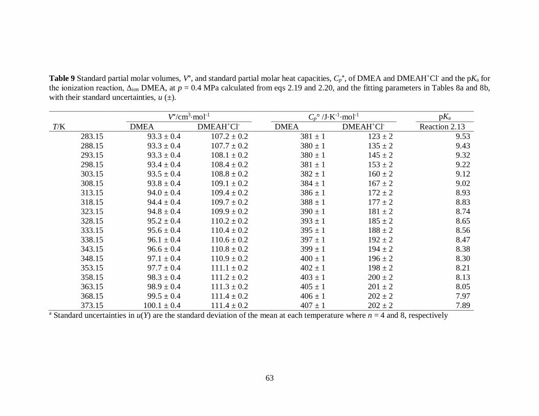
63

Table 9 Standard partial molar volumes, V°, and standard partial molar heat capacities, Cp°, of DMEA and DMEAH+Cl- and the pKa for

the ionization reaction, Δion DMEA, at p = 0.4 MPa calculated from eqs 2.19 and 2.20, and the fitting parameters in Tables 8a and 8b,

with their standard uncertainties, u (±).

V°/cm3·mol-1 Cp° /J·K-1·mol-1 pKa

T/K DMEA DMEAH+Cl- DMEA DMEAH+Cl- Reaction 2.13

283.15 93.3 ± 0.4 107.2 ± 0.2 381 ± 1 123 ± 2 9.53

288.15 93.3 ± 0.4 107.7 ± 0.2 380 ± 1 135 ± 2 9.43

293.15 93.3 ± 0.4 108.1 ± 0.2 380 ± 1 145 ± 2 9.32

298.15 93.4 ± 0.4 108.4 ± 0.2 381 ± 1 153 ± 2 9.22

303.15 93.5 ± 0.4 108.8 ± 0.2 382 ± 1 160 ± 2 9.12

308.15 93.8 ± 0.4 109.1 ± 0.2 384 ± 1 167 ± 2 9.02

313.15 94.0 ± 0.4 109.4 ± 0.2 386 ± 1 172 ± 2 8.93

318.15 94.4 ± 0.4 109.7 ± 0.2 388 ± 1 177 ± 2 8.83

323.15 94.8 ± 0.4 109.9 ± 0.2 390 ± 1 181 ± 2 8.74

328.15 95.2 ± 0.4 110.2 ± 0.2 393 ± 1 185 ± 2 8.65

333.15 95.6 ± 0.4 110.4 ± 0.2 395 ± 1 188 ± 2 8.56

338.15 96.1 ± 0.4 110.6 ± 0.2 397 ± 1 192 ± 2 8.47

343.15 96.6 ± 0.4 110.8 ± 0.2 399 ± 1 194 ± 2 8.38

348.15 97.1 ± 0.4 110.9 ± 0.2 400 ± 1 196 ± 2 8.30

353.15 97.7 ± 0.4 111.1 ± 0.2 402 ± 1 198 ± 2 8.21

358.15 98.3 ± 0.4 111.2 ± 0.2 403 ± 1 200 ± 2 8.13

363.15 98.9 ± 0.4 111.3 ± 0.2 405 ± 1 201 ± 2 8.05

368.15 99.5 ± 0.4 111.4 ± 0.2 406 ± 1 202 ± 2 7.97

373.15 100.1 ± 0.4 111.4 ± 0.2 407 ± 1 202 ± 2 7.89 a Standard uncertainties in u(Y) are the standard deviation of the mean at each temperature where n = 4 and 8, respectively

64

Table 10 Standard partial molar volumes, V°, and standard partial molar heat capacities, Cp°, of DMEA and DMEAH+Cl- and the pKa

for the ionization reaction, Δion DMEA, at p = 15 MPa calculated from eqs 2.19 and 2.20, and the fitting parameters in Tables 8a and

8b, with their standard uncertainties, u (±).


T/K DMEA DMEAH+Cl- DMEA DMEAH+Cl- Reaction 2.13

283.15 93.0 ± 0.4 107.9 ± 0.2 374 ± 1 140 ± 2 9.57

298.15 93.1 ± 0.4 109.1 ± 0.2 376 ± 1 164 ± 2 9.25

323.15 94.5 ± 0.4 110.6 ± 0.2 387 ± 1 188 ± 2 8.77

348.15 96.8 ± 0.4 111.7 ± 0.2 398 ± 1 202 ± 2 8.32

373.15 99.7 ± 0.4 112.4 ± 0.2 404 ± 1 208 ± 2 7.92

398.15 103.0 ± 0.4 112.4 ± 0.2 407 ± 1 206 ± 2 7.55

423.15 106.6 ± 0.4 111.7 ± 0.2 408 ± 1 195 ± 2 7.21

448.15 110.5 ± 0.4 109.8 ± 0.2 410 ± 1 195 ± 2 6.89

473.15 115.0 ± 0.4 106.4 ± 0.2 412 ± 1 172 ± 2 6.60

498.15 120.3 ± 0.4 100.6 ± 0.2 423 ± 1 83 ± 2 6.32

523.15 127.2 ± 0.4 90.7 ± 0.2 448 ± 1 -11 ± 2 6.05

548.15 137.1 ± 0.4 73.0 ± 0.2 506 ± 1 -187 ± 2 5.78

573.15 154.2 ± 0.4 37.8 ± 0.2 664 ± 1 -606 ± 2 5.51

598.15 194.9 ± 0.4 -54.8 ± 0.2 1285 ± 1 -2141 ± 2 5.20 a Standard uncertainties in u(Y) are the standard deviation of the mean at each temperature where n = 4 and 8, respectively

65

Table 11 Standard partial molar heat capacities, ΔionCp°, enthalpies, ΔionH°, and values of pKa for reaction 2.13, at 10, 15, and 20 MPa

with standard relative uncertainties of the fit ur.

a Standard relative uncertainties, ur(Y°), are equal to the propagated standard uncertainties given by regression parameters in Table 8c

T/K ΔionCp° /J·K-1·mol-1 ΔionH° /kJ·mol-1 pKa

10 MPa 15 MPa 20 MPa 10 MPa 15 MPa 20 MPa 10 MPa 15 MPa 20 MPa

283.15 108.8 110.0 111.3 31.2 30.3 29.4 9.45 9.41 9.37

298.15 103.8 105.9 108.1 32.7 31.9 31.1 9.16 9.12 9.09

323.15 98.4 100.7 103.1 35.3 34.5 33.7 8.70 8.67 8.65

348.15 92.0 94.1 96.2 37.7 36.9 36.2 8.27 8.26 8.25

373.15 86.2 87.7 89.4 39.9 39.2 38.5 7.88 7.88 7.87

398.15 82.8 83.6 89.6 42.0 41.3 40.7 7.52 7.52 7.52

423.15 83.8 83.6 83.6 44.1 43.4 42.8 7.19 7.20 7.20

448.15 91.0 90.7 87.8 46.2 45.6 44.9 6.88 6.89 6.90

473.15 108.4 102.8 100.2 48.7 48.0 47.3 6.59 6.38 6.62

498.15 142.2 132.5 124.9 51.8 50.9 50.0 6.31 6.37 6.35

523.15 208.9 187.6 170.4 56.1 54.8 53.7 6.04 6.33 6.09

548.15 353.2 298.2 259.4 62.8 60.7 58.9 5.77 6.23 5.83

573.15 759.4 574.7 456.9 75.7 71.1 67.5 5.49 6.03 5.57

598.15 - 1608.9 1038.1 - 95.0 84.7 - 5.53 5.29

ur(Y°) 2.68 2.68 2.68 0.15 0.15 0.15 0.23 0.23 0.23

66


of DMEA(aq), reaction 2.13, from 283.15 to 393.15 K at p = 0.4 MPa: ●, Hamborg and

Versteeg (2009) [55]; ○, Littel et al. (1990) [56]; ▼, Christensen et al. (1969) [53]; Δ,

Fernandes et al. (2012) [54]; ▬, density model (eq 2.24, Table 8c).

67


of DMEA(aq), reaction 2.13, from 283.15 to 598.15 K at p = 15 MPa: ●, Hamborg and

Versteeg (2009) [55]; ○, Littel et al. (1990) [56]; ▼, Christensen et al. (1969) [53]; Δ,

Fernandes et al. (2012) [54]; ▬, density model (eq 2.24, Table 8c).

68

at 298.15 K from the regression reported in this work is 93.40 ± 0.40 cm3·mol-1.

This value compares well to literature values (94.20 ± 0.2) cm3·mol-1, (94.1 ± 0.3) cm3·mol-

1 measured at 298.15 K by Collins et al. (2000) [48], and Lebrette et al. (2002) [59],

respectively. The only available literature data for + -DMEAH ClV at 298.15 K by Collins et al.

(2000) [48], (107.11 ± 0.2) cm3·mol-1, is close to agreement of the reported regression

value in this work at the same temperature, (108.4 ± 0.2) cm3·mol-1.

Measurements of Cp° for both the protonated and neutral DMEA species have been

made only by Collins et al. (2000). The values at 298.15 K, , DMEAH Clp

C = (153.4 ± 2.5)

J·K-1·mol-1 reported by Collins et al. (2000) [48] agree to within the combined uncertainties

for , DMEAH Clp

C (153 ± 2) J·K-1·mol-1 from the regression fit in this work. The value

obtained for , DMEApC = (381 ± 1) J·K-1·mol-1 from the regression in this work, does not

agree with the values , DMEApC = (372.9 ± 1.7) J·K-1·mol-1 reported by Collins et al. (2000)

[48] to within the combined uncertainties. This is likely caused by the difference in method

used to obtain these values and a larger than reported uncertainty as the final reported value

by Collins et al. (2000) [48] is given at 328.15 K as (376.7 ± 7.0) J·K-1·mol-1.

The results for the regression fit of the equilibrium constant for the ionization

reaction 2.13 are plotted in Figure 17 with comparisons to literature values and extrapolated

to 598.15 K in Figure 18. The value reported for the regression fit from this work at 298.15

K is pKb = (9.22 ± 0.02) is within combined error of (9.22 ± 0.04), (9.23 ± 0.02), (9.26 ±

0.01), by Hamborg and Versteeg (2009) [55] and Fernandes et al. (2012) [54], and

Christensen et al. (1969) [53], respectively.

69

Other thermodynamic values in from literature are also comparable to those

calculated using the density model reported in this work. The enthalpy of ionization, ΔH°,

at 298.15 K from this work (34.40 ± 0.15) kJ·mol-1, is within combined error of (34.40 ±

0.20), (34.00 ± 0.35), (34.57 ± 0.54) reported by Hamborg and Versteeg (2009) [55],

Fernandes et al. (2012) [54], and Christensen et al. (1969) [53], respectively.

2.4.2 Density Model

The use of data allows for the fit to be internally consistent for calculations for

all thermodynamic parameters. This model includes several species specific fitting

parameters that dominate at low temperature and a simple high temperature term allowing

for extrapolation to limiting high temperature behaviour. This limiting behaviour is visible

in the and regressions plotted in Figures 13-16 where the neutral species

approaches postive infinty at 228 K, and ions approach negative infinity. Although this

idea is present in the Helgeson-Kirkham-Flowers (HKF) model, it cannot be used to

appriopriately model all species [19; 24]. The HKF model uses ionic charge in part to

calculate limiting high temperature behaviour which becomes a problem when attempting

to model neutral species. The density model avoids this with the use of empirical terms

fitted to data through regression. The density model also improves the ability to include

pressure and temperature dependance through the low temperature V° parameters. These

fitting terms described in eq 2.20 are derivatives of pressure and influence the regression

fit of the high temperature terms for all other thermodynamic values.

Very few other works have used heat capacity data to determine other

thermodynamic values, including equilibrium constants indirectly. The most common

determinations use a form of conductivity or spectroscopy to measure equilibrium

pC

pC oV

70

constants directly and then calculate thermodynamic properties as a result. These

techniques become more difficult at high temperature where amine species begin to

undergo thermal decomposition and organic species pose a variety of other experimental

challenges for obtaining quantitative thermodynamic data. Other versions of a density

model, like those provided in the work of McGregor et al. (2017) [60], Lowe et al. (2017)

[67], and Shvedov and Tremaine (1997) [68] who also used calorimetry in their

experimental measurements, are not as simple as the model by Anderson et al. (1991) [34]

used in this work. The models used in these works contain a (T-228 K) term making the

integration of the equation to obtain other themodynamic properties complicated. There

are no other works that have used both high and low temperature volumetic data to

complete a full model and obtain high temperature equilibrium constants as desscribed in

this work.

The refit of HCl to the same density model used in this work allows for the addition

and subtraction of model parameters to obtain the correct parameters for the desired

species. Regressions were only completed for the experimentally measured data, and

for DMEA(aq) and DMEAH+Cl-(aq), and a refit of the HCl data all used to determine

the parameters for the ionization reaction. This allows the ionization reaction values to be

determined individually under any conditions.

2.5 Acknowledgements

Financial support was provided by the Natural Science and Engineering Council of

Canada (NSERC) and the University Network of Excellence in Nuclear Engineering

(UNENE). We are grateful to Farnood Pakravan for his technical assistance with the

computers and titrator equipment used in this work.

pC

oV

71

Chapter 3 Standard Partial Molar Heat Capacities and

Volumes of Aqueous 3-Methoxypropylamine and 3-

Methoxypropylammonium Chloride from 283 K to 393 K

Abstract

Densities for dilute aqueous solutions of 3-methoxypropylamine (3-MPA) and 3-

methoxypropylammonium chloride (3-MPAH+Cl-) were measured relative to water at

283.15 K ≤ T ≤ 363.15 K and 0.1 MPa using vibrating tube densimeters. Volumetric heat

capacities of the same solutions were measured at 283.15 K ≤ T ≤ 393.15 K and 0.4 MPa

using twin fixed-cell, power compensation, differential temperature scanning nano

calorimeters. From these measurements apparent molar volumes, Vϕ, and heat capacities,

Cp,ϕ, were calculated and corrected for speciation to obtain standard partial molar

properties Vo and Cpo, for the species 3-MPA(aq) and 3-MPAH+Cl-(aq). The experimental

values for Vo and Cpo, measured in this work were combined with high temperature values

reported by Bulemela and Tremaine (J. Phys. Chem. B 2008, 112, 5626-5645) over the

range 423.15 to 598.15 K to derive parameters for the semi-empirical “density” model that

expresses the standard partial molar thermodynamic properties of aqueous species as a

function of temperature and solvent density. The fitted parameters were used with

critically evaluated literature values for the standard partial molar Gibbs energy and

enthalpy of reaction at 298.15 K to obtain values for the ionization constant of 3-

methoxypropylamine from 283.15 K to 598.15 K up to 20 MPa.

72

3.1 Introduction

Pressurised water reactors (PWR) and pressurized heavy water reactors (PHWR)

generally use an all volatile treatment (AVT) in the secondary steam system to control

corrosion and fouling [3]. Fouling involves the depositing of corrosion products, like

magnetite, in the steam generator causing flow restriction, crevice corrosion, and improper

heat transfer that can lead to pitting and cracking of the boiler tubes [5]. This treatment is

characterised by a volatile amine like ammonia, cyclohexylamine, or morpholine to the

steam system. Ammonia is so volatile that it concentrates in the steam phase, leaving

condensed phases of the steam generating system unprotected [3]. Possible solutions are to

increase the concentration of ammonia in the system, which may cause additional metal

dissolution problems, or to substitute with less volatile alkaline bases [2; 4]. Currently there

is a large literature gap in thermodynamic data for amines being evaluated as alternatives

for use in steam-water cycles.

3-Methoxypropylamine (3-MPA) is used as a flocculent in water treatment systems, a

solvent in dye and textile industries, and is being considered as an alternative pH control

additive for steam generating systems [5]. The availability of high temperature

thermodynamic data can be used to accurately describe the behaviour of 3-

methoxypropylamine in solution and its effectiveness in steam-water cycles.

Values for the ionization constant, Ka, and enthalpy, , of 3-

methoxypropylamine (3-MPA) have been reported by several workers at temperatures up

to 548.15 K and 298.15 K, respectively [1; 69; 70]. Apparent molar volumes were

determined under ambient conditions at 298.15 by Cabani et al. (1977, 1979) [69; 71].

o

ion aH

73

Only one worker has reported standard partial volumes at elevated temperatures

and pressures. The measurements by Bulemela and Tremaine (2008) [49] for the neutral

and protonated species are reported from 424.15 K to 598.15 K and at 15 MPa.

Values for the apparent molar heat capacities of 3-MPA(aq) and 3-MPAH+Cl-(aq)

have been reported at 298.15 K and 313.15 K by Cabani et al. (1979) [71; 72].

This paper reports measured densities and heat capacities, from 283.15 K to 363.15

K and 393.15 K, respectively, for dilute aqueous solutions of 3-methoxypropylamine and

3-methoxypropylammonium chloride. From these measurements of apparent molar

volumes, Vϕ, and heat capacities, Cp,ϕ, were calculated and corrected for speciation to

obtain standard partial molar properties V° and Cp°, for the species 3-MPA(aq) and 3-

MPAH+Cl-(aq). The semi-empirical “density” model [18; 34] was fit to experimental

values of V° and Cp° in combination with high temperature, 423.15 to 598.15 K, V° values

reported by Bulemela and Tremaine (2008) [49]. The fitted parameters were used, with

critically evaluated literature values of Gibbs energy and enthalpy at 298.15 K to obtain

values of pKa for the ionization of 3-MPA from 283.15 K to 598.15 K at pressures up to

20 MPa.

3.2 Experimental

3.2.1 Materials and Solution Preparation

All chemicals used are listed in Table 12, and were used as received with no

additional purification. Solutions of 3-MPA (0.1 mol·kg-1) were prepared by mass and

standardized in triplicate against dried potassium hydrogen phthalate (KHP) using a

Metrohm 794 Basic Titrino autotitrator. The 3-MPAH+Cl- (0.1 mol·kg-1) sample was

prepared using 3-MPA (0.2 mol·kg-1) through the addition of excess 0.2 mol·kg-1

74

Table 12 List of the chemicals used in this work (3-MPA), including purities as listed by

the supplier.

Chemical Name (CAS #)

Formula

Source

Mass

Fraction

Purity

Analytic

Technique

Hydrochloric acid

(7647-01-0)

HCl Fluka ≥ 0.95 Titration

3-Methoxypropylamine

(5332-73-0)

C6H13N Sigma-Aldrich

ACROS

Organics

≥ 0.999

≥ 0.95

Titration

Potassium hydrogen

phthalate

(877-24-7)

C8H5KO4 Sigma-Aldrich ≥ 0.9995 Titration

Sodium chloride

(7647-14-5)

NaCl Sigma-Aldrich 0.995 Titration

Tris(hydroxymethyl)-

aminomethane

(77-86-1)

C4H11NO3 Sigma-Aldrich ≥ 0.999 Titration

75

hydrochloric acid. Standard solutions of KHP at 0.1 mol·kg-1,

tris(hydroxymethyl)aminomethane (TRIS) at 0.2 mol·kg-1, and NaCl at 1 mol·kg-1 were

prepared by mass after drying the solid chemicals for 2 h at 383.15 K, 4 h at 373.15 K and

24 h at 573.15 K, respectively. The KHP and HCl solutions were standardized against

TRIS. All solutions were prepared from degassed ultra-pure water (18.2 MΩ·cm) from an

EMD Millipore Direct-Q® 3 UV remote water purification system.

3.2.2 Densimetry

Two Anton Paar DMA5000 vibrating tube densimeters were used to make

measurements of solution densities. Although the Anton Paar software automatically

calculates solution densities, the experimental period of vibration was used to calculate

densities. The automatic density calculation uses the equation of state for water by

Spieweck and Bettin (1992) [61], which is inconsistent with the properties of water from

Hill (1990) [62] used to calculate apparent molar properties in this work.

Solutions were measured at ambient pressure, p = (0.10 ± 0.01) MPa, over a

temperature range from 283.150 K to 363.150 K (± 0.001 K). The period of vibration was

recorded at intervals of 5.00 K, after equilibrating for 10 and 15 minutes at each

temperature step. All solutions were degassed before injection by withdrawing the plunger

of a solution-filled, sealed syringe as described by McGregor et al. (2017) [60].

Solution density of each sample was calculated using the experimental period of

vibration at each temperature interval based on a relationship with Hooke’s law [43]

2 2

s w s wk (3.1)

76

where ρs, ρw, are the densities (g·cm-3) and τs, τw, are periods of vibration (μs) for the

solution and water, respectively. Measurements are carried out over six days, following the

calibration described in Chapter 2.

Apparent molar volumes, , for 3-MPA(aq) and 3-MPAH+Cl-(aq) were calculated,

s wexp 3-MPA

3-MPA, st

s 3-MPA s w

1000M

Vm

(3.2)

+ - + -

+ -

+ - + -

st ex

HCl HCl3-MPAH Cl 3-MPAH Cl s wexp

3-MPAH Cl , st ex st exs HCl HCl s w3-MPAH Cl 3-MPAH Cl

11000

M m M mV

m m m m

(3.3)

where 89.130 g·mol-1, 125.591 g·mol-1, and HClM 36.461 g·mol-

1. Superscripts indicate the stoichiometric molality of amine (st) or the molality of excess

HCl (ex).

3.2.3 Calorimetry

Solution heat capacities were determined using two twin fixed-cell, nano-

differential-output temperature-scanning, power-compensation calorimeters (DSC)

manufactured by TA Instruments, a Nano DSC 60200 and Nano DSC 6300.

Measurements of ΔP were taken over a temperature range from 283.15 K to 393.15

K at a scan rate of 1 K·min-1 and at a pressure of p = (0.40 ± 0.01) MPa. A total of twelve

scans, six with increasing temperature and six with decreasing temperature, were

completed for each sample. Each set of twelve scans takes 24 hours to complete, and

follows the same six-day calibration sequence used for the densimeter measurements.

The first two scans from each sample were discarded because they contain a larger

difference from the mean than the results of subsequent consecutive runs, as also found in

exp

V

3-MPAM + -3-MPAH ClM

77

the procedures by Woolley (2007) [43]. Values of ΔP from scans 3-12 at each temperature

were average and used in combination with the experimentally measured densities to obtain

the massic heat capacity

s w

,s s ,w w

c

p p

k P Pc c

r

(3.4)

where cp,s, and cp,w are the massic heat capacities (J·K-1·g-1) for the solution and water

respectively, r is the temperature scan rate (K·s-1), kc is the cell constant, and P is the

difference in power (W).

Equations 3.5 and 3.6 were used to calculate the apparent molar heat capacities,

, for the 3-MPA neutral and protonated species

,s ,wexp

, , 3-MPA 3-MPA ,s st

3-MPA

1000p p

p p

c cC M c

m

(3.5)

+ - + -

+ - + -

st ex

HCl HCl ,s ,w3-MPAH Cl 3-MPAH Clexp

,s, , 3-MPAH Cl st ex st ex

HCl HCl3-MPAH Cl 3-MPAH Cl

1000p p

pp

M m M m c cC c

m m m m

(3.6)

The solution densities required to calculate for temperatures greater than

363.15 K were obtained through extrapolation using the density model, discussed in

Section 3.3. The standard partial molar volumes were assumed to be constant between 0.1

MPa and 0.4 MPa so that the densities at 0.4 MPa could be calculated from the standard

partial properties using the appropriate values for the water properties found in Appendix

A.

exp

,pC

exp

,pC

78

3.3 Results

3.3.1 Apparent Molar Volumes and Heat Capacities

The experimental relative densities (ρs - ρw) of 3-MPA(aq) and 3-MPAH+Cl-(aq)

from the average of each set of measurements in each densimeter are reported in Table 13.

The experimental relative volumetric heat capacities (cp,sρs - cp,wρw) are tabulated in Tables

14 and 15. The average values of the experimental apparent molar volumes, , and heat

capacities, , at each temperature are listed in Tables 16 and 17. The standard

uncertainties in and were calculated as the standard error of the mean and are no

more than ± 0.5 cm3·mol-1 for and ± 2.5 J·K-1 ·mol-1 for . At temperatures T >

363.15 K, additional systematic errors may be present in the calculated standard partial

molar heat capacities due to the method of extrapolating densities from the density model

described in Section 3.3.3.

3.3.2 Speciation Corrections

Speciation corrections were completed using the same procedure reported by

McGregor et al. (2017) [60]. Measurements of apparent molar properties, , contain

contributions from all species in the solution. The neutral amine, 3-MPA (aq), ionizes in

water forming additional species in solution whose concentrations can be determined by

the degree of dissociation, ,

st st st3-MP

2

A 3-MPA 3-MPA

H O 3-MPA 3-MPAH OH

1

laq aq aq

m m m

(3.7)

The speciation of the neutral amine was calculated from temperature dependent

values of Ka reported by Balakrishnan (1988) [1], following the reaction

expV

exp

,pC

expV

exp

,pC

expV

exp

,pC

expY

79

Table 13 Experimental densities relative to water (ρs - ρw) of 3-MPA (aq) and 3-MPAH+Cl- (aq) as a function of temperature T at p =

0.10 MPa, for each stoichiometric molality, mst, with standard uncertainties, u.a, b

(ρs-ρw)·103/g·cm-3

3-MPA(aq) 3-MPAH+Cl-(aq)

0.1033 ± 0.0002 0.0976 ± 0.0002 0.1049 ± 0.005 0.1049 ± 0.005

-

-

5.616x10-5 ± 0.0003 5.616x10-5 ± 0.0003

Densimeter 1 Densimeter 2 Densimeter 1 Densimeter 2

T/K 1st Loading 2nd Loading 1st Loading 2nd Loading 1st Loading 2nd Loading 1st Loading 2nd Loading

283.15 -0.392 -0.455 -0.293 -0.406 1.842 1.727 1.902 1.877

293.15 -0.453 -0.514 -0.355 -0.464 1.752 1.624 1.886 1.776

303.15 -0.502 -0.562 -0.409 -0.508 1.672 1.557 1.848 1.712

313.15 -0.551 -0.604 -0.466 -0.546 1.631 1.513 1.798 1.670

323.15 -0.600 -0.643 -0.530 -0.597 1.606 1.479 1.762 1.642

333.15 -0.652 -0.687 -0.596 -0.655 1.594 1.450 1.741 1.632

343.15 -0.703 -0.725 -0.649 -0.693 1.607 1.425 1.736 1.630

353.15 -0.744 -0.755 -0.689 -0.719 1.631 1.414 1.749 1.636

363.15 -0.777 -0.778 -0.716 -0.730 1.667 1.425 1.775 1.650

373.15 -0.740b 1.827b

383.15 -0.800b 1.915b

393.15 -0.859b 2.017b a The standard uncertainties are u(T) = 0.01 K, u(p) = 0.01 MPa, and u(ρs-ρw) = 0.01 g·cm-3

b Calculated from V° to values by Bulemela and Tremaine (2008) [49], eq 3.17

st 1

3-MPA /m mol kg st 1



3-MPA /m mol kg

st 1

HCl /m mol kg st 1

HCl /m mol kg

80

Table 14 Experimental volumetric heat capacities relative to water (cp,s·ρs – cp,w·ρw) of 3-MPA (aq) at stoichiometric, “st”, molalities,

mst, at temperature T and pressure p = 0.40 MPa with standard uncertainties, u.a, b, c

(cp,s·ρs – cp,w·ρw) · 103/J·K-1·cm-3

Nano DSC 6300

mst3-MPA/mol·kg-1 = 0.0976 ± 0.0002

Nano DSC 60200

mst3-MPA/mol·kg-1 = 0.1033 ± 0.0002


283.15 (-7.978) -8.023 (-7.922) -7.877 (-7.895) -8.346 (-7.699) -7.788

288.15 -7.423 -7.210 -7.381 -7.299 -7.868 -7.818 -7.687 -7.333

293.15 -7.316 -7.183 -7.234 -7.120 -7.393 -7.308 -6.996 -6.883

298.15 -6.696 -6.605 -6.763 -6.672 -6.914 -6.908 -6.620 -6.513

303.15 -5.840 -5.746 -5.885 -5.664 -6.377 -6.527 -6.176 -6.153

308.15 -5.558 -5.418 -5.337 -5.255 -5.934 -6.209 -5.812 -5.766

313.15 -5.219 -4.966 -4.947 -5.186 -5.533 -5.776 -5.435 -5.355

318.15 -4.833 -4.495 -4.537 -4.673 -5.173 -5.282 -5.057 -4.825

323.15 -4.330 -3.923 -3.974 -4.026 -4.814 -4.713 -4.643 -4.505

328.15 -3.797 -3.648 -3.637 -3.509 -4.438 -4.228 -4.298 -4.063

333.15 -3.318 -3.590 -3.352 -3.379 -3.974 -3.847 -4.083 -3.709

338.15 -2.957 -3.067 -2.722 -2.664 -3.533 -3.512 -3.728 -3.436

343.15 -2.670 -2.766 -2.390 -2.347 -3.221 -3.127 -3.397 -3.149

348.15 -2.402 -2.499 -2.150 -2.090 -2.977 -2.921 -3.180 -2.926

353.15 -2.162 -2.296 -1.874 -1.924 -2.771 -2.659 -2.959 -2.897

358.15 -1.976 -2.109 -1.732 -1.769 -2.560 -2.481 -2.771 -2.723

363.15 -1.899 -1.958 -1.647 -1.633 -2.466 -2.386 -2.631 -2.599

368.15 -1.763 -1.615 -1.538 -1.377 -2.273 -2.191 -2.400 -2.428

373.15 -1.995 -2.076 -1.969 -1.852 -2.247 -2.120 -2.350 -2.337

378.15 -2.236 -2.202 -1.931 -2.040 -2.223 -2.090 -2.264 -2.061

383.15 -2.270 -2.549 -2.387 -2.388 -2.231 -2.135 -2.181 -1.995

388.15 -2.363 -6.689 -2.130 -6.571 -2.239 -2.094 -2.193 -2.037

393.15 -2.416 (-2.215) -1.997 (-2.105) -2.397 (-2.159) -2.150 (-2.268) a The standard uncertainties are u(T) = 0.01 K, u(p) = 0.01 MPa, and u(cp,s·ρs – cp,w·ρw) = 0.007 J·K-1·cm-3

81


82

Table 15 Experimental volumetric heat capacities relative to water (cp,s·ρs – cp,w·ρw) of 3-MPAH+Cl- (aq) at stoichiometric, “st”,

molalities, mst, at temperature T and pressure p = 0.40 MPa with standard uncertainties, u.a, b, c

(cp,s·ρs – cp,w·ρw) · 103 /J·K-1·cm-3


mst3-MPA/mol·kg-1 = 0.1049 ± 0.0002 b mst

3-MPA/mol·kg-1 = 0.1049 ± 0.0002 b

mstHCl/ mol·kg-1 = 0.2262 ± 0.0003 b mst

HCl/ mol·kg-1 = 0.2262 ± 0.0003 b


283.15 (-27.15) -27.16 (-27.18) -27.17 (-26.09) -26.01 (-25.64) -25.54

288.15 -25.89 -26.16 -26.10 -26.17 -25.30 -25.21 -24.94 -24.68

293.15 -25.04 -25.36 -25.26 -25.35 -24.65 -24.51 -24.27 -24.04

298.15 -24.43 -24.76 -24.76 -24.75 -24.16 -23.96 -23.73 -23.60

303.15 -23.95 -24.22 -24.30 -24.21 -23.70 -23.55 -23.26 -23.13

308.15 -23.53 -23.78 -23.95 -23.82 -23.26 -23.16 -22.95 -22.68

313.15 -23.17 -23.57 -23.69 -23.49 -22.95 -22.82 -22.68 -22.40

318.15 -22.89 -23.36 -23.45 -23.20 -22.68 -22.56 -22.42 -22.11

323.15 -22.69 -22.95 -23.26 -22.97 -22.44 -22.30 -22.08 -21.89

328.15 -22.56 -22.72 -23.06 -22.74 -22.15 -22.03 -21.82 -21.66

333.15 -22.30 -22.54 -22.87 -22.56 -21.91 -21.73 -21.64 -21.47

338.15 -22.12 -22.38 -22.71 -22.40 -21.65 -21.75 -21.48 -21.33

343.15 -22.01 -22.25 -22.57 -22.27 -21.46 -21.64 -21.31 -21.24

348.15 -21.90 -22.13 -22.44 -22.15 -21.34 -21.41 -21.19 -21.07

353.15 -21.84 -22.03 -22.33 -22.04 -21.26 -21.33 -21.06 -20.91

358.15 -21.76 -21.93 -22.21 -21.94 -21.16 -21.21 -20.94 -20.83

363.15 -21.69 -21.82 -22.08 -21.83 -21.06 -21.09 -20.80 -20.69

368.15 -21.16 -21.28 -21.49 -21.29 -20.68 -20.65 -20.33 -20.31

373.15 -21.10 -21.23 -21.41 -21.24 -20.57 -20.52 -20.24 -20.23

378.15 -21.08 -21.21 -21.36 -21.20 -20.54 -20.49 -20.20 -20.21

383.15 -21.07 -21.14 -21.29 -21.12 -20.48 -20.45 -20.15 -20.13

388.15 -21.13 -21.14 -21.19 -21.09 -20.53 -20.36 -20.21 -20.17

393.15 -21.22 (-21.22) -21.21 (-21.25) -20.50 (-20.59) -20.15 (-20.17)

83

a The standard uncertainties are u(T) = 0.01 K, u(p) = 0.01 MPa, and u(cp,s·ρs – cp,w·ρw) = 0.004 J·K-1·cm-3



84

Table 16 Mean values of experimental, ‘exp’, apparent and standard partial molar volumes and heat capacities of 3-MPA(aq), (Vφexp,

V°) and (Cp,φexp, Cp°) at p = 0.40 MPa and their standard uncertainties, u (±).a,b

T/K Vφexp/cm3·mol-1 V°/cm3·mol-1 Cp,φ


283.15 93.03 ± 0.27 92.70 ± 0.28 311.06 ± 1.16 316.55 ± 1.19

288.15 93.14 ± 0.26 92.99 ± 0.27 316.88 ± 0.56 322.33 ± 0.57

293.15 93.78 ± 0.26 93.25 ± 0.27 320.80 ± 0.85 326.14 ± 0.86

298.15 94.15 ± 0.25 93.50 ± 0.27 326.29 ± 0.58 331.55 ± 0.60

303.15 94.53 ± 0.24 93.73 ± 0.26 333.81 ± 0.70 338.97 ± 0.72

308.15 94.94 ± 0.22 93.99 ± 0.24 338.60 ± 0.81 343.59 ± 0.83

313.15 95.35 ± 0.20 94.23 ± 0.22 343.06 ± 0.71 347.85 ± 0.73

318.15 95.82 ± 0.19 94.53 ± 0.21 348.49 ± 0.79 353.06 ± 0.80

323.15 96.31 ± 0.16 94.83 ± 0.18 354.55 ± 1.04 358.89 ± 1.06

328.15 96.84 ± 0.14 95.19 ± 0.16 359.93 ± 1.06 364.01 ± 1.08

333.15 97.39 ± 0.13 95.58 ± 0.15 364.14 ± 0.92 367.92 ± 0.94

338.15 97.93 ± 0.11 95.91 ± 0.13 370.04 ± 1.34 373.55 ± 1.36

343.15 98.43 ± 0.09 96.33 ± 0.12 374.54 ± 1.36 377.76 ± 1.38

348.15 98.94 ± 0.07 96.72 ± 0.09 378.18 ± 1.45 381.09 ± 1.47

353.15 99.45 ± 0.06 97.15 ± 0.08 381.39 ± 1.56 384.00 ± 1.58

358.15 99.96 ± 0.06 97.63 ± 0.08 384.36 ± 1.54 386.69 ± 1.56

363.15 100.42 ± 0.04 98.10 ± 0.06 386.59 ± 1.54 388.63 ±1.56

368.15 386.53 ± 0.85 390.59 ± 0.86

373.15 389.83 ± 0.66 391.61 ± 0.66

378.15 392.53 ± 1.36 394.08 ± 1.38

383.15 393.97 ± 2.25 395.30 ± 2.27

388.15 394.04 ± 2.53 395.17 ± 2.55

393.15 398.84 ± 2.54 399.84 ± 2.56 a The standard uncertainties are u(T) = 0.01 K and u(p) = 0.01 MPa


85

Table 17 Mean values of experimental, ‘exp’, apparent and standard partial molar volumes and heat capacities of 3-MPAH+Cl-(aq),

(Vφexp, V°) and (Cp,φ

exp, Cp°) at p = 0.40 MPa and their standard uncertainties, u (±).a, b

Vφexp/cm3·mol-1 V°/cm3·mol-1 Cp,φ


T/K 3-MPAH+Cl- 3-MPAH+Cl- Cl- 3-MPAH+ 3-MPAH+Cl- 3-MPAH+Cl- Cl- 3-MPAH+

283.15 107.27 ± 0.46 106.95 ± 0.46 17.16 91.47 ± 2.99 187.56 ± 0.24 182.08 ± 0.28 -145.05 330.89 ± 1.68

288.15 107.82 ± 0.47 107.48 ± 0.47 17.44 91.13 ± 2.99 199.15 ± 0.42 192.93 ± 0.45 -135.94 329.18 ± 1.68

293.15 108.38 ± 0.42 108.02 ± 0.42 17.66 90.91 ± 2.99 208.46 ± 0.48 201.67 ± 0.51 -128.76 328.46 ± 1.68

298.15 108.87 ± 0.47 108.49 ± 0.47 17.81 90.79 ± 2.99 214.69 ± 0.52 207.42 ± 0.56 -123.20 328.54 ± 1.68

303.15 109.33 ± 0.44 108.93 ± 0.44 17.92 90.77 ± 2.99 220.36 ± 0.48 212.68 ± 0.52 -119.02 329.22 ± 1.68

308.15 109.74 ± 0.44 109.32 ± 0.44 17.98 90.84 ± 2.99 224.63 ± 0.56 216.56 ± 0.59 -116.01 330.42 ± 1.68

313.15 110.11 ± 0.44 109.67 ± 0.44 18.00 90.98 ± 2.99 227.67 ± 0.69 219.23 ± 0.73 -113.98 331.98 ± 1.68

318.15 110.50 ± 0.41 110.03 ± 0.41 17.98 91.19 ± 2.99 230.33 ± 0.76 221.53 ± 0.81 -112.77 333.83 ± 1.68

323.15 110.86 ± 0.39 110.36 ±0.39 17.92 91.46 ± 2.99 233.03 ± 0.72 223.86 ± 0.77 -112.25 335.84 ± 1.68 328.15 111.20 ± 0.37 110.67 ± 0.37 17.82 91.78 ± 2.99 234.81 ± 0.65 225.27 ± 0.70 -112.30 338.00 ± 1.68

333.15 111.54 ± 0.36 110.98 ± 0.36 17.69 92.15 ± 2.99 236.62 ± 0.72 226.69 ± 0.77 -112.83 340.17 ± 1.68

338.15 111.84 ± 0.34 111.24 ± 0.34 17.53 92.56 ± 2.99 237.84 ± 0.74 227.50 ± 0.79 -113.77 342.35 ± 1.68

343.15 112.14 ± 0.31 111.51 ± 0.31 17.33 93.01 ± 2.99 238.78 ± 0.71 228.02 ± 0.76 -115.06 344.47 ± 1.68

348.15 112.43 ± 0.27 111.75 ± 0.27 17.10 93.48 ± 2.99 239.49 ± 0.69 228.28 ± 0.74 -116.68 346.55 ± 1.68

353.15 112.74 ± 0.26 112.03 ± 0.26 16.83 93.99 ± 2.99 240.03 ± 0.65 228.34 ± 0.69 -118.58 348.50 ± 1.68

358.15 113.03 ± 0.26 112.27 ± 0.26 16.53 94.52 ± 2.99 240.48 ± 0.60 228.30 ± 0.64 -120.76 350.34 ± 1.68

363.15 113.33 ± 0.28 112.53 ± 0.28 16.19 95.07 ± 2.99 241.09 ± 0.53 228.37 ± 0.56 -123.22 352.01 ± 1.68

368.15 244.00 ± 1.53 230.71 ± 1.64 -125.98 353.55 ± 1.68

373.15 242.77 ± 1.59 228.87 ± 1.70 -129.05 354.87 ± 1.68

378.15 240.92 ± 1.59 226.38 ± 1.70 -132.47 356.07 ± 1.68 383.15 239.12 ± 1.60 223.88 ± 1.71 -136.28 357.04 ± 1.68

388.15 236.63 ± 1.52 220.65 ± 1.63 -140.52 357.86 ± 1.68

393.15 233.50 ± 2.36 216.72 ± 2.73 -145.26 358.50 ± 1.68 a The standard uncertainties are u(T) = 0.01 K and u(p) = 0.01 MPa


86

3-MPAH 3-MPA Haq aq aq (3.8)

and extrapolated using an equation for determining lnK as a function of heat capacity by

Anderson and Crerar (1993) [73].

Values for the apparent molar properties of 3-MPA (aq) are obtained by removing

the contributions of additional species in solution using Young’s rule [64] for both V and

,pC

+ -

2

exp *

H O,3 MPAH ,OH

1

V V V VV

(3.9)

+ -

2

exp * rel

, p,H O, ,3 MPAH , ,OH

,1

p pp p

p

C C C C CC

(3.10)

where the standard molar properties of water, were obtained from Hill’s equation of

state [62] and values for and were calculated using equations

+ - +

+

,3 MPA ,HCl,3 MPAH Cl ,H

,NaOH ,NaCl ,HCl,OH ,H

Y Y Y Y

Y Y Y Y Y

(3.11)

where and Y is any thermodynamic property. The apparent molar properties for

3-MPAH+Cl-(aq) are from this work and are reported in Table 17. The contributions of

OH-(aq) were calculated using values of for NaOH(aq), and NaCl(aq) taken from

Patterson et al. (2001) [41]. The values of and were obtained from Sharygin

and Wood (1997) [65], and Patterson et al. (2001) [41], respectively. The chemical

relaxation, , gives the contribution from heat released by the shift in equilibrium of the

ionization reaction 3.8 with temperature and is not required for the volumetric calculations

[66]. The complete data treatment for the relaxation calculation used in this work is

described in full in Appendix C from the work by Collins et al. (2000) [48].

2

*

H OY

, 3-MPAHY , OH

Y

,H0Y

Y

HClV,HClpC

rel

pC

87

Apparent molar properties for 3-MPAH+Cl- required the removal of excess HCl

using Young’s rule in the form

- -

-

-

st ex exp ex

HCl HCl ,HCl3-MPAH Cl ,3-MPAH Cl

st, 3-MPAH Cl

3-MPAH Cl

m m Y m YY

m

(3.12)

where the values of and were obtained from Sharygin and Wood (1997) [65],

and Patterson et al. (2001) [41], respectively.

The apparent molar properties were converted to standard partial molar properties,

Y°, for the neutral and protonated species using eqs 3.13 and 3.14, respectively.

Y Y (3.13)

1

2

sYY Y A I

(3.14)

where is the temperature dependent Debye-Hückel limiting slope, and is the ionic

strength of the solution. The average values of the experimental apparent molar and

standard partial molar properties at each temperature are reported in Tables 16 and 17.

Average values of and of 3-MPA(aq) and 3-MPAH+Cl-(aq) over the measured

temperature range with literature data are plotted in Figures 19-22.

3.3.3 Single-Ion Properties

The single-ion standard partial molar properties of 3-MPAH+(aq), from the

ionization reaction 3.8 were determined using eq 3.15:

+ - HCl3-MPAH 3-MPAH Cl HY Y Y Y

(3.15)

The resulting standard partial molar volumes and heat capacities for 3-MPAH+(aq) are

tabulated in Table 17. The standard uncertainties in V° and Cp°, estimated as equal to the

HClV,HClpC

YA sI

oVo

pC

88

Figure 19. Standard partial molar volumes for 3-MPA(aq) with density model fit from

283.15 to 363.15 K: ●, this work; ▬, fit to the density model (eq 3.17, Table 18a).

Figure 20. Standard partial molar volumes for 3-MPAH+Cl-(aq) with density model from

283.15 to 363.15 K: ●, this work; ▬, fit to the density model (eq 3.17, Table 18a).

89

Figure 21. Standard partial molar heat capacities for 3-MPA(aq) from 283.15 to 393.15 K

at 0.4 MPa: ●, this work; ▬, fit to the density model (eq 3.16, Table 18c).

Figure 22. Standard partial molar heat capacities for 3-MPAH+Cl-(aq) from 283.15 to

393.15 K at 0.4 MPa: ●, this work; ▬, fit to the density model (eq 3.16, Table 18c).

90

standard error of the mean, are no more than ± 2 cm3·mol-1 for and ± 1 J·K-1 ·mol-1

for .

The density model, in the same form found in Chapter 2, was fit to the experimental

data;

2 w

2 3 4

2 6 12ln 10p

p

c d e gC R RT

T T T T T

(3.16)

2 3 4

' ' ' 'ln 10 ' w

b c d e gV RT a RT

T T T T T

(3.17)

where,

' 0, ' , c ' , etc.T T

b ca b

p p

(3.18)


coefficient of water in MPa-1, obtained from the NIST formulation for the properties of

water and steam. Fitting parameters, a, b, c, d, and e dominate at low temperature and

describe the species-specific hydration effects and fitting parameter, g dominates at high

temperature and describes the long-range hydration effects.

The same data analysis technique used in Chapter 2 was employed to predict the

high temperature heat capacity behaviour. Briefly, the density model eq 3.17 was fit to the

low temperature experimental data, measured in this work, in combination with high

temperature reported by Bulemela and Tremaine (2008) [49]. The experimental V°

data and density model are plotted for 3-MPA in Figures 19 and 23 and 3-MPAH+Cl- in

Figures 20 and 24. The resulting fitting g term was then used as a constant when density

model eq 3.16 was used to fir the experimental data measured in this work. This

oV

o

pC

3-MPAV

3-MPAV

,3 MPApC

91

Figure 23. Standard partial molar volumes for 3-MPA(aq) with density model from 283.15

to 613.15 K: ●, this work; ○, Bulemela and Tremaine (2008) [49]; ▬, fit to the density

model (eq 3.17, Table 18a).

Figure 24. Standard partial molar volumes for 3-MPAH+Cl-(aq) with density model fit

from 283.15 to 598.15 K: ●, this work; ○, Bulemela and Tremaine (2008) [49]; ▬, fit to

the density model (eq 3.17, Table 18a).

92

data treatment was repeated for the protonated species with all fitting parameters listed in

Tables 18a and 18c. The experimental Cp° results and fitted model are plotted for 3-

MPA(aq) in Figure 25 and 3-MPAH+Cl-(aq) in Figure 26 [49]. The fitting parameters for

and are from the same refit to experimental data from Patterson et al. (2001)

[41] and Sharygin and Wood (1997) [65] reported in Chapter 2. The estimated relative

standard uncertainty in the fit is ur = 0.7 for , ur = 2.1 for , and ur = 0.8

and ur = 0.6 for and , respectively.

3.3.4 Thermodynamic Functions for the Ionization of 3-MPAH+ at Elevated T and p

Values for the ionization of 3-MPA(aq), reported in Tables 19 and 20, were

calculated according to eq 3.19, based on reaction 3.8,

+ +ion 3-MPA H 3-MPAHY Y Y Y

(3.19)

where Y°(H+) ≡ 0 and the ionization constant was obtained using eq 3.20

w2 3 4

log logb c d e g

K aT T T T T

(3.20)

Fitting constants a and b were solved for using literature values for the Gibbs energy and

enthalpy of ionization at 298.15 K from Balakrishnan (1988) [1].


the low temperature fitting constants from and ΔV° in eq 3.21

' 0.1 MPaY b b p (3.21)

,HClpC HClV

3-MPAV3-MPAH Cl

V

,3-MPApC,3 MPAH Clp

C

pC

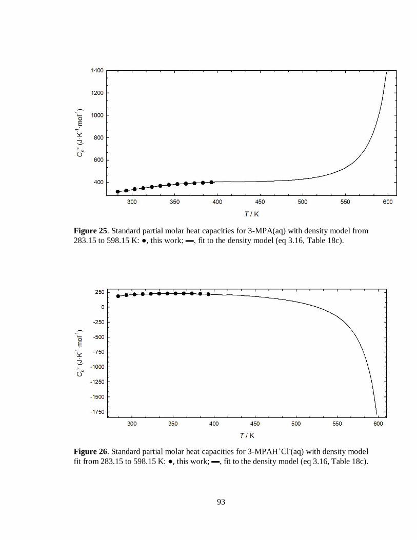
93

Figure 25. Standard partial molar heat capacities for 3-MPA(aq) with density model from

283.15 to 598.15 K: ●, this work; ▬, fit to the density model (eq 3.16, Table 18c).

Figure 26. Standard partial molar heat capacities for 3-MPAH+Cl-(aq) with density model

fit from 283.15 to 598.15 K: ●, this work; ▬, fit to the density model (eq 3.16, Table 18c).

94

Table 18a-c Fitting parameters for the temperature dependence of the standard partial molar volume of reaction for 3-MPA, 3-

MPAH+Cl-, H+Cl- and ΔV°ion for reaction 3.8 with standard uncertainties of the parameters, u (±), and relative uncertainties of the fit

ur.

V°/cm3·mol-1 ΔionV°/cm3·mol-1

Parameter 3-MPA 3-MPAH+Cl- H+Cl-a Reaction 3.8

a’/(cm3·mol-1) 0 0 0 0

b’/(cm3·K·mol-1) -8.39 ± 0.17 -7.16 ± 0.07 3.31 ± 0.31 2.08 ± 0.36

c’/(cm3·K2·mol-1) 1669 ± 83 0 -2443 ± 169 -774 ± 188

d’·10-4/(cm3·K3·mol-1) 0 6.11 ± 0.67 0 -6.11 ± 0.67

e’·10-5/(cm3·K4·mol-1) -436 ± 31 0 864 ± 74 427 ± 81

g/ (K) -2220 ± 32 4099 ± 30 3573 ± 50 -2746 ± 66

ur(Y°) 0.71 2.10 2.11 3.06 a Refit of Eq. 15 to data from Patterson et al. (2001) [41]

Table 18b Fitting parameters for the calculated* pressure dependence of the standard partial molar thermodynamics constants for

reaction 3.8, .

Pressure 0.4 MPa 10 MPa 15 MPa 20 MPa

Δa/(J·mol-1) -3.588 -3.588 -3.588 -3.588

Δb/(J·K·mol-1) 355.2 375.1 385.5 395.9

Δc·10-4/(J·K2·mol-1) -151.2 -152.0 -152.4 -152.7

Δd·10-5/(J·K3·mol-1) 3814 3808 3805 3802

Δe·10-7/(J·K4·mol-1) -3658 -3617 -3595 -3574

Δg/(K) -2746 -2746 -2746 -2746

*Y°= Δb + Δb’(p - 0.1 MPa)

ionY

95

Table 18c Fitting parameters for the temperature dependence of the standard partial molar heat capacities for 3-MPA, 3-MPAH+Cl-,

H+Cl- and thermodynamics constants for reaction 3.8, , with standard uncertainties of the parameters, u (±), and relative

uncertainties of the fit ur.

Cp° /J·K-1·mol-1 ΔionCp° /J·K-1·mol-1 ΔionG° /J·mol-1 and

Parameter 3-MPA 3-MPAH+Cl- H+Cl-a ΔionH° /J·mol-1

a/(J·K-1·mol-1) - - - - -3.59 ± 0.32

b/(J·K·mol-1) - - - - 355 ± 32

c·10-4/(J·K2·mol-1) 640 ± 10 489 ± 7.4 -302 ± 11 -151 ± 17 -

d·10-5/(J·K3·mol-1) -8846 ± 215 -7149 ± 156 5511 ± 244 3814 ± 361 -

e·10-7/(J·K4·mol-1) 4658 ± 170 4456 ± 123 -3861 ± 199 -3359 ± 289 -

ur(Y°) 0.80 0.56 1.58 1.89 - a Refit of Eq. 14 to data from Sharygin and Wood (1997) [65]

ionY

96

Table 19 Standard partial molar volumes, V°, and standard partial molar heat capacities, Cp°, of 3-MPA and 3-MPAH+Cl- and the pKa

for the ionization reaction, Δion 3-MPA, at p = 0.4 MPa calculated from eqs 3.16 and 3.17, and the fitting parameters in Tables 18a and



T/K 3-MPA 3-MPAH+Cl- 3-MPA 3-MPAH+Cl- Reaction 3.8

283.15 93.4 ± 0.7 106 ± 2 317.5 ± 0.8 183.0 ± 0.6 10.085

288.15 93.2 ± 0.7 107 ± 2 321.7 ± 0.8 192.9 ± 0.6 9.930

293.15 93.2 ± 0.7 108 ± 2 326.6 ± 0.8 200.8 ± 0.6 9.781

298.15 93.3 ± 0.7 109 ± 2 332.0 ± 0.8 207.1 ± 0.6 9.636

303.15 93.4 ± 0.7 109 ± 2 337.7 ± 0.8 211.9 ± 0.6 9.496

308.15 93.6 ± 0.7 110 ± 2 343.4 ± 0.8 216.0 ± 0.6 9.361

313.15 93.9 ± 0.7 110 ± 2 349.0 ± 0.8 219.3 ± 0.6 9.229

318.15 94.2 ± 0.7 110 ± 2 354.3 ± 0.8 222.0 ± 0.6 9.102

323.15 94.6 ± 0.7 111 ± 2 359.5 ± 0.8 224.0 ± 0.6 8.979

328.15 95.0 ± 0.7 111 ± 2 364.2 ± 0.8 225.8 ± 0.6 8.858

333.15 95.5 ± 0.7 111 ± 2 368.8 ± 0.8 227.0 ± 0.6 8.742

338.15 96.0 ± 0.7 112 ± 2 373.0 ± 0.8 227.9 ± 0.6 8.628

343.15 96.5 ± 0.7 112 ± 2 377.0 ± 0.8 228.3 ± 0.6 8.517

348.15 97.0 ± 0.7 112 ± 2 380.5 ± 0.8 228.6 ± 0.6 8.409

353.15 97.6 ± 0.7 112 ± 2 383.8 ± 0.8 228.5 ± 0.6 8.304

358.15 98.2 ± 0.7 112 ± 2 386.8 ± 0.8 228.1 ± 0.6 8.201

363.15 98.8 ± 0.7 112 ± 2 389.6 ± 0.8 227.3 ± 0.6 8.101

368.15 99.4 ± 0.7 112 ± 2 392.1 ± 0.8 226.4 ± 0.6 8.003

373.15 100.1 ± 0.7 112 ± 2 394.5 ± 0.8 224.9 ± 0.6 7.907 a Standard uncertainties in u(Y) are the standard deviation of the mean at each temperature where n = 4 and 8, respectively

97

Table 20 Standard partial molar volumes, V°, and standard partial molar heat capacities, Cp°, of 3-MPA and 3-MPAH+Cl- and the pKa

for the ionization reaction, Δion 3-MPA, at p = 15 MPa calculated from eqs 3.16 and 3.17, and the fitting parameters in Tables 18a and



T/K 3-MPA 3-MPAH+Cl- 3-MPA 3-MPAH+Cl- Reaction 3.8

283.15 93.0 ± 0.7 107 ± 2 309.4 ± 0.8 197.9 ± 0.6 10.090

298.15 93.0 ± 0.7 109 ± 2 326.9 ± 0.8 216.5 ± 0.6 9.642

323.15 94.3 ± 0.7 111 ± 2 356.2 ± 0.8 230.0 ± 0.6 8.985

348.15 96.7 ± 0.7 112 ± 2 377.8 ± 0.8 233.6 ± 0.6 8.416

373.15 99.7 ± 0.7 113 ± 2 391.6 ± 0.8 230.3 ± 0.6 7.914

398.15 103.0 ± 0.7 112 ± 2 399.4 ± 0.8 220.8 ± 0.6 7.467

423.15 106.8 ± 0.7 111 ± 2 404.0 ± 0.8 204.9 ± 0.6 7.065

448.15 111.0 ± 0.7 108 ± 2 408.7 ± 0.8 179.6 ± 0.6 6.700

473.15 115.8 ± 0.7 104 ± 2 413.5 ± 0.8 148.1 ± 0.6 6.366

498.15 121.5 ± 0.7 99 ± 2 427.4 ± 0.8 95.6 ± 0.6 6.055

523.15 129.0 ± 0.7 89 ± 2 456.7 ± 0.8 12.3 ± 0.6 5.762

548.15 139.8 ± 0.7 73 ± 2 522.2 ± 0.8 -139.0 ± 0.6 5.480

573.15 158.4 ± 0.7 43 ± 2 698.5 ± 0.8 -495.7 ± 0.6 5.198

598.15 203.2 ± 0.7 -36 ± 2 1384.0 ± 0.8 -1792.2 ± 0.6 4.891 a Standard uncertainties in u(Y) are the standard deviation of the mean at each temperature where n = 4 and 8, respectively

98

where the equation used for b/b’ is also used for all other fitting constants. The parameters

listed in Table 18b can be used to obtain thermodynamic values at any pressures.

Comparison of the predicted ionization constant using the density model in this work to

literature data is plotted in Figure 27. Values of ΔCp°, ΔH° and log K at pressures 10 MPa,

15 MPa, and 20 MPa are reported in Table 21.

3.4 Discussion

3.4.1 Comparison with Literature Results

Several papers by Cabani et al. have reported apparent molar volumes and heat

capacities for 3-MPA and 3-MPAH+Cl- at non-specific concentrations [69; 71; 72]. The

apparent molar volume, , at 298.15 K from the regression reported in this work, at

0.1 MPa, is (94.47 ± 0.25) cm3·mol-1. This value compares well to the literature value

(95.55 ± 0.04) cm3·mol-1 with a reported by Cabani et al. (1977) [69] with a concentration

range of 0.02-0.51 mol·kg-1. The apparent molar volume, at 298.15 K is

reported by this work as (109.27 ± 0.24) cm3·mol-1, is close to agreement of the reported

value, (107.89 ± 0.03) cm3·mol-1, at the same temperature with a concentration range of

0.02-0.50 M [69]. Literature standard partial molar volume data was reported by Bulemela

and Tremaine (2008) with a temperature range of 423.15 to 613.15 K, beyond the

measurements made in this work [49].

Measurements of apparent molar heat capacities for both the protonated and neutral

3-MPA species have been made only by Cabani et al. (1979) within a given concentration

range [71; 72]. Two values at 298.15 and 313.15 K, (325 ± 6) J·K-1·mol-1 and (333 ± 6)

J·K-1·mol-1, respectively, have been reported by Cabani et al. (1979) with a concentration.

exp

, 3-MPAV

exp

, 3-MPAH ClV

99

Table 21 Standard partial molar heat capacities, ΔionCp°, enthalpies, ΔionH°, and values of pKa for reaction 3.8, at 10, 15, and 20 MPa

with their standard relative uncertainties, ur.

a Standard relative uncertainties, ur(Y°), are equal to the propagated standard uncertainties given by regression parameters in Table 18c

T/K ΔionCp° /J·K-1·mol-1 ΔionH° /kJ·mol-1 pKa

10 MPa 15 MPa 20 MPa 10 MPa 15 MPa 20 MPa 10 MPa 15 MPa 20 MPa

283.15 -11.8 -10.9 -9.8 48.3 48.3 48.2 10.09 10.09 10.09

298.15 5.5 6.6 7.8 48.3 48.3 48.2 9.64 9.64 9.64

323.15 24.9 25.6 26.3 48.7 48.7 48.7 8.98 8.99 8.99

348.15 34.2 34.4 34.6 49.5 49.5 49.5 8.41 8.42 8.42

373.15 38.7 38.3 37.9 50.4 50.4 50.4 7.91 7.91 7.92

398.15 41.9 40.9 40.0 51.4 51.4 51.3 7.46 7.47 7.47

423.15 46.8 45.0 43.3 52.5 52.4 52.4 7.06 7.07 7.07

448.15 55.8 53.8 49.8 53.8 53.6 53.5 6.70 6.70 6.70

473.15 72.3 66.1 62.3 55.3 55.1 54.9 6.36 6.37 6.37

498.15 101.9 92.4 84.6 57.5 57.1 56.7 6.05 6.06 6.06

523.15 158.6 139.5 123.8 60.7 59.9 59.3 5.75 5.76 5.77

548.15 279.6 232.5 199.0 65.9 64.4 63.2 5.47 5.48 5.49

573.15 618.4 463.5 364.3 76.3 72.7 70.0 5.17 5.20 5.22

598.15 - 1324.6 848.6 - 92.2 83.9 - 4.89 4.93

ur(Y°) 1.9 1.9 1.9 0.19 0.19 0.19 0.15 0.15 0.15

100


of 3-MPA(aq), reaction 3.8, from 283.15 to 573.15 K at p = 15 MPa: ●, Balakrishnan

(1988) [1]; ○, Cabani et al. (1977) [69]; ▼, Lobo and Robertson (1976) [70]; ▬, fit to the

density model (eq 3.20, Table 18c).

101

range of 0.44-1.15 mol·kg-1 [71]. The values obtained in this work for = (326.3

± 0.6) J·K-1·mol-1 and (343.1 ± 0.7) J·K-1·mol-1 at 298.15 and 313.15 K respectively agree

with Cabani et al. (1979) within combined uncertainties at 298.15 K. Cabani et al. (1979)

have also reported apparent molar heat capacities, , at the same temperatures;

(203 ± 6) J·K-1·mol-1 and (217 ± 6) J·K-1·mol-1 within a concentration range of 0.2-1.0

mol·kg-1 [72]. The values obtained for = (214.7 ± 0.5) J·K-1·mol-1 and (227.7

± 0.7) at a concentration of 0.1049 mol·kg-1 do not agree with the results by Cabani et al.

The lack of agreement between the results in this work and the work by Cabani et al. (1979)

is likely due to the difference in concentrations used to make the measurements. The used

of a standard state would allow for better comparison of experimental results.

The results for the regression fit of the equilibrium constant for the ionization

reaction 3.8 are plotted with literature values and extrapolated to 573.15 K in Figure 27.

The value reported for the regression fit from this work at 298.15 K is pKa = (9.64 ± 0.15)

is within combined error of (9.38 ± 0.4), by Lobo et al. (1976) [70], but not (9.91 ± 0.04)

by Balakrishnan (1988) [1]. At 373.15 K and 15 MPa the regression in this work, (7.907 ±

0.15), and data reported by Balakrishnan (1988), (7.99 ± 0.07), is within combined error

and remains within combined error to 523.15 K as plotted in Figure 27.

Other thermodynamic values in from literature are also comparable to those

calculated using the density model reported in this work. The enthalpy of ionization, ΔH°,

at 298.15 K from this work (49.7 ± 0.2) kJ·mol-1, is within combined error of (49.7 ± 0.4)

reported by Balakrishnan (1988) [1] but not within combined error (53.74 ± 0.2), (53.72)

reported by Lobo et al. (1976) [70], and Cabani et al. (1977) [69], respectively.

exp

, , 3-MPApC

-

exp

, , 3-MPAH ClpC

-

exp

, , 3-MPAH ClpC

102

3.4.2 Density Model

The density model was developed by Marshall and Frank (1981) [35] based on

previous observations made by Frank; ionization constants of many aqueous species, when

log K is plotted against log ρw over a broad range, act as a linear function ρw of at high

temperatures and pressures. Equation 3.20 shows the version of the density model used in

this work where, when compared to the model reported by Mesmer et al. (1988) [18] to

describe general ionization reactions, there is an additional fitting parameter, e, to the

species specific fitting terms of the model. This fitting parameter was added following the

natural Taylor expansion in the model to improve the overall regression to the experimental

data. The addition of this term to improve the low temperature regression is a novel addition

to the density model.

Few workers have previously used the density model to heat capacity and

volumetric measurements. The works by McGregor et al. (2017) [60] Lowe et al. (2017)

[67] and Shvedov and Tremaine (1997) [68] have all used a version of the density model

to fit experimental heat capacities. No authors have reported the heat capacity extrapolation

used in this work to obtain predictive high temperature ionization constants. The agreement

of the density model in this work with existing high temperature ionization constants is

unprecedented in literature and is promising as a method to obtain high temperature

thermodynamic data for organic species.

3.5 Acknowledgements

Financial support was provided by the Natural Science and Engineering Council of

Canada (NSERC) and the University Network of Excellence in Nuclear Engineering

(UNENE). We are grateful to Farnood Pakravan for his technical assistance with the

103

computers and titrator equipment used in this work. Thank you to Dr. Olivia Fandino

Torres for her expertise in operation and diagnosis of the nano DSC.

Chapter 4 Conclusions and Future Work

The objective of this thesis was to develop a method by which high temperature

thermodynamic values for amines of interest for the nuclear industry can be measured and

accurately extrapolated to reactor temperatures. This thesis was of interest both from the

perspective of high temperature amine thermodynamics, and for its application to the

secondary steam system of nuclear reactors.

This thesis provides quantitative data for two amines, DMEA and 3-MPA, for which

experimental measurements of Cp° and V° were made from 283.15 K to 393.15 K and

283.15 K to 363.15 K, respectively. The experimental V° measurements in this work were

successfully combined with experimental data from Bulemela and Tremaine [49] to obtain

fitted parameters for the density model. The fitted V° parameters were used to extrapolate

the Cp° results measured in this work to 598.15 K. The model used in this work was

expanded from the original version, described in section 1.5.4, to contain an additional

species specific low temperature fitting term. This additional term was effective to

improving the Cp° regression while maintaining the form of the model.

The density model has not previously been used in this form to obtain ionization

constants. Similar work was completed previously by McGregor et al. (2017) [60] and

Lowe et al. (2017) [67] and Shvedov and Tremaine (1997) [68] who all fitted experimental

heat capacity data to some variation of a density model. The comparison of the ionization

constant for 3-MPA with the fitted density model and high temperature experimental data

104

from Balakrishnan (1988) [1] displays the successful predictive ability of this model for

both high and low temperature data. The results for DMEA predict new high temperature

data for a pH control candidate for which there is no high temperature data available.

In the future these methods and data treatment could be used to make measurements

and extrapolations of amine species to close the existing literature gaps for hydrothermal

amine data. In the paper by Bulemela and Tremaine (2008) [49], high temperature V° data

was obtained for seven amines. Following the work reported in this thesis, there are five

more amines this method could be used to predict high temperature thermodynamic values

for. These measurements would contribute to the high temperature data required to begin

amine functional group additivity models. The development of a functional additivity

model for amines would limit the quantity of measurements required to obtain relatively

accurate thermodynamic properties for amines, limiting experimental cost and time for data

collection.

Hydrazine, an additive used for controlling the redox potential in the secondary steam

system, is not stable at the operational temperature of the reactor, is highly flammable,

toxic, and must be injected into the coolant circuit continuously due to thermal

decomposition. The by-products of this decomposition (ammonia, nitrogen, and

hydrogen), change the pH and reduction potential of the solution. Possible hydrazine

replacements include carbohydrazide, N-isopropylhydroxylamine, and

diethylhydroxylamine. The methods used in this thesis are a practical way of obtaining

thermodynamic data to high temperature for species that undergo thermal decomposition

at reactor temperatures and could be applied to several additional species. As the method

continues to be improved on, it may be possible to extend measurements to organic species

105

beyond the model solute, amines. Measurements of other species would allow for further

development of functional group additivity models for all organic species.

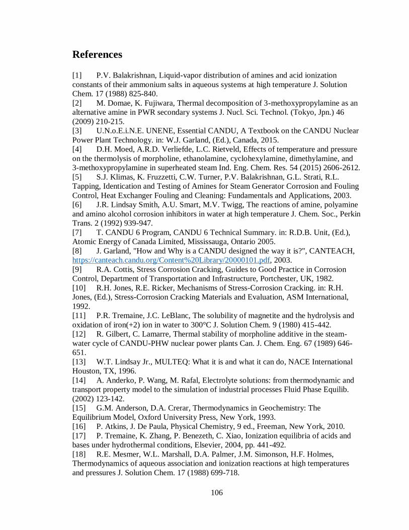
106

References

[1] P.V. Balakrishnan, Liquid-vapor distribution of amines and acid ionization

constants of their ammonium salts in aqueous systems at high temperature J. Solution

Chem. 17 (1988) 825-840.

[2] M. Domae, K. Fujiwara, Thermal decomposition of 3-methoxypropylamine as an

alternative amine in PWR secondary systems J. Nucl. Sci. Technol. (Tokyo, Jpn.) 46

(2009) 210-215.

[3] U.N.o.E.i.N.E. UNENE, Essential CANDU, A Textbook on the CANDU Nuclear

Power Plant Technology. in: W.J. Garland, (Ed.), Canada, 2015.

[4] D.H. Moed, A.R.D. Verliefde, L.C. Rietveld, Effects of temperature and pressure

on the thermolysis of morpholine, ethanolamine, cyclohexylamine, dimethylamine, and

3-methoxypropylamine in superheated steam Ind. Eng. Chem. Res. 54 (2015) 2606-2612.

[5] S.J. Klimas, K. Fruzzetti, C.W. Turner, P.V. Balakrishnan, G.L. Strati, R.L.

Tapping, Identication and Testing of Amines for Steam Generator Corrosion and Fouling

Control, Heat Exchanger Fouling and Cleaning: Fundamentals and Applications, 2003.

[6] J.R. Lindsay Smith, A.U. Smart, M.V. Twigg, The reactions of amine, polyamine

and amino alcohol corrosion inhibitors in water at high temperature J. Chem. Soc., Perkin

Trans. 2 (1992) 939-947.

[7] T. CANDU 6 Program, CANDU 6 Technical Summary. in: R.D.B. Unit, (Ed.),

Atomic Energy of Canada Limited, Mississauga, Ontario 2005.

[8] J. Garland, "How and Why is a CANDU designed the way it is?", CANTEACH,

https://canteach.candu.org/Content%20Library/20000101.pdf, 2003.

[9] R.A. Cottis, Stress Corrosion Cracking, Guides to Good Practice in Corrosion

Control, Department of Transportation and Infrastructure, Portchester, UK, 1982.

[10] R.H. Jones, R.E. Ricker, Mechanisms of Stress-Corrosion Cracking. in: R.H.

Jones, (Ed.), Stress-Corrosion Cracking Materials and Evaluation, ASM International,

1992.

[11] P.R. Tremaine, J.C. LeBlanc, The solubility of magnetite and the hydrolysis and

oxidation of iron(+2) ion in water to 300°C J. Solution Chem. 9 (1980) 415-442.

[12] R. Gilbert, C. Lamarre, Thermal stability of morpholine additive in the steam-

water cycle of CANDU-PHW nuclear power plants Can. J. Chem. Eng. 67 (1989) 646-

651.

[13] W.T. Lindsay Jr., MULTEQ: What it is and what it can do, NACE International

Houston, TX, 1996.

[14] A. Anderko, P. Wang, M. Rafal, Electrolyte solutions: from thermodynamic and

transport property model to the simulation of industrial processes Fluid Phase Equilib.

(2002) 123-142.

[15] G.M. Anderson, D.A. Crerar, Thermodynamics in Geochemistry: The

Equilibrium Model, Oxford University Press, New York, 1993.

[16] P. Atkins, J. De Paula, Physical Chemistry, 9 ed., Freeman, New York, 2010.

[17] P. Tremaine, K. Zhang, P. Benezeth, C. Xiao, Ionization equilibria of acids and

bases under hydrothermal conditions, Elsevier, 2004, pp. 441-492.

[18] R.E. Mesmer, W.L. Marshall, D.A. Palmer, J.M. Simonson, H.F. Holmes,

Thermodynamics of aqueous association and ionization reactions at high temperatures

and pressures J. Solution Chem. 17 (1988) 699-718.

https://canteach.candu.org/Content%20Library/20000101.pdf

107

[19] P. Tremaine, H. Arcis, Solution calorimetry under hydrothermal conditions Rev.

Mineral. Geochem. 76 (2013) 219-263.

[20] H.S. Frank, M.W. Evans, Free volume and entropy in condensed systems. III.

Entropy in binary liquid mixtures; partial molal entropy in dilute solutions; structure and

thermodynamics in aqueous electrolytes J. Chem. Phys. 13 (1945) 507-532.

[21] A.H. Harvey, D.G. Friend, Physical properties of water. in: P.D. A., F.-P. R., H.A.

H., (Eds.), Aqueous systems at elevated temperatures and pressures, Elsevier, London,

UK, 2004, pp. 1-28.

[22] V. Majer, J. Sedlbauer, R.H. Wood, Calculation of standard thermodynamic

properties of aqueous electrolytes and nonelectrolytes, Elsevier, 2004, pp. 99-147.

[23] W.R. Fawcett, Liquids, solutions, and interfaces: from classical macroscopic

descriptions to modern microscopic details, Oxford University Press, New York, 2004.

[24] E.L. Shock, H.C. Helgeson, Calculation of the thermodynamic and transport

properties of aqueous species at high pressures and temperatures: Correlation algorithms

for ionic species and equation of state predictions to 5 kb and 1000°C Geochim.

Cosmochim. Acta 52 (1988) 2009-2036.

[25] H.C. Helgeson, D.H. Kirkham, G.C. Flowers, Theoretical prediction of the

thermodynamic behavior of aqueous electrolytes at high pressures and temperatures: IV.

Calculation of activity coefficients, osmotic coefficients, and apparent molal and standard

and relative partial molal properties to 600°C and 5 kb Am. J. Sci. 281 (1981) 1249-1516.

[26] E.L. Shock, E.H. Oelkers, J.W. Johnson, D.A. Sverjensky, H.C. Helgeson,

Calculation of the thermodynamic properties of aqueous species at high pressures and

temperatures: effective electrostatic radii, dissociation constants and standard partial

molal properties to 1000°C and 5 kbar J. Chem. Soc., Faraday Trans. 88 (1992) 803-826.

[27] J.C.I.V. Tanger, H.C. Helgeson, Calculation of the thermodynamic and transport

properties of aqueous species at high pressures and temperatures: Revised equations of

state for the standard partial molal properties of ions and electrolytes Am. J. Sci. 288

(1988) 19-98.

[28] A. Inglese, R.H. Wood, Apparent molar heat capacities of aqueous solutions of 1-

propanol, butane-1,4-diol, and hexane-1,6-diol at temperatures from 300 K to 525 K and

a pressure of 28 MPa J. Chem. Thermodyn. 28 (1996) 1059-1070.

[29] M.D. Schulte, E.L. Shock, R.H. Wood, The temperature dependence of the

standard-state thermodynamic properties of aqueous nonelectrolytes Geochim.

Cosmochim. Acta 65 (2001) 3919-3930.

[30] N.N. Akinfiev, L.W. Diamond, Thermodynamic description of aqueous

nonelectrolytes at infinite dilution over a wide range of state parameters Geochim.

Cosmochim. Acta 67 (2003) 613-629.

[31] R.G. Clarke, L. Hnedkovsky, P.R. Tremaine, V. Majer, Amino Acids under

Hydrothermal Conditions: Apparent Molar Heat Capacities of Aqueous α-Alanine, β-

Alanine, Glycine, and Proline at Temperatures from 298 to 500 K and Pressures up to

30.0 MPa J. Phys. Chem. B 104 (2000) 11781-11793.

[32] J.P. O'Connell, A.V. Sharygin, R.H. Wood, Infinite Dilution Partial Molar

Volumes of Aqueous Solutes over Wide Ranges of Conditions Ind. Eng. Chem. Res. 35

(1996) 2808-2812.

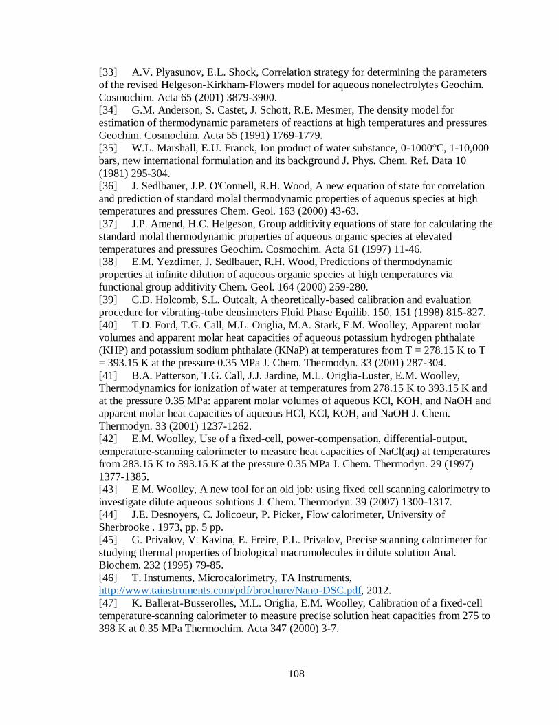
108

[33] A.V. Plyasunov, E.L. Shock, Correlation strategy for determining the parameters

of the revised Helgeson-Kirkham-Flowers model for aqueous nonelectrolytes Geochim.

Cosmochim. Acta 65 (2001) 3879-3900.

[34] G.M. Anderson, S. Castet, J. Schott, R.E. Mesmer, The density model for

estimation of thermodynamic parameters of reactions at high temperatures and pressures

Geochim. Cosmochim. Acta 55 (1991) 1769-1779.

[35] W.L. Marshall, E.U. Franck, Ion product of water substance, 0-1000°C, 1-10,000

bars, new international formulation and its background J. Phys. Chem. Ref. Data 10

(1981) 295-304.

[36] J. Sedlbauer, J.P. O'Connell, R.H. Wood, A new equation of state for correlation

and prediction of standard molal thermodynamic properties of aqueous species at high

temperatures and pressures Chem. Geol. 163 (2000) 43-63.

[37] J.P. Amend, H.C. Helgeson, Group additivity equations of state for calculating the

standard molal thermodynamic properties of aqueous organic species at elevated

temperatures and pressures Geochim. Cosmochim. Acta 61 (1997) 11-46.

[38] E.M. Yezdimer, J. Sedlbauer, R.H. Wood, Predictions of thermodynamic

properties at infinite dilution of aqueous organic species at high temperatures via

functional group additivity Chem. Geol. 164 (2000) 259-280.

[39] C.D. Holcomb, S.L. Outcalt, A theoretically-based calibration and evaluation

procedure for vibrating-tube densimeters Fluid Phase Equilib. 150, 151 (1998) 815-827.

[40] T.D. Ford, T.G. Call, M.L. Origlia, M.A. Stark, E.M. Woolley, Apparent molar

volumes and apparent molar heat capacities of aqueous potassium hydrogen phthalate

(KHP) and potassium sodium phthalate (KNaP) at temperatures from T = 278.15 K to T

= 393.15 K at the pressure 0.35 MPa J. Chem. Thermodyn. 33 (2001) 287-304.

[41] B.A. Patterson, T.G. Call, J.J. Jardine, M.L. Origlia-Luster, E.M. Woolley,

Thermodynamics for ionization of water at temperatures from 278.15 K to 393.15 K and

at the pressure 0.35 MPa: apparent molar volumes of aqueous KCl, KOH, and NaOH and

apparent molar heat capacities of aqueous HCl, KCl, KOH, and NaOH J. Chem.

Thermodyn. 33 (2001) 1237-1262.

[42] E.M. Woolley, Use of a fixed-cell, power-compensation, differential-output,

temperature-scanning calorimeter to measure heat capacities of NaCl(aq) at temperatures

from 283.15 K to 393.15 K at the pressure 0.35 MPa J. Chem. Thermodyn. 29 (1997)

1377-1385.

[43] E.M. Woolley, A new tool for an old job: using fixed cell scanning calorimetry to

investigate dilute aqueous solutions J. Chem. Thermodyn. 39 (2007) 1300-1317.

[44] J.E. Desnoyers, C. Jolicoeur, P. Picker, Flow calorimeter, University of

Sherbrooke . 1973, pp. 5 pp.

[45] G. Privalov, V. Kavina, E. Freire, P.L. Privalov, Precise scanning calorimeter for

studying thermal properties of biological macromolecules in dilute solution Anal.

Biochem. 232 (1995) 79-85.

[46] T. Instuments, Microcalorimetry, TA Instruments,

http://www.tainstruments.com/pdf/brochure/Nano-DSC.pdf, 2012.

[47] K. Ballerat-Busserolles, M.L. Origlia, E.M. Woolley, Calibration of a fixed-cell

temperature-scanning calorimeter to measure precise solution heat capacities from 275 to

398 K at 0.35 MPa Thermochim. Acta 347 (2000) 3-7.

http://www.tainstruments.com/pdf/brochure/Nano-DSC.pdf

109

[48] C. Collins, J. Tobin, D. Shvedov, R. Palepu, P.R. Tremaine, Thermodynamic

properties of aqueous diethanolamine (DEA), N,N-dimethylethanolamine (DMEA), and

their chloride salts: apparent molar heat capacities and volumes at temperatures from

283.15 to 328.15 K Can. J. Chem. 78 (2000) 151-165.

[49] E. Bulemela, P.R. Tremaine, Standard Partial Molar Volumes of Some Aqueous

Alkanolamines and Alkoxyamines at Temperatures up to 325 °C: Functional Group

Additivity in Polar Organic Solutes under Hydrothermal Conditions J. Phys. Chem. B

112 (2008) 5626-5645.

[50] A.R. Lowe, Measuring the Thermodynamic Properties of Adenine; Towards a

Model for the Origins of Life Chemistry, University of Guelph, Guelph, 2013, pp. 311.

[51] C. McGregor, Thermodynamic Properties and Speciation of Aqueous

Methylpiperidines for Applications to Carbon Capture, Chemistry, University of Guelph,

Guelph, 2017, pp. 131.

[52] I. Kim, C.M. Jens, A. Grimstvedt, H.F. Svendsen, Thermodynamics of

protonation of amines in aqueous solutions at elevated temperatures J. Chem.

Thermodyn. 43 (2011) 1754-1762.

[53] J.J. Christensen, R.M. Izatt, D.P. Wrathall, L.D. Hansen, Thermodynamics of

proton ionization in dilute aqueous solution. XI. pK, ΔH.deg., and ΔS.deg. values for

proton ionization from protonated amines at 25.deg J. Chem. Soc. A (1969) 1212-1223.

[54] D. Fernandes, W. Conway, X. Wang, R. Burns, G. Lawrance, M. Maeder, G.

Puxty, Protonation constants and thermodynamic properties of amines for post

combustion capture of CO2 J. Chem. Thermodyn. 51 (2012) 97-102.

[55] E.S. Hamborg, G.F. Versteeg, Dissociation constants and thermodynamic

properties of alkanolamines Energy Procedia 1 (2009) 1213-1218.

[56] R.J. Littel, M. Bos, G.J. Knoop, Dissociation constants of some alkanolamines at

293, 303, 318, and 333 K J. Chem. Eng. Data 35 (1990) 276-277.

[57] Z. Fu-Qiang, L. Hong-Ping, D. Ming, Z. Jian-Ping, Volumetric properties of

binary mixtures of water with ethanolamine alkyl derivatives Thermochim. Acta 254

(1995) 347-357.

[58] B. Hawrylak, S.E. Burke, R. Palepu, Partial molar and excess volumes and

adiabatic compressibilities of binary mixtures of ethanolamines with water J. Solution

Chem. 29 (2000) 575-594.

[59] L. Lebrette, Y. Maham, T.T. Teng, L.G. Hepler, A.E. Mather, Volumetric

properties of aqueous solutions of mono, and diethylethanolamines at temperatures from

5 to 80 °C II Thermochim. Acta 386 (2002) 119-126.

[60] C. McGregor, O. Fandino, J.S. Cox, K. Ballerat-Busserolles, P.R. Tremaine,

Standard partial molar heat capacities and volumes of aqueous N-methylpiperidine and

N-methylpiperidinium chloride from 283 K to 393 K J. Chem. Thermodyn. 113 (2017)

377-387.

[61] F. Spieweck, H. Bettin, Review: solid and liquid density determination Tech.

Mess. 59 (1992) 285-292.

[62] P.G. Hill, A unified fundamental equation for the thermodynamic properties of

water J. Phys. Chem. Ref. Data 19 (1990) 1233-1274.

[63] D.G. Archer, Thermodynamic properties of the sodium chloride + water system.

II. Thermodynamic properties of NaCl(aq), NaCl.2H2O(cr), and phase equilibria J. Phys.

Chem. Ref. Data 21 (1992) 793-829.

110

[64] T.F. Young, M.B. Smith, Thermodynamic properties of mixtures of electrolytes in

aqueous solutions J. Phys. Chem. 58 (1954) 716-724.

[65] A.V. Sharygin, R.H. Wood, Volume and heat capacities of aqueous solutions of

hydrochloric acid at temperatures from 298.15 K to 623 K and pressures to 28 MPa J.

Chem. Thermodyn. 29 (1997) 125-148.

[66] E.M. Woolley, L.G. Hepler, Heat capacities of weak electrolytes and ion

association reactions: method and application to aqueous magnesium sulfate and

hydrogen iodate at 298 K Can. J. Chem. 55 (1977) 158-163.

[67] A.R. Lowe, J.S. Cox, P.R. Tremaine, Thermodynamics of aqueous adenine:

Standard partial molar volumes and heat capacities of adenine, adeninium chloride, and

sodium adeninate from T = 278.15 K to 393.15 K J. Chem. Thermodyn. 112 (2017) 129-

145.

[68] D. Shvedov, P.R. Tremaine, Thermodynamic properties of aqueous

dimethylamine and dimethylammonium chloride at temperatures from 283 K to 523 K:

apparent molar volumes, heat capacities, and temperature dependence of ionization J.

Solution Chem. 26 (1997) 1113-1143.

[69] S. Cabani, V. Mollica, L. Lepori, S.T. Lobo, Volume changes in the proton

ionization of amines in water. 2. Amino alcohols, amino ethers, and diamines J. Phys.

Chem. 81 (1977) 987-993.

[70] S.T. Lobo, R.E. Robertson, Thermodynamics of basic ionization of some amino

ethers in water Can. J. Chem. 54 (1976) 3600-3606.

[71] S. Cabani, S.T. Lobo, E. Matteoli, Apparent molal heat capacities of organic

solutes in water. V. Aminoalcohols, aminoethers, diamines, and polyethers J. Solution

Chem. 8 (1979) 5-10.

[72] S. Cabani, E. Matteoli, E. Selli, Heat capacity changes in proton addition to the

nitrogen of saturated organic molecules in water. Effects of solvation J. Chem. Soc.,

Faraday Trans. 1 75 (1979) 363-369.

[73] G.M. Anderson, D.A. Crerar, Thermodynamics in Geochemistry (1993).

[74] D.G. Archer, P. Wang, The dielectric constant of water and Debye-Hueckel

limiting law slopes J. Phys. Chem. Ref. Data 19 (1990) 371-411.

[75] A.H. Harvey, A.P. Peskin, S.A. Klein, NIST/ASME Steam Standard Reference

Database 10, International Association for the Properties of Water and Steam, Boulder,

Co, 1996.

[76] F.M. Jones, III, E.M. Arnett, Thermodynamics of ionization and solution of

aliphatic amines in water Prog. Phys. Org. Chem. 11 (1974) 263-322.

[77] J.K. Hovey, L.G. Hepler, P.R. Tremaine, Thermodynamics of aqueous aluminate

ion: standard partial molar heat capacities and volumes of tetrahydroxyaluminate(1-)(aq)

from 10 to 55°C J. Phys. Chem. 92 (1988) 1323-1332.

111

SUPPLEMENTARY INFORMATION

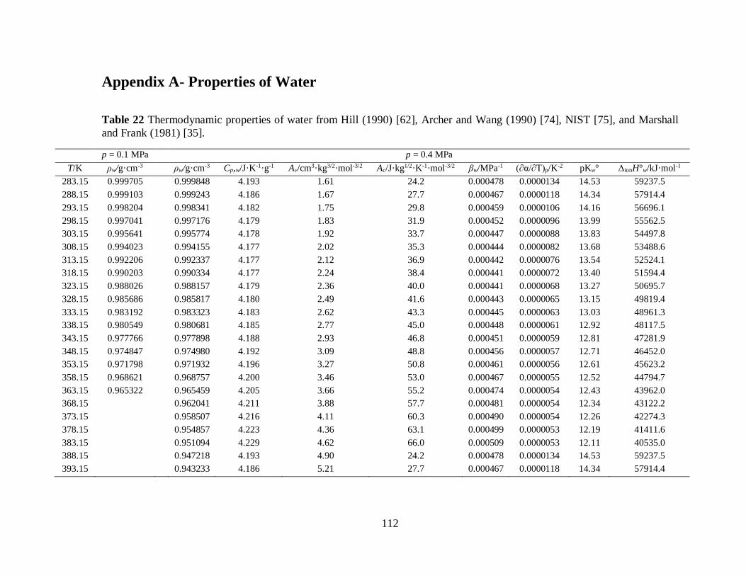
112

Appendix A- Properties of Water

Table 22 Thermodynamic properties of water from Hill (1990) [62], Archer and Wang (1990) [74], NIST [75], and Marshall

and Frank (1981) [35].

p = 0.1 MPa p = 0.4 MPa

T/K ρw/g·cm-3 ρw/g·cm-3 Cp,w/J·K-1·g-1 Av/cm3·kg3/2·mol-3/2 Ac/J·kg1/2·K-1·mol-3/2 βw/MPa-1 (∂α/∂T)p/K-2 pKw° ΔionH°w/kJ·mol-1

283.15 0.999705 0.999848 4.193 1.61 24.2 0.000478 0.0000134 14.53 59237.5

288.15 0.999103 0.999243 4.186 1.67 27.7 0.000467 0.0000118 14.34 57914.4

293.15 0.998204 0.998341 4.182 1.75 29.8 0.000459 0.0000106 14.16 56696.1

298.15 0.997041 0.997176 4.179 1.83 31.9 0.000452 0.0000096 13.99 55562.5

303.15 0.995641 0.995774 4.178 1.92 33.7 0.000447 0.0000088 13.83 54497.8

308.15 0.994023 0.994155 4.177 2.02 35.3 0.000444 0.0000082 13.68 53488.6

313.15 0.992206 0.992337 4.177 2.12 36.9 0.000442 0.0000076 13.54 52524.1

318.15 0.990203 0.990334 4.177 2.24 38.4 0.000441 0.0000072 13.40 51594.4

323.15 0.988026 0.988157 4.179 2.36 40.0 0.000441 0.0000068 13.27 50695.7

328.15 0.985686 0.985817 4.180 2.49 41.6 0.000443 0.0000065 13.15 49819.4

333.15 0.983192 0.983323 4.183 2.62 43.3 0.000445 0.0000063 13.03 48961.3

338.15 0.980549 0.980681 4.185 2.77 45.0 0.000448 0.0000061 12.92 48117.5

343.15 0.977766 0.977898 4.188 2.93 46.8 0.000451 0.0000059 12.81 47281.9

348.15 0.974847 0.974980 4.192 3.09 48.8 0.000456 0.0000057 12.71 46452.0

353.15 0.971798 0.971932 4.196 3.27 50.8 0.000461 0.0000056 12.61 45623.2

358.15 0.968621 0.968757 4.200 3.46 53.0 0.000467 0.0000055 12.52 44794.7

363.15 0.965322 0.965459 4.205 3.66 55.2 0.000474 0.0000054 12.43 43962.0

368.15 0.962041 4.211 3.88 57.7 0.000481 0.0000054 12.34 43122.2

373.15 0.958507 4.216 4.11 60.3 0.000490 0.0000054 12.26 42274.3

378.15 0.954857 4.223 4.36 63.1 0.000499 0.0000053 12.19 41411.6

383.15 0.951094 4.229 4.62 66.0 0.000509 0.0000053 12.11 40535.0

388.15 0.947218 4.193 4.90 24.2 0.000478 0.0000134 14.53 59237.5

393.15 0.943233 4.186 5.21 27.7 0.000467 0.0000118 14.34 57914.4

113

a ur(ρw) = 0.0001%, ur(cp,w) = 0.01%, ur(Av) = 2%, ur(Ac) = 5%, ur(βw) = 0.5%, ur((∂αw/∂T)p) = 0.1%, u( wpK ) = 0.01, u( ion wH )

= 0.4 kJ·mol-1 .

114

Appendix B- Density Model Derivations

The density model:

2 3 4

log log w

b c d eK a k

T T T T

(4.1)

2

gf

hk

T T

(4.2)

Gibbs energy of reaction is related to K by:

lnG RT K (4.3)

2 3 4ln 10 log w

b c d eG RT a k

T T T T

(4.4)

For species, in a mixture, the chemical potential (μ) is the partial molar Gibbs free

energy,

2 3 4ln 10 logi i i i

i i i w

b c d eRT a k

T T T T

(4.5)

Enthalpy of reaction can be obtained using the Gibbs-Helmholtz identity:

2

G H

T T T

(4.6)

2

2 3

2 3 4 2ln 10 log w w

c d e hH R b g RT k

T T T T

(4.7)

where k is the same as equation 4.2 and

1 w

w

pw T

(4.8)

Entropy of reaction can be obtained using the relationship:

G

ST

(4.9)

115

2 3 4 2

2 3ln 10 f log w w

c d e hS R a RT k

T T T T

(4.10)

Standard molar heat capacity of reaction can be described using equation 4.6 and the

relationship

p

p

HC

T

(4.11)

to obtain

2

2 3 4 2

2 6 12 2 2ln 10 log 2 f w

p w w

p

c d e h hC R R T RT k

T T T T T T

(4.12)

The standard partial molar heat capacity can be represented as

2

, 2 3 4 2

2 6 12 2 2ln 10 log 2fi i i i i w

p i w w i i

p

c d e h hC R R T RT k

T T T T T T

(4.13)

Standard molar volume of reaction can be derived using the density model in its original

form and

ln

T

K V

p RT

(4.14)

wV RT k (4.15)

2 3 4

' ' ' 'ln 10 ' w

b c d eV RT a RT k

T T T T

(4.16)

where

'T

zz

p

(4.17)

z’ could be a’, b’, c’, d’, or e’ and

1 w

w

w Tp

(4.18)

116

The standard partial molar volume for species can be derived using the relationship

ii

T

Vp

(4.19)

from equation 4.5 where,

1 bar ' 1i ia a a p (4.20)

is used to obtain,

' ' ' '

'

2 3 4ln 10 i i i i

i i i w

b c d eV RT a RTk

T T T T

(4.21)

and

' ii

T

zz

p

(4.22)

where zi’ is representative of ai’, bi’, ci’, and di’.

117

Appendix C- Data Treatment

4.1 Apparent Molar Volume

Calculations of apparent molar volume begin with measurements using an Anton

Paar vibrating tube densimeter at 0.1 MPa from 283.15 to 363.15 K. The densimeter

automatically calculates solution densities using the equation of state by Spieweck and

Bettin (1992) [61]. The automatically calculated densities were not used to maintain

internal consistency with the calculation of apparent molar properties in this work using

properties of water from Hill [62]. Solution densities are calculated using the experimental

period of vibration with a relationship from Hooke’s law described by equations 1.39 and

1.40.

The cell constant, kρ, is determined at each temperature using water and 1 mol·kg-1

NaCl solutions as calibration fluids with properties calculated from Hill’s equation of state

for water [62] and Archer’s thermodynamic model for the properties of NaCl [63]. Period

of vibration measurements of the calibration fluids are taken at each temperature before

and after every two sample measurements. Apparent molar volumes, expV , are calculated

using equations

s 1exp B

,B st

s B s 1

1000M

Vm

(5.1)

+ - + - + - + -

+ -

+ - + - + - + -

st ex

BH Cl BH Cl H Cl H Cl s 1exp

,BH Cl st ex st exs s 1BH Cl H Cl BH Cl H Cl

11000

M m M mV

m m m m

(5.2)

where M is the molar mass and m is the molality of the neutral amine, B, or protonated

amine, BH+Cl-, or hydrochloric acid, H+Cl-. The superscripts indicate the stoichiometric

118

molality of amine (st) and the molality of HCl (ex). The standard partial molar volumes

were assumed to be constant between 0.1 MPa and 0.4 MPa so that the densities at 0.4 MPa

could be calculated from the standard partial properties using the appropriate values for the

water properties.

4.2 Apparent Molar Heat Capacity

Relative volumetric heat capacities ,s s ,1 1p pc c are obtained using the

relationship between the relative volumetric heat capacities and the measured values of

ΔP, the differential power input between the twin cells of the nanocalorimeter, at 0.4

MPa from 283.15 to 393.15 K,

c s 1

,s s ,1 1p p

k P Pc c

r

(5.3)

where cp,s and cp,1 are the massic heat capacities (J·K-1·g-1) for the solution and water

respectively; r is the temperature scan rate of the calorimeter (K·s-1), and kc is the cell

constant obtained in the calorimeter using the same process as for the densimeter. The

apparent molar heat capacities, exp

,pC , were calculated for the neutral species and

protonated salt of the amine using the equations

,s ,1exp

, ,B B ,s st

B

( )1000

p p

p p

c cC M c

m

(5.4)

+ - + -

+ -

+ - + -

st ex

HCl HCl ,s ,1exp BH Cl BH Cl,s st ex st exp, ,BH Cl

HCl HClBH Cl BH Cl

( ) ( )1000

( ) ( )

p p

p

M m M m c cC c

m m m m

(5.5)

As the experimental calorimetry results were measured to 393.15 K and the densimetry

results were measured to 363.15 K, an extrapolation was completed using the “density”

119

model described in section 2.2. The “density” was fit to the standard partial molar volumes

from this work and the work of Bulemela and Tremaine (2008) [49] over a temperature

range of 283.15 to 598.15 K. Using the values obtained from the model, densities for each

temperature from 363.15 to 393.15 K, not measured experimentally, were calculated.

4.3 Standard Partial Molar Volume

The experimental apparent molar properties, expV , contain contributions from all

species in solution. A neutral amine will ionize in water to form the protonated amine

B(aq) + H2O (l) ⇌ BH+(aq) + OH-(aq)

st st st

B B B1 m m m (5.6)

where the degree of dissociation, , can be used to determine the concentration of all other

species in solution. The degree of dissociation of the neutral amine was calculated from

temperature dependent values of Ka, reported by Hamborg and Versteeg (2009) [55] and

Balakrishnan (1988) [1] for DMEA and 3-MPA, respectively, as the acid ionization

reaction:

BH B Haq aq aq (5.7)

and converted to Kb for reaction 5.6 using equation 5.8:

b w apK pK pK (5.8)

Here, the value for pKw was obtained from the equation of state from Marshall and Frank

[35]. The contributions of all species from reaction 5.6 to expV were removed using

Young’s rule [64]:

+ -

2

exp *

H O,BH ,OH

1

V V V VV

(5.9)

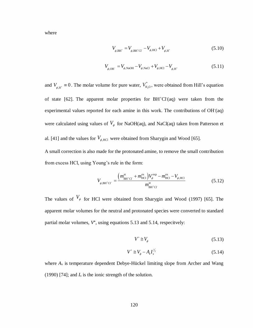
120

where

+ - ,HCl,BH ,BH Cl ,HV V V V (5.10)

,NaOH ,NaCl ,HCl,OH ,HV V V V V (5.11)

and ,H

0V . The molar volume for pure water,

2

*

H OV , were obtained from Hill’s equation

of state [62]. The apparent molar properties for BH+Cl-(aq) were taken from the

experimental values reported for each amine in this work. The contributions of OH-(aq)

were calculated using values of V for NaOH(aq), and NaCl(aq) taken from Patterson et

al. [41] and the values for ,HClV were obtained from Sharygin and Wood [65].

A small correction is also made for the protonated amine, to remove the small contribution

from excess HCl, using Young’s rule in the form:

+ -

+

+ -

st ex exp ex

HCl HCl ,HClBH Cl

st,BH Cl

BH Cl

m m V m VV

m

(5.12)

The values of V for HCl were obtained from Sharygin and Wood (1997) [65]. The

apparent molar volumes for the neutral and protonated species were converted to standard

partial molar volumes, V°, using equations 5.13 and 5.14, respecitvely:

V V (5.13)

1

2

v sV V A I (5.14)

where Av is temperature dependent Debye-Hückel limiting slope from Archer and Wang

(1990) [74]; and Is is the ionic strength of the solution.

121

4.4 Standard Partial Molar Heat Capacity

Species contributing to exp

,pC from the ionization of the neutral amine in water are

again removed using Young’s rule [64] according to equation 5.15:

+ -

2

exp * rel

, p,H O, ,BH , ,OH

,1

p pp p

p

V C C C CC

(5.15)

where the terms for +, ,BHpC

and

, ,OHpC

can be calculated from equations 5.10 and 5.11

with ,pC for NaOH, NaCl and HCl from Patterson et al. (2001) [41]. The term rel

pC is the

chemical relaxation term, representing the change in heat caused by the shift in equilibrium

with temperature:

2

brel

2

1

2

r

p

HC

RT

(5.16)

Here, the degree of dissociation was obtained as described in section 2.1.3 and ion bH was

calculated from values of ion aH from the acid ionization reaction 5.7, reported by

Christensen et al. (1969) [53] and Cabani et al. (1979) [69] for DMEA and 3-MPA,

respectively, using equation 5.17:

b b w ar r r rH H H H (5.17)

298.15 ,298.15 298.15r r pH H C T (5.18)

where the values for ion wH was taken from the equation of state by Marshall and Frank

(1981) [35] and r pC is assumed to be constant over the temperature range;

+ -2, B , H O, BH Cl , Cl , OHr p p pp p p

C C C C C C (5.19)

122

The value for 2, H OpC was obtained from Jones and Arnett (1974) [76] and values for

, ClpC and

, OHpC are from Hovey et al. (1988) [77].

Speciation corrections for the protonated amine follow those in section 5.3

+ -

+

+ -

st ex exp ex

HCl , HCl , ,HClBH Cl

st, ,BH Cl

BH Cl

p p

p

m m C m CC

m

(5.20)

where values for , ,HClpC were obtained from Patterson et al. (2001) [41]. The apparent

molar heat capacities for the neutral and protonated species were converted to standard

partial molar heat capacities, Cp°, using equations 5.21 and 5.22, respecitvely:

,p pC C (5.21)

1

2

,p p c sC C A I (5.22)

where Ac is temperature dependent Debye-Hückel limiting slope from Archer and Wang

(1990) [74].

4.5 Single- Ion Properties

The “density” model, described in section 1.4.4, was fit the standard partial molar

volume and heat capacity data obtained in this work. For this work an additional term was

added to the model

12 3 4

2

ln logb c d e

K a kT T T T

g hk f

T T

(5.23)

Here the model contains five fitting parameters, a-e, instead of four, to describe low

temperature species specific effects. This additional term was found to improve the overall

123

fit of the model to the volume and heat capacity data obtained in this work. The high

temperature fitting parameters, now f, g, and h, remain the same as described in section

1.4.4. To obtain the pressure and temperature dependence of the standard partial molar

volume and heat capacity equations 5.24 and 5.25 were fit to the experimental data:

2 3 4

' ' ' 'ln 10 ' w

b c d e gV RT a RT

T T T T T

(5.24)

2 w

2 3 4

2 6 12ln 10p

p

c d e gC R RT

T T T T T

(5.25)

where,

' 0, ' , c ' , etc.T T

b ca b

p p

(5.26)


coefficient of water in MPa-1. Values for αw and βw were obtained from the NIST

formulation for the properties of water and steam. The regression of equations 5.24 and

5.25 was performed using the Levenberg-Marquardt algorithm in Sigma Plot 11.0.

The terms a’-e’ in equation 5.24, used to determine the pressure dependence of the

low temperature species specific fitting terms, are from the density model fit to the

experimental data obtained in this work from 283.15 to 363.15 K. High temperature fitting

parameter, g, for V° was obtained by fitting equation 5.24 to data reported by Bulemela and

Tremaine (2008) [49] at 15 MPa and temperatures of 423.15 to 598 K for the protonated

and neutral species. The V° high temperature fitting parameter, g, was then used as constant

in the model for the pC density model fit where experimental data was recorded from

283.15 to 393.15 K.

124

The single-ion standard partial molar properties of DMEAH+(aq), from the

ionization reaction were determined using equation 5.27:

+ + - +HClBH BH Cl HY Y Y Y (5.27)

where +H0Y and the values for , HClpC and HClV are from Patterson et al. (2001) [41] and

Sharygin and Wood (1997) [65], respectively, and were reported as fits of experimental

data. Equations 5.24 and 5.25 were fit to the values from the fits reported by Patterson et

al. (2001) [41] and Sharygin and Wood (1997) [65] for , HClpC and HClV .

4.6 Thermodynamic Functions for the Ionization of BH+ at Elevated T and

p

Thermodynamic values for the ionization of BH+ were calculated according to the

isocoulombic reaction 5.28 and equation 5.29:

BH B Haq aq aq (5.28)

+ +ion B H BHY Y Y Y (5.29)

Where the ionization constant was obtained using equation 5.28:

w2 3 4log log

b c d e gK a

T T T T T

(5.30)

Fitting constants a and b were obtained using the Gibbs energy and enthalpy of ionization.

The enthalpy of ionization:

2

w w2 3

2 3 4 2ln 10 log

c d e h gH R b g RT

T T T T T

(5.31)

125

contains fitting constants Δc, Δd, and Δe from ion pC and fitting constants Δg and Δh from

ionV Equation 5.31 was solved for fitting constant Δb using a literature value for ΔH° at

298.15 K from Hamborg and Versteeg (2009) [55] and Balakrishnan (1988) [1] for DMEA

and 3-MPA, respectively. This calculation was repeated with equation 5.32 for Gibbs

energy of ionization to obtain the fitting constant Δa:

w2 3 4ln 10 log

b c d e gG RT a

T T T T T

(5.32)

where values for ΔG° at 298.15 K for DMEA and 3-MPA were obtained from Hamborg

and Versteeg (2009) [55] and Balakrishnan (1988) [1], respectively.


the low temperature fitting constants from pC and ΔV° in equation 5.33:

' 0.1 MPaY b b p (5.33)

where the equation used for b/b’ is also used for all other fitting constants.

Standard Partial Molar Heat Capacities and Volumes of ...

Documents

Transcript of Standard Partial Molar Heat Capacities and Volumes of ...