STABILITY OFSTRUCTURESPrinciples andApplications

CHAI H. YOOAuburn University

SUNG C. LEEDongguk University

AMSTERDAM • BOSTON • HEIDELBERG • LONDON

NEW YORK • OXFORD • PARIS • SAN DIEGO

SAN FRANCISCO • SINGAPORE • SYDNEY • TOKYO

Butterworth-Heinemann is an imprint of Elsevier

Butterworth-Heinemann is an imprint of Elsevier

30 Corporate Drive, Suite 400, Burlington, MA 01803, USA

The Boulevard, Langford Lane, Kidlington, Oxford OX5 1GB, UK

Copyright � 2011 Elsevier Inc. All rights reserved.

No part of this publication may be reproduced, stored in a retrieval system, or transmitted in

any form or by any means, electronic, mechanical, photocopying, recording, or otherwise,

without the prior written permission of the publisher.

Permissions may be sought directly from Elsevier’s Science & Technology Rights

Department in Oxford, UK: phone: (+44) 1865 843830, fax: (+44) 1865 853333, E-mail:

permissions@elsevier.com. You may also complete your request online via the Elsevier

homepage (http://elsevier.com), by selecting “Support & Contact” then “Copyright and

Permission” and then “Obtaining Permissions.”

Library of Congress Cataloging-in-Publication Data

Yoo, Chai Hong.

Stability of structures: principles and applications/Chai H. Yoo, Sung C. Lee.

p. cm.

Summary: “The current trend of building more streamlined structures has made stability

analysis a subject of extreme importance. It is mostly a safety issue because Stability loss

could result in an unimaginable catastrophe. Written by two authors with a combined

80 years of professional and academic experience, the objective of Stability of Structures:

Principles and Applications is to provide engineers and architects with a firm grasp of the

fundamentals and principles that are essential to performing effective stability analysts”–

Provided by publisher.

Includes bibliographical references and index.

ISBN 978-0-12-385122-2 (hardback)

1. Structural stability. 2. Safety factor in engineering. I. Lee, Sung Chul, 1957- II. Title.

TA656.Y66 2011

624.1’71–dc22

2010048927

British Library Cataloguing-in-Publication Data

A catalogue record for this book is available from the British Library.

ISBN: 978-0-12-385122-2

For information on all ButterwortheHeinemann publications visit

our Web site at elsevierdirect.com

Printed and bound in the U.S.

11 12 13 10 9 8 7 6 5 4 3 2 1

PREFACE

The subject of this book is the stability of structures subjected to external

loading that induces compressive stresses in the body of the structures. The

structural elements examined are beams, columns, beam-columns, frames,

rectangular plates, circular plates, cylindrical shells, and general shells.

Emphasis is on understanding the behavior of structures in terms of load-

displacement characteristics; on formulation of the governing equations;

and on calculation of the critical load.

Buckling is essentially flexural behavior. Therefore, it is imperative to

examine the condition of equilibrium in a flexurally deformed configura-

tion (adjacent equilibrium position). The governing stability equations are

derived by both the equilibrium method and the energy method based on

the calculus of variations invoking the Trefftz criterion.

Stability analysis is a topic that fundamentally belongs to nonlinear

analysis. The fact that the eigenvalue procedure in modern matrix and/or

finite element analysis is a fortuitous by-product of incremental nonlinear

analysis is a reaffirming testimony. The modern emphasis on fast-track

education designed to limit the number of required credit hours for core

courses in curriculums left many budding practicing structural analysts with

gaping gaps in their understanding of the theory of elastic stability. Many

advanced works on structural stability describe clearly the fundamental

aspects of general nonlinear structural analysis. We believe there is a need for

an introductory textbook such as this, which will present the fundamentals

of structural stability analysis within the context of elementary nonlinear

flexural analysis. It is believed that a firm grasp of these fundamentals and

principles is essential to performing the important interpretation required of

analysts when computer solutions are adopted.

The book has been planned for a two-semester course. The first chapter

introduces the buckling of columns. It begins with the linear elastic theory

and proceeds to include the effects of large deformations and inelastic

behavior. In Chapter 2 various approximate methods are illustrated along

with the fundamentals of energy methods. The chapter concludes by

introducing several special topics, some of them advanced, that are useful in

understanding the physical resistance mechanisms and consistent and

rigorous mathematical analysis. Chapters 3 and 4 cover buckling of beam-

columns. Chapter 5 presents torsion in structures in some detail, which is

ix j

x Preface

one of the least-well-understood subjects in the entire spectrum of structural

mechanics. Strictly speaking, torsion itself does not belong to a work on

structural stability, but it needs to be covered to some extent if one is to have

a better understanding of buckling accompanied with torsional behavior.

Chapters 6 and 7 consider stability of framed structures in conjunction with

torsional behavior of structures. Chapters 8 to 10 consider buckling of plate

elements, cylindrical shells, and general shells. Although the book is devoted

primarily to analysis, rudimentary design aspects are also discussed.

The reader is assumed to have a good foundation in elementary

mechanics of deformable bodies, college-level calculus, and analytic

geometry, and some exposure to differential equations. The book is

designed to be a textbook for advanced seniors and/or first-year graduate

students in aerospace, civil, mechanical, engineering mechanics, and

possibly naval architects and shipbuilding fields and as a reference book for

practicing structural engineers.

Needless to say, we have relied heavily on previously published work.

Consequently, we have tried to be meticulous in citing the works and hope

that we have not erred on the side of omission.

AUTHORS BIOGRAPHY

Chai H. Yoo, PhD., PE., F.ASCE, is professor emeritus at Auburn

University. He has over 40 years of teaching, research, and consulting

experience. He received his BS from Seoul National University in Korea

and his MS and PhD degrees from the University of Maryland. He is the

recipient of the 2008 ASCE Shortridge Hardesty Award for his outstanding

research and practical engineering efforts dealing with the strength and

stability of thin-walled sections, especially as it applies to bridge girders.

Author of over 75 refereed journal papers and a book on curved steel girder

bridges, Dr. Yoo has been active on numerous ASCE and SSRC technical

committee activities. He was the principal investigator/project director of

NCHRP Project 12-38 that produced AASHTO Guide Specifications for

Horizontally Curved Steel Girder Highway Bridges with Design Examples

for I-Girder and Box-Girder Bridges.

Sung C. Lee, PhD., M.ASCE, is professor and head of the Department of

Civil and Environmental Engineering at Dongguk University in Seoul,

Korea. He received his BS from Seoul National University in Korea, his MS

from Oregon State University, and his PhD from Auburn University. He is

the author of over 100 refereed journal articles, technical papers, and

proceedings. Dr. Lee’s breakthrough research on the strength and stability of

web panels in plate- and box-girders renders a correct understanding on

a topic that has been controversial over the last five decades.

xi j

CHAPTER11

Buckling of ColumnsContents

1.1. Introduction 11.2. Neutral Equilibrium 31.3. Euler Load 41.4. Differential Equations of Beam-Columns 81.5. Effects of Boundary Conditions on the Column Strength 151.6. Introduction to Calculus of Variations 181.7. Derivation of Beam-Column GDE Using Finite Strain 241.8. Galerkin Method 271.9. Continuous Beam-Columns Resting on Elastic Supports 29

1.9.1. One Span 291.9.2. Two Span 301.9.3. Three Span 311.9.4. Four Span 34

1.10. Elastic Buckling of Columns Subjected to Distributed Axial Loads 381.11. Large Deflection Theory (The Elastica) 441.12. Eccentrically Loaded ColumnsdSecant Formula 521.13. Inelastic Buckling of Straight Column 56

1.13.1. Double-Modulus (Reduced Modulus) Theory 571.13.2. Tangent-Modulus Theory 60

1.14. Metric System of Units 66General References 67References 68Problems 69

1.1. INTRODUCTION

A physical phenomenon of a reasonably straight, slender member (or body)

bending laterally (usually abruptly) from its longitudinal position due to

compression is referred to as buckling. The term buckling is used by engi-

neers as well as laypeople without thinking too deeply. A careful exami-

nation reveals that there are two kinds of buckling: (1) bifurcation-type

buckling; and (2) deflection-amplification-type buckling. In fact, most, if

not all, buckling phenomena in the real-life situation are the deflection-

amplification type. A bifurcation-type buckling is a purely conceptual one

that occurs in a perfectly straight (geometry) homogeneous (material)

member subjected to a compressive loading of which the resultant must pass

Stability of Structures � 2011 Elsevier Inc.ISBN 978-0-12-385122-2, doi:10.1016/B978-0-12-385122-2.10001-6 All rights reserved. 1 j

2 Chai Yoo

though the centroidal axis of the member (concentric loading). It is highly

unlikely that any ordinary column will meet these three conditions perfectly.

Hence, it is highly unlikely that anyone has ever witnessed a bifurcation-

type buckling phenomenon. Although, in a laboratory setting, one could

demonstrate setting a deflection-amplification-type buckling action that is

extremely close to the bifurcation-type buckling. Simulating those three

conditions perfectly even in a laboratory environment is not probable.

Structural members resisting tension, shear, torsion, or even short

stocky columns fail when the stress in the member reaches a certain

limiting strength of the material. Therefore, once the limiting strength of

material is known, it is a relatively simple matter to determine the load-

carrying capacity of the member. Buckling, both the bifurcation and the

deflection-amplification type, does not take place as a result of the resisting

stress reaching a limiting strength of the material. The stress at which

buckling occurs depends on a variety of factors ranging from the

dimensions of the member to the boundary conditions to the properties of

the material of the member. Determining the buckling stress is a fairly

complex undertaking.

If buckling does not take place because certain strength of the material is

exceeded, then, why, one may ask, does a compression member buckle?

Chajes (1974) gives credit to Salvadori and Heller (1963) for clearly eluci-

dating the phenomenon of buckling, a question not so easily and directly

explainable, by quoting the following from Structure in Architecture:

A slender column shortens when compressed by a weight applied to its top, and,in so doing, lowers the weight’s position. The tendency of all weights to lower theirposition is a basic law of nature. It is another basic law of nature that, wheneverthere is a choice between different paths, a physical phenomenon will follow theeasiest path. Confronted with the choice of bending out or shortening, the columnfinds it easier to shorten for relatively small loads and to bend out for relativelylarge loads. In other words, when the load reaches its buckling value the columnfinds it easier to lower the load by bending than by shortening.

Although these remarks will seem excellent to most laypeople, they do

contain nontechnical terms such as choice, easier, and easiest, flavoring the

subjective nature. It will be proved later that buckling is a phenomenon that

can be explained with fundamental natural principles.

If bifurcation-type buckling does not take place because the afore-

mentioned three conditions are not likely to be simulated, then why, one

may ask, has so much research effort been devoted to study of this

phenomenon? The bifurcation-type buckling load, the critical load, gives

Buckling of Columns 3

the upper-bound solution for practical columns that hardly satisfies any one

of the three conditions. This will be shown later by examining the behavior

of an eccentrically loaded cantilever column.

1.2. NEUTRAL EQUILIBRIUM

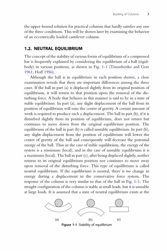
The concept of the stability of various forms of equilibrium of a compressed

bar is frequently explained by considering the equilibrium of a ball (rigid-

body) in various positions, as shown in Fig. 1-1 (Timoshenko and Gere

1961; Hoff 1956).

Although the ball is in equilibrium in each position shown, a close

examination reveals that there are important differences among the three

cases. If the ball in part (a) is displaced slightly from its original position of

equilibrium, it will return to that position upon the removal of the dis-

turbing force. A body that behaves in this manner is said to be in a state of

stable equilibrium. In part (a), any slight displacement of the ball from its

position of equilibrium will raise the center of gravity. A certain amount of

work is required to produce such a displacement. The ball in part (b), if it is

disturbed slightly from its position of equilibrium, does not return but

continues to move down from the original equilibrium position. The

equilibrium of the ball in part (b) is called unstable equilibrium. In part (b),

any slight displacement from the position of equilibrium will lower the

center of gravity of the ball and consequently will decrease the potential

energy of the ball. Thus in the case of stable equilibrium, the energy of the

system is a minimum (local), and in the case of unstable equilibrium it is

a maximum (local). The ball in part (c), after being displaced slightly, neither

returns to its original equilibrium position nor continues to move away

upon removal of the disturbing force. This type of equilibrium is called

neutral equilibrium. If the equilibrium is neutral, there is no change in

energy during a displacement in the conservative force system. The

response of the column is very similar to that of the ball in Fig. 1-1. The

straight configuration of the column is stable at small loads, but it is unstable

at large loads. It is assumed that a state of neutral equilibrium exists at the

(a) (b) (c)

Figure 1-1 Stability of equilibrium

4 Chai Yoo

transition from stable to unstable equilibrium in the column. Then the load

at which the straight configuration of the column ceases to be stable is the

load at which neutral equilibrium is possible. This load is usually referred to

as the critical load.

To determine the critical load, eigenvalue, of a column, one must find

the load under which the member can be in equilibrium, both in the

straight and in a slightly bent configuration. How slightly? The magnitude

of the slightly bent configuration is indeterminate. It is conceptual. This is

why the free body of a column must be drawn in a slightly bent configu-

ration. The method that bases this slightly bent configuration for evaluating

the critical loads is called the method of neutral equilibrium (neighboring

equilibrium, or adjacent equilibrium).

At critical loads, the primary equilibrium path (stable equilibrium,

vertical) reaches a bifurcation point and branches into neutral equilibrium

paths (horizontal). This type of behavior is called the buckling of bifurcation

type.

1.3. EULER LOAD

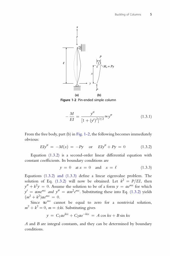
It is informative to begin the formulation of the column equation with

a much idealized model, the Euler1 column. The axially loaded member

shown in Fig. 1-2 is assumed to be prismatic (constant cross-sectional area)

and to be made of homogeneous material. In addition, the following further

assumptions are made:

1. The member’s ends are pinned. The lower end is attached to an

immovable hinge, and the upper end is supported in such a way that it

can rotate freely and move vertically, but not horizontally.

2. The member is perfectly straight, and the load P, considered positive

when it causes compression, is concentric.

3. The material obeys Hooke’s law.

4. The deformations of the member are small so that the term (y0)2 is

negligible compared to unity in the expression for the curvature,

y00=½1þ ðy0Þ2�3=2. Therefore, the curvature can be approximated by y00. 2

1 The Euler (1707–1783) column is due to the man who, in 1744, presented the first accurate column

analysis. A brief biography of this remarkable man is given by Timoshenko (1953). Although it is

customary today to refer to a simply supported column as an Euler column, Euler in fact analyzed

a flag-pole-type cantilever column in his famous treatise according to Chajes (1974).2 y0and y0 0 denote the first and second derivatives of y with respect to x. Note: jy00j < jy0j but

jy0jz thousandths of a radian in elastic columns.

xx

P

y

P

P

x

y

(a) (b)

Mx = Py= Py

Figure 1-2 Pin-ended simple column

Buckling of Columns 5

� M

EI¼ y00

½1þ ðy0Þ2�3=2xy00 (1.3.1)

From the free body, part (b) in Fig. 1-2, the following becomes immediately

obvious:

EIy00 ¼ �MðxÞ ¼ �Py or EIy00 þ Py ¼ 0 (1.3.2)

Equation (1.3.2) is a second-order linear differential equation with

constant coefficients. Its boundary conditions are

y ¼ 0 at x ¼ 0 and x ¼ ‘ (1.3.3)

Equations (1.3.2) and (1.3.3) define a linear eigenvalue problem. The

solution of Eq. (1.3.2) will now be obtained. Let k2 ¼ P=EI , then

y00 þ k2y ¼ 0. Assume the solution to be of a form y ¼ aemx for which

y0 ¼ amemx and y00 ¼ am2emx. Substituting these into Eq. (1.3.2) yields

ðm2 þ k2Þaemx ¼ 0.

Since aemx cannot be equal to zero for a nontrivial solution,

m2 þ k2 ¼ 0, m ¼ �ki. Substituting gives

y ¼ C1aekix þ C2ae

�kix ¼ A cos kxþ B sin kx

A and B are integral constants, and they can be determined by boundary

conditions.

6 Chai Yoo

y ¼ 0 at x ¼ 00A ¼ 0

y ¼ 0 at x ¼ ‘0B sin k‘ ¼ 0

As B s 0 (if B ¼ 0, then it is called a trivial solution; 0 ¼ 0),

sin k‘ ¼ 00 k‘ ¼ np

where n ¼ 1, 2, 3, . . . but n s 0. Hence, k2 ¼ P=EI ¼ n2p2=‘2, fromwhich it follows immediately

Pcr ¼ n2p2EI

‘2ðn ¼ 1; 2; 3; ::Þ (1.3.4)

The eigenvaluesPcr, called critical loads, denote the values of loadP forwhich

a nonzero deflection of the perfect column is possible. The deflection shapes

at critical loads, representing the eigenmodes or eigenvectors, are given by

y ¼ B sinnpx

‘(1.3.5)

Note that B is undetermined, including its sign; that is, the column may

buckle in any direction. Hence, the magnitude of the buckling mode shape

cannot be determined, which is said to be immaterial.

The smallest buckling load for a pinned prismatic column corresponding

to n¼ 1 is

PE ¼ p2EI

‘2(1.3.6)

If a pinned prismatic column of length ‘ is going to buckle, it will buckle at

n ¼ 1 unless external bracings are provided in between the two ends.

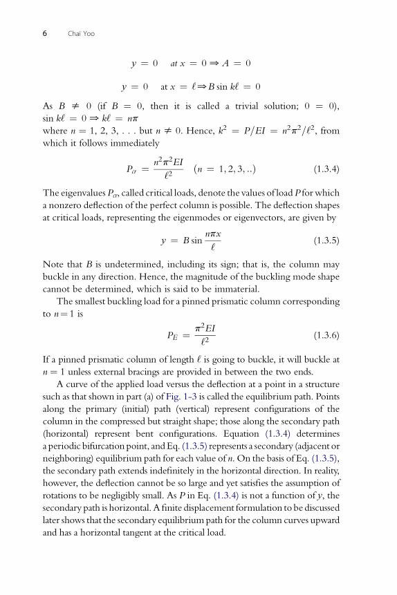
A curve of the applied load versus the deflection at a point in a structure

such as that shown in part (a) of Fig. 1-3 is called the equilibrium path. Points

along the primary (initial) path (vertical) represent configurations of the

column in the compressed but straight shape; those along the secondary path

(horizontal) represent bent configurations. Equation (1.3.4) determines

a periodic bifurcation point, andEq. (1.3.5) represents a secondary (adjacent or

neighboring) equilibrium path for each value of n. On the basis of Eq. (1.3.5),

the secondary path extends indefinitely in the horizontal direction. In reality,

however, the deflection cannot be so large and yet satisfies the assumption of

rotations to be negligibly small. As P in Eq. (1.3.4) is not a function of y, the

secondary path is horizontal. A finite displacement formulation to be discussed

later shows that the secondary equilibrium path for the column curves upward

and has a horizontal tangent at the critical load.

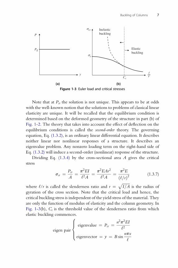
(a)

PE

P

y

(b)

Ccr

Inelasticbuckling

cr

y

Elasticbuckling

Figure 1-3 Euler load and critical stresses

Buckling of Columns 7

Note that at Pcr the solution is not unique. This appears to be at odds

with the well-known notion that the solutions to problems of classical linear

elasticity are unique. It will be recalled that the equilibrium condition is

determined based on the deformed geometry of the structure in part (b) of

Fig. 1-2. The theory that takes into account the effect of deflection on the

equilibrium conditions is called the second-order theory. The governing

equation, Eq. (1.3.2), is an ordinary linear differential equation. It describes

neither linear nor nonlinear responses of a structure. It describes an

eigenvalue problem. Any nonzero loading term on the right-hand side of

Eq. (1.3.2) will induce a second-order (nonlinear) response of the structure.

Dividing Eq. (1.3.4) by the cross-sectional area A gives the critical

stress

scr ¼ Pcr

A¼ p2EI

‘2A¼ p2EAr2

‘2A¼ p2E

ð‘=rÞ2 (1.3.7)

where ‘/r is called the slenderness ratio and r ¼ ffiffiffiffiffiffiffiffiI=A

pis the radius of

gyration of the cross section. Note that the critical load and hence, the

critical buckling stress is independent of the yield stress of the material. They

are only the function of modulus of elasticity and the column geometry. In

Fig. 1-3(b), Cc is the threshold value of the slenderness ratio from which

elastic buckling commences.

eigen pair

(eigenvalue ¼ Pcr ¼ n2p2EI

‘2

eigenvector ¼ y ¼ B sinnpx

‘

8 Chai Yoo

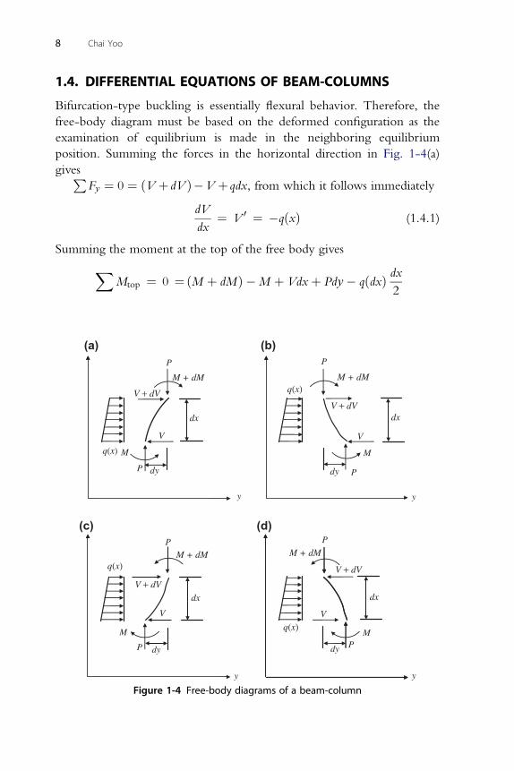
1.4. DIFFERENTIAL EQUATIONS OF BEAM-COLUMNS

Bifurcation-type buckling is essentially flexural behavior. Therefore, the

free-body diagram must be based on the deformed configuration as the

examination of equilibrium is made in the neighboring equilibrium

position. Summing the forces in the horizontal direction in Fig. 1-4(a)

givesPFy ¼ 0 ¼ ðV þ dV Þ�V þ qdx, from which it follows immediately

dV

dx¼ V 0 ¼ �qðxÞ (1.4.1)

Summing the moment at the top of the free body gives

XMtop ¼ 0 ¼ðM þ dMÞ �M þ Vdxþ Pdy� qðdxÞ dx

2

y

y

M

M MPdy

V

M

P

P

P

P

P

P

P

V + dV

V + dV

V + dVV + dV

dx

dx

y

y

dy dy

dy

V V

V

q(x)

q(x)

q(x)

(b)(a)

(c) (d)

M + dM

M + dM M + dM

M + dM

dx

dx

q(x)

Figure 1-4 Free-body diagrams of a beam-column

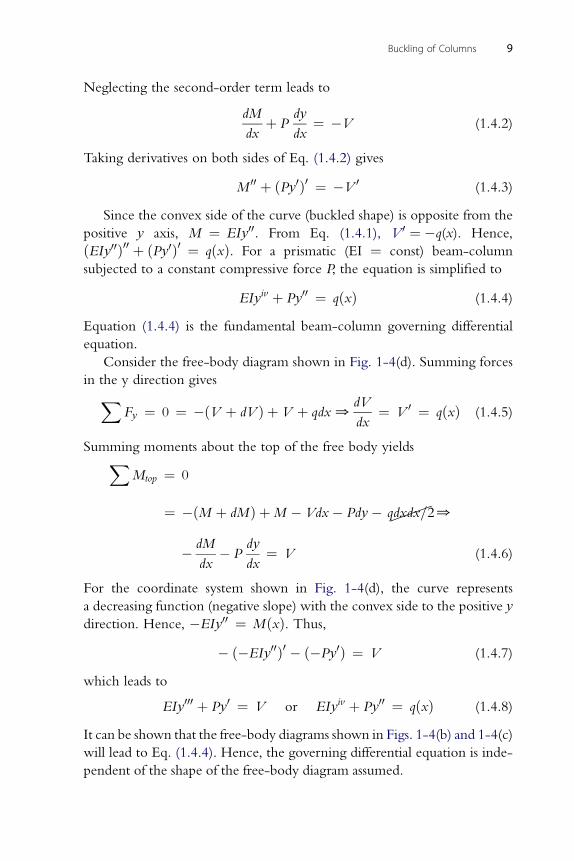
Buckling of Columns 9

Neglecting the second-order term leads to

dM

dxþ P

dy

dx¼ �V (1.4.2)

Taking derivatives on both sides of Eq. (1.4.2) gives

M 00 þ ðPy0Þ0 ¼ �V 0 (1.4.3)

Since the convex side of the curve (buckled shape) is opposite from the

positive y axis, M ¼ EIy00. From Eq. (1.4.1), V 0 ¼ �q(x). Hence,

ðEIy00Þ00 þ ðPy0Þ0 ¼ qðxÞ. For a prismatic (EI ¼ const) beam-column

subjected to a constant compressive force P, the equation is simplified to

EIyiv þ Py00 ¼ qðxÞ (1.4.4)

Equation (1.4.4) is the fundamental beam-column governing differential

equation.

Consider the free-body diagram shown in Fig. 1-4(d). Summing forces

in the y direction givesXFy ¼ 0 ¼ �ðV þ dV Þ þ V þ qdx0

dV

dx¼ V 0 ¼ qðxÞ (1.4.5)

Summing moments about the top of the free body yieldsXMtop ¼ 0

¼ �ðM þ dMÞ þM � Vdx� Pdy�

�

qdxdx=20

� dM

dx� P

dy

dx¼ V (1.4.6)

For the coordinate system shown in Fig. 1-4(d), the curve represents

a decreasing function (negative slope) with the convex side to the positive y

direction. Hence, �EIy00 ¼ MðxÞ. Thus,� ð�EIy00Þ0 � ð�Py0Þ ¼ V (1.4.7)

which leads to

EIy000 þ Py0 ¼ V or EIyiv þ Py00 ¼ qðxÞ (1.4.8)

It can be shown that the free-body diagrams shown in Figs. 1-4(b) and 1-4(c)

will lead to Eq. (1.4.4). Hence, the governing differential equation is inde-

pendent of the shape of the free-body diagram assumed.

10 Chai Yoo

The homogeneous solution of Eq. (1.4.4) governs the bifurcation

buckling of a column (characteristic behavior). The concept of geometric

imperfection (initial crookedness), material heterogeneity, and an eccen-

tricity is equivalent to having nonvanishing q(x) terms.

Rearranging Eq. (1.4.4) gives

EIyiv þ Py00 ¼ 00 yiv þ k2y00 ¼ 0; where k2 ¼ P

EI

Assuming the solution to be of a form y ¼ aemx, then y0 ¼ amemx,y00 ¼ am2emx, y000 ¼ am3emx, and yiv ¼ am4ex. Substituting these derivatives

back to the simplified homogeneous differential equation yields

am4emx þ ak2m2emx ¼ 00aemxðm4 þ k2m2Þ ¼ 0

Since as 0 and emxs 00m2ðm2 þ k2Þ ¼ 00m ¼ �0; �ki. Hence,

yh ¼ c1ekix þ c2e

�kix þ c3xe0 þ c4e

0

Know the mathematical identities

�e0 ¼ 1

eikx ¼ cos kxþ i sin kx

e�ikx ¼ cos kx� i sin kx

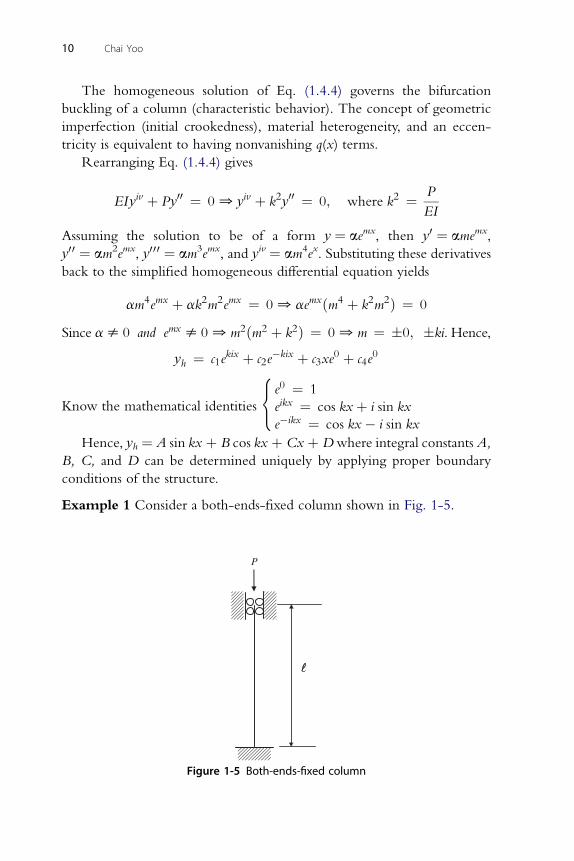
Hence, yh ¼ A sin kx þ B cos kx þ Cx þ Dwhere integral constants A,

B, C, and D can be determined uniquely by applying proper boundary

conditions of the structure.

Example 1 Consider a both-ends-fixed column shown in Fig. 1-5.

P

Figure 1-5 Both-ends-fixed column

Buckling of Columns 11

y0 ¼ Ak cos kx� Bk sin kxþ C

00 2 2

y ¼ �Ak sin kx� Bk kx

y ¼ 0 at x ¼ 0 0 BþD ¼ 0

y0 ¼ 0 at x ¼ 0 0 Akþ C ¼ 0

y ¼ 0 at x ¼ ‘0 A sin k‘þ B cos k‘þ C‘þD ¼ 0

y0 ¼ 0 at x ¼ ‘ 0 Ak cos k‘� Bk sin k‘þ C ¼ 0

For a nontrivial solution for A, B, C, and D (or the stability condition

equation), the determinant of coefficients must vanish. Hence,

Det ¼

�����������

0 1 0 1

k 0 1 0

sin k‘ cos k‘ ‘ 1

k cos k‘ �k sin k‘ 1 0

����������¼ 0

Expanding the determinant (Maple�) gives

2ðcos k‘� 1Þ þ k‘ sin k‘ ¼ 0

Know the following mathematical identities:8>><>>:

sin k‘ ¼ sin

�k‘

2þ k‘

2

�¼ sin

k‘

2cos

k‘

2þ cos

k‘

2sin

k‘

2¼ 2 sin

k‘

2cos

k‘

2

cos k‘ ¼ cos

�k‘

2þ k‘

2

�¼ cos

k‘

2cos

k‘

2� sin

k‘

2sin

k‘

2¼ 1� 2 sin2

k‘

2

0cos k‘� 1 ¼ �2 sin2k‘

2

Rearranging the determinant given above yields:

2

�� 2 sin2

k‘

2

�þ k‘

�2 sin

k‘

2cos

k‘

2

�¼ 0

0 sink‘

2

�k‘

2cos

k‘

2� sin

k‘

2

�¼ 0

12 Chai Yoo

Let u ¼ k‘=2, then the solution becomes sin u ¼ 0 or tan u ¼ u.

For sin u ¼ 00u ¼ np or k‘ ¼ 2np0Pcr ¼ 4n2p2EI=‘2. Substituting

the eigenvalue k ¼ 2np=‘ into the buckling mode shape yields

y ¼ c1 sin2npx

‘þ c2 cos

2npx

‘þ c3xþ c4

y ¼ 0 at x ¼ 000 ¼ c2þ c40 c4 ¼ �c2 Hence, y ¼ c1 sinð2npx=‘Þþc2�cosð2npx=‘Þ�1

�þ c3x

y ¼ 0 at x ¼ ‘0 0 ¼ c1 sin 2npþ c2ðcos 2np� 1Þ þ c3‘0 c3 ¼ 0

2np 2npx 2np 2npx

y0 ¼ �

‘c2 sin

‘þ

‘c1 cos

‘

2np

y0 ¼ 0 at x ¼ 00 y0 ¼ 0þ

‘c10c1 ¼ 0

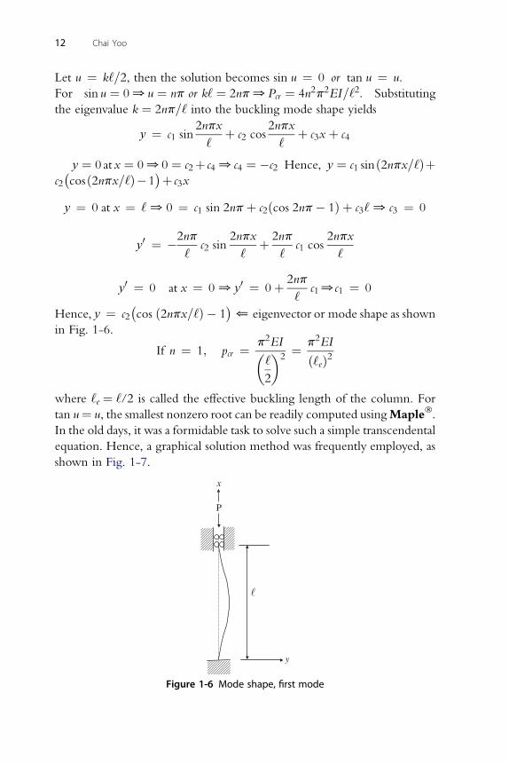
Hence, y ¼ c2�cos ð2npx=‘Þ � 1

�* eigenvector or mode shape as shown

in Fig. 1-6.

If n ¼ 1; pcr ¼ p2EI�‘

2

�2¼ p2EI

ð‘eÞ2

where ‘e ¼ ‘/2 is called the effective buckling length of the column. For�

tan u¼ u, the smallest nonzero root can be readily computed usingMaple .

In the old days, it was a formidable task to solve such a simple transcendental

equation. Hence, a graphical solution method was frequently employed, as

shown in Fig. 1-7.

x

y

P

Figure 1-6 Mode shape, first mode

y = x

0 1 3 4 5 6 2

6

5

4

3

2

1

0

y

x

4.5

y = tanx

Figure 1-7 Graphical solution

xP

y0.3495

Figure 1-8 Mode shape, second mode

Buckling of Columns 13

From Maple� output, the smallest nonzero root is

u ¼ 4:49340940k‘

2¼ 4:4930 k‘ ¼ 8:98680 k2‘2 ¼ 80:763

80:763EI 8:183p2EI p2EI p2EI

Pcr ¼

‘2¼

‘2¼ ð0:349578‘Þ2 ¼ ½0:699156ð0:5‘Þ�2:

The corresponding mode shape is shown in Fig. 1-8.

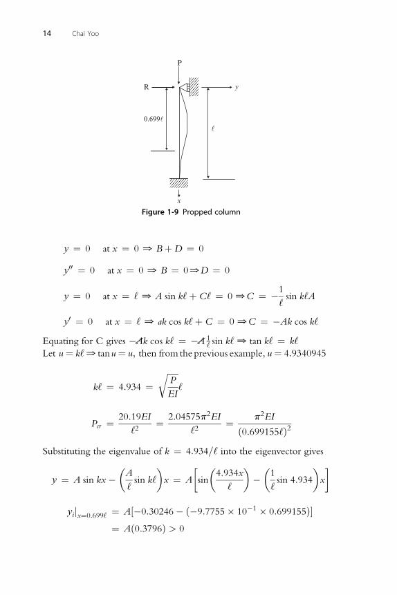
Example 2 Consider propped column as shown in Fig. 1-9.

y ¼ A sin kxþ B cos kxþ CxþD

y0 ¼ Ak cos kx� Bk sin kxþC

y00 ¼ �Ak2 sin kx� Bk2 cos kx

P

x

R y

0.699

Figure 1-9 Propped column

14 Chai Yoo

y ¼ 0 at x ¼ 0 0 BþD ¼ 0

y00 ¼ 0 at x ¼ 00 B ¼ 00D ¼ 0

y ¼ 0 at x ¼ ‘ 0 A sin k‘þ C‘ ¼ 00C ¼ �1

‘sin k‘A

y0 ¼ 0 at x ¼ ‘ 0 ak cos k‘þ C ¼ 00C ¼ �Ak cos k‘

Equating for C gives �

�

Ak cos k‘ ¼ �

�

A 1‘ sin k‘0 tan k‘ ¼ k‘

Let u¼ k‘0tanu¼ u; then from the previous example; u¼ 4:9340945

k‘ ¼ 4:934 ¼ffiffiffiffiffiP

EI

r‘

20:19EI 2:04575p2EI p2EI

Pcr ¼

‘2¼

‘2¼ ð0:699155‘Þ2

Substituting the eigenvalue of k ¼ 4:934=‘ into the eigenvector gives

y ¼ A sin kx��A

‘sin k‘

�x ¼ A

sin

�4:934x

‘

���1

‘sin 4:934

�x

�1

yijx¼0:699‘ ¼ A½�0:30246� ð�9:7755� 10 � 0:699155Þ�¼ Að0:3796Þ > 0

Buckling of Columns 15

Summing the moment at the inflection point yields

XM jx¼0:699‘ ¼ 0 ¼ 20:19EI

‘2Að0:3796Þ � Rð0:699155‘Þ0

R ¼ 11EI

‘3As0

For W10 � 49, Iy ¼ 93.4 in4, ry ¼ 2.54 in, say ‘ ¼ 25 ft ¼ 300 in,

Area ¼ 14.4 in2

If it is assumed that this column has initial imperfection of ‘/250 at the

inflection point, then

yx¼0:699155‘ ¼ ‘=250 ¼ 300=250 ¼ 1:2 in0A ¼ 1:758

Then, R ¼ 11� �ð29� 103 � 93:4Þ=3003�� 1:758 ¼ 1:94 kips

k‘

r¼ 1� 0:699155� 300

2:54¼ 82:60Fcr ¼ 15:6 ksi0 Pcr ¼ 224:6 kips

R ¼ 1:94=224:6� 100 ¼ 0:86% < 2%* rule of thumb

1.5. EFFECTS OF BOUNDARY CONDITIONS ON THECOLUMN STRENGTH

The critical column buckling load on the same column can be increased in

two ways.

1. Change the boundary conditions such that the new boundary condition

will make the effective length shorter.

(a) pinned-pinned 0 ‘e ¼ ‘(b) pinned-fixed 0 ‘e ¼ 0.7 ‘(c) fixed-fixed 0 ‘e ¼ 0.5 ‘(d) flag pole (cantilever) 0 ‘e ¼ 2.0 ‘, etc.

2. Provide intermediate bracing to make the column buckle in higher

modes 0 achieve shorter effective length.

Consider an elastically constrained column AB shown in Fig. 1-10.

The two members, AB and BC, are assumed to have identical member

length and flexural rigidity for simplicity. The moments, m and M, are due

to the rotation at point B and possibly due to the axial shortening of member

AB.

Since Q ¼ ðM þ mÞ=‘ <<< pcr, Q is set equal to zero and the effect

of any axial shortening is neglected.

B

A

CPP

x

x

EI

EI

Q

Q

M

m

/m

/m

/m

P Q

P Qm

P

Figure 1-10 Buckling of simple frame

y

x xP

P P

P

M (x)M (x)

y

y

y

m / /m

/m

Figure 1-11 Free body of column

16 Chai Yoo

Summing moment at the top of the free body gives

(from the left free body) (from the right free body)

MðxÞ þ Py� mx

‘¼ 0 MðxÞ � Pð�yÞ � mx

‘¼ 0

�mx

�mx

EIy00 ¼ �MðxÞ ¼ � Py�‘

EIy00 ¼ MðxÞ ¼ �Pyþ‘

As expected, the assumed deformed shape does not affect the Governing

Differential Equation (GDE) of the behavior of member AB.

EIy00 þ Py ¼ mx

‘

Let k2 ¼ P=EI0y00 þ k2y ¼ ðmx=‘PÞ k2The general solution to this DE is given

y ¼ A sin kxþ B cos kxþ m

‘Px

y ¼ 0 at x ¼ 00 B ¼ 0

y ¼ 0 at x ¼ ‘ 0 A ¼ � m

Buckling of Columns 17

P sin k‘

m�x sin kx

�

y ¼

P ‘�

sin k‘* buckling mode shape

Since joint B is assumed to be rigid, continuity must be preserved. That is

dy

dx

����col

¼ dy

dx

����bm

dy�� m

�1 k cos kx

�m�1 k

�

for col

dx��x¼‘

¼P ‘

�sin k‘

¼P ‘

�tan k‘

¼ m

kEI

�1

k‘� 1

tan k‘

�

for beamdy

dx x¼0¼ qN ¼ m‘

4EI

����Recall the slope deflection equation: m ¼ ð2EI=‘Þð2qN þ

�qF �

�34Þ0

qN ¼ m‘=4EI

Equating the two slopes at joint B gives

m‘

4EI¼ � m

kEI

�1

k‘� 1

tan k‘

�*Note the direction of rotation at joint B!

If the frame is made of the same material, then

‘

4Ib¼ � 1

kIc

�1

k‘� 1

tan k‘

�or

k‘

4¼ �Ib

Ic

�1

k‘� 1

tan k‘

�* stability condition equation

Rearranging the stability condition equation gives

k‘Ic4Ib

¼ � 1

k‘þ 1

tan k‘0

1

tan k‘¼ 1

k‘þ k‘Ic

4Ib¼ 4Ib þ ðk‘Þ2Ic

k‘4Ib0

tan k‘ ¼ 4k‘Ib

4Ib þ ðk‘Þ2Ic

18 Chai Yoo

p2EIc

If Ib ¼ 0; then Pcr ¼

‘2

If Ib ¼ N; then Pcr ¼ 2p2EIc

‘2

For Ib ¼ Ic, then tan k‘ ¼ 4k‘=ð4þ ðk‘Þ2Þ, the smallest root of this equa-

tion is k‘ ¼ 3.8289.

Pcr ¼ 14:66EIc‘2

¼ 1:485p2EIc

‘20 as expected 1 < 1:485 < 2:

1.6. INTRODUCTION TO CALCULUS OF VARIATIONS

The calculus of variations is a generalization of the minimum and maximum

problem of ordinary calculus. It seeks to determine a function, y ¼ f(x), that

minimizes/maximizes a definite integral

I ¼Z x2

x1

Fðx; y; y0; y00; ::::::Þ (1.6.1)

which is called a functional (function of functions) and whose integrand

contains y and its derivatives and the independent variable x.

Although the calculus of variations is similar to the maximum and

minimum problems of ordinary calculus, it does differ in one important

aspect. In ordinary calculus, one obtains the actual value of a variable for

which a given function has an extreme point. In the calculus of variations,

one does not obtain a function that provides extreme value for a given

P

P

ds dxx

dy

b

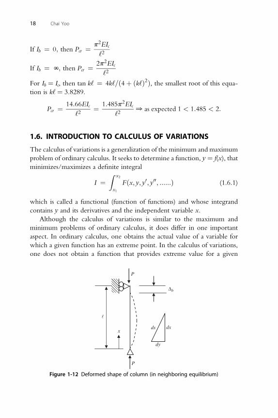
Figure 1-12 Deformed shape of column (in neighboring equilibrium)

Buckling of Columns 19

integral (functional). Instead, one only obtains the governing differential

equation that the function must satisfy to make the given function have

a stationary value. Hence, the calculus of variations is not a computational

tool, but it is only a device for obtaining the governing differential equation

of the physical stationary value problem.

The bifurcation buckling behavior of a both-end-pinned column

shown in Fig. 1-12 may be examined in two different perspectives.

Consider first that the static deformation prior to buckling has taken place

and the examination is being conducted in the neighboring equilibrium

position where the axial compressive load has reached the critical value

and the column bifurcates (is disturbed) without any further increase of

the load. The strain energy stored in the elastic body due to this flexural

action is

U ¼ 1

2

Zv

sTw

3wdv ¼ 1

2

Zv

�EIy00

Iy

�ðy00yÞdv

¼ E

2

Z‘ðy00Þ2

ZA

ðyÞ2dAd‘ ¼ EI

2

Z ‘

0

ðy00Þ2dx (1.6.2)

In calculating the strain energy, the contributions from the shear strains are

generally neglected as they are very small compared to those from normal

strains.3

Neglecting the small axial shortening prior to buckling (Ds < 3‘ where3 < 0:0005}=}, hence, Ds < 0.05 % of ‘), the vertical distance, Db, due to

the flexural action can be computed as

Db ¼Z ‘

0

ds� ‘ ¼Z ‘

0

ffiffiffiffiffiffiffiffiffiffiffiffiffiffiffiffiffiffiffidx2 þ dy2

p� ‘ ¼

Z ‘

0

ffiffiffiffiffiffiffiffiffiffiffiffiffiffiffiffiffiffi1þ ðy0Þ2

qdx� ‘

¼Z ‘

0

1þ 1

2ðy0Þ2

dx� ‘ ¼ 1

2

Z ‘

0

ðy0Þ2dx

Hence, the change (loss) in potential energy of the critical load is

V ¼ �1

2P

Z ‘

0

ðy0Þ2dx (1.6.3)

3 Of course, the shear strains can be included in the formulation. The resulting equation is called the

differential equation, considering the effect of shear deformations.

20 Chai Yoo

and the total potential energy functional becomes

I ¼ P ¼ U þ V ¼ EI

2

Z ‘

0

ðy00Þ2dx� 1

2P

Z ‘

0

ðy0Þ2dx (1.6.4)

Now the task is to find a function, y ¼ f(x) which will make the total

functional, p, have a stationary value.

dP ¼ dðU þ V Þ¼ 0* necessary condition for equilibrium or stationary value

8> 0*minimum value or stable equilbrium

9

d2P

>><>>:< 0*maximum value or unstable equilbrium

¼0* neutral or neutral equilibrium

>>=>>;

* sufficient condition

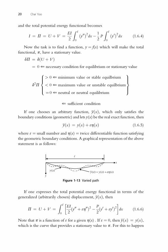
If one chooses an arbitrary function, yðxÞ, which only satisfies the

boundary conditions (geometric) and lets y(x) be the real exact function, then

yðxÞ ¼ yðxÞ þ 3hðxÞ (1.6.5)

where 3 ¼ small number and h(x) ¼ twice differentiable function satisfying

the geometric boundary conditions. A graphical representation of the above

statement is as follows:

x

y

y (x) y (x) y(x) (x)

Figure 1-13 Varied path

If one expresses the total potential energy functional in terms of the

generalized (arbitrarily chosen) displacement, yðxÞ, then

P ¼ U þ V ¼Z ‘

0

EI

2ðy00 þ 3h00Þ2 � P

2ðy0 þ 3y0Þ2

dx (1.6.6)

Note that p is a function of 3 for a given h(x) . If 3 ¼ 0, then yðxÞ ¼ yðxÞ,which is the curve that provides a stationary value to p. For this to happen

Buckling of Columns 21

����dðU þ V Þd3

����3¼0

¼ 0 (1.6.7)

Differentiating Eq. (1.6.6) under the integral sign leads to

dðU þ V Þd3

¼Z ‘

0

½EIðy00 þ 3h00Þh00 � Pðy0 þ 3h0Þh0�dx

Making use of Eq. (1.6.7) yieldsZ ‘

0

ðEIy00h00 � Py0h0Þdx ¼ 0 (1.6.8)

To simplify Eq. (1.6.8) further, use integration by parts. Consider the second

term in Eq. (1.6.8).

Let u ¼ y0; du ¼ y00; dv ¼ h0dx; v ¼ h ðR udv ¼ uv � RvduÞ

Z ‘

0

y0h0dx ¼ y0h

�����‘

0�Z ‘

0

hy00dx

¼ �Z ‘

0

hy00dx ðh satisfies the geometric bc’sÞ (a)

Similarly,Z ‘

0

y00h00dx ¼ y00h0�����‘

0�Z ‘

0

h0y000dx ¼ y00h0�����‘

0� y000h

�����‘

0þZ ‘

0

yivhdx

(b)

Equations (a) and (b) lead toZ ‘

0

ðEIyiv þ Py00Þhdxþ ðEIy00h0Þ�����‘

0¼ 0 (1.6.9)

Except h(0) ¼ h(‘) ¼ 0, h(x) is completely arbitrary and therefore nonzero;

hence, the only way to hold Eq. (1.6.9) to be true is that each part of

Eq. (1.6.9) must vanish simultaneously. That isZ ‘

0

ðEIyiv þ Py00Þhdx ¼ 0 and ðEIy00h0Þ�����‘

0¼ 0

Since h0(0), h0(1), and h(x) are not zero and h0(0) s h0(‘), it follows thaty(x) must satisfy

22 Chai Yoo

EIyiv þ Py00 ¼ 0*Euler-Lagrange differential equation (1.6.10)

EIy00j ¼ 0* natural boundary condition (1.6.11)

x¼0

EIy00j ¼ 0* natural boundary condition (1.6.12)

x¼‘

It is recalled that one imposed the geometric boundary conditions, y(0) ¼y(‘) ¼ 0 at the beginning; however, it can be shown that these conditions are

not necessarily required. Shames andDym (1985) elegantlyexplain the case for

the problem that has the properties of being self-adjoint and positive definite.

The governing differential equation can be obtained either by (1)

considering the equilibrium of deformed elements of the system or (2) using

the principle of stationary potential energy and the calculus of variations.

For a simple system such as a simply supported column buckling, method

(1) is much easier to apply, but for a complex system such as cylindrical or

spherical shell or plate buckling, method (2) is preferred as the concept is

almost automatic although the mathematical manipulations involved are

fairly complex. In dealing with the total potential energy, the kinematic (or

geometric) boundary conditions involve displacement conditions (deflec-

tion or slope) of the boundary, while natural boundary conditions involve

internal force conditions (moment or shear) at the boundary.

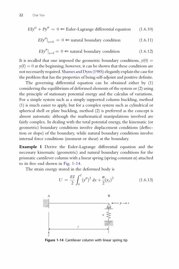
Example 1 Derive the Euler-Lagrange differential equation and the

necessary kinematic (geometric) and natural boundary conditions for the

prismatic cantilever column with a linear spring (spring constant a) attached

to its free end shown in Fig. 1-14.

The strain energy stored in the deformed body is

U ¼ EI

2

Z ‘

0

ðy00Þ2 dxþ a

2ðy‘Þ2 (1.6.13)

y

x

A B

a

P

l

Figure 1-14 Cantilever column with linear spring tip

Buckling of Columns 23

The loss of potential energy of the external load due to the deformation to

the neighboring equilibrium position is

V ¼ �P

2

Z ‘

0

ðy0Þ2dx (1.6.14)

Hence, the total potential energy functional becomes

P ¼ U þ V ¼ EI

2

Z ‘

0

ðy00Þ2dxþ a

2ðy‘Þ2 �

P

2

Z ‘

0

ðy0Þ2dx

or

P ¼Z ‘

0

EI

2ðy00Þ2 � P

2ðy0Þ2

dxþ a

2ðy‘Þ2 (1.6.15)

The total potential energy functional must be stationary if the first variation

dP ¼ 0. Since the differential operator and the variational operator are

interchangeable, one obtains

dP ¼Z ‘

0

ðEIy00dy00 � Py0dy0Þdxþ ay‘dy‘ ¼ 0 (1.6.16)

Integrating by parts each term in the parenthesis of Eq. (1.6.16) yields

Z ‘

0

EIy00dy00dx ¼ ½EIy00dy0�‘

0� ½EIy000dy�

‘

0þZ ‘

0

EIyIV dydx (1.6.17)

Z ‘ ‘ Z ‘

�0

Py0dy0dx ¼ �½Py0dy�0þ

0

Py00dydx (1.6.18)

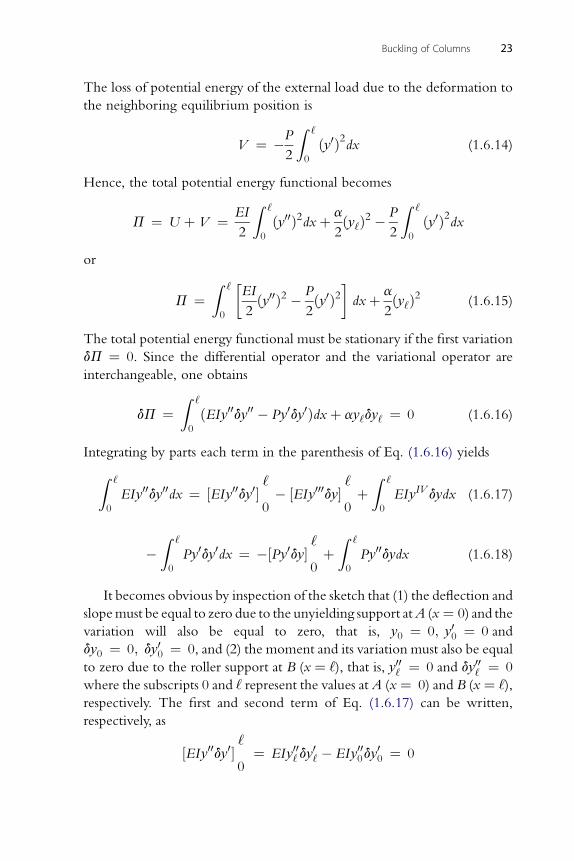
It becomes obvious by inspection of the sketch that (1) the deflection and

slopemust be equal to zero due to the unyielding support atA (x ¼ 0) and the

variation will also be equal to zero, that is, y0 ¼ 0; y00 ¼ 0 and

dy0 ¼ 0; dy00 ¼ 0, and (2) the moment and its variation must also be equal

to zero due to the roller support at B (x ¼ ‘), that is, y00‘ ¼ 0 and dy00‘ ¼ 0

where the subscripts 0 and ‘ represent the values at A (x ¼ 0) and B (x ¼ ‘),respectively. The first and second term of Eq. (1.6.17) can be written,

respectively, as

½EIy00dy0�‘

0¼ EIy00‘ dy

0‘ � EIy000dy

00 ¼ 0

24 Chai Yoo

and

� ½EIy000dy�‘

0¼ �EIy000‘ dy‘ þ EIy0000 dy0 ¼ �EIy000‘ dy‘:

The first term of Eq. (1.6.18) can be written as

� ½Py0dy�‘

0¼ �Py0‘dy‘ þ Py00dy0 ¼ �Py0‘dy‘

Equation (1.6.16) may now be rearranged

dp ¼ ðay‘ � EIy000‘ � Py0‘Þdy‘ þZ ‘

0

ðEIyIV þ Py00Þdydx ¼ 0 (1.6.19)

It is noted here in Eq. (1.6.19) that dy‘ is not zero. In order for Eq. (1.6.19)

to be equal to zero for all values of dy between x¼ 0 and x ¼ ‘, it is requiredthat the function ymust satisfy the Euler-Lagrange differential equation (the

integrand inside the parenthesis)

EIyIV þ Py00 ¼ 0 (1.6.20)

and additional condition

ay‘ � EIy000‘ � Py0‘ ¼ 0 (1.6.21)

must be met.

Equation (1.6.21), along with the condition y00‘ ¼ 0, are the natural

boundary conditions of the problem, and y0 ðand=or dy0Þ ¼ 0 y00 ðand=or dy00Þ ¼ 0 are the geometric boundary conditions of the problem.

Hence, four boundary conditions are available as required for a fourth-order

differential equation. The sum of all of the expanded integral terms at the

end points consisting of a multiple of the geometric boundary conditions

and/or the natural boundary conditions is collectively called a conjunct or

a concomitant and is equal to zero for all positive definite and self-adjoint

problems.

1.7. DERIVATION OF BEAM-COLUMN GDE USINGFINITE STRAIN

Recall the following Green-Lagrange finite strain:

eij ¼ 1

2ðui;j þ uj;i þ uk;iuk;jÞ (1.7.1)

� �2

� �2 � �2

exx ¼ dux

dxþ 1

2

dux

dxþ duy

dxþ duz

dx* axial strain (1.7.2)

U

P

y Prismatic member

xP

w (x)

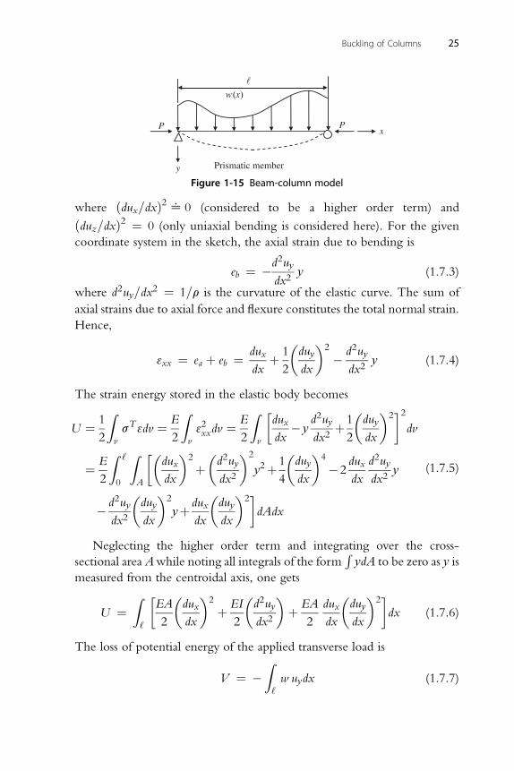
Figure 1-15 Beam-column model

Buckling of Columns 25

where ðdux=dxÞ2^ 0 (considered to be a higher order term) and

ðduz=dxÞ2 ¼ 0 (only uniaxial bending is considered here). For the given

coordinate system in the sketch, the axial strain due to bending is

eb ¼ �d2uy

dx2y (1.7.3)

where d2uy=dx2 ¼ 1=r is the curvature of the elastic curve. The sum of

axial strains due to axial force and flexure constitutes the total normal strain.

Hence,

3xx ¼ ea þ eb ¼ dux

dxþ 1

2

�duy

dx

�2

� d2uy

dx2y (1.7.4)

The strain energy stored in the elastic body becomes

¼ 1

2

Zv

sT 3dv ¼ E

2

Zv

32xxdv ¼E

2

Zv

dux

dx� y

d2uy

dx2þ1

2

�duy

dx

�22dv

¼ E

2

Z ‘

0

ZA

�dux

dx

�2

þ�d2uy

dx2

�2

y2þ1

4

�duy

dx

�4

�2dux

dx

d2uy

dx2y

� d2uy

dx2

�duy

dx

�2

yþ dux

dx

�duy

dx

�2dAdx

(1.7.5)

Neglecting the higher order term and integrating over the cross-

sectional area Awhile noting all integrals of the formRydA to be zero as y is

measured from the centroidal axis, one gets

U ¼Z‘

EA

2

�dux

dx

�2

þ EI

2

�d2uy

dx2

�þ EA

2

dux

dx

�duy

dx

�2dx (1.7.6)

The loss of potential energy of the applied transverse load is

V ¼ �Z‘w uydx (1.7.7)

26 Chai Yoo

Hence, the total potential energy functional of the system becomes

P ¼ U þV ¼Z‘

EA

2

�dux

dx

�2

þEI

2

�d2uy

dx2

�þEA

2

dux

dx

�duy

dx

�2

�w uy

dx

(1.7.8)

or

P ¼ U þ V ¼Z‘

EA

2

�dux

dx

�2

þ EI

2

�d2uy

dx2

�� P

2

�duy

dx

�2

� w uy

dx

(1.7.9)

Note that P ¼ sA ¼ EAea ¼ EAðdux=dxÞ, which is called the stress

resultant. The negative sign corresponds to the fact that P is in compression.

The quantity inside the square bracket, the integrand, is denoted by F.

Applying the principle of the minimum potential energy (or applying the

Euler-Lagrange differential equation), one obtains

F ¼ EA

2ðu0Þ2 þ EI

2ðy00Þ2 � P

2ðy0Þ2 � wy (1.7.10)

where u ¼ ux, y ¼ uy .

Recall the Euler-Lagrange DE (see Bleich 1952, pp. 91–103):

Fu � d

dxFu0 þ d2

dx2Fu00 � ::: ¼ 0 (1.7.11)

d d2

Fy �

dxFy0 þ

dx2Fy00 � ::: ¼ 0 (1.7.12)

d

Fu ¼ 0; Fu0 ¼ EAu00�

dxFu0 ¼ �EAu00; Fu00 ¼ 0

EAu00 ¼ 0 (1.7.13)

d

Fy ¼ �w; Fy0 ¼ �Py00�

dx¼ Py00;

Fy00 ¼ EIy000d2

dx2Fy00 ¼ EIyiv

EIyiv þ Py00 ¼ w (1.7.14)

Buckling of Columns 27

It should be noted that the concept of finite axial strain implicitly implies the

buckled shape (lateral displacement) and any prebuckling state is ignored.

1.8. GALERKIN METHOD

The requirement that the total potential energy of a hinged column has

a stationary value is shown in the following equation:Z ‘

0

ðEIyiv þ Py00Þdydxþ ðEIy00Þdy0�����‘

0¼ 0 (1.8.1)

where dy is a virtual displacement.

Assume that it is possible to approximate the deflection of the column by

a series of independent functions, gi(x), multiplied by undetermined coef-

ficients, ai.

yapprox ^ a1g1ðxÞ þ a2g2ðxÞ þ ::::::þ angnðxÞ (1.8.2)

If each gi(x) satisfies the geometric and natural boundary conditions, then

the second term in Eq. (1.8.1) vanishes when it substitutes yapprox to y. Also,

the coefficients, ai , must be chosen such that yapproxwill satisfy the first term.

Let the operator be

Q ¼ EId4

dx4þ P

d2

dx2(1.8.3)

and

f ¼Xni¼ 1

aigiðxÞ (1.8.4)

From Eqs. (1.8.3) and (1.8.4), the first term of Eq. (1.8.1.) becomes:Z ‘

0

QðfÞdf dx ¼ 0 (1.8.5)

Since f is a function of n parameters, ai,

df ¼ vf

va1da1 þ vf

va2da2 þ ::::þ vf

vandan

¼ g1da1 þ g2da2 þ :::::þ gndan ¼Xni¼ 1

gidai

(1.8.6)

Z ‘ Xn

0

QðfÞi¼ 1

giðxÞdai dx ¼ 0 (1.8.7)

28 Chai Yoo

Since it has been assumed that gi(x) are independent of each other, the

only way to hold Eq. (1.8.7) is that each integral of Eq. (1.8.7) must vanish,

that is Z ‘

0

QðfÞgiðxÞdai dx ¼ 0 i ¼ 1; 2; :::::; n

ai are arbitrary; hence dai s 0.Z ‘

0

QðfÞgiðxÞdx ¼ 0 i ¼ 1; 2; :::::; n (1.8.8)

Equation (1.8.8) is somewhat similar to the weighted integral process in the

finite element method.

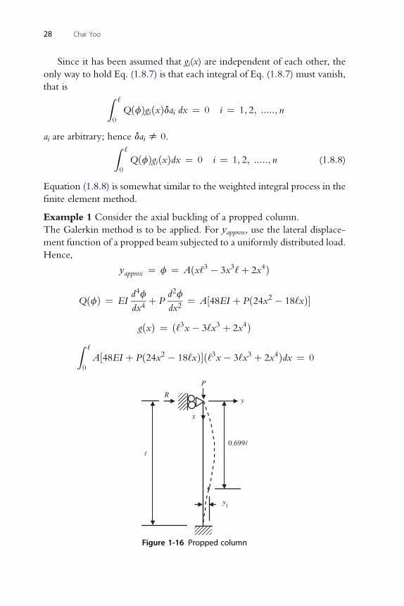
Example 1 Consider the axial buckling of a propped column.

The Galerkin method is to be applied. For yapprox, use the lateral displace-

ment function of a propped beam subjected to a uniformly distributed load.

Hence,

yapprox ¼ f ¼ Aðx‘3 � 3x3‘þ 2x4Þ

d4f d2f

QðfÞ ¼ EI

dx4þ P

dx2¼ A½48EI þ Pð24x2 � 18‘xÞ�

3 3 4

gðxÞ ¼ ð‘ x� 3‘x þ 2x ÞZ ‘

0

A½48EI þ Pð24x2 � 18‘xÞ�ð‘3x� 3‘x3 þ 2x4Þdx ¼ 0

x

y1

yR

P

0.699

Figure 1-16 Propped column

Buckling of Columns 29

Carrying out the integration gives

A�ð36EI‘5=5Þ � ð12P‘7=35Þ

�¼ 00As0 for a nontrivial solution

Pcr ¼ 21EI=‘2*3:96% greater than the exact value, Pcr exact ¼ 20:2EI=‘2

1.9. CONTINUOUS BEAM-COLUMNS RESTINGON ELASTIC SUPPORTS

A general method to evaluate the minimum required spring constants of

a beam-column resting on an elastic support is to apply the slope-deflection

equations with axial compression. In order to simplify the illustration, all

beam-columns are assumed to be rigid and equal spans.

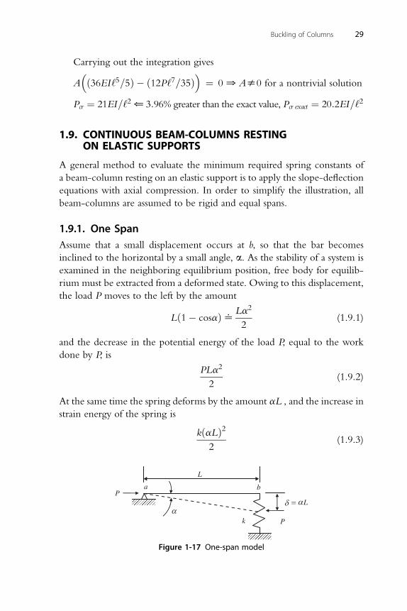
1.9.1. One SpanAssume that a small displacement occurs at b, so that the bar becomes

inclined to the horizontal by a small angle, a. As the stability of a system is

examined in the neighboring equilibrium position, free body for equilib-

rium must be extracted from a deformed state. Owing to this displacement,

the load P moves to the left by the amount

Lð1� cosaÞ^La2

2(1.9.1)

and the decrease in the potential energy of the load P, equal to the work

done by P, is

PLa2

2(1.9.2)

At the same time the spring deforms by the amount aL , and the increase in

strain energy of the spring is

kðaLÞ22

(1.9.3)

P

LP

k

ba

L

Figure 1-17 One-span model

30 Chai Yoo

where k denotes the spring constant. The system will be stable if

kðaLÞ22

>PLa2

2(1.9.4)

and will be unstable if

kðaLÞ22

<PLa2

2(1.9.5)

Therefore the critical value of the load P is found from the condition

that

kðaLÞ22

¼ PLa2

2(1.9.6)

from which

k ¼ bPcr

L0b ¼ 1 (1.9.7)

The same conclusion can be reached by considering the equilibrium of

the forces acting on the bar. However, if the system has three or more

springs, simple statics may not be sufficient to determine the small

displacement associated with each spring. Hence, the energy method

appears to be better suited.

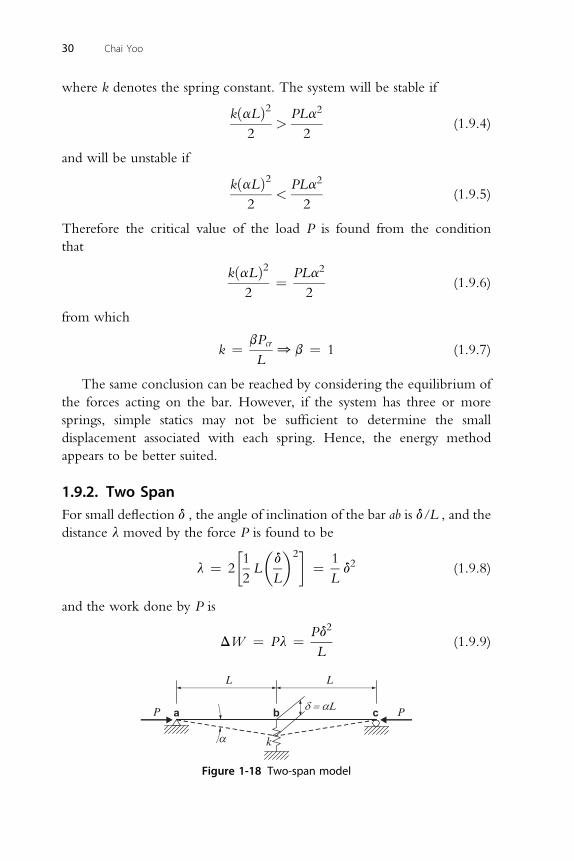
1.9.2. Two SpanFor small deflection d , the angle of inclination of the bar ab is d/L , and the

distance l moved by the force P is found to be

l ¼ 2

1

2L

�d

L

�2¼ 1

Ld2 (1.9.8)

and the work done by P is

DW ¼ Pl ¼ Pd2

L(1.9.9)

P P

L L

k

a b c

Figure 1-18 Two-span model

Buckling of Columns 31

The strain energy stored in the spring is

DU ¼ kd2

2(1.9.10)

The critical value of the load P is found from the equation

DU ¼ DW (1.9.11)

which represents the condition when the equilibrium configuration

changes from stable to unstable. Hence,

k ¼ bPcr

L¼ 2Pcr

L0b ¼ 2 (1.9.12)

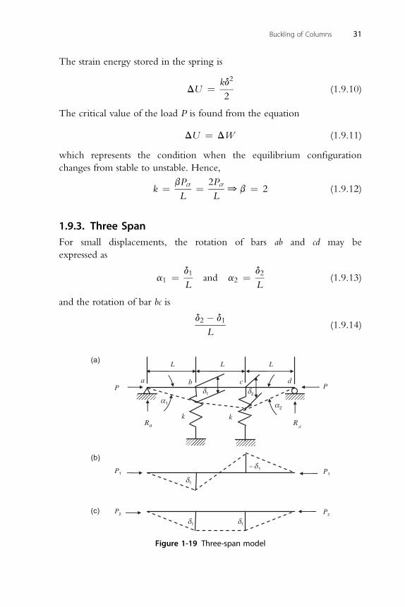
1.9.3. Three SpanFor small displacements, the rotation of bars ab and cd may be

expressed as

a1 ¼ d1

Land a2 ¼ d2

L(1.9.13)

and the rotation of bar bc is

d2 � d1

L(1.9.14)

aR

L L

P P

P1

P2

P1

P2

dba c

k kd

R

1

1

12

2

1 1

– 1

L(a)

(b)

(c)

Figure 1-19 Three-span model

32 Chai Yoo

The distance l moved by the force P is found to be

l ¼ 1

2L

�d1

L

�2

þ�d2 � d1

L

�2

þ�d2

L

�2

¼ 1

2Lðd21 þ d22 þ d21 � 2d1d2 þ d22Þ ¼ 1

Lðd21 � d1d2 þ d22Þ (1.9.15)

and the work done by the force P is

DW ¼ Pl ¼ P

Lðd21 � d1d2 þ d22Þ (1.9.16)

The strain energy stored in the elastic supports during buckling is

DU ¼ k

2ðd21 þ d22Þ (1.9.17)

The critical condition is found by equating these two expressions

P

Lðd21 � d1d2 þ d22Þ ¼ k

2ðd21 þ d22Þ0 P ¼ kL

2

d21 þ d22

d21 � d1d2 þ d22¼ kL

2

N

D

(1.9.18)

where N and D represent the numerator and denominator of the fraction.

To find the critical value of P, one must adjust the deflections d1 and d2,

which are unknown, so as to make P a minimum value. This is accom-

plished by setting vP=vd1 ¼ 0 and vP=vd2 ¼ 0.

vP

vd1¼ kL

2

DðvN=vd1Þ �NðvD=vd1ÞD2

¼ 00

vN

vd1�N

D

vD

vd1¼ vN

vd1� 2P

kL

vD

vd1¼ 0 (1.9.19)

Similarly,vN

vd2� 2P

kL

vD

vd2¼ 0 (1.9.20)

and

vN

vd1¼ 2d1;

vN

vd2¼ 2d2;

vD

vd1¼ 2d1 � d2;

vD

vd2¼ 2d2 � d1 (1.9.21)

Substituting these values, one obtains

2d1 � 2P

kLð2d1 � d2Þ ¼ d1

�1� 2P

kL

�þ d2

P

kL¼ 0 (1.9.22)

2P P�

2P�

2d2 �kL

ð2d2 � d1Þ ¼ d1kL

þ d2 1�kL

¼ 0 (1.9.23)

For nontrivial solutions, the coefficient determinant must vanish.

Hence,

1� 2P

kL

P

kL

P

kL1�2P

kL

��������

��������¼ 00

�1� 2P

kL

�2

��P

kL

�2

¼ 00P1 ¼ kL

3; P2 ¼ kL

(1.9.24)

The critical load P1 corresponds to the buckling mode shape shown in

Fig. 1-19(b), and the critical load P2 corresponds to the buckling mode

shape shown in Fig. 1-19(c). For a given system, the critical load is the small

one. Hence, P1 is the correct solution. Hence,

k ¼ bPcr

L¼ 3Pcr

L0b ¼ 3 (1.9.25)

The same problem can be solved readily by using equations of equi-

librium. Noting that the reactive force of the spring is given by kd, the end

reactions are

Ra ¼ 2

3kd1 þ 1

3kd2 (1.9.26)

1 2

Buckling of Columns 33

Rd ¼3kd1 þ

3kd2 (1.9.27)

Another equation for Ra is found by taking the moment about point B for

bar ab, which gives

Pd1 ¼ RaL (1.9.28)

and similarly, for ad

Pd2 ¼ RdL (1.9.29)

Combining these four equations yields

P

Ld1 ¼ 2

3kd1 þ 1

3kd20 d1

�2� 3P

kL

�þ d2 ¼ 0 (1.9.30)

P 1 2�

3P�

Ld2 ¼

3kd1 þ

3kd20 d1 þ d2 2�

kL¼ 0 (1.9.31)

34 Chai Yoo

Setting the determinant equal to zero yields”

2� 3P

kL1

1 2� 3P

kL

��������

��������¼

�2� 3P

kL

�2

� 1 ¼ 00P1 ¼ kL

3and P2 ¼ kL

(1.9.32)

By definition, P1 is the correct solution.

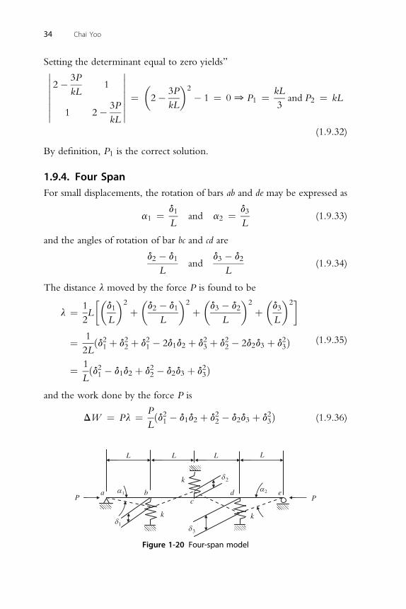
1.9.4. Four SpanFor small displacements, the rotation of bars ab and de may be expressed as

a1 ¼ d1

Land a2 ¼ d3

L(1.9.33)

and the angles of rotation of bar bc and cd are

d2 � d1

Land

d3 � d2

L(1.9.34)

The distance l moved by the force P is found to be

l ¼ 1

2L

�d1

L

�2

þ�d2 � d1

L

�2

þ�d3 � d2

L

�2

þ�d3

L

�2

¼ 1

2Lðd21 þ d22 þ d21 � 2d1d2 þ d23 þ d22 � 2d2d3 þ d23Þ

¼ 1

Lðd21 � d1d2 þ d22 � d2d3 þ d23Þ

(1.9.35)

and the work done by the force P is

DW ¼ Pl ¼ P

Lðd21 � d1d2 þ d22 � d2d3 þ d23Þ (1.9.36)

L

P P

LLL

da bc

e

k

k

k1

2

3

1 2

Figure 1-20 Four-span model

Buckling of Columns 35

The strain energy stored in the elastic supports during buckling is

DU ¼ k

2ðd21 þ d22 þ d23Þ (1.9.37)

The critical condition is found by equating these two expressions

P

Lðd21 � d1d2 þ d22 � d2d3 þ d23Þ ¼ k

2ðd21 þ d22 þ d23Þ0

P ¼ kL

2

d21 þ d22 þ d23

d21 � d1d2 þ d22 � d2d3 þ d23¼ kL

2

N

D(1.9.38)

where N and D represent the numerator and denominator of the fraction.

To find the critical value of P, one must adjust the deflections d1; d2 and d3,which are unknown, so as to make P a minimum value. This is accom-

plished by setting vP=vd1 ¼ 0; vP=vd2 and vP=vd3 ¼ 0.

vP

vd1¼ kL

2

DðvN=vd1Þ �NðvD=vd1ÞD2

¼ 00

vN

vd1�N

D

vD

vd1¼ vN

vd1� 2P

kL

vD

vd1¼ 0 (1.9.39)

Similarly,

vN

vd2� 2P

kL

vD

vd2¼ 0 (1.9.40)

vN 2P vD

vd3�

kL vd3¼ 0 (1.9.41)

and

vN

vd1¼ 2d1;

vN

vd2¼ 2d2;

vN

vd3¼ 2d3;

vD

vd1¼ 2d1 � d2;

vD

vd2¼ 2d2 � d1 � d3;

vD

vd3¼ 2d3 � d2 (1.9.42)

Substituting these values, one obtains

2d1 � 2P

kLð2d1 � d2Þ ¼ d1

�1� 2P

kL

�þ d2

P

kLþ 0d3 ¼ 0 (1.9.43)

2P P�

2P�

P

2d2 �

kLð2d2 � d1 � d3Þ ¼ d1

kLþ d2 1�

kLþ d3

kL¼ 0 (1.9.44)

2P P�

2P�

36 Chai Yoo

2d3 �kL

ð2d3 � d2Þ ¼ 0 d1 þ d2kL

þ d3 1�kL

¼ 0 (1.9.45)

For nontrivial solutions, the coefficient determinant must vanish. Hence,�������������

1� 2P

kL

P

kL0

P

kL1� 2P

kL

P

kL

0P

kL1� 2P

kL

�������������¼

�1� 2P

kL

�3

� 2

�1� 2P

kL

��P

kL

�2

¼�1� 2P

kL

��1� 2P

kL

�2

� 2

�P

kL

�2¼ 0

(1.9.46)

The smallest critical load P1 ¼ 0.29289kL corresponds to the buckling

mode shape shown in sketch.

k ¼ bPcr

L¼ Pcr

0:29289L¼ 3:414Pcr

L0 b ¼ 3:414 (1.9.47)

The equilibrium method cannot be applied to problems with three or

more elastic supports as there are only two equations of equilibrium avail-

able, that is,P

moment ¼ 0 andP

vertical force ¼ 0. It is further noted

that b varies from 1 for one span to 4 for infinite equal spans. Since b equals

3.414 for four equal spans, the use of b ¼ 4 for multistory frames would

seem justified.

Compression members in real structures are not perfectly straight

(sweep, camber), perfectly aligned, or concentrically loaded as is assumed in

design calculations; there is always an initial imperfection. Examining the

single-story column of Fig. 1-17 assuming there is an initial deflection d0reveals that the following equilibrium equation is required:

ðkdÞL ¼ Pðdþ d0Þ (1.9.48)

for P ¼ Pcr

kreqd ¼ Pcr

L

�1þ d0

d

�(1.9.49)

Buckling of Columns 37

Since kideal ¼ Pcr=L, Eq. (1.9.48) becomes

kreqd ¼ kideal

�1þ d0

d

�(1.9.50)

which is the stiffness requirement for compression members having initial

imperfection d0. The stiffness requirement is

Q ¼ kreqdd ¼ kideal

�1þ d0

d

�d ¼ kidealðdþ d0Þ (1.9.51)

Winter (1960) has suggested d ¼ d0 ¼ L/500. Substitution of this into Eqs.

(1.9.49) and (1.9.50) gives the following design equations:

For stiffness; kreqd ¼ 2kideal (1.9.52)

For nominal strength

Qn ¼ kidealð2d0Þ ¼ kidealð0:004LÞ ¼ bPcr

Lð0:004LÞ (1.9.53)

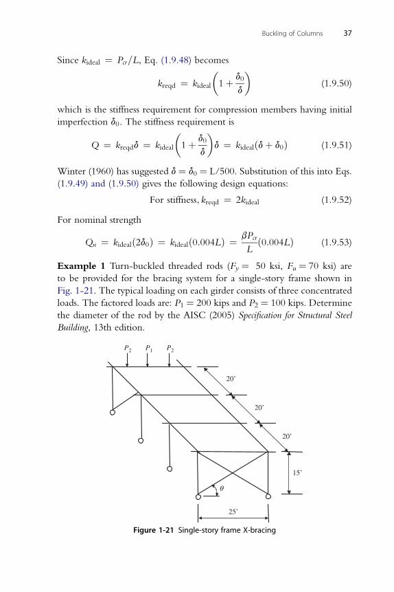
Example 1 Turn-buckled threaded rods (Fy ¼ 50 ksi, Fu ¼ 70 ksi) are

to be provided for the bracing system for a single-story frame shown in

Fig. 1-21. The typical loading on each girder consists of three concentrated

loads. The factored loads are: P1 ¼ 200 kips and P2 ¼ 100 kips. Determine

the diameter of the rod by the AISC (2005) Specification for Structural Steel

Building, 13th edition.

P1 P2P2

20’

20’

20’

15’

25’

Figure 1-21 Single-story frame X-bracing

38 Chai Yoo

XP ¼ 4� ð200þ 2� 100Þ ¼ 1; 600 kips;b ¼ 1;Ae ¼ UAn

¼ 1� An

25

Qu ¼ 1� 1; 600� 0:004 ¼ 6:4 kips; cos q ¼ ffiffiffiffiffiffiffiffiffiffiffiffiffiffiffiffiffiffiffiffiffiffiffið252 þ 152Þp ¼ 0:8575

Design for strength:

Qn for yielding; Qn ¼ Qu=0:9 ¼ 6:4=0:9 ¼ 7:11 kips

Q for fracture;Q ¼ Q =0:75 ¼ 6:4=0:75 ¼ 8:53 kips

n n u

The required diameter of the rod against yielding is

7:11 ¼ p

4� d2 � 50� 0:8575; d ¼ 0:46 in:

The required diameter of the rod against fracture is

8:53 ¼ p

4��d � 0:9743

11

�2

� 70� 0:8575;

d ¼ 0:154 in:ð11 threads per inch is justifiedÞDesign for stiffness:

kreqd ¼ 2kideal ¼ 2bPcr

L¼ 2� 1� 1; 600

25� 12¼ EA

Lcos2 q

29; 000� p� d2 � 0:85752

10:67 ¼

4� 25� 12; d ¼ 0:44 in: < 0:514 in:; use

d ¼ 5=8 in:ð¼ 0:625 in:Þ

1.10. ELASTIC BUCKLING OF COLUMNS SUBJECTED TODISTRIBUTED AXIAL LOADS

When a column is subjected to distributed compressive forces along its

length, the governing differential equation of the deflected curve is no

longer a differential equation with constant coefficients.

The solution to this problem may be considered in three different ways:

(1) application of infinite series such as Bessel functions, (2) one of the

approximate methods, such as the energy method, and (3) the finite element

method (the solution converges to the exact one following the grid

nym

y

x

x

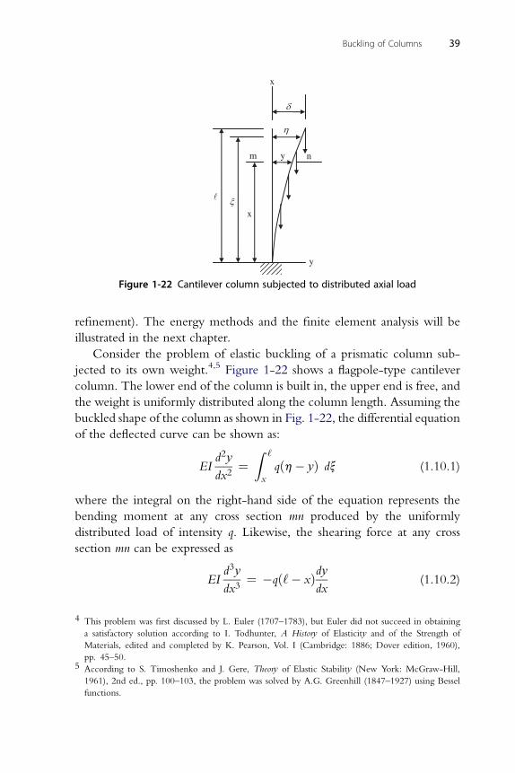
Figure 1-22 Cantilever column subjected to distributed axial load

Buckling of Columns 39

refinement). The energy methods and the finite element analysis will be

illustrated in the next chapter.

Consider the problem of elastic buckling of a prismatic column sub-

jected to its own weight.4,5 Figure 1-22 shows a flagpole-type cantilever

column. The lower end of the column is built in, the upper end is free, and

the weight is uniformly distributed along the column length. Assuming the

buckled shape of the column as shown in Fig. 1-22, the differential equation

of the deflected curve can be shown as:

EId2y

dx2¼

Z ‘

x

qðh� yÞ dx (1.10.1)

where the integral on the right-hand side of the equation represents the

bending moment at any cross section mn produced by the uniformly

distributed load of intensity q. Likewise, the shearing force at any cross

section mn can be expressed as

EId3y

dx3¼ �qð‘� xÞdy

dx(1.10.2)

4 This problem was first discussed by L. Euler (1707–1783), but Euler did not succeed in obtaining

a satisfactory solution according to I. Todhunter, A History of Elasticity and of the Strength of

Materials, edited and completed by K. Pearson, Vol. I (Cambridge: 1886; Dover edition, 1960),

pp. 45–50.5 According to S. Timoshenko and J. Gere, Theory of Elastic Stability (New York: McGraw-Hill,

1961), 2nd ed., pp. 100–103, the problem was solved by A.G. Greenhill (1847–1927) using Bessel

functions.

40 Chai Yoo

Note that the moment given in Eq. (1.10.1) is a decreasing function against

the x-axis, and hence, the rate of change of the moment must be negative as

shown in Eq. (1.10.2). Equation (1.10.2) is an ordinary differential equation

with a variable coefficient. Many differential equations with variable

coefficients can be reduced to Bessel equations. In order to facilitate the

solution, a new independent variable z is introduced such that

z ¼ 2

3

ffiffiffiffiffiffiffiffiffiffiffiffiffiffiffiffiffiffiffiffiffiq

EIð‘� xÞ3

r(1.10.3)

By taking successive derivatives, one obtains

dy

dx¼ dy

dz

dz

dx¼ �dy

dz

ffiffiffiffiffiffiffiffiffi3

2

qz

EI

3

r(1.10.4)

2� �2

3

�2�

d y

dx2¼ 3

2

q

EI

1

3z�

13dy

dzþ z

23d y

dz2(1.10.5)

d3y 3 q�1 dy d2y d3y

�

dx3

¼2 EI 9

z�1

dz�dz2

� zdz3

(1.10.6)

Substituting Eqs. (1.10.4) and (1.10.5) into Eq. (1.10.2) and letting

dy

dz¼ u (1.10.7)

One obtains

d2u

dz2þ 1

z

du

dzþ�1� 1

9z2

�u ¼ d2u

dz2þ 1

z

du

dzþ�1� p2

z2

�u ¼ 0 (1.10.8)

Equation (1.10.8) is a Bessel equation, and its solution can be expressed in

terms of Bessel functions.

Invoking the method of Frobenius,6 it is assumed that a solution of the

form

uðzÞ ¼XNn¼ 0

cnzrþn (1.10.9)

exists for Bessel’s equation, Eq. (1.10.8) of 7 order p (�1=3 in this case).

Substituting Eq. (1.10.9) into Eq. (1.10.8), one obtains:

6 Frobenius (1848–1917) was a German mathematician.7 See, for example, S.I. Grossman and W.R. Derrick, Advanced Engineering Mathematics (New York:

Harper & Row, 1988), pp. 272–274.

Buckling of Columns 41

XNn¼ o

cnðr þ nÞðr þ n� 1Þzrþn�2 þXNn¼ o

cnðr þ nÞzrþn�2 þXNn¼ o

ð�p2Þcnzrþn�2

þXNn¼ 2

cn�2zrþn�2 ¼ 0

or

c0ðr2 � p2Þzr�2 þ c1½ðr þ 1Þ2 � p2�zr�1

þXNn¼ 2

fcn½ðnþ rÞ2 � p2� þ cn�2gzrþn�2 ¼ 0(1.10.10)

The indicial equation is r2 � p2 ¼ 0 with roots r1 ¼ p ¼ 1/3 and

r2 ¼ �p ¼ �1/3. Setting r ¼ p in Eq. (1.10.10) yields

ð1þ 2pÞc1zp�1 þXNn¼ 2

½nðnþ 2pÞcn þ cn�2�znþp�2 ¼ 0

�cn�2

indicating that c1 ¼ 0 and cn ¼

nðnþ 2pÞ; for n � 2: (1.10.11)

Hence, all the coefficients with odd-numbered subscripts equal to zero.

Letting n ¼ 2j þ 2 one sees that the coefficients with even-numbered

subscripts satisfy

c2ðjþ1Þ ¼ �c2j

22ðj þ 1Þðpþ j þ 1Þ; for j � 0;

which yields

c2 ¼ �c0

22ðpþ 1Þ; c4 ¼ �c2

22ð2Þðpþ 2Þ ¼ c0

24ð2!Þðpþ 1Þðpþ 2Þ;

c6 ¼ �c4

22ð3Þðpþ 3Þ ¼ �c0

26ð3!Þðpþ 1Þðpþ 2Þðpþ 3Þ;.::

Hence, the series of Eq. (1.10.9) becomes

u1 ¼ zpc0 � c0

22ðpþ 1Þz2 þ c0

242!ðpþ 1Þðpþ 2Þz4 � :::

¼ c0zpXNn¼ 0

ð�1Þn z2n

22nn!ðpþ 1Þðpþ 2Þ:::ðpþ nÞ (1.10.12)

42 Chai Yoo

It is customary in Eq. (1.10.12) to let the integral constant,

c0 ¼ ½2pGðpþ 1Þ��1in which Gðpþ 1Þ is the gamma function. Then,

Eq. (1.10.12) becomes

JpðzÞ ¼ ðz=2ÞpXNn¼ 0

ð�1Þn ðz=2Þ2nn!Gðpþ nþ 1Þ

which is known as the Bessel function of the first kind of order p. Thus Jp(z)

is the first solution of Eq. (1.10.8). One will again be able to apply the

method of Frobenius with r ¼ �p to find the second solution. From

Eq. (1.10.10), one immediately obtains

ð1� 2pÞc1z�p�1 þXNn¼ 2

½nðn� 2pÞcn þ cn�2�zn�p�2 ¼ 0 (1.10.13)

indicating c1 ¼ 0 as before and

cn ¼ �cn�2

nðn� 2pÞ (1.10.14)

With algebraic operations similar to those done earlier, one obtains the

second solution of Eq. (1.10.8)

J�pðzÞ ¼ ðz=2Þ�pXNn¼ 0

ð�1Þn ðz=2Þ2nn!Gðn� pþ 1Þ (1.10.15)

Hence, the complete solution of Eq. (1.10.8) is

uðzÞ ¼ u1ðzÞ þ u2ðzÞ ¼ AJpðzÞ þ BJ�pðzÞ (1.10.16)

In Eq. (1.10.16), A and B are constants of integration, and they must be

determined from the boundary conditions of the column. Since the upper

end of the column is free, the condition yields�d2y

dx2

�x¼‘

¼ 0

Observing that z ¼ 0 at x ¼ ‘ and using Eqs. (1.10.5) and (1.10.7), one canexpress this condition as�

1

3z�

13uþ z

23du

dz

�z¼0

¼ 0

Substituting Eq. (1.10.16) into this equation, one obtains A ¼ 0 and

hence

uðzÞ ¼ BJ�pðzÞ (1.10.17)

Buckling of Columns 43

At the lower end of the column the condition is

�dy

dx

�x¼0

¼ 0

With the use of Eqs. (1.10.3), (1.10.4), and (1.10.7), this condition is

expressed in the form

u ¼ 0 when z ¼ 2

3

ffiffiffiffiffiffiq‘3

EI

r:

The value of z which makes u ¼ 0 can be found from Eq. (1.10.17) by trial

and error, from a table of the Bessel function of order �(1/3) , or from

a computerized symbolic algebraic code such as Maple�. The lowest value

of zwhich makes u¼ 0, corresponding to the lowest buckling load, is found

from Maple� to be z ¼ 1.866350859, and hence

z ¼ 2

3

ffiffiffiffiffiffiq‘3

EI

r¼ 1:866

or

ðqlÞcr ¼ 7:837EI

‘2: (1.10.18)

This is the critical value of the uniform load for the column shown in

Fig. 1-22.

Equation (1.10.2) above is differentiated once more to derive the gov-

erning equation of the buckling of the column under its own weight as

EId2

dx2

�d2y

dx2

�þ q

d

dx

ð‘� xÞdy

dx

¼ 0 (1.10.19)

Equation (1.10.19) is accompanied by appropriate boundary conditions. For

the column that is pinned, clamped, and free at its end, the boundary

conditions are, respectively

y ¼ 0;d2y

dx2¼ 0 (1.10.20a)

dy

y ¼ 0;

dx¼ 0 (1.10.20b)

2 3

d y

dx2¼ 0;

d y

dx3¼ 0 (1.10.20c)

44 Chai Yoo

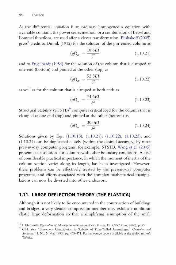
As the differential equation is an ordinary homogeneous equation with

a variable constant, the power series method, or a combination of Bessel and

Lommel functions, are used after a clever transformation. Elishakoff (2005)

gives8 credit to Dinnik (1912) for the solution of the pin-ended column as

ðq‘Þcr ¼ 18:6EI

‘2(1.10.21)

and to Engelhardt (1954) for the solution of the column that is clamped at

one end (bottom) and pinned at the other (top) as

ðq‘Þcr ¼ 52:5EI

‘2(1.10.22)

as well as for the column that is clamped at both ends as

ðq‘Þcr ¼ 74:6EI

‘2(1.10.23)

Structural Stability (STSTB)9 computes critical load for the column that is

clamped at one end (top) and pinned at the other (bottom) as

ðq‘Þcr ¼ 30:0EI

‘2(1.10.24)

Solutions given by Eqs. (1.10.18), (1.10.21), (1.10.22), (1.10.23), and

(1.10.24) can be duplicated closely (within the desired accuracy) by most

present-day computer programs, for example, STSTB. Wang et al. (2005)

present exact solutions for columns with other boundary conditions. A case

of considerable practical importance, in which the moment of inertia of the

column section varies along its length, has been investigated. However,

these problems can be effectively treated by the present-day computer

programs, and efforts associated with the complex mathematical manipu-

lations can now be diverted into other endeavors.

1.11. LARGE DEFLECTION THEORY (THE ELASTICA)

Although it is not likely to be encountered in the construction of buildings

and bridges, a very slender compression member may exhibit a nonlinear

elastic large deformation so that a simplifying assumption of the small

8 I. Elishakoff, Eigenvalues of Inhomogeneous Structures (Boca Raton, FL: CRC Press, 2005), p. 75.9 C.H. Yoo, “Bimoment Contribution to Stability of Thin-Walled Assemblages,” Computers and

Structures, 11, No. 5 (May 1980), pp. 465–471. Fortran source code is available at the senior author’s

Website.

P P

y

x

0θ dx

dyds..sin

dy

dsθ=

Figure 1-23 Large deflection model

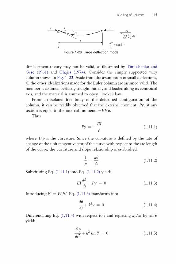
Buckling of Columns 45

displacement theory may not be valid, as illustrated by Timoshenko and

Gere (1961) and Chajes (1974). Consider the simply supported wiry

column shown in Fig. 1-23. Aside from the assumption of small deflections,

all the other idealizations made for the Euler column are assumed valid. The

member is assumed perfectly straight initially and loaded along its centroidal

axis, and the material is assumed to obey Hooke’s law.

From an isolated free body of the deformed configuration of the

column, it can be readily observed that the external moment, Py, at any

section is equal to the internal moment, �EI/r.

Thus

Py ¼ �EI

r(1.11.1)

where 1/r is the curvature. Since the curvature is defined by the rate of

change of the unit tangent vector of the curve with respect to the arc length

of the curve, the curvature and slope relationship is established.

1

r¼ dq

ds(1.11.2)

Substituting Eq. (1.11.1) into Eq. (1.11.2) yields

EIdq

dsþ Py ¼ 0 (1.11.3)

Introducing k2 ¼ P/EI, Eq. (1.11.3) transforms into

dq

dsþ k2y ¼ 0 (1.11.4)

Differentiating Eq. (1.11.4) with respect to s and replacing dy/ds by sin q

yields

d2q

ds2þ k2 sin q ¼ 0 (1.11.5)

46 Chai Yoo

Multiplying each term of Eq. (1.11.5) by 2 dq and integrating gives

Zd2q

ds22dq

dsdsþ

Z2k2 sin q dq ¼ 0 (1.11.6)

Recalling the following mathematical identities

d

ds

�dq

ds

�2

¼ 2

�dq

ds

��d2q

ds2

�and sin q dq ¼ �dðcos qÞ;

it follows immediately thatZd

�dq

ds

�2

� 2k2Z

dðcos qÞ ¼ 0 (1.11.7)

Carrying out the integration gives�dq

ds

�2

� 2k2 cos q ¼ C (1.11.8)

The integral constant C can be determined from the proper boundary

condition. That is

dq

ds¼ 0 at x ¼ 0;�moment ¼ 00

1

r¼ 0 or r ¼ N; straight line

�and q ¼ q0

Hence,

C ¼ �2k2 cos q0

and Eq. (1.11.8) becomes�dq

ds

�2

� 2k2ðcos q� cos q0Þ ¼ 0 (1.11.9)

Taking the square root of Eq. (1.11.9) and rearranging gives

ds ¼ � dqffiffiffi2

pk

ffiffiffiffiffiffiffiffiffiffiffiffiffiffiffiffiffiffiffiffiffiffiffiffiffiffifficos q� cos q0

p (1.11.10)

Notice the negative sign in Eq. (1.11.10), which implies that q decreases as s

increases. Carrying out the integral of Eq. (1.11.10) gives

Buckling of Columns 47

Z ‘=2

0

ds ¼ � 1ffiffiffi2

pk

Z 0

q0

dqffiffiffiffiffiffiffiffiffiffiffiffiffiffiffiffiffiffiffiffiffiffiffiffiffiffifficos q� cos q0

p or‘

2¼ 1ffiffiffi

2p

k

Z q0

0

dqffiffiffiffiffiffiffiffiffiffiffiffiffiffiffiffiffiffiffiffiffiffiffiffiffiffifficos q� cos q0

p

or

‘ ¼ 2

k

Z q0

0

dqffiffiffiffiffiffiffiffiffiffiffiffiffiffiffiffiffiffiffiffiffiffiffiffiffiffiffiffiffiffiffiffiffi2 cos q� 2 cos q0

p (1.11.11)

Notice the negative sign is eliminated by reversing the limits of integration.

Making use of mathematical identities

cos q ¼ 1� 2 sin2q

2and cos q0 ¼ 1� 2 sin2

q0

2

in Eq. (1.11.11) yields:

‘ ¼ 1

k

Z q0

0

dqffiffiffiffiffiffiffiffiffiffiffiffiffiffiffiffiffiffiffiffiffiffiffiffiffiffiffiffiffisin2

q0

2� sin2

q

2

r (1.11.12)

In order to simplify Eq. (1.11.12) further, let

sinq0

2¼ a (1.11.13)

and introduce a new variable f such that

sinq

2¼ a sin f (1.11.14)

Then q ¼ 00f ¼ 0 and q ¼ q00sinf ¼ 10f ¼ p=2.Differentiating Eq. (1.11.14) yields

1

2cos

q

2dq ¼ a cos f df (1.11.15)

which can be rearranged to show

dq ¼ 2a cos f dfffiffiffiffiffiffiffiffiffiffiffiffiffiffiffiffiffiffi1� sin2 q

2

q ¼ 2a cos f dfffiffiffiffiffiffiffiffiffiffiffiffiffiffiffiffiffiffiffiffiffiffiffiffiffi1� a2 sin2 f

p (1.11.16)

Substituting Eqs. (1.11.13), (1.11.14), (1.11.15), and (1.11.16) into Eq.

(1.11.12) yields

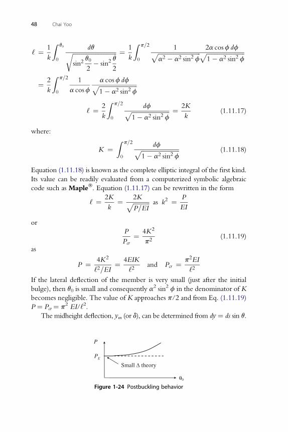
48 Chai Yoo

‘ ¼ 1

k

Z q0

0

dqffiffiffiffiffiffiffiffiffiffiffiffiffiffiffiffiffiffiffiffiffiffiffiffiffiffiffiffiffisin2

q0

2� sin2

q

2

r ¼ 1

k

Z p=2

0

1ffiffiffiffiffiffiffiffiffiffiffiffiffiffiffiffiffiffiffiffiffiffiffiffiffiffiffiffia2 � a2 sin2 f

p 2a cosf dfffiffiffiffiffiffiffiffiffiffiffiffiffiffiffiffiffiffiffiffiffiffiffiffiffi1� a2 sin2 f

p

¼ 2

k

Z p=2

0

1

a cosf

a cosf dfffiffiffiffiffiffiffiffiffiffiffiffiffiffiffiffiffiffiffiffiffiffiffiffiffi1� a2 sin2 f

pZ p=2

‘ ¼ 2

k 0

dfffiffiffiffiffiffiffiffiffiffiffiffiffiffiffiffiffiffiffiffiffiffiffiffiffi1� a2 sin2 f

p ¼ 2K

k(1.11.17)

where:

K ¼Z p=2

0

dfffiffiffiffiffiffiffiffiffiffiffiffiffiffiffiffiffiffiffiffiffiffiffiffiffi1� a2 sin2 f

p (1.11.18)

Equation (1.11.18) is known as the complete elliptic integral of the first kind.

Its value can be readily evaluated from a computerized symbolic algebraic

code such as Maple�. Equation (1.11.17) can be rewritten in the form

‘ ¼ 2K

k¼ 2Kffiffiffiffiffiffiffiffiffiffiffi

P=EIp as k2 ¼ P

EI

or

P

Pcr¼ 4K2

p2(1.11.19)

as

P ¼ 4K2

‘2=EI¼ 4EIK

‘2and Pcr ¼ p2EI

‘2

If the lateral deflection of the member is very small (just after the initial

bulge), then q0 is small and consequently a2 sin2 f in the denominator of K

becomes negligible. The value of K approaches p/2 and from Eq. (1.11.19)

P ¼ Pcr ¼ p2 EI/‘2.The midheight deflection, ym (or d), can be determined from dy¼ ds sin q.

P

PE

Small theory

0

Figure 1-24 Postbuckling behavior

Buckling of Columns 49

Substituting Eq. (1.11.10) into the above equation yields

dy ¼ � sin q dqffiffiffi2

pk

ffiffiffiffiffiffiffiffiffiffiffiffiffiffiffiffiffiffiffiffiffiffiffiffiffiffifficos q� cos q0

p

Integrating the above equation givesZ ym

0

dy ¼ � 1

2k

Z 0

q0

sinqdqffiffiffiffiffiffiffiffiffiffiffiffiffiffiffiffiffiffiffiffiffiffiffiffifficosq� cosq0

p or ym ¼ 1

2k

Z q0

0

sinqdqffiffiffiffiffiffiffiffiffiffiffiffiffiffiffiffiffiffiffiffiffiffiffiffiffiffiffisin2

q0

2� sin2

q

2

r

Recall sin ðq=2Þ ¼ a sinf and dq ¼ 2a cosf df=ffiffiffiffiffiffiffiffiffiffiffiffiffiffiffiffiffiffiffiffiffiffiffiffiffi1� a2 sin2 f

pHence,

sin q ¼ 2 sinq

2cos

q

2¼ 2 sin

q

2

ffiffiffiffiffiffiffiffiffiffiffiffiffiffiffiffiffiffiffi1� sin2

q

2

r¼ 2a sinf

ffiffiffiffiffiffiffiffiffiffiffiffiffiffiffiffiffiffiffiffiffiffiffiffiffi1� a2 sin2 f

pym ¼ 1

2k

Z q0

0

sin q dqffiffiffiffiffiffiffiffiffiffiffiffiffiffiffiffiffiffiffiffiffiffiffiffiffiffiffiffiffisin2

q0

2� sin2

q

2

r

¼ 1

2k

Z p=2

0

2a sinfffiffiffiffiffiffiffiffiffiffiffiffiffiffiffiffiffiffiffiffiffiffiffiffiffiffi1� a2 sin2 f

p2a cosf dfffiffiffiffiffiffiffiffiffiffiffiffiffiffiffiffiffiffiffiffiffiffiffiffiffiffiffiffi

a2 � a2 sin2 fp ffiffiffiffiffiffiffiffiffiffiffiffiffiffiffiffiffiffiffiffiffiffiffiffiffi

1� a2 sin2 fp

Z p=2

ym ¼ d ¼ 2a

k 0

sinf df ¼ 2a

kor

ym‘

¼ 2a

p

ffiffiffiffiffiffiP

PE

rThe distance between the two load points (x-coordinates) can be deter-

mined from

dx ¼ ds cos q

Substituting Eq. (1.11.10) into the above equation yields

dx ¼ � cos q dqffiffiffi2

pk

ffiffiffiffiffiffiffiffiffiffiffiffiffiffiffiffiffiffiffiffiffiffiffiffiffiffifficos q� cos q0

p

Integrating (xm is the x-coordinate at the midheight) the above equation

givesZ xm

0

dx ¼ � 1ffiffiffi2

pk

Z 0

q0

cos q dqffiffiffiffiffiffiffiffiffiffiffiffiffiffiffiffiffiffiffiffiffiffiffiffiffiffifficos q� cos q0

p ¼ � 1ffiffiffik

pZ 0

q0

cos q dqffiffiffiffiffiffiffiffiffiffiffiffiffiffiffiffiffiffiffiffiffiffiffiffiffiffiffiffiffiffiffiffiffi2 cos q� 2 cos q0

p or

xm ¼ 1

2k

Z q0

0

cos q dqffiffiffiffiffiffiffiffiffiffiffiffiffiffiffiffiffiffiffiffiffiffiffiffiffiffiffiffiffisin2

q0

2� sin2

q

2

r

50 Chai Yoo

Recall sin ðq=2Þ ¼ a sinf and dq ¼ 2a cosf df=ffiffiffiffiffiffiffiffiffiffiffiffiffiffiffiffiffiffiffiffiffiffiffiffiffi1� a2 sin2 f

pand cosq ¼ cos2 ðq=2Þ� sin2 ðq=2Þ ¼ 1�2sin2 ðq=2Þ ¼ 1�2a2 sin2f

xm ¼ 1

2k

Z q0

0

cos q dqffiffiffiffiffiffiffiffiffiffiffiffiffiffiffiffiffiffiffiffiffiffiffiffiffiffiffiffiffisin2

q0

2� sin2

q

2

r

¼ 1

2k

Z p=2

0

ð1� 2a2 sin2 fÞ2a cosf dfffiffiffiffiffiffiffiffiffiffiffiffiffiffiffiffiffiffiffiffiffiffiffiffiffiffiffiffia2 � a2 sin2 f

p ffiffiffiffiffiffiffiffiffiffiffiffiffiffiffiffiffiffiffiffiffiffiffiffiffi1� a2 sin2 f

p¼ 1

k

Z p=2

0

ð1� 2a2 sin2 fÞdfffiffiffiffiffiffiffiffiffiffiffiffiffiffiffiffiffiffiffiffiffiffiffiffiffi1� a2 sin2 f

pZ p=2 2 2

x0 ¼ 2xm ¼ 2

k 0

½2ð1� a sin fÞ � 1�dfffiffiffiffiffiffiffiffiffiffiffiffiffiffiffiffiffiffiffiffiffiffiffiffiffi1� a2 sin2 f

p¼ 4

k

Z p=2

0

ffiffiffiffiffiffiffiffiffiffiffiffiffiffiffiffiffiffiffiffiffiffiffiffiffi1� a2 sin2 f

pdf

� 2

k

Z p=2

0

dfffiffiffiffiffiffiffiffiffiffiffiffiffiffiffiffiffiffiffiffiffiffiffiffiffi1� a2 sin2 f

p ¼ 4

kEðaÞ � ‘

where E(a) is the complete elliptic integral of the second kind

x0

‘¼ 4EðaÞ

‘

ffiffiffiffiffiP

EI

r � 1 ¼ 4EðaÞp

ffiffiffiffiffiffiP

PE

r � 1

The complete elliptic integral of the first kind can be evaluated by an infinite

series given by

K ¼Z p=2

0

dfffiffiffiffiffiffiffiffiffiffiffiffiffiffiffiffiffiffiffiffiffiffiffiffiffi1� a2 sin2 f

p¼ p

2

1þ

�1

2

�2

a2 þ�1$3

2$4

�2

a4 þ�1$3$5

2$4$6

�2

a6 þ $$$

with a2 < 1

Summing the first four terms of the above infinite series for a ¼ 0:5 yieldsK ¼ 1.685174.

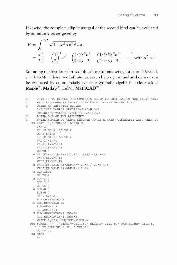
Buckling of Columns 51

Likewise, the complete elliptic integral of the second kind can be evaluated

by an infinite series given by

E ¼Z p=2

0

ffiffiffiffiffiffiffiffiffiffiffiffiffiffiffiffiffiffiffiffiffiffiffiffiffi1� a2 sin2 f

pdf

¼ p

2

1�

�1

2

�2

a2 ��1$3

2$4

�2a4

3��1$3$5

2$4$6

�2a6

5� $$$

with a2 < 1

Summing the first four terms of the above infinite series for a ¼ 0:5 yieldsE ¼1.46746. These two infinite series can be programmed as shown or can

be evaluated by commercially available symbolic algebraic codes such as

Maple�, Matlab�, and/or MathCAD�.

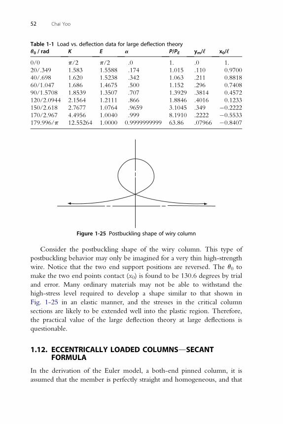
Table 1-1 Load vs. deflection data for large deflection theoryq0 / rad K E a P/PE ym/‘‘ x0/‘‘

0/0 p/2 p/2 .0 1. .0 1.

20/.349 1.583 1.5588 .174 1.015 .110 0.9700

40/.698 1.620 1.5238 .342 1.063 .211 0.8818

60/1.047 1.686 1.4675 .500 1.152 .296 0.7408

90/1.5708 1.8539 1.3507 .707 1.3929 .3814 0.4572

120/2.0944 2.1564 1.2111 .866 1.8846 .4016 0.1233

150/2.618 2.7677 1.0764 .9659 3.1045 .349 �0.2222

170/2.967 4.4956 1.0040 .999 8.1910 .2222 �0.5533

179.996/p 12.55264 1.0000 0.9999999999 63.86 .07966 �0.8407

52 Chai Yoo

Consider the postbuckling shape of the wiry column. This type of

postbuckling behavior may only be imagined for a very thin high-strength

wire. Notice that the two end support positions are reversed. The q0 to

make the two end points contact (x0) is found to be 130.6 degrees by trial

and error. Many ordinary materials may not be able to withstand the

high-stress level required to develop a shape similar to that shown in

Fig. 1-25 in an elastic manner, and the stresses in the critical column

sections are likely to be extended well into the plastic region. Therefore,

the practical value of the large deflection theory at large deflections is

questionable.

Figure 1-25 Postbuckling shape of wiry column

1.12. ECCENTRICALLY LOADED COLUMNSdSECANTFORMULA

In the derivation of the Euler model, a both-end pinned column, it is

assumed that the member is perfectly straight and homogeneous, and that

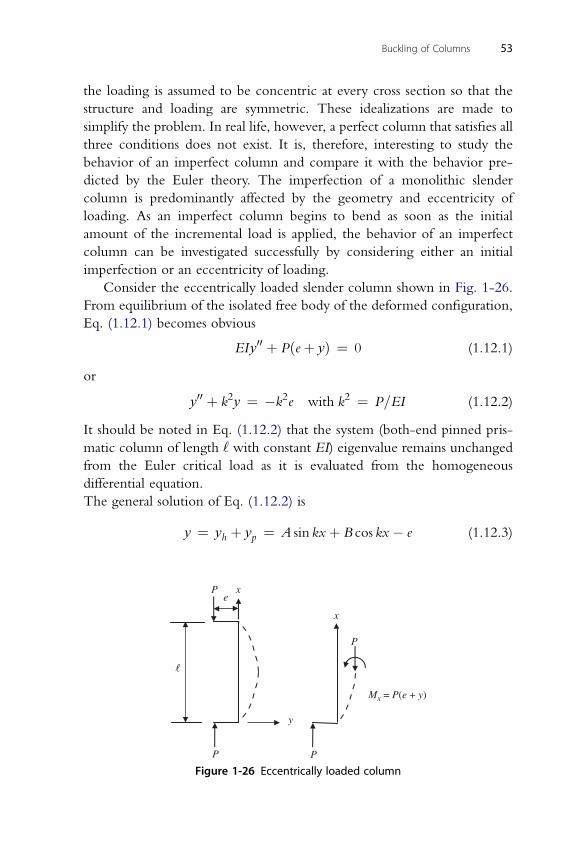
Buckling of Columns 53

the loading is assumed to be concentric at every cross section so that the

structure and loading are symmetric. These idealizations are made to

simplify the problem. In real life, however, a perfect column that satisfies all

three conditions does not exist. It is, therefore, interesting to study the

behavior of an imperfect column and compare it with the behavior pre-

dicted by the Euler theory. The imperfection of a monolithic slender

column is predominantly affected by the geometry and eccentricity of

loading. As an imperfect column begins to bend as soon as the initial

amount of the incremental load is applied, the behavior of an imperfect

column can be investigated successfully by considering either an initial

imperfection or an eccentricity of loading.

Consider the eccentrically loaded slender column shown in Fig. 1-26.

From equilibrium of the isolated free body of the deformed configuration,

Eq. (1.12.1) becomes obvious

EIy00 þ Pðeþ yÞ ¼ 0 (1.12.1)

or

y00 þ k2y ¼ �k2e with k2 ¼ P=EI (1.12.2)

It should be noted in Eq. (1.12.2) that the system (both-end pinned pris-

matic column of length ‘ with constant EI) eigenvalue remains unchanged

from the Euler critical load as it is evaluated from the homogeneous

differential equation.

The general solution of Eq. (1.12.2) is

y ¼ yh þ yp ¼ A sin kxþ B cos kx� e (1.12.3)

P x

P

P

x

e

y

P

Mx = P(e + y)

Figure 1-26 Eccentrically loaded column

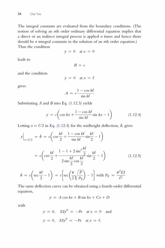
54 Chai Yoo

The integral constants are evaluated from the boundary conditions. (The

notion of solving an nth order ordinary differential equation implies that

a direct or an indirect integral process is applied n times and hence there

should be n integral constants in the solution of an nth order equation.)

Thus the conditiony ¼ 0 at x ¼ 0

leads to

B ¼ e

and the conditiony ¼ 0 at x ¼ ‘

gives

A ¼ e1� cos k‘

sin k‘

Substituting A and B into Eq. (1.12.3) yields

y ¼ e

�cos kxþ 1� cos k‘

sin k‘sin kx� 1

�(1.12.4)

Letting x ¼ ‘/2 in Eq. (1.12.4) for the midheight deflection, d, gives

y

���x¼‘=2

¼ d ¼ e

�cos

k‘

2þ 1� cos k‘

sin k‘sin

k‘

2� 1

�

¼ e

�cos

k‘

2þ1� 1þ 2 sin2

k‘

2

2 sink‘

2cos

k‘

2

sink‘

2� 1

�

d ¼ e

�sec

k‘

2� 1

�¼ e

sec

�p

2

ffiffiffiffiffiffiP

PE

r �� 1

with PE ¼ p2EI

‘2

(1.12.5)

The same deflection curve can be obtained using a fourth-order differential

equation,

y ¼ A cos kxþ B sin kxþ CxþD

with

y ¼ 0; EIy00 ¼ �Pe at x ¼ 0 and

y ¼ 0; EIy00 ¼ �Pe at x ¼ ‘:

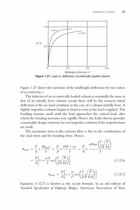
0. 2.0 4.0 6.0

0.5

1.0e=0.1

e=0.3

/P PE

Midheight deflection,

Figure 1-27 Load vs. deflection, eccentrically loaded column

Buckling of Columns 55

Figure 1-27 shows the variation of the midheight deflection for two values

of eccentricity, e.

The behavior of an eccentrically loaded column is essentially the same as

that of an initially bent column except there will be the nonzero initial

deflection at the no-load condition in the case of a column initially bent. A

slightly imperfect column begins to bend as soon as the load is applied. The

bending remains small until the load approaches the critical load, after

which the bending increases very rapidly. Hence, the Euler theory provides

a reasonable design criterion for real imperfect columns if the imperfections

are small.

The maximum stress in the extreme fiber is due to the combination of

the axial stress and the bending stress. Hence,

smax ¼ P

AþMmaxc

I¼ P

Aþ Pðdþ eÞc

I¼ P

AþcePsec

�‘

2

ffiffiffiffiffiP

EI

r �I

¼ P

A

1þ ecA

Isec

�‘

2

ffiffiffiffiffiP

EI

r �(1.12.6)

� ffiffiffiffiffiffiffir �

smax ¼ P

A1þ ec

r2sec

‘

2r

P

EA(1.12.7)

Equation (1.12.7) is known as the secant formula. In an old edition of

Standard Specification of Highway Bridges, American Association of State

56 Chai Yoo

Highway and Transportation Official (AASHTO) stipulated a constant

value of 0.25 to account for a minimum initial imperfection usually

encountered in practice, as shown in Eq. (1.12.8)

sAASHTO ¼ P

A

1þ

�0:25þ ec

r2

�sec

�‘

2r

ffiffiffiffiffiffiffiP

EA

r �(1.12.8)

1.13. INELASTIC BUCKLING OF STRAIGHT COLUMN

In the discussions presented heretofore, the assumption has been made that

thematerial obeys Hooke’s law. For this assumption to be valid, the stresses in

the column must be below the proportional limit of the material. The linear

elastic analysis is correct for slender columns. On the other hand, the axial

stress in a shot column will exceed the proportional limit. Consequently, the

elastic analysis is not valid for short columns, and the limiting load for short

columns must be determined by taking inelastic behavior into account.

Before proceeding to consider the development of the theory of inelastic

column behavior, it would be informative to review its historic perspective.

The Euler hyperbola was derived by Leonhard Euler in 1744. It was believed

at the time that the formula applied to all columns, short and slender. It was

soon discovered that the formula was grossly unconservative for short

columns; the Euler formula was considered to be completely erroneous and

was discarded for a lengthy period of time, approximately 150 years. An

anecdotal story reveals that people ridiculed Euler when he could not

adequately explain why a coin (a compression member with an extremely

small slenderness ratio) on an anvil smashed by a hammer yielded (flattened)

instead of carrying an infinitely large stress. It is of interest to note that the

concept of flexural rigidity, EI, was not clearly defined at the time, and the

modulus of elasticity of steel was determined by Thomas Young in 1807.10

However, Theodore von Karman developed the double-modulus theory

in 1910 in his doctoral dissertation at Gottingen University under Ludwig

Prandtl direction. It gained widespread acceptance and the validity of Euler’s

work reestablished if the constant modulus E is replaced by an effective

modulus for short columns. Later in 1947, F.R. Shanley11 demonstrated that

the tangent modulus and not the double modulus is the correct effective

modulus, which leads to lower buckling load than the double-modulus

10 S.P. Timoshenko, History of Strength of Materials (New York: Dover Edition, 1983), p. 92.11 A. Chajes, Principles of Structural Stability Theory (Englewood Cliffs, NJ: Prentice-Hall, 1974), p. 37.

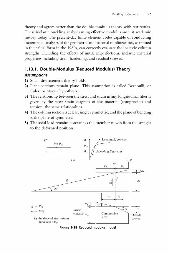
Buckling of Columns 57

theory and agrees better than the double-modulus theory with test results.

These inelastic buckling analyses using effective modulus are just academic

history today. The present-day finite element codes capable of conducting

incremental analyses of the geometric and material nonlinearities, as refined

in their final form in the 1980s, can correctly evaluate the inelastic column

strengths, including the effects of initial imperfections, inelastic material

properties including strain hardening, and residual stresses.

1.13.1. Double-Modulus (Reduced Modulus) TheoryAssumptions1) Small displacement theory holds.

2) Plane sections remain plane. This assumption is called Bernoulli, or

Euler, or Navier hypothesis.

3) The relationship between the stress and strain in any longitudinal fiber is

given by the stress-strain diagram of the material (compression and

tension, the same relationship).

4) The column section is at least singly symmetric, and the plane of bending

is the plane of symmetry.

5) The axial load remains constant as the member moves from the straight

to the deformed position.

Et: the slope of stress-straincurve at = cr

PP = Pcr

cr

p Unloading E governs

Loading Et governs

Compressivestress

1

2

R

d

e

cg

NAh2 h1

dx

dx

cr

s2

s1

z2 z1

Outsideconvex

Insideconcave

1 = E 1

2 = Et 2

Figure 1-28 Reduced modulus model

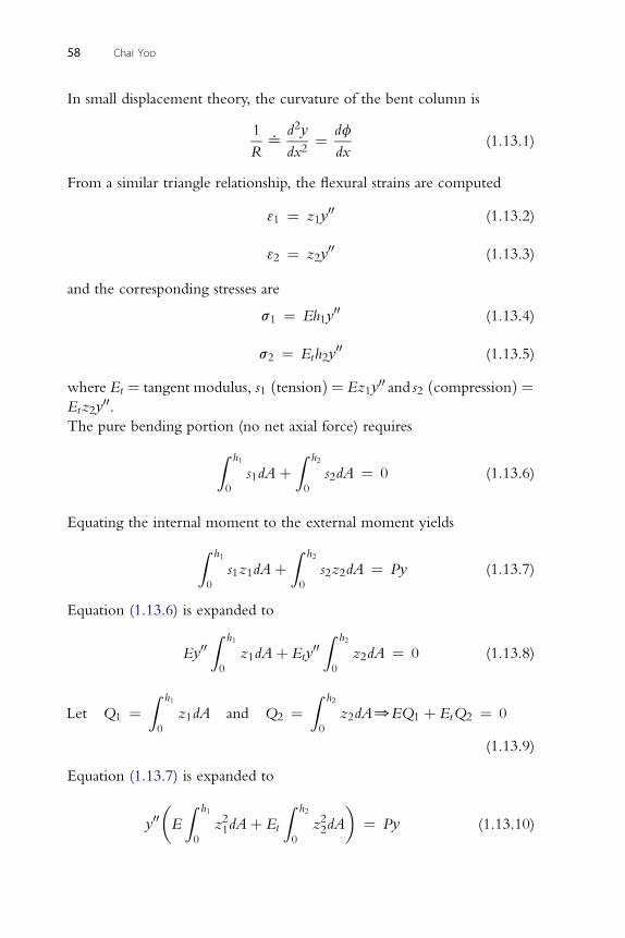
58 Chai Yoo

In small displacement theory, the curvature of the bent column is

1

R^

d2y

dx2¼ df

dx(1.13.1)

From a similar triangle relationship, the flexural strains are computed

31 ¼ z1y00 (1.13.2)

3 ¼ z y00 (1.13.3)

2 2

and the corresponding stresses are

s1 ¼ Eh1y00 (1.13.4)

s ¼ E h y00 (1.13.5)

2 t 2

where Et ¼ tangent modulus, s1 ðtensionÞ ¼ Ez1y00 and s2 ðcompressionÞ ¼

Etz2y00.

The pure bending portion (no net axial force) requires

Z h1

0

s1dAþZ h2

0

s2dA ¼ 0 (1.13.6)

Equating the internal moment to the external moment yields

Z h1

0

s1z1dAþZ h2

0

s2z2dA ¼ Py (1.13.7)

Equation (1.13.6) is expanded to

Ey00Z h1

0

z1dAþ Ety00Z h2

0

z2dA ¼ 0 (1.13.8)

Z h1Z h2

Let Q1 ¼0

z1dA and Q2 ¼0

z2dA0EQ1 þ EtQ2 ¼ 0

(1.13.9)

Equation (1.13.7) is expanded to

y00�E

Z h1

0

z21dAþ Et

Z h2

0

z22dA

�¼ Py (1.13.10)

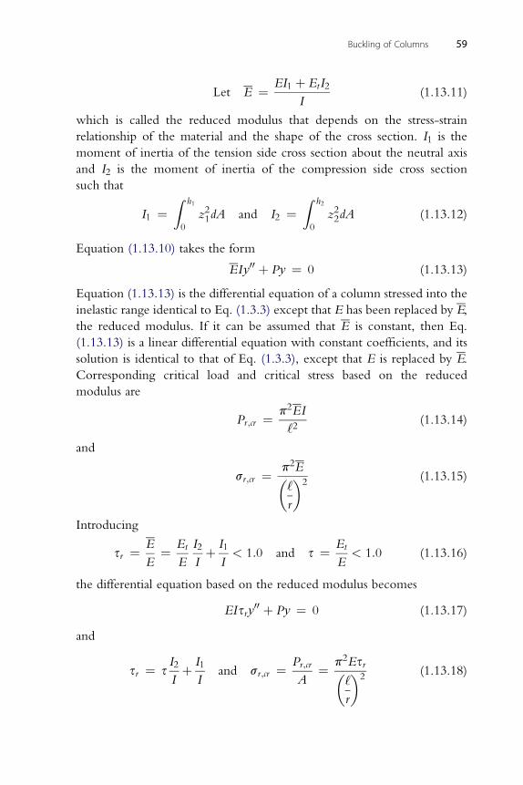
EI1 þ EtI2

Let E ¼

I(1.13.11)

which is called the reduced modulus that depends on the stress-strain

Buckling of Columns 59

relationship of the material and the shape of the cross section. I1 is the

moment of inertia of the tension side cross section about the neutral axis

and I2 is the moment of inertia of the compression side cross section

such that

I1 ¼Z h1

0

z21dA and I2 ¼Z h2

0

z22dA (1.13.12)

Equation (1.13.10) takes the form

EIy00 þ Py ¼ 0 (1.13.13)

Equation (1.13.13) is the differential equation of a column stressed into the

inelastic range identical to Eq. (1.3.3) except that E has been replaced by E,

the reduced modulus. If it can be assumed that E is constant, then Eq.

(1.13.13) is a linear differential equation with constant coefficients, and its

solution is identical to that of Eq. (1.3.3), except that E is replaced by E.

Corresponding critical load and critical stress based on the reduced

modulus are

Pr;cr ¼ p2EI

‘2(1.13.14)

and

sr;cr ¼ p2E�‘

r

�2(1.13.15)

Introducing

sr ¼ E

E¼ Et

E

I2

Iþ I1

I< 1:0 and s ¼ Et

E< 1:0 (1.13.16)

the differential equation based on the reduced modulus becomes

EIsry00 þ Py ¼ 0 (1.13.17)

and

sr ¼ sI2

Iþ I1

Iand sr;cr ¼ Pr;cr

A¼ p2Esr�

‘

r

�2(1.13.18)

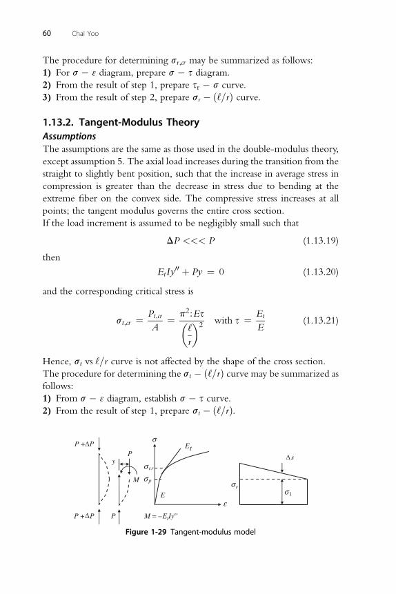
60 Chai Yoo

The procedure for determining sr;cr may be summarized as follows:

1) For s � 3 diagram, prepare s � s diagram.

2) From the result of step 1, prepare sr � s curve.

3) From the result of step 2, prepare sr � ð‘=rÞ curve.

1.13.2. Tangent-Modulus TheoryAssumptionsThe assumptions are the same as those used in the double-modulus theory,

except assumption 5. The axial load increases during the transition from the

straight to slightly bent position, such that the increase in average stress in

compression is greater than the decrease in stress due to bending at the

extreme fiber on the convex side. The compressive stress increases at all

points; the tangent modulus governs the entire cross section.

If the load increment is assumed to be negligibly small such that

DP <<< P (1.13.19)

then

EtIy00 þ Py ¼ 0 (1.13.20)

and the corresponding critical stress is

st;cr ¼ Pt;cr

A¼ p2:Es�

‘

r

�2with s ¼ Et

E(1.13.21)

Hence, st vs ‘=r curve is not affected by the shape of the cross section.

The procedure for determining the st � ð‘=rÞ curve may be summarized as

follows:

1) From s � 3 diagram, establish s � s curve.2) From the result of step 1, prepare st � ð‘=rÞ.

tE

E

y

rp

cr

s

M

P + P

P + P

P

P

M

1

= – EtIy

Figure 1-29 Tangent-modulus model

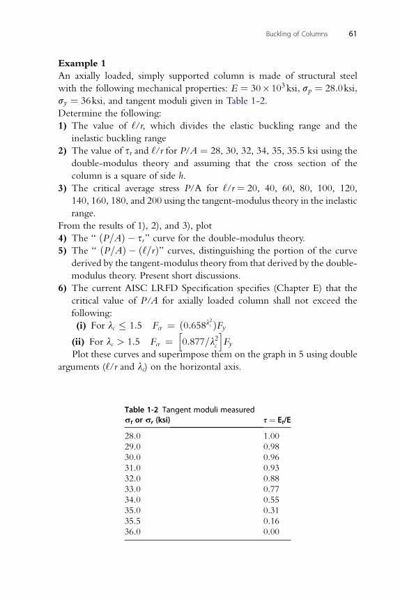
Buckling of Columns 61

Example 1

An axially loaded, simply supported column is made of structural steel

with the following mechanical properties: E ¼ 30�103 ksi; sp ¼ 28:0ksi;sy ¼ 36ksi; and tangent moduli given in Table 1-2.

Determine the following:

1) The value of ‘/r, which divides the elastic buckling range and the

inelastic buckling range

2) The value of sr and ‘/r for P/A ¼ 28, 30, 32, 34, 35, 35.5 ksi using the

double-modulus theory and assuming that the cross section of the

column is a square of side h.

3) The critical average stress P/A for ‘/r ¼ 20, 40, 60, 80, 100, 120,

140, 160, 180, and 200 using the tangent-modulus theory in the inelastic

range.

From the results of 1), 2), and 3), plot

4) The “ ðP=AÞ � sr” curve for the double-modulus theory.

5) The “ ðP=AÞ � ð‘=rÞ” curves, distinguishing the portion of the curve

derived by the tangent-modulus theory from that derived by the double-

modulus theory. Present short discussions.

6) The current AISC LRFD Specification specifies (Chapter E) that the

critical value of P/A for axially loaded column shall not exceed the

following:

(i) For lc � 1:5 Fcr ¼ ð0:658l2c ÞFy

(ii) For lc > 1:5 Fcr ¼h0:877=l2c

iFy

Plot these curves and superimpose them on the graph in 5 using double

arguments (‘/r and lc) on the horizontal axis.

Table 1-2 Tangent moduli measuredst or sr (ksi) s ¼ Et/E

28.0 1.00

29.0 0.98

30.0 0.96

31.0 0.93

32.0 0.88

33.0 0.77

34.0 0.55

35.0 0.31

35.5 0.16

36.0 0.00

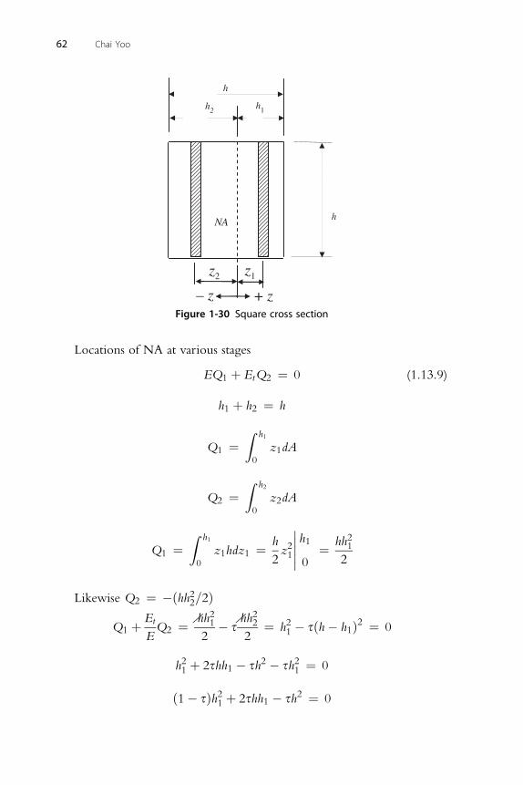
+ z– z

NA

z2 z1

h1h2

h

h

Figure 1-30 Square cross section

62 Chai Yoo

Locations of NA at various stages

EQ1 þ EtQ2 ¼ 0 (1.13.9)

h1 þ h2 ¼ h

Z h1

Q1 ¼0

z1dA

Z h2

Q2 ¼0

z2dA

Z h1�� h 2

Q1 ¼0

z1hdz1 ¼ h

2z21��� 1

0¼ hh1

2

Likewise Q2 ¼ �ðhh22=2Þ

Q1 þ Et

EQ2 ¼

�

hh212

� s

�

hh222

¼ h21 � sðh� h1Þ2 ¼ 0

2 2 2

h1 þ 2shh1 � sh � sh1 ¼ 0

ð1� sÞh2 þ 2shh � sh2 ¼ 0

1 1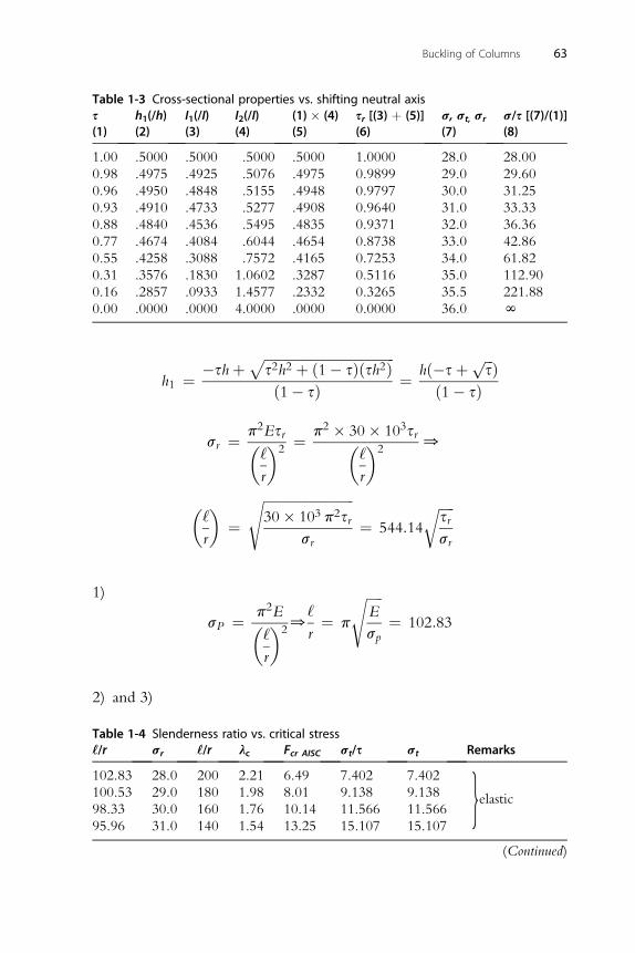

Table 1-3 Cross-sectional properties vs. shifting neutral axiss

(1)h1(/h)(2)

I1(/I)(3)

I2(/I)(4)

(1) � (4)(5)

sr [(3) þ (5)](6)

s, st, sr

(7)s/s [(7)/(1)](8)

1.00 .5000 .5000 .5000 .5000 1.0000 28.0 28.00

0.98 .4975 .4925 .5076 .4975 0.9899 29.0 29.60

0.96 .4950 .4848 .5155 .4948 0.9797 30.0 31.25

0.93 .4910 .4733 .5277 .4908 0.9640 31.0 33.33

0.88 .4840 .4536 .5495 .4835 0.9371 32.0 36.36

0.77 .4674 .4084 .6044 .4654 0.8738 33.0 42.86

0.55 .4258 .3088 .7572 .4165 0.7253 34.0 61.82

0.31 .3576 .1830 1.0602 .3287 0.5116 35.0 112.90

0.16 .2857 .0933 1.4577 .2332 0.3265 35.5 221.88

0.00 .0000 .0000 4.0000 .0000 0.0000 36.0 N

Buckling of Columns 63

�shþ ffiffiffiffiffiffiffiffiffiffiffiffiffiffiffiffiffiffiffiffiffiffiffiffiffiffiffiffiffiffiffiffiffiffiffiffiffiffiffis2h2 þ ð1� sÞðsh2Þp

hð�sþ ffiffiffis

p Þ

h1 ¼ ð1� sÞ ¼ ð1� sÞ

p2Es p2 � 30� 103s

sr ¼ r�

‘

r

�2¼ r�

‘

r

�20

�‘

r

�¼

ffiffiffiffiffiffiffiffiffiffiffiffiffiffiffiffiffiffiffiffiffiffiffiffiffiffiffi30� 103 p2sr

sr

s¼ 544:14

ffiffiffiffiffisrsr

r

1)

sP ¼ p2E�‘

r

�20

‘

r¼ p

ffiffiffiffiffiE

sp

s¼ 102:83

2) and 3)

Table 1-4 Slenderness ratio vs. critical stress‘‘/r sr ‘‘/r lc Fcr AISC st/s st Remarks

102.83 28.0 200 2.21 6.49 7.402 7.402 gelastic100.53 29.0 180 1.98 8.01 9.138 9.138

98.33 30.0 160 1.76 10.14 11.566 11.566

95.96 31.0 140 1.54 13.25 15.107 15.107

(Continued)

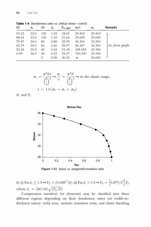
Table 1-4 Slenderness ratio vs. critical stressdcont'd‘‘/r sr ‘‘/r lc Fcr AISC st/s st Remarks

93.12 32.0 120 1.32 18.03 20.562 20.562

88.54 33.0 100 1.10 21.64 29.609 29.000 g st ; from graph79.47 34.0 80 0.88 25.99 46.264 33.200

65.79 35.0 60 0.66 29.97 82.247 34.200

52.18 35.5 40 0.44 33.18 185.055 35.300

0.00 36.0 20 0.22 35.27 740.220 35.990

0 0.00 36.00 N 36.000

64 Chai Yoo

st ¼ p2Es�‘r

�20

st

s¼ p2E�‘

r

�20 in the elastic range;

s ¼ 1:0 ðst ¼ sr ¼ sEÞ

4) and 5)

Stress-Tau

28

30

32

34

36

0 0.2 0.4 0.6 0.8 1Tau

Stress

Figure 1-31 Stress vs. tangential-modulus ratio

6) (i) For lc � 1:50Fcr ¼ ð0:658l2c ÞFy (ii) For lc > 1:50Fcr ¼h0:877=l2c

iFy

where lc ¼ ðk‘=rpÞ ffiffiffiffiffiffiffiffiffiffiffiffiðFy=Ep Þ

Compression members (or elements) may be classified into three

different regions depending on their slenderness ratios (or width-to-

thickness ratios): yield zone, inelastic transition zone, and elastic buckling

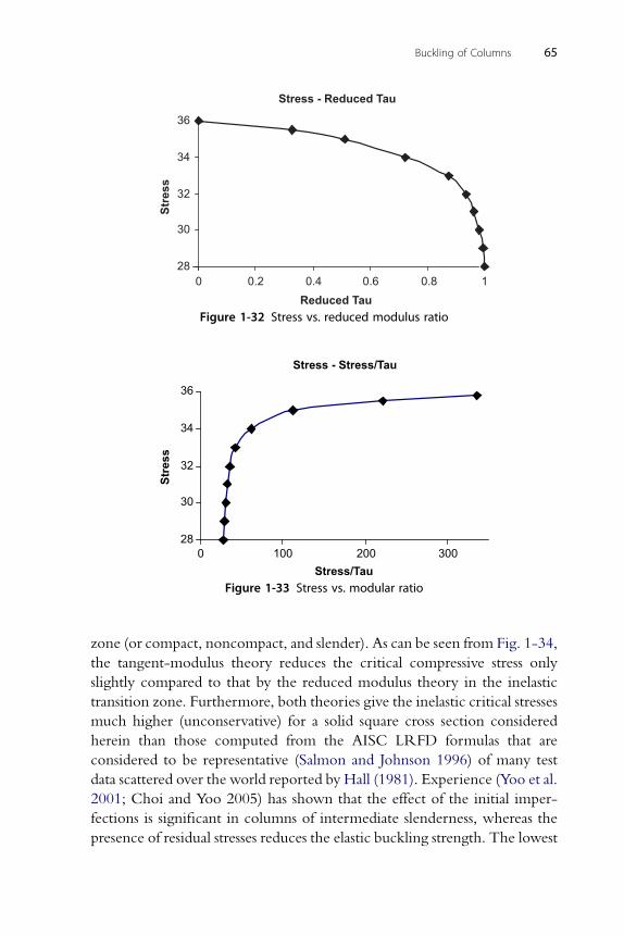
Stress - Reduced Tau

28

30

32

34

36

0 0.2 0.4 0.6 0.8 1Reduced Tau

Stre

ss

Figure 1-32 Stress vs. reduced modulus ratio

Stress - Stress/Tau

28

30

32

34

36

0 100 200 300Stress/Tau

Stress

Figure 1-33 Stress vs. modular ratio

Buckling of Columns 65

zone (or compact, noncompact, and slender). As can be seen from Fig. 1-34,

the tangent-modulus theory reduces the critical compressive stress only

slightly compared to that by the reduced modulus theory in the inelastic

transition zone. Furthermore, both theories give the inelastic critical stresses

much higher (unconservative) for a solid square cross section considered

herein than those computed from the AISC LRFD formulas that are

considered to be representative (Salmon and Johnson 1996) of many test

data scattered over the world reported by Hall (1981). Experience (Yoo et al.

2001; Choi and Yoo 2005) has shown that the effect of the initial imper-

fections is significant in columns of intermediate slenderness, whereas the

presence of residual stresses reduces the elastic buckling strength. The lowest

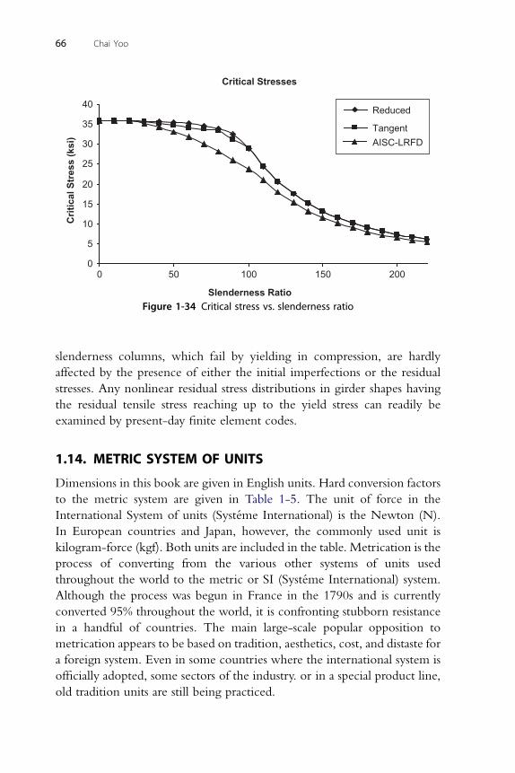
Critical Stresses

0

5

10

15

20

25

30

35

40

0 50 100 150 200

Slenderness Ratio

Critic

al S

tre

ss

(k

si)

Reduced

TangentAISC-LRFD

Figure 1-34 Critical stress vs. slenderness ratio

66 Chai Yoo

slenderness columns, which fail by yielding in compression, are hardly

affected by the presence of either the initial imperfections or the residual

stresses. Any nonlinear residual stress distributions in girder shapes having

the residual tensile stress reaching up to the yield stress can readily be

examined by present-day finite element codes.

1.14. METRIC SYSTEM OF UNITS

Dimensions in this book are given in English units. Hard conversion factors

to the metric system are given in Table 1-5. The unit of force in the

International System of units (Systeme International) is the Newton (N).

In European countries and Japan, however, the commonly used unit is

kilogram-force (kgf). Both units are included in the table. Metrication is the

process of converting from the various other systems of units used

throughout the world to the metric or SI (Systeme International) system.

Although the process was begun in France in the 1790s and is currently

converted 95% throughout the world, it is confronting stubborn resistance

in a handful of countries. The main large-scale popular opposition to

metrication appears to be based on tradition, aesthetics, cost, and distaste for

a foreign system. Even in some countries where the international system is

officially adopted, some sectors of the industry. or in a special product line,

old tradition units are still being practiced.

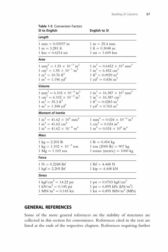
Table 1-5 Conversion FactorsSI to English English to SI

Length

1 mm ¼ 0.03937 in 1 in ¼ 25.4 mm

1 m ¼ 3.281 ft 1 ft ¼ 0.3048 m

1 km ¼ 0.6214 mi 1 mi ¼ 1.609 km

Area

1 mm2 ¼ 1.55 � 10�3 in2 1 in2 ¼ 0.6452 � 103 mm3

1 cm2 ¼ 1.55 � 10�1 in2 1 in2 ¼ 6.452 cm2

1 m2 ¼ 10.76 ft2 1 ft2 ¼ 0.0929 m2

1 m2 ¼ 1.196 yd2 1 yd2 ¼ 0.836 m2

Volume

1 mm3 ¼ 6.102 � 10�5 in3 1 in3 ¼ 16.387 � 103 mm3

1 cm3 ¼ 6.102 � 10�2 in3 1 in3 ¼ 16.387 cm3

1 m3 ¼ 35.3 ft3 1 ft3 ¼ 0.0283 m3

1 m3 ¼ 1.308 yd3 1 yd3 ¼ 0.765 m3

Moment of inertia

1 in4 ¼ 41.62 � 104 mm4 1 mm4 ¼ 0.024 � 10�4 in4

1 in4 ¼ 41.62 cm4 1 cm4 ¼ 0.024 in4

1 in4 ¼ 41.62 � 10�8 m4 1 m4 ¼ 0.024 � 108 in4

Mass

1 kg ¼ 2.205 lb 1 lb ¼ 0.454 kg

1 kg ¼ 1.102 � 10�3 ton 1 ton (2000 lb) ¼ 907 kg

1 Mg ¼ 1.102 ton 1 tonne (metric) ¼ 1000 kg

Force

1 N ¼ 0.2248 lbf 1 lbf ¼ 4.448 N

1 kgf ¼ 2.205 lbf 1 kip ¼ 4.448 kN

Stress

1 kgf/cm2 ¼ 14.22 psi 1 psi ¼ 0.0703 kgf/cm2

1 kN/m2 ¼ 0.145 psi 1 psi ¼ 6.895 kPa (kN/m2)

1 MN/m2 ¼ 0.145 ksi 1 ksi ¼ 6.895 MN/m2 (MPa)

Buckling of Columns 67

GENERAL REFERENCES

Some of the more general references on the stability of structures are

collected in this section for convenience. References cited in the text are

listed at the ends of the respective chapters. References requiring further

68 Chai Yoo

details are given in the footnotes. Relatively recent textbooks and reference

books include those by Bleich (1952), Timoshenko and Gere (1961),

Ziegler (1968), Britvec (1973), Chajes (1974), Brush and Almroth (1975),

Allen and Bulson (1980), Chen and Lui (1991), Bazant and Cedolin (1991),

Godoy (2000), Simitses and Hodges (2006), and Galambos and Surovek

(2008). Some of these books address only the elastic stability of framed

structures, while others extend the coverage into the stability of plates and

shells, including dynamic stability and stability of nonconservative force

systems.

The design of structural elements and components is beyond the scope

of this book. For stability design criteria for columns and plates, Guide to

Stability Design Criteria (Galambos, 1998) is an excellent reference. The

design of highway bridge structures is to be carried out based on AASHTO

(2007) specifications, and steel building frames are to follow AISC (2005)

specifications. In the case of ship structures, separate design rules are stip-

ulated for different vessel types such as IACS (2005) and IACS (2006). A

variety of organizations and authorities are claiming jurisdiction over the

certificates of airworthiness of civil aviation aircrafts.

REFERENCESAASHTO. (2007). LRFD Bridge Design Specifications (4th ed.). Washington, DC: American

Association of State Highway and Transportation Officials.AASHTO. (1973). Standard Specifications for Highway Bridges (11th ed.). Washington, DC:

American Association of State Highway and Transportation Officials.AISC. (2005). Specification for Structural Steel Building (13th ed.). Chicago, IL: American

Institute of Steel Construction.Allen, H. G., & Bulson, P. S. (1980). Background to Buckling. London: McGraw-Hill (UK).Bazant, Z. P., & Cedolin, L. (1991). Stability of Structures, Elastic, Inelastic, Fracture, and

Damage Theories. Oxford: Oxford University Press.Bleich, F. (1952). Buckling Strength of Metal Structures. New York: McGraw-Hill.Britvec, S. J. (1973). The Stability of Elastic Systems. Elmsford, NY: Pergamon Press.Brush, D. O., & Almroth, B. O. (1975). Buckling of Bars, Plates, and Shells. New York:

McGraw-Hill.Chajes, A. (1974). Principles of Structural Stability Theory. Englewood Cliffs, NJ: Prentice-

Hall.Chen, W. F., & Lui, E. M. (1991). Stability Design of Steel Frames. Boca Raton, FL: CRC

Press.Choi, B. H., & Yoo, C. H. (2005). Strength of Stiffened Flanges in Horizontally Curved

Box Girders. J. Engineering Mechanics, ASCE, Vol. 131(No. 2), 167–176, February 2005.Dinnik, A.N. (1912). Buckling Under Own Weight, Proceedings of Don Polytechnic

Institute, 1, Part 2, pp. 12 (in Russian).Elishakoff, I. (2005). Eigenvalues of Inhomogeneous Structures, Unusual Closed-Form Solutions.

Boca Raton, FL: CRC Press.

Buckling of Columns 69

Engelhardt., H. (1954). Die einheitliche Behandlung der Stabknickung mit Berucksichtung desStabeiggengewichte in den Eulerfallen 1 bis 4 als Eigenwertproblem. Der Stahlbau. 23(4),80–84 (in German).

Euler, L. (1744). Methodus Inveniendi Lineas Curvas Maximi Minimive Propreietate Gaudentes(Appendix, De Curvis Elasticis). Lausanne and Geneva: Marcum Michaelem Bousquet.

Galambos, T. V. (Ed.). (1998). Guide to Stability Design Criteria for Metal Structures (5th ed.).New York: Structural Stability Research Council, John Wiley and Sons.

Galambos, T. V., & Surovek, A. E. (2008). Structural Stability of Steel, Concepts and Appli-cations for Structural Engineers. Hoboken, NJ: John Wiley and Sons.

Godoy, L. A. (2000). Theory of Elastic Stability: Analysis and Sensitivity. Philadelphia, PA:Taylor and Francis.

Grossman, S. I., & Derrick, W. R. (1988). Advanced Engineering Mathematics. New York:Harper & Row.

Hall, D. H. (1981). Proposed Steel Column Strength Criteria. J. Structural Div., ASCE,Vol. 107(No. ST4). April 1981, pp. 649–670. Discussed by B.G. Johnston, Vol. 108,No. ST4 (April 1982), pp. 956–957; by Z. Shen and L.W. Lu, Vol. 108, No.ST7 (July 1982),pp. 1680–1681; by author, Vol. 108, No. ST12 (December 1982), pp. 2853–2855.

Hoff, N. F. (1956). The Analysis of Structures. New York: John Wiley and Sons.IACS. (2005). Common Structural Rules for Bulk Carriers. London: International Association

of Classification Societies.IACS. (2006). Common Structural Rules for Double Hull Oil Tankers. London: International

Association of Classification Societies.Salmon, C. G., & Johnson, J. E. (1996). Steel Structures, Design and Behavior (4th ed.).

New York: Haper Collins.Salvadori,M., &Heller, R. (1963). Structure in Architecture. EnglewoodCliffs, NJ: Prentice-Hall.Shames, I. H., & Dym, C. L. (1985). Energy and Finite Element Methods in Structural

Mechanics. New York: Hemisphere Publishing Corporation.Simitses, G. J., & Hodges, D. H. (2006). Fundamentals of Structural Stability. Burlington, MA:

Elsevier.Timoshenko, S. P. (1953). History of Strength of Materials. New York: McGraw-Hill.Timoshenko, S. P., & Gere, J. M. (1961). Theory of Elastic Stability (2nd ed.). New York:

McGraw-Hill.Todhunter, I. (1886). In K. Pearson (Ed.) (Dover ed). A History of Elasticity and of the Strength

of Materials, Vol. I. New York: Cambridge. 1960.Wang, C. M., Wang, C. Y., & Reddy, J. N. (2005). Exact Solutions for Buckling of Structural

Members. Boca Raton, FL: CRC Press.Winter, G. (1960). Lateral Bracing of Columns and Beams. Transactions, ASCE, Vol. 125,

807–845.Yoo, C. H. (1980). Bimoment Contribution to Stability of Thin-Walled Assemblages.

Computers and Structures, Vol. 11(No. 5), 465–471.Yoo, C. H., Choi, B. H., & Ford, E. M. (2001). Stiffness Requirements for Longitudinally

Stiffened Box Girder Flanges. J. Structural Engineering, ASCE, Vol. 127(No. 6),705–711, June 2001.

Ziegler, H. (1968). Principles of Structural Stability. Waltham, MA: Blaisdell Publishing Co.

PROBLEMS

1.1 For structures shown in Fig. P1-1, determine the following:

(a) Using fourth-order DE, determine the lowest three critical loads.

(b) Determine the lowest two critical loads.

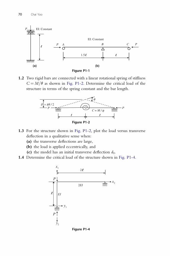
P

A

EI: Constant

B C P

EI: Constant

P

1.5

(a) (b)

Figure P1-1

70 Chai Yoo

1.2 Two rigid bars are connected with a linear rotational spring of stiffness

C ¼M=q as shown in Fig. P1-2. Determine the critical load of the

structure in terms of the spring constant and the bar length.

P PC = M /

= / 2

Figure P1-2

1.3 For the structure shown in Fig. P1-2, plot the load versus transverse

deflection in a qualitative sense when:

(a) the transverse deflections are large,

(b) the load is applied eccentrically, and

(c) the model has an initial transverse deflection d0.

1.4 Determine the critical load of the structure shown in Fig. P1-4.

x1

y1

y2

P

P

2

2EI

EI

x2

Figure P1-4

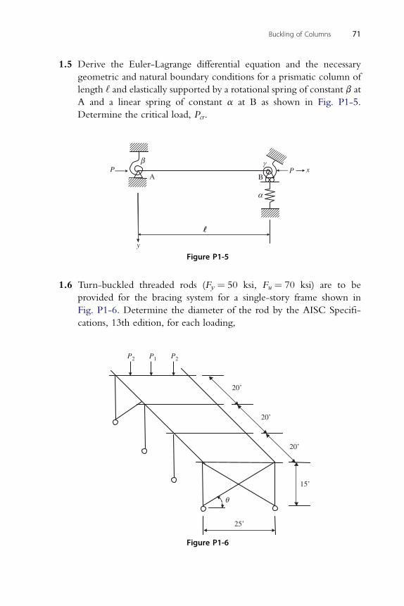
Buckling of Columns 71

1.5 Derive the Euler-Lagrange differential equation and the necessary

geometric and natural boundary conditions for a prismatic column of

length ‘ and elastically supported by a rotational spring of constant b at

A and a linear spring of constant a at B as shown in Fig. P1-5.

Determine the critical load, Pcr.

P

y

A B P x

Figure P1-5

1.6 Turn-buckled threaded rods (Fy ¼ 50 ksi, Fu ¼ 70 ksi) are to be

provided for the bracing system for a single-story frame shown in

Fig. P1-6. Determine the diameter of the rod by the AISC Specifi-

cations, 13th edition, for each loading,

P1 P2P2

20’

20’

20’

15’

25’

Figure P1-6

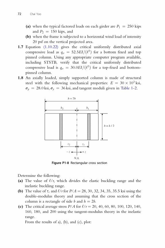
72 Chai Yoo

(a) when the typical factored loads on each girder are P1 ¼ 250 kips

and P2 ¼ 150 kips, and

(b) when the frame is subjected to a horizontal wind load of intensity

20 psf on the vertical projected area.

1.7 Equation (1.10.22) gives the critical uniformly distributed axial

compressive load as qcr ¼ 52:5EI=ð‘3Þ for a bottom fixed and top

pinned column. Using any appropriate computer program available,

including STSTB, verify that the critical uniformly distributed

compressive load is qcr ¼ 30:0EI=ð‘3Þ for a top-fixed and bottom-

pinned column.

1.8 An axially loaded, simply supported column is made of structural

steel with the following mechanical properties: E ¼ 30� 103 ksi;sp ¼ 28:0 ksi; sy ¼ 36 ksi; and tangent moduli given in Table 1-2.

h = 2b

b = h / 2

h2

z2

h1

z1

– z + z

N.A.

Figure P1-8 Rectangular cross section

Determine the following:

(a) The value of ‘/r, which divides the elastic buckling range and the

inelastic buckling range.

(b) The value of sr and ‘/r for P/A ¼ 28, 30, 32, 34, 35, 35.5 ksi using the

double-modulus theory and assuming that the cross section of the

column is a rectangle of side b and h ¼ 2b.

(c) The critical average stress P/A for ‘/r ¼ 20, 40, 60, 80, 100, 120, 140,

160, 180, and 200 using the tangent-modulus theory in the inelastic

range.

From the results of a), (b), and (c), plot:

Buckling of Columns 73

(d) The “ ðP=AÞ � sr” curve for the double-modulus theory.

(e) The “ ðP=AÞ � ð‘=rÞ” curves, distinguishing the portion of the curve

derived by the tangent-modulus theory from that derived by the

double-modulus theory. Present short discussions.

(f) The current AISC LRFD Specification specifies (Chapter E) that the

critical value of P/A for axially loaded column shall not exceed the

following:

(i) For lc � 1:5 Fcr ¼ ð0:658l2c ÞFy

(ii) For lc > 1:5 Fcr ¼h0:877=l2c

iFy

Plot these curves and superimpose them on the graph in (e) using

double arguments (‘/r and lc) on the horizontal axis.

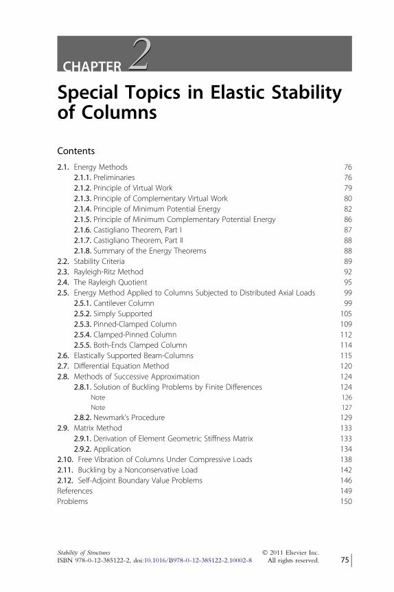
CHAPTER22

Special Topics in Elastic Stabilityof Columns

Contents

2.1. Energy Methods 762.1.1. Preliminaries 762.1.2. Principle of Virtual Work 792.1.3. Principle of Complementary Virtual Work 802.1.4. Principle of Minimum Potential Energy 822.1.5. Principle of Minimum Complementary Potential Energy 862.1.6. Castigliano Theorem, Part I 872.1.7. Castigliano Theorem, Part II 882.1.8. Summary of the Energy Theorems 88

2.2. Stability Criteria 892.3. Rayleigh-Ritz Method 922.4. The Rayleigh Quotient 952.5. Energy Method Applied to Columns Subjected to Distributed Axial Loads 99

2.5.1. Cantilever Column 992.5.2. Simply Supported 1052.5.3. Pinned-Clamped Column 1092.5.4. Clamped-Pinned Column 1122.5.5. Both-Ends Clamped Column 114

2.6. Elastically Supported Beam-Columns 1152.7. Differential Equation Method 1202.8. Methods of Successive Approximation 124

2.8.1. Solution of Buckling Problems by Finite Differences 124Note 126Note 127

2.8.2. Newmark’s Procedure 1292.9. Matrix Method 133

2.9.1. Derivation of Element Geometric Stiffness Matrix 1332.9.2. Application 134

2.10. Free Vibration of Columns Under Compressive Loads 1382.11. Buckling by a Nonconservative Load 1422.12. Self-Adjoint Boundary Value Problems 146References 149Problems 150

Stability of Structures � 2011 Elsevier Inc.ISBN 978-0-12-385122-2, doi:10.1016/B978-0-12-385122-2.10002-8 All rights reserved. 75 j

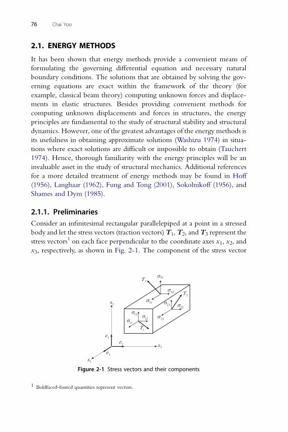
76 Chai Yoo

2.1. ENERGY METHODS

It has been shown that energy methods provide a convenient means of

formulating the governing differential equation and necessary natural

boundary conditions. The solutions that are obtained by solving the gov-

erning equations are exact within the framework of the theory (for

example, classical beam theory) computing unknown forces and displace-

ments in elastic structures. Besides providing convenient methods for

computing unknown displacements and forces in structures, the energy

principles are fundamental to the study of structural stability and structural

dynamics. However, one of the greatest advantages of the energy methods is

its usefulness in obtaining approximate solutions (Washizu 1974) in situa-

tions where exact solutions are difficult or impossible to obtain (Tauchert

1974). Hence, thorough familiarity with the energy principles will be an

invaluable asset in the study of structural mechanics. Additional references

for a more detailed treatment of energy methods may be found in Hoff

(1956), Langhaar (1962), Fung and Tong (2001), Sokolnikoff (1956), and

Shames and Dym (1985).

2.1.1. PreliminariesConsider an infinitesimal rectangular parallelepiped at a point in a stressed

body and let the stress vectors (traction vectors) T1, T2, and T3 represent the

stress vectors1 on each face perpendicular to the coordinate axes x1, x2, and

x3, respectively, as shown in Fig. 2-1. The component of the stress vector

x3

x2

x1

1e

2ee

1T

3T

2T

11

1213

21

2223

31

32

s

s

s

s

s

ss

s

s

33

3

Figure 2-1 Stress vectors and their components

1 Boldfaced-fonted quantities represent vectors.

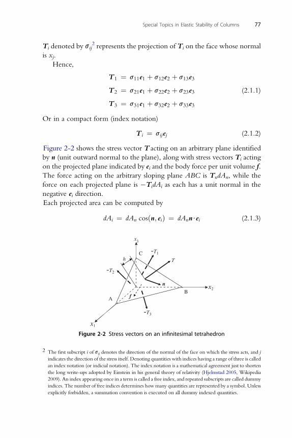
Special Topics in Elastic Stability of Columns 77

Ti denoted by sij2 represents the projection of Ti on the face whose normal

is xj.

Hence,

T1 ¼ s11e1 þ s12e2 þ s13e3

T2 ¼ s21e1 þ s22e2 þ s23e3

T3 ¼ s31e1 þ s32e2 þ s33e3

(2.1.1)

Or in a compact form (index notation)

T i ¼ sijej (2.1.2)

Figure 2-2 shows the stress vector T acting on an arbitrary plane identified

by n (unit outward normal to the plane), along with stress vectors Ti acting

on the projected plane indicated by ei and the body force per unit volume f.

The force acting on the arbitrary sloping plane ABC is TndAn, while the

force on each projected plane is �TidAi as each has a unit normal in the

negative ei direction.

Each projected area can be computed by

dAi ¼ dAn cosðn; eiÞ ¼ dAnn$ei (2.1.3)

x3

x1

x2

AB

C

n

T

f

h

-T3

-T1

-T2

Figure 2-2 Stress vectors on an infinitesimal tetrahedron

2 The first subscript i of sij denotes the direction of the normal of the face on which the stress acts, and j

indicates the direction of the stress itself. Denoting quantities with indices having a range of three is called

an index notation (or indicial notation). The index notation is a mathematical agreement just to shorten

the long write-ups adopted by Einstein in his general theory of relativity (Hjelmstad 2005, Wikipedia

2009). An index appearing once in a term is called a free index, and repeated subscripts are called dummy

indices. The number of free indices determines howmany quantities are represented by a symbol. Unless

explicitly forbidden, a summation convention is executed on all dummy indexed quantities.

78 Chai Yoo

so that

dAn ¼ dAi

n$ei¼ dAi

ni(2.1.4)

where

ni ¼ n$ei ¼ cosðn; eiÞ (2.1.5)

is a direction cosine of n.

Since the tetrahedron is in equilibrium, the resultant of all forces acting

on it must vanish. Hence,�Tn � T ini þ h

3f

�dAn ¼ 0 (2.1.6)

Resolving Tn into Cartesian components (Tn ¼ Tiei) and taking the limit as

h/0, Eq. (2.1.6) reduces to

Tn ¼ Tiei ¼ T ini (2.1.7)

Substituting Eq. (2.1.2) into Eq. (2.1.7) yields

Tiei ¼ T ini ¼ T jnj ¼ sjieinj (2.1.8)

from which

Ti ¼ sjinj (2.1.9)

Consider a volume of material V bounded by a closed surface S. Let the

body force per unit volume distributed throughout the body V be f, and

the stress vectors or tractions distributed over the surface S be T. If the

body is in equilibrium, then the sum of all forces acting on V must vanish;

that is ZV

f dV þZS

T dS ¼ 0 (2.1.10)

or in component form ZV

fi dV þZS

Ti dS ¼ 0 (2.1.11)

Equation (2.1.9) may be rewritten asZS

Ti dS ¼ZS

sjinj dS (2.1.12)

Special Topics in Elastic Stability of Columns 79

Assuming that the components sji and their first derivatives are continuous,

the surface integral in Eq. (2.1.12) can be transformed into a volume integral

using the divergence theorem, asZS

sjinj dS ¼ZV

sji;j dV (2.1.13)

From Eqs. (2.1.11), (2.1.12), and (2.1.13), it follows immediately thatZV

�fi þ sji;j

�dV ¼ 0 (2.1.14)

Equation (2.1.14) can only be satisfied if the integrand is equal to zero at

every point in the body. Hence,

fi þ sji;j ¼ 0 (2.1.15)

Equation (2.1.15) presents three equations of equilibrium written in terms

of stresses and body forces.

2.1.2. Principle of Virtual WorkIf a structure is in equilibrium and remains in equilibrium while it is subjected to

a virtual displacement, the external virtual work dWE done by the external (real)

forces acting on the structure is equal to the internal virtual work dWI done by the

internal stresses (due to real forces).

The external virtual work is

dWE ¼ZS

Tidui dS þZV

fidui dV (2.1.16)

Using Eq. (2.1.9) and the divergence theorem, the first term in Eq. (2.1.16)

can be transformed intoZS

Tidui dS ¼ZS

sijnjdui dS ¼ZV

ðsijdui;jÞ dV

¼ZV

ðsij;jdui þ sijdui;jÞ dV (2.1.17)

Substituting Eq. (2.1.17) into Eq. (2.1.16) yields

dWE ¼ZV

��sij;j þ fi

�dui þ sijdui;j

�dV (2.1.18)

Since the structure is in equilibrium, fi þ sji,j ¼ 0. Hence, Eq. (2.1.18)

reduces to

80 Chai Yoo

dWE ¼ZV

sijdui;j dV (2.1.19)

Recalling that deij ¼ (dui,jþduj,i)/2 and dui,j ¼ duj,i leads to:

sijdui;j ¼ sijdeij (2.1.20)

This transforms Eq. (2.1.20) toZV

sijdeij dV ¼ dWI ¼ dU (2.1.21)

Equation (2.1.21) describes the internalwork done by the actual stresses (due to

real forces) and virtual strains produced during the virtual displacement. The

internal work is frequently referred to as the strain energy stored in the elastic

body. From Eqs. (2.1.16), (2.1.20), and (2.1.21), one immediately obtains

dWE ¼ZS

Tidui dS þZV

fidui dV ¼ZV

sijdeij dV ¼ dWI ¼ dU

(2.1.22)

Equation (2.1.22) is a mathematical statement of the principle of virtual

work. The reverse of this principle is also true. That is, if dWE ¼ dWI for

virtual displacement, then the body is in equilibrium (Tauchert 1974). The

principle of virtual work is valid regardless of the material stress-strain

relations as shown in the derivation.

2.1.3. Principle of Complementary Virtual WorkFigure 2-3 shows the stress-strain diagram of a nonlinearly elastic rod. The

strain energy U represents the energy stored in a deformed elastic body;

however, the physical interpretation of the complementary strain energy U*is not clear.

The strain energy U in the rod is defined by

U ¼ZV

�Z e11

0

s11de11

�dV ¼ V

Z e11

0

s11de11 (2.1.23)

The strain energy density or the strain energy per unit volume is equal to

the area under the material’s stress-strain curve (Fig. 2-3). The comple-

mentary strain energy U* in the rod is defined by

U� ¼ZV

�Z s11

0

e11ds11

�dV ¼ V

Z s11

0

e11ds11 (2.1.24)

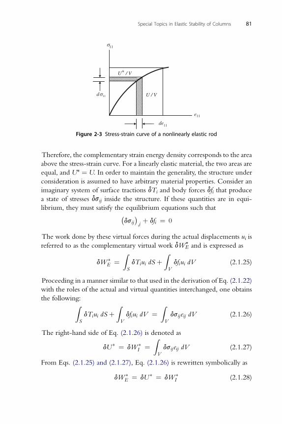
de11

e11

ds11

s11

U / V

U* / V

Figure 2-3 Stress-strain curve of a nonlinearly elastic rod

Special Topics in Elastic Stability of Columns 81

Therefore, the complementary strain energy density corresponds to the area

above the stress-strain curve. For a linearly elastic material, the two areas are

equal, and U* ¼ U. In order to maintain the generality, the structure under

consideration is assumed to have arbitrary material properties. Consider an

imaginary system of surface tractions dTi and body forces dfi that producea state of stresses dsij inside the structure. If these quantities are in equi-

librium, they must satisfy the equilibrium equations such that�dsij�;jþ dfi ¼ 0

The work done by these virtual forces during the actual displacements ui is

referred to as the complementary virtual work dWE) and is expressed as

dW �E ¼

ZS

dTiui dS þZV

dfiui dV (2.1.25)

Proceeding in a manner similar to that used in the derivation of Eq. (2.1.22)

with the roles of the actual and virtual quantities interchanged, one obtains

the following:ZS

dTiui dS þZV

dfiui dV ¼ZV

dsijeij dV (2.1.26)

The right-hand side of Eq. (2.1.26) is denoted as

dU� ¼ dW �I ¼

ZV

dsijeij dV (2.1.27)

From Eqs. (2.1.25) and (2.1.27), Eq. (2.1.26) is rewritten symbolically as

dW �E ¼ dU� ¼ dW �

I (2.1.28)

82 Chai Yoo

Equation (2.1.28) is the principle of complementary virtual work. If

a structure is in equilibrium, the complementary virtual work done by

the external virtual force system under the actual displacement is equal to

the complementary virtual work done by the internal virtual stresses

under the actual strains.

2.1.4. Principle of Minimum Potential EnergyIt is assumed that there exists a strain energy density u that is a homogeneous

quadratic function of the strains u(eij)3, such that

sij ¼ vu

veij(2.1.29)

It is recalled that the virtual displacement field dui was a priori not relatedto the stress field sij when applying the principle of virtual work. They are

now related through a constitutive law expressed by Eq. (2.1.29).

Substituting Eq. (2.1.29) into the principle of virtual work, Eq.(2.1.22),

one obtainsZS

Tidui dS þZV

fidui dV ¼ZV

vu

veijdeij dV ¼

ZV

dð1Þu dV

¼ dð1ÞZV

u dV ¼ dð1ÞU (2.1.30)

Notice that the variation and integration operations are interchanged. The

(loss of) potential energy of the applied loads is now defined as a function of

displacement field ui and the applied loads.

V ¼ �ZV

fiui dV �ZS

Tiui dS (2.1.31)

Taking the first variation of Eq. (2.1.31) gives

dð1ÞV ¼ �ZV

fivui

vujduj dV �

ZS

Tivui

vujduj dS

Noting that dui/duj ¼ dij and dij ¼ 1 for i ¼ j and dij ¼ 0 for i s j , the

equation leads to

3 This concept is attributed to George Green (1793–1841). It can be shown to be a positive definite

quadratic function (Shames and Dym 1985; Sokolnikoff 1956).

Special Topics in Elastic Stability of Columns 83

dð1ÞV ¼ �ZV

fiduj dV �ZS

Tiduj dS (2.1.32)

From Eqs. (2.1.30) and (2.1.32), it follows immediately

dð1ÞðU þ V Þ ¼ 0 (2.1.33)

The quantity (UþV ) denoted by p is the total potential energy of the body

and is given as

P ¼ZV

�Z eij

0

sijdeij

�dV �

ZV

fiui dV �ZS

Tiui dS (2.1.34)

Equation (2.1.33) is known as the principle of minimum potential energy; it

may be stated as follows (several variations are also used):

An elastic structure is in equilibrium if no change occurs in the total potentialenergy (stationary value) of the system when its displacement is changed bya small arbitrary amount.

Equation (2.1.33) is the necessary condition for the stationary value of the

total potential energy provided that (a) fi and Ti are statically compatible and

(b) the deformation field eij, to which the stress filed sij is related through

a constitutive law (not necessarily linear elastic) for elastic behavior,

extremizes P with respect to all other kinematically compatible, admissible

deformation field (Shames and Dym 1985).

In the early days of the original development of the calculus of variations,

the developers including Bernoulli (1654–1705), Euler (1707–1783), and

Lagrange (1736–1813) did not consider the stationary value of the total

potential energy as indeed a minimum until Legendre (1752–1833) postu-

lated the so-called Legendre test seeking a mathematical rigor for a minimum

(Forsyth 1960). A proof thatP actually assumes a minimum value in the case

of stable equilibrium is illustrated below.

From Eqs. (2.1.33) and (2.1.34), it follows immediately that

d(1)P ¼ d(1) (U þ V ) ¼ 0. Hence

dð1ÞP ¼ 0 ¼ZV

vu

veijdeij dV �

ZV

fidui dV �ZS

Tidui dS (2.1.35)

Using the constitutive relations of Eq. (2.1.29) and the strain-displacement

relations for small displacement theory (Cauchy strain), the first integral of

Eq. (2.1.35) is expanded to

84 Chai Yoo

ZV

vu

veijdeij dV ¼

ZV

1

2sijd�ui;j þ uj;i

�dV

¼ZV

�1

2sijd�ui;j�þ 1

2sijd�uj;i�

dV (2.1.36)

Noting that sij¼ sji and interchanging the dummy indices j and i, the right-

hand side of Eq. (2.1.36) is expanded toZV

vu

veijdeij dV ¼

ZV

�1

2sijd�ui;j�þ 1

2sijd�uj;i�

dV ¼ZV

sijd�ui;j�dV

¼ZV

sijdðuiÞ;j dV ¼ZV

�sijdui

�;jdV �

ZV

sij;jdui dV

¼ZS

sijduinj dS �ZV

sij;jdui dV

Substituting this into Eq. (2.1.35) yieldsZS

sijduinj dS �ZV

sij;jdui dV �ZV

fidui dV �ZS

Tidui dS ¼ 0

or ZS

�sijnj � Ti

�dui dS �

ZV

�sij;j þ fi

�dui dV ¼ 0

This must be true for all dui. Then it follows that

sij;j þ fi ¼ 0 (2.1.15)

and

sijnj ¼ Ti (2.1.9)

The Euler-Lagrange equations are the equations of equilibrium, and

the necessary boundary conditions are embedded into the Cauchy

formula Eq. (2.1.9). Hence it has been proved that d(1) P ¼ 0 is a suffi-

cient condition for equilibrium (Shames and Dym 1985). If it can be

shown that the total potential energy of an admissible state having

a displacement field ui þ dui and a corresponding strain field eij þ deji isalways greater than that of the equilibrium state, then it suffices that the

total potential energy P is a local minimum for the equilibrium

configuration.

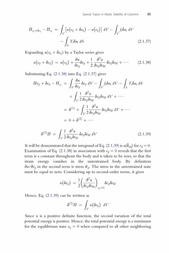
Special Topics in Elastic Stability of Columns 85

Peijþdeij �Peij ¼ZV

�u�eij þ deij

�� u�eij��

dV �ZV

fidui dV

�ZS

Tidui dS (2.1.37)

Expanding uðeij þ deijÞ by a Taylor series gives

u�eij þ deij

� ¼ u�eij�þ vu

veijdeij þ 1

2

v2u

veijvekldeijdekl þ $$$ (2.1.38)

Substituting Eq. (2.1.38) into Eq. (2.1.37) gives

Peij þ deij �Peij ¼ZV

vu

veijdeij dV �

ZV

fidui dV �ZS

Tidui dS

þZV

1

2

v2u

veijvekldeijdekl dV þ $$$

¼ dð1Þ þZV

1

2

v2u

veijvekldeijdekl dV þ $$$

¼ 0þ dð2Þ þ $$$

Z 2

dð2ÞP ¼V

1

2

v u

veijvekldeijdekl dV (2.1.39)

It will be demonstrated that the integrand of Eq. (2.1.39) is u(deij) for eij¼ 0.

Examination of Eq. (2.1.38) in association with eij ¼ 0 reveals that the first

term is a constant throughout the body and is taken to be zero, so that the

strain energy vanishes in the unrestrained body. By definition

vu/veij in the second term is stress sij. The stress in the unrestrained state

must be equal to zero. Considering up to second-order terms, it gives

u�deij� ¼ 1

2

�v2u

veijvekl

�eij¼0

deijdekl

Hence, Eq. (2.1.39) can be written as

dð2ÞP ¼ZV

u�deij�dV

Since u is a positive definite function, the second variation of the total

potential energy is positive. Hence, the total potential energy is a minimum

for the equilibrium state eij ¼ 0 when compared to all other neighboring

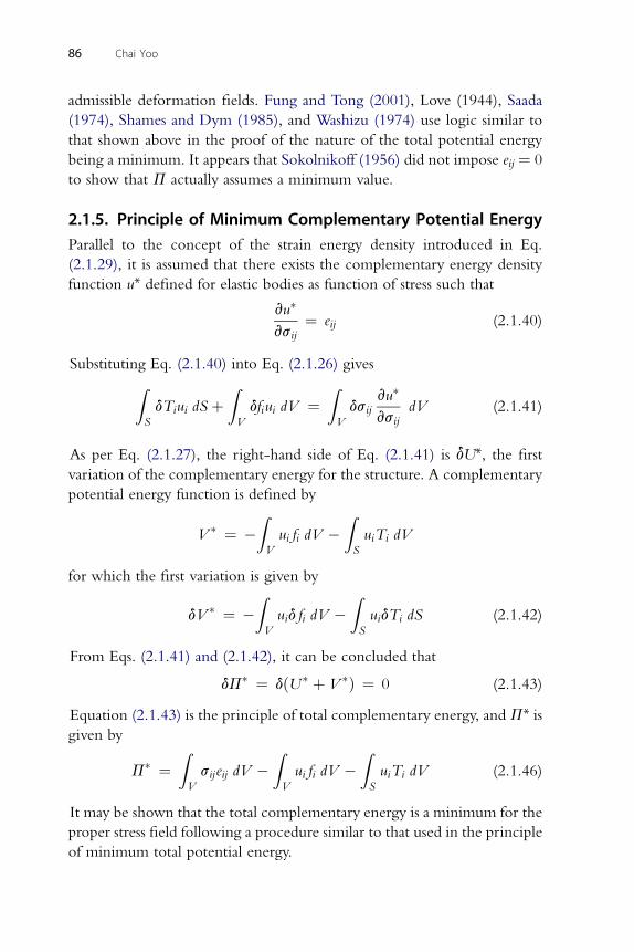
86 Chai Yoo

admissible deformation fields. Fung and Tong (2001), Love (1944), Saada

(1974), Shames and Dym (1985), and Washizu (1974) use logic similar to

that shown above in the proof of the nature of the total potential energy

being a minimum. It appears that Sokolnikoff (1956) did not impose eij ¼ 0

to show that P actually assumes a minimum value.

2.1.5. Principle of Minimum Complementary Potential EnergyParallel to the concept of the strain energy density introduced in Eq.

(2.1.29), it is assumed that there exists the complementary energy density

function u* defined for elastic bodies as function of stress such that

vu�

vsij¼ eij (2.1.40)

Substituting Eq. (2.1.40) into Eq. (2.1.26) givesZS

dTiui dS þZV

dfiui dV ¼ZV

dsijvu�

vsijdV (2.1.41)

As per Eq. (2.1.27), the right-hand side of Eq. (2.1.41) is dU*, the first

variation of the complementary energy for the structure. A complementary

potential energy function is defined by

V � ¼ �ZV

ui fi dV �ZS

uiTi dV

for which the first variation is given by

dV � ¼ �ZV

uid fi dV �ZS

uidTi dS (2.1.42)

From Eqs. (2.1.41) and (2.1.42), it can be concluded that

dP� ¼ dðU� þ V �Þ ¼ 0 (2.1.43)

Equation (2.1.43) is the principle of total complementary energy, andP* isgiven by

P� ¼ZV

sijeij dV �ZV

ui fi dV �ZS

uiTi dV (2.1.46)

It may be shown that the total complementary energy is a minimum for the

proper stress field following a procedure similar to that used in the principle

of minimum total potential energy.

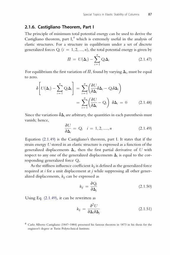
Special Topics in Elastic Stability of Columns 87

2.1.6. Castigliano Theorem, Part IThe principle of minimum total potential energy can be used to derive the

Castigliano theorem, part I,4 which is extremely useful in the analysis of

elastic structures. For a structure in equilibrium under a set of discrete

generalized forces Qi ði ¼ 1; 2; :::; nÞ, the total potential energy is given by

P ¼ UðDiÞ �Xni¼ 1

QiDi (2.1.47)

For equilibrium the first variation ofP, found by varying Di, must be equal

to zero.

d

"UðDiÞ �

Xni¼ 1

QiDi

#¼Xni¼ 1

�vU

vDidDi �QidDi

�

¼Xni¼ 1

�vU

vDi�Qi

�dDi ¼ 0 (2.1.48)

Since the variations dDi are arbitrary, the quantities in each parenthesis must

vanish; hence,

vU

vDi¼ Qi i ¼ 1; 2; ::::; n (2.1.49)

Equation (2.1.49) is the Castigliano’s theorem, part I. It states that if the

strain energy U stored in an elastic structure is expressed as a function of the

generalized displacements Di, then the first partial derivative of U with

respect to any one of the generalized displacements Di is equal to the cor-

responding generalized force Qi.

As the stiffness influence coefficient kij is defined as the generalized force

required at i for a unit displacement at j while suppressing all other gener-

alized displacements, kij can be expressed as

kij ¼ vQi

vDj(2.1.50)

Using Eq. (2.1.49), it can be rewritten as

kij ¼ v2U

vDivDj(2.1.51)

4 Carlo Alberto Castigliano (1847–1884) presented his famous theorem in 1873 in his thesis for the

engineer’s degree at Turin Polytechnical Institute.

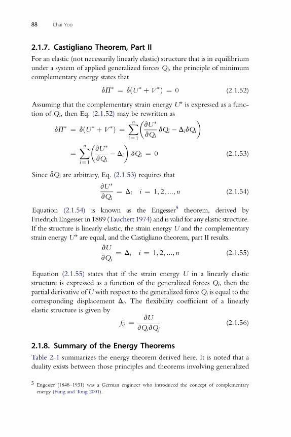
88 Chai Yoo

2.1.7. Castigliano Theorem, Part II

For an elastic (not necessarily linearly elastic) structure that is in equilibrium

under a system of applied generalized forces Qi, the principle of minimum

complementary energy states that

dP� ¼ dðU� þ V �Þ ¼ 0 (2.1.52)

Assuming that the complementary strain energy U* is expressed as a func-

tion of Qi, then Eq. (2.1.52) may be rewritten as

dP� ¼ dðU� þ V �Þ ¼Xni¼ 1

�vU�

vQidQi � DidQi

�

¼Xni¼ 1

�vU�

vQi� Di

�dQi ¼ 0 (2.1.53)

Since dQi are arbitrary, Eq. (2.1.53) requires that

vU�

vQi¼ Di i ¼ 1; 2; :::; n (2.1.54)

Equation (2.1.54) is known as the Engesser5 theorem, derived by

Friedrich Engesser in 1889 (Tauchert 1974) and is valid for anyelastic structure.

If the structure is linearly elastic, the strain energy U and the complementary

strain energy U* are equal, and the Castigliano theorem, part II results.

vU

vQi¼ Di i ¼ 1; 2; :::; n (2.1.55)

Equation (2.1.55) states that if the strain energy U in a linearly elastic

structure is expressed as a function of the generalized forces Qi, then the

partial derivative ofUwith respect to the generalized forceQi is equal to the

corresponding displacement Di. The flexibility coefficient of a linearly

elastic structure is given by

fij ¼ vU

vQivQj(2.1.56)

2.1.8. Summary of the Energy TheoremsTable 2-1 summarizes the energy theorem derived here. It is noted that a

duality exists between those principles and theorems involving generalized

5 Engesser (1848–1931) was a German engineer who introduced the concept of complementary

energy (Fung and Tong 2001).

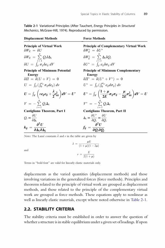
Table 2-1 Variational Principles (After Tauchert, Energy Principles in StructuralMechanics, McGraw-Hill, 1974). Reproduced by permission.

Displacement Methods Force Methods

Principle of Virtual Work Principle of Complementary Virtual WorkdWE ¼ dU dW �

E ¼ dU �

dWE ¼ Pni¼ 1

QidDi dW �E ¼ Pn

i¼ 1DidQi

dU ¼ RV sijdeij dV dU� ¼ R

V eijdsij dV

Principle of Minimum PotentialEnergy

Principle of Minimum ComplementaryEnergy

dP ¼ dðU þ V Þ ¼ 0 dP� ¼ dðU � þ V �Þ ¼ 0

U ¼ RV ðR eij0 sijdeijÞ dv U � ¼ R

V ðR sij0 eijdsijÞ dv

U ¼ RV�neijeij þ l

2e2kk

�dV ¼ U� U� ¼ RV

�1þ m

2Esijsij � m

2Es2kk

�dV ¼ U

V ¼ �Pni¼ 1

QiDi V � ¼ �Pni¼ 1

QiDi

Castigliano Theorem, Part I Castigliano Theorem, Part II

Qi [vU

vDiDi [

vU�

vQi[

vU

vQi

kij ¼ v2UvDivDj

fij ¼ v2UvQivQj

Notes: The Lame constants l and v in the table are given by

l ¼ mE

ð1þ mÞð1� 2mÞand

v ¼ E

2ð1þ mÞTerms in “bold font” are valid for linearly elastic materials only.

Special Topics in Elastic Stability of Columns 89

displacements as the varied quantities (displacement methods) and those

involving variations in the generalized forces (force methods). Principles and

theorems related to the principle of virtual work are grouped as displacement

methods, and those related to the principle of the complementary virtual

work are grouped as force methods. These equations apply to nonlinear as

well as linearly elastic materials, except where noted otherwise in Table 2-1.

2.2. STABILITY CRITERIA

The stability criteria must be established in order to answer the question of

whether a structure is in stable equilibriumunder a given set of loadings. If upon

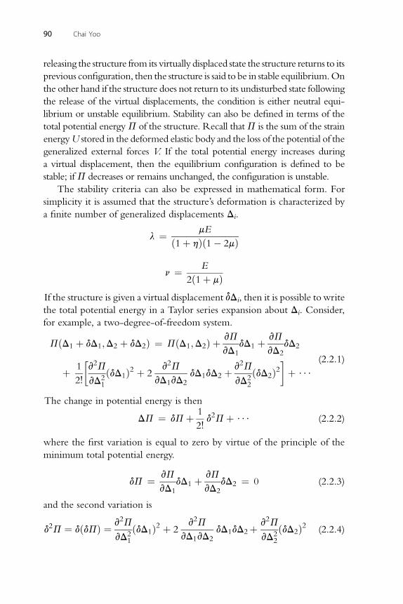
90 Chai Yoo

releasing the structure from its virtually displaced state the structure returns to its

previous configuration, then the structure is said to be in stable equilibrium.On

the other hand if the structure does not return to its undisturbed state following

the release of the virtual displacements, the condition is either neutral equi-

librium or unstable equilibrium. Stability can also be defined in terms of the

total potential energyP of the structure. Recall thatP is the sum of the strain

energyU stored in the deformed elastic body and the loss of the potential of the

generalized external forces V. If the total potential energy increases during

a virtual displacement, then the equilibrium configuration is defined to be

stable; ifP decreases or remains unchanged, the configuration is unstable.

The stability criteria can also be expressed in mathematical form. For

simplicity it is assumed that the structure’s deformation is characterized by

a finite number of generalized displacements Di.

l ¼ mE

ð1þ hÞð1� 2mÞ

E

n ¼

2ð1þ mÞIf the structure is given a virtual displacement dDi, then it is possible to write

the total potential energy in a Taylor series expansion about Di. Consider,

for example, a two-degree-of-freedom system.

PðD1 þ dD1;D2 þ dD2Þ ¼ PðD1;D2Þ þ vP

vD1dD1 þ vP

vD2dD2

þ 1

2!

�v2P

vD21

ðdD1Þ2 þ 2v2P

vD1vD2dD1dD2 þ v2P

vD22

ðdD2Þ2þ $$$

(2.2.1)

The change in potential energy is then

DP ¼ dPþ 1

2!d2Pþ $$$ (2.2.2)

where the first variation is equal to zero by virtue of the principle of the

minimum total potential energy.

dP ¼ vP

vD1dD1 þ vP

vD2dD2 ¼ 0 (2.2.3)

and the second variation is

d2P ¼ dðdPÞ ¼ v2P

vD21

ðdD1Þ2 þ 2v2P

vD1vD2dD1dD2þ v2P

vD22

ðdD2Þ2 (2.2.4)

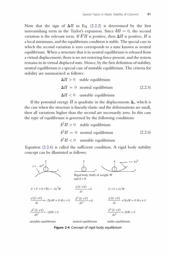
Special Topics in Elastic Stability of Columns 91

Note that the sign of DP in Eq. (2.2.2) is determined by the first

nonvanishing term in the Taylor’s expansion. Since dP ¼ 0, the second

variation is the relevant term. If d2P is positive, then DP is positive, P is

a local minimum, and the equilibrium condition is stable. The special case in

which the second variation is zero corresponds to a state known as neutral

equilibrium. When a structure that is in neutral equilibrium is released from

a virtual displacement, there is no net restoring force present, and the system

remains in its virtual displaced state. Hence, by the first definition of stability,

neutral equilibrium is a special case of unstable equilibrium. The criteria for

stability are summarized as follows:

DP > 0 stable equilibrium

DP ¼ 0 neutral equilibrium

DP < 0 unstable equilibrium

(2.2.5)

If the potential energy P is quadratic in the displacements Di, which is

the case when the structure is linearly elastic and the deformations are small,

then all variations higher than the second are necessarily zero. In this case

the type of equilibrium is governed by the following conditions:

d2P > 0 stable equilibrium

d2P ¼ 0 neutral equilibrium

d2P < 0 unstable equilibrium

(2.2.6)

Equation (2.2.6) is called the sufficient condition. A rigid body stability

concept can be illustrated as follows:

2U V 0 Wy kx W+ = + = − 0

dx=

dx== −2kxW = 0 @x = 0 0

dx2 = =2kxW = 0 @x = 0dx

= −2kW < 0

stable equilibrium

y kx2=

x xxy kx2= -

neutral equilibriumunstable equilibrium

d2 (U +V)

d2 (U +V)

d2 (U +V)

d (U +V)

d (U +V)

d (U +V)

= 2kW > 0 dx2dx2

U +V = kx2W

Rigid body (ball) of weight Wkand > 0.

Figure 2-4 Concept of rigid body equilibrium

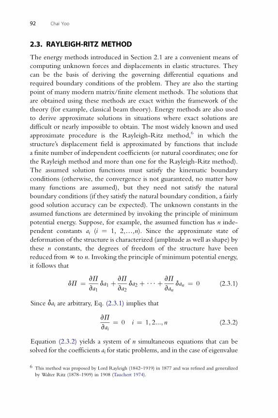
92 Chai Yoo

2.3. RAYLEIGH-RITZ METHOD

The energy methods introduced in Section 2.1 are a convenient means of

computing unknown forces and displacements in elastic structures. They

can be the basis of deriving the governing differential equations and

required boundary conditions of the problem. They are also the starting

point of many modern matrix/finite element methods. The solutions that

are obtained using these methods are exact within the framework of the

theory (for example, classical beam theory). Energy methods are also used

to derive approximate solutions in situations where exact solutions are

difficult or nearly impossible to obtain. The most widely known and used

approximate procedure is the Rayleigh-Ritz method,6 in which the

structure’s displacement field is approximated by functions that include

a finite number of independent coefficients (or natural coordinates; one for

the Rayleigh method and more than one for the Rayleigh-Ritz method).

The assumed solution functions must satisfy the kinematic boundary

conditions (otherwise, the convergence is not guaranteed, no matter how

many functions are assumed), but they need not satisfy the natural

boundary conditions (if they satisfy the natural boundary condition, a fairly

good solution accuracy can be expected). The unknown constants in the

assumed functions are determined by invoking the principle of minimum

potential energy. Suppose, for example, the assumed function has n inde-

pendent constants ai (i ¼ 1, 2,.,n). Since the approximate state of

deformation of the structure is characterized (amplitude as well as shape) by

these n constants, the degrees of freedom of the structure have been

reduced fromN to n. Invoking the principle of minimum potential energy,

it follows that

dP ¼ vP

va1da1 þ vP

va2da2 þ $$$þ vP

vandan ¼ 0 (2.3.1)

Since dai are arbitrary, Eq. (2.3.1) implies that

vP

vai¼ 0 i ¼ 1; 2:::; n (2.3.2)

Equation (2.3.2) yields a system of n simultaneous equations that can be

solved for the coefficients ai for static problems, and in the case of eigenvalue

6 This method was proposed by Lord Rayleigh (1842–1919) in 1877 and was refined and generalized

by Walter Ritz (1878–1909) in 1908 (Tauchert 1974).

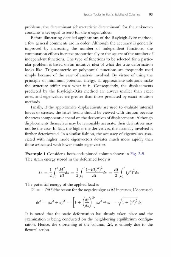
Special Topics in Elastic Stability of Columns 93

problems, the determinant (characteristic determinant) for the unknown

constants is set equal to zero for the n eigenvalues.

Before illustrating detailed applications of the Rayleigh-Ritz method,

a few general comments are in order. Although the accuracy is generally

improved by increasing the number of independent functions, the

computation efforts increase proportionally to the square of the number of

independent functions. The type of functions to be selected for a partic-

ular problem is based on an intuitive idea of what the true deformation

looks like. Trigonometric or polynomial functions are frequently used

simply because of the ease of analysis involved. By virtue of using the

principle of minimum potential energy, all approximate solutions make

the structure stiffer than what it is. Consequently, the displacements

predicted by the Rayleigh-Ritz method are always smaller than exact

ones, and eigenvalues are greater than those predicted by exact solution

methods.

Finally, if the approximate displacements are used to evaluate internal

forces or stresses, the latter results should be viewed with caution because

the stress components depend on the derivatives of displacements. Although

displacements themselves may be reasonably accurate, their derivatives may

not be the case. In fact, the higher the derivatives, the accuracy involved is

further deteriorated. In a similar fashion, the accuracy of eigenvalues asso-

ciated with higher mode eigenvectors deviates much more rapidly than

those associated with lower mode eigenvectors.

Example 1 Consider a both-ends pinned column shown in Fig. 2-5.

The strain energy stored in the deformed body is

U ¼ 1

2

Z ‘

0

M2

EIdx ¼ 1

2

Z ‘

0

ð�EIy00Þ2EI

dx ¼ EI

2

Z ‘

0

ðy00Þ2dx

The potential energy of the applied load is

V ¼ �PD‘ (the reason for the negative sign: asD‘ increases,V decreases)

ds2 ¼ dx2 þ dy2 ¼�1þ

�dy

dx

�2dx20ds ¼

ffiffiffiffiffiffiffiffiffiffiffiffiffiffiffiffiffiffi1þ ðy0Þ2

qdx

It is noted that the static deformation has already taken place and the

examination is being conducted on the neighboring equilibrium configu-

ration. Hence, the shortening of the column, D‘, is entirely due to the

flexural action.

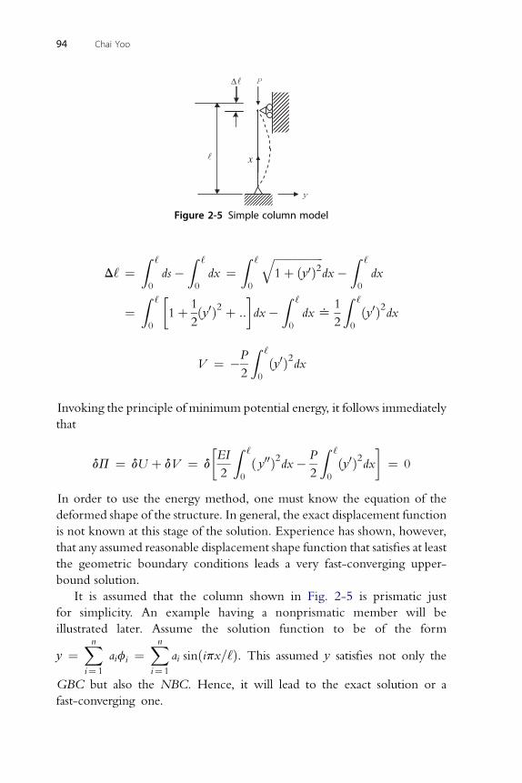
x

Figure 2-5 Simple column model

94 Chai Yoo

D‘ ¼Z ‘

0

ds�Z ‘

0

dx ¼Z ‘

0

ffiffiffiffiffiffiffiffiffiffiffiffiffiffiffiffiffiffi1þ ðy0Þ2

qdx�

Z ‘

0

dx

¼Z ‘

0

�1þ 1

2ðy0Þ2 þ ::

dx�

Z ‘

0

dx ^1

2

Z ‘

0

ðy0Þ2dx

Z ‘

V ¼ �P

2 0

ðy0Þ2dx

Invoking the principle of minimum potential energy, it follows immediately

that

dP ¼ dU þ dV ¼ d

�EI

2

Z ‘

0

ð y00Þ2dx� P

2

Z ‘

0

ðy0Þ2dx¼ 0

In order to use the energy method, one must know the equation of the

deformed shape of the structure. In general, the exact displacement function

is not known at this stage of the solution. Experience has shown, however,

that any assumed reasonable displacement shape function that satisfies at least

the geometric boundary conditions leads a very fast-converging upper-

bound solution.

It is assumed that the column shown in Fig. 2-5 is prismatic just

for simplicity. An example having a nonprismatic member will be

illustrated later. Assume the solution function to be of the form

y ¼Xni¼ 1

aifi ¼Xni¼ 1

ai sinðipx=‘Þ. This assumed y satisfies not only the

GBC but also the NBC. Hence, it will lead to the exact solution or a

fast-converging one.

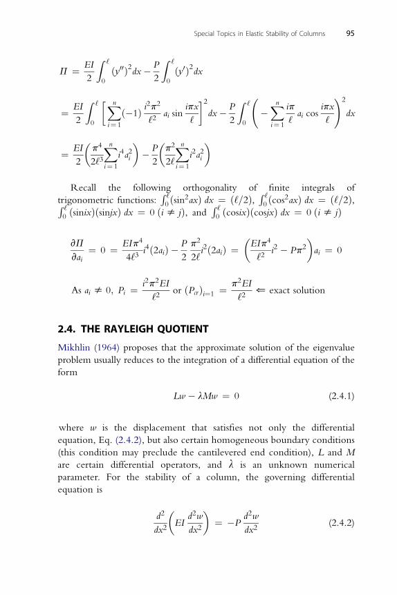
Special Topics in Elastic Stability of Columns 95

P ¼ EI

2

Z ‘

0

ðy00Þ2dx� P

2

Z ‘

0

ðy0Þ2dx

¼ EI

2

Z ‘

0

�Xni¼ 1

ð�1Þ i2p2

‘2ai sin

ipx

‘

2dx� P

2

Z ‘

0

�Xni¼ 1

ip

‘ai cos

ipx

‘

!2

dx

¼ EI

2

�p4

2‘3

Xni¼ 1

i4a2i

�� P

2

�p2

2‘

Xni¼ 1

i2a2i

�

Recall the following orthogonality of finite integrals ofR R

trigonometric functions:

‘0 ðsin2axÞ dx ¼ ð‘=2Þ, ‘

0 ðcos2axÞ dx ¼ ð‘=2Þ,R ‘0 ðsinixÞðsinjxÞ dx ¼ 0 ði s jÞ, and R ‘0 ðcosixÞðcosjxÞ dx ¼ 0 ðis jÞ

vP

vai¼ 0 ¼ EIp4

4‘3i4ð2aiÞ � P

2

p2

2‘i2ð2aiÞ ¼

�EIp4

‘2i2 � Pp2

�ai ¼ 0

As ai s 0; Pi ¼ i2p2EI

‘2or ðPcrÞi¼1 ¼ p2EI

‘2* exact solution

2.4. THE RAYLEIGH QUOTIENT

Mikhlin (1964) proposes that the approximate solution of the eigenvalue

problem usually reduces to the integration of a differential equation of the

form

Lw � lMw ¼ 0 (2.4.1)

where w is the displacement that satisfies not only the differential

equation, Eq. (2.4.2), but also certain homogeneous boundary conditions

(this condition may preclude the cantilevered end condition), L and M

are certain differential operators, and l is an unknown numerical

parameter. For the stability of a column, the governing differential

equation is

d2

dx2

�EI

d2w

dx2

�¼ �P

d2w

dx2(2.4.2)

96 Chai Yoo

For Eq. (2.4.2)

Lhd2

dx2EI

d2

dx2(2.4.3)

M h � d2(2.4.4)

dx2

l ¼ P (2.4.5)

Equations (2.4.3) and (2.4.4) are self-adjoint (symmetric), positive definite

operators for the usual end supports of columns. If a linear differential

operator L has the following property, it is called a self-adjoint or symmetric

operator:

ðLu; vÞ ¼ ðu;LvÞ (2.4.6)

The inner product of two functions g and h over the domain V is defined as

ðg; hÞh inner product of g and hh

ZV

gh dv (2.4.7)

An operator is said to be positive definite if the following inequality is valid

for any function from its field of definition, uðqÞ s 0:

ðLu; uÞ > 0; ðLu; uÞh 0 for uðqÞh 0 (2.4.8)

The reason why one is concerned whether or not a boundary-value problem

has the properties of being self-adjoint (symmetric) and positive definite is

that boundary-value problems having these properties are said to be properly

posed, and there exists a unique solution to a properly posed boundary-value

problem. An improperly posed boundary-value problem due to haphazardly

or arbitrarily assigned boundary conditions is meaningless.

Multiplying both sides of Eq. (2.4.2) by w and integrating over the

domain yields Z ‘

0

wd2

dx2

�EI

d2w

dx2

�dx ¼ �P

Z ‘

0

wd2w

dx2dx (2.4.9)

Integrate the left-hand side of Eq. (2.4.9) by parts twice, as follows:

Z ‘

0

wd2

dx2

�EI

d2w

dx2

�dx ¼

Z ‘

0

EI

�d2w

dx2

�2

dxþ wd

dx

�EI

d2w

dx2

������‘

0

� EIdw

dx

d2w

dx2

�����‘

0

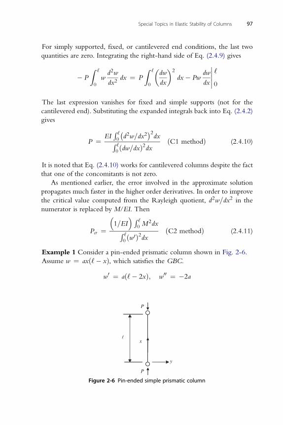
Special Topics in Elastic Stability of Columns 97

For simply supported, fixed, or cantilevered end conditions, the last two

quantities are zero. Integrating the right-hand side of Eq. (2.4.9) gives

� P

Z ‘

0

wd2w

dx2dx ¼ P

Z ‘

0

�dw

dx

�2

dx� Pwdw

dx

�����‘

0

The last expression vanishes for fixed and simple supports (not for the

cantilevered end). Substituting the expanded integrals back into Eq. (2.4.2)

gives

P ¼ EIR ‘0

�d2w=dx2

�2dxR ‘

0 ðdw=dxÞ2dxðC1 methodÞ (2.4.10)

It is noted that Eq. (2.4.10) works for cantilevered columns despite the fact

that one of the concomitants is not zero.

As mentioned earlier, the error involved in the approximate solution

propagates much faster in the higher order derivatives. In order to improve

the critical value computed from the Rayleigh quotient, d2w=dx2 in the

numerator is replaced by M/EI. Then

Pcr ¼�1=EI

R ‘0 M

2dxR ‘0 ðw0Þ2dx

ðC2 methodÞ (2.4.11)

Example 1 Consider a pin-ended prismatic column shown in Fig. 2-6.

Assume w ¼ axð‘� xÞ, which satisfies the GBC.

w0 ¼ að‘� 2xÞ; w00 ¼ �2a

y

x

P

P

Figure 2-6 Pin-ended simple prismatic column

4EIa2R ‘

dx

Pcr ¼ 0

a2R ‘0 ð‘� 2xÞ2dx

¼ 12EI

‘2*21:6% greater than Euler load

For C2 method: M ¼ Pcrw ¼ Pcraxð‘� xÞ

Pcr ¼ ð1=EIÞ R ‘0 ðPcrwÞ2dxR ‘0 ðw0Þ2dx

¼ ðP2cr a

2=EIÞ R ‘0�‘x� x2�2dx

a2R ‘0 ð‘� 2xÞ2dx

ð10EIÞ

98 Chai Yoo

Pcr ¼‘2

*only 1:32% greater than the exact solution;

p2EI 9:8696EI

PE ¼

‘2¼

‘2

If the true deflection curve is used, both the C1 method and the C2

method lead to the same exact solution. However, if an approximate

expression for the deflection curve is used for w, the error in w00 is

considerably greater than the error in w or w0. Hence, C2 method gives

a better solution than the C1 method does. In general, the energy method

leads to the values of the critical load that are greater than the exact solution

as a consequence of using the principle of minimum potential energy. Such

greater values are called the upper-bound solution.

Example 2 Consider a prismatic cantilever column with the fixed support

at x ¼ 0.

Assume w ¼ ax2, which satisfies the GBC.

w0 ¼ 2ax; w00 ¼ 2a

2R ‘

Pcr ¼ 4EIa 0 dx

4a2R ‘0 x

2dx¼ 3EI

‘2*21:6% greater than exact load

For the C2 method: MðxÞ ¼ Pcrað‘2 � x2Þ

Pcr ¼ ð1=EIÞ R ‘0 ½MðxÞ�2dxR ‘0 ðw0Þ2dx

¼ ð1=EIÞP2cr a

2R ‘0

�‘2 � x2

�2dx

4a2R ‘0 x

2dx

¼�8=15EIÞP2

cr a2‘5

4=3a2‘3¼ 2P2

cr‘2

5EI

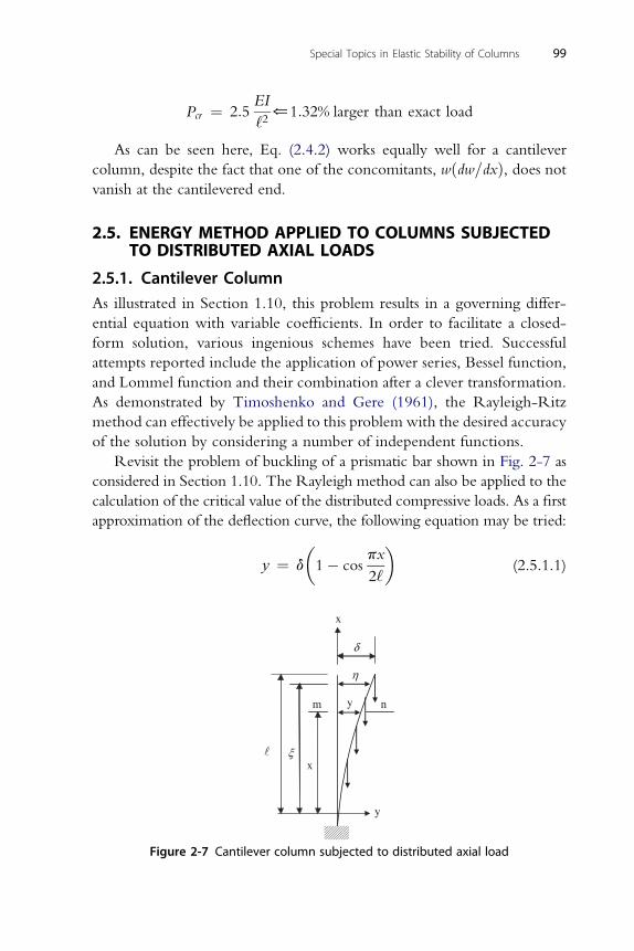
EI

Pcr ¼ 2:5

‘2*1:32% larger than exact load

As can be seen here, Eq. (2.4.2) works equally well for a cantilever

column, despite the fact that one of the concomitants, wðdw=dxÞ, does notvanish at the cantilevered end.

Special Topics in Elastic Stability of Columns 99

2.5. ENERGY METHOD APPLIED TO COLUMNS SUBJECTEDTO DISTRIBUTED AXIAL LOADS

2.5.1. Cantilever ColumnAs illustrated in Section 1.10, this problem results in a governing differ-

ential equation with variable coefficients. In order to facilitate a closed-

form solution, various ingenious schemes have been tried. Successful

attempts reported include the application of power series, Bessel function,

and Lommel function and their combination after a clever transformation.

As demonstrated by Timoshenko and Gere (1961), the Rayleigh-Ritz

method can effectively be applied to this problem with the desired accuracy

of the solution by considering a number of independent functions.

Revisit the problem of buckling of a prismatic bar shown in Fig. 2-7 as

considered in Section 1.10. The Rayleigh method can also be applied to the

calculation of the critical value of the distributed compressive loads. As a first

approximation of the deflection curve, the following equation may be tried:

y ¼ d

�1� cos

px

2‘

�(2.5.1.1)

x

n y m

y

x

Figure 2-7 Cantilever column subjected to distributed axial load

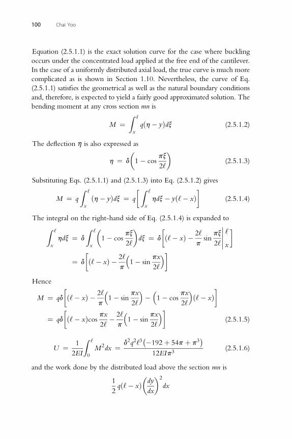
100 Chai Yoo

Equation (2.5.1.1) is the exact solution curve for the case where buckling

occurs under the concentrated load applied at the free end of the cantilever.

In the case of a uniformly distributed axial load, the true curve is much more

complicated as is shown in Section 1.10. Nevertheless, the curve of Eq.

(2.5.1.1) satisfies the geometrical as well as the natural boundary conditions

and, therefore, is expected to yield a fairly good approximated solution. The

bending moment at any cross section mn is

M ¼Z ‘

x

qðh� yÞdx (2.5.1.2)

The deflection h is also expressed as

h ¼ d

�1� cos

px

2‘

�(2.5.1.3)

Substituting Eqs. (2.5.1.1) and (2.5.1.3) into Eq. (2.5.1.2) gives

M ¼ q

Z ‘

x

ðh� yÞdx ¼ q

� Z ‘

x

hdx� yð‘� xÞ

(2.5.1.4)

The integral on the right-hand side of Eq. (2.5.1.4) is expanded toZ ‘

x

hdx ¼ d

Z ‘

x

�1� cos

px

2‘

�dx ¼ d

�ð‘� xÞ � 2‘

psin

px

2‘

�����‘

x

¼ d

�ð‘� xÞ � 2‘

p

�1� sin

px

2‘

Hence

M ¼ qd

�ð‘� xÞ � 2‘

p

�1� sin

px

2‘

��1� cos

px

2‘

ð‘� xÞ

¼ qd

�ð‘� xÞcos px

2‘� 2‘

p

�1� sin

px

2‘

(2.5.1.5)

Z ‘ 2 2 3�

3�

U ¼ 1

2EI 0

M2dx ¼ d q ‘ �192þ 54pþ p

12EIp3(2.5.1.6)

and the work done by the distributed load above the section mn is

1

2qð‘� xÞ

�dy

dx

�2

dx

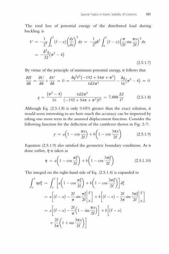
Special Topics in Elastic Stability of Columns 101

The total loss of potential energy of the distributed load during

buckling is

V ¼ �1

2q

Z ‘

0

ð‘� xÞ�dy

dx

�2

dx ¼ �1

2qd2Z ‘

0

ð‘� xÞ�p2‘

sinpx

2‘

2dx

¼ �d2q

32

�p2 � 4

�(2.5.1.7)

By virtue of the principle of minimum potential energy, it follows that

vP

vd¼ vU

vdþ vV

vd¼ 0 ¼ dq2‘3

��192þ 54pþ p3�

6EIp3� dq

16

�p2 � 4

� ¼ 0

�p2 � 4

�3

q ¼16

6EIp

ð�192þ 54pþ p3Þ‘3 ¼ 7:888EI

‘3(2.5.1.8)

Although Eq. (2.5.1.8) is only 0.65% greater than the exact solution, it

would seem interesting to see how much the accuracy can be improved by

taking one more term in the assumed displacement function. Consider the

following function for the deflection of the cantilever shown in Fig. 2-7:

y ¼ a�1� cos

px

2‘

þ b

�1� cos

3px

2‘

�(2.5.1.9)

Equation (2.5.1.9) also satisfied the geometric boundary conditions. As is

done earlier, h is taken as

h ¼ a

�1� cos

px

2‘

�þ b

�1� cos

3px

2‘

�(2.5.1.10)

The integral on the right-hand side of Eq. (2.5.1.4) is expanded to

Z ‘

x

hdx ¼Z ‘

x

�a

�1� cos

px

2‘

�þ b

�1� cos

3px

2‘

�dx

¼ a

�ð‘� xÞ � 2‘

psin

px

2‘

�����‘

x

þ b

�ð‘� xÞ � 2‘

3psin

3px

2‘

�����‘

x

¼ a

�ð‘� xÞ � 2‘

p

�1� sin

px

2‘

þ b

�ð‘� xÞ

þ 2‘

3p

�1þ sin

3px

2‘

�

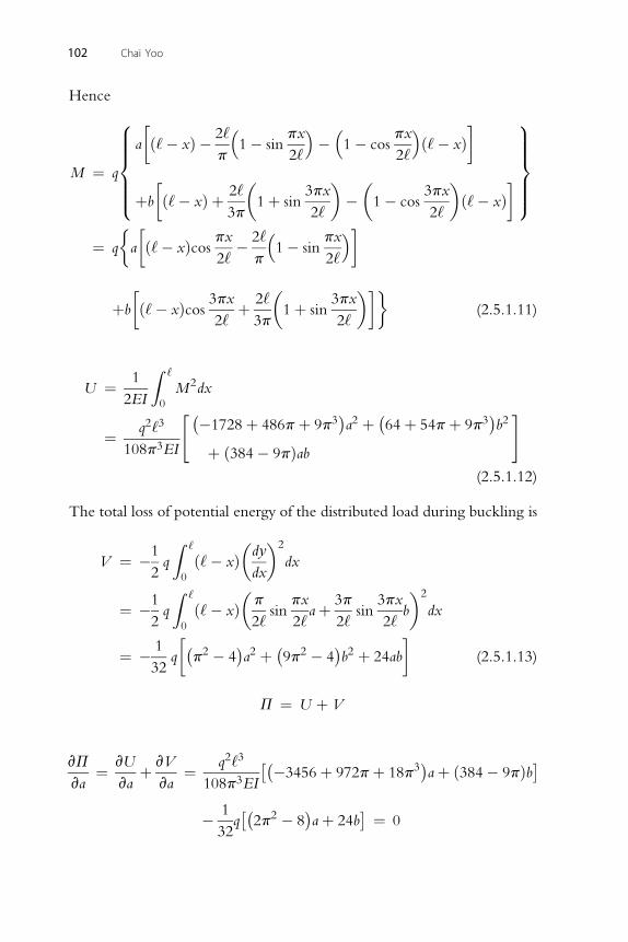
102 Chai Yoo

Hence

M ¼ q

a

�ð‘� xÞ � 2‘

p

�1� sin

px

2‘

��1� cos

px

2‘

ð‘� xÞ

þb

�ð‘� xÞ þ 2‘

3p

�1þ sin

3px

2‘

���1� cos

3px

2‘

�ð‘� xÞ

8>>>><>>>>:

9>>>>=>>>>;

¼ q

�a

�ð‘� xÞcos px

2‘� 2‘

p

�1� sin

px

2‘

þb

�ð‘� xÞcos 3px

2‘þ 2‘

3p

�1þ sin

3px

2‘

��(2.5.1.11)

U ¼ 1

2EI

Z ‘

0

M2dx

¼ q2‘3

108p3EI

" ��1728þ 486pþ 9p3�a2 þ �64þ 54pþ 9p3

�b2

þ ð384� 9pÞab

#

(2.5.1.12)

The total loss of potential energy of the distributed load during buckling is

V ¼ �1

2q

Z ‘

0

ð‘� xÞ�dy

dx

�2

dx

¼ �1

2q

Z ‘

0

ð‘� xÞ�p

2‘sin

px

2‘aþ 3p

2‘sin

3px

2‘b

�2

dx

¼ � 1

32q

��p2 � 4

�a2 þ �9p2 � 4

�b2 þ 24ab

(2.5.1.13)

P ¼ U þ V

vP

va¼ vU

vaþ vV

va¼ q2‘3

108p3EI

���3456þ 972pþ 18p3�aþ ð384� 9pÞb�

� 1

32q��2p2 � 8

�aþ 24b

� ¼ 0

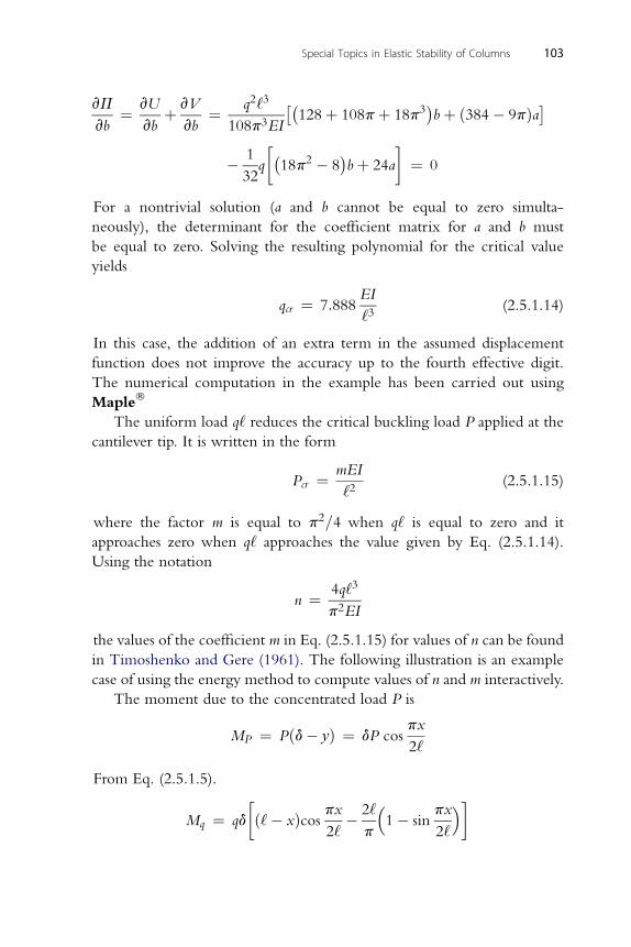
vP vU vV q2‘3 �� � �

vb

¼vb

þvb

¼108p3EI

128þ 108pþ 18p3 bþ ð384� 9pÞa

� 1

32q

��18p2 � 8

�bþ 24a

¼ 0

For a nontrivial solution (a and b cannot be equal to zero simulta-

Special Topics in Elastic Stability of Columns 103

neously), the determinant for the coefficient matrix for a and b must

be equal to zero. Solving the resulting polynomial for the critical value

yields

qcr ¼ 7:888EI

‘3(2.5.1.14)

In this case, the addition of an extra term in the assumed displacement

function does not improve the accuracy up to the fourth effective digit.

The numerical computation in the example has been carried out using

Maple�

The uniform load q‘ reduces the critical buckling load P applied at the

cantilever tip. It is written in the form

Pcr ¼ mEI

‘2(2.5.1.15)

where the factor m is equal to p2=4 when q‘ is equal to zero and it

approaches zero when q‘ approaches the value given by Eq. (2.5.1.14).

Using the notation

n ¼ 4q‘3

p2EI

the values of the coefficient m in Eq. (2.5.1.15) for values of n can be found

in Timoshenko and Gere (1961). The following illustration is an example

case of using the energy method to compute values of n and m interactively.

The moment due to the concentrated load P is

MP ¼ Pðd� yÞ ¼ dP cospx

2‘

From Eq. (2.5.1.5).

Mq ¼ qd

�ð‘� xÞcos px

2‘� 2‘

p

�1� sin

px

2‘

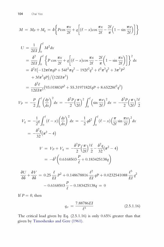
�px

�px 2‘� px �

M ¼ MP þMq ¼ d Pcos2‘

þ q ð‘� xÞcos2‘

�p

1� sin2‘

Z ‘

104 Chai Yoo

U ¼ 1

2EI 0

M2dx

¼ d2

2EI

Z ‘

0

�P cos

px

2‘þ q

�ð‘� xÞcos px

2‘� 2‘

p

�1� sin

px

2‘

��2

dx

¼ d2‘��12p‘pqP þ 54‘2pq2 � 192‘2q2 þ ‘2p3q2 þ 3p3P2

þ 3‘p3qP���

12EIp3�

¼ d2‘

12EIp3

�93:01883P2 þ 55:3197182‘qP þ 8:65228‘2q2

�Z ‘� �2 2 � 2 Z ‘� 2 2 � 2

VP ¼ �P

2 0

dy

dxdx ¼ �d P

2

p

2‘ 0

sinpx

2‘dx ¼ �d P

2

p

2‘

‘

2

Z ‘ � �2 Z ‘ � 2

Vq ¼ �1

2q

0

ð‘� xÞ dy

dxdx ¼ �1

2qd2

0

ð‘� xÞ p

2‘sin

px

2‘dx

¼ �d2q

32

�p2 � 4

�2 � 2 2 � �

V ¼ VP þ Vq ¼ �d P

2

p

2‘

‘

2� d q

32p2 � 4

¼ �d2�0:6168503

P

‘þ 0:183425138q

�

vU vV ‘ ‘2 ‘3

vdþ

vd¼ 0:25

EIP2 þ 0:148678816

EIqP þ 0:0232541088

EIq2

� 0:6168503P

‘� 0:183425138q ¼ 0

If P ¼ 0, then

qcr ¼ 7:88786EI

‘3(2.5.1.16)

The critical load given by Eq. (2.5.1.16) is only 0.65% greater than that

given by Timoshenko and Gere (1961).

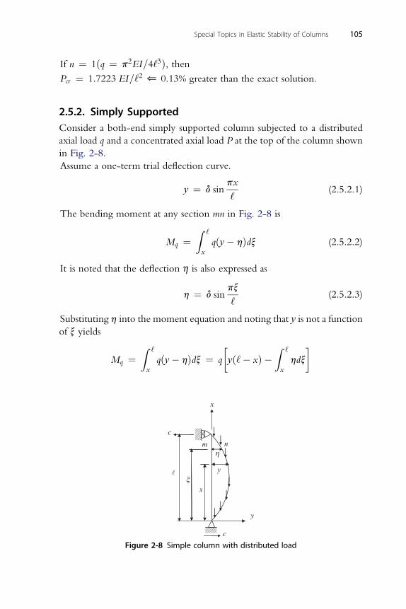
Special Topics in Elastic Stability of Columns 105

If n ¼ 1ðq ¼ p2EI=4‘3Þ, thenPcr ¼ 1:7223 EI=‘2 * 0.13% greater than the exact solution.

2.5.2. Simply SupportedConsider a both-end simply supported column subjected to a distributed

axial load q and a concentrated axial load P at the top of the column shown

in Fig. 2-8.

Assume a one-term trial deflection curve.

y ¼ d sinpx

‘(2.5.2.1)

The bending moment at any section mn in Fig. 2-8 is

Mq ¼Z ‘

x

qðy� hÞdx (2.5.2.2)

It is noted that the deflection h is also expressed as

h ¼ d sinpx

‘(2.5.2.3)

Substituting h into the moment equation and noting that y is not a function

of x yields

Mq ¼Z ‘

x

qðy� hÞdx ¼ q

�yð‘� xÞ �

Z ‘

x

hdx

x

y

hm

xx

n

y

c

c

Figure 2-8 Simple column with distributed load

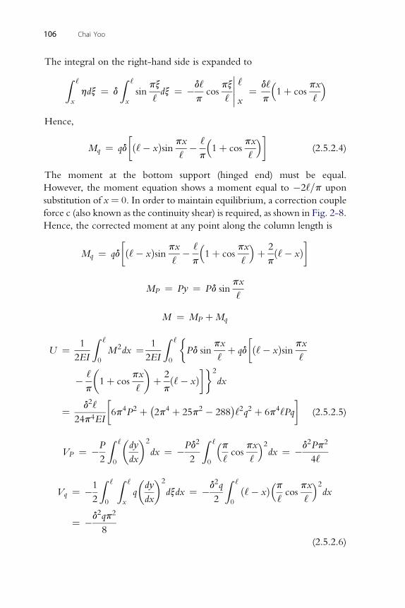
106 Chai Yoo

The integral on the right-hand side is expanded to

Z ‘

x

hdx ¼ d

Z ‘

x

sinpx

‘dx ¼ �d‘

pcos

px

‘

�����‘

x¼ d‘

p

�1þ cos

px

‘

Hence,

Mq ¼ qd

�ð‘� xÞsin px

‘� ‘

p

�1þ cos

px

‘

(2.5.2.4)

The moment at the bottom support (hinged end) must be equal.

However, the moment equation shows a moment equal to �2‘=p upon

substitution of x¼ 0. In order to maintain equilibrium, a correction couple

force c (also known as the continuity shear) is required, as shown in Fig. 2-8.

Hence, the corrected moment at any point along the column length is

Mq ¼ qd

�ð‘� xÞsin px

‘� ‘

p

�1þ cos

px

‘

þ 2

pð‘� xÞ

px

MP ¼ Py ¼ Pd sin

‘

M ¼ M þM

P q

Z ‘ Z ‘� �

U ¼ 1

2EI 0

M2dx ¼ 1

2EI 0

Pd sinpx

‘þ qd ð‘� xÞsin px

‘

� ‘

p

�1þ cos

px

‘

�þ 2

pð‘� xÞ

�2

dx

¼ d2‘

24p4EI

�6p4P2 þ �2p4 þ 25p2 � 288

�‘2q2 þ 6p4‘Pq

(2.5.2.5)

Z ‘� �2 2 Z ‘� 2 2 2

VP ¼ �P

2 0

dy

dxdx ¼ �Pd

2 0

p

‘cos

px

‘dx ¼ �d Pp

4‘

Z ‘ Z ‘ � �2 2 Z ‘ � 2

Vq ¼ �1

2 0 x

qdy

dxdxdx ¼ �d q

2 0

ð‘� xÞ p

‘cos

px

‘dx

¼ �d2qp2

8

(2.5.2.6)

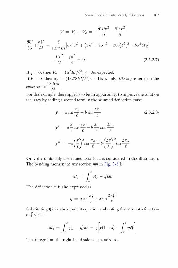
d2Pp2 d2qp2

V ¼ VP þ Vq ¼ �4‘

�8

vU vV ‘ �4 2

�4 2

�2 2 4

�

Special Topics in Elastic Stability of Columns 107

vdþ

vd¼

12p4EI6p P þ 2p þ 25p � 288 ‘ q þ 6p ‘Pq

� Pp2

2‘� qp2

4¼ 0 ð2:5:2:7Þ

If q ¼ 0, then Pcr ¼ ðp2EI=‘2Þ * As expected.

If P ¼ 0, then qcr ¼ ð18:78EI=‘3Þ* this is only 0.98% greater than the

exact value18:6EI

‘3.

For this example, there appears to be an opportunity to improve the solution

accuracy by adding a second term in the assumed deflection curve.

y ¼ a sinpx

‘þ b sin

2px

‘(2.5.2.8)

0 p px 2p 2px

y ¼ a

‘cos

‘þ b

‘cos

‘�p�2 px

�2p�2 2px

y 00 ¼ �a‘

sin‘� b

‘sin

‘

Only the uniformly distributed axial load is considered in this illustration.

The bending moment at any section mn in Fig. 2-8 is

Mq ¼Z ‘

x

qðy� hÞdx

The deflection h is also expressed as

h ¼ a sinpx

‘þ b sin

2px

‘

Substituting h into the moment equation and noting that y is not a function

of x yields:

Mq ¼Z ‘

x

qðy� hÞdx ¼ q

�yð‘� xÞ �

Z ‘

x

hdx

The integral on the right-hand side is expanded to

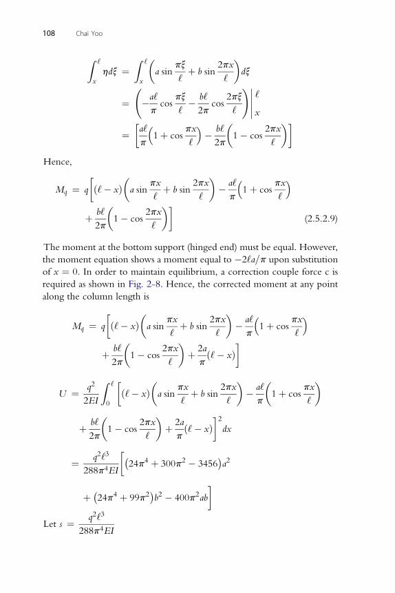
108 Chai Yoo

Z ‘

x

hdx ¼Z ‘

x

�a sin

px

‘þ b sin

2px

‘

�dx

¼ �a‘

pcos

px

‘� b‘

2pcos

2px

‘

!�����‘

x

¼�a‘

p

�1þ cos

px

‘

� b‘

2p

�1� cos

2px

‘

�

Hence,

Mq ¼ q

�ð‘� xÞ

�a sin

px

‘þ b sin

2px

‘

�� a‘

p

�1þ cos

px

‘

þ b‘

2p

�1� cos

2px

‘

�(2.5.2.9)

The moment at the bottom support (hinged end) must be equal. However,

the moment equation shows a moment equal to �2‘a=p upon substitution

of x ¼ 0. In order to maintain equilibrium, a correction couple force c is

required as shown in Fig. 2-8. Hence, the corrected moment at any point

along the column length is

Mq ¼ q

�ð‘� xÞ

�a sin

px

‘þ b sin

2px

‘

�� a‘

p

�1þ cos

px

‘

þ b‘

2p

�1� cos

2px

‘

�þ 2a

pð‘� xÞ

2 Z ‘ � � � � �

U ¼ q

2EI 0

ð‘� xÞ a sinpx

‘þ b sin

2px

‘� a‘

p1þ cos

px

‘

þ b‘

2p

�1� cos

2px

‘

�þ 2a

pð‘� xÞ

2dx

¼ q2‘3

288p4EI

��24p4 þ 300p2 � 3456

�a2

þ �24p4 þ 99p2�b2 � 400p2ab

Let s ¼ q2‘3

4

288p EI

Special Topics in Elastic Stability of Columns 109

V ¼ �1

2

Z ‘

0

Z ‘

x

q

�dy

dx

�2

dxdx

¼ �q

2

Z ‘

0

ð‘� xÞ�ap

‘cos

px

‘þ b

2p

‘cos

2px

‘

�2

dx

¼ �q

�20

9abþ p2

8a2 þ p2

2b2�

vU vV

vaþ

va¼ ð3685:4s� 2:4674Þaþ ð3947:84s� 2:22222Þb ¼ 0

vU vV

vbþ

vb¼ ð3947:84s� 2:222222Þaþ ð6629:818s� 9:8696Þb ¼ 0

�� 3685:4s� 2:4674 3947:84s� 2:22222��

��� 3947:84s� 2:22222 6629:818s� 9:8696

��� ¼ 0

For a nontrivial solution (a and b cannot be equal to zero simultaneously),

the determinant of the coefficient must be zero.

Solving for s gives

s ¼ 0:000661938 ¼ q2‘3

288p4EI0 qcr ¼ 18:57

EI

‘3

2.5.3. Pinned-Clamped ColumnA propped column with the top rotationally clamped and the bottom

pinned is subjected to a uniformly distributed axial compression as shown

in Fig. 2-9. Because of the boundary condition, a continuity shear or

a correction couple force is expected for equilibrium.

Assume a one-term trial displacement function as

y ¼ að‘3x� 3‘x3 þ 2x4Þ (2.5.3.1)

Boundary conditions are

y ¼ 0 @ x ¼ 0 and y ¼ 0 @ x ¼ ‘

y0 ¼ 0 @ x ¼ ‘ and y00 ¼ 0 @ x ¼ 0

The function satisfies the geometric and natural boundary conditions at

both ends.

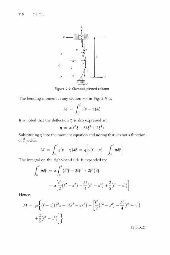
x

n

y

h

y

xx

m

q

c

c

Figure 2-9 Clamped-pinned column

110 Chai Yoo

The bending moment at any section mn in Fig. 2-9 is:

M ¼Z ‘

x

qðy� hÞdx

It is noted that the deflection h is also expressed as:

h ¼ a�‘3x� 3‘x3 þ 2x4

�Substituting h into the moment equation and noting that y is not a function

of x yields:

M ¼Z ‘

x

qðy� hÞdx ¼ q

�yð‘� xÞ �

Z ‘

x

hdx

The integral on the right-hand side is expanded to:

Z ‘

x

hdx ¼ a

Z ‘

x

�‘3x� 3‘x3 þ 2x4

�dx

¼ a

�‘3

2

�‘2 � x2

�� 3‘

4

�‘4 � x4

�þ 2

5

�‘5 � x5

�Hence,

M ¼ qa

�ð‘� xÞ�‘3x� 3‘x3 þ 2x4

�� �‘32

�‘2 � x2

�� 3‘

4

�‘4 � x4

�

þ 2

5

�‘5 � x5

��(2.5.3.2)

Special Topics in Elastic Stability of Columns 111

The moment at the bottom support (hinged end) must be equal to zero.

However, the moment equation shows a moment equal to �3‘5=20 upon

substitution of x ¼ 0. In order to maintain equilibrium, a correction couple

force c (also known as the continuity shear) is required as shown in Fig. 2-9.

Hence, the corrected moment at any point along the column length is

M ¼ qa

�ð‘� xÞ

�‘3x� 3‘x3 þ 2x4 þ 3‘4

20

���‘3

2

�‘2 � x2

�

� 3‘

4

�‘4 � x4

�þ 2

5

�‘5 � x5

��

The assumed deflection function has an inflection point at x ¼ 0:75‘. In

order to ensure the moment to be equal to zero at the inflection point, the

moment equation needs an additional adjustment.

M ¼ qa

ð‘� xÞ�‘3x� 3‘x3 þ 2x4 þ 3‘4

20

�� 0:074211875‘4x

��‘3

2

�‘2 � x2

�� 3‘

4

�‘4 � x4

�þ 2

5

�‘5 � x5

�8>>><>>>:

9>>>=>>>;

(2.5.3.3)Z ‘

U ¼ 1

2EI 0

M2dx

¼ q2a2

2EI

Z ‘

0

ð‘� xÞ�‘3x� 3‘x3 þ 2x4 þ 3‘4

20

�� 0:07421875‘4x

��‘3

2ð‘2 � x2Þ � 3‘

4ð‘4 � x4Þ þ 2

5ð‘5 � x5Þ

8>>><>>>:

9>>>=>>>;

2

dx

¼ 0:007519762734 ‘11q2a2=2EI

Z ‘ Z ‘ � �2

Vq ¼ �1

2 0 x

qdy

dxdxdx

¼ �a2q

2

Z ‘

0

ð‘� xÞ�‘3 � 9‘x2 þ 8x3�2dx ¼ 3‘8qa2

28

vU vV ‘11q 6‘8

vaþ

va¼

EIð0:0075197627534Þ �

28¼ 00

q ¼ 28:5EI

‘3ð5% less than the exact solutionÞ

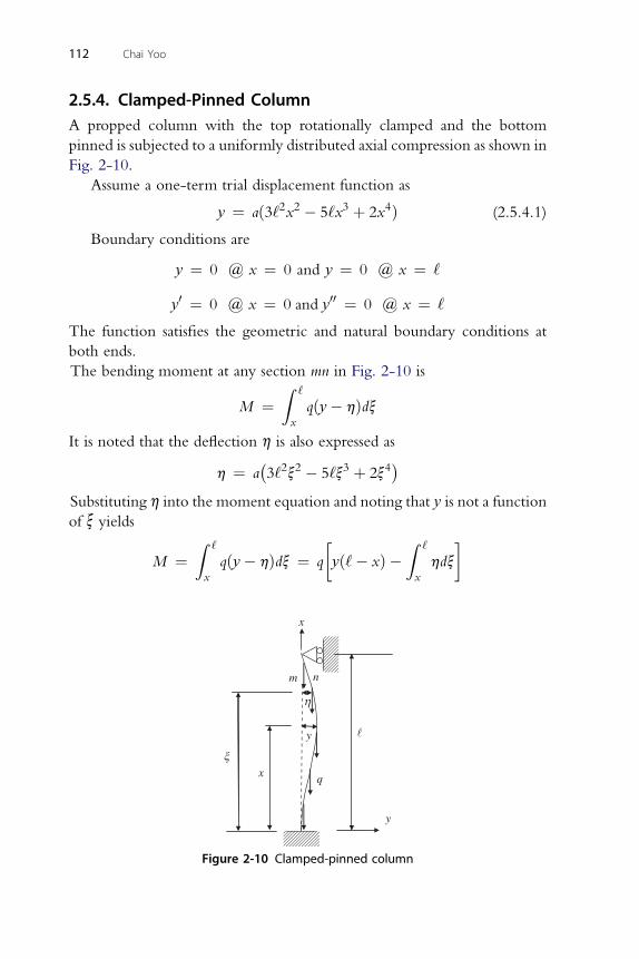
112 Chai Yoo

2.5.4. Clamped-Pinned Column

A propped column with the top rotationally clamped and the bottom

pinned is subjected to a uniformly distributed axial compression as shown in

Fig. 2-10.

Assume a one-term trial displacement function as

y ¼ að3‘2x2 � 5‘x3 þ 2x4Þ (2.5.4.1)

Boundary conditions are

y ¼ 0 @ x ¼ 0 and y ¼ 0 @ x ¼ ‘

y0 ¼ 0 @ x ¼ 0 and y00 ¼ 0 @ x ¼ ‘

The function satisfies the geometric and natural boundary conditions at

both ends.

The bending moment at any section mn in Fig. 2-10 is

M ¼Z ‘

x

qðy� hÞdxIt is noted that the deflection h is also expressed as

h ¼ a�3‘2x2 � 5‘x3 þ 2x4

�Substituting h into the moment equation and noting that y is not a function

of x yields

M ¼Z ‘

x

qðy� hÞdx ¼ q

�yð‘� xÞ �

Z ‘

x

hdx

x

y

h

x

m n

y

x

q

Figure 2-10 Clamped-pinned column

Special Topics in Elastic Stability of Columns 113

The integral on the right-hand side is expanded to

Z ‘

x

hdx ¼ a

Z ‘

x

�3‘2x2 � 5‘x3 þ 2x4

�dx

¼ a

�‘2�‘3 � x3

�� 5‘

4

�‘4 � x4

�þ 2

5

�‘5 � x5

�

Hence,

M ¼ qa

�ð‘� xÞ�3‘2x2 � 5‘x3 þ 2x4

�� �‘2�‘3 � x3�� 5‘

4

�‘4 � x4

�þ 2

5

�‘5 � x5

��

The assumed deflection function has an inflection point at x ¼ 0.25‘. Inorder to ensure the moment to be equal to zero at the inflection point, the

moment equation needs an adjustment.

M ¼ qa

ð‘� xÞ�3‘2x2 � 5‘x3 þ 2x4 þ 0:067968747‘4�

��‘2�‘3 � x3

�� 5‘

4

�‘4 � x4

�þ 2

5

�‘5 � x5

�8><>:

9>=>; (2.5.4.2)

1Z ‘

2

U ¼2EI 0

M dx

¼ q2a2

2EI

Z ‘

0

ð‘� xÞð3‘2x2 � 5‘x3 þ 2x4 þ 0:067968747‘4Þ

��‘2ð‘3 � x3Þ � 5‘

4ð‘4 � x4Þ þ 2

5ð‘5 � x5Þ

8><>:

9>=>;

2

dx

11 2 2

¼ 0:002425669952‘ q a =2EI

Z ‘ Z ‘ � �2

Vq ¼ �1

2 0 x

qdy

dxdxdx

¼ �a2q

2

Z ‘

0

ð‘� xÞ�6‘2x� 15‘x2 þ 8x3�2dx ¼ �9‘8qa2

140

vU vV ‘11q 18‘8

vaþ

va¼

EIð0:002425669952Þ �

140¼ 00

q ¼ 53EI

‘3ð0:95% greater than the exact solutionÞ

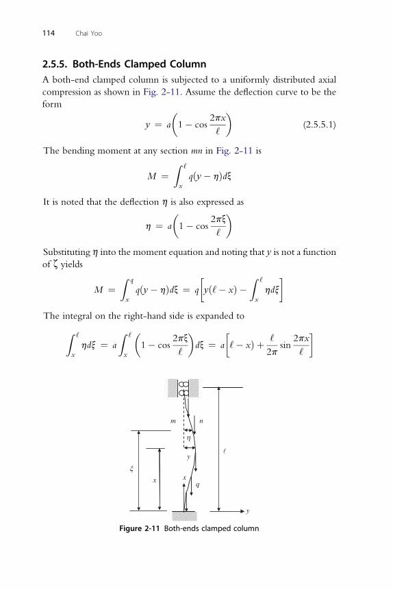
114 Chai Yoo

2.5.5. Both-Ends Clamped Column

A both-end clamped column is subjected to a uniformly distributed axial

compression as shown in Fig. 2-11. Assume the deflection curve to be the

form

y ¼ a

�1� cos

2px

‘

�(2.5.5.1)

The bending moment at any section mn in Fig. 2-11 is

M ¼Z ‘

x

qðy� hÞdx

It is noted that the deflection h is also expressed as

h ¼ a

�1� cos

2px

‘

�

Substituting h into the moment equation and noting that y is not a function

of z yields

M ¼Z q

x

qðy� hÞdx ¼ q

�yð‘� xÞ �

Z ‘

x

hdx

The integral on the right-hand side is expanded to

Z ‘

x

hdx ¼ a

Z ‘

x

�1� cos

2px

‘

�dx ¼ a

�‘� xÞ þ ‘

2psin

2px

‘

xx

y

h

y

x

q

m n

Figure 2-11 Both-ends clamped column

Special Topics in Elastic Stability of Columns 115

Hence,

M ¼ qa

�ð‘� xÞ

�1� cos

2px

‘

���ð‘� xÞ þ ‘

2psin

2px

‘

�(2.5.5.2)

The assumed deflection curve is to have two inflection points at

x ¼ 0:25‘ and x ¼ 0:75‘.

M ¼ qa

�ð‘� xÞ

�1� cos

2px

‘

���ð‘� xÞ þ ‘

2psin

2px

‘

þ 2

p

�‘

2� x

��(2.5.5.3)

1Z ‘

2 q2a2Z ‘� �

2px�

U ¼2EI 0

M dx ¼2EI 0

ð‘� xÞ 1� cos‘

��ð‘� xÞ þ ‘

2psin

2px

‘

þ 2

p

�‘

2� x

��2

dx

¼ ð767=277200Þ ‘11q2a2=2EI

V ¼ �1Z ‘ Z ‘

q

�dy�2

dxdx ¼ �a2qZ ‘

ð‘� xÞð‘3 � 9‘x2 þ 8x3Þ2dx

q2 0 x dx 2 0

¼ 3‘8qa2

28

vU vV ‘11q�

767�

6‘8

vaþ

va¼

EI 277200�

28¼ 00q

¼ 77:4EI

‘3ð3:8% greater than the exact solutionÞ

2.6. ELASTICALLY SUPPORTED BEAM-COLUMNS

As an example of the stability of a bar on elastic supports, consider a pris-

matic continuous beam simply supported at the ends on rigid supports and

having several intermediate elastic supports. A similar problem was

considered in Section 1.9 in which the bar was considered to be rigid so that

the strain energy stored was in the elastic supports only. Let q ¼ force

developed in the spring¼ ky. Then the work done by the spring is

ð1=2Þqy ¼ ð1=2Þky2. Rotational spring can also be considered at any

support. Total potential energy function of the system becomes

P ¼ U þ V ¼ EI

2

Z ‘

0

ðy00Þ2dx� P

2

Z ‘

0

ðy0Þ2dxþ 1

2

Xni¼ 1

kiy2i (2.6.1)

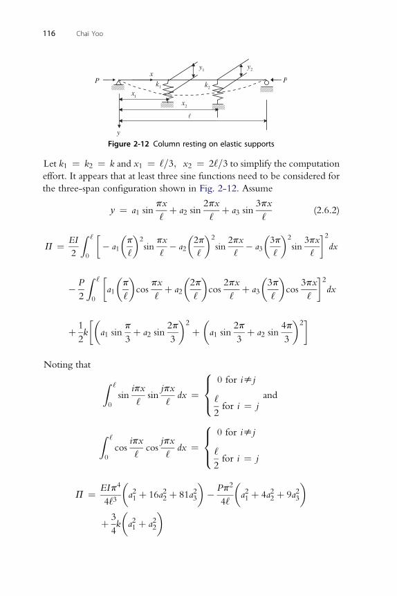
y1y2

k2k1

y

P

x1

x

x2

P

Figure 2-12 Column resting on elastic supports

116 Chai Yoo

Let k1 ¼ k2 ¼ k and x1 ¼ ‘=3; x2 ¼ 2‘=3 to simplify the computation

effort. It appears that at least three sine functions need to be considered for

the three-span configuration shown in Fig. 2-12. Assume

y ¼ a1 sinpx

‘þ a2 sin

2px

‘þ a3 sin

3px

‘(2.6.2)

Z ‘ � � �2

� �2

� �2

2

P ¼ EI

2 0

� a1p

‘sin

px

‘� a2

2p

‘sin

2px

‘� a3

3p

‘sin

3px

‘dx

Z ‘ � � � � � � � 2

� P

2 0

a1p

‘cos

px

‘þ a2

2p

‘cos

2px

‘þ a3

3p

‘cos

3px

‘dx

1��

p 2p�2

�2p 4p

�2

þ2k a1 sin

3þ a2 sin

3þ a1 sin

3þ a2 sin

3

Noting that

Z ‘

0

sinipx

‘sin

jpx

‘dx ¼

8><>:

0 for isj

‘

2for i ¼ j

and

Z ‘

0

cosipx

‘cos

jpx

‘dx ¼

0 for isj

‘

2for i ¼ j

8><>:

EIp4� �

Pp2� �

P ¼4‘3

a21 þ 16a22 þ 81a23 �4‘

a21 þ 4a22 þ 9a23

þ 3

4k

�a21 þ a22

�

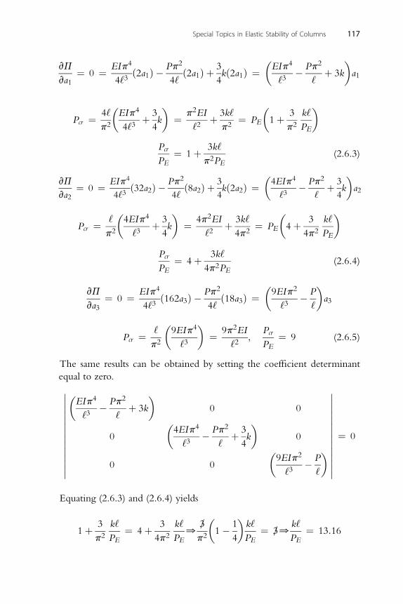
vP EIp4 Pp2 3�EIp4 Pp2

�

va1

¼ 0 ¼4‘3

ð2a1Þ �4‘

ð2a1Þ þ4kð2a1Þ ¼

‘3�

‘þ 3k a1

�4

�2

� �

Special Topics in Elastic Stability of Columns 117

Pcr ¼ 4‘

p2

EIp

4‘3þ 3

4k ¼ p EI

‘2þ 3k‘

p2¼ PE 1þ 3

p2

k‘

PE

Pcr

PE¼ 1þ 3k‘

p2PE(2.6.3)

vP EIp4 Pp2 3�4EIp4 Pp2 3

�

va2

¼ 0 ¼4‘3

ð32a2Þ �4‘

ð8a2Þ þ4kð2a2Þ ¼

‘3�

‘þ4k a2

‘�4EIp4 3

�4p2EI 3k‘

�3 k‘

�

Pcr ¼

p2 ‘3þ4k ¼

‘2þ4p2

¼ PE 4þ4p2 PE

Pcr 3k‘

PE¼ 4þ

4p2PE(2.6.4)

vP EIp4 Pp2�9EIp2 P

�

va3

¼ 0 ¼4‘3

ð162a3Þ �4‘

ð18a3Þ ¼‘3

�‘

a3

‘�9EIp4

�9p2EI P

Pcr ¼p2 ‘3

¼‘2

;cr

PE¼ 9 (2.6.5)

The same results can be obtained by setting the coefficient determinant

equal to zero.��������������

�EIp4

‘3� Pp2

‘þ 3k

�0 0

0

�4EIp4

‘3� Pp2

‘þ 3

4k

�0

0 0

�9EIp2

‘3� P

‘

�

��������������¼ 0

Equating (2.6.3) and (2.6.4) yields

1þ 3

p2

k‘

PE¼ 4þ 3

4p2

k‘

PE0

�

3

p2

�1� 1

4

�k‘

PE¼

�

30k‘

PE¼ 13:16

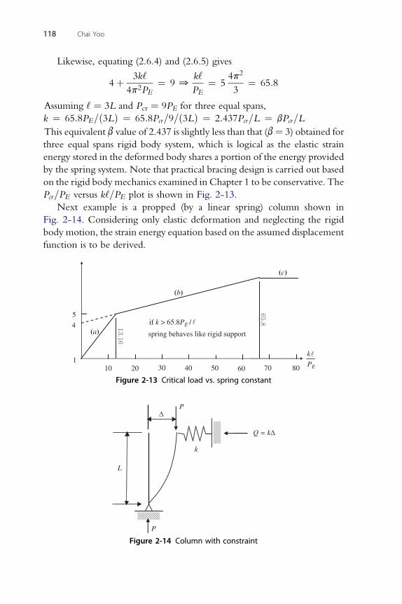
118 Chai Yoo

Likewise, equating (2.6.4) and (2.6.5) gives

4þ 3k‘

4p2PE¼ 90

k‘

PE¼ 5

4p2

3¼ 65:8

Assuming ‘ ¼ 3L and Pcr ¼ 9PE for three equal spans,

k ¼ 65:8PE=ð3LÞ ¼ 65:8Pcr=9=ð3LÞ ¼ 2:437Pcr=L ¼ bPcr=L

This equivalent b value of 2.437 is slightly less than that (b¼ 3) obtained for

three equal spans rigid body system, which is logical as the elastic strain

energy stored in the deformed body shares a portion of the energy provided

by the spring system. Note that practical bracing design is carried out based

on the rigid body mechanics examined in Chapter 1 to be conservative. The

Pcr=PE versus k‘=PE plot is shown in Fig. 2-13.

Next example is a propped (by a linear spring) column shown in

Fig. 2-14. Considering only elastic deformation and neglecting the rigid

body motion, the strain energy equation based on the assumed displacement

function is to be derived.

5

4spring behaves like rigid support

80706050403020101

k

PE

(a)

(b)

(c)

if k > 65.8PE /

Figure 2-13 Critical load vs. spring constant

L

D P

Q = kD

k

P

Figure 2-14 Column with constraint

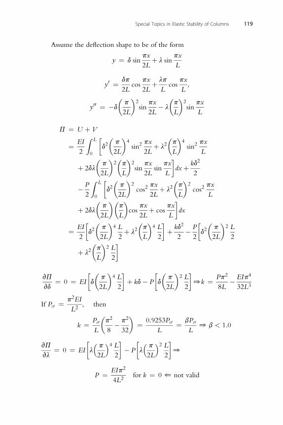
Special Topics in Elastic Stability of Columns 119

Assume the deflection shape to be of the form

y ¼ d sinpx

2Lþ l sin

px

L

dp px lp px

y0 ¼

2Lcos

2Lþ

Lcos

L;

00�p�2 px

�p�2 px

y ¼ �d2L

sin2L

� lL

sinL

P ¼ U þ V

¼ EI

2

Z L

0

�d2�p

2L

�4sin2

px

2Lþ l2

�p

L

�4sin2

px

L

þ 2dl

�p

2L

�2�p

L

�2sin

px

2Lsin

px

L

dxþ kd2

2

� P

2

Z L

0

�d2�p

2L

�2cos2

px

2Lþ l2

�p

L

�2cos2

px

L

þ 2dl

�p

2L

��p

L

�cos

px

2Lþ cos

px

L

dx

¼ EI

2

�d2�p

2L

�4 L

2þ l2

�p

L

�4 L

2

þ kd2

2� P

2

�d2�p

2L

�2 L

2

þ l2�p

L

�2 L

2

� � � � � � 2 4

vP

vd¼ 0 ¼ EI d

p

2L

4 L

2þ kd� P d

p

2L

2 L

20k ¼ Pp

8L� EIp

32L3

If Pcr ¼ p2EI2, then

L

k ¼ Pcr

L

�p2

8� p2

32

�¼ 0:9253Pcr

L¼ bPcr

L0 b < 1:0

vP� � p 4 L � � p 2 L

vl¼ 0 ¼ EI l

2L 2� P l

2L 20

P ¼ EIp2

4L2for k ¼ 0 * not valid

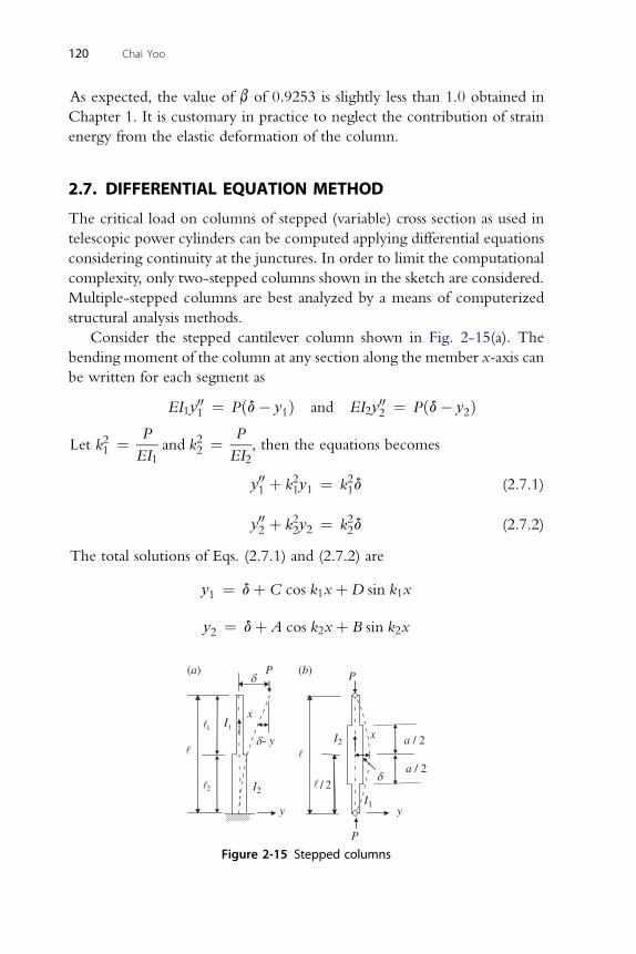
120 Chai Yoo

As expected, the value of b of 0.9253 is slightly less than 1.0 obtained in

Chapter 1. It is customary in practice to neglect the contribution of strain

energy from the elastic deformation of the column.

2.7. DIFFERENTIAL EQUATION METHOD

The critical load on columns of stepped (variable) cross section as used in

telescopic power cylinders can be computed applying differential equations

considering continuity at the junctures. In order to limit the computational

complexity, only two-stepped columns shown in the sketch are considered.

Multiple-stepped columns are best analyzed by a means of computerized

structural analysis methods.

Consider the stepped cantilever column shown in Fig. 2-15(a). The

bending moment of the column at any section along the member x-axis can

be written for each segment as

EI1y001 ¼ Pðd� y1Þ and EI2y

002 ¼ Pðd� y2Þ

Let k21 ¼ P

EI1and k22 ¼ P

EI2, then the equations becomes

y001 þ k21y1 ¼ k21d (2.7.1)

y00 þ k2y ¼ k2d (2.7.2)

2 2 2 2

The total solutions of Eqs. (2.7.1) and (2.7.2) are

y1 ¼ dþ C cos k1xþD sin k1x

y ¼ dþ A cos k2xþ B sin k2x

2

2

x

y

P

- y1 I1

x

/ 2

I2

I2I1

a / 2

a / 2

P

P

y

(a) (b)

Figure 2-15 Stepped columns

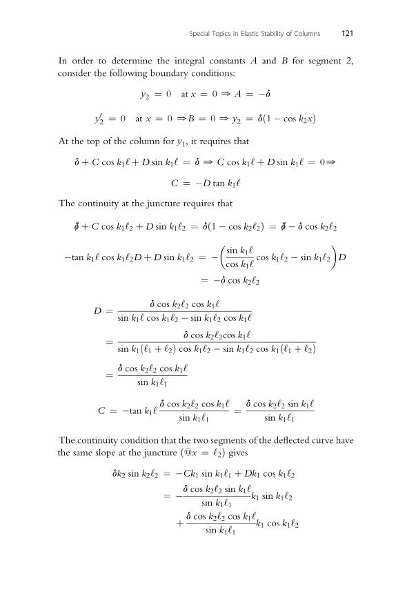
Special Topics in Elastic Stability of Columns 121

In order to determine the integral constants A and B for segment 2,

consider the following boundary conditions:

y2 ¼ 0 at x ¼ 0 0 A ¼ �d

0

y2 ¼ 0 at x ¼ 0 0B ¼ 0 0 y2 ¼ dð1� cos k2xÞ

At the top of the column for y1, it requires that

dþ C cos k1‘þD sin k1‘ ¼ d0 C cos k1‘þD sin k1‘ ¼ 00

C ¼ �D tan k1‘

The continuity at the juncture requires that

�

dþC cos k1‘2 þD sin k1‘2 ¼ dð1� cos k2‘2Þ ¼

�

d� d cos k2‘2

�sin k ‘

�

�tan k1‘ cos k1‘2DþD sin k1‘2 ¼ � 1

cos k1‘cos k1‘2 � sin k1‘2 D

¼ �d cos k2‘2

d cos k2‘2 cos k1‘

D ¼

sin k1‘ cos k1‘2 � sin k1‘2 cos k1‘

¼ d cos k2‘2cos k1‘

sin k1ð‘1 þ ‘2Þ cos k1‘2 � sin k1‘2 cos k1ð‘1 þ ‘2Þ

¼ d cos k2‘2 cos k1‘

sin k1‘1

d cos k2‘2 cos k1‘ d cos k2‘2 sin k1‘

C ¼ �tan k1‘

sin k1‘1¼

sin k1‘1

The continuity condition that the two segments of the deflected curve have

the same slope at the juncture ð@x ¼ ‘2Þ givesdk2 sin k2‘2 ¼ �Ck1 sin k1‘1 þDk1 cos k1‘2

¼ �d cos k2‘2 sin k1‘

sin k1‘1k1 sin k1‘2

þ d cos k2‘2 cos k1‘

sin k1‘1k1 cos k1‘2

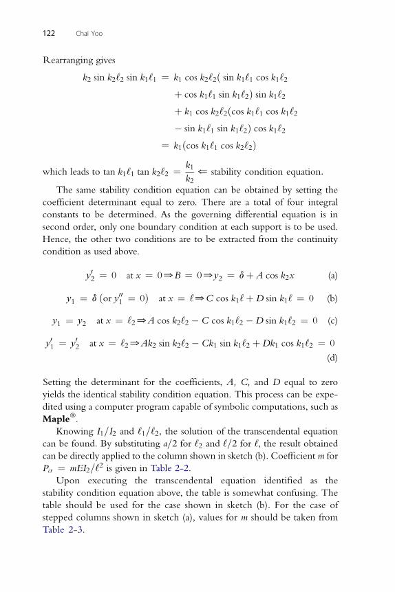
122 Chai Yoo

Rearranging gives

k2 sin k2‘2 sin k1‘1 ¼ k1 cos k2‘2ð sin k1‘1 cos k1‘2

þ cos k1‘1 sin k1‘2Þ sin k1‘2

þ k1 cos k2‘2ðcos k1‘1 cos k1‘2� sin k1‘1 sin k1‘2Þ cos k1‘2

¼ k1ðcos k1‘1 cos k2‘2Þ

which leads to tan k1‘1 tan k2‘2 ¼ k1

k2* stability condition equation:

The same stability condition equation can be obtained by setting the

coefficient determinant equal to zero. There are a total of four integral

constants to be determined. As the governing differential equation is in

second order, only one boundary condition at each support is to be used.

Hence, the other two conditions are to be extracted from the continuity

condition as used above.

y02 ¼ 0 at x ¼ 00B ¼ 00y2 ¼ dþ A cos k2x (a)

y ¼ d ðor y00 ¼ 0Þ at x ¼ ‘0C cos k ‘þD sin k ‘ ¼ 0 (b)

1 1 1 1

y ¼ y at x ¼ ‘20A cos k2‘2 � C cos k1‘2 �D sin k1‘2 ¼ 0 (c)

1 2

y0 ¼ y0 at x ¼ ‘ 0Ak sin k ‘ �Ck sin k ‘ þDk cos k ‘ ¼ 0

1 2 2 2 2 2 1 1 2 1 1 2

(d)

Setting the determinant for the coefficients, A, C, and D equal to zero

yields the identical stability condition equation. This process can be expe-

dited using a computer program capable of symbolic computations, such as

Maple�.

Knowing I1=I2 and ‘1=‘2, the solution of the transcendental equation

can be found. By substituting a=2 for ‘2 and ‘=2 for ‘, the result obtainedcan be directly applied to the column shown in sketch (b). Coefficient m for

Pcr ¼ mEI2=‘2 is given in Table 2-2.

Upon executing the transcendental equation identified as the

stability condition equation above, the table is somewhat confusing. The

table should be used for the case shown in sketch (b). For the case of

stepped columns shown in sketch (a), values for m should be taken from

Table 2-3.

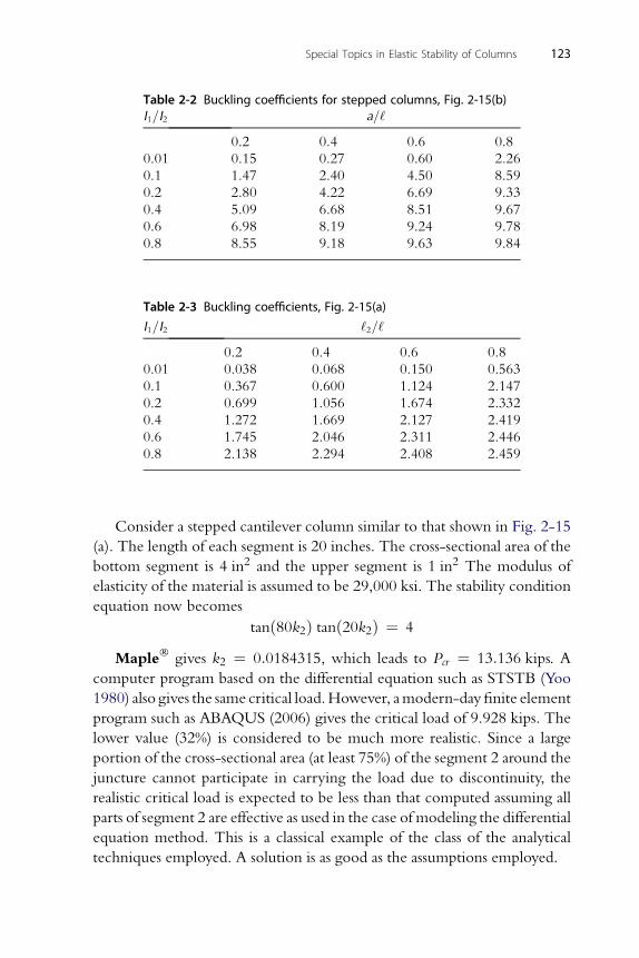
Table 2-2 Buckling coefficients for stepped columns, Fig. 2-15(b)I1=I2 a=‘

0.2 0.4 0.6 0.8

0.01 0.15 0.27 0.60 2.26

0.1 1.47 2.40 4.50 8.59

0.2 2.80 4.22 6.69 9.33

0.4 5.09 6.68 8.51 9.67

0.6 6.98 8.19 9.24 9.78

0.8 8.55 9.18 9.63 9.84

Table 2-3 Buckling coefficients, Fig. 2-15(a)

I1=I2 ‘2=‘

0.2 0.4 0.6 0.8

0.01 0.038 0.068 0.150 0.563

0.1 0.367 0.600 1.124 2.147

0.2 0.699 1.056 1.674 2.332

0.4 1.272 1.669 2.127 2.419

0.6 1.745 2.046 2.311 2.446

0.8 2.138 2.294 2.408 2.459

Special Topics in Elastic Stability of Columns 123

Consider a stepped cantilever column similar to that shown in Fig. 2-15

(a). The length of each segment is 20 inches. The cross-sectional area of the

bottom segment is 4 in2 and the upper segment is 1 in2 The modulus of

elasticity of the material is assumed to be 29,000 ksi. The stability condition

equation now becomes

tanð80k2Þ tanð20k2Þ ¼ 4

Maple� gives k2 ¼ 0:0184315, which leads to Pcr ¼ 13:136 kips. Acomputer program based on the differential equation such as STSTB (Yoo

1980) also gives the same critical load.However, amodern-day finite element

program such as ABAQUS (2006) gives the critical load of 9.928 kips. The

lower value (32%) is considered to be much more realistic. Since a large

portion of the cross-sectional area (at least 75%) of the segment 2 around the

juncture cannot participate in carrying the load due to discontinuity, the

realistic critical load is expected to be less than that computed assuming all

parts of segment 2 are effective as used in the case of modeling the differential

equation method. This is a classical example of the class of the analytical

techniques employed. A solution is as good as the assumptions employed.

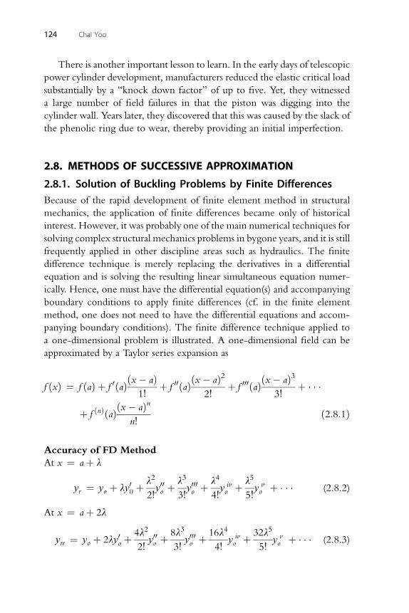
124 Chai Yoo

There is another important lesson to learn. In the early days of telescopic

power cylinder development, manufacturers reduced the elastic critical load

substantially by a “knock down factor” of up to five. Yet, they witnessed

a large number of field failures in that the piston was digging into the

cylinder wall. Years later, they discovered that this was caused by the slack of

the phenolic ring due to wear, thereby providing an initial imperfection.

2.8. METHODS OF SUCCESSIVE APPROXIMATION

2.8.1. Solution of Buckling Problems by Finite DifferencesBecause of the rapid development of finite element method in structural

mechanics, the application of finite differences became only of historical

interest. However, it was probably one of the main numerical techniques for

solving complex structural mechanics problems in bygone years, and it is still

frequently applied in other discipline areas such as hydraulics. The finite

difference technique is merely replacing the derivatives in a differential

equation and is solving the resulting linear simultaneous equation numer-

ically. Hence, one must have the differential equation(s) and accompanying

boundary conditions to apply finite differences (cf. in the finite element

method, one does not need to have the differential equations and accom-

panying boundary conditions). The finite difference technique applied to

a one-dimensional problem is illustrated. A one-dimensional field can be

approximated by a Taylor series expansion as

f ðxÞ ¼ f ðaÞ þ f 0ðaÞðx� aÞ1!

þ f 00ðaÞðx� aÞ22!

þ f 000ðaÞðx� aÞ33!

þ � � �

þ f ðnÞðaÞðx� aÞnn!

ð2:8:1Þ

Accuracy of FD Method

At x ¼ aþ l

yr ¼ yo þ ly00 þl2

2!y00o þ

l3

3!y000o þ l4

4!y ivo þ l5

5!y vo þ � � � (2.8.2)

At x ¼ aþ 2l

yrr ¼ yo þ 2ly0o þ4l2

2!y00o þ

8l3

3!y000o þ 16l4

4!y ivo þ 32l5

5!y vo þ � � � (2.8.3)

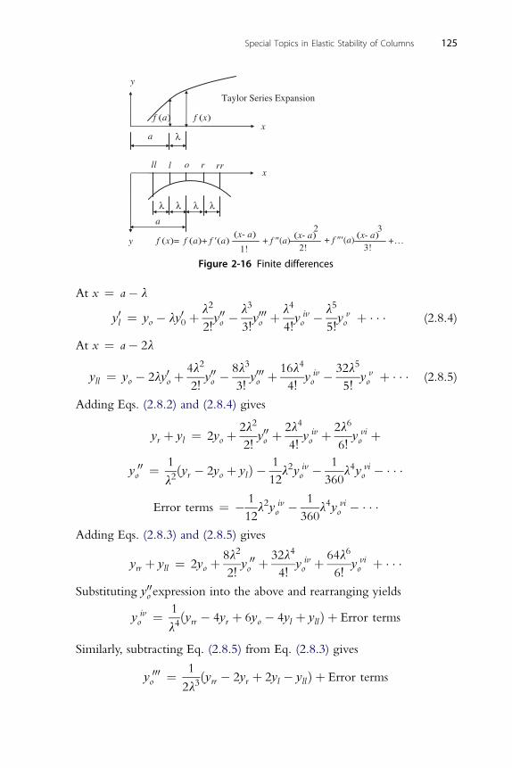
y

32(x- a)

1! 2!(x- a)

3!f (x)= f (a)+ f ¢(a)

Taylor Series Expansion

xa

f (a) f (x)

a

ll o r rrl

y

x

(x- a)+ f ²(a) + f ²¢(a) + . . .

Figure 2-16 Finite differences

Special Topics in Elastic Stability of Columns 125

At x ¼ a� l

y0l ¼ yo � ly00 þl2

2!y00o �

l3

3!y000o þ l4

4!y ivo � l5

5!y vo þ � � � (2.8.4)

At x ¼ a� 2l

yll ¼ yo � 2ly0o þ4l2

2!y00o �

8l3

3!y000o þ 16l4

4!y ivo � 32l5

5!y vo þ � � � (2.8.5)

Adding Eqs. (2.8.2) and (2.8.4) gives

yr þ yl ¼ 2yo þ2l2

2!y00o þ

2l4

4!y ivo þ 2l6

6!y vio þ

1 1 1

y 00o ¼

l2ðyr � 2yo þ ylÞ � 12

l2y ivo �

360l4y vi

o � � � �

Error terms ¼ � 1

12l2y iv

o � 1

360l4y vi

o � � � �Adding Eqs. (2.8.3) and (2.8.5) gives

yrr þ yll ¼ 2yo þ8l2

2!y 00o þ 32l4

4!y ivo þ 64l6

6!y vio þ � � �

Substituting y00o expression into the above and rearranging yields

y ivo ¼ 1

l4ðyrr � 4yr þ 6yo � 4yl þ yllÞ þ Error terms

Similarly, subtracting Eq. (2.8.5) from Eq. (2.8.3) gives

y 000o ¼ 1

2l3ðyrr � 2yr þ 2yl � yllÞ þ Error terms

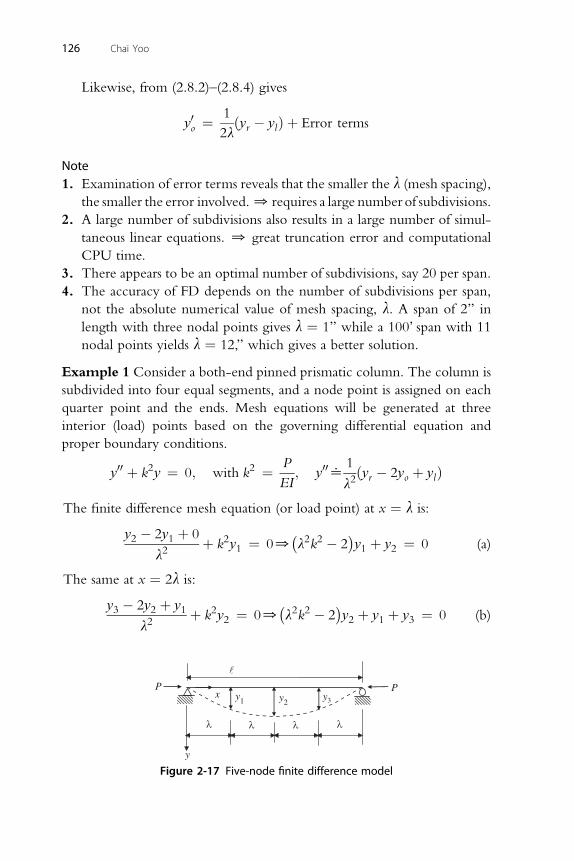
126 Chai Yoo

Likewise, from (2.8.2)–(2.8.4) gives

y0o ¼ 1

2lðyr � ylÞ þ Error terms

Note1. Examination of error terms reveals that the smaller the l (mesh spacing),

the smaller the error involved.0 requires a large number of subdivisions.

2. A large number of subdivisions also results in a large number of simul-

taneous linear equations. 0 great truncation error and computational

CPU time.

3. There appears to be an optimal number of subdivisions, say 20 per span.

4. The accuracy of FD depends on the number of subdivisions per span,

not the absolute numerical value of mesh spacing, l. A span of 2” in

length with three nodal points gives l ¼ 1” while a 100’ span with 11

nodal points yields l ¼ 12,” which gives a better solution.

Example 1 Consider a both-end pinned prismatic column. The column is

subdivided into four equal segments, and a node point is assigned on each

quarter point and the ends. Mesh equations will be generated at three

interior (load) points based on the governing differential equation and

proper boundary conditions.

y00 þ k2y ¼ 0; with k2 ¼ P

EI; y00^

1

l2ðyr � 2yo þ ylÞ

The finite difference mesh equation (or load point) at x ¼ l is:

y2 � 2y1 þ 0

l2þ k2y1 ¼ 00

�l2k2 � 2

�y1 þ y2 ¼ 0 (a)

The same at x ¼ 2l is:

y3 � 2y2 þ y1

l2þ k2y2 ¼ 00

�l2k2 � 2

�y2 þ y1 þ y3 ¼ 0 (b)

P

l l l

P

l

x y1 y2y3

y

Figure 2-17 Five-node finite difference model

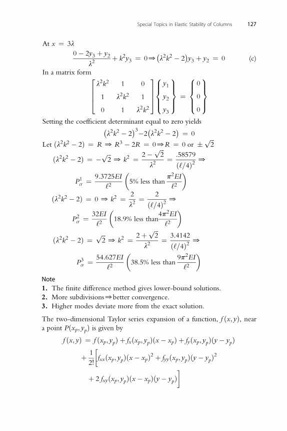
Special Topics in Elastic Stability of Columns 127

At x ¼ 3l

0� 2y3 þ y2

l2þ k2y3 ¼ 00

�l2k2 � 2

�y3 þ y2 ¼ 0 (c)

In a matrix form2664l2k2 1 0

1 l2k2 1

0 1 l2k2

37758>><>>:

y1

y2

y3

9>>=>>; ¼

8>><>>:

0

0

0

9>>=>>;

Setting the coefficient determinant equal to zero yields�l2k2 � 2

�3�2�l2k2 � 2

� ¼ 0

Let ðl2k2 � 2Þ ¼ R 0 R3 � 2R ¼ 00R ¼ 0 or � ffiffiffi2

p

ðl2k2 � 2Þ ¼ �ffiffiffi2

p0 k2 ¼ 2� ffiffiffi

2p

l2¼ :58579

ð‘=4Þ2 0

P1cr ¼ 9:3725EI

‘2

�5% less than

p2EI

‘2

�

ðl2k2 � 2Þ ¼ 0 0 k2 ¼ 2

l2¼ 2

ð‘=4Þ2 0

P2cr ¼ 32EI

‘2

�18:9% less than

4p2EI

‘2

�

ðl2k2 � 2Þ ¼ffiffiffi2

p0 k2 ¼ 2þ ffiffiffi

2p

¼ 3:41420

l2 ð‘=4Þ2

P3cr ¼ 54:627EI

‘2

�38:5% less than

9p2EI

‘2

�Note1. The finite difference method gives lower-bound solutions.

2. More subdivisions0better convergence.

3. Higher modes deviate more from the exact solution.

The two-dimensional Taylor series expansion of a function, f ðx; yÞ, neara point Pðxp; ypÞ is given by

f ðx; yÞ ¼ f ðxp; ypÞ þ fxðxp; ypÞðx� xpÞ þ fyðxp; ypÞðy� ypÞ1�

þ2!

fxxðxp; ypÞðx� xpÞ2 þ fyyðxp; ypÞðy� ypÞ2

þ 2 fxyðxp; ypÞðx� xpÞðy� ypÞ

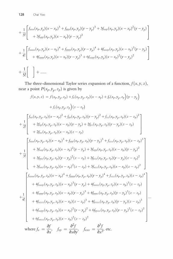
2fxxxðxp; ypÞðx� xpÞ3 þ fyyyðxp; ypÞðy� ypÞ3 þ 3fxxyðxp; ypÞðx� xpÞ2ðy� ypÞ

3

þ 1

3!4

þ 3fxyyðxp; ypÞðx� xp�ðy� ypÞ2

52f ðx ; y Þðx� x Þ4 þ f ðx ; y Þðy� y Þ4 þ 4f ðx ; y Þðx� x Þ3ðy� y Þ

3

128 Chai Yoo

þ 1

4!4 xxxx p p p yyyy p p p xxxy p p p p

þ 4fxyyyðxp; ypÞðx� xpÞðy� ypÞ3 þ 6fxxyyðxp; ypÞðx� xpÞ2ðy� ypÞ25

1�

::

þ5!

þ :::::

The three-dimensional Taylor series expansion of a function, f ðx; y; zÞ,near a point Pðxp; yp; zpÞ is given by

f ðx; y; zÞ ¼ f ðxp; yp; zpÞ þ fxðxp; yp; zpÞðx� xpÞ þ fyðxp; yp; zp ðy� yp

þ fzðxp; yp; zp ðz� zp

�

þ 1

2!

26664fxxðxp; yp; zpÞðx� xpÞ2 þ fyyðxp; yp; zpÞðy� ypÞ2 þ fzzðxp; yp; zpÞðz� zpÞ2

þ 2fxyðxp; yp; zpÞðx� xpÞðy� ypÞ þ 2fyzðxp; yp; zpÞðy� ypÞðz� zpÞþ 2fxzðxp; yp; zpÞðx� xpÞðz� zpÞ

37775

þ 1

3!

2666666664

fxxxðxp; yp; zpÞðx� xpÞ3 þ fyyyðxp; yp; zpÞðy� ypÞ3 þ fzzzðxp; yp; zpÞðz� zpÞ3

þ 3fxxyðxp; yp; zpÞðx� xpÞ2ðy� ypÞ þ 3fxyyðxp; yp; zpÞðx� xpÞðy� ypÞ2

þ 3fyyzðxp; yp; zpÞðy� ypÞ2ðz� zpÞ þ 3fyzzðxp; yp; zpÞðy� ypÞðz� zpÞ2

þ 3fxxzðxp; yp; zpÞðx� xpÞ2ðz� zpÞ þ 3fxzzðxp; yp; zpÞðx� xpÞðz� zpÞ2

3777777775

þ1

4!

266666666666666664

fxxxxðxp; yp; zpÞðx� xpÞ4 þ fyyyyðxp; yp; zpÞðy� ypÞ4 þ fzzzðxp; yp; zpÞðz� zpÞ4

þ 4fxxxyðxp; yp; zpÞðx� xpÞ3ðy� ypÞ þ 4fxxxzðxp; yp; zpÞðx� xpÞ3ðz� zpÞ

þ 4fxyyyðxp; yp; zpÞðx� xpÞðy� ypÞ3 þ 4fyyyzðxp; yp; zpÞðy� ypÞ3ðz� zpÞ

þ 4fxzzzðxp; yp; zpÞðx� xpÞðz� zpÞ3 þ 4fyzzzðxp; yp; zpÞðy� ypÞðz� zpÞ3

þ 6fxxyyðxp; yp; zpÞðx� xpÞ2ðy� ypÞ2 þ 6fyyzzðxp; yp; zpÞðy� ypÞ2ðz� zpÞ2

þ 6fxxzzðxp; yp; zpÞðx� xpÞ2ðz� zpÞ2

377777777777777775

:

where fx ¼ vf; fxy ¼ v2f

; fxxx ¼ v3f3, etc.

vx vxvy vx

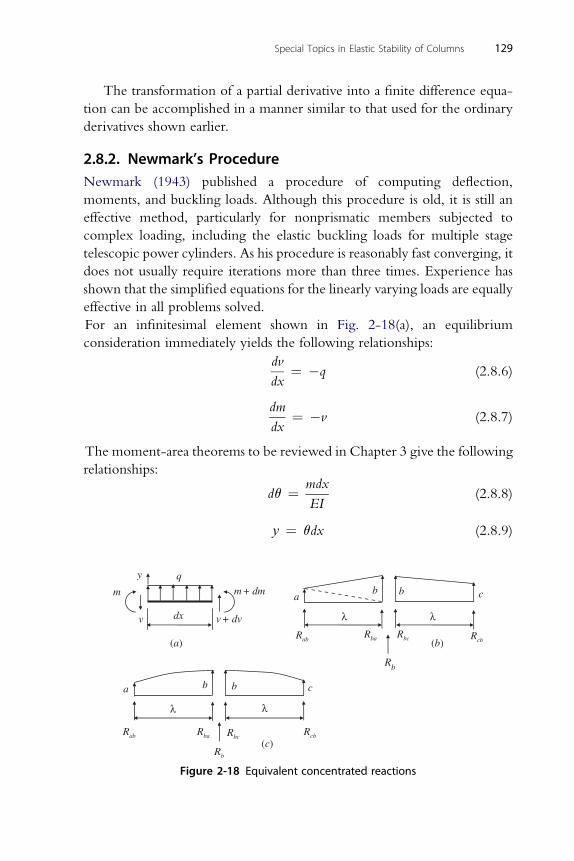
Special Topics in Elastic Stability of Columns 129

The transformation of a partial derivative into a finite difference equa-

tion can be accomplished in a manner similar to that used for the ordinary

derivatives shown earlier.

2.8.2. Newmark’s ProcedureNewmark (1943) published a procedure of computing deflection,

moments, and buckling loads. Although this procedure is old, it is still an

effective method, particularly for nonprismatic members subjected to

complex loading, including the elastic buckling loads for multiple stage

telescopic power cylinders. As his procedure is reasonably fast converging, it

does not usually require iterations more than three times. Experience has

shown that the simplified equations for the linearly varying loads are equally

effective in all problems solved.

For an infinitesimal element shown in Fig. 2-18(a), an equilibrium

consideration immediately yields the following relationships:

dv

dx¼ �q (2.8.6)

dm

dx¼ �v (2.8.7)

The moment-area theorems to be reviewed in Chapter 3 give the following

relationships:

dq ¼ mdx

EI(2.8.8)

y ¼ qdx (2.8.9)

y q

m

v dv+

m dm+

v dx

ab b c

λλ

Rb

a b b c

λ λ

Rcb

RabRba Rbc Rcb

Rb

RbcRbaRab

(a) (b)

(c)

Figure 2-18 Equivalent concentrated reactions

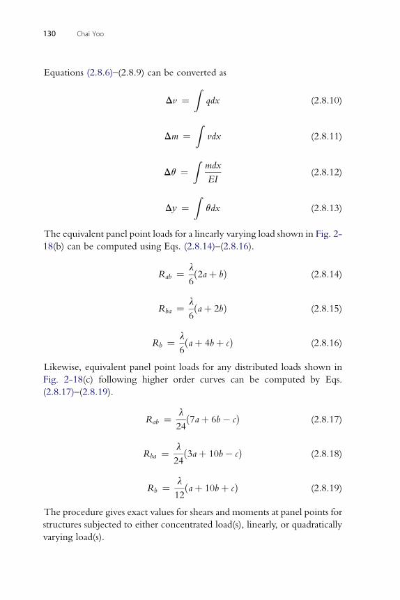
130 Chai Yoo

Equations (2.8.6)–(2.8.9) can be converted as

Dv ¼Z

qdx (2.8.10)

Z

Dm ¼ vdx (2.8.11)

Zmdx

Dq ¼EI

(2.8.12)

Z

Dy ¼ qdx (2.8.13)

The equivalent panel point loads for a linearly varying load shown in Fig. 2-

18(b) can be computed using Eqs. (2.8.14)–(2.8.16).

Rab ¼ l

6ð2aþ bÞ (2.8.14)

l

Rba ¼

6ðaþ 2bÞ (2.8.15)

l

Rb ¼

6ðaþ 4bþ cÞ (2.8.16)

Likewise, equivalent panel point loads for any distributed loads shown in

Fig. 2-18(c) following higher order curves can be computed by Eqs.

(2.8.17)–(2.8.19).

Rab ¼ l

24ð7aþ 6b� cÞ (2.8.17)

l

Rba ¼

24ð3aþ 10b� cÞ (2.8.18)

l

Rb ¼

12ðaþ 10bþ cÞ (2.8.19)

The procedure gives exact values for shears and moments at panel points for

structures subjected to either concentrated load(s), linearly, or quadratically

varying load(s).

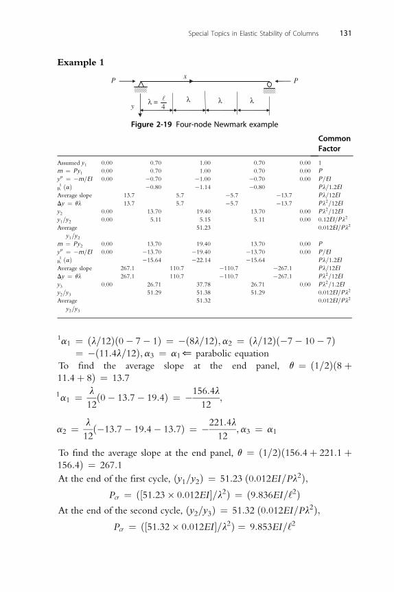
Special Topics in Elastic Stability of Columns 131

Example 1

Px

P

λy

λλλ =4

Figure 2-19 Four-node Newmark example

CommonFactor

Assumed y1 0.00 0.70 1.00 0.70 0.00 1

m ¼ Py1 0.00 0.70 1.00 0.70 0.00 P

y00 ¼ �m=EI 0.00 �0.70 �1.00 �0.70 0.00 P=EI

R1 ðaÞ �0.80 �1.14 �0.80 Pl=1:2EI

Average slope 13.7 5.7 �5.7 �13.7 Pl=12EI

Dy ¼ ql 13.7 5.7 �5.7 �13.7 Pl2=12EI

y2 0.00 13.70 19.40 13.70 0.00 Pl2=12EI

y1=y2 0.00 5.11 5.15 5.11 0.00 0:12EI=Pl2

Average

y1=y2

51.23 0:012EI=Pl2

m ¼ Py2 0.00 13.70 19.40 13.70 0.00 P

y00 ¼ �m=EI 0.00 �13.70 �19.40 �13.70 0.00 P=EI

R1 ðaÞ �15.64 �22.14 �15.64 Pl=1:2EI

Average slope 267.1 110.7 �110.7 �267.1 Pl=12EI

Dy ¼ ql 267.1 110.7 �110.7 �267.1 Pl2=12EI

y3 0.00 26.71 37.78 26.71 0.00 Pl2=1:2EI

y2=y3 51.29 51.38 51.29 0:012EI=Pl2

Average

y2=y3

51.32 0:012EI=Pl2

1 2

1a ¼ ðl=12Þð0� 7� 1Þ ¼ �ð8l=12Þ;a ¼ ðl=12Þð�7� 10� 7Þ

¼ �ð11:4l=12Þ;a3 ¼ a1* parabolic equation

To find the average slope at the end panel, q ¼ ð1=2Þð8 þ11:4þ 8Þ ¼ 13:7

1a1 ¼ l

12ð0� 13:7� 19:4Þ ¼ �156:4l

12;

l 221:4l

a2 ¼

12ð�13:7� 19:4� 13:7Þ ¼ �

12;a3 ¼ a1

To find the average slope at the end panel, q ¼ ð1=2Þð156:4þ 221:1 þ156:4Þ ¼ 267:1

At the end of the first cycle, ðy1=y2Þ ¼ 51:23 ð0:012EI=Pl2Þ;Pcr ¼ ð½51:23� 0:012EI �=l2Þ ¼ ð9:836EI=‘2Þ

At the end of the second cycle, ðy2=y3Þ ¼ 51:32 ð0:012EI=Pl2Þ;

Pcr ¼ ð½51:32� 0:012EI �=l2Þ ¼ 9:853EI=‘2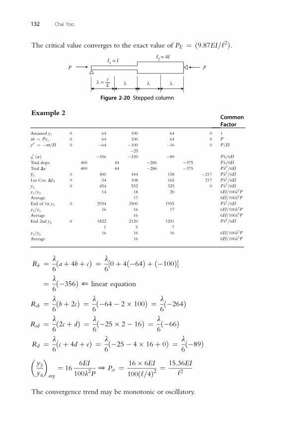

132 Chai Yoo

The critical value converges to the exact value of PE ¼ ð9:87EI=‘2Þ.

P

I2 = 4II1 = I

l

P

lll =4

Figure 2-20 Stepped column

Example 2Common

Factor

Assumed y1

0 64 100 64 0 1

m ¼ Py1

0 64 100 64 0 P

y00 ¼ �m=EI

0 �64 �100

�25

�16

0 P=EI

R1 ðaÞ

�356 �330 �89 Pl=6EI

Trial slope

400 44 �286 �375 Pl=6EI

Trial Dy

400 44 �286 �375 Pl2=6EI

y2

0 400 444 158 �217 Pl2=6EI

Lin Cor, Dy2

0 54 108 165 217 Pl2=6EI

y2

0 454 552 325 0 Pl2=6EI

y1=y2

14 18 20 6EI=100l2P

Average

17 6EI=100l2P

End of 1st y3

0 2934 3500 1955 Pl2=6EI

y2=y3

16 16 17 6EI=100l2P

Average

16 6EI=100l2P

End 2nd y4

0 1822

1

2120

5

1201

7

Pl2=6EI

y3=y4

16 16 16 6EI=100l2P

Average

16 6EI=100l2P

Rb ¼ l

6ðaþ 4bþ cÞ ¼ l

6½0þ 4ð�64Þ þ ð�100Þ�

¼ l

6ð�356Þ* linear equation

Rcb ¼ l

6ðbþ 2cÞ ¼ l

6ð�64� 2� 100Þ ¼ l

6ð�264Þ

Rcd ¼ l

6ð2c þ dÞ ¼ l

6ð�25� 2� 16Þ ¼ l

6ð�66Þ

Rd ¼ l

6ðc þ 4d þ eÞ ¼ l

6ð�25� 4� 16þ 0Þ ¼ l

6ð�89Þ

�y3�

6EI 16� 6EI 15:36EI

y4 avg

¼ 16100l2P

0 Pcr ¼100ð‘=4Þ2 ¼

‘2

The convergence trend may be monotonic or oscillatory.

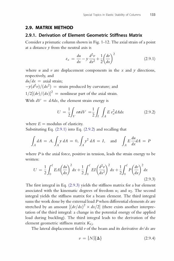
Special Topics in Elastic Stability of Columns 133

2.9. MATRIX METHOD

2.9.1. Derivation of Element Geometric Stiffness MatrixConsider a prismatic column shown in Fig. 1-12. The axial strain of a point

at a distance y from the neutral axis is

3x ¼ du

dx� y

d2v

dx2þ 1

2

�dv

dx

�2

(2.9.1)

where u and v are displacement components in the x and y directions,

respectively, and

du=dx ¼ axial strain;

�yðd2vÞ=ðdx2Þ ¼ strain produced by curvature; and

1=2½ðdvÞ=ðdxÞ�2 ¼ nonlinear part of the axial strain.

With dV ¼ dAdx; the element strain energy is

U ¼ 1

2

ZV

3sdV ¼ 1

2

Z‘

ZA

E 32xdAdx (2.9.2)

where E ¼ modulus of elasticity.

Substituting Eq. (2.9.1) into Eq. (2.9.2) and recalling thatZA

dA ¼ A;

ZA

y dA ¼ 0;

ZA

y2 dA ¼ I ; and

ZA

Edu

dxdA ¼ P

where P is the axial force, positive in tension, leads the strain energy to be

written:

U ¼ 1

2

Z ‘

0

EA

�du

dx

�2

dxþ 1

2

Z ‘

0

EI

�d2v

dx2

�2

dxþ 1

2

Z ‘

0

P

�dv

dx

�2

dx

(2.9.3)

The first integral in Eq. (2.9.3) yields the stiffness matrix for a bar element

associated with the kinematic degrees of freedom u1 and u2. The second

integral yields the stiffness matrix for a beam element. The third integral

sums the work done by the external load Pwhen differential elements dx are

stretched by an amount ½ðdv=dxÞ2 � dx=2� (there exists another interpre-

tation of the third integral: a change in the potential energy of the applied

load during buckling). The third integral leads to the derivation of the

element geometric stiffness matrix KG.

The lateral displacement field v of the beam and its derivative dv/dx are

v ¼ PN RfDg (2.9.4)

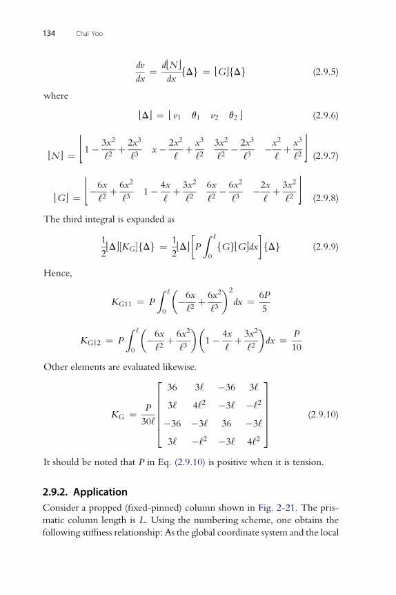
dv dPN R

dx

¼dx

fDg ¼ PGRfDg (2.9.5)

where

PDR ¼ P v1 q1 v2 q2 R (2.9.6)

2 3 2 3 2 3 2 3

134 Chai Yoo

PN R ¼ P 1� 3x

‘2þ 2x

‘3x� 2x

‘þ x

‘23x

‘2� 2x

‘3�x

‘þ x

‘2 R (2.9.7)

2 2 2 2

PGR ¼ P�6x

‘2þ 6x

‘31� 4x

‘þ 3x

‘26x

‘2� 6x

‘3�2x

‘þ 3x

‘2 R (2.9.8)

The third integral is expanded as

1

2PDR½KG�fDg ¼ 1

2PDR

�P

Z ‘

0

fGgPGRdx

fDg (2.9.9)

Hence,

KG11 ¼ P

Z ‘

0

��6x

‘2þ 6x2

‘3

�2

dx ¼ 6P

5

Z ‘� 6x 6x2��

4x 3x2�

P

KG12 ¼ P

0

�‘2

þ‘3

1�‘þ

‘2dx ¼

10

Other elements are evaluated likewise.

KG ¼ P

30‘

2666664

36 3‘ �36 3‘

3‘ 4‘2 �3‘ �‘2

�36 �3‘ 36 �3‘

3‘ �‘2 �3‘ 4‘2

3777775 (2.9.10)

It should be noted that P in Eq. (2.9.10) is positive when it is tension.

2.9.2. ApplicationConsider a propped (fixed-pinned) column shown in Fig. 2-21. The pris-

matic column length is L. Using the numbering scheme, one obtains the

following stiffness relationship: As the global coordinate system and the local

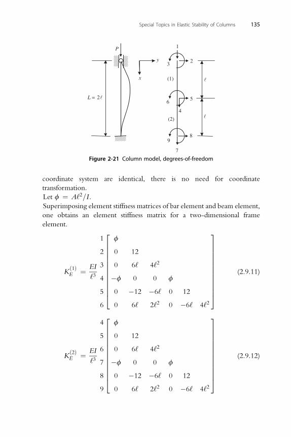
L = 2

1

x

P

98

7

65

4

32y

(1)

(2)

Figure 2-21 Column model, degrees-of-freedom

Special Topics in Elastic Stability of Columns 135

coordinate system are identical, there is no need for coordinate

transformation.

Let f ¼ A‘2=I .Superimposing element stiffness matrices of bar element and beam element,

one obtains an element stiffness matrix for a two-dimensional frame

element.

Kð1ÞE ¼ EI

‘3

1

2

3

4

5

6

2666666666664

f

0 12

0 6‘ 4‘2

�f 0 0 f

0 �12 �6‘ 0 12

0 6‘ 2‘2 0 �6‘ 4‘2

3777777777775

(2.9.11)

42

f3

Kð2ÞE ¼ EI

‘3

5

6

7

8

9

666666666664

0 12

0 6‘ 4‘2

�f 0 0 f

0 �12 �6‘ 0 12

0 6‘ 2‘2 0 �6‘ 4‘2

777777777775(2.9.12)

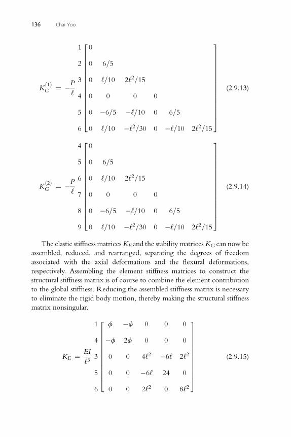
120

3

Kð1ÞG ¼ �P

‘

2

3

4

5

6

666666666666664

0 6=5

0 ‘=10 2‘2=15

0 0 0 0

0 �6=5 �‘=10 0 6=5

0 ‘=10 �‘2=30 0 �‘=10 2‘2=15

777777777777775

(2.9.13)

420

3

136 Chai Yoo

Kð2ÞG ¼ �P

‘

5

6

7

8

9

666666666666664

0 6=5

0 ‘=10 2‘2=15

0 0 0 0

0 �6=5 �‘=10 0 6=5

0 ‘=10 �‘2=30 0 �‘=10 2‘2=15

777777777777775

(2.9.14)

The elastic stiffness matricesKE and the stability matricesKG can now be

assembled, reduced, and rearranged, separating the degrees of freedom

associated with the axial deformations and the flexural deformations,

respectively. Assembling the element stiffness matrices to construct the

structural stiffness matrix is of course to combine the element contribution

to the global stiffness. Reducing the assembled stiffness matrix is necessary

to eliminate the rigid body motion, thereby making the structural stiffness

matrix nonsingular.

KE ¼ EI

‘3

1

4

3

5

6

266666666664

f �f 0 0 0

�f 2f 0 0 0

0 0 4‘2 �6‘ 2‘2

0 0 �6‘ 24 0

0 0 2‘2 0 8‘2

377777777775

(2.9.15)

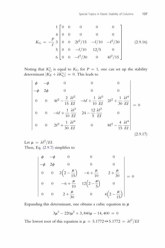
120 0 0 0 0

3

KG ¼ �P

‘

4

3

5

6

666666664

0 0 0 0 0

0 0 2‘2=15 �‘=10 �‘2=30

0 0 �‘=10 12=5 0

0 0 �‘2=30 0 4‘2=15

777777775(2.9.16)

Noting that K�G is equal to KG for P ¼ 1, one can set up the stability

determinant jKE þ lK�Gj ¼ 0. This leads to��������������������

f �f 0 0 0

�f 2f 0 0 0

0 0 4‘2 � 2

15

l‘2

EI�6‘þ 1

10

l‘3

EI2‘2 þ 1

30

l‘4

EI

0 0 �6‘þ 1

10

l‘3

EI24� 12

5

l‘2

EI0

0 0 2‘2 þ 1

30

l‘4

EI0 8‘2 � 4

15

l‘4

EI

��������������������

¼ 0

(2.9.17)

Let m ¼ l‘2=EI .

Special Topics in Elastic Stability of Columns 137

Then, Eq. (2.9.7) simplifies to

����������������

f �f 0 0 0

�f 2f 0 0 0

0 0 2�2� m

15

�6þ m

102þ m

30

0 0 �6þ m

1012�2� m

5

0

0 0 2þ m

300 4

�2� m

15

����������������

¼ 0

Expanding this determinant, one obtains a cubic equation in m

3m3 � 220m2 þ 3; 840m� 14; 400 ¼ 0

The lowest root of this equation is m ¼ 5:177205:1772 ¼ l‘2=EI

138 Chai Yoo

Hence,

Pcr ¼ 5:1772EI

‘2¼ 5:1772EI

ð0:5LÞ2 ¼ 20:7088EI

L2¼ 2:098p2EI

L2

¼ 1:026Pexact ¼ 1:026

�20:19EI

L2

�Considering the fact that only two elements were used to model the

column, this (2.6% difference) is a fairly good performance.

2.10. FREE VIBRATION OF COLUMNS UNDERCOMPRESSIVE LOADS

In Chapter 1, deflection-amplification-type buckling and bifurcation-type

bucklingwere discussed. In order to reach the solution of the critical load of the

column problem, three different approaches were applied. In the deflection-

amplification-type problem, the concern is: What is the value of the

compressive load for which the static deflections of a slightly crooked column

become excessive? In the bifurcation-type buckling problem, two general

approaches were taken: eigenvalue method and energy method. In the

eigenvaluemethod, the concern is:What is thevalueof the compressive load for

which a perfect column bifurcates into a nontrivial equilibrium configuration?

In the energymethod, the concern is:What is the value of the compressive load

for which the potential energy of the column ceases to be positive definite? As

illustrated in Fig. 1-1, the body will return to its undeformed position upon

release of the disturbing action if the potential energy is positive and the system is

in stable equilibrium.On the other hand, if the potential energyof the system is

not positive, the disturbed body will remain at the displaced position or be

displaced further upon the release of the disturbing action.

All of these approaches are based on static concepts. The fourth

approach is based on the dynamic concept. In this approach the concern is:

What is the value of the compressive load for which the free vibration of the

perfect column ceases to occur?

It will be demonstrated that the natural frequency of the column is altered

depending on the presence of the axial compressive load on the column.

The governing differential equation of a prismatic column is given by

EIvivy

vx4þ P

v2y

vx2¼ �m

v2y

vt2(2.10.1)

wherem is the mass per unit length of the column and the right-hand side of

Eq. (2.10.1) is the inertia force per unit length of the column. Note that the

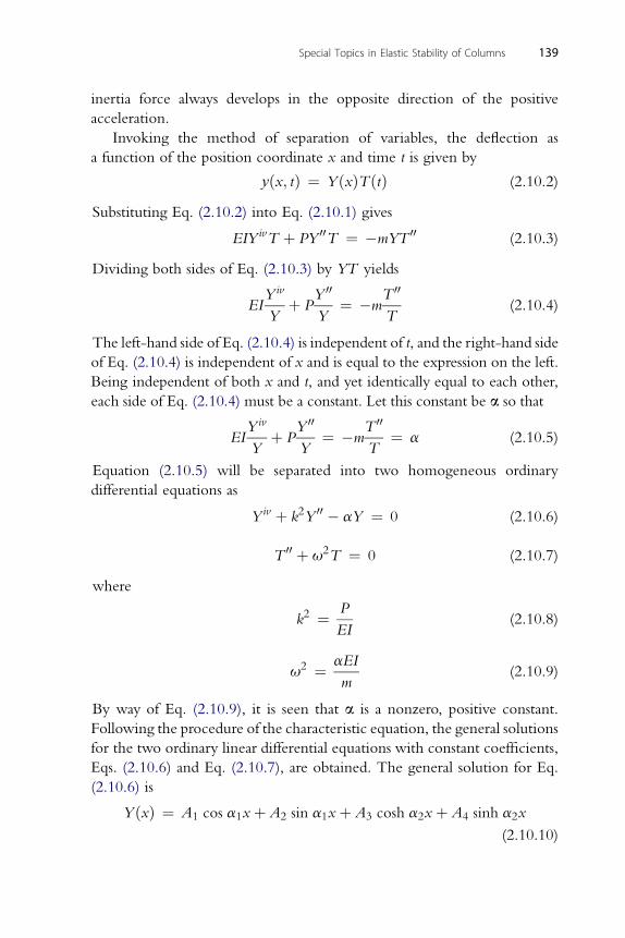
Special Topics in Elastic Stability of Columns 139

inertia force always develops in the opposite direction of the positive

acceleration.

Invoking the method of separation of variables, the deflection as

a function of the position coordinate x and time t is given by

yðx; tÞ ¼ YðxÞTðtÞ (2.10.2)

Substituting Eq. (2.10.2) into Eq. (2.10.1) gives

EIY ivT þ PY 00T ¼ �mYT 00 (2.10.3)

Dividing both sides of Eq. (2.10.3) by YT yields

EIY iv

Yþ P

Y 00

Y¼ �m

T 00

T(2.10.4)

The left-hand side of Eq. (2.10.4) is independent of t, and the right-hand side

of Eq. (2.10.4) is independent of x and is equal to the expression on the left.

Being independent of both x and t, and yet identically equal to each other,

each side of Eq. (2.10.4) must be a constant. Let this constant be a so that

EIY iv

Yþ P

Y 00

Y¼ �m

T 00

T¼ a (2.10.5)

Equation (2.10.5) will be separated into two homogeneous ordinary

differential equations as

Yiv þ k2Y 00 � aY ¼ 0 (2.10.6)

00 2

T þ u T ¼ 0 (2.10.7)

where

k2 ¼ P

EI(2.10.8)

2 aEI

u ¼

m(2.10.9)

By way of Eq. (2.10.9), it is seen that a is a nonzero, positive constant.

Following the procedure of the characteristic equation, the general solutions

for the two ordinary linear differential equations with constant coefficients,

Eqs. (2.10.6) and Eq. (2.10.7), are obtained. The general solution for Eq.

(2.10.6) is

YðxÞ ¼ A1 cos a1xþ A2 sin a1xþ A3 cosh a2xþ A4 sinh a2x

(2.10.10)

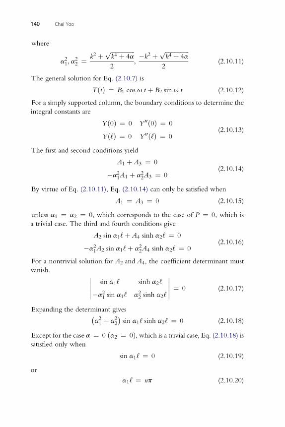
140 Chai Yoo

where

a21;a22 ¼ k2 þ ffiffiffiffiffiffiffiffiffiffiffiffiffiffiffiffi

k4 þ 4ap

2;�k2 þ ffiffiffiffiffiffiffiffiffiffiffiffiffiffiffiffi

k4 þ 4ap

2(2.10.11)

The general solution for Eq. (2.10.7) is

TðtÞ ¼ B1 cos u t þ B2 sin u t (2.10.12)

For a simply supported column, the boundary conditions to determine the

integral constants are

Yð0Þ ¼ 0 Y 00ð0Þ ¼ 0

Yð‘Þ ¼ 0 Y 00ð‘Þ ¼ 0(2.10.13)

The first and second conditions yield

A1 þ A3 ¼ 0

�a21A1 þ a22A3 ¼ 0(2.10.14)

By virtue of Eq. (2.10.11), Eq. (2.10.14) can only be satisfied when

A1 ¼ A3 ¼ 0 (2.10.15)

unless a1 ¼ a2 ¼ 0, which corresponds to the case of P ¼ 0, which is

a trivial case. The third and fourth conditions give

A2 sin a1‘þ A4 sinh a2‘ ¼ 0

�a21A2 sin a1‘þ a22A4 sinh a2‘ ¼ 0(2.10.16)

For a nontrivial solution for A2 and A4, the coefficient determinant must

vanish. �����sin a1‘ sinh a2‘

�a21 sin a1‘ a22 sinh a2‘

����� ¼ 0 (2.10.17)

Expanding the determinant gives�a21 þ a22

�sin a1‘ sinh a2‘ ¼ 0 (2.10.18)

Except for the case a ¼ 0 ða2 ¼ 0Þ, which is a trivial case, Eq. (2.10.18) issatisfied only when

sin a1‘ ¼ 0 (2.10.19)

or

a1‘ ¼ np (2.10.20)

Special Topics in Elastic Stability of Columns 141

Substituting Eq. (2.10.11) into Eq. (2.10.20) for a1, the constant a is

computed

a ¼�np‘

4�1� k2‘2

n2p2

�(2.10.21)

Substituting Eq. (2.10.21) into Eq. (2.10.9) gives the natural frequencies of

the column

un ¼ffiffiffiffiffiEI

m

r �np‘

2 ffiffiffiffiffiffiffiffiffiffiffiffiffiffiffiffiffiffiffiffiffiffiffiffiffi�1� k2‘2

n2p2

�s(2.10.22)

Rearranging Eq. (2.10.22) gives

mu2n ¼ n2p2

‘2

�n2p2

‘2EI � P

�ðn ¼ 1; 2; :::Þ (2.10.23)

Substituting Eq. (2.10.19) into the second Eq. (2.10.16) yields

A4 ¼ 0 (2.10.24)

and the vibration mode of the column is determined from Eq. (2.10.10) as

YnðxÞ ¼ A2 sinnpx

‘(2.10.25)

Two initial conditions determine the other integral constants, B1 and B2 in

Eq. (2.10.12). Assume the vibration is initiated by an initial displacement

such that

yðx; 0Þ ¼ wðxÞ andvyðx; 0Þ

vt¼ 0 (2.10.26)

Then

YðxÞðB1 cos ut þ B2 sin utÞjt¼0 ¼ wðxÞYðxÞð � B1 sin ut þ B2 cos utÞjt¼0¼ 0

(2.10.27)

from which one obtains the following:

B1YðxÞ ¼ wðxÞ and B2 ¼ 0 (2.10.28)

Hence, the general solution of Eq. (2.10.2) for the simply supported

column is given by an infinite sum of natural vibration modes

yðx; tÞ ¼XNn¼ 1

Cn sinnpx

‘cos unt (2.10.29)

142 Chai Yoo

where Cn ¼ A2B2. The coefficient Cn can be determined from the first

condition of Eq. (2.10.28)

XNn¼ 1

Cn sinnpx

‘¼ wðxÞ (2.10.30)

Since Eq. (2.10.30) is a Fourier series expansion for the given initial

deflection, the coefficient can be readily determined by use of the

orthogonality condition

Cn ¼ 2

‘

Z ‘

0

wðxÞ sin npx

‘dx ðn ¼ 1; 2; :::Þ (2.10.31)

As the initial deflection wðxÞis assumed to be known, Eq. (2.10.31) can be

evaluated. Note thatR ‘0 sin

2nx dx ¼ ‘=2. The general solution of the free

vibration of a simply supported column is

yðx; tÞ ¼ 2

‘

XNn¼ 1

� Z ‘

0

wðxÞ sin npx

‘dx

sin

npx

‘cos unt (2.10.32)

It is of interest to note in Eq. (2.10.23) that the frequency of the vibration of

the compressed column is reduced due to the presence of the compressive

load. Once the load P reaches PE, the frequency becomes equal to zero and

the column vibrates with an infinitely long period.

2.11. BUCKLING BY A NONCONSERVATIVE LOAD

Consider a free-standing prismatic cantilever column that is loaded by

a follower force, P, a force that turns its direction so as to always remain

tangential to the deflection curve at the column top as shown in Fig. 2-22.

Such a load is called a tangential load or nonconservative load. As was done

in all three static approaches, assume a nontrivial (neighboring) equilibrium

position and establish a static equilibrium equation. The moment at any

point along the slightly (small deflection) deflected column is

EIy00 ¼ Pðy‘ � yÞ � Py0‘ð‘� xÞ (2.11.1)

Differentiating twice gives

EIyiv þ Py00 ¼ 0 (2.11.2)

and the general solution of Eq. (2.11.2) is

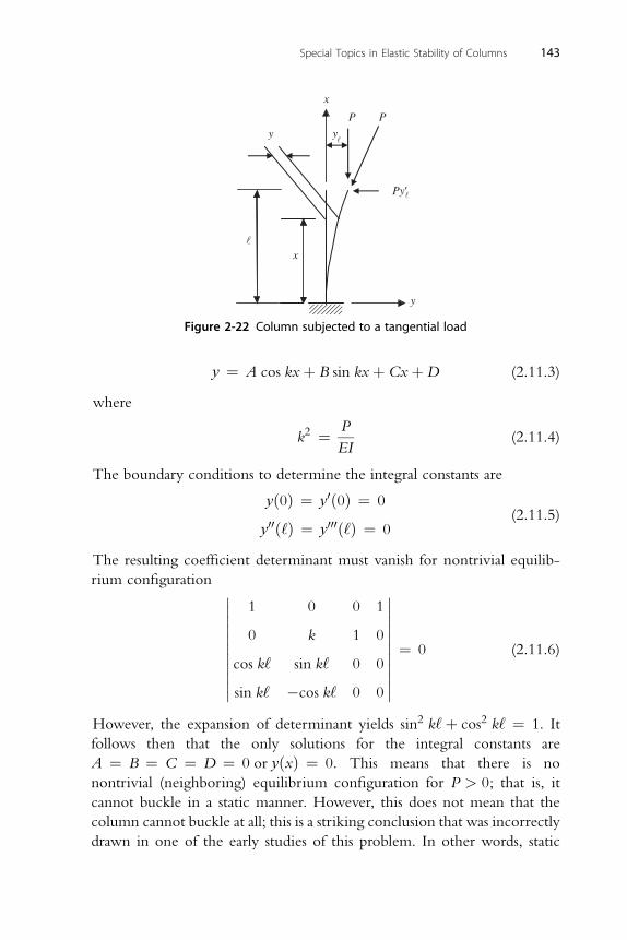
x

Py

PP

yy

x

y

Figure 2-22 Column subjected to a tangential load

Special Topics in Elastic Stability of Columns 143

y ¼ A cos kxþ B sin kxþCxþD (2.11.3)

where

k2 ¼ P

EI(2.11.4)

The boundary conditions to determine the integral constants are

yð0Þ ¼ y0ð0Þ ¼ 0

y00ð‘Þ ¼ y000ð‘Þ ¼ 0(2.11.5)

The resulting coefficient determinant must vanish for nontrivial equilib-

rium configuration �����������

1 0 0 1

0 k 1 0

cos k‘ sin k‘ 0 0

sin k‘ �cos k‘ 0 0

�����������¼ 0 (2.11.6)

However, the expansion of determinant yields sin2 k‘þ cos2 k‘ ¼ 1. It

follows then that the only solutions for the integral constants are

A ¼ B ¼ C ¼ D ¼ 0 or yðxÞ ¼ 0. This means that there is no

nontrivial (neighboring) equilibrium configuration for P > 0; that is, it

cannot buckle in a static manner. However, this does not mean that the

column cannot buckle at all; this is a striking conclusion that was incorrectly

drawn in one of the early studies of this problem. In other words, static

144 Chai Yoo

approaches are insufficient to solve this problem. Ziegler (1968) credits Beck

(1952) as the first to solve this problem correctly, thereby prompting the

free-standing column shown in Fig. 2-22 to be called “Beck’s column.”

Bolotin (1963) and Chen and Atsuta (1976) present highlights of the present

problem in some detail.

Consider investigating the stability of the column by a dynamic

approach. Solution of a column vibration has been given by Eq. (2.10.2),

which is rewritten as

yðx; tÞ ¼ YðxÞTðtÞ ¼ YðxÞðB2 cos ut þ B2 sin utÞ (2.11.7)

YðxÞ ¼ A1 cos a1xþ A2 sin a1xþ A3 cosh a2xþ A4 sinh a2x (2.11.8)

where

a21;a22 ¼ k2 þ ffiffiffiffiffiffiffiffiffiffiffiffiffiffiffiffi

k4 þ 4ap

2;�k2 þ ffiffiffiffiffiffiffiffiffiffiffiffiffiffiffiffi

k4 þ 4ap

2(2.11.9)

andm u2

a ¼EI

(2.11.10)

From the boundary conditions at the fixed end given in Eq. (2.11.5), one

obtainsA1 þ A3 ¼ 0

a1A2 þ a2A4 ¼ 0(2.11.11)

Substituting Eq. (2.11.11) into Eq. (2.11.8) yields

YðxÞ ¼ A1ðcos a1x� cosh a2xÞ þ A2

�sin a1x� a1

a2sinh a2x

�(2.11.15)

The other two boundary conditions at the free end, Eq. (2.11.5), applied to

Eq. (2.11.15) give two additional relationships.

A1

�a21 cos a1xþ a22 cosh a2x

�þ A2

�a22 sin a2xþ a1a2 sinh a2x

� ¼ 0

A1

�a31 sin a1x� a32 cosh a2x

�� A2

�a32 cos a2xþ a1a

22 cosh a2x

� ¼ 0

(2.11.16)

For a nontrivial solution, the determinant of Eq. (2.11.16) for coefficients,

A1 and A2, must vanish.

a41 þ a42 þ 2 a21a22 cos a1‘ cosh a2‘þ a1a2

�a21 � a22

�sin a1‘ sinh a2‘ ¼ 0

(2.11.17)

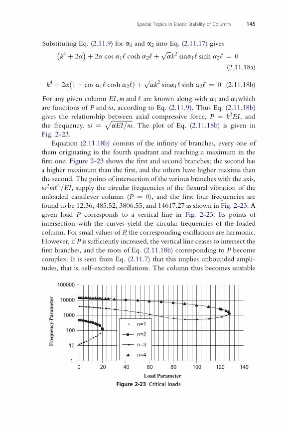
Special Topics in Elastic Stability of Columns 145

Substituting Eq. (2.11.9) for a1 and a2 into Eq. (2.11.17) gives

�k4 þ 2a

�þ 2a cos a1‘ cosh a2‘þffiffiffia

pk2 sina1‘ sinh a2‘ ¼ 0

(2.11.18a)

k4 þ 2að1þ cos a ‘ cosh a ‘Þ þ ffiffiffia

pk2 sina ‘ sinh a ‘ ¼ 0 (2.11.18b)

1 2 1 2

For any given column EI ;m and ‘ are known along with a1 and a1which

are functions of P and u, according to Eq. (2.11.9). Thus Eq. (2.11.18b)

gives the relationship between axial compressive force, P ¼ k2EI , and

the frequency, u ¼ ffiffiffiffiffiffiffiffiffiffiffiffiffiffiaEI=m

p. The plot of Eq. (2.11.18b) is given in

Fig. 2-23.

Equation (2.11.18b) consists of the infinity of branches, every one of

them originating in the fourth quadrant and reaching a maximum in the

first one. Figure 2-23 shows the first and second branches; the second has

a higher maximum than the first, and the others have higher maxima than

the second. The points of intersection of the various branches with the axis,

u2m‘4=EI , supply the circular frequencies of the flexural vibration of the

unloaded cantilever column (P ¼ 0), and the first four frequencies are

found to be 12.36, 485.52, 3806.55, and 14617.27 as shown in Fig. 2-23. A

given load P corresponds to a vertical line in Fig. 2-23. Its points of

intersection with the curves yield the circular frequencies of the loaded

column. For small values of P, the corresponding oscillations are harmonic.

However, if P is sufficiently increased, the vertical line ceases to intersect the

first branches, and the roots of Eq. (2.11.18b) corresponding to P become

complex. It is seen from Eq. (2.11.7) that this implies unbounded ampli-

tudes, that is, self-excited oscillations. The column thus becomes unstable

1

10

100

1000

10000

100000

0 20 40 60 80 100 120 140Load Parameter

Fre

quen

cy P

aram

eter

n=1

n=2

n=3

n=4

Figure 2-23 Critical loads

146 Chai Yoo

when the load parameter, P‘2=EI , reaches the maximum of the first branch

in Fig. 2-23, which is found to be 20.05095 by Maple�.

Therefore the buckling load is

P1 ¼ 20:05EI

‘2¼ 2:031p2EI

‘2(2.11.19)

Despite the early researchers’ misguided conclusions, the column really

buckles by a follower load, and the smallest critical load is approximately

eight times the Euler load for the case of cantilever column.

As shown in Fig. 2-23, the second critical load is found to be

P2 ¼ 127:811EI

‘2¼ 12:95p2EI

‘2(2.11.20)

As stated by Bolotin (1963) and Ziegler (1968), the vertical line corre-

sponding to a level of the tangential load intersects two distinct points on

each branch until the load reaches the maximum where the two points

meet. This is confirmed for the second branch in Fig. 2-23.

No definite conclusion can be drawn regarding the practical value of the

critical tangential load since no method has been devised for applying

a tangential force to a cantilever column undergoing flexural oscillations,

although an idea of attaching a rocket engine of thrust P at the end of the

pulsating column has been proposed, which is highly impractical.

2.12. SELF-ADJOINT BOUNDARY VALUE PROBLEMS

As it was shown in the previous section, when the frequency of the system

becomes complex, then the system is not stable. In an eigenvalue problem,

a system is stable if all eigenvalues are real and positive. In this section,

conditions for real eigenvalues will be examined.

A boundary value problem is defined as a problem consisting of

a differential equation and a collection of boundary values that must be

satisfied by the solution of the differential equation or its derivatives at no

less than two different points. By this definition, a boundary value

problem must have the governing differential equation of at least second

order.

The governing differential equation of an eigenvalue problem may be in

the form

L½y� ¼ ly (2.12.1)

Special Topics in Elastic Stability of Columns 147

where L½ � is a linear differential operator. In the case of a prismatic column

vibration problem, for example, the differential equation for the deflection

has the form

L½y� ¼ EIyiv þ Py00 and l ¼ mu2 (2.12.2)

Only when l takes specific value, ln, Eq. (2.12.1) has solutions, yn(x). ln areeigenvalues, and yn(x) are the corresponding eigenfunctions of the system.

Assume the eigenvalue li is complex, then the corresponding eigenfunction

yi is also complex such that

L½yi� ¼ liyi (2.12.3)

The pair of complex conjugates must also satisfy the equation

L½yi� ¼ liyi (2.12.4)

where the bar denotes the complex conjugate, so that

li ¼ ai þ ibi; li ¼ ai � ibi

yi ¼ uþ ivi; yi ¼ u� ivi(2.12.5)

where i ¼ ffiffiffiffiffiffiffi�1p

. Executing inner (scalar) products of two functions

yi and yi from Eqs. (2.12.3) and (2.12.4) and integrating over the domain of

the column yield Z ‘

0

yiL½yi�dx ¼ li

Z ‘

0

yiyidx

Z ‘

0

yiL½yi�dx ¼ li

Z ‘

0

yiyidx

(2.12.6)

Subtracting the second equation from the first givesZ ‘

0

yiL½yi�dx�Z ‘

0

yiL½yi�dx ¼ ðli � liÞZ ‘

0

yiyidx (2.12.7)

If the eigenvalues are real, it follows

ðli � liÞ ¼ 0 (2.12.8)

Hence, Z ‘

0

yiL½yi�dx ¼Z ‘

0

yiL½yi�dx (2.12.9)

Equation (2.12.9) is known to be the condition for the linear operator L to

be symmetric, and if it is bounded, it is also called self-adjoint. In a system

148 Chai Yoo

dealing with only bounded (continuous) operators, these two terms become

synonymous. Operator L is defined to be positive definite in Section 2.4 if

ðLy; yÞ > 0 for any admissible function y (except y ¼ 0). If the system is

a discrete one and the eigenvalue equation is written in matrix form.

½L�fyg ¼ lfyg (2.12.10)

Equation (2.12.9) can be rewritten as

0 ¼ fygT ½L�fyg � fygT ½L�fyg ¼�fygT ½L�fyg

T�fygT ½L�fyg

¼ fygT ½L�Tfyg � fygT ½L�fyg ¼ fygT�½L�T�½L�

fyg

(2.12.11)

or

½L�T ¼ ½L� (2.12.12)

which implies that L is a symmetric matrix.

In the case of the column vibration problem given by Eq. (2.12.2), an

inner product of two functions, y and L½y�, integrated over the domain isZ ‘

0

yL½y�dx ¼Z ‘

0

y�EIyiv þ Py00

�dx (2.12.13)

Integrating by parts the right-hand side of Eq. (2.12.13) (four times the first

term and twice the second term) givesZ ‘

0

yL½y� dx ¼Z ‘

0

y�EIyiv þ Py00

�dx

¼ �yðEIy000 þ Py0Þ‘0 þ yðEIy000 þ Py0Þ‘0 � y0ðEIy00Þ‘0

þy0ðEIy00Þ‘0 þZ ‘

0

yL½y�dx (2.12.14)

Invoking the self-adjoint condition of Eq. (2.12.9), the sum of integrated

terms in Eq. (2.12.14), which is referred to as conjunct or concomitant,

vanishes.

� yðEIy000 þ Py0Þ‘0 þ yðEIy000 þ Py0Þ‘0 � y0ðEIy00Þ‘0 þ y0ðEIy00Þ‘0 ¼ 0

(2.12.15)

Special Topics in Elastic Stability of Columns 149

In fact, each term of Eq. (2.12.15) vanishes for any combination of column

end support conditions: free, pinned, and fixed. This is called the self-

adjoint boundary conditions for a column.

Consider now the case of a column loaded tangentially. The boundary

conditions given in Eq. (2.11.5) do not satisfy the self-adjoint boundary

condition for a column given by Eq. (2.12.15). Thus a cantilever column

loaded by a tangential force does not provide a self-adjoint boundary

condition, and hence, all the eigenvalues are not necessarily real. This does

not render the problem to be a self-adjoint boundary value problem. Hence,

the problem is not a properly posed one, and a unique solution is not

guaranteed by any one of the classical solution methods.

Another way of discerning whether or not a system of boundary

conditions is conservative is to evaluate the potential energy of the boundary

forces at elastically constrained supports. If the potential energy thus

computed is path-independent, then it is said to be a system of conservative

boundary conditions.

REFERENCESABAQUS. (2006). ABAQUS Analysis User’s Manual. Pawtucket, RI: ABAQUS.Beck, M. (1952). Die Knicklast des einseitig eingespannten, tangential gedruckten Stabes.

Z. Angew. Math. Phys., 3, 225.Bolotin, V.V. (1963). Nonconservative Problems of the Theory of Elastic Stability. Translated from

the Russian by T.K. Lusher, English Translation edited by G. Herrmann, PergamonPress, London, UK.

Chen, W. F., & Atsuta, T. (1976). Theory of Beam-columns, Vol. 1. New York: InplaneBehavior and Design, McGraw-Hill.

Forsyth, A. R. (1960). Calculus of Variations. New York: Dover.Fung, Y. C., & Tong, P. (2001). Classical and Computational Solid Mechanics. Singapore:

World Scientific.Hjelmstad, K. D. (2005). Fundamentals of Structural Mechanics (2nd ed.). New York: Springer.Hoff, N. J. (1956). The Analysis of Structures. New York: John Wiley and Sons.Langhaar, H. L. (1962). Energy Methods in Applied Mechanics. New York: John Wiley and

Sons.Love, A. E. H. (1944). ATreatise of the Mathematical Theory of Elasticity. New York, NY: Dover.Mikhlin, S. G. (1964). Variational Methods in Mathematical Physics. Macmillan Company.Newmark, N. (1943). Numerical Procedure for Computing Deflection, Moments, and

Buckling Loads. Transaction, ASCE, Vol. 108, 1161.Saada, A. S. (1974). Elasticity Theory and Applications (2nd ed.). Malabar, FL: Krieger

Publishing Company.Shames, I. H., & Dym, C. L. (1985). Energy and Finite Element Methods in Structural

Mechanics. New York: Hemisphere.Sokolnikoff, I. S. (1956).Mathematical Theory of Elasticity (2nd ed.). NewYork:McGraw-Hill.Tauchert, T. R. (1974). Energy Principles in Structural Mechanics. New York: McGraw-Hill.Timoshenko, S. P., & Gere, J. M. (1961). Theory of Elastic Stability. New York: McGraw-Hill.Washizu, K. (1974). Variational Methods in Elasticity and Plasticity (2nd ed.). Oxford, UK:

Pergamon Press, Ltd.

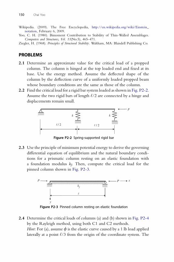
150 Chai Yoo

Wikipedia. (2009). The Free Encyclopedia, http://en.wikipedia.org/wiki/Einstein_notation, February 6, 2009.

Yoo, C. H. (1980). Bimoment Contribution to Stability of Thin-Walled Assemblages.Computers and Structures, Vol. 11(No.5), 465–471.

Ziegler, H. (1968). Principles of Structural Stability. Waltham, MA: Blaisdell Publishing Co.

PROBLEMS

2.1 Determine an approximate value for the critical load of a propped

column. The column is hinged at the top loaded end and fixed at its

base. Use the energy method. Assume the deflected shape of the

column by the deflection curve of a uniformly loaded propped beam

whose boundary conditions are the same as those of the column.

2.2 Find the critical load for a rigid bar system loaded as shown in Fig. P2-2.

Assume the two rigid bars of length ‘/2 are connected by a hinge and

displacements remain small.

P

k

/ 2 / 2

k

Figure P2-2 Spring-supported rigid bar

2.3 Use the principle of minimum potential energy to derive the governing

differential equation of equilibrium and the natural boundary condi-

tions for a prismatic column resting on an elastic foundation with

a foundation modulus kf. Then, compute the critical load for the

pinned column shown in Fig. P2-3.

P

y

x

kf

P

Figure P2-3 Pinned column resting on elastic foundation

2.4 Determine the critical loads of columns (a) and (b) shown in Fig. P2-4

by the Rayleigh method, using both C1 and C2 methods.

Hint: For (a), assume f is the elastic curve caused by a 1 lb load applied

laterally at a point ‘/3 from the origin of the coordinate system. The

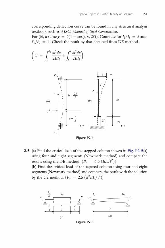
Special Topics in Elastic Stability of Columns 151

corresponding deflection curve can be found in any structural analysis

textbook such as AISC, Manual of Steel Construction.

For (b), assume y ¼ dð1� cosðpx=2‘ÞÞ. Compute for I2=I1 ¼ 5 and

‘1=‘2 ¼ 4. Check the result by that obtained from DE method.

�U ¼

Z ‘2

0

m2dx

2EI2þZ ‘

‘2

m2dx

2EI1

�

d P

x

a =3

b = 23

(a) (b)

y

P

1#

P

5I1

I1

y

x

.8

.2

Figure P2-4

2.5 (a) Find the critical load of the stepped column shown in Fig. P2-5(a)

using four and eight segments (Newmark method) and compare the

results using the DE method. ðPcr ¼ 6:5 ðEIo=‘2ÞÞ(b) Find the critical load of the tapered column using four and eight

segments (Newmark method) and compare the result with the solution

by the C2 method. ðPcr ¼ 2:5 ðp2EIo=‘2ÞÞ

P 4 PP

2 4

4I0I0I0I0

P

4

(a) (b)

Figure P2-5

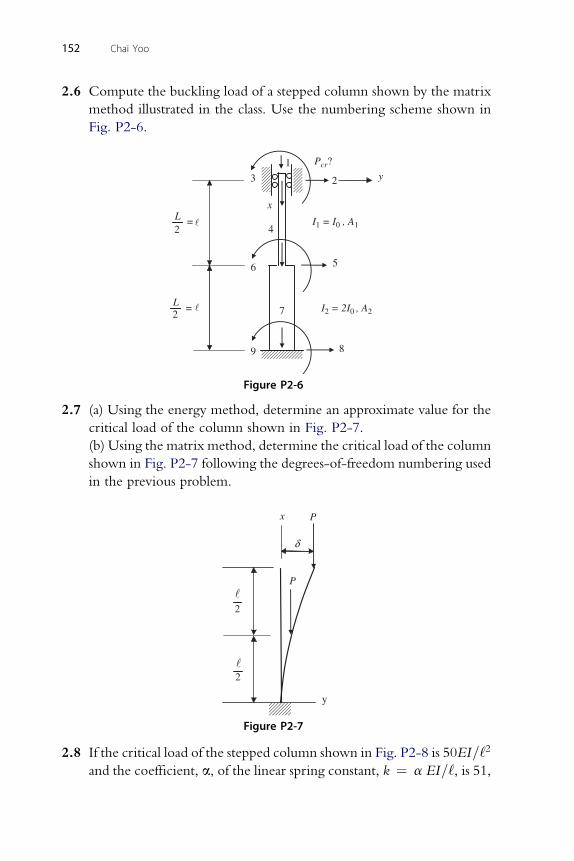
152 Chai Yoo

2.6 Compute the buckling load of a stepped column shown by the matrix

method illustrated in the class. Use the numbering scheme shown in

Fig. P2-6.

Pcr?1

5

3 y

4

x

6

7

8

I1 = I0 , A1

I2 = 2I0 , A2

9

2

L = 2

L2

=

Figure P2-6

2.7 (a) Using the energy method, determine an approximate value for the

critical load of the column shown in Fig. P2-7.

(b) Using the matrix method, determine the critical load of the column

shown in Fig. P2-7 following the degrees-of-freedom numbering used

in the previous problem.

x P

y

P

2

2

Figure P2-7

2.8 If the critical load of the stepped column shown in Fig. P2-8 is 50EI=‘2

and the coefficient, a, of the linear spring constant, k ¼ a EI=‘, is 51,

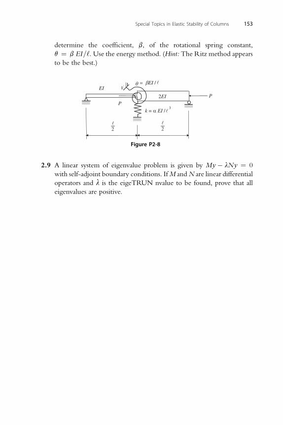
Special Topics in Elastic Stability of Columns 153

determine the coefficient, b, of the rotational spring constant,

q ¼ b EI=‘. Use the energy method. (Hint: The Ritz method appears

to be the best.)

EI

2EI

2

k = α EI / 3

= βEI /

P

2

P

Figure P2-8

2.9 A linear system of eigenvalue problem is given by My� lNy ¼ 0

with self-adjoint boundary conditions. IfM andN are linear differential

operators and l is the eigeTRUN nvalue to be found, prove that all

eigenvalues are positive.

CHAPTER33

Beam-ColumnsContents

3.1. Transversely Loaded Beam Subjected to Axial Compression 1553.1.1. The Concept of Amplification 1553.1.2. Stress Amplification in Columns 157

3.2. Beam-Columns with Concentrated Lateral Loads 1613.3. Beam-Columns with Distributed Lateral Loads 1633.4. Effect of Axial Force on Bending Stiffness 164

3.4.1. Review of Moment-Area Theorems 1643.4.2. Slope-Deflection Equation without Axial Force 1673.4.3. Effects of Axial Loads on Bending Stiffness 1713.4.4. Slope-Deflection Equations with Axial Tension 179

3.5. Ultimate Strength of Beam-Columns 1853.6. Design of Beam-Columns 192References 195Problems 196

3.1. TRANSVERSELY LOADED BEAM SUBJECTEDTO AXIAL COMPRESSION

3.1.1. The Concept of AmplificationThis chapter seeks to familiarize the student with buckling of some simple

structural members and frames, and it presents a few methods that can be

successfully used to arrive at the critical condition. A more comprehensive

treatment of the buckling analysis of structures may be found in the books

by Bleich (1952), Britvec (1973), and Bazant and Credolin (1991). Since

one of the methods employed for analysis of the structural stability is based

on the theory of beam-columns, a brief review will be in order (see also

Timoshenko and Gere 1961).

A slender member meeting the Euler-Bernoulli-Navier hypotheses

under transverse loads and inplane compressive load (see Fig. 3-1) is called

a beam-column. An exact analysis of a beam-column can only be accom-

plished by solving the governing differential equation or its derivatives (for

example, slope-deflection equations).

Consider a very simple case of a beam-column shown in Fig. 3-1. The

beam-column is subjected simultaneously to a transverse load Q at its mid-

span and a concentric compressive force P. Since the response of

Stability of Structures � 2011 Elsevier Inc.ISBN 978-0-12-385122-2, doi:10.1016/B978-0-12-385122-2.10003-X All rights reserved. 155 j

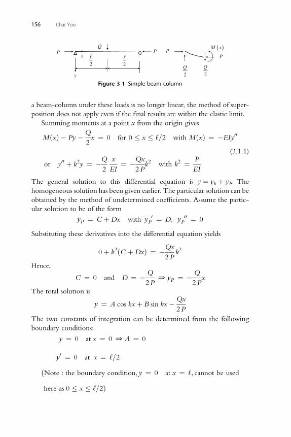
y 2

Q2

Q

P Px

2 2

PP

( )M xQ

Figure 3-1 Simple beam-column

156 Chai Yoo

a beam-column under these loads is no longer linear, the method of super-

position does not apply even if the final results are within the elastic limit.

Summing moments at a point x from the origin gives

MðxÞ � Py�Q

2x ¼ 0 for 0 � x � ‘=2 with MðxÞ ¼ �EIy00

(3.1.1)

or y00 þ k2y ¼ �Q x ¼ �Qxk2 with k2 ¼ P

2 EI 2P EI

The general solution to this differential equation is y ¼ yh þ yP. The

homogeneous solution has been given earlier. The particular solution can be

obtained by the method of undetermined coefficients. Assume the partic-

ular solution to be of the form

yP ¼ C þDx with y 0P ¼ D; y 00

P ¼ 0

Substituting these derivatives into the differential equation yields

0þ k2ðC þDxÞ ¼ �Qx

2Pk2

Hence,Q Q

C ¼ 0 and D ¼ �2P

0 yP ¼ �2P

x

The total solution isQx

y ¼ A cos kxþ B sin kx�2P

The two constants of integration can be determined from the following

boundary conditions:

y ¼ 0 at x ¼ 0 0A ¼ 0

0

y ¼ 0 at x ¼ ‘=2

ðNote : the boundary condition; y ¼ 0 at x ¼ ‘; cannot be used

here as 0 � x � ‘=2Þ

Q k‘ Q Q

y0 ¼ Bk cos kx�

2P; 0 ¼ Bk cos

2�2P

0B ¼2Pk cos

k‘

2

2

Beam-Columns 157

y ¼ Q sin kx

2Pk cosk‘

2

�Qx

2Pfor 0 � x � ‘

2with Pcr ¼ PE ¼ p EI

‘2

By observation, the maximum lateral deflection occurs at the midspan.

ymax

�����x ¼ ‘2

¼ Q

2Pk

�tan

k‘

2� k‘

2

�with u ¼ k‘

2¼ ‘

2

ffiffiffiffiffiP

EI

r

�� 3 3� �

3� �

3

ymax���x ¼ ‘

2

¼ Qk ‘

16Pku3tan

k‘

2� k‘

2¼ Q‘

48EI

3ðtan u� uÞu3

¼ Q‘

48EIXðuÞ

(3.1.2)

�� 3

ymax���x ¼ ‘

2

¼ dmax ¼ Q‘

48EIwhen P ¼ 0

2 2 2

u2 ¼ ‘

4

P

EI0 P ¼ 4EIu

‘2and PE ¼ p EI

‘2

P

PE¼ 4EIu2

‘2‘2

p2EI¼ 4u2

p2; XðuÞ ¼ 3ðtan u� uÞ

u3

3.1.2. Stress Amplification in ColumnsThe behavior of a compression member under increasing load can be seen

most clearly by calculating the bending stresses and lateral deflections that

occur as the axial load is gradually applied. Consider a perfectly straight,

slender member supporting a nominal axial load P. The ends of the member

are assumed free to rotate in this case. If thememberwere perfectly straight and

homogeneous and the loadwere perfectly centered, the stress in the column at

any section would be simply sa ¼ P/A, where A is the cross-sectional area of

the column. No actual member ever would be perfectly straight and homo-

geneous, norwould the load be perfectly centered. Evenwhen great efforts are

made to achieve such perfection in laboratory tests, it is not completely

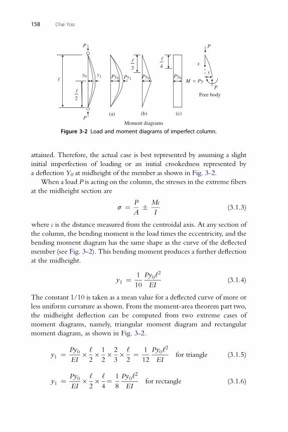
P

Moment diagrams

y1

2

3 4

Py1Py0 Py0 Py0

Free body

x

y

M Py=P

P

y0

P(a) (b) (c)

Figure 3-2 Load and moment diagrams of imperfect column.

158 Chai Yoo

attained. Therefore, the actual case is best represented by assuming a slight

initial imperfection of loading or an initial crookedness represented by

a deflection Y0 at midheight of the member as shown in Fig. 3-2.

When a load P is acting on the column, the stresses in the extreme fibers

at the midheight section are

s ¼ P

A� Mc

I(3.1.3)

where c is the distance measured from the centroidal axis. At any section of

the column, the bending moment is the load times the eccentricity, and the

bending moment diagram has the same shape as the curve of the deflected

member (see Fig. 3-2). This bending moment produces a further deflection

at the midheight.

y1 ¼ 1

10

Py0‘2

EI(3.1.4)

The constant 1/10 is taken as a mean value for a deflected curve of more or

less uniform curvature as shown. From the moment-area theorem part two,

the midheight deflection can be computed from two extreme cases of

moment diagrams, namely, triangular moment diagram and rectangular

moment diagram, as shown in Fig. 3-2.

y1 ¼ Py0EI

� ‘

2� 1

2� 2

3� ‘

2¼ 1

12

Py0‘2

EIfor triangle (3.1.5)

2

y1 ¼ Py0EI

� ‘

2� ‘

4¼ 1

8

Py0‘

EIfor rectangle (3.1.6)

Beam-Columns 159

For other cases of initial curvature or eccentricity, the constant may vary

between limits of 1/8 and 1/12 (If it were known to be a sine function, then

the factor would be 1/p2 ¼1/9.8696 and the correct Euler load would

result.) Because of the added deflection y1, there will be an increased

bending moment Py1 , and additional deflection y2.

y2 ¼ 1

10

Py1‘2

EI(3.1.7)

Continuing this process, the total deflection becomes

y ¼ y0 þ y1 þ y2 þ.

¼ y0 þP‘2

10EIy0 þ

P‘2

10EIy1 þ.

¼ y0 þ�

P‘2

10EI

�y0 þ

�P‘2

10EI

�2

y0 þ.

¼ y0

�1þ

�P‘2

10EI

�þ�

P‘2

10EI

�2

þ�

P‘2

10EI

�3

þ.

�

(3.1.8)

The series in the bracket is the multiplier by which the initial deflection y0 is

increased under load P to give the final deflection y at that load. For values

of P less than 10EI/‘2 (Euler buckling load), the terms in the series are less

than unity and the series is convergent, having the limit

1

1� P‘2

10EI

(3.1.9)

The final deflection is thus

y ¼ y01

1� P‘2

10EI

(3.1.10)

This requires a slight modification that will be discussed later if the curve of

initial deflection differs greatly from the uniform curvature assumed.

For any value of P such that (P‘2/10EI)� 1, the series is divergent. This

indicates that any small initial deflection will be indefinitely magnified at the

load P ¼ PE ¼ (10EI/‘2) or greater.

160 Chai Yoo

Let denote PE ¼ p2EI=‘2^10EI=‘2. Then the total stress of a column at

mid height is

s ¼ P

A� Py0c

I

1

1� P

PE

(3.1.11)

2 2 2

Let sa ¼ P

Aand scr ¼ PE

A¼ p EAr

A‘2¼ p E�

‘

r

�2

Further, recall that

1

1� P

PE

¼ 1

1� sa

scr

and

Py0c

I¼ Py0c

Ar2¼ sa

y0c

r2¼ sa

�c

r

�2y0c

The total stress is then

s ¼ sa � sa

�c

r

�2y0c

1

1� sa

scr

(3.1.12)

Thus, the magnitude of the bending stress, the second term in Eq. (3.1.12),

depends on P represented in sa; the shape of the cross section (c/r); and the

initial curvature (y0/c).

As the critical stress, scr ¼ p2E/(‘/r)2, is a function of the stiffness of the

material of the column and the slenderness ratio, it is convenient to make

the expression for stress dimensionless by dividing Eq. (3.1.12) by scr.Thus

s

scr¼ sa

scr� sa

scr

�c

r

�2y0c

1

1� sa

scr

(3.1.13)

The value of shape factor (c/r ) ranges from 1.0 for a section in which all

(most) of the area is assumed concentrated in the flanges toffiffiffi3

pfor rect-

angular section and 2.0 for a solid circular section. Rolled shapes generally

used for columns have (c/r)2 in the vicinity of 1.4 about the strong axis and

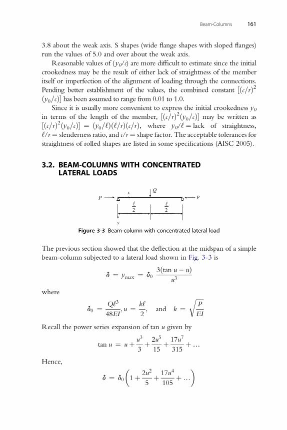
Beam-Columns 161

3.8 about the weak axis. S shapes (wide flange shapes with sloped flanges)

run the values of 5.0 and over about the weak axis.

Reasonable values of (y0/c) are more difficult to estimate since the initial

crookedness may be the result of either lack of straightness of the member

itself or imperfection of the alignment of loading through the connections.

Pending better establishment of the values, the combined constant ½ðc=rÞ2ðy0=cÞ� has been assumed to range from 0.01 to 1.0.

Since it is usually more convenient to express the initial crookedness y0in terms of the length of the member, ½ðc=rÞ2ðy0=cÞ� may be written as

½ðc=rÞ2ðy0=cÞ� ¼ ðy0=‘Þð‘=rÞðc=rÞ, where y0/‘ ¼ lack of straightness,

‘/r ¼ slenderness ratio, and c/r ¼ shape factor. The acceptable tolerances for

straightness of rolled shapes are listed in some specifications (AISC 2005).

3.2. BEAM-COLUMNS WITH CONCENTRATEDLATERAL LOADS

y

2

Px

P

2

Q

Figure 3-3 Beam-column with concentrated lateral load

The previous section showed that the deflection at the midspan of a simple

beam-column subjected to a lateral load shown in Fig. 3-3 is

d ¼ ymax ¼ d03ðtan u� uÞ

u3

where

d0 ¼ Q‘3

48EI; u ¼ k‘

2; and k ¼

ffiffiffiffiffiP

EI

r

Recall the power series expansion of tan u given by

tan u ¼ uþ u3

3þ 2u5

15þ 17u7

315þ.

Hence,

d ¼ d0

�1þ 2u2

5þ 17u4

105þ.

�

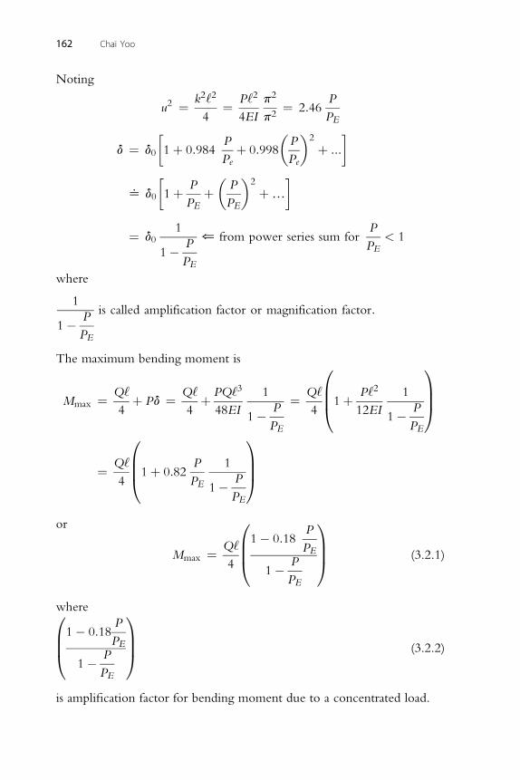
162 Chai Yoo

Noting

u2 ¼ k2‘2

4¼ P‘2

4EI

p2

p2¼ 2:46

P

PE�P

�P�2

�

d ¼ d0 1þ 0:984

Peþ 0:998

Peþ :::

�P

�P�2

�

^ d0 1þ

PEþ

PEþ.

¼ d01

1� P

PE

* from power series sum forP

PE< 1

where

1

1� P

PE

is called amplification factor or magnification factor:

The maximum bending moment is

Mmax ¼ Q‘

4þ Pd ¼ Q‘

4þ PQ‘3

48EI

1

1� P

PE

¼ Q‘

4

0BB@1þ P‘2

12EI

1

1� P

PE

1CCA

¼ Q‘

4

0BB@1þ 0:82

P

PE

1

1� P

PE

1CCA

or 0P1

Mmax ¼ Q‘

4

BB@1� 0:18

PE

1� P

PE

CCA (3.2.1)

where0BB@1� 0:18

P

PE

1� P

PE

1CCA (3.2.2)

is amplification factor for bending moment due to a concentrated load.

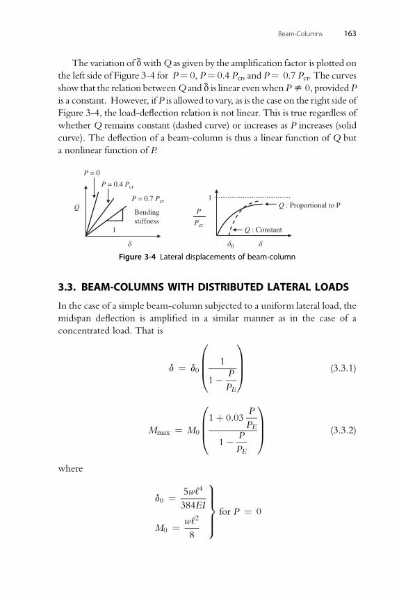
Beam-Columns 163

The variation of dwithQ as given by the amplification factor is plotted on

the left side of Figure 3-4 for P¼ 0, P¼ 0.4 Pcr, and P¼ 0.7 Pcr. The curves

show that the relation betweenQ and d is linear evenwhen Ps 0, provided P

is a constant. However, if P is allowed to vary, as is the case on the right side of

Figure 3-4, the load-deflection relation is not linear. This is true regardless of

whether Q remains constant (dashed curve) or increases as P increases (solid

curve). The deflection of a beam-column is thus a linear function of Q but

a nonlinear function of P.

P = 0

d0

1Q

Bendingstiffness

P = 0.7 Pcr

P = 0.4 Pcr

dd

1

P

Pcr

Q : Proportional to P

Q : Constant

Figure 3-4 Lateral displacements of beam-column

3.3. BEAM-COLUMNS WITH DISTRIBUTED LATERAL LOADS

In the case of a simple beam-column subjected to a uniform lateral load, the

midspan deflection is amplified in a similar manner as in the case of a

concentrated load. That is

d ¼ d0

0BB@ 1

1� P

PE

1CCA (3.3.1)

0P1

Mmax ¼ M0

BB@1þ 0:03

PE

1� P

PE

CCA (3.3.2)

where

d0 ¼ 5w‘4

384EI

M0 ¼ w‘2

8

9>>>=>>>;

for P ¼ 0

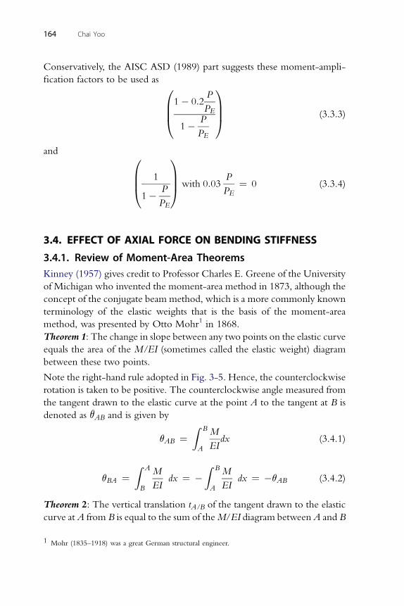
164 Chai Yoo

Conservatively, the AISC ASD (1989) part suggests these moment-ampli-

fication factors to be used as 0BB@1� 0:2

P

PE

1� P

PE

1CCA (3.3.3)

and 0 1

BB@ 1

1� P

PE

CCA with 0:03P

PE¼ 0 (3.3.4)

3.4. EFFECT OF AXIAL FORCE ON BENDING STIFFNESS

3.4.1. Review of Moment-Area TheoremsKinney (1957) gives credit to Professor Charles E. Greene of the University

of Michigan who invented the moment-area method in 1873, although the

concept of the conjugate beam method, which is a more commonly known

terminology of the elastic weights that is the basis of the moment-area

method, was presented by Otto Mohr1 in 1868.

Theorem 1: The change in slope between any two points on the elastic curve

equals the area of the M/EI (sometimes called the elastic weight) diagram

between these two points.

Note the right-hand rule adopted in Fig. 3-5. Hence, the counterclockwise

rotation is taken to be positive. The counterclockwise angle measured from

the tangent drawn to the elastic curve at the point A to the tangent at B is

denoted as qAB and is given by

qAB ¼Z B

A

M

EIdx (3.4.1)

Z A Z B

qBA ¼B

M

EIdx ¼ �

A

M

EIdx ¼ �qAB (3.4.2)

Theorem 2: The vertical translation tA/B of the tangent drawn to the elastic

curve at A from B is equal to the sum of theM/EI diagram betweenA and B

1 Mohr (1835–1918) was a great German structural engineer.

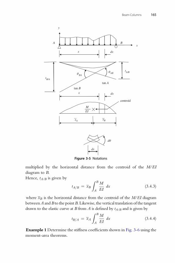
y

B

x

xA

dx

q ABq BAt

x

t

MEI

xA xB

tan A

dq

dx

centroid

tan B

dx

A/B

B/A

Figure 3-5 Notations

Beam-Columns 165

multiplied by the horizontal distance from the centroid of the M/EI

diagram to B.

Hence, tA/B is given by

tA=B ¼ xB

Z B

A

M

EIdx (3.4.3)

where xB is the horizontal distance from the centroid of the M/EI diagram

betweenA andB to the pointB. Likewise, the vertical translation of the tangent

drawn to the elastic curve at B from A is defined by tA/B and is given by

tB=A ¼ xA

Z B

A

M

EIdx (3.4.4)

Example 1Determine the stiffness coefficients shown in Fig. 3-6 using the

moment-area theorems.

+

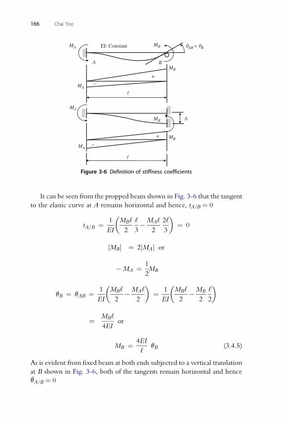
A B

qAB = qB

+

-

-

D

EI: ConstantMA

MA

MA

MA

MB

MB

MB

MB

Figure 3-6 Definition of stiffness coefficients

166 Chai Yoo

It can be seen from the propped beam shown in Fig. 3-6 that the tangent

to the elastic curve at A remains horizontal and hence, tA/B ¼ 0

tA=B ¼ 1

EI

�MB‘

2

‘

3�MA‘

2

2‘

3

�¼ 0

jM j ¼ 2jM j or

B A

1

�MA ¼2MB

1�M ‘ M ‘

�1�M ‘ M ‘

�

qB ¼ qAB ¼

EI

B

2� A

2¼

EI

B

2� B

2 2

M ‘

¼ B

4EIor

4EI

MB ¼

‘qB (3.4.5)

As is evident from fixed beam at both ends subjected to a vertical translation

at B shown in Fig. 3-6, both of the tangents remain horizontal and hence

qA/B ¼ 0

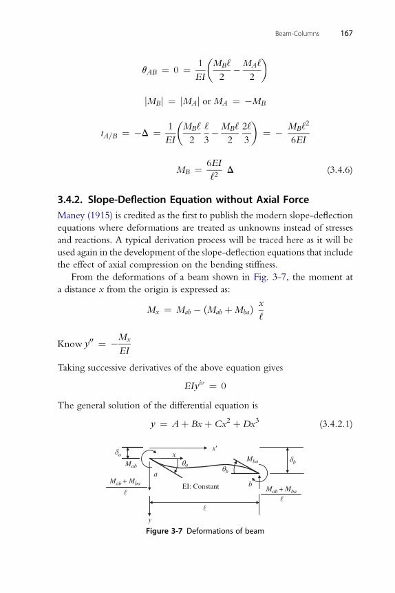
Beam-Columns 167

qAB ¼ 0 ¼ 1

EI

�MB‘

2�MA‘

2

�

jM j ¼ jM j or M ¼ �M

B A A B

� �2

tA=B ¼ �D ¼ 1

EI

MB‘

2

‘

3�MB‘

2

2‘

3¼ � MB‘

6EI

6EI

MB ¼

‘2D (3.4.6)

3.4.2. Slope-Deflection Equation without Axial ForceManey (1915) is credited as the first to publish the modern slope-deflection

equations where deformations are treated as unknowns instead of stresses

and reactions. A typical derivation process will be traced here as it will be

used again in the development of the slope-deflection equations that include

the effect of axial compression on the bending stiffness.

From the deformations of a beam shown in Fig. 3-7, the moment at

a distance x from the origin is expressed as:

Mx ¼ Mab � ðMab þMbaÞ x

‘

Mx

Know y00 ¼ �

EI

Taking successive derivatives of the above equation gives

EIyiv ¼ 0

The general solution of the differential equation is

y ¼ Aþ Bxþ Cx2 þDx3 (3.4.2.1)

x¢

qb

dadbqaMab

Mab + MbaMab + Mba

xMba

EI: Constant

y

a

b

Figure 3-7 Deformations of beam

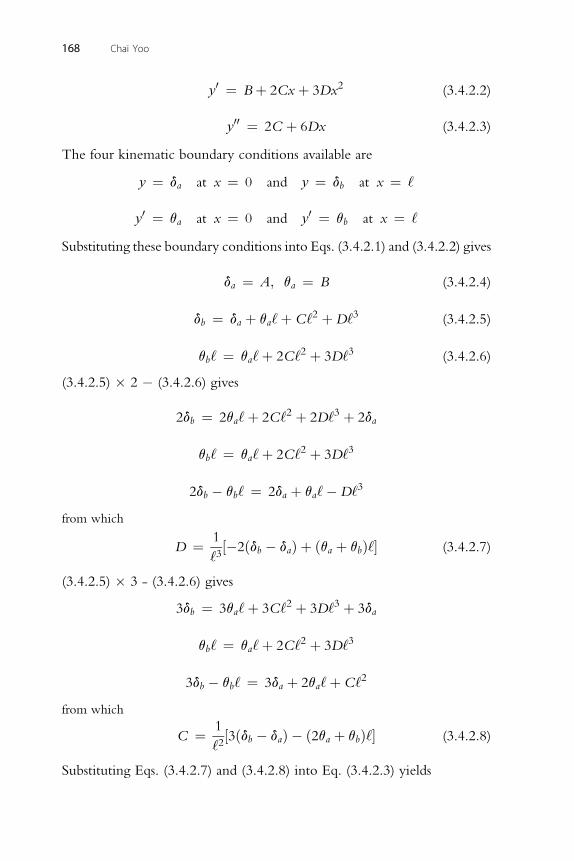
y0 ¼ Bþ 2Cxþ 3Dx2 (3.4.2.2)

00

168 Chai Yoo

y ¼ 2C þ 6Dx (3.4.2.3)

The four kinematic boundary conditions available are

y ¼ da at x ¼ 0 and y ¼ db at x ¼ ‘

0 0

y ¼ qa at x ¼ 0 and y ¼ qb at x ¼ ‘

Substituting these boundary conditions into Eqs. (3.4.2.1) and (3.4.2.2) gives

da ¼ A; qa ¼ B (3.4.2.4)

2 3

db ¼ da þ qa‘þ C‘ þD‘ (3.4.2.5)

2 3

qb‘ ¼ qa‘þ 2C‘ þ 3D‘ (3.4.2.6)

(3.4.2.5) � 2 � (3.4.2.6) gives

2db ¼ 2qa‘þ 2C‘2 þ 2D‘3 þ 2da

2 3

qb‘ ¼ qa‘þ 2C‘ þ 3D‘

3

2db � qb‘ ¼ 2da þ qa‘�D‘

from which

D ¼ 1

‘3½�2ðdb � daÞ þ ðqa þ qbÞ‘� (3.4.2.7)

(3.4.2.5) � 3 - (3.4.2.6) gives

3db ¼ 3qa‘þ 3C‘2 þ 3D‘3 þ 3da

2 3

qb‘ ¼ qa‘þ 2C‘ þ 3D‘

2

3db � qb‘ ¼ 3da þ 2qa‘þ C‘

from which

C ¼ 1

‘2½3ðdb � daÞ � ð2qa þ qbÞ‘� (3.4.2.8)

Substituting Eqs. (3.4.2.7) and (3.4.2.8) into Eq. (3.4.2.3) yields

Beam-Columns 169

y00 ¼ 2

‘2½3ðdb � daÞ � ð2qa þ qbÞ‘� þ 6

‘3½�2ðdb � daÞ þ ðqa þ qbÞ‘�x

2 M

y00ð0Þ ¼

‘2½3ðdb � daÞ � ð2qa þ qbÞ‘� ¼ � ab

EI(3.4.2.9)

2 6

y00ð‘Þ ¼

‘3½3ðdb � daÞ � ð2qa þ qbÞ‘�‘þ

‘2½�2ðdb � daÞ þ ðqa þ qbÞ‘�‘

Mab 6 Mba

¼ �EI

þ‘2½�2ðdb � daÞ þ ðqa þ qbÞ‘� ¼

EI(3.4.2.10)

From Eq. (3.4.2.9), one obtains

Mab ¼ 2EI

‘

�2qa þ qb � 3

‘ðdb � daÞ

�(3.4.2.11)

From Eq. (3.4.2.10), one obtains

Mba ¼ 2EI

‘

�2qb þ qa � 3

‘ðdb � daÞ

�(3.4.2.12)

If any fixed end moments exist prior to releasing the joint constraints such as

Mab fixed and Mba fixed, then final member end moments become

MAB ¼ 2EI

‘

�2qa þ qb � 3

‘ðdb � daÞ

�þMab fixed (3.4.2.13)

2EI�

3�

Mba ¼‘

2qb þ qa �‘ðdb � daÞ þMba fixed (3.4.2.14)

Example 1 Consider a frame shown in Fig. 3-8. If each member is

inextensible, then the frame is a 6-degree indeterminate structure. (Note:

This elementary slope-deflection equation cannot handle member exten-

sibility.) Assume just for simplicity that all four members are identical.

Dimensions of the frame, cross-sectional properties, and material constant

are¼ 100 in., I¼ 1 in.4,A¼ 106 in.2, E¼ 29,000 ksi, respectively. Member

ab is subjected to a uniform load, w ¼ 0.1 kip/in.

There is only one unknown, qb (kinematic degree-of-freedom).

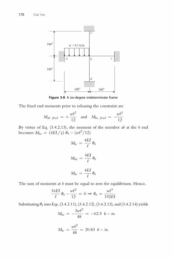
100"

100"

100" 100"

d

e

cba

w = 0.1 k/in

Figure 3-8 A six-degree indeterminate frame

170 Chai Yoo

The fixed end moments prior to releasing the constraint are

Mab fixed ¼ þ w‘2

12and Mba fixed ¼ �w‘2

12

By virtue of Eq. (3.4.2.13), the moment of the member ab at the b end

becomes Mba ¼ ð4EI.‘Þ qb � ðw‘2=12Þ

Mbc ¼ 4EI

‘qb

4EI

Mbd ¼

‘qb

4EI

Mbe ¼

‘qb

The sum of moments at b must be equal to zero for equilibrium. Hence,

16EI

‘qb � w‘2

12¼ 0 0 qb ¼ w‘3

192EI

Substituting qb into Eqs. (3.4.2.11), (3.4.2.12), (3.4.2.13), and (3.4.2.14) yields

Mba ¼ �3w‘2

48¼ �62:5 k� in:

2

Mbc ¼ w‘

48¼ 20:83 k� in:

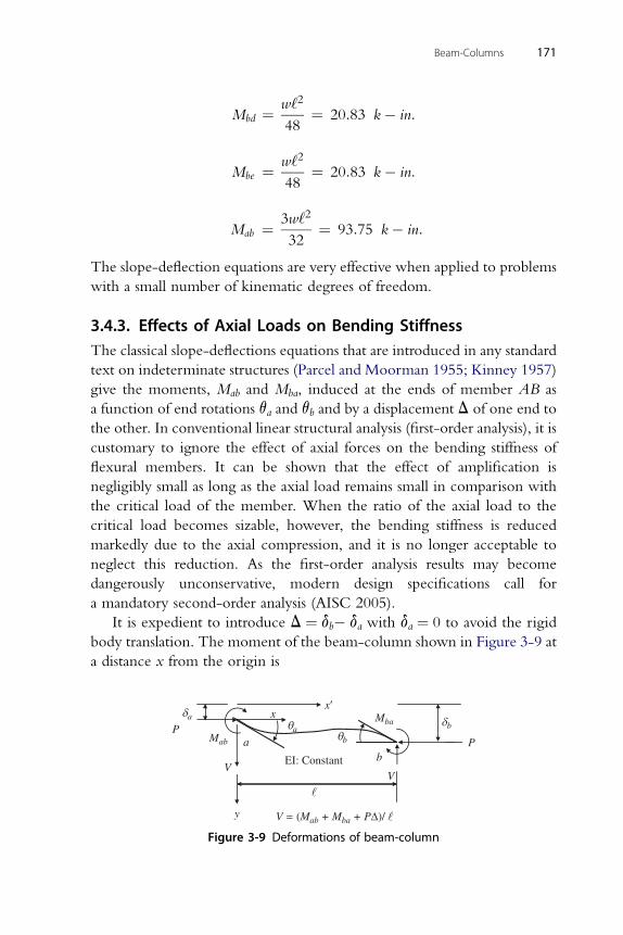
w‘2

Mbd ¼

48¼ 20:83 k� in:

2

Beam-Columns 171

Mbe ¼ w‘

48¼ 20:83 k� in:

2

Mab ¼ 3w‘

32¼ 93:75 k� in:

The slope-deflection equations are very effective when applied to problems

with a small number of kinematic degrees of freedom.

3.4.3. Effects of Axial Loads on Bending StiffnessThe classical slope-deflections equations that are introduced in any standard

text on indeterminate structures (Parcel and Moorman 1955; Kinney 1957)

give the moments, Mab and Mba, induced at the ends of member AB as

a function of end rotations qa and qb and by a displacement D of one end to

the other. In conventional linear structural analysis (first-order analysis), it is

customary to ignore the effect of axial forces on the bending stiffness of

flexural members. It can be shown that the effect of amplification is

negligibly small as long as the axial load remains small in comparison with

the critical load of the member. When the ratio of the axial load to the

critical load becomes sizable, however, the bending stiffness is reduced

markedly due to the axial compression, and it is no longer acceptable to

neglect this reduction. As the first-order analysis results may become

dangerously unconservative, modern design specifications call for

a mandatory second-order analysis (AISC 2005).

It is expedient to introduce D ¼ db� da with da ¼ 0 to avoid the rigid

body translation. The moment of the beam-column shown in Figure 3-9 at

a distance x from the origin is

x¢da

b

bq

dqa

x Mba

Mab

EI: Constant

y

ab

P

V

V = (Mab + Mba + PD)/

V

P

Figure 3-9 Deformations of beam-column

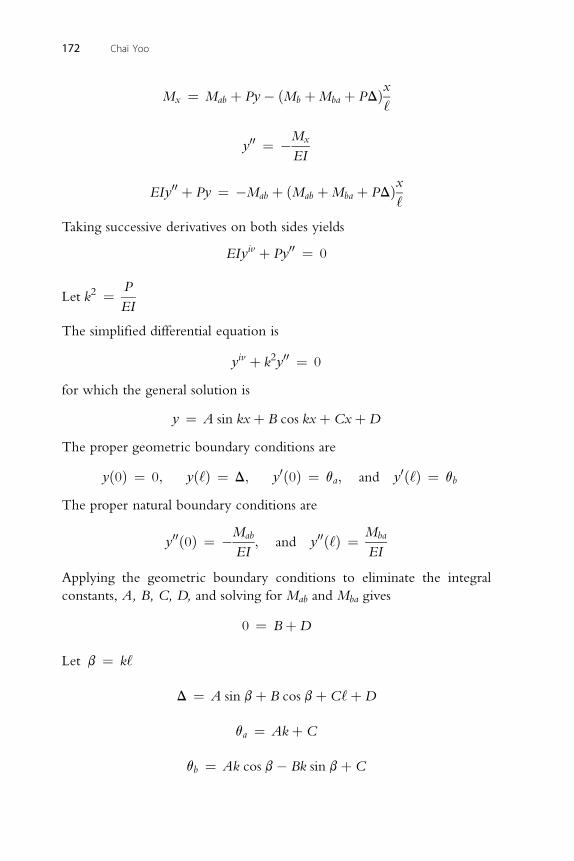
172 Chai Yoo

Mx ¼ Mab þ Py� ðMb þMba þ PDÞx‘

Mx

y00 ¼ �

EI

00 x

EIy þ Py ¼ �Mab þ ðMab þMba þ PDÞ

‘

Taking successive derivatives on both sides yields

EIyiv þ Py00 ¼ 0

P

Let k2 ¼

EI

The simplified differential equation is

yiv þ k2y00 ¼ 0

for which the general solution is

y ¼ A sin kxþ B cos kxþ CxþD

The proper geometric boundary conditions are

yð0Þ ¼ 0; yð‘Þ ¼ D; y0ð0Þ ¼ qa; and y0ð‘Þ ¼ qb

The proper natural boundary conditions are

y00ð0Þ ¼ �Mab

EI; and y00ð‘Þ ¼ Mba

EI

Applying the geometric boundary conditions to eliminate the integral

constants, A, B, C, D, and solving for Mab and Mba gives

0 ¼ BþD

Let b ¼ k‘

D ¼ A sin bþ B cos bþ C‘þD

q ¼ Akþ C

a

q ¼ Ak cos b� Bk sin bþ C

b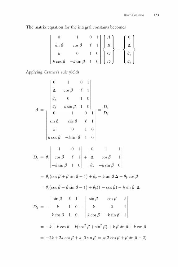

Beam-Columns 173

The matrix equation for the integral constants becomes

2666664

0 1 0 1

sin b cos b ‘ 1

k 0 1 0

k cos b �k sin b 1 0

3777775

8>>>>><>>>>>:

A

B

C

D

9>>>>>=>>>>>;

¼

8>>>>><>>>>>:

0

D

qa

qb

9>>>>>=>>>>>;

Applying Cramer’s rule yields

A ¼

�����������

0 1 0 1

D cos b ‘ 1

qa 0 1 0

qb �k sin b 1 0

����������������������

0 1 0 1

sin b cos b ‘ 1

k 0 1 0

k cos b �k sin b 1 0

�����������

¼ Da

Dd

�� �� �� ��

Da ¼ qa

������1 0 1

cos b ‘ 1

�k sin b 1 0

������þ������0 1 1

D cos b 1

qb �k sin b 0

������¼ q ðcos bþ b sin b� 1Þ þ q � k sin b D� q cos b

a b b

¼ qaðcos bþ b sin b� 1Þ þ qbð1� cos bÞ � k sin b D

�� �� �� ��

Dd ¼ �

������sin b ‘ 1

k 1 0

k cos b 1 0

�������������sin b cos b ‘

k 0 1

k cos b �k sin b 1

������2 2

¼ �kþ k cos b� kðcos bþ sin bÞ þ k b sin bþ k cos b

¼ �2kþ 2k cos bþ k b sin b ¼ kð2 cos bþ b sin b� 2Þ

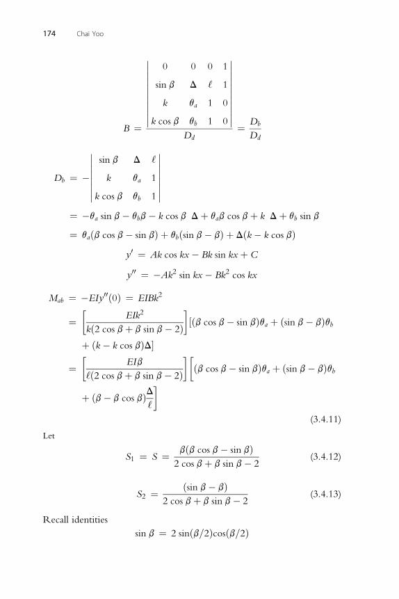
�� 0 0 0 1��

B ¼

���������sin b D ‘ 1

k qa 1 0

k cos b qb 1 0

���������Dd

¼ Db

Dd�� ��

174 Chai Yoo

Db ¼ �������sin b D ‘

k qa 1

k cos b qb 1

������¼ �qa sin b� qbb� k cos b Dþ qab cos bþ k Dþ qb sin b

¼ qaðb cos b� sin bÞ þ qbðsin b� bÞ þ Dðk� k cos bÞ

y0 ¼ Ak cos kx� Bk sin kxþ C

y00 ¼ �Ak2 sin kx� Bk2 cos kx

Mab ¼ �EIy00ð0Þ ¼ EIBk2

¼�

EIk2

kð2 cos bþ b sin b� 2Þ�½ðb cos b� sin bÞqa þ ðsin b� bÞqb

þ ðk� k cos bÞD�

¼�

EIb

‘ð2 cos bþ b sin b� 2Þ��

ðb cos b� sin bÞqa þ ðsin b� bÞqb

þ ðb� b cos bÞD‘

�(3.4.11)

Let

S1 ¼ S ¼ bðb cos b� sin bÞ2 cos bþ b sin b� 2

(3.4.12)

ðsin b� bÞ

S2 ¼

2 cos bþ b sin b� 2(3.4.13)

Recall identities

sin b ¼ 2 sinðb=2Þcosðb=2Þ

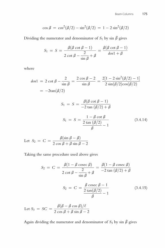
cos b ¼ cos2ðb=2Þ � sin2ðb=2Þ ¼ 1� 2 sin2ðb=2Þ

Dividing the numerator and denominator of S1 by sin b gives

S1 ¼ S ¼ bðb cot b� 1Þ2 cot b� 2

sin bþ b

¼ bðb cot b� 1Þden1þ b

where

den1 ¼ 2 cot b� 2

sin b¼ 2 cos b� 2

sin b¼ 2½1� 2 sin2ðb=2Þ � 1�

2 sinðb=2Þcosðb=2Þ¼ �2tanðb=2Þ

Beam-Columns 175

S1 ¼ S ¼ bðb cot b� 1Þ�2 tan ðb=2Þ þ b

1� b cot b

S1 ¼ S ¼

2 tan ðb=2Þb

� 1

(3.4.14)

bðsin b� bÞ

Let S2 ¼ C ¼

2 cos bþ b sin b� 2

Taking the same procedure used above gives

S2 ¼ C ¼ bð1� b cosec bÞ2 cot b� 2

sin bþ b

¼ bð1� b cosec bÞ�2 tan ðb=2Þ þ b

b cosec b� 1

S2 ¼ C ¼

2 tanðb=2Þb

� 1

(3.4.15)

bðb� b cos bÞ=‘

Let S3 ¼ SC ¼

2 cos bþ b sin b� 2

Again dividing the numerator and denominator of S3 by sin b gives

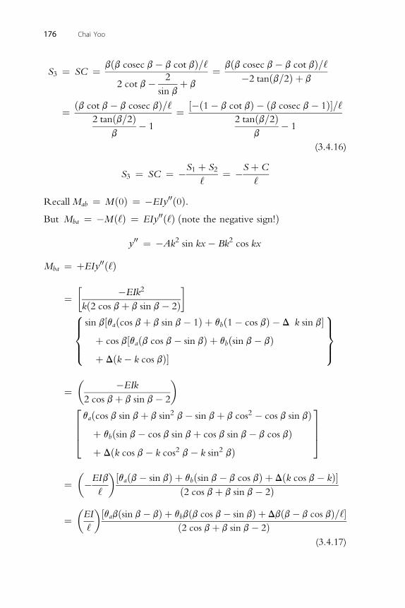
176 Chai Yoo

S3 ¼ SC ¼ bðb cosec b� b cot bÞ=‘2 cot b� 2

sin bþ b

¼ bðb cosec b� b cot bÞ=‘�2 tanðb=2Þ þ b

¼ ðb cot b� b cosec bÞ=‘2 tanðb=2Þ

b� 1

¼ ½�ð1� b cot bÞ � ðb cosec b� 1Þ�=‘2 tanðb=2Þ

b� 1

(3.4.16)

S1 þ S2 S þ C

S3 ¼ SC ¼ �

‘¼ �

‘

RecallMab ¼ Mð0Þ ¼ �EIy00ð0Þ:

But Mba ¼ �Mð‘Þ ¼ EIy00ð‘Þ ðnote the negative sign!Þ

y00 ¼ �Ak2 sin kx� Bk2 cos kx

Mba ¼ þEIy00ð‘Þ

�

2�

¼ �EIk

kð2 cos bþ b sin b� 2Þ8>><>>:

sin b½qaðcos bþ b sin b� 1Þ þ qbð1� cos bÞ � D k sin b�þ cos b½qaðb cos b� sin bÞ þ qbðsin b� bÞþ Dðk� k cos bÞ�

9>>=>>;

� �EIk�

¼2 cos bþ b sin b� 22

664qaðcos b sin bþ b sin2 b� sin bþ b cos2 � cos b sin bÞþ qbðsin b� cos b sin bþ cos b sin b� b cos bÞþ Dðk cos b� k cos2 b� k sin2 bÞ

3775

�EIb

�½q ðb� sin bÞ þ q ðsin b� b cos bÞ þ Dðk cos b� kÞ�

¼ �‘

a b

ð2 cos bþ b sin b� 2Þ�EI�½qabðsin b� bÞ þ qbbðb cos b� sin bÞ þ Dbðb� b cos bÞ=‘�

¼

‘ ð2 cos bþ b sin b� 2Þ(3.4.17)

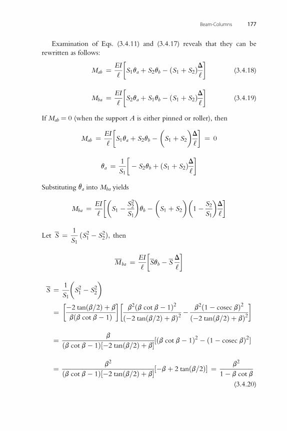
Beam-Columns 177

Examination of Eqs. (3.4.11) and (3.4.17) reveals that they can be

rewritten as follows:

Mab ¼ EI

‘

�S1qa þ S2qb � ðS1 þ S2ÞD

‘

�(3.4.18)

EI�

D�

Mba ¼‘

S2qa þ S1qb � ðS1 þ S2Þ‘

(3.4.19)

If Mab ¼ 0 (when the support A is either pinned or roller), then

Mab ¼ EI

‘

�S1qa þ S2qb �

�S1 þ S2

�D

‘

�¼ 0

1�

D�

qa ¼S1

� S2qb þ ðS1 þ S2Þ‘

Substituting qa into Mba yields

Mba ¼ EI

‘

��S1 � S22

S1

�qb �

�S1 þ S2

��1� S2

S1

�D

‘

�

1

Let S ¼

S1ðS21 � S22Þ; then

EI�

D�

Mba ¼‘

Sqb � S‘

� �

S ¼ 1

S1S21 � S22

¼��2 tanðb=2Þ þ b

bðb cot b� 1Þ��

b2ðb cot b� 1Þ2ð�2 tanðb=2Þ þ bÞ2 �

b2ð1� cosec bÞ2ð�2 tanðb=2Þ þ bÞ2

�

b

¼ ðb cot b� 1Þ½�2 tanðb=2Þ þ b�½ðb cot b� 1Þ2 � ð1� cosec bÞ2�

2 2

¼ b

ðb cot b� 1Þ½�2 tanðb=2Þ þ b�½�bþ 2 tanðb=2Þ� ¼ b

1� b cot b

(3.4.20)

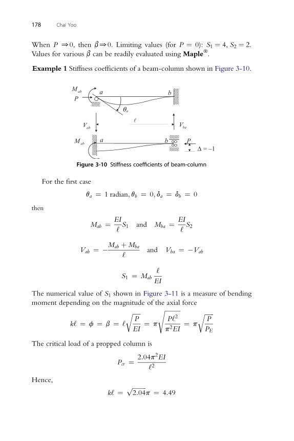
178 Chai Yoo

When P 00, then b00. Limiting values (for P ¼ 0): S1 ¼ 4, S2 ¼ 2.

Values for various b can be readily evaluated using Maple�.

Example 1 Stiffness coefficients of a beam-column shown in Figure 3-10.

Figure 3-10 Stiffness coefficients of beam-column

For the first case

qa ¼ 1 radian; qb ¼ 0; da ¼ db ¼ 0

then

Mab ¼ EI

‘S1 and Mba ¼ EI

‘S2

Mab þMba

Vab ¼ �

‘and Vba ¼ �Vab

‘

S1 ¼ Mab

EI

The numerical value of S1 shown in Figure 3-11 is a measure of bending

moment depending on the magnitude of the axial force

k‘ ¼ f ¼ b ¼ ‘

ffiffiffiffiffiP

EI

r¼ p

ffiffiffiffiffiffiffiffiffiffiP‘2

p2EI

s¼ p

ffiffiffiffiffiffiP

PE

r

The critical load of a propped column is

Pcr ¼ 2:04p2EI

‘2

Hence,

k‘ ¼ ffiffiffiffiffiffiffiffiffi2:04

pp ¼ 4:49

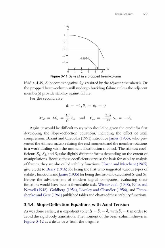
S1

–2

0

2

4

–4

k0 1 2 3 4 5

4.4934

Figure 3-11 S1 vs k‘ in a propped beam-column

Beam-Columns 179

If k‘ > 4.49, S1 becomes negative. qa is resisted by the adjacentmember(s). Or

the propped beam-column will undergo buckling failure unless the adjacent

member(s) provide stability against failure.

For the second case

D ¼ �1; qa ¼ qb ¼ 0

EI 2EI

Mab ¼ Mba ¼

‘2S3 and Vab ¼ �

‘3S3 ¼ �Vba

Again, it would be difficult to say who should be given the credit for first

developing the slope-deflection equations, including the effect of axial

compression. Bazant and Credolin (1991) introduce James (1935), who pre-

sented the stiffness matrix relating the endmoments and themember rotations

in a work dealing with the moment-distribution method. The stiffness coef-

ficients S1, S2, and S3 take slightly different forms depending on the extent of

manipulations. Because these coefficients serve as the basis for stability analysis

of frames, they are also called stability functions. Horne and Merchant (1965)

give credit to Berry (1916) for being the first who suggested various types of

stability functions and James (1935) for being thefirstwho calculatedS1 andS2.

Before the advancement of modern digital computers, evaluating these

functions would have been a formidable task. Winter et al. (1948), Niles and

Newell (1948), Goldberg (1954), Livesley and Chandler (1956), and Timo-

shenko andGere (1961) published tables and charts of these stability functions.

3.4.4. Slope-Deflection Equations with Axial TensionAs was done earlier, it is expedient to letD ¼ db � dawith da ¼ 0 in order to

avoid the rigid body translation. The moment of the bean-column shown in

Figure 3-12 at a distance x from the origin is

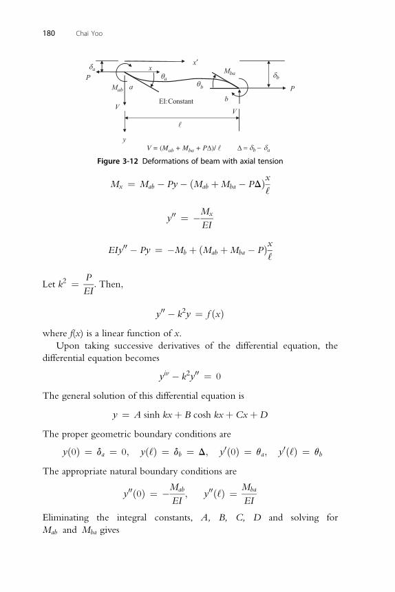
x¢

Pbq

dadb

db da

qa

Mab

x Mba

EI: Constant

D = y

ab

P

V V

V = (Mab + Mba + PD)/ -

Figure 3-12 Deformations of beam with axial tension

180 Chai Yoo

Mx ¼ Mab � Py� ðMab þMba � PDÞx‘

Mx

y00 ¼ �

EI

00 x

EIy � Py ¼ �Mb þ ðMab þMba � PÞ

‘

P

Let k2 ¼

EI: Then;

00 2

y � k y ¼ f ðxÞwhere f(x) is a linear function of x.

Upon taking successive derivatives of the differential equation, the

differential equation becomes

yiv � k2y00 ¼ 0

The general solution of this differential equation is

y ¼ A sinh kxþ B cosh kxþCxþD

The proper geometric boundary conditions are

yð0Þ ¼ da ¼ 0; yð‘Þ ¼ db ¼ D; y0ð0Þ ¼ qa; y0ð‘Þ ¼ qb

The appropriate natural boundary conditions are

y00ð0Þ ¼ �Mab

EI; y00ð‘Þ ¼ Mba

EI

Eliminating the integral constants, A, B, C, D and solving for

Mab and Mba gives

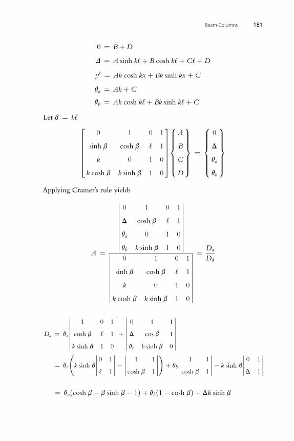
Beam-Columns 181

0 ¼ BþD

D ¼ A sinh k‘þ B cosh k‘þ C‘þD

y0 ¼ Ak cosh kxþ Bk sinh kxþ C

qa ¼ Akþ C

qb ¼ Ak cosh k‘þ Bk sinh k‘þ C

Let b ¼ k‘

20 1 0 1

38>>A9>> 8>> 0

9>>

666664sinh b cosh b ‘ 1

k 0 1 0

k cosh b k sinh b 1 0

777775>>><>>>>>:

B

C

D

>>>=>>>>>;

¼>>><>>>>>:

D

qa

qb

>>>=>>>>>;

Applying Cramer’s rule yields

A ¼

�����������

0 1 0 1

D cosh b ‘ 1

qa 0 1 0

qb k sinh b 1 0

����������������������

0 1 0 1

sinh b cosh b ‘ 1

k 0 1 0

k cosh b k sinh b 1 0

�����������

¼ Da

Dd

� � � �

Da ¼ qa

�������1 0 1

cosh b ‘ 1

k sinh b 1 0

�������þ�������0 1 1

D cos b 1

qb k sinh b 0

�������¼ qa

k sinh b

�����0 1

‘ 1

�����������

1 1

cosh b 1

�����!

þ qb

�����1 1

cosh b 1

������ k sinh b

�����0 1

D 1

�����¼ q ðcosh b� b sinh b� 1Þ þ q ð1� cosh bÞ þ Dk sinh b

a b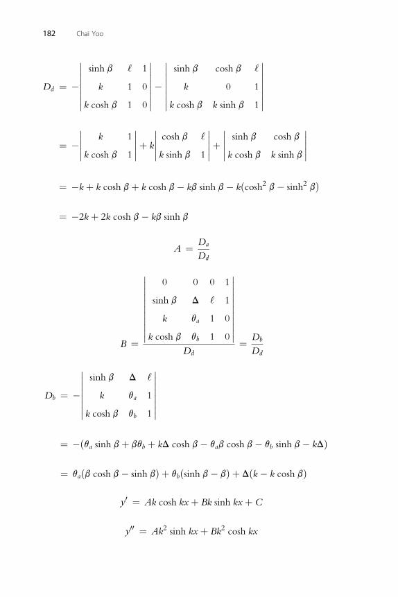

�� �� �� ��

Dd ¼ �

������sinh b ‘ 1

k 1 0

k cosh b 1 0

�������������sinh b cosh b ‘

k 0 1

k cosh b k sinh b 1

������� � � � � �

182 Chai Yoo

¼ �����

k 1

k cosh b 1

����þ k

����cosh b ‘

k sinh b 1

����þ����sinh b cosh b

k cosh b k sinh b

����

¼ �kþ k cosh bþ k cosh b� kb sinh b� kðcosh2 b� sinh2 bÞ

¼ �2kþ 2k cosh b� kb sinh b

A ¼ Da

Dd

� �

B ¼

����������

0 0 0 1

sinh b D ‘ 1

k qa 1 0

k cosh b qb 1 0

����������Dd

¼ Db

Dd

� �

Db ¼ �

�������sinh b D ‘

k qa 1

k cosh b qb 1

�������

¼ �ðqa sinh bþ bqb þ kD cosh b� qab cosh b� qb sinh b� kDÞ

¼ qaðb cosh b� sinh bÞ þ qbðsinh b� bÞ þ Dðk� k cosh bÞ

0

y ¼ Ak cosh kxþ Bk sinh kxþ C

y00 ¼ Ak2 sinh kxþ Bk2 cosh kx

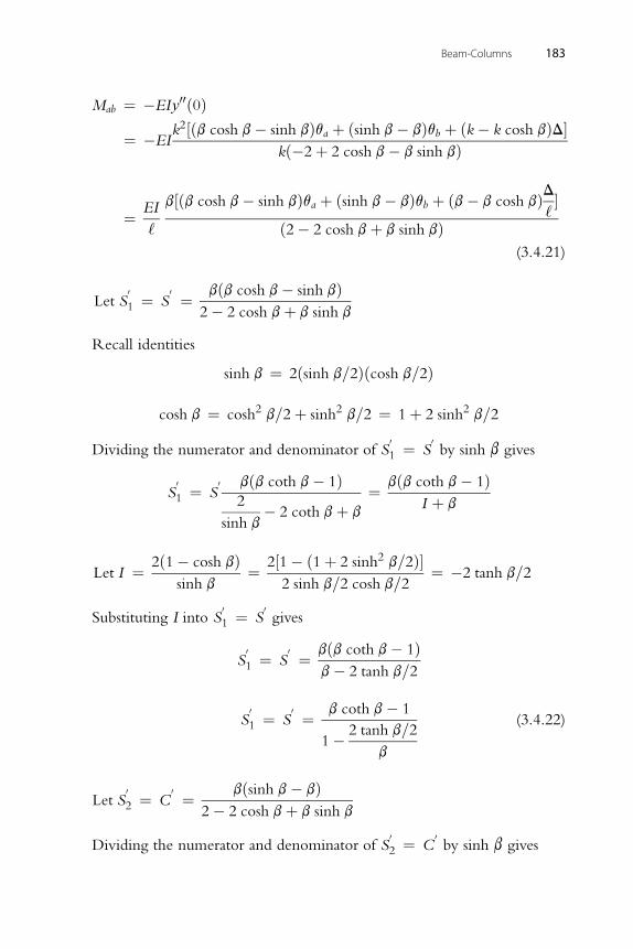
M ¼ �EIy00ð0Þ

ab

¼ �EIk2½ðb cosh b� sinh bÞqa þ ðsinh b� bÞqb þ ðk� k cosh bÞD�

Beam-Columns 183

kð�2þ 2 cosh b� b sinh bÞ

D

¼ EI

‘

b½ðb cosh b� sinh bÞqa þ ðsinh b� bÞqb þ ðb� b cosh bÞ‘�

ð2� 2 cosh bþ b sinh bÞ(3.4.21)

0 0 bðb cosh b� sinh bÞ

Let S1 ¼ S ¼

2� 2 cosh bþ b sinh b

Recall identities

sinh b ¼ 2ðsinh b=2Þðcosh b=2Þ2 2 2

cosh b ¼ cosh b=2þ sinh b=2 ¼ 1þ 2 sinh b=2

Dividing the numerator and denominator of S01 ¼ S

0by sinh b gives

S01 ¼ S

0 bðb coth b� 1Þ2

sinh b� 2 coth bþ b

¼ bðb coth b� 1ÞI þ b

2

Let I ¼ 2ð1� cosh bÞsinh b

¼ 2½1� ð1þ 2 sinh b=2Þ�2 sinh b=2 cosh b=2

¼ �2 tanh b=2

Substituting I into S01 ¼ S

0gives

S01 ¼ S

0 ¼ bðb coth b� 1Þb� 2 tanh b=2

0 0 b coth b� 1

S1 ¼ S ¼

1� 2 tanh b=2

b

(3.4.22)

0 0 bðsinh b� bÞ

Let S2 ¼ C ¼

2� 2 cosh bþ b sinh b

Dividing the numerator and denominator of S02 ¼ C

0by sinh b gives

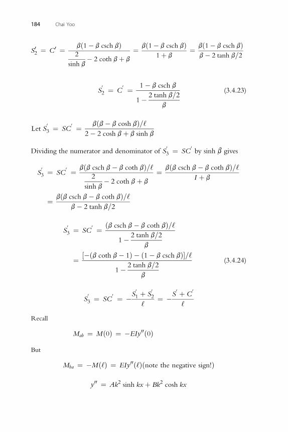
184 Chai Yoo

S02 ¼ C0 ¼ bð1� b csch bÞ2

sinh b� 2 coth bþ b

¼ bð1� b csch bÞ1þ b

¼ bð1� b csch bÞb� 2 tanh b=2

S02 ¼ C

0 ¼ 1� b csch b

1� 2 tanh b=2

b

(3.4.23)

Let S03 ¼ SC

0 ¼ bðb� b cosh bÞ=‘2� 2 cosh bþ b sinh b

Dividing the numerator and denominator of S03 ¼ SC

0by sinh b gives

S03 ¼ SC

0 ¼ bðb csch b� b coth bÞ=‘2

sinh b� 2 coth bþ b

¼ bðb csch b� b coth bÞ=‘I þ b

¼ bðb csch b� b coth bÞ=‘b� 2 tanh b=2

S03 ¼ SC

0 ¼ ðb csch b� b coth bÞ=‘1� 2 tanh b=2

b

¼ ½�ðb coth b� 1Þ � ð1� b csch bÞ�=‘1� 2 tanh b=2

b

(3.4.24)

0 0 0 0

S03 ¼ SC

0 ¼ �S1 þ S2‘

¼ �S þ C

‘

Recall

Mab ¼ Mð0Þ ¼ �EIy00ð0Þ

But

Mba ¼ �Mð‘Þ ¼ EIy00ð‘Þðnote the negative sign!Þ

00 2 2

y ¼ Ak sinh kxþ Bk cosh kx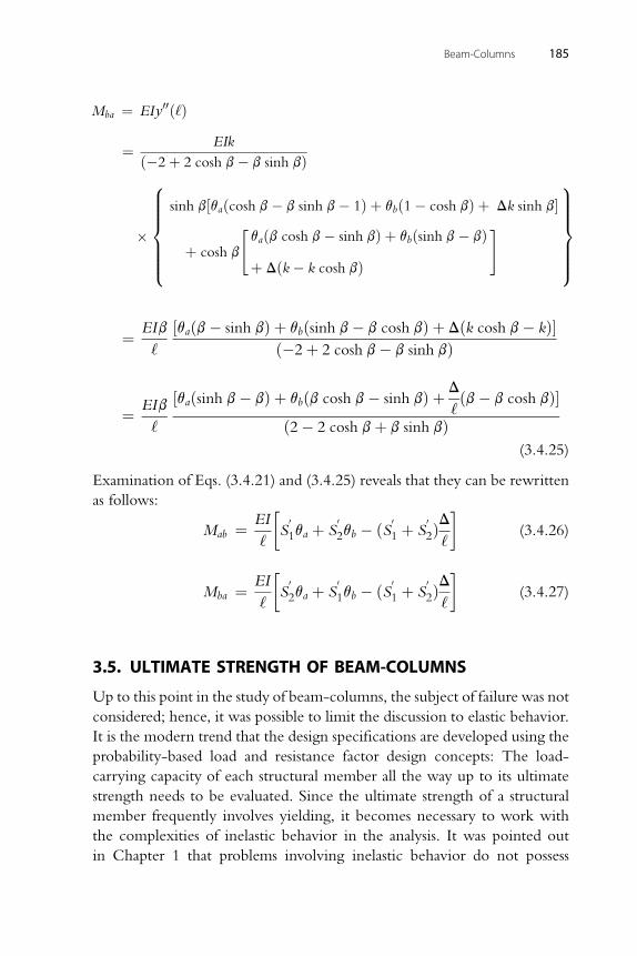

00

Mba ¼ EIy ð‘Þ

¼ EIk

ð�2þ 2 cosh b� b sinh bÞ

�sinh b½qaðcosh b� b sinh b� 1Þ þ qbð1� cosh bÞ þ Dk sinh b�

þ cosh b

"qaðb cosh b� sinh bÞ þ qbðsinh b� bÞþ Dðk� k cosh bÞ

#9>>>>>=>>>>>;

8>>>>><>>>>>:

Beam-Columns 185

¼ EIb

‘

½qaðb� sinh bÞ þ qbðsinh b� b cosh bÞ þ Dðk cosh b� kÞ�ð�2þ 2 cosh b� b sinh bÞ

D

¼ EIb

‘

½qaðsinh b� bÞ þ qbðb cosh b� sinh bÞ þ‘ðb� b cosh bÞ�

ð2� 2 cosh bþ b sinh bÞ(3.4.25)

Examination of Eqs. (3.4.21) and (3.4.25) reveals that they can be rewritten

as follows:

Mab ¼ EI

‘

�S

01qa þ S

02qb � ðS0

1 þ S02ÞD

‘

�(3.4.26)

� �

Mba ¼ EI

‘S

02qa þ S

01qb � ðS0

1 þ S02ÞD

‘(3.4.27)

3.5. ULTIMATE STRENGTH OF BEAM-COLUMNS

Up to this point in the study of beam-columns, the subject of failure was not

considered; hence, it was possible to limit the discussion to elastic behavior.

It is the modern trend that the design specifications are developed using the

probability-based load and resistance factor design concepts: The load-

carrying capacity of each structural member all the way up to its ultimate

strength needs to be evaluated. Since the ultimate strength of a structural

member frequently involves yielding, it becomes necessary to work with

the complexities of inelastic behavior in the analysis. It was pointed out

in Chapter 1 that problems involving inelastic behavior do not possess

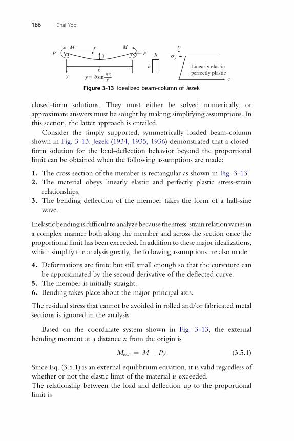
sP

MM

d

y

xP b

sinx

ypd=

h

ys

e

Linearly elasticperfectly plastic

Figure 3-13 Idealized beam-column of Jezek

186 Chai Yoo

closed-form solutions. They must either be solved numerically, or

approximate answers must be sought by making simplifying assumptions. In

this section, the latter approach is entailed.

Consider the simply supported, symmetrically loaded beam-column

shown in Fig. 3-13. Jezek (1934, 1935, 1936) demonstrated that a closed-

form solution for the load-deflection behavior beyond the proportional

limit can be obtained when the following assumptions are made:

1. The cross section of the member is rectangular as shown in Fig. 3-13.

2. The material obeys linearly elastic and perfectly plastic stress-strain

relationships.

3. The bending deflection of the member takes the form of a half-sine

wave.

Inelastic bending is difficult to analyze because the stress-strain relationvaries in

a complex manner both along the member and across the section once the

proportional limit has been exceeded. In addition to these major idealizations,

which simplify the analysis greatly, the following assumptions are also made:

4. Deformations are finite but still small enough so that the curvature can

be approximated by the second derivative of the deflected curve.

5. The member is initially straight.

6. Bending takes place about the major principal axis.

The residual stress that cannot be avoided in rolled and/or fabricated metal

sections is ignored in the analysis.

Based on the coordinate system shown in Fig. 3-13, the external

bending moment at a distance x from the origin is

Mext ¼ M þ Py (3.5.1)

Since Eq. (3.5.1) is an external equilibrium equation, it is valid regardless of

whether or not the elastic limit of the material is exceeded.

The relationship between the load and deflection up to the proportional

limit is

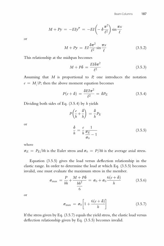
Beam-Columns 187

M þ Py ¼ �EIy00 ¼ �EI

�� d

p2

‘2

�sin

px

‘

or

M þ Py ¼ EIdp2

‘2sin

px

‘(3.5.2)

This relationship at the midspan becomes

M þ Pd ¼ EIdp2

‘2(3.5.3)

Assuming that M is proportional to P, one introduces the notation

e ¼ M.P; then the above moment equation becomes

Pðeþ dÞ ¼ dEIp2

‘2¼ dPE (3.5.4)

Dividing both sides of Eq. (3.5.4) by h yields

P

�e

hþ d

h

�¼ d

hPE

ord

h¼ e

h

1sE

s0� 1

(3.5.5)

where

sE ¼ PE=bh is the Euler stress and s0 ¼ P=bh is the average axial stress:

Equation (3.5.5) gives the load versus deflection relationship in the

elastic range. In order to determine the load at which Eq. (3.5.5) becomes

invalid, one must evaluate the maximum stress in the member.

smax ¼ P

bhþM þ Pd

bh2

6

¼ s0 þ s06ðeþ dÞ

h(3.5.6)

or

smax ¼ s0

�1þ 6ðeþ dÞ

h

�(3.5.7)

If the stress given by Eq. (3.5.7) equals the yield stress, the elastic load versus

deflection relationship given by Eq. (3.5.5) becomes invalid.

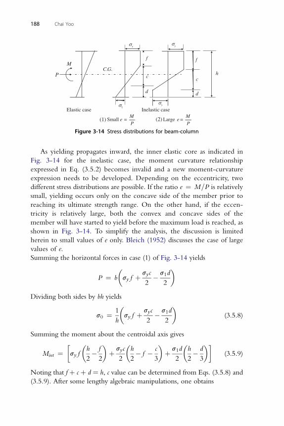
P. .C G

M

Elastic case Inelastic case

Large M

eP

= Small e M

P=

d

c

f

s1ys

d

c

f

h

sysy

(1) (2)

Figure 3-14 Stress distributions for beam-column

188 Chai Yoo

As yielding propagates inward, the inner elastic core as indicated in

Fig. 3-14 for the inelastic case, the moment curvature relationship

expressed in Eq. (3.5.2) becomes invalid and a new moment-curvature

expression needs to be developed. Depending on the eccentricity, two

different stress distributions are possible. If the ratio e ¼ M=P is relatively

small, yielding occurs only on the concave side of the member prior to

reaching its ultimate strength range. On the other hand, if the eccen-

tricity is relatively large, both the convex and concave sides of the

member will have started to yield before the maximum load is reached, as

shown in Fig. 3-14. To simplify the analysis, the discussion is limited

herein to small values of e only. Bleich (1952) discusses the case of large

values of e.

Summing the horizontal forces in case (1) of Fig. 3-14 yields

P ¼ b

�sy f þ syc

2� s1d

2

�

Dividing both sides by bh yields

s0 ¼ 1

h

�sy f þ syc

2� s1d

2

�(3.5.8)

Summing the moment about the centroidal axis gives

Mint ¼�sy f

�h

2� f

2

�þ syc

2

�h

2� f � c

3

�þ s1d

2

�h

2� d

3

��(3.5.9)

Noting that f þ c þ d ¼ h, c value can be determined from Eqs. (3.5.8) and

(3.5.9). After some lengthy algebraic manipulations, one obtains

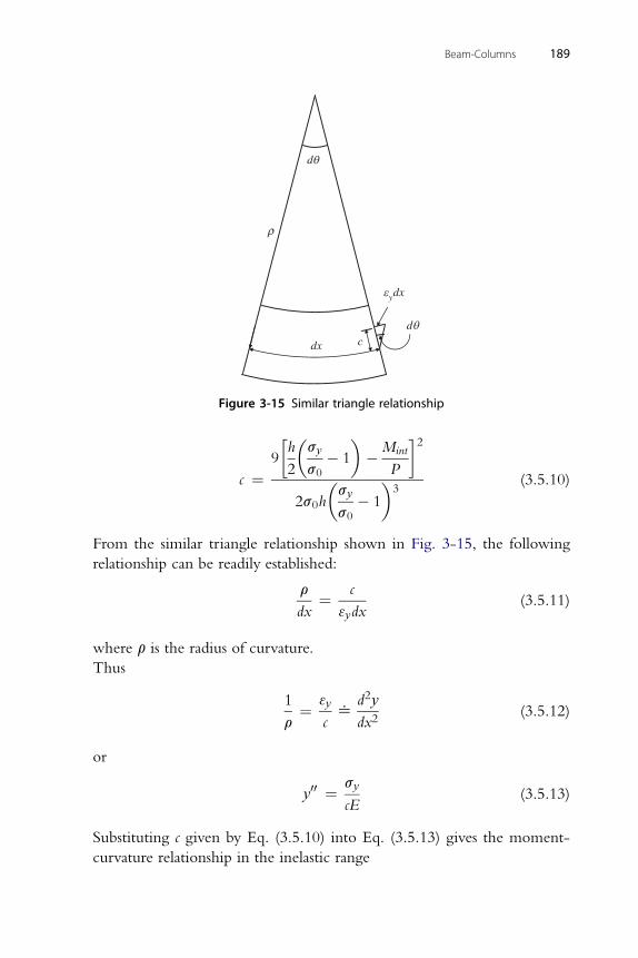
ydxe

dx

dq

dq

c

r

Figure 3-15 Similar triangle relationship

Beam-Columns 189

c ¼9

�h

2

�sy

s0� 1

��Mint

P

�2

2s0h

�sy

s0� 1

�3

(3.5.10)

From the similar triangle relationship shown in Fig. 3-15, the following

relationship can be readily established:

r

dx¼ c

3ydx(3.5.11)

where r is the radius of curvature.

Thus

1

r¼ 3y

c^

d2y

dx2(3.5.12)

or

y00 ¼ sy

cE(3.5.13)

Substituting c given by Eq. (3.5.10) into Eq. (3.5.13) gives the moment-

curvature relationship in the inelastic range

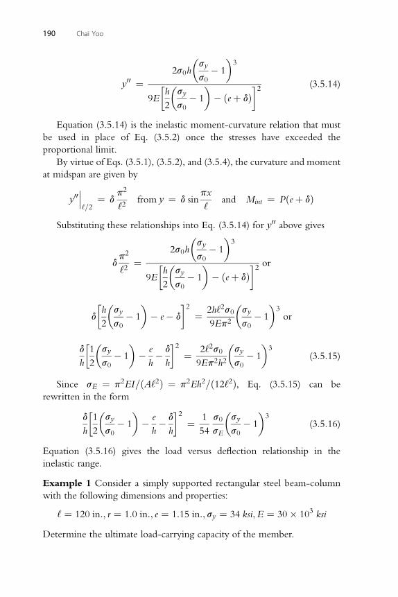
190 Chai Yoo

y00 ¼2s0h

�sy

s0� 1

�3

9E

�h

2

�sy

s0� 1

�� ðeþ dÞ

�2

(3.5.14)

Equation (3.5.14) is the inelastic moment-curvature relation that must

be used in place of Eq. (3.5.2) once the stresses have exceeded the

proportional limit.

By virtue of Eqs. (3.5.1), (3.5.2), and (3.5.4), the curvature and moment

at midspan are given by

y00���‘=2

¼ dp2

‘2from y ¼ d sin

px

‘and Mint ¼ Pðeþ dÞ

Substituting these relationships into Eq. (3.5.14) for y00 above gives

dp2

‘2¼

2s0h

�sy

s0� 1

�3

9E

�h

2

�sy

s0� 1

�� ðeþ dÞ

�2or

� � � �2 2

� �3

dh

2

sy

s0� 1 � e� d ¼ 2h‘ s0

9Ep2

sy

s0� 1 or

� � � �2 2� �

3

d

h

1

2

sy

s0� 1 � e

h� d

h¼ 2‘ s0

9Ep2h2sy

s0� 1 (3.5.15)

Since sE ¼ p2EI=ðA‘2Þ ¼ p2Eh2=ð12‘2Þ, Eq. (3.5.15) can be

rewritten in the form

d

h

�1

2

�sy

s0� 1

�� e

h� d

h

�2¼ 1

54

s0

sE

�sy

s0� 1

�3

(3.5.16)

Equation (3.5.16) gives the load versus deflection relationship in the

inelastic range.

Example 1 Consider a simply supported rectangular steel beam-column

with the following dimensions and properties:

‘ ¼ 120 in:; r ¼ 1:0 in:; e ¼ 1:15 in:; sy ¼ 34 ksi;E ¼ 30� 103 ksi

Determine the ultimate load-carrying capacity of the member.

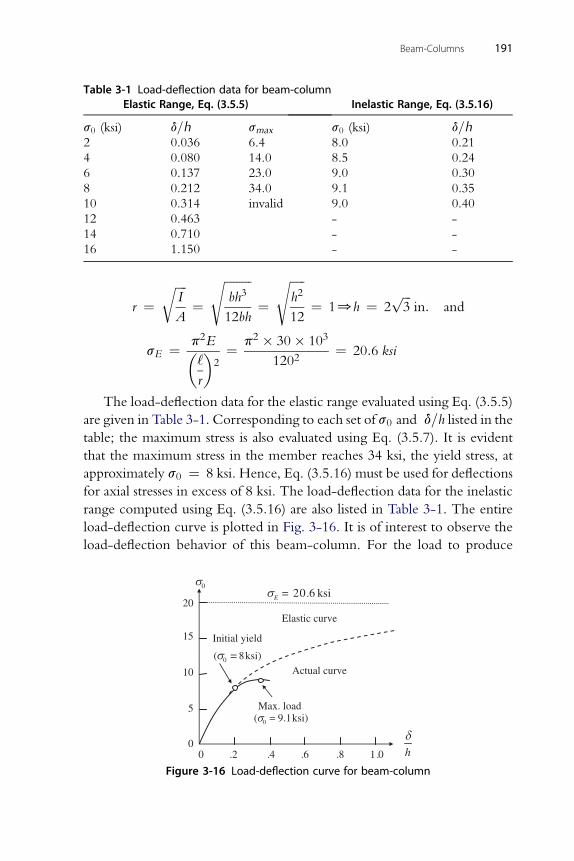
Table 3-1 Load-deflection data for beam-columnElastic Range, Eq. (3.5.5) Inelastic Range, Eq. (3.5.16)

s0 (ksi) d=h smax s0 (ksi) d=h2 0.036 6.4 8.0 0.21

4 0.080 14.0 8.5 0.24

6 0.137 23.0 9.0 0.30

8 0.212 34.0 9.1 0.35

10 0.314 invalid 9.0 0.40

12 0.463 - -

14 0.710 - -

16 1.150 - -

Beam-Columns 191

r ¼ffiffiffiffiI

A

r¼

ffiffiffiffiffiffiffiffiffibh3

12bh

s¼

ffiffiffiffiffih2

12

s¼ 10h ¼ 2

ffiffiffi3

pin: and

sE ¼ p2E�‘

r

�2¼ p2 � 30� 103

1202¼ 20:6 ksi

The load-deflection data for the elastic range evaluated using Eq. (3.5.5)

are given in Table 3-1. Corresponding to each set of s0 and d=h listed in thetable; the maximum stress is also evaluated using Eq. (3.5.7). It is evident

that the maximum stress in the member reaches 34 ksi, the yield stress, at

approximately s0 ¼ 8 ksi. Hence, Eq. (3.5.16) must be used for deflections

for axial stresses in excess of 8 ksi. The load-deflection data for the inelastic

range computed using Eq. (3.5.16) are also listed in Table 3-1. The entire

load-deflection curve is plotted in Fig. 3-16. It is of interest to observe the

load-deflection behavior of this beam-column. For the load to produce

σ0

0 .2 .4 .6 .8 .1 0

. ksiE = 20 620

10

15

5

0h

δ

Elastic curve

Actual curve

Initial yield

( 8 ksi)σ

σ

=0

Max. load ( 9.1 ksi)σ =0

Figure 3-16 Load-deflection curve for beam-column

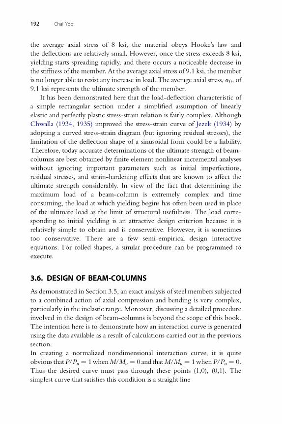
192 Chai Yoo

the average axial stress of 8 ksi, the material obeys Hooke’s law and

the deflections are relatively small. However, once the stress exceeds 8 ksi,

yielding starts spreading rapidly, and there occurs a noticeable decrease in

the stiffness of the member. At the average axial stress of 9.1 ksi, the member

is no longer able to resist any increase in load. The average axial stress, s0, of

9.1 ksi represents the ultimate strength of the member.

It has been demonstrated here that the load-deflection characteristic of

a simple rectangular section under a simplified assumption of linearly

elastic and perfectly plastic stress-strain relation is fairly complex. Although

Chwalla (1934, 1935) improved the stress-strain curve of Jezek (1934) by

adopting a curved stress-strain diagram (but ignoring residual stresses), the

limitation of the deflection shape of a sinusoidal form could be a liability.

Therefore, today accurate determinations of the ultimate strength of beam-

columns are best obtained by finite element nonlinear incremental analyses

without ignoring important parameters such as initial imperfections,

residual stresses, and strain-hardening effects that are known to affect the

ultimate strength considerably. In view of the fact that determining the

maximum load of a beam-column is extremely complex and time

consuming, the load at which yielding begins has often been used in place

of the ultimate load as the limit of structural usefulness. The load corre-

sponding to initial yielding is an attractive design criterion because it is

relatively simple to obtain and is conservative. However, it is sometimes

too conservative. There are a few semi-empirical design interactive

equations. For rolled shapes, a similar procedure can be programmed to

execute.

3.6. DESIGN OF BEAM-COLUMNS

As demonstrated in Section 3.5, an exact analysis of steel members subjected

to a combined action of axial compression and bending is very complex,

particularly in the inelastic range. Moreover, discussing a detailed procedure

involved in the design of beam-columns is beyond the scope of this book.

The intention here is to demonstrate how an interaction curve is generated

using the data available as a result of calculations carried out in the previous

section.

In creating a normalized nondimensional interaction curve, it is quite

obvious thatP/Pu ¼ 1whenM/Mu ¼ 0 and thatM/Mu ¼ 1whenP/Pu ¼ 0.

Thus the desired curve must pass through these points (1,0), (0,1). The

simplest curve that satisfies this condition is a straight line

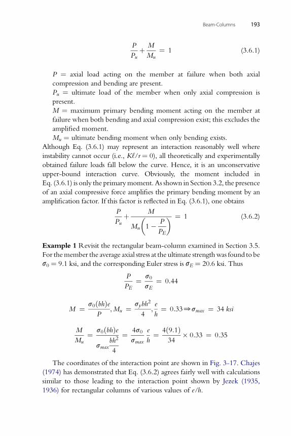
Beam-Columns 193

P

Puþ M

Mu¼ 1 (3.6.1)

P ¼ axial load acting on the member at failure when both axial

compression and bending are present.

Pu ¼ ultimate load of the member when only axial compression is

present.

M ¼ maximum primary bending moment acting on the member at

failure when both bending and axial compression exist; this excludes the

amplified moment.

Mu ¼ ultimate bending moment when only bending exists.

Although Eq. (3.6.1) may represent an interaction reasonably well where

instability cannot occur (i.e., K‘/r ¼ 0), all theoretically and experimentally

obtained failure loads fall below the curve. Hence, it is an unconservative

upper-bound interaction curve. Obviously, the moment included in

Eq. (3.6.1) is only the primarymoment. As shown in Section 3.2, the presence

of an axial compressive force amplifies the primary bending moment by an

amplification factor. If this factor is reflected in Eq. (3.6.1), one obtains

P

Puþ M

Mu

�1� P

PE

� ¼ 1 (3.6.2)

Example 1 Revisit the rectangular beam-column examined in Section 3.5.

For themember the average axial stress at the ultimate strengthwas found to be

s0 ¼ 9.1 ksi, and the corresponding Euler stress is sE ¼ 20.6 ksi. Thus

P

PE¼ s0

sE¼ 0:44

2

M ¼ s0ðbhÞeP

;Mu ¼ sybh

4;e

h¼ 0:330smax ¼ 34 ksi

M s ðbhÞe 4s e 4ð9:1Þ

Mu

¼ 0

smaxbh2

4

¼ 0

smax h¼

34� 0:33 ¼ 0:35

The coordinates of the interaction point are shown in Fig. 3-17. Chajes

(1974) has demonstrated that Eq. (3.6.2) agrees fairly well with calculations

similar to those leading to the interaction point shown by Jezek (1935,

1936) for rectangular columns of various values of e/h.

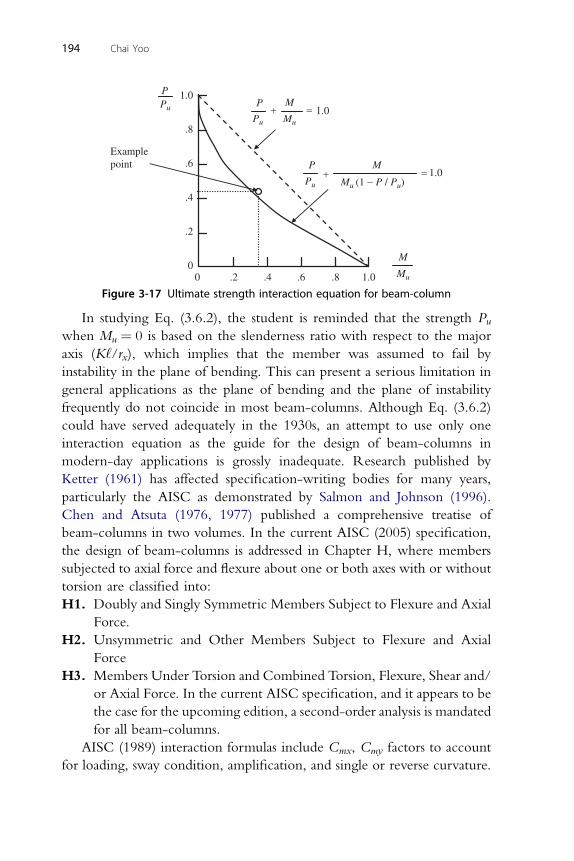
.4

0.2 .8

PPu

Pu

Pu

Mu

Mu (1 − P / Pu)

Mu

P+ 1.0

Example point .6

.8

1.0

1.0

0

.2

.6.4 1.0

M

P M

M

+ =

=

Figure 3-17 Ultimate strength interaction equation for beam-column

194 Chai Yoo

In studying Eq. (3.6.2), the student is reminded that the strength Puwhen Mu ¼ 0 is based on the slenderness ratio with respect to the major

axis (K‘/rx), which implies that the member was assumed to fail by

instability in the plane of bending. This can present a serious limitation in

general applications as the plane of bending and the plane of instability

frequently do not coincide in most beam-columns. Although Eq. (3.6.2)

could have served adequately in the 1930s, an attempt to use only one

interaction equation as the guide for the design of beam-columns in

modern-day applications is grossly inadequate. Research published by

Ketter (1961) has affected specification-writing bodies for many years,

particularly the AISC as demonstrated by Salmon and Johnson (1996).

Chen and Atsuta (1976, 1977) published a comprehensive treatise of

beam-columns in two volumes. In the current AISC (2005) specification,

the design of beam-columns is addressed in Chapter H, where members

subjected to axial force and flexure about one or both axes with or without

torsion are classified into:

H1. Doubly and Singly Symmetric Members Subject to Flexure and Axial

Force.

H2. Unsymmetric and Other Members Subject to Flexure and Axial

Force

H3. Members Under Torsion and Combined Torsion, Flexure, Shear and/

or Axial Force. In the current AISC specification, and it appears to be

the case for the upcoming edition, a second-order analysis is mandated

for all beam-columns.

AISC (1989) interaction formulas include Cmx, Cmy factors to account

for loading, sway condition, amplification, and single or reverse curvature.

Beam-Columns 195

REFERENCESAISC. (1989).Manual of Steel Construction (9th ed.). Chicago, IL: American Institute of Steel

Construction.AISC. (2005). Specification for Structural Steel Buildings, ANSI/AISC 360–05. Chicago, IL:

American Institute of Steel Construction.Bazant, Z. P., & Cedolin, L. (1991). Stability of Structures, Elastic, Inelastic, Fracture, and

Damage Theories. Oxford: Oxford University Press.Berry, A. (1916). The Calculation of Stresses in Aeroplane Spars, Trans. Roy. Aer. Soc., No.1.,

LondonBleich, F. (1952). Buckling Strength of Metal Structures. New York: McGraw-Hill.Britvec, S. J. (1973). The Stability of Elastic Systems. Elmsford, NY: Pergamon Press.Chajes, A. (1974). Principles of Structural Stability Theory. Englewood Cliffs, NJ: Prentice-

Hall.Chen, W. F., & Atsuta, T. (1976). Theory of Beam-columns, Vol. 1 Inplane Behavior and Design.

New York: McGraw-Hill.Chen, W. F., & Atsuta, T. (1977). Theory of Beam-columns, Vol. 2 Space Behavior and Design.

New York: McGraw-Hill.Chwalla, E. (1934). Ugber die experimentelle Untersuchung des Tragverhaltensgedrhckter Stabe aus

Baustahl, Vol. 7. Berlin, Germany: Der Stahlbau.Chwalla, E. (1935). Der Einfluss der Querschnittsform auf das Tragvermogen aussermittig gedruckter

Baustahlstabe, Vol. 8. Berlin, Germany: Der Stahlbau.Goldberg, J. E. (1954). Stiffness Charts for Gusseted Members Under Axial Load, Trans-

action. ASCE, 119 (Paper No. 2657), 43–54.Horne, M. R., & Merchant, W. (1965). The Stability of Frames (1st ed.). Oxford: Pergamon

Press.James, B.W. (1935). Principal Effects of Axial Load by Moment Distribution Analysis of

Rigid Structures, NACA, Technical Note No. 534 (Sec. 2.1).Jezek, K. (1934). “Die Tragfahigkeit des exzentrisch beanspruchten und des querbelasteten

Druckstabes aus einen ideal plastischen Material,” Sitzunggsberichte der Akademie derWissenschaften in Wien, Abt. IIa, Vol. 143.

Jezek, K. (1935). Naherungsberechnung der Tragkraft exzentrisch gedrhckter Stahlstabe, Vol. 8.Berlin, Germany: Der Stahlbau.

Jezek, K. (1936). Die Tragfahigkeit axial gedruckter und auf Biegung beanspruchter Stahlstabe,Vol. 9. Berlin, Germany: Der Stahlbau.

Ketter, R. L. (1961). Further Studies of the Strength of Beam-Columns. Journal of theStructural Div., ASCE, Vol. 87 (No. ST6), 135–152.

Kinney, J. S. (1957). Indeterminate Structural Analysis. Reading, MA: Addison-Wesley.Livesley, R. K., & Chandler, D. B. (1956). Stability Functions for Structural Frameworks.

Manchester, UK: Manchester University Press.Maney, G. A. (1915). Studies in EngineeringdNo. 1. Minneapolis, MN: University of

Minnesota.Niles, A. S., & Newell, J. S. (1948). Airplane Structures, Vol. II (3rd ed.). New York:

John Wiley and Sons.Parcel, J. I., & Moorman, R. B. B. (1955). Analysis of Statically Indeterminate Structures.

New York: John Wiley and Sons.Salmon, C. G., & Johnson, J. E. (1996). Steel Structures, Design and Behavior (4th ed.).

New York: Harper Collins.Timoshenko, S. P., & Gere, J. M. (1961). Theory of Elastic Stability (2nd ed.). New York:

McGraw-Hill.Winter, G., Hsu, P. T., Koo, B., & Loh, M. H. (1948). Buckling of Trusses and Rigid Frames.

Ithaca, NY: Cornel Engineering Experiment Station Bulletin, No. 36.

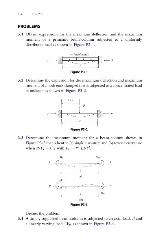
196 Chai Yoo

PROBLEMS

3.1 Obtain expressions for the maximum deflection and the maximum

moment of a prismatic beam-column subjected to a uniformly

distributed load as shown in Figure P3-1.

P P

w (force/length)

Figure P3-1

3.2 Determine the expression for the maximum deflection and maximum

moment of a both ends clamped that is subjected to a concentrated load

at midspan as shown in Figure P3-2.

P P

Q

/ 2

Figure P3-2

3.3 Determine the maximum moment for a beam-column shown in

Figure P3-3 that is bent in (a) single curvature and (b) reverse curvature

when P/PE ¼ 0.2 with PE ¼ p2 EI/‘2.

M0 M0

M0

M0

PP

P P

(a)

(b)

Figure P3-3

Discuss the problem.

3.4 A simply supported beam-column is subjected to an axial load, P, and

a linearly varying load, W0, as shown in Figure P3-4.

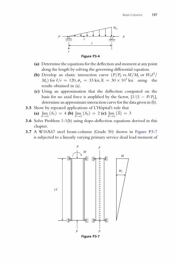
Px

y

W0

P

Figure P3-4

Beam-Columns 197

(a) Determine the equations for the deflection andmoment at any point

along the length by solving the governing differential equation.

(b) Develop an elastic interaction curve ðP=Py vsM=My or W0‘2=

MyÞ for ‘=r ¼ 120; sy ¼ 33 ksi;E ¼ 30� 103 ksi using the

results obtained in (a).

(c) Using an approximation that the deflection computed on the

basis for no axial force is amplified by the factor, [1/(1 � P/Py],

determine an approximate interaction curve for the data given in (b).

3.5 Show by repeated applications of L’Hopital’s rule that

(a) limP/0

ðS1Þ ¼ 4 (b) limP/0

ðS2Þ ¼ 2 (c) limP/0

ðSÞ ¼ 3

3.6 Solve Problem 1-1(b) using slope-deflection equations derived in this

chapter.

3.7 A W16X67 steel beam-column (Grade 50) shown in Figure P3-7

is subjected to a linearly varying primary service dead load moment of

PP

PP

MM

Mx

15'

Figure P3-7

198 Chai Yoo

15 ft-kips and live load moment of Problem 1-1(b) at one end with

none on the other end and a concentric service dead load of 87.5 kips

and live load of 262.5 kips. An effective bracing system is available at 15

ft for both the flexure and the axial force. Assume both ends are pinned

and there is no sidesway. Assess the acceptability of the design (a) by

Eq. 3.6.2 and (b) by AISC specification.

3.8 Would the final results, internal forces, and deflections be different or

the same if the axial force is applied first followed by the transverse load

or vice versa in a beam-column? State the reason for your answer.

CHAPTER44

Continuous Beams and RigidFramesContents

4.1. Introduction 1994.2. Continuous Beams 1994.3. Buckling Modes of Frames 2034.4. Critical Loads of Frames 205

4.4.1. Review of the Differential Equation Method 2054.4.2. Application of Slope-Deflection Equations to Frame Stability 210

4.5. Stability of Frames by Matrix Analysis 2164.6. Second-Order Analysis of a Frame by Slope-Deflection Equations 2204.7. Effect of Primary Bending and Plasticity on the Behavior of Frames 2284.8. Stability Design of Frames 230References 240Problems 241

4.1. INTRODUCTION

In the study of isolated column stability in Chapter 1, the member ends are

idealized to be pinned, fixed, or free. However, members in a real framed

structure are usually part of a larger framework, and their ends are elastically

restrained by the adjacent members to which they are framed. In this chapter,

the investigation is extended to consider the behavior of framed members.

In a framework, the members are usually rigidly connected at joints.

Therefore, no single compression member can buckle independently from

the adjacent members. Hence, it is often necessary to investigate the stability

of the entire structure just to obtain the critical load of one or two members

that are part of a larger framework.

Using an example problem, it will be demonstrated that the effect of

a second-order analysis becomes significant over that of the first-order

analysis when the compressive axial load is, say, greater than 10% of the

critical load of the member.

4.2. CONTINUOUS BEAMS

Slope-deflection equations with axial forces have been derived in the

previous chapter. These equations will be used to solve elastic stability

Stability of Structures � 2011 Elsevier Inc.ISBN 978-0-12-385122-2, doi:10.1016/B978-0-12-385122-2.10004-1 All rights reserved. 199 j

200 Chai Yoo

problems of continuous beams and rigid frames in this chapter. Recall the

slope-deflection equations.

Mab ¼ EI

‘

�S1qa þ S2qb þ ðS1 þ S2Þ da � db

‘

�(4.2.1)

� �

Mba ¼ EI

‘S2qa þ S1qb þ ðS1 þ S2Þ da � db

‘(4.2.2)

In the case when the end “b” is hinged, Mba ¼ 0 and Mab is modified as

a result of eliminating qb as

M0ab ¼

EI

‘S3

�qa þ da � db

‘

�(4.2.3)

where

S1 ¼ 1� b cot b

2 tan b=2

b� 1

b cosec b� 1

S2 ¼

2 tan b=2

b� 1

b2

S3 ¼

1� b cot bffiffiffiffiffiffiffi2

s

b ¼ k‘ ¼ P‘

EI* referred to as buckling parameter:

It can be shown by applying the L’Hopital’s rule that the limit values for S1,

S2, and S3 are 4, 2, and 3, respectively, when b ¼ 0 (or P ¼ 0).

Example 1 Determine Pcr for the structure shown in Figure 4-1.

For AB:

M0ba ¼

�EI

‘S3

�1qb

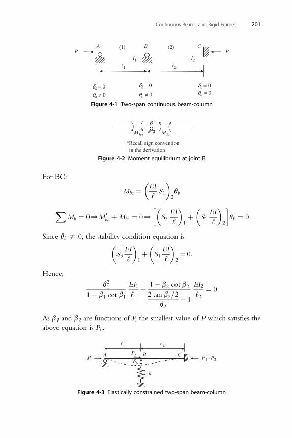
PA B C

I1 I2

�1 �2

0aδ = 0bδ = 0cδ =

0aθ ≠ 0bθ ≠ = 0cθ

P(1) (2)

Figure 4-1 Two-span continuous beam-column

B

'baM bcM

*Recall sign convention in the derivation

Figure 4-2 Moment equilibrium at joint B

Continuous Beams and Rigid Frames 201

For BC: � �

Mbc ¼ EI

‘S1

2qb

X 0��

EI� �

EI� �

Mb ¼ 00Mba þMbc ¼ 00 S3‘ 1

þ S1‘ 2

qb ¼ 0

Since qb s 0, the stability condition equation is�S3

EI

‘

�1þ�S1

EI

‘

�2¼ 0:

Hence,

b211� b1 cot b1

EI1

‘1þ 1� b2 cot b22 tan b2=2

b2� 1

EI2

‘2¼ 0

As b1 and b2 are functions of P, the smallest value of P which satisfies the

above equation is Pcr.

1l 2l

1PA B C2P

P1+P2bδ

k

Figure 4-3 Elastically constrained two-span beam-column

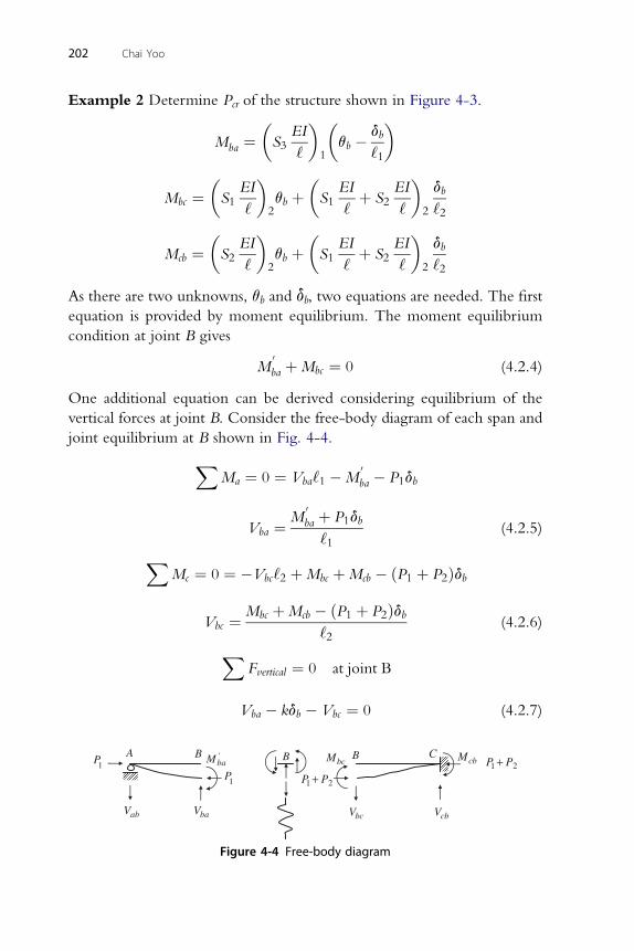
202 Chai Yoo

Example 2 Determine Pcr of the structure shown in Figure 4-3.

Mba ¼�S3

EI

‘

�1

�qb � db

‘1

��

EI� �

EI EI�

db

Mbc ¼ S1

‘ 2qb þ S1

‘þ S2

‘ 2 ‘2�EI

� �EI EI

�db

Mcb ¼ S2‘ 2

qb þ S1‘þ S2

‘ 2 ‘2

As there are two unknowns, qb and db, two equations are needed. The first

equation is provided by moment equilibrium. The moment equilibrium

condition at joint B gives

M0ba þMbc ¼ 0 (4.2.4)

One additional equation can be derived considering equilibrium of the

vertical forces at joint B. Consider the free-body diagram of each span and

joint equilibrium at B shown in Fig. 4-4.

XMa ¼ 0 ¼ Vba‘1 �M

0ba � P1db

M0 þ P1db

Vba ¼ ba

‘1(4.2.5)

XM ¼ 0 ¼ �V ‘ þM þM � ðP þ P Þd

c bc 2 bc cb 1 2 b

Mbc þMcb � ðP1 þ P2Þdb

Vbc ¼

‘2(4.2.6)

XF ¼ 0 at joint B

vertical

V � kd � V ¼ 0 (4.2.7)

ba b bc

1P

1P

A1P P2+

1P P2+

bcV cbV

cbM'baM

abV

bcMB B

baV

B C

Figure 4-4 Free-body diagram

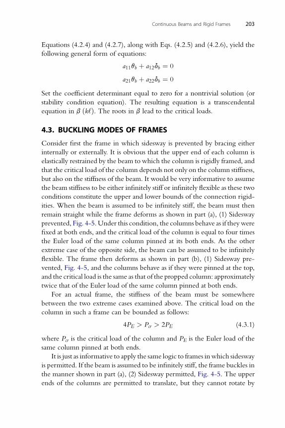
Continuous Beams and Rigid Frames 203

Equations (4.2.4) and (4.2.7), along with Eqs. (4.2.5) and (4.2.6), yield the

following general form of equations:

a11qb þ a12db ¼ 0

a q þ a d ¼ 0

21 b 22 b

Set the coefficient determinant equal to zero for a nontrivial solution (or

stability condition equation). The resulting equation is a transcendental

equation in b ðk‘Þ. The roots in b lead to the critical loads.

4.3. BUCKLING MODES OF FRAMES

Consider first the frame in which sidesway is prevented by bracing either

internally or externally. It is obvious that the upper end of each column is

elastically restrained by the beam towhich the column is rigidly framed, and

that the critical load of the column depends not only on the column stiffness,

but also on the stiffness of the beam. It would be very informative to assume

the beam stiffness to be either infinitely stiff or infinitely flexible as these two

conditions constitute the upper and lower bounds of the connection rigid-

ities. When the beam is assumed to be infinitely stiff, the beam must then

remain straight while the frame deforms as shown in part (a), (1) Sidesway

prevented, Fig. 4-5.Under this condition, the columns behave as if theywere

fixed at both ends, and the critical load of the column is equal to four times

the Euler load of the same column pinned at its both ends. As the other

extreme case of the opposite side, the beam can be assumed to be infinitely

flexible. The frame then deforms as shown in part (b), (1) Sidesway pre-

vented, Fig. 4-5, and the columns behave as if they were pinned at the top,

and the critical load is the same as that of the propped column: approximately

twice that of the Euler load of the same column pinned at both ends.

For an actual frame, the stiffness of the beam must be somewhere

between the two extreme cases examined above. The critical load on the

column in such a frame can be bounded as follows:

4PE > Pcr > 2PE (4.3.1)

where Pcr is the critical load of the column and PE is the Euler load of the

same column pinned at both ends.

It is just as informative to apply the same logic to frames inwhich sidesway

is permitted. If the beam is assumed to be infinitely stiff, the frame buckles in

the manner shown in part (a), (2) Sidesway permitted, Fig. 4-5. The upper

ends of the columns are permitted to translate, but they cannot rotate by

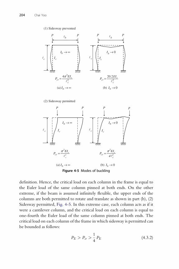
(1) Sidesway prevented

2

24 c

crc

EIP

l

π= 220.2 c

crc

EIP

l=

(a) bI → ∞ (b) 0bI →

(2) Sidesway permitted

2c

cr 2c

EIP

π=

l

2c

cr 2c

EIP

4

π=

l

(a) bI → ∞ (b) 0bI →

PP P

cl cI

P

cl

cl

0bI →bI → ∞

cI

0bI →

P P

cl cI

P

bI → ∞

blP

bl

cI

Figure 4-5 Modes of buckling

204 Chai Yoo

definition. Hence, the critical load on each column in the frame is equal to

the Euler load of the same column pinned at both ends. On the other

extreme, if the beam is assumed infinitely flexible, the upper ends of the

columns are both permitted to rotate and translate as shown in part (b), (2)

Sidesway permitted, Fig. 4-5. In this extreme case, each column acts as if it

were a cantilever column, and the critical load on each column is equal to

one-fourth the Euler load of the same column pinned at both ends. The

critical load on each column of the frame in which sidesway is permitted can

be bounded as follows:

PE > Pcr >1

4PE (4.3.2)

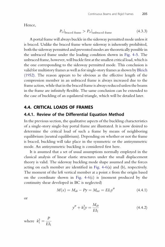
Continuous Beams and Rigid Frames 205

Hence,

Pcr jbraced frame > Pcr junbraced frame (4.3.3)

A portal framewill always buckle in the sidesway permitted mode unless it

is braced. Unlike the braced frame where sidesway is inherently prohibited,

both the sidesway permitted and preventedmodes are theoretically possible in

the unbraced frame under the loading condition shown in Fig. 4-5. The

unbraced frame, however, will buckle first at the smallest critical load,which is

the one corresponding to the sidesway permitted mode. This conclusion is

valid for multistory frames aswell as for single-story frames as shown byBleich

(1952). The reason appears to be obvious as the effective length of the

compression member in an unbraced frame is always increased due to the

frame action,while that in the braced frame is always reduced unless the beams

in the frame are infinitely flexible. The same conclusion can be extended to

the case of buckling of an equilateral triangle, which will be detailed later.

4.4. CRITICAL LOADS OF FRAMES

4.4.1. Review of the Differential Equation MethodIn the previous section, the qualitative aspects of the buckling characteristics

of a single-story single-bay portal frame are illustrated. It is now desired to

determine the critical load of such a frame by means of neighboring

equilibrium (neutral equilibrium). Depending on whether or not the frame

is braced, buckling will take place in the symmetric or the antisymmetric

mode. An antisymmetric buckling is considered first here.

It is assumed that a set of usual assumptions normally employed in the

classical analysis of linear elastic structures under the small displacement

theory is valid. The sidesway buckling mode shape assumed and the forces

acting on each member are identified in Fig. 4-6(a) and (b), respectively.

The moment of the left vertical member at a point x from the origin based

on the coordinate shown in Fig. 4-6(c) is (moment produced by the

continuity shear developed in BC is neglected)

MðxÞ ¼ Mab � Py ¼ Mint ¼ EI1y00 (4.4.1)

or

y00 þ k21y ¼Mab

EI1(4.4.2)

where k21 ¼P

EI1

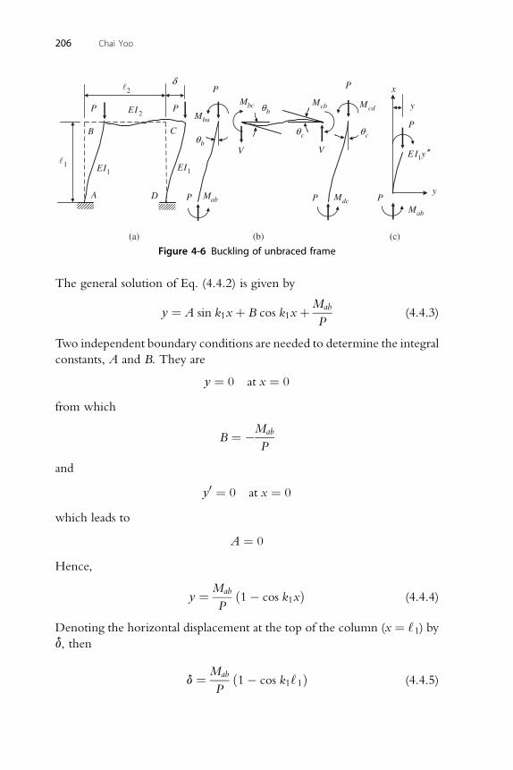
(a) (b) (c)

1l

yD

PP

P

P

P

P P

PB C

A

δ

abM

1EI

2EI

2l

1EI

V

dcM

cdM

baMcbMbcM

V

bθ

cθ cθbθ

x

y

abM

1EI y ′′

Figure 4-6 Buckling of unbraced frame

206 Chai Yoo

The general solution of Eq. (4.4.2) is given by

y ¼ A sin k1xþ B cos k1xþMab

P(4.4.3)

Two independent boundary conditions are needed to determine the integral

constants, A and B. They are

y ¼ 0 at x ¼ 0

from which

B ¼ �Mab

P

and

y0 ¼ 0 at x ¼ 0

which leads to

A ¼ 0

Hence,

y ¼ Mab

Pð1� cos k1xÞ (4.4.4)

Denoting the horizontal displacement at the top of the column (x ¼ ‘1) byd, then

d ¼ Mab

Pð1� cos k1‘1Þ (4.4.5)

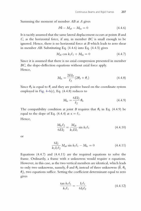
Continuous Beams and Rigid Frames 207

Summing the moment of member AB at A gives

Pd�Mab �Mba ¼ 0 (4.4.6)

It is tacitly assumed that the same lateral displacement occurs at points B and

C, as the horizontal force, if any, in member BC is small enough to be

ignored. Hence, there is no horizontal force at B which leads to zero shear

in member AB. Substituting Eq. (4.4.6) into Eq. (4.4.5) gives

Mab cos k1‘1 þMba ¼ 0 (4.4.7)

Since it is assumed that there is no axial compression presented in member

BC, the slope-deflection equations without axial force apply.

Hence,

Mbc ¼ 2EI2

‘2ð2qb þ qcÞ (4.4.8)

Since qb ia equal to qc and they are positive based on the coordinate system

employed in Fig. 4-6(c), Eq. (4.4.8) reduces to

Mbc ¼ 6EI2

‘2qb (4.4.9)

The compatibility condition at joint B requires that qb in Eq. (4.4.9) be

equal to the slope of Eq. (4.4.4) at x ¼ ‘1.

Hence,

Mbc‘26EI2

¼ Mab

k1EI1sin k1‘1 (4.4.10)

or

6I2

k1I1‘2Mab sin k1‘1 �Mbc ¼ 0 (4.4.11)

Equations (4.4.7) and (4.4.11) are the required equations to solve the

frame. Ordinarily, a frame with n unknowns would require n equations.

However, in this case, as the two vertical members are identical, which leads

to only two unknowns, namely, d and qb instead of three unknowns (d, qb,qc), two equations suffice. Setting the coefficient determinant equal to zero

gives

tan k1‘1k1‘1

¼ � I1‘16I2‘2

(4.4.12)

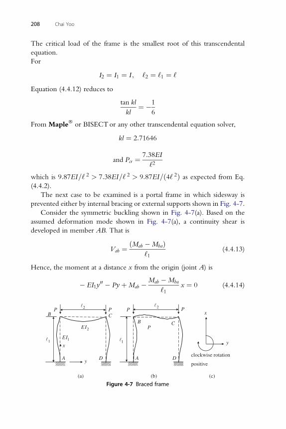
208 Chai Yoo

The critical load of the frame is the smallest root of this transcendental

equation.

For

I2 ¼ I1 ¼ I ; ‘2 ¼ ‘1 ¼ ‘

Equation (4.4.12) reduces to

tan kl

kl¼ �1

6

From Maple� or BISECTor any other transcendental equation solver,

kl ¼ 2:71646

7:38EI

and Pcr ¼

‘2

which is 9:87EI=‘ 2 > 7:38EI=‘ 2 > 9:87EI=ð4‘ 2Þ as expected from Eq.

(4.4.2).

The next case to be examined is a portal frame in which sidesway is

prevented either by internal bracing or external supports shown in Fig. 4-7.

Consider the symmetric buckling shown in Fig. 4-7(a). Based on the

assumed deformation mode shown in Fig. 4-7(a), a continuity shear is

developed in member AB. That is

Vab ¼ ðMab �MbaÞ‘1

(4.4.13)

Hence, the moment at a distance x from the origin (joint A) is

� EI1y00 � PyþMab �Mab �Mba

‘1x ¼ 0 (4.4.14)

1�

clockwise rotation

positive

PPP

1�

A

P

y

x

D

2EI

1EI

CB

A

B C

P

Dy

x

2� 2�

(a) (b) (c)

Figure 4-7 Braced frame

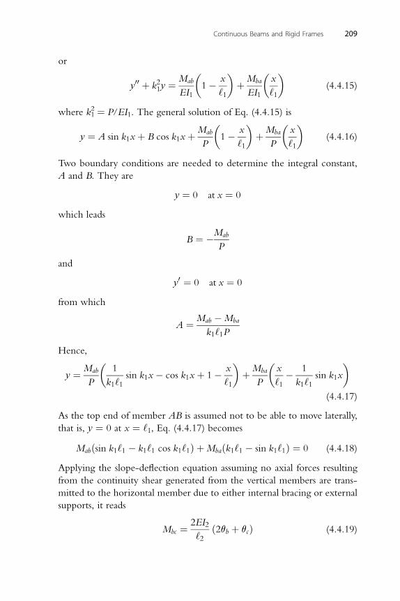
Continuous Beams and Rigid Frames 209

or

y00 þ k21y ¼Mab

EI1

�1� x

‘1

�þMba

EI1

�x

‘1

�(4.4.15)

where k12 ¼ P/EI1. The general solution of Eq. (4.4.15) is

y ¼ A sin k1xþ B cos k1xþMab

P

�1� x

‘1

�þMba

P

�x

‘1

�(4.4.16)

Two boundary conditions are needed to determine the integral constant,

A and B. They are

y ¼ 0 at x ¼ 0

which leads

B ¼ �Mab

P

and

y0 ¼ 0 at x ¼ 0

from which

A ¼ Mab �Mba

k1‘1P

Hence,

y ¼ Mab

P

�1

k1‘1sin k1x� cos k1xþ 1� x

‘1

�þMba

P

�x

‘1� 1

k1‘1sin k1x

�(4.4.17)

As the top end of member AB is assumed not to be able to move laterally,

that is, y ¼ 0 at x ¼ ‘1, Eq. (4.4.17) becomes

Mabðsin k1‘1 � k1‘1 cos k1‘1Þ þMbaðk1‘1 � sin k1‘1Þ ¼ 0 (4.4.18)

Applying the slope-deflection equation assuming no axial forces resulting

from the continuity shear generated from the vertical members are trans-

mitted to the horizontal member due to either internal bracing or external

supports, it reads

Mbc ¼ 2EI2

‘2ð2qb þ qcÞ (4.4.19)

210 Chai Yoo

Since qc ¼ �qb, Eq. (4.4.19) reduces to

Mbc ¼ 2EI2

‘2qb (4.4.20)

Compatibility of slope at joint B requires that qb of the horizontal member

be equal to �y0 at x ¼ ‘1 of the vertical member for the consistent sign

convention adopted in Fig. 4-7(c). It is noted here that the condition of

Mba ¼Mbc has been used in the above derivation starting from Eq. (4.4.13).

Thus

Mb‘22EI2

¼ �Ma

P

�1

‘1cos k1‘1 þ k1sin k1‘1 � 1

‘1

��Mb

P

�1

‘1� 1

‘1cos k1‘1

�

which is rearranged to

Maðcos k1‘1 þ k1‘1 sink1‘1 � 1Þ þMb

�1� cos k1‘1 þ I1‘1k

21‘2

2I2

�¼ 0

(4.4.21)

For a nontrivial solution, set the determinant for the coefficient matrix

equal to zero. The resulting transcendental equation is

2� 2 cos k1‘1 � k1‘1 sin k1‘1 þ ‘2I1k12I2

ðsin k1‘1 � k1‘1cos k1‘1Þ ¼ 0

(4.4.22)

By setting I1 ¼ I2 ¼ I and ‘1 ¼ ‘2 ¼ ‘ in Eq. (4.4.22), the smallest root is

k‘ ¼ 5:018 and

Pcr ¼ 25:18EI

‘2

This load is considerably larger than that of the same frame (7:34EI=‘2)where sidesway is permitted. The critical load also satisfies Eq. (4.4.1), as

expected.

4.4.2. Application of Slope-Deflection Equationsto Frame Stability

Although the differential equation method examined in the previous section

is theoretically applicable to any frame, it becomes prohibitively complex in

actuality, particularly in a frame of many kinematic degrees of freedom. In

order to show the versatility of the slope-deflection equations, the same

example examined above will be revisited.

Continuous Beams and Rigid Frames 211

It is assumed again that the axial compression in member BC would be

negligibly small.

Since qa h 0, the moment at the top joint of member AB is

Mba ¼ ðS1kÞ1qb (4.4.23)

where ki ¼ ½ðEIÞ=‘�iThe moment in the horizontal member is

Mbc ¼ ðS1kÞ2qb þ ðS2kÞ2qc (4.4.24)

As qc ¼ �qb for the buckling mode shown in Fig. 4-7(a), Eq. (4.4.24)

reduces to

Mbc ¼ ½ðS1kÞ2 � ðS2kÞ2�qb (4.4.25)

Since there is no axial force in member BC, (S1)2 ¼ 4 and (S2)2 ¼ 2.

For joint equilibrium Mba and Mbc are the same in magnitude and opposite

in sign. Thus XMb ¼ 00Mba þMbc ¼ 0 (4.4.26)

For I ¼ I ¼ I and ‘ ¼ ‘ ¼ ‘;Eq: ð4:4:26Þ reduces to

2 1 2 1

� �

S1EI

‘qb ¼ ð4� 2ÞEI

‘qb (4.4.27)

from which

S1 ¼ 2 (4.4.28)

Equation (4.4.28) will lead to the critical load of Pcr ¼ ð25:18EIÞ=‘2.For the buckling mode shown in Fig. 4-7(b), qb ¼ qc. By keeping qb and qcas unknown independent variables, the analysis can be generalized. The

unknown moments at joint C are

Mcd ¼ ðS1kÞ1qc (4.4.29)

and

Mcb ¼ ðS1kÞ2 qc þ ðS2kÞ2 qb (4.4.30)

212 Chai Yoo

The equilibrium condition at B requires

XMb ¼ 00½ðS1kÞ1 þ ðS1kÞ2�qb þ ðS2kÞ2qc ¼ 0

from which

ðS1 þ 4Þqb þ 2qc ¼ 0 (4.4.31)

Likewise, moment equilibrium at C demandsXMc ¼ 00½ðS1kÞ1 þ ðS1kÞ2�qc þ ðS2kÞ2qb ¼ 0 (4.4.32)

from which

2qb þ ðS1 þ 4Þqc ¼ 0 (4.4.33)

Setting the determinant of the coefficient matrix of the unknowns qb and qcfor the stability condition gives�����

S1 þ 4 2

2 S1 þ 4

����� ¼ 00ðS1 þ 4Þ2 � 4 ¼ 00S1 ¼ �2;�6

By Maple�, BISECTor any other transcendental equation solver, one can

obtain k‘ ¼ 5.01818 and 5.52718 for S1 ¼ �2 and �6.

The smallest root for k‘ ¼ 5.01818 gives the critical load of 25.18EI/‘2

for the buckling mode shown in Fig. 4-7(a), and k‘ ¼ 5.52718 yields the

critical load of 30.55EI/‘2 for the buckling mode shown in Fig. 4-7(b). It is

of interest to note that the critical load is larger for the antisymmetric

buckling mode than that for the symmetric buckling mode within the same

braced frame. This difference can be explained by examining the buckling

mode shapes shown in Fig. 4-7. In the antisymmetric buckling mode, the

beam deformed in such a manner as to create an inflection point at the

middle of the member (reducing the effective length by half), thereby

increasing its stiffness. The increased stiffness of the beam, in turn, provides

a little bit more constraint at the top of the column, which would shorten

the effective length of the column.

The next example is buckling of a rigidly connected equilateral triangle

shown in Fig. 4-8.

Take the counterclockwise moment and rotation as positive quantities

as adopted in the derivation of the slope-deflection equations in Chapter

3. As the joints are assumed rigid, the original subtended angle of

60 degrees will be maintained throughout the history of deformations.

Hence,

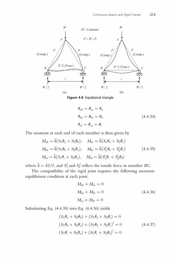
(a) (b)/ 2W

A

W

B

A

C

W

PP

C B

(Comp.) (Comp.) (Comp.) (Comp.)

/ 3P = W

PP

/ 2 (Tens.)P / 2 (Tens.)P

l

EI : Constant

l

/ 2W/ 2W/ 2W

Figure 4-8 Equilateral triangle

Continuous Beams and Rigid Frames 213

qab ¼ qac ¼ qa

qba ¼ qbc ¼ qb

qcb ¼ qca ¼ qc

(4.4.34)

The moment at each end of each member is then given by

Mab ¼ kðS1qa þ S2qbÞ; Mac ¼ kðS1qa þ S2qcÞMba ¼ kðS1qb þ S2qaÞ; Mbc ¼ kðS01qb þ S02qcÞMca ¼ kðS1qc þ S2qaÞ; Mcb ¼ kðS01qc þ S02qbÞ

(4.4.35)

where k ¼ EI=‘, and S10 and S20 reflect the tensile force in member BC.

The compatibility of the rigid joint requires the following moment-

equilibrium condition at each joint:

Mab þMac ¼ 0

Mba þMbc ¼ 0

Mca þMcb ¼ 0

(4.4.36)

Substituting Eq. (4.4.35) into Eq. (4.4.36) yields

ðS1qa þ S2qbÞ þ ðS1qa þ S2qcÞ ¼ 0

ðS1qb þ S2qaÞ þ ðS1qb þ S2qcÞ0 ¼ 0

ðS1qc þ S2qaÞ þ ðS1qc þ S2qbÞ0 ¼ 0

(4.4.37)

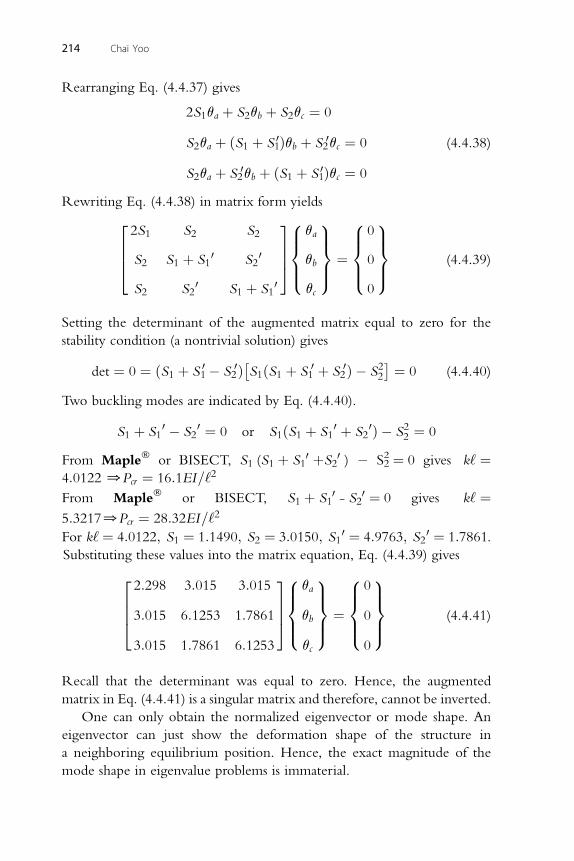
214 Chai Yoo

Rearranging Eq. (4.4.37) gives

2S1qa þ S2qb þ S2qc ¼ 0

S2qa þ ðS1 þ S10Þqb þ S2

0qc ¼ 0

S2qa þ S20qb þ ðS1 þ S1

0Þqc ¼ 0

(4.4.38)

Rewriting Eq. (4.4.38) in matrix form yields26642S1 S2 S2

S2 S1 þ S10 S2

0

S2 S20 S1 þ S1

0

37758>><>>:

qa

qb

qc

9>>=>>; ¼

8>><>>:

0

0

0

9>>=>>; (4.4.39)

Setting the determinant of the augmented matrix equal to zero for the

stability condition (a nontrivial solution) gives

det ¼ 0 ¼ ðS1 þ S10 � S2

0Þ�S1ðS1 þ S10 þ S2

0Þ � S22 ¼ 0 (4.4.40)

Two buckling modes are indicated by Eq. (4.4.40).

S1 þ S10 � S2

0 ¼ 0 or S1ðS1 þ S10 þ S2

0Þ � S22 ¼ 0

From Maple� or BISECT, S1 (S1 þ S10 þS2

0 ) � S22 ¼ 0 gives k‘ ¼

4:01220Pcr ¼ 16:1EI=‘2

From Maple� or BISECT, S1 þ S10 - S20 ¼ 0 gives k‘ ¼

5:32170Pcr ¼ 28:32EI=‘2

For k‘ ¼ 4:0122; S1 ¼ 1:1490; S2 ¼ 3:0150; S10 ¼ 4:9763; S2

0 ¼ 1:7861.Substituting these values into the matrix equation, Eq. (4.4.39) gives

26642:298 3:015 3:015

3:015 6:1253 1:7861

3:015 1:7861 6:1253

37758>><>>:

qa

qb

qc

9>>=>>; ¼

8>><>>:

0

0

0

9>>=>>; (4.4.41)

Recall that the determinant was equal to zero. Hence, the augmented

matrix in Eq. (4.4.41) is a singular matrix and therefore, cannot be inverted.

One can only obtain the normalized eigenvector or mode shape. An

eigenvector can just show the deformation shape of the structure in

a neighboring equilibrium position. Hence, the exact magnitude of the

mode shape in eigenvalue problems is immaterial.

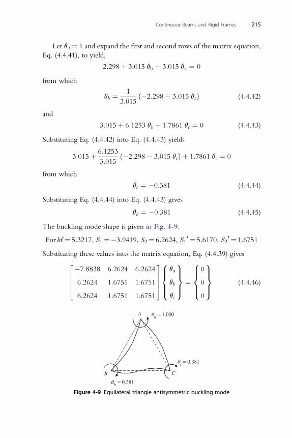
Continuous Beams and Rigid Frames 215

Let qa ¼ 1 and expand the first and second rows of the matrix equation,

Eq. (4.4.41), to yield,

2:298þ 3:015 qb þ 3:015 qc ¼ 0

from which

qb ¼ 1

3:015ð�2:298� 3:015 qcÞ (4.4.42)

and

3:015þ 6:1253 qb þ 1:7861 qc ¼ 0 (4.4.43)

Substituting Eq. (4.4.42) into Eq. (4.4.43) yields

3:015þ 6:1253

3:015ð�2:298� 3:015 qcÞ þ 1:7861 qc ¼ 0

from which

qc ¼ �0:381 (4.4.44)

Substituting Eq. (4.4.44) into Eq. (4.4.43) gives

qb ¼ �0:381 (4.4.45)

The buckling mode shape is given in Fig. 4-9.

For k‘¼ 5:3217; S1¼�3:9419; S2¼ 6:2624; S10 ¼ 5:6170; S2

0 ¼ 1:6751

Substituting these values into the matrix equation, Eq. (4.4.39) gives

2664�7:8838 6:2624 6:2624

6:2624 1:6751 1:6751

6:2624 1:6751 1:6751

37758>><>>:

qa

qb

qc

9>>=>>; ¼

8>><>>:

0

0

0

9>>=>>; (4.4.46)

bθ = 0.381

A

B C

aθ = 1.000

cθ = 0.381

Figure 4-9 Equilateral triangle antisymmetric buckling mode

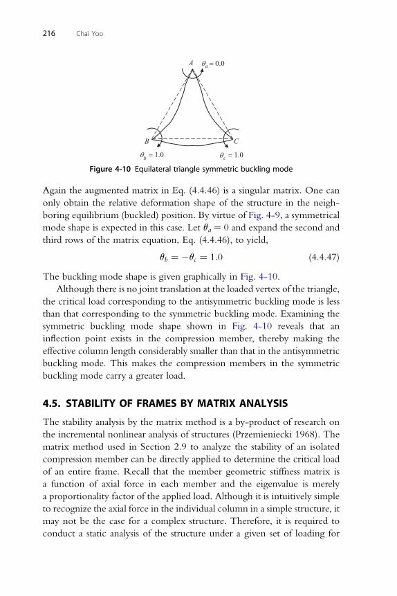
A

B C

aθ = 0.0

bθ = 1.0 = 1.0cθ

Figure 4-10 Equilateral triangle symmetric buckling mode

216 Chai Yoo

Again the augmented matrix in Eq. (4.4.46) is a singular matrix. One can

only obtain the relative deformation shape of the structure in the neigh-

boring equilibrium (buckled) position. By virtue of Fig. 4-9, a symmetrical

mode shape is expected in this case. Let qa ¼ 0 and expand the second and

third rows of the matrix equation, Eq. (4.4.46), to yield,

qb ¼ �qc ¼ 1:0 (4.4.47)

The buckling mode shape is given graphically in Fig. 4-10.

Although there is no joint translation at the loaded vertex of the triangle,

the critical load corresponding to the antisymmetric buckling mode is less

than that corresponding to the symmetric buckling mode. Examining the

symmetric buckling mode shape shown in Fig. 4-10 reveals that an

inflection point exists in the compression member, thereby making the

effective column length considerably smaller than that in the antisymmetric

buckling mode. This makes the compression members in the symmetric

buckling mode carry a greater load.

4.5. STABILITY OF FRAMES BY MATRIX ANALYSIS

The stability analysis by the matrix method is a by-product of research on

the incremental nonlinear analysis of structures (Przemieniecki 1968). The

matrix method used in Section 2.9 to analyze the stability of an isolated

compression member can be directly applied to determine the critical load

of an entire frame. Recall that the member geometric stiffness matrix is

a function of axial force in each member and the eigenvalue is merely

a proportionality factor of the applied load. Although it is intuitively simple

to recognize the axial force in the individual column in a simple structure, it

may not be the case for a complex structure. Therefore, it is required to

conduct a static analysis of the structure under a given set of loading for

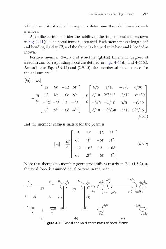
Continuous Beams and Rigid Frames 217

which the critical value is sought to determine the axial force in each

member.

As an illustration, consider the stability of the simple portal frame shown

in Fig. 4-11(a). The portal frame is unbraced. Each member has a length of ‘and bending rigidity EI, and the frame is clamped at its base and is loaded as

shown.

Positive member (local) and structure (global) kinematic degrees of

freedom and corresponding force are defined in Figs. 4-11(b) and 4-11(c).

According to Eqs. (2.9.11) and (2.9.13), the member stiffness matrices for

the column are

½k1�¼ ½k3�

¼EI

‘3

2666664

12 6‘ �12 6‘

6‘ 4‘2 �6‘ 2‘2

�12 �6‘ 12 �6‘

6‘ 2‘2 �6‘ 4‘2

3777775�P

‘

2666664

6=5 ‘=10 �6=5 ‘=30

‘=10 2‘2=15 �‘=10 �‘2=30

�6=5 �‘=10 6=5 �‘=10

‘=10 �‘2=30 �‘=10 2‘2=15

3777775

(4.5.1)

and the member stiffness matrix for the beam is

½k2� ¼ EI

‘3

2666664

12 6‘ �12 6‘

6‘ 4‘2 �6‘ 2‘2

�12 �6‘ 12 �6‘

6‘ 2‘2 �6‘ 4‘2

3777775 (4.5.2)

Note that there is no member geometric stiffness matrix in Eq. (4.5.2), as

the axial force is assumed equal to zero in the beam.

Figure 4-11 Global and local coordinates of portal frame

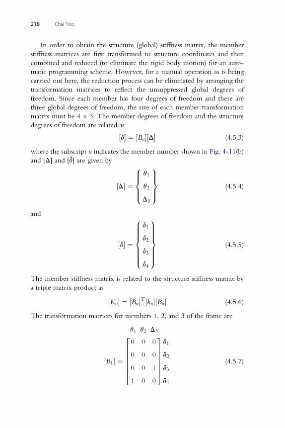
218 Chai Yoo

In order to obtain the structure (global) stiffness matrix, the member

stiffness matrices are first transformed to structure coordinates and then

combined and reduced (to eliminate the rigid body motion) for an auto-

matic programming scheme. However, for a manual operation as is being

carried out here, the reduction process can be eliminated by arranging the

transformation matrices to reflect the unsuppressed global degrees of

freedom. Since each member has four degrees of freedom and there are

three global degrees of freedom, the size of each member transformation

matrix must be 4 � 3. The member degrees of freedom and the structure

degrees of freedom are related as

½d� ¼ ½Bn�½D� (4.5.3)

where the subscript n indicates the member number shown in Fig. 4-11(b)

and [D] and [d] are given by

½D� ¼

8>><>>:

q1

q2

D3

9>>=>>; (4.5.4)

and

½d� ¼

8>>>>><>>>>>:

d1

d2

d3

d4

9>>>>>=>>>>>;

(4.5.5)

The member stiffness matrix is related to the structure stiffness matrix by

a triple matrix product as

½Kn� ¼ ½Bn�T ½kn�½Bn� (4.5.6)

The transformation matrices for members 1, 2, and 3 of the frame are

q1 q2 D320 0 0

3d

½B1� ¼6666640 0 0

0 0 1

1 0 0

777775

1

d2

d3

d4

(4.5.7)

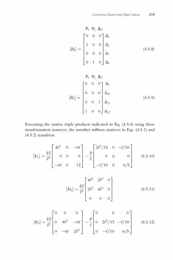
q1 q2 D3

2 3

Continuous Beams and Rigid Frames 219

½B2� ¼6666664

0 0 0

1 0 0

0 0 0

0 1 0

7777775

d5

d6

d7

d8

(4.5.8)

q q D

1 2 320 0 0

3d

½B3� ¼66666640 0 0

0 0 1

1 0 0

7777775

9

d10

d11

d12

(4.5.9)

Executing the matrix triple products indicated in Eq. (4.5.6) using these

transformation matrices, the member stiffness matrices in Eqs. (4.5.1) and

(4.5.2) transform

½K1� ¼ EI

‘3

26664

4‘2 0 �6‘

0 0 0

�6‘ 0 12

37775� P

‘

266642‘2=15 0 �‘=10

0 0 0

�‘=10 0 6=5

37775 (4.5.10)

22 2

3

½K2� ¼ EI

‘3

66644‘ 2‘ 0

2‘2 4‘2 0

0 0 0

7775 (4.5.11)

20 0 0

3 20 0 0

3

½K3� ¼ EI

‘3

6664 0 4‘2 �6‘

0 �6‘ 2‘2

7775� P

‘

6664 0 2‘2=15 �‘=10

0 �‘=10 6=5

7775 (4.5.12)

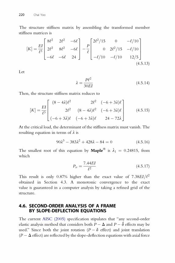
220 Chai Yoo

The structure stiffness matrix by assembling the transformed member

stiffness matrices is

½K � ¼ EI

‘3

26648‘2 2‘2 �6‘

2‘2 8‘2 �6‘

�6‘ �6‘ 24

3775� P

‘

26642‘2=15 0 �‘=10

0 2‘2=15 �‘=10

�‘=10 �‘=10 12=5

3775

(4.5.13)

Let

l ¼ P‘2

30EI(4.5.14)

Then, the structure stiffness matrix reduces to

½K � ¼ EI

‘3

2664

ð8� 4lÞ‘2 2‘2 ð�6þ 3lÞ‘2‘2 ð8� 4lÞ‘2 ð�6þ 3lÞ‘

ð�6þ 3lÞ‘ ð�6þ 3lÞ‘ 24� 72l

3775 (4.5.15)

At the critical load, the determinant of the stiffness matrix must vanish. The

resulting equation in terms of l is

90l3 � 383l2 þ 428l� 84 ¼ 0 (4.5.16)

The smallest root of this equation by Maple� is l1 ¼ 0.24815, from

which

Pcr ¼ 7:44EI

‘2(4.5.17)

This result is only 0.87% higher than the exact value of 7:38EI=‘2

obtained in Section 4.3. A monotonic convergence to the exact

value is guaranteed in a computer analysis by taking a refined grid of the

structure.

4.6. SECOND-ORDER ANALYSIS OF A FRAMEBY SLOPE-DEFLECTION EQUATIONS

The current AISC (2005) specification stipulates that “any second-order

elastic analysis method that considers both P � D and P � d effects may be

used.” Since both the joint rotation (P � d effect) and joint translation

(P � D effect) are reflected by the slope-deflection equations with axial force

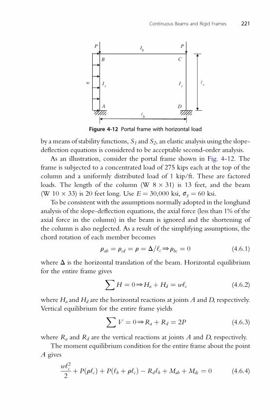
P

D

cIcI

bI

b�

c�

A

w

B C

P

Figure 4-12 Portal frame with horizontal load

Continuous Beams and Rigid Frames 221

by ameans of stability functions, S1 and S2, an elastic analysis using the slope-

deflection equations is considered to be acceptable second-order analysis.

As an illustration, consider the portal frame shown in Fig. 4-12. The

frame is subjected to a concentrated load of 275 kips each at the top of the

column and a uniformly distributed load of 1 kip/ft. These are factored

loads. The length of the column (W 8 � 31) is 13 feet, and the beam

(W 10 � 33) is 20 feet long. Use E ¼ 30,000 ksi, sy ¼ 60 ksi.

To be consistent with the assumptions normally adopted in the longhand

analysis of the slope-deflection equations, the axial force (less than 1% of the

axial force in the column) in the beam is ignored and the shortening of

the column is also neglected. As a result of the simplifying assumptions, the

chord rotation of each member becomes

rab ¼ rcd ¼ r ¼ D=‘c0rbc ¼ 0 (4.6.1)

where D is the horizontal translation of the beam. Horizontal equilibrium

for the entire frame givesXH ¼ 00Ha þHd ¼ w‘c (4.6.2)

where Ha andHd are the horizontal reactions at joints A andD, respectively.

Vertical equilibrium for the entire frame yieldsXV ¼ 00Ra þ Rd ¼ 2P (4.6.3)

where Ra and Rd are the vertical reactions at joints A and D, respectively.

The moment equilibrium condition for the entire frame about the point

A gives

w‘2c2

þ Pðr‘cÞ þ Pð‘b þ r‘cÞ � Rd‘b þMab þMdc ¼ 0 (4.6.4)

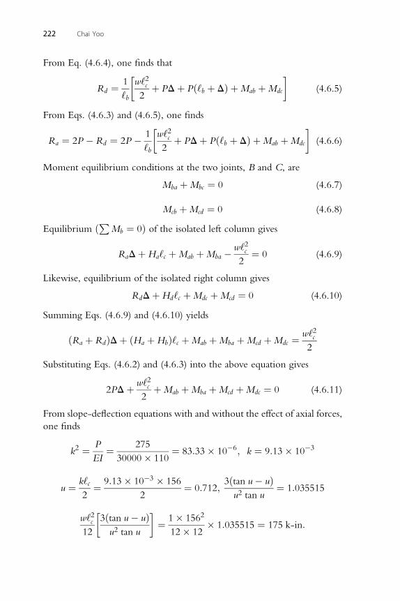
222 Chai Yoo

From Eq. (4.6.4), one finds that

Rd ¼ 1

‘b

�w‘2c2

þ PDþ Pð‘b þ DÞ þMab þMdc

�(4.6.5)

From Eqs. (4.6.3) and (4.6.5), one finds

Ra ¼ 2P � Rd ¼ 2P � 1

‘b

�w‘2c2

þ PDþ Pð‘b þ DÞ þMab þMdc

�(4.6.6)

Moment equilibrium conditions at the two joints, B and C, are

Mba þMbc ¼ 0 (4.6.7)

M þM ¼ 0 (4.6.8)

cb cd

Equilibrium ðPMb ¼ 0Þ of the isolated left column gives

RaDþHa‘c þMab þMba � w‘2c2

¼ 0 (4.6.9)

Likewise, equilibrium of the isolated right column gives

RdDþHd‘c þMdc þMcd ¼ 0 (4.6.10)

Summing Eqs. (4.6.9) and (4.6.10) yields

ðRa þ RdÞDþ ðHa þHbÞ‘c þMab þMba þMcd þMdc ¼ w‘2c2

Substituting Eqs. (4.6.2) and (4.6.3) into the above equation gives

2PDþ w‘2c2

þMab þMba þMcd þMdc ¼ 0 (4.6.11)

From slope-deflection equations with and without the effect of axial forces,

one finds

k2 ¼ P

EI¼ 275

30000� 110¼ 83:33� 10�6; k ¼ 9:13� 10�3

�3

u ¼ k‘c2

¼ 9:13� 10 � 156

2¼ 0:712;

3ðtan u� uÞu2 tan u

¼ 1:035515

2� �

2

w‘c12

3ðtan u� uÞu2 tan u

¼ 1� 156

12� 12� 1:035515 ¼ 175 k-in:

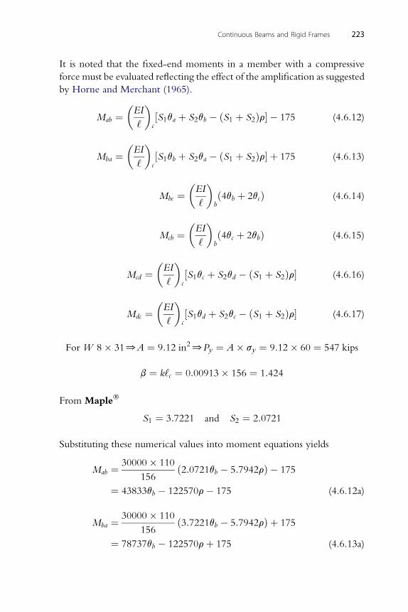
Continuous Beams and Rigid Frames 223

It is noted that the fixed-end moments in a member with a compressive

force must be evaluated reflecting the effect of the amplification as suggested

by Horne and Merchant (1965).

Mab ¼�EI

‘

�c½S1qa þ S2qb � ðS1 þ S2Þr� � 175 (4.6.12)

� �

Mba ¼ EI

‘ c½S1qb þ S2qa � ðS1 þ S2Þr� þ 175 (4.6.13)

�EI

�

Mbc ¼

‘ bð4qb þ 2qcÞ (4.6.14)

� �

Mcb ¼ EI

‘ bð4qc þ 2qbÞ (4.6.15)

�EI

�

Mcd ¼

‘ c½S1qc þ S2qd � ðS1 þ S2Þr� (4.6.16)

�EI

�

Mdc ¼

‘ c½S1qd þ S2qc � ðS1 þ S2Þr� (4.6.17)

2

For W 8� 310A ¼ 9:12 in 0Py ¼ A� sy ¼ 9:12� 60 ¼ 547 kips

b ¼ k‘ ¼ 0:00913� 156 ¼ 1:424

c

From Maple�

S1 ¼ 3:7221 and S2 ¼ 2:0721

Substituting these numerical values into moment equations yields

Mab ¼ 30000� 110

156ð2:0721qb � 5:7942rÞ � 175

¼ 43833qb � 122570r� 175 (4.6.12a)

30000� 110

Mba ¼

156ð3:7221qb � 5:7942rÞ þ 175

¼ 78737qb � 122570rþ 175 (4.6.13a)

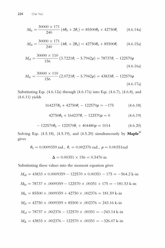
30000� 171

Mbc ¼

240ð4qb þ 2qcÞ ¼ 85500qb þ 42750qc (4.6.14a)

30000� 171

224 Chai Yoo

Mcb ¼240

ð4qc þ 2qbÞ ¼ 42750qb þ 85500qc (4.6.15a)

30000� 110

Mcd ¼

156ð3:7221qc � 5:7942rÞ ¼ 78737qc � 122570r

(4.6.16a)

30000� 110

Mdc ¼

156ð2:0721qc � 5:7942rÞ ¼ 43833qc � 122570r

(4.6.17a)

Substituting Eqs. (4.6.12a) through (4.6.17a) into Eqs. (4.6.7), (4.6.8), and

(4.6.11) yields

164237qb þ 42750qc � 122570r ¼ �175 (4.6.18)

42750q þ 164237q � 122570r ¼ 0 (4.6.19)

b c

� 122570q � 122570q þ 404480r ¼ 1014 (4.6.20)

b c

Solving Eqs. (4.5.18), (4.5.19), and (4.5.20) simultaneously by Maple�

gives

qb ¼ 0:0009359 rad:; qc ¼ 0:002376 rad:; r ¼ 0:00351rad

D ¼ 0:00351� 156 ¼ 0:5476 in

Substituting these values into the moment equation gives

Mab ¼ 43833� 0:0009359� 122570� 0:00351� 175 ¼ �564:2 k-in

M ¼ 78737� :0009359� 122570� :00351þ 175 ¼ �181:53 k-in

ba

M ¼ 85500� :0009359þ 42750� :002376 ¼ 181:59 k-in

bc

M ¼ 42750� :0009359þ 85500� :002376 ¼ 243:16 k-in

cb

M ¼ 78737� :002376� 122570� :00351 ¼ �243:14 k-in

cd

M ¼ 43833� :002376� 122570� :00351 ¼ �326:07 k-in

dc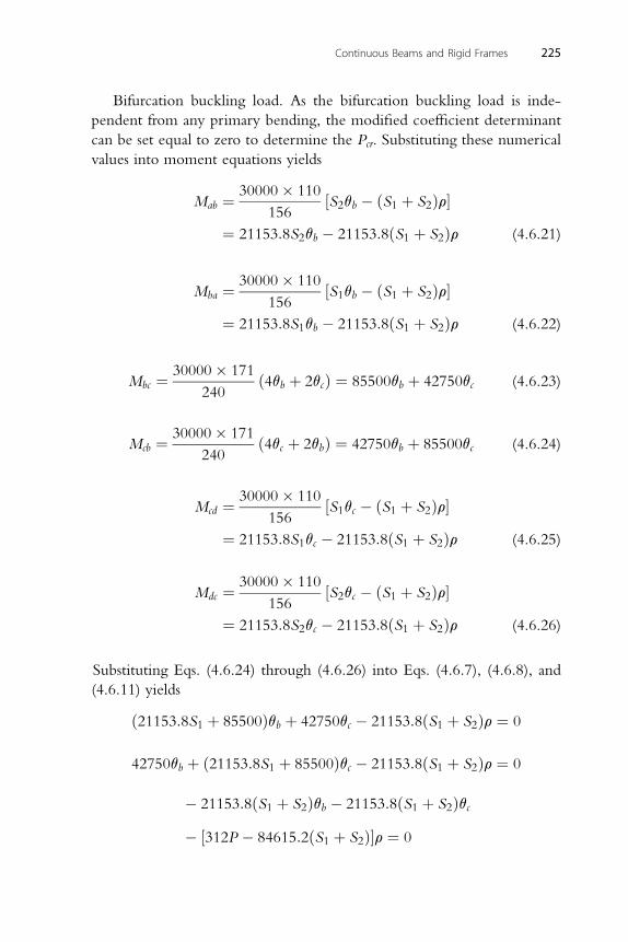

Continuous Beams and Rigid Frames 225

Bifurcation buckling load. As the bifurcation buckling load is inde-

pendent from any primary bending, the modified coefficient determinant

can be set equal to zero to determine the Pcr. Substituting these numerical

values into moment equations yields

Mab ¼ 30000� 110

156½S2qb � ðS1 þ S2Þr�

¼ 21153:8S2qb � 21153:8ðS1 þ S2Þr (4.6.21)

30000� 110

Mba ¼

156½S1qb � ðS1 þ S2Þr�

¼ 21153:8S1qb � 21153:8ðS1 þ S2Þr (4.6.22)

30000� 171

Mbc ¼

240ð4qb þ 2qcÞ ¼ 85500qb þ 42750qc (4.6.23)

30000� 171

Mcb ¼

240ð4qc þ 2qbÞ ¼ 42750qb þ 85500qc (4.6.24)

30000� 110

Mcd ¼

156½S1qc � ðS1 þ S2Þr�

¼ 21153:8S1qc � 21153:8ðS1 þ S2Þr (4.6.25)

30000� 110

Mdc ¼

156½S2qc � ðS1 þ S2Þr�

¼ 21153:8S2qc � 21153:8ðS1 þ S2Þr (4.6.26)

Substituting Eqs. (4.6.24) through (4.6.26) into Eqs. (4.6.7), (4.6.8), and

(4.6.11) yields

ð21153:8S1 þ 85500Þqb þ 42750qc � 21153:8ðS1 þ S2Þr ¼ 0

42750q þ ð21153:8S þ 85500Þq � 21153:8ðS þ S Þr ¼ 0

b 1 c 1 2

� 21153:8ðS1 þ S2Þqb � 21153:8ðS1 þ S2Þqc� ½312P � 84615:2ðS1 þ S2Þ�r ¼ 0

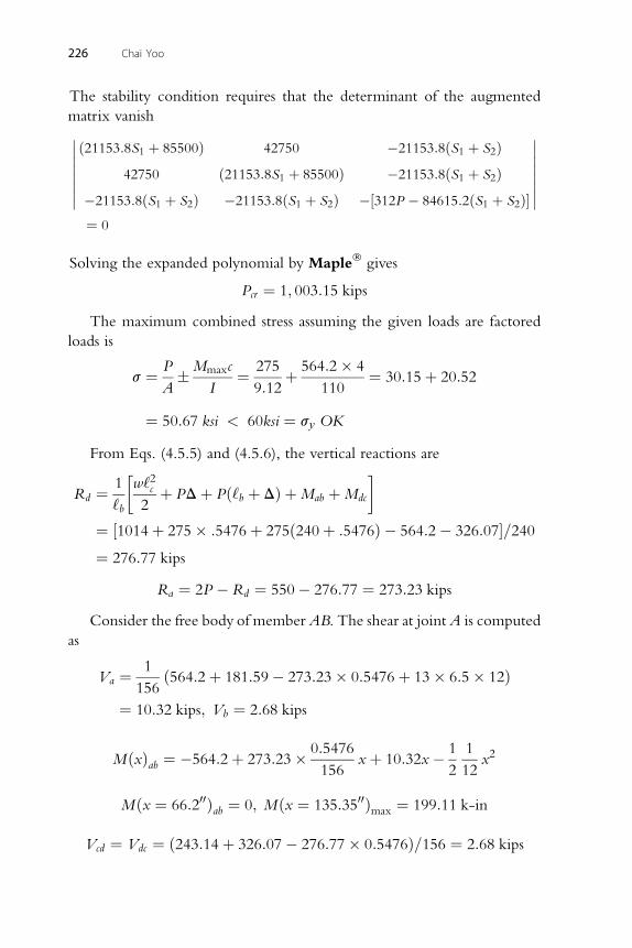
226 Chai Yoo

The stability condition requires that the determinant of the augmented

matrix vanish��������ð21153:8S1 þ 85500Þ 42750 �21153:8ðS1 þ S2Þ

42750 ð21153:8S1 þ 85500Þ �21153:8ðS1 þ S2Þ�21153:8ðS1 þ S2Þ �21153:8ðS1 þ S2Þ �½312P � 84615:2ðS1 þ S2Þ�

��������¼ 0

Solving the expanded polynomial by Maple� gives

Pcr ¼ 1; 003:15 kips

The maximum combined stress assuming the given loads are factored

loads is

s ¼ P

A�Mmaxc

I¼ 275

9:12þ 564:2� 4

110¼ 30:15þ 20:52

¼ 50:67 ksi < 60ksi ¼ sy OK

From Eqs. (4.5.5) and (4.5.6), the vertical reactions are

Rd ¼ 1

‘b

�w‘2c2

þ PDþ Pð‘b þ DÞ þMab þMdc

�¼ ½1014þ 275� :5476þ 275ð240þ :5476Þ � 564:2� 326:07�=240¼ 276:77 kips

R ¼ 2P � R ¼ 550� 276:77 ¼ 273:23 kips

a d

Consider the free body of memberAB. The shear at joint A is computed

as

Va ¼ 1

156ð564:2þ 181:59� 273:23� 0:5476þ 13� 6:5� 12Þ

¼ 10:32 kips; Vb ¼ 2:68 kips

0:5476 1 1

MðxÞab ¼ �564:2þ 273:23�

156xþ 10:32x�

2 12x2

00 00

Mðx ¼ 66:2 Þab ¼ 0; Mðx ¼ 135:35 Þmax ¼ 199:11 k-in

V ¼ V ¼ ð243:14þ 326:07� 276:77� 0:5476Þ=156 ¼ 2:68 kips

cd dc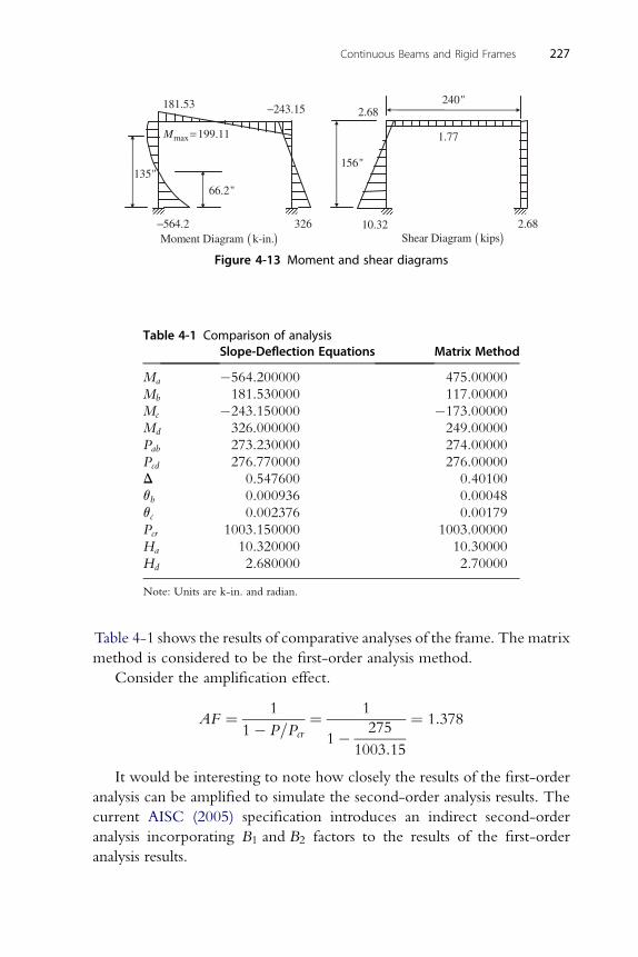

Table 4-1 Comparison of analysisSlope-Deflection Equations Matrix Method

Ma �564.200000 475.00000

Mb 181.530000 117.00000

Mc �243.150000 �173.00000

Md 326.000000 249.00000

Pab 273.230000 274.00000

Pcd 276.770000 276.00000

D 0.547600 0.40100

qb 0.000936 0.00048

qc 0.002376 0.00179

Pcr 1003.150000 1003.00000

Ha 10.320000 10.30000

Hd 2.680000 2.70000

Note: Units are k-in. and radian.

240"

2.68

135"

181.53

564.2−

66.2"

326

243.15−

156"

10.32

1.77max 199.11M =

( )Shear Diagram kips( )Moment Diagram k-in.

2.68

Figure 4-13 Moment and shear diagrams

Continuous Beams and Rigid Frames 227

Table 4-1 shows the results of comparative analyses of the frame. The matrix

method is considered to be the first-order analysis method.

Consider the amplification effect.

AF ¼ 1

1� P=Pcr¼ 1

1� 275

1003:15

¼ 1:378

It would be interesting to note how closely the results of the first-order

analysis can be amplified to simulate the second-order analysis results. The

current AISC (2005) specification introduces an indirect second-order

analysis incorporating B1 and B2 factors to the results of the first-order

analysis results.

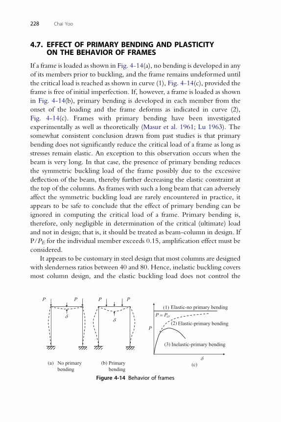
228 Chai Yoo

4.7. EFFECT OF PRIMARY BENDING AND PLASTICITYON THE BEHAVIOR OF FRAMES

If a frame is loaded as shown in Fig. 4-14(a), no bending is developed in any

of its members prior to buckling, and the frame remains undeformed until

the critical load is reached as shown in curve (1), Fig. 4-14(c), provided the

frame is free of initial imperfection. If, however, a frame is loaded as shown

in Fig. 4-14(b), primary bending is developed in each member from the

onset of the loading and the frame deforms as indicated in curve (2),

Fig. 4-14(c). Frames with primary bending have been investigated

experimentally as well as theoretically (Masur et al. 1961; Lu 1963). The

somewhat consistent conclusion drawn from past studies is that primary

bending does not significantly reduce the critical load of a frame as long as

stresses remain elastic. An exception to this observation occurs when the

beam is very long. In that case, the presence of primary bending reduces

the symmetric buckling load of the frame possibly due to the excessive

deflection of the beam, thereby further decreasing the elastic constraint at

the top of the columns. As frames with such a long beam that can adversely

affect the symmetric buckling load are rarely encountered in practice, it

appears to be safe to conclude that the effect of primary bending can be

ignored in computing the critical load of a frame. Primary bending is,

therefore, only negligible in determination of the critical (ultimate) load

and not in design; that is, it should be treated as beam-column in design. If

P/PE for the individual member exceeds 0.15, amplification effect must be

considered.

It appears to be customary in steel design that most columns are designed

with slenderness ratios between 40 and 80. Hence, inelastic buckling covers

most column design, and the elastic buckling load does not control the

P

δδ

P

crP = P

P PElastic-no primary bending

PElastic-primary bending

Inelastic-primary bending

Primarybending

(a) (b)

(1)

(2)

(3)

(c)No primarybending

δ

Figure 4-14 Behavior of frames

Continuous Beams and Rigid Frames 229

design. Frames having columns in this range will fail at a load that is smaller

than the elastic critical load as shown in curve (2), Fig. 4-14(c). Frequently,

an elastic second-order analysis as shown in curve (2), Fig. 4-14, is very

deceptive unless the stress level is checked at every step.

If instability were the only factor leading to collapse, failure would

occur at the critical load. If collapse were solely due to the plasticity effect,

the frame would fail when it becomes a mechanism due to formation of

plastic hinge(s). In the actual case, both instability and plasticity are

present, and collapse occurs due to an interaction of these two at a load

that is lower than either the critical load or the mechanism load. To

predict this kind of failure load, Horne and Merchant (1965) proposed

the following empirical interaction equation, known as the Rankine

equation:

Pf

Peþ Pf

Pp¼ 1:0 (4.7.1)

Equation (4.7.1) can be rearranged into a convenient form as

Pf ¼ PpPe

Pe þ Pp(4.7.2)

where

Pf ¼ failure load

Pe ¼ elastic buckling load

P ¼ plastic mechanism load

p

Although Horne and Merchant demonstrated the reasonableness of the

proposed Rankine equation by a scattering chart of experimental data, the

data do not appear to be representative of a wide spectrum of plausible cases.

It appears that if Pe is greater than 3 times Pp, Eq. (4.7.1) overestimates the

failure load. It was noted that if Pe is less than 3 times Pp, the scatter of points

away from Eq. (4.7.2) becomes considerable. The derivation of Eq. (4.7.1)

is conservative. Hence, Eq. (4.7.2) might be used to give rapid, but safe,

estimates of Pf. Since an access to a general-purpose finite element code

such as ABAQUS (2006) is readily available to most academics and prac-

titioners and a much better estimate can be obtained with the computer, the

attractiveness of Merchant’s use of the Rankine equation is greatly dimin-

ished. Examples of refined analyses include Alvarez and Birnstiel (1969) and

Ojalvo and Lu (1961). Further treatises of this important topic are presented

by Galambos (1968).

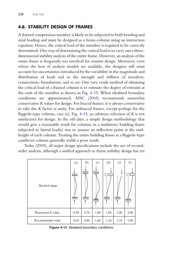
230 Chai Yoo

4.8. STABILITY DESIGN OF FRAMES

A framed compression member is likely to be subjected to both bending and

axial loading and must be designed as a beam-column using an interaction

equation. Hence, the critical load of the member is required to be correctly

determined. One way of determining the critical load is to carry out a three-

dimensional stability analysis of the entire frame. However, an analysis of the

entire frame is frequently too involved for routine design. Moreover, even

where the best of analysis models are available, the designer still must

account for uncertainties introduced by the variability in the magnitude and

distribution of loads and in the strength and stiffness of members,

connections, foundations, and so on. One very crude method of obtaining

the critical load of a framed column is to estimate the degree of restraint at

the ends of the member as shown in Fig. 4-15. When idealized boundary

conditions are approximated, AISC (2005) recommends somewhat

conservative K values for design. For braced frames, it is always conservative

to take the K factor as unity. For unbraced frames, except perhaps for the

flagpole-type column, case (e), Fig. 4-15, an arbitrary selection of K is not

satisfactory for design. In the old days, a simple design methodology that

would give a reasonable result for columns in a multistory building frame

subjected to lateral load(s) was to assume an inflection point at the mid-

height of each column. Treating the entire building frame as a flagpole-type

cantilever column generally yields a poor result.

Today (2009), all major design specifications include the use of second-

order analysis, although a unified approach to frame stability design has yet

(a) (b) (c) (d) (e) (f)

0.80

0.50 0.70 1.00 1.00 2.00 2.00

0.65 1.00 1.20 2.10 2.00

Buckled shape

Theoretical K value

Recommended value

Figure 4-15 Idealized boundary conditions

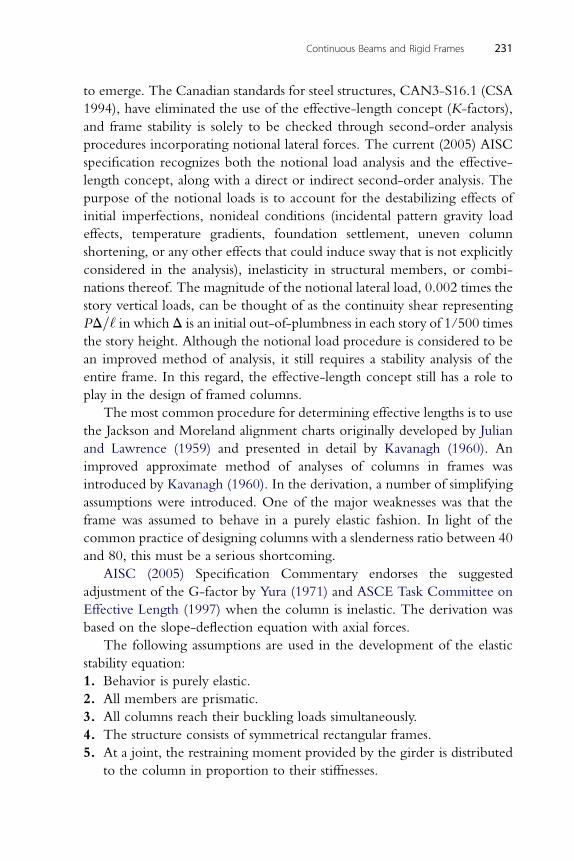
Continuous Beams and Rigid Frames 231

to emerge. The Canadian standards for steel structures, CAN3-S16.1 (CSA

1994), have eliminated the use of the effective-length concept (K-factors),

and frame stability is solely to be checked through second-order analysis

procedures incorporating notional lateral forces. The current (2005) AISC

specification recognizes both the notional load analysis and the effective-

length concept, along with a direct or indirect second-order analysis. The

purpose of the notional loads is to account for the destabilizing effects of

initial imperfections, nonideal conditions (incidental pattern gravity load

effects, temperature gradients, foundation settlement, uneven column

shortening, or any other effects that could induce sway that is not explicitly

considered in the analysis), inelasticity in structural members, or combi-

nations thereof. The magnitude of the notional lateral load, 0.002 times the

story vertical loads, can be thought of as the continuity shear representing

PD=‘ in which D is an initial out-of-plumbness in each story of 1/500 times

the story height. Although the notional load procedure is considered to be

an improved method of analysis, it still requires a stability analysis of the

entire frame. In this regard, the effective-length concept still has a role to

play in the design of framed columns.

The most common procedure for determining effective lengths is to use

the Jackson and Moreland alignment charts originally developed by Julian

and Lawrence (1959) and presented in detail by Kavanagh (1960). An

improved approximate method of analyses of columns in frames was

introduced by Kavanagh (1960). In the derivation, a number of simplifying

assumptions were introduced. One of the major weaknesses was that the

frame was assumed to behave in a purely elastic fashion. In light of the

common practice of designing columns with a slenderness ratio between 40

and 80, this must be a serious shortcoming.

AISC (2005) Specification Commentary endorses the suggested

adjustment of the G-factor by Yura (1971) and ASCE Task Committee on

Effective Length (1997) when the column is inelastic. The derivation was

based on the slope-deflection equation with axial forces.

The following assumptions are used in the development of the elastic

stability equation:

1. Behavior is purely elastic.

2. All members are prismatic.

3. All columns reach their buckling loads simultaneously.

4. The structure consists of symmetrical rectangular frames.

5. At a joint, the restraining moment provided by the girder is distributed

to the column in proportion to their stiffnesses.

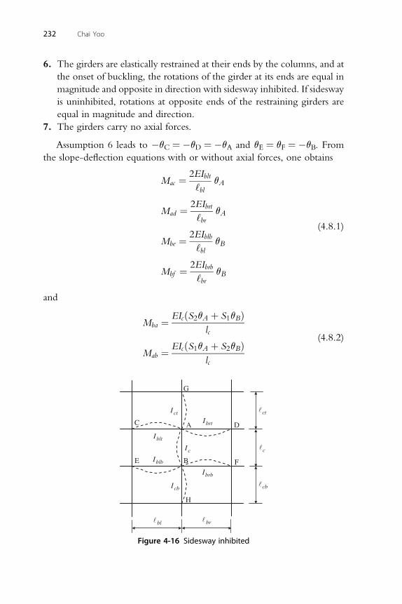
232 Chai Yoo

6. The girders are elastically restrained at their ends by the columns, and at

the onset of buckling, the rotations of the girder at its ends are equal in

magnitude and opposite in direction with sidesway inhibited. If sidesway

is uninhibited, rotations at opposite ends of the restraining girders are

equal in magnitude and direction.

7. The girders carry no axial forces.

Assumption 6 leads to �qC ¼ �qD ¼ �qA and qE ¼ qF ¼ �qB. From

the slope-deflection equations with or without axial forces, one obtains

Mac ¼ 2EIblt

‘blqA

Mad ¼ 2EIbrt

‘brqA

Mbe ¼ 2EIblb

‘blqB

Mbf ¼ 2EIbrb

‘brqB

(4.8.1)

and

Mba ¼ EIcðS2qA þ S1qBÞlc

Mab ¼ EIcðS1qA þ S2qBÞlc

(4.8.2)

F

A

B

C D

E

bll

cl

ctlctI

cblcbI

cI

brl

bltI

brtI

blbI

brbI

G

H

Figure 4-16 Sidesway inhibited

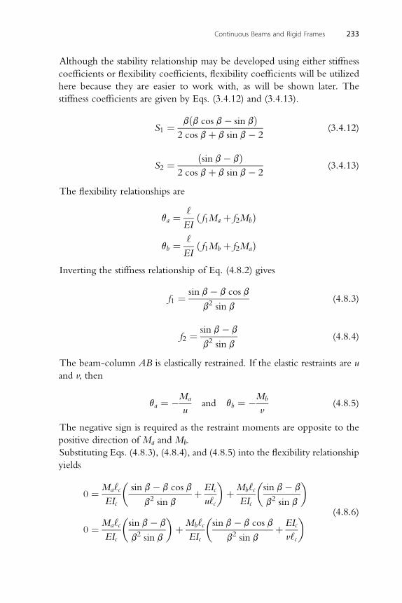
Continuous Beams and Rigid Frames 233

Although the stability relationship may be developed using either stiffness

coefficients or flexibility coefficients, flexibility coefficients will be utilized

here because they are easier to work with, as will be shown later. The

stiffness coefficients are given by Eqs. (3.4.12) and (3.4.13).

S1 ¼ bðb cos b� sin bÞ2 cos bþ b sin b� 2

(3.4.12)

S2 ¼ ðsin b� bÞ2 cos bþ b sin b� 2

(3.4.13)

The flexibility relationships are

qa ¼ ‘

EIð f1Ma þ f2MbÞ

qb ¼ ‘

EIð f1Mb þ f2MaÞ

Inverting the stiffness relationship of Eq. (4.8.2) gives

f1 ¼ sin b� b cos b

b2 sin b(4.8.3)

sin b� b

f2 ¼

b2 sin b(4.8.4)

The beam-column AB is elastically restrained. If the elastic restraints are u

and v, then

qa ¼ �Ma

uand qb ¼ �Mb

v(4.8.5)

The negative sign is required as the restraint moments are opposite to the

positive direction of Ma and Mb.

Substituting Eqs. (4.8.3), (4.8.4), and (4.8.5) into the flexibility relationship

yields

0 ¼ Ma‘cEIc

�sin b� b cos b

b2 sin bþ EIc

u‘c

�þMb‘c

EIc

�sin b� b

b2 sin b

�

0 ¼ Ma‘cEIc

�sin b� b

b2 sin b

�þMb‘c

EIc

�sin b� b cos b

b2 sin bþ EIc

v‘c

� (4.8.6)

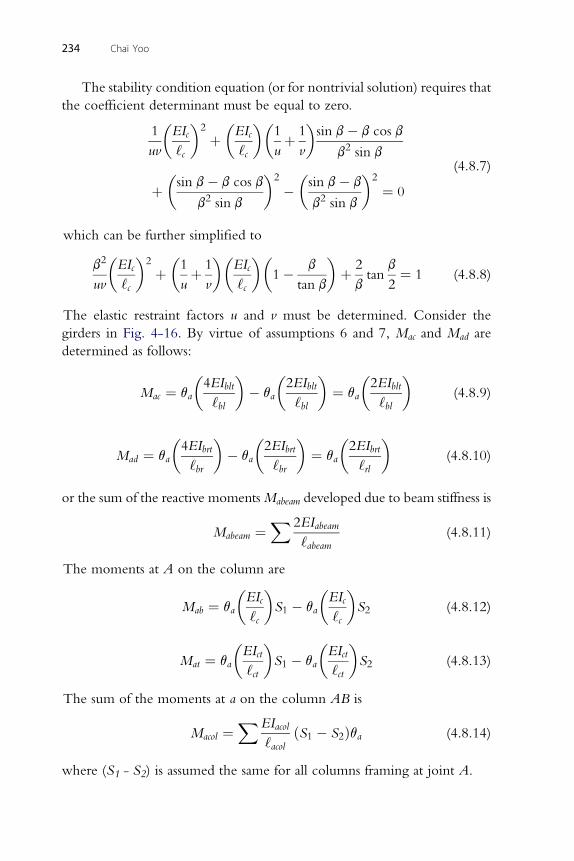
234 Chai Yoo

The stability condition equation (or for nontrivial solution) requires that

the coefficient determinant must be equal to zero.

1

uv

�EIc

‘c

�2

þ�EIc

‘c

��1

uþ 1

v

�sin b� b cos b

b2 sin b

þ�sin b� b cos b

b2 sin b

�2

��sin b� b

b2 sin b

�2

¼ 0

(4.8.7)

which can be further simplified to

b2

uv

�EIc

‘c

�2

þ�1

uþ 1

v

��EIc

‘c

��1� b

tan b

�þ 2

btan

b

2¼ 1 (4.8.8)

The elastic restraint factors u and v must be determined. Consider the

girders in Fig. 4-16. By virtue of assumptions 6 and 7, Mac and Mad are

determined as follows:

Mac ¼ qa

�4EIblt

‘bl

�� qa

�2EIblt

‘bl

�¼ qa

�2EIblt

‘bl

�(4.8.9)

� � � � � �

Mad ¼ qa

4EIbrt

‘br� qa

2EIbrt

‘br¼ qa

2EIbrt

‘rl(4.8.10)

or the sum of the reactive momentsMabeam developed due to beam stiffness is

Mabeam ¼X 2EIabeam

‘abeam(4.8.11)

The moments at A on the column are

Mab ¼ qa

�EIc

‘c

�S1 � qa

�EIc

‘c

�S2 (4.8.12)

� � � �

Mat ¼ qa

EIct

‘ctS1 � qa

EIct

‘ctS2 (4.8.13)

The sum of the moments at a on the column AB is

Macol ¼XEIacol

‘acolðS1 � S2Þqa (4.8.14)

where (S1 - S2) is assumed the same for all columns framing at joint A.

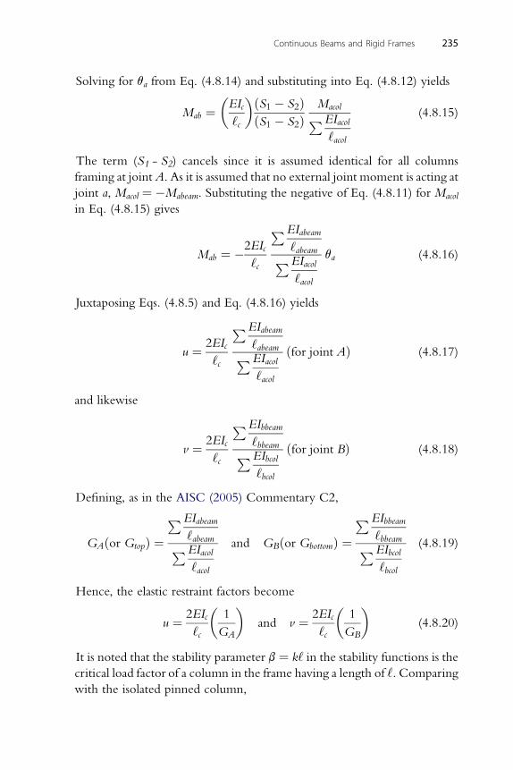
Continuous Beams and Rigid Frames 235

Solving for qa from Eq. (4.8.14) and substituting into Eq. (4.8.12) yields

Mab ¼�EIc

‘c

�ðS1 � S2ÞðS1 � S2Þ

MacolPEIacol

‘acol

(4.8.15)

The term (S1 - S2) cancels since it is assumed identical for all columns

framing at jointA. As it is assumed that no external joint moment is acting at

joint a, Macol ¼ �Mabeam. Substituting the negative of Eq. (4.8.11) for Macol

in Eq. (4.8.15) gives

Mab ¼ �2EIc

‘c

PEIabeam

‘abeamPEIacol

‘acol

qa (4.8.16)

Juxtaposing Eqs. (4.8.5) and Eq. (4.8.16) yields

u ¼ 2EIc

‘c

PEIabeam

‘abeamPEIacol

‘acol

ðfor joint AÞ (4.8.17)

and likewise

v ¼ 2EIc

‘c

PEIbbeam

‘bbeamPEIbcol

‘bcol

ðfor joint BÞ (4.8.18)

Defining, as in the AISC (2005) Commentary C2,

GAðor GtopÞ ¼PEIabeam

‘abeamPEIacol

‘acol

and GBðor GbottomÞ ¼PEIbbeam

‘bbeamPEIbcol

‘bcol

(4.8.19)

Hence, the elastic restraint factors become

u ¼ 2EIc

‘c

�1

GA

�and v ¼ 2EIc

‘c

�1

GB

�(4.8.20)

It is noted that the stability parameter b ¼ k‘ in the stability functions is the

critical load factor of a column in the frame having a length of ‘. Comparing

with the isolated pinned column,

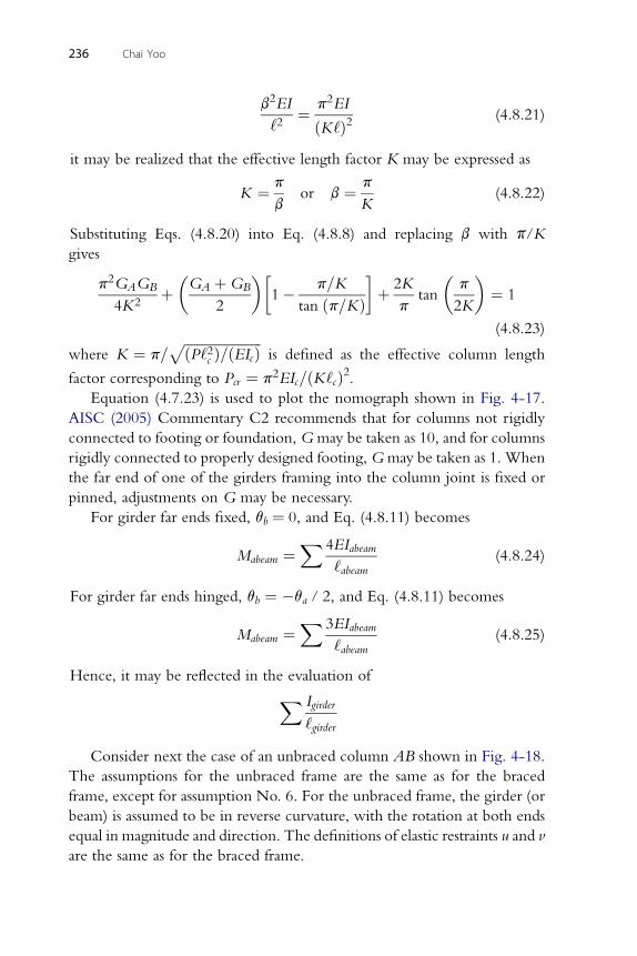
236 Chai Yoo

b2EI

‘2¼ p2EI

ðK‘Þ2 (4.8.21)

it may be realized that the effective length factor K may be expressed as

K ¼ p

bor b ¼ p

K(4.8.22)

Substituting Eqs. (4.8.20) into Eq. (4.8.8) and replacing b with p/Kgives

p2GAGB

4K2þ�GA þGB

2

��1� p=K

tan ðp=KÞ�þ 2K

ptan

�p

2K

�¼ 1

(4.8.23)

where K ¼ p=ffiffiffiffiffiffiffiffiffiffiffiffiffiffiffiffiffiffiffiffiffiffiffiðP‘2c Þ=ðEIcÞ

pis defined as the effective column length

factor corresponding to Pcr ¼ p2EIc=ðK‘cÞ2.Equation (4.7.23) is used to plot the nomograph shown in Fig. 4-17.

AISC (2005) Commentary C2 recommends that for columns not rigidly

connected to footing or foundation, Gmay be taken as 10, and for columns

rigidly connected to properly designed footing,Gmay be taken as 1. When

the far end of one of the girders framing into the column joint is fixed or

pinned, adjustments on G may be necessary.

For girder far ends fixed, qb ¼ 0, and Eq. (4.8.11) becomes

Mabeam ¼X 4EIabeam

‘abeam(4.8.24)

For girder far ends hinged, qb ¼ �qa / 2, and Eq. (4.8.11) becomes

Mabeam ¼X 3EIabeam

‘abeam(4.8.25)

Hence, it may be reflected in the evaluation ofX Igirder

‘girder

Consider next the case of an unbraced column AB shown in Fig. 4-18.

The assumptions for the unbraced frame are the same as for the braced

frame, except for assumption No. 6. For the unbraced frame, the girder (or

beam) is assumed to be in reverse curvature, with the rotation at both ends

equal in magnitude and direction. The definitions of elastic restraints u and v

are the same as for the braced frame.

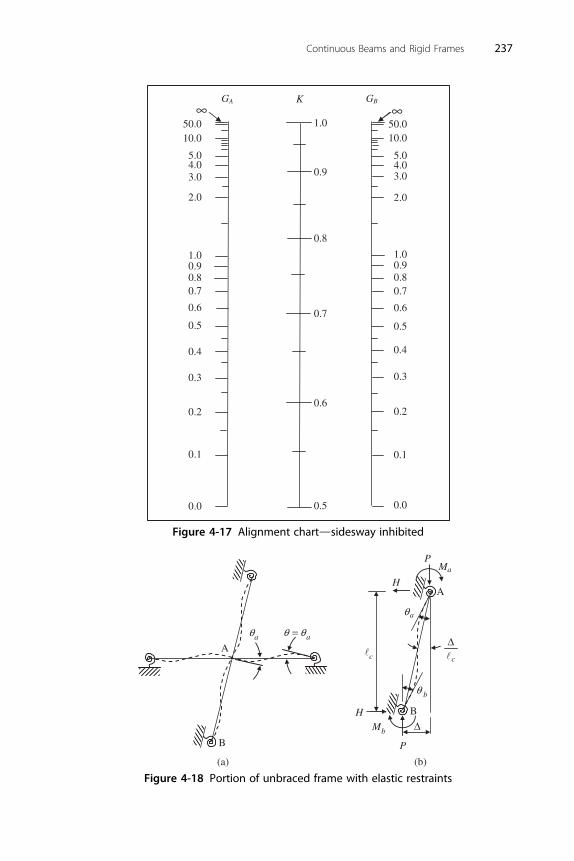
50.010.0

50.010.0

∞

0.9

5.0

3.0

1.0

4.0

2.0

0.80.7

0.6

0.5

0.4

0.2

0.1

0.0

0.3

∞

5.0

3.04.0

2.0

1.0

0.80.9

0.7

0.6

0.5

0.4

0.3

0.2

0.1

0.0 0.5

0.6

0.7

0.9

1.0

0.8

GBGA K

Figure 4-17 Alignment chartdsidesway inhibited

(a) (b)

P

P

aθ θ=A

B

aθ

c�

aM

H

H

bM Δ

A

aθ

bθ

c

Δ�

B

Figure 4-18 Portion of unbraced frame with elastic restraints

Continuous Beams and Rigid Frames 237

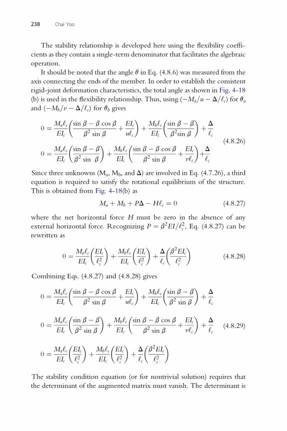
238 Chai Yoo

The stability relationship is developed here using the flexibility coeffi-

cients as they contain a single-term denominator that facilitates the algebraic

operation.

It should be noted that the angle q in Eq. (4.8.6) was measured from the

axis connecting the ends of the member. In order to establish the consistent

rigid-joint deformation characteristics, the total angle as shown in Fig. 4-18

(b) is used in the flexibility relationship. Thus, using (�Ma=u� D=‘c) for qaand (�Mb=v � D=‘c) for qb gives

0 ¼ Ma‘cEIc

�sin b� b cos b

b2 sin bþ EIc

u‘c

�þMb‘c

EIc

�sin b� b

b2sin b

�þ D

‘c

0 ¼ Ma‘cEIc

�sin b� b

b2 sin b

�þMb‘c

EIc

�sin b� b cos b

b2 sin bþ EIc

v‘c

�þD

‘c

(4.8.26)

Since three unknowns (Ma, Mb, and D) are involved in Eq. (4.7.26), a third

equation is required to satisfy the rotational equilibrium of the structure.

This is obtained from Fig. 4-18(b) as

Ma þMb þ PD�H‘c ¼ 0 (4.8.27)

where the net horizontal force H must be zero in the absence of any

external horizontal force. Recognizing P ¼ b2EI=‘2c , Eq. (4.8.27) can be

rewritten as

0 ¼ Ma‘cEIc

�EIc

‘2c

�þMb‘c

EIc

�EIc

‘2c

�þ D

‘c

�b2EIc

‘2c

�(4.8.28)

Combining Eqs. (4.8.27) and (4.8.28) gives

0 ¼ Ma‘cEIc

�sin b� b cos b

b2 sin bþ EIc

u‘c

�þMb‘c

EIc

�sin b� b

b2 sin b

�þ D

‘c

0 ¼ Ma‘cEIc

�sin b� b

b2 sin b

�þMb‘c

EIc

�sin b� b cos b

b2 sin bþ EIc

v‘c

�þ D

‘c

0 ¼ Ma‘cEIc

�EIc

‘2c

�þMb‘c

EIc

�EIc

‘2c

�þ D

‘c

�b2EIc

‘2c

�(4.8.29)

The stability condition equation (or for nontrivial solution) requires that

the determinant of the augmented matrix must vanish. The determinant is

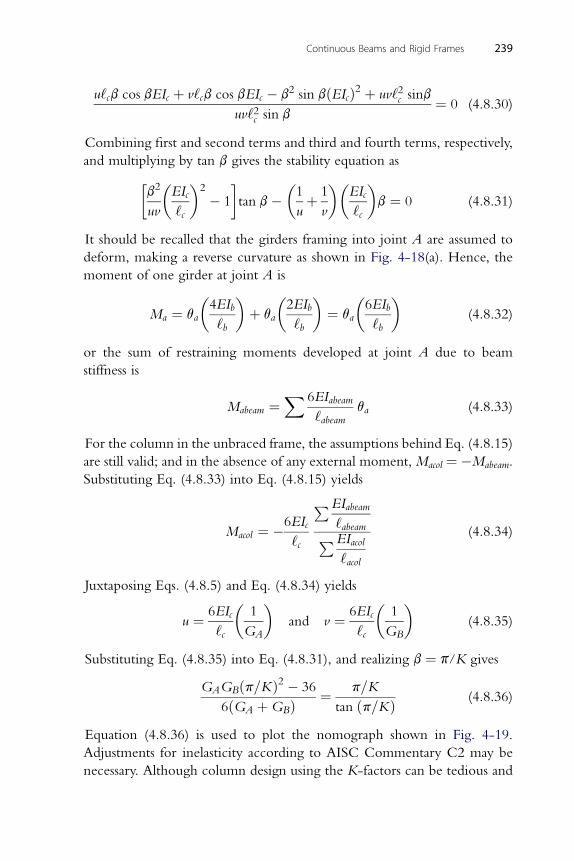
Continuous Beams and Rigid Frames 239

u‘cb cos bEIc þ v‘cb cos bEIc � b2 sin bðEIcÞ2 þ uv‘2c sinb

uv‘2c sin b¼ 0 (4.8.30)

Combining first and second terms and third and fourth terms, respectively,

and multiplying by tan b gives the stability equation as�b2

uv

�EIc

‘c

�2

� 1

�tan b�

�1

uþ 1

v

��EIc

‘c

�b ¼ 0 (4.8.31)

It should be recalled that the girders framing into joint A are assumed to

deform, making a reverse curvature as shown in Fig. 4-18(a). Hence, the

moment of one girder at joint A is

Ma ¼ qa

�4EIb

‘b

�þ qa

�2EIb

‘b

�¼ qa

�6EIb

‘b

�(4.8.32)

or the sum of restraining moments developed at joint A due to beam

stiffness is

Mabeam ¼X 6EIabeam

‘abeamqa (4.8.33)

For the column in the unbraced frame, the assumptions behind Eq. (4.8.15)

are still valid; and in the absence of any external moment, Macol ¼ �Mabeam.

Substituting Eq. (4.8.33) into Eq. (4.8.15) yields

Macol ¼ �6EIc

‘c

PEIabeam

‘abeamPEIacol

‘acol

(4.8.34)

Juxtaposing Eqs. (4.8.5) and Eq. (4.8.34) yields

u ¼ 6EIc

‘c

�1

GA

�and v ¼ 6EIc

‘c

�1

GB

�(4.8.35)

Substituting Eq. (4.8.35) into Eq. (4.8.31), and realizing b ¼ p/K gives

GAGBðp=KÞ2 � 36

6ðGA þGBÞ ¼ p=K

tan ðp=KÞ (4.8.36)

Equation (4.8.36) is used to plot the nomograph shown in Fig. 4-19.

Adjustments for inelasticity according to AISC Commentary C2 may be

necessary. Although column design using the K-factors can be tedious and

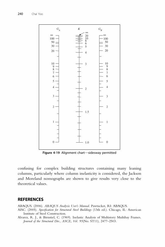
100 10050 50

3030

20 20

10 109 98 87 76 6

5 5

4 4

3 3

22

1 1

∞∞∞

GA GBK

2010865

4

3

2

1.5

1.00 0

Figure 4-19 Alignment chartdsidesway permitted

240 Chai Yoo

confusing for complex building structures containing many leaning

columns, particularly where column inelasticity is considered, the Jackson

and Moreland nomographs are shown to give results very close to the

theoretical values.

REFERENCESABAQUS. (2006). ABAQUS Analysis User’s Manual. Pawtucket, RI: ABAQUS.AISC. (2005). Specification for Structural Steel Buildings (13th ed.). Chicago, IL: American

Institute of Steel Construction.Alvarez, R. J., & Birnstiel, C. (1969). Inelastic Analysis of Multistory Multibay Frames.

Journal of the Structural Div., ASCE, Vol. 95(No. ST11), 2477–2503.

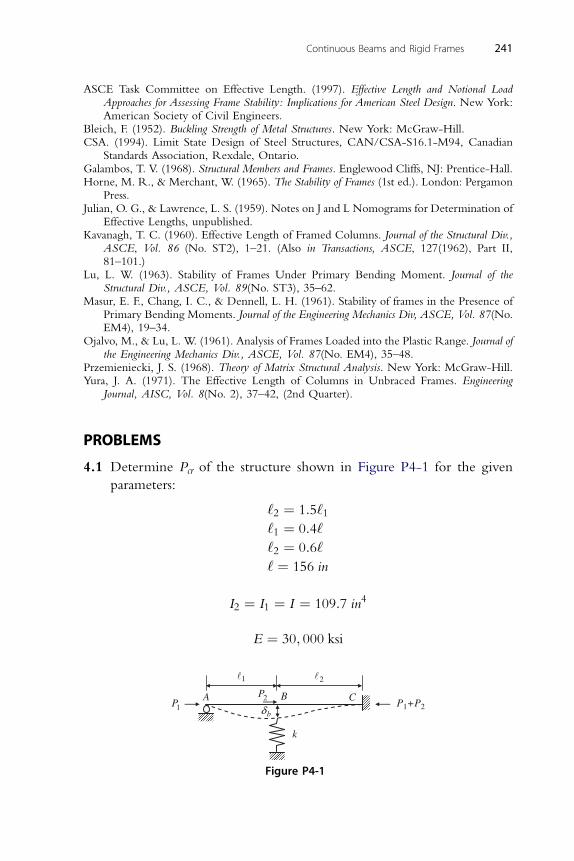
Continuous Beams and Rigid Frames 241

ASCE Task Committee on Effective Length. (1997). Effective Length and Notional LoadApproaches for Assessing Frame Stability: Implications for American Steel Design. New York:American Society of Civil Engineers.

Bleich, F. (1952). Buckling Strength of Metal Structures. New York: McGraw-Hill.CSA. (1994). Limit State Design of Steel Structures, CAN/CSA-S16.1-M94, Canadian

Standards Association, Rexdale, Ontario.Galambos, T. V. (1968). Structural Members and Frames. Englewood Cliffs, NJ: Prentice-Hall.Horne, M. R., & Merchant, W. (1965). The Stability of Frames (1st ed.). London: Pergamon

Press.Julian, O. G., & Lawrence, L. S. (1959). Notes on J and L Nomograms for Determination of

Effective Lengths, unpublished.Kavanagh, T. C. (1960). Effective Length of Framed Columns. Journal of the Structural Div.,

ASCE, Vol. 86 (No. ST2), 1–21. (Also in Transactions, ASCE, 127(1962), Part II,81–101.)

Lu, L. W. (1963). Stability of Frames Under Primary Bending Moment. Journal of theStructural Div., ASCE, Vol. 89(No. ST3), 35–62.

Masur, E. F., Chang, I. C., & Dennell, L. H. (1961). Stability of frames in the Presence ofPrimary Bending Moments. Journal of the Engineering Mechanics Div, ASCE, Vol. 87(No.EM4), 19–34.

Ojalvo, M., & Lu, L. W. (1961). Analysis of Frames Loaded into the Plastic Range. Journal ofthe Engineering Mechanics Div., ASCE, Vol. 87(No. EM4), 35–48.

Przemieniecki, J. S. (1968). Theory of Matrix Structural Analysis. New York: McGraw-Hill.Yura, J. A. (1971). The Effective Length of Columns in Unbraced Frames. Engineering

Journal, AISC, Vol. 8(No. 2), 37–42, (2nd Quarter).

PROBLEMS

4.1 Determine Pcr of the structure shown in Figure P4-1 for the given

parameters:

‘2 ¼ 1:5‘1‘1 ¼ 0:4‘

‘2 ¼ 0:6‘

‘ ¼ 156 in

4

I2 ¼ I1 ¼ I ¼ 109:7 in

E ¼ 30; 000 ksi

1l 2l

1PA B C2P

P1+P2bδ

k

Figure P4-1

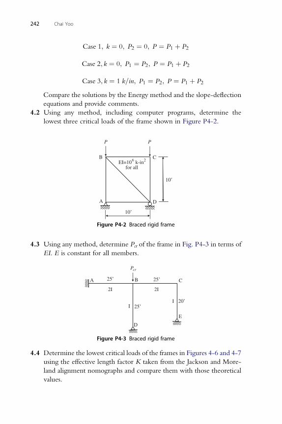
Case 1; k ¼ 0; P2 ¼ 0; P ¼ P1 þ P2

Case 2; k ¼ 0; P ¼ P ; P ¼ P þ P

242 Chai Yoo

1 2 1 2

Case 3; k ¼ 1 k=in; P ¼ P ; P ¼ P þ P

1 2 1 2

Compare the solutions by the Energy method and the slope-deflection

equations and provide comments.

4.2 Using any method, including computer programs, determine the

lowest three critical loads of the frame shown in Figure P4-2.

B

A

C

D

P

10’

10’

P

6 2EI=10 k-infor all

Figure P4-2 Braced rigid frame

4.3 Using any method, determine Pcr of the frame in Fig. P4-3 in terms of

EI. E is constant for all members.

B CA

D

E

25’ 25’

2I

II

2I

crP

25’ 20’

Figure P4-3 Braced rigid frame

4.4 Determine the lowest critical loads of the frames in Figures 4-6 and 4-7

using the effective length factor K taken from the Jackson and More-

land alignment nomographs and compare them with those theoretical

values.

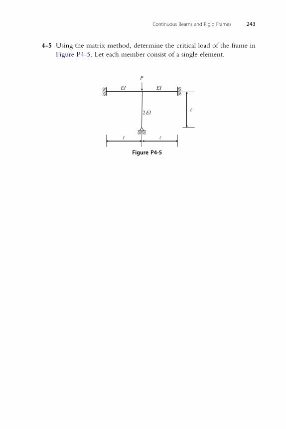
Continuous Beams and Rigid Frames 243

4-5 Using the matrix method, determine the critical load of the frame in

Figure P4-5. Let each member consist of a single element.

EI

��

2EI

P

�

EI

Figure P4-5

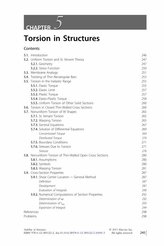
CHAPTER55

Torsion in StructuresContents

5.1. Introduction 2465.2. Uniform Torsion and St. Venant Theory 247

5.2.1. Geometry 2475.2.2. Stress Function 250

5.3. Membrane Analogy 2515.4. Twisting of Thin Rectangular Bars 2535.5. Torsion in the Inelastic Range 255

5.5.1. Elastic Torque 2555.5.2. Elastic Limit 2575.5.3. Plastic Torque 2575.5.4. Elasto-Plastic Torque 2585.5.5. Uniform Torsion of Other Solid Sections 260

5.6. Torsion in Closed Thin-Walled Cross Sections 2605.7. Nonuniform Torsion of W Shapes 265

5.7.1. St. Venant Torsion 2655.7.2. Warping Torsion 2655.7.3. General Equations 2675.7.4. Solution of Differential Equations 269

Concentrated Torque 269Distributed Torque 270

5.7.5. Boundary Conditions 2715.7.6. Stresses Due to Torsion 271

Stresses 2765.8. Nonuniform Torsion of Thin-Walled Open Cross Sections 280

5.8.1. Assumptions 2805.8.2. Symbols 2805.8.3. Warping Torsion 281

5.9. Cross-Section Properties 2875.9.1. Shear Center Location e General Method 287

Definition 287Development 287Evaluation of Integrals 290

5.9.2. Numerical Computations of Section Properties 292Determination of u 292Determination of Iux 293Expansion of Integral 294

References 298Problems 298

Stability of Structures � 2011 Elsevier Inc.ISBN 978-0-12-385122-2, doi:10.1016/B978-0-12-385122-2.10005-3 All rights reserved. 245 j

246 Chai Yoo

5.1. INTRODUCTION

Torsion in structures is perhaps one of the least-well-understood subjects in

structural mechanics. Purely torsional loading rarely occurs in structures

except in the power-transmitting shafts of automobiles or generators.

Frequently, torsion develops in structures along with bending from unin-

tended eccentricities of transverse loading due to the limitation of work-

manship or from unavoidable eccentricities as can be found in spandrel

beams.

Generally, thin-walled sections do not behave according to the law of the

plane sections employed by Euler-Bernoulli-Navier. A thin-walled section

is referred to as a rolled shape in which the thickness of an element is less

than one-tenth of the width. Many stocky rolled shapes do not meet this

definition; however, the general theory of thin-walled section developed by

Vlasov (1940, 1961) in the 1930s appears to be applicable without signifi-

cant consequences.

A thin-walled section becomes “warped” when it is subjected to end

couples (torsional moment). Hence, the cross section does not remain plane

after deformation. Exceptions to this rule are tubular sections and thin-

walled open sections in which all elements meet at a point, such as the

cruciform, angle, and tee section.

Another distinct feature of the response of structural members to torsion

is that the externally applied twisting moment is resisted internally by some

combination of uniform (or pure, or St. Venant) torsion and nonuniform

(or warping) torsion depending on the boundary conditions, that is,

whether a member is free to warp or whether warping is restrained.

Thin-walled open sections are very weak against torsion and are

susceptible to lateral-torsional buckling (or flexural-torsional buckling),

which is affected by the torsional strength of the member, even though no

intentional torsional loading is applied.

If warping does not occur or if warping is not restrained, the applied

twisting moment is entirely carried by uniform torsion. When a member is

free to warp, no internal normal stresses develop despite the warping

deformation. This is tantamount to the fact that a heated rod will not

develop any internal stresses if it is free to expand at one or both ends,

despite the temperature-induced elongation of the rod.

If warping is restrained, the member develops additional shearing

stresses, as well as normal stresses. Frequently, warping stresses are fairly high

in magnitude, and they are not to be ignored.

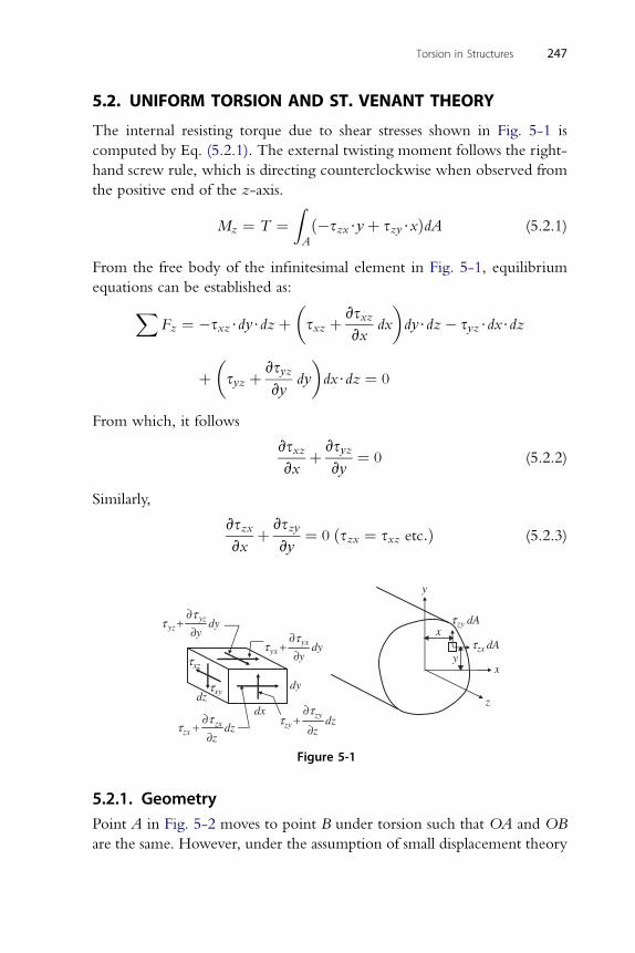
Torsion in Structures 247

5.2. UNIFORM TORSION AND ST. VENANT THEORY

The internal resisting torque due to shear stresses shown in Fig. 5-1 is

computed by Eq. (5.2.1). The external twisting moment follows the right-

hand screw rule, which is directing counterclockwise when observed from

the positive end of the z-axis.

Mz ¼ T ¼ZA

ð�szx$yþ szy$xÞdA (5.2.1)

From the free body of the infinitesimal element in Fig. 5-1, equilibrium

equations can be established as:XFz ¼ �sxz$dy$dzþ

�sxz þ vsxz

vxdx

�dy$dz� syz$dx$dz

þ�syz þ vsyz

vydy

�dx$dz ¼ 0

From which, it follows

vsxzvx

þ vsyzvy

¼ 0 (5.2.2)

Similarly,

vszxvx

þ vszyvy

¼ 0 ðszx ¼ sxz etc:Þ (5.2.3)

yxyx dy

y

ττ

∂+

∂

yzyz dy

y

ττ

∂+

∂

xzτ

xyτ

zyzy dz

z

ττ

∂+

∂zx

zx dzz

ττ

∂+

∂

dx

dydz

zy dAτ

zx dAτ

x

y

z

x

y

Figure 5-1

5.2.1. GeometryPoint A in Fig. 5-2 moves to point B under torsion such that OA and OB

are the same. However, under the assumption of small displacement theory

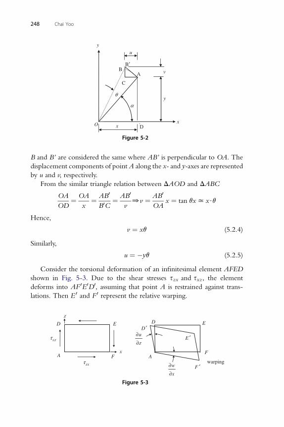
x

y

x

y

u

vAB

B′

C

O

α

θ

D.

Figure 5-2

248 Chai Yoo

B and B’ are considered the same where AB’ is perpendicular to OA. The

displacement components of pointA along the x- and y-axes are represented

by u and v, respectively.

From the similar triangle relation between DAOD and DABC

OA

OD¼ OA

x¼ AB0

B0C¼ AB0

v0v ¼ AB0

OAx ¼ tan qxx x$q

Hence,

v ¼ xq (5.2.4)

Similarly,

u ¼ �yq (5.2.5)

Consider the torsional deformation of an infinitesimal element AFED

shown in Fig. 5-3. Due to the shear stresses szx and sxz, the element

deforms into AF 0E0D0, assuming that point A is restrained against trans-

lations. Then E 0 and F 0 represent the relative warping.

w

x

∂∂

A

D

F

E

x

z

AF

F ′

E ′

EDD ′

zxτ

xzτ u

z

∂∂

warping

Figure 5-3

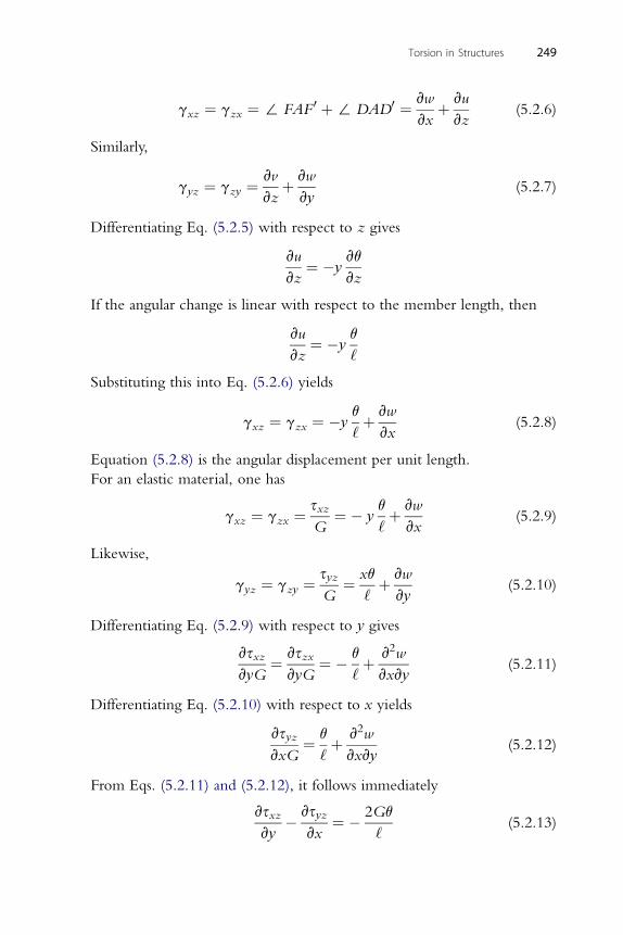
Torsion in Structures 249

gxz ¼ gzx ¼ : FAF 0 þ: DAD0 ¼ vw

vxþ vu

vz(5.2.6)

Similarly,

gyz ¼ gzy ¼vv

vzþ vw

vy(5.2.7)

Differentiating Eq. (5.2.5) with respect to z gives

vu

vz¼ �y

vq

vz

If the angular change is linear with respect to the member length, then

vu

vz¼ �y

q

‘

Substituting this into Eq. (5.2.6) yields

gxz ¼ gzx ¼ �yq

‘þ vw

vx(5.2.8)

Equation (5.2.8) is the angular displacement per unit length.

For an elastic material, one has

gxz ¼ gzx ¼sxzG

¼ � yq

‘þ vw

vx(5.2.9)

Likewise,

gyz ¼ gzy ¼syzG

¼ xq

‘þ vw

vy(5.2.10)

Differentiating Eq. (5.2.9) with respect to y gives

vsxzvyG

¼ vszxvyG

¼ � q

‘þ v2w

vxvy(5.2.11)

Differentiating Eq. (5.2.10) with respect to x yields

vsyzvxG

¼ q

‘þ v2w

vxvy(5.2.12)

From Eqs. (5.2.11) and (5.2.12), it follows immediately

vsxzvy

� vsyzvx

¼ � 2Gq

‘(5.2.13)

250 Chai Yoo

Taking partial derivatives of Eqs. (5.2.13) and (5.2.3) and adding yields

v2sxzvxvy

� v2syzvx2

¼ 0 ..ðaÞ andv2sxzvy2

� v2syzvxvy

¼ 0..ðbÞ

2 2 2 2

v sxzvx2

þ v syzvxvy

¼ 0 ..ðcÞ andv sxzvxvy

þ v syzvy2

¼ 0..ðdÞ

2 2

ðbÞ þ ðcÞ v sxzvx2

þ v sxzvy2

¼ 0

ðdÞ � ðaÞ v2syzvx2

þ v2syzvy2

¼ 0g (5.2.14)

5.2.2. Stress FunctionThe analysis of uniform torsion is greatly simplified by the fortuitous fact

that certain relationships exist between the torsion problem and the

deformations of a soap film stretched across an opening equal in size and

shape to the cross section for which torsional behavior is sought. The

membrane analogy introduced by Prandtl (1903) is applicable not only to

solid sections but also to open and closed thin-walled cross sections. Also,

the membrane analogy can be extended to inelastic and fully plastic ranges if

the concept of the soap-film is replaced by constant-slope surfaces. This was

indicated by Prandtl according to Nadai (1923) who coined the term sand-

heap analogy. Nadai (1950) also carried out many interesting experiments

illustrating the sand-heap analogy to plastic torsion.

Let

sxz ¼ szx ¼ vf

vy

syz ¼ szy ¼ �vf

vx

g (5.2.15)

It is noted that f ¼ f ðx; yÞ in Eq. (5.2.15) is a stress function introduced by

Prandtl (1903).

Substituting Eq. (5.2.15) into Eq. (5.2.13) gives

v2f

vx2þ v2f

vy2¼ � 2Gq

‘(5.2.16)

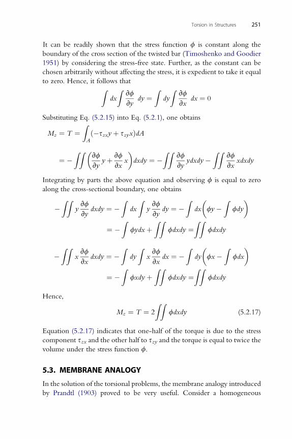
Torsion in Structures 251

It can be readily shown that the stress function f is constant along the

boundary of the cross section of the twisted bar (Timoshenko and Goodier

1951) by considering the stress-free state. Further, as the constant can be

chosen arbitrarily without affecting the stress, it is expedient to take it equal

to zero. Hence, it follows thatZdx

Zvf

vydy ¼

Zdy

Zvf

vxdx ¼ 0

Substituting Eq. (5.2.15) into Eq. (5.2.1), one obtains

Mz ¼ T ¼ZA

ð�szxyþ szyxÞdA

ZZ �vf vf

� ZZvf

ZZvf

¼ �

vyyþ

vxx dxdy ¼ �

vyydxdy�

vxxdxdy

Integrating by parts the above equation and observing f is equal to zero

along the cross-sectional boundary, one obtains

�ZZ

yvf

vydxdy ¼ �

Zdx

Zyvf

vydy ¼ �

Zdx

�fy�

Zfdy

�

¼ �Z

fydxþZZ

fdxdy ¼ZZ

fdxdy

ZZvf

Z Zvf

Z � Z �

� x

vxdxdy ¼ � dy x

vxdx ¼ � dy fx� fdx

¼ �Z

fxdyþZZ

fdxdy ¼ZZ

fdxdy

Hence,

Mz ¼ T ¼ 2

ZZfdxdy (5.2.17)

Equation (5.2.17) indicates that one-half of the torque is due to the stress

component szx and the other half to szy and the torque is equal to twice thevolume under the stress function f.

5.3. MEMBRANE ANALOGY

In the solution of the torsional problems, the membrane analogy introduced

by Prandtl (1903) proved to be very useful. Consider a homogeneous

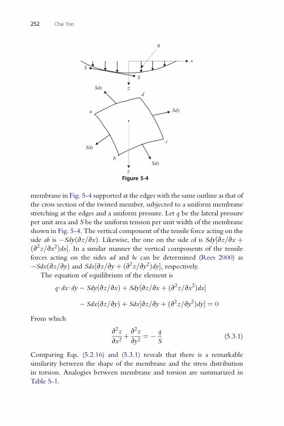
c

a

d

b

Sdy

Sdx

Sdy

Sdx

S

S

q

x

Figure 5-4

252 Chai Yoo

membrane in Fig. 5-4 supported at the edges with the same outline as that of

the cross section of the twisted member, subjected to a uniform membrane

stretching at the edges and a uniform pressure. Let q be the lateral pressure

per unit area and S be the uniform tension per unit width of the membrane

shown in Fig. 5-4. The vertical component of the tensile force acting on the

side ab is �Sdyðvz=vxÞ. Likewise, the one on the side cd is Sdy½vz=vx þðv2z=vx2Þdx�. In a similar manner the vertical components of the tensile

forces acting on the sides ad and bc can be determined (Rees 2000) as

�Sdxðvz=vyÞ and Sdx½vz=vyþ ðv2z=vy2Þdy�, respectively.The equation of equilibrium of the element is

q$dx$dy� Sdyðvz=vxÞ þ Sdy½vz=vxþ ðv2z=vx2Þdx�

� Sdxðvz=vyÞ þ Sdx½vz=vyþ ðv2z=vy2Þdy� ¼ 0

From which

v2z

vx2þ v2z

vy2¼ � q

S(5.3.1)

Comparing Eqs. (5.2.16) and (5.3.1) reveals that there is a remarkable

similarity between the shape of the membrane and the stress distribution

in torsion. Analogies between membrane and torsion are summarized in

Table 5-1.

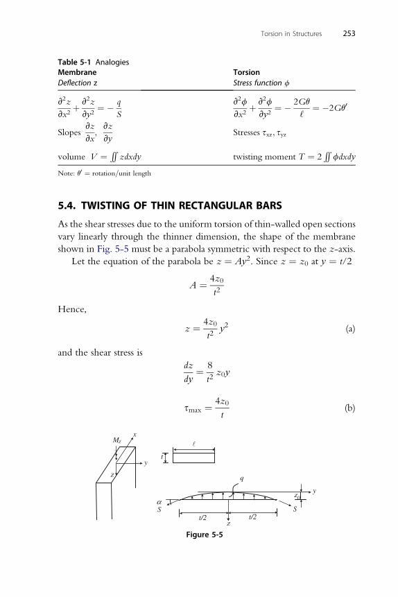
Table 5-1 AnalogiesMembrane TorsionDeflection z Stress function f

v2z

vx2þ v2z

vy2¼ � q

S

v2f

vx2þ v2f

vy2¼ � 2Gq

‘¼ �2Gq0

Slopesvz

vx;vz

vyStresses sxz; syz

volume V ¼ RR zdxdy twisting moment T ¼ 2RR

fdxdy

Note: q0 ¼ rotation=unit length

Torsion in Structures 253

5.4. TWISTING OF THIN RECTANGULAR BARS

As the shear stresses due to the uniform torsion of thin-walled open sections

vary linearly through the thinner dimension, the shape of the membrane

shown in Fig. 5-5 must be a parabola symmetric with respect to the z-axis.

Let the equation of the parabola be z ¼ Ay2. Since z ¼ z0 at y ¼ t/2

A ¼ 4z0

t2

Hence,

z ¼ 4z0

t2y2 (a)

and the shear stress is

dz

dy¼ 8

t2z0y

4z0

smax ¼t

(b)

x

y

z

z

Mz

q

t/2 t/2

y z0

�

t

S Sα

Figure 5-5

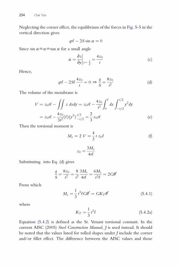
254 Chai Yoo

Neglecting the corner effect, the equilibrium of the forces in Fig. 5-5 in the

vertical direction gives

qt‘� 2S sin a ¼ 0

Since sin a^a^tan a for a small angle

a ¼ vz

vy

����z¼ t2

¼ 4z0

t(c)

Hence,

qt‘� 2S‘4z0

t¼ 0 0

q

S¼ 8z0

t2(d)

The volume of the membrane is

V ¼ z0t‘�ZZ

z dxdy ¼ z0t‘� 4z0

t2

Z ‘

0

dx

Z t=2

�t=2y2dy

¼ z0t‘� 4z0

3t2ð‘Þðy3Þ t=2�t=2

¼ 2

3z0t‘ (e)

Then the torsional moment is

Mz ¼ 2 V ¼ 4

3t z0‘ (f)

3Mz

z0 ¼

4t‘

Substituting into Eq. (d) gives

q

S¼ 8z0

t2¼ 8

t23Mz

4t‘¼ 6Mz

t3‘¼ 2Gq0

From which

Mz ¼ 1

3t3‘Gq0 ¼ GKTq

0 (5.4.1)

where

KT ¼ 1

3t3‘ (5.4.2a)

Equation (5.4.2) is defined as the St. Venant torsional constant. In the

current AISC (2005) Steel Construction Manual, J is used instead. It should

be noted that the values listed for rolled shapes under J include the corner

and/or fillet effect. The difference between the AISC values and those

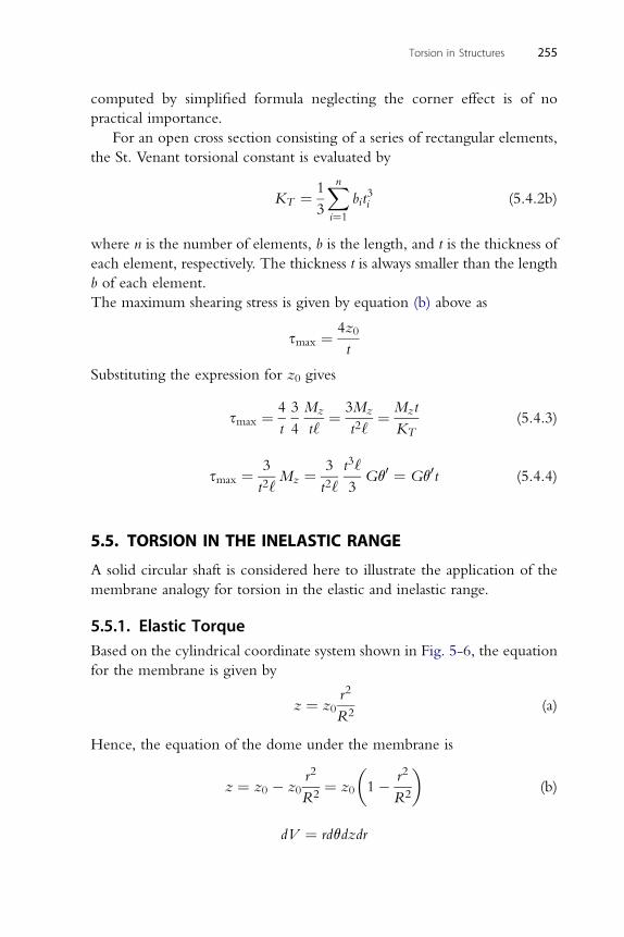
Torsion in Structures 255

computed by simplified formula neglecting the corner effect is of no

practical importance.

For an open cross section consisting of a series of rectangular elements,

the St. Venant torsional constant is evaluated by

KT ¼ 1

3

Xni¼1

bit3i (5.4.2b)

where n is the number of elements, b is the length, and t is the thickness of

each element, respectively. The thickness t is always smaller than the length

b of each element.

The maximum shearing stress is given by equation (b) above as

smax ¼ 4z0

t

Substituting the expression for z0 gives

smax ¼ 4

t

3

4

Mz

t‘¼ 3Mz

t2‘¼ Mzt

KT(5.4.3)

3 3 t3‘

smax ¼

t2‘Mz ¼

t2‘ 3Gq0 ¼ Gq0t (5.4.4)

5.5. TORSION IN THE INELASTIC RANGE

A solid circular shaft is considered here to illustrate the application of the

membrane analogy for torsion in the elastic and inelastic range.

5.5.1. Elastic TorqueBased on the cylindrical coordinate system shown in Fig. 5-6, the equation

for the membrane is given by

z ¼ z0r2

R2(a)

Hence, the equation of the dome under the membrane is

z ¼ z0 � z0r2

R2¼ z0

�1� r2

R2

�(b)

dV ¼ rdqdzdr

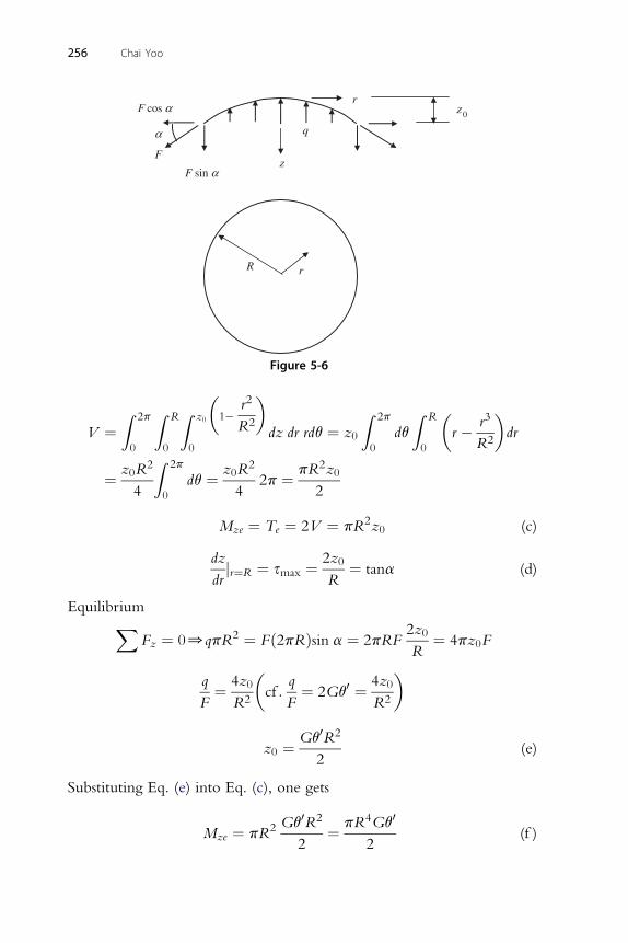
r

rR

0z

z

qα

cosF α

sinF αF

256 Chai Yoo

�r2�

V ¼Z 2p

0

Z R

0

Z z0

0

1�R2

dz dr rdq ¼ z0

Z 2p

0

dq

Z R

0

�r � r3

R2

�dr

¼ z0R2

4

Z 2p

0

dq ¼ z0R2

42p ¼ pR2z0

2

Mze ¼ Te ¼ 2V ¼ pR2z0 (c)

Figure 5-6

dz 2z0

drjr¼R ¼ smax ¼

R¼ tana (d)

EquilibriumXFz ¼ 00qpR2 ¼ Fð2pRÞsin a ¼ 2pRF

2z0

R¼ 4pz0F

q 4z0�

q 0 4z0�

F¼

R2cf :

F¼ 2Gq ¼

R2

Gq0R2

z0 ¼2

(e)

Substituting Eq. (e) into Eq. (c), one gets

Mze ¼ pR2 Gq0R2

2¼ pR4Gq0

2(f )

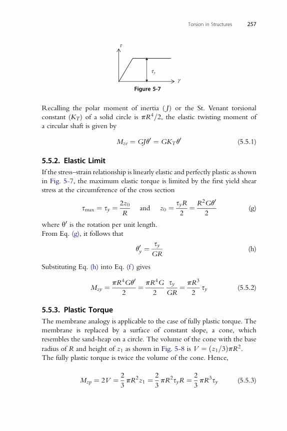
τ

γyτ

Figure 5-7

Torsion in Structures 257

Recalling the polar moment of inertia ( J ) or the St. Venant torsional

constant (KT ) of a solid circle is pR4=2, the elastic twisting moment of

a circular shaft is given by

Mze ¼ GJq0 ¼ GKTq0 (5.5.1)

5.5.2. Elastic LimitIf the stress–strain relationship is linearly elastic and perfectly plastic as shown

in Fig. 5-7, the maximum elastic torque is limited by the first yield shear

stress at the circumference of the cross section

smax ¼ sy ¼ 2z0

Rand z0 ¼ syR

2¼ R2Gq0

2(g)

where q0 is the rotation per unit length.

From Eq. (g), it follows that

q0y ¼syGR

(h)

Substituting Eq. (h) into Eq. (f ) gives

Mzy ¼ pR4Gq0

2¼ pR4G

2

syGR

¼ pR3

2sy (5.5.2)

5.5.3. Plastic TorqueThe membrane analogy is applicable to the case of fully plastic torque. The

membrane is replaced by a surface of constant slope, a cone, which

resembles the sand-heap on a circle. The volume of the cone with the base

radius of R and height of z1 as shown in Fig. 5-8 is V ¼ ðz1=3ÞpR2.

The fully plastic torque is twice the volume of the cone. Hence,

Mzp ¼ 2V ¼ 2

3pR2z1 ¼ 2

3pR2syR ¼ 2

3pR3sy (5.5.3)

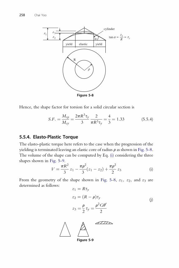
yield elastic yield

cylinder

2z α1tan y

z

Rα τ= =

R

ρ

1z 3z

Figure 5-8

258 Chai Yoo

Hence, the shape factor for torsion for a solid circular section is

S:F: ¼ Mzp

Mzy¼ 2pR3sy

3

2

pR3sy¼ 4

3¼ 1:33 (5.5.4)

5.5.4. Elasto-Plastic TorqueThe elasto-plastic torque here refers to the case when the progression of the

yielding is terminated leaving an elastic core of radius r as shown in Fig. 5-8.

The volume of the shape can be computed by Eq. (i) considering the three

shapes shown in Fig. 5-9.

V ¼ pR2

3z1 � pr2

3ðz1 � z2Þ þ pr2

2z3 (i)

From the geometry of the shape shown in Fig. 5-8, z1; z2; and z3 are

determined as follows:z1 ¼ Rsy

z2 ¼ ðR � rÞsy

z3 ¼ r

2sy ¼ r2Gq0

2

(j)

Figure 5-9

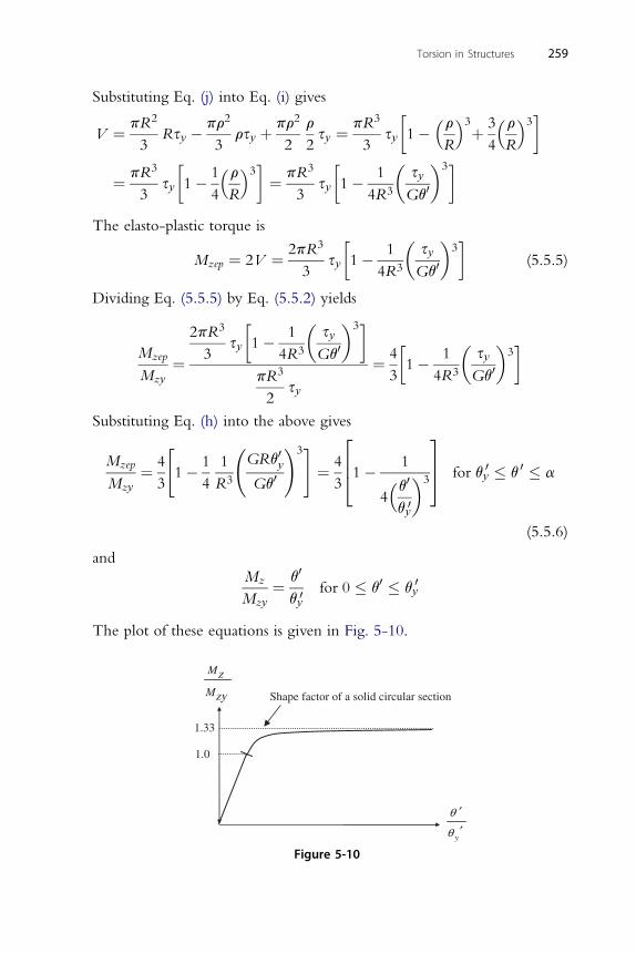
Torsion in Structures 259

Substituting Eq. (j) into Eq. (i) gives

V ¼ pR2

3Rsy � pr2

3rsy þ pr2

2

r

2sy ¼ pR3

3sy

�1�

�rR

�3þ 3

4

�rR

�3�

¼ pR3

3sy

�1� 1

4

�rR

�3� ¼ pR3

3sy

�1� 1

4R3

�syGq0

�3�

The elasto-plastic torque is

Mzep ¼ 2V ¼ 2pR3

3sy

�1� 1

4R3

�syGq0

�3�

(5.5.5)

Dividing Eq. (5.5.5) by Eq. (5.5.2) yields

Mzep

Mzy¼

2pR3

3sy

�1� 1

4R3

�syGq0

�3�pR3

2sy

¼ 4

3

�1� 1

4R3

�syGq0

�3�

Substituting Eq. (h) into the above gives

Mzep

Mzy¼ 4

3

"1� 1

4

1

R3

GRq0yGq0

!3#¼ 4

3

2641� 1

4�q0qy0

�3

375 for qy

0 � q 0 � a

(5.5.6)

and0

Mz

Mzy¼ q

qy0for 0 � q0 � qy

0

The plot of these equations is given in Fig. 5-10.

Shape factor of a solid circular section

1.33

1.0

z

zy

M

M

y

θ

θ

′

′

Figure 5-10

260 Chai Yoo

5.5.5. Uniform Torsion of Other Solid SectionsTorsion in other solid cross sections such as triangle, square, rectangle, and

prestressed bridge girders (bulb tees and AASHTO girders) is primarily res-

isted by St. Venant torsion. Using the Prandtl stress function, the St. Venant

torsional constant (KT ) can be computed for cross sections with relatively

simple boundaries such as equilateral triangle, rectangle, or even an ellipse as

demonstrated in textbookson the theoryof elasticity (for example, Saada 1974;

Sokolnokoff 1956; Timoshenko and Goodier 1951), it would be impractical

at best to apply the same procedure to bulb tees and AASHTO girders.

The shape of the soap bubble (membrane) is controlled by the second-

order partial differential equation, as shown in Table 5-1

v2z

vx2þ v2z

vy2¼ � q

S(5.5.7)

where z ¼ ordinate of membrane, x,y ¼ planar coordinates, q ¼ lateral

pressure under membrane, and S ¼ membrane tension. The St. Venant

torsional constant (KT) is related to the volume, V, of the membrane by

KT ¼ 4SV

q(5.5.8)

Equation (5.5.7) has been transformed into central differences by a Taylor

series expansion and program (Yoo 2000). Fortran source code can

be downloaded from the senior author’s Web pages. Access codes are available

from the back flap of the book. Illustrations of input and output schemes are

inserted into the source code by a liberal use of comment statements.

5.6. TORSION IN CLOSED THIN-WALLED CROSS SECTIONS

The membrane analogy developed by Prandtl (1903), which has been

successfully applied to solid cross sections, can also be used for hollow cross

sections in the same form with a condition that the inner boundary has to

correspond to a contour line of the membrane. The membrane across the-

hollow space may be considered as being replaced by a horizontal plane lid as

illustrated by Kollbrunner and Basler (1969). This satisfies the requirement of

the zero slope of the membrane over the stress-free hollow space.

The membrane analogy applies to the whole region that is contained by

the plane of the cross section, the membrane, and the lid, even though the

true membrane is only stretched across the effective area of the cross section.

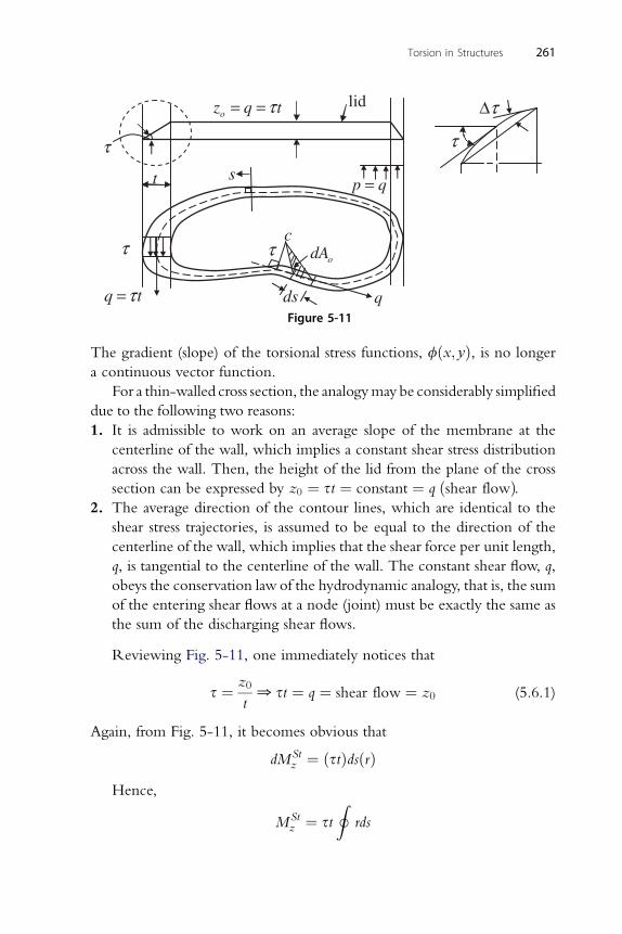
lid

t

q tτ=

τ

oz q tτ= =

p q=

odAτc

ds q

s

τΔ

τ

Figure 5-11

Torsion in Structures 261

The gradient (slope) of the torsional stress functions, fðx; yÞ, is no longer

a continuous vector function.

For a thin-walled cross section, the analogymay be considerably simplified

due to the following two reasons:

1. It is admissible to work on an average slope of the membrane at the

centerline of the wall, which implies a constant shear stress distribution

across the wall. Then, the height of the lid from the plane of the cross

section can be expressed by z0 ¼ st ¼ constant ¼ q ðshear flowÞ.2. The average direction of the contour lines, which are identical to the

shear stress trajectories, is assumed to be equal to the direction of the

centerline of the wall, which implies that the shear force per unit length,

q, is tangential to the centerline of the wall. The constant shear flow, q,

obeys the conservation law of the hydrodynamic analogy, that is, the sum

of the entering shear flows at a node (joint) must be exactly the same as

the sum of the discharging shear flows.

Reviewing Fig. 5-11, one immediately notices that

s ¼ z0

t0 st ¼ q ¼ shear flow ¼ z0 (5.6.1)

Again, from Fig. 5-11, it becomes obvious that

dMStz ¼ ðstÞdsðrÞ

Hence,

MStz ¼ st

Irds

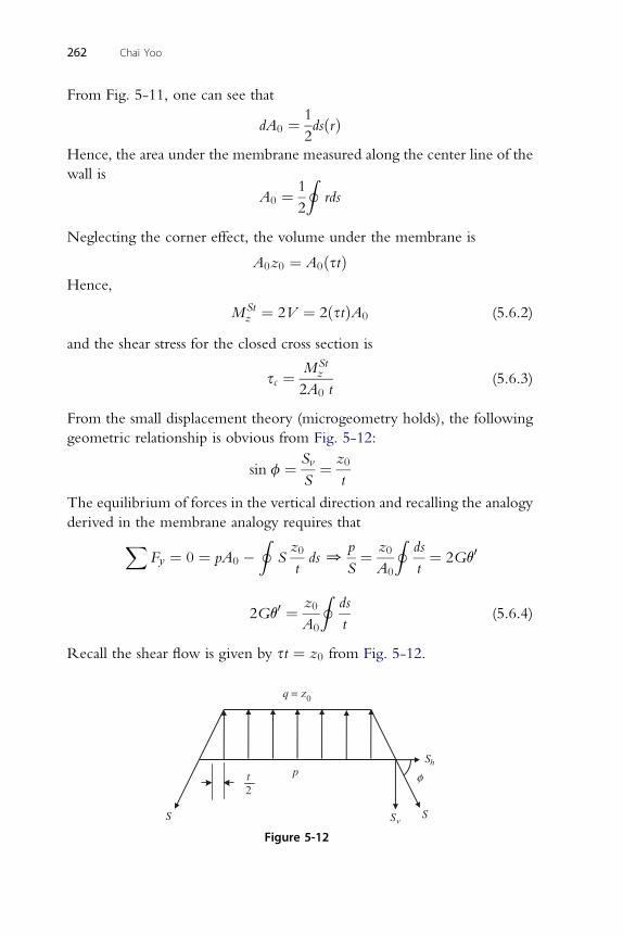
262 Chai Yoo

From Fig. 5-11, one can see that

dA0 ¼ 1

2dsðrÞ

Hence, the area under the membrane measured along the center line of the

wall is

A0 ¼ 1

2

Irds

Neglecting the corner effect, the volume under the membrane is

A0z0 ¼ A0ðstÞHence,

MStz ¼ 2V ¼ 2ðstÞA0 (5.6.2)

and the shear stress for the closed cross section is

sc ¼ MStz

2A0 t(5.6.3)

From the small displacement theory (microgeometry holds), the following

geometric relationship is obvious from Fig. 5-12:

sin f ¼ Sv

S¼ z0

t

The equilibrium of forces in the vertical direction and recalling the analogy

derived in the membrane analogy requires thatXFy ¼ 0 ¼ pA0 �

ISz0

tds 0

p

S¼ z0

A0

Ids

t¼ 2Gq0

z0I

ds

2Gq0 ¼

A0 t(5.6.4)

Recall the shear flow is given by st ¼ z0 from Fig. 5-12.

0q = z

S vS

hSp

S

φ2t

Figure 5-12

Torsion in Structures 263

The shear flow is also defined in Eq. (5.6.2) as

st ¼ MStz

2A0

Hence, the height of the membrane is

z0 ¼ MStz

2A0

It should be noted that the shear flows become indeterminate for a multi-

cellular section. As a consequence, the torsional properties of a multicellular

section become indeterminate, too.

For a single-cell section

2Gq0 ¼ MStz

2A20

Ids

t0MSt

z ¼ 4A20Gq0=

Ids

t(5.6.5)

Generally,

MStz ¼ GKTq

0 and q0 ¼ dq

dz

Therefore the St. Venant torsional constant for closed cross sections is

KTc ¼ 4A20H dst

(5.6.6)

The torsional shear stress in a closed cross section is computed from

sc ¼ MStz

2A0 t

and the general differential relationship for the St. Venant torsion is

MStz ¼ GKTq

0

Therefore, the shear stress of the closed cross section under the St. Venant

(uniform) torsion is also computed by

sc ¼ GKTcq0

2A0 t(5.6.7)

Notice that the thickness of the wall in a closed cross section is constant at

a location along the length of the member (prismatic, not a variable). It varies

only along the perimeter of the cross section. The corresponding shear stress,

torsional moment, and the St. Venant torsional constant to the open and

closed cross section shown in Fig. 5-13 are tabulated in Tables 5-2 and 5-3.

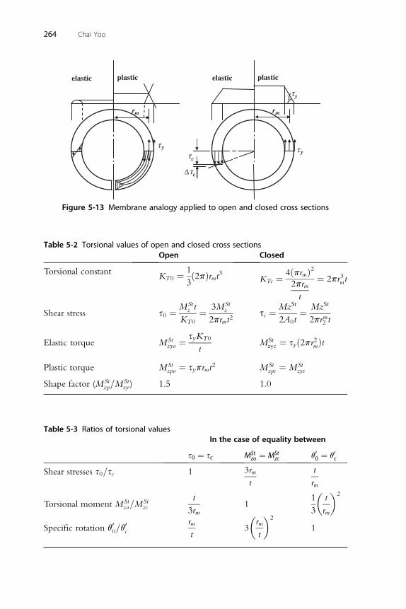
Table 5-2 Torsional values of open and closed cross sectionsOpen Closed

Torsional constantKT0 ¼ 1

3ð2pÞrmt3 KTc ¼ 4ðprmÞ2

2prm

t

¼ 2pr3mt

Shear stress s0 ¼ MStz t

KT0

¼ 3MStz

2prmt2sc ¼ MzSt

2A0t¼ MzSt

2prm2 t

Elastic torque MStzyo ¼

syKT0

tMSt

zyc ¼ syð2pr2mÞt

Plastic torque MStzpo ¼ syprmt2 MSt

zpc ¼ MStzyc

Shape factor (MStzp=M

Stzy) 1.5 1.0

mr

elastic plastic

yττ yτ

mr

elastic plastic

yτ

c

τcΔ

Figure 5-13 Membrane analogy applied to open and closed cross sections

Table 5-3 Ratios of torsional valuesIn the case of equality between

s0 ¼ sc MStzo ¼ MSt

zc q00 ¼ q0c

Shear stresses s0=sc 1 3rm

t

t

rm

Torsional moment MStzo=M

Stzc

t

3rm1

1

3

�t

rm

�2

Specific rotation q00=q0c

rm

t3

�rm

t

�2

1

264 Chai Yoo

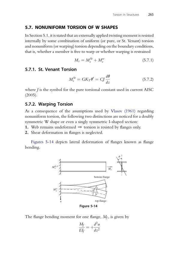
Torsion in Structures 265

5.7. NONUNIFORM TORSION OF W SHAPES

In Section 5.1, it is stated that an externally applied twistingmoment is resisted

internally by some combination of uniform (or pure, or St. Venant) torsion

and nonuniform (or warping) torsion depending on the boundary conditions,

that is, whether a member is free to warp or whether warping is restrained

Mz ¼ MStz þMw

z (5.7.1)

5.7.1. St. Venant Torsion

MStz ¼ GKTq

0 ¼ CJdq

dz(5.7.2)

where J is the symbol for the pure torsional constant used in current AISC

(2005).

5.7.2. Warping TorsionAs a consequence of the assumptions used by Vlasov (1961) regarding

nonuniform torsion, the following two distinctions are noticed for a doubly

symmetric W shape or even a singly symmetric I-shaped section:

1. Web remains undeformed 0 torsion is resisted by flanges only.

2. Shear deformation in flanges is neglected.

Figures 5-14 depicts lateral deformation of flanges known as flange

bending.

St.VM

wMd

u

bottom flange

top flange

zz

z

z

M

φ

Figure 5-14

The flange bending moment for one flange, Mf , is given by

Mf

EIf¼ þd2u

dz2

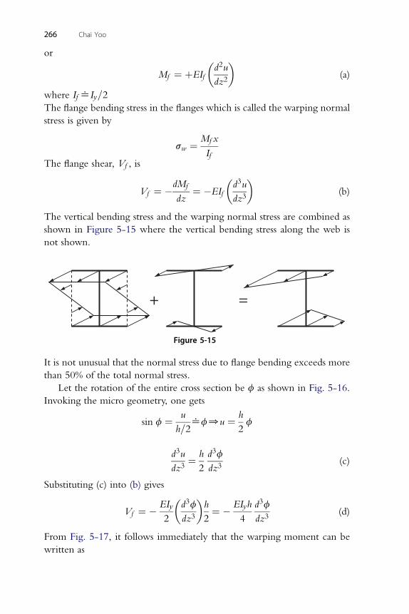
266 Chai Yoo

�d2u�

or

Mf ¼ þEIfdz2

(a)

where If^Iy=2

The flange bending stress in the flanges which is called the warping normal

stress is given by

sw ¼ Mf x

IfThe flange shear, Vf , is � �

Vf ¼ �dMf

dz¼ �EIf

d3u

dz3(b)

The vertical bending stress and the warping normal stress are combined as

shown in Figure 5-15 where the vertical bending stress along the web is

not shown.

+ =

Figure 5-15

It is not unusual that the normal stress due to flange bending exceeds more

than 50% of the total normal stress.

Let the rotation of the entire cross section be f as shown in Fig. 5-16.

Invoking the micro geometry, one gets

sin f ¼ u

h=2^f0u ¼ h

2f

d3u h d3f

dz3¼

2 dz3(c)

Substituting (c) into (b) gives

Vf ¼ � EIy

2

�d3f

dz3

�h

2¼ � EIyh

4

d3f

dz3(d)

From Fig. 5-17, it follows immediately that the warping moment can be

written as

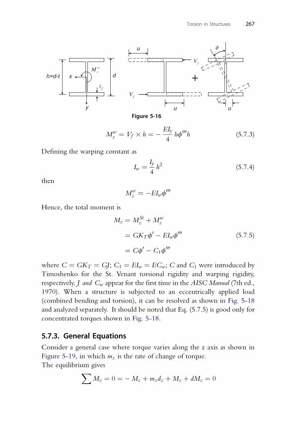
fV

y

h=d-t

wzM

x

ft

fV

+

u

φ

d

u

u

Figure 5-16

Torsion in Structures 267

Mwz ¼ Vf � h ¼ � EIy

4hf000h (5.7.3)

Defining the warping constant as

Iw ¼ Iy

4h2 (5.7.4)

then

Mwz ¼ �EIwf

000

Hence, the total moment is

Mz ¼ MStz þMw

z

¼ GKTf0 � EIwf

000

¼ Cf0 � C1f000

(5.7.5)

where C ¼ GKT ¼ GJ ; C1 ¼ EIw ¼ ECw; C and C1 were introduced by

Timoshenko for the St. Venant torsional rigidity and warping rigidity,

respectively. J and Cw appear for the first time in the AISC Manual (7th ed.,

1970). When a structure is subjected to an eccentrically applied load

(combined bending and torsion), it can be resolved as shown in Fig. 5-18

and analyzed separately. It should be noted that Eq. (5.7.5) is good only for

concentrated torques shown in Fig. 5-18.

5.7.3. General EquationsConsider a general case where torque varies along the z axis as shown in

Figure 5-19, in which mz is the rate of change of torque.

The equilibrium givesXMz ¼ 0 ¼�Mz þ mzdz þMz þ dMz ¼ 0

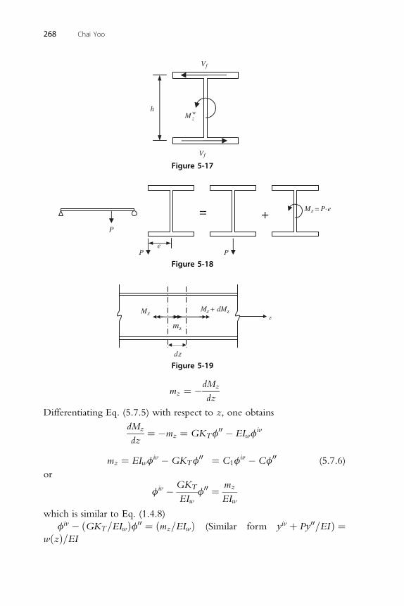
P

eP P

Mz = P·e = +

Figure 5-18

h wzM

Vf

Vf

Figure 5-17

zM + dMzMz

mz

z

268 Chai Yoo

dMz

mz ¼ �

dz

Differentiating Eq. (5.7.5) with respect to z, one obtains

dz

Figure 5-19

dMz

dz¼ �mz ¼ GKTf

00 � EIwfiv

mz ¼ EIwfiv �GKTf

00 ¼ C1fiv �Cf00 (5.7.6)

orGK m

fiv � T

EIwf00 ¼ z

EIw

which is similar to Eq. (1.4.8)

fiv � ðGKT=EIwÞf00 ¼ ðmz=EIwÞ (Similar form yiv þ Py00=EIÞ ¼wðzÞ=EI

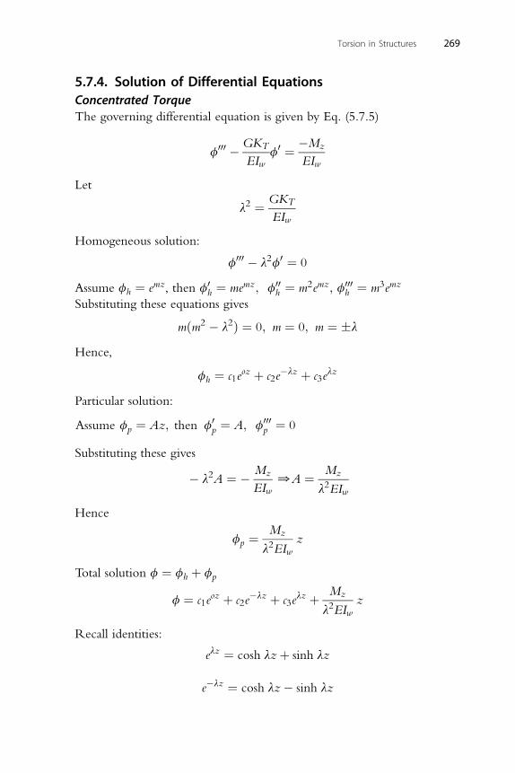
Torsion in Structures 269

5.7.4. Solution of Differential EquationsConcentrated TorqueThe governing differential equation is given by Eq. (5.7.5)

f000 �GKT

EIwf0 ¼ �Mz

EIw

Let

l2 ¼ GKT

EIw

Homogeneous solution:

f000 � l2f0 ¼ 0

Assume fh ¼ emz, then f0h ¼ memz; f00

h ¼ m2emz; f000h ¼ m3emz

Substituting these equations gives

mðm2 � l2Þ ¼ 0; m ¼ 0; m ¼ �l

Hence,

fh ¼ c1eoz þ c2e

�lz þ c3elz

Particular solution:

Assume fp ¼ Az; then f0p ¼ A; f000

p ¼ 0

Substituting these gives

� l2A ¼ � Mz

EIw0A ¼ Mz

l2EIw

Hence

fp ¼Mz

l2EIwz

Total solution f ¼ fh þ fp

f ¼ c1eoz þ c2e

�lz þ c3elz þ Mz

l2EIwz

Recall identities:

elz ¼ cosh lzþ sinh lz

�lz

e ¼ cosh lz� sinh lz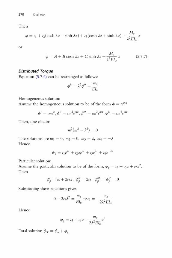

270 Chai Yoo

Then

f ¼ c1 þ c2ðcosh lz� sinh lzÞ þ c3ðcosh lzþ sinh lzÞ þ Mz

l2EIwz

or

f ¼ Aþ B cosh lzþ C sinh lzþ Mz

l2EIwz (5.7.7)

Distributed TorqueEquation (5.7.6) can be rearranged as follows:

fiv � l2f00 ¼ mz

EIw

Homogeneous solution:

Assume the homogeneous solution to be of the form f ¼ cemz

f0 ¼ cmez;f00 ¼ cm2emz;f000 ¼ cm3emz;fiv ¼ cm4emz

Then, one obtains

m2ðm2 � l2Þ ¼ 0

The solutions are m1 ¼ 0; m2 ¼ 0; m3 ¼ l; m4 ¼ �l

Hence

fh ¼ c1eoz þ c2ze

oz þ c3elz þ c4e

�lz

Particular solution:

Assume the particular solution to be of the form, fp ¼ c5 þ c6zþ c7z2.

Then

f0p ¼ c6 þ 2c7z; f00

p ¼ 2c7; f000p ¼ fiv

p ¼ 0

Substituting these equations gives

0� 2c7l2 ¼ mz

EIw0c7 ¼ � mz

2l2EIw

Hence

fp ¼ c5 þ c6z� mz

2l2EIwz2

Total solution fT ¼ fh þ fp

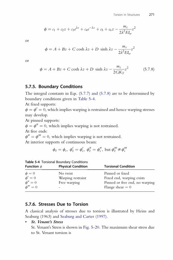
Torsion in Structures 271

f ¼ c1 þ c2zþ c3elz þ c4e

�lz þ c5 þ c6z� mz

2l2EIwz2

or

f ¼ Aþ Bzþ C cosh lzþD sinh lz� mz

2l2EIwz2

or

f ¼ Aþ Bzþ C cosh lzþD sinh lz� mz

2GKTz2 (5.7.8)

5.7.5. Boundary ConditionsThe integral constants in Eqs. (5.7.7) and (5.7.8) are to be determined by

boundary conditions given in Table 5-4.

At fixed supports:

f ¼ f0 ¼ 0, which implies warping is restrained and hence warping stresses

may develop.

At pinned supports:

f ¼ f00 ¼ 0, which implies warping is not restrained.

At free ends:

f00 ¼ f000 ¼ 0, which implies warping is not restrained.

At interior supports of continuous beam:

f‘ ¼ fr ; f0‘ ¼ f0

r ; f00‘ ¼ f00

r ; but f000‘ sf000

r

Table 5-4 Torsional Boundary ConditionsFunction f Physical Condition Torsional Condition

f ¼ 0 No twist Pinned or fixed

f0 ¼ 0 Warping restraint Fixed end, warping exists

f00 ¼ 0 Free warping Pinned or free end, no warping

f000 ¼ 0 - Flange shear ¼ 0

5.7.6. Stresses Due to TorsionA classical analysis of stresses due to torsion is illustrated by Heins and

Seaburg (1963) and Seaburg and Carter (1997).

• St. Venant’s Stress

St. Venant’s Stress is shown in Fig. 5-20. The maximum shear stress due

to St. Venant torsion is

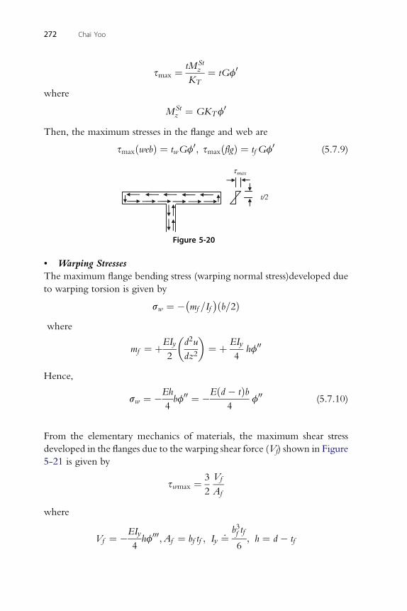
272 Chai Yoo

smax ¼ tMStz

KT¼ tGf0

where

MStz ¼ GKTf

0

Then, the maximum stresses in the flange and web are

smaxðwebÞ ¼ twGf0; smaxðflgÞ ¼ tf Gf0 (5.7.9)

t/2

τmax

Figure 5-20

• Warping Stresses

The maximum flange bending stress (warping normal stress)developed due

to warping torsion is given by

sw ¼ �mf =Ifðb=2Þ

where

mf ¼ þEIy

2

�d2u

dz2

�¼ þ EIy

4hf00

Hence,

sw ¼ �Eh

4bf00 ¼ �Eðd � tÞb

4f00 (5.7.10)

From the elementary mechanics of materials, the maximum shear stress

developed in the flanges due to the warping shear force (Vf) shown in Figure

5-21 is given by

swmax ¼ 3

2

Vf

Af

where

Vf ¼ �EIy

4hf000;Af ¼ bf tf ; Iy _¼ b3f tf

6; h ¼ d � tf

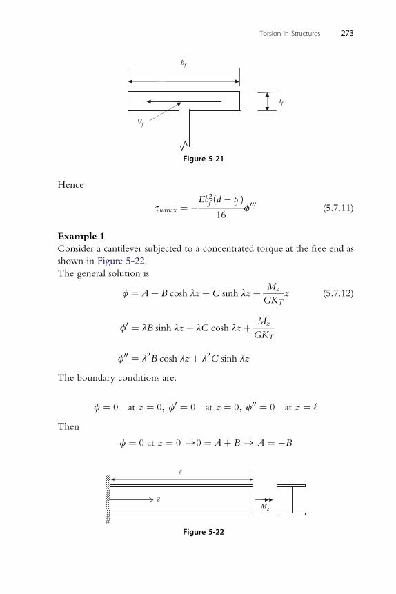
tf

Vf

bf

Figure 5-21

Torsion in Structures 273

Hence

swmax ¼ �Eb2f ðd � tf Þ16

f000 (5.7.11)

Example 1

Consider a cantilever subjected to a concentrated torque at the free end as

shown in Figure 5-22.

The general solution is

f ¼ Aþ B cosh lzþ C sinh lzþ Mz

GKTz (5.7.12)

0 Mz

f ¼ lB sinh lzþ lC cosh lzþ

GKT

00 2 2

f ¼ l B cosh lzþ l C sinh lz

The boundary conditions are:

f ¼ 0 at z ¼ 0; f0 ¼ 0 at z ¼ 0; f00 ¼ 0 at z ¼ ‘

Then

f ¼ 0 at z ¼ 0 00 ¼ Aþ B 0 A ¼ �B

�

zMz

Figure 5-22

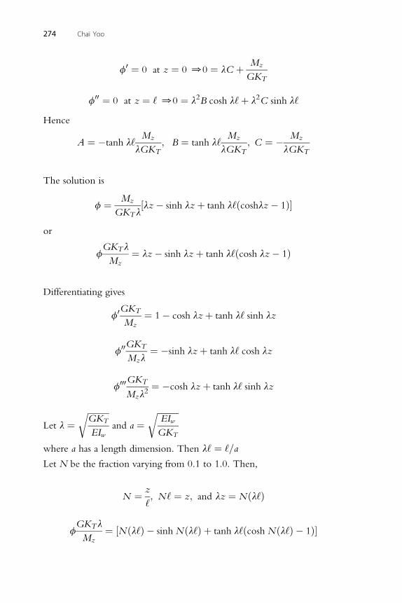
274 Chai Yoo

f0 ¼ 0 at z ¼ 0 00 ¼ lC þ Mz

GKT

f00 ¼ 0 at z ¼ ‘ 00 ¼ l2B cosh l‘þ l2C sinh l‘

Hence

A ¼ �tanh l‘Mz

lGKT; B ¼ tanh l‘

Mz

lGKT; C ¼ � Mz

lGKT

The solution is

f ¼ Mz

GKTl½lz� sinh lzþ tanh l‘ðcoshlz� 1Þ�

or

fGKTl

Mz¼ lz� sinh lzþ tanh l‘ðcosh lz� 1Þ

Differentiating gives

f0GKT

Mz¼ 1� cosh lzþ tanh l‘ sinh lz

GKT

f00

Mzl¼ �sinh lzþ tanh l‘ cosh lz

GKT

f000

Mzl2¼ �cosh lzþ tanh l‘ sinh lz

Let l ¼ffiffiffiffiffiffiffiffiffiffiGKT

EIw

rand a ¼

ffiffiffiffiffiffiffiffiffiffiEIw

GKT

rwhere a has a length dimension. Then l‘ ¼ ‘=a

Let N be the fraction varying from 0.1 to 1.0. Then,

N ¼ z

‘; N‘ ¼ z; and lz ¼ Nðl‘Þ

GK l

f

T

Mz¼ ½Nðl‘Þ � sinh Nðl‘Þ þ tanh l‘ðcosh Nðl‘Þ � 1Þ�

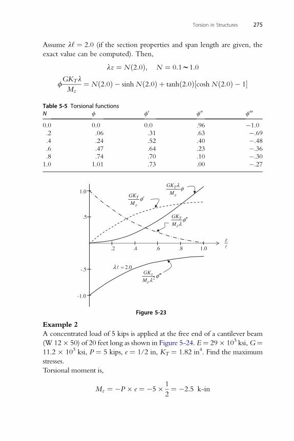
Torsion in Structures 275

Assume l‘ ¼ 2:0 (if the section properties and span length are given, the

exact value can be computed). Then,

lz ¼ Nð2:0Þ; N ¼ 0:1w1:0

fGKTl ¼ Nð2:0Þ � sinh Nð2:0Þ þ tanhð2:0Þ½cosh Nð2:0Þ � 1�

Mz

Table 5-5 Torsional functionsN f f0 f00 f000

0.0 0.0 0.0 .96 �1.0

.2 .06 .31 .63 �.69

.4 .24 .52 .40 �.48

.6 .47 .64 .23 �.36

.8 .74 .70 .10 �.30

1.0 1.01 .73 .00 �.27

-1.0

-.5

.5

�

TGK

M

λ φ1.0

.2 .4 .6 .8 1.0

2.0λ =�

TGK

Mφ

λ′′

T

z

z

z

z

zGK

Mφ′

2TGK

Mφ

λ′′′

Figure 5-23

Example 2

A concentrated load of 5 kips is applied at the free end of a cantilever beam

(W 12� 50) of 20 feet long as shown in Figure 5-24. E¼ 29� 103 ksi,G¼11.2 � 103 ksi, P ¼ 5 kips, e ¼ 1/2 in, KT ¼ 1.82 in4. Find the maximum

stresses.

Torsional moment is,

Mz ¼ �P � e ¼ �5� 1

2¼ �2:5 k-in

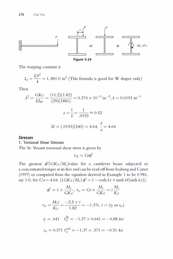
P

eP P

Mz =P·e = + .

Figure 5-24

276 Chai Yoo

The warping constant is

Iw ¼ Iyh2

4¼ 1; 881:0 in6 ðThis formula is good for W shapes onlyÞ

Then

l2 ¼ GKT

EIW¼ ð11:2Þð1:82Þ

ð29Þð1881Þ ¼ 0:374� 10�3 in�2; l ¼ 0:0193 in�1

1 1

a ¼

l¼

:0193^ 0:52

‘

l‘ ¼ ð:0193Þð240Þ ¼ 4:64;

a¼ 4:64

Stresses1. Torsional Shear StressesThe St. Venant torsional shear stress is given by

sSt ¼ Gtf0

The greatest f0ðGKT=MzÞvalue for a cantilever beam subjected to

a concentrated torque at its free end can be read off from Seaburg and Carter

(1997) or computed from the equation derived in Example 1 to be 0.981,

say 1.0, for ‘=a¼ 4:64. ððGKT=MzÞf0 ¼ 1� cosh lzþ tanh l‘ðsinh lzÞÞ.

f0 ¼ 1� Mz

GKT; sst ¼ Gt � Mz

GKT¼ t

Mz

KT

Mzt �2:5� t

sst ¼

KT¼

1:82¼ �1:37t; t ¼ ðtf or twÞ

flg

tf ¼ :641 sst ¼ �1:37� 0:641 ¼ �0:88 ksi

web

tw ¼ 0:371 sst ¼ �1:37� :371 ¼ �0:51 ksi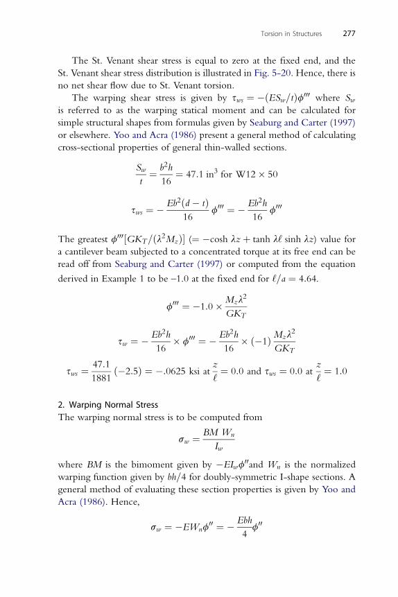

Torsion in Structures 277

The St. Venant shear stress is equal to zero at the fixed end, and the

St. Venant shear stress distribution is illustrated in Fig. 5-20. Hence, there is

no net shear flow due to St. Venant torsion.

The warping shear stress is given by sws ¼ �ðESw=tÞf000 where Swis referred to as the warping statical moment and can be calculated for

simple structural shapes from formulas given by Seaburg and Carter (1997)

or elsewhere. Yoo and Acra (1986) present a general method of calculating

cross-sectional properties of general thin-walled sections.

Sw

t¼ b2h

16¼ 47:1 in3 for W12� 50

Eb2ðd � tÞ Eb2h

sws ¼ �

16f000 ¼ �

16f000

The greatest f000½GKT=ðl2MzÞ� (¼ �cosh lzþ tanh l‘ sinh lz) value for

a cantilever beam subjected to a concentrated torque at its free end can be

read off from Seaburg and Carter (1997) or computed from the equation

derived in Example 1 to be –1.0 at the fixed end for ‘=a ¼ 4:64.

f000 ¼ �1:0�Mzl2

GKT

Eb2h Eb2h M l2

sw ¼ �

16� f000 ¼ �

16� ð�1Þ z

GKT

47:1 z z

sws ¼

1881ð�2:5Þ ¼ �:0625 ksi at

‘¼ 0:0 and sws ¼ 0:0 at

‘¼ 1:0

2. Warping Normal StressThe warping normal stress is to be computed from

sw ¼ BM Wn

Iw

where BM is the bimoment given by �EIwf00and Wn is the normalized

warping function given by bh=4 for doubly-symmetric I-shape sections. A

general method of evaluating these section properties is given by Yoo and

Acra (1986). Hence,

sw ¼ �EWnf00 ¼ � Ebh

4f00

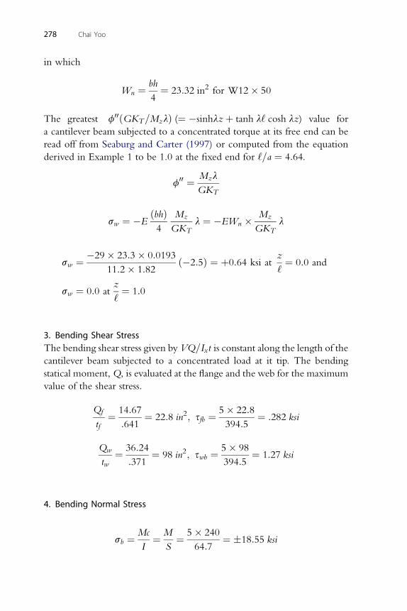
278 Chai Yoo

in which

Wn ¼ bh

4¼ 23:32 in2 for W12� 50

The greatest f00ðGKT=MzlÞ (¼ �sinhlzþ tanh l‘ cosh lz) value for

a cantilever beam subjected to a concentrated torque at its free end can be

read off from Seaburg and Carter (1997) or computed from the equation

derived in Example 1 to be 1.0 at the fixed end for ‘=a ¼ 4:64.

f00 ¼ Mzl

GKT

ðbhÞ M M

sw ¼ �E

4

z

GKTl ¼ �EWn � z

GKTl

sw ¼ �29� 23:3� 0:0193

11:2� 1:82ð�2:5Þ ¼ þ0:64 ksi at

z

‘¼ 0:0 and

sw ¼ 0:0 atz

‘¼ 1:0

3. Bending Shear StressThe bending shear stress given by VQ=Ixt is constant along the length of thecantilever beam subjected to a concentrated load at it tip. The bending

statical moment,Q, is evaluated at the flange and the web for the maximum

value of the shear stress.

Qf

tf¼ 14:67

:641¼ 22:8 in2; sfb ¼ 5� 22:8

394:5¼ :282 ksi

Qw 36:24 5� 98

tw¼

:371¼ 98 in2; swb ¼

394:5¼ 1:27 ksi

4. Bending Normal Stress

sb ¼ Mc

I¼ M

S¼ 5� 240

64:7¼ �18:55 ksi

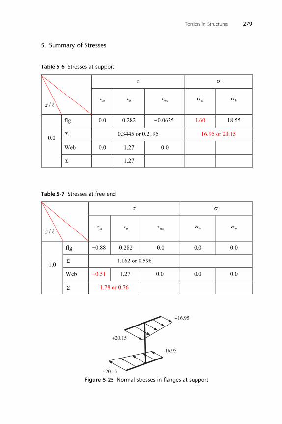
Torsion in Structures 279

5. Summary of Stresses

Table 5-6 Stresses at support

−

Table 5-7 Stresses at free end

−

−

+16.95

−20.15

+20.15

−16.95

Figure 5-25 Normal stresses in flanges at support

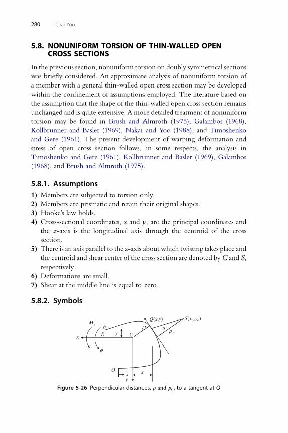
280 Chai Yoo

5.8. NONUNIFORM TORSION OF THIN-WALLED OPENCROSS SECTIONS

In the previous section, nonuniform torsion on doubly symmetrical sections

was briefly considered. An approximate analysis of nonuniform torsion of

a member with a general thin-walled open cross section may be developed

within the confinement of assumptions employed. The literature based on

the assumption that the shape of the thin-walled open cross section remains

unchanged and is quite extensive. A more detailed treatment of nonuniform

torsion may be found in Brush and Almroth (1975), Galambos (1968),

Kollbrunner and Basler (1969), Nakai and Yoo (1988), and Timoshenko

and Gere (1961). The present development of warping deformation and

stress of open cross section follows, in some respects, the analysis in

Timoshenko and Gere (1961), Kollbrunner and Basler (1969), Galambos

(1968), and Brush and Almroth (1975).

5.8.1. Assumptions1) Members are subjected to torsion only.

2) Members are prismatic and retain their original shapes.

3) Hooke’s law holds.

4) Cross-sectional coordinates, x and y, are the principal coordinates and

the z-axis is the longitudinal axis through the centroid of the cross

section.

5) There is an axis parallel to the z-axis about which twisting takes place and

the centroid and shear center of the cross section are denoted byC and S,

respectively.

6) Deformations are small.

7) Shear at the middle line is equal to zero.

5.8.2. Symbols

y

x

⋅

φ

zM

C y

x

b

E

O

ρoρa

s

Q(x,y) S(xo,yo)

Figure 5-26 Perpendicular distances, r and r0, to a tangent at Q

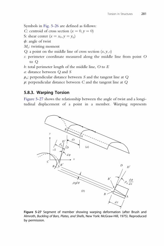
Torsion in Structures 281

Symbols in Fig. 5-26 are defined as follows:

C: centroid of cross section (x ¼ 0; y ¼ 0)

S: shear center (x ¼ x0; y ¼ y0)

f: angle of twist

Mz: twisting moment

Q: a point on the middle line of cross section (x; y; s)s: perimeter coordinate measured along the middle line from point O

to Q

b: total perimeter length of the middle line, O to E

a: distance between Q and S

ro: perpendicular distance between S and the tangent line at Q

r: perpendicular distance between C and the tangent line at Q

5.8.3. Warping TorsionFigure 5-27 shows the relationship between the angle of twist and a longi-

tudinal displacement of a point in a member. Warping represents

B

dz

z

A

(a)

(b)

D ′

D

dφ

0ρ

S

C

y

x

0dρ φ 0

d

d

zd

φρ

D ′D

B ′

BA

B ′B

•

Figure 5-27 Segment of member showing warping deformation (after Brush andAlmroth, Buckling of Bars, Plates, and Shells, New York: McGraw-Hill, 1975). Reproducedby permission.

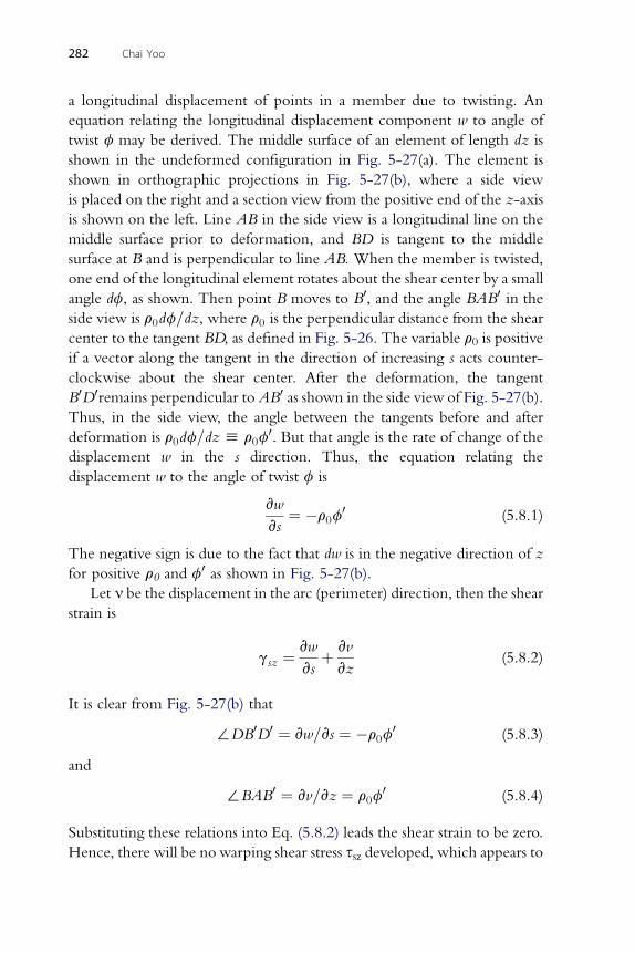
282 Chai Yoo

a longitudinal displacement of points in a member due to twisting. An

equation relating the longitudinal displacement component w to angle of

twist f may be derived. The middle surface of an element of length dz is

shown in the undeformed configuration in Fig. 5-27(a). The element is

shown in orthographic projections in Fig. 5-27(b), where a side view

is placed on the right and a section view from the positive end of the z-axis

is shown on the left. Line AB in the side view is a longitudinal line on the

middle surface prior to deformation, and BD is tangent to the middle

surface at B and is perpendicular to line AB. When the member is twisted,

one end of the longitudinal element rotates about the shear center by a small

angle df, as shown. Then point B moves to B0, and the angle BAB0 in the

side view is r0df=dz, where r0 is the perpendicular distance from the shear

center to the tangent BD, as defined in Fig. 5-26. The variable r0 is positive

if a vector along the tangent in the direction of increasing s acts counter-

clockwise about the shear center. After the deformation, the tangent

B0D0remains perpendicular to AB0 as shown in the side view of Fig. 5-27(b).

Thus, in the side view, the angle between the tangents before and after

deformation is r0df=dzh r0f0. But that angle is the rate of change of the

displacement w in the s direction. Thus, the equation relating the

displacement w to the angle of twist f is

vw

vs¼ �r0f

0 (5.8.1)

The negative sign is due to the fact that dw is in the negative direction of z

for positive r0 and f0 as shown in Fig. 5-27(b).

Let n be the displacement in the arc (perimeter) direction, then the shear

strain is

gsz ¼vw

vsþ vv

vz(5.8.2)

It is clear from Fig. 5-27(b) that

:DB0D0 ¼ vw=vs ¼ �r0f0 (5.8.3)

and

:BAB0 ¼ vv=vz ¼ r0f0 (5.8.4)

Substituting these relations into Eq. (5.8.2) leads the shear strain to be zero.

Hence, there will be no warping shear stress ssz developed, which appears to

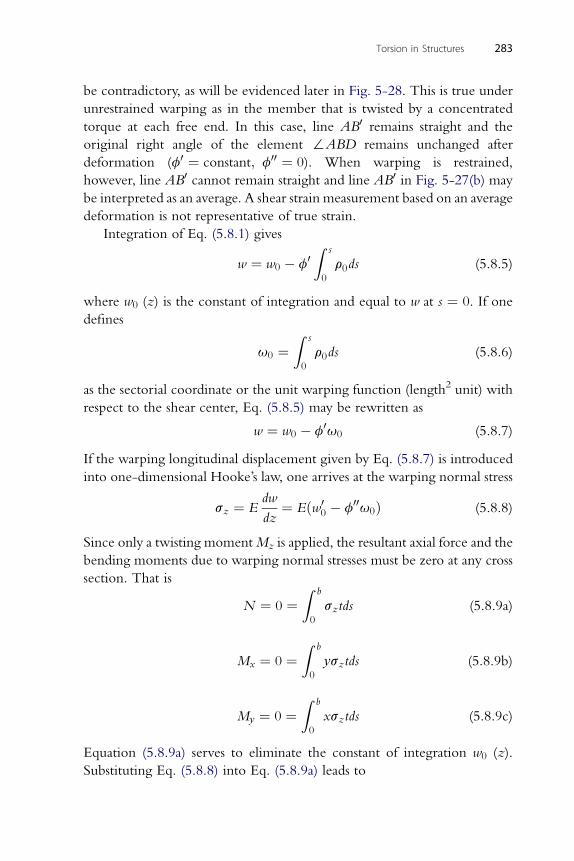
Torsion in Structures 283

be contradictory, as will be evidenced later in Fig. 5-28. This is true under

unrestrained warping as in the member that is twisted by a concentrated

torque at each free end. In this case, line AB0 remains straight and the

original right angle of the element :ABD remains unchanged after

deformation (f0 ¼ constant; f00 ¼ 0). When warping is restrained,

however, line AB0 cannot remain straight and line AB0 in Fig. 5-27(b) may

be interpreted as an average. A shear strain measurement based on an average

deformation is not representative of true strain.

Integration of Eq. (5.8.1) gives

w ¼ w0 � f0Z s

0

r0ds (5.8.5)

where w0 (z) is the constant of integration and equal to w at s ¼ 0. If one

defines

u0 ¼Z s

0

r0ds (5.8.6)

as the sectorial coordinate or the unit warping function (length2 unit) with

respect to the shear center, Eq. (5.8.5) may be rewritten as

w ¼ w0 � f0u0 (5.8.7)

If the warping longitudinal displacement given by Eq. (5.8.7) is introduced

into one-dimensional Hooke’s law, one arrives at the warping normal stress

sz ¼ Edw

dz¼ Eðw0

0 � f00u0Þ (5.8.8)

Since only a twisting momentMz is applied, the resultant axial force and the

bending moments due to warping normal stresses must be zero at any cross

section. That is

N ¼ 0 ¼Z b

0

sztds (5.8.9a)

Z b

Mx ¼ 0 ¼0

ysztds (5.8.9b)

Z b

My ¼ 0 ¼0

xsztds (5.8.9c)

Equation (5.8.9a) serves to eliminate the constant of integration w0 (z).

Substituting Eq. (5.8.8) into Eq. (5.8.9a) leads to

284 Chai Yoo

w00

Z b

0

tds� f00Z b

0

u0tds ¼ 0 (5.8.10a)

or

w00 ¼

f00

A

Z b

0

u0tds (5.8.10b)

where

A ¼Z b

0

tds (5.8.11)

Substituting Eq. (5.8.10b) into Eq. (5.8.8) yields

sz ¼ Ef00�1

A

Z b

0

u0tds� u0

�(5.8.12)

Defining a new cross-sectional property un1, the normalized unit warping

(length2 unit), as

un ¼ 1

A

Z b

0

u0tds� u0 (5.8.13)

one can rewrite Eq. (5.8.12) as

sz ¼ Eunf00 (5.8.14)

The variation of the normal stresses sz along the z-axis produces shearing

stresses, which constitute resisting warping torque Mwz :

To calculate the shearing stresses, consider an element mnop (Fig. 5-28)

cut out from the wall of the member in Fig. 5-27.

From summing forces in the z-direction, one obtains

vðssztÞvs

dsdzþ tvsz

vzdsdz ¼ 0

1 The first term in Eq. (5.8.12), R b

0u0tds

=A, is replaced by

R b0u0ds

=b in Timoshenko and

Gere (1961) and Brush and Almroth (1975). If the integration process is replaced by a summation of

discrete elements asPi

u0itiLi=Pi

tiLi such that ti is constant in each element, ti may be replaced by

tavg

�Pi

tiLi=b�

as it is independent of u0i and Li. ThenPi

u0itiLi=Pi

tiLi ¼ tavgPi

u0iLi=

tavgPi

Li ¼Pi

u0iLi=Pi

Li. In fact, the two expressions are identical. This has been confirmed

numerically by SECP (Yoo and Acra 1986).

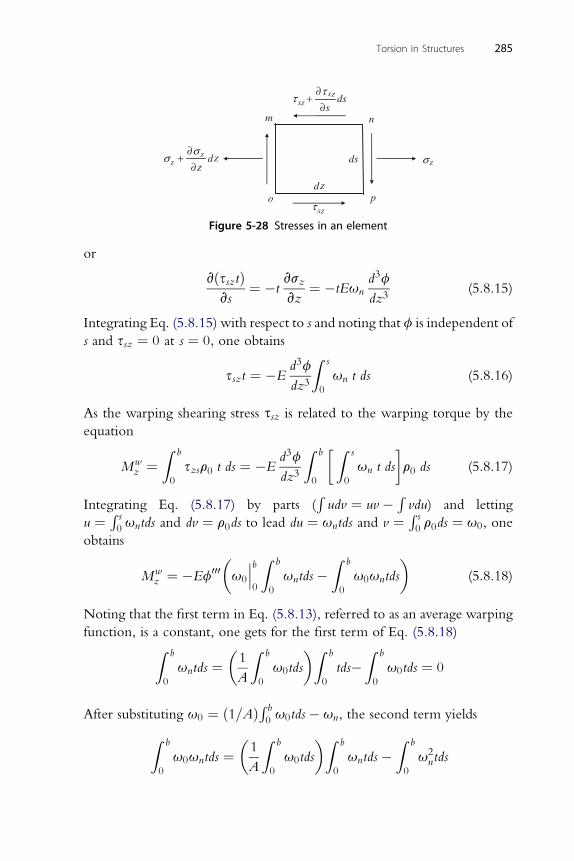
nm

o p

ds σzz

z

zdz

z

z

dz

σσ

∂+

∂

ss ds

s

ττ

zsτ

∂+

∂

Figure 5-28 Stresses in an element

Torsion in Structures 285

or

vðssztÞvs

¼ �tvsz

vz¼ �tEun

d3f

dz3(5.8.15)

Integrating Eq. (5.8.15) with respect to s and noting that f is independent of

s and ssz ¼ 0 at s ¼ 0; one obtains

sszt ¼ �Ed3f

dz3

Z s

0

un t ds (5.8.16)

As the warping shearing stress ssz is related to the warping torque by the

equation

Mwz ¼

Z b

0

szsr0 t ds ¼ �Ed3f

dz3

Z b

0

� Z s

0

un t ds

�r0 ds (5.8.17)

Integrating Eq. (5.8.17) by parts (Rudv ¼ uv � R vdu) and letting

u ¼ R s0 untds and dv ¼ r0ds to lead du ¼ untds and v ¼ R s0 r0ds ¼ u0, one

obtains

Mwz ¼ �Ef000

�u0

���b0

Z b

0

untds�Z b

0

u0untds

�(5.8.18)

Noting that the first term in Eq. (5.8.13), referred to as an average warping

function, is a constant, one gets for the first term of Eq. (5.8.18)Z b

0

untds ¼�1

A

Z b

0

u0tds

�Z b

0

tds�Z b

0

u0tds ¼ 0

After substituting u0 ¼ ð1=AÞR b0 u0tds� un, the second term yields

Z b

0

u0untds ¼�1

A

Z b

0

u0tds

�Z b

0

untds�Z b

0

u2ntds

286 Chai Yoo

SinceR b

untds ¼ 0 by virtue of Eq. (5.8.9a), Eq. (5.8.18) becomes

0

Mwz ¼ �Ef000

Z b

0

u2ntds (5.8.19)

Introducing the warping constant (length6 unit) or warping moment of

inertia, Iw

Iw ¼Z b

0

u2ntds (5.8.20)

one gets

Mwz ¼ �EIwf

000 (5.8.21)

The total resisting twisting moment is the sum of the warping contribution

and the St. Venant contribution; that is, as per Eq. (5.7.1),

Mz ¼ MStz þMw

z

For concentrated torques

Mz ¼ GKTf0 � EIwf

000 (5.7.5)

For a distributed torque

mz ¼ EIwfiv �GKTf

00 (5.7.6)

The warping shear flow is given by Eq. (5.8.16). Defining the warping

statical moment (length4 unit) as

Sw ¼Z s

0

untds (5.8.22)

the warping shear flow equation is

swt ¼ �ESwf000 (5.8.23)

The bimoment (force-length2 unit) is defined by

BM ¼ EIwf00 (5.8.24)

or

f00 ¼ BM

EIw(5.8.25)

Torsion in Structures 287

Substitution of Eq. (5.8.25) into Eq. (5.8.14) yields

sz ¼ BMun

Iw(5.8.26)

5.9. CROSS-SECTION PROPERTIES

5.9.1. Shear Center Location – General MethodDefinitionIf a general system of forces acting on a member is resolved into torsional

and bending components with respect to the shear center, these cause,

respectively, pure rotation and pure bending of the member (Kollbrunner

and Basler 1969). That is, if a member is fixed at one end and subjected to

a transverse load applied through the shear center at the other end, it

undergoes bending without twisting. Conversely, a torque applied to this

member induces no transverse deflection of the shear center. Hence, in such

a case the shear-center axis remains straight during twisting, and the cross

sections of the member rotate about the shear center during the deforma-

tion (Brush and Almroth 1975). The position of the shear center depends on

the properties of the cross section only. It is therefore constant with respect

to the cross section for prismatic members and the shear-center axis remains

parallel to the centroidal axis. The resultant of the shear flows must be equal

to the shearing forces acting on the cross section.

DevelopmentIn the theoretical development of the shear center location, the following

assumptions are employed:

1) No torsion (only pure bending is considered).

2) Bending about one centroidal axis (not necessarily principal) is

considered because the case of biaxial bending can be handled by

repeating the same procedure.

3) Hooke’s law holds.

4) Shearing stress is constant across plate thickness (i.e., thin-walled x-section).

5) Member is prismatic.

6) Cross section retains shape.

7) Small deflection.

8) Open cross section.

9) The thickness of the cross section is a function of the perimeter coor-

dinate s, but not the longitudinal member axis.

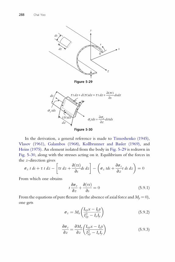
ds

t

( )t dz

dz

τ

( )( )

tt d d t d t d dsd

s

ττ τ τ ∂+ = +∂

tds d tdsz

z

z z z z

σσ ∂+

∂

z

zz

tdsσ

Figure 5-30

0

sx

y

ds

d

Figure 5-29

288 Chai Yoo

In the derivation, a general reference is made to Timoshenko (1945),

Vlasov (1961), Galambos (1968), Kollbrunner and Basler (1969), and

Heins (1975). An element isolated from the body in Fig. 5-29 is redrawn in

Fig. 5-30, along with the stresses acting on it. Equilibrium of the forces in

the z-direction gives

sz t dsþ s t dz��st dzþ vðstÞ

vsds dz

���sz tdsþ vsz

vzt ds dz

�¼ 0

From which one obtains

tvsz

vzþ vðstÞ

vs¼ 0 (5.9.1)

From the equations of pure flexure (in the absence of axial force andMy¼ 0),

one gets

sz ¼ Mx

�Ixyx� Iyy

I2xy � IxIy

�(5.9.2)

vs vM�I x� I y

�

z

vz¼ x

vz

xy y

I2xy � IxIy(5.9.3)

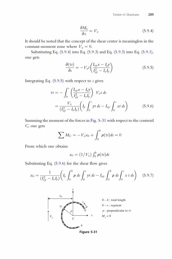
vMx

vz¼ Vx (5.9.4)

It should be noted that the concept of the shear center is meaningless in the

constant-moment zone where Vx ¼ 0.

Substituting Eq. (5.9.4) into Eq. (5.9.3) and Eq. (5.9.3) into Eq. (5.9.1),

one gets

vðstÞvs

¼ �Vxt

�Ixyx� Iyy

I2xy � IxIy

�(5.9.5)

Integrating Eq. (5.9.5) with respect to s gives

Torsion in Structures 289

st ¼ �Z s

0

�Ixyx� Iyy

I2xy � IxIy

�Vxt ds

¼ Vx

ðI2xy � IxIyÞ�Iy

Z s

0

yt ds� Ixy

Z s

0

xt ds

�(5.9.6)

Summing the moment of the forces in Fig. 5-31 with respect to the centroid

C, one gets XMC ¼ �Vxx0 þ

Z b

0

rðstÞds ¼ 0

From which one obtains

x0 ¼ ð1=VxÞR b0 rðstÞds

Substituting Eq. (5.9.6) for the shear flow gives

x0 ¼ 1

ðI2xy � IxIyÞ�Iy

Z b

0

r ds

Z s

0

yt ds� Ixy

Z b

0

r ds

Z s

0

x t ds

�(5.9.7)

y

s

0

C

ρ

xV

tτtτ

0x

x

0 − b : total length

0 − s : segment

: perpendicular to

0yM

ρ

=

b

Figure 5-31

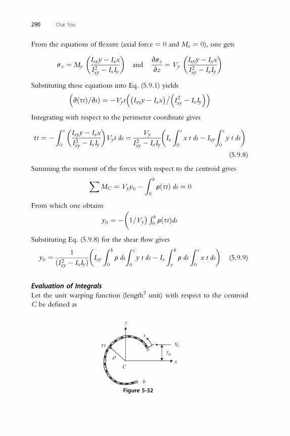
290 Chai Yoo

From the equations of flexure (axial force ¼ 0 and Mx ¼ 0), one gets

sz ¼ My

�Ixyy� Ixx

I2xy � IxIy

�and

vsz

vz¼ Vy

�Ixyy� Ixx

I2xy � IxIy

�

Substituting these equations into Eq. (5.9.1) yields�vðstÞ=vsÞ ¼ �Vyt

�Ixyy� Ixx

��I2xy � IxIy

��Integrating with respect to the perimeter coordinate gives

st ¼ �Z s

0

�Ixyy� Ixx

I2xy � IxIy

�Vyt ds ¼ Vy

I2xy � IxIy

�Ix

Z s

0

x t ds� Ixy

Z s

0

y t ds

�(5.9.8)

Summing the moment of the forces with respect to the centroid givesXMC ¼ Vyy0 �

Z b

0

rðstÞ ds ¼ 0

From which one obtains

y0 ¼ ��1=Vy

R b0 rðstÞds

Substituting Eq. (5.9.8) for the shear flow gives

y0 ¼1

ðI2xy � IxIyÞ�Ixy

Z b

0

r ds

Z s

0

y t ds� Ix

Z b

o

r ds

Z s

0

x t ds

�(5.9.9)

Evaluation of IntegralsLet the unit warping function (length2 unit) with respect to the centroid

C be defined as

y

s

o

xC

ρ

yVtτ

0y

b

Figure 5-32

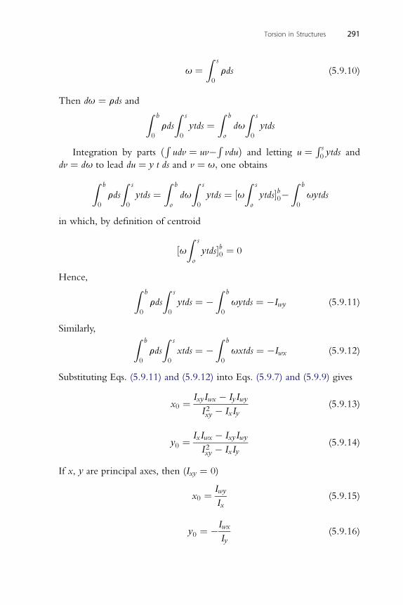
Torsion in Structures 291

u ¼Z s

0

rds (5.9.10)

Then du ¼ rds and Z b

0

rds

Z s

0

ytds ¼Z b

o

du

Z s

0

ytds

Integration by parts ðR udv ¼ uv�R vduÞ and letting u ¼ R s0 ytds and

dv ¼ du to lead du ¼ y t ds and v ¼ u; one obtains

Z b

0

rds

Z s

0

ytds ¼Z b

o

du

Z s

0

ytds ¼ ½uZ s

o

ytds�b0�Z b

0

uytds

in which, by definition of centroid

½uZ s

o

ytds�b0 ¼ 0

Hence, Z b

0

rds

Z s

0

ytds ¼ �Z b

0

uytds ¼ �Iwy (5.9.11)

Similarly, Z b

0

rds

Z s

0

xtds ¼ �Z b

0

uxtds ¼ �Iwx (5.9.12)

Substituting Eqs. (5.9.11) and (5.9.12) into Eqs. (5.9.7) and (5.9.9) gives

x0 ¼ IxyIwx � IyIwy

I2xy � IxIy(5.9.13)

IxIwx � IxyIwy

y0 ¼ I2xy � IxIy

(5.9.14)

If x, y are principal axes, then (Ixy ¼ 0)

x0 ¼ Iwy

Ix(5.9.15)

Iwx

y0 ¼ �

Iy(5.9.16)

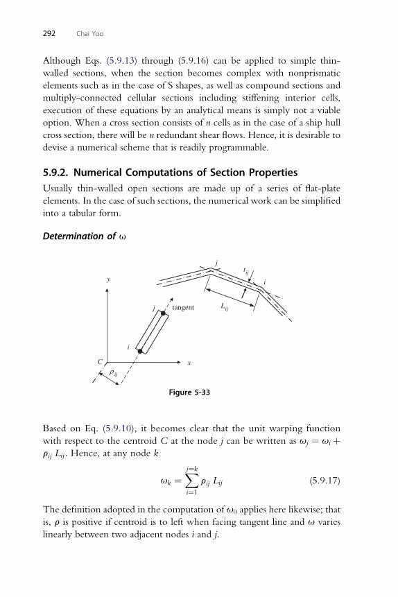
292 Chai Yoo

Although Eqs. (5.9.13) through (5.9.16) can be applied to simple thin-

walled sections, when the section becomes complex with nonprismatic

elements such as in the case of S shapes, as well as compound sections and

multiply-connected cellular sections including stiffening interior cells,

execution of these equations by an analytical means is simply not a viable

option. When a cross section consists of n cells as in the case of a ship hull

cross section, there will be n redundant shear flows. Hence, it is desirable to

devise a numerical scheme that is readily programmable.

5.9.2. Numerical Computations of Section PropertiesUsually thin-walled open sections are made up of a series of flat-plate

elements. In the case of such sections, the numerical work can be simplified

into a tabular form.

Determination of u

j

C

ijL

i

ijt

x

y

ijρ

tangent j

i

Figure 5-33

Based on Eq. (5.9.10), it becomes clear that the unit warping function

with respect to the centroid C at the node j can be written as uj ¼ uiþrij Lij: Hence, at any node k

uk ¼Xj¼k

i¼1

rij Lij (5.9.17)

The definition adopted in the computation of u0 applies here likewise; that

is, r is positive if centroid is to left when facing tangent line and u varies

linearly between two adjacent nodes i and j.

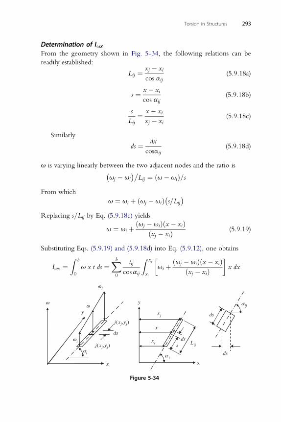
Torsion in Structures 293

Determination of IuxFrom the geometry shown in Fig. 5-34, the following relations can be

readily established:

Lij ¼ xj � xi

cos aij(5.9.18a)

s ¼ x� xi(5.9.18b)

cos aij

s ¼ x� xi(5.9.18c)

Lij xj � xi

Similarly

ds ¼ dx

cosaij(5.9.18d)

u is varying linearly between the two adjacent nodes and the ratio isuj � ui

�Lij ¼ ðu� uiÞ=s

From which

u ¼ ui þ ðuj � uiÞs=Lij

Replacing s=Lij by Eq. (5.9.18c) yields

u ¼ ui þ ðuj � uiÞðx� xiÞðxj � xiÞ (5.9.19)

Substituting Eqs. (5.9.19) and (5.9.18d) into Eq. (5.9.12), one obtains

Iwx ¼Z b

0

u x t ds ¼Xb0

tij

cosaij

Z xj

xi

�ui þ ðuj � uiÞðx� xiÞ

ðxj � xiÞ�x dx

ω

iα

x

y

ds

j(xj,yj)

j(xj,yj)

x

y

x

jx

ixs

dsijL

ds

dx

jω

iω

ω

iα

ijα

Figure 5-34

294 Chai Yoo

Expansion of Integral

Z xj

xi

�ui þ ðuj � uiÞðx� xiÞ

ðxj � xiÞ�x dx

¼ ui

2

�x2j � x2i

�þ�uj � ui

xj � xi

��x3j

3� x3i

3� xix

2j

2þ x3i

2

�

u 1�u � u

�

¼ i

2½ðxj þ xiÞðxj � xiÞ� þ

6

j i

xj � xi½2x2j ðxj � xiÞ þ xiðx2i � x2j Þ�

Recalling ðxj � xiÞ ¼ Lij cos aij

Iwx ¼Xb0

tij

cos aij

�ui

2ðxj þ xiÞLij cos aij

þ 1

6ðuj � uiÞ

2x2j ðxj � xiÞ � xiðx2j � x2i Þðxj � xiÞ

��

¼Xb0

ðtijÞ�uiLijðxj þ xiÞ

2þ 1

6

ðuj � uiÞð2x2j � xixj � x2i ÞLijðxj � xiÞ

�

¼Xb0

ðtijLijÞ�uiðxj þ xiÞ

2þ 1

6ðuj � uiÞ

ð2x2j � 2xixj � x2i þ xixjÞðxj � xiÞ

�

¼Xb0

tijLij

�uiðxj þ xiÞ

2þ 1

6ðuj � uiÞð2xj þ xiÞ

�

Iwx ¼ 1

3

Xb0

ðuixi þ ujxjÞtijLij þ 1

6

Xb0

ðuixj þ ujxiÞ tijLij

(5.9.20)

Similarly, Iwy and Ixy may be derived

Iwy ¼ 1

3

Xb0

ðuiyi þ ujyjÞtijLij þ1

6

Xb0

ðuiyj þ ujyiÞ tijLij (5.9.21)

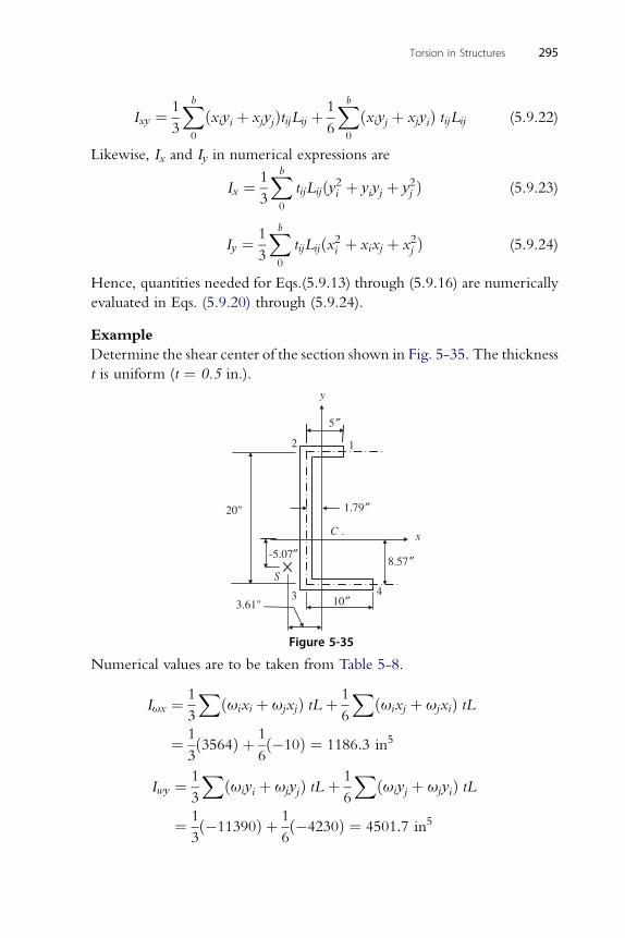
Xb Xb

Ixy ¼ 1

30

ðxiyi þ xjyjÞtijLij þ1

60

ðxiyj þ xjyiÞ tijLij (5.9.22)

Likewise, Ix and Iy in numerical expressions are

Torsion in Structures 295

Ix ¼ 1

3

Xb0

tijLijðy2i þ yiyj þ y2j Þ (5.9.23)

1Xb 2 2

Iy ¼3

0

tijLijðxi þ xixj þ xj Þ (5.9.24)

Hence, quantities needed for Eqs.(5.9.13) through (5.9.16) are numerically

evaluated in Eqs. (5.9.20) through (5.9.24).

Example

Determine the shear center of the section shown in Fig. 5-35. The thickness

t is uniform (t ¼ 0.5 in.).

x

y

1.79″

1 2

5″

8.57″

4 10″3

-5.07″

C .

20"

S

3.61"

Figure 5-35

Numerical values are to be taken from Table 5-8.

Iux ¼ 1

3

Xðuixi þ ujxjÞ tL þ 1

6

Xðuixj þ ujxiÞ tL

¼ 1

3ð3564Þ þ 1

6ð�10Þ ¼ 1186:3 in5

Iwy ¼ 1Xðuiy þ ujy Þ tL þ 1Xðuiy þ ujy Þ tL

3 i j 6 j i

¼ 1

3ð�11390Þ þ 1

6ð�4230Þ ¼ 4501:7 in5

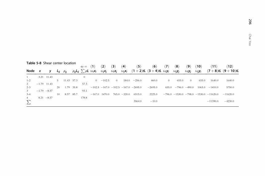
Table 5-8 Shear center location

Node x y Lij rij rijLiju ¼P

rLð1Þuixi

ð2Þujxj

ð3Þuixj

ð4Þujxi

ð5Þð1þ 2ÞtL

ð6Þð3þ 4ÞtL

ð7Þuiyi

ð8Þujyj

ð9Þuiyj

ð10Þujyi

ð11Þð7þ 8ÞtL

ð12Þð9þ 10ÞtL

1 3.21 11.43 0

1-2 5 11.43 57.3 0 �102.5 0 184.0 �256.0 460.0 0 655.0 0 655.0 1640.0 1640.0

2 �1.79 11.43 57.3

2-3 20 1.79 35.8 �102.5 �167.0 �102.5 �167.0 �2695.0 �2695.0 655.0 �796.0 �490.0 1065.0 �1410.0 5750.0

3 �1.79 �8.57 93.1

3-4 10 8.57 85.7 �167.0 1470.0 765.0 �320.0 6515.0 2225.0 �796.0 �1530.0 �798.0 �1530.0 �11620.0 �11620.0

4 8.21 �8.57 178.8P3564.0 �10.0 �11390.0 �4230.0

296ChaiYoo

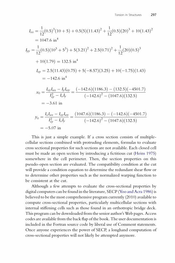
1 3 2 1 3 2

Ixx ¼

12ð0:5Þ ð10þ 5Þ þ 0:5ð5Þð11:43Þ þ

12ð0:5Þð20Þ þ 10ð1:43Þ

¼ 1047:6 in4

1 2 2 1 3

Torsion in Structures 297

Iyy ¼12ð0:5Þð103 þ 53Þ þ 5ð3:21Þ þ 2:5ð0:71Þ þ

12ð20Þð0:5Þ

þ 10ð1:79Þ ¼ 132:5 in4

I ¼ 2:5ð11:43Þð0:75Þ þ 5ð�8:57Þð3:25Þ þ 10ð�1:75Þð1:43Þ

xy

¼ �142:6 in4

IxyIwx � IyIwy ð�142:6Þð1186:3Þ � ð132:5Þð�4501:7Þ

x0 ¼

I2xy � IxIy¼ ð�142:6Þ2 � ð1047:6Þð132:5Þ

¼ �3:61 in

IxIwx � IxyIwy ð1047:6Þð1186:3Þ � ð�142:6Þð�4501:7Þ

y0 ¼ I2xy � IxIy

¼ ð�142:6Þ2 � ð1047:6Þð132:5Þ¼ �5:07 in

This is just a simple example. If a cross section consists of multiple-

cellular sections combined with protruding elements, formulas to evaluate

cross sectional properties for such sections are not available. Each closed cell

must be made an open section by introducing a fictitious cut (Heins 1975)

somewhere in the cell perimeter. Then, the section properties on this

pseudo-open section are evaluated. The compatibility condition at the cut

will provide a condition equation to determine the redundant shear flow or

to determine other properties such as the normalized warping function to

be consistent at the cut.

Although a few attempts to evaluate the cross-sectional properties by

digital computers can be found in the literature, SECP (Yoo andAcra 1986) is

believed to be the most comprehensive program currently (2010) available to

compute cross-sectional properties, particularly multicellular sections with

internal stiffening cells such as those found in an orthotropic bridge deck.

This program can be downloaded from the senior author’sWeb pages. Access

codes are available from the back flap of the book. The user documentation is

included in the Fortran source code by liberal use of Comment statements.

Once anyone experiences the power of SECP, a longhand computation of

cross-sectional properties will not likely be attempted anymore.

298 Chai Yoo

REFERENCESBrush, D. O., & Almroth, B. O. (1975). Buckling of Bars, Plates, and Shells. New York:

McGraw-Hill.Galambos, T. V. (1968). Structural Members and Frames. Englewood Cliffs, NJ: Prentice-Hall.Heins, C. P. (1975). Bending and Torsional Design in Structural Members. Lexington, MA:

Lexington Book.Heins, C. P., & Seaburg, P. A. (1963). Torsional Analysis of Rolled Steel Sections. Bethlehem,

PA: Bethlehem Steel Company.Kollbrunner, C. F., & Basler, K. (1969). Torsion in Structure: An engineering Approach. In:

E. C. Glauser (Ed.). Berlin: Springer-Verlag. translated from German.Nadai, A. (1923). Sand-heap Analogy. Z. angew. Math. Mechanik, Vol. 3(No. 6), 442.Nadai, A. (1950) (2nd ed.).Theory of Flow and Fracture of Solids, Vol. 1. New York: McGraw-

Hill.Nakai, H., & Yoo, C. H. (1988). Analysis and Design of Curved Steel Bridges. New York:

McGraw-Hill.Prandtl, L. (1903). Membrane Analogy. Physik. Z., Vol. 4.Rees, D. W. A. (2000). Mechanics of Solids and Structures. London: Imperial College Press.Saada, A. S. (1974). Elasticity, Theory and Application (2nd ed.). Malabar, FL: Krieger.Saint-Venant, B. D. (1855). Mem. acad. sci. savants, Vol. 14, 233–560.Seaburg, P. A., & Carter, C. J. (1997). Torsional Analysis of Structural Steel Members. Chicago,

IL: American Institute of Steel Construction.Sokolnikoff, I. S. (1956). Mathematical Theory of Elasticity (2nd ed.). New York: McGraw-

Hill.Timoshenko, S. P. (1945). Theory of Bending, Torsion, and Buckling of Thin-Walled Members

of Open Cross Section. Philadelphia: J. Franklin Institute. Vol. 239, No. 3, p. 201, No. 4,pp. 248, No. 5, p. 343.

Timoshenko, S. P., & Gere, J. M. (1961). The Theory of Elastic Stability (2nd ed.). New York:McGraw-Hill.

Timoshenko, S. P., & Goodier, J. N. (1951). Theory of Elasticity (2nd ed.). New York, NY:McGraw-Hill.

Vlasov, V. Z. (1940). Tonkostennye uprugie sterzhni (Thin-walled elastic beams). Stroiizdat(in Russian).

Vlasov, V. Z. (1961). In Tonkostennye uprugie sterzhni (Thin-walled elastic beams). Moscow,1959, (2nd ed.), translated by Schechtman. Jerusalem: Israel Program for ScientificTranslation.

Yoo, C. H. (2000). Torsional and Other Properties of Prestressed Concrete Sections. PCIJournal, Vol. 45(No. 3), 66–72.

Yoo, C. H., & Acra, S. V. (1986). Cross Sectional Properties of Thin-Walled Multi-CellularSection. Computers and Structures, Vol. 112(No. 9), 53–61.

PROBLEMS

5.1 In order to minimize the potential stress concentration at the reentrant

corners at the bottom of a rectangular keyway, the sharp corners are

smoothed out by a circular hole. Show that the Prandtl stress function

f ¼ mðr2 � b2Þð2a cos q=r � 1Þ (Sokolnikoff 1956) leads to the solu-

tion of the circular shaft with a circular keyway, shown in Fig. P5-1.

Determine the constant m and the expressions of the stresses, szx and

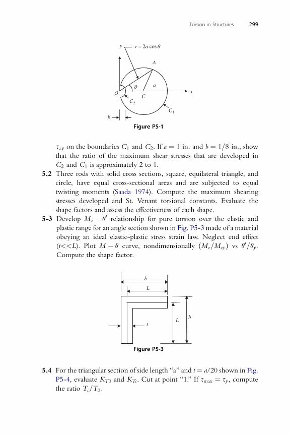
O x

y

b1C

a

C

A

θ

2C

r = 2a cosθ

Figure P5-1

Torsion in Structures 299

szy on the boundaries C1 and C2. If a ¼ 1 in: and b ¼ 1=8 in:, showthat the ratio of the maximum shear stresses that are developed in

C2 and C1 is approximately 2 to 1.

5.2 Three rods with solid cross sections, square, equilateral triangle, and

circle, have equal cross-sectional areas and are subjected to equal

twisting moments (Saada 1974). Compute the maximum shearing

stresses developed and St. Venant torsional constants. Evaluate the

shape factors and assess the effectiveness of each shape.

5-3 Develop Mz � q0 relationship for pure torsion over the elastic and

plastic range for an angle section shown in Fig. P5-3 made of a material

obeying an ideal elastic-plastic stress strain law. Neglect end effect

(t<<L). Plot M � q curve, nondimensionally ðMz=MzyÞ vs q0=qy.Compute the shape factor.

b

L

Lt

b

Figure P5-3

5.4 For the triangular section of side length “a” and t¼ a/20 shown in Fig.

P5-4, evaluate KT0 and KTc. Cut at point “1.” If smax ¼ sy, compute

the ratio Tc=T0.

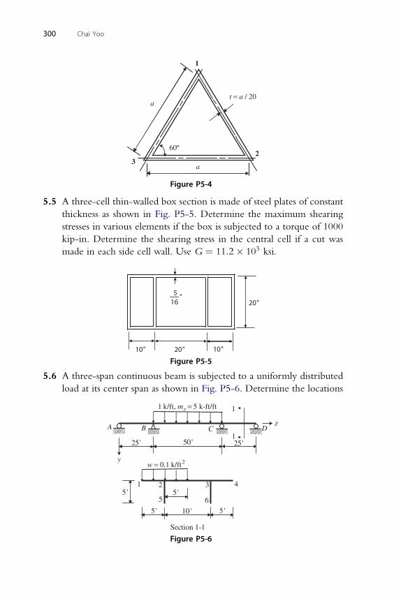
1

t = a / 20a

60º

a

23

Figure P5-4

300 Chai Yoo

5.5 A three-cell thin-walled box section is made of steel plates of constant

thickness as shown in Fig. P5-5. Determine the maximum shearing

stresses in various elements if the box is subjected to a torque of 1000

kip-in. Determine the shearing stress in the central cell if a cut was

made in each side cell wall. Use G ¼ 11:2� 103 ksi.

20"5 "16

10"10" 20"

Figure P5-5

5.6 A three-span continuous beam is subjected to a uniformly distributed

load at its center span as shown in Fig. P5-6. Determine the locations

A

1

z

25' 25'

20.1 k/ftw =

Section 1-1

5'

10 ' 5'5'

5'

1DCB

50'

65

4321

y

1 k/ft, 5 k-ft/ftzm =

Figure P5-6

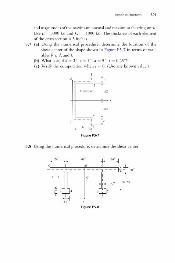
Torsion in Structures 301

and magnitudes of the maximum normal and maximum shearing stress.

Use E ¼ 3000 ksi and G ¼ 1000 ksi. The thickness of each element

of the cross section is 5 inches.

5.7 (a) Using the numerical procedure, determine the location of the

shear center of the shape shown in Figure P5-7 in terms of vari-

ables b, c, d, and t.

(b) What is x0 if b ¼ 3}, c ¼ 1}, d ¼ 5}, t ¼ 0:25}?(c) Verify the computation when c ¼ 0. (Use any known value.)

d/2

d/2

x

3

4

b

2

5

6

c

c

t: constant

Figure P5-7

5.8 Using the numerical procedure, determine the shear center.

.58

24 48 24

00

1

11

2 4

3 9 7

8

y

.2834.20

61 5

Cx

Figure P5-8

CHAPTER66

Torsional and Flexural-TorsionalBucklingContents

6.1. Introduction 3036.2. Strain Energy of Torsion 305

6.2.1. St. Venant Torsion 3056.2.2. Warping Torsion 306

6.3. Torsional and Flexural-Torsional Buckling of Columns 3076.4. Torsional and Flexural-Torsional Buckling under Thrust and End Moments 317

6.4.1. Pure Torsional Buckling 3186.4.2. Flexural-Torsional Buckling 3196.4.3. Torsional and Flexural-Torsional Buckling under Thrust and End

Moments 321References 325Problems 326

6.1. INTRODUCTION

In Chapter 1, the fundamental case of buckling of centrally loaded columns

is presented under the assumption that columns will buckle in the plane of

a principal axis without the accompanying rotation of the cross sections.

This assumption, first made by Euler (1744), appears reasonable for the

doubly symmetric cross section but becomes problematic if cross sections

have only one axis of symmetry or none at all. The possibility of torsional

column failure had never been recognized until open thin-walled sections

were used in aircraft design in the 1930s. Experience has revealed that

columns having an open section with only one or no axis of symmetry show

a tendency to bend and twist simultaneously under axial compression. The

ominous nature of this type of failure lies in the fact that the actual critical

load of such columns may be less than that predicted by the generalized

Euler formula due to their small torsional rigidities. Bleich (1952) gives

a fairly thorough overview of the early development of the theory on the

torsional buckling.

Bleich and Bleich (1936) were among the early developers of the theory

on torsional buckling along with Wagner and Pretschner (1936), Ostenfeld

(1931), Kappus (1938), Lundquist and Fligg (1937), Goodier (1941), Hoff

Stability of Structures � 2011 Elsevier Inc.ISBN 978-0-12-385122-2, doi:10.1016/B978-0-12-385122-2.10006-5 All rights reserved. 303 j

304 Chai Yoo

(1944), and Timoshenko (1945). All of these authors make the fundamental

assumption that the plane cross sections of the column warp but that their

geometry does not change during buckling. Thus, the theories consider

primary failure (global buckling) of columns as opposed to local failure

characterized by distortion of the cross sections. The dividing line between

primary and local failure is not always sharp. Separate analysis of primary and

local buckling based on governing differential equations, without aban-

doning the assumption that cross sections of the column will not deform,

may yield only approximate solutions since there could be coupling of

primary and local buckling. Modern finite element codes with refined

modeling capabilities incorporating at least flat shell elements may be able to

assess this combined buckling action.

The notion of “unit warping” or the concept of sectorial coordinate

appears to have gained currency in the literature including Goodier (1941),

Galambos (1968), Kollbrunner and Basler (1969), Timoshenko (1945), and

Vlasov (1961). Bleich and Bleich (1936) developed their differential equa-

tions governing the torsional buckling behavior of columns with thin-

walled open sections based on the principle of minimum potential energy

without invoking the notion of “unit warping” or the concept of the

sectorial coordinate. Although they claim that their equations are practically

the same as those developed under the concept of the sectorial coordinate,

they differ in a significant aspect. The warping constant Iw (or G in their

notation) for the cross section consisting of thin rectangular elements does

not vanish according to their theory, in which the axial strain and the

curvature are considered to be coupled. This consideration appears to be

odd since in the linearized bifurcation-type buckling analysis, an adjacent

equilibrium configuration is examined after all static deformations have

taken place. As a consequence of their theory of nonvanishing warping

constant, a beam having a cross section consisting of a series of narrow

rectangular elements that meet at the shear center will become warped. This

is a direct contradiction to Timoshenko and Gere (1961)1 and Vlasov

(1961).2 According to the definition of unit warping, the warping constant

Iw must be equal to zero for such sections where the perpendicular distance

from the shear center to each element wall becomes zero. Therefore, the

differential equations to be developed for torsional and flexural-tosional

1 See page 217.2 See page 27: a thin-walled beam consisting of a single bundle of very thin rectangular plates does not

become warped.

Torsional and Flexural-Torsional Buckling 305

buckling here in this chapter and for lateral-torsional buckling in the next

chapter will be based on the concept of unit warping.

6.2. STRAIN ENERGY OF TORSION

Recall that the concept of the stress tensor arises from equilibrium

considerations and that the concept of the strain tensor arises from kine-

matic (deformation) considerations. These tensors are related to each other

by laws that are called constitutive laws. The constitutive laws relating

stresses and strains directly and uniquely can be expressed mathematically as

sij ¼ sijð311; 312; ::::; 333Þ (6.2.1)

where sij ¼ stresses and 3ij ¼ strains.

Consider a quantity, U0, strain energy density function which is also

known to be a point function that is independent from the integral path

taken:

U0 ¼Z 3ij

0

sijd3ij

A strain energy density function is measured in energy per volume and is

a scalar quantity. For linearly elastic materials, it becomes

U0 ¼ 1

2sij 3ij (6.2.2)

Then, the strain energy stored in a body is

U ¼ZV

Uodv ¼ 1

2

ZV

sij 3ijdv (6.2.3)

The strain energy stored in a twisted member is broken down into two

parts, one due to St. Venant torsion and the other due to warping torsion. In

order to maintain a generality, torsional stresses and corresponding strain

expressions are explicitly developed and substituted in Eq. (6.2.3). As

columns of a closed cross section are not likely to develop torsional or

flexural-torsional buckling, such columns are not considered here.

6.2.1. St. Venant TorsionRecall that the St. Venant torsional moment is given by Eq. (5.4.1) as

MStz ¼ GKTf

0

306 Chai Yoo

The corresponding shear stress in an open cross section shown in Fig. 5-20 is

given by

szs ¼ sStz ¼ 2MStz h

KT¼ 2Ghf0 (6.2.4a)

and the corresponding shear strain is

3zs ¼ gzs

2¼ szs

2G¼ hf0 (6.2.4b)

Then, the strain energy due to St. Venant torsion is

UStT ¼

ZV

Uodv ¼ 1

2

ZV

sij3ijdv ¼ 1

2

ZV

ðszs3zs þ ssz3szÞdv

Substituting (6.2.4a) and (6.2.4b) gives

UStz ¼ 2Gðf0Þ2

Z ‘

0

Z b

0

Z t=2

�t=2h2dhdsdv ¼ 2Gðf0Þ2

Z ‘

0

Z b

0

h3��� t2� t

2

dsdz

Z ‘

¼ 1

2 0

GKT ðf0Þ2dz (6.2.4c)

where b is the width of a thin-walled element and h is measured from the

centerline of a thin-walled element thickness so that hmax ¼ t=2.

6.2.2. Warping TorsionFor a member subjected to warping torsion, the dominant strain energy

stored in the member due to its resistance to warping is assumed to be the

strain energy due to warping normal stresses. Even though warping shear

stresses produce strain energy, it is usually considered to be negligibly small

and is neglected as in the case of not including the shear deformation effect

in ordinary flexural analysis. Warping normal stresses and corresponding

strains are evaluated by

swz ¼ BMun

Iw¼ EIwf

00un

Iw¼ Eunf

00 (5.8.26)

w swz 00

3z ¼E

¼ unf

Hence,

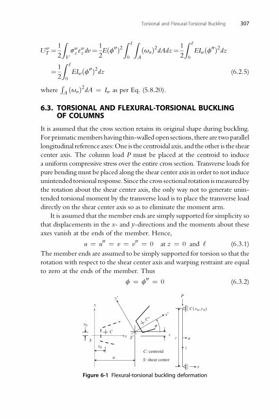
Torsional and Flexural-Torsional Buckling 307

UwT ¼ 1

2

ZV

swz 3wz dv¼

1

2Eðf00Þ2

Z ‘

0

ZA

ðunÞ2dAdz¼ 1

2

Z ‘

0

EIwðf00Þ2dz

¼ 1

2

Z ‘

0

EIwðf00Þ2dz (6.2.5)

whereRA ðunÞ2dA ¼ Iw as per Eq. (5.8.20).

6.3. TORSIONAL AND FLEXURAL-TORSIONAL BUCKLINGOF COLUMNS

It is assumed that the cross section retains its original shape during buckling.

For prismaticmembers having thin-walled open sections, there are twoparallel

longitudinal reference axes:One is the centroidal axis, and theother is the shear

center axis. The column load P must be placed at the centroid to induce

a uniform compressive stress over the entire cross section. Transverse loads for

pure bendingmust be placed along the shear center axis in order to not induce

unintended torsional response. Since the cross sectional rotation ismeasuredby

the rotation about the shear center axis, the only way not to generate unin-

tended torsional moment by the transverse load is to place the transverse load

directly on the shear center axis so as to eliminate the moment arm.

It is assumed that the member ends are simply supported for simplicity so

that displacements in the x- and y-directions and the moments about these

axes vanish at the ends of the member. Hence,

u ¼ u00 ¼ v ¼ v00 ¼ 0 at z ¼ 0 and ‘ (6.3.1)

The member ends are assumed to be simply supported for torsion so that the

rotation with respect to the shear center axis and warping restraint are equal

to zero at the ends of the member. Thus

f ¼ f00 ¼ 0 (6.3.2)

P

C (x0,y0)

u

φC′

C

y0

x0

vS ′

S

y ′y

x′

x

zC: centroid

S: shear center

x

u

Figure 6-1 Flexural-torsional buckling deformation

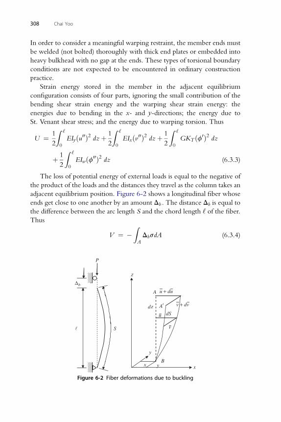
308 Chai Yoo

In order to consider a meaningful warping restraint, the member ends must

be welded (not bolted) thoroughly with thick end plates or embedded into

heavy bulkhead with no gap at the ends. These types of torsional boundary

conditions are not expected to be encountered in ordinary construction

practice.

Strain energy stored in the member in the adjacent equilibrium

configuration consists of four parts, ignoring the small contribution of the

bending shear strain energy and the warping shear strain energy: the

energies due to bending in the x- and y-directions; the energy due to

St. Venant shear stress; and the energy due to warping torsion. Thus

U ¼ 1

2

Z ‘

0

EIyðu00Þ2 dzþ 1

2

Z ‘

0

EIxðv00Þ2 dzþ 1

2

Z ‘

0

GKT ðf0Þ2 dz

þ 1

2

Z ‘

0

EIwðf00Þ2 dz (6.3.3)

The loss of potential energy of external loads is equal to the negative of

the product of the loads and the distances they travel as the column takes an

adjacent equilibrium position. Figure 6-2 shows a longitudinal fiber whose

ends get close to one another by an amount Db . The distance Db is equal to

the difference between the arc length S and the chord length ‘ of the fiber.Thus

V ¼ �ZA

DbsdA (6.3.4)

bΔ

P

x

z

z

y

A

x

A′

u + du

v + dv

u

vS

By

ddS

Figure 6-2 Fiber deformations due to buckling

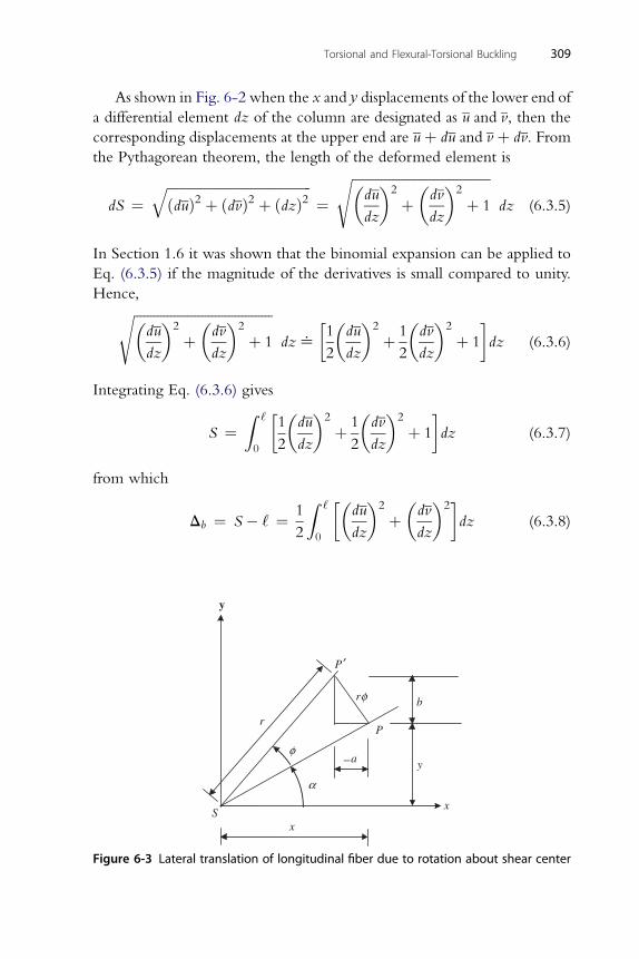
Torsional and Flexural-Torsional Buckling 309

As shown in Fig. 6-2 when the x and y displacements of the lower end of

a differential element dz of the column are designated as u and v, then the

corresponding displacements at the upper end are uþ du and v þ dv. From

the Pythagorean theorem, the length of the deformed element is

dS ¼ffiffiffiffiffiffiffiffiffiffiffiffiffiffiffiffiffiffiffiffiffiffiffiffiffiffiffiffiffiffiffiffiffiffiffiffiffiffiffiffiffiffiffiðduÞ2 þ ðdvÞ2 þ ðdzÞ2

q¼

ffiffiffiffiffiffiffiffiffiffiffiffiffiffiffiffiffiffiffiffiffiffiffiffiffiffiffiffiffiffiffiffiffiffiffiffiffiffiffiffiffi�du

dz

�2

þ�dv

dz

�2

þ 1

sdz (6.3.5)

In Section 1.6 it was shown that the binomial expansion can be applied to

Eq. (6.3.5) if the magnitude of the derivatives is small compared to unity.

Hence,ffiffiffiffiffiffiffiffiffiffiffiffiffiffiffiffiffiffiffiffiffiffiffiffiffiffiffiffiffiffiffiffiffiffiffiffiffiffiffiffiffi�du

dz

�2

þ�dv

dz

�2

þ 1

sdz^

�1

2

�du

dz

�2

þ 1

2

�dv

dz

�2

þ 1

�dz (6.3.6)

Integrating Eq. (6.3.6) gives

S ¼Z ‘

0

�1

2

�du

dz

�2

þ 1

2

�dv

dz

�2

þ 1

�dz (6.3.7)

from which

Db ¼ S � ‘ ¼ 1

2

Z ‘

0

��du

dz

�2

þ�dv

dz

�2�dz (6.3.8)

y

S

α

φ

rφ

P

P ′

b

y

x

x

a−

r

Figure 6-3 Lateral translation of longitudinal fiber due to rotation about shear center

310 Chai Yoo

where u and v are the translation of the shear center u and v plus additional

translation due to rotation of the cross section about the shear center. The

additional translations du and dv, in the x- and y-directions, are denoted, as

shown in Fig. 6-3 by –a and b. From the geometry of the figure, it is evident

that PP 0 ¼ rf, a ¼ rf sin a, and b ¼ rf cos a.

Since x ¼ r cos a and y ¼ r sin a, one may also write �a ¼ �yf and

b ¼ xf. Hence, the total displacements of the fiber are

u ¼ u� yf

v ¼ v þ xf(6.3.9)

Substituting Eq. (6.3.9) into Eq. (6.3.8) yields

Db ¼ 1

2

Z ‘

0

��du

dz

�2

þ�dv

dz

�2

þ ðx2 þ y2Þ�dq

dz

�2

� 2y

�du

dz

��dq

dz

�þ 2x

�dv

dz

��dq

dz

��dz ð6:3:10Þ

Z ‘ Z �� �2

� �2

� �2

V ¼ �1

2 0A

sdu

dzþ dv

dzþ ðx2 þ y2Þ dq

dz

�2y

�du

dz

��dq

dz

�þ 2x

�dv

dz

��dq

dz

��dAdz (6.3.11)

In order to simplify Eq. (6.3.11), the following geometric relations can be

used: RA

dA ¼A;RA

ydA ¼ y0A;RA

xdA ¼ x0A

RA

ðx2 þ y2ÞdA ¼ Ix þ Iy ¼ r20A(6.3.12)

where r0 is polar radius of gyration of the cross section with respect to the

shear center. It should be noted that the shear center is the origin of the

coordinate system shown in Fig. 6-3. Hence,

V ¼ �P

2

Z ‘

0

��du

dz

�2

þ�dv

dz

�2

þ r20

�df

dz

�2

� 2y0

�du

dz

��df

dz

�

þ 2x0

�dv

dz

��df

dz

��dz (6.3.13)

Torsional and Flexural-Torsional Buckling 311

The total potential energy functional p is given by the sum of Eq. (6.3.3)

and Eq. (6.3.13) as

P ¼ UðEq:ð6:3:3ÞÞ þ V ðEq:ð6:3:13ÞÞ ¼Z‘Fðz; u0; v0;f0; u00; v00;f00Þdz

(6.3.14)

According to the rules of the calculus of variations, P will be stationary

(minimum) if the following three Euler-Lagrange differential equations are

satisfied:

vF

vu� d

dz

vF

vu0þ d2

dz2vF

vu00¼ 0

vF

vv� d

dz

vF

vv0þ d2

dz2vF

vv00¼ 0

vF

vf� d

dz

vF

vf0 þd2

dz2vF

vf00 ¼ 0

(6.3.15)

Execution of Eq. (6.3.15) gives

EIyuiv þ Pu00 � Py0f

00 ¼ 0 (6.3.16a)

EI viv þ Pv00 þ Px f00 ¼ 0 (6.3.16b)

x 0

iv 2 00 00 00

EIwf þ ðr0P �GKT Þf � y0Pu þ x0Pv ¼ 0 (6.3.16c)

These three differential equations are the simultaneous differential equations

of torsional and flexural-torsional buckling for centrally applied loads only.

Each of the three equations in Eq. (6.3.16) is a fourth-order differential

equation. Hence, the system must have 12 (4 � 3) boundary conditions to

determine uniquely the integral constants.

Equations (6.3.16) are linear and homogeneous, and have constant

coefficients. Their general solution in the most general case can be obtained

by means of the characteristic polynomial approach. Assume the solution to

be of the form,3

u ¼ A sinpz

‘; v ¼ B sin

pz

‘; f ¼ C sin

pz

‘

where A, B, and C are arbitrary constants. Substituting derivatives of these

functions into the differential equations (6.3.16) and reducing by the

common factor sin(pz/‘), one obtains

3 Vlasov (1961) shows this is indeed the solution of the eigenfunctions for a simply supported column;

see p. 271.

312 Chai Yoo

ðEIyk2 � PÞAþ y0PC ¼ 0

ðEIxk2 � PÞB� x0PC ¼ 0

y0PA� x0PBþ ðEIwk2 þGKT � r20PÞC ¼ 0

(6.3.17)

where k2 ¼ p2=‘2.For a nontrivial solution for A, B, and C, the determinant of the system

of homogeneous equations must vanish. Thus��������Py � P 0 y0P

0 Px � P �x0P

y0P �x0P r20�Pf � P

��������¼ 0 (6.3.18)

where

Px ¼ p2EIx

‘2; Py ¼ p2EIy

‘2;Pf ¼ 1

r20

�EIw

p2

‘2þGKT

�(6.3.19)

Expanding Eq. (6.3.18) gives

ðPy � PÞðPx � PÞðPf � PÞ � ðPy � PÞP2x20r20

� ðPx � PÞP2y20r20

¼ 0

(6.3.20)

The solution of the above cubic equation gives the critical load of the

column.

Case 1: If the cross section is doubly symmetrical, then x0¼ y0 ¼ 0, and

Eq. (6.3.20) reduces to

ðPy � PÞðPx � PÞðPf � PÞ ¼ 0

The three roots and corresponding mode shapes are:

Pcr ¼ Py ¼ p2EIy

‘2: As 0;B ¼ C ¼ 00pure flexural buckling

p2EI

Pcr ¼ Px ¼ x

‘2: B s 0;A ¼ C ¼ 00pure flexural buckling�

2�

Pcr ¼ Pf ¼ 1

r20

p EIw

‘2þGKT :

C s 0;A ¼ B ¼ 00pure torsional buckling

Torsional and Flexural-Torsional Buckling 313

Coupled flexural-torsional buckling does not occur in a column with a cross

section where the shear center coincides with the center of gravity. Doubly

symmetric sections and the Z purlin section have the shear center and the

center of gravity at the same location.

Example Consider a pinned column (W14 � 43) of length ‘ ¼ 280

inches. Use E ¼ 29 �103 ksi and G ¼ 11.2 � 103 ksi

For W14� 43, Ix ¼ 428 in4, Iy ¼ 45.2 in 4, KT ¼ 1.05 in 4, Iw ¼ 1, 950 in 6

Py ¼ p2EIy

‘2¼ p2 � 29� 103 � 45:2

2802¼ 165 kips

p2EI 2 3

Px ¼ y

‘2¼ p � 29� 10 � 428

2802¼ 1; 563 kips

1=2 1=2

r0 ¼ ½ðIx þ IyÞ=A� ¼ ½ð428þ 45:2Þ=12:6� ¼ 6:13 in

1�

p2 � 29000� 1950�

Pf ¼6:132

11200� 1:05þ2802

¼ 505 kips

Usually in a column fabricated of a W section, torsional buckling is not

checked as it is likely to buckle with respect to the weak axis.

Case 2: If there is only one axis of symmetry as shown in Fig. 6-4, say

the x axis, then shear center lies on the x axis and y0 ¼ 0. Then Eq. (6.3.20)

reduces to

ðPy � PÞ�ðPx � PÞðPf � PÞ � P2x20

r20

�¼ 0

This equation is satisfied either if

Pcr ¼ Py

or if

ðPx � PÞðPf � PÞ � P2x20r20

¼ 0

The first expression corresponds to pure flexural buckling with respect to

the y axis. The second is a quadratic equation in P and its solutions

correspond to buckling by a combination of flexure and twisting, that is,

flexural-torsional buckling. The smaller root of the second equation is

PF�T ¼ 1

2K

�Pf þ Px �

ffiffiffiffiffiffiffiffiffiffiffiffiffiffiffiffiffiffiffiffiffiffiffiffiffiffiffiffiffiffiffiffiffiffiffiffiffiffiffiffiffiffiffiðPf þ PxÞ2 � 4KPxPf

q �

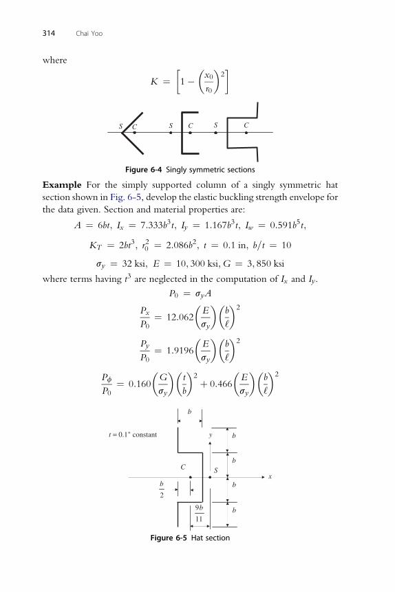
314 Chai Yoo

where

K ¼�1�

�x0

r0

�2�

S C S CCS

Figure 6-4 Singly symmetric sections

Example For the simply supported column of a singly symmetric hat

section shown in Fig. 6-5, develop the elastic buckling strength envelope for

the data given. Section and material properties are:

A ¼ 6bt; Ix ¼ 7:333b3t; Iy ¼ 1:167b3t; Iw ¼ 0:591b5t;

3 2 2

KT ¼ 2bt ; r0 ¼ 2:086b ; t ¼ 0:1 in; b=t ¼ 10

s ¼ 32 ksi; E ¼ 10; 300 ksi;G ¼ 3; 850 ksi

y

where terms having t3 are neglected in the computation of Ix and Iy.

P0 ¼ syA

P�E��

b�2

x

P0¼ 12:062

sy ‘

P�E��

b�2

y

P0¼ 1:9196

sy ‘

P�G��

t�2

�E��

b�2

f

P0¼ 0:160

sy bþ 0:466

sy ‘

b

C

y

9

11

b b

b

S

2

bx

b

bt = 0.1" constant

Figure 6-5 Hat section

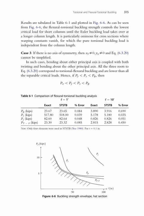
Torsional and Flexural-Torsional Buckling 315

Results are tabulated in Table 6-1 and plotted in Fig. 6-6. As can be seen

from Fig. 6-6, the flexural-torsional buckling strength controls the lowest

critical load for short columns until the Euler buckling load takes over at

a longer column length. It is particularly ominous for cross sections where

warping constants vanish, for which the pure torsional buckling load is

independent from the column length.

Case 3: If there is no axis of symmetry, then x0s0; y0s0 and Eq. (6.3.20)

cannot be simplified.

In such cases, bending about either principal axis is coupled with both

twisting and bending about the other principal axis. All the three roots to

Eq. (6.3.20) correspond to torsional-flexural buckling and are lower than all

the separable critical loads. Hence, if Py < Px < Pf, then

Pcr < Py < Px < Pf

Table 6-1 Comparison of flexural-torsional buckling analysis‘‘ ¼ 1’ ‘‘ ¼ 10’

Exact STSTB % Error Exact STSTB % Error

Pf (kips) 23.67 23.65 0.084 3.890 3.916 0.690

Px (kips) 517.80 518.00 0.039 5.178 5.180 0.035

Py (kips) 82.60 82.64 0.048 0.826 0.826 0.051

PT � F (kips) 23.30 23.32 0.085 2.815 2.828 0.450

Note: Only four elements were used in STSTB (Yoo 1980). For t ¼ 0.1 in.

( )kipscrP

( )in

F TP −

Pφ

yP

xP

10

5

10050

Figure 6-6 Buckling strength envelope, hat section

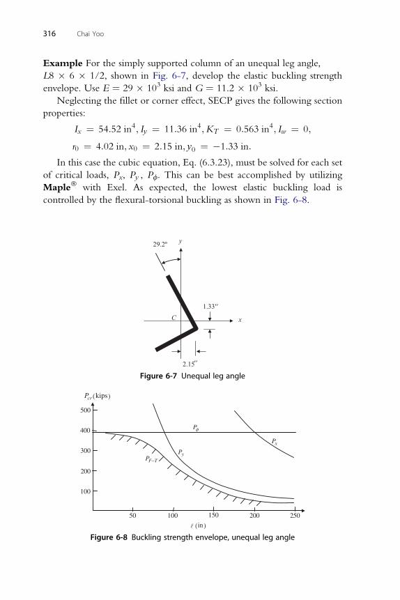
316 Chai Yoo

Example For the simply supported column of an unequal leg angle,

L8 � 6 � 1/2, shown in Fig. 6-7, develop the elastic buckling strength

envelope. Use E ¼ 29 � 103 ksi and G ¼ 11.2 � 103 ksi.

Neglecting the fillet or corner effect, SECP gives the following section

properties:

Ix ¼ 54:52 in4; Iy ¼ 11:36 in4;KT ¼ 0:563 in4; Iw ¼ 0;

r0 ¼ 4:02 in; x0 ¼ 2:15 in; y0 ¼ �1:33 in:

In this case the cubic equation, Eq. (6.3.23), must be solved for each set

of critical loads, Px, Py , Pf. This can be best accomplished by utilizing

Maple� with Exel. As expected, the lowest elastic buckling load is

controlled by the flexural-torsional buckling as shown in Fig. 6-8.

y29.2º

2.15

C1.33

x

Figure 6-7 Unequal leg angle

500

400

300

200

100

250

( )inl

( )kipscrP

F−TPyP

Pφ

xP

200100 15050

Figure 6-8 Buckling strength envelope, unequal leg angle

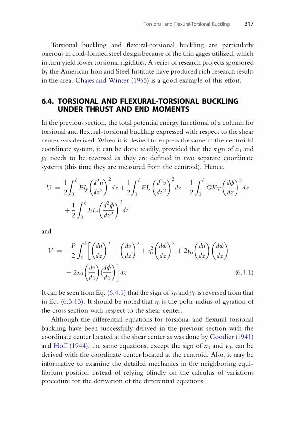
Torsional and Flexural-Torsional Buckling 317

Torsional buckling and flexural-torsional buckling are particularly

onerous in cold-formed steel design because of the thin gages utilized, which

in turn yield lower torsional rigidities. A series of research projects sponsored

by the American Iron and Steel Institute have produced rich research results

in the area. Chajes and Winter (1965) is a good example of this effort.

6.4. TORSIONAL AND FLEXURAL-TORSIONAL BUCKLINGUNDER THRUST AND END MOMENTS

In the previous section, the total potential energy functional of a column for

torsional and flexural-torsional buckling expressed with respect to the shear

center was derived. When it is desired to express the same in the centroidal

coordinate system, it can be done readily, provided that the sign of x0 and

y0 needs to be reversed as they are defined in two separate coordinate

systems (this time they are measured from the centroid). Hence,

U ¼ 1

2

Z ‘

0

EIy

�d2u

dz2

�2

dzþ 1

2

Z ‘

0

EIx

�d2v

dz2

�2

dzþ 1

2

Z ‘

0

GKT

�df

dz

�2

dz

þ 1

2

Z ‘

0

EIw

�d2f

dz2

�2

dz

and

V ¼ �P

2

Z ‘

0

��du

dz

�2

þ�dv

dz

�2

þ r20

�df

dz

�2

þ 2y0

�du

dz

��df

dz

�

� 2x0

�dv

dz

�ðdfdz

��dz (6.4.1)

It can be seen from Eq. (6.4.1) that the sign of x0 and y0 is reversed from that

in Eq. (6.3.13). It should be noted that r0 is the polar radius of gyration of

the cross section with respect to the shear center.

Although the differential equations for torsional and flexural-torsional

buckling have been successfully derived in the previous section with the

coordinate center located at the shear center as was done by Goodier (1941)

and Hoff (1944), the same equations, except the sign of x0 and y0, can be

derived with the coordinate center located at the centroid. Also, it may be

informative to examine the detailed mechanics in the neighboring equi-

librium position instead of relying blindly on the calculus of variations

procedure for the derivation of the differential equations.

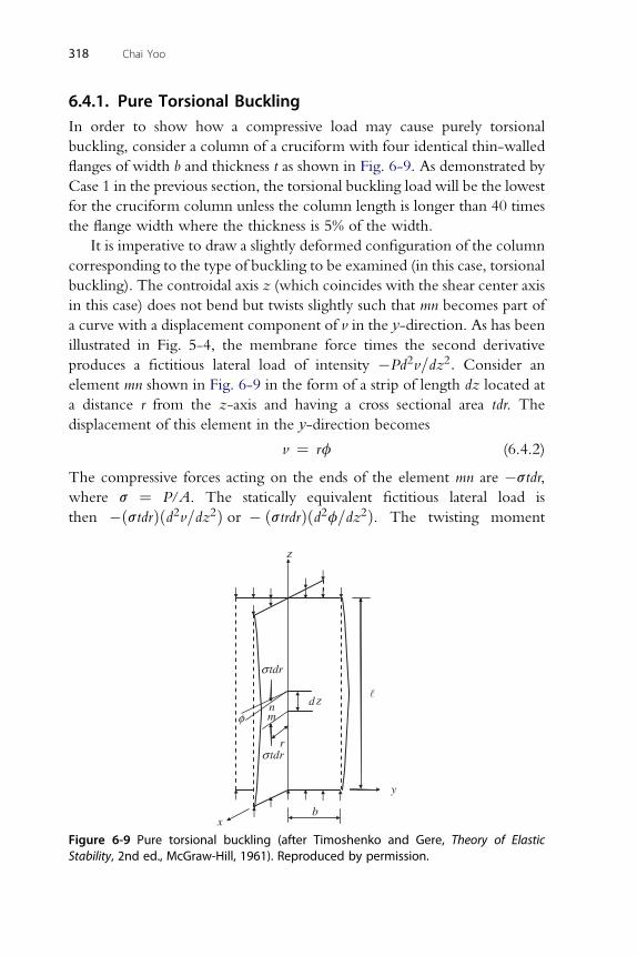
318 Chai Yoo

6.4.1. Pure Torsional BucklingIn order to show how a compressive load may cause purely torsional

buckling, consider a column of a cruciform with four identical thin-walled

flanges of width b and thickness t as shown in Fig. 6-9. As demonstrated by

Case 1 in the previous section, the torsional buckling load will be the lowest

for the cruciform column unless the column length is longer than 40 times

the flange width where the thickness is 5% of the width.

It is imperative to draw a slightly deformed configuration of the column

corresponding to the type of buckling to be examined (in this case, torsional

buckling). The controidal axis z (which coincides with the shear center axis

in this case) does not bend but twists slightly such that mn becomes part of

a curve with a displacement component of v in the y-direction. As has been

illustrated in Fig. 5-4, the membrane force times the second derivative

produces a fictitious lateral load of intensity �Pd2v=dz2: Consider an

element mn shown in Fig. 6-9 in the form of a strip of length dz located at

a distance r from the z-axis and having a cross sectional area tdr. The

displacement of this element in the y-direction becomes

v ¼ rf (6.4.2)

The compressive forces acting on the ends of the element mn are �stdr,

where s ¼ P/A. The statically equivalent fictitious lateral load is

then �ðstdrÞðd2v=dz2Þ or � ðstrdrÞðd2f=dz2Þ. The twisting moment

z

z

x

y

nm

d

r

b

tdrσ

tdrσ

φ

�

Figure 6-9 Pure torsional buckling (after Timoshenko and Gere, Theory of ElasticStability, 2nd ed., McGraw-Hill, 1961). Reproduced by permission.

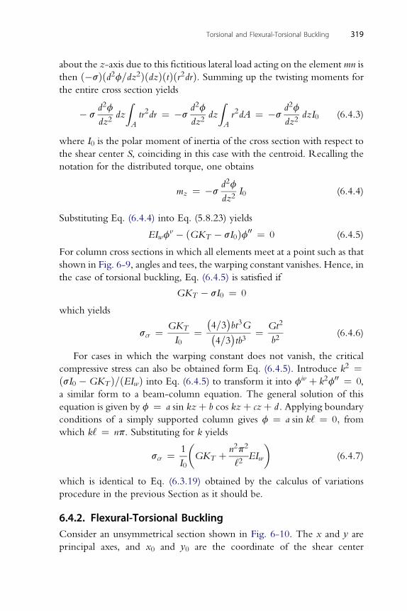
Torsional and Flexural-Torsional Buckling 319

about the z-axis due to this fictitious lateral load acting on the element mn is

then ð�sÞðd2f=dz2ÞðdzÞðtÞðr2drÞ. Summing up the twisting moments for

the entire cross section yields

� sd2f

dz2dz

ZA

tr2dr ¼ �sd2f

dz2dz

ZA

r2dA ¼ �sd2f

dz2dzI0 (6.4.3)

where I0 is the polar moment of inertia of the cross section with respect to

the shear center S, coinciding in this case with the centroid. Recalling the

notation for the distributed torque, one obtains

mz ¼ �sd2f

dz2I0 (6.4.4)

Substituting Eq. (6.4.4) into Eq. (5.8.23) yields

EIwfv � ðGKT � sI0Þf00 ¼ 0 (6.4.5)

For column cross sections in which all elements meet at a point such as that

shown in Fig. 6-9, angles and tees, the warping constant vanishes. Hence, in

the case of torsional buckling, Eq. (6.4.5) is satisfied if

GKT � sI0 ¼ 0

which yields

scr ¼ GKT

I0¼

�4=3

bt3G�

4=3tb3

¼ Gt2

b2(6.4.6)

For cases in which the warping constant does not vanish, the critical

compressive stress can also be obtained form Eq. (6.4.5). Introduce k2 ¼ðsI0 �GKT Þ=ðEIwÞ into Eq. (6.4.5) to transform it into fiv þ k2f00 ¼ 0,

a similar form to a beam-column equation. The general solution of this

equation is given by f ¼ a sin kzþ b cos kzþ czþ d . Applying boundary

conditions of a simply supported column gives f ¼ a sin k‘ ¼ 0; fromwhich k‘ ¼ np. Substituting for k yields

scr ¼ 1

I0

�GKT þ n2p2

‘2EIw

�(6.4.7)

which is identical to Eq. (6.3.19) obtained by the calculus of variations

procedure in the previous Section as it should be.

6.4.2. Flexural-Torsional BucklingConsider an unsymmetrical section shown in Fig. 6-10. The x and y are

principal axes, and x0 and y0 are the coordinate of the shear center

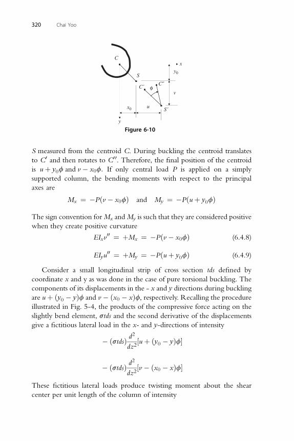
y

S´

v

y0

ux0

C

S

C˝C´

x

φ

Figure 6-10

320 Chai Yoo

S measured from the centroid C. During buckling the centroid translates

to C0 and then rotates to C00. Therefore, the final position of the centroid

is uþ y0f and v � x0f: If only central load P is applied on a simply

supported column, the bending moments with respect to the principal

axes are

Mx ¼ �Pðv � x0fÞ and My ¼ �Pðuþ y0fÞ

The sign convention forMx andMy is such that they are considered positive

when they create positive curvature

EIxv00 ¼ þMx ¼ �Pðv � x0fÞ (6.4.8)

EI u00 ¼ þM ¼ �Pðuþ y fÞ (6.4.9)

y y 0

Consider a small longitudinal strip of cross section tds defined by

coordinate x and y as was done in the case of pure torsional buckling. The

components of its displacements in the - x and y directions during buckling

are uþ ðy0 � yÞf and v � ðx0 � xÞf, respectively. Recalling the procedure

illustrated in Fig. 5-4, the products of the compressive force acting on the

slightly bend element, stds and the second derivative of the displacements

give a fictitious lateral load in the x- and y-directions of intensity

� ðstdsÞ d2

dz2½uþ ðy0 � yÞf�

d2

� ðstdsÞdz2

½v � ðx0 � xÞf�

These fictitious lateral loads produce twisting moment about the shear

center per unit length of the column of intensity

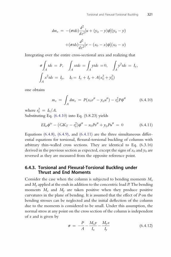
Torsional and Flexural-Torsional Buckling 321

dmz ¼ �ðstdsÞ d2

dz2½uþ ðy0 � yÞf�ðy0 � yÞ

þðstdsÞ d2

dz2½v � ðx0 � xÞf�ðx0 � xÞ

Integrating over the entire cross-sectional area and realizing that

s

ZA

tds ¼ P;

ZA

xtds ¼ZA

ytds ¼ 0;

ZA

y2tds ¼ Ix;ZA

x2tds ¼ Iy; I0¼ Ix þ Iy þ Aðx20 þ y20Þ

one obtains

mz ¼ZA

dmz ¼ Pðx0v00 � y0u00Þ � r20Pf

00 (6.4.10)

where r20 ¼ I0=A.Substituting Eq. (6.4.10) into Eq. (5.8.23) yields

EIwfiv � ðGKT � r20Þf00 � x0Pv

00 þ y0Pu00 ¼ 0 (6.4.11)

Equations (6.4.8), (6.4.9), and (6.4.11) are the three simultaneous differ-

ential equations for torsional, flexural-torsional buckling of columns with

arbitrary thin-walled cross sections. They are identical to Eq. (6.3.16)

derived in the previous section as expected, except the signs of x0 and y0 are

reversed as they are measured from the opposite reference point.

6.4.3. Torsional and Flexural-Torsional Buckling underThrust and End Moments

Consider the case when the column is subjected to bending moments Mx

andMy applied at the ends in addition to the concentric load P. The bending

moments Mx and My are taken positive when they produce positive

curvatures in the plane of bending. It is assumed that the effect of P on the

bending stresses can be neglected and the initial deflection of the column

due to the moments is considered to be small. Under this assumption, the

normal stress at any point on the cross section of the column is independent

of z and is given by

s ¼ �P

A�Mxy

Ix�Myx

Iy(6.4.12)

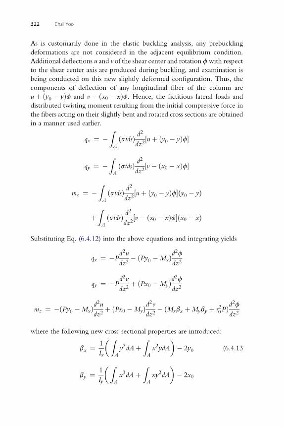
322 Chai Yoo

As is customarily done in the elastic buckling analysis, any prebuckling

deformations are not considered in the adjacent equilibrium condition.

Additional deflections u and v of the shear center and rotation fwith respect

to the shear center axis are produced during buckling, and examination is

being conducted on this new slightly deformed configuration. Thus, the

components of deflection of any longitudinal fiber of the column are

uþ ðy0 � yÞf and v � ðx0 � xÞf. Hence, the fictitious lateral loads and

distributed twisting moment resulting from the initial compressive force in

the fibers acting on their slightly bent and rotated cross sections are obtained

in a manner used earlier.

qx ¼ �ZA

ðstdsÞ d2

dz2½uþ ðy0 � yÞf�

Zd2

qy ¼ �A

ðstdsÞdz2

½v � ðx0 � xÞf�

Z 2

mz ¼ �A

ðstdsÞ ddz2

½uþ ðy0 � yÞf�ðy0 � yÞ

þZA

ðstdsÞ d2

dz2½v � ðx0 � xÞf�ðx0 � xÞ

Substituting Eq. (6.4.12) into the above equations and integrating yields

qx ¼ �Pd2u

dz2� ðPy0 �MxÞd

2f

dz2

d2v d2f

qy ¼ �P

dz2þ ðPx0 �MyÞ

dz2

d2u d2v d2f

mz ¼ �ðPy0 �MxÞ

dz2þ ðPx0 �MyÞ

dz2� ðMxbx þMyby þ r20PÞdz2

where the following new cross-sectional properties are introduced:

bx ¼ 1

Ix

�ZA

y3dAþZA

x2ydA

�� 2y0 (6.4.13

1�Z Z �

by ¼Iy A

x3dAþA

xy2dA � 2x0

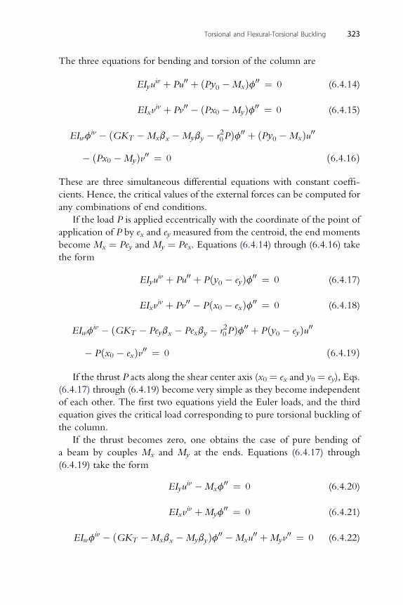
Torsional and Flexural-Torsional Buckling 323

The three equations for bending and torsion of the column are

EIyuiv þ Pu00 þ ðPy0 �MxÞf00 ¼ 0 (6.4.14)

iv 00 00

EIxv þ Pv � ðPx0 �MyÞf ¼ 0 (6.4.15)

iv 2 00 00

EIwf � ðGKT �Mxbx �Myby � r0PÞf þ ðPy0 �MxÞu

� ðPx0 �MyÞv00 ¼ 0 ð6:4:16Þ

These are three simultaneous differential equations with constant coeffi-

cients. Hence, the critical values of the external forces can be computed for

any combinations of end conditions.

If the load P is applied eccentrically with the coordinate of the point of

application of P by ex and ey measured from the centroid, the end moments

become Mx ¼ Pey and My ¼ Pex. Equations (6.4.14) through (6.4.16) take

the form

EIyuiv þ Pu00 þ Pðy0 � eyÞf00 ¼ 0 (6.4.17)

EI viv þ Pv00 � Pðx � e Þf00 ¼ 0 (6.4.18)

x 0 x

iv 2 00 00

EIwf � ðGKT � Peybx � Pexby � r0PÞf þ Pðy0 � eyÞu

� Pðx0 � exÞv00 ¼ 0 ð6:4:19Þ

If the thrust P acts along the shear center axis (x0 ¼ ex and y0 ¼ ey), Eqs.

(6.4.17) through (6.4.19) become very simple as they become independent

of each other. The first two equations yield the Euler loads, and the third

equation gives the critical load corresponding to pure torsional buckling of

the column.

If the thrust becomes zero, one obtains the case of pure bending of

a beam by couples Mx and My at the ends. Equations (6.4.17) through

(6.4.19) take the form

EIyuiv �Mxf

00 ¼ 0 (6.4.20)

EI viv þM f00 ¼ 0 (6.4.21)

x y

iv 00 00 00

EIwf � ðGKT �Mxbx �MybyÞf �Mxu þMyv ¼ 0 (6.4.22)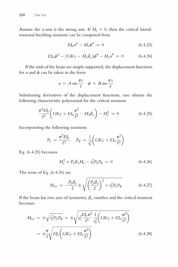

324 Chai Yoo

Assume the x-axis is the strong axis. If My ¼ 0, then the critical lateral-

torsional buckling moment can be computed from

EIyuiv �Mxf

00 ¼ 0 (6.4.23)

EI fiv � ðGK �M b Þf00 �M u00 ¼ 0 (6.4.24)

w T x x x

If the ends of the beam are simply supported, the displacement functions

for u and f can be taken in the form

u ¼ A sinpz

‘f ¼ B sin

pz

‘

Substituting derivatives of the displacement functions, one obtains the

following characteristic polynomial for the critical moment:

p2EIy

‘2

�GKT þ EIw

p2

‘2�Mxbx

��M2

x ¼ 0 (6.4.25)

Incorporating the following notations

Py ¼ p2EIy

‘2; Pf ¼ 1

r20

�GKT þ EIw

p2

‘2

�

Eq. (6.4.25) becomes

M2x þ PybxMx � r20PyPf ¼ 0 (6.4.26)

The roots of Eq. (6.4.26) are

Mxcr ¼ �Pybx

2�

ffiffiffiffiffiffiffiffiffiffiffiffiffiffiffiffiffiffiffiffiffiffiffiffiffiffiffiffiffiffiffiffiffiffiffiffiffiffi�Pybx

2

�2

þ r20PyPf

s(6.4.27)

If the beam has two axes of symmetry, bx vanishes and the critical moment

becomes

Mxcr ¼ �ffiffiffiffiffiffiffiffiffiffiffiffiffiffir20PyPf

q¼ �

ffiffiffiffiffiffiffiffiffiffiffiffiffiffiffiffiffiffiffiffiffiffiffiffiffiffiffiffiffiffiffiffiffiffiffiffiffiffiffiffiffiffiffiffiffiffiffiffiffiffiffiffiffiffiffir20EIyp

2

‘21

r20

�GKT þ EIw

p2

‘2

�s

¼ �p

‘

ffiffiffiffiffiffiffiffiffiffiffiffiffiffiffiffiffiffiffiffiffiffiffiffiffiffiffiffiffiffiffiffiffiffiffiffiffiffiffiffiffiffiEIy

�GKT þ EIw

p2

‘2

�s(6.4.28)

Torsional and Flexural-Torsional Buckling 325

where � sign in Eq. (6.4.28) implies that a pair of end moments equal in

magnitude but opposite in direction can cause lateral-torsional buckling of

a doubly symmetrical beam.

In this discussion, considerations have been given for the bending of

a beam by couples applied at the ends so that the normal stresses caused by

these moments remain constant, thereby maintaining the governing

differential equations with constant coefficients. If a beam is subjected to

lateral loads, the bending stresses vary with z and the resulting differential

equations will have variable coefficients, for which there are no general

closed-form solutions available and a variety of numerical integration

schemes are used. The computation of critical loads of lateral-torsional

buckling is discussed in the next chapter.

REFERENCESBleich, F. (1952). Buckling Strength of Metal Structures. New York: McGraw-Hill.Bleich, F. & Bleich, H. (1936). Bending Torsion and Buckling of Bars Composed of Thin

Walls, Prelim. Pub. 2nd Cong. International Association for Bridge and StructuralEngineering, English ed., p. 871, Berlin.

Euler, L. (1744). Methodus Inveniendi Lineas Curvas Maximi Minimive Propreietate Gaudentes(Appendix, De Curvis Elasticis). Lausanne and Geneva: Marcum Michaelem Bousquet.

Chajes, A., & Winter, G. (1965). Torsional-Flexural Buckling of Thin-Walled Members.Journal of the Structural Div., ASCE, Vol. 91(No. ST4), 103–124.

Galambos, T. V. (1968). Structural Members and Frames. Englewood Cliffs, NJ: Prentice-Hall.Goodier, J. N. (1941). The Buckling of Compressed Bars by Torsion and Flexure. Cornell

University Engineering Experiment Station. Bulletin No. 27.Hoff, N. J. (1944). A Strain Energy Derivation of the Torsional-Flexural Buckling Loads

of Straight Columns of Thin-Walled Open Sections. Quarterly of Applied Mathematics,Vol. 1(No. 4), 341–345.

Kappus, R. (1938). Drillknicken zentrisch gedrhckter Stabe emit offenem Profile imelastischen Bereich. Lufthahrt-Forschung, Vol. 14(No. 9), 444–457, English translation,Twisting Failure of Centrally Loaded Open-Sections Columns in the Elastic Range,NACA Tech. Mem. No. 851.

Kollbrunner, C. F., & Basler, K. (1969). E.C. Glauser (ed.) Torsion in Structures; An Engi-neering Approach, translated from German Berlin: Springer-Verlag.

Lundquist, E.F., & Fligg, C.M. (1937). A Theory for Primary Failure of Straight CentrallyLoaded Columns, NACA Tech: Report No. 582.

Ostenfeld, A. (1931). Politechnisk Laereanstalts Laboratorium for Bygningsstatik. Copenhagen:Meddelelse No. 5.

Timoshenko, S.P. (1945). Theory of Bending, Torsion and Buckling of Thin-WalledMembers of Open Cross Section, J. Franklin Institute (Philadelphia), Vol. 239, No. 3,p. 201, No. 4, p. 248, No. 5, p. 343.

Vlasov, V.Z. (1961). Tonkostennye uprugie sterzhni (Thin-walled elastic beams), (2nd ed.), Moscow,1959, translated by Schechtman, Israel Program for Scientific Translation, Jerusalem.

Wagner, H. & Pretschner, W. (1936). Torsion and Buckling of Open Sections, NACATech. mem. No. 784.

Yoo, C. H. (1980). Bimoment Contribution to Stability of Thin-Walled Assemblages.Computers and Structures, Vol. 11(No. 5), 465–471.

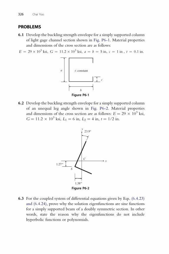
326 Chai Yoo

PROBLEMS

6.1 Develop the buckling strength envelope for a simply supported column

of light gage channel section shown in Fig. P6-1. Material properties

and dimensions of the cross section are as follows:

E ¼ 29� 103 ksi; G ¼ 11:2� 103 ksi; a ¼ b ¼ 5 in; c ¼ 1 in ; t ¼ 0:1 in:

a

b

c

: constantt

Figure P6-1

6.2 Develop the buckling strength envelope for a simply supported column

of an unequal leg angle shown in Fig. P6-2. Material properties

and dimensions of the cross section are as follows: E ¼ 29 � 103 ksi,

G ¼ 11.2 � 103 ksi, L1 ¼ 6 in, L2 ¼ 4 in, t ¼ 1/2 in.

y

C

23.9°

x1.27

1.38

S

Figure P6-2

6.3 For the coupled system of differential equations given by Eqs. (6.4.23)

and (6.4.24), prove why the solution eigenfunctions are sine functions

for a simply supported beam of a doubly symmetric section. In other

words, state the reason why the eigenfunctions do not include

hyperbolic functions or polynomials.

CHAPTER77

Lateral-Torsional BucklingContents

7.1. Introduction 3277.2. Differential Equations for Lateral-Torsional Buckling 3287.3. Generalization of Governing Differential Equations 3367.4. Lateral-Torsional Buckling for Various Loading and Boundary Conditions 3377.5. Application of Bessel Function to Lateral-Torsional Buckling Problems 3437.6. Lateral-Torsional Buckling by Energy Method 347

7.6.1. Uniform Bending 3487.6.2. One Concentrated Load at Midspan 3527.6.3. Uniformly Distributed Load 3557.6.4. Two Concentrated Loads Applied Symmetrically 359

7.7. Design Simplification for Lateral-Torsional Buckling 362References 368Problems 369

7.1. INTRODUCTION

A transversely (or combined transversely and axially) loaded member that is

bent with respect to its major axis may buckle laterally if its compression

flange is not sufficiently supported laterally. The reason buckling occurs in

a beam at all is that the compression flange or the extreme edge of the

compression side of a narrow rectangular beam, which behaves like

a column resting on an elastic foundation, becomes unstable. If the flexural

rigidity of the beam with respect to the plane of the bending is many times

greater than the rigidity of the lateral bending, the beam may buckle and

collapse long before the bending stresses reach the yield point. As long as the

applied loads remain below the limit value, the beam remains stable; that is,

the beam that is slightly twisted and/or bent laterally returns to its original

configuration upon the removal of the disturbing force. With increasing

load intensity, the restoring forces become smaller and smaller, until

a loading is reached at which, in addition to the plane bending equilibrium

configuration, an adjacent, deflected, and twisted, equilibrium position

becomes equally possible. The original bending configuration is no longer

stable, and the lowest load at which such an alternative equilibrium

configuration becomes possible is the critical load of the beam. At the

critical load, the compression flange tends to bend laterally, exceeding the

Stability of Structures � 2011 Elsevier Inc.ISBN 978-0-12-385122-2, doi:10.1016/B978-0-12-385122-2.10007-7 All rights reserved. 327 j

328 Chai Yoo

restoring force provided by the remaining portion of the cross section to

cause the section to twist. Lateral buckling is a misnomer, for no lateral

deflection is possible without concurrent twisting of the section.

Bleich (1952) gives credit to Prandtl (1899) and Michell (1899) for

producing the first theoretical studies on the lateral buckling of beams

with long narrow rectangular sections. Similar credit is also extended to

Timoshenko (1910) for deriving the fundamental differential equation of

torsion of symmetrical I-beams and investigating the lateral buckling of

transversely loaded deep I-beams with the derived equation. Since then,

many investigators, including Vlasov (1940), Winter (1943), Hill (1954),

Clark and Hill (1960), and Galambos (1963), have contributed on both

elastic and inelastic lateral-torsional buckling of various shapes. Some of the

early developments of the resisting capacities of steel structural members

leading to the Load and Resistance Factor Design (LRFD) are summarized

by Vincent (1969).

7.2. DIFFERENTIAL EQUATIONS FOR LATERAL-TORSIONALBUCKLING

If transverse loads do not pass through the shear center, they will induce

torsion. In order to avoid this additional torsional moment (thereby

weakening the flexural capacity) in the flexural members, it is customary to

use flexural members of at least singly symmetric sections so that the

transverse loads will pass through the plane of the web as shown in Fig. 7-1.

The section is symmetric about the y-axis, and u and v are the components

of the displacement of the shear center parallel to the axes x and h. The

rotation of the shear center f is taken positive about the z-axis according to

the right-hand screw rule, and the z-axis is perpendicular to the xh plane.

The following assumptions are employed:

1. The beam is prismatic.

2. The member cross section retains its original shape during buckling.

3. The externally applied loads are conservative.

4. The analysis is limited within the elastic limit.

5. The transverse load passes through the axis of symmetry in the plane of

bending.

In the derivation of the governing differential equations of the lateral-

torsional buckling of beams, it is necessary to define two coordinate systems:

one for the undeformed configuration, x, y, z, and the other for the

deformed configuration, x, h, 2 as shown in Fig. 7-1. Hence, the fixed

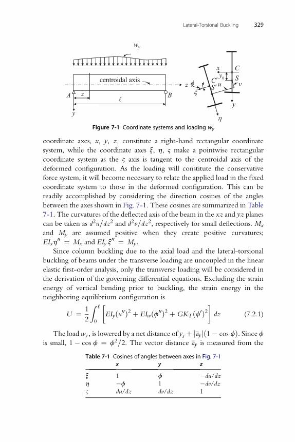
Figure 7-1 Coordinate systems and loading wy

Lateral-Torsional Buckling 329

coordinate axes, x, y, z, constitute a right-hand rectangular coordinate

system, while the coordinate axes x, h, 2 make a pointwise rectangular

coordinate system as the 2 axis is tangent to the centroidal axis of the

deformed configuration. As the loading will constitute the conservative

force system, it will become necessary to relate the applied load in the fixed

coordinate system to those in the deformed configuration. This can be

readily accomplished by considering the direction cosines of the angles

between the axes shown in Fig. 7-1. These cosines are summarized in Table

7-1. The curvatures of the deflected axis of the beam in the xz and yz planes

can be taken as d2u=dz2 and d2v=dz2, respectively for small deflections. Mx

and My are assumed positive when they create positive curvatures;

EIxh00 ¼ Mx and EIy x

00 ¼ My.

Since column buckling due to the axial load and the lateral-torsional

buckling of beams under the transverse loading are uncoupled in the linear

elastic first-order analysis, only the transverse loading will be considered in

the derivation of the governing differential equations. Excluding the strain

energy of vertical bending prior to buckling, the strain energy in the

neighboring equilibrium configuration is

U ¼ 1

2

Z ‘

0

�EIyðu00Þ2 þ EIwðf00Þ2 þGKT ðf0Þ2

�dz (7.2.1)

The load wy , is lowered by a net distance of ys þ jayjð1� cos fÞ. Since fis small, 1� cos f ¼ f2=2. The vector distance ay is measured from the

Table 7-1 Cosines of angles between axes in Fig. 7-1x y z

x 1 f �du/dz

h �f 1 �dv/dz

2 du/dz dv/dz 1

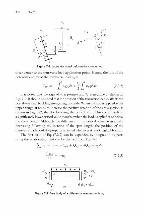
Figure 7-2 Lateral-torsional deformations under wy

330 Chai Yoo

shear center to the transverse load application point. Hence, the loss of the

potential energy of the transverse load wy is

Vwy ¼ �Z ‘

0

wyysdzþay

2

Z ‘

0

wyf2dz (7.2.2)

It is noted that the sign of ys is positive and ay is negative as shown in

Fig. 7-2. It should be noted that the position of the transverse load ay affects the

lateral-torsional buckling strength significantly.When the load is applied at the

upper flange, it tends to increase the positive rotation of the cross section as

shown in Fig. 7-2, thereby lowering the critical load. This could result in

a significantly lower critical value than thatwhen the load is applied at or below

the shear center. Although the difference in the critical values is gradually

decreasing following the increase of the span length, the position of the

transverse load should be properly reflectedwhenever it is not negligibly small.

The first term of Eq. (7.2.2) can be expanded by integration by parts

using the relationships that can be derived from Fig. 7-3.XFy ¼ 0 ¼ �Qwy þQwy þ dQwy þ wydz

dQwy

dz¼ �wy (7.2.3)

wy

bxMbx bxM dM+

wyQwy wyQ dQ+

dz

Az

y

Figure 7-3 Free body of a differential element with wy

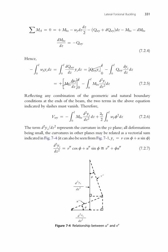
X dz

MA ¼ 0 ¼ þMbx � wydz

2� ðQwy þ dQwyÞdz�Mbx � dMbx

dMbx

dz¼ �Qwy

(7.2.4)

Hence,

�Z ‘

0

wyysdz ¼Z ‘

0

dQwy

dzysdz ¼

�

½Qwyys�‘

0�Z ‘

0

Qwydysdz

dz

¼ þ

��Mbx

dysdz

�‘

0�Z ‘

0

Mbxd2ysdz2

dz (7.2.5)

Reflecting any combination of the geometric and natural boundary

conditions at the ends of the beam, the two terms in the above equation

indicated by slashes must vanish. Therefore,

Vwy ¼ �Z ‘

0

Mbxd2ysdz2

dzþ ay

2

Z ‘

0

wyf2dz (7.2.6)

The term d2ys=dz2 represents the curvature in the yz plane; all deformations

being small, the curvatures in other planes may be related as a vectorial sum

indicated in Fig. 7-4 (it can also be seen fromFig. 7-1, ys ¼ v cos fþ u sin f)

d2ysdz2

¼ v00 cos fþ u00 sin fy v00 þ fu00 (7.2.7)

Lateral-Torsional Buckling 331

v”φ

2

2

dz

2dz

yd s

2xd s

u”

φ

Figure 7-4 Relationship between u00 and v00

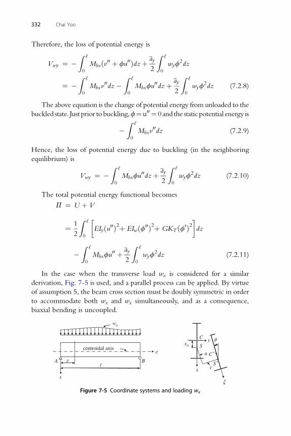
332 Chai Yoo

Therefore, the loss of potential energy is

Vwy ¼ �Z ‘

0

Mbxðv00 þ fu00Þdzþ ay

2

Z ‘

0

wyf2dz

¼ �Z ‘

0

Mbxv00dz�

Z ‘

0

Mbxfu00dzþ ay

2

Z ‘

0

wyf2dz (7.2.8)

The above equation is the change of potential energy from unloaded to the

buckled state. Just prior tobuckling,f¼u00 ¼ 0 and the static potential energy is

�Z ‘

0

Mbxv00dz (7.2.9)

Hence, the loss of potential energy due to buckling (in the neighboring

equilibrium) is

Vwy ¼ �Z ‘

0

Mbxfu00dzþ ay

2

Z ‘

0

wyf2dz (7.2.10)

The total potential energy functional becomes

P ¼ U þ V

Z ‘ � �

¼ 1

2 0

EIyðu00Þ2þ EIwðf00Þ2þ GKT ðf0Þ2 dz

�Z ‘

0

Mbxfu00 þ ay

2

Z ‘

0

wyf2dz (7.2.11)

In the case when the transverse load wx is considered for a similar

derivation, Fig. 7-5 is used, and a parallel process can be applied. By virtue

of assumption 5, the beam cross section must be doubly symmetric in order

to accommodate both wx and wx simultaneously, and as a consequence,

biaxial bending is uncoupled.

xw

z

zcentroidal axis

A B

C

S

xx

u

ξ

S

φ

C

v

y0x

Figure 7-5 Coordinate systems and loading wx

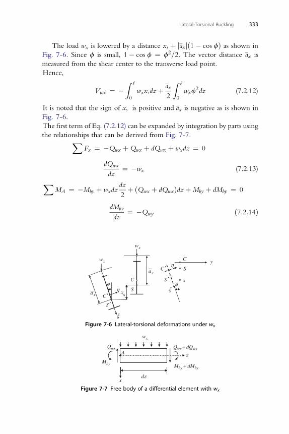
Lateral-Torsional Buckling 333

The load wx is lowered by a distance xs þ jaxjð1� cos fÞ as shown in

Fig. 7-6. Since f is small, 1� cos f ¼ f2=2. The vector distance ax is

measured from the shear center to the transverse load point.

Hence,

Vwx ¼ �Z ‘

0

wxxsdzþ ax

2

Z ‘

0

wxf2dz (7.2.12)

It is noted that the sign of xs is positive and ax is negative as is shown in

Fig. 7-6.

The first term of Eq. (7.2.12) can be expanded by integration by parts using

the relationships that can be derived from Fig. 7-7.XFx ¼ �Qwx þQwx þ dQwx þ wxdz ¼ 0

dQwx

dz¼ �wx (7.2.13)

X dz

MA ¼ �Mby þ wxdz

2þ ðQwx þ dQwxÞdzþMby þ dMby ¼ 0

dMby

dz¼ �Qwy ð7:2:14Þ

C

SS

x

xw

ξ

y

x

xa

C

Sη

S ′

C ′

xw

η

S ′C ′

φ

xa

φξ

Figure 7-6 Lateral-torsional deformations under wx

xw

QwxQwx dQwx+

dzx

zA

Mby

MbydMby+

Figure 7-7 Free body of a differential element with wx

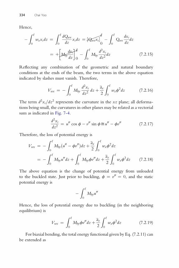
334 Chai Yoo

Hence,

�Z ‘

0

wxxsdz ¼Z ‘

0

dQwx

dzxsdz ¼

�

½Qwxxs�‘

0�Z ‘

0

Qwxdxs

dzdz

¼ þ

��Mby

dxs

dz

�‘

0�Z ‘

0

Mbyd2xs

dz2dz (7.2.15)

Reflecting any combination of the geometric and natural boundary

conditions at the ends of the beam, the two terms in the above equation

indicated by slashes must vanish. Therefore,

Vwx ¼ �Z ‘

0

Mbyd2xs

dz2dzþ ax

2

Z ‘

0

wxf2dz (7.2.16)

The term d2xs=dz2 represents the curvature in the xz plane; all deforma-

tions being small, the curvatures in other planes may be related as a vectorial

sum as indicated in Fig. 7-4.

d2xs

dz2¼ u00 cos f� v00 sin fyu00 � fv00 (7.2.17)

Therefore, the loss of potential energy is

Vwx ¼ �Z ‘

0

Mbyðu00 � fv00Þdzþ ax

2

Z ‘

0

wxf2dz

¼ �Z ‘

0

Mbyu00dzþ

Z ‘

0

Mbyfv00dzþ ax

2

Z ‘

0

wxf2dz (7.2.18)

The above equation is the change of potential energy from unloaded

to the buckled state. Just prior to buckling, f ¼ v00 ¼ 0, and the static

potential energy is

�Z ‘

0

Mbyu00

Hence, the loss of potential energy due to buckling (in the neighboring

equilibrium) is

Vwx ¼Z ‘

0

Mbyfv00dzþ ax

2

Z ‘

0

wxf2dz (7.2.19)

For biaxial bending, the total energy functional given by Eq. (7.2.11) can

be extended as

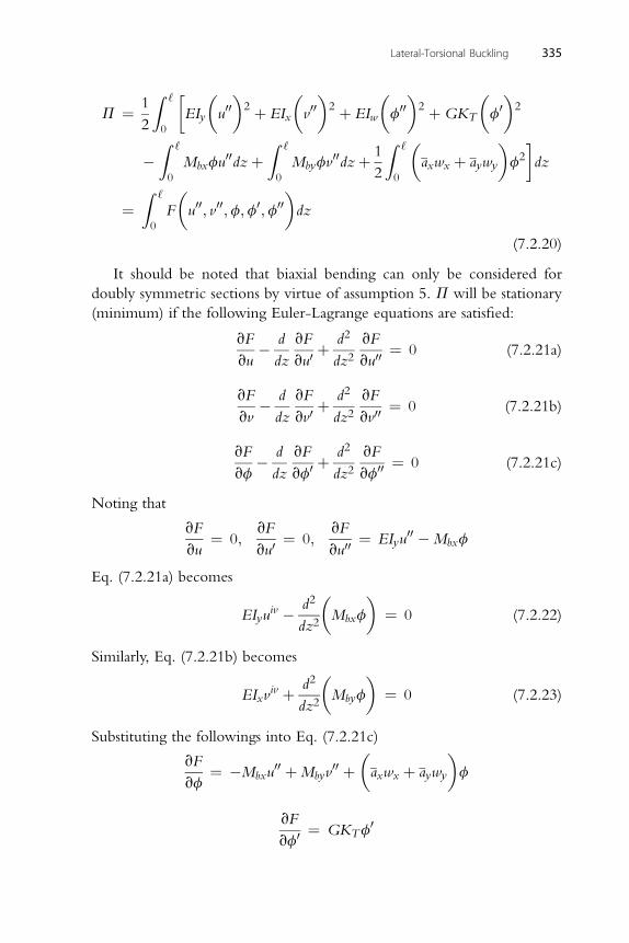
Lateral-Torsional Buckling 335

P ¼ 1

2

Z ‘

0

�EIy

�u00�2 þ EIx

�v00�2 þ EIw

�f00

�2 þGKT

�f0�2

�Z ‘

0

Mbxfu00dzþ

Z ‘

0

Mbyfv00dzþ 1

2

Z ‘

0

�axwx þ aywy

�f2

�dz

¼Z ‘

0

F

�u00; v00;f;f0;f00

�dz

(7.2.20)

It should be noted that biaxial bending can only be considered for

doubly symmetric sections by virtue of assumption 5. P will be stationary

(minimum) if the following Euler-Lagrange equations are satisfied:

vF

vu� d

dz

vF

vu0þ d2

dz2vF

vu00¼ 0 (7.2.21a)

vF d vF d2 vF

vv�dz vv0

þdz2 vv00

¼ 0 (7.2.21b)

vF d vF d2 vF

vf�dz vf0 þ dz2 vf00 ¼ 0 (7.2.21c)

Noting that

vF

vu¼ 0;

vF

vu0¼ 0;

vF

vu00¼ EIyu

00 �Mbxf

Eq. (7.2.21a) becomes

EIyuiv � d2

dz2

�Mbxf

�¼ 0 (7.2.22)

Similarly, Eq. (7.2.21b) becomes

EIxviv þ d2

dz2

�Mbyf

�¼ 0 (7.2.23)

Substituting the followings into Eq. (7.2.21c)

vF

vf¼ �Mbxu

00 þMbyv00 þ

�axwx þ aywy

�f

vF

vf0 ¼ GKTf0

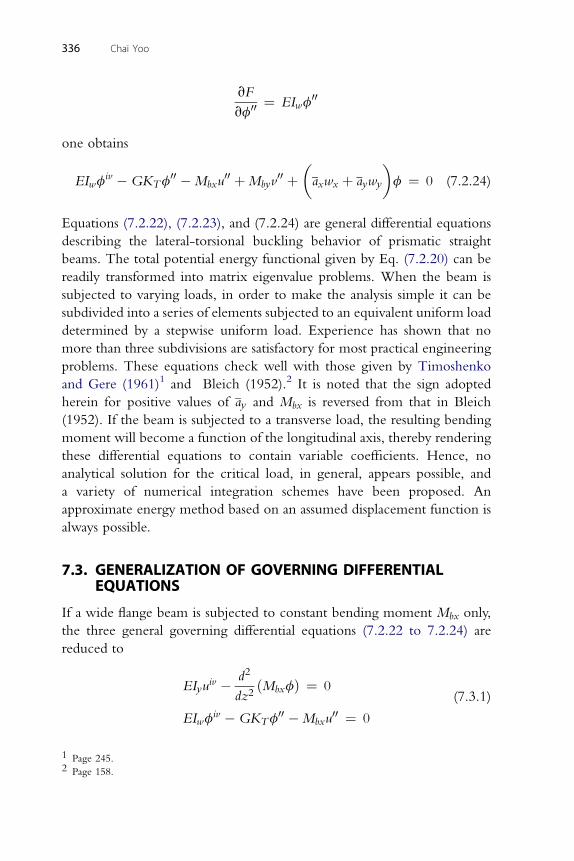
vF 00

vf00 ¼ EIwf

one obtains

EIwfiv �GKTf

00 �Mbxu00 þMbyv

00 þ�axwx þ aywy

�f ¼ 0 (7.2.24)

Equations (7.2.22), (7.2.23), and (7.2.24) are general differential equations

describing the lateral-torsional buckling behavior of prismatic straight

beams. The total potential energy functional given by Eq. (7.2.20) can be

readily transformed into matrix eigenvalue problems. When the beam is

subjected to varying loads, in order to make the analysis simple it can be

subdivided into a series of elements subjected to an equivalent uniform load

determined by a stepwise uniform load. Experience has shown that no

more than three subdivisions are satisfactory for most practical engineering

problems. These equations check well with those given by Timoshenko

and Gere (1961)1 and Bleich (1952).2 It is noted that the sign adopted

herein for positive values of ay and Mbx is reversed from that in Bleich

(1952). If the beam is subjected to a transverse load, the resulting bending

moment will become a function of the longitudinal axis, thereby rendering

these differential equations to contain variable coefficients. Hence, no

analytical solution for the critical load, in general, appears possible, and

a variety of numerical integration schemes have been proposed. An

approximate energy method based on an assumed displacement function is

always possible.

336 Chai Yoo

7.3. GENERALIZATION OF GOVERNING DIFFERENTIALEQUATIONS

If a wide flange beam is subjected to constant bending moment Mbx only,

the three general governing differential equations (7.2.22 to 7.2.24) are

reduced to

EIyuiv � d2

dz2ðMbxfÞ ¼ 0

EIwfiv �GKTf

00 �Mbxu00 ¼ 0

(7.3.1)

1 Page 245.2 Page 158.

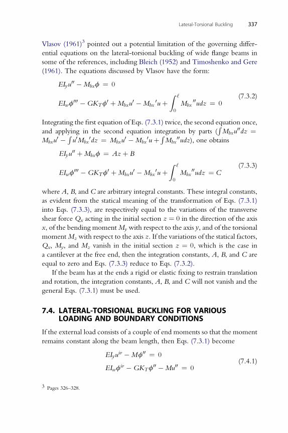
Lateral-Torsional Buckling 337

Vlasov (1961)3 pointed out a potential limitation of the governing differ-

ential equations on the lateral-torsional buckling of wide flange beams in

some of the references, including Bleich (1952) and Timoshenko and Gere

(1961). The equations discussed by Vlasov have the form:

EIyu00 �Mbxf ¼ 0

EIwf000 �GKTf

0 þMbxu0 �Mbx

0uþZ ‘

0

Mbx00udz ¼ 0

(7.3.2)

Integrating the first equation of Eqs. (7.3.1) twice, the second equation once,

and applying in the second equation integration by parts (RMbxu

00dz ¼Mbxu

0 � Ru0Mbx

0dz ¼ Mbxu0 �Mbx

0uþRMbx

00udz), one obtains

EIyu00 þMbxf ¼ Azþ B

EIwf000 �GKTf

0 þMbxu0 �Mbx

0uþZ ‘

0

Mbx00udz ¼ C

(7.3.3)

where A, B, and C are arbitrary integral constants. These integral constants,

as evident from the statical meaning of the transformation of Eqs. (7.3.1)

into Eqs. (7.3.3), are respectively equal to the variations of the transverse

shear force Qx acting in the initial section z ¼ 0 in the direction of the axis

x, of the bending momentMy with respect to the axis y, and of the torsional

momentMzwith respect to the axis z. If the variations of the statical factors,

Qx, My, and Mz vanish in the initial section z ¼ 0, which is the case in

a cantilever at the free end, then the integration constants, A, B, and C are

equal to zero and Eqs. (7.3.3) reduce to Eqs. (7.3.2).

If the beam has at the ends a rigid or elastic fixing to restrain translation

and rotation, the integration constants, A, B, and C will not vanish and the

general Eqs. (7.3.1) must be used.

7.4. LATERAL-TORSIONAL BUCKLING FOR VARIOUSLOADING AND BOUNDARY CONDITIONS

If the external load consists of a couple of end moments so that the moment

remains constant along the beam length, then Eqs. (7.3.1) become

EIyuiv �Mf00 ¼ 0

EIwfiv �GKTf

00 �Mu00 ¼ 0(7.4.1)

3 Pages 326–328.

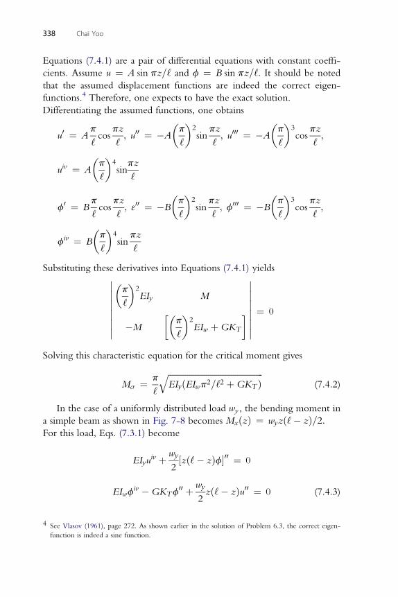
338 Chai Yoo

Equations (7.4.1) are a pair of differential equations with constant coeffi-

cients. Assume u ¼ A sin pz=‘ and f ¼ B sin pz=‘. It should be noted

that the assumed displacement functions are indeed the correct eigen-

functions.4 Therefore, one expects to have the exact solution.

Differentiating the assumed functions, one obtains

u0 ¼ Ap

‘cos

pz

‘; u00 ¼ �A

�p

‘

�2sin

pz

‘; u000 ¼ �A

�p

‘

�3cos

pz

‘;

uiv ¼ A

�p

‘

�4sin

pz

‘

p pz�p�2 pz

�p�3 pz

f0 ¼ B‘cos

‘; 300 ¼ �B

‘sin

‘; f000 ¼ �B

‘cos

‘;

fiv ¼ B

�p

‘

�4sin

pz

‘

Substituting these derivatives into Equations (7.4.1) yields�������p

‘

�2EIy M

�M

��p

‘

�2EIw þGKT

������� ¼ 0

Solving this characteristic equation for the critical moment gives

Mcr ¼ p

‘

ffiffiffiffiffiffiffiffiffiffiffiffiffiffiffiffiffiffiffiffiffiffiffiffiffiffiffiffiffiffiffiffiffiffiffiffiffiffiffiffiffiffiffiffiffiEIyðEIwp2=‘2 þGKT Þ

q(7.4.2)

In the case of a uniformly distributed load wy , the bending moment in

a simple beam as shown in Fig. 7-8 becomes MxðzÞ ¼ wyzð‘� zÞ=2:For this load, Eqs. (7.3.1) become

EIyuiv þ wy

2½zð‘� zÞf�00 ¼ 0

iv 00 wy 00

EIwf �GKTf þ2zð‘� zÞu ¼ 0 (7.4.3)

4 See Vlasov (1961), page 272. As shown earlier in the solution of Problem 6.3, the correct eigen-

function is indeed a sine function.

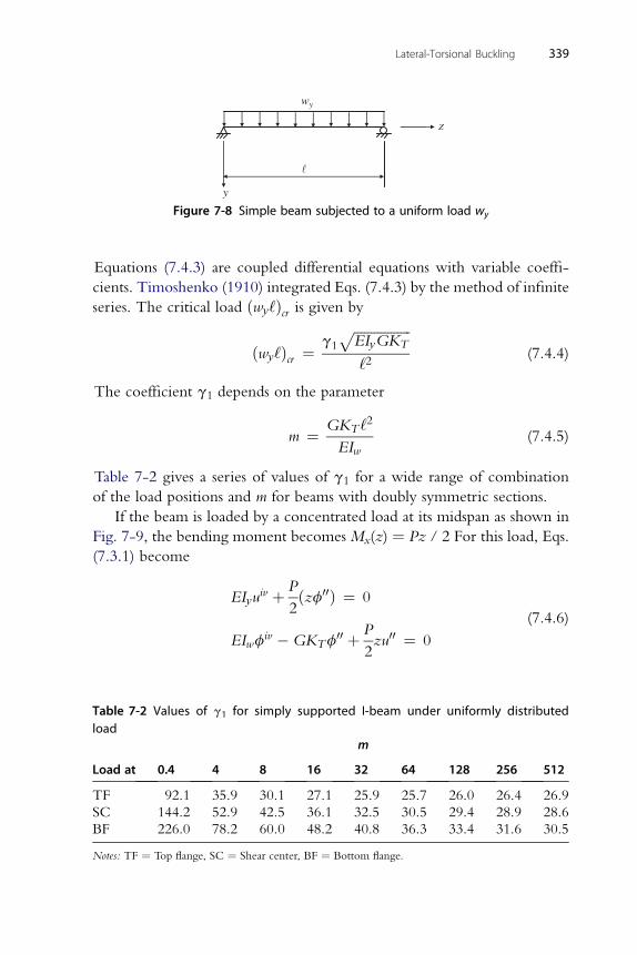
yw

z

y

Figure 7-8 Simple beam subjected to a uniform load wy

Lateral-Torsional Buckling 339

Equations (7.4.3) are coupled differential equations with variable coeffi-

cients. Timoshenko (1910) integrated Eqs. (7.4.3) by the method of infinite

series. The critical load ðwy‘Þcr is given by

ðwy‘Þcr ¼ g1

ffiffiffiffiffiffiffiffiffiffiffiffiffiffiffiffiffiEIyGKT

p‘2

(7.4.4)

The coefficient g1 depends on the parameter

m ¼ GKT ‘2

EIw(7.4.5)

Table 7-2 gives a series of values of g1 for a wide range of combination

of the load positions and m for beams with doubly symmetric sections.

If the beam is loaded by a concentrated load at its midspan as shown in

Fig. 7-9, the bending moment becomes Mx(z) ¼ Pz / 2 For this load, Eqs.

(7.3.1) become

EIyuiv þ P

2ðzf00Þ ¼ 0

EIwfiv �GKTf

00 þ P

2zu00 ¼ 0

(7.4.6)

Table 7-2 Values of g1 for simply supported I-beam under uniformly distributedload

Load at

m

0.4 4 8 16 32 64 128 256 512

TF 92.1 35.9 30.1 27.1 25.9 25.7 26.0 26.4 26.9

SC 144.2 52.9 42.5 36.1 32.5 30.5 29.4 28.9 28.6

BF 226.0 78.2 60.0 48.2 40.8 36.3 33.4 31.6 30.5

Notes: TF ¼ Top flange, SC ¼ Shear center, BF ¼ Bottom flange.

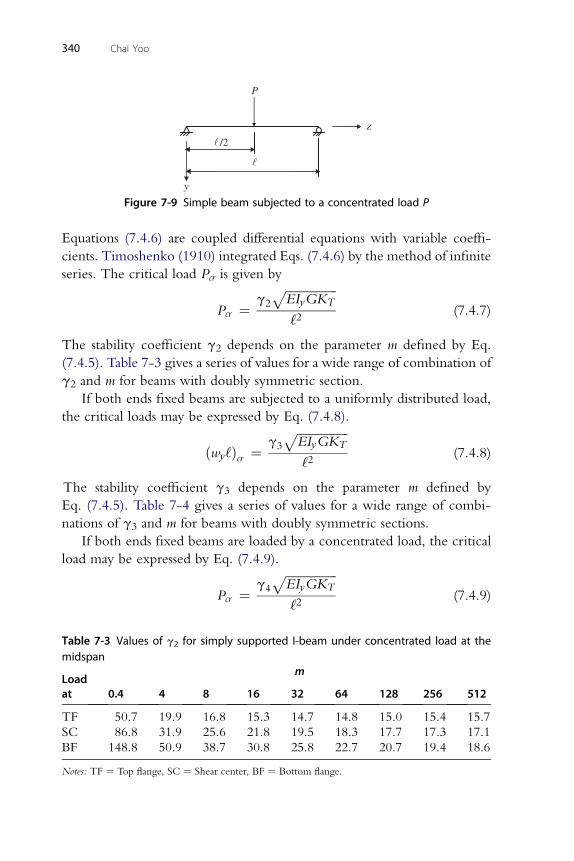
P

/2

z

y

Figure 7-9 Simple beam subjected to a concentrated load P

340 Chai Yoo

Equations (7.4.6) are coupled differential equations with variable coeffi-

cients. Timoshenko (1910) integrated Eqs. (7.4.6) by the method of infinite

series. The critical load Pcr is given by

Pcr ¼ g2

ffiffiffiffiffiffiffiffiffiffiffiffiffiffiffiffiffiEIyGKT

p‘2

(7.4.7)

The stability coefficient g2 depends on the parameter m defined by Eq.

(7.4.5). Table 7-3 gives a series of values for a wide range of combination of

g2 and m for beams with doubly symmetric section.

If both ends fixed beams are subjected to a uniformly distributed load,

the critical loads may be expressed by Eq. (7.4.8).

ðwy‘Þcr ¼ g3ffiffiffiffiffiffiffiffiffiffiffiffiffiffiffiffiffiEIyGKT

p‘2

(7.4.8)

The stability coefficient g3 depends on the parameter m defined by

Eq. (7.4.5). Table 7-4 gives a series of values for a wide range of combi-

nations of g3 and m for beams with doubly symmetric sections.

If both ends fixed beams are loaded by a concentrated load, the critical

load may be expressed by Eq. (7.4.9).

Pcr ¼ g4

ffiffiffiffiffiffiffiffiffiffiffiffiffiffiffiffiffiEIyGKT

p‘2

(7.4.9)

Table 7-3 Values of g2 for simply supported I-beam under concentrated load at themidspan

Loadat

m

0.4 4 8 16 32 64 128 256 512

TF 50.7 19.9 16.8 15.3 14.7 14.8 15.0 15.4 15.7

SC 86.8 31.9 25.6 21.8 19.5 18.3 17.7 17.3 17.1

BF 148.8 50.9 38.7 30.8 25.8 22.7 20.7 19.4 18.6

Notes: TF ¼ Top flange, SC ¼ Shear center, BF ¼ Bottom flange.

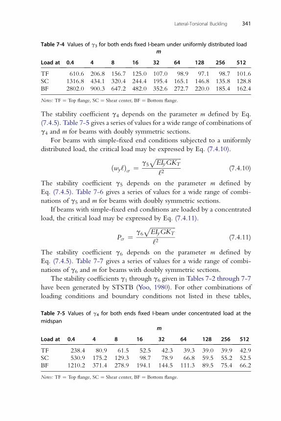
Table 7-4 Values of g3 for both ends fixed I-beam under uniformly distributed load

Load at

m

0.4 4 8 16 32 64 128 256 512

TF 610.6 206.8 156.7 125.0 107.0 98.9 97.1 98.7 101.6

SC 1316.8 434.1 320.4 244.4 195.4 165.1 146.8 135.8 128.8

BF 2802.0 900.3 647.2 482.0 352.6 272.7 220.0 185.4 162.4

Notes: TF ¼ Top flange, SC ¼ Shear center, BF ¼ Bottom flange.

Lateral-Torsional Buckling 341

The stability coefficient g4 depends on the parameter m defined by Eq.

(7.4.5). Table 7-5 gives a series of values for a wide range of combinations of

g4 and m for beams with doubly symmetric sections.

For beams with simple-fixed end conditions subjected to a uniformly

distributed load, the critical load may be expressed by Eq. (7.4.10).

ðwy‘Þcr ¼ g5

ffiffiffiffiffiffiffiffiffiffiffiffiffiffiffiffiffiEIyGKT

p‘2

(7.4.10)

The stability coefficient g5 depends on the parameter m defined by

Eq. (7.4.5). Table 7-6 gives a series of values for a wide range of combi-

nations of g5 and m for beams with doubly symmetric sections.

If beams with simple-fixed end conditions are loaded by a concentrated

load, the critical load may be expressed by Eq. (7.4.11).

Pcr ¼ g6

ffiffiffiffiffiffiffiffiffiffiffiffiffiffiffiffiffiEIyGKT

p‘2

(7.4.11)

The stability coefficient g6 depends on the parameter m defined by

Eq. (7.4.5). Table 7-7 gives a series of values for a wide range of combi-

nations of g6 and m for beams with doubly symmetric sections.

The stability coefficients g1 through g6 given in Tables 7-2 through 7-7

have been generated by STSTB (Yoo, 1980). For other combinations of

loading conditions and boundary conditions not listed in these tables,

Table 7-5 Values of g4 for both ends fixed I-beam under concentrated load at themidspan

Load at

m

0.4 4 8 16 32 64 128 256 512

TF 238.4 80.9 61.5 52.5 42.3 39.3 39.0 39.9 42.9

SC 530.9 175.2 129.3 98.7 78.9 66.8 59.5 55.2 52.5

BF 1210.2 371.4 278.9 194.1 144.5 111.3 89.5 75.4 66.2

Notes: TF ¼ Top flange, SC ¼ Shear center, BF ¼ Bottom flange.

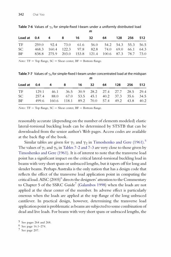
Table 7-6 Values of g5 for simple-fixed I-beam under a uniformly distributed load

Load at

m

0.4 4 8 16 32 64 128 256 512

TF 259.0 92.4 73.0 61.6 56.0 54.2 54.3 55.3 56.5

SC 468.3 160.4 122.3 97.8 82.8 74.0 69.0 66.1 64.3

BF 838.8 275.9 203.0 153.8 121.4 100.6 87.3 78.7 73.0

Notes: TF ¼ Top flange, SC ¼ Shear center, BF ¼ Bottom flange.

Table 7-7 Values of g6 for simple-fixed I-beam under concentrated load at the midspan

Load at

m

0.4 4 8 16 32 64 128 256 512

TF 129.1 46.1 36.5 30.9 28.2 27.4 27.7 28.5 29.4

SC 257.4 88.0 67.0 53.5 45.1 40.2 37.3 35.6 34.5

BF 499.6 160.6 118.1 89.2 70.0 57.4 49.2 43.8 40.2

Notes: TF ¼ Top flange, SC ¼ Shear center, BF ¼ Bottom flange.

342 Chai Yoo

reasonably accurate (depending on the number of elements modeled) elastic

lateral-torsional buckling loads can be determined by STSTB that can be

downloaded from the senior author’s Web pages. Access codes are available

at the back flap of the book.

Similar tables are given for g1 and g2 in Timoshenko and Gere (1961).5

The values of g1 and g6 in Tables 7-2 and 7-3 are very close to those given by

Timoshenko and Gere (1961). It is of interest to note that the transverse load

point has a significant impact on the critical lateral-torsional buckling load in

beams with very short spans or unbraced lengths, but it tapers off for long and

slender beams. Perhaps Australia is the only nation that has a design code that

reflects the effect of the transverse load application point in computing the

critical load. AISC (2005)6 directs the designers’ attention to theCommentary

to Chapter 5 of the SSRC Guide7 (Galambos 1998) when the loads are not

applied at the shear center of the member. Its adverse effect is particularly

onerous when the loads are applied at the top flange of the long unbraced

cantilever. In practical design, however, determining the transverse load

application point is problematic as beams are subjected to some combination of

dead and live loads. For beams with very short spans or unbraced lengths, the

5 See pages 264 and 268.6 See page 16.1–274.7 See page 207.

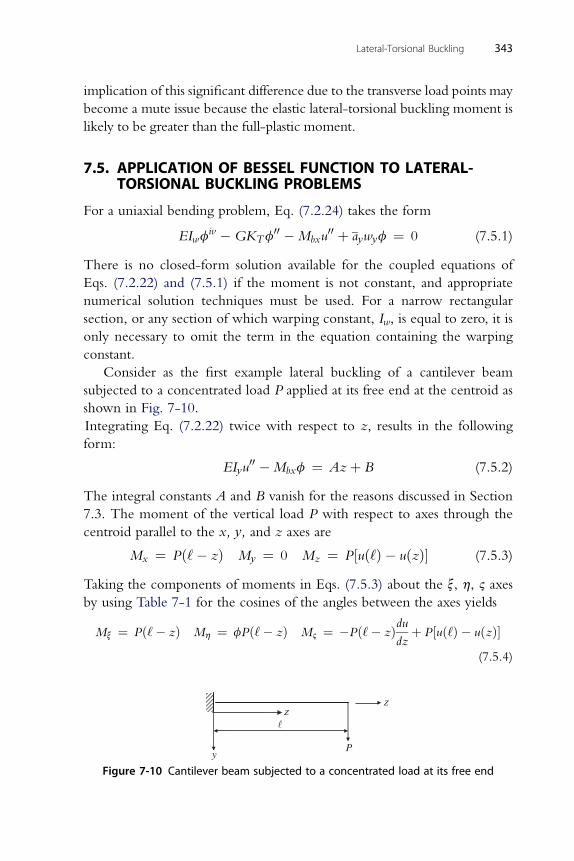
Lateral-Torsional Buckling 343

implication of this significant difference due to the transverse load points may

become a mute issue because the elastic lateral-torsional buckling moment is

likely to be greater than the full-plastic moment.

7.5. APPLICATION OF BESSEL FUNCTION TO LATERAL-TORSIONAL BUCKLING PROBLEMS

For a uniaxial bending problem, Eq. (7.2.24) takes the form

EIwfiv �GKTf

00 �Mbxu00 þ aywyf ¼ 0 (7.5.1)

There is no closed-form solution available for the coupled equations of

Eqs. (7.2.22) and (7.5.1) if the moment is not constant, and appropriate

numerical solution techniques must be used. For a narrow rectangular

section, or any section of which warping constant, Iw, is equal to zero, it is

only necessary to omit the term in the equation containing the warping

constant.

Consider as the first example lateral buckling of a cantilever beam

subjected to a concentrated load P applied at its free end at the centroid as

shown in Fig. 7-10.

Integrating Eq. (7.2.22) twice with respect to z, results in the following

form:

EIyu00 �Mbxf ¼ Azþ B (7.5.2)

The integral constants A and B vanish for the reasons discussed in Section

7.3. The moment of the vertical load P with respect to axes through the

centroid parallel to the x, y, and z axes are

Mx ¼ Pð‘� zÞ My ¼ 0 Mz ¼ P½uð‘Þ � uðzÞ� (7.5.3)

Taking the components of moments in Eqs. (7.5.3) about the x, h, 2 axes

by using Table 7-1 for the cosines of the angles between the axes yields

Mx ¼ Pð‘� zÞ Mh ¼ fPð‘� zÞ M2 ¼ �Pð‘� zÞdudz

þ P½uð‘Þ � uðzÞ�(7.5.4)

P

zz

y

Figure 7-10 Cantilever beam subjected to a concentrated load at its free end

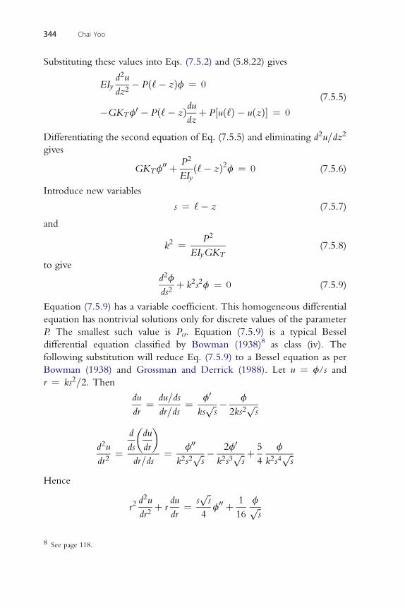
344 Chai Yoo

Substituting these values into Eqs. (7.5.2) and (5.8.22) gives

EIyd2u

dz2� Pð‘� zÞf ¼ 0

�GKTf0 � Pð‘� zÞdu

dzþ P½uð‘Þ � uðzÞ� ¼ 0

(7.5.5)

Differentiating the second equation of Eq. (7.5.5) and eliminating d2u=dz2

gives

GKTf00 þ P2

EIyð‘� zÞ2f ¼ 0 (7.5.6)

Introduce new variables

s ¼ ‘� z (7.5.7)

and

k2 ¼ P2

EIyGKT(7.5.8)

to give

d2f

ds2þ k2s2f ¼ 0 (7.5.9)

Equation (7.5.9) has a variable coefficient. This homogeneous differential

equation has nontrivial solutions only for discrete values of the parameter

P. The smallest such value is Pcr. Equation (7.5.9) is a typical Bessel

differential equation classified by Bowman (1938)8 as class (iv). The

following substitution will reduce Eq. (7.5.9) to a Bessel equation as per

Bowman (1938) and Grossman and Derrick (1988). Let u ¼ f/s and

r ¼ ks2=2. Then

du

dr¼ du=ds

dr=ds¼ f0

ksffiffis

p � f

2ks2ffiffis

p

d�du�

d2u

dr2¼ ds dr

dr=ds¼ f00

k2s2ffiffis

p � 2f0

k2s3ffiffis

p þ 5

4

f

k2s4ffiffis

p

Hence

r2d2u

dr2þ r

du

dr¼ s

ffiffis

p4

f00 þ 1

16

fffiffis

p

8 See page 118.

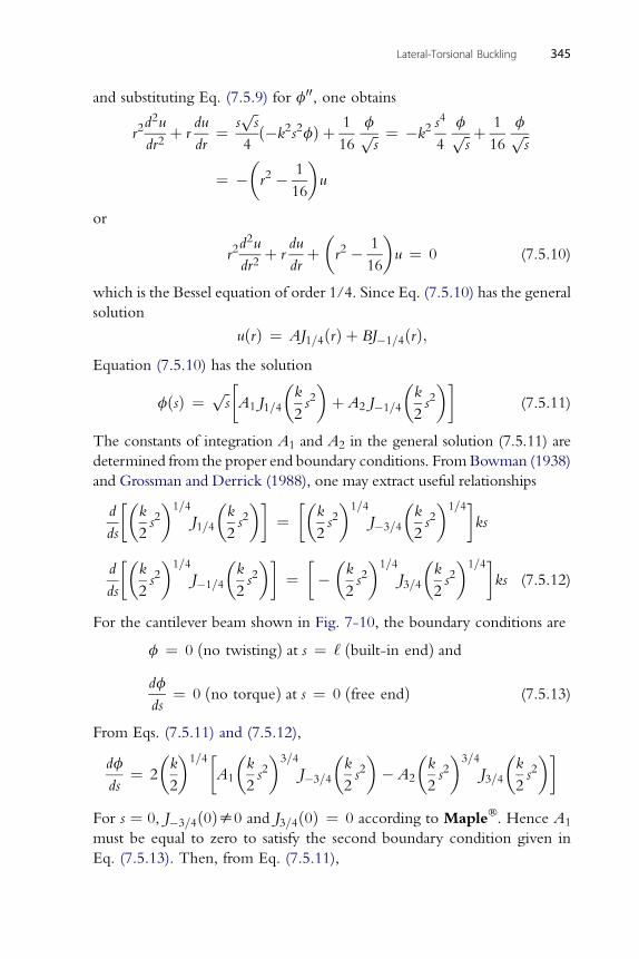
Lateral-Torsional Buckling 345

and substituting Eq. (7.5.9) for f00, one obtains

r2d2u

dr2þ r

du

dr¼ s

ffiffis

p4ð�k2s2fÞ þ 1

16

fffiffis

p ¼ �k2s4

4

fffiffis

p þ 1

16

fffiffis

p

¼ ��r2 � 1

16

�u

or

r2d2u

dr2þ r

du

drþ�r2 � 1

16

�u ¼ 0 (7.5.10)

which is the Bessel equation of order 1/4. Since Eq. (7.5.10) has the general

solution

uðrÞ ¼ AJ1=4ðrÞ þ BJ�1=4ðrÞ;Equation (7.5.10) has the solution

fðsÞ ¼ ffiffis

p �A1 J1=4

�k

2s2�þ A2 J�1=4

�k

2s2��

(7.5.11)

The constants of integration A1 and A2 in the general solution (7.5.11) are

determined from the proper end boundary conditions. FromBowman (1938)

and Grossman and Derrick (1988), one may extract useful relationships

d

ds

��k

2s2�1=4

J1=4

�k

2s2��

¼��

k

2s2�1=4

J�3=4

�k

2s2�1=4�

ks

d

ds

��k

2s2�1=4

J�1=4

�k

2s2��

¼���k

2s2�1=4

J3=4

�k

2s2�1=4�

ks (7.5.12)

For the cantilever beam shown in Fig. 7-10, the boundary conditions are

f ¼ 0 ðno twistingÞ at s ¼ ‘ ðbuilt-in endÞ anddf

ds¼ 0 ðno torqueÞ at s ¼ 0 ðfree endÞ (7.5.13)

From Eqs. (7.5.11) and (7.5.12),

df

ds¼ 2

�k

2

�1=4�

A1

�k

2s2�3=4

J�3=4

�k

2s2�� A2

�k

2s2�3=4

J3=4

�k

2s2��

For s ¼ 0, J�3=4ð0Þs0 and J3=4ð0Þ ¼ 0 according to Maple�. Hence A1

must be equal to zero to satisfy the second boundary condition given in

Eq. (7.5.13). Then, from Eq. (7.5.11),

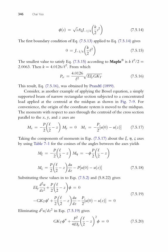
346 Chai Yoo

fðsÞ ¼ ffiffis

pA2J�1=4

�k

2s2�

(7.5.14)

The first boundary condition of Eq. (7.5.13) applied to Eq. (7.5.14) gives

0 ¼ J�1=4

�k

2‘2�

(7.5.15)

The smallest value to satisfy Eq. (7.5.15) according to Maple� is k ‘2/2 ¼2.0063. Then k ¼ 4.0126/‘2. From which

Pcr ¼ 4:0126

‘2ffiffiffiffiffiffiffiffiffiffiffiffiffiffiffiffiffiEIyGKT

p(7.5.16)

This result, Eq. (7.5.16), was obtained by Prandtl (1899).

Consider, as another example of applying the Bessel equation, a simply

supported beam of narrow rectangular section subjected to a concentrated

load applied at the centroid at the midspan as shown in Fig. 7-9. For

convenience, the origin of the coordinate system is moved to the midspan.

The moments with respect to axes through the centroid of the cross section

parallel to the x, y, and z axes are

Mx ¼ �P

2

�‘

2� z

�My ¼ 0 Mz ¼ �P

2½uð0Þ � uðzÞ� (7.5.17)

Taking the components of moments in Eqs. (7.5.17) about the x, h, 2 axes

by using Table 7-1 for the cosines of the angles between the axes yields

Mx ¼ �P

2

�‘

2� z

�Mh ¼ �f

P

2

�‘

2� z

�

M2 ¼ P

2

�‘

2� z

�du

dz� P½uð0Þ � uðzÞ� (7.5.18)

Substituting these values in to Eqs. (7.5.2) and (5.8.22) gives

EIyd2u

dz2þ P

2

�‘

2� z

�f ¼ 0

�GKTf0 þ P

2

�‘

2� z

�du

dz� P

2½uð0Þ � uðzÞ� ¼ 0

(7.5.19)

Eliminating d2u=dz2 in Eqs. (7.5.19) gives

GKTf00 þ P2

4EIy

�‘

2� z

�2

f ¼ 0 (7.5.20)

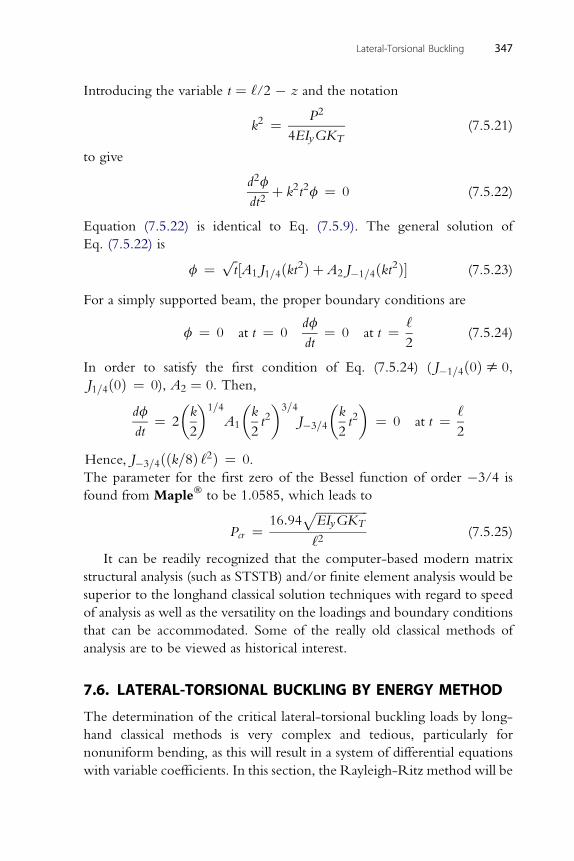
Lateral-Torsional Buckling 347

Introducing the variable t ¼ ‘/2 � z and the notation

k2 ¼ P2

4EIyGKT(7.5.21)

to give

d2f

dt2þ k2t2f ¼ 0 (7.5.22)

Equation (7.5.22) is identical to Eq. (7.5.9). The general solution of

Eq. (7.5.22) is

f ¼ ffiffit

p ½A1 J1=4ðkt2Þ þ A2 J�1=4ðkt2Þ� (7.5.23)

For a simply supported beam, the proper boundary conditions are

f ¼ 0 at t ¼ 0df

dt¼ 0 at t ¼ ‘

2(7.5.24)

In order to satisfy the first condition of Eq. (7.5.24) ( J�1=4ð0Þs 0;J1=4ð0Þ ¼ 0), A2 ¼ 0. Then,

df

dt¼ 2

�k

2

�1=4

A1

�k

2t2�3=4

J�3=4

�k

2t2�

¼ 0 at t ¼ ‘

2

Hence, J�3=4ððk=8Þ ‘2Þ ¼ 0.

The parameter for the first zero of the Bessel function of order �3/4 is

found from Maple� to be 1.0585, which leads to

Pcr ¼ 16:94ffiffiffiffiffiffiffiffiffiffiffiffiffiffiffiffiffiEIyGKT

p‘2

(7.5.25)

It can be readily recognized that the computer-based modern matrix

structural analysis (such as STSTB) and/or finite element analysis would be

superior to the longhand classical solution techniques with regard to speed

of analysis as well as the versatility on the loadings and boundary conditions

that can be accommodated. Some of the really old classical methods of

analysis are to be viewed as historical interest.

7.6. LATERAL-TORSIONAL BUCKLING BY ENERGY METHOD

The determination of the critical lateral-torsional buckling loads by long-

hand classical methods is very complex and tedious, particularly for

nonuniform bending, as this will result in a system of differential equations

with variable coefficients. In this section, the Rayleigh-Ritz method will be

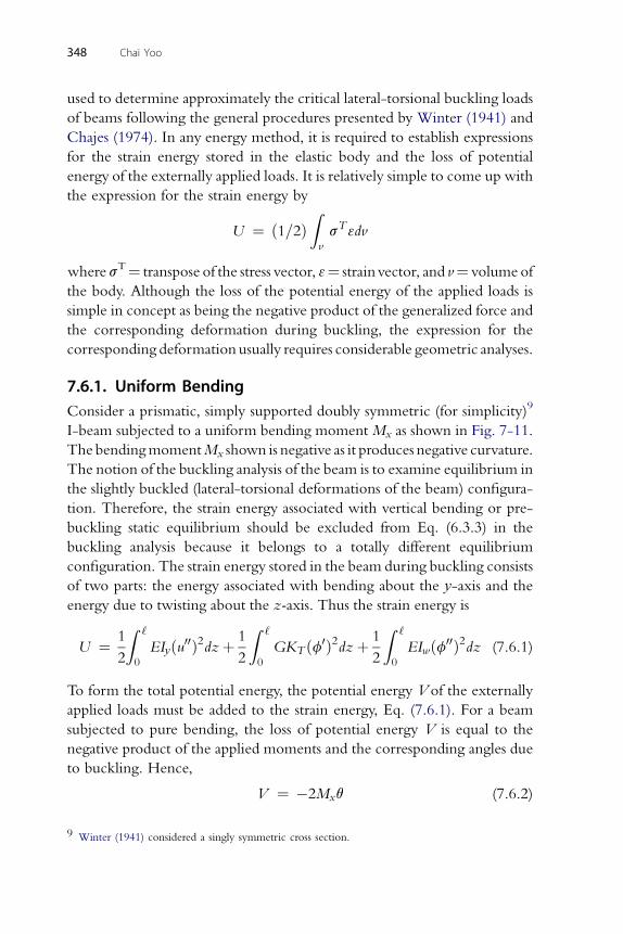
348 Chai Yoo

used to determine approximately the critical lateral-torsional buckling loads

of beams following the general procedures presented by Winter (1941) and

Chajes (1974). In any energy method, it is required to establish expressions

for the strain energy stored in the elastic body and the loss of potential

energy of the externally applied loads. It is relatively simple to come up with

the expression for the strain energy by

U ¼ ð1=2ÞZv

sT 3dv

wheresT¼ transpose of the stress vector, 3¼ strain vector, and v¼ volume of

the body. Although the loss of the potential energy of the applied loads is

simple in concept as being the negative product of the generalized force and

the corresponding deformation during buckling, the expression for the

corresponding deformation usually requires considerable geometric analyses.

7.6.1. Uniform BendingConsider a prismatic, simply supported doubly symmetric (for simplicity)9

I-beam subjected to a uniform bending moment Mx as shown in Fig. 7-11.

The bendingmomentMx shown is negative as it produces negative curvature.

The notion of the buckling analysis of the beam is to examine equilibrium in

the slightly buckled (lateral-torsional deformations of the beam) configura-

tion. Therefore, the strain energy associated with vertical bending or pre-

buckling static equilibrium should be excluded from Eq. (6.3.3) in the

buckling analysis because it belongs to a totally different equilibrium

configuration. The strain energy stored in the beam during buckling consists

of two parts: the energy associated with bending about the y-axis and the

energy due to twisting about the z-axis. Thus the strain energy is

U ¼ 1

2

Z ‘

0

EIyðu00Þ2dzþ 1

2

Z ‘

0

GKT ðf0Þ2dzþ 1

2

Z ‘

0

EIwðf00Þ2dz (7.6.1)

To form the total potential energy, the potential energy V of the externally

applied loads must be added to the strain energy, Eq. (7.6.1). For a beam

subjected to pure bending, the loss of potential energy V is equal to the

negative product of the applied moments and the corresponding angles due

to buckling. Hence,

V ¼ �2Mxq (7.6.2)

9 Winter (1941) considered a singly symmetric cross section.

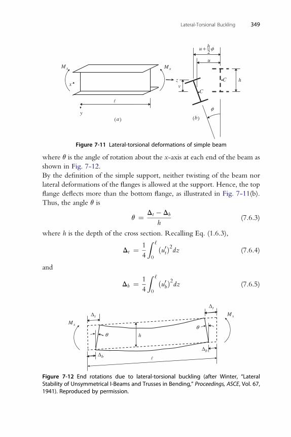
2hu φ+

( )b( )a

h

u

v

M Mx

z

x

C

Cx

φy

i

i

Figure 7-11 Lateral-torsional deformations of simple beam

Lateral-Torsional Buckling 349

where q is the angle of rotation about the x-axis at each end of the beam as

shown in Fig. 7-12.

By the definition of the simple support, neither twisting of the beam nor

lateral deformations of the flanges is allowed at the support. Hence, the top

flange deflects more than the bottom flange, as illustrated in Fig. 7-11(b).

Thus, the angle q is

q ¼ Dt � Db

h(7.6.3)

where h is the depth of the cross section. Recalling Eq. (1.6.3),

Dt ¼ 1

4

Z ‘

0

ðu0tÞ2dz (7.6.4)

and

Db ¼ 1

4

Z ‘

0

ðu0bÞ2dz (7.6.5)

xMxM

tΔ

tΔ

bΔ

θ h

bΔ

θ

Figure 7-12 End rotations due to lateral-torsional buckling (after Winter, “LateralStability of Unsymmetrical I-Beams and Trusses in Bending,” Proceedings, ASCE, Vol. 67,1941). Reproduced by permission.

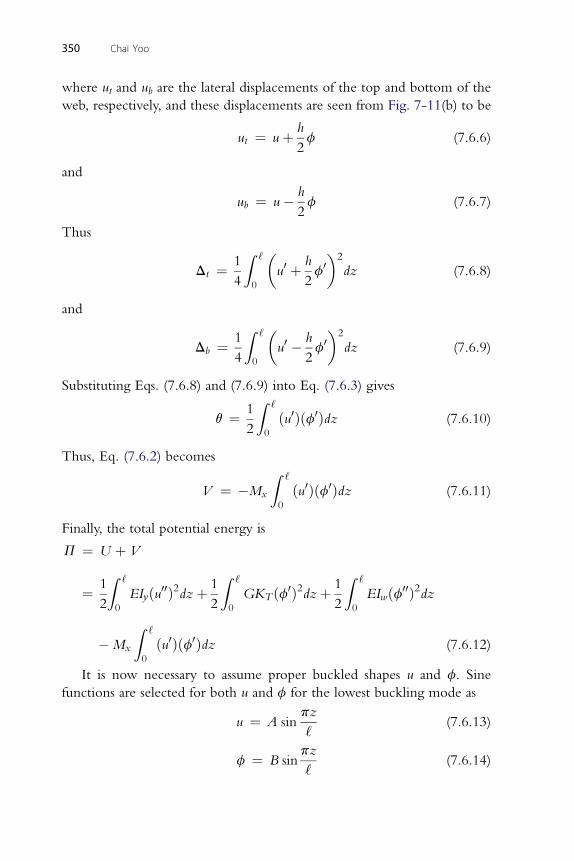
350 Chai Yoo

where ut and ub are the lateral displacements of the top and bottom of the

web, respectively, and these displacements are seen from Fig. 7-11(b) to be

ut ¼ uþ h

2f (7.6.6)

and

ub ¼ u� h

2f (7.6.7)

Thus

Dt ¼ 1

4

Z ‘

0

�u0 þ h

2f0�2

dz (7.6.8)

and

Db ¼ 1

4

Z ‘

0

�u0 � h

2f0�2

dz (7.6.9)

Substituting Eqs. (7.6.8) and (7.6.9) into Eq. (7.6.3) gives

q ¼ 1

2

Z ‘

0

ðu0Þðf0Þdz (7.6.10)

Thus, Eq. (7.6.2) becomes

V ¼ �Mx

Z ‘

0

ðu0Þðf0Þdz (7.6.11)

Finally, the total potential energy is

P ¼ U þ V

¼ 1

2

Z ‘

0

EIyðu00Þ2dzþ 1

2

Z ‘

0

GKT ðf0Þ2dzþ 1

2

Z ‘

0

EIwðf00Þ2dz

�Mx

Z ‘

0

ðu0Þðf0Þdz (7.6.12)

It is now necessary to assume proper buckled shapes u and f. Sine

functions are selected for both u and f for the lowest buckling mode as

u ¼ A sinpz

‘(7.6.13)

pz

f ¼ B sin

‘(7.6.14)

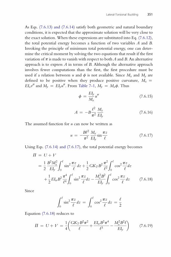
Lateral-Torsional Buckling 351

As Eqs. (7.6.13) and (7.6.14) satisfy both geometric and natural boundary

conditions, it is expected that the approximate solution will be very close to

the exact solution. When these expressions are substituted into Eq. (7.6.12),

the total potential energy becomes a function of two variables A and B.

Invoking the principle of minimum total potential energy, one can deter-

mine the critical moment by solving the two equations that result if the first

variation of p is made to vanish with respect to both A and B. An alternative

approach is to express A in terms of B. Although the alternative approach

involves fewer computations than the first, the first procedure must be

used if a relation between u and f is not available. Since Mx and My are

defined to be positive when they produce positive curvature, Mx ¼EIxv

00 and My ¼ EIyu00. From Table 7-1, My ¼ Mxf. Thus

f ¼ EIy

Mxu00 (7.6.15)

‘2 M

A ¼ �B

p2

x

EIy(7.6.16)

The assumed function for u can now be written as

u ¼ �B‘2

p2

Mx

EIysin

pz

‘(7.6.17)

Using Eqs. (7.6.14) and (7.6.17), the total potential energy becomes

P ¼ U þ V

¼ 1

2

B2M2x

EIy

Z ‘

0

sin2pz

‘dzþ 1

2GKTB

2 p2

‘2

Z ‘

0

cos2pz

‘dz

þ 1

2EIwB

2 p4

‘4

Z ‘

0

sin2pz

‘dz�M2

xB2

EIy

Z ‘

0

cos2pz

‘dz (7.6.18)

Since Z ‘

0

sin2pz

‘dz ¼

Z ‘

0

cos2pz

‘dz ¼ ‘

2

Equation (7.6.18) reduces to

P ¼ U þ V ¼ 1

4

�GKTB

2p2

‘þ EIwB

2p4

‘3�M2

xB2‘

EIy

�(7.6.19)

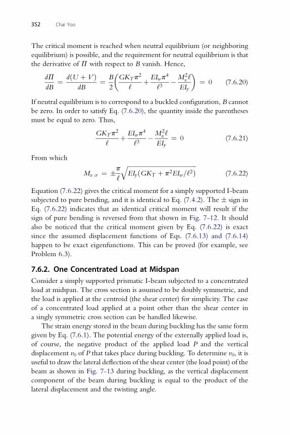
352 Chai Yoo

The critical moment is reached when neutral equilibrium (or neighboring

equilibrium) is possible, and the requirement for neutral equilibrium is that

the derivative of P with respect to B vanish. Hence,

dP

dB¼ dðU þ V Þ

dB¼ B

2

�GKTp

2

‘þ EIwp

4

‘3�M2

x ‘

EIy

�¼ 0 (7.6.20)

If neutral equilibrium is to correspond to a buckled configuration, B cannot

be zero. In order to satisfy Eq. (7.6.20), the quantity inside the parentheses

must be equal to zero. Thus,

GKTp2

‘þ EIwp

4

‘3�M2

x ‘

EIy¼ 0 (7.6.21)

From which

Mx cr ¼ �p

‘

ffiffiffiffiffiffiffiffiffiffiffiffiffiffiffiffiffiffiffiffiffiffiffiffiffiffiffiffiffiffiffiffiffiffiffiffiffiffiffiffiffiffiffiffiffiEIyðGKT þ p2EIw=‘2Þ

q(7.6.22)

Equation (7.6.22) gives the critical moment for a simply supported I-beam

subjected to pure bending, and it is identical to Eq. (7.4.2). The � sign in

Eq. (7.6.22) indicates that an identical critical moment will result if the

sign of pure bending is reversed from that shown in Fig. 7-12. It should

also be noticed that the critical moment given by Eq. (7.6.22) is exact

since the assumed displacement functions of Eqs. (7.6.13) and (7.6.14)

happen to be exact eigenfunctions. This can be proved (for example, see

Problem 6.3).

7.6.2. One Concentrated Load at MidspanConsider a simply supported prismatic I-beam subjected to a concentrated

load at midspan. The cross section is assumed to be doubly symmetric, and

the load is applied at the centroid (the shear center) for simplicity. The case

of a concentrated load applied at a point other than the shear center in

a singly symmetric cross section can be handled likewise.

The strain energy stored in the beam during buckling has the same form

given by Eq. (7.6.1). The potential energy of the externally applied load is,

of course, the negative product of the applied load P and the vertical

displacement v0 of P that takes place during buckling. To determine v0, it is

useful to draw the lateral deflection of the shear center (the load point) of the

beam as shown in Fig. 7-13 during buckling, as the vertical displacement

component of the beam during buckling is equal to the product of the

lateral displacement and the twisting angle.

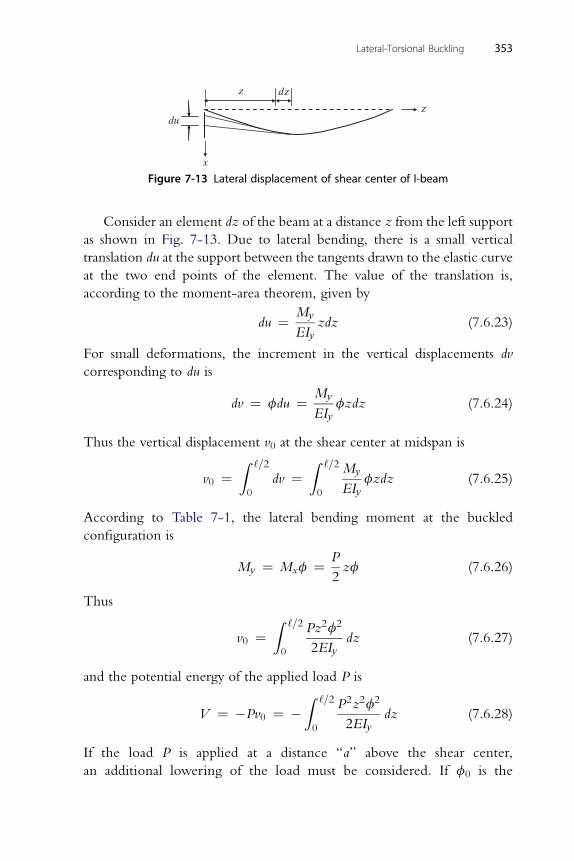
x

du

dz z

z

Figure 7-13 Lateral displacement of shear center of I-beam

Lateral-Torsional Buckling 353

Consider an element dz of the beam at a distance z from the left support

as shown in Fig. 7-13. Due to lateral bending, there is a small vertical

translation du at the support between the tangents drawn to the elastic curve

at the two end points of the element. The value of the translation is,

according to the moment-area theorem, given by

du ¼ My

EIyzdz (7.6.23)

For small deformations, the increment in the vertical displacements dv

corresponding to du is

dv ¼ fdu ¼ My

EIyfzdz (7.6.24)

Thus the vertical displacement v0 at the shear center at midspan is

v0 ¼Z ‘=2

0

dv ¼Z ‘=2

0

My

EIyfzdz (7.6.25)

According to Table 7-1, the lateral bending moment at the buckled

configuration is

My ¼ Mxf ¼ P

2zf (7.6.26)

Thus

v0 ¼Z ‘=2

0

Pz2f2

2EIydz (7.6.27)

and the potential energy of the applied load P is

V ¼ �Pv0 ¼ �Z ‘=2

0

P2z2f2

2EIydz (7.6.28)

If the load P is applied at a distance “a” above the shear center,

an additional lowering of the load must be considered. If f0 is the

354 Chai Yoo

twisting angle of the member at midspan, the additional lowering of the

load is

að1� cosf0Þ zaf2

0

2(7.6.29)

and an additional loss of the potential energy is

DV ¼ �Paf20

2(7.6.30)

Combining Eqs. (7.6.1) and (7.6.28), the total potential energy of the

system becomes

P ¼ U þ V

¼ 1

2

Z ‘

0

EIyðu00Þ2dzþ 1

2

Z ‘

0

GKT ðf0Þ2dzþ 1

2

Z ‘

0

EIwðf00Þ2dz

� P2

2EIy

Z ‘=2

0

f2z2dz (7.6.31)

As before, it is desirable to reduce the number of variables by expressing u in

terms of f. From Eq. (7.6.15)

f ¼ EIy

Mxu00 ¼ �2EIyu

00

Pz

Hence

u00 ¼ �Pzf

2EIy(7.6.32)

Substituting Eq. (7.6.32) into Eq. (7.6.31) gives

P ¼ U þ V

¼ 1

2

Z ‘

0

GKT ðf0Þ2dzþ 1

2

Z ‘

0

EIwðf00Þ2dz� P2

4EIy

Z ‘=2

0

f2z2dz

(7.6.33)

Assume f to be of the form

f ¼ B sinpz

‘(7.6.34)

Lateral-Torsional Buckling 355

Substituting f and its derivatives into Eq. (7.6.33) yields

U þ V ¼ �P2B2

4EIy

Z ‘=2

0

z2 sin2pz

‘dzþGKTB

2p2

2‘2

Z ‘

0

cos2pz

‘dz

þ EIwB2p4

2‘4

Z ‘

0

sin2pz

‘dz (7.6.35)

Substituting the definite integrals

Z ‘=2

0

z2 sin2pz

‘dz ¼ ‘3

48p2ðp2 þ 6Þ

Z ‘ Z ‘

0

sin2pz

‘dz ¼

0

cos2pz

‘dz ¼ ‘

2(7.6.36)

into Eq. (7.6.35) gives

U þ V ¼ � P2B2‘3

192EIyp2ðp2 þ 6Þ þGKTB

2p2

4‘þ EIwB

2p4

4‘3(7.6.37)

At the critical load, the first variation of U þ V with respect to B must

vanish. Thus,

d

dBðU þ V Þ ¼ B

2

�� P2‘3

48EIyp2ðp2 þ 6Þ þGKTp

2

‘þ EIwp

4

‘3

�¼ 0

which leads to

Pcr ¼ �4p2

‘2

ffiffiffiffiffiffiffiffiffiffiffiffiffiffiffiffiffiffiffiffiffiffiffiffiffiffiffiffiffiffiffiffiffiffiffiffiffiffiffiffiffiffiffiffiffiffiffiffiffiffiffiffiffiffiffi3

p2 þ 6EIy

�GKT þ EIwp2

‘2

�s(7.6.38)

Equation (7.5.38) gives the critical load for a simply supported I-beam

subjected to a concentrated load at midspan. The � sign in Eq. (7.5.38)

indicates that an identical critical load will result if the direction of the load is

reversed from that shown in Fig. 7-9.

7.6.3. Uniformly Distributed LoadThe procedure described above for the case of a concentrated load at

midspan can also be used when the I-beam (Fig. 7-8) carries a uniformly

distributed load. The strain energy given by Eq. (7.6.1) remains unchanged.

However, the expression for the loss of potential energy of the externally

applied load must be determined.

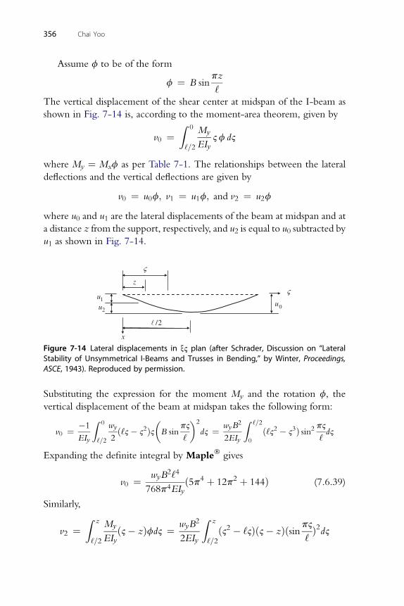
356 Chai Yoo

Assume f to be of the form

f ¼ B sinpz

‘The vertical displacement of the shear center at midspan of the I-beam as

shown in Fig. 7-14 is, according to the moment-area theorem, given by

v0 ¼Z 0

‘=2

My

EIy2 f d2

where My ¼ Mxf as per Table 7-1. The relationships between the lateral

deflections and the vertical deflections are given by

v0 ¼ u0f; v1 ¼ u1f; and v2 ¼ u2f

where u0 and u1 are the lateral displacements of the beam at midspan and at

a distance z from the support, respectively, and u2 is equal to u0 subtracted by

u1 as shown in Fig. 7-14.

ς

x

/2

z

2u1u

ς

0u

Figure 7-14 Lateral displacements in x2 plan (after Schrader, Discussion on “LateralStability of Unsymmetrical I-Beams and Trusses in Bending,” by Winter, Proceedings,ASCE, 1943). Reproduced by permission.

Substituting the expression for the moment My and the rotation f, the

vertical displacement of the beam at midspan takes the following form:

v0 ¼ �1

EIy

Z 0

‘=2

wy

2ð‘2� 22Þ2

�B sin

p2

‘

�2

d2 ¼ wyB2

2EIy

Z ‘=2

0

ð‘22 � 23Þ sin2 p2‘d2

Expanding the definite integral by Maple� gives

v0 ¼ wyB2‘4

768p4EIyð5p4 þ 12p2 þ 144Þ (7.6.39)

Similarly,

v2 ¼Z z

‘=2

My

EIyð2� zÞfd2 ¼ wyB

2

2EIy

Z z

‘=2ð22 � ‘2Þð2� zÞðsinp2

‘Þ2d2

wyB2

v2 ¼768p4EIy

�

5p4‘4 � 48p2‘3z� 16‘3p4zþ 12‘4p2 � 96‘2p2z2 cos2pz

‘

þ 48‘2p2z2 þ 144‘4 cos2pz

‘� 96‘4p cos

pz

‘sin

pz

‘

þ 96‘3p2z cos2pz

‘� 16p4z4 þ 32‘p4z3 þ 192p‘3z cos

pz

‘sin

pz

‘

266666664

377777775

ð7:6:40Þ

From Fig. 7-14, it is seen that

Lateral-Torsional Buckling 357

v1 ¼ v0 � v2 (7.6.41)

Hence, the loss of the potential energy of the uniformly distributed load,

wy , is

V ¼ �2wy

Z ‘=2

0

ðv0 � v2Þdz ¼ � w2yB

2‘5

240p4EIyðp4 þ 45Þ (7.6.42)

Expanding the first term of the strain energy in Eq. (7.6.1) gives

EIy

2

Z ‘

0

ðu00Þ2dz ¼ EIy

2

Z ‘

0

ð�My

EIyÞ2dz ¼ 1

2EIy

Z ‘

0

ð�MxfÞ2dz

¼ w2yB

2

8EIy

Z ‘

0

ð‘z� z2Þ2sin2 pz‘dz

¼ w2yB

2‘5

480p4EIyðp4 þ 45Þ

Hence,

U ¼ w2yB

2‘5

480p4EIyðp4 þ 45Þ þGKTB

2p2

4‘þ EIwB

2p4

4‘3(7.6.43)

and

U þ V ¼ � w2yB

2‘5

480p4EIyðp4 þ 45Þ þGKTB

2p2

4‘þ EIwB

2p4

4‘3(7.6.44)

358 Chai Yoo

At the critical load, the first variation of U þ V with respect to B must

vanish. Thus,

d

dBðU þ V Þ ¼ B

2

�� w2

y‘5

120EIyp4ðp4 þ 45Þ þGKTp

2

‘þ EIwp

4

‘3

�¼ 0

which leads to

ðwy‘Þcr ¼ �2p3

‘2

ffiffiffiffiffiffiffiffiffiffiffiffiffiffiffiffiffiffiffiffiffiffiffiffiffiffiffiffiffiffiffiffiffiffiffiffiffiffiffiffiffiffiffiffiffiffiffiffiffiffiffiffiffiffiffiffiffiffi30

p4 þ 45EIy

�GKT þ EIwp2

‘2

�s(7.6.45)

Schrader (1943) obtained an expression for the critical uniformly distrib-

uted load of a simply supported prismatic beam of a singly symmetric cross

section based on the energy method. In the formula, he allowed that the load

could be applied at any point along theweb axis. He extended the approach to

include two concentrated loads applied symmetrically on the span.

Ix ¼ 307 in4; Iy ¼ 44:1 in4;KT ¼ 0:906 in4; Iw ¼ 1440 in6;

‘ ¼ 180 in;E ¼ 29000 ksi; and G ¼ 11200 ksi

For m ¼ 8,

‘ ¼ffiffiffiffiffiffiffiffiffiffiffiffiffiffiffiffiffiffiffiffiffiffi8EIw=GKT

p¼

ffiffiffiffiffiffiffiffiffiffiffiffiffiffiffiffiffiffiffiffiffiffiffiffiffiffiffiffiffiffiffiffiffiffiffiffiffiffiffiffiffiffiffiffiffiffiffiffiffiffiffiffiffiffiffiffiffiffiffiffiffiffiffiffiffiffiffiffiffiffi8� 29000� 1440=ð11200� 0:906Þ

p¼ 181:45 in:

From Tables 7-2 and 7-3, g1 and g2 are read to be 42.5 and 25.6,

respectively. Hence,

ðwy‘Þcr ¼ g1ffiffiffiffiffiffiffiffiffiffiffiffiffiffiffiffiffiEIyGKT

p‘2

¼ 42:5

181:452� 113917:75 ¼ 147:05 kips

3ffiffiffiffiffiffiffiffiffiffiffiffiffiffiffiffiffiffiffiffiffiffiffiffiffiffiffiffiffiffiffiffiffiffiffiffiffiffiffiffiffiffiffiffiffiffiffiffiffiffiffiffiffiffiffiffiffiffi� �s

ðwy‘Þcr ¼ 2p

‘230

p4 þ 45EIy GKT þ EIwp2

‘2¼ 147:2 kips (7.6.45)

and

Pcr ¼ g2

ffiffiffiffiffiffiffiffiffiffiffiffiffiffiffiffiffiEIyGKT

p‘2

¼ 25:6

181:452

ffiffiffiffiffiffiffiffiffiffiffiffiffiffiffiffiffiffiffiffiffiffiffiffiffiffiffiffiffiffiffiffiffiffiffiffiffiffiffiffiffiffiffiffiffiffiffiffiffiffiffiffiffiffiffiffiffiffiffiffiffi29000� 44:1� 11200� 0:906

p

¼ 88:58 kips

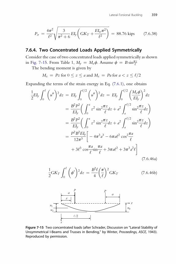
2ffiffiffiffiffiffiffiffiffiffiffiffiffiffiffiffiffiffiffiffiffiffiffiffiffiffiffiffiffiffiffiffiffiffiffiffiffiffiffiffiffiffiffiffiffiffiffiffiffiffiffiffiffiffiffiffi�

2�s

Pcr ¼ 4p

‘23

p2 þ 6EIy GKT þ EIwp

‘2¼ 88:76 kips (7.6.38)

7.6.4. Two Concentrated Loads Applied SymmetricallyConsider the case of two concentrated loads applied symmetrically as shown

in Fig. 7-15. From Table 1, My ¼ Mxf. Assume f ¼ B sinpz‘The bending moment is given by

Mx ¼ Pz for 0 � z � a and Mx ¼ Pa for a < z � ‘=2

Expanding the terms of the strain energy in Eq. (7.6.1), one obtains

1

2EIy

Z ‘

0

�u00�2dz ¼ EIy

Z ‘=2

0

�u00�2dz ¼ EIy

Z ‘=2

0

�Mxf

EIy

�2

dz

¼ B2P2

EIy

�Z a

0

z2 sin2pz

‘dzþ a2

Z ‘=2

a

sin2pz

‘dz

�

¼ B2P2

EIy

�Z a

0

z2 sin2pz

‘dzþ a2

Z ‘=2

a

sin2pz

‘dz

�

¼ P2B2EIy

12p3

�� 4p3a3 � 6pa‘2 cos2

pa

‘

þ 3‘3 cospa

‘sin

pa

‘þ 3pa‘2 þ 3p3a2‘

�(7.6.46a)

Z ‘� �2� �

2

Lateral-Torsional Buckling 359

1

2GKT

0

f0 2dz ¼ B ‘

4

p

‘GKT (7.6.46b)

P

1u

x

2u

a

/2

zz

0u

Pa

Figure 7-15 Two concentrated loads (after Schrader, Discussion on “Lateral Stability ofUnsymmetrical I-Beams and Trusses in Bending,” by Winter, Proceedings, ASCE, 1943).Reproduced by permission.

1Z ‘� �

B2‘�p�4

2EIw

0

f00 2dz ¼

4 ‘EIw (7.6.46c)

The loss of potential energy of the applied load P is negative of the product

of P and v1. From Fig. 7-15, it is seen that v1 ¼ v0 � v2 as the vertical

displacement v is obtained by the lateral displacement u multiplied by f as

per Table 7-1.

v0 ¼Z 0

‘=2

My

EIyfz dz

where My ¼ Mxf. Hence,

v0 ¼ � 1

EIy

�Z a

‘=2Paz

�B sin

pz

‘

�2dzþ

Z 0

a

Pz2�B sin

pz

‘

�2dz

�

¼ � PB2

48p3EIy

�3p3a‘2 þ 12pa‘2 � 4p3a3 � 12pal2cos2

pa

‘

þ 12‘2 cospa

‘sin

pa

‘

�(7.6.47)

Z a M�

pz�2

360 Chai Yoo

v2 ¼‘=2

x

EIyðz� aÞ B sin

‘dz

¼ � PB2

16p2

�p2a‘2 � 4p2a2‘þ 4a‘2cos2

pa

‘þ 4p2a3

�(7.6.48)

PB2�

pa pa pa

v1 ¼ �

12p3EIy�4p3a3 � 6pa‘2cos2

‘þ 3‘3cos

‘sin

‘

þ 3pa‘2 þ 3p3a2‘

�(7.6.49)

Hence, the loss of potential energy of the two applied loads is (note v1 is

already negative)

2Pv1 ¼ � P2B2

6p3EIy

��4p3a3 � 6pa‘2cos2

pa

‘

þ 3‘3cospa

‘sin

pa

‘þ 3pa‘2 þ 3p3a2‘

�

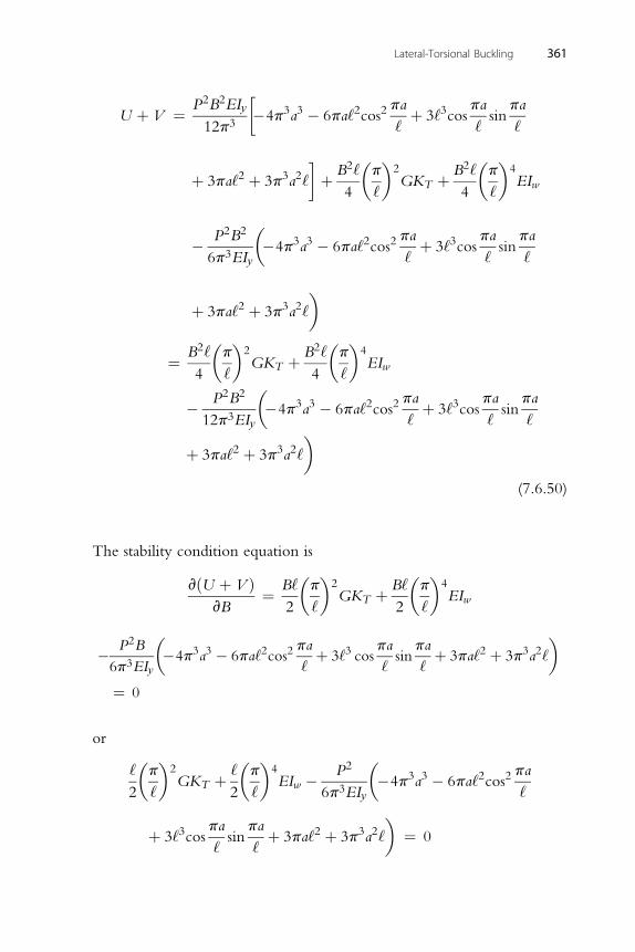
P2B2EIy�

pa pa pa

U þ V ¼

12p3�4p3a3 � 6pa‘2cos2

‘þ 3‘3cos

‘sin

‘

þ 3pa‘2 þ 3p3a2‘

�þ B2‘

4

�p

‘

�2GKT þ B2‘

4

�p

‘

�4EIw

� P2B2

6p3EIy

��4p3a3 � 6pa‘2cos2

pa

‘þ 3‘3cos

pa

‘sin

pa

‘

þ 3pa‘2 þ 3p3a2‘

�

¼ B2‘

4

�p

‘

�2GKT þ B2‘

4

�p

‘

�4EIw

� P2B2

12p3EIy

��4p3a3 � 6pa‘2cos2

pa

‘þ 3‘3cos

pa

‘sin

pa

‘

þ 3pa‘2 þ 3p3a2‘

�(7.6.50)

The stability condition equation is

vðU þ V ÞvB

¼ B‘

2

�p

‘

�2GKT þ B‘

2

�p

‘

�4EIw

P2B�

pa pa pa�

Lateral-Torsional Buckling 361

�6p3EIy

�4p3a3 � 6pa‘2cos2‘þ 3‘3 cos

‘sin

‘þ 3pa‘2 þ 3p3a2‘

¼ 0

or

‘

2

�p

‘

�2GKT þ ‘

2

�p

‘

�4EIw � P2

6p3EIy

��4p3a3 � 6pa‘2cos2

pa

‘

þ 3‘3cospa

‘sin

pa

‘þ 3pa‘2 þ 3p3a2‘

�¼ 0

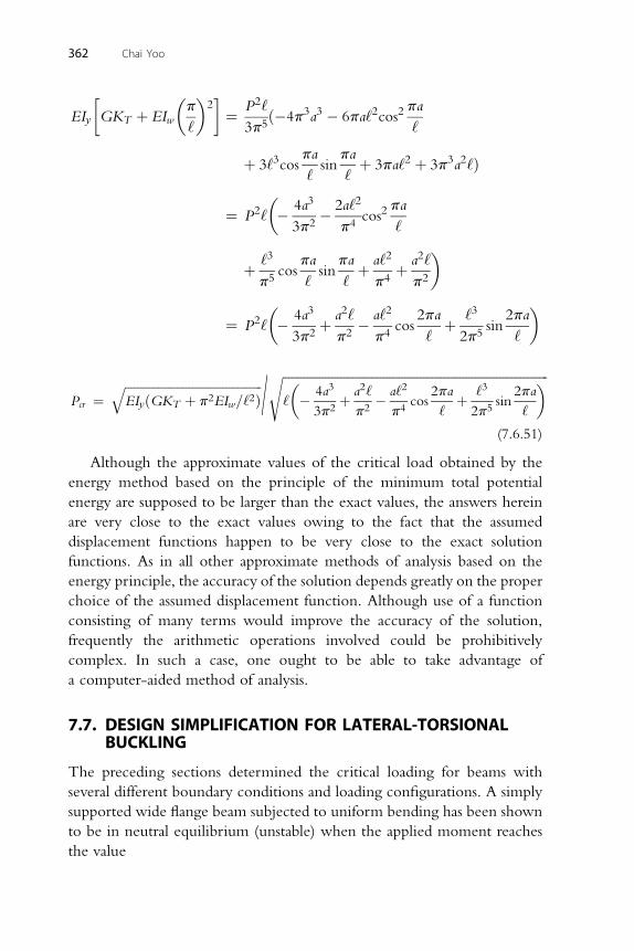
� �p�2�

P2‘ pa

EIy GKT þ EIw

‘¼

3p5ð�4p3a3 � 6pa‘2cos2

‘

þ 3‘3cospa

‘sin

pa

‘þ 3pa‘2 þ 3p3a2‘Þ

¼ P2‘

�� 4a3

3p2� 2a‘2

p4cos2

pa

‘

þ ‘3

p5cos

pa

‘sin

pa

‘þ a‘2

p4þ a2‘

p2

�

¼ P2‘

�� 4a3

3p2þ a2‘

p2� a‘2

p4cos

2pa

‘þ ‘3

2p5sin

2pa

‘

�

ffiffiffiffiffiffiffiffiffiffiffiffiffiffiffiffiffiffiffiffiffiffiffiffiffiffiffiffiffiffiffiffiffiffiffiffiffiffiffiffiffiffiffiffiffiffiffiffiffiffiffiffiffiffiffiffiffiffiffiffiffiffiffiffiffiffiffiffiffiffiffiffiffiffiffiffiffiffiffiffiffiffiffiffiffiffiffi� �s

362 Chai Yoo

Pcr ¼ffiffiffiffiffiffiffiffiffiffiffiffiffiffiffiffiffiffiffiffiffiffiffiffiffiffiffiffiffiffiffiffiffiffiffiffiffiffiffiffiffiffiffiffiffiEIyðGKT þ p2EIw=‘2Þ

q = ‘ � 4a3

3p2þ a2‘

p2� a‘2

p4cos

2pa

‘þ ‘3

2p5sin

2pa

‘

(7.6.51)

Although the approximate values of the critical load obtained by the

energy method based on the principle of the minimum total potential

energy are supposed to be larger than the exact values, the answers herein

are very close to the exact values owing to the fact that the assumed

displacement functions happen to be very close to the exact solution

functions. As in all other approximate methods of analysis based on the

energy principle, the accuracy of the solution depends greatly on the proper

choice of the assumed displacement function. Although use of a function

consisting of many terms would improve the accuracy of the solution,

frequently the arithmetic operations involved could be prohibitively

complex. In such a case, one ought to be able to take advantage of

a computer-aided method of analysis.

7.7. DESIGN SIMPLIFICATION FOR LATERAL-TORSIONALBUCKLING

The preceding sections determined the critical loading for beams with

several different boundary conditions and loading configurations. A simply

supported wide flange beam subjected to uniform bending has been shown

to be in neutral equilibrium (unstable) when the applied moment reaches

the value

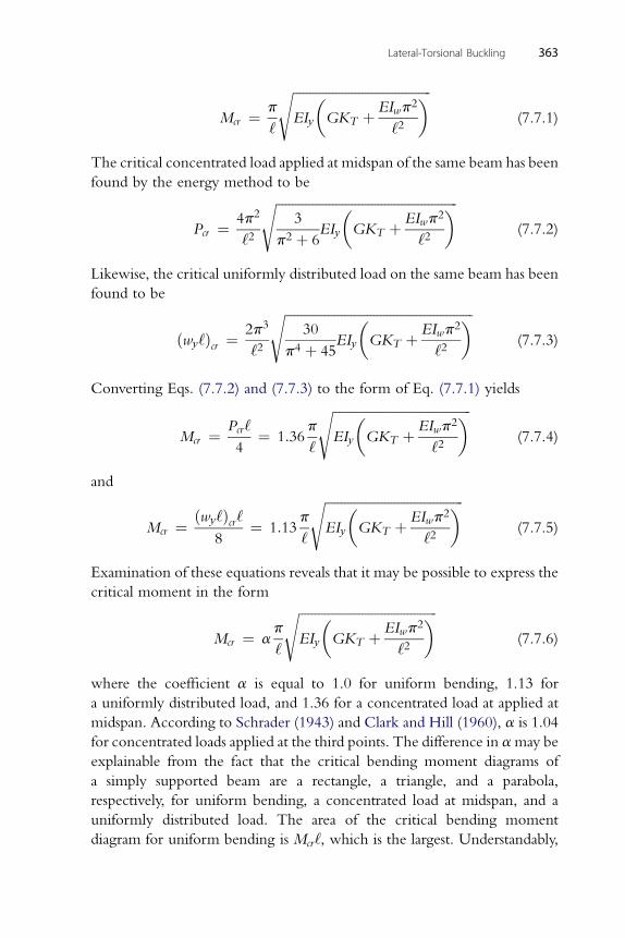
Lateral-Torsional Buckling 363

Mcr ¼ p

‘

ffiffiffiffiffiffiffiffiffiffiffiffiffiffiffiffiffiffiffiffiffiffiffiffiffiffiffiffiffiffiffiffiffiffiffiffiffiffiffiffiffiffiEIy

�GKT þ EIwp2

‘2

�s(7.7.1)

The critical concentrated load applied at midspan of the same beam has been

found by the energy method to be

Pcr ¼ 4p2

‘2

ffiffiffiffiffiffiffiffiffiffiffiffiffiffiffiffiffiffiffiffiffiffiffiffiffiffiffiffiffiffiffiffiffiffiffiffiffiffiffiffiffiffiffiffiffiffiffiffiffiffiffiffiffiffiffi3

p2 þ 6EIy

�GKT þ EIwp2

‘2

�s(7.7.2)

Likewise, the critical uniformly distributed load on the same beam has been

found to be

ðwy‘Þcr ¼ 2p3

‘2

ffiffiffiffiffiffiffiffiffiffiffiffiffiffiffiffiffiffiffiffiffiffiffiffiffiffiffiffiffiffiffiffiffiffiffiffiffiffiffiffiffiffiffiffiffiffiffiffiffiffiffiffiffiffiffiffiffi30

p4 þ 45EIy

�GKT þ EIwp2

‘2

�s(7.7.3)

Converting Eqs. (7.7.2) and (7.7.3) to the form of Eq. (7.7.1) yields

Mcr ¼ Pcr‘

4¼ 1:36

p

‘

ffiffiffiffiffiffiffiffiffiffiffiffiffiffiffiffiffiffiffiffiffiffiffiffiffiffiffiffiffiffiffiffiffiffiffiffiffiffiffiffiffiffiEIy

�GKT þ EIwp2

‘2

�s(7.7.4)

and

Mcr ¼ ðwy‘Þcr‘8

¼ 1:13p

‘

ffiffiffiffiffiffiffiffiffiffiffiffiffiffiffiffiffiffiffiffiffiffiffiffiffiffiffiffiffiffiffiffiffiffiffiffiffiffiffiffiffiffiEIy

�GKT þ EIwp2

‘2

�s(7.7.5)

Examination of these equations reveals that it may be possible to express the

critical moment in the form

Mcr ¼ ap

‘

ffiffiffiffiffiffiffiffiffiffiffiffiffiffiffiffiffiffiffiffiffiffiffiffiffiffiffiffiffiffiffiffiffiffiffiffiffiffiffiffiffiffiEIy

�GKT þ EIwp2

‘2

�s(7.7.6)

where the coefficient a is equal to 1.0 for uniform bending, 1.13 for

a uniformly distributed load, and 1.36 for a concentrated load at applied at

midspan. According to Schrader (1943) and Clark and Hill (1960), a is 1.04

for concentrated loads applied at the third points. The difference in amay be

explainable from the fact that the critical bending moment diagrams of

a simply supported beam are a rectangle, a triangle, and a parabola,

respectively, for uniform bending, a concentrated load at midspan, and a

uniformly distributed load. The area of the critical bending moment

diagram for uniform bending is Mcr‘, which is the largest. Understandably,

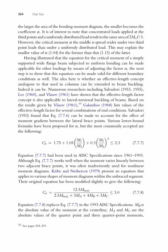
364 Chai Yoo

the larger the area of the bending moment diagram, the smaller becomes the

coefficient a. It is of interest to note that concentrated loads applied at the

third points and a uniformly distributed load result in the same area of 2Mcr‘/3.However, the critical moment at the middle is spread wider under two third

point loads than under a uniformly distributed load. This may explain the

smaller value of a (1.04) for the former than that (1.13) of the latter.

Having illustrated that the equation for the critical moment of a simply

supported wide flange beam subjected to uniform bending can be made

applicable for other loadings by means of adjusting the factor a, the next

step is to show that this equation can be made valid for different boundary

conditions as well. The idea here is whether an effective-length concept

analogous to that used in columns can be extended to beam buckling.

Indeed it can be. Numerous researchers including Salvadori (1953, 1955),

Lee (1960), and Vlasov (1961) have shown that the effective-length factor

concept is also applicable to lateral-torsional buckling of beams. Based on

the results given by Vlasov (1961),10 Galambos (1968) lists values of the

effective-length factor for several combinations of end conditions. Salvadori

(1953) found that Eq. (7.7.6) can be made to account for the effect of

moment gradient between the lateral brace points. Various lower-bound

formulas have been proposed for a, but the most commonly accepted are

the following:

Cb ¼ 1:75þ 1:05

�M1

M2

�þ 0:3

�M1

M2

�2

� 2:3 (7.7.7)

Equation (7.7.7) had been used in AISC Specifications since 1961–1993.

Although Eq. (7.7.7) works well when the moment varies linearly between

two adjacent brace points, it was often inadvertently used for nonlinear

moment diagrams. Kirby and Nethercot (1979) present an equation that

applies to various shapes of moment diagrams within the unbraced segment.

Their original equation has been modified slightly to give the following:

Cb ¼ 12:5Mmax

2:5Mmax þ 3MA þ 4MB þ 3MC� 3:0 (7.7.8)

Equation (7.7.8) replaces Eq. (7.7.7) in the 1993 AISC Specifications.MB is

the absolute value of the moment at the centerline, MA and MC are the

absolute values of the quarter point and three quarter-point moments,

10 See pages 292–297.

Lateral-Torsional Buckling 365

respectively, and Mmax is the maximum moment regardless of its location

within the brace points.

The nominal flexural strength of a beam is limited by the lateral-

torsional buckling strength controlled by the unbraced length Lb of the

compression flange. The critical moment equation (Eq. 7.7.6) was derived

under the assumption that the material obeys Hooke’s law. This means that

it cannot be directly applicable to inelastic lateral-torsional buckling.

The credit goes to Lay and Galambos (1965, 1967) for determining the

unbraced length Lp required for compact sections to reach the plastic

bending moment Mp.

Lp ¼ 2:7ry

ffiffiffiffiffiE

sy

s(7.7.9)

where E¼ elastic modulus, ry ¼ radius of gyration with respect to the weak

axis, and sy ¼ mill specified minimum yield stress.

Later on, their simplified design equation was calibrated using experi-

mental data (Bansal, 1971) in order to give compact-section beams adequate

rotational capacity after reaching the plastic moment.

Lp ¼ 1:76ry

ffiffiffiffiffiE

sy

s(7.7.10)

Equation (7.7.10) is identical to Eq. (F2-5) in AISC (2005) Specifications.

In plastic analysis, larger rotation capacities are required to ensure that

successive plastic hinges are formed without inducing excessive lateral-

torsional deformations. Bansal (1971) suggested the following equation

from tests of three-span continuous beams to ensure rotation capacity

greater than or equal to 3:

Lpd ¼�0:12þ 0:076

�M1

M2

���E

sy

�ry (7.7.11)

whereM1 is the smaller moment at the ends of a laterally unbraced segment

(taken positive when moments cause reverse curvature). Equation (7.7.11) is

identical to Eq. (F1-17) in AISC (2001) Specifications.

The limiting value of the unbraced length for girders of compact

sections to buckle in the elastic range is given by Lr. In the presence of

residual stress, the maximum elastic critical moment is defined by

Mcr ¼ Sxðsy � srÞ ¼ 0:7Sxsy ¼ scrSx (7.7.12)

366 Chai Yoo

where Sx ¼ elastic section modulus about the x-axis, sr ¼ residual stress

0.3 sy for both rolled and welded shapes. From Eqs. (7.7.6) and (7.7.12),

scr ¼ Mcr

Sx¼ Cbp

LbSx

ffiffiffiffiffiffiffiffiffiffiffiffiffiffiffiffiffiffiffiffiffiffiffiffiffiffiffiffiffiffiffiffiffiffiffiffiffiffiffiffiffiffiffiffiffiffiffiffiEIyGKT þ

�pE

Lb

�2

IyEIw

s(7.7.13)

Equation (7.7.13) is identical to Eq. (F1-13) in the AISC (1986) LRFD

Specifications. Equation (7.7.13) is rewritten as

scr ¼ Cbp2E�

Lb

rts

�2

ffiffiffiffiffiffiffiffiffiffiffiffiffiffiffiffiffiffiffiffiffiffiffiffiffiffiffiffiffiffiffiffiffiIyGKTL

2b

p2r4tsES2x

þ IyIw

r4tsS2x

s(7.7.14)

where

rts2 ¼

ffiffiffiffiffiffiffiffiffiffiffiIyEIw

pSx

(7.7.15)

Letting h0 be the distance between the flange centroids and substituting

2G=p2E ¼ 0:0779 and Eq. (7.7.14), Eq. (7.7.13) becomes

scr ¼ Cbp2E�

Lb

rts

�2

ffiffiffiffiffiffiffiffiffiffiffiffiffiffiffiffiffiffiffiffiffiffiffiffiffiffiffiffiffiffiffiffiffiffiffiffiffiffiffiffiffiffiffiffiffiffiffi�Lb

rts

�2 IyGKT

p2E

ffiffiffiffiffiffiffiffiIyIw

pSx

S2x

þ 1

vuuut

¼ Cbp2E�

Lb

rts

�2

ffiffiffiffiffiffiffiffiffiffiffiffiffiffiffiffiffiffiffiffiffiffiffiffiffiffiffiffiffiffiffiffiffiffiffiffiffiffiffiffiffiffiffiffi1þ 0:0779

KTc

Sxh0

�Lb

rts

�2

s(7.7.16)

where Iw ¼ Iyh20=4 for doubly symmetric I-beams with rectangular

flanges and c ¼ h0ffiffiffiffiffiffiffiffiffiffiffiIw=Iw

p=2 and hence, c ¼ 1.0 for a doubly symmetric

I-beam. Equation (7.7.16) is identical to Eq. (F2-4) in the AISC (2005)

Specifications. Limiting the maximum critical stress in Eq. (7.7.16) to

0.7sy to account for residual stress sr and solving Eq. (7.7.16) for Lr gives

Lr ¼ 1:95rtsE

0:7sy

ffiffiffiffiffiffiffiffiffiKTc

Sxh0

r ffiffiffiffiffiffiffiffiffiffiffiffiffiffiffiffiffiffiffiffiffiffiffiffiffiffiffiffiffiffiffiffiffiffiffiffiffiffiffiffiffiffiffiffiffiffiffiffiffiffiffiffiffiffiffiffiffiffiffiffiffiffi1þ

ffiffiffiffiffiffiffiffiffiffiffiffiffiffiffiffiffiffiffiffiffiffiffiffiffiffiffiffiffiffiffiffiffiffiffiffiffiffiffiffiffiffiffiffiffiffiffiffiffi1þ 6:767

�0:7syE

Sxh0

KTc

�2

svuut(7.7.17)

Equation (7.7.17) is identical to Eq. (F2-6) in AISC (2005) Specifications.

The calculation of the inelastic critical moment is fairly complex.

Galambos (1963, 1998) has contributed greatly to this subject. In 2005

Lateral-Torsional Buckling 367

AISC Specifications, when Lp < Lb � Lr , the nominal flexural strengthMn

of compact sections is linearly interpolated between the plastic momentMp

and the elastic critical moment Mr ¼ 0:7Sxsy as

Mn ¼ Cb

�Mp � ðMp � 0:7sySxÞ

�Lb � Lp

Lr � Lp

��� Mp (7.7.18)

It should be remembered that local buckling of compression flanges and

web is precluded in the derivation of the unbraced lengths. The mathe-

matical procedure for the solution of local buckling is identical to that of the

lateral-torsional buckling phenomenon, except that the governing differ-

ential equations are now partial differential equations, and so the details of

the solution process are different and complicated, as will be shown in the

next chapter. In order to systematically reflect the effects of local buckling

on the nominal flexural strength, AISC (2005) Specifications categorize

sections into several types depending on the compactness of the flanges and

web (compact, noncompact, or slender).

Also, it needs to be noted that the limiting values for the unbraced length

given by Eqs. (7.7.10), (7.7.11), and (7.7.17) are valid only for bare-steel

members. Composite systems are often utilized tomaximize the efficiency of

structural members. In composite girders, the top flange and concrete slab are

connected with shear studs. Lateral-torsional buckling is not likely to take

place when subjected to positive flexure, as the top compression flange is

continuously braced by the concrete slab.However, the loss of stability should

be checkedwhendesigning composite girders in negativemoment zone.The

steel section of a composite girder will necessarily undergo the deformation

depicted in Fig. 7-16 during buckling due to the restraint provided by the

concrete slab. This type of buckling is referred to as lateral-distortional

buckling. The classical assumption that the member cross section retains its

original shape during buckling is no longer valid in this case. Lateral-

distortional buckling is basically a combined mode of lateral-torsional

buckling (global buckling) and local buckling, and the derivation of a closed-

form solution is, therefore, not straightforward. Limited research, including

Hancock et al. (1980), Bradford and Gao (1992), and Hong et al. (2002), has

shown that the unbraced length requirements for noncomposite girders give

too conservative results for composite girders. A general design rule has yet to

be developed due to lack of comprehensive study. With the advancement of

digital computers, along with highly sophisticated computer programs such

as ABAQUS, NASTRAN, and ADINA just to name a few, performing the

lateral-distortional buckling analysis should present no problem.

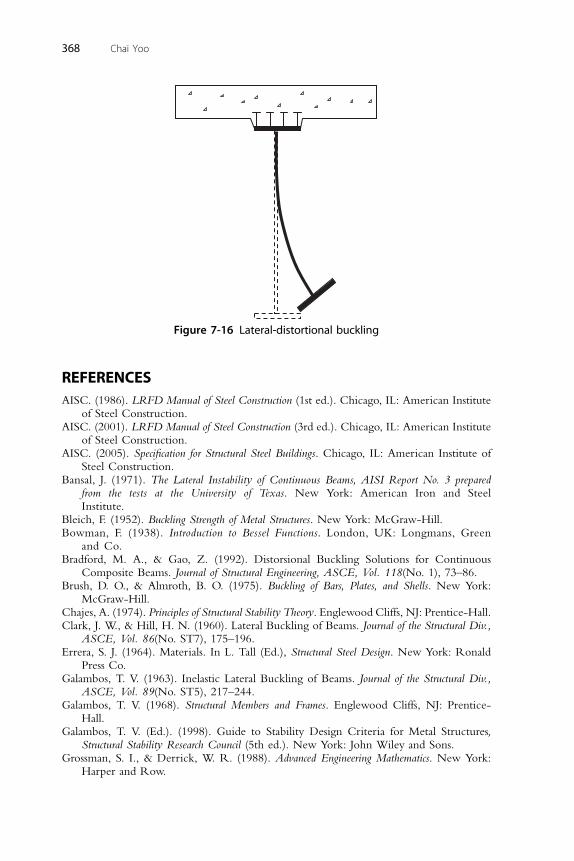
Figure 7-16 Lateral-distortional buckling

368 Chai Yoo

REFERENCESAISC. (1986). LRFD Manual of Steel Construction (1st ed.). Chicago, IL: American Institute

of Steel Construction.AISC. (2001). LRFD Manual of Steel Construction (3rd ed.). Chicago, IL: American Institute

of Steel Construction.AISC. (2005). Specification for Structural Steel Buildings. Chicago, IL: American Institute of

Steel Construction.Bansal, J. (1971). The Lateral Instability of Continuous Beams, AISI Report No. 3 prepared

from the tests at the University of Texas. New York: American Iron and SteelInstitute.

Bleich, F. (1952). Buckling Strength of Metal Structures. New York: McGraw-Hill.Bowman, F. (1938). Introduction to Bessel Functions. London, UK: Longmans, Green

and Co.Bradford, M. A., & Gao, Z. (1992). Distorsional Buckling Solutions for Continuous

Composite Beams. Journal of Structural Engineering, ASCE, Vol. 118(No. 1), 73–86.Brush, D. O., & Almroth, B. O. (1975). Buckling of Bars, Plates, and Shells. New York:

McGraw-Hill.Chajes, A. (1974). Principles of Structural Stability Theory. Englewood Cliffs, NJ: Prentice-Hall.Clark, J. W., & Hill, H. N. (1960). Lateral Buckling of Beams. Journal of the Structural Div.,

ASCE, Vol. 86(No. ST7), 175–196.Errera, S. J. (1964). Materials. In L. Tall (Ed.), Structural Steel Design. New York: Ronald

Press Co.Galambos, T. V. (1963). Inelastic Lateral Buckling of Beams. Journal of the Structural Div.,

ASCE, Vol. 89(No. ST5), 217–244.Galambos, T. V. (1968). Structural Members and Frames. Englewood Cliffs, NJ: Prentice-

Hall.Galambos, T. V. (Ed.). (1998). Guide to Stability Design Criteria for Metal Structures,

Structural Stability Research Council (5th ed.). New York: John Wiley and Sons.Grossman, S. I., & Derrick, W. R. (1988). Advanced Engineering Mathematics. New York:

Harper and Row.

Lateral-Torsional Buckling 369

Hill, H. N. (1954). Lateral Buckling of Channels and Z-Beams. Transactions, ASCE,Vol. 119, pp. 829–841.

Hong, A.R., Lee, D.S., & Lee, S.C. (2002). A Study on Unbraced Length Requirement forComposite Steel I Girder in Negative Bending, Proceedings of 2002 Annual Conference,KSCE, Korea, pp. 70–73 (in Korean).

Kirby, P. A., & Nethercot, D. A. (1979). Design for Structural Stability. New York: John Wileyand Sons.

Lay, M. G., & Galambos, T. V. (1965). Inelastic Steel Beams Under Moment Gradient.Journal of the Structural Div., ASCE, Vol. 91(No. ST6), 67–93.

Lay, M. G., & Galambos, T. V. (1967). Inelastic Beams Under Moment Gradient. Journal ofthe Structural Div., ASCE, Vol. 93(No. ST1), 381–399.

Lee, G.C. (1960). A Survey of the Literature on the Lateral Instability of Beams, WeldingResearch Council Bulletin No. 63, August.

Michell, A. G. M. (1899). Elastic Stability of Long Beams Under Transverse Forces.Philosophic Magazine, Vol. 48, 298.

Prandtl, L. (1899). Kipperscheinungen, Dissertation, Munich Polytechnical Institute.Salmon, C. G., & Johnson, J. E. (1996). Steel Structures, Design and Behavior (4th ed.).

New York: HarperCollins.Salvadori, M.G. (1953). Lateral Buckling of I Beams Under Thrust and Unequal End

Moments, Proceedings, ASCE, Vol. 79(No.291), pp. 1–25, also a transaction paperNo 2773, Lateral Buckling of I-Beams, Transactions, ASCE, Vol. 120, 1955, pp. 1165–1182.

Salvadori, M.G. (1955). Lateral Buckling of Eccentrically Loaded I-Columns, Proceedings,ASCE, Vol. 81, pp. 607–622, also a transaction paper No. 2836 with the same title,Transactions, ASCE, Vol. 121, 1956, pp. 1163–1178.

Schrader, R.K. (1943). Discussion on Lateral Stability of Unsymmetrical I-Beams andTrusses in Bending, by G. Winter, Paper No. 2178, Transactions, ASCE, Vol. 108, 1943,pp. 247–268.

Timoshenko, S. P. (1910). Einige Stabilitats-problme der Elasticitats-theorie. Zeitschrift furMathematik und Phisik, Vol. 58, 337–385.

Timoshenko, S. P., & Gere, J. M. (1961). Theory of Elastic Stability (2nd ed.). New York:McGraw-Hill.

Vincent, G. S. (1969). Tentative Criteria for Load Factor Design of Steel Highway Bridges. AISIReport No. 15. New York: American Iron and Steel Institute.

Vlasov, V. Z. (1940). Tonkostennye uprugie sterzhni (Thin-walled elastic beams), Stroiizdat(in Russian).

Vlasov, V. Z. (1961). Tonkostennye uprugie sterzhni (Thin-walled elastic beams), (2nd ed.),Moscow 1959, translated by Schechtman, Israel Program for Scientific Translation,Jerusalem.

Winter, G. (1941). Lateral Stability of Unsymmetrical I-Beams and Trusses in Bending,Proceedings, ASCE. Vol. 67, pp. 1851–1864, also a transaction paper No. 2178 with thesame title, Transactions, ASCE, Vol. 108, 1943, pp. 247–268.

Yoo, C. H. (1980). Bimoment Contribution to Stability of Thin-Walled Assemblages.Computers and Structures, Vol. 11(No.5), 465–471.

PROBLEMS

7.1 Equation (7.4.2) can be nondimensionalized to investigate the influ-

ence of the various parameters affecting the lateral-torsional buckling

strength.

370 Chai Yoo

Mcr

My¼

ffiffiffiffiffiffiffiffiffiffiffiffiffiffiffiffiffiffiffiffiffiffiffiffiffiffiffiffiffiffiffiffiffiffiffiffiffiffiffiffiffiffiffiffiffiffiffiffiffiffiffip2EIyGKT

‘2S2xs2y

�1þ p2EIw

GKT ‘2

�s(P7.1.1)

where My ¼ Sxsy. After introducing the following identities:

3y ¼ sy

E; Iw ¼ Iyðd � tf Þ2

4; Ix ¼ Ar2x ; Iy ¼ Ar2y ; Sx ¼ 2Ix

d

(P7.1.2)

and the abbreviation

DT ¼ KT

Ad2(P7.1.3)

one gets the following nondimensionalized buckling moment:

Mcr

My¼ pðd=rxÞ2

23y

� ffiffiffiffiffiffiffiffiffiffiffiffiffiffiffiffiffiDTG=E

p‘=ry

� ffiffiffiffiffiffiffiffiffiffiffiffiffiffiffiffiffiffiffiffiffiffiffiffiffiffiffiffiffiffiffiffiffiffiffiffiffiffi1þ p2Eð1� tf =dÞ2

4GDT ð‘=ryÞ2

s(P7.1.4)

For most wide flange shapes,

d=rx y 2:38; ð1� tf Þ=d y 0:95; and

G=E ¼ 1=2ð1þ mÞ ¼ 0:385 for m ¼ 0:3

Substituting these values into Eq. (P7.1.4) yields

Mcr

My¼ 5:56

3y

� ffiffiffiffiffiffiffiDT

p‘=ry

� ffiffiffiffiffiffiffiffiffiffiffiffiffiffiffiffiffiffiffiffiffiffiffiffiffiffiffiffi1þ 5:78

DT ð‘=ryÞ2s

(P7.1.5)

Plot the buckling curve (1000Mcr 3y/My vs. ‘/rr) for W27 � 94 using

Eqs. (P7.1.4). Limit ‘/rr < 500.

7.2 Using the Rayleigh-Ritz method, determine the critical uniformly

distributed load for a prismatic simply supported beam. The load is

applied at the centroid. Assume u ¼ A sin pz=‘; f ¼ B sin pz=‘. Use

P ¼ 1

2

Z ‘

0

�EIyðu00Þ2 þ EIwðf00Þ2 þGKT ðf0Þ2 � 2Mxu

00f�dz with

Mx ¼ �w

2ð‘z� z2Þ

What is the coefficient a in association with Eq. (7.7.6)?

7.3 Using the system of differential equations, Eqs. (7.2.22)–(7.2.24),

derive the total potential energy expression of Problem 7.2.

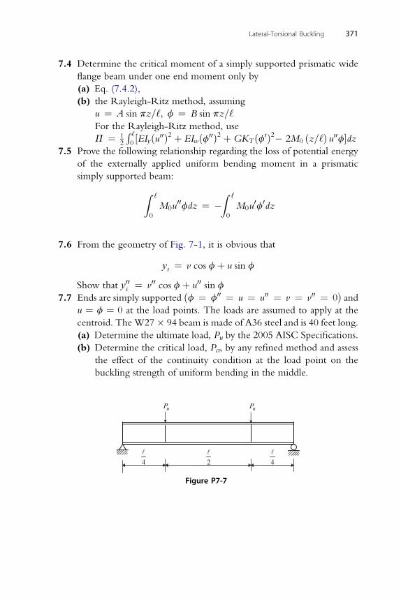
Lateral-Torsional Buckling 371

7.4 Determine the critical moment of a simply supported prismatic wide

flange beam under one end moment only by

(a) Eq. (7.4.2),

(b) the Rayleigh-Ritz method, assuming

u ¼ A sin pz=‘; f ¼ B sin pz=‘For the Rayleigh-Ritz method, use

P ¼ 12

R ‘

0½EIyðu00Þ2 þ EIwðf00Þ2 þGKT ðf0Þ2� 2M0 ðz=‘Þ u00f�dz

7.5 Prove the following relationship regarding the loss of potential energy

of the externally applied uniform bending moment in a prismatic

simply supported beam:

Z ‘

0

M0u00fdz ¼ �

Z ‘

0

M0u0f0dz

7.6 From the geometry of Fig. 7-1, it is obvious that

ys ¼ v cos fþ u sin f

Show that y00s ¼ v00 cos fþ u00 sin f

7.7 Ends are simply supported ðf ¼ f00 ¼ u ¼ u00 ¼ v ¼ v00 ¼ 0Þ andu ¼ f ¼ 0 at the load points. The loads are assumed to apply at the

centroid. The W27� 94 beam is made of A36 steel and is 40 feet long.

(a) Determine the ultimate load, Pu by the 2005 AISC Specifications.

(b) Determine the critical load, Pcr, by any refined method and assess

the effect of the continuity condition at the load point on the

buckling strength of uniform bending in the middle.

uP uP

2 44

Figure P7-7

CHAPTER88

Buckling of Plate ElementsContents

8.1. Introduction 3738.2. Differential Equation of Plate Buckling 374

8.2.1. Plate Bending Theory 3748.2.2. Equilibrium Equations 3818.2.3. Stationary Potential Energy 384

8.3. Linear Equations 3908.3.1. Adjacent-Equilibrium Criterion 3918.3.2. Minimum Potential Energy Criterion 393

8.4. Application of Plate Stability Equation 4018.4.1. Plate Simply Supported on Four Edges 4018.4.2. Longitudinally Stiffened Plates 4058.4.3. Shear Loading 414

Plate Simply Supported on Four Edges 415Plate Clamped on Four Edges 415Plate Clamped on Two Opposite Edges and Simply Supportedon the Other Two Edges 416

8.5. Energy Methods 4188.5.1. Strain Energy of a Plate Element 4188.5.2. Critical Loads of Rectangular Plates by the Energy Method 4208.5.3. Shear Buckling of a Plate Element by the Galerkin Method 4228.5.4. Postbuckling of Plate Elements 426

8.6. Design Provisions for Local Buckling of Compression Elements 4318.7. Inelastic Buckling of Plate Elements 4328.8. Failure of Plate Elements 433References 434Problems 437

8.1. INTRODUCTION

Equilibrium and stability equations of one-dimensional elements such as

beams, columns, and framed members have been treated in the preceding

chapters. The analysis of these members is relatively simple as bending, the

essential characteristic of buckling, can be assumed to take place in one plane

only. The buckling of a plate, however, involves bending in two planes and is

therefore much more complicated. From a mathematical point of view, the

main difference between framedmembers and plates is that quantities such as

Stability of Structures � 2011 Elsevier Inc.ISBN 978-0-12-385122-2, doi:10.1016/B978-0-12-385122-2.10008-9 All rights reserved. 373 j

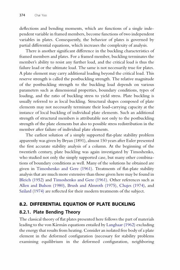
374 Chai Yoo

deflections and bending moments, which are functions of a single inde-

pendent variable in framed members, become functions of two independent

variables in plates. Consequently, the behavior of plates is governed by

partial differential equations, which increases the complexity of analysis.

There is another significant difference in the buckling characteristics of

framed members and plates. For a framed member, buckling terminates the

member’s ability to resist any further load, and the critical load is thus the

failure load or the ultimate load. The same is not necessarily true for plates.

A plate element may carry additional loading beyond the critical load. This

reserve strength is called the postbuckling strength. The relative magnitude

of the postbuckling strength to the buckling load depends on various

parameters such as dimensional properties, boundary conditions, types of

loading, and the ratio of buckling stress to yield stress. Plate buckling is

usually referred to as local buckling. Structural shapes composed of plate

elements may not necessarily terminate their load-carrying capacity at the

instance of local buckling of individual plate elements. Such an additional

strength of structural members is attributable not only to the postbuckling

strength of the plate elements but also to possible stress redistribution in the

member after failure of individual plate elements.

The earliest solution of a simply supported flat-plate stability problem

apparently was given by Bryan (1891), almost 150 years after Euler presented

the first accurate stability analysis of a column. At the beginning of the

twentieth century, plate buckling was again investigated by Timoshenko,

who studied not only the simply supported case, but many other combina-

tions of boundary conditions as well. Many of the solutions he obtained are

given in Timoshenko and Gere (1961). Treatments of flat-plate stability

analysis that are much more extensive than those given here may be found in

Bleich (1952) and Timoshenko and Gere (1961). Other references such as

Allen and Bulson (1980), Brush and Almroth (1975), Chajes (1974), and

Szilard (1974) are reflected for their modern treatments of the subject.

8.2. DIFFERENTIAL EQUATION OF PLATE BUCKLING

8.2.1. Plate Bending TheoryThe classical theory of flat plates presented here follows the part of materials

leading to the von Karman equations entailed by Langhaar (1962) excluding

the energy that results from heating. Consider an isolated free body of a plate

element in the deformed configuration (necessary for stability problems

examining equilibrium in the deformed configuration, neighboring

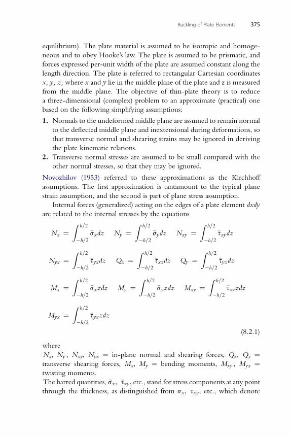
Buckling of Plate Elements 375

equilibrium). The plate material is assumed to be isotropic and homoge-

neous and to obey Hooke’s law. The plate is assumed to be prismatic, and

forces expressed per-unit width of the plate are assumed constant along the

length direction. The plate is referred to rectangular Cartesian coordinates

x, y, z, where x and y lie in the middle plane of the plate and z is measured

from the middle plane. The objective of thin-plate theory is to reduce

a three-dimensional (complex) problem to an approximate (practical) one

based on the following simplifying assumptions:

1. Normals to the undeformed middle plane are assumed to remain normal

to the deflected middle plane and inextensional during deformations, so

that transverse normal and shearing strains may be ignored in deriving

the plate kinematic relations.

2. Transverse normal stresses are assumed to be small compared with the

other normal stresses, so that they may be ignored.

Novozhilov (1953) referred to these approximations as the Kirchhoff

assumptions. The first approximation is tantamount to the typical plane

strain assumption, and the second is part of plane stress assumption.

Internal forces (generalized) acting on the edges of a plate element dxdy

are related to the internal stresses by the equations

Nx ¼Z h=2

�h=2�sxdz Ny ¼

Z h=2

�h=2�sydz Nxy ¼

Z h=2

�h=2�sxydz

Nyx ¼Z h=2

�h=2�syxdz Qx ¼

Z h=2

�h=2�sxzdz Qy ¼

Z h=2

�h=2�syzdz

Mx ¼Z h=2

�h=2�sxzdz My ¼

Z h=2

�h=2�syzdz Mxy ¼

Z h=2

�h=2�sxyzdz

Myx ¼Z h=2

�h=2�syxzdz

(8.2.1)

where

Nx, Ny , Nxy, Nyx ¼ in-plane normal and shearing forces, Qx, Qy ¼transverse shearing forces, Mx, My ¼ bending moments, Mxy , Myx ¼twisting moments.

The barred quantities, �sx; �sxy; etc., stand for stress components at any point

through the thickness, as distinguished from sx; sxy; etc., which denote

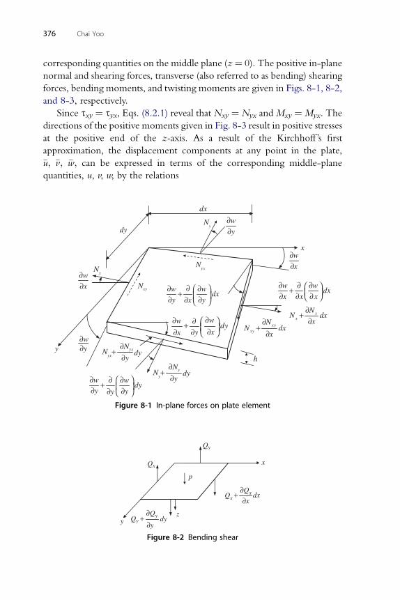
376 Chai Yoo

corresponding quantities on the middle plane (z¼ 0). The positive in-plane

normal and shearing forces, transverse (also referred to as bending) shearing

forces, bending moments, and twisting moments are given in Figs. 8-1, 8-2,

and 8-3, respectively.

Since sxy ¼ syx, Eqs. (8.2.1) reveal that Nxy ¼ Nyx and Mxy ¼Myx. The

directions of the positive moments given in Fig. 8-3 result in positive stresses

at the positive end of the z-axis. As a result of the Kirchhoff ’s first

approximation, the displacement components at any point in the plate,

�u; �v; �w; can be expressed in terms of the corresponding middle-plane

quantities, u, v, w, by the relations

w wdx

x x x

∂ ∂ ∂⎛ ⎞+ ⎜ ⎟∂ ∂ ∂⎝ ⎠

x

y

dy

dx

Ny

w

x

∂∂

∂w

∂w∂w

∂w

∂w

∂w∂w

∂

∂

∂ ∂w

∂x

∂x ∂x

∂y∂y

∂y

∂x

∂y

∂y ∂y∂y

Nx

Nxy

Nyx

h

dx⎛ ⎞

+ ⎜ ⎟⎝ ⎠

dy⎛ ⎞+ ⎜ ⎟⎝ ⎠

dy⎛ ⎞

+ ⎜ ⎟⎝ ⎠

Nyx

+ dy∂y

xx

NN dx

x

∂+∂

xyxy

NN dx

x

∂+

∂

∂w

∂y

∂Nyx

Ny+ dy

∂y

∂Ny

Figure 8-1 In-plane forces on plate element

Qx

Qy

Qy

Qx

x

dx+

zy +

p

dy∂Qy

∂Qx

∂y

∂x

Figure 8-2 Bending shear

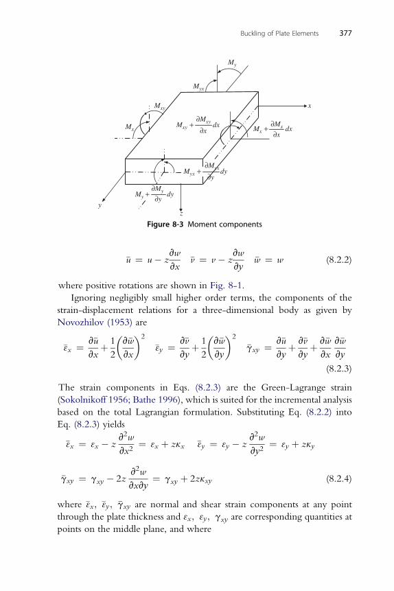
x

yz

Myx

My

Mxy

Mxy

My

∂Myx

∂My

∂Mxy ∂MxMx +

Myx

Mx

dy+∂y

dx dx+∂x ∂x

∂ydy+

Figure 8-3 Moment components

Buckling of Plate Elements 377

�u ¼ u� zvw

vx�v ¼ v � z

vw

vy�w ¼ w (8.2.2)

where positive rotations are shown in Fig. 8-1.

Ignoring negligibly small higher order terms, the components of the

strain-displacement relations for a three-dimensional body as given by

Novozhilov (1953) are

�3x ¼ v�u

vxþ 1

2

�v�w

vx

�2

�3y ¼ v�v

vyþ 1

2

�v�w

vy

�2

�gxy ¼ v�u

vyþ v�v

vyþ v�w

vx

v�w

vy

(8.2.3)

The strain components in Eqs. (8.2.3) are the Green-Lagrange strain

(Sokolnikoff 1956; Bathe 1996), which is suited for the incremental analysis

based on the total Lagrangian formulation. Substituting Eq. (8.2.2) into

Eq. (8.2.3) yields

�3x ¼ 3x � zv2w

vx2¼ 3x þ zkx �3y ¼ 3y � z

v2w

vy2¼ 3y þ zky

�gxy ¼ gxy � 2zv2w

vxvy¼ gxy þ 2zkxy (8.2.4)

where �3x; �3y; �gxy are normal and shear strain components at any point

through the plate thickness and 3x; 3y; gxy are corresponding quantities at

points on the middle plane, and where

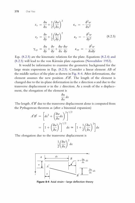
378 Chai Yoo

3x ¼ vu

vxþ 1

2

�vw

vx

�2

kx ¼ � v2w

vx2

3y ¼ vv

vyþ 1

2

�vw

vy

�2

ky ¼ � v2w

vy2

gxy ¼ vu

vyþ vv

vyþ vw

vx

vw

vykxy ¼ � v2w

vxvy

(8.2.5)

Eqs. (8.2.5) are the kinematic relations for the plate. Equations (8.2.4) and

(8.2.5) will lead to the von Karman plate equations (Novozhilov 1953).

It would be informative to examine the geometric background for the

large strain expressions in Eqs. (8.2.5). Consider a linear element AB of

the middle surface of the plate as shown in Fig. 8-4. After deformations, the

element assumes the new position A0B0. The length of the element is

changed due to the in-plane deformation in the x direction u and due to the

transverse displacement w in the z direction. As a result of the u displace-

ment, the elongation of the element is

vu

vxdx

The length A0B0 due to the transverse displacement alone is computed from

the Pythagorean theorem as (after a binomial expansion)

A0B0 ¼�dx2 þ

�vw

vxdx

�2�1=2

¼�1þ

�vw

vx

�2�1=2dxx

�1þ 1

2

�vw

vx

�2�dx

The elongation due to the transverse displacement is

1

2

�vw

vx

�2

dx

Au ∂u+

∂x

dx∂w∂x

w

u

x

z

dx

B′

A′

Bdx

Figure 8-4 Axial straindlarge deflection theory

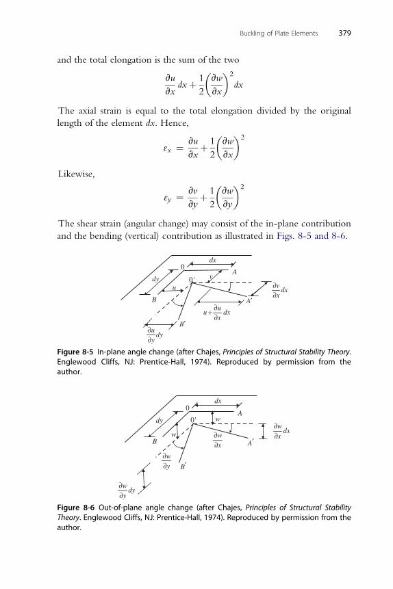
Buckling of Plate Elements 379

and the total elongation is the sum of the two

vu

vxdxþ 1

2

�vw

vx

�2

dx

The axial strain is equal to the total elongation divided by the original

length of the element dx. Hence,

3x ¼ vu

vxþ 1

2

�vw

vx

�2

Likewise,

3y ¼ vv

vyþ 1

2

�vw

vy

�2

The shear strain (angular change) may consist of the in-plane contribution

and the bending (vertical) contribution as illustrated in Figs. 8-5 and 8-6.

0

0'

dx

dy

B

A

B′

A′

u

v

dy∂u∂y

u dx∂u+∂x

dx∂v∂x

Figure 8-5 In-plane angle change (after Chajes, Principles of Structural Stability Theory.Englewood Cliffs, NJ: Prentice-Hall, 1974). Reproduced by permission from theauthor.

0

0'

dx

dy

B

A

B′

A′w

w

∂w

∂y

dx∂w∂x∂w

∂x

dy∂w

∂y

Figure 8-6 Out-of-plane angle change (after Chajes, Principles of Structural StabilityTheory. Englewood Cliffs, NJ: Prentice-Hall, 1974). Reproduced by permission from theauthor.

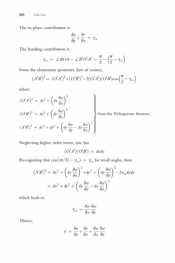
380 Chai Yoo

The in-plane contribution is

vu

vyþ vv

vx¼ gn

The bending contribution is

gw ¼ :BOA�:B0O0A0 ¼ p

2��p2� gw

�From the elementary geometry (law of cosine),

ðA0B0Þ2¼ ðO0A0Þ2þðO0B0Þ2�2ðO0A0ÞðO0B0Þcos�p2� gw

�where

ðO0A0Þ2 ¼ dx2 þ�dx

vw

vx

�2

ðO0B0Þ2 ¼ dy2 þ�dy

vw

vy

�2

ðA0B0Þ2 ¼ dx2 þ dy2 þ�dy

vw

vy� dx

vw

vx

�2

9>>>>>>>>>>=>>>>>>>>>>;

from the Pythagorean theorem

Neglecting higher order terms, one has

ðO0A0ÞðO0B0Þ ¼ dxdy

Recognizing that cosððp=2Þ � gwÞ ¼ gw for small angles, then

ðA0B0Þ2¼ dx2 þ�dx

vw

vx

�2

þdy2 þ�dy

vw

vy

�2

�2gwdxdy

¼ dx2 þ dy2 þ�dy

vw

vy� dx

vw

vx

�2

which leads to

gw ¼ vw

vx

vw

vy

Hence,

g ¼ vu

vyþ vv

vxþ vw

vx

vw

vy

Buckling of Plate Elements 381

Modifying the generalized Hooke’s law in a three-dimensional isotropic

medium with the Kirchhoff ’s assumptions leads to the following stress-strain

relations:

�sx ¼ E

1� m2

��3x þ m�3y

�sy ¼ E

1� m2

��3y þ m�3x

�sxy ¼ E

2ð1þ mÞ �gxy

(8.2.6)

Substituting Eqs. (8.2.6) and (8.2.4) into Eq. (8.2.1) and integrating the

result gives

Nx ¼ C�3x þ m3y

Ny ¼ C

�3y þ m3x

Nxy ¼ Cð1� mÞgxy=2

Mx ¼ �D

�v2w

vx2þ m

v2w

vy2

�My ¼ �D

�v2w

vy2þ m

v2w

vx2

�

Mxy ¼ �Dð1� mÞ v2w

vxvy

(8.2.7)

with3

C ¼ Eh

1� m2and D ¼ Eh

12ð1� m2Þ (8.2.8)

The coefficients C and D are axial and bending rigidities of the plate per

unit width shown in Fig. 8-7, respectively.

h

1

Figure 8-7 Plate cross section

8.2.2. Equilibrium EquationsIn order to account for the interaction between forces and deformations,

the equations representing equilibrium must be derived in a slightly

deformed configuration (neighboring equilibrium), as shown in Fig. 8-1.

The forces and deformations are assumed to vary across the plate element.

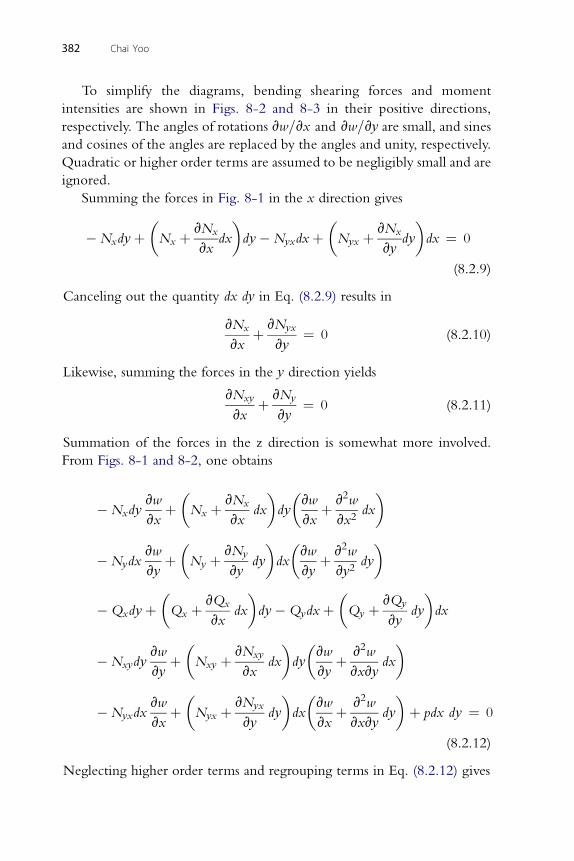
382 Chai Yoo

To simplify the diagrams, bending shearing forces and moment

intensities are shown in Figs. 8-2 and 8-3 in their positive directions,

respectively. The angles of rotations vw=vx and vw=vy are small, and sines

and cosines of the angles are replaced by the angles and unity, respectively.

Quadratic or higher order terms are assumed to be negligibly small and are

ignored.

Summing the forces in Fig. 8-1 in the x direction gives

�Nxdyþ�Nx þ vNx

vxdx

�dy�Nyxdxþ

�Nyx þ vNx

vydy

�dx ¼ 0

(8.2.9)

Canceling out the quantity dx dy in Eq. (8.2.9) results in

vNx

vxþ vNyx

vy¼ 0 (8.2.10)

Likewise, summing the forces in the y direction yields

vNxy

vxþ vNy

vy¼ 0 (8.2.11)

Summation of the forces in the z direction is somewhat more involved.

From Figs. 8-1 and 8-2, one obtains

�Nxdyvw

vxþ�Nx þ vNx

vxdx

�dy

�vw

vxþ v2w

vx2dx

�

�Nydxvw

vyþ�Ny þ vNy

vydy

�dx

�vw

vyþ v2w

vy2dy

�

�Qxdyþ�Qx þ vQx

vxdx

�dy�Qydxþ

�Qy þ vQy

vydy

�dx

�Nxydyvw

vyþ�Nxy þ vNxy

vxdx

�dy

�vw

vyþ v2w

vxvydx

�

�Nyxdxvw

vxþ�Nyx þ vNyx

vydy

�dx

�vw

vxþ v2w

vxvydy

�þ pdx dy ¼ 0

(8.2.12)

Neglecting higher order terms and regrouping terms in Eq. (8.2.12) gives

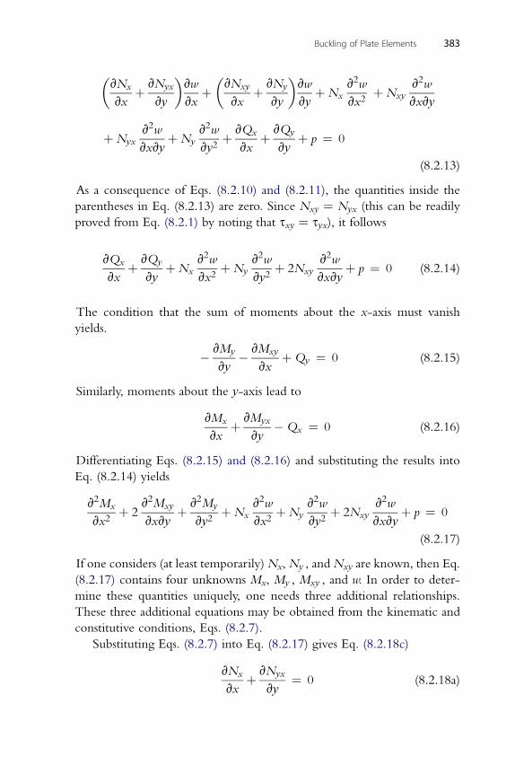
Buckling of Plate Elements 383

�vNx

vxþ vNyx

vy

�vw

vxþ�vNxy

vxþ vNy

vy

�vw

vyþNx

v2w

vx2þNxy

v2w

vxvy

þNyxv2w

vxvyþNy

v2w

vy2þ vQx

vxþ vQy

vyþ p ¼ 0

(8.2.13)

As a consequence of Eqs. (8.2.10) and (8.2.11), the quantities inside the

parentheses in Eq. (8.2.13) are zero. Since Nxy ¼ Nyx (this can be readily

proved from Eq. (8.2.1) by noting that sxy ¼ syx), it follows

vQx

vxþ vQy

vyþNx

v2w

vx2þNy

v2w

vy2þ 2Nxy

v2w

vxvyþ p ¼ 0 (8.2.14)

The condition that the sum of moments about the x-axis must vanish

yields.

� vMy

vy� vMxy

vxþQy ¼ 0 (8.2.15)

Similarly, moments about the y-axis lead to

vMx

vxþ vMyx

vy�Qx ¼ 0 (8.2.16)

Differentiating Eqs. (8.2.15) and (8.2.16) and substituting the results into

Eq. (8.2.14) yields

v2Mx

vx2þ 2

v2Mxy

vxvyþ v2My

vy2þNx

v2w

vx2þNy

v2w

vy2þ 2Nxy

v2w

vxvyþ p ¼ 0

(8.2.17)

If one considers (at least temporarily)Nx, Ny , and Nxy are known, then Eq.

(8.2.17) contains four unknowns Mx, My , Mxy , and w. In order to deter-

mine these quantities uniquely, one needs three additional relationships.

These three additional equations may be obtained from the kinematic and

constitutive conditions, Eqs. (8.2.7).

Substituting Eqs. (8.2.7) into Eq. (8.2.17) gives Eq. (8.2.18c)

vNx

vxþ vNyx

vy¼ 0 (8.2.18a)

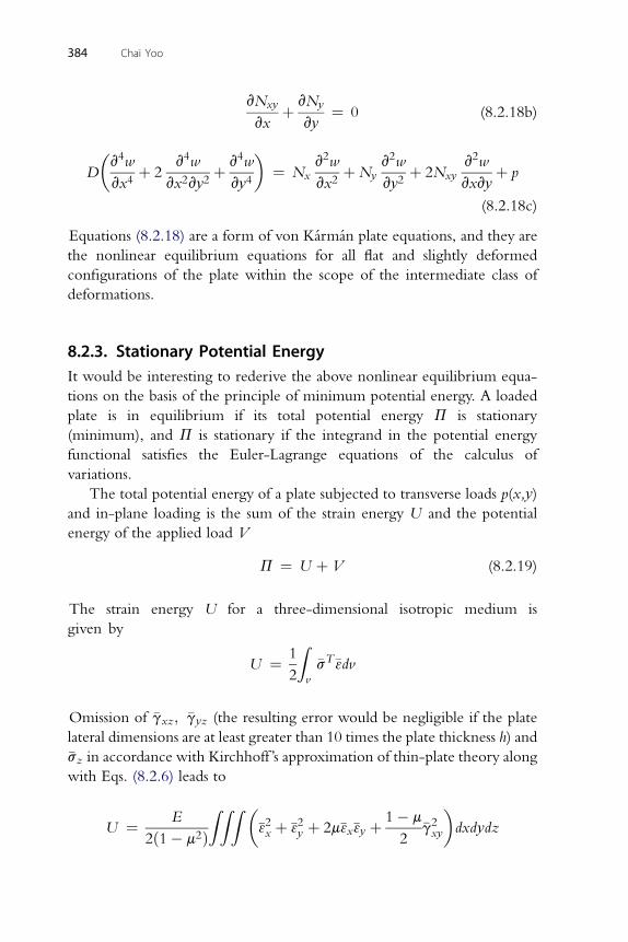
vNxy vNy

vxþ

vy¼ 0 (8.2.18b)

�v4w v4w v4w

�v2w v2w v2w

384 Chai Yoo

Dvx4

þ 2vx2vy2

þvy4

¼ Nxvx2

þNyvy2

þ 2Nxyvxvy

þ p

(8.2.18c)

Equations (8.2.18) are a form of von Karman plate equations, and they are

the nonlinear equilibrium equations for all flat and slightly deformed

configurations of the plate within the scope of the intermediate class of

deformations.

8.2.3. Stationary Potential EnergyIt would be interesting to rederive the above nonlinear equilibrium equa-

tions on the basis of the principle of minimum potential energy. A loaded

plate is in equilibrium if its total potential energy P is stationary

(minimum), and P is stationary if the integrand in the potential energy

functional satisfies the Euler-Lagrange equations of the calculus of

variations.

The total potential energy of a plate subjected to transverse loads p(x,y)

and in-plane loading is the sum of the strain energy U and the potential

energy of the applied load V

P ¼ U þ V (8.2.19)

The strain energy U for a three-dimensional isotropic medium is

given by

U ¼ 1

2

Zv

�sT�3dv

Omission of �gxz; �gyz (the resulting error would be negligible if the plate

lateral dimensions are at least greater than 10 times the plate thickness h) and

�sz in accordance with Kirchhoff ’s approximation of thin-plate theory along

with Eqs. (8.2.6) leads to

U ¼ E

2ð1� m2ÞZZZ �

�32x þ �32y þ 2m�3x�3y þ 1� m

2�g2xy

�dxdydz

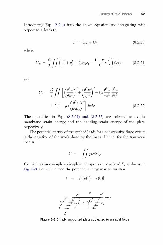
Buckling of Plate Elements 385

Introducing Eqs. (8.2.4) into the above equation and integrating with

respect to z leads to

U ¼ Um þ Ub (8.2.20)

where

Um ¼ C

2

ZZ �32x þ 32y þ 2m3x3y þ 1� m

2g2xy

�dxdy (8.2.21)

and

Ub ¼ D

2

ZZ ��v2w

vx2

�2

þ�v2w

vy2

�2

þ2mv2w

vx2v2w

vy2

þ 2ð1� mÞ�v2w

vxvy

�2�dxdy (8.2.22)

The quantities in Eqs. (8.2.21) and (8.2.22) are referred to as the

membrane strain energy and the bending strain energy of the plate,

respectively.

The potential energy of the applied loads for a conservative force system

is the negative of the work done by the loads. Hence, for the transverse

load p,

V ¼ �ZZ

pwdxdy

Consider as an example an in-plane compressive edge load Px as shown in

Fig. 8-8. For such a load the potential energy may be written

V ¼ �Px½uðaÞ � uð0Þ�

a

b

x

y

Px

Figure 8-8 Simply supported plate subjected to uniaxial force

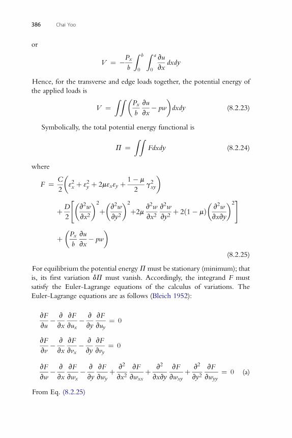
386 Chai Yoo

or

V ¼ �Px

b

Z b

0

Z a

0

vu

vxdxdy

Hence, for the transverse and edge loads together, the potential energy of

the applied loads is

V ¼ZZ �

Px

b

vu

vx� pw

�dxdy (8.2.23)

Symbolically, the total potential energy functional is

P ¼ZZ

Fdxdy (8.2.24)

where

F ¼ C

2

�32x þ 32y þ 2m3x3y þ 1� m

2g2xy

�

þD

2

"�v2w

vx2

�2

þ�v2w

vy2

�2

þ2mv2w

vx2v2w

vy2þ 2ð1� mÞ

�v2w

vxvy

�2#

þ�Px

b

vu

vx� pw

�(8.2.25)

For equilibrium the potential energyPmust be stationary (minimum); that

is, its first variation dP must vanish. Accordingly, the integrand F must

satisfy the Euler-Lagrange equations of the calculus of variations. The

Euler-Lagrange equations are as follows (Bleich 1952):

vF

vu� v

vx

vF

vux� v

vy

vF

vuy¼ 0

vF

vv� v

vx

vF

vvx� v

vy

vF

vvy¼ 0

vF

vw� v

vx

vF

vwx� v

vy

vF

vwyþ v2

vx2vF

vwxxþ v2

vxvy

vF

vwxyþ v2

vy2vF

vwyy¼ 0 (a)

From Eq. (8.2.25)

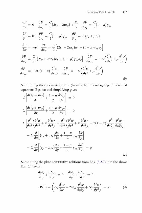
Buckling of Plate Elements 387

vF

vu¼ 0

vF

vux¼ C

2

�23x þ 2m3y

þ Px

b

vF

vuy¼ C

2ð1� mÞgxy

vF

vv¼ 0

vF

vvx¼ C

2ð1� mÞgxy

vF

vvy¼ C

�3y þ m3x

vF

vw¼ �p

vF

vwx¼ C

2

h�23x þ 2m3y

wx þ ð1� mÞgxywy

ivF

vwy¼ C

2

h�23y þ 2m3x

wy þ ð1� mÞgxywx

i vF

vwxx¼ �D

�v2w

vx2þ m

v2w

vy2

�

vF

vwxy¼ �2Dð1� mÞ v2w

vxvy

vF

vwxx¼ �D

�v2w

vy2þ m

v2w

vx2

�(b)

Substituting these derivatives Eqs. (b) into the Euler-Lagrange differential

equations Eqs. (a) and simplifying gives

C

�v�3x þ m3y

vx

þ 1� m

2

vgxy

vy

�¼ 0

C

�v�3y þ m3x

vy

þ 1� m

2

vgxy

vx

�¼ 0

D

�v2

vx2

�v2w

vx2þ m

v2w

vy2

�þ v2

vy2

�v2w

vy2þ m

v2w

vx2

�þ 2ð1� mÞ v2

vxvy

v2w

vxvy

�

� Cv

vx

��3x þ m3y

vwvx

þ 1� m

2gxy

vw

vy

�

� Cv

vy

��3y þ m3x

vwvy

þ 1� m

2gxy

vw

vx

�¼ p

(c)

Substituting the plate constitutive relations from Eqs. (8.2.7) into the above

Eqs. (c) yields

vNx

vxþ vNxy

vy¼ 0

vNy

vyþ vNxy

vx¼ 0

DV4w ��Nx

v2w

vx2þ 2Nxy

v2w

vxvyþNy

v2w

vy2

�¼ p (d)

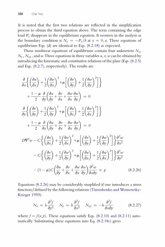
388 Chai Yoo

It is noted that the first two relations are reflected in the simplification

process to obtain the third equation above. The term containing the edge

load Px disappears in the equilibrium equation. It reenters in the analysis as

the boundary condition is Nx ¼ �Px=b at x ¼ 0; a: These equations of

equilibrium Eqs. (d) are identical to Eqs. (8.2.18) as expected.

These nonlinear equations of equilibrium contain four unknowns Nx,

Ny ,Nxy , and w. Three equations in three variables u, v, w can be obtained by

introducing the kinematic and constitutive relations of the plate (Eqs. (8.2.5)

and Eqs. (8.2.7), respectively). The results are

v

vx

�vu

vx

�þ 1

2

�vw

vx

�2

þm

��vv

vy

�þ 1

2

�vw

vy

�2��

þ 1� m

2

v

vy

�vu

vyþ vv

vxþ vw

vx

vw

vy

�¼ 0

v

vy

�vv

vy

�þ 1

2

�vw

vy

�2

þm

��vu

vx

�þ 1

2

�vw

vx

�2��

þ 1� m

2

v

vx

�vu

vyþ vv

vxþ vw

vx

vw

vy

�¼ 0

DV4w �C

�vu

vx

�þ 1

2

�vw

vx

�2

þm

��vv

vy

�þ 1

2

�vw

vy

�2��v2w

vx2

� C

�vv

vy

�þ 1

2

�vw

vy

�2

þm

��vu

vx

�þ 1

2

�vw

vx

�2��v2w

vy2

� ð1� mÞC�vu

vyþ vv

vxþ vw

vx

vw

vy

�v2w

vxvy¼ p (8.2.26)

Equations (8.2.26) may be considerably simplified if one introduces a stress

function f defined by the following relations (Timoshenko andWoinowsky-

Krieger 1959):

Nx ¼ hv2f

vy2Ny ¼ h

v2f

vx2Nxy ¼ �h

v2f

vxvy(8.2.27)

where f ¼ f (x,y). These equations satisfy Eqs. (8.2.10) and (8.2.11) auto-

matically. Substituting these equations into Eq. (8.2.18c) gives

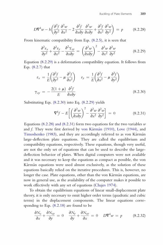
Buckling of Plate Elements 389

DV4w � h

�v2f

vy2v2w

vx2� 2

v2f

vxvy

v2w

vxvyþ v2f

vx2v2w

vy2

�¼ p (8.2.28)

From kinematic compatibility from Eqs. (8.2.5), it is seen that

v23x

vy2þ v23y

vx2� v2gxy

vxvy¼�v2w

vxvy

�2

� v2w

vx2v2w

vy2(8.2.29)

Equation (8.2.29) is a deformation compatibility equation. It follows from

Eqs. (8.2.7) that

3x ¼ 1

E

�v2f

vy2� m

v2f

vx2

�3y ¼ 1

E

�v2f

vx2� m

v2f

vy2

�

gxy ¼ � 2ð1þ mÞE

v2f

vxvy(8.2.30)

Substituting Eqs. (8.2.30) into Eq. (8.2.29) yields

V4f � E

��v2w

vxvy

�2

� v2w

vx2v2w

vy2

�¼ 0 (8.2.31)

Equations (8.2.28) and (8.2.31) form two equations for the two variables w

and f. They were first derived by von Karman (1910), Love (1944), and

Timoshenko (1983), and they are accordingly referred to as von Karman

large-deflection plate equations. They are called the equilibrium and

compatibility equations, respectively. These equations, though very useful,

are not the only set of equations that can be used to describe the large-

deflection behavior of plates. When digital computers were not available

and it was necessary to keep the equations as compact as possible, the von

Karman equations were used almost exclusively, as the solution of these

equations basically relied on the iterative procedures. This is, however, no

longer the case. Plate equations, other than the von Karman equations, are

now in general use, as the availability of the computer makes it possible to

work effectively with any set of equations (Chajes 1974).

To obtain the equilibrium equations of linear small-displacement plate

theory, it is only necessary to omit higher order terms (quadratic and cubic

terms) in the displacement components. The linear equations corre-

sponding to Eqs. (8.2.18) are found to be

vNx

vxþ vNxy

vy¼ 0

vNy

vyþ vNxy

vx¼ 0 DV4w ¼ p (8.2.32)

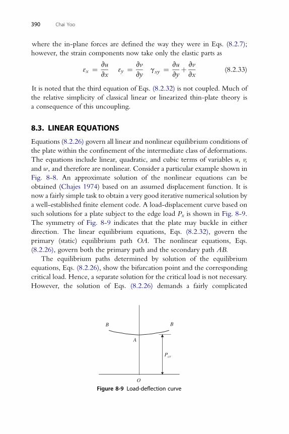
390 Chai Yoo

where the in-plane forces are defined the way they were in Eqs. (8.2.7);

however, the strain components now take only the elastic parts as

3x ¼ vu

vx3y ¼ vv

vygxy ¼ vu

vyþ vv

vx(8.2.33)

It is noted that the third equation of Eqs. (8.2.32) is not coupled. Much of

the relative simplicity of classical linear or linearized thin-plate theory is

a consequence of this uncoupling.

8.3. LINEAR EQUATIONS

Equations (8.2.26) govern all linear and nonlinear equilibrium conditions of

the plate within the confinement of the intermediate class of deformations.

The equations include linear, quadratic, and cubic terms of variables u, v,

and w, and therefore are nonlinear. Consider a particular example shown in

Fig. 8-8. An approximate solution of the nonlinear equations can be

obtained (Chajes 1974) based on an assumed displacement function. It is

now a fairly simple task to obtain a very good iterative numerical solution by

a well-established finite element code. A load-displacement curve based on

such solutions for a plate subject to the edge load Px is shown in Fig. 8-9.

The symmetry of Fig. 8-9 indicates that the plate may buckle in either

direction. The linear equilibrium equations, Eqs. (8.2.32), govern the

primary (static) equilibrium path OA. The nonlinear equations, Eqs.

(8.2.26), govern both the primary path and the secondary path AB.

The equilibrium paths determined by solution of the equilibrium

equations, Eqs. (8.2.26), show the bifurcation point and the corresponding

critical load. Hence, a separate solution for the critical load is not necessary.

However, the solution of Eqs. (8.2.26) demands a fairly complicated

O

B B

A

Pcr

Figure 8-9 Load-deflection curve

Buckling of Plate Elements 391

numerical procedure. The purpose of stability analysis to be presented

herein is to permit determination of the critical load by solution of linear

differential equations.

The linear differential equations for the determination of the critical

load of a rectangular plate subjected to in-plane loading are derived by

applying the adjacent-equilibrium criterion. The same equations are

rederived based on the minimum potential energy criterion as was done in

the previous section.

8.3.1. Adjacent-Equilibrium CriterionAdjacent equilibrium configurations are examined using the procedure

outlined by Brush and Almroth (1975). Consider the equilibrium config-

uration at the bifurcation point. Then, the equilibrium configuration is

perturbed by the small incremental displacement. The incremental

displacement in u1, v1, w1 is arbitrary and tentative. Variables in the two

adjacent configurations before and after the increment are represented by u0,

v0, w0 and u, v, w. Let

u/u0 þ u1

v/v0 þ v1

w/w0 þ w1

(8.3.1)

where the arrow is read “be replaced by.” Substitution of Eqs. (8.3.1)

into Eqs. (8.2.26) results in equations containing terms that are linear,

quadratic, and cubic in u0, v0, w0 and u1, v1, w1 displacement compo-

nents. In the new equation thus obtained, the terms containing u0, v0, w0

alone are equal to zero as u0, v0, w0 constitute an equilibrium configu-

ration, and terms that are quadratic and cubic in u1, v1, w1 may be

ignored because of the smallness of the incremental displacement.

Therefore, the resulting equations are homogeneous and linear in u1, v1,

w1 with variable coefficients. The coefficients in u0, v0, w0 are governed

by the original nonlinear equations. It will simplify the procedure greatly

by simply limiting the range of applicability of the linearized equations by

requiring that u0, v0, w0 be limited to configurations that are governed by

the linear equations, Eqs. (8.2.32). This limitation has the additional

advantage of w0 and its derivatives being equal to zero for in-plane

loading (there is no lateral displacement in the primary path as shown in

Fig. 8-9).

392 Chai Yoo

Equations (8.2.18) will be used instead as it will shorten the derivation.

The increment in u, v, w causes a concomitant change in the internal force

such as

Nx/Nx0 þ DNx

Ny/Ny0 þ DNy

Nxy/Nxy0 þ DNxy

(8.3.2)

where terms with subscript 0 correspond to the u0, v0, w0 displacement, and

DNx, DNy , DNxy are increments corresponding to u1, v1, w1. Let also Nx1,

Ny1, Nxy1 represent parts of DNx, DNy , DNxy , respectively, that are linear

in u1, v1, w1. For example, from Eqs. (8.2.5) and (8.2.7),

Nx ¼ C

vu

vxþ 1

2

�vw

vx

�2

þ m

�vv

vyþ 1

2

�vw

vy

�2��

As w0 and its derivatives are equal to zero for in-plane loading, one may

write

Nx0 þ DNx ¼ C

vu0

vxþ vu1

vxþ 1

2

�vw1

vx

�2

þ m

�vv0

vyþ vv1

vyþ 1

2

�vw1

vy

�2��

From which

Nx0 ¼ C

�vu0

vxþ m

vv0

vy

�

� �2 � � �2��

DNx ¼ C

vu1

vxþ 1

2

vw1

vxþ m

vv1

vyþ 1

2

vw1

vy

�vu vv

�

Nx1 ¼ C

1

vxþ m

1

vy

Substituting these into Eqs. (8.2.18) gives

vNx1

vxþ vNxy1

vy¼ 0 (8.3.3a)

vN vN

y1

vyþ xy1

vx¼ 0 (8.3.3b)

�v2w1 v2w1 v2w1

�

DV4w1 � Nx0

vx2þ 2Nxy0

vxvyþNy0

vy2¼ 0 (8.3.3c)

where

Nx0 ¼ C

�vu0

vxþ m

vv0

vy

�Nx1 ¼ C

�vu1

vxþ m

vv1

vy

�

Ny0 ¼ C

�vv0

vyþ m

vu0

vx

�Ny1 ¼ C

�vv1

vyþ m

vu1

vx

�

Nxy0 ¼ C1� m

2

�vu0

vyþ vv0

vx

�Nxy1 ¼ C

1� m

2

�vu1

vyþ vv1

vx

�(8.3.4)

Equations (8.3.3) are the stability equations for the plate subjected to in-

plane edge loading. As in the case of linear equilibrium equations, Eq.

(8.3.3c) is uncoupled from the other two equations. Equation (8.3.3c) is

a homogeneous linear equation in w1 with variable coefficients inNx0, Ny0,

Nxy0, depending on the edge conditions of the plate, which are determined

by the other two linear equations (8.3.3a) and (8.3.3b). It is an eigenvalue

problem. As such, it has solutions for discrete values of the applied load. At

each solution point or bifurcation point, two adjacent equilibrium

configurations existdan undeformed one on the primary equilibrium path

and a slightly deformed one on a secondary equilibrium path.

8.3.2. Minimum Potential Energy CriterionThe plate stability equations (8.3.3) will be rederived by applying the

minimum potential energy criterion. The equilibrium changes from stable

to neutral when the total potential energy functional P ceases to be a

relative minimum. The criterion for the loss of stability is that the integrand

in the expression for the second variation of P satisfies the Euler-Lagrange

equations, which is known as the Trefftz criterion according to Langhaar

(1962).1

Symbolically, the total potential energy increment may be written in the

form

DP ¼ dPþ 1

2!d2Pþ 1

3!d3Pþ : : : (8.3.5)

Each nonzero term in Eq. (8.3.5) is much larger than the sum of the suc-

ceeding terms. Since dP vanishes by virtue of the principle of minimum

Buckling of Plate Elements 393

1 See page 211.

394 Chai Yoo

potential energy, the sign of DP is governed by the second variation. For

sufficiently small values of the applied load, the second variation is positive

definite (condition for P to be relative minimum). The critical load is

defined as the smallest load for which the second variation no longer is

positive definite (it is positive semidefinite). According to the Trefftz

criterion, the equations for the critical load are given by the Euler-Lagrange

equations for the integrand in the second variation. Since the expression for

the second variation is a homogeneous quadratic functional, its variational

derivatives (Euler-Lagrange equations) are necessarily linear homogeneous

differential equations. In order to obtain the second variation, Eqs. (8.3.1)

are used again

u/u0 þ u1

v/v0 þ v1

w/w0 þ w1

(8.3.1)

where (u0, v0, w0) is a configuration on the primary path, including the

bifurcation point, and (u1, v1, w1) is a virtual displacement. The total

potential energy in a Taylor series expansion is

Pðu0 þ u1; v0 þ v1;w0 þ w1Þ ¼ Pðu0; v0;w0Þ þ vP

vu0u1 þ vP

vv0v1 þ vP

vw0w1

þ 1

2!

�v2P

vu20ðu1Þ2 þ v2P

vv20ðv1Þ2 þ v2P

vw20

ðw1Þ2 þ 2v2P

vu0vv0u1v1

þ 2v2P

vu0vw0u1w1 þ 2

v2P

vv0vw0v1w1

�þ : : :

The change in potential energy DP ¼ Pðu0 þ u1; v0 þ v1;w0 þ w1Þ�Pðu0; v0;w0Þ can be written as

DP ¼ dPþ 1

2!d2Pþ : : :

where the first variation is equal to zero by virtue of the principle of

minimum potential energy and the second variation is defined as

d2P ¼ v2P

vu20ðu1Þ2 þ v2P

vv20ðv1Þ2 þ v2P

vw20

ðw1Þ2 þ2v2P

vu0vv0u1v1

þ 2v2P

vu0vw0u1w1 þ 2

v2P

vv0vw0v1w1

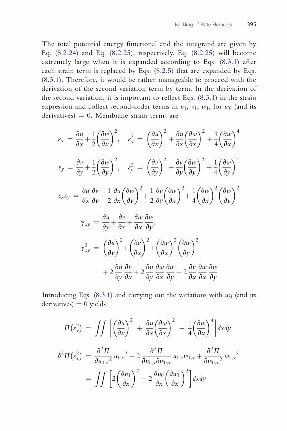
Buckling of Plate Elements 395

The total potential energy functional and the integrand are given by

Eq. (8.2.24) and Eq. (8.2.25), respectively. Eq. (8.2.25) will become

extremely large when it is expanded according to Eqs. (8.3.1) after

each strain term is replaced by Eqs. (8.2.5) that are expanded by Eqs.

(8.3.1). Therefore, it would be rather manageable to proceed with the

derivation of the second variation term by term. In the derivation of

the second variation, it is important to reflect Eqs. (8.3.1) in the strain

expression and collect second-order terms in u1, v1, w1, for w0 (and its

derivatives) ¼ 0. Membrane strain terms are

3x ¼ vu

vxþ 1

2

�vw

vx

�2

; 32x ¼�vu

vx

�2

þ vu

vx

�vw

vx

�2

þ 1

4

�vw

vx

�4

� �2 � �2 � �2 � �4

3y ¼ vv

vyþ 1

2

vw

vy; 32y ¼ vv

vyþ vv

vy

vw

vyþ 1

4

vw

vy

� �2 � �2 � �2� �2

3x3y ¼ vu

vx

vv

vyþ 1

2

vu

vx

vw

vyþ 1

2

vv

vy

vw

vxþ 1

4

vw

vx

vw

vy

vu vv vw vw

gxy ¼

vyþvx

þvx vy

;

g2xy ¼�vu

vy

�2

þ�vv

vx

�2

þ�vw

vx

�2�vw

vy

�2

þ 2vu

vy

vv

vxþ 2

vu

vy

vw

vx

vw

vyþ 2

vv

vx

vw

vx

vw

vy

Introducing Eqs. (8.3.1) and carrying out the variations with w0 (and its

derivatives) ¼ 0 yields

P�32x ¼

ZZ ��vu

vx

�2

þ vu

vx

�vw

vx

�2

þ 1

4

�vw

vx

�4�dxdy

� 2 2 2

d2P 32x ¼ v P

vu0;x2u1;x

2 þ 2v P

vu0;xvw0;xu1;xw1;x þ v P

vw0;x2w1;x

2

¼ZZ �

2

�vu1

vx

�2

þ 2vu0

vx

�vw1

vx

�2�dxdy

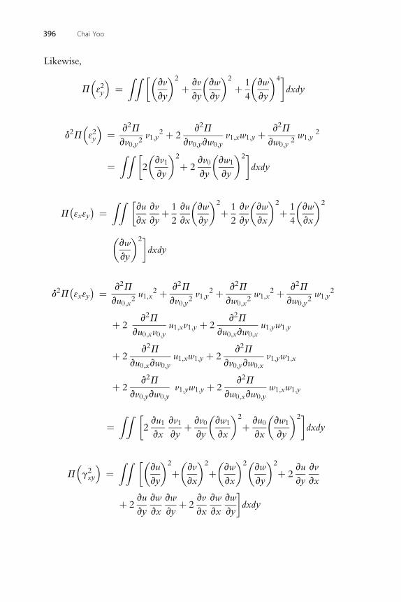
396 Chai Yoo

Likewise,

P�32y

�¼ZZ ��

vv

vy

�2

þ vv

vy

�vw

vy

�2

þ 1

4

�vw

vy

�4�dxdy

d2P�32y

�¼ v2P

vv0;y2v1;y

2 þ 2v2P

vv0;yvw0;yv1;xw1;y þ v2P

vw0;y2w1;y

2

¼ZZ �

2

�vv1

vy

�2

þ 2vv0

vy

�vw1

vy

�2�dxdy

P�3x3y

¼ZZ �

vu

vx

vv

vyþ 1

2

vu

vx

�vw

vy

�2

þ 1

2

vv

vy

�vw

vx

�2

þ 1

4

�vw

vx

�2

�vw

vy

�2�dxdy

d2P�3x3y

¼ v2P

vu0;x2u1;x

2 þ v2P

vv0;y2v1;y

2 þ v2P

vw0;x2w1;x

2 þ v2P

vw0;y2w1;y

2

þ 2v2P

vu0;xv0;yu1;xv1;y þ 2

v2P

vu0;xvw0;xu1;yw1;y

þ 2v2P

vu0;xvw0;yu1;xw1;y þ 2

v2P

vv0;yvw0;xv1;yw1;x

þ 2v2P

vv0;yvw0;yv1;yw1;y þ 2

v2P

vw0;xvw0;yw1;xw1;y

ZZ � � �2 � �2�

¼ 2

vu1

vx

vv1

vyþ vv0

vy

vw1

vxþ vu0

vx

vw1

vydxdy

P�g2xy

�¼ZZ ��

vu

vy

�2

þ�vv

vx

�2

þ�vw

vx

�2�vw

vy

�2

þ 2vu

vy

vv

vx

þ 2vu

vy

vw

vx

vw

vyþ 2

vv

vx

vw

vx

vw

vy

�dxdy

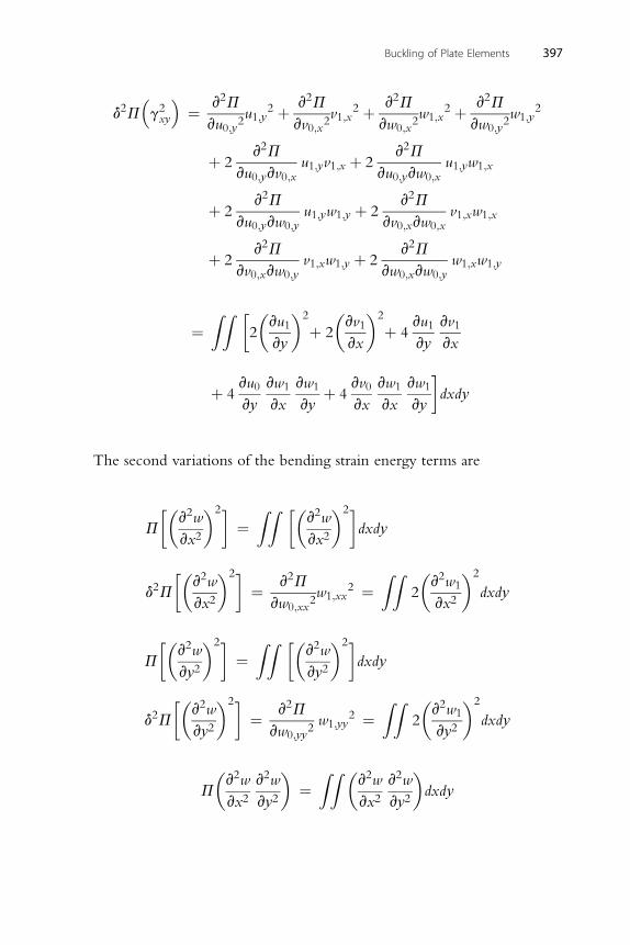
Buckling of Plate Elements 397

d2P�g2xy

�¼ v2P

vu0;y2u1;y

2 þ v2P

vv0;x2v1;x

2 þ v2P

vw0;x2w1;x

2 þ v2P

vw0;y2w1;y

2

þ 2v2P

vu0;yvv0;xu1;yv1;x þ 2

v2P

vu0;yvw0;xu1;yw1;x

þ 2v2P

vu0;yvw0;yu1;yw1;y þ 2

v2P

vv0;xvw0;xv1;xw1;x

þ 2v2P

vv0;xvw0;yv1;xw1;y þ 2

v2P

vw0;xvw0;yw1;xw1;y

ZZ � � � � �

¼ 2

vu1

vy

2

þ 2vv1

vx

2

þ 4vu1

vy

vv1

vx

þ 4vu0

vy

vw1

vx

vw1

vyþ 4

vv0

vx

vw1

vx

vw1

vy

�dxdy

The second variations of the bending strain energy terms are

P

��v2w

vx2

�2�¼ZZ ��

v2w

vx2

�2�dxdy

d2P

��v2w

vx2

�2�¼ v2P

vw0;xx2w1;xx

2 ¼ZZ

2

�v2w1

vx2

�2

dxdy

�� �2� ZZ �� �2�

P

v2w

vy2¼ v2w

vy2dxdy

d2P

��v2w

vy2

�2�¼ v2P

vw0;yy2w1;yy

2 ¼ZZ

2

�v2w1

vy2

�2

dxdy

� � ZZ � �

P

v2w

vx2v2w

vy2¼ v2w

vx2v2w

vy2dxdy

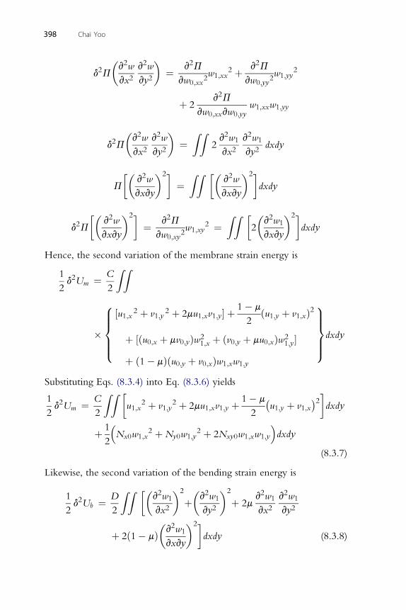
398 Chai Yoo

d2P

�v2w

vx2v2w

vy2

�¼ v2P

vw0;xx2w1;xx

2 þ v2P

vw0;yy2w1;yy

2

þ 2v2P

vw0;xxvw0;yyw1;xxw1;yy

� 2 2 � ZZ 2 2

d2Pv w

vx2v w

vy2¼ 2

v w1

vx2v w1

vy2dxdy

�� 2 �2� ZZ �� 2 �2�

P

v w

vxvy¼ v w

vxvydxdy

�� 2 �2� 2 ZZ � � 2 �2�

d2P

v w

vxvy¼ v P

vw0;xy2w1;xy

2 ¼ 2v w1

vxvydxdy

Hence, the second variation of the membrane strain energy is

1

2d2Um ¼ C

2

ZZ

�

8>>><>>>:

½u1;x 2 þ v1;y2 þ 2mu1;xv1;y� þ 1� m

2ðu1;y þ v1;xÞ2

þ ½ðu0;x þ mv0;yÞw21;x þ ðv0;y þ mu0;xÞw2

1;y�þ ð1� mÞðu0;y þ v0;xÞw1;xw1;y

9>>>=>>>;dxdy

Substituting Eqs. (8.3.4) into Eq. (8.3.6) yields

1

2d2Um ¼ C

2

ZZ �u1;x

2 þ v1;y2 þ 2mu1;xv1;y þ 1� m

2

�u1;y þ v1;x

2�dxdy

þ 1

2

�Nx0w1;x

2 þNy0w1;y2 þ 2Nxy0w1;xw1;y

�dxdy

(8.3.7)

Likewise, the second variation of the bending strain energy is

1

2d2Ub ¼ D

2

ZZ ��v2w1

vx2

�2

þ�v2w1

vy2

�2

þ 2mv2w1

vx2v2w1

vy2

þ 2ð1� mÞ�v2w1

vxvy

�2�dxdy (8.3.8)

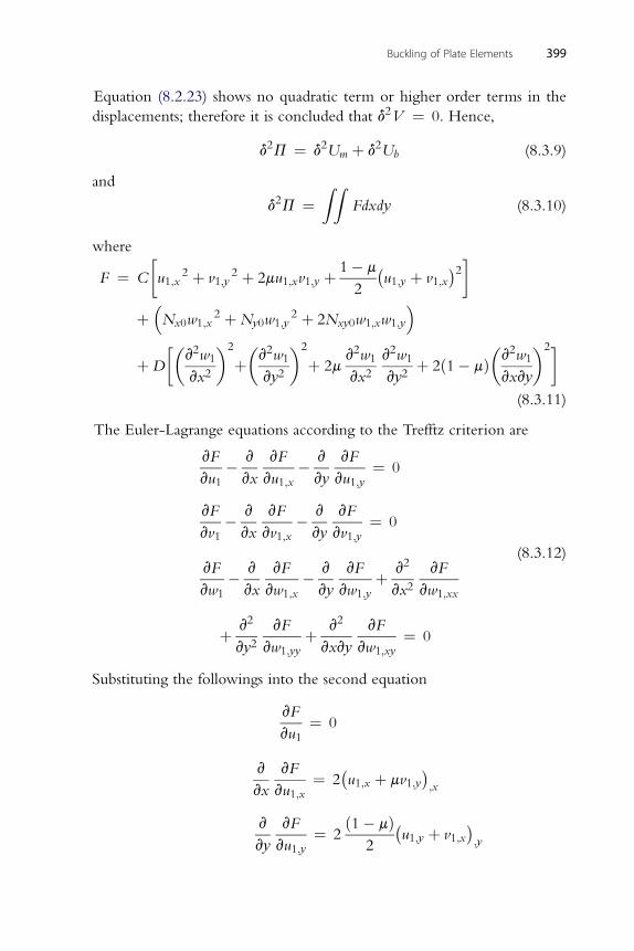
Buckling of Plate Elements 399

Equation (8.2.23) shows no quadratic term or higher order terms in the

displacements; therefore it is concluded that d2V ¼ 0. Hence,

d2P ¼ d2Um þ d2Ub (8.3.9)

and

d2P ¼ZZ

Fdxdy (8.3.10)

where

F ¼ C

�u1;x

2 þ v1;y2 þ 2mu1;xv1;y þ 1� m

2

�u1;y þ v1;x

2�

þ�Nx0w1;x

2 þNy0w1;y2 þ 2Nxy0w1;xw1;y

�

þD

��v2w1

vx2

�2

þ�v2w1

vy2

�2

þ 2mv2w1

vx2v2w1

vy2þ 2ð1� mÞ

�v2w1

vxvy

�2�(8.3.11)

The Euler-Lagrange equations according to the Trefftz criterion are

vF

vu1� v

vx

vF

vu1;x� v

vy

vF

vu1;y¼ 0

vF

vv1� v

vx

vF

vv1;x� v

vy

vF

vv1;y¼ 0

vF

vw1� v

vx

vF

vw1;x� v

vy

vF

vw1;yþ v2

vx2vF

vw1;xx

þ v2

vy2vF

vw1;yyþ v2

vxvy

vF

vw1;xy¼ 0

(8.3.12)

Substituting the followings into the second equation

vF

vu1¼ 0

v vF �

vx vu1;x

¼ 2 u1;x þ mv1;y ;x

v

vy

vF

vu1;y¼ 2

ð1� mÞ2

�u1;y þ v1;x

;y

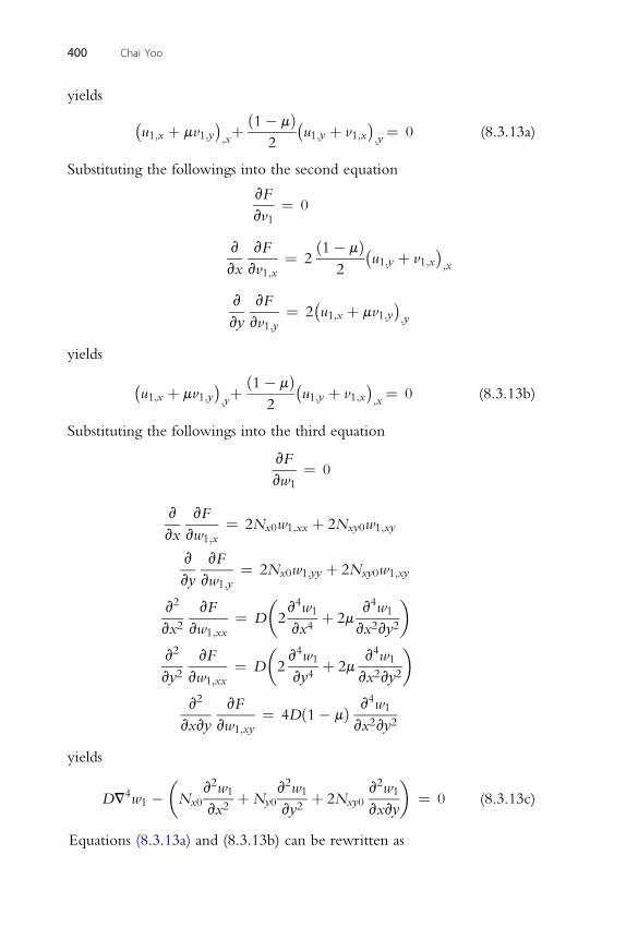
400 Chai Yoo

yields

�u1;x þ mv1;y

;xþ ð1� mÞ

2

�u1;y þ v1;x

;y¼ 0 (8.3.13a)

Substituting the followings into the second equation

vF

vv1¼ 0

v vF ð1� mÞ�

vx vv1;x

¼ 22

u1;y þ v1;x ;x

v

vy

vF

vv1;y¼ 2

�u1;x þ mv1;y

;y

yields

�u1;x þ mv1;y

;yþ ð1� mÞ

2

�u1;y þ v1;x

;x¼ 0 (8.3.13b)

Substituting the followings into the third equation

vF

vw1¼ 0

v vF

vx vw1;x¼ 2Nx0w1;xx þ 2Nxy0w1;xy

v

vy

vF

vw1;y¼ 2Nx0w1;yy þ 2Nxy0w1;xy

v2

vx2vF

vw1;xx¼ D

�2v4w1

vx4þ 2m

v4w1

vx2vy2

�

v2

vy2vF

vw1;xx¼ D

�2v4w1

vy4þ 2m

v4w1

vx2vy2

�

v2

vxvy

vF

vw1;xy¼ 4Dð1� mÞ v4w1

vx2vy2

yields

DV4w1 ��Nx0

v2w1

vx2þNy0

v2w1

vy2þ 2Nxy0

v2w1

vxvy

�¼ 0 (8.3.13c)

Equations (8.3.13a) and (8.3.13b) can be rewritten as

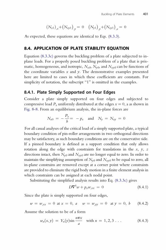
Buckling of Plate Elements 401

ðNx1Þ;xþ�Nxy1

;y¼ 0

�Ny1

;yþ�Nxy1

;x¼ 0

As expected, these equations are identical to Eqs. (8.3.3).

8.4. APPLICATION OF PLATE STABILITY EQUATION

Equation (8.3.3c) governs the buckling problem of a plate subjected to in-

plane loads. For a properly posed buckling problem of a plate that is pris-

matic, homogeneous, and isotropic, Nx0, Ny0, and Nxy0 can be functions of

the coordinate variables x and y. The demonstrative examples presented

here are limited to cases in which these coefficients are constants. For

simplicity of notation, the subscript “1” is omitted in the examples.

8.4.1. Plate Simply Supported on Four EdgesConsider a plate simply supported on four edges and subjected to

compressive load Px uniformly distributed at the edges x ¼ 0, a as shown in

Fig. 8-8. From an equilibrium analysis, the in-plane forces are

Nx0 ¼ � Px

b¼ � px and Ny ¼ Nxy ¼ 0

For all casual analyses of the critical load of a simply supported plate, a typical

boundary condition of pin-roller arrangements in two orthogonal directions

may be satisfactory, as such boundary conditions are on the conservative side.

If a pinned boundary is defined as a support condition that only allows

rotation along the edge with constraints for translations in the x, y, z

directions intact, then Ny0 and Nxy0 are no longer equal to zero. In order to

maintain the simplifying assumption of Ny0 and Nxy0 to be equal to zero, all

in-plane constrains are removed except at a corner point where constraints

are provided to eliminate the rigid body motion in a finite element analysis in

which constraints can be assigned at each nodal point.

Substituting the simplified analysis results into Eq. (8.3.3c) gives

DV4w þ pxw;xx ¼ 0 (8.4.1)

Since the plate is simply supported on four edges,

w ¼ w;xx ¼ 0 at x ¼ 0; a w ¼ w;yy ¼ 0 at y ¼ 0; b (8.4.2)

Assume the solution to be of a form

wnðx; yÞ ¼ YnðyÞsin npx

awith n ¼ 1; 2; 3 : : : (8.4.3)

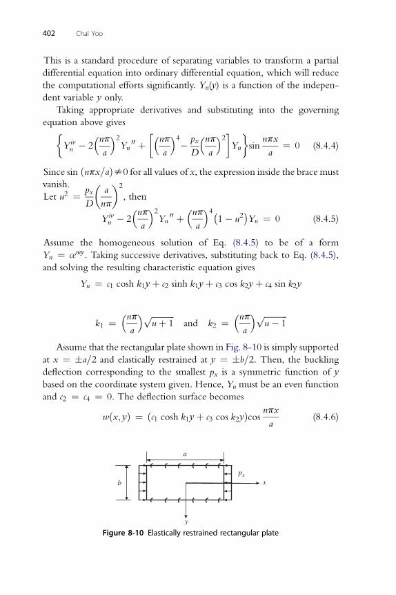
402 Chai Yoo

This is a standard procedure of separating variables to transform a partial

differential equation into ordinary differential equation, which will reduce

the computational efforts significantly. Yn(y) is a function of the indepen-

dent variable y only.

Taking appropriate derivatives and substituting into the governing

equation above givesYivn � 2

�npa

�2Yn

00 þ��np

a

�4� px

D

�npa

�2�Yn

�sin

npx

a¼ 0 (8.4.4)

Since sin ðnpx=aÞs0 for all values of x, the expression inside the brace must

vanish.

Let u2 ¼ px

D

�a

np

�2

, then

Yivn � 2

�npa

�2Yn

00 þ�npa

�4�1� u2

Yn ¼ 0 (8.4.5)

Assume the homogeneous solution of Eq. (8.4.5) to be of a form

Yn ¼ cemy. Taking successive derivatives, substituting back to Eq. (8.4.5),

and solving the resulting characteristic equation gives

Yn ¼ c1 cosh k1yþ c2 sinh k1yþ c3 cos k2yþ c4 sin k2y

k1 ¼�npa

� ffiffiffiffiffiffiffiffiffiffiffiuþ 1

pand k2 ¼

�npa

� ffiffiffiffiffiffiffiffiffiffiffiu� 1

p

Assume that the rectangular plate shown in Fig. 8-10 is simply supported

at x ¼ �a=2 and elastically restrained at y ¼ �b=2. Then, the buckling

deflection corresponding to the smallest px is a symmetric function of y

based on the coordinate system given. Hence, Yn must be an even function

and c2 ¼ c4 ¼ 0. The deflection surface becomes

wðx; yÞ ¼ ðc1 cosh k1yþ c3 cos k2yÞcos npxa

(8.4.6)

px

y

xb

a

Figure 8-10 Elastically restrained rectangular plate

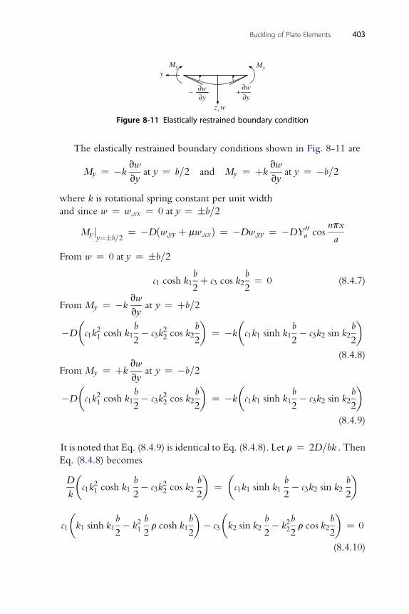
MyMyy

,z w

∂w−∂y

∂w+∂y

Figure 8-11 Elastically restrained boundary condition

Buckling of Plate Elements 403

The elastically restrained boundary conditions shown in Fig. 8-11 are

My ¼ �kvw

vyat y ¼ b=2 and My ¼ þk

vw

vyat y ¼ �b=2

where k is rotational spring constant per unit width

and since w ¼ w;xx ¼ 0 at y ¼ �b=2

Myjy¼�b=2

¼ �Dðw;yy þ mw;xxÞ ¼ �Dw;yy ¼ �DY 00n cos

npx

a

From w ¼ 0 at y ¼ �b=2

c1 cosh k1b

2þ c3 cos k2

b

2¼ 0 (8.4.7)

From My ¼ �kvw

at y ¼ þb=2

vy

�D

�c1k

21 cosh k1

b

2� c3k

22 cos k2

b

2

�¼ �k

�c1k1 sinh k1

b

2� c3k2 sin k2

b

2

�(8.4.8)

From My ¼ þkvw

vyat y ¼ �b=2

�D

�c1k

21 cosh k1

b

2� c3k

22 cos k2

b

2

�¼ �k

�c1k1 sinh k1

b

2� c3k2 sin k2

b

2

�(8.4.9)

It is noted that Eq. (8.4.9) is identical to Eq. (8.4.8). Let r ¼ 2D=bk . ThenEq. (8.4.8) becomes

D

k

�c1k

21 cosh k1

b

2� c3k

22 cos k2

b

2

�¼�c1k1 sinh k1

b

2� c3k2 sin k2

b

2

��

b b b� �

b b b�

c1 k1 sinh k12� k21 2

r cosh k12

� c3 k2 sin k22� k222

r cos k22

¼ 0

(8.4.10)

404 Chai Yoo

Setting the coefficient determinant of Eqs. (8.4.7) and (8.4.10) for the

constants c1 and c3 yields cosh k1

b

2cos k2

b

2

k1sinh k1b

2� k21

b

2r cosh k1

b

2�k2 sin k2

b

2þ k22

b

2r cos k2

b

2

¼ 0

Expanding the above determinant gives

k1tanhk1b

2þ k2tan

k2b

2� 1

2br�k21 þ k22

¼ 0 (8.4.11)

Let a ¼ a=b be the aspect ratio of the rectangular plate. Then

k1b

2¼ np

2a

ffiffiffiffiffiffiffiffiffiffiffiuþ 1

pand k2

b

2¼ np

2a

ffiffiffiffiffiffiffiffiffiffiffiu� 1

p

ffiffiffiffiffiffiffiffiffiffiffip �p ffiffiffiffiffiffiffiffiffiffiffip n� ffiffiffiffiffiffiffiffiffiffiffip �p ffiffiffiffiffiffiffiffiffiffiffip n� �n�

uþ 1tanh

2uþ 1

aþ u� 1tan

2u� 1

a� pru

a¼ 0

(8.4.12)

Equation (8.4.12) is the general buckling condition equation.

If the plate is simply supported along the boundary at y ¼ �b=2, thenk ¼ 0 and r ¼ N. Therefore, Eq. (8.4.2) becomesffiffiffiffiffiffiffiffiffiffiffi

u� 1p

tan

�p

2

ffiffiffiffiffiffiffiffiffiffiffiu� 1

p n

a

�¼ N

sinceffiffiffiffiffiffiffiffiffiffiffiuþ 1

ptanhðp2

ffiffiffiffiffiffiffiffiffiffiffiuþ 1

pnaÞ is a finite value.

Hence ffiffiffiffiffiffiffiffiffiffiffiu� 1

p n

a¼ 1

from which

u2 ¼��

a

n

�2 þ 1

�2

¼ px

D

�a

np

�2

Then

pxcr ¼ D

��a

n

�2 þ 1

�2�np

a

�2 ¼ Dp2

b2

�a

nþ n

a

�2

p�h�2 Ep2

�a n

�2

scr ¼ xcr

h¼

b 12ð1� m2Þ nþa

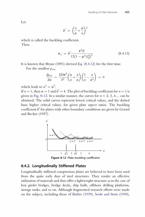
Buckling of Plate Elements 405

Let

k0 ¼�n

aþ a

n

�2

which is called the buckling coefficient.

Then

scr ¼ k0p2E

12ð1� m2ÞðbhÞ2(8.4.13)

It is known that Bryan (1891) derived Eq. (8.4.12) for the first time.

For the smallest pxcr,

dpxcr

da¼ 2Dp2

b2

�a

nþ n

a

��1

n� n

a2

�¼ 0

which leads to n2 ¼ a2.

If n¼ 1, then a¼ 1 and k0 ¼ 4. The plot of buckling coefficient for n¼ 1 is

given in Fig. 8-12. In a similar manner, the curves for n ¼ 2, 3, 4. can be

obtained. The solid curves represent lowest critical values, and the dotted

lines higher critical values, for given plate aspect ratios. The buckling

coefficient k0 for plates with other boundary conditions are given by Gerard

and Becker (1957).

n = 2

n = 1

n = 3 n = 44

1 3 4 2 2 6α

k′

Figure 8-12 Plate buckling coefficient

8.4.2. Longitudinally Stiffened PlatesLongitudinally stiffened compression plates are believed to have been used

from the quite early days of steel structures. They render an effective

utilization of materials and thus offer a lightweight structure as in the case of

box girder bridges, bridge decks, ship hulls, offshore drilling platforms,

storage tanks, and so on. Although fragmented research efforts were made

on the subject, including those of Barbre (1939), Seide and Stein (1949),

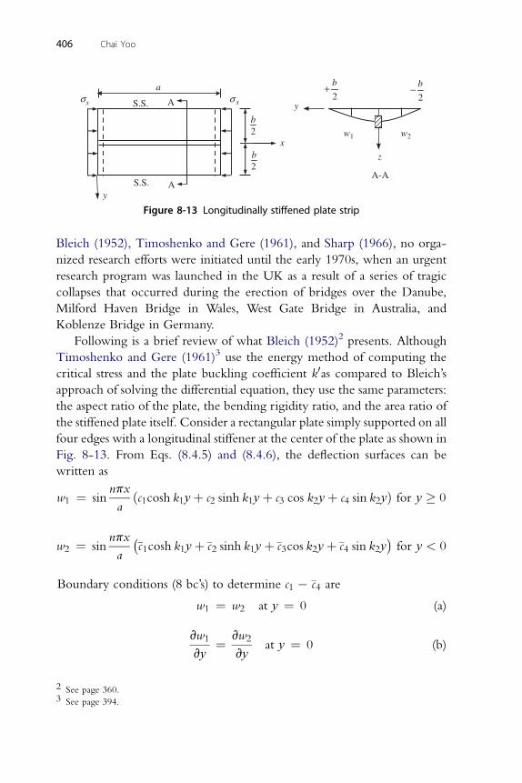
A

A

y

z

w1 w2

2

b+2

b−a

2b

2b

x x σσ

y

x

S.S.

S.S.A-A

Figure 8-13 Longitudinally stiffened plate strip

406 Chai Yoo

Bleich (1952), Timoshenko and Gere (1961), and Sharp (1966), no orga-

nized research efforts were initiated until the early 1970s, when an urgent

research program was launched in the UK as a result of a series of tragic

collapses that occurred during the erection of bridges over the Danube,

Milford Haven Bridge in Wales, West Gate Bridge in Australia, and

Koblenze Bridge in Germany.

Following is a brief review of what Bleich (1952)2 presents. Although

Timoshenko and Gere (1961)3 use the energy method of computing the

critical stress and the plate buckling coefficient k0as compared to Bleich’s

approach of solving the differential equation, they use the same parameters:

the aspect ratio of the plate, the bending rigidity ratio, and the area ratio of

the stiffened plate itself. Consider a rectangular plate simply supported on all

four edges with a longitudinal stiffener at the center of the plate as shown in

Fig. 8-13. From Eqs. (8.4.5) and (8.4.6), the deflection surfaces can be

written as

w1 ¼ sinnpx

aðc1cosh k1yþ c2 sinh k1yþ c3 cos k2yþ c4 sin k2yÞ for y � 0

npx �

w2 ¼ sin

a�c1cosh k1yþ�c2 sinh k1yþ�c3cos k2yþ�c4 sin k2y for y < 0

Boundary conditions (8 bc’s) to determine c1 � �c4 are

w1 ¼ w2 at y ¼ 0 (a)

vw1 vw2

vy¼

vyat y ¼ 0 (b)

2 See page 360.3 See page 394.

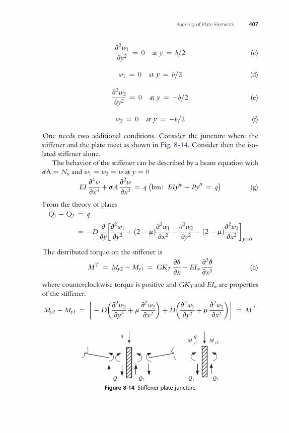
v2w1

vy2¼ 0 at y ¼ b=2 (c)

w1 ¼ 0 at y ¼ b=2 (d)

Buckling of Plate Elements 407

2

v w2

vy2¼ 0 at y ¼ �b=2 (e)

w ¼ 0 at y ¼ �b=2 (f)

2

One needs two additional conditions. Consider the juncture where the

stiffener and the plate meet as shown in Fig. 8-14. Consider then the iso-

lated stiffener alone.

The behavior of the stiffener can be described by a beam equation with

sA ¼ Nx and w1 ¼ w2 ¼ w at y ¼ 0

EIv4w

vx4þ sA

v2w

vx2¼ q

�bm: EIyiv þ Py00 ¼ q

(g)

From the theory of plates

Q1 �Q2 ¼ q

¼ �Dv

vy

�v2w1

vy2þ ð2� mÞv

2w1

vx2� v2w2

vy2� ð2� mÞv

2w2

vx2

�y¼0

The distributed torque on the stiffener is

MT ¼ My2 �My1 ¼ GKTvq

vx� EIw

v3q

vx3(h)

where counterclockwise torque is positive and GKT and EIw are properties

of the stiffener.

My2 �My1 ¼��D

�v2w2

vy2þ m

v2w2

vx2

�þD

�v2w1

vy2þ m

v2w1

vx2

��¼ MT

2yM1yMq

Q1 Q2 Q2

q

Q1

Figure 8-14 Stiffener-plate juncture

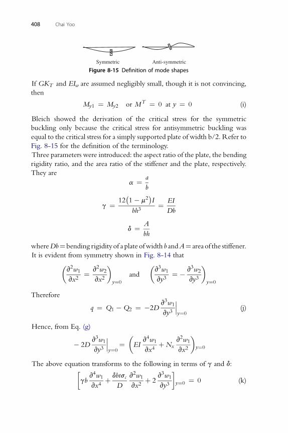
Symmetric Anti-symmetric

Figure 8-15 Definition of mode shapes

408 Chai Yoo

If GKT and EIw are assumed negligibly small, though it is not convincing,

then

My1 ¼ My2 or MT ¼ 0 at y ¼ 0 (i)

Bleich showed the derivation of the critical stress for the symmetric

buckling only because the critical stress for antisymmetric buckling was

equal to the critical stress for a simply supported plate of width b/2. Refer to

Fig. 8-15 for the definition of the terminology.

Three parameters were introduced: the aspect ratio of the plate, the bending

rigidity ratio, and the area ratio of the stiffener and the plate, respectively.

They are

a ¼ a

b

12�1� m2

I EI

g ¼bh3

¼Db

A

d ¼

bh

whereDb¼ bending rigidityof a plate ofwidth b andA¼ area of the stiffener.

It is evident from symmetry shown in Fig. 8-14 that�v2w1

vx2¼ v2w2

vx2

�y¼0

and

�v3w1

vy3¼ � v3w2

vy3

�y¼0

Therefore

q ¼ Q1 �Q2 ¼ �2Dv3w1

vy3

y¼0

(j)

Hence, from Eq. (g)

� 2Dv3w1

vy3

y¼0

¼ EIv4w1

vx4þNx

v2w1

vx2

�y¼0

�

The above equation transforms to the following in terms of g and d:

gbv4w1

vx4þ dbtsc

D

v2w1

vx2þ 2

v3w1

vy3

�y¼0 ¼ 0

�(k)

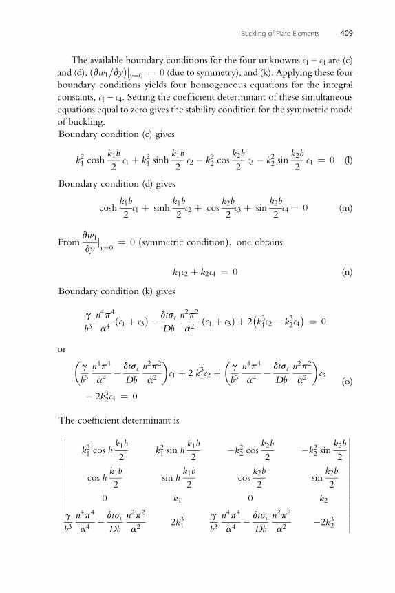
Buckling of Plate Elements 409

The available boundary conditions for the four unknowns c1 – c4 are (c)

and (d), ðvw1=vyÞjy¼0 ¼ 0 (due to symmetry), and (k). Applying these four

boundary conditions yields four homogeneous equations for the integral

constants, c1 – c4. Setting the coefficient determinant of these simultaneous

equations equal to zero gives the stability condition for the symmetric mode

of buckling.

Boundary condition (c) gives

k21 coshk1b

2c1 þ k21 sinh

k1b

2c2 � k22 cos

k2b

2c3 � k22 sin

k2b

2c4 ¼ 0 (l)

Boundary condition (d) gives

coshk1b

2c1 þ sinh

k1b

2c2 þ cos

k2b

2c3 þ sin

k2b

2c4¼ 0 (m)

vw

From

1

vyjy¼0

¼ 0 ðsymmetric conditionÞ; one obtains

k c þ k c ¼ 0 (n)

1 2 2 4

Boundary condition (k) gives

g

b3n4p4

a4ðc1 þ c3Þ � dtsc

Db

n2p2

a2ðc1 þ c3Þ þ 2

�k31c2 � k32c4

¼ 0

or �g

b3n4p4

a4� dtsc

Db

n2p2

a2

�c1 þ 2 k31c2 þ

�g

b3n4p4

a4� dtsc

Db

n2p2

a2

�c3

� 2k32c4 ¼ 0

(o)

The coefficient determinant is

k21 cos hk1b

2k21 sin h

k1b

2�k22 cos

k2b

2�k22 sin

k2b

2

cos hk1b

2sin h

k1b

2cos

k2b

2sin

k2b

2

0 k1 0 k2

g

b3n4p4

a4� dtsc

Db

n2p2

a22k31

g

b3n4p4

a4� dtsc

Db

n2p2

a2�2k32

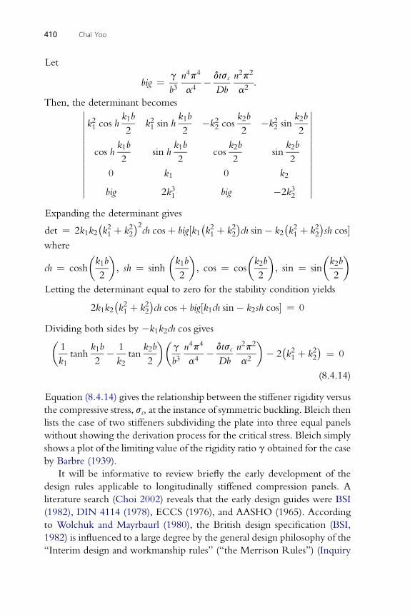
410 Chai Yoo

Let

big ¼ g

b3n4p4

a4� dtsc

Db

n2p2

a2:

Then, the determinant becomes

k21 cos hk1b

2k21 sin h

k1b

2�k22 cos

k2b

2�k22 sin

k2b

2

cos hk1b

2sin h

k1b

2cos

k2b

2sin

k2b

2

0 k1 0 k2

big 2k31 big �2k32

Expanding the determinant gives

det ¼ 2k1k2�k21 þ k22

2ch cosþ big½k1

�k21 þ k22

ch sin� k2

�k21 þ k22

sh cos�

where �k b� �

k b� �

k b� �

k b�

ch ¼ cosh1

2; sh ¼ sinh

1

2; cos ¼ cos

2

2; sin ¼ sin

2

2

Letting the determinant equal to zero for the stability condition yields�

2k1k2 k21 þ k22 ch cosþ big½k1ch sin� k2sh cos� ¼ 0

Dividing both sides by �k1k2ch cos gives�1

k1tanh

k1b

2� 1

k2tan

k2b

2

��g

b3n4p4

a4� dtsc

Db

n2p2

a2

�� 2�k21 þ k22

¼ 0

(8.4.14)

Equation (8.4.14) gives the relationship between the stiffener rigidity versus

the compressive stress, sc, at the instance of symmetric buckling. Bleich then

lists the case of two stiffeners subdividing the plate into three equal panels

without showing the derivation process for the critical stress. Bleich simply

shows a plot of the limiting value of the rigidity ratio g obtained for the case

by Barbre (1939).

It will be informative to review briefly the early development of the

design rules applicable to longitudinally stiffened compression panels. A

literature search (Choi 2002) reveals that the early design guides were BSI

(1982), DIN 4114 (1978), ECCS (1976), and AASHO (1965). According

to Wolchuk and Mayrbaurl (1980), the British design specification (BSI,

1982) is influenced to a large degree by the general design philosophy of the

“Interim design and workmanship rules” (“the Merrison Rules”) (Inquiry

Buckling of Plate Elements 411

1974). The Merrison Rules method is essentially the culmination of the

urgent research program in response to the series of collapses. The method

considers the individual stiffener strut separately, which consists of a stiffener

with a corresponding width of the flange plate. The strength of the entire

stiffened plate is then obtained by multiplying the ultimate stress of the strut

by the total area of the plate. This is referred to as the “column behavior”

theory, which prevails in European countries.

Highly theoretical and extremely complex analytical research on

compression panels stiffened by one or two stiffeners has been carried out by

Barbre (1939), Bleich (1952), and Timoshenko and Gere (1961). It appears

that their research results on the antisymmetric buckling mode, which

might be classified as the “plate behavior” theory, are not currently in use in

any national design specifications. Mattock et al. (1967) prepared the

“Commentary on criteria for design of steel-concrete composite box girder

highway bridges” in August 1967. These criteria were intended to

supplement the provisions of Division I of the Standard Specifications for

Highway Bridges of the AASHO (1965). An overly conservative approach

appears to have been adopted during the course of simplifying and

extrapolating the limited research results (some of which appear question-

able) to incorporate the case where the number of longitudinal stiffeners

was greater than two. Although the equations in the AASHO (1965) give

a reasonable value for the minimum required moment of inertia of the

stiffener when the number of stiffeners is less than or equal to two, the

equations require unreasonably large value for the moment of inertia when

the number of stiffeners becomes large. It was found that an old bridge

(curved box girder approach spans to the Fort Duquesne Bridge in

Pittsburg) designed and built before the enactment of the criteria did not

rate well, despite having served safely for many years. After this incident, the

latest AASHTO (2007) specifications limit the maximum number of stiff-

eners to two as a stopgap measure.

In a series of numerical researches at Auburn University, Yoo and his

colleagues (Yoo 2001; Yoo et al. 2001), extracted a regression formula for

the minimum required moment of inertia for the longitudinal stiffener to

assure an antisymmetric buckling mode. The coefficient of correlation R

was found to be greater than 0.95.

Is ¼ 0:3ha2ffiffiffin

pwh3 (8.4.15)

where a ¼ aspect ratio of subpanel; n ¼ number of stiffeners; h ¼ thickness

of plate; w ¼ width of stiffened subpanel; h ¼ ratio of the postbuckling

412 Chai Yoo

stress to the elastic buckling stress. The elastic buckling stress is to be

computed by Eq. (8.4.13) with a value of the buckling coefficient k0 equalto four. The ratio of the postbuckling stress to the elastic buckling stress h

should be set equal to one when the postbuckling strength is not recog-

nized for reasons other than the strength or the analysis is carried out in the

inelastic zone. Choi and Yoo (2005) showed that Eq. (8.4.15) works well

for horizontally curved box girder compression flanges too, and its validity

has been verified by an experimental study (Choi et al. 2009).

It is reassuring to note that Eq. (8.4.15) includes the length of the

member (indirectly by the aspect ratio a). The longitudinal stiffener is, after

all, a compression member whether it is examined in the “column

behavior” theory or in the “plate behavior” theory. As such, the length of

the compression member must be a prominent variable in determining the

strength. In order to control the length of the longitudinal stiffener (the

aspect ratio a, shall not exceed, say 7), transverse stiffeners are to be used.

Choi, Kang, and Yoo (2007) furnish a design guide for transverse stiffeners.

Mittelstedt (2008) demonstrates the superiority of the “column behavior”

theory by an explicit elastic analysis of longitudinally stiffened plates for

buckling loads and the minimum stiffener requirements.

Compression members in general can be classified into three groups:

compact, noncompact, and slender. Yielding, inelastic buckling, and elastic

buckling, respectively, control the ultimate strength of the members in each

group. Geometric imperfections appear to affect the inelastic buckling

strength of the members belonging to the noncompact group. Residual

stresses are particularly onerous to the postbuckling strength of the slender

members and affect the inelastic buckling strength to a much smaller degree.

The ultimate strengths of the stocky members in the compact group are not

affected by the presence of either initial imperfections or residual stresses.

The current AASHTO (2007) provisions for the limiting value of the

width-to-thickness ratio classifying the subpanels into these three groups

appear reasonable. However, it seems reasonable to classify the zones into

just twodthe elastic buckling zone and the inelastic buckling zonedas is

being done in AISC (2005).

Based on the observations made during the series of investigations by

Yoo and his coworkers, a new simple formula is proposed for the ultimate

stress in the inelastic buckling zone.

scr ¼ sy � sr

C2c

�wh

�2¼ sy

�1� sr

syC2c

�wh

�2�(8.4.16)

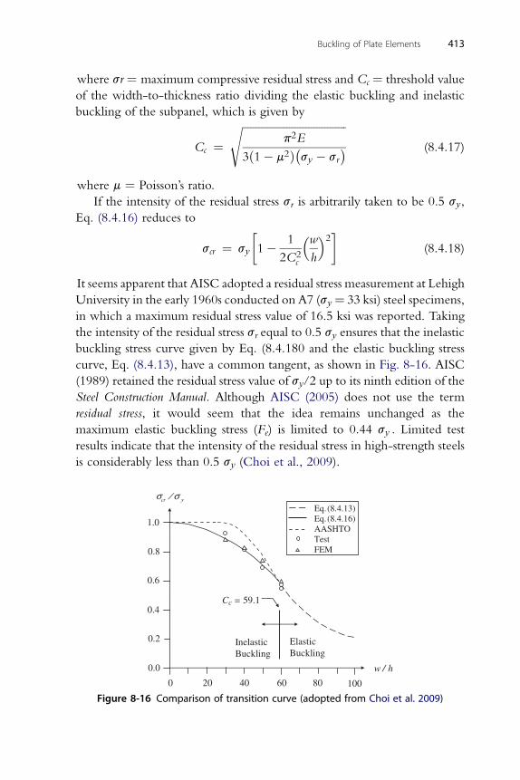
Buckling of Plate Elements 413

where sr ¼ maximum compressive residual stress and Cc ¼ threshold value

of the width-to-thickness ratio dividing the elastic buckling and inelastic

buckling of the subpanel, which is given by

Cc ¼ffiffiffiffiffiffiffiffiffiffiffiffiffiffiffiffiffiffiffiffiffiffiffiffiffiffiffiffiffiffiffiffiffiffiffiffiffiffi

p2E

3ð1� m2Þ�sy � sr

s(8.4.17)

where m ¼ Poisson’s ratio.

If the intensity of the residual stress sr is arbitrarily taken to be 0.5 sy,

Eq. (8.4.16) reduces to

scr ¼ sy

�1� 1

2C2c

�wh

�2�(8.4.18)

It seems apparent that AISC adopted a residual stress measurement at Lehigh

University in the early 1960s conducted on A7 (sy¼ 33 ksi) steel specimens,

in which a maximum residual stress value of 16.5 ksi was reported. Taking

the intensity of the residual stress sr equal to 0.5 sy ensures that the inelastic

buckling stress curve given by Eq. (8.4.180 and the elastic buckling stress

curve, Eq. (8.4.13), have a common tangent, as shown in Fig. 8-16. AISC

(1989) retained the residual stress value of sy/2 up to its ninth edition of the

Steel Construction Manual. Although AISC (2005) does not use the term

residual stress, it would seem that the idea remains unchanged as the

maximum elastic buckling stress (Fe) is limited to 0.44 sy . Limited test

results indicate that the intensity of the residual stress in high-strength steels

is considerably less than 0.5 sy (Choi et al., 2009).

σcr / σ y

w / h

0 20 40 60 80 100

Eq. (8.4.13) Eq. (8.4.16) AASHTO Test FEM

Inelastic Buckling

ElasticBuckling

1.0

0.8

0.6

0.4

0.0

0.2

Cc = 59.1

Figure 8-16 Comparison of transition curve (adopted from Choi et al. 2009)

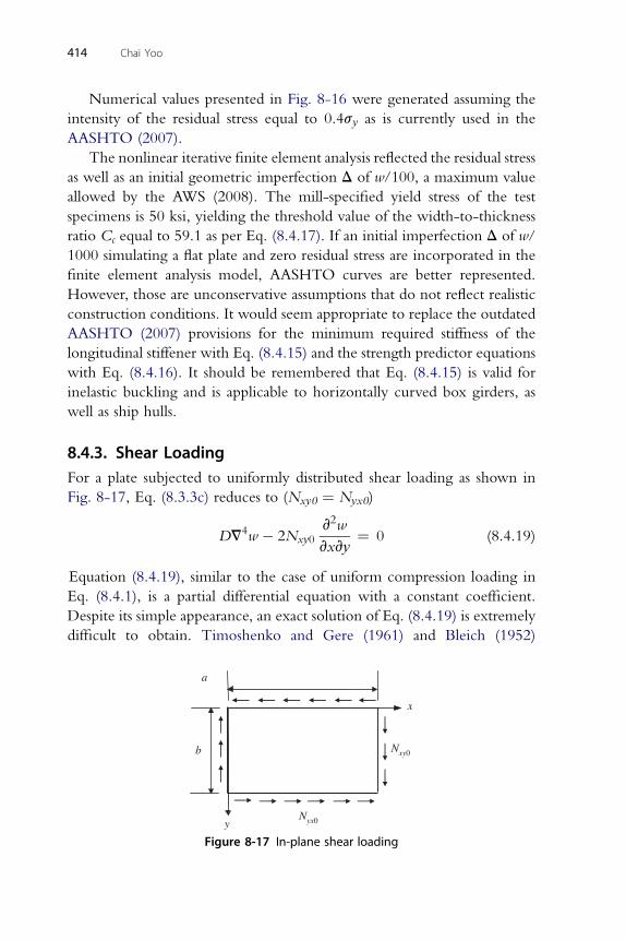
414 Chai Yoo

Numerical values presented in Fig. 8-16 were generated assuming the

intensity of the residual stress equal to 0.4sy as is currently used in the

AASHTO (2007).

The nonlinear iterative finite element analysis reflected the residual stress

as well as an initial geometric imperfection D of w/100, a maximum value

allowed by the AWS (2008). The mill-specified yield stress of the test

specimens is 50 ksi, yielding the threshold value of the width-to-thickness

ratio Cc equal to 59.1 as per Eq. (8.4.17). If an initial imperfection D of w/

1000 simulating a flat plate and zero residual stress are incorporated in the

finite element analysis model, AASHTO curves are better represented.

However, those are unconservative assumptions that do not reflect realistic

construction conditions. It would seem appropriate to replace the outdated

AASHTO (2007) provisions for the minimum required stiffness of the

longitudinal stiffener with Eq. (8.4.15) and the strength predictor equations

with Eq. (8.4.16). It should be remembered that Eq. (8.4.15) is valid for

inelastic buckling and is applicable to horizontally curved box girders, as

well as ship hulls.

8.4.3. Shear LoadingFor a plate subjected to uniformly distributed shear loading as shown in

Fig. 8-17, Eq. (8.3.3c) reduces to (Nxy0 ¼ Nyx0)

DV4w � 2Nxy0v2w

vxvy¼ 0 (8.4.19)

Equation (8.4.19), similar to the case of uniform compression loading in

Eq. (8.4.1), is a partial differential equation with a constant coefficient.

Despite its simple appearance, an exact solution of Eq. (8.4.19) is extremely

difficult to obtain. Timoshenko and Gere (1961) and Bleich (1952)

x

y

b Nxy0

Nyx0

a

Figure 8-17 In-plane shear loading

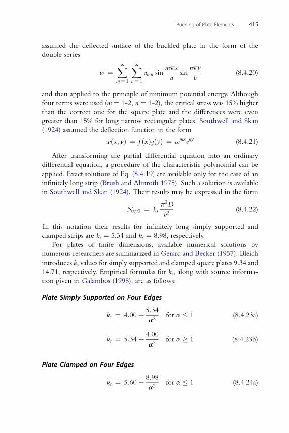
Buckling of Plate Elements 415

assumed the deflected surface of the buckled plate in the form of the

double series

w ¼XNm¼ 1

XNn¼ 1

amn sinmpx

asin

npy

b(8.4.20)

and then applied to the principle of minimum potential energy. Although

four terms were used (m ¼ 1-2, n ¼ 1-2), the critical stress was 15% higher

than the correct one for the square plate and the differences were even

greater than 15% for long narrow rectangular plates. Southwell and Skan

(1924) assumed the deflection function in the form

wðx; yÞ ¼ f ðxÞgðyÞ ¼ cemxeny (8.4.21)

After transforming the partial differential equation into an ordinary

differential equation, a procedure of the characteristic polynomial can be

applied. Exact solutions of Eq. (8.4.19) are available only for the case of an

infinitely long strip (Brush and Almroth 1975). Such a solution is available

in Southwell and Skan (1924). Their results may be expressed in the form

Nxy0 ¼ ksp2D

b2(8.4.22)

In this notation their results for infinitely long simply supported and

clamped strips are ks ¼ 5.34 and ks ¼ 8.98, respectively.

For plates of finite dimensions, available numerical solutions by

numerous researchers are summarized in Gerard and Becker (1957). Bleich

introduces ks values for simply supported and clamped square plates 9.34 and

14.71, respectively. Empirical formulas for ks, along with source informa-

tion given in Galambos (1998), are as follows:

Plate Simply Supported on Four Edges

ks ¼ 4:00þ 5:34

a2for a � 1 (8.4.23a)

4:00

ks ¼ 5:34þ

a2for a � 1 (8.4.23b)

Plate Clamped on Four Edges

ks ¼ 5:60þ 8:98

a2for a � 1 (8.4.24a)

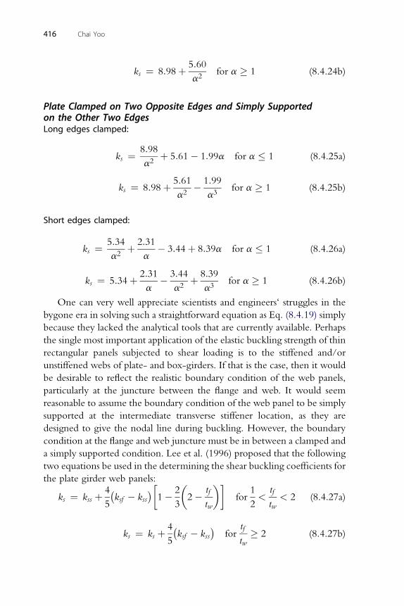
5:60

ks ¼ 8:98þ

a2for a � 1 (8.4.24b)

Plate Clamped on Two Opposite Edges and Simply Supportedon the Other Two EdgesLong edges clamped:

ks ¼ 8:98

a2þ 5:61� 1:99a for a � 1 (8.4.25a)

5:61 1:99

416 Chai Yoo

ks ¼ 8:98þa2

�a3

for a � 1 (8.4.25b)

Short edges clamped:

ks ¼ 5:34

a2þ 2:31

a� 3:44þ 8:39a for a � 1 (8.4.26a)

2:31 3:44 8:39

ks ¼ 5:34þ

a�

a2þ

a3for a � 1 (8.4.26b)

One can very well appreciate scientists and engineers‘ struggles in the

bygone era in solving such a straightforward equation as Eq. (8.4.19) simply

because they lacked the analytical tools that are currently available. Perhaps

the single most important application of the elastic buckling strength of thin

rectangular panels subjected to shear loading is to the stiffened and/or

unstiffened webs of plate- and box-girders. If that is the case, then it would

be desirable to reflect the realistic boundary condition of the web panels,

particularly at the juncture between the flange and web. It would seem

reasonable to assume the boundary condition of the web panel to be simply

supported at the intermediate transverse stiffener location, as they are

designed to give the nodal line during buckling. However, the boundary

condition at the flange and web juncture must be in between a clamped and

a simply supported condition. Lee et al. (1996) proposed that the following

two equations be used in the determining the shear buckling coefficients for

the plate girder web panels:

ks ¼ kss þ 4

5

�ksf � kss

�1� 2

3

�2� tf

tw

��for

1

2<

tf

tw< 2 (8.4.27a)

4� tf

ks ¼ ks þ

5ksf � kss for

tw� 2 (8.4.27b)

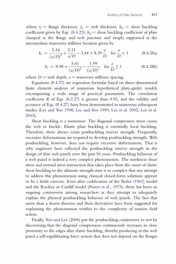
Buckling of Plate Elements 417

where tf ¼ flange thickness; tw ¼ web thickness; kss ¼ shear buckling

coefficient given by Eqs. (8.4.23); ksf ¼ shear buckling coefficient of plate

clamped at the flange and web juncture and simply supported at the

intermediate transverse stiffener location given by

ks ¼ 5:34

ða=DÞ2 þ2:31

a=D� 3:44þ 8:39

a

Dfor

a

D< 1 (8.4.28a)

k ¼ 8:98þ 5:61 � 1:99for

a � 1 (8.4.28b)

s ða=DÞ2 ða=DÞ3 D

where D ¼ web depth; a ¼ transverse stiffener spacing.

Equations (8.4.27) are regression formulas based on three-dimensional

finite element analyses of numerous hypothetical plate-girder models

encompassing a wide range of practical parameters. The correlation

coefficient R of Eqs. (8.2.27) is greater than 0.95, and the validity and

accuracy of Eqs. (8.4.27) have been demonstrated in numerous subsequent

studies (Lee and Yoo 1998; Lee and Yoo 1999; Lee et al. 2002; Lee et al.

2003).

Shear buckling is a misnomer. The diagonal compressive stress causes

the web to buckle. Elastic plate buckling is essentially local buckling.

Therefore, there always exists postbuckling reserve strength. Frequently,

excessive deformations are required to develop postbuckling strength. Web

postbuckling, however, does not require excessive deformations. That is

why engineers have reflected the postbuckling reserve strength in the

design of thin web panels over the past 50 years. Postbuckling behavior of

a web panel is indeed a very complex phenomenon. The nonlinear shear

stress and normal stress interaction that takes place from the onset of elastic

shear buckling to the ultimate strength state is so complex that any attempt

to address this phenomenon using classical closed-form solutions appears

to be a futile exercise. Even after codification of the Basler (1961) model

and the Rockey or Cardiff model (Porter et al., 1975), there has been an

ongoing controversy among researchers as they attempt to adequately

explain the physical postbuckling behavior of web panels. The fact that

more than a dozen theories and their derivatives have been suggested for

explaining the phenomenon testifies to the complexity of tension field

action.

Finally, Yoo and Lee (2006) put the postbuckling controversy to rest by

discovering that the diagonal compression continuously increases in close

proximity to the edges after elastic buckling, thereby producing in the web

panel a self-equilibrating force system that does not depend on the flanges

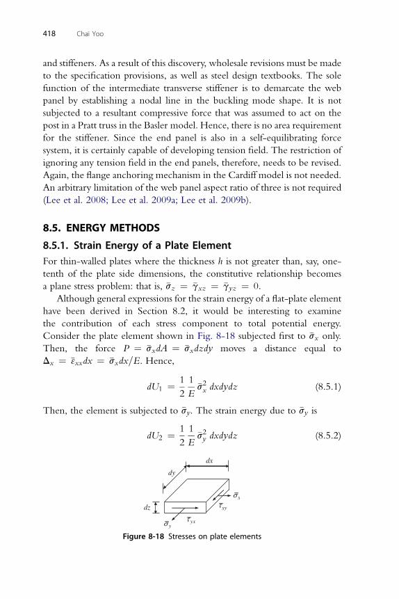
418 Chai Yoo

and stiffeners. As a result of this discovery, wholesale revisions must be made

to the specification provisions, as well as steel design textbooks. The sole

function of the intermediate transverse stiffener is to demarcate the web

panel by establishing a nodal line in the buckling mode shape. It is not

subjected to a resultant compressive force that was assumed to act on the

post in a Pratt truss in the Basler model. Hence, there is no area requirement

for the stiffener. Since the end panel is also in a self-equilibrating force

system, it is certainly capable of developing tension field. The restriction of

ignoring any tension field in the end panels, therefore, needs to be revised.

Again, the flange anchoring mechanism in the Cardiff model is not needed.

An arbitrary limitation of the web panel aspect ratio of three is not required

(Lee et al. 2008; Lee et al. 2009a; Lee et al. 2009b).

8.5. ENERGY METHODS

8.5.1. Strain Energy of a Plate ElementFor thin-walled plates where the thickness h is not greater than, say, one-

tenth of the plate side dimensions, the constitutive relationship becomes

a plane stress problem: that is, �sz ¼ �gxz ¼ �gyz ¼ 0.

Although general expressions for the strain energy of a flat-plate element

have been derived in Section 8.2, it would be interesting to examine

the contribution of each stress component to total potential energy.

Consider the plate element shown in Fig. 8-18 subjected first to �sx only.

Then, the force P ¼ �sxdA ¼ �sxdzdy moves a distance equal to

Dx ¼ �3xxdx ¼ �sxdx=E. Hence,

dU1 ¼ 1

2

1

E�s2x dxdydz (8.5.1)

Then, the element is subjected to �sy. The strain energy due to �sy is

dU2 ¼ 1

2

1

E�s2y dxdydz (8.5.2)

dx

dy

dz

xσ

yσ yxτ

xyτ

Figure 8-18 Stresses on plate elements

Buckling of Plate Elements 419

However, this time the force in the x direction rides a distance ¼

�m ð�sy=EÞ dx. Hence,

dU3 ¼ �m1

E�sy�sx dxdydz (8.5.3)

Assuming that normal stresses produce no shear stresses and vice versa, it is

possible to obtain strain energy of a plate element due to shear independently

of the normal forces. Due to a shear stress, there exists a force, �sxydxdz and

a corresponding deformation �gxydy as shown in Fig. 8-19. Hence,

dU4 ¼ 1

2�sxydxdz

��gxydy

�¼ 1þ m

E�s2xy dxdydz (8.5.4)

The total strain energy is then

dU ¼ 1

2E½�s2x þ �s2y � 2m�sx�sy þ 2ð1þ mÞ�s2xy�dxdydz (8.5.5)

For the entire plate of length a, width b, and thickness h, the strain energy

becomes

U ¼Z h=2

�h=2

Z b

0

Z a

0

1

2E�s2x þ �s2y � 2m�sx�sy þ 2ð1þ mÞ�s2xy

idxdydz

h(8.5.6)

As a consequence of neglecting �sz; �gxz; �gyz, Eq. (8.5.6) is limited to thin

plates only. It is also limited to linearly elastic materials and/or linearized

problems but it is not limited to problems of either small displacements or

membrane forces only. Substituting Eqs. (8.2.4) into Eq. (8.5.6) and

carrying out the integration with respect to z, one obtains:

Um ¼ C

2

ZZ �32x þ 32y þ 2m3x3y þ 1� m

2g2xy

�dxdy (8.5.7)

y

dyγ

x

γ xyxy

xy

τ

Figure 8-19 Shear strain

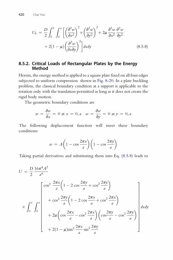
Z b Z a �� 2 �2 � 2 �2 2 2

Ub ¼ D

2 0 0

v w

vx2þ v w

vy2þ 2m

v w

vx2v w

vy2

þ 2ð1� mÞ�v2w

vxvy

�2�dxdy (8.5.8)

8.5.2. Critical Loads of Rectangular Plates by the EnergyMethod

Herein, the energy method is applied to a square plate fixed on all four edges

subjected to uniform compression shown in Fig. 8-20. In a plate buckling

problem, the classical boundary condition at a support is applicable to the

rotation only with the translation permitted as long as it does not create the

rigid body motion.

The geometric boundary conditions are

w ¼ vw

vx¼ 0 at x ¼ 0; a w ¼ vw

vy¼ 0 at y ¼ 0; a

The following displacement function will meet these boundary

conditions:

w ¼ A

�1� cos

2px

a

��1� cos

2py

a

�

Taking partial derivatives and substituting them into Eq. (8.5.8) leads to

U ¼ D

2

16p4A2

a4

�Z a

0

Z a

0

266666666666664

cos22px

a

�1� 2 cos

2py

aþ cos2

2py

a

�

þ cos22py

a

�1� 2 cos

2px

aþ cos2

2px

a

�

þ 2m

�cos

2px

a� cos2

2px

a

��cos

2py

a� cos2

2py

a

�

þ 2ð1� mÞsin2 2pxa

sin22py

a

377777777777775dxdy

420 Chai Yoo

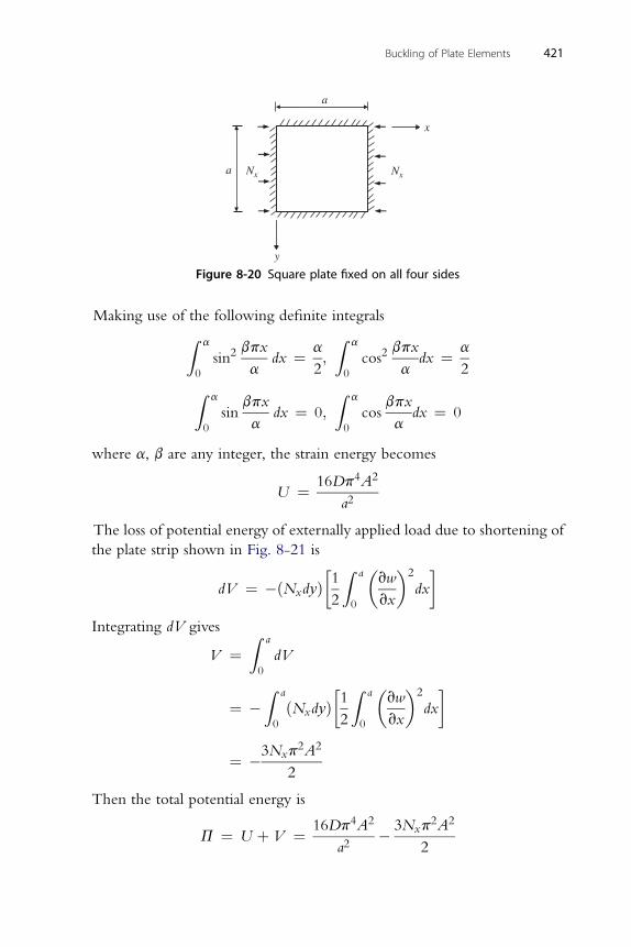
a

a

x

y

Nx Nx

Figure 8-20 Square plate fixed on all four sides

Buckling of Plate Elements 421

Making use of the following definite integrals

Z a

0

sin2bpx

adx ¼ a

2;

Z a

0

cos2bpx

adx ¼ a

2Z a

0

sinbpx

adx ¼ 0;

Z a

0

cosbpx

adx ¼ 0

where a, b are any integer, the strain energy becomes

U ¼ 16Dp4A2

a2

The loss of potential energy of externally applied load due to shortening of

the plate strip shown in Fig. 8-21 is

dV ¼ �ðNxdyÞ�1

2

Z a

0

�vw

vx

�2

dx

�

Integrating dV gives

V ¼Z a

0

dV

¼ �Z a

0

ðNxdyÞ�1

2

Z a

0

�vw

vx

�2

dx

�

¼ �3Nxp2A2

2

Then the total potential energy is

P ¼ U þ V ¼ 16Dp4A2

a2� 3Nxp

2A2

2

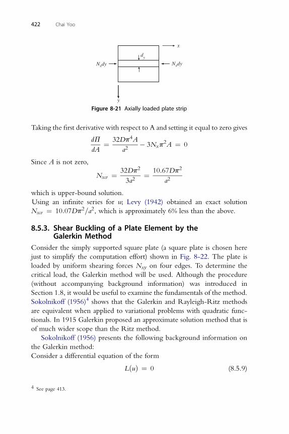
x

y

dy

NxdyNxdy

Figure 8-21 Axially loaded plate strip

422 Chai Yoo

Taking the first derivative with respect to A and setting it equal to zero gives

dP

dA¼ 32Dp4A

a2� 3Nxp

2A ¼ 0

Since A is not zero,

Nxcr ¼ 32Dp2

3a2¼ 10:67Dp2

a2

which is upper-bound solution.

Using an infinite series for w, Levy (1942) obtained an exact solution

Nxcr ¼ 10:07Dp2=a2, which is approximately 6% less than the above.

8.5.3. Shear Buckling of a Plate Element by theGalerkin Method

Consider the simply supported square plate (a square plate is chosen here

just to simplify the computation effort) shown in Fig. 8-22. The plate is

loaded by uniform shearing forces Nxy on four edges. To determine the

critical load, the Galerkin method will be used. Although the procedure

(without accompanying background information) was introduced in

Section 1.8, it would be useful to examine the fundamentals of the method.

Sokolnikoff (1956)4 shows that the Galerkin and Rayleigh-Ritz methods

are equivalent when applied to variational problems with quadratic func-

tionals. In 1915 Galerkin proposed an approximate solution method that is

of much wider scope than the Ritz method.

Sokolnikoff (1956) presents the following background information on

the Galerkin method:

Consider a differential equation of the form

LðuÞ ¼ 0 (8.5.9)

4 See page 413.

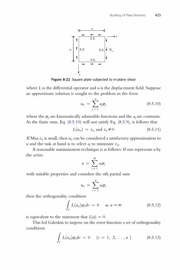
x

y

Nxy a

S.S.

S.S.

S.S.

S.S.

a

Figure 8-22 Square plate subjected to in-plane shear

Buckling of Plate Elements 423

where L is the differential operator and u is the displacement field. Suppose

an approximate solution is sought to the problem in the form

un ¼Xnj¼ 1

aj4j (8.5.10)

where the 4j are kinematically admissible functions and the aj are constants.

As the finite sum, Eq. (8.5.10) will not satisfy Eq. (8.5.9), it follows that

LðunÞ ¼ 3n and 3ns0 (8.5.11)

If Max 3n is small, then un can be considered a satisfactory approximation to

u and the task at hand is to select aj to minimize 3n.

A reasonable minimization technique is as follows: If one represents u by

the series

u ¼XNi¼ 1

ai4i

with suitable properties and considers the nth partial sum

un ¼Xni¼ 1

ai4i

then the orthogonality conditionZ

v

LðunÞ4idv ¼ 0 as n/N (8.5.12)

is equivalent to the statement that L(u) ¼ 0.

This led Galerkin to impose on the error function a set of orthogonality

conditions Zv

LðunÞ4idv ¼ 0 ði ¼ 1; 2; : : ; n Þ (8.5.13)

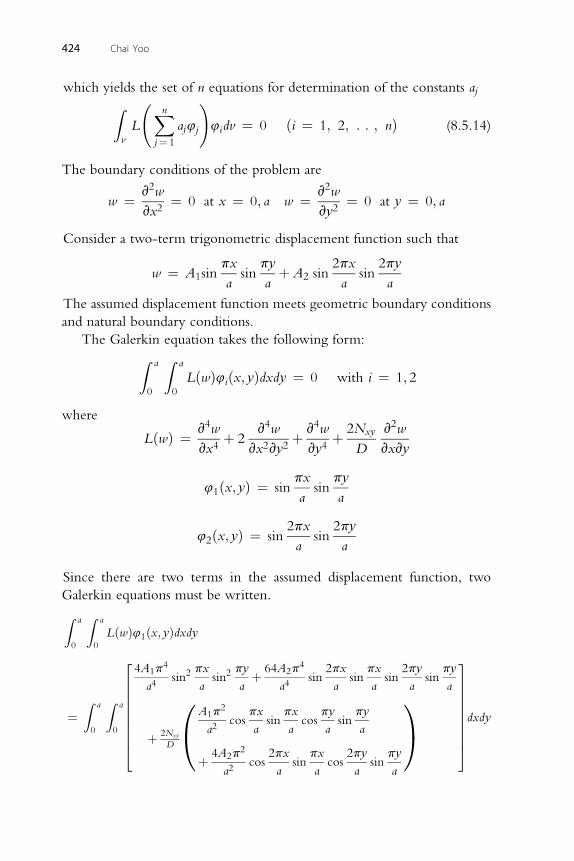
424 Chai Yoo

which yields the set of n equations for determination of the constants aj

Zv

L

Xnj¼ 1

aj4j

!4idv ¼ 0 ði ¼ 1; 2; : : ; nÞ (8.5.14)

The boundary conditions of the problem are

w ¼ v2w

vx2¼ 0 at x ¼ 0; a w ¼ v2w

vy2¼ 0 at y ¼ 0; a

Consider a two-term trigonometric displacement function such that

w ¼ A1sinpx

asin

py

aþ A2 sin

2px

asin

2py

a

The assumed displacement function meets geometric boundary conditions

and natural boundary conditions.

The Galerkin equation takes the following form:Z a

0

Z a

0

LðwÞ4iðx; yÞdxdy ¼ 0 with i ¼ 1; 2

where

LðwÞ ¼ v4w

vx4þ 2

v4w

vx2vy2þ v4w

vy4þ 2Nxy

D

v2w

vxvy

px py

41ðx; yÞ ¼ sin

asin

a

2px 2py

42ðx; yÞ ¼ sin

asin

a

Since there are two terms in the assumed displacement function, two

Galerkin equations must be written.

Z a

0

Z a

0

LðwÞ41ðx; yÞdxdy

¼Z a

0

Z a

0

2666666664

4A1p4

a4sin2

px

asin2

py

aþ 64A2p

4

a4sin

2px

asin

px

asin

2py

asin

py

a

þ 2Nxy

D

0@A1p

2

a2cos

px

asin

px

acos

py

asin

py

a

þ 4A2p2

a2cos

2px

asin

px

acos

2py

asin

py

a

1A

3777777775dxdy

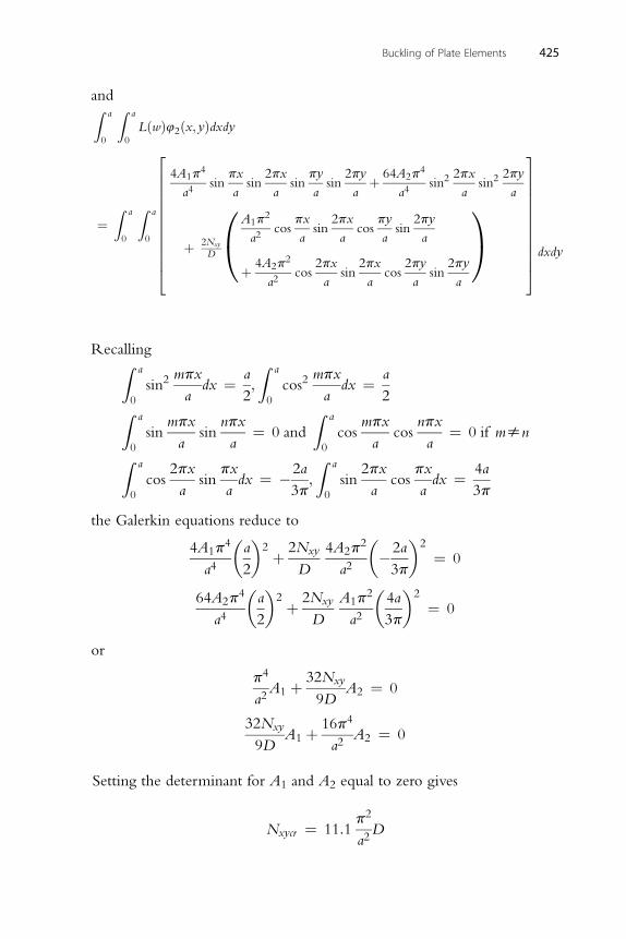
Buckling of Plate Elements 425

and

Z a

0

Z a

0

LðwÞ42ðx; yÞdxdy

¼Z a

0

Z a

0

4A1p4

a4sin

px

asin

2px

asin

py

asin

2py

aþ 64A2p

4

a4sin2

2px

asin2

2py

a

þ 2Nxy

D

0@A1p

2

a2cos

px

asin

2px

acos

py

asin

2py

a

þ 4A2p2

a2cos

2px

asin

2px

acos

2py

asin

2py

a

1A

dxdy

3777777777775

2666666666664

RecallingZ a

0

sin2mpx

adx ¼ a

2;

Z a

0

cos2mpx

adx ¼ a

2Z a

0

sinmpx

asin

npx

a¼ 0 and

Z a

0

cosmpx

acos

npx

a¼ 0 if msn

Z a

0

cos2px

asin

px

adx ¼ �2a

3p;

Z a

0

sin2px

acos

px

adx ¼ 4a

3p

the Galerkin equations reduce to

4A1p4

a4

�a

2

�2 þ 2Nxy

D

4A2p2

a2

��2a

3p

�2

¼ 0

64A2p4

a4

�a

2

�2 þ 2Nxy

D

A1p2

a2

�4a

3p

�2

¼ 0

or

p4

a2A1 þ 32Nxy

9DA2 ¼ 0

32Nxy

9DA1 þ 16p4

a2A2 ¼ 0

Setting the determinant for A1 and A2 equal to zero gives

Nxycr ¼ 11:1p2

a2D

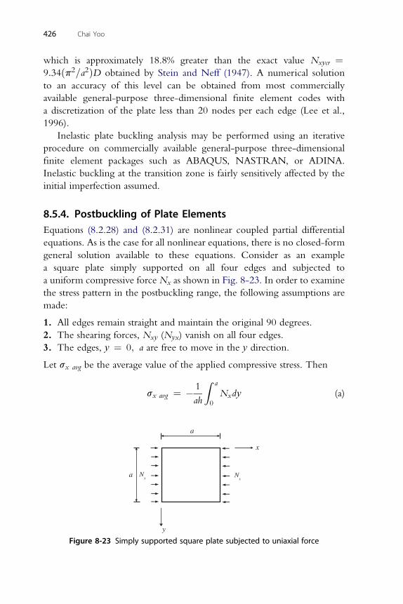
426 Chai Yoo

which is approximately 18.8% greater than the exact value Nxycr ¼

9:34ðp2=a2ÞD obtained by Stein and Neff (1947). A numerical solution

to an accuracy of this level can be obtained from most commercially

available general-purpose three-dimensional finite element codes with

a discretization of the plate less than 20 nodes per each edge (Lee et al.,

1996).

Inelastic plate buckling analysis may be performed using an iterative

procedure on commercially available general-purpose three-dimensional

finite element packages such as ABAQUS, NASTRAN, or ADINA.

Inelastic buckling at the transition zone is fairly sensitively affected by the

initial imperfection assumed.

8.5.4. Postbuckling of Plate ElementsEquations (8.2.28) and (8.2.31) are nonlinear coupled partial differential

equations. As is the case for all nonlinear equations, there is no closed-form

general solution available to these equations. Consider as an example

a square plate simply supported on all four edges and subjected to

a uniform compressive force Nx as shown in Fig. 8-23. In order to examine

the stress pattern in the postbuckling range, the following assumptions are

made:

1. All edges remain straight and maintain the original 90 degrees.

2. The shearing forces, Nxy (Nyx) vanish on all four edges.

3. The edges, y ¼ 0; a are free to move in the y direction.

Let sx avg be the average value of the applied compressive stress. Then

sx avg ¼ � 1

ah

Z a

0

Nxdy (a)

a

a

x

y

Nx N

x

Figure 8-23 Simply supported square plate subjected to uniaxial force

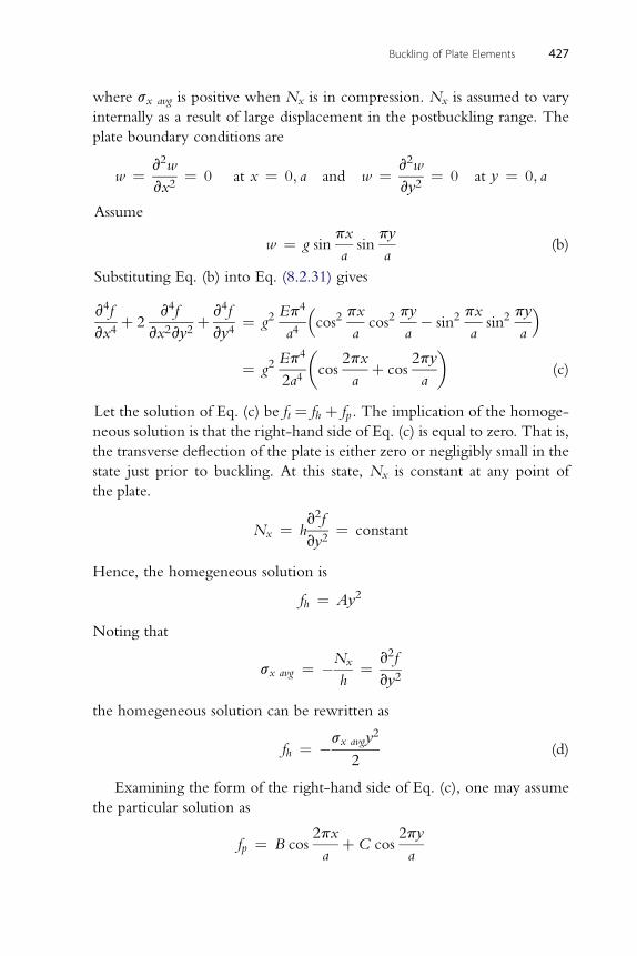
Buckling of Plate Elements 427

where sx avg is positive when Nx is in compression. Nx is assumed to vary

internally as a result of large displacement in the postbuckling range. The

plate boundary conditions are

w ¼ v2w

vx2¼ 0 at x ¼ 0; a and w ¼ v2w

vy2¼ 0 at y ¼ 0; a

Assume

w ¼ g sinpx

asin

py

a(b)

Substituting Eq. (b) into Eq. (8.2.31) gives

v4f

vx4þ 2

v4f

vx2vy2þ v4f

vy4¼ g2

Ep4

a4

�cos2

px

acos2

py

a� sin2

px

asin2

py

a

�

¼ g2Ep4

2a4

�cos

2px

aþ cos

2py

a

�(c)

Let the solution of Eq. (c) be ft ¼ fh þ fp . The implication of the homoge-

neous solution is that the right-hand side of Eq. (c) is equal to zero. That is,

the transverse deflection of the plate is either zero or negligibly small in the

state just prior to buckling. At this state, Nx is constant at any point of

the plate.

Nx ¼ hv2f

vy2¼ constant

Hence, the homegeneous solution is

fh ¼ Ay2

Noting that

sx avg ¼ �Nx

h¼ v2f

vy2

the homegeneous solution can be rewritten as

fh ¼ �sx avgy2

2(d)

Examining the form of the right-hand side of Eq. (c), one may assume

the particular solution as

fp ¼ B cos2px

aþ C cos

2py

a

428 Chai Yoo

Substituting this into Eq. (c) and equating coefficient of the terms yields

B16p4

a4cos

2px

a¼ g2

Ep4

2a4cos

2px

a

2

B ¼ Eg

32¼ C

Hence, the total solution is

ft ¼ Eg2

32

�cos

2px

aþ cos

2py

a

�� sx avgy

2

2(e)

To determine the coefficient g, use the Galerkin methodZ a

0

Z a

0

LðgÞ4ðx; yÞdxdy ¼ 0 (f )

where

LðgÞ ¼ v4w

vx4þ 2

v4w

vx2vy2þ v4w

vy4� h

D

�v2f

vy2v2w

vx2þ v2f

vx2v2w

vy2� 2

v2f

vxvy

v2w

vxvy

�

px py

4ðx; yÞ ¼ sin

asin

a

Using (b) for w and (e) for f, one can write L(g) as

LðgÞ ¼ 1

D

�4gDp4

a4� Ehg3p4

8a4

�cos

2px

aþ cos

2py

a

�

� sx avghgp2

a2

�sin

px

asin

py

a

Hence, the Galerkin equation takes the following form:Z a

0

Z a

0

L

�g

�4

�x; y

�dxdy

¼ 1

D

Z a

0

Z a

0

��4gDp4

a4� sx avghg

p2

a2

��sin2

px

asin2

py

a

�� Ehg3p4

8a4

��cos

2px

asin2

px

asin2

py

aþ cos

2py

asin2

px

asin2

py

a

��dxdy ¼ 0

Buckling of Plate Elements 429

Recalling

Z a

0

sin22px

adx ¼ a

2

the Galerkin equation reduces to�4gDp4

a4� sxavghg

p2

a2

�a2

4� Ehg3p4

8a4a

2

�Z a

0

cos2px

asin2

px

adx

þZ a

0

cos2py

asin2

py

ady

�¼ 0

Making use of the following relations

cos2px

asin2

px

a¼ 1

2

�cos

2px

a� cos2

2px

a

�Z a 2px a

Z a 2px

0

cos2a

dx ¼2;

0

cosa

dx ¼ 0

The Galerkin Equation can be further simplified as

gDp4

a2� sxavghg

p2

4þ Ehg3p4

32a2¼ 0

Hence

sx avg ¼ 4Dp2

ha2þ Ep2g2

8a2¼ scr þ Ep2g2

8a2(g)

or

g2 ¼ 8a2

Ep2

�sx avg � scr

�(h)

Figure 8-24 graphically shows the relationship between the average applied

stress sx avg and the maximum lateral deflection g subsequent to onset of

buckling.

In order to understand why the plate is able to develop postbuckling

strength, one has to investigate the middle-surface stresses subsequent to

buckling.

Recall that the longitudinal stress sx is

sx ¼ Nx

h¼ �v2f

vy2

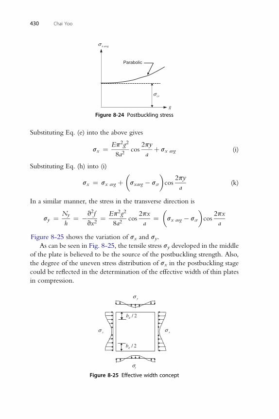
x avgσ

g

Parabolic

crσ

Figure 8-24 Postbuckling stress

430 Chai Yoo

Substituting Eq. (e) into the above gives

sx ¼ Ep2g2

8a2cos

2py

aþ sx avg (i)

Substituting Eq. (h) into (i)

sx ¼ sx avg þ�sxavg � scr

�cos

2py

a(k)

In a similar manner, the stress in the transverse direction is

sy ¼ Ny

h¼ �v2f

vx2¼ Ep2g2

8a2cos

2px

a¼�sx avg � scr

�cos

2px

a

Figure 8-25 shows the variation of sx and sy.

As can be seen in Fig. 8-25, the tensile stress sy developed in the middle

of the plate is believed to be the source of the postbuckling strength. Also,

the degree of the uneven stress distribution of sx in the postbuckling stage

could be reflected in the determination of the effective width of thin plates

in compression.

σy

σ y

σ xσ x

be / 2

be / 2

Figure 8-25 Effective width concept

Buckling of Plate Elements 431

The results shown above are based on an approximate analysis and

hence may contain inaccuracies. For example, a refined analysis would

show that in-plane shear stresses develop in addition to transverse tensile

stresses after initial buckling. Such a refined analysis can readily be

performed on any three-dimensional general-purpose finite element

codes. However, the refined analysis results would not likely add any

significant new information that the simplified analysis was unable to

detect.

It should be noted that the postbuckling strength discussed above is due

to the geometric nonlinearity. As can be seen in Fig. 8-24, any significant

postbuckling (reserve) strength can only be recognized after a considerable

deformation. Therefore, in most design specifications dealing with hot-

rolled structural plates subjected to in-plane compression, the postbuckling

strength is not recognized, whereas it is recognized in the design of cold-

formed structures.

8.6. DESIGN PROVISIONS FOR LOCAL BUCKLING OFCOMPRESSION ELEMENTS

In proportioning the width-to-thickness ratio of flat-plate elements of

hot-rolled structural shapes, it is common practice to design the member

so that overall failure occurs prior to local buckling failure. When a shape

is produced with the same dimensions for different yield stresses, a section

that satisfies the local buckling provision for a lower yield stress may not

do so for a higher yield stress. In the AISC Specifications, the local buck-

ling stress is kept above the yield stress for most rolled shapes, thereby

making it possible to specify a single provision for beam and column

sections.

If local buckling is not to occur at a stress smaller than the yield stress, scrmust be greater than sy . Since the plate buckling stress is given by Eq.

(8.4.13), it requires

k0p2E

12ð1� m2Þ�h

b

�2

> sy

For m ¼ 0.3, one obtains

b

h< 0:95

ffiffiffiffiffiffiffik0Esy

s(8.6.1)

432 Chai Yoo

For an unstiffened element of free-simple edge conditions, the

plate buckling coefficient k0 is 0.425. Substituting this value into Eq. (8.6.1)

gives

b

h< 0:615

ffiffiffiffiffiE

sy

s(8.6.2)

The plate buckling coefficient k0 could be as low as 0.35 due to web–flange

interactions. Using the lower value of k0 ¼ 0.35 yields

b

h< 0:56

ffiffiffiffiffiE

sy

s(8.6.3)

The width-to-thickness ratio is further reduced in the current AISC (2005)

and AASHTO (2007) to reflect the initial imperfections and residual stresses

for compact sections.

b

h< 0:38

ffiffiffiffiffiE

sy

s(8.6.4)

For the corresponding width-to-thickness ratio of the stiffened

element of a box-girder flange, the plate buckling coefficient k0 of 4.0 for

simple supports along both unloaded edges is substituted into Eq. (8.6.1)

to yield

b

h< 1:90

ffiffiffiffiffiE

sy

s(8.6.5)

AISC (2005) reduces this further for compact sections to

b

h< 1:12

ffiffiffiffiffiE

sy

s(8.6.6)

8.7. INELASTIC BUCKLING OF PLATE ELEMENTS

When the applied load is increased beyond the elastic buckling load, the plate

structure’s response exhibits some form of nonlinear behavior, either

geometric or material or a combination of these two. In the past, attempts

weremade to solve thematerial nonlinear problems by adjusting themodulus

of elasticity either by the tangent-modulus theory or the reduced-modulus

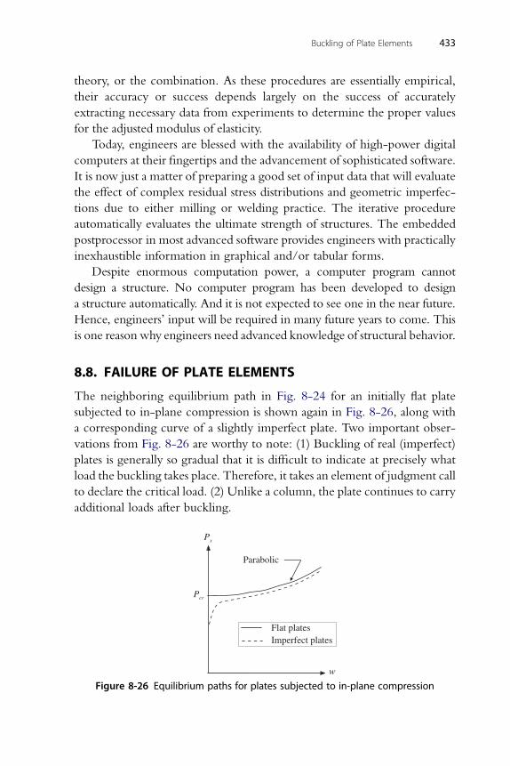
Buckling of Plate Elements 433

theory, or the combination. As these procedures are essentially empirical,

their accuracy or success depends largely on the success of accurately

extracting necessary data from experiments to determine the proper values

for the adjusted modulus of elasticity.

Today, engineers are blessed with the availability of high-power digital

computers at their fingertips and the advancement of sophisticated software.

It is now just a matter of preparing a good set of input data that will evaluate

the effect of complex residual stress distributions and geometric imperfec-

tions due to either milling or welding practice. The iterative procedure

automatically evaluates the ultimate strength of structures. The embedded

postprocessor in most advanced software provides engineers with practically

inexhaustible information in graphical and/or tabular forms.

Despite enormous computation power, a computer program cannot

design a structure. No computer program has been developed to design

a structure automatically. And it is not expected to see one in the near future.

Hence, engineers’ input will be required in many future years to come. This

is one reason why engineers need advanced knowledge of structural behavior.

8.8. FAILURE OF PLATE ELEMENTS

The neighboring equilibrium path in Fig. 8-24 for an initially flat plate

subjected to in-plane compression is shown again in Fig. 8-26, along with

a corresponding curve of a slightly imperfect plate. Two important obser-

vations from Fig. 8-26 are worthy to note: (1) Buckling of real (imperfect)

plates is generally so gradual that it is difficult to indicate at precisely what

load the buckling takes place. Therefore, it takes an element of judgment call

to declare the critical load. (2) Unlike a column, the plate continues to carry

additional loads after buckling.

Px

Pcr

w

Imperfect plates Flat plates

Parabolic

Figure 8-26 Equilibrium paths for plates subjected to in-plane compression

434 Chai Yoo

Hence, Pcr for the plate is not the ultimate strength. In order to take

advantage of the additional load-carrying capacity, the postbuckling strength

of plates must be correctly assessed.

In fact, Brush and Almroth (1975) credits Wagner (1929) for establishing

a criterion for the postbuckling strength of a shear web. As alluded to in

Section 8.4.3, this was the beginning of the long series of attempts to

understand the true mechanics behind the tension field action. Nearly 80

years would elapse until Yoo and Lee (2006) could finally explain the true

mechanics of the tension field action.

Unlike the shear web, a plate subjected to uniformly distributed in-plane

compressive load Px, it is much simpler to do. The applied load Px as shown

in Fig. 8-23 can be expressed as

Px ¼ h

Z b

0

sxdy

where h and b are plate thickness and width, respectively. When Px � Pcr ,

the stress across the plate is uniform. Then Px ¼ hbsx. If Px ¼ Pcr , then

Pcr ¼ hbsx (8.8.1)

For Px>Pcr , the stress at y¼ 0, b is greater than that at the center of the plate

because of the stiffening effect of the supports as shown in Fig. 8-25. For

design purposes, it is customary to express the results of the analysis in terms

of an effective width over which the stress is assumed to be uniform. Then

Px ¼ hbesmax (8.8.2)

where smax is the maximum stress at the supports y ¼ 0; b. An approxi-

mate expression for the effective plate width be is

be ¼ b

ffiffiffiffiffiffiffiffiffiscr

smax

r(8.8.3)

Equation (8.8.3) is referred to as the von Karman effective-width formula.

The effective-width concept has been applied to the design of cold-formed

steel and aluminum structural members (Galambos 1998).

REFERENCESAASHO. (1965). Standard Specifications for Highway Bridges (9th ed.). Washington, DC:

American Association of Highway Officials.AASHTO. (2007). AASHTO LRFD Bridge Design Specifications (4th ed.). Washington, DC:

American Association of Highway Officials.

Buckling of Plate Elements 435

AISC. (2005). Specification for Structural Steel Building (13th ed.). Chicago, IL: AmericanInstitute of Steel Construction.

Allen, H. G., & Bulson, P. S. (1980). Background to Buckling. London: McGraw-Hill (UK).AWS. (2008). Bridge Welding Code (5th ed.). Miami, FL: AASHTO/AWS D1.5M/

D1.5:2008, A Joint Publication of American Association of State Highway andTransportation Officials, Washington, DC and American Welding Society.

Barbre, F. (1939). Stability of Rectangular Plates with Longitudinal or Transverse StiffenersUnder Uniform Compression. Washington, DC: NACA-TM-904.

Basler, K. (1961). Strength of Plate Girders in Shear. Journal of the Structural Div., ASCE.,Vol. 87(No. 7), 151–181.

Bathe, K. J. (1996). Finite Element Procedures. Englewood Cliffs, NJ: Prentice-Hall.Bleich, F. (1952). Buckling Strength of Metal Structures. New York: McGraw-Hill.Brush, D. O., & Almroth, B. O. (1975). Buckling of Bars, Plates, and Shells. New York:

McGraw-Hill.Bryan, G. H. (1891). On the Stability of a Plane Plate Under Thrusts in Its Own Plane with

Applications to the Buckling of the Sides of a Ship. Proceedings London MathematicalSociety, Vol. 22, pp. 54–67.

BSI. (1982). Steel, Concrete, and Composite Bridges, BS 5400, Part 3, Code of Practice for Designof Steel Bridges. London: British Standard Institution.

Chajes, A. (1974). Principles of Structural Stability Theory. Englewood Cliffs, NJ: Prentice-Hall.

Choi, B. H. (2002). Design Requirements for Longitudinally Stiffeners for Horizontally CurvedBox Girders. Auburn, AL: Ph.D. dissertation, Auburn University.

Choi, B. H., & Yoo, C. H. (2005). Strength of Stiffened Flanges in Horizontally CurvedBox Girders. Journal of Engineering Mechanics, ASCE, Vol. 131(No. 1), 20–27, January.

Choi, B. H., Kang, Y. J., & Yoo, C. H. (2007). Stiffness Requirements for TransverseStiffeners of Compression Flanges, Engineering Structures. Elsevier. Vol. 29, No. 9,September, pp. 2087–2096.

Choi, B. H., Hwang, M., Yoon, T., & Yoo, C. H. (2009). Experimental Study on InelasticBuckling Strength and Stiffness Requirements for Longitudinally Stiffened Compres-sion Panels, Engineering Structures. Elsevier. Vol. 31, No.5, May, pp. 1141–1153.

DIN 4114 (1978). Beulsicherheitsnachweise fur Platten, DASt Richtline 12, Deutscher Aus-schuss fur Stahlbau, Draft, Berlin (in German).

ECCS (1976). Manual on the Stability of Steel Structures, Introductory Report (2nd. ed.). Tokyo:Second International Colloquium on Stability-ECCS.

Galambos, T. V. (1998). Guide to Stability Design Criteria for Metal Structures. In StructuralStability Research Council (5th ed.). New York: John Wiley and Sons.

Gerard, G., & Becker, H. (1957). Handbook of Structural Stability, Part I, Buckling of FlatPlates. Washington, DC: NACA, Tech. Note No. 3781.

Inquiry (1974). Inquiry into the Basis of Design and Method of Erection of Steel BoxGirder Bridges, Appendix I, Interim Design and Workmanship Rules, Part III: Basis forthe Design Rules and for the Design of Special Structures not within the Scope of PartII. Report of the Committee. London: Her Majesty’s Stationery Office.

Langhaar, H. L. (1962). EnergyMethods in Applied Mechanics. New York: John Wiley and Sons.Lee, S. C., Davidson, J. S., & Yoo, C. H. (1996). Shear Buckling Coefficients of Plate

Girder Web Panels. Computers and Structures, Vol. 59(No. 5), 789–795.Lee, S. C., & Yoo, C. H. (1998). Strength of Plate Girder Web Panels Under Pure Shear.

Journal of Structural Engineering, ASCE, Vol. 124(No. 2), 184–194.Lee, S. C., & Yoo, C. H. (1999). Strength of Curved I-Girder Web Panels Under Pure

Shear. Journal of Structural Engineering, ASCE, Vol. 125(No. 8), 847–853.Lee, S. C., & Yoo, C. H. (1999). Experimental Study on Ultimate Shear Strength of Web

Panels. Journal of Structural Engineering, ASCE, Vol. 125(No. 8), 838–846.

436 Chai Yoo

Lee, S. C., Yoo, C. H., & Yoon, D. Y. (2002). Behavior of Intermediate Transverse StiffenersAttached on Web Panels. Journal of Structural Engineering, ASCE, Vol. 128(No. 3),337–345.

Lee, S. C., Yoo, C. H., & Yoon, D. Y. (2003). New Design Rule for IntermediateTransverse Stiffeners Attached on Web Panels. Journal of Structural Engineering, ASCE,Vol. 129(No. 12), 1607–1614.

Lee, S. C., Lee, D. S., & Yoo, C. H. (2008). Ultimate Shear Strength of Long Web Panels,Journal of Constructional Steel Research. Elsevier. No. 12 (pp. 1357–1365).

Lee, S. C., Lee, D. S., & Yoo, C. H. (2009a). Further Insight into Postbuckling of WebPanels, I: Review of Flange Anchoring Mechanism. Journal of Structural Engineering,ASCE, Vol. 135(No.1), 3–10.

Lee, S. C., Lee, D. S., Park, C. S., & Yoo, C. H. (2009b). Further Insight into Postbucklingof Web Panels, II: Experiments and Verification of New Theory. Journal of StructuralEngineering, ASCE, Vol. 135(No. 1), 11–18.

Levy, S. (1942). Buckling of Rectangular Plates with Built-in Edges. Journal of AppliedMechanics, ASME, Vol. 9, A-171–174.

Love, A. E. H. (1944). In A Treatise on the Mathematical Theory of Elasticity (4th ed.).New York: Dover Publications.

Mattock, A. H. (1967). Criteria for Design of Steel Concrete Composite Box Girder HighwayBridges, Appendix B. Report of the Committee (unpublished).

Mittelstedt, C. (2008). Explicit Analysis and Design Equations for Buckling Loads andMinimum Stiffener Requirements of Orthotropic and Isotropic Plates UnderCompressive Load Braced by Longitudinal Stiffeners. Thin-Walled Structures, 46(No.12), 1409–1429.

Novozhilov, V. V. (1953). Foundations of the Nonlinear Theory of Elasticity. In F. Bagemihl,H. Komm, & W. Seidel (Eds.). Translated from the 1st (1948) Russian edition.Rochester, NY: Greylock Press.

Porter, D. M., Rockey, K. C., & Evans, H. R. (1975). The Collapse Behavior of PlateGirders Loaded in Shear. Structural Engineering, Vol. 53(No. 8), 313–325.

Seide, P., & Stein, M. (1949). In Compressive Buckling of Simply Supported Plates withLongitudinal Stiffeners. Washington, DC: NACA Technical Note, No. 1825.

Sharp, M. L. (1966). Longitudinal Stiffeners for Compression Members. Journal of StructuralDiv., ASCE, Vol. 92(No. ST5), 187–212.

Sokolnikoff, I. S. (1956). Mathematical Theory of Elasticity. New York: McGraw-Hill.Southwell, R. V., & Skan, S. W. (1924). On the Stability Under Shearing Forces of a Flat

Elastic Strip. Proc. Roy. Soc. London, Ser. A, Vol. 105, 582–607.Stein, M., & Neff, J. (1947). Buckling Stresses of Simply Supported Rectangular Plates in Shear.

Washington, DC: NACA Technical Note, No. 1222.Szilard, R. (1974). Theory and Analysis of Plate: Classical and Numerical Methods. Englewood

Cliffs, NJ: Prentice-Hall.Timoshenko, S. P. (1983). History of Strength of Materials. New York: Dover Publications.Timoshenko, S. P., & Gere, J. M. (1961). Theory of Elastic Stability (2nd ed.). New York:

McGraw-Hill.Timoshenko, S. P., & Woinowsky-Krieger, S. (1959). In Theory of Plates and Shells (2nd ed.).

New York: McGraw-Hill.von Karman, T. (1910). “Festigkeit im Machinenbau,” Enzyklopadie der mathematischn

Wissenschaften, Vol. 4, pp. 349.Wagner, H. (1929). “Ebene Blechweandtrager mit sehr dunnem Stegblech,” Z. Flugtech.

Motorluftschiffahrt, Vol. 20, pp. 200, 227, 256, 279, and 306.Wolchuk, R., & Mayrbaurl, R. M. (1980). Proposed Design Specifications for Steel Box

Girder Bridges. Report No. FHWA-TS-80-205. Washington, DC: Federal HighwayAdministration.

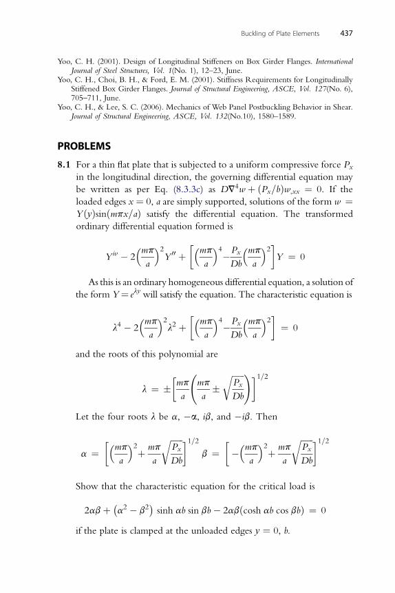
Buckling of Plate Elements 437

Yoo, C. H. (2001). Design of Longitudinal Stiffeners on Box Girder Flanges. InternationalJournal of Steel Structures, Vol. 1(No. 1), 12–23, June.

Yoo, C. H., Choi, B. H., & Ford, E. M. (2001). Stiffness Requirements for LongitudinallyStiffened Box Girder Flanges. Journal of Structural Engineering, ASCE, Vol. 127(No. 6),705–711, June.

Yoo, C. H., & Lee, S. C. (2006). Mechanics of Web Panel Postbuckling Behavior in Shear.Journal of Structural Engineering, ASCE, Vol. 132(No.10), 1580–1589.

PROBLEMS

8.1 For a thin flat plate that is subjected to a uniform compressive force Pxin the longitudinal direction, the governing differential equation may

be written as per Eq. (8.3.3c) as DV4w þ ðPx=bÞw;xx ¼ 0. If the

loaded edges x ¼ 0, a are simply supported, solutions of the form w ¼YðyÞsinðmpx=aÞ satisfy the differential equation. The transformed

ordinary differential equation formed is

Yiv � 2�mp

a

�2Y 00 þ

��mpa

�4�Px

Db

�mpa

�2�Y ¼ 0

As this is an ordinary homogeneous differential equation, a solution of

the form Y ¼ ely will satisfy the equation. The characteristic equation is

l4 � 2�mp

a

�2l2 þ

��mpa

�4�Px

Db

�mpa

�2� ¼ 0

and the roots of this polynomial are

l ¼ ��mp

a

mp

a�

ffiffiffiffiffiffiPx

Db

r !�1=2

Let the four roots l be a, �a, ib, and �ib. Then

a ¼��mp

a

�2þ mp

a

ffiffiffiffiffiffiPx

Db

r �1=2b ¼

���mp

a

�2þ mp

a

ffiffiffiffiffiffiPx

Db

r �1=2

Show that the characteristic equation for the critical load is

2abþ �a2 � b2sinh ab sin bb� 2abðcosh ab cos bbÞ ¼ 0

if the plate is clamped at the unloaded edges y ¼ 0, b.

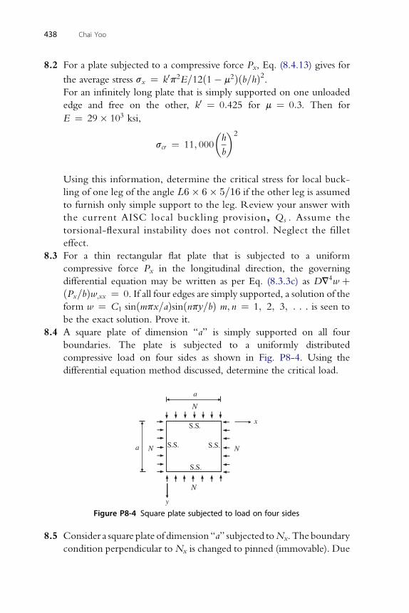
438 Chai Yoo

8.2 For a plate subjected to a compressive force Px, Eq. (8.4.13) gives for

the average stress sx ¼ k0p2E=12ð1� m2Þðb=hÞ2.For an infinitely long plate that is simply supported on one unloaded

edge and free on the other, k0 ¼ 0:425 for m ¼ 0:3. Then for

E ¼ 29� 103 ksi,

scr ¼ 11; 000

�h

b

�2

Using this information, determine the critical stress for local buck-

ling of one leg of the angle L6� 6� 5=16 if the other leg is assumed

to furnish only simple support to the leg. Review your answer with

the current AISC local buckling provision, Qs . Assume the

torsional-flexural instability does not control. Neglect the fillet

effect.

8.3 For a thin rectangular flat plate that is subjected to a uniform

compressive force Px in the longitudinal direction, the governing

differential equation may be written as per Eq. (8.3.3c) as DV4w þðPx=bÞw;xx ¼ 0. If all four edges are simply supported, a solution of the

form w ¼ C1 sinðmpx=aÞsinðnpy=bÞ m; n ¼ 1; 2; 3; : : : is seen to

be the exact solution. Prove it.

8.4 A square plate of dimension “a” is simply supported on all four

boundaries. The plate is subjected to a uniformly distributed

compressive load on four sides as shown in Fig. P8-4. Using the

differential equation method discussed, determine the critical load.

y

a

a

x

NN

N

N

S.S.

S.S. S.S.

S.S.

Figure P8-4 Square plate subjected to load on four sides

8.5 Consider a square plate of dimension “a” subjected toNx. The boundary

condition perpendicular to Nx is changed to pinned (immovable). Due

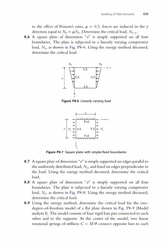
Buckling of Plate Elements 439

to the effect of Poisson’s ratio, m ¼ 0.3, forces are induced in the y

direction equal to Ny ¼ mNx. Determine the critical load, Nx cr .

8.6 A square plate of dimension “a” is simply supported on all four

boundaries. The plate is subjected to a linearly varying compressive

load, Nx, as shown in Fig. P8-6. Using the energy method discussed,

determine the critical load.

a

x

y

N0N0

S.S.

S.S. S.S.

S.S.

Figure P8-6 Linearly varying load

y

a

x

NxNx

Fxd.

S.S. S.S.

Fxd.

a

Figure P8-7 Square plate with simple-fixed boundaries

8.7 A square plate of dimension “a” is simply supported on edges parallel to

the uniformly distributed load,Nx, and fixed on edges perpendicular to

the load. Using the energy method discussed, determine the critical

load.

8.8 A square plate of dimension “a” is simply supported on all four

boundaries. The plate is subjected to a linearly varying compressive

load, Nx, as shown in Fig. P8-8. Using the energy method discussed,

determine the critical load.

8.9 Using the energy method, determine the critical load for the one-

degree-of-freedom model of a flat plate shown in Fig. P8-9 (Model

analysis I). The model consists of four rigid bars pin-connected to each

other and to the supports. At the center of the model, two linear

rotational springs of stiffness C ¼ M/q connect opposite bars to each

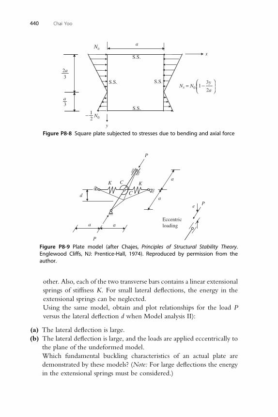
K

e

C

a

a

a

d

KC

a

P

P

P

Eccentricloading

Figure P8-9 Plate model (after Chajes, Principles of Structural Stability Theory.Englewood Cliffs, NJ: Prentice-Hall, 1974). Reproduced by permission from theauthor.

3a

2a3

xN0

N012

−

S.S.

S.S.

S.S.S.S. 3y1

2aNx = N0

⎛ ⎞−⎜ ⎟⎝ ⎠

a

y

Figure P8-8 Square plate subjected to stresses due to bending and axial force

440 Chai Yoo

other. Also, each of the two transverse bars contains a linear extensional

springs of stiffness K. For small lateral deflections, the energy in the

extensional springs can be neglected.

Using the same model, obtain and plot relationships for the load P

versus the lateral deflection d when Model analysis II):

(a) The lateral deflection is large.

(b) The lateral deflection is large, and the loads are applied eccentrically to

the plane of the undeformed model.

Which fundamental buckling characteristics of an actual plate are

demonstrated by these models? (Note: For large deflections the energy

in the extensional springs must be considered.)

CHAPTER99

Buckling of Thin CylindricalShell ElementsContents

9.1. Introduction 4419.2. Large-Deflection Equations (Donnell Type) 4429.3. Energy Method 4469.4. Linear Stability Equations (Donnell Type) 450

9.4.1. Adjacent-Equilibrium Criterion 4509.4.2. Trefftz Criterion 454

9.5. Applications of Linear Buckling Equations 4559.5.1. Uniform External Pressure 4559.5.2. Axially Loaded Cylinders 4589.5.3. Torsional Load 4619.5.4. Combined Axial Compression and External Pressure 4629.5.5. Effect of Boundary Conditions 463

9.6. Failure of Cylindrical Shells 4659.7. Postbuckling of Cylindrical Shells 466References 472Problems 473

9.1. INTRODUCTION

Shell buckling has become one of the important areas of interest in struc-

tural mechanics in recent times. The difference between a plate element and

a shell element is that the plate element has curvatures in the unloaded state,

whereas the shell element is assumed to be initially flat. Although the

presence of initial curvature is of little consequence for bending, it does

affect the membrane action of the element significantly.

Membrane action is caused by in-plane forces. These forces may be the

primary forces caused by applied edge loads or edge deformations, or they

may be secondary forces resulting from flexural deformations. In a stability

analysis, primary in-plane forces must be considered whether or not initial

curvature exists. However, the same is not necessarily the case regarding

secondary in-plane forces. If the element is initially flat, secondary in-plane

forces do not affect membrane action significantly unless the bending

deformations are large. It is for this reason that membrane action due to

secondary forces is ignored in the small-deflection plate theory, but not in

Stability of Structures � 2011 Elsevier Inc.ISBN 978-0-12-385122-2, doi:10.1016/B978-0-12-385122-2.10009-0 All rights reserved. 441 j

442 Chai Yoo

the large-deflection plate theory. If the element has initial curvature, on the

other hand, membrane action caused by secondary in-plane forces will be

significant regardless of the magnitude of the bending deformations.

Membrane action resulting from secondary forces therefore must be

accounted for in both small- and large-deflection shell theories (Chajes

1974).

In addition to this complication is the fact that in many shell problems

the initially buckled form is in a condition of unstable equilibrium and

a new position of equilibrium can exist at a much lower buckling load.

Thus, the theoretical initial buckling load calculated by the classical theories

of stability is rarely attained in experiments. Discussion of shell behavior in

the postbuckling range, which is governed to a great extent by the nature of

the initial imperfection, is therefore a necessary element of any buckling

analysis (Allen and Bulson 1980).

Examination of these problems has resulted in thousands of papers and

reports over the years as well as a number of books. It would be impractical

to condense the whole of this work into a chapter or two, and the aim here

will be to introduce the student to the fundamentals and at the same time

indicate selected simple formulas of interest to the practicing engineers. To

do this, no attempt has been made at a general analysis, but each practical

problem is examined separately.

Development of many governing equations has followed the procedure

given by Brush and Almroth (1975) and Chajes (1974).

9.2. LARGE-DEFLECTION EQUATIONS (DONNELL TYPE)

As the reliability and efficiency of the incremental finite element analysis have

been well established, much of the work in shell analysis is being carried out

on digital computers these days. In such environments, the simplicity of the

governing equations is of little importance other than initial programming

efforts. As a result, interest the Donnell equations has diminished somewhat.

However, the relative simplicity of the equations makes them well suited for

this introductory examination of shell buckling.

Consider a differential shell element of thickness h with a radius of

curvature R as shown in Fig. 9-1(a). The coordinate system is a pointwise

orthogonal rectangular coordinate system with the origin in the middle

surface of the shell so that the x-axis is parallel to the axis of the cylinder, the

y-axis is tangent to the circular arc, and the z-axis is normal to the middle

surface directed toward the center of curvature.

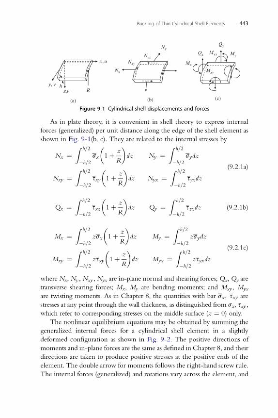
Qy

y, v

,x u

z,w Rh

Mx

Ny

Nx

Nxy

NyxQx

Mxy

MyMyx

(a) (b) (c)

Figure 9-1 Cylindrical shell displacements and forces

Buckling of Thin Cylindrical Shell Elements 443

As in plate theory, it is convenient in shell theory to express internal

forces (generalized) per unit distance along the edge of the shell element as

shown in Fig. 9-1(b, c). They are related to the internal stresses by

Nx ¼Z h=2

�h=2sx

�1þ z

R

�dz Ny ¼

Z h=2

�h=2sydz

Nxy ¼Z h=2

�h=2sxy

�1þ z

R

�dz Nyx ¼

Z h=2

�h=2syxdz

(9.2.1a)

Z h=2 � � Z h=2

Qx ¼�h=2

sxz 1þ z

Rdz Qy ¼

�h=2szxdz (9.2.1b)

Z h=2 � � Z h=2

Mx ¼�h=2

zsx 1þ z

Rdz My ¼

�h=2zsydz

Mxy ¼Z h=2

�h=2zsxy

�1þ z

R

�dz Myx ¼

Z h=2

�h=2zsyxdz

(9.2.1c)

whereNx,Ny ,Nxy , Nyx are in-plane normal and shearing forces;Qx,Qy are

transverse shearing forces; Mx, My are bending moments; and Mxy , Myx

are twisting moments. As in Chapter 8, the quantities with bar sx; sxy arestresses at any point through the wall thickness, as distinguished from sx, sxy ,which refer to corresponding stresses on the middle surface (z ¼ 0) only.

The nonlinear equilibrium equations may be obtained by summing the

generalized internal forces for a cylindrical shell element in a slightly

deformed configuration as shown in Fig. 9-2. The positive directions of

moments and in-plane forces are the same as defined in Chapter 8, and their

directions are taken to produce positive stresses at the positive ends of the

element. The double arrow for moments follows the right-hand screw rule.

The internal forces (generalized) and rotations vary across the element, and

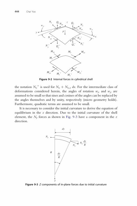
Nx z

y

Ny

Qx+

p

w,y

Qx Nxy

yxN +

yQ +

yN +

Nyx

x

w,x

Mxy

Nxy+

Qy

Nx+

Mx

Myx+

My+ Mxy

+

Myx

Mx+

My

Figure 9-2 Internal forces in cylindrical shell

444 Chai Yoo

the notation Nxþ is used for Nx þ Nx,x dx. For the intermediate class of

deformations considered herein, the angles of rotation w,x and w,y are

assumed to be small so that sines and cosines of the angles can be replaced by

the angles themselves and by unity, respectively (micro geometry holds).

Furthermore, quadratic terms are assumed to be small.

It is necessary to consider the initial curvature to derive the equation of

equilibrium in the z direction. Due to the initial curvature of the shell

element, the Ny forces as shown in Fig. 9-3 have a component in the z

direction.

Ny

z

Ny

R dy

R

dy

dyNy R

Figure 9-3 Z components of in-plane forces due to initial curvature

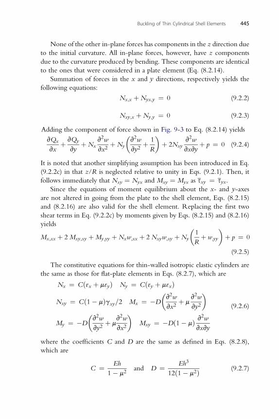
Buckling of Thin Cylindrical Shell Elements 445

None of the other in-plane forces has components in the z direction due

to the initial curvature. All in-plane forces, however, have z components

due to the curvature produced by bending. These components are identical

to the ones that were considered in a plate element (Eq. (8.2.14).

Summation of forces in the x and y directions, respectively yields the

following equations:

Nx;x þNyx;y ¼ 0 (9.2.2)

N þN ¼ 0 (9.2.3)

xy;x y;y

Adding the component of force shown in Fig. 9-3 to Eq. (8.2.14) yields

vQx

vxþ vQy

vyþNx

v2w

vx2þNy

�v2w

vy2þ 1

R

�þ 2Nxy

v2w

vxvyþ p ¼ 0 (9.2.4)

It is noted that another simplifying assumption has been introduced in Eq.

(9.2.2c) in that z/R is neglected relative to unity in Eqs. (9.2.1). Then, it

follows immediately that Nxy ¼ Nyx and Mxy ¼ Myx as sxy ¼ syx.Since the equations of moment equilibrium about the x- and y-axes

are not altered in going from the plate to the shell element, Eqs. (8.2.15)

and (8.2.16) are also valid for the shell element. Replacing the first two

shear terms in Eq. (9.2.2c) by moments given by Eqs. (8.2.15) and (8.2.16)

yields

Mx;xx þ 2Mxy;xy þMy;yy þNxw;xx þ 2 Nxyw;xy þNy

�1

Rþ w;yy

�þ p ¼ 0

(9.2.5)

The constitutive equations for thin-walled isotropic elastic cylinders are

the same as those for flat-plate elements in Eqs. (8.2.7), which are

Nx ¼ Cð3x þ m3yÞ Ny ¼ Cð3y þ m3xÞ

Nxy ¼ Cð1� mÞgxy=2 Mx ¼ �D

�v2w

vx2þ m

v2w

vy2

�

My ¼ �D

�v2w

vy2þ m

v2w

vx2

�Mxy ¼ �Dð1� mÞ v

2w

vxvy

(9.2.6)

where the coefficients C and D are the same as defined in Eqs. (8.2.8),

which are

C ¼ Eh

1� m2and D ¼ Eh3

12ð1� m2Þ (9.2.7)

446 Chai Yoo

The kinematic relations at the middle surface on which the Donnell

equations are based are identical to those given in Eqs. (8.2.5) with one

exception for 3y (Donnell 1933), which are

3x ¼ vu

vxþ 1

2

�vw

vx

�2

kx ¼ �v2w

vx2

3y ¼ vv

vy� w

Rþ 1

2

�vw

vy

�2

ky ¼ �v2w

vy2

gxy ¼ vu

vyþ vv

vxþ vw

vx

vw

vykxy ¼ � v2w

vxvy

(9.2.8)

Substituting the above constitutive and kinematic relations into Eq.

(9.2.3) yields a coupled set of three nonlinear differential equations in the

three variables u, v, and w.

Nx;x þNxy;y ¼ 0 (9.2.9a)

Nxy;x þNy;y ¼ 0 (9.2.9b)

Dðw þ 2w þw Þ� ½N w þ 2N w þN ð1=Rþw Þ� ¼ p

;xxxx ;xxyy ;yyyy x ;xx xy ;xy y ;yy

(9.2.9c)

Equations (9.2.9) are nonlinear equilibrium equations for thin cylindrical

shells. They have been widely used in the large-deflection analyses of

cylindrical shells (von Karman and Tsien 1941).

9.3. ENERGY METHOD

It would be informative to rederive the nonlinear equilibrium equations in

Eqs. (9.2.9) based on the principle of minimum potential energy. The total

potential energy P is the sum of the strain energy U of the cylindrical shell

and the loss of the potential energy of the applied load V.

P ¼ U þ V (9.3.1)

The strain energy of a deformed shell can be expressed in two parts: (1)

the strain energy due to bending and (2) the strain energy due to the

membrane action. Using the general expression of the strain energy of

a plate (Eq. (8.5.6)) and using a separate expression for the bending stress and

the membrane stress, one obtains

Buckling of Thin Cylindrical Shell Elements 447

Ub ¼ D

2

ZZ �kx

2 þ ky2 þ 2mkxky þ 2ð1� mÞkxy2

�dA (9.3.2)

CZZ � ð1� mÞ �

Um ¼2

3x2 þ 3y

2 þ 2m3x3y þ2

gxy2 dA (9.3.3)

where 3x, 3y ,., kxy are given Eqs. (9.2.6). Hence, the total strain energy is

U ¼ Ub þUm (9.3.4)

For a cylindrical shell subjected to lateral pressure p, the potential energy

of the applied pressure is

V ¼ �ZZ

A

pwdxdy (9.3.5)

The Euler-Lagrange differential equations for an integrand of

Eq. (9.3.1) are

vF

vu� v

vx

vF

vu;x� v

vy

vF

vu;y¼ 0 (9.3.6a)

vF v vF v vF

vv�vx vv;x

�vy vv;y

¼ 0 (9.3.6b)

2 2 2

vF

vw� v

vx

vF

vw;x� v

vy

vF

vw;yþ v

vx2vF

vw;xxþ v

vxvy

vF

vw;xyþ v

vy2vF

vw;yy¼ 0 (9.3.6c)

It can be shown that the execution of the Euler-Lagrange differential

equations, Eqs. (9.3.6), will lead to the nonlinear equilibrium equations,

Eqs. (9.2.9) (see Problem 9.2).

Equations (9.2.9) are nonlinear equilibrium equations for thin cylin-

drical shells. They are the counterpart for shells of Eqs. (8.2.18). There are

four unknowns Nx, Ny , Nxy , and w. Three equations in three unknowns u,

v, wmay be obtained by introducing the constitutive and kinematic relations

of Eqs. (9.2.4) and (9.2.6). As was done in Chapter 8, a simpler set of two

equations in two variables can be obtained by use of a stress function

identical to Eqs. (8.2.27).

Nx ¼ f;yy; Ny ¼ f;xx; Nxy ¼ �f;xy (9.3.7)

Rearranging Eqs. (9.2.4), one obtains the following relations:

3x ¼ 1

EhðNx � mNyÞ (9.3.8a)

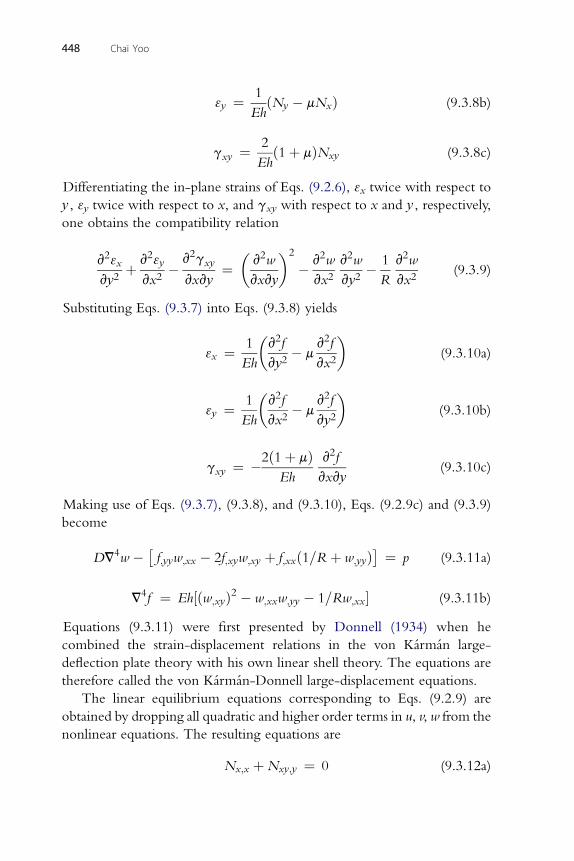
1

3y ¼

EhðNy � mNxÞ (9.3.8b)

2

448 Chai Yoo

gxy ¼Eh

ð1þ mÞNxy (9.3.8c)

Differentiating the in-plane strains of Eqs. (9.2.6), 3x twice with respect to

y , 3y twice with respect to x, and gxy with respect to x and y , respectively,

one obtains the compatibility relation

v23x

vy2þ v23y

vx2� v2gxy

vxvy¼

�v2w

vxvy

�2

� v2w

vx2v2w

vy2� 1

R

v2w

vx2(9.3.9)

Substituting Eqs. (9.3.7) into Eqs. (9.3.8) yields

3x ¼ 1

Eh

�v2f

vy2� m

v2f

vx2

�(9.3.10a)

� 2 2 �

3y ¼ 1

Eh

v f

vx2� m

v f

vy2(9.3.10b)

2

gxy ¼ �2ð1þ mÞEh

v f

vxvy(9.3.10c)

Making use of Eqs. (9.3.7), (9.3.8), and (9.3.10), Eqs. (9.2.9c) and (9.3.9)

become

DV4w � �f;yyw;xx � 2f;xyw;xy þ f;xxð1=R þ w;yyÞ

� ¼ p (9.3.11a)

4 2

V f ¼ Eh½ðw;xyÞ � w;xxw;yy � 1=Rw;xx� (9.3.11b)

Equations (9.3.11) were first presented by Donnell (1934) when he

combined the strain-displacement relations in the von Karman large-

deflection plate theory with his own linear shell theory. The equations are

therefore called the von Karman-Donnell large-displacement equations.

The linear equilibrium equations corresponding to Eqs. (9.2.9) are

obtained by dropping all quadratic and higher order terms in u, v, w from the

nonlinear equations. The resulting equations are

Nx;x þNxy;y ¼ 0 (9.3.12a)

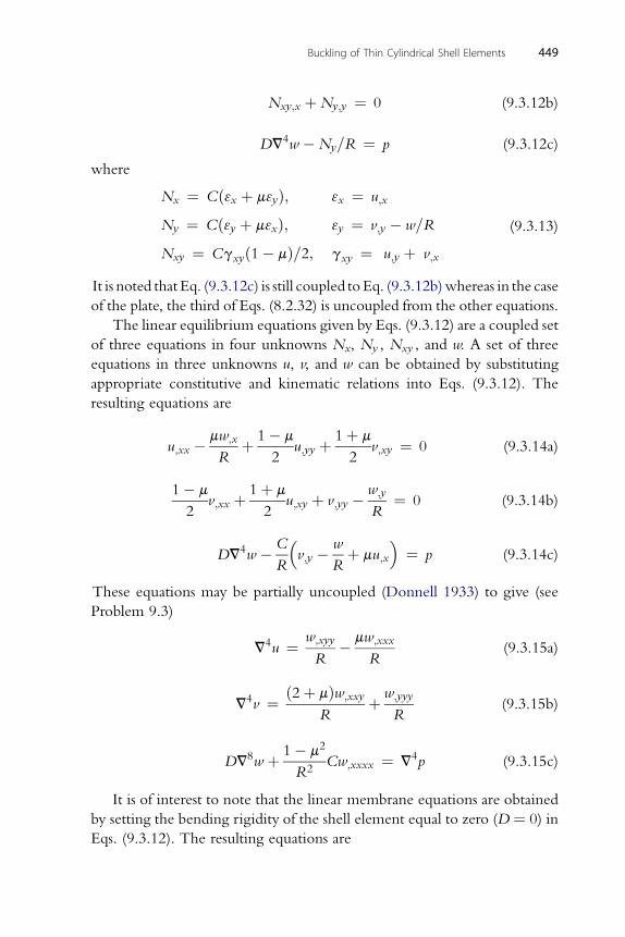
Nxy;x þNy;y ¼ 0 (9.3.12b)

4

Buckling of Thin Cylindrical Shell Elements 449

DV w �Ny=R ¼ p (9.3.12c)

where

Nx ¼ Cð3x þ m3yÞ; 3x ¼ u;x

Ny ¼ Cð3y þ m3xÞ; 3y ¼ v;y � w=R

Nxy ¼ Cgxyð1� mÞ=2; gxy ¼ u;y þ v;x

(9.3.13)

It is noted that Eq. (9.3.12c) is still coupled toEq. (9.3.12b)whereas in the case

of the plate, the third of Eqs. (8.2.32) is uncoupled from the other equations.

The linear equilibrium equations given by Eqs. (9.3.12) are a coupled set

of three equations in four unknowns Nx, Ny , Nxy , and w. A set of three

equations in three unknowns u, v, and w can be obtained by substituting

appropriate constitutive and kinematic relations into Eqs. (9.3.12). The

resulting equations are

u;xx � mw;x

Rþ 1� m

2u;yy þ 1þ m

2v;xy ¼ 0 (9.3.14a)

1� m 1þ m w;y

2v;xx þ

2u;xy þ v;yy �

R¼ 0 (9.3.14b)

C� w �

DV4w �

Rv;y �

Rþ mu;x ¼ p (9.3.14c)

These equations may be partially uncoupled (Donnell 1933) to give (see

Problem 9.3)

V4u ¼ w;xyy

R� mw;xxx

R(9.3.15a)

ð2þ mÞw w

V4v ¼ ;xxy

Rþ ;yyy

R(9.3.15b)

2

DV8w þ 1� m

R2Cw;xxxx ¼ V4p (9.3.15c)

It is of interest to note that the linear membrane equations are obtained

by setting the bending rigidity of the shell element equal to zero (D ¼ 0) in

Eqs. (9.3.12). The resulting equations are

450 Chai Yoo

Nx;x þNxy;y ¼ 0 (9.3.16a)

N þN ¼ 0 (9.3.16b)

xy;x y;y

�N =R ¼ p (9.3.16c)

y

These equations are statically determinate; that is, there are three variables

in three equations. Equation (9.3.16c) gives the well-known hoop

compression (�Ny) due to the external pressure p.

9.4. LINEAR STABILITY EQUATIONS (DONNELL TYPE)

Equations (9.2.9) govern all linear and nonlinear equilibrium conditions of the

cylindrical shell within the confinement of the intermediate class of defor-

mations. The equations include linear, quadratic, and cubic terms of variables

u, v, and w, and therefore are nonlinear. It is now a fairly simple task to obtain

a very good iterative numerical solution by a well-established finite element

code. A load-displacement curve based on such solutions for a cylinder subject

to the edge load is shown in Fig. 9-4. The linear equilibrium equations, Eqs.

(9.3.12), govern the primary (static) path. The nonlinear equations, Eqs.

(9.2.9), govern both the primary path and the secondary path.

The equilibrium paths determined by solution of the equilibrium

equations, Eqs. (9.2.9), show the bifurcation point and the corresponding

critical load. Hence, a separate solution for the critical load is not necessary.

However, the solution of Eqs. (9.2.9) demands a fairly complicated

numerical procedure. The purpose of stability analysis to be presented

herein is to permit determination of the critical load by solution of linear

differential equations.

The linear differential equations for determination of the critical load

of a cylinder subjected to external loading are derived by application of the

adjacent-equilibrium criterion. The same equations are rederived based on

the minimum potential energy criterion as was done in the previous

section.

9.4.1. Adjacent-Equilibrium CriterionAdjacent (or neighboring) equilibrium configurations are examined using

the procedure outlined by Brush and Almroth (1975) as was done in

Chapter 8. Consider the equilibrium configuration at the bifurcation point.

Then, the equilibrium configuration is perturbed by the small incremental

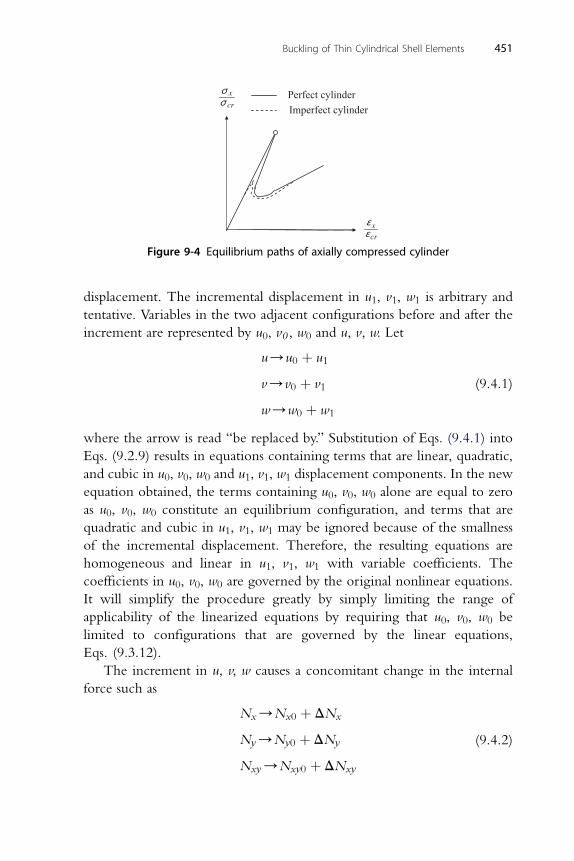
Perfect cylinderx

cr

σσ

x

cr

εε

Imperfect cylinder

Figure 9-4 Equilibrium paths of axially compressed cylinder

Buckling of Thin Cylindrical Shell Elements 451

displacement. The incremental displacement in u1, v1, w1 is arbitrary and

tentative. Variables in the two adjacent configurations before and after the

increment are represented by u0, v0 , w0 and u, v, w. Let

u/u0 þ u1

v/v0 þ v1

w/w0 þ w1

(9.4.1)

where the arrow is read “be replaced by.” Substitution of Eqs. (9.4.1) into

Eqs. (9.2.9) results in equations containing terms that are linear, quadratic,

and cubic in u0, v0, w0 and u1, v1, w1 displacement components. In the new

equation obtained, the terms containing u0, v0, w0 alone are equal to zero

as u0, v0, w0 constitute an equilibrium configuration, and terms that are

quadratic and cubic in u1, v1, w1 may be ignored because of the smallness

of the incremental displacement. Therefore, the resulting equations are

homogeneous and linear in u1, v1, w1 with variable coefficients. The

coefficients in u0, v0, w0 are governed by the original nonlinear equations.

It will simplify the procedure greatly by simply limiting the range of

applicability of the linearized equations by requiring that u0, v0, w0 be

limited to configurations that are governed by the linear equations,

Eqs. (9.3.12).

The increment in u, v, w causes a concomitant change in the internal

force such as

Nx/Nx0 þ DNx

Ny/Ny0 þ DNy

Nxy/Nxy0 þ DNxy

(9.4.2)

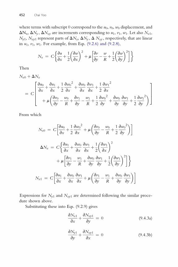
452 Chai Yoo

where terms with subscript 0 correspond to the u0, v0, w0 displacement, and

DNx, DNy , DNxy are increments corresponding to u1, v1, w1. Let also Nx1,

Ny1, Nxy1 represent parts of DNx, DNy , D Nxy , respectively, that are linear

in u1, v1, w1. For example, from Eqs. (9.2.6) and (9.2.8),

Nx ¼ C

�vu

vxþ 1

2

�vw

vx

�2

þ m

vv

vy� w

Rþ 1

2

�vw

vy

�2�

Then

Nx0 þ DNx

¼ C

26664vu0

vxþ vu1

vxþ 1

2

vw0

vx

2

þ vw0

vx

vw1

vxþ 1

2

vw1

vx

2

þ m

�vv0

vy� w0

Rþ vv1

vy� w1

Rþ 1

2

vw0

vy

2

þ vw0

vy

vw1

vyþ 1

2

vw1

vy

2�3775

From which

Nx0 ¼ C

vu0

vxþ 1

2

vw0

vx

2

þ m

�vv0

vy� w0

Rþ 1

2

vw0

vy

2�

� � �2

DNx ¼ Cvu1

vxþ vw0

vx

vw1

vxþ 1

2

vw1

vx

þ m

vv1

vy� w1

Rþ vw0

vy

vw1

vyþ 1

2

�vw1

vy

�2�

� �

Nx1 ¼ C

vu1

vxþ vw0

vx

vw1

vxþ m

vv1

vy� w1

Rþ vw0

vy

vw1

vy

Expressions for Ny1 and Nxy1 are determined following the similar proce-

dure shown above.

Substituting these into Eqs. (9.2.9) gives

vNx1

vxþ vNxy1

vy¼ 0 (9.4.3a)

vN vN

y1

vyþ xy1

vx¼ 0 (9.4.3b)

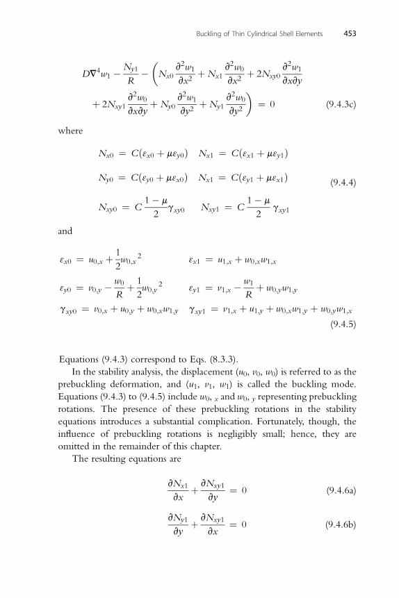
N�

v2w v2w v2w

DV4w1 � y1

R� Nx0

1

vx2þNx1

0

vx2þ 2Nxy0

1

vxvy

þ 2Nxy1v2w0

vxvyþ Ny0

v2w1

vy2þNy1

v2w0

vy2

�¼ 0 (9.4.3c)

where

Nx0 ¼ Cð3x0 þ m3y0Þ Nx1 ¼ Cð3x1 þ m3y1Þ

Ny0 ¼ Cð3y0 þ m3x0Þ Nx1 ¼ Cð3y1 þ m3x1Þ

Nxy0 ¼ C1� m

2gxy0 Nxy1 ¼ C

1� m

2gxy1

(9.4.4)

and

3x0 ¼ u0;x þ 1

2w0;x

2 3x1 ¼ u1;x þ w0;xw1;x

3y0 ¼ v0;y � w0

Rþ 1

2w0;y

2 3y1 ¼ v1;x � w1

Rþ w0;yw1;y

gxy0 ¼ v0;x þ u0;y þ w0;xw1;y gxy1 ¼ v1;x þ u1;y þ w0;xw1;y þ w0;yw1;x

(9.4.5)

Equations (9.4.3) correspond to Eqs. (8.3.3).

In the stability analysis, the displacement (u0, v0, w0) is referred to as the

prebuckling deformation, and (u1, v1, w1) is called the buckling mode.

Equations (9.4.3) to (9.4.5) include w0, x and w0, y representing prebuckling

rotations. The presence of these prebuckling rotations in the stability

equations introduces a substantial complication. Fortunately, though, the

influence of prebuckling rotations is negligibly small; hence, they are

omitted in the remainder of this chapter.

The resulting equations are

vNx1

vxþ vNxy1

vy¼ 0 (9.4.6a)

vNy1 vNxy1

Buckling of Thin Cylindrical Shell Elements 453

vyþ

vx¼ 0 (9.4.6b)

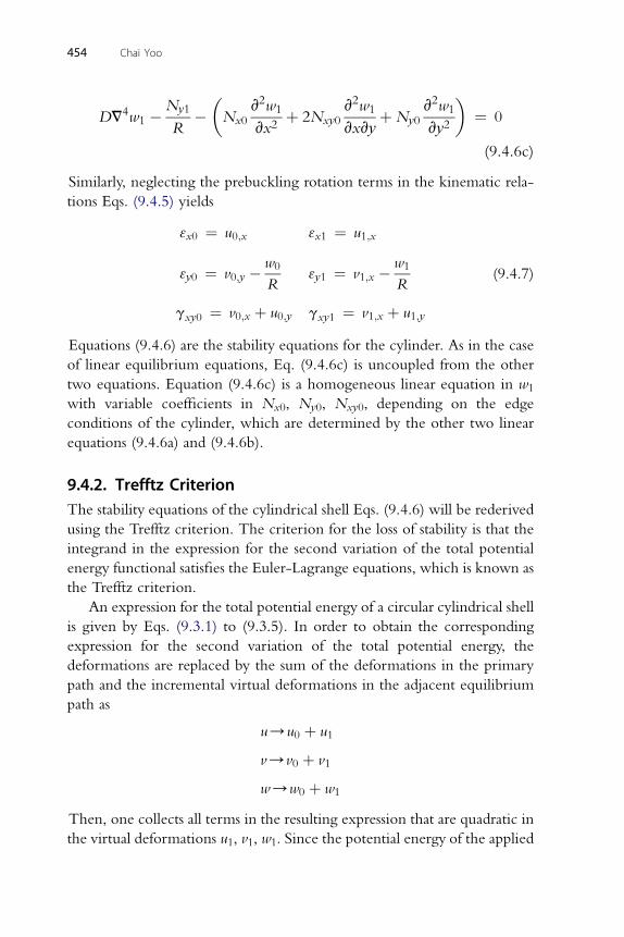
N�

v2w v2w v2w�

DV4w1 � y1

R� Nx0

1

vx2þ 2Nxy0

1

vxvyþNy0

1

vy2¼ 0

(9.4.6c)

Similarly, neglecting the prebuckling rotation terms in the kinematic rela-

tions Eqs. (9.4.5) yields

3x0 ¼ u0;x 3x1 ¼ u1;x

3y0 ¼ v0;y � w0

R3y1 ¼ v1;x � w1

R

gxy0 ¼ v0;x þ u0;y gxy1 ¼ v1;x þ u1;y

(9.4.7)

Equations (9.4.6) are the stability equations for the cylinder. As in the case

of linear equilibrium equations, Eq. (9.4.6c) is uncoupled from the other

two equations. Equation (9.4.6c) is a homogeneous linear equation in w1

with variable coefficients in Nx0, Ny0, Nxy0, depending on the edge

conditions of the cylinder, which are determined by the other two linear

equations (9.4.6a) and (9.4.6b).

454 Chai Yoo

9.4.2. Trefftz CriterionThe stability equations of the cylindrical shell Eqs. (9.4.6) will be rederived

using the Trefftz criterion. The criterion for the loss of stability is that the

integrand in the expression for the second variation of the total potential

energy functional satisfies the Euler-Lagrange equations, which is known as

the Trefftz criterion.

An expression for the total potential energy of a circular cylindrical shell

is given by Eqs. (9.3.1) to (9.3.5). In order to obtain the corresponding

expression for the second variation of the total potential energy, the

deformations are replaced by the sum of the deformations in the primary

path and the incremental virtual deformations in the adjacent equilibrium

path as

u/u0 þ u1

v/v0 þ v1

w/w0 þ w1

Then, one collects all terms in the resulting expression that are quadratic in

the virtual deformations u1, v1, w1. Since the potential energy of the applied

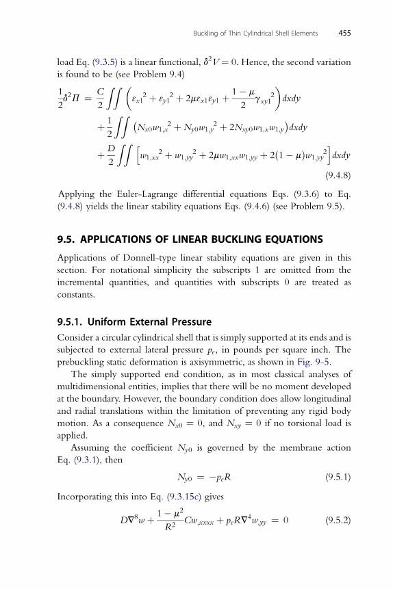
Buckling of Thin Cylindrical Shell Elements 455

load Eq. (9.3.5) is a linear functional, d2V ¼ 0. Hence, the second variation

is found to be (see Problem 9.4)

1

2d2P ¼ C

2

ZZ �3x1

2 þ 3y12 þ 2m3x13y1 þ 1� m

2gxy1

2

�dxdy

þ 1

2

ZZ �Nx0w1;x

2 þNy0w1;y2 þ 2Nxy0w1;xw1;y

dxdy

þD

2

ZZ hw1;xx

2 þ w1;yy2 þ 2mw1;xxw1;yy þ 2ð1� mÞw1;yy

2idxdy

(9.4.8)

Applying the Euler-Lagrange differential equations Eqs. (9.3.6) to Eq.

(9.4.8) yields the linear stability equations Eqs. (9.4.6) (see Problem 9.5).

9.5. APPLICATIONS OF LINEAR BUCKLING EQUATIONS

Applications of Donnell-type linear stability equations are given in this

section. For notational simplicity the subscripts 1 are omitted from the

incremental quantities, and quantities with subscripts 0 are treated as

constants.

9.5.1. Uniform External PressureConsider a circular cylindrical shell that is simply supported at its ends and is

subjected to external lateral pressure pe, in pounds per square inch. The

prebuckling static deformation is axisymmetric, as shown in Fig. 9-5.

The simply supported end condition, as in most classical analyses of

multidimensional entities, implies that there will be no moment developed

at the boundary. However, the boundary condition does allow longitudinal

and radial translations within the limitation of preventing any rigid body

motion. As a consequence Nx0 ¼ 0, and Nxy ¼ 0 if no torsional load is

applied.

Assuming the coefficient Ny0 is governed by the membrane action

Eq. (9.3.1), then

Ny0 ¼ �peR (9.5.1)

Incorporating this into Eq. (9.3.15c) gives

DV8w þ 1� m2

R2Cw;xxxx þ peRV

4w;yy ¼ 0 (9.5.2)

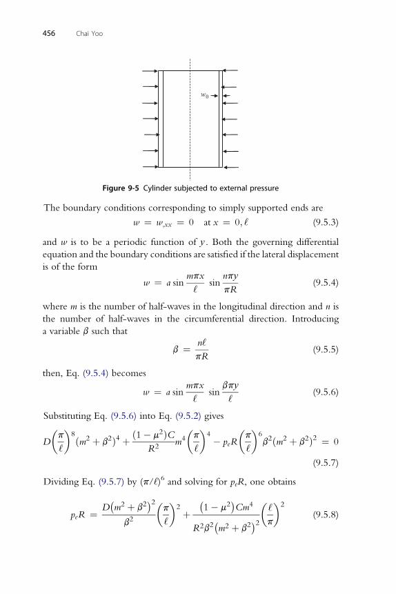
w0

Figure 9-5 Cylinder subjected to external pressure

456 Chai Yoo

The boundary conditions corresponding to simply supported ends are

w ¼ w;xx ¼ 0 at x ¼ 0; ‘ (9.5.3)

and w is to be a periodic function of y . Both the governing differential

equation and the boundary conditions are satisfied if the lateral displacement

is of the form

w ¼ a sinmpx

‘sin

npy

pR(9.5.4)

where m is the number of half-waves in the longitudinal direction and n is

the number of half-waves in the circumferential direction. Introducing

a variable b such that

b ¼ n‘

pR(9.5.5)

then, Eq. (9.5.4) becomes

w ¼ a sinmpx

‘sin

bpy

‘(9.5.6)

Substituting Eq. (9.5.6) into Eq. (9.5.2) gives

D

�p

‘

�8ðm2 þ b2Þ4 þ ð1� m2ÞC

R2m4

�p

‘

�4 � peR

�p

‘

�6b2ðm2 þ b2Þ2 ¼ 0

(9.5.7)

Dividing Eq. (9.5.7) by (p/‘)6 and solving for peR, one obtains

peR ¼ D�m2 þ b2

2b2

�p

‘

�2 þ

�1� m2

Cm4

R2b2�m2 þ b2

2�‘

p

�2

(9.5.8)

Buckling of Thin Cylindrical Shell Elements 457

Substituting C ¼ Eh=�1� m2

and D ¼ Eh3=

�12�1� m2

�and rearr-

anging gives

peR

Eh¼ h2

�m2 þ b2

212�1� m2

b2

�p

‘

�2 þ m4

R2b2�m2 þ b2

2�‘

p

�2

(9.5.9)

For particular values of ‘/R and R/h, the m and n corresponding to the

smallest eigenvalue may be calculated by trial and error.

As an example, calculate pcr for a cylinder with R ¼ 20 in., ‘ ¼ 20

in., h ¼ 0.2 in., E ¼ 10 � 106 psi, and m ¼ 0.3. It is found from

executing Eq. (9.5.9) by Maple� that for m ¼ 1 and n ¼ 7, 8, and 9,

respectively, pe ¼ 122.13, 105.97, and 107.92 psi and that pe is higher for

all other values of m and n. Therefore, pcr is taken to be 105.97 psi. The

values for the sine-wave length parameters m and n indicate that the shell

has one-half sine wave in the axial direction and eight full sine waves in

the circumferential direction in the eigen mode shape. It would seem

intuitively clear that m must be equal to one, otherwise pe would

become larger than that for m ¼ 1. Then, Eq. (9.5.9) may be rewritten

as

pe ¼ Eh

R

264 h2

�1þ b2

212�1� m2

b2

�p

‘

�2 þ 1

R2b2�1þ b2

2�‘

p

�2

375 (9.5.10)

If ‘.R approaches infinity, Eq. (9.5.10) reduces to the following as b also

approaches infinity:

pe ¼ n2D

R3(9.5.11)

Equation (9.5.11) agrees with the Donnell analysis of the circular ring

(Brush and Almroth 1975).1 For n ¼ 2, this value is 33% higher (taking the

classical value as the base) than the classical eigenvalue for the ring given in

Timoshenko and Gere (1961).2 The error occurs because of the approxi-

mations. Langhaar (1962) believes that Donnell’s equation gives more

accurate results when multiple wave patterns occur in the buckled form.

When ‘ ¼ 2000 in. in the above example with n ¼ 2, Eq. (9.5.10) gives

1 See page 139.2 See page 291.

458 Chai Yoo

pe¼ 3.666 psi, while Eq. (9.5.11) yields pe¼ 3.663 psi. Although Eq. (9.5.10)

gives much lower pe for n ¼ 1, Timoshenko and Gere (1961)3 show that the

smallest possible value of nmust be equal to 2 considering an initial ellipticity

and the inextensibility of the member in the circumferential direction.

For external lateral pressure p, the hoop compressive stress sy is related by

sy ¼ pR/h, although the validity of this relationship is questionable at the

ends of the cylinder where simply supported boundary conditions and

corresponding displacement function Eq. (9.5.6) are assumed. Hence, scr ¼pcrR/h. As the cylinder radius approaches infinity, the critical stress scrapproaches the value given in Fig. 8-12 for long flat plates; that is, scr ¼4p2D/‘2 h. In the above example, when R¼ 500 in. and ‘¼ 1 in. with n¼1570, Eq. (9.5.10) gives pe ¼ 578.4389 psi, while the simple hoop

compression relation yields pe ¼ 578.4383 psi.

A good overview of the historical development on the subject is given in

Allen and Bulson (1980), which includes the contribution of von Mises

(1914), Southwell (1914), Donnell (1933), Batdorf (1947), Kraus (1967),

and Brush and Almroth (1975).

9.5.2. Axially Loaded CylindersConsider a circular cylinder of length ‘ and radius R that is simply supported

at its ends and subjected to a uniformly distributed axial compressive load P.

Under the action of the load, the cylinder shortens and except at the

ends, increases its diameter. The prebuckling static deformation is

axisymmetric, and the critical load Pcr is the lowest load at which equilib-

rium in the axisymmetric form ceases to be stable. Although the lateral

displacement w0 is likely to be a function of x, it is assumed, for simplicity,

uniform as shown in Fig. 9-6 and the prebuckling deformation may be

determined by the linear membrane equations. Under these simplifying

assumptions, the critical load can be determined by solving Donnell

equation Eq. (9.3.15c) in the manner outlined by Batdorf (1947).

From a membrane analysis of the unbuckled cylinder

Nx0 ¼ � P

2pRand Nxy0 ¼ Ny0 ¼ 0

Substituting these values into Donnell equation Eq. (9.3.15c) gives

DV8w þ 1� m2

R2Cw;xxxx þ P

2pRV4w;xx ¼ 0 (9.5.12)

3 See page 295.

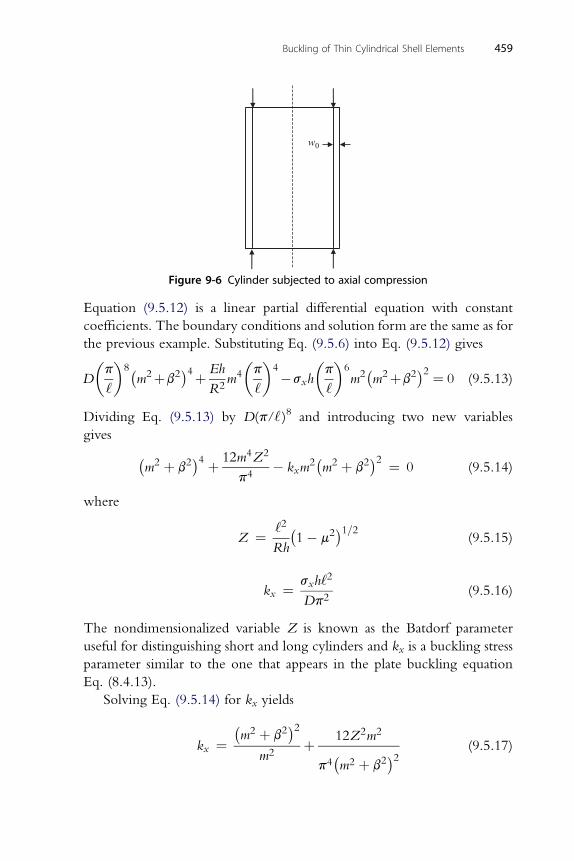
w0

Figure 9-6 Cylinder subjected to axial compression

Buckling of Thin Cylindrical Shell Elements 459

Equation (9.5.12) is a linear partial differential equation with constant

coefficients. The boundary conditions and solution form are the same as for

the previous example. Substituting Eq. (9.5.6) into Eq. (9.5.12) gives

D

�p

‘

�8�m2þb2

4þ Eh

R2m4

�p

‘

�4�sxh

�p

‘

�6m2

�m2þb2

2 ¼ 0 (9.5.13)

Dividing Eq. (9.5.13) by D(p/‘ )8 and introducing two new variables

gives �m2 þ b2

4 þ 12m4Z2

p4� kxm

2�m2 þ b2

2 ¼ 0 (9.5.14)

where

Z ¼ ‘2

Rh

�1� m2

1=2(9.5.15)

2

kx ¼ sxh‘

Dp2(9.5.16)

The nondimensionalized variable Z is known as the Batdorf parameter

useful for distinguishing short and long cylinders and kx is a buckling stress

parameter similar to the one that appears in the plate buckling equation

Eq. (8.4.13).

Solving Eq. (9.5.14) for kx yields

kx ¼�m2 þ b2

2m2

þ 12Z2m2

p4�m2 þ b2

2 (9.5.17)

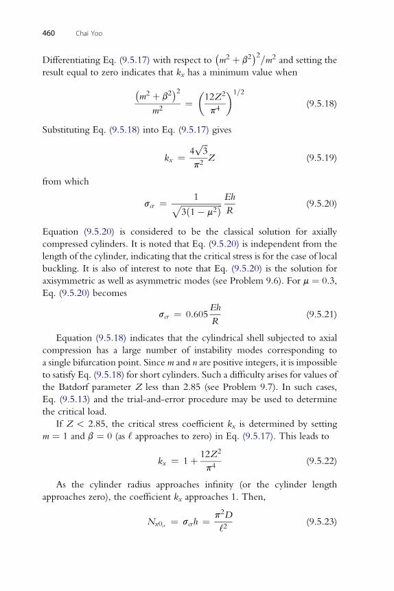
460 Chai Yoo

Differentiating Eq. (9.5.17) with respect to�m2 þ b2

2=m2 and setting the

result equal to zero indicates that kx has a minimum value when

�m2 þ b2

2m2

¼�12Z2

p4

�1=2

(9.5.18)

Substituting Eq. (9.5.18) into Eq. (9.5.17) gives

kx ¼ 4ffiffiffi3

p

p2Z (9.5.19)

from which

scr ¼ 1ffiffiffiffiffiffiffiffiffiffiffiffiffiffiffiffiffiffiffiffi3ð1� m2Þp Eh

R(9.5.20)

Equation (9.5.20) is considered to be the classical solution for axially

compressed cylinders. It is noted that Eq. (9.5.20) is independent from the

length of the cylinder, indicating that the critical stress is for the case of local

buckling. It is also of interest to note that Eq. (9.5.20) is the solution for

axisymmetric as well as asymmetric modes (see Problem 9.6). For m ¼ 0.3,

Eq. (9.5.20) becomes

scr ¼ 0:605Eh

R(9.5.21)

Equation (9.5.18) indicates that the cylindrical shell subjected to axial

compression has a large number of instability modes corresponding to

a single bifurcation point. Since m and n are positive integers, it is impossible

to satisfy Eq. (9.5.18) for short cylinders. Such a difficulty arises for values of

the Batdorf parameter Z less than 2.85 (see Problem 9.7). In such cases,

Eq. (9.5.13) and the trial-and-error procedure may be used to determine

the critical load.

If Z < 2.85, the critical stress coefficient kx is determined by setting

m ¼ 1 and b ¼ 0 (as ‘ approaches to zero) in Eq. (9.5.17). This leads to

kx ¼ 1þ 12Z2

p4(9.5.22)

As the cylinder radius approaches infinity (or the cylinder length

approaches zero), the coefficient kx approaches 1. Then,

Nx0cr ¼ scrh ¼ p2D

‘2(9.5.23)

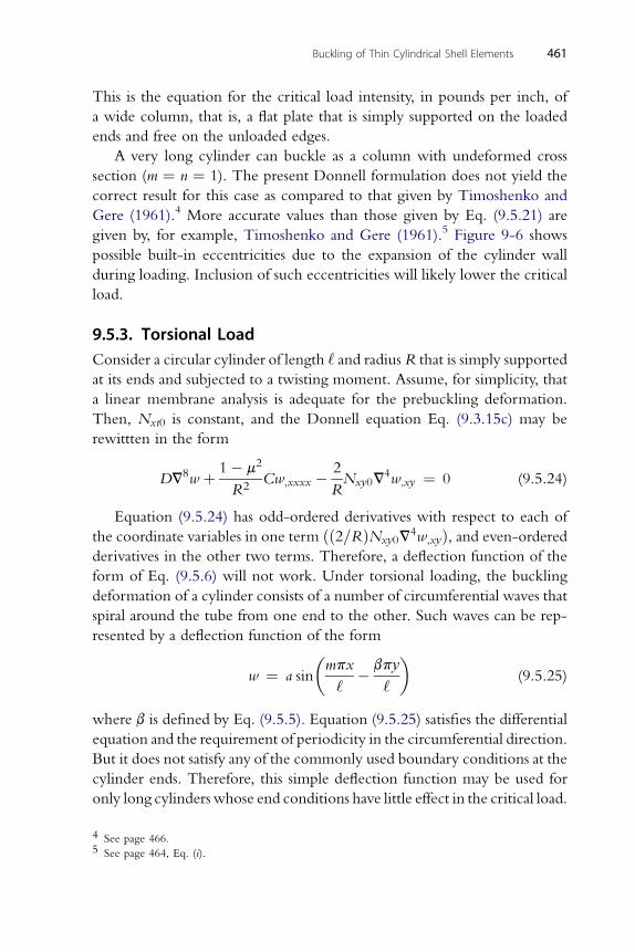
Buckling of Thin Cylindrical Shell Elements 461

This is the equation for the critical load intensity, in pounds per inch, of

a wide column, that is, a flat plate that is simply supported on the loaded

ends and free on the unloaded edges.

A very long cylinder can buckle as a column with undeformed cross

section (m ¼ n ¼ 1). The present Donnell formulation does not yield the

correct result for this case as compared to that given by Timoshenko and

Gere (1961).4 More accurate values than those given by Eq. (9.5.21) are

given by, for example, Timoshenko and Gere (1961).5 Figure 9-6 shows

possible built-in eccentricities due to the expansion of the cylinder wall

during loading. Inclusion of such eccentricities will likely lower the critical

load.

9.5.3. Torsional LoadConsider a circular cylinder of length ‘ and radius R that is simply supported

at its ends and subjected to a twisting moment. Assume, for simplicity, that

a linear membrane analysis is adequate for the prebuckling deformation.

Then, Nxt0 is constant, and the Donnell equation Eq. (9.3.15c) may be

rewittten in the form

DV8w þ 1� m2

R2Cw;xxxx � 2

RNxy0V

4w;xy ¼ 0 (9.5.24)

Equation (9.5.24) has odd-ordered derivatives with respect to each of

the coordinate variables in one term ðð2=RÞNxy0V4w;xyÞ, and even-ordered

derivatives in the other two terms. Therefore, a deflection function of the

form of Eq. (9.5.6) will not work. Under torsional loading, the buckling

deformation of a cylinder consists of a number of circumferential waves that

spiral around the tube from one end to the other. Such waves can be rep-

resented by a deflection function of the form

w ¼ a sin

�mpx

‘� bpy

‘

�(9.5.25)

where b is defined by Eq. (9.5.5). Equation (9.5.25) satisfies the differential

equation and the requirement of periodicity in the circumferential direction.

But it does not satisfy any of the commonly used boundary conditions at the

cylinder ends. Therefore, this simple deflection function may be used for

only long cylinders whose end conditions have little effect in the critical load.

4 See page 466.5 See page 464, Eq. (i).

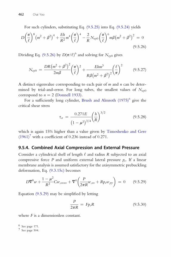
462 Chai Yoo

For such cylinders, substituting Eq. (9.5.25) into Eq. (9.5.24) yields

D

�p

‘

�8�m2 þ b2

4 þ Eh

R2m4

�p

‘

�4 � 2

RNxy0

�p

‘

�6mb

�m2 þ b2

2 ¼ 0

(9.5.26)

Dividing Eq. (9.5.26) by D(p/‘ )6 and solving for Nxy0 gives

Nxy0 ¼ DR�m2 þ b2

22mb

�p

‘

�2 þ Ehm3

Rb�m2 þ b2

2�‘

p

�2

(9.5.27)

A distinct eigenvalue corresponding to each pair of m and n can be deter-

mined by trial-and-error. For long tubes, the smallest values of Nxy0

correspond to n ¼ 2 (Donnell 1933).

For a sufficiently long cylinder, Brush and Almroth (1975)6 give the

critical shear stress

scr ¼ 0:271E�1� m2

3=4�h

R

�3=2

(9.5.28)

which is again 15% higher than a value given by Timoshenko and Gere

(1961)7 with a coefficient of 0.236 instead of 0.271.

9.5.4. Combined Axial Compression and External PressureConsider a cylindrical shell of length ‘ and radius R subjected to an axial

compressive force P and uniform external lateral pressure pe. If a linear

membrane analysis is assumed satisfactory for the axisymmetric prebuckling

deformation, Eq. (9.3.15c) becomes

DV8w þ 1� m2

R2Cw;xxxx þ V4

�P

2pRw;xx þ Rpew;yy

�¼ 0 (9.5.29)

Equation (9.5.29) may be simplified by letting

P

2pR¼ FpeR (9.5.30)

where F is a dimensionless constant.

6 See page 171.7 See page 504.

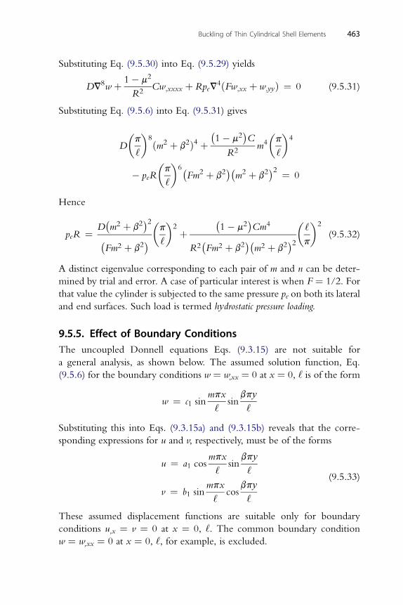
Buckling of Thin Cylindrical Shell Elements 463

Substituting Eq. (9.5.30) into Eq. (9.5.29) yields

DV8w þ 1� m2

R2Cw;xxxx þ RpeV

4ðFw;xx þ w;yyÞ ¼ 0 (9.5.31)

Substituting Eq. (9.5.6) into Eq. (9.5.31) gives

D

�p

‘

�8ðm2 þ b2Þ4 þ

�1� m2

C

R2m4

�p

‘

�4

� peR

�p

‘

�6�Fm2 þ b2

�m2 þ b2

2 ¼ 0

Hence

peR ¼ D�m2 þ b2

2�Fm2 þ b2

�p

‘

�2 þ

�1� m2

Cm4

R2�Fm2 þ b2

�m2 þ b2

2�‘

p

�2

(9.5.32)

A distinct eigenvalue corresponding to each pair of m and n can be deter-

mined by trial and error. A case of particular interest is when F ¼ 1/2. For

that value the cylinder is subjected to the same pressure pe on both its lateral

and end surfaces. Such load is termed hydrostatic pressure loading.

9.5.5. Effect of Boundary ConditionsThe uncoupled Donnell equations Eqs. (9.3.15) are not suitable for

a general analysis, as shown below. The assumed solution function, Eq.

(9.5.6) for the boundary conditions w ¼ w,xx ¼ 0 at x ¼ 0, ‘ is of the form

w ¼ c1 sinmpx

‘sin

bpy

‘

Substituting this into Eqs. (9.3.15a) and (9.3.15b) reveals that the corre-

sponding expressions for u and v, respectively, must be of the forms

u ¼ a1 cosmpx

‘sin

bpy

‘

v ¼ b1 sinmpx

‘cos

bpy

‘

(9.5.33)

These assumed displacement functions are suitable only for boundary

conditions u,x ¼ v ¼ 0 at x ¼ 0, ‘. The common boundary condition

w ¼ w,xx ¼ 0 at x ¼ 0, ‘, for example, is excluded.

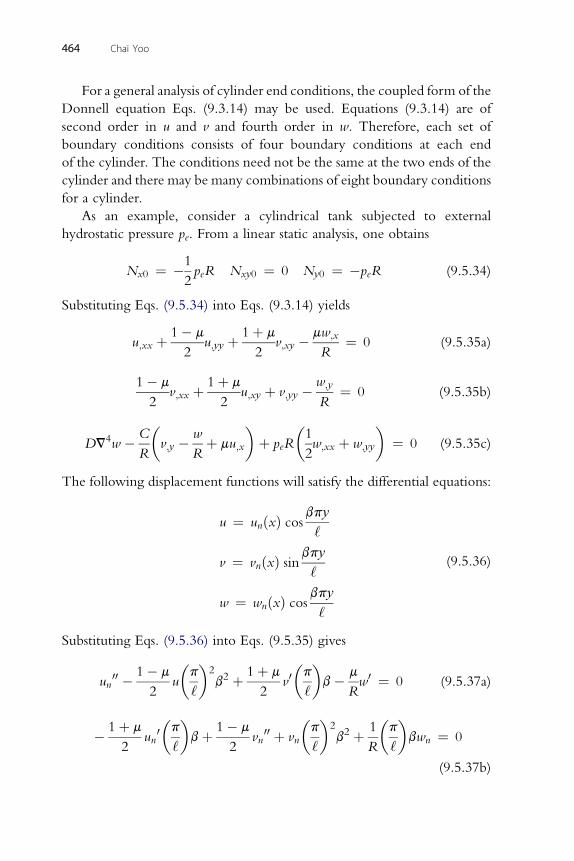
464 Chai Yoo

For a general analysis of cylinder end conditions, the coupled form of the

Donnell equation Eqs. (9.3.14) may be used. Equations (9.3.14) are of

second order in u and v and fourth order in w. Therefore, each set of

boundary conditions consists of four boundary conditions at each end

of the cylinder. The conditions need not be the same at the two ends of the

cylinder and there may be many combinations of eight boundary conditions

for a cylinder.

As an example, consider a cylindrical tank subjected to external

hydrostatic pressure pe. From a linear static analysis, one obtains

Nx0 ¼ �1

2peR Nxy0 ¼ 0 Ny0 ¼ �peR (9.5.34)

Substituting Eqs. (9.5.34) into Eqs. (9.3.14) yields

u;xx þ 1� m

2u;yy þ 1þ m

2v;xy � mw;x

R¼ 0 (9.5.35a)

1� m 1þ m w;y

2v;xx þ

2u;xy þ v;yy �

R¼ 0 (9.5.35b)

C�

w� �

1�

DV4w �R

v;y �Rþ mu;x þ peR

2w;xx þ w;yy ¼ 0 (9.5.35c)

The following displacement functions will satisfy the differential equations:

u ¼ unðxÞ cosbpy‘

v ¼ vnðxÞ sinbpy‘

w ¼ wnðxÞ cos bpy‘

(9.5.36)

Substituting Eqs. (9.5.36) into Eqs. (9.5.35) gives

un00 � 1� m

2u

�p

‘

�2b2 þ 1þ m

2v0�p

‘

�b� m

Rw0 ¼ 0 (9.5.37a)

� � � �2

� �

� 1þ m

2un

0 p

‘bþ 1� m

2vn

00 þ vnp

‘b2 þ 1

R

p

‘bwn ¼ 0

(9.5.37b)

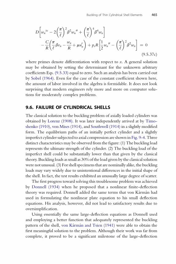
�p�2

�p�4

D wn

iv � 2‘

b2wn00 þ

‘b4wn

�C

R

�p

‘bvn � wn

Rþ mu0n

�þ peR

1

2wn

00 ��p

‘

�2b2wn

¼ 0

(9.5.37c)

where primes denote differentiation with respect to x. A general solution

Buckling of Thin Cylindrical Shell Elements 465

may be obtained by setting the determinant for the unknown arbitrary

coefficients Eqs. (9.5.33) equal to zero. Such an analysis has been carried out

by Sobel (1964). Even for the case of the constant coefficient shown here,

the amount of labor involved in the algebra is formidable. It does not look

surprising that modern engineers rely more and more on computer solu-

tions for moderately complex problems.

9.6. FAILURE OF CYLINDRICAL SHELLS

The classical solution to the buckling problem of axially loaded cylinders was

obtained by Lorenz (1908). It was later independently arrived at by Timo-

shenko (1910), vonMises (1914), and Southwell (1914) in a slightly modified

form. The equilibrium paths of an initially perfect cylinder and a slightly

imperfect cylinder subjected to axial compression are shown in Fig. 9-4. Three

distinct characteristics may be observed from the figure: (1) The buckling load

represents the ultimate strength of the cylinder. (2) The buckling load of the

imperfect shell could be substantially lower than that given by the classical

theory. Buckling loads as small as 30% of the load given by the classical solution

were not unusual. (3) For shell specimens that are nominally alike, the buckling

loads may vary widely due to unintentional differences in the initial shape of

the shell. In fact, the test results exhibited an unusually large degree of scatter.

The first progress toward solving this troublesome problem was achieved

by Donnell (1934) when he proposed that a nonlinear finite-deflection

theory was required. Donnell added the same terms that von Karman had

used in formulating the nonlinear plate equation to his small deflection

equations. His analysis, however, did not lead to satisfactory results due to

oversimplification.

Using essentially the same large-deflection equations as Donnell used

and employing a better function that adequately represented the buckling

pattern of the shell, von Karman and Tsien (1941) were able to obtain the

first meaningful solution to the problem. Although their work was far from

complete, it proved to be a significant milestone of the large-deflection

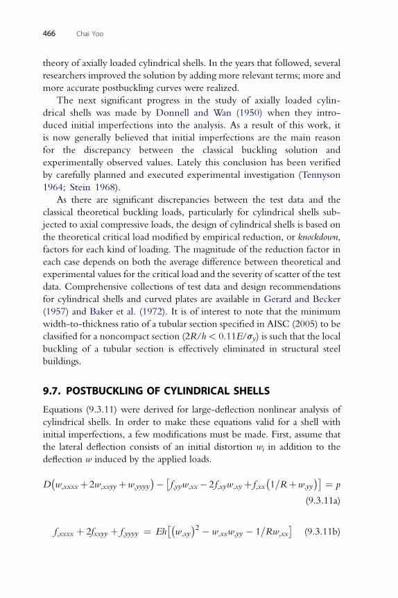
466 Chai Yoo

theory of axially loaded cylindrical shells. In the years that followed, several

researchers improved the solution by adding more relevant terms; more and

more accurate postbuckling curves were realized.

The next significant progress in the study of axially loaded cylin-

drical shells was made by Donnell and Wan (1950) when they intro-

duced initial imperfections into the analysis. As a result of this work, it

is now generally believed that initial imperfections are the main reason

for the discrepancy between the classical buckling solution and

experimentally observed values. Lately this conclusion has been verified

by carefully planned and executed experimental investigation (Tennyson

1964; Stein 1968).

As there are significant discrepancies between the test data and the

classical theoretical buckling loads, particularly for cylindrical shells sub-

jected to axial compressive loads, the design of cylindrical shells is based on

the theoretical critical load modified by empirical reduction, or knockdown,

factors for each kind of loading. The magnitude of the reduction factor in

each case depends on both the average difference between theoretical and

experimental values for the critical load and the severity of scatter of the test

data. Comprehensive collections of test data and design recommendations

for cylindrical shells and curved plates are available in Gerard and Becker

(1957) and Baker et al. (1972). It is of interest to note that the minimum

width-to-thickness ratio of a tubular section specified in AISC (2005) to be

classified for a noncompact section (2R/h< 0.11E/sy) is such that the local

buckling of a tubular section is effectively eliminated in structural steel

buildings.

9.7. POSTBUCKLING OF CYLINDRICAL SHELLS

Equations (9.3.11) were derived for large-deflection nonlinear analysis of

cylindrical shells. In order to make these equations valid for a shell with

initial imperfections, a few modifications must be made. First, assume that

the lateral deflection consists of an initial distortion wi in addition to the

deflection w induced by the applied loads.

D�w;xxxxþ2w;xxyyþw;yyyy

� �f;yyw;xx�2 f;xyw;xyþ f;xx

�1=Rþw;yy

� ¼ p

(9.3.11a)

�� �

f;xxxx þ 2fxxyy þ f;yyyy ¼ Eh w;xy

2 � w;xxw;yy � 1=Rw;xx (9.3.11b)

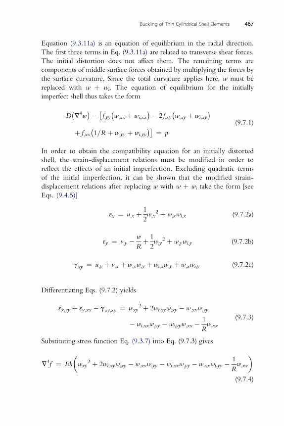
Buckling of Thin Cylindrical Shell Elements 467

Equation (9.3.11a) is an equation of equilibrium in the radial direction.

The first three terms in Eq. (9.3.11a) are related to transverse shear forces.

The initial distortion does not affect them. The remaining terms are

components of middle surface forces obtained by multiplying the forces by

the surface curvature. Since the total curvature applies here, w must be

replaced with w þ wi. The equation of equilibrium for the initially

imperfect shell thus takes the form

D�V4w

� �f;yy

�w;xx þ wi;xx

� 2 f;xy�w;xy þ wi;xy

þ f;xx

�1=R þ w;yy þ wi;yy

� ¼ p

(9.7.1)

In order to obtain the compatibility equation for an initially distorted

shell, the strain-displacement relations must be modified in order to

reflect the effects of an initial imperfection. Excluding quadratic terms

of the initial imperfection, it can be shown that the modified strain-

displacement relations after replacing w with w þ wi take the form [see

Eqs. (9.4.5)]

3x ¼ u;x þ 1

2w;x

2 þ w;xwi;x (9.7.2a)

3y ¼ v;y � w

Rþ 1

2w;y

2 þ w;ywi;y (9.7.2b)

gxy ¼ u;y þ v;x þ w;xw;y þ wi;xw;y þ w;xwi;y (9.7.2c)

Differentiating Eqs. (9.7.2) yields

3x;yy þ 3y;xx � gxy;xy ¼ wxy2 þ 2wi;xyw;xy � w;xxw;yy

� wi;xxw;yy � wi;yyw;xx � 1

Rw;xx

(9.7.3)

Substituting stress function Eq. (9.3.7) into Eq. (9.7.3) gives

V4f ¼ Eh

�wxy

2 þ 2wi;xyw;xy � w;xxw;yy � wi;xxw;yy � w;xxwi;yy � 1

Rw;xx

�(9.7.4)

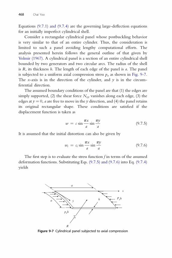
468 Chai Yoo

Equations (9.7.1) and (9.7.4) are the governing large-deflection equations

for an initially imperfect cylindrical shell.

Consider a rectangular cylindrical panel whose postbuckling behavior

is very similar to that of an entire cylinder. Thus, the consideration is

limited to such a panel avoiding lengthy computational efforts. The

analysis presented herein follows the general outline of that given by

Volmir (1967). A cylindrical panel is a section of an entire cylindrical shell

bounded by two generators and two circular arcs. The radius of the shell

is R, its thickness h. The length of each edge of the panel is a. The panel

is subjected to a uniform axial compression stress px as shown in Fig. 9-7.

The x-axis is in the direction of the cylinder, and y is in the circum-

ferential direction.

The assumed boundary conditions of the panel are that (1) the edges are

simply supported, (2) the shear force Nxy vanishes along each edge, (3) the

edges at y¼ 0, a are free to move in the y direction, and (4) the panel retains

its original rectangular shape. These conditions are satisfied if the

displacement function is taken as

w ¼ c sinpx

asin

py

a(9.7.5)

It is assumed that the initial distortion can also be given by

wi ¼ ci sinpx

asin

py

a(9.7.6)

The first step is to evaluate the stress function f in terms of the assumed

deformation functions. Substituting Eqs. (9.7.5) and (9.7.6) into Eq. (9.7.4)

yields

pxh

Pxh

a

a y

x

h

R

Figure 9-7 Cylindrical panel subjected to axial compression

Buckling of Thin Cylindrical Shell Elements 469

V4f ¼ Eh

�c2 þ 2cci

�p4

2a4

�cos

2px

aþ cos

2py

a

�

þ c

R

p2

a2

�sin

px

asin

py

a

�(9.7.7)

A particular solution to this equation, obtained by using the method of

undetermined coefficients, is

fp ¼ Eh�c2 þ 2cci

32

�cos

2px

aþ cos

2py

a

�þ Ehca2

4Rp2sin

px

asin

py

a(9.7.8)

The homogeneous solution is obtained considering the prebuckling stress

px in the x direction and Ny ¼ Nxy ¼ 0. Noting that Nx ¼ �pxh and

recalling Nx ¼ f,xx of Eqs. (9.3.7), one obtains the homogeneous solution

fh ¼ �hpx

2y2 (9.7.9)

Hence, the total solution of Eq. (9.7.7) is

f ¼ Eh�c2 þ 2cci

32

�cos

2px

aþ cos

2py

a

�þ Ehca2

4Rp2sin

px

asin

py

a� hpx

2y2

(9.7.10)

A relation between c, ci, and pxwill be determined from Eq. (9.7.1) by means

of the Galerkin method. For the problem at hand, the Galerkin equation

takes the form

Z a

0

Z a

0

L�c g�x; y

dxdy ¼ 0 (9.7.11)

where L(c) is the left-hand side of Eq. (9.7.1)

LðcÞ ¼ DV4w � �f;yy

�w;xx þ wi;xx

� 2 f;xy�w;xy þ wi;xy

þ f;xx

�1=R þ w;yy þ wi;yy

� (9.7.12)

and g(x,y) ¼ sin (px/a) sin(py/a). Substituting Eqs. (9.7.5), (9.7.6), and

(9.7.10) for w, wi, and f , respectively, Eq. (9.7.12) becomes

470 Chai Yoo

LðcÞ ¼ 4Dc

�p

a

�4sin

px

asin

py

a�p2

8a2Eh

�c2 þ 2cci

cos

2py

a

þ 1

4Ehc sin

px

asin

py

a� hpx

�p

a

�2�c þ ci

sin

px

asin

py

a

þ 1

2R

�p

a

�2Ehc cos3

px

acos3

py

a

�c þ ci

� p2

8a2Eh

�c2 þ 2cci

cos

2px

a

þ 1

4Ehc sin

px

asin

py

a

� 1

Rþ�p

a

�2�c þ ci

sin

px

asin

py

a

Substituting L (c) and g (x,y) into Eq. (9.7.11) and carrying out integration

Maple� gives

Dcp4

a2� pxhp

2

4

�c þ ci

þ Eha2c

16R2� Eh

R

�5

6c2 þ cci

�

þ Ehp4

32a2

�c3 þ 3c2ci þ 2cci

2�

¼ 0

(9.7.13)

from which

px ¼4Dp2

a2hþ Ea2

4p2R2þ Ep2

8a2

�c2 þ 3cci þ 2c2i

�� 4E

p2R

�5

6c þ ci

�c

c þ ci

(9.7.14)

Introduce the following nondimensional parameters into Eq. (9.7.14) to

characterize the influence of each parameter to the postbuckling behavior of

the panel:

px ¼ pxa2

Eh2

k ¼ a2

hR

d ¼ c

h

di ¼ ci

h

The parameters are measures of the loading ( px), of the curvature of the

panel (k), and of the deflections (d and di), respectively. Substituting the

parameters into Eq. (9.7.14) yields

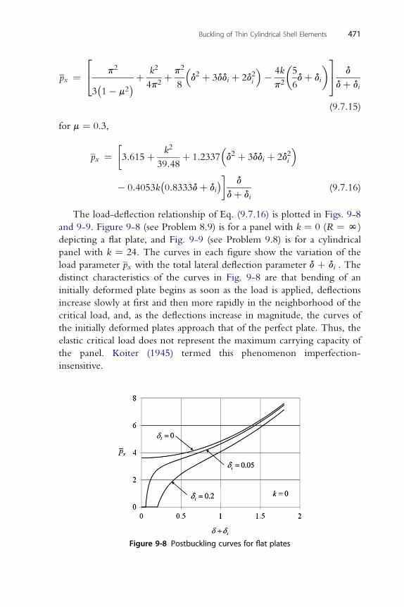
Buckling of Thin Cylindrical Shell Elements 471

px ¼24 p2

3�1� m2

þ k2

4p2þ p2

8

�d2 þ 3ddi þ 2d2i

�� 4k

p2

�5

6dþ di

�35 d

dþ di

(9.7.15)

for m ¼ 0.3,

px ¼3:615þ k2

39:48þ 1:2337

�d2 þ 3ddi þ 2d2i

�

� 0:4053k�0:8333dþ di

d

dþ di(9.7.16)

The load-deflection relationship of Eq. (9.7.16) is plotted in Figs. 9-8

and 9-9. Figure 9-8 (see Problem 8.9) is for a panel with k ¼ 0 (R ¼ N)

depicting a flat plate, and Fig. 9-9 (see Problem 9.8) is for a cylindrical

panel with k ¼ 24. The curves in each figure show the variation of the

load parameter px with the total lateral deflection parameter d þ di . The

distinct characteristics of the curves in Fig. 9-8 are that bending of an

initially deformed plate begins as soon as the load is applied, deflections

increase slowly at first and then more rapidly in the neighborhood of the

critical load, and, as the deflections increase in magnitude, the curves of

the initially deformed plates approach that of the perfect plate. Thus, the

elastic critical load does not represent the maximum carrying capacity of

the panel. Koiter (1945) termed this phenomenon imperfection-

insensitive.

Figure 9-8 Postbuckling curves for flat plates

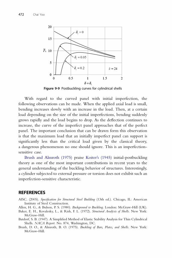
Figure 9-9 Postbuckling curves for cylindrical shells

472 Chai Yoo

With regard to the curved panel with initial imperfection, the

following observations can be made. When the applied axial load is small,

bending increases slowly with an increase in the load. Then, at a certain

load depending on the size of the initial imperfections, bending suddenly

grows rapidly and the load begins to drop. As the deflection continues to

increase, the curve of the imperfect panel approaches that of the perfect

panel. The important conclusion that can be drawn form this observation

is that the maximum load that an initially imperfect panel can support is

significantly less than the critical load given by the classical theory,

a dangerous phenomenon no one should ignore. This is an imperfection-

sensitive case.

Brush and Almroth (1975) praise Koiter’s (1945) initial-postbuckling

theory as one of the most important contributions in recent years to the

general understanding of the buckling behavior of structures. Interestingly,

a cylinder subjected to external pressure or torsion does not exhibit such an

imperfection-sensitive characteristic.

REFERENCESAISC. (2005). Specification for Structural Steel Building (13th ed.). Chicago, IL: American

Institute of Steel Construction.Allen, H. G., & Bulson, P. S. (1980). Background to Buckling. London: McGraw-Hill (UK).Baker, E. H., Kovalesky, L., & Rish, F. L. (1972). Structural Analysis of Shells. New York:

McGraw-Hill.Batdorf, S. B. (1947). A Simplified Method of Elastic Stability Analysis for Thin Cylindrical

Shells. NACA Report. No. 874, Washington, DC.Brush, D. O., & Almroth, B. O. (1975). Buckling of Bars, Plates, and Shells. New York:

McGraw-Hill.

Buckling of Thin Cylindrical Shell Elements 473

Chajes, A. (1974). Principles of Structural Stability Theory. Englewood Cliffs, NJ: Prentice-Hall.

Donnell, L. H. (1933). Stability of Thin-Walled Tubes under Torsion. NACA TechnicalReport. No. 479, Washington, DC.

Donnell, L. H. (1934). New Theory for Buckling of Thin Cylinders Under AxialCompression and Bending. Transactions, ASME, Vol. 56, 795–806.

Donnell, L. H., & Wan, C. C. (1950). Effect of Imperfections on Buckling of ThinCylinders and Columns Under Axial Compression. Journal of Applied Mechanics, Vol. 17(No. 1), 73–88.

Gerard, G., & Becker, H. (1957). Handbook of Structural Stability, Part III, Buckling ofCurved Plates and Shells. NACA Technical Note. No. 3787, Washington, DC.

Koiter, W. T. (1945). On the Stability of Elastic Equilibrium (in Dutch with Englishsummary), thesis, Delft, H.J. Paris, Amsterdam. English translation, Air Force FlightDynamics Laboratory, Technical Report, AFFDL-TR-70-25, February 1970.

Kraus, H. (1967). Thin Elastic Shells. New York: John Wiley and Sons.Langhaar, H. L. (1962). Energy Methods in Applied Mechanics. New York: John Wiley and

Sons.Lorenz, R. (1908). Achsensymmetrische Verzerrungen in dhnnwandigen Hohlzylindern,

Zeitschrift des Vereines Deutscher Ingeniere, Vol. 52(No. 43), 1766.Sobel, L. H. (1964). Effects of Boundary Conditions on the Stability of Cylinders Subjected

to Lateral and Axial Pressure. AIAA J., Vol. 2, 1437–1440.Southwell, R. V. (1914). On the General Theory of Elastic Stability. Phil. Trans. Roy. Soc.

London, Series A, 213, 187.Stein, M. (1968). Some Recent Advances in the Investigation of Shell Buckling. AIAA

Journal, Vol. 6(No. 12), 2339–2345.Tennyson, R. C. (1964). An Experimental Investigation of the Buckling of Circular Cylindrical

Shells in Axial Compression Using the Photoelastic Technique. Institute of AerospaceScience, University of Toronto. Report No. 102.

Timoshenko, S. P. (1910). Einige Stabilitytsprobleme der Elastizityts-theorie. Zeitschriftfur Mathematik und Physik, Vol. 58(No.4), 378.

Timoshenko, S. P., & Gere, J. M. (1961). Theory of Elastic Stability (2nd ed.). New York:McGraw-Hill.

Volmir, A. S. (1967). A Translation of Flexible Plates and Shells. Air Force Flight DynamicsLaboratory, Technical Report No. 66-216, Wright-

von Karman, T., & Tsien, H. S. (1941). The Buckling of Thin Cylindrical Shells underAxial Compression. Journal of the Aeronautical Sciences, Vol. 8(No. 8), 303–312.

von Mises, R. (1914). Z. Ver. deut. Ingr., Vol. 58, 750.

PROBLEMS

9.1 Show that Eqs. (9.2.9) may be derived from those in Eqs. (9.2.2),

(9.2.3), and (9.2.5) by introducing appropriate constitutive and kine-

matic relations.

9.2 Show that the application of the Euler-Lagrange differential equations

Eqs. (9.3.6) to the integrand of Eq. (9.3.1) leads to the equilibrium

equations given in Eqs. (9.2.9).

9.3 Show that Eqs. (9.3.14a) and (9.3.14b) can be partially uncoupled to

obtain Eqs. (9.3.15a) and (9.3.15b). Show that the u and v may be

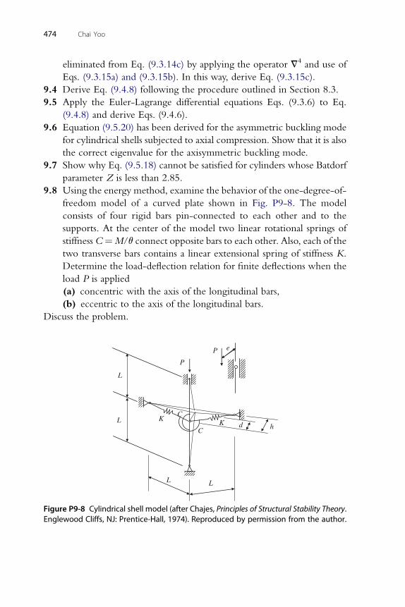
474 Chai Yoo

eliminated from Eq. (9.3.14c) by applying the operator V4 and use of

Eqs. (9.3.15a) and (9.3.15b). In this way, derive Eq. (9.3.15c).

9.4 Derive Eq. (9.4.8) following the procedure outlined in Section 8.3.

9.5 Apply the Euler-Lagrange differential equations Eqs. (9.3.6) to Eq.

(9.4.8) and derive Eqs. (9.4.6).

9.6 Equation (9.5.20) has been derived for the asymmetric buckling mode

for cylindrical shells subjected to axial compression. Show that it is also

the correct eigenvalue for the axisymmetric buckling mode.

9.7 Show why Eq. (9.5.18) cannot be satisfied for cylinders whose Batdorf

parameter Z is less than 2.85.

9.8 Using the energy method, examine the behavior of the one-degree-of-

freedom model of a curved plate shown in Fig. P9-8. The model

consists of four rigid bars pin-connected to each other and to the

supports. At the center of the model two linear rotational springs of

stiffnessC¼M/q connect opposite bars to each other. Also, each of the

two transverse bars contains a linear extensional spring of stiffness K.

Determine the load-deflection relation for finite deflections when the

load P is applied

(a) concentric with the axis of the longitudinal bars,

(b) eccentric to the axis of the longitudinal bars.

Discuss the problem.

L

L

L L

h

P

P

K KC

Cd

e

Figure P9-8 Cylindrical shell model (after Chajes, Principles of Structural Stability Theory.Englewood Cliffs, NJ: Prentice-Hall, 1974). Reproduced by permission from the author.

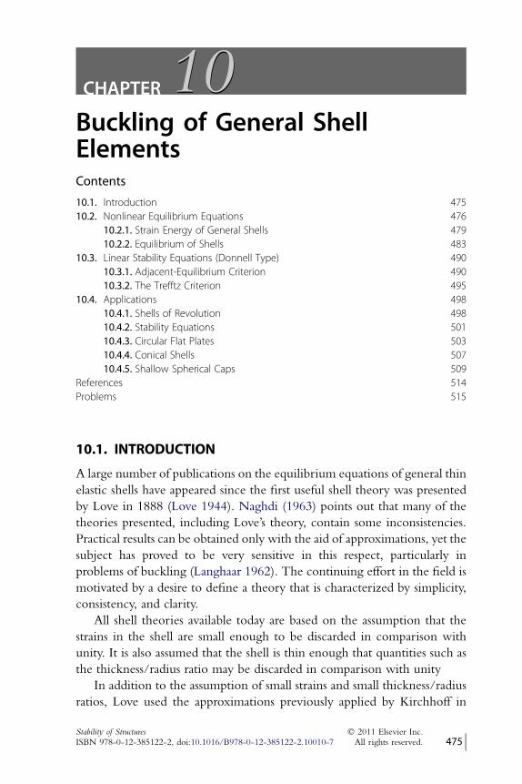
CHAPTER1100

Buckling of General ShellElementsContents

10.1. Introduction 47510.2. Nonlinear Equilibrium Equations 476

10.2.1. Strain Energy of General Shells 47910.2.2. Equilibrium of Shells 483

10.3. Linear Stability Equations (Donnell Type) 49010.3.1. Adjacent-Equilibrium Criterion 49010.3.2. The Trefftz Criterion 495

10.4. Applications 49810.4.1. Shells of Revolution 49810.4.2. Stability Equations 50110.4.3. Circular Flat Plates 50310.4.4. Conical Shells 50710.4.5. Shallow Spherical Caps 509

References 514Problems 515

10.1. INTRODUCTION

A large number of publications on the equilibrium equations of general thin

elastic shells have appeared since the first useful shell theory was presented

by Love in 1888 (Love 1944). Naghdi (1963) points out that many of the

theories presented, including Love’s theory, contain some inconsistencies.

Practical results can be obtained only with the aid of approximations, yet the

subject has proved to be very sensitive in this respect, particularly in

problems of buckling (Langhaar 1962). The continuing effort in the field is

motivated by a desire to define a theory that is characterized by simplicity,

consistency, and clarity.

All shell theories available today are based on the assumption that the

strains in the shell are small enough to be discarded in comparison with

unity. It is also assumed that the shell is thin enough that quantities such as

the thickness/radius ratio may be discarded in comparison with unity

In addition to the assumption of small strains and small thickness/radius

ratios, Love used the approximations previously applied by Kirchhoff in

Stability of Structures � 2011 Elsevier Inc.ISBN 978-0-12-385122-2, doi:10.1016/B978-0-12-385122-2.10010-7 All rights reserved. 475 j

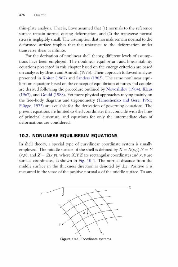
476 Chai Yoo

thin-plate analysis. That is, Love assumed that (1) normals to the reference

surface remain normal during deformation, and (2) the transverse normal

stress is negligibly small. The assumption that normals remain normal to the

deformed surface implies that the resistance to the deformation under

transverse shear is infinite.

For the derivation of nonlinear shell theory, different levels of assump-

tions have been employed. The nonlinear equilibrium and linear stability

equations presented in this chapter based on the energy criterion are based

on analyses by Brush and Amroth (1975). Their approach followed analyses

presented in Koiter (1967) and Sanders (1963). The same nonlinear equi-

librium equations based on the concept of equilibrium of forces and couples

are derived following the procedure outlined by Novozhilov (1964), Klaus

(1967), and Gould (1988). Yet more physical approaches relying mainly on

the free-body diagrams and trigonometry (Timoshenko and Gere, 1961;

Flugge, 1973) are available for the derivation of governing equations. The

present equations are limited to shell coordinates that coincide with the lines

of principal curvature, and equations for only the intermediate class of

deformations are considered.

10.2. NONLINEAR EQUILIBRIUM EQUATIONS

In shell theory, a special type of curvilinear coordinate system is usually

employed. The middle surface of the shell is defined by X ¼ X(x,y),Y ¼ Y

(x,y), and Z ¼ Z(x,y), where X,Y,Z are rectangular coordinates and x, y are

surface coordinates, as shown in Fig. 10-1. The normal distance from the

middle surface in the thickness direction is denoted by �z. Positive z is

measured in the sense of the positive normal n of the middle surface. To any

X

Y Z

x

y

z

Figure 10-1 Coordinate systems

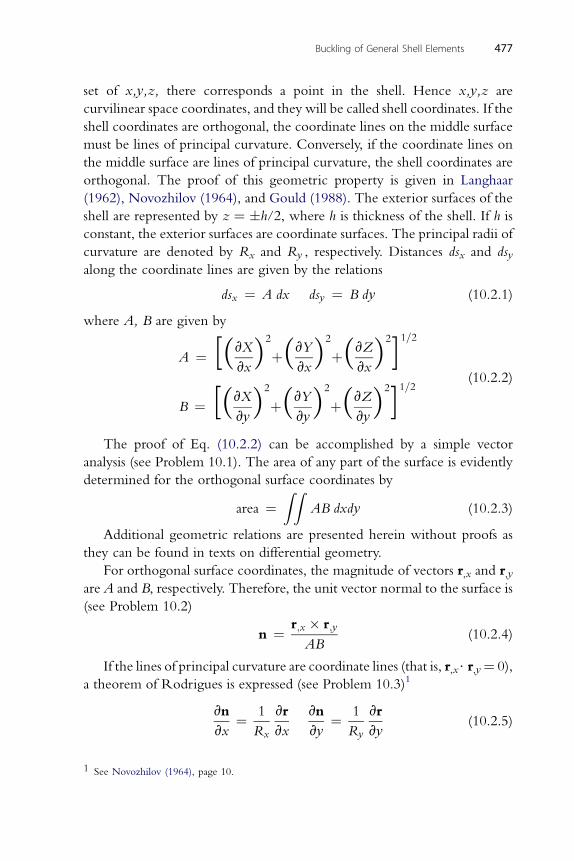
Buckling of General Shell Elements 477

set of x,y,z, there corresponds a point in the shell. Hence x,y,z are

curvilinear space coordinates, and they will be called shell coordinates. If the

shell coordinates are orthogonal, the coordinate lines on the middle surface

must be lines of principal curvature. Conversely, if the coordinate lines on

the middle surface are lines of principal curvature, the shell coordinates are

orthogonal. The proof of this geometric property is given in Langhaar

(1962), Novozhilov (1964), and Gould (1988). The exterior surfaces of the

shell are represented by z ¼ �h/2, where h is thickness of the shell. If h is

constant, the exterior surfaces are coordinate surfaces. The principal radii of

curvature are denoted by Rx and Ry , respectively. Distances dsx and dsyalong the coordinate lines are given by the relations

dsx ¼ A dx dsy ¼ B dy (10.2.1)

where A, B are given by

A ¼ ½ðvXvxÞ2

þðvYvxÞ2

þðvZvxÞ2�1=2

B ¼ ½ðvXvyÞ2

þðvYvyÞ2

þðvZvyÞ2�1=2

(10.2.2)

The proof of Eq. (10.2.2) can be accomplished by a simple vector

analysis (see Problem 10.1). The area of any part of the surface is evidently

determined for the orthogonal surface coordinates by

area ¼ZZ

AB dxdy (10.2.3)

Additional geometric relations are presented herein without proofs as

they can be found in texts on differential geometry.

For orthogonal surface coordinates, the magnitude of vectors r,x and r,yare A and B, respectively. Therefore, the unit vector normal to the surface is

(see Problem 10.2)

n ¼ r;x � r;y

AB(10.2.4)

If the lines of principal curvature are coordinate lines (that is, r,x$ r,y¼ 0),

a theorem of Rodrigues is expressed (see Problem 10.3)1

vn

vx¼ 1

Rx

vr

vx

vn

vy¼ 1

Ry

vr

vy(10.2.5)

1 See Novozhilov (1964), page 10.

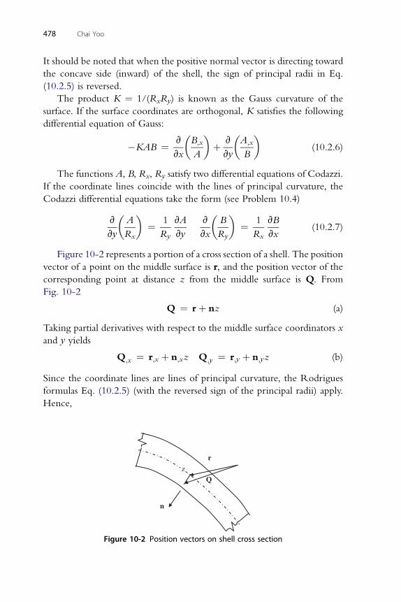
478 Chai Yoo

It should be noted that when the positive normal vector is directing toward

the concave side (inward) of the shell, the sign of principal radii in Eq.

(10.2.5) is reversed.

The product K ¼ 1/(RxRy) is known as the Gauss curvature of the

surface. If the surface coordinates are orthogonal, K satisfies the following

differential equation of Gauss:

�KAB ¼ v

vx

�B;x

A

�þ v

vy

�A;x

B

�(10.2.6)

The functions A, B, Rx, Ry satisfy two differential equations of Codazzi.

If the coordinate lines coincide with the lines of principal curvature, the

Codazzi differential equations take the form (see Problem 10.4)

v

vy

�A

Rx

�¼ 1

Ry

vA

vy

v

vx

�B

Ry

�¼ 1

Rx

vB

vx(10.2.7)

Figure 10-2 represents a portion of a cross section of a shell. The position

vector of a point on the middle surface is r, and the position vector of the

corresponding point at distance z from the middle surface is Q. From

Fig. 10-2

Q ¼ rþ nz (a)

Taking partial derivatives with respect to the middle surface coordinators x

and y yields

Q;x ¼ r;x þ n;xz Q;y ¼ r;y þ n;yz (b)

Since the coordinate lines are lines of principal curvature, the Rodrigues

formulas Eq. (10.2.5) (with the reversed sign of the principal radii) apply.

Hence,

n

r

Q

z

Figure 10-2 Position vectors on shell cross section

Buckling of General Shell Elements 479

Q;x ¼�1� z

Rx

�r;x Q;y ¼

�1� z

Ry

�r;y Q;z ¼ n (c)

By Eq. (10.2.2)

r;x$r;x ¼ A2 and r;y$r;y ¼ B2

Recall

r;x$n ¼ r;y$n ¼ r;x$r;y ¼ 0

Consequently, since ds2 ¼ dQ$dQ ¼ ðQ;xdx þQ;ydy þQ;zdzÞ2;Eq. (c) gives

ds2 ¼ a2dx2 þ b2dy2 þ g2dz2 (10.2.8)

where

a ¼ A

�1� z

Rx

�b ¼ B

�1� z

Ry

�g ¼ 1 (10.2.9)

The factors a; b; g are called the Lame coefficients.2 Note that a ¼ A

and b ¼ B, if z ¼ 0, that is, on the middle surface. Eq. (c) shows that Q;x

and Q;y are parallel to the vectors r;x and r;y.

10.2.1. Strain Energy of General ShellsKoiter (1960) theory is based on a strain energy expression derived in terms

of the following three simplifying assumptions:

1. The shell is thin, that is, h=R <<< 1, where R is the smallest principal

radius of curvature of the undeformed middle surface of the shell.

2. The strains are small compared with unity, and the strain energy density

function is given by the quadratic function of the strain components for

an isotropic elastic material.

3. The state of stress is approximately plane; the effects of transverse

shearing and normal stresses to the middle surface may be neglected in

the strain energy density function.

The third of Koiter’s assumptions is equivalent to the Kirchhoff approxi-

mation used in Chapter 8. Under these assumptions, Koiter (1960) presents

the following equations for the strain energy of a thin elastic shell:

U ¼ Um þ Ub (10.2.10a)

2 See Langhaar (1962), page 181.

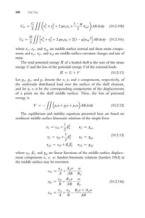
CZZ �

2 2 1� m�

Um ¼2

3x þ 3y þ 2 m3x3y þ2

gxy2 AB dxdy (10.2.10b)

DZZ h i

480 Chai Yoo

Ub ¼2

k2x þ k2y þ 2 mkxky þ 2ð1� mÞkxy 2 AB dxdy (10.2.10c)

where 3x; 3y; and gxy are middle-surface normal and shear strain compo-

nents, and kx; ky; and kxy are middle-surface curvature changes and rate of

twist.

The total potential energy P of a loaded shell is the sum of the strain

energy U and the loss of the potential energy V of the external loads:

P ¼ U þ V (10.2.11)

Let px; py; and pz denote the x, y, and z components, respectively, of

the uniformly distributed load over the surface of the shell element,

and let u, v, w be the corresponding components of the displacements

of a point on the shell middle surface. Then, the loss of potential

energy is

V ¼ �ZZ �

pxuþ pyv þ pzw�AB dxdy (10.2.12)

The equilibrium and stability equations presented here are based on

nonlinear middle-surface kinematic relations of the simple form

3x ¼ exx þ 1

2b2x kx ¼ cxx

3y ¼ eyy þ 1

2b2y ky ¼ cyy

gxy ¼ exy þ bxby kxy ¼ cxy

(10.2.13)

where eij; bi; and cij are linear functions of the middle-surface displace-

ment components u; v; w: Sanders kinematic relations (Sanders 1963) at

the middle surface may be rewritten

exx ¼ u;x

Aþ A;yv

AB� w

Rx

eyy ¼ v;y

Bþ B;xu

AB� w

Ry

exy ¼ v;x

Aþ u;y

B� B;xv þ A;yu

AB

(10.2.14a)

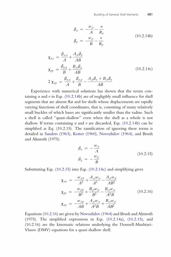
w;x u

bx ¼ �

A�Rx

by ¼ �w;y

B� v

Ry

(10.2.14b)

b A;yb

Buckling of General Shell Elements 481

cxx ¼ x;x

Aþ y

AB

cyy ¼ by;y

Bþ B;xbx

AB

2 cxy ¼ by;x

Aþ bx;y

B� A;ybx þ B;xby

AB

(10.2.14c)

Experience with numerical solutions has shown that the terms con-

taining u and v in Eqs. (10.2.14b) are of negligibly small influence for shell

segments that are almost flat and for shells whose displacements are rapidly

varying functions of shell coordinates, that is, consisting of many relatively

small buckles of which bases are significantly smaller than the radius. Such

a shell is called “quasi-shallow” even when the shell as a whole is not

shallow. If terms containing u and v are discarded, Eqs. (10.2.14b) can be

simplified as Eq. (10.2.15). The ramification of ignoring these terms is

detailed in Sanders (1963), Koiter (1960), Novozhilov (1964), and Brush

and Almroth (1975).

bx ¼ � w;x

A

by ¼ � w;y

B

(10.2.15)

Substituting Eqs. (10.2.15) into Eqs. (10.2.14c) and simplifying gives

cxx ¼ �w;xx

A2þ A;xw;x

A3� A;yw;y

AB2

cyy ¼ �w;yy

B2þ B;yw;y

B3� B;xw;x

A2B

cxy ¼ �w;xy

ABþ A;yw;x

A2Bþ B;xw;y

AB2

(10.2.16)

Equations (10.2.16) are given by Novozhilov (1964) and Brush and Almroth

(1975). The simplified expressions in Eqs. (10.2.14a), (10.2.15), and

(10.2.16) are the kinematic relations underlying the Donnell-Mushtari-

Vlasov (DMV) equations for a quasi-shallow shell.

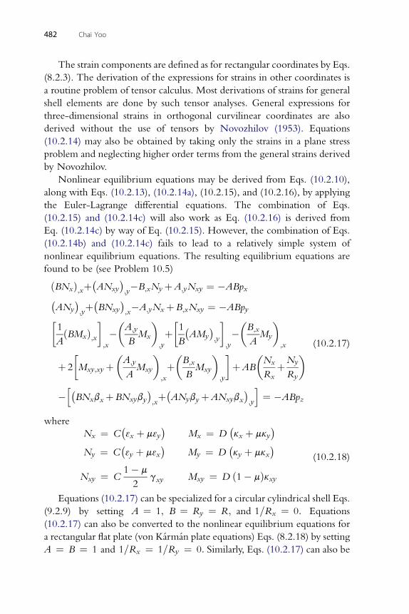
482 Chai Yoo

The strain components are defined as for rectangular coordinates by Eqs.

(8.2.3). The derivation of the expressions for strains in other coordinates is

a routine problem of tensor calculus. Most derivations of strains for general

shell elements are done by such tensor analyses. General expressions for

three-dimensional strains in orthogonal curvilinear coordinates are also

derived without the use of tensors by Novozhilov (1953). Equations

(10.2.14) may also be obtained by taking only the strains in a plane stress

problem and neglecting higher order terms from the general strains derived

by Novozhilov.

Nonlinear equilibrium equations may be derived from Eqs. (10.2.10),

along with Eqs. (10.2.13), (10.2.14a), (10.2.15), and (10.2.16), by applying

the Euler-Lagrange differential equations. The combination of Eqs.

(10.2.15) and (10.2.14c) will also work as Eq. (10.2.16) is derived from

Eq. (10.2.14c) by way of Eq. (10.2.15). However, the combination of Eqs.

(10.2.14b) and (10.2.14c) fails to lead to a relatively simple system of

nonlinear equilibrium equations. The resulting equilibrium equations are

found to be (see Problem 10.5)

ðBNxÞ;xþ�ANxy

�;y�B;xNyþA;yNxy ¼ �ABpx�

ANy

�;yþ�

BNxy

�;x�A;yNxþB;xNxy ¼ �ABpy�

1

AðBMxÞ;x

;x

��A;y

BMx

�;y

þ�1

B

�AMy

�;y

;y

��B;x

AMy

�;x

þ 2

�Mxy;xyþ

�A;y

AMxy

�;x

þ�B;x

BMxy

�;y

þAB

�Nx

RxþNy

Ry

�

�h�BNxbxþBNxyby

�;xþ�

ANybyþANxybx�;y

i¼ �ABpz

(10.2.17)

where

Nx ¼ C�3x þ m3y

�Mx ¼ D

�kx þ mky

�Ny ¼ C

�3y þ m3x

�My ¼ D

�ky þ mkx

�Nxy ¼ C

1� m

2gxy Mxy ¼ D ð1� mÞkxy

(10.2.18)

Equations (10.2.17) can be specialized for a circular cylindrical shell Eqs.

(9.2.9) by setting A ¼ 1; B ¼ Ry ¼ R; and 1=Rx ¼ 0: Equations

(10.2.17) can also be converted to the nonlinear equilibrium equations for

a rectangular flat plate (von Karman plate equations) Eqs. (8.2.18) by setting

A ¼ B ¼ 1 and 1=Rx ¼ 1=Ry ¼ 0: Similarly, Eqs. (10.2.17) can also be

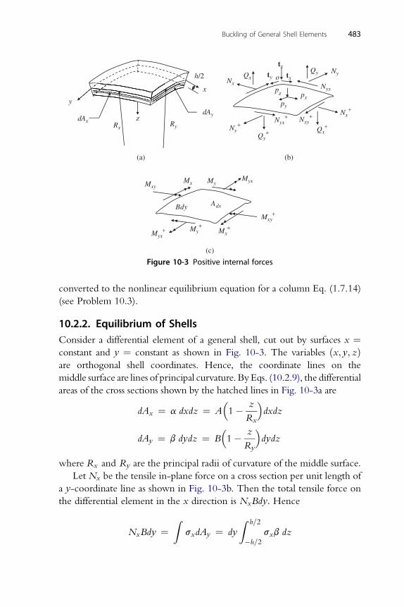
(c)

MyxMy

Mx+

Mxy+

Myx+ My

+

MxyMx

Bdy Adx

(b)

Nx+

Nx

Ny

Nyx

Qx+

Nxy+

Qx

Ny+

Qy+

Nyx+

zppx

py

Qy

tz

ty txo

(a)

y

dAy

x

zRyRx

dAx

h/2

Figure 10-3 Positive internal forces

Buckling of General Shell Elements 483

converted to the nonlinear equilibrium equation for a column Eq. (1.7.14)

(see Problem 10.3).

10.2.2. Equilibrium of ShellsConsider a differential element of a general shell, cut out by surfaces x ¼constant and y ¼ constant as shown in Fig. 10-3. The variables ðx; y; zÞare orthogonal shell coordinates. Hence, the coordinate lines on the

middle surface are lines of principal curvature. ByEqs. (10.2.9), the differential

areas of the cross sections shown by the hatched lines in Fig. 10-3a are

dAx ¼ a dxdz ¼ A�1� z

Rx

�dxdz

dAy ¼ b dydz ¼ B�1� z

Ry

�dydz

where Rx and Ry are the principal radii of curvature of the middle surface.

Let Nx be the tensile in-plane force on a cross section per unit length of

a y-coordinate line as shown in Fig. 10-3b. Then the total tensile force on

the differential element in the x direction is NxBdy: Hence

NxBdy ¼Z

sxdAy ¼ dy

Z h=2

�h=2sxb dz

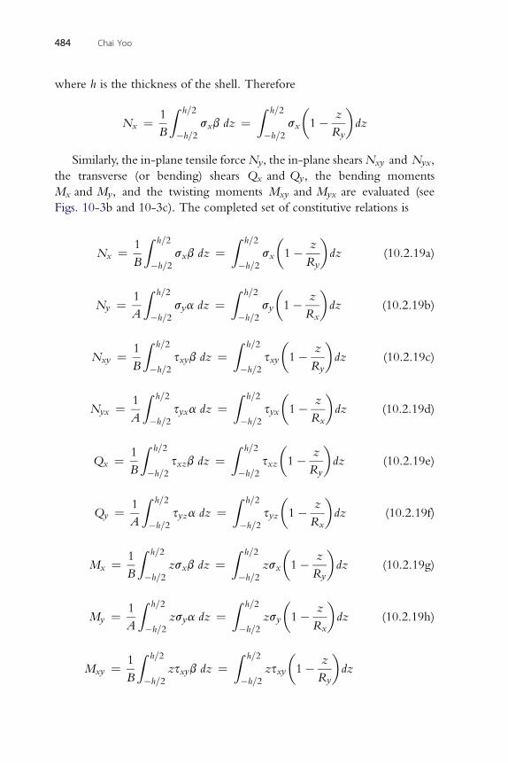
484 Chai Yoo

where h is the thickness of the shell. Therefore

Nx ¼ 1

B

Z h=2

�h=2sxb dz ¼

Z h=2

�h=2sx

�1� z

Ry

�dz

Similarly, the in-plane tensile forceNy, the in-plane shearsNxy and Nyx,

the transverse (or bending) shears Qx and Qy, the bending moments

Mx and My, and the twisting moments Mxy and Myx are evaluated (see

Figs. 10-3b and 10-3c). The completed set of constitutive relations is

Nx ¼ 1

B

Z h=2

�h=2sxb dz ¼

Z h=2

�h=2sx

�1� z

Ry

�dz (10.2.19a)

Z h=2 Z h=2 � �

Ny ¼ 1

A �h=2sya dz ¼

�h=2sy 1� z

Rxdz (10.2.19b)

Z h=2 Z h=2 � �

Nxy ¼ 1

B �h=2sxyb dz ¼

�h=2sxy 1� z

Rydz (10.2.19c)

Z h=2 Z h=2 � �

Nyx ¼ 1

A �h=2syxa dz ¼

�h=2syx 1� z

Rxdz (10.2.19d)

Z h=2 Z h=2 � �

Qx ¼ 1

B �h=2sxzb dz ¼

�h=2sxz 1� z

Rydz (10.2.19e)

Z h=2 Z h=2 � �

Qy ¼ 1

A �h=2syza dz ¼

�h=2syz 1� z

Rxdz (10.2.19f)

Z h=2 Z h=2 � �

Mx ¼ 1

B �h=2zsxb dz ¼

�h=2zsx 1� z

Rydz (10.2.19g)

Z h=2 Z h=2 � �

My ¼ 1

A �h=2zsya dz ¼

�h=2zsy 1� z

Rxdz (10.2.19h)

Z h=2 Z h=2 � �

Mxy ¼ 1

B �h=2zsxyb dz ¼

�h=2zsxy 1� z

Rydz

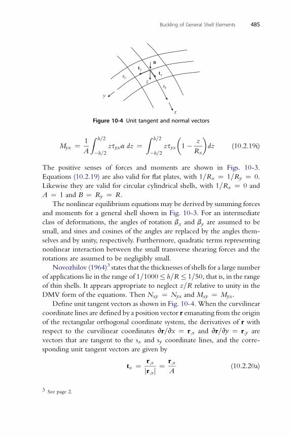
x

y

z

tyn

tx

xsys

Buckling of General Shell Elements 485

1Z h=2 Z h=2 �

z�

Myx ¼A �h=2

zsyxa dz ¼�h=2

zsyx 1�Rx

dz (10.2.19i)

The positive senses of forces and moments are shown in Figs. 10-3.

Equations (10.2.19) are also valid for flat plates, with 1=Rx ¼ 1=Ry ¼ 0.

Likewise they are valid for circular cylindrical shells, with 1=Rx ¼ 0 and

A ¼ 1 and B ¼ Ry ¼ R.

The nonlinear equilibrium equations may be derived by summing forces

and moments for a general shell shown in Fig. 10-3. For an intermediate

class of deformations, the angles of rotation bx and by are assumed to be

small, and sines and cosines of the angles are replaced by the angles them-

selves and by unity, respectively. Furthermore, quadratic terms representing

nonlinear interaction between the small transverse shearing forces and the

rotations are assumed to be negligibly small.

Novozhilov (1964)3 states that the thicknesses of shells for a large number

of applications lie in the range of 1=1000� h=R� 1=50, that is, in the rangeof thin shells. It appears appropriate to neglect z=R relative to unity in the

DMV form of the equations. Then Nxy ¼ Nyx and Mxy ¼ Myx.

Define unit tangent vectors as shown in Fig. 10-4. When the curvilinear

coordinate lines are defined by a position vector r emanating from the origin

of the rectangular orthogonal coordinate system, the derivatives of r with

respect to the curvilinear coordinates vr=vx ¼ r;x and vr=vy ¼ r;y are

vectors that are tangent to the sx and sy coordinate lines, and the corre-

sponding unit tangent vectors are given by

tx ¼ r;x

jr;xj ¼r;x

A(10.2.20a)

Figure 10-4 Unit tangent and normal vectors

3 See page 2.

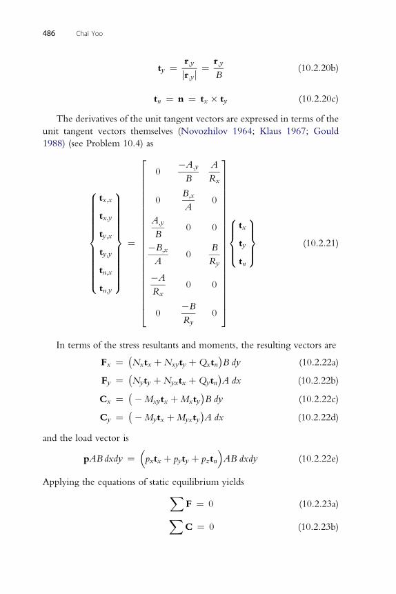
r;y r;y

ty ¼ jr;yj ¼ B

(10.2.20b)

t ¼ n ¼ t � t (10.2.20c)

486 Chai Yoo

n x y

The derivatives of the unit tangent vectors are expressed in terms of the

unit tangent vectors themselves (Novozhilov 1964; Klaus 1967; Gould

1988) (see Problem 10.4) as

8>>>>>>>>>>><>>>>>>>>>>>:

tx;x

tx;y

ty;x

ty;y

tn;x

tn;y

9>>>>>>>>>>>=>>>>>>>>>>>;

¼

266666666666666666666664

0�A;y

B

A

Rx

0B;x

A0

A;y

B0 0

�B;x

A0

B

Ry

�A

Rx0 0

0�B

Ry0

377777777777777777777775

8>><>>:

tx

ty

tn

9>>=>>; (10.2.21)

In terms of the stress resultants and moments, the resulting vectors are

Fx ¼ �Nxtx þNxyty þQxtn

�B dy (10.2.22a)

Fy ¼ �Nyty þNyxtx þQytn

�A dx (10.2.22b)

Cx ¼ ��Mxytx þMxty�B dy (10.2.22c)

Cy ¼ ��Mytx þMyxty�A dx (10.2.22d)

and the load vector is

pAB dxdy ¼�pxtx þ pyty þ pztn

�AB dxdy (10.2.22e)

Applying the equations of static equilibrium yieldsXF ¼ 0 (10.2.23a)XC ¼ 0 (10.2.23b)

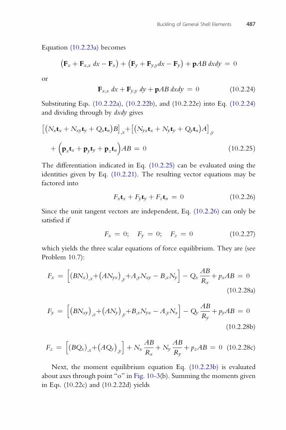
Buckling of General Shell Elements 487

Equation (10.2.23a) becomes

�Fx þ Fx;x dx� Fx

�þ �Fy þ Fy;ydx� Fy

�þ pAB dxdy ¼ 0

or

Fx;x dxþ Fy;y dyþ pAB dxdy ¼ 0 (10.2.24)

Substituting Eqs. (10.2.22a), (10.2.22b), and (10.2.22e) into Eq. (10.2.24)

and dividing through by dxdy gives�Nxtx þNxyty þQxtn

�B�;xþ�

Nyxtx þNyty þQytn�A�;y

þ�pxtx þ pyty þ pztn

�AB ¼ 0 ð10:2:25Þ

The differentiation indicated in Eq. (10.2.25) can be evaluated using the

identities given by Eq. (10.2.21). The resulting vector equations may be

factored into

Fxtx þ Fyty þ Fztn ¼ 0 (10.2.26)

Since the unit tangent vectors are independent, Eq. (10.2.26) can only be

satisfied if

Fx ¼ 0; Fy ¼ 0; Fz ¼ 0 (10.2.27)

which yields the three scalar equations of force equilibrium. They are (see

Problem 10.7):

Fx ¼hðBNxÞ;xþ

�ANyx

�;yþA;yNxy � B;xNy

i�Qx

AB

Rxþ pxAB ¼ 0

(10.2.28a)

h� � � � i AB

Fy ¼ BNxy ;x

þ ANy ;yþB;xNyx � A;yNx �Qy

Ryþ pyAB ¼ 0

(10.2.28b)

h � � i AB AB

Fz ¼ ðBQxÞ;xþ AQy ;y

þNxRx

þNyRy

þ pzAB ¼ 0 (10.2.28c)

Next, the moment equilibrium equation Eq. (10.2.23b) is evaluated

about axes through point “o” in Fig. 10-3(b). Summing the moments given

in Eqs. (10.22c) and (10.2.22d) yields

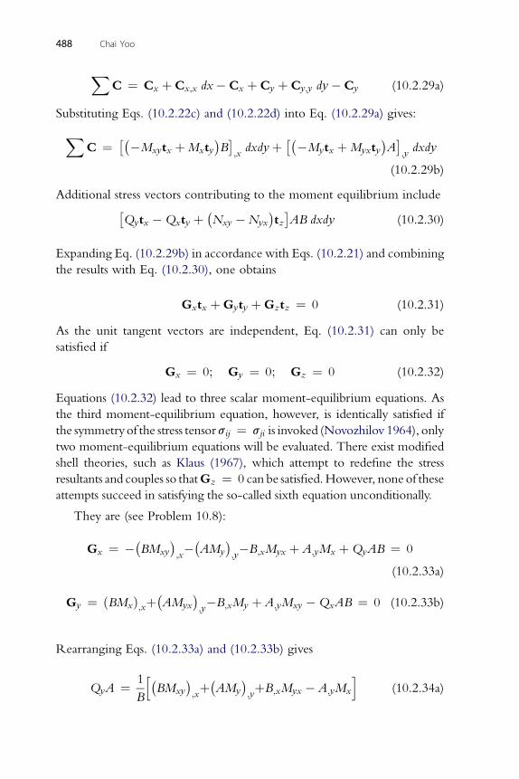
488 Chai Yoo

XC ¼ Cx þ Cx;x dx� Cx þ Cy þ Cy;y dy�Cy (10.2.29a)

Substituting Eqs. (10.2.22c) and (10.2.22d) into Eq. (10.2.29a) gives:

XC ¼ ��Mxytx þMxty

�B�;xdxdyþ ��Mytx þMyxty

�A�;ydxdy

(10.2.29b)

Additional stress vectors contributing to the moment equilibrium includeQytx �Qxty þ

�Nxy �Nyx

�tz�AB dxdy (10.2.30)

Expanding Eq. (10.2.29b) in accordance with Eqs. (10.2.21) and combining

the results with Eq. (10.2.30), one obtains

Gxtx þGyty þGztz ¼ 0 (10.2.31)

As the unit tangent vectors are independent, Eq. (10.2.31) can only be

satisfied if

Gx ¼ 0; Gy ¼ 0; Gz ¼ 0 (10.2.32)

Equations (10.2.32) lead to three scalar moment-equilibrium equations. As

the third moment-equilibrium equation, however, is identically satisfied if

the symmetryof the stress tensorsij ¼ sji is invoked (Novozhilov 1964), only

two moment-equilibrium equations will be evaluated. There exist modified

shell theories, such as Klaus (1967), which attempt to redefine the stress

resultants and couples so thatGz ¼ 0 can be satisfied.However, none of these

attempts succeed in satisfying the so-called sixth equation unconditionally.

They are (see Problem 10.8):

Gx ¼ ��BMxy

�;x��

AMy

�;y�B;xMyx þ A;yMx þQyAB ¼ 0

(10.2.33a)

G ¼ ðBM Þ þ�AM

� �B M þ A M �Q AB ¼ 0 (10.2.33b)

y x ;x yx ;y ;x y ;y xy x

Rearranging Eqs. (10.2.33a) and (10.2.33b) gives

QyA ¼ 1

B

h�BMxy

�;xþ�

AMy

�;yþB;xMyx � A;yMx

i(10.2.34a)

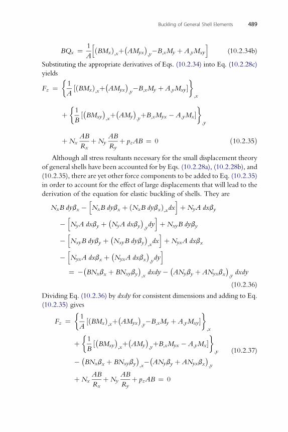
1h � � i

BQx ¼

AðBMxÞ;xþ AMyx ;y

�B;xMy þ A;yMxy (10.2.34b)

Substituting the appropriate derivatives of Eqs. (10.2.34) into Eq. (10.2.28c)

Buckling of General Shell Elements 489

yields

Fz ¼�1

A½ðBMxÞ;xþ

�AMyx

�;y�B;xMy þ A;yMxy�

;x

þ�1

B½�BMxy

�;xþ�

AMy

�;yþB;xMyx � A;yMx�

;y

þNxAB

RxþNy

AB

Ryþ pzAB ¼ 0 ð10:2:35Þ

Although all stress resultants necessary for the small displacement theory

of general shells have been accounted for by Eqs. (10.2.28a), (10.2.28b), and

(10.2.35), there are yet other force components to be added to Eq. (10.2.35)

in order to account for the effect of large displacements that will lead to the

derivation of the equation for elastic buckling of shells. They are

NxB dybx �hNxB dybx þ ðNxB dybxÞ;xdx

iþNyA dxby

�hNyA dxby þ

�NyA dxby

�;ydyiþNxyB dyby

�hNxyB dyby þ

�NxyB dyby

�;xdxiþNyxA dxbx

�hNyxA dxbx þ

�NyxA dxbx

�;ydyi

¼ ��BNxbx þ BNxyby

�;xdxdy� �

ANyby þ ANyxbx�;ydxdy

(10.2.36)

Dividing Eq. (10.2.36) by dxdy for consistent dimensions and adding to Eq.

(10.2.35) gives

Fz ¼�1

A½ðBMxÞ;xþ

�AMyx

�;y�B;xMy þ A;yMxy�

;x

þ�1

B½�BMxy

�;xþ�

AMy

�;yþB;xMyx � A;yMx�

;y

� �BNxbx þ BNxyby

�;x��

ANyby þ ANyxbx�;y

þNxAB

RxþNy

AB

Ryþ pzAB ¼ 0

(10.2.37)

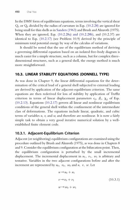
490 Chai Yoo

In the DMV form of equilibrium equations, terms involving the vertical shear

Qx orQy divided by the radius of curvature in Eqs. (10.2.28) are ignored for

being small for thin shells as in Sanders (1963) and Brush and Almroth (1975).

When they are ignored, Eqs. (10.2.28a) and (10.2.28b), and (10.2.37) are

identical to Eqs. (10.2.17) (see Problem 10.9) derived by the principle of

minimum total potential energy by way of the calculus of variations.

It should be noted that the use of the equilibrium method of deriving

a governing differential equation based on an isolated free-body diagram is

much easier for a simple structure, such as a column, but for complex three-

dimensional structures, such as a general shell, the energy method is much

more straightforward.

10.3. LINEAR STABILITY EQUATIONS (DONNELL TYPE)

As was done in Chapter 9, the linear differential equations for the deter-

mination of the critical load of a general shell subjected to external loading

are derived by application of the adjacent-equilibrium criterion. The same

equations are then rederived for loss of stability by application of Trefftz

criterion in terms of linear displacement parameters eij; bi; cij of Eqs.

(10.2.13). Equations (10.2.17) govern all linear and nonlinear equilibrium

conditions of the general shell within the confinement of the intermediate

class of deformations. The equations include linear, quadratic, and cubic

terms of variables u, v, and w, and therefore are nonlinear. It is now a fairly

simple task to obtain a very good iterative numerical solution by a well-

established finite element code.

10.3.1. Adjacent-Equilibrium CriterionAdjacent (or neighboring) equilibrium configurations are examined using the

procedure outlined by Brush and Almroth (1975), as was done in Chapters 8

and 9. Consider the equilibrium configuration at the bifurcation point. Then,

the equilibrium configuration is perturbed by the small incremental

displacement. The incremental displacement in u1; v1; w1 is arbitrary and

tentative. Variables in the two adjacent configurations before and after the

increment are represented by u0; v0; w0 and u; v; w. Let

u/u0 þ u1

v/v0 þ v1

w/w0 þ w1

(10.3.1)

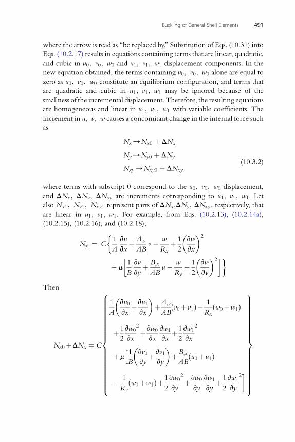
Buckling of General Shell Elements 491

where the arrow is read as “be replaced by.” Substitution of Eqs. (10.31) into

Eqs. (10.2.17) results in equations containing terms that are linear, quadratic,

and cubic in u0; v0; w0 and u1; v1; w1 displacement components. In the

new equation obtained, the terms containing u0; v0; w0 alone are equal to

zero as u0; v0; w0 constitute an equilibrium configuration, and terms that

are quadratic and cubic in u1; v1; w1 may be ignored because of the

smallness of the incremental displacement. Therefore, the resulting equations

are homogeneous and linear in u1; v1; w1 with variable coefficients. The

increment in u; v; w causes a concomitant change in the internal force such

as

Nx/Nx0 þ DNx

Ny/Ny0 þ DNy

Nxy/Nxy0 þ DNxy

(10.3.2)

where terms with subscript 0 correspond to the u0; v0; w0 displacement,

and DNx; DNy; DNxy are increments corresponding to u1; v1; w1. Let

also Nx1; Ny1; Nxy1 represent parts of DNx;DNy; DNxy, respectively, that

are linear in u1; v1; w1. For example, from Eqs. (10.2.13), (10.2.14a),

(10.2.15), (10.2.16), and (10.2.18),

Nx ¼ C

�1

A

vu

vxþ A;y

ABv � w

Rxþ 1

2

�vw

vx

�2

þ m

�1

B

vv

vyþ B;x

ABu� w

Ryþ 1

2

�vw

vy

�2

Then

Nx0þDNx ¼ C

8>>>>>>>>>>>>>>>>><>>>>>>>>>>>>>>>>>:

1

A

�vu0

vxþvu1

vx

�þA;y

ABðv0þ v1Þ� 1

Rxðw0þw1Þ

þ1

2

vw0

vx

2

þvw0

vx

vw1

vxþ1

2

vw1

vx

2

þmh1B

�vv0

vyþvv1

vy

�þB;x

ABðu0þu1Þ

� 1

Ryðw0þw1Þþ1

2

vw0

vy

2

þvw0

vy

vw1

vyþ1

2

vw1

vy

2

9>>>>>>>>>>>>>>>>>=>>>>>>>>>>>>>>>>>;

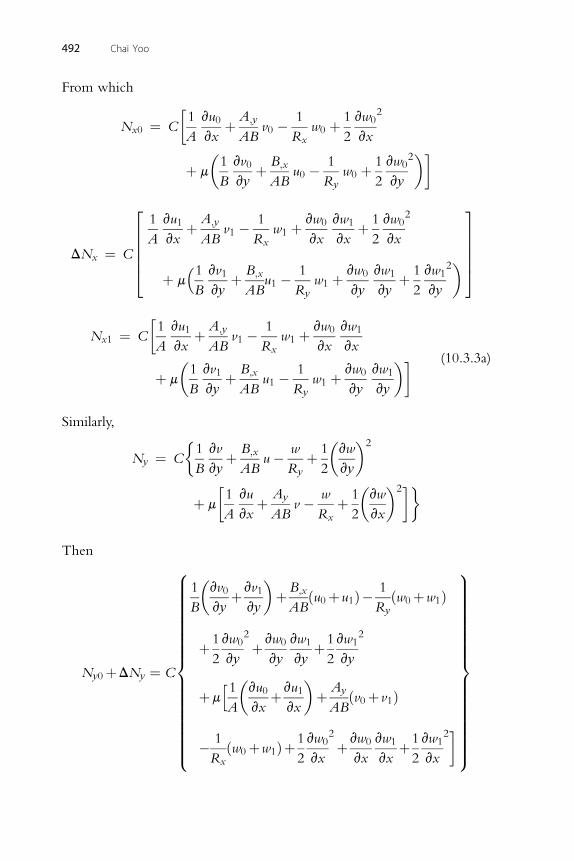
492 Chai Yoo

From which

Nx0 ¼ C

�1

A

vu0

vxþ A;y

ABv0 � 1

Rxw0 þ 1

2

vw0

vx

2

þ m

�1

B

vv0

vyþ B;x

ABu0 � 1

Ryw0 þ 1

2

vw0

vy

2�

232

DNx ¼ C

1

A

vu1

vxþ A;y

ABv1 � 1

Rxw1 þ vw0

vx

vw1

vxþ 1

2

vw0

vx

þ m�1B

vv1

vyþ B;x

ABu1 � 1

Ryw1 þ vw0

vy

vw1

vyþ 1

2

vw1

vy

2�77775

66664�1 vu A 1 vw vw

Nx1 ¼ CA

1

vxþ ;y

ABv1 �

Rxw1 þ 0

vx

1

vx

þ m

�1

B

vv1

vyþ B;x

ABu1 � 1

Ryw1 þ vw0

vy

vw1

vy

� (10.3.3a)

Similarly,

Ny ¼ C

�1

B

vv

vyþ B;x

ABu� w

Ryþ 1

2

�vw

vy

�2

þ m

�1

A

vu

vxþ Ay

ABv � w

Rxþ 1

2

�vw

vx

�2

Then

Ny0þDNy ¼ C

8>>>>>>>>>>>>>>>>><>>>>>>>>>>>>>>>>>:

1

B

�vv0

vyþvv1

vy

�þB;x

ABðu0þu1Þ� 1

Ryðw0þw1Þ

þ 1

2

vw0

vy

2

þvw0

vy

vw1

vyþ1

2

vw1

vy

2

þmh1A

�vu0

vxþvu1

vx

�þ Ay

ABðv0þ v1Þ

� 1

Rxðw0þw1Þþ1

2

vw0

vx

2

þvw0

vx

vw1

vxþ1

2

vw1

vx

2

9>>>>>>>>>>>>>>>>>=>>>>>>>>>>>>>>>>>;

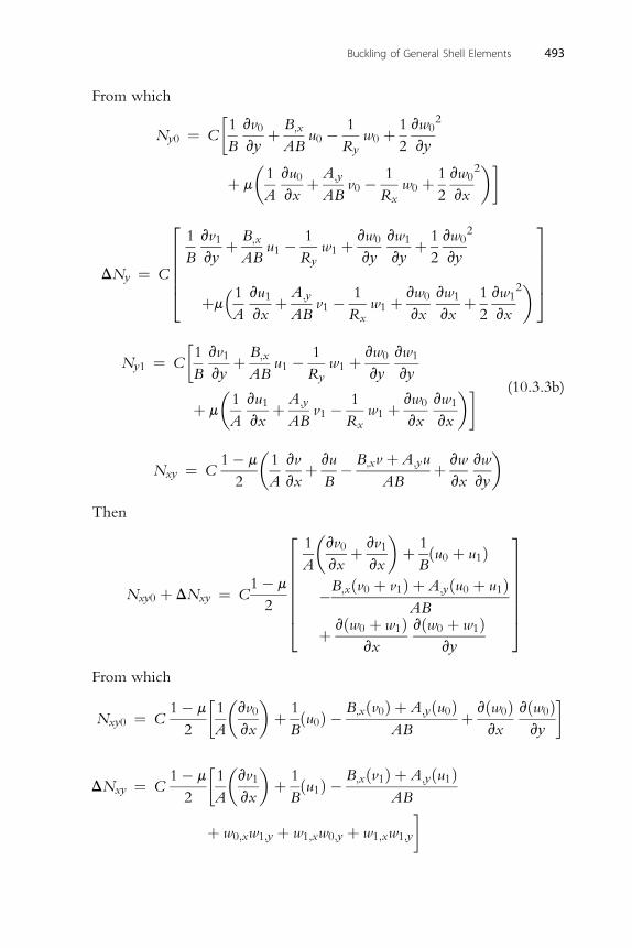
Buckling of General Shell Elements 493

From which

Ny0 ¼ C

�1

B

vv0

vyþ B;x

ABu0 � 1

Ryw0 þ 1

2

vw0

vy

2

þ m

�1

A

vu0

vxþ A;y

ABv0 � 1

Rxw0 þ 1

2

vw0

vx

2�

1 vv B 1 vw vw 1 vw 232

DNy ¼ CB

1

vyþ ;x

ABu1 �

Ryw1 þ 0

vy

1

vyþ2

0

vy

þm�1A

vu1

vxþ A;y

ABv1 � 1

Rxw1 þ vw0

vx

vw1

vxþ 1

2

vw1

vx

2�77775

66664�1 vv B 1 vw vw

Ny1 ¼ CB

1

vyþ ;x

ABu1 �

Ryw1 þ 0

vy

1

vy

þ m

�1

A

vu1

vxþ A;y

ABv1 � 1

Rxw1 þ vw0

vx

vw1

vx

� (10.3.3b)

1� m�1 vv vu B v þ A u vw vw

�

Nxy ¼ C

2 A vxþ

B� ;x ;y

ABþ

vx vy

Then

Nxy0 þ DNxy ¼ C1� m

2

1

A

�vv0

vxþ vv1

vx

�þ 1

Bðu0 þ u1Þ

�B;xðv0 þ v1Þ þ A;yðu0 þ u1ÞAB

þ vðw0 þ w1Þvx

vðw0 þ w1Þvy

37777775

26666664

From which

Nxy0 ¼ C1� m

2

�1

A

�vv0

vx

�þ 1

Bðu0Þ � B;xðv0Þ þ A;yðu0Þ

ABþ vðw0Þ

vx

vðw0Þvy

1� m�1�vv

�1 B;xðv1Þ þ A;yðu1Þ

DNxy ¼ C2 A

1

vxþBðu1Þ �

AB

þ w0;xw1;y þ w1;xw0;y þ w1;xw1;y

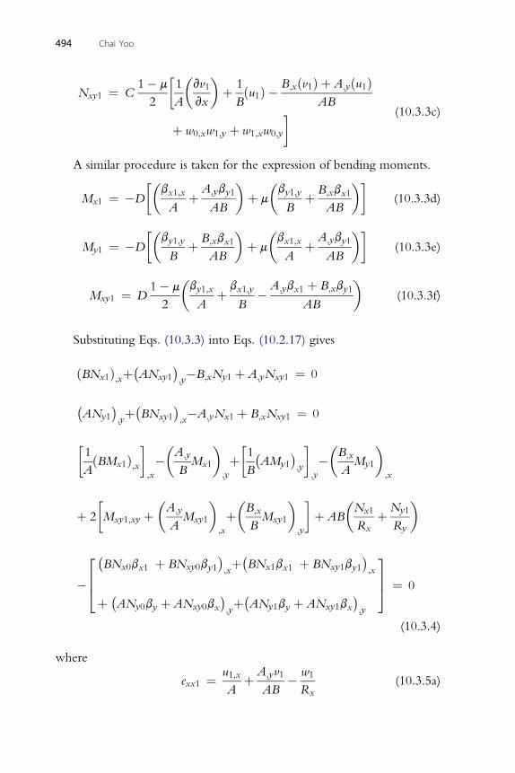
1� m�1�vv1

�1 B;xðv1Þ þ A;yðu1Þ

Nxy1 ¼ C2 A vx

þBðu1Þ �

AB

þ w0;xw1;y þ w1;xw0;y

(10.3.3c)

A similar procedure is taken for the expression of bending moments.

Mx1 ¼ �D

��bx1;x

Aþ A;yby1

AB

�þ m

�by1;y

Bþ B;xbx1

AB

�(10.3.3d)

��b B b

� �b A b

�

494 Chai Yoo

My1 ¼ �Dy1;y

Bþ ;x x1

ABþ m

x1;x

Aþ ;y y1

AB(10.3.3e)

1� m�b b A;yb þ B;xb

�

Mxy1 ¼ D

2

y1;x

Aþ x1;y

B� x1 y1

AB(10.3.3f)

Substituting Eqs. (10.3.3) into Eqs. (10.2.17) gives

ðBNx1Þ;xþ�ANxy1

�;y�B;xNy1 þ A;yNxy1 ¼ 0

�ANy1

�;yþ�

BNxy1

�;x�A;yNx1 þ B;xNxy1 ¼ 0

�1

AðBMx1Þ;x

;x

��A;y

BMx1

�;y

þ�1

B

�AMy1

�;y

;y

��B;x

AMy1

�;x

þ 2

�Mxy1;xy þ

�A;y

AMxy1

�;x

þ�B;x

BMxy1

�;y

þ AB

�Nx1

RxþNy1

Ry

�

�

264�BNx0bx1 þ BNxy0by1

�;xþ�

BNx1bx1 þ BNxy1by1�;x

þ �ANy0by þ ANxy0bx

�;yþ�

ANy1by þ ANxy1bx�;y

375 ¼ 0

(10.3.4)

where

exx1 ¼ u1;x

Aþ A;yv1

AB� w1

Rx(10.3.5a)

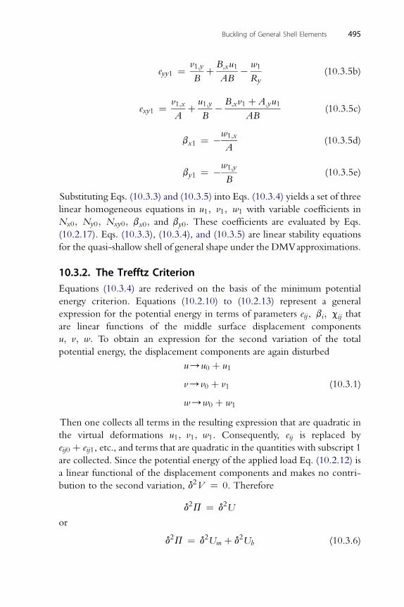
v1;y B;xu1 w1

eyy1 ¼

Bþ

AB�Ry

(10.3.5b)

v1;x u1;y B;xv1 þ A;yu1

Buckling of General Shell Elements 495

exy1 ¼A

þB

�AB

(10.3.5c)

w1;x

bx1 ¼ �

A(10.3.5d)

w1;y

by1 ¼ �

B(10.3.5e)

Substituting Eqs. (10.3.3) and (10.3.5) into Eqs. (10.3.4) yields a set of three

linear homogeneous equations in u1; v1; w1 with variable coefficients in

Nx0; Ny0; Nxy0; bx0; and by0. These coefficients are evaluated by Eqs.

(10.2.17). Eqs. (10.3.3), (10.3.4), and (10.3.5) are linear stability equations

for the quasi-shallow shell of general shape under the DMVapproximations.

10.3.2. The Trefftz CriterionEquations (10.3.4) are rederived on the basis of the minimum potential

energy criterion. Equations (10.2.10) to (10.2.13) represent a general

expression for the potential energy in terms of parameters eij; bi; cij that

are linear functions of the middle surface displacement components

u; v; w: To obtain an expression for the second variation of the total

potential energy, the displacement components are again disturbed

u/u0 þ u1

v/v0 þ v1

w/w0 þ w1

(10.3.1)

Then one collects all terms in the resulting expression that are quadratic in

the virtual deformations u1; v1; w1. Consequently, eij is replaced by

eij0 þ eij1, etc., and terms that are quadratic in the quantities with subscript 1

are collected. Since the potential energy of the applied load Eq. (10.2.12) is

a linear functional of the displacement components and makes no contri-

bution to the second variation, d2V ¼ 0. Therefore

d2P ¼ d2U

or

d2P ¼ d2Um þ d2Ub (10.3.6)

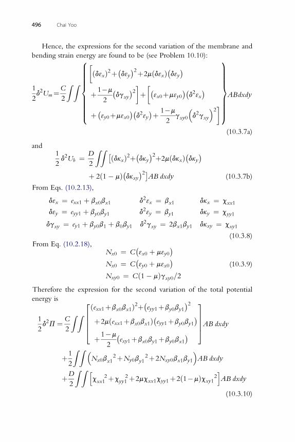
496 Chai Yoo

Hence, the expressions for the second variation of the membrane and

bending strain energy are found to be (see Problem 10.10):

1

2d2Um¼C

2

Z Z�ðd3xÞ2þ

�d3y

�2þ2mðd3xÞ�d3y

�þ1�m

2

�dgxy

�2þ��3x0þm3y0

��d23x

�þ �

3y0þm3x0��d23y

�þ 1�m

2gxy0

�d2gxy

�2

9>>=>>;ABdxdy

8>>>>>>>><>>>>>>>>:

(10.3.7a)

and1

2d2Ub ¼ D

2

ZZ ðdkxÞ2þ�dky

�2þ2mðdkxÞ�dky

�þ 2ð1� mÞ�dkxy�2�AB dxdy (10.3.7b)

From Eqs. (10.2.13),

d3x ¼ exx1 þ bx0bx1 d23x ¼ bx1 dkx ¼ cxx1

d3y ¼ eyy1 þ by0by1 d23y ¼ by1 dky ¼ cyy1

dgxy ¼ ey1 þ by0b1 þ b0by1 d2gxy ¼ 2bx1by1 dkxy ¼ cxy1

(10.3.8)From Eq. (10.2.18),

Nx0 ¼ C�3x0 þ m3y0

�Nx0 ¼ C

�3y0 þ m3x0

�Nxy0 ¼ Cð1� mÞgxy0=2

(10.3.9)

Therefore the expression for the second variation of the total potential

energy is

1

2d2P¼ C

2

Z Z26664ðexx1þbx0bx1Þ2þ

�eyy1þby0by1

�2þ2mðexx1þbx0bx1Þ

�eyy1þby0by1

�þ1�m

2

�exy1þbx0by1þby0bx1

�

37775AB dxdy

þ1

2

Z Z �Nx0b

2x1 þNy0b

2y1 þ2Nxy0bx1by1

�AB dxdy

þD

2

Z Z hc 2xx1 þc 2

yy1 þ2mcxx1cyy1þ2ð1�mÞcxy12iAB dxdy

(10.3.10)

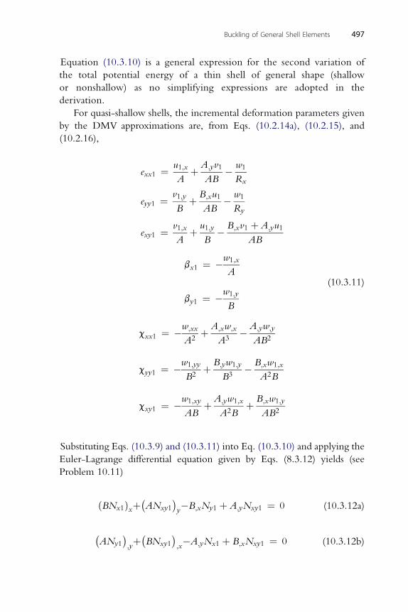
Buckling of General Shell Elements 497

Equation (10.3.10) is a general expression for the second variation of

the total potential energy of a thin shell of general shape (shallow

or nonshallow) as no simplifying expressions are adopted in the

derivation.

For quasi-shallow shells, the incremental deformation parameters given

by the DMV approximations are, from Eqs. (10.2.14a), (10.2.15), and

(10.2.16),

exx1 ¼ u1;x

Aþ A;yv1

AB� w1

Rx

eyy1 ¼ v1;y

Bþ B;xu1

AB� w1

Ry

exy1 ¼ v1;x

Aþ u1;y

B� B;xv1 þ A;yu1

AB

w1;x

bx1 ¼ �

A

by1 ¼ �w1;y

B

(10.3.11)

w;xx A;xw;x A;yw;y

cxx1 ¼ �

A2þ

A3�

AB2

cyy1 ¼ �w1;yy

B2þ B;yw1;y

B3� B;xw1;x

A2B

cxy1 ¼ �w1;xy

ABþ A;yw1;x

A2Bþ B;xw1;y

AB2

Substituting Eqs. (10.3.9) and (10.3.11) into Eq. (10.3.10) and applying the

Euler-Lagrange differential equation given by Eqs. (8.3.12) yields (see

Problem 10.11)

ðBNx1Þxþ�ANxy1

�y�B;xNy1 þ A;yNxy1 ¼ 0 (10.3.12a)

�ANy1

�;yþ�

BNxy1

�;x�A;yNx1 þ B;xNxy1 ¼ 0 (10.3.12b)

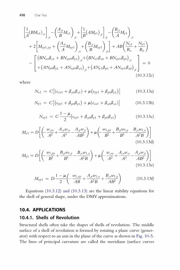
�1

�A;y

� �1� � �

B;x�

AðBMx1Þ;x

;x

�BMx1

;y

þB

AMy1 ;y;y

�AMy1

;x

þ 2

�Mxy1;xy þ

�A;y

AMxy1

�;x

þ�B;x

BMxy1

�;y

þ AB

�Nx1

RxþNy1

Ry

�

�24�BNxobx1 þ BNxy0by1

�;xþ�

BNx1bx0 þ BNxy1by0�;x

þ�ANy0by1 þ ANxy0bx1

�;yþ�

ANy1by0 þ ANxy1bx0�;y

35 ¼ 0

(10.3.12c)

where

498 Chai Yoo

Nx1 ¼ Cðexx1 þ bx0bx1Þ þ m

�eyy1 þ by0by1

��(10.3.13a)

N ¼ C�e þ b b

�þ mðe þ b b Þ� (10.3.13b)

y1 yy1 y0 y1 xx1 x0 x1

1� m� �

Nxy1 ¼ C

2exy1 þ bx0by1 þ by0bx1 (10.3.13c)

��w A w A;yw;y

� �w1;yy B;yw1;y B w

�

Mx1 ¼ D � ;xx

A2þ ;x ;x

A3�

AB2þm �

B2þ

B3� ;x 1;x

A2B

(10.3.13d)

��w B w B w

� �w A w A w

�

My1 ¼ D � 1;yy

B2þ ;y 1;y

B3� ;x 1;x

A2Bþm � ;xx

A2þ ;x ;x

A3� ;y ;y

AB2

(10.3.13e)

1� m�

w1;xy A;yw1;x B;xw1;y�

Mxy1 ¼ D2

�AB

þA2B

þAB2

(10.3.13f)

Equations (10.3.12) and (10.3.13) are the linear stability equations for

the shell of general shape, under the DMV approximations.

10.4. APPLICATIONS

10.4.1. Shells of RevolutionStructural shells often take the shapes of shells of revolution. The middle

surface of a shell of revolution is formed by rotating a plane curve (gener-

ator) with respect to an axis in the plane of the curve as shown in Fig. 10-5.

The lines of principal curvature are called the meridians (surface curves

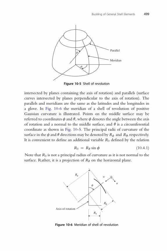
Meridian

Parallelφ

θ

Figure 10-5 Shell of revolution

Buckling of General Shell Elements 499

intersected by planes containing the axis of rotation) and parallels (surface

curves intersected by planes perpendicular to the axis of rotation). The

parallels and meridians are the same as the latitudes and the longitudes in

a glove. In Fig. 10-6 the meridian of a shell of revolution of positive

Gaussian curvature is illustrated. Points on the middle surface may be

referred to coordinates f and q, where f denotes the angle between the axis

of rotation and a normal to the middle surface, and q is a circumferential

coordinate as shown in Fig. 10-5. The principal radii of curvature of the

surface in the f and q directions may be denoted byRf and Rq, respectively.

It is convenient to define an additional variable R0 defined by the relation

R0 ¼ Rq sin f (10.4.1)

Note that R0 is not a principal radius of curvature as it is not normal to the

surface. Rather, it is a projection of Rq on the horizontal plane.

Axis of rotationR0

R

R

u

w

Figure 10-6 Meridian of shell of revolution

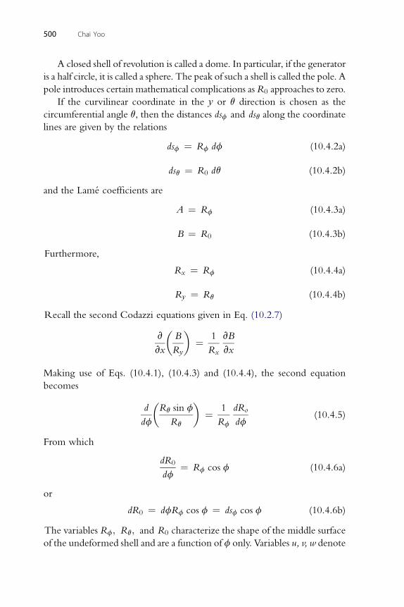
500 Chai Yoo

A closed shell of revolution is called a dome. In particular, if the generator

is a half circle, it is called a sphere. The peak of such a shell is called the pole. A

pole introduces certain mathematical complications asR0 approaches to zero.

If the curvilinear coordinate in the y or q direction is chosen as the

circumferential angle q, then the distances dsf and dsq along the coordinate

lines are given by the relations

dsf ¼ Rf df (10.4.2a)

ds ¼ R dq (10.4.2b)

q 0

and the Lame coefficients are

A ¼ Rf (10.4.3a)

B ¼ R0 (10.4.3b)

Furthermore,

Rx ¼ Rf (10.4.4a)

R ¼ R (10.4.4b)

y q

Recall the second Codazzi equations given in Eq. (10.2.7)

v

vx

�B

Ry

�¼ 1

Rx

vB

vx

Making use of Eqs. (10.4.1), (10.4.3) and (10.4.4), the second equation

becomes

d

df

�Rq sin f

Rq

�¼ 1

Rf

dRo

df(10.4.5)

From which

dR0

df¼ Rf cos f (10.4.6a)

or

dR0 ¼ dfRf cos f ¼ dsf cos f (10.4.6b)

The variables Rf; Rq; and R0 characterize the shape of the middle surface

of the undeformed shell and are a function of f only. Variables u, v, w denote

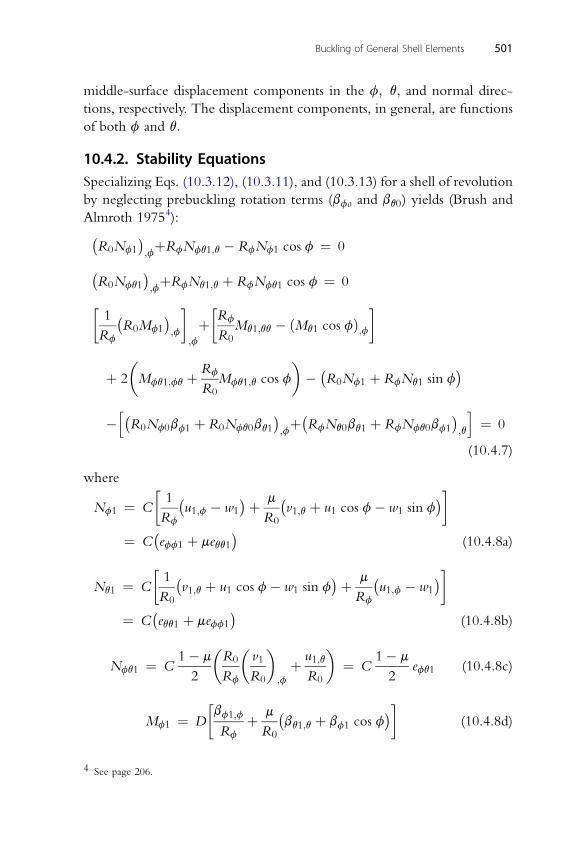
Buckling of General Shell Elements 501

middle-surface displacement components in the f; q; and normal direc-

tions, respectively. The displacement components, in general, are functions

of both f and q:

10.4.2. Stability EquationsSpecializing Eqs. (10.3.12), (10.3.11), and (10.3.13) for a shell of revolution

by neglecting prebuckling rotation terms (bfo and bq0) yields (Brush and

Almroth 19754):�R0Nf1

�;fþRfNfq1;q � RfNf1 cos f ¼ 0

�R0Nfq1

�;fþRfNq1;q þ RfNfq1 cos f ¼ 0

�1

Rf

�R0Mf1

�;f

;f

þ�Rf

R0Mq1;qq � ðMq1 cos fÞ;f

þ 2

�Mfq1;fq þ Rf

R0Mfq1;q cos f

�� �

R0Nf1 þ RfNq1 sin f�

�h�R0Nf0bf1 þ R0Nfq0bq1

�;fþ�

RfNq0bq1 þ RfNfq0bf1�;q

i¼ 0

(10.4.7)

where

Nf1 ¼ C

�1

Rf

�u1;f � w1

�þ m

R0

�v1;q þ u1 cos f� w1 sin f

�¼ C

�eff1 þ meqq1

�(10.4.8a)

�1 � � m � �

Nq1 ¼ CR0

v1;q þ u1 cos f� w1 sin f þRf

u1;f � w1

¼ C�eqq1 þ meff1

�(10.4.8b)

1� m�R

�v�

u�

1� m

Nfq1 ¼ C

2

0

Rf

1

R0 ;fþ 1;q

R0¼ C

2efq1 (10.4.8c)

�b m � �

Mf1 ¼ Df1;f

RfþR0

bq1;q þ bf1 cos f (10.4.8d)

4 See page 206.

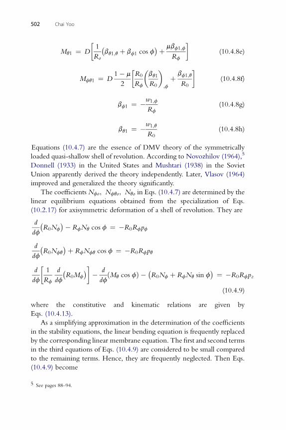
�1 � � mbf1;f

Mq1 ¼ D

Robq1;q þ bf1 cos f þ

Rf(10.4.8e)

1� m�R

�b

�b

502 Chai Yoo

Mfq1 ¼ D2

0

Rf

q1

R0 ;f

þ f1;q

R0(10.4.8f)

w1;f

bf1 ¼ �

Rf(10.4.8g)

w1;q

pz

bq1 ¼ �R0

(10.4.8h)

Equations (10.4.7) are the essence of DMV theory of the symmetrically

loaded quasi-shallow shell of revolution. According to Novozhilov (1964),5

Donnell (1933) in the United States and Mushtari (1938) in the Soviet

Union apparently derived the theory independently. Later, Vlasov (1964)

improved and generalized the theory significantly.

The coefficients Nfo; Nfqo; Nqo in Eqs. (10.4.7) are determined by the

linear equilibrium equations obtained from the specialization of Eqs.

(10.2.17) for axisymmetric deformation of a shell of revolution. They are

d

df

�R0Nf

�� RfNq cos f ¼ �R0Rfpf

d

df

�R0Nfq

�þ RfNfq cos f ¼ �R0Rfpq

d

df

�1

Rf

d

df

�R0Mf

�� d

dfðMq cos fÞ �

�R0Nf þ RfNq sin f

� ¼ �R0Rf

(10.4.9)

where the constitutive and kinematic relations are given by

Eqs. (10.4.13).

As a simplifying approximation in the determination of the coefficients

in the stability equations, the linear bending equation is frequently replaced

by the corresponding linear membrane equation. The first and second terms

in the third equations of Eqs. (10.4.9) are considered to be small compared

to the remaining terms. Hence, they are frequently neglected. Then Eqs.

(10.4.9) become

5 See pages 88–94.

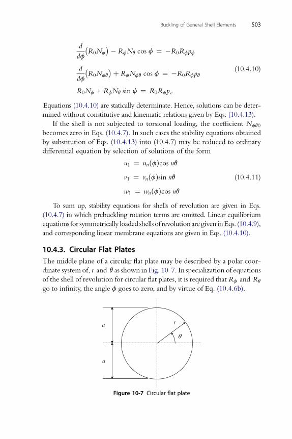
Buckling of General Shell Elements 503

d

df

�R0Nf

�� RfNq cos f ¼ �R0Rfpf

d

df

�R0Nfq

�þ RfNfq cos f ¼ �R0Rfpq

R0Nf þ RfNq sin f ¼ R0Rfpz

(10.4.10)

Equations (10.4.10) are statically determinate. Hence, solutions can be deter-

mined without constitutive and kinematic relations given by Eqs. (10.4.13).

If the shell is not subjected to torsional loading, the coefficient Nfq0

becomes zero in Eqs. (10.4.7). In such cases the stability equations obtained

by substitution of Eqs. (10.4.13) into (10.4.7) may be reduced to ordinary

differential equation by selection of solutions of the form

u1 ¼ unðfÞcos nqv1 ¼ vnðfÞsin nq

w1 ¼ wnðfÞcos nq(10.4.11)

To sum up, stability equations for shells of revolution are given in Eqs.

(10.4.7) in which prebuckling rotation terms are omitted. Linear equilibrium

equations for symmetrically loaded shells of revolution are given inEqs. (10.4.9),

and corresponding linear membrane equations are given in Eqs. (10.4.10).

10.4.3. Circular Flat PlatesThe middle plane of a circular flat plate may be described by a polar coor-

dinate system of, r and q as shown in Fig. 10-7. In specialization of equations

of the shell of revolution for circular flat plates, it is required that Rf and Rq

go to infinity, the angle f goes to zero, and by virtue of Eq. (10.4.6b).

θ

ra

a

Figure 10-7 Circular flat plate

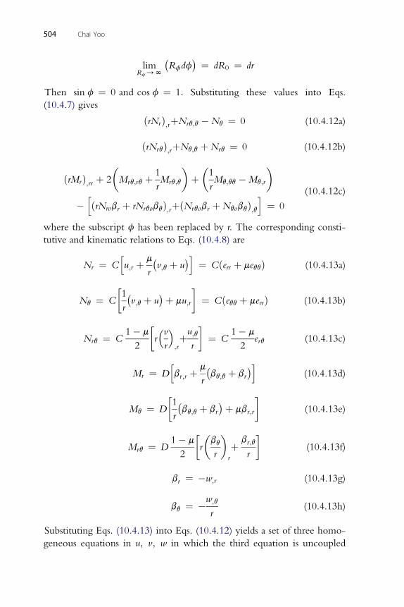
504 Chai Yoo

limRf/N

�Rfdf

� ¼ dR0 ¼ dr

Then sin f ¼ 0 and cos f ¼ 1: Substituting these values into Eqs.

(10.4.7) gives

ðrNrÞ;rþNrq;q �Nq ¼ 0 (10.4.12a)

ðrN Þ þN þN ¼ 0 (10.4.12b)

rq ;r q;q rq

�1

� �1

�

ðrMrÞ;rr þ 2 Mrq;rq þ

rMrq;q þ

rMq;qq �Mq;r

�hðrNrobr þ rNrqobqÞ;rþðNrqobr þNqobqÞ;q

i¼ 0

(10.4.12c)

where the subscript f has been replaced by r. The corresponding consti-

tutive and kinematic relations to Eqs. (10.4.8) are

Nr ¼ Chu;r þ m

r

�v;q þ u

�i ¼ Cðerr þ meqqÞ (10.4.13a)

�1� �

Nq ¼ Crv;q þ u þ mu;r ¼ Cðeqq þ merrÞ (10.4.13b)

1� m� �v� u

1� m

Nrq ¼ C2

rr ;r

þ ;q

r¼ C

2erq (10.4.13c)

h m� �i

Mr ¼ D br;r þ

rbq;q þ br (10.4.13d)

�1� �

Mq ¼ Drbq;q þ br þ mbr;r (10.4.13e)

1� m� �

b�

b

Mrq ¼ D2

rq

r r

þ r;q

r(10.4.13f)

b ¼ �w (10.4.13g)

r ;r

w;q

bq ¼ �

r(10.4.13h)

Substituting Eqs. (10.4.13) into Eqs. (10.4.12) yields a set of three homo-

geneous equations in u; v; w in which the third equation is uncoupled

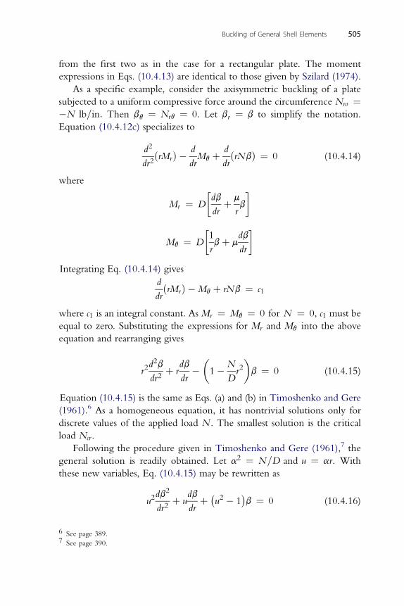
Buckling of General Shell Elements 505

from the first two as in the case for a rectangular plate. The moment

expressions in Eqs. (10.4.13) are identical to those given by Szilard (1974).

As a specific example, consider the axisymmetric buckling of a plate

subjected to a uniform compressive force around the circumference Nro ¼�N lb=in: Then bq ¼ Nrq ¼ 0. Let br ¼ b to simplify the notation.

Equation (10.4.12c) specializes to

d2

dr2ðrMrÞ � d

drMq þ d

drðrNbÞ ¼ 0 (10.4.14)

where

Mr ¼ D

�db

drþ m

rb

�1 db

Mq ¼ D

rbþ m

dr

Integrating Eq. (10.4.14) gives

d

drðrMrÞ �Mq þ rNb ¼ c1

where c1 is an integral constant. As Mr ¼ Mq ¼ 0 for N ¼ 0, c1 must be

equal to zero. Substituting the expressions for Mr and Mq into the above

equation and rearranging gives

r2d2b

dr2þ r

db

dr��1�N

Dr2�b ¼ 0 (10.4.15)

Equation (10.4.15) is the same as Eqs. (a) and (b) in Timoshenko and Gere

(1961).6 As a homogeneous equation, it has nontrivial solutions only for

discrete values of the applied load N . The smallest solution is the critical

load Ncr .

Following the procedure given in Timoshenko and Gere (1961),7 the

general solution is readily obtained. Let a2 ¼ N=D and u ¼ ar. With

these new variables, Eq. (10.4.15) may be rewritten as

u2db2

dr2þ u

db

drþ �

u2 � 1�b ¼ 0 (10.4.16)

6 See page 389.7 See page 390.

506 Chai Yoo

The general solution of this equation is given by Grossman and Derrick

(1988)8

b ¼ A1J1ðuÞ þ A2Y1ðuÞ (10.4.17)

where J1ðuÞ and Y1ðuÞ are Bessel functions of the first and second kinds of

order one, respectively. At the center of the plate (r ¼ u ¼ 0), b must be

equal to zero in order to satisfy the condition of symmetry. Since

Y1ð0Þ/N, A2 must be equal to zero9 and

b ¼ A1J1ðuÞSolutions for two boundary conditions are given by Timoshenko and Gere

(1961). For the clamped edge, b ¼ 0 at r ¼ a and therefore J1ðaaÞ ¼ 0.

Maple� gives the smallest nontrivial solution aa ¼ 3:8317. Hence the

critical load is

Ncr ¼ 3:83172D

a2¼ 14:68D

a2(10.4.17)

For the simply supported plate

ðMrÞr¼a¼ D

�db

drþ mb

r

�r¼a

¼ 0

Therefore

�dJ1ðuÞdr

þ mJ1ðuÞr

r¼0

¼ 0

or �

udJ1ðuÞdu

þ mJ1ðuÞu¼aa

¼ 0

Applying the derivative formula dJ1ðuÞ=du ¼ J0 � J1=u, where J0 is the

Bessel function of the first kind of order zero from Grossman and Derrick

(1988) 10 to the above equation gives

aaJ0ðaaÞ � ð1� mÞJ1ðaaÞ ¼ 0

For m ¼ 0:3,

aaJ0ðaaÞ � 0:7J1ðaaÞ ¼ 0

8 See page 276.9 See Grossman and Derrick (1988), page 277.10 See page 278.

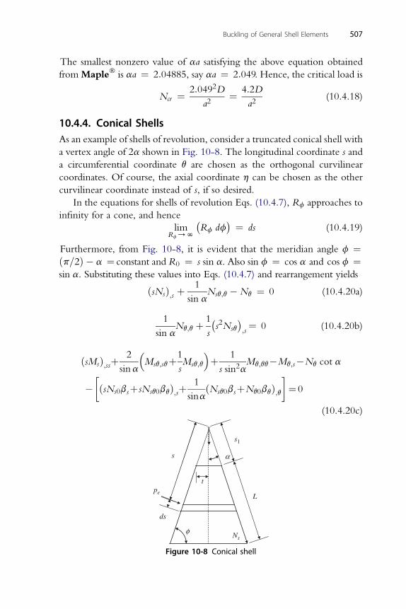
Buckling of General Shell Elements 507

The smallest nonzero value of aa satisfying the above equation obtained

fromMaple� is aa ¼ 2:04885, say aa ¼ 2:049. Hence, the critical load is

Ncr ¼ 2:0492D

a2¼ 4:2D

a2(10.4.18)

10.4.4. Conical ShellsAs an example of shells of revolution, consider a truncated conical shell with

a vertex angle of 2a shown in Fig. 10-8. The longitudinal coordinate s and

a circumferential coordinate q are chosen as the orthogonal curvilinear

coordinates. Of course, the axial coordinate h can be chosen as the other

curvilinear coordinate instead of s, if so desired.

In the equations for shells of revolution Eqs. (10.4.7), Rf approaches to

infinity for a cone, and hence

limRf/N

�Rf df

� ¼ ds (10.4.19)

Furthermore, from Fig. 10-8, it is evident that the meridian angle f ¼

ðp=2Þ � a ¼ constant and R0 ¼ s sin a. Also sin f ¼ cos a and cos f ¼sin a. Substituting these values into Eqs. (10.4.7) and rearrangement yields

ðsNsÞ;s þ1

sin aNsq;q �Nq ¼ 0 (10.4.20a)

1 1� �

sin a

Nq;q þss2Nsq ;s

¼ 0 (10.4.20b)

2 � 1 � 1

ðsMsÞ;ssþsinaMsq;sqþ

sMsq;q þ

s sin2aMq;qq�Mq;s�Nq cot a

��ðsNs0bsþsNsq0bqÞ;sþ

1

sinaðNsq0bsþNq0bqÞ;q

¼0

(10.4.20c)

Ns

α

φ

t

s

s1

L

ds

pe

Figure 10-8 Conical shell

508 Chai Yoo

where the subscript f has been replaced by s using the relationship given in

Eq. (10.4.19). Converting directly from Eqs. (10.4.8), the constitutive

relations for conical shells are

Ns ¼ Chu;s þ m

s

� v;q

sin aþ uþ w cot a

�i(10.4.21a)

�1� v �

Nq ¼ Cs

;q

sin aþ uþ w cot a þ mu;s (10.4.21b)

1� m� v u;q�

Nsq ¼ C2

v;s �sþs sin a

(10.4.21c)

�m�b

�

Ms ¼ D bs;s þ

s

q;q

sin aþ bs (10.4.21d)

�1�b

�

Mq ¼ D

s

q;q

sin aþ bs þ mbs;s (10.4.21e)

1� m� �

b�

b

Msq ¼ D2

sq

s ;s

þ q

s sin a(10.4.21f)

b ¼ �w (10.4.21g)

s ;s

w;q

bq ¼ �

s sin a(10.4.21h)

It should be of interest to note that at one extreme, when a ¼ p=2, theseequations reduce to the equations for flat circular plates and at the other

extreme, for a ¼ 0, these equations correspond to the expressions for

cylindrical shells in Chapter 9 with the replacement of s sin a by the radiusR.

Substituting Eqs. (10.4.21) into Eqs. (10.4.20) gives

suss þ u;s � u

sþ 1� m

2

u;qq

s sin2aþ 1þ m

2

v;sq

sin a

� 3� m

2

v;q

s sin aþ�mws � w

s

�cot a ¼ 0

(10.4.22a)

1þ m u;sq 3� m u;q 1� m

2 sin aþ

2 s sin aþ

2sv;ss

þ 1� m

2

�v;s � v

s

�þ v;qq

s sin2aþ w;q

s sin acot a ¼ 0

(10.4.22b)

� w;sss w;ss w;s w;sqq w;ssqq w;qq

Ds w;ssss þ 2

s�

s2þ

s3� 2

s3sin2aþ 2

s2sin2aþ 4

s4sin2a

þ w;qqqq

s4sin4a

�þ C

� v;q

s sin aþ u

sþ w cot a

sþ mu;s

�cot a

���

Ns0sw;s þNsq0

w;q

sin a

�;sþ 1

sin a

�Nsq0w;s þNq0

w;q

s sin a

�;q

¼ 0

(10.4.22c)

Equations (10.4.22) give a coupled set of three homogeneous differential

Buckling of General Shell Elements 509

equations in u; v; and w:Consider, as an example, a conical shell subjected to uniform external

hydrostatic pressure or internal suction pe in pounds per square inch and an

axial compressive force P in pounds. Suppose that a membrane analysis is

adequate for the prebuckling static deformation; then the coefficients are

computed by the simple static relations

Ns0 ¼ �1

2pes tan a� P

2ps sin a; Nq0 ¼ �pes tan a; Nsq0 ¼ 0 (10.4.23)

Substituting these values into Eqs. (10.4.22) reveals that Eq. (10.4.22c) is

a stability equationwith variable coefficients. In general, a solution for critical

values of the applied load needs to rely on numerical methods. An excellent

numerical analysis is reported by Baruch, Harari, and Singer (1967). They

obtained extensive numerical results based on the Galerkin procedure for

hydrostatic-pressure loading, with a fairly wide range of parameters.

10.4.5. Shallow Spherical CapsA cross section of a spherical cap is shown in Fig. 10-8. The middle surface

is described by curvilinear coordinates r and q. The rise H of the shell is

much smaller than the base chord (2a).

From Fig. 10-9, rf ¼ R, a constant, and sin f ¼ r=R. For the shallowshell, approximately, cos f ¼ 1 and rfdf ¼ dr. Substituting these

approximations into Eq. (10.4.7) yields

ðrNrÞ;r þ Nrq;q �Nq ¼ 0 (10.4.24a)

ðrNrqÞ;r þ Nq;q þNrq ¼ 0 (10.4.24b)

�1

� �1

�r

ðrMrÞ;rrþ2 Mrq;rqþ

rMrq;q þ

rMq;qq�Mq;r þ

RðNrþNqÞ

�hðrNrobrþrNrqobqÞ;rþðNrqobrþNqobqÞ;q

i¼0

(10.4.24c)

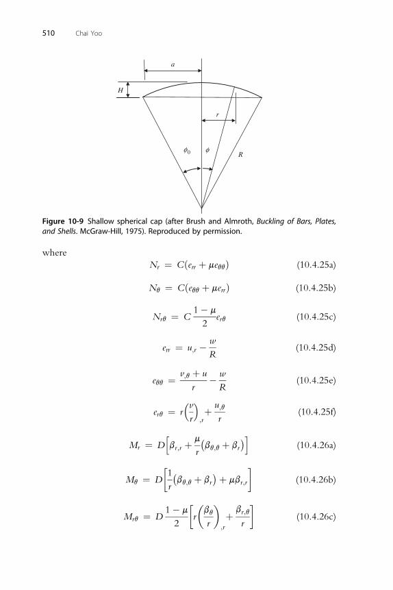
a

H

r

R0φ φ

Figure 10-9 Shallow spherical cap (after Brush and Almroth, Buckling of Bars, Plates,and Shells. McGraw-Hill, 1975). Reproduced by permission.

510 Chai Yoo

where

Nr ¼ Cðerr þ meqqÞ (10.4.25a)

N ¼ Cðe þ me Þ (10.4.25b)

q qq rr

1� m

Nrq ¼ C

2erq (10.4.25c)

w

err ¼ u;r �

R(10.4.25d)

v;q þ u w

eqq ¼

r�R

(10.4.25e)

�v� u;q

erq ¼ r

r ;rþ

r(10.4.25f)

h m� �i

Mr ¼ D br;r þ

rbq;q þ br (10.4.26a)

�1� �

Mq ¼ Drbq;q þ br þ mbr;r (10.4.26b)

1� m� �

b�

b

Mrq ¼ D2

rq

r ;r

þ r;q

r(10.4.26c)

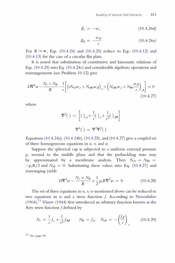
br ¼ �w;r (10.4.26d)

w;q

Buckling of General Shell Elements 511

bq ¼ �r

(10.4.26e)

For R/N, Eqs. (10.4.24) and (10.4.25) reduce to Eqs. (10.4.12) and

(10.4.13) for the case of a circular flat plate.

It is noted that substitution of constitutive and kinematic relations of

Eqs. (10.4.25) into Eq. (10.4.24c) and considerable algebraic operations and

rearrangements (see Problem 10.12) give

DV4w�Nr þNq

R�1

r

��rNr0w;r þNrq0w;q

�;rþ�Nrq0w;r þNq0

w;q

r

�;q

¼ 0

(10.4.27)

where

V2ð Þ ¼�ð Þ;rrþ

1

rð Þ;rþ

1

r2ð Þ;qq

V4ð Þ ¼ V2V2ð Þ

Equations (10.4.24a), (10.4.24b), (10.4.25), and (10.4.27) give a coupled set

of three homogeneous equations in u, v, and w.

Suppose the spherical cap is subjected to a uniform external pressure

pe normal to the middle plane and that the prebuckling state may

be approximated by a membrane analysis. Then Nr0 ¼ Nq0 ¼�peR=2 and Nrq ¼ 0. Substituting these values into Eq. (10.4.27) and

rearranging yields

DV4w �Nr þNq

Rþ 1

2peRV

2w ¼ 0 (10.4.28)

The set of three equations in u, v, w mentioned above can be reduced to

two equations in w and a stress function f. According to Novozhilov

(1964),11 Vlasov (1944) first introduced an arbitrary function known as the

Airy stress function f defined by

Nr ¼ 1

rf;r þ 1

r2f;qq Nq ¼ f;rr Nrq ¼ �

�f;q

r

�;r

(10.4.29)

11 See page 90.

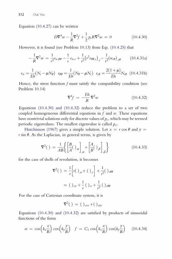
512 Chai Yoo

Equation (10.4.27) can be written

DV4w � 1

RV2f þ 1

2peRV

2w ¼ 0 (10.4.30)

However, it is found (see Problem 10.13) from Eqs. (10.4.25) that

� 1

RV2w ¼ 1

r2err;qq � 1

rerr;r þ 1

r2

�r2eqq;r

�;r� 1

r2ðrerqÞ;rq (10.4.31a)

1 1 2ð1þmÞ

err ¼

EhðNr �mNqÞ eqq ¼

EhðNq�mNrÞ erq ¼

EhNrq (10.4.31b)

Hence, the stress function f must satisfy the compatibility condition (see

Problem 10.14)

V4f ¼ �Eh

RV2w (10.4.32)

Equations (10.4.30) and (10.4.32) reduce the problem to a set of two

coupled homogeneous differential equations in f and w. These equations

have nontrivial solutions only for discrete values of pe, which may be termed

periodic eigenvalues. The smallest eigenvalue is called pcr .

Hutchinson (1967) gives a simple solution. Let x ¼ r cos q and y ¼r sin q. As the Laplacian, in general terms, is given by

V2ð Þ ¼ 1

AB

��B

Að Þ;a

;a

þ�A

Bð Þ;b

;b

(10.4.33)

for the case of shells of revolution, it becomes

V2ð Þ ¼ 1

r

�rð Þ;rrþ ð Þ;r

þ 1

r2ð Þ;qq

¼ ð Þ;rr þ 1

rð Þ;r þ 1

r2ð Þ;qq

For the case of Cartesian coordinate system, it is

V2ð Þ ¼ ð Þ;xxþð Þ;yyEquations (10.4.30) and (10.4.32) are satisfied by products of sinusoidal

functions of the form

w ¼ cos�kxx

R

�cos

�kyy

R

�f ¼ C1 cos

�kxx

R

�cosðky y

R

�(10.4.34)

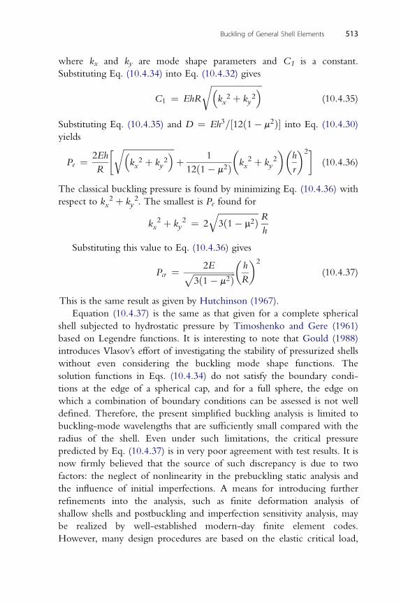
Buckling of General Shell Elements 513

where kx and ky are mode shape parameters and C1 is a constant.

Substituting Eq. (10.4.34) into Eq. (10.4.32) gives

C1 ¼ EhR

ffiffiffiffiffiffiffiffiffiffiffiffiffiffiffiffiffiffiffiffiffiffiffiffi�k 2x þ k 2

y

�r(10.4.35)

Substituting Eq. (10.4.35) and D ¼ Eh3=½12ð1� m2Þ� into Eq. (10.4.30)

yields

Pe ¼ 2Eh

R

� ffiffiffiffiffiffiffiffiffiffiffiffiffiffiffiffiffiffiffiffiffiffiffiffi�k 2x þ k 2

y

�rþ 1

12ð1� m2Þ�k 2x þ k 2

y

��h

r

�2(10.4.36)

The classical buckling pressure is found by minimizing Eq. (10.4.36) with

respect to k 2x þ k 2

y . The smallest is Pe found for

k 2x þ k 2

y ¼ 2

ffiffiffiffiffiffiffiffiffiffiffiffiffiffiffiffiffiffiffi3ð1� m2Þ

qR

h

Substituting this value to Eq. (10.4.36) gives

Pcr ¼ 2Effiffiffiffiffiffiffiffiffiffiffiffiffiffiffiffiffiffiffiffi3ð1� m2Þp �

h

R

�2

(10.4.37)

This is the same result as given by Hutchinson (1967).

Equation (10.4.37) is the same as that given for a complete spherical

shell subjected to hydrostatic pressure by Timoshenko and Gere (1961)

based on Legendre functions. It is interesting to note that Gould (1988)

introduces Vlasov’s effort of investigating the stability of pressurized shells

without even considering the buckling mode shape functions. The

solution functions in Eqs. (10.4.34) do not satisfy the boundary condi-

tions at the edge of a spherical cap, and for a full sphere, the edge on

which a combination of boundary conditions can be assessed is not well

defined. Therefore, the present simplified buckling analysis is limited to

buckling-mode wavelengths that are sufficiently small compared with the

radius of the shell. Even under such limitations, the critical pressure

predicted by Eq. (10.4.37) is in very poor agreement with test results. It is

now firmly believed that the source of such discrepancy is due to two

factors: the neglect of nonlinearity in the prebuckling static analysis and

the influence of initial imperfections. A means for introducing further

refinements into the analysis, such as finite deformation analysis of

shallow shells and postbuckling and imperfection sensitivity analysis, may

be realized by well-established modern-day finite element codes.

However, many design procedures are based on the elastic critical load,

514 Chai Yoo

reduced by a “knockdown factor” of five or even more. This is perhaps

the reason why Miller12 of CB&I (Chicago Bridge and Iron) relied

heavily on experimental investigations for the company’s new form of

shell structures to build until the late 1980s, when reliable finite element

codes were made available.

The subject of this book is the buckling behavior of structural members

that are subjected to loading that induces compressive stresses in the body.

Buckling is essentially flexural behavior. As such, it has been necessary to

investigate the flexural behavior of each structural element covered in the

book. However, quite a few structural members can carry the applied load

primarily or dominantly through membrane actions. In such cases, the static

analysis for membrane action is considerably less complicated than the

analysis for combined membrane and flexural actions. When compressive

stresses are developed in the body, an elastic buckling strength check is

necessary, but for loading cases that produce no, or low, compressive stress,

a simplified membrane analysis may suffice.

REFERENCESBaruch, M., Harari, O., & Singer, J. (1967). Influence of In-Plane Boundary Conditions on

the Stability of Conical Shells Under Hydrostatic Pressure. Israel Journal of Technology,5(1–2), 12–24.

Brush, D. O., & Almroth, B. O. (1975). Buckling of Bars, Plates, and Shells. New York, NY:McGraw-Hill.

Donnell, L. H. (1933). Stability of Thin-Walled Tubes Under Torsion. Washington, DC:NACA Technical Report, No. 479.

Flugge, W. (1973). Stresses in Shells (2nd ed.). Berlin: Springer-Verlag.Gould, P. L. (1988). Analysis of Shells and Plates. New York: Springer-Verlag.Grossman, S. I., & Derrick, W. R. (1988). Advanced Engineering Mathematics. New York:

Harper and Row.Hutchinson, J. W. (1967). Imperfection Sensitivity of Externally Pressurized Spherical

Shells. Journal of Applied Mechanics, Vol. 34, 49–56.Klaus, H. (1967). Thin Elastic Shells. New York: John Wiley and Sons.Koiter, W. T. (1960). A Consistent First Approximation in the General Theory of Thin

Elastic Shells. In The Theory of Thin Elastic Shells (pp. 12–33). Armsterdam: North-Holland.

Koiter, W. T. (1967). General Equations of Elastic Stability for Thin Shells. Proc. Symp.Theory of Shells to Honor Lloyd Hamilton Donnell. Houston, TX: University of Houston.187–223.

Langhaar, H. L. (1962). Energy Methods in Applied Mechanics. New York: John Wiley andSons.

Love, A. E. H. (1944). ATreatise on the Mathematical Theory of Elasticity (4th ed.). New York:Dover.

12 Private communication.

Buckling of General Shell Elements 515

Mushtari, K. M. (1938). On the Stability of Cylindrical Shells Subjected to Torsion. TrudyKaz. aviats. in-ta., 2 (in Russian).

Naghdi, P. M. (1963). Foundations of Elastic Shell Theory. In Progress in Solid Mechanics,Vol 4. New York: John Wiley and Sons.

Novozhilov, V. V. (1953). Foundations of the Nonlinear Theory of Elasticity. InF. Bagemihl, H. Komm, & W. Seidel (Eds.), Translated from the 1st (1948) Russian.Rochester, NY: Graylock Press.

Novozhilov, V. V. (1964). Thin Shell Theory. In: Lowe, P.G. and Radok, J.R. (eds),Translated from the 2nd Russian ed. The Netherlands: Noordhoff, Groningen.

Sanders, J. L. (1963). Nonlinear Theories for Thin Shells. Q. Appl. Math., 21(1), 21–36.Timoshenko, S. P., & Gere, J. M. (1961). Theory of Elastic Stability (2nd ed.). New York:

McGraw-Hill.Szilard, R. (1974). Theory and Analysis of Plates, Classical and Numerical Methods. Englewood

Cliffs, NJ: Prentice-Hall.Vlasov, V. Z. (1944). The fundamental differential equations of the general theory of elastic

shells, Prikl. Mat. Mekh., Akademiya, Nauk. SSSR, Vol. VIII, No. 2, also BasicDifferential Equations in the General Theory of Elastic Shells, NACA TM 1241,February 1951.

Vlasov, V. Z. (1964). General Theory of Shells and Its Application in Engineering. Washington,DC: NASA TTF-99 National Aeronautics and Space Administration.

PROBLEMS

10.1 Derive the Lame coefficients Eq. (10.2.2) from Fig. 10-1.

10.2 Derive Eq. (10.2.4).

10.3 Derive Eq. (10.2.5).

10.4 Derive Eq. (10.2.7).

10.5 Show that the application of Euler-Lagrange differential equations to

the energy equations Eqs. (10.2.10) to (10.2.12) along with Eqs.

(10.2.14a), (10.2.15), and (10.2.16) yields the nonlinear equilibrium

equations for the shell of the general shape in Eqs. (10.2.17).

10.6 Show that (a) Equations (10.2.17) can be specialized for a circular

cylindrical shell Eqs. (9.2.9) by setting A ¼ 1, B ¼ Ry ¼ R, and

1/Rx ¼ 0, (b) Equations (10.2.17) can also be converted to the

nonlinear equilibrium equations for a rectangular flat plate (von

Karman plate equations) Eqs. (8.2.18) by setting A ¼ B ¼ 1 and

1/Rx ¼ 1/Ry ¼ 0, and (c) Similarly, Eqs. (10.2.17) can also be

converted to the nonlinear equilibrium equation for a column

Eq. (1.7.14).

10.7 Verify Eqs. (10.2.28).

10.8 Verify Eqs. (10.2.33).

10.9 Verify that Eqs. (10.2.28a) and (10.2.28b), and (10.2.37) are identical

to Eqs. (10.2.17).

10.10 Derive Eq. (10.3.7) following the procedure outlined in Section 8.3.

516 Chai Yoo

10.11 Derive Eqs. (10.3.12) by applying Eqs. (8.3.12) and (10.3.11) on

Eq. (10.3.10).

10.12 Derive Eq. (10.4.27) by substituting Eqs. (10.4.26) into Eq.

(10.4.24c).

10.13 Derive Eq. (10.4.31a) from Eqs. (10.4.25a)–10.4.25f ).

10.14 Derive Eq. (10.4.32) relating the stress function f and the displace-

ment component w for a shallow spherical cap.

AUTHOR INDEX

AAcra, S. V., 277, 297, 298

Allen, H. G., 65, 68, 374, 435, 442, 458,

472

Almroth, B. O.,, 68, 280, 287, 298, 374,

391, 415, 434, 435, 442, 450, 457,

458, 462, 472, 481, 490, 501, 510,

514

Alvarez, R. J., 229, 240

Atsuta, T., 144, 149, 194, 195

BBaker, E. H., 466, 472

Bansal, J., 365, 368

Barbre, F., 405, 410, 411, 435

Baruch, M., 509, 514

Basler, K., 260, 280, 287, 288, 298, 304,

325, 417, 435

Batdorf, S. B., 458, 472

Bathe, K. J., 377, 435

Bazant, Z. P., 68, 155, 179, 195

Beck, M., 144, 149

Becker, H., 405, 415, 435, 466, 473

Berry, A., 179, 195

Birnstiel, C., 229, 240

Bleich, F., 26, 68, 155, 188, 195, 205, 241,

303, 304, 325, 328, 336, 337, 368,

374, 386, 406, 411, 414, 435

Bolotin, V. V., 144, 146, 149

Bowman, F., 344, 345, 368

Bradford, M. A., 367, 368

Bryan, G. H., 374, 405, 435

Britvec, S. J., 68, 155, 195

Brush, D. O,, 68, 280, 287, 298, 374, 391,

415, 434, 435, 442, 450, 457, 458,

462, 472, 481, 490, 501, 510, 514

Bulson, P. S., 68, 374, 435, 442, 458, 472

CCarter, C. J., 271, 276, 277, 278, 298

Chajes, A., 2, 45, 68, 193, 195, 317, 325,

348, 368, 374, 379, 389, 390, 435,

440, 442, 473, 474

Chandler, D. B., 179, 195

Chen, W. F., 68, 144, 149, 194, 195

Choi, B. H., 65, 68, 410, 412, 413, 435,

437

Chwalla, E., 192, 195

Clark, J. W., 328, 363, 368

DDavidson, J. S., 506

Dinnik, A. N., 44, 68

Derrick, W. R., 40, 69, 344, 345, 368,

506, 514

Donnel, L. H., 446, 448, 449, 458, 462,

465, 466, 473

Dym, C. L., 22, 69, 76, 82, 83, 84, 86, 149

EElishakoff, I., 44, 68

Engelhardt, H., 44, 69

Euler, L., 4, 39, 56, 69, 83, 303, 325

Evans, H. R., 436

FFligg, C. M., 303, 325

Flugge, W., 476, 514

Forsyth, A. R., 83, 149

Fung, Y. C., 76, 86, 88, 149

GGalambos, T. V., 68, 69, 229, 241, 280,

288, 298, 304, 325, 328, 342, 364,

365, 366, 368, 369, 415, 434, 435

Gao, Z., 367, 368

Gere, J. M., 3, 45, 68, 69, 99, 103, 104,

149, 155, 179, 195, 280, 298, 304,

318, 325, 336, 337, 342, 369, 374,

406, 411, 414, 436, 457, 458, 461,

462, 473

Gerard, G., 405, 415, 435, 466, 473

Godoy, L. A., 68, 69

Goldberg, J. E., 179, 195

Goodier, J. N., 251, 260, 298, 303, 304,

317, 325

517 j

518 Author Index

Gould, P. L., 476, 477, 486, 513, 514

Grossman, L. A., 40, 69, 344, 345, 368,

506, 514

HHall, D. H., 65, 69

Harari, O., 509, 514

Heins, C. P., 271, 288, 297, 298

Heller, R., 2, 69

Hill, H. N., 328, 363, 368, 369

Hjelmstad, K. D., 77, 149

Hodges, D. H., 68, 69

Hoff, N. F., 3, 69, 76, 149, 303, 317,

325

Hong, A. R., 367, 369

Horne, M. R., 179, 195, 223, 229, 241

Hsu, P. T., 195

Hutchinson, J. W., 512, 513, 514

Hwang, M., 435

JJames, B. W., 179, 195

Jezek, K., 186, 192, 193, 195

Johnson, J. E., 65, 69, 194, 195

Julian, O. G., 231, 241

KKang, Y. J., 412, 435

Kappus, R., 303, 325

Kavanagh, T. C., 231, 241

Ketter, R. L., 194, 195

Kirby, P. A., 364, 369

Koiter, W. T., 471, 472, 473, 476, 479,

481, 514

Kollbrunner, C. F., 260, 280, 287, 288,

298, 304, 325

Koo, B., 195

Kraus, H., 458, 473

LLanghaar, H. L., 76, 149, 374, 435, 457,

473, 475, 477, 514

Lawrence, L. S., 231, 241

Lay, M. G., 365, 369

Lee, D. S., 417, 418, 436

Lee, G. C., 364, 369

Lee, S. C., 416, 418, 426, 434, 435, 436,

437

Levy, S., 422, 436

Livesley, R. K., 179, 195

Loh, M. H., 195

Lorenz, R., 465, 473

Love, A. E. H., 86, 149, 389, 436

Lu, L. W., 228, 229, 241

Lundquist, E. F., 303, 325

MManey, G. A., 167, 195

Masur, E. F., 228, 241

Mattock, A. H., 411, 436

Mayrbaurl, R. M., 410, 436

Merchant, W., 223, 229, 241

Michell, A. G. M., 328, 369

Mikhlin, S. G., 95, 149

Mittelstedt, C., 412, 436

Moorman, R. B. B., 171, 195

Mushtari, K. M., 502, 515

NNadai, A., 250, 298

Naghdi, P. M., 475, 515

Nakai, H., 280, 298

Neff, J., 426, 436

Nethercot, D. A., 364, 369

Newmark, N., 129, 149

Newell, J. S., 179, 195

Niles, A. S., 179, 195

Novozhilov, V. V., 375, 377, 378, 436,

476, 477, 481, 482, 485, 486, 488,

502, 511, 515

OOjalvo, M., 229, 241

Ostenfeld, A., 303, 325

PParcel, J. I., 171, 195

Park, C. S., 436

Porter, D. M., 417, 436

Prandtl, L., 250, 251, 260, 298, 328, 346,

369

Przemieniecki, J. S., 216, 241

Author Index 519

RReddy, J. N., 69

Rees, D. W. A., 252, 298

Rish, F. L., 472

Rockey, K. C., 417, 436

SSaada, A. S., 86, 149, 260, 298, 299

Salmon, C. G., 65, 69, 194, 195

Salvadori, M., 2, 69, 364, 369

Sanders, J. L., 476, 480, 481, 490, 515

Schrader, R. K., 356, 358, 359, 363, 369

Seaburg, P. A., 271, 276, 277, 278, 298

Seide, P., 405, 436

Shames, I. H., 22, 69, 76, 82, 83, 84, 86,

149

Sharp, M. L., 406, 436

Simitses, G. J., 68, 69

Singer, J., 509, 514

Skan, S. W., 415, 436

Sobel, L. H., 465, 473

Sokolnikoff, I. S., 76, 86, 149, 298, 377,

422, 436

Southwell, R. V., 481, 537, 545

Stein, M., 415, 436, 458, 465, 473

Szilard, R., 374, 436

TTauchert, T. R., 76, 80, 88, 89, 149

Tennyson, R. C., 466, 473

Timoshenko, S. P., 3, 4, 45, 68, 69, 99,

103, 104, 149, 155, 179, 195, 251,

260, 280, 284, 288, 298, 304, 318,

325, 328, 336, 337, 339, 340, 342,

369, 374, 388, 389, 406, 411, 414,

436, 457, 461, 462, 465, 473

Todhunter, I., 39, 69

Tong. P., 76, 86, 88, 149

VVincent, G. S., 328, 369

Vlasov, V. Z., 246, 265, 288, 298, 304,

311, 325, 328, 337, 338, 364, 369,

502, 511, 515

Volmir, A. S., 468, 473

von Karman, T., 389, 436, 446, 465,

473

von Mises, R., 458, 465, 473

WWagner, H., 303, 325, 434, 436

Wan, C. C., 466, 473

Wang, C. M., 44, 69

Wang, C. Y., 69

Washizu, K., 76, 86, 149

Winter, G., 37, 69, 179, 195, 317, 325,

328, 348, 349, 356, 359, 369

Woinowsky-Kreiger, S., 388, 436

Wolchuk, R., 410, 436

YYoo, C. H., 65, 69, 123, 150, 260, 277,

280, 297, 298, 315, 325, 341,

369, 411, 412, 417, 434, 435, 436,

437

Yoon, D. Y., 436

Yoon, T., 435

Yura, J. A., 231, 241

ZZiegler, H., 68, 69, 144, 146,

150

SUBJECT INDEX

AAdjacent equilibrium, 4, 391–393

Alignment chart

sidesway inhibited, 237

sidesway permited, 240

Amplification factor for beam-columns,

162–164

Antisymmetric buckling of frames, 205,

212, 215, 216

BBatdorf parameter, 459, 460, 474

Beam-columns

amplification (magnification) factor,

162–164

design, 192–194

slope-deflection equations with axial

compression, 155–161

slope-deflection equations with axial

tension, 179–185

ultimate strength, 185–192

Beams, lateral-torsional buckling

design formulas, 362–368

differential equations, 328–336

energy method, 347–362

Bessel function, 343–347

Bifurcation type buckling, 1–2

Bimoment, 277, 286

Boundary conditions

effect of, on columns, 15–18

effect of, on cylindrical shells, 463–465

effect of, on plates, 406–409, 420–424

Buckling load see Critical load

CCalculus of variations, 18–24

Castigliano theorem, 87–88

Cauchy formula, 84

Cauchy strain, 83

Circular flat plate, 503–507

Codazzi differential equations, 478

Columns

eccentrically loaded, 52–56

Euler load, 4–7

inelastic buckling, 56–66

large deflection theory (the elastica),

44–52

Complementary strain energy, 80–81

Conical shells, 507–509

Critical load, 2, 4, 6

Cylindrical shells, 441–472

failure, 465–466

large deflection theory, 442–446

linear stability equations, 450–455

postbuckling, 466–472

DDeflection-amplification type buckling, 1

DMV (Donnell-Mushtari-Vlasov)

equations, 481, 485

Donnell equations, 442, 450

Double (reduced) modulus theory, 57–60

EEccentrically loaded columns, 52–56

Effective length of columns, 15, 212,

231

Effective width of plates, 430

Eigenvalues, 6, 44, 93

Elastically restrained, 203

Elastic support, 29–38

Elliptic integral, 48, 50–51

Euler-Lagrange equations, 22, 24, 26, 71,

84, 311, 335, 384, 386, 387, 393,

394, 399, 447, 454, 455

Euler load, 4–7

FFailure

beam-columns, 185–192

cylindrical shells, 465–466

frames, 229

plates, 433–434

Finite difference method, 127

Finite element method (matrix method),

28

521 j

522 Subject Index

Flexural-torsional buckling of columns,

303–325

Frames

buckling modes, 203–205

critical loads, 205–216

matrix analysis, 216–220

second-order analysis, 220–227

Functional, total potential energy, 23,

26

GGalerkin method

columns, 27–29

cylindrical shells, 469

shear buckling of plates, 422–426

Gauss-Codazzi conditions, 478

Gauss curvature of surface, 478

Gauss, differential equation of, 478

Geometric stiffness matrix, 133–134

Green-Lagrange finite strain, 24, 377

HHydrostatic pressure loading, 463, 464

IImperfection see Initial imperfections

Inelastic buckling

beam, 412, 413

columns, 56–66, 228

plates, 432–433

Initial imperfections, 15, 36, 37, 53, 56,

57, 65, 66, 124, 158, 192, 228, 231,

412, 414, 426, 432, 442, 466, 467,

472

Inner product, 96, 148

Intermediate class of deformations, 384,

390, 444, 450

JJoint translation, 216, 220

KKirchhoff assumptions, 375

Knock down factors, 124

Koiter’s initial postbuckling theory, 471,

472

LLame coefficients, 89

Large deflections

columns, 44–52

cylindrical shells, 442–446, 465, 466, 468

plates, 389, 440

Lateral-distortional buckling, 367

Lateral-torsional buckling see Beams,

lateral-torsional buckling

Linear stability equations

cylindrical shells, 450–455

general shells, 490

Local buckling, 367, 431–432, 438, 460,

466

MMagnification factor see Amplification

factor for beam-columns

Matrix method

columns, 133–138

frames, 216–220

Membrane analogy, 250, 251–253

Membrane equations

cylindrical shells, 458

shells of revolution, 498–501

Minimum potential energy, 26, 82–86

NNeighboring equilibrium, 4

Neutral equilibrium, 3–4

Newmark method, 129–132

Nonconservative load, buckling by,

142–146

Nonlinear equilibrium equations

cylindrical shells, 443, 446, 447

general shells, 479–483, 489, 490

plates, 384

Nonuniform torsion, 265–287

OOrthogonality conditions, 142, 423

PPlasticity, effect on frames, 228–229

Plates

circular flat, 503–507

Subject Index 523

energy method, 418–431

longitudinally stiffened, 405–414

shear loading, 414–418

Positive definite, 22, 24, 82, 85, 96, 138,

148, 394

Postbuckling

columns, 48, 52

plates, 411–412, 417, 426–431, 434

shells, 442, 466–472

Prandtl stress function, 260

Principal radii, 477, 478, 483, 499

QQuasi-shallow shells, 481, 495, 497, 502

RRayleigh quotient, 95–99

Rayleigh-Ritz method, 92–95, 99,

347–348

Reduced modulus theory, 57–60

Residual stresses, 57, 65–66, 192,

365–366, 412–414, 432–433

Rodrigues theorem, 477

SSt. Venant torsion, 265, 305–306

Secant formula, 52–56

Second-order analysis, 220–227

Sectorial coordinate, 283, 304

Self-adjoint, 22, 24, 96, 146–149

Shear buckling of plates, 417, 422–426

Shear center, 287–292

Shells

conical, 507–509

cylindrical, 441–472

of revolution, 498–501, 503, 507, 512

shallow spherical cap, 509–514

Sidesway buckling, 205

Slenderness ratio, column, 7

Slope-deflection equations

effect of axial loads, 171–179

with axial tension, 179–185

without axial force(compression),

167–171

Strain energy, 80

Symmetric buckling

frames, 208, 212, 216, 228

plates, 408, 410

TTangent modulus theory, 60–66

Taylor’s series expansion, 85, 90–91, 124,

125, 127, 128, 260, 394

Thin-walled members, 246

Torsion

St. Venant, 305–306

warping, 265–267, 281–286

Torsional buckling, 307–325

Torsional constant, St. Venant, 254–255,

257, 260

Trefftz criterion, 393, 394, 399,

454–455

UUniform torsion, 247–251

Unit tangent vector, 45

VVariations, calculus of, 18–24

Virtual displacement, 27, 79–80

Virtual work, 79–80

Von Karman effective width formula,

434

Von Karman plate equations, 374, 378,

384, 389, 448, 465

WWarping, 246, 248

Warping constant (moment of inertia),

257, 286, 319, 411

Warping functions

average, 285

normalized, 297

unit, 283, 290, 392

Warping stress

normal, 246, 266, 272, 277–278, 279

shear, 306, 308

Warping torsion, 281–287, 306

Wiry column, postbuckling of, 45, 52