Stability Analysis with an NVH Minimal Model for Brakes ...
22
vibration Article Stability Analysis with an NVH Minimal Model for Brakes under Consideration of Polymorphic Uncertainty of Friction Georg-Peter Ostermeyer *, Michael Müller , Stephan Brumme and Tarin Srisupattarawanit Institut für Dynamik und Schwingungen, Technische Universität Braunschweig, Schleinitzstr. 20, 38106 Braunschweig, Germany; [email protected] (M.M.); [email protected] (S.B.); [email protected] (T.S.) * Correspondence: [email protected]; Tel.: +49-(0)531-391-7000 Received: 30 January 2019; Accepted: 26 February 2019; Published: 6 March 2019 Abstract: In brake systems, some dynamic phenomena can worsen the performance (e.g., fading, hot banding), but a major part of the research concerns phenomena which reduce driving comfort (e.g., squeal, judder, or creep groan). These dynamic phenomena are caused by specific instabilities that lead to self-excited oscillations. In practice, these instabilities can be investigated using the Complex Eigenvalues Analysis (CEA), in which positive real parts of the eigenvalues are identified to characterize instable regions. Measurements on real brake test benches or tribometers show that the coefficient of friction (COF), μ, is not a constant, but dynamic, system variable. In order to consider this aspect, the Method of Augmented Dimensioning (MAD) has been introduced and implemented, which couples the mechanical degrees of freedom of the brake system with the degrees of freedom of the friction dynamics. In addition to this, instability prediction techniques can often determine whether a system is stable or instable, but cannot eliminate the instability phenomena on a real brake system. To address this, the current work deals with the quantification of the relevant polymorphic uncertainty of the friction dynamics, wherein the aleatory and epistemic uncertainties are described simultaneously. Aleatory uncertainty is concerned with the stochastic variability of the friction dynamics and incorporated with probabilistic methods (e.g., a Monte Carlo simulation), while the epistemic uncertainty resulting from model uncertainties is modeled via fuzzy methods. The existing measurement data are collected and processed through Data Driven Methods (DDM) for the identification of the dynamic friction models and corresponding parameters. Total Variation Regularization is used for the evaluation of derivatives within noisy data. Using an established minimal model for brake squealing, this paper addresses the question of probabilities for instabilities and the degree of certainty with which this conclusion can be made. The focus is on a comparison between the conventional Coulomb friction model and a dynamic friction model in combination with the MAD. This shows that the quality of the predictive accuracy improves dramatically with the more precise friction model. Keywords: brake system; Complex Eigenvalue Analysis; friction induced vibrations; polymorphic uncertainty; fuzzy methods; Dynamic Friction Models; Data Driven Methods 1. Introduction In mechanical engineering, numerous applications are strongly influenced by friction. This concerns systems in which minimal friction is desired (such as for bearings and joints), as well as systems with a need for a high friction level (such as clutches or brakes). For the latter mentioned group, the overall goal of manufacturers is to reach a high friction force, in combination with low wear Vibration 2019, 2, 135–156; doi:10.3390/vibration2010009 www.mdpi.com/journal/vibration
-
Upload
khangminh22 -
Category
Documents
-
view
5 -
download
0
Transcript of Stability Analysis with an NVH Minimal Model for Brakes ...
vibration
Article
Stability Analysis with an NVH Minimal Model forBrakes under Consideration of PolymorphicUncertainty of Friction
Georg-Peter Ostermeyer *, Michael Müller , Stephan Brumme and Tarin Srisupattarawanit
Institut für Dynamik und Schwingungen, Technische Universität Braunschweig, Schleinitzstr. 20,38106 Braunschweig, Germany; [email protected] (M.M.); [email protected] (S.B.);[email protected] (T.S.)* Correspondence: [email protected]; Tel.: +49-(0)531-391-7000
Received: 30 January 2019; Accepted: 26 February 2019; Published: 6 March 2019�����������������
Abstract: In brake systems, some dynamic phenomena can worsen the performance (e.g., fading,hot banding), but a major part of the research concerns phenomena which reduce driving comfort(e.g., squeal, judder, or creep groan). These dynamic phenomena are caused by specific instabilitiesthat lead to self-excited oscillations. In practice, these instabilities can be investigated using theComplex Eigenvalues Analysis (CEA), in which positive real parts of the eigenvalues are identifiedto characterize instable regions. Measurements on real brake test benches or tribometers show thatthe coefficient of friction (COF), µ, is not a constant, but dynamic, system variable. In order toconsider this aspect, the Method of Augmented Dimensioning (MAD) has been introduced andimplemented, which couples the mechanical degrees of freedom of the brake system with the degreesof freedom of the friction dynamics. In addition to this, instability prediction techniques can oftendetermine whether a system is stable or instable, but cannot eliminate the instability phenomena ona real brake system. To address this, the current work deals with the quantification of the relevantpolymorphic uncertainty of the friction dynamics, wherein the aleatory and epistemic uncertaintiesare described simultaneously. Aleatory uncertainty is concerned with the stochastic variability ofthe friction dynamics and incorporated with probabilistic methods (e.g., a Monte Carlo simulation),while the epistemic uncertainty resulting from model uncertainties is modeled via fuzzy methods.The existing measurement data are collected and processed through Data Driven Methods (DDM)for the identification of the dynamic friction models and corresponding parameters. Total VariationRegularization is used for the evaluation of derivatives within noisy data. Using an establishedminimal model for brake squealing, this paper addresses the question of probabilities for instabilitiesand the degree of certainty with which this conclusion can be made. The focus is on a comparisonbetween the conventional Coulomb friction model and a dynamic friction model in combination withthe MAD. This shows that the quality of the predictive accuracy improves dramatically with the moreprecise friction model.
Keywords: brake system; Complex Eigenvalue Analysis; friction induced vibrations; polymorphicuncertainty; fuzzy methods; Dynamic Friction Models; Data Driven Methods
1. Introduction
In mechanical engineering, numerous applications are strongly influenced by friction.This concerns systems in which minimal friction is desired (such as for bearings and joints), as wellas systems with a need for a high friction level (such as clutches or brakes). For the latter mentionedgroup, the overall goal of manufacturers is to reach a high friction force, in combination with low wear
Vibration 2019, 2, 135–156; doi:10.3390/vibration2010009 www.mdpi.com/journal/vibration

Vibration 2019, 2 136
rates and acceptable vibration behavior. The design of the components and the materials of the contactpartners determine these aspects.
Very often, the resulting friction behavior is the consequence of tribological processes withinteractions across various research areas, e.g., Mechanics, Thermodynamics, and Tribo-Chemistry [1].A very prominent example that is under high-effort-investigation in both academia and industry is thetechnical brake system. The modeling of its vibration behavior and its correlation with the coefficientof friction (COF) plays a crucial role in this application.
1.1. NVH in Brake Systems and Modeling Techniques
In brake systems, some dynamic phenomena can worsen the performance (e.g., fading,hot banding), but most of the research concerns phenomena that reduce driving comfort (e.g.,squeal, judder, or creep groan). These phenomena, summarized under the terms Noise, Vibration,and Harshness (NVH) [2,3], are caused by specific instabilities that lead to self-excited oscillations [4].
The automotive industry started its investigations of NVH nearly 80 years ago, [5–7]. It has asignificant economic impact, with yearly investments above 100 Million Euros worldwide. Despitethis effort, the knowledge gained and technology developed are still not yet sufficient to completelyeliminate NVH problems. According to the literature, the three most common mechanisms that induceNVH phenomena are as follows: The first mechanism is based on stick-slip behavior between the padand disc. The lateral pad oscillation is described by macroscopic self-excited oscillations caused by amacroscopic decreasing friction characteristic with respect to sliding speed. This mechanism has beeninvestigated experimentally and numerically in many works, for example, in [8]. The discovery ofthe second mechanism led to the realization that stick-slip is not the only possible cause of brake squealnoise. The geometric or kinematic constraint-induced instability known as the sprag-slip mechanismcan bring a system to an instable state, and result in brake squeal noise, even in the case of a constantCOF. The third mechanism is based on the mode-coupling characteristic of the pad and disk, whereinlateral and normal movements of the brake pad are coupled with the bending modes of the brake disk.Mode coupling seems to have become the focus of many researchers in this field [9–12]. Although notcalled mode-coupling or more general follower force instability, many further papers have been publishedon this issue, e.g., [13].
In order to describe these phenomena, various modeling strategies have been investigated.For fundamental investigations of the onset mechanisms, minimal models with few degrees of freedomare sufficient, for instance, squealing [14–16] or creep groan [17,18]. The latter problem has also beenstudied using commercial Multi-Body System tools with a greater number of masses [19]. The mostwidespread approach in industry to model squealing concerns complex Finite Element models withup to 1 million degrees of freedom to quantify the relevant frequencies and eigenmodes [9,20]. Due tothe great numerical effort required, only few computations are performed in the time-domain; instead,many are carried out in the frequency domain. In all of these models, the COF (u) is an importantparameter, which significantly affects the outputs. It represents the relation between tangential force Fr
and normal force Fn and is implemented according to µ = Fr/Fn.Realistic investigations of brake stability employ a transient analysis in the time domain. Here,
increasing oscillation amplitudes are observed, which continue up to some steady state motion,known as Limit Cycle Oscillations (LCO). Accurate results can be attained via direct numerical timeintegrations. Through this method, nonlinearity can be accounted for in systems, but is computationallyexpensive, especially when dealing with large-scale Finite Element analysis or uncertainty analysis(e.g., Monte Carlo simulations).
In practical applications, the transient analysis with nonlinear systems is generally avoided.The stability analysis often only deals with linearized systems via Complex Eigenvalues Analysis(CEA).

Vibration 2019, 2 137
1.2. Friction in Brake Systems
Friction is essentially determined by mechanical and chemical effects on an atomic scale.Mesoscopic surface structures and textures, as well as wear and material transport, also determine thedynamic properties of friction. The in situ calculation of macroscopic friction phenomena based onthese nanoscale effects is still not yet possible. In addition, friction usually has very application-specificproperties, which are rather well-understood in very few applications. Therefore, measurements closeto the problem are necessary, especially with regard to the variation of problem-specific influencingvariables. More information about the measurement technology of the COF can be found in [21–24]and references therein.
In Figure 1, an example of industrial COF measurement for brakes resulting from an “AK MasterTest,” which is performed through a series of parameter variations, is shown. All blue lines show theCOF and all red lines plot the disk temperature. The point of interest here is that the results highlightedin yellow are very different from one another, despite identical test parameters.
Vibration 2019, 3 FOR PEER REVIEW 3
on these nanoscale effects is still not yet possible. In addition, friction usually has very application-specific properties, which are rather well-understood in very few applications. Therefore, measurements close to the problem are necessary, especially with regard to the variation of problem-specific influencing variables. More information about the measurement technology of the COF can be found in [21–24] and references therein.
In Figure 1, an example of industrial COF measurement for brakes resulting from an “AK Master Test,” which is performed through a series of parameter variations, is shown. All blue lines show the COF and all red lines plot the disk temperature. The point of interest here is that the results highlighted in yellow are very different from one another, despite identical test parameters.
Figure 1. Example of real industrial measurement of the COF (AK Master Test), where the results with a yellow background correspond to identical testing conditions, the COF is shown in blue, and temperature is shown in red.
The measurements are difficult to reproduce–the mean value varies significantly, the deviations are large, and these effects are not yet well-understood. It is well-known that many aspects contribute to these effects, for instance, normal pressure, relative velocity, temperature, humidity, and load history [1,21]. Despite this complexity, many models treat the COF as a constant whose value is set to the mean value gained by a large number of measurements. In order to take into account the aforementioned dependencies, this procedure of averaging over mean values of many applications is usually provided for different conditions. Nonetheless, the COF is treated as a stationary parameter.
The analysis of friction in brake systems reveals a complex dynamic dependence between friction and wear. Friction produces wear, but wear affects the surface topography, and in turn the friction power itself. The wear in technical brake systems causes a dynamic equation of growth and destruction of surface structures (known as “patches”) on the brake pad, which carry the friction power.
The fact that the growth and destruction of patches over time is a key element for the understanding of transient friction phenomena was first discussed in [25], resulting in a set of two first order differential equations (also see Section 2.2). This friction model can reproduce unsteady,
Figure 1. Example of real industrial measurement of the COF (AK Master Test), where the resultswith a yellow background correspond to identical testing conditions, the COF is shown in blue,and temperature is shown in red.
The measurements are difficult to reproduce–the mean value varies significantly, the deviationsare large, and these effects are not yet well-understood. It is well-known that many aspects contributeto these effects, for instance, normal pressure, relative velocity, temperature, humidity, and loadhistory [1,21]. Despite this complexity, many models treat the COF as a constant whose value is setto the mean value gained by a large number of measurements. In order to take into account theaforementioned dependencies, this procedure of averaging over mean values of many applications isusually provided for different conditions. Nonetheless, the COF is treated as a stationary parameter.
The analysis of friction in brake systems reveals a complex dynamic dependence between frictionand wear. Friction produces wear, but wear affects the surface topography, and in turn the frictionpower itself. The wear in technical brake systems causes a dynamic equation of growth and destructionof surface structures (known as “patches”) on the brake pad, which carry the friction power.
Vibration 2019, 2 138
The fact that the growth and destruction of patches over time is a key element for theunderstanding of transient friction phenomena was first discussed in [25], resulting in a set of twofirst order differential equations (also see Section 2.2). This friction model can reproduce unsteady,temperature-dependent friction force characteristics. Friction phenomena, such as time lag behavior,hysteresis, and the fading effect, can be simulated with this friction model. It furthermore includes ageneric type of dynamics, which provides physical explanations for phenomena that are sometimes(mis-) interpreted as noise in the measurement signal. Additionally, in [1], this model was extended bytwo further system parameters (disk temperature and amount of wear), allowing for a comprehensiontowards the coupling effects of friction, wear, and heat in the boundary layer.
The latter models already capture the dynamics of friction much better, but still lack a fundamentalexplanation of why a brake system’s squealing behavior changes from one application to anotheralthough all external parameters are identical. In addition to appropriate friction models, one way totreat such behaviors is through analysis incorporating uncertainty methods with friction as a dynamicsystem variable, which is the main focus of the current research.
1.3. Scope of the Studies
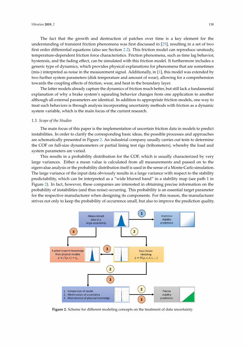
The main focus of this paper is the implementation of uncertain friction data in models to predictinstabilities. In order to clarify the corresponding basic ideas, the possible processes and approachesare schematically presented in Figure 2. An industrial company usually carries out tests to determinethe COF on full-size dynamometers or partial lining test rigs (tribometers), whereby the load andsystem parameters are varied.
This results in a probability distribution for the COF, which is usually characterized by verylarge variances. Either a mean value is calculated from all measurements and passed on to theeigenvalue analysis or the probability distribution itself is used in the sense of a Monte-Carlo simulation.The large variance of the input data obviously results in a large variance with respect to the stabilitypredictability, which can be interpreted as a “wide blurred band” in a stability map (see path 1 inFigure 2). In fact, however, these companies are interested in obtaining precise information on theprobability of instabilities (and thus noise) occurring. This probability is an essential target parameterfor the respective manufacturer when designing its components. For this reason, the manufacturerstrives not only to keep the probability of occurrence small, but also to improve the prediction quality.
Vibration 2019, 3 FOR PEER REVIEW 4
temperature-dependent friction force characteristics. Friction phenomena, such as time lag behavior, hysteresis, and the fading effect, can be simulated with this friction model. It furthermore includes a generic type of dynamics, which provides physical explanations for phenomena that are sometimes (mis-) interpreted as noise in the measurement signal. Additionally, in [1], this model was extended by two further system parameters (disk temperature and amount of wear), allowing for a comprehension towards the coupling effects of friction, wear, and heat in the boundary layer.
The latter models already capture the dynamics of friction much better, but still lack a fundamental explanation of why a brake system’s squealing behavior changes from one application to another although all external parameters are identical. In addition to appropriate friction models, one way to treat such behaviors is through analysis incorporating uncertainty methods with friction as a dynamic system variable, which is the main focus of the current research.
1.3. Scope of the Studies
The main focus of this paper is the implementation of uncertain friction data in models to predict instabilities. In order to clarify the corresponding basic ideas, the possible processes and approaches are schematically presented in Figure 2. An industrial company usually carries out tests to determine the COF on full-size dynamometers or partial lining test rigs (tribometers), whereby the load and system parameters are varied.
This results in a probability distribution for the COF, which is usually characterized by very large variances. Either a mean value is calculated from all measurements and passed on to the eigenvalue analysis or the probability distribution itself is used in the sense of a Monte-Carlo simulation. The large variance of the input data obviously results in a large variance with respect to the stability predictability, which can be interpreted as a “wide blurred band” in a stability map (see path 1 in Figure 2). In fact, however, these companies are interested in obtaining precise information on the probability of instabilities (and thus noise) occurring. This probability is an essential target parameter for the respective manufacturer when designing its components. For this reason, the manufacturer strives not only to keep the probability of occurrence small, but also to improve the prediction quality.
Figure 2. Scheme for different modeling concepts on the treatment of data uncertainty. Figure 2. Scheme for different modeling concepts on the treatment of data uncertainty.

Vibration 2019, 2 139
For this purpose, concepts are to be applied which precondition the measurement data in thesense of a better description of the friction dynamics and prediction quality. There are several possibleways of achieving this goal. A purely data-based approach, in which Data Driven Methods are appliedto the original data without any knowledge of physics, is one possible approach (path 2). However,this approach contains the risk that mathematical artifacts instead of physical laws will be identified.Since physical models are available for the COF description, an alternative approach will be takenin this paper. This is based on a-priori knowledge, which provides hypotheses for the mathematicalstructure of the differential equation. Data Driven Methods will be used to model the remaininguncertainty (path 3). The aim of this approach is to identify a much sharper and thus more precisestability limit than the one according to path 1.
Future work will focus on the comparison between the approaches according to path 2 and 3and should highlight the advantages and disadvantages of the respective strategy. This also includesconcepts where the strategies of path 2 and 3 are coupled with each other.
2. Methods
In this paper, models with polymorphic uncertainty are applied to a minimal model for instabilitiesof NVH phenomena. In the following subsections, the system to be investigated and the inclusion ofthe measurement data are presented.
2.1. The Method of Augmented Dimensioning
Concerning the brake dynamics in this study, the friction is not only treated as one uncertainparameter, but also as a dynamic system variable incorporated as a differential equation (also seeSections 1.2 and 2.2). Here, the authors follow the new concept where the system state space isexpanded by the dynamic state variables representing the friction, the so-called Method of AugmentedDimensioning (MAD) [26]. The MAD considers the system as a coupled system of brake dynamics andfriction dynamics. The stability of this coupled system is different compared to the single uncoupledbrake dynamics. With M
..x(t) = fx
( .x, x, µ, t
)and
.µ(t) = fµ
( .x, x, µ, t
), the general form of this coupled
system can be written for an eigenvalue analysis (where only the homogenous part is necessary),as follows:[
M 00 0
][ ..x(t)..µ(t)
]+
[D 0
− ∂ fµ
∂.x
I
][ .x(t).µ(t)
]+
C − ∂ fx∂µ
− ∂ fµ
∂x − ∂ fµ
∂µ
[ x(t)µ(t)
]=
[00
], (1)
where the first line in Equation (1) represents the system of the brake dynamics, while the second linerepresents the friction dynamics, and x(t) describes the mechanical degrees of freedom. Similarly,µ(t) represents the degrees of freedom for the friction system and its time-derivative
.µ(t) takes into
account the existence of dynamic friction behaviour. The coupling term ∂ fµ/∂.x in the damping matrix
contains the friction model with respect to the velocity dependence, such as a falling characteristicor a Stribeck-like effect. The term ∂ fµ/∂x combines the normal force resulting from the mechanicaldeformations with the COF in the contact, i.e., it primarily considers the normal force dependenceof the COF. Finally, the coupling term ∂ fx/∂µ takes into account the friction force resulting from theCOF. For all CEA calculations, the derivatives must be provided in a linearized form; for this purpose,the generally non-linear functions must be linearized at the respective equilibrium points. Furtherdetails on this method and its effects can be found in [26].
Based on the equations in Equation (1), the CEA is performed and provides eigenvalues inthe complex form, i.e., λj = αj + iωj, where αj is the real part and ωj is the imaginary part of thejth eigenvalues.
The sign of the real part eigenvalues is the well-known criterion for the stability evaluation ofthe investigated system. If any of the eigenvalues’ real parts are positive, the system is unstable,corresponding to increasing oscillation amplitudes. Only if all real parts are negative is this a stable
Vibration 2019, 2 140
system with decaying oscillating amplitudes. The imaginary part ωj depicts the correspondingfrequency, whereas the corresponding eigenvector represents the oscillation’s shape. The CEAcomputations are performed by using the polynomial eigenvalues solver in MATLAB R2017b.
2.2. Eigenvalue Analysis with an NVH Minimal Model for Brakes
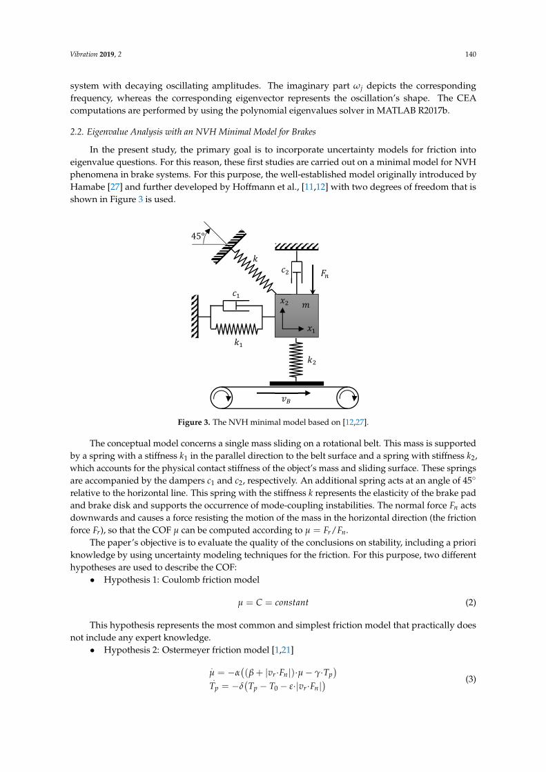
In the present study, the primary goal is to incorporate uncertainty models for friction intoeigenvalue questions. For this reason, these first studies are carried out on a minimal model for NVHphenomena in brake systems. For this purpose, the well-established model originally introduced byHamabe [27] and further developed by Hoffmann et al., [11,12] with two degrees of freedom that isshown in Figure 3 is used.
Vibration 2019, 3 FOR PEER REVIEW 6
frequency, whereas the corresponding eigenvector represents the oscillation’s shape. The CEA computations are performed by using the polynomial eigenvalues solver in MATLAB R2017b.
2.2. Eigenvalue Analysis with an NVH Minimal Model for Brakes
In the present study, the primary goal is to incorporate uncertainty models for friction into eigenvalue questions. For this reason, these first studies are carried out on a minimal model for NVH phenomena in brake systems. For this purpose, the well-established model originally introduced by Hamabe [27] and further developed by Hoffmann et al., [11,12] with two degrees of freedom that is shown in Figure 3 is used.
Figure 3. The NVH minimal model based on [12,27].
The conceptual model concerns a single mass sliding on a rotational belt. This mass is supported by a spring with a stiffness 𝑘 in the parallel direction to the belt surface and a spring with stiffness 𝑘 , which accounts for the physical contact stiffness of the object’s mass and sliding surface. These springs are accompanied by the dampers c1 and c2, respectively. An additional spring acts at an angle of 45∘ relative to the horizontal line. This spring with the stiffness 𝑘 represents the elasticity of the brake pad and brake disk and supports the occurrence of mode-coupling instabilities. The normal force 𝐹 acts downwards and causes a force resisting the motion of the mass in the horizontal direction (the friction force 𝐹 ), so that the COF 𝜇 can be computed according to 𝜇 = 𝐹 𝐹⁄ .
The paper’s objective is to evaluate the quality of the conclusions on stability, including a priori knowledge by using uncertainty modeling techniques for the friction. For this purpose, two different hypotheses are used to describe the COF:
• Hypothesis 1: Coulomb friction model 𝜇 = 𝐶 = 𝑐𝑜𝑛𝑠𝑡𝑎𝑛𝑡 (2)
This hypothesis represents the most common and simplest friction model that practically does not include any expert knowledge.
• Hypothesis 2: Ostermeyer friction model [1,21] 𝜇 = −𝛼 (𝛽 + |𝑣 ∙ 𝐹 |) ∙ 𝜇 − 𝛾 ∙ 𝑇 𝑇 = −𝛿 𝑇 − 𝑇 − 𝜀 ∙ |𝑣 ∙ 𝐹 | (3)
where 𝑇 is the contact temperature, 𝐹 is the normal force, 𝑣 is the relative velocity, and (𝛼, 𝛽, 𝛾, 𝛿, 𝜀, 𝑇 ) are the corresponding system parameters. This model was developed especially for
45°
𝑣
𝑥
𝑥
𝑘 𝑘
𝑘
𝑐
𝑐 𝐹
𝑚
Figure 3. The NVH minimal model based on [12,27].
The conceptual model concerns a single mass sliding on a rotational belt. This mass is supportedby a spring with a stiffness k1 in the parallel direction to the belt surface and a spring with stiffness k2,which accounts for the physical contact stiffness of the object’s mass and sliding surface. These springsare accompanied by the dampers c1 and c2, respectively. An additional spring acts at an angle of 45◦
relative to the horizontal line. This spring with the stiffness k represents the elasticity of the brake padand brake disk and supports the occurrence of mode-coupling instabilities. The normal force Fn actsdownwards and causes a force resisting the motion of the mass in the horizontal direction (the frictionforce Fr), so that the COF µ can be computed according to µ = Fr/Fn.
The paper’s objective is to evaluate the quality of the conclusions on stability, including a prioriknowledge by using uncertainty modeling techniques for the friction. For this purpose, two differenthypotheses are used to describe the COF:
• Hypothesis 1: Coulomb friction model
µ = C = constant (2)
This hypothesis represents the most common and simplest friction model that practically doesnot include any expert knowledge.
• Hypothesis 2: Ostermeyer friction model [1,21]
.µ = −α
((β + |vr·Fn|)·µ− γ·Tp
).
Tp = −δ(Tp − T0 − ε·|vr·Fn|
) (3)
Vibration 2019, 2 141
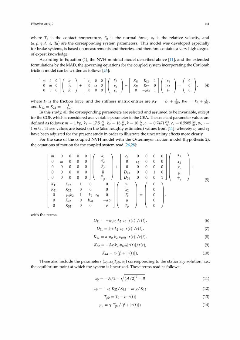
where Tp is the contact temperature, Fn is the normal force, vr is the relative velocity, and(α, β, γ, δ, ε, T0) are the corresponding system parameters. This model was developed especiallyfor brake systems, is based on measurements and theories, and therefore contains a very high degreeof expert knowledge.
According to Equation (1), the NVH minimal model described above [11], and the extendedformulations by the MAD, the governing equations for the coupled system incorporating the Coulombfriction model can be written as follows [26]: m 0 0
0 m 00 0 0
..x1..
x2..Fr
+
c1 0 00 c2 00 0 0
.x1.x2.Fr
+
K11 K12 1K21 K22 00 −µk2 1
x1
x2
Fr
=
000
, (4)
where Fr is the friction force, and the stiffness matrix entries are K11 = k1 +k
2m , K22 = k2 +k
2m ,and K12 = K21 = − k
2m .In this study, all the corresponding parameters are selected and assumed to be invariable, except
for the COF, which is considered as a variable parameter in the CEA. The constant parameter values aredefined as follows: m = 1 kg, k1 = 17.5 N
m , k2 = 18 Nm , k = 10 N
m , c1 = 0.7471 Nsm , c2 = 0.5985 Ns
m , vbelt =
1 m/s . These values are based on the (also roughly estimated) values from [11], whereby c1 and c2
have been adjusted for the present study in order to illustrate the uncertainty effects more clearly.For the case of the coupled NVH model with the Ostermeyer friction model (hypothesis 2),
the equations of motion for the coupled system read [26,28]:
m0000
0m000
00000
00000
00000
..x1..
x2..Fr..µ..Tp
+
c1
00
D41
D51
0c2
000
00000
00010
00001
.x1.x2.Fr.µ.Tp
+
K11
K21
000
K12
K22
−µ0k2
K42
K52
10100
00k2
K44
0
z0
000−αγ
δ
x1
x2
Fr
µ
Tp
=
00000
,
(5)
with the termsD41 = −α·µ0·k2·z0·|r(t)|/r(t), (6)
D51 = δ·ε·k2·z0·|r(t)|/r(t), (7)
K42 = α·µ0·k2·vbelt·|r(t)|/r(t), (8)
K52 = −δ·ε·k2·vbelt|r(t)|/r(t), (9)
K44 = α·(β + |r(t)|), (10)
These also include the parameters (z0, x0,Tp0, µ0) corresponding to the stationary solution, i.e.,the equilibrium point at which the system is linearized. These terms read as follows:
z0 = −A/2−√(A/2)2 − B (11)
x0 = −z0·K22/K12 −m·g/K12 (12)
Tp0 = T0 + ε·|r(t)| (13)
µ0 = γ·Tp0/(β + |r(t)|) (14)

Vibration 2019, 2 142
A =
(K12 − K11·K22
K12
)·β + k2·γ·T0 − K11/K12·m·g·k2·vbelt
vbelt·k2·(
k2·γ·ε +(
K12 − K11·K22K12
)) (15)
B =
K22K12·m·g·β
vbelt·k2·(
k2·γ·ε +(
K12 − K11·K22K12
)) (16)
r(t) = −k2·z0·vbelt (17)
Since the Coulomb friction model is a 0th order differential equation and the Ostermeyer modelis a 2nd order differential equation, the latter obviously results in two more eigenvalues. In addition,the existing eigenvalues shift, especially with the increasing influence of the friction dynamics.Equations (4) and (5) serve as the basis for the eigenvalue analyses for all further investigationsfound in Section 3.
2.3. Data Modeling
The following subsection documents the COF measurement data obtained for the studies andtheir exploitation for uncertainty studies.
2.3.1. Considered Data Set
In the present case, the COF characteristic is performed on an automated tribometer, the so-calledAutomated Universal Tribotester (AUT), available at the Institute of Dynamics and Vibrations atBraunschweig University of Technology [29], (see Figure 4). These are measurements in which a 2 cm2
(height: 2 cm (tangential to sliding velocity), width: 1 cm (perpendicular to sliding velocity)) part ofthe pad material (pin) is pressed against a rotating disk. Here, the forces in the pin and the temperatureof the disk near the contact are measured. The COF is calculated from the ratio of tangential force tonormal force.
Vibration 2019, 3 FOR PEER REVIEW 8
𝐵 = 𝐾𝐾 ∙ 𝑚 ∙ 𝑔 ∙ 𝛽𝑣 ∙ 𝑘 ∙ (𝑘 ∙ 𝛾 ∙ 𝜀 + (𝐾 − 𝐾 ∙ 𝐾𝐾 )) (16)
𝑟(𝑡) = −𝑘 ∙ 𝑧 ∙ 𝑣 (17)
Since the Coulomb friction model is a 0th order differential equation and the Ostermeyer model is a 2nd order differential equation, the latter obviously results in two more eigenvalues. In addition, the existing eigenvalues shift, especially with the increasing influence of the friction dynamics. Equations (4) and (5) serve as the basis for the eigenvalue analyses for all further investigations found in Section 3.
2.3. Data Modeling
The following subsection documents the COF measurement data obtained for the studies and their exploitation for uncertainty studies.
2.3.1. Considered Data Set
In the present case, the COF characteristic is performed on an automated tribometer, the so-called Automated Universal Tribotester (AUT), available at the Institute of Dynamics and Vibrations at Braunschweig University of Technology [29], (see Figure 4). These are measurements in which a 2cm² (height: 2cm (tangential to sliding velocity), width: 1cm (perpendicular to sliding velocity)) part of the pad material (pin) is pressed against a rotating disk. Here, the forces in the pin and the temperature of the disk near the contact are measured. The COF is calculated from the ratio of tangential force to normal force.
Figure 4. Automated Universal Tribotester (AUT), taken from [29].
The normal force and rotational speed are specified for each application. This specification is made according to a certain scheme in which the frictional power is increased successively from application to application. This results in a procedure consisting of a total of 461 applications. These two controlled variables are also measured during the application, whereby, in [29], it has been demonstrated that the automation can very well maintain these specified values over the entire procedure.
Much greater variation during an application can be observed for the COF and the temperature. Figure 5 shows the corresponding values at application 78 as an example of this.
Figure 4. Automated Universal Tribotester (AUT), taken from [29].
The normal force and rotational speed are specified for each application. This specification is madeaccording to a certain scheme in which the frictional power is increased successively from applicationto application. This results in a procedure consisting of a total of 461 applications. These two controlled
Vibration 2019, 2 143
variables are also measured during the application, whereby, in [29], it has been demonstrated that theautomation can very well maintain these specified values over the entire procedure.
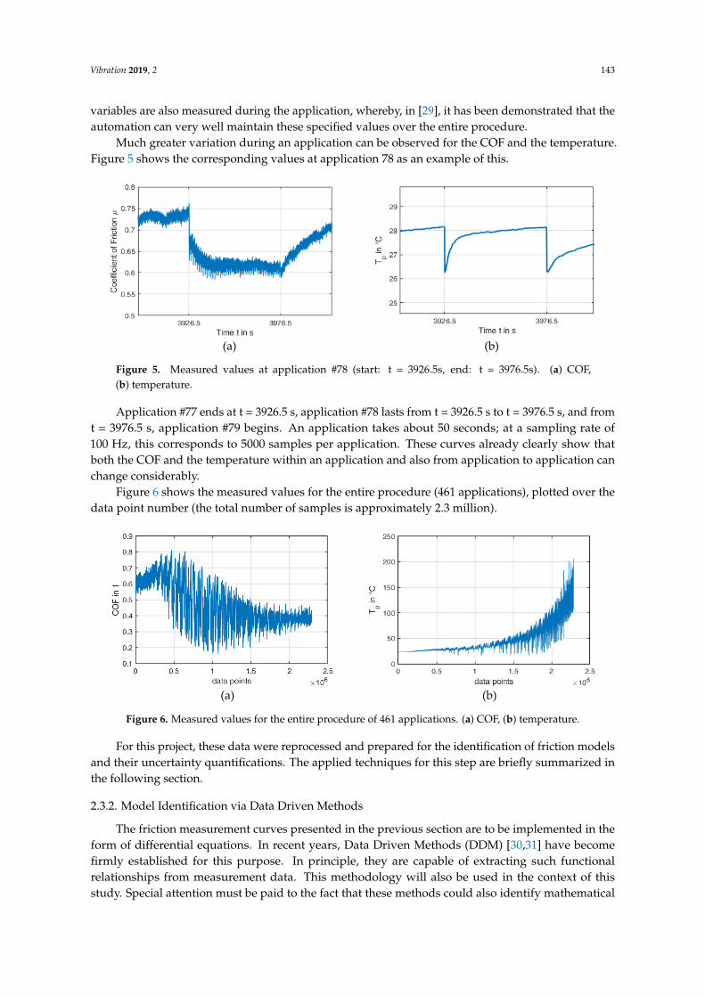
Much greater variation during an application can be observed for the COF and the temperature.Figure 5 shows the corresponding values at application 78 as an example of this.
Vibration 2019, 3 FOR PEER REVIEW 9
(a) (b)
Figure 5. Measured values at application #78 (start: t = 3926.5s, end: t = 3976.5s). (a) COF, (b) temperature.
Application #77 ends at t = 3926.5 s, application #78 lasts from t = 3926.5 s to t = 3976.5 s, and from t = 3976.5 s, application #79 begins. An application takes about 50 seconds; at a sampling rate of 100 Hz, this corresponds to 5000 samples per application. These curves already clearly show that both the COF and the temperature within an application and also from application to application can change considerably.
Figure 6 shows the measured values for the entire procedure (461 applications), plotted over the data point number (the total number of samples is approximately 2.3 million).
(a) (b)
Figure 6. Measured values for the entire procedure of 461 applications. (a) COF, (b) temperature.
For this project, these data were reprocessed and prepared for the identification of friction models and their uncertainty quantifications. The applied techniques for this step are briefly summarized in the following section.
2.3.2. Model Identification via Data Driven Methods
The friction measurement curves presented in the previous section are to be implemented in the form of differential equations. In recent years, Data Driven Methods (DDM) [30,31] have become firmly established for this purpose. In principle, they are capable of extracting such functional relationships from measurement data. This methodology will also be used in the context of this study. Special attention must be paid to the fact that these methods could also identify mathematical artifacts instead of physical models, which is disadvantageous for the understanding of the system [32]. The corresponding backgrounds and mathematical approaches are explained below.
This model identification method refers to the research field of Machine Learning (ML) and has recently been the focus in different fields of applications.
In the present work, the DDM chosen by the authors is based on optimization with sparse regression techniques [30], which is applicable to identifying Ordinary Differential Equations or even Partial Differential Equations. The governing equations for complex physical systems are oftentimes
Figure 5. Measured values at application #78 (start: t = 3926.5s, end: t = 3976.5s). (a) COF,(b) temperature.
Application #77 ends at t = 3926.5 s, application #78 lasts from t = 3926.5 s to t = 3976.5 s, and fromt = 3976.5 s, application #79 begins. An application takes about 50 seconds; at a sampling rate of100 Hz, this corresponds to 5000 samples per application. These curves already clearly show thatboth the COF and the temperature within an application and also from application to application canchange considerably.
Figure 6 shows the measured values for the entire procedure (461 applications), plotted over thedata point number (the total number of samples is approximately 2.3 million).
Vibration 2019, 3 FOR PEER REVIEW 9
(a) (b)
Figure 5. Measured values at application #78 (start: t = 3926.5s, end: t = 3976.5s). (a) COF, (b) temperature.
Application #77 ends at t = 3926.5 s, application #78 lasts from t = 3926.5 s to t = 3976.5 s, and from t = 3976.5 s, application #79 begins. An application takes about 50 seconds; at a sampling rate of 100 Hz, this corresponds to 5000 samples per application. These curves already clearly show that both the COF and the temperature within an application and also from application to application can change considerably.
Figure 6 shows the measured values for the entire procedure (461 applications), plotted over the data point number (the total number of samples is approximately 2.3 million).
(a) (b)
Figure 6. Measured values for the entire procedure of 461 applications. (a) COF, (b) temperature.
For this project, these data were reprocessed and prepared for the identification of friction models and their uncertainty quantifications. The applied techniques for this step are briefly summarized in the following section.
2.3.2. Model Identification via Data Driven Methods
The friction measurement curves presented in the previous section are to be implemented in the form of differential equations. In recent years, Data Driven Methods (DDM) [30,31] have become firmly established for this purpose. In principle, they are capable of extracting such functional relationships from measurement data. This methodology will also be used in the context of this study. Special attention must be paid to the fact that these methods could also identify mathematical artifacts instead of physical models, which is disadvantageous for the understanding of the system [32]. The corresponding backgrounds and mathematical approaches are explained below.
This model identification method refers to the research field of Machine Learning (ML) and has recently been the focus in different fields of applications.
In the present work, the DDM chosen by the authors is based on optimization with sparse regression techniques [30], which is applicable to identifying Ordinary Differential Equations or even Partial Differential Equations. The governing equations for complex physical systems are oftentimes
Figure 6. Measured values for the entire procedure of 461 applications. (a) COF, (b) temperature.
For this project, these data were reprocessed and prepared for the identification of friction modelsand their uncertainty quantifications. The applied techniques for this step are briefly summarized inthe following section.
2.3.2. Model Identification via Data Driven Methods
The friction measurement curves presented in the previous section are to be implemented in theform of differential equations. In recent years, Data Driven Methods (DDM) [30,31] have becomefirmly established for this purpose. In principle, they are capable of extracting such functionalrelationships from measurement data. This methodology will also be used in the context of thisstudy. Special attention must be paid to the fact that these methods could also identify mathematical
Vibration 2019, 2 144
artifacts instead of physical models, which is disadvantageous for the understanding of the system [32].The corresponding backgrounds and mathematical approaches are explained below.
This model identification method refers to the research field of Machine Learning (ML) and hasrecently been the focus in different fields of applications.
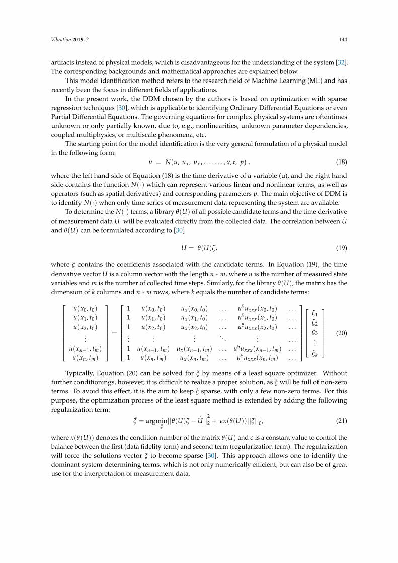
In the present work, the DDM chosen by the authors is based on optimization with sparseregression techniques [30], which is applicable to identifying Ordinary Differential Equations or evenPartial Differential Equations. The governing equations for complex physical systems are oftentimesunknown or only partially known, due to, e.g., nonlinearities, unknown parameter dependencies,coupled multiphysics, or multiscale phenomena, etc.
The starting point for the model identification is the very general formulation of a physical modelin the following form:
.u = N(u, ux, uxx, . . . . . . , x, t, p) , (18)
where the left hand side of Equation (18) is the time derivative of a variable (u), and the right handside contains the function N(·) which can represent various linear and nonlinear terms, as well asoperators (such as spatial derivatives) and corresponding parameters p. The main objective of DDM isto identify N(·) when only time series of measurement data representing the system are available.
To determine the N(·) terms, a library θ(U) of all possible candidate terms and the time derivativeof measurement data
.U will be evaluated directly from the collected data. The correlation between
.U
and θ(U) can be formulated according to [30]
.U = θ(U)ξ, (19)
where ξ contains the coefficients associated with the candidate terms. In Equation (19), the timederivative vector
.U is a column vector with the length n ∗m, where n is the number of measured state
variables and m is the number of collected time steps. Similarly, for the library θ(U), the matrix has thedimension of k columns and n ∗m rows, where k equals the number of candidate terms:
.u(x0, t0).u(x1, t0).u(x2, t0)
....u(xn−1, tm)
.u(xn, tm)
=
1 u(x0, t0) ux(x0, t0) . . . u5uxxx(x0, t0) . . .1 u(x1, t0) ux(x1, t0) . . . u5uxxx(x1, t0) . . .1 u(x2, t0) ux(x2, t0) . . . u5uxxx(x2, t0) . . ....
......
. . .... . . .
1 u(xn−1, tm) ux(xn−1, tm) . . . u5uxxx(xn−1, tm) . . .1 u(xn, tm) ux(xn, tm) . . . u5uxxx(xn, tm) . . .
ξ1
ξ2
ξ3...
ξk
(20)
Typically, Equation (20) can be solved for ξ by means of a least square optimizer. Withoutfurther conditionings, however, it is difficult to realize a proper solution, as ξ will be full of non-zeroterms. To avoid this effect, it is the aim to keep ξ sparse, with only a few non-zero terms. For thispurpose, the optimization process of the least square method is extended by adding the followingregularization term:
ξ̂ = argminξ||θ(U)ξ −
.U||
22 + εκ(θ(U))||ξ||0, (21)
where κ(θ(U)) denotes the condition number of the matrix θ(U) and ε is a constant value to control thebalance between the first (data fidelity term) and second term (regularization term). The regularizationwill force the solutions vector ξ to become sparse [30]. This approach allows one to identify thedominant system-determining terms, which is not only numerically efficient, but can also be of greatuse for the interpretation of measurement data.
Vibration 2019, 2 145
2.3.3. Tracking Information of Noisy Data via Total Variation Regularization (TVR)
In order to perform the identification of a physical model and its parameters via DDMs describedin the previous section, it is very important to appropriately consider time-derivatives for values thatcould be influenced by noisy data ( f ). Let
f := µd = µm + δm + ε , (22)
where µm + δm := µ contains physical information and ε contains uncorrelated random noise.To calculate the derivative value of noisy data via the typical finite difference method is obviouslyunsuitable and might result in very large errors. Oftentimes, the methods used to calculate derivativesafter denoising also do not produce satisfactory results. Therefore, regularization should take placedirectly in the processes of differentiation, as it can guarantee that the derivative will have a higherdegree of regularity. This method, the so—called method of Total Variation Regularization (TVR),was further developed by Rick Chartrand [33] and followed up the methods of Tikhonov [34].The associated ideas are briefly explained below.
The evaluation of the derivation of data ( f ) in a time interval [0, T] can be completed byminimizing the following functional:
F(w) = α∫ T
0
∣∣ .w∣∣dt +
12
∫ T
0|Aw− f |2dt :=
∫ T
0L(w,
.w, t)dt (23)
The functional F(w) is defined on the interval [0, T], where f is the noisy and possibly non-smoothdata, w (in this context it can be understood as an analogy to
.u in Equation (18)) is the required
differentiation of f , and.
w is the first derivative of w. The usage of the TVR accomplishes twoadvantages. It suppresses the noise as the noise function would have a large total variation. It also doesnot suppress jump discontinuities, unlike the typical regularizations. This allows for the computationof discontinuous derivatives, and detection of corners and edges in noisy data [33].
To find the minimum of the functional F(w), the well-known Euler-Lagrange equation is applied:
∂L∂w− d
dt∂L∂
.w
= AT(Aw− f )− αddt
.w∣∣ .w∣∣ = 0, (24)
where AT( f (a)) :=∫ T
a f (a)dt is the adjoint of the operator A. The approach continues with the iterativeGradient Descent procedure. In this method, it is assumed that the variation parameter w is changedalong with artificial time evolution. Therefore, Equation (24) can be rewritten in the following form:
∂w∂τ
:= αddt
.w∣∣ .w∣∣ − AT(Aw− f ) = 0. (25)
Substituting the term∣∣ .w∣∣ with
√( .w)2
+ e, while e > 0, e � 1, introduces a small number foravoiding the (otherwise possible) dividing by zero:
∂w∂τ
:= αddt
.w√( .
w)2
+ e− AT(Aw− f ) = 0. (26)
Typically, Equation (26) can be efficiently solved with an explicit time marching scheme,discretized as ∂w/∂τ := (wn+1 − wn)/∆τ for fixed values of ∆τ, and wn+1 − wn = ∆τgn, where gn
characterizes the discretized right side term of Equation (26) at the current iteration step (n) [33,34].When ∆τ is small, the convergence is rather slow, while with increasing ∆τ, divergence might
occur. The optimum of ∆τ should not be greater than the inverse of the Hessian (second-order

Vibration 2019, 2 146
partial derivation) (Hn) of F(wn). In this case, ∆τ is replaced by H−1n and the iteration steps are then
performed according to Equation (27):
wn+1 = wn + H−1n gn. (27)
To construct gn and Hn, it is firstly assumed that w is defined on a uniform grid {t}T0 =
{0, ∆t, 2∆t, . . . , T}. The derivatives of w are computed halfway between two grid points as centereddifference Dw(ti + ∆t/2) = (w(ti+1)− w(ti))/∆t; this procedure defines the differentiation matrix D.The integrals of w are likewise computed halfway between two grid points, using the trapezoid rule to
define matrix A. Let Qn be the diagonal matrix whose ith entry is (((wn(ti)− wn(ti−1))/∆t)2 + e)−1/2
,and Ln := ∆tDTQnD. Then, the term gn becomes gn = αLnwn − AT(Awn − f ). The approximation ofthe Hessian of F(wn) is derived according to: Hn := ∂2F(wn)/∂w2
n = AT A− αLn.With these two methods (DDM and TVR), the measurement data of the COF and the contact
temperature are processed. Especially for the signal of the COF µ, TVR produces a reasonablesmoothing and reduces the strong noise very well.
2.4. Polymorphic Uncertainty Modeling
In general terms, uncertainty can be classified into two classes with respect to its characteristics.One is an irreducible uncertainty, namely aleatory uncertainty, which refers to the natural stochasticsin system processes, e.g., the variations of manufacturing processes, material properties, geometryproperties, etc. In contrast to this, uncertainty with reducible characteristics is known as epistemicuncertainty. This may refer to, i.e., the lack of knowledge (model uncertainty), lack of statisticalinformation (statistical uncertainty), or accuracy of data (perceptual uncertainty), etc. This type ofuncertainty can be significantly reduced when, e.g., better knowledge, more statistical information,or an improved measurement accuracy are available. This concept has already been applied to simpleCOF formulations for eigenvalue problems in brake systems [35].
The occurrence of only one uncertainty (aleatory or epistemic) can also be referred toas monomorphic uncertainty, whereas the joint occurrence is called polymorphic uncertainty.The uncertainty quantification could be carried out based on, e.g., a probabilistic approach,a possibilistic approach, or even a combination of both techniques. In general, the probabilisticapproach is used for aleatory uncertainty analysis, when the informative variation is available, e.g.,in a typical stochastic process.
The possibilistic approach has proven to be an adequate description, if the range or interval ofthe statistical output is of particular interest or statistical data or knowledge are limited etc., so theprobabilistic approach would not provide much more information [36]. In these cases, fuzzy-likealgorithms can improve the informative value of the possibilistic approach by using the fuzzymembership function instead of only a simple interval.
The transition between the usefulness of a probabilistic and possibilistic description is sometimesfluent and primarily linked to the available amount of data and knowledge. Thus, in some cases,the possibilistic approach can be replaced by the probabilistic approach. For example, when theincompleteness (statistical uncertainty) is based on a low volume of available data, the possibilisticapproach is suitable. However, if more statistical data are collected, the probabilistic approach can beused instead of the possibilistic one, as more informative statistical outputs can be obtained.
For the probabilistic approach, the Monte Carlo simulation is often used. This methodologyspreads a large number of sampling data over the design parameter space, and forwards them throughthe analysis of the model or mapping function.
The epistemic uncertainty analysis is carried out via the possibilistic approach; the fuzzymethod [37] is used in this study. The fuzzy members are defined as the convex set of fuzzy valuesover the universal set (R). The membership function is generally defined with p̃(x) ∈ {0, 1} and atthe nominal point x, the fuzzy value is p̃(x) = 1, which represents the true value for the case of no
Vibration 2019, 2 147
epistemic uncertainty. The form of the membership function can be defined as the corresponding kernel,in which the distribution of epistemic (when information is available) data can be well-described.For a simplified example, the fuzzy number can be defined as a triangular kernel, for which only threepoints of information are required. Between these three points, a linear interpolation is carried out, asshown in Equation (28):
p̃ =
1
r−q (x− q) for q < x ≤ r1
s−r (s− x) for r < x ≤ s0 otherwise
, (28)
where (q, r, s) denote the minimum, nominal, and maximum point of the interval, respectively.This kernel function can take on other forms based on the characteristic information inside the interval,and more information on this aspect can be found in [36,37].
In the present study, polymorphic uncertainty modeling shall be performed. The problem to beconsidered is the calculation of eigenvalues, which are influenced by different forms of uncertainty.The basis of the calculations is provided by the measurement data introduced in Section 2.3.1. For thispurpose, the parameters for two different friction models (Coulomb, Ostermeyer) are calculated foreach of the 461 measurement applications. The parameters determining the friction characteristicsvary between the individual applications so that there are 461 parameter sets for each friction model.These parameter sets should be regarded as aleatory uncertainties, since it is assumed here that thecause of these uncertainties is primarily of a physical nature, i.e., no significant reduction of theuncertainty can be expected from further measurements. As a result of the aleatory uncertainty model,a corresponding probability density function for the eigenvalues is determined.
Neither friction models are able to reproduce the measured COFs exactly over time. This resultsin a “band of uncertainty” for each individual application. The reason of this can be understood asa lack of knowledge, since even more suitable friction models can further reduce this band. Thus,this aspect represents an epistemic uncertainty and the implementation of this band can be carried outwith fuzzy methods. The exact procedures and results are discussed in Section 3.
3. Results
As already introduced in Equation (22), the relation between the measurement data (µd) and theresponse of model (µm) can be written in the general form µd = µm + δm + ε, where δm is the biasrepresenting model uncertainty and ε is the measurement uncertainty, e.g., noise. Typically, in practice,µm is assumed to be constant (as in the Coulomb friction model) and used like this in analysis, such asNVH problems. This assumption is expected to lead to a large model uncertainty δm, which makes theNVH prediction rather inaccurate.
In order to reduce this uncertainty caused by the bias term, a sophisticated and more realisticfriction model (the Ostermeyer friction model, see Section 2.2) is implemented and compared toCoulomb’s model with respect to polymorphic uncertainty quantification for stability studies.
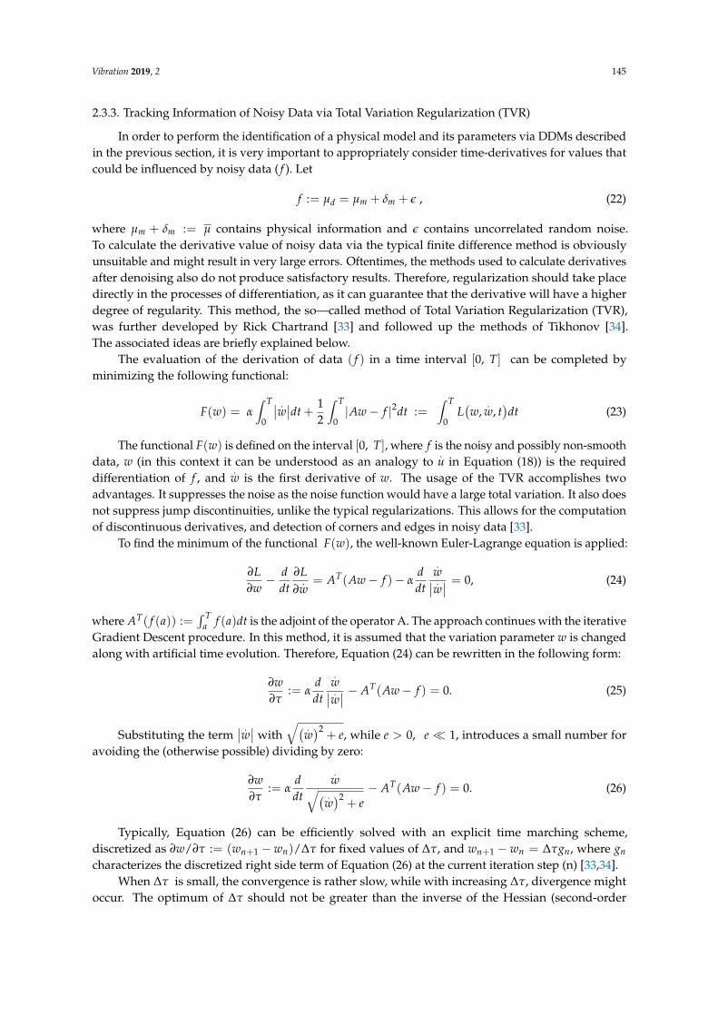
3.1. Stability of NVH Model with Coulomb Friction Model and Polymorphic Uncertainty
First, polymorphic uncertainty quantification is carried out with the conventional Coulombfriction model. Figure 7 shows the basic procedure.
Vibration 2019, 3 FOR PEER REVIEW 13
cause of these uncertainties is primarily of a physical nature, i.e., no significant reduction of the uncertainty can be expected from further measurements. As a result of the aleatory uncertainty model, a corresponding probability density function for the eigenvalues is determined.
Neither friction models are able to reproduce the measured COFs exactly over time. This results in a “band of uncertainty” for each individual application. The reason of this can be understood as a lack of knowledge, since even more suitable friction models can further reduce this band. Thus, this aspect represents an epistemic uncertainty and the implementation of this band can be carried out with fuzzy methods. The exact procedures and results are discussed in Section 3.
3. Results
As already introduced in Equation (22), the relation between the measurement data (𝜇 ) and the response of model (𝜇 ) can be written in the general form 𝜇 = 𝜇 + 𝛿 + 𝜖, where 𝛿𝑚 is the bias representing model uncertainty and 𝜖 is the measurement uncertainty, e.g., noise. Typically, in practice, 𝜇 is assumed to be constant (as in the Coulomb friction model) and used like this in analysis, such as NVH problems. This assumption is expected to lead to a large model uncertainty 𝛿 , which makes the NVH prediction rather inaccurate.
In order to reduce this uncertainty caused by the bias term, a sophisticated and more realistic friction model (the Ostermeyer friction model, see Section 2.2) is implemented and compared to Coulomb’s model with respect to polymorphic uncertainty quantification for stability studies.
3.1. Stability of NVH Model with Coulomb Friction Model and Polymorphic Uncertainty
First, polymorphic uncertainty quantification is carried out with the conventional Coulomb friction model. Figure 7 shows the basic procedure.
Figure 7. Flowchart of polymorphic uncertainty quantification for stability analysis with Coulomb’s friction model.
The measurement data for the coefficient of friction are carried out application-wise. First, the procedure for determining the nominal characteristic values is presented (Figure 7, dark blue, lower path). For an ith application, the mean COF is first determined (this correlates to Coulomb’s friction model that the COF is a constant). For this COF, all eigenvalues are calculated according to Equation (4) in Section 2.2. To find instabilities, the real parts belonging to the complex eigenvalues are extracted and the largest value is stored. This largest value ultimately determines whether the system is stable (value is negative) or unstable (value is positive) for the COF applied.
For the 461 applications examined, this results in 461 maximum real parts that can be represented in a probability density function. From this, conclusions can be made about stability according to the nominal values 𝜇 (fraction of applications with a maximum real part greater than 0).
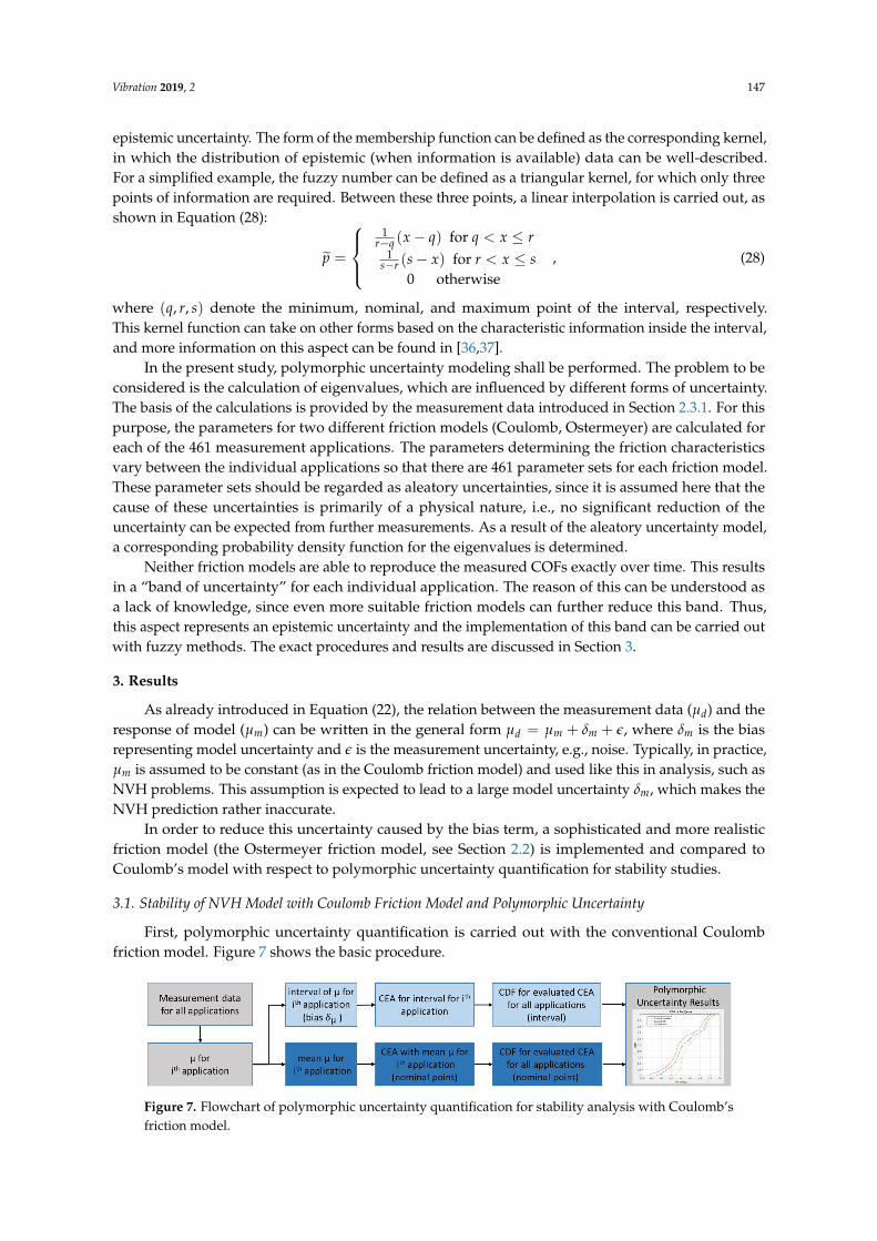
Figure 8a shows the histogram for the averaged COFs, while Figure 8b shows the empirical cumulative distribution function for the largest eigenvalue real parts. This graph shows that, according to the measurement data, the nominal probability of an instable behaviour of the NVH minimal model in Section 2.2 combined with the Coulomb friction model is about 55%.
Figure 7. Flowchart of polymorphic uncertainty quantification for stability analysis with Coulomb’sfriction model.
Vibration 2019, 2 148
The measurement data for the coefficient of friction are carried out application-wise. First,the procedure for determining the nominal characteristic values is presented (Figure 7, dark blue,lower path). For an ith application, the mean COF is first determined (this correlates to Coulomb’sfriction model that the COF is a constant). For this COF, all eigenvalues are calculated according toEquation (4) in Section 2.2. To find instabilities, the real parts belonging to the complex eigenvalues areextracted and the largest value is stored. This largest value ultimately determines whether the systemis stable (value is negative) or unstable (value is positive) for the COF applied.
For the 461 applications examined, this results in 461 maximum real parts that can be representedin a probability density function. From this, conclusions can be made about stability according to thenominal values µm (fraction of applications with a maximum real part greater than 0).
Figure 8a shows the histogram for the averaged COFs, while Figure 8b shows the empiricalcumulative distribution function for the largest eigenvalue real parts. This graph shows that, accordingto the measurement data, the nominal probability of an instable behaviour of the NVH minimal modelin Section 2.2 combined with the Coulomb friction model is about 55%.Vibration 2019, 3 FOR PEER REVIEW 14
(a) (b)
Figure 8. Uncertainty quantification for stability analysis of 461 measurement applications with an NVH-minimal model with Coulomb’s friction model: (a) histogram for the mean COF and (b) cumulated density function for the maximum real parts.
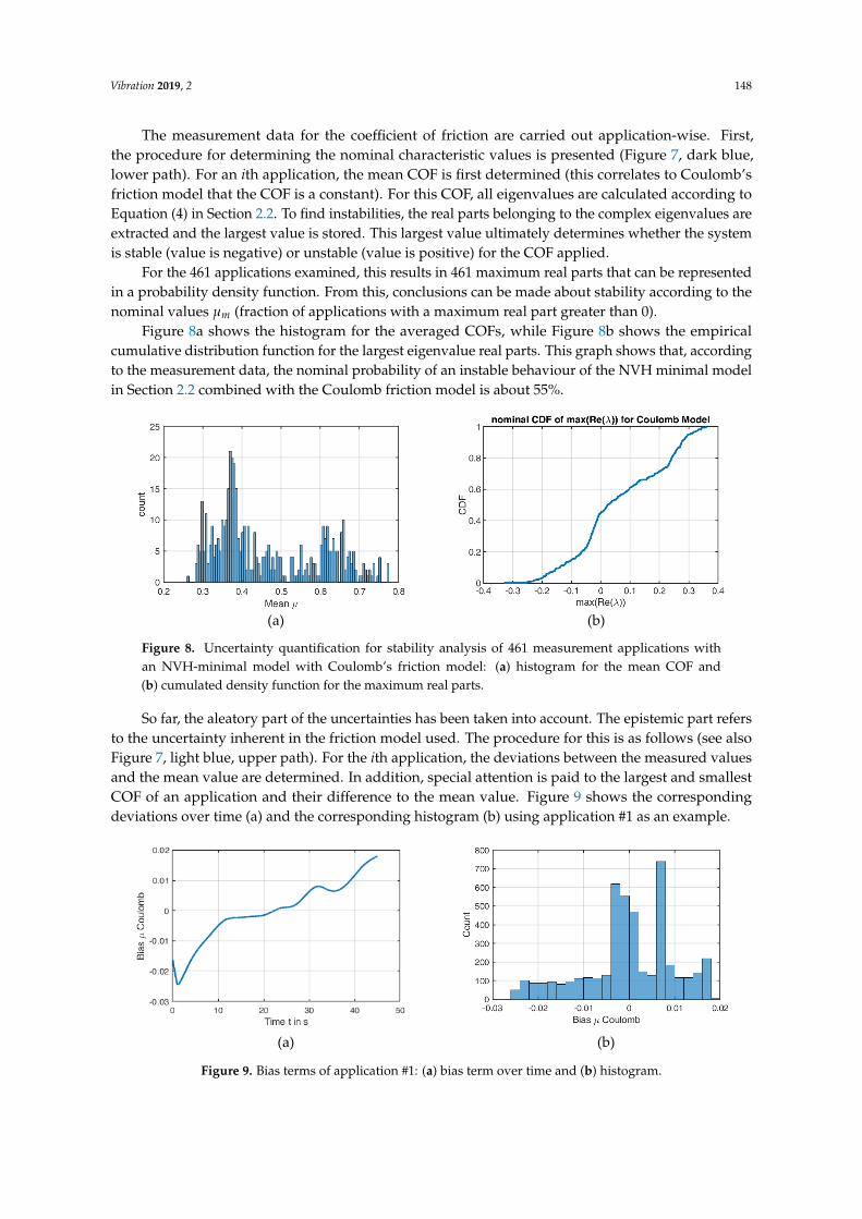
So far, the aleatory part of the uncertainties has been taken into account. The epistemic part refers to the uncertainty inherent in the friction model used. The procedure for this is as follows (see also Figure 7, light blue, upper path). For the ith application, the deviations between the measured values and the mean value are determined. In addition, special attention is paid to the largest and smallest COF of an application and their difference to the mean value. Figure 9 shows the corresponding deviations over time (a) and the corresponding histogram (b) using application #1 as an example.
(a) (b)
Figure 9. Bias terms of application #1: (a) bias term over time and (b) histogram.
This results in a band for each application, which characterizes the inaccuracy of the friction model. This interval correlates to the bias term of the model uncertainty. For the modeling of the epistemic uncertainty, the largest and smallest values of an application are used. These values are transferred to the eigenvalue solver and, as for the mean COF, the maximum real part is determined. This results in two further curves for the cumulated probability density function; one curve for the respective minimum COFs and another for the respective maximum COFs.
Figure 10 shows the three corresponding curves (nominal, maximum, minimum) in one plot. Of particular interest here are the values at alpha-cut 0 (minimum and maximum) and 1 (nominal value) at max 𝑅𝑒(𝜆) = 0, as this represents the stability border. The corresponding values here are (0.449, 0.178, 0.564). This information is, for example, very unsatisfactory for the engineer who designs the brake system, since a conclusion like "The system will be most likely stable with 44.9% probability, but it could also be up to 17.8% or 56.4%" is difficult to handle for the development process, since the width of the uncertainty is very large.
The width of this probability interval can be reduced by improving the friction model, thus reducing the bias term. In the next section, the authors present the results when using Ostermeyer’s friction model instead of Coulomb’s.
Figure 8. Uncertainty quantification for stability analysis of 461 measurement applications withan NVH-minimal model with Coulomb’s friction model: (a) histogram for the mean COF and(b) cumulated density function for the maximum real parts.
So far, the aleatory part of the uncertainties has been taken into account. The epistemic part refersto the uncertainty inherent in the friction model used. The procedure for this is as follows (see alsoFigure 7, light blue, upper path). For the ith application, the deviations between the measured valuesand the mean value are determined. In addition, special attention is paid to the largest and smallestCOF of an application and their difference to the mean value. Figure 9 shows the correspondingdeviations over time (a) and the corresponding histogram (b) using application #1 as an example.
Vibration 2019, 3 FOR PEER REVIEW 14
(a) (b)
Figure 8. Uncertainty quantification for stability analysis of 461 measurement applications with an NVH-minimal model with Coulomb’s friction model: (a) histogram for the mean COF and (b) cumulated density function for the maximum real parts.
So far, the aleatory part of the uncertainties has been taken into account. The epistemic part refers to the uncertainty inherent in the friction model used. The procedure for this is as follows (see also Figure 7, light blue, upper path). For the ith application, the deviations between the measured values and the mean value are determined. In addition, special attention is paid to the largest and smallest COF of an application and their difference to the mean value. Figure 9 shows the corresponding deviations over time (a) and the corresponding histogram (b) using application #1 as an example.
(a) (b)
Figure 9. Bias terms of application #1: (a) bias term over time and (b) histogram.
This results in a band for each application, which characterizes the inaccuracy of the friction model. This interval correlates to the bias term of the model uncertainty. For the modeling of the epistemic uncertainty, the largest and smallest values of an application are used. These values are transferred to the eigenvalue solver and, as for the mean COF, the maximum real part is determined. This results in two further curves for the cumulated probability density function; one curve for the respective minimum COFs and another for the respective maximum COFs.
Figure 10 shows the three corresponding curves (nominal, maximum, minimum) in one plot. Of particular interest here are the values at alpha-cut 0 (minimum and maximum) and 1 (nominal value) at max 𝑅𝑒(𝜆) = 0, as this represents the stability border. The corresponding values here are (0.449, 0.178, 0.564). This information is, for example, very unsatisfactory for the engineer who designs the brake system, since a conclusion like "The system will be most likely stable with 44.9% probability, but it could also be up to 17.8% or 56.4%" is difficult to handle for the development process, since the width of the uncertainty is very large.
The width of this probability interval can be reduced by improving the friction model, thus reducing the bias term. In the next section, the authors present the results when using Ostermeyer’s friction model instead of Coulomb’s.
Figure 9. Bias terms of application #1: (a) bias term over time and (b) histogram.
Vibration 2019, 2 149
This results in a band for each application, which characterizes the inaccuracy of the frictionmodel. This interval correlates to the bias term of the model uncertainty. For the modeling of theepistemic uncertainty, the largest and smallest values of an application are used. These values aretransferred to the eigenvalue solver and, as for the mean COF, the maximum real part is determined.This results in two further curves for the cumulated probability density function; one curve for therespective minimum COFs and another for the respective maximum COFs.
Figure 10 shows the three corresponding curves (nominal, maximum, minimum) in one plot.Of particular interest here are the values at alpha-cut 0 (minimum and maximum) and 1 (nominalvalue) at maxRe(λ) = 0, as this represents the stability border. The corresponding values here are(0.449, 0.178, 0.564). This information is, for example, very unsatisfactory for the engineer who designsthe brake system, since a conclusion like “The system will be most likely stable with 44.9% probability,but it could also be up to 17.8% or 56.4%” is difficult to handle for the development process, since thewidth of the uncertainty is very large.
The width of this probability interval can be reduced by improving the friction model,thus reducing the bias term. In the next section, the authors present the results when usingOstermeyer’s friction model instead of Coulomb’s.Vibration 2019, 3 FOR PEER REVIEW 15
Figure 10. Polymorphic uncertainty for Coulomb’s friction model.
3.2. Stability of NVH Model with Ostermeyer Friction Model and Polymorphic Uncertainty
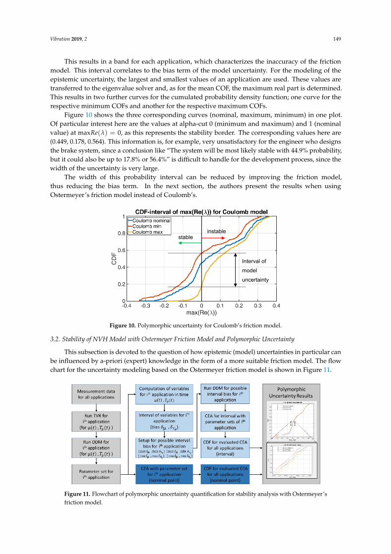
This subsection is devoted to the question of how epistemic (model) uncertainties in particular can be influenced by a-priori (expert) knowledge in the form of a more suitable friction model. The flow chart for the uncertainty modeling based on the Ostermeyer friction model is shown in Figure 11.
Figure 11. Flowchart of polymorphic uncertainty quantification for stability analysis with Ostermeyer’s friction model.
As with Coulomb's friction model, the recorded measurement data is evaluated application-wise. For this purpose, regularization (TVR) is first performed according to Section 2.3.3. For the DDM, the mathematical structure (the candidate functions) is taken directly from the Ostermeyer friction model and an optimized parameter set is identified for the corresponding application. Thus, in this study, only a subfunctionality of the DDM algorithm is used, but future work will also refer to the finding of extended mathematical structures.
The resulting probability distributions for the six parameters are shown in the histograms in Figure 12. This shows that all parameters are subject to certain variations.
Interval of model uncertainty
instable stable
Figure 10. Polymorphic uncertainty for Coulomb’s friction model.
3.2. Stability of NVH Model with Ostermeyer Friction Model and Polymorphic Uncertainty
This subsection is devoted to the question of how epistemic (model) uncertainties in particular canbe influenced by a-priori (expert) knowledge in the form of a more suitable friction model. The flowchart for the uncertainty modeling based on the Ostermeyer friction model is shown in Figure 11.
Vibration 2019, 3 FOR PEER REVIEW 15
Figure 10. Polymorphic uncertainty for Coulomb’s friction model.
3.2. Stability of NVH Model with Ostermeyer Friction Model and Polymorphic Uncertainty
This subsection is devoted to the question of how epistemic (model) uncertainties in particular can be influenced by a-priori (expert) knowledge in the form of a more suitable friction model. The flow chart for the uncertainty modeling based on the Ostermeyer friction model is shown in Figure 11.
Figure 11. Flowchart of polymorphic uncertainty quantification for stability analysis with Ostermeyer’s friction model.
As with Coulomb's friction model, the recorded measurement data is evaluated application-wise. For this purpose, regularization (TVR) is first performed according to Section 2.3.3. For the DDM, the mathematical structure (the candidate functions) is taken directly from the Ostermeyer friction model and an optimized parameter set is identified for the corresponding application. Thus, in this study, only a subfunctionality of the DDM algorithm is used, but future work will also refer to the finding of extended mathematical structures.
The resulting probability distributions for the six parameters are shown in the histograms in Figure 12. This shows that all parameters are subject to certain variations.
Interval of model uncertainty
instable stable
Figure 11. Flowchart of polymorphic uncertainty quantification for stability analysis with Ostermeyer’sfriction model.
Vibration 2019, 2 150
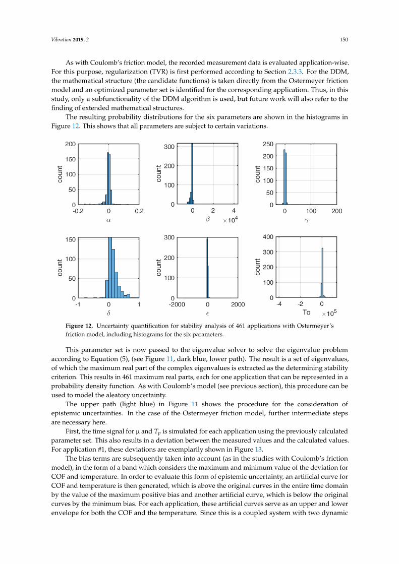
As with Coulomb’s friction model, the recorded measurement data is evaluated application-wise.For this purpose, regularization (TVR) is first performed according to Section 2.3.3. For the DDM,the mathematical structure (the candidate functions) is taken directly from the Ostermeyer frictionmodel and an optimized parameter set is identified for the corresponding application. Thus, in thisstudy, only a subfunctionality of the DDM algorithm is used, but future work will also refer to thefinding of extended mathematical structures.
The resulting probability distributions for the six parameters are shown in the histograms inFigure 12. This shows that all parameters are subject to certain variations.Vibration 2019, 3 FOR PEER REVIEW 16
Figure 12. Uncertainty quantification for stability analysis of 461 applications with Ostermeyer’s friction model, including histograms for the six parameters.
This parameter set is now passed to the eigenvalue solver to solve the eigenvalue problem according to Equation (5), (see Figure 11, dark blue, lower path). The result is a set of eigenvalues, of which the maximum real part of the complex eigenvalues is extracted as the determining stability criterion. This results in 461 maximum real parts, each for one application that can be represented in a probability density function. As with Coulomb’s model (see previous section), this procedure can be used to model the aleatory uncertainty.
The upper path (light blue) in Figure 11 shows the procedure for the consideration of epistemic uncertainties. In the case of the Ostermeyer friction model, further intermediate steps are necessary here.
First, the time signal for µ and 𝑇 is simulated for each application using the previously calculated parameter set. This also results in a deviation between the measured values and the calculated values. For application #1, these deviations are exemplarily shown in Figure 13.
The bias terms are subsequently taken into account (as in the studies with Coulomb's friction model), in the form of a band which considers the maximum and minimum value of the deviation for COF and temperature. In order to evaluate this form of epistemic uncertainty, an artificial curve for COF and temperature is then generated, which is above the original curves in the entire time domain by the value of the maximum positive bias and another artificial curve, which is below the original curves by the minimum bias. For each application, these artificial curves serve as an upper and lower envelope for both the COF and the temperature. Since this is a coupled system with two dynamic variables, the determining combination of upper and lower envelopes for COF and temperature for the eigenvalues is not known a priori.
Figure 12. Uncertainty quantification for stability analysis of 461 applications with Ostermeyer’sfriction model, including histograms for the six parameters.
This parameter set is now passed to the eigenvalue solver to solve the eigenvalue problemaccording to Equation (5), (see Figure 11, dark blue, lower path). The result is a set of eigenvalues,of which the maximum real part of the complex eigenvalues is extracted as the determining stabilitycriterion. This results in 461 maximum real parts, each for one application that can be represented in aprobability density function. As with Coulomb’s model (see previous section), this procedure can beused to model the aleatory uncertainty.
The upper path (light blue) in Figure 11 shows the procedure for the consideration ofepistemic uncertainties. In the case of the Ostermeyer friction model, further intermediate stepsare necessary here.
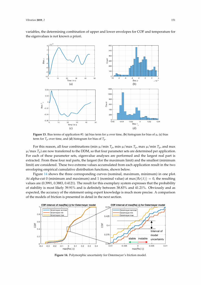
First, the time signal for µ and Tp is simulated for each application using the previously calculatedparameter set. This also results in a deviation between the measured values and the calculated values.For application #1, these deviations are exemplarily shown in Figure 13.
The bias terms are subsequently taken into account (as in the studies with Coulomb’s frictionmodel), in the form of a band which considers the maximum and minimum value of the deviation forCOF and temperature. In order to evaluate this form of epistemic uncertainty, an artificial curve forCOF and temperature is then generated, which is above the original curves in the entire time domainby the value of the maximum positive bias and another artificial curve, which is below the originalcurves by the minimum bias. For each application, these artificial curves serve as an upper and lowerenvelope for both the COF and the temperature. Since this is a coupled system with two dynamic
Vibration 2019, 2 151
variables, the determining combination of upper and lower envelopes for COF and temperature forthe eigenvalues is not known a priori.Vibration 2019, 3 FOR PEER REVIEW 17
(a) (b)
(c) (d)
Figure 13. Bias terms of application #1: (a) bias term for µ over time, (b) histogram for bias of µ, (c) bias term for 𝑇 over time, and (d) histogram for bias of 𝑇 .
For this reason, all four combinations (min µ/min 𝑇 , min µ/max 𝑇 , max µ/min 𝑇 , and max µ/max 𝑇 ) are now transferred to the DDM, so that four parameter sets are determined per application. For each of these parameter sets, eigenvalue analyses are performed and the largest real part is extracted. From these four real parts, the largest (for the maximum limit) and the smallest (minimum limit) are considered. These two extreme values accumulated from each application result in the two enveloping empirical cumulative distribution functions, shown below.
Figure 14 shows the three corresponding curves (nominal, maximum, minimum) in one plot. At alpha-cut 0 (minimum and maximum) and 1 (nominal value) at max 𝑅𝑒(𝜆) = 0, the resulting values are (0.3991, 0.3883, 0.4121). The result for this exemplary system expresses that the probability of stability is most likely 39.91% and is definitely between 38.83% and 41.21%. Obviously and as expected, the accuracy of the statement using expert knowledge is much more precise. A comparison of the models of friction is presented in detail in the next section.
Figure 14. Polymorphic uncertainty for Ostermeyer’s friction model.
Interval of model uncertainty stable instable
Figure 13. Bias terms of application #1: (a) bias term for µ over time, (b) histogram for bias of µ, (c) biasterm for Tp over time, and (d) histogram for bias of Tp.
For this reason, all four combinations (min µ/min Tp, min µ/max Tp, max µ/min Tp, and maxµ/max Tp) are now transferred to the DDM, so that four parameter sets are determined per application.For each of these parameter sets, eigenvalue analyses are performed and the largest real part isextracted. From these four real parts, the largest (for the maximum limit) and the smallest (minimumlimit) are considered. These two extreme values accumulated from each application result in the twoenveloping empirical cumulative distribution functions, shown below.
Figure 14 shows the three corresponding curves (nominal, maximum, minimum) in one plot.At alpha-cut 0 (minimum and maximum) and 1 (nominal value) at max(Re(λ)) = 0, the resultingvalues are (0.3991, 0.3883, 0.4121). The result for this exemplary system expresses that the probabilityof stability is most likely 39.91% and is definitely between 38.83% and 41.21%. Obviously and asexpected, the accuracy of the statement using expert knowledge is much more precise. A comparisonof the models of friction is presented in detail in the next section.
Vibration 2019, 3 FOR PEER REVIEW 17
(a) (b)
(c) (d)
Figure 13. Bias terms of application #1: (a) bias term for µ over time, (b) histogram for bias of µ, (c) bias term for 𝑇 over time, and (d) histogram for bias of 𝑇 .
For this reason, all four combinations (min µ/min 𝑇 , min µ/max 𝑇 , max µ/min 𝑇 , and max µ/max 𝑇 ) are now transferred to the DDM, so that four parameter sets are determined per application. For each of these parameter sets, eigenvalue analyses are performed and the largest real part is extracted. From these four real parts, the largest (for the maximum limit) and the smallest (minimum limit) are considered. These two extreme values accumulated from each application result in the two enveloping empirical cumulative distribution functions, shown below.
Figure 14 shows the three corresponding curves (nominal, maximum, minimum) in one plot. At alpha-cut 0 (minimum and maximum) and 1 (nominal value) at max 𝑅𝑒(𝜆) = 0, the resulting values are (0.3991, 0.3883, 0.4121). The result for this exemplary system expresses that the probability of stability is most likely 39.91% and is definitely between 38.83% and 41.21%. Obviously and as expected, the accuracy of the statement using expert knowledge is much more precise. A comparison of the models of friction is presented in detail in the next section.
Figure 14. Polymorphic uncertainty for Ostermeyer’s friction model.
Interval of model uncertainty stable instable
Figure 14. Polymorphic uncertainty for Ostermeyer’s friction model.
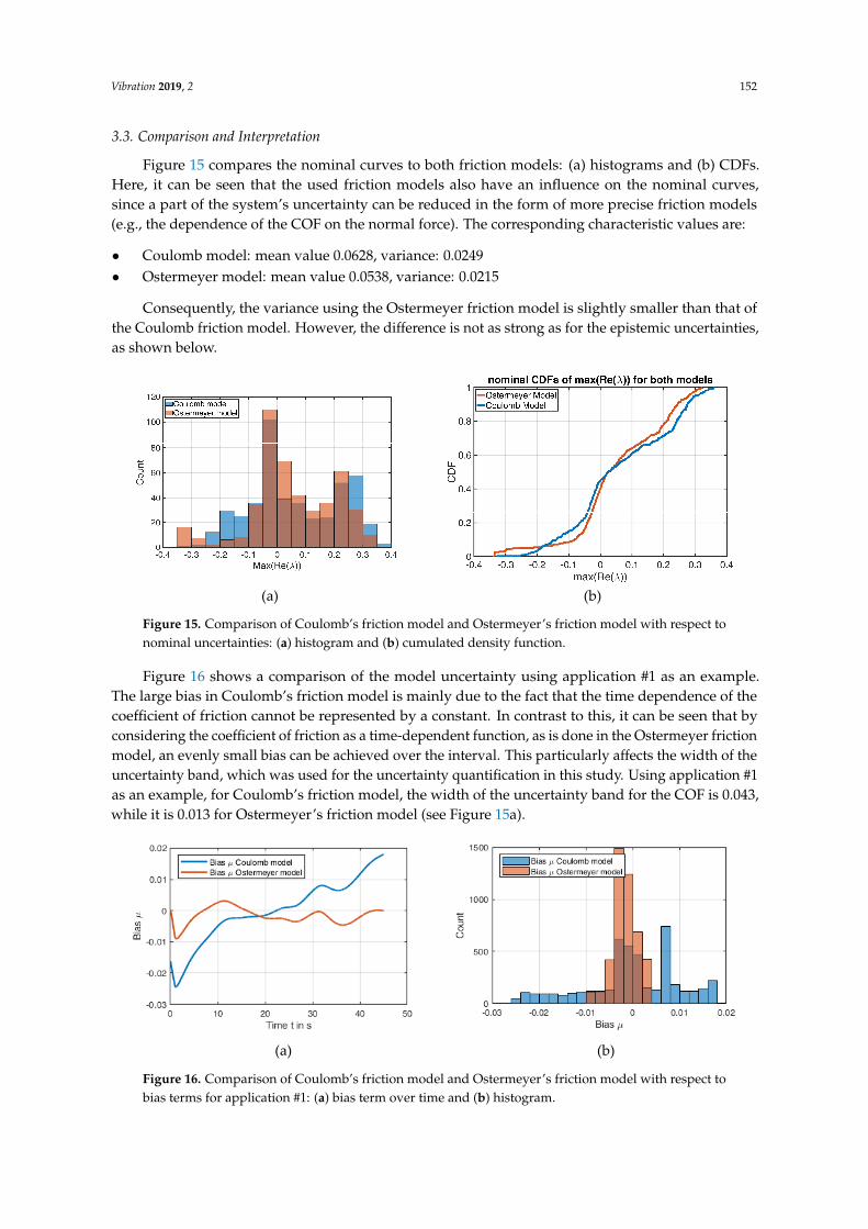
Vibration 2019, 2 152
3.3. Comparison and Interpretation
Figure 15 compares the nominal curves to both friction models: (a) histograms and (b) CDFs.Here, it can be seen that the used friction models also have an influence on the nominal curves,since a part of the system’s uncertainty can be reduced in the form of more precise friction models(e.g., the dependence of the COF on the normal force). The corresponding characteristic values are:
• Coulomb model: mean value 0.0628, variance: 0.0249• Ostermeyer model: mean value 0.0538, variance: 0.0215
Consequently, the variance using the Ostermeyer friction model is slightly smaller than that ofthe Coulomb friction model. However, the difference is not as strong as for the epistemic uncertainties,as shown below.
Vibration 2019, 3 FOR PEER REVIEW 18
3.3. Comparison and Interpretation
Figure 15 compares the nominal curves to both friction models: (a) histograms and (b) CDFs. Here, it can be seen that the used friction models also have an influence on the nominal curves, since a part of the system’s uncertainty can be reduced in the form of more precise friction models (e.g., the dependence of the COF on the normal force). The corresponding characteristic values are:
• Coulomb model: mean value 0.0628, variance: 0.0249 • Ostermeyer model: mean value 0.0538, variance: 0.0215
Consequently, the variance using the Ostermeyer friction model is slightly smaller than that of the Coulomb friction model. However, the difference is not as strong as for the epistemic uncertainties, as shown below.
(a) (b)
Figure 15. Comparison of Coulomb’s friction model and Ostermeyer’s friction model with respect to nominal uncertainties: (a) histogram and (b) cumulated density function.
Figure 16 shows a comparison of the model uncertainty using application #1 as an example. The large bias in Coulomb's friction model is mainly due to the fact that the time dependence of the coefficient of friction cannot be represented by a constant. In contrast to this, it can be seen that by considering the coefficient of friction as a time-dependent function, as is done in the Ostermeyer friction model, an evenly small bias can be achieved over the interval. This particularly affects the width of the uncertainty band, which was used for the uncertainty quantification in this study. Using application #1 as an example, for Coulomb's friction model, the width of the uncertainty band for the COF is 0.043, while it is 0.013 for Ostermeyer's friction model (see Figure 15a).
Figure 15 b compares the corresponding histograms. This shows a relatively small variance for the Ostermeyer friction model in comparison to a large variance for Coulomb's friction model.
(a) (b)
Figure 16. Comparison of Coulomb’s friction model and Ostermeyer’s friction model with respect to bias terms for application #1: (a) bias term over time and (b) histogram.
Figure 15. Comparison of Coulomb’s friction model and Ostermeyer’s friction model with respect tonominal uncertainties: (a) histogram and (b) cumulated density function.
Figure 16 shows a comparison of the model uncertainty using application #1 as an example.The large bias in Coulomb’s friction model is mainly due to the fact that the time dependence of thecoefficient of friction cannot be represented by a constant. In contrast to this, it can be seen that byconsidering the coefficient of friction as a time-dependent function, as is done in the Ostermeyer frictionmodel, an evenly small bias can be achieved over the interval. This particularly affects the width of theuncertainty band, which was used for the uncertainty quantification in this study. Using application #1as an example, for Coulomb’s friction model, the width of the uncertainty band for the COF is 0.043,while it is 0.013 for Ostermeyer’s friction model (see Figure 15a).
Vibration 2019, 3 FOR PEER REVIEW 18
3.3. Comparison and Interpretation
Figure 15 compares the nominal curves to both friction models: (a) histograms and (b) CDFs. Here, it can be seen that the used friction models also have an influence on the nominal curves, since a part of the system’s uncertainty can be reduced in the form of more precise friction models (e.g., the dependence of the COF on the normal force). The corresponding characteristic values are:
• Coulomb model: mean value 0.0628, variance: 0.0249 • Ostermeyer model: mean value 0.0538, variance: 0.0215
Consequently, the variance using the Ostermeyer friction model is slightly smaller than that of the Coulomb friction model. However, the difference is not as strong as for the epistemic uncertainties, as shown below.
(a) (b)
Figure 15. Comparison of Coulomb’s friction model and Ostermeyer’s friction model with respect to nominal uncertainties: (a) histogram and (b) cumulated density function.
Figure 16 shows a comparison of the model uncertainty using application #1 as an example. The large bias in Coulomb's friction model is mainly due to the fact that the time dependence of the coefficient of friction cannot be represented by a constant. In contrast to this, it can be seen that by considering the coefficient of friction as a time-dependent function, as is done in the Ostermeyer friction model, an evenly small bias can be achieved over the interval. This particularly affects the width of the uncertainty band, which was used for the uncertainty quantification in this study. Using application #1 as an example, for Coulomb's friction model, the width of the uncertainty band for the COF is 0.043, while it is 0.013 for Ostermeyer's friction model (see Figure 15a).
Figure 15 b compares the corresponding histograms. This shows a relatively small variance for the Ostermeyer friction model in comparison to a large variance for Coulomb's friction model.
(a) (b)
Figure 16. Comparison of Coulomb’s friction model and Ostermeyer’s friction model with respect to bias terms for application #1: (a) bias term over time and (b) histogram.
Figure 16. Comparison of Coulomb’s friction model and Ostermeyer’s friction model with respect tobias terms for application #1: (a) bias term over time and (b) histogram.
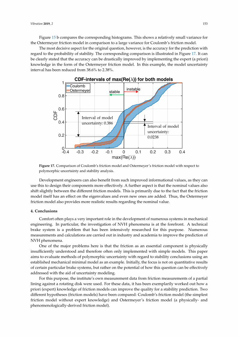
Vibration 2019, 2 153
Figure 15 b compares the corresponding histograms. This shows a relatively small variance forthe Ostermeyer friction model in comparison to a large variance for Coulomb’s friction model.
The most decisive aspect for the original question, however, is the accuracy for the prediction withregard to the probability of stability. The corresponding comparison is illustrated in Figure 17. It canbe clearly stated that the accuracy can be drastically improved by implementing the expert (a priori)knowledge in the form of the Ostermeyer friction model. In this example, the model uncertaintyinterval has been reduced from 38.6% to 2.38%.
Vibration 2019, 3 FOR PEER REVIEW 19
The most decisive aspect for the original question, however, is the accuracy for the prediction with regard to the probability of stability. The corresponding comparison is illustrated in Figure 17. It can be clearly stated that the accuracy can be drastically improved by implementing the expert (a priori) knowledge in the form of the Ostermeyer friction model. In this example, the model uncertainty interval has been reduced from 38.6% to 2.38%.
Figure 17. Comparison of Coulomb’s friction model and Ostermeyer’s friction model with respect to polymorphic uncertainty and stability analysis.
Development engineers can also benefit from such improved informational values, as they can use this to design their components more effectively. A further aspect is that the nominal values also shift slightly between the different friction models. This is primarily due to the fact that the friction model itself has an effect on the eigenvalues and even new ones are added. Thus, the Ostermeyer friction model also provides more realistic results regarding the nominal value.
4. Conclusions
Comfort often plays a very important role in the development of numerous systems in mechanical engineering. In particular, the investigation of NVH phenomena is at the forefront. A technical brake system is a problem that has been intensively researched for this purpose. Numerous measurements and calculations are carried out in industry and academia to improve the prediction of NVH phenomena.
One of the major problems here is that the friction as an essential component is physically insufficiently understood and therefore often only implemented with simple models. This paper aims to evaluate methods of polymorphic uncertainty with regard to stability conclusions using an established mechanical minimal model as an example. Initially, the focus is not on quantitative results of certain particular brake systems, but rather on the potential of how this question can be effectively addressed with the aid of uncertainty modeling.
For this purpose, the institute's own measurement data from friction measurements of a partial lining against a rotating disk were used. For these data, it has been exemplarily worked out how a priori (expert) knowledge of friction models can improve the quality for a stability prediction. Two different hypotheses (friction models) have been compared: Coulomb's friction model (the simplest friction model without expert knowledge) and Ostermeyer's friction model (a physically- and phenomenologically-derived friction model).
The identification of the parameters of the friction models is conducted by a Data Driven Method, which utilizes a sparse regression technique in combination with a Total Variation Regularization to filter noise out of the data. The evaluation of the measured data indicates a large
Interval of model uncertainty: 0.0238
Interval of modeluncertainty: 0.386
stable instable
Figure 17. Comparison of Coulomb’s friction model and Ostermeyer’s friction model with respect topolymorphic uncertainty and stability analysis.
Development engineers can also benefit from such improved informational values, as they canuse this to design their components more effectively. A further aspect is that the nominal values alsoshift slightly between the different friction models. This is primarily due to the fact that the frictionmodel itself has an effect on the eigenvalues and even new ones are added. Thus, the Ostermeyerfriction model also provides more realistic results regarding the nominal value.
4. Conclusions
Comfort often plays a very important role in the development of numerous systems in mechanicalengineering. In particular, the investigation of NVH phenomena is at the forefront. A technicalbrake system is a problem that has been intensively researched for this purpose. Numerousmeasurements and calculations are carried out in industry and academia to improve the prediction ofNVH phenomena.
One of the major problems here is that the friction as an essential component is physicallyinsufficiently understood and therefore often only implemented with simple models. This paperaims to evaluate methods of polymorphic uncertainty with regard to stability conclusions using anestablished mechanical minimal model as an example. Initially, the focus is not on quantitative resultsof certain particular brake systems, but rather on the potential of how this question can be effectivelyaddressed with the aid of uncertainty modeling.
For this purpose, the institute’s own measurement data from friction measurements of a partiallining against a rotating disk were used. For these data, it has been exemplarily worked out how apriori (expert) knowledge of friction models can improve the quality for a stability prediction. Twodifferent hypotheses (friction models) have been compared: Coulomb’s friction model (the simplestfriction model without expert knowledge) and Ostermeyer’s friction model (a physically- andphenomenologically-derived friction model).
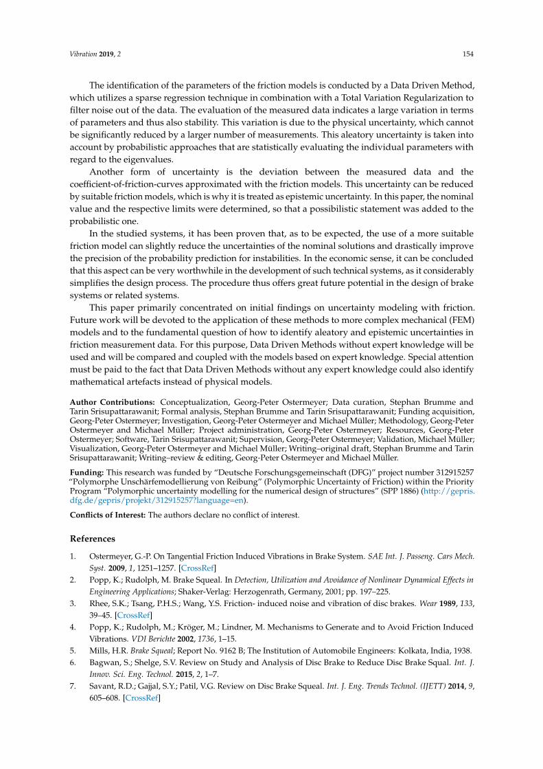
Vibration 2019, 2 154
The identification of the parameters of the friction models is conducted by a Data Driven Method,which utilizes a sparse regression technique in combination with a Total Variation Regularization tofilter noise out of the data. The evaluation of the measured data indicates a large variation in termsof parameters and thus also stability. This variation is due to the physical uncertainty, which cannotbe significantly reduced by a larger number of measurements. This aleatory uncertainty is taken intoaccount by probabilistic approaches that are statistically evaluating the individual parameters withregard to the eigenvalues.
Another form of uncertainty is the deviation between the measured data and thecoefficient-of-friction-curves approximated with the friction models. This uncertainty can be reducedby suitable friction models, which is why it is treated as epistemic uncertainty. In this paper, the nominalvalue and the respective limits were determined, so that a possibilistic statement was added to theprobabilistic one.
In the studied systems, it has been proven that, as to be expected, the use of a more suitablefriction model can slightly reduce the uncertainties of the nominal solutions and drastically improvethe precision of the probability prediction for instabilities. In the economic sense, it can be concludedthat this aspect can be very worthwhile in the development of such technical systems, as it considerablysimplifies the design process. The procedure thus offers great future potential in the design of brakesystems or related systems.
This paper primarily concentrated on initial findings on uncertainty modeling with friction.Future work will be devoted to the application of these methods to more complex mechanical (FEM)models and to the fundamental question of how to identify aleatory and epistemic uncertainties infriction measurement data. For this purpose, Data Driven Methods without expert knowledge will beused and will be compared and coupled with the models based on expert knowledge. Special attentionmust be paid to the fact that Data Driven Methods without any expert knowledge could also identifymathematical artefacts instead of physical models.
Author Contributions: Conceptualization, Georg-Peter Ostermeyer; Data curation, Stephan Brumme andTarin Srisupattarawanit; Formal analysis, Stephan Brumme and Tarin Srisupattarawanit; Funding acquisition,Georg-Peter Ostermeyer; Investigation, Georg-Peter Ostermeyer and Michael Müller; Methodology, Georg-PeterOstermeyer and Michael Müller; Project administration, Georg-Peter Ostermeyer; Resources, Georg-PeterOstermeyer; Software, Tarin Srisupattarawanit; Supervision, Georg-Peter Ostermeyer; Validation, Michael Müller;Visualization, Georg-Peter Ostermeyer and Michael Müller; Writing–original draft, Stephan Brumme and TarinSrisupattarawanit; Writing–review & editing, Georg-Peter Ostermeyer and Michael Müller.
Funding: This research was funded by “Deutsche Forschungsgemeinschaft (DFG)” project number 312915257“Polymorphe Unschärfemodellierung von Reibung” (Polymorphic Uncertainty of Friction) within the PriorityProgram “Polymorphic uncertainty modelling for the numerical design of structures” (SPP 1886) (http://gepris.dfg.de/gepris/projekt/312915257?language=en).
Conflicts of Interest: The authors declare no conflict of interest.
References
1. Ostermeyer, G.-P. On Tangential Friction Induced Vibrations in Brake System. SAE Int. J. Passeng. Cars Mech.Syst. 2009, 1, 1251–1257. [CrossRef]
2. Popp, K.; Rudolph, M. Brake Squeal. In Detection, Utilization and Avoidance of Nonlinear Dynamical Effects inEngineering Applications; Shaker-Verlag: Herzogenrath, Germany, 2001; pp. 197–225.
3. Rhee, S.K.; Tsang, P.H.S.; Wang, Y.S. Friction- induced noise and vibration of disc brakes. Wear 1989, 133,39–45. [CrossRef]
4. Popp, K.; Rudolph, M.; Kröger, M.; Lindner, M. Mechanisms to Generate and to Avoid Friction InducedVibrations. VDI Berichte 2002, 1736, 1–15.
5. Mills, H.R. Brake Squeal; Report No. 9162 B; The Institution of Automobile Engineers: Kolkata, India, 1938.6. Bagwan, S.; Shelge, S.V. Review on Study and Analysis of Disc Brake to Reduce Disc Brake Squal. Int. J.
Innov. Sci. Eng. Technol. 2015, 2, 1–7.7. Savant, R.D.; Gajjal, S.Y.; Patil, V.G. Review on Disc Brake Squeal. Int. J. Eng. Trends Technol. (IJETT) 2014, 9,
605–608. [CrossRef]
Vibration 2019, 2 155
8. Pilipchuk, V.; Olejnik, P.; Awrejcewicz, J. Transient friction-induced vibrations in a 2-DOF model of brakes.J. Sound Vib. 2015, 344, 297–312. [CrossRef]
9. Chung, C.-H.J.; Steed, W.; Dong, J.; Kim, B.S.; Ryu, G.S. Virtual Design of Brake Squeal; SAE InternationalTechnical Paper 2003-01-1625; SAE International: Warrendale, PA, USA, 2003.
10. Fischer, M.; Gaul, L. Application of the fast multipole BEM for structural-acoustic simulations. J. Comput.Acoust. 2005, 13, 87–98. [CrossRef]
11. Hoffmann, N.; Gaul, L. Effects of damping on mode-coupling instability in friction induced oscillations.ZAMM J. Appl. Math. Mech. 2003, 83, 524–534. [CrossRef]
12. Hoffmann, N.; Bieser, S.; Gaul, L. Harmonic Balance and Averaging Techniques for Stick Slip Limit-CycleDetermination in Mode-Coupling Friction Self-Excited Systems. Technische Mechanik 2004, 24, 185–197.
13. Awrejcewicz, J.; Olejnik, P. Friction Pair Modeling by a 2-DOF System: Numerical and ExperimentalInvestigations. Int. J. Bifurc. Chaos 2005, 15, 1931–1944. [CrossRef]
14. Von Wagner, U.; Jearsiripongkul, T.; Vomstein, T.; Chakraborty, G.; Hagedorn, P. Brake Squeal: Modelingand Experiments. VDI-Berichte 1749, 2003, 173–186.
15. Chen, F. Automotive Disc Brake Squeal: An Overview. Int. J. Veh. Des. 2009, 51, 167–172. [CrossRef]16. Ouyang, H. Pole assignment of friction-induced vibration for stabilisation through state-feedback control.
J. Sound Vib. 2010, 329, 1985–1991. [CrossRef]17. Okayama, K.; Fujikawa, H.; Kubota, T.; Kakihara, K. A Study on Rear Disc Brake Groan Noise Immediately
After Stopping. In Proceedings of the 23rd SAE Brake Colloquium and Exhibition, Orlando, FL, USA, 9–12October 2005.
18. Gauterin, F.; Grochowitz, J.; Haverkamp, M.; Marschner, H.; Pankau, J.; Rostek, M. Bremsenknarzen—Phänomenologie und Abhilfe. Automobiltechnische Zeitschrift 2004, 7–8, 652–659. [CrossRef]
19. Brommundt, E. Ein Reibschwinger mit Selbsterregung ohne fallende Reibkennlinie. ZAMM J. Appl. Math.Mech. 1995, 75, 811–820. [CrossRef]
20. Abu Bakar, A.R.; Ouyang, H.; Li, L.; Siegel, J.E. Brake Pad Surface Topography Part I: Contact PressureDistribution. In Proceedings of the 23rd SAE Brake Colloquium and Exhibition, Orlando, FL, USA,9–12 October 2005.
21. Ostermeyer, G.-P.; Perzborn, N. Test-Variability of Tribological Measurements; SAE International Technical Paper2012-01-1805; SAE International: Warrendale, PA, USA, 2012.
22. Ostermeyer, G.-P.; Wilkening, L. Experimental Investigations of the Topography Dynamics in Brake Pads.SAE Int. J. Passeng. Cars Mech. Syst. 2013, 6, 1398–1407. [CrossRef]
23. Perzborn, N.; Agudelo, C.; Ostermeyer, G.-P. On Similarities and Differences of Measurements on InertiaDynamometer and Scale Testing Tribometer for Friction Coefficient Evaluation. SAE Int. J. Mater. Manuf.2015, 8, 104–117. [CrossRef]
24. Wilkening, L.; Paul, H.-G.; Ostermeyer, G.-P. Test Procedure for Tribological Memory Effect in FrictionMaterials for Automotive Brakes. In Proceedings of the Eurobrake, Paper EB2014-FF-004, Vienna, Austria,13–15 May 2014.
25. Ostermeyer, G.-P. Friction and Wear of Brake Systems. Forschung im Ingenieurwesen 2001, 66, 267–272.[CrossRef]
26. Ostermeyer, G.-P.; Völpel, A.; Müller, M. A Methods towards Investigating the Influence of ODE basedFriction Laws in the Frequency Domain. In Proceedings of the Eurobrake, Milan, Italy, 13–15 June 2016.EB2016-FBR-026.
27. Hamabe, T.; Yamazaki, I.; Yamada, K.; Matsui, H.; Nakagawa, S.; Kawamura, M. Study of a Method forReducing Drum Brake Squal; SAE International Technical Paper 1999-01-0144; SAE International: Warrendale,PA, USA, 1999.
28. Völpel, A.; Ostermeyer, G. Investigation of the Influence of ODE Based Friction Models on Complex FEMBrake Models in the Frequency Domain. SAE Int. J. Passeng. Cars Mech. Syst. 2016, 9, 1206–1213. [CrossRef]
29. Ostermeyer, G.-P.; Schramm, T.; Raczek, S.; Bubser, F.; Perzborn, N. The Automated Universal Tribotester.In Proceedings of the Eurobrake, EB2015-STQ-016, Dresden, Germany, 4–6 May 2015.
30. Quade, M.; Abel, M.; Kutz, N.; Brunton, S.L. Sparse Identification of Nonlinear Dynamics for Rapid ModelRecovery. arXiv, 2018; arXiv:1803.00894v2.
31. Rudy, S.; Brunton, S.L.; Proctor, J.L.; Kutz, J.N. Data-driven discovery of partial differential equations.arXiv 2016, arXiv:1609.06401.
Vibration 2019, 2 156
32. Stender, M.; Oberst, S.; Hoffmann, N. Recovery of Differential Equations from Impulse Response Time SeriesData for Model Identification and Feature Extraction. Vibration 2019, 2, 25–46. [CrossRef]
33. Chartrand, R. Numerical differentiation of noisy, nonsmooth data. J. Appl. Math. 2011, 2011, 164564.[CrossRef]
34. Tikhonov, A.N. Regularization of incorrectly posed problems. Sov. Math. Dokl. 1963, 4, 1624–1627.35. Hanselowski, A.; Hanss, M. Analysis of epistemic uncertainty for the friction-induced vibration. ZAMM J.
Appl. Math. Mech. 2014, 94, 933–944. [CrossRef]36. Graf, W.; Götz, M.; Kaliske, M. Analysis of dynamical processes under consideration of polymorphic
uncertainty. Struct. Saf. 2015, 52, 194–201. [CrossRef]37. Hanss, M. Applied Fuzzy Arithmetic; Springer: Berlin/Heidelberg, Germany, 2005.
© 2019 by the authors. Licensee MDPI, Basel, Switzerland. This article is an open accessarticle distributed under the terms and conditions of the Creative Commons Attribution(CC BY) license (http://creativecommons.org/licenses/by/4.0/).