SQL Performance Explained - Central University Of Kashmir
301
-
Upload
khangminh22 -
Category
Documents
-
view
0 -
download
0
Transcript of SQL Performance Explained - Central University Of Kashmir

SQL Performance Explained
Volume 1 — Basic Indexing
Markus Winand
Copyright © 2011 Markus Winand
Creative Commons Attribution-Noncommercial-No DerivativeWorks 3.0 Unported License.
THE INFORMATION IN THIS BOOK IS PROVIDED “AS IS”WITHOUT WARRANTY OF ANY KIND BY ANY PERSON,INCLUDING WITHOUT LIMITATION, THE AUTHOR ANDTHE PUBLISHER.
DB2 is a registered trademark of IBM Corporation.
Oracle, Java and MySQL are registered trademarks of Oracleand/or its affiliates.
Microsoft and SQL Server are either registered trademarks ortrademarks of Microsoft Corporation in the United States and/orother countries.
PostgreSQL is a registered trademark of PostgreSQL GlobalDevelopment Group.
2011-03-08
Foreword To The E-Book Edition
SQL Performance Explained is the e-Book edition of Use TheIndex, Luke—A Guide to SQL Performance for Developers,available at http://Use-The-Index-Luke.com/. Both editions arefreely available under the terms of the Creative CommonsAttribution-Noncommercial-No Derivative Works 3.0 UnportedLicense.
The content of both editions is identical. The same chapters, thesame examples and the same words appear in both editions.However, there are some differences:
Appendices
The appendices "Execution Plans" and "Example Schema"are most useful in front of a computer—when actuallyworking with a database. They are therefore not included inthis e-book edition.
Two Volumes
“Use The Index, Luke” is a living book that is constantlyextended—about once or twice each month. The e-bookedition is released in two volumes. “Volume 1 — BasicIndexing” is the current release—it covers the whereclause.
“Volume 2—Advanced Indexing” is scheduled for release in2012. However, the content will be made available on UseThe Index, Luke during 2011.
The Name
The most obvious difference between the two editions is thename. Although "Use The Index, Luke" is "cute and verygeeky", it's rather hard to recognize the books topic by itstitle. But that doesn't stop search engines from indexing theentire text so that it becomes searchable on the Internet. A

self-explanatory title is, however, much more important in abook store. It is, after all, a marketing issue.
Markus WinandJanuary 2011

About Markus Winand
Markus Winand has been developing SQL applications since 1998.His main interests include performance, scalability, reliability, andbasically all other technical aspects of software quality. He iscurrently an independent consultant and helps developersbuilding better software. He can be reached at http://winand.at.

Preface
Performance problems are as old as SQL itself. There are evenopinions that say that SQL is inherently giving poor performance.Although it might have been true in the early days of SQL, it isdefinitely not true anymore. Nevertheless SQL performanceproblems are everywhere, everyday. How does this happen?
The SQL language is perhaps the most successful fourthgeneration programming language (4GL). The main goal of SQL isto separate the “what” from the “how”. An SQL statement is astraight expression of what is needed without instructions how toget it. Consider the following example:
SELECT date_of_birth FROM employees WHERE last_name = 'WINAND'
Writing this SQL statement doesn't require any knowledge aboutthe physical properties of the storage (such as disks, files, blocks,...) or any knowledge how the database executes that statement.There are no instructions what to do first, which files to open orhow to find the requested records inside the data files. From adeveloper's perspective, the database is a black box.
Although developers know a great deal how to write SQL, there isno need to know anything about the inner workings of a databaseto do it. This abstraction greatly improves programmersproductivity and works very well in almost all cases. However,there is one common problem where the abstraction doesn't workanymore: performance.
That's where separating “what” and “how” bites back. Perdefinition, the author of the SQL statement should not care howthe statement is executed. Consequently, the author is notresponsible if the execution is slow. However, experience provesthe opposite; the author must know a little bit about the database
to write efficient SQL.
As it turns out, the only thing developers need to know to writeefficient SQL is how indexes work.
That's because missing and inadequate indexes are among themost common causes of poor SQL performance. Once themechanics of indexes are understood, another performance killerdisappears automatically: bad SQL statements.
This book covers everything a developer must know to useindexes properly—and nothing more. To be more precise, thebook actually covers only the most important type of index in theSQL databases: the B-Tree index.
The B-Tree index works almost identical in many SQL databaseimplementation. That's why the principles explained in this bookare applicable to many different databases. However, the mainbody of this book uses the vocabulary of the Oracle database. Sidenotes explain the differences to four more major SQL databases:IBM DB2, MySQL, PostgreSQL and Microsoft SQL Server.
The structure of the book is tailor-made for developers; most ofthe chapters correspond to a specific part of an SQL statement.
CHAPTER 1 - Anatomy of an Index
The first chapter is the only one that doesn't cover SQL; it'sabout the fundamental structure of an index. Theunderstanding of the index structure is essential to followthe later chapters—don't skip this.
Although the chapter is rather short—about 4 printed pages—you will already understand the phenomenon of slowindexes after working through the chapter.
CHAPTER 2 - The Where Clause
This is where we pull out all the stops. This chapter explainsall aspects of the where clause; beginning with very simplesingle column lookups down to complex clauses for ranges
and special cases like NULL.
The chapter will finally contain the following sections:
The Equals Operator
Functions
Indexing NULL
Searching for Ranges
Obfuscated Conditions
This chapter makes up the main body of the book. Once youlearn to use these techniques properly, you will alreadywrite much faster SQL.
CHAPTER 3 - Testing and Scalability
This chapter is a little digression about a performancephenomenon that hits developers very often. It explains theperformance differences between development andproduction databases and covers the effects of growing datavolumes.
CHAPTER 4 - Joins (not yet published)
Back to SQL: how to use indexes to perform a fast tablejoin?
CHAPTER 5 - Fetching Data (not yet published)
Have you ever wondered if there is any difference betweenselecting a single column or all columns? Here is the answer—along with a trick to get even better performance.
CHAPTER 6 - Sorting, Grouping and Partitioning (notyet published)
ORDER BY, GROUP BY and even PARTITION BY canbenefit from an index.

CHAPTER 7 - Views (not yet published)
There is actually nothing magic about indexes on views;they just don't exist. However, there are materialized views.
CHAPTER 8 - Advanced Techniques (not yet published)
This chapter explains how to index for some frequently usedstructures like Top-N Queries or min()/max() searches.
CHAPTER 9 - Insert, Delete and Update (not yetpublished)
How do indexes affect data changes? An index doesn't comefor free—use them wisely!
APPENDIX A - Execution Plans
Asking the database how it executes a statement.
APPENDIX B - Myth Directory
Lists some common myth and explains the truth. Will beextended as the book grows.

Chapter 1. Anatomy of an Index
“An index makes the query fast” is the most basic explanation ofan index I have ever heard of. Although it describes the mostimportant aspect of an index very well, it is—unfortunately—notsufficient for this book. This chapter describes the index structureon a high level, like an X-Ray, but provides all the required detailsto understand the performance aspects discussed throughout thebook.
First of all, an index is a distinct object in the database thatrequires space, and is stored at a different place than the tabledata. Creating an index does not change the table; it just creates anew data structure that refers to the table. A certain amount oftable data is copied into the index so that the index has redundantdata. The book index analogy describes the concept very well; it isstored at a different place (typically at the end of the book), hassome redundancy, and refers to the main part of the book.
Clustered Indexes (SQL Server, MySQL/InnoDB)
There is an important difference how SQL Server and MySQL(with InnoDB engine) handle tables.
SQL Server and InnoDB organize tables always as indexes thatconsists of all table columns. That index (that is in fact thetable) is a clustered index. Other indexes on the same table,secondary indexes or non-clustered indexes, work likedescribed in this chapter.
Volume 2 explains the corresponding Oracle database feature;Index Organized Tables. The benefits and drawbacks describedthere apply to Clustered Indexes in SQL Server and InnoDB.
A database index supports fast data access in a very similar wayto a book index or a printed phone book. The fundamental concept

is to maintain an ordered representation of the indexed data.
Once the data is available in a sorted manner, localizing anindividual entry becomes a simple task. However, a databaseindex is more complex than a phone book because it undergoesconstant change. Imagine maintaining a phone book manually byadding new entries in the correct place. You will quickly find outthat the individual pages don't have enough space to write a newentry between two existing ones. That's not a problem for printedphone books because every new print covers all the accumulatedupdates. An SQL database cannot work that way. There isconstant need to insert, delete and update entries withoutdisturbing the index order.
The database uses two distinct data structures to meet thischallenge: the leaf nodes and the tree structure.

The Leaf Nodes
The primary goal of an index is to maintain an orderedrepresentation of the indexed data. However, the database cannotstore the records sequentially on the disk because an insertstatement would need to move data to make room for the newentry. Unfortunately, moving data becomes very slow when datavolume grows.
The solution to this problem is a chain of data fragments (nodes)—each referring to its neighboring nodes. Inserting a new node intothe chain means to update the references in the preceding andfollowing nodes, so that they refer to the new node. The physicallocation of the new node doesn't matter, it is logically linked at thecorrect place between the preceding and following nodes.
Because each node has two links with each adjacent node, the datastructure is called a double linked list. The key feature of a doublelinked list is to support the insertion and deletion of nodes inconstant time—that is, independent of the list length. Doublelinked list are also used for collections (containers) in manyprogramming languages. Table 1.1, “Various Double-Linked ListImplementations” lists some of them.
Table 1.1. Various Double-Linked List Implementations
ProgrammingLanguage Name
Java java.util.LinkedList.NET Framework System.Collections.Generic.LinkedListC++ std::list
Databases uses double linked lists to connect the individual indexleaf nodes. The leaf nodes are stored in database blocks or pages;that is, the smallest storage unit databases use. Every block

within an index has the same size; that is, typically a fewkilobytes. The database stores as many index entries as possiblein each block to use the space optimally. That means that the sortorder is maintained on two different levels; the index entrieswithin each leaf node, and then the leaf nodes among each otherwith a double linked list.
Figure 1.1. Index Leaf Nodes and Corresponding TableData
Figure 1.1, “Index Leaf Nodes and Corresponding Table Data”illustrates the index leaf nodes and their connection to the tabledata. Each index entry consists of the indexed data (the key) anda reference to the corresponding table row (the ROWID—that is, thephysical address of the table row). Unlike an index, the table datais not sorted at all. There is neither a relationship between therows stored in the same block, nor is there any connectionbetween the blocks.

The index leaf nodes allow the traversal of index entries in bothdirections very efficiently. The number of leaf nodes accessedduring a range scan is minimal. For example, a search for the keyrange 15 to 35 in Figure 1.1, “Index Leaf Nodes andCorresponding Table Data” needs to visit only three index nodesto find all matching entries.

The Tree
Because the leaf nodes are not physically sorted on the disk—theirlogical sequence is established with the double linked list—thesearch for a specific entry can't be performed as in a phone book.
A phone book lookup works because the physical order of thepages (sheets) is correct. If you search for “Smith” in but open itat “Robinson” in the first place, you know that Smith must comefarther back. A search in the index leaf nodes doesn't work thatway because the nodes are not stored sequentially. It's likesearching in a phone book with shuffled pages.
A second data structure is required to support the fast search fora specific entry. The balanced search tree, or B-Tree in short, isthe perfect choice for this purpose.
Figure 1.2. Tree Structure
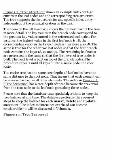
Figure 1.2, “Tree Structure” shows an example index with 30entries in the leaf nodes and the corresponding tree structure.The tree supports the fast search for any specific index entry—independent of the physical location on the disk.
The zoom on the left hand side shows the topmost part of the treein more detail. The key values in the branch node correspond tothe greatest key values stored in the referenced leaf nodes. Forinstance, the highest value in the first leaf node is 18; thecorresponding entry in the branch node is therefore also 18. Thesame is true for the other two leaf nodes so that the first branchnode contains the keys 18, 27 and 39. The remaining leaf nodesare processed in the same so that the first level of tree nodes isbuilt. The next level is built on top of the branch nodes. Theprocedure repeats until all keys fit into a single node, the rootnode.
The entire tree has the same tree depth; all leaf nodes have thesame distance to the root node. That means that each element canbe accessed as fast as all other elements. The index in Figure 1.2,“Tree Structure” has a tree depth of three because the traversalfrom the root node to the leaf node goes along three nodes.
Please note that the database uses special algorithms to keep thetree balance at any time. The database performs the requiredsteps to keep the balance for each insert, delete and updatestatement. The index maintenance overhead can becomeconsiderable—it will be discussed in Volume 2.
Figure 1.3. Tree Traversal

The strength of the balanced tree is a very efficient traversal.Figure 1.3, “Tree Traversal” shows an index fragment to illustratethe tree traversal to the key "57". The index lookup starts at theroot node on the left hand side. Each entry of the root node isprocessed in ascending order until an index entry is bigger orequal (>=) to the search term (57). The same procedure continuesat the referenced node until the scan reaches a leaf node.
A textual explanation of an algorithm is always difficult. Let'srepeat it with the real numbers from the figure. The processstarts with the entry 39 at the first entry of the root node. 39 notbigger than or equal to 57 (search term), that means that theprocedure repeats for the next entry in the same node. 83satisfies the bigger or equal (>=) test so that the traversal followsthe reference the next level—the branch node. The process skipsthe first two entries in the branch node (46 and 53) because theyare smaller than the search term. The next entry is equal to thesearch term (57)—the traversal descends along that reference tothe leaf node. The leaf node is also inspected entry-by-entry tofind the search key.
The tree traversal is a very efficient operation. The tree traversalworks almost instantly—even upon a huge data volume. Theexcellent performance comes from the logarithmic grows of thetree depth. That means that the depth grows very slowly incomparison to the number of leaf nodes. The sidebar LogarithmicScalability describes this in more detail. Typical real world indexes
with millions of records have a tree depth of four or five. A treedepth of six is hardly ever seen.
Logarithmic Scalability
In mathematics, the logarithm of a number to a given base isthe power or exponent to which the base must be raised inorder to produce the number (Wikipedia:http://en.wikipedia.org/wiki/Logarithm).
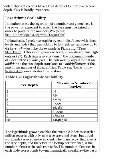
In databases, I prefer to explain by example. A tree with threelevels and nodes that can hold up to four entries can store up to64 keys (43)—just like the example in Figure 1.2, “TreeStructure”. If this index grows one level, it can already hold 256entries (44). Each time a level is added, the maximum numberof index entries quadruples. The noteworthy aspect is that anaddition to the tree depth translates to a multiplication of themaximum number of index entries. Table 1.2, “LogarithmicScalability” demonstrates this relation.
Table 1.2. Logarithmic Scalability
Tree Depth Maximum Number ofEntries
3 644 2565 1.0246 4.0967 16.3848 65.5369 262.14410 1.048.576
The logarithmic growth enables the example index to search amillion records with only nine tree traversal steps, but a realworld index is even more efficient. The main factor that affectsthe tree depth, and therefore the lookup performance, is thenumber of entries in each tree node. The number of entries ineach node corresponds to—mathematically speaking—the basis

of the logarithm. The higher the basis, the shallower and fasterthe tree.
The Oracle database exposes this concept to a maximumextent and puts as many entries as possible into each node,typically hundreds. That means, every new index levelsupports hundred times more entries in the index.

Slow Indexes
Despite the efficiency of the tree traversal, there are still caseswhere an index lookup doesn't work as fast as expected. Thiscontradiction has fueled the myth of the “degenerated index“ for along time. The miracle solution is usually to rebuild the index.Appendix A, Myth Directory covers this myth in detail. For now,you can take it for granted that rebuilding an index does notimprove performance in the long run. The real reason for trivialstatements becoming slow—even if it's using an index—can beexplained on the basis of the previous sections.
The first ingredient for a slow index lookup is scanning a widerrange than intended. As in Figure 1.3, “Tree Traversal”, thesearch for an index entry can return many records. In thatparticular example, the value 57 occurs twice in the index leafnode. There could be even more matching entries in the next leafnode, which is not shown in the figure. The database must readthe next leaf node to see if there are any more matching entries.The number of scanned leaf nodes can grow large, and thenumber of matching index entries can be huge.
The second ingredient for a slow index lookup is the table access.As in Figure 1.1, “Index Leaf Nodes and Corresponding TableData”, the rows are typically distributed across many table blocks.Each ROWID in a leaf node might refer to a different table block—inthe worst case. On the other hand, many leaf node entries could,potentially, refer to the same table block so that a single readoperation retrieves many rows in one shot. That means that thenumber of required blocks depends on the tree depth; on thenumber of rows that match the search criteria; but also on therow distribution in the table. The Oracle database is aware of thiseffect of clustered row data and accounts for it with the so-calledclustering factor.
Clustering Factor

The clustering factor is a benchmark that expresses thecorrelation between the row order in the index and the roworder in the table.
For example, an ORDERS table, that grows every day, might havean index on the order date and another one on the customer id.Because orders don't get deleted there are no holes in the tableso that each new order is added to the end. The table growschronologically. An index on the order date has a very lowclustering factor because the index order is essentially the sameas the table order. The index on customer id has a higherclustering factor because the index order is different from thetable order; the table row will be inserted at the end of thetable, the corresponding index entry somewhere in the middleof the index—according to the customer id.
The overall number of blocks accessed during an index lookup canexplode when the two ingredients play together. For example, anindex lookup for some hundred records might need to access fourblocks for the tree traversal (tree depth), a few more blocks forsubsequent index leaf nodes, but some hundred blocks to fetchthe table data. It's the table access that becomes the limitingfactor.
The main cause for the “slow indexes” phenomenon is themisunderstanding of the three most dominant index operations:
INDEX UNIQUE SCAN
The INDEX UNIQUE SCAN performs the tree traversal only. Thedatabase can use this operation if a unique constraintensures that the search criteria will match no more than oneentry.
INDEX RANGE SCAN
The INDEX RANGE SCAN performs the tree traversal and walksthrough the leaf nodes to find all matching entries. This is

the fall back operation if multiple entries could possiblymatch the search criteria.
TABLE ACCESS BY INDEX ROWID
The TABLE ACCESS BY INDEX ROWID operation retrieves the rowfrom the table. This operation is (often) performed for everymatched record from a preceding index scan operation.
The important point to note is that an INDEX RANGE SCAN can,potentially, read a large fraction of an index. If a TABLE ACCESS BYINDEX ROWID follows such an inefficient index scan, the indexoperation might appear slow.

Chapter 2. Where Clause
In the previous chapter, we have explored the index structureand discussed the most dominant cause of poor indexperformance. The next step is to put it into context of the SQLlanguage, beginning with the where clause.
The where clause is the most important component of an SQLstatement because it's used to express a search condition. There ishardly any useful SQL statement without a where clause.Although so commonplace, there are many pitfalls that canprevent an efficient index lookup if the where clause is notproperly expressed.
This chapter explains how a where clause benefits from an index,how to define multi-column indexes for maximum usability, andhow to support range searches. The last section of the chapter isdevoted to common anti-patterns that prevent efficient indexusage.

The Equals Operator
The most trivial type of where clause is also the most frequent one:the primary key lookup. That's a result of highly normalizedschema design as well as the broadening use of Object-relationalmapping (ORM) frameworks.
This section discusses the single column surrogate primary keys;concatenated keys; and general-purpose multi column indexes.You will see how the order of columns affects the usability of anindex and learn how to use a concatenated primary key index formore than primary key lookups.
Surrogate Keys
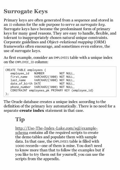
Primary keys are often generated from a sequence and stored inan ID column for the sole purpose to serve as surrogate key.Surrogate keys have become the predominant form of primarykeys for many good reasons. They are easy to handle, flexible, andtolerant to inappropriately chosen natural unique constraints.Corporate guidelines and Object-relational mapping (ORM)frameworks often encourage, and sometimes even enforce, theuse of surrogate keys.
As first example, consider an EMPLOYEES table with a unique indexon the EMPLOYEE_ID column:
CREATE TABLE employees ( employee_id NUMBER NOT NULL, first_name VARCHAR2(1000) NOT NULL, last_name VARCHAR2(1000) NOT NULL, date_of_birth DATE NOT NULL, phone_number VARCHAR2(1000) NOT NULL, CONSTRAINT employees_pk PRIMARY KEY (employee_id));
The Oracle database creates a unique index according to thedefinition of the primary key automatically. There is no need for aseparate create index statement in that case.
Tip
http://Use-The-Index-Luke.com/sql/example-schema contains all the required scripts to createthe demo tables and populate them with sampledata. In that case, the EMPLOYEES table is filled with1000 records—one of them is mine. You don't needto know more than that to follow the examples but ifyou like to try them out for yourself, you can use thescripts from the appendix.
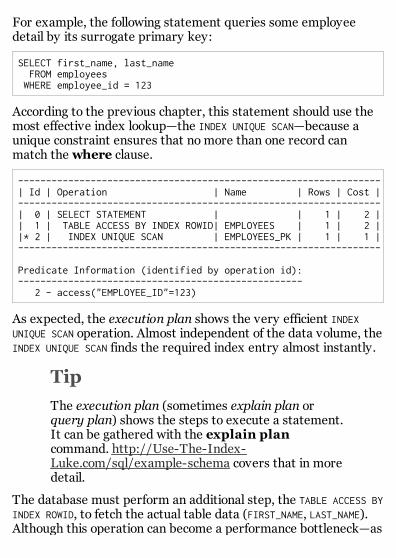
For example, the following statement queries some employeedetail by its surrogate primary key:
SELECT first_name, last_name FROM employees WHERE employee_id = 123
According to the previous chapter, this statement should use themost effective index lookup—the INDEX UNIQUE SCAN—because aunique constraint ensures that no more than one record canmatch the where clause.
-----------------------------------------------------------------| Id | Operation | Name | Rows | Cost |-----------------------------------------------------------------| 0 | SELECT STATEMENT | | 1 | 2 || 1 | TABLE ACCESS BY INDEX ROWID| EMPLOYEES | 1 | 2 ||* 2 | INDEX UNIQUE SCAN | EMPLOYEES_PK | 1 | 1 |-----------------------------------------------------------------
Predicate Information (identified by operation id):--------------------------------------------------- 2 - access("EMPLOYEE_ID"=123)
As expected, the execution plan shows the very efficient INDEXUNIQUE SCAN operation. Almost independent of the data volume, theINDEX UNIQUE SCAN finds the required index entry almost instantly.
Tip
The execution plan (sometimes explain plan orquery plan) shows the steps to execute a statement.It can be gathered with the explain plancommand. http://Use-The-Index-Luke.com/sql/example-schema covers that in moredetail.
The database must perform an additional step, the TABLE ACCESS BYINDEX ROWID, to fetch the actual table data (FIRST_NAME, LAST_NAME).Although this operation can become a performance bottleneck—as

explained in the section called “The Leaf Nodes”—there is no suchrisk with an INDEX UNIQUE SCAN. An INDEX UNIQUE SCAN can not returnmore than one ROWID. The subsequent table access is therefore notat risk to read many blocks.
The primary key lookup, based on a single column surrogate key,is bullet proof with respect to performance.
Primary Keys Supported by Nonunique Indexes
Nonunique indexes can be used to support a primary key orunique constraint. In that case the lookup requires an INDEXRANGE SCAN instead of an INDEX UNIQUE SCAN. Because theconstraint still maintains the uniqueness of every key, theperformance impact is often negligible. In case the searchedkey is the last in its leaf node, the next leaf node will be read tosee if there are more matching entries. The example in thesection called “The Tree ” explains this phenomenon.
One reason to intentionally use a nonunique index to enforce aprimary key or unique constraint is to make the constraintdeferrable. While regular constraints are validated duringstatement execution the validation of a deferrable constraint ispostponed until the transaction is committed. Deferredconstraints are required to propagate data into tables withcircular foreign key dependencies.

Concatenated Keys
Although surrogate keys are widely accepted and implemented,there are cases when a key consists of more than one column. Theindexes used to support the search on multiple columns are calledconcatenated or composite indexes.
The order of the individual columns within a concatenated index isnot only a frequent cause of confusion but also the foundation foran extraordinary resistant myth; the „most selective first” myth—Appendix A, Myth Directory has more details. The truth is thatthe column order affects the number of statements that can usethe index.
For the sake of demonstration, let's assume the 1000 employeescompany from the previous section was bought by a Very BigCompany. Unfortunately the surrogate key values used in ourEMPLOYEES table collide with those used by the Very Big Company.The EMPLOYEE_ID values can be reassigned—theoretically—becauseit's not a natural but a surrogate key. However, surrogate keysare often used in interface to other systems—like an access controlsystem—so that changing is not as easy. Adding a new column tomaintain the uniqueness is often the path of least resistance.
After all, reality bites, and the SUBSIDIARY_ID column is added tothe table. The primary key is extended accordingly, thecorresponding unique index is replaced by a new one onEMPLOYEE_ID and SUBSIDIARY_ID:
CREATE UNIQUE INDEX employee_pk ON employees (employee_id, subsidiary_id);
The new employee table contains all employees from bothcompanies and has ten times as many records as before. A queryto fetch the name of a particular employee has to state bothcolumns in the where clause:

SELECT first_name, last_name FROM employees WHERE employee_id = 123 AND subsidiary_id = 30;
As intended and expected, the query still uses the INDEX UNIQUESCAN operation:
-----------------------------------------------------------------| Id | Operation | Name | Rows | Cost |-----------------------------------------------------------------| 0 | SELECT STATEMENT | | 1 | 2 || 1 | TABLE ACCESS BY INDEX ROWID| EMPLOYEES | 1 | 2 ||* 2 | INDEX UNIQUE SCAN | EMPLOYEES_PK | 1 | 1 |-----------------------------------------------------------------
Predicate Information (identified by operation id):--------------------------------------------------- 2 - access("EMPLOYEE_ID"=123 AND "SUBSIDIARY_ID"=30)
This setup becomes more interesting when the where clausedoesn't contain all the indexed columns. For example, a query thatlists all employees of a subsidiary:
SELECT first_name, last_name FROM employees WHERE subsidiary_id = 20;
----------------------------------------------------| Id | Operation | Name | Rows | Cost |----------------------------------------------------| 0 | SELECT STATEMENT | | 110 | 477 ||* 1 | TABLE ACCESS FULL| EMPLOYEES | 110 | 477 |----------------------------------------------------
Predicate Information (identified by operation id):--------------------------------------------------- 1 - filter("SUBSIDIARY_ID"=20)
The database performs a FULL TABLE SCAN. A FULL TABLE SCAN readsall table blocks and evaluates every row against the where clause.No index is used. The performance degrades linear with the datavolume; that is, double the amount of data, twice as long to wait
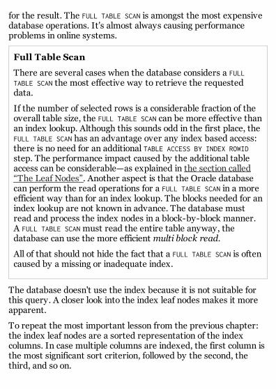
for the result. The FULL TABLE SCAN is amongst the most expensivedatabase operations. It's almost always causing performanceproblems in online systems.
Full Table Scan
There are several cases when the database considers a FULLTABLE SCAN the most effective way to retrieve the requesteddata.
If the number of selected rows is a considerable fraction of theoverall table size, the FULL TABLE SCAN can be more effective thanan index lookup. Although this sounds odd in the first place, theFULL TABLE SCAN has an advantage over any index based access:there is no need for an additional TABLE ACCESS BY INDEX ROWIDstep. The performance impact caused by the additional tableaccess can be considerable—as explained in the section called“The Leaf Nodes”. Another aspect is that the Oracle databasecan perform the read operations for a FULL TABLE SCAN in a moreefficient way than for an index lookup. The blocks needed for anindex lookup are not known in advance. The database mustread and process the index nodes in a block-by-block manner.A FULL TABLE SCAN must read the entire table anyway, thedatabase can use the more efficient multi block read.
All of that should not hide the fact that a FULL TABLE SCAN is oftencaused by a missing or inadequate index.
The database doesn't use the index because it is not suitable forthis query. A closer look into the index leaf nodes makes it moreapparent.
To repeat the most important lesson from the previous chapter:the index leaf nodes are a sorted representation of the indexcolumns. In case multiple columns are indexed, the first column isthe most significant sort criterion, followed by the second, thethird, and so on.

As a consequence, the tree structure can be used only if thewhere clause includes the leading columns of the index. Thevalues of the subsequent index columns are not centralized withinthe leaf node structure and cannot be localized with a treetraversal.
Figure 2.1. Concatenated Index
Figure 2.1, “Concatenated Index” shows an index fragment withthree leaf nodes and the corresponding branch node. The indexconsists of the EMPLOYEE_ID and SUBSIDIARY_ID columns (in thatorder), as in the example above.
The search for SUBSIDIARY_ID = 20 is not supported by the indexbecause the matching entries are distributed over a wide range ofthe index. Although two index entries match the filter, the branchnode doesn't contain the search value at all. The tree cannot beused to find those entries.
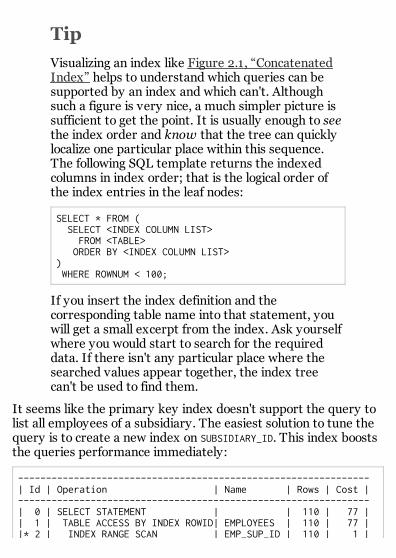
Tip
Visualizing an index like Figure 2.1, “ConcatenatedIndex” helps to understand which queries can besupported by an index and which can't. Althoughsuch a figure is very nice, a much simpler picture issufficient to get the point. It is usually enough to seethe index order and know that the tree can quicklylocalize one particular place within this sequence.The following SQL template returns the indexedcolumns in index order; that is the logical order ofthe index entries in the leaf nodes:
SELECT * FROM ( SELECT <INDEX COLUMN LIST> FROM <TABLE> ORDER BY <INDEX COLUMN LIST>) WHERE ROWNUM < 100;
If you insert the index definition and thecorresponding table name into that statement, youwill get a small excerpt from the index. Ask yourselfwhere you would start to search for the requireddata. If there isn't any particular place where thesearched values appear together, the index treecan't be used to find them.
It seems like the primary key index doesn't support the query tolist all employees of a subsidiary. The easiest solution to tune thequery is to create a new index on SUBSIDIARY_ID. This index booststhe queries performance immediately:
---------------------------------------------------------------| Id | Operation | Name | Rows | Cost |---------------------------------------------------------------| 0 | SELECT STATEMENT | | 110 | 77 || 1 | TABLE ACCESS BY INDEX ROWID| EMPLOYEES | 110 | 77 ||* 2 | INDEX RANGE SCAN | EMP_SUP_ID | 110 | 1 |
---------------------------------------------------------------
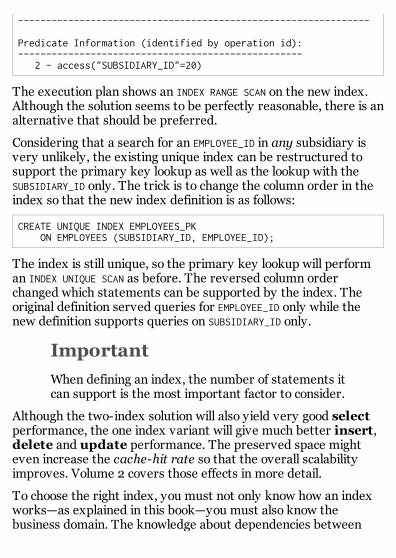
Predicate Information (identified by operation id):--------------------------------------------------- 2 - access("SUBSIDIARY_ID"=20)
The execution plan shows an INDEX RANGE SCAN on the new index.Although the solution seems to be perfectly reasonable, there is analternative that should be preferred.
Considering that a search for an EMPLOYEE_ID in any subsidiary isvery unlikely, the existing unique index can be restructured tosupport the primary key lookup as well as the lookup with theSUBSIDIARY_ID only. The trick is to change the column order in theindex so that the new index definition is as follows:
CREATE UNIQUE INDEX EMPLOYEES_PK ON EMPLOYEES (SUBSIDIARY_ID, EMPLOYEE_ID);
The index is still unique, so the primary key lookup will performan INDEX UNIQUE SCAN as before. The reversed column orderchanged which statements can be supported by the index. Theoriginal definition served queries for EMPLOYEE_ID only while thenew definition supports queries on SUBSIDIARY_ID only.
Important
When defining an index, the number of statements itcan support is the most important factor to consider.
Although the two-index solution will also yield very good selectperformance, the one index variant will give much better insert,delete and update performance. The preserved space mighteven increase the cache-hit rate so that the overall scalabilityimproves. Volume 2 covers those effects in more detail.
To choose the right index, you must not only know how an indexworks—as explained in this book—you must also know thebusiness domain. The knowledge about dependencies between

various attributes is essential to define an index correctly.
An external performance consultant can have a very hard time tofigure out which columns can go alone into the where clause andwhich are always paired with other attributes. As long as you arenot familiar with the business domain, this kind of exercise isactually reverse engineering. Although I admit that reverseengineering can be fun if practiced every now and then, I knowthat it becomes a very depressing task if practiced on an everyday basis.
Despite the fact that internal database administrators know theindustry of their company often better than external consultants,the detailed knowledge needed to optimally define the indexes ishardly accessible to them. The only place where the technicaldatabase knowledge meets the functional knowledge of thebusiness domain is the development department.

Slow Indexes, Part II
The previous chapter has demonstrated that a changed columnorder can gain additional benefits from an existing index.However, this was considering two statements only. An indexchange can influence all statements that access the correspondingtable. You probably know from your own experience: neverchange a running system. At least not without comprehensivetesting beforehand.
Although the changed EMPLOYEE_PK index improves performance ofall queries that use a subsidiary filter without any other clause,the index might be more tempting than it should. Even if an indexcan support a query, it doesn't mean that it will give the bestpossible performance. It's the optimizer's job to decide whichindex to use—or not to use an index at all. This section drafts acase that tempts the optimizer to use an inappropriate index.
The Query Optimizer
The query optimizer is the database component thattransforms an SQL statement into an execution plan. Thisprocess is often called parsing.
The so-called Cost Based Optimizer (CBO) generates variousexecution plan permutations and assigns a cost value to eachone. The cost value serves as benchmark to compare thevarious execution plans; the plan with the lowest cost value isconsidered best.
Calculating the cost value is a complex matter that easily fills abook of its own. From users perspective it is sufficient to knowthat the optimizer believes a lower cost value results in a betterstatement execution.
The so-called Rule Based Optimizer (RBO) was the CBO'spredecessor and is of no practical use nowadays.
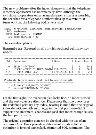
The new problem—after the index change—is that the telephonedirectory application has become very slow. Although theswitchboard operators enter as much search criteria as possible,the searches for a telephone number takes up to a minute. Itturns out that the following SQL is very slow:
SELECT first_name, last_name, subsidiary_id, phone_number FROM employees WHERE last_name = 'WINAND' AND subsidiary_id = 30;
The execution plan is:
Example 2.1. Execution plan with revised primary keyindex
-----------------------------------------------------------------| Id | Operation | Name | Rows | Cost |-----------------------------------------------------------------| 0 | SELECT STATEMENT | | 1 | 30 ||* 1 | TABLE ACCESS BY INDEX ROWID| EMPLOYEES | 1 | 30 ||* 2 | INDEX RANGE SCAN | EMPLOYEES_PK | 40 | 2 |-----------------------------------------------------------------
Predicate Information (identified by operation id):--------------------------------------------------- 1 - filter("LAST_NAME"='WINAND') 2 - access("SUBSIDIARY_ID"=30)
On the first sight, the execution plan looks fine. An index is usedand the cost value is rather low. Please note that the query usesthe redefined primary key index. Bearing in mind that the originalindex definition—with EMPLOYEE_ID in the first position—didn'tsupport the statement, chances are good that index change causesthe bad performance.
The original execution plan can be checked with the use of anoptimizer hint. Hints provide additional information to theoptimizer in form of particularly formatted SQL comments. The

following statement uses a hint that instructs the optimizer not touse the new index for this query:
SELECT /*+ NO_INDEX(EMPLOYEES EMPLOYEE_PK) */ first_name, last_name, subsidiary_id, phone_number FROM employees WHERE last_name = 'WINAND' AND subsidiary_id = 30;
The original execution plan uses a FULL TABLE SCAN and has a highercost value than the INDEX RANGE SCAN:
----------------------------------------------------| Id | Operation | Name | Rows | Cost |----------------------------------------------------| 0 | SELECT STATEMENT | | 1 | 477 ||* 1 | TABLE ACCESS FULL| EMPLOYEES | 1 | 477 |----------------------------------------------------
Predicate Information (identified by operation id):--------------------------------------------------- 1 - filter("LAST_NAME"='WINAND' AND "SUBSIDIARY_ID"=30)
Even though the FULL TABLE SCAN must read all table blocks andprocess all table rows, it is—in this particular case—faster than theINDEX RANGE SCAN. The optimizer is well aware that my name isn'tvery common and estimates a total row count of one. An indexlookup for one particular record should outperform the FULL TABLESCAN—but it doesn't; the index is slow.
A step-by-step investigation of the execution plan is the best wayto find the problem. The first step is the INDEX RANGE SCAN, whichfinds all entries that match the filter SUBSIDIARY_ID = 30. Becausethe second filter criteria—on LAST_NAME—is not included in theindex, it can't be considered during the index lookup.
The “Predicate Information” section of the execution plan inExample 2.1, “Execution plan with revised primary key index”reveals which filter criteria (predicates) are applied at eachprocessing step. The INDEX RANGE SCAN operation has the operationId 2; the corresponding predicate information is

“access("SUBSIDIARY_ID"=30)”. That means, the index tree structureis traversed to find the first entry for SUBSIDIARY_ID 30.Afterwards, the leaf node chain is followed to find all matchingentries. The result of the INDEX RANGE SCAN is a list of matchingROWIDs that satisfy the filter on SUBSIDIARY_ID. Depending on thesize of the subsidiary, the number of rows matching that criterioncan vary from a few dozen to some thousands.
The next step in the execution plan is the TABLE ACCESS BY INDEXROWID that fetches the identified rows from the table. Once thecomplete row—with all columns—is available, the outstanding partof the where clause can be evaluated. All the rows returned fromthe INDEX RANGE SCAN are read from the table and filtered by thepredicate related to the TABLE ACCESS BY INDEX ROWID operation:“filter("LAST_NAME"='WINAND')”. The remaining rows are those thatfulfill the entire where clause.
The performance of this select statement is vastly depended onthe number of employees in the particular subsidiary. For a smallsubsidiary—e.g., only a few dozen members—the INDEX RANGE SCANwill result in good performance. On the other hand, a search in ahuge subsidiary can become less efficient than a FULL TABLE SCANbecause it can not utilize multi block reads (see Full Table Scan)and might suffer from a bad clustering factor (see ClusteringFactor).
The phone directory lookup is slow because the INDEX RANGE SCANreturns thousand records—all employees from the originalcompany—and the TABLE ACCESS BY INDEX ROWID must fetch all ofthem. Remember the two ingredients for a “Slow Index”experience: a wider index scan than intended and the subsequenttable access.
Besides the individual steps performed during the query, theexecution plan provides information about the optimizer'sestimates. This information can help to understand why theoptimizer has chosen a particular execution plan. The “Rows”column is of particular interest for that purpose. It reveals the

optimizer's estimation that the INDEX RANGE SCAN will return 40rows—Example 2.1, “Execution plan with revised primary keyindex”. Under this presumption, the decision to perform an INDEXRANGE SCAN is perfectly reasonable. Unfortunately, it's off by afactor of 25.
The optimizer uses the so-called optimizer statistics for itsestimates. They are usually collected and updated on a regularbasis by the administrator or an automated job. They consist ofvarious information about the tables and indexes in the database.The most important statistics for an INDEX RANGE SCAN are the sizeof the index (number of rows in the index) and the selectivity ofthe respective predicate (the fraction that satisfies the filter).
Statistics and Dynamic Sampling
The optimizer can use a variety of statistics on table, index, andcolumn level. Most statistics are collected per table column: thenumber of distinct values, the smallest and biggest value (datarange), the number of NULL occurrences and the columnhistogram (data distribution). As of Oracle 11g it is also possibleto collect extended statistics for column concatenations andexpressions.
There are only very few statistics for the table as such: the size(in rows and blocks) and the average row length. However, thecolumn statistics belong to the table; that is, they are computedwhen the table statistics are gathered.
The most important index statistics are the tree depth, thenumber of leaf nodes, the number of distinct keys and theclustering factor (see Clustering Factor).
The optimizer uses these values to estimate the selectivity ofthe predicates in the where clause.
If there are no statistics available, the optimizer can performdynamic sampling. That means that it reads a small fraction ofthe table during query planning to get a basis for the estimates.
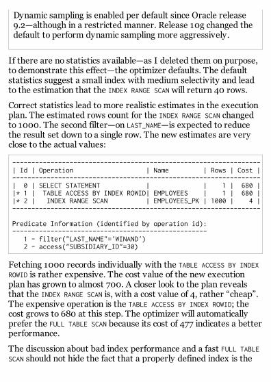
Dynamic sampling is enabled per default since Oracle release9.2—although in a restricted manner. Release 10g changed thedefault to perform dynamic sampling more aggressively.
If there are no statistics available—as I deleted them on purpose,to demonstrate this effect—the optimizer defaults. The defaultstatistics suggest a small index with medium selectivity and leadto the estimation that the INDEX RANGE SCAN will return 40 rows.
Correct statistics lead to more realistic estimates in the executionplan. The estimated rows count for the INDEX RANGE SCAN changedto 1000. The second filter—on LAST_NAME—is expected to reducethe result set down to a single row. The new estimates are veryclose to the actual values:
-----------------------------------------------------------------| Id | Operation | Name | Rows | Cost |-----------------------------------------------------------------| 0 | SELECT STATEMENT | | 1 | 680 ||* 1 | TABLE ACCESS BY INDEX ROWID| EMPLOYEES | 1 | 680 ||* 2 | INDEX RANGE SCAN | EMPLOYEES_PK | 1000 | 4 |-----------------------------------------------------------------
Predicate Information (identified by operation id):--------------------------------------------------- 1 - filter("LAST_NAME"='WINAND') 2 - access("SUBSIDIARY_ID"=30)
Fetching 1000 records individually with the TABLE ACCESS BY INDEXROWID is rather expensive. The cost value of the new executionplan has grown to almost 700. A closer look to the plan revealsthat the INDEX RANGE SCAN is, with a cost value of 4, rather “cheap”.The expensive operation is the TABLE ACCESS BY INDEX ROWID; thecost grows to 680 at this step. The optimizer will automaticallyprefer the FULL TABLE SCAN because its cost of 477 indicates a betterperformance.
The discussion about bad index performance and a fast FULL TABLESCAN should not hide the fact that a properly defined index is the

best solution. To support a search by last name, an appropriateindex should be added:
CREATE INDEX emp_name ON employees (last_name);
The optimizer calculates a cost value of 3 for the new plan:
Example 2.2. Execution Plan with Dedicated Index
--------------------------------------------------------------| Id | Operation | Name | Rows | Cost |--------------------------------------------------------------| 0 | SELECT STATEMENT | | 1 | 3 ||* 1 | TABLE ACCESS BY INDEX ROWID| EMPLOYEES | 1 | 3 ||* 2 | INDEX RANGE SCAN | EMP_NAME | 1 | 1 |--------------------------------------------------------------
Predicate Information (identified by operation id):--------------------------------------------------- 1 - filter("SUBSIDIARY_ID"=30) 2 - access("LAST_NAME"='WINAND')
Because of the statistics, the optimizer knows that LAST_NAME ismore selective than the SUBSIDIARY_ID. It estimates that only onerow will fulfill the predicate of the index lookup—on LAST_NAME—sothat only row has to be retrieved from the table.
Please note that the difference in the execution plans as shown infigures Example 2.1, “Execution plan with revised primary keyindex” and Example 2.2, “Execution Plan with Dedicated Index” isminimal. The performed operations are the same and the cost islow in both cases. Nevertheless the second plan performs muchbetter than the first. The efficiency of an INDEX RANGE SCAN—especially when accompanied by a TABLE ACCESS BY INDEX ROWID—can vary in a wide range. Just because an index is used doesn'tmean the performance is good.
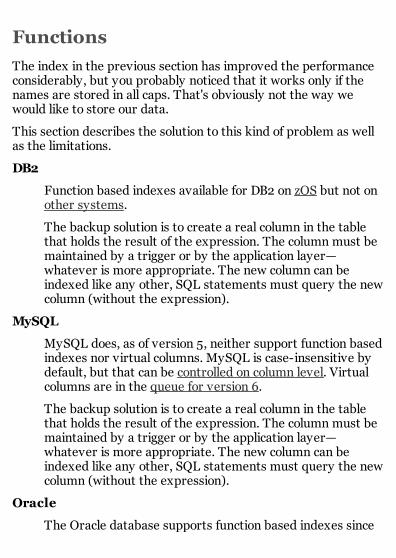
Functions
The index in the previous section has improved the performanceconsiderably, but you probably noticed that it works only if thenames are stored in all caps. That's obviously not the way wewould like to store our data.
This section describes the solution to this kind of problem as wellas the limitations.
DB2
Function based indexes available for DB2 on zOS but not onother systems.
The backup solution is to create a real column in the tablethat holds the result of the expression. The column must bemaintained by a trigger or by the application layer—whatever is more appropriate. The new column can beindexed like any other, SQL statements must query the newcolumn (without the expression).
MySQL
MySQL does, as of version 5, neither support function basedindexes nor virtual columns. MySQL is case-insensitive bydefault, but that can be controlled on column level. Virtualcolumns are in the queue for version 6.
The backup solution is to create a real column in the tablethat holds the result of the expression. The column must bemaintained by a trigger or by the application layer—whatever is more appropriate. The new column can beindexed like any other, SQL statements must query the newcolumn (without the expression).
Oracle
The Oracle database supports function based indexes since

release 8i. Virtual columns were additionally added with 11g.
PostgreSQL
PostgreSQL supports Indexes on Expressions.
SQL Server
SQL Server supports Computed Columns that can beindexed.

Case-Insensitive Search
The SQL for a case-insensitive search is very simple—just uppercase both sides of the search expression:
SELECT first_name, last_name, subsidiary_id, phone_number FROM employees WHERE UPPER(last_name) = UPPER('winand');
The query works by converting both sides of the comparison tothe same notation. No matter how the LAST_NAME is stored, or thesearch term is entered, the upper case on both sides will makethem match. From functional perspective, this is a reasonableSQL statement. However, let's have a look at the execution plan:
----------------------------------------------------| Id | Operation | Name | Rows | Cost |----------------------------------------------------| 0 | SELECT STATEMENT | | 10 | 477 ||* 1 | TABLE ACCESS FULL| EMPLOYEES | 10 | 477 |----------------------------------------------------
Predicate Information (identified by operation id):---------------------------------------------------
1 - filter(UPPER("LAST_NAME")='WINAND')
It's a comeback of our old friend the full table scan. The index onLAST_NAME is unusable because the search is not on last name—it'son UPPER(LAST_NAME). From the database's perspective, that'ssomething entirely different.
It's a trap we all fall into. We instantly recognize the relationbetween LAST_NAME and UPPER(LAST_NAME) and expect the database to“see” it as well. In fact, the optimizer's picture is more like that:
SELECT first_name, last_name, subsidiary_id, phone_number FROM employees WHERE BLACKBOX(...) = 'WINAND';
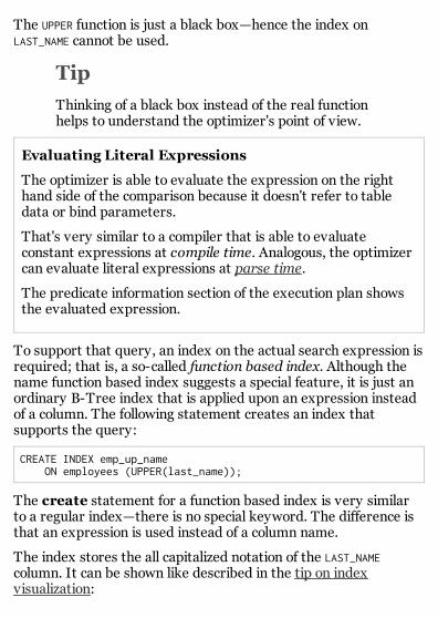
The UPPER function is just a black box—hence the index onLAST_NAME cannot be used.
Tip
Thinking of a black box instead of the real functionhelps to understand the optimizer's point of view.
Evaluating Literal Expressions
The optimizer is able to evaluate the expression on the righthand side of the comparison because it doesn't refer to tabledata or bind parameters.
That's very similar to a compiler that is able to evaluateconstant expressions at compile time. Analogous, the optimizercan evaluate literal expressions at parse time.
The predicate information section of the execution plan showsthe evaluated expression.
To support that query, an index on the actual search expression isrequired; that is, a so-called function based index. Although thename function based index suggests a special feature, it is just anordinary B-Tree index that is applied upon an expression insteadof a column. The following statement creates an index thatsupports the query:
CREATE INDEX emp_up_name ON employees (UPPER(last_name));
The create statement for a function based index is very similarto a regular index—there is no special keyword. The difference isthat an expression is used instead of a column name.
The index stores the all capitalized notation of the LAST_NAMEcolumn. It can be shown like described in the tip on indexvisualization:

SELECT * FROM ( SELECT UPPER(last_name) FROM employees ORDER BY UPPER(last_name)) WHERE ROWNUM < 10;
The statement will return the first 10 index entries in indexorder:
UPPER(LAST_NAME)--------------------AAACHAAAXPPKUAABCZLTSCNMAAGJXAAIIARNAAQVASLRAASQDAAUMEJHQUEIABAIHSJFYGABAS
The Oracle database can use a function based index if the exactexpression of the index definition appears in an SQL statement—like in the example above—so that the new execution plan usesthe index:
----------------------------------------------------------------| Id | Operation | Name | Rows | Cost |----------------------------------------------------------------| 0 | SELECT STATEMENT | | 100 | 41 || 1 | TABLE ACCESS BY INDEX ROWID| EMPLOYEES | 100 | 41 ||* 2 | INDEX RANGE SCAN | EMP_UP_NAME | 40 | 1 |----------------------------------------------------------------
Predicate Information (identified by operation id):---------------------------------------------------
2 - access(UPPER("LAST_NAME")='WINAND')
It is a normal INDEX RANGE SCAN, exactly as described in Chapter 1,Anatomy of an Index; the tree is traversed and the leaf nodes are

followed to see if there is more than one match. There are no“special” operations for function based indexes.
Warning
UPPER and LOWER is sometimes used withoutdeveloper's knowledge. E.g., some ORM frameworkssupport case-insensitive natively but implement itby using UPPER or LOWER in the SQL. Hibernate, forexample, injects an implicit LOWER for a case-insensitive search.
The execution plan has one more issue: the row estimates are waytoo high. The number of rows returned by the table access is evenhigher than the number of rows expected from the INDEX RANGESCAN. How can the table access match 100 records if the precedingindex scan returned only 40 rows? Well, it can't. These kind of“impossible” estimates indicate a problem with the statistics (seealso Statistics and Dynamic Sampling).
This particular problem has a very common cause; the tablestatistics were not updated after creating the index. Although theindex statistics are automatically collected on index creation (since10g), the table stats are left alone. The box Collecting Statisticshas more information why the table statistics are relevant andwhat to take care of when updating statistics.
Collecting Statistics
The column statistics, which include the number of distinctcolumn values, are part to the table statistics. That means,even if multiple indexes contain the same column, thecorresponding statistics are kept one time only—as part of thetable statistics.
Statistics for a function based index (FBI) are implemented asvirtual columns on table level. The DBMS_STATS package cancollect the statistics on the virtual column after the FBI was
created—when the virtual column exists. The Oracledocumentation says:
After creating a function-based index, collect statistics onboth the index and its base table using the DBMS_STATSpackage. Such statistics will enable Oracle Database tocorrectly decide when to use the index.
Collecting and updating statistics is a task that should becoordinated with the DBAs. The optimizer is heavily dependingon the statistics—there is a high risk to run into trouble. Mygeneral advice is to always backup statistics before updatingthem, always collect the table statistics and all related indexstatistics in one shot, and talk to the DBAs.
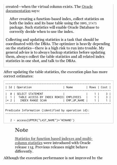
After updating the table statistics, the execution plan has morecorrect estimates:
----------------------------------------------------------------| Id | Operation | Name | Rows | Cost |----------------------------------------------------------------| 0 | SELECT STATEMENT | | 1 | 3 || 1 | TABLE ACCESS BY INDEX ROWID| EMPLOYEES | 1 | 3 ||* 2 | INDEX RANGE SCAN | EMP_UP_NAME | 1 | 1 |----------------------------------------------------------------
Predicate Information (identified by operation id):---------------------------------------------------
2 - access(UPPER("LAST_NAME")='WINAND')
Note
Statistics for function based indexes and multi-column statistics were introduced with Oraclerelease 11g. Previous releases might behavedifferently.
Although the execution performance is not improved by the
updated statistics—because the index was correctly used anyway—it is always good to have a look at the optimizer's estimates. Thenumber of rows processed for each step (cardinality) is a veryimportant figure for the optimizer—getting them right for simplequeries can easily pay off for complex queries.

User Defined Functions
A case-insensitive search is probably the most common use for afunction based index—but other functions can be "indexed" aswell. In fact, almost every function—even user defined functions—can be used with an index.
It is, however, not possible to use the SYSDATE function as part of anindex definition. For example, the following function can't beindexed:
CREATE FUNCTION get_age(date_of_birth DATE) RETURN NUMBERASBEGIN RETURN TRUNC(MONTHS_BETWEEN(SYSDATE, date_of_birth)/12);END;/
The function converts the date of birth into an age—according tothe current system time. It can be used in the select-list to queryan employees age, or as part of the where clause:
SELECT first_name, last_name, get_age(date_of_birth) FROM employees WHERE get_age(date_of_birth) = 42;
Although it's a very convenient way search for all employees whoare 42 years old, a function based index can not tune thisstatement because the GET_AGE function is not deterministic. Thatmeans, the result of the function call is not exclusively determinedby its parameters. Only functions that always return the sameresult for the same parameters—functions that are deterministic—can be indexed.
The reason behind this limitation is easily explained. Justremember that the return value of the function will be physicallystored in the index when the record is inserted. There is no
background job that would update the age on the employee'sbirthday—that's just not happening. The only way to update anindividual index entry is to update an indexed column of therespective record.
Besides being deterministic, a function must be declaredDETERMINISTIC in order to be usable with a function based index.
Caution
The Oracle database trusts the DETERMINISTICkeyword—that means, it trust the developer. TheGET_AGE function can be declared DETERMINISTIC so thatthe database allows an index onGET_AGE(date_of_birth).
Regardless of that, it will not work as intendedbecause the index entries will not increase as theyears pass; the employees will not get older—atleast not in the index.
Other examples for functions that cannot be indexed are themembers of the DBMS_RANDOM package and functions that implicitlydepend on the environment—such as NLS (National LanguageSupport) settings. In particular, the use of TO_CHAR withoutformating mask is often causing trouble.
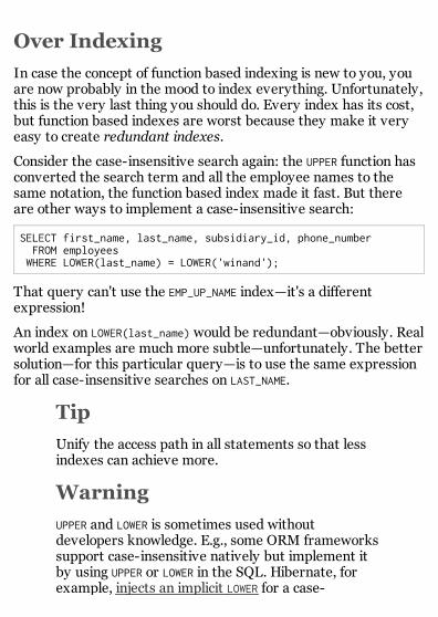
Over Indexing
In case the concept of function based indexing is new to you, youare now probably in the mood to index everything. Unfortunately,this is the very last thing you should do. Every index has its cost,but function based indexes are worst because they make it veryeasy to create redundant indexes.
Consider the case-insensitive search again: the UPPER function hasconverted the search term and all the employee names to thesame notation, the function based index made it fast. But thereare other ways to implement a case-insensitive search:
SELECT first_name, last_name, subsidiary_id, phone_number FROM employees WHERE LOWER(last_name) = LOWER('winand');
That query can't use the EMP_UP_NAME index—it's a differentexpression!
An index on LOWER(last_name) would be redundant—obviously. Realworld examples are much more subtle—unfortunately. The bettersolution—for this particular query—is to use the same expressionfor all case-insensitive searches on LAST_NAME.
Tip
Unify the access path in all statements so that lessindexes can achieve more.
Warning
UPPER and LOWER is sometimes used withoutdevelopers knowledge. E.g., some ORM frameworkssupport case-insensitive natively but implement itby using UPPER or LOWER in the SQL. Hibernate, forexample, injects an implicit LOWER for a case-

insensitive search.
Every CREATE INDEX statement puts a huge burden on thedatabase: the index needs space—on the disks and in thememory; the optimizer has to consider the index for each queryon the base table; and, each and every insert, update, deleteand merge statement on the base table must update the index.All of that, just because of one CREATE INDEX statement. Use itwisely.
Tip
Always aim to index the original data. That is oftenthe most useful information you can put into anindex.
Exercise
One problem from the section called “User Defined Functions” isstill unanswered; how to use an index to search for employeeswho are 42 years old?
Try to find the solution and share your thoughts on the forum. Butwatch out, it's a trap. Open your mind to find the solution.
Another question to think about is when to use function basedindexes? Do you have examples?

Bind Parameter
This section covers a topic that is way too often ignored intextbooks; the use of bind parameters in SQL statements.
Bind parameter—also called dynamic parameters or bindvariables—are an alternative way to provide data to the database.Instead of putting the values literally into the SQL statement, aplaceholder (like ?, :name or @name) is used. The actual values forthe placeholder are provided through a separate API call.
Even though literal values are very handy for ad-hoc statements,programs should almost always use bind variables. That's for tworeasons:
Security
Bind variables are the best way to prevent SQL injection.
Performance
The Oracle optimizer can re-use a cached execution plan ifthe very same statement is executed multiple times. Assoon as the SQL statement differs—e.g., because of adifferent search term—the optimizer has to redo theexecution plan (see also: CURSOR_SHARING).
The general rule is therefore to use bind variables in programs.
There is, of course, one small exception. Re-using an executionplan means that the same execution plan will be used for differentsearch terms. Different search terms can, however, have animpact on the data volume. That has, in turn, a huge impact onperformance.
For example, the number of rows selected by the following SQLstatement is vastly depending on the subsidiary:
99 rows selected.
SELECT first_name, last_name FROM employees WHERE subsidiary_id = 20;
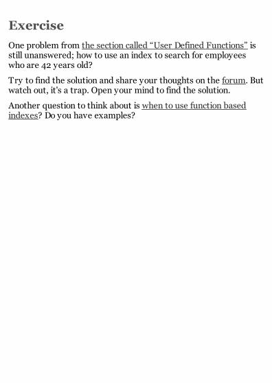
----------------------------------------------------------------| Id | Operation | Name | Rows | Cost |----------------------------------------------------------------| 0 | SELECT STATEMENT | | 99 | 70 || 1 | TABLE ACCESS BY INDEX ROWID| EMPLOYEES | 99 | 70 ||* 2 | INDEX RANGE SCAN | EMPLOYEE_PK | 99 | 2 |----------------------------------------------------------------
Predicate Information (identified by operation id):---------------------------------------------------
2 - access("SUBSIDIARY_ID"=20)
While an INDEX RANGE SCAN is best for small and mediumsubsidiaries, a FULL TABLE SCAN can outperform the index for largesubsidiaries:
1000 rows selected.
SELECT first_name, last_name FROM employees WHERE subsidiary_id = 30;
----------------------------------------------------| Id | Operation | Name | Rows | Cost |----------------------------------------------------| 0 | SELECT STATEMENT | | 1000 | 478 ||* 1 | TABLE ACCESS FULL| EMPLOYEES | 1000 | 478 |----------------------------------------------------
Predicate Information (identified by operation id):---------------------------------------------------
1 - filter("SUBSIDIARY_ID"=30)
The statistics—the column histogram —indicate that one queryselects ten times more than the other, therefore the optimizercreates different execution plans so that both statements canexecute with the best possible performance. However, theoptimizer has to know the actual search term to be able to use thestatistics—that is, it must be provided as literal value. the sectioncalled “Indexing LIKE Filters” covers another cases that is verysensible to bind parameters: LIKE filters.
Column Histograms

A column histogram is the part of the table statistics that holdsthe outline of the data distribution of a column. The histogramindicates which values appear more often than others.
The Oracle database uses two different types of histogramsthat serve the same purpose: frequency histograms and height-balanced histograms.
In this respect, the optimizer is similar to a compiler; if the literalvalues are available during parsing (compiling), they can be takeninto consideration. If bind variables are used, the actual values arenot known during parsing (compiling) and the execution plan cannot be optimized for a nonuniform data distribution.
Tip
Status flags such as "todo" and "done" have anonuniform distribution very often. E.g., the "done"records can typically outnumber the "todo" recordsby an order of magnitude.
The use of bind parameters might prevent the bestpossible execution plan for each status value. In thiscase, the status values should be escaped andvalidated against a white list before they are putliterally into the SQL statement.
An execution plan that is tailor-made for a particular search valuedoesn't come for free. The optimizer has to re-create theexecution plan every time a new distinct value appears. Thatmeans, executing the same SQL with 1000 different values willcause the optimizer to compute the execution plan 1000 times. Inthe compiler analogy, it's like compiling the source code everytime you run the program.
The database has a little dilemma when deciding to use a cachedversion of the execution plan or to parse the statement again. Onthe one hand, can the column histogram greatly improveexecution performance for some statements. On the other hand isparsing a very expensive task that should be avoided whenever
possible. The dilemma is that the optimizer doesn't know inadvance if the different values will result in a different executionplan.
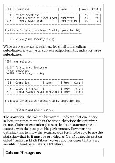
The application developer can come to help with this dilemma.The rule is to use bind values except for fields where you expect abenefit from a column histogram—e.g., because a full table scanmakes sense in one case, but an index lookup in another case.
Tip
In case of doubt, use bind parameters.
Please note that the SQL standard defines positional parametersonly—not named ones. Most databases and abstraction layerssupport named bind parameters nevertheless—in a nonstandardway. The following code snippets are examples how to use bindparameters.
C#
Instead of
int subsidiary_id;SqlCommand command = new SqlCommand( "select first_name, last_name" + " from employees" + " where subsidiary_id = " + subsidiary_id , connection);
use the following
int subsidiary_id;SqlCommand command = new SqlCommand( "select first_name, last_name" + " from employees" + " where subsidiary_id = @subsidiary_id , connection);command.Parameters.AddWithValue("@subsidiary_id", subsidiary_id);
Further documentation: SqlParameterCollection.
Java
Instead of

int subsidiary_id;Statement command = connection.createStatement( "select first_name, last_name" + " from employees" + " where subsidiary_id = " + subsidiary_id );
use the following
int subsidiary_id;PreparedStatement command = connection.prepareStatement( "select first_name, last_name" + " from employees" + " where subsidiary_id = ?" );command.setInt(1, subsidiary_id);
Further documentation: PreparedStatement.
Perl
Instead of
my $subsidiary_id;my $sth = $dbh->prapare( "select first_name, last_name" . " from employees" . " where subsidiary_id = $subsidiary_id" );$sth->execute();
use the following
my $subsidiary_id;my $sth = $dbh->prapare( "select first_name, last_name" . " from employees" . " where subsidiary_id = ?" );$sth->execute($subsidiary_id);
Further documentation: Programming the Perl DBI.
PHP
The following example is for MySQL—probably the mostcommonly used database with PHP.

Instead of
$mysqli->query("select first_name, last_name" . " from employees" . " where subsidiary_id = " . $subsidiary_id);
use the following
if ($stmt = $mysqli->prepare("select first_name, last_name" . " from employees" . " where subsidiary_id = ?")) { $stmt->bind_param("i", $subsidiary_id); $stmt->execute();} else { /* handle SQL error */}
Further documentation: mysqli_stmt::bind_param.
The PDO interface supports prepared statements as well.
Ruby
Instead of
dbh.execute("select first_name, last_name" + " from employees" + " where subsidiary_id = #{subsidiary_id}");
use the following:
dbh.prepare("select first_name, last_name" + " from employees" + " where subsidiary_id = ?");dbh.execute(subsidiary_id);
Further documentation: Ruby DBI Tutorial
Even though the SQL standard (par. 6.2, page 114) defines thequestion mark (?) as the placeholder sign, the implementationsvary. The Oracle database does not natively support questionmarks but uses the colon syntax for named placeholder (:name).On top of that, many database abstraction layers (e.g., Java JDBCand perl DBI) emulate the question mark support so that it can be

used with the Oracle database when accessed through theselayers.
Note
Bind parameters cannot change the structure of anSQL statement.
That means, you cannot use bind parameters in thefrom clause or change the where clausedynamically. Non of the following two bindparameters works:
String sql = prepare("SELECT * FROM ? WHERE ?");
sql.execute('employees', 'employee_id = 1');
If you need to change the structure of an SQLstatement, use dynamic SQL.
Oracle Cursor Sharing, Bind Peeking and AdaptiveCursor Sharing
Because bind parameters and histograms are very important,the Oracle database has undergone various attempts to makethem work together.
The by far most common problem are applications that do notuse bind parameters at all. For that reason, Oracle hasintroduced the setting CURSOR_SHARING that allows the databaseto re-write the SQL to use bind parameters (typically named:SYS_Bx). However, that feature is a workaround for applicationsthat do not use bind parameters and should never be used fornew applications.
With release 9i, Oracle introduced the so-called bind peeking.Bind peeking enables the optimizer to use the actual bindvalues of the first execution during parsing. The problem withthat approach is its nondeterministic behavior: whatever valuewas used in the first execution (e.g., since database startup)affects all executions. The execution plan can change everytime the database is restarted or, more problematic, the cached

time the database is restarted or, more problematic, the cachedplan expires. In other words; the execution plan can change atany time.
Release 11g introduced adaptive cursor sharing to cope withthe problem. This feature enables the database to havemultiple execution plans for the same SQL statement. The“adaptive” approach is to run everything as usual, but to takenote of the time each execution takes. In case one executionruns much slower than the others, the optimizer will create atailor-made plan for the specific bind values. However, thattailor-made plan is created the next time the statementexecutes with the problematic bind values. That means that thefirst execution must run slow before the second execution canbenefit.
All those features attempt to cope with a problem that can behandled by the application. If there is a heavy imbalance uponthe distribution of search keys, using literal variables should beconsidered.

NULL And Indexes
SQL's NULL is a constant source of confusion. Although the basicidea of NULL—to represent missing data—is rather simple, thereare numerous side effects. Some of them need special attention inSQL—e.g., "IS NULL" as opposed to "= NULL". Other side effects aremuch more subtle—but have a huge performance impact.
This section describes the most common performance issues whenhandling NULL in the Oracle database—in that respect, the Oracledatabase is very special.
DB2
DB2 does not treat the empty string as NULL.
MySQL
MySQL does not treat the empty string as NULL.
mysql> SELECT 0 IS NULL, 0 IS NOT NULL, '' IS NULL, '' IS NOT NULL;
+-----------+---------------+------------+----------------+| 0 IS NULL | 0 IS NOT NULL | '' IS NULL | '' IS NOT NULL |+-----------+---------------+------------+----------------+| 0 | 1 | 0 | 1 |+-----------+---------------+------------+----------------+
Oracle
The most annoying “special” handling of the Oracle databaseis that an empty string is considered NULL:
select * from dual where '' is null;
D-X
1 row selected.
PostgreSQL
PostgreSQL does not treat the empty string as NULL.
SQL Server

SQL Server
SQL Server does not treat the empty string as NULL.

Indexing NULL
The Oracle database does not include rows into an index if allindexed columns are NULL.
DB2
DB2 includes NULL into every index.
MySQL
MySQL includes NULL into every index.
Oracle
The Oracle database does not include rows into an index ifall indexed columns are NULL.
PostgreSQL
PostgreSQL has "Index support for IS NULL" since release8.3.
SQL Server
SQL Server includes NULL into every index.
For example, the EMP_DOB index, which consists of the DATE_OF_BIRTHcolumn only, will not contain an entry for a record whereDATE_OF_BIRTH is null:
INSERT INTO employees ( subsidiary_id, employee_id, first_name, last_name, phone_number)VALUES (?, ?, ?, ?, ?);
The DATE_OF_BIRTH is not specified and defaults to NULL—hence, therecord is not added to the EMP_DOB index. As a consequence, theindex cannot support a query for records where the date of birthis null:
SELECT first_name, last_name

FROM employees WHERE date_of_birth IS NULL;
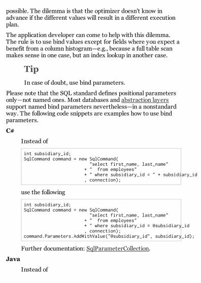
----------------------------------------------------| Id | Operation | Name | Rows | Cost |----------------------------------------------------| 0 | SELECT STATEMENT | | 1 | 477 ||* 1 | TABLE ACCESS FULL| EMPLOYEES | 1 | 477 |----------------------------------------------------
Predicate Information (identified by operation id):---------------------------------------------------
1 - filter("DATE_OF_BIRTH" IS NULL)
Nevertheless, the record will be inserted into a concatenatedindex if at least one column is not NULL:
CREATE INDEX demo_null ON employees (subsidiary_id, date_of_birth);
The new row is included in the demo index because the subsidiaryis not null for that row. As soon as any index column is not null,the entire row is added to the index. This index can thereforesupport a query for all employees of a specific subsidiary wherethe date of birth is null:
SELECT first_name, last_name FROM employees WHERE subsidiary_id = ? AND date_of_birth IS NULL;
--------------------------------------------------------------| Id | Operation | Name | Rows | Cost |--------------------------------------------------------------| 0 | SELECT STATEMENT | | 1 | 2 || 1 | TABLE ACCESS BY INDEX ROWID| EMPLOYEES | 1 | 2 ||* 2 | INDEX RANGE SCAN | DEMO_NULL | 1 | 1 |--------------------------------------------------------------
Predicate Information (identified by operation id):---------------------------------------------------
2 - access("SUBSIDIARY_ID"=TO_NUMBER(?) AND "DATE_OF_BIRTH" IS NULL)

Please note that the index covers the entire where clause; allpredicates are evaluated during the index lookup (Id 2). Thatmeans, the NULL is in the index.
This concept can be extended to find all records where date ofbirth is null—regardless of the subsidiary. Like with any otherconcatenated index, the DATE_OF_BIRTH column must be the first tosupport that query. However, it is required to keep theSUBSIDIARY_ID in the index, otherwise NULL would not be included inthe index at all. Any column that cannot be NULL—e.g., because of anot null constraint—is suitable to enforce inclusion of NULL into anindex. Even faked columns can be used, just for the purpose toinclude NULL into an index:
DROP INDEX emp_dob;CREATE INDEX emp_dob ON employees (date_of_birth, '1');
The index is postfixed with a constant string that can never beNULL. That makes sure that the index has all rows, even if the dateof birth is NULL.
Tip
Putting a column that cannot be NULL into an indexallows indexing NULL like any value.
It is, however, very important that the dummy column can neverbecome NULL and that the database knows that. Otherwise, theside effects might surprise you, as the next section explains.

NOT NULL Constraints
Whenever an Oracle index should support "where column IS NULL"queries, the index must include a column that can never be NULL.
However, it is not sufficient that there are no NULL entries—it mustbe enforced by a constraint. Otherwise, there could be a rowwhere all indexed columns are null; that row would not beincluded in the index.
For example, the following index supports the select if theLAST_NAME column has a NOT NULL constraint:
DROP INDEX emp_dob;CREATE INDEX emp_dob ON employees (date_of_birth, last_name);
SELECT * FROM employees WHERE date_of_birth IS NULL;
-----------------------------------------------------------------| Id | Operation | Name | Rows | Cost |-----------------------------------------------------------------| 0 | SELECT STATEMENT | | 1 | 3 || 1 | TABLE ACCESS BY INDEX ROWID| EMPLOYEES | 1 | 3 ||* 2 | INDEX RANGE SCAN | EMP_DOB_NAME | 1 | 2 |-----------------------------------------------------------------
Predicate Information (identified by operation id):---------------------------------------------------
2 - access("DATE_OF_BIRTH" IS NULL)
As soon as the not null constraint is removed, the index can't beused for the query anymore:
ALTER TABLE employees MODIFY last_name NULL;
SELECT * FROM employees WHERE date_of_birth IS NULL;
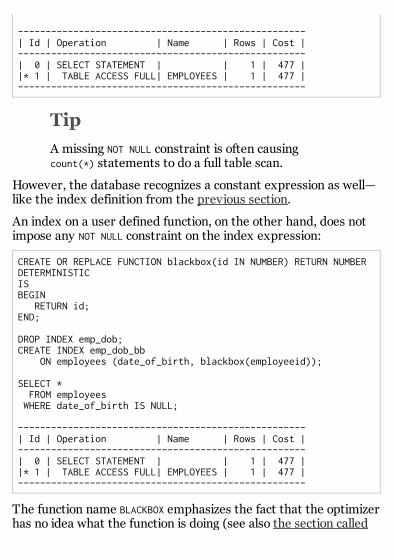
----------------------------------------------------| Id | Operation | Name | Rows | Cost |----------------------------------------------------| 0 | SELECT STATEMENT | | 1 | 477 ||* 1 | TABLE ACCESS FULL| EMPLOYEES | 1 | 477 |----------------------------------------------------
Tip
A missing NOT NULL constraint is often causingcount(*) statements to do a full table scan.
However, the database recognizes a constant expression as well—like the index definition from the previous section.
An index on a user defined function, on the other hand, does notimpose any NOT NULL constraint on the index expression:
CREATE OR REPLACE FUNCTION blackbox(id IN NUMBER) RETURN NUMBERDETERMINISTICISBEGIN RETURN id;END;
DROP INDEX emp_dob;CREATE INDEX emp_dob_bb ON employees (date_of_birth, blackbox(employeeid));
SELECT * FROM employees WHERE date_of_birth IS NULL;
----------------------------------------------------| Id | Operation | Name | Rows | Cost |----------------------------------------------------| 0 | SELECT STATEMENT | | 1 | 477 ||* 1 | TABLE ACCESS FULL| EMPLOYEES | 1 | 477 |----------------------------------------------------
The function name BLACKBOX emphasizes the fact that the optimizerhas no idea what the function is doing (see also the section called

“Case-Insensitive Search”). Although we can see that the functionpasses the input value straight through, the database doesn'trecognize—it's just a user defined function that returns a numericvalue. The NOT NULL property of the EMPLOYEE_ID column is lost. It'snot possible to use the index to find all records. However, there isstill a way to use the index if you know that the expression willnever return NULL:
SELECT * FROM employees WHERE date_of_birth IS NULL AND blackbox(employee_id) IS NOT NULL;
---------------------------------------------------------------| Id | Operation | Name | Rows | Cost |---------------------------------------------------------------| 0 | SELECT STATEMENT | | 1 | 3 || 1 | TABLE ACCESS BY INDEX ROWID| EMPLOYEES | 1 | 3 ||* 2 | INDEX RANGE SCAN | EMP_DOB_BB | 1 | 2 |---------------------------------------------------------------
The added where clause is an indirect way to put the not nullconstraint on the expression. The statement can use the indexbecause it selects only the records where the expression is notnull; they are in the index—per definition.
There is, unfortunately, no way to declare a function so that NULL isreturned only if NULL is provided as input.
NOT NULL Constraints on Virtual Columns
Oracle introduced virtual columns that can be indexed withrelease 11g.
Virtual columns serve a similar purpose as functional indexes,but they have a distinct column name that can be referenced.They are, in fact, very similar to a column that is added via aview. But they can be indexed.
These virtual columns can have a NOT NULL constraint:

DROP INDEX emp_dob_bb;
ALTER TABLE employees ADD bb_expression GENERATED ALWAYS AS (blackbox(employee_id)) NOT NULL;
CREATE INDEX emp_dob_bb ON employees (date_of_birth, bb_expression);
SELECT * FROM employees WHERE date_of_birth IS NULL;
---------------------------------------------------------------| Id | Operation | Name | Rows | Cost |---------------------------------------------------------------| 0 | SELECT STATEMENT | | 1 | 3 || 1 | TABLE ACCESS BY INDEX ROWID| EMPLOYEES | 1 | 3 ||* 2 | INDEX RANGE SCAN | EMP_DOB_BB | 1 | 2 |---------------------------------------------------------------
In fact, virtual columns existed before Oracle 11g as animplementation vehicle for function based indexes. Eachindexed expression automatically creates a virtual column("SYS_....") that is not shown when the table is described.Altering system generated virtual columns to NOT NULL ispossible, as it seems.
However, the Oracle database knows that there are functions thatmay return NULL only in case NULL is provided as input. But that'sfor internal functions only:
DROP INDEX emp_dob_bb;
CREATE INDEX emp_dob_upname ON employees (date_of_birth, upper(last_name));
SELECT * FROM employees WHERE date_of_birth IS NULL;
-------------------------------------------------------------------| Id | Operation | Name | Rows | Cost |

-------------------------------------------------------------------| 0 | SELECT STATEMENT | | 1 | 3 || 1 | TABLE ACCESS BY INDEX ROWID| EMPLOYEES | 1 | 3 ||* 2 | INDEX RANGE SCAN | EMP_DOB_UPNAME | 1 | 2 |-------------------------------------------------------------------
The upper function preserves the NOT NULL property of the indexedcolumns. Removing the constraint on the base columns rendersthe index unusable:
ALTER TABLE employees MODIFY last_name NULL;
SELECT * FROM employees WHERE date_of_birth IS NULL;
----------------------------------------------------| Id | Operation | Name | Rows | Cost |----------------------------------------------------| 0 | SELECT STATEMENT | | 1 | 477 ||* 1 | TABLE ACCESS FULL| EMPLOYEES | 1 | 477 |----------------------------------------------------
Partial Indexes, Part I
The Oracle way to handle NULL in indexes opens a door toimplement a missing feature: partial indexes―sometimes alsocalled filtered indexes.
DB2
DB2 does not support partial indexes.
MySQL
The MySQL community uses the term "partial index" forfeature that is different from the one that is explained here.
There is no equivalent for the feature that is described here.
Oracle
The Oracle database has only indirect support for partialindexes that is described in this section.
PostgreSQL
PostgreSQL has support for partial indexes since release 7.2.
Documentation is available in the PostgreSQL manual.
SQL Server
SQL Server supports filtered indexes.
A partial index is an index that does not contain all rows from thetable, but only those that match a filter predicate. It is oftenimplemented as where clause in the index definition. Thepurpose of a partial index is to keep the index small, even if thebase table grows large. However, as of release 11g, the Oracledatabase doesn't support partial indexes.
For example, consider a queue table where each item can haveone of three states: todo (T), done (D), and error (E). New items
are constantly put into the queue, picked up by a periodic process,and updated when processed. If something goes wrong, the stateis set to error otherwise to done.
This scenario will lead to a non-uniform data distribution becausethe "done" records accumulate over the time. Whenever a queryselects the "done" rows, a column histogram will probably tell theoptimizer to perform a full table scan because that's the bestexecution plan to retrieve a large fraction of the table. Regardlessof that, the index on state is still required to support queries forthe "todo" records.
An index on state is a good candidate for a partial index thatdoesn't contain the "done" records. The index definition, whichworks in PostgreSQL and SQL Server only, would be:
CREATE INDEX task_state ON tasks (state) WHERE state IN ('T','E');
Databases with native support for partial indexes can use it toselect all T and E records—but not for any other state. This is,however, the same effect that a column histogram would cause inthat scenario.
The Oracle database doesn't support partial indexes asdemonstrated above but has an implicit where clause in everyindex; that is, "column is not null". In other words, every Oracleindex is a partial index that doesn't contain entries where allcolumns are null. Mapping any value that shall not be indexed toNULL simulates a partial index:
CREATE OR REPLACE FUNCTION active_state(state CHAR)RETURN CHARDETERMINISTICASBEGIN IF state IN ('T', 'E') THEN RETURN state; ELSE RETURN NULL; END IF;
END;/
CREATE INDEX task_state ON tasks (active_state(state));
The oddity with that is that the SQL statement must use thefunction—otherwise the index can't be used:
SELECT * FROM tasks WHERE active_state(state) = 'T';
On the other hand, the function must not be used to find theprocessed records:
SELECT * FROM tasks WHERE state = 'D';
Although this kind of emulated partial index is known to work, it israther awkward.
Partial Indexes, Part II
As of Oracle release 11g, there is a second approach to simulatea partial index.
However, as of writing I do not have any practical experiencewith that, so I prefer not to push that approach right now. Thenew approach does not exploit the NULL trick and does thereforenot belong into this section anyway.
In case you would like to try the new approach, just drop me anote.

Searching For Ranges
SQL inequality operators such as <, > and between can be tunedjust like exact key lookups. The same rules apply—but the columnorder becomes even more important than before.
However, there is one special case that is hardly tunable—it is, infact, the only case where a B-Tree index can act as a makeshiftonly.
Greater, Less and Between
The most important performance factor of an INDEX RANGE SCAN isthe leaf node traversal—keeping that small is the golden rule ofindexing. The question to answer for every range scan intherefore: where will the scan start and where will it stop?Although the question is valid for every index access, it becomesmore important in conjunction with inequality operators.
The question is easy to answer if the SQL statement states thestart and stop conditions explicitly:
SELECT first_name, last_name, date_of_birth FROM employees WHERE date_of_birth <= TO_DATE(?, 'YYYY-MM-DD') AND date_of_birth >= TO_DATE(?, 'YYYY-MM-DD')
An index on DATE_OF_BIRTH will be scanned for the specified daterange only. The scan will start at the first date and end at thesecond one. It can't be narrowed any further.
The scenario becomes more complex if a second column getsinvolved:
SELECT first_name, last_name, date_of_birth FROM employees WHERE date_of_birth <= TO_DATE(?, 'YYYY-MM-DD') AND date_of_birth >= TO_DATE(?, 'YYYY-MM-DD') AND subsidiary_id = ?
There are two different ways to define the corresponding index—either DATE_OF_BIRTH first or SUBSIDIARY_ID first. Although it doesn'tmake any difference with the equals operator, it makes adifference when a range condition is used.
Important
The column order in a concatenated index does notmake any performance difference for statementsthat use the equals operators only.
However, the column order can be re-arranged tosupport more queries that use only some of these

columns (see the section called “ConcatenatedKeys”).
Whenever a range comparison is used, the columnorder matters for a single statement. The freedomto re-arrange it to support other queries is lost.
The following figures demonstrate the effect of the two indexvariants with a search for subsidiary 27 and a date range between1st till 9th of January 1971.
Figure 2.2, “Range Scan in DATE_OF_BIRTH, SUBSIDIARY_IDindex” visualizes a detail of the index on DATE_OF_BIRTH andSUBSIDIARY_ID—in that order. Where will the scan start? Or, to putit another way: Where would the tree traversal go?
Figure 2.2. Range Scan in DATE_OF_BIRTH,SUBSIDIARY_ID index
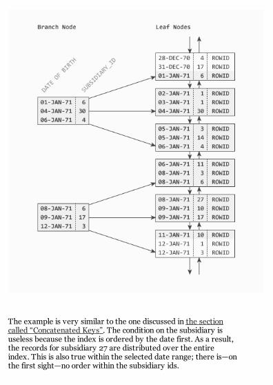
The example is very similar to the one discussed in the sectioncalled “Concatenated Keys”. The condition on the subsidiary isuseless because the index is ordered by the date first. As a result,the records for subsidiary 27 are distributed over the entireindex. This is also true within the selected date range; there is—onthe first sight—no order within the subsidiary ids.
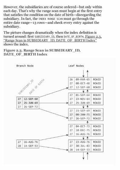
However, the subsidiaries are of course ordered—but only withineach day. That's why the range scan must begin at the first entrythat satisfies the condition on the date of birth—disregarding thesubsidiary. In fact, the INDEX RANGE SCAN must go through theentire date range—13 rows—and check every entry against thesubsidiary.
The picture changes dramatically when the index definition isturned around: first SUBSIDIARY_ID, then DATE_OF_BIRTH. Figure 2.3,“Range Scan in SUBSIDIARY_ID, DATE_OF_BIRTH Index”shows the index.
Figure 2.3. Range Scan in SUBSIDIARY_ID,DATE_OF_BIRTH Index
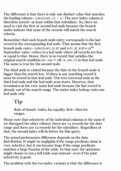
The difference is that there is only one distinct value that matchesthe leading column—SUBSIDIARY_ID = 27. The next index column istherefore sorted—at least within that subsidiary. So, there noneed to visit the first or second leaf node because the branchnodes indicate that none of the records will match the searchcriteria.
Remember that each branch node entry corresponds to the lastrecord in the corresponding leaf node. That means that the firstbranch node entry—SUBSIDIARY_ID 27 and DATE_OF_BIRTH 12th
September 1960—refers to a leaf node where all records are lessor equal to that. Hence, there is no record that satisfies theoriginal search condition (01-JAN-71 till 10-JAN-71) in that leaf node.The same is true for the second node.
The third node is visited because the date in the branch node isbigger than the search key. If there is any matching record itmust be stored in that leaf node. The tree traversal ends in thethird leaf node and the leaf node scan starts. However, thatterminates in the very same leaf node because the last record isalready out of the search range. The entire index lookup visits oneleaf node only.
Tip
Rule of thumb: Index for equality first—then forranges.
Please note that selectivity of the individual columns is the same ifwe disregard the other column; there are 13 records for the daterange and there are 13 records for the subsidiary. Regardless ofthat, the second index will do better for this query.
The actual performance difference depends on the datadistribution. It might be negligible if the range predicate alone isvery selective, but it can become huge if the range predicatematches a large fraction of the table. In that case, the optimizermight choose to run a full table scan instead—even if the jointselectivity is good.
The problem with the two index variants is that the difference is

almost invisible in the execution plan; both variants perform anINDEX RANGE SCAN. Still there is a difference shown in the executionplan:
---------------------------------------------------------------| Id | Operation | Name | Rows | Cost |---------------------------------------------------------------| 0 | SELECT STATEMENT | | 1 | 4 ||* 1 | FILTER | | | || 2 | TABLE ACCESS BY INDEX ROWID| EMPLOYEES | 1 | 4 ||* 3 | INDEX RANGE SCAN | EMP_TEST | 2 | 2 |---------------------------------------------------------------
Predicate Information (identified by operation id):---------------------------------------------------
1 - filter(TO_DATE(:END_DT,'YYYY-MM-DD') >=TO_DATE(:START_DT,'YYYY-MM-DD')) 3 - access("DATE_OF_BIRTH">=TO_DATE(:START_DT,'YYYY-MM-DD') AND "SUBSIDIARY_ID"=TO_NUMBER(:SUBS_ID) AND "DATE_OF_BIRTH"<=TO_DATE(:END_DT ,'YYYY-MM-DD')) filter("SUBSIDIARY_ID"=TO_NUMBER(:SUBS_ID))
First of all, the plan looks more complicated than expected—butthat's just a side effect of using bind parameters. In this case,there is an extra FILTER step to check if the end date is not beforethe start date. If the real values contradict each other—e.g., a daterange from 1970 to 1960—the following steps will not be executedat all.
Apart from that, the execution plan is as expected; a range scanon the index and the corresponding table access. All the predicatesare applied during the index lookup and there is no filter on tablelevel.
However, the predicate section reveals the one detail that makesall the difference; the SUBSIDIARY_ID condition shows up as filterpredicate—that means the EMP_TEST index is on DATE_OF_BIRTH first.
Important
Filter predicates are applied during the leaf nodetraversal only.
They don't contribute to the start and stopconditions and do therefore not narrow the scanned
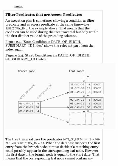
range.
Filter Predicates that are Access Predicates
An execution plan is sometimes showing a condition as filterpredicate and as access predicate at the same time—likeSUBSIDIARY_ID in the example above. That means that thecondition can be used during the tree traversal but only withinthe first distinct value of the preceding columns.
Figure 2.4, “Start Condition in DATE_OF_BIRTH,SUBSIDIARY_ID Index” shows the relevant part from theindex again:
Figure 2.4. Start Condition in DATE_OF_BIRTH,SUBSIDIARY_ID Index
The tree traversal uses the predicates DATE_OF_BIRTH >= '01-JAN-71' AND SUBSIDIARY_ID = 27. When the database inspects the firstentry from the branch node, it must decide if a matching entrycould possibly appear in the corresponding leaf node. However,the first date in the branch node is equal to the start date. Thatmeans that the corresponding leaf node cannot contain any

record with a later date nor can it contain any record for 1stJanuary with a subsidiary bigger than the one stored in the thatbranch node entry (6). In other words, there can't be anymatching record in the corresponding leaf node. Even if therewould be a record for 1st January and subsidiary 27, it wouldnot be stored in the first branch node. So, the subsidiarypredicate narrows the scanned range just a little bit; the rangescan must filter 12 rows only—instead of all 13 that match thedata range.
To compare it with the execution plan on the better index, there isno filter applied during the index scan:
---------------------------------------------------------------| Id | Operation | Name | Rows | Cost |---------------------------------------------------------------| 0 | SELECT STATEMENT | | 1 | 3 ||* 1 | FILTER | | | || 2 | TABLE ACCESS BY INDEX ROWID| EMPLOYEES | 1 | 3 ||* 3 | INDEX RANGE SCAN | EMP_TEST2 | 1 | 2 |---------------------------------------------------------------
Predicate Information (identified by operation id):---------------------------------------------------
1 - filter(TO_DATE(:END_DT,'YYYY-MM-DD') >=TO_DATE(:START_DT,'YYYY-MM-DD')) 3 - access("SUBSIDIARY_ID"=TO_NUMBER(:SUBS_ID) AND "DATE_OF_BIRTH">=TO_DATE(:START_DT,'YYYY-MM-DD') AND "DATE_OF_BIRTH"<=TO_DATE(:END_T,'YYYY-MM-DD'))
Another useful detail about the Predicate Information section foran index access is that it can be read from top to bottom. Theimportant point is that the access predicates appear in a definedorder; first the conditions for the tree traversal—that is, the startof the range scan. They show up in index order. Whatever followsthose predicates is the stop condition—the end date in this case.
Important
The access predicates express the start and stopconditions for the range scan.
The order of the access predicates indicates the

order of use: first the clauses used in the treetraversal, then the stop condition. However, theycan collapse so that only one remains; e.g., whenthere is only one equality clause. The stop conditionwill also disappear for an unbounded range scan,e.g., WHERE DATE_OF_BIRTH >= '01-JAN-71'.
Finally, there is the BETWEEN keyword. It is just a shortcut sothat
DATE_OF_BIRTH >= '01-JAN-71' AND DATE_OF_BIRTH <= '10-JAN-71'
is equivalent to
DATE_OF_BIRTH BETWEEN '01-JAN-71' AND '10-JAN-71'
Note that BETWEEN is always inclusive (see page 210, §8.6/6 ofSQL92).
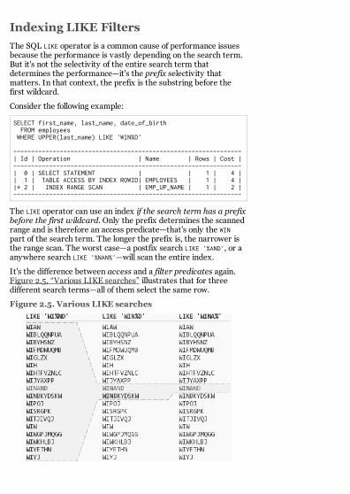
Indexing LIKE Filters
The SQL LIKE operator is a common cause of performance issuesbecause the performance is vastly depending on the search term.But it's not the selectivity of the entire search term thatdetermines the performance—it's the prefix selectivity thatmatters. In that context, the prefix is the substring before thefirst wildcard.
Consider the following example:
SELECT first_name, last_name, date_of_birth FROM employees WHERE UPPER(last_name) LIKE 'WIN%D'
----------------------------------------------------------------| Id | Operation | Name | Rows | Cost |----------------------------------------------------------------| 0 | SELECT STATEMENT | | 1 | 4 || 1 | TABLE ACCESS BY INDEX ROWID| EMPLOYEES | 1 | 4 ||* 2 | INDEX RANGE SCAN | EMP_UP_NAME | 1 | 2 |----------------------------------------------------------------
The LIKE operator can use an index if the search term has a prefixbefore the first wildcard. Only the prefix determines the scannedrange and is therefore an access predicate—that's only the WINpart of the search term. The longer the prefix is, the narrower isthe range scan. The worst case—a postfix search LIKE '%AND', or aanywhere search LIKE '%NAN%'—will scan the entire index.
It's the difference between access and a filter predicates again.Figure 2.5, “Various LIKE searches” illustrates that for threedifferent search terms—all of them select the same row.
Figure 2.5. Various LIKE searches

The prefix length before the first wildcard affects the scannedindex range—it's highlighted in the figure. The longer the prefix,the shorter the scanned range. A postfix filter is not able tonarrow the index access; it just removes the records that don'tmatch.
Important
Only the LIKE prefix can serve as access predicate.
Everything after the first wildcard is a filterpredicate.
The first query in the figure has only two prefix characters. Itneeds to read 18 records. The postfix filter removes 17 of them.The second expression reduces the range scan to two records—but it still needs to filter one record. The last search doesn't need afilter at all and reads the selected record only.
Tip
Avoid anywhere LIKE searches (e.g., LIKE '%TERM%')whenever possible.
In case it is inevitable, try to provide another accesspath to the selected rows—using the LIKE clause asfilter predicate on index or table level.
In case there is no other access path you shouldconsider using a full text index.
The Oracle optimizer recognizes prefix wildcards in LIKE searchesto avoid an ineffective range scan. However, the use of bindparameters makes that impossible. The optimizer assumes ausable prefix and uses an INDEX RANGE SCAN for a LIKE ? clause.
Statically Prefixing Anywhere LIKE Expressions
There are, theoretically, three solutions to that problem.
The first is not to use bind parameters for anywhere searches.However, that might introduce a considerable parsingoverhead.
The second doesn't work in the Oracle database as of release11r2. However, it would statically prefix the bind parameter.E.g., LIKE '%' || ?. However, the database evaluates the entireexpression only when the bind value is available. So, thatdoesn't change anything but it would be very nice if thedatabase would recognize that case.
The third solution is to use a hint that disallows the respectiveindex. However, hints should be avoided in production code.But reality bites—it's often the only possible solution.

The LIKE operator—as well as a regular expression—is noadequate way to implement full text searches. Most databasesoffer a special purpose index to for that. The following overviewgives some examples.
DB2
DB2 supports the CONTAINS keyword:
http://www.ibm.com/developerworks/data/tutorials/dm-0810shettar/index.html
MySQL
MySQL implements the MATCH and AGAINST keywords, butthey work on MyISAM tables only:
http://dev.mysql.com/doc/refman/5.5/en/fulltext-search.html
Oracle
Oracle supports the CONTAINS keyword:
http://download.oracle.com/docs/cd/B19306_01/text.102/b14218/csql.htm#i997503
PostgreSQL
PostgreSQL uses the @@ operator to implement full textsearches:
http://www.postgresql.org/docs/9.0/static/textsearch-intro.html#TEXTSEARCH-MATCHING
Another option is using the wildspeed extension. This isbasically storing the string in all possible rotations, so thateach character of the string is at the beginning. That means,that the indexed string is not stored once, but as many timesas there are characters in the string—so, it needs quite somespace. However, that makes it possible to effectively querythe index without a wildcard prefix.
SQL Server
SQL Server implements the CONTAINS keyword:
http://msdn.microsoft.com/en-us/library/ms142571.aspx
Index Combine
It's actually the most common question about indexing at all: is itbetter to have one index with all columns or one individual indexfor every column? The answer is quite simple in almost all cases:one index with multiple columns is better—that is, a concatenatedor compound index. the section called “Concatenated Keys”explains that in detail.
However, there is one case where a single index can't do a perfectjob—no matter how the index definition is changed. That's thecase when there are two or more independent range conditions inthe where clause.
Consider the following SQL:
SELECT first_name, last_name, date_of_birth FROM employees WHERE UPPER(last_name) < ? AND date_of_birth < ?
It's impossible to define a B-Tree index so that there isn't a filterpredicate. This limitation is quite simple to understand—bearingin mind that an index is essentially an ordered list.
For example, when indexing UPPER(LAST_NAME), DATE_OF_BIRTH (inthat order), the list will start with A and end with Z. However, arecord for the employee Brown will be rather close to the start ofthe list —regardless of the date of birth. The date of birthinfluences the list position only marginally—just if the same nameappears twice. That means that scanning from the beginning ofthe list will need to filter for the date of birth. The date of birthdoesn't narrow the scanned range.
The same is true when defining the index the other way around.The scan will start with the earlier dates but will need a filter toremove the names that don't match.

After all, the problem is as simple as that: a chain with one axissupports one range condition as an access predicate. Supportingtwo range conditions as an access predicate would mean to scan acorner of a chessboard. However, a B-Tree index is a chain—thereis no second axis.
There are two workarounds for this problem. The first is to definea concatenated index just as described above—accepting the filterpredicate. This is the only case where the most selective first ruleapplies. Whatever condition is more selective should go first sothat the scanned range is as small as possible.
The second approach is to borrow a feature from the data-warehousing world.
Data-warehousing is the mother of all ad-hoc queries. A few clicksallow querying any combination of search filters. It's impossible totell which columns will be queried together. That makes indexingas described so far rather impossible.
There is, of course, a solution to that problem. That is, the bitmapindex—a special purpose index type. However, bitmap indexeshave limitations that make them truly special purpose indexes.One problem is that bitmap operations are very CPU bound. Butthe more limiting problem is their terribleinsert/update/delete scalability. In fact, concurrent writeoperations on bitmap indexes are almost impossible so thatbitmap indexes are hardly usable in an OLTP environment.
However, the key benefit of bitmap indexes is that merging ofmultiple indexes is rather easy. That is, multiple indexes can beused and combined for a single table access.
Important
The database can—in principle—use one B-Treeindex only per table access. However, a single SQLstatement can access many tables—by means of

joins and subqueries—hence, a single SQL statementcan use many B-Tree indexes.
Bitmap indexes can be combined on the fly so that asingle table access can use multiple indexes.
There are many databases, including the Oracle database, thatuse a hybrid solution between regular B-Tree indexes and bitmapindexes. They can, despite any better option, transform the resultof multiple B-Tree scans to a bitmaps and merge them on the fly.That means that the concurrency limitation of bitmap indexes isbypassed by making the overall operation even more CPU bound.After all, a B-Tree based bitmap merge is an option of last resortonly.
Important
The limitations of bitmap indexes make them hardlyusable in a OLTP environment.
Some databases use different techniques to combine multiple B-Tree indexes. The following table gives a short overview fordifferent implementations:
DB2
DB2 supports multiple index access on LUW 9r7 (using adynamic bitmap) and on zOS v10.
MySQL
MySQL has an index merge optimization starting withrelease 5.0.
Oracle
The Oracle database uses BITMAP CONVERSIONs to combinemultiple indexes on the fly (introduced with 9i).
PostgreSQL

PostgreSQL uses bitmaps to combine multiple indexes sinceversion 8.1.
SQL Server
SQL Server can use multiple indexes ("Index Intersect")starting with V7.0 using a hash algorithm.
It's often better to use a single B-Tree index instead of bitmapindexes or multiple B-Tree indexes—even in case of multipleindependent range conditions.
The following execution plan shows the bitmap conversionscaused by two individual B-Tree indexes for two independentrange conditions.
--------------------------------------------------------------| Id | Operation | Name | Cost (%CPU)|--------------------------------------------------------------| 0 | SELECT STATEMENT | | 17 (12)|| 1 | TABLE ACCESS BY INDEX ROWID | EMPLO | 17 (12)|| 2 | BITMAP CONVERSION TO ROWIDS | | || 3 | BITMAP AND | | || 4 | BITMAP CONVERSION FROM ROWIDS| | || 5 | SORT ORDER BY | | ||* 6 | INDEX RANGE SCAN | DOB | 2 (0)|| 7 | BITMAP CONVERSION FROM ROWIDS| | || 8 | SORT ORDER BY | | ||* 9 | INDEX RANGE SCAN | UNAME | 2 (0)|--------------------------------------------------------------
Predicate Information (identified by operation id):---------------------------------------------------
6 - access("DATE_OF_BIRTH"<:DOB) filter("DATE_OF_BIRTH"<:DOB) 9 - access(UPPER("LAST_NAME")<:NAME) filter(UPPER("LAST_NAME")<:NAME)
Please note that the Rows column was removed in favor of the CPUcost information.
The notable operations are the sorts that follow the index rangescans and the bitmap operations. There are two independent

scans and the bitmap operations. There are two independentrange scans; the result is sorted and converted to an in-memorybitmap index. Those in-memory indexes are then combined withthe BITMAP AND operation and the result is converted back to getthe ROWIDs. The last step is to fetch the records from the table.
Another, very important, detail in the execution plan is the CPUcost—12% in that case.
In comparison to the plan above, a single index on UPPER(last_name)and DATE_OF_BIRTH will perform better and not cause any notableCPU cost:
-------------------------------------------------------------| Id | Operation | Name | Cost (%CPU)|-------------------------------------------------------------| 0 | SELECT STATEMENT | | 3 (0)|| 1 | TABLE ACCESS BY INDEX ROWID| EMPLOYEES | 3 (0)||* 2 | INDEX RANGE SCAN | UNAME_DOB | 2 (0)|-------------------------------------------------------------
Predicate Information (identified by operation id):---------------------------------------------------
2 - access(UPPER("LAST_NAME")<:NAME AND "DATE_OF_BIRTH"<:DOB) filter("DATE_OF_BIRTH"<:DOB)
Please note that both plans were created with bind parameters.Hence, the cardinality estimates are ballpark figures and theoverall cost might be very different.

Obfuscated Conditions
The following sections demonstrate some popular (and somefunny) ways to obfuscate conditions. Obfuscated conditions arewhere clauses that are phrased in a way which prevents properindex usage. It is therefore a collection of anti-patterns—explained and tuned.

Dates
The by far most common obfuscation affects DATE columns. TheOracle database is particularly vulnerable to that because the DATEtype always includes time. It's common practice to use the TRUNCfunction to get rid of the time part:
SELECT ... FROM ... WHERE TRUNC(date_column) = TRUNC(sysdate - 1)
It's a perfectly valid and correct statement—except that it can'tuse an index on DATE_COLUMN. That's because TRUNC(date_column) isan entirely different thing than DATE_COLUMN—at least to thedatabase. the section called “Case-Insensitive Search” explainsthat in more detail and suggests to think of every function as aBLACKBOX.
There is a rather simple solution to that problem: a function basedindex.
CREATE INDEX index_name ON table_name (TRUNC(date_column))
However, that requires all queries to use TRUNC. If there areinconsistent queries (some with, others without TRUNC), twoindexes are required.
Even databases that have plain DATE types—that don't need TRUNCfor day wise filters—can run into similar problems. E.g., withmonthly queries like this MySQL example:
SELECT ... FROM ... WHERE DATE_FORMAT(date_column, "%Y-%M") = DATE_FORMAT(now() , "%Y-%M')
That is very similar to the Oracle example above. However, the

solution (function based index) doesn't apply—MySQL doesn'thave function based indexes.
There is a generic solution that works in all environments:rephrasing the condition as an explicit range query.
SELECT ... FROM ... WHERE date_column BETWEEN quarter_begin(?) AND quarter_end(?)
If you have done your homework, you probably recognize thatpattern from the exercise about all employees aged 42.
The benefit of this technique is that a straight index on DATE_COLUMNworks. The two functions QUARTER_BEGIN and QUARTER_END hide thecomplexity of the boundary date calculation. That's especiallyhandy because the BETWEEN operator is always inclusive—theQUARTER_END function must return a time just before the first day ofthe next quarter.
The following samples implement QUARTER_BEGIN and QUARTER_END forvarious databases. That's another benefit of using functions; thedatabase dependent code is not in the select statement.
DB2
CREATE FUNCTION quarter_begin(dt TIMESTAMP)RETURNS TIMESTAMPRETURN TRUNC(dt, 'Q');
CREATE FUNCTION quarter_end(dt TIMESTAMP)RETURNS TIMESTAMPRETURN TRUNC(dt, 'Q') + 3 MONTHS - 1 SECOND;
MySQL
CREATE FUNCTION quarter_begin(dt DATETIME)RETURNS DATETIME DETERMINISTICRETURN CONVERT (

CONCAT ( CONVERT(YEAR(dt),CHAR(4)) , '-' , CONVERT(QUARTER(dt)*3-2,CHAR(2)) , '-01' ) , datetime );
CREATE FUNCTION quarter_end(dt DATETIME)RETURNS DATETIME DETERMINISTICRETURN DATE_ADD ( DATE_ADD ( quarter_begin(dt), INTERVAL 3 MONTH ) , INTERVAL -1 MICROSECOND);
Oracle
CREATE FUNCTION quarter_begin(dt IN DATE) RETURN DATEASBEGIN RETURN TRUNC(dt, 'Q');END;/
CREATE FUNCTION quarter_end(dt IN DATE) RETURN DATEASBEGIN -- the Oracle DATE type has seconds resolution -- subtract one second from the first -- day of the following quarter RETURN TRUNC(ADD_MONTHS(dt, +3), 'Q') - (1/(24*60*60));END;/
PostgreSQL
CREATE FUNCTION quarter_begin(dt timestamp with time zone)RETURNS timestamp with time zone AS $$BEGIN RETURN date_trunc('quarter', dt);END;$$ LANGUAGE plpgsql;
CREATE FUNCTION quarter_end(dt timestamp with time zone)RETURNS timestamp with time zone AS $$BEGIN RETURN date_trunc('quarter', dt) + interval '3 month' - interval '1 microsecond';END;$$ LANGUAGE plpgsql;
SQL Server
CREATE FUNCTION quarter_begin (@dt DATETIME )RETURNS DATETIMEBEGIN RETURN DATEADD (qq, DATEDIFF (qq, 0, @dt), 0) ENDGO
CREATE FUNCTION quarter_end (@dt DATETIME )RETURNS DATETIMEBEGIN RETURN DATEADD ( ms , -3 , DATEADD(mm, 3, dbo.quarter_begin(@dt)) );ENDGO
Similar auxiliary functions can be used for other periods—they'llprobably be less complex than the examples above.
Tip
Write queries for continuous periods as explicitrange condition.
That's also true when the period is a single day—e.g.,in Oracle: DATE_COLUMN >= TRUNC(sysdate) ANDDATE_COLUMN < TRUNC(sysdate+1).
There is another frequent problem with date columns that hitsapplications that use string representations for dates. Consider

the following PostgreSQL example:
SELECT ... FROM ... WHERE TO_CHAR(date_column, 'YYYY-MM-DD') = '1970-01-01'
The problem is again the conversion of the DATE_COLUMN. The betterapproach (regarding indexing) is to convert the string to thenative DATE representation of the database:
SELECT ... FROM ... WHERE date_column = TO_DATE('1970-01-01', 'YYYY-MM-DD')
That allows a straight index on DATE_COLUMN. Moreover, it convertsthe input string only once. The other statement needs to convertall the dates from the table before they can be compared againstthe string literal.
However, there is a problem with that approach. In case theDATE_COLUMN includes the time of day—like the Oracle DATE typedoes—the statement must read like that:
SELECT ... FROM ... WHERE date_column >= TO_DATE('1970-01-01', 'YYYY-MM-DD') AND date_column < TO_DATE('1970-01-01', 'YYYY-MM-DD') + 1
Numeric Strings
Numeric strings are numbers that are stored in string fields.There is no problem with that if all filters use string comparisons:
SELECT ... FROM ... WHERE numeric_string = '42'
That statement can, of course, use an index on NUMERIC_STRING.However, an index range scan is not possible if the condition isexpressed as numeric comparison:
SELECT ... FROM ... WHERE numeric_string = 42
Note the missing quotes. The database transforms that querybefore execution. The result is something like this:
SELECT ... FROM ... WHERE TO_NUMBER(numeric_string) = 42
It's the same story again. The function prevents an INDEX RANGESCAN on the NUMERIC_STRING column (if there is such an index). Thesolution is, again, to change the query so that the straight columnis queried—that is, convert the literal search term to a string:
SELECT ... FROM ... WHERE numeric_string = TO_CHAR(42)
You might wonder why the database doesn't do it that way? It'sbecause transforming a string to a number is unambiguous. That'snot the case the other way around. A formatted, numeric stringmight contain spaces, or thousands separators, or leading zeros:
42

042004200042...
The database doesn't know the format of the numeric strings inthe table. It's therefore done the other way around; the stringsare turned into numbers—that's an unambiguous transformation.
However, an explicit TO_CHAR(42) evaluates to a single stringrepresentation—the query will match only one from the abovestrings.
The important point is that there is a semantic difference betweenthe two variants. The TO_CHAR variant matches only one recordfrom the list, the TO_NUMBER variant matches all of them.
The obfuscation becomes even more subtle with bind parametersbecause the Oracle database always assumes matching types forbind parameters:
SELECT ... FROM ... WHERE numeric_string = ?
The Oracle database expects a string value for the placeholder. Ifthat assumption doesn't hold true, the transformation appliesagain. However, that might make the prepared execution planuseless if an INDEX RANGE SCAN isn't possible anymore.
This is one of the cases where the execution plan made withEXPLAIN PLAN doesn't tell the truth. The execution plan might differif the parameter types don't match.
SQL*Plus Autotrace And SQL Trace Files
The SQL*Plus autotrace functionality is also vulnerable to thebind parameter type confusion. In fact, autotrace is performingan explain plan in the background. The autotrace plan is not theactually executed plan, but just an automatically explained

plan.
The Oracle SQL traces log the actually executed plan.
Numeric strings introduce many problems. That's the semanticdifference that can lead to unexpected results; the unusableindexes that lead to bad performance; but there is also the risk ofexceptions. A transparently transformed statement can fail ifTO_NUMBER fails to parse a string. That's why a trivial statement—without any explicit conversion—can still raise number conversionerrors if there is a type mismatch.
Tip
Use numeric types to store numbers.
The problem doesn't exist the other way around:
SELECT ... FROM ... WHERE numeric_number = '42'
The database will, consistently, transform the string into anumber. However, that does not wrap the—potentially indexed—column through any function. A regular index will work. But amanual conversion can still be done in the wrong way:
SELECT ... FROM ... WHERE TO_CHAR(numeric_number) = '42'
Using the TO_CHAR function on an indexed column renders theexpression unusable as access predicate.

Date/Time Concatenation
This section is about a popular way to obfuscate concatenatedindexes. It is very similar to the "Dates" section but the other wayaround. It is about concatenation date and time columns to applya range filter.
Consider the following MySQL example. It queries a table thatstores DATE and TIME separately—in two columns:
SELECT ... FROM ... WHERE ADDTIME(date_column, time_column) > DATE_ADD(now(), INTERVAL -1 DAY)
It selects all records from the past 24 hours. However, the querycan't do an index range scan on a concatenated index (DATE_COLUMN,TIME_COLUMN) because the search expression is, again, completelyunrelated to the indexed columns.
The problem doesn't exist if the time is stored along with the datein a single column (e.g., MySQL DATETIME). One column can bequeried without any obfuscation:
SELECT ... FROM ... WHERE datetime_column > DATE_ADD(now(), INTERVAL -1 DAY)
However, once the table is designed, it's hard to change. Theremight be a good reason for that design anyway—so, is usually notpossible to change.
The next option is a function based index, if the RDBMS supportsit. That works very well, but there are all the drawbacksdiscussed before. However, that example assumes a MySQLdatabase—function based index are not an option.
Still, there is one more option that improves performance. It

works by adding a redundant where clause on DATE:
SELECT ... FROM ... WHERE ADDTIME(date_column, time_column) > DATE_ADD(now(), INTERVAL -1 DAY) AND date_column >= DATE(DATE_ADD(now(), INTERVAL -1 DAY))
The new part of the where clause is absolutely redundant from afunctional point of view—but it's a straight filter DATE_COLUMN. Thatmeans any index that starts with DATE_COLUMN will improveperformance greatly. Even though this technique is not perfect—because the time component can't use the index—it's still a majorimprovement over a full scan.
Tip
The date part of a date/time concatenation can usean index with a redundant where clause.
This technique works also if date and time are stored as strings.However, that requires date and time formats that yields thecorrect sort order—e.g., like ISO 8601 suggests it (YYYY-MM-DDHH:MM:SS). It is also very important that the date has a fixed length—including leading zeros, as ISO suggests.
The following Oracle example demonstrates it.
SELECT ... FROM ... WHERE date_string || time_string > TO_CHAR(sysdate - 1, 'YYYY-MM-DD HH24:MI:SS') AND date_string >= TO_CHAR(sysdate - 1, 'YYYY-MM-DD')
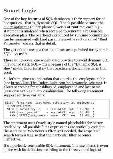
Smart Logic
One of the key features of SQL databases is their support for ad-hoc queries—that is, dynamic SQL. That's possible because thequery optimizer (query planner) works at runtime; each SQLstatement is analyzed when received to generate a reasonableexecution plan. The overhead introduced by runtime optimizationcan be minimized with bind parameters—the section called “BindParameter” covers that in detail.
The gist of that recap is that databases are optimized for dynamicSQL—so, use it.
There is, however, one widely used practice to avoid dynamic SQLif favour of static SQL—often because of the "Dynamic SQL isslow" myth. Unfortunately that practice is doing more harm thangood.
So, let's imagine an application that queries the employees table(see http://Use-The-Index-Luke.com/sql/example-schema). Itallows searching for subsidiary id, employee id and last name(case-insensitive) in any combination. The following statementsupport all these variants:
SELECT first_name, last_name, subsidiary_id, employee_id FROM employees WHERE ( subsidiary_id = :sub_id OR :sub_id IS NULL ) AND ( employee_id = :emp_id OR :emp_id IS NULL ) AND ( UPPER(last_name) = :name OR :name IS NULL )
The statement uses Oracle style named placeholder for betterreadability. All possible filter expressions are statically coded inthe statement. Whenever a filter isn't needed, the respectivesearch term is NULL so that the particular filter becomesineffective.
It's a perfectly reasonable SQL statement. The use of NULL is evenin line with its definition according to the three valued logic of

SQL. Regardless of that, it is still amongst the worst things forperformance.
It's impossible to know which filters will be effective and whichwill be canceled out. The database has to prepare for all cases—it'stherefore impossible to use an index:
----------------------------------------------------| Id | Operation | Name | Rows | Cost |----------------------------------------------------| 0 | SELECT STATEMENT | | 2 | 478 ||* 1 | TABLE ACCESS FULL| EMPLOYEES | 2 | 478 |----------------------------------------------------
Predicate Information (identified by operation id):---------------------------------------------------
1 - filter( (:NAME IS NULL OR UPPER("LAST_NAME")=:NAME) AND (:EMP_ID IS NULL OR "EMPLOYEE_ID"=TO_NUMBER(:EMP_ID)) AND (:SUB_ID IS NULL OR "SUBSIDIARY_ID"=TO_NUMBER(:SUB_ID)))
The database has to run a full table scan even if proper indexesexist.
Please remember that the purpose of bind parameters is todecrease parsing overhead—as explained in the section called“Bind Parameter”. The database will therefore not re-evaluatethe plan when the actual bind parameters are sent—hence, theprepared query plan has to cover all cases.
It's not that the Oracle database is "stupid". The optimizerresolves the (tautological) expressions when inlined literally:
SELECT first_name, last_name, subsidiary_id, employee_id FROM employees WHERE( subsidiary_id = NULL OR NULL IS NULL ) AND( employee_id = NULL OR NULL IS NULL ) AND( UPPER(last_name) = 'WINAND' OR 'WINAND' IS NULL )
The execution plan is now optimized:

----------------------------------------------------------------| Id | Operation | Name | Rows | Cost |----------------------------------------------------------------| 0 | SELECT STATEMENT | | 1 | 2 || 1 | TABLE ACCESS BY INDEX ROWID| EMPLOYEES | 1 | 2 ||* 2 | INDEX RANGE SCAN | EMP_UP_NAME | 1 | 1 |----------------------------------------------------------------
Predicate Information (identified by operation id):---------------------------------------------------
2 - access(UPPER("LAST_NAME")='WINAND')
Warning
Using literal values in SQL exposes your applicationto SQL Injection and causes performance problemsdue to the parsing overhead.
However, that is not a good solution—avoid literal valueswhenever possible.
The best solution is to build the SQL statement dynamically—onlywith the required clauses—with bind parameters.
SELECT first_name, last_name, subsidiary_id, employee_id FROM employees WHERE UPPER(last_name) = :name
The bind parameter prevents SQL Injection and improvesexecution plan caching. The caching is still effective, even if thereare multiple variants of the statement. Some of them won't beused anyway, the others will be cached and expired according thedatabase's policy.
Tip
Use dynamic SQL if you need dynamic whereclauses.
Still use bind parameters when generating dynamic

SQL—otherwise, the “Dynamic SQL is Slow” mythmight become true.

Math
There is one more cluster of techniques that's smart, but preventsindex usage in most cases. It's similar to smart logic, but usingmathematics.
Consider the following statement. Can it use an index onNUMERIC_COLUMN?
SELECT numeric_number FROM table_name WHERE numeric_number - 1000 > ?
Or can the following statement use an index on A and B (in anyorder)?
SELECT a, b FROM table_name WHERE 3 * a + 5 = b
Let's put that question into a different perspective; if you weredeveloping an SQL database, would you add an equation solvingengine?
Most database vendors say "no" to that question. So, they doesn'tuse an index for any of the samples above.
That technique is sometimes even used to intentionally disable aparticular index—e.g., by adding zero:
SELECT numeric_number FROM table_name WHERE numeric_number + 0 = ?
This is actually more portable than a hint—however, that's not arecommendation to do it.
Never the less, a function based index will work for all the samplesabove. It's even possible to use a function based index along with a
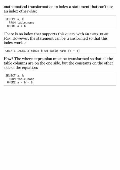
mathematical transformation to index a statement that can't usean index otherwise:
SELECT a, b FROM table_name WHERE a = b
There is no index that supports this query with an INDEX RANGESCAN. However, the statement can be transformed so that thisindex works:
CREATE INDEX a_minus_b ON table_name (a - b)
How? The where expression must be transformed so that all thetable columns are on the one side, but the constants on the otherside of the equation:
SELECT a, b FROM table_name WHERE a - b = 0

Appendix A. Myth Directory
One of the major issues with “mature” software is that it is oftensurrounded by myths. The Oracle database seems to beparticularly vulnerable to this phenomenon, probably because thename Oracle is used since 1979. There are some myth that werethe best current practice at that time but are outdated since manyreleases.
In an attempt to thin out the dark woods of Oracle databasemyths, I list and explain some of the most common myth andmisbeliefs here.
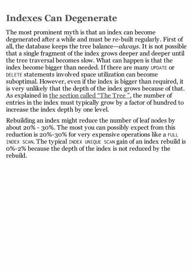
Indexes Can Degenerate
The most prominent myth is that an index can becomedegenerated after a while and must be re-built regularly. First ofall, the database keeps the tree balance—always. It is not possiblethat a single fragment of the index grows deeper and deeper untilthe tree traversal becomes slow. What can happen is that theindex become bigger than needed. If there are many UPDATE orDELETE statements involved space utilization can becomesuboptimal. However, even if the index is bigger than required, itis very unlikely that the depth of the index grows because of that.As explained in the section called “The Tree ”, the number ofentries in the index must typically grow by a factor of hundred toincrease the index depth by one level.
Rebuilding an index might reduce the number of leaf nodes byabout 20% - 30%. The most you can possibly expect from thisreduction is 20%-30% for very expensive operations like a FULLINDEX SCAN. The typical INDEX UNIQUE SCAN gain of an index rebuild is0%-2% because the depth of the index is not reduced by therebuild.

Most Selective First
Every time a compound index is created, the order of the columnsmust be chosen wisely. the section called “Concatenated Keys” isdevoted to this question.
However, there is the myth that you should always put the mostselective column to the first position; that is just wrong. Othershave tried to proof that before, but the myth persists.
Important
The most important factor to consider when defininga concatenated index is the number of statements itcan support.
After that, there are even reasons to put the least selectivecolumn first:
To utilize an INDEX SKIP SCAN
To accomplish a better compression
However, that's advanced stuff. But the most importantfactor...uhm, did I say that before?
I'm not the first to fight this myth. Here are some morereferences that disproof the myth:
Tom Kyte - "Expert Oracle Database Architecture" -Apress
Devotes the section "Myth: Most Discriminating ElementsShould Be First" to this topic.
Tom Kyte also commented this on AskTom.
Guy Harrison - Oracle Performance Survival Guide -Prentice Hall

In "Guidelines for Concatenated Indexes":
Don't automatically put the most selective term first ina concatenated index. [...]
Jonathan Lewis - Author of "Cost-Based OracleFundamentals" - Apress
I didn't find it explicitly in his book, however, JonathanLewis blogged it:
One of the often-quoted fairy-tales about indexes wasthe directive to “put the most selective column first”. Itwas never a sensible rule of thumb (except, possibly,prior to version 6.0). But if you have a lot of code thatuses this nvl() construct then there may actually be agood argument for adopting this approach. (There’s abetter argument for fixing the code, of course).
The core of truth behind this myth is related to indexingindependent range conditions—that is the only case where theselectivity should influence the index design (see the section called“Index Combine”).
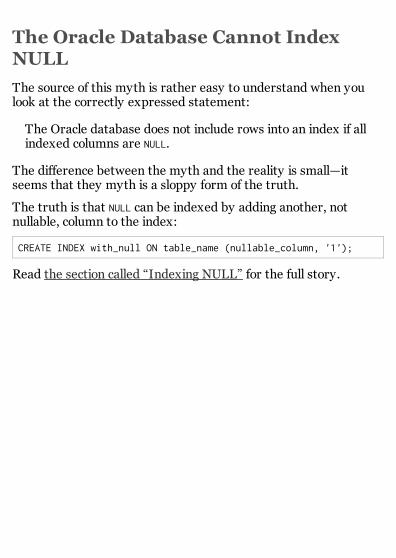
The Oracle Database Cannot IndexNULL
The source of this myth is rather easy to understand when youlook at the correctly expressed statement:
The Oracle database does not include rows into an index if allindexed columns are NULL.
The difference between the myth and the reality is small—itseems that they myth is a sloppy form of the truth.
The truth is that NULL can be indexed by adding another, notnullable, column to the index:
CREATE INDEX with_null ON table_name (nullable_column, '1');
Read the section called “Indexing NULL” for the full story.

Dynamic SQL is Slow
The core of truth behind the “Dynamic SQL is Slow” myth israther simple; dynamic SQL can be slow—when done wrong.
So, what's dynamic SQL? It's the opposite of embedding SQLdirectly into the program's source code. PL/SQL and other storedprocedure dialects are good examples for embedded SQL but it'salso possible to embed SQL into C and other languages. Thebenefit of embedded SQL is that it integrates very smoothly withthe respective programming language. However, embedded SQLis compiled into the program. It can not change when the programruns—it's static.
Dynamic SQL, to the contrary, is handled as string within theapplication. The program can change it at runtime. However,that's probably the cause of the myth. Consider the followingexample:
String sql = "SELECT first_name, last_name" + " FROM employees" + " WHERE employee_id = " + employeeId;
ResultSet rs = con.executeQuery(sql);
So, is that dynamic SQL? The actual SQL string is builtdynamically during program runtime. However, that is not what'smeant with dynamic SQL because the structure of the SQLstatement doesn't change. That example should be changed to usebind parameters—that's all, nothing dynamic here.
Real dynamic SQL changes the structure of the statement duringruntime. That's something that cannot be done with bindparameters—like a conditional where clause:
String where = "";if (subsidiaryId != null) { where += (where == "") ? " WHERE " : " AND " + "subsidiary_id = " + subsidiaryId;}

if (employeeId != null) { where += (where == "") ? " WHERE " : " AND " + "employee_id = " + employeeId;}if (lastName != null) { where += (where == "") ? " WHERE " : " AND " + "UPPER(last_name) = '" + lastName.toUpperCase() + "'";}String SQL = "SELECT employee_id, first_name, last_name " + " FROM employees" + where;// execute SQL
The code constructs an SQL statement to fetch employees basedon any combination of three filter criteria. Although the code israther awkward, the constructed SQL can be executed and thedatabase will use the best index to retrieve the data. The problemwith that code is not only the highlighted SQL Injectionvulnerability, but also that it introduces a very high parsingoverhead.
That means that the database has to recreate the execution planevery time, because the inlined search terms—that are differentevery time—prevents caching. the section called “BindParameter” explains parsing overhead in more detail.
Implementing the example with plain JDBC and bind parametersyields even more awkward code—it's omitted here. However,most ORM frameworks provide a sufficiently convenient way todynamically create SQL using bind parameters. The followingoverview shows some samples:
Java
The following sample demonstrates Hibernate's Criteriaclasses:
Criteria criteria = session.createCriteria(Employees.class);
if (subsidiaryId != null) { criteria.add(Restrictions.eq("subsidiaryId", subsidiaryId));}if (employeeId != null) { criteria.add(Restrictions.eq("employeeId", employeeId));
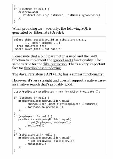
}if (lastName != null) { criteria.add( Restrictions.eq("lastName", lastName).ignoreCase() );}
When providing LAST_NAME only, the following SQL isgenerated by Hibernate (Oracle):
select this_.subsidiary_id as subsidiary1_0_0_, [... other columns ...] from employees this_ where lower(this_.last_name)=?
Please note that a bind parameter is used and the LOWERfunction to implement the ignoreCase() functionality. Thesame is true for the ilike restriction. That's a very importantfact for function based indexing.
The Java Persistence API (JPA) has a similar functionality:
However, it's less straight and doesn't support a native case-insensitive search that's probably good):
List<Predicate> predicates = new ArrayList<Predicate>();
if (lastName != null) { predicates.add(queryBuilder.equal( queryBuilder.upper(r.get(Employees_.lastName)) , lastName.toUpperCase()) );}if (employeeId != null) { predicates.add(queryBuilder.equal( r.get(Employees_.employeeId) , employeeId) );}if (subsidiaryId != null) { predicates.add(queryBuilder.equal( r.get(Employees_.subsidiaryId) , subsidiaryId) );}
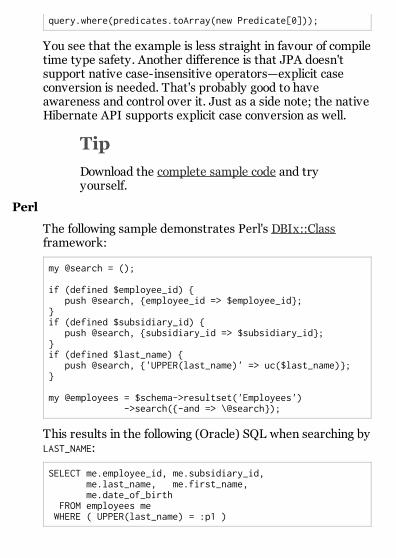
query.where(predicates.toArray(new Predicate[0]));
You see that the example is less straight in favour of compiletime type safety. Another difference is that JPA doesn'tsupport native case-insensitive operators—explicit caseconversion is needed. That's probably good to haveawareness and control over it. Just as a side note; the nativeHibernate API supports explicit case conversion as well.
Tip
Download the complete sample code and tryyourself.
Perl
The following sample demonstrates Perl's DBIx::Classframework:
my @search = ();
if (defined $employee_id) { push @search, {employee_id => $employee_id};}if (defined $subsidiary_id) { push @search, {subsidiary_id => $subsidiary_id};}if (defined $last_name) { push @search, {'UPPER(last_name)' => uc($last_name)};}
my @employees = $schema->resultset('Employees') ->search({-and => \@search});
This results in the following (Oracle) SQL when searching byLAST_NAME:
SELECT me.employee_id, me.subsidiary_id, me.last_name, me.first_name, me.date_of_birth FROM employees me WHERE ( UPPER(last_name) = :p1 )

Tip
Download the complete sample code and tryyourself.
PHP
The following sample demonstrates PHP's Doctrineframework:
$filter = $qb->expr()->andx();
if (isset($employee_id)) { $filter->add( $qb->expr()->eq('e.employee_id', ':employee_id')); $qb->setParameter('employee_id', $employee_id);}if (isset($subsidiary_id)) { $filter->add( $qb->expr()->eq('e.subsidiary_id', ':subsidiary_id')); $qb->setParameter('subsidiary_id', $subsidiary_id);}if (isset($last_name)) { $filter->add($qb->expr()->eq( $qb->expr()->upper('e.last_name'), ':last_name')); $qb->setParameter('last_name', strtoupper($last_name));}
if ($filter->count() > 0) { $qb->where($filter);}
Please note that you have to use bind parameters explicitly.
Doctrine generates the following SQL for a search by lastname (MySQL):
SELECT e0_.employee_id AS employee_id0, [... other columns ...] FROM employees e0_ WHERE UPPER(e0_.last_name) = ?
Tip
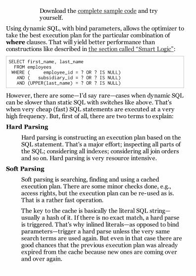
Download the complete sample code and tryyourself.
Using dynamic SQL, with bind parameters, allows the optimizer totake the best execution plan for the particular combination ofwhere clauses. That will yield better performance thanconstructions like described in the section called “Smart Logic”:
SELECT first_name, last_name FROM employees WHERE ( employee_id = ? OR ? IS NULL) AND ( subsidiary_id = ? OR ? IS NULL) AND (UPPER(last_name) = ? OR ? IS NULL)
However, there are some—I'd say rare—cases when dynamic SQLcan be slower than static SQL with switches like above. That'swhen very cheap (fast) SQL statements are executed at a veryhigh frequency. But, first of all, there are two terms to explain:
Hard Parsing
Hard parsing is constructing an execution plan based on theSQL statement. That's a major effort; inspecting all parts ofthe SQL; considering all indexes; considering all join ordersand so on. Hard parsing is very resource intensive.
Soft Parsing
Soft parsing is searching, finding and using a cachedexecution plan. There are some minor checks done, e.g.,access rights, but the execution plan can be re-used as is.That is a rather fast operation.
The key to the cache is basically the literal SQL string—usually a hash of it. If there is no exact match, a hard parseis triggered. That's why inlined literals—as opposed to bindparameters—trigger a hard parse unless the very samesearch terms are used again. But even in that case there aregood chances that the previous execution plan was alreadyexpired from the cache because new ones are coming overand over again.
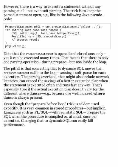
However, there is a way to execute a statement without anyparsing at all—not even soft parsing. The trick is to keep theparsed statement open, e.g., like in the following Java pseudo-code:
PreparedStatement pSQL = con.prepareStatement("select ...");for (String last_name:last_names) { pSQL.setString(1, last_name.toUpperCase()); ResultSet rs = pSQL.executeQuery(); // process result}pSQL.close();
Note that the PreparedStatement is opened and closed once only—yet it can be executed many times. That means that there is onlyone parsing operation—during prepare—but non inside the loop.
The pitfall is that converting that to dynamic SQL moves theprepareStatement call into the loop—causing a soft-parse for eachexecution. The parsing overhead, that might also include networklatencies, can exceed the savings of a better execution plan whenthe statement is executed often and runs fast anyway. That'sespecially true if the actual execution plan doesn't vary for thedifferent where clauses—e.g., because one well indexed whereclause is always present.
Even though the “prepare before loop” trick is seldom usedexplicitly, it is very common in stored procedures—but implicit.Languages such as PL/SQL—with real static SQL—prepare theSQL when the procedure is compiled or, at most, once perexecution. Changing that to dynamic SQL can easily killperformance.


CONTENTS 1 INTRODUCTION
1.1 A Collection of Related Data : Databases and Database Management
Systems.
1.2 The Database as a Collection of Tables: Relational Databases and SQL. 1.2.1 Tables, Columns and Rows. 1.2.2 The Primary Key.
1.3 Communicating to the DBMS What You Want it to do: Introduction to the
SQL language.
1.4 A Research Project Conducted by IBM: The History of SQL.
1.5 SQL Commands Build Upon Themselves: Organization of This Book. 1.5.1 Notational Conventions.
2 A ROUGH GUIDE TO SQL.
2.1 Consider the Simple Address Book: A Basic Relational Database.
2.2 SQL Commands Fall into Different Categories: Subdivisions of SQL.
2.3 Enter SQL Statements at the Command Line: Using interpretive SQL.
2.4 Use the CREATE TABLE statement: Creating Database Tables.
2.5 Use the INSERT INTO Statement: Adding Data to Tables.
2.6 Use the SELECT Statement: Extracting data from tables.
2.7 Use the UPDATE and DELETE Statements: Modifying data.
2.8 Another Kind of Table, Called a Virtual Table: Views.
2.9 Prevent Access to Sensitive Information: Database security.

3 CREATING AND MAINTAINING TABLES.
3.1 The ANSI Standard Makes Such a Distinction...: The DDL and the ANSI/ISO
standard.
3.2 Single and Multiple Database Architectures: The structure of SQL databases.
3.3 Creating a Database Table: The CREATE TABLE command.
3.4 Apply Restrictions to Groups of Columns: Column and table modifiers. 3.4.1 The NOT NULL modifier. 3.4.2 The UNIQUE modifier. 3.4.3 The INDEX modifier. 3.4.4 The PRIMARY KEY modifier. 3.4.5 The FOREIGN KEY modifier. 3.4.6 The DEFAULT modifier. 3.4.7 The CHECK modifier
3.5 Indexes are Ordered for Extremely Fast Searches: Indexes.
3.6 Changing the Structure of a Table: The ALTER TABLE Command.
3.7 Remove Redundant Tables from the Database: The DROP TABLE
Command.
4 QUERYING SQL TABLES.
4.1 The most basic query: The Simple SELECT statement. 4.1.1 Calculated columns.
4.2 Selecting rows for output: The WHERE clause. 4.2.1 Comparison Test Operators: =, <, <=, >, >=, <>. 4.2.2 Range Test Operator: BETWEEN. 4.2.3 Set Membership Test Operator: IN. 4.2.4 Pattern Matching Test Operator: LIKE. 4.2.5 NULL Value Test Operator: IS NULL. 4.2.6 Logical Operators: AND, OR and NOT.
4.3 Ordering the output of a query: The ORDER BY clause.
4.4 Summary of data in tables: The ANSI aggregate functions. 4.4.1 The number of values or rows: The COUNT() function. 4.4.2 The total of values: The SUM() function. 4.4.3 The average value: The AVG() function. 4.4.4 The minimum and maximum values: The MIN() and MAX() functions.
4.4.5 Sub-totals of grouped values: The GROUP BY clause. 4.4.6 Eliminating groups of data: The HAVING clause.
4.5 Retrieving data from multiple tables: SQL joins. 4.5.1 Classification of joins.
4.6 Joining a table to itself: The self-join.
4.7 Nested SELECT statements: The subquery.
4.8 Linked SELECT statements: The correlated subquery.
4.9 Does the subquery retrieve values: The EXISTS operator.
4.10 Two more subquery operators: The ANY and ALL operators.
4.11 Combining multiple queries: The UNION clause.
5 ADDING AND UPDATING DATA.
5.1 Adding Single Rows at a Time: INSERT command.
5.2 Adding Multiple Rows at a Time: The INSERT with SELECT command.
5.3 Modifying Data in Rows: The UPDATE command.
5.4 Removing Rows Form Tables: The DELETE command.
6 DATA INTEGRITY
6.1 Keeping the Data Tidy: The Basics of Data Integrity.
6.2 Fields That Must Have Values: Non-NULL Columns.
6.3 Values Must be the Right Values: Data Validity.
6.4 Primary key values must be unique: Entity Integrity.
6.5 All Child Rows must have parents: Referential Integrity.
6.6 Integrity Requirements of the User: SQL Triggers.

7 VIEWS
7.1 Restrict the Data You Can See: What is a view?
7.2 How To Make Views: The CREATE VIEW command.
7.3 Looking Through the Window: Using Views.
7.4 Changing Data Through Views: Updating Views.
7.5 Verifying Data Changes: The WITH CHECK Option.
7.6 Shutting the Window: The DROP VIEW Command.
8 DATABASE SECURITY
8.1 The Term Security is Defined as Protection: SQL Privileges.
8.2 Users Must Introduce Themselves: The Logon Procedure.
8.3 The Library Database: An Example System.
8.4 How Privileges Are Passed: The GRANT Statement. 8.4.1 Using views to limit access to columns. 8.4.2 The ALL PRIVILEGES and PUBLIC keywords. 8.4.3 Selectively granting the UPDATE privilege. 8.4.4 Allowing grantees to grant privileges.
8.5 Taking Back Privileges: The REVOKE Statement.
9 TRANSACTION PROCESSING
9.1 A Transaction as a Fundamental Unit of Work: The COMMIT and
ROLLBACK commands. 9.1.1 A Practical Example of Transaction Processing.
9.2 Transactions From Multiple Users: Concurrency Control. 9.2.1 The Lost Update Problem. 9.2.2 The Temporary Update Problem. 9.2.3 The Incorrect Summary Problem.
9.2.4 Data Locking.
10 THE DATABASE SYSTEM CATALOG
10.1 The DBMS Needs to Manage it's Resources: A typical system catalog. 10.1.1 Table information in the system catalog. 10.1.2 View information in the system catalog. 10.1.3 Column information in the system catalog. 10.1.4 User information in the system catalog. 10.1.5 Privileges and other information in the system catalog. 10.1.6 Commenting the tables, views and columns.
11 USING SQL WITH A HOST LANGUAGE.
11.1 SQL is not a Computer Programming Language: Why SQL needs a host
language.
11.2 How Embedded SQL Programs are Processed: Compile, Bind and Link.
11.3 How SQL Statements Are Embedded: The EXEC SQL clause.
11.4 How SQL Talks to the Host Language: Host language variables.
11.5 Handling Queries That Retrieve Multiple Rows: The SQL cursor. 11.5.1 Selects with Cursors. 11.5.2 Deletes and Updates with Cursors.
11.6 SQL Statements That Fail: Error Handling.
11.7 Dealing With NULL Values: Indicator Variables.
11.8 A Library of SQL Functions: The SQL API.
APPENDIX A The ANSI/ISO standard data types.
APPENDIX B The Sample University Administration Database.

Chapter 1 INTRODUCTION.
The Structured Query Language, SQL is a query language which is used with relational databases. This chapter starts by describing some of the terms used in data processing and how they relate to SQL. The later part of this chapter describes relational databases and how SQL is used to query them. 1.1 "A Collection of Related Data": Databases and Database Management Systems. Let's start from basics. What is a database? In very general terms, a database is a collection of related data. Notice the word related, this implies that the collection of letters on this page do not by themselves constitute a database. But if we think of them as a collection of letters arranged to form words, then they can be conceptualised as data in a database. Using similar reasoning, we can also say that a tome such as a telephone directory is also a database. It is a database first, because it is a collection of letters that form words and second, because it is an alphabetical listing of people's names, their addresses and their telephone numbers. How we think of a database depends on what use we want to make of the information that it contains. So far, we have talked about a database in it's broadest sense. This very general definition is not what most people mean when they talk about a database. In this electronic age, the word database has become synonymous with the term "computerised database". Collins English Dictionary describes a database as "A store of a large amount of information, esp. in a form that can be handled by a computer." In this book, we will be dealing only with computerised databases. In keeping with popular trend though, we will be using the word database to refer to a computerised database. A database (computerised database remember) by itself, is not much use. The data is stored electronically on the computer's disk in a format which we humans cannot read or understand directly. What we need is some way of accessing this data and converting it into a form which we do understand. This is the job of the database management system or DBMS for short. A DBMS is essentially a suite of programs that act as the interface between the human operator and the data held in the database. Using the DBMS, it is possible to retrieve useful information, update or delete obsolete information and add new information to the database. As well as data entry and retrieval, the DBMS plays an important role in maintaining the overall integrity of the data in the database. The simplest example of is ensuring that the values entered into the database conform to the data types that are specified. For example, in the telephone book database, the DBMS might have to ensure that each phone number entered conforms to a set format of XXX-XXXXXXX where X represents an integer.
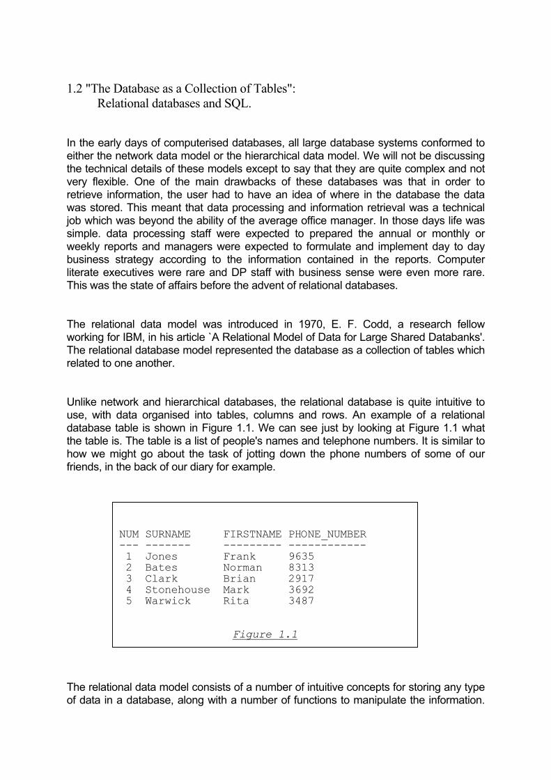
1.2 "The Database as a Collection of Tables": Relational databases and SQL. In the early days of computerised databases, all large database systems conformed to either the network data model or the hierarchical data model. We will not be discussing the technical details of these models except to say that they are quite complex and not very flexible. One of the main drawbacks of these databases was that in order to retrieve information, the user had to have an idea of where in the database the data was stored. This meant that data processing and information retrieval was a technical job which was beyond the ability of the average office manager. In those days life was simple. data processing staff were expected to prepared the annual or monthly or weekly reports and managers were expected to formulate and implement day to day business strategy according to the information contained in the reports. Computer literate executives were rare and DP staff with business sense were even more rare. This was the state of affairs before the advent of relational databases. The relational data model was introduced in 1970, E. F. Codd, a research fellow working for IBM, in his article `A Relational Model of Data for Large Shared Databanks'. The relational database model represented the database as a collection of tables which related to one another. Unlike network and hierarchical databases, the relational database is quite intuitive to use, with data organised into tables, columns and rows. An example of a relational database table is shown in Figure 1.1. We can see just by looking at Figure 1.1 what the table is. The table is a list of people's names and telephone numbers. It is similar to how we might go about the task of jotting down the phone numbers of some of our friends, in the back of our diary for example.
NUM SURNAME FIRSTNAME PHONE_NUMBER --- ------- --------- ------------ 1 Jones Frank 9635 2 Bates Norman 8313 3 Clark Brian 2917 4 Stonehouse Mark 3692 5 Warwick Rita 3487
Figure 1.1
The relational data model consists of a number of intuitive concepts for storing any type of data in a database, along with a number of functions to manipulate the information.

The relational data model as proposed by Codd provided the basic concepts for a new database management system, the relational database management system (RDBMS). Soon after the relational model was defined, a number of relational database languages were developed and used for instructing the RDBMS. Structured Query Language being one of them. The SQL language is so inextricably tied to relational database theory that it is impossible to discuss it without also discussing the relational data model. The next two sections briefly describe some of the concepts of this model.
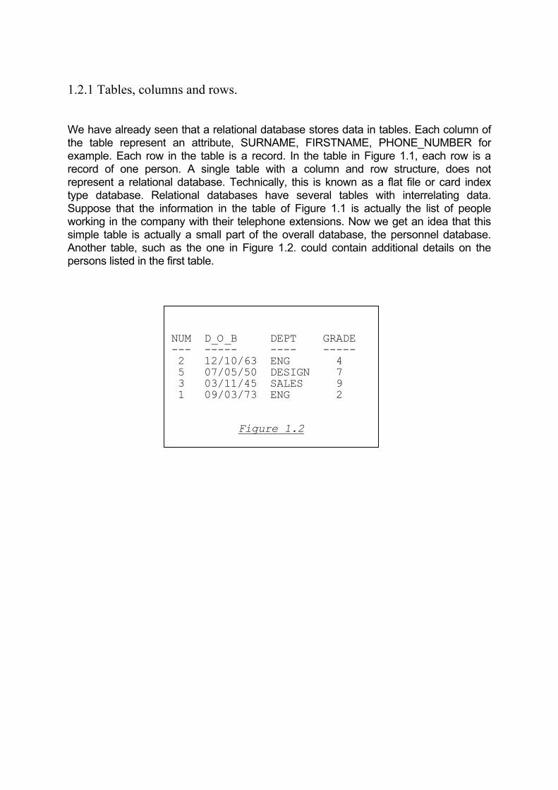
1.2.1 Tables, columns and rows. We have already seen that a relational database stores data in tables. Each column of the table represent an attribute, SURNAME, FIRSTNAME, PHONE_NUMBER for example. Each row in the table is a record. In the table in Figure 1.1, each row is a record of one person. A single table with a column and row structure, does not represent a relational database. Technically, this is known as a flat file or card index type database. Relational databases have several tables with interrelating data. Suppose that the information in the table of Figure 1.1 is actually the list of people working in the company with their telephone extensions. Now we get an idea that this simple table is actually a small part of the overall database, the personnel database. Another table, such as the one in Figure 1.2. could contain additional details on the persons listed in the first table.
NUM D_O_B DEPT GRADE --- ----- ---- ----- 2 12/10/63 ENG 4 5 07/05/50 DESIGN 7 3 03/11/45 SALES 9 1 09/03/73 ENG 2
Figure 1.2
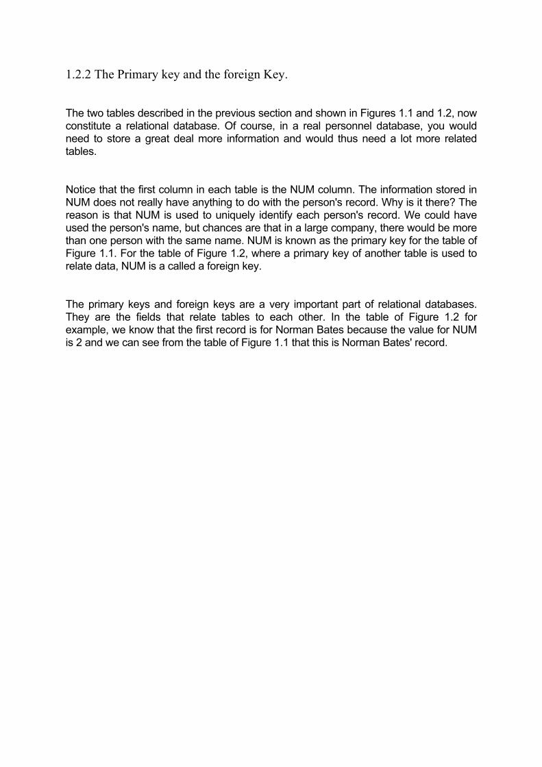
1.2.2 The Primary key and the foreign Key. The two tables described in the previous section and shown in Figures 1.1 and 1.2, now constitute a relational database. Of course, in a real personnel database, you would need to store a great deal more information and would thus need a lot more related tables. Notice that the first column in each table is the NUM column. The information stored in NUM does not really have anything to do with the person's record. Why is it there? The reason is that NUM is used to uniquely identify each person's record. We could have used the person's name, but chances are that in a large company, there would be more than one person with the same name. NUM is known as the primary key for the table of Figure 1.1. For the table of Figure 1.2, where a primary key of another table is used to relate data, NUM is a called a foreign key. The primary keys and foreign keys are a very important part of relational databases. They are the fields that relate tables to each other. In the table of Figure 1.2 for example, we know that the first record is for Norman Bates because the value for NUM is 2 and we can see from the table of Figure 1.1 that this is Norman Bates' record.

1.3 "Communicating to the DBMS what you want it to do": Introduction to the SQL language. The Structured Query Language is a relational database language. By itself, SQL does not make a DBMS. It is just a medium which is used to as a means of communicating to the DBMS what you want it to do. SQL commands consist of english like statements which are used to query, insert, update and delete data. What we mean by `english like', is that SQL commands resemble english language sentences in their construction and use. This does not mean that you can type in something like "Pull up the figures for last quarter's sales" and expect SQL to understand your request. What it does mean is that SQL is a lot easier to learn and understand than most of the other computer languages. SQL is sometimes referred to as a non-procedural database language. What this means is that when you issue an SQL command to retrieve data from a database, you do not have to explicitly tell SQL where to look for the data. It is enough just to tell SQL what data you want to be retrieved. The DBMS will take care of locating the information in the database. This is very useful because it means that users do not need to have any knowledge of where the data is and how to get at it. Procedural languages such as COBOL or Pascal and even older databases based on the network and hierarchical data models require that users specify what data to retrieve and also how to get at it. Most large corporate databases are held on several different computers in different parts of the building or even at different geographic locations. In such situations, the non-procedural nature of SQL makes flexible, ad hoc querying and data retrieval possible. Users can construct and execute an SQL query, look at the data retrieved, and change the query if needed all in a spontaneous manner. To perform similar queries using a procedural language such as COBOL would mean that you would have to create, compile and run one computer programs for each query. Commercial database management systems allow SQL to be used in two distinct ways. First, SQL commands can be typed at the command line directly. The DBMS interprets and processes the SQL commands immediately, and any result rows that are retrieved are displayed. This method of SQL processing is called interactive SQL. The second method is called programmatic SQL. Here, SQL statements are embedded in a host language such as COBOL or C. SQL needs a host language because SQL is not really a complete computer programming language as such. It has no statements or constructs that allow a program to branch or loop. The host language provides the necessary looping and branching structures and the interface with the user, while SQL provides the statements to communicate with the DBMS.

1.4 "A Research Project Conducted by IBM": The history of SQL. The origins of the SQL language date back to a research project conducted by IBM at their research laboratories in San Jose, California in the early 1970s. The aim of the project was to develop an experimental RDBMS which would eventually lead to a marketable product. At that time, there was a lot of interest in the relational model for databases at the academic level, in conferences and seminars. IBM, which already had a large share of the commercial database market with hierarchical and network model DBMSs, realised quite quickly that the relational model would figure prominently in future database products. The project at IBM's San Jose labs was started in 1974 and was named System R. A language called Sequel (for Structured English QUEry Language) was chosen as the relational database language for System R. In the project, Sequel was abbreviated to SQL. This is the reason why SQL is still generally pronounced as see-quel. In the first phase of the System R project, researchers concentrated on developing a basic version of the RDBMS. The main aim at this stage was to verify that the theories of the relational model could be translated into a working, commercially viable product. This first phase was successfully completed by the end of 1975, and resulted in a rudimentary, single-user DBMS based on the relational model. The subsequent phases of System R concentrated on further developing the DBMS from the first phase. Additional features were added, multi-user capability was implemented, and by 1978, a completed RDBMS was ready for user evaluation. The System R project was finally completed in 1979. During this time, the SQL language was modified and added to as the needs of the System R DBMS dictated. The theoretical work of the System R project resulted in the development and release in 1981 of IBM's first commercial relational database management system. The product was called SQL/DS and ran under the DOS/VSE operating system environment. Two years later, IBM announced a version of SQL/DS for the VM/CMS operating system. In 1983, IBM released a second SQL based RDBMS called DB2, which ran under the MVS operating system. DB2 quickly gained widespread popularity and even today, versions of DB2 form the basis of many database systems found in large corporate data-centres. During the development of System R and SQL/DS, other companies were also at work creating their own relational database management systems. Some of them, Oracle being a prime example, even implemented SQL as the relational database language for

their DBMSs concurrently with IBM. Today, the SQL language has gained ANSI (American National Standards Institute) and ISO (International Standards Organization) certification. A version of SQL is available for almost any hardware platform from CRAY supercomputers to IBM PC microcomputers. In recent years, there has been a marked trend for software manufacturers to move away from proprietary database languages and settle on the SQL standard. The microcomputer platform especially has seen a proliferation of previously proprietary packages that have implemented SQL functionality. Even spreadsheet and word processing packages have added options which allow data to be sent to and retrieved from SQL based databases via a Local Area or a Wide Area network connection.

1.5 "SQL Commands Build Upon Themselves": Organization of this book. After this introduction, this book first presents the SQL language in a nutshell. Subsequent chapters then focus on explaining each of the SQL command groups (the SELECT, the UPDATE, the CREATE etc) more fully. The reason for this method of presentation is that a lot of the SQL commands build upon themselves. For example, you cannot discuss the INSERT INTO with SELECT command without having knowledge of and understanding the SELECT statement itself. So where do you put the chapter on INSERT INTO with SELECT? You can't put it before the chapter on SELECT because as we've said, it requires the reader to have knowledge of the SELECT statement. You can't put it after the chapter on SELECT because the SELECT statement requires data to be input into the tables by using the INSERT statement. We have gone for the second option because it is a lot easier to take a leap of faith and believe that somehow the tables are already populated with data and use SELECT to query them rather than trying to understand the INSERT INTO with SELECT without any knowledge of how SELECT works. To save having to put phrases such as "see the later chapter on SELECT" or "see the earlier chapter on INSERT" throughout the book, we have started off by describing the SQL language globally, and then detailing each command group separately. It's a bit like a course for auto mechanics, say, you start off by first describing the layout of the car and all it's major parts such as the engine, the gearbox etc., before going on to discuss topics like the detailed construction of the engine. Primarily, this book is designed to teach you how to use SQL to create, modify, maintain and use databases in practical situations. It is not intended to be an academic treatise on the subject, and so does not go into the mathematical basis of the topics considered. What it does contain is lots of examples and discussions on how they work. You should work your way through this book by reading through a section, and actually trying out each SQL query presented for yourself. If you do not have access to an SQL based database, then you can order a fully functional ANSI/ISO SQL database at an affordable price, by sending off the order form at the back of this book. The quickest and easiest method of learning SQL (or indeed any computer language) is to use it in real life, practical situations. The chapters of this book are laid out so that each section builds upon the information and examples presented in the previous chapters. By following the SQL query examples, you will create a database, populate it and then use it to retrieve information. Remember that the SQL queries in this book are only given as examples. They represent one possible method of retrieving the results that you want. As you gain confidence in SQL, you may be able to construct a more elegant query to solve a problem than the one that we have used. This just goes to show the power and flexibility of SQL.

The structure of this book is such that as you progress through it, you will be exposed to more and more complex aspects of SQL. If you follow through the book, you will find that you are not suddenly presented with anything particularly difficult. Rather, you will be gradually lead through and actively encouraged to try out SQL queries and variations of queries until you have thoroughly understood the underlying ideas. The chapters will not all take the same amount of time to read and understand. You will benefit most if you sit down, start at a new section, and work your way through until it is completed. Although we understand that you may find some of the longer sections difficult to finish in one session. You should nonetheless endeavour to complete each section in as few sittings as possible. Taking short breaks to think over concepts learned as you progress through the section is also a good idea as it reinforces the learning process. You should try to understand the underlying concepts of what you are learning rather than coasting through the book.
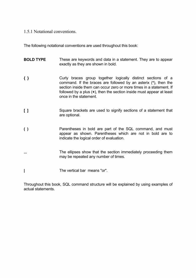
1.5.1 Notational conventions. The following notational conventions are used throughout this book: BOLD TYPE These are keywords and data in a statement. They are to appear
exactly as they are shown in bold. { } Curly braces group together logically distinct sections of a
command. If the braces are followed by an asterix (*), then the section inside them can occur zero or more times in a statement. If followed by a plus (+), then the section inside must appear at least once in the statement.
[ ] Square brackets are used to signify sections of a statement that
are optional. ( ) Parentheses in bold are part of the SQL command, and must
appear as shown. Parentheses which are not in bold are to indicate the logical order of evaluation.
... The ellipses show that the section immediately proceeding them
may be repeated any number of times. | The vertical bar means "or". Throughout this book, SQL command structure will be explained by using examples of actual statements.
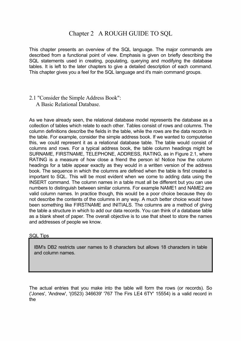
Chapter 2 A ROUGH GUIDE TO SQL This chapter presents an overview of the SQL language. The major commands are described from a functional point of view. Emphasis is given on briefly describing the SQL statements used in creating, populating, querying and modifying the database tables. It is left to the later chapters to give a detailed description of each command. This chapter gives you a feel for the SQL language and it's main command groups. 2.1 "Consider the Simple Address Book": A Basic Relational Database. As we have already seen, the relational database model represents the database as a collection of tables which relate to each other. Tables consist of rows and columns. The column definitions describe the fields in the table, while the rows are the data records in the table. For example, consider the simple address book. If we wanted to computerise this, we could represent it as a relational database table. The table would consist of columns and rows. For a typical address book, the table column headings might be SURNAME, FIRSTNAME, TELEPHONE, ADDRESS, RATING, as in Figure 2.1, where RATING is a measure of how close a friend the person is! Notice how the column headings for a table appear exactly as they would in a written version of the address book. The sequence in which the columns are defined when the table is first created is important to SQL. This will be most evident when we come to adding data using the INSERT command. The column names in a table must all be different but you can use numbers to distinguish between similar columns. For example NAME1 and NAME2 are valid column names. In practice though, this would be a poor choice because they do not describe the contents of the columns in any way. A much better choice would have been something like FIRSTNAME and INITIALS. The columns are a method of giving the table a structure in which to add our data records. You can think of a database table as a blank sheet of paper. The overall objective is to use that sheet to store the names and addresses of people we know. SQL Tips
IBM's DB2 restricts user names to 8 characters but allows 18 characters in table and column names.
The actual entries that you make into the table will form the rows (or records). So ('Jones', 'Andrew', '(0523) 346639' '767 The Firs LE4 6TY' 15554) is a valid record in the
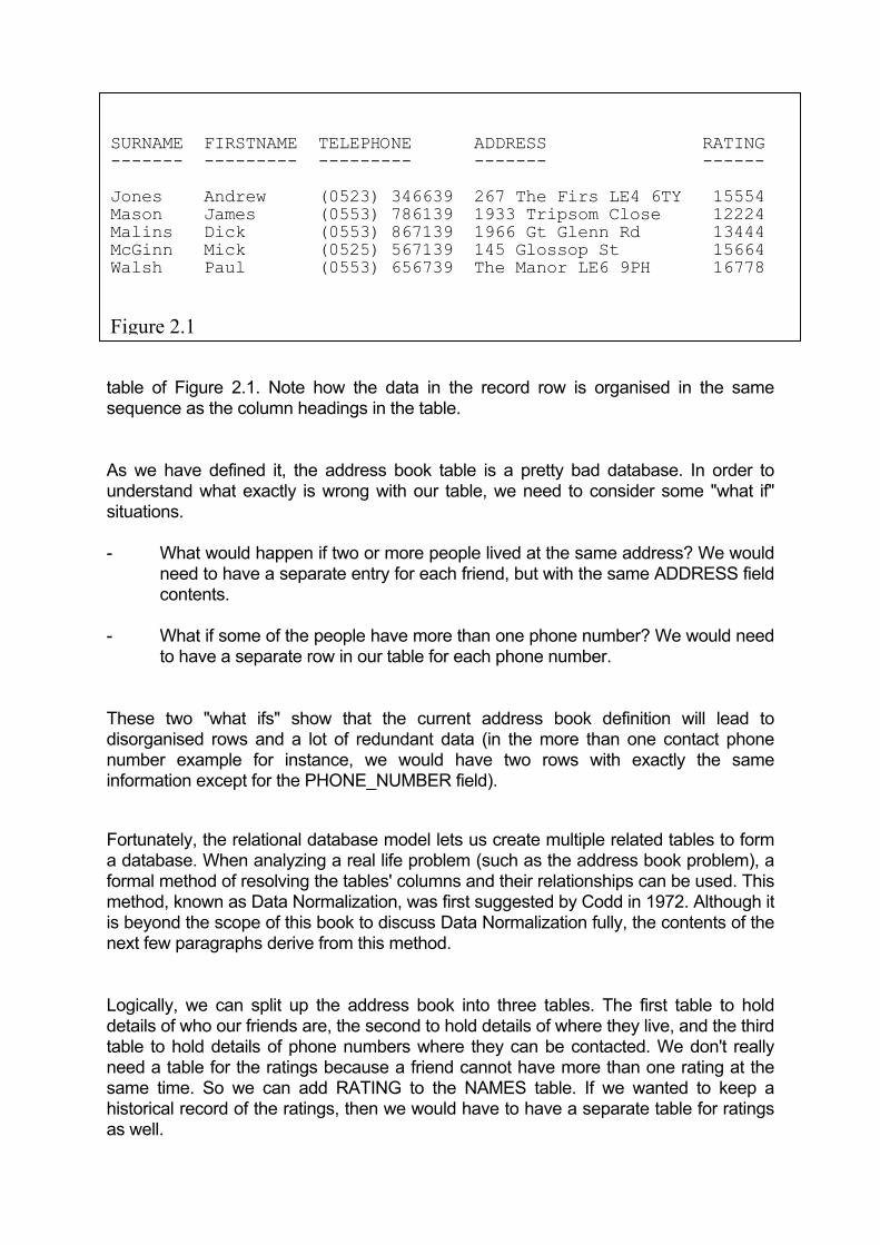
SURNAME FIRSTNAME TELEPHONE ADDRESS RATING ------- --------- --------- ------- ------ Jones Andrew (0523) 346639 267 The Firs LE4 6TY 15554 Mason James (0553) 786139 1933 Tripsom Close 12224 Malins Dick (0553) 867139 1966 Gt Glenn Rd 13444 McGinn Mick (0525) 567139 145 Glossop St 15664 Walsh Paul (0553) 656739 The Manor LE6 9PH 16778
Figure 2.1
table of Figure 2.1. Note how the data in the record row is organised in the same sequence as the column headings in the table. As we have defined it, the address book table is a pretty bad database. In order to understand what exactly is wrong with our table, we need to consider some "what if" situations. - What would happen if two or more people lived at the same address? We would
need to have a separate entry for each friend, but with the same ADDRESS field contents.
- What if some of the people have more than one phone number? We would need
to have a separate row in our table for each phone number. These two "what ifs" show that the current address book definition will lead to disorganised rows and a lot of redundant data (in the more than one contact phone number example for instance, we would have two rows with exactly the same information except for the PHONE_NUMBER field). Fortunately, the relational database model lets us create multiple related tables to form a database. When analyzing a real life problem (such as the address book problem), a formal method of resolving the tables' columns and their relationships can be used. This method, known as Data Normalization, was first suggested by Codd in 1972. Although it is beyond the scope of this book to discuss Data Normalization fully, the contents of the next few paragraphs derive from this method. Logically, we can split up the address book into three tables. The first table to hold details of who our friends are, the second to hold details of where they live, and the third table to hold details of phone numbers where they can be contacted. We don't really need a table for the ratings because a friend cannot have more than one rating at the same time. So we can add RATING to the NAMES table. If we wanted to keep a historical record of the ratings, then we would have to have a separate table for ratings as well.

Figure 2.2 shows how our address book can be split up to form a true relational database. Each table has a new field, FRNO. This field is the primary key in the NAMES table, and a foreign key in the other tables. It is what relates the tables to each other. A record which refers to a particular friend will have the same FRNO in all the tables. Thus, for our friend who has two houses, there will be an entry in tables one and three and two entries in table two.
FRNO SURNAME FIRSTNAME RATING ---- ------- --------- ------ 1 Jones Andrew 15554 2 Mason James 12224 3 Malins Dick 13444 4 McGinn Mick 15664 5 Walsh Paul 16778 The NAMES Table
FRNO ADDRESS ---- ------- 1 267 The Firs LE4 6TY 2 1933 Tripsom Close 3 1966 Gt Glenn Rd 4 145 Glossop St 5 The Manor LE6 9PH The ADDRESS Table FRNO TELEPHONE ---- --------- 1 (0523) 346639 2 (0553) 786139 3 (0553) 867139 4 (0525) 567139 5 (0553) 656739 The TELEPHONE_NUMBER Table
Figure 2.2
In this simple example, the splitting up of the database into three tables is not very practical. For a personal address book, we would have been better off with the flat file (single table) database The point to note though is that the three table version of the database is more flexible (we can store the details of a friend even if he has 25 telephones and 14 houses, without having to store redundant data). For large and complex databases which may consist of dozens of tables and tens of thousands of records, this logical splitting up of data into separate tables (known as Data Normalization) is vital in preventing data redundancy and creating a relationally correct database. 2.2 "SQL Commands Fall into Different Categories": Subdivisions of SQL. The SQL language as defined by ANSI is subdivided into a number of different sections. This means that the SQL commands fall into different categories depending on what function they perform. The Data Definition Language or DDL, (called Schema Definition Language by ANSI) consists of those commands in SQL that directly create database objects such as tables, indexes views. A lot of SQL commands also create temporary database objects during processing. The SELECT command for example, creates a temporary table to hold the results of a query. Such commands are not part of the DDL. The Data Manipulation Language or DML consists of those commands which operate on the data in the database. This includes statements which add data to the tables as well as those statements which are used to query the database. A third, unofficial, subdivision of SQL commands is Data Control Language or DCL. It is generally used to refer to those SQL commands are used for data security. These are commands that are used to determine whether a user is allowed to carry out a particular operation or not. The ANSI standard groups these commands as being part of the DDL. 2.3 "Enter SQL Statements at the Command Line": Using Interpretive SQL. All SQL statements in this book have been run using the Data-Lab SQL RDBMS and interpreter. The interpreter is the interface that you use to communicate with the DBMS. It allows you to type, compose and edit your SQL queries and has special editing commands to help you with this. When you are satisfied with the wording of the query, you can enter a semicolon character which instructs the interpreter to pass the query on

to the SQL engine for processing. If you are using a different SQL interpreter, you will in most cases, not need to modify the SQL statements because they follow the ANSI standard quite closely. Where extensions to the ANSI standard are discussed, you will need to consult the reference manual for your product to find out the exact form of the statement. Note that since Data-Lab SQL is quite close to Oracle SQL, Oracle users should have no problems. 2.4 "Use the CREATE TABLE statement": Creating Database Tables. The SQL command to create tables is the CREATE TABLE statement. We will use this to create a simple car dealership database which will be used throughout the rest of this chapter. This simple database consists of the three tables shown in Figure 2.3. The CARS table holds details of the car's model name, the body style and the year of manufacturer. The MD_NUM field is used as the primary key. The SPECS table stores the information on additional equipment on each of the cars. The STOCK table holds details of the number of cars of each model that are currently in stock, and their retail price.
CARS SPECS STOCK ---- ----- ----- MD_NUM MD_NUM MD_NUM MD_NAME MPG QTY STYLE RADIO PRICE YEAR ENGINE Tables used in the used car dealership database
Figure 2.3
To create the first table in the car dealership database: CREATE TABLE CARS ( MD_NUM INTEGER, MD_NAME CHAR(10), STYLE CHAR(6), YEAR INTEGER ); Table CARS created.

This statement creates a database table on disk, and assign it the name CARS. The table's columns are also defined along with their data types. When you create tables, each of the columns must be defined as a specific data type. For example, the MD_NUM column is defined as an INTEGER, and MD_NAME is defined as CHAR(10). This means that when data is added to the table, the MD_NUM column will only hold integers and the MD_NAME column will hold character string values up to a maximum of 10 characters. The subject of data types and valid and invalid values will be discussed in detail in the next chapter. Now that we have seen how to use the CREATE TABLE statement, we can create the next two tables in our car dealership database by typing: CREATE TABLE SPECS ( MD_NUM INTEGER, MPG INTEGER, RADIO CHAR(3), ENGINE CHAR(7) ); Table SPECS successfully created. CREATE TABLE STOCK ( MD_NUM INTEGER, QTY INTEGER, PRICE INTEGER ); Table STOCK successfully created. When created, the tables are empty. In order to be of any use they need data. The next section describes the INSERT statement which is used to add data to the tables.
SQL Tips
Oracle allows you to use up to 30 characters for both table and column names.

2.5 "Use the INSERT INTO Statement": Adding Data to Tables. Data is added to tables by using the INSERT statement. The values that we need to add to the car dealership database are shown in Figure 2.4
MD_NUM MD_NAME STYLE YEAR ------ ------- ----- ---- 1 HONDA COUPE 1983 2 TOYOTA SALOON 1990 3 BUICK ESTATE 1991 4 NISSAN VAN 1992 5 FORD SALOON 1993 The Cars Table MD_NUM MPG RADIO ENGINE ------ --- ----- ------ 1 43 YES 2L-4CYL 2 25 NO 4L-V8 3 18 YES 5L-V8 4 50 NO 2L-4CYL 5 45 YES 3L-V6 The Specs Table MD_NUM QTY PRICE ------ --- ----- 1 10 4980 2 3 13865 3 5 14900 4 1 11000 5 2 24600 The Stock Table
Figure 2.4
Starting with the first table, the CARS table, the first record or row is added by: INSERT INTO CARS (MD_NUM, MD_NAME, STYLE, YEAR) VALUES (1, 'HONDA', 'COUPE', 1983);
1 row successfully inserted. The rest of the rows can be added to CARS by using exactly the same statement format, but changing data values each time. INSERT INTO CARS (MD_NUM, MD_NAME, STYLE, YEAR) VALUES (2, 'TOYOTA', 'SALOON', 1990); INSERT INTO CARS (MD_NUM, MD_NAME, STYLE, YEAR) VALUES (3, 'BUICK', 'ESTATE', 1991); INSERT INTO CARS (MD_NUM, MD_NAME, STYLE, YEAR) VALUES (4, 'NISSAN', 'VAN', 1992); INSERT INTO CARS (MD_NUM, MD_NAME, STYLE, YEAR) VALUES (5, 'FORD', 'SALOON', 1993); 4 rows successfully inserted. In the form of the INSERT statement that we have used above, you must specify three pieces of information. First, the name of the table to insert data into. Second, the names of the columns where data is to be added. Finally, you need to specify the actual data values. We can add data to the SPECS table by: INSERT INTO SPECS VALUES (1, 43, 'YES', '2L-4CYL'); INSERT INTO SPECS VALUES (2, 25, 'NO', '4L-V8'); INSERT INTO SPECS VALUES (3, 18, 'YES', '5L-V8'); INSERT INTO SPECS VALUES (4, 50, 'NO', '2L-4CYL'); INSERT INTO SPECS VALUES (5, 45, 'YES', '3L-V6'); 5 rows successfully inserted. and to the STOCK table by: INSERT INTO STOCK VALUES (1, 10, 4980);
INSERT INTO STOCK VALUES (2, 3, 13865); INSERT INTO STOCK VALUES (3, 5, 14900); INSERT INTO STOCK VALUES (4, 1, 11000); INSERT INTO STOCK VALUES (5, 2, 24600); 5 rows successfully inserted. The INSERT statements for the SPECS and the STOCK table did not use a value list. This is a shortcut which SQL allows you to use when you specify values for all the columns in each row, as we have been doing. 2.6 "Use the SELECT Statement": Extracting data from tables. The most important job of any database is to provide you with information. In SQL, the act of retrieving information is called querying the database. Information is retrieved from the database by using the SELECT statement. The previous two sections, first created the car dealership database, them added data to it. To retrieve the data from the CARS table of this database for example, you could use a SELECT statement. A SELECT statement is also called a query because it interrogates the database: SELECT MD_NAME, STYLE, YEAR FROM CARS; MD_NAME STYLE YEAR ---------- ------- -------- HONDA COUPE 1983 TOYOTA SALOON 1990 BUICK ESTATE 1991 NISSAN VAN 1992 FORD SALOON 1993 The data retrieval requirements vary from user to user. For example, in our car dealership database, one user might want to know how many Nissan cars there are in stock while another might need to know how many cars there are which have a radio, eight cylinders and cost less than 10,000. As long as the information that you require is stored in the database in some form, you will be able to construct a form of SELECT statement which retrieves it. It because of this flexibility that the SELECT statement is the most complex and also the most useful of all the SQL commands.

2.7 "Use the UPDATE and DELETE Statements": Modifying data. In daily use, a database is a constantly changing store of data. The SQL commands which are used to modify data that is already in the database are the UPDATE and the DELETE commands. For example, to change the record of the Ford model in the CARS table to show the year of manufacture as 1989 and not 1993: UPDATE CARS SET YEAR = 1989 WHERE MD_NAME = 'FORD'; 1 row updated. We can express what this query is doing in words as "Update the CARS table and set the YEAR column value to 1989 for all those records where the MD_NAME column value is FORD." An important point to note is that UPDATE is capable of modifying the values of more than one record in a table. So if the CARS table had several Fords, then this statement would have changed the date of manufacture on all of them to 1989. You need to be wary of this when modifying values with UPDATE. The trick is to be so specific in the WHERE clause that only those records that you want to be changed are changed. Another reason for wanting to modify the database is when deleting unwanted records from the tables SQL uses the DELETE command for this. For example, if we decide that the Ford model in the CARS table is not available for sale, we can simply delete it's record from the table by: DELETE FROM CARS WHERE MD_NAME = 'FORD' AND YEAR = 1989; 1 row deleted. Just as with the UPDATE statement, care must be taken when using DELETE to ensure that only those records that you want deleted are actually deleted. The WHERE clause in this statement is a little more specific than the one we used in the last UPDATE statement. It asks SQL to delete only those records where the MD_NAME is Ford and also the YEAR is 1989. To confirm that the DELETE statement did remove the record for the Ford, we can query the CARS table: SELECT * FROM CARS;

MD_NUM MD_NAME STYLE YEAR -------- --------- ------- -------- 1 HONDA COUPE 1983 2 TOYOTA SALOON 1990 3 BUICK ESTATE 1991 4 NISSAN VAN 1992 2.8 "Another Kind of Table, Called a Virtual Table": Views. The tables that you have been using up to now are called base tables. There is another kind of table, called a virtual table or view that is allowed for in SQL. Base tables are database objects whose structure and the data they contain are both stored on disk. Views are tables whose contents are derived from base tables. Only their structure is stored on disk. SQL's DML statements operate on views just as they do on base tables, but with one exception: when data is apparently added to, deleted or modified from a view, the actual data that is operated on is that in the underlying base tables that make up the view. You can think of a view as a stencil or a window into a table or tables. Suppose that in a company personnel database, a staff table contains relevant work related information on employees such as department, supervisor, date joined etc. The table might also contain sensitive information such as salary, home address and telephone number etc. An excellent method of limiting casual user access to only the relevant work related information, and restrict access to the sensitive information would be to use a view. In the used car dealership database for example, if the manager decides that he does not want everyone to see the price of the cars in the STOCK table, he could create a view called NO_PRICE: CREATE VIEW NO_PRICE AS SELECT MD_NUM, QTY FROM STOCK; View NO_PRICE successfully created. Notice that the CREATE VIEW statement contains a SELECT statement as well. A view is in fact just a stored query that gets executed whenever the view is used as the subject of a command. The results of the query define the records `held' in the view ie. the data in the view. Once created, the view's definition is stored by the DBMS and can be queried just like a regular base table. For example, to list all the "rows" in NO_PRICE:
SELECT * FROM NO_PRICE ; MD_NUM QTY -------- -------- 1 10 2 3 3 5 4 1 5 2 Notice that the view only displays two columns from the STOCK table. PRICE has been hidden from the user. 2.9 "Prevent Access to Sensitive Information": Database security. As we have already seen, views can be used to prevent access to sensitive information in the database. Another method of enforcing security is by use of the GRANT and the REVOKE statements. SQL operates on the concepts of user identification, ownership of database objects, and that of granting and revoking privileges from users. When a table is first created, it is owned by the user who created it. This means that the user who created the table is automatically given full privileges to operate on that table (INSERT data, UPDATE values, DELETE rows etc). All other users are given no privileges on the table. Let's see how this works. We will first create a view called NEW_CARS (which consists of cars whose year of manufacture is after 1990). We'll create this view under the user ID of JOE. Don't worry too much if the format of the CREATE VIEW appears a little strange. What it is doing is to temporarily set the user ID to JOE, then create the view, then revert back to the original user ID: CREATE SCHEMA AUTHORIZATION JOE CREATE VIEW NEW_CARS AS SELECT * FROM CARS WHERE YEAR > 1990 ; View NEW_CARS successfully created. Now if we try to look at the data in the view: SELECT *

FROM NEW_CARS; Error 98: User does not have the necessary SELECT privileges. SQL tells us that we do not have the necessary privileges for this operation. We can confirm that the owner of the view, JOE, is allowed to look at the information by prefixing the JOE user-id to the viewname: SELECT * FROM JOE.NEW_CARS ; MD_NUM MD_NAME STYLE YEAR --------- ----------- ------- -------- 3 BUICK ESTATE 1991 4 NISSAN VAN 1992 This query tells SQL that we know the user ID of the person who created the table is JOE, and we want it to use this for retrieving data from NEW_CARS.
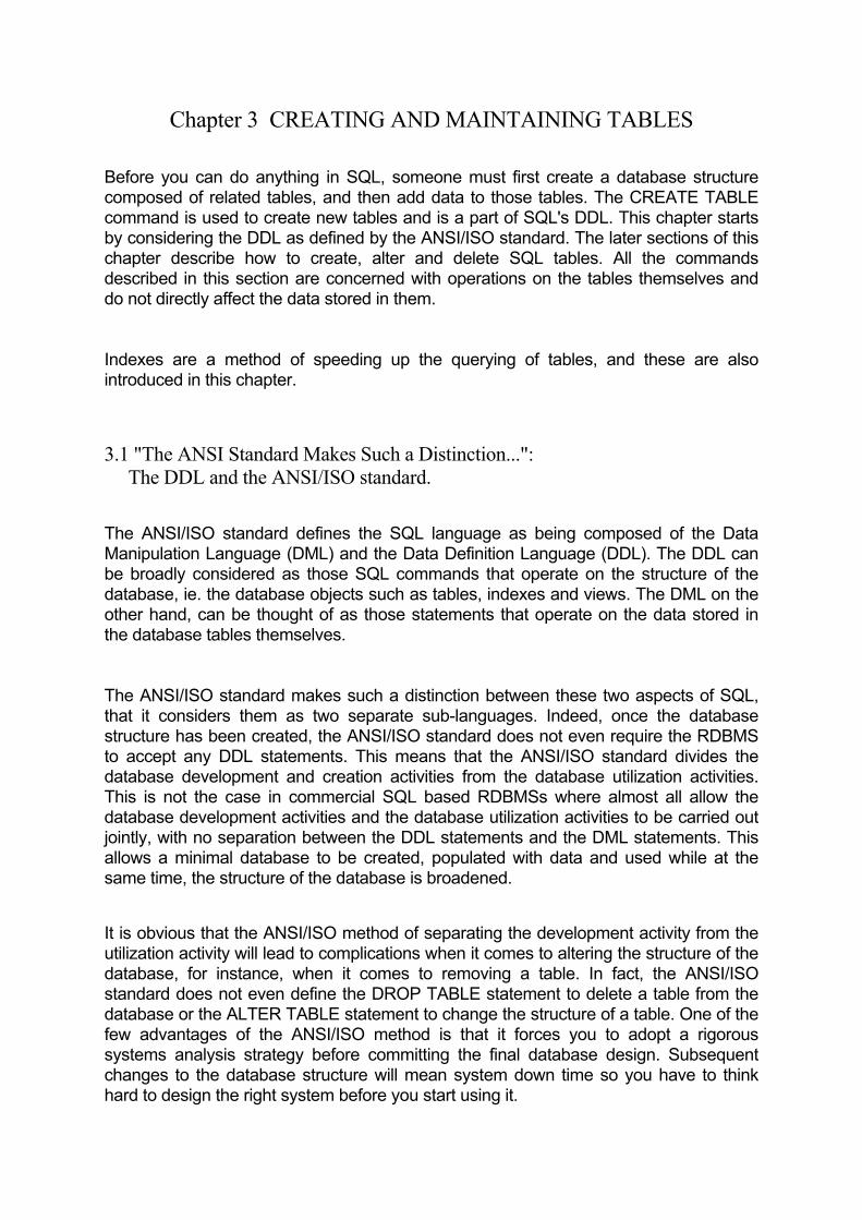
Chapter 3 CREATING AND MAINTAINING TABLES Before you can do anything in SQL, someone must first create a database structure composed of related tables, and then add data to those tables. The CREATE TABLE command is used to create new tables and is a part of SQL's DDL. This chapter starts by considering the DDL as defined by the ANSI/ISO standard. The later sections of this chapter describe how to create, alter and delete SQL tables. All the commands described in this section are concerned with operations on the tables themselves and do not directly affect the data stored in them. Indexes are a method of speeding up the querying of tables, and these are also introduced in this chapter. 3.1 "The ANSI Standard Makes Such a Distinction...": The DDL and the ANSI/ISO standard. The ANSI/ISO standard defines the SQL language as being composed of the Data Manipulation Language (DML) and the Data Definition Language (DDL). The DDL can be broadly considered as those SQL commands that operate on the structure of the database, ie. the database objects such as tables, indexes and views. The DML on the other hand, can be thought of as those statements that operate on the data stored in the database tables themselves. The ANSI/ISO standard makes such a distinction between these two aspects of SQL, that it considers them as two separate sub-languages. Indeed, once the database structure has been created, the ANSI/ISO standard does not even require the RDBMS to accept any DDL statements. This means that the ANSI/ISO standard divides the database development and creation activities from the database utilization activities. This is not the case in commercial SQL based RDBMSs where almost all allow the database development activities and the database utilization activities to be carried out jointly, with no separation between the DDL statements and the DML statements. This allows a minimal database to be created, populated with data and used while at the same time, the structure of the database is broadened. It is obvious that the ANSI/ISO method of separating the development activity from the utilization activity will lead to complications when it comes to altering the structure of the database, for instance, when it comes to removing a table. In fact, the ANSI/ISO standard does not even define the DROP TABLE statement to delete a table from the database or the ALTER TABLE statement to change the structure of a table. One of the few advantages of the ANSI/ISO method is that it forces you to adopt a rigorous systems analysis strategy before committing the final database design. Subsequent changes to the database structure will mean system down time so you have to think hard to design the right system before you start using it.

3.2 "Single and Multiple Database Architectures": The structure of SQL databases. The ANSI/ISO SQL standard specifies that the database schema consist of a single large database with tables which are owned by various users. The ownership of the tables sub-classifies them into different virtual database groups. This is shown in Figure 3.1. The tables owned by FRANK_G might be the Accounts (sub)database and those owned by MARK_B, the Suppliers (sub)database. Under the ANSI/ISO standard, both the Accounts tables and the Suppliers tables are part of the overall system database. All the tables in such single-database architectures can easily reference each other. The single-database architecture is used in both the Oracle and IBM's DB2 systems.
------------------------------------------------------------- | || ____________________ ________ ___________________ || |TABLE 1 TABLE 2 | |TABLE 3 | |TABLE 4 TABLE 5 | || | | | | | | || |TABLE 7 TABLE 9 | |TABLE 67| |TABLE 56 TABLE 45| || | | | | | | || |TABLE 56 TABLE 19| |TABLE 82| |TABLE 92 TABLE 23| || |____________________| |________| |___________________| || Owned by FRANK_G Owned by Owned by MARK_B || SALLY_R || || || || || || | ------------------------------------------------------------- System Database ANSI/ISO structure consists of one large system database, which all tables are a part of. Tables are owned by users.
Figure 3.1
One of the disadvantages of the single-database architecture is that over time, as more and more tables are added to the system, the database becomes very big and bulky. Performing database administration tasks such as back-ups, performance analyzing etc. on such large databases becomes a complex process, requiring the services of a dedicated database administrator. A database architecture which does not suffer from this disadvantage is the multiple-database architecture. Here, tables are organized into

several distinct databases. This is shown in Figure 3.2. Although the data is split into several smaller, more manageable databases, the multiple-database architecture does suffer from a serious disadvantage. The tables in one database cannot (easily) contain foreign key references to keys in another database's table. The multiple-database architecture is used in Sybase, SQL Server and Ingres systems.
The ACCOUNTS database ____________________ |TABLE 1 TABLE 2 | | | |TABLE 7 TABLE 9 | | | |TABLE 56 TABLE 19| |____________________| Owned by FRANK_G The CUSTOMERS database ________ |TABLE 3 | | | |TABLE 67| | | |TABLE 82| |________| Owned by SALLY_R The SUPPLIERS database ___________________ |TABLE 4 TABLE 5 | | | |TABLE 56 TABLE 45| | | |TABLE 92 TABLE 23| |___________________| Owned by MARK_B
Figure 3.2
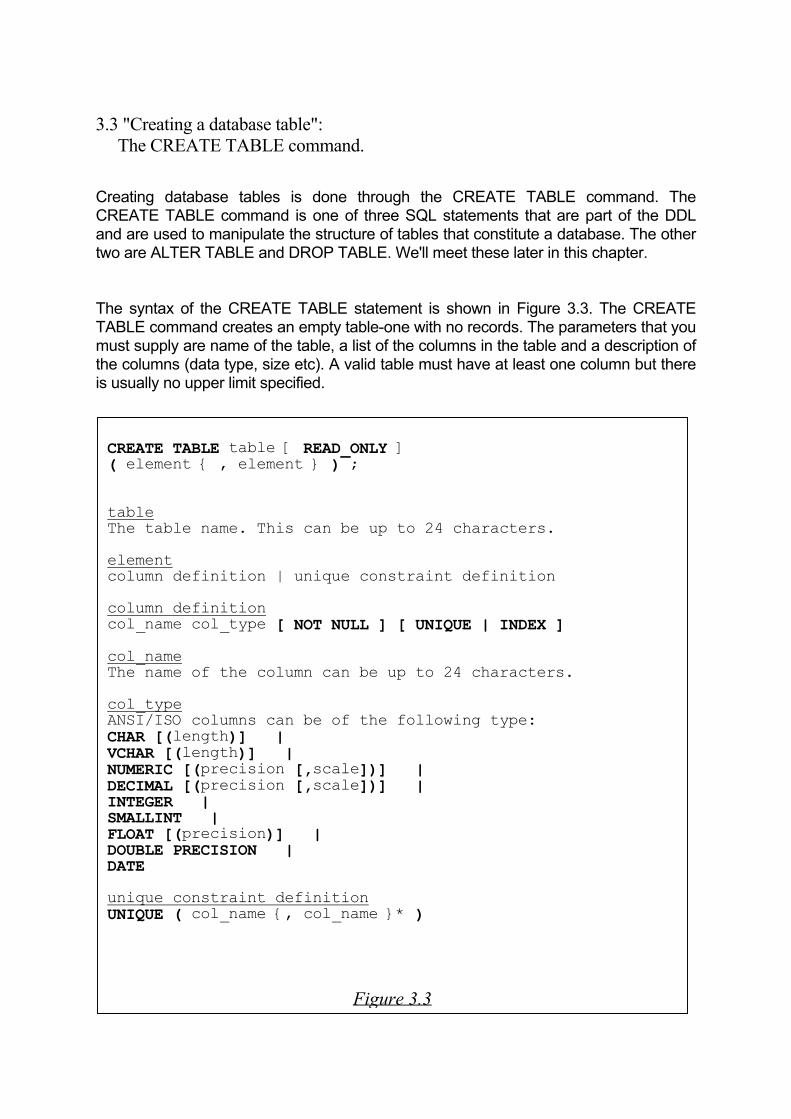
3.3 "Creating a database table": The CREATE TABLE command. Creating database tables is done through the CREATE TABLE command. The CREATE TABLE command is one of three SQL statements that are part of the DDL and are used to manipulate the structure of tables that constitute a database. The other two are ALTER TABLE and DROP TABLE. We'll meet these later in this chapter. The syntax of the CREATE TABLE statement is shown in Figure 3.3. The CREATE TABLE command creates an empty table-one with no records. The parameters that you must supply are name of the table, a list of the columns in the table and a description of the columns (data type, size etc). A valid table must have at least one column but there is usually no upper limit specified. REATE TABLE table [ READ_ONLY ] C( element { , element } ) ; table The table name. This can be up to 24 characters. element column definition | unique constraint definition column definition col_name col_type [ NOT NULL ] [ UNIQUE | INDEX ] col_name The name of the column can be up to 24 characters. col_type ANSI/IS mns ca
ength)O colu n be of the following type:
CHAR [(l ] | VCHAR [(le ngth)] |NUMERIC [( [, ])] |
recision [,scale])] | precision scale
DECIMAL [(pINTEGER | SMALLINT | FLOAT [(precision)]
LE PRECISION | |
DOUBDATE unique constraint definition UNIQUE ( col_name {, col_name }* )
Figure 3.3

ANSI/ISO SQL also allows you to create READ ONLY tables. This means that once created, SQL commands cannot be used to insert or update or delete data any in the tables. Creating READ ONLY tables only makes sense if some non-SQL process (an application program for example) is going to add the data. The data types allowed in the column definitions vary considerably from product to product. Most commercial SQL systems support the ANSI data types as a minimum, and add additional types that are proprietary. The valid ANSI/ISO data types are given in Appendix A.
SQL Tips
IBM's DB2 lets you store oriental language characters such as Kanji in fixed and variable length strings of 16-bit characters.
The UNIQUE and the INDEX column modifiers both create indexes for the field to which they are applied. Indexes will be discussed in detail in the next section. The NOT NULL column modifier adds the condition that a record cannot be inserted into the table if no value is supplied for this particular field. In SQL, tables are owned by the user who created them. Initially, only the table's owner is allowed to perform any operations involving that table. Other users must refer to the table by preceding the table name with the owner's user's ID. A table which is meant for use by all users can be created under a special user identifier known as PUBLIC. Tables created under PUBLIC allow all users on the system to access them. We came across the concept of ownership and privileges briefly in chapter 2. The subject of table ownership is discussed more fully in the chapter on database security. The names of tables which are owned by any given user must all be different. Some systems extend this so that the names of all the tables in the whole system must be different from each other. This also applies to column names within a table, but separate tables can however, have repeating column names. We will be using a database based on a university administration system throughout this book. The database consists of five tables: STUDENTS, LECTURERS, SUBJECTS, EXAMS and DEPARTMENTS. The whole database will be created and used in stages as we progress through the chapters. The structure of the tables as well as the data in them is shown in Figure 3.4. Appendix B gives an in depth description of this sample database.

SURNAME FIRST_NAME D_O_B STUDENT_NO DEPT_NO YEAR ------- ---------- ----- ---------- ------- ---- Duke Fitzroy 11-26-1970 1 4 2 Al-Essawy Zaid M A 11-26-1970 2 4 2 Ayton Phil J M A 07-13-1967 3 3 1 Patel Mahesh 12-07-1970 4 2 1 Jones Gareth P Y 01-24-1970 5 2 1 Scott Gavin T J 02-20-1971 6 2 2 Baker Abu-Mia 03-13-1971 7 4 1 Brown Joseph P A 04-19-1970 8 3 3 Monkhouse Robert Jones 05-23-1967 9 1 1 Grimm Hans Johan 06-21-1971 10 2 1 Gyver Sue L J V 07-30-1968 11 4 2 Hung-Sun Jimmy Lau 08-11-1969 12 1 3 Middleton Jane P 09-14-1971 13 1 3 Mulla Farook F U 10-24-1968 14 3 2 Layton Hugh 11-16-1971 15 5 1 Wickes Wendy Y Y W 12-05-1969 16 1 1 THE STUDENTS TABLE SURNAME INITL LECT_NO DEPT_NO SUB_N GRADE PAY JOINED ------- ----- ------- ------- ----- ----- --- ------ Jones R A 1 1 2 E 24000 03-25-1990 Scrivens T R 2 3 1 D 31800 09-30-1986 Nizamuddin W M 3 3 4 A 86790 05-26-1969 Campbell J G 4 5 3 C 43570 02-23-1980 Ramanujan S 5 4 5 C 40900 01-01-1985 Finley G Y 6 4 5 D 34210 03-28-1960 THE LECTURERS TABLE SUB_NO SUB_NAME DEPT_NO CREDITS PASS ------ -------- ------- ------- ---- 1 Mathematics 1 2 65 2 English Lit 2 1 60 3 Engineering Drwg 1 1 71 4 Basic Accounts 3 1 67 5 Industrial Law 4 2 52 6 Organic Chemistry 5 3 57 7 Physiology 6 3 78 8 Anatomy 6 1 74 9 Electronics 1 3 71 10 Marketing 3 2 56 THE SUBJECTS TABLE
Figure 3.4
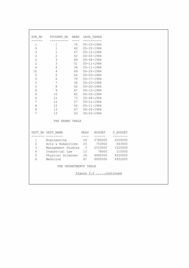
SUB_NO STUDENT_NO MARK DATE_TAKEN ------ ---------- ---- ---------- 1 1 76 05-23-1984 9 1 42 05-20-1984 3 1 67 05-15-1984 2 2 52 06-05-1984 2 3 89 06-08-1984 2 3 51 05-11-1984 4 4 34 05-11-1984 10 4 49 06-26-1984 5 5 62 05-03-1984 5 6 70 05-17-1984 5 7 36 05-23-1984 5 8 52 05-20-1984 6 9 67 05-15-1984 6 10 82 06-05-1984 6 11 73 06-08-1984 7 12 27 05-11-1984 8 12 56 05-11-1984 8 13 67 06-26-1984 7 13 63 05-03-1984 THE EXAMS TABLE DEPT_NO DEPT_NAME HEAD BUDGET P_BUDGET ------- --------- ---- ------ -------- 1 Engineering 59 5780000 6200000 2 Arts & Humanities 23 753000 643000 3 Management Studies 3 2510000 1220000 4 Industrial Law 12 78000 210000 5 Physical Sciences 18 4680000 4250000 6 Medicine 67 6895000 6932000 THE DEPARTMENTS TABLE
Figure 3.4 .....continued
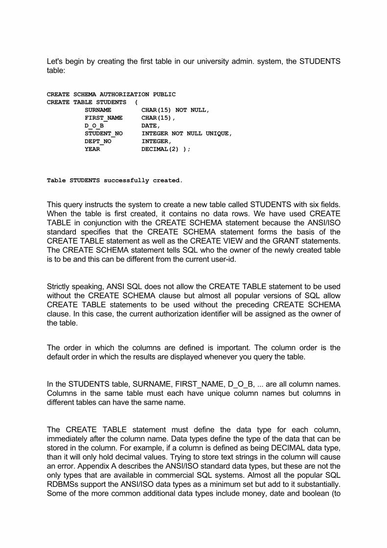
Let's begin by creating the first table in our university admin. system, the STUDENTS table: CREATE SCHEMA AUTHORIZATION PUBLIC CREATE TABLE STUDENTS ( SURNAME CHAR(15) NOT NULL, FIRST_NAME CHAR(15), D_O_B DATE, STUDENT_NO INTEGER NOT NULL UNIQUE, DEPT_NO INTEGER, YEAR DECIMAL(2) ); Table STUDENTS successfully created. This query instructs the system to create a new table called STUDENTS with six fields. When the table is first created, it contains no data rows. We have used CREATE TABLE in conjunction with the CREATE SCHEMA statement because the ANSI/ISO standard specifies that the CREATE SCHEMA statement forms the basis of the CREATE TABLE statement as well as the CREATE VIEW and the GRANT statements. The CREATE SCHEMA statement tells SQL who the owner of the newly created table is to be and this can be different from the current user-id. Strictly speaking, ANSI SQL does not allow the CREATE TABLE statement to be used without the CREATE SCHEMA clause but almost all popular versions of SQL allow CREATE TABLE statements to be used without the preceding CREATE SCHEMA clause. In this case, the current authorization identifier will be assigned as the owner of the table. The order in which the columns are defined is important. The column order is the default order in which the results are displayed whenever you query the table. In the STUDENTS table, SURNAME, FIRST_NAME, D_O_B, ... are all column names. Columns in the same table must each have unique column names but columns in different tables can have the same name. The CREATE TABLE statement must define the data type for each column, immediately after the column name. Data types define the type of the data that can be stored in the column. For example, if a column is defined as being DECIMAL data type, than it will only hold decimal values. Trying to store text strings in the column will cause an error. Appendix A describes the ANSI/ISO standard data types, but these are not the only types that are available in commercial SQL systems. Almost all the popular SQL RDBMSs support the ANSI/ISO data types as a minimum set but add to it substantially. Some of the more common additional data types include money, date and boolean (to
store true/false values).
SQL Tips
DB2 supports three different date and time data types: DATE, TIME and TIMESTAMP which is used to specify an instant in time.
Now let's construct the other tables that form the sample database. The LECTURERS table holds details of the teaching staff at the university. To create the LECTURERS table: CREATE TABLE LECTURERS ( SURNAME CHAR(15) NOT NULL, INITL CHAR(4), LECT_NO INTEGER NOT NULL, DEPT_NO INTEGER, SUB_NO INTEGER, GRADE CHAR(1), PAY DECIMAL(6), JOINED DATE, UNIQUE (SURNAME, LECT_NO) ); Table LECTURERS successfully created. Notice that this time, the unique constraint definition is at the end of the CREATE TABLE statement. ANSI/ISO SQL allows you to specify a group of columns as being UNIQUE in this way. This differs from using the UNIQUE keyword as a column modifier in that SQL considers the combination of fields (SURNAME and LECT_NO in this case) to be unique.
SQL Tips
OS/2 Extended Edition does not support date arithmetic.
The SUBJECTS table holds the details of the subjects taught at the university. To create the SUBJECTS table:

CREATE TABLE SUBJECTS ( SUB_NO INTEGER NOT NULL UNIQUE, SUB_NAME CHAR(20), DEPT_NO INTEGER, CREDITS NUMERIC(2), PASS NUMERIC(2) ); Table SUBJECTS successfully created. The EXAMS table holds the details of the exams taken by the students and the results they achieved. To create the exams table: CREATE TABLE EXAMS ( SUB_NO INTEGER NOT NULL, STUDENT_NO INTEGER NOT NULL, MARK DECIMAL(3), DATE_TAKEN DATE ); Table EXAMS successfully created. The DEPARTMENTS table holds the details of all the university departments. To create the departments table: CREATE TABLE DEPARTMENTS ( DEPT_NO INTEGER NOT NULL, DEPT_NAME CHAR(20), HEAD INTEGER, BUDGET DECIMAL(10), P_BUDGET DECIMAL(10), UNIQUE (DEPT_NO) ); Table DEPARTMENTS successfully created.
SQL Tips
Oracle's DATE type stores both date and time down to a second accuracy. In this respect, it is similar to DB2's TIMESTAMP type.
3.4 "Apply Restrictions to Groups of Columns": Column and table modifiers. The CREATE TABLE command allows you to specify column modifiers, such as NOT NULL for the DEPT_NO column in DEPARTMENTS and UNIQUE for the STUDENT_NO column in STUDENTS. These modifiers tell SQL to control the data that can be input into the column. The CREATE TABLE command also lets you specify table modifiers which apply restrictions to groups of columns such as the UNIQUE table modifier in the LECTURERS table definition which applies the UNIQUE constraint to both the SURNAME and the LECT_NO fields jointly. 3.4.1 The NOT NULL modifier. The NOT NULL modifier prevents NULL (a token that designates a column as being empty) values from appearing in the column. This means that a row cannot be added to the table if values for the NOT NULL columns is not supplied. NOT NULL is usually used for primary keys, for which there must be a value for all rows in the table. 3.4.2 The UNIQUE modifier. The UNIQUE modifier is used in the STUDENTS table on the SURNAME and the STUDENT_NO fields. UNIQUE ensures that the values entered into the column are all different from each other. Rows cannot be added to the table if the value for a UNIQUE column is already in the table. It only makes sense to apply UNIQUE to columns that are also declared NOT NULL. If this is not done, then only one row will be allowed to have a NULL value for that column because the UNIQUE constraint will prevent other NULLs from being entered. Subsequent rows will thus have the NOT NULL constraint applied by default. SQL Tips
Most commercial SQL systems use the non-standard CREATE INDEX statement to specify a column as being unique.

3.4.3 The INDEX modifier. The INDEX modifier is not part of the ANSI/ISO standard but is quite common in commercial SQL systems. INDEX causes an index to be created based on the values in the column, which greatly speeds up query processing. Almost all commercial SQL systems also create an index for columns that are defined as UNIQUE. Index maintenance is taken care of by the DBMS, and so the user is not always aware of when indexes are being created. 3.4.4 The PRIMARY KEY modifier. The PRIMARY KEY modifier is a relatively new feature in SQL which is not available in all systems. It modifier enables us to tell SQL which columns in our tables are the primary keys. Up to now, we have been dealing with primary keys as logical concepts only. This modifier enables us to extend this so that we can formally define primary keys. For example, in the SUBJECTS table, we said that the SUB_NO column is the primary key. To formally define this, the CREATE TABLE statement would be: CREATE TABLE SUBJECTS ( SUB_NO INTEGER NOT NULL, SUB_NAME CHAR(20), DEPT_NO INTEGER, CREDITS NUMERIC(2), PASS NUMERIC(2), PRIMARY KEY (SUB_NO) ); Table SUBJECTS successfully created. Note that a column must be declared as NOT NULL before the PRIMARY KEY modifier can be applied to it. 3.4.5 The FOREIGN KEY modifier. This modifier is closely related to the PRIMARY KEY modifier. Most tables contain references to primary keys in other tables, called foreign keys. SQL allows you to define these relations when you create the table. In the SUBJECTS table for example, the DEPT_NO column is a foreign key. Thus a more complete CREATE TABLE statement would be: CREATE TABLE SUBJECTS ( SUB_NO INTEGER NOT NULL,
SUB_NAME CHAR(20), DEPT_NO INTEGER, CREDITS NUMERIC(2), PASS NUMERIC(2), PRIMARY KEY (SUB_NO), FOREIGN KEY (DEPT_NO) REFERENCES DEPARTMENTS ); Table SUBJECTS successfully created. This statement tells SQL that the DEPT_NO column is a foreign key in this table what references the DEPARTMENTS table. Since there can only be one primary key for each table, the DBMS knows that the DEPT_NO column (foreign key in SUBJECTS) references the DEPT_NO column (primary key) in the DEPARTMENTS table. 3.4.6 The DEFAULT modifier. The ANSI/ISO standard allows you to define default values that columns should have. Usually, if no value is supplied for a column, then it is assigned the NULL value. The DEFAULT column modifier overrides this. In the SUBJECTS table for example, if the default pass mark for an exam is 65%, then we can set this at the CREATE TABLE stage by: CREATE TABLE SUBJECTS ( SUB_NO INTEGER NOT NULL, SUB_NAME CHAR(20), DEPT_NO INTEGER, CREDITS NUMERIC(2), PASS NUMERIC(2) DEFAULT 65, PRIMARY KEY (SUB_NO), FOREIGN KEY (DEPT_NO) REFERENCES DEPARTMENTS ); Table SUBJECTS successfully created. You should use default values where you would otherwise have to type repetitive data. Such as the city column in an address table, where most of the values might be for the same city. Default values can also be used as an alternative to NULLs. NULL values appear false in any comparison operations and hence tend to be excluded in a lot of SQL queries where their inclusion might give more meaningful results.

3.4.7 The CHECK modifier. Some of the columns in the tables you create will have a range of acceptable values or the values may need to be entered in a particular format. The CHECK modifier allows you to tell SQL about these acceptable values or format. In the EXAMS table for example, the CREDITS awarded for a subject must be greater than 0 and the maximum number of credits that can be awarded for any subject is 10. This can be expressed in the CREATE TABLE statement as: CREATE TABLE SUBJECTS ( SUB_NO INTEGER NOT NULL, SUB_NAME CHAR(20), DEPT_NO INTEGER, CREDITS NUMERIC(2) CHECK (CREDITS > 0 AND CREDITS <= 10), PASS NUMERIC(2) DEFAULT 65, PRIMARY KEY (SUB_NO), FOREIGN KEY (DEPT_NO) REFERENCES DEPARTMENTS ); Table SUBJECTS successfully created. As with the other column modifiers, CHECK can also be applied as a table constraint. This is useful where CHECK is to be applied to more than one column. Thus for the LECTURERS table, if a salary of 100,000 or more is only allowed if the lecturer is on seniority grade A or B, then we could use CHECK as a table modifier: CREATE TABLE LECTURERS ( SURNAME CHAR(15) NOT NULL, INITL CHAR(4), LECT_NO INTEGER NOT NULL, DEPT_NO INTEGER, SUB_NO INTEGER, GRADE CHAR(1), PAY DECIMAL(6), JOINED DATE UNIQUE (SURNAME, LECT_NO), CHECK (PAY < 100000 OR GRADE <= 'B') ); Table LECTURERS successfully created.
3.5 "Indexes are Ordered for Extremely Fast Searches": Inxexes. An index is a database object created and maintained by the DBMS. It is essentially a list of the contents of a column or group of columns. Indexes are ordered so that extremely fast searches can be conducted through them to find data. The rows in tables are not ordered in any particular sequence, they are merely stored in the order in which they were inserted into the table. As most large SQL databases have tables with thousands or even millions of rows, searching through them to find particular values can become quite time consuming. Indexes speed up this search process by keeping a sorted list of values which the DBMS can search through. How does the DBMS use indexes? To answer this question, let's consider an example. Figure 3.5 shows a table in a corporate database. Assume that it holds records of all potential suppliers listed for all the cities of the world. If we run the query for an un-indexed table, SQL would need to look through 99003 rows before it found the record for Hyderabad, which we wanted. In executing such a query, SQL starts at record 1 and checks if the condition CITY = 'HYBD' is true. If it is, then the record is retrieved into the results table. SQL then moves on to record 2 and repeats the process. This is done until it reaches the last row in the table.
QUERY: SELECT * FROM SUPPLIERS
WHERE CITY = 'HYBD';
. . . C_NUM QTY CITY . . . . . .
----- --- -----
~ ~ ~
~ ~ ~
~ ~ ~
99001 934 N.Y.
99002 467 LOND
99003 12 HYBD <----- The query needs to look through
99004 456 L.A. | 99005 rows to find these records.
99005 23 HYBD <-----
The SUPPLIERS table
Figure 3.5

Now let's see how the query is speeded up by using an index. If the CITY field was indexed, then the index will keep an ordered list of all the data in the CITY column as well as information that tells the DBMS where to find each record on disk. Figure 3.6 shows how the index is organized. To resolve the query with condition CITY = 'HYBD', the DBMS only needs to scan through the index and find the first entry for HYBD. The index tells the DBMS where to look in the table to find the actual record. The index holds all the entries for HYBD sequentially, and so the database can quickly refer to the index to find all the rows where CITY = 'HYBD'.
KEY-FIELD LOCATION . . . HAMBURG 0033433344 HELSINKI 0042124442 HYBD 0001276900 HYBD 0001276902 JHBG 0034412344 KBUL 0056789877 . . . The KEY-FIELD is an ordered list of the CITIES column in theSUPPLIERS table. The LOCATION is number that tells the DBMS exactly where on thedisk to find each record.
Figure 3.6
Although indexing tables has many advantages, it also has disadvantages. Indexes use up additional disk space, and also when tables are added to, deleted from or the values of indexed columns are modified, the DBMS needs to maintain the index as well. This additional makes INSERT, UPDATE and DELETE commands run slower. Indexes are created with the non ANSI/ISO CREATE INDEX command. On most systems, this command also lets you specify the name of the index to be created. Although you will not be allowed to directly manipulate the index in any way, the index name is useful when you want to delete the index. To create an index on the CITY column of the SUPPLIERS table in Figure 3.5 for example:
CREATE INDEX SUPP_CTY_IDX ON SUPPLIERS (CITY) ; Index SUPP_CTY_IDX successfully created. We could have also used CREATE UNIQUE INDEX instead of CREATE INDEX. The UNIQUE keyword tells SQL that the CITY columns can only contain unique values. Recall that the ANSI/ISO standard allows you to specify UNIQUE as a column modifier in the CREATE TABLE statement itself. As CREATE INDEX is not a part of the ANSI/ISO standard, systems vendors allow many additional clauses to this command that deal with the physical characteristics of the index to be created. Indexes created with the CREATE INDEX command can later be deleted by the DROP INDEX command. To get rid of the SUPP_CTY_IDX index: DROP INDEX SUPP_CTY_IDX ; Index SUPP_CTY_IDX successfully dropped. 3.6 "Changing the Structure of a Table": The ALTER TABLE Command. The ALTER TABLE command allows a user to change the structure of a table. New columns can be added with the ADD clause. Existing columns can be modified with the MODIFY clause. Columns can be removed from a table by using the DROP clause. The syntax of the ALTER TABLE command is shown in Figure 3.7.

ALTER TABLE tbl_name ADD ( column definition [ BEFORE col_name ] { , column definition [BEFORE col_name ] }* ) DROP ( col_name { , col_name }* ) MODIFY ( column definition { , column definition }* ) ; tbl_name The name of the table to alter. col_name The name of the column to alter. column definition See the CREATE TABLE section for the syntax of columndefinition.
Figure 3.7
The ALTER TABLE command is not part of the ANSI/ISO standard. According to ANSI/ISO reasoning, you should have designed your tables on paper first, and subsequent alterations to them should not be necessary. The nonstandard nature of the ALTER TABLE command means that, all the commercial dialects of SQL implement different clauses and command syntax. On most systems, you are allowed to add more than one column with a single ALTER TABLE command. However, you should not count on this feature. To add the departmental phone number column to the DEPARTMENTS table for example: ALTER TABLE DEPARTMENTS ADD (PHONE_NO CHAR(12) BEFORE HEAD); Table DEPARTMENTS successfully altered. This query alters the structure of the DEPARTMENTS table by adding an additional column called PHONE_NO The BEFORE clause is optional and tells SQL to position the new column immediately before the column called HEAD. The new structure of the table is shown in Figure 3.8. If the BEFORE clause is omitted, then the new column will be added at the end of the existing columns ie. after P_BUDGET Most dialects of SQL set the values in the newly added column to NULL for all extant rows, but as ever, this should not always be assumed.
DEPT_NO DEPT_NAME PHONE_NO HEAD BUDGET P_BUDGET ------- ----------- --------- ---- ------- -------- 1 Engineering ? 59 5790000 6200000 2 Art & Humanities ? 23 753000 643000 3 Management Studies ? 34 2510000 1220000 4 Industrial Law ? 12 78000 210000 5 Physical Sciences ? 18 4680000 4250000 6 Medicine ? 67 6895000 6932000 The ? in the PHONE_NO column indicates a NULL value added to the column values for all extant rows.
Figure 3.8
Most forms of ALTER TABLE also allow you to delete columns from tables. Thus: ALTER TABLE DEPARTMENTS DROP (PHONE_NO); Table DEPARTMENTS successfully altered. will remove the PHONE_NO column from the DEPARTMENTS table. Once the column is dropped, then the data is lost. It cannot be retrieved. The MODIFY clause of the ALTER TABLE command allows you to modify the UNIQUE or the NOT NULL status of a column. To make more extensive changes to a column, you should DROP it and then ADD it with the changes incorporated. You should only modify the UNIQUE or NOT NULL status of a column if the table is empty. If the UNIQUE or the NOT NULL status of a column is modified on a non-empty table, an error may occur because duplicate or NULL values of that column may already exist in the table data. Changing the structure of a table already populated with data is risky to say the least. On corporate databases especially, even on the best administered system, there are always some views created by users or embedded SQL programs which may no longer function because they relied on the previous structure of the modified table. Modifications need to be carefully planned and implemented. For a well designed table, you should never need to change the constraints (UNIQUE, NOT NULL etc.) on a table column and you should only use the ALTER TABLE command as a last resort, when all else fails. An alternative to using the ALTER TABLE command is to simply create a new table with the modified structure and populate it with

data from the old table. (A simple way of doing this is to use the INSERT command with a SELECT * query. This is discussed in full in the next chapter). Remember that in order to be able to use the ALTER TABLE command, in the first place, you must be either the table's owner or have been granted ALL PRIVILEGES for the table by the owner. 3.7 "Remove Redundant Tables from the Database": The DROP TABLE Command. As your database evolves, you will eventually want to remove redundant tables from the database. The DROP TABLE command is used to delete a table from the database. Some DBMSs require that the table to be eliminated must be empty before it can be dropped from the database. This is used as a safety feature, to prevent accidental deletion of tables that are still in use. You should not count on this and should always delete tables with extreme care. Since the DROP TABLE option removes all trace of the table as far as SQL is concerned, it is important to ensure that no command files, embedded SQL programs or columns from other tables refer to the dropped table's fields in the form of foreign keys. Also, the table should not be accessed by any VIEWS but most implementations of SQL are smart enough to prevent you from deleting tables that have associated views. To delete the STUDENTS table for example: DROP TABLE STUDENTS ; Table STUDENTS successfully dropped. Although DROP TABLE is not part of the ANSI standard (ANSI specifies no means of destroying table definitions) it is nonetheless, a very useful command for restructuring and maintaining your database.
Chapter 4 QUERYING SQL TABLES A query is a method of interrogating an SQL database. It is used to tell the DBMS what information you want it to retrieve from the database and also how you want the data to appear. When you think about it, the only reason for storing and maintaining a database of information is to make it easy to get at the information that you need, when you need it. One of the most important functions of any query language is to make the retrieval of information as easy and also as powerful as possible for the user. Data retrieval needs to be easy because most of the time, the people who query the database are not the same people who programmed the database. Users are not interested in the technicalities of how the database is organized or how it is managed. The query language needs to have easy to understand (preferably plain english) commands that users can use intuitively. The query language also needs to be powerful because it needs to be capable of providing users with all the information that they may want. As the DBMS has no idea of what the user queries are going to be beforehand, the language constructs must be powerful enough to deal with all the requests the user is likely to make. 4.1 "The most basic query": The Simple SELECT statement. The SELECT statement allows you to specify the data that you want to retrieve, what order to arrange the data, what calculations to perform on the retrieved data and many, many more operations. As it's the only SQL verb that enables you to query the database and SQL is a query language, it is necessarily the most complex of all SQL commands. ANSI/ISO SQL allows up to six different clauses in the SELECT statement of which the first two are mandatory. The syntax of the full SELECT statement is shown in Figure 4.1. The simple SELECT statement, as the name implies, is the most elementary form of query which uses only the mandatory clauses of the full SELECT. It only requires you to supply two pieces of information. First, the columns that you wish to see, and second, the name of the table that the columns are in. For example, this query retrieves all the rows in the DEPARTMENTS table: SELECT DEPT_NO, DEPT_NAME, HEAD, BUDGET, P_BUDGET FROM DEPARTMENTS ; DEPT_NO DEPT_NAME HEAD BUDGET P_BUDGET ------- --------------------- --------- ------------ ----------- 1 Engineering 59 5780000 6200000 2 Arts & Humanities 23 753000 643000 3 Management Studies 3 2510000 1220000 4 Industrial Law 12 78000 210000

5 Physical Sciences 18 4680000 4250000 6 Medicine 67 6895000 6932000
SELECT [ DISTINCT ] field_expression { , field expression }* FROM table_spec { , table_spec }* [ WHERE search condition ] [ ORDER BY field_name {, field_name }* ] [ GROUP BY field_name {, field_name }* ] [ HAVING condition ] ; field_expression The field expression may be one of the following: - Field name eg SNO, S.SNO. - ANSI aggregate function SUM(), AVG(), MIN(), MAX() andCOUNT(). - * is a special field expression which means select all fields. table_spec The name for the table(s) to select from. search condition The WHERE search condition specifies what records are to beretrieved in the SELECT. field_name The field name may be up to 24 characters in length. condition The HAVING condition is used to eliminate some groups from aSELECT query.
Figure 4.1
You can specify more than one table name in the FROM clause, but in this case, SQL will produce a listing of all the rows from the second named table for each row in the first named table. This is known as the cartesian product of the tables. For example: SELECT DEPT_NAME, SUB_NAME FROM DEPARTMENTS, SUBJECTS ; DEPT_NAME SUB_NAME --------------------- --------------------- Engineering Mathematics

Engineering English Lit Engineering Engineering Drwg Engineering Basic Accounts Engineering Industrial Law Engineering Organic Chemistry Engineering Physiology Engineering Anatomy Engineering Electronics Engineering Marketing Arts & Humanities Mathematics Arts & Humanities English Lit Arts & Humanities Engineering Drwg Arts & Humanities Basic Accounts Arts & Humanities Industrial Law Arts & Humanities Organic Chemistry Arts & Humanities Physiology Arts & Humanities Anatomy The information retrieved by a cartesian product query can quickly grow if more than two tables are specified. For three tables of 100 rows each, a cartesian product SELECT will produce 1 million result rows. In most cases, the results are not of much use as they do not easily relate to real life situations. To find out what the simple SELECT does, let's have a closer look at what the query we've just used is telling the DBMS; "SELECT the DEPT_NO, the DEPT_NAME, the HEAD, the BUDGET and the P_BUDGET columns FROM the DEPARTMENTS table". When you read it out like this, it is obvious what information this query is requesting from the DBMS. In most versions of interpreted SQL, the results are displayed as soon as the DBMS finishes executing the query. In most cases, the results appear on the screen as they are shown in this book. Column names are at the top with the columns shown in the order in which they were specified in the SELECT statement. If more columns are specified in the SELECT statement than can fit on the screen, on some systems they are split up on two or more lines. Other systems allow you to scroll up, down, left or right through the results by using the arrow keys. The second method is better because when results columns are split up on different lines, the formatting is lost and data appears to be displayed haphazardly. The query result rows are not listed in any particular order. The DBMS just lists the rows in the order in which it comes across them in the table. Note that all SQL queries (and other statements too, for that matter) end with the semicolon character. Newline can be used to format the query into clauses so that it is easier to understand what the query is doing when you refer to it several weeks later say. Most SQL interpreters and programs treat the newline and the tab characters as equivalent to the space character. You can type all SQL statements on a long single line if you wanted. To tell SQL that you have finished entering the query, you must type the semicolon character at the end.

To retrieve all the columns from a table, SQL allows you to use the asterisk, *, character as a shortcut. Thus the following query is exactly the same as the previous query where we retrieved all the columns from the DEPARTMENTS table: SELECT * FROM DEPARTMENTS ; DEPT_NO DEPT_NAME HEAD BUDGET P_BUDGET ------- ------------------- --------- ------------ ------------ 1 Engineering 59 5780000 6200000 2 Arts & Humanities 23 753000 643000 3 Management Studies 3 2510000 1220000 4 Industrial Law 12 78000 210000 5 Physical Sciences 18 4680000 4250000 6 Medicine 67 6895000 6932000 In place of the asterisk, you should read "all the fields" in the SELECT statement. Notice how the columns in the results appear in the order in which they were defined when the table was created. So far, we have looked at SELECT statements that retrieve all the columns from a table. In most cases, we are only interested in certain columns in a table. SQL allows us to specify these columns in the first clause of the SELECT. As an example, say we wanted to look at the pass mark for each subject in the SUBJECTS table, we are only interested in the SUB_NAME and the PASS columns in the SUBJECTS table: SELECT PASS, SUB_NAME FROM SUBJECTS ; PASS SUB_NAME ----- -------------------- 65 Mathematics 60 English Lit 71 Engineering Drwg 67 Basic Accounts 52 Industrial Law 57 Organic Chemistry 78 Physiology 74 Anatomy 71 Electronics 56 Marketing If a column list is used the columns in the results table appear in the order in which they

are specified in the SELECT. You can use this fact to change the order in which the columns appear in the results. Leaving columns out of the SELECT statement only affects the results of the query. It does not affect the data in the named table in any way. As well as simple column names, the SELECT clause also lets you use scalar expressions and string constants. Scalar expressions are simple calculations performed on numeric type column values. The results of the calculation are displayed in the results table as columns. For example, we can use a scalar expression using the annual pay field to display the monthly pay for each lecturer: SELECT SURNAME, PAY, (PAY / 12) FROM LECTURERS ; SURNAME PAY ---------------- -------- ----------- Jones 24000 2000 Scrivens 31800 2650 Nizamuddin 86790 7232 Campbell 43570 3630 Ramanujan 40900 3408 Finley 34210 2850 The third column in the results table has been generated as a direct result of the PAY / 12 calculation that we specified. The data in this column is not actually stored in any table, but has been calculated by SQL. In most versions of SQL, expressions are only allowed to use the addition, subtraction, multiplication and division functions. The fields used in expressions must be numeric type. Notice that the heading of the generated column is the expression that we used in the SELECT clause. This feature depends on the particular version of SQL that you use. Some dialects of SQL have blank headings for calculated columns. SQL lets you use string constants in the column list to output text messages. When you use string constants, the string value will appear in the column position for each row of the results table. As with all string values, constants must be inside single quotes: SELECT SUB_NAME, 'has pass mark of', PASS, '%' FROM SUBJECTS ; SUB_NAME PASS --------------------- ----------------- ---- -
Mathematics has pass mark of 65 % English Lit has pass mark of 60 % Engineering Drwg has pass mark of 71 % Basic Accounts has pass mark of 67 % Industrial Law has pass mark of 52 % Organic Chemistry has pass mark of 57 % Physiology has pass mark of 78 % Anatomy has pass mark of 74 % Electronics has pass mark of 71 % Marketing has pass mark of 56 %
SQL Tips
SQL Server, Informix and dBase IV accept string constants enclosed in double quotes ("...").
In this query, the use of string constants is not very elegant. The same comment appears for all the result rows. Constants are most useful when used with aggregate functions that produce a single calculated value based on the data in tables for example: SELECT 'The average pass mark is', AVG(PASS), '% per subject' FROM SUBJECTS ; AVG(PASS) ------------------------ --------- - ----------- The average pass 65.1 % per subject AVG(PASS) is an aggregate function which calculates the average value of the PASS column. This will be discussed further in a later section. ANSI/ISO SQL defines SELECT statements as part of the DML. ANSI/ISO SQL further defines DML commands as having the ability to change the data in the database. SELECT by itself, cannot alter data in the database and so it is not strictly a part of the DML. Database data is modified only when SELECT is used in conjunction with other DML commands such as INSERT and UPDATE. It is best to think of the SELECT as being in a category by itself. SELECT lets you use the DISTINCT keyword to eliminate duplicate rows from the query results. Consider the DEPT_NO column in the STUDENTS table. This gives the department number that each student belongs to. If we simply wanted to know which

departments are represented in the STUDENTS table, we could use the DISTINCT argument to remove repeat values for this column from the results table: SELECT DISTINCT DEPT_NO FROM STUDENTS ; DEPT_NO --------- 1 2 3 4 5 DISTINCT is very useful in queries where you simply want to know if a value is present in a table and are not interested in how many times it occurs. DISTINCT itself can only be used once in a SELECT statement. However, you can specify more than one column after DISTINCT. In this case, SQL will eliminate those rows where the values are the same in all the columns. The opposite of DISTINCT is ALL. This is the default that SQL assumes if neither is specified. In practice, ALL is not used. It is understood that if DISTINCT is absent, then the default, ALL is in effect and all columns, including duplicates will be displayed in the results table. 4.1.1 Calculated columns. As well as using simple column names, you can also specify scalar mathematical expressions. These are known as calculated columns; for example: SELECT DEPT_NAME, (BUDGET + 15000), (BUDGET - P_BUDGET), (BUDGET * 2.25), (BUDGET / 4.5) FROM DEPARTMENTS; DEPT_NAME -------------------- ------- -------- --------- ---------- Engineering 5795000 -420000 65025000 1284444.4 Arts & Humanities 768000 110000 8471250 167333.3 Management Studies 2525000 1290000 28237500 557777.7 Industrial Law 93000 -132000 877500 17333.3 Physical Sciences 4695000 430000 52650000 1040000 Medicine 6910000 -37000 77568750 1532222.2
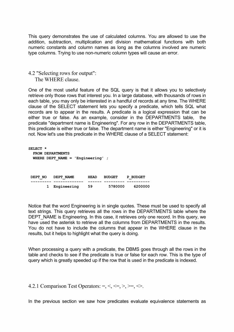
This query demonstrates the use of calculated columns. You are allowed to use the addition, subtraction, multiplication and division mathematical functions with both numeric constants and column names as long as the columns involved are numeric type columns. Trying to use non-numeric column types will cause an error. 4.2 "Selecting rows for output": The WHERE clause. One of the most useful feature of the SQL query is that it allows you to selectively retrieve only those rows that interest you. In a large database, with thousands of rows in each table, you may only be interested in a handful of records at any time. The WHERE clause of the SELECT statement lets you specify a predicate, which tells SQL what records are to appear in the results. A predicate is a logical expression that can be either true or false. As an example, consider in the DEPARTMENTS table, the predicate "department name is Engineering". For any row in the DEPARTMENTS table, this predicate is either true or false. The department name is either "Engineering" or it is not. Now let's use this predicate in the WHERE clause of a SELECT statement: SELECT * FROM DEPARTMENTS WHERE DEPT_NAME = 'Engineering' ; DEPT_NO DEPT_NAME HEAD BUDGET P_BUDGET --------- ------------- ------ --------- ---------- 1 Engineering 59 5780000 6200000 Notice that the word Engineering is in single quotes. These must be used to specify all text strings. This query retrieves all the rows in the DEPARTMENTS table where the DEPT_NAME is Engineering. In this case, it retrieves only one record. In this query, we have used the asterisk to retrieve all the columns from DEPARTMENTS in the results. You do not have to include the columns that appear in the WHERE clause in the results, but it helps to highlight what the query is doing. When processing a query with a predicate, the DBMS goes through all the rows in the table and checks to see if the predicate is true or false for each row. This is the type of query which is greatly speeded up if the row that is used in the predicate is indexed. 4.2.1 Comparison Test Operators: =, <, <=, >, >=, <>. In the previous section we saw how predicates evaluate equivalence statements as
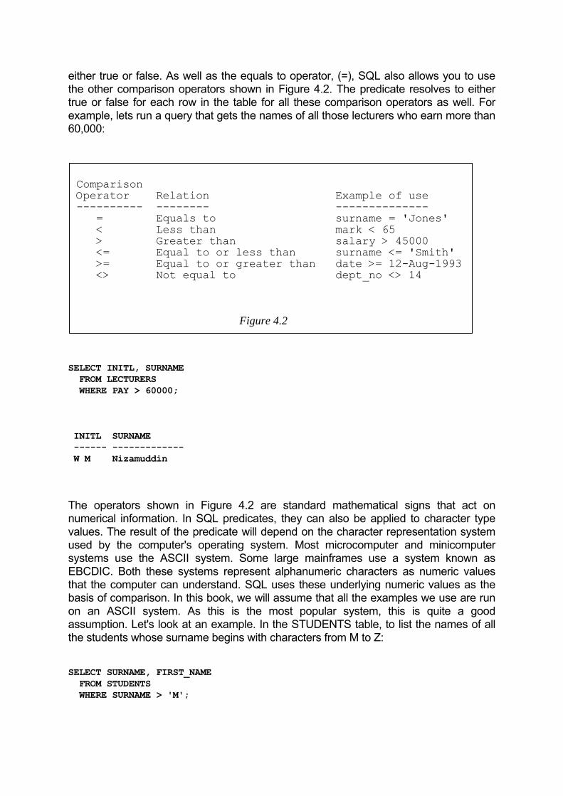
either true or false. As well as the equals to operator, (=), SQL also allows you to use the other comparison operators shown in Figure 4.2. The predicate resolves to either true or false for each row in the table for all these comparison operators as well. For example, lets run a query that gets the names of all those lecturers who earn more than 60,000: Comparison Operator Relation Example of use ---------- -------- -------------- = Equals to surname = 'Jones' < Less than mark < 65 > Greater than salary > 45000 <= Equal to or less than surname <= 'Smith' >= Equal to or greater than date >= 12-Aug-1993 <> Not equal to dept_no <> 14
Figure 4.2 SELECT INITL, SURNAME FROM LECTURERS WHERE PAY > 60000; INITL SURNAME ------ ------------- W M Nizamuddin The operators shown in Figure 4.2 are standard mathematical signs that act on numerical information. In SQL predicates, they can also be applied to character type values. The result of the predicate will depend on the character representation system used by the computer's operating system. Most microcomputer and minicomputer systems use the ASCII system. Some large mainframes use a system known as EBCDIC. Both these systems represent alphanumeric characters as numeric values that the computer can understand. SQL uses these underlying numeric values as the basis of comparison. In this book, we will assume that all the examples we use are run on an ASCII system. As this is the most popular system, this is quite a good assumption. Let's look at an example. In the STUDENTS table, to list the names of all the students whose surname begins with characters from M to Z: SELECT SURNAME, FIRST_NAME FROM STUDENTS WHERE SURNAME > 'M';
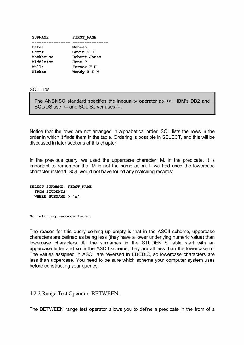
SURNAME FIRST_NAME ---------------- --------------- Patel Mahesh Scott Gavin T J Monkhouse Robert Jones Middleton Jane P Mulla Farook F U Wickes Wendy Y Y W
SQL Tips
The ANSI/ISO standard specifies the inequality operator as <>. IBM's DB2 and SQL/DS use ¬= and SQL Server uses !=.
Notice that the rows are not arranged in alphabetical order. SQL lists the rows in the order in which it finds them in the table. Ordering is possible in SELECT, and this will be discussed in later sections of this chapter. In the previous query, we used the uppercase character, M, in the predicate. It is important to remember that M is not the same as m. If we had used the lowercase character instead, SQL would not have found any matching records: SELECT SURNAME, FIRST_NAME FROM STUDENTS WHERE SURNAME > 'm'; No matching records found. The reason for this query coming up empty is that in the ASCII scheme, uppercase characters are defined as being less (they have a lower underlying numeric value) than lowercase characters. All the surnames in the STUDENTS table start with an uppercase letter and so in the ASCII scheme, they are all less than the lowercase m. The values assigned in ASCII are reversed in EBCDIC, so lowercase characters are less than uppercase. You need to be sure which scheme your computer system uses before constructing your queries. 4.2.2 Range Test Operator: BETWEEN. The BETWEEN range test operator allows you to define a predicate in the from of a
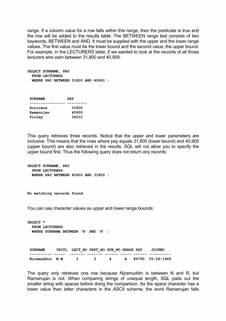
range. If a column value for a row falls within this range, then the predicate is true and the row will be added to the results table. The BETWEEN range test consists of two keywords, BETWEEN and AND. It must be supplied with the upper and the lower range values. The first value must be the lower bound and the second value, the upper bound. For example, in the LECTURERS table, if we wanted to look at the records of all those lecturers who earn between 31,800 and 40,900: SELECT SURNAME, PAY FROM LECTURERS WHERE PAY BETWEEN 31800 AND 40900 ; SURNAME PAY ---------------- --------- Scrivens 31800 Ramanujan 40900 Finley 34210 This query retrieves three records. Notice that the upper and lower parameters are inclusive. This means that the rows where pay equals 31,800 (lower bound) and 40,900 (upper bound) are also retrieved in the results. SQL will not allow you to specify the upper bound first. Thus the following query does not return any records: SELECT SURNAME, PAY FROM LECTURERS WHERE PAY BETWEEN 40900 AND 31800 ; No matching records found. You can use character values as upper and lower range bounds: SELECT * FROM LECTURERS WHERE SURNAME BETWEEN 'N' AND 'R' ; SURNAME INITL LECT_NO DEPT_NO SUB_NO GRADE PAY JOINED ---------- ----- ------- ------- ------ ----- ------ ---------- Nizamuddin W M 3 3 4 A 86790 05-26-1969 The query only retrieves one row because Nizamuddin is between N and R, but Ramanujan is not. When comparing strings of unequal length, SQL pads out the smaller string with spaces before doing the comparison. As the space character has a lower value than letter characters in the ASCII scheme, the word Ramanujan falls
outside the upper bound. BETWEEN does not actually add any new functionality to SQL. All queries that use BETWEEN can be rephrased to run using only the comparison test operators instead. For example the last query can be expressed without using BETWEEN as: SELECT * FROM LECTURERS WHERE (SURNAME >= 'N') AND (SURNAME <= 'R') ; SURNAME INITL LECT_NO DEPT_NO SUB_NO GRADE PAY JOINED ----------- ----- ------- ------- ------ ----- ------ ---------- Nizamuddin W M 3 3 4 A 86790 05-26-1969 The AND keyword is a boolean operator that tells SQL that both expressions inside the parentheses must be true for the predicate to be true. Although this query is functionally the same as the previous query, the one using BETWEEN is more elegant and it is clearer to the reader what the query is trying to achieve. 4.2.3 Set Membership Test Operator: IN. We've seen that BETWEEN defines a range of values to check against for inclusion or exclusion from the results table. This is not always enough. What if you needed to check for certain values only? Values that do not always fit into a neat range. To accommodate this, SQL allows the use of the IN operator. An example will illustrate the use of IN. In the SUBJECTS table, if we wanted to look at the rows of the Anatomy and the Physiology subjects, we could use a query with IN: SELECT * FROM SUBJECTS WHERE SUB_NAME IN ('Anatomy', 'Physiology') ; SUB_NO SUB_NAME DEPT_NO CREDITS PASS ------ ------------- ------- ------- ---- 7 Physiology 6 3 78 8 Anatomy 6 1 74 You must define the set values within parentheses, and must separate each value with a comma. In this example, we have used string values. IN also allows other valid data types to be used as set members for example to list the subjects rows given that their pass marks are 52, 56 and 57:
SELECT SUB_NAME, PASS FROM SUBJECTS WHERE PASS IN (52, 56, 57) ; SUB_NAME PASS -------------------- ---- Industrial Law 52 Organic Chemistry 57 Marketing 56 As with all the SQL query commands, the result records are not displayed in any order unless the ordering is explicitly specified. In the above query for example, we specified pass marks of 52, 56 and 57 in the inclusion set. The results table displayed the rows in the 52, 57, 56 order. The reason for this is that this is the order in which the DBMS found the rows in the table. As with BETWEEN, IN does not add to SQL's functionality. What IN does can also be accomplished by using comparison and boolean operators. For example, the previous query can also be expressed as: SELECT SUB_NAME, PASS FROM SUBJECTS WHERE PASS = 52 OR PASS = 56 OR PASS = 57 ; SUB_NAME PASS --------------------- ---- Industrial Law 52 Organic Chemistry 57 Marketing 56 4.2.4 Pattern Matching Test Operator: LIKE. The LIKE operator is used to match string pattern values. LIKE uses wildcard characters to specify one or more string character values. ANSI/ISO SQL defines two wildcard characters, the underscore (_) and the percent (%). These are the characters that are almost universally used in commercial SQL systems for pattern matching. String pattern matching is useful in cases where you are not sure of the exact string value that you need to search for. For example if you cannot remember the spelling of a person's name:
SELECT * FROM STUDENTS WHERE SURNAME LIKE 'A_ton'; SURNAME FIRST_NAME D_O_B STUDENT_NO DEPT_NO YEAR --------- ----------- ---------- ---------- ------- ---- Ayton Phil J M A 07-13-1967 3 3 1 The underscore character is one of the wildcards, and is used to represent any valid character (one only). In this query, we are not sure if the student's surname is spelt as Ayton or Aeton or even Aiton. The LIKE 'A_ton' predicate tells SQL that the first letter of the surname is 'A' and the last three letters are 'ton', but we are not sure of the second letter. If you are familiar with the MS-DOS or OS/2 or UNIX operating systems, then the _ character performs the same function in SQL as ? does in MS-DOS, and . does in UNIX. The previous query told SQL to retrieve those rows where the second letter of the surname is any valid character. The rest of the pattern ie. the first and the last three letters must match exactly as specified. The second wildcard character you can use in LIKE is the percent (%) character. This is used to represent a sequence of zero or more characters. The percent wildcard in SQL corresponds to the * wildcard in MS-DOS and OS/2 and UNIX. Let's use percent to look at the records of all those students whose surname ends in 'ton': SELECT * FROM STUDENTS WHERE SURNAME LIKE '%ton' ; SURNAME FIRST_NAME D_O_B STUDENT_NO DEPT_NO YEAR --------- ----------- ---------- ---------- ------- ---- Ayton Phil J M A 07-13-1967 3 3 1 You can also mix and match the % and the _ wildcard characters in a single query: SELECT * FROM STUDENTS WHERE SURNAME LIKE 'A_t%' ; SURNAME FIRST_NAME D_O_B STUDENT_NO DEPT_NO YEAR --------- ----------- ---------- ---------- ------- ---- Ayton Phil J M A 07-13-1967 3 3 1
The % and _ characters are themselves legal ASCII characters. Using valid characters as wildcards can cause problems. What if you wanted to use % or _ as part of the string and not as wildcards? SQL's solution to this is to allow you to define and use the escape character. The escape character has a special meaning in the LIKE string in that the character immediately following it is treated as a regular character and not a wildcard. For example suppose we wanted to search for the string '_search%' where % and _ are regular characters and not wildcards, then we could use the following query with the ESCAPE clause: SELECT * FROM SUBJECTS WHERE SUB_NAME LIKE '$_search$%' ESCAPE '$' ; No matching records found. The ESCAPE clause at the end of the query defines the dollar ($) character as the escape character. In the string, '$_search$%', % and _ are treated as characters and not as wildcards. Of course, this query comes up empty because we do not have a subject called '%search_' in the SUBJECTS table. SQL Tips
IBM's DB2, OS/2 Extended Edition, Oracle and SQL Server do not support the ESCAPE clause.
4.2.5 NULL Value Test Operator: IS NULL. As we know NULL values are used to indicate that no data has been defined yet. This is different from blank string values or zero numeric values. Blank and zero values are just that, values. NULL marks the column as not having any definite value. When you use NULLs in SQL expressions, the result will always be undefined. For example, if you wanted to look at the rows in the LECTURERS table where the value for the DEPT_NO field is NULL, the following query will not retrieve the results you want: SELECT SURNAME, DEPT_NO FROM LECTURERS WHERE DEPT_NO = NULL ; SURNAME DEPT_NO --------------- ------- Jones 1 Scrivens 3 Nizamuddin 3
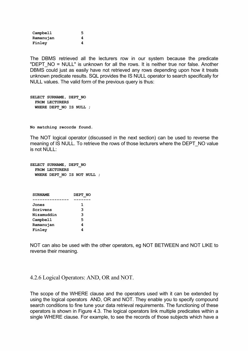
Campbell 5 Ramanujan 4 Finley 4 The DBMS retrieved all the lecturers row in our system because the predicate "DEPT_NO = NULL" is unknown for all the rows. It is neither true nor false. Another DBMS could just as easily have not retrieved any rows depending upon how it treats unknown predicate results. SQL provides the IS NULL operator to search specifically for NULL values. The valid form of the previous query is thus: SELECT SURNAME, DEPT_NO FROM LECTURERS WHERE DEPT_NO IS NULL ; No matching records found. The NOT logical operator (discussed in the next section) can be used to reverse the meaning of IS NULL. To retrieve the rows of those lecturers where the DEPT_NO value is not NULL: SELECT SURNAME, DEPT_NO FROM LECTURERS WHERE DEPT_NO IS NOT NULL ; SURNAME DEPT_NO --------------- ------- Jones 1 Scrivens 3 Nizamuddin 3 Campbell 5 Ramanujan 4 Finley 4 NOT can also be used with the other operators, eg NOT BETWEEN and NOT LIKE to reverse their meaning. 4.2.6 Logical Operators: AND, OR and NOT. The scope of the WHERE clause and the operators used with it can be extended by using the logical operators AND, OR and NOT. They enable you to specify compound search conditions to fine tune your data retrieval requirements. The functioning of these operators is shown in Figure 4.3. The logical operators link multiple predicates within a single WHERE clause. For example, to see the records of those subjects which have a
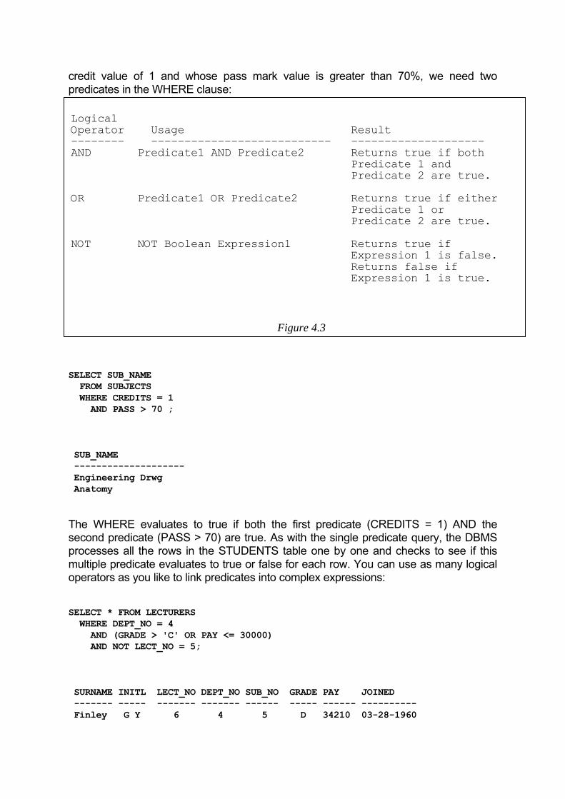
credit value of 1 and whose pass mark value is greater than 70%, we need two predicates in the WHERE clause: Logical Operator Usage Result -------- --------------------------- -------------------- AND Predicate1 AND Predicate2 Returns true if both Predicate 1 and Predicate 2 are true. OR Predicate1 OR Predicate2 Returns true if either Predicate 1 or Predicate 2 are true. NOT NOT Boolean Expression1 Returns true if Expression 1 is false. Returns false if Expression 1 is true.
Figure 4.3 SELECT SUB_NAME FROM SUBJECTS WHERE CREDITS = 1 AND PASS > 70 ; SUB_NAME -------------------- Engineering Drwg Anatomy The WHERE evaluates to true if both the first predicate (CREDITS = 1) AND the second predicate (PASS > 70) are true. As with the single predicate query, the DBMS processes all the rows in the STUDENTS table one by one and checks to see if this multiple predicate evaluates to true or false for each row. You can use as many logical operators as you like to link predicates into complex expressions: SELECT * FROM LECTURERS WHERE DEPT_NO = 4 AND (GRADE > 'C' OR PAY <= 30000) AND NOT LECT_NO = 5; SURNAME INITL LECT_NO DEPT_NO SUB_NO GRADE PAY JOINED ------- ----- ------- ------- ------ ----- ------ ---------- Finley G Y 6 4 5 D 34210 03-28-1960

SQL lets you group expressions by using parentheses. These have the same effect in SQL expressions as they do in mathematical expressions. The expressions inside the parenthesis are evaluated first, and are treated as a single expression. In the above query, AND applies to the expression inside the parenthesis as a whole, ie. GRADE > 'C' OR PAY <= 30000. When you are analyzing complex WHERE clauses, it is best to break the WHERE into it's constituent predicates and reading them in plain english. Let's apply this to the last query. The first search condition is "department number is equal to 4". The AND links this to a parenthesized expression, "either the grade is lower than C or pay is 30000 or less". You need to be careful here because grade D is lower than grade C but the character D is greater than C. The last predicate is slightly more tricky. In english, we would say " lecturer number is not equal to 5". SQL doesn't let you construct this as LECT_NO NOT = 5. The NOT must precede the boolean expression that it operates on. If we now put these all together, the WHERE clause can be expressed as "Where department number is equal to 4 and either the grade is lower than C or pay is 30000 or less and also, the lecturer number is not equal to 5".
SQL Tips
The ANSI/ISO standard specifies that NOT has the highest precedence, followed by AND and then OR.
4.3 "Ordering the output of a query": The ORDER BY clause. In all the queries we've seen so far, the rows in the results table have not been ordered in any way. SQL just retrieved the rows in the order in which it found them in the table. The ORDER BY clause allows you to impose an order on the query results. You can use ORDER BY with one or more column names to specify the ordering of the query results. For example, to list student's records in alphabetical order by surname: SELECT * FROM STUDENTS ORDER BY SURNAME ; SURNAME FIRST_NAME D_O_B STUDENT_NO DEPT_NO YEAR ---------- ------------- ----------- ---------- ------- ---- Al-Essawy Zaid M A 11-26-1970 2 4 2 Ayton Phil J M A 07-13-1967 3 3 1 Baker Abu-Mia 03-13-1971 7 4 1 Brown Joseph P A 04-19-1970 8 3 3 Duke Fitzroy 11-26-1970 1 4 2

Grimm Hans Johan 06-21-1971 10 2 1 Gyver Sue L J V 07-30-1968 11 4 2 Hung-Sun Jimmy Lau 08-11-1969 12 1 3 Jones Gareth P Y 01-24-1970 5 2 1 Layton Hugh 11-16-1971 15 5 1 Middleton Jane P 09-14-1971 13 1 3 Monkhouse Robert Jones 05-23-1967 9 1 1 Mulla Farook F U 10-24-1968 14 3 2 Patel Mahesh 12-07-1970 4 2 1 Scott Gavin T J 02-20-1971 6 2 2 The ORDER BY clause only affects the manner in which these rows are displayed by SQL. If there are NULL values in the ORDER BY column then they appear either at the beginning or at the end of the list depending on your dialect of SQL. This query listed the student's rows alphabetically by SURNAME, in ascending order. This is the default. We can explicitly specify the ordering by using the ASC (for ascending) and the DESC (for descending) keywords. If we had used DESC in the previous query: SELECT * FROM STUDENTS ORDER BY SURNAME DESC ; SURNAME FIRST_NAME D_O_B STUDENT_NO DEPT_NO YEAR ----------- ------------- ---------- ----------- ------- ---- Wickes Wendy Y Y W 12-05-1969 16 1 1 Scott Gavin T J 02-20-1971 6 2 2 Patel Mahesh 12-07-1970 4 2 1 Mulla Farook F U 10-24-1968 14 3 2 Monkhouse Robert Jones 05-23-1967 9 1 1 Middleton Jane P 09-14-1971 13 1 3 Layton Hugh 11-16-1971 15 5 1 Jones Gareth P Y 01-24-1970 5 2 1 Hung-Sun Jimmy Lau 08-11-1969 12 1 3 Gyver Sue L J V 07-30-1968 11 4 2 Grimm Hans Johan 06-21-1971 10 2 1 Duke Fitzroy 11-26-1970 1 4 2 Brown Joseph P A 04-19-1970 8 3 3 Baker Abu-Mia 03-13-1971 7 4 1 Ayton Phil J M A 07-13-1967 3 3 1 The students are now listed in reverse alphabetical order. Note that ASC is optional. If neither DESC OR ASC is specified then ASC is assumed to be in effect. You can use ORDER BY with more than one column. In this case, SQL will use the first column as the primary ordering field, the second column as the secondary and so on. In our STUDENTS table for example, to list the student's records by departments and
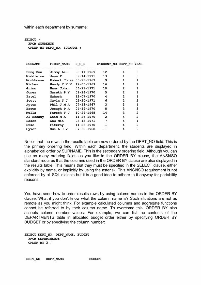
within each department by surname: SELECT * FROM STUDENTS ORDER BY DEPT_NO, SURNAME ; SURNAME FIRST_NAME D_O_B STUDENT_NO DEPT_NO YEAR ----------- ------------ ---------- ---------- ------- ---- Hung-Sun Jimmy Lau 08-11-1969 12 1 3 Middleton Jane P 09-14-1971 13 1 3 Monkhouse Robert Jones 05-23-1967 9 1 1 Wickes Wendy Y Y W 12-05-1969 16 1 1 Grimm Hans Johan 06-21-1971 10 2 1 Jones Gareth P Y 01-24-1970 5 2 1 Patel Mahesh 12-07-1970 4 2 1 Scott Gavin T J 02-20-1971 6 2 2 Ayton Phil J M A 07-13-1967 3 3 1 Brown Joseph P A 04-19-1970 8 3 3 Mulla Farook F U 10-24-1968 14 3 2 Al-Essawy Zaid M A 11-26-1970 2 4 2 Baker Abu-Mia 03-13-1971 7 4 1 Duke Fitzroy 11-26-1970 1 4 2 Gyver Sue L J V 07-30-1968 11 4 2 Notice that the rows in the results table are now ordered by the DEPT_NO field. This is the primary ordering field. Within each department, the students are displayed in alphabetical order by SURNAME. This is the secondary ordering field. Although you can use as many ordering fields as you like in the ORDER BY clause, the ANSI/ISO standard requires that the columns used in the ORDER BY clause are also displayed in the results table. This means that they must be specified in the SELECT clause, either explicitly by name, or implicitly by using the asterisk. This ANSI/ISO requirement is not enforced by all SQL dialects but it is a good idea to adhere to it anyway for portability reasons. You have seen how to order results rows by using column names in the ORDER BY clause. What if you don't know what the column name is? Such situations are not as remote as you might think. For example calculated columns and aggregate functions cannot be referred to by their column name. To overcome this, ORDER BY also accepts column number values. For example, we can list the contents of the DEPARTMENTS table in allocated budget order either by specifying ORDER BY BUDGET or by specifying the column number: SELECT DEPT_NO, DEPT_NAME, BUDGET FROM DEPARTMENTS ORDER BY 3 ; DEPT_NO DEPT_NAME BUDGET

--------- --------------------- ------------ 6 Medicine 6895000 1 Engineering 5780000 5 Physical Sciences 4680000 3 Management Studies 2510000 2 Arts & Humanities 753000 4 Industrial Law 78000 The first column specified in the SELECT clause is always column 1. Subsequent columns have numeric values according to where they are specified in SELECT and not where they occur in the table itself. This applies to calculated columns as well: SELECT DEPT_NAME, (BUDGET * 2.25) FROM DEPARTMENTS ORDER BY 2 ; DEPT_NAME -------------------- ----------- Medicine 775687500 Physical Sciences 526500000 Industrial Law 877500 Management Studies 28237500 Arts & Humanities 8471250 Engineering 65025000 4.4 "Summary of data in tables": The ANSI aggregate functions. The rows in a table are elemental pieces of information that you can use to base your decisions on. Very often, the data that you need can be found directly in one or more columns. But sometimes, the data is based on the values of all the rows in the table. For example, if you need to know the average mark in the exams table, you must add up the marks for all the students, then divide that value by the number of students in the table. ANSI/ISO SQL provides five functions, known as aggregate functions which can be used to summarize data in tables. These functions operate on the table data and produce a single value as output. The five ANSI/ISO functions are: COUNT() outputs the number of rows or column values that would be selected by
the query. The function does not actually list any of the rows, but only a value denoting the total number of rows or column values that the query retrieves.
SUM() outputs the sum total of all the column values that are addressed by the
query. This function can only be used with numeric type columns.

AVG() outputs the average (arithmetic mean) of the column values addressed by the query. As with the SUM() function, AVG() can only be used with numeric type columns.
MIN() outputs the minimum, the smallest, column value from those that are
addressed by the query. MAX() outputs the maximum, the largest, column value from those that are
addressed by the query. Aggregate functions can be used in the select list just like regular columns with the following provisions: You cannot nest aggregate functions and you cannot mix regular columns and aggregate functions in the same query. 4.4.1 The number of values or rows: The COUNT() function. There are two different versions of the COUNT() aggregate function that ANSI/ISO allows. The first counts and lists the number of non-NULL values in a particular column. The second counts and displays the total number of rows that would be retrieved by a query. These two versions of COUNT() differ only in the arguments that are passed to them. Let's use COUNT() to count the number of data values in a column. To find out how many students have been assigned to a department in the STUDENTS table: SELECT COUNT(DEPT_NO) FROM STUDENTS; COUNT(DEPT_NO) -------------- 16 In our case, all the students are assigned a department number and the number output by the query is the same as the number of students there are in the table. If this were not the case, ie. if there were NULL values in the DEPT_NO field for some of the student's rows, then these rows would not appear in the COUNT() function's total. To count the number of different values in a column, the column name must be preceded by the DISTINCT keyword. For example, to look at the number of different departments that are represented in the DEPT_NO field of the STUDENTS table:
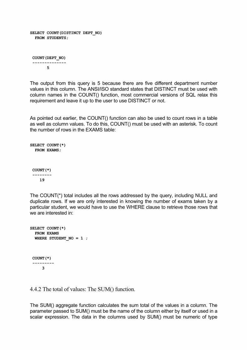
SELECT COUNT(DISTINCT DEPT_NO) FROM STUDENTS; COUNT(DEPT_NO) -------------- 5 The output from this query is 5 because there are five different department number values in this column. The ANSI/ISO standard states that DISTINCT must be used with column names in the COUNT() function, most commercial versions of SQL relax this requirement and leave it up to the user to use DISTINCT or not. As pointed out earlier, the COUNT() function can also be used to count rows in a table as well as column values. To do this, COUNT() must be used with an asterisk. To count the number of rows in the EXAMS table: SELECT COUNT(*) FROM EXAMS; COUNT(*) -------- 19 The COUNT(*) total includes all the rows addressed by the query, including NULL and duplicate rows. If we are only interested in knowing the number of exams taken by a particular student, we would have to use the WHERE clause to retrieve those rows that we are interested in: SELECT COUNT(*) FROM EXAMS WHERE STUDENT_NO = 1 ; COUNT(*) --------- 3 4.4.2 The total of values: The SUM() function. The SUM() aggregate function calculates the sum total of the values in a column. The parameter passed to SUM() must be the name of the column either by itself or used in a scalar expression. The data in the columns used by SUM() must be numeric of type

such as integer, decimal etc. Let's use SUM() to find the total expenditure on staff pay: SELECT SUM(PAY) FROM LECTURERS ; SUM(PAY) -------- 261270 This query adds up all the values in the PAY column and lists the final total. The output of SUM() (and also the other aggregate functions that deal with numeric type data) is usually of the same data type as the column data but sometimes, the result is of greater precision then the column data. You can use scalar expressions as parameters to the aggregate functions. The following query adds 1500 to each lecturer's pay and calculates the sum total: SELECT SUM(PAY), SUM(PAY + 1500) FROM LECTURERS ; SUM(PAY) SUM(PAY+1500) ---------- ------------- 261270 270270 In this simple example, we could have calculated this value by adding 1500 x 6 = 9000 to the SUM(PAY) value. Scalar expressions are most useful when you want to look at say, the total expenditure on pay for a percentage increase in salary for each lecturer. For example, this query finds the total expenditure on pay if we increase each lecturer's salary by 7.5%: SELECT SUM(PAY), SUM(PAY * 1.075) FROM LECTURERS ; SUM(PAY) SUM(PAY*1.075) ----------- -------------- 261270 280865 4.4.3 The average value: The AVG() function. The AVG() function calculates the average or arithmetic mean of the values in a column. AVG() can only be applied to numeric type columns and outputs a numeric value. SQL calculates the average by adding up all the values in the column, then
dividing the total by the number of values. As an example, the following query calculates the average pay for a lecturer: SELECT AVG(PAY) FROM LECTURERS ; AVG(PAY) --------- 43545 We can also selectively calculate averages. This query finds the average mark obtained by students in a particular subject: SELECT AVG(MARK) FROM EXAMS WHERE SUB_NO = 5 ; AVG(MARK) --------- 55 4.4.4 The minimum and maximum values: The MIN() and MAX() functions. The MIN() function finds the smallest value in a column of data. MIN() can operate on string and numeric data types as well as non-ANSI types such as date and time. For example, to find the earliest date when a lecturer joined the staff: SELECT MIN(JOINED) FROM LECTURERS ; MIN(JOINED) ------------- 03-28-1960
SQL Tips
In the EBCDIC character set, which is used in IBM mainframes, the lowercase characters precede the uppercase characters which precede digits.
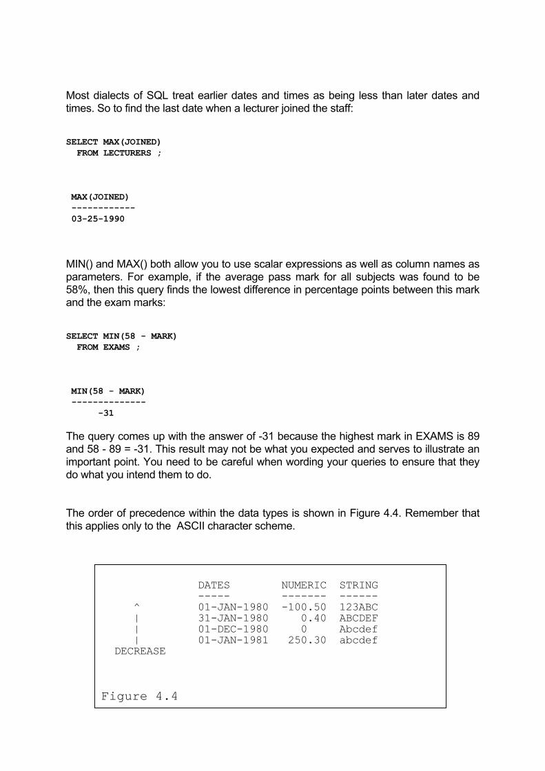
Most dialects of SQL treat earlier dates and times as being less than later dates and times. So to find the last date when a lecturer joined the staff: SELECT MAX(JOINED) FROM LECTURERS ; MAX(JOINED) ------------ 03-25-1990 MIN() and MAX() both allow you to use scalar expressions as well as column names as parameters. For example, if the average pass mark for all subjects was found to be 58%, then this query finds the lowest difference in percentage points between this mark and the exam marks: SELECT MIN(58 - MARK) FROM EXAMS ; MIN(58 - MARK) -------------- -31 The query comes up with the answer of -31 because the highest mark in EXAMS is 89 and 58 - 89 = -31. This result may not be what you expected and serves to illustrate an important point. You need to be careful when wording your queries to ensure that they do what you intend them to do. The order of precedence within the data types is shown in Figure 4.4. Remember that this applies only to the ASCII character scheme.
DATES NUMERIC STRING ----- ------- ------ ^ 01-JAN-1980 -100.50 123ABC | 31-JAN-1980 0.40 ABCDEF | 01-DEC-1980 0 Abcdef | 01-JAN-1981 250.30 abcdef DECREASE
Figure 4.4

SQL Tips
The ANSI/ISO standard specifies that NULL values are ignored by the column functions.
4.4.5 Sub-totals of values: The GROUP BY clause. The aggregate functions described in the previous section have been used to produce grand totals. Values output by them are just like the totals that appear at the end of each column listing in a report. You can also use these functions to output sub-total values. The GROUP BY clause of the SELECT statement lets you split up the values in a column into subsets. The aggregate functions are then applied to these subsets instead of the column as a whole. For example, in the EXAMS table, we could find the average mark obtained by the students by: SELECT AVG(MARK) FROM EXAMS ; AVG(MARK) --------- 55
SQL Tips
SQL Server allows the COMPUTE clause which is used to calculate subtotals of subtotals.
This value is not very informative as the exams were sat by students of all abilities. It would be more meaningful to get the average mark for each student. This can be obtained by using the GROUP BY clause: SELECT STUDENT_NO, AVG(MARK) FROM EXAMS GROUP BY STUDENT_NO ;

STUDENT_NO AVG(MARK) ----------- ---------- 1 62 2 52 3 70 4 42 5 55 6 74 7 45 8 62 This query first groups the rows in the EXAMS table by the values in STUDENT_NO. The AVG() function then operates on each group. The average values output are thus the averages for the exams taken by individual students. Queries using the GROUP BY clause are known as grouped queries. All the rules for using the ANSI/ISO functions that we have looked at also apply to grouped queries. The only difference being that in grouped queries, the DBMS applies the functions to each group individually rather than to the column as a whole. You can also get the same results by running several queries with a WHERE clause. For example, to find the average mark for a student: SELECT STUDENT_NO, AVG(MARK) FROM EXAMS WHERE STUDENT_NO = 1 ; STUDENT_NO AVG(MARK) ----------- --------- 1 65 By changing the 1 value in the predicate, we could calculate the average for different students. GROUP BY can be used with multiple fields. For example, in the SUBJECTS table, to find the highest pass mark for each department/credits combination:

SELECT SUB_NAME, DEPT_NO, CREDITS, MAX(PASS) FROM SUBJECTS GROUP BY DEPT_NO, CREDITS ; SUB_NAME DEPT_NO CREDITS MAX(PASS) ---------------- ------- ------- --------- Engineering Drwg 1 1 71 Mathematics 1 2 65 Electronics 1 3 71 English Lit 2 1 60 Basic Accounts 3 1 67 Marketing 3 2 56 Industrial Law 4 2 52 Organic Chemistry 5 3 57 Anatomy 6 1 74 Physiology 6 3 78
SQL Tips
SQL Server's COMPUTE clause produces non-table results which are, needless to say, highly non-standard.
4.4.6 Eliminating groups of data: The HAVING clause. You cannot use aggregate functions in the WHERE clause of a SELECT statement. This means that you cannot use WHERE to selectively eliminate data that does not interest you from the results of aggregate queries. For example, in the query that we used to find the average mark for each student, if we are only interested in averages that are above 56%, then SQL won't let you use the following query because it uses AVG() in the WHERE clause: SELECT STUDENT_NO, AVG(MARK) FROM EXAMS WHERE AVG(MARK) > 56 GROUP BY STUDENT_NO ; Error 67: Aggregate function used in WHERE. The HAVING clause performs a similar function to WHERE in that it eliminates groups

from the results table. Thus to list only those students where the average is above 56%: SELECT STUDENT_NO, AVG(MARK) FROM EXAMS GROUP BY STUDENT_NO HAVING AVG(MARK) > 56 ; STUDENT_NO AVG(MARK) ----------- ---------- 1 62 3 70 6 74 8 62 The field referenced by HAVING can not have more than one value for each group. This means that in practice HAVING can only reference aggregate functions and columns that are used in GROUP BY. 4.5 "Retrieving data from multiple tables": SQL joins. So far, we've been looking at queries that retrieve data from single table at a time. Single table queries are useful but they do not exploit the full power of the SQL language. SQL is a relational database query language and as such, one of it's most important features is it's ability to retrieve information from several different related tables. In relational database terms, this process is called a join. The tables to be joined are named in the FROM clause of the SELECT with each table name separated by a comma. The relationships between the tables in a join are defined by the predicate in the WHERE clause. The predicate can refer to any column from the joined tables to form the relations. For example, to list the names of all the lecturers and the subjects that they teach: SELECT LECTURERS.SURNAME, SUBJECTS.SUB_NAME FROM LECTURERS, SUBJECTS WHERE LECTURERS.DEPT_NO = SUBJECTS.DEPT_NO ; LECTURERS.SURNAME SUBJECTS.SUB_NAME ------------------ --------------------- Jones Electronics Jones Engineering Drwg Jones Mathematics Scrivens Marketing
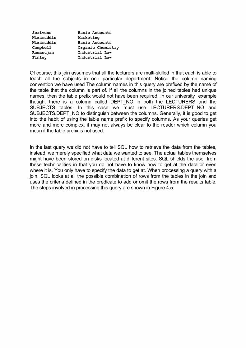
Scrivens Basic Accounts Nizamuddin Marketing Nizamuddin Basic Accounts Campbell Organic Chemistry Ramanujan Industrial Law Finley Industrial Law Of course, this join assumes that all the lecturers are multi-skilled in that each is able to teach all the subjects in one particular department. Notice the column naming convention we have used The column names in this query are prefixed by the name of the table that the column is part of. If all the columns in the joined tables had unique names, then the table prefix would not have been required. In our university example though, there is a column called DEPT_NO in both the LECTURERS and the SUBJECTS tables. In this case we must use LECTURERS.DEPT_NO and SUBJECTS.DEPT_NO to distinguish between the columns. Generally, it is good to get into the habit of using the table name prefix to specify columns. As your queries get more and more complex, it may not always be clear to the reader which column you mean if the table prefix is not used. In the last query we did not have to tell SQL how to retrieve the data from the tables, instead, we merely specified what data we wanted to see. The actual tables themselves might have been stored on disks located at different sites. SQL shields the user from these technicalities in that you do not have to know how to get at the data or even where it is. You only have to specify the data to get at. When processing a query with a join, SQL looks at all the possible combination of rows from the tables in the join and uses the criteria defined in the predicate to add or omit the rows from the results table. The steps involved in processing this query are shown in Figure 4.5.
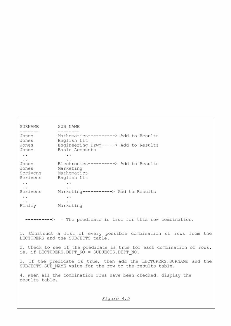
SURNAME SUB_NAME ------- -------- Jones Mathematics----------> Add to Results Jones English Lit Jones Engineering Drwg-----> Add to Results Jones Basic Accounts .. .. .. .. Jones Electronics----------> Add to Results Jones Marketing Scrivens Mathematics Scrivens English Lit .. .. .. .. Scrivens Marketing-----------> Add to Results .. .. .. .. Finley Marketing ----------> = The predicate is true for this row combination. 1. Construct a list of every possible combination of rows from the LECTURERS and the SUBJECTS table.
2. Check to see if the predicate is true for each combination of rows.ie. if LECTURERS.DEPT_NO = SUBJECTS.DEPT_NO.
3. If the predicate is true, then add the LECTURERS.SURNAME and theSUBJECTS.SUB_NAME value for the row to the results table. 4. When all the combination rows have been checked, display the results table.
Figure 4.5
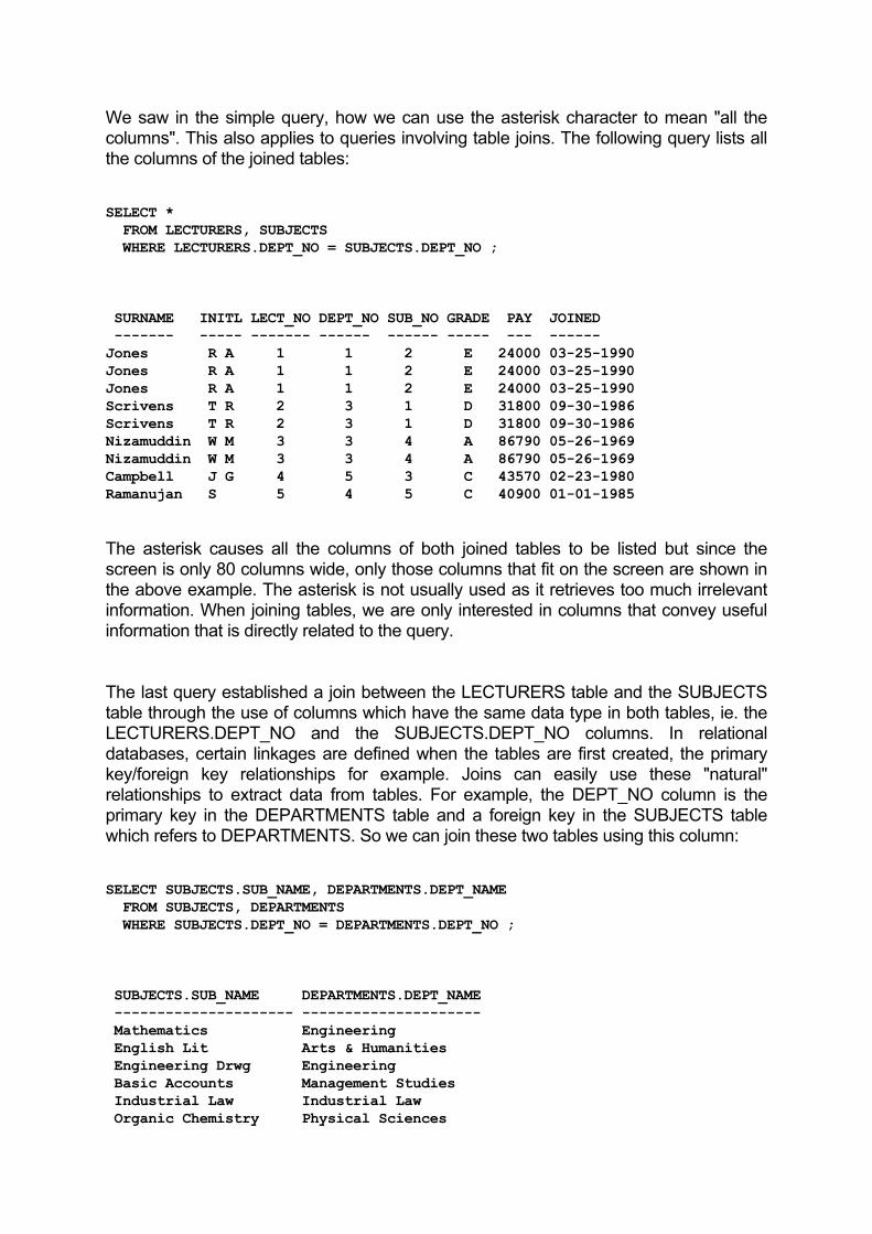
We saw in the simple query, how we can use the asterisk character to mean "all the columns". This also applies to queries involving table joins. The following query lists all the columns of the joined tables: SELECT * FROM LECTURERS, SUBJECTS WHERE LECTURERS.DEPT_NO = SUBJECTS.DEPT_NO ; SURNAME INITL LECT_NO DEPT_NO SUB_NO GRADE PAY JOINED ------- ----- ------- ------ ------ ----- --- ------ Jones R A 1 1 2 E 24000 03-25-1990 Jones R A 1 1 2 E 24000 03-25-1990 Jones R A 1 1 2 E 24000 03-25-1990 Scrivens T R 2 3 1 D 31800 09-30-1986 Scrivens T R 2 3 1 D 31800 09-30-1986 Nizamuddin W M 3 3 4 A 86790 05-26-1969 Nizamuddin W M 3 3 4 A 86790 05-26-1969 Campbell J G 4 5 3 C 43570 02-23-1980 Ramanujan S 5 4 5 C 40900 01-01-1985 The asterisk causes all the columns of both joined tables to be listed but since the screen is only 80 columns wide, only those columns that fit on the screen are shown in the above example. The asterisk is not usually used as it retrieves too much irrelevant information. When joining tables, we are only interested in columns that convey useful information that is directly related to the query. The last query established a join between the LECTURERS table and the SUBJECTS table through the use of columns which have the same data type in both tables, ie. the LECTURERS.DEPT_NO and the SUBJECTS.DEPT_NO columns. In relational databases, certain linkages are defined when the tables are first created, the primary key/foreign key relationships for example. Joins can easily use these "natural" relationships to extract data from tables. For example, the DEPT_NO column is the primary key in the DEPARTMENTS table and a foreign key in the SUBJECTS table which refers to DEPARTMENTS. So we can join these two tables using this column: SELECT SUBJECTS.SUB_NAME, DEPARTMENTS.DEPT_NAME FROM SUBJECTS, DEPARTMENTS WHERE SUBJECTS.DEPT_NO = DEPARTMENTS.DEPT_NO ; SUBJECTS.SUB_NAME DEPARTMENTS.DEPT_NAME --------------------- --------------------- Mathematics Engineering English Lit Arts & Humanities Engineering Drwg Engineering Basic Accounts Management Studies Industrial Law Industrial Law Organic Chemistry Physical Sciences
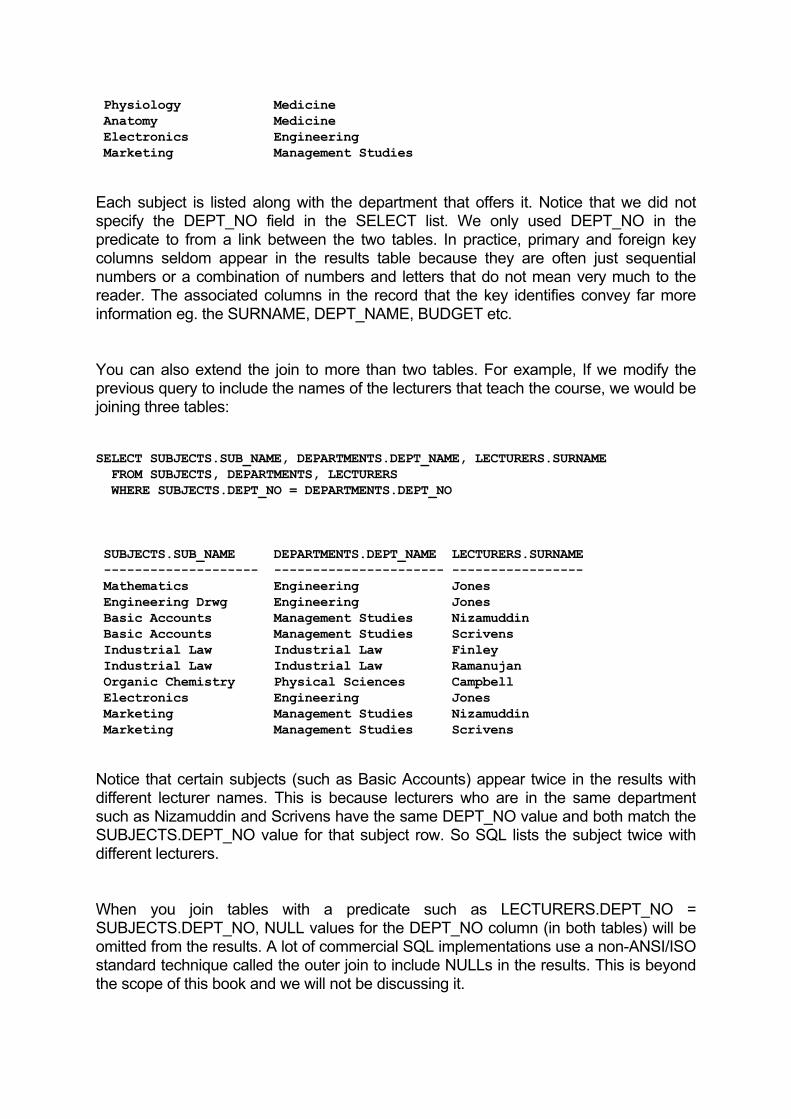
Physiology Medicine Anatomy Medicine Electronics Engineering Marketing Management Studies Each subject is listed along with the department that offers it. Notice that we did not specify the DEPT_NO field in the SELECT list. We only used DEPT_NO in the predicate to from a link between the two tables. In practice, primary and foreign key columns seldom appear in the results table because they are often just sequential numbers or a combination of numbers and letters that do not mean very much to the reader. The associated columns in the record that the key identifies convey far more information eg. the SURNAME, DEPT_NAME, BUDGET etc. You can also extend the join to more than two tables. For example, If we modify the previous query to include the names of the lecturers that teach the course, we would be joining three tables: SELECT SUBJECTS.SUB_NAME, DEPARTMENTS.DEPT_NAME, LECTURERS.SURNAME FROM SUBJECTS, DEPARTMENTS, LECTURERS WHERE SUBJECTS.DEPT_NO = DEPARTMENTS.DEPT_NO SUBJECTS.SUB_NAME DEPARTMENTS.DEPT_NAME LECTURERS.SURNAME -------------------- ---------------------- ----------------- Mathematics Engineering Jones Engineering Drwg Engineering Jones Basic Accounts Management Studies Nizamuddin Basic Accounts Management Studies Scrivens Industrial Law Industrial Law Finley Industrial Law Industrial Law Ramanujan Organic Chemistry Physical Sciences Campbell Electronics Engineering Jones Marketing Management Studies Nizamuddin Marketing Management Studies Scrivens Notice that certain subjects (such as Basic Accounts) appear twice in the results with different lecturer names. This is because lecturers who are in the same department such as Nizamuddin and Scrivens have the same DEPT_NO value and both match the SUBJECTS.DEPT_NO value for that subject row. So SQL lists the subject twice with different lecturers. When you join tables with a predicate such as LECTURERS.DEPT_NO = SUBJECTS.DEPT_NO, NULL values for the DEPT_NO column (in both tables) will be omitted from the results. A lot of commercial SQL implementations use a non-ANSI/ISO standard technique called the outer join to include NULLs in the results. This is beyond the scope of this book and we will not be discussing it.
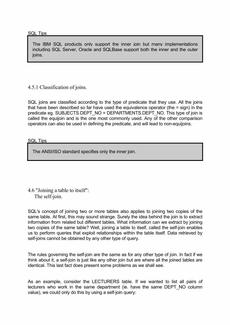
SQL Tips
The IBM SQL products only support the inner join but many implementations including SQL Server, Oracle and SQLBase support both the inner and the outer joins.
4.5.1 Classification of joins. SQL joins are classified according to the type of predicate that they use. All the joins that have been described so far have used the equivalence operator (the = sign) in the predicate eg. SUBJECTS.DEPT_NO = DEPARTMENTS.DEPT_NO. This type of join is called the equijoin and is the one most commonly used. Any of the other comparison operators can also be used in defining the predicate, and will lead to non-equijoins.
SQL Tips
The ANSI/ISO standard specifies only the inner join.
4.6 "Joining a table to itself": The self-join. SQL's concept of joining two or more tables also applies to joining two copies of the same table. At first, this may sound strange. Surely the idea behind the join is to extract information from related but different tables. What information can we extract by joining two copies of the same table? Well, joining a table to itself, called the self-join enables us to perform queries that exploit relationships within the table itself. Data retrieved by self-joins cannot be obtained by any other type of query. The rules governing the self-join are the same as for any other type of join. In fact if we think about it, a self-join is just like any other join but are where all the joined tables are identical. This last fact does present some problems as we shall see. As an example, consider the LECTURERS table. If we wanted to list all pairs of lecturers who work in the same department (ie. have the same DEPT_NO column value), we could only do this by using a self-join query:
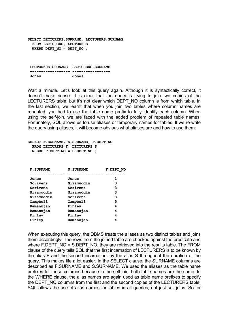
SELECT LECTURERS.SURNAME, LECTURERS.SURNAME FROM LECTURERS, LECTURERS WHERE DEPT_NO = DEPT_NO ; LECTURERS.SURNAME LECTURERS.SURNAME ------------------ ----------------- Jones Jones Wait a minute. Let's look at this query again. Although it is syntactically correct, it doesn't make sense. It is clear that the query is trying to join two copies of the LECTURERS table, but it's not clear which DEPT_NO column is from which table. In the last section, we learnt that when you join two tables where column names are repeated, you had to use the table name prefix to fully identify each column. When using the self-join, we are faced with the added problem of repeated table names. Fortunately, SQL allows us to use aliases or temporary names for tables. If we re-write the query using aliases, it will become obvious what aliases are and how to use them: SELECT F.SURNAME, S.SURNAME, F.DEPT_NO FROM LECTURERS F, LECTURERS S WHERE F.DEPT_NO = S.DEPT_NO ; F.SURNAME S.SURNAME F.DEPT_NO --------------- ---------------- --------- Jones Jones 1 Scrivens Nizamuddin 3 Scrivens Scrivens 3 Nizamuddin Nizamuddin 3 Nizamuddin Scrivens 3 Campbell Campbell 5 Ramanujan Finley 4 Ramanujan Ramanujan 4 Finley Finley 4 Finley Ramanujan 4 When executing this query, the DBMS treats the aliases as two distinct tables and joins them accordingly. The rows from the joined table are checked against the predicate and where F.DEPT_NO = S.DEPT_NO, they are retrieved into the results table. The FROM clause of the query tells SQL that the first incarnation of LECTURERS is to be known by the alias F and the second incarnation, by the alias S throughout the duration of the query. This makes life a lot easier. In the SELECT clause, the SURNAME columns are described as F.SURNAME and S.SURNAME. We used the aliases as the table name prefixes for these columns because in the self-join, both table names are the same. In the WHERE clause, the alias names are again used as table name prefixes to specify the DEPT_NO columns from the first and the second copies of the LECTURERS table. SQL allows the use of alias names for tables in all queries, not just self-joins. So for

example if your database consisted of tables with long names, then you could define and use simple aliases to refer to them instead. You must remember though that the alias only exists for as along as the query is being executed but most commercial implementations allow you to define more permanent aliases for tables called synonyms. Oracle for example lets you use the CREATE SYNONYM statement to assign a permanent alias to a table. The results of the previous self-join query contain redundant data. For example, the first row lists Jones twice. We are only interested in pairs of different lecturers who work in the same department. The first row only lists one lecturer, Jones as being in department 1. To eliminate such redundancy, we need to add an extra condition to the WHERE clause: SELECT F.SURNAME, S.SURNAME, F.DEPT_NO FROM LECTURERS F, LECTURERS S WHERE F.DEPT_NO = S.DEPT_NO AND F.SURNAME <> S.SURNAME ; F.SURNAME S.SURNAME F.DEPT_NO --------------- --------------- --------- Scrivens Nizamuddin 3 Nizamuddin Scrivens 3 Ramanujan Finley 4 Finley Ramanujan 4 Although this last condition gets rid of some of the redundant rows, the remaining pairs of values are still listed twice. eg. Scrivens with Nizamuddin in one row, and Nizamuddin with Scrivens in another. Such repetition is usually eliminated by using > or < instead of <> in the extra condition of the WHERE clause: SELECT F.SURNAME, S.SURNAME, F.DEPT_NO FROM LECTURERS F, LECTURERS S WHERE F.DEPT_NO = S.DEPT_NO AND F.SURNAME > S.SURNAME ; F.SURNAME S.SURNAME F.DEPT_NO --------------- ---------------- --------- Scrivens Nizamuddin 3 Ramanujan Finley 4
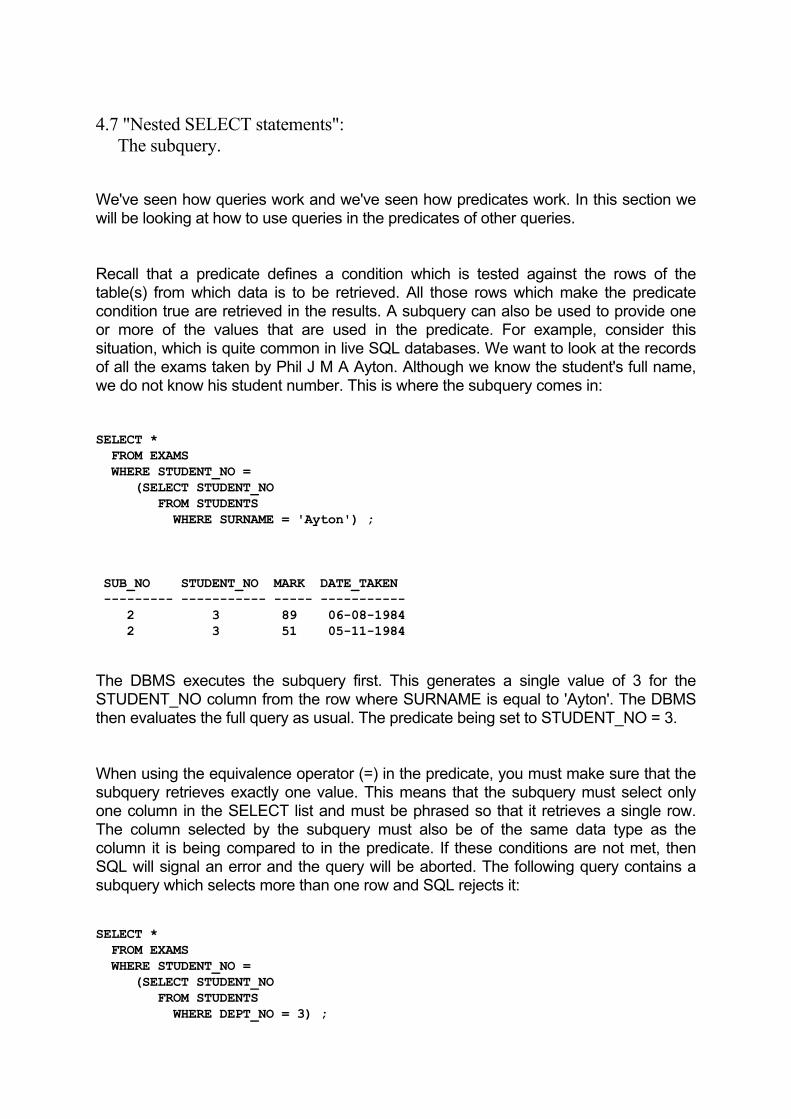
4.7 "Nested SELECT statements": The subquery. We've seen how queries work and we've seen how predicates work. In this section we will be looking at how to use queries in the predicates of other queries. Recall that a predicate defines a condition which is tested against the rows of the table(s) from which data is to be retrieved. All those rows which make the predicate condition true are retrieved in the results. A subquery can also be used to provide one or more of the values that are used in the predicate. For example, consider this situation, which is quite common in live SQL databases. We want to look at the records of all the exams taken by Phil J M A Ayton. Although we know the student's full name, we do not know his student number. This is where the subquery comes in: SELECT * FROM EXAMS WHERE STUDENT_NO = (SELECT STUDENT_NO FROM STUDENTS WHERE SURNAME = 'Ayton') ; SUB_NO STUDENT_NO MARK DATE_TAKEN --------- ----------- ----- ----------- 2 3 89 06-08-1984 2 3 51 05-11-1984 The DBMS executes the subquery first. This generates a single value of 3 for the STUDENT_NO column from the row where SURNAME is equal to 'Ayton'. The DBMS then evaluates the full query as usual. The predicate being set to STUDENT_NO = 3. When using the equivalence operator (=) in the predicate, you must make sure that the subquery retrieves exactly one value. This means that the subquery must select only one column in the SELECT list and must be phrased so that it retrieves a single row. The column selected by the subquery must also be of the same data type as the column it is being compared to in the predicate. If these conditions are not met, then SQL will signal an error and the query will be aborted. The following query contains a subquery which selects more than one row and SQL rejects it: SELECT * FROM EXAMS WHERE STUDENT_NO = (SELECT STUDENT_NO FROM STUDENTS WHERE DEPT_NO = 3) ;

Error 76: The subquery found more than one value. And this variation of the same query selects no rows, and also fails: SELECT * FROM EXAMS WHERE STUDENT_NO = (SELECT STUDENT_NO FROM STUDENTS WHERE DEPT_NO = 365) ; Error 75: The subquery did not find any values. Aggregate functions are allowed in the subquery as long as they do not use the GROUP BY or the HAVING clauses. The reason for this is that aggregate functions on their own operate on the whole column and produce a single value as output. When used with GROUP BY and HAVING, aggregate functions operate on subsets of values in the column and produce one value per group as output. Even if you phrased the subquery with GROUP BY so that the HAVING clause retrieves only one value as output, the query will still be rejected by most SQL systems. You can usually get round this restriction by judicious use of the WHERE clause in the subquery. Let's look at an example of a subquery which uses an aggregate function to get the names of those lecturers who earn less than the average pay for all the lecturers: SELECT SURNAME, PAY FROM LECTURERS WHERE PAY < (SELECT AVG(PAY) FROM LECTURERS) ; SURNAME PAY ---------------- ------- Nizamuddin 86790 Campbell 43570 The ANSI/ISO standard requires that the format of the predicate with subquery cannot change. The subquery always appear after the comparison operator and cannot appear before. Thus, we cannot re-arrange the previous query to read: SELECT * FROM EXAMS WHERE (SELECT STUDENT_NO
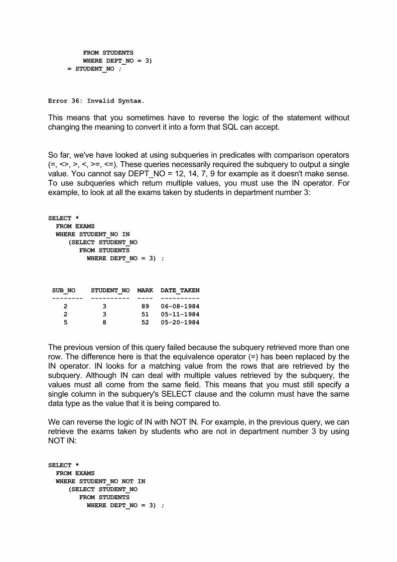
FROM STUDENTS WHERE DEPT_NO = 3) = STUDENT_NO ; Error 36: Invalid Syntax. This means that you sometimes have to reverse the logic of the statement without changing the meaning to convert it into a form that SQL can accept. So far, we've have looked at using subqueries in predicates with comparison operators (=, <>, >, <, >=, <=). These queries necessarily required the subquery to output a single value. You cannot say DEPT_NO = 12, 14, 7, 9 for example as it doesn't make sense. To use subqueries which return multiple values, you must use the IN operator. For example, to look at all the exams taken by students in department number 3: SELECT * FROM EXAMS WHERE STUDENT_NO IN (SELECT STUDENT_NO FROM STUDENTS WHERE DEPT_NO = 3) ; SUB_NO STUDENT_NO MARK DATE_TAKEN -------- ---------- ---- ---------- 2 3 89 06-08-1984 2 3 51 05-11-1984 5 8 52 05-20-1984 The previous version of this query failed because the subquery retrieved more than one row. The difference here is that the equivalence operator (=) has been replaced by the IN operator. IN looks for a matching value from the rows that are retrieved by the subquery. Although IN can deal with multiple values retrieved by the subquery, the values must all come from the same field. This means that you must still specify a single column in the subquery's SELECT clause and the column must have the same data type as the value that it is being compared to. We can reverse the logic of IN with NOT IN. For example, in the previous query, we can retrieve the exams taken by students who are not in department number 3 by using NOT IN: SELECT * FROM EXAMS WHERE STUDENT_NO NOT IN (SELECT STUDENT_NO FROM STUDENTS WHERE DEPT_NO = 3) ;

SUB_NO STUDENT_NO MARK DATE_TAKEN -------- ----------- ---- ---------- 1 1 76 05-23-1984 9 1 42 05-20-1984 3 1 67 05-15-1984 2 2 52 06-05-1984 4 4 34 05-11-1984 10 4 49 06-26-1984 5 5 62 05-03-1984 5 6 70 05-17-1984 5 7 36 05-23-1984 6 9 67 05-15-1984 6 10 82 06-05-1984 6 11 73 06-08-1984 7 12 27 05-11-1984 8 12 56 05-11-1984 8 13 67 06-26-1984 7 13 63 05-03-1984 Because IN uses a set of values to match against, it can also be used in place of the equivalence operator (=). This means that we can rephrase one of our earlier queries as: SELECT * FROM EXAMS WHERE STUDENT_NO IN (SELECT STUDENT_NO FROM STUDENTS WHERE SURNAME = 'Ayton') ; SUB_NO STUDENT_NO MARK DATE_TAKEN -------- ---------- ---- ---------- 2 3 89 06-08-1984 2 3 51 05-11-1984 Here, we've simply replaced the equivalence operator (=) with IN but the query still retrieves exactly the same rows. You might well ask why bother with the equivalence operator at all? Why not use the IN operator all the time? The answer is we could, but the equivalence operator is very useful in highlighting cases where potential errors could affect the results. In the above query for example, if there were two students with the surname Ayton, then the query with IN would have retrieved the exam results for both of them. Looking at the results, you would mistakenly think that these exams were taken by the same person. The version of the query, which used the equivalence operator, would have simply failed if the subquery retrieved two rows for Ayton. When we were discussing aggregate functions, remember we said that the value

supplied to the HAVING clause can also be generated by a subquery. Let's look at an example where this is done: SELECT SUB_NO, SUB_NAME, AVG(MARK) FROM EXAMS GROUP BY SUB_NO HAVING SUB_NO = (SELECT SUB_NO FROM SUBJECTS WHERE PASS = 60) ; SUB_NO SUB_NAME AVG(MARK) ------ -------- --------- 2 English Lit 64 This query calculates the average mark obtained by students in the department whose budget is 2,510,000. The nested queries that we've used so far have all been second level. The ANSI/ISO standard itself does not place any restriction on the number of levels of nesting that you can have, but practical constraints limit nesting to quite a low number. Higher levels of nesting require far greater processing and it becomes difficult for the reader to follow what the query is trying to do. Many implementations of SQL restrict subquery nesting to a low value. You can usually phrase all your queries to fit this level of nesting. 4.8 "Linked SELECT statements": The correlated subquery. We have seen how you can link two or more tables in a single query by using the SQL join operation. In this section, we will look at the correlated subquery. This is another method of extracting data from different tables by linking them through the subquery. A subquery becomes a correlated subquery when it refers to columns from the main query's table. As you will see, correlated subqueries are similar to joins in that they both involve comparing each row of a table against every row of another table. The similarity does not end there. Just as we can join two copies of the same table, so we can also correlate a table to itself. An advanced warning. The concepts of correlated subqueries are probably the most difficult in SQL for a beginner to understand. Don't worry too much if you find this section a bit confusing on the first reading. As we've said before, the best teacher is experience. Try the queries given for yourself, on your own SQL system. Vary the query to see the different results and you will soon grasp the ideas behind correlated subqueries by seeing and by doing.
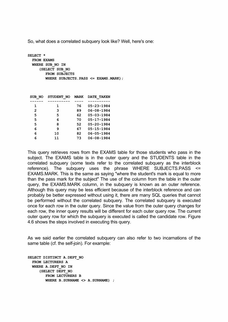
So, what does a correlated subquery look like? Well, here's one: SELECT * FROM EXAMS WHERE SUB_NO IN (SELECT SUB_NO FROM SUBJECTS WHERE SUBJECTS.PASS <= EXAMS.MARK); SUB_NO STUDENT_NO MARK DATE_TAKEN ------ ---------- ---- ---------- 1 1 76 05-23-1984 2 3 89 06-08-1984 5 5 62 05-03-1984 5 6 70 05-17-1984 5 8 52 05-20-1984 6 9 67 05-15-1984 6 10 82 06-05-1984 6 11 73 06-08-1984 This query retrieves rows from the EXAMS table for those students who pass in the subject. The EXAMS table is in the outer query and the STUDENTS table in the correlated subquery (some texts refer to the correlated subquery as the interblock reference). The subquery uses the phrase WHERE SUBJECTS.PASS <= EXAMS.MARK. This is the same as saying "where the student's mark is equal to more than the pass mark for the subject" The use of the column from the table in the outer query, the EXAMS.MARK column, in the subquery is known as an outer reference. Although this query may be less efficient because of the interblock reference and can probably be better expressed without using it, there are many SQL queries that cannot be performed without the correlated subquery. The correlated subquery is executed once for each row in the outer query. Since the value from the outer query changes for each row, the inner query results will be different for each outer query row. The current outer query row for which the subquery is executed is called the candidate row. Figure 4.6 shows the steps involved in executing this query. As we said earlier the correlated subquery can also refer to two incarnations of the same table (cf. the self-join). For example: SELECT DISTINCT A.DEPT_NO FROM LECTURERS A WHERE A.DEPT_NO IN (SELECT DEPT_NO FROM LECTURERS B WHERE B.SURNAME <> A.SURNAME) ;

A.DEPT_NO --------- 3 4 This query lists the department numbers for the departments that have more than one lecturer on staff. SQL runs the subquery once for each A.DEPT_NO (each outer query row). The subquery checks if there is another lecturer who is also in the same department. (it uses the SURNAME field to differentiate between them) This query illustrates the importance of the correlated subquery. It is impossible to perform this type of query without use of the correlated subquery.
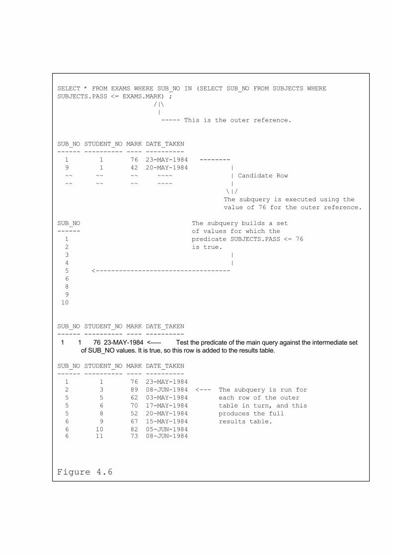
SELECT * FROM EXAMS WHERE SUB_NO IN (SELECT SUB_NO FROM SUBJECTS WHERE SUBJECTS.PASS <= EXAMS.MARK) ;
\|/ The subquery is executed using the
value of 76 for the outer reference.
1 predicate SUBJECTS.PASS <= 76 2 is true.
5 <-----------------------------------
.
SUB_NO STUDENT_NO MARK DATE_TAKEN
5 8 52 20-MAY-1984 produces the full
6 10 82 05-JUN-1984 6 11 73 08-JUN-1984
Figure 4.6
/|\ | ----- This is the outer reference.
SUB_NO STUDENT_NO MARK DATE_TAKEN ------ ---------- ---- ---------- 1 1 76 23-MAY-1984 -------- 9 1 42 20-MAY-1984 | ~~ ~~ ~~ ~~~~ | Candidate Row ~~ ~~ ~~ ~~~~ |
SUB_NO The subquery builds a set ------ of values for which the
3 | 4 |
6 8 9 10
SUB_NO STUDENT_NO MARK DATE_TAKEN ------ ---------- ---- ---------- 1 1 76 23-MAY-1984 <----- Test the predicate of the main query against the intermediate set
of SUB_NO values. It is true, so this row is added to the results table
------ ---------- ---- ---------- 1 1 76 23-MAY-1984 2 3 89 08-JUN-1984 <--- The subquery is run for 5 5 62 03-MAY-1984 each row of the outer 5 6 70 17-MAY-1984 table in turn, and this
6 9 67 15-MAY-1984 results table.

4.9 "Does the subquery retrieve values": The EXISTS operator. The EXISTS operator is used in the predicate of a query just like the IN operator. EXISTS must always have a subquery as its argument and it returns true if the subquery retrieves any values. EXISTS returns false if the subquery does not retrieve any values. As a simplified example consider the following query. It retrieves all the rows in the SUBJECTS table only if there is a subject which has a pass mark of 75% or more: SELECT * FROM SUBJECTS WHERE EXISTS (SELECT * FROM SUBJECTS WHERE PASS >= 75) ; SUB_NO SUB_NAME DEPT_NO CREDITS PASS ------- --------- -------- -------- ----- 7 Physiology 6 3 78 Granted that this query does not make too much sense in the real world, but it does serve to illustrate the use of EXISTS. SQL executes the subquery and finds that there is only one row, the row for Physiology, for which the pass mark is greater than 75%. Because the subquery found a row, EXISTS evaluates to true for all rows in the outer table. The subquery does not make any reference to the outer table columns so it is only run once and not once for each row of the sub-query. The query will thus retrieve all the rows from the SUBJECTS table. Notice that the subquery uses the asterisk in the SELECT clause. This is because EXISTS only checks if output is produced by the subquery. It doesn't care what actual columns are selected or returned. EXISTS can also be used with correlated subqueries. With these, the EXISTS clause is evaluated separately for each row of the outer query table. EXISTS will return true or false depending on the value of each row in the outer query table unlike in the previous example where the subquery was only evaluated once. The following query uses a correlated subquery with EXISTS. It lists the student number for those students who have sat more than one exam: SELECT DISTINCT STUDENT_NO FROM EXAMS A WHERE EXISTS (SELECT * FROM EXAMS B WHERE B.STUDENT_NO = A.STUDENT_NO AND B.SUB_NO <> A.SUB_NO) ;

STUDENT_NO ---------- 1 4 12 13 For each outer query row, the subquery searches the EXAMS table to find rows where the student numbers in both the outer and the inner query are the same. The AND clause eliminates those cases where the student sat more than one exam in the same subject. The DISTINCT keyword is used in the outer query because without it, the query would have listed each student number more than once (once for each exam that they took). The EXISTS examples that we have seen so far have been simple queries with subqueries. EXISTS can also be applied to queries where the outer query joins tables. For example, if we wanted to extend the previous query so that it displayed the student's name as well as the student number, we would have to use a query which joined the EXAMS and the STUDENTS tables: SELECT DISTINCT A.STUDENT_NO, B.SURNAME FROM EXAMS A, STUDENTS B WHERE EXISTS (SELECT * FROM EXAMS C WHERE C.STUDENT_NO = A.STUDENT_NO AND C.STUDENT_NO = B.STUDENT_NO AND C.SUB_NO <> A.SUB_NO) ; A.STUDENT_NO B.SURNAME ------------ ----------------- 1 Duke 4 Patel 12 Hung-Sun 13 Middleton The outer query joins the EXAMS and the STUDENTS tables. The extra AND clause (AND C.STUDENT_NO = B.STUDENT_NO) in the inner query ensures that the subquery only retrieves rows where the STUDENT_NO value from the STUDENTS table matches the STUDENT_NO value from the EXAMS table. This in turn ensures that the right SURNAME value is listed against each STUDENT_NO value in the results table. The meaning of EXISTS is reversed by adding the NOT boolean operator. Thus the

following query lists the student numbers of those students who sat only one exam: SELECT DISTINCT STUDENT_NO FROM EXAMS A WHERE NOT EXISTS (SELECT * FROM EXAMS B WHERE B.STUDENT_NO = A.STUDENT_NO AND B.SUB_NO <> A.SUB_NO) ; STUDENT_NO ---------- 2 3 5 6 7 8 9 10 11 4.10 "Two more subquery operators": The ANY and ALL operators. We have looked at the IN operator and we've also looked at the EXISTS operator. Now let's examine the last two specialized operators used specifically with subqueries. The ANY (also called SOME which is synonymous with ANY) and ALL operators differ from EXISTS in that they can be used with relational operators. SQL Tips
The ANSI/ISO standard specifies that SOME and ANY can be used interchangeably.
The ANY operator evaluates to true if any of the values retrieved by the subquery equal the outer query column value used in the predicate. For example the following query retrieves the names of the lecturers who work in a department which has a budget of more than 3,000,000: SELECT SURNAME, INITL, DEPT_NO FROM LECTURERS A WHERE A.DEPT_NO = ANY
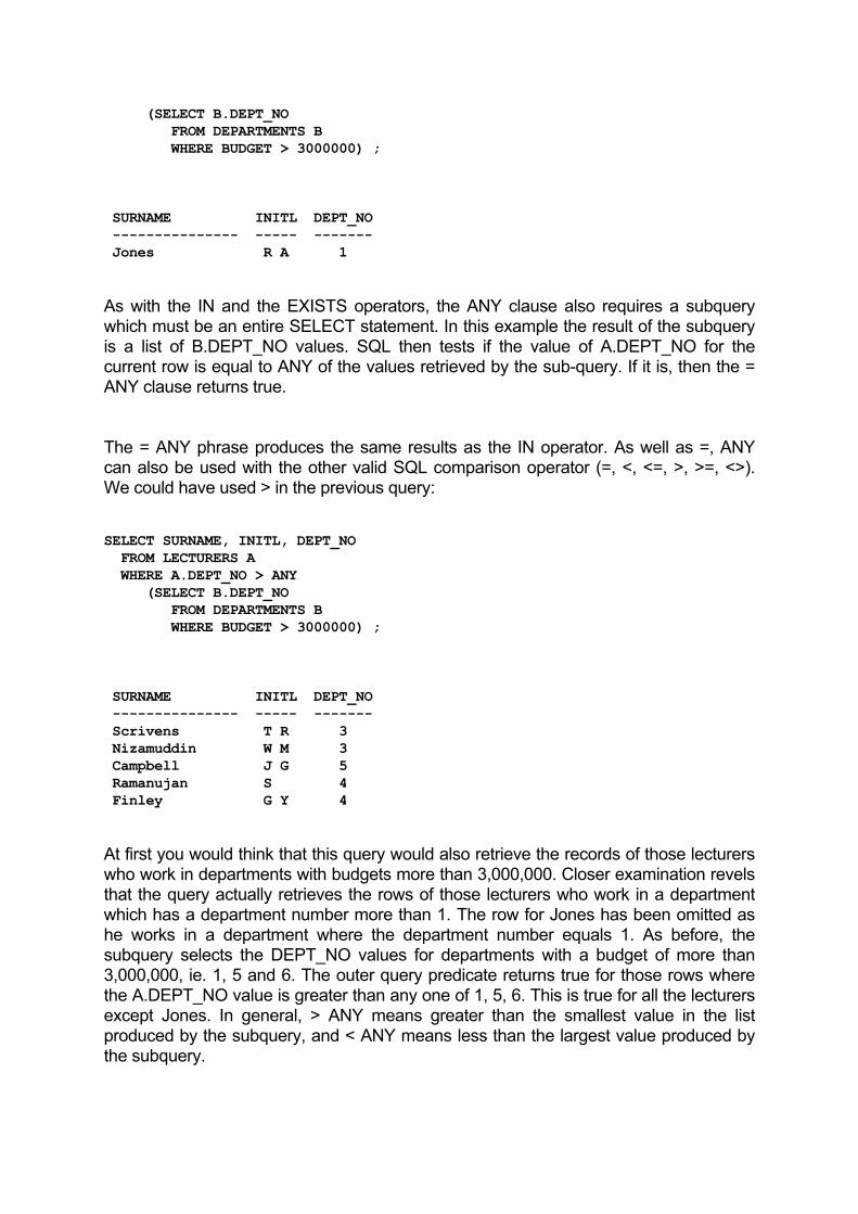
(SELECT B.DEPT_NO FROM DEPARTMENTS B WHERE BUDGET > 3000000) ; SURNAME INITL DEPT_NO --------------- ----- ------- Jones R A 1 As with the IN and the EXISTS operators, the ANY clause also requires a subquery which must be an entire SELECT statement. In this example the result of the subquery is a list of B.DEPT_NO values. SQL then tests if the value of A.DEPT_NO for the current row is equal to ANY of the values retrieved by the sub-query. If it is, then the = ANY clause returns true. The = ANY phrase produces the same results as the IN operator. As well as =, ANY can also be used with the other valid SQL comparison operator (=, <, <=, >, >=, <>). We could have used > in the previous query: SELECT SURNAME, INITL, DEPT_NO FROM LECTURERS A WHERE A.DEPT_NO > ANY (SELECT B.DEPT_NO FROM DEPARTMENTS B WHERE BUDGET > 3000000) ; SURNAME INITL DEPT_NO --------------- ----- ------- Scrivens T R 3 Nizamuddin W M 3 Campbell J G 5 Ramanujan S 4 Finley G Y 4 At first you would think that this query would also retrieve the records of those lecturers who work in departments with budgets more than 3,000,000. Closer examination revels that the query actually retrieves the rows of those lecturers who work in a department which has a department number more than 1. The row for Jones has been omitted as he works in a department where the department number equals 1. As before, the subquery selects the DEPT_NO values for departments with a budget of more than 3,000,000, ie. 1, 5 and 6. The outer query predicate returns true for those rows where the A.DEPT_NO value is greater than any one of 1, 5, 6. This is true for all the lecturers except Jones. In general, > ANY means greater than the smallest value in the list produced by the subquery, and < ANY means less than the largest value produced by the subquery.
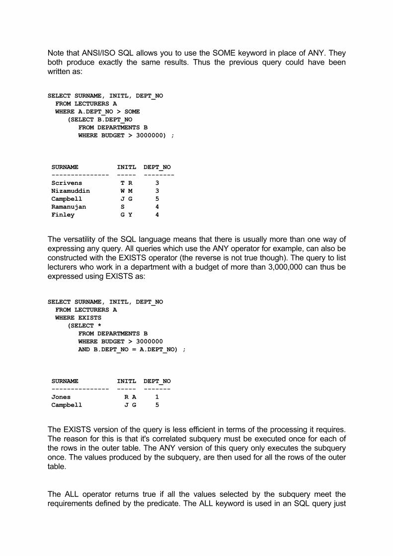
Note that ANSI/ISO SQL allows you to use the SOME keyword in place of ANY. They both produce exactly the same results. Thus the previous query could have been written as: SELECT SURNAME, INITL, DEPT_NO FROM LECTURERS A WHERE A.DEPT_NO > SOME (SELECT B.DEPT_NO FROM DEPARTMENTS B WHERE BUDGET > 3000000) ; SURNAME INITL DEPT_NO --------------- ----- -------- Scrivens T R 3 Nizamuddin W M 3 Campbell J G 5 Ramanujan S 4 Finley G Y 4 The versatility of the SQL language means that there is usually more than one way of expressing any query. All queries which use the ANY operator for example, can also be constructed with the EXISTS operator (the reverse is not true though). The query to list lecturers who work in a department with a budget of more than 3,000,000 can thus be expressed using EXISTS as: SELECT SURNAME, INITL, DEPT_NO FROM LECTURERS A WHERE EXISTS (SELECT * FROM DEPARTMENTS B WHERE BUDGET > 3000000 AND B.DEPT_NO = A.DEPT_NO) ; SURNAME INITL DEPT_NO --------------- ----- ------- Jones R A 1 Campbell J G 5 The EXISTS version of the query is less efficient in terms of the processing it requires. The reason for this is that it's correlated subquery must be executed once for each of the rows in the outer table. The ANY version of this query only executes the subquery once. The values produced by the subquery, are then used for all the rows of the outer table. The ALL operator returns true if all the values selected by the subquery meet the requirements defined by the predicate. The ALL keyword is used in an SQL query just
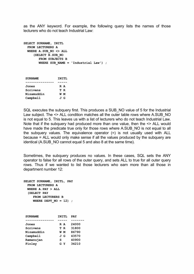
as the ANY keyword. For example, the following query lists the names of those lecturers who do not teach Industrial Law: SELECT SURNAME, INITL FROM LECTURERS A WHERE A.SUB_NO <> ALL (SELECT B.SUB_NO FROM SUBJECTS B WHERE SUB_NAME = 'Industrial Law') ; SURNAME INITL --------------- ----- Jones R A Scrivens T R Nizamuddin W M Campbell J G SQL executes the subquery first. This produces a SUB_NO value of 5 for the Industrial Law subject. The <> ALL condition matches all the outer table rows where A.SUB_NO is not equal to 5. This leaves us with a list of lecturers who do not teach Industrial Law. Note that if the subquery had produced more than one value, then the <> ALL would have made the predicate true only for those rows where A.SUB_NO is not equal to all the subquery values. The equivalence operator (=) is not usually used with ALL because = ALL would only make sense if all the values produced by the subquery are identical (A.SUB_NO cannot equal 5 and also 8 at the same time). Sometimes, the subquery produces no values. In these cases, SQL sets the ANY operator to false for all rows of the outer query, and sets ALL to true for all outer query rows. Thus if we wanted to list those lecturers who earn more than all those in department number 12: SELECT SURNAME, INITL, PAY FROM LECTURERS A WHERE A.PAY > ALL (SELECT PAY FROM LECTURERS B WHERE DEPT_NO = 12) ; SURNAME INITL PAY --------------- ----- ------- Jones R A 24000 Scrivens T R 31800 Nizamuddin W M 86790 Campbell J G 43570 Ramanujan S 40900 Finley G Y 34210

As there are no lecturers in department 12, the subquery comes back empty. This means that the ALL predicate is true for all rows. Thus the query lists all the lecturers because they all earn more then the no-existent lecturers of department 12. Similarly, if we had used ANY instead of ALL: SELECT SURNAME, INITL, PAY FROM LECTURERS A WHERE A.PAY > ANY (SELECT PAY FROM LECTURERS B WHERE DEPT_NO = 12) ; No matching records found. The ANY predicate is now false for all rows. So this query retrieves no rows. 4.11 "Combining multiple queries": The UNION clause. The UNION clause allows you to combine the output of two or more individual queries. UNION differs from subqueries in that it is made up of queries that are independent from each other. UNION combines the output of these individual SELECTs and lists them as part of a single output table. For example, to get a list of all students and lecturers in department number 3: SELECT SURNAME, DEPT_NO FROM STUDENTS WHERE DEPT_NO = 3 UNION SELECT SURNAME, DEPT_NO FROM LECTURERS WHERE DEPT_NO = 3 ; SURNAME DEPT_NO --------------- ------- Ayton 3 Brown 3 Mulla 3 Scrivens 3 Nizamuddin 3 Notice that the output columns don't have column headings. This is because the
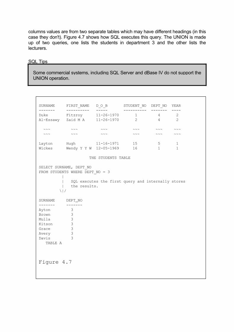
columns values are from two separate tables which may have different headings (in this case they don't). Figure 4.7 shows how SQL executes this query. The UNION is made up of two queries, one lists the students in department 3 and the other lists the lecturers.
SQL Tips
Some commercial systems, including SQL Server and dBase IV do not support the UNION operation.
SURNAME FIRST_NAME D_O_B STUDENT_NO DEPT_NO YEAR ------- ---------- ----- ---------- ------- ---- Duke Fitzroy 11-26-1970 1 4 2 Al-Essawy Zaid M A 11-26-1970 2 4 2
~~~ ~~~ ~~~ ~~~ ~~~ ~~~ ~~~ ~~~ ~~~ ~~~ ~~~ ~~~
| SQL executes the first query and internally stores
\|/ SURNAME DEPT_NO
Ayton 3
TABLE A
Layton Hugh 11-16-1971 15 5 1 Wickes Wendy Y Y W 12-05-1969 16 1 1
THE STUDENTS TABLE SELECT SURNAME, DEPT_NO FROM STUDENTS WHERE DEPT_NO = 3 |
| the results.
------- -------
Brown 3 Mulla 3 Kitson 3 Grace 3 Avery 3 Davis 3
Figure 4.7

SURNAME INITL LECT_NO DEPT_NO SUB_N GRADE PAY JOINED ------- ----- ------- ------- ----- ----- --- ------ Jones R A 1 1 2 E 24000 03-25-1990
FROM LECTURERS WHERE DEPT_NO = 3 |
Brown 3
Kitson 3 Grace 3
Ayton 3 Brown 3
Kitson 3 Grace 3
~~~ ~~~ ~~~ ~~~ ~~~ ~~~ ~~~ ~~~ ~~~ ~~~ ~~~ ~~~ ~~~ ~~~ ~~~ ~~~ Finley G Y 6 4 5 D 34210 03-28-1960 THE LECTURERS TABLE
SELECT SURNAME, DEPT_NO
| SQL executes the second query and internally stores | the results. \|/ | SURNAME DEPT_NO ------- ------- Ayton 3
Mulla 3
Avery 3 Davis 3 TABLE B SQL internally combines results tables A and B and outputs the results as a UNION of these tables.
------- -------
Mulla 3
Avery 3 Davis 3 Scrivens 3 Nizamuddin 3
Figure 4.7 … Continued

The ANSI/ISO standard applies some restrictions on the use of the UNION clause. These include: - The columns selected by the individual SELECT statements must be compatible.
ie. each query must select the same number of columns and each corresponding column must have the same data type.
- If one column is specified as NOT NULL, then the corresponding column in the
other SELECT statements must also be NOT NULL. - The UNION clause cannot be used in subqueries. - The individual SELECT statements in the UNION must not use aggregate
functions. - The individual SELECT statements must not use the ORDER BY clause. The UNION will eliminate duplicate rows from the final results table by default. This is the opposite of SELECT statements, where duplicate rows are included in the results by default. You can instruct SQL to leave the duplicate rows in the results by using UNION ALL instead of UNION. Although you cannot use ORDER BY in the individual queries, you can specify ordering on the results of the UNION itself. For example, to rephrase the previous query and order the results alphabetically by surname: SELECT SURNAME, DEPT_NO FROM LECTURERS WHERE DEPT_NO = (SELECT DEPT_NO FROM DEPARTMENTS WHERE DEPT_NAME = 'Management Studies') UNION SELECT SURNAME, DEPT_NO FROM STUDENTS WHERE DEPT_NO = (SELECT DEPT_NO FROM DEPARTMENTS WHERE DEPT_NAME = 'Management Studies') ORDER BY 1 ; SURNAME DEPT_NO --------------- ------- Ayton 3 Brown 3 Mulla 3

Nizamuddin 3 Scrivens 3 The ORDER BY appears at the end of the UNION and acts on the results produced by it. ORDER BY uses a column number to define the ordering sequence instead of a column name because the results of a UNION query do not show column names. This query also shows us that, we can use subqueries in the individual SELECT statements of the UNION.

Chapter 5 ADDING AND UPDATING DATA. SQL allows data to be added to, updated in and deleted from tables by using the INSERT, UPDATE and DELETE Data Manipulation Language (DML) commands. ANSI/ISO SQL refers to all these commands generically as the update commands and this sometimes causes confusion because UPDATE is also a specific SQL command. In this book, we will be using the word UPDATE to refer to the SQL command and update to refer to the group of commands. When you use any of the DML commands to manipulate the data in the database, the DBMS must be capable of carrying out your request as well as similar requests from other users of the system. This means that the DBMS must protect the overall integrity of the database at all times, preventing the changes made by one user from interfering with those made by other users on the system. 5.1 "Adding Single Rows at a Time": The INSERT command. Records are added to tables by using the INSERT command. Essentially, there are two variations on this command. First, INSERT statements that add records a row at a time. And second, INSERT statements that add several rows at a time. The syntax of the single-row INSERT statement is shown in Figure 5.1. For example, to insert the first row into the STUDENTS table:
INSERT INTO tbl_name [ ( col_ c ) name { , ol_name }* ] VALUES ( value { , value }* ) ; tbl_name The name of the table to insert data into. This must have been previously defined with the CREATE TABLE command. col_name The name of a table column to insert data into. If no column names are mentioned, then it is assumed that data is to be INSERTed for all the columns in the table.
The value to insert into the corresponding table column. CHAR type data must be inside single-quotes. The data in the value list must correspond to the column names specified in the column list.
Figure 5.1
value

INSERT INTO STUDENTS (SURNAME, FIRST_NAME, D_O_B, STUDENT_NO, DEPT_NO, YEAR) VALUES ('Duke', 'Fitzroy', '26-NOV-70', 1, 4, 2); 1 row successfully inserted. Obviously, in order to be able to add data to a table, the table must have already been created by using the CREATE TABLE command. The INSERT command does not produce any output data. On most interactive SQL systems though, the DBMS tells you if rows have been added, and if so, how many. Data can only be INSERTED into tables which the user owns or has INSERT privilege on. In practice, what this means is that you must have created the table or the person who created it must give you permission to insert data by using the GRANT command. The column list is optional in the INSERT statement. If a list of columns is specified, then the values list must contain the same number of items and in the same order. The data type of each column/value pair must also be compatible. If no column names are mentioned, then it is assumed that data is to be INSERTed for all columns. Thus the following is also a valid SQL statement: INSERT INTO STUDENTS VALUES ('Al-Essawy', 'Zaid M A', '26-NOV-70', 2, 4, 2); 1 row successfully inserted. This query also inserts a row into the STUDENTS table, but it does not specify a column list. SQL assumes that data is to be added to all the columns in the table. CHAR type data must be inside single-quotes, ' '. The DATE-TIME type is not defined by ANSI/ISO so different SQL vendors have different specifications on how a DATE-TIME value must be entered. Usually, it is entered as if it is a CHAR type, eg '01271990' or '27-Jan-1990'. You can enter NULLs as column values by using the NULL keyword in place of a column value. In the SUBJECTS table for instance, if you don't know the credits that are awarded for a subject, you could enter NULL for this column: INSERT INTO SUBJECTS VALUES (1, 'Mathematics', 1, NULL, 65 );

1 row successfully inserted. Columns will also be set to NULL (or the default value if one was defined in the CREATE TABLE statement) if they are omitted from the column list. The previous INSERT could also have been expressed as: INSERT INTO SUBJECTS (SUB_NO, SUB_NAME, DEPT_NO, PASS) VALUES (1, 'Mathematics', 1, 65 ); 1 row successfully inserted. The CREDITS column is missing from the column list, so SQL sets the value in this column to the default value. As we have not defined a default value for this column, SQL enters a NULL for this column. 5.2 "Adding Multiple Rows at a Time": The INSERT with SELECT command. The INSERT command can be used to add more than one row at a time to a table if it is used in conjunction with an appropriate SQL query. To do this, the VALUES clause of the INSERT statement must be replaced with a SELECT statement that retrieves the required rows from a second table. As an example, suppose we create a table called ELITE_EXAMS which holds those exam results where students have scored 80% or more. An easy way of populating this table would be to extract the rows from the EXAMS table where the value for the MARK column is 80% or greater. After creating the ELITE_EXAMS table, the following query will populate it: INSERT INTO ELITE_EXAMS SELECT * FROM EXAMS WHERE MARK >= 80 ; 2 rows inserted. In order for this INSERT to work, the ELITE_EXAMS table must have the same column types as the EXAMS table and in the same order. Thus the first two columns of ELITE_EXAMS must be INTEGER types with the third column being DECIMAL and the fourth DATE. Once it is created and populated, the ELITE_EXAMS table is a database entity in its own right. It is not related to the EXAMS table in any way except that it shares some of the values of that table. So if the data in EXAMS changes, then SQL does not pass the changes to ELITE_EXAMS.

The INSERT with SELECT statement can be used with column names if you wish to move only selected columns: INSERT INTO ELITE_EXAMS (E_MARK, E_STUDENT) SELECT MARK, STUDENT_NO FROM EXAMS WHERE MARK >= 80 ; 2 rows inserted. This statement takes only the MARK and the STUDENT_NO columns from EXAMS. Of course, in this case, only the E_MARK and the E_STUDENT columns from ELITE_EXAMS will have valid values. SQL will enter NULLs for the other two columns. In this section, we have so far seen how queries are used with the INSERT statement to add data that already exists in other tables. The SQL update commands, namely INSERT, UPDATE and DELETE, also allow the use of sub-queries as well as queries in targeting rows that you are interested in. As an example consider if we created a table called LOW_BUDGET which holds the records of those students who study in a department with an annual budget of less than 100,000. The data that we need to populate this table already exists in the university database. The following INSERT selects qualifying rows from the STUDENTS table and adds them to the LOW_BUDGET table: INSERT INTO LOW_BUDGET SELECT * FROM STUDENTS WHERE DEPT_NO IN (SELECT DEPT_NO FROM DEPARTMENTS WHERE BUDGET < 100000) ; 4 rows inserted. The query (along with the sub-query) sifts through the STUDENTS and the DEPARTMENTS tables and finds the records of those students where the department that they study in has a budget of less than 100000. It is important to note that the query (or the sub-query) must not make any reference to the table that INSERT is operating on, in our case, LOW_BUDGET. This constraint means that you cannot easily perform updates based on information contained in the table that is going to be updated. In all such cases, the desired update can be accomplished by using two queries. One, a query to get the information from a table and the second to update the table based on this information. Apart from this restriction, all the material described in the section on queries and sub-queries is also applicable to queries and sub-queries used as part on an INSERT statement.
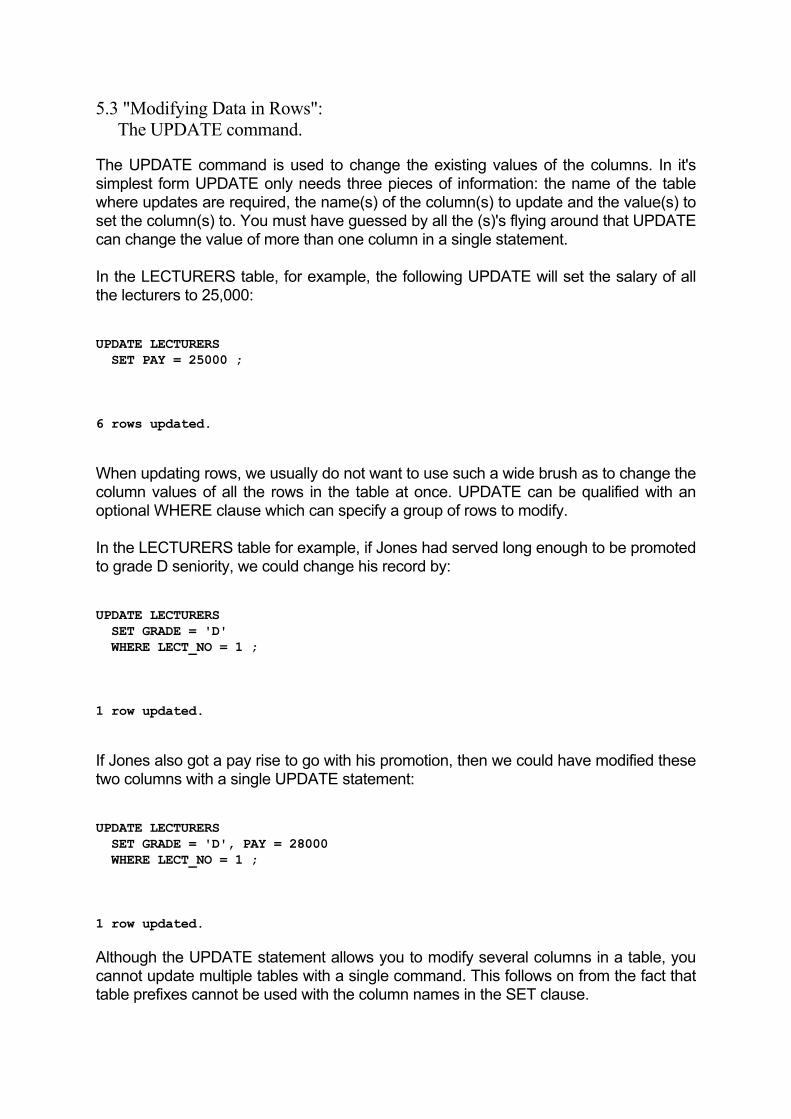
5.3 "Modifying Data in Rows": The UPDATE command. The UPDATE command is used to change the existing values of the columns. In it's simplest form UPDATE only needs three pieces of information: the name of the table where updates are required, the name(s) of the column(s) to update and the value(s) to set the column(s) to. You must have guessed by all the (s)'s flying around that UPDATE can change the value of more than one column in a single statement. In the LECTURERS table, for example, the following UPDATE will set the salary of all the lecturers to 25,000: UPDATE LECTURERS SET PAY = 25000 ; 6 rows updated. When updating rows, we usually do not want to use such a wide brush as to change the column values of all the rows in the table at once. UPDATE can be qualified with an optional WHERE clause which can specify a group of rows to modify. In the LECTURERS table for example, if Jones had served long enough to be promoted to grade D seniority, we could change his record by: UPDATE LECTURERS SET GRADE = 'D' WHERE LECT_NO = 1 ; 1 row updated. If Jones also got a pay rise to go with his promotion, then we could have modified these two columns with a single UPDATE statement: UPDATE LECTURERS SET GRADE = 'D', PAY = 28000 WHERE LECT_NO = 1 ; 1 row updated. Although the UPDATE statement allows you to modify several columns in a table, you cannot update multiple tables with a single command. This follows on from the fact that table prefixes cannot be used with the column names in the SET clause.

Scalar expressions can be used in the SET clause as a multiplication factor for example. This is useful in situations where you need to change the values of a column by a preset amount. In the LECTURERS table for example, if it is university policy to award a set percentage pay increase to all the staff, we can update the PAY column by: UPDATE LECTURERS SET PAY = PAY * 1.05 ; 6 rows updated. The PAY column value for all the lecturers will be multiplied by 1.05 (or in other words, a 5% pay rise). Queries and subqueries can also be used with the UPDATE command just as they can with the INSERT. This enables you to define complex criteria for choosing exactly the rows that you want to be modified. As an example, consider this situation. As a result of human error, all the exam papers for subjects offered by the Engineering department have been marked down by 4 percent. To correct this in the EXAMS table: UPDATE EXAMS SET MARK = MARK + 4 WHERE SUB_NO = ANY (SELECT SUB_NO FROM SUBJECTS WHERE DEPT_NO = 1) ; 2 rows updated. The query part of this UPDATE finds all the subjects which have a value of 1 in the DEPT_NO field. As this is a primary key field which refers to the DEPARTMENTS table, this will only apply to one department, the Engineering department. The subjects offered by this department are Mathematics, Engineering Drwg., and Electronics and are returned by the query. The UPDATE adds 4 percent to all exams in these subjects. The query part of the previous UPDATE requires that you know the value of the DEPT_NO column for the Engineering department. In most real life cases, you will not readily have such information at hand. This means that you will either have to run a separate query on the DEPARTMENTS table to get the value or alternatively, you can compose an UPDATE command with an additional sub-query: UPDATE EXAMS SET MARK = MARK + 4 WHERE SUB_NO = ANY (SELECT SUB_NO FROM SUBJECTS WHERE DEPT_NO = (SELECT DEPT_NO FROM DEPARTMENTS

WHERE DEPT_NAME = 'Engineering') ) ; 2 rows updated. At first, you may have been puzzled at the sequence of chapters in this book. We started by creating tables, then went straight on to discuss how to query the (already populated) tables. We described how to populate and update the tables after the section on querying tables because in order to fully understand the SQL update commands, you need a firm grasp of composing SQL queries. Trying to make sense of the last UPDATE command without 5.4 "Removing Rows Form Tables": The DELETE command. Sooner or later you will want to delete some of the data from your tables. This might be incorrect information or redundant data. SQL allows you to remove data by using the DELETE statement. DELETE allows you to remove one or several rows from tables. This command operates on entire rows. It does not allow you to remove individual field values. You must remove an entire row or not at all. When used without a predicate, DELETE removes all the rows from a table. To clear the ELITE_EXAMS table of all data: DELETE FROM ELITE_EXAMS ; 2 rows deleted. As with all the SQL update commands, before you can delete from a table, you must either be the table's owner or you must have been given the necessary privileges by the owner. Usually, you do not want to delete all the rows from the table. DELETE allows the use of the WHERE clause to selectively remove rows from a table. In the STUDENTS table, suppose that Wendy Wickes decided to leave the course, and we wanted to remove her record from the table. We can do this by: DELETE FROM STUDENTS WHERE SURNAME = 'Wickes' AND FIRST_NAME = 'Wendy Y Y W' ; 1 row deleted.

Although this command does indeed delete the required row from the table, it is not the best method. If there had been another student with the same name, than that student's record would also have been removed with this command. In real life situations, where each table might contain thousands or even hundreds of thousands of rows, we must be absolutely sure that only the row that we want to be removed is deleted. It is good policy to first look at the row that is to be deleted by using a SELECT query, with the same WHERE clause as the intended DELETE statement. To make absolutely sure that only the right row is deleted, it by referenced only by the primary key field in the DELETE statement. Thus to remove Wendy Wickes' record: DELETE FROM STUDENTS WHERE STUDENT_NO = 16 ; 1 row deleted. This is a foolproof method of removing only the intended row from our table. As the STUDENT_NO field is a primary key, it is unique for each row and only Wendy Y Y W Wickes has a value of 16 for this column.

Chapter 6 DATA INTEGRITY This section looks at the concepts used by SQL to restrict the information that can be added to the database. Restrictions are usually thought of as negative (constraints, limitations, confines etc). When they are applied to data integrity, they do a positive job. ie. that of ensuring you do not inadvertently add junk data to the database. Data integrity restrictions in effect, act as policemen for the database. They are responsible for protecting the overall integrity of the database from rogue data that may be introduced by INSERT and UPDATE statements. 6.1 "Keeping the Data Tidy": The Basics of Data Integrity. By definition, a relational database is made up of interrelated tables. The relationships between each table being formed by foreign and primary keys. Data integrity is concerned with ensuring that any new data that is added to the tables is compatible with the existing inter-table relationships. Data integrity is implemented by applying certain restrictions to the data that is added to and updated in a table. These restrictions can be broadly divided into four categories; Non-NULL columns, data validity, table integrity and referential integrity. 6.2 "Fields That Must Have Values": Non-NULL Columns. This type of integrity constraint is the easiest to implement and comply with. It is applied to columns that must have valid values for all rows in the table. These are usually the primary keys which are used to uniquely identify each row and so must have different values for each table row. Non-NULL columns are supported by the ANSI/ISO standard and are implemented by use of the NOT NULL column modifier. A column must be declared as NOT NULL when the table is first created, in the CREATE TABLE statement. Subsequent INSERT statements that add rows to the table are checked by the DBMS to make sure that a value is supplied for the non-NULL declared column. This check also applies to UPDATE statements where the DBMS ensures that the proposed update supplies a value for the non-NULL column. Columns specified as NOT NULL are exactly that. They must contain a value that is not NULL for all rows in the table. This means that you can supply a value of zero for numeric type columns or spaces for character type columns. In ensuring this type of integrity constraint, the DBMS does not check and does not care if the value supplied is total nonsense. For example, the SURNAME column in the STUDENTS table is defined

as NOT NULL. But the DBMS will still allow you to insert a row into STUDENTS even if you specify a SURNAME value of '123QRTY456'. Obviously the surname doesn't make sense, but as it is a non-NULL value, the DBMS accepts it. 6.3 "Values Must be the Right Values": Data Validity. This type of data integrity constraint addresses the problem that we touched on at the end of the last section. It ensures that the right values are inserted into the columns. The ANSI/ISO standard provides only limited support for confirming data validity. The DBMS only guarantees that any data added to a column is of the same type as the column. Recall that the data type of each column must be specified in the CREATE TABLE statement. This means that if you try to add a text string to a numeric type column, or vice versa, then the DBMS will reject the operation. Data type checking still does not ensure the full validity of the data. We could still add the '123QRTY456' value to the SURNAME column of the STUDENTS table for example. The fact that the value is enclosed in single quotes tells SQL that it is a character string. As far as the DBMS is concerned, it is a legal value for the SURNAME field which was declared as CHAR(15). What we really need to ensure against such errors is a method of defining a range or a set of valid values for each column. Although this is not supported by the current ANSI/ISO standard, many commercial SQL systems vendors provide ways of checking the values that are added to the table. Oracle, for example has data validity checking built into its data entry forms package. This is a separate program which checks the data values as they are entered on a form on the screen. The data values are thus validated before they are submitted to SQL. DB2 also leaves the data validation to separate programs. It allows you to create external programs called validation procedures and assign them to each table. DB2 passes the proposed INSERT and UPDATE column values to the validation procedure which checks it against its defined parameters. Although validation procedures mean that DB2 does not have to extend the SQL language to support validity checking, they have to be created by someone with programming experience. 6.4 "Primary key values must be unique": Entity Integrity. A primary key in a table has the job of uniquely identifying each row in the table. It is a bit like the social security number that is allocated to you by the state. It uniquely identifies you as an individual. Just as there would be serious problems if more than one person was allocated the same social security number, so it is with primary keys. If more than one row in the table had the same value for the primary key, then the DBMS
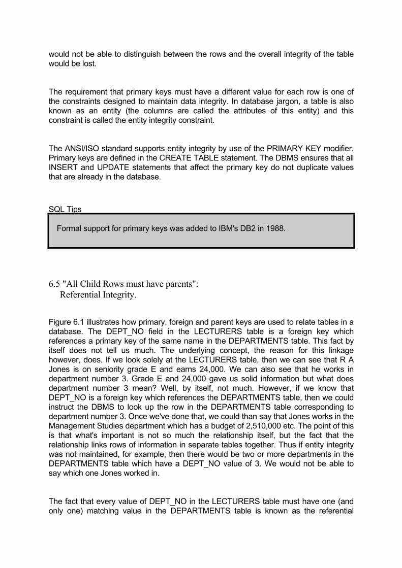
would not be able to distinguish between the rows and the overall integrity of the table would be lost. The requirement that primary keys must have a different value for each row is one of the constraints designed to maintain data integrity. In database jargon, a table is also known as an entity (the columns are called the attributes of this entity) and this constraint is called the entity integrity constraint. The ANSI/ISO standard supports entity integrity by use of the PRIMARY KEY modifier. Primary keys are defined in the CREATE TABLE statement. The DBMS ensures that all INSERT and UPDATE statements that affect the primary key do not duplicate values that are already in the database. SQL Tips
Formal support for primary keys was added to IBM's DB2 in 1988.
6.5 "All Child Rows must have parents": Referential Integrity. Figure 6.1 illustrates how primary, foreign and parent keys are used to relate tables in a database. The DEPT_NO field in the LECTURERS table is a foreign key which references a primary key of the same name in the DEPARTMENTS table. This fact by itself does not tell us much. The underlying concept, the reason for this linkage however, does. If we look solely at the LECTURERS table, then we can see that R A Jones is on seniority grade E and earns 24,000. We can also see that he works in department number 3. Grade E and 24,000 gave us solid information but what does department number 3 mean? Well, by itself, not much. However, if we know that DEPT_NO is a foreign key which references the DEPARTMENTS table, then we could instruct the DBMS to look up the row in the DEPARTMENTS table corresponding to department number 3. Once we've done that, we could than say that Jones works in the Management Studies department which has a budget of 2,510,000 etc. The point of this is that what's important is not so much the relationship itself, but the fact that the relationship links rows of information in separate tables together. Thus if entity integrity was not maintained, for example, then there would be two or more departments in the DEPARTMENTS table which have a DEPT_NO value of 3. We would not be able to say which one Jones worked in. The fact that every value of DEPT_NO in the LECTURERS table must have one (and only one) matching value in the DEPARTMENTS table is known as the referential
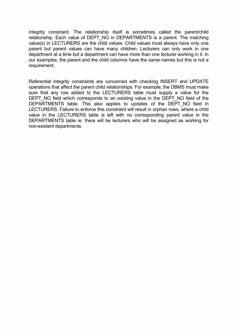
integrity constraint. The relationship itself is sometimes called the parent/child relationship. Each value of DEPT_NO in DEPARTMENTS is a parent. The matching value(s) in LECTURERS are the child values. Child values must always have only one parent but parent values can have many children. Lecturers can only work in one department at a time but a department can have more than one lecturer working in it. In our examples, the parent and the child columns have the same names but this is not a requirement. Referential integrity constraints are concerned with checking INSERT and UPDATE operations that affect the parent child relationships. For example, the DBMS must make sure that any row added to the LECTURERS table must supply a value for the DEPT_NO field which corresponds to an existing value in the DEPT_NO field of the DEPARTMENTS table. This also applies to updates of the DEPT_NO field in LECTURERS. Failure to enforce this constraint will result in orphan rows, where a child value in the LECTURERS table is left with no corresponding parent value in the DEPARTMENTS table ie. there will be lecturers who will be assigned as working for non-existent departments.

/|\
| |
Nizamuddin W M 3 3 4 A 86790 05-26-1969 Campbell J G 4 5 3 C 43570 02-23-1980
THE DEPARTMENTS TABLE DEPT_NO DEPT_NAME HEAD BUDGET P_BUDGET ------- --------- ---- ------ -------- 1 Engineering 59 5780000 6200000 2 Arts & Humanities 23 753000 643000 3 Management Studies 3 2510000 1220000 4 Industrial Law 12 78000 210000 5 Physical Sciences 18 4680000 4250000 6 Medicine 67 6895000 6932000
| | |DEPT_NO in the DEPARTMENTS |table is a primary key. |(parent) | | ------------------------- | |
|DEPT_NO in the LECTURERS table |is a foreign key. |(child) THE LECTURERS TABLE | | SURNAME INITL LECT_NO DEPT_NO SUB_N GRADE PAY JOINED ------- ----- ------- ------- ----- ----- --- ------ Jones R A 1 1 2 E 24000 03-25-1990 Scrivens T R 2 3 1 D 31800 09-30-1986
Ramanujan S 5 4 5 C 40900 01-01-1985 Finley G Y 6 4 5 D 34210 03-28-1960
The foreign key references a parent key which is in almost all cases, a primary key of the referenced table but it needn't be.
Figure 6.1
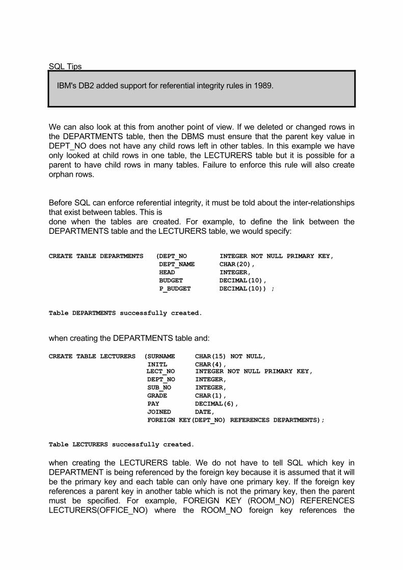
SQL Tips
IBM's DB2 added support for referential integrity rules in 1989.
We can also look at this from another point of view. If we deleted or changed rows in the DEPARTMENTS table, then the DBMS must ensure that the parent key value in DEPT_NO does not have any child rows left in other tables. In this example we have only looked at child rows in one table, the LECTURERS table but it is possible for a parent to have child rows in many tables. Failure to enforce this rule will also create orphan rows. Before SQL can enforce referential integrity, it must be told about the inter-relationships that exist between tables. This is done when the tables are created. For example, to define the link between the DEPARTMENTS table and the LECTURERS table, we would specify: CREATE TABLE DEPARTMENTS (DEPT_NO INTEGER NOT NULL PRIMARY KEY, DEPT_NAME CHAR(20), HEAD INTEGER, BUDGET DECIMAL(10), P_BUDGET DECIMAL(10)) ; Table DEPARTMENTS successfully created. when creating the DEPARTMENTS table and: CREATE TABLE LECTURERS (SURNAME CHAR(15) NOT NULL, INITL CHAR(4), LECT_NO INTEGER NOT NULL PRIMARY KEY, DEPT_NO INTEGER, SUB_NO INTEGER, GRADE CHAR(1), PAY DECIMAL(6), JOINED DATE, FOREIGN KEY(DEPT_NO) REFERENCES DEPARTMENTS); Table LECTURERS successfully created. when creating the LECTURERS table. We do not have to tell SQL which key in DEPARTMENT is being referenced by the foreign key because it is assumed that it will be the primary key and each table can only have one primary key. If the foreign key references a parent key in another table which is not the primary key, then the parent must be specified. For example, FOREIGN KEY (ROOM_NO) REFERENCES LECTURERS(OFFICE_NO) where the ROOM_NO foreign key references the

OFFICE_NO parent key. Some SQL dialects (eg. DB2) allow you to tell the DBMS about rules governing deletions of rows in the parent table. If you want to delete or change parent key values that have associated child rows, then they give you one of three options: 1. You can prohibit the deletion from taking place. This is known as the restrict rule and must be specified in the CREATE TABLE statement of the child table. For example, to apply the restrict rule to the DEPARTMENTS table: CREATE TABLE LECTURERS (SURNAME CHAR(15) NOT NULL, INITL CHAR(4), LECT_NO INTEGER NOT NULL PRIMARY KEY, DEPT_NO INTEGER, SUB_NO INTEGER, GRADE CHAR(1), PAY DECIMAL(6), JOINED DATE, FOREIGN KEY(DEPT_NO) REFERENCES DEPARTMENTS DELETE OF DEPARTMENTS RESTRICTED) ; Table LECTURERS successfully created. If you try to delete a row from the DEPARTMENTS table which has associated child rows in the LECTURERS table, then SQL will reject the command. 2. You can tell the DBMS to apply the changes made to the parent key to the child rows as well. This is known as the cascade rule and it applies only to the UPDATE command. The cascade rule is compatible with the restrict rule. So for example, you can tell the DBMS to reject deletions of parent keys but allow alterations and pass any changes on to the child rows: CREATE TABLE LECTURERS (SURNAME CHAR(15) NOT NULL, INITL CHAR(4), LECT_NO INTEGER NOT NULL PRIMARY KEY, DEPT_NO INTEGER, SUB_NO INTEGER, GRADE CHAR(1), PAY DECIMAL(6), JOINED DATE, FOREIGN KEY(DEPT_NO) REFERENCES DEPARTMENTS DELETE OF DEPARTMENTS RESTRICTED UPDATE OF DEPARTMENTS CASCADES) ; Table LECTURERS successfully created. If you now UPDATE the value of the Physical Sciences row in the DEPARTMENTS

table and set DEPT_NO to 9, then the cascade rule will also update the row of Campbell in the LECTURERS table and set DEPT_NO to 9 as well. Note that if we specified only the cascade rule, then SQL would have allowed deletions of the parent key and it would have cascaded the deletion down to the child rows as well ie. it would have deleted the associated child rows. 3. You can tell the DBMS to allow updates to the parent keys but set the value of the foreign keys to NULL. This rule is known as the set to NULL rule. For example to tell the DBMS to implement the set to NULL rule on the DEPARTMENTS table: CREATE TABLE LECTURERS (SURNAME CHAR(15) NOT NULL, INITL CHAR(4), LECT_NO INTEGER NOT NULL PRIMARY KEY, DEPT_NO INTEGER, SUB_NO INTEGER, GRADE CHAR(1), PAY DECIMAL(6), JOINED DATE, FOREIGN KEY(DEPT_NO) REFERENCES DEPARTMENTS DELETE OF DEPARTMENTS NULLS) ; Table LECTURERS successfully created. For example, if the Physical Sciences department is to be axed, SQL will allow us to delete it's row from the DEPARTMENTS table, but will set the value of DEPT_NO for Campbell's row in the LECTURERS table to NULL. Note that the set to NULL rule will only work on columns that do not have the NOT NULL constraint. It is safer than the "cascade the delete" rule in that child rows are not actually deleted from the tables. 6.6 "Integrity Requirements of the User": SQL Triggers. The integrity constraints that we have seen so far have all been implemented to ensure the validity of the overall data. In a typical organization, there are other rules that apply to normal day to day transactions. These will also need to be reflected in the database, but their non-enforcement will not invalidate the data integrity. For example, say it is university policy that when a new value is added to the BUDGET column in the DEPARTMENTS table, then the old BUDGET value must be written to the P_BUDGET field. The DBMS will not be bothered too much if this rule is not enforced because it does not affect any important database relationships. These types of constraints are non-critical, and the SQL language does not support them directly. To address these integrity requirements (which are important from the user's point of view), some commercial SQL implementations have added what are known as SQL triggers to their functionality. Triggers were first implemented by Sybase in 1986. The concept of triggers is similar to the DB2 concept of validation procedures. You can define a set of operations, collectively called a trigger, that the DBMS must execute

whenever there is a change in the contents of a table. For example, to enforce the rule on alterations to the BUDGET column using Sybase triggers, the command to create the trigger would be: CREATE TRIGGER UPDATE_BUDGET ON DEPARTMENTS FOR UPDATE AS UPDATE DEPARTMENTS SET P_BUDGET = BUDGET FROM DEPARTMENTS, INSERTED WHERE DEPARTMENTS.DEPT_NO = INSERTED.DEPT_NO This command creates a trigger called UPDATE_BUDGET and tells the DBMS to activate it whenever a row is updated in the DEPARTMENTS table. The trigger itself sets the value of P_BUDGET to the current value of BUDGET for the row where the DEPT_NO value matches the DEPT_NO for the update row (Note the new row values are identified by the INSERTED prefix). As with DB2's validation procedures, the complexity of triggers means that they usually require a programmer to set them up. Triggers also add a lot of hidden logic to database operations. Seemingly simple SQL commands may have hidden triggers associated with them which may require a lot of additional processing. To a certain extent, this takes away some control you have over the database.

Chapter 7. VIEWS We've created them, dropped them and used them quite a lot. By now you have a pretty good idea what a database table is and how you can use it store and retrieve information. In this chapter, we will introduce you to another database object (remember that a table is a database object) called the view. Whereas the rows in a table are based on the contents of a physical disk file, the contents of a view are derived from the rows of other tables. In this respect, views are similar to queries in that they too derive a results table based on the contents of other tables. This similarity is more than just coincidence. Views are in fact defined by an SQL query and their contents are the results of executing that query. The difference between queries and views is that views can be queried just like tables. The query defining the view is run (to derive the contents of the view) every time the view becomes the subject of a query. Figure 7.1 shows the relationship between tables and views. In the rest of this chapter, we will be using the term base tables to refer to the actual SQL tables that you have been using so far and virtual tables to refer to views.

---------------------------------- | •♣♦_Jones RA☺☺☺E2400003051990 |-------------------------- | •♣_Scrivens TR☺♥
/\/\/\/\/\/\/\/\/\/\/\/\/\/\/\/\/\ | The computer |
| |
|
|
Jones R A 1 <------ View is generated from: ---- Scrivens T R 2 SELECT SURNAME, INITL, DEPT_NO Nizamuddin W M 3 FROM LECTURERS;
is ultimately based on the
☺D3180009301986 |----------- | | •♣_NizamuddinWM♥♥♦A8679005261969 | | | | | | |
Disk file holds the contents | translates this of the LECTURERS table in | to... | machine readable format. | |
| | | | \|/ |
SURNAME INITL LECT_NO DEPT_NO SUB_N GRADE PAY JOINED | ------- ----- ------- ------- ----- ----- --- ------ | Jones R A 1 1 2 E 24000 03-25-1990| Scrivens T R 2 3 1 D 31800 09-30-1986| Nizamuddin W M 3 3 4 A 86790 05-26-1969| ~~~ ~~~ ~ ~ ~ ~ ~~~ ~~~~ | ~~~ ~~~ ~ ~ ~ ~ ~~~ ~~~~ | The LECTURERS base table is a | computer generated representation | (of the LECTURERS disk file) which | users can understand. | |
| SURNAME INITL DEPT_NO | ------- ----- ------- |
~~~ ~~~ ~ ~~~ ~~~ ~ Like the base table, the view
LECTURERS disk file.
Figure 7.1

7.1 "Restrict the Data You Can See": What is a view? Most textbooks on the subject like to describe views as windows into base tables. The argument being that views let you look at the table as though through a window. Conceptually, this doesn't make sense. The purpose of a window is to look through it and see the outside world in all it's detail. So following on from that, is the idea behind views to look through them and see the contents of the base tables in detail? Not at all. The main point of views is to restrict what you can see of the underlying base tables. The use of views is similar to the use of blinkers. Blinkers are leather sidepieces attached to a horse's bridle which prevent the horse being distracted by side-vision. In the same way, views are applied to tables to prevent users from having access to all the data in the tables. There are four good reasons why we might need to do this. 1. Database security. Views allow you to restrict user's access to only those sections of the database that directly concerns them. In the LECTURERS table for example, you will not want every casual user to be able to access the lecturer's salary information. 2. Data integrity. The DBMS can check the data entered through views to ensure that it meets the conditions defined in the view query. 3. Shielding from change. The view presents a uniform front to the user even if the underlying base table structure is modified, the view can remain constant. 4. Easier querying. Because the view is itself a result of a query, it can reduce complex multi-table queries down to simple SELECT statements. A view cannot be based on more than one query. This means that you are not allowed to use the UNION clause in the view definition (CREATE VIEW) statement. 7.2 "How To Make Views": The CREATE VIEW command. Views are created by the CREATE VIEW command. The syntax of this command is shown in Figure 7.2. You can specify the names of the columns for the view if you wish, but it is optional. For example, to restrict users' view of the LECTURERS table to the first five columns only, you could create a view as: CREATE VIEW TEACHING_STAFF AS SELECT SURNAME, INITL, LECT_NO, DEPT_NO, SUB_NO FROM LECTURERS ; FROM TEACHING_STAFF ; View TEACHING_STAFF successfully created.

REATE VIEW view_name [ READ_ONLY ] C( ) col_name {, col_name }* AS select_statement [ WITH CHECK OPTION ] ; view_name The name of the view. col_name The name of the view's columns. These are optional. select_statement The SELECT statement which is used to create the view.
Figure 7.2 The view is called TEACHING_STAFF and is made up of the first five columns from the LECTURERS table. The names of the columns in the view will be the same as the corresponding columns in the base tables. If as the database administrator, we deny casual users access to the LECTURERS table directly and let them use the view TEACHING_STAFF instead, confidential information such as salary, seniority, grade etc. will be secure. The view can be queried just like any other table: SELECT * FROM TEACHING_STAFF ; SURNAME INITL LECT_NO DEPT_NO SUB_NO ---------------- ----- ------- ------- ------ Jones R A 1 1 2 Scrivens T R 2 3 1 Nizamuddin W M 3 3 4 Campbell J G 4 5 3 Ramanujan S 5 4 5 Finley G Y 6 4 5 To look at the contents of the TEACHING_STAFF view, or: SELECT * FROM TEACHING_STAFF WHERE DEPT_NO = 3 ; SURNAME INITL LECT_NO DEPT_NO SUB_NO --------------- ----- ------- ------- ------ Scrivens T R 2 3 1 Nizamuddin W M 3 3 4

To selectively retrieve rows from the view. The views we have described so far, allow access to only certain columns in the tables, are known as vertical views. You can think of them as being made up of vertical slices (columns) of the base table. Horizontal views as you might have guessed consist of horizontal slices (rows) of data in the table. For example, this command creates a horizontal view which limits access of the STUDENTS table to the rows of first year students only: CREATE VIEW FRESHMEN AS SELECT * FROM STUDENTS WHERE YEAR = 1 ; View FRESHMEN successfully created. The concept of horizontal and vertical views is not absolute in any way. Indeed, most views are a combination of both. For example, this view, which restricts access to certain columns of first year students in the STUDENTS table is both a horizontal and a vertical view: CREATE VIEW FRESHMEN_2 AS SELECT SURNAME, FIRST_NAME, DEPT_NO, YEAR FROM STUDENTS WHERE YEAR = 1 ; View FRESHMEN_2 successfully created. 7.3 "Looking Through the Window": Using Views. When you query a view, you are in fact performing a query on another query. If we query the FRESHMEN_2 view and retrieve those students who study in department 5 as this query does for example: SELECT * FROM FRESHMEN_2 WHERE DEPT_NO = 5 ;

SURNAME FIRST_NAME DEPT_NO YEAR --------------- --------------- ------- ---- Layton Hugh 5 1 then we are in fact looking at those students who are in department 5 and who are also freshmen ie. whose YEAR column has a value of 1. The query is in effect a combination of the query used to create the view and the query and the query operating on the view. Thus the query on the view can also be expressed in terms of the base table as: SELECT SURNAME, FIRST_NAME, DEPT_NO, YEAR FROM STUDENTS WHERE YEAR = 1 AND DEPT_NO = 5 ; SURNAME FIRST_NAME DEPT_NO YEAR --------------- --------------- ------- ---- Layton Hugh 5 1 This combination of view query and the query on the view sometimes leads to problems. For example, this view lists the number of students in each department: CREATE VIEW STUDENT_NUMBERS(DEPT, STUDENTS) AS SELECT DEPT_NO, COUNT(*) FROM STUDENTS GROUP BY DEPT_NO ; View STUDENT_NUMBERS successfully created. A query on this view to find how many departments have more than 5 students, such as: SELECT * FROM STUDENT_NUMBERS WHERE STUDENTS > 5 ; Error 67: Aggregate function used in WHERE. is rejected by SQL. The reason for this is that the combination of the two queries results in an illegal query: SELECT DEPT_NO, COUNT(*) FROM STUDENTS WHERE COUNT(*) > 5 AND GROUP BY DEPT_NO ;

Error 67: Aggregate function used in WHERE. The STUDENTS column in the view is in fact a calculated column based on COUNT(*). SQL does not allow aggregate functions to be used in a predicate so the query is rejected. If you not aware of the underlying query used to create the view, then it appears as if SQL has rejected a perfectly legal query. We listed one of the advantages of using views as leading to easier querying. The chapter on multi-table querying and joins has shown us how complex some SQL queries can get. Views allow you to transfer most of the complex structure of such queries into the view definition itself. Subsequent queries operating on the view will themselves be simple, but the database activity needed to retrieve the results will still be the same. Consider this query which lists the exams taken by students along with the subject and student names. The query implements a three table join: SELECT A.MARK, B.SUB_NAME, C.SURNAME FROM EXAMS A, SUBJECTS B, STUDENTS C WHERE A.SUB_NO = B.SUB_NO AND A.STUDENT_NO = C.STUDENT_NO ; A.MARK B.SUB_NAME C.SURNAME ------ -------------------- ------------ 76 Mathematics Duke 42 Electronics Duke 67 Engineering Drwg Duke 52 English Lit Al-Essawy 89 English Lit Ayton 51 English Lit Ayton 34 Basic Accounts Patel 49 Marketing Patel 62 Industrial Law Jones 70 Industrial Law Scott 36 Industrial Law Baker 52 Industrial Law Brown 67 Organic Chemistry Monkhouse 82 Organic Chemistry Grimm 73 Organic Chemistry Gyver 27 Physiology Hung-Sun 56 Anatomy Hung-Sun 67 Anatomy Middleton 63 Physiology Middleton Additional predicate clauses need to be applied to this basic query to selectively retrieve exam records. Such a query is an ideal candidate for a view. To create a view that joins the EXAMS, the SUBJECTS and the STUDENTS table:
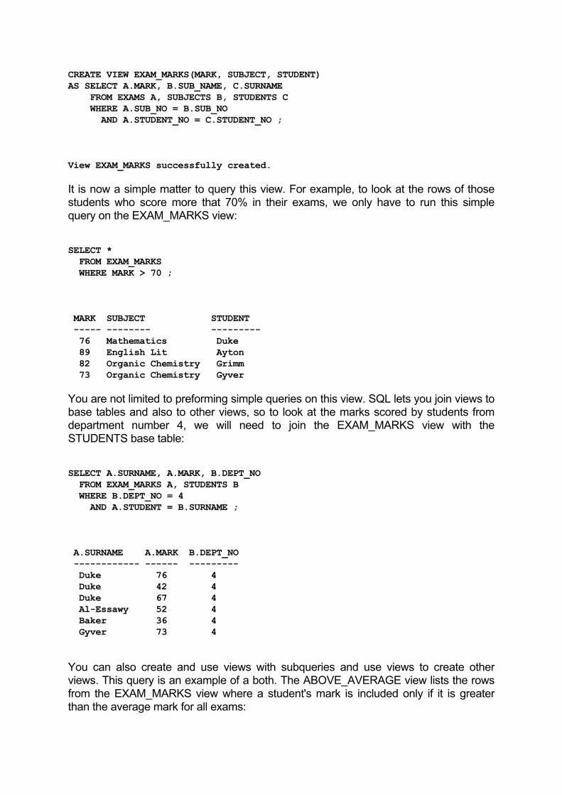
CREATE VIEW EXAM_MARKS(MARK, SUBJECT, STUDENT) AS SELECT A.MARK, B.SUB_NAME, C.SURNAME FROM EXAMS A, SUBJECTS B, STUDENTS C WHERE A.SUB_NO = B.SUB_NO AND A.STUDENT_NO = C.STUDENT_NO ; View EXAM_MARKS successfully created. It is now a simple matter to query this view. For example, to look at the rows of those students who score more that 70% in their exams, we only have to run this simple query on the EXAM_MARKS view: SELECT * FROM EXAM_MARKS WHERE MARK > 70 ; MARK SUBJECT STUDENT ----- -------- --------- 76 Mathematics Duke 89 English Lit Ayton 82 Organic Chemistry Grimm 73 Organic Chemistry Gyver You are not limited to preforming simple queries on this view. SQL lets you join views to base tables and also to other views, so to look at the marks scored by students from department number 4, we will need to join the EXAM_MARKS view with the STUDENTS base table: SELECT A.SURNAME, A.MARK, B.DEPT_NO FROM EXAM_MARKS A, STUDENTS B WHERE B.DEPT_NO = 4 AND A.STUDENT = B.SURNAME ; A.SURNAME A.MARK B.DEPT_NO ------------ ------ --------- Duke 76 4 Duke 42 4 Duke 67 4 Al-Essawy 52 4 Baker 36 4 Gyver 73 4 You can also create and use views with subqueries and use views to create other views. This query is an example of a both. The ABOVE_AVERAGE view lists the rows from the EXAM_MARKS view where a student's mark is included only if it is greater than the average mark for all exams:
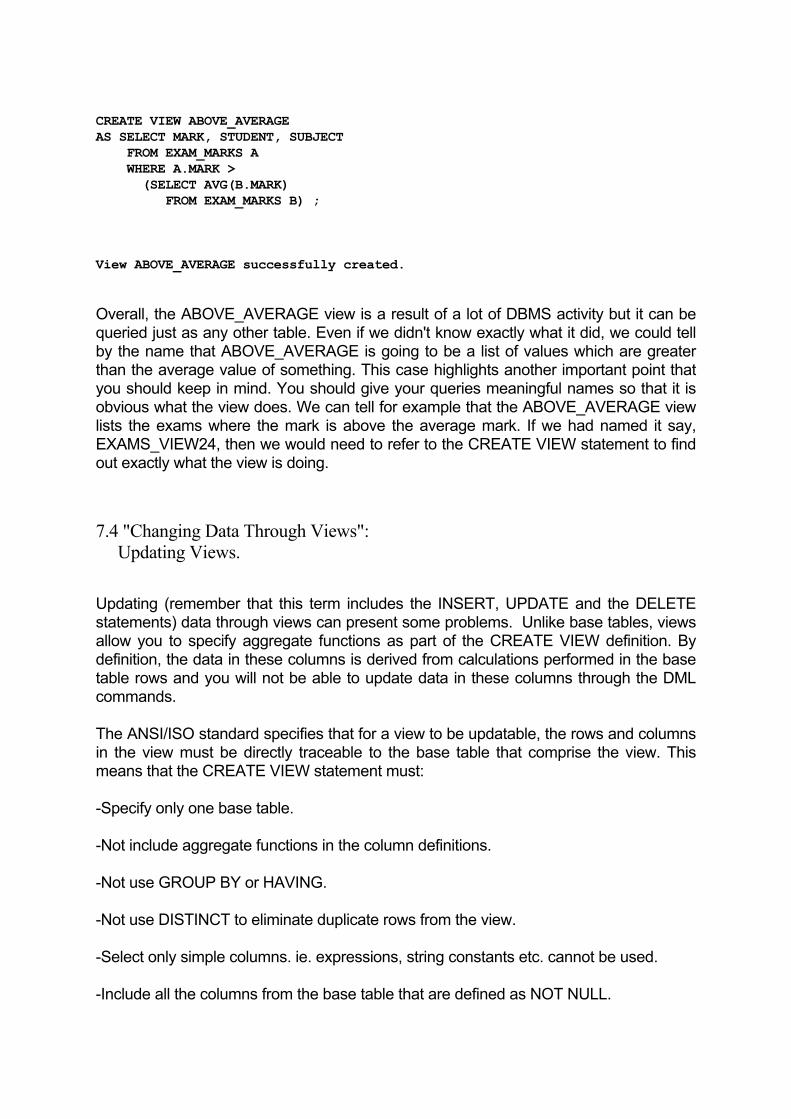
CREATE VIEW ABOVE_AVERAGE AS SELECT MARK, STUDENT, SUBJECT FROM EXAM_MARKS A WHERE A.MARK > (SELECT AVG(B.MARK) FROM EXAM_MARKS B) ; View ABOVE_AVERAGE successfully created. Overall, the ABOVE_AVERAGE view is a result of a lot of DBMS activity but it can be queried just as any other table. Even if we didn't know exactly what it did, we could tell by the name that ABOVE_AVERAGE is going to be a list of values which are greater than the average value of something. This case highlights another important point that you should keep in mind. You should give your queries meaningful names so that it is obvious what the view does. We can tell for example that the ABOVE_AVERAGE view lists the exams where the mark is above the average mark. If we had named it say, EXAMS_VIEW24, then we would need to refer to the CREATE VIEW statement to find out exactly what the view is doing. 7.4 "Changing Data Through Views": Updating Views. Updating (remember that this term includes the INSERT, UPDATE and the DELETE statements) data through views can present some problems. Unlike base tables, views allow you to specify aggregate functions as part of the CREATE VIEW definition. By definition, the data in these columns is derived from calculations performed in the base table rows and you will not be able to update data in these columns through the DML commands. The ANSI/ISO standard specifies that for a view to be updatable, the rows and columns in the view must be directly traceable to the base table that comprise the view. This means that the CREATE VIEW statement must: -Specify only one base table. -Not include aggregate functions in the column definitions. -Not use GROUP BY or HAVING. -Not use DISTINCT to eliminate duplicate rows from the view. -Select only simple columns. ie. expressions, string constants etc. cannot be used. -Include all the columns from the base table that are defined as NOT NULL.

So the view TEACHING_STAFF is updatable because all it's rows relate directly to those of the LECTURERS base table. ie: UPDATE TEACHING_STAFF SET SUB_NO = 9 WHERE LECT_NO = 4 ; 1 row updated. will change the value of SUB_NO 9 for lecturer number 4. The effect will be the same as performing the UPDATE on the LECTURERS base table itself. The STUDENT_NUMBERS view on the other hand is not updatable because its definition contains the aggregate function COUNT(*). 7.5 "Verifying Data Changes": The WITH CHECK Option. Even though a view is updatable, this does not mean that all updates will be trouble free. One particular problem occurs when you add data to through the view. When a row is added to an updatable view, sometimes, it appears as if the row that you added has gone down a black hole. It is never seen in the view again. Acute observers of SQL queries may already have guessed how this can come about. In order to explain it, let's consider an example. Consider the view: CREATE VIEW LOW_CREDITS AS SELECT SUB_NO, SUB_NAME, CREDITS FROM SUBJECTS WHERE CREDITS = 1 ; View LOW_CREDITS successfully created. It limits access of the SUBJECTS table to only those subjects where the value for CREDITS is 1. If we now add a row through the view: INSERT INTO LOW_CREDITS VALUES (11, 'Geology', 2) ; 1 row inserted.
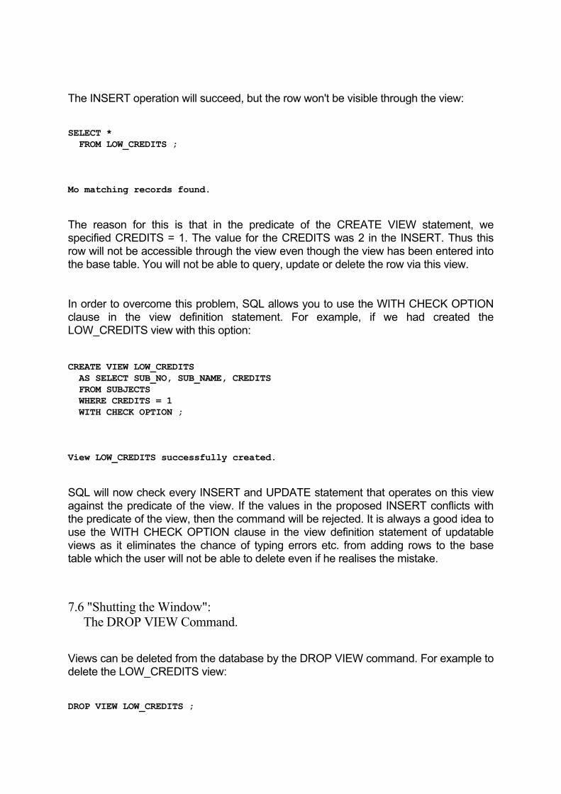
The INSERT operation will succeed, but the row won't be visible through the view: SELECT * FROM LOW_CREDITS ; Mo matching records found. The reason for this is that in the predicate of the CREATE VIEW statement, we specified CREDITS = 1. The value for the CREDITS was 2 in the INSERT. Thus this row will not be accessible through the view even though the view has been entered into the base table. You will not be able to query, update or delete the row via this view. In order to overcome this problem, SQL allows you to use the WITH CHECK OPTION clause in the view definition statement. For example, if we had created the LOW_CREDITS view with this option: CREATE VIEW LOW_CREDITS AS SELECT SUB_NO, SUB_NAME, CREDITS FROM SUBJECTS WHERE CREDITS = 1 WITH CHECK OPTION ; View LOW_CREDITS successfully created. SQL will now check every INSERT and UPDATE statement that operates on this view against the predicate of the view. If the values in the proposed INSERT conflicts with the predicate of the view, then the command will be rejected. It is always a good idea to use the WITH CHECK OPTION clause in the view definition statement of updatable views as it eliminates the chance of typing errors etc. from adding rows to the base table which the user will not be able to delete even if he realises the mistake. 7.6 "Shutting the Window": The DROP VIEW Command. Views can be deleted from the database by the DROP VIEW command. For example to delete the LOW_CREDITS view: DROP VIEW LOW_CREDITS ;

View LOW_CREDITS successfully dropped. The view will be removed from the database and all queries that reference it will fail. Removal of a view does not affect the underlying base tables or any of the records in them.
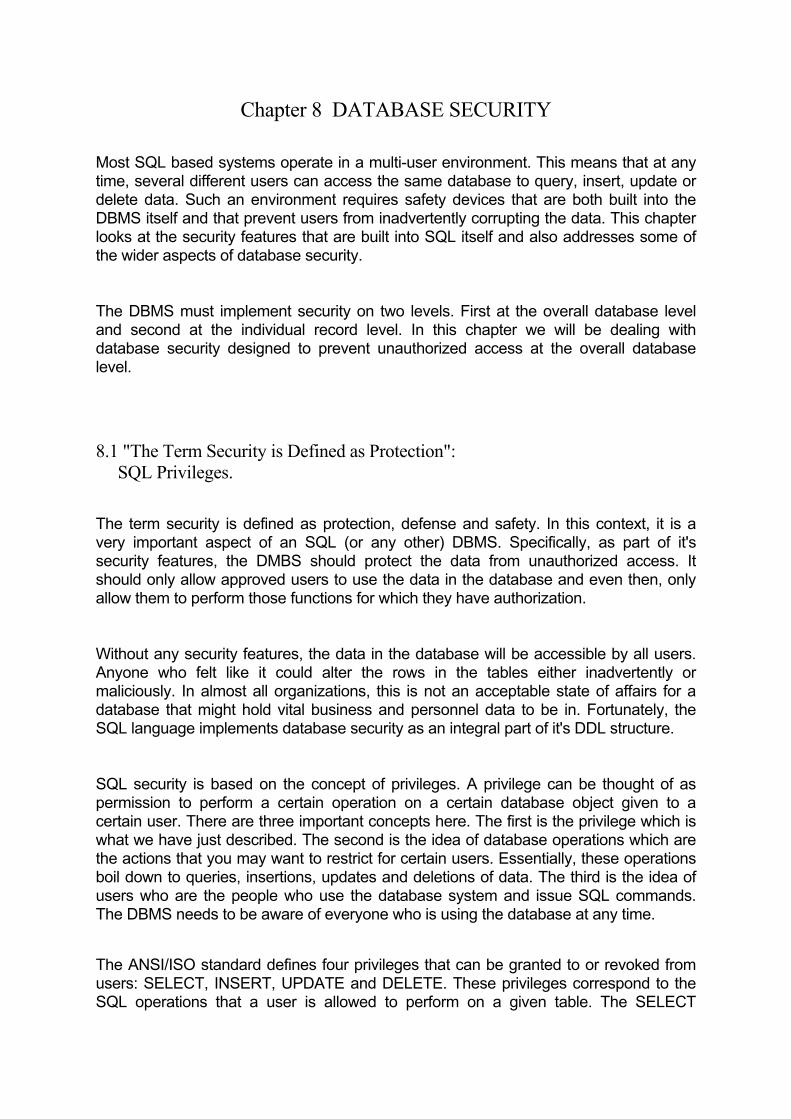
Chapter 8 DATABASE SECURITY Most SQL based systems operate in a multi-user environment. This means that at any time, several different users can access the same database to query, insert, update or delete data. Such an environment requires safety devices that are both built into the DBMS itself and that prevent users from inadvertently corrupting the data. This chapter looks at the security features that are built into SQL itself and also addresses some of the wider aspects of database security. The DBMS must implement security on two levels. First at the overall database level and second at the individual record level. In this chapter we will be dealing with database security designed to prevent unauthorized access at the overall database level. 8.1 "The Term Security is Defined as Protection": SQL Privileges. The term security is defined as protection, defense and safety. In this context, it is a very important aspect of an SQL (or any other) DBMS. Specifically, as part of it's security features, the DMBS should protect the data from unauthorized access. It should only allow approved users to use the data in the database and even then, only allow them to perform those functions for which they have authorization. Without any security features, the data in the database will be accessible by all users. Anyone who felt like it could alter the rows in the tables either inadvertently or maliciously. In almost all organizations, this is not an acceptable state of affairs for a database that might hold vital business and personnel data to be in. Fortunately, the SQL language implements database security as an integral part of it's DDL structure. SQL security is based on the concept of privileges. A privilege can be thought of as permission to perform a certain operation on a certain database object given to a certain user. There are three important concepts here. The first is the privilege which is what we have just described. The second is the idea of database operations which are the actions that you may want to restrict for certain users. Essentially, these operations boil down to queries, insertions, updates and deletions of data. The third is the idea of users who are the people who use the database system and issue SQL commands. The DBMS needs to be aware of everyone who is using the database at any time. The ANSI/ISO standard defines four privileges that can be granted to or revoked from users: SELECT, INSERT, UPDATE and DELETE. These privileges correspond to the SQL operations that a user is allowed to perform on a given table. The SELECT

privilege allows the user to query a table or view. The INSERT privilege allows the user to add rows to a table or view. The DELETE privilege allows the user to delete rows from a table or view and the UPDATE privilege allows the user to modify data in a table or view. Unlike the other three privileges, you can grant UPDATE on selective columns in a table or a view. 8.2 "Users Must Introduce Themselves": The Logon Procedure. In order to be able to implement system wide security, the DBMS needs to be aware of exactly who is using the database at any point in time. To do this, almost all commercial SQL DBMSs rely on the concept of authorization-ids. The authorization-id is a label by which SQL identifies each person who is allowed to issue commands to the DBMS (note that a group of users may have similar requirements and may thus share an authorization-id, but is not very common. Usually, each user has his or her own authorization-id). An authorization-id may also be used to identify a program rather than a person that issues SQL commands. SQL Tips
SQL Server and Sybase support group-ids which can be used to identify groups of users with similar needs.
New users are registered onto the system by the database administrator who must tell the DBMS to add the new user's authorization-id and password to the list of valid users. Some commercial SQL implementations, including Ingres and Informix, use the username that is specified in the host computer's logon procedure as the authorization-id for the user. Other systems including Oracle require users to specify the username and also an associated password at the start of the interactive SQL session. The username is used as the authorization-id, but the password is not used in SQL.
SQL Tips
The ANSI/ISO standard uses the term authorization-id instead of user-id.

8.3 "The Library Database": An example system. For any table that you create, SQL assigns you as the owner of that table. Ownership of tables means that you automatically have full privileges for that table (these are the four standard ANSI/ISO privileges; SELECT, INSERT, UPDATE and DELETE, already described as well as any other non-ANSI privileges that are supported by your particular dialect of SQL). Initially, all the other users of the database will have no privileges on your new table. Figure 8.1 shows a group of users and the lending library database that they use. The structure of this simple database will be explained as we progress through this chapter.

The users:
| |by | | The tables: | |
|_______|_|
|_______|_|
FRANK BARBARA ADAM PUBLIC JONES MORRIS O O O ☺☺☺☺☺☺ O O -|- -|- -|- ☺☺☺☺ -|- -|- I I / \ I I ☺☺ I I I I I I I~I I I ☺☺ I I I I / \ / \ | is owned by | ------------------ | | | | |is owned
------------------ | ---------- |__|_|___|_|__|__|_| -- |__|____|__| |__|_|___|_|__|__|_| |__|____|__| |__|_|___|_|__|__|_| |__|____|__| |__|_|___|_|__|__|_| |__|____|__| |__|_|___|_|__|__|_| |__|____|__| |__|_|___|_|__|__|_| |__|____|__| ------------------ ---------- BOOKS /|\ VIDEOS |is based --- on The views: | ~~~~~~~~~
|_______|_| (Point) |_______|_| --------> TO BARBARA |_______|_|
TITLES THE CONTENTS OF VIDEOS: ('Star Trek','Universal', 'PG') ('Duck Tales','Disney', 'U') THE CONTENTS OF BOOKS: ('English','U.K.Author', 'IN') ('French','E.E.C.Author', 'OUT') THE CONTENTS OF TITLES view: ('German', 'Otto Matic');
Figure 8.1

SQL Tips
The ANSI/ISO standard allows authorization-ids to be up to 18 characters long, but many commercial implementations do not stick to this.
User Frank logs onto the system under the authorization-id FRANK and creates a table called BOOKS by: CREATE TABLE BOOKS ( TITLE CHAR(10), AUTHOR CHAR(15), STATUS CHAR(3)) ; Table BOOKS successfully created. FRANK is now the owner of the BOOKS table. No other user is allowed to access the table. If FRANK adds two rows of data to his table, then SQL accepts this because FRANK has the INSERT privilege on the BOOKS table: INSERT INTO books VALUES ('English','U.K.Author', 'IN'); INSERT INTO books VALUES ('French','E.E.C.Author', 'OUT'); 2 rows successfully inserted. But if user ADAM tries to add a row, then SQL will reject his command because he does not have the necessary privilege: INSERT INTO BOOKS VALUES ('Spanish','E.S.Panya', 'OUT') ; Error 136: User does not have INSERT privileges. Similarly, the VIDEOS table is owned by PUBLIC (this is a special authorization identifier which means that all the users have ownership rights on it), and the view TITLES is owned by BARBARA. Notice that BARBARA doesn't own the BOOKS table on which the view is based.
SQL only lets you create a view, if you have the SELECT privilege on every table used in the view. Ownership of the view will thus guarantee you only the SELECT privilege on it. The other privileges will only be given to you if you already have them for all the base tables used in the view. Thus if you have the INSERT privilege on all of the tables used in the view, then you will also get the INSERT privilege on the view. In the lending library database, user BARBARA must have been granted at least the SELECT and the INSERT privileges on the BOOKS base table in order to be able to create the view and add a row to it. 8.4 "How privileges are passed": The GRANT and REVOKE commands. In all the SQL commands used in this book so far, it was assumed that the user was referring to tables that he either owned or ones for which he had been granted the required privileges by the owner of the table. In live database systems, very few users actually own the tables that they query.
SQL Tips
The ANSI/ISO standard specifies only four privileges for tables and views: SELECT, INSERT, UPDATE and DELETE.
Database users are given access to tables, views (collectively known as database objects) and columns by the GRANT statement. This is part of SQL's DDL (data definition language) and is a part of the ANSI/ISO standard. The opposite of GRANT is REVOKE. Privileges that were granted with GRANT are rescinded by the REVOKE command. REVOKE is not included in the ANSI/ISO standard, but is so widely used that it has become almost a de facto standard. The syntax of the GRANT and REVOKE statements is shown in Figures 8.2 and 8.3 respectively.

GRANT rights ON tbl_name TO auth_id ; [ WITH GRANT OPTION ] rights The rights GRANTed may be: ALL PRIVILEGES | SELECT | INSERT | UPDATE | DELETE { , SELECT | INSERT | UPDATE | DELETE }* tbl_name The table or view name on which privilege(s) are to be GRANTed.This may be up to 24 characters. auth_id The authorization identifier to which privilege(s) are to beGRANTed.
Figure 8.2
REVOKE rights ON tbl_name FROM auth_id ; rights The rights REVOKEd may be: ALL PRIVILEGES | SELECT | INSERT | UPDATE | DELETE { , SELECT | INSERT | UPDATE | DELETE }* tbl_name The table or view name on which privilege(s) are to be REVOKEd. This may be up to 24 characters. auth_id The authorization identifier from which privilege(s) are to be REVOKEd.
Figure 8.3
The table's owner must explicitly grant privileges to all other users who need to use the table. For example, if FRANK wanted to allow BARBARA to be able to query the BOOKS table, then he must grant her the SELECT privilege on BOOKS: GRANT SELECT ON BOOKS TO BARBARA ; Privileges successfully granted. 8.4.1 Using views to limit access to columns. The ANSI/ISO standard doesn't let you to specify columns as arguments to the SELECT privilege command. This means that you must grant SELECT rights for the whole of the table or for none of it. You can get round this stipulation by defining a view which only displays the data that you want the user to see and granting him the SELECT privilege on the view and not on the base table. For example, if BARBARA grants ADAM the SELECT privilege on the TITLES view by: GRANT SELECT ON TITLES TO ADAM ; Privileges successfully granted. then ADAM will be able to query the view as much as he likes, but he won't be able to update the data in the view and he won't have any access to the view's base table. SQL will thus reject this query from ADAM: SELECT * FROM BOOKS; Error 137: User does not have SELECT privileges. A serious drawback with using views solely to implement a security structure is the considerable processing overhead that they incur. Indiscriminate use of views can significantly reduce the response time of the overall database. 8.4.2 The ALL PRIVILEGES and PUBLIC keywords.

Grant allows you to bestow more than one privilege in a single statement, but does not let you specify more than one authorization-id. Thus FRANK can grant all four privileges to BARBARA on the BOOKS table by: GRANT SELECT, INSERT, UPDATE, DELETE ON BOOKS TO BARBARA ; Privileges successfully granted. Some DBMS have broken from the ANSI/ISO standard and allow you to specify a list of authorization-ids as well as privileges in the GRANT statement. For example, this statement is perfectly legal in DB2's SQL dialect: GRANT SELECT, INSERT, UPDATE, DELETE ON TO BARBARA, MORRIS ; Privileges successfully granted. If you want to grant all the available privileges to a user, ANSI/ISO SQL allows you use the ALL PRIVILEGES clause as a shortcut. So if FRANK wants to give all privileges on the BOOKS table to PUBLIC for example, then he could specify: GRANT ALL PRIVILEGES ON BOOKS TO PUBLIC ; Privileges successfully granted. The PUBLIC keyword is a special authorization-id that applies to all users. So the above GRANT statement effectively issues a free for all on the BOOKS table. All users are allowed to perform all operations on BOOKS. This is not a good idea as it means that FRANK now has no control over who is allowed to alter or add data to his table. If an inexperienced user modifies some of the rows without regard to the inter-table relationships that exist, it could easily result in loss of data integrity
SQL Tips
Oracle and IBM's DB2 and SQL/DS support and ALTER TABLE privilege and a CREATE INDEX privilege.

8.4.3 Selectively granting the UPDATE privilege. The SELECT, INSERT and the DELETE privileges, must be either granted for all the columns in a table (or view) or for none of them. The exception to this is the UPDATE privilege. The ANSI/ISO standard allows you to grant the UPDATE privilege selectively for individual columns of a table or view. So if in the lending library example, if user ADAM is to be allowed to update the STATUS column of the BOOKS table but not the TITLE or the AUTHOR columns, then FRANK, the owner of the table, can grant this limited update privilege by: GRANT UPDATE(STATUS) ON BOOKS TO ADAM ; Privileges successfully granted. Now, ADAM will be able to update the status of books as they are lent out or bought in, but he will not be able to change the values of the TITLE and AUTHOR columns. The column list in UPDATE is optional. If it is omitted, then SQL assumes that the UPDATE privilege is to apply to all the columns. For example, this command gives BARBARA update rights for all columns in the BOOKS table: GRANT UPDATE ON BOOKS TO BARBARA ; Privileges successfully granted. 8.4.4 Allowing grantees to grant privileges. All the privileges have so far been granted by the owners of the relevant tables and views. But what if a user who himself was granted privileges, a grantee, wants to grant those privileges to other users. The owner can allow this by specifying a WITH GRANT OPTION clause in the initial grant statement. For example, Figure 8.4 shows the chain of privileges that we want to establish. The BOOKS table is owned by FRANK who wants to grant the SELECT privilege on it to BARBARA. User BARBARA in turn wants to grant the SELECT privilege to MORRIS. To accomplish this, FRANK must first grant BARBARA the SELECT privilege:
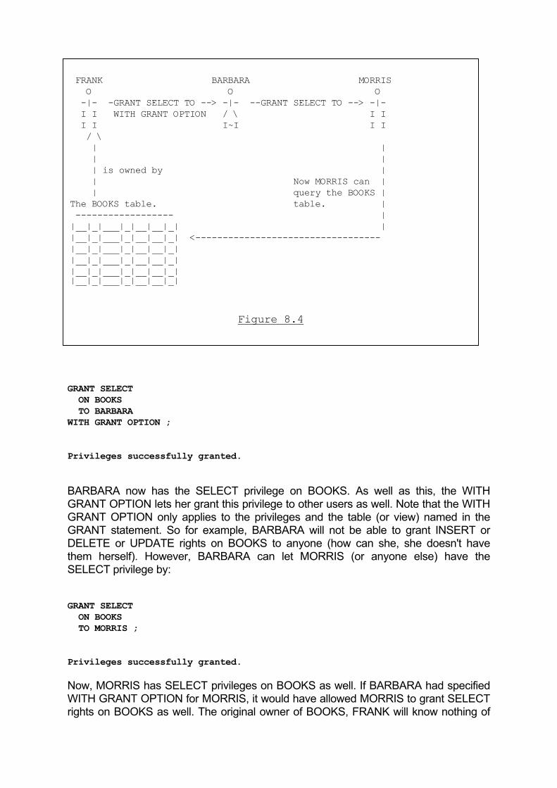
FRANK BARBARA MORRIS O O O -|- -GRANT SELECT TO --> -|- --GRANT SELECT TO --> -|- I I WITH GRANT OPTION / \ I I I I I~I I I / \ | | | | | is owned by | | Now MORRIS can | | query the BOOKS | The BOOKS table. table. | ------------------ | |__|_|___|_|__|__|_| | |__|_|___|_|__|__|_| <---------------------------------- |__|_|___|_|__|__|_| |__|_|___|_|__|__|_| |__|_|___|_|__|__|_| |__|_|___|_|__|__|_|
Figure 8.4
GRANT SELECT ON BOOKS TO BARBARA WITH GRANT OPTION ; Privileges successfully granted. BARBARA now has the SELECT privilege on BOOKS. As well as this, the WITH GRANT OPTION lets her grant this privilege to other users as well. Note that the WITH GRANT OPTION only applies to the privileges and the table (or view) named in the GRANT statement. So for example, BARBARA will not be able to grant INSERT or DELETE or UPDATE rights on BOOKS to anyone (how can she, she doesn't have them herself). However, BARBARA can let MORRIS (or anyone else) have the SELECT privilege by: GRANT SELECT ON BOOKS TO MORRIS ; Privileges successfully granted. Now, MORRIS has SELECT privileges on BOOKS as well. If BARBARA had specified WITH GRANT OPTION for MORRIS, it would have allowed MORRIS to grant SELECT rights on BOOKS as well. The original owner of BOOKS, FRANK will know nothing of
this chain of privileges propagating through the users, and will in effect have lost charge of the BOOKS table. For tight control of access rights, it is a good idea to be careful about who gets the WITH CHECK option. 8.5 "Taking back privileges": The REVOKE statement. All commercial SQL vendors offer the REVOKE command as a method of taking back the privileges that were granted with GRANT. The REVOKE command is in fact an extension to the ANSI/ISO standard. ANSI/ISO SQL includes the GRANT command on the assumption that a database designer will have finalised the design on paper first and then use the DDL commands to create all the tables, views and security privileges. The standard gives the designer a very limited ability to change his mind once the design has been implemented. So under ANSI, once privileges have been assigned, they can only be changed with great difficulty.
SQL Tips
The REVOKE statement is totally absent from the ANSI/ISO standard.
The format of REVOKE that's implemented by most commercial SQL systems is shown in Figure 8.3. It's format is very similar to the GRANT statement. For example, this command revokes the INSERT and the UPDATE privileges on the TITLES view from MORRIS: REVOKE INSERT, UPDATE ON TITLES FROM MORRIS ; Privileges successfully revoked. You can also use the ALL PRIVILEGES clause in the REVOKE command. For example, to stop ADAM using the BOOKS table, FRANK could specify: REVOKE ALL PRIVILEGES ON BOOKS FROM ADAM ; Privileges successfully revoked. REVOKE only allows you rescind those privileges that you yourself granted. This

means that if we consider the privilege chain discussed previously and shown in Figure 8.4, FRANK cannot revoke the SELECT privilege on the BOOKS table from MORRIS even though he is the owner of the table. He can however revoke this privilege from BARBARA by: REVOKE SELECT ON BOOKS FROM BARBARA ; Privileges successfully revoked. On most systems this will result in the DBMS automatically revoking the corresponding privilege from all the grantees lower down the chain. Thus MORRIS will also lose the SELECT rights on BOOKS as it was granted by BARBARA. As REVOKE is a non-standard feature, different dialects of SQL implement it in subtly different ways. This cascading effect of REVOKE may not be a feature of your particular dialect of SQL.
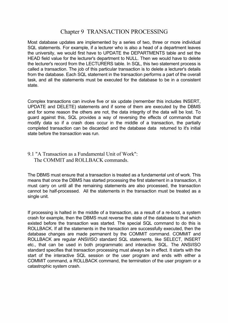
Chapter 9 TRANSACTION PROCESSING Most database updates are implemented by a series of two, three or more individual SQL statements. For example, if a lecturer who is also a head of a department leaves the university, we would first have to UPDATE the DEPARTMENTS table and set the HEAD field value for the lecturer's department to NULL. Then we would have to delete the lecturer's record from the LECTURERS table. In SQL, this two statement process is called a transaction. The job of this particular transaction is to delete a lecturer's details from the database. Each SQL statement in the transaction performs a part of the overall task, and all the statements must be executed for the database to be in a consistent state. Complex transactions can involve five or six update (remember this includes INSERT, UPDATE and DELETE) statements and if some of them are executed by the DBMS and for some reason the others are not, the data integrity of the data will be lost. To guard against this, SQL provides a way of reversing the effects of commands that modify data so if a crash does occur in the middle of a transaction, the partially completed transaction can be discarded and the database data returned to it's initial state before the transaction was run. 9.1 "A Transaction as a Fundamental Unit of Work": The COMMIT and ROLLBACK commands. The DBMS must ensure that a transaction is treated as a fundamental unit of work. This means that once the DBMS has started processing the first statement in a transaction, it must carry on until all the remaining statements are also processed, the transaction cannot be half-processed. All the statements in the transaction must be treated as a single unit. If processing is halted in the middle of a transaction, as a result of a re-boot, a system crash for example, then the DBMS must reverse the state of the database to that which existed before the transaction was started. The special SQL command to do this is ROLLBACK. If all the statements in the transaction are successfully executed, then the database changes are made permanent by the COMMIT command. COMMIT and ROLLBACK are regular ANSI/ISO standard SQL statements, like SELECT, INSERT etc., that can be used in both programmatic and interactive SQL. The ANSI/ISO standard specifies that transaction processing must always be in effect. It starts with the start of the interactive SQL session or the user program and ends with either a COMMIT command, a ROLLBACK command, the termination of the user program or a catastrophic system crash.
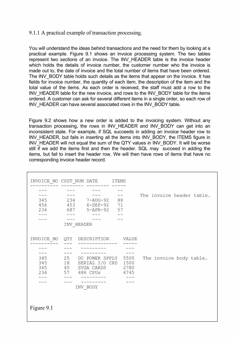
9.1.1 A practical example of transaction processing. You will understand the ideas behind transactions and the need for them by looking at a practical example. Figure 9.1 shows an invoice processing system. The two tables represent two sections of an invoice. The INV_HEADER table is the invoice header which holds the details of invoice number, the customer number who the invoice is made out to, the date of invoice and the total number of items that have been ordered. The INV_BODY table holds such details as the items that appear on the invoice. It has fields for invoice number, the quantity of each item, the description of the item and the total value of the items. As each order is received, the staff must add a row to the INV_HEADER table for the new invoice, and rows to the INV_BODY table for the items ordered. A customer can ask for several different items in a single order, so each row of INV_HEADER can have several associated rows in the INV_BODY table. Figure 9.2 shows how a new order is added to the invoicing system. Without any transaction processing, the rows in INV_HEADER and INV_BODY can get into an inconsistent state. For example, if SQL succeeds in adding an invoice header row to INV_HEADER, but fails in inserting all the items into INV_BODY, the ITEMS figure in INV_HEADER will not equal the sum of the QTY values in INV_BODY. It will be worse still if we add the items first and then the header. SQL may succeed in adding the items, but fail to insert the header row. We will then have rows of items that have no corresponding invoice header record. INVOICE_NO CUST_NUM DATE ITEMS ---------- -------- -------- ----- ~~~ ~~~ ~~~ ~~
~~~ ~~~ ~~~ ~~ The invoice header table. 345 234 7-AUG-92 88 456 453 6-SEP-92 71 234 687 5-APR-92 57 ~~~ ~~~ ~~~ ~~ ~~~ ~~~ ~~~ ~~ INV_HEADER
INVOICE_NO QTY DESCRIPTION VALUE ---------- --- -------------- ----- ~~~ ~~~ ~~~~~~~~~ ~~~ ~~~ ~~~ ~~~~~~~~~ ~~~ 345 25 DC POWER SPPLY 5500 The invoice body table.
345 18 SERIAL I/O CRD 1500 345 45 SVGA CARDS 2780 234 57 486 CPUs 6745 ~~~ ~~~ ~~~~~~~~~ ~~~ ~~~ ~~~ ~~~~~~~~~ ~~~ INV_BODY
Figure 9.1

With transaction processing in effect, if the system fails or the program crashes, you can discard the half completed transaction with a ROLLBACK statement. In Figure 9.2, the state that it was in before the transaction was started. You can then re-run the whole transaction again and if SQL succeeds in executing all the statements, make the INSERTs permanent by issuing the COMMIT command.
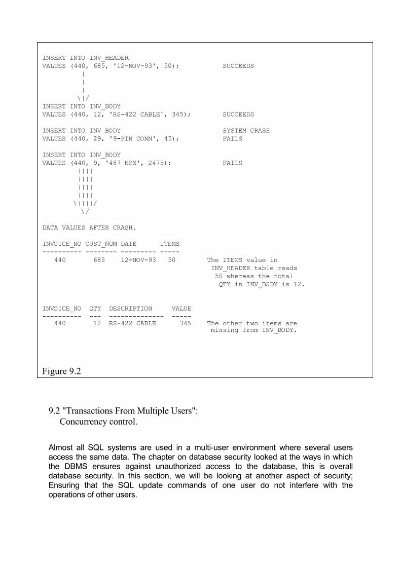
INSERT INTO INV_HEADER VALUES (440, 685, '12-NOV-93', 50); SUCCEEDS | | | \|/ INSERT INTO INV_BODY VALUES (440, 12, 'RS-422 CABLE', 345); SUCCEEDS INSERT INTO INV_BODY SYSTEM CRASH VALUES (440, 29, '9-PIN CONN', 45); FAILS INSERT INTO INV_BODY VALUES (440, 9, '487 NPX', 2475); FAILS |||| |||| |||| |||| \||||/ \/ DATA VALUES AFTER CRASH. INVOICE_NO CUST_NUM DATE ITEMS ---------- -------- --------- ----- 440 685 12-NOV-93 50 The ITEMS value in INV_HEADER table reads 50 whereas the total QTY in INV_BODY is 12. INVOICE_NO QTY DESCRIPTION VALUE ---------- --- -------------- ----- 440 12 RS-422 CABLE 345 The other two items are missing from INV_BODY.
Figure 9.2 9.2 "Transactions From Multiple Users": Concurrency control. Almost all SQL systems are used in a multi-user environment where several users access the same data. The chapter on database security looked at the ways in which the DBMS ensures against unauthorized access to the database, this is overall database security. In this section, we will be looking at another aspect of security; Ensuring that the SQL update commands of one user do not interfere with the operations of other users.

Having multiple users access the same database at the same time can lead to a number of potential problems. Three of the most well known of these are described next. 9.2.1 The Lost Update Problem. This occurs when two or more transactions have their statements interleaved by the DBMS in a certain way. Figure 9.3 shows how this can happen. Transactions 1 and 2 are started at about the same time by different programs. The DBMS executes the individual statements in each transaction as shown in Figure 9.3. The overall result of this sequence of operations will be that the update performed by the Order Processing transaction (number 1) on the STOCK field will be lost. At time=1, transaction 1 sets the value of STOCK to STOCK-10, but does not write this to disk. The computer allocates the next two time slices to transaction 2 which updates the value of STOCK to STOCK+75. The STOCK value that is eventually written to disk (at time=4) by transaction 1 is the value set by transaction 2. Transaction 1's update has in fact been lost. In a live database, such "lost" updates result in serious database inconsistency. 9.2.2 The Temporary Update Problem. This problem occurs when one transaction updates a table row and then cancels the update with ROLLBACK. The temporarily updated row can be accessed by another transaction before it is changed back to it's original value. Figure 9.4 shows the sequence of operations that can cause the temporary update problem. Transaction 1 sets the value of STOCK to STOCK-10 and writes this to disk. The DBMS then starts transaction 2 which reads the value of STOCK which has just been updated by transaction 1. This value is set to STOCK+75 and written to disk by transaction 2. When control is given back to transaction 1, it issues a ROLLBACK command (as a result of program crash for example) and cancels the STOCK = STOCK-10 update. This means that the value for STOCK read by transaction 2 at time=3 was incorrect. It had in fact read the temporary value. As with the lost update problem, the temporary update problem will also results in database inconsistency if left unchecked.

TRANSACTION 1 (Order Processing)
-------------
READ STOCK VALUE
SET STOCK = STOCK-10
WRITE STOCK VALUE
READ QTY VALUE
SET QTY = QTY+10
WRITE QTY VALUE
TRANSACTION 2 (Goods Received)
-------------
READ STOCK VALUE
SET STOCK = STOCK+75
WRITE STOCK VALUE
Two programs run these transactions at about the same time. Transaction 1 is
a part of the new order processing program and transaction 2 is a part of the
stock control system for goods received.
The DBMS might execute these transaction statements in the following order:
TIME STATEMENT TRANSACTION No.
---- --------- ---------------
0 READ STOCK VALUE Order Proc. (1)
1 SET STOCK = STOCK-10 Order Proc. (1)
2 READ STOCK VALUE Goods Recv. (2)
3 SET STOCK = STOCK+75 Goods Recv. (2)
4 WRITE STOCK VALUE Order Proc. (1)
5 READ QTY VALUE Order Proc. (1)
6 WRITE STOCK VALUE Goods Recv. (2)
7 SET QTY = QTY+10 Order Proc. (1)
8 WRITE QTY VALUE Order Proc. (1)
At time=6, transaction 2 has written an incorrect value because the update by transaction 1 has been lost.
Figure 9.3
9.2.3 The incorrect summary problem. This is the third common problem that can occur when multiple transactions operate on the data without any form of concurrency control by the DBMS. It is illustrated in Figure 9.5. Transaction 4 is part of a report generating program. It reads the value of the STOCK column for each row in the table and adds up the sum total. Transaction 3 is part of the order processing program that handles returned products. The problem
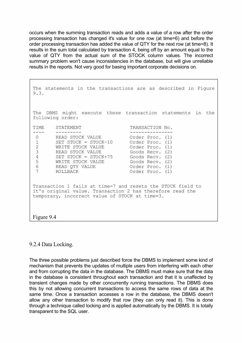
occurs when the summing transaction reads and adds a value of a row after the order processing transaction has changed it's value for one row (at time=6) and before the order processing transaction has added the value of QTY for the next row (at time=8). It results in the sum total calculated by transaction 4, being off by an amount equal to the value of QTY from the actual sum of the STOCK column values. The incorrect summary problem won't cause inconsistencies in the database, but will give unreliable results in the reports. Not very good for basing important corporate decisions on.
The statements in the transactions are as described in Figure
9.3.
The DBMS might execute these transaction statements in the
following order:
TIME STATEMENT TRANSACTION No.
---- --------- ---------------
0 READ STOCK VALUE Order Proc. (1)
1 SET STOCK = STOCK-10 Order Proc. (1)
2 WRITE STOCK VALUE Order Proc. (1)
3 READ STOCK VALUE Goods Recv. (2)
4 SET STOCK = STOCK+75 Goods Recv. (2)
5 WRITE STOCK VALUE Goods Recv. (2)
6 READ QTY VALUE Order Proc. (1)
7 ROLLBACK Order Proc. (1)
Transaction 1 fails at time=7 and resets the STOCK field to
it's original value. Transaction 2 has therefore read the
temporary, incorrect value of STOCK at time=3.
Fi
gure 9.4
9.2.4 Data Locking. The three possible problems just described force the DBMS to implement some kind of mechanism that prevents the updates of multiple users from interfering with each other and from corrupting the data in the database. The DBMS must make sure that the data in the database is consistent throughout each transaction and that it is unaffected by transient changes made by other concurrently running transactions. The DBMS does this by not allowing concurrent transactions to access the same rows of data at the same time. Once a transaction accesses a row in the database, the DBMS doesn't allow any other transaction to modify that row (they can only read it). This is done through a technique called locking and is applied automatically by the DBMS. It is totally transparent to the SQL user.

TRANSACTION 3 (Order Processing) ------------- READ STOCK VALUE SET STOCK = STOCK-10 WRITE STOCK VALUE READ STOCK VALUE READ QTY VALUE
WRITE STOCK VALUE
lues.
The DBMS might execute these transaction statements in the following order:
4 SET STOCK = STOCK-10 (row2) Order Proc. (3) 5 WRITE STOCK VALUE (row2) Order Proc. (3)
9 SUM=SUM+STOCK (row3) Total Stok. (4) 10 READ STOCK (row3) Order Proc. (3)
13 WRITE STOCK VALUE (row3) Order Proc. (3)
Figure 9.5
SET STOCK = STOCK+QTY
TRANSACTION 4 (Total Stock) ------------- SUM(STOCK) FOR ALL ITEMS
Two programs run these transactions at about the same time. Transaction 3 is a part of the new order processing program and transaction 2 is a part of areport generation program that calculates the sum of the STOCK row va
TIME STATEMENT TRANSACTION No. ---- --------- --------------- 0 SUM=0; Total Stok. (4) 1 READ STOCK (row1) Total Stok. (4) 2 SUM=SUM+STOCK (row1) Total Stok. (4) 3 READ STOCK (row2) Order Proc. (3)
6 READ STOCK (row2) Total Stok. (4) 7 SUM=SUM+STOCK (row2) Total Stok. (4) 8 READ STOCK (row3) Total Stok. (4)
11 READ QTY VALUE Order Proc. (3) 12 SET STOCK = STOCK+QTY (row3) Order Proc. (3)
Transaction 4 reads the value of STOCK (row2), at time=6, after transaction 3 has subtracted 10 from it. At time=8, transaction 4 reads STOCK (row3) before transaction 3 subtracts QTY. The sum of the STOCK field values will thus be off by the value of QTY.
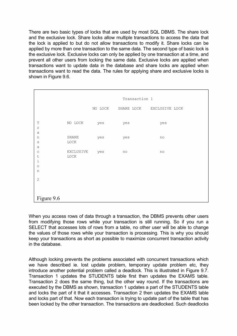
There are two basic types of locks that are used by most SQL DBMS. The share lock and the exclusive lock. Share locks allow multiple transactions to access the data that the lock is applied to but do not allow transactions to modify it. Share locks can be applied by more than one transaction to the same data. The second type of basic lock is the exclusive lock. Exclusive locks can only be applied by one transaction at a time, and prevent all other users from locking the same data. Exclusive locks are applied when transactions want to update data in the database and share locks are applied when transactions want to read the data. The rules for applying share and exclusive locks is shown in Figure 9.6. Transaction 1
a
s LOCK a c EXCLUSIVE yes no no
o
Fi
NO LOCK SHARE LOCK EXCLUSIVE LOCK
T NO LOCK yes yes yes r
n SHARE yes yes no t LOCK i
n 2
gure 9.6
When you access rows of data through a transaction, the DBMS prevents other users from modifying those rows while your transaction is still running. So if you run a SELECT that accesses lots of rows from a table, no other user will be able to change the values of those rows while your transaction is processing. This is why you should keep your transactions as short as possible to maximize concurrent transaction activity in the database. Although locking prevents the problems associated with concurrent transactions which we have described ie. lost update problem, temporary update problem etc, they introduce another potential problem called a deadlock. This is illustrated in Figure 9.7. Transaction 1 updates the STUDENTS table first then updates the EXAMS table. Transaction 2 does the same thing, but the other way round. If the transactions are executed by the DBMS as shown, transaction 1 updates a part of the STUDENTS table and locks the part of it that it accesses. Transaction 2 then updates the EXAMS table and locks part of that. Now each transaction is trying to update part of the table that has been locked by the other transaction. The transactions are deadlocked. Such deadlocks
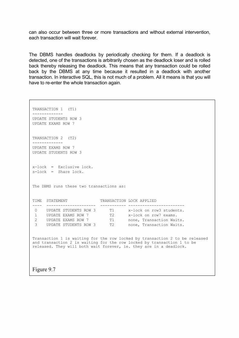
can also occur between three or more transactions and without external intervention, each transaction will wait forever. The DBMS handles deadlocks by periodically checking for them. If a deadlock is detected, one of the transactions is arbitrarily chosen as the deadlock loser and is rolled back thereby releasing the deadlock. This means that any transaction could be rolled back by the DBMS at any time because it resulted in a deadlock with another transaction. In interactive SQL, this is not much of a problem. All it means is that you will have to re-enter the whole transaction again.
TRANSACTION 1 (T1) -------------
x-lock = Exclusive lock. s-lock = Share lock.
The DBMS runs these two transactions as:
2 UPDATE EXAMS ROW 7 T1 none, Transaction Waits.
UPDATE STUDENTS ROW 3 UPDATE EXAMS ROW 7
TRANSACTION 2 (T2) ------------- UPDATE EXAMS ROW 7 UPDATE STUDENTS ROW 3
TIME STATEMENT TRANSACTION LOCK APPLIED ---- --------------------- ----------- ------------------------ 0 UPDATE STUDENTS ROW 3 T1 x-lock on row3 students. 1 UPDATE EXAMS ROW 7 T2 x-lock on row7 exams.
3 UPDATE STUDENTS ROW 3 T2 none, Transaction Waits.
Transaction 1 is waiting for the row locked by transaction 2 to be released and transaction 2 is waiting for the row locked by transaction 1 to be released. They will both wait forever, ie. they are in a deadlock.
Figure 9.7

Chapter 10 THE DATABASE SYSTEM CATALOG In a working SQL database, the DBMS needs to keep track of tables, columns, views, authorization-ids and privileges. Most commercial systems rely on special relational database tables called the system catalog for this. The system catalog or system tables consist of tables that are created and owned by the DBMS itself. The DBMS does not allow anyone to modify or add data to these tables, but on most systems, users can query them and obtain information on tables, views, other users etc. The system catalog is not defined in the ANSI/ISO standard, in fact, the standard does not specify how SQL DBMSs should maintain the database at all. As a result of this, this area is the most diverse amongst the commercial SQL based DBMSs. Although all the major vendors have chosen to use the system catalog to administer the database, they all differ in the implementation details. This chapter describes the structure and content of a typical system catalog by looking at the system tables of some popular commercial SQL DBMSs.
TABLES VIEWS |---|-| |---|-|--------| :.:...:.: :.:.....:.: | | | | | | | : : : : : : : : | | | | | | | : : : : : : : : |---|-| |---|-|--------| :.:...:.: :.:.....:.:
/|\ /|\ /|\/|\ /|\ /|\/|\/|\ /|\ /|\ /|\ | | | | | | | | | | |
ACCESS PRIVILEGES
ooooOOOOooooOOOoooOOoO 0000oooOoooOoooooooo
C O L U M N S C O L U M N S /\ /\ || || ||-----------------------------------|| ||-----------------------------------||
oooOoOooOoOoOOo USER AUTHORIZATION-IDS
Figure 10.1
10.1 "The DBMS Needs to Manage it's Resources": A typical system catalog. Although the various commercial SQL systems offer widely varying features, they all have a common base of resources that the DBMS needs to manage as a minimum requirement. These are shown in Figure 10.1. They include: 1. Tables. All the tables in the database must be known to the DBMS. The information must include the table's name and the table's owner. 2. Views. These are related to tables and indeed, some system catalogs have a single table that stores details of both tables and views. Typically, the DBMS needs to know the view's name, it's owner and the defining query. 3. Columns. The DBMS must know details of all columns for both tables and views. Typical information includes the column name, the table or view which the column is part of and the data type and size of the column. 4. Users. Each user has an associated authorization-id. The DBMS needs to keep track of all the authorization-ids as well as the passwords that they are identified by. 5. Privileges. The DBMS needs to be aware of the privileges that have been granted. Specifically, it needs to know the authorization-id of the grantor, and the grantee, the privilege that's been granted and the table/view that the privilege was granted on. All this information is itself stored in relational database tables. Most systems use a different table for each of the five categories listed above.
SQL Tips
The ANSI/ISO standard does not specify any form database regulation. Almost all commercial systems rely on the system catalog for this.
10.1.1 Table information in the system catalog. The system table that keeps track of the details of all other tables in the database is called SYSTABLES in IBM's OS/2 EE. The table is owned by the DBMS itself so to query it, you must use the SYSIBM prefix. For example to list the names of all the tables and views in the database along with the owner and the number of columns, an OS/2 EE query would be:

SELECT NAME, CREATOR, COLCOUNT FROM SYSIBM.SYSTABLES ; Note that NAME, CREATOR, COLCOUNT and TYPE are all fields in the SYSTABLES system table where NAME is the name of the table or view. CREATOR is the owner of the object. COLCOUNT is a number specifying the number of columns in the object and TYPE is either T for tables or V for views. SYSTABLES can be queried just like any other table, and stores it's information as other tables, in rows and columns. For example it has multiple columns and one row of data for each table or view in the database. You could also add a predicate to your query, as you would for any other query, to list only the tables that are owned by FRANK for example: SELECT NAME, CREATOR, COLCOUNT FROM SYSIBM.SYSTABLES WHERE TYPE = ‘T’ AND CREATOR = 'FRANK' ; 10.1.2 View information in the system catalog. Some systems include basic information on views with the tables and store them both in a system objects table. IBM's OS/2 EE for example has a TYPE column in SYSTABLES to distinguish between tables and views. Other information relating directly to views is stored in different tables. OS/2 EE has two further system catalog tables that hold information on views. The SYSVIEWS table holds the SQL text information that defines the view. The SYSVIEWDEP table holds the details of the base tables (and views) that the view derives it's information from. You can also query these like ordinary tables. For example to list the base tables/views and their owners which the MGRS view depends on: SELECT BNAME, BCREATOR, BTYPE FROM SYSIBM.SYSVIEWDEP WHERE DNAME = 'MGRS' ; BNAME holds the name of a table/view on which the view depends. BCREATOR holds the name of the owner and BTYPE is either 'T' for tables and 'V' for views. DNAME is the column that holds the name of the dependent view. SYSVIEWDEP has one row for each base object. So if the MGRS view has three tables in it's definition, there will be three rows in SYSVIEWDEP with a DNAME value of 'MGRS'. 10.1.3 Column information in the system catalog. Just keeping details of tables and views is not enough to manage a database. The

DBMS also needs to know about all the columns in each table and view. All the major commercial SQL DBMSs use a system catalog table to keep track of columns. IBM's OS/2 EE for example uses the SYSCOLUMNS table for this. This table holds the information directly relating to the column such as the column name, data type, the table or view it is part of etc. as well as statistical information which the DBMS uses to optimize queries which access the column. This information is generally of no use to the us directly, but we can query SYSCOLUMNS to extract useful information. For example, to find the number of columns and their types in the LECTURERS table: SELECT NAME, COLTYPE, LENGTH FROM SYSIBM.SYSCOLUMNS WHERE TBNAME = 'LECTURERS' ; NAME, COLTYPE and LENGTH are fields in SYSCOLUMNS which hold details of the name of the column, it's data type and it's size respectively. TBNAME stores the name of the table which the column is part of. 10.1.4 User information in the system catalog. Knowledge of all valid authorization-ids is essential if the DBMS is going to maintain system security. Information on users is stored in a table in the system catalog. There is usually one row per user in this table. Typical details that are stored include the authorization-id and the associated password for each user. The nature of this information is such that sensitive information such as user passwords is only available to database administrators and users who have very high security clearance. 10.1.5 Privileges and other information in the system catalog. The privileges information table holds the details of the privileges granted to users. Typically, the DBMS stores details such as the privilege granted, the user who granted the privilege, the user who received the privilege, the database object to which the privilege applies, a time stamp to indicate when the privilege was granted etc. Whenever a user enters an SQL statement, the DBMS first check if that user has the required privileges to carry out the task. 10.1.6 Commenting the tables, views and columns. In large, complex databases, it can become difficult to remember the exact functions of

all the tables, views and columns. Although there is no substitute for thorough design documentation, most commercial SQL systems also allow you to attach labels and comments to each table, view and column defined in the database. The remarks are usually stored in the system catalog's objects definition table, eg. SYSTABLES. Labels are attached by using the LABEL statement. Thus to add a label to the EXAMS table: LABEL ON TABLE EXAMS IS 'The exams taken by the students' The label is stored with the table definition in the system catalog. You can also attach labels to the individual columns. For example, to label the BUDGET column in the DEPARTMENTS table: LABEL ON COLUMN DEPARTMENTS.BUDGET IS 'Internally allocated budget.' ; LABEL is used to attach a short descriptive label to a table or column. The COMMENT statement lets you add a longer description to the SYSTABLES row for the table or view or the SYSCOLUMNS row for the column. For example, to add a remark to the GRADE column in the LECTURERS table: COMMENT ON LECTURERS (GRADE IS 'Grade A is the most senior and E, the most junior') The remark is stored in the SYSCOLUMNS table and is appended to the row for the GRADE column. You should add labels and remarks for all but the very simplest of database tables. This is because when you someone else refers to the structure of the database on a few months time say, comments are an invaluable aid in finding out exactly what information the columns store and how the inter-table relationships are formed.

Chapter 11 EMBEDDING SQL IN A HOST LANGUAGE. The SQL language as we have used it so far has been used as an interactive database query language. All the queries have been typed in at the system prompt and the DBMS executed each query and output the results immediately (or at least, while we waited!). This is fine for ad hoc queries that will not be repeated or are run infrequently. Almost all commercial SQL systems provide this type of interface called either interpretive SQL or interactive SQL. This chapter looks at the other method of using SQL, programmatic SQL. The term programmatic SQL is used to refer to SQL statements that are used in conjunction with another computer language called the host language. 11.1 "SQL is not a Computer Programming Language": Why SQL needs a host language. By itself, SQL is a very powerful query language. However, it is not a computer programming language in the real sense of the word. For instance, it does not have any commands that enable programs to loop or branch to different sections of the program code, such as FOR, DO..WHILE and IF..THEN statements. In programmatic SQL, these are provided by a host language such as Pascal, C, FORTRAN or COBOL. There are basically two distinct methods of interfacing SQL with a host language. One is embedded SQL and the other is through an application program interface (API). Embedded SQL is concerned with mixing SQL statements directly with the host language code. Embedded SQL is the subject of this chapter. The application program interface or API is a library of DBMS functions through which the host language program issues commands to the DBMS. The API appears to the host language program as just another library which the linker can link into the program. Originally, the ANSI/ISO standard supported programmatic SQL through the concept of modules. These are SQL procedures which must be called from a separate module language program. The standard was extended in 1989 to include embedded SQL in the COBOL, FORTRAN, C, PL/1, Pascal and Ada host languages.

11.2 "How Embedded SQL Programs are Processed": Compile, Bind and Link. Figure 11.1 shows a short embedded SQL program written in the C language. The SQL statements are highlighted for clarity. Don't worry too much if you do not fully understand how the program operates, we will be discussing it fully in the next few sections. When this program is run, it asks the user for a department number. The program then runs an SQL query which fetches the row from the DEPARTMENTS table that the department number applies to, and displays the department name and the current year's budget. The output from the program is shown in Figure 11.2. Although we have chosen to write in C, other languages such as Pascal, COBOL etc. would have been just as applicable. The embedded SQL program, such as the one in Figure 11.1 cannot be directly compiled by the C compiler because of the embedded SQL statements. Figure 11.3 shows the steps involved in converting the embedded SQL source code (shown in Figure 11.1) into an executable embedded SQL program. The sequence of operations that are illustrated in Figure 11.3 are invisible to the program developer. Typically, the developer is only required to start the process with a single command. This is not so different from "normal" program development, where you would start off the compile and link process with a single MAKE command. Even though the whole process is initiated by a single command, it follows distinct stages: 1. The embedded SQL program is passed to a precompiler. A precompiler is a software tool provided by the SQL system vendors. It separates the embedded SQL program code into a host language program file and the SQL statements stored in a file called the database request module (DBRM). 2. The host language file from the precompiler is submitted to the standard language compiler for compilation into an object file. 3. The compiled object files from the compiler are then submitted to the linker and linked with any library routines that may be required. 4. The DBRM file from the precompiler is operated upon by a binding program which produces an application plan for all the SQL statements. This plan tells the DBMS all it needs to know about accessing the data in the database requested by the SQL statements. The application plan is stored in the database. By the end of these stages, the host language part of the program is compiled and

linked and the SQL part is parsed, validated and optimised. When the program is run, the executable host language program will be loaded and executed as any other program. Whenever the program needs to execute an SQL statement, it instructs the DBMS to find and load the application plan for that statement. The main program and the DBMS thus co-operate to run the whole embedded SQL program. 11.3 "How SQL Statements Are Embedded": The EXEC SQL clause. In the embedded SQL program of Figure 11.1, the SQL statements are preceded by the "exec sql" precompiler directive. This introducer tells the precompiler that the next statement is an SQL command. The statement ends with a terminator. In C, this is the semicolon character Other languages use other terminators eg. COBOL uses END-EXEC. Although the C language is case sensitive (printf is not the same as Printf), the SQL statement after EXEC SQL can be either upper or lower case. This is because these statements are removed by the precompiler before they reach the C compiler so the compiler does not see them directly. 11.4 "How SQL Talks to the Host Language": Host language variables. Host language variables are used to supply values or receive values from SQL. The variables should first be declared in the program using the ANSI/ISO standard BEGIN DECLARE SECTION and END DECLARE SECTION statements. For example, in the program listed in Figure 11.1, the host language variables that are going to be used with SQL are declared as: exec sql begin declare section; int input_val; /* User input */ int d_no; /* Department Number */ char d_name[21]; /* Department Name */ int d_head; /* Departmental Head */ float budget; /* Current Budget */ float p_budget; /* Previous Budget */ exec sql end declare section;
The host language variables must be compatible with the SQL data types which they refer to. For example, SQL's INTEGER type corresponds to C's int type and SQL's CHARACTER type is compatible with C's char type. Sometimes, there will not be an exact match eg. the BUDGET field is DECIMAL and the closest match in C is the float type.
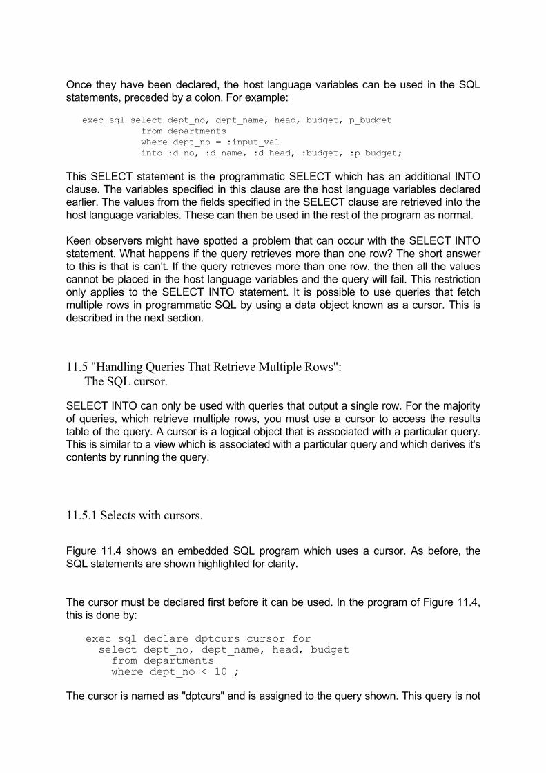
Once they have been declared, the host language variables can be used in the SQL statements, preceded by a colon. For example: exec sql select dept_no, dept_name, head, budget, p_budget from departments where dept_no = :input_val into :d_no, :d_name, :d_head, :budget, :p_budget; This SELECT statement is the programmatic SELECT which has an additional INTO clause. The variables specified in this clause are the host language variables declared earlier. The values from the fields specified in the SELECT clause are retrieved into the host language variables. These can then be used in the rest of the program as normal. Keen observers might have spotted a problem that can occur with the SELECT INTO statement. What happens if the query retrieves more than one row? The short answer to this is that is can't. If the query retrieves more than one row, the then all the values cannot be placed in the host language variables and the query will fail. This restriction only applies to the SELECT INTO statement. It is possible to use queries that fetch multiple rows in programmatic SQL by using a data object known as a cursor. This is described in the next section. 11.5 "Handling Queries That Retrieve Multiple Rows": The SQL cursor. SELECT INTO can only be used with queries that output a single row. For the majority of queries, which retrieve multiple rows, you must use a cursor to access the results table of the query. A cursor is a logical object that is associated with a particular query. This is similar to a view which is associated with a particular query and which derives it's contents by running the query. 11.5.1 Selects with cursors. Figure 11.4 shows an embedded SQL program which uses a cursor. As before, the SQL statements are shown highlighted for clarity. The cursor must be declared first before it can be used. In the program of Figure 11.4, this is done by: exec sql declare dptcurs cursor for select dept_no, dept_name, head, budget from departments where dept_no < 10 ; The cursor is named as "dptcurs" and is assigned to the query shown. This query is not

executed immediately, it is only used to define the cursor at this stage. In order to actually execute the query, you must open the cursor. For example: exec sql open dptcurs ; This statement causes the query associated with the cursor called dptcurs to be executed. The results of the query can be accessed by the FETCH statement. In the program of Figure 11.4, this is done by: exec sql fetch dptcurs into :d_no, :d_name, :d_head, :budget ; The FETCH statement retrieves the first row from the results table into the host language variables specified and sets the row pointer to point to the next row in the results. We placed the FETCH statement in a repeating loop because it retrieves the next row from the results each time it is run. The do..while loop continues to fetch results and display them until no more rows are left to be fetched. When FETCH reaches the end of the results table, it causes the program to jump to the "no_more_rows" label where a "No more rows" message is output. Note that although you can move down through the results table by using the FETCH command, there is no way of moving up through the results table. This means that when all the rows have been fetched through a cursor, it must be closed. There is no point in tying up system resources in maintaining an exhausted cursor. The CLOSE CURSOR command releases the resources allocated to the cursor, for example: exec sql close dptcurs ; To use the dptcurs cursor again, you must be re-declare it and then open it. The output of this program is shown in Figure 11.5 11.5.2 Deletes and Updates with cursors. You can use cursors to delete and update data in SQL tables. Cursors by themselves can only access data through a query. They cannot therefore be directly used with a DELETE statement. However, programmatic SQL allows the use of a DELETE statement with WHERE CURRENT OF clause which uses a cursor to specify the row to delete. Figure 11.6 shows extracts of a program that declares a cursor named finalists that refers to all the year 3 students in the STUDENTS table. The cursor is declared and opened in the usual way. The do..while loop near the end of the program contains a DELETE statement which deletes all the year 3 students from STUDENTS. Here's how it works. When the loop is executed for the first time, The FETCH statement causes the cursor to point to the first row of the results table ie. to the first year 3 student's row. The actual field values of this row are retrieved into the host language variables a, b, c, d, e

and f. The DELETE statement: exec sql delete from students where current of finalists ; tells the DBMS to delete the row which the cursor is currently pointing to. In this case, this is the first year 3 student's row. When the loop is repeated, the FETCH command causes the cursor to point to the next year 2 student's row and this too is deleted by the DELETE with WHERE CURRENT OF clause. When the last has been deleted, the DBMS returns a code to the program which tells it to exit the loop and jump to the appropriate program section. We have illustrated the case of updating data via cursors by using the DELETE statement. You can also use UPDATE in exactly the same way to modify the value of rows on the same principle. To be updatable (by either DELETE or UPDATE), the cursor must satisfy the same criteria as an updatable view.
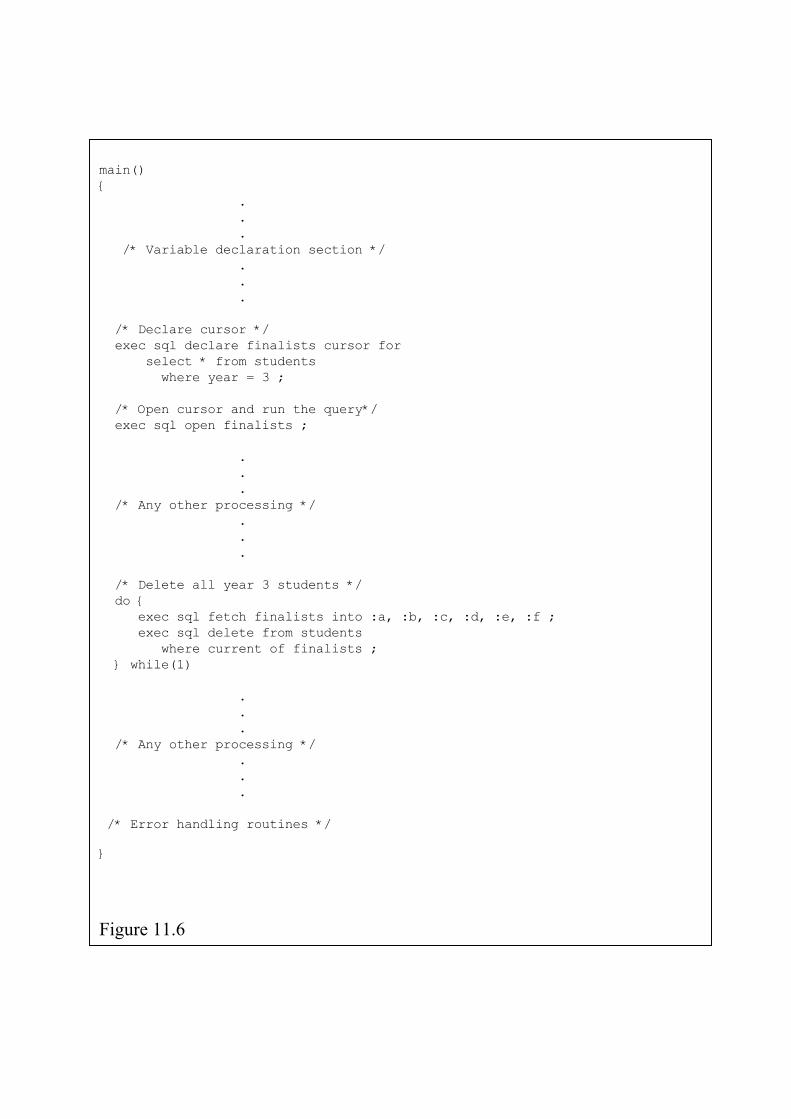
main()
. .
/* Variable declaration section */ .
/* Delete all year 3 students */
exec sql fetch finalists into :a, :b, :c, :d, :e, :f ;
}
{
.
. . /* Declare cursor */ exec sql declare finalists cursor for select * from students where year = 3 ; /* Open cursor and run the query*/ exec sql open finalists ; . . . /* Any other processing */ . . .
do {
exec sql delete from students where current of finalists ; } while(1)
. . . /* Any other processing */ . . . /* Error handling routines */
Figure 11.6

11.6 "SQL Statements That Fail": Error Handling. You've seen in the programs of Figures 11.1 and 11.4 that we have used the error and warning handling statements without much explanation of how they operate. The SQL error handling allows you to identify run-time errors and warnings produced by the DBMS and to act on them. Run-time errors are those that result from running the program, for example if an embedded SQL statement refers to a table which does not exist, then the DBMS will signal a run-time error. The error handling routines provided by SQL only apply to errors and warnings produced by the DBMS. They do not deal with the run-time errors generated through the host language. The DBMS reports all errors and warnings to the program through a structure called the SQL Communications Area or SQLCA. The first line of the program of Figure 11.1 is: exec sql include sqlca; This tells the precompiler that we will be using SQL's error handling features later in the program. Whenever an SQL command is executed, the DBMS sets the value of a variable, called sqlcode, in the sqlca structure to indicate that the command was successfully executed (sqlcode set to zero), that the command failed as a result of an error (sqlcode set to a negative value) or that the command was executed but generated a warning (sqlcode set to a positive value). You tell SQL how to deal with errors and warnings by the WHENEVER statement. There are three versions of WHENEVER which correspond to the "serious error", "warning" and "row not found" possible results of executing an SQL command. For example, in the program of Figure 11.1: exec sql whenever sqlerror goto error_handler; exec sql whenever not found goto no_number; The first statement tells the precompiler to generate code which will cause the program to jump to the part of the program labelled as "error_handler". The second statement causes the program to jump to the "no_number" label if any SQL command returns a row not found warning. Note that the "row not found" is a particular type of warning which is specified by sqlca.sqlcode having a value of 100 (positive indicates a warning and 100 indicates the nature of the warning ie. "row not found"). The third WHENEVER statement is: whenever sqlwarning goto wrng_hdlr We have not used it in our programs, but it will cause the program to jump to the label "wrng_hdlr" whenever an SQL command generates a warning (sqlca.sqlcode has a positive value). If we had not used the WHENEVER statements in the program of

Figure 11.4, the do..while(1) loop would have repeated forever. The fact that the FETCH statement in this loop generates a warning when the last row has been retrieved causes the program flow to jump from the loop to the "no_more_rows" label.
SQL Tips
The ANSI/ISO standard specifies the NOT FOUND warning, but does not specify the particular value that must be returned.
If no WHENEVER statements are defined, the default condition is to ignore the warnings and errors generated by the SQL commands. This is what will happen to the warnings generated in the programs of Figure 11.1 and 11.4 because we have not used the WHENEVER SQLWARNING commands. We could have explicitly stated this by using CONTINUE. For example, to explicitly tell the program to ignore warnings, we could add the line: exec sql whenever sqlwarning continue; It is good programming practice to add this line instead of leaving out the WHENEVER SQLWARNING condition altogether because it clearly indicates that you wish the warnings to be ignored and not that you've simply forgotten to add it. SQL Tips
The SQLCODE variable, used for reporting errors and warnings is supported by the ANSI/ISO standard and is implemented by all commercial embedded SQL products.
11.7 "Dealing With NULL Values": Indicator Variables. As we have seen, NULLs are special markers that are used by SQL whenever a value in a field is not known. The concept of NULL markers is not used in any common programming language. Because of this, host language variables cannot directly be assigned NULL values.
SQL Tips
The use of indicator variables in retrieving NULL values is not specified by the ANSI/ISO standard.
In order to accommodate NULLs, the host language uses indicator variables. These are integer type variables that are used in conjunction with regular host language variables and indicate if the value in the host language variable is a NULL or not. For example, if the FETCH statement in the program of Figure 11.4 could retrieve a NULL value for the HEAD column in the DEPARTMENTS table, then we must allow for this by using an indicator variable with the d_head host language variable. The modified FETCH would be: exec sql fetch dptcurs into :d_no, :d_name, :d_headINDICATOR:n_hd, :budget ; The variable, n_hd, is used as an indicator variable. It must first be declared just as any other host language variable. The keyword INDICATOR tells us that n_hd is used to indicate if d_head is set to a NULL value by the FETCH. If a NULL value is produced for d_head, the indicator variable, n_hd will be set to a negative number. The program can check the value of n_hd and carry out the appropriate actions (such as display a message "No head assigned" in the column) if a NULL is detected. Indicator variables can also be used to assign NULL values to SQL columns. The indicator variable must first be set to a negative value and then appended to the host language variable in the INSERT or UPDATE statement. For example, to set the BUDGET value in the DEPARTMENTS table to NULL, the programmatic SQL sequence of commands is: n_bdg = -1; exec sql insert into departments values (:d_no, :d_name, :d_head, :budget:n_bdg, :p_budget); The n_bdg variable is assigned a value of -1 and is then used in the SQL statement as an indicator variable. The negative value tells the DBMS to insert a NULL value for the BUDGET column regardless of the current value of the budget host variable. 11.8 "A Library of SQL Functions": The SQL API. Some commercial SQL systems take a different approach to programmatic SQL. Rather than using embedded SQL, products such as SQL Server, SQLBase and Oracle (which also offers embedded SQL) use the SQL application program interface.

The host language sees the application program interface (API) as just another library of prepackaged routines and functions. The names and syntax of the API functions vary from one DBMS to another, and from one host language to another but most SQL APIs follow the same general principles: - They provide an API function to make a logical connection to the SQL DBMS. - They provide a function to send an SQL command, in the form of a text string, to
the DBMS. - The API provides functions to check the status of the DBMS and to handle any
errors. - The API provides the host language functions to DECLARE, OPEN, FETCH and
CLOSE cursors. - At the end of the program, the API provides a function to enable the program to
drop the logical connection to the DBMS. Most commercial SQL implementations provide many more API functions then the basic ones described. Microsoft SQL Server's API for instance consists of over a hundred different functions. A typical SQL program might only use about a dozen of them. Unlike the embedded SQL statements used in mainframe languages, which are stored as an application plan, API calls are parsed, validated, optimised and executed all at run time, rather like interactive SQL statements.
SQL Tips
Oracle's primary method of programmatic SQL is embedded SQL but it also supports the API method through the Oracle Call Interface.
Having to parse, validate and optimise SQL statements at run time results in slower program execution but many commercial SQL implementations incorporate additional features that help in speeding up program execution. SQL Server for example uses the concept of stored procedures. These are a sequence of SQL commands that are given a name and stored in the database already parsed, validated and optimised. At run time, the program makes API calls to execute stored procedures rather than complex sequences of SQL commands.

APPENDIX A - The ANSI/ISO standard data types.
The ANSI/ISO standard only specifies eight data types that can be used to represent the data stored in tables. 1. CHARACTER(len) Fixed length character string. The len or CHAR(len) argument refers to the maximum length of the string.
All character type values must be enclosed in single quotes ('...').
2. INTEGER Integer types are whole numbers or INT (without a decimal point). INT types are frequently
used as row identifying columns eg. SUB_NO, LECT_NO, EXAM_NO etc. Usually a 32-bit signed integer.
3. SMALLINT Same as INTEGER type, but used for smaller
numbers. Usually a 16-bit signed integer. 4. DECIMAL(prec, scale) Used to represent real numbers (ie. or DEC(prec, scale) with a decimal point). The precision argument
specifies how many significant digits the number is to have. The scale argument is optional and specifies how many digits are to appear after the decimal point.
5. NUMERIC(prec, scale) The same as DECIMAL type, except that the
precision argument specifies the maximum number of digits that may be used.
6. FLOAT(prec) Floating point numbers in scientific (base 10)
notation. The precision argument specifies the minimum precision of the data. 7. REAL Same as float, but no minimum precision is
specified. 8. DOUBLE PRECISION Same as REAL, but the implementation or DOUBLE -defined precision is greater than that for REALs.

APPENDIX B - The Sample University Administration Database. The university administration database is used in most of the examples in this book. The database consists of five tables: 1. The STUDENTS table, which holds details of the students in the university. 2. The LECTURERS table, which holds details of the teaching staff at the university. 3. The SUBJECTS table, which holds details of the subjects that are available. 4. The EXAMS table, which holds details of all the exams taken by the students. 5. The DEPARTMENTS table, which holds details of the various departments (faculties). The SQL statement used to create each table is shown below: CREATE TABLE STUDENTS (SURNAME CHAR(15) NOT NULL, FIRST_NAME CHAR(15), D_O_B DATE, STUDENT_NO INTEGER NOT NULL UNIQUE, DEPT_NO INTEGER, YEAR DECIMAL(2) );
CREATE TABLE LECTURERS (SURNAME CHAR(15) NOT NULL, INITL CHAR(4), LECT_NO INTEGER NOT NULL, DEPT_NO INTEGER, SUB_NO INTEGER, GRADE CHAR(1), PAY DECIMAL(6), JOINED DATE UNIQUE (SURNAME, LECT_NO) );
CREATE TABLE SUBJECTS (SUB_NO INTEGER NOT NULL UNIQUE, SUB_NAME CHAR(20), DEPT_NO INTEGER, CREDITS NUMERIC(2), PASS NUMERIC(2) );

CREATE TABLE EXAMS (SUB_NO INTEGER NOT NULL, STUDENT_NO INTEGER NOT NULL, MARK DECIMAL(3), DATE_TAKEN DATE ); CREATE TABLE DEPARTMENTS (DEPT_NO INTEGER NOT NULL, DEPT_NAME CHAR(20), HEAD INTEGER, BUDGET DECIMAL(10), P_BUDGET DECIMAL(10), UNIQUE (DEPT_NO) );
The contents of the university database tables are shown in Figure B.1.

SURNAME FIRST_NAME D_O_B STUDENT_NO DEPT_NO YEAR ------- ---------- ----- ---------- ------- ---- Duke Fitzroy 11-26-1970 1 4 2
Mulla Farook F U 10-24-1968 14 3 2
THE STUDENTS TABLE
Jones R A 1 1 2 E 24000 03-25-1990
7 Physiology 6 3 78
10 Marketing 3 2 56
Al-Essawy Zaid M A 11-26-1970 2 4 2 Ayton Phil J M A 07-13-1967 3 3 1 Patel Mahesh 12-07-1970 4 2 1 Jones Gareth P Y 01-24-1970 5 2 1 Scott Gavin T J 02-20-1971 6 2 2 Baker Abu-Mia 03-13-1971 7 4 1 Brown Joseph P A 04-19-1970 8 3 3 Monkhouse Robert Jones 05-23-1967 9 1 1 Grimm Hans Johan 06-21-1971 10 2 1 Gyver Sue L J V 07-30-1968 11 4 2 Hung-Sun Jimmy Lau 08-11-1969 12 1 3 Middleton Jane P 09-14-1971 13 1 3
Layton Hugh 11-16-1971 15 5 1 Wickes Wendy Y Y W 12-05-1969 16 1 1
SURNAME INITL LECT_NO DEPT_NO SUB_N GRADE PAY JOINED ------- ----- ------- ------- ----- ----- --- ------
Scrivens T R 2 3 1 D 31800 09-30-1986 Nizamuddin W M 3 3 4 A 86790 05-26-1969 Campbell J G 4 5 3 C 43570 02-23-1980 Ramanujan S 5 4 5 C 40900 01-01-1985 Finley G Y 6 4 5 D 34210 03-28-1960 THE LECTURERS TABLE SUB_NO SUB_NAME DEPT_NO CREDITS PASS ------ -------- ------- ------- ---- 1 Mathematics 1 2 65 2 English Lit 2 1 60 3 Engineering Drwg 1 1 71 4 Basic Accounts 3 1 67 5 Industrial Law 4 2 52 6 Organic Chemistry 5 3 57
8 Anatomy 6 1 74 9 Electronics 1 3 71
THE SUBJECTS TABLE
Figure B.1

SUB_NO STUDENT_NO MARK DATE_TAKEN ------ ---------- ---- ---------- 1 1 76 05-23-1984 9 1 42 05-20-1984 3 1 67 05-15-1984 2 2 52 06-05-1984 2 3 89 06-08-1984
6 11 73 06-08-1984 7 12 27 05-11-1984
DEPT_NO DEPT_NAME HEAD BUDGET P_BUDGET
3 Management Studies 3 2510000 1220000
Figure B.1 .....continued
2 3 51 05-11-1984 4 4 34 05-11-1984 10 4 49 06-26-1984 5 5 62 05-03-1984 5 6 70 05-17-1984 5 7 36 05-23-1984 5 8 52 05-20-1984 6 9 67 05-15-1984 6 10 82 06-05-1984
8 12 56 05-11-1984 8 13 67 06-26-1984 7 13 63 05-03-1984
THE EXAMS TABLE
------- --------- ---- ------ -------- 1 Engineering 59 5780000 6200000 2 Arts & Humanities 23 753000 643000
4 Industrial Law 12 78000 210000 5 Physical Sciences 18 4680000 4250000 6 Medicine 67 6895000 6932000
THE DEPARTMENTS TABLE