Species groups can be transferred across different scales

ORIGINALARTICLE

Species groups can be transferred acrossdifferent scales

Petr Petrık1* and Helge Bruelheide2

INTRODUCTION

The scales of space and time are of the utmost importance

for understanding ecological patterns and processes

(Levin, 1992), and the role of scales and scaling is

increasingly incorporated both in biodiversity studies (e.g.

Gaston, 1996; Koleff & Gaston, 2002) and in ecological

experiments (e.g. Wiens, 1989). For species abundances,

scale-independent measures have been suggested (Kunin,

1998).

1Institute of Botany, Academy of Sciences of the

Czech Republic, Pruhonice, Czech Republic,

and 2Institute of Geobotany and Botanical

Garden, Martin Luther University Halle-

Wittenberg, Halle, Germany

*Correspondence: Petr Petrık, Institute of

Botany, Academy of Sciences of the Czech

Republic, 252 43 Pruhonice, Czech Republic.

E-mail: [email protected]

ABSTRACT

Aim To test whether species groups (i.e. assemblages of species co-occurring in

nature) that are statistically derived at one scale (broad, medium, or fine scale)

can be transferred to another scale, and to identify the driving forces that

determine species groups at the various scales.

Location Northern Bohemia (Czech Republic, central Europe) in the Jestedsky

hrbet mountain range and its neighbourhood.

Methods Three data sets were sampled: a floristic data set at the broad scale,

another floristic data set at the intermediate scale, and a vegetation data set at the

habitat scale. First, in each data set, species groups were produced by the

COCKTAIL algorithm, which ensures maximized joint occurrence in the data set

using a fidelity coefficient. Corresponding species groups were produced in the

individual data sets by employing the same species for starting the algorithm.

Second, the species groups formed in one data set, i.e. at a particular scale, were

applied crosswise to the other data sets, i.e. to the other scales. Correspondence of

a species group formed at a particular scale with a species group at another scale

was determined. Third, to highlight the driving factors for the distribution of the

plant species groups at each scale, canonical correspondence analysis was carried

out.

Results Twelve species groups were used to analyse the transferability of the

groups across the three scales, but only six of them were found to be common to

all scales. Correspondence of species groups derived from the finest scale with

those derived at the broadest scale was, on average, higher than in the opposite

direction. Forest (tree layer) cover, altitude and bedrock type explained most of

the variability in canonical correspondence analysis across all scales.

Main conclusions Transferability of species groups distinguished at a fine scale

to broader scales is better than it is in the opposite direction. Therefore, a possible

application of the results is to use species groups to predict the potential

occurrence of missing species in broad-scale floristic surveys from fine-scale

vegetation-plot data.

Keywords

COCKTAIL method, Czech Republic, distribution, Ellenberg indicator values,

grid mapping, multivariate analysis, sampling bias, scaling, vascular plants,

vegetation.

Journal of Biogeography (J. Biogeogr.) (2006) 33, 1628–1642

1628 www.blackwellpublishing.com/jbi ª 2006 The Authorsdoi:10.1111/j.1365-2699.2006.01514.x Journal compilation ª 2006 Blackwell Publishing Ltd

We know that the distribution patterns of species are shaped

by various factors that might differ across scales (e.g. Pearson

& Dawson, 2003). In addition, with varying principal scale

entities (grain, extent, and focus) the results of studies will

differ (see Gurevitch et al., 2002). In studies of macroecolog-

ical processes, extent and focus are the most important

components (Blackburn & Gaston, 2002). Species relationships

are features that can be compared in samples across different

scales. When the objective of a study moves from the analysis

of single-species patterns to the analysis of species assemblages

across scales, a further difficulty is data inconsistency. In most

cases, the available data sets at the different scales will differ in

species composition. This is mainly because at broader scales

more species are involved than at finer scales, but also because

the effort of data sampling at smaller scales often forces the

researcher to focus on a restricted number of species. One way

to overcome this difficulty is to use the smallest subset of

species for which information is consistent across all scales.

However, this type of data-set truncation has the disadvantage

that changing species relationships with scale are ignored. For

example, if at the finest scale only woodland species have been

sampled and the data set is restricted to this set, no change of

species co-occurrences between forest and grassland species

will be detectable. We have employed both the approach of a

fixed subset of species and the use of species groups of variable

species composition across scales.

It has already been demonstrated that inter-specific associ-

ations defined by species groups can be compared across scales

(Bruelheide & Chytry, 2000; Kuzelova & Chytry, 2004). In

general, species of the same species group share similar

ecological and spatial requirements at a given scale. Species

groups that emerge at different scales (here termed spatially

stable species groups) might be particularly useful for scaling

data. The spatially stable species groups that display the same

pattern at different scales are likely to depend on the same

environmental factors at each scale, including climate, topo-

graphy, land use, soil conditions, and biotic interactions. If the

co-occurrence of species is incidental at a particular scale (e.g.

one species might depend on particular chemical soil condi-

tions while another might depend on a favourable microcli-

mate), this co-occurrence will disappear at a different scale, as

environmental factors do not co-vary consistently across scales

(Pearson & Dawson, 2003). Conversely, all species of a spatially

stable species group can be expected to depend on the same

principal environmental factor at a particular scale. In other

words, the relative importance of environmental factors at a

particular scale should be similar for all species in a spatially

stable species group. In contrast, the different species compo-

sition of a species group at a different scale should reflect

differences in the relative importance of environmental

variables between these scales, resulting in different scale-

domains (see Wiens, 1989).

There are many data sets in which information on the

occurrence of plant species or vegetation samples are stored

digitally. Floristic data sets have the advantage that they rely on

systematic sampling with a defined extent and grain. They are

available mainly at coarse scales and have only rarely been

produced at finer scales (e.g. Scheller, 1989), however, and they

are increasingly less complete at broader scales (e.g. 20%

completeness of the Atlas Florae Europaeae mapping, see

Kurtto et al., 2004). There is a need for methods that can

provide estimates of the completeness of floristic surveys, for

example for detecting overlooked species or for reducing

sampling effort. Such methods might use information on

species relationships from a different source, that is, from

vegetation data. At present, around one million vegetation

records exist (Ewald, 2001). These data have the disadvantage

that they were collected using different sampling designs and

for different purposes (e.g. Mucina et al., 2001). Their main

purpose is to describe vegetation at the regional scale, for

example for assessing conservation status, risk assessment, or

preparation of vegetation maps. Another goal is to produce a

broad-scale classification from vegetation plots (releves) of

different regions, i.e. to follow a bottom-up approach. It is the

aim of the International Association of Vegetation Science

(IAVS), Ecoinformatics Working Group, which was formed in

2003, to facilitate access to these large vegetation data sets

(http://www.bio.unc.edu/faculty/peet/vegdata/). In addition,

the on-going project SYNBIOSYS deals with the integration

of differently scaled data sets at the species, vegetation and

landscape level scattered throughout Europe (Schaminee &

Hennekens, 2001).

A convenient method to extract species groups

from independent data sets is the COCKTAIL algorithm

(Bruelheide, 1995, 2000). So far, this method has only been

applied to vegetation data sets; our study is the first example of

its use with floristic data as well. For vegetation data, the

COCKTAIL method has successfully produced species groups

across various scales (Kuzelova & Chytry, 2004), and across

various plant syntaxa at a regional scale (montane grasslands by

Bruelheide, 1995; limestone grasslands by Bruelheide & Jandt,

1995 and Jandt, 1999; deciduous forests by Pflume, 1999) and a

national scale [wet grasslands by Bruelheide & Chytry, 2000;

dwarf spike-rush (Eleocharis) communities by Tauber, 2000;

rock-outcrop dry grasslands by Chytry et al., 2002b].

In this study, three data sets gathered in the same area have

been investigated at three different scales. First, a floristic

broad-scale data set (BD) has a coarse grain and an extent of a

whole mountain range. Second, a floristic meso-scale data set

(MD) consists of a grain four times finer than of the BD.

Third, a vegetation fine-scale data set (FD) is compiled from

phytosociological releves. All data sets differed greatly in grain

but only slightly in extent.

Our main questions are (1) whether the vegetation data set

(i.e. the fine scale) can be used to predict the results of

floristic mapping (at the broad scale) or vice versa, and (2)

which environmental factors characterize the species groups

at the various scales. This is very important to know if we

want to compare different vegetation and floristic data sets,

i.e. data sets of different grain, across scales. To our

knowledge, this is the first attempt to use species groups

for such a purpose.

Transferability of species groups across scales

Journal of Biogeography 33, 1628–1642 1629ª 2006 The Authors. Journal compilation ª 2006 Blackwell Publishing Ltd

https://www.researchgate.net/publication/226340695_Interspecific_associations_in_phytosociological_data_sets_How_do_they_change_between_local_and_regional_scale?el=1_x_8&enrichId=rgreq-082b7147-8710-4678-9002-943913632534&enrichSource=Y292ZXJQYWdlOzIyNzkyMjU1NjtBUzo5ODc0NTIxNTYxOTA3NEAxNDAwNTU0MTAyNTAw

https://www.researchgate.net/publication/272493037_Atlas_Florae_Europaeae_Distribution_of_Vascular_Plants_in_Europe_15_Rosaceae_Rubus?el=1_x_8&enrichId=rgreq-082b7147-8710-4678-9002-943913632534&enrichSource=Y292ZXJQYWdlOzIyNzkyMjU1NjtBUzo5ODc0NTIxNTYxOTA3NEAxNDAwNTU0MTAyNTAw

https://www.researchgate.net/publication/40151341_Common_data_standards_for_recording_releves_in_field_survey_for_vegetation_classification?el=1_x_8&enrichId=rgreq-082b7147-8710-4678-9002-943913632534&enrichSource=Y292ZXJQYWdlOzIyNzkyMjU1NjtBUzo5ODc0NTIxNTYxOTA3NEAxNDAwNTU0MTAyNTAw

https://www.researchgate.net/publication/201996209_Scale_in_macroecology?el=1_x_8&enrichId=rgreq-082b7147-8710-4678-9002-943913632534&enrichSource=Y292ZXJQYWdlOzIyNzkyMjU1NjtBUzo5ODc0NTIxNTYxOTA3NEAxNDAwNTU0MTAyNTAw

https://www.researchgate.net/publication/264375994_TURBOVEG_Comprehensive_data_base_management_system_for_vegetation_data?el=1_x_8&enrichId=rgreq-082b7147-8710-4678-9002-943913632534&enrichSource=Y292ZXJQYWdlOzIyNzkyMjU1NjtBUzo5ODc0NTIxNTYxOTA3NEAxNDAwNTU0MTAyNTAw

MATERIALS AND METHODS

Study area

The field survey was carried out in the Jestedsky hrbet Range

(northern Bohemia) and its neighbourhood (Fig. 1). The range

extends in a NW–SE direction (between 14.87� and 15.06� E,

and 50.68� and 50.82� N) along a geological fault dividing

sediments poor in minerals in the west (sandstone) and granite

with Quaternary sediments in the east by a geologically

complicated part in the centre of the mountain range

consisting of different types of metamorphic bedrock (schist,

quartzite, and dolomitic limestone), plutonic rocks (basalt),

and sediments (loam and loess, chalk and marl). With altitudes

from 270 to 1012 m a.s.l., the terrain has a substantial

influence on the micro- and meso-climatic conditions. The

north-west and central parts of the study area are colder and

drier and floristically characterized by forest species with a

suboceanic distribution range, while thermophilous continen-

tal elements are typical of the warmer south-east part. The

actual vegetation consists of a mosaic of managed meadows

and spruce forest plantations with remnants of beech forests,

which are the potential natural vegetation.

Floristic and vegetation data sets

The floristic data sets were obtained by systematic mapping by

recording species presence within defined grid cells from 1998

to 2004. Each basic grid cell (1/256 of the Central European

Basic Area – CEBA, i.e. c. 0.52 km2) was visited at least twice to

cover the early spring and the summer periods. The time spent

on a single grid cell depended on the environmental hetero-

geneity of the given cell and varied between one and two days.

Some grid cells, mainly marginal ones, which were sampled

with less intensity, were excluded from the analysis. The basic

data base (not analysed here) contained information on the

presence/absence distribution of 1082 vascular plant taxa

(including hybrids) within 213 basic grid cells. The BD was

derived from this data set after data unification (see below).

The MD was obtained by additional field mapping of 852 grid

cells (1/1024 CEBA, i.e. c. 0.13 km2) for 547 selected species.

These species were either diagnostic species of phytosociologic

units (mostly at the level of alliances; Chytry & Tichy, 2003) or

anthropophytes, conserved, endangered or rare species

(< three localities within the surveyed area).

In the analysis, 47 species had to be excluded from the BD

and MD because it was not certain whether they had escaped

from cultivation (planted species were not recorded in the

field). In addition, all 52 hybrids in the BD and MD, and 173

cryptogam taxa in the FD were excluded, as they were not

recorded systematically. In sum, 37 species aggregates were

used to unify inconsistent field recordings and to minimize

determination bias. After this data adjustment, 807 species in

the BD, 513 species in the MD, and 722 species in the FD were

used for analysis.

In total, 1141 phytosociological releves (cryptogams exclu-

ded) sampled according to the Braun-Blanquet approach

(Braun-Blanquet, 1921) were gathered from five authors (see

Acknowledgements) and combined into the FD. The releves

covered mainly forests, clearings and grassland vegetation, and

were located in the study area (within 80% of all 213 grids of

the BD) or in the nearest surroundings (60 releves from

22 adjacent grid cells). The releves in the FD represented

19 vegetation types (according to Chytry et al., 2001): beech,

oak-hornbeam and spruce forest plantations (41%), meadows

and pastures, submontane and montane Nardus grasslands

(19%), clearings (15%), herbaceous ruderal and anthropogenic

vegetation (9%), dry grasslands and forest fringe vegetation

(6%), vegetation of vernal therophytes and chasmophytic

vegetation on cliffs (4%), springs and acidic moss-rich fens

(3%), reed and tall sedge beds and alder carrs (2%), mesic

scrub (1%), and others (subalpine tall-herb vegetation,

Fig. 1 Study area covered by the mapping

grid used in the broad-scale data set (BD).

The finer resolution used in the meso-scale

data set (MD) is indicated by the arrow.

P. Petrık and H. Bruelheide

1630 Journal of Biogeography 33, 1628–1642ª 2006 The Authors. Journal compilation ª 2006 Blackwell Publishing Ltd

macrophyte vegetation of naturally eutrophic and mesotrophic

still waters, vegetation of river banks, riverine willow scrub,

and the unclassified releves).

The grain of the FD was much finer than that in the BD and

MD (sample areas from 1 to more than 900 m2). The most

frequent sample areas were between 20 and 25 (or 50 and 100)

m2 for grasslands, and 300 and 500 m2 for forests. The FD had

89% of its species in common with the BD and 60% with the

MD.

In order to analyse the effect of the different species

numbers of the three data sets, truncated versions of the FD

and BD were produced by selecting 513 species, corresponding

to the species number of the smallest data set (the MD).

Species nomenclature follows Kubat et al. (2002), and

vegetation terminology follows Chytry & Tichy (2003). All

data sets were stored in a turboveg program (Hennekens &

Schaminee, 2001).

Analyses

Formation of species groups and their correlations across

scales

To produce plots (groups of samples) in each data set, the

COCKTAIL species group method (Bruelheide, 1995, 2000)

was used. The method produces a group of species whose joint

occurrences are more frequent than would be expected in a

random species distribution in the data sets. The COCKTAIL

method works with presence/absence data and is therefore

appropriate for data sets with varying species abundances.

First, we started the algorithm with a single arbitrarily

chosen species, which gave the name to a species group. The

first species was always chosen on the basis of locally known

conditions as it reflects the real situation better than choices

based on nationally defined groups (Chytry & Tichy, 2003).

Furthermore, the species contained in the smallest data base

(MD) were selected with priority for starting a species group in

order to have as many as possible common species in the

species groups among all data sets.

Second, further species were added to the species group if

their association to the one or more species in the group

exceeded a certain fidelity threshold. As a fidelity measure we

used the U-coefficient, recommended by Chytry et al.

(2002b) if data sets of unequal sizes are to be compared.

The U-coefficient of association describes the correlation

between two categorial factors in a 2 by 2 contingency table

(Sokal & Rohlf, 1995). A positive value of U means that there

is a positive correlation between a species and an existing

species group. Based on preliminary runs we chose an

arbitrary threshold value of U ¼ 0.5 for including new

species into a group. The value of this threshold determines

the size of the species group, and the lower the threshold, the

more species are included in a group. A value of U ¼ 0.5 was

low enough to yield groups of more than two species but

high enough to prevent species groups from becoming too

large and, thus, from becoming too environmentally unspe-

cific. However, a choice of U ¼ 0.4 or 0.6 resulted in the

same overall pattern.

A problem of the species groups’ method is the selection of

the initial species with which a group-forming algorithm is

started. However, we overcame this problem by choosing the

same initial species at all scales, and using identical threshold

values. In this way, we were able to focus on comparable

sections of data sets with very different species compositions. A

similar approach is also recommended for vegetation classifi-

cation (Chytry et al., 2002a). In most cases, however, the same

species group is obtained irrespective of which initial species of

the group is chosen to start the algorithm (Bruelheide, 1995).

The COCKTAIL criterion for allocating a plot to a species

group is that a certain minimum number of species from the

species group must be present in this plot. This minimum

number is also defined statistically, using cumulative distribu-

tion functions, which ensure that fewer plots always belong to

a species group than would be expected if the species in the

group were distributed randomly among plots (Bruelheide &

Jandt, 1995; Bruelheide, 1995, 2000). Only the species groups

that had at least three plots assigned to them in a data set were

used for further analysis. The final number of species groups

reflected the main environmental gradients both in the study

area and in the set of the releves included in the FD. In a few

cases, we obtained several species groups with slightly different

species composition but with essentially the same plots

assigned to them. To avoid this problem a new species group

was recognized as different from another one if it had at most

one or two species in common. No species group typical of

water habitats was formed, as these habitats are very rare and

did not provide enough diagnostic species in the data sets. The

final results of the COCKTAIL species group method were

clear assignment criteria of how many species of a certain

species group, plot, or grid cell must be present to be allocated

to this group. The crucial advantage over alternative approa-

ches is that these assignment criteria can be transferred from

one data set to another.

Third, correspondence between the groups formed in one

data set and the groups resulting from application from other

data sets to the data set under consideration was also calculated

using the U-coefficient, as described in Bruelheide & Chytry

(2000). As the BD and the MD were not independent (the

species found only in the MD were added to the BD), the

correspondence between them was not investigated. In con-

trast, the FD was fully independent from the floristic data sets

(BD and MD).

The above-described steps were performed for all three data

sets and also for the truncated BD and FD data sets.

All these operations were performed using software juice

(Tichy, 2002).

Environmental factors

Environmental factors were compiled for 192 grid cells in the

BD (with 794 species), for 800 cells in the MD (with 509

species), and for 1121 samples (with 717 species) in the FD.



For all BD and MD cells, two principal variables were derived

from a digital elevation model (DEM): mean altitude, and

mean potential direct solar irradiation (PDSI). The PDSI

describes how much incident radiation a grid cell receives

during a certain period and is calculated from slope and aspect

of the terrain, taking into account shading of the grid cell by

the horizon [see Conrad (2002) for further details]. Further-

more, eight bedrock types according to their influence on

vegetation were used: granite and acid volcanic rock; meta-

conglomerate; quartzite and silicates; metamorphosed pelite

(i.e. phyllite and mica schist); basic volcanic rock and

metamorphic rock (i.e. green schist and amphibolite); Qua-

ternary sediments (i.e. alluvium and colluvium); chalk and

marl; loam and loess. In addition, a particular unit (anthropo-

genic substrates) was used for the FD. Land-cover information

was only included through distinguishing forested areas from

open land. In the FD, the cover of the tree layer in releves was

used as land-cover information. The PDSI in the BD and MD

was calculated using the program digem (Conrad, 2002); in

the FD it was obtained using the program pot_rad (down-

loadable from http://botany.natur.cuni.cz/cz/studium/pot_

radiace.php; for a discussion of the method see Herben,

1987). All GIS operations were compiled in arcview 3.2

(ESRI, 1999) with the Spatial Analyst extension. For an

overview of all environmental variables see Appendix S1 in the

Supplementary Material.

The relationship between environmental factors and species

composition was explored using canonical correspondence

analysis (CCA) with downweighting of rare species, forward

selection and unrestricted Monte Carlo permutation tests (499

permutations, P < 0.05) in canoco (ter Braak & Smilauer,

2002). Supplementary (passive) variables for each sample

without any influence on the analysis were used to include

some common species-related features: species number;

Shannon–Wiener diversity index; and Ellenberg indicator

values (see Ellenberg et al., 2001) for light (L), temperature

(T), soil moisture (F), continentality (K), soil reaction (R), and

soil nitrogen or productivity (N). To account for autocorre-

lation, grid cells in the BD and MD were coded as x and y in a

Cartesian coordinate system (see e.g. Titeux et al., 2004). The

statistical significance of the coordinates in single (x, y), in

double (x2, y2, xy) and in triple (x3, y3, x2y, xy2) combinations

was tested using forward selection. As all these combinations

were statistically significant, they were all used as covariables in

CCA. In the FD, two data sets were chosen for CCA: one with

weighted species abundances (FDcv) according to seven classes

in the degree of species cover (1%, 2%, 3%, 13%, 38%, 68%,

and 88%, square-root transformation), and a second one

(FDpa) with presence/absence data only.

RESULTS

Species groups formed at various scales

All species groups produced with their complete species

composition and characteristics are listed in Table 1. Origin-

ally, 25 well-defined species groups were formed at the fine

scale (not shown), but for various reasons it was not possible

to form corresponding species groups at the other scales. Only

six species groups were found that occurred in all data sets (i.e.

at all scales). A general trend was that the species groups

formed in the MD were poorer in species than those formed in

the BD and FD. In addition, the broader the scale, the more

plots were assigned to a species group. In the BD, 12 species

groups were detected. Species number varied between 2 and 48

species, and, at maximum, 95% of the BD cells were assigned

to a species group. In the MD, six species groups were formed,

with species number varying between 2 and 21. The largest

species group comprised 50% of all MD cells. In the FD,

12 species groups were recognized, with species numbers

ranging between 2 and 17. At maximum, 33% of plots were

assigned to a species group.

In the case of the analysis of the truncated data sets, only five

species groups across all scales could be formed. In one case

(the GaleLute group) in the BD, the U-value had to be reduced

to 0.48 instead of 0.5.

Different scaling applications

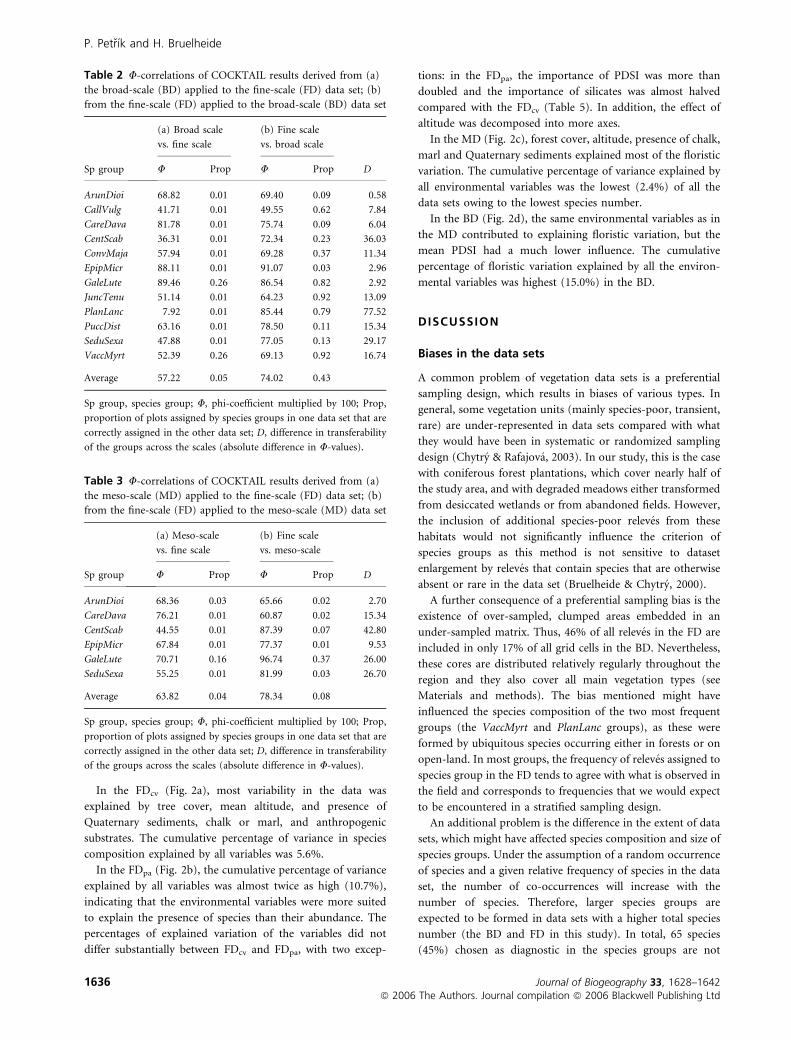
Table 2a shows the comparisons of fidelity coefficients between

species groups derived from the BD and applied to the FD

(downwards in scale), and Table 2b those for species groups

derived from the FD and applied to the BD (upwards in scale).

Scaling in a top-down direction generally resulted in lower

correspondence (mean U-coefficient in the diagonal of the

U-correlation matrix was 0.57) than scaling bottom-up (mean

U ¼ 0.74). In addition, the proportion of plots assigned by

species groups in BD that were correctly assigned in FD was

0.05 compared with 0.43 in the opposite direction. This means

that transferability of species groups was better in the bottom-

up than in the top-down direction. The comparison between

the MD and the FD gave similar results (Table 3). Neverthe-

less, there were fewer species groups and smaller proportions

of plots assigned by species groups as a result of the smaller

species number in the MD compared with the BD.

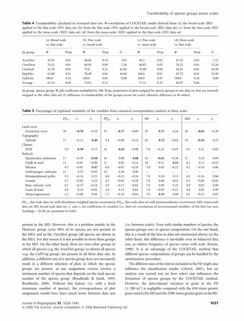
The comparison of truncated data sets resulted in a similar

general pattern, i.e. a better bottom-up than top-down

transferability of the species groups (Table 4).

The difference in the transferability of species groups (D in

Table 2) between bottom-up and top-down directions was

negatively related to the size of species groups. The more

species in a group, the more different downward scaling was

from upward scaling (R2 ¼ 0.80, n ¼ 12, P < 0.01). The

groups in which this difference was the highest were the groups

richest in species: the PlanLanc group (difference in U ¼ 0.78),

and the CentScab group (difference in U ¼ 0.36).

Effect of the environmental factors at various scales

All studied variables had a significant influence on explaining

floristic variation at all scales. In all data sets, the most

important variables in CCA were size of forest area (tree



https://www.researchgate.net/publication/235710596_Zeigerwerte_von_Pflanzen_in_Mitteleuropa_Scr_Geobot?el=1_x_8&enrichId=rgreq-082b7147-8710-4678-9002-943913632534&enrichSource=Y292ZXJQYWdlOzIyNzkyMjU1NjtBUzo5ODc0NTIxNTYxOTA3NEAxNDAwNTU0MTAyNTAw

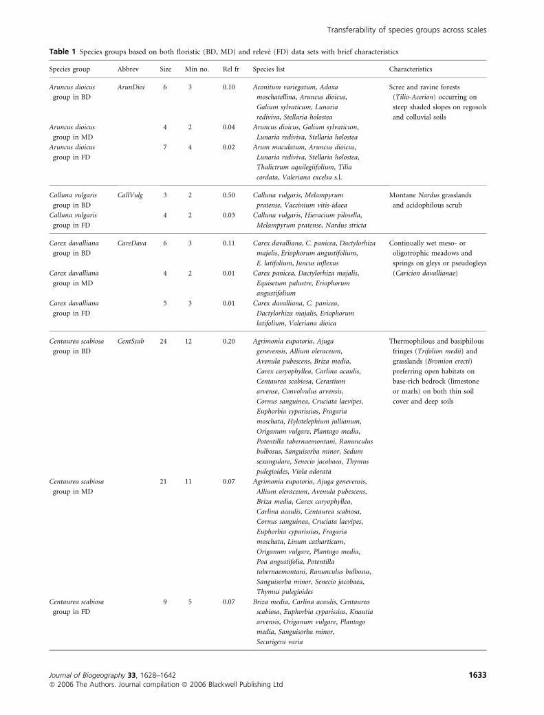
Table 1 Species groups based on both floristic (BD, MD) and releve (FD) data sets with brief characteristics

Species group Abbrev Size Min no. Rel fr Species list Characteristics

Aruncus dioicus

group in BD

ArunDioi 6 3 0.10 Aconitum variegatum, Adoxa

moschatellina, Aruncus dioicus,

Galium sylvaticum, Lunaria

rediviva, Stellaria holostea

Scree and ravine forests

(Tilio-Acerion) occurring on

steep shaded slopes on regosols

and colluvial soils

Aruncus dioicus

group in MD

4 2 0.04 Aruncus dioicus, Galium sylvaticum,

Lunaria rediviva, Stellaria holostea

Aruncus dioicus

group in FD

7 4 0.02 Arum maculatum, Aruncus dioicus,

Lunaria rediviva, Stellaria holostea,

Thalictrum aquilegiifolium, Tilia

cordata, Valeriana excelsa s.l.

Calluna vulgaris

group in BD

CallVulg 3 2 0.50 Calluna vulgaris, Melampyrum

pratense, Vaccinium vitis-idaea

Montane Nardus grasslands

and acidophilous scrub

Calluna vulgaris

group in FD

4 2 0.03 Calluna vulgaris, Hieracium pilosella,

Melampyrum pratense, Nardus stricta

Carex davalliana

group in BD

CareDava 6 3 0.11 Carex davalliana, C. panicea, Dactylorhiza

majalis, Eriophorum angustifolium,

E. latifolium, Juncus inflexus

Continually wet meso- or

oligotrophic meadows and

springs on gleys or pseudogleys

(Caricion davallianae)Carex davalliana

group in MD

4 2 0.01 Carex panicea, Dactylorhiza majalis,

Equisetum palustre, Eriophorum

angustifolium

Carex davalliana

group in FD

5 3 0.01 Carex davalliana, C. panicea,

Dactylorhiza majalis, Eriophorum

latifolium, Valeriana dioica

Centaurea scabiosa

group in BD

CentScab 24 12 0.20 Agrimonia eupatoria, Ajuga

genevensis, Allium oleraceum,

Avenula pubescens, Briza media,

Carex caryophyllea, Carlina acaulis,

Centaurea scabiosa, Cerastium

arvense, Convolvulus arvensis,

Cornus sanguinea, Cruciata laevipes,

Euphorbia cyparissias, Fragaria

moschata, Hylotelephium jullianum,

Origanum vulgare, Plantago media,

Potentilla tabernaemontani, Ranunculus

bulbosus, Sanguisorba minor, Sedum

sexangulare, Senecio jacobaea, Thymus

pulegioides, Viola odorata

Thermophilous and basiphilous

fringes (Trifolion medii) and

grasslands (Bromion erecti)

preferring open habitats on

base-rich bedrock (limestone

or marls) on both thin soil

cover and deep soils

Centaurea scabiosa

group in MD

21 11 0.07 Agrimonia eupatoria, Ajuga genevensis,

Allium oleraceum, Avenula pubescens,

Briza media, Carex caryophyllea,

Carlina acaulis, Centaurea scabiosa,

Cornus sanguinea, Cruciata laevipes,

Euphorbia cyparissias, Fragaria

moschata, Linum catharticum,

Origanum vulgare, Plantago media,

Poa angustifolia, Potentilla

tabernaemontani, Ranunculus bulbosus,

Sanguisorba minor, Senecio jacobaea,

Thymus pulegioides

Centaurea scabiosa

group in FD

9 5 0.07 Briza media, Carlina acaulis, Centaurea

scabiosa, Euphorbia cyparissias, Knautia

arvensis, Origanum vulgare, Plantago

media, Sanguisorba minor,

Securigera varia



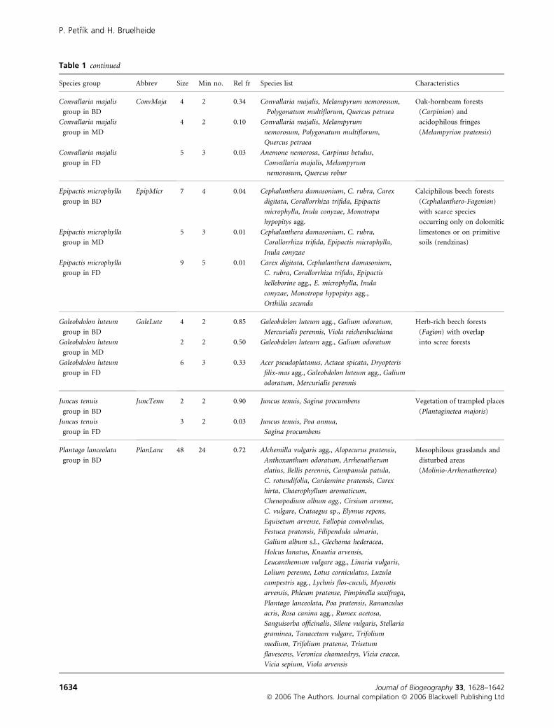
Table 1 continued


Convallaria majalis

group in BD

ConvMaja 4 2 0.34 Convallaria majalis, Melampyrum nemorosum,

Polygonatum multiflorum, Quercus petraea

Oak-hornbeam forests

(Carpinion) and

acidophilous fringes

(Melampyrion pratensis)

Convallaria majalis

group in MD

4 2 0.10 Convallaria majalis, Melampyrum

nemorosum, Polygonatum multiflorum,

Quercus petraea

Convallaria majalis

group in FD

5 3 0.03 Anemone nemorosa, Carpinus betulus,

Convallaria majalis, Melampyrum

nemorosum, Quercus robur

Epipactis microphylla

group in BD

EpipMicr 7 4 0.04 Cephalanthera damasonium, C. rubra, Carex

digitata, Corallorrhiza trifida, Epipactis

microphylla, Inula conyzae, Monotropa

hypopitys agg.

Calciphilous beech forests

(Cephalanthero-Fagenion)

with scarce species

occurring only on dolomitic

limestones or on primitive

soils (rendzinas)


group in MD

5 3 0.01 Cephalanthera damasonium, C. rubra,

Corallorrhiza trifida, Epipactis microphylla,

Inula conyzae


group in FD

9 5 0.01 Carex digitata, Cephalanthera damasonium,

C. rubra, Corallorrhiza trifida, Epipactis

helleborine agg., E. microphylla, Inula

conyzae, Monotropa hypopitys agg.,

Orthilia secunda

Galeobdolon luteum

group in BD

GaleLute 4 2 0.85 Galeobdolon luteum agg., Galium odoratum,

Mercurialis perennis, Viola reichenbachiana

Herb-rich beech forests

(Fagion) with overlap

into scree forestsGaleobdolon luteum

group in MD

2 2 0.50 Galeobdolon luteum agg., Galium odoratum

Galeobdolon luteum

group in FD

6 3 0.33 Acer pseudoplatanus, Actaea spicata, Dryopteris

filix-mas agg., Galeobdolon luteum agg., Galium

odoratum, Mercurialis perennis

Juncus tenuis

group in BD

JuncTenu 2 2 0.90 Juncus tenuis, Sagina procumbens Vegetation of trampled places

(Plantaginetea majoris)

Juncus tenuis

group in FD

3 2 0.03 Juncus tenuis, Poa annua,

Sagina procumbens

Plantago lanceolata

group in BD

PlanLanc 48 24 0.72 Alchemilla vulgaris agg., Alopecurus pratensis,

Anthoxanthum odoratum, Arrhenatherum

elatius, Bellis perennis, Campanula patula,

C. rotundifolia, Cardamine pratensis, Carex

hirta, Chaerophyllum aromaticum,

Chenopodium album agg., Cirsium arvense,

C. vulgare, Crataegus sp., Elymus repens,

Equisetum arvense, Fallopia convolvulus,

Festuca pratensis, Filipendula ulmaria,

Galium album s.l., Glechoma hederacea,

Holcus lanatus, Knautia arvensis,

Leucanthemum vulgare agg., Linaria vulgaris,

Lolium perenne, Lotus corniculatus, Luzula

campestris agg., Lychnis flos-cuculi, Myosotis

arvensis, Phleum pratense, Pimpinella saxifraga,

Plantago lanceolata, Poa pratensis, Ranunculus

acris, Rosa canina agg., Rumex acetosa,

Sanguisorba officinalis, Silene vulgaris, Stellaria

graminea, Tanacetum vulgare, Trifolium

medium, Trifolium pratense, Trisetum

flavescens, Veronica chamaedrys, Vicia cracca,

Vicia sepium, Viola arvensis

Mesophilous grasslands and

disturbed areas

(Molinio-Arrhenatheretea)



cover), mean altitude, and mean PDSI (Table 5). The effects

of bedrock types did not differ substantially across scales: the

most important substrates were Quaternary sediments, chalk

and marl, and silicates. The anthropogenic substrate was very

important at the fine scale, but this category was not

distinguished at the other scales. Mean PDSI was negatively

correlated with forest (tree) cover at all scales. Altitude

revealed no relationship with mean PDSI at the fine and the

meso-scales, but showed a negative correlation at the broad

scale (ordination diagrams see Fig. 2). Spatial autocorrelation

increased with grain: 18% of the total variation in the BD was

explained by the spatial covariables, in comparison with only

3% in the MD. Species number and Shannon–Wiener

diversity index in grid cells were negatively correlated with

forest (tree) cover, as were the Ellenberg values for light,

temperature, and continentality. The Ellenberg values for soil

reaction were positively correlated with the occurrence of

chalk and marl and Quaternary sediments at fine and broad

scales, but not at the meso-scale. The Ellenberg values for soil

nutrients and soil moisture did not show any stable pattern.

Table 1 continued


Plantago lanceolata

group in FD

17 9 0.20 Achillea millefolium agg.,

Anthoxanthum odoratum,

Arrhenatherum elatius,

Campanula rotundifolia,

Dactylis glomerata, Festuca

rubra agg., Galium album

agg., Knautia arvensis,

Leontodon hispidus,

Leucanthemum vulgare agg.,

Lotus corniculatus, Luzula

campestris agg., Plantago

lanceolata, Ranunculus acris,

Rumex acetosa, Trisetum

flavescens, Veronica

chamaedrys

Puccinellia distans

group in BD

PuccDist 2 2 0.09 Echinochloa crus-galli,

Puccinellia distans

Subhalophilous

communities along

the roadsidesPuccinellia distans

group in FD

6 3 0.01 Brassica oleracea,

Chenopodium glaucum,

Echinochloa crus-galli,

Matricaria recutita,

Puccinellia distans,

Setaria pumila

Sedum sexangulare

group in BD

SeduSexa 6 3 0.18 Carex caryophyllea, Plantago

media, Potentilla

tabernaemontani, Sedum

sexangulare, Senecio

jacobaea, Thymus pulegioides

Vegetation of

succulents on

shallow soils

(Sedo-Scleranthetea)

Sedum sexangulare

group in MD

2 2 0.05 Carex caryophyllea,

Sedum sexangulare

Sedum sexangulare

group in FD

3 2 0.01 Jovibarba globifera, Sedum

sexangulare, Thymus

pulegioides

Vaccinium myrtillus

group in BD

VaccMyrt 7 4 0.95 Athyrium filix-femina,

Avenella flexuosa, Dryopteris

dilatata, Fagus sylvatica,

Oxalis acetosella, Picea abies,

Vaccinium myrtillus

Acidophilous forests

(Luzulo-Fagion),

clearings and conifer

plantations

(Epilobietea

angustifolii)Vaccinium myrtillus

group in FD

2 2 0.22 Avenella flexuosa,

Vaccinium myrtillus

Abbrev, abbreviation of the group in the text; Size, number of species in a species group; Min no, minimum species number required for a plot to be

assigned to a species group; Rel fr, relative frequency of plots assigned to the species group.



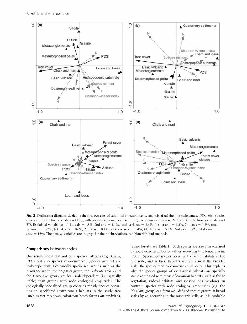
In the FDcv (Fig. 2a), most variability in the data was

explained by tree cover, mean altitude, and presence of

Quaternary sediments, chalk or marl, and anthropogenic

substrates. The cumulative percentage of variance in species

composition explained by all variables was 5.6%.

In the FDpa (Fig. 2b), the cumulative percentage of variance

explained by all variables was almost twice as high (10.7%),

indicating that the environmental variables were more suited

to explain the presence of species than their abundance. The

percentages of explained variation of the variables did not

differ substantially between FDcv and FDpa, with two excep-

tions: in the FDpa, the importance of PDSI was more than

doubled and the importance of silicates was almost halved

compared with the FDcv (Table 5). In addition, the effect of

altitude was decomposed into more axes.

In the MD (Fig. 2c), forest cover, altitude, presence of chalk,

marl and Quaternary sediments explained most of the floristic

variation. The cumulative percentage of variance explained by

all environmental variables was the lowest (2.4%) of all the

data sets owing to the lowest species number.

In the BD (Fig. 2d), the same environmental variables as in

the MD contributed to explaining floristic variation, but the

mean PDSI had a much lower influence. The cumulative

percentage of floristic variation explained by all the environ-

mental variables was highest (15.0%) in the BD.

DISCUSSION

Biases in the data sets

A common problem of vegetation data sets is a preferential

sampling design, which results in biases of various types. In

general, some vegetation units (mainly species-poor, transient,

rare) are under-represented in data sets compared with what

they would have been in systematic or randomized sampling

design (Chytry & Rafajova, 2003). In our study, this is the case

with coniferous forest plantations, which cover nearly half of

the study area, and with degraded meadows either transformed

from desiccated wetlands or from abandoned fields. However,

the inclusion of additional species-poor releves from these

habitats would not significantly influence the criterion of

species groups as this method is not sensitive to dataset

enlargement by releves that contain species that are otherwise

absent or rare in the data set (Bruelheide & Chytry, 2000).

A further consequence of a preferential sampling bias is the

existence of over-sampled, clumped areas embedded in an

under-sampled matrix. Thus, 46% of all releves in the FD are

included in only 17% of all grid cells in the BD. Nevertheless,

these cores are distributed relatively regularly throughout the

region and they also cover all main vegetation types (see

Materials and methods). The bias mentioned might have

influenced the species composition of the two most frequent

groups (the VaccMyrt and PlanLanc groups), as these were

formed by ubiquitous species occurring either in forests or on

open-land. In most groups, the frequency of releves assigned to

species group in the FD tends to agree with what is observed in

the field and corresponds to frequencies that we would expect

to be encountered in a stratified sampling design.

An additional problem is the difference in the extent of data

sets, which might have affected species composition and size of

species groups. Under the assumption of a random occurrence

of species and a given relative frequency of species in the data

set, the number of co-occurrences will increase with the

number of species. Therefore, larger species groups are

expected to be formed in data sets with a higher total species

number (the BD and FD in this study). In total, 65 species

(45%) chosen as diagnostic in the species groups are not

Table 2 U-correlations of COCKTAIL results derived from (a)

the broad-scale (BD) applied to the fine-scale (FD) data set; (b)

from the fine-scale (FD) applied to the broad-scale (BD) data set

Sp group

(a) Broad scale

vs. fine scale

(b) Fine scale

vs. broad scale

DU Prop U Prop

ArunDioi 68.82 0.01 69.40 0.09 0.58

CallVulg 41.71 0.01 49.55 0.62 7.84

CareDava 81.78 0.01 75.74 0.09 6.04

CentScab 36.31 0.01 72.34 0.23 36.03

ConvMaja 57.94 0.01 69.28 0.37 11.34

EpipMicr 88.11 0.01 91.07 0.03 2.96

GaleLute 89.46 0.26 86.54 0.82 2.92

JuncTenu 51.14 0.01 64.23 0.92 13.09

PlanLanc 7.92 0.01 85.44 0.79 77.52

PuccDist 63.16 0.01 78.50 0.11 15.34

SeduSexa 47.88 0.01 77.05 0.13 29.17

VaccMyrt 52.39 0.26 69.13 0.92 16.74

Average 57.22 0.05 74.02 0.43

Sp group, species group; U, phi-coefficient multiplied by 100; Prop,

proportion of plots assigned by species groups in one data set that are

correctly assigned in the other data set; D, difference in transferability

of the groups across the scales (absolute difference in U-values).

Table 3 U-correlations of COCKTAIL results derived from (a)

the meso-scale (MD) applied to the fine-scale (FD) data set; (b)

from the fine-scale (FD) applied to the meso-scale (MD) data set

Sp group

(a) Meso-scale

vs. fine scale

(b) Fine scale

vs. meso-scale

DU Prop U Prop

ArunDioi 68.36 0.03 65.66 0.02 2.70

CareDava 76.21 0.01 60.87 0.02 15.34

CentScab 44.55 0.01 87.39 0.07 42.80

EpipMicr 67.84 0.01 77.37 0.01 9.53

GaleLute 70.71 0.16 96.74 0.37 26.00

SeduSexa 55.25 0.01 81.99 0.03 26.70

Average 63.82 0.04 78.34 0.08

Sp group, species group; U, phi-coefficient multiplied by 100; Prop,

proportion of plots assigned by species groups in one data set that are

correctly assigned in the other data set; D, difference in transferability

of the groups across the scales (absolute difference in U-values).



present in the MD. However, this is a problem mainly in the

PlanLanc group (over 90% of its species are not present in

the MD) and in the VaccMyrt group (all species are absent in

the MD). For this reason it is not possible to form these groups

in the MD. On the other hand, there are nine other groups in

which all species (e.g. the ArunDioi group) or almost all species

(e.g. the CallVulg group) are present in all three data sets. In

addition, a different size of a species group does not necessarily

result in a different selection of plots in which the species

groups are present, as our assignment criteria involve a

minimum number of species that depends on the total species

number of the species group (Bruelheide & Jandt, 1995;

Bruelheide, 2000). Without this feature (i.e. with a fixed

minimum number of species), the correspondence of plot

assignment would have been much lower between data sets

(i.e. between scales). Even with similar numbers of species, the

species groups vary in species composition. On the one hand,

this is a result of the bias in data sets mentioned above; on the

other hand, this difference is inevitable even in balanced data

sets, as relative frequency of species varies with scale (Kunin,

1998). It is an advantage of the COCKTAIL method that

different species compositions of groups can be handled by the

optimization procedure.

The different sizes of the releves included in the FD might also

influence the classification results (Chytry, 2001), but no

analysis was carried out on how releve size influences the

formation of species groups by the COCKTAIL method.

However, the intra-dataset variation in grain in the FD

(± 200 m2) is negligible compared with the 650-times greater

grain used in the MD and the 2500-times greater grain in the BD.

Table 5 Percentages of explained variability of the variables from canonical correspondence analysis at three scales

FDcv k1 k2 FDpa k1 k2 BD k1 k2 MD k1 k2

Land-cover

Forest/tree cover 30 )0.78 )0.10 35 )0.77 )0.09 29 0.71 0.24 28 )0.63 )0.20

Topography

Altitude 11 )0.12 0.40 9.4 )0.08 )0.22 29 0.73 )0.02 19 )0.45 0.27

Climate

PDSI 5.9 0.39 0.15 14 0.43 )0.08 7.0 )0.23 )0.07 8.1 0.21 0.02

Bedrock

Quarternary sediments 17 )0.19 )0.50 16 0.08 0.68 14 )0.41 )0.26 11 0.24 0.09

Chalk & marl 11 )0.01 )0.09 11 0.05 )0.14 14 )0.11 0.53 8.1 0.12 )0.22

Silicates 9.5 )0.01 0.47 6.0 )0.01 )0.29 7.0 0.05 )0.21 8.1 )0.14 0.06

Anthropogen. substrate 12 0.25 )0.05 14 0.26 0.00 – – – – – –

Metamorphosed pelite 5.3 )0.14 0.21 6.0 )0.13 )0.24 7.0 0.24 0.15 6.5 )0.16 0.06

Granite 4.7 )0.02 0.22 4.3 )0.05 )0.20 7.0 0.08 0.01 6.5 )0.05 )0.04

Basic volcanic rock 4.1 )0.15 )0.14 4.3 )0.13 )0.02 7.0 0.09 0.23 4.9 0.02 0.00

Loam & loess 3.0 0.16 )0.02 2.6 0.15 0.02 7.0 )0.03 )0.21 4.9 0.05 0.09

Metaconglomerate 1.2 )0.08 0.09 1.7 )0.10 )0.04 7.0 0.35 0.08 6.5 )0.15 0.05

FDcv, fine-scale data set with abundance-weighted species occurrences; FDpa, fine-scale data set with presence/absence occurrences; MD, meso-scale

data set; BD, broad-scale data set; k1 and k1 are coefficients of variation (i.e. inter-set correlations of environmental variables) of the first two axes

(loadings > |0.30| are presented in bold).

Table 4 Transferability calculated in truncated data sets. U-correlations of COCKTAIL results derived from (a) the broad-scale (BD)

applied to the fine-scale (FD) data set; (b) from the fine-scale (FD) applied to the broad-scale (BD) data set; (c) from the fine-scale (FD)

applied to the meso-scale (MD) data set; (d) from the meso-scale (MD) applied to the fine-scale (FD) data set

Sp group

(a) Broad scale

vs. fine scale

(b) Fine scale

vs. broad scale

D

(c) Fine scale

vs. meso-scale

(d) Meso-scale

vs. fine scale

DU Prop U Prop U Prop U Prop

ArunDioi 45.03 0.01 48.86 0.10 3.83 46.2 0.03 47.42 0.03 1.22

CareDava 76.21 0.01 68.95 0.09 7.26 60.87 0.02 76.21 0.01 15.34

CentScab 32.78 0.01 73.8 0.23 41.02 79.49 0.08 43.01 0.01 36.50

EpipMicr 61.80 0.01 78.48 0.04 16.68 100.0 0.01 67.73 0.01 32.30

GaleLute 100.0 0.16 100.0 0.65 0.00 100.0 0.35 100.0 0.16 0.00

Average 63.16 0.04 74.02 0.22 77.31 0.10 66.87 0.04

Sp group, species group; U, phi-coefficient multiplied by 100; Prop, proportion of plots assigned by species groups in one data set that are correctly

assigned in the other data set; D, difference in transferability of the groups across the scales (absolute difference in U-values).



Comparisons between scales

Our results show that not only species patterns (e.g. Kunin,

1998) but also species co-occurrences (species groups) are

scale-dependent. Ecologically specialized groups such as the

ArunDioi group, the EpipMicr group, the GaleLute group and

the CareDava group are less scale-dependent (i.e. spatially

stable) than groups with wide ecological amplitudes. The

ecologically specialized group contains mostly species occur-

ring in specialized (extra-zonal) habitats in the study area

(such as wet meadows, calcareous beech forests on rendzinas,

ravine forests; see Table 1). Such species are also characterized

by more extreme indicator values according to Ellenberg et al.

(2001). Specialized species occur in the same habitats at the

fine scale, and as these habitats are rare also at the broader

scale, the species tend to co-occur at all scales. This explains

why the species groups of extra-zonal habitats are spatially

stable compared with those of common habitats, such as fringe

vegetation, ruderal habitats, and mesophilous meadows. In

contrast, species with wide ecological amplitudes (e.g. the

PlanLanc group) can form well-defined species groups at broad

scales by co-occurring in the same grid cells, as it is probable

Fig. 2 Ordination diagrams depicting the first two axes of canonical correspondence analysis of (a) the fine-scale data set FDcv with species

coverage, (b) the fine-scale data set FDpa with presence/absence occurrence, (c) the meso-scale data set MD, and (d) the broad-scale data set

BD. Explained variability: (a) 1st axis ¼ 1.8%, 2nd axis ¼ 1.1%, total variance ¼ 5.6%; (b) 1st axis ¼ 4.3%, 2nd axis ¼ 1.8%, total

variance ¼ 10.7%; (c) 1st axis ¼ 0.6%, 2nd axis ¼ 0.4%, total variance ¼ 2.4%; (d) 1st axis ¼ 5.1%, 2nd axis ¼ 2%, total vari-

ance ¼ 15%. The passive variables are in grey; for their abbreviations, see Materials and methods.



that at least one of a larger number of habitats occurs in this

grid cell, but can co-occur at fine scales (i.e. in releves) only to

a limited degree, as a certain area in one habitat can only

contain a limited species number as a result of dispersal

limitation and local exclusion mechanisms (Gause, 1934).

Kuzelova & Chytry (2004) stated that the transferability of

species groups formed at a regional scale is best in those areas

with high habitat heterogeneity, which is congruent with our

observation of better transferability of specialized groups. They

also found better transferability of species groups that had a

central position along the major environmental gradients

existing at the regional scale. However, this is not the case in

our study. For example, the PlanLanc group has low

transferability although it occupies a central ecological position

in our study. In contrast, Kuzelova & Chytry’s (2004) result

seems to apply to the GaleLute group, with a central position in

forests in our study area.

Considering all the factors that influence transferability of

species groups across scales, the degree of correspondence

across scales is remarkable, in particular in the bottom-up

direction. With an average U of 0.74, about three-quarters of

the discriminant capability of a species group at the broad scale

can be predicted by fine-scale co-occurrences. This result was

also obtained in the truncated data sets.

Effect of environmental factors

A comparison of the driving factors with those of other studies

is difficult as different studies use different extents (e.g.

regional scale, see Heikkinen & Neuvonen, 1997; Chytry et al.,

1999; and national scale, see Hill, 1991), varying resolution,

and different species dataset structures with various environ-

mental variables according to the character of the study area.

In addition, often only selected species are analysed in such

studies (Pedersen, 1990; Myklestad & Birks, 1993; Myklestad,

1993). Moreover, the studies listed above ignore the spatial

structure of grid data, which might be unimportant (Heikk-

inen & Birks, 1996; Heikkinen et al., 1998; Korvenpaa et al.,

2003; bird distribution data in Titeux et al., 2004), but might

be the main explanatory factor in the data set (bird and

butterfly distribution data in Storch et al., 2003). In our case,

spatial autocorrelation explains a large proportion of the

floristic variation in the BD. This could be connected with

the rather fine resolution, which was not used in similar

studies.

The main correlating variables, altitude, geology and forest

(tree) cover, are also considered to have a causal influence on

plant distribution in meso-scale studies (Gaston, 2003; Pearson

& Dawson, 2003). Potential direct solar irradiation is used only

occasionally (e.g. Hennenberg & Bruelheide, 2003), as it is not

easy to obtain precise data. The biases listed above are more

severe when comparing ordination results across scales com-

pared with species groups, as outliers have a strong influence.

Thus, generalizations should be made only with caution.

Nevertheless, the results obtained make sense: environmental

factors that have a more direct (proximal) impact on plants,

i.e. are closer to the effect on plants in the causal chain, are

more important at the fine scale (e.g. PDSI), while more

indirect (distal) factors have a greater importance at the broad

scale (e.g. altitude).

Applications

The statistical approach to defining species groups across

scales might have wide applications in assessing biodiversity.

If spatially stable species groups have been identified in areas

with completed floristic or vegetation surveys, these groups

can be used to complement corresponding vegetation or

floristic data sets. Another application might be temporal

prediction, which has not yet been tested. As vegetation

surveys are repeated with less expenditure of time and

money (e.g. monitoring in the Natura 2000 network) than

complete floristic mappings, bottom-up predictions would

be valuable. As Wilson et al. (2004) stated that biodiversity

change (decline or increase rate) can be revealed from

current species distribution data alone using spatial patterns

of occupancy in combination with the size of the occupied

area, spatially stable groups from vegetation data sets might

be monitored for changes in time and then applied across

various scales. Thus, we may detect a declining species

group at the regional or national scale by using monitoring

results from local scales. As there are already abundant data

on the sociology of endangered species and vegetation plot

data are increasingly collected for monitoring purposes, a

scaling-up approach would offer a new approach to utilizing

such data.

Using species groups for risk assessment is another possible

application. For this purpose, the predictive power of species

groups for particular risks (e.g. land abandonment) would

have to be assessed first. Then, various scales would have to be

compared, as it has been shown that rates of decline are scale-

dependent (Hartley & Kunin, 2003).

The next step will be to repeat our approach in other areas.

The most suitable areas will be those in which both floristic

and vegetation surveys have already been undertaken, and

preferably those with high biodiversity with a high number of

different species groups. An example at the regional scale is the

Krivoklatsko Biosphere Reserve (Czech Republic), where a

floristic mapping in 1/100 CEBA grids and vegetation survey

with more than 4000 releves have already been performed (see

Kolbek et al., 1999). Similarly, in Mecklenburg-Western

Pomerania (northern Germany), vegetation and a floristic

data bases have been produced at the level of a federal state

(Berg et al., 2004). Unfortunately, this case is the exception

rather than the rule in central Europe. At the national level

there are many floristic distribution atlases using different

resolutions (e.g. Universal Transverse Mercator UTM

10 · 10 km grid in Preston et al., 2002; Distribution Atlas of

Vascular Plants in Poland ATPOL 10 · 10 km grid in Zajac &

Zajac, 2001; CEBA 10¢ E · 6¢ N grid c. 133 km2 in Haeupler &

Schonfelder, 1989). At this national scale, digital vegetation

data bases are still lacking but are under preparation. If we



apply the method at a continental scale, other available floristic

data sets could be used (Meusel et al., 1965–92; Jalas &

Suominen, 1972–94; Jalas et al., 1996, 1999; Kurtto et al.,

2004), even reaching the worldwide level (e.g. project

WORLDMAP; Gaston, 2003). The final aim would be to use

vegetation or floristic data sets from all available scales to make

predictions of species distribution at the global scale, but this

goal is still far out of reach.

ACKNOWLEDGEMENTS

We thank John Birks, Zuzana Munzbergova, David Storch

and two anonymous referees for their valuable comments on

this paper. Lubos Tichy and Jan Wild are acknowledged for

their help with the data analyses. Tim C. G. Rich kindly

improved our English. We are indebted to the late Tomas

Sykora, and to Kveta Moravkova, Richard Visnak and Jarmila

Sykorova for providing their vegetation samples. This

research was partly supported by Biodiversity Research

Center (grant no. LC06073 funded by Ministry of Education,

Youth and Sports of the CR) and grant nos AV0Z60050516

and 206/03/H137 (GACR). P.P. is indebted to the Deutsche

Bundesstiftung Umwelt (http://www.dbu.de) and to BioHab

(http://www.biohab.alterra.nl) for financial support for his

study visits.

SUPPLEMENTARY MATERIAL

The following supplementary material is available for this

article online from http://www.blackwell-synergy.com.

Appendix S1. Environmental variables with brief descriptive

statistics.

REFERENCES

Berg, C., Dengler, J., Abdank, A. & Isermann, M. (2004) Die

Pflanzengesellschaften Mecklenburg-Vorpommerns und ihre

Gefahrdung – Textband. Weissdorn-Verlag, Jena.

Blackburn, T. & Gaston, K.J. (2002) Scale in macroecology.

Global Ecology and Biogeography, 11, 185–189.

ter Braak, C.J.F. & Smilauer, P. (2002) CANOCO reference

manual and CanoDraw for Windows. User’s guide. Software

for canonical community ordination, Ver. 4.5. Microcompu-

ter Power, Ithaca, NY.

Braun-Blanquet, J. (1921) Prinzipien einer Systematik der

Pflanzengesellschaften auf floristischer Grundlage. Jahrbuch

der St. Gallen Naturwissenschaftlichen Gesellschaft, 57, 305–

351.

Bruelheide, H. (1995) Die Grunlandgesellschaften des Harzes

und ihre Standortsbedingungen. Mit einem Beitrag zum

Gliederungssystem auf der Basis von statistisch ermittelten

Artengruppen. Dissertationes Botanicae, 244, 1–338.

Bruelheide, H. (2000) A new measure of fidelity and its

application to defining species groups. Journal of Vegetation

Science, 11, 167–178.

Bruelheide, H. & Chytry, M. (2000) Towards unification of

national vegetation classifications: a comparison of two

methods for analysis of large datasets. Journal of Vegetation

Science, 11, 295–306.

Bruelheide, H. & Jandt, U. (1995) Survey of limestone grass-

lands by statistically formed groups of differential species.

Colloques Phytosociologiques, 23, 319–338.

Chytry, M. (2001) Phytosociological data give biased estimates

of species richness. Journal of Vegetation Science, 12, 439–444.

Chytry, M. & Rafajova, M. (2003) Czech national phytoso-

ciological database: basic statistics of the available vegeta-

tion-plot data. Preslia, 75, 1–15.

Chytry, M. & Tichy, L. (2003) Diagnostic, constant and domi-

nant species of vegetation classes and alliances of the Czech

Republic: a statistical revision. Folia Facultatis Scientiarum

Naturalium Universitatis Masarykianae Brunensis, 108, 1–231.

Chytry, M., Grulich, V., Tichy, L. & Kouril, M. (1999) Phy-

togeographical boundary between the Pannonicum and

Hercynicum: a multivariate analysis of landscape in the

Podyjı/Thayatal National Park, Czech Republic/Austria.

Preslia, 71, 23–41.

Chytry, M., Kucera, T. & Kocı, M. (2001) Katalog biotopu

Ceske republiky. Interpretacnı prırucka k evropskym pro-

gramum Natura 2000 a Smaragd. AOPK CR, Praha.

Chytry, M., Exner, A., Hrivnak, R., Ujhazy, K., Valachovic, M.

& Willner, W. (2002a) Context-dependence of diagnostic

species: a case study of the central European spruce forests.

Folia Geobotanica, 37, 403–417.

Chytry, M., Tichy, L., Holt, J. & Botta-Dukat, Z. (2002b)

Determination of diagnostic species with statistical fidelity

measures. Journal of Vegetation Science, 13, 79–90.

Conrad, O. (2002) DiGeM 2.0. Gottingen. http://www.ge-

ogr.uni-goettingen.de/pg/saga/digem/.

Ellenberg, H., Weber, H.E., Dull, R., Wirth, V. & Werner, W.

(2001) Zeigerwerte von Pflanzen in Mitteleuropa. 3rd edn.

Scripta Geobotanica, 18, 1–262.

ESRI (1999) ArcView GIS. Environmental Systems Research

Institute Inc., Redlands.

Ewald, J. (2001) Der Beitrag pflanzensoziologischer Daten-

banken zur vegetationsokologischen Forschung. Berichte der

Reinhold Tuxen Gesellschaft, 13, 53–69.

Gaston, K.J. (1996) Biodiversity. A biology of numbers and

difference. Blackwell Science Ltd, Oxford.

Gaston, K.J. (2003) The structure and dynamics of geographic

ranges. Oxford University Press, Oxford.

Gause, G.F. (1934) The struggle for existence. Williams &

Wilkins, Baltimore, MD.

Gurevitch, J., Scheiner, S.M. & Fox, G.A. (2002) The ecology of

plants. Sinauer Associates, Sunderland, MA.

Haeupler, H. & Schonfelder, P. (1989) Atlas der Farn- und

Blutenpflanzen der Bundesrepublik Deutschland, 2nd edn.

Ulmer, Stuttgart.

Hartley, S. & Kunin, W.E. (2003) Scale dependency of rarity,

extinction risk, and conservation priority. Conservation

Biology, 17, 1559–1570.



Heikkinen, R.K. & Birks, H.J.B. (1996) Spatial and environ-

mental components of variation in the distribution patterns

of subarctic plant species at Kevo, N Finland – a case study

at the meso-scale level. Ecography, 19, 341–351.

Heikkinen, R.K. & Neuvonen, S. (1997) Species richness of

vascular plants in the subarctic landscape of northern Fin-

land: modelling relationships to environment. Biodiversity

and Conservation, 6, 1181–1201.

Heikkinen, R.K., Birks, H.J.B. & Kalliola, R.J. (1998) A nu-

merical analysis of the mesoscale distribution patterns of

vascular plants in the subarctic Kevo Nature Reserve,

northern Finland. Journal of Biogeography, 25, 123–146.

Hennekens, S.M. & Schaminee, J.H.J. (2001) TURBOVEG, a

comprehensive data base management system for vegetation

data. Journal of Vegetation Science, 12, 589–591.

Hennenberg, K.J. & Bruelheide, H. (2003) Ecological in-

vestigations on the northern distribution range of Hippo-

crepis comosa L. in Germany. Plant Ecology, 166, 167–188.

Herben, T. (1987) Dynamika invaze Orthodontium lineare

Schwaegr. v Cechach. PhD thesis, Academy of Sciences of the

Czech Republic, Pruhonice.

Hill, M.O. (1991) Patterns of species distribution in Britain

elucidated by canonical correspondence analysis. Journal of

Biogeography, 18, 247–255.

Jalas, J. & Suominen, J. (1972–94) Atlas Florae Europaeae, Vols

1–10. The Committee for Mapping the Flora of Europe &

Societas Biologica Fennica Vanamo, Helsinki.

Jalas, J., Suominen, J. & Lampinen, R. (1996) Atlas Florae

Europaeae, Vol. 11. The Committee for Mapping the Flora

of Europe & Societas Biologica Fennica Vanamo, Helsinki.

Jalas, J., Suominen, J., Lampinen, R. & Kurtto, A. (1999) Atlas

Florae Europaeae, Vol. 12. The Committee for Mapping the

Flora of Europe & Societas Biologica Fennica Vanamo,

Helsinki.

Jandt, U. (1999) Kalkmagerrasen am Sudharzrand und im

Kyffhauser. Gliederung im uberregionalen Kontext, Ver-

breitung, Flora und Standortsverhaltnisse. Dissertationes

Botanicae, 322, 1–246.

Kolbek, J., Mlady, F. & Petrıcek, V. (eds) (1999) Kvetena

Chranene krajinne oblasti a Biosfericke rezervace Krivoklatsko.

1. Mapy rozsırenı cevnatych rostlin. AOPK CR & Institute of

Botany, Praha.

Koleff, P. & Gaston, J.K. (2002) The relationship between local

and regional species richness and spatial turnover. Global

Ecology and Biogeography, 11, 363–375.

Korvenpaa, T., von Numers, M. & Hinneri, S. (2003) A me-

soscale analysis of floristic patterns in the south-west Finnish

Archipelago. Journal of Biogeography, 30, 1019–1031.

Kuzelova, I. & Chytry, M. (2004) Interspecific associations in

phytosociological data sets: how do they change between

local and regional scale? Plant Ecology, 173, 247–257.

Kubat, K., Hrouda, L., Chrtek, J.jun., Kaplan, Z., Kirschner, J.

& Stepanek, J. (eds) (2002) Klıc ke kvetene Ceske republiky.

Academia, Praha.

Kunin, W. (1998) Extrapolating species abundance across

spatial scales. Science, 281, 1513–1515.

Kurtto, A., Lampinen, R. & Junikka, L. (2004) Atlas Florae

Europaeae. Distribution of Vascular Plants in Europe, Vol. 13.

The Committee for Mapping the Flora of Europe & Societas

Biologica Fennica Vanamo, Helsinki.

Levin, S. (1992) The problem of pattern and scale in ecology.

Ecology, 73, 1943–1967.

Meusel, H., Jager, E.J., Rauschert, S. & Weinert, E. (1965–92)

Vergleichende Chorologie der zentraleuropaischen Flora, Vols

1–3. G. Fischer Verlag, Jena.

Mucina, L., Schaminee, J. & Rodwell, J.S. (2001) Common

data standards for recording releves in field survey for ve-

getation classification. Journal of Vegetation Science, 11, 769–

772.

Myklestad, A. (1993) The distribution of Salix species in

Fennoscandia – a numerical analysis. Ecography, 16, 329–

344.

Myklestad, A. & Birks, H.J.B. (1993) A numerical analysis of

the distribution patterns of Salix species in Europe. Journal

of Biogeography, 20, 1–32.

Pearson, R.G. & Dawson, T.P. (2003) Predicting the impacts of

climate change on the distribution of species: are bioclimate

envelope models useful? Global Ecology and Biogeography,

12, 361–371.

Pedersen, B. (1990) Distributional patterns of vascular plants

in Fennoscandia: a numerical approach. Nordic Journal of

Botany, 10, 163–189.

Pflume, S. (1999) Laubwaldgesellschaften im Harz. Gliederung,

Okologie, Verbreitung. Archiv naturwissenschaftlicher Dis-

sertationen, 9, 1–238. Galuuder-Verlag, Wiehl.

Preston, C.D., Pearman, D.A. & Dines, T.D. (2002) New atlas

of the British and Irish Flora. An atlas of the vascular plants of

Britain, Ireland, the Isle of Man and the Channel Islands.

Oxford University Press, Oxford.

Schaminee, J.H.J. & Hennekens, S.M. (2001) TURBOVEG,

MEGATAB und SYNBIOSYS: neue Entwicklungen in der

Pflanzensoziologie. Berichte der Reinhold Tuxen Gesellschaft,

13, 21–34.

Scheller, H. (1989) Flora von Coburg. Die Farn- und Bluten-

pflanzen des Coburger Landes. Natur-Museum Coburg,

Coburg.

Sokal, R.R. & Rohlf, F.J. (1995) Biometry, 3rd edn. Freeman,

New York.

Storch, D., Konvicka, M., Benes, J., Martınkova, J. & Gaston,

K.J. (2003) Distribution patterns in butterflies and birds

of the Czech Republic: separating effects of habitat and

geographical position. Journal of Biogeography, 30, 1195–

1205.

Tauber, T. (2000) Zwergbinsen-Gesellschaften (Isoeto-Nano-

juncetea) in Niedersachsen – Verbreitung, Gliederung, Dy-

namik, Keimungsbedingungen der Arten und Schutzkonzepte.

Cuvilier, Gottingen.

Tichy, L. (2002) JUICE, software for vegetation classification.

Journal of Vegetation Science, 13, 451–453.

Titeux, N., Dufrene, M., Jacob, J.P., Paquay, M. & Defourny, P.

(2004) Multivariate analysis of a fine-scale breeding bird

atlas using a geographical information system and partial



canonical correspondence analysis: environmental and spa-

tial effects. Journal of Biogeography, 31, 1841–1856.

Wiens, J. (1989) Spatial scaling in ecology. Functional Ecology,

3, 385–397.

Wilson, R.J., Thomas, C.D., Fox, R., Roy, D.B. & Kunin, W.

(2004) Spatial patterns in species distributions reveal bio-

diversity change. Nature, 432, 393–396.

Zajac, A. & Zajac, M. (2001) Atlas rozmieszczenia roslin nac-

zyniowych w Polsce. Instytut Botaniki Uniwersytetu Jagi-

ellonskiego, Krakow.

BIOSKETCHES

Petr Petrık is a PhD student currently working on a biogeographical evaluation of grid mapping distribution data. His main

research interests are numerical phytogeography, phytosociology (formalized classification) and field floristic surveys.

Helge Bruelheide is head of the Institute of Geobotany at the Martin Luther University of Halle-Wittenberg. His work includes

studies of numerical phytosociology, soil science, experimental phytogeography, invasive species, forest dynamics and desert ecology.

His most recent interests are ecoinformatics, in particular the development of methods that allow ecological data sets of different

scopes, grains and extents to be combined.

Editor: John Birks



Species groups can be transferred across different scales

Documents

Transcript of Species groups can be transferred across different scales