Special Issue Paper A Bayesian predictive sample size selection design for single-arm exploratory...

Special Issue Paper

Received 9 September 2011, Accepted 4 June 2012 Published online 16 July 2012 in Wiley Online Library

(wileyonlinelibrary.com) DOI: 10.1002/sim.5505

A Bayesian predictive sample sizeselection design for single-armexploratory clinical trialsSatoshi Teramukai,a*† Takashi Daimonb and Sarah Zoharc

The aim of an exploratory clinical trial is to determine whether a new intervention is promising for further test-ing in confirmatory clinical trials. Most exploratory clinical trials are designed as single-arm trials using a binaryoutcome with or without interim monitoring for early stopping. In this context, we propose a Bayesian adaptivedesign denoted as predictive sample size selection design (PSSD). The design allows for sample size selectionfollowing any planned interim analyses for early stopping of a trial, together with sample size determinationbefore starting the trial. In the PSSD, we determine the sample size using the method proposed by Sambucini(Statistics in Medicine 2008; 27:1199–1224), which adopts a predictive probability criterion with two kinds ofprior distributions, that is, an ‘analysis prior’ used to compute posterior probabilities and a ‘design prior’ usedto obtain prior predictive distributions. In the sample size determination of the PSSD, we provide two samplesizes, that is, N and Nmax, using two types of design priors. At each interim analysis, we calculate the predictiveprobabilities of achieving a successful result at the end of the trial using the analysis prior in order to stop thetrial in case of low or high efficacy (Lee et al., Clinical Trials 2008; 5:93–106), and we select an optimal samplesize, that is, either N or Nmax as needed, on the basis of the predictive probabilities. We investigate the operatingcharacteristics through simulation studies, and the PSSD retrospectively applies to a lung cancer clinical trial.(243) Copyright © 2012 John Wiley & Sons, Ltd.

Keywords: Bayesian approach; adaptive design; analysis and design priors; prior predictive distributions;interim monitoring

1. Introduction

The aim of exploratory clinical trials, such as phase II trials and proof-of-concept studies, is to determinewhether a new intervention is promising for further testing in confirmatory clinical trials, such asphase III randomised controlled trials. Most exploratory clinical trials are designed as single-armtrials with or without interim monitoring for early stopping. In this setting, the efficacy of treatmentis commonly evaluated using a binary outcome such as tumour shrinkage or response to treatment.Zohar et al. [1] emphasised that Bayesian approaches are ideal for such exploratory clinical trials as theytake into account previous information about the quantity of interest as well as accumulated data duringa trial.

In this context, various Bayesian approaches or designs have been proposed for single-arm clinicaltrials. For instance, Tan and Machin [2] developed a Bayesian two-stage design called single thresholddesign (STD), and Mayo and Gajewski [3, 4] extended this proposition into a design incorporatinginformative prior distributions. Whitehead et al. [5] formulated a simple approach to sample sizedetermination (SSD) in which they incorporate historical data in the Bayesian inference. Furthermore,Sambucini [6] proposed a predictive version of the STD (PSTD) using two kinds of prior distributions

aDepartment of Clinical Trial Design and Management, Translational Research Center, Kyoto University Hospital,Kyoto, Japan

bDepartment of Biostatistics, Hyogo College of Medicine, Hyogo, JapancInserm, U717 Biostatistics Department, F75010 Paris, France*Correspondence to: Satoshi Teramukai, Department of Clinical Trial Design and Management, Translational ResearchCenter, Kyoto University Hospital, 54 Shogoin-kawaharacho, Sakyo-ku, Kyoto 606-8507, Japan.

†E-mail: [email protected]

Copyright © 2012 John Wiley & Sons, Ltd. Statist. Med. 2012, 31 4243–4254

4243

S. TERAMUKAI, T. DAIMON AND S. ZOHAR

pursuing different aims: the ‘analysis prior’ used to compute posterior probabilities and the ‘designprior’ used to obtain prior predictive distributions. Indeed, according to Sambucini and Brutti [6, 7], thetwo-priors approach is useful when implementing the Bayesian SSD process and providing a generalframework that incorporates frequentist SSD (corresponding to a non-informative analysis prior and adegenerate design prior) as a special case.

Recently, Sambucini [8] modified the PSTD and suggested a Bayesian adaptive two-stage design inwhich the sample size for the second stage depends on the results of the first stage. However, as thesemethods [2–4, 6, 8] focus on the two-stage design only, their application is somewhat restricted. In addi-tion, Brutti et al. [9] proposed a Bayesian SSD with sample size re-estimation based on a two-priorsapproach; however, their approach was based on approximately normally distributed outcomes and notdirectly on binary outcomes.

Motivated by these studies, in this paper, we propose a Bayesian adaptive design for single-armexploratory clinical trials with binary outcomes based on a two-priors approach and predictive prob-abilities. The proposed design, denoted as predictive sample size selection design (PSSD), consists ofSSD at the planning stage and sample size selection at any required stage following interim analysesduring the course of the trial. The SSD of the proposed design is based on the method proposed bySambucini [6] without interim evaluations. However, in our design two sample sizes can be provided inadvance; one is an initial sample size to mention how many subjects are needed, whereas another is anoptional sample size to increase the initial sample size as necessary following the interim analyses dur-ing the trial, where we calculate predictive probabilities of achieving a successful result at the end of thetrial. The optional sample size is based on a maximal sample size that is motivated by ethical considera-tions and resource limitations. As a consequence, using the sample size selection that is an option at eachof the planned interim analyses, a choice can be made between the aforementioned two sample sizes. Inaddition, although Lee and Liu [10] proposed a Bayesian predictive probability approach for single-armtrials that combines SSD with multiple interim analyses, our design separates interim monitoring fromthe SSD procedure, and so it can easily incorporate adaptive features such as sample size selection, asshown in this paper, or sample size re-estimation into a more flexible design.

The outline of the paper is as follows. Section 2 introduces the basic idea for SSD and interim mon-itoring. In Section 3, we propose a PSSD that incorporates multiple interim analyses and sample sizeselection based on predictive probabilities. We discuss the properties of the new design on the basis ofsome simulations in Section 4. Finally, we present an illustrative example in Section 5 and conclude witha discussion in Section 6.

2. Methods

2.1. Notations

Let � be the unknown success probability parameter. Let Y be the binary outcome variable, whichtakes a value of 1 if we consider the treatment successful in a patient and 0 otherwise. We denote byS D

PniD1 Yi the random ‘total number of successes’ obtained at the end of study out of n patients.

The sampling distribution of S is

fn.sj�/D Bin.sIn; �/ 8s D 0; : : : ; n

where ‘Bin’ denotes the binomial probability mass function. In a Bayesian conjugate analysis, byintroducing the Beta prior for � with hyperparameters a and b, �.�/ D Beta.� I a; b/, we obtain theposterior distribution

�n.� jS D s/D Beta.� I aC s; bC n� s/

Furthermore, the predictive distribution of S is beta-binomial, as is well known.Let �0 denote a fixed value that previous evidence suggests would be the success probability with a

control or standard treatment, and let ı represent a ‘minimally clinically significant effect’. Therefore,�0C ı is a pre-specified target value for the success probability.

2.2. Sample size determination

2.2.1. The two-priors approach. Two kinds of prior distributions have been proposed: the analysis priorand the design prior [6, 7]. The analysis prior reflects the prior information about the efficacy of the new

4244



treatment, and we use it to obtain posterior probabilities. By contrast, the design prior expresses theuncertainty about � in a specific subspace of the parameter space, and we use it to obtain the priorpredictive distribution of the number of successes. For binary observations, we use beta distributions;for the analysis prior, �A.�/ D Beta.� I aA; bA/, and for the design prior, �D.�/ D Beta.� I aD; bD/. Atthe design stage, we recommend that an analysis prior �A.�/ should be objectively determined on thebasis of prior information such as reliable historical or external data. In practice, Biswas et al. [11] havereported that they have used 20% or less as a discount factor for historical information. As a result, if itis difficult to take existing information into consideration, because the amount of available data can belimited and there can be some uncertainty about the treatment effect in most exploratory clinical trials, auniform non-informative analysis prior Beta.1; 1/ may be appropriate. We can specify the design prior�D.�/ with hyperparameters as proposed by Sambucini [6]

aD D nD�D0 C 1 and bD D nD

�1� �D

0

�C 1

where �D0 represents the prior mode that should be chosen such that �D

0 > �0 C ı, and nD is a kind oftuning parameter for the variance of �D.�/. Therefore, as nD increases, the distribution �D.�/ becomesmore concentrated around �D

0 . Particularly, when nD D1, �D.�/ is the degenerate distribution at �D0 .

In practice, nD can be derived from the prior mode �D0 and its uncertainty, that is, a credible interval

for �D.�/.

2.2.2. Sample size determined on the basis of the design prior. If we pre-specify �0, ı, aD and bD, theposterior probability that the success probability is greater than the target value for S D 1; : : : ; n after nobservations is as follows:

pn.S/D �An .� > �0C ıjS/

where �An .� jS/ is the posterior distribution computed using the analysis prior �A.�/. For a pre-specified

probability threshold � 2 .0; 1/, we declare the treatment efficacious if the observed number of successess is such that

pn.S D s/D �An .� > �0C ıjS D s/> �

In order to determine the sample size for a clinical trial, a probability measure corresponding to the priorpredictive distribution of S has been introduced [6, 7]. The prior predictive distribution in this setting isbeta-binomial with parameters .aD; bD; n/, that is,

mD.s/D

Z 1

0

fn.sj�/�D.�/d� 8s D 0; : : : ; n

When �D.�/ is the degenerate distribution at �D0 (i.e. nD D1/,

mD.s/D fn�sj�D

0

�D Bin

�sIn; �D

0

�8s D 0; : : : ; n

Two kinds of criteria for SSD based on the prior predictive distribution have been proposed [7]; one isthe predictive probability criterion (PPC), and the other is the predictive expectation criterion (PEC).

The PPC is defined as follows: for a pre-specified probability threshold � 2 .0; 1/, the smallest valueis selected as the sample size N , such that 8n>N

PDŒpn.S D s/> ��> �

where PD is the probability measure associated with the prior predictive probability obtained using thedesign prior. Therefore,

PDŒpn.S D s/> ��DXn

sDumD.s/

where u D minfs 2 f0; : : : ; ng W pn.s/ > �g. As remarked by Sambucini [6], we should considersawtooth behaviour for PDŒpn.S D s/ > �� due to the discreteness of the random variable S . Note thatthe approach using PPC is also known as the Bayesian power approach [12].


4245


On the other hand, the PEC is defined as follows: given a pre-specified probability threshold � 2 .0; 1/,we select the smallest value as the sample size N , such that 8n>N

EDŒpn.S/�> �

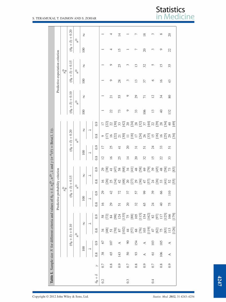
where ED is the expected value of the random posterior probability pn.S/ with respect to mD.s/.Table I shows the required sample size N for different criteria and values of �0 C ı, �D

0 , nD, � and� (�A.�/ D Beta.1; 1/: non-informative). nD D 100 corresponds to approximately 0:20 for the rangeof 95% credible interval. With regard to both the PPC and the PEC, the larger � or � is relative to theother parameters, the greater the sample size. The choice of �D

0 has some degree of impact on the sam-ple size, and nD has a large effect if �D

0 is close to �0 C ı. The two-priors approach using the PPC is ageneral framework that incorporates the frequentist SSD method as a special case when �A.�/ is non-informative and �D.�/ is degenerate [8]. The sample size for nD D1 based on the PPC is slightly largerbut almost the same as that obtained from the frequentist approach that corresponds to the hypothesistesting framework: null hypothesis H0 W � 6 �0 C ı and alternative hypothesis H1 W � > �D

0 , ˛ D 1� �and ˇ D 1� � . We display the frequentist results in brackets in Table I.

The sample size based on the PEC is somewhat smaller than that based on the PPC because the PECguarantees only average control on the predictive distribution of pn.S/, whereas the PPC also controlsits sampling variability [7, 9]. In the following, we consider only the PPC, which is a more stringentcriterion and is widely used [6, 8, 10]

2.2.3. Maximal sample size determined on the basis of the sceptical design prior. We determine an ini-tial sample size N on the basis of a design prior �D.�/. The design prior might be an integrated opinionof investigators taking part in the trial based on a variety of sources of available evidence. As the designprior might have some uncertainty at the planning stage, the initial sample size should be reconsideredusing interim data. Although one approach to alter the sample size is to re-estimate it at interim looks[8], the other approach can be to set in advance a maximal sample size Nmax and to adaptively make achoice between N and Nmax during the trial course (see Section 3). The provision of such a maximalsample size will be motivated by ethical considerations and resource limitations. A simple method fordetermining Nmax can be based on a ‘sceptical’ design prior �D

scept.�/ that reflects a sceptical belief ofthe probability of success, such that

�Dscept.�/D Beta

�� I nD�D

0,sceptC 1; nD�1� �D

0,scept

�C 1

�; �0C ı < �

D0,scept < �

D0

Note that N <Nmax because �D0,scept < �

D0 .

2.3. Interim monitoring

If the interim analyses are required for reconsidering the sample size as well as early stopping of thetrial, we consider J interim looks at the data on the basis of predictive probabilities. Let nj be the num-ber of observations at the j th interim look .j D 1; 2; : : : ; J /. We define the predictive probability oftrial success at the j th interim look as follows:

PAŒpN.S D s/> ��DXrj

sDvmA.s/

where PA is the probability measure associated with the predictive probability obtained using the analy-sis prior, v Dminfs 2 f0; : : : ; rjg W pN.S D s/> �g and rj DN � nj. The predictive distribution of S isbeta-binomial

mA.s/D

Z 1

0

frj.sj�/�Anj.�/d� 8s D 0; : : : ; rj

where �Anj.�/ is the posterior distribution at the j th interim look, and the sampling distribution is

frj.sj�/D Bin.sI rj; �/ 8s D 0; : : : ; rj

The basic stopping rule is as follows: let �L and �U be pre-specified probability thresholds such that �L;

�U 2 Œ0; 1�. If the predictive probability of trial success is less than �L, that is, PAŒpN.S D s/ > �� < �L,stop the trial for inefficacy; if PAŒpN.S D s/ > �� > �U, stop the trial for efficacy; and otherwise

4246



Tabl

eI.

Sam

ple

sizeN

for

diff

eren

tcri

teri

aan

dva

lues

of�0Cı,�D 0

,nD

,�an

d�.�A.�/D

Bet

a.1;1//

.

Pred

ictiv

epr

obab

ility

crite

rion

Pred

ictiv

eex

pect

atio

ncr

iteri

on

�D 0

�D 0

.�0Cı/C0:10

.�0Cı/C0:15

.�0Cı/C0:20

.�0Cı/C0:10

.�0Cı/C0:15

.�0Cı/C0:20

nD

nD

nD

nD

nD

nD

100

110

01

100

110

01

100

110

01

��

��

��

�0Cı

�0.

80.

90.

80.

90.

80.

90.

80.

90.

80.

90.

80.

9

0.2

0.7

3867

3458

1629

1629

1217

917

11

11

11

[48]

[72]

[26]

[38]

[17]

[22]

0.8

6510

751

8429

4225

4116

2516

2222

219

94

4[7

0][9

8][3

4][4

7][2

2][3

0]0.

914

3A

8712

451

7242

5825

4121

3373

5528

2515

14[1

02]

[135

][4

8][6

8][3

0][4

2]0.

30.

750

9044

7520

3720

3414

2011

209

93

31

1[5

7][8

8][2

7][4

1][1

8][2

4]0.

893

154

6810

532

5729

4820

3117

2833

2913

137

7[7

6][1

15]

[36]

[58]

[24]

[32]

0.9

AA

103

154

6599

4769

3251

2637

106

7137

3220

18[1

19]

[162

][5

7][7

9][3

3][4

4]0.

40.

761

103

4782

2439

2439

1524

1522

1312

65

33

[62]

[97]

[26]

[45]

[16]

[29]

0.8

106

185

7511

740

6633

4822

3316

2840

3416

159

8[8

3][1

25]

[41]

[58]

[25]

[34]

0.9

AA

113

166

7511

052

7333

5129

4013

280

4335

2220

[126

][1

79]

[55]

[83]

[34]

[49]


4247


Tabl

eI.

Con

tinu

ed.

Pred

ictiv

epr

obab

ility

crite

rion

Pred

ictiv

eex

pect

atio

ncr

iteri

on

�D 0

�D 0

.�0Cı/C0:10

.�0Cı/C0:15

.�0Cı/C0:20

.�0Cı/C0:10

.�0Cı/C0:15

.�0Cı/C0:20

nD

nD

nD

nD

nD

nD

100

110

01

100

110

01

100

110

01

��

��

��

�0Cı

�0.

80.

90.

80.

90.

80.

90.

80.

90.

80.

90.

80.

9

0.5

0.7

6111

053

8927

4325

4114

2514

2316

147

74

4[6

0][9

4][2

8][4

4][1

7][2

6]0.

811

819

976

121

4065

3652

2334

1830

4436

1816

109

[83]

[126

][4

1][5

7][2

4][3

3]0.

9A

A11

816

776

112

5376

3652

2941

142

8245

3623

20[1

25]

[179

][5

8][7

9][3

2][4

4]0.

60.

759

110

5180

2644

2338

1523

1520

1715

87

54

[57]

[92]

[27]

[42]

[16]

[24]

0.8

112

185

7211

040

6032

4621

2918

2644

3518

1610

9[7

6][1

19]

[35]

[53]

[22]

[30]

0.9

AA

112

155

6710

248

6932

4626

3813

477

4234

2118

[115

][1

62]

[52]

[73]

[30]

[42]

0.7

0.7

5893

4775

2036

2032

1320

1315

1715

87

55

[48]

[76]

[21]

[33]

[14]

[21]

0.8

9415

261

9336

5228

4017

2417

2039

3116

149

8[7

0][1

02]

[29]

[45]

[18]

[25]

0.9

AA

9413

454

7839

5624

3620

2810

766

3528

1715

[98]

[135

][4

4][5

7][2

1][2

9]

Not

e:L

abel

Am

eansN>

200.

The

num

bers

with

inbr

acke

tsin

dica

tesa

mpl

esi

zes

base

don

abi

nom

iald

istr

ibut

ion

usin

gth

efr

eque

ntis

tapp

roac

hw

ith˛D1��

andˇD1��

.

4248



continue the trial until the next interim look or N patients have been reached. In exploratory clinicaltrials, most investigators prefer to set �L as a small value and �U D 1:0 to allow early stopping due toinefficacy but not due to efficacy because, if the treatment is working, enrolling more patients in theactive treatment would not be unethical and can also increase precision when evaluating the efficacy andsafety of treatment [10].

3. Predictive sample size selection design

This approach consists of SSD before starting a trial and early stopping followed by sample sizeselection during multiple interim analyses. We plan K sample size selections out of J interim looksfor reconsidering a sample size based on the interim data.

Before starting a trial

Step 1: For sample size determination, we respectively specify the parameters �D.�/ and �Dscept.�/

together with �0, ı, �A.�/, � and � to determine two sample sizes, N and Nmax (Section 2).Step 2: For interim monitoring plan, we specify the parameters J; nj .j D 1; 2; : : : ; J /, �L and �U. We

choose �U D 1:0 as mentioned earlier (Section 2).Step 3: For sample size selection plan, we specify the number of sample size selections K out of J

interim looks .0 6 K 6 J /. Therefore, any sample size selection requires an interim look,whereas an interim look does not require sample size selection. K D 1 may be recommendedbecause the multiple sample size selections cause some complicated going back and forthbetween N and Nmax.

During the trial

After collecting nj observations for a pre-specified j th interim analysis,

Step 1: If PAŒpN.S D sj/ > �� < �L, where sj is the success number at the j th interim analysis.0 6 sj 6 nj/, stop the trial for inefficacy; otherwise, continue the trial until the next interimor final analysis.

Step 2: For an interim look with sample size selection, we also make a choice between N and Nmax

on the basis of the predictive probabilities calculated for N and Nmax; if PAŒpN.S D sj / > ��is greater than or equal to PAŒpNmax.S D sj/ > ��, we select N and otherwise select Nmax asan optimal sample size. If we choose Nmax, the interim analysis after the sample size selectionshould be performed according to Nmax, using rj DNmax � nj instead of rj DN � nj.

Example

Suppose that we specify the design parameters as �0 C ı D 0:3, �D0 D 0:50, �D

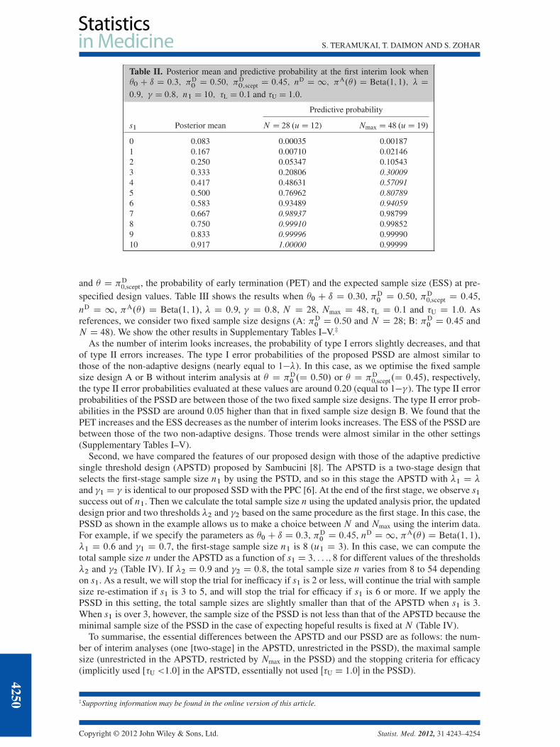
0,scept D 0:45, nD D 1,�A.�/ D Beta.1; 1/, � D 0:9 and � D 0:8. In this case, we will calculate the two sample sizes asN D 28 and Nmax D 48 on the basis of the PPC. We plan an interim analysis after enrolling 10 patients;that is, J D 1 and n1 D 10, and we also plan sample size selection at that time, that is, K D 1. Supposethat the probability threshold for inefficacy stopping �L is 0.1. Table II shows the posterior mean andpredictive probability for success number at the first interim look s1.D 0; : : :; 10/. If s1 is 2 or less,the predictive probability of trial success PAŒpN.S D s1/ > �� is smaller than 0.1, and the trial willbe stopped for inefficacy. If s1 is 3 or more, the trial will be continued until the final analysis, and thesample size will be selected by comparing PAŒpN.S D s1/ > �� with PAŒpNmax.S D s1/ > ��. If s1 is7 or more, PAŒpN.S D s1/ > �� is larger than PAŒpNmax.S D s1/ > ��, and thus the initial sample sizeN D 28 should be selected . If s1 is 3 to 6, PAŒpNmax.S D s1/ > �� is larger than PAŒpN.S D s1/ > ��,and thus the maximal sample size Nmax D 48 should be selected.

4. Simulations

First, we have compared the frequentist operating characteristics of the proposed design with those offixed sample size designs based on 10,000 simulated trials. We generated the data from Bernoulli dis-tributions. In the context of hypothesis testing H0 W � 6 �0 C ı versus H1 W � > �D

0 , the evaluatedproperties are the probability of a type I error at � D �0 C ı, the probability of type II errors at � D �D

0


4249


Table II. Posterior mean and predictive probability at the first interim look when�0 C ı D 0:3; �D

0D 0:50; �D

0;scept D 0:45; nD D 1; �A.�/ D Beta.1; 1/; � D

0:9; � D 0:8; n1 D 10; �L D 0:1 and �U D 1:0.

Predictive probability

s1 Posterior mean N D 28 .uD 12) Nmax D 48 .uD 19/

0 0.083 0.00035 0.001871 0.167 0.00710 0.021462 0.250 0.05347 0.105433 0.333 0.20806 0.300094 0.417 0.48631 0.570915 0.500 0.76962 0.807896 0.583 0.93489 0.940597 0.667 0.98937 0.987998 0.750 0.99910 0.998529 0.833 0.99996 0.9999010 0.917 1.00000 0.99999

and � D �D0,scept, the probability of early termination (PET) and the expected sample size (ESS) at pre-

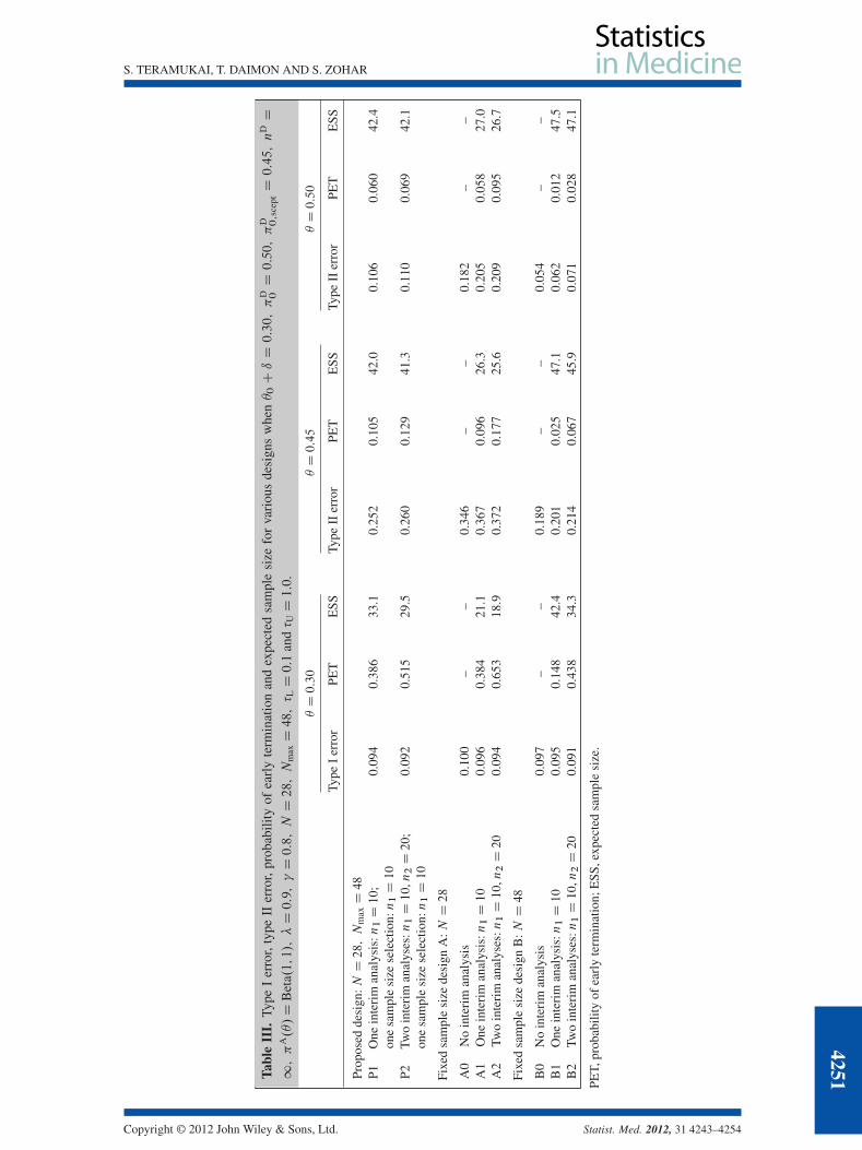
specified design values. Table III shows the results when �0 C ı D 0:30, �D0 D 0:50, �D

0,scept D 0:45,nD D 1, �A.�/ D Beta.1; 1/, � D 0:9, � D 0:8, N D 28, Nmax D 48; �L D 0:1 and �U D 1:0. Asreferences, we consider two fixed sample size designs (A: �D

0 D 0:50 and N D 28; B: �D0 D 0:45 and

N D 48). We show the other results in Supplementary Tables I–V.‡

As the number of interim looks increases, the probability of type I errors slightly decreases, and thatof type II errors increases. The type I error probabilities of the proposed PSSD are almost similar tothose of the non-adaptive designs (nearly equal to 1��). In this case, as we optimise the fixed samplesize design A or B without interim analysis at � D �D

0 .D 0:50/ or � D �D0,scept.D 0:45/, respectively,

the type II error probabilities evaluated at these values are around 0.20 (equal to 1��). The type II errorprobabilities of the PSSD are between those of the two fixed sample size designs. The type II error prob-abilities in the PSSD are around 0.05 higher than that in fixed sample size design B. We found that thePET increases and the ESS decreases as the number of interim looks increases. The ESS of the PSSD arebetween those of the two non-adaptive designs. Those trends were almost similar in the other settings(Supplementary Tables I–V).

Second, we have compared the features of our proposed design with those of the adaptive predictivesingle threshold design (APSTD) proposed by Sambucini [8]. The APSTD is a two-stage design thatselects the first-stage sample size n1 by using the PSTD, and so in this stage the APSTD with �1 D �and �1 D � is identical to our proposed SSD with the PPC [6]. At the end of the first stage, we observe s1success out of n1. Then we calculate the total sample size n using the updated analysis prior, the updateddesign prior and two thresholds �2 and �2 based on the same procedure as the first stage. In this case, thePSSD as shown in the example allows us to make a choice between N and Nmax using the interim data.For example, if we specify the parameters as �0 C ı D 0:3, �D

0 D 0:45, nD D1, �A.�/ D Beta.1; 1/,�1 D 0:6 and �1 D 0:7, the first-stage sample size n1 is 8 (u1 D 3). In this case, we can compute thetotal sample size n under the APSTD as a function of s1 D 3; : : :; 8 for different values of the thresholds�2 and �2 (Table IV). If �2 D 0:9 and �2 D 0:8, the total sample size n varies from 8 to 54 dependingon s1. As a result, we will stop the trial for inefficacy if s1 is 2 or less, will continue the trial with samplesize re-estimation if s1 is 3 to 5, and will stop the trial for efficacy if s1 is 6 or more. If we apply thePSSD in this setting, the total sample sizes are slightly smaller than that of the APSTD when s1 is 3.When s1 is over 3, however, the sample size of the PSSD is not less than that of the APSTD because theminimal sample size of the PSSD in the case of expecting hopeful results is fixed at N (Table IV).

To summarise, the essential differences between the APSTD and our PSSD are as follows: the num-ber of interim analyses (one [two-stage] in the APSTD, unrestricted in the PSSD), the maximal samplesize (unrestricted in the APSTD, restricted by Nmax in the PSSD) and the stopping criteria for efficacy(implicitly used [�U <1.0] in the APSTD, essentially not used Œ�U D 1:0� in the PSSD).

‡Supporting information may be found in the online version of this article.

4250



Tabl

eII

I.Ty

peI

erro

r,ty

peII

erro

r,pr

obab

ility

ofea

rly

term

inat

ion

and

expe

cted

sam

ple

size

for

vari

ous

desi

gns

whe

n�0CıD0:30;�

D 0D0:50;�

D 0;s

ceptD0:45;n

DD

1;�

A.�/D

Bet

a.1;1/;�D0:9;�D0:8;ND28;N

maxD48;� LD0:1

and� UD1:0

.

�D0:30

�D0:45

�D0:50

Type

Ier

ror

PET

ESS

Type

IIer

ror

PET

ESS

Type

IIer

ror

PET

ESS

Prop

osed

desi

gn:ND28;N

maxD48

P1O

nein

teri

man

alys

is:n1D10;

0.09

40.

386

33.1

0.25

20.

105

42.0

0.10

60.

060

42.4

one

sam

ple

size

sele

ctio

n:n1D10

P2Tw

oin

teri

man

alys

es:n1D10,n2D20;

0.09

20.

515

29.5

0.26

00.

129

41.3

0.11

00.

069

42.1

one

sam

ple

size

sele

ctio

n:n1D10

Fixe

dsa

mpl

esi

zede

sign

A:ND28

A0

No

inte

rim

anal

ysis

0.10

0–

–0.

346

––

0.18

2–

–A

1O

nein

teri

man

alys

is:n1D10

0.09

60.

384

21.1

0.36

70.

096

26.3

0.20

50.

058

27.0

A2

Two

inte

rim

anal

yses

:n1D10,n2D20

0.09

40.

653

18.9

0.37

20.

177

25.6

0.20

90.

095

26.7

Fixe

dsa

mpl

esi

zede

sign

B:ND48

B0

No

inte

rim

anal

ysis

0.09

7–

–0.

189

––

0.05

4–

–B

1O

nein

teri

man

alys

is:n1D10

0.09

50.

148

42.4

0.20

10.

025

47.1

0.06

20.

012

47.5

B2

Two

inte

rim

anal

yses

:n1D10,n2D20

0.09

10.

438

34.3

0.21

40.

067

45.9

0.07

10.

028

47.1

PET,

prob

abili

tyof

earl

yte

rmin

atio

n;E

SS,e

xpec

ted

sam

ple

size

.


4251


Table IV. Sample size n.u/ under Sambucini’s APSTD for different criteria of �2 and �2, when �0Cı D 0:3,�D0D 0:45, nD D1, �A.�/D Beta.1; 1/ and n1 .u1/D 8.3/.

�2

0.8 0.9

�2 �2

s1 0.7 0.8 0.7 0.8

3 23 (9) 32 (12) 40 (16) 54 (21)4 11 (5) 17 (7) 28 (12) 37 (15)5 B B B 17 (8)6–8 B B B B

s1 PSSD��D0;scept D 0:45; �

D0 D 0:50; �D �2 and � D �2

�

3 20 (8) 29 (11) 34 (14) 48 (19)4 11 (5) 29 (11) 34 (14) 48 (19)5 11 (5) 17 (7) 34 (14) 48 (19)6–8 11 (5) 17 (7) 20 (9) 28 (12)

Note: Label B denotes that nD n1.

5. An illustrative example

Yanagihara et al. [13] conducted a phase II single-arm trial of S-1 and docetaxel for previously treatedpatients with locally advanced or metastatic non-small cell lung cancer. The primary endpoint wasoverall response rate (ORR), with success being defined as a complete or partial response. The plannedsample size was 35, assuming a null hypothesis of a 9% ORR and an alternative hypothesis of a 25%ORR, with one-sided type I error D 0:1 and type II error D 0:1. As a result, 38 eligible patients wereanalysed, and the final ORR was 18.4% (7/38, 90% confidence interval: 9.0% to 31.8%). Out of the first

0 5 10 15 20 25 30

0.00

0.02

0.04

0.06

0.08

0.10

0.12

Number of future subjects

Pre

dict

ive

prob

abili

ty

0 2 4 6 8 10

0.00

0.05

0.10

0.15

0.20

0.25


Pre

dict

ive

prob

abili

ty

0.0 0.2 0.4 0.6 0.8 1.0

01

23

4

Den

sity

PriorPosterior

(a) (b) (c)

0 5 10 15

0.00

0.05

0.10

0.15


Pre

dict

ive

prob

abili

ty

(d) (e) (f)

0.0 0.2 0.4 0.6 0.8 1.0

01

23

4

Den

sity

PriorPosterior

0.0 0.2 0.4 0.6 0.8 1.0

01

23

45

67

Den

sity

PriorPosterior

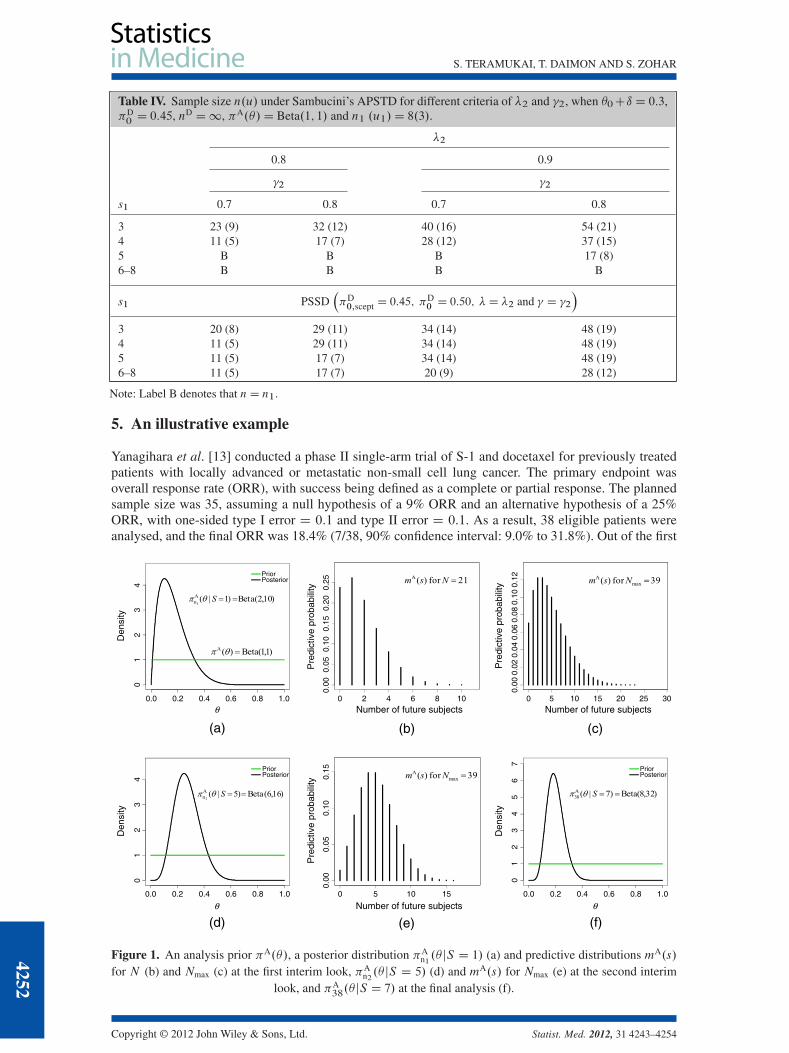
Figure 1. An analysis prior �A.�/, a posterior distribution �An1.� jS D 1/ (a) and predictive distributions mA.s/

for N (b) and Nmax (c) at the first interim look, �An2.� jS D 5/ (d) and mA.s/ for Nmax (e) at the second interim

look, and �A38.� jS D 7/ at the final analysis (f).

4252



10, 20, 30 and 38 enrolled patients, partial responses were observed in one, five, six and seven patients(no complete response), respectively.

For illustration of the proposed approach, we modified and specified the design parameters such that�0 C ı D 0:09, �D

0 D 0:25, �D0,scept D 0:20, nD D1, �A.�/ D Beta.1; 1/, � D 0:9 and � D 0:8. From

these parameters, we calculated the two sample sizes as N D 21 (u D 4) and Nmax D 39 (u D 6). Sup-pose that we planned two interim analyses after enrolling the first 10 and 20 patients (n1 D 10, n2 D 20)and we planned sample size selection at the first interim analysis, that is, J D 2 and K D 1. Supposethat the probability threshold for inefficacy stopping �L was 0.1 and no efficacy stopping (�U D 1:0).

At the first interim analysis, the ORR was 10% (1/10). The posterior mean was 16.7% (Figure 1(a)),and we show the predictive distributions mA.s/ for N and Nmax in Figure 1(b and c), respectively; thepredictive probability PAŒpN.S D 1/ > 0:9� D

P11sD3m

A.s/ was 0.293, and PAŒpNmax.S D 1/ > 0:9� DP29sD5m

A.s/ was 0.464. Because the former value was over 0.10, we had not stopped the trial for ineffi-cacy. For the sample size selection, as the predictive probability based onNmax was larger than that basedon N , we should select Nmax as the re-determined sample size. At the second interim analysis, the ORRwas 25% (5/20). The posterior mean was 27.2% (Figure 1(d)), and the predictive distributions for Nmax

shifted to the right (Figure 1(e)). As the predictive probability PAŒpNmax.S D 5/ > 0:9� DP19sD1m

A.s/

was 0.986, we had continued the trial until 39 patients were enrolled. Because the final ORR was 18.4%(7/38), the posterior mean was 20% (Figure 1(f)), and the posterior probability was greater than thetarget value:

�A38.� > 0:09jS D 7/D 0:979 > �

Accordingly, we would conclude that the test treatment was promisingly effective as also concluded inthe original report.

6. Discussion

The aim of our work was to propose a simple, coherent and unified Bayesian adaptive design. RobustBayesian SSD [7] considers a class of plausible analysis priors instead of a single analysis prior in orderto incorporate the uncertainty of prior information into SSD. However, we should emphasise that uncer-tainty in a design prior is more important for SSD where the inference could be based on subjectiveinformation about the quantity of interest. To consider the uncertainty of prior information, we employnD (a tuning parameter for the variance of design priors) and two kinds of design priors. The elicitationand determination of design parameters including �0, ı, �A.�/, �D.�/ and �D

scept.�/ are essential aspectsof designing clinical trials.

In our design, we base the SSD for PPC on the approach of Sambucini [6] and Brutti et al. [7]. Onthe other hand, the interim monitoring using predictive probability is based on the method of Lee andLiu [10]. As they emphasised, the predictive probability approach for interim monitoring is a consis-tent, efficient and flexible method that more closely resembles the clinical decision-making process.Unlike the approach by Lee and Liu [10], the PSSD does not require intensive computation for samplesize searching because of the separation of the interim monitoring procedure from the SSD procedure.Instead, comprehensive simulations may be required at the design phase to evaluate the operatingcharacteristics (including type I and type II error probabilities) from the frequentist point of view.

The APSTD by Sambucini [8] is an adaptive design that allows additional sample size while keepingthe ‘Bayesian power’ on the basis of updated information, that is, updated analysis priors and updateddesign priors. In the APSTD, the consistency of design parameters between SSD at the first stage andsample size re-estimation at the second stage (adaptive stage) seems to be not clear, and early stopping forefficacy is inevitably incorporated into the procedure. In contrast, our design provides two fixed samplesizes (N and Nmax/ mainly for practical reasons, and it selects an optimal sample size by comparing the‘Bayesian power’ between the two sample sizes at the interim stage. The difference in ‘Bayesian power’may be very small (at most 0.10 as shown in the example of Table II). By applying sample size selection,however, we reduce type II error probabilities by 0.10 to 0.12, whereas type I error probabilities remainunchanged as shown in Table III.

From a practical standpoint, the proposed design could be useful in single-arm clinical trials with abinary endpoint. The number of interim analyses should depend on the targeted type of disease and therequired time to evaluate the endpoint. Although we have considered a maximum of two interim analyses


4253


in the example and the simulations, the number should be modulated by discussing with investigatorsat the design stage. In the near future, this approach will be implemented in actual exploratory clinicaltrials to assess its usefulness and to extend it to more complicated clinical trials.

Acknowledgements

This work was supported in part by Grants-in Aid for Scientific Research (C) No. 22500257 from Japan Societyfor the Promotion of Science, Japan. The authors wish to thank Mr. Keiichi Yamamoto, who provided technicalsupport, and Dr. Kazuhiro Yanagihara, who allowed the lung cancer clinical trial data to be used.

References1. Zohar S, Teramukai S, Zhou Y. Bayesian design and conduct of phase II single-arm clinical trials with binary outcomes:

a tutorial. Contemporary Clinical Trials 2008; 29:608–616. DOI: 10.1016/j.cct.2007.11.005.2. Tan SB, Machin D. Bayesian two-stage designs for phase II clinical trials. Statistics in Medicine 2002; 21:1991–2012.

DOI: 10.1002/sim.1176.3. Mayo MS, Gajewski BJ. Bayesian sample size calculations in phase II clinical trials using informative conjugate priors.

Controlled Clinical Trials 2004; 25:157–167. DOI: 10.1016/j.cct.2003.11.006.4. Gajewski BJ, Mayo MS. Bayesian sample size calculations in phase II clinical trials using a mixture of informative priors.

Statistics in Medicine 2006; 25:2554–2566. DOI: 10.1002/sim.2450.5. Whitehead J, Valdés-Márquez E, Johnson P, Graham G. Bayesian sample size for exploratory clinical trials incorporating

historical data. Statistics in Medicine 2008; 27:2307–2327. DOI: 10.1002/sim.3140.6. Sambucini V. A Bayesian predictive two-stage design for phase II clinical trials. Statistics in Medicine 2008; 27:

1199–1224. DOI: 10.1002/sim.3021.7. Brutti P, De Santis F, Gubbiotti S. Robust Bayesian sample size determination in clinical trials. Statistics in Medicine

2008; 27:2290–2306. DOI: 10.1002/sim.3175.8. Sambucini V. A Bayesian predictive strategy for an adaptive two-stage design in phase II clinical trials. Statistics in

Medicine 2010; 29:1430–1442. DOI: 10.1002/sim.3800.9. Brutti P, De Santis F, Gubbiotti S. Mixtures of prior distributions for predictive Bayesian sample size calculations in

clinical trials. Statistics in Medicine 2009; 28:2185–2201. DOI: 10.1002/sim.3609.10. Lee JJ, Liu DD. A predictive probability design for phase II cancer clinical trials. Clinical Trials 2008; 5:93–106. DOI:

10.1177/1740774508089279.11. Biswas S, Liu DD, Lee JJ, Berry DA. Bayesian clinical trials at the University of Texas M. D. Anderson Cancer Center.

Clinical Trials 2009; 6:205–216. DOI: 10.1177/1740774509104992.12. Spiegelhalter DJ, Freedman LS, Parmar MKB. Bayesian approaches to randomized trials (with discussion). Journal of the

Royal Statistics Society, Series A 1994; 157:357–416.13. Yanagihara K, Yoshimura K, Niimi M, Yasuda H, Sasaki T, Nishimura T, Ishiguro H, Matsumoto S, Kitano T,

Kanai M, Misawa A, Tada H, Teramukai S, Mio T, Fukushima M. Phase II study of S-1 and docetaxel for previouslytreated patients with locally advanced or metastatic non-small cell lung cancer. Cancer Chemotherapy and Pharmacology2010; 66:913–918. DOI: 10.1007/s00280-009-1239-7.

4254


Special Issue Paper A Bayesian predictive sample size selection design for single-arm exploratory...

Documents

Transcript of Special Issue Paper A Bayesian predictive sample size selection design for single-arm exploratory...