lable at ScienceDirect

Estuarine, Coastal and Shelf Science 84 (2009) 637–644

Contents lists avai

Estuarine, Coastal and Shelf Science

journal homepage: www.elsevier .com/locate/ecss

Spatio-temporal structure of diatom assemblages in a temperate estuary.A STATICO analysis

Susana Mendes a,*, Ma Jose Fernandez-Gomez b, Paula Resende c, Mario Jorge Pereira d,Ma Purificacion Galindo-Villardon b, Ulisses Miranda Azeiteiro e,c

a GIRM-Research Group on Marine Resources, Polytechnic Institute of Leiria, School of Tourism and Maritime Technology – Campus 4, 2520-641 Peniche, Portugalb University of Salamanca, Department of Statistics, 37007 Salamanca, Spainc IMAR-Institute of Marine Research, University of Coimbra, Department of Zoology, 3004-517 Coimbra, Portugald University of Aveiro, Department of Biology, 3810-193 Aveiro, Portugale University Aberta, Department of Sciences and Technology, 4200-055 Porto, Portugal

a r t i c l e i n f o

Article history:Received 2 May 2009Accepted 7 August 2009Available online 12 August 2009

Keywords:environmental forcingDiatomsEstuariesmultitable analysisSTATICO

* Corresponding author. GIRM – Grupo de InvestigInstituto Politecnico de Leiria, Escola Superior de TuCampus 4, Santuario Nossa Senhora dos Remedios, 25

E-mail addresses: smendes@estm.ipleiria.pt ((M.J. Fernandez-Gomez), presende@zoo.uc.pt (P. Rese

Pereira), pgalindo@usal.es (M.P. Galindo-VillardonAzeiteiro).

0272-7714/$ – see front matter � 2009 Elsevier Ltd.doi:10.1016/j.ecss.2009.08.003

a b s t r a c t

This study examines the spatio-temporal structure of diatom assemblages in a temperate estuary (Ria deAveiro, Western Portugal). Eighteen monthly surveys were conducted, from January 2002 to June 2003,at three sampling sites (at both high and low tide) along the estuarine salinity gradient. The relationshipof diatom assemblages and environmental variables was analysed using the STATICO method, which hasbeen designed for the simultaneous analysis of paired ecological tables. This method allowed exami-nation of the stable part of the environment-diatom relationship, and also the variations of this rela-tionship through time. The interstructure factor map showed that the relationship between the 11environmental variables and the abundance of the 231 diatom species considered was strongest in themonths May and September 2002 and January, February and May 2003. The stable part of the species–environment relationships mainly consisted of a combined phosphate, chlorophyll a and salinity gradientlinked to a freshwater-marine species gradient. A more pronounced gradient was observed in January,February and May 2003. Diatom assemblages showed clear longitudinal patterns due to the presence ofboth marine and freshwater components. May and September 2002 had the least structured gradientswith marine-estuarine species appearing in the freshwater side of the gradient. The most completegradient in February 2003 could be considered, in terms of bio-ecological categories, as the moststructured period of the year, with a combination of strong marine influence in the lower zone andfreshwater influence in the upper. The best-structured gradients were during periods of a diatom bloom.Stable diatom assemblages (with a strong structure and a good fit between the diatoms and environ-ment) are described and characterized. This study shows the efficiency of the STATICO analysis. Theinclusion of space-time data analysis tools in ecological studies may therefore improve the knowledge ofthe dynamics of species–environmental assemblages.

� 2009 Elsevier Ltd. All rights reserved.

1. Introduction

Various studies on phytoplankton communities in estuaries haveconcluded that diatoms are the most important taxonomic groups,either in terms of abundance or in terms of diversity or both

açao em Recursos Marinhos,rismo e Tecnologia do Mar,20-641 Peniche, Portugal.S. Mendes), mjfg@usal.es

nde), mverde@ua.pt (M. Jorge), ulisses@univ-ab.pt (U.M.

All rights reserved.

(Trigueros and Orive, 2001; Lemaire et al., 2002; Adolf et al., 2006;Gameiro et al., 2007). Diatoms can survive in systems with a highturbidity and a short water retention time (Lionard et al., 2008).These communities are composed of dynamic multi-speciesassemblages characterized by high diversity and rapid successionalshifts in species composition in response to environmental changes.Identifying the ecological variables that regulate the seasonalsuccession of diatom communities is essential to understand theconsequences of eutrophication and climate change. Beyond that,phytoplankton composition and abundance are intimately linked tohigher trophic levels through grazing by herbivores and cascadingeffects on ecosystem trophodynamics (Mallin and Paerl, 1994;Pinckney et al., 1998; Urrutxurtu et al., 2003).

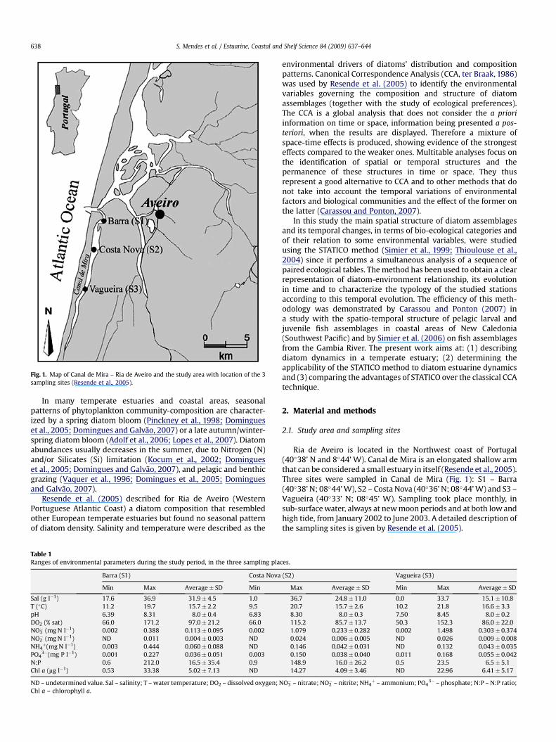
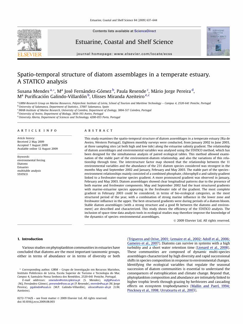
Fig. 1. Map of Canal de Mira – Ria de Aveiro and the study area with location of the 3sampling sites (Resende et al., 2005).

S. Mendes et al. / Estuarine, Coastal and Shelf Science 84 (2009) 637–644638

In many temperate estuaries and coastal areas, seasonalpatterns of phytoplankton community-composition are character-ized by a spring diatom bloom (Pinckney et al., 1998; Domingueset al., 2005; Domingues and Galvao, 2007) or a late autumn/winter-spring diatom bloom (Adolf et al., 2006; Lopes et al., 2007). Diatomabundances usually decreases in the summer, due to Nitrogen (N)and/or Silicates (Si) limitation (Kocum et al., 2002; Domingueset al., 2005; Domingues and Galvao, 2007), and pelagic and benthicgrazing (Vaquer et al., 1996; Domingues et al., 2005; Dominguesand Galvao, 2007).

Resende et al. (2005) described for Ria de Aveiro (WesternPortuguese Atlantic Coast) a diatom composition that resembledother European temperate estuaries but found no seasonal patternof diatom density. Salinity and temperature were described as the

Table 1Ranges of environmental parameters during the study period, in the three sampling pla

Barra (S1) Costa Nova

Min Max Average� SD Min

Sal (g l�1) 17.6 36.9 31.9� 4.5 1.0T (�C) 11.2 19.7 15.7� 2.2 9.5pH 6.39 8.31 8.0� 0.4 6.83DO2 (% sat) 66.0 171.2 97.0� 21.2 66.0NO3� (mg N l�1) 0.002 0.388 0.113� 0.095 0.002

NO2� (mg N l�1) ND 0.011 0.004� 0.003 ND

NH4þ(mg N l�1) 0.003 0.444 0.060� 0.088 ND

PO43�(mg P l�1) 0.001 0.227 0.036� 0.051 0.003

N:P 0.6 212.0 16.5� 35.4 0.9Chl a (mg l�1) 0.53 33.38 5.02� 7.13 ND

ND – undetermined value. Sal – salinity; T – water temperature; DO2 – dissolved oxygen; NChl a – chlorophyll a.

environmental drivers of diatoms’ distribution and compositionpatterns. Canonical Correspondence Analysis (CCA, ter Braak, 1986)was used by Resende et al. (2005) to identify the environmentalvariables governing the composition and structure of diatomassemblages (together with the study of ecological preferences).The CCA is a global analysis that does not consider the a prioriinformation on time or space, information being presented a pos-teriori, when the results are displayed. Therefore a mixture ofspace-time effects is produced, showing evidence of the strongesteffects compared to the weaker ones. Multitable analyses focus onthe identification of spatial or temporal structures and thepermanence of these structures in time or space. They thusrepresent a good alternative to CCA and to other methods that donot take into account the temporal variations of environmentalfactors and biological communities and the effect of the former onthe latter (Carassou and Ponton, 2007).

In this study the main spatial structure of diatom assemblagesand its temporal changes, in terms of bio-ecological categories andof their relation to some environmental variables, were studiedusing the STATICO method (Simier et al., 1999; Thioulouse et al.,2004) since it performs a simultaneous analysis of a sequence ofpaired ecological tables. The method has been used to obtain a clearrepresentation of diatom-environment relationship, its evolutionin time and to characterize the typology of the studied stationsaccording to this temporal evolution. The efficiency of this meth-odology was demonstrated by Carassou and Ponton (2007) ina study with the spatio-temporal structure of pelagic larval andjuvenile fish assemblages in coastal areas of New Caledonia(Southwest Pacific) and by Simier et al. (2006) on fish assemblagesfrom the Gambia River. The present work aims at: (1) describingdiatom dynamics in a temperate estuary; (2) determining theapplicability of the STATICO method to diatom estuarine dynamicsand (3) comparing the advantages of STATICO over the classical CCAtechnique.

2. Material and methods

2.1. Study area and sampling sites

Ria de Aveiro is located in the Northwest coast of Portugal(40�38’ N and 8�44’ W). Canal de Mira is an elongated shallow armthat can be considered a small estuary in itself (Resende et al., 2005).Three sites were sampled in Canal de Mira (Fig. 1): S1 – Barra(40�38’ N; 08�44’ W), S2 – Costa Nova (40�36’ N; 08�44’ W) and S3 –Vagueira (40�33’ N; 08�45’ W). Sampling took place monthly, insub-surface water, always at new moon periods and at both low andhigh tide, from January 2002 to June 2003. A detailed description ofthe sampling sites is given by Resende et al. (2005).

ces.

(S2) Vagueira (S3)

Max Average� SD Min Max Average� SD

36.7 24.8� 11.0 0.0 33.7 15.1� 10.820.7 15.7� 2.6 10.2 21.8 16.6� 3.38.30 8.0� 0.3 7.50 8.45 8.0� 0.2115.2 85.7� 13.7 50.3 152.3 86.0� 22.01.079 0.233� 0.282 0.002 1.498 0.303� 0.3740.024 0.006� 0.005 ND 0.026 0.009� 0.0080.146 0.042� 0.031 ND 0.132 0.043� 0.0350.150 0.038� 0.040 0.011 0.168 0.055� 0.042148.9 16.0� 26.2 0.5 23.5 6.5� 5.114.27 4.09� 3.46 ND 22.96 6.41� 5.17

O3� – nitrate; NO2

� – nitrite; NH4þ – ammonium; PO4

3� – phosphate; N:P – N:P ratio;

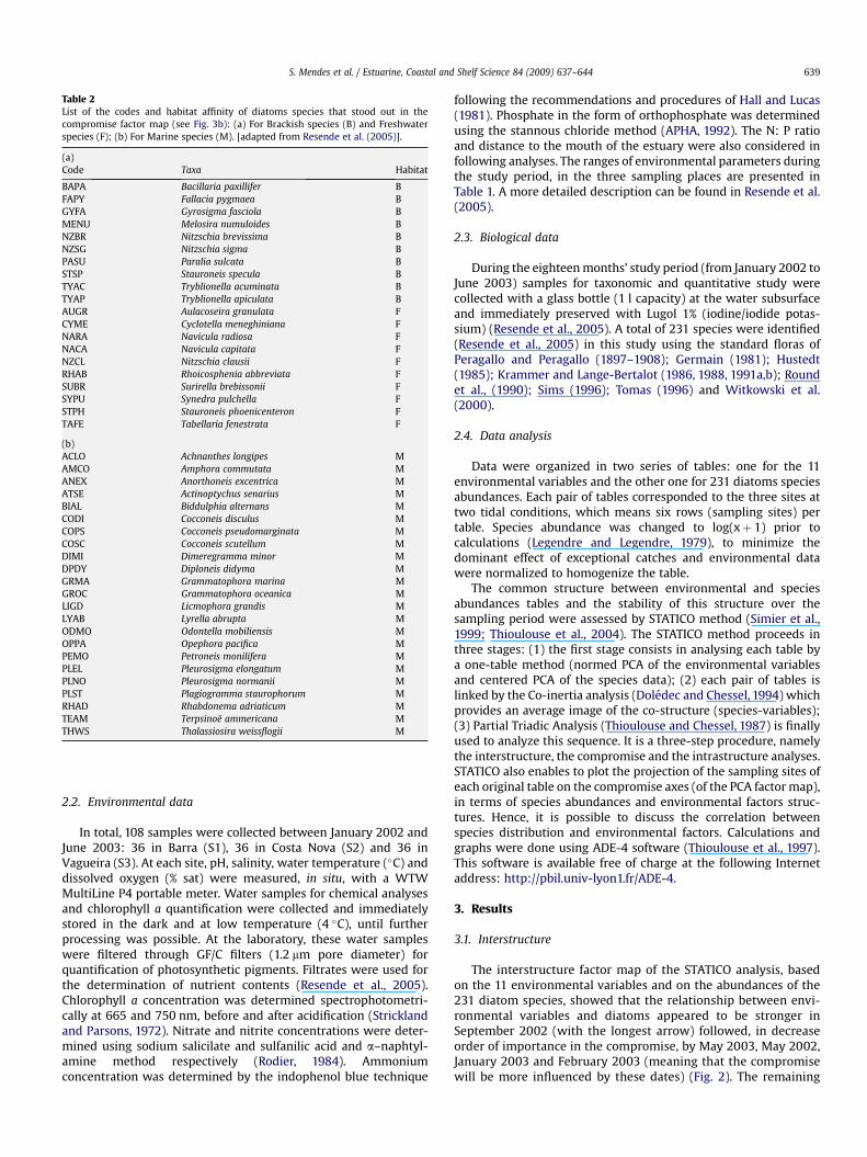
Table 2List of the codes and habitat affinity of diatoms species that stood out in thecompromise factor map (see Fig. 3b): (a) For Brackish species (B) and Freshwaterspecies (F); (b) For Marine species (M). [adapted from Resende et al. (2005)].

(a)Code Taxa Habitat

BAPA Bacillaria paxillifer BFAPY Fallacia pygmaea BGYFA Gyrosigma fasciola BMENU Melosira numuloides BNZBR Nitzschia brevissima BNZSG Nitzschia sigma BPASU Paralia sulcata BSTSP Stauroneis specula BTYAC Tryblionella acuminata BTYAP Tryblionella apiculata BAUGR Aulacoseira granulata FCYME Cyclotella meneghiniana FNARA Navicula radiosa FNACA Navicula capitata FNZCL Nitzschia clausii FRHAB Rhoicosphenia abbreviata FSUBR Surirella brebissonii FSYPU Synedra pulchella FSTPH Stauroneis phoenicenteron FTAFE Tabellaria fenestrata F

(b)ACLO Achnanthes longipes MAMCO Amphora commutata MANEX Anorthoneis excentrica MATSE Actinoptychus senarius MBIAL Biddulphia alternans MCODI Cocconeis disculus MCOPS Cocconeis pseudomarginata MCOSC Cocconeis scutellum MDIMI Dimeregramma minor MDPDY Diploneis didyma MGRMA Grammatophora marina MGROC Grammatophora oceanica MLIGD Licmophora grandis MLYAB Lyrella abrupta MODMO Odontella mobiliensis MOPPA Opephora pacifica MPEMO Petroneis monilifera MPLEL Pleurosigma elongatum MPLNO Pleurosigma normanii MPLST Plagiogramma staurophorum MRHAD Rhabdonema adriaticum MTEAM Terpsinoe ammericana MTHWS Thalassiosira weissflogii M

S. Mendes et al. / Estuarine, Coastal and Shelf Science 84 (2009) 637–644 639

2.2. Environmental data

In total, 108 samples were collected between January 2002 andJune 2003: 36 in Barra (S1), 36 in Costa Nova (S2) and 36 inVagueira (S3). At each site, pH, salinity, water temperature (�C) anddissolved oxygen (% sat) were measured, in situ, with a WTWMultiLine P4 portable meter. Water samples for chemical analysesand chlorophyll a quantification were collected and immediatelystored in the dark and at low temperature (4 �C), until furtherprocessing was possible. At the laboratory, these water sampleswere filtered through GF/C filters (1.2 mm pore diameter) forquantification of photosynthetic pigments. Filtrates were used forthe determination of nutrient contents (Resende et al., 2005).Chlorophyll a concentration was determined spectrophotometri-cally at 665 and 750 nm, before and after acidification (Stricklandand Parsons, 1972). Nitrate and nitrite concentrations were deter-mined using sodium salicilate and sulfanilic acid and a–naphtyl-amine method respectively (Rodier, 1984). Ammoniumconcentration was determined by the indophenol blue technique

following the recommendations and procedures of Hall and Lucas(1981). Phosphate in the form of orthophosphate was determinedusing the stannous chloride method (APHA, 1992). The N: P ratioand distance to the mouth of the estuary were also considered infollowing analyses. The ranges of environmental parameters duringthe study period, in the three sampling places are presented inTable 1. A more detailed description can be found in Resende et al.(2005).

2.3. Biological data

During the eighteen months’ study period (from January 2002 toJune 2003) samples for taxonomic and quantitative study werecollected with a glass bottle (1 l capacity) at the water subsurfaceand immediately preserved with Lugol 1% (iodine/iodide potas-sium) (Resende et al., 2005). A total of 231 species were identified(Resende et al., 2005) in this study using the standard floras ofPeragallo and Peragallo (1897–1908); Germain (1981); Hustedt(1985); Krammer and Lange-Bertalot (1986, 1988, 1991a,b); Roundet al., (1990); Sims (1996); Tomas (1996) and Witkowski et al.(2000).

2.4. Data analysis

Data were organized in two series of tables: one for the 11environmental variables and the other one for 231 diatoms speciesabundances. Each pair of tables corresponded to the three sites attwo tidal conditions, which means six rows (sampling sites) pertable. Species abundance was changed to log(xþ 1) prior tocalculations (Legendre and Legendre, 1979), to minimize thedominant effect of exceptional catches and environmental datawere normalized to homogenize the table.

The common structure between environmental and speciesabundances tables and the stability of this structure over thesampling period were assessed by STATICO method (Simier et al.,1999; Thioulouse et al., 2004). The STATICO method proceeds inthree stages: (1) the first stage consists in analysing each table bya one-table method (normed PCA of the environmental variablesand centered PCA of the species data); (2) each pair of tables islinked by the Co-inertia analysis (Doledec and Chessel, 1994) whichprovides an average image of the co-structure (species-variables);(3) Partial Triadic Analysis (Thioulouse and Chessel, 1987) is finallyused to analyze this sequence. It is a three-step procedure, namelythe interstructure, the compromise and the intrastructure analyses.STATICO also enables to plot the projection of the sampling sites ofeach original table on the compromise axes (of the PCA factor map),in terms of species abundances and environmental factors struc-tures. Hence, it is possible to discuss the correlation betweenspecies distribution and environmental factors. Calculations andgraphs were done using ADE-4 software (Thioulouse et al., 1997).This software is available free of charge at the following Internetaddress: http://pbil.univ-lyon1.fr/ADE-4.

3. Results

3.1. Interstructure

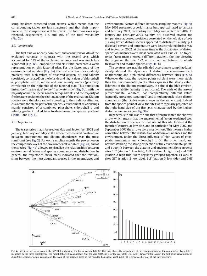
The interstructure factor map of the STATICO analysis, basedon the 11 environmental variables and on the abundances of the231 diatom species, showed that the relationship between envi-ronmental variables and diatoms appeared to be stronger inSeptember 2002 (with the longest arrow) followed, in decreaseorder of importance in the compromise, by May 2003, May 2002,January 2003 and February 2003 (meaning that the compromisewill be more influenced by these dates) (Fig. 2). The remaining

S. Mendes et al. / Estuarine, Coastal and Shelf Science 84 (2009) 637–644640

sampling dates presented short arrows, which means that thecorresponding tables are less structured and that their impor-tance in the compromise will be lower. The first two axes rep-resented, respectively, 21% and 10% of the total variability(Fig. 2b).

3.2. Compromise

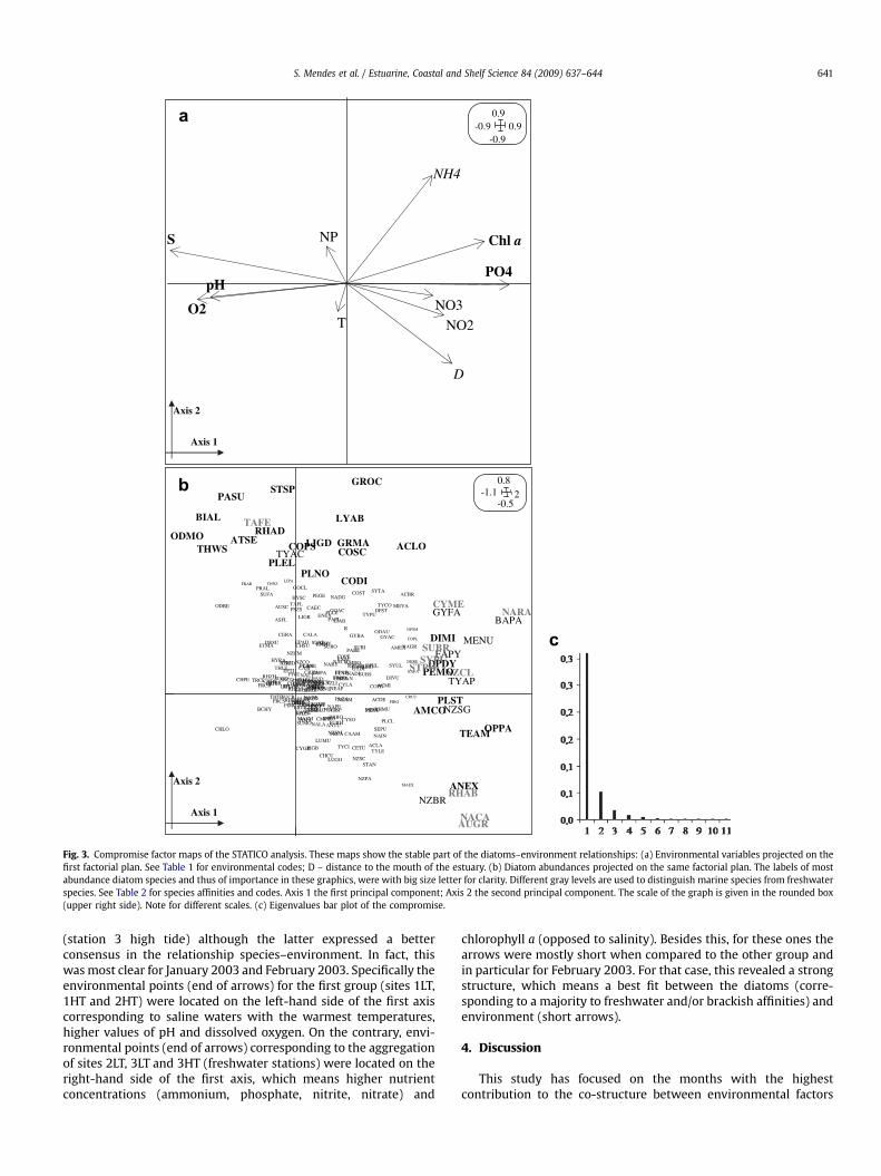
The first axis was clearly dominant, and accounted for 78% of theexplained variance in contrast with the second axis whichaccounted for 13% of the explained variance and was much lesssignificant (Fig. 3c). Temperature and N: P ratio presented a weakrepresentation on this factorial plan. For the factor map of theenvironmental variables (Fig. 3a), the first axis describes a salinitygradient, with high values of dissolved oxygen, pH and salinity(positively correlated) on the left side and high values of chlorophylla, phosphate, nitrite, nitrate and low salinity waters (positivelycorrelated) on the right side of the factorial plan. This oppositionlinked the ‘‘marine side’’ to the ‘‘freshwater side’’ (Fig. 3b), with themajority of marine species on the left quadrants and the majority offreshwater species on the right quadrants of the ordination. Diatomspecies were therefore ranked according to their salinity affinities.As a result, the stable part of the species–environment relationshipsmainly consisted of a combined phosphate, chlorophyll a andsalinity gradient linked to a freshwater-marine species gradient(Table 1 and Fig. 3).

3.3. Trajectories

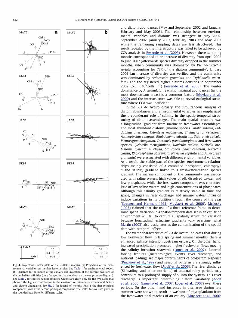
The trajectories maps focused on May and September 2002 andJanuary, February and May 2003, when the observed co-structurebetween environment and diatom abundances was the mostsignificant (see Fig. 2). For each sampling month, the projection onthe compromise axes of the environmental variables (Fig. 4a) and ofthe species (Fig. 4b) allowed to visualize the relationships betweenenvironmental factors and species abundances and distribution. Ingeneral, the trajectories factor maps indicated that the relation-ships between the most abundant species in the assemblages and

JAN2 FEB2MAR2

APR2

MAY2

JUN2JUL2

AUG2

SE

OCT2

NOV2

DEC2

JAN3

FEB3

MAR3

APR3

MAY3

JUN3

-0.2

0.2-0.010

Axis 1

Axis 2

a

Fig. 2. Interstructure factor map of the STATICO analysis on the Ria de Aveiro data. (a) Thidentified by the three first letters of the month followed by a number: 2 for the year 2002 aAxis 2 the second principal component. The scale of the graph is given in the rounded box

environmental factors differed between sampling months (Fig. 4).May 2003 presented a performance best approximated to Januaryand February 2003, contrasting with May and September 2002. InJanuary and February 2003, salinity, pH, dissolved oxygen andtemperature appeared positively correlated on the left side of axis1, along which diatom species appeared to distribute. Salinity, pH,dissolved oxygen and temperature were less correlated during Mayand September 2002 (at the same time as the distribution of diatomspecies abundances were most correlated with axis 2). The trajec-tories factor maps showed a different gradient, the line bisectingthe origin on the plan 1–2, with a contrast between brackish,freshwater and marine species (Figs 4a, b).

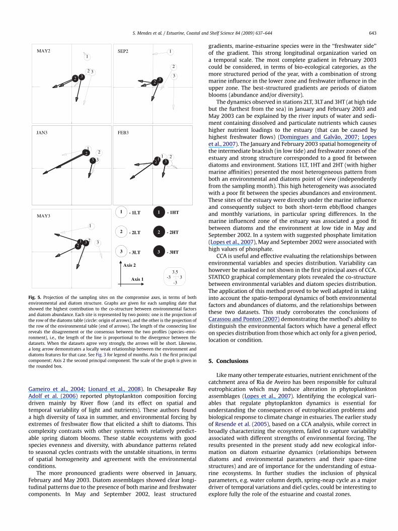
The co-structure graphics (divided according to sampling dates)clearly showed the dynamics of diatom species–environmentrelationships and highlighted differences between sites (Fig. 5).Whatever the date, the species points (circles) were more stablethan the environmental points. This expresses the steady estab-lishment of the diatom assemblages, in spite of the high environ-mental variability (salinity in particular). The ends of the arrows(environmental variables) had comparatively different values(generally presented separated) and simultaneously close diatomabundances (the circles were always in the same area). Indeed,from the species point of view, the sites were regularly projected onthe right-hand side of the first axis, characterized by the highestdiatom abundances (see Fig. 3b).

In general, site one was the one that often presented the shortestarrow, which means that the environmental factors explained wellthe distribution of species for that site. At this site, located at themouth of estuary, at low tide, and in particular for May 2002 andSeptember 2002 the arrows were mostly short. This means a highercorrelation between the distribution of diatom abundances and theenvironment, under the direct influence of high values of phos-phate, ammonium and chlorophyll a. On the other hand, andnotwithstanding the strong dispersion of the environmental pointsand a poor fit between the diatoms and environment (long arrows),sites 1LT (station 1 low tide), 1HT (station 1 high tide) and 2HT(station 2 high tide) were regularly grouped together, as well assites 2LT (station 2 low tide), 3LT (station 3 low tide) and 3HT

P2

5

50.3

0,0

0,1

0,1

0,2

0,2

0,3

0,3

0,4

0,4

0,5

1 2 3 4 5 6 7 8 9 10 11 12 13 14 15 16 17 18

b

is map shows the importance of each sampling date in the compromise. Each date isnd 3 for the year 2003 (e.g. JAN2 – January 2002). Axis 1 the first principal component;(upper right side). (b) Eigenvalues bar plot of the interstructure.

S

T

pH

O2 NO3NO2

NH4

PO4

NP Chl a

D

-0.9

0.9-0.9 0.9

Axis 1

Axis 2

ACBR

ACCO

ACDE

ACLA

ACLO

ACMI

ATSE

ATSP AMCO

AMEX

AMHO

AMOV

ANTU

ANEX

ASFL

AUGR

AUSC

BAPA

BCHY

BIAL

BIBD

BRBO

CAAM

CACR

CALA

CASI

CAWE

CAEC

CAIN

CAVL

CERA

CETU

CHCU

CHDECHDS

CHEI

CHLO

CHPE

CHSU

CODI

COPD

COPE

COPL

COPS COSC

COST

CSCO

CMPU

CRCU

CRHA

CYME

CYSO

CYAF

CYGR

CYLA

DESU

DIVU

DIMI

DPDYDPEL

DPSM

DPST

DTBR

DKREENAL

ENPA

EPAD

EPAREPTU

EUZO

ENEX

ENPEETMA

FAFO

FAPY

FRAR

FRCA

FRCO

FRCR

FRVA

FRCS

FURH

FUVU

GOAC

GOCL

GOPA

R

GRMA

GROC

GRSE

GYACGYBA

GYDI

GYFA

HYMA

HYRA

HYSC

LIAB

LIDA

LIFL

LIGR

LIGD

LIPA

LUGO

LUMU

LUNI

LYAB

LYAT

MAEX

MASM

MENU

MEVA

MECCNABR

NACA

NACR

NACY

NADE

NADG

NADI

NAGR

NAIN

NALA

NALYNAPA

NAPE

NARA

NARY

NAVI

NEAM NEAP

NEDUNZAC

NZAM

NZBR

NZCLNZCO

NZCM

NZIN

NZLI

NZPA

NZSC

NZSG

NZSM

NZVE

NZVT

ODAU

ODMO

ODRE

OPPA

PASU

PABE

PAPL

PEGE

PEMOPIVE

PIBO

PIBRPIBSPIDV

PIGB

PIMA

PIMC PISUPISD

PIVD

PLCL

PLGA PLST

PLLE

PLAN

PLELPLNO

PLLV

PRAL

PSPAPSZP

PSZS

RHAD

RHAM

RHZH

RHZS

RHZY

RHAB

RHGI

RHGB

RHMU

RHRU

SEPU

SKCO

STAN

STPH

STSM

STSP

SPAL

SPRO

SUANSUBS

SUBRSUBI

SUCASUCO

SUCNSUCR

SUFA

SULI

SUMO

SUOV

SUROSUST

SYCA

SYPUSYRU

SYTA

SYUL

TAFE

TAFL

TEAM

THNZ

THLE

THTE

THWS

TRASTRCLTRFA

TYAC

TYAP

TYCI

TYCO

TYLE

TYPU

-0.5

0.8-1.1 2

Axis 1

Axis 2

a

b

c

Fig. 3. Compromise factor maps of the STATICO analysis. These maps show the stable part of the diatoms–environment relationships: (a) Environmental variables projected on thefirst factorial plan. See Table 1 for environmental codes; D – distance to the mouth of the estuary. (b) Diatom abundances projected on the same factorial plan. The labels of mostabundance diatom species and thus of importance in these graphics, were with big size letter for clarity. Different gray levels are used to distinguish marine species from freshwaterspecies. See Table 2 for species affinities and codes. Axis 1 the first principal component; Axis 2 the second principal component. The scale of the graph is given in the rounded box(upper right side). Note for different scales. (c) Eigenvalues bar plot of the compromise.

S. Mendes et al. / Estuarine, Coastal and Shelf Science 84 (2009) 637–644 641

(station 3 high tide) although the latter expressed a betterconsensus in the relationship species–environment. In fact, thiswas most clear for January 2003 and February 2003. Specifically theenvironmental points (end of arrows) for the first group (sites 1LT,1HT and 2HT) were located on the left-hand side of the first axiscorresponding to saline waters with the warmest temperatures,higher values of pH and dissolved oxygen. On the contrary, envi-ronmental points (end of arrows) corresponding to the aggregationof sites 2LT, 3LT and 3HT (freshwater stations) were located on theright-hand side of the first axis, which means higher nutrientconcentrations (ammonium, phosphate, nitrite, nitrate) and

chlorophyll a (opposed to salinity). Besides this, for these ones thearrows were mostly short when compared to the other group andin particular for February 2003. For that case, this revealed a strongstructure, which means a best fit between the diatoms (corre-sponding to a majority to freshwater and/or brackish affinities) andenvironment (short arrows).

4. Discussion

This study has focused on the months with the highestcontribution to the co-structure between environmental factors

S

TpH

O2

NO3

NO2

NH4

PO 4

NP

Ch l a

D

MAY2

S T

pH

O2

NO3

NO2

NH4

PO 4

NPCh l a

D

SEP2

S

T

pH

O2

NO3

NO2NH4

PO 4

NP

Ch l a

D

JAN3

Axis 1

Axis 2

S

T

pHO2 NO3

NO2

NH4

PO 4

NP

Ch l a

D

MAY3

-0.35

0.5-0.4 0.5

ST

pHO2

NO3NO2

NH4 PO 4NP

Ch l a

D

FEB3

-0.8

0.8-0.9 1.2

B FM

MAY2

B F M

F M

B F M

B F

M

SEP2

JAN3

FEB3

MAY3

a b

Fig. 4. Trajectories factor plots of the STATICO analysis: (a) Projection of the envi-ronmental variables on the first factorial plan. See Table 1 for environmental codes;D – distance to the mouth of the estuary. (b) Projection of the average positions ofdiatom habitat affinities (only for species that stood out on the compromise diagram).See Table 2 for species habitat affinities. Graphs are given only for the five dates thatshowed the highest contribution to the co-structure between environmental factorsand diatom abundance. See Fig. 3 for legend of months. Axis 1 the first principalcomponent; Axis 2 the second principal component. The scales for axes are given inthe rounded box. Note for different scales.

S. Mendes et al. / Estuarine, Coastal and Shelf Science 84 (2009) 637–644642

and diatom abundances (May and September 2002 and January,February and May 2003). The relationship between environ-mental variables and diatoms was strongest in May 2002,September 2002, January 2003, February 2003 and May 2003while the remaining sampling dates are less structured. Thisresult revealed by the interstructure was failed to be achieved byCCA analysis in Resende et al. (2005). However, these samplingmonths corresponded to an increase of diversity from April 2002to June 2002 (afterwards species diversity dropped in the summermonths, when community was dominated by Pseudo-nitzschiaseriata accounting for 73% of the diatom community), January2003 (an increase of diversity was verified and the communitywas dominated by Aulacoseira granulata and Tryblionella apicu-lata), and the registered higher diatoms densities in September2002 (5.6 �105 cells l�1) (Resende et al., 2005). The winterdominance by A. granulata, reaching maximal abundances (in themost downstream areas) is a common feature (Muylaert et al.,2000) and the interstructure was able to reveal ecological struc-ture where CCA was inefficient.

In the Ria de Aveiro estuary, the simultaneous analysis ofdiatom abundances and environmental variables has emphasizedthe preponderant role of salinity in the spatio-temporal struc-turing of diatom assemblages. The main spatial structure wasa longitudinal gradient from marine to freshwater assemblages.The most abundant diatoms (marine species Paralia sulcata, Bid-dulphia alternans, Odontella mobiliensis, Thalassiosira weissflogii,Actinoptychus senarius, Rhabdonema adriaticum, Stauroneis spicula,Pleurosigma elongatum, Cocconeis pseudomarginata and freshwaterspecies Cyclotella meneghiniana, Navicula radiosa, Surirella bre-bissonii, Synedra pulchella, Stauroneis phoenicenteron, Nitzschiaclausii, Rhoicosphenia abbreviata, Navicula capitata and Aulacoseiragranulata) were associated with different environmental variables.As a result, the stable part of the species–environment relation-ships mainly consisted of a combined phosphate, chlorophylla and salinity gradient linked to a freshwater-marine speciesgradient. The marine component of the community was associ-ated with saline waters, high values of pH, dissolved oxygen andlow phosphates, while the freshwater component was character-istic of low saline waters and high concentrations of phosphates.Although this salinity gradient is relatively stable in time andspace, changes in river discharge and marine waters intrusioninduce variations in its position through the course of the year(Soetaert and Herman, 1995; Muylaert et al., 2000). McLusky(1993) claimed that the use of a fixed reference frame to deter-mine spatial variation in a spatio-temporal data set in an estuarineenvironment will fail to capture all spatially structured variationbecause longitudinal estuarine gradients vary overtime, whatMartin (2003) also designates as the contamination of the spatialdata with temporal effects.

The water characteristics of Ria de Aveiro indicates that duringlow freshwater flow, in late spring and summer months, there isenhanced salinity intrusion upstream estuary. On the other hand,increased precipitation promoted higher freshwater flows movingthe salinity intrusion seawards (Lopes et al., 2007). Externalforcing features (meteorological events, river discharge, andnutrient loading) are major determinants of ecosystem response(Pinckney et al., 1998) and seasonal patterns are strongly influ-enced by freshwater flow (Adolf et al., 2006). The river discharge(Si loading, and other nutrients) of unusual rainy periods maycontribute to a prolonged supply of Si into the system. This riverdischarge is important, determining diatom variability (Adolfet al., 2006; Gameiro et al., 2007; Lopes et al., 2007) over theseperiods. On the other hand increases in discharge during latesummer were shown to result in washout of phytoplankton fromthe freshwater tidal reaches of an estuary (Muylaert et al., 2000;

1

2

2

33

MAY2 1

2

23

3

SEP2

122

33

JAN3

11 2

2 5

FEB3

3

1

1 22

33

MAY3

-3

3.5-3 3

1 - 1LT 1 - 1HT

2 - 2LT 2 - 2HT

3 - 3LT 3 - 3HT

Axis 1

Axis 2

3

Fig. 5. Projection of the sampling sites on the compromise axes, in terms of bothenvironmental and diatom structure. Graphs are given for each sampling date thatshowed the highest contribution to the co-structure between environmental factorsand diatom abundance. Each site is represented by two points: one is the projection ofthe row of the diatoms table (circle: origin of arrows), and the other is the projection ofthe row of the environmental table (end of arrows). The length of the connecting linereveals the disagreement or the consensus between the two profiles (species–envi-ronment), i.e., the length of the line is proportional to the divergence between thedatasets. When the datasets agree very strongly, the arrows will be short. Likewise,a long arrow demonstrates a locally weak relationship between the environment anddiatoms features for that case. See Fig. 3 for legend of months. Axis 1 the first principalcomponent; Axis 2 the second principal component. The scale of the graph is given inthe rounded box.

S. Mendes et al. / Estuarine, Coastal and Shelf Science 84 (2009) 637–644 643

Gameiro et al., 2004; Lionard et al., 2008). In Chesapeake BayAdolf et al. (2006) reported phytoplankton composition forcingdriven mainly by River flow (and its effect on spatial andtemporal variability of light and nutrients). These authors founda high diversity of taxa in summer, and environmental forcing byextremes of freshwater flow that elicited a shift to diatoms. Thiscomplexity contrasts with other systems with relatively predict-able spring diatom blooms. These stable ecosystems with goodspecies evenness and diversity, with abundance patterns relatedto seasonal cycles contrasts with the unstable situations, in termsof spatial homogeneity and agreement with the environmentalconditions.

The more pronounced gradients were observed in January,February and May 2003. Diatom assemblages showed clear longi-tudinal patterns due to the presence of both marine and freshwatercomponents. In May and September 2002, least structured

gradients, marine-estuarine species were in the ‘‘freshwater side’’of the gradient. This strong longitudinal organization varied ona temporal scale. The most complete gradient in February 2003could be considered, in terms of bio-ecological categories, as themore structured period of the year, with a combination of strongmarine influence in the lower zone and freshwater influence in theupper zone. The best-structured gradients are periods of diatomblooms (abundance and/or diversity).

The dynamics observed in stations 2LT, 3LT and 3HT (at high tidebut the furthest from the sea) in January and February 2003 andMay 2003 can be explained by the river inputs of water and sedi-ment containing dissolved and particulate nutrients which causeshigher nutrient loadings to the estuary (that can be caused byhighest freshwater flows) (Domingues and Galvao, 2007; Lopeset al., 2007). The January and February 2003 spatial homogeneity ofthe intermediate brackish (in low tide) and freshwater zones of theestuary and strong structure corresponded to a good fit betweendiatoms and environment. Stations 1LT, 1HT and 2HT (with highermarine affinities) presented the most heterogeneous pattern fromboth an environmental and diatoms point of view (independentlyfrom the sampling month). This high heterogeneity was associatedwith a poor fit between the species abundances and environment.These sites of the estuary were directly under the marine influenceand consequently subject to both short-term ebb/flood changesand monthly variations, in particular spring differences. In themarine influenced zone of the estuary was associated a good fitbetween diatoms and the environment at low tide in May andSeptember 2002. In a system with suggested phosphate limitation(Lopes et al., 2007), May and September 2002 were associated withhigh values of phosphate.

CCA is useful and effective evaluating the relationships betweenenvironmental variables and species distribution. Variability canhowever be masked or not shown in the first principal axes of CCA.STATICO graphical complementary plots revealed the co-structurebetween environmental variables and diatom species distribution.The application of this method proved to be well adapted in takinginto account the spatio-temporal dynamics of both environmentalfactors and abundances of diatoms, and the relationships betweenthese two datasets. This study corroborates the conclusions ofCarassou and Ponton (2007) demonstrating the method’s ability todistinguish the environmental factors which have a general effecton species distribution from those which act only for a given period,location or condition.

5. Conclusions

Like many other temperate estuaries, nutrient enrichment of thecatchment area of Ria de Aveiro has been responsible for culturaleutrophication which may induce alteration in phytoplanktonassemblages (Lopes et al., 2007). Identifying the ecological vari-ables that regulate phytoplankton dynamics is essential forunderstanding the consequences of eutrophication problems andbiological response to climate change in estuaries. The earlier studyof Resende et al. (2005), based on a CCA analysis, while correct inbroadly characterizing the ecosystem, failed to capture variabilityassociated with different strengths of environmental forcing. Theresults presented in the present study add new ecological infor-mation on diatom estuarine dynamics (relationships betweendiatoms and environmental parameters and their space-timestructures) and are of importance for the understanding of estua-rine ecosystems. In further studies the inclusion of physicalparameters, e.g. water column depth, spring-neap cycle as a majordriver of temporal variations and diel cycles, could be interesting toexplore fully the role of the estuarine and coastal zones.

S. Mendes et al. / Estuarine, Coastal and Shelf Science 84 (2009) 637–644644

Acknowledgments

The statistical analyses were run using the ADE-4 package(Thioulouse et al., 1997). The authors are very grateful to thecontributors who have made such a valuable tool available. Sincerethanks to Ana Lillebø from CESAM (University of Aveiro) and toDepartment of Statistics (University of Salamanca) for their inputsand constructive discussions. We also thank Maria Jose Sa andAnnemarie Belenkov in editing the English text. We thank theanonymous referees for their helpful and constructive commentson the manuscript.

References

APHA (American Public Health Association), 1992. Standard Methods for theExamination of Water and Wastewater, 18th ed. American Public HealthAssociation, Washington, DC, p. 991.

Adolf, J.E., Yeager, C.L., Miller, W.D., Mallonee, M.E., Harding Jr., L.W., 2006. Envi-ronmental forcing of phytoplankton floral composition, biomass, and primaryproductivity in Chesapeake Bay, USA. Estuarine. Coastal and Shelf Science 67,108–122.

Carassou, L., Ponton, D., 2007. Spatio-temporal structure of pelagic larval andjuvenile fish assemblages in coastal areas of New Caledonia, southwest Pacific.Marine Biology 150, 697–711.

Doledec, S., Chessel, D., 1994. Co-inertia analysis: an alternative method forstudying species-environment relationships. Freshwater Biology 31, 277–294.

Domingues, R.B., Barbosa, A., Galvao, H., 2005. Nutrients, light and phytoplanktonsuccession in a temperate estuary (the Guadiana, south-western Iberia). Estu-arine, Coastal and Shelf Science 64, 249–260.

Domingues, R.B., Galvao, H., 2007. Phytoplankton and environmental variability ina dam regulated temperate estuary. Hydrobiologia 586, 117–134.

Gameiro, C., Cartaxana, P., Brotas, V., 2007. Environmental drivers of phytoplanktondistribution and composition in Tagus Estuary, Portugal. Estuarine, Coastal andShelf Science 75, 21–34.

Gameiro, C., Cartaxana, P., Cabrita, M.T., Brotas, V., 2004. Variability in chlorophylland phytoplankton composition in an estuarine system. Hydrobiologia 525,113–124.

Germain, H., 1981. Flore des diatomees. Diatomophycees eaux douces et saumatresdu Massif Armoricain et des contrees voisines d’Europe Occidentale. SocieteNouvelle des Editions. Boubee, Paris, pp. 444.

Hall, A., Lucas, M., 1981. Analysis of ammonia in brackish waters by the indophenol’sblue technique: comparison of two alternative methods. Revista Portuguesa deQuımica 23, 205–211.

Hustedt, F., 1985. The Pennate Diatoms, a translation of Husted’s ‘‘Die Kieselalgen, 2.Teil’’. With supplement by Norman G. Jensen. Koeltz Scientific Books, Koenig-stein, p. 918.

Kocum, E., Underwood, G.J., Nedwell, D.B., 2002. Simultaneous measurement ofphytoplankton primary production, nutrient and light availability alonga turbid, eutrophic UK east coast estuary/the Colne Estuary. Marine EcologyProgress Series 231, 1–12.

Krammer, K., Lange-Bertalot, H., 1986. Bacillariophyceae, 1. Teil: Naviculaceae. In:Ettl, H., Gerloff, J., Heying, H., Mollenhauer, D. (Eds.), Subwasserflora von Mit-teleuropa, 2/1. Gustav Fischer Verlag, Stuttgart, p. 876.

Krammer, K., Lange-Bertalot, H., 1988. Bacillariophyceae, 2. Teil: Bacillareaceae, Epi-themiaceae, Surirellaceae. In: Ettl, H., Gerloff, J., Heying, H., Mollenhauer, D. (Eds.),Subwasserflora von Mitteleuropa, 2/2. Gustav Fischer Verlag, Stuttgart, p. 596.

Krammer, K., Lange-Bertalot, H., 1991a. Bacillariophyceae, 3. Teil: Centrales, Fragi-lariaceae, Eunotiaceae. In: Ettl, H., Gerloff, J., Heying, H., Mollenhauer, D. (Eds.),Subwasserflora von Mitteleuropa, 2/3. Gustav Fischer Verlag, Stuttgart, p. 577.

Krammer, K., Lange-Bertalot, H., 1991b. Bacillariophyceae, 4. Teil: Achnanthaceae.In: Ettl, H., Gartner, G., Gerloff, J., Heying, H., Mollenhauer, D. (Eds.), Subwasserflora von Mitteleuropa, 2/4. Gustav Fischer Verlag, Stuttgart, p. 437.

Legendre, L., Legendre, P., 1979. Ecologie numerique. 1. Le traitement multiple desdonnees ecologiques. et les Presses de 1’Universite du Quebec, Masson, Paris,p. 197.

Lemaire, E., Abril, G., De Wit, R., Etcheber, H., 2002. Distribution of phytoplanktonpigments in nine European estuaries and implications for in estuarine typology.Biogeochemistry 59, 5–23.

Lionard, M., Muylaert, K., Hanoutti, A., Maris, T., Tackx, M., Vyverman, W., 2008.Inter-annual variability in phytoplankton summer blooms in the freshwatertidal reaches of the Schelde estuary (Belgium). Estuarine, Coastal and ShelfScience 79, 694–700.

Lopes, C.B., Lillebø, A.I., Dias, J.M., Pereira, E., Vale, C., Duarte, A.C., 2007. Nutrientdynamics and seasonal succession of phytoplankton assemblages in a SouthernEuropean Estuary: Ria de Aveiro, Portugal. Estuarine, Coastal and Shelf Science71, 480–490.

Mallin, M.A., Paerl, H.W., 1994. Planktonic trophic transfer in an estuary: seasonal,diel, and community structure effects. Ecology 75, 2168–2184.

Martin, A.P., 2003. Phytoplankton patchiness: the role of lateral stirring and mixing.Progress in Oceanography 57, 125–174.

McLusky, D.S., 1993. Marine and estuarine gradients – an overview. NetherlandsJournal of Aquatic Ecology 27, 489–493.

Muylaert, K., Sabbe, K., Vyverman, W., 2000. Spatial and temporal dynamics ofphytoplankton communities in a freshwater Tidal Estuary (Schelde, Belgium).Estuarine, Coastal and Shelf Science 50, 673–687.

Peragallo, H., Peragallo, M., 1897–1908. Diatomees Marines de France et desDistricts maritimes voisins. Koeltz Scientific Books, Koenigstein, p. 509,pl. I-CXXXVII.

Pinckney, J.L., Paerl, H.W., Harrington, M.B., Howe, K.E., 1998. Annual cycles ofphytoplankton community-structure and bloom dynamics in the Neuse RiverEstuary, North Carolina. Marine Biology 131, 371–381.

Resende, P., Azeiteiro, U., Pereira, M.J., 2005. Diatom ecological preferences ina shallow temperate estuary (Ria de Aveiro, Western Portugal). Hydrobiologia544, 77–88.

Rodier, J., 1984. L’analyse de l’eau, eaux naturelles, eaux residuaires, eau de mer(chimie, physico-chimie, bacteriologie, biologie), seventh ed., Dunoud, Bordas,Paris. p. 1365.

Round, F., Crawford, R., Mann, D., 1990. The Diatoms. Biology & Morphology of theGenera. Cambridge University Press, Cambridge, p. 747.

Simier, M., Blanc, L., Pellegrin, F., Nandris, D., 1999. Approche simultanee de Kcouples de tableaux: application a l’etude des relations pathologie vegetale –environnement. Revue de statisque appliquee 47, 31–46.

Simier, M., Laurent, C., Ecoutin, J.-M., Albaret, J.-J., 2006. The Gambia River estuary:a reference point for estuarine fish assemblages studies in West Africa. Estua-rine, Coastal and Shelf Science 69, 615–628.

Sims, P. (Ed.), 1996. An Atlas of British Diatoms. Biopress Limited, Bristol, p. 601.Soetaert, K., Herman, P.M.J., 1995. Estimating estuarine residence times in the

Westerschelde (The Netherlands) using a box model with fixed dispersioncoefficients. Hydrobiologia 311, 215–224.

Strickland, J., Parsons, T., 1972. A Practical Handbook of Seawater Analysis. Canada,Ottawa.

ter Braak, C.J.F., 1986. Canonical correspondence analysis: a new eigenvector tech-nique for multivariate direct gradient analysis. Ecology 67, 1167–1179.

Thioulouse, J., Chessel, D., 1987. Les analyses multitableaux en ecologie factorielle. I.De la typologie d’etat a la typologie de fonctionnement par l’analyse triadique.Acta Oecologica, Oecologia Generalis 8, 463–480.

Thioulouse, J., Chessel, D., Doledec, S., Olivier, J.M., 1997. ADE-4: a multivariateanalysis and graphical display software. Statistics and Computing 7, 75–83.

Thioulouse, J., Simier, M., Chessel, D., 2004. Simultaneous analysis of a sequence ofpaired ecological tables. Ecology 85, 272–283.

Tomas, C., 1996. Identifying Marine Diatoms and Dinoflagellates. Academic Press,Inc., San Diego, p. 598.

Trigueros, J.M., Orive, E., 2001. Seasonal variations of diatoms and dinoflagellates ina shallow, temperate estuary, with emphasis on neritic assemblages. Hydro-biologia 444, 119–133.

Urrutxurtu, I., Orive, E., Sota, A., 2003. Seasonal dynamics of ciliated protozoa andtheir potential food in an eutrophic estuary (Bay of Byscay). Estuarine, Coastaland Shelf Science 57, 1169–1182.

Vaquer, A., Trousselier, M., Courties, C., Bibent, B., 1996. Standing stock anddynamics of picophytoplankton in the Thau Lagoon (northwest Mediterraneancoast). Limnology and Oceanography 41, 1821–1828.

Witkowski, A., Lange-Bertalot, H., Metzeltin, D., 2000. Diatom flora of marine coastsI. In: Lange-Bertalot, H. (Ed.), Iconographia Diatomologica, p. 925. In: K.G., G.V.(Ed.), Ruggell.