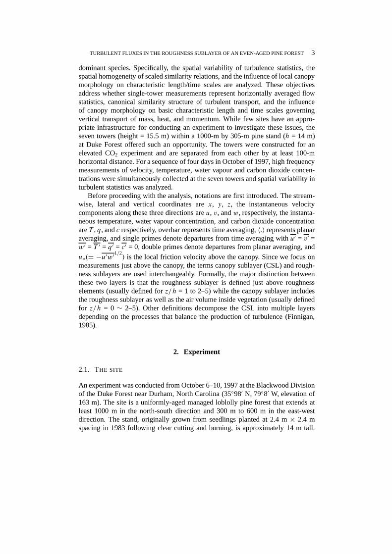
SPATIAL VARIABILITY OF TURBULENT FLUXES IN THEROUGHNESS SUBLAYER OF AN EVEN-AGED PINE FOREST

GABRIEL KATUL 1,∗, CHENG-I HSIEH1, DAVID BOWLING 2, KENNETH CLARK3,NARASINHA SHURPALI4, ANDREW TURNIPSEED2, JOHN ALBERTSON5,KEVIN TU6, DAVE HOLLINGER6, BOB EVANS6, BRIAN OFFERLE4, DEAN

ANDERSON7, DAVID ELLSWORTH1,8, CHRIS VOGEL9 and RAM OREN1

1School of the Environment, Duke University, Durham, NC 27708-0328, U.S.A.;2Environmental,Population, and Organismic Biology, University of Colorado, Bolder, CO 80309, U.S.A.;3School of

Forest Resources and Conservation, University of Florida, Gainesville, FL 32611, U.S.A.;4Department of Geography, Indiana University, Bloomington, IN 47405, U.S.A.;5Department ofEnvironmental Sciences, University of Virginia, Charlottesville, VA 22903, U.S.A.;6United States

Department of Agriculture Forest Service, 271 Mast Rd., Durham, NH 03824, U.S.A.;7UnitedStates Geological Survey, M.S.413, Federal Center, Denver, CO 80225, U.S.A.;8Brookhaven

National Laboratory, Upton, Long Island, NY 11973, U.S.A.;9University of Michigan BiologicalStation, 9008 Biological Rd, Pellston, MI 49769, U.S.A.;∗ Current address: Environment and

Ecology, School of Humanities and Social Sciences, National Taiwan University of Science andTechnology, Taipei 10660, Taiwan

(Received in final form 7 April 1999)

Abstract. The spatial variability of turbulent flow statistics in the roughness sublayer (RSL) of auniform even-aged 14 m (=h) tall loblolly pine forest was investigated experimentally. Using sevenexisting walkup towers at this stand, high frequency velocity, temperature, water vapour and carbondioxide concentrations were measured at 15.5 m above the ground surface from October 6 to 10 in1997. These seven towers were separated by at least 100 m from each other. The objective of thisstudy was to examine whether single tower turbulence statistics measurements represent the flowproperties of RSL turbulence above a uniform even-aged managed loblolly pine forest as a best-casescenario for natural forested ecosystems. From the intensive space-time series measurements, it wasdemonstrated that standard deviations of longitudinal and vertical velocities (σu, σw) and temper-ature (σT ) are more planar homogeneous than their vertical flux of momentum (u2∗) and sensibleheat (H ) counterparts. Also, the measuredH is more horizontally homogeneous when compared tofluxes of other scalar entities such as CO2 and water vapour. While the spatial variability in fluxeswas significant (>15%), this unique data set confirmed that single tower measurements represent the‘canonical’ structure of single-point RSL turbulence statistics, especially flux-variance relationships.Implications to extending the ‘moving-equilibrium’ hypothesis for RSL flows are discussed. Thespatial variability in all RSL flow variables was not constant in time and varied strongly with spatiallyaveraged friction velocityu∗, especially whenu∗ was small. It is shown that flow properties derivedfrom two-point temporal statistics such as correlation functions are more sensitive to local variabilityin leaf area density when compared to single point flow statistics. Specifically, that the local relation-ship between the reciprocal of the vertical velocity integral time scale (Iw) and the arrival frequencyof organized structures (u/h) predicted from a mixing-layer theory exhibited dependence on thelocal leaf area index. The broader implications of these findings to the measurement and modellingof RSL flows are also discussed.

Keywords: Canopy turbulence, Moving equilibrium hypothesis, Planar homogeneity, Roughnesssublayer, Spatial variability, Turbulent fluxes.

Boundary-Layer Meteorology93: 1–28, 1999.© 1999Kluwer Academic Publishers. Printed in the Netherlands.

2 GABRIEL KATUL ET AL.

1. Introduction

Long-term monitoring of carbon dioxide (CO2) and water vapour fluxes abovea wide range of ecosystems has recently received much attention worldwidewith the establishment of measurement networks in Europe and North America(Kaiser, 1998). There is particular interest in monitoring fluxes above tall forestedecosystems because of the magnitude of their mass and energy exchange with theatmosphere (Wofsy et al., 1993). Above tall forests, long-term carbon dioxide (Fc),water vapour (LE), and sensible heat fluxes (H) are commonly measured usingeddy covariance methods within the so-called roughness sublayer (hereafter re-ferred to as RSL). The RSL is loosely defined as that layer within the atmosphericboundary layer (ABL) that is dynamically influenced by length scales associatedwith the roughness elements and is situated below the inertial sublayer (in whichlogarithmic profiles exist for mean velocity and other mean scalar concentrationentities for neutral conditions). The RSL typically ranges from the mean canopyheighth to 2–5h (Raupach and Thom, 1981). The structure of turbulence within theRSL is complicated by its neighbourhood to quasi-random distribution of air spacesembedded in three-dimensional arrays of sources and sinks of momentum andscalar entities (Kaimal and Finnigan, 1994). Despite this complexity, the statisticaldescription of turbulence within the RSL is commonly assumed one-dimensional,varying only in the vertical (z) direction (Kondo and Akashi, 1976; Wilson andShaw, 1977; Lewellen et al., 1980; Albini, 1981; Moritz, 1989; Raupach and Thom,1981; Raupach and Shaw, 1982; Raupach, 1988; Raupach et al., 1991, 1996; Wil-son, 1988, 1989; Amiro and Davis, 1988; Amiro, 1990; Baldocchi and Meyers,1988).

Theoretical justification for a one-dimensional flow approximation is attributedto horizontal averaging the time-averaged equations of motion for momentumand scalar conservation (Wilson and Shaw, 1977; Raupach and Shaw, 1982).Hence, flow statistics modelled from such equations represent horizontally aver-aged quantities. Nonetheless, comparisons between model predictions and fieldmeasurements are typically based on single tower experiments (Meyers and PawU, 1986; Wilson, 1988, 1989; Raupach, 1988; Katul et al., 1997a; Katul and Albert-son, 1998; Katul and Chang, 1999) and not horizontally averaged flow statistics.Whether single-point measurements above the canopy represent horizontally aver-aged flow statistics or the ‘canonical’ dynamics of turbulent transport within theRSL of tall forests has not been explored experimentally. This question also hassignificance for understanding the extent to which a single eddy-covariance fluxmonitoring system above forested canopies can be extrapolated to the scale of theforest stand.

The objective of this study is to examine whether single-tower turbulencestatistics measurements represent the flow properties of RSL turbulence abovea uniform, even-aged forest as a best-case scenario for natural forested ecosys-tems, many of which are not even-aged and are often populated by multiple

TURBULENT FLUXES IN THE ROUGHNESS SUBLAYER OF AN EVEN-AGED PINE FOREST3

dominant species. Specifically, the spatial variability of turbulence statistics, thespatial homogeneity of scaled similarity relations, and the influence of local canopymorphology on characteristic length/time scales are analyzed. These objectivesaddress whether single-tower measurements represent horizontally averaged flowstatistics, canonical similarity structure of turbulent transport, and the influenceof canopy morphology on basic characteristic length and time scales governingvertical transport of mass, heat, and momentum. While few sites have an appro-priate infrastructure for conducting an experiment to investigate these issues, theseven towers (height = 15.5 m) within a 1000-m by 305-m pine stand (h = 14 m)at Duke Forest offered such an opportunity. The towers were constructed for anelevated CO2 experiment and are separated from each other by at least 100-mhorizontal distance. For a sequence of four days in October of 1997, high frequencymeasurements of velocity, temperature, water vapour and carbon dioxide concen-trations were simultaneously collected at the seven towers and spatial variability inturbulent statistics was analyzed.

Before proceeding with the analysis, notations are first introduced. The stream-wise, lateral and vertical coordinates arex, y, z, the instantaneous velocitycomponents along these three directions areu, v, andw, respectively, the instanta-neous temperature, water vapour concentration, and carbon dioxide concentrationareT , q, andc respectively, overbar represents time averaging,〈.〉 represents planaraveraging, and single primes denote departures from time averaging withu′ = v′ =w′ = T ′ = q ′ = c′ = 0, double primes denote departures from planar averaging, and

u∗(= −u′w′1/2) is the local friction velocity above the canopy. Since we focus onmeasurements just above the canopy, the terms canopy sublayer (CSL) and rough-ness sublayers are used interchangeably. Formally, the major distinction betweenthese two layers is that the roughness sublayer is defined just above roughnesselements (usually defined forz/h = 1 to 2–5) while the canopy sublayer includesthe roughness sublayer as well as the air volume inside vegetation (usually definedfor z/h = 0 ∼ 2–5). Other definitions decompose the CSL into multiple layersdepending on the processes that balance the production of turbulence (Finnigan,1985).

2. Experiment

2.1. THE SITE

An experiment was conducted from October 6–10, 1997 at the Blackwood Divisionof the Duke Forest near Durham, North Carolina (35◦98′ N, 79◦8′ W, elevation of163 m). The site is a uniformly-aged managed loblolly pine forest that extends atleast 1000 m in the north-south direction and 300 m to 600 m in the east-westdirection. The stand, originally grown from seedlings planted at 2.4 m× 2.4 mspacing in 1983 following clear cutting and burning, is approximately 14 m tall.

4 GABRIEL KATUL ET AL.

Given the stand uniformity and the tree-to-tree spacing in relation to the canopyheight, the stand can be classified as extensive (i.e., the tree-to-tree spacing is anorder of magnitude smaller than the mean tree height). Six central walkup towersat the Free Air CO2 Enrichment (FACE) Rings (see Ellsworth et al., 1995 fordescription), which are part of an on-going Forest-Atmosphere Carbon Transferand Storage (FACTS) experiment, were used when the CO2 enrichment was shutdown for routine maintenance and repairs. Three of the six towers were in Ringscontinuously exposed to 560 ppm elevated atmospheric CO2 during 1997, althoughthere were no significant long-term effects of elevated CO2 on leaf area or physi-ological properties of the foliage other than photosynthetic enhancement as of thetime of this study (Ellsworth, 1999).

The walkup-tower and the mean canopy heights are 15.5 m and 14.0 m(± 0.5 m) respectively. A seventh central walkup tower (tower height = 20.6 m) fora prototype FACE Ring is also present in the same stand (see Katul et al., 1996a,1997a,b). The seven FACE Rings and local topographic variations are shown inFigure 1. From Figure 1, it is important to note that the separation distance be-tween Rings is at least 100 m, and much of the local topographic variations aresmall (< 5% slopes) so that their influence on turbulent transport can be neglected(Kaimal and Finngan, 1994).

2.2. LEAF AREA DENSITY VARIATIONS

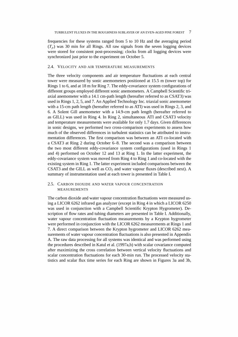
The leaf area density was measured one week prior to the experiment near eachmeasurement tower using aLICOR 2000canopy analyzer. Measurements weremade for a 180◦ view masking the central tower for two azimuthal directionsfrom the tower. Since the predominant wind directions were northerly, the northernazimuth readings were used throughout in this study. The conversion of these mea-surements to leaf area density is discussed in Katul et al. (1997a). The leaf areaindex (LAI) at these seven locations varied from 2.65–4.56 m2 m−2 (coefficientof variation = 18%). The measured leaf area density profiles for each tower siteare shown in Figure 2. For clarity, the cumulative leaf area density is displayedsuch that at the canopy top the cumulative leaf area density of the stand becomesidentical to LAI. Implications of such LAI variations on turbulent statistics andcharacteristic length and time scales is discussed in Section 3.3.

2.3. INSTRUMENTATION SETUP AND LOGGING

Seven research groups participated in the experiment with each group measuringturbulent fluxes at the top of one of theFACE towers (see Figure 1 for towerlocations in thex–y plane). Each participating group assembled their own eddycovariance system on October 4 and 5 (see Table I) and measurements from allRings (except Ring 2) commenced midday of October 6. The predominant winddirection was from north to south. The measurements from Ring 2 were intermit-tent and were primarily used in cross-comparisons of instruments. The sampling

TURBULENT FLUXES IN THE ROUGHNESS SUBLAYER OF AN EVEN-AGED PINE FOREST5

Figure 1.Site description, topographic variation, and relative Ring locations. For Rings 1 to 6, thecentral walkup towers are 15.5 m tall. For the prototype ring (Ring 7), the walkup tower is 20.6 mtall.

6 GABRIEL KATUL ET AL.

0 0.5 1 1.5 2 2.5 3 3.5 4 4.5 50

5

10

15

Hei

ght (

m)

Cumulative Leaf Area Density (m 2 m−2)

Figure 2. The variation of measured cumulative leaf area density with height (from the groundsurface). Thex-axis is displayed such that at the canopy-top the cumulative leaf area density isidentical to LAI. The symbols are as follows: dot for Ring 1, triangle for Ring 2, square for Ring 3,diamond for Ring 4,x for Ring 5, circle for Ring 6, and plus for Ring 7.

TURBULENT FLUXES IN THE ROUGHNESS SUBLAYER OF AN EVEN-AGED PINE FOREST7

frequencies for these systems ranged from 5 to 10 Hz and the averaging period(Tp) was 30 min for all Rings. All raw signals from the seven logging deviceswere stored for consistent post-processing; clocks from all logging devices weresynchronized just prior to the experiment on October 5.

2.4. VELOCITY AND AIR TEMPERATURE MEASUREMENTS

The three velocity components and air temperature fluctuations at each centraltower were measured by sonic anemometers positioned at 15.5 m (tower top) forRings 1 to 6, and at 18 m for Ring 7. The eddy-covariance system configurations ofdifferent groups employed different sonic anemometers. A Campbell Scientific tri-axial anemometer with a 14.1 cm-path length (hereafter referred to as CSAT3) wasused in Rings 1, 2, 5, and 7. An Applied Technology Inc. triaxial sonic anemometerwith a 15-cm path length (hereafter referred to as ATI) was used in Rings 2, 3, and6. A Solent Gill anemometer with a 14.9-cm path length (hereafter referred toas GILL) was used in Ring 4. In Ring 2, simultaneous ATI and CSAT3 velocityand temperature measurements were available for only 1.7 days. Given differencesin sonic designs, we performed two cross-comparison experiments to assess howmuch of the observed differences in turbulent statistics can be attributed to instru-mentation differences. The first comparison was between an ATI co-located witha CSAT3 at Ring 2 during October 6–8. The second was a comparison betweenthe two most different eddy-covariance system configurations (used in Rings 1and 4) performed on October 12 and 13 at Ring 1. In the latter experiment, theeddy-covariance system was moved from Ring 4 to Ring 1 and co-located with theexisting system in Ring 1. The latter experiment included comparisons between theCSAT3 and the GILL as well as CO2 and water vapour fluxes (described next). Asummary of instrumentation used at each tower is presented in Table I.

2.5. CARBON DIOXIDE AND WATER VAPOUR CONCENTRATION

MEASUREMENTS

The carbon dioxide and water vapour concentration fluctuations were measured us-ing a LICOR 6262 infrared gas analyzer (except in Ring 4 in which a LICOR 6250was used in conjunction with a Campbell Scientific Krypton Hygrometer). De-scription of flow rates and tubing diameters are presented in Table I. Additionally,water vapour concentration fluctuation measurements by a Krypton hygrometerwere performed in conjunction with the LICOR 6262 measurements at Rings 1 and7. A direct comparison between the Krypton hygrometer and LICOR 6262 mea-surements of water vapour concentration fluctuations is also presented in AppendixA. The raw data processing for all systems was identical and was performed usingthe procedures described in Katul et al. (1997a,b) with scalar covariance computedafter maximizing the cross correlation between vertical velocity fluctuations andscalar concentration fluctuations for each 30-min run. The processed velocity sta-tistics and scalar flux time series for each Ring are shown in Figures 3a and 3b,

8 GABRIEL KATUL ET AL.

TABLE I

Measuring instruments at the seven towers: CSAT3 = Campbell Scientific Instruments (CSI)sonic anemometer, ATI = Applied Technology Inc, KH2O = CSI Krypton hygrometer, LICOR= LICOR infrared gas analyzer, GILL = Gill sonic anemometer.

Ring # Investigator Sonic type Scalar measurement

1 G. Katul/C.I. Hsieh CSAT3 LICOR 6262, KH2O

Flow Rate = 7 L min−1

Tube Length/Diameter = 3 m/1/4′′Sampling Frequency = 5 Hz

2 D. Anderson ATI/CSAT3 LICOR 6262

Flow Rate = 10 L min−1

Tube Length/Diameter = 5 m/1/4′′Sampling Frequency = 10 Hz

3 D. Bowling/A. Turnipseed ATI LICOR 6251, KH2O

Flow Rate = 7 L min−1

Tube Length/Diameter = 5 m/1/4′′Sampling Frequency = 10 Hz

4 K. Clark GILL LICOR 6262

Flow Rate = 6 L min−1

Tube Length/Diameter = 20 m/1/4′′Sampling Frequency = 10 Hz

5 D. Hollinger/K. Tu CSAT3 LICOR 6262

Flow Rate = 5 L min−1

Tube Length/Diameter = 20 m/3/16′′Sampling Frequency = 5 Hz

6 N. Shurpali/B. Orff ATI LICOR 6262

Flow Rate = 30 L min−1

Tube Length/Diameter = 30 m/1/2′′Sampling Frequency = 10 Hz

7 J. D. Albertson CSAT3 LICOR 6262, KH2O

Flow Rate = 6 L min−1

Tube Length/Diameter = 5 m/1/8′′Sampling Frequency = 10 Hz

respectively. The spatial variability in these time series measurements is used toaddress the study objectives.

TURBULENT FLUXES IN THE ROUGHNESS SUBLAYER OF AN EVEN-AGED PINE FOREST9

3. Results and Discussion

To examine whether single-tower measurements of eddy-covariance turbulentfluxes represent basic statistical properties of RSL turbulence, this section is di-vided into three parts: spatial variability of turbulence statistics, homogeneity ofsimilarity relations, and the role of local canopy morphology on the characteristiclength/time scales. These three sections address whether single-tower measure-ments represent horizontally averaged flow statistics, canonical similarity structureof turbulent transport, and the influence of canopy morphology on characteristiclength and time scales governing vertical motion.

3.1. SPATIAL VARIABILITY OF FLOW STATISTICS

The coefficient of variation(CV (s)) is commonly used as a non-dimensional sta-tistic to quantify the spatial variability of a flow variable(s) around its mean valuefor a given time period. The spatial coefficient of variation is defined as

CV (s) =√〈s′′2〉〈s〉 , (1)

which is a dimensionless measure of the spatial dispersion of a flow variables

about its mean value. Based on time series in Figures 3a and 3b, the daytime (cho-

sen for runs withH > 30 W m−2) averagedCV (s) for σu =√u′u′, σw =

√w′w′,

u∗, σT =√T ′T ′, H , LE, andFc are 0.11, 0.06, 0.16, 0.10, 0.17, 0.33, and 0.27,

respectively. From this analysis, it is clear thatσw is the most uniform RSL flowvariable. Based on the comparisons from the Appendix, differences between theCSAT3 and the ATI sonic anemometer measuredσw was 4%, which is comparablewith the observed 6%CV from this experiment. Hence,σw variability in thex–yplane can be neglected in a first-order analysis of RSL turbulence.

In terms of vertical fluxes,H andu∗ have large but comparable spatial variabil-ity (∼17%) though this variability is not entirely spatial. It is important to note thatdifferences in CSAT3 and ATI-measuredu∗ were approximately 8% and accountfor perhaps as much as 50% of the observed spatial variability. Nonetheless, thenear equality in theCV s betweenH andu∗ brings about important implications

on the spatial similarity in heat and momentum transport. Given thatu∗ =√−u′w′

(i.e., directly proportional to the square root of a second-order statistic) and sensibleheat is directly related to a second-order statistic suggests a spatial dissimilarity ineddies responsible for the vertical transport of heat and momentum. Care shouldbe exercised when interpreting differences in momentum and scalar fluxCV s.Lenschow and Kristensen (1985) and Ritter et al. (1990) suggest that errors in thelocal momentum flux (u′w′) measurement for finite (∼30 min) averaging intervalsare about twice the errors in scalar fluxes. Such increased measurement errorsin u′w′ due to the finite sampling period may partially explain why theCV s in

10 GABRIEL KATUL ET AL.

momentum flux are larger than sensible heat flux (vis-à-vis differences in transportcharacteristics).

The mass fluxCV was much larger than the sensible heatCV , suggesting thatheat may appear more uniformly transported than water vapour or CO2. To interpretdifferences between heat and mass transport, consider the relationship betweenthe turbulent flux above the canopy and local sources and sinks from the canopyfoliage. In a one-dimensional approximation,

w′s′(z=h) =∫ h

0Ss(z)dz+ w′s′(z=0)

wherew′s′ andSs are the local flux and source (or sink) density per unit depthof a scalar entitys emitted or absorbed by the foliage. The sources (or sinks) ofwater vapour (and CO2) from pine needles are controlled by both stomatal andboundary-layer conductance, whereas the transport of heat is only controlled byboundary-layer conductance. Additionally, the ground flux (w′s′(z=0)) contributessignificantly to the above-canopy CO2 and water vapour when compared to heat.Hence, differences inCV betweenH andLEmay be interpreted through the addedstomatal regulation variability and ground flux differences.

Also, daytimeCV s for σu and σT are, for all practical purposes, identical(∼10%). Much of the measuredCV in σu andσT cannot be attributed to instru-mentation differences (maximum∼2%). Recall that the longitudinal velocity andtemperature spectra close to the canopy-atmosphere interface are strongly influ-enced by inactive eddies (Katul et al., 1998). Inactive eddy motion is a larger-scale(� h) quasi-horizontal eddy motion that does not contribute significantly to verti-cal transport (Townsend, 1976; Katul et al., 1996b, 1998). Typically, inactive eddieshave a characteristic length scale comparable to the height of the atmosphericboundary layer (≈1 km). Such a length scale is of the same order as the total lengthof the pine forest stand. Hence, the near equality inσu andσT CV s suggests thatthe same larger-scale eddy motion phenomenon governs the spatial variability ofthese two flow variables.

What is also evident from Figures 3a and 3b is that theCV for a flow variables cannot be the same for all runs and varies with time. However, a limitation tousingCV for all the runs in Figures 3a and 3b is that the CV is ill defined when〈s〉 → 0 (e.g., for evening runs for scalar fluxes). To circumvent this limitation,another relative spatial variation parameter (RV ) given by

RV (s) =√〈s′′2〉

|〈s〉| +√〈s′′2〉 (2)

is proposed and used instead of the traditionalCV . Note thatRV has many desir-able limits for our analysis sinceRV → 0 when〈s′′2〉1/2 → 0 (but for 〈s〉 6= 0),RV → 1 when〈s〉 → 0, andRV is well bounded between [0, 1]. Hence, a flow

TURBULENT FLUXES IN THE ROUGHNESS SUBLAYER OF AN EVEN-AGED PINE FOREST11

(a)

279 279.5 280 280.5 281 281.5 282 282.5 2830

0.5

1

1.5

σ u (

m s

−1)

279 279.5 280 280.5 281 281.5 282 282.5 2830

0.1

0.2

0.3

0.4

0.5

0.6

0.7

σ w (

m s

−1)

279 279.5 280 280.5 281 281.5 282 282.5 2830

0.1

0.2

0.3

0.4

0.5

0.6

0.7

u* (

m s

−1)

Time (d)

(b)

279 279.5 280 280.5 281 281.5 282 282.5 283−100

−50

0

50

100

150

200

250

300

H (

W m

−2)

279 279.5 280 280.5 281 281.5 282 282.5 283−100

0

100

200

300

400

LE (

W m

−2)

279 279.5 280 280.5 281 281.5 282 282.5 283−1

−0.5

0

0.5

Fc (

mg

m−2

s−1

)

Time (d)

Figure 3.(a) Time series variation ofσu, σw, andu∗ for Rings 1, 3, 4, 5, 6, and 7. The symbols areidentical to Figure 2. (b) Same as Figure 3a but forH , LE, andFc.

12 GABRIEL KATUL ET AL.

variables with large spatial variability but small mean value yieldsRV close tounity, and a flow variable that is planar homogeneous yields a smallRV . A flowvariable with a spatial mean comparable to its spatial standard deviation yields anRV close to 0.5. Using theRV , we investigate how different turbulence conditionsinfluence the temporal changes of the spatial variability of all RSL turbulent flowvariables.

Near the canopy-atmosphere interface (z/h ∼ 1.0–1.2), the mechanical pro-duction of turbulence (∝ 〈u∗〉3) is the largest contributor to the turbulent kineticenergy (TKE) budget balancing the divergent vertical turbulent transport and vis-cous dissipation terms. Of the three velocity variances defining the TKE (= 0.5[σ 2u + σ 2

v + σ 2w]), the largest contributor isσu (indicated by slopes in Table II).

As demonstrated by Raupach et al. (1996) and Katul et al. (1998), the spectrumof u′ at low frequencies is controlled by inactive eddy motion. For this stand, as〈u∗〉 increases, the frequency of occurrence of inactive eddy motion (∼〈u∗〉/hb)also increases, wherehb is the ABL height. Since inactive eddies close toz/h = 1introduce a large horizontal length scale (characterized byhb), these eddies tendto better aggregate (i.e., mix) local sources (or sinks) for scalars and momentumin thex, y plane. Hence, it is expected thatRV decreases for increasing〈u∗〉 untilsome limitingRV is attained that reflects inherent ‘forest-scale’ variability. Thelatter variability exists at scales much larger than the characteristic length scale ofenergetic eddies responsible for much of the vertical transport (∼h).

In Figures 4a and 4b, theRV for variances (σu, σw, σT ) and turbulent fluxes(w′u′,w′T ′,w′q ′,w′c′) as a function of〈u∗〉3 is shown. Note that, for〈u∗〉3 smallerthat 0.02 m3 s−3 (or 〈u∗〉 0.27 m s−1), theRV rapidly increases with decreasing〈u∗〉3. However, for〈u∗〉3 exceeding 0.02 m3 s−3 the RV for all variables ap-proaches a near-constant minimum limit. While the above argument is a reasonablehypothesis to explain the dependence ofRV on 〈u∗〉, an equally plausible hypoth-esis is the dependence of sampling statistics onu∗. Higher values ofu∗ results inmore turbulent events passing through the sampling point which, in turn, leads toa reduction in the standard error of estimate of the mean. Hence, the reduction ofRV with u∗ may be attributed to sampling errors vis-à-vis the turbulent transportmechanisms.

3.2. HOMOGENEITY OF SIMILARITY RELATIONSHIPS

In the previous section, it was demonstrated that variances and fluxes do vary in(x, y) within the RSL. However, this variation does not necessarily imply thatsingle-tower measurements do not scale locally in accordance with canonical sim-ilarity structure of RSL turbulent transport. The small variation of both variancesand fluxes over such large distances (>100 m) suggests that RSL flows may be ina state of ‘moving equilibrium’. The ‘moving equilibrium’ concept, first proposedby Yaglom (1979) foru∗, states that ifu∗ varies slowly in thex, y plane (see e.g.,Yaglom, 1979; Raupach et al., 1991), thenu∗ can be considered as a local velocity

TURBULENT FLUXES IN THE ROUGHNESS SUBLAYER OF AN EVEN-AGED PINE FOREST13

(a)

0 0.02 0.04 0.06 0.08 0.1 0.120

0.1

0.2

0.3

0.4

0.5

0.6

RV

(σu)

0 0.02 0.04 0.06 0.08 0.1 0.120

0.1

0.2

0.3

0.4

0.5

0.6

RV

(σw

)

0 0.02 0.04 0.06 0.08 0.1 0.120

0.1

0.2

0.3

0.4

0.5

0.6

RV

(σT)

<u*>3

(b)

0 0.02 0.04 0.06 0.08 0.10

0.1

0.2

0.3

0.4

0.5

0.6

0.7

0.8

0.9

1

RV

(u*)

0 0.02 0.04 0.06 0.08 0.10

0.1

0.2

0.3

0.4

0.5

0.6

0.7

0.8

0.9

1

RV

(H)

0 0.02 0.04 0.06 0.08 0.10

0.1

0.2

0.3

0.4

0.5

0.6

0.7

0.8

0.9

1

RV

(LE

)

<u*>3

0 0.02 0.04 0.06 0.08 0.10

0.1

0.2

0.3

0.4

0.5

0.6

0.7

0.8

0.9

1

RV

(Fc)

<u*>3

Figure 4.(a) Variation ofRV (σu), RV (σw), RV (σT ) with 〈u∗〉3 for day time and night time runs.(b) Same as Figure 4a but forRV (u∗), RV (H), RV (LE), andRV (Fc). TheRV (s) for a flowvariables is computed using Equation (2).

14 GABRIEL KATUL ET AL.

TABLE II

Regression analysis of turbulent velocity standard deviations (σu, σw)as a function of friction velocity (u∗) for all Rings. The regressionmodel is of the form:σ = Au∗ + B. The coefficient of determination(R2), the standard error of estimate (SEE), and the number of runs usedin the regression (N) are presented. The second line for each ring arefor regression forced through the origin (B = 0).

Variable Ring # SlopeA InterceptB R2 SEE N

σw 1 1.06 0.05 0.91 0.04 358

1.25 0.00 0.86 0.06

3 1.11 0.04 0.90 0.05 175

1.25 0.00 0.86 0.05

4 1.14 0.04 0.87 0.06 149

1.30 0.00 0.84 0.06

5 1.13 0.04 0.89 0.05 148

1.29 0.00 0.86 0.05

6 1.10 0.04 0.90 0.05 150

1.26 0.00 0.86 0.05

7 1.26 0.04 0.91 0.05 127

1.43 0.00 0.89 0.05

σu 1 1.83 0.15 0.87 0.10 358

2.40 0.00 0.71 0.14

3 1.82 0.09 0.88 0.09 175

2.19 0.00 0.82 0.11

4 1.97 0.11 0.86 0.10 149

2.41 0.00 0.79 0.13

5 1.98 0.10 0.88 0.09 148

2.40 0.00 0.81 0.12

6 1.81 0.12 0.86 0.09 150

2.26 0.00 0.77 0.12

7 1.96 0.13 0.86 0.10 127

2.50 0.00 0.75 0.13

scale independent of (x, y) for small perturbations in thex–y plane. That is, theforest stand can be decomposed into planar homogeneous patches, with each patchcharacterized by its ownh andu∗ as length and velocity scales.

TURBULENT FLUXES IN THE ROUGHNESS SUBLAYER OF AN EVEN-AGED PINE FOREST15

A direct consequence of the moving equilibrium assumption is that when localflow variables are properly normalized by local length and velocity scales, theirvariability in the (x, y) plane becomes insignificant. For example, in the RSL,

σu

u∗= Au, σw

u∗= Aw, σT

T∗= AT (ξ)−1/3, (3)

for ξ > 0;

ξ = −z − dL

.

In (3), T∗ is a temperature scale defined asT∗ = w′T ′/u∗ andL and d are theObukhov length and zero-plane displacement heights, respectively,Au, Aw, andAT are similarity constants and must be independent of (x, y) by the moving equi-librium hypothesis. Here, the zero-plane displacement was computed for each Ringfrom the mean height of momentum absorption by the local leaf area density (seeThom, 1971) and was found to vary from 0.59 to 0.65 h. The momentum absorptionwas computed from modelledu′w′ profiles using the second-order closure modeldescribed in Katul and Albertson (1998). Figure 5 presents measuredσu andσwas a function of measuredu∗, and measuredT∗ as a function of measuredξ for allthe Rings. The lines in the figure are ‘best-fit’ to Raupach et al.’s (1996) data forvelocity, and ‘best-fit’ atmospheric surface-layer (ASL) data for temperature.

If single-tower measurements obey the RSL similarity structure, thenAu, Aw,andAT cannot be dependent on position in the (x, y) space. For each Ring,Au,Aw,andAT were computed and presented in Table II for momentum and in Table IIIfor heat. Due to differences in flow rate, tube length, and tube diameter withinthe gas analyzer setup (see Table I), we did not perform a similar analysis forc

andq given the significant spectral contribution of high frequency events to theoverall scalar variances (see Section A.3 in Appendix A). Based on the regressionanalysis of Tables II and III, we found that the spatially averagedAu = 1.90 (±0.075),Aw = 1.14 (± 0.065), andAT = 1.12 (± 0.04). These velocity similarityconstants are in good agreement withAu = 1.8 andAw = 1.1 reported by Raupachet al. (1996) for a laboratory RSL wind-tunnel experiment. In addition, Table IIIdemonstrates that measuredσT /T∗ exhibits a strong−1/3 power law (i.e.,ξ−1/3)dependence for all Rings. That is, the−1/3 power-law also does not vary in thex–y plane. The occurrence of a−1/3 power law is commonly associated with‘free-convection’ withσT becoming independent ofu∗, but strongly dependent onsensible heatH (Albertson et al., 1995; Hsieh and Katul, 1997). The measuredATis in close agreement with atmospheric surface-layer values (AT = 0.97) reportedby Albertson et al. (1995), Katul et al. (1995), and Hsieh et al. (1996). We also didnot find statistically significant differences between the individual RingAu, Aw,andAT at the 95% confidence limits. The significance tests were referenced toRing 4 sinceAw andAu for Ring 4 are closest to the spatially averagedAu andAw

16 GABRIEL KATUL ET AL.

0 0.1 0.2 0.3 0.4 0.5 0.6 0.70

0.2

0.4

0.6

0.8

1

1.2

1.4σ u

(m

s−1

)

u*(m s−1)

0 0.1 0.2 0.3 0.4 0.5 0.6 0.70

0.1

0.2

0.3

0.4

0.5

0.6

0.7

σ w (

m s

−1)

u*(m s−1)

10−2

10−1

100

101

102

10−1

100

101

σ T/T

*

ξ

Figure 5.The variation ofσu andσw with u∗ is shown for Rings 1, 3, 4, 5, 6, and 7 and all runs. Thesolid lines are best-fit regressions (i.e.,Au = 1.8,Aw = 1.1) to measurements from Raupach et al.(1996). The variation ofσT /T∗, with the stability parameterξ is shown for daytime conditions (i.e.,H > 30 W m−2) only. The solid line isσT /T∗ = 1.0ξ−1/3. Symbols are the same as in Figure 2.

TURBULENT FLUXES IN THE ROUGHNESS SUBLAYER OF AN EVEN-AGED PINE FOREST17

TABLE III

Regression analysis of normalized temperature standard de-viation (σT /T∗) as a function of the stability parameterξ = −(z − d)/L for all Rings and daytime conditions(H > 30 W m−2). The regression model is of the form:ln(σT /T∗) = A ln(ξ)+B. The coefficient of determination (R2)and the standard error of estimate (SEE) along with the interceptB are shown. The interceptB is used to calculate the similarityconstantAT of Equation (3) and is presented in brackets. In theASL,AT = 1.

Ring # n SlopeA InterceptB/(AT ) R2 SEE

1 50 −0.32 0.16 (1.18) 0.87 0.18

3 38 −0.33 0.10 (1.11) 0.89 0.13

4 46 −0.32 0.06 (1.06) 0.83 0.14

5 46 −0.33 0.17 (1.19) 0.81 0.21

6 46 −0.34 0.10 (1.11) 0.72 0.24

7 42 −0.34 0.09 (1.10) 0.90 0.15

for this stand. Finally, we note that the spatial coefficient of variation forAu, Aw,andAT (4.0%, 5.8%, and 3.9%, respectively) are close to the reported magnitude ofinstrumentation measurement differences forσw presented in Appendix A (∼4%).Hence, the invariance ofAu, Aw, andAT in the x–y plane is consistent with the‘moving equilibrium’ hypothesis.

3.3. CANOPY MORPHOLOGY AND INTEGRAL TIME SCALES

Estimating RSL characteristic length or time scales from single-point measure-ments is commonly performed via the integral time scale (Iw) defined as

Iw =∫ ∞

0ρw(τ)ds;

(4)

ρw(τ) = w′(t + τ)w′(t)σ 2w

whereρw(τ) is the vertical velocity auto-correlation function, andτ is the time lag.In practice, the integration ofρw(τ) is terminated at the first zero crossing as dis-cussed in Katul et al. (1997a). In RSL turbulence,Iw represents the characteristictime scale of ‘active’ eddies responsible for much of the scalar transport.

To derive similarity relationships forIw, we consider the mixing-layer analogyof Raupach et al. (1996). Raupach et al. (1996) argued that vertical transport close

18 GABRIEL KATUL ET AL.

to the canopy-atmosphere interface resembles a mixing layer rather than a bound-ary layer because the canopy-atmosphere interface is a porous medium and cannotimpose the same severe constraint on fluid continuity (i.e., the no-slip boundarycondition) as an impervious boundary. A mixing layer is a boundary-free shear flowformed in a region between two co-flowing fluid streams of different velocity butthe same density. The resemblance between canopy-atmosphere vertical transportand a mixing layer is mainly attributed to the strong inflection point in the meanvelocity profile atz/h = 1. Such an inflection point inu(z) leads to the gener-ation of two-dimensional Kelvin–Helmholtz (KH) instabilities with a streamwisewavelength (3x).

Using the mixing-layer analogy of Raupach et al. (1996),Iw can be related tothe characteristic frequency of KH instabilities, after some algebraic manipulation,using

1

Iw= Am u

h(5)

whereAm ≈ 2.84 estimated by use for the ‘generic canopy’ data in Raupach etal. (1996) withu defined atz/h = 1. Table IV presents the measuredAm foreach Ring obtained by regressing measuredI−1

w versus measuredu/h shown inFigure 6. We restricted the analysis in Table IV and Figure 6 toH > 30 W m−2 sothat daytime runs are included for each Ring. Uncertainty in computedIw as wellas the existence of factors other thanu/h that strongly influencesIw precludedinvestigating (5) for evening runs (not shown in Figure 6).

From our measurements, the spatially averagedAm value of 2.18 (± 0.17) isfound to be lower than the value determined from Raupach et al.’s (1996) data(shown as the solid line in Figure 6). This is not surprising since Raupach et al.(1996) estimatedAm at z = h, while the measurements from this experiment arefor z/h = 1.11 (except for Ring 7,z/h = 1.29). Given thatIw does not varyappreciably withz for z/h = 1.0–1.5, asz/h increases,u increases leading toa reduction inAm (Kaimal and Finnigan, 1994; Thompson, 1979). For Ring 7,we present both rawAm values obtained forz/h = 1.28 and adjustedAm forz/h = 1.11. The adjustment in Ring 7 is based on a logarithmic interpolation ofu

at z = 15.5 m from measuredu at z = 18 m.While the spatial variation inAm is not large (spatial coefficient of variation

is 8% for an 18% variation in LAI), it is sufficiently significant to warrant fur-ther analysis. Irvine and Brunet (1996) demonstrated thatAm does not vary withatmospheric stability. Hence, it is unlikely that Ring-to-Ring variations inAm arecaused by the spatial variability in flow properties such as sensible heat and frictionvelocity. The conclusions from Irvine and Brunet (1996) lead us to consider canopymorphology (particularly LAI) as a source of variability. The potential dependenceof Am on LAI seems plausible. For small LAI (but the same canopy heighth), theinstabilities close to the canopy-atmosphere interface are not KH produced and theflow resembles a boundary layer (vis-à-vis a mixing layer) in which no inflection

TURBULENT FLUXES IN THE ROUGHNESS SUBLAYER OF AN EVEN-AGED PINE FOREST19

TABLE IV

Regression analysis to determineAm (inI−1w =Amu/h) for all Rings and forH >

30 W m−2. The coefficient of determina-tion (R2) and the standard error of esti-mate (SEE) are also presented. The mea-sured leaf area index (LAI) around thecentral tower of each Ring is also shown.The values for Ring 7∗ are adjusted val-ues of Ring 7 to reflectu measured at15.5 m rather than 18 m as in Ring 7. Thisadjustment assumes thatu varies loga-rithmically betweenz = 15.5 m andz =18 m, and that the zero-plane displace-ment is 0.65 h.

Ring # Am R2 SEE LAI

1 1.82 0.54 0.05 2.65

3 2.33 0.69 0.04 4.56

4 2.14 0.67 0.05 3.09

5 2.31 0.65 0.05 4.24

6 2.21 0.40 0.07 3.58

7 2.05 0.58 0.06 3.90

7∗ 2.28 0.58 0.06 3.90

in u exists. Measurements by Paw U et al. (1992) over short vegetation, and theseasonal variation in measuredIw and u/u∗ by Lu and Fitzjarrald (1994), indi-rectly support this argument. For such boundary-layer flows,I−1

w becomes poorlycorrelated withu/h resulting in a smallAm. That is, for the same canopy height,a decrease in LAI results in a decrease inAm. This experiment uniquely examinedthe dependence ofAm on LAI for the same stand (i.e., tree height, tree architecture,pine needle sizes and orientation are all similar in this experiment) in Figure 7.Figure 7 clearly demonstrates that as LAI decreases,Am also decreases, confirmingthe above argument.

4. Conclusions

This study is the first to examine experimentally the spatial variability of turbu-lent statistics within the RSL above a tall even-aged forest. We demonstrated thefollowing:

1. The velocity and temperature standard deviations (σu, σw, andσT ) are moreplanar homogeneous (CV ∼ 10%) thanu∗ and sensible heat (H ) (CV ∼ 17%).

20 GABRIEL KATUL ET AL.

0 0.02 0.04 0.06 0.08 0.1 0.12 0.14 0.16 0.18 0.20

0.1

0.2

0.3

0.4

0.5

0.6

1/I w

(s−1

)

u/h (s −1)

R1R3R4R5R6R7

Figure 6.The variation ofI−1w with the arrival frequencyu/h for Rings 1, 3, 4, 5, 6, and 7. The solid

line is derived from the ‘generic canopy’ data of Raupach et al. (1996).

2. The sensible heat flux is more homogeneous than the fluxes of other scalarentities such as CO2 (Fc) and water vapour (LE). This conclusion confirmsearlier suggestions by Katul et al. (1995) and Andreas et al. (1998) that the fluxof sensible heat appears more uniformly distributed than other scalars such aswater vapour.

3. Single-tower measurements when scaled with local variables can representthe canonical structure of single-point turbulence statistics. Particularly, itis demonstrated that flux-variance similarity functions are independent oflocation.

4. The spatial variability of all RSL flow variables is not constant in time butstrongly depends on〈u∗〉3. One possible explanation is that the increase inmechanical production of turbulent kinetic energy increases the frequency ofinactive eddies. Such eddy motion introduces a horizontal length scale muchlarger than the canopy height (h) that enhances aggregation of local sourcesand sinks near the canopy-atmosphere interface. Another equally plausible(and inter-related) explanation is that the reduction ofRV with u∗ may beattributed to the dependence of sampling errors onu∗. Future large eddy simu-

TURBULENT FLUXES IN THE ROUGHNESS SUBLAYER OF AN EVEN-AGED PINE FOREST21

2.6 2.8 3 3.2 3.4 3.6 3.8 4 4.2 4.4 4.61.8

1.9

2

2.1

2.2

2.3

2.4

2.5

LAI (m 2 m−2)

Am

(in

1/I

w =

Am

u/h

)R1R3R4R5R6R7

adjR7

Figure 7.The dependence ofAm on LAI for Rings 1, 3, 4, 5, 6, and 7. In Ring 7, the adjusted value(R7adj) is refers to interpolatingu from its 18.0 m measured value to 15.5 m logarithmically. Thisadjustment is necessary for consistency with the measurement heights ofu for the other rings.

lation runs with differentu∗ can provide systematic diagnostics as to which ofthese arguments better explains the dependence ofRV onu∗.

5. Flow properties derived from lagged correlation function analysis are moresensitive to the local variability in leaf area density when compared to othersecond-order statistics. Particularly, the local relationship between the recip-rocal of the integral time scale (Iw) and the arrival frequency of organizedstructures (u/h) predicted from the mixing-layer analogy of Raupach et al.(1996) exhibits dependence on the local leaf area index.

The broader implications of these findings to the measurement and modelling ofRSL flows above uniform canopies (i.e.,CV (LAI) < 20%) are as follows:

1. The planar homogeneity assumption inσu, σw, u∗ , andH (or the atmosphericstability parameter) commonly employed in Lagrangian dispersion models tocompute the source-weight function of scalar entities such as water vapour orCO2 in the roughness sublayer (e.g., Leclerc et al., 1988; Baldocchi, 1992;Katul et al., 1997a) is reasonable.

22 GABRIEL KATUL ET AL.

2. The ‘moving equilibrium’ hypothesis, originally developed for surface-layerflows, can be extended to RSL flows as evidenced by conclusion 3. Strictlyspeaking, conclusion 3 is a necessary and not a sufficient condition. Nonethe-less, agreement between the present measurements and wind-tunnel experi-ments (see Raupach et al., 1996; Raupach, 1988) suggest that the ‘movingequilibrium’ hypothesis is a practical approximation for the RSL. The ‘movingequilibrium’ hypothesis has direct consequences for the comparisons betweenclosure-modelling calculations, which represent horizontally averaged flowstatistics, and single-tower measurements. Horizontally averaged flow statis-tics computed from higher-order closure principles and normalized by〈u∗〉and〈h〉 can be converted to ‘local’ flow statistics if the local length (e.g.,h)and velocity scales (e.g.,u∗) are used. Additionally, the planar homogeneityin σu, σw, u∗ indirectly supports the negligence of ‘dispersive’ fluxes arisingfrom horizontal averaging of the time-averaged equations of motion (Finnigan,1985) in RSL flows.

3. The planar homogeneity inσT , coupled with the invariance of the similarityrelationshipσT /T∗ = AT ξ

−1/3 in the x–y plane, demonstrates that the flux-variance method, developed for the atmospheric surface layer, can accuratelyreproduce the daytime sensible heat flux (of local relevance) from single-towerσT measurements within the RSL.

4. The strong local relationship betweenI−1w and u/h (i.e., I−1

w = Amu/h) forall Rings suggests that the mixing-layer analogy for vertical transport nearz/h = 1 provides an analytic linkage between the ‘origins’ of organizedmotion and characteristic time scales for RSL transport. Local canopy mor-phology changes do not alter the functional relationship betweenI−1

w andu/hbut can alterAm.

5. When comparing net carbon uptake and water budgets between differentecosystems derived from single-tower measurements within each system, itis necessary to interpret budget differences that are less than 20% with greatcaution. As evidenced from this experiment, unless special care is taken ininstrument calibration and cross comparison, it will be difficult to meaningfullyevaluate budget differences smaller than 20%. Additionally, because of theircontrol by stomatal and boundary-layer conductances and the more complexnature of the sources and sinks (e.g., influence of soil),LE andFc are inher-ently more spatially variable thanH . This experiment demonstrated that atleast 8% spatial variability in daytimeH is not uncommon.

Acknowledgements

The authors would like to thank Andrew Palmiatti, Galen Hon, and Greg Burklandfor their help during the experiment. We also thank Betsy Nettleton for all herefforts in coordinating travel, lodging and equipment shipping for various inves-

TURBULENT FLUXES IN THE ROUGHNESS SUBLAYER OF AN EVEN-AGED PINE FOREST23

tigators, and George Hendrey and William Schlesinger for facilitating the use ofthe Free Air CO2 Enrichment Facilities (FACE) at Duke Forest. We also thankthe two reviewers for their helpful comments and suggestions. Particularly, wethank the reviewers for pointing out the potential dependence of RV onu∗ dueto sampling errors. This project was funded by the Department of Energy (DOE)through the National Institute for Global Environmental Change (NIGEC) throughthe SouthEast Regional Center at the University of Alabama, Tuscaloosa (DOECooperative agreement DE-FC03-90ER61010) and through the Office of Healthand Environmental Research (DE-ACO2-76CH00016), and the National ScienceFoundation (NSF-BIR 12333).

Appendix A: Comparisons between Different Instruments

In this appendix, the inter-comparison statistics for different eddy-covariancesystems are reported.

A.1. VELOCITY SENSORS

Because three sonic types (ATI, GILL, and CSAT3) were used in this experiment,it was necessary to quantify differences in the statistics due to differences in sonicanemometer configurations. We compared the ATI, GILL, and CSAT3 velocity andtemperature measurements side by side (80 cm apart) using measurements fromtwo experiments described next.

A.1.1. ATI/CSAT3 Comparison (Table A.I)At Ring 2, 67 runs, each of 30-minute duration, were collected between Dayof Year (DOY) 279 and 281 in which the CSAT3 and ATI were simultaneouslymeasuring velocity and temperature at 10 Hz. Table V reports the regressioncomparison between the two anemometers. The maximum variability between theanemometers was at most 4% (based on the slope of the regression analysis) forstandard deviations, 9% for the friction velocity, and 8% for sensible heat.

A.1.2. GILL/CSAT3 Comparison (Table A.II)At Ring 1, 87 runs, each of 30-minute duration, were collected between DOY 284and 286 in which the CSAT3 and the GILL anemometers were simultaneouslymeasuring velocity and temperature at 5 Hz and 10 Hz, respectively. In this exper-iment, the system from Ring 4 was co-located with the setup at Ring 1. Table A.IIreports the regression comparison between the two anemometers. The variabilitybetween the anemometers was at most 1% for all standard deviations, 1% for thefriction velocity, and 4% for sensible heat.

24 GABRIEL KATUL ET AL.

TABLE A.I

Comparisons between ATI and CSAT3 at Ring 2 (Dayof Year 279–281/1997; number of runsn = 67) usinga linear regression model. The regression statistics forthe relevant flow variables, including the coefficient ofdetermination (R2) and the standard error of estimate(SEE), are shown. The independent and dependentvariables are the ATI and CSAT3, respectively.

Flow variable Slope Intercept R2 SEE

u (m s−1) 1.00 0.02 0.983 0.04

T (◦C) 0.96 0.52 0.999 0.03

σu (m s−1) 0.98 0.00 0.999 0.02

σv (m s−1) 0.98 0.00 0.995 0.01

σw (m s−1) 1.04 0.00 1.000 0.00

σT (◦C) 0.99 0.00 0.990 0.02

u∗ (m s−1) 0.91 0.00 0.901 0.02

H (W m−2) 1.08 0.50 0.997 2.40

TABLE A.II

Comparisons between GILL and CSAT3 at Ring 1 (Day ofYear 284–286/1997; number of runsn = 87) using a linearregression model. The regression statistics for the relevantflow variables, including the coefficient of determination (R2)and the standard error of estimate (SEE), are shown. The in-dependent and dependent variables are the GILL and CSAT3,respectively.

Flow variable Slope Intercept R2 SEE

u (m s−1) 0.93 0.17 0.968 0.08

T (◦C) 1.26 −4.0 0.997 0.27

σu (m s−1) 0.99 0.03 0.993 0.02

σv (m s−1) 1.00 0.02 0.991 0.02

σw (m s−1) 1.04 0.00 0.999 0.01

σT (◦C) 1.00 0.05 0.990 0.02

u∗ (m s−1) 1.01 −0.01 0.980 0.02

H (W m−2) 1.04 0.53 0.990 7.05

LE (W m−2) 0.94 4.93 0.920 21.2

Fc (mg m−2 s−1) 0.87 −0.01 0.910 −0.08

TURBULENT FLUXES IN THE ROUGHNESS SUBLAYER OF AN EVEN-AGED PINE FOREST25

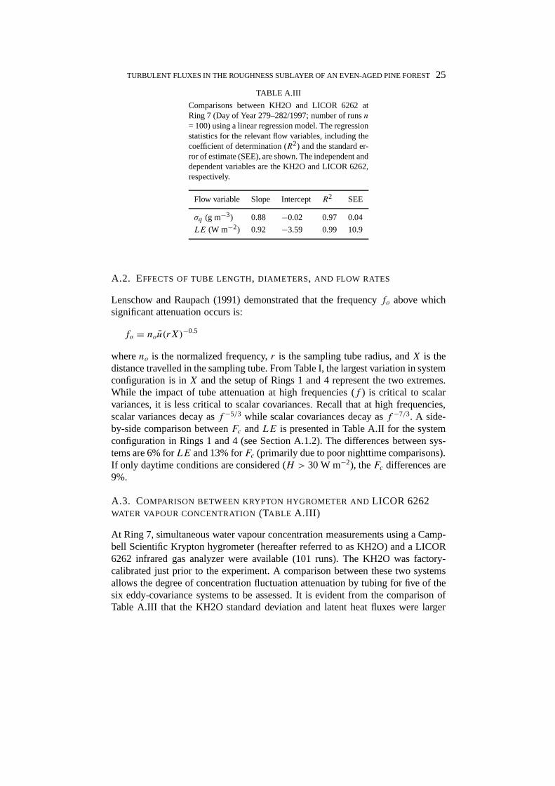
TABLE A.III

Comparisons between KH2O and LICOR 6262 atRing 7 (Day of Year 279–282/1997; number of runsn= 100) using a linear regression model. The regressionstatistics for the relevant flow variables, including thecoefficient of determination (R2) and the standard er-ror of estimate (SEE), are shown. The independent anddependent variables are the KH2O and LICOR 6262,respectively.

Flow variable Slope Intercept R2 SEE

σq (g m−3) 0.88 −0.02 0.97 0.04

LE (W m−2) 0.92 −3.59 0.99 10.9

A.2. EFFECTS OF TUBE LENGTH, DIAMETERS, AND FLOW RATES

Lenschow and Raupach (1991) demonstrated that the frequencyfo above whichsignificant attenuation occurs is:

fo = nou(rX)−0.5

whereno is the normalized frequency,r is the sampling tube radius, andX is thedistance travelled in the sampling tube. From Table I, the largest variation in systemconfiguration is inX and the setup of Rings 1 and 4 represent the two extremes.While the impact of tube attenuation at high frequencies (f ) is critical to scalarvariances, it is less critical to scalar covariances. Recall that at high frequencies,scalar variances decay asf −5/3 while scalar covariances decay asf −7/3. A side-by-side comparison betweenFc andLE is presented in Table A.II for the systemconfiguration in Rings 1 and 4 (see Section A.1.2). The differences between sys-tems are 6% forLE and 13% forFc (primarily due to poor nighttime comparisons).If only daytime conditions are considered (H > 30 W m−2), theFc differences are9%.

A.3. COMPARISON BETWEEN KRYPTON HYGROMETER AND LICOR 6262WATER VAPOUR CONCENTRATION(TABLE A.III)

At Ring 7, simultaneous water vapour concentration measurements using a Camp-bell Scientific Krypton hygrometer (hereafter referred to as KH2O) and a LICOR6262 infrared gas analyzer were available (101 runs). The KH2O was factory-calibrated just prior to the experiment. A comparison between these two systemsallows the degree of concentration fluctuation attenuation by tubing for five of thesix eddy-covariance systems to be assessed. It is evident from the comparison ofTable A.III that the KH2O standard deviation and latent heat fluxes were larger

26 GABRIEL KATUL ET AL.

than their LICOR 6262 counterpart by 12, and 8%, respectively. As expected, theKH2O and LICOR 6262 fluxes are in closer agreement than the variances given therapid decay of thew′q ′ covariance at high frequencies (∼f −7/3) when comparedto the variance decay (∼f −5/3).

References

Albertson, J. D., Parlange, M. B., Katul, G. G., Chu, C. R., and Stricker, H.: 1995, ‘Sensible Heat FluxEstimates for Arid Regions: A Simple Flux-Variance Method’,Water Resour. Res.31, 969–973.

Albini, F. A.: 1981, ‘A Phenomenological Model for Wind Speed and Shear Stress Profiles inVegetation Cover Layers’,J. Appl. Meteorol. 20, 1325–1335.

Amiro, B. D.: 1990, ‘Comparison of Turbulence Statistics within Three Boreal Forest Canopies’,Boundary-Layer Meteorol.51, 99–121.

Amiro, B. D. and Davis, P. A.: 1988, ‘Statistics of Atmospheric Turbulence within a Natural BlackSpruce Forest Canopy’,Boundary-Layer Meteorol.44, 267–283.

Andreas, E. L., Hill, R., Gosz, J., Moore, D., Otto, W., and Sarma, A.: 1998, ‘Statistics of SurfaceLayer Turbulence over Terrain with Metre-Scale Heterogeneity’,Boundary-Layer Meteorol. 86,379–408.

Baldocchi, D. and Meyers, T. P.: 1989, ‘The Effects of Extreme Turbulent Events of the Estimationof Aerodynamic Variables in a Decidous Forest Canopy’,Agric. For. Meteorol.48, 117–134.

Baldocchi, D. and Meyers, T. D.: 1988, ‘Turbulence Structure in a Deciduous Forest’,Boundary-Layer Meteorol.43, 345–364.

Baldocchi, D.: 1992, ‘A Lagrangian Random Walk Model for Simulating Water Vapour, CO2 andSensible Heat Densities and Scalar Profiles over and within a Soybean Canopy’,Boundary-LayerMeteorol. 61, 113–144.

Ellsworth, D. S., Oren, R., Huang, C., Phillips, N., and Hendrey, G.: 1995, ‘Leaf and Canopy Re-sponses to Elevated CO2 in a Pine Forest under Free-Air CO2 Enrichment’,Oecologia104,139–146.

Ellsworth, D. S.: 1999, ‘CO2 Enrichment in a Maturing Pine Forest: Are CO2 Exchange and WaterStatus in the Canopy Affected?’,Plant, Cell Environ., in press.

Finnigan, J. J.: 1985 , ‘Turbulent Transport in Flexible Plant Canopies’, in B. A. Hutchinson and B.B. Hicks (eds.),The Forest-Atmosphere Interaction, D. Reidel Publishing Company, Dordrecht,pp. 443–480.

Hsieh, C. I., Katul, G. G., Scheildge, J., Sigmon, J. T., and Knoerr, K. R.: 1996, ‘Estimation of Mo-mentum and Heat Fluxes Using Dissipation and Flux-Variance Methods in the Unstable SurfaceLayer’, Water Resour. Res.8, 2453–2462.

Hsieh, C. I. and Katul, G. G.: 1997, ‘The Dissipation Methods, Taylor’s Hypothesis, and StabilityCorrection Functions in the Atmospheric Surface Layer’,J. Geophys. Res. 102, 16,391–16,405.

Irvine, M. R. and Brunet, Y.: 1996, ‘Wavelet Analysis of Coherent Eddies in the Vicinity of SeveralVegetation Canopies’,Phys. Chem. Earth21, 161–165.

Kaimal, J. C. and Finnigan, J. J.: 1994,Atmospheric Boundary Layer Flows: Their Structure andMeasurements, Oxford University Press, 289 pp.

Kaiser, J.: 1998, ‘Climate Change – New Network Aims to Take the Worlds CO2 Pulse Source’,Science281, 506–507.

Katul, G. G., Geron, C., Hsieh, C. I., Vidakovic, B., and Guenther, A.: 1998, ‘Active Turbulence andScalar Transport near the Forest-Atmosphere Interface’,J. Appl. Meteorol. 37, 1533–1546.

Katul, G. G. and Albertson, J. D.: 1998, ‘An Investigation of Higher Order Closure Models for aForested Canopy’,Boundary-Layer Meteorol. 89, 47–74.

TURBULENT FLUXES IN THE ROUGHNESS SUBLAYER OF AN EVEN-AGED PINE FOREST27

Katul, G. G., Oren, R., Ellsworth, D., Hsieh, C. I., and Phillips, N.: 1997a, ‘A Lagrangian DispersionModel for Predicting CO2 Sources, Sinks, and Fluxes in a Uniform Loblolly Pine Stand’,J.Geophys. Res. 102, 9309–9321.

Katul, G. G., Hsieh, C. I., Kuhn, G., Ellsworth, D., and Nie, D.: 1997b, ‘Turbulent Eddy Motion atthe Forest-Atmosphere Interface’,J. Geophys. Res.102, 13,409–13,421.

Katul, G. G., Hsieh, C. I., Oren, R., Ellsworth, D., and Phillips, N.: 1996a, ‘Latent and SensibleHeat Flux Predictions from a Uniform Pine Forest Using Surface Renewal and Flux VarianceMethods’,Boundary-Layer Meteorol.80, 249–282.

Katul, G. G., Albertson, J. D., Hsieh, C. I., Conklin, P. S., Sigmon, J. T., Parlange, M. B., and Knoerr,K. R.: 1996b, ‘The Inactive Eddy-Motion and the Large-Scale Turbulent Pressure Fluctuationsin the Dynamic Sublayer’,J. Atmos. Sci. 53, 2512–2524.

Katul, G. G., Goltz, S. M., Hsieh, C. I., Cheng, Y., Mowry, F., and Sigmon, J.: 1995, ‘Estimationof Surface Heat and Momentum Fluxes Using the Flux-Variance Method above Uniform andNon-Uniform Terrain’,Boundary-Layer Meteorol.74, 237–260.

Kondo, J. and Akashi, S.: 1976, ‘Numerical Studies on the Two-Dimensional Flow in HorizontallyHomogeneous Canopy Layers’,Boundary-Layer Meteorol.10, 255–272.

Leclerc, M. Y., Thurtell, G. W., and Kidd, G. E.: 1988, ‘Measurements and Langevin Simulations ofMean Tracer Concentration Fields Downwind from a Circular Source inside an Alfalfa Canopy’,Boundary-Layer Meteorol. 43, 287–308.

Leclerc, M. Y., Beissner, K. C., Shaw, R. H., Den Hartog, G., and Neumann, H. H.: 1990, ‘TheInfluence of, Atmospheric Stability on the Budgets of the Reynolds Stress and Turbulent KineticEnergy within and above a Deciduous Forest’,J. Appl. Meteorol.29, 916–933.

Lenschow, D. H. and Kristensen, L.: 1985, ‘Uncorrelated Noise in Turbulence Measurements’,J.Atmos. Oceanic Tech.2, 68–81.

Lenschow, D. H. and Raupach, M. R.: 1991, ‘The Attenuation of Fluctuations in Scalar Concentra-tions through Sampling Tubes’,J. Geophys. Res.96, 15,259–15,268.

Lewellen, W. S., Teske, M. E., and Sheng, Y. P.: 1980, ‘Micrometeorological Applications of a Sec-ond Order Closure Model of Turbulent Transport’, in L. J. S. Bradbury, F. Durst, B. E. Launder, F.W. Schmidt, and J. H. Whitelaw (eds.),Turbulent Shear Flows II, Springer-Verlag, pp. 366–378.

Lu, C. H. and Fitzjarrald, D. R.: 1994, ‘Seasonal and Diurnal Variations of Coherent Structures overa Deciduous Forest’,Boundary-Layer Meteorol.69, 43–69.

Moritz, E.: 1989, ‘Heat and Momentum Transport in an Oak Forest Canopy’,Boundary-LayerMeteorol.49, 317–329.

Meyers, T. and Paw U, K. T.: 1986, ‘Testing of a Higher-Order Closure Model for Modeling Airflowwithin and above Plant Canopies’,Boundary-Layer Meteorol. 37, 297–311.

Paw U, K. T., Brunet, Y., Collineau, S., Shaw, R. H., Maitani, T., Qiu, J., and Hipps, L.: 1992, ‘OnCoherent Structures in Turbulence above and within Agricultural Plant Canopies’,Agric. For.Meteorol.61, 55–68.

Raupach, M. R., Antonia, R. A., and Rajagopalan, S.: 1991, ‘Rough-Wall Turbulent BoundaryLayers’,Appl. Mech. Rev.44, 1–25.

Raupach, M. R., Finnigan, J. J., and Brunet, Y.: 1996, ‘Coherent Eddies and Turbulence in VegetationCanopies: The Mixing Layer Analogy’,Boundary-Layer Meteorol.78, 351–382.

Raupach, M. R.: 1988, ‘Canopy Transport Processes’, in W. L. Steffem and O. T. Denmead (eds.),Flow and Transport in the Natural Environment: Advances and Applications, Springer-Verlag,pp. 95–127.

Raupach, M. R. and Shaw, R. H.: 1982, ‘Averaging Procedures for Flow within Vegetation Canopies’,Boundary-Layer Meteorol. 22, 79–90.

Raupach, M. R. and Thom, A. S.: 1981, ‘Turbulence in and above Canopies’,Ann. Rev. Fluid Mech.13, 97–129.

28 GABRIEL KATUL ET AL.

Ritter, J. A., Lenschow, D. H., Barrick, J. D., Gregory, G. L., Sache, G. W., Hill, G. F., and Woerner,M. A.: 1990, ‘Airborne Flux Measurements and Budget Estimates of Trace Species over theAmazon Basin during the GTE/ABLE 2B Expedition’,J. Geophys. Res.95, 16,875–16,886.

Thompson, N.: 1979, ‘Turbulence Measurements above a Pine Forest’,Boundary-Layer Meteorol.16, 293–310.

Thom, A. S.: 1971, ‘Momentum Absorption by Vegetation’,Quart. J. Roy. Meteorol. Soc.97, 414–428.

Townsend, A. A.: 1976,The Structure of Turbulent Shear Flow, Cambridge University Press, 428pp.

Wilson, N. R. and Shaw, R. H.: 1977, ‘A Higher Order Closure Model for Canopy Flow’,J. Appl.Meteorol. 16, 1198–1205.

Wilson, J. D.: 1988, ‘A Second Order Closure Model for Flow through Vegetation’,Boundary-LayerMeteorol. 42, 371–392.

Wilson, J. D.: 1989, ‘Turbulent Transport within the Plant Canopy’, in T. A. Black, D. L. Spit-tlehouse, M. D. Novak, and D. T. Price (eds.),Estimation of Areal Evapotranspiration, IAHSPublication No. 177, pp. 43–80.

Wofsy, S. C., Goulden, M. L., Munger, J. W., Fan, S. M., Bakwin, P. S., Daube, B. C., Bassow,S. L., and Bazzaz, F. A.: 1993, ‘Net Exchange of CO2 in a Mid-Latitude Forest’,Science260,1314–1317.

Yaglom, A. M.: 1979, ‘Similarity Laws for Constant-Pressure and Pressure Gradient Turbulent WallFlows’, Ann. Rev. Fluid Mech. 11, 505–540.