Spatial pump-meter quantum correlations in a vectorial Kerrmedium modelMiguel Hoyuelos1, Alice Sinatra2, Pere Colet1, Luigi Lugiato2 and Maxi San Miguel11 Instituto Mediterr�aneo de Estudios Avanzados, IMEDEA (CSIC-UIB), Campus UniversitatIlles Balears, E-07071 Palma de Mallorca, Spain. http://www.imedea.uib.es/PhysDept/2Istituto Nazionale della Materia, Dipartimento di Fisica dell'Universit�a di Milano, Via Celoria16, 20133 Milano, ItalyAbstractWe consider a vectorial Kerr-medium model including transverse spatial ef-fects. We analyze cases in which, immediately above the threshold of thespatial instability, the homogeneous pump wave gives rise to two tilted wavescorresponding to a stripe pattern in the near �eld. We analyze both the self-focusing and the self-defocusing case and we point out the existence of anti-correlations between the quantum uctuations of the intensity of the pumpand the sum of the intensities of the two tilted waves creating the transversepattern in the near �eld. We also evaluate the e�ciency of this scheme asa Quantum non Demolition (QND) scheme which uses the tilted waves as a\meter" to measure the intensity uctuations of the pump. Our results showthe posibility of a QND measurement in the self-defocusing case. In this case,and for a linearly polarized pump, the output pump beam (uniform in thetransverse plane) and the pattern have orthogonal polarization and could beeasily separated experimentally.I. INTRODUCTIONIt is well known that transverse optical patterns [1,2] are capable of allowing notewor-thy aspects linked to quantum uctuations [2,3]. These issues have been mainly studiedin a model of cavity �lled with Kerr medium and driven by a plane wave input �eld [3{5],in degenerate optical parametric oscillators [6{17] and in cavityless con�gurations for �(2)[15,18{23] and �(3) [24,25] media. The results of most of these papers are related to phe-nomena of quantum noise reduction or squeezing and to spatial quantum correlations; fewof them discuss Einstein-Podolsky-Rosen aspects [13,16]. In the case of cavity systems,quantum phenomena arise both above [3,4,10,16] and below [6{9,11{15] the threshold forspontaneous pattern formation.The original Kerr medium model, formulated in [26] for a scalar electric �eld, has beengeneralized to include the vectorial character of the �eld [27]. Assuming an x-polarized input�eld, the generalized model displays a richer scenario of pattern forming instabilities thatwe describe below. 1

In the self-focusing case the system develops an instability that is formally identicalto that of the scalar model [26]. In the case of two transverse dimensions it leads to theformation of an hexagonal pattern [4]; while in the case of one transverse dimension, asit can be obtained by imposing a waveguide con�guration, it leads to the formation of astripe pattern in the near �eld. In the far �eld, this stripe pattern corresponds to a 3-spotstructure [1,2], in which the central spot arises from the axial pump beam (P ), while theother two spots arise from two beams (M1 and M2) generated by the spatial instability andpropagating symmetrically with respect to the axis of the system (Fig. 1).In the self-defocusing case, on the other hand, the system develops an instability, absentin the scalar model [26], leading to the formation of two y-polarized beams M1 and M2[27,28]. In one or two transverse dimensions, the picture still corresponds to that of Fig. 1,in this case however the output pump beam Pout is x-polarized, while the beamsM1 andM2are y-polarized. Hence in the near �eld the con�guration of the output �eld (of frequency !0as the input �eld) is such that the y-polarized component corresponds to a stripe pattern,whereas the x-polarized component is uniform in the transverse plane exactly as the input�eld.In general pattern formation processes, the spatial instability is associated with a de�nite\critical" wave number kc, which characterizes the periodicity of the pattern that arisesimmediately above the instability threshold [1,2]. Precisely, this pattern is given by a linearcombination of plane waves exp(i~k~r) (~r � (x; y) is the position vector in the transverseplane, and ~k � (kx; ky) is the wave vector), where ~k belongs to the critical circle j~kj = kc.The selection of a discrete set of wavevectors within this ring is a nonlinear process in whichthe correlations among the wavevectors play the crucial role. In the case of optical systems,the nonlinear process corresponds to the simultaneous absorption and emission of a numberof photons, which gives rise to correlations of quantum nature. This is the very origin ofthe quantum aspects, that characterize nonlinear optical patterns against spatial patternsin other �elds.In most of the analysis of quantum e�ects in nonlinear optical patterns in the con�gu-ration shown in Fig. 1, the interesting e�ects arise from the correlations between the twobeamsM1 andM2. In this paper, instead, we study the correlation between the pump beamand the pattern beams which turn out to be anticorrelated as previously shown within aclassical framework [29]. This anticorrelation arises from the fact that in each elementarynonlinear process in Fig. 1 two photons of the pump beam are converted in one photonof beam M1 and one photon of beam M2. We perform this analysis in the framework ofthe vectorial Kerr medium model, above the threshold of the spatial instability, both in theself-focusing case for one transverse dimension and in the self-defocusing case for one ortwo transverse dimensions. Immediately above threshold, we can use a simpli�ed quantummodel, in which the pump beam as well as beams M1 and M2 are described by single planewaves, of wavenumber 0 for the pump and wavenumber kc for the waves M1 and M2.We analyze the anticorrelation using the concepts of quantum non demolition (QND)measurements [30]. Precisely, we consider the beamsM1 andM2 as meter beams to measurethe quantum uctuations of the pump beam that we will also call the signal beam. Bythinking of the QND device as a \black-box" with incoming and outcoming �elds, QNDmeasurements are characterized by three correlation coe�cients: Cs, Cm and Vsjm relatingthe quantum uctuations of the �elds that enter or exit the black-box [30,31].2

The �rst coe�cient Cs measures the correlation between the incoming and the outcomingsignal �eld that is the pump beam in our case. Such correlation is complete only for aperfectly non destroying measurement for which Cs = 1.The second coe�cient Cm measures the correlation between the incoming signal and theoutcoming meter, represented in our case by the two tilted waves M1 and M2 of Fig.1. ForCm=1 the correlation is complete, so that by performing a direct measurement on the meterwe perform an ideally accurate measurement of the incoming signal's uctuations.Finally the third coe�cient Vsjm quanti�es the correlation between the outcoming signaland the outcoming meter. More precisely, due to its de�nition, Vsjm represents the residualquantum noise in the outcoming signal once all the noise correlated to the outcoming meterhas been substracted; so that for a perfect correlation between the outcoming meter andoutcoming signal one has Vsjm = 0. In our case we study the conditional variance whichlinks the intensity of the pump wave and the sum of the intensities of the two meter wavesM1 and M2. The quantum nature of the correlation becomes manifest when the conditionalvariance becomes smaller than unity; once again this means that by measuring the intensity uctuations of the meter beams M1 and M2 and by introducing an appropriate feedbackloop, one can reduce the uctuations of the pump beam below the shot-noise level [30,31].The complete QND regime is reached when, in addition to Vsjm < 1, one has Cs + Cm > 1[30,31].The outline of this paper is as follows. In Sect. II we derive the quantum-mechanicalmodel for a Kerr medium with the polarization degree of freedom. In Sect. III we calculatethe correlations between the quantum uctuations of the di�erent modes. The analysisshown in sections II and III is general and describes both self-focusing and self-defocusingcases. In section IV we discuss our results for both cases. Finally, in Sect. V we summarizethe work presented here and give some concluding remarks.II. VECTORIAL KERR MEDIUM MODELIn this section we derive the quantum-mechanical counterpart of a semiclassical model[27{29] which accounts for the polarization degree of freedom of the electric �eld in anoptical cavity �lled with an isotropic �(3) nonlinear medium. The semiclassical equationsthat describe the behavior of the electric �eld ~E inside the cavity are,1� @E�@t = �(1 + i��0)E� + iar2E� + E0� + i�[�jE�j2 + �jE�j2]E� ; (1)where E+ (E�) is the circularly right (left) polarized component of the �eld, E0� are thecomponents of the input �eld, � takes the value 1 ({1) for the self-focusing (self-defocusing)case, ��0 is the cavity detuning, a is the strength of di�raction,r2 is the transverse laplacian,� is the cavity decay rate, and � and � [32] are parameters associated with the nonlinearsusceptibility tensor �(3). Since we are considering an isotropic medium, �+� = 2 [33]. Thescalar case described in [3,26] can be recovered from Eq. (1) taking E+ = E�, and rescalingthe electrical �eld amplitude.3

A. Stability analysis of the homogeneous solutionThe steady state homogeneous solutions of Eq. (1) are reference states from whichtransverse patterns emerge as they become unstable. We will consider an x linearly polarizedinput �eld, i.e., E0+ = E0� = E0. In this case the homogeneous solution is also x-polarized,with Es+ = Es� = Es, and is given by the implicit equationIp = Is(1 + (Is � �0)2) ; (2)where Ip = 2jE0j2 and Is = 2jEsj2. As it is well known Eq. (2) implies bistability for�0 > p3.Basic features of the stability of the steady state homogeneous solutions can be analyzedby considering the evolution equations for perturbations � de�ned byE� = Es[1 + �] : (3)>From Eqs. (1) and (3) the linearized equations become,@0t � = � h1 + i� (�0 � Is)� iar2i �+i�Is h�( � + ��) + (2� �) ( � + ��)i =2 ; (4)where t0 = �t is the dimensionless time.It is convenient to make a change of variables to the following basis [27,28]� = 8>>><>>>: �1�2�3�49>>>=>>>; = 8>>><>>>:<( + + �)=( + + �)<( + � �)=( + � �)9>>>=>>>; : (5)In this basis, which emphasizes the role of symmetric ( + = �) and anti-symmetric ( + =� �) modes, Eq. (4) may be written as:@t0� = L� ; (6)where the linear matrix (in Fourier space) is,L = 0BBB@ �1 ��(Is � �k) 0 0�(3Is � �k) �1 0 00 0 �1 ��(Is � �k)0 0 �(Is(2�� 1)� �k) �1 1CCCA ; (7)with �k = �0 + �ak2 : (8)L is a matrix with 2 � 2 blocks in which the symmetric and antisymmetric modes aredecoupled. As a consequence the linear instabilities lead to the growth of either a symmetricor an antisymmetric mode. The eigenvalues � of L are [27],4

�1;2 = �1�q(�k � 3Is)(Is � �k)�3;4 = �1�q(�k + (1� 2�)Is)(Is � �k) : (9)For the self-focusing case the homogeneous solution becomes unstable for Ics = 1 with acritical wavenumber given by ak2c = 2� �0. The instability comes from the �1; �2 box of thelinear matrix L in Eq. (7). The critical mode is therefore symmetric and x-polarized.In the self-defocusing case the homogeneous solution becomes unstable for Ics = 1=(1��)and the critical wavenumber is given by ak2c = �0 � �=(1� �). The instability comes fromthe �3; �4 box of L, so that the critical mode is an antisymmetric mode and y polarized.B. Quantum formulationThe approach that we follow to obtain the quantum mechanical version of Eq. (1)is described in [3], where the scalar model was studied. We assume periodic boundaryconditions in the transverse plane in a square of side b for the self-defocusing case or asegment of length b for the self-focusing case. The Master Equation for the density operator� is _� =X~n �~n+� +X~n �~n��� i�h [H; �] : (10)The dot designates derivatives with respect to the dimensionless time t0 = �t. The Liouvil-lians �~n� are �~n�� = [a~n��; ay~n�] + [a~n�; �ay~n�] ; (11)where ay~n+ and a~n+ (ay~n� and a~n�) are the creation and annihilation operators of circularlyright (left) polarized photons with wavevector ~k = (2�=b)~n, where ~n = (nx) for the self-focusing case and ~n = (nx; ny) for the self-defocusing case, with nx, ny = 0, �1, �2, : : :.The Hamiltonian is the sum of three parts H = H0 +Hext +Hint. The free Hamiltonianis given by H0 = �h�X~n �n �ay~n+a~n+ + ay~n�a~n�� : (12)The mode detuning ��n is given by ��n = ��0 + 4�2an2=b2 where n � j~nj.The external Hamiltonian representing the driving �eld isHext = i�h�I+(ay0+ � a0+) + i�h�I�(ay0� � a0�) ; (13)where �I� = E0�=pg, g being the absolute value of the coupling constant, de�ned asg = 2C=(j�j3Ns). C is the bistability parameter, � is the atomic detuning, and Ns is thesaturation parameter [3]. In our de�nition g is always positive, the sign being accounted by� which is +1 for self-focusing and �1 for self-defocusing. Finally, the modes representedby the operators a~n� are coupled via the interaction Hamiltonian,Hint = ��h�gb2 Z Z dxdy ��2Ay+2A+2 + �Ay+Ay�A+A� + �2Ay�2A�2� ; (14)5

where A�(x; y) is proportional to the �eld envelope andA�(x; y) = 1bX~n a~n� exp �i~k~n~r� ; (15)with ~r � (x; y). Eq. (1) can be recovered from the evolution equation for the operator A�,by taking E�=pg = hA�i and using the semiclassical approximation hABi = hAihBi, beingA and B quantum operators.In this work we are going to consider only the case of linearly polarized input �eld andwe restrict ourselves to the case �0 < p3, where the homogeneous solution is monostable.As described in the introduction and in subsection IIA, the linear stability analysis of thesemiclassical equations shows di�erent scenarios in the self-focusing or in the self-defocusingcase. In the �rst one, when the homogeneous solution becomes unstable, an hexagonalpattern is formed in systems with two transverse dimensions, while for systems with onerelevant transverse dimension, a stripe pattern emerges. When the input is linearly x-polarized, the linear stability analysis shows that the pattern produced above threshold isalso x-polarized. In the second case (self-defocusing), a stripe pattern develops, and, if theinput is x-polarized, the pattern is polarized in the y direction.In the two cases in which stripes are formed, the �eld can be described near thresholdin terms of only three transverse modes for each polarization component of the �eld: thehomogeneous one, and two with wavevectors +~kc and �~kc. Labeling these three modes 0,1, 2, we have A� = 1b �a0� + a1�ei~kc~r + a2�e�i~kc~r� : (16)Since we will consider a linearly polarized input, for de�nitness along the x direction,it is convenient to use a base where the modes are linearly polarized. We introduce thefollowing change of variables: ai = (ai+ + ai�)=p2 (x-polarized) and bi = (ai+ � ai�)=p2(y-polarized). In this base, the �elds A+ and A� are,A� = 1p2b ha0 � b0 + (a1 � b1)ei~kc~r + (a2 � b2)e�i~kc~ri : (17)The free Hamiltonian becomes:H0 = �h� h�0 �ay0a0 + by0b0�+ �1 �ay1a1 + ay2a2 + by1b1 + by2b2�i ; (18)with �1 = �0 + �aj~kcj2: (19)The external Hamiltonian is Hext = i�h�I(ay0 � a0) (20)where, since the input �eld is x-polarized, �I=p2 = �I+ = �I� and, for de�nitness, �I isassumed real. From the de�nition of �I� and the de�nition of Ip given after Eq. (2), wehave �2I = Ip=g. 6

The interaction Hamiltonian can be written as Hint = Hfwm +Hcpm +Hspm, where eachpart corresponds to the following microscopic processes: four wave mixing,Hfwm = ��hg� ha20ay1ay2 + b20by1by2 + (�� 1) �a20by1by2 + b20ay1ay2�+ � a0b0 �ay1by2 + ay2by1�+Xi<j h2(�� 1)aiaj byi byj + �ayj byi aibji+ 12(�� 1)Xi ay2i b2i35+ h:c:; (21)cross phase modulation,Hcpm = ��hg� 242Xi<j �ayi aiayj aj + byi bibyj bj�+ �Xi;j ayi byj aibj35 ; (22)and self phase modulation,Hspm = ��hg�2 Xi �ay2i a2i + by2i b2i � ; (23)where we have used the relation � = 2� �.In the self-focusing case (� = 1), if we set b0 = b1 = b2 = 0, these Hamiltonians areindependent of � and become identical to the ones of the scalar case [3,34].III. QUANTUM FLUCTUATIONSWe are interested in the quantum correlations between the intensity uctuations of thepump mode a0 and the uctuations in the sum of the intensities of the two transversemodes a1 and a2 (self-focusing) or b1 and b2 (self-defocusing). Due to the structure of theHamiltonian, we expect to �nd strong correlations between these variables near the thresholdfor the pattern formation.The time evolution equations in the semiclassical approximation are obtained by fac-torising mean values of products into products of mean values. In the following we indicateby ai, bi (i = 0; 1; 2) the mean values haii and hbii of the corresponding operators (a�i , b�i aretheir complex conjugates).For the self-focusing case we look for stationary solutions polarized in the x direction,bsi = 0. From the evolution equations, for the stationary solution, we obtain,0 = [2a�0a1a2 + a�0a20 + 2a0(a�2a2 + a�1a1)]ig � (1 + i�0)a0 + �I; (24)0 = [a�2a20 + a�1a21 + 2a1(a�2a2 + a�0a0)]ig � (1 + i�1)a1: (25)0 = [a�1a20 + a�2a22 + 2a2(a�1a1 + a�0a0)]ig � (1 + i�1)a2: (26)Here we consider solutions such that asi = jasi jei�i , with jas1j = jas2j, and we use, for shortness,the following notation for the intensities of the homogeneous and meter modes: I0 = gjas0j2and I1 = gjas1j2 = gjas2j2. In this case, Eqs. (25) and (26) yield,ei� = 1I0 [�1 � 3I1 � 2I0 � i] ; (27)7

where � = 2�0 � �1 � �2. Taking the modulus squared of (27) we derive an expression forI0 as function of I1, I0 = 2(�1 � 3I1)�q(�1 � 3I1)2 � 33 : (28)Using the relation (27) in (24) we �nd for the pump intensity �2I and the phase �0,Ip = g�2I = I0 "��0 � I0 � 2I1I0 (�1 � 3I1)�2 + �1 + 2I1I0�2# (29)ei�0 = qIppI0 hi� ��0 � I0 � 2 I1I0 (�1 � 3I1)�+ 1 + 2 I1I0 i : (30)Finally, the amplitudes of the stationary solution I1 and I0 are obtained solving simultane-ously the implicit equations (28) and (29) for a given pump �I. The phases �0 and � aregiven by (30) and (27) respectively. Note that this only �xes the value of the sum �1 + �2,not the individual values �1, �2.In order to deal with intensity and phase uctuations, it is convenient to introduce thevariables �ai = ai exp(�i�i) (i = 0; 1; 2), where �i are the stationary values of the phases(�1 and �2 are chosen arbitrarily with the link that �1 + �2 has the correct value). Forsimplicity, we drop the bar in the rest of the paper. We now separate the mean value andthe uctuations as ai(t) = asi + �ai = qIi=g + �ai ; (31)for i = 0; 1; 2, and I2 = I1. Linearizing with respect to the uctuations, one sees that theterms containing bi and b�i (i = 0; 1; 2) do not contribute in the linearized approximation(because bsi = 0) and the equations for the uctuations �ai read,_�a0 = �(1 + i�0)�a0 + 2i (I0 + 2I1) �a0 + i �I0 + 2I1e�i�� �a�0+2iqI0I1 �1 + e�i�� (�a1 + �a2) + 2iqI0I1(�a�1 + �a�2) (32)_�a1 = �(1 + i�1)�a1 + 2i (2I1 + I0) �a1 + iI1�a�1+2iqI0I1 �1 + ei�� �a0 + 2iqI0I1�a�0+2iI1�a2 + i �2I1 + I0ei�� �a�2; (33)where we took into account that gjas0j = pI0, gjas1j = gjas2j = pI1. The equation for _�a2 isobtained by exchanging the indexes 1 and 2 in (33).For the self-defocusing case, since the meter is y-polarized, we look for stationary solu-tions such that as0 = jas0jei�0 , as1 = as2 = 0, bs0 = 0, bs1 = jbs1jei 1 , and bs2 = jbs2jei 2, withjbs1j = jbs2j. We will use the same notation as before for the homogeneous and meter station-ary intensities: I0 = gjas0j2 and I1 = gjbs1j2. The stationary solution is obtained as in theself-focusing case and Eqs. (29 - 30) are the same. Eqs. (27) and (28) become now,8

ei� = 1(�� 1)I0 [�1 � 3I1 � �I0 + i] ; (34)I0 = �(�1 � 3I1)�q(�� 1)2(�1 � 3I1)2 + 1� 2�(2�� 1) ; (35)where now � is de�ned as � = 2�0 � 1 � 2.As we did before we introduce the variables �a0 = ai exp(�i�0), �bi = bi exp(�i i) (i =1; 2), and we drop the bar in the rest of the paper, for simplicity. We then seta0(t) = qI0=g + �a0(t)b1(t) = qI1=g + �b1(t)b2(t) = qI1=g + �b2(t); (36)Linearizing with respect to the uctuations, we obtain in this case a closed set of equationsfor �a0, �b1 and �b2 which reads,_�a0 = �(1� i�0)�a0 � 2i (I0 + �I1) �a0 � i �I0 + 2(�� 1)I1e�i�� �a�0�i �� + 2(�� 1)e�i��qI0I1(�a1 + �a2)� i�qI0I1(�a�1 + �a�2) (37)_�b1 = �(1� i�1)�b1 � i (4I1 + �I0) �b1 � iI1�b�1�i ��+ 2(�� 1)ei��qI0I1�a0 � i�qI0I1�a�0�2iI1�b2 � i �2I1 + (�� 1)I0ei�� �b�2 (38)The equation for _�b2 is obtained exchanging the indexes 1 and 2 in (38).We de�ne now the quadratures of the pump mode and of the sum and di�erence of thetransverse modes as�X0; �Y0;�X+ = �X1+�X2p2 ; �Y+ = �Y1+�Y2p2 ;�X� = �X1��X2p2 ; �Y� = �Y1��Y2p2 ; (39)where, for the self-focusing case, �Xj = �aj + �a�j and �Yj = �i�aj + i�a�j for j = 0; 1; 2.For the self-defocusing case the meter modes are y polarized and we have �Xj = �bj + �b�j ,�Yj = �i�bj + i�b�j , for j = 1; 2. The reason for the denominator p2 in (39) and (39) is tohave the shot noise of the new variables normalized to one.Using the linearized equations, we calculate the drift matrix A and the di�usion matrixD for the classical-looking Fokker-Planck equation in the P-representation, using the indexes1 : : : 6 for the components of the vector ~ = (�a0; �a�0; �a1; �a�1; �a2; �a�2) for the self-focusingcase or ~ = (�a0; �a�0; �b1; �b�1; �b2; �b�2) for the self-defocusing case. The elements of matricesA and D are given in the appendix.It is then straightforward to calculate the spectral matrix M [35]:M(!) = (A + i!I)�1D(AT � i!I)�1; (40)9

and the response matrix R [36]:R(!) = (A+ i!I)�1C; (41)where C is the matrix of the equal time commutators Ci;j = h[ i; j]i. From matrices Mand R all quantum correlations can be obtained.We are interested in the intensity uctuations of the three relevant modes. In the lin-earized regime, instead of intensity uctuations one can equivalently consider the uctuationsof the quadrature components which correspond to the amplitudes. Since there is no input(apart from vacuum noise) for the modes 1 and 2, the output phase coincides with the intra-cavity phases �1 and �2 for these modes, so that the amplitude quadrature components areX1 and X2, in the sense that the uctuations �Ii are equal to 2pgIi�Xi (i = 1; 2, I1 = I2).So, the uctuations in the sum I1+ I2 correspond to the noise in the quadrature componentXout+ , de�ned in the self-focusing case as Xout+ = (a1 + a�1 + a2 + a�2)=p2 and in the self-defocusing case as Xout+ = (b1 + b�1 + b2 + b�2)=p2. For the pump mode 0, instead, there isa non vanishing input �eld and therefore the output phase is di�erent from the intracavityphase �0. The intensity uctuations correspond to the noise in the quadrature componentXout0 = a0e�i�out0 + ay0ei�out0 ; (42)where �out0 is the output phase of the mode a0. The calculation of the phase �out0 is doneusing the input-output relation aout0 = 2a0 � ain0 : (43)By de�nition a0 = qI0=g and ain0 = �Ie�i�0 = qIp=ge�i�0 with �I real, we then obtain fromEqs. (30) and (43)ei�out0 = s I0Iout0 �1� 2I1I0 � i� ��0 � I0 � 2I1I0 (�1 � 3I1)�� ; (44)where Iout0 = gjaout0 j2. Eq. (44) is valid for the self-focusing and self-defocusing case.The expressions for the squeezing spectra of the amplitudes Xout0 and X+ are [36],SXout0 = h�Xout0 �Xout0 i! = 1 + 2 �M12 +M21 +M11e�i2�out0 +M22ei2�out0 � ; (45)SXout+ = h�Xout+ �Xout+ i! = 1 +M34 +M43 +M33 +M44 +M56 +M65 +M55 +M66 +M35+M36 +M45 +M46 +M53 +M54 +M63 +M64: (46)The notation hi! means Fourier transform of the symmetrized correlation, and it is de�ned,for some generic variables W and Z, as,hWZi! = Z 1�1hW (t)Z(0)isymme�i!tdt: (47)We are interested in the conditional variance of X0 given the result of a measurement onX+ [31]: 10

Vsjm[Xout0 jXout+ ] = SXout0 0@1� jh�Xout0 �Xout+ i!j2SXout0 SXout+ 1A ; (48)withh�Xout0 �Xout+ i! = �p2 h(M31 +M41 +M51 +M61) e�i�out0 + (M32 +M42 +M52 +M62) ei�out0 i(49)With these de�nitions, the shot-noise is normalized to 1. For a QND measurementone requires that the information gained by the measurement is su�cient to reduce the uctuation of the signal beam (pumping) below the shot-noise level, corresponding toVsjm[Xout0 jXout+ ] < 1.Additionally, we study how the uctuations are transferred from the signal input to thesignal output (the non-demolition character of the measurement), and from the signal inputto the meter output or pattern modes (accuracy of the measurement). We consider thenormalized correlations, �rst introduced in [31], de�ned as,Cs = jh�X in0 �Xout0 i!j2h�X in0 �X in0 i!h�Xout0 �Xout0 i! (50)Cm = jh�X in0 �Xout+ i!j2h�X in0 �X in0 i!h�Xout+ �Xout+ i! ; (51)where h�X in0 �Xout0 i! = � cos(�out0 � �in0 )�R11e�i(�out0 +�in0 ) +R22ei(�out0 +�in0 )+R12e�i(�out0 ��in0 ) � R21ei(�out0 ��in0 ); (52)h�X in0 �Xout+ i! = [(R41 +R31 +R61 +R51)e�i�in0�(R42 +R32 +R62 +R52)ei�in0 ]=p2: (53)�X in0 = �a0e�i�in0 + �ay0ei�in0 denotes the uctuations of the coherent input pump in thequadrature component corresponding to the input intensity; since ain0 = �Ie�i�0 , �in0 = ��0.Since the input beam is in a coherent state, the uctuations correspond to the shot noiselevel and h�X in0 �X in0 i! = 1. The condition for achieving QND performances is Cs+Cm > 1.IV. RESULTSWe present �rst the results concerning the self-focusing case (� = 1). >From the stabilityanalysis of the continuous semiclassical model [26] we know that the �rst modes that becomeunstable are characterized by a critical wavenumber kc = q(2� �0)=a. So, from Eq. (19)we obtain that the detuning of the critical modes is �1 = 2. For � = 1 the Hamiltonians(18) - (23) are independent of � so that in the self-focusing case we are left with only onefree parameter �0, which can be adjusted to optimize the results. However, its value can notexceed 41/30 for the pattern formation bifurcation to be supercritical [26], which guaranteesthat the amplitude of the pattern modes is small close to threshold.11

We show an example of the three-mode steady-state solution in �gure 2 for �0 = 1:3.As shown in the �gure, the instability threshold for pattern formation takes place at I thp =g�Ith2 = 1:1. We take a value for the pump Ip = g�2I = 1:3 which is close to the thresholdand for which I1 = 0:04. In �gure 3 we plot the squeezing spectra SXout0 and SXout+ for thesevalues of �0 and I1. As shown in the �gure, the squeezing spectrum SXout+ never goes belowthe shot noise level (SXout+ = 1), so there is no squeezing in the uctuations of the sum of thetilted modes. Fluctuations in the the homogeneous mode go slightly below shot noise levelfor frequencies j!j > 1:2. Note that as we have scaled the time with �, ! is a dimensionlessfrequency. The actual frequency would be �!.Figure 4 shows the result for the correlation between the outcoming signal and theoutcoming meter Vsjm[Xout0 jXout+ ], between the incoming and the outcoming signal Cs andbetween the incoming signal and outcoming meter Cm. We �nd that Vsjm[Xout0 jXout+ ] lies inthe QND domain for frequencies j!j > 0:2, although it never reaches values smaller than0:75. Still the fact that it is below shot noise level indicates that a self-focusing Kerr mediacan be used for quantum state preparation of the homogeneous output mode by acting onthe quantum state of the meter modes. On the other hand, the condition Cs + Cm > 1 isnot ful�lled, indicating a poor correlation between the incoming and outcoming signal andmeter. This fact precludes the possibility of a QND measurement of the uctuations of theinput pump beam by using the uctuations of the output tilted modes as meter. Similar orworst results are obtained for other values of the detuning �0 within the range �0 < 41=30.The results for the correlation Vsjm improve signi�cantly if we consider the correlationbetween Xout+ and the quadrature component X0 instead of Xout0 , where X0 = a0 + ay0corresponds to the amplitude quadrature inside the cavity. X0 and can be described as alinear combination of the amplitude and phase quadratures of the �eld outside the cavity.Therefore it can be observed using a local oscillator instead of performing a direct intensitydetection. The conditional variance Vsjm[X0jXout+ ] exhibits, for zero frequency, a minimummuch more pronounced than that of Vsjm[Xout0 jXout+ ], with values smaller than 0.3 for thesame values of the detuning and pump used before.For the self-defocusing vector case (� = �1), the linear stability analysis of the semiclas-sical equations [27,28] shows that the �rst transverse modes that become unstable have awavenumber kc = q[�0 � �=(1� �)]=a, and �1 = �=(1� �). In this case we have thereforetwo free parameters, � and �0. We need to keep �0 < p3, to avoid bistability of the homo-geneous solution, and �0 > �1, in order to have a non-zero critical wave number. We �rstconsider the case � = 1=4, which is a typical value for a liquid Kerr media, so that � = 7=4and �1 = 1=3. Figure 5 displays the steady state value for I1 and I0 as functions of the input�eld Ip for �0 = 1:7. In this case the threshold for pattern formation is located at I thp = 1:51.Figure 6 shows the squeezing spectra close to threshold, Ip = 1:76, so that I1 = 0:06. Thespectrum of uctuations for the sum of the y-polarized tilted modes is very similar to theone obtained in the self-focusing case and it does not go below the shot noise level. Thespectrum of uctuations for the output homogeneous x-polarized mode does in fact go belowshot noise level for frequencies j!j > 0:8, reaching a minimum value of SXout0 = 0:4.Figure 7 shows the correlations Vsjm[Xout0 jXout+ ], Cs and Cm for the self-defocusing case.Particularly interesting is that despite the fact that there is no squeezing for X0 at ! = 0,the correlation between the outcoming signal and the outcoming meter is clearly belowthe shot noise level. This strong correlations are the quantum counterpart of the ones12

found classically in the far �eld between the uctuations in the x-polarized pump beamand the uctuations in the y-polarized modes with wavevectors �~kc [29]. The result forVsjm[Xout0 jXout+ ] implies that we can use a vectorial self-defocusing Kerr medium to preparea state of the homogeneous output mode with known uctuations. Compared with the self-focusing case, the advantage is that now the correlations are much stronger (Vsjm[Xout0 jXout+ ]reaches a minimum value of 0:13). What is more important is that now the coe�cients Csand Cm satisfy the condition Cs + Cm > 1 for the range of frequencies j!j < 0:4. In thisrange of frequencies a QND measurement of the x-polarized input uctuations can be doneusing the y-polarized pattern modes as meter.Decreasing the value of the detuning �0, the results for Vsjm[Xout0 jXout+ ], Cs and Cm be-come worse. However, for pumping levels close to the pattern formation instability threshold,the conditions for a QND measurement are ful�lled in the range p3 � �0 > 1:6. On theother hand, the results for the correlations V , Cs and Cm can be improved if we considerdi�erent values of the non-linear coe�cient �. For example, for � = 0:15 and detuning�0 = 1:7, the pattern formation instability threshold takes place at I thp = 1:50. For pumpintensity Ip = 1:73, so that I1 = 0:06, we have almost perfect QND conditions, that is,Vsjm[Xout0 jXout+ ] is close to 0 and Cs + Cm close to 2 at ! = 0 (see Fig. 8).V. SUMMARY AND CONCLUSIONSWe have studied the quantum correlation between the uctuations of the pump andthe uctuations of the transverse modes above the threshold for spatial instability in aKerr medium, including also the polarization degree of freedom. We have considered twocases in which a stripe pattern is formed when the system is pumped with a linearly x-polarized input �eld. In the �rst case we consider a transverse one dimensional self focusingKerr medium and the stripe pattern is also linearly x-polarized. In this case the polarizationdegree of freedom plays no role (scalar case). In the second case (vectorial case) we consider atransverse bidimensional self-defocusing Kerr medium and the stripe pattern is orthogonallypolarized to the pump. In both cases our theoretical description is reduced to a three modemodel: a homogeneous mode corresponding to the pump and two modes associated withthe transverse pattern.While in both cases we found anti-correlations between the quantum uctuations ofthe pump intensity and the sum of the intensities of the stripe pattern, they turn outto be much stronger in the vectorial case. We have analyzed the possibility of using thesystem as a QND device taking the beams associated with transverse stripe pattern asmeter beams to measure the uctuations of the pump beam. We have calculated the 3correlation coe�cients that measure correlations between incoming and outcoming signal(pump), between incoming signal and outcoming meter and between outcoming signal andoutcoming meter. We have shown that all the conditions for a QND measurement aresatis�ed in the vectorial case within a range of parameters. The best results were obtainedfor detunings close to bistability.Our results con�rm the possibility of a QND measurement in a quantum structure [37]where the cause of the pattern formation is a polarization instability and where quantumcorrelations between pump and meter can be physically described as polarization anticorre-lations. 13

For the range of parameters that we have explored, the quantum nature of the anticorre-lation between signal and meter is also manifested for the scalar case. This can be used forquantum state preparation of the homogeneous component of the output �eld by acting onthe meter modes. However, the fact that the QND conditions for correlations between theincoming and outcoming uctuations of the signal and between the incoming signal uctua-tions and outcoming meter uctuations are not satis�ed, precludes the possibility of a QNDmeasurement in this case. VI. ACKNOWLEDGMENTSThis work is supported by the European Comission through the TMR networkQSTRUCT (Project ERB FMRX-CT96-0077). Financial support from DGICYT (Spain)Project PB94-1167 is also acknowledged. M. H. wants to acknowledge �nancial supportfrom the FOMEC project 290, Dep. de F��sica FCEyN, Universidad Nacional de Mar delPlata, Argentina. VII. APPENDIXSince Eqs. (32) and (33) are similar to Eqs. (37) and (38), we obtain similar drift anddi�usion matrices, and we can present them in a uni�ed form as follows (we only show thenon-zero components of A and D),A1;1 = A�2;2 = 1� i (2�I0 + 4�I1 � ��0 � 2uI1 + 4I1) ;A1;2 = A�2;1 = 2I1 � i� �I02 + 2�1I1 � 2uI0I1 � 6I12�I0 ;A1;3 = A1;5 = A�2;4 = A�2;6 = �A�3;1 = �A�5;1 = �A4;2 = �A6;2;= sI1I0 [2 + i� (uI0 � 2�1 + 6I1)] ;A1;4 = A1;6 = �A4;1 = �A6;1 = �A2;3 = �A2;5 = A3;2 = A5;2 = �i�uqI0I1;A3;3 = A5;5 = A�4;4 = A�6;6 = 1� i (2�I0 + 4�I1 � ��1 � uI0 + 2I0) ;A3;4 = A5;6 = �A4;3 = �A6;5 = �i� I1;A3;5 = A5;3 = �A4;6 = �A6;4 = �2 i� I1;A3;6 = A�4;5 = A5;4 = A�6;3 = �1 + i� (uI0 � �1 + I1) ; (54)D1;1 = D�2;2 = �2I1 + i� �I02 + 2�1 I1 � 2uI0 I1 � 6I12�I0 ;0D1;3 = D1;5 = D3;1 = D5;1 = �D2;4 = �D2;6 = �D4;2 = �D6;2 = i�uqI0I1;D3;3 = D�4;4 = D5;5 = D�6;6 = i� I1;D3;5 = D5;3 = D�4;6 = D�6;4 = 1� i� (uI0 � �1 + I1) ; (55)where the constant u takes di�erent values depending on the case: for self-focusing it isu = 2 and for self-defocusing u = �. 14

REFERENCES[1] L. A. Lugiato, Chaos, Solitons and Fractals 4, 1251 (1994) and references quoted therein;L. A. Lugiato, M. Brambilla and A. Gatti, Optical Pattern Formation, to appear inAdvances in Atomic Molecular and Optical Physics, ed. by B. Bederson and H. Walther,Academic Press, in press.[2] L. A. Lugiato, A. Gatti and H. Wiedemann, Quantum uctuations and nonlinear opticalpatterns, in Quantum Fluctuations, ed by S. Reynaud, E. Giacobino and J Zim Justin,Elsevier-North-Holland, Amsterdam 1997.[3] L. A. Lugiato, F. Castelli, Phys. Rev. Lett. 68, 3284 (1992).[4] G. Grynberg, L. A. Lugiato, Opt. Comm. 101, 69, (1993)[5] M. Santagiustina, P. Colet, M. San Miguel and D. Walgraef, Phys. Rev. Lett 79, 3633(1997).[6] L. A. Lugiato and A. Gatti, Phys. Rev. Lett. 70, 3868 (1993).[7] A. Gatti and L. A. Lugiato, Phys. Rev. A 52, 1675 (1995).[8] L. A. Lugiato and I. Marzoli, Phys. Rev. A 52, 4886 (1995).[9] M. Kolobov and L. A. Lugiato, Phys. Rev. A 52, 4930 (1995).[10] L. A. Lugiato and G Grynberg, Europhys. Lett. 29, 675 (1995).[11] I. Marzoli, A. Gatti and L. A. Lugiato, Phys. Rev. Lett. 78, 2092 (1997).[12] A. Gatti, H. Wiedemann, L. A. Lugiato, I. Marzoli, G. L. Oppo and S. M. Barnett,Phys. Rev. A 56, 877 (1997).[13] L. A. Lugiato, A. Gatti, H. Ritsch, I. Marzoli and G. L. Oppo, J. Mod. Opt. 44, 1899(1997).[14] L. A. Lugiato and Ph. Grangier, J. Opt. Soc. Am. B 14, 225 (1997).[15] A. Gatti, L. A. Lugiato, G. L. Oppo, R. Martin, P. Di Trapani and A. Berzanskis, Opt.Express 1, 21 (1997).[16] F. Castelli and L. A. Lugiato, J. Mod. Opt. 44, 765 (1997).[17] M. Santagiustina, P. Colet, M. San Miguel and D. Walgraef, Phys. Rev. E 58, 3843(1998).[18] M. I. Kolobov and I. V. Sokolov, Sov. Phys. JETP 69, 1097 (1989).[19] M. I. Kolobov and I. V. Sokolov, Phys. Lett. A 140, 101 (1989).[20] M. I. Kolobov and I. V. Sokolov, Europhys. Lett. 15, 271 (1991).[21] M. I. Kolobov, Phys. Rev. A 44, 1986 (1991).[22] M. I. Kolobov and P. Kumar, Opt. Lett. 18, 849 (1993).[23] B. Saleh, Quantum Imaging, in Proceedings of the Fifth International Conference onSqueezed States and Uncertainty Relations, May 1997, in press.[24] C. Sibilia, V. Schiavone, M. Bertolotti, R. Horak and I. Perina, J. Opt. Soc. Am. B 11,2175 (1994).[25] E. M. Nagasako, R. W. Boyd and G. S. Agarwal, Phys. Rev. A 55, 1412 (1997).[26] L. A. Lugiato and L. Lefever, Phys. Rev. Lett 58, 2209 (1987).[27] J. B. Geddes, J. V. Moloney, E. M. Wright and W. J. Firth, Opt. Comm. 111, 623,(1994).[28] M. Hoyuelos, P. Colet, M. San Miguel and D. Walgraef, \Polarization Patterns in aKerr Medium", Phys. Rev. E 58, 2992 (1998).[29] M. Hoyuelos, P. Colet and M. San Miguel, \Fluctuations and correlations in the polar-ization patterns of a Kerr medium", Phys. Rev. E 58, 74 (1988).15

[30] Ph. Grangier, Phys. Rep. 219, 121 (1992).[31] M. J. Holland, M. Collett, D. F. Walls, M. D. Levenson, Phys. Rev. A 42, 2995 (1990).[32] Notice that the correspondence with the notation used in [27,28] is � = A and � = A+B.[33] This relation comes from the fact that for an isotropic Kerr medium the elements of thesusceptibility tensor satisfy �1111 = �1122 + �1212 + �1221, and the parameters � and �are � = (�1122 + �1212)=�1111 and � = (�1122 + �1212 + 2�1221)=�1111. See, for example,R. W. Boyd, Nonlinear optics (Boston, Academic Press, 1992).[34] Notice that in ref. [3] g was de�ned as negative whereas it is here taken as positive.[35] D. F. Walls and G. J. Milburn, Quantum Optics, Springer-Verlag, Heidelberg 1994.[36] A. Sinatra, J. F. Roch, K. Vigneron, Ph. Grelu, J. Ph. Poizat, Kaige Wang and P.Grangier, Phys. Rev. A 57, 2980 (1998).[37] Optics Express (http://epubs.osa.org/opticsexpress), special issue on Quantum Struc-tures in Nonlinear Optics and Atomic Physics, 3(2), 59-103 (July 20, 1998).

16

FIGURES

K

1 2

M1

M2

PoutPin

FARFIELD

FIG. 1. The cavity with plane mirrors 1 and 2 contains the Kerr medium K. Pin is themonochromatic input pump �eld, which has a plane wave con�guration and frequency !0. Theinput/output mirror 1 has a high re ectivity, while mirror 2 is completely re ecting. In additionto the output pump beam Pout, the spatial instability generates the two o�-axial meter beams M1and M2 of frequency !0. Hence the far �eld has a 3-spot structure.

17

FIG. 2. Steady state in the self-focusing case. (a) Intensity of I0 as a function of the driving�eld intensity Ip. (b) Intensity of I1 = gjas1j2 as a function of Ip. Parameters: �0 = 1:3, �1 = 2.18

FIG. 3. Squeezing spectra in the self-focusing case. X-axis: scaled frequency !. Y-axis: (a)squeezing spectrum SXout0 , (b) squeezing spectrum SXout+ . Parameters: �0 = 1:3, �1 = 2, I1 = 0:04.19

FIG. 4. Self-focusing case. (a) Conditional variance Vsjm[Xout0 jXout+ ]. (b) Coe�cients Cs (dot-ted line), Cm (solid line), and Cs + Cm (dashed line). Same parameters as in Fig. 3.20

FIG. 5. Steady state in the self-defocusing case. (a) Intensity of I0 as a function of the driving�eld intensity Ip. (b) Intensity of I1 = gjas1j2 as a function of Ip. Parameters: �0 = 1:7, �1 = 1=3,� = 0:25. 21

FIG. 6. Squeezing spectra in the self-defocusing case. X-axis: scaled frequency !=�. Y-axis:(a) squeezing spectrum SXout0 , (b) squeezing spectrum SXout+ . Parameters: �0 = 1:7, �1 = 1=3,� = 0:25, I1 = 0:06. 22

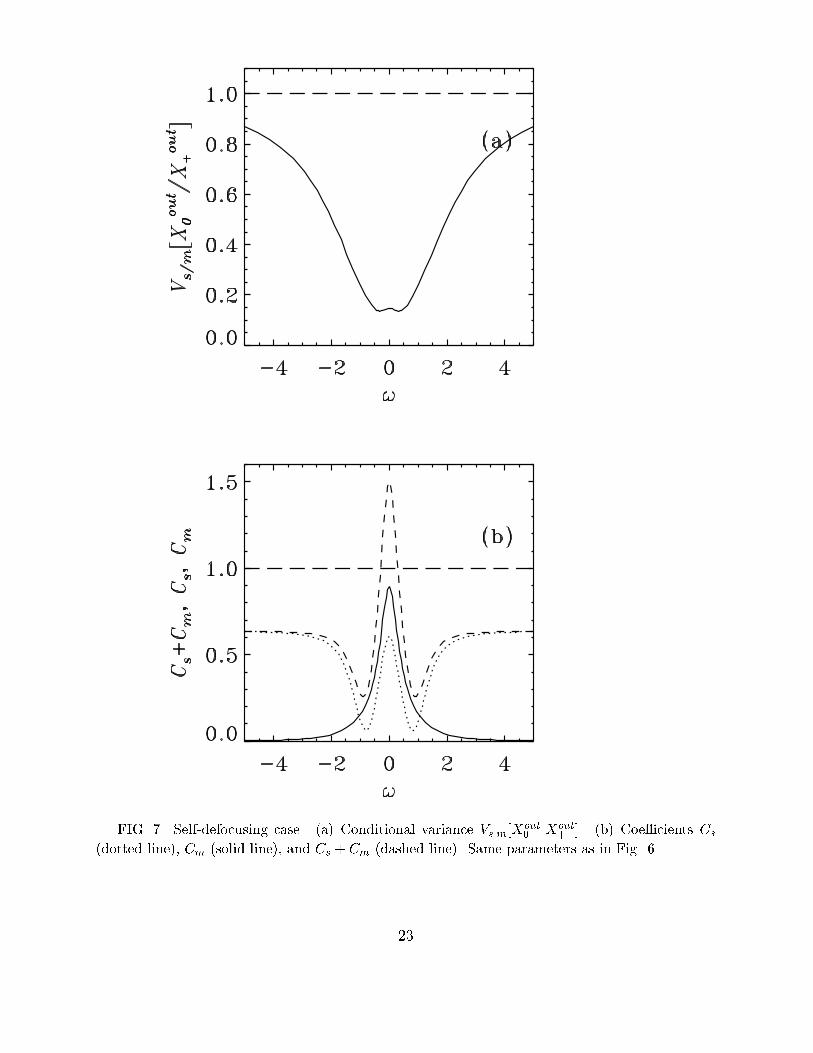
FIG. 7. Self-defocusing case. (a) Conditional variance Vsjm[Xout0 jXout+ ]. (b) Coe�cients Cs(dotted line), Cm (solid line), and Cs + Cm (dashed line). Same parameters as in Fig. 623

FIG. 8. Self-defocusing case. (a) Conditional variance Vsjm[Xout0 jXout+ ]. (b) Coe�cients Cs(dotted line), Cm (solid line), and Cs+Cm (dashed line). Same parameters as in �g. 6 except thenon-linear coe�cient �. Here we take � = 0:15.24