Spatial patterns of urbanization in Mysore: Emerging Tier II City

in Karnataka

Bharath H. Aithal2, Bharath Settur1, Sreekantha S3, Sanna Durgappa D2 and

Ramachandra TV1, 2, 3*

1Energy & Wetlands Research Group, Centre for Ecological Sciences, 2Centre for Sustainable Technologies (astra)

3 Centre for infrastructure, Sustainable Transportation and Urban Planning [CiSTUP] Indian Institute of Science, Bangalore, Karnataka, 560 012, India

*Corresponding Author: cestvr@ces.iisc.ernet.in

Abstract

Urban growth patterns are characteristic of spatial temporal changes that take place in specific and confined only to particular area. Urbanisation process is very prominent in more recently emerging cities, such as those in certain locations in India, where the structure of the traditional city is undergoing rapid changes. Mysore is one of the growing traditional regions of Karnataka, India. The spatial and temporal dynamic pattern of the urbanization process of the Semi-megalopolis region is studied. The objective of this work is to analyse spatial and temporal dynamics of the urban growth during the last five decades. The study indicates the coalescence of urban areas occurred in the core area (surrounding the CBD- Central business district), during the rapid urban growth from 2000 to 2009 and there was a moderate growth during 1980’s and 1990’s.

Keywords: Urban growth, tier-II cities, urban sprawl, regional planning

1. Introduction

Patterns and processes of globalization are influencing factors for contemporary land use trends and unknown challenges for sustaining land use systems (Currit and Easterling, 2009) for newly emerging cities. Analysing these landscape patterns and dynamics becomes one of the main goals of landscape, geographical and ecology studies. Landscape dynamics involving large scale deforestation play an important role in the global climate (Wood and Handley, 2001; Firmino, 1999), earth dynamics (Vitousek, 1994), etc. The spatial patterns of their transformation through time are undoubtedly related to changes in land uses (Potter and Lobley, 1996).

Landscape changes are often influenced by regional policies (Calvo-Iglesias et al., 2008). The main driving factors for global environmental changes are been identified as agriculture intensification (Green, 1990; Harms et al., 1984) or urbanisation (Phipps et al., 1986) in the context of local policies (Lipsky, 1992; Meeus, 1993; Kubes, 1994). Also, socio-economic policies determine the types of land use within a given region; they in turn affect environmental issues (Mander and Palang, 1994; Melluma, 1994). In order to address the challenges of urbanization without compromising the environment quality and their sustenance, land use planning with appropriate spatial data are crucial, especially in the regions undergoing severe environmental and demographic strains (Food and Agriculture Organization, 1995). Urbanization involves changes in vast expanse of land cover with the progressive concentration of human population. Rapidly urbanising landscapes will invariably have high population density with the poor infrastructure and basic amenities. The urban population in India is growing at about 2.3% per annum with the global urban population increasing from 13% (220 million in 1900) to 49% (3.2 billion, in 2005) and is projected to escalate to 60% (4.9 billion) by 2030 (Ramachandra and Kumar, 2008; Urbanization Prospects, 2005). Population of Mysore is 0.789 million as per census 2001 which was 0.653 million as per census 1991. The increase in urban population in response to the growth in urban areas is mainly due to migration consequent to setting up IT industries (2000) apart from service industries in 1990’s. There are 48 urban cities (Tier I) having a population of more than one million in India (in 2011). Tier 1 cities have reached the saturation level of providing basic amenities and are affected with over population, necessitating the impetus for the industrial and commercial activities in Tier 2 cities. These cities offer humongous potential as they already possess the basic amenities required or have capability of providing the provision of infrastructure with appropriate developmental planning. This entails provision of basic infrastructure like roads, air and rail connectivity apart from adequate social infrastructure such as educational institutions, health facilities. Unplanned growth over next few decades, will often lead to a phenomena of urban sprawl.

Urban sprawl is characterised by a sharp imbalance between urban spatial expansion and the underlying population growth (Bruekner, 2001). Sprawl of human settlements, both around existing cities and within rural areas, is a major driving force of land use and land cover changes in developing countries (Batisani & Yarnal, 2009; Gonzalez-Abraham et al., 2007). Sprawl is a process entails the growth of the urban area from the urban center towards the pheriphery of the city municipal jurisdiction. These small pockets in the outskirts will be lacking in basic amenities like supply of treated water, electricity, sanitation facilities.  Sprawl is associated with high negative impacts and especially the increasing dependency for basic amenities (Torrens & Alberti, 2000), the need for more infrastructure (Bruekner, 2001), the loss of agricultural and natural land, higher energy consumption, the degradation of peri urban ecosystems etc., (Johnson, 2001; Li et al., 2006; Lagarias, 2011). Understanding the spatio-

temporal patterns of the growth is essential for better administration to handle the population growth and helps to provide basic amenities and more importantly the sustainable management of local natural resources through regional planning.

The basic information about the current and historical land cover/land use plays a major role for urban planning and management (Zhang et al., 2002). Mapping landscapes on temporal scale provide an opportunity to monitor the changes, which is important for natural resource management and sustainable planning activities. In this context, “Density Gradient” with the time series spatial data analysis is potentially useful in measuring urban development (Torrens and alberti, 2000). This article presents the temporal land use analysis and adopts the density gradient approach to evaluate and monitor landscape dynamics and the landscape pattern.

Objective

According to the City Development Plan (CDP) of Mysore, which is a 20-year vision document for Mysore, the expansion is significant and there is a 70 per cent increase in the total area of the city since 2001 that would lead to higher degree of urban sprawl. The objectives of this study are to understand and interpret the evolving Landscape dynamics which involves:

(i) Temporal analysis of Land cover pattern of Mysore city: (ii) Understanding the spatial patterns of the landscape through temporal land use and using

Shannon entropy.

Study Area The present communication deals with the Mysore city (Figure 1), which is one of the tier II cities in Karnataka, India. Mysore being the cultural capital of India is also a hub of industrial activities and is also called the 2nd capital of Karnataka. This city is one of the most preferred destinations for industries including IT hubs other than Bangalore due to salubrious climate and availability of natural resources (water, etc.). It is a main trading centre of silk and sandalwood. Mysore district is bounded by Mandya to the northeast, Chamrajnagar to the southeast, Kerala state to the south, Kodagu to the west, and Hassan to the north. It has an area of 6,268 km² and a population of 2,651,027 (2001 census). The district lies in the southern Deccan plateau, within the watershed region of Kaveri River, which flows through the northern and eastern parts of the district. To understand the potential urbansiataion (or current sprawl), a 3 km buffer surrounding the city has also been considered for the analysis.

Figure 1. Study Area: Mysore city and 3 km buffer

Materials used

Remote sensing data Year Purpose

Landsat Series Multispectral sensor(57.5m)

1973 Land cover and Land use analysis

Landsat Series Thematic mapper (28.5m) and Enhanced Thematic Mapper sensors

1989, 1999,

land cover and Land use analysis

IRS p6: Liss-4 MX data (5.6m) 2009 land cover and Land use analysis (Last two circles data missing)

Survey of India (SOI) toposheets of 1:50000 and 1:250000 scales

To Generate boundary and Base layer maps.

Field visit data –captured using GPS For geo-correcting and generating validation dataset

Table 1. Materials used in Analysis

Method

Figure 2. Procedure followed to understand the spatial pattern of landscape change

A two-step approach as outlined in Figure 2, has been adopted to chart the direction of the City’s development. This includes a normative approach to understand the land use and the pattern of growth during the past 4 decades, complemented by a gradient approach of 1km radius.

Preprocessing: Table 1 lists the data used for the analysis. These data were geo-referenced, rectified and cropped pertaining to the study area. The Landsat satellite 1973 images have a spatial resolution of 57.5 m x 57.5 m (nominal resolution) were resampled to 28.5m comparable to the 1989 - 1999 data which are 28.5 m x 28.5 m (nominal resolution). IRS P6 image was obtained from NRSC, Hyderabad and has a spatial resolution of 5.6m.

Land cover Analysis: To understand the changes in the vegetation cover Normalised Difference Vegetation index (NDVI) was computed for all images. Its value ranges from values -1 to +1. Very low values of NDVI (-0.1 and below) correspond to soil or barren areas of rock, sand, or urban builtup. Zero indicates the water cover. Moderate values represent low density vegetation (0.1 to 0.3), while high values indicate thick canopy vegetation (0.6 to 0.8).

Land use analysis: The geometricaly corrected and processed data is classified using supervised classification method by the aid of Maximum likelihood algorithm. The image was classified using signatures from training sites that include all the land use types detailed in Table 2. Signatures collected from the field using GPS (Global Positioning System) represented all four classes covering all terrains in the city. Then the signatures were digitized as polygons of the signatures with the help of Google earth and Bhuvan. Then these polygons were overlaid on the data to provide better accuracy in digitizing. This involves generation of false color composite of remote sensing data (bands – green, red and NIR), this helps us in visualising the heterogeneous patches in the landscape and then overlaying it. Maximum Likelihood classifier is then used to classify the data using these signatures generated. This method has already been proved as a superior method as it uses various classification decisions using probability and cost functions (Duda et al., 2000). Mean and covariance matrix are computed using estimate of maximum likelihood estimator. Land Use was computed using the temporal data through a free and open source program GRASS - Geographic Resource Analysis Support System (http://wgbis.ces.iisc.ernet.in/grass/welcome.html).70% of the total generated signatures were used in classification, 30% signatures were used in validation and accuracy assessment. Classes of the resulting image were reclassed and recoded to form four land-use classes.

Accuracy assessment methods evaluate the performance of classifiers (Song et al., 2001; Gao and Liu, 2008). This is done either through testing the statistical significance of a difference, comparison of kappa coefficients (Congalton et al., 1983, Redmond and Heneghan 2006, Liu et al., 2007) or proportion of correctly allocated classes (Gao & Liu, 2008). For the purpose of accuracy assessment, a confusion matrix was calculated. Accuracy assesment, Kappa coefficient, are common measurements used in various publications to demonstrate the effectiveness of the classifications (Congalton, 1983; Congalton, 1991; Lillesand & Kiefer, 2000).

Land use Class Land uses included in the class

Urban This category includes residential area, industrial area, and all paved surfaces and mixed pixels having built up area.

Water bodies Tanks, Lakes, Reservoirs.

Vegetation Forest, Cropland, nurseries.

Others Rocks, quarry pits, open ground at building sites, kaccha roads.

Table 2. Land use classification categories adopted

Density Gradient Analysis: In order to understand the pattern of growth in the city, the city has been divided into 4 zones based on directions (North, South, East and West). As most of the definitions of a city or its growth is defined in directions it was considered more appropriate to divide the regions in 4 zones based on direction. The classified image is then divided into four zones based on four directions based on the Central pixel (Central Business district). The zones are named as – Northwest (NW), Northeast (NE), Southwest (SW) and Southeast (SE) respectively (Figure 2). The growth of the urban areas was understood in each zone separately through the computation of urban density for different periods.

Division of the zones to concentric circles and computation of Shannon’s Entropy: Further each zone was divided into concentric circle of incrementing radius of 1 km (figure 2) from the center of the city would help in visualizing the changes at neighborhood level. This also helps in understanding the agents responsible for changes. This helps in identifying the causal factors and locations experiencing various levels of urbanization in response to the economic, social and political forces and visualizing the forms of urban sprawl. The built up density in each circle is monitored overtime using time series analysis.

Figure 2. Google earth representation of the study region

Computation of Shannon’s Entropy: To determine whether the growth of urban areas was compact or divergent the Shannon’s entropy (Yeh and Liu, 2001; Li and Yeh, 2004; Lata et al., 2001; Sudhira et al., 2004; Pathan et al., 2004) was computed for each zones. Shannon’s entropy (Hn) given in equation 1, gives us an insight into how to development in the city are happening (either the growth is clumped or is it distributed sparsely) and its connection with geographical variables among ‘n’ concentric circles across Zones.

…… (1)

Where Pi is the proportion of the built-up in the ith concentric circle. As per Shannon’s Entropy, if the distribution is maximally concentrated in one circle the lowest value zero will be obtained. Conversely, if it is an even distribution among the concentric circles will be given maximum of log n.

Results & Discussion

Land use Land Cover analysis: a. Vegetation cover of the study area analysed through NDVI (Figure 3), shows

that area under vegetation has declined to 9.24% from 51.09%.

Figure 3: Temporal Land cover changes during 1973 – 2009

Year

Vegetation Non vegetation % Ha % Ha

1973 51.09 10255.554 48.81 9583.83 1989 57.58 34921.69 42.42 8529.8 1999 44.65 8978.2 55.35 11129.77 2009 09.24 1857.92 90.76 19625.41

Table 3: Temporal Land cover details.

b. Land use analysis for the period 1973 to 2009 is computed using Gaussian maximum likelihood classifier is given in figure 4. Overall accuracy of the classification of was 75% (1973), 79% (1989), 78% (1999), and 84% (2009) respectively. There has been an enormous growth in built-up area during 1999 to 2009 it can be observed that there was 514% of growth from 1999 to 2010 whereas growth of built up was 1685 % in past four decades. Vegetation cover declined by 923% in past four decades. Other category also had an enormous increase and covers 166 % of the land use. The water category seems to increase which can be attributed to large scale waste water treatment STP’s (ex. Vidyaranyapura, Rayankere, Kesare) covering large area post 90’s. The temporal land use details are given in table 2. Kappa stats and overall accuracy was calculated and is as listed in Table 5.

Figure 4:.Classification output of Mysore

Land use ->

Urban

Vegetation

Water

Others Year

1973 222.93 10705.68 124.47 9054.99

1989 229.41 13242.51 78.75 6557.4

1999 730.8 8360.1 117.9 10899.2

2009 3757.489 1159.336 142.58 15050.5

Total (Land in ha) 20108.91

Table 4: Temporal land use details for Mysore

Year Kappa coefficient Overall accuracy (%)

1973 0.76 75.04

1989 0.72 79.52 1999 0.82 78.46

2009 0.86 84.58

Table 5: Kappa statistics and overall accuracy

Built up Density Gradient Analysis:

Built up density was minimal in the year 1973 and had a maximum value of 0.026 (considering 3km buffer) in the North east direction in the year 1973. The policy of the government to develop the tier 2 cities other than Bangalore during 1990 gave a boost to the urban area which periodically increased till 1999 which has a maximal value of 0.06 in NE direction. There was a sharp growth in the region in almost all direction from 1999 till 2009, maximum value reaching 0.216 in the NE direction (considering 3km buffer) and. This can be attributed to development of this region with the IT & BT industry which were till then were confined to locations in Bangalore.

Figure 7: Urban density analysis of Mysore (considering 3km buffer)

Calculation of Shannon’s Entropy: Shannon entropy was calculated for the all the years and is listed in Table 5. The value of entropy ranges from zero to log (n). Greater Bangalore grew in all the directions and has almost reached the threshold value of growth (log (n) = log (8) = 0.9). Higher the value or closer to log (n) indicates the sprawl or dispersed or sparse development. Lower the entropy values the development is either aggregated or compact. Lower entropy values of 0.007 (NW), 0.008 (SW) during 70’s shows an aggregated growth. However, the region grew phenomenally with dispersed growth in 90’s and reached higher values of entropy during post 2000’s and reached 0.352 (NE), 0.241 (NW) in 2009. These values may look comparatively lower as the buffer zone is taken into consideration where in the sprawl is rampant and other land use also exists in large hectares. When the Shannon entropy is calculated with just Mysore boundary it has a value of 0.582(NE) and 0.431(NW) indicating the occurrence of sprawl.

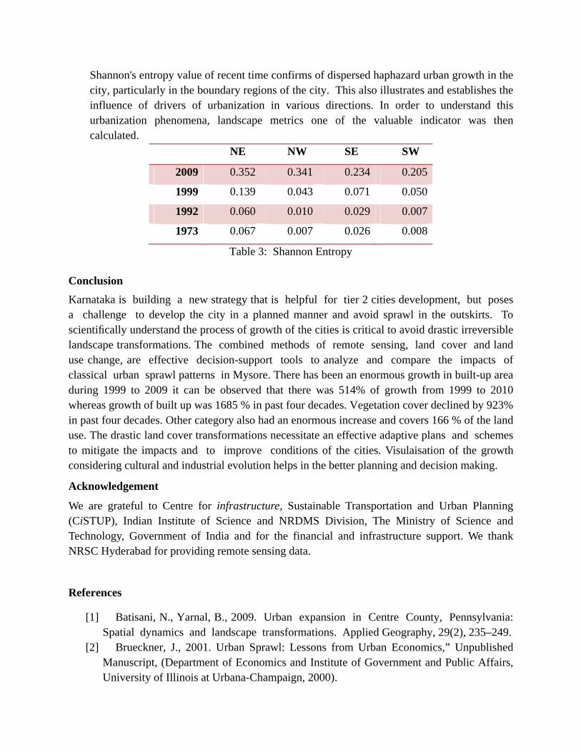
Shannon's entropy value of recent time confirms of dispersed haphazard urban growth in the city, particularly in the boundary regions of the city. This also illustrates and establishes the influence of drivers of urbanization in various directions. In order to understand this urbanization phenomena, landscape metrics one of the valuable indicator was then calculated. 

NE NW SE SW

2009 0.352 0.341 0.234 0.205

1999 0.139 0.043 0.071 0.050

1992 0.060 0.010 0.029 0.007

1973 0.067 0.007 0.026 0.008

Table 3: Shannon Entropy

Conclusion

Karnataka is building a new strategy that is helpful for tier 2 cities development, but poses a challenge to develop the city in a planned manner and avoid sprawl in the outskirts. To scientifically understand the process of growth of the cities is critical to avoid drastic irreversible landscape transformations. The combined methods of remote sensing, land cover and land use change, are effective decision-support tools to analyze and compare the impacts of classical urban sprawl patterns in Mysore. There has been an enormous growth in built-up area during 1999 to 2009 it can be observed that there was 514% of growth from 1999 to 2010 whereas growth of built up was 1685 % in past four decades. Vegetation cover declined by 923% in past four decades. Other category also had an enormous increase and covers 166 % of the land use. The drastic land cover transformations necessitate an effective adaptive plans and schemes to mitigate the impacts and to improve conditions of the cities. Visulaisation of the growth considering cultural and industrial evolution helps in the better planning and decision making.

Acknowledgement

We are grateful to Centre for infrastructure, Sustainable Transportation and Urban Planning (CiSTUP), Indian Institute of Science and NRDMS Division, The Ministry of Science and Technology, Government of India and for the financial and infrastructure support. We thank NRSC Hyderabad for providing remote sensing data.

References

[1] Batisani, N., Yarnal, B., 2009. Urban expansion in Centre County, Pennsylvania: Spatial dynamics and landscape transformations. Applied Geography, 29(2), 235–249.

[2] Brueckner, J., 2001. Urban Sprawl: Lessons from Urban Economics,” Unpublished Manuscript, (Department of Economics and Institute of Government and Public Affairs, University of Illinois at Urbana-Champaign, 2000).

[3] Calvo-Iglesias,M.S., Fra-Paleo,U.,Dias-Varela, R.A., 2008. Changes in farming system and population as drivers of land cover and landscape dynamics: the case of enclosed and semi openfield systems in Northern Galicia (Spain). Landscape & Urban Plan. 90, 168–177.

[4] Congalton, R. G., 1991. A review of assessing the accuracy of classifications of remotely sensed data. Remote Sensing of Environment, 37, 35-46.

[5] Congalton, R. G., Oderwald, R. G., & Mead, R. A., 1983. Assessing Landsat classification accuracy using discrete multivariate analysis statistical techniques. Photogrammetric Engineering and Remote Sensing, 49, 1671-1678.

[6] Currit, N., Easterling, W., 2009. Globalization and population drivers of rural-urban land-use change in Chihauhua, Mexico. Land Use Policy, 26, 535–544.

[7] Duda, R.O., Hart, P.E., Stork, D.G., 2000, Pattern Classification, A Wiley-Interscience Publication, Second Edition, ISBN 9814-12-602-0.

[8] Firmino A., 1999. Agriculture and landscape in Portugal. Landscape and Urban Planning 46, 83–91.

[9] Food and Agriculture Organization, 1995. Planning for Sustainable Use of Land Resources: Towards a New Approach. Land and Water Development Division, Rome.

[10] Gonzalez-Abraham, C. E., Radeloff, V. C., Hammer, R. B., Hawbaker, T. J., Stewart, S. I. & Clayton, M. K., 2007. Building patterns and landscape fragmentation in northern Wisconsin, USA. Landscape Ecology, 22, 217–230.

[11] Green, B.H. (1990). Agricultural intensification and the loss of habitat, species and anemity in British grasslands: a review of historical change and assessment of future prospects. Grass Forage Sci. 45, 365-372.

[12] Harms, W.B., Stottelder, A.H.F., Vos, W., 1984. Effects of intensification of agriculture on nature and landscape in the netherlands. Ekologia (CSSR) 3, 281-304.

[13] Johnson, M., 2001. Environmental impacts of urban sprawl: a survey of the liter-ature and proposed research agenda. Environment and Planning A, 33,717-735.

[14] Kubes, J., 1994. Bohemian agricultural landscape and villages, 1950 and 1990: Landuse, landcover and other characteristics. Ekologia (Bratislava) 13, 187-l98.

[15] Lagarias, A., 2011. Land use planning for sustainable development in periurban ecosystems: the case of Lake Koroneia in Thessaloniki, Greece. In Proceedings of the 2nd international exergy, life cycle assessment and sustainability workshop & symposium, ELCAS 2, Nisyros, Greece.

[16] Lata, K.M., Rao, C.H.S., Prasad, V.K., Badarianth, K.V.S., Raghavasamy, V., 2001. Measuring Urban sprawl' A case study of Hyderabad, gis@development, 5(12), 26-29.

[17] Li, Y., Zhao, S., Zhao, K., Xie, P., & Fang, J., 2006. Land-cover changes in an urban lake watershed in a mega-city, central China. Environmental Monitoring and Assess-ment, 115, 349 e 359.

[18] Liu, C., Frazier, P., Kumar, L., 2007. Comparative assessment of the measures of thematic classification accuracy. Remote Sensing of Environment, 107, 606-616.

[19] Lillesand, T. M., & Kiefer, R. W., 2005. Remote sensing and image interpretation .New York: John Wiley & Sons.

[20] Lipsky, Z. 1992. Landscape structure changes in the Czech rural landscape. In: Cultural aspects of landscape. 2nd Int. Con., 1992. IALE, pp. 80-86.

[21] Mander, U., Palang, H., 1994. Change on landscape structure in Estonia during the Soviet period. GeoJournal 33:55–62.

[22] Meeus, J.H.A., 1993. The transformation of agricultural landscapes in Western Europe. The Science of the Total Environment 129. 171-190.

[23] Melluma, A., 1994. Metamorphoses of Latvian landscapes during fifty years of Soviet rule. GeoJournal 33, 55–62

[24] Pathan, S.K., Patel, J G., Bhanderi. R.J., Ajai, Kulshrestha, Goyal, V.P., Banarjee. D.L., Marthe, S., Nagar, V.K., Katare, V., 2004. Urban planning with specific rel;erence to master plan of lndore city using RS and GIS techniques. Proc. of GSDI-7 International Conference on Spatial Data Infrastructure tbr Sustainable Development, held at Bangalore from Feb, 2-6, 2004.

[25] Phipps, M., Baudry, J., Burel, F., 1986. Dynamique de I’organisation ecologique d’un paysage rural: Modalites de la desorganisation dans une zone peri-urbaine. C.R. Acad. SC. Paris. 303. 263-268.

[26] Potter, C., Lobley, M., 1996. Unbroken threads? Succession and its effects on family farms in Britain. Sociologia Ruralis 36, 286–306.

[27] Ramachandra T. V., Kumar, U., 2008. Wetlands of Greater Bangalore, India: Automatic Delineation through Pattern Classifiers. Electronic Green Journal, Issue 26, Spring 2008 ISSN: 1076-7975.

[28] Redmond S. J., Heneghan C., 2006 Cardiorespiratory-based sleep staging in subjects with obstructive sleep apnea IEEE Trans. Biomed. Eng. 53, 485–96.

[29] Seto, K.C., Fragkias, M., 2005. Quantifying spatiotemporal patterns of urban land-use change in four cities of China with time series landscape metrics. Landsc. Ecol. 20, 871–888.

[30] Sudhira, H.S., Ramachandra, T.V., and Jagadish, K.S., 2004. Urban sprawl: metrics, dynamics and modelling using G1S. Int. J Applied Earth Observation and Geoinformation, 5, 29-39.

[31] Torrens, P., & Alberti, M. (2000). Measuring sprawl. CASA working paper series 27. UCL. http://www.casa.ucl.ac.uk/publications/workingpapers.asp Last accessed 24.12.11.

[32] Vitousek, P. M. 1994. Beyond global warming:ecology and global change. Ecology 75, 1861-1876.

[33] Wood, R. and Handley, J., 2001. Landscape dynamics and the management of change. Landscape Research, 26 (1), 45-54.

[34] http://censusindia.gov.in/2011census/censusinfodashboard/index.html [35] Zhang, Q., Wang, J., Peng, X., Gang, R., Shi, P., 2002. Urban built-up land change

detection with road density and spectral information from multi- temporal Landsat TM data. Int. J. Remote Sensing, 23(15), 3057-3078.