Spatial competition between shopping centers

Spatial competition Spatial competition Spatial competition Spatial competition Spatial competition Spatial competition Spatial competition Spatial competition between shopping between shopping between shopping between shopping between shopping between shopping between shopping between shopping

centerscenterscenterscenterscenterscenterscenterscenters

FEP WORKING PAPERSFEP WORKING PAPERSFEP WORKING PAPERSFEP WORKING PAPERSFEP WORKING PAPERSFEP WORKING PAPERSFEP WORKING PAPERSFEP WORKING PAPERSResearch Research Research Research Work in Work in Work in Work in ProgressProgressProgressProgressFEP WORKING PAPERSFEP WORKING PAPERSFEP WORKING PAPERSFEP WORKING PAPERSFEP WORKING PAPERSFEP WORKING PAPERSFEP WORKING PAPERSFEP WORKING PAPERS

n. n. n. n. 394, 394, 394, 394, Dec. 2010Dec. 2010Dec. 2010Dec. 2010

centerscenterscenterscenterscenterscenterscenterscenters

António Brandão António Brandão António Brandão António Brandão 1 21 21 21 2

João CorreiaJoão CorreiaJoão CorreiaJoão Correia----dadadada----Silva Silva Silva Silva 1 21 21 21 2

Joana Pinho Joana Pinho Joana Pinho Joana Pinho 1111

1111 Faculdade de Economia, Universidade do PortoFaculdade de Economia, Universidade do PortoFaculdade de Economia, Universidade do PortoFaculdade de Economia, Universidade do Porto2222 CEF.UPCEF.UPCEF.UPCEF.UP

Spatial competition between shopping centers?

Antonio Brandao

CEF.UP and Faculdade de Economia. Universidade do Porto.

Joao Correia-da-Silva

CEF.UP and Faculdade de Economia. Universidade do Porto.

Joana Pinho

Faculdade de Economia. Universidade do Porto.

November 23rd, 2010.

Abstract. We study competition between two shopping centers (department stores or

shopping malls) located at the extremes of a linear city. In contrast with the existing

literature, we do not restrict consumers to make all their purchases at a single place.

We obtain this condition as an equilibrium result. In the case of competition between a

shopping mall and a department store, we find that the shops at the mall, taken together,

obtain a lower profit than the department store. However, the shops at the mall have no

incentives to merge into a department store (both sides would lose). It is the department

store that has incentives to separate itself into a shopping mall (both sides win).

Keywords: Retail organization, Multi-product firms, Horizontal differentiation, Hotelling

model.

JEL Classification Numbers: D43, L13.

? Joao Correia-da-Silva ([email protected]) acknowledges support from CEF.UP and research grant from

Fundacao para a Ciencia e Tecnologia and FEDER (PTDC/EGE-ECO/108331/2008). Joana Pinho

([email protected]) acknowledges support from Fundacao para a Ciencia e Tecnologia (Ph.D. scholarship).

The autors would also like to thank the participants in the workhop “Perspectivas da Investigacao em

Portugal - Economia Industrial” for their comments.

1

1 Introduction

Shopping centers have existed for many centuries as galleries, market squares, bazaars or

seaport districts. The oldest indoor space where consumers can buy a huge variety of goods

is the Al-Hamidiyah Souq, in Damascus (Syria), and dates back to the seventh century.

One of the reasons why shopping centers are so attractive is because they allow con-

sumers to buy many different kinds of goods without spending much time and money

commuting between shops. Therefore, to study competition between shopping centers, one

should take into account the demand for many different goods and also the commuting

costs of traveling to one or more shopping centers. The existing spatial competition mod-

els fail to do so, because they either restrict the analysis to markets with a single good

or assume that consumers make all their purchases at the same place (Bliss, 1988; Beggs,

1994; Smith and Hay, 2005; Innes, 2006). This “one stop shopping” assumption is very

convenient because it allows treating multiple goods as a single bundled good.

We provide a study of competition between shopping centers by extending the standard

model of spatial competition (Hotelling, 1929; d’Aspremont, Gabszewicz and Thisse, 1979)

to the case of multiple goods without using the “one stop shopping” assumption. This

extension is straightforward in concept but technically difficult. We consider the existence

of two shopping centers located at the extremes of a linear city, selling the same set of

goods. In the model, a shopping center may be either a shopping mall (where each good

is sold by an independent firm) or a department store (where a single firm sells all the

goods). Consumers are uniformly spread across the linear city and buy exactly one unit of

each good. They may travel to a shopping center and buy all the goods there or travel to

both shopping centers and buy each good where it is cheaper.1

We solve for the equilibrium prices, market shares and profits in three scenarios of

retail organization: (i) competition between a department store and a shopping mall; (ii)

competition between two department stores; (iii) competition between two shopping malls.

Our first result is that, regardless of the scenario that is considered, no consumer travels

to both extremes of the city. “One stop shopping” is obtained as a result. The equilibrium

price differences across shopping centers are not sufficient to make it worthwhile for a

1Consumers are assumed to be fully informed about the prices charged in each extreme of the city.

2

consumer to travel to both extremes of the city.2

In the case of competition between a department store and a shopping mall, we find that

the department store sets lower prices and captures a greater demand than the shops at the

mall. To understand why this occurs, observe that unrelated goods become complements

when they are sold at the same location (and substitutes when they are sold at different

extremes of the city). When a shop at the mall considers the possibility of decreasing its

price, it only cares about the increase of its own demand and not about the increase of the

demand of the other shops at the mall. In contrast, the department store internalizes this

effect, and takes into account the fact that decreasing the price of one good also increases

the demand for the other goods that are sold there.3 Despite charging lower prices, the

department store obtains a higher profit than the shops at the mall taken together because

it captures a sufficiently greater market share.

When competition is between two department stores, the equilibrium prices are lower.

The price that each department store charges for the bundle of goods is actually equal

to the price charged in the single-good model (independently of the number of goods).

The two department stores obviously capture equal shares of the market and obtain equal

profits. These are, unsurprisingly, lower than the profits obtained when competing against

a shopping mall (because a department store competes more aggressively).

Finally, in the scenario of competition between two shopping malls, we arrive at the

same equilibrium price (for each good) as in the single-good model. The shops behave as

if consumers only bought one good. This is the scenario in which prices are higher. The

explanation is the same as before: the shops at the mall set higher prices because they do

not internalize the positive effect of a price decrease on the other shops at the same mall.

After finding the equilibrium in each of the three competitive scenarios, it is straight-

forward to analyze whether it is more profitable to have a department store offering many

2Even ruling out bundling strategies (we assume that the price of a bundle of goods is equal to the sumof the price of the individual goods), we find that the consumers that travel to a department store buy allthe goods there. Therefore, allowing the department store to charge for the bundle a price that is lowerthan the sum of the prices of the individual goods would make no difference. For a careful analysis of thebundle pricing problem, see, for example, Hanson and Martin (1990).

3The asymmetry between the department store and the shopping mall becomes more pronounced asthe number of goods increases. We find that when the number of goods tends to infinity, the market shareof the department store converges to 100%.

3

products or several independent shops at a mall. To find out which retail organization is

expected to appear endogenously, we solve for the equilibrium of the corresponding merger

game. Mergers are typically carried out to increase market power or to obtain cost savings.

The integration of independent shops at a mall could be seen as a conglomerate merger,

since the products involved have neither horizontal nor vertical relationships. However, we

must not forget that the products sold in the same shopping center are complements. Thus,

the merger of shops at the same mall is a merger between firms that sell complementary

goods.4

In our merger game, it is a dominant strategy to be organized as a shopping mall rather

than as a department store. Both sides win whenever a department store separates into

several independent shops. Therefore, the retail organization that is expected to appear in

equilibrium is that of competition between two shopping malls. This result is not surprising

because the greater is the number of department stores, the more competitive is the retail

industry. As we have explained above, a department store has stronger incentives to

charge lower prices than the independent shops at a mall. If the prices of the rival retailers

remained the same, behaving as a department store would be profitable. However, it

induces the rivals to lower their prices as well. This competitive effect dominates, leading

to lower prices and profits for everyone. It is better to be organized as a shopping mall

because, as explained by Innes (2006): “a multi-product retailer can effectively pre-commit

to higher prices by organizing itself as a mall of independent outlets”.

The first result of this kind was presented by Edgeworth (1925), who found that it is

better, for consumers, to have a single monopolist selling two complementary goods than

to have two separate monopolists. More recently, Salant, Switzer and Reynolds (1983) also

came up with a similar result, but in a model of Cournot competition. Using a framework

that is closer to ours, Bertrand competition with linear demand, Beggs (1994) concluded

that separating into several shops at a mall may be desirable or not. Depending on whether

the degree of substitutability between the goods sold at the competing shopping centers

is low or high, either two department stores or two shopping malls emerge as equilibria

of the merger game. Innes (2006) studied the effect of entry and concluded that only

department stores survive in equilibrium because they compete more aggressively and,

4There is a vast literature dealing with mergers of firms selling complementary goods. See, for example,Matutes and Regibeau (1992), Economides and Salop (1992) or Bart (2008).

4

therefore, are more effective in deterring entry. Shopping malls would be driven out of

the market by department stores because when there is competition between department

stores and shopping malls, the former have higher profits.

We also compare the consumers’ surplus and the total surplus in the different scenarios

of retail organization. Since all the consumers are assumed to buy exactly one unit of

each good, a change in prices simply transfers surplus between consumers and producers.

Therefore, total surplus is maximized when consumers shop at the closest shopping center

(transportation costs are minimized). This occurs when there are either two department

stores or two shopping malls. Unsurprinsingly, the consumers’ surplus is the highest in the

case of competition between two department stores. The equilibrium of the merger game

(two shopping malls) is actually the worst scenario for consumers. In spite of having to

support higher transportation costs, consumers are better off when there is a department

store and a shopping mall than when there are two shopping malls.

Our model is pioneer in extending the spatial competition model (Hotelling, 1929;

d’Aspremont, Gabszewicz and Thisse, 1979) to analyze multi-product competition be-

tween department stores and shopping malls. To the best of our knowledge, only Lal and

Matutes (1989) have presented a multi-product version of the model of Hotelling (1929).5

They restricted the analysis to the case of competition between two department stores that

sell two goods. We have greatly generalized their analysis by allowing a finite number of

goods and an alternative mode of retail: the shopping mall.6

Other authors have analyzed multi-product price competition, but no one used the

spatial competition model to do so. Moreover, most of them based the analysis on the

assumption that consumers make all their purchases at the same shopping center (Bliss,

1988; Beggs, 1994; Smith and Hay, 2005; Innes, 2006). They support this “one stop

shopping” assumption on the fact that shopping implies time and transportation costs.

They argue that, in order to save costs, customers make all their purchases at the same

5There are other extensions of the spatial competition model that allow for multi-product firms, butin which consumers only buy one of the goods that are available (Laussel, 2006; Giraud-Heraud, Ham-moudi and Mokrane, 2003). Goods available in a shopping center are, in this case, substitutes instead ofcomplements. These models correspond to completely different economic settings.

6In the model of Lal and Matutes (1989), there are two types of consumers: the poor and the rich. Thepoor do not support transportation costs, therefore, they buy each good where it is cheaper (“one stopshopping” is not assumed). The rich, on the other hand, support transportation costs and, in equilibrium,are not interested in shopping around. Their focus is to study price discrimination across the two segments.

5

place. In our opinion, even with the support of empirical works as the one of Rhee and Bell

(2002), who have found that consumers make 94% of their weekly groceries expenditures at

the same supermarket, the assumption that consumers necessarily make all their purchases

at the same store is too strong. We have relaxed this hypothesis, allowing consumers to

shop in more than one place. In the end, we have validated the “one stop shopping”

hypothesis, but as a result.

The paper that is closest to ours is perhaps that of Beggs (1994), who studied a sim-

ilar merger game in a model in which firms face a linear demand function. He restricted

the analysis to the case of two goods and, as mentioned before, assumed that consumers

purchase both goods at the same location (“one stop shopping” assumption). Smith and

Hay (2005) have also studied price competition under alternative modes of retail organiza-

tion (shopping streets, shopping malls and department stores), but they did not consider

competition between the different modes.

The remainder of the article is organized as follows. In Section 2, we setup the model,

introduce notation and obtain the demand and the profit functions. In Section 3, we present

the possible competitive scenarios and find the equilibrium prices in each one. Section 4

is dedicated to a welfare analysis. We study the merger game in Section 5. Section 6

concludes the article with some remarks. The proofs of all propositions are collected in the

Appendix.

2 The model

2.1 Basic setup

We consider a multi-product version of the model of Hotelling (1929). There is a continuum

of consumers uniformly distributed across a linear city, [0, 1]. Each consumer buys one unit

of each of the products, i ∈ {1, ..., n} = I, which are sold at the extremes of the city (x = 0

and x = 1). The price of good i at the left extreme (L) is denoted by piL and the price of

good i at the right extreme (R) is denoted by piR.

The reservation price for each product, Vi, is assumed to be high enough for the market to

6

be fully covered. Thus, the demand is perfectly inelastic and the only decision of consumers

is where to buy each product. Each consumer chooses among three possibilities:

(L) to buy all the goods at x = 0;

(R) to buy all the goods at x = 1;

(LR) to travel to both extremes and buy each good where it is cheaper.

We denote by PL and by PR the price that a consumer pays for all the goods at x = 0

and at x = 1, respectively (PL =∑n

i=1 piL and PR =∑n

i=1 piR). By PLR, we denote the

price that a consumer pays for all the goods if she buys each good where it is cheaper

(PLR =∑n

i=1 min{piL, piR}).

To make their decision, consumers take into account not only the prices charged for the

products, but also the transportation costs that they must support to acquire them. We

assume that the transportation costs are linear in distance. Let uL(x), uR(x) and uLR(x)

denote the utility attained by an agent located at x ∈ [0, 1] who chooses to purchase,

respectively: (L) all the goods at x = 0; (R) all the goods at x = 1; (LR) each good where

it is cheaper. Then:

uL(x) =∑n

i=1 Vi − PL − tx,

uR(x) =∑n

i=1 Vi − PR − t(1− x),

uLR(x) =∑n

i=1 Vi − PLR − t.

It is fundamental to keep in mind that if a consumer travels to both extremes, she supports

higher transportation costs than if she had chosen to purchase both goods at the same

location. For this reason, the demand for each product at a certain location is related to

the demand for any other product at any location. Products sold at the same location are

complementary goods, while products sold at different locations are substitutes.

2.2 Demand and profit functions

The consumers that are most likely to purchase a good that is sold at one of the extremes

are those that are located closer to that extreme. When all the goods have strictly positive

demand at both locations, the consumers near the left extreme are surely buying all the

goods at x = 0 (their choice is L), while those near the right extreme are surely buying all

the goods at x = 1 (their choice is R).

7

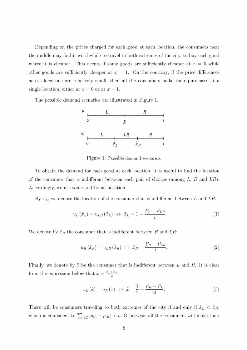
Depending on the prices charged for each good at each location, the consumers near

the middle may find it worthwhile to travel to both extremes of the city, to buy each good

where it is cheaper. This occurs if some goods are sufficiently cheaper at x = 0 while

other goods are sufficiently cheaper at x = 1. On the contrary, if the price differences

across locations are relatively small, then all the consumers make their purchases at a

single location, either at x = 0 or at x = 1.

The possible demand scenarios are illustrated in Figure 1.

Figure 1: Possible demand scenarios.

To obtain the demand for each good at each location, it is useful to find the location

of the consumer that is indifferent between each pair of choices (among L, R and LR).

Accordingly, we use some additional notation.

By xL, we denote the location of the consumer that is indifferent between L and LR:

uL (xL) = uLR (xL) ⇔ xL = 1− PL − PLR

t. (1)

We denote by xR the consumer that is indifferent between R and LR:

uR (xR) = uLR (xR) ⇔ xR =PR − PLR

t. (2)

Finally, we denote by x be the consumer that is indifferent between L and R. It is clear

from the expression below that x = xL+xR

2:

uL (x) = uR (x) ⇔ x =1

2+

PR − PL

2t. (3)

There will be consumers traveling to both extremes of the city if and only if xL < xR,

which is equivalent to∑

i∈I |piL − piR| > t. Otherwise, all the consumers will make their

8

purchases at a single place. It is easy to verify that∑

i∈I |piL − piR| ≤ t implies that

0 ≤ x ≤ 1. Therefore, in this case, the demand for any good sold at L is x and the demand

for any good sold at R is 1− x.

It is convenient to denote the vector of prices of all the goods at both locations by

p ∈ IR2n+ and to consider the following sets:

S1 ={p ∈ IR2n

+ :∑

i∈I |piL − piR| ≤ t}

;

S2 ={p ∈ IR2n

+ :∑

i∈I |piL − piR| > t}.

If there are consumers that travel to both extremes, the demand for a good depends on

whether this good is cheaper at L or at R. Denoting by IL and IR the sets of goods

that are strictly cheaper at L and R, respectively, we can write the expressions for the

indifferent consumers as follows:

xL = 1− 1

t

∑i∈IR

(piL − piR) (4)

and

xR =1

t

∑i∈IL

(piR − piL) . (5)

The demand for a good i ∈ IL at L is min {xR, 1}, while its demand at R is max {0, 1− xR}.If i ∈ IR, its demand at L is max {0, xL} and its demand at R is min {1− xL, 1}. In case

of a tie (piL = piR), each consumer that travels to both extremes may either buy good i

at L or at R. Any tie-breaking assumption leads to the same results. We can assume, for

example, that half of the consumers buys good i at L and the other half buys it at R.

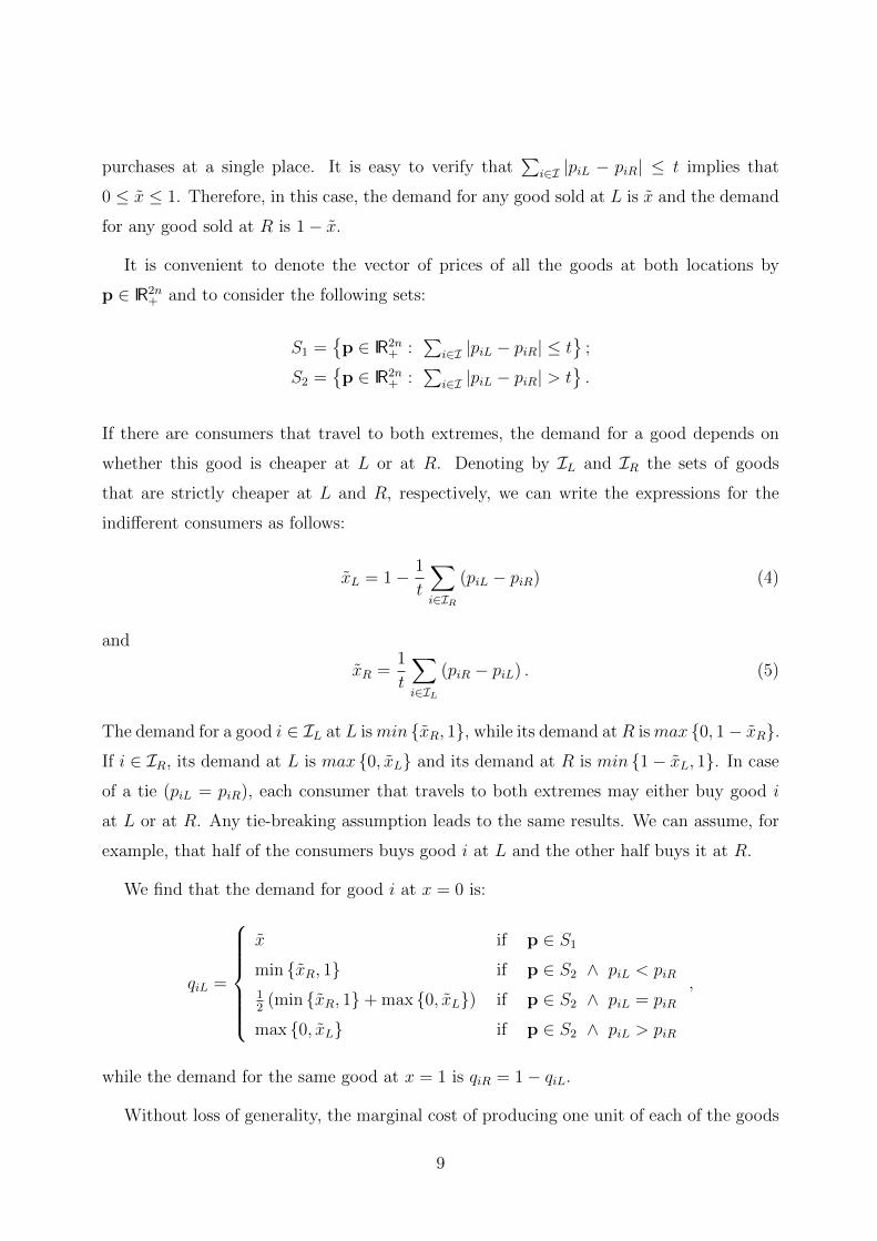
We find that the demand for good i at x = 0 is:

qiL =

x if p ∈ S1

min {xR, 1} if p ∈ S2 ∧ piL < piR12

(min {xR, 1}+ max {0, xL}) if p ∈ S2 ∧ piL = piR

max {0, xL} if p ∈ S2 ∧ piL > piR

,

while the demand for the same good at x = 1 is qiR = 1− qiL.

Without loss of generality, the marginal cost of producing one unit of each of the goods

9

is assumed to be zero. Under this assumption, the profits coincide with the sales revenues.

This simplification does not affect the any of the results in the paper.7

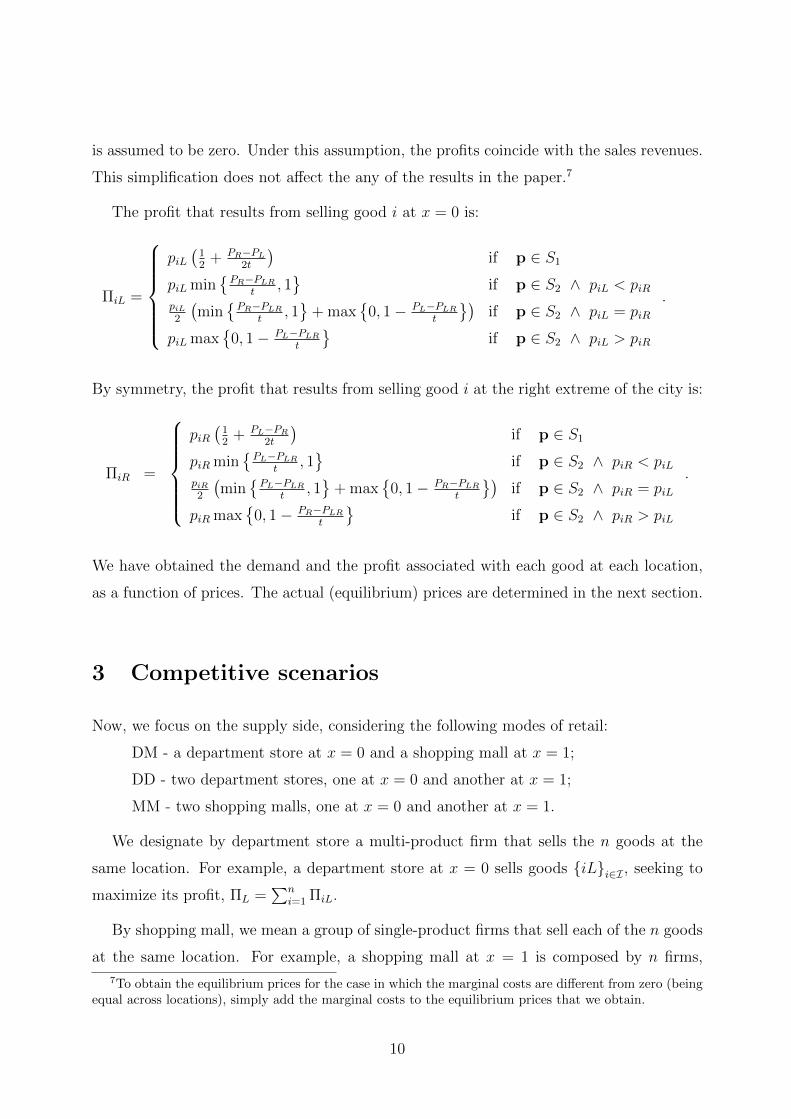
The profit that results from selling good i at x = 0 is:

ΠiL =

piL(

12

+ PR−PL

2t

)if p ∈ S1

piL min{

PR−PLR

t, 1}

if p ∈ S2 ∧ piL < piRpiL2

(min

{PR−PLR

t, 1}

+ max{

0, 1− PL−PLR

t

})if p ∈ S2 ∧ piL = piR

piL max{

0, 1− PL−PLR

t

}if p ∈ S2 ∧ piL > piR

.

By symmetry, the profit that results from selling good i at the right extreme of the city is:

ΠiR =

piR(

12

+ PL−PR

2t

)if p ∈ S1

piR min{

PL−PLR

t, 1}

if p ∈ S2 ∧ piR < piLpiR2

(min

{PL−PLR

t, 1}

+ max{

0, 1− PR−PLR

t

})if p ∈ S2 ∧ piR = piL

piR max{

0, 1− PR−PLR

t

}if p ∈ S2 ∧ piR > piL

.

We have obtained the demand and the profit associated with each good at each location,

as a function of prices. The actual (equilibrium) prices are determined in the next section.

3 Competitive scenarios

Now, we focus on the supply side, considering the following modes of retail:

DM - a department store at x = 0 and a shopping mall at x = 1;

DD - two department stores, one at x = 0 and another at x = 1;

MM - two shopping malls, one at x = 0 and another at x = 1.

We designate by department store a multi-product firm that sells the n goods at the

same location. For example, a department store at x = 0 sells goods {iL}i∈I , seeking to

maximize its profit, ΠL =∑n

i=1 ΠiL.

By shopping mall, we mean a group of single-product firms that sell each of the n goods

at the same location. For example, a shopping mall at x = 1 is composed by n firms,

7To obtain the equilibrium prices for the case in which the marginal costs are different from zero (beingequal across locations), simply add the marginal costs to the equilibrium prices that we obtain.

10

with each firm selling one good, iR, with the objective of maximizing its individual profit,

ΠiR. We exclude the possibility of concerted behavior between shops at a mall. Each shop

chooses how much to charge for the product it sells, taking the remaining prices as given.

3.1 Competition between a department store and a shopping

mall

We start by considering the case in which there is a department store located at x = 0 and

a shopping mall located at x = 1. The department store chooses the prices of the n goods

with the objective of maximizing its total profit (∑n

i=1 ΠiL), while each of the shops at the

mall seeks to maximize its individual profit (ΠiR).

The profit of the department store is given by:8

ΠL =

PL

(12

+ PR−PL

2t

), p ∈ S1

xL

∑i∈IR piL + xR

∑i∈IL piL, p ∈ S2 ∧ xL ∈ [0, 1] ∧ xR ∈ [0, 1] ∧ IL ∪ IR = I

.

The following result is instrumental. It states that if the department store sets profit-

maximizing prices, there is “one stop shopping”.

Lemma 1. Independently of the prices set at the right extreme, {piR}i∈I ∈ IRn+, the prices

that maximize the profit of the department store, ΠL, are such that p ∈ S1.

Proof. See Appendix.

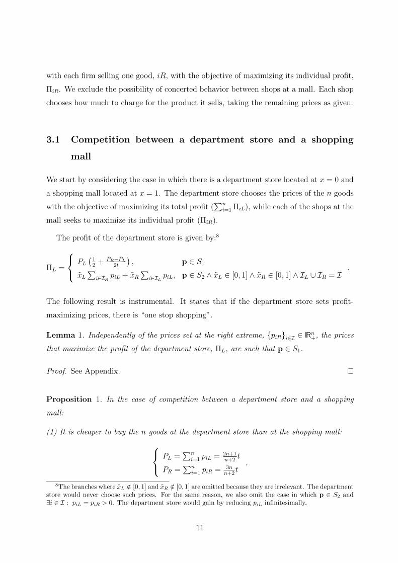
Proposition 1. In the case of competition between a department store and a shopping

mall:

(1) It is cheaper to buy the n goods at the department store than at the shopping mall: PL =∑n

i=1 piL = 2n+1n+2

t

PR =∑n

i=1 piR = 3nn+2

t,

8The branches where xL /∈ [0, 1] and xR /∈ [0, 1] are omitted because they are irrelevant. The departmentstore would never choose such prices. For the same reason, we also omit the case in which p ∈ S2 and∃i ∈ I : piL = piR > 0. The department store would gain by reducing piL infinitesimally.

11

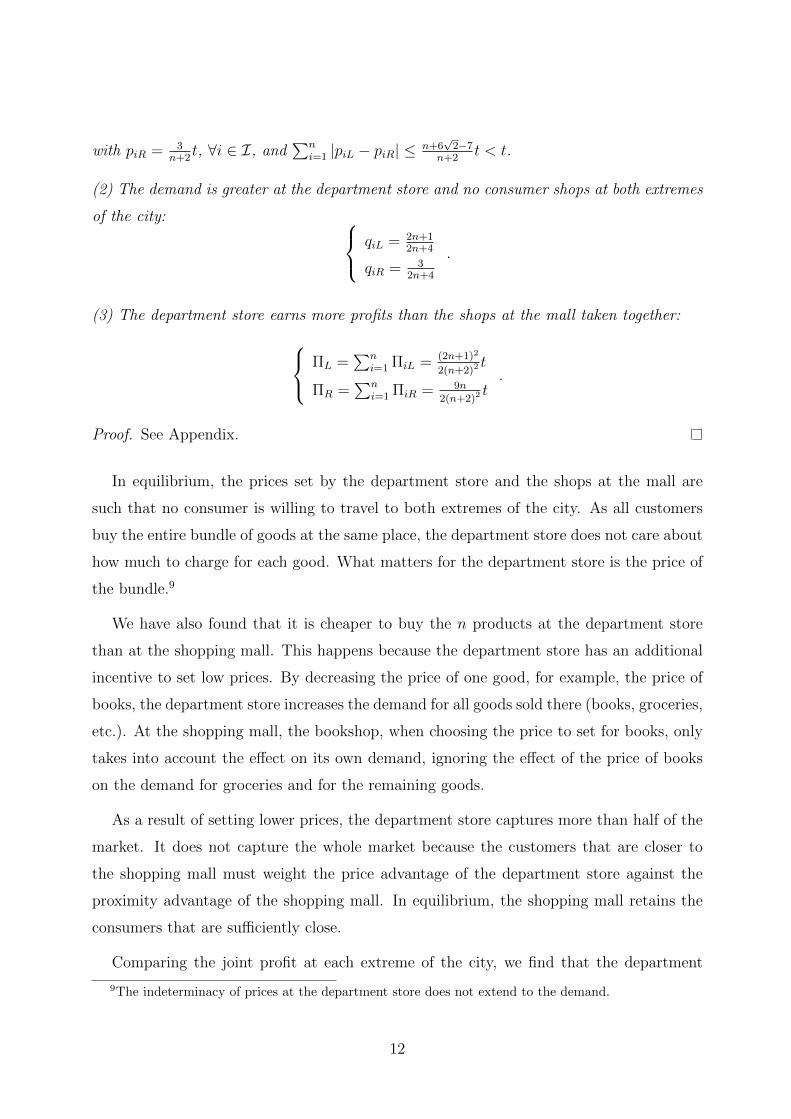
with piR = 3n+2

t, ∀i ∈ I, and∑n

i=1 |piL − piR| ≤ n+6√

2−7n+2

t < t.

(2) The demand is greater at the department store and no consumer shops at both extremes

of the city: qiL = 2n+12n+4

qiR = 32n+4

.

(3) The department store earns more profits than the shops at the mall taken together: ΠL =∑n

i=1 ΠiL = (2n+1)2

2(n+2)2t

ΠR =∑n

i=1 ΠiR = 9n2(n+2)2

t.


In equilibrium, the prices set by the department store and the shops at the mall are

such that no consumer is willing to travel to both extremes of the city. As all customers

buy the entire bundle of goods at the same place, the department store does not care about

how much to charge for each good. What matters for the department store is the price of

the bundle.9

We have also found that it is cheaper to buy the n products at the department store

than at the shopping mall. This happens because the department store has an additional

incentive to set low prices. By decreasing the price of one good, for example, the price of

books, the department store increases the demand for all goods sold there (books, groceries,

etc.). At the shopping mall, the bookshop, when choosing the price to set for books, only

takes into account the effect on its own demand, ignoring the effect of the price of books

on the demand for groceries and for the remaining goods.

As a result of setting lower prices, the department store captures more than half of the

market. It does not capture the whole market because the customers that are closer to

the shopping mall must weight the price advantage of the department store against the

proximity advantage of the shopping mall. In equilibrium, the shopping mall retains the

consumers that are sufficiently close.

Comparing the joint profit at each extreme of the city, we find that the department

9The indeterminacy of prices at the department store does not extend to the demand.

12

store earns more than the rival firms taken together. Aware of this, the shops at the mall

could believe that a merger would benefit them, that is, increase their joint profit. In the

next subsection, we study the effects of such a merger.

Observe also that as the number of products increases to infinity, the price of the

bundle increases to 2t at the department store and to 3t at the shopping mall. Moreover,

the higher is n, the higher is the difference between the price of the bundle of goods in

the two extremes. As a result, the department store captures an increasing share of the

market (in the limit, it actually captures the whole market). Profits at the department

store increase to 2t while the profits at the shopping mall initially increase (are maximal

for n = 2) but then decrease to zero.

When the number of products tends to infinity, the department store becomes monopo-

listic in the market, since all consumers purchase the bundle there. However, the price she

charges for the bundle remains bounded by 2t, because additional price increases would

lead to a loss of consumers to the shopping mall. Then, although not buying from the

shopping mall, consumers benefit from its existence.

3.2 Competition between two department stores

Now, we consider the case in which there are two department stores, one at each extreme

of the city. Each department store chooses the price to charge for each of the n products,

with the objective of maximizing its profit, taking as given the prices set by the other

department store.10

Proposition 2. In the case of competition between two department stores:

(1) The price of the bundle is equal to the transportation cost parameter:

PL = PR = t, withn∑

i=1

|piL − piR| ≤ t.

10This is an extension of the case analyzed by Lal and Matutes (1989), where both department storessell only two products (n = 2).

13

(2) Consumers make all their purchases at the closest department store, thus:

qiL = qiR =1

2.

(3) The resulting profits are also independent of the number of goods:

ΠL = ΠR =t

2.


Again, no consumer is willing to travel to both extremes of the city. They all buy the n

goods at the department store that is closer.

As expected, the department stores charge the same price for the bundle of n goods

(there is, once more, some indeterminacy regarding the split of the bill between the goods).

What is a bit surprising is that the margin (difference between price and marginal cost)

obtained with n goods is the same as that obtained in the single-product model. The

margin is not greater with n products than in the case of a single product because the

reservation utility of the customer is not relevant for the pricing decisions of the firms (as

long as it is high enough, as typically assumed). Despite the fact that customers prefer n

goods instead of one, the margin remains constant and equal to the transportation cost

parameter.11

As a result, the two department stores obtain exactly the same profit as in the standard

Hotelling model, in which a single good is sold. Comparing these profits with those obtained

in the previous scenario, we find that transforming a shopping mall into a department

store is not profitable. The joint profit of the n shops at the mall that compete with

a department store is greater than the profit of a department store that competes with

another department store.

Hence, in spite of the fact that the department store obtains a higher profit than the

shops at the mall taken together, it is not profitable for the shops at the mall to merge

into a department store. To put it in another way, to compete with a department store it

11The same would occur in the case of Bertrand competition with homogeneous products. Independentlyof the number of products that firms sell, their equilibrium margin is always null.

14

is better to construct a shopping mall than to construct another department store.

This result makes us wonder whether it is not better for the department store that sells

the n goods to separate into a shopping mall with n single-product shops. We investigate

this possibility in the next subsection.

3.3 Competition between two shopping malls

In the case of competition between two shopping malls (one at each extreme of the city),

there are 2n independent stores that maximize their individual profits.

The stores selling the same good in different locations are direct competitors. However,

the demand of a store also depends on the price of the other goods sold in the mall where

it is located. A store that sells good i benefits from: (i) a low price for the good j sold

at the same location (since this attracts customers to its location); (ii) a high price for

the good j sold at the other location (since this repels customers from the other location).

This interdependence across goods occurs because when deciding where to buy each good,

a costumer takes into account not only the price but also the transportation costs that she

has to support.

Lemma 2. When there are two shopping malls in the city, no consumer shops at both

extremes of the city (in equilibrium).


Combining Lemma 1 and Lemma 2, we conclude that no consumer finds it worthwhile

to travel to both extremes of the city.

Corollary 1. In equilibrium, regardless of the mode of retail, there is “one stop shopping”.

Proposition 3. In the case of competition between two shopping malls:

(1) The price of each good is equal to the transportation cost parameter:

piL = piR = t, ∀i ∈ I.

(2) Consumers make all their purchases at the closest shopping mall:

15

qiL = qiR =1

2, ∀i ∈ I.

(3) The profit of each firm is also independent of the number of goods:

ΠiL = ΠiR =t

2, ∀i ∈ I.


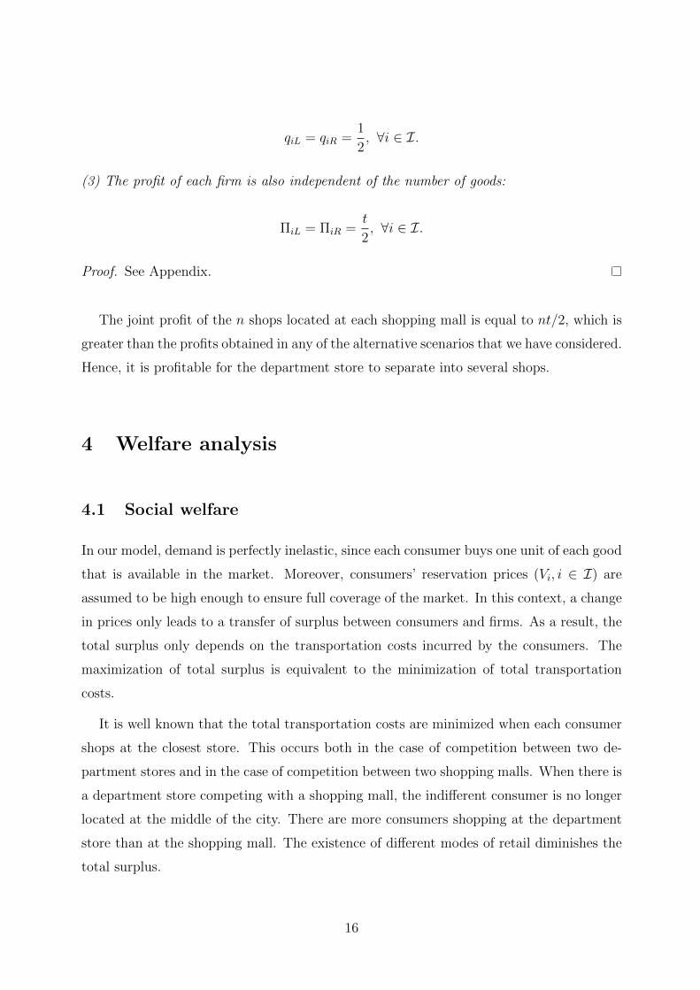
The joint profit of the n shops located at each shopping mall is equal to nt/2, which is

greater than the profits obtained in any of the alternative scenarios that we have considered.

Hence, it is profitable for the department store to separate into several shops.

4 Welfare analysis

4.1 Social welfare

In our model, demand is perfectly inelastic, since each consumer buys one unit of each good

that is available in the market. Moreover, consumers’ reservation prices (Vi, i ∈ I) are

assumed to be high enough to ensure full coverage of the market. In this context, a change

in prices only leads to a transfer of surplus between consumers and firms. As a result, the

total surplus only depends on the transportation costs incurred by the consumers. The

maximization of total surplus is equivalent to the minimization of total transportation

costs.

It is well known that the total transportation costs are minimized when each consumer

shops at the closest store. This occurs both in the case of competition between two de-

partment stores and in the case of competition between two shopping malls. When there is

a department store competing with a shopping mall, the indifferent consumer is no longer

located at the middle of the city. There are more consumers shopping at the department

store than at the shopping mall. The existence of different modes of retail diminishes the

total surplus.

16

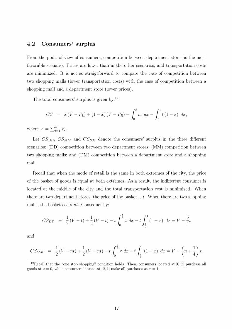
4.2 Consumers’ surplus

From the point of view of consumers, competition between department stores is the most

favorable scenario. Prices are lower than in the other scenarios, and transportation costs

are minimized. It is not so straigtforward to compare the case of competition between

two shopping malls (lower transportation costs) with the case of competition between a

shopping mall and a department store (lower prices).

The total consumers’ surplus is given by:12

CS = x (V − PL) + (1− x) (V − PR)−∫ x

0

tx dx−∫ 1

x

t (1− x) dx,

where V =∑n

i=1 Vi.

Let CSDD, CSMM and CSDM denote the consumers’ surplus in the three different

scenarios: (DD) competition between two department stores; (MM) competition between

two shopping malls; and (DM) competition between a department store and a shopping

mall.

Recall that when the mode of retail is the same in both extremes of the city, the price

of the basket of goods is equal at both extremes. As a result, the indifferent consumer is

located at the middle of the city and the total transportation cost is minimized. When

there are two department stores, the price of the basket is t. When there are two shopping

malls, the basket costs nt. Consequently:

CSDD =1

2(V − t) +

1

2(V − t)− t

∫ 12

0

x dx− t

∫ 1

12

(1− x) dx = V − 5

4t

and

CSMM =1

2(V − nt) +

1

2(V − nt)− t

∫ 12

0

x dx− t

∫ 1

12

(1− x) dx = V −(n +

1

4

)t.

12Recall that the “one stop shopping” condition holds. Then, consumers located at [0, x[ purchase allgoods at x = 0, while consumers located at ]x, 1] make all purchases at x = 1.

17

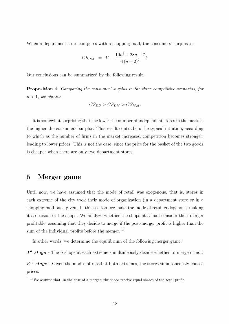
When a department store competes with a shopping mall, the consumers’ surplus is:

CSDM = V − 10n2 + 28n + 7

4 (n + 2)2 t.

Our conclusions can be summarized by the following result.

Proposition 4. Comparing the consumer’ surplus in the three competitive scenarios, for

n > 1, we obtain:

CSDD > CSDM > CSMM .

It is somewhat surprising that the lower the number of independent stores in the market,

the higher the consumers’ surplus. This result contradicts the typical intuition, according

to which as the number of firms in the market increases, competition becomes stronger,

leading to lower prices. This is not the case, since the price for the basket of the two goods

is cheaper when there are only two department stores.

5 Merger game

Until now, we have assumed that the mode of retail was exogenous, that is, stores in

each extreme of the city took their mode of organization (in a department store or in a

shopping mall) as a given. In this section, we make the mode of retail endogenous, making

it a decision of the shops. We analyze whether the shops at a mall consider their merger

profitable, assuming that they decide to merge if the post-merger profit is higher than the

sum of the individual profits before the merger.13

In other words, we determine the equilibrium of the following merger game:

1st stage - The n shops at each extreme simultaneously decide whether to merge or not;

2nd stage - Given the modes of retail at both extremes, the stores simultaneously choose

prices.

13We assume that, in the case of a merger, the shops receive equal shares of the total profit.

18

We only allow for two outcomes in the first stage: full merger or no merger. We do not

consider the possibility of a merger between k stores located at one extreme while the other

n − k stores remain separated. This would be an interesting case to study, but it is out

of our scope. Moreover, we restrict the analysis to mergers between stores at the same

extreme of the city. Otherwise, a store selling the product i ∈ I at x = 0 could merge with

a store selling the same product at x = 1 to form a monopoly in this market.

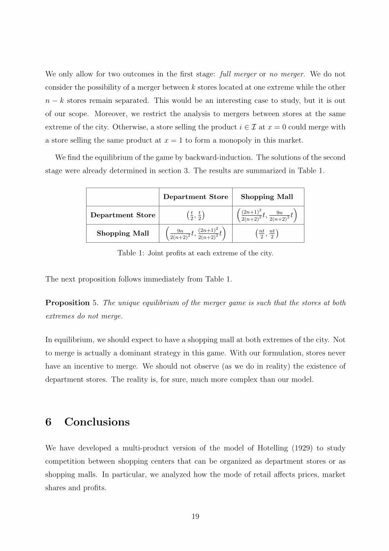
We find the equilibrium of the game by backward-induction. The solutions of the second

stage were already determined in section 3. The results are summarized in Table 1.

Department Store Shopping Mall

Department Store(t2, t

2

) ((2n+1)2

2(n+2)2t, 9n

2(n+2)2t)

Shopping Mall(

9n2(n+2)2

t, (2n+1)2

2(n+2)2t) (

nt2, nt

2

)Table 1: Joint profits at each extreme of the city.

The next proposition follows immediately from Table 1.

Proposition 5. The unique equilibrium of the merger game is such that the stores at both

extremes do not merge.

In equilibrium, we should expect to have a shopping mall at both extremes of the city. Not

to merge is actually a dominant strategy in this game. With our formulation, stores never

have an incentive to merge. We should not observe (as we do in reality) the existence of

department stores. The reality is, for sure, much more complex than our model.

6 Conclusions

We have developed a multi-product version of the model of Hotelling (1929) to study

competition between shopping centers that can be organized as department stores or as

shopping malls. In particular, we analyzed how the mode of retail affects prices, market

shares and profits.

19

A distinctive feature of our work, with respect to the existing literature, is that we do not

restrict consumers to make all their purchases in a single place. However, we found that,

in equilibrium, no consumer finds it worthwhile to visit more than one shopping center.

Since we have obtained the “one-stop shopping” condition as an equilibrium outcome, our

work provides a theoretical justification for this commonly made assumption.

Comparing the competitive behaviour of a department store with that of a shopping

mall, we found (as in previous works) that the department store competes more aggressively

(charges a lower price for the bundle of products). This occurs because a department store,

when choosing prices, takes into account the fact that a price drop in one good increases

the demand for all its goods. In contrast, a shop at a mall only takes into account its

individual demand when choosing the price to charge for its good.

When a department store competes with a shopping mall, the bundle of goods is cheaper

at the department store. Nevertheless, the demand-effect more than compensates the price-

effect and the department store obtains higher profits than the shops at the mall taken

together. As the number of goods increases, consumers worry more and more about price

differences across shopping centers (and less and less about transportation costs). In the

limit, the department store actually captures the whole market.

In spite of having a lower profit, the shops at mall have no incentives to merge into a

department store. It is the department store that has incentives to separate itself into a

shopping mall. The equilibrium of a merger game, in which the shops at each extreme

decide whether to organize themselves as a shopping mall or as a department store, is

competition between two shopping malls. In other words, if the mode of retail organization

is made endogeous, only shopping malls are expected to appear.

Having two shopping malls or two department stores is equally optimal in terms of

total surplus. However, consumers are better off in the case of competition between two

department stores (since they pay less for the bundle). Therefore, the equilibrium of the

merger game (two shopping malls) is the competitive scenario that consumers less desire.

20

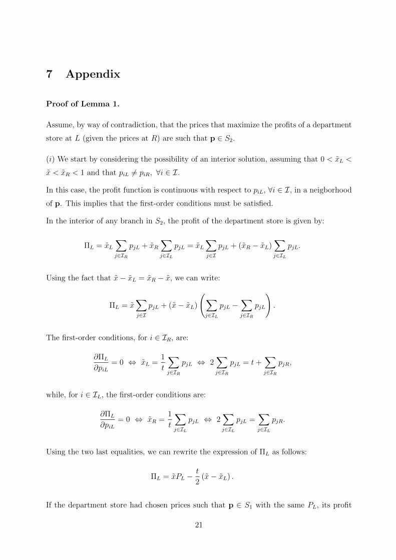
7 Appendix

Proof of Lemma 1.

Assume, by way of contradiction, that the prices that maximize the profits of a department

store at L (given the prices at R) are such that p ∈ S2.

(i) We start by considering the possibility of an interior solution, assuming that 0 < xL <

x < xR < 1 and that piL 6= piR, ∀i ∈ I.

In this case, the profit function is continuous with respect to piL, ∀i ∈ I, in a neigborhood

of p. This implies that the first-order conditions must be satisfied.

In the interior of any branch in S2, the profit of the department store is given by:

ΠL = xL

∑j∈IR

pjL + xR

∑j∈IL

pjL = xL

∑j∈I

pjL + (xR − xL)∑j∈IL

pjL.

Using the fact that x− xL = xR − x, we can write:

ΠL = x∑j∈I

pjL + (x− xL)

(∑j∈IL

pjL −∑j∈IR

pjL

).

The first-order conditions, for i ∈ IR, are:

∂ΠL

∂piL= 0 ⇔ xL =

1

t

∑j∈IR

pjL ⇔ 2∑j∈IR

pjL = t +∑j∈IR

pjR,

while, for i ∈ IL, the first-order conditions are:

∂ΠL

∂piL= 0 ⇔ xR =

1

t

∑j∈IL

pjL ⇔ 2∑j∈IL

pjL =∑j∈IL

pjR.

Using the two last equalities, we can rewrite the expression of ΠL as follows:

ΠL = xPL −t

2(x− xL) .

If the department store had chosen prices such that p ∈ S1 with the same PL, its profit

21

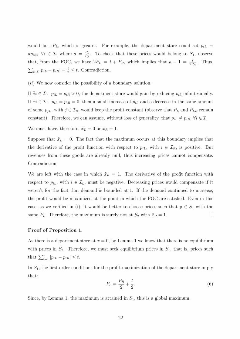
would be xPL, which is greater. For example, the department store could set piL =

apiR, ∀i ∈ I, where a = PL

PR. To check that these prices would belong to S1, observe

that, from the FOC, we have 2PL = t + PR, which implies that a − 1 = t2PR

. Thus,∑i∈I |piL − piR| = t

2≤ t. Contradiction.

(ii) We now consider the possibility of a boundary solution.

If ∃i ∈ I : piL = piR > 0, the department store would gain by reducing piL infinitesimally.

If ∃i ∈ I : piL = piR = 0, then a small increase of piL and a decrease in the same amount

of some pjL, with j ∈ IR, would keep the profit constant (observe that PL and PLR remain

constant). Therefore, we can assume, without loss of generality, that piL 6= piR, ∀i ∈ I.

We must have, therefore, xL = 0 or xR = 1.

Suppose that xL = 0. The fact that the maximum occurs at this boundary implies that

the derivative of the profit function with respect to piL, with i ∈ IR, is positive. But

revenues from these goods are already null, thus increasing prices cannot compensate.

Contradiction.

We are left with the case in which xR = 1. The derivative of the profit function with

respect to piL, with i ∈ IL, must be negative. Decreasing prices would compensate if it

weren’t for the fact that demand is bounded at 1. If the demand continued to increase,

the profit would be maximized at the point in which the FOC are satisfied. Even in this

case, as we verified in (i), it would be better to choose prices such that p ∈ S1 with the

same PL. Therefore, the maximum is surely not at S2 with xR = 1. �

Proof of Proposition 1.

As there is a department store at x = 0, by Lemma 1 we know that there is no equilibrium

with prices in S2. Therefore, we must seek equilibrium prices in S1, that is, prices such

that∑n

i=1 |piL − piR| ≤ t.

In S1, the first-order conditions for the profit-maximization of the department store imply

that:

PL =PR

2+

t

2. (6)

Since, by Lemma 1, the maximum is attained in S1, this is a global maximum.

22

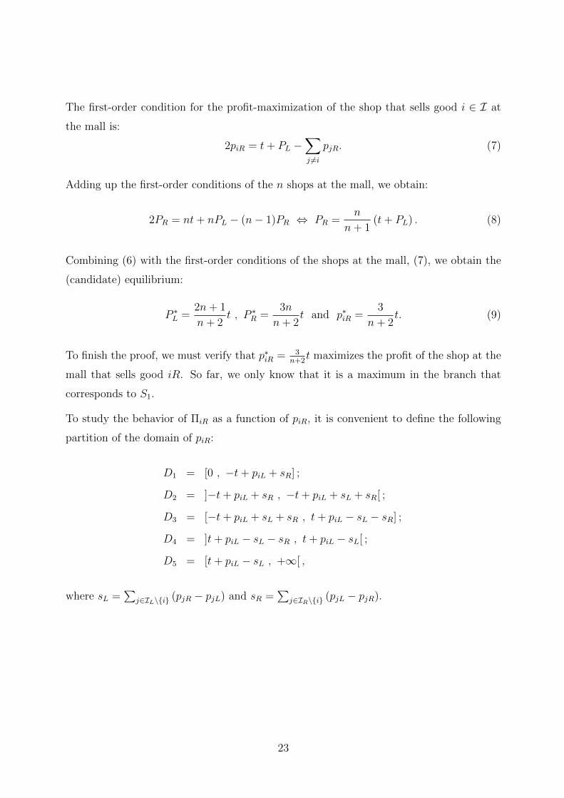
The first-order condition for the profit-maximization of the shop that sells good i ∈ I at

the mall is:

2piR = t + PL −∑j 6=i

pjR. (7)

Adding up the first-order conditions of the n shops at the mall, we obtain:

2PR = nt + nPL − (n− 1)PR ⇔ PR =n

n + 1(t + PL) . (8)

Combining (6) with the first-order conditions of the shops at the mall, (7), we obtain the

(candidate) equilibrium:

P ∗L =2n + 1

n + 2t , P ∗R =

3n

n + 2t and p∗iR =

3

n + 2t. (9)

To finish the proof, we must verify that p∗iR = 3n+2

t maximizes the profit of the shop at the

mall that sells good iR. So far, we only know that it is a maximum in the branch that

corresponds to S1.

To study the behavior of ΠiR as a function of piR, it is convenient to define the following

partition of the domain of piR:

D1 = [0 , −t + piL + sR] ;

D2 = ]−t + piL + sR , −t + piL + sL + sR[ ;

D3 = [−t + piL + sL + sR , t + piL − sL − sR] ;

D4 = ]t + piL − sL − sR , t + piL − sL[ ;

D5 = [t + piL − sL , +∞[ ,

where sL =∑

j∈IL\{i} (pjR − pjL) and sR =∑

j∈IR\{i} (pjL − pjR).

23

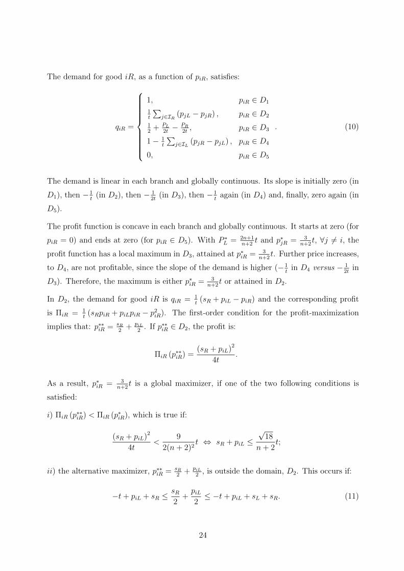
The demand for good iR, as a function of piR, satisfies:

qiR =

1, piR ∈ D1

1t

∑j∈IR (pjL − pjR) , piR ∈ D2

12

+ PL

2t− PR

2t, piR ∈ D3

1− 1t

∑j∈IL (pjR − pjL) , piR ∈ D4

0, piR ∈ D5

. (10)

The demand is linear in each branch and globally continuous. Its slope is initially zero (in

D1), then −1t

(in D2), then − 12t

(in D3), then −1t

again (in D4) and, finally, zero again (in

D5).

The profit function is concave in each branch and globally continuous. It starts at zero (for

piR = 0) and ends at zero (for piR ∈ D5). With P ∗L = 2n+1n+2

t and p∗jR = 3n+2

t, ∀j 6= i, the

profit function has a local maximum in D3, attained at p∗iR = 3n+2

t. Further price increases,

to D4, are not profitable, since the slope of the demand is higher (−1t

in D4 versus − 12t

in

D3). Therefore, the maximum is either p∗iR = 3n+2

t or attained in D2.

In D2, the demand for good iR is qiR = 1t

(sR + piL − piR) and the corresponding profit

is ΠiR = 1t

(sRpiR + piLpiR − p2iR). The first-order condition for the profit-maximization

implies that: p∗∗iR = sR2

+ piL2

. If p∗∗iR ∈ D2, the profit is:

ΠiR (p∗∗iR) =(sR + piL)2

4t.

As a result, p∗iR = 3n+2

t is a global maximizer, if one of the two following conditions is

satisfied:

i) ΠiR (p∗∗iR) < ΠiR (p∗iR), which is true if:

(sR + piL)2

4t<

9

2(n + 2)2t ⇔ sR + piL ≤

√18

n + 2t;

ii) the alternative maximizer, p∗∗iR = sR2

+ piL2

, is outside the domain, D2. This occurs if:

−t + piL + sR ≤sR2

+piL2≤ −t + piL + sL + sR. (11)

24

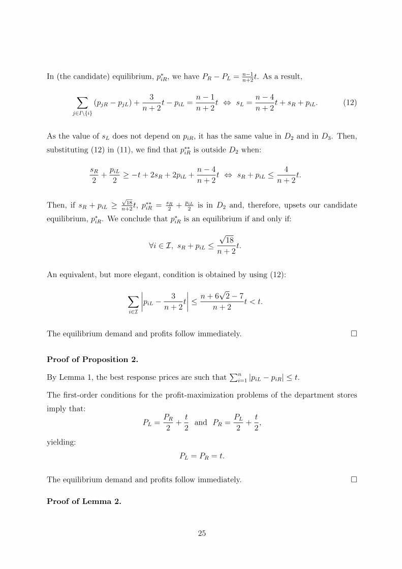
In (the candidate) equilibrium, p∗iR, we have PR − PL = n−1n+2

t. As a result,

∑j∈I\{i}

(pjR − pjL) +3

n + 2t− piL =

n− 1

n + 2t ⇔ sL =

n− 4

n + 2t + sR + piL. (12)

As the value of sL does not depend on piR, it has the same value in D2 and in D3. Then,

substituting (12) in (11), we find that p∗∗iR is outside D2 when:

sR2

+piL2≥ −t + 2sR + 2piL +

n− 4

n + 2t ⇔ sR + piL ≤

4

n + 2t.

Then, if sR + piL ≥√

18n+2

t, p∗∗iR = sR2

+ piL2

is in D2 and, therefore, upsets our candidate

equilibrium, p∗iR. We conclude that p∗iR is an equilibrium if and only if:

∀i ∈ I, sR + piL ≤√

18

n + 2t.

An equivalent, but more elegant, condition is obtained by using (12):

∑i∈I

∣∣∣∣piL − 3

n + 2t

∣∣∣∣ ≤ n + 6√

2− 7

n + 2t < t.

The equilibrium demand and profits follow immediately. �


By Lemma 1, the best response prices are such that∑n


The first-order conditions for the profit-maximization problems of the department stores

imply that:

PL =PR

2+

t

2and PR =

PL

2+

t

2,

yielding:

PL = PR = t.


Proof of Lemma 2.

25

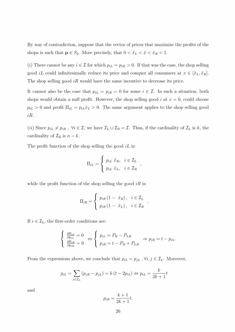
By way of contradiction, suppose that the vector of prices that maximize the profits of the

shops is such that p ∈ S2. More precisely, that 0 < xL < x < xR < 1.

(i) There cannot be any i ∈ I for which piL = piR > 0. If that was the case, the shop selling

good iL could infinitesimally reduce its price and conquer all consumers at x ∈ [xL, xR].

The shop selling good iR would have the same incentive to decrease its price.

It cannot also be the case that piL = piR = 0 for some i ∈ I. In such a situation, both

shops would obtain a null profit. However, the shop selling good i at x = 0, could choose

piL > 0 and profit ΠiL = piLxL > 0. The same argument applies to the shop selling good

iR.

(ii) Since piL 6= piR , ∀i ∈ I, we have IL ∪ IR = I. Thus, if the cardinality of IL is k, the

cardinality of IR is n− k.

The profit function of the shop selling the good iL is:

ΠiL =

piL xR, i ∈ ILpiL xL, i ∈ IR

,

while the profit function of the shop selling the good iR is:

ΠiR =

piR (1− xR) , i ∈ ILpiR (1− xL) , i ∈ IR

.

If i ∈ IL, the first-order conditions are: ∂ΠiL

∂piL= 0

∂ΠiR

∂piR= 0

⇔

piL = PR − PLR

piR = t− PR + PLR

⇒ piR = t− piL.

From the expressions above, we conclude that piL = pjL ,∀i, j ∈ IL. Moreover,

piL =∑j∈IL

(pjR − pjL) = k (t− 2piL)⇔ piL =k

2k + 1t

and

piR =k + 1

2k + 1t.

26

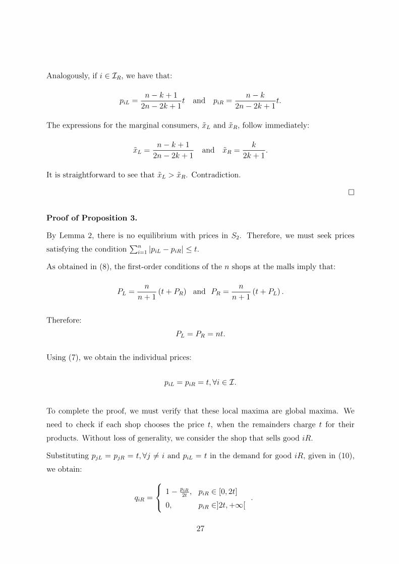
Analogously, if i ∈ IR, we have that:

piL =n− k + 1

2n− 2k + 1t and piR =

n− k

2n− 2k + 1t.

The expressions for the marginal consumers, xL and xR, follow immediately:

xL =n− k + 1

2n− 2k + 1and xR =

k

2k + 1.

It is straightforward to see that xL > xR. Contradiction.

�


By Lemma 2, there is no equilibrium with prices in S2. Therefore, we must seek prices

satisfying the condition∑n


As obtained in (8), the first-order conditions of the n shops at the malls imply that:

PL =n

n + 1(t + PR) and PR =

n

n + 1(t + PL) .

Therefore:

PL = PR = nt.

Using (7), we obtain the individual prices:

piL = piR = t,∀i ∈ I.

To complete the proof, we must verify that these local maxima are global maxima. We

need to check if each shop chooses the price t, when the remainders charge t for their

products. Without loss of generality, we consider the shop that sells good iR.

Substituting pjL = pjR = t, ∀j 6= i and piL = t in the demand for good iR, given in (10),

we obtain:

qiR =

1− piR2t, piR ∈ [0, 2t]

0, piR ∈]2t,+∞[.

27

The profit function is:

ΠiR =

piR(1− piR

2t

), piR ∈ [0, 2t]

0, piR ∈]2t,+∞[,

which is globally concave and continuous. Therefore, the local maximum is also the global

maximum.


References

Bart, Y. (2008), “Multiproduct competition with demand complementarity”, mimeo.

Beggs, A.W. (1994), “Mergers and malls”, Journal of Industrial Economics, 44 (4), pp.

419-428.

Bliss, C. (1988), “A theory of retail pricing”, Journal of Industrial Economics, 36 (4), pp.

375-391.

D’Aspremont, C., J.J. Gabszewicz and J.-F. Thisse (1979), “On Hotelling’s ‘Stability in

competition’ ”, Econometrica, 47, pp. 1145-1150.

Economides, N. and S.C. Salop (1992), “Competition and integration among complements,

and network market structure”, Journal of Industrial Economics, 40 (1), pp. 105-133.

Edgeworth, F.Y. (1925), “Papers Relating to Political Economy”, London: MacMillan.

Giraud-Heraud, E., H. Hammoudi and M. Mokrane (2003), “Multiproduct firm behaviour

in a differentiated market”, Canadian Journal of Economics, 36 (1), pp. 41-61.

Hanson, W. and R.K. Martin (1990), “Optimal Bundle Pricing”, Management Science, 36

(2), pp. 155-174.

Hotelling, H. (1929), “Stability in competition”, Economic Journal, 39, pp. 41-57.

Lal, R. and C. Matutes (1989), “Price competition in multimarket duopolies”, RAND

Journal of Economics, 20 (4), pp. 516-537.

28

Laussel, D. (2006), “Are manufacturers competing through or with supermarkets? A

theoretical investigation”, The B.E. Journal of Theoretical Economics, Berkeley Electronic

Press, 6 (1), pp. 1-18.

Matutes, C. and P. Regibeau (1992),“Compatibility and bundling of complementary goods

in a duopoly”, Journal of Industrial Economics, 40 (1), pp. 37-54.

Rhee, H. and D.R. Bell (2002), “The inter-store mobility of supermarket shoppers”, Journal

of Retailing, 78 (4), pp. 225-237.

Salant, S., S. Switzer and R. Reynolds (1983), “Losses from horizontal merger: the effects

of an exogenous change in industry structure on Cournot-Nash equilibrium”, The Quarterly

Journal of Economics, 98 (2), pp. 185-199.

Smith, H. and Hay, D. (2005), “Streets, malls and supermarkets”, Journal of Economics

and Management Strategy, 14 (1), pp. 29-59.

29

Recent FEP Working Papers

Nº 393 Susana Silva, Isabel Soares and Óscar Afonso, “E3 Models Revisited”, December 2010

Nº 392 Catarina Roseira, Carlos Brito and Stephan C. Henneberg, “Innovation-based Nets as Collective Actors: A Heterarchization Case Study from the Automotive Industry”, November 2010

Nº 391 Li Shu and Aurora A.C. Teixeira, “The level of human capital in innovative firms located in China. Is foreign capital relevant”, November 2010

Nº 390 Rui Moura and Rosa Forte, “The Effects of Foreign Direct Investment on the Host Country Economic Growth - Theory and Empirical Evidence”, November 2010

Nº 389 Pedro Mazeda Gil and Fernanda Figueiredo, “Firm Size Distribution under Horizontal and Vertical R&D”, October 2010

Nº 388 Wei Heyuan and Aurora A.C. Teixeira, “Is human capital relevant in attracting innovative FDI to China?”, October 2010

Nº 387 Carlos F. Alves and Cristina Barbot, “Does market concentration of downstream buyers squeeze upstream suppliers’ market power?”, September 2010

Nº 386 Argentino Pessoa “Competitiveness, Clusters and Policy at the Regional Level: Rhetoric vs. Practice in Designing Policy for Depressed Regions”, September 2010

Nº 385 Aurora A.C. Teixeira and Margarida Catarino, “The importance of Intermediaries organizations in international R&D cooperation: an empirical multivariate study across Europe”, July 2010

Nº 384 Mafalda Soeiro and Aurora A.C. Teixeira, “Determinants of higher education students’ willingness to pay for violent crime reduction: a contingent valuation study”, July 2010

Nº 383 Armando Silva, “The role of subsidies for exports: Evidence for Portuguese manufacturing firms”, July 2010

Nº 382 Óscar Afonso, Pedro Neves and Maria Thompsom, “Costly Investment, Complementarities, International Technological-Knowledge Diffusion and the Skill Premium”, July 2010

Nº 381 Pedro Cunha Neves and Sandra Tavares Silva, “Inequality and Growth: Uncovering the main conclusions from the empirics”, July 2010

Nº 380 Isabel Soares and Paula Sarmento, “Does Unbundling Really Matter? The Telecommunications and Electricity Cases”, July 2010

Nº 379 António Brandão and Joana Pinho, “Asymmetric information and exchange of information about product differentiation”, June 2010

Nº 378 Mónica Meireles, Isabel Soares and Óscar Afonso, “Economic Growth, Ecological Technology and Public Intervention”, June 2010

Nº 377 Nuno Torres, Óscar Afonso and Isabel Soares, “The connection between oil and economic growth revisited”, May 2010

Nº 376 Ricardo Correia and Carlos Brito, “O Marketing e o Desenvolvimento Turístico: O Caso de Montalegre”, May 2010

Nº 375 Maria D.M. Oliveira and Aurora A.C. Teixeira, “The determinants of technology transfer efficiency and the role of innovation policies: a survey”, May 2010

Nº 374 João Correia-da-Silva and Carlos Hervés-Beloso, “Two-period economies with private state verification”, May 2010

Nº 373 Armando Silva, Óscar Afonso and Ana Paula Africano, “Do Portuguese manufacturing firms learn by exporting?”, April 2010

Nº 372 Ana Maria Bandeira and Óscar Afonso, “Value of intangibles arising from R&D activities”, April 2010

Nº 371 Armando Silva, Óscar Afonso and Ana Paula Africano, “Do Portuguese manufacturing firms self select to exports?”, April 2010

Nº 370 Óscar Afonso, Sara Monteiro and Maria Thompson, “A Growth Model for the Quadruple Helix Innovation Theory”, April 2010

Nº 369 Armando Silva, Óscar Afonso and Ana Paula Africano, “Economic performance and international trade engagement: the case of Portuguese manufacturing firms”, April 2010

Nº 368 Andrés Carvajal and João Correia-da-Silva, “Agreeing to Disagree with Multiple Priors”,

April 2010

Nº 367 Pedro Gonzaga, “Simulador de Mercados de Oligopólio”, March 2010

Nº 366 Aurora A.C. Teixeira and Luís Pinheiro, “The process of emergency, evolution, and sustainability of University-Firm relations in a context of open innovation ”, March 2010

Nº 365 Miguel Fonseca, António Mendonça and José Passos, “Home Country Trade Effects of Outward FDI: an analysis of the Portuguese case, 1996-2007”, March 2010

Nº 364 Armando Silva, Ana Paula Africano and Óscar Afonso, “Learning-by-exporting: what we know and what we would like to know”, March 2010

Nº 363 Pedro Cosme da Costa Vieira, “O problema do crescente endividamento de Portugal à luz da New Macroeconomics”, February 2010

Nº 362 Argentino Pessoa, “Reviewing PPP Performance in Developing Economies”, February 2010

Nº 361 Ana Paula Africano, Aurora A.C. Teixeira and André Caiado, “The usefulness of State trade missions for the internationalization of firms: an econometric analysis”, February 2010

Nº 360 Beatriz Casais and João F. Proença, “Inhibitions and implications associated with celebrity participation in social marketing programs focusing on HIV prevention: an exploratory research”, February 2010

Nº 359 Ana Maria Bandeira, “Valorização de activos intangíveis resultantes de actividades de I&D”, February 2010

Nº 358 Maria Antónia Rodrigues and João F. Proença, “SST and the Consumer Behaviour in Portuguese Financial Services”, January 2010

Nº 357 Carlos Brito and Ricardo Correia, “Regions as Networks: Towards a Conceptual Framework of Territorial Dynamics”, January 2010

Nº 356 Pedro Rui Mazeda Gil, Paulo Brito and Óscar Afonso, “Growth and Firm Dynamics with Horizontal and Vertical R&D”, January 2010

Nº 355 Aurora A.C. Teixeira and José Miguel Silva, “Emergent and declining themes in the Economics and Management of Innovation scientific area over the past three decades”, January 2010

Nº 354 José Miguel Silva and Aurora A.C. Teixeira, “Identifying the intellectual scientific basis of the Economics and Management of Innovation Management area”, January 2010

Nº 353 Paulo Guimarães, Octávio Figueiredo and Douglas Woodward, “Accounting for Neighboring Effects in Measures of Spatial Concentration”, December 2009

Nº 352 Vasco Leite, Sofia B.S.D. Castro and João Correia-da-Silva, “A third sector in the core-periphery model: non-tradable goods”, December 2009

Nº 351 João Correia-da-Silva and Joana Pinho, “Costly horizontal differentiation”, December 2009

Nº 350 João Correia-da-Silva and Joana Resende, “Free daily newspapers: too many incentives to print?”, December 2009

Nº 349 Ricardo Correia and Carlos Brito, “Análise Conjunta da Dinâmica Territorial e Industrial: O Caso da IKEA – Swedwood”, December 2009

Nº 348 Gonçalo Faria, João Correia-da-Silva and Cláudia Ribeiro, “Dynamic Consumption and Portfolio Choice with Ambiguity about Stochastic Volatility”, December 2009

Nº 347 André Caiado, Ana Paula Africano and Aurora A.C. Teixeira, “Firms’ perceptions on the usefulness of State trade missions: an exploratory micro level empirical analysis”, December 2009

Nº 346 Luís Pinheiro and Aurora A.C. Teixeira, “Bridging University-Firm relationships and Open Innovation literature: a critical synthesis”, November 2009

Editor: Sandra Silva ([email protected]) Download available at: http://www.fep.up.pt/investigacao/workingpapers/ also in http://ideas.repec.org/PaperSeries.html

��

��

��

��

��

��

��

��

��

��

��

��

��

��

��

��

��

��

��

Spatial competition between shopping centers

Documents

Transcript of Spatial competition between shopping centers