Spatial and Temporal Occurrence of Blue Whales off theU.S. West Coast, with Implications for ManagementLadd M. Irvine1*, Bruce R. Mate1, Martha H. Winsor1, Daniel M. Palacios2,3¤, Steven J. Bograd3,

Daniel P. Costa4, Helen Bailey5

1 Marine Mammal Institute, Department of Fisheries and Wildlife, and Coastal Oregon Marine Experiment Station, Oregon State University, Hatfield Marine Science Center,

Newport, Oregon, United States of America, 2 Cooperative Institute for Marine Ecosystems and Climate, Institute of Marine Sciences, Division of Physical and Biological

Sciences, University of California Santa Cruz, Santa Cruz, California, United States of America, 3 NOAA/NMFS/SWFSC/Environmental Research Division, Pacific Grove,

California, United States of America, 4 Ecology and Evolutionary Biology, Long Marine Laboratory, University of California Santa Cruz, Santa Cruz, California, United States

of America, 5 Chesapeake Biological Laboratory, University of Maryland Center for Environmental Science, Solomons, Maryland, United States of America

Abstract

Mortality and injuries caused by ship strikes in U.S. waters are a cause of concern for the endangered population of bluewhales (Balaenoptera musculus) occupying the eastern North Pacific. We sought to determine which areas along the U.S.West Coast are most important to blue whales and whether those areas change inter-annually. Argos-monitored satellitetags were attached to 171 blue whales off California during summer/early fall from 1993 to 2008. We analyzed portions ofthe tracks that occurred within U.S. Exclusive Economic Zone waters and defined the ‘home range’ (HR) and ‘core areas’(CAU) as the 90% and 50% fixed kernel density distributions, respectively, for each whale. We used the number ofoverlapping individual HRs and CAUs to identify areas of highest use. Individual HR and CAU sizes varied dramatically, butwithout significant inter-annual variation despite covering years with El Nino and La Nina conditions. Observed within-yeardifferences in HR size may represent different foraging strategies for individuals. The main areas of HR and CAU overlapamong whales were near highly productive, strong upwelling centers that were crossed by commercial shipping lanes.Tagged whales generally departed U.S. Exclusive Economic Zone waters from mid-October to mid-November, with highvariability among individuals. One 504-d track allowed HR and CAU comparisons for the same individual across two years,showing similar seasonal timing, and strong site fidelity. Our analysis showed how satellite-tagged blue whales seasonallyused waters off the U.S. West Coast, including high-risk areas. We suggest possible modifications to existing shipping lanesto reduce the likelihood of collisions with vessels.

Citation: Irvine LM, Mate BR, Winsor MH, Palacios DM, Bograd SJ, et al. (2014) Spatial and Temporal Occurrence of Blue Whales off the U.S. West Coast, withImplications for Management. PLoS ONE 9(7): e102959. doi:10.1371/journal.pone.0102959

Editor: Andreas Fahlman, Texas A&M University-Corpus Christi, United States of America

Received December 13, 2013; Accepted June 26, 2014; Published July 23, 2014

Copyright: � 2014 Irvine et al. This is an open-access article distributed under the terms of the Creative Commons Attribution License, which permitsunrestricted use, distribution, and reproduction in any medium, provided the original author and source are credited.

Funding: Funding for this research was provided by a variety of sources across 15 years including the Office of Naval Research (http://www.onr.navy.mil/),Tagging of Pacific Pelagics (http://www.topp.org/), the National Science Foundation (www.nsf.gov), the Oregon State University Marine Mammal InstituteEndowment (mmi.oregonstate.edu), the Alfred P. Sloan Foundation (www.sloan.org), the Packard Foundation (www.packard.org), and National Geographic(www.nationalgeographic.com). Funding was also provided under the interagency NASA, USGS, National Park Service, US Fish and Wildlife Service, SmithsonianInstitution Climate and Biological Response program, Grant Number NNX11AP71G (http://www.nasa.gov/topics/earth/features/climate_partners.html).

number of the authors are employed by theOregon State University Marine Mammal Institute, funding by the Marine Mammal Institute Endowment of some of the work presented here (typically in theform of matching funds) did not influence study design, data collection and analysis, decision to publish, or preparation of this manuscript. None of the otherfunding agencies influenced any aspects of this manuscript.

Competing Interests: Steven Bograd is currently an editor for this journal and is an author on this paper. This does not alter the authors’ adherence to PLOSONE Editorial policies and criteria.

* Email: ladd.irvine@oregonstate.edu

¤ Current address: Marine Mammal Institute, Department of Fisheries and Wildlife, and Coastal Oregon Marine Experiment Station, Oregon State University,Hatfield Marine Science Center, Newport, Oregon, United States of America

Introduction

The blue whale (Balaenoptera musculus) population in the

eastern North Pacific (ENP) was depleted by commercial whaling

in a manner similar to populations that were overexploited in

other parts of the world [1]. While there is some evidence that the

population was increasing in the late 1900s [2], recent population

estimates for waters off California, Oregon, and Washington based

on line-transect methods have ranged from about 500 to nearly

2000 animals [3], suggesting that the proportion of the population

foraging off the U.S. West Coast varies inter-annually. Current

mark-recapture estimates based on photo-identification studies

indicate that the population size is about 2500 whales [4] and that

its distribution may have expanded north into waters off British

Columbia and the Gulf of Alaska in recent years [5]. It was

expected that the ENP blue whale population would begin to

recover following the protections established by the International

Whaling Commission in 1966 [6], so the lack of evidence of

substantial population growth during the past decades may

indicate their recovery is being impeded, possibly by human

impacts, either indirectly through food chain interactions [7], or

directly from physical interactions such as noise [8,9] or ship

strikes [10]. It is therefore essential that areas of importance to

ENP blue whales off the U.S. West Coast are identified so that

appropriate management actions may be taken for this endan-

gered species.

PLOS ONE | www.plosone.org 1 July 2014 | Volume 9 | Issue 7 | e102959

Funding for OpenAccess provided by the University of California, Santa Cruz, Open Access Fund. While a

Most current estimates of blue whale distribution and popula-

tion density in the ENP are based on photo-identification and line-

transect data from shipboard surveys [2,3]. However, tracking

whales with satellite tags has the advantage of higher temporal

resolution than ship-based surveys, allowing for a more detailed

understanding of how the distribution of tagged animals changes

over time, while also providing better spatial resolution than can

be achieved by other techniques like passive acoustic monitoring

[11,12,13]. Tracking data from individual whales allow the

location and extent of important areas to be identified based on

frequency of use, without the limitations of pre-determined survey

areas or times. Here we present results from a large, multi-year set

of blue whale satellite tracking data, collected off the U.S. West

Coast, to determine which areas were most important to tagged

whales and whether those areas changed inter-annually during the

study period. These results provide valuable information on the

home range and core areas of blue whales on their feeding grounds

off the U.S. West Coast, which will help better inform

management agencies.

Methods

Ethics StatementThis research was conducted under U.S. National Marine

Fisheries Service (NMFS) permit numbers 841 (years 1993–1998),

369-1440 (years 1999–2004), and 369-1757 (years 2005–2008),

authorizing the close approach and deployment of implantable

satellite tags on large whales which are protected by the 1972

Marine Mammal Protection Act, and, in many cases, the 1973

Endangered Species Act. All tagging procedures described in the

listed permits, and used in this manuscript, were subjected to an

internal NMFS and external review by veterinarians and other

marine mammal researchers prior to approval. In addition, this

study was carried out in strict accordance with the recommenda-

tions of the Oregon State University Institutional Animal Care

and Use Committee, composed of veterinarians and other

university administrators.

The impacts of tagging on cetaceans relative to the conservation

value of the information that this technique provides has been

reviewed in several fora, beginning with a multi-agency (U.S.

Marine Mammal Commission, NMFS, and U.S. Office of Naval

Research) workshop in 1987 [14] and continuing through a 2011

report by the Scientific Committee of the International Whaling

Commission [15]. These committees and workshops have

repeatedly determined that, for highly endangered species, the

level of health risk from implantable satellite tags is sufficiently low

compared to the high potential conservation value of the data, and

as such has encouraged the conduct of tagging studies. While we

agree with these assessments, we do not discount that some

amount of pain or discomfort may be associated with the

implantation of satellite tags in large cetaceans. However, there

is a lack of understanding of the level of pain felt by a whale

swimming with an implanted tag for extended periods of time [16]

or whether this impedes its natural behaviors in a significant way

[17]. Research on effects of implantable tags has generally been

limited to short-term behavioral responses [17], or long-term

reproductive rate [18]. Nevertheless, several whale species have

been tracked with this technology to known (as well as previously

unknown) areas of concentration [19,20], and using recognized

migration corridors [21], including historical areas of sightings and

whaling catch records [22,23], indicating that the long-term

movements of tagged whales are consistent with other, non-tagged

whales.

Satellite trackingSatellite monitored radio tags were attached to 171 blue whales

in the ENP during 15 years ranging from 1993 to 2008. While the

specific components and construction of the tags varied over the

years, the tags generally consisted of a Telonics UHF transmitter

with batteries housed in a stainless steel cylinder that was attached

to the whale using either two sub-dermal attachments (surface-

mounted style) or one four-bladed attachment on the end of the

housing (implantable style). Tags were also equipped with a salt-

water conductivity switch to prevent them from transmitting while

underwater. Details about the types and evolution of tag designs,

including the exact dimensions of each type and the deployment

methods can be found in Mate et al. [24].

Tags were mainly deployed along the California coast, either at

the western part of the Santa Barbara Channel (n = 113) or in the

Gulf of the Farallones (n = 41), with a few deployed near Cape

Mendocino (1998, n = 2), Big Sur (2005, n = 5) and near Monterey

Bay (2005, n = 10). Tags were attached 1–3 m forward of the

whales’ dorsal fin, near the midline, from a small (,7 m) rigid-

hulled inflatable boat, using either a 68-kg modified Barnett

crossbow (1993–1995, 1998–2002), or the Air Rocket Transmitter

System (ARTS, 2004–2008), a modified line-throwing gun using

compressed air [25]. Whales were visually inspected for evidence

of previous tag attachment during an approach to identify if the

same individual was tagged in multiple years.

For this study, whales were located through visual searches in

nearshore areas of known aggregation rather than through

structured surveys. Once located, whales were approached and

tagged opportunistically, and therefore particular individuals were

not specifically selected for tagging. For these reasons, there is a

possibility, though we believe it is unlikely, that individual

variability of behaviors like surfacing rate or duration at the

surface might make some whales more likely to be tagged.

Additionally, the overall spatial distribution of the tagged whales

presented here may not represent the entire ENP blue whale

population.

Tags were programmed with one of three duty cycles:

transmitting every day; transmitting every other day; or transmit-

ting every day for the first 90 days, then transmitting every other

day for the remainder of the tag life. On scheduled transmission

days, the tags were programmed to transmit every 10 s (when

‘dry’, i.e. at the surface) during four 1-h periods with the

transmission periods scheduled to coincide with the most likely

times a satellite was overhead. Locations were calculated by

Service Argos from the Doppler shift of the transmissions when

three or more messages reached a satellite during a single pass

overhead. Each location was assigned an estimated accuracy

classification (in descending order of accuracy: 3, 2, 1, 0, A, B, Z)

based on the timing and number of transmissions received during

a satellite pass [26].

A Bayesian switching state-space model [27] was applied to the

raw, unfiltered locations from each track to account for satellite

location errors based on the Argos quality classes and to provide

regularized tracks with one estimated location per day [27,28].

This also provided an estimated behavioral state for each location

as either transiting, when the whale moves in a relatively rapid,

linear path, or Area Restricted Search (ARS), when locations are

clustered. Since this study focused on the summer foraging

grounds off the U.S. West Coast, ARS locations likely correspond

to foraging behavior. A full description of this model and the tracks

from tags deployed in 1993 to 2007 (n = 159) are presented in

Bailey et al. [28]. Here we additionally present new tracking data

from tags deployed in 2008 (n = 12), and analyze the tracks on a

Blue Whale Occurrence with Management Implications

PLOS ONE | www.plosone.org 2 July 2014 | Volume 9 | Issue 7 | e102959

finer scale focusing on the whales’ movements on the foraging

grounds off the U.S. West Coast.

Data AnalysisThe U.S. Exclusive Economic Zone (EEZ) consists of ocean

waters extending out to 200 nautical miles from the coastline [29].

The portions of tracks that occurred inside the EEZ were extracted

and used in all further analyses. The Julian day when a whale

departed the EEZ (number of days from 1 January) was recorded

to help identify the seasonality of blue whale occurrence in U.S.

waters.

Home ranges created from tracking data have been used in a

variety of wildlife studies to describe the geographically restricted

area used by animals and how it relates to the distribution and

abundance of a population [30], habitat selection [31,32], and

predator-prey dynamics [33] among others topics [34]. The

modern statistical modelling of home ranges implemented in this

study uses the location data to estimate a probability density

function that describes the likelihood of an animal being present at

a given point within the home range [34,35,36]. For each track,

kernel home ranges were created from EEZ locations using the

least-squares cross-validation (LSCV) bandwidth selection method

[37,38]. The kernel analysis was implemented using the adehabitat

package [39] in R (v 2.11.1) [40]. The 90% (home range, HR) and

50% (core area of use, CAU) isopleths were produced for each

track with 30 or more estimated locations [41] and all portions

that overlapped land were removed. The 90% contour was chosen

for the HR because the 95% contour can include more extraneous

or transitory locations [42].

HR and CAU areas were calculated for each individual and

tested for dependence on track duration using linear regression.

The variation in HR and CAU areas among years was then tested

using a linear regression to identify potential inter-annual

variability. The HRs and CAUs were then compared among

whales and the number of individuals sharing overlapping areas

was calculated for all tracks and for tracks within each year. We

used the number of overlapping individual HRs and CAUs in an

area as a metric to characterize how much it was used by the

tagged whales. Locations of designated shipping lanes were

overlaid on the HR and CAU maps to identify possible areas of

increased vessel collision risk.

To confirm the areas of highest use shown by the HR and CAU

areas were not a product of tagging location bias, we created a

gridded utilization distribution using all the locations that

accounted for variation in track duration, and reduced the bias

of the tagging location by implementing a weighting scheme

developed in Block et al. [43]. This scheme weighted each location

by the inverse of the number of individuals that had locations on

the same relative day up to the 85th percentile of track lengths,

beyond which location weights were set equal to the weight at that

threshold. These location weights were summed within each

quarter-degree latitude/longitude grid cell to provide a relative

estimate of habitat use.

The timing of blue whale presence in U.S. waters is important

information for managers trying to estimate the likelihood of

human-whale interactions, so a histogram of the total number of

locations by week was used to characterize the seasonality of blue

whale occurrence in the EEZ. The latitudes of all locations were

also grouped and plotted by week to better visualize how the

north-south distribution of the tagged whales varied over time.

Departure from the EEZ may be initiated based on feeding success

during the summer, so we tested for differences in EEZ departure

day by year using an ANOVA, and for the effect of foraging

behavior on the EEZ departure day using a linear regression with

a range of metrics based on the ARS locations classified by the

state-space model. We calculated the number of ARS patches (.3

consecutive ARS locations) per track, average ARS patch duration

(average number of consecutive ARS locations), longest ARS

patch duration, duration of the last ARS patch prior to departure,

and overall fraction of all track locations that were classified as

ARS behavior, to test for an effect on the departure day.

Results

Tag duration increased as tag attachment types and deployment

methods changed. Surface-mounted tags (1993–1995) were the

shortest-lived tags with a median duration of 0.5 d (range: 0–81 d,

n = 52). Duration dramatically improved for implantable tags

deployed by crossbow (median = 58 d, range: 0–306, n = 44), and

ARTS-deployed implantable tags were the longest lasting

(median = 85 d, range: 0–504 d, n = 75, Table 1). Fifty-three

individual tracks from eight years had 30 or more locations after

applying the state-space model and extracting locations inside the

EEZ (Table 1). A few tracks required special treatment because the

animals left and re-entered the EEZ. One tag (No. 3300840 from

2004) lasted 504 d, so the initial movements within the EEZ were

recorded as a 2004 track, while its movements in the EEZ the

following spring-fall were recorded as a 2005 track. Five tracks left

the EEZ and returned later after having traveled north to

Vancouver Island, Canada, and Alaska, and in one case south to

the southern tip of Baja California, Mexico (Figures S1 & S2). The

resulting gaps in the tracks within the EEZ could bias the home-

range estimates, so only the longest continuous series of locations

within the EEZ was used from these tracks. This criterion

excluded ,5% of the locations for all but two of the tracks and the

locations of core areas were unchanged for all tracks.

HR and CAU sizes varied considerably between individuals and

years (Figure 1), but were not dependent on track duration

(p = 0.20 and p = 0.68, respectively, from a log-transformed linear

regression). No significant difference was observed among years in

HR or CAU size (p = 0.10 and 0.18, respectively, from ANOVA).

The combined HRs of all tagged whales covered most of the EEZ

(Figure 2A). Areas of highest overlap among individuals were

typically near the continental slope between the Channel Islands

and the Gulf of the Farallones, California, and in some years

extended up to Cape Blanco, Oregon (Figures S3, S4, S5, S6, S7,

S8 & S9). CAUs showed a similar distribution of high overlap

areas among individuals, but the degree of overlap was much

lower (Figure 2B) both in number (as many as 40 HRs overlapping

compared to 26 CAUs) and area (33,500 km2 area of . = 20 HRs

overlapping compared to 846 km2 area of . = 20 CAUs

overlapping). The area of highest CAU overlap was at the western

part of the Channel Islands, with other high overlap areas located

near the Gulf of the Farallones and at the northern part of Cape

Mendocino. The gridded utilization distribution showed the same

pattern with high use on the continental slope and hot spots off

California at the Channel Islands, Gulf of the Farallones, and

Cape Mendocino (Figure 3), confirming that variable track

duration did not bias the pattern of occupancy.

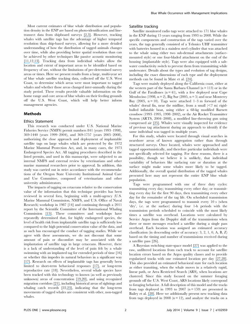
While the whale tracks were distributed over a wide area, they

tended to occupy the more northerly portion of the range during

the latter part of the feeding season in late October-November

(Figure 4). The trend was most pronounced in 2005, with 1999

and 2008 showing relatively little northward movement (Figures

S10 & S11). Track durations were sufficiently long that EEZ

departure days were recorded for 48 tracks in nine years (Table 1).

Tracks with recorded departure days did not always meet the 30-d

home-range criterion, as some whales began their southerly

Blue Whale Occurrence with Management Implications

PLOS ONE | www.plosone.org 3 July 2014 | Volume 9 | Issue 7 | e102959

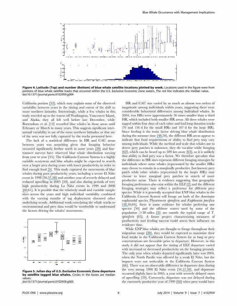
migration shortly after being tagged. Tagged whales typically

departed the EEZ in October (mean = 21 October) although it

ranged from as early as late July (in 1999) to as late as 11 January

(in 2004, represented as Julian day 375; Figure 5). Departure from

the EEZ was significantly later in 2004 than all other years

(p = 0.004, F1,47 = 8.915, ANOVA), with no significant difference

in departure date for the other years (p = 0.775, F7,40 = 0.571,

ANOVA). No measures of ARS foraging behavior (number of

ARS patches/track, average ARS patch duration, longest ARS

patch duration, duration of the last ARS patch, and overall

fraction of all track locations that were classified as ARS behavior)

had a significant effect on the departure date (p = 0.159, 0.668,

0.271, 0.925, and 0.608 respectively from linear regression).

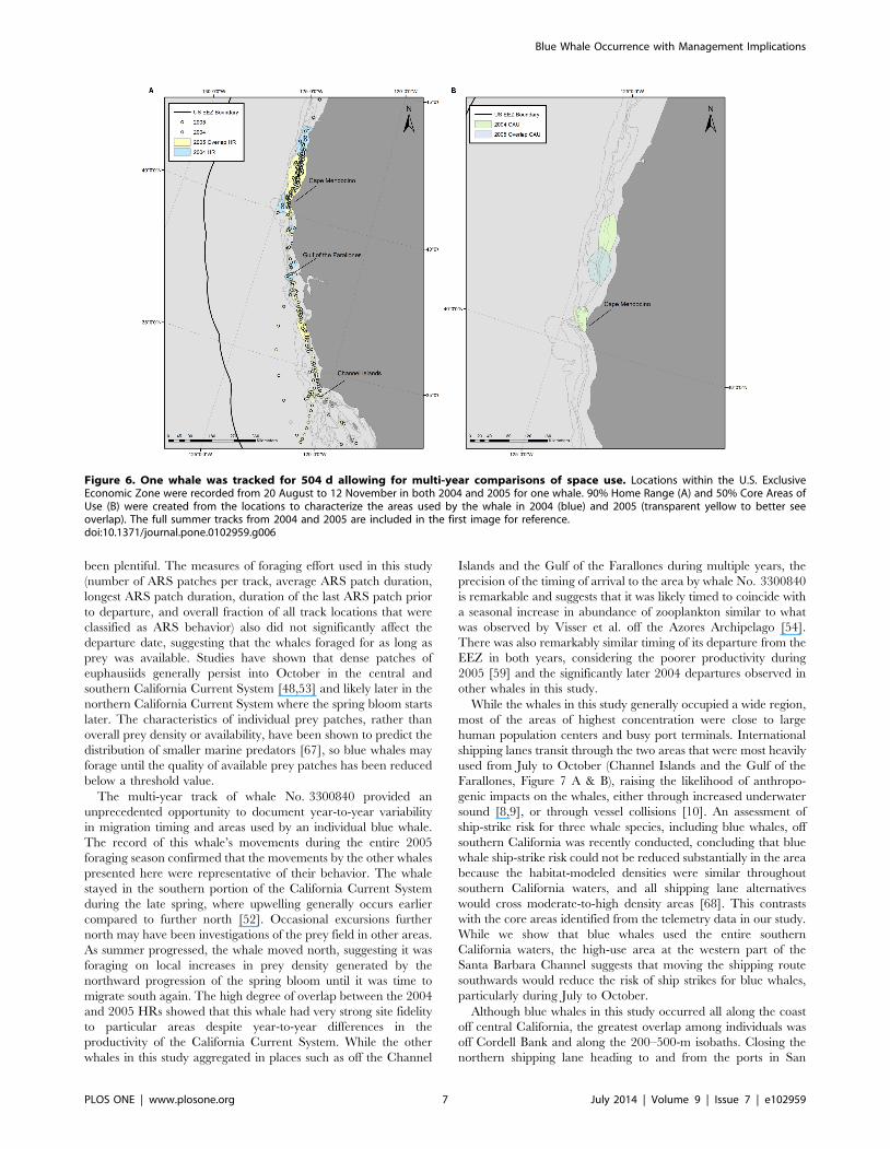
The multi-year track of whale No. 3300840 allowed us to

characterize its entire EEZ range in 2005, as well as any variability

in distribution between 2004 and 2005. The whale spent the

majority of its time before departure in 2004 in the area north of

Cape Mendocino after being tagged in the Gulf of the Farallones

on 20 August 2004. It arrived at the Channel Islands again in late

April 2005 but immediately turned south and spent May near

Ensenada, Mexico. The whale returned to the Channel Islands in

early June and spent most of its time there with occasional

northward excursions to the Gulf of the Farallones, until mid-

August when it again moved to the area north of Cape

Mendocino, arriving in 2005 only one week earlier than in the

previous year. The whale departed the EEZ on 12 November

2005, one week prior to its departure in 2004. A HR created from

the period temporally overlapping in summer 2004 and 2005 was

slightly larger in 2004 than 2005 (HR 20,800 km2 vs. 18,200 km2)

but overall 66% of the 2005 HR overlapped with that in 2004

(Figure 6A). If we consider the largest contiguous HR areas from

each year, 89% of the area from 2005 overlapped with that from

the same period in 2004, showing very high site fidelity between

years. The CAU in 2004 was almost twice the size of 2005

(4863 km2 vs. 2632 km2) and showed a lower percentage of

overlap between years than the HRs with 47% of the 2005 CAU

overlapping with the 2004 CAU (Figure 6B).

Discussion

This data set represents the largest and most comprehensive

collection of tracking data for any whale species. Considering that

tagging occurred at several locales along the coast of California

over multiple years, it is likely that this data set represents the

majority of movement patterns of ENP blue whales off the U.S.

West Coast. However, since ENP blue whales range widely

[2,5,11], there may be other important areas along the coasts of

Table 1. Summary of satellite tagged blue whale tracks.

YearNumber of Tags w/. = 30 USEEZ locs

Number of Tags w/DepartureDay

1993 0 0 Surface Mount Crossbow Deployed

1995 0 3 median duration = 0.5 d, range: 0–81 d, n = 52

1998 3 4 Implantable Crossbow Deployed

1999 7 11 median duration = 58 d, range: 0–306, n = 44

2000 1 2

2004 11 5

2005 12 6 Implantable ARTS Deployed

2006 2 4 median duration = 85 d, range: 0–504 d, n = 75

2007 7 8

2008 10 5

total 53 48

Number of tracks with . = 30 locations in the U.S. Exclusive Economic Zone waters and the number of tracks that departed U.S. Exclusive Economic Zone waters listedby year. Deployment method and duration summary for all tags deployed is listed to the right.doi:10.1371/journal.pone.0102959.t001

Figure 1. Blue whale 90% Home Range area (A) and 50% Core Area of Use (B). Kernel derived Home Ranges and Core Areas of Use werecreated from blue whale satellite tracks with . = 30 daily locations inside the U.S. Exclusive Economic Zone. Tags were deployed off California from1998–2008. Data are presented by year on a log scale and the circles inside the boxes are median values.doi:10.1371/journal.pone.0102959.g001

Blue Whale Occurrence with Management Implications

PLOS ONE | www.plosone.org 4 July 2014 | Volume 9 | Issue 7 | e102959

Canada and Alaska, or further offshore, that may be less well

represented in our data (Figures S1 & S2).

The blue whales in this study were generally concentrated in

regions of typically high summer productivity along the upper

continental slope from central to southern California. Summer

upwelling throughout the California Current System produces

high concentrations of euphausiids [44], while currents and

bathymetric features aggregate them [45,46], creating patches

dense enough for blue whales to profitably feed on. The two areas

of highest use were near the Gulf of the Farallones and at the

western part of the Channel Islands. Both locations are sites of

active upwelling, primary productivity, and krill [47,48,49,50] and

places where blue whales traditionally congregate [50]. Other

regions of high krill density along central California presented in

Santora et al. [47] also correspond to a large extent with the blue

whale HRs and CAUs presented here, indicating a close

association between high krill abundance and blue whale presence

throughout the EEZ. The relatively low degree of overall CAU

overlap compared to the amount of HR overlap throughout the

tagged whales’ summer range suggests that, while blue whales

return to the same broad area to forage in predictable prey

habitat, they will focus their foraging effort in different fine-scale

areas within this range based on where they find specific prey

patches. A similar pattern was found for fin whales in the

Mediterranean [51].

The northward progression of tagged whale locations later in

the season (Figure 4) confirms the findings of Burtenshaw et al.

[12] that the location of calling blue whales shifted northward

from late summer into winter. The trend follows the timing of

productivity generated by the spring bloom as it moves north

along the California coast [12,52]. Upwelling off southern

California (33–36uN) occurs nearly year round, though at only

moderate intensity [52]. The upwelling season occurs later and

gets progressively shorter with increasing latitudes, and the

greatest intensity of upwelling, and therefore, the region of highest

productivity, occurs off northern California (36–42uN) [52].

Aggregations of euphausiids that are dense enough for blue

whales to forage on have been shown to lag increases in primary

productivity by 1–4 months [48,53,54]. The maximum rate of

upwelling in the California Current System occurs from early-mid

June off southern California to mid-August off northern California

and Oregon [52], suggesting the whales may arrive in southern

California early in the summer to forage on prey generated there

by the moderate, early productivity until more intense upwelling to

the north has developed and the density of prey increased. While

the northern California portion of the California Current System

produces greater upwelling intensity, the variability in timing and

overall productivity of the region is much higher than the southern

Figure 2. Individual overlapping 90% Home Range areas (A) and 50% Core Areas of Use (B). Kernel derived Home Ranges and Core Areasof Use were created from blue whale satellite tracks with . = 30 daily locations inside the U.S. Exclusive Economic Zone. Shading in the figurerepresents the number of individual home range and core areas of use that are overlapping in that area. Number of overlapping areas was used as ametric to characterize how much an area was used by the tagged whales. Tags were deployed off California from 1998–2008.doi:10.1371/journal.pone.0102959.g002

Figure 3. Relative time spent by satellite tagged blue whales inquarter degree grid cells. Relative time spent was calculated fromsatellite-tagged blue whale tracks using weighted locations to accountfor unequal tracking durations among individuals. Tags were deployedoff California from 1998–2008.doi:10.1371/journal.pone.0102959.g003

Blue Whale Occurrence with Management Implications

PLOS ONE | www.plosone.org 5 July 2014 | Volume 9 | Issue 7 | e102959

California portion [52], which may explain some of the observed

variability between years in the timing and extent of the shift to

more northern latitudes. Interestingly, while a few whales in this

study traveled up to the waters off Washington, Vancouver Island,

and Alaska, they all left well before late December, while

Burtenshaw et al. [12] recorded blue whales in those areas until

February or March in many years. This suggests significant inter-

annual variability in use of the more northern latitudes, or that use

of the area was not fully captured by the tracks presented here.

The lack of a statistical difference in HR and CAU areas

between years was surprising given that foraging behavior

occurred significantly farther north in some years [28] and line-

transect surveys have observed blue whale distribution varying

from year to year [55]. The California Current System is a highly

variable ecosystem and blue whales might be expected to search

over a larger area during years with lower productivity in order to

find enough food [5]. This study captured the movements of blue

whales during poor productivity years, including a severe El Nino

event in 1998 [56,57,58] and another year of severely delayed and

reduced upwelling in 2005 [59], and also during periods of very

high productivity during La Nina events in 1999 and 2008

[60,61]. It is possible that the relatively small and variable sample

sizes across the years and high individual variability combined

with the varying months of tag deployment obscured other

underlying trends. Additional work correlating the whale tracks to

environmental and prey data would be worthwhile to understand

the factors driving the whales’ movements.

HR and CAU size varied by as much as almost two orders of

magnitude among individuals within years, suggesting there were

considerable behavioral differences among individual whales. In

2004, two HRs were approximately 36 times smaller than a third

HR, which included both smaller HR areas. All three whales were

tagged within four days of each other and had long duration tracks

(76 and 156 d for the small HRs and 107 d for the large HR).

Since feeding is the main factor driving blue whale distribution

during the summer time [48,50], the different HR areas appear to

indicate that food requirements or ability to find prey may vary

among individuals. While the method and scale that whales use to

detect prey patches is unknown, they do vocalize while foraging

[62], which can be heard up to 500 km away [63], so it is unlikely

that ability to find prey was a factor. We therefore speculate that

the difference in HR sizes represent different foraging strategies by

individuals where some whales (represented by the smaller HRs)

may choose to remain in a marginally productive (but known) prey

patch while other whales (represented by the larger HRs) may

choose to leave marginal prey patches in search of more

productive areas. There is evidence suggesting that geographic

foraging preferences also exist within the EEZ [2] and the different

foraging strategies may reflect a preference for different prey

species. While it is generally accepted that ENP blue whales in the

California Current System will forage on both of the dominant

euphausiid species Thysanoessa spinifera and Euphausia pacifica[48,50,64], there is some evidence for whales preferring one

species [50] and the offshore waters used by some of the

population (.30 miles [2]) are outside the typical range of T.spinifera [65]. A future project characterizing measures of

productivity and feeding success could assess their influence on

residence time.

While ENP blue whales are thought to forage throughout their

migration range [28], they would be expected to maximize their

food intake in the California Current System for as long as prey

concentrations are favorable prior to departure. However, in this

study it did not appear that the timing of EEZ departure varied

with increased or decreased productivity on the foraging grounds.

The only year when whales departed significantly later was 2004,

when the North Pacific was affected by a weak El Nino, but the

impacts were not noticeable in the California Current System

[66]. There was no observable difference in departure date during

the very strong 1998 El Nino event [56,57,58], and departure

occurred slightly later in 2005, a year with severely delayed onset

of upwelling [59]. Conversely, departure was not delayed during

the extremely productive year of 1999 [60] when prey would have

Figure 4. Latitude (Top) and number (Bottom) of blue whale satellite locations plotted by week. Locations used in the figure were fromportions of blue whale satellite tracks that occurred within the U.S. Exclusive Economic Zone waters. The red line indicates the median value.doi:10.1371/journal.pone.0102959.g004

Figure 5. Julian day of U.S. Exclusive Economic Zone departureby satellite tagged blue whales. Circles in the boxes are medianvalues.doi:10.1371/journal.pone.0102959.g005

Blue Whale Occurrence with Management Implications

PLOS ONE | www.plosone.org 6 July 2014 | Volume 9 | Issue 7 | e102959

been plentiful. The measures of foraging effort used in this study

(number of ARS patches per track, average ARS patch duration,

longest ARS patch duration, duration of the last ARS patch prior

to departure, and overall fraction of all track locations that were

classified as ARS behavior) also did not significantly affect the

departure date, suggesting that the whales foraged for as long as

prey was available. Studies have shown that dense patches of

euphausiids generally persist into October in the central and

southern California Current System [48,53] and likely later in the

northern California Current System where the spring bloom starts

later. The characteristics of individual prey patches, rather than

overall prey density or availability, have been shown to predict the

distribution of smaller marine predators [67], so blue whales may

forage until the quality of available prey patches has been reduced

below a threshold value.

The multi-year track of whale No. 3300840 provided an

unprecedented opportunity to document year-to-year variability

in migration timing and areas used by an individual blue whale.

The record of this whale’s movements during the entire 2005

foraging season confirmed that the movements by the other whales

presented here were representative of their behavior. The whale

stayed in the southern portion of the California Current System

during the late spring, where upwelling generally occurs earlier

compared to further north [52]. Occasional excursions further

north may have been investigations of the prey field in other areas.

As summer progressed, the whale moved north, suggesting it was

foraging on local increases in prey density generated by the

northward progression of the spring bloom until it was time to

migrate south again. The high degree of overlap between the 2004

and 2005 HRs showed that this whale had very strong site fidelity

to particular areas despite year-to-year differences in the

productivity of the California Current System. While the other

whales in this study aggregated in places such as off the Channel

Islands and the Gulf of the Farallones during multiple years, the

precision of the timing of arrival to the area by whale No. 3300840

is remarkable and suggests that it was likely timed to coincide with

a seasonal increase in abundance of zooplankton similar to what

was observed by Visser et al. off the Azores Archipelago [54].

There was also remarkably similar timing of its departure from the

EEZ in both years, considering the poorer productivity during

2005 [59] and the significantly later 2004 departures observed in

other whales in this study.

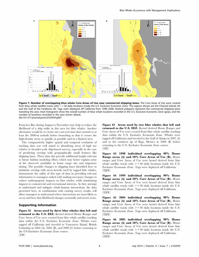
While the whales in this study generally occupied a wide region,

most of the areas of highest concentration were close to large

human population centers and busy port terminals. International

shipping lanes transit through the two areas that were most heavily

used from July to October (Channel Islands and the Gulf of the

Farallones, Figure 7 A & B), raising the likelihood of anthropo-

genic impacts on the whales, either through increased underwater

sound [8,9], or through vessel collisions [10]. An assessment of

ship-strike risk for three whale species, including blue whales, off

southern California was recently conducted, concluding that blue

whale ship-strike risk could not be reduced substantially in the area

because the habitat-modeled densities were similar throughout

southern California waters, and all shipping lane alternatives

would cross moderate-to-high density areas [68]. This contrasts

with the core areas identified from the telemetry data in our study.

While we show that blue whales used the entire southern

California waters, the high-use area at the western part of the

Santa Barbara Channel suggests that moving the shipping route

southwards would reduce the risk of ship strikes for blue whales,

particularly during July to October.

Although blue whales in this study occurred all along the coast

off central California, the greatest overlap among individuals was

off Cordell Bank and along the 200–500-m isobaths. Closing the

northern shipping lane heading to and from the ports in San

Figure 6. One whale was tracked for 504 d allowing for multi-year comparisons of space use. Locations within the U.S. ExclusiveEconomic Zone were recorded from 20 August to 12 November in both 2004 and 2005 for one whale. 90% Home Range (A) and 50% Core Areas ofUse (B) were created from the locations to characterize the areas used by the whale in 2004 (blue) and 2005 (transparent yellow to better seeoverlap). The full summer tracks from 2004 and 2005 are included in the first image for reference.doi:10.1371/journal.pone.0102959.g006

Blue Whale Occurrence with Management Implications

PLOS ONE | www.plosone.org 7 July 2014 | Volume 9 | Issue 7 | e102959

Francisco Bay during August to November may help to reduce the

likelihood of a ship strike in this area for blue whales. Another

alternative would be to create one east-west lane that extends to at

least the 2000-m isobath before branching so that it crosses the

high-density areas as quickly as possible and in a limited area.

The comparatively higher spatial and temporal resolution of

tracking data was well suited to identifying areas of high use

relative to broader-scale ship-based surveys, especially in the case

of predicting overlap with geographically small features like

shipping lanes. These data also provide additional insight relevant

to future habitat modeling effort, which may better explain some

of the observed variability in home range size and migratory

timing. The possible changes to shipping lanes identified here to

minimize overlap with areas heavily used by tagged blue whales,

demonstrate the utility of this type of data in providing relevant

information to managers tasked with making necessary changes to

reduce anthropogenic impacts on blue whales, while minimizing

impacts to commercial and recreational interests. As they attempt

to understand and mitigate whale-human interactions, the data

presented here, in combination with existing survey results, will

allow managers to understand where interactions are most likely to

occur and how that likelihood changes seasonally and across years.

Supporting Information

Figure S1 Areas used by three blue whales that left andreturned to the U.S. EEZ. Kernel derived Home Ranges and

Core Areas of Use were created from blue whale satellite tracking

data within the U.S. Exclusive Economic Zone. Whales were

tagged off California and traveled to Vancouver Island, British

Columbia in 2004 (A), 2005 (B), and 2008 (C) before returning to

the US Exclusive Economic Zone waters.

(TIF)

Figure S2 Areas used by two blue whales that left andreturned to the U.S. EEZ. Kernel derived Home Ranges and

Core Areas of Use were created from blue whale satellite tracking

data within the U.S. Exclusive Economic Zone. Whales were

tagged off California and traveled to the Gulf of Alaska in 2007 (A)

and to the southern tip of Baja, Mexico in 2008 (B) before

returning to the U.S. Exclusive Economic Zone waters.

(TIF)

Figure S3 1998 individual overlapping 90% HomeRange areas (A) and 50% Core Areas of Use (B). Home

ranges and Core Areas of Use were kernel derived from blue

whale satellite tracks with . = 30 daily locations inside the U.S.

Exclusive Economic Zone. Tags were deployed off California.

(TIFF)

Figure S4 1999 individual overlapping 90% HomeRange areas (A) and 50% Core Areas of Use (B). Home

ranges and Core Areas of Use were kernel derived from blue

whale satellite tracks with . = 30 daily locations inside the U.S.

Exclusive Economic Zone. Tags were deployed off California.

(TIFF)

Figure S5 2004 individual overlapping 90% HomeRange areas (A) and 50% Core Areas of Use (B). Home

ranges and Core Areas of Use were kernel derived from blue

whale satellite tracks with . = 30 daily locations inside the U.S.

Exclusive Economic Zone. Tags were deployed off California.

(TIFF)

Figure S6 2005 individual overlapping 90% HomeRange areas (A) and 50% Core Areas of Use (B). Home

ranges and Core Areas of Use were kernel derived from blue

whale satellite tracks with . = 30 daily locations inside the U.S.

Exclusive Economic Zone. Tags were deployed off California.

(TIFF)

Figure 7. Number of overlapping blue whale Core Areas of Use near commercial shipping lanes. The Core Areas of Use were createdfrom blue whale satellite tracks with . = 30 daily locations inside the U.S. Exclusive Economic Zone. The regions shown are the Channel Islands (A)and the Gulf of the Farallones (B). Tags were deployed off California from 1998–2008. Hashed polygons represent the commercial shipping lanestransiting the area. Inset histograms show the overall number of blue whale locations recorded in the U.S. Exclusive Economic Zone (gray), and thenumber of locations recorded in the area shown (black).doi:10.1371/journal.pone.0102959.g007

Blue Whale Occurrence with Management Implications

PLOS ONE | www.plosone.org 8 July 2014 | Volume 9 | Issue 7 | e102959

Figure S7 2006 individual overlapping 90% HomeRange areas (A) and 50% Core Areas of Use (B). Home

ranges and Core Areas of Use were kernel derived from blue

whale satellite tracks with . = 30 daily locations inside the U.S.

Exclusive Economic Zone. Tags were deployed off California.

(TIFF)

Figure S8 2007 individual overlapping 90% HomeRange areas (A) and 50% Core Areas of Use (B). Home

ranges and Core Areas of Use were kernel derived from blue

whale satellite tracks with . = 30 daily locations inside the U.S.

Exclusive Economic Zone. Tags were deployed off California.

(TIFF)

Figure S9 2008 individual overlapping 90% HomeRange areas (A) and 50% Core Areas of Use (B). Home

ranges and Core Areas of Use were kernel derived from blue

whale satellite tracks with . = 30 daily locations inside the U.S.

Exclusive Economic Zone. Tags were deployed off California.

(TIFF)

Figure S10 Latitude of blue whale locations from 1998(A), 1999 (B), 2000 (C), and 2004 (D). Locations used in the

figure were from portions of blue whale satellite tracks that

occurred within the U.S. Exclusive Economic Zone waters. The

red line indicates the median value.

(TIF)

Figure S11 Latitude of blue whale locations from 2005(E), 2006 (F), 2007 (G), and 2008 (H). Locations used in the

figure were from portions of blue whale satellite tracks that

occurred within the U.S. Exclusive Economic Zone waters. The

red line indicates the median value.

(TIF)

Acknowledgments

We thank the many people who assisted with tagging, including Craig

Hayslip, Barbara Lagerquist, and Tomas Follett, as well as the various

crews of the R/V Pacific Storm. Joel Ortega originated the idea of

overlaying individual home ranges as a metric to characterize how much

an area was used by tagged whales. Michelle Ferraro helped with data

formatting for parts of the analysis. Jennifer Oleson helped compile data for

the analysis. The crew of the M/V Condor Express provided helpful

information on blue whale sightings during fieldwork. We also thank Karin

Forney for her constructive comments on the manuscript. This is

Contribution 4922 of the University of Maryland Center for Environ-

mental Science, Chesapeake Biological Laboratory.

Author Contributions

Conceived and designed the experiments: LI BM. Performed the

experiments: LI BM MW. Analyzed the data: LI HB DP. Contributed

reagents/materials/analysis tools: HB. Wrote the paper: LI BM MW DP

SB DC HB.

References

1. Gregr EJ, Nichol L, Ford JKB, Ellis G, Trites AW (2000) Migration and

population structure of northeastern Pacific whales off coastal British Columbia:

an analysis of commercial whaling records from 1908–1967. Mar Mamm Sci 16:

699–727.

2. Calambokidis J, Barlow J (2004) Abundance of blue and humpback whales in the

eastern North Pacific estimated by capture-recapture and line-transect methods.

Mar Mamm Sci 20: 63–85.

3. Barlow J, Forney KA (2007) Abundance and population density of cetaceans in

the California Current ecosystem. Fish Bull 105: 509–526.

4. Calambokidis J, Falcone EA, Douglas A, Schlender L, Huggins J (2010)

Photographic identification of humpback and blue whales off the U.S. West

Coast: results and updated abundance estimates from 2008 field season. Final

Report for Contract AB133F08SE2786 from Southwest Fisheries Science

Center. 18. Available: http://cascadiaresearch.org.

5. Calambokidis J, Barlow J, Ford JKB, Chandler TE, Douglas AB (2009) Insights

into the population structure of blue whales in the Eastern North Pacific from

recent sightings and photographic identification. Mar Mamm Sci 25: 816–832.

6. International Whaling Commission (1967) Seventeenth report of the commis-

sion. Rep Int Whal Comm 17: 1:138.

7. Pauly D, Christensen V, Dalsgaard J, Froese R, Torres F (1998) Fishing down

marine food webs. Science 279: 860–863.

8. Weilgart LS (2007) The impacts of anthropogenic ocean noise on cetaceans and

implications for management. Can J Zool 85: 1091–1116.

9. Melcon ML, Cummins AJ, Kerosky SM, Roche LK, Wiggins SM, et al. (2012)

Blue Whales Respond to Anthropogenic Noise. PLoS ONE 7.

10. Berman-Kowalewski M, Gulland FMD, Wilkin S, Calambokidis J, Mate B, et al.

(2010) Association Between Blue Whale (Balaenoptera musculus) Mortality and

Ship Strikes Along the California Coast. Aquat Mam 36: 59–66.

11. Stafford KM, Nieukirk SL, Fox CG (2001) Geographic and seasonal variation of

blue whale calls in the North Pacific. J Cetacean Res Manage 3: 65–76.

12. Burtenshaw JC, Oleson EM, Hildebrand JA, McDonald MA, Andrew RK, et al.

(2004) Acoustic and satellite remote sensing of blue whale seasonality and habitat

in the Northeast Pacific. Deep Sea Res II 51: 967–986.

13. Oleson EM, Calambokidis J, Barlow J, Hildebrand JA (2007) Blue whale visual

and acoustic encounter rates in the Southern California Bight. Mar Mamm Sci

23: 574–597.

14. Montgomery S (1987) Workshop to assess possible systems for tracking large

cetaceans MMS Study 87-0029. NTIS PB87-182135.

15. International Whaling Commission (2011) Report of the Scientific Committee.

Annex F. Report of the sub-committee on bowhead, right, and gray whales.

J Cetacean Res Manage (Suppl) 13: 154–174.

16. Moore M, Andrews R, Austin T, Bailey J, Costidis A, et al. (2013) Rope trauma,

sedation, disentanglement, and monitoring-tag associated lesions in a terminally

entangled North Atlantic right whale (Eubalaena glacialis). Mar Mamm Sci 29:

E98–E113.

17. Walker KA, Trites AW, Haulena M, Weary DM (2012) A review of the effects of

different marking and tagging techniques on marine mammals. Wildlife Res 39:

15–30.

18. Best PB, Mate BR (2007) Sighting history and observations of southern right

whales following satellite tagging off South Africa. J Cetacean Res Manage 9:

111–114.

19. Mate B, Best PB, Lagerquist B, Winsor MH (2011) Coastal, offshore, and

migratory movements of South African right whales revealed by satellite

telemetry. Mar Mamm Sci 27: 455–476.

20. Baumgartner MF, Mate BR (2005) Summer and fall habitat of North Atlantic

right whales (Eubalaena glacialis) inferred from satellite telemetry. Can J FishAquat Sci 62: 527–543.

21. Mate B, Urban RJ (2003) A note on the route and speed of a gray whale on its

northern migration from Mexico to central California, tracked by satellite-monitored radio tag. J Cetacean Res Manage 5: 155–157.

22. Zerbini A, Andriolo A, Heide-Jorgensen Mads P, Pizzorno JL, Maia YG, et al.

(2006) Satellite-monitored movements of humpback whales Megaptera novan-gliae in the Southwest Atlantic Ocean. Mar Ecol Prog Ser 313: 295–304.

23. Double MC, Andrews-Goff V, Jenner KCS, Jenner MN, Laverick SM, et al.(2014) Migratory movements of pigmy blue whales (Balaenoptera musculus

brevicauda) between Australia and Indonesia as revealed by Satellite Telemetry.

PLoS ONE 9: 1–11.

24. Mate BR, Mesecar R, Lagerquist B (2007) The evolution of satellite-monitored

radio tags for large whales: one laboratory’s experience. Deep-Sea Res II 54:

224–247.

25. Heide-Jørgensen MP, Kleivane L, Øien N, Laidre KL, Jensen MV (2001) A new

technique for deploying satellite transmitters on baleen whales: tracking a blue

whale (Balaenoptera musculus) in the North Atlantic. Mar Mamm Sci 17: 949–954.

26. Argos (2014) Argos User’s Manual 2007–2014. In: (CLS) CLS, editor.

27. Jonsen ID, Flemming JM, Myers RA (2005) Robust state-space modeling of

animal movement data. Ecology 86: 2874–2880.

28. Bailey H, Mate B, Palacios D, Irvine L, Bograd SJ, et al. (2010) Behaviouralestimation of blue whale movements in the Northeast Pacific from state-space

model analysis of satellite tracks. Endanger Species Res 10: 93–106.

29. UN General Assembly (1982) Convention on the Law of the Sea. Available:http://www.refworld.org/docid/3dd8fd1b4.html. Accessed 2013 Nov 20.

30. Gautestad AO, Mysterud I (2005) Intrinsic scaling complexity in animaldispersion and abundance. Am Nat 165: 44–55.

31. Rhodes JR, McAlpine CA, Lunney D, Possingham HP (2005) A spatially explicit

habitat selection model incorporating home range behavior. Ecology 86: 1199–1205.

32. Marzluff JM, Millspaugh JJ, Hurvitz P, Handcock MS (2004) Relating resources

to a probabilistic measure of space use: Forest fragments and Steller’s Jays.Ecology 85: 1411–1427.

33. Lewis MA, Murray JD (1993) Modeling Territoriality and Wolf Deer

Interactions. Nature 366: 738–740.

Blue Whale Occurrence with Management Implications

PLOS ONE | www.plosone.org 9 July 2014 | Volume 9 | Issue 7 | e102959

34. Borger L, Dalziel BD, Fryxell JM (2008) Are there general mechanisms of

animal home range behaviour? A review and prospects for future research. Ecol

Lett 11: 637–650.

35. Getz WM, Fortmann-Roe S, Cross PC, Lyons AJ, Ryan SJ, et al. (2007) LoCoH:

Nonparametric kernel methods for constructing home ranges and utilization

distributions. PLoS ONE 2: e207.

36. Kernohan BJ, Glitzen RA, Millspaugh JJ (2001) Analysis of animal space use

and movements. In: Millspaugh JJ, Marzluff J, editors. Radiotracking and

Animal Populations. San Diego: Academic Press. pp. 126–166.

37. Worton BJ (1995) Using Monte-Carlo Simulation to Evaluate Kernel-Based

Home-Range Estimators. J Wildl Manage 59: 794–800.

38. Powell RA (2000) Animal Home Ranges and Territories and Home Range

Estimators. In: Boitani L, Fuller TK, editors. Research Techniques in Animal

Ecology: Controversies and Consequences. New York, NY: Columbia

University Press. pp. 65–110.

39. Calenge C (2006) The package ‘‘adehabitat’’ for the R software: A tool for the

analysis of space and habitat use by animals. Ecol Model 197: 516–519.

40. Team RDC (2008) R: A language and environment for statistical computing.

Vienna, Austria: R Foundation for Statistical Computing.

41. Seaman DE, Millspaugh JJ, Kernohan BJ, Brundige GC, Raedeke KJ, et al.

(1999) Effects of sample size on kernel home range estimates. Journal of Wildlife

Management 63: 739–747.

42. Borger L, Franconi N, De Michele G, Gantz A, Meschi F, et al. (2006) Effects of

sampling regime on the mean and variance of home range size estimates. J Anim

Ecol 75: 1393–1405.

43. Block BA, Jonsen ID, Jorgensen SJ, Winship AJ, Shaffer SA, et al. (2011)

Tracking apex marine predator movements in a dynamic ocean. Nature 475:

86–90.

44. Checkley DM, Barth JA (2009) Patterns and processes in the California Current

System. Progress in Oceanography 83: 49–64.

45. Wing SR, Botsford LW, Ralston SV, Largier JL (1998) Meroplanktonic

distribution and circulation in a coastal retention zone of the northern California

upwelling system. Limnol Ocenogr 43: 1710–1721.

46. Graham WM, Field JG, Potts DC (1992) Persistent Upwelling Shadows and

Their Influence on Zooplankton Distributions. Marine Biology 114: 561–570.

47. Santora JA, Sydeman WJ, Schroeder ID, Wells BK, Field JC (2011) Mesoscale

structure and oceanographic determinants of krill hotspots in the California

Current: Implications for trophic transfer and conservation. Prog Oceanogr 91:

397–409.

48. Croll DA, Marinovic B, Benson S, Chavez FP, Black N, et al. (2005) From wind

to whales: trophic links in a coastal upwelling system. Mar Ecol Prog Ser 289:

117–130.

49. Palacios DM, Bograd SJ, Foley DG, Schwing FB (2006) Oceanographic

characteristics of biological hot spots in the North Pacific: A remote sensing

perspective. Deep-Sea Res II 53: 250–269.

50. Fiedler PC, Reilly SB, Hewitt RP, Demer D, Philbrick VA, et al. (1998) Blue

whale habitat and prey in the California Channel Islands. Deep-Sea Res II 45:

1781–1801.

51. Cotte C, Guinet C, Taupier-Letage I, Mate B, Petiau E (2009) Scale-dependent

habitat use by a large free-ranging predator, the Mediterranean fin whale. Deep-Sea Research I 56: 801–811.

52. Bograd SJ, Schroeder I, Sarkar N, Qiu XM, Sydeman WJ, et al. (2009)

Phenology of coastal upwelling in the California Current. Geophys Res Let 36.53. Hayward TL, Venrick EL (1998) Nearsurface pattern in the California Current:

coupling between physical and biological structure. Deep-Sea Res II 45: 1617–1638.

54. Visser F, Hartman KL, Pierce GJ, Valavanis VD, Huisman J (2011) Timing of

migratory baleen whales at the Azores in relation to the North Atlantic springbloom. Mar Ecol Prog Ser 440: 267–279.

55. Peterson B, Emmett R, Goericke R, Venrick E, Mantyla A, et al. (2006) Thestate of the California current, 2005–2006: Warm in the North, cool in the

South. CalCOFI Reports 47: 30–74.56. Chavez FP, Pennington JT, Castro CG, Ryan JP, Michisaki RP, et al. (2002)

Biological and chemical consequences of the 1997–1998 El Nino in central

California waters. Prog Oceanogr 54: 205–232.57. Chavez FP, Collins CA, Huyer A, Mackas DL (2002) El Nino along the west

coast of North America. Prog Oceanogr 54: 1–5.58. McPhaden MJ (1999) Genesis and evolution of the 1997–98 El Nino. Science

283: 950–954.

59. Schwing FB, Bond NA, Bograd SJ, Mitchell T, Alexander MA, et al. (2006)Delayed coastal upwelling along the U.S. West Coast in 2005: A historical

perspective. Geophys Res Lett 33: L22S01.60. Bograd SJ, Lynn RJ (2001) Physical-biological coupling in the California

Current during the 1997–99 El Nino-La Nina cycle. Geophys Res Lett 28: 275–278.

61. McClatchie S, Charter R, Watson W, Lo N, Hill K, et al. (2009) The State of the

California Current, Spring 2008–2009 Cold Conditions Drive RegionalDifferences in Coastal Production. CalCOFI Reports 50: 43–68.

62. Oleson EM, Calambokidis J, Burgess WC, McDonald MA, LeDuc CA, et al.(2007) Behavioral context of call production by eastern North Pacific blue

whales. Mar Ecol Prog Ser 330: 269–284.

63. Watkins WA, Daher MA, Reppucci GM, George JE, Martin DL, et al. (2000)Seasonality and distribution of whale calls in the north Pacific. Oceanogr 13: 62–

67.64. Croll DA, Tershy BR, Hewitt RP, Demer DA, Fiedler PC, et al. (1998) An

integrated approach to the foraging ecology of marine birds and mammals.Deep-Sea Res II 45: 1353–1371.

65. Brinton E (1962) The distribution of Pacific euphausiids. B Scripps Inst

Oceanogr 8: 51–269.66. Goericke R, Venrick E, Mantyla A, Bograd SJ, Schwing FB, et al. (2005) The

state of the California current, 2004–2005: Still cool? CalCOFI Reports 46: 32–71.

67. Benoit-Bird KJ, Battaile BC, Heppell SA, Hoover B, Irons D, et al. (2013) Prey

Patch Patterns Predict Habitat Use by Top Marine Predators with DiverseForaging Strategies. PLoS ONE 8.

68. Redfern JV, Mckenna MF, Moore TJ, Calambokidis J, Deangelis ML, et al.(2013) Assessing the Risk of Ships Striking Large Whales in Marine Spatial

Planning. Cons Bio 27: 292–302.

Blue Whale Occurrence with Management Implications

PLOS ONE | www.plosone.org 10 July 2014 | Volume 9 | Issue 7 | e102959