W&M ScholarWorks W&M ScholarWorks

Dissertations, Theses, and Masters Projects Theses, Dissertations, & Master Projects

2011

Spatial and Temporal Analysis of Fecal Coliform Distribution in Spatial and Temporal Analysis of Fecal Coliform Distribution in

Virginia Coastal Waters Virginia Coastal Waters

Jie Huang College of William and Mary - Virginia Institute of Marine Science

Follow this and additional works at: https://scholarworks.wm.edu/etd

Part of the Environmental Health and Protection Commons, and the Natural Resources Management

and Policy Commons

Recommended Citation Recommended Citation Huang, Jie, "Spatial and Temporal Analysis of Fecal Coliform Distribution in Virginia Coastal Waters" (2011). Dissertations, Theses, and Masters Projects. Paper 1539616702. https://dx.doi.org/doi:10.25773/v5-t4n1-cv18

This Dissertation is brought to you for free and open access by the Theses, Dissertations, & Master Projects at W&M ScholarWorks. It has been accepted for inclusion in Dissertations, Theses, and Masters Projects by an authorized administrator of W&M ScholarWorks. For more information, please contact scholarworks@wm.edu.

Spatial and Temporal Analysis of Fecal Coliform Distribution in Virginia Coastal Waters

A Dissertation Presented to

The Faculty of the School of Marine Science The College of William and Mary in Virginia

In Partial Fulfillment of the Requirement for the Degree of

Doctor of Philosophy

By

Jie Huang

December 2010

APPROVAL SHEET

This Dissertation is submitted in partial fulfillment of

the requirements for the degree of

Doctor of Philosophy

Ji~H~ JieH

Carl H. er ner, Ph. D. Committee Chairman/ Advisor

!1·c . - !piwV '7) /h, j 'v v' Jian Shen, Ph.D.

Co-Advisor

,~~DMa i/4 Jjj;u Donna if Bilkovic, Ph.D.

J L~/C~ /.Jv,v--,_ Julie Herman, Ph.D.

11~£~&~ \flo ward Kator ~Ph.D.

~~~ Robert E. Croonenberghs, h.D. Virginia Department of Health,

Division of Shellfish Sanitation, Richmond, Virginia.

TABLE OF CONTENTS

LIST OF TABLES ....................................................................................................... iv

LIST OF FIGURES ..................................................................................................... vi

ACKNOLEDGEMENT ................................................................................................. x

ABSTRACT .................................................................................................................. xi

I. INTRODUCTION .................................................................................................. 1

II. OBJECTIVES .......................................................................................................... 5

III. BACKGROUND AND LITERATURE REVIEW ................................................ 7

III-I. Background ............................................................................................... 7 III-1-1. Fecal contamination- pathogens and their indicators ................................. 7

III-1.3. Regional difference of water quality in Virginia coastal area .................... 9

III-2. Literature Review .................................................................................... 10 III-2-1. Spatial Pattern of Fecal contamination ........................................................... 10

III-2.2. Temporal Pattern of Fecal contamination ...................................................... 11

III-2.3. Relationship between different variables and water quality ..................... 13

III-2.4. FC loading estimation .......................................................................................... 16

IV. SPATIAL AND TEMPORAL ANALYSIS ......................................................... 19

IV -1. Introduction ............................................................................................ 19

IV-2. Materials ................................................................................................. 20 IV-2.1 Site Description ...................................................................................................... 20

IV-2.2 FC Monitoring Data .............................................................................................. 21

IV-2.3 Environmental Data ............................................................................................... 22

IV-3. Methods .................................................................................................. 24 IV-3.1 Tidal and seasonal effects .................................................................................... 24

IV-3.2 Re-define study sites in Virginia coastal regions .......................................... 25

IV-3.3 FC distribution among different land cover dominated watersheds ........ 28

IV-3.4 The effects of impervious land surface on fecal contamination ............... 29

IV-3.5 FC distribution in different river regions ........................................................ 31

IV-3.6 Climate effect... ....................................................................................................... 32

IV-3.7 Relationship between environmental variables and FC contamination. 33

ii

IV -4 Results ..................................................................................................... 34 IV -4.1 Tidal and seasonal effects .................................................................................... 34

IV-4.2 Re-define study sites in Virginia coastal regions .......................................... 35

IV -4.3 FC distribution among different land cover dominated watersheds ........ 37

IV -4.5 FC distribution in different river regions ........................................................ 38

IV -4.6 Climate effect.. ........................................................................................................ 40

IV-4.7. Relationship between environmental variables and FC contamination 42

IV-5 Discussion ............................................................................................... 43 IV-5.1 Tidal and seasonal effects .................................................................................... 43

IV-5.2 Re-define study sites in Virginia coastal regions .......................................... 44

IV -5.3 FC distribution among different land cover dominated watersheds ........ 46

IV -5.4 The effects of impervious land surface on fecal contamination ............... 49

IV -5.5 FC distribution in different river regions ........................................................ so IV-5.6 Climate effects ........................................................................................................ 57

IV-5.7 Relationship between environmental variables and FC contamination. 64

IV -6 Conclusions ................................................................................................................. 69

V. QUANTIFICATION OF FC LOADING ......................................................... 181

V -1. Introduction ............................................................................................. 73

V-2. Materials and Methods .............................................................................. 79 V-2.1 Study area .................................................................................................................. 79

V-2.2 Inverse approach ...................................................................................................... 79

V-3 Results ...................................................................................................... 88 V -3.1 Inverse calculation on categorized watersheds ............................................... 88

V-3.2 Alternate approach: Inverse calculation on land-cover-dominated watersheds ................................................................................................................. 88

V-4. Model Verification ................................................................................... 89 V-4.1 Model verification from literature data ............................................................. 89

V -4.2 Model verification from analytic data ............................................................... 90

V-4.3 Model verification from observed data ............................................................. 91

V -5 Discussion ................................................................................................ 93 V-5.2 Alternate approach: Inverse calculation on land-cover-dominated

watersheds ................................................................................................................. 93

V-5.3 Model sensitivity test... ........................................................................................... 95

V-5.4 How to improve the model? ................................................................................. 97

V -6 Conclusions .................................................................................................. 98

VI. SUMMARY ........................................................................................................ 100

VII. REFERENCES .................................................................................................. 103

VITA ......................................................................................................................... 114

iii

LIST OFT ABLES

Table IV -3.6.1: Monthly means of precipitation, temperature, and flow discharge in Virginia coastal regions. Monthly means of precipitation and temperature were calculated as average of data from 1946 to 2008 in three cities (Norfolk, Richmond, and Williamsburg). Monthly water flow discharges were calculated based on daily stream flow data during the period between 1984 and 1996 from USGS gaging station in the headwaters of Great Wicomico River, VA. .............................................. .. 115

Table IV- 3. 7.1: Fifteen predictor variables used in Classification And Regression Tree statistical analysis to_associate environmental condition with fecal contamination levels in 165 upstream watersheds ...................................................................... 116

Table IV -4.2.1: Areas of upstream watersheds. Delineation was based on the EOF results and the number of DSS water quality monitoring stations in their receiving waters ................................................................................................................ 121

Table IV -4.3.1: Selected upstream watersheds that are dominated by one type of_land cover using criteria described in the text for the analysis of land cover on fecal contamination levels. . ...................................................................................... 123

Table IV -4.4.1: Impervious surface percentage in 187 upstream Watersheds in Virginia coastal regions based on the RESAC impervious dataset in1990 and 2000 . ......................................................................................................................... 124

Table IV -4.5.1: Sample sizes, calculated D values, and critical D values of five regions (Rappahannock River, York River, James River, Potomac River, and Eastern Shore regions) from Kolmogorov-Smirnov test. FC distributions in five regions are significantly different from each other with corresponding low p values (p < 0.001 in all pairs of) and greater D values than each of their critical values . ....................... 126

Table IV-4.5.2: The grouping of I 07 upstream watersheds into 4 regions: Rappahannock_River, York River, James River, and the Eastern Shore . ................ 127

Table IV-4.5.3: Eigenvectors of Environmental Variables for the first 5 Principal Components based on Principal Component Analysis on 107 upstream watersheds located in the Rappahannock River, York River, James River, and Eastern Shore regions . ............................................................................................................. 128

Table IV-4.5.4: Eigenvectors of Environmental Variables for the first 5 Principal Components based on Principal Component Analysis on 94 upstream watersheds located in Rappahannock River, York River, and Eastern Shore regions . .............. 129

Table IV -4.6.1: The linear regressions equation, as well as p-value and R square values, showing the relationships between FC concentrations with rainfall intensities for each 7 days before sampling dates . ................................................................ 130

iv

Table IV-4.7.1: Leaf report based on CART analysis on 165 upstream watersheds in Virginia coastal regions in order to demonstrate the relationship between environmental variables and fecal contamination levels, indicated by FC mean concentration . .................................................................................................... 131

Table V -2.1: Runoff coefficients for pervious and impervious surfaces in warm and cold season based on values in the Manuals and Reports of Engineering (1992) from American Society of Civil Engineers . ................................................................. 132

Table V-3.1. FCMCs derived based on categorized watersheds using Group 2 (which has 56 watersheds) as an example. The value of coefficient for each variable is the value of FCMC for each type of land cover. Pasture has a negative value .............. 133

Table V-3.2: FCMCs and their standard deviation for different land covers derived from single-land-cover-dominated watersheds . .................................................... 134

Table V-3.3. Comparison of FCMCs between this study and previous studies. The units of FCMC from previous studies were converted to the same unit used in this study. Previous studies didn't separate FC loading into seasons and research sites are located in different state. The sites in Reinelt and Homer, (1995) are in Washington state and the study sites from W eiskel et al., (1996) are located in Massachusetts . . 135

Table V-3.4. Selected watersheds and their major land cover change from 1984 to 2005 in percentage (%) based on the RESAC impervious dataset in 1990 and 2005 . ......................................................................................................................... 136

Table V -4.1. Sensitivity test with parameters changing by ± 20 percent. Four parameters (pervious area runoff coefficient, impervious area runoff coefficient, return ratio in one tidal cycle, and fecal bacteria decay rate in the water) were adjuested by ±20% to see how much change the output values (FCMC values) would undergo . ............................................................................................................ 137

v

LIST OF FIGURES

Figure IV -2.1.1: Study Sites in Virginia Coastal Plain in Lower Chesapeake Bay .. 138

Figure IV -3.1.1: Tidal levels coded into 9 groups by DSS. These codes are: 1 (high tide-1.4 hours ebb), 2 (1.5 hours ebb-2.9 hours ebb), 3 (3.0 hours ebb-4.4 hours ebb), 4 (4.5 hours Ebb-low tide), 5(Low tide- 1.4 hours flood), 6(1.5 hours flood-2.9 hours flood), 7(3.0 hours flood-4.4 hours flood), 8(4.5 hours flood-high tide), 9(no data) . ......................................................................................................................... 139

Figure IV -4.1.1: 392 FC monitoring stations that have tidal information collected along with FC survey by DSS . ............................................................................ 140

Figure IV -4.1.2: Comparison of FC concentration difference due to the effect from the season and the tides. Comparing the seasonal difference between winter FC concentration (January to March) and summer FC concentration (July to September), which is 18.04 MPN/lOOml as median value with first quartile equaling 7.31 MPN/1 OOml and third quartile equaling 41.76 MPN/1 OOml, to the tidal difference, which is 0.17 MPN/1 OOml as median value with first quartile equaling -1.17 MPN/1 OOml and third quartile equaling 7.05 MPN/1 OOml, the difference caused by tide is much smaller than the difference caused by seasons ................................... 141

Figure IV- 4.2.1.: Map of first spatial components from EOF methods applied to the data matrix of 1460 stations x 12 months. Figure a demonstrates that there was a consistent spatial pattern almost in every embayment, with high spatial component values in upstream area, and decreasing values downstream. Figure b shows that the eigenvalues in red and cumulated variation in purple. The first component explained about 78% of data variation. Figure c showes the first temporal component with the positive values, indicating that the first spatial pattern was consistent within the month, but varied in magnitude between the months . ........................................... 142

Figure IV-4.2.2: DSS stations were evenly separated into 3 groups according to their first spatial component values. Red dots represent high spatial component values, which indicate areas of relatively high fecal contamination levels, yellow are medium values and green are low values. High fecal contamination levels are almost all located in headwater regions. The stations in red are called upstream stations, yellow stations are middlestream stations and green ones are downstream stations .. ........ 144

Figure IV-4.2.3: FC Concentration Frequency Distribution in upstream, uiddlestream, and downstream stations. Highest FC concentrations appear most frequently in upstream regions, occur less frequently in the middlestream, and lowest occurs in downstream ................................................................................................... .... 145

Figure IV -4.2.4: Upstream watersheds in Virginia coastal area. The watersheds surrounding upstream stations were called upstream watersheds. There are a total of 187 upstream watersheds. Most of later analyses were conducted in these upstream stations and upstream watershed shown as pink areas . ......................................... 146

vi

Figure IV -4.3 .I: The locations of selected upstream watersheds dominated by a single land cover. In a watershed, if forest, urban, or crop and pastureland together occupy more than 80%, 70%, or 70%, respectively, this watershed was called single land-cover-dominated. Here crop and pastureland were combined together, since neither one consisted of more than 60% of the total area of any watershed ............ 147

Figure IV-4.3.2: FC Frequency Distribution in the receiving waters of crop-pastureland, forest, and urban-dominated upstream watersheds. FC monitoring stations located in each watershed were grouped together. Green curve represents cumulative frequency distribution in urban-dominated watersheds, black is crop-pastureland-dominated watersheds, and red is forest-dominated watersheds. The figure shows that the highest FC concentrations occur most frequently in urban-dominated waters, with lower concentrations in crop-pastureland-dominated waters and forest-dominated waters .................................................................... 148

Figure IV-4.3.3. FC Frequency Distribution in Forest and Urban Dominated Upstream Watersheds and their Monthly FC Frequency Distribution .................... 149

Figure IV -4.4.I: Cumulative probability curves resulted from N onparametric changepoint analysis method show FC geometric means in response to percent impervious surface covers in the year of I990 and 2000. The method showed that potential impervious percentage threshold was about I4% in I990 and around I8% in 2000 with low p values ....................................................................................... 150

Figure IV -4.5.I: FC Concentration Distribution with and without Outliers in different regions and their distributions are significantly different from each other with p < O.OOI from K-S test. ........................................................................................... 151

Figure IV-4.5.2: Pair comparison of FC Concentration Frequency Distribution in Different Regions. a) All FC distribution in different regions in one graph; b) Pair comparison of FC distribution in different regions ............................................... 152

Figure IV-4.5.3: PCA Plot based on Environmental Variables from Rappahannock Rive, York River, James River, and Eastern shore regions. PCA Analysis on 107 upstream watersheds showed that the first principal component accounts for 30.2% of the variability and the second component accounts for 21.8% of the variability (cumulatively 52%) ............................................................................................ 154

Figure IV-4.5.4: PCA Plot based on Environmental Variables from Rappahannock Rive, York River, and Eastern shore regions. PCA analysis showed that the first PC explains 47% of data variation, with I2.6% for the second PC (cumulatively 59.6%) . ......................................................................................................................... 155

Figure IV -4.6.I: Comparison of annual precipitation and FC geometric mean concentration from I985 to I998 in Virginia coastal regions. The Chesapeake Bay Program watershed model (Phase V) provides hourly rainfall data for the period from 1/I/1985 to I2/3I/1998. Annual rainfall data were obtained by summing all the hourly rainfall records of each year . .................................................................... 156

Figure IV-4.6.3: Comparison of FC concentration and precipitation after grouping rainfall intensity. Precipitation of first group is small amount of rain, the intensity of which ranges from 0 to 0.4 inches/day. The second group is medium rain, ranging from 0.4 to I inches/day. The third group is large rain, from 1 to 2 inches/day. The

vii

fourth is pouring rain, from 2 to 4 inches/day, as well as the rainfall greater than 4 inches/day. (The classification is based on the regulation of China Meteorological Administration.) ................................................................................................. 157

Figure IV -4.6.4: A general temporal pattern of fecal contamination throughout Virginia coastal regions. The red lines separate locations into three groups - 1) the Potomac, the Rappahannock, and Mobjack Bay, 2) the York and the James river, and 3) the Eastern shore. These graphs are all on the same scales ............................... 158

Figure IV-4.6.5. EOF results in 487 upstream water quality stations. a) First three temporal components with calculated variation; b) First spatial pattern associated with first temporal pattern; c) Second spatial pattern associated with second temporal pattern; d) Third spatial pattern associated with third temporal pattern . .............................................................................................................. 161

Figure IV -4.6.6: The linkage between first three PCA temporal components and monthly precipitation, temperature and flow discharge for upstream stations ......... 165

Figure IV -4.7.1: Classification and Regression Tree analysis of FC contamination level for environmental variables in Virginia coastal regions. Environmental variable listed are Ratio (watershed/water area), Soil runoff potential, forest percentage, impervious percentage, pasture, and wetland percentage, and residence time in the water . ................................................................................................................ 166

Figure IV-4.7.2: Environmental variables contributions to fecal contamination levels based on CART analysis. The width of the pink bar indicates the degree of a variable contribution, with longer representing a greater contribution . ............................... 167

Figure IV-5.3.1: Correlation of percentage of pastureland and percentage of cropland in Virginia coastal regions . ................................................................................. 168

Figure IV-5.3.2: Boxplot comparison of FC concentrations between crop-pastureland-dominated watersheds and forest-dominated watersheds .......... 169

Figure IV -5.4.1: Geometric mean FC bacterial concentration vs. percentage impervious surface coverage for five coastal watersheds in Southeastern North Carolina (Mallin et al., 2000) . ............................................................................. 170

Figure IV-5.5.1: Daily Rainfall Frequency Distribution in 1998 and 1999 based on the precipitation data of Norfolk.International Airport, VA. ....................................... 171

Figure IV-5.5.2: FC concentration frequency distribution divided into various data ranges in different regions (Eastern Shore, Rappahannock River, Potomac River, James River, and York River regions) . ................................................................ 172

Figure IV-5.5.3: Hydrologic Soil Group Comparison between Watersheds surrounding the York River and the Rappahannock River. Soil data is from ST ATSGO database. Group A is characterized by low runoff potential soils, which have a high infiltration rate even when thoroughly wetted. Group B soil has a moderate infiltration rate when thoroughly wetted. Group C has a slow infiltration rate when thoroughly wetted. And Group D is high runoff potential soils, which have a very slow infiltration rate when thoroughly wetted . ........................................... 173

viii

Figure IV -5.6.1: Monthly flow discharge comparison from USGS gage stations located in headwaters of Rappahannock River, Pamunkey River, and Appomattox River in Virginia . ............................................................................................... 174

Figure IV-5.6.2: Hurricanes and Tropical Storms in the Atlantic basin. The peak of hurricane season occurs in September in the Atlantic basin according to NOAA hurricane and storm data from 1851 to 2005 ........................................................ 175

Figure V-2.1 Box model simplifying FC input and output of a water segment located in the headwater of a river. This single water segment represents headwater water body, and the fecal bacteria are well mixed in the segment. The characteristics of the transport processes for fecal bacteria depend primarily on the water exchange with downstream and water discharge from upland watershed . .................................... 176

Figure V-3.1. Cluster analysis results utilizing Manhattan Distance and Complete Linkage method. Each observation represents an individual watershed and the resulting 5 groups are shown with different colors . .............................................. 177

Figure V-3.2: Upstream watersheds groups according to cluster analysis . ............. 178

Figure V-3.4: The comparison of LOG-transformed FC total loading estimated from water and FC total loadings based on derived FCMCs in warm and cold season . ... 179

Figure V-3.6. Comparison of FC total loadings estimated from receiving waters and FC total loadings based on derived FCMCs in warm and cold seasons. The red box indicates a watershed with a poor match between estimated total loads from FCMCs and calculated total loads from TPM .. ................................................................. 180

Figure V -3.8. Comparison between FC concentration percentage change and estimated FC total loading percentage change from 1984 to 2005. The percentage change is defined as ratio of the difference between the values in 2005 and 1984 to values in 2005 .................................................................................................... 181

ix

ACKNOWLEDGMENTS

I would like to express my appreciation to my advisor, committee chairman, Dr. Carl H.

Hershner for his advice, guidance, and support during the course of this study. I also

wish to thank my co-advisor, Dr. Jian Shen and my committee member, Dr. Donna M.

Bilkovic for their definition of the topic and selection of appropriate methodologies.

Huge help from other member of my committees, Dr. Julie Herman, Dr. Howard Kator,

and Dr. Robert E. Croonenberghs are gratefully acknowledged for their constructive

critics and their many helpful comments leading to the final draft of this study. My

appreciation is extended to people in Center for Coastal Research Management for their

generous help on GIS and for freely giving their knowledge and technology. Thanks are

also extended to my brothers and sisters from Peninsular Chinese Baptist Church for

their tremendous help leading me and my family to know the GOD and experience HIS

love.

Finally, I would like to thank my family and my friends for their support and patience

throughout my studies.

X

ABSTRACT

The collection of fecal coliform (FC) monitoring data in shellfish growing waters is primarily

to assess public health risks from consumption of contaminated product. The data is also

commonly used to assess the potential sources and loads of bacteria entering the aquatic

system. This project is intended to extend traditional methods of developing these

assessments, by applying an inverse modeling approach to improve the estimation of FC

loads in the small watersheds typically contributing to shellfish growing waters in Virginia.

Many fecal contamination studies in lower Chesapeake Bay, Virginia, have conveniently

focused on analyses over relatively small spatial and temporal scales. The potential sources of

bacteria are numerous and the magnitude of their contributions is commonly unknown (Hyer

and Moyer, 2004). The effects of stochastic events merely complicate the already difficult task of quantifying sources and loads in an inherently variable system (White et al., 2008).

Instead of identifying and quantifying individual fecal bacteria sources, like deer or raccoons or domestic animals, it is herein proposed to analyze spatial and temporal patterns of fecal

contamination on relatively large scales and quantify FC loadings based on land cover. The

result would make it easier for managers to assign land-cover-based accountability to restore

fecal contaminated environments.

Monitoring of FC concentrations throughout Virginia by the Division of Shellfish Sanitation (DSS) provided an opportunity to analyze FC levels from 1984 to the present and quantify FC

loadings by type of land cover. There are three aspects in this study - spatial analysis of FC data, temporal analysis of FC data, and FC loadings quantification based on the findings from

spatial and temporal analyses. GIS tools and a variety of statistical methods are used in

combination with an inverse modeling approach. The modeling method was based on some

basic concepts incorporated in the Watershed Management Model and the Tidal Prism Model currently used to develop Total Maximum Daily Load (TMDL) models for Virginia waters.

The core contributions of this dissertation are:

1) This study provided a thorough examination of FC monitoring data in Virginia coastal waters and described how contamination levels are expressed at different spatial and temporal

scales. Analyses examined tidal effects, regional effects, land condition effects, and climate

effects. Results not only inform management decisions, but also provide guidance for the

subsequent quantification of fecal bacteria loadings.

2) Fecal bacteria loadings are quantified as a function of land cover. The model developed in

this study avoids the problems associated with using highly varied and poorly documented

FC production rates and population numbers. Although the model is simple, the magnitude of

Fecal Coliform Event Mean Concentration (FCMC) values based on land covers effectively

distinguished the seasonal FC loadings.

xi

Spatial and Temporal Analysis of Fecal Coliform Distribution in Virginia Coastal Waters

xii

I. INTRODUCTION

Today, protection from fecal microbial contamination is one of the most important and

difficult challenges that environmental scientists face in trying to safeguard waters used for

recreation (primary and secondary contact), public water supplies, and propagation of fish

and shellfish (USEP A, 2005). Fecal contaminated waters not only harbor pathogens and pose

potential high risks to human health, but they also result in significant economic loss due to

closure of shellfish harvesting areas and recreational beaches (Rabinovici et al., 2004). As

required by The Clean Water Act, states should survey waterways every two years and report

those that fail to meet water quality standards to the U.S. Environmental Protection Agency

(EPA). For effective management of fecal contamination in water systems, the sources must

be identified and quantified prior to implementing remediation practices (USEPA, 2005).

Shellfish monitoring is intended to identify and quantify problems with fecal bacteria

contamination .. The purpose of interpreting these monitoring data is to describe spatial and

temporal patterns in contamination and to identify the key factors and processes that

determine or influence those patterns (National Research Council, 1994; Mueller et al., 1997).

These descriptions and identifications should eventually facilitate the process of quantifying

the major sources of pollutants.

Many fecal contamination studies in lower Chesapeake Bay, Virginia, have been focused on

relatively small spatial and temporal scale. While these studies have identified some causes

and sources of contamination, and have related them to land use, hydrology, and so on, the

situation still often like blind men describing an elephant in the old Indian tale. Even though

each study can bring something new to the big picture, small scales probably prevent

researchers from looking at broad patterns, revealing overall characteristics of fecal

contamination in lower Chesapeake Bay, and identifying key factors and processes.

Fecal coliform (FC) data collections from the Virginia Division of Shellfish Sanitation (DSS)

provide an opportunity to analyze FC levels in large spatial and temporal scales. In Virginia,

there have been no published studies analyzing FC data on such a large scale, covering all the

Virginia coastal waters. Although large scales do not predict with certainty what one will

actually find on a particular site at a given time, they can aid the prediction of how external

factors or processes will alter certain patterns (Urban et al., 1987). Multivariate statistical

methods are commonly used statistic tools and would be expected to reflect the effect from

broad-scale physical processes or forcing functions on fecal contamination in the lower

Chesapeake Bay.

Small watershed classification based on FC contamination processes, and how contamination

levels are expressed at different temporal and spatial scales, can aid and guide successful

management decisions and the process of mitigation. However, quantification of major fecal

bacteria sources involves many challenges, one being the limited data sources for

quantification. Another challenge is that the potential sources of bacteria are numerous and

the magnitude of their contributions is commonly unknown (Hyer and Moyer, 2004). The

effects of stochastic events are also often difficult to quantify spatially and temporally due to

inherent variability in the systems (White et al., 2008).

Currently, there are two commonly used methods to quantify FC bacteria sources, that is, to

estimate fecal bacteria loadings from land. One is through model simulation. Most models for

simulating FC transport require data such as population numbers for human and animals and

FC production rates. However, Hyer and Moyer (2004) mentioned that values of FC

production rate and population number are very variable and poorly documented.

Furthermore, most models estimated FC loads based on a watershed unit, that is, loads per

2

watershed. This creates challenges for managers to decide how to allocate pollution reduction

responsibility among sources and to address the specific problems of a particular water body

(USEPA, 2000). The second method to quantify fecal bacteria sources is called Bacteria

Source Tracking (BST). A recently developed technology called Microbial source tracking

(MST) is one type of BST. It has been used successfully to discriminate between ruminant

and human fecal sources in fresh and marine waters (Boehm et al., 2003; Field et al., 2003;

Gilpin et al., 2003). However, there are problems that need to be addressed, including the

problems related to detection limits, temporal and spatial variability of markers (Simpson et

al., 2002), among others. It is still not clear how effectively the MST technique can relate

specific genes to measurement of fecal indicators in natural water (Shanks et al., 2006).

Presently, there is no single method that has emerged as a definitive answer to the source

identification problem (Kelsey et al., 2008).

This study attempts to quantify FC bacteria loadings based on different land cover types.

Because of large uncertainties involved in the determination of FC loads from the watershed

and the problems of BST technology in identifying FC sources, an alternative approach is to

use inverse modeling. This approach involves quantifying FC loads from Virginia coastal

watersheds based on observed FC concentration in relatively small tidal embayments at

steady state. The quantification method is built on some basic concepts drawn from the

existing Watershed Management Model (WMM) and Tidal Prism Model (TPM). The

amounts of FC mean concentration from each land cover estimated from this study would be

expected to help a state to assign land-cover-based accountability and establish a Total

Maximum Daily Load (TMDL) allocation based on land-cover related sources.

This study will provide a thorough examination of FC data in Virginia coastal waters. The

objectives of this study are to identify spatial and temporal patterns in lower Chesapeake Bay,

to hypothesize reasons for the patterns, and to quantify land cover related sources for

pollutant allocation purposes. By describing a general picture of fecal contamination in the

3

lower Chesapeake Bay, this project will provide some guidance on setting management goals

based on a region's specific characteristics. Spatial patterns will categorize water bodies

based on their contamination pattern similarity. Among the implications of this analysis

might be a basis for decreasing the number of sampling stations within a given category of

water bodies. Temporal patterns will hopefully offer some recommendations on the number

of required samples for different times of a year. For example, less sampling in winter due to

small variations in FC data and more sampling in summer due to high variations. The

relationship between fecal contamination levels and environmental variables will provide a

better understanding of the factors and processes contributing to fecal contamination. The

quantification of land cover type fecal bacteria loads should help a state to allocate allowable

loads to the contributing sources, so that water quality standards can be attained. In other

words, the project should lead to more awareness about watershed influence on fecal

contamination, and may lead to improved management decisions regarding FC monitoring

design and pollution mitigation planning.

4

II. OBJECTIVES

The general goal of this study was to improve the understanding of fecal coliform (FC)

spatial and temporal distribution in Virginia coastal areas and to quantify FC loads based on

land cover. The study is based on the investigation of long term FC monitoring data and the

analysis of large spatial and temporal scale FC distribution in Virginia coastal waters

(regional scale, local scale, etc.). The specific objectives of this study are:

I. to describe FC spatial and temporal distribution patterns in Virginia coastal water;

2. to identify the factors and processes that determine or influence these patterns; and

3. to derive FC loads for major types of land cover

The following questions are addressed:

I. Is there any spatial pattern of FC distribution and how does it relate to environmental

characteristics in Virginia coastal regions?

This question was addressed from the aspects of:

i) the areas where different fecal contamination levels occurred in general

ii) regional comparisons among the areas around the Potomac River, the Rappahannock

River, the York River, the James River, and the Eastern shore

iii) comparison between different land-cover-dominated watersheds

iv) relationship between environmental variables and FC contamination levels

2. What is the temporal pattern of fecal contamination and how does it relate to

environmental variables in Virginia coastal regions?

This question was addressed from the aspects of:

i) tidal effects

ii) climate effects

5

iii) the effects from changing land condition, such as impervious surface area or

percentage change

3. How much FC load per unit area per inch of rainfall is transported through forest, urban,

crop-pastureland?

This question was addressed from the aspects of:

i) introduction of inverse modeling approach

ii) model verification

iii) model sensitivity test

6

III. BACKGROUND AND LITERATURE REVIEW

III-I. Background

III -1-1. Fecal contamination - pathogens and their indicators

Waterborne microbial pathogens consist of three major groups, which vary in size from enteric

viruses (20 to 80 nm diameter), through bacteria (0.5 to 3 [m11]m long) to cysts and oocysts (4 to

18 [m11]m long) of parasitic protozoa (Ferguson, 2003). Enteric viruses mostly derive from

human feces and exist in sewage, such as bacteriophages (bacteria virus). Most of the pathogens,

represented by Escherichia coli 0157:H7, can cause gastroenteritis; they may also cause severe

illnesses such as meningitis, encephalitis, paralytic poliomyelitis, and/or conjunctivitis (Ferguson,

2003). If domestic cattle or sheep are a major source within a watershed, Campylobacter,

Salmonella, and enterohemorrhagic E. coli are likely to be the bacteria of prime concern

(Donnison, 1999; Galland, 2001; Jones, 2000). However, it is difficult to examine the fate and

transport of pathogens in water, soil, and groundwater because it is time-consuming and

expensive for large-scale field experiments (Ferguson, 2003).

The potential presence of pathogens in the water usually can be estimated by measuring their

indicator organisms' concentration. Since 1904, FC has been used to assess the presence of fecal

contamination in water and foods. FC or its subgroup E. coli and enterococci are the most

commonly used indicators. EPA recommended E. coli and enterococci to replace FC as

indicators to monitor water quality of freshwater and marine waters, respectively (USEPA,

1986). This recommendation was based on the results of studies showing that elevated levels

7

of E. coli and/or enterococci groups exhibited a stronger correlation with gastrointestinal diseases

than did FC (U.S. EPA, 1986). Another reason could be recent advances in the detection of E.

coli which require only 24 hours or less detection time (Doyle and Erichson, 2006). Nevertheless,

FC remains the most commonly used indicator of pathogen at present (Mallin et al., 2000; Rees et

al., 1998).

Currently recommended criteria for shellfish harvesting waters are: 1) a 30-day log mean of 14

Most Probable Number (MPN) organisms per 100 milliliters (ml); and 2) the 90th percentile shall

not exceed an MPN of 43 for a 5-tube, 3-dilution test or 49 for a 3-tube, 3-dilution test (VDEQ,

2009). By comparison, the standard for drinking water is 0 FC/100 ml, while the swimming water

standard is 200 MPN organisms per 100 rnl. The Virginia Department of Environmental Quality

(DEQ) has applied a translator equation to convert daily average FC concentrations to daily

average E. coli concentrations (VDEQ, 2003). The translator equation is:

E. coli concentration = 2 -o.om x (FC concentration) 0·91905

III-1.2. Shellfish closure due to fecal contamination

Pathogens are one of the most commonly found pollutants in TMDL studies other than sediments

and nutrients. Currently, there are about 112 square miles of estuary water in Virginia

contaminated by pathogens because of elevated concentration of FC bacteria. Portions of some

shellfish growing areas are either permanently or seasonally closed to direct shellfish harvesting

due to the presence of either marinas or wastewater treatment facility discharges (VA VDH, 2007).

DEQ released the Final 2008 305(b)/303(d) Water Quality Assessment Integrated Report, which

listed about 40 percent of the state's waters as polluted, including rivers, lakes and estuaries

(V ADEQ, 2008). More than half of the newly listed impaired waters during the last two years

were polluted by excess bacteria.

8

III-1.3. Regional difference of water quality in Virginia coastal area

Regional differences in land use, geology, and climate can lead to regional differences in water

quality (Lapham et al., 2005). All major tributaries on the Western Shore of Chesapeake Bay are

partially mixed coastal plain estuaries and have a deep basin near the mouth (Kuo et al., 1991).

Kuo and Neilson (1987) reported that hypoxia occurred frequently in the deep waters of the

lowest reaches of the Rappahannock and the York Rivers and rarely occurred in the James River

even though it received the heaviest wastewater loadings among the Virginia estuaries. This

difference has been attributed to the relatively strong gravitational circulation in the James River.

Bricker et al. (1999) characterized the eutrophic condition for the estuaries of the United States

based upon a survey of over 300 experts on estuarine eutrophication. They listed three Virginia

Rivers as follows: the James River as having a low eutrophic condition; the Rappahannock River

as having a moderate eutrophic condition; and the York River has having a high eutrophic

condition. A survey from 1985 to 2000 showed that two rivers in Chesapeake Bay with the

highest sediment yield were the Rappahannock River (329 tons mi-2) and the Potomac River (167

tons mi-2). The James River had a moderate sediment yield (11 0 ton mi-2

), and the lowest yields

were observed in Choptank River (23 tons mi-2) from the Eastern shore region (Cronin et al.,

2003). Recent studies have shown that the Rappahannock River delivers more sediment per

square unit of watershed than any of the other tributaries of the Chesapeake Bay. A York River

study indicated that little sediment from the upper watershed reached the estuary. Water quality

may be more affected by locally derived sediments near the estuary. Therefore, the improvement

of water quality in the York River estuary may be largely independent of soil conservation

practices implemented extended distances upstream (Herman, 2001).

9

III-2. Literature Review

III-2-1. Spatial Pattern of Fecal contamination

The presence of a spatial gradient in fecal contamination levels among monitoring stations may

reflect the effects of physical processes or "forcing functions" that create gradients in the physical

environment (Legendre and Troussellier, 1988). Mallin et al. (2000) showed that there was a

spatial pattern of decreasing enteric bacteria away from upstream areas, and both FC and E. coli

abundance were inversely correlated with salinity within five estuarine creeks in North Carolina.

This pattern has also been noted along the Texas coast (Goyal et al., 1977; Esham, 1994). Mallin

et al. (2000) gave several possible reasons to explain the pattern, such as the effect from salinity

and location. A number of experiments have demonstrated that FC survival is shorter in waters of

greater salinity (Hanes and Fragala, 1967; Evison, 1988; Solie and Krstulovic, 1992). Also,

higher salinity creek stations are probably better flushed and diluted than low salinity headwaters

stations. Finally, headwaters stations in general are closer to pollution sources than high salinity

creek mouth stations. Burkhardt et al. (2000) also found that the levels of indicators and

pathogens occurring in effluents decrease with increasing distances from the point of discharge

due to factors such as dilution, sedimentation, predation and inactivation.

A study in the Geum River located in South Korea shows that the FC concentration of combined

sewer overflow was the highest, followed by combined agricultural land use-forestry watershed,

and was lowest in a forestry land use dominated watershed (Kim, 2005). Line et al. (2008)

compared geometric mean FC levels between two sites, whose primary land use at one site was

residential and industrial, and for the other was national forest. The results showed that the

geometric mean FC levels in residential and industrial sites ranged from 593 to 2096 MPN/lOOml,

which was much higher than the mean in national forest site, 191 MPN/1 OOml. Monitoring

10

studies of coastal North Carolina watersheds by Cahoon et al. (2006) and Mallin et al. (2000)

both mentioned development as the cause of increased levels of FC in coastal waters. However,

Mallin et al. (2000) emphasized that imperviousness, storm water, or nonpoint source related

issues were the primary factor that leads to higher fecal contamination levels, whereas Cahoon et

al. (2006) indicated that septic systems were the primary factor in rapidly developing area.

III-2.2. Temporal Pattern of Fecal contamination

The presence of temporal gradients may be highly affected by tide, climate, or temporally related

factors. The variation in these factors would have a strong effect on surface runoff and river flow

and, hence, on the FC concentration in the receiving waters. MallinO et al. (1999) has shown that

lowest FC abundance occurs near high tide, and highest abundance occurs at or near low tide in

tidal creeks in North Carolina. These authors attributed this pattern to decreases in salinity of over

20% between high and low tides. This difference occurred simultaneously with sharp increases in

FC concentrations and reintroduction of FC bacteria into water column by tidal stirring (tidal

resuspension).

The levels of fecal contamination in coastal waters may change seasonally with temperature,

rainfall, and other influences (Wyer et al., 1995; Ferguson et al., 1996). This may be particularly

pronounced in areas with non-point sources of pollution that contribute to both increased levels of

nutrients and microbial pathogens in coastal waters (Lipp et al., 2001). In the coastal North

Carolina, FC concentrations were the highest during the spring and the summer, but lowest from

December to February (Line et al., 2008). In Charlotte Harbor, Florida., FC indicator

concentration tend to be greatest in August and lowest in December through February (Lipp et al.,

11

2001). Warm weather FC concentrations were often much greater than cold weather

concentrations (Novotny and Olen, 1994; Schueler, 1999a), apparently due to greater

survival and regrowth (Howell et al., 1996).

While seasonal infections and excretion in a population may influence pollutant loads to

receiving waters (Jaykus et al., 1994), climate may also influence the distribution and

survival of certain microorganisms. Concentrations of FC bacteria, enterococci, and

coliphage in the water column increased significantly with increased rainfall in the 7 days

preceding sample collection (Lipp et al., 2001). Furthermore, all indicators (except C

perfringens) showed a significant positive response to increased river discharge in the

Peace and Myakka Rivers in Florida (Lipp et al., 2001). Others have also demonstrated

the importance of rainfall and stream flow in the loading of fecal indicator organisms to

coastal waters (Goyal et al., 1979; Wyer et al., 1995; Ferguson et al., 1996; Weiskel et al.,

1996; Mallin et al., 2001). Rain events can disturb stream sediments and release

sediment-bound FC into the water column (Struck, 1988). In New Orleans, it was

observed that significant rainfall events up to 2 to 3 days prior to sample collection can

affect FC levels (Barbe et al., 2001).

However, discrepancies were likely to occur between expected and observed FC

concentration for any given event or day. Past studies using empirical models, have

shown that these discrepancies were reduced when grouping estimates over longer time

periods, such as groups of storms or seasons (Chui, 1981; Little et al., 1983).

Precipitation analysis in New Orleans (Barbe et al., 2001) showed a reduction in mean

total annual rainfall during the study period amounting to nearly one-third of the typical

mean total annual rainfall for the area. Lower FC concentrations observed may be due to

uncharacteristic drought conditions rather than decreased pollution.

12

III-2.3. Relationship between different variables and water quality

As geographic information system (GIS) has been developed into a powerful research

approach, many studies have been relying more heavily on land use or land cover as

broad, geographic scale predictors or indicators for aquatic conditions (Hunsaker and

Levine, 1995; Allan and Johnson, 1997; O'Neill, et al., 1997). Land uses within a

watershed can account for much of the variability in stream water quality (Omemik

1977). In the following several paragraphs, potential influences from different land

covers are reviewed.

Urban Land: Populated areas are closely associated with impervious surface areas, such

as roofs, roads, driveways, sideways, and parking lots. Mallin et al. (2000) found that the

percentage of impervious cover could explain 95% of the variability of geometric mean

FC density in several estuarine systems in North Carolina. Pet wastes from dogs and cats

are another important fecal pollution source from urban areas (Kelsey, 2004). After pet

waste reaches the impervious land, these land surfaces provide a quick way to transport

the microorganisms inside the wastes into the downstream water systems.

Agriculture and Pastureland: In many types of farming systems, animals or poultry are

raised confined in barns, and their manure is stored, sometimes in extremely large

holding tanks, for several months prior to release onto agricultural lands or pasture lands

(Lu et al., 2005). Pathogens, especially those which are capable of surviving for longer

times in manure, could possibly find their way into the water from these sources. Treated

sewage sludge as by-products from wastewater treatment plants is an organic-rich

alternative to fertilizer to improve soil properties. Many organisms can survive for

several months and multiply in sludge-amended soils (Gibbs et al., 1997; Tierney et al.,

13

1997). There are growing concerns that such land-applied manures or treated sewage

sludge are making their way through either land runoff or airborne transmission into

adjacent water systems and degrading water quality (Carrington et al., 1998).

Forest: Wildlife in the forest, such as the deer, raccoon, and birds, are the primary

contributors to fecal contamination. The fecal bacteria loading from forested land is the

lowest in comparison with other land uses, such as combined sewer overflow (urban),

agricultural land, and separate sewer overflow (suburban) (Kim, 2005). Mallin et al.

(2000) described the benefits to water quality of having vegetation in a watershed as

following: "Lateral flow through vegetation settles out solids and associated bacteria,

vegetation utilizes nitrogen and phosphorus through uptake, downward percolation

achieves further nitrogen removal through denitrification by soil bacteria, and soil

particles adsorb phosphate, ammonium, enteric bacteria, and other pollutants."

Wetlands: The use of wetlands for wastewater treatment was stimulated by a number of

studies in the early 1970s that demonstrated the ability of natural wetlands to remove

suspended sediments, nutrients, and fecal bacteria, from domestic wastewater (Nichols,

1983; Godfrey et al., 1985; Knight, 1990). However, a study in a southern California

marsh suggests that the marsh could be a source of fecal bacteria loading to the coastal

ocean (Grant et al., 2001). A potential tradeoff is identified between restoring coastal

wetlands and protecting beach water quality (Grant et al., 2001). The debate regarding

wetlands as a source/sink for nutrients and sediments, as well as fecal bacteria (Grant et

al., 2001) has yet to be resolved. Tidal wetlands' role in FC transport could be embodied

in the net sediment transport between tidal wetlands and adjacent coastal waters (Huang,

2005).

14

Runoff: As rainwater passes over a land surface, anything on the land surface which

could be carried, is frequently entrained and carried into the receiving waters. This

pollutant-carrying ability could dramatically increase fecal contamination levels in

receiving waters after rainstorms (Crabill et al., 1999; Jin et al., 2000). Three to seven

days were needed for the elevated indicator organisms to return to background levels in

the water column and sediments in the Lake Pontchartrain estuary in southeastern

Louisiana (Jeng, 2004 ). Hydrological characteristics vary significantly in different land

uses. In a typical forested ecosystem, approximately 40% of the runoff is returned to the

atmosphere by evapotranspiration and approximately 50% infiltrates into the soil, with

the remaining 10% returned to receiving waters via surface runoff (e.g., Dunne and

Leopold, 1978; Harbor, 1994; Arnold and Gibbons, 1996). In a developed watershed with

16% to 85% impervious cover, approximately 15-75% of the rainfall was estimated to be

returned to the receiving waters (Holland, 2004). These data suggest that for rainfall

events of similar magnitude, the volume of runoff returned to the water was 3-25 times

greater in developed watersheds in South Carolina than in forested watersheds.

Residence Time: Zimmerman (1976) defined residence time as the time taken for an

element in a water body to reach the outlet. It is an important determinant of water

quality because, in combination with rates of chemical reaction, boundary loss, internal

decay or die-off, it determines the biogeochemical fate of the contaminants (Hilton et al.,

1998). Since Virginia coastal areas are influenced by tide, part of the water flowing out

returns with the flood tide. In this study, the return ratio was set at the same range

suggested by previous studies for Virginia coastal embayment as 0.7 (Kuo et al., 1998).

The classical empirical model of lake eutrophication (Vollenweider, 1976) describes

algal biomass as a function of phosphorus loading rate scaled by the hydraulic residence

time. Since this paper has been published, water retention time or flushing rate has been

15

widely applied in biological, hydrologic and geochemical studies (Monsen et al., 2002).

From a management perspective, it is important to know the time scale for a pollutant

discharged into a water body, and then transported to another location or out of the

system under different hydrological conditions (Shen and Haas, 2004). Residence time

is a convenient integrated measure of transport that can be used to validate more

sophisticated water quality analyses (Hilton et al., 1998).

III-2.4. FC loading estimation

Currently, there are two approaches to quantify fecal bacteria pollutants from land. The

first approach is using watershed-scale models, as suggested by the EPA, to generate

loading from different land use based on hydrological variation. The watershed model

simulates the daily FC loads from the watershed and discharges to the receiving water

where the hydrodynamic model is used to simulate FC transport in the water column of

the receiving waters. Most watershed models are lumped parameter models and are

mainly driven by precipitation. The accuracy of precipitation is quite important to

determine the performance of watershed models. The estimation of fecal bacteria amount

by these watershed models also highly depends on the input data, such as land use

distribution, hydrologic data, livestock, wildlife, and human population estimates, and FC

production rate from each individual human and/or animal. FC production rates, however,

generally are highly variable and poorly documented (Hyer and Moyer, 2004).

Population levels are commonly unknown for humans, pets, and wildlife, and the

proportion of the population that contributes to the instream FC load is also generally

unknown (Hyer and Moyer, 2004). The variability of data leads to large uncertainty

involved in the estimation of FC loads from watersheds.

16

The way to "resolve" the problem of uncertainty is through model calibration. But model

calibration is subjective and often relies on visual comparison of model results against

observations (Shen et al., 2006). It is assumed that observed fecal data in the water comes

from well-mixed conditions, but in estuarine settings this is not always true. After careful

calibration, it is still difficult to answer questions as to whether or not the derived solution

is correct, how many other solutions are equally viable, and what degree of uncertainty is

associated with loading estimation (Shen, et al., 2006). Even though some models, like

HSPF, have been demonstrated to be an effective tool for simulating FC transport (Shen

et al.,2005), the variation in the data sources and uncertainty involved in model

calibration limit the capability of models to successfully identify and quantify FC

sources.

Another way to identify and quantify the sources of fecal bacteria is to use Microbial

Source Tracking (MST). It has been used successfully to discriminate between ruminant

and human fecal sources in fresh and marine waters (Boehm et al., 2003; Field et al.,

2003; Gilpin et al., 2003). For example, sources of fecal pollution in Virginia's

Blackwater River have been identified using antibiotic resistance analysis (ARA), a type

of MST, showing that livestock contributed the highest percentage of isolates (47.6%),

followed by wildlife (29.1% ), and human (24.9%) (Booth et al., 2003). The results from

this research are being used to develop TMDL project allocations for FC in the

Blackwater River. While results from MST studies could help significantly in the

implementation of best management practices, there are a number of problems that need

to be addressed, including the problems relating to detection limits, reproducibility of the

assays, and temporal and spatial variability of markers, (Simpson et al., 2002). Beside

these problems, it is still not clear how the MST technique can relate specific genes to

measurement of fecal indicators in natural water (Shanks et al., 2006). So far there is no

single method that has emerged as a definitive answer to the source identification

17

problem (Kelsey et al., 2008). Therefore one must be very careful when applying an

estimated quantification result from MST methods.

18

IV. SPATIAL AND TEMPORAL ANALYSIS

IV -1. Introduction

Although many studies have tried to reveal the relationships between environmental

variables and fecal contamination (Mallin et al., 2001; Holland et al., 2004; Kelsey et al.,

2004), the subject remains the focus of numerous investigations.

In this research, I addressed the following concerns: 1) Since the study sites are located in

the coastal zone, it would be interesting to investigate the relative effect of tides and

seasons on fecal contamination level. 2) Since land uses have characteristic FC sources,

is it possible to characterize the FC load arising from various land covers? 3) Impervious

land surface areas (including roads, roofs, parking lots, etc.) are often used as an indicator

of human influence on the environment. Is there a threshold in impervious cover that

can be related to significant increases in fecal contamination? 4) If land cover or land

surface conditions do have impact on fecal contamination levels, what about other

environmental variables such as slope and residence time? 5) Will regional differences

surrounding major rivers in Virginia estuaries lead to regional difference in fecal

contamination levels? Could regional characteristics explain the difference? 6) In

addition to land condition, climate plays a big role in pollution issues. Beyond the general

understanding of rainfall, temperature, and other factors' influence on fecal pollution, to

what extent can their affect be seen in Virginia monitoring data? 7). Not all the variables

contribute equally to the fecal contamination levels. In Virginia, what are the most

important variable for prediction of fecal pollution?

19

This study seeks to advance understanding of spatial and temporal characteristics of fecal

contamination in Virginia tidal waters. It is expected that the results from this study will

provide guidance in the management and remediation of fecal pollution in Virginia

coastal regions.

IV-2. Materials

IV-2.1 Site Description

This investigation is primarily concerned with the effects of non-point source inputs on

coastal pollution. This study is focused on sites located in Virginia's Coastal Plain, as

shown in Figure IV-2.1.1. Virginia's Coastal Plain is bordered by the fall line to the west

and by the Atlantic Ocean to the east, with the Chesapeake Bay and its tributaries in the

middle. The Coastal Plain varies in topography from north to south. The western Coastal

Plain consists of the three peninsulas formed between the four major tributaries of the

Chesapeake Bay; the Potomac, the Rappahannock, the York and the James Rivers. The

Eastern shore, separated from the mainland by the Chesapeake Bay, exhibits little

topographic relief. The subtle differences in topography and the variety of fresh, brackish,

and saltwater systems from ocean and inland bay to rivers, ponds and bogs, have

contributed to the great variety of natural communities found on the Coastal Plain. The

soil of the coastal plain is dominantly deep, moist Aquults and Aqualfs (McNab and

Avers, 1994). Rainfall in the region averages 110 em per year, and the average

temperature ranges from 13 to 14 C (McNab and Avers, 1994). The growing season

generally lasts between 185 and 259 days (shortest in the northern portion, longest in the

city of Virginia Beach) (Woodward and Hoffman, 1991). Most streams are small to

intermediate in size and have very low flow rates (McNab and Avers, 1994). Due to its

position in the middle of the East Coast, Virginia's coastline is critical to hundreds of

20

species of migrant birds (Hill, 1984). The Delmarva Peninsula and Cape Charles, in

particular, are one of the most important areas for migratory bird staging in North

America (Hill, 1984; Watts and Mabey, 1994). Since major improvements to

wastewater treatment plants occurred in the 1970s and early 1980s (Barber et al., 1993),

most major point source problems were controlled by 1983. Over the years, many of the

Commonwealth's wastewater treatment facilities have become models for the industry,

receiving national accolades for their water cleaning technology (Barber et al., 1993).

IV-2.2 FC Monitoring Data

Fecal coliform data used in this study were collected by the DSS monitoring surveys of

Virginia shellfish growing waters from 1985 to 2003. Samples were taken at any given

station once per month varying from 2 years to 23 years. Department of Shellfish

Sanitation also provided the GIS layer for the location of each sampling station. More

than 85% of the DSS stations have sample periods longer than 15 years. In total, there are

about 2100 sampling stations distributed throughout the lower Chesapeake Bay. Stations

were chosen with sample periods longer than 5 years. The geometric mean was calculated

for each station each month to represent monthly FC levels because the data mainly

contain numerous small values with a few very large values skewing the data distribution.

Mean FC abundance for the water of each watershed is represented with the geometric

mean of all samples collected during the studied sampling period. Annual mean FC levels

in Virginia coastal regions are determined by the geometric mean of all available stations

in Virginia coastal waters for each year.

21

IV -2.3 Environmental Data

The selection of variables representing environmental characteristics focuses on those

with potential influence on fecal pollution. These include watershed morphology (i.e.

land area, surface water area, and shape of watershed), land use/land cover information,

land surface condition (slope, runoff potential), as well as hydrodynamic characteristics

(drainage density and embayment water residence time).

Land cover: The National Land Cover Data (NLCD) served as the land cover

information dataset. All land use classifications were reclassified into five by grouping

similar land use categories: developed, forest, pastureland, cropland, and wetland. With

ArcMap 9.3, the area of different land covers in each watershed was derived by

extracting land use information from NLCD GIS layers.

Watershed area, Water area, and Water volume: Water area and watershed area for

studied areas were calculated from the NLCD dataset with the help of ArcMap 9.3. Water

volume for each watershed was estimated and obtained from bathymetric data using

NOAA Hydrographic Surveys and National Ocean Service data.

Slope, Drainage density, and Eccentricity: The slope estimate for each watershed was the

averaged value from all the individual slopes of grid cells inside the watershed based on

the USGS digital elevation model (DEM) dataset. Drainage density was calculated by

dividing the total length of the stream within a watershed by watershed area based on the

National Hydrography Dataset (NHD). Another hydrograph parameter considered is

watershed Eccentricity (Black, 1972) which takes into consideration the unique shape of

watersheds. Watershed eccentricity is an easily measured, meaningful, and useful

expression of watershed shape which reflects maximum peak flows and time parameters

of the hydrograph (Black, 1972). Eccentricity equation is shown here:

T = (IL/ -WL21)0"5 I WL

22

Where r =watershed eccentricity, a dimensionless parameter; Lc =length from the outlet

to center of the watershed, W L = width of the watershed perpendicular to Lc and at the

basin's center of mass, both in the same units. Low values of r are found to be associated

with high flood peak potential and high values of r with low flood peaks (Black, 1996).

Soil: The State Soil Geographic (ST A TSGO) database was used to determine the

hydrologic soil group for the analysis areas. The primary soil attribute used in STATSGO

is the hydrologic soil group (A, B, C, D and AID, BID, and CID). Hydrologic group is

defined by National Soil Survey Handbook as a group of soils having similar runoff

potential under similar storm and cover conditions. Group A is characterized by low

runoff potential soils, which have a high infiltration rate even when thoroughly wetted.

Group B soil has a moderate infiltration rate when thoroughly wetted. Group C has a

slow infiltration rate when thoroughly wetted. And Group D is high runoff potential soils,

which have a very slow infiltration rate when thoroughly wetted. Only soils that are rated

Din their natural condition are assigned to dual classes AID, BID, and CID. Here, Group

A and Group B will be regrouped together to represent low runoff potential soils. The

other groups (Group C, D, AID, BID, C/D) will be regrouped together as high runoff

potential soils. Soil drainage condition in a watershed will be determined by total area of

low runoff potential soils divided by total area of high runoff potential soils.

Residence time: Part of the volume of water that enters an estuary during the flood tide is

made up of water that left the estuary on the previous ebb tides. The remainder is water

that one may think of as "new" ocean water, and since this portion is what is available for

dilution of pollutants inside the estuary an estimate of its amount is an important part of a

one-dimensional analysis (Fisher, 1979). The residence time, RT, is an estimate of time

required to replace the existing pollutant concentration (or water) in a system; it can be

calculated as follows: RT = Vb I Qb, where Vb is mean volume of the embayment, Qb is

the quantity of mixed water that leaves the bay on the ebb tide that did not enter the bay

23

on the previous flood tides (m3 per tidal cycle);. In a steady-state condition, the mass

balance equations for the water can be written as follows: Qb = Qo + Q1 , Q1 is total

freshwater input over the tidal cycle (m3); Qo is the volume of new ocean water entering

the embayment on the flood tide, which can be determined by the use of the ocean tidal

exchange ratio fJ as: Qo = fJ * Qr, where Qr is the total ocean water entering the bay on

the flood tide (equal to the multiplication of water surface area and tidal range). fJ is

defined as the ratio of new ocean water to total volume of water that enter the estuary

during a flood tide (Fisher, 1979). Usually, the return ratio was set as 0.7, as previous

studies suggested for Virginia coastal embayment (Kuo, et al, 1998).

IV -3. Methods

IV-3.1 Tidal and seasonal effects

The DSS FC database not only stores observed FC data, but also provides the tidal

information for selected sampling stations. The DSS code tidal levels with 9 assigned

numbers, as shown in Figure IV-3.1.1. These codes are: 1 (high tide-1.4 hours ebb), 2 (1.5

hours ebb-2.9 hours ebb), 3 (3.0 hours ebb-4.4 hours ebb), 4 (4.5 hours ebb-low tide),

5(Low tide - 1.4 hours flood), 6(1.5 hours flood-2.9 hours flood), 7(3.0 hours flood-4.4

hours flood), 8(4.5 hours flood-high tide), and 9(no data). Since not all the stations have

recorded tidal information, only the stations with tidal information were chosen for this

study. In order to determine the tidal effects on FC concentration levels, FC data were

separated into two groups according to the tidal levels during the sample collecting time.

One group includes all FC data collected at high tide (code 1 and code 8) and another group

includes all FC data collected at low tide (code 4, and code 5). For each month, at each

chosen station, FC geometric mean concentrations at high tide and low tide are treated as a

pair of data. A non-parametric 1-sample Wilcoxon signed-rank test, was applied to the

24

paired FC geometric mean concentrations both at high and low tide, since the difference in

FC concentration between high and low tide did not follow a normal distribution curve for

the paired-t test. Null hypothesis is that there is no difference between FC concentration

medians between low tide and high tide. The alternative hypothesis is that FC

concentration median in low tide is greater than median in high tide. A significance level <t

was set as 0.05. Using the same stations, FC data were grouped into summer and winter

seasons. Summer was defined from July to September, while winter from January to March.

The 1-sample Wilcoxon signed-rank test was also applied to the paired FC geometric mean

concentration in summer and winter. For each station, FC concentration at low tide in

summer was compared to FC concentration at low tide in winter. Similarly for high tide,

FC concentration at high tide in summer was compared to high tide in winter. The

alternative hypothesis is that FC concentration in summer is greater than in winter. The

difference in fecal contamination levels due to tide was compared to the difference due to

seasonal change by looking at their distributions using box plots.

IV -3.2 Re-define study sites in Virginia coastal regions

Instead of looking at the whole Virginia coastal region, the areas with relatively high

fecal contamination levels were selected as the focus regions for further analysis.

Empirical Orthogonal Functions (EOF) method was applied to redefine the study sites

where high fecal contamination levels occurred. This statistical method decomposed FC

data into spatial components and associated temporal components. Targeted FC data

matrix A (mxn) can be constructed by vectors U(rnxm), V(nxn), and S(rnxn) as shown as:

A= usvT

In this matrix the columns of U describe most of the space-dependent variation (this is

the Empirical orthogonal function (EOFs), sometimes called an Eigenvector or Principal

25

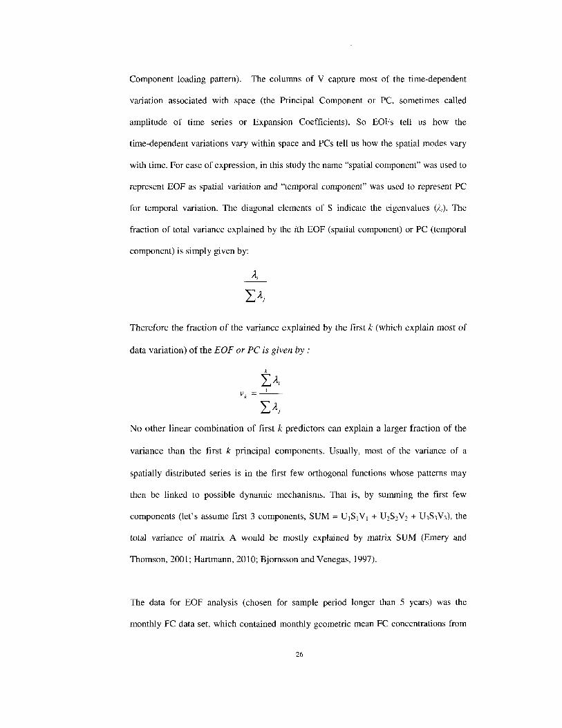
Component loading pattern). The columns of V capture most of the time-dependent

variation associated with space (the Principal Component or PC, sometimes called

amplitude of time series or Expansion Coefficients). So EOFs tell us how the

time-dependent variations vary within space and PCs tell us how the spatial modes vary

with time. For ease of expression, in this study the name "spatial component" was used to

represent EOF as spatial variation and "temporal component" was used to represent PC

for temporal variation. The diagonal elements of S indicate the eigenvalues ().;). The

fraction of total variance explained by the ith EOF (spatial component) or PC (temporal

component) is simply given by:

Therefore the fraction of the variance explained by the first k (which explain most of

data variation) ofthe EOF or PC is given by:

k

LA; vk =-~-

LAJ No other linear combination of first k predictors can explain a larger fraction of the

variance than the first k principal components. Usually, most of the variance of a

spatially distributed series is in the first few orthogonal functions whose patterns may

then be linked to possible dynamic mechanisms. That is, by summing the first few

total variance of matrix A would be mostly explained by matrix SUM (Emery and

Thomson, 2001; Hartmann, 2010; Bjornsson and Venegas, 1997).

The data for EOF analysis (chosen for sample period longer than 5 years) was the

monthly FC data set, which contained monthly geometric mean FC concentrations from

26

the year 1981 to 2003, at only stations located inside of river branches (not in the main

channel). This totaled 1460 monitoring stations. This set of observed FC concentration

values, in general, reflects both spatial and temporal information, which contains where

and when the sample has been collected. The data matrix for EOF was constructed with

1460 stations by 12 months. Each element in the matrix represented the geometric mean

of FC concentration for a specific month at a specific station. The created data matrix was

run using the statistic software Primer 6.0. Spatial components and associated temporal

components were analyzed to divide receiving waters into high, middle, low FC

contaminated regions.

Cumulative frequency graphs were used on these different contaminated level regions for

the comparison. The non-parametric Kolmogorov-Smirnov test (KS-test) was

performed to determine whether each pair of datasets (high, middle, and low FC

contaminated regions) differed significantly based on their cumulative frequency

distribution. The advantage of the K-S test is that there is no assumption about the

distribution of data. The significance level of K-S test was set as 0.05. The null

hypothesis is that two data sets follow the same distribution. The alternative

hypothesis is that two data sets didn't follow the same distribution if the test statistic,

D, is greater than the critical value Da obtained from the equation for large sample

size:

Da= 1.36

27

IV-3.3 FC distribution among different land cover dominated watersheds

Among upstream watersheds, single land-cover-dominated watersheds were chosen to

look at the effect of different land covers on fecal contamination levels in their receiving

waters. It was assumed that there should be at least 4 or 5 watersheds in each type of

single land-cover dominated watersheds group in order to have sufficient data points to

examine the effects of different land covers. The standard for a watershed to be called a

single land-cover-dominated watershed is defined as following: a"Forest dominated"

watershed is one with forestland occupying more than 80% of the entire watershed area.

A"Crop-Pastureland dominated" watershed is one for which the cropland and pastureland

together occupy about 70% of the entire watershed. An"Urban dominated" watershed is

one where more than 70% of land has been developed. The numbers of 80% for forest,

and 70% for urban and crop-pastureland were determined by the frequency of their

occurrences in the watersheds of coastal Virginia. In the end, there are 4 watersheds

whose percentages of forest were more than 80%. There are 5 watersheds whose

percentages of urban were more than 70%, and another 5 watersheds whose percentage of

crop-pastureland exceed 70%. NLCD 1992 land cover data set was used to derive the

percentage of occupation by each land cover for each watershed. FC concentration values

from DSS water quality monitoring stations located in the receiving waters of chosen

watersheds were extracted from the period between 11111990 and 12/3111994. A

combination of the box plots and cumulative frequency graphs were used on these

extracted FC concentration values for the comparison between different

land-cover-dominated watersheds. Their differences were tested by performing the

non-parametric Kolmogorov-Smirnov test (KS-test) on their cumulative frequency

distribution. The significance level of K-S test was set as 0.05 as usual.

28

IV -3.4. The effects of impervious land surface on fecal contamination

The Mid-Atlantic Regional Earth Science Applications Center (RESAC) at the University

of Maryland provides highly detailed impervious surface maps, which span the Virginia

coastal watersheds. Smith et al (2003) noted "The RESAC has selected two eras for land

cover mapping; one centered on 1990 and the other on 2000. Eras are used rather than

specific years because adequate data are not always available for the target year. The

RESAC team has advanced the capabilities of the Landsat series of satellites to measure

the amount of impervious surface within a 30-m pixel. Impervious surfaces include all

surfaces (man-made or natural) that inhibit infiltration by rainfall. The sub-pixel

classification technique used by the RESAC assigns a percentage value (between 0 and

100%) to each location based on the spectral measurements of the ETM+ sensor." The

new maps have found applications in the study of surface water redistribution, runoff and

pollution (Goetz et al., 2003). An impervious percentage for each watershed was derived

by overlaying upstream watersheds boundaries on the RESAC layer using ArcMap 9.3.

An impervious surface area analysis was conducted on the upstream watersheds. Since

impervious data centers on 1990 and 2000, 5 years ofFC monthly data surrounding 1990

(1988 to 1992) and 2000 (1998 to 2002) were extracted to represent the fecal

contamination levels in 1990 and 2000, respectively. From these five years, a subset of

FC data was selected for which rainfall occurred within four days before the sampling

date. The FC geometric mean concentration in 1990 was derived by averaging FC data

from 1988 to 1992, and the FC geometric mean in 2000 was averaged from 1998 to 2002.

Thresholds in the relationship between impervious surface percentage and FC levels in

the post-rainfall data sets for 1990 and 2000 were identified by nonparametric

changepoint analysis (nCPA) (Qian, et al., 2003). The method was proposed by Qian et

al., for detection of environmental thresholds. Changepoint analysis works best when

29

stressor-response relationships are nonlinear or heteroscedastic, properties very common

to ecological data (King and Richardson, 2003). This analysis is based on the idea that a

structural change in an ecosystem (indicating a threshold) may result in a change in both

the mean and the variance of an ecological response variable (King and Richardson,

2003). It tries to find threshold values by separating the response variable into two groups,

which have the greatest difference in their means and/or variances. The deviance

(Venables and Ripley, 1994), a measure of homogeneity, is defined for a continuous

variable, as:

n

D = L(Yk- J1)2

k=!

where D is the deviance, n is the sample size, Yk is the observed value, and f.1 is the

mean of n observations. Each possible changepoint is associated with a deviance

reduction:

Where: D is the deviance of the entire data set; Ds; is the deviance of first i observed

values; and D>i is the deviance of the remaining observed values, where i = 1, ... , n.

The changepoint r is the i value that maximizes L1i : r = maxiL1i. Nonparametric

changepoint analysis estimates uncertainty in the changepoint using a bootstrap

simulation. With bootstrap simulations repeated 1000 times, a distribution of change

points is estimated and illustrated with a cumulative probability curve that describes the

probability of a change-point occurring at various levels of disturbance (Bilkovic et al.,

2007). When probabilities of Type I error for potential changepoint were less than 0.05,

the cumulative probability curves were assumed to accurately assess the likelihood of an

ecological threshold occurring. Change-point analyses were conducted in S-Plus using

the custom function "nopar.chngp." Detailed descriptions of this method are found in

Qian et al., (2003) and King and Richardson (2003).

30

IV-3.5 FC distribution in different river regions

FC stations located in the upstream receiving waters were grouped as the Potomac River

stations, the Rappahannock River stations, the York River stations, the James River

(including Lynnhaven area), and the Eastern shore stations according to their location.

The differences in FC distribution among these groups were shown by a FC

concentration frequency analysis using box plot and cumulative frequency distribution

graphs with all available FC data from DSS using Minitab 5.0. The median values, and

25th and 75th percentiles were plotted for easy comparison between the four regions.

The cumulative frequency distribution curve was plotted against the boxplots to help

with analysis. The non-parametric Kolmogorov-Smirnov test (KS-test) was performed

to determine whether each pair of datasets differed significantly based on their

cumulative frequency distribution. The significance level of K-S test was set as 0.05.

The null hypothesis is that two data set follow the same distribution. The alternative

hypothesis is that two data set didn't follow the same distribution if the test statistic,

D, is greater than the critical value Da.

In order to show the linkage between environmental characteristics surrounding the

Rappahannock River, the York River, the James River, and the Eastern shore to their own

fecal contamination condition, Principal Component Analysis (PCA) was applied in their

upstream watersheds with a total of 14 variables. The variable included: soil condition,

slope, drainage density, eccentricity, residence time, ratio of watershed area divided by

water area, watershed area, water area, water volume, wetland percentage, cropland

percentage, pasture percentage, forest percentage, and developed percentage. Land cover

used here comes from NLCD 1992 land cover dataset. Since only the southern side of the

31

Potomac River was located in Virginia, it was not included for its environmental

characteristic analysis. The results from PCA were used to explain fecal contamination

level differences among the four regions.

IV-3.6 Climate effect

The Chesapeake Bay Program watershed model (Phase V) uses an hourly rainfall data set

for the period from 1/1/1985 to 12/31/1998. Annual rainfall data for this analysis were

obtained by summing all the hourly rainfall records of each year. The annual rainfall

amounts were related to the yearly FC average levels in Virginia coastal waters from

1985 to 1998. The yearly FC average levels were derived from the geometric mean of all

the stations for all measurement dates of each year. Correlation coefficients were

estimated for rainfall and FC by Pearson Correlation method using MINIT AB 5.

DSS not only provides FC data, but also precipitation intensity for each sampling station

for the 7 days before any sampling date. Precipitation was grouped into 5 classes

according to the rainfall intensity provided by DSS. Precipitation in the first class is

drizzle, the intensity of which range from 0 to 0.4 inches/day. The second class is

medium rain, ranging from 0.4 to 1 inches/day. The third class is large rain, from 1 to 2

inches/day. The fourth is pouring rain, from 2 to 4 inches/day. And the last one is any

rainfall greater than 4 inches/day. The classification is based on the protocols of the

China Meteorological Administration. FC concentration variation was graphed with each

rainfall group for 1 day, 2 days, 3 days, and 7 days before sampling dates.

The study on temporal variability of fecal contamination levels was only conducted on

DSS water quality monitoring stations located in receiving waters of upstream

watersheds. There are 487 water quality monitoring stations in the receiving waters of

32

upstream watersheds. EOF method was applied on a created data matrix with arrays of

487 (stations) x 12 (months). Analysis of the data matrix was run using Primer 6.0

software. Monthly precipitation, air and water temperature, and flow discharge, as shown

in Table IV -3.6.1, were hypothesized to be correlated with principal components (PCs).

Monthly precipitation and temperature was derived by averaging monthly precipitation

and temperature data in three cities (Norfolk, Richmond, and Williamsburg) extracted

from National Climatic Data Center with the aid of Climatology Office in University of

Virginia. Available precipitation and air temperature data in Norfolk is from 11111946 to

12/3112008, from 81111948 to 12/31/2008 in Williamsburg, and from 811/1948 to

12/3112008 m Richmond. Monthly water temperature data was from National

Oceanographic Data Center of NOAA (www.nodc.noaa.gov/dsdt/cwtg/satl.html).

Monthly water discharge data was averaged from daily stream flow data during the

period between 1/1/1984 and 12/3111996 from USGS gage station 01661800 located in

the headwater of Great Wicomico River, VA. Environmental variables were graphically

displayed in relation to temporal principal components to visually assess their

relationships.

IV-3.7 Relationship between environmental variables and FC contamination

Fifteen variables (comparing to 14 variables in section IV-3.5, impervious surface

percentage was added here) were chosen based on their likelihood of association with

FC contamination levels in Virginia coastal upstream watersheds. It was assumed that

not all the variables contribute equally to FC contamination levels. It was necessary to

put weights on variables as an indicator of their contribution. Classification and

Regression Tree (CART) analysis helped to address the problem. CART is a

non-parametric technique that can recursively partition data into mutually exclusive

33

groups by selecting a predictor variable that best explains variation in the response

variable (Urban, 2002). Statistical software, called JMP 8, was used to perform a

CART analysis. The CART model was built for the response variable (FC

contamination levels) with 15 predictor variables in 165 upstream watersheds (Table

IV- 3.7.1). FC contamination levels were represented by FC geometric mean. FC data

were extracted from DSS FC sampling data between 1990 and 1994. The fifteen

variables were impervious surface percentage, soil condition, slope, drainage density,

eccentricity, residence time, watershed area, water area, water volume, wetland

percentage, cropland percentage, pasture percentage, forest percentage, developed

percentage, and ratio of watershed area to surface water area. Land cover came

from the NLCD 1992 land cover dataset. Prior to the CART analysis, the minimum

number of observations permitted within terminal groups was set at 5 and

cross-validation was conducted by randomly dividing data into 10 equal size groups.

IV -4 Results

IV -4.1 Tidal and seasonal effects

There were 392 stations that had tidal information and FC concentration data in the study

area (Figure IV -4.1.1 ). The available sample size for a 1-sample Wilcoxon signed-rank

test was 2310 (FC data from 392 stations for available months). The result from this test

indicated that the FC geometric mean concentration was significantly greater at low tide

than at high tide (n=2310, p<0.001 ). The difference between the low and high tide

median FC concentration values is about 1.92 MPN/lOOml with a 95% confidence

interval between 1.43 and 2.46 MPN/1 OOml. The result from seasonal comparisons show

that FC geometric mean concentration in summer (n=614) is significantly greater than the

concentration in winter (n=596) (p<0.001). The difference in FC levels due to seasonal

34

and tidal effect is evident when examining boxplots of data distribution (Figure IV -4.1.2).

Comparing the seasonal difference between winter (January to March) and summer (July

to September), (Q1: 7.31 MPN/lOOml, median: 18.04 MPN/lOOml, Q3: 41.76

MPN/lOOml), to the tidal difference, (Q1: -1.17 MPN/lOOml, median: 0.17 MPN/lOOml,

Q3: 7.05 MPN/lOOml), the difference caused by tide is much smaller than the difference

caused by seasons

IV -4.2 Re-define study sites in Virginia coastal regions

Three classes of high, middle, and low fecal contamination could be divided by using

EOF method. The first spatial component or first temporal component, which contains

the largest data variation while reducing the dimensionality of the data, explains about 76%

of the data variation. From Figure IV -4.2.1, we can see that the highest FC contamination

across months (indicated by the brightest red color) appear in most upstream regions.

The contamination (and representative color) decreases in the downstream direction. In

order to show more clearly how FC distributes spatially along the waters, the DSS

stations were evenly separated into 3 groups according to their first spatial component

values, as shown in Figure IV -4.2.2. The first group is the stations which show the

greatest spatial component values, second group having second greatest spatial

component values, and the third one with the lowest values. It is interesting to see that

almost every river branch follows the same pattern with high first spatial component

values appearing in the upstream waters represented by the red color. These values

decrease moving toward downstream, turning into yellow in the middle stream and then

green color in downstream. The first spatial component suggests that in the embayment

close to land, there is very high FC concentration variation across different months. In

segments closer and closer to the river mouth, the variation in FC concentration loses

strength and becomes weaker and weaker across the months. Positive values in PCl

35

indicate that the spatial pattern shown by the first spatial component is quite consistent

through different months. This spatial pattern is more obvious in the warm season than in

the cold season. Since the separation into three groups seems to divide most of the water

ways similarly into upstream, middle and downstream regions, that is how stations were

categorized for subsequent analysis. At same time, watersheds associated with each

region were also delineated into upstream watersheds, middle, and downstream

watersheds. Only upstream watersheds were actually used for study purposes. Upstream

watersheds were delineated using the contour lines on digital 7.5 minute USGS

topographic maps for the Virginia coastal region. The contour interval is 10 feet.

Streamlines and contour lines were used to determine overland water flows through each

basin. The boundaries of the upstream watersheds were assigned to the location between

upstream and middle stream water quality stations.

Cumulative frequency graphs were drawn for upstream, midstream, and downstream

stations using Mini tab 5.1. Figure IV -4.2.3 shows FC frequency distributions among

upstream (n= 96047), middle stream (n=100064) and downstream (n=97770). There are

much higher FC concentration values in the upstream than in the downstream. Highest

FC concentrations appear most frequently in upstream regions, less frequently occurring

in the middle stream regions, and lowest in downstream.

There are a total of 187 upstream watersheds delineated as shown in Figure IV -4.2.4. The

sizes of upstream watersheds range from 167,102 m2 to 173,718,943 m2 with a mean of

17,933,206 m2 (Table IV-4.2.1). The average number of DSS water quality monitoring

stations in their receiving waters is 3 with the standard deviation of2 (Table IV-4.2.1).

36

IV -4.3 FC distribution among different land cover dominated watersheds

There are 5 watersheds representing Crop-Pasture dominated watersheds, 4 for Forest

dominated, and 5 for Urban dominated watersheds (Table IV -4.3.1 and Figure IV -4.3.1 ).

Most Crop-Pasture dominated watersheds were located on Virginia's Eastern Shore.

Forest dominated watersheds were located in the northern part of Virginia"s coastal

regions, and Urban dominated watershed were found in the southern portion. Table

IV -4.3.1 shows their land cover distributions, related water quality monitoring stations,

and the number of available FC data for each station from 1990 to 1994. Results from the

K-S test indicated that each pair of FC data between crop-pasture dominated watersheds,

forest, and urban dominated watersheds was significantly different from the others, even

though green (indicating forest dominated watersheds) and yellow (indicating cropland

and pastureland dominated watersheds) curves almost overlapped. The result suggested

that fecal contamination levels respond differently between urban dominated, forest

dominated and crop-pastureland dominated watersheds. The highest FC concentrations

appear most frequently in Urban dominated regions, followed by Crop-Pastureland, and

with the lowest occurring in Forest dominated regions (Figure IV-4.3.2). The FC

frequency distribution curve for Crop-Pastureland is quite similar to the curve of Forest

dominated. The probability of exceeding a given FC levels is higher in urban-dominated

upstream watersheds than in forest-dominated upstream watersheds in almost every

month as shown in Figure IV-4.3.3. FC distribution in three groups of single land cover

dominated watersheds were significantly different from each other with corresponding

low p values (p <0.001 in all pairs of K-S test) and greater D values than each of their

critical values. D value between forest-dominated and crop-pastureland dominated

watersheds is 0.16, which is greater than their critical value 0.11. D value between

forest-dominated and urban dominated watersheds is 0.38, which is much greater than

37

their critical value 0.087. D value between urban-dominated and crop-pastureland

dominated watersheds is 0.36, which is also much greater than their critical value 0.088.

IV -4.4 The effects of impervious land surface on fecal contamination

The impervious surface percentage in 1990 and 2000 (Table IV -4.4.1) in 187 upstream

watersheds was related to FC contamination levels based on the subset of FC sampling

data characterized by rain occurring within 4 days before the sampling date. In 1990,

there is at least 96.8% cumulative probability that a detectable change in the FC

geometric mean concentration occurs in upstream watersheds with impervious cover

percentage at or below 13.78%. Above the impervious surface threshold value, FC

geometric mean increased from 22.08 to 37.94 MPN!lOOml. In 2000, there is at least 83.5%

cumulative probability that a detectable change in the FC geometric mean concentration

occurs in upstream watersheds with impervious cover percentage at or below 17.39%.

Above the imperious surface threshold value, FC geometric mean increased from 24.67

MPN!lOOml to 44.78 MPN/lOOml. The probabilities of Type I error were quite low (p =

0.0008, and p = 0.002). Low p values indicate that there is a strong probability that the

derived potential changepoint is real and could represent significant change in fecal

contamination levels.

IV -4.5 FC distribution in different river regions

FC concentrations in excess of 200 MPN!lOOml (swimming water quality standard)

predominately ranged between 210MPN/100ml and 1210MPN/100ml (Figure IV-4.5.1).

There are two notable outliers (They are thought as outlier because more than 99.9% of

FC concentration data are much lower than these two values). One (4600MPN/100ML)

occurred in the James River on March 16th, 1989 at station 62_9.1A, which is located in

38

the mouth of Brewers Creek, on the south side of the James River. Another notable

outlier (2440MPN/100ml) occurred on June 28th, 1988 on the south side of Potomac

River. Regional differences in FC distribution were revealed by K-S test after removing

these two outliers. FC distributions in these five regions were significantly different

from each other with corresponding low p values (p < 0.001 in all pairs of K-S test)

and greater D values than each of their critical values. Sample sizes of each region,

their calculated D values, and critical D values are shown in Table IV-4.5.1 and

Figure IV-4.5.2. The result showed that the James River region has the greatest FC

concentration data range, followed by the York River, the Rappahannock River, the

Potomac River, and the Eastern shore region. Median values (23MPN/100ml) were equal

in the James River, the York River, the Rappahannock River, and the Potomac River. The

Eastern shore showed the lowest median value (15MPN/100ml). There was about 10% of

chance of FC concentrations exceeding a value around 200 MPN/lOOml.

There are 33 upstream watersheds around the Rappahannock River, 33 upstream

watersheds located on the Eastern Shore, 13 around James River, and 28 around York

River (Table IV-4.5.2). The Principal Component Analysis of these 107 upstream

watersheds showed that the first principal component accounts for 30.2% of the

variability and the second component accounts for 21.8% of the variability (cumulatively

52%) (Figure IV -4.5.3). The first component was correlated with a non-urban gradient,

with percentage of forest and slope increasing in the negative direction together with

percentage of cropland and pastureland increasing in the positive direction as shown in

Table IV-4.5.3. Slope, percentage of forest, pasture, and cropland contributed most to this

component. Coefficients of these variables showed their correlation with each other.

Results suggested that forest was located in areas with relatively steep land surface,

indicated by the value of slope (both coefficients are negative values). Cropland and

39

pastureland occur where the land has a low value of slope (cropland and pasture have a

positive coefficient, slope is negative). The second PC seemed to make a quick sketch

about what the environment looks like based on the size of the watershed, water area, and

water volume. At the same time, it shows an urban gradient with percentage of developed

land, watershed area, water area and water volume increasing in the positive direction,

and the percentage of forest decreasing in the negative direction. Developed land tends to

correlate significantly with water area, drainage density, and less significantly with

watershed area and water volume.

Based on Figure IV-4.5.3, the separation of the James River region from others was

relatively clear. It seems the Eastern Shore region might possibly be distinguished from other

two regions. PCA analysis was conducted on the Rappahannock, York, and the Eastern

shore regions (94 watersheds) as shown in Figure IV-4.5.5. The first PC explains 37.4%

of data variation, with 20.1% for second PC (cumulatively 57.5%), as shown in Table

IV -4.5.4. There is clear separation among these 3 regions as shown in Figure IV -4.5.5,

even though the first two PCs only explain 57.5% of data variation. Slope is probably one

of the major factors separating the Eastern Shore from the other two regions. The

separation between the Rappahannock and York depends largely on runoff potential and

the percentage of pasture land.

IV-4.6 Climate effect

The examination of FC level response to annual precipitation reveals a close relationship

between FC amount and precipitation intensity from 1985 to 1998 (linear regression with

r2=0.75) (Figure IV-4.6.1). The rise and fall of FC bacteria concentration closely

associates with annual precipitation cycles. After grouping rainfall intensity, FC

40

concentration variation seems to have a positive relationship with grouped rainfall

intensity, especially with Day 1 precipitation, as shown in Figure IV -4.6.3.

A general temporal pattern of fecal contamination throughout Virginia coastal regions

has been shown in Figure IV -4.6.4. The red lines separate locations into three groups - I)

the Potomac, the Rappahannock, and Mobjack Bay group, 2) the York and the James

River group, and 3) the Eastern Shore group. These graphs are all on the same scale. FC

concentrations from January to March are quite low across almost all the stations. In

February, these concentration values are probably the lowest during the year. Starting in

April, FC concentration values increase until October. FC concentrations start to drop in

November and are even lower in December.

In order to quantify the influence of several natural forces on fecal contamination levels,

the first several temporal components were linked to monthly precipitation, temperature,

and water discharge. Based on EOF results, the first spatial component or temporal

component explains about 63% of the data variation with second accounting for 12.7%

and the third only 5.3% (Figure IV-4.6.5). The first 3 principal components together

explain 81% of the data variation. The first principal component was linked to monthly

precipitation intensity (Figure IV -4.6.6a). Variability in fecal contamination levels

appears to be an upstream-wide response to precipitation. High FC concentration values

occur in the wet season with more rainfall, and low values occur in the dry season with

less rainfall. The second component was linked to monthly temperature. Figure IV -4.6.6b

shows a positive relationship between air, water temperature and FC count, which means

that temperatures play a role in the amount of FC measured in the receiving water. And

the third component was linked to monthly water discharge (Figure IV-4.6.6c). Fecal

contamination levels respond to temperature and flow discharge. These two factors

41

account for 12.7% and 5.3% of the total variance, respectively. There is about 19% of

data variation left unexplained.

IV -4.7. Relationship between environmental variables and FC contamination

Initially there were 15 variables chosen to represent environmental characteristics. The

number of potential predictors was reduced to 12 variables after removing 3 variables

(water volume, water area, and watershed area), since they closely correlate to each other

with Pearson's correlation coefficient greater than 0.6. Pearson's correlation coefficient

of the other pairs of variables were all less than 0.6. In order to avoid collinearity (King et

al., 2005; Norton 2000), bare land and the area of open water were included in the land

cover percentage calculation. So the sum of 5 major land cover percentages (not

including bare land and the area of open water) won't equal to 1. The median of FC

abundance in these watersheds is 23.2MPN/100ml (Ql = 17.1 MPN!lOOml and Q3= 28.9

MPN/lOOml). Based on the minimum value from cross-validation, 7 splits were

determined from CART analysis (Table IV-4.7.1. The complete tree explains a total of

42.7% of FC abundance variation. This variation was explained by Impervious surface

percentage (r2=4.3%), Forest(r2=4.7%), Pasture(r=3.5%), and Wetland

percentage(r2=8.2% ), ratio of watershed area divided by water area(r2=7% ), residence

time(r2=8%), and runoff potential(r2=7.4%) (Figure IV-4.7.2). FC concentrations were

highest in 13 watersheds that met the following conditions at the same time: 1.

watershed:water area ratio value is less than 76.35; 2. runoff potential is greater than

0.034; 3. impervious surface percentage is greater than 0.6%; 4. wetland area is greater

than 5%; and 5. residence time is longer than 0.6 day. The second highest FC

concentration occurred in 20 watersheds with ratio values greater than 76.35. FC

concentrations were lowest at 7 watersheds with ratio values less than 76.35, runoff

42

potential smaller than 0.034 and forest occupying more than 49% of the whole watershed.

The remaining watersheds were classified into 5 groups with similar FC concentration

values.

IV -5 Discussion

IV-5.1 Tidal and seasonal effects

One of the principal physical forcing mechanisms affecting the water quality in Virginia

coastal waters is tidal variation. Monthly comparison of the tidal effects on the FC

geometric mean concentration was done in order to separate bacteria loading differences

induced by tidal influences from those induced by seasonal influences. The result

indicates that FC geometric mean concentration is greater at low tide than at high tide.

This is consistent with the previous study by Mallin et al. (1999), which observed the

increase in the abundance of FC bacteria in tidal creek waters at or near low tide. Since

Virginia coastal waters are located in the lower part of Chesapeake Bay, no tidal

oscillation inside Chesapeake Bay will ever be free from the tidal 'hammer' perpetually

at work at its entrance (Boon, 2004). Boon (2004) also mentioned that, of the four major

tributaries in Chesapeake Bay, one is relatively short (i.e., the York River) and displays a

uniform increase in tidal range upstream, while the longer ones (the James, the

Rappahannock, and the Potomac Rivers) show a slight decrease in range before the final

increase upstream. The tidal range at the head of all four tributaries approaches the range

at the bay entrance itself (90 em). Tidal ranges in Virginia coastal water area varies from

0.6 - 1.0 m. Factors contributing to the greater FC geometric mean concentration at low

tides could be the salinity variation between high and low tide, increasing turbidity during

low tide disturbing FC bacteria into water column, and dilution effect during flood and

ebb (Mallin et al., 1999).

43

One of the objectives of this study was to quantify FC sources with an inverse modeling

approach. Because increasing the number of independent variables being modeled could

promote the development of a widely varying (chaotic) solution (Nihoul, 1998), limiting

the number of independent variables is a critical decision to make before designing a

successful water quality model. The results of the preceding analyses suggest FC

concentration differences due to season are greater than the differences between high and

low tide. It is therefore better to consider seasonal effect prior to the tidal effect. The

quantification process could be separated into two periods - cold and warm when

considering seasonal effects. Given monthly FC data, it is not feasible to quantify FC

sources during either flood or ebb period.

IV -5.2 Re-define study sites in Virginia coastal regions

Although causal factors of FC contamination have been identified by numerous research

studies (Mallin et al., 2000; Kim, 2005; Line et al., 2008) their inter-connection or

interaction limits the ability to clearly differentiate the effects of specific attributes of

land and water on fecal pollution. The capability of predicting the levels of contamination

is low as well. In this study, the separation into upstream, middle and downstream

reaches helped differentiate factor effects, especially from water-based processes such as

salinity, tidal flushing and dilution. Most of the analysis focused on upstream land and

water, because upstream water quality reflects the concentrated effect from land. In

addition, FC monitoring data in middle and downstream reaches alone couldn't provide

sufficient information to compare watersheds. This is because the effect of local

pollution sources on in-stream water quality cannot be separated from the effects of

contaminants originating in upstream watersheds (Smith, et al., 1997).

44

Results from FC distribution comparison of upstream, middle and downstream suggested

that the probability for FC concentrations to exceed a given bacteria level increased

significantly from downstream, up to the headwater region (Figure IV -4.2.3). Highest FC

concentrations mostly occurred in upstream regions, where salinities are low and there

are relatively larger FC contributing land areas compared to middle and downstream.

Lowest FC contamination levels occur in downstream regions, which experience high

salinity, accompanied by greater tidal flushing and dilution processes. Many studies have

demonstrated that there is a negative relationship between FC bacteria survival and

salinity (Hanes and Fragala, 1967; Evison, 1988; Solie and Krstulovic, 1992).

Downstream stations also have wider and deeper water, less local contribution, and are

further from FC sources as opposed to upstream reaches (Burkhardt et a!., 2000). Fecal

bacteria decay rates are directly related to the distance from the sources. However, since

water quality reflects the land characteristics that are drained, it is hard to definitely

conclude that dominant reason for FC contamination gradient along river is from

water-based processes, such as salinity, tidal flushing and dilution, or from land-based

processes. The conclusions made by other papers based on single observations seem to

lack sufficiently supportive evidence (Goyal et a!., 1977; Esham, 1994; Mallin et a!.,

2000).

This study demonstrated that there was a consistent spatial pattern in almost every

embayment, with high spatial component values upstream, decreasing when moving

downstream. This consistency suggests that some processes exist either in land or water,

which occur relatively ubiquitously. The variation in land parameters is relatively greater

than the variation occurring in water parameters such as salinity, dilution, and tidal

influence from headwater to the mouth. The consistent spatial pattern infers that FC

45

distribution difference between upstream, middle and downstream can be mostly

attributed to the gradient of salinity, dilution, and tidal influence instead of land-based

activities.

IV-5.3 FC distribution among different land cover dominated watersheds

Most watershed models use land cover or impervious land condition as one of the input

variables (O'Neill, et al., 1997). Land cover refers to physical or biological features on

the land surface. In general, there are 6 major types of land cover - Forest, Cropland,

Pastureland, Urban, Wetland and Water. Each land cover has its own specific

characteristics. For example, forest has many standing trees, pervious soils with low

erodibility, and habitat for wild animals. In this studied area, slope is more closely

correlated to forest land (Pearson correlation coefficient 0.47, p < 0.001) than any other

type of land cover (Urban: -0.147, p=0.072; Cropland: -0.288, p < 0.001; Pastureland:

-0.136, p=0.095). So each land cover represents the sum of effects from lands, which

include the effects from slope, soil properties, vegetation cover, etc. Their total effects

may be reflected in the water quality responses within the upstream embayment. FC

contamination responds differently between urban-dominated and forest-dominated

upstream watersheds, which probably mirror the differences between these two

contrasting land covers.

It must be emphasized that frequency comparison only focused on the type of land cover

in a watershed. It didn't incorporate any specific information about other variables, like

slope, runoff potential and so on. However, there was a difference between two of the

frequency curves (Figure IV-4.3.2). It is not surprising that embayments in

urban-dominated upstream watersheds pose a higher risk for human health exposure to

46

pathogens, indicated by the amount of FC bacteria. It has been suggested that impervious

surfaces in urban area increase the transport of bacteria to water, heightening

contamination. Many studies have been trying to reduce the negative impact from urban

development on pollution issues (Maiolo and Tschetter, 1981; Kocasoy, 1995). As

suggested by Mallin et al. (200 1 ), direct discharge of storm water runoff from urban area

to coastal waters should be prevented. One management alternative is to redirect

stormwater via leaching structures to the groundwater pathway, where FC transport could

be limited. Rain barrels are recommended by EPA to reduce stormwater runoff. Citizens

have been encouraged to install rain barrels under their roofs to collect rainwater in order

to hold back the pollutants, which are otherwise washed off from land surfaces into

receiving waters.

Many experimental designs have demonstrated that vegetated surfaces may ameliorate

the degree of fecal pollution (Tufford and Marshall, 2002; Roodsari et al., 2005). What

makes forest-dominated upstream watersheds different from urban ones maybe be

attributed to runoff volume during rainfall events. Research data suggest that for rainfall

events of similar magnitude, the volume of runoff was 3-25 times greater in the receiving

waters of developed watersheds in South Carolina than in forested watersheds (Holland et

al., 2004). The large difference between runoff volumes is likely a major reason for the

differences m the FC bacteria probability distribution between urban and

forested-dominated upstream watersheds, since the transport of microbes into water

systems often occurs through sediments in surface runoff (Reddy et al., 1981). Even

though forest-dominated embayment showed lower fecal contamination levels, forest is

still considered a source for FC bacteria from land. Elevated FC concentrations have been

detected from streams and spring located in national forest parks (Silsbee and Larson,

1982; Becker, 2006). The numbers of visitors, as well as the FC bacteria existing in soil,

47

leaf litter, and stream sediments from natural sources, appear to be the major contributors

to bacterial contamination. The more remote an area is from human and animal pollution,

the less likely are fecal types to be found (Geldreich et al., 1962). Forest-dominated

upstream watersheds in this study might be remote from human pollution, but definitely

are not remote from animal pollution.

Urban and forest-dominated upstream watersheds were compared with watersheds

dominated by cropland-pastureland (Figure IV-4.3.2). One of the reasons to combine

cropland and pastureland together is the percentage of these two kinds of land cover

correlate quite well with each other (Figure IV-5.3.1).

Figure IV-5.3.2 shows that the median value (15MPN/100ml) for Cropland-Pasture is

lower than forest (23MPN/100ml). The result seems contradictory to the idea that

cropland is a major source of fecal bacteria from land. The EPA's National Water Quality

Inventory report (USEPA, 2000) identified bacteria from cropland as the leading cause of

impairments in rivers and streams in the United States and agricultural practices were

identified as the leading source of all bacterial impairments. It has been well-documented

that runoff from cropland, as well as livestock and poultry litter-applied areas, is a source

of fecal contamination in water (Edwards et al., 1994, 2000; Crowther et al., 2002; Tian

et al., 2002; Gerba and Smith, 2005).

As a livestock and poultry litter-applied area, pastureland has been identified as a source

of fecal bacteria (Soupir et al., 2006). Pinney and Barten ( 1997) mentioned that manure is

collected and spread on pastureland. However, pastureland soil probably contains less

fecal bacteria than cropland soil. Geldreich et al. (1962) examined coli-aerogenes bacteria

that was isolated from 251 soil samples collected from 26 states and 3 countries. Their

48

results suggested that the percentile distribution of MPN values/gin Pasture soil is much

lower than Cropland soil. FC concentrations in soil are an important parameter

determining the potential for contamination of water resources. The greater the

concentration, the more likely some will be transported (Gosset al., 2002). It is therefore

the combination of cropland with pastureland could underestimate cropland contribution

to fecal contamination in their receiving water.

IV -5.4 The effects of impervious land surface on fecal contamination

The quantity of impervious cover is useful to measure changes in development and

reflect the gradients of human influence. In 1990, there were only 10% of upstream

watersheds in which impervious cover occupied more than 5% of all land cover. After 10

years, the number of upstream watersheds with more than 5% of land as impervious

cover increased to 15%. Land conversion from rural to urban and suburban has proceeded

rapidly along coastal watersheds due to increasing human population in coastal areas.

Mallin et al. (2000) pointed out that the percentage of impervious surface area alone

could explain 95% of the variability in average estuarine FC abundance for five estuarine

watersheds (Figure IV-5.4.1). Even though it emphasizes the relationship between

impervious surface area and FC abundance, five data points alone may not provide

sufficient information to demonstrate a comprehensive relationship.

Results from Nonparametric Changepoint Analysis showed that the potential impervious

cover threshold values were 13.78% in 1990 and 17.39% in 2000 (Figure IV-4.4.1). This

indicates that there is significant change in fecal contamination levels when impervious

cover percentages exceed around 15%. The result is similar to previous research. Based

on a variety of studies, when more than ten percent of the acreage of a watershed is

covered in roads, parking lots, rooftops, and other impervious surfaces, the rivers and

49

streams within the watershed become seriously degraded (Schueler and Holland, 2000,).

The principle of the ten percent impervious threshold has been brought up as important

consideration for marine ecosystem protection programs. Even with fiscal, social, and

environmental unsustainability as consequences, hypersprawl, that is housing at densities

ot no more than one unit per three acres, is encouraged by current environmental policies

as a solution to nonpoint source pollution (Beach, 2002). Mallin (2002) suggested that in

a watershed with urban land exceeding 10 percent, surface runoff should be directed into

natural or artificial wetlands, grassy swales, and other porous areas before surface water

runoff can enter coastal receiving waters.

King and Richardson (2003) mentioned that one potential criticism of nonparametric

changepoint analysis is that it may not detect a low-level changepoint if a second,

competing changepoint occurs at a higher concentration. They suggested splitting data

into multiple subsets. This was not attempted in the present study because there are only a

few data points with high impervious cover percentage in each of the two data sets (7

data points with impervious cover > 15% in 1990, 8 data points with impervious

cover > 17% in 2000). Data splitting would be quite arbitrary and the lack of data points

at higher levels of imperviousness would confound the purpose of the analysis. Even

though several studies have identified thresholds for development impacts on water uses,

none of studies has identified the threshold values from such large dataset, especially for

the coastal area in Virginia.

IV-5.5 FC distribution in different river regions

IV -5.5.1 Data discussion in different regions

In general, 90% of the FC data in the study regions were less than 200 MPN/100ml. The

magnitude of high FC concentration values (any values greater than 200MPN/100ml, a

50

water quality standard for safe swimming) in the study area was between 210MPN

11 OOml and 1210MPN/1 OOml. One outlier occurred in the mouth of Brewers Creek, on

the Southside of the James River. Daily precipitation records at Norfolk International

Airport from the NOAA web database showed that there was a large amount of rainfall

during the previous 3 days. The observation is consistent with previous research that FC

concentrations increased significantly with increasing rainfall occurring in the days

before sample collection due to storm runoff (Lipp et al., 2000; Sullivan, 2004). The high

FC concentration at station 62_9.1A may be attributed to boating activity. The data from

the DSS survey shows there are some boating activities close to the sample station.

Pettibone et al. (1996) observed that the levels of FC increased immediately after a ship

passed. An et al. (2002) mentioned that recreational boating activity in lake marinas may

have resuspended bottom sediments with bound E. coli, and the presence of E. coli in

marinas was not an indication of recent fecal contamination.

Another notable outlier (2440MPN 11 OOml) occurred on June 28th, 1988. After checking

related information, it was found to be similar to the other outlier. Rainfall on June 27th

was recorded in the DSS database as 0.66 inches and there were boating activities nearby.

Regional differences in FC distribution were revealed in part through examination of FC

data distribution patterns (Figure IV -4.5 .I b). A comparison of their medians was not

sufficient to distinguish regions. Box plots, together with histograms or frequency

distributions in cumulative curve, help in this regard, and are important statistical

methods in exploratory data analysis. A useful comparison is between the FC

concentration cumulative frequency distribution plot in different regions (Figure IV-4.5.2)

and the daily rainfall cumulative frequency distribution in 1998 and 1999 obtained from

Norfolk International Airport NOAA web database (Figure IV-5.5.1). The two frequency

51

distributions exhibit a similar shape. The FC frequency graph showed there is about 10%

of chance for FC concentrations to exceed the value around 200 MPN/lOOml. On the

daily rainfall graph, when rainfall intensity is greater than about 0.5 inch/day, the curve

coincidently flattens with a percentage around 90%. That is, the frequency of FC

distribution matches quite well with the frequency of precipitation that occurred in

Virginia coastal areas. The comparison provides additional support that precipitation is an

important driving force for FC bacteria transport from land into water, as proposed in

previous researches (Sullivan, 2004). The results might imply that there is at least a 10%

chance of exceeding the swimming standard. This I 0% seems to be unrelated to human

activities, , resulting instead from natural forces.

The characteristics of FC distribution within the river regions were different from each

other as shown in Figure IV -4.5.2. The probability of having high FC concentration

values is greatest in The James River region. The Eastern Shore has a large amount of

low FC concentration values compared to other regions, while it has a slightly greater

percentage of high values than the Rappahannock and the Potomac. There is probably no

distinction between the Rappahannock River and the Potomac River, which have the

lowest percentage of high concentration values. The York River lies between these

curves. One interesting observation here is that since The Eastern Shore has a greater

percentage of low concentration values than the Rappahannock and the Potomac River,

you would expect that the Eastern Shore should have relatively lower percentage of high

values than the other two river regions. But this is not the case even though the

probability of high values in The Eastern Shore is only slightly higher than the other two.

52

IV -5.5.2 Regional Environmental Characteristics

Although FC concentrations provide important information on the local (onsite) pollution

levels, data alone give little indication of how the system generates the amount of fecal

bacteria in the water. For instance, FC concentration may be low or moderate in the water

that receives high fecal material input because the bacteria is quickly diluted and flushed

out. On the other hand, FC concentrations may be high in water that receives low to

medium input, possibly because land surface conditions, either impervious or steep,

provide a quick way to drive bacteria into the water without experiencing huge losses

during land transport. Successful management requires a variety of information,

including the knowledge of environmental and physical settings, such as land cover

combinations, soil type, climatic setting, and topography.

Even though fourteen variables were selected to represent environmental characteristics,

they still provide an incomplete description of the surrounding land's influence on fecal

pollution. For example, the analysis did not include reservoirs, lakes, retention pond or

detention ponds, which probably have an effect. In addition, the effects of land

fragmentation, roads, population density, exposure to ultraviolet radiation, sediment

resuspension, and other phenomena were not considered, although they have important

consequences for fecal pollution (Cook, 1984; 0' Neill, et al., 1997; Mallin et al., 2000;).

For this analysis, direct measurements of land and water characteristics were the focus. In

addition, the analysis was confined to the upstream watersheds, not the middle or

downstream regions.

The separation of the James River from other regions is apparent when the scores of each

watershed were plotted from the first two principal components (Figure IV-4.5.3). The

James River upstream watersheds are characterized as having a high percentage of

53

developed lands with large watershed areas, water areas, as well as large amounts of

water indicated by water volume. Many of the hydrologic impacts on streams are the

result of development, represented by impervious areas in urban and suburban areas.

There was no clear distinctions between the Rappahannock, the York, and the Eastern

Shore (Figure IV-4.5.3), even though K-S test showed significant differences. Therefore,

a secondary PCA analysis was conducted on these 3 regions (94 watersheds) as shown in

Figure IV-4.5.4. The first PC explains 47% of data variation, with 12.6% for the second

PC (cumulatively 59.6%). There is a clear separation between the 3 regions (Figure

IV-4.5.4) even though the first two PCs only explain 59.6% of data variation. Slope is

probably one of the major factors separating the Eastern Shore from the other two regions.

The Eastern Shore upstream watersheds also are characterized by relatively higher

percentage of land as cropland and smaller size of watershed area. The area of Eastern

Shore is very flat according to Digital Elevation Models (DEMs) by USGS The area was

dominated by cotton, soybean, vegetable and truck farming, and large-scale chicken

farms. The separation between The Rappahannock and York depends largely on runoff

potential and the percentage of pastureland. The Rappahannock study area has more

percentage of land as pastureland than York, but soil in the Rappahannock studied area

has less runoff potential than in York. Since there are no studies exactly analyzing runoff

potential in the same locations as my study areas, sediment yields from two rivers were

used as a reference. Studies have shown that the Rappahannock River delivers more

sediment per square unit of watershed than any of the other tributaries of the Chesapeake

Bay (USGS, 2003). However, these study areas for regional comparison are only located

in upstream watersheds of lower the Rappahannock River and the York River. The York

River study indicated that little sediment from the watersheds located in upper York

River reached the estuary and water quality may be more affected by locally derived

sediments near the estuary (Herman, 2001). According to USGS report, we can probably

54

infer that the lower York River has the possibility to deliver more sediment per square

unit of watershed than the Rappahannock, since sediment source in the York river might

be concentrated in the places near the estuary mouth.

IV -5.3.3 Correlation between FC contamination and environmental characteristics

Based on analyses discussed above, FC concentration distribution reflects environmental

characteristics of different regions. The highest FC concentration range occurs in the

James River, as well as the highest incidence of sampled data having elevated FC

concentrations, probably due to the high percentage of developed land. Many studies

have shown a strong correlation between urbanization and declining water quality. It is

not surprising that the upstream watersheds in the lower James River had the worst

contamination levels compared to the other regions. For other associated variables, like

the size of land and water, they indicate that FC contamination in the James River reach

further downstream than other regions because of the way the embayment was separated

into upstream, middle and downstream. The lines to divide the water into upstream and

middle stream in all embayment represent reaches where FC contamination exhibits

similar levels. For areas with the worst case, the line would extend further downstream

and the size of watershed and water would increase simultaneously if water-based

processes, such as water dilution, are not strong enough to push the line back toward

headwaters. Therefore the size of land and water in part reflect FC contamination levels

in all study areas.

The lowest FC concentration median values occur in the Eastern Shore which has a large

percentage of low FC concentration values, a small percentage of medium values, and a

relatively larger percentage of high values as compared to the Rappahannock and the

Potomac. This pattern probably is attributable to the environmental variables of the

55

Eastern Shore, characterized as a flat area with small slope values and intensive

agricultural operations. Although the Eastern Shore comprises only about 5% of the total

Bay watershed, it contains the most concentrated grain and poultry producing regions in

the entire watershed (Staver and Brinsfield, 2001). The ratio of agricultural land to forest

on the Eastern shore is approximately 1:1 versus 1:2 for the entire bay watershed. Huge

amounts of manure that are applied in a concentrated time period probably contribute to

the larger percentage of high FC concentration values compared to the Rappahannock

and the York River. Flat land surface in the Eastern Shore is conducive to water

infiltration which probably transfers surface water into groundwater. Reay (2004)

examined several sites, including ones in Cherrystone Inlet, which is a small tidal

tributary located on the Eastern shore, and found that FC concentrations were at or near

background levels in groundwater immediately adjacent to a waste water drain field and

along the shoreline. In addition, the study sites generally had a shallow water table and

permeable sandy substrates, which represent a high risk setting for groundwater

contamination from domestic wastewater disposal. Flat topography and special soil

purification capability probably can explain low FC contamination levels in the Eastern

Shore. Comparison between the York and the Rappahannock River, indicates the

probability to exceed a given FC concentration values is greater in the York than the

Rappahannock. Percentage of pastureland and soil runoff potential probably distinguishes

the York from the Rappahannock. Spatial variability of hydrologic soil groups, as well as

land cover, results in spatial variability of runoff within a watershed (Figure IV -4.5.4 ).

Soil hydrologic characteristics contrasted between the two regions (Figure IV-5.5.3). The

study area in the Rappahannock contains more soils with moderately low (B) runoff

potential, while the York contains more soils with moderate and high runoff potential.

The standard deviations for all hydrologic soil groups were generally high, which

reflected the high variation of runoff potential in each region. Soils may contribute large

56

amounts of bacteria to drainage water since they abound with lots of bacteria (Geldreich

et al., 1962). Thus the York upstream studied watersheds may have a higher possibility of

exceeding water quality standards for shellfish harvesting than the Rappahannock, if both

of them have similar environmental settings except for their soil runoff potential.

IV-5.6 Climate effects

Although the hydrodynamic phenomenon is generally independent of the water quality

component, water quality depends on the hydrologic transport process (NRC, 2000). The

association between FC levels and annual precipitation suggests that FC source loadings

are potentially consistent with rainfall events. Pollutants existing on the land surface

would build up on the land between rain events and be washed off by subsequent rain

events. Average FC levels in the receiving water may be determined by the quantity of

water running over the land. As the rainwater passed over land surfaces, anything on the

land surface, which could be carried away, would be entrained and flow together into the

adjacent waters. As rainwater increases, combined sewer overflow would release a

combination of diluted sewage and storm water into the rivers when the interceptors are

unable to transport the extra volume of water to the treatment plant (3RWWDP, 1998).

Both processes would increase the amount of fecal bacteria in the water.

Annual precipitation correlates well with FC mean concentration values (Figure IV -4.6.1).

A good correlation was expected between FC concentration and precipitation occurring 7

days before sampling dates, since a previous study showed that there is a significant

correlation between FC concentrations and rain during the 24 h prior to the day of sample

collection (r = 0.601, p < 0.0001) (Mallin et al., 2001). However, when scaled down from

the annual temporal cycle to daily rainfall data, the strong association turns into a weak

57

correlation, even though it shows positive relationship between FC concentration and

grouped rainfall intensity. Grouping rainfall intensity is because the FC data didn't follow

a continuous distribution within the range of rainfall intensity. It might expose the

weakness of FC MPN measurement. Or the amount of FC bacteria has nonlinear

relationship with rainfall intensity and the linear regression might not show clear FC

abundance response to the precipitation. It might exist threshold values for FC abundance

to reach when the rainfall intensity exceeds certain amount. Also the weakened

relationship could be due to that the analysis on the prior rainfall condition relies heavily

on local rainfall variation. The inaccuracy of local rainfall data is probably one of the

reasons for this poor correlation. Another possible reason is that most studies focus on the

rainfall intensity and few of them pay attention to rainfall duration. Mentioned by Hunter

et al. ( 1992), as rain continues, an increased rate of bacteria removal from land depleted

the land storage of bacteria sufficiently for a dilution in the FC concentration in the

receiving water to occur. The result might also suggest that when looking at the fecal

contamination issues from smaller temporal scales, site-specific information such as land

cover, slope, soil condition, and other variables cannot be neglected. Key factors with

significant impacts on fecal contamination issues include sediment resuspension, salinity,

temperature, nutrient availability, growth and mortality, distance to water, boat activity,

and wind (Anderson et al., 1979; Struck, 1988; Pettibone et al., 1996; Edwards et al.,

2000). It is important to have site assessments to help understand these factors and their

contributions in a complex watershed.

In addition to the natural factors (i.e. precipitation), key temporal factors with significant

impacts on FC contamination also include temperature variations, water discharge, wind,

and tides. However, beyond the general understanding of rainfall, temperature, and other

factors' influence on fecal pollution, there is little guidance in the literature as to what

58

degree fecal contamination levels are determined by these natural forces. This study

attempted to quantify the influences of several natural forces on fecal contamination

levels.

One way to examine the temporal variability of fecal contamination levels is to analyze

all the FC water quality monitoring stations individually throughout Virginia coastal

waters. It is obviously a time-consuming and tedious task. EOF method was applied to

easily extract temporal principal components, which represent trends, seasonality, or

regular fluctuations using all observed data points. In this study, time series were based

on monthly observations, but only for one-year periods. One reason for this is due to the

monthly data collection and missing data. It is unlikely that one observed value in a

month could represent the FC contamination levels for that month. The second reason is

that in most cases, water quality monitoring stations for an entire watershed will be

sampled in the same day. The data show that, once a missing data value is encountered, it

is often the case that all the values from that watershed are missing. Therefore those

monthly FC geometric mean concentrations were calculated for each station from all

available data to represent the fecal contamination levels for each month. An inevitable

outcome for doing this is that the data variation has been reduced before applying the

EOF method.

Even though there are some shortcomings to applying the EOF method, the results are

still informative. Postulating physical or environmental characteristics that may be

correlated with principal components allow for further interpretation of observed patterns.

The first temporal principal component shows a similar pattern with the general temporal

pattern for all the sampling stations (Figure IV -4.6.4), with high FC concentration values

occurring in the warm season, low values in the cold season. Previous studies have shown

59

similar results with high FC counts in summer, but low FC counts in winter (Novotny and

Olen, 1994; Lipp et al., 2001; Line et al., 2008).

A close association between precipitation and FC levels can be easily identified (Figure

IV -4.6.6a). This relationship has been examined and discussed in many different ways in

the literature review (Lipp et al., 2001) and previous sections. Even though the rainfall 7

days before sampling date has a weak correlation with the FC levels, annual precipitation

can explain almost 75% of the annual FC concentration variation in the studied Virginia

coastal waters. Mallin et al. (2001) found that there was a significant correlation between

FC counts and the amount of rainfall during the 24 h prior to the day of sample collection

(r = 0.601, p < 0.0001). Even though there is quite close relationship suggested by Figure

IV -4.6.6a, it is still possible that PC1 could relate to a combination of precipitation,

temperature, or other factors.

There was a positive relationship between temperature and FC counts suggested by

Figure IV -4.6.6b. The result suggests temperature is an important factor determining FC

bacteria survival rate, with warm temperatures favoring survival more than cold

temperature. Previous investigations have found that temperature has both direct and

indirect effects on bacteria survival, with both positive and negative consequences.

Bacterial densities at elevated temperatures were the net result of multiplication (during

the initial 3 days) and predation-antagonism and death (Rhodes and Kator, 1988).

Bacteria sublethal stress and mortality in filtered estuarine water are inversely related to

temperature (Anderson et al., 1979; Rhodes et al., 1983). This means enteric bacteria

would be expected to have increased survival rates in warm water. However, bacterial

predators also flourish in warmer waters, and grazing by microheterotrophic flagellates

controls bacterial numbers in coastal waters (Anderson and Fenchel, 1985). Studies by

60

Rhodes and Kator (1988) demonstrated that, although pronounced multiplication of

enteric bacteria occurs at warmer temperatures, the net effect of increased temperature in

non-filtered estuarine water was E. coli removal. FC in stabilization ponds effluent

discharge showed similar pattern with E coli, that is longer survival in winter than in

summer (Legendre et al., 1984; Monfort and Baleux, 1991). Even though there are some

controversies in previous research, the results suggest that in warmer conditions less

sub-lethal stress and low mortality of FC bacteria more likely offset increased predation.

On Figure IV-4.6.6b, both lines don't match quite well, with temperature peaking on July

and August, but the second temporal component (PC2) peaking on September. One

explanation is that the response of FC amount to the temperature was delayed due to the

net result of multiplication, predation, and death. Another explanation is that temperature

is probably not a good variable to be chosen. The alternated variable might be the

frequency and the intensity of tropical hurricane in September. Since tropical hurricane in

Virginia occurs frequently in September (Figure IV-5.6.2) (Aiyyer and Thorncroft, 2006).

A weak association between FC concentration and water discharge has been observed in

Figure IV-4.6.6c. It seems questionable that FC concentration was greatly influenced by

the amount of rain, but much less influenced by water discharge. One possible

confounding factor is that water discharge data used in this analysis is from a USGS gage

station located in the headwaters of the Great Wicomico River, VA Compared to the

general water discharge in VA, these data show similar patterns (Figure IV-5.6.1).

However, the UGSG monitoring network was not designed specifically to assess inputs

to coastal regions (NRC, 2000). The NRC committee concluded that "there are major

missing pieces in the resultant data set that are needed to support the management of

healthy coastal ecosystems; for instance, monitoring sites "below the fall line" (the

transition point between lowland and upland portions of rivers, marked by waterfalls and

61

other rocky stretches that limit navigability) are few and far between." Nevertheless, the

quantity of rainwater running on the ground may determine the amount of bacteria

mobilized and carried away. This means that a large amount of rainwater may carry more

bacteria traveling a longer distance. Once bacteria have been mobilized, they will flow

with the confluence of rain water on the land surface, even though the water itself may

experience evaporation, infiltration, absorption by plants, or other processes. The initial

separation of bacteria from land by rainwater probably leads to the closer relationship to

rain intensity rather than the amount of water discharge. This suggests that precipitation

is more useful in predicting the FC contamination levels than water discharge values.

Hence, an important strategy for reducing FC levels is to mitigate runoff from different

land covers before they enter into the waters.

The degree of FC levels is largely determined by the intensity of rainfall and temperature,

or their combinations. The mobilization of bacteria from the land by rain water may

explain the low contribution of water discharge volume to the degree of fecal

contamination levels. Based on the analysis, rainfall, together with temperature and flow

discharge, explained about 81% of data variation. These three natural forces cause

difficulties in reducing pollutant loads. Because the control of these nature forces is

impractical and probably beyond human control, it seems that there is not much

opportunity left to really improve environmental condition. However, this study

demonstrates the need for exploration and support of innovative approaches to reducing

runoff, such as Environmental Site Design. This approach attempts to capture

stormwater onsite rather than rushing it away through curbs and gutters.

The percentage of data variation left unexplained (about 19%) in FC temporal patterns

could probably be attributed to the effects from wind, tide, boat activity, or other factors

62

(Anderson et al., 1979; Struck, 1988; Pettibone et al., 1996; Edwards et al., 2000).

Despite the limitations of the monthly FC data set available for this study, the analysis

provides a baseline that can be built upon with future refinement of data, and the

analytical method can be easily applied to other contaminants.

Mallin et al. (2001) speculated that if global warming brings about increased coastal

rainfall, this may have a synergistic effect with increased developed land that causes

microbial pathogen loadings to coastal waterways to increase in both frequency and

concentration. Virginia might experience higher temperature and more frequent rainfall

events, accompanied by rising sea levels in the future. A USEPA report (1998) about

climate change in Virginia mentioned that, based on projections made by the

Intergovernmental Panel on Climate Change and results from the United Kingdom

Hadley Centre climate model (HadCM2), by the year 2100 temperatures could increase

by 3° Fin winter, spring, and summer (with a range of 1-6° F) and 4°F in fall (with a

range of 2-8° F). Precipitation is estimated to increase by 20% in all seasons (with a

range of 10-30%). In Newport News, sea level already is rising by 12 inches per century,

and it is likely to rise another 23.3 inches by 2100. Changing temperature and rainfall

patterns, as well as rising sea levels, may contribute to greater fecal contamination

variation both spatially and temporally in Virginia coastal regions.

I) Spatial influence on fecal contamination from climate change:

i) With increasing rainfall events, freshwater flow would strengthen estuarine circulation

and change the salinity regime. It could move freshwater further downstream if the

rainfall event was strong enough and high FC concentration values would be expected to

occur more frequently in the downstream regions. This might lead to larger closure

zones for safe swimming and shellfish harvesting.

63

ii) Existing salinity levels may move landward due to rising sea levels. Since salinity has

been shown to have a negative impact on fecal bacteria survival (Anderson et al., 1979),

the size of condemned zones due to elevated fecal bacteria might be reduced if the

current water quality standards are still used without regard to the influence of

stormwater events.

iii) Increasing fecal bacteria loading from land due to increasing rainfall and runoff could

be balanced by intensified UV radiation, changing salinity regimes, or other factors.

Climate change might influence crop and livestock production, change species

composition in forests, and contribute to the inundation and increased salinity of not only

wildlife habitats, but also human dwellings. Therefore, it is hard to predict how fecal

contamination levels would change spatially without carefully examination of the

interaction among factors.

II) Temporal influence on fecal contamination from climate change:

i) Increased temperature with an unchanging rainfall pattern probably would prolong the

period of time that a water body would exceed the water quality standards for safe

swimming and shellfish harvesting, by simply affecting the activity of animals and the

metabolism of bacteria on the land and water.

ii) If rainfall and runoff increase with a warmer climate, the fecal contamination levels

may increase. But, if a hot summer with arid conditions occurs, fecal contamination

might be reduced leading to improved water.

IV-5.7 Relationship between environmental variables and FC contamination

The complete tree from CART analysis explains a total of 42.7% of FC abundance

variation. Given the high degree of variability of FC measurements and random events,

64

the ability to explain even half of this variability is remarkable (Kelsey et al., 2004 ).

Although the unexplained variability may be too great to develop predictive equations,

interpretation of the models reveals that specific land-use parameters can be identified as

substantial contributors of fecal contamination and are important considerations for

management of fecal pollution in the estuary (Kelsey et al., 2004).

Results from the CART analysis were generally consistent with expectation about

primary variables affecting FC distribution in Virginia upstream coastal waters. It was

expected that the variation in FC distribution would be related to the variables like land

cover, residence time, and runoff potential. Highest FC concentrations occurred in

watersheds with lower ratio (which means smaller watershed area compared to water

area), longer residence time, higher runoff potential, and greater amounts of impervious

surface and wetlands. The size of the watershed may indicate the distance fecal bacteria

have to travel before entering the water. The longer the distance bacteria travel, the more

opportunity for their levels to decay down to background levels. The positive relationship

with water areas may reflect the probability of random dropping of feces from birds into

the water. The direct release of feces into the water eliminates the transport loss of FC

and correspondingly increases the possibility and degree of fecal pollution in the aquatic

system. Longer residence times probably lead to FC bacteria accumulation since the

existing waters take longer to be replaced. Higher runoff potential and greater impervious

surface both provide a quick way to deliver FC bacteria into adjacent water bodies. When

wetlands account for more than 5% of the whole watershed, wetlands could become a FC

source, likely due to large amounts of wild animals living close to the waters. The second

highest FC concentration interestingly occurred in about 12.5% watersheds with only one

condition that the ratio value was greater than 76.35. This might be explained by the fact

that large amounts of pollutants are being concentrated in small water bodies, which

65

results in higher FC concentrations. As expected, the lowest FC concentrations appeared

in watersheds with low runoff potential, larger amounts of forest, as well as smaller ratio

values.

Although cause and effect of fecal contamination has been demonstrated by many studies

(Mallin et al., 2000; Van Dolah et al., 2000), growth and mortality kinetics of the FC

bacteria, as well as how they relate to environmental variables are still under

investigation. Management decisions must occur even without the luxury of complete

knowledge of the system (NAS, 2000). Results from analogous situations, correlation

models, and other empirical models may provide sufficient predictive abilities even

though they do not incorporate a full understanding of the processes involved (NAS,

2000). In this study, results re-emphasize the importance of variables like land cover and

residence time, and provide a reference for managers analyzing FC pollution from

different watershed conditions.

It was unexpected that the CART analysis didn't show a strong relationship between FC

concentration and cropland percentage, since agriculture has been associated with high

levels of pollution, like fecal bacteria, nutrients, etc (Mehaffey, 2005). In many types of

farming systems, poultry are raised confined in barns, and their manure is stored

sometimes in extremely large holding tanks for several months prior to release on

agricultural land or pasture land (Lu et al., 2005). In addition to the rich organic matter

and minerals, studies have shown the presence and survival of pathogenic, or indicator

bacteria in treated sludge (Paul et al. 1995a; Guardabassi et al. 1998; Iwane et al. 2001;

Iversen et al. 2002; Vernozy-Rozand et al. 2002). Many of these organisms can survive

for several months and multiply in sludge-amended soils (Straub et al. 1992, 199 3;

Tierney et al. 1997; Gibbs et al. 1997). There are growing concerns that such

66

land-applied manures or treated sewage sludge are making their way either through land

runoff or airborne transmission into adjacent water systems and degrading the water

quality (Carrington et al., 1998). Therefore the lack of agricultural influence on FC

contamination levels is confusing.

There are several possible explanations for this unexpected result:

i) Land covers data accuracy:

Land cover used in the spatial analysis comes from the NLCD 1992 land cover dataset.

NLCD 1992 was the first land-cover mapping project with a national (conterminous)

scope. It is a set of consistent land cover maps at 30-m spatial resolution for the entire

nation (Vogelmann et al., 2001). Stehman et al. (2003) conducted a study to assess the

accuracy of the 1992 National Land-Cover Data (NLCD). Their results show that overall

accuracies for Level I (7 major land cover types) and Level II (more detailed

classification) are 70% and 43% for the Mid-Atlantic, including Virginia. Obviously,

errors in NLCD 1992 can "average out" when using Levels 1, which is a broader land

cover classification. The inaccuracies in land cover data may be transformed into a

misleading representation of the real world when trying to relate the variables like land

cover percentage to fecal contamination levels.

ii) Accuracy of other variables:

The accuracy of the research result is limited by the availability of existing data,

incomplete understanding of influences on fecal pollution, data mis-representation of the

real world, unintentional data processing errors, etc. The accuracy of other variables such

as slope, all have the ability to contribute to the uncorrected result.

iii) No relationship between cropland and fecal contamination:

What makes cropland so different and why there is a great deal of attention on fecal

contamination issues is the manure operations and application on this land surface.

67

Manure application doesn't occur continuously. Manure is spread on fields usually prior

to crop-planting. Similarly, the timing of biosolid land applications must be scheduled

around tillage, planting and harvesting operations and is influenced by crop, climate, and

soil properties (Evanylo, 1999). A possible reason for the absence of a relationship

between amount of cropland and FC levels is given by Hunter et al. (1992) in their effort

to explain the negative relationship between FC concentration and water flow that

occurred in 25% of their overland flow sites. They mentioned that when land surface

water flow increased, an increased rate of bacterial removal from the local land store

depleted this store sufficiently for a dilution in FC concentration to occur. Areas of land

subject to continual water movement, and therefore bacterial removal at the surface, may

be particularly prone to such depletion. Therefore, depletion of FC bacteria in the

cropland soil, resulting from soil erodibility, growing season rainfall, and irrigation

practices, might contribute to the absence of a relationship. This explanation could also

be used to understand the results from the regional comparison which found the Eastern

shore, which has large amounts of cropland, to have many low FC concentration values

in its embayments compared to the other regions, while has also having slightly greater

percentages of high FC concentration values than the Rappahannock and the Potomac

Rivers. The depletion of FC bacteria in the land store during storm events may explain

the high concentration values, and also account for the many low FC concentrations

found which may represent conditions between rainfall events in areas having lots of

cropland. Many studies on cropland make strong recommendations about manure storage

and application to reduce fecal contamination from land. While these recommendations

seem to offer effective management options for improving water quality, they also may

convey a false impression that agriculture is the main source of fecal contamination in

some waters (Boesch et al., 2001).

68

IV -6 Conclusions

The identification of watersheds characteristics influencing FC contamination patterns, as

well as how contamination levels are expressed at different temporal and spatial scales

can aid and guide successful management decisions.

One of the principal physical forcing mechanisms affecting the water quality in Virginia

coastal waters is tidal variation. Since the analysis on tidal effects showed that there is

clearly seasonal difference in FC levels between summer and winter and the difference

due to seasonal change is much larger than the difference due to tidal effects, the results

suggest that the proposed quantification process in next chapter may be better separated

into two periods -the warm season and the cold season.

The increasing FC contamination levels along the tributaries from downstream to

upstream do not conflict with previous studies. This consistent spatial pattern throughout

Virginia coastal regions which have very varied patterns of land use implies that FC

distribution differences between upstream, middle and downstream regions are mostly

due to the gradient of salinity and tidal influence. It also suggests the importance of

restoring water quality upstream in order to improve conditions downstream.

The comparison between different land-cover-dominated watersheds suggested that

embayments in urban-dominated upstream watersheds were prone to higher fecal

contamination than forest-dominated upstream watersheds. Embayments in

forest-dominated watersheds have fecal contamination levels similar to those m

cropland-pastureland-dominated watersheds. The result suggested that fecal

contamination levels can be related to land cover. to the implication for the proposed

69

quantification approach in next chapter is that land cover could be used as a unit to

quantify FC loadings from land.

Impervious surface areas reflect the gradients of human influence. Results from

nonparametric changepoint analysis show there is significant change in fecal

contamination levels when impervious cover percentage exceeds the values around 15%.

This is similar to previous studies. Since few studies have revealed a threshold for

development levels impacting safe shellfish harvesting, and none of the studies has

identified a threshold based on analysis of such a large dataset, the result might offer a

new basis for management of development practices in the future.

The broadest FC concentration range, as well as the highest incidence of elevated FC

concentrations occurred in the James River. This may be attributable to the high

percentage of developed land. The lowest FC concentration median values occurred

along the Eastern Shore which was characterized by a large percentage of small FC

concentration values, a small percentage of medium values, and a relatively larger

percentage of high values compared to the Rappahannock and the Potomac Rivers. This

pattern may be associated with the landscape characteristics of the Eastern Shore which

include a flat land surface with small slope values and areas with quite intensive

agricultural operations. The probability of exceeding a given FC concentration value is

greater in the York than the Rappahannock Rivers. This may be explained by the

differences in soil runoff potential. The Rappahannock River contains more soils with

moderately low (B) runoff potential, while the York River contains more soils with

moderate and high runoff potential.

70

The magnitude of FC levels may be determined by the intensity of rainfall, temperature,

and water discharge. Rainfall, temperature and flow discharge together explained about

81% of data variation. These three natural forces create a challenge for pollutant

reduction from land. Even though these natural forces cannot be controlled, there still is

some ability to manage their influence, such as the installation of best management

practices to reduce amounts of runoff from precipitation. Even though there is quite close

relationship suggested by the visual comparison between temporal components of the

dataset and these variables, it is also possible that other factors, such as storm frequency,

play a significant role in determining the patterns observed.

Many studies try to reveal the relationship between FC concentration and different

environmental variables. But few researchers have applied classification and regression

tree analysis to predict or classify conditions affecting FC levels. Not all variables

contribute equally to observed FC levels. In this study, environmental variables making

significant contribution to the FC levels were determined to be impervious surface

percentage, forest percentage, pasture percentage, wetland percentage, runoff potential,

ratio of watershed area divided by water area, and residence time. The results for these

variables show consistency with previous studies except for cropland. Explanations for

this unexpected result are possibly due to inaccuracy of land cover data, but another

explanation may lie in the patterns of FC bacteria export from cropland over time. The

potential for short term and very high levels of FC discharge related to significant rainfall

events may create a long term water quality record that with the statistical characteristics

of the one used in this study.

This study provided a thorough examination of FC spatial and temporal distribution in

Virginia coastal waters. It can offer some guidance for management goals within each of

the river based regions that comprised the study area. For example, with limited resources,

71

management might be most efficiently targeted in upstream watersheds. Another

example might be the seasonal pattern of sampling necessary to detect significant FC

contamination problems.

72

V. QUANTIFICATION OF FC LOADING

V -1. Introduction

While waterways can be impaired in numerous ways, the protection from pathogenic

microbe contamination is most important for waters used for human recreation, drinking

water and aquaculture (Simpson et al., 2002). Most contamination in water is considered

to originate from human and animal feces through direct or indirect dumping into water.

To effectively manage fecal-contaminated water systems, pollutant sources must be

identified and quantified prior to implementing remediation practices (USEP A, 2005).

Generally accepted fecal pollution sources to coastal waters include point source

discharges of treated and untreated sewage from shoreline outfalls and boats, and a

variety of nonpoint sources, such as runoff from naturally vegetated areas (including

wetlands), agricultural runoff, storm water runoff from impervious surfaces associated

with urban, commercial, or industrial land uses, malfunctioning or poorly-sited septic

systems, and direct deposition of waterfowl feces (Weiskel et al., 1996). There is no

single method that has emerged as a definitive answer to the source identification

problem (Kelsey et al., 2008). Without accurate source identification, the study of

quantification of FC loadings develops, as expected, slowly and less effectively. This

problem affects the TMDL implementation in Chesapeake Bay, which as a national

model, has to face the challenges of cleaning up bay water polluted partly by excess

bacteria. It's absolutely necessary to accelerate the pace and come up with a way to

quantify FC loadings.

73

Attempts to quantify the amount of indicator bacteria from pastures, grazing systems,

cropland and feedlots have been tried in many studies (Miner et al., 1966; Kunkle, 1970;

Doran and Linn, 1979; Young et al., 1980; Moore et al., 1988; Edward et al., 2000;

Soupir et al., 2006; Mishra and Benham, 2008). For example, Reinelt and Horner (1995)

estimated FC loadings were 4.2x1010 and 1.4 xl09 organisms ha-1 year-1 for urban and

nonurban wetlands, respectively, in King County, Washington. Soupir et al. (2006)

showed from their results that the flow-weighted E. coli bacteria concentrations were

highest in runoff samples from the plots treated with cowpies (1.37 x105 cfu/100 ml),

followed by liquid dairy manure (1.84x104 cfu/lOOml) and turkey litter (1.29x104

cfu/lOOml). However, most of the quantification efforts have been conducted on designed

plots, not on real field observations. For example, an experiment by Soupir et al. (2006)

was conducted with each transport plot 3m wide by 18.3 m long on an approximate 5.5

percent slope. Although researchers try to deal with numerous challenges in designing

fields hydrologically similar to the real situation, the development of quantification

processes is still not mature since switching from local scales to large scales generally

introduces greater variation due to increasing environmental impact and land use

practices. The quantification of the amount of FC bacteria transported in runoff from

different sources may also have been hindered by sampling protocols, parameter selection,

cost concerns, and so on.

Currently, there are two approaches to quantify fecal bacteria pollutants from land that

are used most often. The first approach uses watershed-scale models, as suggested by the

EPA, such as HSPF, LSPC, or GWLF to generate loading information for reduction

allocation. The watershed model simulates the daily FC loads from the watershed and

discharges to the receiving water where a hydrodynamic model is used to simulate FC

transport in the water column. Most watershed models are lumped-parameter models and

74

are driven mainly by precipitation. The accuracy of precipitation is quite important to

determine the performance of watershed models. The estimation of fecal bacteria amount

by these watershed models also highly depends on the data such as land use distribution,

hydrologic data, livestock, wildlife, human population estimates, and FC production rates

from human and/or animals. It is assumed that observed fecal data from water come from

well-mixed estuary water, but this is not always true in real situations. In addition,

population values and FC production rates are variable and poorly documented (Hyer and

Moyer, 2004). Population values commonly are unknown for human, pet, and wildlife

populations, and the proportion of the population that contributes to the instream FC load

is also unknown (Hyer and Moyer, 2004). The variability of the data leads to large

uncertainties in the estimation of FC loads from watersheds. The common way to

"resolve" the problem of uncertainty is through model calibration. But the model

calibration is subjective and often relies on visual comparison of model results against

observations based on professional judgment (Shen et al., 2006). After careful calibration,

it is still difficult to answer questions as to whether or not the derived solution is correct,

how many other solutions are equally viable, and what degree of uncertainty is associated

with loading estimation (Shen, et al., 2006). Even though some models, like HSPF, have

been demonstrated to be an effective tool for simulating FC transport (Shen et al.,2005),

the variation in data sources and uncertainty involved in model calibration limit the

capability of models to successfully identify FC sources and quantify the loadings.

Another way to identify and quantify the sources of fecal bacteria is to use microbial

source tracking (MST) technology. It has been used successfully to discriminate between

ruminant and human fecal sources in fresh and marine waters (Boehm et al., 2003; Field

et al., 2003; Gilpin et al., 2003). For example, sources of fecal pollution in Virginia's

Blackwater River have been identified using antibiotic resistance analysis (ARA), a type

75

of MST, showing that livestock contributed the highest percentage of isolates (47.6%),

followed by wildlife (29.1%), and human (24.9%) (Booth eta!., 2003). The results from

this research are being used to develop TMDL project allocations for FC m the

Blackwater River. While results from MST studies could help significantly in the

implementation of best management practices, there are a number of problems that need

to be addressed, including the problems relating to detection limits, reproducibility of the

assays, and temporal and spatial variability of markers (Simpson et a!., 2002). The

problem relating to temporal and spatial variability was more sophisticated in the estuary,

which is influenced by tidal flushing. MST data alone from a sampling station can't

provide sufficient information to separate upstream pollutants input from downstream

pollutant sources, which could be possibly carried upstream by the rising tide. Beside

these problems, it is still not clear how the MST technique could relate specific genes to

measurement of fecal indicators in natural water (Shanks et al., 2006). There is no single

method that has emerged as a definitive answer to the source identification problem

(Kelsey eta!., 2008). Without a definite answer to this problem, tone must be very careful

when using the estimated quantification result from the MST method.

Because of large uncertainties involved in the determination of FC loads from watershed

models and the problems of MST technology to identify FC sources, an alternative

approach was proposed to use inverse modeling to derive the amount of FC loads from

each land cover as a result of given FC concentrations in receiving waters, located in

Virginia coastal watersheds with relatively small tidal embayments. Rather than a direct

modeling approach, an inverse modeling approach can be interpreted as the meanings of

the input and output functions are exchanged. The unknown variables of a direct model

are treated as the known input functions of the inverse model, and the known variables of

the direct model are treated as the unknown output functions of the inverse model (Bals

76

et al., 2003). Inverse modeling has been applied over a wide range of environmental

problems including model parameter estimation (Yeh, 1986; Sun, 1994; Shen and Kuo,

1996; Shen et al., 2006; Yang and Hamrick, 2005), point source loading estimation

(Piasecki and Katopodes, 1997), parameter estimation for virus transport (Barth and Hill,

2005), the determination of decay rates (Munavalli and Kumar, 2005), and estimation of

nonpoint sources of FC (Shen et al., 2006).

The inverse modeling approach was applied twice in two closely connected steps. The

result from one step was used as input for the next step. Firstly, the inverse modeling

approach was used to backcalculate FC total loads for each watershed from observed FC

concentrations in the receiving waters. Secondly, the derived FC total loads for each

watershed were used as input to backcalculate FC loading rates for each individual land

cover based on a linear model of FC deposition from these land covers. Here land cover

was treated as a single fecal bacteria source and used as a management unit because of

the large uncertainties in estimation of the amount of FC bacteria from each individual

fecal source such as cattle, geese, and so on. The amount of fecal pollutants washed off

by rainfall depends on the amount of feces that accumulated during the preceding dry

period and the volume and velocity of runoff during a rain event (Simpson et al.,

2002). Uncertainties in this proposed method include changing activities of humans

and animals, unknown population sizes, varied and poorly documented FC production

rates, durations of preceding dry period, FC decay rate, random events, and the

variation in FC measurement, etc. All these factors complicate the issues regarding

source quantification. Although using land cover as a management unit could not resolve

all the problems, expanding the scale from each individual source up to a type of land

cover could possibly aid the prediction of how external factors or processes will alter

77

some patterns (Urban eta!., 1987). The variation of derived results may be reduced and

the credibility of the results could be improved.

The derived FC loading rate for each land cover from the inverse modeling approach can

be used to estimate the amount of FC bacteria coming from each individual watershed. A

major improvement on the FC quantification process in this study was to inversely

calculate FC loading rates, instead of estimating FC loading rates which later are adjusted

by model calibration. As mentioned earlier, model calibration is quite tedious and

subjective. It is hard to determine what degree of confidence one can have on the

estimated FC loading rates after all these subjective adjustments. In this inverse modeling

approach, FC loading rates from each land cover were treated as a set of unknown

parameters instead of measured or estimated parameters that need adjustment by

subjective model calibration. The advantage of the inverse modeling approach is to lower

model complexity so the errors associated with the loading rates can be estimated (Shen

et a!., 2006). The model used to quantify loads is based on event mean concentration,

land cover, rainfall, and hydrological properties of the watershed, such as runoff

coefficients. FC event mean concentration (FCMC) was used to represent the FC loading

rate with the unit of MPN/per unit area of land cover/per unit of rainfall. This means how

much FC bacteria could be carried by one unit of rainfall from each type of land cover.

The inverse modeling approach with derived FCMC could be used to quantify FC

loadings from each land cover type instead of individual human or animal sources. The

application of this approach may also aid and guide successful fecal bacteria source

control and predict the impact on fecal contamination levels from land use change.

78

V-2. Materials and Methods

V-2.1 Study area

The research was conducted within Virginia coastal watersheds, located on southern

Chesapeake Bay. The study sites were distributed in upstream regions. The climate of

Virginia coastal regions can be characterized as humid with hot summers, mild

winters, and a fairly uniform distribution of precipitation throughout the year. In

January the average temperature along the Virginia coast is 4 degrees Celsius. In July

the average temperature is about 26 degrees Celsius. Average annual precipitation is

approximately 108 centimeters. SemOi-diurnal tide is the major tidal pattern. Tide

ranges from 0.6 meter to 1.0 meter. Forest (53%) and agricultural land (17%)

comprise most of the land cover. In total 165 watersheds were delineated within the

Virginia coastal region, occurring in the upstream areas of most rivers and their

tributaries. These watersheds ranged in size from 369,388 to 173,718,943 m2,

encompassing different land types.

V-2.2 Inverse approach

V -2.2.1 Pollutant loading estimation from land

The total fecal bacteria loading from a watershed can be derived from the linear

combination of available FC amounts from each type of land cover. Here land cover was

treated as the fecal bacteria source and used as a management unit. Total loading of FC

from a watershed was given by

T = I: {Ij) (1)

79

where 1j is total loading of bacteria in the surface runoff from land cover j on the

watershed (MPN/unit time), and Tis the sum ofloading from a land cover.

It was assumed that there was a constant FC bacteria loading rate for each type of land

cover, represented by FC event mean concentration (FCMC). Total loading of bacteria in

the surface runoff from land cover j was derived from

(2)

where Qjis the amount of surface runoff from land cover j (m3/unit time), and FCMCj is

FC event mean concentration for land cover j (MPN/unit of rainfall/per unit of area).

The total amount of annual runoff from a particular land cover area, Qj is then derived as:

(3)

where Aj is the area of each land cover (m2), and Rj is total average annual surface runoff

from land cover j (m). Therefore the total loading of bacteria from a watershed can be

written as:

(4)

The quantity of runoff is determined by one of the fundamental equations used in the

Watershed Management Model (WMM):

(5)

Where IMPj is fractional imperviousness of land cover j, I is long-term average annual

precipitation (m), Cp is the pervious area runoff coefficient, and C; is the impervious area

runoff coefficient. The WMM was developed specifically to estimate annual/seasonal

non-point pollutant loads from direct runoff on watersheds and subbasins and was

modified to address watershed management needs (WMM, 1998). It has been widely

80

applied for estimating different pollutant loads, such as nutrients and BOD (Shelley and

Petrus, 2004; Sargaonkar, 2006; Gao, 2008). The assumption here is that the amount of

storm water runoff from any given land cover is in direct proportion to annual rainfall,

and the quantity of runoff is controlled by the fraction of the land cover category that is

characterized as impervious (Sargaonkar, 2006).

V-2.2.2. Pollutant loads estimation from receiving water

Tidal Prism Water Quality Model (TPWQM) was developed in late 1970s at the Virginia

Institute of Marine Science as a tool to assist water quality management of small coastal

basins (Kuo and Neilson, 1988). The model simulates the physical transport and

biochemical processes in a water body based on the concept of tidal flushing (Ketchum,

1951 ). That is, the water and material in the water exchange through the waterway due to

the tidal flow and river flow. The kinetic portion of the TPWQM was later expanded by

Kuo and Park (1994). The refined TPWQM has been successfully applied to the

Lynnhaven River (Park et al., 1995), four other small coastal basins in Virginia (Kuo et

al., 1998) and the Poquoson River in Virginia (Shen et al., 2002). The model was also

adopted by the Virginia Department of Environmental Quality for their use in

determining wastewater discharge permits in Virginia small coastal basins.

Since study areas are located in the headwaters of tidal rivers, characteristics of the

transport processes for fecal bacteria depend primarily on water exchange with

downstream regions and water discharge from the upland watershed. It was assumed that

a single water segment represents a headwater water body, and the fecal bacteria are well

mixed in the segment, as shown in Figure V -2.1. The mass balance of water can be

written as follows (Guo and Lordi, 2000):

81

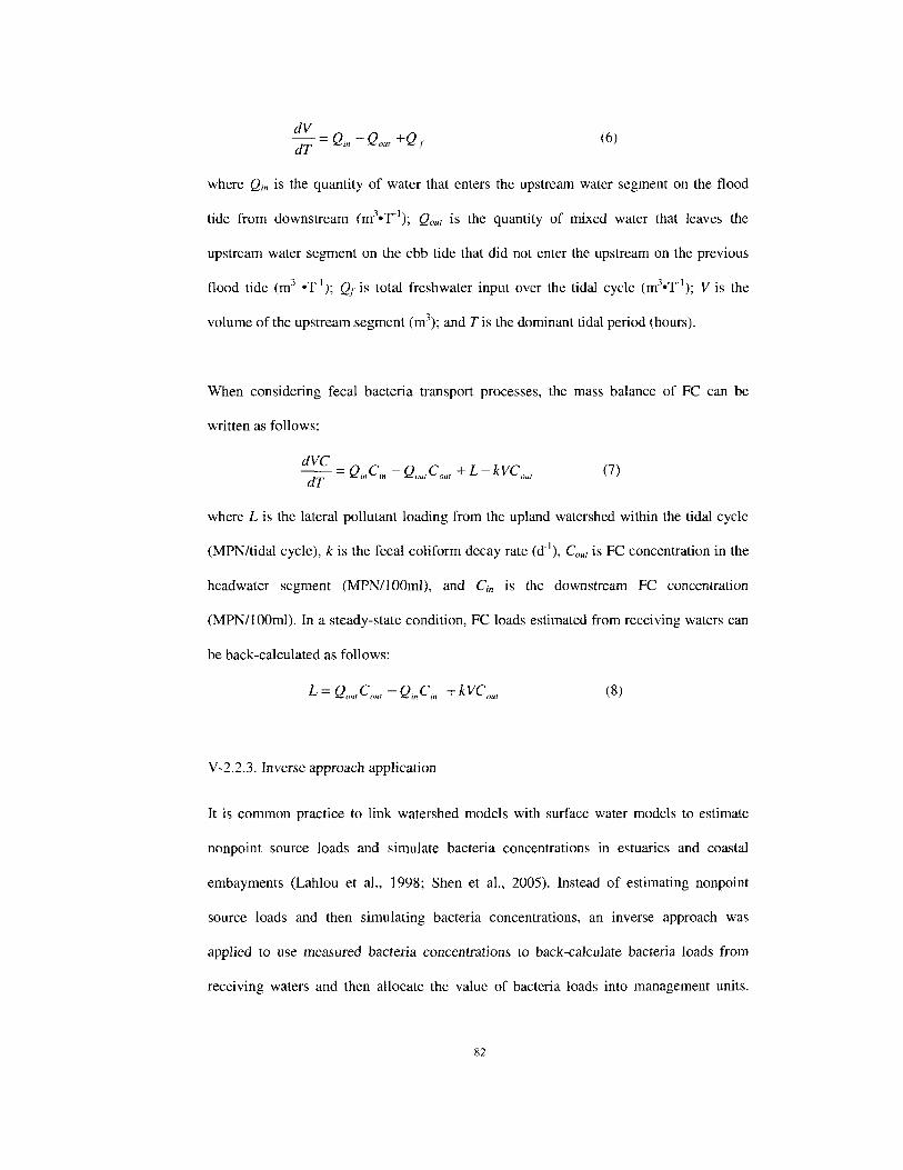
dV --Q -Q +Q dT- in out f (6)

where Q;11 is the quantity of water that enters the upstream water segment on the flood

tide from downstream (m3•T1); Qout is the quantity of mixed water that leaves the

upstream water segment on the ebb tide that did not enter the upstream on the previous

flood tide (m3 •T1); Q1 is total freshwater input over the tidal cycle (m3•T1

); Vis the

volume of the upstream .segment (m3); and Tis the dominant tidal period (hours).

When considering fecal bacteria transport processes, the mass balance of FC can be

written as follows:

(7)

where L is the lateral pollutant loading from the upland watershed within the tidal cycle

(MPN/tidal cycle), k is the fecal coliform decay rate (d-1), Cout is FC concentration in the

headwater segment (MPN/lOOml), and Cn is the downstream FC concentration

(MPN/lOOml). In a steady-state condition, FC loads estimated from receiving waters can

be back-calculated as follows:

L=QoutCour -QinCin +kVCour (8)

V-2.2.3. Inverse approach application

It is common practice to link watershed models with surface water models to estimate

nonpoint source loads and simulate bacteria concentrations in estuaries and coastal

embayments (Lahlou et al., 1998; Shen et al., 2005). Instead of estimating nonpoint

source loads and then simulating bacteria concentrations, an inverse approach was

applied to use measured bacteria concentrations to back-calculate bacteria loads from

receiving waters and then allocate the value of bacteria loads into management units.

82

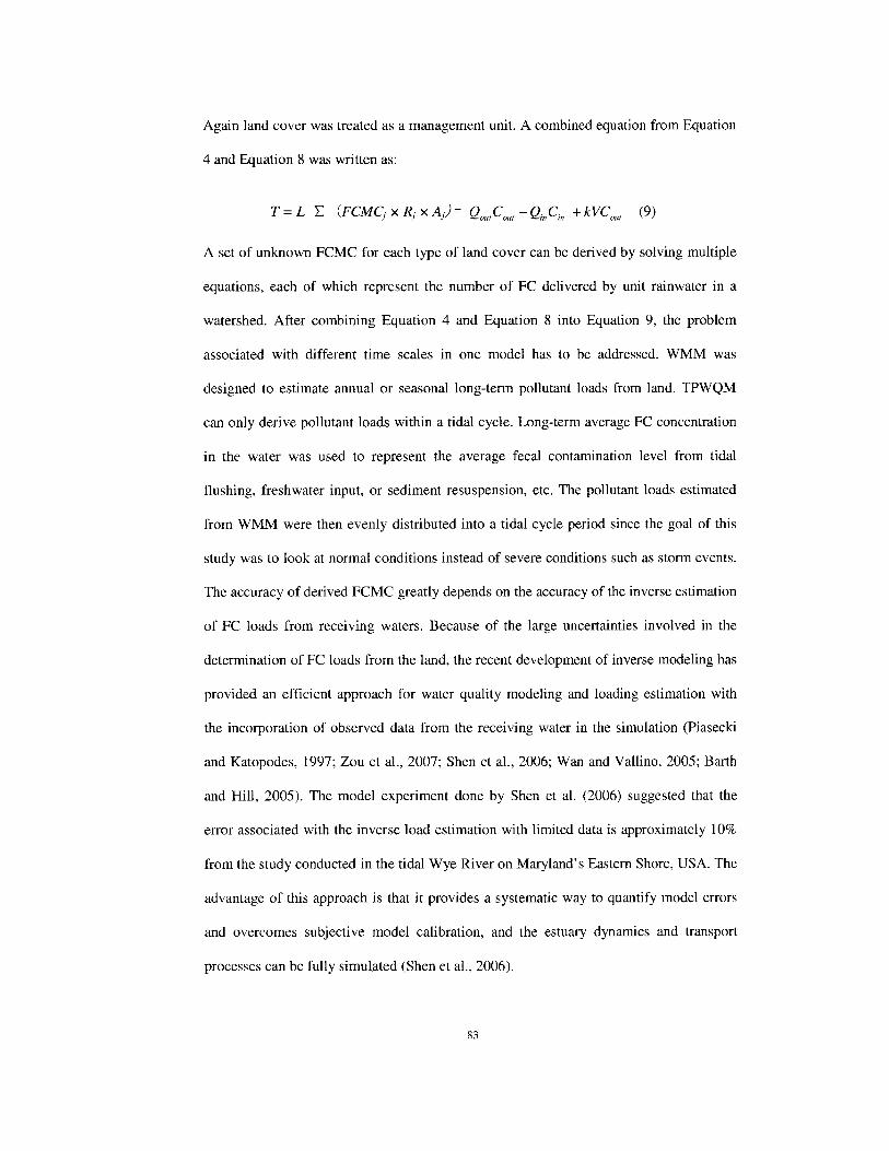
Again land cover was treated as a management unit. A combined equation from Equation

4 and Equation 8 was written as:

A set of unknown FCMC for each type of land cover can be derived by solving multiple

equations, each of which represent the number of FC delivered by unit rainwater in a

watershed. After combining Equation 4 and Equation 8 into Equation 9, the problem

associated with different time scales in one model has to be addressed. WMM was

designed to estimate annual or seasonal long-term pollutant loads from land. TPWQM

can only derive pollutant loads within a tidal cycle. Long-term average FC concentration

in the water was used to represent the average fecal contamination level from tidal

flushing, freshwater input, or sediment resuspension, etc. The pollutant loads estimated

from WMM were then evenly distributed into a tidal cycle period since the goal of this

study was to look at normal conditions instead of severe conditions such as storm events.

The accuracy of derived FCMC greatly depends on the accuracy of the inverse estimation

of FC loads from receiving waters. Because of the large uncertainties involved in the

determination of FC loads from the land, the recent development of inverse modeling has

provided an efficient approach for water quality modeling and loading estimation with

the incorporation of observed data from the receiving water in the simulation (Piasecki

and Katopodes, 1997; Zou et al., 2007; Sherr et al., 2006; Wan and Vallino, 2005; Barth

and Hill, 2005). The model experiment done by Sherr et al. (2006) suggested that the

error associated with the inverse load estimation with limited data is approximately 10%

from the study conducted in the tidal Wye River on Maryland's Eastern Shore, USA. The

advantage of this approach is that it provides a systematic way to quantify model errors

and overcomes subjective model calibration, and the estuary dynamics and transport

processes can be fully simulated (Sherr et al., 2006).

83

V-2.2.4 Inverse approach applied on categorized watersheds

There were a total of 15 variables chosen to associate with FC contamination levels in

165 upstream watersheds. These variables were: impervious surface percentage, forest

area, developed area, wetland area, crop area, pasture area, runoff potential, slope,

drainage density, eccentricity, residence time, and ratio of watershed area to water area,

watershed area, water area, and water volume. The GIS software ARCMAP 9.3 was used

to extract the necessary data from GIS data layers. FC data used in this study were

collected by the DSS monitoring survey. FC concentrations were extracted between 1994

and 1998, and their geometric means were calculated during this five-year period. These

five-year averages of FC concentrations were used to better represent seasonal average

conditions in each watershed to correspond with land cover data. NOAA Coastal Change

Analysis Program (C-CAP) 1996 land cover data was used in this study to estimate land

and water area and percentage of each land cover. Mid-Atlantic Regional Earth Science

Center (RESAC) impervious surface maps are available for 1990 and 2000, so RESAC

2000 impervious data were used for the calculation. It was assumed that there were not

significant changes for the impervious cover during the 4 years from 1996 and 2000. The

STATSGO database was used to determine the hydrologic soil runoff potential. The

primary soil attribute used in ST ATSGO is the hydrologic soil group (A, B, C, D). Group

A and Group B were grouped together to represent low runoff potential soils, while

Group C and D were grouped as high runoff potential soils. Soil drainage condition in a

watershed was determined by total area of low runoff potential soils divided by total area

of high runoff potential soils. The slope estimates for each watershed were the averaged

value from all the individual slope of grid cells inside the watershed using the USGS

DEM dataset. Drainage density was calculated by dividing the total length of the stream

within a watershed by its watershed area based on the National Hydrography Dataset

(NHD) dataset. Another hydrograph parameter considered was watershed eccentricity

84

(Black, 1972) which takes into consideration the unique shape of watersheds. The

eccentricity equation is shown here:

T = (IL/ -WL21l5 I WL

where r = watershed eccentricity, a dimensionless parameter, Lc =length from the outlet

to the center of mass of the watershed, and WL = width of the watershed perpendicular to

Lc and at the basin's center of mass, both in the same units (m). Low values of r are

found to be associated with high flood peak potential and high values ofT with low flood

peaks (Black, 1996). The residence time, RT, is an estimate of time required to replace

the existing pollutant concentration (or water) in a system; it can be calculated as follows:

RT = Vb I Qb , where Vb is mean volume of the embayment, and Qb is the quantity of

mixed water that leaves the bay on the ebb tide that did not enter the bay on the previous

flood tides (m3 per tidal cycle). In a steady-state condition, the mass balance equations for

the water can be written as follows: Qb = Qo + Q1 , where Q1 is total freshwater input over

the tidal cycle (m3), and Q0 is the volume of new ocean water entering the embayment on

the flood tide, which can be determined by the use of the ocean tidal exchange ratio fJ as:

Q0 = fJ * Qr, where Qr is the total ocean water entering the bay on the flood tide (equal to

water surface area multiplied by tidal range). fJ is defined as the ratio of new ocean water

to total volume of water that enters the estuary during a flood tide (Fisher et al., 1979).

Usually, the return ratio was set as 0.7, as previous studies suggested for a Virginia

coastal embayment (Kuo et al., 1998).

The CART method was applied to account for FC concentration variability as a function

of the variables mentioned above. Cluster analysis was then applied to the variables

derived from the CART analysis. In each cluster of watersheds, the total FC loading in

each watershed derived from the WMM equaled the hydrological model calculation

result of the total FC loading from the TPWQM, as shown in Equation 9 (where

85

R j = C P + ( C; - C P )IMPj ]I). In any given system, values of the runoff coefficient vary

from 0.05 to 0.95 (ASCE, 1992). Runoff coefficients applied in this study use the average

value of the range and the values were slightly adjusted for seasonal differences as shown

in Table V-2.1. Seasonal impacts on FC abundance were considered based on the results

of PCl in Figure IV-4.6.5. FC abundance is obviously higher in the months from April to

October, but lower in the months from November to March. Here the period from April

to October is considered the warm season, and the cold season is from November to

March. Annual and monthly precipitation was derived by averaging monthly

precipitation data in three Virginia cities (Norfolk, Richmond, and Williamsburg)

extracted from the National Climatic Data Center with the aid of the Climatology Office

at the University of Virginia. Available precipitation data in Norfolk is from 1/1/1946 to

12/3112008, from 811/1948 to 12/31/2008 in Williamsburg, and from 811/1948 to

12/31/2008 in Richmond. Monthly water discharge data for the western side of

Chesapeake Bay was averaged from daily stream flow data during the period between

1/1/1984 and 12/31/1996 from USGS gaging station 01661800 located in the headwaters

of Great Wicomico River, VA. Water discharge data from USGS gaging station

01844800 located in the headwaters of Nassawadox Creek, VA was used for the Eastern

Shore. Values of the FC decay rate range from 0.5 to 3.0 per day in salt water (Thomann

and Mueller, 1987; Mancini, 1978). A constant bacteria decay rate of 1.0 d.1 was used for

the warm season, and 0.3 d- 1 for the cold season, which is a common practice in water

quality modeling (Shen and Zhao, 2009). There were five unknown variables: FCMC of

forest, urban, cropland, pastureland, and wetland. This means the values of each FCMC

could be derived only if there were at least five equations. The FCMCs for each group

were obtained by a least squares method that used the minimal sum of the deviations

from the given set of data. Watersheds in each group are supposed to have similar FC

86

mean concentrations (FCMCs), which were derived for each land cover and had the unit

of MPN per square meter per inch of rainfall.

V-2.2.5 Alternate Approach: Inverse calculation on land-cover-dominated watersheds

An alternate approach was used as well, in order to help explain unexpected results due to

large uncertainties, as well as variations in FC measurements. For example, negative

FCMC values could possibly result from the inverse calculation method. In the alternate

approach, an ideal situation was assumed where a watershed was only occupied by one

land cover type. This ideal situation would simplify all the inverse calculation processes

and avoid unexpected results such as negative FCMC values. Although this ideal

situation didn't exist at the scales of studied watersheds, this exercise still provides useful

information. An approximate situation is a watershed dominated by a single land cover,

the percentage of which exceeds 70 -80 % of the whole watershed area. Cropland and

pastureland were combined together because each occupies less than 60% of the total

watershed and neither could be regarded as the dominant land cover with a criterion set

as 70%. The standard for a watershed to be called a single land-cover-dominated

watershed is designated as follows: A "forest-dominated" watershed is one with

forestland occupying more than 80% of the entire watershed area.

A "crop-pastureland-dominated" watershed is one for which the cropland and pastureland

together occupy about 70% of the entire watershed. An "urban-dominated" watershed is

one with more than 70% land as developed area. It was assumed that total FC loads from

a watershed all come from this dominant land cover. Based on this assumption,

FCMCdominan1 can be derived from the following equation, for both warm and cold seasons,

based on Equation (9):

FCMC dominantRdominantAdominant = QoutCout - Q,.,C;, + kVCour (10)

87

V-3 Results

V-3.1 Inverse calculation on categorized watersheds

The variables output from the CART analysis were supposed to contribute significantly

to the FC levels. These variables were impervious surface percentage, forest percentage,

pasture percentage, wetland percentage, ratio of watershed area divided by water area,

and residence time as shown in Figure IV-4.7.2. Cluster analysis was applied to these

variables derived from the CART analysis. Paul et al. (2006) mentioned that, in the

current study, there was no clear guidance from any of the criteria for the number of

clusters. After an initial analysis based on criteria described in the statistic software

Minitab 15 where the abrupt change in the similarity levels determines the number of

clusters, the result was 5 clusters (i.e. 5 groups) of watersheds (Figure V -3.1) utilizing the

Manhattan Distance and Complete Linkage method. The clusters have 78, 56, 20, 7, and

4 watersheds as shown in Figure V-3.2. There are problems with the results. Table V-3.1

shows the results of Group 2, which has 56 watersheds, as an example. In Table V-3.1,

the value of the coefficient for each variable is the value of FCMC for each type of land

cover. Pasture has a negative value, which is incorrect. After trying to force the constant

to equal a minimum of zero, several negative values still exist.

V-3.2 Alternate approach: Inverse calculation on land-cover-dominated watersheds

Since there were some negative values in the derived FCMC values using the inverse

approach, the alternate approach was applied for further analysis. Selected upstream

watersheds were shown in Table IV -4.3.1. Each watershed is dominated by one type of

land cover. Derived FCMCs for three types of land cover (forest, urban, and

88

crop-pastureland) and their standard deviations are given in Table V-3.2 for both warm

and cold seasons. The data show that FCMCs are similar to each other in the warm

season with forest having the smallest values. FCMCs in urban areas during the cold

season are less than FCMCs in urban areas during the warm season. During the cold

season, FCMCs in urban areas are about one order of magnitude higher than FCMCs in

forest and crop-pastureland.

V-4. Model Verification

It is often said that all models are wrong but some are useful. Uncertainty exists in any

model because of imperfect representations of the real world. Thus it is necessary to

verify the model performance and check carefully to ensure the model reflects a

reasonable reality. Model verification in this study was performed by using literature data,

analytical data, and available observed data.

V -4.1 Model verification from literature data

From the literature data, FC loadings estimated by Reinelt and Horner (1995) were 4.2 x

1010 and 1.4 x 109 organisms ha-1 year -I for the urban and non-urban wetlands,

respectively, in King County, Washington. According to the records at the University of

Washington station in Seattle, mean annual precipitation is about 34.78 inches in King

County, Washington. Total FC loading can then be converted to the unit defined as FC

generated per m2 of surface per inch of rainfall. Weiskel et al. (1996) related total FC

loads, defined as the FC generated per m2 of surface per centimeter of rainfall, to the

surrounding land use. Since the author provided the area for associated land use, total FC

loading can also be converted to the unit defined as FC generated per m2 of surface per

inch of rainfall. Table V-3.3 shows the comparison between the estimated FC mean

concentration in this study and the mean concentrations from previous studies, mentioned

89

above, but converted to the same units as this study. Previous studies did not separate FC

loading into seasons, which makes the verification more difficult. Overall, the

magnitudes of estimated FC mean concentrations are close to each other among similar

land conditions, even though the research sites are located in different areas: one is in

King County, Washington (Reinelt and Horner, 1995), one is in Buttermilk Bay,

Massachusetts (Weiskel et al. 1996), and this study is in Chesapeake Bay, Virginia. The

previous studies suggest that the estimated FCMCs were reasonable.

V-4.2 Model verification from analytic data

The accuracy of the results was also evaluated through the comparison between the

estimated total FC loading using FCMCs and the calculated total FC loading using

TPWQM in all 165 upstream watersheds. The estimated total FC loadings were obtained

by summing the FC loadings from each individual land cover. FC loadings from each

individual land cover were calculated by applying FCMC in the equation: FCMC *

Runoff * Land cover area. This calculation is based on land processes. The calculated

total FC load using TPWQM is based on processes occurring in the water. Since FC

concentration in the water depends on hydrodynamic processes (such as flushing) and

biological process (such as FC decay), total FC loading from the land is back-calculated

after considering these processes in the water. TPWQM simulates net water flow over a

tidal cycle and can be coupled with observed FC concentrations and FC decay rate to

produce total FC loadings from land at steady state. Figure V-3.4 shows the

log-transformed comparison both in warm and cold seasons between the estimated and

the calculated total FC loadings over a wide range of FC total loadings. In general,

estimated loadings agree well with FCMC derived FC total loading, with R square

equaling 0.54. Figure V-3.6 shows the same comparison but with actual values (not

log-transformed). Like the log-transformed comparison, they match well with each other

90

except for a watershed in the warm season and several in the cold season. No specific

reasons have been found to explain their differences. The comparison suggests that

FCMCs offer a simple, but effective way to quantify the fecal contamination sources

based on land cover.

V -4.3 Model verification from observed data

In order to better verify the accuracy of the FCMCs, four watersheds with the greatest

land cover change from 1984 to 2005 (using C-CAP 1984 and C-CAP 2005 land cover

datasets) were selected to test the FCMCs reliability. Selected watersheds and their major

land cover change are shown in Table V-3.4. Watershed 52_M1_UP, 58_Ml_UP,

58_M2_UP, AND 63_M3_UP show the urban areas increasing by 35%, 40%, 25% and

27%, respectively. Without changing any parameter values used in the equations, such as

runoff coefficients, between 1984 and 2005. Figure V-3.8 shows the comparison between

observed FC concentration percentage changes and estimated total FC loading percentage

changes. The assumption for this comparison was that nothing changed in the

hydrodynamic processes (such as streamflow or return ratio) and biological processes

(FC decay rate) in these watersheds' receiving waters. From the graph, all the observed

FC concentrations show an increasing trend during this 21-year period indicating

percentage increases. One can also notice the same trend from the estimated FC total

loading with all the percentage increases. This similar trend suggests that FCMC can

capture the increasing phase of observed FC concentration variability during these years.

The magnitude of the percentage change, however, is different; most of the estimated FC

total loading percentage changes are smaller than the observed FC concentration

percentage changes, especially in the warm season. There are a few reasons to explain

this discrepancy. One of the possibilities is due to the inaccuracy of the impervious data.

91

The impervious data used in this study was from 1990 and 2000, but the time period for

land cover change is from 1984 to 2005. The accuracy of the result is largely limited by

the difference in the data collection and availability. The second reason is likely due to

the assumption that there was no change in streamflow discharge from 1984 to 2005.

Jennings and Jarnagin (2002) observed that historical changes in streamflow in the upper

Accotink Creek subwatershed (close to Annandale, Virginia) appear to be related to

increases in anthropogenic impervious surface cover. The third reason is that the same set

of runoff coefficients was used in both 1984 and 2005. In the cold or warm season for

each individual year, runoff coefficients only varied for different land covers but didn't

vary between watersheds. Even though the same kind of land cover existed in the two

watersheds, physical characteristics of the two land areas would differentiate them from

each other, such as slope, percentage of vegetation cover, and so on. Strictly speaking,

runoff coefficients should be given different values to reflect the discrepancies among

watersheds. But in the classical "rational formula" (Dooge, 1957) the runoff coefficient is

considered to be a constant, differing in value between different types of surface cover of

a watershed. Whether the runoff coefficient can be considered a constant has been a

controversial question in hydrology (Gottschalk and Weingartner, 1998).

Liitschg-Loetscher (1945) sums up the problem as follows: "In spite of the fact that Karl

Fischer (1934) and Walter Wundt (1937) have expressed their opinion repeatedly and in

depth, the erroneous opinion is at hand still here and there that the value of this relation

(the runoff coefficient) for a certain drainage basin is a hydrographic constant, so that by

changing precipitation runoff can be determined in advance or, vice versa, the

precipitation can be determined from the runoff." Unit hydrographs, including rainfall

volumes and runoff coefficients, have been extensively studied by Weingartner (1989)

for 17 well-equipped Swiss drainage basins with an area ranging between 5 and 200 km2•

From his work, runoff coefficients could at least be influenced by altitude, slope, river

92

network density, and soil permeability, etc. Therefore, using the same set of runoff

coefficients for both 1984 and 2005 introduces errors in the estimation of percentage

changes in terms of FC total loading.

V-5 Discussion

V-5.1 Inverse calculation on categorized watersheds

Even though the inverse calculation on categorized watersheds didn't result in expected

results, it still appears to be a theoretically correct approach to obtain FCMCs. The

purpose of using cluster analysis was to group watersheds that have similar watershed

characteristics and, hence, have similar fecal contamination levels. Such a grouping

scheme would be helpful in reducing the cost of restoration of water quality by restricting

the development of the TMDL to one or two representative water bodies under a single

group and applying the knowledge to other water bodies in the same group (Paul et al.,

2006). There were some negative values in the results, which are incorrect. But it is

possible to get these negative values since the derived values (FCMCs) vary in a large

range due to individual watershed differences, amount of data collection, natural

variability, random events, and the variation in FC measurements, etc. The estimation of

total FC loadings was based on an additive model and assumes linear processes, which

was probably an incomplete representation compared to the reality. The loadings can

potentially overestimate or underestimate the impacts of land cover on fecal

contamination.

V-5.2 Alternate approach: Inverse calculation on land-cover-dominated watersheds

The alternate approach tried to avoid the production of negative FCMC values and

switched the target from watersheds with mixed types of land cover to watersheds with

93

one dominant land cover. This approach produced two sets of FCMCs, one for the warm

season, and one for the cold season. The similarity of FCMCs for different land covers in

the warm season can be explained by the increased outdoor activities of domestic animals,

increasing movement and behavior of wildlife, and manure spreading on fields during the

growing season. The forest FCMCs having the lowest values could be probably attributed

to the vegetation and its special soil infiltration capability. In a typical forested ecosystem,

approximately 40% of the precipitation is returned to the atmosphere by

evapotranspiration, and approximately 50% infiltrates into the soil, with the remaining 10%

returned to receiving waters via surface runoff (e.g., Dunne and Leopold, 1978; Harbor,

1994; Arnold and Gibbons, 1996). FCMCs in urban areas during the cold season were

less than FCMCs in urban areas during the warm season. The major reason for this is

probably due to decreased precipitation in the cold season compared to warm season.

During the cold season, FCMCs in urban areas are about one order of magnitude higher

than FCMCs in forest and crop-pastureland. Major FC sources from urban areas are

through on-site septic tanks or combined sewer overflow, while FC sources from

non-urban areas are mostly carried by runoff and/or through direct feces deposition into

water. The time domestic and wild animals spend on the fields and accessing the water

possibly determines the amount of potential FC loadings. Human activities were not

affected by season as much as domestic animals and wildlife, and it is reasonable to

obtain larger FCMCs in urban than in non-urban areas. In many cases, the hydrology in

urban areas has been severely altered to allow for urban development, which has resulted

in an increase in the amount of impervious surfaces, and subsequently, a drastic rise in

the volume of runoff that ultimately may cause combined sewer overflow in some areas

(McLellan et al., 2007). This is probably one of the reasons why urban areas are the focal

point of the fecal contamination issues. The issues about how to deal with human wastes

remain one of the most difficult environmental and fiscal challenges in the United States

94

(Heaney et al. 1999). Much of the population increase is occurring in rural areas that are

typically not served by municipal wastewater facilities, resulting in the expanded use of

on-site wastewater disposal systems. Although removal efficiencies in properly

functioning drain fields are high (Hagedorn et al., 1981; Reneau eta!., 1989), there is

only limited FC purification of wastewater within a septic tank (Reay, 2004). Recent

studies suggested that failing septic tanks might pose a serious risk for human source

fecal contamination (Scheuler, 1999). In many municipal areas, urban stormwater is

discharged directly into waterways with no treatment. Urban stormwater and sewage

overflow are still considered major sources of water-body impairment in the U.S.

(USEPA, 2004).

One of the advantages of using FCMCs is that they can fit easily into a spreadsheet to

estimate fecal bacteria loadings and can be coupled with any hydrologic simulation to

produce bacteria loads. Their uncertainty was represented as FC mean concentration plus

a standard deviation in warm and cold seasons, respectively. However, the FCMCs will

have little value unless they are used with site-specific information, such as the spatial

and temporal information from land and water.

V-5.3 Model sensitivity test

Assembling the types of data necessary for running and calibrating a model is typically

expensive and time consuming (NRC, 2000). Therefore, a sensitivity test run before

using the model can provide two benefits. One is that the sensitivity test often indicates

the relative importance of model input parameters and indicates which parameters should

receive the most management attention (NRC, 2000). Another is that the potential effect

of errors inherent to the model must be considered before evaluating the effect of errors

95

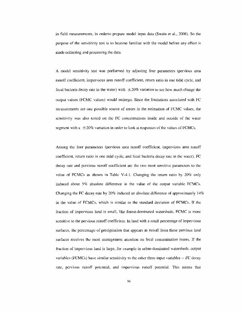
in field measurements, in orderto prepare model input data (Swain et al., 2008). So the

purpose of the sensitivity test is to become familiar with the model before any effort is

made collecting and processing the data.

A model sensitivity test was performed by adjusting four parameters (pervious area

runoff coefficient, impervious area runoff coefficient, return ratio in one tidal cycle, and

fecal bacteria decay rate in the water) with ±20% variation to see how much change the

output values (FCMC values) would undergo. Since the limitations associated with FC

measurements are one possible source of errors in the estimation of FCMC values, the

sensitivity was also tested on the FC concentrations inside and outside of the water

segment with a ± 20% variation in order to look at responses of the values of FCMCs.

Among the four parameters (pervious area runoff coefficient, impervious area runoff

coefficient, return ratio in one tidal cycle, and fecal bacteria decay rate in the water), FC

decay rate and pervious runoff coefficient are the two most sensitive parameters to the

value of FCMCs as shown in Table V -4.1. Changing the return ratio by 20% only

induced about 5% absolute difference in the value of the output variable FCMCs.

Changing the FC decay rate by 20% induced an absolute difference of approximately 14%

in the value of FCMCs, which is similar to the standard deviation of FCMCs. If the

fraction of impervious land is small, like forest-dominated watersheds, FCMC is more

sensitive to the pervious runoff coefficient. In land with a small percentage of impervious

surfaces, the percentage of precipitation that appears as runoff from these pervious land

surfaces receives the most management attention on fecal contamination issues. If the

fraction of impervious land is large, for example in urban-dominated watersheds, output

variables (FCMCs) have similar sensitivity to the other three input variables -- FC decay

rate, pervious runoff potential, and impervious runoff potential. This means that

96

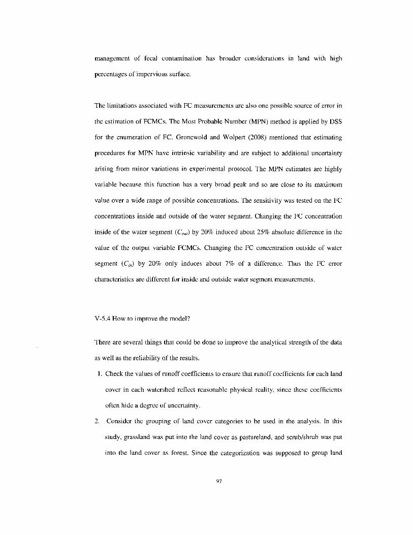
management of fecal contamination has broader considerations m land with high

percentages of impervious surface.

The limitations associated with FC measurements are also one possible source of error in

the estimation of FCMCs. The Most Probable Number (MPN) method is applied by DSS

for the enumeration of FC. Gronewold and Wolpert (2008) mentioned that estimating

procedures for MPN have intrinsic variability and are subject to additional uncertainty

arising from minor variations in experimental protocol. The MPN estimates are highly

variable because this function has a very broad peak and so are close to its maximum

value over a wide range of possible concentrations. The sensitivity was tested on the FC

concentrations inside and outside of the water segment. Changing the FC concentration

inside of the water segment (Caur) by 20% induced about 25% absolute difference in the

value of the output variable FCMCs. Changing the FC concentration outside of water

segment (Cn) by 20% only induces about 7% of a difference. Thus the FC error

characteristics are different for inside and outside water segment measurements.

V-5.4 How to improve the model?

There are several things that could be done to improve the analytical strength of the data

as well as the reliability of the results.

1. Check the values of runoff coefficients to ensure that runoff coefficients for each land

cover in each watershed reflect reasonable physical reality, since these coefficients

often hide a degree of uncertainty.

2. Consider the grouping of land cover categories to be used in the analysis. In this

study, grassland was put into the land cover as pastureland, and scrub/shrub was put

into the land cover as forest. Since the categorization was supposed to group land

97

with similar characteristics, the groupings would partially determine the accuracy of

the results. For example, should open space in urban areas or bare land be put into the

urban category or another land cover category?

3. Have data collected from the outlets draining a single land cover in individual

watershed. These data would be helpful in the quantification processes. However,

there are few coordinated efforts to maintain a database of samples collected from

outlets downstream of a single land cover region. Such a database would be valuable

for developing loading estimates of receiving waters, for model calibration, and for

the purposes of developing simplified relationships between concentration, loads, and

causative factors.

V -6 Conclusions

Protection from fecal microbial contamination is one of the challenges to safeguard water

quality. Environmental management of fecal contamination has forced many states and

federal agencies to allocate pollution reduction responsibility using management units to

reduce fecal pollutants released from land and transported in runoff to water. For an

effective management of fecal pollution processes, it is important to quantify fecal

bacteria sources in relation to commonly used management units. In this study, fecal

bacteria sources are quantified as a function of land cover (land cover area, land cover

runoff coefficients, impervious condition). Here each kind of land cover is a management

unit. The derived FCMCs for land covers provide an easy way to estimate the amount of

fecal bacteria coming from any individual land cover and offer a reference, which could

assist the allocation of pollution reduction responsibility.

The model developed in this study avoids the problems associated with using highly

varied and poorly documented FC production rates and population numbers. Although

98

the model is simple, the magnitude of FCMC values based on land covers effectively

distinguished the seasonal FC loadings and captures the difference between land covers.

The quantification of FC bacteria sources based on land cover could make it easier for

managers to assign land cover based accountability to restore fecal contaminated

environment. In general, FCMCs provide suggestions for the effective management of

fecal contamination m water systems. The derived FCMCs can also be powerful

parameters for predicting effects of land cover change on fecal contamination issues. The

accuracy and reliability of the suggestions and predictions is dependent on how FCMCs

are used. Incorporation of site-specific information is necessary to understand how

different sources contribute to the pollution in any single watershed.

99

VI. SUMMARY

This study provided the first comprehensive examination of FC spatial and temporal

distribution in the Virginia portion of Chesapeake Bay. Based on the information from

FC spatial and temporal distributions, fecal bacteria loadings from land were quantified

as a function of land cover from this research. FC quantification processes were a

relatively easy but efficient way to estimate the amount of fecal bacteria coming from

different land sources.

By describing how fecal contamination levels are distributed at different spatial and

temporal scales and the resulting patterns, this research demonstrated several interesting

findings. 1) The analysis on tidal effects showed that there was clearly seasonal

differences in FC levels between summer and winter, and the differences due to seasonal

change were much larger than the differences due to tidal effects. FC quantification must

account for seasonal variation rather than tidal variation. 2) The consistent spatial pattern

throughout Virginia coastal regions inferred that FC distribution differences among

upstream, middle and downstream regions were mostly due to the gradient of salinity and

tidal influence. Restoring water quality upstream may help improve water quality

downstream. 3) The results from the comparison between different land-cover-dominated

watersheds suggested that fecal contamination levels respond differently between

urban-dominated, forest-dominated and crop-pastureland-dominated watersheds,

reflecting the different characteristics among these contrasting land covers. The effect of

land cover on the quantification approach supports the use of land cover as a unit to

quantify FC loadings from land. 4) Investigation of impervious surface areas using

100

Nonparametric Changepoint Analysis demonstrated that the threshold value for

impervious surfaces expanding due to development was 15%. In a watershed whose

impervious surface percentage exceeds this threshold, water quality has a high possibility

of being seriously impaired from fecal contamination. Even though threshold values have

been mentioned in previous research, none of the studies identified threshold values using

such large amount of data, especially in Virginia coastal regions. 5) The probability to

exceed a given FC concentration value is greatest in the James River, followed by the

York and the Rappahannock Rivers, with the lowest occurring on Eastern Shore. This

pattern could probably be associated with the landscape characteristics of the different

river systems, resulting in different management decisions. 6) Previous studies described

physical factors as having important effects on fecal pollution. This study demonstrated

that the magnitude of FC levels may be determined by the intensity of rainfall,

temperature, and water discharge. Rainfall, temperature and flow discharge together

explained about 81% of data variation. 7) Environmental variables making significant

contributions to FC levels were determined to be impervious surface percentage, forest

percentage, pasture percentage, wetland percentage, runoff potential, ratio of watershed

area divided by water area, and residence time based on classification and regression tree

analysis. Quantifying the magnitude of the contribution of environmental variables to

fecal contamination levels has not been studied in previous research. This study also

raises some interesting points for future research, such as the large contributions from

wetlands compared to forest and pastureland, and no significant contribution of fecal

contamination from cropland. Even though there are some limitations in the dataset, the

author believes that the results offer valid insights and ideas for additional research.

In addition to the investigation of FC spatial and temporal distribution patterns, another

core contribution from this study is that FC loadings are quantified as a function of land

101

cover based on real data, not estimates of the number of wild and domestic animals living

in the study sites. The model developed in this study avoids the problems associated with

using highly variable and poorly documented population numbers and FC production

rates. Although the model is simple, the magnitude of Fecal Coliform Event Mean

Concentration (FCMC) values based on land covers effectively distinguished the seasonal

FC loadings and captured the difference between land covers. The derived FCMC is a

very useful variable which can be used to calculate FC loading from each land cover.

Actually, it provides a very practical suggestion for effective management of fecal

contamination, for example, in the development of TMDLs to deal with excess bacteria

in coastal waters. It also is easier for managers to assign land-cover-based accountability

to help restore fecally contaminated environments.

102

VII. REFERENCES

3RWWDP (The 3 Rivers Wet Weather Demonstration Program), 1998. Understanding the sewer collection system. http://www.3riverswetweather.org/d weather/d know.stm

Aiyyer, Anantha R., Chris Thorncroft, 2006: Climatology of Vertical Wind Shear over the Tropical Atlantic. Journal of Climate, 19, 2969-2983

Aneta!., 2002. E coli and Total Coliforms in Water and Sediments at Lake Marinas, Environmental Pollution, Elsevier Science Ltd, New York, NY, 120(2002):771-778, (2002).

Anderson, I. C., M. Rhodes, and H. Kator. 1979. Sublethal stress in Escherichia coli: a function of salinity. Applied and Environmental Microbiology, 38: 1147-1152.

Arnold, C.L., and C.J. Gibbons, 1996. Impervious surface coverage. Journal of the American Planning Association. 62 2, pp. 243-258.

American Society of Civil Engineers (ASCE), 1992. Design and Construction of Urban Stormwater Management Systems. Manuals and Reports of Engineering Practice No. 77, New York, NY: WEF Manual of Practice RD-20.

Barbe, D.E., S. Carnelos, and J. A. McCorquodale, 2001. Climatic effect on water quality evaluation. Journal of Environmental Science and Health, A36(1 0): 1919-1933.

Barber, R. T., R. L. Ohrel, P. K. Fowler, and G. L. Gilbert, 1993. Why we are convinced that traditional strategies for wastewater management are not working. In Ohrel, R. L. (ed.), Symposium on Integrated Wastewater Management in North Carolina. North Carolina Coastal Federation, Wilmington, N.C.: 7-13.

Barth, G., Hill, M., 2005. Numerical methods for improving sensitivity analysis and parameter estimation of virus transport simulated using sorptive-reactive processes. Journal of Contaminant Hydrology. 76, 251-277.

Bay Journal, 2008. VA adds 1,100 miles of rivers to polluted list. www.Bavjournal.com

Becker, Carol J. 2004. Water quality and possible sources of nitrogen and bacteria to Rock and Travertine Creeks, Chickasaw National Recreation Area, Oklahoma, 2004. Scientific Investigations Report, Report: SIR 2005-5279, 24 pp., 2004

Bilkovic, D.M. and M.M. Roggero, Effects of coastal development on nearshore estuarine nekton communities. Marine Ecology Progress Series, Vol. 358: 27-39.

Bjornsson, H. and S.A.Venegas, 1997. A manual for EOF and SVD analyses of climate data. McGill University, CCGCR Report No. 97-1, Montreal, Quebec, p. 52.

Black, P.E., 1972. Hydrograph responses to geomorphic model watershed characteristics and precipitation variables, Journal of Hydrology 17:309.

Black, P. E., 1996. Watershed Hydrology. Second Edition. Ann Arbor Press, Inc. 121 South Main Street, Chelsea, Michigan 48118.

Boehm, A. B., J. A. Fuhrman, R. D. Morse, and S. B. Grant. 2003. Tiered approach for identification of a human fecal pollution source at a recreational beach: case study at Avalon Bay, Catalina Island, California. Environmental Science & Technology. 37:673-680.

Boesch, D.F., R.B. Brinsfield, and R.E. Magnien. 2001. Chesapeake Bay eutrophication: scientific understanding, ecosystem restoration, and challenges for agriculture. Journal of Environmental Quality, 30:303-320.

Boon, 2004. Secrets of the Tide. Published by Horwood Publishing Limited, Col House, Westergate,

103

Chichester, West Sussex, P020 3QL, England.

Booth, A.M., Hagedorn, C., Graves, A.K., Hagedorn, S.C., and K.H. Mentz, 2003. Sources of fecal pollution in Virginia's blackwater river. Journal of Environmental Engineering, 129, 547-552.

Bricker, S.B., Clement, C.G., Pirhalla, D.E., Orlando, S.P., and D. R. G. Farrow, 1999. National estuarine eutrophication assessment: effects of nutrient enrichment in the nation's estuaries, NOAA. National Ocean Service, Special Projects Office and the National Centers for Coastal Science. Silver Spring, Maryland, 71 pp.

Burkhardt III, W., K.R. Calci, W.D. Watkins, S.R. Rippey, and S.J. Chirtel, 2000. Inactivation of indicator microorganisms in estuarine waters. Wat. Res. 34(8): 2207-2214.

Cahoon, L.B., J.C. Hales, E.S. Carey, S. Loucaides, K.R. Rowland, and J.E. Nearhoof, 2006. Shellfish Closures in Southwest Brunswick County, North Carolina: Septic Tanks vs Storm-Water Runoff as FC Sources. Journal of Coastal Research 22(2):319-327.

Carrington E.G., Davis, R.D. and E.B. Pike, 1998. Review of the scientific evidence relating to the controls on the agricultural use of sewage sludge, Part I. The evidence underlying the 1989 Department of the Environment code of practice for agricultural use of sewage sludge and the sludge (use in agriculture) regulations. DETR Report No. DETR 4415/3 (now DEFRA) 17 Smith Square London SW1P 3JR UK.

Chui, T.W., 1981. Highway runoff in the State of Washington: model verification and statistical analysis. M.S.E thesis, Department of Civil Engineering, University of Washington, Seattle, W A.

Crabill, C., Donald, R., Snellling, J., Fourst, R.. and G. Southam,. 1999. The impact of sediment FC reservoirs on seasonal water quality in Oak Creek, Arizona, Water Research 33, 2163-2171.

Crowther, J., Kay, D. and Wyer, M. D.: 2002, 'Faecal-indicator concentrations in waters draining lowland pastoral catchments in the UK: Relationships with land use and farming practices', Water Research. 36(7), 1725-1734.

Donnison, A.M. and C.M. Ross, 1999. Animal and human faecal pollution in New Zealand rivers, N.Z. Journal of Marine Freshwater Research, 33(1 ). 119.

Dooge, J.C.I., 1957. The rational method for estimating flood peaks. Engineering, 184, 311-313, 374-377.

Doran, J. W. and D.M. Linn, 1979. Bacteriological quality of runoff water from pastureland. Applied Environmental Microbiology, 37(5), 985-991.

Doyle, M.P. and M.C. Erickson, 2006. Closing the Door on the FC Assay. Microbe 1(4): 162- 163.

Dunne, T. and L.B. Leopold. 1978. Water in Environmental Planning., Freeman, New York.

Edwards, D. R., Daniel, T. C., Moore, Jr., P. A. and Sharpley, A. N.: 1994, 'Solids transport and erodibility of poultry litter surface-applied to fescue', Transactions of ASAE. 37(3), 771-776.

Edwards, D. R., Larson, B. T., and T.T. Lim, 2000. Runoff nutrient and fecal coliform content from cattle manure application to fescue plots. Journal of the American Water Resources Association, 36(4), 711-722.

El-Sharkawi, F., L. El-Atar, A. A. Gawad, and S. Molazern. 1989. Some environmental factors affecting the survival of fecal pathogens and indicator organisms in seawater. Water Science and Technology 21:115-120.

Esham, E. C. 1994. Effects of physical parameters on two techniques, mFC and mTEC. for determining sources of fecal pollution in tidal creeks. Thesis. University of North Carolina at Wilmington, Wilmington, North Carolina, USA.

Evanylo, G.K., 1999. Agricultural Land Application of Biosolids in Virginia: Managing Biosolids for Agricultural Use. Crop and Soil Environmental Sciences, Publication Number 452-303.

Evison, L. M. 1988. Comparative studies on the survival of indicator organisms and pathogens in fresh and sea water. Water Science and Technology 20:309-315.

104

Ferguson, C. M., B. G. Coote, N. J. Ashbolt, and I. M. Stevenson, 1996. Relationships between indicators, pathogens and water quality in an estuarine system. Water Research 30: 2045-2054.

Ferguson, C. de Roda Husman, A. M., Altavilla, N., Deere, D., and Ashbolt, N., 2003. Fate and transport of surface water pathogens in watersheds. Critical Reviews in Environmental Science and Technology, 33 (3), 299- 361.

Field, K. G., E. C. Chern, L. K. Dick, J. Fuhrman, J. Griffith. P. A. Holden, M.G. LaMontagne, J. Le, B. Olson, and M. T. Simonich. 2003. A comparative study of culture-independent, library-independent genotypic methods of fecal source tracking. Journal of Water I: 181-194.

Fischer, K., 1934. Klassifikation der Flu .. sse nach dem Abflusskoeffizienten. Deutsche Wasserwitschaft Heft 12, Stuttgart.

Fisher,H.B .. List,E.J., Koh,R.C. Y., Imberger,J. and Brooks,N.H. (1979) Mixing in Land and Coastal Waters. Academic Press, NY.

Galland, J.C., Hyatt, D.R., Crupper, S.S., and D.W. Acheson, 2001. Prevalence, antibiotic susceptibility, and diversity of Escherichia coli 0157:H7 isolates from a longitudinal study of beef cattle feedlots, Applied and Environmental Microbioogyl., 67, 1619.

Geldreich, E.E., Huff, C.B., Bordner, R.H., Kabler, P.W. and Clark, H.F. 1962. The faecal coli-aerogenes flora of soils from various geographic areas. Journal of Applied Bacteriology. 25:87-93.

Gerba, C. P. and Smith, J. E.: 2005, 'Sources of pathogenic microorganisms and their fate during land application of wastes', Journal of the Environmental Quality. 34, 42-48.

Gibbs, R.A., Hu, C.J., Ho, G.E., and Unkiovich, I. 1997. Regrowth of FCs and salmonellae in stored biosolids and soil amended with biosolids. Water Science & Technology. 35: 269-275.

Gilpin, B., T. James, F. Nourozi, D. Saunders, P. Scholes, and M. Savill, 2003. The use of chemical and molecular microbial indicators for faecal source identification. Water Science & Technology. 47:39-43.

Godfrey, P. J., E. R. Kaynor, S. Pelczarski, and J. Benforado, eds. 1985. Ecological Considerations in Wetlands Treatment of Municipal Wastewaters. Van Nostrand Reinhold, New York, 474 pp.

Goss, M.J., Rollins, K.S., McEwan, K., Shaw, J.R., Lammers-Helps, H., 2002. The management of manure in Ontario with respect to water quality (Commissioned Paper No. 6). In: The Walkerton Inquiry. Queen's Printer for Ontario. Ontario Ministry of the Attorney General, Toronto, Ont.

Gottschalk, L. and Weingartner, R., 1998. Distribution of peak flow derived from a distribution of rainfall volume and runoff coefficient, and a unit hydrograph. Journal of Hydrology 208, 148-162.

Goyal, S. M., C. P. Gerba, and J. L. Melanik. 1977. Occurrence and distribution of bacterial indicators and pathogens in canal communities along the Texas coast. Applied and Environmental Microbiology 34:139-149.

Goyal, S.M., C. P. Gerba, and J. L. Melanik. 1979. Human enteroviruses in oysters and their overlying waters. Applied and Environmental Microbiology 37:572-581.

Grant, S.B., Sanders, B.F., Boehm, A.B., Redman, J.A., Kim, J.H., Morse, R.D., Chu, A.K., Gouldin, M., McGee, C.D., Gardiner, N.A., Jones, B.H., Svejkovsky, J., Leipzig, G.V., and A. Brown, 2001. Generation of enterococci bacteria in a coastal saltwater marsh and its impact on surf zone water quality. Environmental Science Technology 2001; 35(12):2407-16.

Gronewold, A.D. , R.L. Wolpert, 2008. Modeling the Relationship Between Most Probable Num-ber (MPN) and Colony-Forming Unit (CFU) Estimates of Fecal Coliform Concentration. Water Research, 42( 13), 3327-3334.

Guardabassi. L., Petersen, A., Olsen, J.E., and A. Dalsgaard, 1998. Antibiotic resistance in cineto bacter spp. isolated from sewers receiving waste effluent from a hospital and a pharmaceutical plant. Appled and Environmental Microbiology. 64: 3499-3502.

Hagedorn, C., E.L. McCoy, and T.M. Rahe. 1981. The potential for ground water contamination from septic effluents. Journal of Environmental Quality 10, no. 1: 1-8.

105

Hanes, N. B., and R. Fragala. 1967. Effect of seawater concentration on survival of indicator bacteria. Journal of the Water Pollution Control Federation 39:97-104.

Harbor, J .M., 1994. A practical method for estimating the impact of land use change on surface runoff, groundwater recharge and wetland hydrology. Journal of the American Planning Association. 60 I (1994), pp. 95-108.

Hartmann, D.L., 2010. Matrix Methods for Analysis of Structure in Data Sets. ATM 552 Notes. http://www.atmos.washington.edu/-dennis/552_Notes_ 4.pdf

Heaney, J.P., Wright, L., and Sample, D. 1999. Research Needs in Urban Wet Weather Flows. Water Environmental Research. 71:241-250.

Herman, J.D., 2001. Sediment budgets, estuarine sediment loads, and wetland sediment storage at watershed scales, The York river watershed, Virginia.: Ph.d Dissertation. Virginia Institute of Marine Science, the College of William and Mary, Gloucester Point, VA ..

Hill, J.M. 1984. Autunm migration of selected reptors and passerines on the Delmarva Peninsula. Thesis., George Mason University, Fairfax, Virginia.

Hilton, A.B., McGillivary, D.L., and E.E. Adams, 1998. Residence time of freshwater in Boston's inner harbor. Journal of Waterway, Port, Coastal, and Ocean Engineering 124 (2), 82-89.

Holland, A. Frederick; Sanger, Denise M.; Gawle, Christopher P.; Lerberg, Scott B.; Santiago, Marielis Sexto; Riekerk, George H. M.; Zimmerman, Lynn E.; and Scott, Geoffrey I.; 2004. Linkages between tidal creek ecosystems and the landscape and demographic attributes of their watersheds. Journal of Experimental Marine Biology and Ecology. Vol 298,( 2), page 151-178.

Howell, J. M., M. S. Coyne, and P. L. Cornelius, 1996. Effect of Sediment Particle Size and Temperature on Fecal Bacteria Mortality Rates and the FC/Fecal Streptococci Ratio. Journal of Environmental Quality 25(6): 1216-1220.

Huang, J., 2005. Tidal Wetland Contributions to Fecal Coliform Loads in Shellfish Growing Waters By Analysis of Model Prediction Discrepancy. Master Thesis. Virginia Institute of Marine Science, the College of William and Mary, Gloucester Point, VA. .

Hunter, C., A. McDonald, and K. Beven, 1992. Input of Fecal Coliform Bacteria to an Upland Stream Channel in the Yorkshine Dales. Water Resources Research, 28(7): 1869-1876.

Hyer, K.E., and D.L. Moyer, 2004. Enhancing FC total maximum daily load models through bacterial source tracking. Journal of the American Water Resources Association. 40(6):1511-1526.

Iversen, A., Kuhn, I., Franklin, A., and R. Mollby, 2002. High prevalence of vancomycin-resistant enterococci in Swedish sewage. Applied & Environmental Microbiology. 68: 2838-2842.

!wane, T., Urase, T., and K. Yamamoto, 2001. Possible impact of treated wastewater discharge on incidence of antibiotic resistant bacteria in river water. Water Science & Technology. 43: 91-99.

Jantz, P., Goetz, S., Janitz, C., 2005. Urbanization and the Loss of Resource Lands in the Chesapeake Bay Watershed. Environmental Management, Vol. 36, No. 6, pp 808-825.

Jaykus, L.-A., M. T. Hemard, AND M.D. Sobsey. 1994. Human enteric pathogenic viruses, p. 92-153. In C. R. Hackney and M. D. Pierson (eds.), Environmental Indicators and Shellfish Safety. Chapman and Hall, New York.

Jeng, H.A.C., A.J. Englande, R.M. Bakeer, and H.B. Bradford, 2004. Impact of urban stormwater runoff on estuarine environmental quality. Estuarine, Coastal and Shelf Science. 63(4): 513-526.

Jennings, D.B., and Jarnagin, S.T., 2002. Changes in anthropogenic impervious surfaces, precipitation and daily streamflow discharge: a historical perspective in a mid-atlantic subwatershed. Landscape Ecology 17:471-489.

Jin, A.J. Englande, H. Bradford and H.C. Jeng, 2000. Indicator organisms of water quality in Lake Pontchartrain, Proceeding ofWEFEC' 00, June 10-13,2000, New Orleans.

Jones, K. B., A. C. Neale, M. S. Nash, R. D. Van Remortel, J. D. Wickham, K. H. Riiters, and R. V. O'Neill, 2000. Predicting Nutrient and Sediment Loadings to Streams From Landscape Metrics: A Multiple Watershed Study From the United States Mid-Atlantic Region. Landscape Ecology

106

Kelsey, H, Porter, DE, Scott, G, Neet, M, and D. White, 2004. Using geographic information systems and regression analysis to evaluate relationships between land use and FC bacterial pollution. Journal of Experimental Marine Biology and Ecology, Vol. 298, no. 2, pp. 197-209.

Kelsey, R.H., L.F. Webster, D.J. Kenny, J.R. Stewart, and G.I. Scott, 2008. Spatial and temporal variability of ribotyping results at a small watershed in South Carolina. Water Research 42: 2220-2229.

Ketchum, B. H. 1951. The exchange of fresh and salt water in estuaries. Journal of Marine Research 10:18-38.

Kim, G., Choi, E., L. Dongryul, 2005. Diffuse and point pollution impacts on the pathogen indicator organism level in the Geum River, Korea. Science of the Total Environment, vol. 350, pp. 94-105.

King, R. S. and C. J. Richardson. 2003. Integrating bioassessment and ecological risk assessment: an approach to developing numerical water-quality criteria. Environmental Management 31:795-809.

King, R. S., A. H. Hines, F. D. Craige, and S. Grap. 2005. Regional, watershed, and local correlates of blue crab and bivalve abundances in subestuaries of Chesapeake Bay, USA. Journal of Experimental Marine Biology and Ecology 319:101-116.

Knight, R. L. 1990. Wetland Systems, In Natural Systems for Wastewater Treatment, Manual of Practice FD-16. Water Pollution Control Federation Alexandria, VA, pp. 211-260.

Kocasoy, G. 1995. Effects of tourist population pressure on pollution of coastal seas. Environmental Management 19: 75-79.

Kunkle, S. H. (1970). Concentrations and cycles of bacterial indicators in farm surface runoff (49-60). Cornell University, Ithaca, NY.: Cornell University Relationship of Agriculture to Soil and Water.

Kuo, A., Butt, A., Kim, S., and J. Ling, 1998. Application of a tidal prism water quality model to Virginia Small Coastal Basins. SRAMSOE, No. 348.

Kuo, A.Y., Neilson, B.J., 1988. A modified tidal prism model for water quality in small coastal embayments. Water Science and Technology 20 (617), 133e142.

Kuo A. Y. and Park K. (1994) A PC-based tidal prism water quality model for small coastal basins and tidal creeks. Special Report in Applied Marine Science and Ocean Engineering No. 324, Virginia Institute of Marine Science, The College of William and Mary, VA, 119 pp.

Lahlou M, Shoemaker L, Choudhury S, Elmer R, Hu A, Manguerra H, Parker A (1998) BASINS Version 2.0 User's Manual. United States Environmental Protection Agency, publication EPA-823-B-98- 006. Washington, DC. 348 p.

Lapham, W.W., P.A. Hamilton, and D.N. Myers, 2005. National Water-Quality Assessment Program - Cycle II Regional Assessments of Aquifers Regional Assessments of Aquifers. U.S. Department of the Interior U.S. Geological Survey Fact Sheet 2005-3013.

Legendre P., Baleux B. and Troussellier M. (1984). Dynamics of pollution-indicator and heterotrophic bacteria in sewage treatment lagoons. Applied and Environmental Microbiology. 48, 586-593.

Lewis, D.J., Atwill, E.R., Lennox, M.S. Hou, L. Karle, B, and K.W. Tate, 2005. Linking on-farm dairy management practices to storm-flow FC loading for California coastal watersheds. Environmental monitoring and assessment, 107(1-3):407-25.

Line, D.E., N.M. White, W.W. Kirby-Smith, and J.D. Potts, 2008. FC export from four coastal North Carolina areas. Journal of the American Water Resources Association. 44(3): 606-617.

Lipp EK, Kurz R, Vincent R, Rodriguez-Palacios C, Farrah SR, Rose JB. 2000. The effects of seasonal variability and weather on microbial fecal pollution and enteric pathogens in a subtropical estuary. Estuaries 24: 238-248.

107

Lipp, E.K., R. Kurz, R. Vincent, C. Rodriguez-Palacios, S.R. Farrah, and J.B. Rose, 2001. The effect of seasonal variability and weather on microbial fecal pollution and enteric pathogens in a subtropical estuary. Estuaries, 24(2): 266-276.

Little, L.M., R.R. Horner, and B.W. Mar, 1983. Assessment of pollutant loadings and oncentrations in highway stormwater runoff. Washington State Department of Transportation, Report No. 17, FHW A WA-RD-39.12.1.

Lu, Z., Lapen, D., Scott, A., Dang, A., and E. Topp, 2005. Identifying Host Sources of Fecal Pollution: Diversity of Escherichia coli in Confined Dairy and Swine Production Systems. Applied and environmental microbiology., vol. 71, no. 10, pp. 5992-5998.

Lu .. tschg-Loetscher, 0., 1945. Zum Wasserhaushalt des Schweizer Hochgebirges. Beitra"ge zur Geologie der Schweiz-Geotechnische Serie-Hydrologie, 4. Liferung, Zu"rich.

Maiolo, J. R., and P. Tschetter. 1981. Relating population growth to shellfish bed closures: a case study from North Carolina. Coastal Zone Management Journal 9: 1-18.

Mallin, M.A., K.E. Williams, E.C. Esham, and R.P. Lowe, 2000. Effect of human development on bacteriological water quality in coastal watersheds. Ecological Applications. 10(4): 1047-1056.

Mallin, M.A., Esham, E.C., Williams, K.E., Nearhoof, J.E., 1999. Tidal stage variability of fecal coliform and chlorophyll a concentrations in coastal creeks. Marine Pollution Bulletin. 38 (5), 414-422.

Mallin, M.A., S.H. Ensign, M.R. Mciver, G.C. Shank, and P.K. Fowler. 2001. Demographic, landscape, and meteorological factors controlling the microbial pollution of coastal waters. Hydrobiologia 460:185-193.

Mancini, J.L. (1978) Numerical Estimates of Coliform Mortality Rates Under Various Conditions. Journal WPCF, November, 2477-2484.

McLellan, S.L., Hollisa, E.J., Depasa, M.M., Dykea, M.V., Harrisa, J., and Scopela, C.O., 2007. Distribution and Fate of Escherichia coli in Lake Michigan Following Contamination with Urban Stormwater and Combined Sewer Overflows. Journal of Great Lakes Research, Volume 33, Issue 3, 2007, Pages 566-580

McNab, W.H. and P.E. Avers. 1994. Ecological subregions of the United States. Technical Report WO-WSA-5, U.S. Forest Service, Washington, DC.

Medema, G. J., M. Bahar, and F. M. Schets, 1997. Survival of Cryptosporidium Paruum, Escherichia Coli, Faecal Enterococci and Clostridium Perfringens in River Water: Influence of Temperature and Autochthonous Microorganisms. Water Sciences Technology 35(11-12):249-252.

Miner, J. R., Bernard, L. R., Fina, L. R., Larson, G. H., and Lipper, R.I. (1966). Cattle feedlot runoff nature and behavior, 21st Ind. Waste Conference, pp. 834-847.

Mishra, A. and B. L. Benham, 2008. Bacterial Tranport from Agicultureal Lands Fertilized with Animal Manure. Water Air Soil Pollution. 189: 127-134.

Monfort P. and Baleux B. (1991). Distribution and survival of motile Aeromonas spp. in brakish water receiving sewage treatment effluent. Appl, environ. Microbiology. 57, 2459-2467.

Monsen, N.E., J.E. Cloern, L.V. Lucas, and S.G. Monismith, 2002. A Comment on the Use of Flushing Time, Residence Time, and Age as Transport Time Scales. Limnology and Oceanography, 47(5): 1545-1553.

Moore, L. W., Matheny, H., Tyree, T., Sabatini, D., and S.J. Klaine, 1988. Agricultural runoff modeling in a small west Tennessee watershed. Journal of Water Pollution Control Federation, 60(2), 242-249.

Mueller, D. K., B. C. Ruddy, and W. A. Battaglin, 1997. Logistic model of nitrate in streams of the upper-midwestern United States, Journal ofthe Environmental Quality, 26, 1223-1230.

Munavalli, G.R., Kumar, M.S.M., 2005. Water quality parameter estimation in a distributed system under dynamic state. Water Research. 39 (18), 4287-4298.

108

National Academy of Sciences (NAS), 2000. Clean Coastal Waters: Understanding and Reducing the Effects of Nutrient Pollution. National Academy Press, 2101 Constitution Avenue, NW, Box 285, Washington, DC 20055.

National Research Council, 1994. National water quality assessment program: The challenge of national synthesis, Committee on U.S. Geological Survey water resources research, Nat!. Acad. Press, Washington, D. C..

National Shellfish Sanitation Program (NSSP) model ordinance, 2003. Updated NSSP guide for the Control of Molluscan Shellfish 2002. www.issc.org/On-Linedocs/onlinedocs.htm

Nichols, D.S. 198. Capacity of natural wetlands to remove nutrients from wastewater. Jounal of the Water Pollution Control Federation 55:495-505.

Nihoul, J.C.J. 1998. Optimum complexity in ecohydrodynamic modeling: an ecosystem dynamics standpoint. Journal of Marine System. 16:3-5.

Norton, S. B. 2000. Can biological assessments discriminate among types of stress? A case study from the Eastern Com belt Plains Ecoregion. Environmental Toxicology and Chemistry 19:1113-1119.

Novotny, V. and H. Olem, 1994. Water Quality: Prevention, Identification, and Management of Diffuse Pollution. Van Nostrand Reinhold, New York, New York.

National Research Council (NRC), 2000. Clean Coastal Waters: understanding and reduce the effects of nutrient pollution. National Academy Press, 2101 Constitution Avenue, NW, BOX 285, Washington, DC 20055.

O'Neill, R.V.C. T. Hunsaker, K.B. Jones, K.h.Riiters. J.D. Wickham, P.M. Schwartz, LA. Goodman, B.L. Jackson, and W.S. Baillargeon, 1997. Monitoring environmental quality at the landscape scale. BioScience 47: 513-519.

Paul, J.H., Rose, J.B., Brown, B., Shin, E.A., Miller, S., and S.R. Farrrah, 1995. Viral tracer studies indicate contamination of marine waters by sewage disposal practices in Key Largo, Florida. Applied and Environmental Microbiology. 61: 2230-2234.

Paul, S., R. Srinivasan, J. Sanabria, P.K. Haan, S. Mukhtar, and K. Neimann, 2006. Groupwise modeling study of bacterially impaired watersheds in Texas: clustering analysis. Journal of the American Water Resources Association. 42(4): 1017-1031.

Pettibone et a!., 1996. Impact of a ship passage on bacteria levels and suspended sediment characteristic in the buffalo river, New York, 1996.

Piasecki, M., Katopodes, N.D., 1997. Control of contaminant releases in rivers and estuaries, part I: sensitivity analysis. Journal of Hydraulic Engineering, ASCE 123 (6), 486-492.

Pinney, D.A.K., and P.K. Barten. 1997. Characterization of livestock management practices in the Tivoli Bays watersheds. Section VIII: 26 pp In J.R. Waldman, W.C. Nieder, and E.A. Blair (Eds.). Final Reports of the Tibor T. Polgar Fellowship Program, 1996. Hudson River Foundation, New York.

Qian, S. S., R. S. King, and C. J. Richardson. 2003. Two statistical methods for the detection of environmental thresholds. Ecological Modelling 166:87-97.

Rabinovici, S. J. M., R. L. Berhknopf, A. M. Wein, D. L. Coursey, and R. L. Whitman. 2004. Economic and health risk trade-offs of swim closures at a Lake Michigan Beach. Environmental Science & Technology. 38:2737-2745.

Reay, W. G., 2004. Septic Tank Impacts on Ground Water Quality and Nearshore Sediment Nutrient Flux. Ground Water 42 (7), 1079-1089.

Reddy, K.R .. R. Khaleel and M.R. Overcash. 1981. Behavior and transport of microbial pathogens and indicator organisms in soils treated with organic wastes. Journal of Environmental Quality 10:255-266.

Reinelt, L E.; Horner, R. R., 1995. Pollutant removal from stormwater runoff by palustrine wetlands based on comprehensive budgets. Ecological Engineering, Vol. 4, no. 2, pp. 77-97. 1995.

Reneau Jr., R.B., C. Hagedorn, and M.J. Degen. 1989. Fate and transport of biological and inorganic contaminants from onsite disposal of domestic wastewater. Journal of Environmental Quality 18, 135-144.

109

Rhodes, M.W. and H. Kator. 1988. Survival of Escherichia coli and Salmonella spp. in estuarine environments. Applied and Environmental Microbiology. 54(11): 2902- 2907.

Rhodes, M.W., I.C. Anderson and H.I. Kator. 1983. In situ development of sublethel stress in Escherichia coli: effects on enumeration. Applied and Environmental Microbiology. 45: 1870- 1876.

Roodsari, RM; Shelton, DR; Shirmohammadi, A; Pachepsky, Y A; Sadeghi, AM; Starr, JL, 2005. Fecal Coliform Transport as Affected by Surface Condition. Transactions of the ASAE. Vol. 48, no. 3, pp. 1055-1061. May-Jun 2005.

Sargaonkar, A. (2006). Estimation of land use specific runoff and pollutant concentration for Tapi river basin in India. Environmental Monitoring and Assessment, 117, 491-503. doi: 10.1007 /s10661-006-0769-2.

Schueler, T. R., 1999. Microbes and Urban Watersheds: II. Concentrations, Sources, and Pathways. Watershed Protection Techniques 3(1 ):554-565.

Shanks, 0. C., J. W. Santo Domingo, R. Lamendella, C. A. Kelty, and J. E. Graham. 2006. Competitive metagenomic DNA hybridization identifies host-specific microbial genetic markers in cow fecal samples. Applied and Environmental Microbiology. 72:4054-4060.

Shelley, Z. and Petrus, K.: 2004, TMDL Report 'Nutrient TMDL for Lower Sweetwater Creek', WBID 1570A, Southwest District, Tampa Bay Basin, July 12.

Shen, J., Kuo, A.Y., 1996. Inverse estimation of parameters for an estuarine eutrophication model. Journal of Environmenal Enginerring, ASCE 122 (11), 1031-1040.

Shen, J., Wang, H., and M. Sisson, 2002. Application of an intergrated watershed and tidal prism model to the Poquoson coastal embayment. A report to the Department of Environmental Quality, Commonwealth of Virginia. Special report No. 380, in Applied Marine Science and Ocean Engineering.

Shen, J. and L. Haas, 2004. Calculating age and residence time in the tidal York River using three-dimensional model experiments. Estuarine, Coastal and Shelf Science 61 (2004) 449-461.

Shen, J., J. Jia, and G. M. Sisson, 2006. Inverse estimation of nonpoint sources of FC for establishing allowable load for Wye River, Maryland. Water Research 40 3333- 3342.

Shen, J., Sun, S. and T. Wang, 2005. Development of the FC Total Maximum Daily Load Using Loading Simulation Program C++ and Tidal Prism Model in Estuarine Shellfish Growing Areas: A Case Study in the Nassawadox Coastal Embayment, Virginia. Journal of Environmental Science and Health, 40:1-17.

Shen, J. andY. Zhao,2009. A Bayesian approach for estimating bacterial nonpoint source loading in an estuary with limited observations. Journal of Environmental Science and Health, Part A, Volume 44, Issue 14 December 2009, pages 1574- 1584

Silsbee, DG; Larson, GL, 1982. Bacterial Water Quality: Springs and Streams in the Great Smoky Mountains National Park. Environmental Management Vol 6, No 4, p 353-359, July, 1982.

Simpson, J.M., Santo Domingo, J.W., and D.J. Reasoner, 2002. Microbial Source Tracking: State of the Science. Environmental Science and Technology, 36 (24) 5279-5288.

Smith, A. J. , S. J. Goetz, S. D. Prince, R. Wright, B. Melchior, E. M. Mazzacato, and C. Jantz. 2003. Estimation of sub-pixel impervious surface area using a decision tree approach, IKONOS, and Landsat imagery. Remote Sensing of Environment Forthcoming. Land Cover Mapping of the Chesapeake Bay Watershed. 2003. College Park: University of Maryland, Department of Geography, Regional Earth Science Applications Center.

Smith, R.A., G.E. Schwarz, and R.B. Alexander, 1997. Regional interpretation of water-quality monitoring data. Water Resources Research, 33(12): 2781-2798.

Solie, M., and N. Krstulovic. 1992. Separate and combined effects of solar radiation, temperature, salinity, and pH on the survival of faecal coliforms in seawater. Marine Pollution Bulletin 24:411-416.

110

Soupir, M. L., Mostaghimi, S .. Yagow, E. R., Hagedorn, C., and D.H. Vaughan, 2006. Transport of fecal bacteria from poultry litter and cattle manures applied to pastureland. Water, Air, & Soil Pollution, 169(1), 125-136.

Staver and Brinsfield, 2001. Agriculture and Water Quality on the Maryland Eastern Shore: Where Do We Go from Here? BioScience 51, no. 10 (October 2001): 859-868.

Stehman, S., Wickham, J., Smith, J. Yang, L, 2003. Thematic accuracy of the 1992 National Land-Cover Data for the eastern United States: Statistical methodology and regional results. Remote Sensing of Environment 86, 500-516.

Straub, T.M., Pepper, I.L., and C.P. Gerba, 1992. Persistence of viruses in desert soils amended with anaerobically digested sewage sludge. Applied and Environmental Microbiology. 58: 636-641.

Straub, T.M., Pepper, I.L., and C.P. Gerba, 1993. Hazards from pathogenic microorganisms in land-disposed sewage sludge. Reviews of Environmental Contamination & Toxicology. 132: 55-91.

Struck, P. H., 1988. The relationship between sediment and fecal coliform levels in a Puget Sound estuary. Journal of Environmental Health 5550: 403-407.

Sullivan, T.J., Snyder, K.U., Gilbert, E., Bischoff, J.M., Wustenberg, M., Moore, J., and D. Moore, 2005. Assessment of water quality in association with land use in the Tillamook Bay watershed, Oregon, USA. Water, air, and soil pollution., vol. 161, no. 1-4, pp. 3-23.

Sun, N.Z., 1994. Inverse Problem in Groundwater Modeling. Kluwer Academic Publishers, Dordrecht, The Netherlands, 337pp.

Swain, E.D., Langevin, C.D., Wang, J.D., 2008. Utilizing Spectral Analysis of Coastal Discharge Computed by a Numerical Model to Determine Boundary Influence. Journal of Coastal Research 24(6), 1418-1429.

Tian, Y. Q., Gong, P., Radke, J. D. and Scarborough, J.: 2002, 'Spatial and temporal modeling of microbial contaminants on grazing farmlands', Journal of the Environmental Quality. 31 (3), 860-869.

Tierney, J.T., Sullivan, R.. and E.P. Larkin, 1997. Persistence of poliovirus 1 in soil and on vegetables grown in soil previously flooded with inoculated sewage sludge or effluent. Applied and Environmental Microbiology. 33: 109-113.

Thomann, R. V. and J. A. Mueller. 1987. Principles of Surface Water Modeling and Control. Harper and Row, Inc., New York.

Tufford, D.L., Marshall, W.D., 2002. Fecal coliform source assessment in a small, mixed land use watershed. Journal of the American Water Resources Association. 38 (6), 1625-1635.,

Tukey, John W., 1977. Exploratory data analysis. Publisher: Addison-Wesley Pub. Co., 1977. SBN-13: 9780201076165.

Urban, D.L., R.V. O'Neill, and H.H. Shugart, 1987. A hierarchical perspective can help scientists understand spatial patterns. Landscape Ecology: Whence Came This Creature? Columbia University Press, New York. ISBN: 0-231-12680-8

Urban, D.L., 2002. Classification and regression trees. In: McCune, B., Grace, J.B. (Eds.), Analysis of Ecological Communities. MjM Software Design, Gleneden Beach, Oregon, USA, pp 222-232)

U.S. Environmental Protection Agency (USEPA), 1986. Ambient water quality criteria for bacteria. EPA 440/5-84-002. U.S. Environmental Protection Agency, Washington, D.C.

USEPA, 2000. U.S. Environmental Protection Agency Atlas of America's Polluted Waters. EPA 840-B-00-002, Office of Water (4503F), U.S. Environmental Protection Agency, Washington, D.C., 53,pp.

USEPA, 2004. Region 5. Mahoning river total maximum daily load (TMDL) for FC bacteria.

USEP A, 2005. Microbial Source Tracking Guide Document. National Risk Management Research Laboratory, Office of Research and Development U. S. Environmental Protection Agency, Cincinnati, OH 45268.

Ill

USGS, 2003. A Summary Report of Sediment Processes in Chesapeake Bay and Watershed. Edited by Michael Langland and Thomas Cronin, Water-Resources Investigations Report 03-4123 U.S. Department of the Interior U.S. Geological Survey.

VAVDH, 2007. Classification of Shellfish Growing Areas. http://www. vdh. state. va. us/En vironmenta!Health/Shellfi sh/cl assification/index.htm

VDEQ (Virginia Department of Environmental Quality). 2009.9 VAC 25-260 Virginia Water Quality Standards with Amendments Effective August 20, 2009. Statutory Authority § 62.1-44.15 3a of the Code of Virginia. Virginia State Water Control Board. Venables, W. N., and Ripley, B. D., 1994, Modem applied statistics with S-Plus: statistics and computing: Springer-Verlag, New York, 462 p.

Vemozy-Rozand, C., Montet, M.P., Lequerrec, F., Serillon, E., Tilly, B., Bavai, C., Ray-Gueniot, S., Bouvet, J., Mazuy- Cruchaudet, C., and Y. Richard, 2002. Prevalence of verotoxin producing Escherichia coli (VTEC) in slurry, farmyard manure and sewage sludge in France. Journal of Applied Microbiology. 93: 473-478.

Virginia Department of Environmental Quality (VDEQ). 2003. Guidance ation, Richmond. Memorandum 03-2013, Method for calculating E. coli TMDLs Mostaghimi, S., B. Benham, K. Brannan, T. Dillaha, J. Wynn, G. based on FC modeling.

Vollenweider, R. A. 1976. Advances in defining critical loading levels of phosphorus in lake eutrophication. Mem. /st. /tal. Idrobiol. 33: 53-83.

Vogelmann eta!., 2001. Vogelmann, J.E.; Howard, S.M.; Yang, L.; Larson, C.R.; Wylie, B.K.; Driel, N.Y. 2001. Completion of the 1990s national land cover data set for the conterminous United States from Landsat Thematic Mapper data and ancillary data sources. Photogrammetric Engineering & Remote Sensing. 67(6): 650-662.

Watts, B.D. and S.E. Mabey. 1994. Migratory landbirds of the lower Delmarva: Habitat selection and geographic distribution. Center for Conservation Biology Technical Report CCBTR-94-05, College of William and Mary, Williamsburg, Virginia.

Wan, Z., Vallino, J.J. (2005). An inverse ecosystem model of year-to-year variations with first order approximation to the annual mean fluxes. Ecological Model., 187 (4), 369-388.

Weiskel, P.K., B. L. Howes, and G. R. Heufelder. 1996. Coliform contamination of a coastal embayment: Sources and transport pathways. Environmental Science and Technology 30: 1872-1881.

Weingartner, R., 1989. Application of the Unit Hydrograph Model to Swiss Catchments. In: IAHS-Publication No. 193, pp. 669-676. CABS, Wallingford.

White, D.L., D.E. Porter, A.J. Lewitus, and J. Keesee, 2008. Spatial gradient analyses of nutrients and chlorophyll a biomass in an urbanized logoonal estuary: a comparison between wet and dry periods. Jounal of Coastal Research, 24(3).

WMM, 1998. User's Manual: Watershed Management Model Version 4.1. Rouge River National Wet Weather Demonstration Project Wayne County, Michigan. http://www .rougeri ver .com/proddata/wmmmanul. pdf

Woodward, S.L. and R.L. Hoffman, 1991. The naure of Virginia. Page 23-48 in K. Terwilliger, editor. Virginia's endangered species. McDonald and Woodward Publishing, Blacksburg, Virginia.

Wundt, W., 1937. Niederschlag und Abfluss in Zusammenhang mit der Temperatur und der Lage der Trockengrenze, Petermanns Geographisches Mitteilungen, 4 (83), 72-110.

Wyer, M.D., D. Kay, G. F. Jackson, H. M. Dawson, J. Yeo, and L. Tanguy. 1995. Indicator organism sources and coastal water quality: A catchment study on the Isle of Jersey. Journal of Applied Bacteriology 78:290-296.

Yeh. W.W-G., 1986. Review of parameter identification procedures in groundwater hydrology: the inverse problem. Water Resource Research. 22 (2), 95-108.

Yang, Z.Q., Hamrick, J.M., 2005. Optimal control of salinity boundary condition in a tidal model using a variational inverse method. Estuarine Coastal Shelf Science. 62, 13-24.

112

Young, R. A., Huntrods, T., & Anderson, W. (1980). Effectiveness Of vegetated buffer strips in controlling pollution from feedlot runoff. Journal of Environmental Quality, 9(3), 483-487.

Zimmerman, J.T.F., 1976. Mixing and flushing of tidal embayments in the Western Dutch Wadden Sea, Part 1: distribution of salinity and calculation of mixing time scales. Netherlands Journal of Sea Research 10, 149-191.

Zou, R., Lung, W.S., Wu, J., 2007. An adaptive neural network embedded genetic algorithm approach for inverse water quality modeling. Water Resource Research. 43, W08427.

113

VITA

JIEHUANG

Born in Fujian Province, People's Republic of China, on April11, 1972. Received B.S. in

Meteorology from Ocean University of China (Ocean University of Qingdao), Qingdao,

People's Republic of China in July, 1994. Received M.A. in Coastal and Ocean Policy

from Virginia Institute of Marine Science/School of Marine Science, College of William

and Mary in August, 2005. Entered Ph.D. program at Virginia Institute of Marine

Science/School of Marine Science, College of William and Mary in September, 2005.

114

TABLES

Table IV -3.6.1: Monthly means of precipitation, temperature, and flow discharge in Virginia coastal regions. Monthly means of precipitation and temperature were calculated as average of data from 1946 to 2008 in three cities (Norfolk, Richmond, and Williamsburg). Monthly water flow discharges were calculated based on daily stream flow data during the period between 1984 and 1996 from USGS gaging station in the headwaters of Great Wicomico River, VA.

Month Precipitation Temperature Flow Discharge

(inches/month) (F) (cubic feet/second)

1 3.56 39.57 1.75 2 3.30 42.54 1.95 3 3.88 49.09 2.55 4 2.92 57.73 1.87

5 3.90 66.50 0.96 6 3.75 74.47 0.37 7 5.17 79.05 0.52 8 5.01 76.93 0.91 9 4.10 71.48 0.40 10 3.57 61.14 0.64 11 3.13 52.26 1.02 12 3.33 43.66 1.18

Note: Monthly precipitation and temperature were from the National Climatic Data Center www.ncdc.noaa.gov/oa/climate/climatedata.html), with the aid of the Climatology Office at University of Virginia (http://climate. virginia.edu ). Monthly water discharges were averaged from USGS data (http://va. water. usgs. gov ).

115

Table IV- 3.7 .1: Fifteen predictor variables used in Classification And Regression Tree statistical analysis to associate environmental condition with fecal contamination levels in 165 upstream watersheds

"' ~ " ~ "' "" " 0.

Ml UP

10 Ill ll'

!O_Ml_UP

II ~I UP

12_\1l_LIP

J:l_lll_lll'l

J:l Ill Ul'2

J:J_Ill_UI':J

J:J_MI_UI'

14_Ml_UP

15 Ill cl'l

1SJ31_L'P2

Jo Ill tll':l

lo Ill U1'4

lS_BI_UPS

IS_Ml_UI'

ln_Bl_UI'l

16_B1_UP2

16_1li_LI':1

lo_MI_LI'

16 M2 LV

16 ~n LT

2 Ml UP

2 M2 UP

20_MI_UP

20_M2_UP

-;;

"' "' 2 ~ ·~

:\1.09

lH. 6.\

20.40

21. on 21. 76

29. SR

JS. 5S

JR. 2:1

:m. 26

21. 7fl

17. II

IH.1R

14.1R

10.20

l0.4S

lR. 22

29. RO

20.01

JR. II

20. sn 2.'J. 51

21. 12

:l2 .. 10

29. 2B

JR. 91

20. 19

~.a (.0 0 0 ~

<

~g "' 0. 10

0. J:l

o.:m 1. 29

I. 98

0. 06

0. OR

o.:m 0. 10

0. 09

o. on 0. Oli

0. 07

o. oo II. 04

0. 07

:!. 62

1. s:1

0. 27

0. 21

0. 72

0. 2.'l

2. 01

0. 51

o.oli

L o6

vo

.g "'

20. (1:1

10 .. 1R

9. FiR

7. 11

li. 96

2R. 05

27. 12

I H. 47

21.99

19. Fi2

9.:17

1:1. 9S

R. 01

4. 9:1

1. 74

0.11

11. 72

9. "9

9. 2H

fi. 19

t:l. 7R

6. 09

4 .. 511

14.41

16.72

12 .. 17

0 0 g 2 ~. :;· r 00

'...-: ~

0. OOOn

0.0011

0. 001

0. 0019

o. oo:lR 0. 0009

0. (1(1(.\

0. OOIH

0. 01112

0. 0011

0. DOlo

0. 0021

0. OOilo

11.11111

0. OOOo

0. (I(X)(i

0. 002

0. 002

0. OOJH

0. 0017

0. 0011

0. 001

0. ()()]

0. 0012

0. 0012

0. 0011

r;'

'"' "' r " '< M

~. J

2. 2!1

0.71

0. 51

0. 92

0. 16

0. HO

0. 70

0. 79

0. 84

o. s:~ 1.77

0. 67

0. Hi

0. 94

II. 96

0. 70

1.111

1. 62

0. fiR

0. 94

0. 72

0. 66

0. 76

0. 71

0.!17

0. 90

"' ~ cr

'" "

0. 01

0. Ill

0. 04

o. s~ 0. 2.1

0. 04

0. 01

0. 00

0. 01

II. 05

0. 01

0. 00

0. 02

0. 00

o. no 0. OR

0. 17

0. OR

0. 06

0. 02

0. 04

11.111

0. ll

0. 04

0. 10

II. 10

.., 0 ~

" ;;

0. 76

O.liO

0. (1:,

0. 28

0. 49

0. 7S

0. R:l

0. "" 0. 71

o. 6.o

0. f)f)

0. S7

0. H:l

0. 6R

0. H2

0. !11

0. Sl

0. fi()

o. :ri 0. fi(l

o. o4 0. 66

0. 67

0. 67

0. 611

0. 60

"" :;; rl c ~

0. 0.1

0. 20

0. 21

0. lli

0. 12

0. 10

0. OR

0. 29

0. II

0. IH

0. 2R

0. 2H

0. OR

0. 06

0. OS

0. 21

0. II

0. 07

0. 06

0. 07

0. lR

0. Ill

0. 07

0. 09

0. 19

0. 11

n ~ c ~ [

116

0. 12

0. IH

0.10

0. 0:1

0. 12

0. 09

0. Oli

0. lS

0. II

0. ][)

0. 17

0. 1:1

0. 0.1

0. 2.'l

0. 10

0. OFi

0.20

0. 2S

0. 51

0. 24

0. 12

0. 16

II. OR

0. 17

0. 10

0. IS

~ " " 0.

0. 01

0.01

0. OJ

0. Ill

0. 02

0. o:J

0. 02

0. 01

0. o:J

0. 02

o. no (1.()1

0. 02

0. o:J

0. o:J

0. ll

0. 02

0.01

0. 01

0, 07

0. 02

0. 06

0. 07

0. 04

0. Ol

0. 02

"' ~ ~ , ;6

" f) 127:~6

J:ll097

:107S2fi

4Ril:l7

26;';:199:'

J:l61HO

17HSS

9\.J2.'~R

7.1.'l.SH2

.170712

2.'3001

.514R6

II 1.\H·l

149611

27fi.'Hi

199(J:l7

149151

85170

71i50S

:lfl:Hi:n

26.'H87

1R60.'l7

1671519

1309784

S40Sili

IS1054

"' ~ c

76. :J.o 27.02

2S. 9Fi

:l. 48

:L 22

82. I o :19. 26

1o. :19

1111. :15

4n. 29

72. 18

64.79

27.01

24. fi9

:1:1.56

26.60

JR. 27

10. R:l

21. R:l

IR. 16

49.42

IS. Sl

12.10

51. 14

10. 79

42.0:1

"' "' ~ ~-3 0.

" "' ii " 1.77

:L 17

.1. 61

:L :J:J

9. nO

!. 26

1. 15

:L 42

I. 611

o. :10

0. 77

I. 51

2. t12

LIR

L ·15

2. 71

.5. 14

:1. 91

:t 22

:1. SO

:1.61

:1. 45

2. lR

2. 16

4. 7R

2.16

< "' 0 " ~ r c " 3 ~ ~

219R40

6R040

2161-SO

:lOloO

479o:l7o

4o560

119970

7:1870

128680

505620

4500

2o:J!JO

6.1:160

:l!RO

H910

I 17900

IS4170

61HOO

.oOI:lO

z,t8190

2lfltHO

127260

10o:11190

906120

5622:10

90450

"' ;'. " "' " ~ " "' " "" ~

:m11717o

:lo4220R

9.1:18112

167102

8.1.147%

111H7120

6H4R70:I

1!)01:1R7

7R6.11091

2641R119

lfi60199

:l46S279

.101.1.510

:169oRR

927491

.~291761

27:!0109

9228 I 2

lfifi9H21i

(1120187

1:1021491

2RR.o I Rl

20722216

li69HoH·12

SR:lJOS2

6:l1RS27

., 0 "" M C

"' " " c ~- H:

ec

1.1\1

2. OR

4. :lO

2. F)6

1. !12

R. 7:1

21.89

7. 00

6. 70

H. 69

I. 62

2.12

0. :HJ

0. 26

0. 21

O.H

1. n.1 1. 2R

I. 4:1

0. 21

:LOS

0.12

0. 1:1

0. 72

2. RO

.'L 17

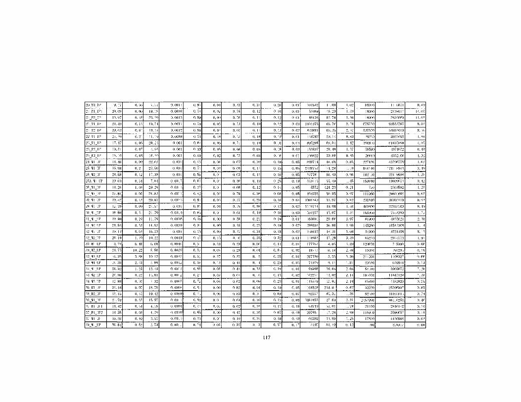
20 \1:1 l'i' 9. 17 0 .. 161 7. 72 0. 00l7 0. H7 0.01 0. :1:1 o. :n 0. 2fi 0. Oil 101.\12 11.00 1. 02 RR920 1116871 0. R9

2\_Jli_LPI 20.09 0. 001 19. IH 0. 0008 0. 71 0. 02 0. 7fi 0. 12 0. 10 0. Oil 5:1109 16.2:1 1,:]:1 IR:1n0 21B9ll1 H.OFi

21 132 LV J:t 97 0. lRI 2:3. 29 0. 001:1 0. 99 0. 00 0. 7() 0. II 0. 12 tl. otl 461 :m 62.70 l. 50 18900 2R926DO 11. 0.~

21 \11 UP 2·1.1:1 0. \:11 19.74 0. 0011 0. 70 o. o:t 0. 7:1 0. 10 0. 12 o. o:ll 1101:175 no. 76 2. 7H 107h770 9:lSS:17R7 H. 02

21 \12 UP :19.6:1 0.671 19.72 0. 00\2 0. 96 0. 07 0. 67 0. II 0. 1:1 0. 021 R2:1R8\ 66 .. 1.\ 2. :17 s:nh70 116G:I0\9 H. 56

22_\H_IJP 2l.:N 0. 211 11. 19 0. 0009 0. 71 0. IR 0. h2 0. IH 0. 12 0. Oil I :11782 29. H 0. 8:1 29250 :1927692 l. HR

2:l_\11_UP 17.17 ll.(lfil 20.2:1 0. 001 0. fi1 II.Ofi 0.71 0.111 0.10 0. 1111 R9S2RH GR. H1 1. 42 o96RIO 6Jfi:l5H90 1. 01

2:1_M2_LJP Ill .. \ I o. o71 1. 4o 0. 001 o. :to 0. OS 0. fill 0.06 0. IR o. o:ll ts:ts:l7 28.19 1. o7 .18S90 1:174072 11.1R

2:l_Mo_UP 15. \0 0. OR! lfi .. \0 0. 001 0. 50 0. 02 0. 7.\ 11.116 0. 16 0. Oil \08fi22 :m, RH 0. B.\ 2fifi111 1:1:12106 I. 92

2·1_MJ_UP 14.16 0. 091 22.62 0. 001 0.1:1 0. OH 0. 67 0. 09 0.10 0. OS! 899714 4R. fiR 0. R.\ 2211:w 1:l7\-l677H t. R2

2fl_l,fl_UP 16. 9R 0. 211 2:1.10 0. 001 0. 77 o. o:t 0. fi() 0. 17 0. LS 0. 051 2:1:18712 71. 2R I. 10 H11710 17:17!R94:l :1.19

2fl 1.12 UP 28.18 0.121 17.:lR 0. 001 O.lfi 0. Ill 0.6:1 II. \.1 11.\fi 0. OS! .12778 I 68.111 0. 96 102150 22119998 I. 28

2SA \11 UP 19.11:1 0. :HI 7. H1 0. 01117 II. 67 0. 01 o.:tn 0. 19 0. 2!) 0. 191 .15:1115 Fih.19 1.11 1.19840 1960967:1 0.12

26 Ml UP 11.26 1. 11:11 29. 29 0. 0011 0. 27 0. 01 0. 68 0. 12 0. J.1 II. Oil 5572 424. 2:1 0. 21 720 2:1fi:ll92 1. 2!1

27 Ml UP 22. R1 0. OS I 24. s:' 0. 0011 0. 42 o. o:t 0. 79 0. OR 0. 06 0. (I.\ I 404:1:15 .\0.% 0. 97 1119611 20601681 0. 65

28 M1 l1P 19.42 0. \:11 20.87 0. 0011 0. Ri o. o:1 0. 57 0. 20 0. 16 II. 011 I 086149 :J:t 97 0. R2 2:118111 :16907110 0. 9:1

29 Ml L'P 12.76 11.691 27 .. 11 0. 1101 0. 87 0. 04 0. 7~ II. OR 0. 12 0.021 1119711 19. 9H 1. .\6 4608011 22:ln77oo 0.19

:lO Ml LP lfi. 80 0. :111 21. 79 0. 01111 o. ns 11.111 0. 61 II. 19 o. In o. 11:11 lll\2:17 15.07 \.:11 1!)6960 7Fi.~:l290 1. 72

:11 Ml LV 19.90 0. 191 II. 79 0. OIIIIR 0. 16 0. 00 0 .. \R 0. 21 II. 19 ll.Oll 163001 29.66 I. 97 H\900 18:1.\021 ') :~8

:11 M2 LP 21. Si o. :1:11 11.42 II. 0009 0. 91 0.00 0 .. ~5 0. 2:1 0. \9 0. 021 2860(H :m.Rfi 1. 9S 14o2nO \11.\12:108 1.11

:t2 Ml LP 19. II o.n:tl lf\.2o 0. 001 0. 7:l 0. 09 0.:37 o. o1 0. IR 0. 021 2h8012 lB. :11 1.00 .\19911 472·11.~8 R. 15

:12 M2 l;P 2G. 19 I. 191 10. 22 0. 0019 0. 47 0. l f) 0. 16 0. JS 0.:12 0.011 118964 17. 2R :1.:19 R!12:Hl 20FiS77:l I. 9:1

:t:l_~I_UI' 1:3. 78 6. 1RI 6. fiO o. oo4n O.f\L 0. 5:3 0. 29 o. on 0. II 0. Oil 177762 4. 0:1 :1.39 !29870 71.\900 O.On

:t\ \12 UP 2:1. 7S 10. 221 R. SO 0. 0029 0. R7 0. fi9 0. 20 0. 01 0. 0.\ 0. 021 18777 HI. Ill 2.1R 10260 191205 0. 19

:1.1_Mo_UP !h. 9S :1. Hill 10. 12 o. oo:17 0. 61 0.:17 0. 2:1 0. [f) 0. 2S 0. Oil 207759 s.:B s.:ln 241200 IIOH:\27 0. fi(i

:1:1 M1 uP 19. :tfi 2. 5:11 .\. 89 0. Oo:l2 0. 68 0. \:1 0.11 0, 14 0. 29 0.0:11 71979 9. 17 1. 87 29.~20 ni4R41 0. \:1

:34 Ml 1_:p 28.92 1. 2SI 12.4:1 0. 0012 0. RR 0. OS 0, 41 0.:1:1 0. IH 0. Oil 99988 :m. fin 2. on S41RO :l96h672 7. 28

:l1. M2 t;p 26.96 0. 221 15.8 I 0. 0012 0. 21 0. 02 o. 01 0. 16 0. 17 0. 021 1tl22S1 7:L 02 2. 1·1 101070 1181.7128 1. 2H

:1·1 M:l ll' 12. RR 0. 701 7. :l2 0. {){)().~ 0. 72 0. OS 0. 62 0. 09 0. 2:3 0. Oil 111579 :17.91 2. 18 G.~RRO :t:l82020 0. 7h

:lS Bl UP 2n. In 0. 071 18. 79 0. 0008 ll. 51 0. ()() 0. 82 0. 0·1 0. 10 0. OS I 1 ORS2R z:H.OI 0. 62 :12220 2s:m5997 0. RS

:lS~H2_UP 1.~. 1.~ 0. 151 19.42 0. 0009 0.15 0. 00 0. H:l (1.11\ 0. 09 0. 071 192:1:17 So. :11 1.:1() 92.\20 J(H0761.S 0. 71

:l5_\1l_UP 21.70 0. :l.~l IS. fl7 0. 0011 0. H4 0. 01 0. 69 0. 09 0.1:1 0. 081 :1181855 27.60 2. :11 24S7990 9tlll02S1 11.1n

:l7 Bl UP! H. ,12 o. o'll 1. 78 0.0001 O.!J7 0. 0:2 0. 1:)2 0. O:l 0. 17 0. lfil 51719 !12. 01 l. 7H 211SO 2R16112 0. 10

:n Bl UP2 11. o.l o. o:tl 1. 74 0. OOOH 0. RS 0. ()(I 0. 17 11.0.\ o. 07 0, 401 207811 17. 2H 2. 99 llfi9lll :l5906fi7 0. II

:17 Ml UP 16.26 0. 1111 :1. 57 0. 0011 0. 7:1 11.111 0.:11 0. 0.\ 0. 10 0.191 60.192 /:l. HO 1. 2S 17820 1456901 o. o:t

:l9_M1~UP :m.nt 0. fi21 2. 79 0.0011 0. 71 0.00 o. o:t o. to 0. :l7 0.171 1-!97 H1.19 0. 12 IHO :!79917 0. 00

117

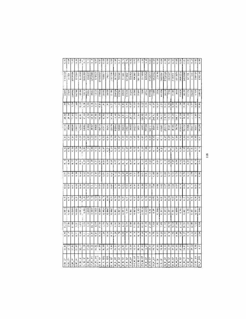
~ 0 0 ~ c c

c c 0 ~ c ~ 0 0 c c ~ c ~ 0 0

r- oc t- oc "" ~ c c c c 0

~ 0 0 0 0 ~ 0 0 0 0 ~ c c c c 0 0 0 ~ ~ c 0 0 c c c c c 0 c c c 0 c ~ ~

~ 0 ~ 0 ~ c 0 c ~ c ~ c c 0 - c 0 ~ ~ c c c 0 0 0 0 c 0 0 c c ~ c ~ 0 0

~ ~ ~ £ ~ ~ oc ~ ~ ~ X ~ ~ c ~ 0 ~ 0 0 ~ 0 c - 0 - ~ ~ 0 0 ~ ~ 0 c 0 0 c 0 c c c 0 ~ ~ - 0 c c

~ ~ t- ~ 0C t- t- ~ ~ X ~ X

x c ~ g 0 ; § Q Q g g § g g x x ~ C c : g ~ : : ~c~ c g ~c~ gc· § ~ C : ~c~ g ~ c 0 ~ 0 ~ ~ 0 ~ 0 ~ 0 0 0 ~ c 0 c 0 ~ ~ c c ~ 0 ~

-=-~ oc ...,... ~ ~

~ -:-.i

.31 ~I

~I ;I 5

: __ 1 ::1 ~~ c•· ~·

c;l ~I ~I ::31 ~I 51 §sl §I

~I ~I ·d ;I ~I -~

00

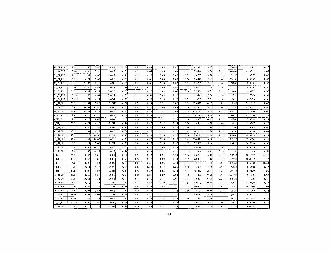
s:1 111 L'l'-1 4.12 ~- ORI 7, o2 \L 0021 (), 61 0. fi2 0, :1:1 0. OS 0. 07 0, <HI 2719H fi.ll 0. \-)() IOfif\EiO 1696711 0.07

s:1 Ill Cl'-1 S, 90 1. HS! 7. S6 0, 0017 0, 71 0, 19 0. 6S 0. OS 0, 08 o. o:ll 72\.J.'i 1\.J I H. fiR 1. 29 -111~00 1 :~EiSS:t~:~ 0,0:\

.1:1 Bl CPfi -L 71 ~- 121 1.li6 0. 001-7 0. 90 0. :19 0.19 0. OS 0. 06 0. 02) 25R7:lS S. 7R 0. 91 101210 11\Ei:l'iR 0. 00

S:l \11 UP fi. 74 1.211 7.09 0. 001:1 0. 70 0. 18 o. nl 0. 09 0. 06 o. on 1 R1nH79 17.12 0. 66 261\SO 40!1:10:167 0. o:l

.'i:l \t! UP .1. 59 II. 811 1. 18 0. OOOn 0. 7:3 0. 2-1 0. 61 0. 10 0. 02 0. 021 21 :t~1!) 17.:11 0. f\:1 EiRRfiO :H1922H I 0, 0:]

.11 Bl UP2 20. 6.1 2:1. 061 1. R-1 0. 0011 0. :\I 0. 60 0. 17 0. OR 0. OR 0. 01 I :176RR2 II. 8,1 0. tiS 102120 1166261 0.00

Fi1 B2 UP\ 20. Sl 10.881 6.19 0. 001:1 0. 2(-i 0 .. 14 0. 17 0.11:1 0. 06 o. I o I 7:17811 s:1. s:1 0. 41 114900 :19198671 0. 06

.11 B2 UP2 J:L 76 1.661 4.\H 0. 0017 0. 2:l 0.1.\ 0. 19 0. 01 0. 12 0. Ill 1:19192 ,17. Rll 0. :16 21780 5272916 ().()]

S1 B2 UP:l 15. R7 1:1.781 1. H 0. 0007 0. S6 0. :JO o. z:l 0. 26 0. 12 0. 091 1696:17 17.62 o. :n 27Rl0 8078816 0.110

!)1_Ml_L'P 22. 71 ~2. o11 .\. RO 0. 001 0. 21 0. 71 0.1:1 0.11 0. 02 0. 041 ~O-In.17R ln. 99 II. 89 11-1~180 .1\910022 0.0:1

SH Ml l:P 2R. f\2 16. 141 12.17 0. 0009 0. 68 0. 4:1 0. -10 0. OR 0.\L\ 0.011 4129:12 :18. 49 o. n9 \:190,\0 J.1R\-l:lfiS9 0. 00

ilR_M2_1 P 29. o:l 1-1. 281 9. 8,\ 0. 0012 0. 89 0. 4:1 0. :16 0. 01 0. 0.\ II. 081 :\ORS77:1 16.78 I. :15 1974780 s 1782:106 0.00

n __ lll_LP 22.66 0. 171 12. 27 0. 0012 0.17 0. 01 0. 4~ 0. 21 0. IH O.ORI :102012 3~. 14 1.:1:1 11061\1 IIR2lJ:HJ8 2. :\9

6_\12_LP 18. o9 0. 171 8. 02 0. 0009 1.10 0. 0() 0. :12 0. 21 0. 21 0. 201 2~R%7 :10. II 1. 2:1 RSSOO 77964R4 0. 88

n 1\:l U' 2:1. 71 0. 2-11 4. 10 0. 001 0. 91 0. 01 0.17 0. !2 0. IS 0. 2ol I S1:1H-1 24. 1R o. 8o :11920 :17:\2977 0. 20

BO_Ml_!JP 29. 7:\ 0. 4SI B. So 0. 0007 0. -1~ 0. 02 0. ,\9 0. 09 0. I~ 0. 101 1111H2 77. 71 2.11 5R7160 12Rfl072:l 0. {)()

til Ill IJP 40. 25 2. 9:11 H. 7S 0. 001f) 0. 7:1 0. OR 0.16 0. II 0. 21 0.141 ~01021 27.70 1. 4o 070:150 21960096 0. OH

61_\11_UP .15. 7:\ 2. If\ I 14. ~7 0. 001 0. 82 0. OS 0. 41 0. I o 0. 26 0. 091 114018:1 21. 14 1.17 :1111960 959~H22R 0.1:1

fi2 M1 LIP :17. R7 1. 091 10.07 0. 0012 0. n1 0. 0.1 0. 12 0. lFi 0. 26 0. 121 :l:100h72 20. ,1H 0. 79 1.1:1.\240 67590762 0. 21

6:1 ~1 UP 15. 74 .1. 141 7. 68 0. 001 0. 6:1 o. On O.lfi 0. 1:\ 0. :w o. 2~ 1 7178:\n :JR. 1n 0. 4:1 186840 2R762280 0. 09

6:\_M2_UP 28. 40 0. :lRI 10.72 0. Oll\:1 0. 75 0. 40 0. 2:\ o. on 0. 11 0. 171 310670 21. fjj 0. :10 59220 R.19.'i1.10 0. 20

6:\ \f:l UP 17. 52 2 .. \til 10. I :1 0. 0018 0. 81 o. 2,1 0. 2R 0. 21 0. 16 0.111 :\2:1-11 4:1.9:1 0. 20 :l7RO 1·120920 O.SI

7 B1 UP 2:1. 56 0 .. 121 2:1.01 0. 0011 0. 41 0. o:J o. 4n 0. 21 0. 2:\ o. <H 1 2:ln7R:1 4:1. 1-1 :1.:16 2(\H:L\0 10217S20 22. 2R

; 11.1 LP 22. 1:1 <Lo61 21. nl 0. 0012 0. 50 o. o:1 0. 47 0. 29 0. I~ o. 021 2,1ROn7 67. IS 2. ,1:\ 162990 [,\~8701:1 .1. 12

7 Ml CP 17. :t~ 0. 221 24. 2:1 0. 000~ 0. 70 (\.()[ 0. 51 0. 26 0. I R 0.011 .\1218,\ 71. SH 2. 66 :1R91nO 366n 18S6 [(J.:\4

7 M2 UP tn. on 0. 111 7.17 0. OOOR 0. 48 0. 02 0. so 0. 19 0. 20 0. 0~1 9\i:IHS S9. :u~ I. 99 128:10 S722R90 2. 77

7 M:l UP 27. RS o. RSI 21.00 0. 001 o. :n o. o:1 0. 52 0. 2S 0. IR <J.Otl n01912 :m. H1 :l. fi2 549R 10 2:H91720 4. 89

'iO_M1_UP :1-1. S7 29.501 R.:l7 0. 0015 0. 5:1 o. n8 0. 21 0. 09 0. 00 o. o21 :lo41:176 l0.7:l l. 29 t.177S20 38\H0021 o. o:l

70_M2_LP .\0. so 26. 6:11 7. :12 0. 0011 o. 5n 0. SH 0. IS 0. IS 0. 04 o. 071 ~.\.\nOH 16. 2Fi 1. 20 1488,1:10 .1777020:1 0. I R

7n Ml uP 14.8:1 0. 411 I. 88 0. 002 l. 20 0. OS 0. ss 0. 10 0. 17 0. 141 1197:12 ~9. 60 o.-n 8:1070 11 R062RS o. 2:1

76 \12 UP 12.91 0. 361 -1. :16 0. 001 0. 91 0. 02 0.12 0. 2:1 0. 2,\ 0. 091 2RY2H7 61. I -1 o. "" 8:1160 1RR1.1162 I. 01

16 \1:l UP II. 6R 0. 071 2. SR 0. 0011 I. 6R 0. 00 0 .. 16 0. 11 0. 14 0. 191 178141 50. H6 o. S2 :N420 90-19ti:ln 0. 2.1

77 \11 UP 2R. 92 \l.-\:11 1. OH 0. 001 0. <17 o.tn 0. 41 0. 21 0. :]() 0. 021 4 70RRO 5.1. 20 0. Rl 159-170 2S991 :1.12 1. 20

77._M2 UP :11.9-1 1. :l21 :l. 82 0. 001:1 I. :t\ o. o-1 0. 43 0. 28 0. 1h 0. 101 2R24:l0 -11. 7n 0. S6 6S2SO Hni9440 0. 89

77_M:1_UP .1:1. 20 0. R91 2. R6 0. 0009 o. n9 0. OR 0. 13 0. 22 0. 21 o. o:JI 4100:!9 69. 2.1 o. n1 11~~70 :l\HnOORO 0. 71

79 M1 UP 40.\0 0. :111 2. 12 0. 001 0. S4 0. 00 0. 19 0. 21 0. 19 0. 021 210677 2S. 61 0. 67 .12920 S101940 0. 40

119

R Ill UP! 2R. 70 o. :t~l z:t fl2 0. 0012 0. 79 0. OJ o. so 0, 2R 11.11 0. 02 20R921 ·19. lfi 2 .. 12 17Jo:w 1:12210:!;! 12.92

8 Ill UP~ 21. 2R O.OJI 22.64 0.0011 1. 20 0. 00 0. 61 0. IH II. IH 0. 0:1 .1714.1 :11.1:1 2. 12 29160 J9ho1so 2:1.1:1

R_]ll UP:l lH.:H 0. ill H. 91 0. 0012 0.17 0.01 0.2:1 0.44 0. :11 0. ()() :~1274 2:1.6:1 2. 7fl l99HO 7:1R9:HJ I. :16

H Ml UP 29. 6R 0. 191 21.·11 0.0111 0. 21 0. OJ 0. 61 0. 2:1 O.HI 0.0:1 6962/R 14.1:1 :1. :!9 oHROfiO '09:lRRO:I 9.:12

R_M2 liP 18. HI 0. 111 10 . .1•1 II. OI)J:I 0. R:? o.o:1 0. :~6 o.:w 0. 19 0. 0:1 ](i,'lR7fl 22. 99 2.1S 9:.?700 :1707187 I. S9

H M:l UP H .. \6 I. 7.11 7.90 o.oo:H 0. 61 0. ()() 0. 22 0. :~7 0.11 0. (I() RIHOS 1. 59 fi. 02 R72\0 .169071 1. 21

RO Ml UP 21. 2() 2. S71 4. 02 0.001 0. R:l 0. 12 0.11 0. 25 0. 21 0. 02 991601 z:L sfl 2. 9R 9%210 2:l:!F)61f'l:l l. 27

HO M2 UP 2R. fi(-i o. I HI 2. 21 0. 0012 0. 2r\ 0. 00 o. ss 0. 10 0. 29 0. 0:1 J:lR67R IS. 97 0. H7 1ooso 221SI79 0. fi7

Rll M:l 1.1' z:t flo 0. 101 I. HI 0. 0008 0. ·12 0.00 0. 6G 0.1:1 0. 19 0.02 1151:19 'I. 09 0. (-ii) 2.1920 :\589:1"1 II. 09

Hi Ml W :11. ss o .. 1SI 4. 62 0. 001 0.70 0. 0:1 0. 50 0. 17 0. 29 0. 02 9962fi0 'I. 00 1.11 1o7R:IO :1]1:17:\:\:1 1.:11

Hi _\12_UP :12. fiR 0. 121 :1.4:1 0. 0111 0. fi7 0. 00 0. so 0. 2F) 0. 2:1 0. 01 4220f;6 11.1s 0. 91 129870 18/fill :11 J.:l.1

R2_lll_UPI :n. o~ 0. 091 :1.11 0. 001 2. 20 (1.1\1 0.:17 0. 19 0. 11 (1.01 .\R911 "'· 78 11. ""

10710 :1168268 :1.99

R2_\11_UP :n. 5o 0. 161 2. R2 0. 001 II. 9:1 11.111 11.19 0. 'I 0.17 0. 02 :19:1~6.\ 2l.:HJ I. .\1 17911111 H:l7!17Rf1 II. H9

Rt_Ml_lll' 29. :lY 0. 711 1. OR 0. 0009 0. 76 0. 02 0. 42 0. 29 0. 2(-i 0.112 69R55fi 11. 2R 1.1:1 :J:l6120 :109:10690 2. YS

8.\ HI Ll'l IR. :16 0. 711 :1.67 0. 0110.\ 0.11 0. 02 0. 4:1 0. 26 0. 2R (1.111 20S70R st. ·1H 0. 4.1 70200 I OS90:1o9 l.fil

H.\ Ill Ul'2 17.9:1 2. o7f :1. gz 0. 0(10.\ II. fi9 0. 06 o.:11 0. 27 0 .. 1:1 0. 02 ,IR<J99:1 2·1. OY 1. 02 lfiHI\90 117090S:l s .. :;o

ss nt uP:1 17 . .17 0. ROI :1. 2fi 0. OOOH 0. fiO 0. 02 0.:1:1 0. :32 11.:11 0. 02 21 029:~ Fiil. R2 1.11 RS:{20 Jt7:nnss I. 99

R5 ~I Ul' 2R. :l2 2. 071 :1. 70 0. OCKI7 l.o:J o. o:1 0.1:1 0. 19 11. :n 0. 02 :189:190 12. 11 I. OR 114510 16108089 1. ss

86 Ill UPI 16. :Hl II. 611 :1. 52 O.IIOIIH o.1s O.o:J 11.11 o.:n 0. IR 11.11:1 21/llR :ll. 26 II. 96 111110 67R614.1 2. 77

R(-i HI UP2 IH.1:1 II. 7RI ·1. :19 0. 0007 0 .. \(i (1.(11 0.11 0. 2:) 0. 27 0.0:1 19Bfi:l-l :n. G9 0. 97 a126o 627417S :l. R2

Hfi _ ~ l_UP 12. RSl 0 .. 1RI :l. Otl 0. 01108 0. ·14 0. 01 0. :19 0. 2H 0. 27 0.0!) :mRzfi:~ 22.40 0. SlY 7:H120 R9210il1 :1. 11

R6_M2_l'P 17.61 0 .. 111 5. IH 0. 001 0. R9 0. Ill o.:\11 0. :Hl 0.10 0. 01 1:11821 2:l. H:l 1. S2 12:l·1RO I 02HR197 J:l. 22

R7 \11 liP 19 .. ~6 I. 071 1.:16 0, ()()()() 0. 60 0.11:1 o. :ln 11.1.1 II. 11 O.o:\ 2.192!19 :w. 57 II .. \1 46620 7921891 6.:16

RR Ill Ul' :11. H7 2. 721 s. 01 0. 0001 I. 06 0. 01 0. 16 0.1·1 0. :lfi 0. 02 :lH.~f14 41. :11 11.11 6:190 170R9f}0 JS. 02

H8 Ml Ll' :l4. 20 .1.1RI ·1. 8:1 0. OOIIH 0. 29 0. OS 0. 24 0. :lS 0.111 o. o:t 10921.1 :1:1.16 0. 51 215111 :16.1·1191 7. 56

9 Ml UP 24. 2:~ (1.011 7.'\i II. 0012 0 •. 19 0.00 0. 62 0. 20 0. 17 II. 01 112701 2:L 77 2. 20 ,)()j()() 267R9H6 I.,., 9_M2_liP 23. 9H 0. Ill 6. 91 0. 0()()9 1. 21 O.lKI 0. 7S 0. 11 0. 09 0. 01 9720.1} ,'J\. 2S J. f)() llfiOOO :lO:JRI 00 1.1.5

9 M:l IJI' :W.21 0. OS! 21.96 II. 0011 0. HI 0. 00 0. 70 0. 11 0. H 0. 02 5176SO :~G. 49 :J. hH 1:J:1R90 I RRHHIS6 t:l. 79

4_\14_l!P 22.01 0.1191 7.Hl II. 011119 0. 12 0. 00 II. 811 11.119 0. OR O.o:\ !12f\Rhh 1 :1.1s 0. Hi 9,1110 70RR724 2, /1:~

90 Ml Ll' 17.96 I. S21 4. II O.IIOOH 0. 79 0. 02 0. 26 0. :19 0. :10 0. 0.1 11912,1 17. :11 0. 2:1 1:12:10 !)fi:\8788 16. 19

91 Ml l'P 2fi. 12 1. H71 .~. 27 II. 0(\1:1 II. 61 0. 01 0. S2 O.lf\ 0. 2H 11. o:1 119012 41. :10 ].:1:1 20700 f)27:J7:J? n. 70

120

Table IV -4.2.1: Areas of upstream watersheds. Delineation was based on the EOF results and the number of DSS water quality monitoring stations in their receiving waters.

"8 "" "8 .... "8 "" 1 ;::;-0 "' 1 ~ 0 "' ~ ~ 0"' s ... c ... § ].~ ,8.2 ,8.i ~

i!: ~ e \0 i!: " ~- i!: ~ e" .g < ~~ .g ~ z"' .b < icii ::s

"' "' "' I Ml UP 39147175 3 34M3 UP 4382020 I 21 81 UP! 2469114 I

10 81 UP 3542208 I 35 81_UP 25396997 I 21 81_UP2 3325128 I

10 Ml UP 9538112 3 35 82 UP 16407615 I 21 81 UP3 610259 I

100 Ml UP 35553748 2 35 Ml UP 96110254 3 21 81 UP4 881349 I

11 Ml UP 167102 I 37 81 UP! 2846142 I 21 82 UP 2892660 I

12 Ml UP 8554795 3 37 81 UP2 3590657 3 21 Ml UP 93553787 5

13 81_UPI 11187120 I 37 Ml UP 4456904 2 21M2 UP 54663019 7

13 81 UP2 6848703 I 37M2 UP 13035259 5 22 Ml UP 3927692 2

13 81 UP3 4504387 I 39_MI UP 379917 I 23 Ml UP 61635890 3

13 81 UP4 3800558 2 4 81 UP 17832559 I 23M2 UP 4374072 I

13 Ml UP 78634091 I 4 82 UP 1315241 I 23M3 UP 4332106 I

14 Ml UP 26418149 2 4 Ml UP 97856136 3 24 Ml UP 43796778 5

15 81 UPI 1660199 I 4M2 UP 5757540 2 25 Ml UP 173718943 4

15 81 UP2 3465279 I 41 81 UP 6559710 2 25M2 UP 22419998 2

15 81 UP3 3013510 3 41 Ml UP 16941908 I 25A Ml UP 19609673 I

15 81 UP4 369388 I 42_81 UP 3494730 4 26 Ml UP 2363592 I

15 81 UP5 927491 I 43_81_UPI 12725366 2 26A Ml UP 20822804 I

15 Ml UP 5294761 3 43 81 UP2 3156114 I 26A M2 UP 73687291 2

16 81 UP! 2730409 5 43 MI_UP 120950165 8 27_MI_UP 20601684 3

16 81 UP2 922812 2 44_81 UPI 7579563 I 28 Ml UP 36907110 5

16_81_UP3 1669826 I 44 81 UP2 7049012 2 29 Ml UP 22367700 2

16 82 UP 239005 I 44 81 UP3 1795515 3 30 Ml UP 7553290 3

16_MI UP 6420187 3 44 Ml UP 12417783 I 31_MI UP 4835021 I

16M2 UP 13021494 3 46 81 UP 6618157 6 31M2 UP 10542308 2

16M3 UP 2885181 2 46 Ml UP 3597682 2 32 Ml UP 4724458 3

lA 81 UP 11851128 3 46 M2_UP 2755631 3 32M2 UP 2055773 2

lA Ml UP 94505000 2 47 Ml UP 10198527 9 33 Ml UP 715900 3

2 Ml UP 20722216 4 47 M2_UP 5541816 2 33M2 UP 191205 I

2M2 UP 66985842 4 47A MI_UP 20900563 4 33_M3 UP 1108327 3

20 Ml UP 5831052 II 47A M2 UP 8062035 2 33 M4 UP 659844 I

20M2 UP 6348527 I 47A M3_UP 10573533 4 34 Ml UP 3965672 2

20M3 UP 1116871 2 47A M4_UP 7379936 I 34M2 UP 11847128 I

121

--- Continued ---

"2 ... "2 N ... ~ N

... ii N 0 ~ ] 0 ~ 0 ~

ll §, ll 8 §, .8 .§ .. §, ~ 8 'iii .Cl -~ 'iii 'iii ..8 -~

" "' E i'! l "' E 'iii

~ "' E i'! e e e .h < :irJ'.I < :i.:;; < :irJ'.I ::s ::s rJ'.I rJ'.I rJ'.I

48 Ml UP 8059699 3 60 Ml UP 42850723 I 80M3 UP 3589320 I

48M2 UP 92535416 3 60_M2 UP 1690344 I 81 MI_UP 31437333 5

49 Ml UP 19022622 2 61 81 UP 24960096 10 8I_M2 UP 18761131 2

5 81 UP 1216189 I 61 Ml UP 95994228 10 82_81 UPI 3168268 I

5 Ml UP 24093301 4 62 Ml UP 67590762 12 82 81 UP2 2663258 I

50 Ml UP 57526426 3 63 Ml UP 28762280 I 82 Ml UP 8376786 4

50M2 UP 10031647 3 63M2 UP 8595436 4 84 Ml UP 30930690 2

50M3 UP 3198944I 2 63M3 UP 1420920 I 85 81 UPI 10590359 I

50 M4 UP 16313670 I 7 81 UP 10217520 2 85 81 UP2 11709053 3

51 Ml UP 38087279 3 7 83 UP 15987013 I 85 81 UP3 11738755 I

51M2 UP 19430800 3 7 Ml UP 36661856 5 85 Ml UP 16408089 2

52 81 UP 6411531 I 7M2 UP 5722890 I 86 81 UPI 6786145 I

52 Ml UP 4115113 3 7M3 UP 23494720 5 86 81 UP2 6274175 I

53 81 UPI 2206408 3 70 Ml UP 38040024 6 86 Ml UP 8921051 2

53 81 UP2 450736 I 70M2 UP 57770263 3 86M2 UP 10288497 3

53 81 UP3 4782164 3 73 Ml UP 5444992 I 87 Ml UP 7924894 2

53 81 UP4 1696711 3 76 Ml UP 41806285 3 88 81 UP 1708960 I

53 8I UP5 I3555323 6 76M2 UP 18845162 I 88 Ml UP 3654194 3

53 81 UP6 1495378 I 76M3 UP 9059636 I 9 Ml UP 2678986 I

53 Ml UP 40630367 4 77 MI_UP 25991332 3 9M2 UP 3038100 I

53 M2_UP 3692281 3 77M2 UP 14619440 3 9M3 UP 18888456 4

54 81 UPI 928519 2 77M3 UP 30466080 2 9 M4 UP 7088724 5

54 81 UP2 4466261 2 79 MI_UP 5401940 3 90_MI UP 5638788 I

54 82 UPI 39498671 3 8 81 UPI 13221032 2 94 Ml UP 5273737 2

54 82 UP2 5272976 I 8_81_UP2 1950450 I 95 Ml UP 9929727 I

54_82 UP3 8078816 3 8 81 UP3 738930 I 97 Ml UP 15387866 3

54 Ml UP 51940022 2 8 Ml UP 30938803 5 98 Ml UP 22647950 3

58_MI UP 15893659 3 8M2 UP 3767187 I 99 Ml UP 28800993 5

58M2 UP 51782306 6 8M3 UP 369071 I

6 MI_UP 11820308 2 80 Ml UP 23356163 4

6M2 UP 7796484 2 80M2 UP 2215179 I

6M3 UP 3732977 I

122

Table IV-4.3.1: Selected upstream watersheds that are dominated by one type of land cover (using criteria described in the text), for the analysis of land cover effect on fecal contamination levels.

Dominated GA

Number of Land cover Subwatershds Land Cover

station FC

Percentage Observations

8 81 UP3 0.7506 8-34 53

8M3 UP 0.7949 8-27 54

Crop-Pasture 82 81 UP2 0.7546 82-68 46

88 81 UP 0.8054 88-21 54

94 Ml_UP 0.7046

94-3W 59

94 Ml_UP 94-3X 58

13 81 UPl 0.8237 13-21 51

13 81 UP2 0.8488 13-16 53

Forest 21 81 UPl 0.8171 21-43 53

27 Ml UP 27-6 52

27 Ml UP 0.853 27-7 52

27 Ml UP 27-8 50

53_81 UP4 53-44.1 58

53 81 UP4 0.7153 53-44.2Z 57

53 81_UP4 53-44.5 58

54 Bl_UP2 0.7207

54-30 57

54 Bl UP2 54-31 55

54 Ml UP 0.8495

54-23 57

54 Ml UP 54-24 57

Urban 70_Ml UP 70-10 60

70_Ml_UP 70-11 60

70_Ml UP 0.8004

70-12 60

70_Ml UP 70-7 60

70 Ml UP 70-8 60

70 Ml UP 70-9 60

70_M2 UP 70-17 60

70 M2 UP 0.7559 70-24 60

70 M2 UP 70-25 60

123

Table IV-4.4.1: Impervious surface percentages in 187 upstream watersheds in Virginia coastal regions based on the RESAC impervious dataset in1990 and 2000.

lJ ~ § "C ~ § "C ~ § "' ... "' ... "' .r:. .... N .r:. .... N .r:. .... N

~ .. .. ~ .. "' ~ "' "' !l :::>~ :::>~ !l :::>~ :::>~ !l :::>~ :::>~

O'</e 0'</e 0'* 0* O'</e O'</e "' ·~- ·~- "' ·~- ~- "' ·~- ·~-! ~ ! 8.

., ..0 ... ... ., 8. :::> a. :::> a. c. :::J c.

"' .§ .§ "' .§ .§ "' .§ .§

1_M1_UP 0.4 0.69 32_M1_UP 0.63 1.2 21_B1_UP1 0 0.11

10_B1_UP 0.13 0.48 32_M2_UP 1.19 1.79 21_B1_UP2 0.29 0.4

10_Ml_UP 0.3 0.71 33_Ml_UP 6.48 7.97 21_B1_UP3 0.03 0.28

100_Ml_UP 1.45 3.56 33_M2_UP 10.22 10.58 21_B1_UP4 0.51 1.11

11_M1_UP 1.29 4.39 33_M3_UP 3.88 5.1 21_B2_UP 0.18 0.96

12_Ml_UP 1.98 3.53 33_M4_UP 2.53 3.17 21_Ml_UP 0.13 0.39

13_B1_UP1 0.06 0.18 34_M1_UP 1.25 1.75 21_M2_UP 0.67 1.15

13_B1_UP2 0.08 0.51 34_M2_UP 0.22 0.7 22_M1_UP 0.21 0.99

13_81_UP3 0.3 1.33 34_M3_UP 0.7 1.1 23_M1_UP 0.06 0.2

13_B1_UP4 0.58 1.11 35_B1_UP 0.07 0.14 23_M2_UP 0.07 0.25

13_M1_UP 0.1 0.33 35_B2_UP 0.15 0.31 23_M3_UP 0.08 0.31

14_M1_UP 0.09 0.44 35_Ml_UP 0.35 0.76 24_M1_UP 0.09 0.29

15_Bl_UP1 0 0.01 37_B1_UP1 0.54 1.3 25_M1_UP 0.21 0.67

15_81_UP2 0.06 0.34 37_B1_UP2 0.03 0.26 25_M2_UP 0.12 0.47

15_B1_UP3 0.07 0.26 37_M1_UP 0.4 0.89 25A_M1_UP 0.34 1.02

15_B1_UP4 0 0.36 37_M2_UP 0.28 0.54 26_M1_UP 1.03 1.25

15_81_UP5 0.04 0.43 39_M1_UP 0.52 1.36 26A_M1_UP 2.73 4.25

15_M1_UP 0.07 0.39 4_81_UP 0.8 1.12 26A_M2_UP 0.13 0.55

16_B1_UP1 3.62 5.7 4_B2_UP 0.1 0.15 27_M1_UP 0.05 0.25

16_B1_UP2 1.53 2.34 4_M1_UP 0.22 0.43 28_M1_UP 0.13 0.5

16_B1_UP3 0.27 0.84 4_M2_UP 0.31 0.42 29_M1_UP 0.69 1.21

16_B2_UP 0 0.62 41_Bl_UP 1.64 3.38 30_M1_UP 0.31 0.91

16_M1_UP 0.24 0.64 41_M1_UP 0.11 0.37 31_M1_UP 0.19 0.82

16_M2_UP 0.72 1.7 42_B1_UP 0.11 0.97 31_M2_UP 0.33 0.75

16_M3_UP 0.23 0.59 43_B1_UP1 0.87 1.57 46_M1_UP 1.79 3.22

1A_B1_UP 2.26 3.48 43_B1_UP2 0.03 0.12 46_M2_UP 0.6 2

1A_M1_UP 0.4 0.76 43_M1_UP 0.53 1 47_M1_UP 1.19 2.37

2_M1_UP 2.04 2.67 44_B1_UP1 1.48 2.49 47_M2_UP 0.19 0.45

2_M2_UP 0.51 0.75 44_B1_UP2 1.29 1.82 47A_M1_UP 0.61 0.98

20_M1_UP 0.66 1.28 44_B1_UP3 0.64 1.28 47A_M2_UP 0.18 0.45

20_M2_UP 1.56 2.6 44_M1_UP 0.56 0.9 47A_M3_UP 0.13 0.37

20_M3_UP 0.56 0.83 46_B1_UP 5.25 8.36 47A_M4_UP 0.24 0.59

124

-- Continued-

0 8 ~ § "C 0 8 "C 0\ "C 0\

~ 0\ cu "' ~ 0\ ..... N .t: .... N .... N ~

~~ "' ~ "' .. ~ "' .. ~

::J-

~ ::J- ::J-

~ ::J- ::J-0'*- 0'*- 0'*- 0'*- 0 '*

~ -~- -~- ~ -~- -~- ~ -~- -~-..<> .. ., ..<> cu .. ..<> cu ., :;;J c. c. :;;J c. c. :;;J c. c.

V> ~ ~ V> ~ ~ V> ~ ~

49_M1_UP 0.25 0.6 48_M1_UP 0.14 0.47 81_M1_UP 0.55 2.25

5_B1_UP 0.22 0.39 48_M2_UP 0.16 0.5 81_M2_UP 0.12 0.69

5_M1_UP 0.23 0.34 61_B1_UP 2.93 3.71 82_B1_UP1 0.09 0.81

50_M1_UP 0.57 1.26 61_M1_UP 2.16 2.77 82_B1_UP2 0.08 0.5

50_M2_UP 0.18 0.42 62_M1_UP 1.09 1.84 82_M1_UP 0.16 0.77

50_M3_UP 1.85 2.59 63_M1_UP 3.14 5.56 84_M1_UP 0.71 1.99

50_M4_UP 0.48 0.78 63_M2_UP 6.38 13.81 85_B1_UP1 0.71 2.79

51_M1_UP 4.28 5.01 63_M3_UP 2.56 5.08 85_B1_UP2 2.07 4.06

51_M2_UP 3.27 4.73 7_B1_UP 0.32 0.69 85_B1_UP3 0.8 2.31

52_B1_UP 2.18 3.14 7_B3_UP 0.56 1.42 85_M1_UP 2.07 4.44

52_M1_UP 2.62 3.99 7_M1_UP 0.22 0.69 86_B1_UP1 0.61 1.38

53_B1_UP1 1.07 2.08 7_M2_UP 0.14 0.24 86_B1_UP2 0.78 1.44

53_B1_UP2 0.63 2.37 7_M3_UP 0.85 1.65 86_M1_UP 0.38 0.85

53_B1_UP3 3.99 6.51 70_M1_UP 29.5 31.38 86_M2_UP 0.34 1.34

53_B1_UP4 9.08 13.24 70_M2_UP 26.63 29.33 87_M1_UP 1.07 1.85

53_B1_UP5 4.85 7.55 73_M1_UP 19.59 21.95 88_B1_UP 2.72 6.61

53_B1_UP6 3.42 6.54 76_M1_UP 0.41 1.62 88_M1_UP 3.48 5.21

53_M1_UP 4.24 6.74 76_M2_UP 0.36 1.53 9_M1_UP 0.01 0.12

53_M2_UP 11.85 14.58 76_M3_UP 0.07 1.14 9_M2_UP 0.11 0.37

54_B1_UP1 20.17 20.71 77_M1_UP 0.53 2.09 9_M3_UP 0.05 0.24

54_B1_UP2 23.06 24.89 77_M2_UP 1.32 3.67 9_M4_UP 0.09 0.24

54_B2_UP1 10.88 16.01 77_M3_UP 0.89 2.43 90_M1_UP 1.52 4.84

54_B2_UP2 5.66 8.76 79_M1_UP 0.31 1.04 94_M1_UP 1.87 2.69

54_B2_UP3 13.78 17.39 8_B1_UP1 0.32 1.1 95_M1_UP 0.26 1.12

54_M1_UP 32.54 34.48 8_B1_UP2 0.01 0.34 97_M1_UP 0.94 3.1

58_M1_UP 16.54 21.29 8_B1_UP3 0.11 0.93 98_M1_UP 1.19 3.39

58_M2_UP 15.28 18.11 8_M1_UP 0.19 0.5 99_M1_UP 0.76 2.81

6_M1_UP 0.17 0.26 8_M2_UP 0.41 1.35

6_M2_UP 0.17 0.32 8_M3_UP 1.75 2.58

6_M3_UP 0.24 0.31 80_M1_UP 2.57 4.73

60_M1_UP 0.45 0.72 80_M2_UP 0.18 0.79

60_M2_UP 1.08 1.37 80_M3_UP 0.1 0.72

125

Table IV-4.5.1: Sample sizes, calculated D values, and critical D values of five regions (Rappahannock River, York River, James River, Potomac River, and Eastern Shore) from Kolmogorov-Smimov test. FC distributions in the five regions are significantly different from each other, with corresponding low p values (p < 0.001 in all pairs of) and greater D values than each of their critical values.

~critical York James E as tern S hore Potomac

D

0.016751 0.016193 0.015931

York 0.017346 0.017101

James 0.11921 0.051909 0.017442 0.017199

Eastern S hore 0.07691 0.12123 0.16855 1~941·· 0.016656

Potomac 0.032862 0.081923 0.13255 0.067801

Note: The numbers in blue cells are the sample size for each region. The values on upper right side are the critical values, and the values on lower left side are calculated D values for each pair of regions.

126

Table IV -4.5.2: The grouping of 107 upstream watersheds into 4 regions: Rappahannock River, York River, James River, and the Eastern Shore.

1: 0:: 0:: 1:

-! Watershed .S! Watershed .S! Watershed t Watershed :. I I

20_Ml_UP 76_Ml_UP 58_Ml_UP 46_Bl_UP

20_M2_UP 76_M2_UP 58_M2_UP 46_Ml_UP

20_M3_UP 76_M3_UP 60_Ml_UP 46_M2_UP

21_Bl_UP1 77_Ml_UP 60_M2_UP 47_Ml_UP

21_Bl_UP2 77_M2_UP ~

61_Bl_UP 47_M2_UP

21_Bl_UP3 77_M3_UP ~ 61_Ml_UP 47A_Ml_UP

21_Bl_UP4 79_Ml_UP rl 62_Ml_UP 47A_M2_UP E

.!! 21_82_UP SO_Ml_UP ., 63_Ml_UP 47A_M3_UP

~ .... 21_Ml_UP 80_M2_UP 63_M2_UP 47A_M4_UP

21_M2_UP 80_M3_UP 63_M3_UP 48_Ml_UP

22_Ml_UP 81_Ml_UP 70_Ml_UP 48_M2_UP

23_Ml_UP 81_M2_UP 70_M2_UP 49_Ml_UP

23_M2_UP 82_Bl_UP1 73_Ml_UP ~ SO_Ml_UP

23_M3_UP 82_Bl_UP2 ~ SO_M2_UP -!!

24_Ml_UP 0

t ~ 82_Ml_UP > SO_M3_UP .. £ ii: 25_Ml_UP .2 84_Ml_UP SO_M4_UP ""

.. u E 0 0:: 25_M2_UP i 85_Bl_UP1 Sl_Ml_UP .! II 25A_Ml_UP &U 85_Bl_UP2 Sl_M2_UP ... u a. • 26_Ml_UP t= 85_Bl_UP3 52_Bl_UP "'

26A_Ml_UP 85_Ml_UP 52_Ml_UP

26A_M2_UP 86_Bl_UP1 53_Bl_UP1

27_Ml_UP 86_Bl_UP2 53_Bl_UP2

28_Ml_UP 86_Ml_UP 53_Bl_UP3

29_Ml_UP 86_M2_UP 53_Bl_UP4

30_Ml_UP 87_Ml_UP 53_Bl_UP5

31_Ml_UP 88_Bl_UP 53_Bl_UP6

31_M2_UP 88_Ml_UP 53_Ml_UP

32_Ml_UP 90_Ml_UP 53_M2_UP

32_M2_UP 94_Ml_UP

33_Ml_UP 95_Ml_UP

33_M2_UP 97_Ml_UP

33_M3_UP 98_Ml_UP

33_M4_UP 99_Ml_UP

127

Table IV -4.5.3: Eigenvectors of environmental variables for the first 5 principal components based on Principal Component Analysis on 107 upstream watersheds located in the Rappahannock River, York River, James River, and Eastern Shore regions.

Variable PC1 PC2 PC3 PC4 PC5

Slope -0.492 -0.172 0.442 -0.243 -0.27

Drainage density -0.007 0.044 -0.027 0.019 0.005

Eccentricity 0.034 -0.006 0.005 0.223 0.099

Urban -0.087 0.459 -0.366 -0.467 -0.1

Forest -0.437 -0.365 0.109 0.075 0.355

Pasture 0.561 -0.041 0.414 -0.336 -0.173

Agriculture 0.388 -0.074 0.135 0.504 -0.046

Wetland -0.055 0.07 -0.175 0.323 -0.252

Water area -0.131 0.6 0.267 0.13 -0.062

Ratio -0.107 -0.21 -0.019 0.061 -0.769

Residence time 0.009 0.065 0.136 -0.096 0.275

Water Volume -0.079 0.322 0.166 0.098 0.025

Watershed area -0.172 0.305 0.429 0.281 -0.012

Runoff potential 0.156 -0.088 0.369 -0.279 0.117

128

Table IV -4.5.4: Eigenvectors of environmental variables for the first 5 principal components based on Principal Component Analysis on 94 upstream watersheds located in the Rappahannock River, York River, and Eastern Shore regions.

Variable PC1 PC2 PC3 PC4 PC5

Slope -0.492 0.289 0.509 0.309 0.215

Drainage density -0.017 -0.493 0.218 0.035 0.191

Eccentricity 0.036 -0.01 -0.101 -0.258 0.782

Urban -0.045 -0.589 0.305 0.059 -0.02

Forest -0.47 0.227 -0.27 0.019 -0.076

Pasture 0.55 0.33 0.327 0.214 -0.207

Agriculture 0.388 0.14 -0.102 -0.205 0.243

Wetland -0.06 0.019 -0.175 -0.096 0.089

Water area -0.075 0.07 0.187 -0.419 -0.15

Ratio -0.115 0.179 -0.001 0.229 0.127

Residence time 0.022 -0.133 0.326 -0.09 -0.063

Water Volume -0.041 0.024 0.13 -0.227 -0.064

Watershed area -0.152 0.188 0.312 -0.662 -0.132

Runoff potential 0.149 0.234 0.338 0.095 0.356

129

Table N-4.6.1: The linear regressions equation, as well asp-value and R square values, showing the relationships between FC concentrations with rainfall intensities for each 7 days before sampling dates.

Days before sampling Regression Equation P-value R-Square

date

1 FC = 37.3 + 108 Day1 <0.0001 4.80%

2 FC = 45.5 + 40.6 Day2 <0.0001 0.700Ai

3 FC = 46.8 + 26.2 Day3 <0.0001 0.30%

4 FC = 49.1 +6.77 Day4 <0.0001 O.OOOAi

5 FC = 49.4 +5.23 DayS <0.0001 0.00%

6 FC = 49.8 +1.72 Day6 <0.0001 0.00%

7 FC = 49.3 +5.58 Day7 <0.0001 0.00%

130

Table IV -4.7 .I: Leaf report based on CART analysis on 165 upstream watersheds in Virginia coastal regions, in order to demonstrate the relationship between environmental variables and fecal contamination levels, indicated by FC mean concentration.

Leaf Report

FC Mean Leaf Label concentration Count

(MPN/100ml) Ratio < 76. 35 & Runoff Potential < 0.034 & Forest >~ 0.49 6. 3587724 7

Ratio < 76. 35 & Runoff Potential < 0.034 & Forest < 0.49 22.086686 5 Ratio < 76.35 & Runoff Potential>= 0.034 & Impervious 1990 < 0.0065 & Pature <0.066 14.26138 9

Ratio < 76.35 & Runoff Potential>= 0.034 & Impervious 1990 < 0.0065 & Pature >=0.066 22.084475 69 Ratio < 76.35 & Runoff Potential>~ 0.034 & Impervious 1990 >= 0.0065 & Wetland <0.053 22.28672 36 Ratio < 76.35 & Runoff Potential>=- 0.034 & Impervious 1990 >= 0. 0065 & Wetland >=0.053 & Residence

20.512921 6 Time < 0. 56 Ratio < 76.35 & Runoff Potential>~ 0.034 & Impervious 1990 >= 0.0065 & Wetland >=0.053 & Residence

37.807975 13 Time>= 0.56 Ratio>- 76.35 30.093153 20

Note : leaf label shows there are 8 leafs; each leaf represents one condition of matching watersheds. The count indicates how many upstream watersheds match the condition.

131

Table V -2.1: Runoff coefficients for pervious and impervious surfaces in warm and cold seasons based on values in the Manuals and Reports of Engineering (1992) from the American Society of Civil Engineers.

Land Cover Season Pervious Impervious

warm 0.4 0.9 Urban

cold 0.5 0.9

warm 0.15 0.8 Forest

cold 0.2 0.8

warm 0.25 0.8 Crop-pasture

cold 0.35 0.8

132

Table V -3.1. FCMCs derived based on categorized watersheds using Group 2 (which has 56 watersheds) as an example. The value of coefficient for each variable is the value of FCMC for each type of land cover. Pasture has a negative value.

Regression Statistics

Multiple R 0.7549

R Square 0.5699

Adjusted R 0.5241

Square

Standard 6.56E+10 Error

Observation 53

ANOVA

df ss MS F Significance F

Regression 5 2.68E+23 5.36E+22 12.4531 1.02E-07

Residual 47 2.02E+23 4.30E+21

Total 52 4.70E+23

Coefficients Standard tStat P-value Lower95% Upper95%

Lower Upper 95.0'%

(FCMC) Error 95.0"A,

Intercept 1.56E+09 1.24E+10 0.13 0.90 -2.34E+10 2.65E+10 -2.34E+10 2.65E+10

Urban 3.16E+05 2.82E+05 1.12 0.27 -2.52E+05 8.84E+05 -2.52E+05 8.84E+05

Cropland 4.74E+05 2.48E+05 1.91 0.06 -2.51E+04 9.73E+05 -2.51E+04 9.73E+05

Forrest 2.83E+04 1.23E+05 0.23 0.82 -2.20E+05 2.76E+05 -2.20E+05 2.76E+05

Pasture -7.33E+05 7.98E+05 -Q.92 0.36 -2.34E+06 8.72E+05 -2.34E+06 8.72E+05

Wetland 5.89E+05 5.13E+05 1.15 0.26 -4.44E+05 1.62E+06 -4.44E+05 1.62E+06

133

Table V -3.2: FCMCs and their standard deviation for different land covers derived from single-land-cover-dominated watersheds.

Land Cover Season Watershed FCMC Mean Standard

(MPN/M2*INCH) (MPN/M2*INCH) deviation

8_Bl_UP3 2.30E+05

8_M3_UP 1.75E+06 Warm 2.09E+05 9.17E+04

82_Bl_UP2 1.87E+05

88_Ml_UP 1.36E+05 Crop-Pasture

8_Bl_UP3 9.17E+04

8_M3_UP 3.55E+05 Cold 5.62E+04 l.95E+04

82_Bl_UP2 3.39E+04

88_Ml_UP 1.96E+04

13_Bl_UPI 4.80E+04

13_Bl_UP2 1.34E+05 Warm 1.17E+05 4.64E+04

2l_Bl_UP1 l.36E+05

27_Ml_UP 1.50E+05 Forest

13_Bl_UPJ 4.41E+04

13_Bl_UP2 8.86E+04 Cold 5.06E+04 2.57E+04

2l_Bl_UP1 3.71E+04

27_Ml_UP 3.28E+04

54_Bl_UP2 1.45E+05

54_Ml_UP 8.82E+04 Warm l.63E+05 l.88E+05

70_Ml_UP 1.97E+05

Urban 70_M2_UP 2.23E+05

54_Bl_UP2 1.26E+05

54_Ml_UP 6.04E+04 Cold l.l4E+05 1.32E+05

70_Ml_UP 8.43E+04

70_M2_UP 1.85E+05

Note: The value shown in red is one or two orders of magnitude higher than other values. It was not used in the calculation of mean and standard deviation.

134

Table V -3.3. Comparison of FCMCs between this study and previous studies. The units of FCMC from previous studies were converted to the same unit used in this study. Previous studies didn't separate FC loading into seasons and research sites are located in different states. The sites in Reinelt and Horner, (1995) are in Washington state and the study sites from Weiskel et al., (1996) are located in Massachusetts.

Total Additional Converted total Land condition Unit loading (FC m·2 Sources loading information inch-1

)

From this study:

Crop-Pastureland 152903.14 FC m·2 inch-1 1.5 X 105

(Warm) Crop-Pastureland 37838.09 FC m·2 inch·' 3.8 x 104

(Cold)

Forest(Warm) 116814.55 FC m·2 inch·' 1.2 x 105

Forest(Cold) 50627.00 FC m·2 inch·' 5.lxl04

Urban (Warm) 163282.84 FC m·2 inch·' 1.6 x 105

Urban (Cold) I 13879.28 FC m"2 inch·' 1.1 X 105

Previous studies:

Urban 4.2 X 1010 FC ha·' year"1 1.2 X 105 Reinelt and Annual Homer, 1995

precipitation Reinelt and Non urban lAx 109 FC ha·' year"1 34.78 inches 4.0 X 103

Homer, 1995

Low intensity land 1.0 X 1010·06 FC em·' of rain Land area: 1.0 X 103 Weiskel et aL,

use 28.32 km2 1996 Moderate-density

Land area: Weiskel et aL, residential, 1.0 X 1010·2 FC em·' of rain

0.032km2 1.3 X 106

1996 impervious surfaces High-density Land area: Weiskel et aL, residential, 1.0 X 1010.9 FC em·' of rain

0.029km2 6.9 X 106

1996 impervious surfaces

Commercial, 1.0 X 109·4 FC em·' of rain Land area: 3.2 X 105 Weiskel et aL, impervious surfaces 0.020km2 1996

135

Table V-3.4. Selected watersheds and their major land cover change from 1984 to 2005 in percentage(%) based on the RESAC impervious dataset in 1990 and 2005.

Watershed Urban Cropland Pastureland Forest Wetland

52 M1 UP 34.95 -0.37 -11.05 -22.32 -1.40

58 M1 UP 39.93 -11.45 -7.18 -21.62 -1.02

58M2 UP 25.49 -3.84 -7.46 -14.43 -0.88

63M2 UP 27.44 -4.70 -15.59 -7.18 -0.90

136

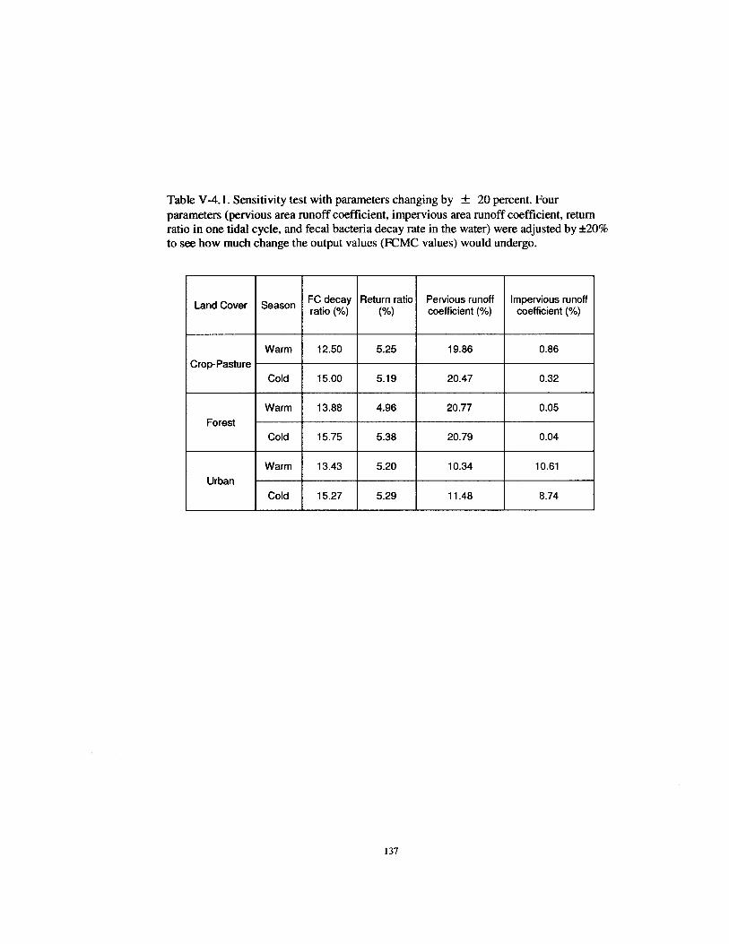
Table V -4.1. Sensitivity test with parameters changing by ± 20 percent. Four parameters (pervious area runoff coefficient, impervious area runoff coefficient, return ratio in one tidal cycle, and fecal bacteria decay rate in the water) were adjusted by ±20% to see how much change the output values (FCMC values) would undergo.

Land Cover Season FC decay Return ratio Pervious runoff Impervious runoff ratio(%) (%) coefficient (%) coefficient (%)

Warm 12.50 5.25 19.86 0.86

Crop-Pasture

Cold 15.00 5.19 20.47 0.32

Warm 13.88 4.96 20.77 0.05

Forest

Cold 15.75 5.38 20.79 0.04

Warm 13.43 5.20 10.34 10.61

Urban

Cold 15.27 5.29 11.48 8.74

137

AGURES

Study S

N

A Miles

0 s 10 l-.J.._J

Legend

~SUiySites

in Lower Chesapeake Bay

138

Figure IV -3.1.1: Tidal levels coded into 9 groups by DSS. These codes are: 1 (high tide-1.4 hours ebb), 2 (1.5 hours ebb-2.9 hours ebb), 3 (3.0 hours ebb-4.4 hours ebb), 4 (4.5 hours Ebb-low tide), 5(Low tide- 1.4 hours flood), 6(1.5 hours flood-2.9 hours flood), 7(3.0 hours flood-4.4 hours flood), 8(4.5 hours flood-high tide), 9(no data).

Time

139

Figure N -4.1.1: 392 FC monitoring stations that have tidal information collected along with FC data by DSS.

FC Monitoring Stations with Tidal Information

140

N

A Miles

0 5 10

Legend

ga_statlons • Stations

Figure IV -4.1.2: Comparison of FC concentration difference due to the effects from seasons and tides. The seasonal difference between winter FC concentration (January to March) and summer FC concentration (July to September) is 18.04 MPN/100ml as the median value, with the first quartile equaling 7.31 MPN/100ml and third quartile equaling 41.76 MPN/100ml. The tidal difference is 0.17 MPN/100rnl as the median value, with the first quartile equaling -1.17 MPN/1 OOrnl and third quartile equaling 7.05 MPN/1 OOml. The difference caused by tides is much smaller than the difference caused by seasons.

FC Conpar I son due to season and due to t i de

100

,.... 80 c

8 ... f 60

...... c 40 0

... Ill .. 1:! 20 Gl

~ 0

0 u u II. +

-20

Seasonal difference ~dal difference

141

Figure IV- 4.2.1.: Map of first spatial component from EOF methods applied to the data matrix of 1460 stations x 12 months. Figure a demonstrates that there was a consistent spatial pattern in almost in every embayment, with high spatial component values in upstream areas, and decreasing values downstream. Figure b shows the eigenvalues in red and cumulated variation in purple. The first component explained about 78% of data variation. Figure c shows the first temporal component with positive values, indicating that the first spatial pattern was consistent within the months, but varied in magnitude between the months.

a)

Miles 0 5 10 L--......1

142

.. _llfllleM 1111 EOf

0 -42.7 --29.5

® -29.5 --25

• -2.5 -429.4

---- Continued ---

b)

95

~ 90 c .g -~ 85 "' > '0

80 !! _'!!

~ 75 " v

70

c)

GA

Q..4

G.Ji$

Q.l

G-21

~ G.2

G.1S

11.1

GAB

0

Eigenvalues and Cumulated Variation for 1460 Water Quality Stations

3.SE+03

3.0E+03

2.SE+03

2.0E+03

1.SE+03

1.0E+03

5.0E+02

· O.OE+OO

1 2 3 4 5

First Tempora.l Prinelpte Component for 1460 Water Quality' Stations

.. .. .a ~ s:: .. ;!!'

2 1 4 5 i 7 i 5 ~ ft u Mcn1h

143

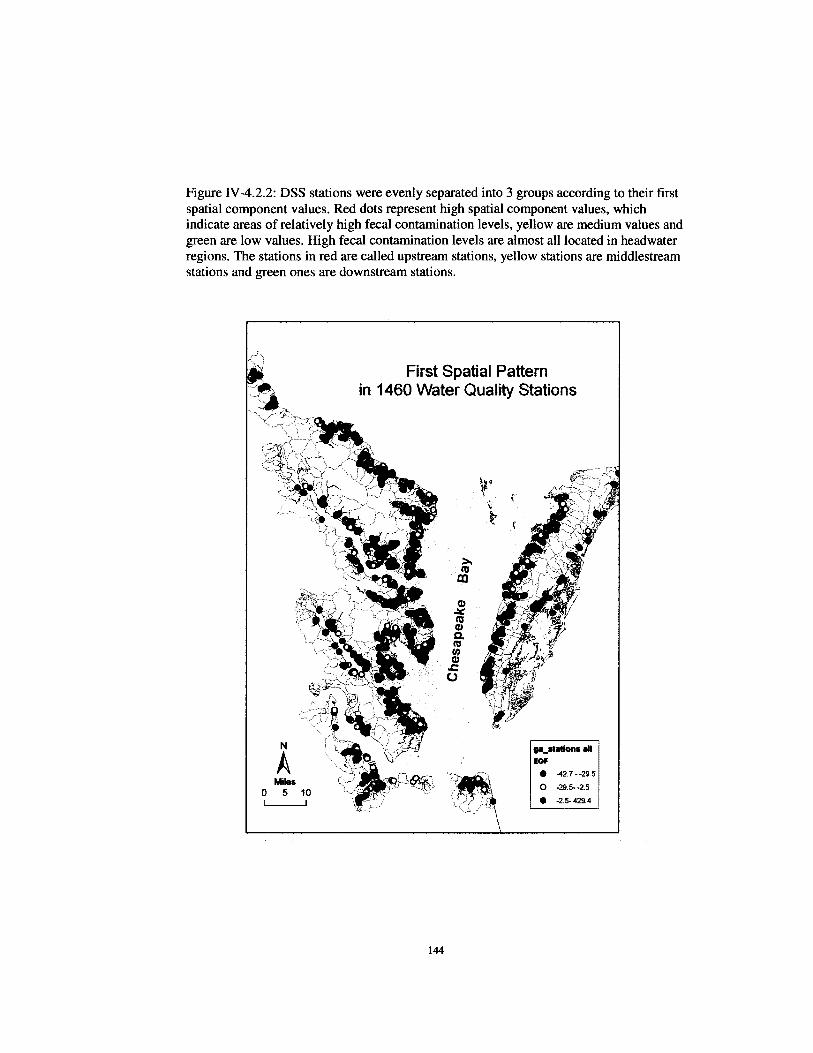
Figure IV -4.2.2: DSS stations were evenly separated into 3 groups according to their first spatial component values. Red dots represent high spatial component values, which indicate areas of relatively high fecal contamination levels, yellow are medium values and green are low values. High fecal contamination levels are almost all located in headwater regions. The stations in red are called upstream stations, yellow stations are rniddlestream stations and green ones are downstream stations.

First Spatial Pattern in 1460 Water Quality Stations

144

.. _stMiensllll EOf

• -42.7 • ·29. 5

0 -29.5--2.5

• -2.5-429.4

Figure N-4.2.3: FC Concentration Frequency Distribution in upstream, uiddlestream, and downstream stations. Highest FC concentrations appear most frequently in upstream regions, occur less frequently in the middlestream, and lowest occurs in downstream.

100

so

60

40

20

Up, Middle, and Downstream FC Frequency Distribution

-1.4 o.o 1.4 2.8 4.2 5.6 7.0 8.4 FC Concentration In Ln (NlN!lOOml)

145

1/ati~

--~ - - Middltslrum ----~

Mein ~v N l-070 1-"1 ~047

l-204 1.284 100064 1.~1 o.,.. 97no

Figure IV -4.2.4: Upstream watersheds in Virginia coastal area. The watersheds surrounding upstream stations were called upstream watersheds. There are a total of 187 upstream watersheds. Most analyses in this study were conducted on these upstream stations and upstream watersheds, shown as pink areas.

N

A Mites

0 5 10

146

Figure IV -4.3.1: The locations of selected upstream watersheds dominated by a single land cover. In a watershed, if forest, urban, or crop and pastureland together occupy more than 80%, 70%, or 70%, respectively, this watershed was called single land-cover-dominated. Here crop and pastureland were combined together, since neither one consisted of more than 60% of the total area of any watershed.

0

147

Legend

-Urban

D Crop-Pasture

-Forest

Figure N-4.3.2: FC Frequency Distribution in the receiving waters of crop-pastureland, forest, and urban-dominated upstream watersheds. FC monitoring stations located in each watershed were grouped together. Green curve represents cumulative frequency distribution in urban-dominated watersheds, black is crop-pastureland-dominated watersheds, and red is forest-dominated watersheds. The figure shows that the highest FC concentrations occur most frequently in urban-dominated waters, with lower concentrations in crop-pastureland-dominated waters and forest-dominated waters.

R: Frequency Dls1rb.tlon In la1d Cover Dcmlnated Watersheds Gimma

--·--------

li'hope~ H 8AA8 MU »4 11»17 ., :w 111

0.403' Jt'-' m

0~~----~----~------~-----r------r-----~ 0

148

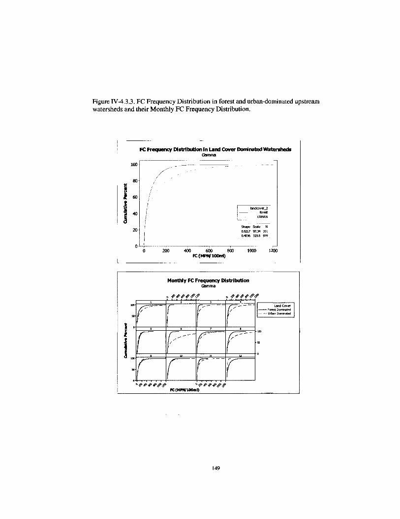
Figure IV-4.3.3. FC Frequency Distribution in forest and urban-dominated upstream watersheds and their Monthly FC Frequency Distribution.

,------····· FC Frequency Distribution In Land Cover Don"inated Watersheds

G!lmma

100

,// ~-

8:1 / I I

60 I I

I I

-40 I I

20 i I

o-L 0

1 HlO r/-50

J 0

t 100

50

0

5

I( 9

If

~----------------.----~--------- ~--

200 -400 600 800 1000 fC (...,., lOCJm)

Monthly FC Frequency Distribution Gamma

2 3 4

( f~ If/-• 7 8

1r/~~-~ If/ If/- -

I( r-- lv ~~~~~~~ ~~~~~~~

FC(MI'N/100ml)

149

1200

I: ~dCov~ I -Forest Dominated - - Urban Dominated

100

"' 0

Figure IV -4.4.1: Cumulative probability curves resulting from a non parametric changepoint analysis show FC geometric means in response to percent impervious surface covers in the years 1990 and 2000. The method showed that the potential impervious percentage threshold was about 14% in 1990 and around 18% in 2000, with low p values.

Chancepoint Distribution for Impervious Cover in 1990

100

100 90

80

80 70

~ <= .~ "' Chan&point =13.78 60 ~= ~ 60 with p = 0.0008

50 -~ g

~ ~~ x 'x ~~ w 40

40 1.!1-u

30 u.

.

20 ~-<~ lU ~>

10 x-'1< X XX

0 0

0 10 20 30 40 50

Impervious Cover(%)

Chancepoint Distribution for lmpervieus Cover in ZOOO

100

100 90

so 80

Chancpoint•17.39 70 ~ with p = 0.002 c .. ::: -60~=[ :s 60 "'

.g g .., so ...... e 40 II <>..

40 1.!1-v u..

30

20 20

x:::r 10 X ;v

0 0

0 10 20 30 40 50

Impervious Cover(%)

150

Figure N-4.5.1: FC Concentration Distribution with and without outliers in different regions. Their distributions are significantly different from each other with p < 0.001 from K-S test.

a) With outliers and all values

FC Concentration Olstrlllutkln with OJtliers In Dlfferert Reolons ooco

- - - - -* - -0 ... ...

YOIJ<

b) Without outliers and only plotting values <200 MPN/lOOml

FC Dletrlbutlan In Quartll• CCirllp4U'Ing Dlff•ent RegiDnl

Note: e: Eastern Shore p: Potomac River y: York river

151

j: James River r: Rappahannock River

Figure IV -4.5.2: Comparison of FC Concentration Frequency Distributions in different regions. a) All FC distributions in different regions on one graph; b) Pair comparison of FC distributions in different regions.

~ :a ! f II.

a) All FC distributions in different regions on one graph

1.0

0.8

0.6

0.4

0.2

0.0

0

FC Distribution in Different Regions

1 2 Lf(FC) MPN/100ml

152

Variable -- LN(Eastern Shore) -- LN(James) 1-~~- LN{Rappahannock)

-- LN(York) 1--- LN{Potomac)

3 4

b) Pair comparison of FC distributions in different regions.

0

0

0 1 2 lN (R:)

3 ..

0.0 o.s 1.0 1.5 2.0 2.5 3.0 3.5 lN (R:)

0.0 0.5 1.0 1.5 2.0 lN (R:)

2.5

153

100

80

20

0

80

0

0.0 0.5 1.0 1.5 2.0 2.5 3.0 3.5

0

0

1-:) --~)

2 lN (R:)

2 . LN (R:)

3

3

4

Figure N-4.5.3: PCA plot based on environmental variables from Rappahannock River, York River, James River, and Eastern Shore regions. PCA analysis on 107 upstream watersheds showed that the first principal component accounts for 30.2% of the variability and the second component accounts for 21.8% ofthe variability (cumulatively 52%).

1.5

•Urban

1.0

• ~ 0.. 0.5

SL R T ~ • A

Forest .., •"" •

0 " " .... f 4f'~.t 4:' ... ...-·.·t· •• •• ... ... ,......, ... •

• -0.5

-1.0 -0.5

Note: Region: r: = Rappahannock River y =York River j = James River e = Eastern Shore

Variables: Drain = Drainage density wtrd = Watershed area RT =Residence time Soil = Runoff potential

0 PC1

Pas = Pastureland percentage Forest = Forest percentage SL =slope

0.5 1.0

W =Water area wet= Wetland percentage EC = Eccentricity Vol= Water volume Agri =Cropland percentage Urban = Urban percentage

R = Ratio of water area divided by watershed area

154

Region .&.r TY •i +e

Figure IV-4.5.4: PCA plot based on environmental variables from Rappahannock River, York River, and Eastern Shore regions. PCA analysis showed that the first PC explains 47% of data variation, with 12.6% for the second PC (cumulatively 59.6%).

0.5

0

D -o.5 0..

-1.0

-1.5

-1.0 ·0.5 0 PC1

Note: Region: r = Rappahannock River y = York River e = Eastern Shore

Variables: Drain= Drainage density wtrd = Watershed area RT = Residence time Soil = Runoff potential Pas = Pastureland percentage Forest = Forest percentage SL =slope

3 Regions A.r

0.5 1.0

W = Water area wet= Wetland percentage EC = Eccentricity Vol= Water volume Agri =Cropland percentage Urban = Urban percentage

R =Ratio of watershed area divided by water area

155

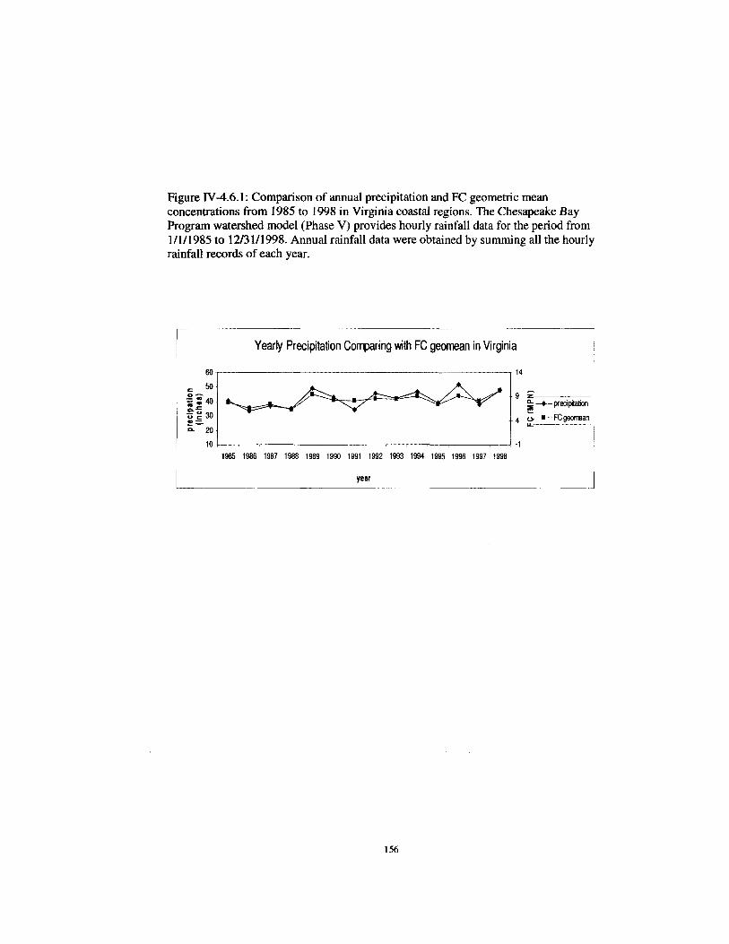
Figure IV -4.6.1: Comparison of annual precipitation and FC geometric mean concentrations from 1985 to 1998 in Virginia coastal regions. The Chesapeake Bay Program watershed model (Phase V) provides hourly rainfall data for the period from 11111985 to 12131/1998. Annual rainfall data were obtained by summing all the hourly rainfall records of each year.

Yearly Precipitation Comparing Vv'ith FC geornean in Virginia

year

156

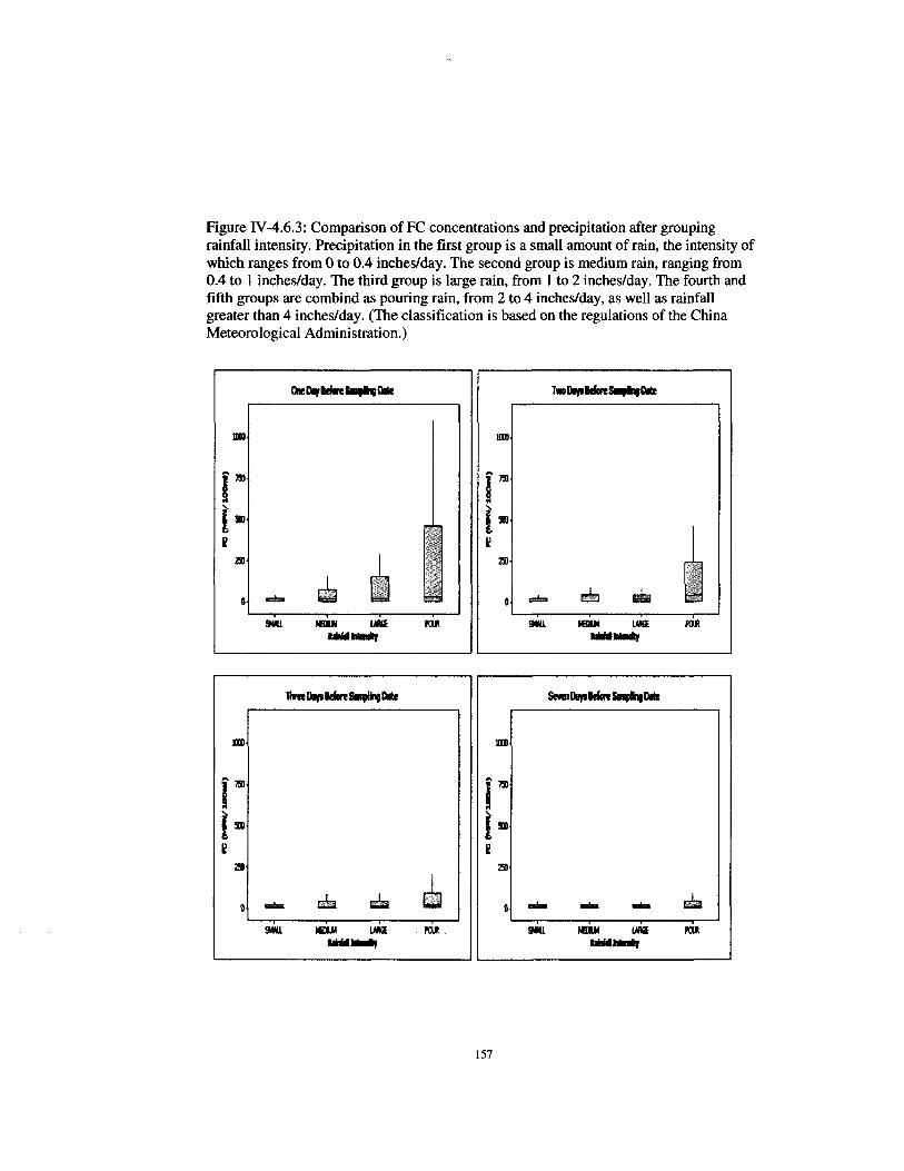
Figure IV -4.6.3: Comparison of FC concentrations and precipitation after grouping rainfall intensity. Precipitation in the first group is a small amount of rain, the intensity of which ranges from 0 to 0.4 inches/day. The second group is medium rain, ranging from 0.4 to 1 inches/day. The third group is large rain, from 1 to 2 inches/day. The fourth and fifth groups are combind as pouring rain, from 2 to 4 inches/day, as well as rainfall greater than 4 inches/day. (The classification is based on the regulations of the China Meteorological Administration.)

llnefllwslelns.,IDJillle SMnfllwsillfcn~lllle

liDl liDl

r~ r~

fs lu ~ ~

291 291

0 ...... ~ ~ ~ 0 ... ... ..... ... !MI. IIIIJI I..N Pal . !MI. IIIIJI LMII Pal ..... ....., .........,

157

Figure IV -4.6.4: A general temporal pattern of fecal contamination throughout Virginia coastal regions. The red lines separate locations into three groups- 1) Potomac River, Rappahannock River, and Mobjack Bay, 2) York River and James River, and 3) the Eastern Shore .

3anuary 300

~ 250 Potomac River Rappahannock River York River

i· James River Eastern Shore 200 Mobjack Bay

Jl 150

100

~ 50

158

May

Watershed

159

: Eastern

I I

September

York River James River

I December

160

Eastern Shore

Figure IV -4.6.5. EOF results from 487 upstream water quality stations. a) First three temporal components with calculated variation; b) First spatial pattern associated with first temporal pattern; c) Second spatial pattern associated with second temporal pattern; d) Third spatial pattern associated with third temporal pattern.

a) First three temporal components with calculated variation

~

~ .. " -;:; > c OJ

-~ "'

1

0.5

0

-0.5

Three Principal Components from PCA on 487 Upstream Water Quality Stations

---,!r-

~

Month

Eigenvalues and Cumulated Variation for 487 Upstream Water Quality Stations

6.1E+03 95

5.1E+03 90

4.1H03 85

80 3.1E+03

I':> 2.1E+03 70 1.1E+03 6'>

G.OE+Ol 60

1 2 3 4 5

161

PCl

PC2

PC3

~ "' ~ :1: ""0

!l .!il :::> E "' u

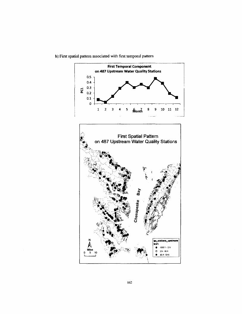
b) First spatial pattern associated with first temporal pattern

First Temporal Component on 487 Upstream Water Quality Stations

0.5

0.4

.... 0.3 ~ 0.2

0.1

0 +-~~~~~·~--~~--~~--~~--~~

Miles 0 5 10 L____j

1 2 3 4 5 1i 7 8 9 10 11 12 Month

162

p_stlllions_upstream EIW1

• -558.1 ·29

0 29·40.4

• 40.4·59.6

c) Second spatial pattern associated with second temporal pattern

1

-0.5

N

A Miles

0 5 10 L_____j

Second Temporal Component on 487 Upstream Water Quality Stations

Month

163

10f2

• 0

-414.8.-4.5

• 5.7 -171.7

d) Third spatial pattern associated with third temporal pattern

N

A Miles

Third Temporal Component on 487 Upstream Water Quality Stations

Month

Third Spatial Pattern on 487 Upstream Water Quality Stations

ga_statiens_upstream I!OF3

• -121.0 --5.2

0 5 10 0 -5.2 -7.0

• 7.0-1117

164

Figure IV -4.6.6: Linkage between the first three PCA temporal components and monthly precipitation, temperature and flow discharge for upstream stations.

a)

b)

c)

5.3

-U s"E -~ e 4.3 ·a--;;. -~1 3.8 ... ..,

t1. c ::;. 3.3

2.8

90

80

70 ;:;:: ~ 60

"' s 50 +'

~ 40 "' ! 30 ....

20

10

0

3

"' 2.5

'ti -g 2

"' ..c 1.5 ~ '0 1 ll: 0

u:: 0.5

II

-Averagelt41in 0.5

-•- PC1 ." 0.4 •

\ 0.3 ,... u

0.2 a. ."' • 0.1

I 0

l 2 3 4 5 6 7 8 9 10 1l 12 Month

-+--Water Te•perature

Air Tc11perature PC2

------1 ~.8

l ::: ~ 0. 2

0

-0.2

'----~-~ -0. 4

2 3 4 6 8 9 10 11 12

Month

__....Row disdlarge -+- PC3

1 2 3 4 5 6 7 8 9 10 11 12 Month

165

0.8

0.6

0.4

0.2

0

·0.2

·11.4

HI u 0..

Figure IV-4.7.1: Classification and Regression Tree analysis ofFC contamination levels for environmental variables in Virginia coastal regions. Environmental variables listed are ratio (watershed/water area), soil runoff potential, forest percentage, impervious percentage, pasture percentage, wetland percentage, and residence time in the water.

>= 76.35

FC Mean: 30.1

Count: 20

1' R tio

Forest

>=0.49 <0.49

< 76.35

Runoff Potential

<0.034 >= 0.034

Impervious

<0.0065

FC Mean: FC Mean: Pasture

>= 0.0065 I Wetland

6.36 22.1 <0.066 >= 0.066 Count: 7 Count :5

FC Mean: FC Mean: 14.3 22.1

Count: 9 Count: 69

166

<0.053 >=0.053

FC Mean: 22.3

Residence Time

<0.56 >=0.56 Count: 36

FC Mean: FC Mean: 20.5 37.8

Count: 6 Count: 13

Figure IV-4.7.2: Contributions of environmental variables to fecal contamination levels based on CART analysis. The width of the pink bar indicates the degree of a variable's contribution, with a longer bar representing a greater contribution.

Term Number of Splits ss Impervious 1990 l 676.626301 Slope 0 0 Drainage density 0 0 Eccentrcity 0 0 Urban 0 0 Forest 721.48784 Pasture l 487.25715

Cropland 0 0 Wetland 1258.5196

Ratio 1085.40049 Residence time 1227.96175 Runoff potential I 1137.03287

Total 7 6594.28157

167

Figure IV -5.3.1: Correlation of percentage of pastureland and percentage of cropland in Virginia coastal regions.

Cor11>arison between Agriculture and Pastureland

0.7

0.6 •

0 0.1

• •

•

•

0.2 0.3

y = 1.4277x + 0.1026

~ = 0.4451

0.4 0.5 0.6

Patureland (%)

168

0.7

Figure IV-5.3.2: Boxplot comparison of FC concentrations between crop-pastureland-dominated watersheds and forest-dominated watersheds.

90

80

70

&60 I so

140 30

20

10

Forest and Agriculture-Pasture Dominated Watersheds

OL-----------.------------------------.----------~ MPN_AgriPasture MPN_forest

169

Figure N-5.4.1: Geometric means ofFC bacterial concentrations vs. percentage impervious surface coverage for five coastal watersheds in Southeastern North Carolina (Mallin et al., 2000).

::J' 110.0 .-----------------------; E 8 100.0 :t:: 90.0 ::l LL 80.0

Q 70.0 t 60.0 0/) 50.0

"C

E 40.0

t 30.0

20.0

~ 10.0

0.~.0

y:: 5.39(~-29.03 R 2 ::0.95, P=0.005

I

5.0 10.0 15.0 20.0 25.0 Wa1ershed impervious surface coverage(%)

170

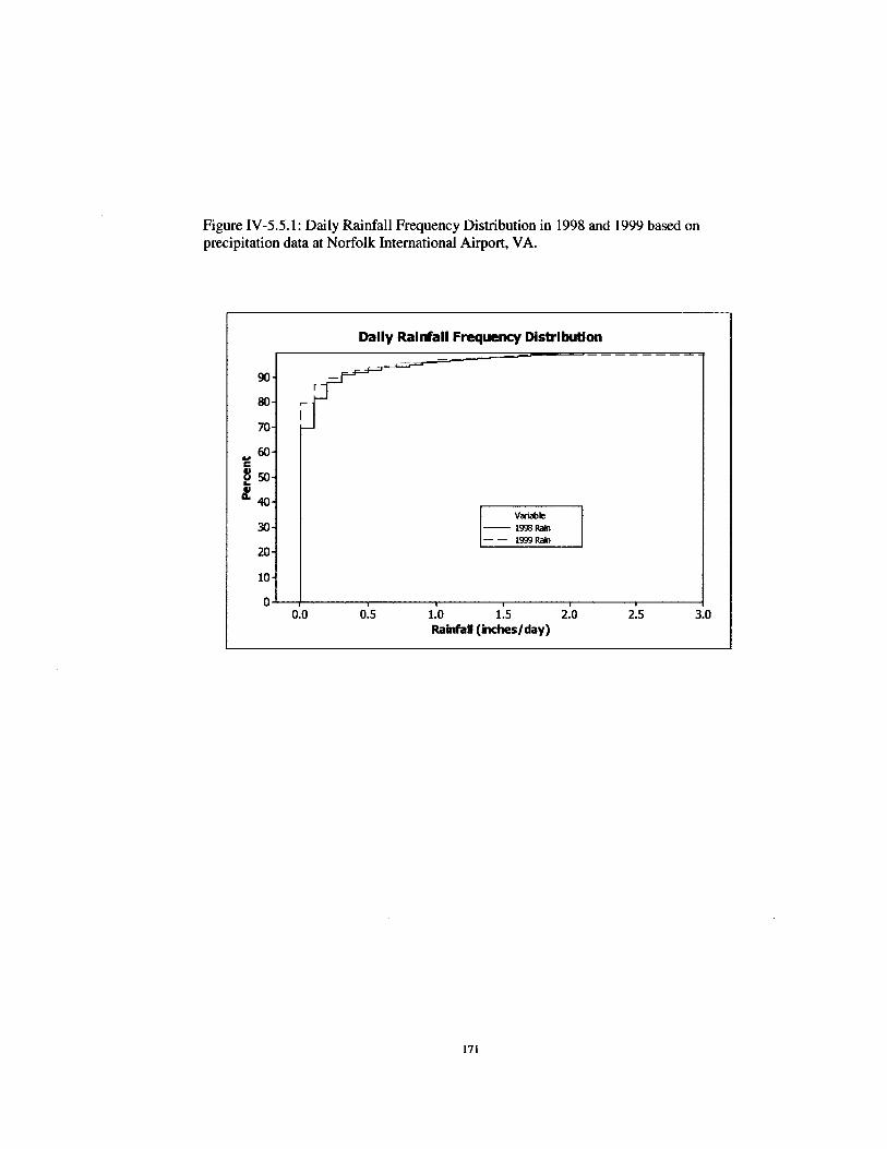
Figure IV -5.5.1: Daily Rainfall Frequency Distribution in 1998 and 1999 based on precipitation data at Norfolk International Airport, VA.

Daily Rainfall Frequency Distribution

90 -r

80 ,... I

70

.,.60 c ~50 !40

I Variable

I 30 -- 1996Rain -- 1999Rain

20

10

0 0.0 0.5 1.0 1.5 2.0 2.5 3.0

RamfaR(mches/day)

171

Figure IV -5.5.2: FC concentration frequency distribution divided into various data ranges for different regions (Eastern Shore, Rappahannock River, Potomac River, James River, and York River regions).

60

40

20

0

FC Frequency Distribution in Different Data Range

0-21 29-93 93-210 FC (MPN/1 OOml)

172

---------l •EasterShore

•Rappahannock

CPotomac

OJ ames

•York

210-

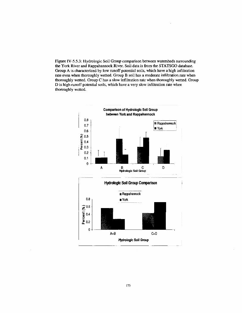
Figure IV-5.5.3: Hydrologic Soil Group comparison between watersheds surrounding the York River and Rappahannock River. Soil data is from the STATSGO database. Group A is characterized by low runoff potential soils, which have a high infiltration rate even when thoroughly wetted. Group B soil has a moderate infiltration rate when thoroughly wetted. Group C has a slow infiltration rate when thoroughly wetted. Group D is high runoff potential soils, which have a very slow infiltration rate when thoroughly wetted.

~- ---~omparison of Hydrologic Soil Group

I n between York and Rappahannock

~:~ l I ~ah~:_noc_j 0.6

~0.5 5l 0.4 <.>

[it~ B C Hydrologic Soil Group

Hydrologic Soil Group Co~J1)arison

0.8

0

1 Rappahannock I YOlk

Hydrologic Soil Group

173

D

Figure IV-5.6.1: Monthly flow discharge comparison from USGS gaging stations located in headwaters of Rappahannock River, Pamunkey River, and Appomattox River in Virginia.

Monthly Flow Discharge from USGS Gage Stations in Virginia

3500

3000-

Iii' ~ 2500 ., ~ 2000 r. II! 1500 i5 ~ 1000 IL

500

2 3 4 5

--Rappahannock Riwr near Fredericksburg, VA1

-11- Pamunkey Riwr near Hanowr, VA

174

~pomattox Riwr at Matoaca, VA

6 7 Month

8 9 10 11 12

Figure N-5.6.2: Hunicanes and Tropical Storms in the Atlantic basin. The peak of hurricane season occurs in September in the Atlantic basin according to NOAA hurricane and storm data from 1851 to 2005.

0 0 0 .... .... N >. Ill

.2:- llill ....

c 1:111 0. «< :3 ::J ::J :J 41 ~ ..... ..., <{ <( IJ1

H,_; r J: d---p-J rHl~1 .. i ~l ::_,.. ~ s ~crT;~ - H,. II( J~l '>

175

,... .... v 0

0 0 0 N ,... .... M

> v v .... v 0 41 41 0 z 0 0

110 "" ... 100

~

~ 90 0

80 0 ...

70 ... flf a.

60 "' 50 E .... 40 B ..... 30

.... 0

20 .... Ql

.Q

10 e :J

0 %

NOAA

Figure V -2.1 Box model of FC input and output for a water segment located in the headwaters of a river. This single water segment represents a headwater water body, and the fecal bacteria are well mixed in the segment. Characteristics of the transport processes for fecal bacteria depend primarily on the water exchange with downstream areas and water discharge from the watershed land surface.

Total FC Loading from Land

Water Segment

where L1.-: Total FC Loadings from land Cm: FC concentration outside of water segment Q;n : Total water volume flow into water segment C0u1: FC concentration inside of water segment Q0u1: Total water volume flow out of water segment V :Volume of the water segment (m3) T: Dominant tidal period (hours) k: Fecal coliform decay rate (d-1)

176

Figure V-3 .1. Cluster analysis results utilizing Manhattan Distance and Complete Linkage method. Each obsel'vation represents an individual watershed and the resulting 5 groups are shown with different colors.

Cluster Analysis on Vlrglnlal Coastal Watersheds Complete Unkage, Manhattan llstance

177

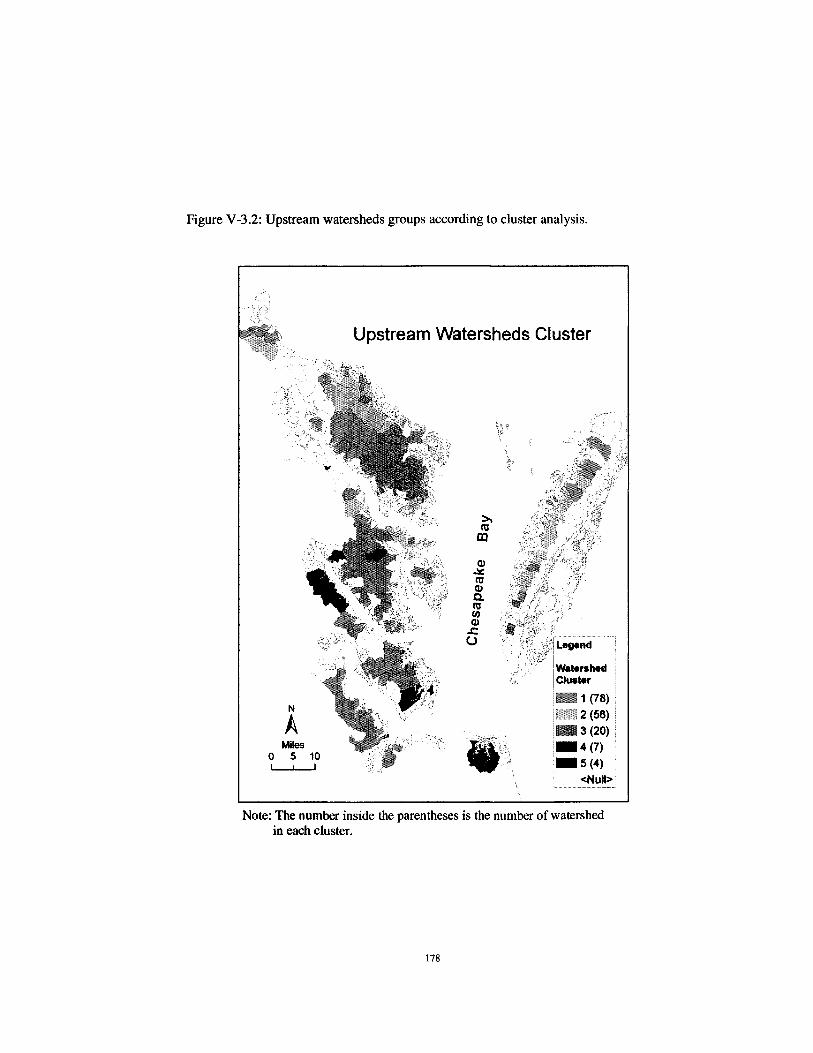
Figure V -3.2: Upstream watersheds groups according to cluster analysis.

N

A Miles

0 5 10 I

Upstream Watersheds Cluster

<.·~f'i'~\. ,,~;

.

Watershed Cluster

1~ 1 (78)

~~~~~~~ 1

-4(7) -5(4) L <Null>

Note: The number inside the parentheses is the number of watershed in each cluster.

178

Figure V-3.4: Comparison of LOG-transformed FC total loadings estimated from water and FC total loadings based on derived FCMCs in warm and cold seasons.

LOG-tnnsfonlK'd FC Total Loading

""' Compaa·tson in 'Varm SE-ason

~ 13

'i

~ 12

§ • 'i 11 ... • • J:>

~ • ·= 10 • "0

.2 Y = 0.9958 'X

~ 9 • R2 = 0.5372 ....

~ 8 8 9 10 11 12 13

LOG (YCTotalloadlats estimlad hm Wiler)

LOG-transformed FC Total Loading Comparison in Cold Season

""' ~ 8

lit 'i 7

~ s 6 'i "' • J:>

5 Q .Ei "0 • .£ 4 • y=0.9737 "'x

~ R2=0.60S9

....

~ 3

3 4 5 6 7 8 s LOG (fCTotalloadlats estimlted fiom water)

179

Figure V -3.6. Comparison of FC total loadings estimated from receiving waters and FC total loadings based on derived FCMCs in warm and cold seasons. The red box indicates a watershed with a poor match between estimated total loads from FCMCs and calculated total loads from TPM.

FC Total Loading Comparison between Estimated and Calculated in Warm Season

- Estimated total loads from FCM::

- Calculated total Loads from TPM

{j,..,.~~

_2.E+07 ., .. c-~~1.E+07 0-

~~ B.E+06

~~ 4.E+06 ~:!.

~ "- "-:::> :::>

:::> I I N

iD "" i I ~

I . "' "' "'

Watershed

FC Total Loading Co1J1)81'ison between Estirmted and Calculated in Cold Season

-Estimated total loads from FCMC

- Calculated total loads from TPM

"- "-:::> :::>

I I -"" :1

I I

"' m

"'

O.E+OO ~~_.,..~rn4J~~->f'i,J,.,~~~0ki\'~~-J,i!,-::r;;t;,~~An(~¢:-m,.~~ "- "' :::> a..

I:::>

:::!' _I I"'

,.,I

u> a.. :::>

I a;

I

~

a.. a.. :::> :::>

I I M "' "" :::!'

I I

~ C>

"'

a.. a.. a.. a.. :::> :::> :::> :::>

I I I - "' "' -:::!' :::!' :::!' :::!' I I I

"' u> ;;; ... "' "' M

a: a.. "' a.. a.. a.. :::> a.. :::> :::> :::>

I :::> I :::> I I N N I i I i a; a; :::!' :::!'

I I I I ,.._ I ... ... I !; "' ;;; ... M ...

W1tel1hed

180

"- a.. "- "- "- a: a.. a.. a.. a.. a.. :::> :::> :::> :::> :::> :::> :::> :::> :::> :::>

I I I I I I :::> I I I I I - - - - "' "' - M -I i :::!' :::; :::; :::; :::; iD "' "' "' :::; I I I I I I I I I I I

M "' ;;; "' C>

"' I C> ;;I "' "' "' u> ...,

"' ,.._

"' "' "'

"-:::>

I

i I

m m

I

I

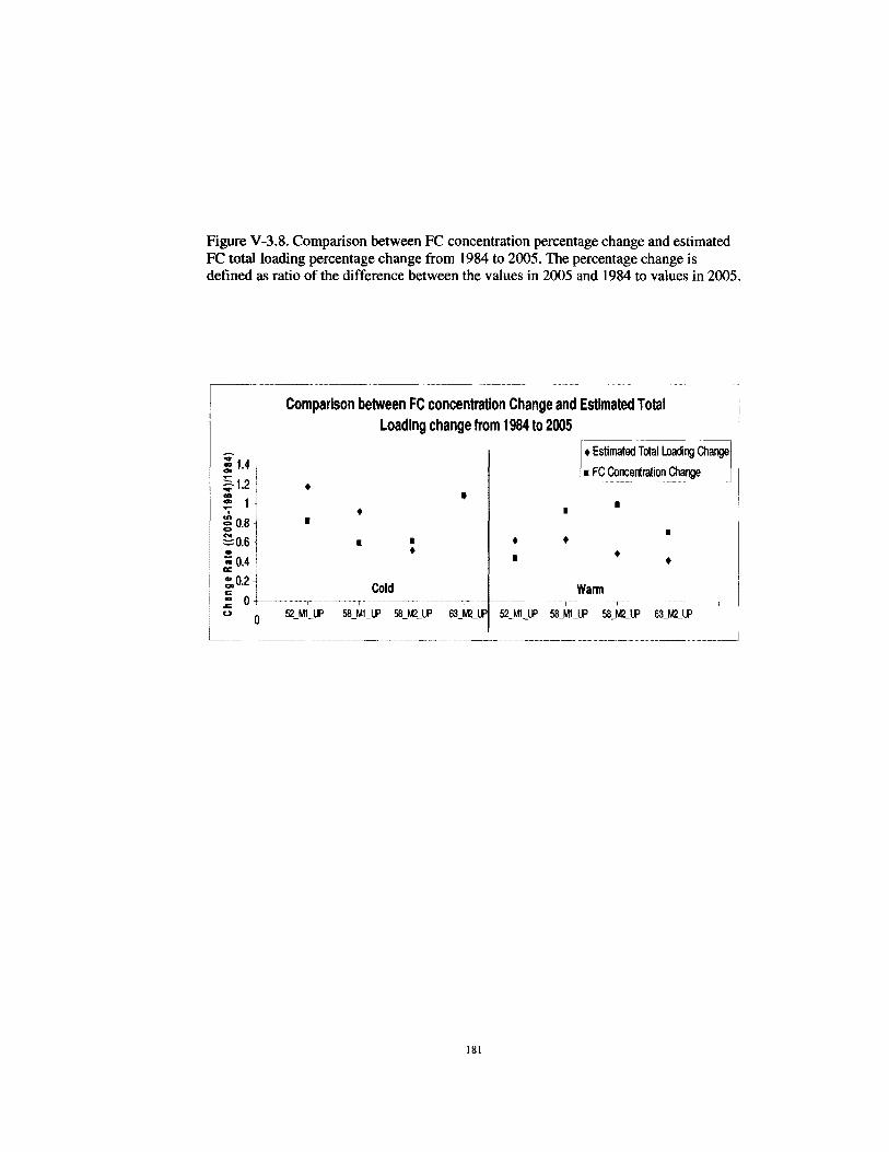
Figure V-3.8. Comparison between FC concentration percentage change and estimated FC total loading percentage change from 1984 to 2005. The percentage change is defined as ratio of the difference between the values in 2005 and 1984 to values in 2005.

:u ~1.2 CD

~ 1

*0.8 ~0.6 .. -0,4 a: :,0.2 c : 0 (.)

0

Comparison between FC concentration Change and Estimated Total Loading change from 1984 to 2005

• • I

I I • Cold

- ----r-··--

52_M1_1.P 58_M1_1.P 58_M!_UP

' I

• • I

[ ..

•. Estimated Total loading Change.j 1 FC Concentration Change --·-------- ----~------

I

I

• • Warm

------"---1"------- ·- - T -~- - -----·-r-·--·· ------1

63_M!_I.P 52_M1_1.P 58_M1_UP 58_M!_I.P 63_M!_I.P

_.I

181