Temporal Association Between Childhood Depressive ...

Temporal Association Between Childhood

Depressive Symptoms and Alcohol Problem Use

in Early Adolescence: Findings from a Large

Longitudinal Population-based Study

Luca Saraceno

UMI Number: U567198

All rights reserved

INFORMATION TO ALL USERS The quality of this reproduction is dependent upon the quality of the copy submitted.

In the unlikely event that the author did not send a complete manuscript and there are missing pages, these will be noted. Also, if material had to be removed,

a note will indicate the deletion.

Dissertation Publishing

UMI U567198Published by ProQuest LLC 2013. Copyright in the Dissertation held by the Author.

Microform Edition © ProQuest LLC.All rights reserved. This work is protected against

unauthorized copying under Title 17, United States Code.

ProQuest LLC 789 East Eisenhower Parkway

P.O. Box 1346 Ann Arbor, Ml 48106-1346

Dedication

To my parents, fo r their continuous love

and support and fo r having taught me to

believe in my dreams.

TABLE OF CONTENTS

Dedication.............................................................................................................................. ii

TABLE OF CONTENTS...................................................................................................... iii

LIST OF TABLES................................................................................................................ xi

LIST OF FIGURES.............................................................................................................xiv

ACKNOWLEDGMENTS....................................................................................................xv

DECLARATION................................................................................................................xvi

ETHICAL STATEMENT..................................................................................................xvii

THESIS SUMMARY.......................................................................................................xviii

PARTI

CHAPTER 1: ALCOHOL PROBLEM USE IN YOUTH AND COMORBIDITY

WITH DEPRESSIVE SYMPTOMS.................................................................................. 1

1.1 Introduction...........................................................................................................1

1.2 The burden of harmful alcohol use in youth........................................................ 4

1.3 Adolescent “alcohol problem use” and “depressive symptoms”......................... 7

CHAPTER 2: RISK AND PROTECTIVE FACTORS FOR HARMFUL ALCOHOL

USE AND DEPRESSIVE SYMPTOMS IN YOUTH.....................................................10

2.1 Introduction......................................................................................................... 10

2.2 Criteria for identification of the relevant epidemiological and molecular

studies................................................................................................................ 11

2.3 Factors identified in epidemiological studies contributing to risk of alcohol

problem use and depressive symptoms in adolescence........................................................13

2.3.1 Socio-demographic factors.................................................................... 13

2.3.2 Substance-related behaviour................................................................. 14

2.3.3 Family environment.............................................................................. 16

2.3.4 Social environment................................................................................17

2.3.5 Personality and psychopathologies....................................................... 19

2.3.5.1 Personality and cognition.....................................................19

2.3.5.2 Psychopathologies.....................................................................21

2.4 Interactions between factors identified through epidemiological studies.........26

2.5 Genetic factors associated with the development of alcohol problem use and

depressive symptoms............................................................................................................27

2.5.1 Heritability of AUDs and depressive disorders.....................................27

2.5.2 Neurotransmitter receptor genes.......................................................... 28

2.5.3 Neurotransmitter transporters................................................................30

2.5.4 Neurotransmitter metabolizing genes................................................... 31

2.5.5 Other genes............................................................................................33

2.5 Epistasis.............................................................................................................. 36

2.6 Gene-environment interaction............................................................................37

PART II

CHAPTER 3: OVERALL STUDY DESIGN..................................................................39

3.1 Purpose of the research....................................................................................... 39

3.2 Theoretical rationales......................................................................................... 39

3.2.1 Association between depressive symptoms and alcohol problem use

in youth 39

iv

3.2.2 Gender differences in the association between depressive symptoms

and alcohol problem use in youth......................................................................40

3.2.3 Peers’ influences in the development of alcohol problem use and

depressive symptoms in youth..........................................................................43

3.3 The analysis at a glance...................................................................................... 45

PART III

CHAPTER 4: METHODS USED TO IDENTIFY THE STUDY SAMPLE AND

SELECT THE RELEVANT VARIABLES.....................................................................47

4.1 The Avon Longitudinal Study of Parents and Children (ALSPAC).................. 47

4.1.1 History of the Avon Longitudinal Study of Parents and Children 47

4.1.2 Representativeness of the ALSPAC sample........................................ 48

4.1.3 Objectives and advantages of the ALSPAC study.............................. 48

4.1.4 Measures of alcohol problem use and depressive symptoms.............. 51

4.1.5 Sample size........................................................................................... 52

4.2 Selection of variables..........................................................................................52

4.2.1 Outcome variable: Alcohol problem use............................................. 52

4.2.2 Predictor variable: Depressive symptoms............................................54

4.2.3 Covariates............................................................................................. 56

4.2.3.1 Socio-demographic characteristics....................................... 59

4.2.3.2 Family environment............................................................. 60

4.2.3.3 Social environment............................................................... 63

4.2.3.4 Personality and psychopathologies...................................... 66

4.2.4 Moderating variables: Peers’ influences...............................................69

4.2.4.1 Child’s bonding with his/her peers........................................70

4.2.4.2 Peers’ risky behaviour...........................................................71

CHAPTER 5: DESCRIPTION OF THE STUDY SAMPLE AND OF THE

SELECTED VARIABLES................................................................................................ 73

5.1 Study sample.......................................................................................................73

5.2 Selection of variables..........................................................................................74

5.2.1 Outcome variable: Alcohol problem use.............................................. 74

5.2.2 Predictor variable: Depressive symptoms.............................................75

5.2.3 Covariates.............................................................................................. 76

5.2.3.1 Socio-demographic characteristics........................................ 77

5.2.3.2 Family environment, social environment, and personality and

psychopathologies................................................................................. 78

5.2.4 Moderating variables............................................................................. 81

PART IV

CHAPTER 6: METHODS AND PROCEDURES FOR THE ANALYSIS OF THE

TEMPORAL ASSOCIATION BETWEEN DEPRESSIVE SYMPTOMS AT AGE 10

YEARS AND ALCOHOL PROBLEM USE AT AGE 14 YEARS...............................83

6.1 Methods: statistical models............................................................................... 83

6.1.1 Regression model: Generalized Ordered Logistic model......................83

6.1.1.1 Vantages and characteristics of the GOLOGIT2 module.. ..85

6.1.2 Data imputation model: Multiple Imputation by Chained Equation

model..................................................................................................... 88

6.1.2.1 Principles and characteristics of the Multiple Imputation by

Chained Equation model....................................................................... 89

6.1.2.2 Auxiliary variables included in the MICE imputation

model......................................................................................................92

6.2 Methods: statistical tests.....................................................................................95

6.2.1 Test for difference between models: Likelihood Ratio test 95

6.2.2 Test for gender differences in the prevalence of the variables: X2 test

and Mann-Whitney-Wilcoxon test....................................................................97

6.3 Analytical procedures......................................................................................... 98

6.3.1 Analysis of univariable GOLOGIT models of age 10 years

depressive symptoms and age 14 years alcohol problem use............................98

6.3.2. Missing data imputation..................................................................100

6.3.3 Analysis of multivariable GOLOGIT models of age 10 years

depressive symptoms and age 14 alcohol problem use in the original (non

imputed) dataset................................................................................................103

6.3.4 Analysis of multivariable GOLOGIT models of age 10 years

depressive symptoms and age 14 years alcohol problem use in the imputed

dataset...............................................................................................................106

6.3.5 Univariable and multivariable GOLOGIT models accounting for the

moderating effects of peers’ influences........................................................... 108

CHAPTER 7: RESULTS OF THE UNIVARIABLE GOLOGIT MODELS.............113

7.1 Gender differences in the predictor and outcome variables............................. 113

7.2 Formats and parallel lines assumptions of the “age 10 years depressive

symptoms variable” in the total sample and in the two genders separately.......................114

7.3 Univariable GOLOGIT models of the association between age 10 depressive

symptoms and age 14 alcohol problem use....................................................................... 116

CHAPTER 8: MISSING DATA IMPUTATION AND RESULTS OF THE

MULTIVARIABLE GOLOGIT MODELS...................................................................119

8.1 Missing data imputation...................................................................................119

8.1.1 Auxiliary variables included in the MICE imputation model 119

8.1.2 Pattern of data missingness............................................................. 120

8.2 Results of the multivariable GOLOGIT models..............................................124

8.2.1 Gender differences in the covariates............................................... 124

8.2.2 Analysis of the covariates: formats of the covariates.......................127

8.2.3 Analysis of the covariates: selection of covariates to be included in

multivariable models 4.............................................................................. 130

8.2.4 Sensitivity analysis for the estimation of mother’s partner’s /

relationship between partners related covariates in single parent and two-parent

families............................................................................................................ 140

8.2.5 Final multivariable GOLOGIT models drawn from the non-imputed

and imputed datasets: total sample.................................................................. 142

8.2.6 Final multivariable GOLOGIT models drawn from the non-imputed

and imputed datasets: gender differences........................................................146

CHAPTER 9: RESULTS OF THE UNIVARIABLE AND MULTIVARIABLE

GOLOGIT MODELS ACCOUNTING FOR PEERS’ INFLUENCES AT AGE 10

AND AT AGE 14 YEARS................................................................................................ 151

9.1 Results of the LR tests assessing the moderating effect of for peers’ influences

(at age 10 and 14 years) in the total sample....................................................................... 151

9.2 Gender differences in the peers’ influences variables .........................153

9.3 Results of the LR tests assessing the moderating effect of peers’ influences (at

age 10 and 14 years) and gender in the total sample................................................... 154

9.4 Results of the LR tests assessing the moderating effect of for peers’ influences

at age 14 years in the subsamples of boys and girls...........................................................155

9.5 Results of the trivariable GOLOGIT interaction models accounting for peers’

influences at age 14 years in the girls’ subsample.............................................................156

9.6 Graphical representation of the univariable GOLOGIT model in the subsample

of girls according to the level of bonding with peers and peers’ alcohol drinking status.. 158

9.7 Results of the multivariable GOLOGIT interaction models accounting for

peers’ influences at age 14 years in the girls’ subsample.................................................... 160

PARTY

CHAPTER 10: DISCUSSION......................................................................................... 165

10.1 Common risk and protective factors for harmful alcohol use and depressive

symptoms in youth identified in the literature.................................................................... 165

10.1.1 Main findings................................................................................ .165

10.1.2 Reasons why genetic risk and protective factors were not included in

the analyses...................................................................................................... 166

10.2 Gender differences in the factors impacting on the relationship between

childhood depressive symptoms and adolescence alcohol problem use.............................169

10.2.1 Main findings..................................................................................169

10.2.2 Link between depressive symptoms and alcohol problem use in the

young............................................................................................................... 170

10.2.3 Gender differences in the relationship between depressive symptoms

and alcohol problem use and in the impact of covariates................................170

10.2.4 Role of family and social environments in the relationship between

childhood depressive symptoms and adolescent alcohol use..........................171

10.2.5 Theoretical frameworks brought to explain the relationship between

depressive symptoms and alcohol problem use in the young..........................172

10.3 Moderating effects of peers’ influences on the relationship between age 10

depressive symptoms and age 14 alcohol problem use......................................................173

10.3.1 Main findings.................................................................................173

10.3.2 Moderating effects of peers’ influences at age 14 years................175

10.3.3 Possible explanations for the complex moderating effects of peers’

influences: peers’ alcohol drinking................................................................. 176

10.3.4 Possible explanations of the complex moderating effects of peers’

influences: bonding with peers........................................................................ 177

10.4 Limitations.........................................................................................................179

10.5 Methodological remarks on data imputation.................................................... 180

10.6 Implications.......................................................................................................181

10.7 Future directions................................................................................................184

REFERENCES...................................................................................................................186

ANNEXES........................................................................................................................ 218

PUBLICATIONS ARISEN FROM THIS DOCTORAL THESIS ,219

LIST OF TABLES

Table 1.1: DSM-IV criteria for Alcohol Dependence and Major Depressive Disorder 2

Table 1.2: Terminology used by the papers cited in Chapters 1 and 2 of this thesis 3

Table 2.2: Search parameters used in the identification of common risk factors for alcohol

problem use and depressive symptoms................................................................................ 11

Table 2.3: Summary of literature search for factors identified through epidemiological

studies contributing to the risk of both alcohol problem use and depressive symptoms in

adolescence.......................................................................................................................... 24

Table 2.4: Summary of literature search for factors identified through molecular studies

contributing to risk of both alcohol problem use and depressive symptoms in

adolescence...........................................................................................................................35

Table 4.1: Comparison of socio-economic characteristics of mothers of children aged<l

year either living in the whole of Great Britain or living in the Avon area or taking part in

the ALSPAC study...............................................................................................................48

Table 4.2: Items in the Short Mood and Feelings Questionnaire....................................... 55

Table 4.3: Parenting activities considered to assess parent-child interaction score 60

Table 4.4: Items of the EPDS used to assess MDD in parents........................................... 61

Table 4.5: Stressful events considered to assess the stressful life event score....................63

Table 4.6: Items assessing peers’ antisocial activities........................................................ 64

Table 4.7: Items of the SDQ used to assess conduct problems and peer problems in

children.................................................................................................................................66

Table 4.8: Items assessing children’s global self-worth self-esteem..................................67

Table 4.9: Items assessing children’s bonding with their peers......................................... 69

Table 5.1: Prevalence of alcohol problem use and depressive symptoms in the study

sample...................................................................................................................................74

Table 5.2: Socio-demographic characteristics of the study sample....................................76

Table 5.3: Prevalence of all the covariates belonging to the family environment, social

environment and personality & psychopathologies domains...............................................78

Table 5.4: Frequencies of the peers’ influences variables in the study sample and

correlations between the two measures of child’s bonding with his/her peers and the two

measures of peers’ risky behaviour...................................................................................... 80

Table 6.1: Bullying-related events ascertained...................................................................91

Table 6.2: Items assessing sensation-seeking score............................................................93

Table 6.3: Type of imputation equation that was specified for each variable included in the

MICE imputation model..................................................................................................... 101

Table 7.1: Prevalence of alcohol problem use and depressive symptoms for boys and girls

separately............................................................................................................................ 113

Table 8.1: Auxiliary variables included in the MICE model............................................120

Table 8.2: Frequency of missing variables in the total sample for all 35 variables included

in the MICE imputation procedure..................................................................................... 121

Table 83: Number of missing values per each variable included in the MICE model and

gender differences in missingness rate............................................................................... 123

Table 8.4: Socio-demographic covariates presented for boys and girls separately 125

Table 8.5: Prevalence of all the covariates belonging to the family environment, social

environment and personality and psychopathologies domains for boys and girls

separately............................................................................................................................126

Table 8.6: Comparison of bivariable models of age 10 depressive symptoms and age 14

alcohol problem use with covariates entered in either quadratic, categorical or linear

formats in the total sample................................................................................................. 129

Table 8.7: Estimates of each covariate when tested independently in bivariable GOLOGIT

models drawn from both the non-imputed and the imputed datasets and based on the total

sample................................................................................................................................. 133


models drawn from both the non-imputed and the imputed datasets and based on the

subsample of boys.............................................................................................................. 136


models drawn from both the non-imputed and the imputed datasets and based on the

subsample of girls............................................................................................................... 139

Table 8.10: Sensitivity analysis of mother’s partner’s / relationship between partners

related covariates in the subsample of children living in two-parent families...................142

Table 8.11: Final multivariable GOLOGIT models drawn from the non-imputed and the

imputed datasets predicting age 14 years high alcohol problem use for the total

sample................................................................................................................................. 145

Table 8.12: Final multivariable GOLOGIT models drawn from the imputed dataset

predicting age 14 high alcohol problem use for the two genders separately.....................148

Table 8.13: Final multivariable GOLOGIT models drawn from the non-imputed dataset

predicting age 14 high alcohol problem use for the two genders separately.....................150

Table 9.1: Peers’ influences variables presented separately for boys and girls................156

Table 9.2: Trivariable GOLOGIT interaction models accounting for peers’ influences at

age 14 years in the girls’ subsample (imputed dataset)......................................................160

Table 9.3: Multivariable GOLOGIT interaction models accounting for peers’ influences at

age 14 years in the girls’ subsample (imputed dataset)......................................................164

LIST OF FIGURES

Figure 2.1: Number of papers gathered through bibliographic searches per year of

publication............................................................................................................................ 12

Figure 4.1: Timeline of the measures in ALSPAC assessing children’s alcohol

involvement and depressive symptoms................................................................................ 51

Figure 4.2: Graphical representation of the variables included in my models, with

information about the age they were collected and the source of information....................57

Figure 5.1: “Scree plot” of first four principal components generated by the PCA..........73

Figure 7.1: Expected probability of developing high alcohol problem use in adolescence

by level of severity of childhood depressive symptoms; results are shown for the total

sample and for both genders separately............................................................................. 117

Figure 9.1: Slopes of the expected probability estimates of the univariable GOLOGIT

model in the subsample of girls according to the level of bonding with peers and peers’

alcohol drinking status........................................................................................................ 163

xiv

ACKNOWLEDGMENTS

I wish to thank first and foremost my main supervisor, Dr. Marianne B. M. van den Bree,

Reader at the Department of Psychological Medicine and Neurology of Cardiff University,

for having been an exceptional guide during the period of my Ph.D., and having helped me

develop and improve all the skills and competences that I have used throughout this thesis.

I then wish to thank all my secondary supervisors; Prof. Marcus Munafo, Professor of

Biological Psychology at the University of Bristol, Prof. Nicholas Craddock, Professor of

Psychiatry at the Department of Psychological Medicine and Neurology of Cardiff

University and Dr. Jon Heron, Research Fellow at the Department of Social Medicine at

the University of Bristol; their feedback and suggestions have been fundamental during all

the stages of my doctorate. I am also extremely grateful to all the children and their

families who took part in this study and to the whole ALSPAC Study Team. Finally, I wish

to thank Mr. Roberto Melotti, statistician in ALSPAC and Dr. Stan Zammit, clinical

lecturer at Cardiff University, for their useful suggestions during the planning of the

analyses. I also wish to thank my friend Tazeen for her editing skills, which have been

providential to help me correct many of my “Italianized” English expressions in this thesis.

My family and my friends have constantly given me the strength I needed to pursue my

Ph.D. I wish to thank particularly my parents, for having always morally supported me for

the occasional setbacks and having praised me for every successful result. If this period of

hard work has been also a joyful period, I owe it to my good friends Loli, Arianna, Elisa,

Ivona, Tazeen and Christina; my warmest thanks for the wonderful moments we spent

together go to all of you.

xv

DECLARATION

This work has not previously been accepted in substance for any degree and is not

concurrently submitted in candidature for any degree.

....Z*Z...JZZZ:.ZZZ..... (candidate) Date 2 3 / 0 . 1 / / J .Signed

STATEMENT 1

This thesis is being submitted in partial fulfilment of the requirements for the degree of

PhD.

Signed ....^Z.^fZZ.ZZC.:... (candidate) Date ......

STATEMENT 2

This thesis is the result of my own independent work/investigation, except where otherwise

stated. Other sources are acknowledged by explicit references.

Signed (candidate) Date 2 3 /o 9 / / /

STATEMENT 3

I hereby give consent for my thesis, if accepted, to be available for photocopying and for

inter-library loan, and for the title and summary to be made available to outside

organisations.

Signed . 7 7 . . . 7 7 7 7 7 7 7 7 . . . . . (candidate) Date .

STATEMENT 4: PREVIOUSLY APPROVED BAR ON ACCESS

I hereby give consent for my thesis, if accepted, to be available for photocopying and for

inter-library loans after expiry of a bar on access previously approved by the Graduate

Development Committee.

Signed................................................................ (candidate) Date................................

xvi

ETHICAL STATEMENT

Ethical approval for this doctoral research was obtained from the Avon Longitudinal Study

of Parents and Children (ALSPAC) Law and Ethics committee and the Local Research

Ethics committee. This doctoral research was specifically funded by a studentship awarded

to Luca Saraceno by the Department of Psychological Medicine and Neurology of Cardiff

University.

THESIS SUMMARY

Alcohol problems during adolescence have been linked to a variety of adverse

consequences, including illicit drug use, delinquency and increased risk of morbidity and

mortality. Depressive symptoms can increase the risk of development of alcohol problems

in young people and a number of risk factors in common for both behaviours has been

identified. However, the peer group plays an important role in the development of both

depressive symptoms as well as alcohol problem use. Moreover, the relationship may also

differ for boys and girls.

My thesis addresses the nature of the longitudinal relationship between depressive

symptoms at age 10 years and alcohol problem use at age 14 years, investigating in

particular the differences between genders in the pattern of a large number of non-genetic

covariates considered as potential confounders of such relationship and the moderating

effects of age 10 and age 14 peers influences. Data were obtained from 4220 participants in

the Avon Longitudinal Study of Parents and Children (ALSPAC), a large population-based

UK birth cohort.

Childhood depressive symptoms were associated with increased risk of alcohol problem

use in early adolescence for girls (O.R. 1.14, p-value=0.016) but not boys. Covariates

describing particularly the family and social environment influenced this association for

girls. This association became smaller when these covariates were taken into account.

Having a strong bond with alcohol-drinking peers at age 14 interacted with depressive

symptoms to increase risk of alcohol problem use in 14 years old girls (O.R. 1.18, p-

value=0.030). These findings corroborate the growing evidence that family-related

interventions to reduce alcohol use are particularly effective for girls. Future policy will

have to consider that girls who experience high levels of depressive symptoms may be at

particular risk of alcohol problem use if they affiliate with a peer group exerting strong

pressure to drink.

xix

PARTI

CHAPTER 1: ALCOHOL PROBLEM USE IN YOUTH AND COMORBIDITY WITH

DEPRESSIVE SYMPTOMS

1.1 Introduction

Harmful use of alcohol is a major public health issue, placing a heavy social, medical and

economic burden on the world. According to the World Health Organization (WHO) in 2004

about 2 billion people worldwide consumed alcoholic beverages and over 75 million had a

diagnosis of alcohol use disorders (AUDs) (WHO, 2004a). Apart from the direct effects of

intoxication and dependence, alcohol is estimated to cause approximately 20% to 30% of

each of the following worldwide: oesophageal cancer, liver cancer, cirrhosis of the liver, and

epilepsy, and is a major contributor to fatalities associated with homicides and motor vehicle

accidents (WHO, 2004b). A clear figure of the social and economical burden of heavy

alcohol consumption is given by the cost of alcohol-related harm from the National Health

Service (NHS) of the United Kingdom (UK), which has been estimated around £8.7-9.0

billion (Cabinet Office, 2004).

Alcohol problem use has been associated with depressive disorders (depression and anxiety)

in a number of samples of adolescents (Stice et al., 1998, Turner et al., 2005) and an

increasing research and clinical interest in the aetiological relationships between both

behaviours exists (Clark et al., 1996). Moreover, depression is the leading cause of nonfatal

disability worldwide, with the greatest impact on younger generations (Lopez et al., 2006).

Different terms are used in the literature to describe alcohol problems; some are more

common and informal (e.g. excessive/ harmful alcohol use), while others have a more defined

meaning within specific classifications (e.g. alcohol abuse/ alcohol dependence (AD) within

1

the DSM-IV classification (APA, 2000)). Still, some of the latter terms are sometimes also

used more informally. This applies also to depressive symptoms, with terms like depression

and depressive traits used more informally, while terms such as Major Depressive Disorder

are more rigorously clinically-defined (APA, 2000).

Table 1.1 reports the clinical criteria that need to be met in order to perform a clinical

diagnosis of Alcohol Dependence or Major Depressive Disorder according to the DSM-IV

classification of mental disorders (APA, 2000).

Table 1.1: DSM-IV criteria for Alcohol Dependence and Major Depressive Disorder

(Ja0)"O04>avQ"o>0©©

A maladaptive pattern of alcohol use, leading to clinically significant impairment or distress, as manifested by three or more of the following seven criteria, occurring at any time in the same 12- month period:

1. Tolerance, as defined by either of the following:• A need for markedly increased amounts of alcohol to achieve intoxication or desired effect.• Markedly diminished effect with continued use of the same amount of alcohol.

2. Withdrawal, as defined by either of the following:• The characteristic withdrawal syndrome for alcohol (refer to DSM-IV for further details).• Alcohol is taken to relieve or avoid withdrawal symptoms.

3. Alcohol is often taken in larger amounts or over a longer period than was intended.4. There is a persistent desire or there are unsuccessful efforts to cut down or control alcohol use.5. A great deal of time is spent in activities necessary to obtain alcohol, use alcohol or recover

from its effects.6. Important social, occupational, or recreational activities are given up or reduced because of

alcohol use.7. Alcohol use is continued despite knowledge of having a persistent or recurrent physical or

psychological problem that is likely to have been caused or exacerbated by the alcohol (e.g., continued drinking despite recognition that an ulcer was made worse by alcohol consumption).

©"O

I*aVP

Five (or more) of the following symptoms have been present during the same 2-week period and represent a change from previous functioning; at least one of the symptoms is either (1) depressed mood or (2) loss of interest or pleasure.

1. Depressed mood most of the day, nearly every day, as indicated by either subjective report (e.g., feels sad or empty) or observation made by others (e.g., appears tearful).

2. Markedly diminished interest or pleasure in all, or almost all, activities most of the day, nearly every day (as indicated by either subjective account or observation made by others).

3. Significant weight loss when not dieting or weight gain (e.g., a change of more than 5% ofbody weight in a month), or decrease or increase in appetite nearly every day.

4. Insomnia or hypersomnia nearly every day.5. Psychomotor agitation or retardation nearly every day (observable by others, not merely

subjective feelings of restlessness or being slowed down).6. Fatigue or loss of energy nearly every day.7. Feelings of worthlessness or excessive or inappropriate guilt (which may be delusional) nearly

every day (not merely self-reproach or guilt about being sick).8. Diminished ability to think or concentrate, or indecisiveness, nearly every day (either by

subjective account or as observed by others)9. Recurrent thoughts of death (not just fear o f dying), recurrent suicidal ideation without a

specific plan, or a suicide attempt or a specific plan for committing suicide

2

Throughout this thesis, where possible, I have used the specific terminology reported in cited

references; however, the generic terms “alcohol problem use” and “depressive symptoms”

were used whenever the sources I cited together differed in the definition and assessment of

alcohol use and misuse or depressive symptoms and disorders. Table 1.2 reports the specific

terminology used to define alcohol and depressive problems by the papers cited in Chapters 1

and 2 of this thesis. 23 different terms, ranging from “alcohol abuse” to “substance use

disorders” were used to describe what I generically define as “alcohol problem use” and 11

different terms, ranging from “anxiety” to “suicidal behaviour” were used to describe what I

generically define as “depressive symptoms.”

Table 1.2: Terminology used by the papers cited in Chapters 1 and 2 of this thesis

Alcohol problem use Depressive symptoms1 Alcohol abuse Anxiety2 Alcohol misuse Anxiety disorder3 Alcohol problems, problem drinking Depression4 Alcohol sensitivity Depressive symptoms5 Alcohol tolerance Internalizing problems6 Alcohol use and problem use Major Depressive Disorder7 Alcohol use disorders Neuroticism8 Alcoholism (alcohol dependence) Other traits associated with internalizing disorders9 Antisocial alcoholism Post Traumatic Stress Disorder

10 Binge and harmful drinking Psychological distress11 Drug and alcohol use Suicidal behaviour12 Drug use13 Excessive alcohol consumption14 Heavy alcohol use15 Heavy drinking of alcohol16 High alcohol consumption17 Illicit drug use18 Other traits associated with alcohol problems19 Substance abuse (including alcohol)20 Substance dependence21 Substance use22 Substance Use (including alcohol use)23 Substance use disorder

3

1.2 The burden of harmful alcohol use in youth

Alcohol is the most prevalent substance used during the developmental period of adolescence

(defined by the WHO as age 10-19 years (WHO Europe, 2005)) (BMA BOSE, 2003) and

alcohol involvement in young people has been associated with increased risk of tobacco and

drug use, academic failure, delinquency, pregnancy and sexually transmitted disease, traffic

accidents and other injuries (Donovan, 2004, Flowers, 1999, Kandel et al., 1993, Sutherland

et al., 1998, U.S. Department of Justice, 2007).

Across the whole European Union (EU) >90% of 15-16 year olds have imbibed alcohol at

some point in their lives, on average initiating use at 12.5 years of age and getting intoxicated

for the first time at 14 years of age; 13% of 15-16 year olds have been intoxicated more than

20 times in their lives (Anderson et al., 2006b). The average amount of alcohol consumed on

a single occasion by 15-16 year old European youth is over 60 grams of alcohol in northern

Europe, and nearly 40 grams of alcohol in southern Europe (Anderson et al., 2006b).

Quantifying this in naturalistic terms, since 8 grams of alcohol are equivalent to 1 UK alcohol

unit (10 ml of pure alcohol), 60 grams of alcohol would correspond approximately to one

fourth of a bottle of spirit (Alcohol by volume (ABV) 40%), or four pints of beer (ABV

3.5%) or a bottle (750 ml) of white wine (ABV 10.5%) (Drinkaware, 2010). Teenagers in the

UK have one of the highest rates of substance use in Europe (SCIAOD, 2000) and are more

likely to have experimented with alcohol as well as illicit drugs than their peers elsewhere in

Europe (EMCDDA, 2007, SCIAOD, 2000). Furthermore, although the percentage of British

adolescents aged 11-13 years who do not consume alcohol has been increasing since 2001

(from 39% in 2001 to 46% in 2006), the weekly consumption in this age range has almost

doubled, indicating heavier use among those who do drink (from 5.6 units in 2001 to 10.1

units in 2006) (NHS, 2007). Statistics report that approximately 1% of 14-16 year olds in the

4

UK drink alcohol nearly every day (EMCDDA, 2007), and are therefore at high risk of AUDs

(McArdle et al., 2007).

In the United States of America (U.S.A.) the average age of consuming the first drink is 11

years for boys and 13 years for girls. In 2004, 19% of 8th graders (13-14 years old) and 48%

of 12th graders (17-18 years old) reported alcohol use in the previous month (Johnston et al.,

2005). Epidemiological studies conducted in the U.S.A. reported that in 2001 the annual

prevalence of AUDs was 5% in both boys and girls aged 12-17 years, with a peak prevalence

of 20% in men and 10% in women between the ages of 18-23 years (Harford et al., 2005).

Since adolescents are highly vulnerable to social influences (Kandel et al., 1987), have lower

alcohol tolerance levels and become dependent at lower doses than adults (Chen et al., 1997),

the period of adolescence is a key developmental time frame with respect to the development

of subsequent alcohol related problems in adulthood.

Moreover, the age of adolescence overlaps for a large extent with puberty, which is a period

of increased vulnerability and adjustment for young people (Caspi et al., 1991). Along with

the physical changes, puberty brings about major psychological and social changes that are

likely to cause stress and susceptibility to psychiatric disorders (Kaltiala-Heino et al., 2011,

Patton et al., 2004), as adolescents may experience not only transitional stress due to new

psychological adaptations and an accumulation of stressful events (e.g., (Rudolph et al.,

1999)), but also stress related to disparities between their chronological age, social age and

biological maturation (Glaser et al., 2011, Petersen, 1980).

Longitudinal studies (DeWit et al., 2000, Grant et al., 1998) have indicated that initiating

alcohol use before age 15 considerably increases the risk of development of alcohol abuse or

dependence in adulthood. A longitudinal study of youth in the United States conducted by

Grant and colleagues estimated that each year of delayed onset of alcohol consumption

reduces this risk of future alcohol related problems by 7.0% (Grant et al., 2001). It has also

5

been estimated that, compared with early adulthood onset (Hingson et al., 2009), adolescent

onset of alcohol use doubles the risk of having a diagnosis of AD or alcohol abuse in

adulthood.

Alcohol use during adolescence is also associated with an increased risk of illicit drug use

(Sutherland et al., 1998). In a cross-sectional study of 17-18-year-old adolescents, Kandel

and Yamaguchi (Kandel et al., 1993) observed that alcohol and tobacco use tend to precede

and increase the use of illicit drugs.

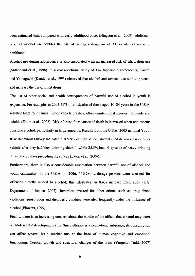
The list of other social and health consequences of harmful use of alcohol in youth is

expansive. For example, in 2005 71% of all deaths of those aged 10-24 years in the U.S.A.

resulted from four causes: motor vehicle crashes, other unintentional injuries, homicide and

suicide (Eaton et al., 2006). Risk of these four causes of death is increased when adolescents

consume alcohol, particularly in large amounts. Results from the U.S.A. 2005 national Youth

Risk Behaviour Survey indicated that 9.9% of high school students had driven a car or other

vehicle after they had been drinking alcohol, while 25.5% had >1 episode of heavy drinking

during the 30 days preceding the survey (Eaton et al., 2006).

Furthermore, there is also a considerable association between harmful use of alcohol and

youth criminality. In the U.S.A. in 2006, 116,280 underage persons were arrested for

offences directly related to alcohol; this illustrates an 8.4% increase from 2005 (U.S.

Department of Justice, 2007). Juveniles arrested for other crimes such as drug abuse

violations, prostitution and disorderly conduct were also frequently under the influence of

alcohol (Flowers, 1999).

Finally, there is an increasing concern about the burden of the effects that ethanol may exert

on adolescents’ developing brains. Since ethanol is a neuro-toxic substance, its consumption

can affect several brain mechanisms at the base of human cognitive and emotional

functioning. Cortical growth and structural changes of the brain (Yurgelun-Todd, 2007)

6

continue to take place throughout adolescence (Crews et al., 2007), occurring until at least

age 21 (Lewinsohn et al., 1993). During adolescence ethanol may affect in particular the fine

modelling of the frontal cortex (Sher, 2006a) and the hippocampus (De Beilis et al., 2000);

brain structures fundamental for memory processes; and the function of the hypothalamic-

pituitary-adrenal axis (HPA), which is crucial for the response to stress (Dai et al., 2007,

Prendergast et al., 2007). The HP A axis is a very complex neuro-endocrine system, which is

fundamental for emotion regulation; its activity also modulates addictive behaviour.

Alteration of this system has been associated with alcohol abuse and dependence, Major

Depressive Disorder and anxiety disorder (Sher, 2007).

1.3 Adolescent “alcohol problem use” and “depressive symptoms”

Depression is a common mental health problem during adolescence. In the EU 4% of 12- to

17-year-olds and 9% of 18-year-olds suffer from depression (WHO Europe, 2005). Studies

indicate that in the UK 5% of those aged 11-16 are affected with clinically diagnosed Major

Depressive Disorder (MDD) or anxiety disorder (Green et al., 2005), while in the U.S.A. 20%

of youth may experience an episode of depression before age 18 (Lewinsohn et al., 1991).

MDD co-occurs frequently with anxiety disorder, with approximately 25-50% of depressed

youth having co-morbid anxiety disorders and about 10-15% of youths with anxiety disorder

also suffering from depression (Axelson et al., 2001).

Many studies indicate that depression plays a fundamental role in the development of AUD

(Bukstein et al., 1992, Clark et al., 1997b). However, the developmental relationship between

the two traits remains unclear, with a number of studies reporting that depressive symptoms

precede alcohol problem use (Bukstein et al., 1992, Buydens-Branchey et al., 1989, Hahesy

et al., 2002, Kuo et al., 2006) while others report the opposite (Alati et al., 2005, Costello et

al., 1999, Deykin et al., 1987, Hovens et al., 1994, White et al., 2001). It also remains unclear

7

which shared factors may increase the risk of co-morbidity between alcohol problem use and

depressive behaviour in youth. Both behaviours have been reported to share non-genetic risk

factors (Windle et al., 1999). In addition, a number of twin studies have indicated that both

adolescent and adult alcohol problem use as well as depressive symptoms are influenced by

genetic factors (Hopfer et al., 2003, Middeldorp et al., 2005) and that some overlap exists in

the genetic influences on both behaviours (Kendler et al., 2003, Tambs et al., 1997).

The high co-morbidity between depressive symptoms and alcohol problem use might

therefore be explained by the large number of common genetic and non-genetic risk factors

for both phenotypes (Kendler et al., 1993). However other mechanisms may also be taken

into account. Tension Reduction Theory (Greeley et al., 1999), for example, suggests that

children with depression may experiment with substances in an attempt to self-medicate their

depressed mood (King et al., 2004). The available evidence suggest that, because adolescence

and young adulthood (Blazer et al., 1994, Disorder, 2005) are pivotal periods of physical and

psychological development, juvenile onset of alcohol problem use (as reviewed in paragraph

1.2) or depressive symptoms may be particularly predictive of continued problems in

adulthood (Blazer et al., 1994, Disorder, 2005). Prospective studies have estimated that

adolescent onset of depressive symptoms is associated with a two-to-threefold increased risk

of adulthood MDD or anxiety disorder (Pine et al., 1998).

In adulthood, one of the most extreme possible consequences of MDD, suicide, is also

strongly associated with a diagnosis of AUDs. Up to 40% of persons with alcohol

dependence attempt suicide at some point in their lives, while 7% end their lives by

committing suicide (Sher, 2006b). Moreover the lifetime risk of suicide in alcohol

dependence has been estimated at 15% (Miles, 1977), with a relative risk (RR) of suicide

among ’’alcohol abusers” of 6.9 (Rossow et al., 1995). In Accident & Emergency (A&E)

settings in particular, a strong association has been observed between suicide attempt and

8

alcohol use, with 10-69% of suicide completers and 10-73% of suicide attempters testing

positive for alcohol in the blood (Cherpitel et al., 2004).

With regards to the co-morbidity between alcohol problems and depression, a longitudinal

study by Hasin et al observed that subjects suffering for both depression and alcohol

dependence are at particularly high risk of committing suicide: one out of every twenty

patients with alcohol dependence who are hospitalized for depression die by committing

suicide within two years (Hasin et al., 1989).

Many studies conducted in young people as well as in adult samples provide evidence that

depression, especially early-onset depressive symptoms (Deas et al., 2002), can precede

alcohol problem use (Bukstein et al., 1992, Buydens-Branchey et al., 1989, Clark et al.,

1997b, Hahesy et al., 2002, Kuo et al., 2006). A better understanding of the relationships

between alcohol problem use and depressive symptoms in adolescence is important for, and

contributes to, the development of optimal prevention and early intervention approaches.

9

CHAPTER 2: RISK AND PROTECTIVE FACTORS FOR HARMFUL ALCOHOL

USE AND DEPRESSIVE SYMPTOMS IN YOUTH

2.1. Introduction

The purpose of this chapter is to describe the most relevant shared risk and protective factors

associated with the development of both alcohol problem use and depressive symptoms in

adolescence that have been reported in published literature.

It is well established that both genetic and non biological factors contribute to the

development of psychiatric disorders (for a review see Cooper et al (Cooper et al., 2001)).

As a result of their frequent co-occurrence, alcohol abuse and depressive disorders are

expected to share these factors to a degree.

A large number of risk and protective factors were identified through systematic

bibliographic searches. These factors may be divided into non-genetic and genetic factors that

may contribute to the co-morbidity between alcohol problem use and depressive symptoms in

adolescence and were identified through epidemiologic and molecular studies. In the first part

of this chapter I initially described the role that non-genetic factors identified in

epidemiological studies may have in the development of both conditions, while in the last

part of the chapter I provided a brief overview of all the genetic risk and protective factors

that have been identified by molecular studies investigating the genetic underpinnings of

AUDs and mood disorders. Genetic factors have been established as being important in the

development of both alcohol problem use and depressive symptoms; however, in my

dissertation I focused only on the role of non-genetic factors.

10

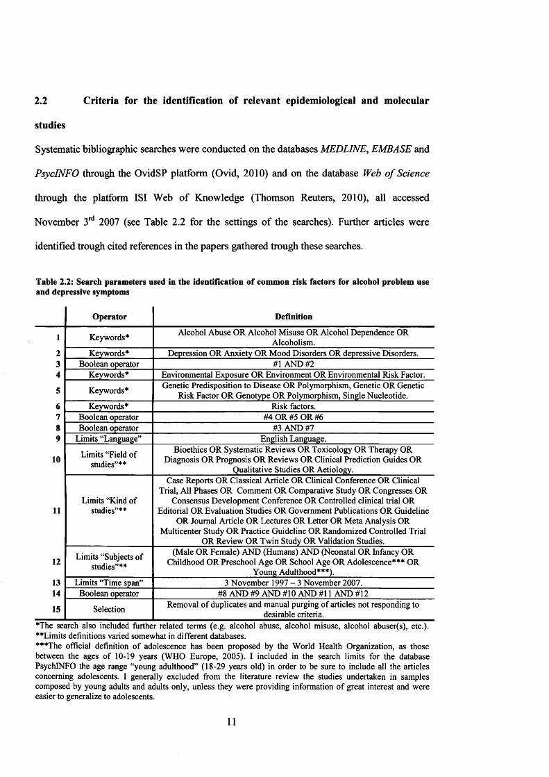
2.2 Criteria for the identification of relevant epidemiological and molecular

studies

Systematic bibliographic searches were conducted on the databases MEDLINE, EMBASE and

PsycINFO through the OvidSP platform (Ovid, 2010) and on the database Web o f Science

through the platform ISI Web of Knowledge (Thomson Reuters, 2010), all accessed

November 3rd 2007 (see Table 2.2 for the settings of the searches). Further articles were

identified trough cited references in the papers gathered trough these searches.

Table 2.2: Search parameters used in the identification of common risk factors for alcohol problem use and depressive symptoms

Operator Definition

1 Keywords* Alcohol Abuse OR Alcohol Misuse OR Alcohol Dependence OR Alcoholism.

2 Keywords* Depression OR Anxiety OR Mood Disorders OR depressive Disorders.3 Boolean operator #1 AND #24 Keywords* Environmental Exposure OR Environment OR Environmental Risk Factor.

5 Keywords* Genetic Predisposition to Disease OR Polymorphism, Genetic OR Genetic Risk Factor OR Genotype OR Polymorphism, Single Nucleotide.

6 Keywords* Risk factors.7 Boolean operator #4 OR #5 OR #68 Boolean operator #3 AND #79 Limits “Language” English Language.

10 Limits “Field of studies”**

Bioethics OR Systematic Reviews OR Toxicology OR Therapy OR Diagnosis OR Prognosis OR Reviews OR Clinical Prediction Guides OR

Qualitative Studies OR Aetiology.Case Reports OR Classical Article OR Clinical Conference OR Clinical

Limits “Kind ofTrial, All Phases OR Comment OR Comparative Study OR Congresses OR

Consensus Development Conference OR Controlled clinical trial OR11 studies”** Editorial OR Evaluation Studies OR Government Publications OR Guideline

OR Journal Article OR Lectures OR Letter OR Meta Analysis OR Multicenter Study OR Practice Guideline OR Randomized Controlled Trial

OR Review OR Twin Study OR Validation Studies.

12 Limits “Subjects of studies”**

(Male OR Female) AND (Humans) AND (Neonatal OR Infancy OR Childhood OR Preschool Age OR School Age OR Adolescence*** OR

Young Adulthood***).13 Limits “Time span” 3 November 1997 - 3 November 2007.14 Boolean operator #8 AND #9 AND #10 AND #11 AND #12

15 Selection Removal of duplicates and manual purging of articles not responding to desirable criteria.

*The search also included further related terms (e.g. alcohol abuse, alcohol misuse, alcohol abuser(s), etc.). ’•‘♦Limits definitions varied somewhat in different databases.***The official definition of adolescence has been proposed by the World Health Organization, as those between the ages of 10-19 years (WHO Europe, 2005). I included in the search limits for the database PsychlNFO the age range “young adulthood” (18-29 years old) in order to be sure to include all the articles concerning adolescents. I generally excluded from the literature review the studies undertaken in samples composed by young adults and adults only, unless they were providing information of great interest and were easier to generalize to adolescents.

11

As a result of the bibliographic searches, 267 papers were identified, of which 102 were read

in detail (see Figure 2.2 for the frequency of identified papers per year of publication). The

remaining papers were not relevant to the current review, or were reports of old studies that

had been replicated more recently. As shown in Figure 2.1 (graphic generated using

Microsoft Office Excel 2007 for Windows (Microsoft Corporation, 2006)), an increasing

trend is observable (0=0.88, t(9)=2.59, p=0.029; R2=0.43, F(l, 9)=6.71, p=0.029) in the

number of publications between 1997-2007 that focused on common risk factors for both

depressive symptoms and alcohol problem use, with a maximum of 20 papers per year being

published in the year 2005.

Figure 2.1: Number of papers gathered through bibliographic searches per year of publication1

20 25

■ I

Number of published papers

10

2005

■ - : i t ? - - ~ i

2007

'Total number o f papers read in detail, N =102.

15

>.««vX&syw; ; szr i W -A ? Y-f* -f w s

R- = 0 43

A* ■- • * V .1 •;

12

2.3 Factors identified in epidemiological studies contributing to risk of alcohol

problem use and depressive symptoms in adolescence

Through bibliographic searches, I identified a number of epidemiological studies that

reported risk and protective factors for both alcohol problem use and depressive symptoms,

which are summarized in Table 2.3.

2.3.1 Socio-demographic factors

• Gender: Males have been reported to be at greater risk for early-onset of alcohol use

as well as heavier use (Cooper, 1994, Ohannessian et al., 2004, Verbrugge, 1985, Waldron,

1983). However, this gender gap may be closing in the UK, where adolescent females are

now reported to drink as much as their male counterparts (IAS, 2007).

Adolescent females are at greater risk for depression (Bond et al., 2005, Maag et al., 2005,

Smucker et al., 1986, Windle et al., 1999) with a reported female/male ratio of 2.5:1 (Windle

et al., 1999). However, Maag et al. (Maag et al., 2005) argued that, although depression

scores on average are higher for girls, boys are more likely to belong to the worst affected

depression group.

• Socioeconomic status (SES): Adolescents from lower socio-economic backgrounds

tend to consume alcohol more frequently and in greater quantity than their peers from higher

socioeconomic groups (Droomers et al., 2003, Ellis et al., 1997, Lowry et al., 1996, Parker et

al., 1980), although some studies contradict these findings (Green et al., 1991, Tuinstra et al.,

1998). We found only one study, among those concerned with co-morbidity, which reported

an association between MDD and low SES in subjects aged 12 years and older (Wang et al.,

2004a).

• Educational level: Studies have been ambiguous, with alcohol problem use having

been associated with higher (Moore et al., 2003) (in adults only) as well as lower (Arellano et

13

al., 1998, Casswell et al., 2003, Droomers et al., 1999, Paschall et al., 2000) (both in adults

and adolescents) educational level. In adolescents, alcohol problem use has been linked with

lower parental educational level (Gogineni et al., 2006). A link has also been reported

between lower educational level and development of depression (Midanik et al., 2007).

• Ethnicity: U.S.A.-based studies indicate Caucasian adolescents may have greater risk

of developing alcohol problem use than other groups, in particular African-American

adolescents (Adlaf et al., 1989, Maag et al., 2005, Singer et al., 1987), although this has not

always been replicated (Guerra et al., 2000).

Findings for depressive symptoms are similarly difficult to interpret, with some studies

reporting greater levels of depressive symptoms in Caucasians (Doerfler et al., 1988, Roberts

et al., 1992), and some in African-Americans (Emslie et al., 1990, Schoenbach et al., 1982),

while a longitudinal study found no difference between both ethnic groups (Garrison et al.,

1990). Maag et al (Maag et al., 2005) reported that African-Americans, while not at

increased risk for depression, may be more likely to experience depression and alcohol

problem use concomitantly.

2.3.2 Substance-related behaviour

• Binge-drinking: Binge-drinking has been defined as the consumption of >5 drinks in a

row for men and >4 drinks for women in a single episode at least once in two weeks, where

the duration of the drinking episode should also be taken into account (Alcoholism, 2004). A

strong link has been reported between binge-drinking in adolescence and later development

of AUD (Jennison, 2004, McCarty et al., 2004).

Longitudinal studies reported adolescents’ binge drinking as a strong risk factor for the

development of later AUD (Jennison, 2004, McCarty et al., 2004). Hill et al. (Hill et al.,

2000) found four binge-drinking trajectories from age 13 to 18: 1) early heavy; 2) increasers;

14

3) late onseters; and 4) non-bingers. Early-onset, heavy binge-drinking may in particular

predict future risk of AUD, with a study reporting that 84% of males and 73% of females

engaging in this type of binging received an AUD diagnosis seven years later (Chassin et al.,

2002). Binge-drinking may also increase risk of depressive symptoms, with a longitudinal

study conducted in an adult sample suggesting that male (but not female) binge-drinkers had

a threefold increased risk of developing anxiety and depression three years later compared

with non-binge-drinking men (Haynes et al., 2005).

• Other substance use: Heavy alcohol use correlates strongly with cigarette and illicit

drug use (Goddard et al., 1999, Sutherland et al., 2001). Several longitudinal studies reported

that nicotine dependence and cannabis use predict adolescents’ alcohol problem use

(Poikolainen et al., 2001, Riala et al., 2004), and heavy use of these substances has been

linked to rapid progression from the first drink of alcohol to AD (Sartor et al., 2007). The

concurrent use of alcohol with marijuana and other illicit drugs has also been associated with

depression (Midanik et al., 2007). Several studies reported many risk factors in common for

alcohol abuse, cigarette smoking or cannabis use. Those factors might modify the

development of alcohol problem use directly or influence the risk of other substance use.

Common risk factors for alcohol problem use and cigarette or marijuana smoking are: male

gender, low SES (Midanik et al., 2007), sleep problems (Tynjala et al., 1997, Vignau et al.,

1997), novelty seeking (Nixon et al., 1990, Pomerleau et al., 1992, Tavares et al., 2005) and

strict dieting (Krahn et al., 2005), which is a risk factor especially for cigarette smoking,

probably used as a means to control weight (Pomerleau et al., 2001). Furthermore, low SES

(Wang et al., 2004a) and sleep problems in particular (Ehlers et al., 1988, Gregory et al.,

2002) have also been implicated in the development of depressive symptoms.

15

2.3.3 Family environment

Although family background is included in my paragraph on non-biological risk factors, it

should be emphasized that family relations are influenced by the behaviours of family

members, which are partially under the influence of genes that may be shared by parents and

offspring (Shelton et al., 2008a).

• Adverse rearing environment: Family environments characterized by high conflict,

parental divorce, low parental monitoring and discipline and lack of warmth and nurturing

(Chassin et al., 2002, Hawkins et al., 1992, Sartor et al., 2007) and, at the extreme end,

parental neglect (Guo et al., 2002) and physical and sexual abuse (Becker et al., 2006, Clark

et al., 1997a) have been reported to contribute to an increased risk of development of

adolescent alcohol problem use. Some evidence suggests that the impact of physical abuse on

the development of later alcohol problem use may be stronger for girls than boys (Gogineni

et al., 2006). Similarly, adverse family experiences, including neglect and abuse (Hussey et

al., 2006) have also been related to depressive symptoms in both adults (Herman et al., 1994)

and adolescents (Smart et al., 1993).

• Family history o f alcohol problems: In a longitudinal study by Alati and colleagues,

maternal heavy drinking alone was found to account for 15% (girls) and 21% (boys) of the

risk of AD (Alati et al., 2005). Other studies in adults suggest that parental heavy drinking

may be a more salient risk factor for females than males (Curran et al., 1999). Gender of the

alcoholic parent may differentially affect offspring risk of alcohol problem use (Bidaut-

Russell et al., 1994), with studies in adolescents (Cotton, 1979) and adults (Bohman et al.,

1981) indicating the risk may be greater for same-sex (e.g., mother-daughter pairs) than

opposite-sex family members (e.g., father-daughter pairs). Density of familial alcoholism

(number of alcoholic parents or other relatives) has been found to be a strong predictor of

16

both adults’ (Hesselbrock, 1982) and adolescents’ (Lieb et al., 2002) alcohol problem use, a

finding that can indicate either non-genetic or genetic risk factors, or both.

Children of alcoholics have also been reported to be at an increased risk for depressive

symptoms (Chassin et al., 1999, Christensen et al., 2000, Sher, 1997) and for co-morbid

alcohol problems, anxiety and depression (Chassin et al., 1999), especially, as reported in

adults, the offspring of alcoholic mothers (Zuckerman et al., 1989). Part of this risk may

relate to prenatal exposure to alcohol (O’Connor et al., 2006).

• Maternal depression: Maternal depression may contribute to adolescents’ risk of

heavy alcohol use (Alati et al., 2005) as well as depression (Hamilton et al., 1993, Jacob et

al., 1997). One explanation may be that maternal depression contributes to disruption of

prenatal and postnatal mother-child interactions (O'Connor et al., 2006).

2.3.4 Social environment

• Peer influences: A longitudinal study by Aseltine et al (Aseltine et al., 1998), found

that close relationships with friends protect against the development of depression; however,

friendships with deviant peers correlated positively with adolescent alcohol problem use

(Beitchman et al., 2005, Wills et al., 1989). Peer alcohol use influences the initiation as well

as continuation of adolescent alcohol use (Musher-Eizenman et al., 2003, Nation et al., 2006),

with perceived peers’ attitudes toward alcohol and number of alcohol-using peers serving as

important factors contributing to adolescents’ alcohol problem use (Bray et al., 2003, Oetting

et al., 1987, Sale et al., 2003, Wills et al., 2001).

Lack of social support by friends can contribute to the development of depression (Beitchman

et al., 2005). Positive peer groups can serve as positive role models, and the exclusion from

such social networks can drive adolescents towards deviant peer groups, thus increasing risk

of substance abuse (Beitchman et al., 2005).

17

• Stress: A link has been reported between stress and alcohol problem use in

adolescents (Jose et al., 2000, King et al., 2003, Wills et al., 1992) and adults (Linsky et al.,

1985). The self-medication model suggests that individuals drink to regulate negative affect

and to cope with negative life events (Peirce et al., 1994, Wills et al., 1992). Linsky et al.

(Linsky et al., 1985) studied the correlation between alcohol related problems and stress in 50

U.S.A. states. On the basis of Bales' Theory, which correlates the rate of alcoholism in

cultures or societies with levels of stress (tension and frustration) (Bales, 1946), the three

global measures of stress examined by Linsky et al. explained 27% of the variation in

cirrhosis death rates, 14% of the variation in alcoholism and alcoholic psychosis and 47% of

the variation in alcohol consumption rates (Linsky et al., 1985). The link between stress and

alcohol problem use can be explained by Conger’s Tension Reduction Theory (Conger,

1956), which posits that alcohol consumption is motivated by the desire to relieve anxiety

and cope with stress.

Stress also increases the risks of anxiety (Copeland et al., 2007) and depression (Garber,

2006, Turner et al., 2004). Garber (Garber, 2006) describes three models (supported by

longitudinal studies) linking stress and depression: the Stress Exposure Model (stating that

exposure to a stressful event will increase likelihood of depression) (Brown, 1993); the

Stress-Generation Model (reported in adults, suggesting that depressed individuals contribute

to negative events by their own behaviour) (Hammen, 1991); and the Reciprocal Model, that

combines these two models and highlights the “vicious circle” between depression and stress

(Kim et al., 2003).

• Religion: Kendler and colleagues identified religion as a protective factor for both

alcohol problem use and depressive symptoms using a large longitudinal study in an adult

sample (Kendler et al., 1997). They underlined that, although very important in human

society and behaviour (Institute, 1995), religion has been relatively neglected in studies

18

exploring the aetiology of mental illness (Crossley, 1995) and substance abuse (Gartner et al.,

1991). Kendler et al (Kendler et al., 1997) distinguished three dimensions of religion:

personal devotion, institutional conservatism and personal conservatism. In adults, these

authors identified a lack of personal devotion to be most strongly related to current use of

alcohol and a lifetime history of alcohol abuse, a finding also replicated in youngsters

(Rachal et al., 1982). Religion has also been reported to be protective against psychological

distress; personal devotion in particular may moderate the effects of stressful life events on

depressive symptoms, both in adults (Williams et al., 1991) and adolescents (Maton, 1989).

2.3.5 Personality and psychopathologies

2.3.5.1 Personality and cognition

• Personality: Novelty seeking, one dimension of Cloninger’s trait and character

inventory (TCI) (Cloninger et al., 1993) has been associated with AD in adult samples (Nixon

et al., 1990). Adult alcohol-dependent subjects have also been found to have higher scores on

the TCI dimension of harm avoidance (tendency to worry, fear of uncertainty, shyness, and

tendency to tire easily) (Tavares et al., 2005), suggesting a link between alcohol problem use

and vulnerability to anxiety (Ball et al., 2002). Although personality factors belonging to

Cloninger’s TCI (Cloninger et al., 1993) may have been studied most extensively in relation

to psychopathology, other dimensions of personality have also been reported to play a role in

addiction and depressive disorders (Anderson et al., 2006a). As reported by Anderson and

Smith (Anderson et al., 2006a), behavioural disinhibition, behavioural under-control and

impulsivity might be associated with adolescents’ alcohol abuse. The association between

disinhibition and alcohol problem use has been confirmed by cross-sectional studies in

youngsters (Anderson et al., 2005, Katz et al., 2000). In a sample of non-alcoholic women,

19

Grau and Ortet (Grau et al., 1999) documented an association between alcohol consumption

and personal dispositions toward impulsivity and risk taking. According to Wadsworth and

colleagues (Wadsworth et al., 2004), the association between heavy alcohol consumption and

risk-taking is consistent with the Sensation Seeking Theory proposed by Zuckerman et al.

(Zuckerman et al., 1964), which has been used to explain alcohol drinking in a sample of

young adults (Conrod et al., 1997). A cognitive factor that has been implicated in the

development of depressive symptoms is behavioural inhibition (Gray, 1991). Rothbart and

Mauro have described behavioural inhibition in childhood as a construct involving

expressions of inhibition (inhibited speech, gestures, motor activity, and withdrawal),

negative emotional reactions and physiological responses (Rothbart et al., 1990). A

longitudinal study by Caspi and colleagues confirmed that inhibition assessed in early

childhood was related to depression in young adults (Caspi et al., 1996).

• Cognition: Positive alcohol expectancy, referring to expected rewarding effects of

alcohol (Prescott et al., 2004) (i.e. facilitation of social interactions, enhancement of

excitement, improved motor performance and escape from negative affect (Christiansen et

al., 1989, Kassel et al., 2000, Newcomb et al., 1988)) has been reported to influence

adolescents’ alcohol problem use in both cross-sectional (Anderson et al., 2006a) and

longitudinal studies (Anderson et al., 2006a, Christiansen et al., 1989, Smith et al., 1995).

Some (Lee et al., 1993), but not all, studies (Rohsenow, 1983) reported that negative alcohol

expectancies may protect against heavy alcohol use (Leigh et al., 1993). A number of studies

have attempted, with positive results (Darkes et al., 1998, Sharkansky et al., 1998, Wiers et

al., 2004), to reduce rates of alcohol problems by modifying adolescents’ alcohol

expectancies, although other findings suggest caution against that (Dermen et al., 1998, Jones

etal., 2001).

20

A cognitive factor that has been related to the development and maintenance of depressive

symptomatology in adolescents is depressive cognitive style, referring to a negative view of

oneself, the future and the world (Beck, 2002, Laurent et al., 1993, Miles et al., 2004).

2.3.5.2 Psychopathologies

Many studies have indicated that AUDs may precede the onset of other mental disorders.

However, a considerable number of studies in adolescent samples with co-morbid psychiatric

pathologies have also indicated that AUDs developed subsequently to the onset of the

psychiatric illness (for a review see Deas et al. (Deas et al., 2002)).

• Externalizing disorders: Externalizing disorders such as conduct disorder (CD)

(Sher, 1991, Stice et al., 1998, Turner et al., 2005, Zucker et al., 1994) and attention deficit

hyperactivity disorder (ADHD) (Biederman et al., 1995, Biederman et al., 1998, Kim et al.,

2006, White et al., 2001, Wilens, 1998, Wilens et al., 1997, Wilens et al., 2002) have been

reported to be important precursors to the development of alcohol problem use in both

adolescence and adulthood (Biederman et al., 1995, Biederman et al., 1998, Kim et al., 2006,

White et al., 2001, Wilens, 1998, Wilens et al., 1997, Wilens et al., 2002). Sartor and

colleagues (Sartor et al., 2007) found that CD was the strongest predictor of early-onset

alcohol initiation (associated with 2.5 times increased risk). CD is also reported to precede

depression in almost three-quarters of cases (Nock et al., 2006). It has been theorized that this

link may be explained by a chain reaction of developmental failures experienced by youth

with conduct problems (Capaldi, 1992, Capaldi et al., 1999).

ADHD has also been implicated in depressive symptoms (Wilens et al., 1997) as well as in

early-onset alcohol problem use and the transition from substance abuse to dependence

(Biederman et al., 1995, Biederman et al., 1998, Kim et al., 2006, White et al., 2001, Wilens,

1998, Wilens et al., 1997, Wilens et al., 2002).

21

Finally, antisocial behaviour, antisocial personality disorder (Becker et al., 2006, Hussong et

al., 1998, Kuperman et al., 2001) and oppositional defiant disorder (ODD) (Gogineni et al.,

2006), have also been reported to predict adolescents’ alcohol problem use; additionally,

ODD has been implicated in the development of depression in youth (Angold et al., 1993).

• Bipolar disorder: The frequent co-occurrence of bipolar disorder (BD) and AD,

originally identified by Kraepelin (Kraepelin, 1976), has long been recognized (Preisig et al.,

2001, Salloum et al., 2000) in adults. Some (Freed, 1969, Reich et al., 1974) (but not all

(Mayfield et al., 1968)) studies have indicated that excessive drinking predominates in the

manic rather than the depressive phase of BD.

BD tends to develop in late adolescence or early adulthood (Pini et al., 2005), and therefore

the number of studies in young samples is limited. However, there is an increasing research

interest in the relationship between BD and alcohol and substance abuse in adolescence (Jolin

et al., 2007, Wilens et al., 2004, Wilens et al., 1999).

• Eating disorders: Both dieting and binge-eating severity in adolescence are strongly

associated with the frequency and intensity of alcohol use (Krahn et al., 1992, Krahn et al.,

2005, Stewart et al., 2000). Binge-eating, dieting, smoking and heavy alcohol drinking may

represent a “cluster” of risky behaviours in adolescence (lessor et al., 1991). Anorexia

nervosa (AN) and bulimia nervosa (BN) are associated with alcohol abuse for distinct

reasons: in women diagnosed with AN excessive concern with body weight and shape, and

use of vomiting to control weight, heightens the vulnerability for development of AUD;

however, in women diagnosed with BN, risk factors may be more global and related to

psychosocial functioning (Franko et al., 2005). Finally, Alati et al. (Alati et al., 2005) have

suggested that strict adherence to a diet may increase the risk of substance abuse, since the

rewarding value of alternate reinforcers (i.e. substances or highly palatable “binge” foods) is

enhanced (Krahn, 1991).

22

Eating disorders in both male and female adolescents have been linked with depression, and

it has been suggested that body image factors, such as body dissatisfaction (Santos et al.,

2007), or peer victimization and marginalization (especially for obese adolescents)

(Robinson, 2006), may moderate depression risk.

• Sleep problems: Sleep problems, primarily insomnia, have been reported to precede

the onset of alcohol problem use among adults (Brower, 2001, Roehrs et al., 1999). Studies

have reported associations between alcohol use and delayed bedtime and irregular sleep

schedule in children (Tynjala et al., 1997, Vignau et al., 1997, Wong et al., 2004).

Instability in biological rhythm, of which sleep problems are one indicator, has been linked to

the risk of depression (Ehlers et al., 1988). Gregory and O’Connor (Gregory et al., 2002)

found that sleep problems at age four predicted depression/anxiety in mid-adolescence, and

that the correlation between sleep problems and depression/anxiety is stronger in adolescence

than in childhood (Gregory et al., 2002).

23

Table 23: Summary of literature search for factors identified through epidemiological studies contributing to the risk of both alcohol problem use and depressive symptoms in adolescence

Alcohol problem use Depressive symptoms*8a Risk factor Association Lack of Association Lack ofQ association association

Gender

[Cooper, 1994, Ohannessian et al., 2004,

Verbrugge, 1985, Waldron, 1983]A

None

[Bond et al., 2005, Maag et al., 2005,

Smucker et al., 1986, Windle et al., 1999]8

None

u2a98I*01)

Socioeconomicstatus

[Droomers et al., 2003, Ellis et al., 1997, Lowry et al., 1996, Parker et al.,

1980, Wang et al., 2004a]c [Green et al.,

1991]°

None [Wang et al., 2004a]c None

a4>"O1JO*3©V i

Educational level

[Arellano et al., 1998, Casswell et al., 2003, Droomers et al., 1999, Paschall et al., 2000]E [Moore et al., 2003]F

[Gogineni et al., 2006]°

None [Midanik et al., 2007]E None

Ethnicity

[Adlaf et al., 1989, Maag et al., 2005, Singer et al.,

1987]h [Guerra et al., 2000]1

None

[Doerfler et al., 1988, Roberts et al., 1992]H [Emslie et al., 1990, Schoenbach et al.,

198211

[Garrison et al., 1990]

&| "2 & ts

Binge-drinking[Chassin et al., 2002,

Jennison, 2004, McCarty et al., 2004]

None [Haynes et al., 2005] None

£> gs *"V i

Other substances use

[Poikolainen et al., 2001, Riala et al., 2004, Sartor

et al., 2007]None [Midanik et al., 2007] None

■Ma©a©ou

Adverse rearing environment

[Becker et al., 2006, Chassin et al., 2002, Clark et al., 1997a,

Gogineni et al., 2006, Guo et al., 2002, Hawkins et al., 1992, Sartor et al.,

2007]

None[Herman et al., 1994, Hussey et al., 2006, Smart et al., 1993]

None

>a4>

a98to

Family history of alcohol problems

[Bohman et al., 1981, Chassin et al., 1999,

Cotton, 1979, Curran et al., 1999, Deykin et al.,

1987, Hesselbrock, 1982, Lieb et al., 2002]

None

[Chassin et al., 1999, Christensen et al.,

2000, O'Connor et al., 2006, Sher, 1997,

Zuckerman et al., 1989]

None

Maternaldepression [Deykin et al., 1987] None [Hamilton et al., 1993,

Jacob et al., 1997] None

1 So

cial

envi

ronm

ent

Peer influence

[Aseltine et al., 1998, Beitchman et al., 2005,

Wills et al., 1989]J [Bray et al., 2003, Musher-

Eizenman, 2003, Nation et al., 2006, Oetting et al.,

1987, Sale et al., 2003, Wills etal., 2 0 0 l f

None [Beitchman et al., 2005]l

None

Table 2.3 continued...

24

Table 2.3 continued..aVSao Stress

[Jose et al., 2000, King et al., 2003, Linsky et al., None

[Brown, 1993, Copeland et a l, 2007, Garber,

2006, Hammen, 1991, None| 1985, Wills etal., 1992] Kim et a l, 2003, Turner4) et a l, 20041

.2'3o!Z> ReligionM [Rachal et al., 1982,

Williams et al., 1991] None[Kendler et a l, 1997,

Maton, 1989, Williams et a l, 1991]

None

[Anderson et al., 2006a, Anderson et al., 2005,

Personality

Conrod et al., 1997, Grau et al., 1999, Katz et al., 2000,

Nixon et al., 1990, Wadsworth et al., 2004, Zuckerman et al., 1964]N

[Tavares et al., 2005]°

None[Ball et a l, 2002, Caspi et a l, 1996, Gray, 1991, Rothbart et a l, 1990]°

None

[Anderson et al., 2006a, Christiansen et al., 1989,

S/34>

CognitionKassel et al., 2000,

Newcomb et al., 1988, Prescott et al., 2004, Smith

[Rohsenow,1983]°

[Beck, 2002, Laurent et a l, 1993, Miles et a l,

2004]RNone

DC£OJ3

et al., 1995]p [Lee et al., 1993, Leigh et al., 1993]Q

■M« [Clark et al., 1996, Sartor et1

o a l, 2007, Sher, 1991, TurnerJSu et a l, 2005, Zucker et a l.s/3a"OaS3

I*aoS 0Sh9 t

Cl.

Externalizingdisorders

1994]s [Biederman et a l, 1995, Biederman et a l, 1998, Kim et a l, 2006,

White et a l, 2001, Wilens, 1998, Wilens et a l, 1997,

Wilens et a l, 2002]7 [Becker et a l, 2006, Gogineni et a l, 2006, Hussong et a l, 1998,

Kuperman et a l, 200l]u

None

[Capaldi, 1992, Capaldi et a l, 1999, Nock et a l,

2006]s [Wilens et a l, 2002]t [Angold et a l,

1993]u

None

Bipolardisorder

[Kraepelin, 1976, Preisig et a l, 2001, Salloum et a l,

20001None Nonev None

Eatingdisorders

[Franko et a l, 2005, Krahn et a l, 1992, Krahn et a l,

2005, Stewart et a l, 2000]None [Robinson, 2006, Santos

et a l, 2007] None

Sleepproblems

[Brower, 2001, Roehrs et a l, 1999, Tynjala et a l, 1997,

Vignau et a l, 1997, Wong et a l, 2004]

None [Ehlers et a l, 1988, Gregory et a l, 2002] None

Males; Females c Low socioeconomic status; D High socioeconomic statusE Low educational level; F High educational level; ° Parental educational level; H Caucasians; 1 African AmericansJ Friendship with deviant peers; K Alcohol misuse by peers; L Exclusion from peer social network M Protective factorN Novelty seeking, disinhibition, risk tacking, impulsivity; °Harm avoidance, behavioural inhibition p Positive alcohol expectancies; Q Negative alcohol expectancies (protective); R depressive cognitive style s Conduct disorder; T Attention deficit hyperactivity disorder; u Oppositional defiant disorder and antisocial personalityv Depression is a feature of bipolar disorder, also known as manic-depressive syndrome

25

2.4 Interactions between factors identified through epidemiological studies

A number of papers have focused on interactions between the risk factors described above in

the development of adolescent alcohol problem use. In contrast, I found only one such paper

on depressive symptoms.

• Parental drinking (Jacob et al., 1991, Weinberg, 1997, Whipple et al., 1995) and

parental depression (Hamilton et al., 1993, Jacob et al., 1997, Kim-Cohen et al., 2005) may

interact to increase disturbances in family relationships, including parent-child relations

(O'Connor et al., 2006), thus increasing the risk of adolescent alcohol problem use (Jacob et

al., 1991).

Low parental control may interact with adolescents’ impulsivity and disinhibition as well as

their engagement with deviant peers to increase the risk of adolescent heavy alcohol use

(Bates et al., 1995a).

• Peer influences may moderate relations between family environmental risk factors

and alcohol and substance abuse (Chassin et al., 2002). It has been hypothesized that stress in

the family environment (e.g., family conflict, lack of support, harsh discipline) results in

affiliation with a negative peer network, which models and reinforces substance use (Dishion

et al., 1988).

Conduct disorder may exert its influence on the onset and perpetuation of heavy alcohol use

through engagement with deviant peers who reinforce heavy drinking (Fowler et al., 2007b,

Jessor et al., 1977). With respect to depression, it has been reported that among children with

ADHD, those with co-morbid ODD have a greater risk of depressive symptoms, compared

with children with ADHD without co-morbid ODD (Biederman et al., 1995, Biederman et al.,

1998, Wilens, 1998, Wilens et al., 1997, Wilens et al., 2002).

26

2.5 Genetic factors associated with the development of alcohol problem use and

depressive symptoms

2.5.1 Heritability of AUDs and depressive disorders

A number of genes have been associated with both alcohol problem use and depressive

symptoms (Clark et al., 1996). A review of adolescent twin studies by Hopfer et al (Hopfer

et al., 2003) reported that the magnitude of genetic influence on adolescent alcohol problem

use is quite modest (compared to adults (Goldman et al., 2005)) and appears to be moderated

by measures of use (Hopfer et al., 2003). Fowler et al. (Fowler et al., 2007a) reported that

initiation of alcohol use and progression to heavier alcohol use during adolescence had

separate but related underlying aetiologies. With respect to initiation of alcohol use,

environmental influences that make twins more similar (common environment) tended to be

greater (explaining 65% of the variation) than genetic influences (explaining 26% of the

variation). However, genetic influences were found to be stronger with regards to progression

to heavier use (explaining up to 64% of the variation). In a Finnish study on 5,638 twins, the

heritability of drinking measures (frequency and amount of alcohol intake) ranged from 0.36

to 0.40 (Kaprio et al., 1987). Moreover, the genetic liability to alcoholism is shared with other

substance dependence, especially nicotine, with 50% of candidate genes being in common

(Goldman et al., 2005). Heritability of anxiety/depression has been assessed in samples of

young people, ranging between 7% and 15% (Towers et al., 2000).

Several genes have been associated with both alcohol problem use and depressive symptoms,

as their inherited functional variants might alter the physiological mechanisms of reward,

cognition, stress coping, emotion regulation and neuronal plasticity (Oroszi et al., 2004).

However, the number of genetic informative studies done in youngsters is small compared to

the research conducted in adults; this is likely due to ethical constraints that might arise from

27

genetic studies in young samples (Knoppers et al., 2002) and to the lower frequency of

clinically diagnosed psychiatric illnesses in young people. Moreover, the literature for

candidate susceptibility genes has long been inconclusive, with positive findings generally

being followed by negative findings (summarized in Table 2.4), a situation which is in

contrast to the epidemiological literature (see Table 2.3). Due to the paucity of molecular

genetic studies in adolescents specifically, the paragraph below also includes relevant articles

from the literature on adults (identified through cited references in the papers yielded by my

literature search). This seems a valid approach, given the consideration that the alleles of a

genetic polymorphism do not change over time (Garber, 2006). Table 2.4 lists the papers that

have analyzed the associations between specific genetic polymorphism and AUDs or

depressive disorder.

2.5.2 Neurotransmitter receptor genes

• GABA Receptors: The gamma-aminobutyric acid (GABA) system has been

implicated in alcohol’s sedating effects and the development of tolerance (Hiller-Sturmhofel

et al., 2004) as well as anxiety- and depression-related traits (for a review see (Petty, 1995)).

An association has been reported between the functional Pro/Ser genotype in the gene

GABRA6 (5q34) coding for the GABA receptor subunit alpha-6 (Pro385Ser polymorphism)

and low benzodiazepine sensitivity (a marker for AD (Iwata et al., 1999)), and low response

to alcohol and AD, by some (but not all (Song et al., 2003)) studies (Radel et al., 2005,

Schuckit et al., 1999). The Pro/Pro genotype has also been associated with neuroticism (Sen

et al., 2004b), a personality trait associated with depression/anxiety (Marques et al., 2006).

However, the need for replication of these findings has been stressed (Song et al., 2003),

particularly because other GABRA6 polymorphisms have been related to an attenuated rather

than heightened stress response (Uhart et al., 2004).

28

• Dopamine receptor D2: The dopaminergic system plays a key role in the reward

circuitry of the brain (Noble, 2000), on which addictive substances act.

The dopamine receptor D2 (DRD2, 1 lq23) gene has been associated with AD, from a study

indicating DRD2 receptor avidity is lower in alcohol-preferring individuals than in control

subjects (Hietala et al., 1994). A number of studies have reported an association between the

DRD2 Taq Al variant and alcohol problem use (Goldman, 1995, Noble, 2003, Noble et al.,

1991, Reich et al., 1999); however, other studies have not replicated these findings (Bolos et

al., 1990, Lu et al., 1996). A study in Han Chinese men reported a higher Taq Al/Bl

haplotype frequency in alcoholics who also had co-morbid anxiety disorder or MDD (Huang

et al., 2007). However, some studies have found no evidence of association between DRD2

gene variants and susceptibility to MDD (Cusin et al., 2002).

• Muscarinic Acetylcholine Receptors: The Cholinergic Muscarinic Receptor 2

(CHRM2, 7q31-q35) belongs to muscarinic acetylcholine receptors (Nathanson, 1987), which

are involved in many functions in the brain, including attention, learning, memory and

cognition (Baxter et al., 1999).

Recently, some studies have reported variants within the 5’-UTR of CHRM2 influence risk of

both AD and MDD (Luo et al., 2005, Wang et al., 2004b), with the latter study suggesting

SNP rs1824024, in particular, may be linked to susceptibility for both AD and affective

disorders (Luo et al., 2005). The first study (Wang et al., 2004b) also reported associations

with AD and/or depression for two other SNPs (termed SNP1 and SNP2); however, the

effects were complex. The results showed that allele T and genotype C/T of SNP1 and/or

genotype C/T of SNP2 may protect against AD and/or MDD, but that the interaction of the

SNP1 T-allele and the SNP2 C-allele may increase risk for both these disorders. Further

haplotype analyses (Wang et al., 2004b) suggested that the most common haplotype

(rsl824024-rs2061174-rs324650, T-T-T) might be protective against risk for alcoholism,

29

MDD and the co-morbid phenotype. However, not all studies have found associations

between CHRM2 variants and AD (Dick et al., 2007a).

2.5.3 Neurotransmitter transporters

Serotonin (5-hydroxytryptamine, 5-HT) contributes to many physiological functions (Lesch

et al., 1996), including a key role in the brain reward circuitry (Koob et al., 1997). Serotonin

is released in response to alcohol (Yoshimoto et al., 1992) and low central serotoninergic

activity has been correlated with an increased alcohol tolerance and vulnerability for alcohol

problem use (Hallikainen et al., 1999, Koob, 2003, Turker et al., 1998).

• Serotonin transporter: A number of studies have focused on the relationship between

the serotonin transporter (5-HTT) gene (SLC6A4, 17qll.l-ql2) and alcohol problem use

(Edenberg et al., 1998, Gelemter et al., 1997, Gorwood et al., 2000, Hallikainen et al., 1999,

Hammoumi et al., 1999, Ishiguro et al., 1999, Kweon et al., 2005, Mannelli et al., 2005,

Matsushita et al., 2001, Munafo et al., 2005, Olsson et al., 2005b, Preuss et al., 2001, Sander

et al., 1998, Thompson et al., 2000, Turker et al., 1998, Wiesbeck et al., 2004). Impairments

in 5-HTT function have considerable impact on extracellular levels of 5-HT (Lesch, 2005). A

deletion/insertion polymorphism affects the transcriptional control region upstream of the

SLC6A4 transcription initiation site (Heils et al., 1996). The long and short variants of

SLC6A4 have a length, respectively, of 528 base pairs (bp) (L-allele) and 484bp (S-allele)

(Heils et al., 1996). The S-allele (defined also as 5-HTTLPR) is associated with an

approximately 50% reduction in transporter availability, resulting in a consequent increase in

synaptic 5-HT concentration compared with L-allele (Enoch, 2006).

The S-allele has been associated with a number of alcohol-related phenotypes, including high

ethanol tolerance (Turker et al., 1998); type-2 alcoholism (Hallikainen et al., 1999)

(characterized by early-onset, impulsivity and antisocial personality traits (Cloninger, 1987));

30

binge-drinking in Japanese alcoholics (Matsushita et al., 2001); alcohol-related antisocial

behaviour (Ishiguro et al., 1999); and combined alcohol-seeking with risk-taking behaviour

(Sander et al., 1998).

The S-allele has also been investigated in relation to mood-related phenotypes (Gorwood et

al., 2000, Hammoumi et al., 1999, Kweon et al., 2005, Mannelli et al., 2005, Munafo et al.,

2005, Olsson et al., 2005b), including depression (Enoch, 2006) and neuroticism (Greenberg

et al., 2000, Lesch et al, 1996, Marques et al., 2006).

Furthermore, a meta-analysis showed a significant effect of the S-allele both in relation to

alcohol problem use (among individuals with alcoholism and a co-morbid psychiatric

condition, or with early-onset or more severe AD) (Feinn et al., 2005) and in relation to the

trait of neuroticism (the latter finding confirmed in two meta-analyses (Schinka et al., 2004,

Sen et al., 2004a)).

2.5.4 Neurotransmitter metabolizing genes

• Monoamine oxidase A (MAOA): MAO A is involved in the metabolism of dopamine,

serotonin and norepinephrine (Shih et al., 1999). A functional 30bp repeat variable-number-

tandem-repeat (VNTR) polymorphism in the promoter region of the MAO A gene (Xpll.3)

has been reported to alter its transcriptional efficiency (Huang et al., 2007). ‘High-activity’

alleles (3.5 or 4 copies of the repeat sequence) show a two- to ten-fold higher transcription

rate of the MAO A gene than ‘low-activity’ alleles (3 or 5 copies) (Sabol et al., 1998).

The MAOA VNTR 3-repeat (low-activity) allele has been associated with antisocial

alcoholism among German men (Samochowiec et al., 1999). Schmidt and colleagues

(Schmidt et al., 2000) replicated these findings and observed a gender difference in the

phenotypic effects on alcoholics, which seems plausible considering the X-chromosomal

localization of the MAOA gene. Alcoholic men had higher scores on antisocial traits, whereas

31

alcoholic women showed more depression. Other studies, however, found no association

between the MAOA VNTR and AD (Koller et al., 2003). MAOA low activity variants have

also been associated with MDD in adulthood (Brummett et al., 2007, Yu et al., 2005).

However, other studies reported an association of seasonal depression with high-activity

alleles (Gutierrez et al., 2004), or no association at all (Kunugi et al., 1999).

• Catechol-O-Methyltransferase (COMT): COMT is involved in the metabolism of

dopamine and norepinephrine (Enoch, 2006). COMT contains a common functional

polymorphism producing a Val/Met substitution at codons 108/158 (Lachman et al., 1996).

The COMT1087158 Met variant is associated with 40% less COMT activity in the brain than the

Val allele, resulting in reduced dopamine turnover and an increased vulnerability to the

development of AD (Tiihonen et al., 1999). The interpretation of the findings regarding the

relationship between the COMT1087158 Met variant and AD is complex, since positive findings

have been reported in different populations, but with opposite effects (Enoch, 2006). The

Met 158 allele has been associated with increased social drinking and late-onset alcoholism in

European Caucasian men (Kauhanen et al., 2000, Tiihonen et al., 1999); however, it has been

found to protect against alcoholism in Plains American Indians (Enoch et al., 2006).

According to Enoch (Enoch, 2006), the opposite effects of Metl58 might be explained by the

differing drinking patterns: among Europeans the Met 158 allele may be a vulnerability factor

for a drinking pattern centred on relief of anxiety, whereas among American Indians, the

anxious, cautious personality associated with the Met 158 allele may protect against episodes

of excessive heavy drinking (Enoch et al., 2006). However, not all studies in Caucasians have

replicated the association with COMTmns% Met variant and risk of AD (Foroud et al., 2007).

The COMT1087158 Met variant has also been associated with anxiety (Enoch et al., 2003,

Olsson et al., 2005a). In a longitudinal study of Australian adolescents, carriers of the

Met/Met genotype were found to have a twofold greater risk of reporting episodes of anxiety

32

(Olsson et al., 2005a). The association of this variant with anxiety might be mediated by the

neural response to unpleasant stimuli, which would be greater depending on the presence and

the number of Metl58 alleles (Smolka et al., 2005). Nevertheless, a recent systematic review

of the COM7408/158 Met variant polymorphism concluded that COMT is probably not "a gene

for” any mental disorder, but might have pleiotropic effects (influencing multiple phenotypic

traits) on human behaviour (Hosak et al., 2007).

2.5.5 Other genes

• Brain derived neurotrophic factor: Brain-derived neurotrophic factor (BDNF, 1 lpl3)

belongs to a neurotrophin superfamily responsible for promoting and modifying growth,

development and survival of neuronal populations (Duman et al., 2006). Chronic alcohol

exposure may affect BDNF mRNA expression and significantly reduce BDNF secretion. This

may impact the role of BDNF in neuroprotection as well as regulate the behavioural response

to ethanol through changes in synaptic plasticity (Crews et al., 2003, Kovalchuk et al., 2002,

Luo et al., 1998, McGough et al., 2004, Sakai et al., 2005).

Uhl et al (Uhl et al., 2001) reported that a dinucleotide-repeat variant (Val66Met), located

close to the 5’-end of the BDNF gene, was associated with drug-abuse vulnerability. This

allele variant, affecting intracellular trafficking and activity-dependent secretion of BDNF

(Chen et al., 2004, Egan et al., 2003), has been further investigated. Matsushita et al

(Matsushita et al., 2004) reported a significant association between the BDNF Val66Met

variant and AD with violent tendencies in Japanese male alcoholics. Another study, however,

did not replicate that finding (Tsai et al., 2005).

Studies of human cortex have indicated carriers with the BDNF Val/Met or Met/Met variant

have reduced amplitude of evoked potentials (Kleim et al., 2006) and reduced volume of

cerebral neocortex grey matter (Pezawas et al., 2004), findings which have stimulated studies

33

of a possible role of BDNF in the development of major depression (Chen et al., 2001,

Karege et al., 2002, Ribeiro et al., 2007, Schumacher et al., 2005). Ribeiro et al reported that

individuals homozygous for the Met variant of the Val66Met allele are at an increased risk of

MDD (Ribeiro et al., 2007). However, another study has not replicated these findings (Tsai et

al., 2003).

34

Table 2.4: Summary of literature search for factors identified through molecular studies contributing to risk of both alcohol problem use and depressive symptoms in adolescence1

Alcohol problem use Depressive symptoms'B’3s Risk factor Association Lack of Association Lack ofQ association association

u4>GABRA6

Pro385Ser

(Iwata et al., 1999, Radel et al., 2005, Schuckit et al.,

1999)

(Song et al., 2003) (Sen et al., 2004b) (Uhart et

al., 2004)

rotr

ansm

itre

cept

ors

DRD2 Taq Al

(Goldman, 1995, Huang et al., 2007, Noble, 2003,

Noble et al., 1991, Reich et al., 1999)

(Bolos et al., 1990, Lu et al., 1996)

(Huang et al., 2007) (Cusin et al., 2002)

3U CHRM2 SNPs 5’-

UTR

(Luo et al., 2005, Wang et al., 2004b)

(Dick et al., 2007a)

(Luo et al., 2005, Wang et al., 2004b) None

Neu

rotr

ansm

itter

s tr

ansp

orte

rs

SLC6A4 S- allele (5-

HTTLPR)

(Edenberg et al., 1998, Gelemter et al., 1997, Gorwood et al., 2000,

Hallikainen et al., 1999, Hammoumi et al., 1999,

Ishiguro et al., 1999, Koob, 2003, Kweon et al., 2005,

Mannelli et al., 2005, Matsushita et al., 2001,

Munafo et al., 2005, Olsson et al., 2005b, Preuss et al., 2001, Sander et al., 1998,

Thompson et al., 2000, Turker et al., 1998,

Wiesbeck et al., 2004) (Feinn et al., 2005)*

None

(Enoch, 2006, Gorwood et al., 2000, Greenberg

et al., 2000, Lesch et al., 1996, Marques et al., 2006, Olsson et al.,

2005b) (Schinka et al., 2004, Sen et al., 2004a)*

None

. u MC u•s «

S **

MAOApromoterVNTR

(Samochowiec et al., 1999, Schmidt et al., 2000)A

(Koller et al., 2003)A

(Schmidt et al., 2000)Ab (Brummett et al., 2007,

Yu et al., 2005)a (Gutierrez et al., 2004)c

(Kunugi et al., 1999)

O V£ a£

COMTVall58Met

(Kauhanen et al., 2000, Tiihonen et al., 1999) (Enoch et al., 2006)°

(Foroud et al., 2007)

(Enoch et al., 2003, Olsson et al., 2005a, Smolka et al., 2005)

(Hosak et al., 2007)

09BDNF

Val66Met (Matsushita et al., 2004) (Tsai et al., 2005) (Ribeiro et al., 2007) (Tsai et al.,

2003)£ o X « O GABRA6

Pro385Ser

(Iwata et al., 1999, Radel et al., 2005, Schuckit et al.,

1999)

(Song et al., 2003) (Sen et al., 2004b) (Uhart et

al., 2004)

1. Although my literature search focussed on adolescents, it did yield articles based on different age groups. To indicate which studies were not conducted specifically in adolescents, I have used the following notations:Bold reference: Study (or review of studies) undertaken in adults;Underlined reference: Study (or review of studies) undertaken in young adults (20-29 Years old);Italic reference: Study (or review of studies) undertaken in populations composed of people of all ages;* Meta-analysis.A Low activity variant.B In women only. c High activity variant.D Protective in Plain American Indians.

35

2.6 Epistasis

In most psychiatric disorders, multiple genes are thought to contribute to the phenotype

(Goldman et al., 2005). The synergic action of several genes on a phenotype is referred to as

epistasis (Schumann, 2007, Schumann et al., 2003). Schumann (Schumann, 2007) suggested

that genetic liability might be explained by two parallel genetic mechanisms: heterogeneity

and poly/oligogenicity. Heterogeneity (the presence of a variety of genetic defects which

cause the same disease) can account for single gene variants giving rise to different aspects of

phenotypes, while poly/oligogenicity refers to situations where phenotypes arise due to

additive and interactive effects of functional mutations within different genes (Schumann,

2007). Although accounts of epistasis influencing addiction in humans are still rare (Van den

Bree, 2005), some publications have suggested such effects play a role in the development of

alcohol problem use or depressive symptoms.

• A longitudinal study in low alcohol-responsive men by Schuckit and colleagues

(Schuckit et al., 1999) reported that all subjects with two 5-HTT promoter L-alleles as well as

the Pro/Ser alleles at the Pro/Ser genotype of the GABRA6 had developed AD at 15-year

follow-up. Heinz et al (Heinz et al., 2001) hypothesized these two polymorphisms might

increase the risk of alcohol problem use by influencing the activity of the brain reward

circuitry (Di Chiara et al., 1996, Diana et al., 1993).

Of relevance to depressive symptoms, Sen and colleagues (Sen et al., 2004b) reported that the

combination of the GABRA6 Pro/Pro genotype and 5-HTT S-allele was strongly associated

with neuroticism.

• Huang and colleagues hypothesized that the low activity variant of the MAOA repeat

promoter polymorphism increases susceptibility to AD in subjects also possessing the DRD2

Taq Al/Al genotype, particularly in individuals co-morbid for alcoholism and

anxiety/depression (Huang et al., 2007).

36

2.7 Gene-environment interaction

Gene-environment interaction occurs when genes and environmental factors jointly influence

the probability that psychopathology will develop. It has also been described as the situation

where the effect of exposure to an environmental pathogen on health is conditional on a

person's genotype (or conversely, where environmental experience moderates genes' effects

on health) (Moffitt et al., 2005). Gene-environment interactions have been long suspected in

psychiatry, and empirical findings of measured gene-environment interaction are now

increasingly emerging (Moffitt et al., 2005), after seminal papers by Caspi et al. (Caspi et al.,

2002, Caspi et al., 2003). For example, Dick et al., using a genetically informative twin-

family design, observed that parental monitoring strongly moderates the effects of addiction

susceptibility genes in 12 years-old adolescents (Dick et al., 2007b).

• Caspi and colleagues reported that the \ovj-MAOA activity genotype increased the risk

of developing CD in the presence of adverse childhood experiences (Caspi et al., 2002). This

hypothesis has been confirmed by another longitudinal study (Foley et al., 2004) and a meta

analysis (Kim-Cohen et al., 2006), suggesting that such interactions predict adolescents’ CD,

one of the major psychiatric condition antecedent to adolescent alcohol problem use (Alati et

al., 2005, Becker et al., 2006, Chassin et al., 1999, Chassin et al., 2002, Hussong et al., 1998,

Sartor et al., 2007, White et al., 2001).

• Caspi et al (Caspi et al., 2003) reported that the 5-HTT S-allele interacts with

cumulative stressful life events to contribute to the severity of depressive symptoms, a

finding replicated by other studies (Taylor et al., 2006, Wilhelm et al., 2006). Hariri and

colleagues reported that individuals with the 5-HTT S-allele have greater amygdala activation

in response to negative stimuli (Hariri et al., 2005), and a greater coupling between the

amygdala and the ventromedial prefrontal cortex (Heinz et al., 2005), a limbic brain area

implicated in depression (Drevets, 2003).

37

• Kaufman and colleagues (Kaufman et al., 2007) have found that the risk of early-

onset of alcohol use (a risk factor for development of AD) may be greater in the presence of

experiences of maltreatment during childhood, particularly for children who possess the 5-

HTTS-allele (Grant et al., 1998).

38

PART II

CHAPTER 3: OVERALL STUDY DESIGN

3.1 Purpose of the research

The purpose of my research is to investigate the temporal association between depressive

traits in childhood (at age 10) and alcohol problem use in early adolescence (at age 14). I

focus particularly on the role that gender differences and peer influences play in the

relationship between age 10 depressive symptoms and age 14 alcohol problem use, using data

collected as part of the Avon Longitudinal Study of Parents and Children (ALSPAC)

(Golding et al., 2001), one of the world’s largest and most comprehensive cohort studies

(Wise, 2001).

3.2 Theoretical rationales

3.2.1 Association between depressive symptoms and alcohol problem use in youth

As extensively reviewed in Chapter 2, the co-morbidity between depressive symptoms and

alcohol problem use might be explained by the large number of genetic and non-genetic risk

factors that both phenotypes share in common; however, two additional intriguing theoretical

rationales of the association between the two behaviours in youth may be provided by

Tension Reduction Theory (Greeley et al., 1999) and Family Interaction Theory (Brook et al.,

1998).

While Tension Reduction Theory (Greeley et al., 1999) suggests that anxious youngsters

might drink alcohol to reduce stress (Kalodner et al., 1989) and, therefore, children with

depression may begin to experiment with alcohol in an attempt to self-medicate (King et al.,

39

2004), Family Interaction Theory argues that both adolescent personality (including

depression) and dysfunction in the complex interaction processes between family and social

environments may increase the risk of substance misuse in young people (Brook et al., 1998).

With my thesis I aim to contribute to the knowledge base addressing the developmental

pathways between depression and alcohol problem use in youngsters, for which there is still a

lack of understanding (King et al., 2004), and particularly to elucidate which factors impact

the relationship between these two behaviours.

3.2.2 Gender differences in the association between depressive symptoms and

alcohol problem use in youth

As reported in paragraph 2.3, adolescent girls are at greater risk for depression than boys

(Bond et al., 2005, Windle et al., 1999), whereas males have been reported in past surveys to

be at greater risk for early-onset of alcohol use as well as heavier use (Cooper, 1994,

Ohannessian et al., 2004, Verbrugge, 1985, Waldron, 1983).

However, as recently reviewed by Conley et al. (Conley et al., 2009), prior to adolescence

rates of depression are similar for boys and girls (Hammen, 2003, Hankin et al., 2001) or

slightly favor boys (Anderson et al., 1987, Hankin et al., 1998). Depression increases then

sharply in adolescence, particularly for girls (Kessler et al., 2001), whereas findings for boys

are mixed, with some studies reporting slight increases (Angold, 1992, Hankin et al., 1998,

Weissman et al., 1987), and others reporting stable rates (Ge et al., 2001, Twenge et al., 2002,

Wichstrom, 1999) or even decreases (Angold, 1996). Furthermore, some studies reported that

boys are more likely to belong to the worst affected depression group than girls (Maag et al.,

2005).

Inconsistent evidence regarding the precise age of onset of this emerging sex difference

might be explained by findings that pubertal development, rather than chronological age,

40

accounts for the difference (Angold et al., 1998, Conley et al., 2009, Glaser et al., 2011,

Hayward et al., 1999, Joinson et al., 2011). Compared to their on-time or late-maturing peers,

in fact, early-maturing girls typically exhibit more depressive symptoms and mood problems

(Benjet, 2002, Ge et al., 2001, Hayward et al., 1997, Kaltiala-Heino et al., 2003), whereas

among boys, late maturation often is associated with elevated depressive symptoms compared

to early and on-time maturation (Benjet, 2002, Dorn, 2003, Ge et al., 2001, Hayward et al.,

1997, Kaltiala-Heino et al., 2003, Weichold, 2003); before Tanner Stage III (which is the

third of five possible stages of breast development and pubic hair growth in girls, and of

genital development and pubic hair growth in boys (Tanner, 1969)), in fact, boys show higher

rates of depression than girls, and the prevalence of depression appears to fall in boys at an

earlier pubertal stage than that at which it begins to rise in girls (Angold et al., 1998) and

recent transition to Tanner Stage III or higher had a transient effect in reducing the

prevalence of depression in boys (Angold et al., 1998).

Also concerning alcohol consumption, the situation is apparently reversing, with girls, both in

the USA and in the UK, now drinking more alcohol and being at greater risk of developing

alcohol problems than are boys (Abuse, 2003, Schinke et al., 2008). As reported by a recent

review by Smith et al. of the alcohol drinking trends in the UK, the average alcohol

consumption has increased in women of all ages, and in men 35 years and older, whereas

consumption in men aged 16 to 24 and 25 to 34 years has either slightly decreased or shown

little change (Smith, 2009). The same authors, analyzing the results of six primary

epidemiological studies focusing on alcohol consumption among UK adolescents (i.e., the

Smoking, Drinking and Drug Use among young people in England Survey (SDD) (Fuller,

2006, Fuller, 2008), the Health Survey for England (HSE) (Statistics, 2006), the Scottish

Schools Adolescent Lifestyle and Substance Use Survey (SALSUS) (Maxwell, 2006), the

Scottish Health Survey (SHS) (Bromley, 2005), and the European School Survey Project on

41

Alcohol and other Drugs (ESPAD) (Hibell et al., 2004)), observed that although there has

been a decrease in the prevalence of weekly drinking, such decline was more evident in boys

than girls, resulting in some cases in the reversing of the gender gap in drinking frequency

(Smith, 2009). Furthermore, despite such reduction in the frequency of alcohol consumption,

data from the European Schools Survey Project on Alcohol and other Drugs (ESPAD) for

pupils 15 and 16 years old in the UK shows an increasing trend in prevalence of drunkenness

and binge drinking in young British adolescents, particularly among girls (Hibell et al., 2004,

Smith, 2009).

Nevertheless, the current literature is still inconclusive with respect to whether the

relationship between depressive symptoms and alcohol problem use is different for males and

females (Bukstein et al., 1992, Clark et al., 1997b, Karlsson et al., 2006, Schwinn et al.

2010). Evidence from large population-based longitudinal studies is lacking. One recent

study by Marmorstein based on the AddHealth sample (Marmorstein, 2009) has indicated

that high levels of depressive symptoms at ages 11-21 were associated with higher levels of

alcohol problems at ages 11-23 and ages 18-28, and that this link was stronger among

females (Marmorstein, 2009). However, with the exclusion of gender, the influence of

covariates on these relationships was not examined. Moreover, because of the wide age range

of the AddHealth sample (approximately ten years), it remains unclear how depressive

symptoms during a specific developmental period are related to alcohol problem use at a later

date.

I intended to address this issue by studying the relationship between depressive symptoms in

childhood and alcohol problem use in early adolescence. My findings are particularly

relevant for the development of prevention/intervention programmes aimed at the early stages

of risk, since the evidence illustrates that the earlier such programmes are implemented, the

greater their likelihood of having a positive impact (van Lier et al., 2009).

42

3.2.3 Peers’ influences in the development of alcohol problem use and depressive

symptoms in youth

As reported in paragraph 2.3, peer influences are one of the strongest risk factors for both

depressive symptoms (Aseltine et al., 1998) and alcohol problem use in youth (Beitchman et

al., 2005, Wills et al., 1989), thus having an implication in the development of both

behaviours (Beitchman et al., 2005). Peer groups can play an important role in the initiation

and progression of alcohol and other substance use among adolescents (Bates et al., 1995b,

Curran et al., 1997, Van den Bree, 2005, van den Bree et al., 2005, van den Bree et al., 2004).

Peers may influence adolescent drinking by serving as role models and influencing attitudes

toward alcohol. According to a social learning approach (Bandura, 1986), friends are major

role models among adolescents, and alcohol-consuming peers can provide opportunities for

drinking and encourage heavy alcohol use (Akers, 1985, Bandura, 1986, Hawkins et al.,

1992, lessor et al., 1991, Kaplan et al., 1984, Oetting et al., 1986, Oetting et al., 1987).

Although not yet sufficiently understood, alternative mechanisms suggest that adolescents

may also selectively seek out or be sought out by deviant peers because they share common

traits (e.g. similar drinking habits) (Deater-Deckard, 2001, Fergusson et al., 2002, Fowler et

al., 2007b, Kandel, 1985). An alternative mechanism, partially or wholly causal, arises from

processes of peer influence and socialization, which, through a variety of mechanisms,

increase the susceptibility of young people who affiliate with deviant peers to substance

problems (Fergusson et al., 1999a, Fergusson et al., 2002, Fergusson et al., 1999b).

In addition, it is becoming increasingly clear that peer influences, particularly influences of

one’s closest friends, can moderate the relationship between a risk-increasing trait such as

risk taking tendency (Epstein et al., 2002) or conduct disorder (Glaser et al., 2010) and

adolescent substance misuse.

43

Although the majority of studies focused more on peers’ influences as a risk factor for

alcohol problem use in adolescents (Barnes, 2009, Wood et al., 2004b), the protective role of

strong bonding with peers for adolescents’ mental health has also been observed for both

depressive symptoms (Aseltine et al., 1998) and alcohol problem use (Verkooijen et al., 2007,

Wills et al., 2004).

Peers have been commonly referred to as an important environmental risk factor for

adolescent substance use and problem use. However, Fowler et al. found that genetic

influences explained about 30% of the variation of twins’ reports of their friends' alcohol use

(Fowler et al., 2007b), which is compatible with a selection process, whereby genetically

influenced characteristics of adolescents influence them in the selection of their peers (or vice

versa, they are selected by their peers for these characteristics) (Bouchard, 1994). However,

despite the documented strength of peer influences on adolescents’ substance involvement

and mood (with peer rejection and peer victimization being particularly associated with

depression in young people) (Deater-Deckard, 2001, Fowler et al., 2007b, Kandel, 1985),

there are no studies in the main scientific literature aiming to better understand the link

between childhood depressive symptoms and alcohol problem use in early adolescence after

taking into account the effects of peer influences as possible moderators in this relationship.

One of the aims of my thesis is therefore to examine whether the relationship between

childhood depressive symptoms and alcohol problem use in adolescence is influenced by peer

factors.

Furthermore, peer influences would be more amenable for intervention than other risk factors

(e.g. stressful events).

Interventions promoting a healthier social environment and reducing the risk represented by

negative peer influences in the development of alcohol problem use among adolescents have

the advantage of being more easily carried out in school settings, which represents one of the

44

main environments in which children and adolescents socialize, develop and maintain

relationships with their peers (Waters et al., 2010), and also a privileged setting in which

effective early forms of prevention and intervention targeted towards this age group may be

set in place (Allott et al., 1999). As observed by Fletcher et al. in a recent review of school’s

effects on young people’s substance use, there is a relationship between modifications of the

school environment to increase student participation, improve peer relationships, and promote

a positive school ethos and a reduction in students’ drug and other substances use (Fletcher et

al., 2008).

3.3 The analysis at a glance

The analysis of the association between childhood depression and alcohol problem use in

early adolescence is conducted both in the complete sample of boys and girls and in boys and

girls separately, and will be performed in three stages.

1) In the first stage of the analysis I investigate the direct association between the age 10

depressive symptoms and age 14 alcohol problem use in simple univariable models and the

moderating effect of gender in such association (see Results in Chapter 7).

2) In a second stage of the analysis I include in such models relevant covariates chosen

on the basis of the results of my bibliographic searches on non-genetic risk factors in

common for both alcohol problem use and depressive symptoms in young people (see

paragraphs 2.3, 2.4 and 2.5). Missing data in the covariates will be imputed (see Results in

Chapter 8).

3) In the third and final stage of the analysis I will investigate the moderating effect of

peers’ influences at age 10 years and at age 14 years in the relationship between age 10

depressive symptoms and age 14 alcohol problem use, testing the interaction between age 10

depressive symptoms and age 10 or age 14 peers’ influences in the univariable models of age

45

10 depressive symptom and age 14 alcohol problem use. If the analysis on the univariable

models will provide evidence of an interaction between age 10 depressive symptoms and age

10 or age 14 peers’ influences, this will be repeated in the multivariable model including the

relevant imputed covariates (see Results in Chapter 9).

46

PART III

CHAPTER 4: METHODS USED TO IDENTIFY THE STUDY SAMPLE AND

SELECT THE RELEVANT VARIABLES

4.1 The Avon Longitudinal Study of Parents and Children (ALSPAC)

4.1.1 History of the Avon Longitudinal Study of Parents and Children

The Avon Longitudinal Study of Parents and Children (ALSPAC) is a large longitudinal

population-based birth cohort study conducted in the Avon area in England, Great Britain.

The original ALSPAC participants were 14,541 pregnant women living in one of three

Bristol-based health districts in the former County of Avon with an expected delivery date

between April 1991 and December 1992 (ALSPAC, 2010). These women were all invited to

take part in the ALSPAC study (also called the ‘Children of the ‘90s’ study) and 85%

accepted this invitation and gave informed consent to be involved in multiple evaluations per

year during their pregnancies and the postnatal period. These pregnancies resulted in 14,062

live births, of which 13,971 babies were still alive at 12 months (Golding et al., 2001,

Schuckit et al., 2008). These children turned 18 in the years 2009/ 2010. By the age of ~5.5

years questionnaires were also sent to children. In 2006 ALSPAC actively engaged with

approximately 11,500 children and their families, of whom approximately 8,000 responded

regularly to questionnaires and attended the annual “clinics” to take part in face-to-face

assessments (Golding, 2006).

47

4.1.2 Representativeness of the ALSPAC sample

One of the major advantages that make the ALSPAC sample unique is that its socio

economic characteristics are broadly similar to those of the overall population of Great

Britain, therefore enabling a better inference of the results obtained in the sample to the

overall British population. The ALSPAC Study Team assessed the representativeness of the

ALSPAC sample using the 1991 British census and comparing the socio-economic data of

the whole British population of mothers with infants aged <1 year with the data of those

residents in the Avon area. The socio-economic characteristics of the population of mothers

with infants aged <1 year living in the whole area of Avon were then compared with those of

the ALSPAC population of mothers completing questionnaires eight months post-delivery

(ALSPAC, 2010). The results of these comparisons, which are available on the ALSPAC

official website (ALSPAC, 2010), are reported in Table 4.1. When comparing the Avon area

with the rest of Britain, it was observed that the mothers of infants in Avon were slightly

more likely to live in owner-occupied accommodation and to have a car available to the

household, and less likely to have one or more persons per room and be non-Caucasian than

those in the rest of Britain; whereas comparing the ALSPAC sample with the Avon

population of mothers of infants aged<l year - similar to all studies where a representative

sample has been attempted - a slight shortfall in the less affluent families and in ethnic

minority mothers was observed (ALSPAC).

Table 4.1: Comparison of socio-economic characteristics of mothers of children aged<l year either living in the whole of Great Britain or living in the Avon area or taking part in the ALSPAC study1

Socio-economiccharacteristic

Whole of Great Britain Avon area ALSPAC sample*

Owner Occupier 63.4% 68.7% 79.1%

1 + person/room 30.8% 26.0% 33.5%

Car in household 75.6% 83.7% 90.8%Married couple 71.8% 71.7% 79.4%

Non-Caucasian mother_________________ __ _____________ M l 1

7.6% 4.1% 2.2%^ab le generated with data available on the ALSPAC website (ALSPAC, 2010).* Assessment conducted when children were aged 8 months.

48

4.1.3 Objectives and advantages of the ALSPAC study

The ALSPAC study, one of the world’s largest and most comprehensive cohort studies

(Wise, 2001), aims to collect detailed data on the children as they progress from toddlerhood

to adulthood with a particular focus on changes in anthropometry, attitudes and behaviour,

fitness and other cardiovascular risk factors, bone mineralisation, allergic symptoms and

mental health. One of the major advantages of ALSPAC is the availability of different

sources of information; detailed data collection started early during pregnancy, and multi

rater information was obtained throughout the study from the mother and her partner, the

child’s main caregiver (usually the child’s mother), the child him/herself, and other

informants at certain stages, such as teachers. Information was obtained through self-

administered questionnaires addressed to the children’s mothers, their partners and the

children themselves, data extraction from medical notes, and during annual face-to-face

interviews with the children. From the time of the child's birth many different aspects of the

child's environment have been monitored, and a wide range of phenotypic data collected.

Moreover, the comprehensiveness of the ALSPAC approach with a total population sample

unselected by disease status provides an adequate sample for performing statistical analysis

and for avoiding spurious results (Ness, 2004).

By virtue of being based in one geographic area, linkage to medical and educational records

is relatively simple, and hands-on assessments of children were conducted in local facilities,

reducing the time and costs necessary to access the clinics where face-to-face assessments

were conducted at a minimum (Ness, 2004). From the age of 7 years onwards 7,000 and

8,000 children attended the annual “clinics” to take part in face-to-face assessments, which

last for about three hours. Information obtained during clinics provide accurate data on

several aspects of children’s lives, such as symptoms of medical conditions, medications

being taken, diet and lifestyle, attitudes and behaviour, and social and environmental features.

49

An additional advantage of the annual “clinics” over children-specific postal-administered

questionnaires sent to their homes is the reduced risk that information is withheld or

misrepresented by the children, a risk that can occur out of children’s unwillingness to make

their parents aware of any problems they may be facing (Golding et al., 2001).

4.1.4 Measures of alcohol problem use and depressive symptoms

Children/ adolescents’ alcohol involvement and depressive symptoms have been assessed

regularly (approximately yearly) during their toddlerhood, childhood and adolescence, with a

first assessment on both early contact with alcoholic beverages and moodiness conducted

shortly after birth. Information about alcohol use and depressive symptoms has been obtained

using both child self-report as well as parental report and from age 10 also during face-to-

face interviews (“clinics”). The only available DSM-IV diagnosis of MDD (DSM-IV AUDs

were never diagnosed) was made when children were aged 7.5 years using the parent version

of the Development and Well Being Assessment (DAWBA) (Goodman et al., 2000); 0.5% of

the participant children were identified as meeting the criteria for a DSM-IV diagnosis of

MDD (ALSPAC, 2010). Such prevalence is comparable with the one reported by another

UK-based survey, the 1999 British Child and Adolescent Mental Health Survey, which

indicated that 0.34% of 2,949 British children aged 8-10 years had a clinical diagnosis of

MDD (Ford et al., 2003). Figure 4.1 displays the ages at which assessments of child

/adolescent alcohol involvement or depressive symptoms were conducted and which

informant provided the information.

50

Figure 4.1: Timeline of the measures in ALSPAC assessing children’s alcohol involvement and depressive symptoms

<1 1 2 3 4 5 6 7 8 9 10 11 12 13 14 15Age Year Year Years Years Years Years Years Years Years Years Years Years Years Years Years Years

C l i n i c

a s s e s s m e n t

C h i l d o w n

q u e s t i o n n a i r e

M a i n

c a r e g i v e r

33

- - - - - - - - - - - - - - - j . - - - - - - - - -

* *

i

; 3 5 3

! 3- - - - - - - - - - - - - H----------------- 1------------

! 3

• •

1 1

1

i........_j_____

1 1

1

1 1

1

1 1

1

L........_______J

• ..

r r

i

1 1

*1

—---

------

------

------

--1--

------

------

------

---1

1 1

1

1 1

1---

------

-----

------

------

------

------

------

---j--

------

------

------

---1

1 1

*1

____

____

____

__I_

____

____

___

i_J i 3 3

i i •3 i \ i 3 ! i 3 3

- - - - - - - - - - - - - - - h -----------\ ----------------- !----------------3 t I

! 1 • If i i i i i e 3 t

t 1 • S i3 3 i 3 i f 3 i i 3 i > i i

M a i n

c a r e g i v e r

C h i l d o w n

q u e s t i o n n a i r e

C l i n i c

a s s e s s m e n t

-------------- j . —\

i\

i

{ 3

- - - - - H----------------- j------------

S ■

■ 3

-----------------1--------------- J - -------------3 3 i i

i 3 1 3 S 3

1 I

I i

i ! 1 1

T 1

1 1

1 1

1 1

1 1

1-----

---1..

......

."1 *■

"1

■ 1

1■

i 3 3

3 3 i

% * I

3 i !3 i 3 f 3 3 i 3 13 i 3 i

7 r , ; , ’f m mf \% 3 3 3 i i 3 3 3 i

Age m „ <1 1 2 3 4 5 6 7 8 9 10 11 12 13 14 15Year Year Years Years Years Years Years Years Years Years Years Years Years Years Years Years

4.1.5 Sample size

6,992 participants completed the questionnaire on depressive symptoms at age 10, while

5,038 participants completed the alcohol problem use questionnaire at age 14. 4,602

participants completed both assessments. Since I aimed to evaluate the depressive symptoms

in childhood before the onset of alcohol use, it was necessary to have information about

possible involvement with alcohol before the age of 10 years, which was obtained via

“clinics” assessment or main caregiver report. Children were asked during the “clinics” at age

8 and age 10 whether they had ever consumed alcohol without parents’ permission, and

during the age 14 “clinic” it was assessed at which age they had their first whole alcoholic

drink (i.e. a can of beer, a glass of wine, a bottle of “alcoholpop”, a shot of spirits (vodka, gin,

etc.)). The children’s main caregivers were asked to describe their children’s “drinking habit”

before they reached the age of 10 years (when children were 103 months old), and

specifically, for what concerned alcoholic beverages (wine, beer and spirits), whether their

51

children had alcohol more than once a week, once a week, less than once a week, or not at all

and, if their children consumed alcohol, whether their children’s alcohol consumption

consisted of either an adult size full glass, a small size full glass, or if they simply tasted from

other people’s glasses. This information was used to remove all children from my sample

who had consumed alcohol before or at age 10 (see results in paragraph 5.1).

4.2 Selection of variables

4.2.1 Outcome variable: Alcohol problem use

The variable to describe adolescents’ alcohol use was derived from four items that had been

extracted by Schuckit et al. (Schuckit et al., 2008) from the Semi-Structured Assessment for

the Genetics of Alcoholism (SSAGA) (Bucholz et al., 1994, Hesselbrock et al., 1999), which

was administered to participants during the “Teen Focus 2” clinic (at age 14). Previous

studies had found the SSAGA alcohol questions to have both higher test - retest reliabilities

and validities compared to other standardized instruments such as the Schedule for Clinical

Assessment in Neuropsychiatry (SCAN) (Hesselbrock et al., 1999).

The four items used to assess adolescent alcohol involvement were: 1) frequency teenager

had consumed any alcohol (such as cider, beer wine or spirits) without parents’ permission in

the past six months; 2) frequency teenager consumed whole alcoholic drinks (i.e. a can of

beer, a glass of wine, a bottle of “alcoholpop,” a shot of spirits (vodka, gin, etc.); not only

sips) in the past six months; 3) largest number of whole drinks teenager had in 24-hour period

in past six months; and 4) whether the adolescent had ever been intoxicated from alcohol

(e.g. unable to talk or losing balance).

The interview was conducted by a trained psychologist who commenced the session with the

following sentence: "Now I'm going to ask you some questions about your experiences with

52

alcohol in the past six months." Before asking questions 3 and 4, the psychologist explained:

“The next set of questions can be with or without parents' permission, ok?”

Using the “POLYCHORICPCA” module implemented by Michael Kolenikov (Kolenikov,

2004) in STATA/IC v.10.1. for Windows (StataCorp, 2007), I created a new variable

“alcohol problem use” that was based on the results of a principal component analysis (PCA)

(Pearson, 1901) on a polychoric correlation matrix (Olsson, 1979, Pearson et al., 1922) of

these four items (see results in paragraph 5.2.1). The PCA is a mathematical procedure that

uses an orthogonal transformation to convert a set of observations of possibly correlated

variables into a set of values of uncorrelated variables called principal components, and

reduces the dimensionality of the data while retaining most of the variation in the data set

(Jolliffe, 2002). It accomplishes this reduction by identifying directions, called principal

components, along which the variation in the data is maximal. The data can be plotted in

what is called a “scree plot,” making it possible to assess the variation in the data set

explained by each principal component and determine whether the variables can be grouped

in fewer principal components (Ringner, 2008, Tabachnick, 1996). The “scree plot” reports

the “eigenvalue” (which is an indicator of the amount of variation explained) of each

principal component; traditionally, only principal components with “eigenvalue” >1 are

considered to be worth analyzing (Gorsuch, 1983). I chose to use a polychoric correlation

matrix because the items used to generate the new variable were ordinal (Wang et al., 2005).

The new “alcohol problem use” variable that resulted from the PCA was subsequently

divided into three levels, representing low, medium or high alcohol problem use. These were

obtained by establishing cut-offs at the 55th and 85th percentiles for the “alcohol problem use”

variable (see results in paragraph 5.2.1). Scores at or above the 85th percentile were classified

as high alcohol problem use, in accordance with previous studies that investigated alcohol

misuse in 14-year-olds (Lintonen, 2001).

53

4.2.2 Predictor variable: Depressive symptoms

Depressive symptoms were measured using the Short Mood and Feelings Questionnaire

(SMFQ) (Angold et al., 1995), administered to participants at age 10 during the “Focus @

10” clinic. The final score “depressive symptoms” was divided in quartiles representing four

levels of depression (“low,” “medium,” “high,” and “very high”) (see results in paragraph

5.2.2). A cut-off of 4 (corresponding to the “high depressive symptoms” level) identifies

children with high risk of Depressive Disorder with sensitivity of 0.66 and specificity of 0.61

(Rhew et al., 2010), whereas a cut-off of 7 (corresponding to the “very high depressive

symptoms” level) exhibits sensitivity of 76.5% and specificity of 67.7% in predicting

SMFQ caseness 12 months later (McKenzie et al., 2011). The SMFQ is a short form of the

Mood and Feelings Questionnaire (MFQ) (Angold et al., 1995, Angold, 1987), consisting of

13 self-report measures of childhood and adolescent depressive traits, for which criterion

validity has been shown (Thapar et al., 1998). The details of the 13 items constituting the

SMFQ are reported in Table 4.2. Results have revealed substantial correlations between the

SMFQ, the Children’s Depression Inventory (Saylor et al., 1984) and the Diagnostic

Interview Schedule for Children depression scale (Costello et al., 1985, DeMaso et al., 2000).

However, it is important to stress the fact that a high SMFQ score indicates the presence of a

high number of depressive symptoms, but does not provide an actual diagnosis of DSM-IV

MDD (APA, 2000), which is commonly assessed in children using the DAWBA test

(Goodman et al., 2000).

The assessment of depressive symptoms was conducted in the following way: the children

were given a series of envelopes on which were printed statements from the Short Mood and

Feelings Questionnaire about how they might have been feeling or acting in the previous two

weeks. These statements were first read out loud by the psychologist, after which the child

54

was asked to post the envelope into one of three boxes, which were marked “true,”

“sometimes,” and “not at all.” The children were told that they were going to play a posting

game about how they had been feeling in the past two weeks and that there were no wrong or

right answers. The child was reassured about confidentiality, and the psychologist sat behind

the box reassuring the child that he/she could not see where the child was posting the

envelopes.

Table 4.2: Items in the Short Mood and Feelings Questionnaire

Question1 I felt miserable or unhappy2 I didn't enjoy anything at all3 I felt so tired I just sat around and did nothing4 I was very restless5 I felt I was no good any more6 I cried a lot7 I found it hard to think properly or concentrate8 I hated myself9 I was a bad person

10 I felt lonely11 I thought nobody really loved me12 I thought I could never been as good as other kids13 I did everything wrong

4.2.3 Covariates

In the analyses described in the following chapters, the potentially confounding effects of a

number of a priori selected covariates have been taken into account. These covariates were

selected because of their well-established evidence for associations with depression and/or

alcohol use in young people and were included in the models using theoretical framework

proposed in paragraph 2.3, classifying the covariates into four major classes: “socio

demographic factors,” “family environment,” “social environment” and “personality and

psychopathologies.” Detailed information on these covariates will be provided in paragraphs

55

4.2.3.1, 4.2.3.2, 4.2.3.3 and 4.2.3.4, whereas their prevalence in my study sample will be

described in paragraphs 5.2.3.1 and 5.2.3.2. As already reviewed in paragraph 4.1.3, two of

the main advantages of the ALSPAC study are the availability of information as collected

from a rich variety of sources and the regular frequency with which this information has been

collected over time, which made it possible to study a range of relevant covariates that had

been assessed at the same time, or close in time to my independent variable of interest (age

10 depressive symptoms). This allowed me to select the most informative source and the

most proximal information for my analyses. All covariate data considered in the analyses

described in the following chapters, with the exclusion of gender (which was obtained from

birth certificates), came from one of four sources: 1) children/adolescents face-to-face

interviews; 2) main caregiver (usually the mother) reports on offspring by postal-

administered questionnaire; 3) maternal self-reports by postal-administered questionnaires;

and 4) mother’s partner reports on the partners themselves by postal-administered

questionnaires (sent to the mothers to pass on to their partners, if they had one).

The covariates considered in my analyses provided information on the children’s families

(i.e., socio-demographic status and family environment) as well as children’s personality and

behavioral problems, social environment and stressful life events.

Most of this information was available between the ages of 8 and 10 for children, although

some information was available at earlier stages. Figure 4.2 provides a graphic representation

created with the program MindManager Pro 6 for Windows (Mindjet Corporation, 2007) of

the exact ages of data collection for each variable.

56

Figure 4.2: Graphical representation of the variables included in my models, with information about the age they were collected and the source of information

Ethnicity3 0 w eek s o f gestation ^Mgtetnaj.sglfggBQg— { social class

Covariates

Birth

years

Birth certificate

Child face-to-face interview (Mmics*)

97 monthsrMaternal self report

Income

Family constellation

Paternal self report

Maternal alcohol use

Maternal depression

Paternal alcohol use

110 m onths self report

1 Paternal depression

Rows between patents

115 months

Main c m report on child i m g ction.behaviour and activities j Conduct problems

[ Peer problems

Religiosity

Child antisocial activities______

10 years Child face-to-face interview ("clinics") [ Peers antisocial ----------- — activities

t Peer drinking

10 Years

Child face-to-face of age,,interview (,,e^lnics,,) j Predictor variable:

; Depressive symptoms

Stressful events

Child face-to-face 14 Y ears interview ("clini'ca")

Outcome variable: Alcohol problem useMeasure o f age

4.2.3.1 Socio-demographic characteristics

• Gender: Information was obtained from birth certificates. Dichotomous variable

coded as: “Boy”=0; “Girl”=l.

• Age at interview: The exact age of the child when he/she was interviewed was

registered during the “Focus @10 clinic” (assessed at the beginning of the “clinic” by trained

personnel, children aged 10 years) and during the “Teen focus 2 clinic” (assessed at the

beginning of the “clinic” by trained personnel, children aged 14 years). Both variables,

indicating the exact ages when the child was interviewed (named as “age 10” and “age 14”

variables), were categorized in quintiles.

• Ethnicity: A dichotomous variable of whether the child had a Caucasian ethnic

background or not (coded as: “Caucasian”=0; “Non-Caucasian”=l). This variable was

derived by the ALSPAC Study Team from two questions in which the children’s mother

indicated her own group and the one of the biological father of the child (if known). The

assessment was conducted through self-reported questionnaires administered to the mothers

at 30 weeks of gestation.

• Family social class: This variable had been generated by the ALSPAC Study Team

by coding parental occupations into six levels accordingly with the 1991 Office of Population

Censuses & Surveys (OPCS) classifications (OPCS, 1991), with the 1st class being the

highest. This was determined through maternal self-reports at 30 weeks of gestation.

• Family income: This variable provided a more specific and proximal measure of the

family socioeconomic status than the “Family social class variable” described above. “Family

income” variable used a measure of the average family income per week (<£100; £100 -

£199; £200 - £299; £300 - £399; >£400) assessed by the children’s mothers through the use

of self-reported questionnaires when the child was aged 97 months.

58

• Family constellation: This variable was generated by me, distinguishing between two-

parent families (either with both biological parents or one biological parent and one partner)

and single-parent families. The variable was coded as: “Both biological parents”=0; “One

biological parent and a partner”=l; “Single parent”=2. The information used was available

from maternal self-report when the children were aged 97 months.

4.2.3.2 Family environment

• Parental alcohol use: The mothers and their partners (if present) reported on their

own alcohol consumption. Alcohol consumption was self-reported by both parental figures

when the children were aged 97 months. Both mother and her partner were asked to indicate

the amount consumed during an average week of the following: a pub measure (loz) of

spirits; half a pint (‘/ditre) of beer or cider; a standard glass (125ml) of wine. These measures

were selected as they correspond approximately to one British unit of alcohol (Drinkaware,

2010, Turner, 1990).

One British unit of alcohol is 10 ml of pure ethyl alcohol - the amount of alcohol the average

adult can process within an hour, although the exact length of time differs depending on a

person’s body size (Turner, 1990). Summing the total amount of alcohol units corresponding

to the indicated servings of beer (or cider), wine and spirits consumed during an average

week, I obtained information on the daily alcohol units intake of the two parental figures.

• Parent-child interaction: The quality of mothers’ and mothers’ partners’ parent-child

interactions was measured with a questionnaire administered to the children’s main

caregivers, usually the mothers, when the children were aged 115 months. This questionnaire

was adapted by the ALSPAC Study Team from the HOME inventory (Caldwell et al., 1984)

and focused on 18 common parenting activities (see Table 4.3). The respondent (either the

mother or the mother’s partner) was asked about the frequency he/she was involved with each

59

of these activities with the child (possible answers were: “nearly every day,” “2-5 times a

week,” “once a week,” “less than once a week,” “never”) generating a final parenting score.

The final score had been categorized by me in deciles.

Table 4 J : Parenting activities considered to assess parent-child interaction score

Question1 Parent baths or showers child2 Parent makes things with child3 Parent sings with child4 Parent reads to or with child5 Parent plays with toys with child6 Parent cuddles child7 Parent does active play with child8 Parent takes child to park or playground9 Parent puts child to bed

10 Parent takes child swimming, fishing or other activity11 Parent draws or paints with child12 Parent prepares food with child13 Parent takes child to classes14 Parent takes child shopping15 Parent takes child to watch sports/football16 Parent does homework with child17 Parent has conversations with child18 Parent helps child prepare things for school

• Parental depression: Information about parental depression (of both the child’s

mother and the mother’s partner, if any) was assessed through self-report when children were

aged 97 months. It was obtained with the self-reported Edinburgh Postnatal Depression Score

(EPDS). The EPDS was developed specifically to screen for postnatal depression (Cox et al.,

1987), and it is a sensitive screening instrument for the early detection of depressive

symptoms as well as a sensitive diagnostic instrument for MDD (Affonso et al., 2000). The

EPDS shows a strong correlation with other instruments to measure depression (Affonso et

al., 2000, Beck et al., 2000), such as the Beck Depression Inventory (BDI) (Beck, 1995). The

EPDS is composed of 10 items, each with possible response categories: “yes quite often,”

“sometimes,” hardly ever” and “never”. For a list of the items of the EPDS scale, see Table

60

4.4. Each question referred to the feelings of the mother (or her partner) in the past week.

Although the measure was developed specifically for use with puerperal women, none of the

ten items is specific to the post-natal experience. The principle feature of the scale that

designates it as a postnatal scale is that it does not include somatic items because of the

possibility of confounding somatic symptoms of depression with normal physiological

symptoms at this time. This feature of the scale was a major factor in its selection for the

ALSPAC study, which aimed to measure depression during pregnancy and the post-partum

years. During pregnancy, there is also the possibility of confounding normal physiological

symptoms with those of depression. A study of Murray and Carothers (Murray et al., 1990)

found the measure to be acceptable to respondents, producing high completion rates with

little evidence of response error. Assessment with this scale during pregnancy, the post

partum period and early parenthood has been validated against standardised psychiatric

interviews with the results indicating the EPDS to have high sensitivity and specificity

(Thorpe, 1993). The EPDS items are summed with the final score ranging between 0 and 30.

I recoded the final score as a dichotomous variable (coded as: “Non-Depressed”=0;

“Depressed”=l) using a cut-off of 9 of the final score. EPDS validation studies found that a

cut-off score of 9 identifies probable Major Depression Disorder with a sensitivity between

78-100% and a specificity between 44-89% (Gibson et al., 2009).

Table 4.4: Items of the EPDS used to assess MDD in parents

Question12345678 9

10

I have been able to laugh and see the funny side of thing (reversed score) I have looked forward with enjoyment to things (reversed score)I have blamed myself unnecessarily when things went wrong I have been anxious or worried for no good reason I have felt scared or panicky for no very good reason Things have been getting on top of me I have been so unhappy that I have had difficulty sleeping I have felt sad or miserable I have been so unhappy that I have been crying The thought of harming myself has occurred to me

61

• Rows between parents: One variable reporting the number of arguments and

disagreements between parents in the previous three months, assessed through maternal self-

report when children were aged 110 months, served as an estimate of the problems in the

relationship between the two parents. Parental bonding, in fact, has been shown to impact the

well being of the offspring (Shelton et al., 2008b, Skeer et al., 2009).

4.2.3.3 Social environment

Stressful events: Children’s stressful life events were ascertained using a self-report

questionnaire that was completed by the mothers when the children were aged 110 months.

The mothers recorded whether they experienced any of a list of 20 upsetting events that may

also have had an impact on the child. The items describing the upsetting events are reported

in Table 4.5 and were adapted from a life event scale for obstetric groups (Barnett et al.,

1983, Brown et al., 1978), and the use of this measure in children has been validated by other

studies conducted in ALSPAC (Araya et al., 2009). Ideally, one would like to ask young

children directly about such events and the impact on their lives, but this is rarely done for

practical as well as ethical reasons (Araya et al., 2009).

The measure provided information on whether the event occurred when the child was 6-7

years old, when he/she was 8 years old, or in both times. Each event was therefore coded as

“0” if did not happen, “1” if happened only once (when the child was either 6-7 years old or 8

years old) and “2” if the event happened in both times. A final score was generated by the

ALSPAC Study Team by summing the number of occurrence of the list of the 20 upsetting

events. The final score ranged from 0 to 6, with each value indicating the number of

occurrences of upsetting events experienced by the child; those children who experienced >6

upsetting events were all grouped in the same top category (“6 or more upsetting events”).

62

Table 4.5: Stressful events considered to assess the stressful life event score1

12345678 9

1011

121314151617181920

QuestionHusband/partner died since the study child's 6th birthdayOne of mother's children died since the study child's 6th birthdayOne of mother's children was ill since the study child's 6th birthdayMother's husband/partner was ill since the study child's 6th birthdayMother was divorced since the study child's 6th birthdayMother was very ill since the study child's 6th birthdayMother's husband/partner went away since the study child's 6th birthdayMother and husband/partner separated since the study child's 6th birthdayMother argued with husband/partner since the study child's 6th birthdayMother's husband/partner was physically cruel to her since the study child's 6th birthdayMother became homeless since the study child's 6th birthdayMother's husband/partner was physically cruel to her children since the study child's 6th birthday Mother was physically cruel to her children since the study child's 6th birthday Mother attempted suicide since the study child's 6th birthday Mother was convicted of an offence since the study child's 6th birthdayMother's husband/partner was emotionally cruel to her children since the study child 6th birthdayMother was emotionally cruel to her children since the study child's 6th birthdayMother found a new partner since the study child's 6th birthdayA pet died since the study child's 6th birthdayMother had an accident since the study child's 6th birthday

Questions were repeated for the period when the child was aged 6-7 years and for the period when he/she was aged 8 years.

• Peers’ antisocial activities: Peers’ antisocial activities were assessed during the

“Focus @ 10” Clinic (children aged 10 years), by means of a structured questionnaire that

was adapted from a measure of self-reported antisocial behaviour for young children (Wolke

et al., 1994) (see Table 4.6 for the complete list of items). The interview followed a certain

order, where children were first asked if their friends had partaken in a specific activity in the

past six months, after which they were asked if they themselves have taken part in this same

activity in the past six months (see paragraph 4.2.3.4 for specific information on the covariate

describing children’s own antisocial activities). 12 activities in total were enquired about.

The children were told that they were going to be asked some questions about whether their

friends or they themselves had done something that could have gotten them into trouble.

63

Confidentiality of the children’s answers was assured and they were informed that everybody

was asked the same questions.

In my analyses I used the “peers’ antisocial activities” variable both as covariate and as

moderating variable (“age 10 peers’ antisocial behaviour,” see paragraph 4.2.4.1). The

questionnaire included questions about peers or children themselves smoking cigarettes and

cannabis, along with alcohol use without parental permission (see Table 4.6). However, when

the “peers’ antisocial activities” variable was considered as a covariate, the question about

friends having consumed alcohol without parental permission was excluded from the final

score as it was considered a separate covariate (see below), whereas when the “peers’

antisocial activities” variable was used to generate the moderating variable “age lOpeers’

antisocial behaviour,” the question about friends having consumed alcohol without parental

permission was included in the final score (see paragraph 4.2.4.1).

Table 4.6: Items assessing peers’ antisocial activities

Question

1 Friends skived off school2 Friends told off by a teacher3 Friends destroyed something for fun4 Friends set fire to something5 Friends stolen something6 Friends got into fights7 Friends have been cruel to an animal8 Friends smoked cigarettes9 Friends been in trouble with the Police

10 Friends consumed alcohol without parental permission11 Friends been offered illegal drugs12 Friends smoked cannabis

Question was excluded when “peers’ antisocial activities” variable was considered as a covariate and included when it was used to generate “peer pressure to engage in antisocial activities” variable (see paragraph 4.2.4.1).

• Religiosity: The frequency with which the child attended a place of worship (response

categories: “yes, often,” “yes sometimes,” “not at all”) was used as a measure of the religious

64

conservatism of the children’s rearing environment. The question was asked to the main

caregiver when the child was aged 115 months.

• Peers' alcohol drinking (age 10): A question about whether friends had ever

consumed alcohol without parent permission in the past six months, extracted from the peers

antisocial activities questionnaire (see above) (Wolke et al., 1994), was used to ascertain

peers’ drinking. Children were asked about peers’ alcohol involvement during the “Focus @

10 clinic” (children aged 10 years).

4.2.3.4 Personality and psychopathologies

• Conduct problems and peer problems: Child behavioural problems such as conduct

problems and peer problems were ascertained using the Strengths and Difficulties

Questionnaire (SDQ) (Goodman, 1997). The child’s main caregiver (usually the mother)

completed the parental version of the SDQ for his/her child when the child was aged 115

months. The SDQ is a valid and reliable measure (Goodman, 2001) comprising of five

subscales: “hyperactivity,” “conduct problems,” “emotional symptoms,” “peer problems,”

and “prosocial behaviour.” Subscales are constituted of five items each and scores for each

subscale range between 0 and 10. I divided the scores of the “conduct problems” and “peer

problems” subscales into tertiles, in accordance with other studies conducted in ALSPAC

defining behavioural problems (with the exception of prosocial behaviour) as the highest

tertile for each subscale (Wiles et al., 2006). The items constituting the SDQ conduct problem

and SDQ peers problem scales are reported in Table 4.7. The main caregiver was asked

whether, considering his/ her child’s behaviour in the past six months, each statement was

either “not true,” “somewhat true” or “certainly true.”

65

Table 4.7: Items of the SDQ used to assess conduct problems and peer problems in children

Question (conduct problems)1 Child has often had temper tantrums or hot tempers in past 6 months2 Child is generally obedient, usually has done what adults request in past 6 months (reversed score)

3 Child often fights with other children or bullies them in past 6 months4 Child often lies or cheats in past 6 months5 Child steals from home school or elsewhere in past 6 months

Question (peer problems)1 Child is rather solitary, tends to play alone in past 6 months2 Child has at least one good friend in past 6 months (reversed score)

3 Child is generally liked by other children in past 6 months (reversed score)

4 Child is picked on or bullied by other children in past 6 months5 Child gets on better with adults than with other children in past 6 months

• Child antisocial activities: Child antisocial activities were assessed by a review of the

number of antisocial activities the child had partaken in during the past six months using a

short structured interview adapted from a measure of self-reported antisocial behaviour for

young children (Wolke et al., 1994), which was administered to the children by trained

psychologists during the “Focus @ 10 clinics” (children aged 10 years). The questions used

to ascertain children’s antisocial behaviour are the same as those used to assess the antisocial

behaviour of their peers and are listed in Table 4.6.

Because the aim of this study is to investigate the relationship between age 10 depressive

symptoms and later development of alcohol problem use, children who answered positively

to the question on whether they had ever (not only in the past six months) consumed alcohol

without parental permission were excluded from the study sample (see paragraph 4.1.5 for

further details on the exclusion criteria used to select the study sample).

• Self-esteem: Self-esteem was measured when children were aged 8 years during the

“Focus @ 8 clinic” using a shortened (12-item) form of Harter’s Self Perception Profile for

Children (Harter, 1985). The shortened measure includes the global self-worth and scholastic

competence subscales. For the purpose of my analyses, only the global self-worth subscale

was used. The task was conducted by a trained psychologist using post-boxes and envelopes.

66

Each envelope corresponded to a single item comprising two statements, one in blue writing,

and one in red; for example, “Some children are often unhappy with themselves” (in blue)

and “Other children are pretty pleased with themselves” (in red). All the statements of the

global self-worth scale are shown in Table 4.8. There were two post-boxes (one blue, one

red), and on each post-box, there were two slots: “Sort of true for me” and “Really true for

me.” Each statement was read aloud to the child, who had to decide whether he or she was

more like the child in the blue writing or in the red (and consequently, whether to post the

envelope into the blue or red post box), and then whether the relevant statement was “sort of

true for him/her” or “really true for him/her” (and consequently, whether to post the envelope

into the “sort of true for me” or “really true for me” slot). This allowed the child to answer

sensitive questions without the member of staff being able to see what the answers were. The

child was also guaranteed confidentiality. The child’s responses were coded as follows:

“blue, really true for me”=l; “blue, sort of true for me”=2; “red, sort of true for me”=3; “red,

really true for me”=4. I categorized the final score in deciles, with a higher score

corresponding to higher self-esteem.

Table 4.8: Items assessing children’s global self-worth self-esteem

Statement “blue” Statement “red”

1 Some children are often unhappy with themselves Other children are pretty pleased with themselves

2

-i

Some children don’t like the way they are living their lifeSome children are happy with themselves as a

Other children do like the way they are living their lifeOther children are often not happy with themselves

person as a person4 Some children like the kind of person they are Other children often wish they were someone else

5 Some children are very happy being the way they are Other children wish they were different

4.2.4 Moderating variables: Peers’ influences

Mediation and moderation are two theories for refining and understanding a causal

relationship; however the terms mediator and moderator have often been misused and

67

misunderstood in social and psychological research, hence a clarification is needed (Baron et

al., 1986, Wu, 2008).

The classical reference paper of Baron et al. (Baron et al., 1986) defines a moderator

variables as “a qualitative (e.g., sex, race, class) or quantitative (e.g., level of reward) variable

that affects the direction and/or strength of the relation between an independent or predictor

variable and a dependent or criterion variable” and a mediator variables as a “variable that

accounts for the relation between the predictor and the criterion. Mediators explain how

external physical events take on internal psychological significance (Baron et al., 1986).”

As reviewed in paragraph 3.2.3, one of the aims of my thesis is to examine whether the

relationship between childhood depressive symptoms and alcohol problem use in adolescence

is moderated by peer influences. I intend to address this issue investigating how the

relationship between age 10 depressive symptoms and age 14 alcohol problem use is

moderated by the combined effect of two peer influences: child’s bonding with his/her peers

and peer’s risky behaviour.

Child’s bonding with his/her peers may be considered both as a risk or a protective factor for

alcohol engagement in young people, as some studies have found that peers’ social support

and affiliation with peers decreased substance use in adolescents (e.g. (Barnes, 2009, Wood

et al., 2004b)), while other studies reported the opposite (e.g. (Verkooijen et al., 2007, Wills

et al., 2004)). Both child’s bonding with his/her peers and peers’ risky behaviour were

assessed at age 10 and at age 14 years through face-to-face interviews. Peers’ risky behaviour

was described either by a variable indicating peers’ antisocial activities (at age 10 years) or

by a variable indicating peers’ alcohol drinking (at age 14 years) (see paragraphs 4.2.4.1 and

4.2.4.2 for further details). Correlations between the two variables assessing child’s bonding

with his/her peers and the two variables assessing peers’ risky behaviour were calculated

using the Pearson product-moment correlation test (for child’s bonding with his/her peers

68

variables) (Pearson, 1901) and the Spearman’s rank correlation test (for peer’s risky

behaviour variables) (Spearman, 1904), ran respectively by the “spearman” and the

“correlate” commands in STATA/IC v. 10.1. for Windows (StataCorp, 2007) (the prevalence

of the four variables in the study sample and results of the correlation tests are described in

paragraph 5.2.4).

4.2.4.1 Child’s bonding with his/her peers

A measure describing “child’s bonding with his/her peers” was assessed on two occasions,

during the face-to-face interview at age 10 years (“Focus @ 10 clinic”) and during the face-

to-face interview at age 14 years (“Teen Focus 2 clinic”), using six questions derived from a

shortened version of the Friendships Questionnaire developed for the Cambridge Hormones

and Moods Project (Goodyer et al., 1990, Goodyer et al., 1989). A trained psychologist told

the children that they were going to be asked some questions about their friends (not just

those at school) and their relationship with them; confidentiality was strongly emphasized.

Details of the items used to ascertain bonding with peers are reported in Table 4.9.

Table 4.9: Items assessing children’s bonding with their peers

Question1 Child is happy with the number of friends he/she has2 Child sees close friends outside school3 Friends understand child4 Child can talk to friends about his/her problems5 Child is overall happy with friends

4.2.4.2 Peers’ risky behaviour

Peers’ risky behaviour was described by a variable indicating peers’ antisocial activities at

age 10 years and by a variable indicating peers’ alcohol drinking at age 14 years.

69

To describe peers’ risky behaviour at age 10 years, I chose to use a general measure of peer’s

antisocial activities rather than a specific measure of peer’s alcohol drinking because of the

very low prevalence of alcohol consumption among children’s peers at that age (see Table

5.3); moreover a number of studies conducted observed a very strong correlation between

alcohol drinking and other antisocial activities in young people (Duncan et al., 2002, Young

et al., 2008).

Peers’ antisocial behaviour was assessed during the “Focus @ 10” Clinic (children aged 10

years), by means of a structured questionnaire that was adapted from a measure of self-

reported antisocial behaviour for young children (Wolke et al., 1994) (see paragraph 4.2.3.3

for details and Table 4.6 for the complete list of items). The questionnaire included questions

about peers’ cigarette and cannabis smoking and alcohol use without parental permission (the

difference between the “age 10 peers’ antisocial behavior” variable described here and the

variable defined as “peers’ antisocial activities” described in paragraph 4.2.3.3 is that in this

case the response to this latter question was included in the final score).

The second peers’ risky behavior variable, peers’ alcohol drinking, was assessed by a trained

psychologist during the “Teen Focus 2 clinic” at age 14 years, when adolescents indicated

how often in the past 6 months his/her friends consumed alcohol without parental permission.

The specific question was: “Have any of your friends ever consumed in the past 6 months

alcohol like beer cider, wine or spirits without their parents' permission?” Possible answers

were: “never,” “1-3 times,” “>4 times,” and “once per week.”

70

CHAPTER 5: DESCRIPTION OF THE STUDY SAMPLE AND OF THE SELECTED

VARIABLES

5.1 Study sample

6,992 participants completed the questionnaire about depressive symptoms at age 10 (mean

age of completion 10.64; SD 0.26) while 5,038 participants completed the alcohol problem

use questionnaire at age 14 (mean age of completion 13.83; SD 0.21). 4,602 participants

(32.7% of the original ALSPAC sample of 14,062 live births) completed both assessments.

For 382 of these youngsters self-and/or parental report indicated they already consumed

alcohol at or before age 10 years.

With regard to self-report, 445 children answered affirmatively when they were asked at the

“clinics” at age 8 and age 10 whether they had ever consumed alcohol without parents’

permission, and 79 children indicated at the age 14 “clinic” that they had consumed a whole

alcoholic drink (meaning that they had at least a can of beer, a glass of wine, a bottle of

“alcoholpop,” a shot of spirits (vodka, gin, etc.)) before the age of 10 years.

Regarding parental report, parents of 382 children indicated that their child’s “drinking habit”

before age 10 (at 103 months of life) for what concerned alcoholic beverages (wine, beer and

spirits) was to have, either more than once a week, once a week, or less than once a week, a

full adult size or small size glass of alcoholic beverage. In total (because for 129 subjects

more than one assessment indicated alcohol use before the age of 10 years), 777 children

were identified as having consumed whole alcoholic drinks before the age of 10 years. Of

these 777 participants, 382 also completed the questionnaire about depressive symptoms at

age 10 and the questionnaire about alcohol problem use at age 14. Because, as explained in

paragraph 4.1.5, the aim of this thesis is to examine the longitudinal relationship between

childhood depression and adolescent alcohol problems, these youngsters were excluded from

71

the analysis, leaving a sample size of 4,220 participants, 30% of the original ALSPAC

sample of 14,062 live births.

5.2 Selection of variables

5.2.1 Outcome variable: Alcohol problem use

The four SSAGA (Bucholz et al., 1994, Hesselbrock et al., 1999) indicators assessed when

children were 14 years old (mean age at assessment 13.8 years, 5D=0.2, see Table 5.1 for

their frequency of endorsement in the 4,220 participants included in my study sample)

correlated between r=+0.68 to r=+0.91 and were combined into an “alcohol problem use”

factor, based on the results of a principal component analysis (PCA) (Pearson, 1901) (see

paragraph 4.2.1 for further details on the PC A). The derived variable “alcohol problem use”

(M=-2.16, SD=0.70) was the first of four principal components generated by PC A, the only

component with “eigenvalue” >1 (“eigenvalue”=3.32, see the “scree plot” displayed in Figure

5.1), accounted for 83% of the variation and its score ranged between -2.66 and 1.00. This

variable was positively skewed (skewness=1.57); as 54.5% of the participants scored -2.66

(the lowest score). The greatest contribution to the “alcohol problem use” derived variable

was given by the alcohol problem use indicators 1 (“consumed alcohol without parental

permission”) and 3 (“largest number of whole drinks in 24 hour-period”) (covariance matrix

range: -0.77 to +0.26), whereas indicators 2 (“frequency of whole alcoholic drinks”) and 4

(“ever been intoxicated from alcohol”) contributed less (covariance matrix range: -0.59 to

+0.24). In accordance with previous studies (Lintonen, 2001), the outcome variable was

tVicategorized in “low,” “medium,” or “high” alcohol problem use, with cut-offs at ~55 and

-85th percentiles.

72

Figure 5.1: “Scree plot” of first four principal components generated by the PCA1

3.5

3

2.5

1.5

1

0.5

041 3

Principal component number

'Only principal components with “eigenvalue” >1 are retained.

■ Principal component

5.2.2 Predictor variable: depressive symptoms

In accordance with previous studies (Rhew et al., 2010), the predictor variable, SMFQ

measure of depressive symptoms (see paragraph 4.2.2; M=4.05, *SZ)=3.53, minimum score=0,

maximum score=23, skewness=1.43) (Angold et al., 1995) assessed when children were 10

years old (mean age at assessment 10.6 years, SD=0.2) was divided in quartiles resulting in

four possible levels of depressive symptoms: “low depressive symptoms” (SMFQ score of 0

to 1); “medium depressive symptoms” (SMFQ score of 2 to 3); “high depressive symptoms”

(SMFQ score of 4 to 6); and “very high depressive symptoms” (SMFQ score of >7). At age

10 years, 26.8% of the 4,220 participants included in my study sample experienced high

depressive symptoms, and 18% of them experienced very high depressive symptoms (see

Table 5.1).

73

Table 5.1: Prevalence of alcohol problem use and depressive symptoms in the study sample

Variable Categories %

Never 79.2

Consumed alcohol without parental 1-3 times 14.8permission* >4 times 4.8

once per week 1.2Never 58.2

<Monthly 33.9

<Twice a month 4.1Frequency of whole alcoholic drinks*

< Weekly 1.9

<Twice a week 1.5

>Twice a week 0.3

0 drinks 57.5

Largest number of whole drinks in 24 1-2 drinks 24.2hour-period* 3-4 drink 10.3

>5 drinks 8.1

Yes 93.8Ever been intoxicated from alcohol*

No 6.2

Low 54.2

Alcohol problem useA Medium 31.0

High 14.9

Low 25.7

^ B Medium 29.6Depressive symptoms

High 26.8

Very high 18.0* Four items used to construct the “alcohol problem use” variable (A).A The outcome variable was the first of three components generated by the principal component analysis. To define alcohol problem use I categorized that variable in “low,” “medium,” or “high” alcohol problem use.B The predictor variable was divided in quartiles obtaining four possible levels of depressive symptoms: “low,” “medium,” “high,” and “very high.”

5.2.3 Covariates

Most of the information provided by the covariates included in my analyses was collected

when children were aged 8-10 years. Figure 4.3 gives a graphic representation of the exact

ages of data collection for each covariate. Details concerning the assessment used and the

collection procedure for each covariate are reported in paragraph 4.2.3.1 for covariates

describing children’s socio-demographic characteristics, in paragraph 4.2.3.2 for covariates

describing children’s family environment, in paragraph 4.2.3.3 for covariates describing

74

children’s social environment and in paragraph 4.2.3.4 for covariates describing children’s

personality and psychopathologies.

5.2.3.1 Socio-demographic characteristics

Table 5.2 reports the prevalence of the socio-demographic information for the study sample

of 4,220 children. With the exclusion of gender and of the age measures at age 10 years and

at age 14 years, all the other socio-demographic covariates contained missing data. Results

indicated that slightly over half of the participating children were female (52.2%). The

majority of the retained sample of children (96.5%) came from a Caucasian ethnic

background, 89.4% lived with both biological parents and 16.2% belonged to the highest

social class. Since the socio-demographic characteristics measured in the original ALSPAC

sample when children were aged 8 months (which were used to assess the representativeness

of the ALSPAC sample with respect to the whole British population, see paragraph 4.1.2 and

Table 4.1) are not the same socio-demographic characteristics assessed in my study sample

(see Table 5.2), it was impossible to precisely assess the representativeness of my study

sample with respect to the original ALSPAC sample. However, it was possible to give an

estimate of the differences between my study sample and the original ALSPAC sample if

three assumptions are made. These assumptions are: 1) that all the children’s biological

parents were cohabiting when the children were aged 8 months; 2) that the mother’s ethnic

background was equivalent to the ethnic background of her child; and 3) that all the families

not owning a car belonged to the lowest social class.

Bearing in mind the limits imposed by these assumptions, it was possible to compare my

study sample with the original ALSPAC sample when children were aged 8 months. Results

of this comparison indicate that in my study sample there was a further shortfall in the

representativeness of families not composed by both biological parents (20.6% in the original

75

ALSPAC sample versus 10.6% in my study sample) and of families belonging to the lowest

social class (10.2% in the original ALSPAC sample versus 2.1% in my study sample), similar

to all studies where a representative sample has been attempted (ALSPAC). However, this

shortfall was not observed for non-Caucasian families, which instead appeared being more

represented in the study sample (3.5%) than in the original ALSPAC sample (2.2%).

Table 5.2: Socio-demographic characteristics of the study sample

Covariate Categories N %

Gender* Females 4220 52.2Males 47.8

Covariate Measure unit N M (SD)AgelOA* Years 4220 10.6 (0.2)Agel4B* Years 4220 13.8 (0.2)


Ethnicity Caucasian 4056 96.5Non Caucasian 3.5

I 16.2II 34.2

Social class III Non Manual 3995 13.4HI Manual 26.1

IV 8.0V 2.1

<£100 1.4£100 -£199 7.1

Income per week £200 - £299 3294 15.1£300 - £399 19.9

>£400 56.5Both biological parents 89.4

Family constellation 1 Biological parent & Partner 3524 4.9

Single Parent 5.7* Absence of missing data.A Age of assessment of depressive symptoms; variable categorized in quintiles. B Age of assessment of alcohol problem use; variable categorized in quintiles.

5.2.3.2 Family environment, social environment, and personality and

psychopathologies

The frequency of endorsement in the 4,220 participants included in my study sample of the

covariates belonging to family environment, social environment and personality/

psychopathologies domains is reported in Table 5.3. All the covariates contained missing

76

data, with the highest rate of “missingness” being observed for the variables describing

mother’s partner’s alcohol use (3,149 participants with missing information) and mother’s

partner’s depression (2,146 participants with missing information).

Considering the family environment domain, the average parental daily alcohol consumption

was 0.7 alcohol units for the mothers and 1.8 alcohol units for their partners. With respect to

parental depressive symptoms, 21.2% of mothers and 11.2% of their partners were classified

as being possibly depressed (EPDS score>9) (Affonso et al., 2000, Gibson et al., 2009) when

children were aged 97 months and, when children were aged 110 months, 4.4% of the

children’s families were experiencing a very high level of conflict between partners (>13

rows occurred between the two partners in the previous three months).

Concerning the social domain, 4.2% of children in the study sample experienced>6 upsetting

stressful events between the ages of 6 - 8 years and 18.9% of children were often attending a

place of worship when they were aged 115 months. At age 10 years 6.2% of children in the

study sample reported that in the previous six months their friends had partaken in >3

antisocial activities, whereas 3.0% of children reported that in the same period their friends

had consumed alcohol without parental permission.

Finally, considering the personality and psychopathologies domain, 13.0% and 25.3% of

children in the study sample were rated by their main caregiver at age 115 months as having

respectively SDQ conduct problems and SDQ peer problems (third tertile of the SDQ

subscale score) (Goodman, 1997, Wiles et al., 2006), whereas at age 10 years 0.2% of the

children in the study sample self-reported having partaken in >3 antisocial activities.

77

Table 5.3: Prevalence of all the covariates belonging to the family environment, social environment and personality & psychopathologies domains

Factor Domain Covariate Measurement Unit N M (SD)Mother’s alcohol useA Daily alcohol units 1993 0.7 (0.9)

Mother’s partner’s alcohol useA Daily alcohol units 1071 1.8 (1.9)Mother-child interaction8 Parenting score 3454 39.3 (8.4)Mother’s partner’s-child

interaction8 Parenting score 3573 27.2 (9.9)


Family No Depression 3593 78.8Possible Depression 21.2

No Depression 2074 88.8Mother s partner s depressionPossible Depression 11.2

Never 16.41-3 times 51.0

Rows between parents0 4-7 times 3394 20.88-13 times 7.3>13 times 4.4No events 26.9

1 event 28.42 events 19.5

Child stressful events0 3 events 3301 11.34 events 6.45 events 3.3

>6 events 4.2Social No activities 63.4

environment 5 ' * | * * * E 1 activity 3795 22.4Peers antisocial activities2 activities 8.0

>3 activities 6.2Never 49.4

Religiosity (attends place of Sometimes 3627 31.7Often 18.9

Peers do not drink3994

97.0Peers alcohol drinking Peers drink 3.01st tertile 40.5

Child conduct problems9 2nd tertile 3587 46.53rd tertile 13.01st tertile 49.7

Personality andChild peer problems9 2nd tertile 3494 25.0

3rd tertile 25.3psycho

pathologiesNo activities 88.6

*1J • • * . . . £ 1 activity 4146 9.4Child antisocial activities2 activities 1.8

>3 activities 0.2

Covariate Measurement Unit N M (SD )

m ------------------—rChild self-esteem8 Self esteem score 3611 19.4 (3.3)

B Variable categorized in deciles.c Number of arguments and disagreements between parents in the previous three months was used as an estimate of the bonding of the relationship between the two parents.D The measure provided information of whether each event occurred when the child was 6-7 years old, when he/she was 8 or in both occasions.E The questionnaire included questions about cigarettes and cannabis smoking in previous 6 months.F Used as a measure of the religious conservatism o f the children’s rearing environment.0 Question extracted from the peers’ antisocial behaviour questionnaire at age 10 years.H Main carers completed the parental version o f the SDQ for their child.

78

5.2.4 Moderating variables: peers’ influences

At age 10 years 6.6% of children in the study sample reported that their friends had partaken

in >3 antisocial activities in the previous six months (note that this variable is different from

the covariate “peers’ antisocial activities” reported in Table 5.3, as in this case the response to

the question on whether friends had ever consumed alcohol without parental permission was

not considered separately but was instead included in the final “age 10 peers antisocial

behaviour score”), whereas at age 14 years 7.5% of children in the study sample reported that

their friends had consumed alcohol without parental permission at least once per week in the

previous six months. The correlation between the two measures was Pearson’s rho=0.13,

p<0.001 (see Table 5.4).

Concerning the measures of children’s bonding with their peers (minimum score 0, maximum

score 8), the average bonding score at age 10 years was slightly lower than the average

bonding score at age 14 years (M= 6.1, SD= 1.9 and M= 6.6, *SZ>=1.8 respectively) and the

correlation between these two variables was Spearman’s r=0.27, p<0.001 (see Table 5.4). My

choice of using two different measures to assess peers’ risky behaviour (i.e. age 10 years

peer’s antisocial activities and age 14 years peer’s alcohol drinking) was appropriate, since

many studies found a strong association between these two measures in young people

(Duncan et al., 2002, Young et al., 2008); moreover my correlations results suggest that the

correlation between the measure of peers’ antisocial behaviour and peers’ alcohol drinking is

comparable to the correlation between the two measures of children’s bonding with their

peers at age 10 and 14 years, which were assessed using an identical questionnaire (Goodyer

et al., 1989) (see paragraph 4.2.4.1). The correlation coefficients between the two pairs of

variables were in fact both comprised between 0.1 and 0.3 (Westgard, 1999).

79

Table 5.4: Frequencies of the peers’ influences variables in the study sample and correlations between the two measures of child’s bonding with his/her peers and the two measures of peers’ risky behaviour

Variable Categories N % Spearman’scorrelation*

No activities 63.4Age 10 peers’ antisocial 1 activity 3738 21.9

behaviour^ B 2 activities 8.1>3 activities 6.6 rho=0.13

Never 58.8 p<0.001

Age 14 peers’ alcohol drinking8 1-3 times 3795 23.6>4 times 10.1

Once per week 7.5

Variable Measurement Unit N M (SD) Pearson’scorrelation

Child bonding with peers at age 10 years Bonding score 4150 6.1 (1.9) r=0.27

p<0.001Child bonding with peers at age 14 years Bonding score 4194 6.6 (1.8)

A Variable included information on whether friends had consumed alcohol without parental permission in the previous six months.B Variables describing peers’ risky behaviour. c Minimum score 0, maximum score 8.

80

PART IV

CHAPTER 6: METHODS AND PROCEDURES FOR THE ANALYSIS OF THE

TEMPORAL ASSOCIATION BETWEEN DEPRESSIVE SYMPTOMS AT AGE 10

YEARS AND ALCOHOL PROBLEM USE AT AGE 14 YEARS

6.1 Methods: statistical models

6.1.1 Regression model: Generalized Ordered Logistic model

In my study sample, the relationship between depressive symptoms at age 10 years and

alcohol problem use at age 14 years was analyzed using Generalized Ordered Logistic

regression models (GOLOGIT). GOLOGIT regressions were performed using the

“GOLOGIT2” module (Williams, 2006) implemented in STATA/IC v.10.1. for Windows

(StataCorp, 2007).

The GOLOGIT2 module is a user written program by Richard Williams (Williams, 2006),

and it is inspired by Vincent Fu’s GOLOGIT routine (Fu, 1998) for STATA (StataCorp,

2007).

A number of articles and books have described in great detail the statistical and mathematical

principles of the GOLOGIT model, which are summarized in the papers cited here (Long et

al., 2006, Norusis, 2005, Peterson et al., 1990, Williams, 2006). However, as Fu notes (Fu,

1998), researchers have given the GOLOGIT model brief attention (Clogg, 1994) but have

generally passed over it in favour of more well-known models, such as the Ordered Logistic

Regression model (OLOGIT) or the Multinomial Logistic Regression model (MLOGIT).

The default GOLOGIT results are similar to the ones of a binary logistic regression. When

number of categories of the dependent variable is=2, the GOLOGIT model is equivalent to a

81

single logistic regression model. When the number of categories of the dependent variable

are>2, the model becomes equivalent to a series of binary logistic regressions (the number of

logistic regression equations being equivalent to the number of categories of the dependent

variable -1) where the categories of the dependent variable are combined (Williams, 2006).

In the analyses I conducted, “alcohol problem use” at age 14 years was the outcome variable

(AKA the dependent variable); since there were three possible levels of “alcohol problem

use” (“low,” “medium,” and “high,” see Table 5.1), running GOLOGIT2 would be

comparable to running two equations of two binary logistic regression analyses. In these two

equations the dependent variable was coded as follows: in the first one the category “low (L)”

alcohol problem use was coded as=0 and the combined categories “medium (M)” & “high

(H)” alcohol problem use were coded as=l (this equation will be defined from now onwards

as “L versus M&H equation”), whereas in the second one the combined categories “low (L)”

& “medium (M)” alcohol problem use were coded as=0 and the category “high (H)” alcohol

problem use were coded as=l (this equation will be defined from now onwards as “L&M

versus H equation”). However, the simultaneous estimation of all equations causes results to

be different than those that would be obtained if the equations would be estimated separately,

especially if parallel-lines constraints are either imposed or relaxed for different covariates in

the model (see paragraph 6.1.1.1 for a more detailed description of the characteristics of the

GOLOGIT2 module).

Using the results of the GOLOGIT models, I will present only the results of the “L&M versus

H equation” of the GOLOGIT models analyzed and will omit those of the “L&M versus H

equation. This will avoid a tedious and lengthy description of the results of the GOLOGIT

models and will focus the attention on how depressive symptoms at age 10 are associated

with high alcohol problem use at age 14, rather than how they are associated with the

broader, more heterogeneous and less high-risk category of medium and high alcohol

82

problem use. From a public health policy perspective this approach may contribute to help

policymakers develop specifically targeted prevention and treatment programs towards the

highest risk groups (Lintonen, 2001, Viner et al., 2007), rather than those that are one-size-

fits-all, which have often been demonstrated to be ineffective (Boyd, 2005, Zucker et al.,

2005).

6.1.1.1 Vantages and characteristics of the GOLOGIT2 module

The major strength of GOLOGIT2 module as opposed to modules fitting other regression

models (e.g. OLOGIT, MLOGIT) is that it can fit three special cases of models: the logistic

regression model (in case the outcome is a dichotomous variable) and the parallel-lines/ non

parallel-lines/ partially parallel-lines (often defined as partial proportional odds) models (in

case the outcome is a categorical variable) (Peterson et al., 1990, Williams, 2006).

The parallel-lines model is based on a parallel-lines assumption, which requires the “p”

regression coefficients to be the same for each category of the dependent variable. The “P”

regression coefficients are the measures of the effect on the independent variable of a unit

change in the predictor variable or in the covariates (AKA the independent variables), by

using them in an equation with the corresponding values of the independent variable it is

possible to compute the expected probability for an observation (Norusis, 2005). An example

of a parallel-line model is represented by the OLOGIT regression model (Long et al., 2006).

In the non parallel-lines models, the parallel-lines assumption is violated (or “relaxed”),

which means that the “P” regression coefficients are assumed to be different for all the

categories of the dependent variable. An example of a non parallels-lines model is the

MLOGIT regression model (Long et al., 2006).

A key problem with the parallel-lines models is that its assumptions are often violated; it is

common for one or more p coefficients to be different across the categories. The parallel-

83

lines models are therefore often overly restrictive and simplistic. The option of using a non

parallel model has the opposite problem, especially when the model includes a large number

of independent variables (like in the case of my thesis). By freeing all independent variables

from the parallel-lines constraint, the number of different p coefficients across the categories

of the dependent variable may become so large that it would be very complicated to interpret

the results of the model. GOLOGIT2 overcame this limitation by fitting a partial proportional

odds model (AKA a partially parallel-lines model), where the parallel-lines constraints are

relaxed (i.e. non-parallel) only for selected independent variables where this is justified,

maximising both the informativeness and straightforwardness of the results (Williams, 2006).

Three options of the GOLOGIT2 module may be used to define more precisely the parallel

lines constraints of any covariate in the final model. The “autofit” option automatically

identifies partial proportional odds models that fit the data; two other options, the “pi”

(parallel lines) option and the “npl” (nonparallel lines) option, can be used to have greater

control over the final model specification. However, a limit in the use of these options exists:

while “pi” and “npl” can be used together, “autofit” can only be used alone (Williams, 2006).

When “autofit” is specified, GOLOGIT2 goes through an iterative process. First, it fits a

totally unconstrained model (equivalent to a MLOGIT model in which all the independent

variables are freed from the parallel-lines constraint); subsequently, a Wald test is conducted

for each independent variable to verify whether the variable meets the parallel-lines

assumption. The Wald test works by testing the null hypothesis that a set of parameters is

equal to some value. In this case the parameters used by the Wald test are the log-likelihoods

(Ls) (which correspond to the P of obtaining the observed results given the (3 coefficient

estimate; see paragraph 6.2.1 for the use of L in the likelihood ratio test) of each independent

variable of the GOLOGIT model. In practice, the Wald test tests the null hypothesis that that

all the Ls are equal across the equations, or in other words, that the difference between the Ls

84

is=0; this difference is then compared against a %2 distribution (Harrell, 2001, Wald, 1939).

Because L depends by the j3 coefficient, an equal L across the equations of the GOLOGIT

model would correspond to equivalent p coefficients of the independent variable (Harrell,

2001). Therefore, if the Wald test is statistically non-significant (p-value>0.05, null

hypothesis accepted) for one or more variables, the independent variable with the least

significant value on the Wald test is constrained to having equal effects (AKA equal ps)

across equations (i.e., it meets the parallel-lines assumption).

The model is then refitted with the parallel-lines constraints imposed for that specific

independent variable, and the process is repeated until there are no more variables meeting

the parallel-lines assumption (Williams, 2006).

An additional feature of the GOLOGIT2 module is the “predict” post-estimation command,

which gives the expected probability of the fitted model (Williams, 2006); the expected

probability can then be plotted against the categories of the independent variable (in my case,

age 10 depressive symptoms). Because GOLOGIT2 runs two parallel equations (L versus

M&H equation and L&M versus H equation, see paragraph 6.1), it is necessary to specify for

which equation the predicted probability has to be estimated. In my analyses I estimated the

predicted probability of the L&M versus H equation only.

6.1.2 Data imputation model: Multiple Imputation by Chained Equation model

Missing values represent a common issue in longitudinal studies. As Vandenbroucke has

argued, prospective studies provide one of the strongest methodologies for studying

aetiological mechanisms (Vandenbroucke, 2008); however, such studies are vulnerable to

selection biases as a result of individuals becoming lost to follow-up (Wood et al., 2004a).

Particular subgroups within longitudinal studies may be more likely to drop out or otherwise

lead to missing data, such as young people with higher rates of mood and behavioral

85

problems (Wolke et al., 2009, Wood et al., 2004a). Therefore, it can be expected that missing

values can also be a problem for the current study, because of its focus on such problems

(e.g., depressive symptoms, alcohol problem use and a large number of behavior-related risk

factors).

Missing data are unavoidable in epidemiological and clinical research, but their potential to

undermine the validity of research results has often been overlooked in medical literature

(Wood et al., 2004a). The risk of bias due to missing data depends particularly on the reasons

why data are missing (Little et al., 2002). Reasons for missing data are commonly classified

as: missing completely at random (MCAR), missing at random (MAR), and missing not at

random (MNAR) (Little et al., 2002). When it is plausible that data are not MCAR, analyses

based on complete cases only (i.e., based only on the subset of participants with all the

information available) may be biased (Sterne et al., 2009).

Major prospective cohort studies, such as the ALSPAC study, provide one of the strongest

methodologies for studying aetiological mechanisms, but are also the most vulnerable to

selection biases as a result of losses to follow-up (Vandenbroucke, 2008), with missing data

being particularly consistent in variables ascertaining behavioural problems (Wolke et al.,

2009); imputation of the missing data may therefore be a solution to reduce bias (Sterne et al.,

2009).

Imputation was conducted using a Multiple Imputation by Chained Equation (MICE)

approach (Carlin et al., 2008, Royston, 2004, Royston, 2005) (the acronym was apparently

coined by Steff van Buuren (van Buuren et al., 1994), see paragraph below for a more

detailed description of the characteristics of this powerful statistical technique), which was

performed using the “ICE” module implemented by Patrick Royston (Royston, 2005) in

STATA/IC v.10.1. for Windows (StataCorp, 2007).

86

6.1.2.1 Principles and characteristics of the Multiple Imputation by Chained

Equation model

MICE (Royston, 2004) is a relatively flexible, general purpose approach to dealing with

missing data and is now available in standard statistical software (van Buuren, 2005). ICE

command performs MICE in STATA and imputes missing values by using switching

regression, an iterative multivariable regression technique (Royston, 2005), which is based on

a methodology originally developed by Donald Rubin (often defined as “Rubin’s rules”)

(Rubin, 1976).

As summarized by Sterne et a l , in order to analyze cases with missing data, MICE uses a

two-stage approach (Sterne et al., 2009). The first stage consists of the creation of multiple

copies of the dataset, with the missing values replaced by imputed values. These are sampled

from their predictive distribution based on the observed data; thus, multiple imputation is

based on the Bayesian Inference Theory, which states that the likelihood that a particular

hypothesis is true (i.e., the value of imputed data) is determined by some observed evidence

(i.e., the values of the available data), the so-called “posterior probability” of the hypothesis

(Bernardo, 2000, Steme et al., 2009). Each variable containing missing data is imputed using

a specific imputation equation that is equivalent to a regression model having the variable to

be imputed as the dependent variable and all other variables in the datasets as independent

variables. In other words, if the variable to be imputed is a dichotomous variable, the

imputation equation will be equivalent to a logistic regression, whereas if the variable will

instead be continuous, the imputation equation will be equivalent to a linear regression, and

so on (Royston, 2005).

The imputation procedure must be a multiple iterative process, as it has to fully account for

all uncertainty in predicting the missing values by injecting appropriate variability into the

imputed values; after all, it is never possible to know the true values of the missing data. This

87

is because single imputation, which is obtained by performing the imputation just once for

each missing value, does not reflect the uncertainty stemming from the fact that the imputed

values are plausible replacements for the missing values but are not the true values

themselves. As a result, analyses of singly imputed data that treat the imputed values as if

they were measured values tend to produce estimated standard errors that are too small,

confidence intervals that are too narrow, and significance tests that reject the null hypothesis

too often when it is true (CDC, 2008, Sterne et al., 2009). Moreover, the MICE model must

include not only the predictor variable and the covariates, but also the outcome variable;

outcome inclusion has been advocated as being a successful strategy to deal with selective

missing values, and it has been observed that imputation models not accounting for the

outcome variable yielded very biased (underestimated) coefficients (Moons et al., 2006).

Multiple imputation allows the uncertainty due to imputation to be reflected in the analysis

(Rubin, 1978, 1987). With multiple imputation, M>1 plausible sets of replacements are

generated for the missing values, each in a different dataset, thereby generating M completed

datasets. The M sets of imputations for the missing values are ideally independent draws

obtained from the predictive distribution of the missing values conditional on the observed

values (using a Bayesian approach, as explained earlier) (CDC, 2008, Rubin, 1978, Rubin,

1987b).

The second stage comprises of the use of standard statistical methods to fit the specified

models to each of the imputed datasets. Each of the M completed datasets is analyzed

separately using the method that would be applied if the data were complete, and the

variation in results among the M datasets provides a measure of missing-data uncertainty in

addition to the usual variation due to sampling. Estimated associations in each of the imputed

datasets will differ because of the variation introduced in the imputation of the missing

values, and the results are only useful when averaged together to give overall estimated

associations. Standard errors, confidence intervals and significance levels are calculated using

Rubin’s rules (Rubin, 1987b), which take into account the variability in results between the

imputed datasets, thus reflecting the uncertainty associated with the missing values (Sterne et

al, 2009).

In ST AT A all the imputed datasets can be stored along with the original data in a single

dataset with a vertically stacked format, in which every entry is repeated for the M number of

imputations. This makes the M imputed dataset easier to be stored and analyzed. The analysis

of the stacked datasets is then performed setting the prefix “mim” above the fitting or

estimation command of choice; “mim” enables STATA to accommodate data imputed by any

method. MIM, in association with the option “category(fit),” can validly fit every regression

model available in STATA (including the GOLOGIT model) and, in association with the

option “category(combine),” can give parameter estimates and confidence intervals computed

according to Rubin’s rules for Bayesian inference for any estimation and post-estimation

command (Carlin et al, 2008).

6.1.2.2 Auxiliary variables included in the MICE imputation model

The theoretical possibility of including auxiliary variables has been explored in the context of

Multiple Imputation by Meng (Meng, 1994) and Rubin (Rubin, 1987a). Both of these authors

argued that nontrivial improvements in efficiency and bias may accrue when auxiliary

variables are added to an imputation procedure, even when the auxiliary variables are not

included in subsequent analyses of the imputed data (Collins et al, 2001, Meng, 1994, Rubin,

1987a). In addition to the variables considered in my subsequent analyses, the multiple

imputation procedure must therefore simultaneously consider two other kinds of variables:

variables that might be associated with the dependent variable (age 14 alcohol problem use in

89

the case of my analyses) and variables that might be associated with information missingness

(Collins et al., 2001, Taylor et al., 2002).

To maximise the efficiency of my imputation procedure I therefore included in the MICE

model five auxiliary variables (for their prevalence in the study sample see Table 8.1): two

variables (house crowding index and parental education) that have been reported as being

associated with information missingness in longitudinal studies based on adolescent samples

(Lingam et al., 2010, Patton et al., 2002) and three variables being theoretically associated

with the dependent variable “age 14 alcohol problem use” (overt bullying status, age 14 years

depressive symptoms and sensation seeking) (Topper et al., 2011). These variables were

included in the imputation model only, with its sole purpose being to improve the

performance of the missing data method; however, they were not included in any of the

subsequent analyses, as doing this could have altered the meaning of the model and the

coefficients being estimated (Collins et al., 2001).

I Variables associated with information missingness

1. House crowding index was based on the number of persons normally residing in the

household divided by the number of rooms in regular use. Both pieces of information were

provided by postal-administered questionnaires filled by the mothers when children were

aged 97 months. I divided the resulting crowding index score in four categories: “low” (index

<0.5); “medium” (index>0.5 and <0.75); “high” (index>0.75 and <1) and “very high”

(index>l).

2. The “parental education” variable was obtained combining information on maternal

and paternal educational level, which were self-reported by postal-administered

questionnaires by the mothers and their partners (if present) before the birth of the study

children, at 30 and 34 weeks of gestation respectively. Possible levels of education were:

90

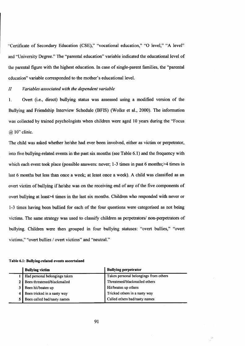
“Certificate of Secondary Education (CSE),” “vocational education,” “O level,” “A level”

and “University Degree.” The “parental education” variable indicated the educational level of

the parental figure with the highest education. In case of single-parent families, the “parental

education” variable corresponded to the mother’s educational level.

II Variables associated with the dependent variable

1. Overt (i.e., direct) bullying status was assessed using a modified version of the

Bullying and Friendship Interview Schedule (BFIS) (Wolke et al., 2000). The information

was collected by trained psychologists when children were aged 10 years during the “Focus

@ 10” clinic.

The child was asked whether he/she had ever been involved, either as victim or perpetrator,

into five bullying-related events in the past six months (see Table 6.1) and the frequency with

which each event took place (possible answers: never; 1 -3 times in past 6 months;>4 times in

last 6 months but less than once a week; at least once a week). A child was classified as an

overt victim of bullying if he/she was on the receiving end of any of the five components of

overt bullying at least>4 times in the last six months. Children who responded with never or

1-3 times having been bullied for each of the four questions were categorised as not being

victims. The same strategy was used to classify children as perpetrators/ non-perpetrators of

bullying. Children were then grouped in four bullying statuses: “overt bullies,” “overt

victims,” “overt bullies / overt victims” and “neutral.”

Table 6.1: Bullying-related events ascertained

Bullying victim Bullying perpetrator

1 Had personal belongings taken Taken personal belongings from others

2 Been threatened/blackmailed Threatened/blackmailed others

3 Been hit/beaten up Hit/beaten up others4 Been tricked in a nasty way Tricked others in a nasty way

5 Been called bad/nasty names Called others bad/nasty names

91

2. “Age 14 years depressive symptoms” was measured using the SMFQ (Angold et al.,

1995); it is therefore the same measure of depressive symptoms I used in my analyses as

predictor variable (see paragraph 4.2.2) being ascertained by a trained psychologist at the

same moment when alcohol problem use was assessed (during the “Teen Focus 2” clinic,

children aged 14 years). Similar to the “age 10 depressive symptoms” variable (see paragraph

4.2.2), the depressive symptoms score at age 14 years was divided into quartiles of “low,”

“medium,” “high” and “very high” depressive symptoms.

3. Sensation-seeking has been defined as “the need for varied, novel and complex

sensations and experienced and the willingness to take physical and social risks for the sake

of such experiences” (Zuckerman, 1979). Sensation-seeking was ascertained using a modified

version of the Arnett’s Inventory of Sensation Seeking (AISS) questionnaire (Arnett, 1994),

which was administered during the “Focus @11” clinic when children were aged 11 years.

The interview was performed on a computer; the child was presented with 20 possible

behaviours (see Table 6.2), each appearing on the screen and being spoken to the child via

headphones. The child was given four options to rate each behaviour: “not like me at all,”

“not much like me,” “quite like me” and “very like me.” I divided the final score into deciles.

92

Table 6.2: Items assessing sensation-seeking score

Statement12345678 9

1011121314151617181920

When the water is very cold, I prefer not to swim even if it is a hot day (reversed score) When I listen to music I like it to be loudI stay away from movies that are said to be frightening (reversed score)I like to ride on the roller coaster and other fast rides I would never gamble with money, even if I could afford it (reversed score)I like a movie where there are lots of explosions and car chases It would be interesting to see a car accident happenI like the feeling o f standing next to the edge on a high place and looking down I think it would be exciting to be in a battle during a war I think it’s fun and exciting to perform or speak before a groupIf it were possible to visit another planet or the moon for free, I ’d be among the first to sign I enjoy playing exciting computer games I like using the diving boards when I go swimming I don’t worry about coming home later than I’m supposed to I don’t do my homework until the very last minuteI am happy to go to new places or do new things on my own without friends or family My parents or carers would be worried if they knew about some of the things I do I always join in with what my friends are doing, even if I am not very sure about it When I ride a bike I go as fast as I can whenever possible I enjoy playing sports and activities which could be dangerous

6.2 Methods: statistical tests

6.2.1 Test for difference between models: Likelihood Ratio test

A very important component of statistics is the interpretation of observed data as indicative of

statistical evidence. However, there is no consensus among statisticians on what constitutes

statistical evidence and how to measure its strength. Confidence intervals, p-values and

posterior probability distributions are commonly used to interpret and communicate statistical

evidence (Zhang, 2009). Hacking suggested that the likelihood function is the optimal

mathematical representation of statistical evidence and that likelihood ratios test (LR) is one

of the most reliable methods to assess the strength of statistical evidence for evaluating one

statistical hypothesis versus a second (Hacking, 1965).

93

As already reviewed in paragraph 6.1.1.1, the log-likelihood (Z) of a single independent

variable corresponds to the probability (P) of obtaining the observed results given the (3

coefficient estimate; however, the more complex the model, the greater the number of Ls for

the single |3s will be necessary to estimate. Hence, in the case of an entire model, the L of the

model is the value that is maximized by a process (often defined as Maximum Likelihood

Estimation, or “MLE” (Pratt, 1976)) that computes the maximum L value for the |3 coefficient

of each independent variable in the model. To simplify (more details about the MLE

procedure can be found in the references provided), MLE, iteratively, starting from randomly

allocated values, “guesses” the values of the L of the independent variables in the model,

gradually increasing them until they converge to a maximum single value (the L of the

model). This L value is the one that maximises the P of obtaining the observed results

(Clayton, 1993, Hacking, 1965, Kirkwood, 2003, Pratt, 1976, Royall, 1997). The L of a

model is therefore an indicator of how well the model fits the data; the higher the Z, the better

the model fits the data (Hacking, 1965). L is a negative value; therefore, a higher value will

correspond to a less negative value.

In hypothesis testing, the Likelihood Ratio (LR) test uses the values of L to compare two

models where one is a restricted form of the other (this procedure is often defined as

“nesting” the restricted model into the unrestricted one) (Clayton, 1993, Kirkwood, 2003).

The test statistics is equivalent to [-2 * (/.(restricted model) - /.(unrestricted model))]

(Kirkwood, 2003). Because minus becomes a plus in the calculation (Z is a negative value), it

follows that the L of the unrestricted model will be added to the L of the restricted model and

the resulting value will be multiplied by -2. LR is therefore a positive value and it will

increase its value as the L of the unrestricted model becomes less negative (increases).

Therefore, the greater LR is, the greater the evidence will be in favour of the unrestricted

model (as explained earlier, the higher the Z, the better the model fits the data). Because LR

94

can be approximated to a quadratic equation, its value is compared against a %2 distribution

with degrees of freedom (d.f.) equivalent to the number of additional parameters (for

example, additional covariates) of the unrestricted model compared to the restricted one

(Clayton, 1993, Kirkwood, 2003, Royall, 1997).

For the analyses I conducted, LR tests were performed using the post-estimation command

“lrtest” in STATA/IC v. 10.1. for Windows (StataCorp, 2007). The command “lrtest” was

used to compare GOLOGIT models in which the predictor (depressive symptoms at age 10

years) and the covariates were entered in different ways (i.e., in either a linear, quadratic or

categorical fashion) and for hypothesis testing of interaction, comparing models with and

without the interaction between age 10 “depressive symptoms” variable and “peers’

influences” variables at either age 10 or age 14 years.

6.2.2 Tests for gender differences in the prevalence of the variables: X2 test and

Mann-Whitney-Wilcoxon test

As reviewed in paragraph 3.2.2, there is convincing evidence for gender differences in the

prevalence as well as risk factors associated with depressive symptoms and alcohol problem

use. I therefore divided the sample into boys and girls, conducting all the analyses on both the

total sample of both boys and girls (from here onwards defined as “total sample”), and on

boys and girls separately. In order to investigate differences in the prevalence of the single

variables (predictor, outcome, covariates and moderating variables) between boys and girls, I

used the X2 test for the categorical/ dichotomous variables and the Mann-Whitney-Wilcoxon

test for the continuous ones.

• X2 test: The X2 test (Pearson, 1900) is a nonparametric (i.e., that it does not make

assumptions on the distribution of the data) statistical test for categorical variables used to

determine whether a distribution of observed frequencies differs from the theoretical

95

expected frequencies (Daniel, 2010). To perform the X2 test in STATA/IC v. 10.1. for

Windows (StataCorp, 2007), the option “chi2” was added after the command “tabulate.”

• Mann-Whitney-Wilcoxon test: The Mann-Whitney-Wilcoxon test (MWW test), which

is often also called the “Mann-Whitney U” test, is a nonparametric statistical test for

continuous variables (Mann, 1947). The MWW test can be used in the same situations in

which the two independent samples Student’s t-test could be used, although it is considered

to be preferable to the Student’s t-test when the variable’s values are not normally distributed

and the sample size is sufficiently large (Conover, 1980), which is the case of all the

continuous variables included in my analyses. The “ranksum” command was used to perform

the MWW test in STATA/IC v. 10.1. for Windows (StataCorp, 2007).

6.3 Analytical procedures

6.3.1 Analysis of univariable GOLOGIT models of age 10 years depressive

symptoms and age 14 years alcohol problem use

The procedures described in the following four steps were taken while performing the

analysis of the univariable models of age 10 depressive symptoms and age 14 alcohol

problem use and helped me to decide: 1) whether to impose an equal (parallel lines

assumption accepted) or a different (parallel lines assumption rejected) effect of age 10

depressive symptoms in the L versus M&H equation and the L&M versus H equation of the

GOLOGIT model (procedure described in step 2); and 2) the most appropriate format of the

depression variable I would use in the subsequent analyses (procedure described in step 3).

The procedure described in step 4, finally, helped me to generate a model in which it was

possible to observe the direct relationship between age 10 depressive symptoms and age 14

alcohol problem use.

96

The analysis was conducted in both the total sample and in boys and girls separately.

1. Gender differences in the prevalence rate of the four indicators of age 14 alcohol

problem use, of the predictor variable “age 14 alcohol problem use” (see paragraph 4.2.1 for

more information about the predictor variable) and on the outcome variable “age 10

depressive symptoms” (see paragraph 4.2.2 for more information on the outcome variable)

were investigated with X2 tests (see paragraph 6.2.2 for more information on the X2 test).

Results are reported in paragraph 7.1.

2. The variable “age 10 years depressive symptoms” was entered in a univariable

GOLOGIT regression model (see paragraph 6.1.1 for more information on the GOLOGIT

model) as single predictor of “age 14 alcohol problem use” in three possible ways: a) as a

linear variable, b) as a categorical variable and c) as a quadratic variable (the generated

multiplying the variable by itself). In all three cases the “autofit” option associated with the

GOLOGIT2 command was specified (for more information on “autofit” see paragraph

6 .1. 1. 1).

3. The LL of the univariable GOLOGIT models in which “age 10 depressive symptoms”

were entered as either a categorical or a quadratic variable were compared with the more

parsimonious model in wich age 10 depressive symptoms were entered as a linear variable

were compared using a LR test, in which one model was nested within the other. The LR test

provided information on the validity of a simplifying assumption for a model (in this case,

whether a linear model is as good as a more complex model, such as a categorical or a

quadratic one; see paragraph 6.2.1 for more information on the LR test). Results are reported

in the paragraph 7.2.

4. The uni variable GOLOGIT models that were identified as better fitting the data were

run, and expected probability of the fitted models was predicted using the “predict” post-

97

estimation command (see paragraph 6.1.1.1 for more information on the “predict” command).

The expected probability estimates were plotted against the four categories of the “age 10

depressive symptoms” variable (“low,” “medium,” “high” and “very high”). Results are

shown in paragraph 7.3.

6.3.1.1 Analysis of univariable GOLOGIT model of age 10 years depressive

symptoms and age 14 years alcohol problem use in the total sample: moderating effect

of gender

The procedure described in the following two steps was performed in order to evaluate the

possible moderating effect of gender in the univariable GOLOGIT model obtained with the

procedures described in paragraph 6.3.1, step 2. However, it must be noted that the result of

this analysis was not used to decide whether or not to conduct the entire analysis on the two

genders separately, but only to confirm or reject the hypothesis of a direct moderating effect

of gender in the univariable relationship between age 10 depressive symptoms and age 14

alcohol problem use. Hence, the entire analysis outlined in paragraph 3.3 has been conducted

in both genders independently from the results of this test, as one of the scopes of my thesis is

to evaluate the pattern of covariates correcting the relationship between age 10 depressive

symptoms and age 14 alcohol problem use in the two genders.

1. In order to generate the interaction terms, the variable “age 10 depressive symptoms”

was centred at its mean (subtracting the value of the variable’s mean to every variable’s

value) and it was multiplied with the binary variable describing the child’s gender. In this

way I obtained the interaction term: “age 10 depressive symptoms X gender”.

2. A LR test (see paragraph 6.2.1) comparing 1) a bivariable GOLOGIT model without

interactions (i.e., a model having as independent variables: a) “age 10 depressive symptoms”

98

and b) “gender”) and 2) an interaction bivariable GOLOGIT model (i.e., a model having as

independent variables: a) “age 10 depressive symptoms” and b) “gender” and also including

the interaction term: “age 10 depressive symptoms X gender” was conducted in the total

sample (see results in paragraph 7.4).

6.3.2 Missing data imputation

The following four steps were taken in order to investigate the pattern of data missingness

(procedure described in steps 1 and 2) and to impute the missing data (procedure described in

steps 3 and 4), obtaining a dataset in which all the variables of interest were fully available

for each participant in the study sample (N=4200). It must be noted that the entire ALSPAC

dataset (N= 14,062 live births) was used in the imputation procedure, obtaining therefore a

complete set of information for each child enrolled in the ALSPAC study. However, the

analysis using the imputed variables (described in the steps below) was conducted only on the

participants included in the study sample (N=4200) and not on the entire ALSPAC dataset. I

chose to do so because, for those children who did not have provided at least both

information on alcohol problem use and depressive symptoms, the amount of information

originally available may have been extremely limited and/ or extremely antecedent to the

years of interest (as in some cases, the only information available was the gender of the

participant child, which was provided for all the live births).

1. An indicator of missingness (indicating whether the information was available or not

available) was generated for each variable included in the imputation model (predictor,

outcome variables, covariates and moderating variables). The indicators of missingness for

each variable were summed, obtaining a score describing the amount of information missing

per each participant in the study sample. Gender difference in the total amount of information

99

missing was assessed using MWW test (see paragraph 6.2.2 for more information on the

MWW test; results are reported in paragraph 8.1.2).

2. The association between two variables theoretically associated with information

missingness (house crowding index and parental education, see paragraph 6.1.2.2) and the

indicator of the amount of information missing per each participant in my study sample was

investigated using the Spearman’s rank correlation test (Spearman, 1904). Gender differences

in the amount of missing data for each variable imputed were assessed using X2 test (see

paragraph 6.2.2 for more information on the X2 test; results are reported in paragraph 8.1.2).

3. A MICE imputation model (see paragraphs 6.1.2 and 6.1.2.1 for more information on

MICE) was defined on the basis of the type of variables included in it. As reviewed in

paragraph 6.1.2.1, each variable in the MICE imputation model must be imputed using a

specific imputation equation that is equivalent to a regression model having the variable to be

imputed as dependent variable. Table 6.3 reports the type of imputation equation that was

specified for each variable included in the MICE imputation model.

Because of the broad variety of variables included in the imputation model (e.g., continuous,

ordered categorical, non-ordered categorical and dichotomous variables, see Tables 5.1, 5.2,

5.3 and 5.4 and Table 8.1), a different imputation equation had to be specified for each

variable (either linear regression, OLOGIT regression, MLOGIT regression (used only for

the non-ordered categorical variable “bullying status”), or logistic regression).

Following the guidelines suggested by Moons et al., the predictor variable was also included

in the MICE imputation model (Moons et al., 2006) (see paragraph 6.1.2.1); however, this

was not included in the form of the derived variable “age 14 alcohol problem use,” but in the

form of the four SSAGA items (Bucholz et al., 1994, Hesselbrock et al., 1999) used to

generate it (see paragraph 4.2.1). This was done because outcome variable “age 14 alcohol

problem use” is the first of four principal components generated by a PCA procedure

100

(Olsson, 1979, Pearson et al., 1922) (see paragraph 4.2.1), and therefore, its distribution

depends on the distribution of the four variables used to generate it (Jolliffe, 2002).

Table 63: Type of imputation equation that was specified for each variable included in the MICE imputation model

Variable’s class Variable Imputation equationConsumed alcohol without parental permission OLOGIT regression

Outcome variable* Frequency of whole alcoholic drinks OLOGIT regressionLargest number o f whole drinks in 24 hour-period OLOGIT regression

Ever been intoxicated from alcohol Logistic regressionPredictor variable Age 10 depressive symptoms OLOGIT regression

Gender Logistic regressionAgelO OLOGIT regression

Socio-demographic Agel4 OLOGIT regressionfactor domain Ethnicity Logistic regression

covariates Social Class OLOGIT regressionIncome per week OLOGIT regression

Family constellation OLOGIT regressionMother’s alcohol use Linear regression

Mother’s partner’s alcohol use Linear regressionFamily environment Mother-child interaction Logistic regression

factor domain Mother’s partner’s-child interaction Linear regressioncovariates Mother’s depression Logistic regression

Mother’s partner’s depression Logistic regressionRows between parents OLOGIT regression

Social environment factor domain

covariates

Child stressful events OLOGIT regressionPeers’ antisocial activities5 OLOGIT regression

Religiosity (attends place of worship) OLOGIT regressionPeers’ alcohol drinking5 Logistic regression

Personality and Child conduct problems OLOGIT regressionpsycho-pathologies Child peer problems OLOGIT regression

factor domain Child antisocial activities OLOGIT regressioncovariates Self-esteem OLOGIT regression

Peers’ influences Age 14 peers’ alcohol drinking OLOGIT regression(moderating Child bonding with peers at age 10 years Linear regressionvariables)$ Child bonding with peers at age 14 years Linear regression

House crowding index OLOGIT regressionAuxiliary variables Parental education OLOGIT regression

(included only in the Bullying status MLOGIT regressionimputation model) Sensation-seeking Linear regression

TTT7T7T7----------- T“Age 14 depressive symptoms OLOGIT regression

SSAGA items used to generate, using PCA, the outcome variable “age 14 alcohol problem use.”$ Age 10 years peers’ antisocial activities and age 10 years peers’ alcohol drinking were combined to generate the moderating variable “age 10 years peers’ antisocial behaviour” (see paragraph 4.2.4.2).

4. When the MICE imputation procedure was started, the model was run iteratively for

50 cycles of imputation, generating 50 complete dataset that were stacked into a single

101

dataset (from here onwards defined as “the imputed dataset”) for subsequently being

analyzed.

6.3.3 Analysis of multivariable GOLOGIT models of age 10 years depressive

symptoms and age 14 years alcohol problem use in the original (non-imputed) dataset

The following seven steps were taken while performing the analysis of the multivariable

model of age 10 depressive symptoms and age 14 alcohol problem use.

Using the procedures described below I obtained a model in which the direct relationship

between age 10 depressive symptoms and age 14 alcohol problem use was corrected by

taking into account the effect of relevant covariates.

The analysis, with the exception of step 3, was conducted in both the total sample and in boys

and girls separately.

1. The carefully a priori selected covariates, chosen after careful examination of the

relevant literature and described in Table 5.2 and Table 5.3, were tested for gender

differences using either the X2 test (for the categorical/ dichotomous variables) or the MWW

test (for the continuous variables) (see paragraph 6.2.2 for more details on these statistical

tests; results are reported in paragraph 8.2.1).

2. In every bivariable and multivariable GOLOGIT model that was drawn (see

paragraph 6.1.1 for more information on the GOLOGIT model), the parallel lines assumption

for age 10 depressive symptoms was maintained identical to the one that was identified in the

GOLOGIT univariable model using the “autofit” option (see step 2 of paragraph 6.3.1). To

do so, the “pi” (parallel lines assumption imposed) or “npl” (parallel lines assumption

relaxed) options were specified (for more information on “autofit,” “pi” and “npl,” see

paragraph 6.1.1.1). I chose to do this in order to obtain bivariable and multivariable

102

GOLOGIT models in which the effect of depressive symptoms was comparable to the one

identified in the univariable GOLOGIT model.

As reviewed in paragraph 6.1.1.1, a limit of the GOLOGIT2 module is that it is not possible

to use the option “autofit” (which tests whether the parallel lines assumption should be

imposed or relaxed) when either the “npl” or the “pi” options are being used (Williams,

2006). Since I was interested in having bivariable GOLOGIT models in which the effect of

age 10 years depressive symptoms was comparable to the one observed in the univariable one

(the effect of age 10 years depressive symptoms being kept fixed with either the “npl” or the

“pi” options as described above), I also had to arbitrarily specify either the “pi” or “npl”

option for any of the covariates being entered in the GOLOGIT models. I chose to use the

“pi” option; for every covariate this imposed equal effect in the L versus M&H equation and

the L&M versus H equation of the GOLOGIT model, and resulted in GOLOGIT models

more easily interpretable than the ones I could have obtained if I would have specified the

“npl” option instead.

3. For each covariate I followed the same procedure as for the depressive symptom

variable (described in steps 2 and 3 of paragraph 6.3.1). Each covariate was specified in three

different ways: as being linear, categorical or quadratic and it was singularly included in the

univariable GOLOGIT model that was identified with the procedure described in paragraph

6.3.1. I generated in this way a bivariable GOLOGIT model accounting for one covariate

only.

The two GOLOGIT models in which each covariate was entered in either a categorical or

quadratic fashion were subsequently compared with the more parsimonious model in which

the covariate was entered in a linear fashion using a LR test (see paragraph 6.2.1 for more

information on the LR test).

103

This analysis was conducted on the total sample and in the non-imputed dataset only; results

are reported in paragraph 8.2.2. The results obtained were then generalized to boys and girls

and to the imputed variables. I chose to do so to ensure the comparability of the estimates of

the covariates included in the subsequent multivariable GOLOGIT models drawn from the

non-imputed and from the imputed datasets and based on the total sample and on the

subsamples of boys and girls. Explaining this with a practical example, it would not have

been possible to compare the estimates of a covariate that in one case is entered as linear

(d.f.=l; hence 1 single coefficient to be estimated) and in the other case is entered as

categorical (d.f.=number of categories - 1; hence number of categories -1 coefficients to be

estimated) (Kirkwood, 2003).

4. Starting from the domain of socio-demographic factors (see Table 5.2), each covariate

(entered with the “pi” option imposed as described in point 2 and in either a categorical,

quadratic or linear way as identified in point 3) was independently tested for significance

level in the bivariable GOLOGIT model (see results in paragraph 8.2.3).

5. In the multivariable GOLOGIT model, only the covariates that were statistically

significant (p-value<0.05) when tested in the bivariable GOLOGIT models were entered. In

case any of the covariates describing mother’s partner’s behaviour and attitudes (mother’s

partner’s alcohol use, mother’s partner’s parent-child interaction and mother’s partner’s

depression) and about the relationship between the two parental figures (rows between

parents) (see Table 5.2 for the prevalence of these variables in the study sample) was

statistically significant when tested in the bivariable GOLOGIT model, the sensitivity

analysis described in step 6 was performed; otherwise, I skipped directly to step 7.

6. As described by the “family constellation” variable in Table 5.2, 5.7% of the children

in the study sample (information on family constellation was available for 3,524 children)

were living in single-parents families composed by a single female parental figure (usually

104

the mother), and therefore, information provided by the covariates describing mother’s

partner’s behaviour and attitudes and about the relationship between the two parental figures

(see step 5) was not relevant for them.

Hence, in case any of those mother’s partner’s-related covariates was still statistically

significant (p-value<0.05) when included in the GOLOGIT multivariable model, two

GOLOGIT multivariable models (one accounting for children with both parental figures

including the mother’s partner’s covariate, and one accounting for children with a single

maternal figure excluding such covariate) were drawn. If, on the contrary, the covariate

became statistically non-significant (p-value >0.05), the covariate was excluded from the

analysis and the multivariable GOLOGIT model was based on children living in both single

and two-parents families (see results in paragraph 8.2.4).

7. A final GOLOGIT multivariable model, correcting the relationship between age 10

years depressive symptoms and age 14 years alcohol problem use, was run (see results in

paragraph 8.2.5 for the total sample and in paragraph 8.2.6 for the boys and girls

subsamples).

6.3.4 Analysis of multivariable GOLOGIT models of age 10 years depressive

symptoms and age 14 years alcohol problem use in the imputed dataset

Analysis of the multivariable GOLOGIT models based on the imputed dataset was conducted

following the same procedure used for the multivariable GOLOGIT models based on the

non-imputed dataset and described in steps 3, 4, 5, 6 and 7 of paragraph 6.3.3. However, in

the imputed dataset the procedure described in step 6 (i.e., the sensitivity analysis of the

covariates describing mother’s partner’s behaviour and attitudes and the relationship between

the two parental figures) was conducted with an additional passage. As explained in

paragraph 6.3.2, the MICE procedure imputed all the missing values in the covariates,

105

however also including those values of the mother’s partner’s related covariates that were

correctly missing in the non-imputed dataset (because the information could not be provided)

for those children living in single-parent families. Hence, to conduct the sensitivity analysis

only on the subsample of children living in two-parent families, children living in single

parent families had to be excluded on the basis of the imputed “family constellation”

variable.

In the bivariable and multivariable GOLOGIT models drawn from the imputed datasets, I

included the same predictor (age 10 years depressive symptoms) and outcome (age 14

alcohol problem use) variables that I included in the GOLOGIT models drawn from the non

imputed dataset. In this way the GOLOGIT models drawn from both the imputed and non

imputed datasets were based on the same study sample (4,220 participants).

Thus, the difference between the GOLOGIT models drawn from the two datasets (imputed

and non-imputed) was that in the models drawn from the imputed dataset (but not in those

drawn from the non-imputed one), I included the imputed covariates and the imputed

moderating variables (imputed using a MICE procedure, see paragraph 6.3.2) in order to

obtain GOLOGIT models that were all based on the same sample size (N=4220) and were not

affected by the presence of missing values in the covariates and/ or in the moderating

variables (see results in paragraphs 8.2.3, 8.2.4, 8.2.5 and 8.2.6).

Hence, the results obtained from the analysis of the imputed dataset - because of their greater

informativeness - have been described more extensively than the results based on the non-

imputed dataset, which have been reported solely as confirmatory results of my analyses.

106

6.3.5 Univariable and multivariable GOLOGIT models accounting for the

moderating effects of peers’ influences

The following twelve steps were taken while performing the analysis of models accounting

for the moderating effects of peers’ influences and based on both the univariable and the

multivariable GOLOGIT models obtained with the procedures described in paragraphs 6.3.1

and 6.3.4. The procedures described here, with the exclusion of step 4, were all conducted in

the imputed dataset only.

Using the procedures described below, I obtained a model in which the direct relationship

between age 10 depressive symptoms and age 14 alcohol problem use was corrected by

taking into account the effect of relevant covariates, and in which the moderating effects of

peer’s influences were taken into account. I also obtained a graphical representation of the

moderating effect of peers’ influences in the direct relationship between age 10 depressive

symptoms and age 14 alcohol problem use.

The analysis was performed twice, once accounting for peers’ influences at age 10 years and

once accounting for peers’ influences at age 14 years (see paragraph 4.2.4).

3. Using the univariable GOLOGIT model obtained with the procedure described in

paragraph 6.3.1, a trivariable GOLOGIT model was generated, including each of the

variables describing peers’ influences (i.e., the variable describing the child’s bonding with

his/ her peers and the variable describing the peers’ risky behaviour (see Table 5.4)).

As it was done for the covariates included in the GOLOGIT multivariable model (see

paragraph 6.3.2, step 2), the parallel lines assumption for age 10 depressive symptoms was

maintained identical to the one that was identified in the GOLOGIT univariable model (see

step 2 of paragraph 6.3.1), whereas the variables describing peers’ influences were entered

with the parallel lines assumption imposed using the option “pi” (see paragraph 6.1.1.1). This

107

was done for all the trivariable, quadrivariable and multivariable GOLOGIT models

described in the steps that follow.

The peers’ influences variables were entered with a linear format in all the GOLOGIT

interactions models I generated. I decided to do so for two reasons: 1) if the variables would

have been entered in a categorical format, the interaction of the two peers influences

variables would have created 36 interaction variables, whose estimation would have been

problematic as some of the categories might not have had sufficient data for being correctly

estimated (the variables describing peers’ influences were a 4 categories variable (peers’

risky behavior) and a 9 categories variable (child bonding with his/ her peers) (see Table

5.4)); and 2) if the variables would have been entered as quadratic, their interaction would

have generated a quartic variable, whose correct estimation would have required the use of

the “fracpoly” command for the analysis of fractional polynomials (Sauerbrei et al., 2006),

which does not support the GOLOGIT regression command in STATA/IC v.10.1. for

Windows (StataCorp, 2007).

4. In order to generate the interaction terms, the variables were centred at their mean

(subtracting the value of the variable’s mean to every variable’s value), reducing the

covariance and by consequence the collinearity between the variables (Aiken, 1991). In this

way I obtained four interaction terms: 1) “age 10 depressive symptoms X child’s bonding

with his/ her peers,” 2) “age 10 depressive symptoms X peers’ risky behaviour,” 3) “child’s

bonding with his/ her peers X peers’ risky behaviour,” and 4) “age 10 depressive symptoms

X child’s bonding with his/ her peers X peers’ risky behaviour.”

5. A LR test comparing 1) a trivariable GOLOGIT model without interactions (i.e., a

model having as independent variables: a) “age 10 depressive symptoms,” b) “peers’ risky

behaviour” and c) “child’s bonding with his/her peers”) and 2) a three-way interaction

trivariable GOLOGIT model (i.e., a model having as independent variables: a) age 10

108

depressive symptoms,” b) “peers’ risky behaviour” and c) “child’s bonding with his/her

peers,” and also including the four interaction terms: d) “age 10 depressive symptoms X

child’s bonding with his/ her peers,” e) “age 10 depressive symptoms X peers’ risky

behaviour,” f) “child’s bonding with his/ her peers X peers’ risky behaviour,” and g) “age 10

depressive symptoms X child’s bonding with his/ her peers X peers’ risky behaviour”) was

conducted in the total sample. The analysis was conducted on both the imputed and non-

imputed dataset; in case of statistically significant results, the three-way interaction

trivariable GOLOGIT model was further analyzed with the procedure described in steps 7-12

(see results in paragraph 9.1).

6. Gender differences in the variables describing peers’ influences (see Table 5.4) were

tested using either the X2 test (for the variables describing peers’ risky behaviour) or the

MWW test (for the variables describing child’s bonding with his/her peers) (see paragraph

6.2.2 for more details on these statistical tests; results are reported in paragraph 9.2).

7. The variable “gender” was included in the three-way interaction trivariable

GOLOGIT model described in step 5, generating a quadrivariable GOLOGIT four-way

interaction model (i.e., a GOLOGIT model having all four interaction terms described in step

4, interacting with gender as well). A LR test comparing the quadrivariable GOLOGIT model

without interactions (including gender) and this four-way interaction quadrivariable

GOLOGIT model (including gender) was conducted. The analysis was conducted on both the

imputed and non-imputed dataset; in case of statistically significant results, the three-way

interaction trivariable GOLOGIT model was further analyzed with the procedure described in

steps 6 (see results in paragraph 9.3).

8. LR tests were conducted on the boys and girls subsamples, following the same

procedure indicated in steps 1-3 for the total sample. The analysis was conducted on both the

imputed and non-imputed dataset; in case of statistically significant results, the three-way

109

interaction trivariable GOLOGIT model was further analyzed with the procedure described in

steps 7-12 (see results in paragraph 9.4).

9. In case the results of the LR tests described in step 3 and 6 were statistically

significant in the imputed dataset (p-value<0.05), the significance level of the three

interaction terms, which included age 10 depressive symptoms (i.e., 1) “age 10 depressive

symptoms X child’s bonding with his/her peers,” 2) “age 10 depressive symptoms X peers’

risky behaviour,” and 3) “age 10 depressive symptoms X child’s bonding with his/ her peers

X peers’ risky behaviour”) was tested in the trivariable GOLOGIT models accounting for the

three-way interaction based either on the total sample (if the LR test described in step 5 was

statistically significant), or on the two genders separately (if the LR test described in step 6

was statistically significant), or on both (if both the LR tests described in step 5 and 6 were

statistically significant) (see results in paragraph 9.5).

10. In order to correctly interpret the three-way interaction estimate, I had to consider

separately the possible combinations of child bonding with his/her peers and of peers’ risky

behaviour (Aiken, 1991). I divided the variable describing child’s bonding with his/her peers

(see Table 5.4) in “low” and “high” “child’s bonding with his/her peers” (cut-off at the -50th

percentile) and recoded the variable describing peers’ risky behaviour (see Table 5.4) in two

categories; “low” and “high” “peers’ risky behaviour”. Therefore, for peers’ alcohol drinking

I distinguished between peers who had never consumed alcohol in previous six months (low)

and peers who had consumed (with any frequency) alcohol in the previous six months (high);

whereas for peers antisocial behaviour I distinguished between peers who had never partaken

in any antisocial activity (low) and peers who had partaken in at least one (high)).

11. I separately ran the univariable GOLOGIT model indentified in paragraph 6.3.1 for

four times in the following groups: 1) children with low bonding with peers and whose peers

have low risky behaviour; 2) children with high bonding with peers and whose peers have

110

low risky behaviour; 3) children with low bonding with peers and whose peers have high

risky behaviour; and 4) children with high bonding with peers and whose peers have high

risky behavior.

12. The expected probabilities of all those four univariable GOLOGIT models were

predicted using the “predict” post-estimation command (see paragraph 6.1.1.1 for more

information on the “predict” command). The expected probability estimates were plotted

against the four categories of the “age 10 depressive symptoms” variable (“low,” “medium,”

“high” and “very high”). As a reference line, it was included in the graph the plot of the

expected probability of the univariable GOLOGIT model not accounting for interaction (see

step 4 in paragraph 6.3.1) (see results in paragraph 9.6).

13. The four interaction terms listed in step 2 were included in the multivariable

GOLOGIT models that were identified with the procedures described in paragraphs 6.3.3 and

6.3.4. LR tests were conducted to compare the multivariable GOLOGIT model and the three-

way interaction multivariable GOLOGIT model in both the non-imputed and the imputed

dataset (see results in paragraph 9.7).

14. If the results of the LR test conducted in step 11 were statistically significant (p-

value<0.05), a three-way interaction multivariable GOLOGIT model drawn from the imputed

dataset was generated (see results in paragraph 9.6).

I l l

CHAPTER 7: RESULTS OF THE UNIVARIABLE GOLOGIT MODELS

7.1 Gender differences in the predictor and outcome variables

As reviewed in paragraph 3.2.2, there is convincing evidence for gender differences in the

prevalence as well as risk factors associated with depression and alcohol misuse. I therefore

divided the sample into boys and girls and compared the prevalence rates of predictor and

outcome variables in the two genders with a X test (see paragraph 6.4.1, step 1). Results are

presented in Table 7.1. Results for the total sample have been presented in Table 5.1.

Boys were more likely to have experienced higher levels of depressive symptoms in

childhood (X2(3)= 11.08, p=0.011) than girls, whereas girls were significantly more likely to

experience alcohol problem use (X2(2)=9.02, p=0.011).

As explained in paragraph 4.2.1, the “alcohol problem use” variable was the first of four

principal components created with a PC A procedure based on four SSAGA items (Bucholz et

al., 1994, Hesselbrock et al., 1999). Gender differences were observed for two of these items

(see Table 7.1): the frequency the teenager has had whole alcoholic drinks (not sips) in the

past six months (boys reported higher frequencies, X2(5)=23.89, p<0.001), and the largest

number of whole drinks the teenager has had in a 24-hour period (girls reported larger

amounts than boys, X2(3)=12.09, p=0.007).

112

Table 7.1: Prevalence of alcohol problem use and depressive symptoms for boys and girls separately

Boys (N=2018) Girls (N=2202)

Variable Categories % % X2fNever 80.1 78.4

X2(3)7.15

p=0.067

Consumed alcohol without parental

permission*

1-3 times 13.4 16.1

>4 times 5.3 4.3

once per week 1.2 1.1

Never 60.5 56.1

<Monthly 30.9 36.7X2(5)23.89

p<0.001

Frequency of whole <Twice a month 3.9 4.3alcoholic drinks* <Weekly 2.5 1.4

<Twice a week 1.8 1.2

>Twice a week 0.4 0.3

0 drinks 59.9 55.2X2(3)12.09

p=0.007

Largest number of whole drinks in 24 hour-

period*

1-2 drinks 23.2 25.0

3-4 drink 9.0 11.5

>5drinks 7.9 8.3

Ever been intoxicated Yes 94.3 93.3 X2(l)1.55

p=0.213from alcohol* No 5.8 6.7

Low 56.6 52.0 X2(2)9.02Alcohol problem useA Medium 29.1 32.7

High 14.3 15.3 p=0.011

Low 23.5 27.7X2(3)11.08

p=0.011Depressive symptoms8

Medium 29.5 29.6

High 28.3 25.5

Very high 18.7-T7T— — -T

17.3

results are shaded.* Four items used to construct the “alcohol problem use” variable (A).A The outcome variable was the first of three components generated by the principal component analysis. To define alcohol problem use I categorized that variable in “low,” “medium,” or “high” alcohol problem use.B The predictor variable was divided in quartiles obtaining four possible levels of depressive symptoms: “low,” “medium,” “high,” and “very high.”

7.2 Formats and parallel lines assumptions of the “age 10 years depressive

symptoms variable” in the total sample and in the two genders separately

As explained in paragraph 6.3.1, steps 2 and 3 ,1 conducted a number of tests to decide on the

most appropriate representation of the independent variable in subsequent models.

First, LR tests were conducted, comparing three GOLOGIT univariable models: two

GOLOGIT models with age “10 depressive symptoms” entered in either a categorical or a

113

quadratic format versus a more parsimonious GOLOGIT model with “age 10 depressive

symptoms” entered in a linear format. The results in the total sample indicated that the more

complex models (depressive symptoms entered in categorical or quadratic formats) did not fit

the data significantly better than the more parsimonious one (depressive symptoms entered

linearly), which was therefore chosen as the standard model in subsequent analyses (LR

X (4)=4.13, p=0.389 comparing models with depressive symptoms entered as a categorical or

as a linear variable and LR X2(l)=1.24, p=0.265 comparing models with depressive

symptoms entered as a quadratic or as a linear variable).

The same results were obtained when analyzing the formats of the depressive symptoms in

the subsamples of boys and girls separately. For the subsample of boys they were: LR

X2(2)=0.35, p=0.841 comparing models with depressive symptoms entered in a categorical

versus a linear format and LR X2(l)=0.33, p=0.564 comparing models with depressive

symptoms entered in a quadratic versus a linear format, whereas for the subsample of girls

results were: LR X2(4)=2.70, p=0.609 comparing models with depressive symptoms entered

in a categorical versus a linear format and LR X2(l)=1.06, p=0.302 comparing models with

depressive symptoms entered in a quadratic versus a linear format.

Therefore, in all the subsequent analyses conducted on both the total sample, and on the

subsamples of boys and girls separately, age 10 years depressive symptoms was entered as a

linear variable.

As explained in paragraph 6.3.1 step 2, the option “autofit,” which performs a Wald test on

the independent variable in the model to verify whether the variable meets the parallel-lines

assumption, was specified in each of the three univariable GOLOGIT models described

above. Because the Wald test tests the null hypothesis that the effect of the independent

variable is equal across the equations (i.e., that the parallel lines assumption is valid, see

114

paragraph 6.1.1.1), a statistically significant (p<0.05) Wald test indicates that the variable

does not meet the parallel lines assumption.

In the models of interest (the ones in which age 10 depressive symptoms was entered as a

linear variable), the results of the Wald tests indicated that: in the total sample (Wald

X2(l)=6.96, p=0.008) age 10 depressive symptoms did not meet the parallel lines assumption;

in the subsample of boys (Wald X2(l)=1.27, p=0.258) age 10 depressive symptoms did meet

the parallel lines assumption; whereas in the subsample of girls (Wald X2(l)=6.02, p=0.014),

similarly to the total sample, age 10 depressive symptoms did not meet the parallel lines

assumption.

7.3 Univariable GOLOGIT models of the association between age 10 depressive

symptoms and age 14 alcohol problem use

Following the results described in paragraph 7.2, estimates of age 10 depressive symptoms

were obtained using univariable GOLOGIT models in which age 10 depressive symptoms

variable was entered in a linear format. Parallel lines assumption was relaxed in the total

sample and in the subsample of girls using the option “npl,” whereas it was imposed in the

subsample of boys, using the option “pi.”

As explained in paragraph 6.1.1, in all my analyses I present only the results of the “L&M

versus H equation” of the GOLOGIT models I developed (“L&M versus H equation” is

equivalent to a binary logistic regression in which the outcome variable is divided in two

categories: 1) adolescents who developed high alcohol problem use, and 2) adolescents who

developed either low or medium alcohol problem use).

In the total sample each increase in the level of childhood depressive symptoms was found to

be associated with a statistically significant 9% increase in the risk for early adolescence high

alcohol problem use (O.R. 1.09, 95% C.I. 1.01; 1.18, p=0.029), which resulted in a 27%

115

increased risk for those adolescents who experienced very high depressive symptoms in

childhood versus those who experienced low depressive symptoms. Examining the genders

separately, in girls, childhood depressive symptoms were more strongly associated with risk

of alcohol problems in early adolescence than for boys. With progressively higher levels of

depressive symptoms girls had experienced in childhood, an association with a 14% greater

risk of developing high alcohol problem use in early adolescence (O.R. 1.14, 95% C.I. 1.02;

1.27, p=0.016) was found, which resulted in a 42% increased risk for those girls who

experienced very high depressive symptoms in childhood compared to those who

experienced depressed symptoms at low levels.

In boys, on the other hand, the association between childhood depression and alcohol

problems at age 14 years was negligible, with all four categories of childhood depressive

symptoms being associated with similar levels of alcohol problem use in early adolescence

(O.R. 0.99, 95% C.I. 0.91; 1.07, p=0.838).

As explained in paragraph 6.3.1 step 4, I used the post-estimation command “predict” to

estimate the expected probability of each of the three GOLOGIT models (corresponding to

the expected probability of developing high alcohol problem use). In Figure 7.1, the expected

probability estimates for the GOLOGIT model in the total sample and in the boys and girls

subsamples are shown graphically, plotting them against the four categories of the “age 10

depressive symptoms” variable (“low,” “medium,” “high” and “very high”).

This graphical representation of the expected probability of the three GOLOGIT models

clearly illustrates how only the total sample and the girls subsample (but not the boys

subsample) an increase in the level of depressive symptoms in childhood corresponded to an

increase in the expected probability of developing high alcohol problem use in early

adolescence.

116

Figure 7.1: Expected probability of developing high alcohol problem use in adolescence by level of severity of childhood depressive symptoms; results are shown for the total sample and for both genders separately

-1.4

£>(CSiOaT3V8& - 1.8 4 - - W

HighMediumLow

—• — Total sample

Boys

-A --G irls

Age 10 depressive symptoms

7.4 Results of the LR test assessing the moderating effect of gender in the

univariable GOLOGIT model

As explained in paragraph 6.3.1.1, step 2, I performed a LR test to compare two models

based on the total sample: 1) a bivariable GOLOGIT model without interactions (i.e., a model

having as independent variables: a) “age 10 depressive symptoms” and b) “gender”) and 2)

an interaction bivariable GOLOGIT model (i.e., a model having as independent variables: a)

“age 10 depressive symptoms” and b) “gender” and also including the interaction term: “age

10 depressive symptoms X gender”) . The scope of this analysis was to confirm or reject the

hypothesis of a direct moderating effect of gender in the univariable relationship between age

10 depressive symptoms and age 14 alcohol problem use.

Results of the LR test indicated that, concerning the bivariable GOLOGIT model accounting

for gender, the more complex interaction model including the interaction term “age 10

117

depressive symptoms X gender” did not fit the data significantly better than the more

parsimonious model not including the interaction term (LR X2(l)=0.49, p=0.483).

However, although gender did not moderate the relationship between age 10 depressive

symptoms and age 14 alcohol problem use, the subsequent parts of the analysis were

nevertheless conducted both on the total sample and on boys and girls separately. This was

done because one of the scopes of my thesis is to evaluate the pattern of covariates correcting

the relationship between age 10 depressive symptoms and age 14 alcohol problem use in the

two genders.

7.5 Results of the univariable GOLOGIT models: synthesis of the chapter

In summary, in this chapter I observed that in my study sample boys were more likely to have

experienced higher levels of depressive symptoms in childhood than girls, whereas girls were

significantly more likely to experience alcohol problem use.

In the total sample each increase in the level of childhood depressive symptoms was found to

be associated with a statistically significant 9% increase in the risk for early adolescence high

alcohol problem use, for girls such increased risk corresponded to 14%, whereas for boys the

relationship between childhood depressive symptoms and adolescence alcohol problem use

was non-significant.

Despite this gender difference in the univariable GOLOGIT model described in this chapter,

results of the LR test indicated that gender does not moderate the relationship between

childhood depressive symptoms and alcohol problem use in adolescence. Nevertheless, it was

decided that the subsequent analyses would have been conducted on both the total sample and

the two separate genders, as one of the scopes of the thesis is to evaluate the gendered pattern

of covariates correcting the univariable GOLOGIT model.

118

CHAPTER 8: MISSING DATA IMPUTATION AND RESULTS OF THE

MULTIVARIABLE GOLOGIT MODELS

8.5 Missing data imputation

8.1.1 Auxiliary variables included in the MICE imputation model

As explained in paragraph 6.1.2.2, five auxiliary variables (that were not used in any of the

subsequent analyses) were included in the MICE imputation model. Two variables were

included because of their theoretical association with information missingness (i.e., house

crowding index and parental education) and three variables because of their theoretical

association with the dependent variable “age 14 alcohol problem use” (i.e., bullying status,

age 14 years depressive symptoms and sensation seeking).

Frequencies of the crowding index variable indicated that 23.7% of children in the study

sample lived in houses with a crowding index <0.5 and 5.0% of them lived in houses with a

crowding index>l. With regard to parental education, 15.6% of children had both parents

holding only a CSE, whereas 25.3% of children in the study sample had at least one of the

two parents holding a university degree certificate.

Concerning the variable “overt bullying status,” the majority of the children in the study

sample were identified as “neutral” (79.3%); the remaining 20.7% belonged to one of the

three other alternative bullying statuses (i.e., bullying perpetrators (0.7%), bullying victims

(15.8%) and bullying perpetrators-victims (4.2%)).

Finally, with regards to depressive symptoms at age 14 years, comparing these data with

those on depressive symptoms available at age 10 years (see Table 5.1) there was a reduction

in the prevalence of high depressive symptoms (26.8% at age 10 years versus 17.8% at age

119

14 years), but on the other hand there was an increase in the prevalence of very high

depressive symptoms (18.0% at age 10 years versus 23.1% at age 14 years).

Table 8.1: Auxiliary variables included in the M ICE model

Variable Categories N %<0.5 23.7

House crowding indexA >0.5 - <0.753400 39.9

>0.75 - <1 31.4>1 5.0

CSE 15.6Vocational education 7.3

Parental educationA O level 4149 24.9A level 27.0

University Degree 25.3Bullying perpetrator 0.7

Overt bullying status8 Bullying victim4099 15.8

Bullying perpetrator-victim 4.2Neutral 79.3

Low 30.1

Age 14 years depressive symptoms8 c Medium 3966 29.0High 17.8

Very high 23.1

Variable M easurement Unit N M(SD)Sensation-seeking8 Sensation-seeking score 3970 5.4 (2.8)

B Auxiliary variables theoretically associated with the outcome variable “age 14 alcohol problem use.”0 The variable “age 14 years depressive symptoms” was divided in quartiles in the same way it was done for the predictor variable “age 10 years depressive symptoms” (see paragraph 4.2.2), obtaining four possible levels of depressive symptoms at age 14 years: “low,” “medium,” “high,” and “very high.”

8.1.2 Pattern of data missingness

Table 8.2 reports the frequency of missing variables for all 35 variables (see Table 6.3) that

were included in the MICE imputation procedure. In my study sample (N=4220), only 5.9%

of participants (N=247) had information available for all those 35 variables. At the other

extreme, the maximum number of missing variables per participant was 19, with only 11

participants (0.3% of the study sample) missing such a large amount of information, whereas

9.5% of the study sample (N=400) had no information available for>10 variables (see Table

8.2).

120

MWW test results comparing the total number of missing variables in boys and girls (see

paragraph 6.3.2, step 1) indicated that there was no statistically significant gender difference

in the total amount of data missingness (M boys=4.6, SD=3.9; M girls=4.4, SD=3.9; MWW

z=-1.88, p=0.060).

Results of the Spearman’s rank correlation test (see paragraph 6.3.2, step 2) indicated that in

my study sample “house crowding index” and “parental education” variables were

significantly associated (p-value<0.05) with the number of missing variables per participant,

with parental education being more strongly inversely associated with missingness

(Spearman’s rho=-0.21, p<0.001) than house crowding index, which was only mildly

positively associated with the number of missing variables per participant (Spearman’s

Table 8.2: Frequency of missing variables in the total sample for all 35 variables included in the MICE imputation procedure

rho=0.06, p<0.001).

Missingvariables N participants# % of the study sample Cumulative %

012345678 9

101112131415161718 19

24749574774256031220319113710284606047786045241511

5.911.717.7 17.613.37.44.84.53.32.4 2.01.41.4 1.11.91.4 1.1 0.6 0.4 0.3

5.917.635.352.9 66.173.578.382.9 86.188.590.591.993.494.596.397.898.899.499.7 100.0

Total sample N=4220 participants.

121

Among all 35 variables included in the MICE model (see Table 6.3), only eight variables

(i.e., age 10 depressive symptoms, the four SSAGA indicators of age 14 alcohol problem use,

gender, age of assessment of depressive symptoms (“age 10” variable) and age of assessment

of alcohol problem use (“age 14” variable)) were fully available for all the 4,220 participant

children included in the study sample. All other 27 variables, including the five auxiliary

variables described in paragraph 8.1.1, were differently available (some more, some less

available) only for a fraction of the participant children (see Tables 5.1, 5.2 and 5.3 and Table

8.1).

Table 8.3 reports the number of missing values for each of the variables included in the

MICE model, both for the total sample (N=4220) and boys (N=2018) and girls (N=2202)

separately. Among the 27 variables containing missing values, the one with the smallest

proportion of missing data was “age 14 child’s bonding with his/her peers,” with only 26

participants (17 boys and 9 girls) without this information available, whereas the variable

with the greatest proportion of missing data was paternal alcohol use, with 3,149 participants

(1,496 boys and 1,653 girls) missing this information.

Results of X2 test comparing the rates of missingness for each covariate in boys and girls

indicated that for most variables these rates were comparable (see Table 8.3). However, for

three covariates (i.e., “social class” (X (1)=5.39, p=0.020), “child’s antisocial activities”

(X2(l) 7.69, p=0.006) and “peers’ antisocial activities” at age 10 years (X2(l) 49.34,

p<0.001)) and for three moderating variables (i.e., “age 14 peers’ alcohol drinking” (X2(l)

34.93 p<0.001), child’s bonding with peers at age 10 years (X2(l) 7.73 p=0.005) and “age 10

years peers’ antisocial behaviour” (X2(l) 7.73 p=0.005, see footnote of Table 8.3), boys had a

higher rate of missingness than girls.

122

Table 8.3: Number of missing values per each variable included in the MICE model and gender differences in missingness rate

Variables’ class VariableMissing

Total sample (N=4220)

MissingBoys

(N=2018)

MissingGirls

(N=2202)

X2 test of gender

difference in missingnessf

Consumed alcoholwithout parental 0 0 0 N/A*

permission

Outcome Frequency of whole alcoholic drinks 0 0 0 N/A*

variable Largest number o f whole drinks in 24 hour-period 0 0 0 N/A*

Ever been alcohol- intoxicated 0 0 0 N/A*

Predictorvariable

Age 10 depressive symptoms 0 0 0 N/A*

Gender 0 0 0 N/A*AgelO 0 0 0 N/A*Agel4 0 0 0 N/A*

Sociodemographic factor domain

covariates

Ethnicity 104 25 79 X2(l) 1.09 p=0.294

Social Class 265 145 120 X2(l) 5.39p=0.020

Income per week 926 447 479 X2(l)0 .10p=0.755

Family constellation 696 324 372 X2(l) 0.53 p=0.464

Maternal alcohol use 2227 1087 1140 X2(l) 1.85 p=0.173

Paternal alcohol use 3149 1496 1653 X*(l) 0.48 p=0.486

FamilyMother-child interaction 766 365 401 X2(l) 0.01

p=0.917environment Mother’s partner’s-child 683 309 374 X2(l) 2.17

factor domain interaction p=0.141covariates Maternal depression 627 306 321 X2(l) 0.28

p=0.593Mother partner’s

depression 2146 1005 1141 X2(l) 1.71 p=0.191

Rows between parents 826 384 442 X2(l) 0.72 p=0.393

Child stressful events 919 428 491 X2(l) 0.73 p=0.392

Socialenvironment

Peers’ antisocial activities* 425 276 149 X^l) 49.34

p<0.001factor domain

covariatesReligiosity (attends place

of worship) 593 264 329 X2(l) 3.01 p=0.083

Peers’ alcohol drinking* 226 122 104 X2(l) 3.63 p=0.057

Personality and psycho Child conduct problems 633 296 337 X2(l) 0.33

p=0.563pathologies

factor domain covariates

Child peer problems 726 348 378 X2(l) 0.01 p=0.946


123

Personality and Table 8.3 continued...psycho

pathologies Child antisocial activities 74 41 33 X2( l) 7,69p=0.006

factor domain covariates Self-esteem 609 291 318 X2( 1)0.00

p=0.984

Peers’Age 14 peers’ alcohol

drinking 604 356 248 XXI) 34.93p<0.001

influences(moderating

Child bonding with peers at age 10 years 70 45 25 X2( l ) 7.73

p=0.005variables)5 Child bonding with peers

at age 14 years 26 17 9 X ^ l) 3.23 p=0.072

House crowding index 820 390 430 X2( 1)0.03 p=0.869

Auxiliaryvariables

Parental education 71 41 30 X2(l) 2.85 p=0.091

(included only in the Bullying status 121 59 62 X2( 1)0.04

p=0.834imputation

model) Sensation-seeking 250 122 128 X2(l)0 .10p=0.749

Age 14 depressive symptoms 254 116 138 X2(l) 0.50

p=0.479t Pearson’s X2 reported. Statistically significant (p-value<0.05) results are shaded.* Pearson’s X2 test not possible when missing values in both boys and girls are equal to 0.# SSAGA items used to generate, using PC A, the outcome variable “age 14 alcohol problem use.”s Age 10 years peers’ antisocial activities and age 10 years peers’ alcohol drinking were combined to generate the moderating variable “age 10 years peers’ antisocial behaviour” (see paragraph 4.2.4.2). Missing data in “age 10 years peers’ antisocial behaviour” variable were: total sample=567 (342 boys and 225 girls); X2 test for gender difference in missingness: X2(l) 40.99, p<0.001.

8.2 Results of the multivariable GOLOGIT models

8.2.1 Gender differences in the covariates

Table 8.4 describes the gender differences among the socio-demographic covariates used in

the multivariable models, while information about the covariates belonging to the family

environment, social environment and personality and psychopathology domain is given in

Table 8.5 (see paragraph 6.3.3, step 1). No differences were found between boys and girls for

all the covariates belonging to the socio-demographic domain. However, among the family

environment domain covariates, girls reported higher levels of mother-child interaction

(MWW z—4.34, p<0.001), whereas boys reported higher levels of father-child interaction

(MWW z=5.56, p<0.001). Among the covariates belonging to social environment domain,

124

boys reported higher levels of peers’ alcohol drinking (X2(l)=5.39, p=0.020) and peers’

antisocial activities (X2(3)=190.62, p<0.001). Among the covariates of the personality and

psychopathology domain boys also reported higher scores of own antisocial activities

(X2(3)=206.26, p<0.001).

Table 8.4: Socio-demographic covariates presented for boys and girls separately

Covariate Measure unit N boys/ N girls M (S D ) boys M (SD) girls MWWf

AgelOA* Years 2018/2202 10.6 (0.2) 10.6 (0.2) z=0.98p=0.325

Agel4B* Years 2018/2202 13.8 (0.2) 13.8 (0.2) z=0.98p=0.325

Covariate Categories N boys/ N girls % boys % girls X2¥

Caucasian 96.7 96.3 x2(i)Ethnicity Non Caucasian 1993/2123

3.3 3.70.50

p=0.479I 17.1 15.5n 34.1 34.4

X2(5)4.14

p=0.530Social class III Non Manual 1873/2082 13.5 13.3

HI Manual 25.4 26.7IV 8.2 7.8V 1.8 2.4

<£100 1.2 1.5£100-£199 7.0 7.2 X2(4)

Income per week £200 - £299 1571/1723 15.5 14.7 1.80£300 - £399 20.5 19.4 p=0.773

>£400 55.8 57.2Both biological parents 90.1 88.7

X2(2)1.84

p=0.399

Familyconstellation

1 Biological parent & Partner 1694/1830 4.6 5.3

Single Parent 5.4 6.0t Wilcoxon-Mann-Whitney test (z score). Statistically significant (p-value<0.05) results are shaded.¥ Cross-tabulation o f each variable with gender. Pearson’s X2 reported. Statistically significant (p-value<0.05) results are shaded.* Absence of missing data.A Age of assessment of depressive symptoms. Variable categorized in quintiles.B Age of assessment of alcohol problem use. Variable categorized in quintiles.

125

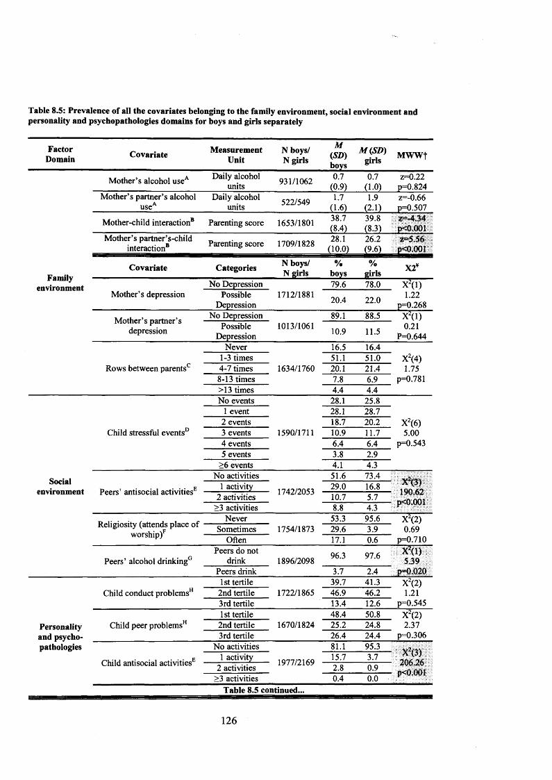
Table 8.5: Prevalence of all the covariates belonging to the family environment, social environment and personality and psychopathologies domains for boys and girls separately

FactorDomain Covariate Measurement

UnitN boys/ N girls

M(SD)boys

M (SD )girls MWWf

Mother’s alcohol useA Daily alcohol units 931/1062 0.7

(0.9)0.7

(1.0)z=0.22

p=0.824Mother’s partner’s alcohol

useADaily alcohol

units 522/549 1.7(1.6)

1.9(2.1)

z=-0.66p=0.507

Mother-child interaction8 Parenting score 1653/1801 38.7(8.4)

39.8(8.3)

z=-4.34p<0.001

Mother’s partner’s-child interaction8 Parenting score 1709/1828 28.1

(10.0)26.2(9.6)

z=5.56p<0.001

Familyenvironment

Covariate Categories N boys/ N girls

%boys

%girls X2¥

No Depression 79.6 78.0 X2(l)Mother’s depression Possible

Depression1712/1881

20.4 22.0 1.22p=0.268

Mother’s partner’s depression

No Depression 89.1 88.5 X2(l)Possible

Depression1013/1061 10.9 11.5 0.21

P=0.644Never 16.5 16.4

1-3 times 51.1 51.0 X2(4)Rows between parents0 4-7 times 1634/1760 20.1 21.4 1.75

8-13 times 7.8 6.9 p=0.781>13 times 4.4 4.4No events 28.1 25.8

1 event 28.1 28.72 events 18.7 20.2 X2(6)

Child stressful events0 3 events 1590/1711 10.9 11.7 5.004 events 6.4 6.4 p=0.5435 events 3.8 2.9

>6 events 4.1 4.3

Socialenvironment

No activities 51.6 73.4X2(3)190.62

p<0.001Peers’ antisocial activitiesE 1 activity 1742/2053 29.0 16.8

2 activities 10.7 5.7>3 activities 8.8 4.3

Religiosity (attends place of w orship/

Never 53.3 95.6 X2(2)Sometimes 1754/1873 29.6 3.9 0.69

Often 17.1 0.6 p=0.710

Peers’ alcohol drinking0Peers do not

drink 1896/2098 96.3 97.6 X2(l)5.39

Peers drink 3.7 2.4 p=0.0201st tertile 39.7 41.3 X2(2)

Child conduct problems11 2nd tertile 1722/1865 46.9 46.2 1.213rd tertile 13.4 12.6 p=0.5451st tertile 48.4 50.8 X2(2)

Personality and psycho

Child peer problemsH 2nd tertile 1670/1824 25.2 24.8 2.373rd tertile 26.4 24.4 p=0.306

pathologies No activities 81.1 95.3Xz(3)

206.26p<0.001

Child antisocial activitiesE1 activity 1977/2169 15.7 3.7

2 activities 2.8 0.9>3 activities 0.4 0.0


126


Personality and psychopathologies

Covariate MeasurementUnit

N boys/ ™ M(SD)1\J nirlc ' ' nirlcN girls ' girls& boys &

MWWf

Child self-esteem8 Self-esteemscore 1727/1884 19.3 19.5 z=1.65

(3.4) (3.3) p=0.098t Wilcoxon-Mann-Whitney test (z score). Statistically significant (p-value<0.05) results are shaded.¥ Cross-tabulation o f each variable with gender. Pearson’s X2 reported. Statistically significant (p-value<0.05) results are shaded.A Measure accounted for alcohol unit from beer, wine and spirits consumed during an average week.8 Variable categorized in deciles.c Number of arguments and disagreements between parents in the previous three months was used as an estimate of the bonding of the relationship between the two parents.D The measure provided information of whether each event occurred when the child was 6-7 years old, when he/she was 8 or in both occasions.E The questionnaire included questions about cigarettes and cannabis smoking in previous six months.F Used as a measure o f the religious conservatism o f the children’s rearing environment.° Question extracted from the peers’ antisocial behaviour questionnaire at age 10 years.H Main carers completed the parental version o f the SDQ for their child.

8.2.2 Analysis of the covariates: formats of the covariates

As explained in paragraph 6.3.3, steps 2 and 3, I conducted a number of tests to decide the

most appropriate representation of the covariates to be included in subsequent GOLOGIT

models.

As explained in paragraph 6.3.3, step 2, all the covariates were entered in the bivariable

GOLOGIT models with parallel lines assumption imposed; concerning the parallel lines

assumption of age 10 depressive symptoms variable, this was imposed for the total sample

and for the subsample of girls and relaxed for the subsample of boys (see paragraph 7.2).

To ensure the comparability of the estimates of the covariates in the final multivariable

GOLOGIT models drawn from the non-imputed and from the imputed dataset, and based on

both the total sample and the boys and girls subsample, this analysis was conducted on the

total sample and in the non-imputed dataset only, with the obtained results then being

generalized to boys and girls and to the imputed variables (see paragraph 6.3.3, step 3).

Table 8.6 reports the results of the LR tests comparing bivariable GOLOGIT models

accounting for age 10 depressive symptoms (linearly entered, see paragraph 7.2), age 14

alcohol problem use and each of the covariates listed in Tables 5.2 and 5.3 (with the

127

exclusion of the dichotomous covariates, i.e., gender, ethnicity, paternal and maternal

depression and age 10 peers’ alcohol drinking) entered in three possible formats (categorical,

quadratic and linear).

For each covariate, the more parsimonious model with the covariate entered as linear was

compared with the less parsimonious models with the covariate entered as quadratic or as

categorical. The two models with the covariate entered as quadratic or categorical were

compared with each other only when both of them would have fit the data significantly better

(p-value<0.05) than the model with the covariate entered as linear (see Table 8.6).

Results indicated that for most of the covariates a linear format would have fit the data better

than the more complex quadratic and categorical formats (see Table 8.6).

However, in the socio-demographic factor domain, for age of assessment of depressive

symptoms (“age 10” covariate) and for age assessment of alcohol problem use (“age 14”

covariate), both the quadratic and the categorical representations fit the data significantly

better than the more parsimonious linear format (for age 10 assessment of depressive

symptoms: X2(l)=4.91 P=0.026 quadratic format versus linear format and X2(3)=8.52

P=0.036 categorical format versus linear format; for age 14 assessment of alcohol problem

use: X2(l)=12.91 PO.OOl quadratic format versus linear format and X2(3)=16.00 P=0.001

categorical fashion versus linear fashion, respectively; see Table 8.6). Further comparison

between the former two models, i.e., with the covariates entered in a quadratic format (1

degree of freedom) versus with the covariates entered in a categorical format (3 degrees of

freedom) revealed that for both age 10 assessment of depressive symptoms as well as age 14

assessment of alcohol problem use the less parsimonious, categorical models did not fit the

data significantly better than the more parsimonious, quadratic models (X2(3)=6.47 P=0.091

for age 10 assessment of depressive symptoms and X2(3)=6.83 P=0.078 for age 14

128

assessment of alcohol problem use, see Table 8.6), thus both these variables were entered as

quadratic in the subsequent bivariable and multivariable GOLOGIT models.

Similar results were obtained for two covariates belonging to the family environment factor

domain: for maternal and paternal alcohol use LR tests indicated that these covariates should

have been entered in a quadratic format rather than a linear format (X2(l)=3.95 P=0.046 and

X2(l)=5.56 P=0.018, respectively; see Table 8.6).

Table 8.6: Comparison of bivariable models of age 10 depressive symptoms and age 14 alcohol problem use with covariates entered in either quadratic, categorical or linear formats in the total sample

FactorDomain Covariate

QuadraticversusLinear5

Categorical versus Linear5

Quadratic versus

Categorical5 *

Final representation decided uponf

Gender N/A N/A N/A, 4*

Dichotomous

Age 10 x ^ iH - 9 1p=0.026

X2(3)=8.52p=0.036

X2(3)=6.47p=0.091 Quadratic

Agel4 X (1)=12.91p<0.001

X(3)=16.00p=0.001

X2(3)=6.83p=0.078 Quadratic

Socio Ethnicity N/A N/A N/A Dichotomous#demographic

Social Class X2(l)=0.01p=0.916

X2(4)=1.19p=0.879 N/A Linear

Income per week X2(l)=0.23p=0.632

X2(3)=4.22p=0.239 N/A Linear

Familyconstellation

X (1)=0.95 p=0.329

X2(l)=0.95p=0.329 N/A Linear

Mother’s alcohol use

X (1)=3.95 p=0.046

X2(4)=7.59p=0.107 N/A Quadratic

Mother’s partner’s alcohol use

X2(l)=5.56p=0.018

X2(5)=7.30p=0.199 N/A Quadratic

Mother-childinteraction

X2(l)=0.31p=0.575

X2(8)=7.12p=0.523 N/A Linear

Familyenvironment

Mother’spartner’s-child

interaction

X2(l)=0.42p=0.516

X2(8)=8.64 p=0 373 N/A Linear

Mother’sdepression N/A N/A N/A Dichotomous#

Mother’s partner’s depression N/A N/A N/A Dichotomous#

Rows between parents

X2(l)=0.66p=0.415

X2(3)=5.5p=0.139 N/A Linear

Child stressful events

X2(l)=0.33P=0.567

X2(3)=3.1P=0.691 N/A Linear

SocialPeers’ antisocial

activitiesX2(l)=2.95

p=0.086X2(2)=0.11

p=0.947 N/A Linear

environment Religiosity (attends worship)

X2(l)=0.87p=0.351

X2(l)=0.87p=0.243 N/A Linear

Peers’ alcohol drinking N/A N/A N/A Dichotomous#


129

Table 8.6 continued...Child conduct

problemsX2(l)=1.62

p=0.203X2(l)=1.62

p=0.203 N/A Linear


Child peer problems

X (1)=0.75 p=0.385

X2(l)=1.62p=0.203 N/A Linear

Child antisocial activities

X2(l)=0.05p=0.826

X2(2)=4.32p=0.115 N/A Linear

Sxn ______i._.

Self-esteem X (1>=0.05 p=0.831

X (2)= 1.67 p=0.432 N/A Linear

s LR test results; statistically significant (p-value<0.05) results are shaded.* LR test comparing models with covariate entered in quadratic and categorical formats performed only in case both those models fitted the data significantly better (p-value<0.05) than the model with covariate entered using a linear format (otherwise N/A=not applicable, it is indicated).t Indicates the most appropriate format (linear, quadratic or categorical) for each variable when this was entered in subsequent bivariable and multivariable GOLOGIT models.# Comparison of data fittings of dichotomous variables cannot be performed (N/A=not applicable).

8.2.3 Analysis of the covariates: selection of covariates to be included in

multivariable models

In order to identify those covariates to be included in the final models, the statistical

significance of all the covariates was tested by entering each of them (starting with the

covariates belong to the socio-demographic factor domain and ending with those belonging to

the personality factor domain, as described in paragraph 6.3.3, step 4) independently in a

bivariable GOLOGIT2 model in which age 14 years alcohol problem use is predicted by age

10 years depressive symptoms.

Table 8.7 reports the estimates (O.R., 95% C.I. and p-value) for each covariate when this was

entered independently in a bivariable GOLOGIT model in the total sample. Estimates from

the subsamples of boys and girls are reported in Table 8.8 and Table 8.9, respectively. These

analyses were conducted on both the non-imputed and imputed datasets (see paragraph

6.3.4).

Due to the presence of missing values in the covariates (see Table 8.3), each bivariable

GOLOGIT model drawn from the non-imputed dataset was based on a different subset of

participants; on the contrary, there were no differences in the numbers of participants on

which each bivariable GOLOGIT model was based upon when this was drawn from the

130

imputed dataset (see paragraph 6.3.4). Please note that only the results of the “L&M versus H

equation” of the GOLOGIT models are reported (see paragraph 6.1.1; “L&M versus H

equation” is equivalent to a binary logistic regression in which the outcome variable is

divided in two categories: 1) adolescents who developed high alcohol problem use, and 2)

adolescents who developed either low or medium alcohol problem use).

As explained in paragraph 6.3.3, step 5 ,1 included in the multivariable models (for both the

total sample and the subsamples of boys and girls separately) only those covariates that, when

tested in a bivariable model, were statistically significant (p-value<0.05).

When considering the total sample, the following covariates reached the threshold of p<0.05

when tested in bivariable GOLOGIT models drawn from the non-imputed and imputed

datasets (see Table 8.7 for detailed estimates).

• Socio-demographic domain

o Non-imputed dataset: gender (p=0.007); age of assessment of depressive

symptoms (age 10) (p=0.025); age of assessment of alcohol problem use (age

14) (p<0.001) and family constellation (p=0.034).

o Imputed dataset: gender (p=0.007); age of assessment of depressive symptoms

(age 10) (p=0.025); age of assessment of alcohol problem use (age 14)

(p<0.001) and family constellation (p<0.001).

• Family environment domain

o Non-imputed dataset: mother’s and mother’s partner’s alcohol use (with both

covariates having p<0.001); mother-child interaction (p=0.003).

o Imputed dataset: mother’s and mother’s partner’s alcohol use (with both

covariates having p<0.001) and mother-child interaction (p=0.003).

131

• Social environment domain

o Non-imputed dataset: all the covariates were significant: childhood stressful

events (p=0.047); peers’ antisocial activity (p<0.001); religiosity (p=0.001);

age 10 years peers’ alcohol drinking (p=0.009).

o Imputed dataset: all the covariates were significant: childhood stressful events

(p=0.028); peers antisocial activities (p<0.001); religiosity (p=0.001) and age

10 years peers; alcohol drinking (p=0.012).

• Personality and psychopathologies domain

o Non-imputed dataset: child peer problems (p=0.001); child antisocial activities

(p<0.001).

o Imputed dataset: child conduct problems (p=0.037); child peer problems

(p=0.001) and child antisocial activities (p<0.001).

The only covariate that was estimated to be significant in the bivariable GOLOGIT model

drawn from the imputed dataset (p=0.037) but not in the bivariable model drawn from the

non-imputed dataset (p=0.055) was child conduct problems, which was therefore included as

a covariate in the multivariable GOLOGIT models based on the imputed dataset (but not in

those based on the non-imputed dataset).

132

Table 8.7: Estimates of each covariate when tested independently in bivariable GOLOGIT models drawnfrom both the non-imputed and the imputed datasets and based on the total sample

Non-imputed dataset Imputed dataset

Domain Covariate O.R. 95% C.I. ps O.R. 95% C.I. p$

Gender*A 0.85 0.76 0.96 0.007 0.85 0.76 0.96 0.007Ageio*A i: ^Agel4*A

s . Ethnicity 1.31 0.94 1.83 0.107 1.30 0.94 1.81 0.114demographic Social Class 1.01 0.96 1.06 0.73 1.00 0.96 1.05 0.917

Income per LQ 4 0 9g 0>19 1-04 0.97 1.11 0.253 week________________________________________________________________________

Ft r ! y *A 1*34 1.02 1.75 0.034 1.58 121 2.05 0.001_______________ constellation*A

Mother’s ^ 1 1 3 x 3 3 <Q m 1 2 0 u 1 1 .2 9 <0.001alcohol use*A

Mother’s :partner’s 1.15 1.08 1.24 0 .0 0 1 1.13 1.07 1.19 0 .0 0 1

alcohol use*AMother-child Q9? 0 9 4 Q 9 9 0 0 0 3 0 % 0 9 4 Q 9 9 0 0 0 3interaction*A ____________________

F Mother’sram ify partner’s-child 0.98 0.96 1.00 0.054 0.98 0.95 1.00 0.063

environment . .interaction______________________________________________________________________

Mother’s LQ1 0 8 6 L 1 8 0.931 1.01 0.86 1.19 0.879depression______________________________________________________________________Mother’spartner’s 1.02 0.78 1.33 0.888 1.12 0.86 1.45 0.400

depression_________Rows between l M Qgg u 3 0 .IO6 1 .06 0.99 1.14 0.075

__________________ parentsChild stressful 104 j 00 L09 0.047 1.05 1.00 1.09 0.028

events*A_____pggfg’ ■ ■ ■ ■ ■■ . ■ ■ ..

antisocial 1.16 1.08 1.25 <0.001 1.16 1.09 1.25 <0.001„ . . activities’1̂

Religiosity environment . 1®(attends a 0 g 7 0.80 0.94 0.001 0.87 0.80 0.95 0.001place of

WOrship)*A .. ■ . y:: : V ■ :::/ ' jv;;v; i l ' - I ^ Peers’ alcohol Lf.g U 2 2JA 00Q9 j $e U Q 2 2 l Q Ql2

_________________dnnking*A -■ - : v "■ ; v :r:^-!|:Child conduct U Q L00 l 2 l Q ()55 U J LQ1 j 22 0 03?

problemsA __________________________________________________________________

Personality ^oblems*A 0 8 7 081 ° '94 0001 088 ° '81 °*95 0001and psycho- , : - : ■ v'- .:: SS:!:::r-v ^

., , . Childpatnoiogies antisocial 1.40 1.20 1.62 <0.001 1.38 1.19 1.60 <0.001

activities’1̂ ______________________________ Self-esteem 1.03 0.97 1.09 0.336 0.98 0.96 1.01 0.2091 Statistically significant (p-value<0.05) estimates of the covariates when tested in the bivariable GOLOGIT models are shaded.* Covariate entered in multivariable GOLOGIT model drawn from the non-imputed dataset.A Covariate entered in multivariable GOLOGIT model drawn from the imputed dataset.

133

Analyzing the two gender subsamples separately, the results indicated that different sets of

covariates should be entered in the multivariable GOLOGIT models for boys and for girls.

When accounting for the subsample of boys only, the following covariates reached the

threshold of p-value<0.05 when tested in bivariable GOLOGIT models drawn from the non-

imputed and imputed datasets were found (see Table 8.8 for detailed estimates).


o Non-imputed dataset: age of assessment of alcohol problem use (p<0.001)

(age 14).

o Imputed dataset: age of assessment of alcohol problem use (age 14)

(p<0.001).


o Non-imputed dataset: mother’s and mother’s partner’s alcohol use

(respectively, p=0.026 and p=0.049).

o Imputed dataset: mother’s and mother’s partner’s alcohol use (with both

covariates having p=0.002).


o Non-imputed dataset: peers’ antisocial activities (p<0.001) and age 10 years

peers’ alcohol drinking (p=0.001).

o Imputed dataset: peers’ antisocial activities (p<0.001) and age 10 years peers’

alcohol drinking (p=0.001).


o Non-imputed dataset: child antisocial activities (p<0.001).

o Imputed dataset: child conduct problems (p=0.037) and child antisocial

activities (p<0.001).

134

Similar to the total sample, the only covariate in the subsample of boys that was estimated to

be significant in the bivariable GOLOGIT model drawn from the imputed dataset (p=0.037),

but not in the bivariable model drawn from the non-imputed dataset (p=0.055), was child

conduct problems, which was therefore included as a covariate in the multivariable

GOLOGIT models based on the imputed dataset (but not in those based on the non-imputed

dataset).

135

Table 8.8: Estimates of each covariate when tested independently in bivariable GOLOGIT models drawnfrom both the non-imputed and the imputed datasets and based on the subsample of boys

Non-imputed dataset Imputed datasetFactor

Domain Covariate O.R. 95% C.I. P$ O.R. 95% C.I. PS

Age 10 1.09 1.00 1.19 0.061 1.09 1.00 1.19 0.062Agel4*A 1.23 1.13 1.34 <0.001 1.23 1.13 1.34 <0.001Ethnicity 0.89 0.45 1.77 0.736 0.91 0.46 1.80 0.783

Socio Social Class 1.02 0.92 1.13 0.722 1.02 0.92 1.12 0.728demographic Income per

week 0.94 0.82 1.07 0.338 0.96 0.85 1.09 0.54

Familyconstellation 0.89 0.47 1.70 0.73 1.36 0.79 2.35 0.267

Mother’s alcohol use*A 1.22 1.02 1.46 0.026 1.24 1.09 1.42 0.002

Mother’s partner’s

alcohol use*A1.17 1.01 1.37 0.049 1.17 1.06 1.28 0.002

Mother-childinteraction 0.99 0.94 1.04 0.762 0.98 0.94 1.03 0.477

Familyenvironment

Mother’spartner’s-child

interaction1.01 0.96 1.06 0.829 1.00 0.95 1.05 0.864

Mother’sdepression 1.32 0.96 1.81 0.093 1.29 0.94 1.76 0.12

Mother’spartner’s

depression1.34 0.77 2.34 0.295 1.32 0.84 2.07 0.223

Rows between parents 0.99 0.85 1.14 0.863 1.02 0.89 1.18 0.763

Child stressful events 1.03 0.95 1.12 0.493 1.05 0.96 1.14 0.274

Social

Peers’antisocial

activities*A1.48 1.29 1.69 <0.001 1,45 1.27 1.65 <0.001

environment Religiosity (attends a place

of worship)0.85 0.71 1.02 0.077 0.83 0.69 1.00 0.053

Peers’ alcohol drinking*A 2.53 1.48 4.33 0.001 2.46 1.43 4.22 0.001

Child conduct problemsA 1.21 1.00 1.48 0.055 1.23 1.01 1.49 0.037


Child peer problems*A 0.85 0.71 1.01 0.064 0.86 0.72 1.02 0.081

pathologies Child antisocial activities’̂ 1.89 1.53 2.33 <0.001 1.86 1.51 2.29 <0.001

Self-esteem 1.02 0.90 1.15 0.815 1.00 0.88 1.14 0.961

models are shaded.* Covariate entered in multivariable GOLOGIT model drawn from the non-imputed dataset. A Covariate entered in multivariable GOLOGIT model drawn from the imputed dataset.

136

When considering only the subsample of girls, compared to the boys subsample, a greater

number of covariates reached the threshold of p-value<0.05 when tested in bivariable

GOLOGIT models drawn from the non-imputed and imputed datasets (see Table 8.9 for

detailed estimates).


o Non-imputed dataset: age of assessment of depressive symptoms (age 10)

(p=0.016); age of assessment of alcohol problem use (age 14) (p<0.001) and

family constellation (p=0.018).

o Imputed dataset: age of assessment of depressive symptoms (age 10)

(p=0.017); age of assessment of alcohol problem use (age 14) (p<0.001) and

family constellation (p=0.001).


o Non-imputed dataset: mother’s and mother’s partner’s alcohol use (p<0.001

and p=0.016 respectively); mother-child interaction (p=0.001) and rows

between parents (p=0.003)

o Imputed dataset: mother’s and mother’s partner’s alcohol use (p<0.001 and

p=0.002 respectively); mother-child interaction (p=0.003) and rows between

parents (p=0.007)


o Non-imputed dataset: childhood stressful events (p=0.007); peers’ antisocial

activity (p=0.039) and religiosity (p=0.034).

o Imputed dataset: childhood stressful events (p=0.008); peers’ antisocial

activity (p=0.046) and religiosity (p=0.035).

137


o Non-imputed dataset: child conduct problems (p=0.047) and child peer

problems (p=0.035).

o Imputed dataset: child conduct problems (p=0.041) and child peer problems

(p=0.032).

These results indicate that the same covariates that were found statistically significant (p-

value<0.05) in the non-imputed dataset were also statistically significant (p-value<0.05) in

the imputed dataset.

138

Table 8.9: Estimates of each covariate when tested independently in bivariable GOLOGIT models drawnfrom both the non-imputed and the imputed datasets and based on the subsample of girls

Non-imputed dataset________________ Im puted datasetFactor

Domain Covariate O.R. 95% C.I. P$ O.R. 95% C.I. P$

AgelO*A 1,07 1.01 1.14 0.016 1.07 1.01 1.14 0.017A gel4*A 1.21 1.14 1.28 <0.001 1.21 1.14 1.28 <0.001Ethnicity 1.37 0.88 2.12 0.164 1.37 0.89 2.12 0.154

Socio Social Class 1.02 0.95 1.08 0.639 1.01 0.95 1.08 0.705demographic Income per

week 1.07 0.98 1.17 0.133 1.05 0.96 1.15 0.279

Familyconstellation*A 1.55 1.08 2.24 0.018 1.77 1.25 2.50 0.001

Mother’s alcohol use*A 1.25 1.13 1.40 <0.001 1.20 1.09 1.32 <0.001


alcohol use*A1.12 1.02 1.22 0.016 1.12 1.04 1.20 0,002

Mother-childinteraction*A 0.95 0.92 0.98 0.001 0.95 0.92 0.98 0.003

Familyenvironment

Mother’s partner’s-child

interaction0.98 0.95 1.01 0.21 0.98 0.95 1.01 0.206

Mother’sdepression 0.91 0.74 1.13 0.391 0.93 0.75 1.15 0.509

Mother’spartner’s

depression0.93 0.64 1.36 0.72 1.13 0.80 1.60 0.480

Rows between parents 1.15 1.05 1.26 0.003 1.13 1.03 1.24 0.007

Child stressful events*A 1.08 1.02 1.14 0.007 1.08 1.02 1.14 0.008

Social

Peers’antisocial

activities’̂1.12 1.01 1.25 0.039 1.12 1.00 1,25 0.046

environment Religiosity (attends a place of worship) *A

0.89 0.79 0.99 0.034 0.89 0.79 0.99 0.035

Peers’ alcohol drinking 1.48 0.88 2.48 0.135 1.47 0.88 2.46 0.137

Child conduct problems’1̂ 1.14 1.00 1,30 0.047 1.14 1.01 1.30 0.041


Child peer problems’1̂ 0.89 0.80 0.99 0.035 0.89 0.80 0.99 0.032

Child antisocial activities 1.29 0.95 1.74 0.098 1.29 0.95 1.75 0.098

Self-esteem 1.03 0.95 1.12 0.428 1.03 0.95 1.11 0.543S Statistically significant (p-value<0.05) estimates o f the covariates when tested in the bivariable GOLOGIT models are shaded.* Covariate entered in multivariable GOLOGIT model drawn from the non-imputed dataset.A Covariate entered in multivariable GOLOGIT model drawn from the imputed dataset.

139

8.2.4 Sensitivity analysis for the estimation of mother’s partner’s / relationship

between partners related covariates in single parent and two-parent families

As explained in paragraph 6.3.3, steps 5 and 6, a sensitivity analysis was conducted on both

the non-imputed and imputed datasets following the statistically significant results (p-

value<0.05) of four bivariable GOLOGIT models accounting for the mother’s partner’s /

relationship between partners related covariates (i.e. mother’s partner’s alcohol use, mother’s

partner’s parent-child interaction and mother’s partner’s depression and rows between

parents).

The results of the bivariable GOLOGIT models reported in paragraph 8.2.3, in fact, indicated

that the “mother’s partner’s alcohol use” covariate was statistically significant (p-value<0.05)

in bivariable GOLOGIT models based on both the total sample (p<0.001 in the non-imputed

dataset, p<0.001 in the imputed dataset) and on the subsamples of boys (p=0.049 in the non-

imputed dataset, p=0.002 in the imputed dataset) and girls (p=0.016 in the non-imputed

dataset, p=0.002 in the imputed dataset), whereas the “parental rows” covariate was

statistically significant (p-value<0.05) in the bivariable GOLOGIT model based on the

subsample of girls only (p=0.003 in the non-imputed dataset, p=0.007 in the imputed dataset)

(see Tables 8.7, 8.8 and 8.9).

This sensitivity analysis was conducted because, for 5.7% of the children in the total sample

(5.4% of the subsample of boys and 6.0% of the subsample of girls; see Table 5.2 and Table

8.4) who, at age 97 months were living in single parents families composed by a single

female parental figure (usually the mother) (information on family constellation was missing

for 696 children in total: 324 boys and 372 girls, see Table 8.3), the covariates describing

mother’s partner’s alcohol use and rows between parents were not relevant.

Results of the sensitivity analysis indicated that, when “mother’s partner’s alcohol use” and

“rows between parents” covariates were included in multivariable models drawn from the

140

imputed dataset (which were including all the covariates statistically significant (p-

value<0.05) when tested in the bivariable GOLOGIT model), none of them reached the

significance level threshold of p-value<0.05 (see Table 8.10). Both covariates were therefore

excluded from all the final multivariable models based on the non-imputed sample.

In order to conduct the sensitivity analysis on the imputed dataset, as explained in paragraph

6.3.4, the frequencies of the imputed covariate “family constellation” (93.1% of children

living in two-parent families (87.7% in families with both biological parents and 5.4% in

families with the biological mother and her partner) and 6.9% of children living in single

parent families) were used to exclude those children living in single-parent families.

Results of the sensitivity analysis conducted on the imputed dataset were similar to those

obtained from the sensitivity analysis conducted on the non-imputed dataset, with both

“mother’s partner’s alcohol use” and “rows between parents” covariates not reaching the

significance level of p-value<0.05 (see Table 8.10).

These results justified the exclusion of these two family environment domain covariates from

the final multivariable models and allowed me to conduct the analysis without the need to

conduct separate analyses in subgroups of children living with either one or two parents.

141

Table 8.10: Sensitivity analysis of mother’s partner’s / relationship between partners related covariates inthe subsample of children living in two-parent families1

Non-imputed dataset Imputed dataset

N* O.R. 95% C.I. P N$ O.R. 95% C.I. P

Mother’sTotal

sample 421 1.01 0.83 1.23 0.882 3906 1.08 0.99 1.18 0.052

partner’salcohol

Girlssubsample 214 0.95 0.73 1.24 0.754 2026 1.06 0.95 1.19 0.273

use Boyssubsample 304 1.18 0.83 1.67 0.351 1880 1.11 0.98 1.27 0.086

Rowsbetweenparents

Girlssubsample 214 1.01 0.64 1.58 0.979 2026 1.10 0.96 1.27 0.180

1. Multivariable GOLOGIT model including all the covariates statistically significant in the bivariable GOLOGIT models (see paragraph 8.2.3). Only the estimates o f the covariates “mother’s partner’s alcohol use” and “rows between parents” are reported.* Reduced sample size in the non-imputed dataset due to the presence of missing values in covariates.$ Reduced sample size in the imputed dataset due to the exclusion o f the children living in single-,parent families (corresponding to 6.9% of the total sample (N total sample=4220); 7.4% of girls (N subsample of girls=2202) and 6.4% o f boys (N subsample of boys=2018)). Imputed “family constellation” covariate was used to identify those children living with one parent only.

8.2.5 Final multivariable GOLOGIT models drawn from the non-imputed and

imputed datasets: total sample

Results of the multivariable analysis using the non-imputed and the imputed covariates are

presented for the total sample in Table 8.11.

Please note that, as explained in paragraph 6.1.1, for this analysis (and likewise for the

analysis described in paragraph 8.2.6 below), I present only the results of the “L&M versus H

equation” of the multivariable GOLOGIT models I developed (see paragraph 6.3.3, step 7),

hence focusing on the role that age 10 years depressive symptoms and the other relevant

covariates have in predicting age 14 years high alcohol problem use (“L&M versus H

equation” is equivalent to a binary logistic regression in which the outcome variable is

divided in two categories: 1) adolescents who developed high alcohol problem use, and 2)

adolescents who developed either low or medium alcohol problem use).

142

These analyses were based on sample size of N=1220 and N=4220, respectively. With the

inclusion of the relevant covariates, the relationship between childhood depressive symptoms

and adolescent high alcohol problem use was diminished compared to the univariable model

(see paragraph 7.3), both in the imputed as well as the non-imputed dataset (O.R. 1.05, 95%

C.I. 0.97; 1.15, p=0.22 for the imputed dataset and O.R. 0.94, 95% C.I. 0.79; 1.13, p=0.52 for

the non imputed dataset, respectively).

The analysis for both the non-imputed and in the imputed dataset showed that in the total

sample, the relationship between age 10 depressive symptoms and age 14 alcohol problem

use was influenced by a number of covariates belonging to all the factor domains taken into

account. The following covariates were statistically significant (p-value<0.05) when included

in the final multivariable GOLOGIT model drawn from the imputed dataset based on the total

sample. Due to the difference in the size of the sample on which these two multivariable

GOLOGIT models were based (imputed dataset N=4220 and non-imputed datasets N=1220),

some differences were observed in the covariates estimation across the two multivariable

GOLOGIT models (see Table 8.11).


• Model drawn from the imputed dataset: gender (O.R. 0.78, 95% C.I. 0.68;

0.89, p<0.001, gender coded as girls=0, boys=l); age of assessment of alcohol

problem use (age 14) (O.R. 1.18, 95% C.I. 1.13; 1.23, p<0.001) and family

constellation (O.R. 1.60, 95% C.I. 1.23; 2.09, p=0.001).

• Differences between the two models (imputed versus non-imputed): family

constellation was no longer statistically significant in the model drawn from

the non-imputed dataset (O.R. 1.36, 95% C.I. 0.84; 2.20, p=0.210).

143


• Model drawn from the imputed dataset: mother’s alcohol use (O.R. 1.19, 95%

C.I. 1.11; 1.28, p<0.001) and mother-child interaction (O.R. 0.96, 95% C.I.

0.94; 0.99, p=0.004).

• Differences between the two models (imputed versus non-imputed): mother-

child interaction was no longer statistically significant in the model drawn

from the non-imputed dataset (O.R. 0.96, 95% C.I. 0.92; 1.01, 0.089).


• Model drawn from the imputed dataset: peers antisocial activities (O.R. 1.13,

95% C.I. 1.04; 1.23, p=0.003) and religiosity (O.R. 0.89, 95% 0.82; 0.97,

p=0.008).

• Differences between the two models: None.


• Model drawn from the imputed dataset: Child peer problems (O.R. 0.84, 95%

C.I. 0.78; 0.91, p<0.001) and child antisocial activities (O.R. 1.28, 95% C.I.

1.08; 1.51, p=0.005).

• Differences between the two models (imputed versus non-imputed): child

antisocial activities was no longer statistically significant in the model drawn

from the non-imputed dataset (O.R. 0.87, 95% C.I. 0.59; 1.28, p=0.488).

144

Table 8.11: Final multivariable GOLOGIT models drawn from the non-imputed and the imputeddatasets predicting age 14 years high alcohol problem use for the total sample

Non-imputed dataset (N=1220)# Imputed dataset (N=4220)^"O.R. 95% C.I. P5 O.R. 95% C.I. PS

Age 10 depressive symptoms 0.94 0.79 1.13 0.520 1.05 0.97 1.15 0.220Factor

Domain Covariate O.R. 95% C.I. P$ O.R. 95% C.I. P$Gender 0 77f 0.61 0.98 0.034 0.78f 0.69 0.89 <0.001AgelO 1.03 0.95 1.13 0.436 1.00 0.96 1.05 0.906Age 14 1.10 1.02 1 20 0.019 1.18 1.13 1.23 <0.001

Sociodemographic

EthnicitySocial ClassIncome per

weekFamily

constellation 1.36f 0.84 2.20 0.21 1.60f 133 2.09 0.001

Mother’s alcohol use I 3 0 f 1.17 1.44 <0.001 1.19 1.11 1.28 <0.001


alcohol useMother-child

interaction 0.96 0.92 1.01 0.089 0.96 0.94 0.99 0.004

Familyenvironment


interaction Mother’s

depression Mother’s partner’s

depression Rows between

Self-esteem

Child stressful events 0.99 0.92 1.07 0.822 1.04 0.99 1.08 0.092

Socialenvironment

Peers’ antisocial activities 1.29 1.10 1.50 0.001 1.13 1.04 1.23 0.003

Religiosity (attends a place

of worship)0.86 0 74 1.00 0.047 0.89 0.82 0.97 0.008

Peers’ alcohol drinking 1.27 0.60 2.71 0.528 1.28 0.88 1.85 0.200

Child conduct problemsA

1.08 0.98 1.20 0.114


Child peer problems 0.78f 0.67 0.90 0.001 0.84 0.78 0.91 <0.001

Child antisocial activities 0.87 0.59 1.28 0.488 1.28 1.08 1.51 0.005

Number of participants with available information for all the covariates included in the models.$ Estimates of the multivariable GOLOGIT model including all the covariates that were statistically significant (p-value<0.05) in the bivariable GOLOGIT models (see paragraph 8.2.3.). Sensitivity analysis excluded mother’s partner’s related covariates (see paragraph 8.2.4.). Statistically significant (p-value<0.05) estimates are shaded.tO.R. >1.30 or <0.80.A Included only in the multivariable GOLOGIT model drawn from the imputed dataset (see Table 8.7.).

145

8.2.6 Final multivariable GOLOGIT models drawn from the non-imputed and

imputed datasets: gender differences

Results of the multivariable analyses on the boys and girls subsamples using the non-imputed

and the imputed covariates are reported in Table 8.12 (for the analysis conducted in the

imputed dataset) and in Table 8.13 (for the analysis conducted in the non-imputed dataset).

Results of the multivariable GOLOGIT models drawn from the imputed dataset indicated

that, with the inclusion of the relevant covariates, there was no longer a relationship between

childhood depressive symptoms and adolescent high alcohol problem use, neither for boys

(O.R. 0.92, 95% C.I. 0.84; 1.00, p=0.063), nor girls (O.R. 1.12, 95% C.I. 1.00; 1.25,

p=0.058), for whom the strength of the relationship was diminished compared to the

univariable model (see paragraph 7.3).

For these analyses, in the imputed dataset (see Table 8.12), a different pattern of influences of

the covariates in the relationship between age 10 depressive symptoms and age 14 alcohol

problem use was found for the genders.


• Subsample o f boys: age of assessment of alcohol problem use (age 14) (O.R.

1.19, 95% C.I. 1.09; 1.30, pO.001).

• Subsample o f girls: age of assessment of alcohol problem use (age 14) (O.R

1.20, 95% C.I. 1.13; 1.28, p<0.001) and family constellation (O.R. 1.76, 95%

C.I. 1.24; 2.49, p=0.002).


• Subsample o f boys: mother’s alcohol use (O.R. 1.24, 95% C.I. 1.08; 1.43,

p-0.002).

146

• Subsample o f girls: mother’s alcohol use (O.R. 1.20, 95% C.I. 1.09; 1.32,

p<0.001) and mother-child interaction (O.R. 0.95, 95% C.I. 0.92; 0.99,

p=0.004).

Social environment domain

• Subsample o f boys: peers’ antisocial activities (O.R. 1.28, 95% C.I. 1.09; 1.49,

p=0.002).

• Subsample o f girls: stressful life events (O.R. 1.06, 95% C.I. 1.00, 1.13,

p=0.045) and peers’ antisocial activities (O.R. 1.14, 95% C.I. 1.02; 1.27,

p=0.024).

Personality and psychopathologies domain

• Subsample o f boys: Child antisocial activities (O.R. 1.43, 95% C.I. 1.12; 1.83,

p=0.004).

• Subsample o f girls: Child peer problems (O.R. 0.84, 95% C.I. 0.75; 0.94,

p=0.002).

147

Table 8.12: Final multivariable GOLOGIT models drawn from the imputed dataset predicting age 14high alcohol problem use for the two genders separately

Boys (N=2018)# Girls (N=2202)*O.R. 95% C.I. p* O.R. 95% C.I. PS

Age 10 depressive symptoms 0.92 0.84 1.00 0.063 1.12 1.00 1.25 0.058

FactorDomain Covariate O.R. 95% C.I. P$ O.R. 95% C.I. PS

AgelO 1.03 0.96 1.09 0.419Agel4 1.19 1.09 1.30 <0.001 1.20 1.13 1.28 <0.001

EthnicitySocio Social Class

demographic Income per week

Familyconstellation 1.76f 1.24 2.49 0.002

Mother’s alcohol use 1.24

5W) : ■■■

oo©

0.002 1.20 1.09 1.32 <0.001



interaction 0.95 0.92 0.99 0.004

Familyenvironment


interactionMother’s

depressionMother’spartner’s

depressionRows between

parentsChild stressful

events 1.06 1.00 1.13 0.045

Socialenvironment

Peers’ antisocial activities 1.28 1.09 1.49 0.002 1.14 1.02 1.27 0.024

Religiosity (attends a place

of worship)0.91 0.81 1.01 0.084

Peers’ alcohol drinking 1.33f 0.72 2.44 0.364

Child conduct problemsA 1.12 0.92 1.37 0.272 1.13 0.98 1.30 0.085


Child peer problems

0.84 0.75 0.94 0.002

pathologies Child antisocial activities 1.43f 1.12 1.83 0.004

Self-esteemNumber of participants with available information for all the covariates included in the models.

$ Estimates of the multivariable GOLOGIT model including all the covariates that were statistically significant (p-value<0.05) in the bivariable GOLOGIT models (see paragraph 8.2.3). Sensitivity analysis excluded mother’s partner’s related covariates (see paragraph 8.2.4). Statistically significant (p-value<0.05) estimates are shaded.fO.R. >1.30 or <0.80.AIn the subsample of boys, included only in the multivariable GOLOGIT model drawn from the imputed dataset (see Table 8.8).

148

The same analyses described above were also conducted using the non-imputed dataset;

however, in this case the multivariable GOLOGIT models were based on a considerably

smaller sample (N=782 for boys and N=649 for girls; see Table 8.13).

Similar to the imputed dataset, the association between age 10 depressive symptoms and age

14 alcohol problem use was no longer significant in boys (O.R. 0.92, 95% C.I. 0.80; 1.07

p=0.296) and was strongly diminished in girls (O.R. 1.07, 95% C.I. 0.84; 1.36, p=0.597),

compared to the one observed in the univariable models (see paragraph 7.3).

Results indicated that most of the covariates that were statistically significant when tested in

the imputed dataset (see Table 8.12) were also statistically significant in the non-imputed

dataset for both boys and girls. The only covariate that was statistically significant when

included in the multivariable GOLOGIT model drawn from the non-imputed dataset, but not

when included in the multivariable GOLOGIT model drawn from the imputed dataset was,

for the subsample of boys only, the covariate age 10 years “peers’ alcohol drinking” (O.R.

3.06, 95% C.I. 1.18; 7.93, p=0.021 in the multivariable GOLOGIT model drawn from the

non-imputed dataset and O.R. 1.33, 95% C.I. 0.72; 2.44, p=0.365 in the multivariable

GOLOGIT model drawn from the imputed dataset).

On the contrary, the following covariates no longer influenced the relationship between age

10 depressive symptoms and age 14 alcohol problem use in the subsamples of boys and girls

(see Table 8.13).

• Subsample o f boys: peers’ antisocial activities (O.R. 1.25, 95% C.I. 0.97; 1.60,

p=0.082) and child antisocial activities (O.R. 1.47, 95% C.I. 0.91; 2.40, p=0.119).

• Subsample o f girls: family constellation (O.R. 1.85, 95% C.I. 0.97; 3.54, p=0.063)

and stressful life events (O.R. 0.99, 95% C.I. 0.89; 1.09, p=0.774).

149

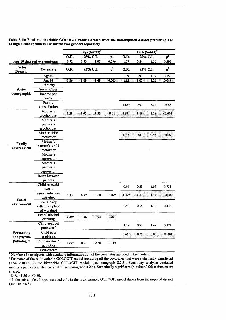
Table 8.13: Final multivariable GOLOGIT models drawn from the non-imputed dataset predicting age14 high alcohol problem use for the two genders separately

Boys (N=782) Girls (N=649)O.R. 95% C.I. PS O.R. 95% C.I. Pf

Age 10 depressive symptoms 0.92 0.80 1.07 0.296 1.07 0.84 1.36 0.597

FactorDomain Covariate O.R. 95% C.I. PS O.R. 95% C.I. P$

AgelO 1.09 0.97 1.22 0.166Age 14 1.26 1.08 1.48 0.003 1,12 1.00 1.26 0.044

EthnicitySocio Social Class

demographic Income per week

Familyconstellation 1.85t 0.97 3.54 0.063

Mother’s alcohol use 1.28 1.06 1.55 0.01 1.37f 1,18 1.58 <0.001



interaction 0.93 0.87 0.98 0.009

Familyenvironment


interactionMother’s

depressionMother’spartner’s

depressionRows between

parentsChild stressful

events0.99 0.89 1.09 0.774

Peers’ antisocial activities 1.25 0.97 1.60 0.082 L39f 1.12 1.73 0.003

socialenvironment Religiosity

(attends a place of worship)

0.92 0.75 1.13 0.438

Peers’ alcohol drinking 3.06t 1.18 7.93 0 021

Child conduct problemsA

1.18 0.93 1.49 0.173


Child peer problems

0 65f 0.53 0.80 <0.001

pathologies Child antisocial activities 1.47T 0.91 2.40 0.119

Self-esteem

$ Estimates of the multivariable GOLOGIT model including all the covariates that were statistically significant (p-value<0.05) in the bivariable GOLOGIT models (see paragraph 8.2.3). Sensitivity analysis excluded mother’s partner’s related covariates (see paragraph 8.2.4). Statistically significant (p-value<0.05) estimates are shaded.|O .R. >1.30 or <0.80.AIn the subsample of boys, included only in the multivariable GOLOGIT model drawn from the imputed dataset (see Table 8.8).

150

7.3 Missing data imputation and results of the multivariable GOLOGIT models:

synthesis of the chapter

In summary, in this chapter I described the results of the imputation procedure used to impute

the missing data and of the multivariable GOLOGIT models used to investigate how the

relationship between childhood depressive symptoms and alcohol problem use in adolescence

is corrected by a number or relevant covariates belonging to the socio-demographic, family

environment, social environment and personality and psychopathology domains.

Among all 35 variables included in the imputation model, only eight variables were fully

available for all the 4,220 participant children included in the study sample, reason for which

a missing data imputation was considered being necessary.

In order to identify those covariates to be included in the final models, the statistical

significance of all the covariates was tested by entering each of them independently in a

bivariable GOLOGIT2 model in which age 14 years alcohol problem use is predicted by age

10 years depressive symptoms.

Due to the presence of missing values in the covariates, each bivariable GOLOGIT model

drawn from the non-imputed dataset was based on a different subset of participants; on the

contrary, there were no differences in the numbers of participants on which each bivariable

GOLOGIT model was based upon when this was drawn from the imputed dataset.

I included in the multivariable models (for both the total sample and the subsamples of boys

and girls separately) only those covariates that, when tested in a bivariable model, were

statistically significant (p-value<0.05).

Concerning the gender difference in the pattern of covariates, when considering only the

subsample of girls, compared to the boys subsample, a greater number of covariates reached

the threshold of p-value<0.05 when tested in bivariable GOLOGIT models drawn from the

non-imputed and imputed datasets.

151

Results of the multivariable analysis using the non-imputed and the imputed covariates were

conducted in the total sample on sample sizes of N=1220 and N=4220, respectively.

With the inclusion of the relevant covariates, the relationship between childhood depressive

symptoms and adolescent high alcohol problem use was diminished compared to the

univariable, both in the imputed dataset (O.R. 1.05, p=0.22). The analysis conducted in the

imputed dataset showed that, in the total sample, the relationship between age 10 depressive

symptoms and age 14 alcohol problem use was influenced by a number of covariates

belonging to all the factor domains taken into account.

Results of the multivariable analyses on the boys and girls subsamples using the imputed

covariates indicated that, with the inclusion of the relevant covariates, there was no longer a

relationship between childhood depressive symptoms and adolescent high alcohol problem

use, neither for boys (O.R. 0.92, p=0.063), nor girls (O.R. 1.12, p=0.058), for whom the

strength of the relationship was diminished compared to the univariable model.

The relationship between depression and alcohol use was influenced by a number of

covariates, some from the personality factor domain (childhood peer problems for girls and

childhood antisocial behaviour for boys), but mostly from the family and social domains.

Family domain-related covariates included: maternal alcohol use for both boys and girls, and

(for girls only) also family constellation, and mother-child interactions. Furthermore, in the

social domain peer antisocial behaviour (for both boys and girls) and stressful life

experiences for girls also had an impact on the longitudinal relationship.

Similar to the imputed dataset, the association between age 10 depressive symptoms and age

14 alcohol problem use was no longer significant in boys and was strongly diminished in

girls, compared to the one observed in the univariable models.

152

Results indicated that most of the covariates that were statistically significant when tested in

the imputed dataset were also statistically significant in the non-imputed dataset for both boys

and girls.

153

CHAPTER 9: RESULTS OF THE UNIVARIABLE AND MULTIVARIABLE

GOLOGIT MODELS ACCOUNTING FOR PEERS’ INFLUENCES AT AGE 10 AND

AT AGE 14 YEARS

9.1 Results of the LR tests assessing the moderating effect of for peers’

influences (at age 10 and 14 years) in the total sample

As reviewed in paragraph 3.2.3 and 4.2.4, one of the aims of my thesis is to examine whether

the relationship between childhood depressive symptoms and alcohol problem use in

adolescence is moderated by the combined effect of two peer influences: child bonding with

his/her peers, and peer’s risky behaviour (see Table 5.4). Both these peers’ influences were

assessed by face-to-face interviews during the “clinics” at age 10 years (the same age of

assessment of depressive symptoms) and age 14 years (the same age of assessment of alcohol

problem use) (see paragraph 4.2.4).

Child bonding with his/ her peers was measured in both occasions with a shortened version of

the Friendships Questionnaire developed for the Cambridge Hormones and Moods Project

(Goodyer et al., 1990, Goodyer et al., 1989) (see paragraph 4.2.4.1). Peers’ risky behavior

was measured at age 10 with a structured questionnaire that was adapted from a measure of

self-reported antisocial behaviour for young children and included a question on peers’

alcohol drinking (Wolke et al., 1994), and at age 14 with a single question assessing how

often the child’s peers’ consumed alcohol in the previous six months (see paragraph 4.2.4.2).

As explained in paragraph 6.3.5, steps 1, 2 and 3, I performed a LR test to compare two

models: 1) a trivariable GOLOGIT model without interactions (i.e., a model having as

independent variables: a) “age 10 depressive symptoms,” b) “peers’ risky behaviour” and c)

“child’s bonding with his/her peers”) and 2) a three-way interaction trivariable GOLOGIT

model (i.e., a model having as independent variables: a) age 10 depressive symptoms,” b)

154

“peers’ risky behaviour” and c) “child’s bonding with his/her peers,” and including also the

four interaction terms: d) “age 10 depressive symptoms X child’s bonding with his/ her

peers,” e) “age 10 depressive symptoms X peers’ risky behaviour,” f) “child’s bonding with

his/ her peers X peers’ risky behaviour,” and g) “age 10 depressive symptoms X child’s

bonding with his/ her peers X peers’ risky behaviour”).

These GOLOGIT models (like all the GOLOGIT models presented in these chapters) were

drawn from the imputed dataset only and were based on the total sample; the analysis was

conducted twice, once including peers’ influences at age 10 years and once including peers’

influences at age 14 years. The results of the LR test helped me decide whether the model

accounting for interaction was fitting the data significantly better than the one without

interaction.

• Peers’ influences at age 10 years: Results of the LR test indicated that, with regards

to the trivariable GOLOGIT models accounting for peers’ influences at age 10 years, the

more complex interaction model including the interaction terms “d,” “e,” “f ’ and “g” did not

fit the data significantly better than the more parsimonious model not including the

interaction terms (LR X2(4)=2.72, p=0.605). Hence, the three-way GOLOGIT interaction

model based on the total sample accounting for peers’ influences at age 10 years was not

further analyzed (see paragraph 6.3.5, step 3).

• Peers’ influences at age 14 years: Results of the LR test, obtained comparing the

trivariable GOLOGIT models with and without the inclusion of the interaction terms with

peers influences at age 14 years, were similar to those obtained analyzing peers’ influences at

age 10 years; the more complex interaction model did not fit the data significantly better than

the more parsimonious model not including the interaction terms (LR X2(4)=7.46, p=0.113).

Hence, the three-way GOLOGIT interaction model based on the total sample accounting for

peers’ influences at age 14 years was not further analyzed (see paragraph 6.3.5, step 3).

155

9.2 Gender differences in the peers’ influences variables

Table 9.1 describes the gender differences from the variables describing peers’ influences

(see paragraph 6.3.5, step 4, note that Table 9.1 indicates the frequencies of the non-imputed

variables). At age 10 boys had peers who had more risky behaviours (they had partaken in a

higher number of antisocial activities) compared to the girls’ peers (LR X2(3) 191.8,

p<0.001), whereas girls had a stronger bonding with their peers than boys did (MWW z=2.9,

p=0.004). At age 14 there was no longer a statistically significant difference between boys’

and girls’ peers’ risky behaviours (peers’ alcohol drinking; LR X2(3) 7.3 p=0.062), although

girls still had a much stronger bonding with their peers than boys did (MWW z=9.8,

p<0.001).

Table 9.1: Peers’ influences variables presented separately for boys and girls

Variable Categories N boys/ N girls % boys % girls X*

No activities 51.4 73.4X2(3)191.8

p<0.001

Age 10 peers’ antisocial 1 activity ■ 1676/1977 28.8 16.1behaviour* B 2 activities 10.4 6.2

>3 activities 9.4 4.3Never 61.1 56.9

X2(3)7.3

p=0.062

Age 14 peers’ alcohol 1-3 times ■ 1662/1954 22.0 24.9drinking8 >4 times 9.4 10.7

Once per week 7.5 7.5

Variable MeasurementUnit

N boys/ N girls M (SD) boys M (SD) girls MWWt

Child bonding with peers at age 10 years Bonding score 2177/1973 5.9 (2.0) 6.1 (1.9) p=0.004

Child bonding with peers at age 14 years Bonding score 2001/2193 6.4 (1.9) 6.9 (1.6) pO.OOl

results are shaded.A Variable included information on whether friends had consumed alcohol without parental permission in the previous 6 months.B Variables describing peers’ risky behaviour.t Wilcoxon-Mann-Whitney test (z score). Statistically significant (p-value<0.05) results are shaded.

156

9.3 Results of the LR tests assessing the moderating effect of peers’ influences (at

age 10 and 14 years) and gender in the total sample

As explained in paragraph 6.3.5, step 5, I performed a LR test to compare two models: 1) a

quadrivariable GOLOGIT model without interaction (i.e., a trivariable GOLOGIT model

without interactions like the one described in paragraph 9.1 also including “gender” as the

fourth variable), and 2) a four-way interaction quadrivariable GOLOGIT model (i.e., a

GOLOGIT model having all four interaction terms of the three-way interactions trivariable

GOLOGIT model described in paragraph 9.1 interacting with gender as well).

This scope of this analysis was to determine whether the analysis investigating the effects of

peers’ influences should be conducted only in the total sample or also separately in the two

subsamples of boys and girls.

These models were therefore based on the total sample, and the analysis was conducted

twice, once including peers’ influences at age 10 years and once including peers’ influences

at age 14 years.

• Peers’ influences at age 10 years: Results of the LR test indicated that, concerning

the quadrivariable GOLOGIT models accounting for peers’ influences at age 10 years plus

gender, the more complex interaction model including the interaction terms “d,” “e,” “f ’ and

“g” (see paragraph 9.1) interacting with gender did not fit the data significantly better than

the more parsimonious model not including any of the interaction terms (LR X2(10)=12.72,

p=0.240). Hence, the effects of age 10 peers’ influences in the relationship between age 10

years depressive symptoms and age 14 years alcohol problem use was not further studied

separately in the two subsamples of boys and girls (see paragraph 6.3.5, step 6).

• Peers ’ influences at age 14 years: In contrast to the results of the analysis conducted

accounting for age 10 peers’ influences, the results of the LR test indicated that the

quadrivariable GOLOGIT models accounting for the interaction terms with peers’ influences

157

at age 14 years plus gender did fit the data significantly better than the more parsimonious

model not including any of the interaction terms (LR X2( 10)= 19.99, p=0.029). These results

warranted further LR tests to be conducted on the two three-way GOLOGIT interaction

models based on the boys and girls subsamples and accounting for peers’ influences at age 14

years (see paragraph 6.3.5, step 6).

9.4 Results of the LR tests assessing the moderating effect of for peers’

influences at age 14 years in the subsamples of boys and girls

Following the results reported in paragraph 9 .3 ,1 performed a LR test comparing, in both the

boys and girls subsamples, the more complex model accounting for interaction between age

10 depressive symptoms and age 14 peers’ influences (i.e., child’s bonding with his/ her

peers at age 14 years and age 14 years peers’ alcohol drinking) and the more parsimonious

model not including the interaction terms (see paragraph 6.3.5, step 6).

Results of the LR test in the subsample of boys indicated that the more complex model did

not fit the data better than the more parsimonious one (LR X2(4)=7.69, p=0.104); however,

the LR test conducted in the subsample of girls provided opposite results (i.e., that the model

including the interaction terms did fit the data better than the models not accounting for

interaction; LR X2(4)=9.55, p=0.048). In order to better understand the role of peers’

influences at age 14 years in the subsample of girls, the three-way GOLOGIT interaction

model accounting for peers’ influences at age 14 years was further analyzed, testing the

significance levels of the three interaction terms including age 10 depressive symptoms (i.e.,

1) “age 10 depressive symptoms X child’s bonding with his/ her peers,” 2) “age 10

depressive symptoms X peers’ alcohol drinking,” and 3) “age 10 depressive symptoms X

child’s bonding with his/her peers X peers’ alcohol drinking”) (see paragraph 6.3.5, step 7).

Results are reported, for the imputed dataset only, in Table 9.2.

158

9.5 Results of the trivariable GOLOGIT interaction models accounting for

peers’ influences at age 14 years in the girls’ subsample

Results of the analysis of the trivariable GOLOGIT interaction model in the subsample of

girls indicated that the interaction term “age 10 depressive symptoms X child’s bonding with

his/ her peers X peers’ alcohol drinking” was statistically significant (O.R 0.95, 95% C.I.

0.89; 1.00, p=0.048) and, therefore, the hypothesis of a three-way interaction between age 10

depressive symptoms, child bonding with peers at 14 years and age 14 years peers’ alcohol

drinking was valid (see Table 9.2).

Accounting for the moderating effect of age 14 peers’ influences (i.e., child’s bonding with

his/ her peers and age 14 years and age 14 years peers’ alcohol drinking) in the relationship

between age 10 depressive symptoms and age 14 alcohol problem use, with progressively

higher levels of depressive symptoms girls had experienced in childhood, there was an

association with a 17% greater risk of developing high alcohol problem use in early

adolescence (O.R. 1.17, 95% C.I. 1.02; 1.34, p=0.029, see Table 9.2), which resulted in a

51% increased risk for those girls who experienced very high depressive symptoms in

childhood compared to those who experienced them at lower levels.

Therefore, when included in the girls’ subsamples GOLOGIT univariable model described in

paragraph 7.3, the combined effect of child’s bonding with his/ her peers and peers’ alcohol

drinking further increased the risk of developing age 14 high alcohol problem use in girls

who experienced very high depressive symptoms at age 10 by 9% (see Table 9.2).

Both age 14 peers’ influences were statistically significant when considered individually

(child’s bonding with his/ her peers at age 14 years; O.R. 1.29; 95% C.I. 1.21; 1.36, p<0.001

and age 14 years peers’ alcohol drinking; O.R. 2.96, 95% C.I. 2.64; 3.32, p<0.001). These

results also excluded the possibility that the moderation of the relationship between age 10

depressive symptoms and age 14 alcohol problem use may be the result of the effect of only

159

one of the two peers’ influences at 14 years taken into account; in fact, neither of the two-way

interactions between “age 10 depressive symptoms X child’s bonding with his/ her peers”

and “age 10 depressive symptoms X peers’ alcohol drinking” were statistically significant (p-

value<0.005), whereas the combined effect of child’s bonding with his/ her peers X peers’

alcohol drinking had O.R. 1.09, 95% C.I. 1.02; 1.16, p=0.007 (see Table 9.2).

Table 9.2: T rivariable GOLOGIT interaction models accounting for peers’ influences at age 14 years in the girls’ subsample (im puted dataset)

G irls’ subsample (N=2202) O.R. 95% C.I. p*Age 10 depressive symptoms NOT accounting for peers’

influencesA 1.14 1.02 1.27 0.016

Age 10 depressive symptoms accounting for peers’ influences6 1.17 1.02 1.34 0.029

Peers’ influences O.R. 95% C.I. p 5Child bonding with peers at age 14 years 1.29 m m r n r n u i 1.36 <0.001

Age 14 years peers alcohol drinking 2.961* m M m m m m m m m <0.001

Interaction term s O.R. 95% C.I. p$child’s bonding with his/ her peers X peers’ alcohol

drinking0 1.09 1.02 1.16 0.007

age 10 depressive symptoms X child’s bonding with his/her peers0 1.00 0.95 1.06 0.958

age 10 depressive symptoms X peers’ alcohol drinking0 1.07 0.97 1.20 0.189age 10 depressive symptoms X child’s bonding with

his/her peers X peers’ alcohol drinking® 0.95 0.89 1.00 0.048

¥ Univariable GOLOGIT model. Statistically significant (p-value<0.05) estimates are shaded.$ Trivariable GOLOGIT interaction model. Statistically significant (p-value<0.05) estimates are shaded. tO.R. >1.30 or <0.80.A Univariable model not accounting for peers’ influences, reported here for reference purposes only (see paragraph 7.3 for more details).

Univariable model accounting for peers’ influences. c Interaction between the two peers’ influences variables.D Two-way interaction with age 10 depressive symptoms.E Three-way interaction with age 10 depressive symptoms.

9.6 Graphical representation of the univariable GOLOGIT model in the

subsample of girls according to the level of bonding with peers and peers’ alcohol

drinking status

160

In order to interpret the estimate of the three-way interaction term “age 10 depressive

symptoms X child’s bonding with his/ her peers X peers’ alcohol drinking” (O.R 0.94, 95%

C.I. 0.89; 1.00, p=0.042, see Table 9.2), it was necessary to analyze how age 10 years

depressive symptoms predict age 14 years alcohol problem use when children experienced

different combinations of bonding with their peers at age 14 years and of age 14 years peers’

alcohol drinking (Aiken, 1991).

To do so, as explained in paragraph 6.3.5, step 8, by using a cut-off at the ~50th percentile I

divided the variable “child’s bonding with his/ her peers at age 14 years” (see Table 5.4) in

two categories: “low bonding” (frequencies in the imputed dataset: 41.3% of the total sample,

34.9% of the subsample of girls) and “high bonding” (frequencies in the imputed dataset:

58.7% of the total sample, 65.1% of the subsample of girls) and divided the variable “age 14

peers’ alcohol drinking” (see Table 5.4) in “non-drinking peers” (never consumed alcohol in

the previous six months, frequencies in the imputed dataset: 59.6% of the total sample, 57.7%

of the subsample of girls) and “drinking peers” (consumed alcohol at least 1 -3 times in the

previous six months, frequencies in the imputed dataset: 40.4% of the total sample, 42.3% of

the subsample of girls).

I have subsequently run the univariable GOLOGIT model in the girls subsample (see

paragraph 7.3) for each of the four possible combinations of “child’s bonding with peers” and

peers’ alcohol drinking” (see paragraph 6.3.5, step 9); i.e.: 1) “low bonding with peers” and

“non drinking peers,” 2) “high bonding with peers” and “non drinking peers,” 3) “low

bonding with peers” and “drinking peers,” and 4) “high bonding with peers” and “drinking

peers.”

Using the post-estimation command “predict” (see paragraph 6.3.5, step 10), I estimated the

expected probability of each of the univariable GOLOGIT models (corresponding to the

expected probability of developing high alcohol problem use) for each of the four possible

161

combinations of peers’ influences described above. Figure 9.1 graphically represents the

expected probability estimates for the four GOLOGIT models in the subsample of girls,

plotting them against the four categories of the “age 10 depressive symptoms” variable

(“low,” “medium,” “high” and “very high”).

Please note that in the graph displayed in Figure 9.1 I have set constant=0 for the expected

probability estimate equation of every model to allow an easier comparison to be made

between the slopes of the plotted predicted probability estimates. As the reference line

(coloured in light gray), I included in both graphs the expected probability estimate of the

univariable GOLOGIT without accounting for peers’ influences (see figure 7.1).

It was observable that, while the effect of peers’ alcohol drinking was constantly increasing

the risk (overall increase of the slope of the expected probability estimate (see figure 9.1) of

developing age 14 high alcohol problem use, compared to the reference line) of developing

high alcohol problem use at age 14 years for girls who experienced very high depressive

symptoms at age 10 years compared to those who experienced low depressive symptoms at

age 10 years, the effect of bonding with peers was highly dependent on the drinking status of

the peers’ themselves.

In fact, if girls’ peers did consume alcohol in the previous six months, having a strong bond

with peers increased the effect of age 10 depressive symptoms as a predictor of age 14

alcohol problem use (overall increase of the slope of the expected probability estimate (see

figure 9.1) of developing age 14 high alcohol problem use, compared to the reference line).

However, for girls who had a strong bond with their peers and who reported that their peers

did not consume alcohol, the risk of developing high alcohol problem use at age 14 years for

girls who experienced very high depressive symptoms at age 10 years, compared to those

who experienced low depressive symptoms at age 10, was reduced compared to the

uni variable GOLOGIT model not accounting for peers’ influences (overall decrease of the

162

slope of the expected probability estimate (see figure 9.1) of developing age 14 high alcohol

problem use, compared to the reference line).

Figure 9.1: Slopes of the expected probability estimates of the univariable GOLOGIT model in the subsample of girls according to the level of bonding with peers and peers’ alcohol drinking status1

0.8

<3£ 0.7

0.6

2£ 0.5

f...wS* 0 3C<u£ 0.20 <u

1 01

Medium High Vety HighLow

— - Lowbondingwith pea’s &Non-drinkingpeers

—• —High bondingwith pea's & Non-drinking pea s

- -a- - Low bonding with pea’s &Drink ingpeers

—■— High bondingwitli pears & Drinkingpeers

■ Univariable model NOT accounting for p ea s ’ influaices (refaaice line)

Age 10 depressive symptoms

!In light gray it is indicated, as the reference line, the expected probability estimate of the girls’ subsamples’ univariable GOLOGIT model not accounting for peers’ influences (see paragraph 7.3 for details).

9.7 Results of the multivariable GOLOGIT interaction models accounting for

peers’ influences at age 14 years in the girls’ subsample

The trivariable three-way interaction GOLOGIT model described in paragraph 9.5 was

included in the multivariable GOLOGIT model (drawn from the imputed dataset) based on

the subsample of girls, which has been described in detail in paragraph 8.2.6.

LR test comparing the multivariable GOLOGIT model with and without the presence of the

four interaction terms, i.e.: a) “age 10 depressive symptoms X child’s bonding with his/ her

peers,” b) “age 10 depressive symptoms X peers’ risky behaviour,” c) “child’s bonding with

163

his/ her peers X peers’ risky behaviour,” and d) “age 10 depressive symptoms X child’s

bonding with his/ her peers X peers’ risky behaviour,” indicated that the more complex

model (including the interaction terms) did fit the data significantly better than the more

parsimonious model not including any of the interaction terms (LR X2(4)= 10.62, p=0.031).

Results of the three-way interaction multivariable GOLOGIT model indicated that the tree

way interaction term “age 10 depressive symptoms X child’s bonding with his/her peers X

peers’ alcohol drinking” was statistically significant, indicating that the hypothesis of a three-

way interaction between age 10 depressive symptoms, child bonding with peers at 14 years

and age 14 years peers’ alcohol drinking was valid also when accounting for the correcting

effect of covariates (O.R. 0.94, 95% C.I. 0.89; 1.00, p=0.042, see Table 9.3).

When accounting for the moderating effects of the combination of bonding with peers at age

14 years and age 14 years peers’ alcohol drinking, age 10 depressive symptoms had a

stronger effect as predictor of age 14 alcohol problem use (O.R. 1.18, 95% C.I. 1.02; 1.37,

p=0.030, see Table 9.3), compared to both the multivariable GOLOGIT model not

accounting for peers’ influences (O.R. 1.12, 95% C.I. 1.00; 1.25, p=0.058; see Table 8.12)

and to the trivariable three-way interaction GOLOGIT model not accounting for the effects of

the covariates (O.R. 1.17, 95% C.I. 1.02; 1.34, p=0.029, see Table 9.2).

Hence, accounting for the moderating effect of age 14 peers’ influences (i.e., child’s bonding

with his/ her peers at age 14 years and age 14 years peers’ alcohol drinking) in the

relationship between age 10 depressive symptoms and age 14 alcohol problem use, and

including all the relevant covariates, each increasing level of depressive symptoms girls had

experienced in childhood was therefore associated with an 18% greater risk of developing

high alcohol problem use in early adolescence, which resulted in a 54% increased risk for

those girls who experienced very high depressive symptoms in childhood compared to those

who experienced low levels of them.

164

Therefore, when included in the girls’ subsample’s GOLOGIT multivariable model described

in paragraph 8.2.6, the combined effect of child’s bonding with his/ her peers and peers’

alcohol drinking further increased by 18% the risk of developing age 14 high alcohol problem

use in girls who experienced very high depressive symptoms at age 10 (see Table 9.3).

No other significant differences were found between the three-way interaction multivariable

GOLOGIT model reported in Table 9.3 and the three-way interaction trivariable GOLOGIT

model reported in Table 9.2. However, some differences in the estimates of the covariates

were found when comparing the three-way interaction multivariable GOLOGIT model

reported in Table 9.3 with the multivariable GOLOGIT model not accounting for peers’

influences reported in Table 8.12.

• Socio-demographic domain: no differences; both age of assessment of alcohol

problem use (age 14) (O.R 1.15, 95% C.I. 1.07; 1.23, p<0.001) and family constellation (O.R.

1.54, 95% C.I. 1.03; 2.29, p=0.034) still statistically significant.

• Family environment domain: no differences; both mothers’ alcohol use (O.R. 1.14,

95% C.I. 1.03; 1.28, p<0.016) and mother-child interaction (O.R. 0.96, 95% C.I. 0.93; 1.00,

p=0.048) still statistically significant.

• Social environment domain: differences between the two models; both stressful life

events and peers’ antisocial activities no longer statistically significant in the model

accounting for peers’ influences (p-value >0.05).

• Personality and psychopathologies domain: differences between the two models;

child peer problems no longer statistically significant in the model accounting for peers’

influences (p-value >0.05).

165

Table 93 : M ultivariable GOLOGIT interaction models accounting for peers’ influences at age 14 years in the girls’ subsample (imputed dataset)

Girls’ subsample (N=2202) O.R. 95% C.I. p sAge 10 depressive symptoms NOT accounting

for peers’ influences and corrected for covariates effectsA

1.12 1.00 1.25 0.058

Age 10 depressive symptoms accounting for peers’ influences6 1.18 1.02 1.37 0.030

Peers’ influences O.R. 95% C.I. PSChild bonding with peers at age 14 years 1.20 1.36 <0.001

Age 14 years peers alcohol drinking m i m t m m r n 2.57 <0.001

Interaction term s O.R. 95% C.I. p*child’s bonding with his/ her peers X peers’

alcohol drinking0 1.10 1.03 1.17 0.004

age 10 depressive symptoms X child’s bonding with his/her peers0 1.00 0.95 1.06 0.995

age 10 depressive symptoms X peers’ alcohol drinking0 1.07 0.96 1.19 0.228

age 10 depressive symptoms X child’s bonding with his/her peers X peers’ alcohol drinking6 0.94 0.89 1.00 0.042

Factor Domain Covariate O.R. 95% C.I. p$AgelO 0.98 0.92 1.05 0.637Agel4 1.15 1.07 123 <0.001

Socio-demographicEthnicity

Social ClassIncome per week

Family constellation 1.54f 1.03 2.29 0.034Mother’s alcohol use 1.14 1.03 1.28 0.016

Mother’s partner’s alcoholuse

Mother-child interaction 0.96 0.93 1.00 0.048Family

environmentMother’s partner’s-child

interactionMother’s depressionMother’s partner’s

depressionRows between parentsChild stressful events 1.05 0.99 1.12 0.121

Peers’ antisocial activities 0.97 0.85 1.11 0.696Social environment Religiosity (attends a place

of worship) 0.91 0.81 1.03 0.147

Peers’ alcohol drinkingChild conduct problems 1.05 0.91 1.23 0.494

Personality and Child peer problems 0.93 0.82 1.06 0.266psycho-pathologies Child antisocial activities

T w -7',Self-esteem

A Multivariable model not accounting for peers’ influences, reported here for reference purposes only (see paragraph 7.3 for more details).B Multivariable model accounting for peers’ influences.0 Interaction between the two peers’ influences variables.D Two-way interaction with age 10 depressive symptoms.E Three-way interaction with age 10 depressive symptoms. fO.R. >1.30 or <0.80.

166

9.8 Results of the univariable and multivariable GOLOGIT models accounting

for peers’ influences at age 10 and at age 14 years: synthesis of the chapter

In summary, in this chapter I tested peers’ influences (i.e., child’s bonding with his/ her peers

and peers’ alcohol drinking) at both age 10 and 14 years as possible moderators of the

relationship between age 10 years depressive symptoms and age 14 years alcohol problem

use in both the univariable and multivariable GOLOGIT models.

In contrast to the results of the analysis conducted accounting for age 10 peers’ influences,

the results of the LR test indicated that the GOLOGIT models accounting for the interaction

terms with peers’ influences at age 14 years did fit the data significantly better than the more

parsimonious model not including any of the interaction terms.

I performed therefore a LR test comparing, in both the boys and girls subsamples, the more

complex model accounting for interaction between age 10 depressive symptoms and age 14

peers’ influences and the more parsimonious model not including the interaction terms.

In the subsample of boys indicated that the more complex model did not fit the data better

than the more parsimonious one (LR X2(4)=7.69, p=0.104); however, the LR test conducted

in the subsample of girls provided opposite results (i.e., that the model including the

interaction terms did fit the data better than the models not accounting for interaction; LR

X2(4)=9.55, p=0.048).

Results indicated the combined effect of child’s bonding with his/ her peers and peers’

alcohol drinking further increased the risk of developing age 14 high alcohol problem use in

girls who experienced very high depressive symptoms at age 10 by 9%, hence progressively

higher levels of depressive symptoms girls had experienced in childhood were associated

with a 16% greater risk of developing high alcohol problem use in early adolescence, which

resulted in a 51% increased risk for those girls who experienced very high depressive

symptoms in childhood compared to those who experienced them at lower levels.

167

When the peers’ influences (i.e., child’s bonding with his/ her peers and peers’ alcohol

drinking) were considered separately, it was observable that, while the effect of peers’

alcohol drinking was constantly increasing the risk of developing high alcohol problem use at

age 14 years for girls who experienced very high depressive symptoms at age 10 years

compared to those who experienced low depressive symptoms at age 10 years, the effect of

bonding with peers was highly dependent on the drinking status of the peers’ themselves.

Finally, results of the three-way interaction multivariable GOLOGIT model indicated that the

hypothesis of a three-way interaction between age 10 depressive symptoms, child bonding

with peers at 14 years and age 14 years peers’ alcohol drinking was valid also when

accounting for the correcting effect of covariates (O.R. 0.94, p=0.041).

168

PARTY

CHAPTER 10: DISCUSSION

10.1 Common risk and protective factors for harmful alcohol use and depressive

symptoms in youth identified in the literature

10.1.1 Main findings

There is a strong association between alcohol problem use and depressive symptomatology in

adolescence, which has been reported by many (but not all (Becker et al., 2006)) studies

(Bukstein et al., 1992, Clark et al., 1997b). The link between these disorders could be direct:

for example, AD may trigger depression (Kuo et al., 2006), or it could be due to the

depressogenic effect of ethanol (Abraham et al., 1999). However, it is also likely that

depressive symptomatology and alcohol problem use share risk factors: a number of non-

genetic and genetic risk factors have been associated with the development of both disorders

in adolescents. Thus, shared risk factors might contribute to the co-morbidity between both

traits.

Results of a systematic review I conducted, reviewing all the epidemiological and genetic

studies that focused on common factors for alcohol problem use and depressive symptoms

published between the years 1997-2007, indicated that factors such as externalizing disorders

(in particular conduct disorder), family alcohol problems and stress, as well as gene variants

such as the 5-HTT S-allele, the MAOA low activity variant and the DDR2 Taq Al allele

have received relatively more research support for a role in the development of the co

morbidity of both disorders. Some of these factors (e.g., 5-HTT S-allele) have also been

supported to play a role in the development of both behaviours by meta-analyses (Feinn et al.,

169

2005, Schinka et al., 2004, Sen et al., 2004a). Other factors have been less frequently studied,

the support provided is weaker, or there are contradicting findings (e.g. ethnicity and the

BDNF Val66Met variant). My systematic search identified only one shared protective factor

(religion).

In interpreting the findings of the literature review, it is important to distinguish between risk

factors and causal risk mechanisms (Beardslee et al., 1997). As Garber (Garber, 2006)

suggested, risk factors are antecedents that increase the probability of an outcome over the

population base rate; however, taken singularly, they do not explain the processes involved in

the development of a pathological condition (Garber, 2006). The study of co-morbidity is

further complicated because among risk factors, some (such as sleep problems) can be

considered both potential causes as well as symptoms of alcohol problem use and

internalizing symptomatology. They could therefore contribute to a vicious circle by

increasing the risk of development of each disorder.

10.1.2 Reasons why genetic risk and protective factors were not included in the

analyses

After the completion of the literature review, I decided to avoid analyzing the impact of

genetic risk and protective factors in the relationship between childhood depressive

symptoms and alcohol problem use in early adolescence.

This decision was taken in concert with my supervisors; four reasons made us agree that, at

the time I started the epidemiological and statistical analyses of the ALSPAC dataset (May

2008), this was a sensible choice to make:

1. In general, there was greater agreement on positive findings for factors identified

through epidemiological studies than for those identified through molecular studies, for both

alcohol problem use and depressive symptomatology in adolescents. For epidemiological

170

factors, conflicting results were found for only three risk factors (ethnicity, SES and

educational level). On closer scrutiny, contradictory findings can sometimes make sense; for

example, one reason for the discrepancies found with respect to SES may be that heavy

alcohol consumption is more likely in those with high income but low educational

qualifications (Casswell et al., 2003). In contrast, for almost all the factors identified through

molecular genetic studies contradictory findings were found. Heterogeneity in the

methodologies among molecular studies is likely to have contributed to the discrepancies. For

example, among the studies we reviewed were: population and pedigree studies (Bolos et al.,

1990), longitudinal genetically informative studies (Olsson et al., 2005a), Positron Emission

Tomography (PET) studies (Hietala et al., 1994) and post-mortem receptor-binding studies

(Noble et al., 1991). In addition, heterogeneity in study samples is also likely to have

contributed to discrepancies in my findings. For example, among molecular studies

examining the BDNF Val66Met variant, studies included male Japanese alcoholics and non

alcoholics (Matsushita et al., 2004), Chinese alcoholics, Northem-Taiwanese prisoners and

controls (Tsai et al., 2005), depressed Mexican-American patients (Ribeiro et al., 2007) and

untreated depressed Chinese patients (Tsai et al., 2003).

2. Moreover, due to variation in research interest for different gene variants, some

variants, such as the 5-HTT S-allele, have been the focus of considerably more research

attention than others, such as the CHRM2 SNPs, for which there is a paucity of studies.

3. While most epidemiological studies that were identified for my literature review were

based on adolescents, the majority of molecular studies were based on adult samples. This is

likely to be due to the lower frequency of clinically diagnosed alcohol dependence abuse

and/or and major depressive disorder in young subjects. This would represent no problem

where the study of genetic polymorphisms is concerned; however, before attempting to

analyze the combined effects of genetic and non-genetic risk factors in adolescent samples, it

171

may be necessary to compare studies of gene expression for adult and adolescent samples,

particularly because some studies of alcohol and internalizing psychopathology indicate

adolescent-onset disorder may represent a more severe phenotype with worse lifetime

prognosis (DeWit et al., 2000, Grant et al, 2001, Pine et al., 1999, Pine et al., 1998).

Moreover, genetic influences may also affect the environment individuals experience,

changing the way individuals shape, select and process their experiences, so-called active

gene-environment correlation (Rutter et al., 1997).

4. Furthermore, even if gene-environment interactions are increasingly detected and

replicated in psychiatry (Uher, 2008), their study is complicated by the large number of

potential interactions (Owen et al., 2000); the relations between risk factors and alcohol

problem use and depressive symptomatology in adolescence can be either direct or indirect,

mediated or moderated by other risk factors (for a definition and examples of mediation and

moderation see (Munafo, 2006)). This situation becomes even more complicated if

hypothetical interactions between different genetic factors and between different non-genetic

factors are also considered (see, for example, Figure 2.1 in Chapter 2, graphically

representing the potential mechanisms by which genetic and non-genetic factors and their

interactions may influence alcohol problem use and depressive symptomatology in

adolescence).

With regard to the study of gene-environment interaction, a cautious research strategy has

been suggested by Moffit et al. (Moffitt et al., 2005), which should include: the identification

of possible environmental risk factors, the identification of putative susceptibility genes and

the elaboration of a gene-environment interaction hypothesis that should extend beyond the

initially hypothesized triad of gene, environmental factor and disorder. Owen and Cardno

(Owen et al., 1999) have furthermore argued that the establishment of the role of a genetic or

environmental factor in the development of a psychiatric disorder will necessarily have to be

172

based on a considerable number of studies, where positive findings are replicated in large

new samples, with meta-analysis providing important additional support for the confirmation

of a hypothesis.

5. Finally, noticeably, among the studies gathered in my systematic review, with the

exception of the gene x environment interaction studies reviewed in paragraph 2.7, there was

no overlap between those studies focusing on non-genetic factors and those focusing on

genetic factors. This further highlights the need of addressing both genetic and environmental

factors in future studies aimed to investigate the underpinnings of alcohol problem and

depressive symptoms in youth, rather than considering genetic and environmental effects

separately.

Given all these considerations, it was decided that at the time I planned my analyses in

ALSPAC, the field of the genetics of alcohol dependence had not progressed sufficiently for

me to test a finite number of a priori well-specified mechanisms of gene-environment

interplay.

10.1.3 Update of the literature analysis for the period November 2007 - May 2011

In order to update the systematic review that I conducted at the beginning of my research (the

3rd November 2007), a new literature search was conducted in order to include into the thesis

more recent articles that focused only on non-genetic risk factors in common for depression

and alcohol problems in youth. This literature search was conducted semi-systematically,

using the same search terms listed in Table 2.2 with the exclusion of the terms “Genetic

Predisposition to Disease OR Polymorphism, Genetic OR Genetic Risk Factor OR Genotype

OR Polymorphism, Single Nucleotide” (this was done because in the analysis I did not

include variables describing relevant genetic variants of the participants, as I explained in the

paragraph above); the date limits imposed were from the day after the initial literature search

173

was conducted (4th November 2007) and the 30 March 2010, date of submission of the

Thesis.

18 papers were found through this search and, excluding duplicates and papers not relevant

for my search (for example because they were mostly focusing on genetic risk factors for

depression and alcohol problems in youth), a total of 12 papers were retained and analyzed.

A number of risk factors belonging to the domains of socio-demographic factors, family

environment and personality and psychopathologies (but not social environment) were

reported by these studies as being associated with the development of alcohol problem use

and/or internalizing problems in youth.

• Socio-demographic factors domain: Residing in urban versus rural areas may

contribute to differences in terms of increased risk to engage with the consumption of either

alcohol or marijuana (Martino et al., 2008). Martino et al. reported that youth may engage in

heavy alcohol consumption at faster rates when residing in micropolitan (as opposed to

metropolitan) areas, marijuana use increases at a faster rate in youth living in urban (versus

rural) areas in general. However, while the locality of an individual is important to take into

consideration, factors that are associated with one’s residence play greater roles; differences

in the rate of change of substance use can be in fact attributed to factors such as racial/ethnic

composition, residential instability, and availability of marijuana (Martino et al., 2008).

Neighborhood quality was assessed also in a sample of 220 males, initially recruited as 3- to

5-year-old children of families composed by at least one alcoholic parent and neighbouring

families. Longitudinal changes over two decades in neighborhood environments (i.e., high

frequency of family mobility) from early childhood to adolescence had significant effects in

increasing the risk of developing alcohol-use disorder, marijuana-use disorder, and major

depressive disorder symptoms in late adolescence (Buu et al., 2009).

174

Neighbourhood characteristics were also associated also with the development of depressive

symptoms. Shaefer-McDaniel reported on a sample of 126 young adolescents in three

disadvantaged New York City neighbourhood that children's evaluations of neighbourhood

quality were positively related to their assessments of depression and there was an positive

association between the neighbourhood drug/alcohol stressor and child depression (Schaefer-

McDaniel, 2009). Furthermore, among young adults, unemployment and living alone were

reported as being associated with a higher risk of having suicidal ideation (Legleye et al.,

2010).

• Family environment domain: Hill et al. observed that children and adolescents

exposed to poor family management had an increased the risk of developing alcohol

problems in young adulthood (Hill et al., 2010). A study by Mackie et al., moreover,

identified four drinking motives classes (family-oriented, social, enhancement/social, and

coping/social). According to the authors, heritable influences may predispose individuals to

drink to cope with negative affect, for social reasons, and to a lesser extent for enhancement

(Mackie et al., 2010), whereas familial environmental influences shaped family-oriented

motives for drinking in adolescents (Mackie et al., 2010).

Concerning internalizing problems, bad relationship between the parents was found

predictive of suicidal ideation among both young men and women (age 18-30 years) in

France (Legleye et al., 2010), whereas a perceived negative family environment increased

both adolescents’ and their parents’ depressive symptoms among shelter-recruited

adolescents (Slesnick et al., 2009). Particularly in children of alcoholics, parent alcohol

dependence has a unique effect on child internalizing symptoms, above and beyond those of

both parent depression and antisocial personality disorder (Hussong et al., 2008). Among

Children of Alcoholics Family density of alcoholism was found significantly related to the

development of mental disorders (particularly depression, phobias and generalized anxiety

175

disorder) also in a multisite epidemiological study conducted in 8 Spanish cities, on 371

Children of Alcoholics and 147 controls aged 6-17 years (Diaz et al., 2008).

Finally parental rearing styles of rejection and lack of emotional warmth were associated with

offspring social phobia. (Knappe et al., 2009). Knappe et al also observed that the analyses of

interaction of parental psychopathology and parental rearing styles indicated combined

effects on the risk for offspring’s social phobia (Knappe et al., 2009).

• Personality and psychopathologies domain: Hill et al. using data from a c o m m u n ity

sample of 808 men and women interviewed from ages 10 to 27 in the Seattle Social

Development Project found that behavioural disinhibition (but not behavioural inhibition)

increased likelihood of both alcohol abuse and alcohol dependence at age 27 (Hill et al.,

2010). Beck et al, moreover, observed that among college students, cognitive reasons such as

drinking for social facilitation was associated with drinking and driving and housing

violations (Beck et al., 2008).

Finally, a recent study by Schulte et al focusing on gender difference in the pattern of risk

factors for alcohol problems in adolescence, observed that personality characteristics such as

positive drinking expectancies and deviance proneness factors appeared to impact boys and

girls similarly, whereas in contrast, physiological and social changes particular to

adolescence appear to differentially affect boys and girls as they transition into adulthood

(Schulte et al., 2009).

Overall, this new literature search showed that between November 2007 and May 2011,

epidemiological studies on non genetic risk factor for alcohol and internalizing problems in

youth focused mainly in the role of neighborhood quality for what concerns the socio

demographic factors domain, on the role of parental alcohol problem for what concerns the

176

family environment factors domain and on the role of cognitive factors such as drinking

expectancies for what concerns the personality and psychopathologies factors domain.

Only 12 studies were included in this update of the bibliographic search. This is somewhat an

unexpected little number if compared with the expected trend in papers publication in the

years 1997 - 2007 showed by figure 2.1. According to such figure it would have been

foreseeable >30 papers responding to the search criteria and being published in the past three

years. However it must be underlined that such figure included both epidemiological studies

focusing on non-genetic risk factors and molecular studies focusing on genetic risk factors.

Therefore the numbers of epidemiological studies I would have expected to include in the

thesis bibliography with this updated search would have been approximately 15. The fact that

instead only 12 studies were fully analyzed indicates probably a steady increase in the

number of published studies focusing on genetic risk factors for both alcohol problem use and

internalizing problems in youth, with increasingly less studies focusing on non-genetic risk

factors only Hopefully this research effort in the field of psychiatric genetics will shed more

light on the role of genes in the development of both alcohol problems and depression in

young people, providing to future researchers sufficient evidence about the role of specific

genetic variants in the development of both behaviours so that a finite number of a priori

well-specified mechanisms of gene-environment interplay may be tested.

10.2 Gender differences in the factors impacting on the relationship between

childhood depressive symptoms and adolescence alcohol problem use


There is a lack of understanding of the developmental relationship between depression and

alcohol problem use in youngsters (King et al., 2004). It remains to be elucidated which

177

factors impact upon this relationship and whether the developmental pathways differ for boys

and girls. My thesis aimed to contribute to this knowledge base. The study I conducted is the

largest to analyze a coetaneous sample of boys and girls; I examined childhood depressive

symptoms (at age 10) and alcohol problem use in early adolescence (at age 14) in a large

population-based sample of narrow age range. The narrow age range means that my findings

have been relatively unconfounded by differences in developmental stages between the

adolescents, compared to previous studies in samples of wider age ranges (Marmorstein,

2009).

10.2.2 Link between depressive symptoms and alcohol problem use in the young

Alcohol problem use and depressive symptomatology have been increasing in frequency in

adolescents in the UK and in the U.S.A. (EMCDDA, 2007, Anderson et al., 2006b, Green et

al., 2005, Harford et al., 2005, Hibell et al., 2004, Lewinsohn et al., 1991, Lopez et al., 2006).

These problems may be particularly common amongst British adolescents (EMCDDA, 2007,

Anderson et al., 2006b, Green et al., 2005, Hibell et al., 2004), with concerns having been

expressed about their declining psychological well-being (Collishaw et al., 2004). A number

of studies have reported a strong association between early-onset depression and subsequent

development of alcohol problem use in adolescence (Bukstein et al., 1992, Clark et al.,

1997b).

My results of the univariable GOLOGIT models indicated that children who experienced

very high levels of depressive symptoms in childhood had a 27% increased risk of developing

alcohol problem use in early adolescence compared to those who had low levels of depressive

symptoms.

178

10.2.3 Gender differences in the relationship between depressive symptoms and

alcohol problem use and in the impact of covariates

Consistent with the most recent findings in UK-based studies (Hibell et al., 2004, Smith,

2009, IAS, 2007), I found that girls at age 14 years had higher levels of alcohol problems

than boys did. Boys showed higher levels of depressive symptoms in childhood than girls, a

finding in accordance with a review by Nolen-Hoeksema and Girgus, which indicated that

pre-adolescent boys may either have similar or higher levels of depression to those in girls

(Nolen-Hoeksema et al., 1994).

Although the LR test for the interaction between gender and age 10 depressive symptoms in

the relationship between age 10 depressive symptoms and age 14 alcohol problem use was

statistically non significant, the entire analysis was nevertheless carried on both the whole

sample and the boys and girls separately. In fact, as reviewed in paragraph 3.2.2, large

amounts of evidence suggest that underlying risk factors may be at the basis of the gender

difference observed in the prevalence of alcohol problems and depressive symptoms in

adolescents. Moreover, since this is the first study investigating the effects of a large number

of covariates in the relationship between age 10 depressive symptoms and age 14 alcohol

problem use, a deeper investigation of the role and of the pattern of the covariates in the two

separate genders was warranted. Hence, although there was no evidence of a moderating

effect of gender in the relationship between age 10 depressive symptoms and age 14 alcohol

problem use, the analysis has been conducted in any case on both separate genders as this

was decided a priori during the outlining of the analysis plan.

Analyzing the two genders separately in the univariable GOLOGIT models, the effect of

childhood depression as a predictor of alcohol problem use in adolescence was found to be

limited to female adolescents. My findings are consistent with a longitudinal study of

179

children of alcoholics, which reported evidence of depression and anxiety being particularly

related to substance use in female adolescents (Chassin et al., 1999).

I also found evidence for gender differences in the influences of covariates on this

relationship. Taking these influences into account, the positive relationship between

childhood depression and alcohol problem use was slightly reduced in girls (from O.R. 1.14

to O.R. 1.12). In boys, the O.R. was also somewhat reduced (from O.R. 0.99 to O.R. 0.92),

and there continued to be no evidence of a relationship.

10.2.3.1 Possible explanation for gender difference in the prevalence of depressive

symptoms and alcohol problems: role of transition into puberty

As discussed in paragraph 10.2.3., in my study sample I observed that boys at age 10 had a

higher prevalence of depressive symptoms than girls, whereas reversely girls had a higher

prevalence of alcohol problems than boys. A possible explanation for this gender difference

(particularly with regard to the excess of depressive symptoms in boys), may be found when

taking into account the particular phase that children traverse between age 10 and 14;

puberty. In adolescence, children enter in the multifaceted process of puberty, which involves

physical and biological changes, as well as psychological and social experiences and

implications (Graber et al., 1997). Pubertal development, and particularly precocious

development, has been associated with heightened risk of depression and other psychiatric

conditions, particularly in girls (Glaser et al., 2011, Kaltiala-Heino et al., 2011, Petersen,

1980).

According to Conley et al., pubertal transition might heighten risk for depression for various

reasons (Conley et al., 2009). In particular, pubertal changes bring about negative

psychological (e.g., body image) and social effects (e.g., exclusion, victimization), which in

turn heighten risk for depression (Conley et al., 2009) . Puberty also brings hormonal changes

180

linked to negative affect and depression (Angold et al., 1999). Just as pubertal hormones

differ for boys and girls, the psychological and social effects of puberty differ greatly, and

these sex differences might play a central role in the emerging sex difference in adolescent

depression (Conley et al., 2009).

Prior to adolescence, at the contrary, rates of depression are similar for boys and girls (for

reviews, see (Hammen, 2003, Hankin et al., 2001) or slightly favour boys (Anderson et al.,

1987, Hankin et al., 1998, Jorm, 1987), as in the case of my study sample. However, it should

be noted that, as argued by Jorm et a l, any excess in young boys’ rate of depression might

reflect a real difference or be an artefact of reporting or observation (Jorm, 1987). The reason

of such observed discrepancy might be, as suggested by Parker et al, associated to the fact

that, when young girls become depressed they tend to go quiet and keep to themselves, while

boys are more likely to act out with anger and irritability, with such ‘externalizing’

behaviours in boys resulting in their ‘depression’ being more likely to be observed by others

and so artificially inflating the rate of ‘observed depression’ in boys (Parker et al., 2011).

Also concerning alcohol problem use, it has been suggested that pubertal changes may play a

specific role in the development of alcohol problems in adolescence, particularly among girls

(Patton et al., 2004). Pubertal timing among girls has been shown to predict patterns of

substance use, with early maturers reporting higher use of tobacco and alcohol in adolescence

(Dick et al., 2000, Wilson et al., 1994).

Ge et al suggested three hypotheses linking pubertal timing with the development of

psychiatric conditions, including depression and substance abuse problems (Ge et al., 2003).

The early timing (stage termination) hypothesis suggests that girls entering puberty earlier

than their peers experience the biological changes too early, without having had time to gain

the necessary cognitive and social skills to cope with the changes. The off-time hypothesis

assumes that entering puberty at a different rate from the majority of peers, and thus without

181

the support of peers facing the same challenges, is stressful and causes vulnerability. Finally,

according to the stressful change hypothesis, the stress and susceptibility to disorders emerge

from being in a phase of change, regardless of when it occurs, and the impact of timing is an

artefact that vanishes in the long run when the whole cohort has gone through puberty (Ge et

al., 2003). However, as summarized by Kaltiala-Heino et al, while previous research suggests

that early pubertal timing in girls is associated with both internalising and externalising

psychiatric symptoms and disorders, among boys, less research on pubertal timing has been

carried out, and the findings have been less consistent (Kaltiala-Heino et al., 2011). A

possible explanation for such gender discrepancy in the findings’ consistency of the studies

investigating the effects of puberty in the development of psychiatric conditions is offered by

Ge et al. (Ge et al., 2001). The authors hypothesize that the unique and sudden or acute

nature of menarche, which is experienced only by girls, may explain why early maturers girls

appear consistently more susceptible than boys to the development of psychiatric conditions,

particularly depression (Ge et al., 2001). As argued by Ge et al., “in a day a girl becomes a

different person, and this stressful event is even more dramatic if she is one of the first among

her peers to have such experience. Other indicators of pubertal change common for both

genders, such as the growth of body hair development or the development of other secondary

sexual characteristics, in fact, occur relatively slowly compared with the overnight transition

marked by the beginning of menstruation (Ge et al., 2001).”

10.2.4 Role of family and social environments in the relationship between childhood

depressive symptoms and adolescent alcohol use

The relationship between depression and alcohol use was influenced by a number of

covariates, some from the personality factor domain (childhood peer problems for girls and

childhood antisocial behaviour for boys), but mostly from the family and social domains.

182

Family domain-related covariates included: maternal alcohol use for both boys and girls, and

(for girls only) also family constellation, and mother-child interactions. Furthermore, in the

social domain peer antisocial behaviour (for both boys and girls) and stressful life

experiences for girls also had an impact on the longitudinal relationship. Together, the

patterns suggest that, for girls in particular, dysfunctional family and social processes may

combine with depressive symptoms to increase the risk of alcohol misuse.

My results, suggesting that the influences of family environmental factors on the relationship

between depressive symptoms and alcohol problem use are stronger for girls than boys, are

consistent with some (Shelton et al., 2010, van den Bree et al., 2004) but not all earlier

observations of substance use/ misuse in adolescents (Schinke et al., 2008, van den Bree et

al., 2005).

Previous research has observed that low parental attachment and monitoring and an

unstructured home environment are more strongly correlated with drinking amongst girls

(Johnson et al., 1988). Finally, the observation that higher alcohol problem use in boys may

be more strongly influenced by their own and their peers’ antisocial behaviour (albeit for the

latter the difference with girls is less evident) is in accordance with a recent review by

Schulte et a l (Schulte et al., 2009), which analyzed gender differences in factors influencing

alcohol use among adolescents. They observed that, since cultural norms dictate a double

standard for the monitoring and punishment of deviance for girls and boys, this discrepancy

between genders may allow boys to have more freedom to interact with deviant peers

teaching and reinforcing alcohol use (Schulte et al., 2009).

10.2.5 Theoretical frameworks brought to explain the relationship between

depressive symptoms and alcohol problem use in the young

183

Two theoretical models, the Tension Reduction Theory (Greeley et al., 1999) and the Family

Interactional theoretical framework (Brook et al., 1998)) may be brought to explain the

relationship between depression and alcohol problem use in youngsters. Tension Reduction

Theory suggests that children with depression may engage in heavy alcohol use in an effort to

self-medicate their mental health problems (Greeley et al., 1999, King et al., 2004). Under

this theory, one would expect less of an influence of social factors (such as the family

environment) on the relationship between depression and alcohol problem use than one

would under the Family Interactional theoretical framework. My finding of a 42% increased

risk of high alcohol problem use for girls with high depressive symptoms versus girls with

low depressive symptoms in the univariable GOLOGIT model provides support for Tension

Reduction Theory. However, when correcting such a univariable model with covariates

describing the family and social environment domains, there was a minor reduction in the

O.R. associated with the depressive symptoms variable, which was no longer statistically

significant. There is, therefore, weaker evidence supporting a tension reduction theoretical

model, and my findings suggest that the more complex Family Interactional theoretical

framework may be brought forward to interpret the results I obtained.

These findings are of particular interest, as only few studies to date have investigated the

precursors of early substance use in females (King et al., 2004). King et al. argued that this is

perhaps due to the higher prevalence in women of later-developing substance use disorders

(King et al., 2004), a situation that is now apparently reversing in the UK (Corbin et al., 2008,

Schinke et al., 2008, Studies, 2007, Wallace et al., 2003, Zatzick et al., 2006).

184

10.3 Moderating effects of peers’ influences on the relationship between age 10

depressive symptoms and age 14 alcohol problem use


Peer influences are central in many theories of adolescent problem behaviour (e.g., (Akers,

1985, Bandura, 1986, Jessor et al., 1991, Oetting et al., 1987)). In general, these theories

posit that youth are more likely to engage in deviant or risky behaviours if they have friends

who do so.

Peers’ influences at both age 10 and 14 years were tested as possible moderators of the

relationship between age 10 years depressive symptoms and age 14 years alcohol problem

use in both the univariable and multivariable GOLOGIT models. To my knowledge, this is

the first large scale longitudinal study considering the role of peers’ influences in the

moderation of the link between childhood depression and alcohol problem use in

adolescence. A further strength of my study is that it investigated the combined effect of two

peers’ influences (i.e., child’s bonding with his/ her peers and peers’ risky behaviour) of

which one (child bonding with peers) has been reported to be both a risk (Barnes, 2009,

Wood et al., 2004b) as well as a protective factor for alcohol problem use in adolescence

(Verkooijen et al., 2007, Wills et al., 2004). Thus, my findings contribute to the elucidation of

this discrepancy.

My results indicated that when considering both peers’ influences at age 10 and 14 years,

only peers’ influences at age 14 years (i.e., child bonding with peers at age 14 years and age

14 peers’ alcohol drinking) moderated the relationship between age 10 depressive symptoms

and age 14 alcohol problem use. The reason why peers’ influences at age 10 years did not

have the same moderating effects of peers’ influence at age 14 years is very likely due to the

very low prevalence of alcohol drinking among children’s peers at age 10 and to the fact that,

185

although mildly correlated, the risky behaviours that were assessed at the two time points

were somewhat different. While at age 14 years the measure used was a specific measure of

the frequency of peers’ alcohol consumption, at age 10 years a wider array of peers’ risky

activities, not always associated with alcohol or other substances use, and including “milder”

antisocial activities such as being told off by a teacher, were included in the peers’ risky

behaviour variable.

10.3.2 Moderating effects of peers’ influences at age 14 years

Results of the interaction analysis showed five characteristics of the moderating effects of age

14 years peers’ influences: 1) the moderating effect of peers’ influences in the relationship

between depressive symptoms and alcohol problem use was statistically significant only

when gender was taken into account; 2) when the analysis was conducted separately in the

two genders, peers’ influences were a statistically significant moderators only in girls; 3)

only the combined effects of both “child bonding with peers” and “peers’ alcohol drinking”

moderated the relationship between age 10 years depressive symptoms and age 14 years

alcohol problem use; whereas when “child bonding with peers” and “peers’ alcohol drinking”

were considered separately they did not moderate such relationship; 4) girls having a strong

bond with peers and having peers who did consume alcohol had an increased probability of

developing high alcohol problem use at age 14 years, compared to a model not accounting for

the moderating effects of peers’ influences; and 5) in contrast, girls having a strong bond with

peers and whose peers did not consume alcohol had a reduced probability of developing high

alcohol problem use at age 14 years, compared to a model not accounting for the moderating

effects of peers’ influences.

Hence, when the combined effects of “child bonding with peers” and “peers’ alcohol

drinking” was taken into account, girls who experienced high depressive symptoms at age 10

186

had a 51% increased risk of developing high alcohol problem use at age 14 compared to girls

who experienced low levels of depressive symptoms; furthermore, the relationship between

the two behaviours was strengthened when the gender-specific covariates for girls were

included in the multivariable GOLOGIT model. These results illustrating a moderating effect

of peers’ influences that was specific to girls are in accordance with some previous studies

showing that females attribute greater importance to peer group membership than do males

(Crockett, 1984, Kiuru et al., 2010).

Results of the three-way interaction GOLOGIT multivariable model indicated that girls who

experienced high levels of depressive symptoms at age 10 had a 54% increased risk of

developing high alcohol problem use at age 14 compared to girls who experienced low levels

of depressive symptoms.

10.3.3 Possible explanations for the complex moderating effects of peers’

influences: peers’ alcohol drinking

The observation that a model including peers’ alcohol consumption (regardless of the level of

bonding with peers) increases the probability that an adolescent develops high alcohol

problem use compared to a model not accounting for the moderating effects of peers

influences, may be explained by Bandura’s Social Learning Theory (Bandura, 1986), which

suggests that individuals make assumptions about their environment based in part on their

perceptions of others’ behaviour and attitudes (Maisto et al., 1999). This explains why

adolescents’ evaluation of their peers’ alcohol use is strongly associated with their own

escalation to alcohol problem use (D'Amico et al., 2001). This social process, which has been

often defined as peer pressure to drink (Kiuru et al., 2010), has been solidly linked to

adolescents’ alcohol misuse (Epstein et al., 2002, Kiuru et al., 2010). Peer pressure to drink

(Kiuru et al., 2010) can be direct, including offers of alcohol, other verbal encouragement,

187

and teasing (Oetting et al., 1986), or may operate in a more subtle way, such as via internal

self-pressure to drink and conform to group norms in order to gain social approval and

facilitate social interactions (Petraitis et al., 1995). Within this theoretical framework, my

findings that girls who experienced high levels of childhood depressive symptoms are more

prone to be influenced by peer’s alcohol use would suggest that low mood may increase

sensitivity to peers’ norms and behaviours. This interpretation may be supported by the

observation, reported by previous studies, that a strong protective factor towards peer

pressure to drink is represented by social competence, which may be defined as the ability to

overcome negative circumstances (Belcher et al., 1998) and, in the context of adolescents’

alcohol misuse, as the ability to assertively refuse to engage in alcohol consumption (Epstein

et al., 2007, Epstein et al., 2002, Glaser et al., 2010). Such protection offered by higher social

competence may be lacking in children exhibiting signs of depression (Cole et al., 1996,

McCauley et al., 1993), who by consequence may have lower refusal assertiveness ability and

be more vulnerable to negative peer effects than other children (Epstein et al., 2007).

10.3.4 Possible explanations of the complex moderating effects of peers’ influences:

bonding with peers

The effect of peer bonding as moderator between depressive symptoms at age 10 and alcohol

problem use at age 14 is more complex than the one observed for peers’ alcohol drinking.

Such complexity is reflected by the conflicting findings reported in literature. While peers’

alcohol drinking has been unanimously reported as a risk factor for adolescents’ alcohol

consumption, for peer affiliation/ bonding with peers (Epstein et al., 2002), the literature does

not allow a firm conclusion on whether this represents either a risk or a protective factor for

alcohol engagement in young people. Although the majority of studies have reported peer

affiliation to be a risk factor for alcohol engagement in adolescents (Barnes, 2009, Wood et

188

al., 2004b), some studies have reported that strong bonding with peers may protect against

high alcohol use (Verkooijen et al., 2007, Wills et al., 2004). My results indicate that both

interpretations are correct; in fact, strong affiliations with peers may either increase or

decrease the probability of developing high alcohol problem use in adolescence, depending,

at least in girls, on the alcohol use of the peers.

Two reasons for which bonding with deviant peers may increase substance use have been

extensively reported in literature. One hypothesis is based on processes of peers’ selection in

which young people who are prone to substance problems tend to affiliate with like-minded

people (Deater-Deckard, 2001, Fergusson et al., 2002, Fowler et al., 2007b, Kandel, 1985).

This hypothesis would imply that, once the common traits of antisociality of both the

adolescents and their peers have been controlled for, the association between bonding with

deviant peers and alcohol problem use would disappear. A second hypothesis is that the

association between engagement with deviant peers and alcohol problems among adolescents

arises because of the selective processes by which deviant peer affiliations are formed. In

particular, it has been well documented that involvement in deviant peer groups is a selective

process in which children from disadvantaged, dysfunctional, or disturbed backgrounds,

which can include children at high risk of depression, are more likely to affiliate with

delinquent peers (Fergusson et al., 1999a, Fergusson et al., 2002, Fergusson et al., 1999b).

Results of the multivariable GOLOGIT model including peers’ influence provide support for

this second explanation, as the moderating effect of peers’ influences in the relationship

between childhood depressive symptom and adolescence alcohol problem use was mildly

strengthened, rather than reduced, when covariates describing socio-demographic family,

social and personality domains were taken into account.

The reasons that may explain why close bonding with lower-risk peers, such as non-alcohol

drinking peers, may reduce the risk of developing high alcohol problem use, may appear

189

intuitive; however, this nevertheless represents an under-studied area of research (Barnes,

2009). Verkooijen et al. (Verkooijen et al., 2007), for example, examined the relationship

between substance use and involvement in different types of youth crowds including sporty,

pop, skate/hip-hop, quiet, techno, computer nerd, religious, and hippie groups. Results of

their analyses, replicated by Barnes et a l (Barnes, 2009), showed that identification with

sporty, quiet, computer nerd, and religious subgroups was associated with lower risk, while

association with pop, skate/hip-hop, techno, and hippie subgroups was associated with higher

substance use.

A possible explanation of this double moderating role of strong bonding with peers has been

suggested by Kiuru et al., who argued that the mechanisms of “risk moderating” peer

influences (i.e., close bonding with peers and peers’ alcohol use) and “protection moderating”

peers influences (i.e., close bonding with peers and peers’ abstinence from alcohol) are in fact

the same. In other words, experience with alcohol and attitudes favouring drinking may be

related to popularity and high status in the peer group only when peer group norms encourage

drinking. Non-drinking peer groups, in turn, may exert considerable pressure on their

members to reduce drinking or to not drink at all. Consequently, depending on the peer

context, a higher level of alcohol consumption or abstinence from drinking may provide a

means of attaining social status, social support, and behavioural confirmation (Kiuru et al.,

2010).

10.4 Limitations

The analyses I conducted on the ALSPAC dataset as part of my thesis have several

limitations. First, children were asked whether they had been intoxicated from alcohol only if

they had consumed >2 whole alcoholic drinks in 24 hours, which may exclude those who

might get intoxicated on lower amounts of alcohol. However, following the most recent

190

guidelines on variable construction (Tannenbaum et al., 2009) I combined four items to

create the alcohol problem use variable; moreover, further data inspection indicated that

information about alcohol intoxication was a relatively minor contributor to this factor.

Secondly, the main carer only (not the youngsters themselves) reported on their children’s

stressful life events. Ideally, one would like to ask young children directly about such events;

however, this was not done in ALSPAC for practical as well as ethical reasons.

Regarding information related to peers, two limitations should be noted. First, children

reported on both their own and their close friends1 alcohol use. Although youngsters’ own

account of their substance use may be more reliable than those of other informants (Fisher et

al., 2006), their accounts of their friends’ alcohol use may be coloured by their own use

(Cleveland et al., 2005). Second, children did not specify whether the peers who they were

reporting the level of bonding with were the same peers that they considered when they were

describing their peers’ risky behaviour; i.e., the ALSPAC study team did not request to

nominate (or even simply think about) specific peers before answering the questions related

to peers’ influences. However, this approach used to ascertain peers’ influences may have

had the advantage of allowing the child to describe the behaviour and attitudes of their

general or their entire peer group, rather than only of a few selected members, thus

overcoming the limitation of the non-representativeness of the peer network associated with

studies using the “nominated peers” approach (Hill et al., 2008).

10.5 Remarks on the measure of depressive symptoms used

The SMFQ cut-off scores used to identify high and very high depressive symptoms in my

study sample has been validated by a number of studies (McKenzie et al., 2011, Rhew et al.,

2010); moreover the prevalence of adolescents who reported having experienced very high

depressive symptoms in childhood (18.7% of boys and 17.3% of girls) was comparable with

191

the prevalence of depressive cases reported by other studies conducted in the UK, the USA

and Australia in samples of similar age range (McKenzie et al., 2011, Stansfeld et al., 2004).

For example, in an epidemiological survey assessing psychological distress in British

adolescence aged 11-14 years Stansfeld and colleagues, using data from 2790 adolescents

participating to the Research with East London Adolescents: Community Health Survey (RE-

LACHS) and using a cut-off of 8 in the SMFQ scale, identified 18.9% boys and 29.8% girls

as cases experiencing more severe depressive symptoms (Stansfeld et al., 2004).

10.6 Methodological remarks on data imputation

A common issue with longitudinal studies is the loss of information and reduction of sample

size as a result of missing values, which increase the risk of selection bias as a result of loss

to follow-up (Wood et al., 2004a). Missing values may particularly affect the retention in

longitudinal studies of sample subgroups with higher rates of behavioral and mood problems

(Wolke et al., 2009).

I imputed missing data in the covariates and in the moderating variables using a MICE

approach (Royston, 2004).

As described in paragraph 6.3.2, I imputed the missing information for the entire ALSPAC

dataset; however I only analyzed the imputed variables of the 4220 participants included in

the study sample. This was done because including all the ALSPAC participants in the

analyses based on the imputed variables of interest might have given biased results. In fact,

for those children whose imputation was not based on at least the predictor and the outcome

variable, the imputed variables might have been less accurate, because the estimates would

have been derived from progressively fewer variables of limited informativeness (e.g. in

some cases gender of the participant only) (CDC, 2008, Steme et al., 2009). In addition, the

limited amount of information on which the imputation would have been based, would have

192

also decreased the variability between the participants’ estimates, narrowing therefore the

confidence interval of the final models’ results (Rubin, 1978, 1987). For those children who

might have dropped out of the study at an earlier stage, moreover, many variables would have

been not MAR (because the reason beyond the missingness would have not been a random

attrition, but the fact of being no longer participating to the study) increasing therefore the

likelihood of obtaining a biased imputed estimate (Sterne et al., 2009). It was therefore

decided that, for being included in the analysis using imputed data, participants should have

provided at least information about gender and age 10 depressive symptoms and age 14

alcohol problem use (participants included in the analysis N= 4220, corresponding to the

study sample).

Furthermore, performing sensitivity analyses on the non-imputed dataset, I observed that the

estimates of the relationship between depression and alcohol problem use obtained using the

imputed covariates were much more consistent with the crude estimates than those obtained

using the non-imputed covariates. This confirmed the validity of choosing this imputation

approach, which had the major advantages of minimizing the selection bias due to missing

data and increasing the representativeness of the sample.

10.7 Implications

Most current alcohol prevention programmes for adolescents are based on a one-size-fits-all

approach, regardless of risk (Boyd, 2005), and prevention efforts have been predominantly

directed towards non-drinking youths, with little evidence of their effect in youngsters who

have already initiated drinking (Zucker et al., 2005). Moreover, despite trends of increasingly

high alcohol use rates for girls in some societies, only very few gender-specific prevention

programs have been developed (Kumpfer et al., 2008). Future policy should also take into

193

consideration the evidence that, for depressed girls in particular, the risk of alcohol problem

use may be strongly influenced by peer and family factors. This may be particularly relevant

given recent reports that girls may be at a greater risk of becoming dependent on alcohol and

other substances than boys (NCASA, 2003, Schinke et al., 2008).

Such risk, combined with the increased prevalence of heavy drinking in girls in some

societies, can lead to serious public health consequences in the future. As argued in an

extensive review by Nolen-Hoeksema (2004) on women's and men's alcohol consumption

and alcohol-related problems, in adulthood, consequences of heavy alcohol use appear to be

more negative for women than men. The author concluded that women may suffer alcohol-

related physical illnesses at lower levels of exposure to alcohol than men and may suffer

more cognitive, physical (including reproductive) and motor impairment due to alcohol than

men. Moreover, women may be more likely than men to suffer physical harm and sexual

assault when they are using alcohol (Nolen-Hoeksema, 2004). Thus, my findings may prove

useful in planning future alcohol prevention and intervention programmes.

In accordance with Bandura’s Self-Efficacy Theory (Bandura, 1977), which posits that

individuals who have less confidence in their ability to change behaviourally (such as

depressed youngsters) (Gilbert et al., 1996) are less likely to actually engage in behaviour

change (DeVellis et al., 2001, Miller et al., 2002), my results highlight the need for specific

help programs for girls exhibiting early signs of depression, particularly where such girls are

experiencing family-related and other social adversity. Furthermore, the findings suggest a

different approach for boys, where the link between depressive symptoms and later alcohol

problems is weaker and appears to be influenced by their own and their peers’ antisocial

behaviour. These findings contribute to a growing theoretical basis suggesting that family-

related interventions to reduce alcohol use may be particularly effective for girls (Mason et

al., 2009, Schinke et al., 2009).

194

My findings from the multivariable GOLOGIT interaction model indicated that the only

covariate impacting the relationship between age 10 depressive symptoms and age 14 alcohol

problem use once the moderating effects of peers influences had been taken into account was

the family environment. This provides further insight to the ongoing debate amongst

researchers on the importance of social support from family and friends on the prevention/

intervention efforts to reduce adolescent substance misuse (Park et al., 2009).

Youth who experience greater parental support tend to participate in fewer negative antisocial

behaviours (Hawkins et al., 1992). This protective relationship can be explained by Social

Control theory (Tomberry, 1987), which states that close relationships can have a positive

influence on adolescent drinking through social support and, therefore, that parental support

can have a mitigating effect on negative peer influences (Park et al., 2009).

Furthermore, my study seems to confirm that, as suggested by King et al., low mood may

increase girls’ vulnerability to deviant peer influences (King et al., 2004). This may be due to

low mood and low self-esteem associated with depression, as girls exhibiting very high

depressive symptoms may be influenced more easily by deviant peers to try substances in an

effort to gain or maintain acceptance in peer networks (King et al., 2004); however, for the

same reason (i.e., attaining social status, social support, and behavioural confirmation (Kiuru

et al.)), they may be easily influenced by positive peers to maintain alcohol abstinence. This

may have particularly important implications in policy and practice. Preventive efforts

towards alcohol problem use in adolescence have increasingly focused on adolescents’ social

environment, particularly enhancing competency skills such as refusal assertiveness, which

play an important role in school-based efforts to reduce the use of alcohol and illicit drugs

(e.g., Dusenbury and Botvin, 1992; Pentz, 1985).

However, even though promoting the ability of individual adolescents to resist peer pressure

to drink, for example through social skills and stress management (Byrne, 2005) may be

195

important, my results suggest, as has also been agued by Kiuru et al (Kiuru et al., 2010), that

it may be even more effective to target intervention efforts to the whole peer network in a

specific setting (for example, a school) to change predominant group norms (Salmivalli et al.,

2005) or to utilize identified peer group leaders as agents of social change (Miller-Johnson,

2004).

It is however important to note that my results, although very intriguing, as this was the first

study attempting to investigate the role of peers influences in the relationship between

childhood depressive symptoms and adolescence alcohol problem use, do not provide an

evidence sufficiently strong (i.e., the effect may be still considered quite modest, particularly

considering the large sample size) for influencing an immediate change in the policy and

practice of prevention and intervention efforts towards alcohol problems in adolescents.

Nevertheless, although more research is certainly warranted in order to replicate my results,

empirical evidence may support my findings. In fact, a recent review of school-based

programs by Fletcher et al, reported that those studies aimed to modify the school

environment, to increase student participation, improve peer relationships, and promote a

positive school ethos resulted in a reduction in students’ substance use (Fletcher et al.,

2008). Moreover, among the randomized control trials reviewed by Fletcher and colleagues

(Fletcher et al., 2008), the ones having the greatest substantial effect in terms of reduction of

adolescents’ substance use were those targeting younger pupils, such as the Aban Aya Youth

Project (age at baseline 10-11 years, follow up of four years) (Flay et al., 2004) and the

D.A.R.E. Plus project (age at baseline 11-12 years, follow up of two years) (Perry et al.,

2003). These studies indicate that early intervention programmes targeting children’s social

and peer environments may be most effective in reducing substance use in adolescence.

196

10.8 Future directions

Adolescence is a key developmental time frame for the future risk of both alcohol problem

use and depressive symptoms, and further research in such samples is warranted (DeWit et

al., 2000, Grant et al., 2001, Pine et al., 1999, Pine et al., 1998). Large-scale longitudinal

studies of youth in which detailed epidemiological information as well as genetic data has

been collected are increasingly becoming available, such as the AddHEALTH study in the

U.S.A. (Bearman et al., 1997) and the ALSPAC study in the UK (Golding et al., 2001).

Moreover, my literature analysis of the molecular studies focusing on depressive symptoms

and alcohol problem use indicated that further research in the field of psychiatric genetics is

needed. For most of the hypothesized susceptibility genes, the presence of both positive as

well as negative findings makes it difficult to draw firm conclusions on the biological

underpinnings of co-morbid alcohol and internalizing disorders. One reason can be that

genetically vulnerable individuals will only meet psychiatric criteria for substance

dependence or mood disorder if they have experienced specific environmental stressors

(gene-environment interplay). Elucidating the complex mechanisms behind the development

of the traits this dissertation has focused on will require combined efforts from different

research disciplines, including epidemiology, neuroscience and molecular psychiatry (Van

den Bree, 2005), with the ultimate potential to integrate knowledge rather than to build

separate camps of supporters (Uher, 2008).

The results of my research, although modest and requiring further replication in other

samples of adolescents, both in the UK and in other countries, may have future implications

in policy and practice; my findings suggest in fact that planning gender-specific help

programmes and facilitating girls in seeking help when experiencing family and other social

problems may not only prove effective in reducing the risk of depression but also reducing

alcohol problems. The moderating effects of peers’ influences in the relationship between

197

childhood depressive symptoms and adolescence alcohol problem use will need to be taken

into account in any programme aiming to reduce the risk of developing high alcohol problem

use in girls exhibiting early signs of depression, particularly in consideration of the protective

role that positive peer groups may have in reducing the probability of developing high

alcohol problem use.

In summary, this study found a gender difference in the relationship between childhood

depression and adolescence alcohol problem use, with depressed girls at age 10 appearing

markedly more at risk of developing alcohol problem use at age 14 than boys. These findings

point to the need for gender-specific prevention and intervention programmes. Future policy

should particularly take into consideration the evidence that, in depressed girls, the higher

risk of developing alcohol problem use is strongly influenced by peer and family factors.

198

REFERENCES

ABRAHAM, H. D., FAVA, M. (1999) Order of onset of substance abuse and depression in a sample of depressed outpatients. Compr Psychiatry, 40,44-50.

ADLAF, E. M., SMART, R. G., TAN, S. H. (1989) Ethnicity and drug use: a critical look. Int JAddict, 24, 1-18.

AFFONSO, D. D., DE, A. K., HOROWITZ, J. A., MAYBERRY, L. J. (2000) An international study exploring levels of postpartum depressive symptomatology. J Psychosom Res, 49, 207-16.

AIKEN, L. S., WEST, S.G. (1991) Multiple regression: testing and interpreting interaction, Thousands Oaks, CA, Sage Publications.

AKERS, R. L. (1985) Deviant behavior: a social learning approach, Belmont, CA, Wadsworth.

ALATI, R., NAJMAN, J. M., KINNER, S. A., MAMUN, A. A., WILLIAMS, G. M., O'CALLAGHAN, M., BOR, W. (2005) Early predictors of adult drinking: a birth cohort study. American Journal o f Epidemiology, 162, 1098-107.

ALCOHOLISM, N. I. O. A. A. A. (2004) NIAAA Council Approves Definition o f Binge Drinking, NIAAA Newsletter, No. 3, Bethesda, MD, National Institute on Alcohol Abuse and Alcoholism.

ALLOTT, R., PAXTON, R., LEONARD, R. (1999) Drug education: a review of British Government policy and evidence on effectiveness. Health Educ Res, 14,491-505.

ALSPAC (AVON LONGITUDINAL STUDY OF PARENTS AND CHILDREN) http://www.bristol.ac.uk/alspac/sci-com/ (Archived by WebCite® at http://www.webcitation.org/5u7oCopxQ) (Access date: 01/11/2010), Department of Social Medicine, University of Bristol.

ANDERSON, J. C., WILLIAMS, S., MCGEE, R., SILVA, P. A. (1987) DSM-III disorders in preadolescent children. Prevalence in a large sample from the general population. Arch Gen Psychiatry, 44, 69-76.

ANDERSON, K. G., SMITH, G. T. (2006a) Specificity in Personality and Cognitive Factors Associated with Drinking and Depressive Symptoms. Cognitive Therapy and Research, 30, 711-22.

ANDERSON, K. G., SMITH, G. T., MCCARTHY, D. M., FISCHER, S. F., FISTER, S., GRODIN, D., BOERNER, L. M., HILL, K. K. (2005) Elementary school drinking: the role of temperament and learning. Psychol Addict Behav, 19,21-7.

ANDERSON, P., BAUMBERG, B. (2006b) Alcohol in Europe. A public health perspective, London, UK, Institute of Alcohol Studies.

ANGOLD, A., COSTELLO, E. J. (1993) Depressive comorbidity in children and adolescents: empirical, theoretical, and methodological issues. American Journal o f Psychiatry, 150, 1779-91.

ANGOLD, A., COSTELLO, E. J., ERKANLI, A., WORTHMAN, C. M. (1999) Pubertal changes in hormone levels and depression in girls. Psychological Medicine, 29, 1043- 53.

ANGOLD, A., COSTELLO, E. J., MESSER, S. C., PICKLES, A. (1995) Development of a short questionnaire for use in epidemiological studies of depression in children and adolescents. International Journal o f Methods in Psychiatric Research., 5, 237-49.

ANGOLD, A., COSTELLO, E. J., WORTHMAN, C. M. (1998) Puberty and depression: the roles of age, pubertal status and pubertal timing. Psychological Medicine, 28, 51-61.

ANGOLD, A., COSTELLO, E. J., PICKLES, A., WINDER, F. (1987) The development o f a questionnaire for use in epidemiological studies o f depression and adolescents., London, Medical Research Council Child Psychiatry Unit.

199

http://www.bristol.ac.uk/alspac/sci-com/

http://www.webcitation.org/5u7oCopxQ

ANGOLD, A., ERKANLI, A. (1996) Disappearing depression in a population sample of boys. . Journal o f Emotional and Behavioral Disorders., 4, 95-104.

ANGOLD, A., RUTTER, M. (1992) Effects of age and pubertal status on depression in a large clinical sample. Development and Psychopathology, 4, 5-28.

APA (AMERICAN PSYCHIATRIC ASSOCIATION). (2000) Diagnostic and statistical manual o f mental disorders 4th edition, text revision, Washington, DC, American Psychiatric Press, Inc.

ARAYA, R., HU, X., HERON, J., ENOCH, M. A., EVANS, J., LEWIS, G., NUTT, D., GOLDMAN, D. (2009) Effects of stressful life events, maternal depression and 5- HTTLPR genotype on emotional symptoms in pre-adolescent children. Am J Med Genet B Neuropsychiatr Genet, 150B, 670-82.

ARELLANO, C. M., CHAVEZ, E. L., DEFFENBACHER, J. L. (1998) Alcohol use and academic status among Mexican American and White non-Hispanic adolescents. Adolescence, 33, 751-60.

ARNETT, J. (1994) Sensation seeking: A new conceptualisation and a new scale. Person. Individ. Diff., 16, 289-96.

ASELTINE, R. H., JR., GORE, S., COLTEN, M. E. (1998) The co-occurrence of depression and substance abuse in late adolescence. Dev Psychopathol, 10, 549-70.

AXELSON, D. A., BIRMAHER, B. (2001) Relation between anxiety and depressive disorders in childhood and adolescence. Depress Anxiety, 14, 67-78.

BALES, R. (1946) Cultural differences in rates of alcoholism. Quarterly Journal o f Studies on Alcohol, 6,480-99.

BALL, S., SMOLIN, J., SHEKHAR, A., BALL, S., SMOLIN, J., SHEKHAR, A. (2002) A psychobiological approach to personality: examination within anxious outpatients. Journal o f Psychiatric Research, 36, 97-103.

BANDURA, A. (1977) Self-Efficacy: The Exercise o f Control, Freeman.BANDURA, A. (1986) Social Foundations o f Thought and Action: A Social Cognitive

Theory, Engelwood Cliffs, NJ, Prentice-Hall, Inc.BARNES, G. E., MITIC, W., LEADBEATER, B., DHAMI, M. K. (2009) Risk and

protective factors for adolescent substance use and mental health symptoms. Canadian Journal o f Community Mental Health, 28,1-15.

BARNETT, B. E., HANNA, B., PARKER, G. (1983) Life event scales for obstetric groups. J Psychosom Res, 27, 313-20.

BARON, R. M., KENNY, D. A. (1986) The moderator-mediator variable distinction in social psychological research: conceptual, strategic, and statistical considerations. JPers Soc Psychol, 51, 1173-82.

BATES, M. E., LABOUVIE, E. W. (1995a) Personality-Environment constellations and alcohol use: A process-oriented study of intraindividual change during adolescence. Psychology o f Addictive Behaviors, 9, 23-35.

BATES, M. E., LABOUVIE, E. W. (1995b) Personality-environment constellations and alcohol use: A process-oriented study of intraindividual change during adolescence. Psychology o f Addictive Behaviors,, 9,23-35.

BAXTER, M. G., CHIBA, A. A. (1999) Cognitive functions of the basal forebrain. Curr Opin Neurobiol, 9, 178-83.

BEARDSLEE, W. R., WRIGHT, E. J., SALT, P., DREZNER, K., GLADSTONE, T. R., VERS AGE, E. M., ROTHBERG, P. C. (1997) Examination of children's responses to two preventive intervention strategies over time. J Am Acad Child Adolesc Psychiatry, 36, 196-204.

BEARMAN, J., JONES, J., UDRY, R. (1997) The National Longitudinal Study o f Adolescent Health, Chapel Hill, NC, Carolina Population Center.

200

BECK, A. T. (2002) Cognitive models of depression. [References]. IN LEAHY, R. L., DOWD, E. T. (Eds.) Clinical advances in cognitive psychotherapy: Theory and Application. New York, NY, Springer Publishing Co.

BECK, C. T. (1995) The effects of postpartum depression on maternal-infant interaction: a meta-analysis. Nurs Res, 44, 298-304.

BECK, C. T., GABLE, R. K. (2000) Postpartum Depression Screening Scale: development and psychometric testing. Nurs Res, 49, 272-82.

BECKER, D. F., GRILO, C. M. (2006) Prediction of drug and alcohol abuse in hospitalized adolescents: comparisons by gender and substance type. Behaviour Research & Therapy, 44, 1431-40.

BEITCHMAN, J. H., ADLAF, E. M., ATKINSON, L., DOUGLAS, L., MASSAK, A., KENASZCHUK, C. (2005) Psychiatric and substance use disorders in late adolescence: the role of risk and perceived social support. Am J Addict, 14, 124-38.

BELCHER, H. M., SHINITZKY, H. E. (1998) Substance abuse in children: prediction, protection, and prevention. Arch Pediatr Adolesc Med, 152, 952-60.

BENJET, C., HERNANDEZ-GUZMAN, L. (2002) A short-term longitudinal study of pubertal change, gender, and psychological well-being of Mexican early adolescents. Journal o f Youth and Adolescence. ,31, 429-42.

BERNARDO, J. M., SMITH, F. M. (2000) Bayesian theory, Chirchester, UK, Wiley.BIDAUT-RUSSELL, M., BRADFORD, S. E., SMITH, E. M. (1994) Prevalence of mental

illnesses in adult offspring of alcoholic mothers. Drug and Alcohol Dependence, 35, 81-90.

BIEDERMAN, J., WILENS, T., MICK, E., MILBERGER, S., SPENCER, T. J., FARAONE, S. V. (1995) Psychoactive substance use disorders in adults with attention deficit hyperactivity disorder (ADHD): effects of ADHD and psychiatric comorbidity. American Journal o f Psychiatry, 152, 1652-8.

BIEDERMAN, J., WILENS, T. E., MICK, E., FARAONE, S. V., SPENCER, T. (1998) Does attention-deficit hyperactivity disorder impact the developmental course of drug and alcohol abuse and dependence? Biological Psychiatry, 44, 269-73.

BLAZER, D. G., KESSLER, R. C., MCGONAGLE, K. A., SWARTZ, M. S. (1994) The prevalence and distribution of major depression in a national community sample: the National Comorbidity Survey. Am J Psychiatry, 151, 979-86.

BMA BOSE (BRITISH MEDICAL ASSOCIATION (BMA) BOARD OF SCIENCE AND EDUCATION). (2003) Adolescent Health., London, UK, BMA Publishing Unit.

BOHMAN, M., SIGVARDSSON, S., CLONINGER, R. (1981) Maternal inheritance of alcohol abuse: Cross-fostering analysis of adopted women. Archives o f General Psychiatry, 38, 965-69.

BOLOS, A. M., DEAN, M., LUCAS-DERSE, S., RAMSBURG, M., BROWN, G. L., GOLDMAN, D. (1990) Population and pedigree studies reveal a lack of association between the dopamine D2 receptor gene and alcoholism. JAMA, 264, 3156-60.

BOND, L., TOUMBOUROU, J. W., THOMAS, L., CATALANO, R. F., PATTON, G., BOND, L., TOUMBOUROU, J. W., THOMAS, L., CATALANO, R. F., PATTON,G. (2005) Individual, family, school, and community risk and protective factors for depressive symptoms in adolescents: a comparison of risk profiles for substance use and depressive symptoms. Prevention Science, 6, 73-88.

BOUCHARD, T. J., JR. (1994) Genes, environment, and personality. Science, 264,1700-1.BOYD, G. (2005) Prevention. In: M Galanter, ed. Alcoholism: Alcohol Problems in

Adolescents and Young Adults, New York, Kluwer Academic/Plenum.BRAY, J. H., ADAMS, G. J., GETZ, J. G., MCQUEEN, A. (2003) Individuation, peers, and

adolescent alcohol use: a latent growth analysis. J Consult Clin Psychol, 71, 553-64.

201

BROMLEY, C., SPROSTON, K., SHELTON, N. (2005) The Scottish Health Survey 2003., Edinburgh, UK, Scottish Executive.

BROOK, J. S., BROOK, D. W., DE LA ROSA, M., DUQUE, L. F., RODRIGUEZ, E., MONTOYA, I. D., WHITEMAN, M. (1998) Pathways to marijuana use among adolescents: cultural/ecological, family, peer, and personality influences. J Am Acad Child Adolesc Psychiatry, 37, 759-66.

BROWER, K. J. (2001) Alcohol's effects on sleep in alcoholics. Alcohol Research & Health, 25, 110-25.

BROWN, A., HARRIS, T. (1978) Social origins o f depression: A study o f psychiatric disorder in women, New York, NY, Free Press.

BROWN, G. W. (1993) Life events and affective disorder: replications and limitations. Psychosom Med, 55, 248-59.

BRUMMETT, B. H., KRYSTAL, A. D., SIEGLER, I. C., KUHN, C., SURWIT, R. S., ZUCHNER, S., ASHLEY-KOCH, A., BAREFOOT, J. C., WILLIAMS, R. B. (2007) Associations of a regulatory polymorphism of monoamine oxidase-A gene promoter (MAOA-uVNTR) with symptoms of depression and sleep quality. Psychosom Med, 69, 396-401.

BUCHOLZ, K. K., CADORET, R., CLONINGER, C. R., DINWIDDIE, S. H., HESSELBROCK, V. M., NURNBERGER, J. I., JR., REICH, T., SCHMIDT, L, SCHUCKIT, M. A. (1994) A new, semi-structured psychiatric interview for use in genetic linkage studies: a report on the reliability of the SSAGA. J Stud Alcohol, 55, 149-58.

BUKSTEIN, O. G., GLANCY, L. J., KAMINER, Y. (1992) Patterns of affective comorbidity in a clinical population of dually diagnosed adolescent substance abusers. J Am Acad Child Adolesc Psychiatry, 31,1041 -5.

BUYDENS-BRANCHEY, L., BRANCHEY, M. H., NOUMAIR, D. (1989) Age of alcoholism onset. I. Relationship to psychopathology. Arch Gen Psychiatry, 46, 225- 30.

BYRNE, D. G., MAZANOV, J. (2005) Prevention of adolescent smoking: A prospective test of three models of intervention. Journal o f Substance Use, 10, 363-74.

CABINET OFFICE. (2004) Alcohol Harm Reduction Strategy for England, London, UK, The Cabinet Office.

CALDWELL, B., BRADLEY, R. (1984) HOME Observation for Measurement o f the Environment., Little Rock (AK), University of Arkansas.

CAPALDI, D. M. (1992) Co-occurrence of conduct problems and depressive symptoms in early adolescent boys: II. A 2-year follow-up at Grade 8. Development and Psychopathology, 4, 125-44.

CAPALDI, D. M., STOOLMILLER, M. (1999) Co-occurrence of conduct problems and depressive symptoms in early adolescent boys: III. Prediction to young-adult adjustment. Dev Psychopathol, 11, 59-84.

CARLIN, J. B., GALATI, J., ROYSTON, P. (2008) A new framework for managing and analyzing multiply imputed data in Stata. Stata Journal, 8,49-67.

CASPI, A., MCCLAY, J., MOFFITT, T. E., MILL, J., MARTIN, J., CRAIG, I. W., TAYLOR, A., POULTON, R. (2002) Role of genotype in the cycle of violence in maltreated children. Science, 297, 851-4.

CASPI, A., MOFFITT, T. E. (1991) Individual differences are accentuated during periods of social change: the sample case of girls at puberty. JPers Soc Psychol, 61, 157-68.

CASPI, A., MOFFITT, T. E., NEWMAN, D. L., SILVA, P. A., CASPI, A., MOFFITT, T. E., NEWMAN, D. L., SILVA, P. A. (1996) Behavioral observations at age 3 years

202

predict adult psychiatric disorders. Longitudinal evidence from a birth cohort. Archives o f General Psychiatry, 53, 1033-9.

CASPI, A., SUGDEN, K., MOFFITT, T. E., TAYLOR, A., CRAIG, I. W., HARRINGTON,H., MCCLAY, J., MILL, J., MARTIN, J., BRAITHWAITE, A., POULTON, R. (2003) Influence of life stress on depression: moderation by a polymorphism in the 5- HTT gene. Science, 301, 386-9.

CASSWELL, S., PLEDGER, M., HOOPER, R. (2003) Socioeconomic status and drinking patterns in young adults. Addiction, 98, 601-10.

CDC (CENTER OF DISEASE CONTROL AND PREVENTION) (2008) National Health and Nutrition Examination Survey: Technical Documentation for the 1999-2004 Dual Energy X-Ray Absorptiometry (DXA) Multiple Imputation Data files IN STATISTICS, CDC/National Center for Health Statistics (Ed.). Atlanta, GE, CDC/National Center for Health Statistics.

CHASSIN, L., PITTS, S. C., DELUCIA, C., TODD, M. (1999) A longitudinal study of children of alcoholics: predicting young adult substance use disorders, anxiety, and depression. J Abnorm Psychol, 108, 106-19.

CHASSIN, L., PITTS, S. C., PROST, J. (2002) Binge drinking trajectories from adolescence to emerging adulthood in a high-risk sample: predictors and substance abuse outcomes. Journal o f Consulting & Clinical Psychology, 70, 67-78.

CHEN, B., DOWLATSHAHI, D., MACQUEEN, G. M., WANG, J. F., YOUNG, L. T.(2001) Increased hippocampal BDNF immunoreactivity in subjects treated with antidepressant medication. Biological Psychiatry, 50,260-5.

CHEN, K., KANDEL, D. B., DAVIES, M. (1997) Relationships between frequency and quantity of marijuana use and last year proxy dependence among adolescents and adults in the United States. Drug Alcohol Depend, 46, 53-67.

CHEN, Z. Y., PATEL, P. D., SANT, G., MENG, C. X., TENG, K. K., HEMPSTEAD, B. L., LEE, F. S. (2004) Variant brain-derived neurotrophic factor (BDNF) (Met66) alters the intracellular trafficking and activity-dependent secretion of wild-type BDNF in neurosecretory cells and cortical neurons. JNeurosci, 24,4401-11.

CHERPITEL, C. J., BORGES, G. L., WILCOX, H. C. (2004) Acute alcohol use and suicidal behavior: a review of the literature. Alcohol Clin Exp Res, 2 8 ,18S-28S.

CHRISTENSEN, H. B., BILENBERG, N. (2000) Behavioural and emotional problems in children of alcoholic mothers and fathers. European Child & Adolescent Psychiatry, 9,219-26.

CHRISTIANSEN, B. A., SMITH, G. T., ROEHLING, P. V., GOLDMAN, M. S. (1989) Using alcohol expectancies to predict adolescent drinking behavior after one year. J Consult Clin Psychol, 57, 93-9.

CLARK, D. B., LESNICK, L., HEGEDUS, A. M. (1997a) Traumas and other adverse life events in adolescents with alcohol abuse and dependence. J Am Acad Child Adolesc Psychiatry, 36, 1744-51.

CLARK, D. B., NEIGHBORS, B. (1996) Adolescent substance abuse and internalizing disorders. Child and Adolescent Psychiatric Clinics o f North America, 5,45-57.

CLARK, D. B., POLLOCK, N., BUKSTEIN, O. G., MEZZICH, A. C., BROMBERGER, J. T., DONOVAN, J. E. (1997b) Gender and comorbid psychopathology in adolescents with alcohol dependence. Journal o f the American Academy o f Child & Adolescent Psychiatry, 36, 1195-203.

CLAYTON, D., HILLS, M. (1993) Statistical models in epidemiology., Oxford, UK, Oxford University Press.

203

CLEVELAND, H. H., WIEBE, R. P., ROWE, D. C. (2005) Sources of exposure to smoking and drinking friends among adolescents: a behavioral-genetic evaluation. J Genet Psychol, 166, 153-69.

CLOGG, C. C., SHINADEH, E. S. (1994) Statistical models for ordinal variables, Thousand Oaks, CA, Sage.

CLONINGER, C. R. (1987) Neurogenetic adaptive machanisms in alcoholism. Science, 236, 410-16.

CLONINGER, C. R., SVRAKIC, D. M., PRZYBECK, T. R. (1993) A psychobiological model of temperament and character. Arch Gen Psychiatry, 50, 975-90.

COLE, D. A., MARTIN, J. M., POWERS, B., TRUGLIO, R. (1996) Modeling causal relations between academic and social competence and depression: a multitrait- multimethod longitudinal study of children. J Abnorm Psychol, 105,258-70.

COLLINS, L. M., SCHAFER, J. L., KAM, C. M. (2001) A comparison of inclusive and restrictive strategies in modem missing data procedures. Psychol Methods, 6, 330-51.

COLLISHAW, S., MAUGHAN, B., GOODMAN, R., PICKLES, A. (2004) Time trends in adolescent mental health. J Child Psychol Psychiatry, 45, 1350-62.

CONGER, J. J. (1956) Alcoholism: theory, problem and challenge. II. Reinforcement theory and the dynamics of alcoholism. Q J Stud Alcohol, 17,296-305.

CONLEY, C. S., RUDOLPH, K. D. (2009) The emerging sex difference in adolescent depression: interacting contributions of puberty and peer stress. Dev Psychopathol, 21,593-620.

CONOVER, W. J. (1980) Practical nonparametric statistics, New York, NY, Wiley.CONROD, P. J., PETERSEN, J. B., PIHL, R. O., CONROD, P. J., PETERSEN, J. B., PIHL,

R. O. (1997) Disinhibited personality and sensitivity to alcohol reinforcement: independent correlates of drinking behavior in sons of alcoholics. Alcoholism: Clinical & Experimental Research, 21, 1320-32.

COOPER, B., COOPER, B. (2001) Nature, nurture and mental disorder: old concepts in the new millennium. British Journal o f Psychiatry - Supplementum, 40, s91-101.

COOPER, M. (1994) Motivations for alcohol use among adolescents: Development and validation of a four-factor model. Psychological Assessment, 6,117-28.

COPELAND, W. E., KEELER, G., ANGOLD, A., COSTELLO, E. J. (2007) Traumatic events and posttraumatic stress in childhood. Archives o f General Psychiatry, 64, 577- 84.

CORBIN, W. R., VAUGHAN, E. L., FROMME, K. (2008) Ethnic differences and the closing of the sex gap in alcohol use among college-bound students. Psychol Addict Behav, 22, 240-8.

CORPORATION, M. (2006) Microsoft Office Excel 2007. Part of Microsoft Office Enterprise 2007. Redmond, WA.

CORPORATION, M. (2007) MindManager Pro 7. San Francisco, CA.COSTELLO, E. J., EDELBROCK, C. S., COSTELLO, A. J. (1985) Validity of the NIMH

Diagnostic Interview Schedule for Children: a comparison between psychiatric and pediatric referrals. J Abnorm Child Psychol, 13, 579-95.

COSTELLO, E. J., ERKANLI, A., FEDERMAN, E., ANGOLD, A. (1999) Development of psychiatric comorbidity with substance abuse in adolescents: effects of timing and sex. Journal o f Clinical Child Psychology, 28, 298-311.

COTTON, N. S. (1979) The familial incidence of alcoholism: A review. Journal o f Studies on Alcohol, 40, 89-116.

COX, J. L., HOLDEN, J. M., SAGOVSKY, R., COX, J. L., HOLDEN, J. M., SAGOVSKY, R. (1987) Detection of postnatal depression. Development of the 10-item Edinburgh Postnatal Depression Scale. British Journal o f Psychiatry, 150, 782-6.

204

CREWS, F., HE, J., HODGE, C. (2007) Adolescent cortical development: a critical period of vulnerability for addiction. Pharmacol Biochem Behav, 86, 189-99.

CREWS, F. T., NIXON, K. (2003) Alcohol, neural stem cells, and adult neurogenesis. Alcohol Res Health, 27, 197-204.

CROCKETT, L., LOSOFF, M., PETERSEN, A. C. (1984) Perceptions of the peer group and friendship in early adolescence. Journal o f Early Adolescence, 4, 155-81.

CROSSLEY, D. (1995) Religious experience within mental illness. Opening the door on research. Br J Psychiatry, 166, 284-6.

CURRAN, G. M., STOLTENBERG, S. F., HILL, E. M., MUDD, S. A., BLOW, F. C., ZUCKER, R. A. (1999) Gender differences in the relationship among SES, family history of alcohol disorders and alcohol dependence. Journal o f Studies on Alcohol, 60, 825-32.

CURRAN, P. J., STICE, E., CHASSIN, L. (1997) The relation between adolescent alcohol use and peer alcohol use: a longitudinal random coefficients model. J Consult Clin Psychol, 65, 130-40.

CUSIN, C., SERRETTI, A., LATTUADA, E., LILLI, R., LORENZI, C., SMERALDI, E.(2002) Association study of MAO-A, COMT, 5-HT2A, DRD2, and DRD4 polymorphisms with illness time course in mood disorders. American Journal o f Medical Genetics - Neuropsychiatric Genetics, 114,380-90.

DAMICO, E. J., METRIK, J., MCCARTHY, D. M., APPELBAUM, M., FRISSELL, K. C., BROWN, S. A. (2001) Progression into and out of binge drinking among high school students. Psychol Addict Behav, 15, 341-9.

DAI, X., THAVUNDAYIL, J., SANTELLA, S., GIANOULAKIS, C. (2007) Response of the HPA-axis to alcohol and stress as a function of alcohol dependence and family history of alcoholism. Psychoneuroendocrinology, 32,293-305.

DANIEL, W. W. (2010) Biostatistics. Basic concepts and methodology for the health sciences., Hoboken, NJ, Wiley.

DARKES, J., GOLDMAN, M. S. (1998) Expectancy challenge and drinking reduction: process and structure in the alcohol expectancy network. Exp Clin Psychopharmacol, 6, 64-76.

DE BELLIS, M. D., CLARK, D. B., BEERS, S. R., SOLOFF, P. H., BORING, A. M., HALL, J., KERSH, A., KESHAVAN, M. S. (2000) Hippocampal volume in adolescent-onset alcohol use disorders. American Journal o f Psychiatry, 157, 737-44.

DEAS, D., THOMAS, S. (2002) Comorbid psychiatric factors contributing to adolescent alcohol and other drug use. Alcohol Research & Health, 26,116-21.

DEATER-DECKARD, K. (2001) Annotation: Recent research examining the role of peer relationships in the development of psychopathology. J Child Psychol Psychiatry, 42, 565-79.

DEMASO, D. R., SPRATT, E. G., VAUGHAN, B. L., D'ANGELO, E. J., VAN DER FEEN, J. R., WALSH, E. (2000) Psychological functioning in children and adolescents undergoing radiofrequency catheter ablation. Psychosomatics, 41,134-9.

DERMEN, K. H., COOPER, M. L., AGOCHA, V. B. (1998) Sex-related alcohol expectancies as moderators of the relationship between alcohol use and risky sex in adolescents. J Stud Alcohol, 59, 71-7.

DEVELLIS, B., DEVELLIS, R. (2001) Self-efficacy and health. IN BAUM A, REVENSON TA, JE, S. (Eds.) Handbook o f Health Psychology. Mahway, NJ, Lawrence Erlbaum Associates

DEWIT, D. J., ADLAF, E. M., OFFORD, D. R., OGBORNE, A. C. (2000) Age at first alcohol use: a risk factor for the development of alcohol disorders. Am J Psychiatry, 157, 745-50.

205

DEYKIN, E. Y., LEVY, J. C., WELLS, V. (1987) Adolescent depression, alcohol and drug abuse. American Journal o f Public Health, 77, 178-82.

DICHLARA, G., ACQUAS, E., TANDA, G. (1996) Ethanol as a neurochemical surrogate of conventional reinforcers: the dopamine-opioid link. Alcohol, 13, 13-7.

DIANA, M., ROSSETTI, Z. L., GESSA, G. (1993) Rewarding and aversive effects of ethanol: interplay of GABA, glutamate and dopamine. Alcohol Alcohol Suppl, 2, 315- 9.

DICK, D. M., AGRAWAL, A., WANG, J. C., HINRICHS, A., BERTELSEN, S., BUCHOLZ, K. K., SCHUCKIT, M., KRAMER, J., NURNBERGER JR, J., TISCHFIELD, J., EDENBERG, H. J., GOATE, A., BIERUT, L. J. (2007a) Alcohol dependence with comorbid drug dependence: Genetic and phenotypic associations suggest a more severe form of the disorder with stronger genetic contribution to risk. Addiction, 102, 1131-39.

DICK, D. M., ROSE, R. J., VDCEN, R. J., KAPRIO, J. (2000) Pubertal timing and substance use: associations between and within families across late adolescence. Dev Psychol, 36, 180-9.

DICK, D. M., VIKEN, R., PURCELL, S., KAPRIO, J., PULKKINEN, L., ROSE, R. J. (2007b) Parental monitoring moderates the importance of genetic and environmental influences on adolescent smoking. JAbnorm Psychol, 116,213-8.

DISHION, T. J., PATTERSON, G. R., REID, J. R. (1988) Parent and peer factors associated with drug sampling in early adolescence: implications for treatment. NIDA Research Monograph, 77, 69-93.

DISORDER, C. O. A. D. A. B. (2005) Depression and bipolar disorder. IN EVANS DL, F.E., GUR RE (Ed.) Treating and Preventing Adolescent Mental Health Disorders: What We Know and What We D on’t Know: A Research Agenda for Improving the Mental Health o f Our Youth. New York, NY, Oxford University Press.

DOERFLER, L. A., FELNER, R. D., ROWLISON, R. T., RALEY, P. A., EVANS, E. (1988) Depression in children and adolescents: a comparative analysis of the utility and construct validity of two assessment measures. J Consult Clin Psychol, 56, 769-72.

DONOVAN, J. E. (2004) Adolescent alcohol initiation: a review of psychosocial risk factors. JAdolesc Health, 35, 529 e7-18.

DORN, L. D., SUSMAN, E.J., PONIRAKIS, A. (2003) Pubertal timing and adolescent adjustment and behavior: Conclusions vary by rater. Journal o f Youth and Adolescence., 32, 157-67.

DREVETS, W. C. (2003) Neuroimaging abnormalities in the amygdala in mood disorders. Ann N Y Acad Sci, 985, 420-44.

DRINKAWARE http://www.drinkaware.co.uk/tips-and-tools/drink-diary/. (Archived by WebCite® at http://www.webcitation.org/5xOoxQ18X) (Access date: 2011-03-23.), Drinkaware.

DROOMERS, M., SCHRIJVERS, C. T., CASSWELL, S., MACKENBACH, J. P. (2003) Occupational level of the father and alcohol consumption during adolescence; patterns and predictors. J Epidemiol Community Health, 57, 704-10.

DROOMERS, M., SCHRIJVERS, C. T., STRONKS, K., VAN DE MHEEN, D., MACKENBACH, J. P. (1999) Educational differences in excessive alcohol consumption: the role of psychosocial and material stressors. Prev Med, 29,1-10.

DUMAN, R. S., MONTEGGIA, L. M. (2006) A neurotrophic model for stress-related mood disorders. Biological Psychiatry, 59, 1116-27.

DUNCAN, S. C., DUNCAN, T. E., STRYCKER, L. A., CHAUMETON, N. R. (2002) Relations between youth antisocial and prosocial activities. JBehavMed, 25,425-38.

206

http://www.drinkaware.co.uk/tips-and-tools/drink-diary/

http://www.webcitation.org/5xOoxQ18X

EATON, D. K., KANN, L., KINCHEN, S., ROSS, J., HAWKINS, J., HARRIS, W. A., LOWRY, R., MCMANUS, T., CHYEN, D., SHANKLIN, S., LIM, C., GRUNBAUM, J. A., WECHSLER, H. (2006) Youth risk behavior surveillance-- United States, 2005. J Sch Health, 76, 353-72.

EDENBERG, H. J., REYNOLDS, J., ROLLER, D. L., BEGLEITER, H., BUCHOLZ, K. K., CONNEALLY, P. M., CROWE, R., GOATE, A., HESSELBROCK, V., LI, T. K., NURNBERGER, J. I., JR., PORJESZ, B., REICH, T., RICE, J. P., SCHUCKIT, M., TISCHFIELD, J. A., FOROUD, T. (1998) A family-based analysis of whether the functional promoter alleles of the serotonin transporter gene HTT affect the risk for alcohol dependence. Alcohol Clin Exp Res, 22, 1080-5.

EGAN, M. F., KOJIMA, M., CALLICOTT, J. H., GOLDBERG, T. E., KOLACHANA, B.S., BERTOLINO, A., ZAITSEV, E., GOLD, B., GOLDMAN, D., DEAN, M., LU,B., WEINBERGER, D. R. (2003) The BDNF val66met polymorphism affects activity-dependent secretion of BDNF and human memory and hippocampal function. Cell, 112,257-69.

EHLERS, C. L., FRANK, E., KUPFER, D. J. (1988) Social zeitgebers and biological rhythms. A unified approach to understanding the etiology of depression. Arch Gen Psychiatry, 45, 948-52.

ELLIS, D. A., ZUCKER, R. A., FITZGERALD, H. E. (1997) The role of family influences in development and risk. Alcohol Health Res World, 21,218-26.

EMCDDA (EUROPEAN MONITORING CENTRE FOR DRUGS AND DRUG ADDICTION). (2007) Annual report on the state o f the drugs problem in Europe, Luxembourg, Office for Official Publications of the European Communities.

EMSLIE, G. J., WEINBERG, W. A., RUSH, A. J., ADAMS, R. M., RINTELMANN, J. W. (1990) Depressive symptoms by self-report in adolescence: phase I of the development of a questionnaire for depression by self-report. J Child Neurol, 5, 114- 21 .

ENOCH, M. A. (2006) Genetic and environmental influences on the development of alcoholism: resilience vs. risk. Annals o f the New York Academy o f Sciences, 1094, 193-201.

ENOCH, M. A., WAHEED, J. F., HARRIS, C. R , ALBAUGH, B., GOLDMAN, D. (2006) Sex differences in the influence of COMT Vall58Met on alcoholism and smoking in plains American Indians. Alcohol Clin Exp Res, 30,399-406.

ENOCH, M. A., XU, K., FERRO, E., HARRIS, C. R., GOLDMAN, D. (2003) Genetic origins of anxiety in women: a role for a functional catechol-O-methyltransferase polymorphism. Psychiatr Genet, 13, 33-41.

EPSTEIN, J. A., BANG, H., BOTVIN, G. J. (2007) Which psychosocial factors moderate or directly affect substance use among inner-city adolescents? Addict Behav, 32, 700-13.

EPSTEIN, J. A., BOTVIN, G. J. (2002) The moderating role of risk-taking tendency and refusal assertiveness on social influences in alcohol use among inner-city adolescents. J Stud Alcohol, 63,456-9.

FEINN, R , NELLISSERY, M., KRANZLER, H. R. (2005) Meta-analysis of the association of a functional serotonin transporter promoter polymorphism with alcohol dependence. Am J Med Genet B Neuropsychiatr Genet, 133,79-84.

FERGUSSON, D. M., HORWOOD, L. J. (1999a) Prospective childhood predictors of deviant peer affiliations in adolescence. J Child Psychol Psychiatry, 40, 581-92.

FERGUSSON, D. M., SWAIN-CAMPBELL, N. R., HORWOOD, L. J. (2002) Deviant peer affiliations, crime and substance use: a fixed effects regression analysis. J Abnorm Child Psychol, 30,419-30.

207

FERGUSSON, D. M., WOODWARD, L. J., HORWOOD, L. J. (1999b) Childhood peer relationship problems and young people's involvement with deviant peers in adolescence. J Abnorm Child Psychol, 27, 357-69.

FISHER, S. L., BUCHOLZ, K. K., REICH, W., FOX, L., KUPERMAN, S., KRAMER, J., HESSELBROCK, V., DICK, D. M., NURNBERGER, J. I., JR., EDENBERG, H. J., BIERUT, L. J. (2006) Teenagers are right—parents do not know much: an analysis of adolescent-parent agreement on reports of adolescent substance use, abuse, and dependence. Alcohol Clin Exp Res, 30, 1699-710.

FLAY, B. R., GRAUMLICH, S., SEGAWA, E., BURNS, J. L., HOLLIDAY, M. Y. (2004) Effects of 2 prevention programs on high-risk behaviors among African American youth: a randomized trial. Arch Pediatr Adolesc Med, 158, 377-84.

FLETCHER, A., BONELL, C., HARGREAVES, J. (2008) School effects on young people's drug use: a systematic review of intervention and observational studies. J Adolesc Health, 42, 209-20.

FLOWERS, R. B. (1999) Drugs, Alcohol and Criminality in American Society, Jefferson, NC, McFarland.

FOLEY, D. L., EAVES, L. J., WORMLEY, B., SILBERG, J. L., MAES, H. H., KUHN, J., RILEY, B. (2004) Childhood adversity, monoamine oxidase a genotype, and risk for conduct disorder. Arch Gen Psychiatry, 61, 738-44.

FORD, T., GOODMAN, R., MELTZER, H. (2003) The British Child and Adolescent Mental Health Survey 1999: the prevalence of DSM-IV disorders. J Am Acad Child Adolesc Psychiatry, 42, 1203-11.

FOROUD, T., WETHERJLL, L. F., DICK, D. M., HESSELBROCK, V., NURNBERGER JR, J. I., KRAMER, J., TISCHFIELD, J., SCHUCKIT, M., BIERUT, L. J., XUEI, X., EDENBERG, H. J. (2007) Lack of association of alcohol dependence and habitual smoking with catechol-O-methyltransferase. Alcoholism: Clinical and Experimental Research, 31, 1773-79.

FOWLER, T., LIFFORD, K., SHELTON, K., RICE, F., THAPAR, A., NEALE, M. C., MCBRIDE, A., VAN DEN BREE, M. B. (2007a) Exploring the relationship between genetic and environmental influences on initiation and progression of substance use. Addiction, 102,413-22.

FOWLER, T., SHELTON, K., LIFFORD, K., RICE, F., MCBRIDE, A., NIKOLOV, I., NEALE, M. C., HAROLD, G., THAPAR, A., VAN DEN BREE, M. B. (2007b) Genetic and environmental influences on the relationship between peer alcohol use and own alcohol use in adolescents. Addiction, 102, 894-903.

FRANKO, D. L., DORER, D. J., KEEL, P. K., JACKSON, S., MANZO, M. P., HERZOG, D. B., FRANKO, D. L., DORER, D. J., KEEL, P. K., JACKSON, S., MANZO, M. P., HERZOG, D. B. (2005) How do eating disorders and alcohol use disorder influence each other? International Journal o f Eating Disorders, 38, 200-7.

FREED, E. X. (1969) Alcohol abuse by manic patients. Psychological Reports, 25,280.FU, V. (1998) Estimating generalized ordered logit models. Stata Technical Bulletin

Reprints. College Station, TX, Stata Press.FULLER, E. (2006) Smoking, Drinking and Drug Use among Young People in England

2006, London, UK, National Centre for Social Research and the National Foundation for Educational Research.

FULLER, E. (2008) Drug Use, Smoking and Drinking among Young People in England in2007, London, UK, National Centre for Social Research and the National Foundation for Educational Research.

GARBER, J. (2006) Depression in children and adolescents: linking risk research and prevention. Am JPrev Med, 31, S104-25.

208

GARRISON, C. Z., JACKSON, K. L., MARSTELLER, F., MCKEOWN, R., ADDY, C.(1990) A longitudinal study of depressive symptomatology in young adolescents. J Am Acad Child Adolesc Psychiatry, 29, 581-5.

GARTNER, J., LARSON, D. B., ALLEN, G. D. (1991) Religious commitment and mental health - a review of the empirical literature. Journal o f Psychology and Theology, 19, 6-25.

GE, X., CONGER, R. D., ELDER, G. H., JR. (2001) Pubertal transition, stressful life events, and the emergence of gender differences in adolescent depressive symptoms. Dev Psychol, 37,404-17.

GE, X., KIM, I. J., BRODY, G. H., CONGER, R. D., SIMONS, R. L., GIBBONS, F. X., CUTRONA, C. E. (2003) It's about timing and change: pubertal transition effects on symptoms of major depression among African American youths. Dev Psychol, 39, 430-9.

GELERNTER, J., KRANZLER, H., CUBELLS, J. F. (1997) Serotonin transporter protein (SLC6A4) allele and haplotype frequencies and linkage disequilibria in African- and European-American and Japanese populations and in alcohol-dependent subjects. Hum Genet, 101, 243-6.

GIBSON, J., MCKENZIE-MCHARG, K., SHAKESPEARE, J., PRICE, J., GRAY, R. (2009) A systematic review of studies validating the Edinburgh Postnatal Depression Scale in antepartum and postpartum women. Acta Psychiatr Scand, 119, 350-64.

GILBERT, P., ALLAN, S., BALL, L., BRADSHAW, Z. (1996) Overconfidence and personal evaluations of social rank. B rJM ed Psychol, 69 ( Pt 1), 59-68.

GLASER, B., GUNNELL, D., TIMPSON, N. J., JOINSON, C., ZAMMIT, S., SMITH, G. D., LEWIS, G. (2011) Age- and puberty-dependent association between IQ score in early childhood and depressive symptoms in adolescence. Psychological Medicine, 41, 333-43.

GLASER, B., SHELTON, K. H., VAN DEN BREE, M. B. M. The moderating role of close friends in the relationship between conduct problems and adolescent substance use. J Adolesc Health, 47, 35-42.

GLASER, B., SHELTON, K. H., VAN DEN BREE, M. B. M. (2010) The moderating role of close friends in the relationship between conduct problems and adolescent substance use. J Adolesc Health, 47, 35-42.

GODDARD, E., HIGGINS, V. (1999) Drug use, smoking and drinking among young teenagers in 1998, London UK, Office for National Statistics.

GOGINENI, A., KING, S., JACKSON, K., KRAMER, J., BUCHOLZ, K , CHAN, G., LACONO, W., KUPERMAN, S., LARKINS, J. M., LONGABAUGH, R., MCGUE, M., POLGREEN, L., SHER, K. J., STOUT, R., STRONG, D., WOOLARD, R. (2006) Female offspring of alcoholic individuals: recent findings on alcoholism and psychopathology risks: symposium presented at the Research Society on Alcoholism, 2004, Vancouver Aruna Gogineni, Chair. Alcoholism: Clinical & Experimental Research, 30, 377-87.

GOLDING, J., FEINSTEIN, L., DAVEY SMITH, G., CHARMICHAEL, D. (2006) Access to the ALSPAC dataset. Bristol, UK, ALSPAC.

GOLDING, J., PEMBREY, M., JONES, R. (2001) ALSPAC-the Avon Longitudinal Study of Parents and Children. I. Study methodology. Paediatr Perinat Epidemiol, 15, 74- 87.

GOLDMAN, D. (1995) Candidate genes in alcoholism. Clin Neurosci, 3,174-81.GOLDMAN, D., OROSZI, G., DUCCI, F. (2005) The genetics of addictions: uncovering the

genes. Nat Rev Genet, 6, 521-32.

209

GOODMAN, R. (1997) The Strengths and Difficulties Questionnaire: a research note. J Child Psychol Psychiatry, 38, 581-6.

GOODMAN, R. (2001) Psychometric properties of the strengths and difficulties questionnaire. J Am Acad Child Adolesc Psychiatry, 40, 1337-45.

GOODMAN, R., FORD, T., RICHARDS, H., GATWARD, R., MELTZER, H. (2000) The Development and Well-Being Assessment: description and initial validation of an integrated assessment of child and adolescent psychopathology. J Child Psychol Psychiatry, 41, 645-55.

GOODYER, I., WRIGHT, C., ALTHAM, P. (1990) Recent achievements and adversities in anxious and depressed school age children. J Child Psychol Psychiatry, 31, 1063-77.

GOODYER, I. M., WRIGHT, C., ALTHAM, P. M. (1989) Recent friendships in anxious and depressed school age children. Psychol Med, 19,165-74.

GORSUCH, R. L. (1983) Factor analysis, Hillsdale, NJ, Lawrence Erlbaum Associates.GORWOOD, P., BATEL, P., ADES, J., HAMON, M., BONI, C. (2000) Serotonin

transporter gene polymorphisms, alcoholism, and suicidal behavior. Biological Psychiatry, 48, 259-64.

GRABER, J. A., LEWINSOHN, P. M., SEELEY, J. R., BROOKS-GUNN, J. (1997) Is psychopathology associated with the timing of pubertal development? J Am Acad Child Adolesc Psychiatry, 36, 1768-76.

GRANT, B. F., DAWSON, D. A. (1998) Age of onset of drug use and its association with DSM-IV drug abuse and dependence: results from the National Longitudinal Alcohol Epidemiologic Survey. Journal o f Substance Abuse, 10, 163-73.

GRANT, B. F., STINSON, F. S., HARFORD, T. C. (2001) Age at onset of alcohol use and DSM-IV alcohol abuse and dependence: a 12-year follow-up. J Subst Abuse, 13, 493- 504.

GRAU, E., ORTET, G. (1999) Personality traits and alcohol consumption in a sample of nonalcoholic women. Personality and Individual Differences, 27, 1057-66.

GRAY, J. A. (1991) The neuropsychology of temperament. IN STRELAU, J., ANGLEITNER, A. (Eds.) Explorations in temperament: International theory and measurement. New York Plenum.

GREELEY, J., OEI, T. (1999) Alcohol and tension reduction. IN LEONARD, K. E. B., H. T. (Ed.) Psychological Theories o f Drinking and Alcoholism. New York, NY, Guilford Press.

GREEN, G., MACINTYRE, S., WEST, P., ECOB, R. (1991) Like parent like child? Associations between drinking and smoking behaviour of parents and their children. BrJAddict, 86, 745-58.

GREEN, H., MCGINNITTY, A., MELTZER, H., FORD, T., GOODMAN, R. (2005) Mental health o f children and young people in Great Britain, 2004, London, UK, Office for National Statistics.

GREENBERG, B. D., LI, Q., LUCAS, F. R., HU, S., SIROTA, L. A., BENJAMIN, J., LESCH, K. P., HAMER, D., MURPHY, D. L. (2000) Association between the serotonin transporter promoter polymorphism and personality traits in a primarily female population sample. Am J Med Genet, 96,202-16.

GREGORY, A. M., O’CONNOR, T. G. (2002) Sleep problems in childhood: a longitudinal study of developmental change and association with behavioral problems. J Am Acad Child Adolesc Psychiatry, 41, 964-71.

GUERRA, L. M., ROMANO, P. S., SAMUELS, S. J., KASS, P. H. (2000) Ethnic differences in adolescent substance initiation sequences. Arch Pediatr Adolesc Med, 154, 1089- 95.

210

GUO, J., HILL, K. G., HAWKINS, J. D., CATALANO, R. F., ABBOTT, R. D. (2002) A developmental analysis of sociodemographic, family, and peer effects on adolescent illicit drug initiation. J Am Acad Child Adolesc Psychiatry, 41, 838-45.

GUTIERREZ, B., ARIAS, B., GASTO, C., CATALAN, R , PAPIOL, S., PINTOR, L., FANANAS, L. (2004) Association analysis between a functional polymorphism in the monoamine oxidase A gene promoter and severe mood disorders. Psychiatr Genet, 14,203-8.

HACKING, I. (1965) Logic o f statistical inference, New York, NY, Cambridge University Press.

HAHESY, A. L., WILENS, T. E., BIEDERMAN, J., VAN PATTEN, S. L., SPENCER, T. (2002) Temporal association between childhood psychopathology and substance use disorders: findings from a sample of adults with opioid or alcohol dependency. Psychiatry Research, 109,245-53.

HALLIKAINEN, T., SAITO, T., LACHMAN, H. M., VOLAVKA, J., POHJALAINEN, T., RYYNANEN, O. P., KAUHANEN, J., SYVALAHTI, E., HIETALA, J., TIIHONEN, J. (1999) Association between low activity serotonin transporter promoter genotype and early onset alcoholism with habitual impulsive violent behavior. Molecular Psychiatry, 4, 385-8.

HAMILTON, E. B., JONES, M., HAMMEN, C. (1993) Maternal interaction style in affective disordered, physically ill, and normal women. Fam Process, 32, 329-40.

HAMMEN, C. (1991) Generation of stress in the course of unipolar depression. J Abnorm Psychol, 100, 555-61.

HAMMEN, C., RUDOLPH, K.D. (2003) Childhood mood disorders. IN MASH, E. J., BARKLEY, R.A. (Ed.) Child psychopathology. Guilford Press, New York, NY.

HAMMOUMI, S., PAYEN, A., FAVRE, J. D., BALMES, J. L., BENARD, J. Y., HUSSON, M., FERRAND, J. P., MARTIN, J. P., DAOUST, M. (1999) Does the short variant of the serotonin transporter linked polymorphic region constitute a marker of alcohol dependence? Alcohol, 17, 107-12.

HANKIN, B. L., ABRAMSON, L. Y. (2001) Development of gender differences in depression: an elaborated cognitive vulnerability-transactional stress theory. Psychol Bull, 127, 773-96.

HANKIN, B. L., ABRAMSON, L. Y., MOFFITT, T. E., SILVA, P. A., MCGEE, R., ANGELL, K. E. (1998) Development of depression from preadolescence to young adulthood: emerging gender differences in a 10-year longitudinal study. J Abnorm Psychol, 107, 128-40.

HARFORD, T. C., GRANT, B. F., YI, H. Y., CHEN, C. M. (2005) Patterns of DSM-IV alcohol abuse and dependence criteria among adolescents and adults: results from the 2001 National Household Survey on Drug Abuse. Alcohol Clin Exp Res, 29, 810-28.

HARIRI, A. R., DRABANT, E. M., MUNOZ, K. E., KOLACHANA, B. S., MATTAY, V.S., EGAN, M. F., WEINBERGER, D. R. (2005) A susceptibility gene for affective disorders and the response of the human amygdala. Arch Gen Psychiatry, 62,146-52.

HARRELL, F. E., JR. (2001) Regression modeling strategies, New York, NY, Spreinger- Verlag.

HARTER, S. (1985) Manual for the self-perception profile for children, Denver (CO), University of Denver.

HASIN, D. S., ENDICOTT, J., KELLER, M. B. (1989) RDC alcoholism in patients with major affective syndromes: two-year course. American Journal o f Psychiatry, 146, 318-23.

211

HAWKINS, J. D., CATALANO, R. F., MILLER, J. Y. (1992) Risk and protective factors for alcohol and other drug problems in adolescence and early adulthood: implications for substance abuse prevention. Psychol Bull, 112, 64-105.

HAYNES, J. C., FARRELL, M., SINGLETON, N., MELTZER, H., ARAYA, R., LEWIS,G., WILES, N. J., HAYNES, J. C., FARRELL, M., SINGLETON, N., MELTZER,H., ARAYA, R., LEWIS, G., WILES, N. J. (2005) Alcohol consumption as a risk factor for anxiety and depression: results from the longitudinal follow-up of the National Psychiatric Morbidity Survey.[see comment]. British Journal o f Psychiatry, 187, 544-51.

HAYWARD, C., GOTLIB, I. H., SCHRAEDLEY, P. K., LITT, I. F. (1999) Ethnic differences in the association between pubertal status and symptoms of depression in adolescent girls. J Adolesc Health, 25, 143-9.

HAYWARD, C., KILLEN, J. D., WILSON, D. M., HAMMER, L. D., LITT, I. F., KRAEMER, H. C., HAYDEL, F., VARADY, A., TAYLOR, C. B. (1997) Psychiatric risk associated with early puberty in adolescent girls. J Am Acad Child Adolesc Psychiatry, 36, 255-62.

HEILS, A., TEUFEL, A., PETRI, S., STOBER, G., RIEDERER, P., BENGEL, D., LESCH, K. P. (1996) Allelic variation of human serotonin transporter gene expression. J Neurochem, 66, 2621-4.

HEINZ, A., BRAUS, D. F., SMOLKA, M. N., WRASE, J., PULS, I., HERMANN, D., KLEIN, S., GRUSSER, S. M., FLOR, H., SCHUMANN, G., MANN, K., BUCHEL,C. (2005) Amygdala-prefrontal coupling depends on a genetic variation of the serotonin transporter. Nat Neurosci, 8, 20-1.

HEINZ, A., MANN, K., WEINBERGER, D. R., GOLDMAN, D. (2001) Serotonergic dysfunction, negative mood states, and response to alcohol. Alcohol Clin Exp Res, 25, 487-95.

HERMAN, D. B., SUSSER, E. S., STRUENING, E. L. (1994) Childhood out-of-home care and current depressive symptoms among homeless adults. Am J Public Health, 84, 1849-51.

HESSELBROCK, M., EASTON, C., BUCHOLZ, K. K., SCHUCKIT, M., HESSELBROCK, V. (1999) A validity study of the SSAGA—a comparison with the SCAN. Addiction, 94, 1361-70.

HESSELBROCK, V. M. (1982) The nature of alcoholism in patients with different family histories for alcoholism. Progress in Neuro-Psychopharmacology & Biological Psychiatry, 6, 607-14.

HIBELL, B., ANDERSSON, B., BJARNASSON, T. (2004) The ESPAD report 2003. Alcohol and other drug use among students in 35 European countries. Stockholm, Sweden, Modintryckoffset AB.

HIETALA, J., WEST, C., SYVALAHTI, E., NAGREN, K., LEHIKOINEN, P., SONNINEN, P., RUOTSALAINEN, U. (1994) Striatal D2 dopamine receptor binding characteristics in vivo in patients with alcohol dependence. Psychopharmacology (Berl), 116,285-90.

HILL, J., EMERY, R. E., HARDEN, K. P., MENDLE, J., TURKHEIMER, E. (2008) Alcohol use in adolescent twins and affiliation with substance using peers. J Abnorm Child Psychol, 36,81-94.

HILL, K. G., WHITE, H. R., CHUNG, I. J., HAWKINS, J. D., CATALANO, R. F. (2000) Early adult outcomes of adolescent binge drinking: person- and variable-centered analyses of binge drinking trajectories. Alcohol Clin Exp Res, 24, 892-901.

212

HILLER-STURMHOFEL, S., SWARTZWELDER, H. (2004) Alcohol's effects on the adolescent brain: What can be learned from animal models. Alcohol Research & Health, 28,213-21.

HINGSON, R. W., ZHA, W. (2009) Age of drinking onset, alcohol use disorders, frequent heavy drinking, and unintentionally injuring oneself and others after drinking Pediatrics, 123, 1477-84.

HOPFER, C. J., CROWLEY, T. J., HEWITT, J. K. (2003) Review of twin and adoption studies of adolescent substance use. J Am Acad Child Adolesc Psychiatry, 42, 710-9.

HOSAK, L., HOSAK, L. (2007) Role of the COMT gene Vall58Met polymorphism in mental disorders: a review. European Psychiatry: the Journal o f the Association o f European Psychiatrists, 22, 276-81.

HOVENS, J. G., CANTWELL, D. P., KIRIAKOS, R. (1994) Psychiatric comorbidity in hospitalized adolescent substance abusers. Journal o f the American Academy o f Child & Adolescent Psychiatry, 33,476-83.

HUANG, S. Y., LIN, W. W., WAN, F. J., CHANG, A. J., KO, H. C., WANG, T. J., WU, P. L., LU, R. B. (2007) Monoamine oxidase-A polymorphisms might modify the association between the dopamine D2 receptor gene and alcohol dependence. J Psychiatry Neurosci, 32, 185-92.

HUSSEY, J. M., CHANG, J. J., KOTCH, J. B. (2006) Child maltreatment in the United States: prevalence, risk factors, and adolescent health consequences. Pediatrics, 118, 933-42.

HUSSONG, A. M., CURRAN, P. J., CHASSIN, L. (1998) Pathways of risk for accelerated heavy alcohol use among adolescent children of alcoholic parents. J Abnorm Child Psychol, 26,453-66.

IAS (INSITUTE OF ALCOHOL STUDIES). (2007) Adolescents and Alcohol, St Ives, UK, Institute of Alcohol Studies.

INSTITUTE, G. (1995) Religion in America—50 Years, Princeton, NJ., Princeton Religious Research Center.

ISHIGURO, H., SAITO, T., AKAZAWA, S., MITUSHIO, H., TADA, K., ENOMOTO, M., MIFUNE, H., TORU, M., SHIBUYA, H., ARINAMI, T. (1999) Association between drinking-related antisocial behavior and a polymorphism in the serotonin transporter gene in a Japanese population. Alcohol Clin Exp Res, 23, 1281-4.

IWATA, N., COWLEY, D. S., RADEL, M., ROY-BYRNE, P. P., GOLDMAN, D. (1999) Relationship between a GABAA alpha 6 Pro385Ser substitution and benzodiazepine sensitivity. Am J Psychiatry, 156, 1447-9.

JACOB, T., JOHNSON, S. L. (1997) Parent-child interaction among depressed fathers and mothers: Impact on child functioning. Journal o f Family Psychology, 11, 391-409.

JACOB, T., KRAHN, G. L., LEONARD, K. (1991) Parent-child interactions in families with alcoholic fathers. J Consult Clin Psychol, 59, 176-81; discussion 83.

JENNISON, K. M. (2004) The short-term effects and unintended long-term consequences of binge drinking in college: a 10-year follow-up study. Am J Drug Alcohol Abuse, 30,659-84.

JESSOR, R., DONOVAN, J. E., COSTA, F. M. (1991) Beyond adolescence: Problem behavior and young adult development: A longitudinal study o f youth, New York, Academic Press.

JESSOR, R., JESSOR, S. (1977) Problem behavior and psychosocial development: a longitudinal study o f youth, New York, Academic Press.

JOHNSON, R. E., MARCOS, A. C. (1988) Correlates of adolescent drug use by gender and geographic location. Am J D ru g Alcohol Abuse, 14, 51-63.

213

JOHNSTON, L. D., O’MALLEY, P. M., BACHMAN, J. G., SCHULENBERG, J. E. (2005) Monitoring the Future.National Results on Adolescent Drug Use: Overview o f Key Findings, 2004, Bethesda, MD, National Institute on Drug Abuse.

JOINSON, C., HERON, J., LEWIS, G., CROUDACE, T., ARAYA, R. (2011) Timing of menarche and depressive symptoms in adolescent girls from a UK cohort. British Journal o f Psychiatry, 198, 17-23, sup 1-2.

JOLIN, E. M., WELLER, E. B., WELLER, R. A. (2007) The public health aspects of bipolar disorder in children and adolescents. Curr Psychiatry Rep, 9,106-13.

JOLLIFFE, I. T. (2002) Principal Component Analysis, New York (NY), Springer.JONES, B. T., CORBIN, W., FROMME, K. (2001) A review of expectancy theory and

alcohol consumption. Addiction, 96, 57-72.JORM, A. F. (1987) Sex and age differences in depression: a quantitative synthesis of

published research. Aust N Z J Psychiatry, 21,46-53.JOSE, B. S., VAN OERS, H. A., VAN DE MHEEN, H. D., GARRETSEN, H. F.,

MACKENBACH, J. P. (2000) Stressors and alcohol consumption. Alcohol Alcohol, 35, 307-12.

KALODNER, C. R., DELUCIA, J. L., URSPRUNG, A. W. (1989) An examination of the tension reduction hypothesis: the relationship between anxiety and alcohol in college students. Addict Behav, 14,649-54.

KALTIALA-HEINO, R., KOIVISTO, A. M., MARTTUNEN, M., FROJD, S. (2011) Pubertal Timing and Substance Use in Middle Adolescence: A 2-Year Follow-up Study. J Youth Adolesc.

KALTIALA-HEINO, R., KOSUNEN, E., RIMPELA, M. (2003) Pubertal timing, sexual behaviour and self-reported depression in middle adolescence. Journal o f Adolescence, 26, 531-45.

KANDEL, D., YAMAGUCHI, K. (1993) From beer to crack: developmental patterns of drug involvement. Am J Public Health, 83, 851-5.

KANDEL, D. B. (1985) On processes of peer influences in adolescent drug use: a developmental perspective. Adv Alcohol Subst Abuse, 4, 139-63.

KANDEL, D. B., ANDREWS, K. (1987) Processes of adolescent socialization by parents and peers. Int J Addict, 22, 319-42.

KAPLAN, H. B., MARTIN, S. S., ROBBINS, C. (1984) Pathways to adolescent drug use: self-derogation, peer influence, weakening of social controls, and early substance use. J Health Soc Behav, 25, 270-89.

KAPRIO, J., KOSKENVUO, M., LANGINVAINIO, H., ROMANOV, K , SARNA, S., ROSE, R. J. (1987) Genetic influences on use and abuse of alcohol: a study of 5638 adult Finnish twin brothers. Alcohol Clin Exp Res, 11, 349-56.

KAREGE, F., PERRET, G., BONDOLFI, G., SCHWALD, M., BERTSCHY, G., AUBRY, J. M. (2002) Decreased serum brain-derived neurotrophic factor levels in major depressed patients. Psychiatry Res, 109, 143-8.

KARLSSON, L., PELKONEN, M., RUUTTU, T., KIVIRUUSU, O., HEILA, H., HOLI, M., KETTUNEN, K., TUISKU, V., TUULIO-HENRIKSSON, A., TORRONEN, J., MARTTUNEN, M. (2006) Current comorbidity among consecutive adolescent psychiatric outpatients with DSM-IV mood disorders. Eur Child Adolesc Psychiatry, 15, 220-31.

KASSEL, J. D., JACKSON, S. I., UNROD, M., KASSEL, J. D., JACKSON, S. I., UNROD, M. (2000) Generalized expectancies for negative mood regulation and problem drinking among college students. Journal o f Studies on Alcohol, 61, 332-40.

214

KATZ, E. C., FROMME, K., D'AMICO, E. J. (2000) Effects of outcome expectancies and personality on young adults’ illicit drug use, heavy drinking, and risky sexual behavior. Cognitive Therapy and Research, 24, 1-22.

KAUFMAN, J., YANG, B. Z., DOUGLAS-PALUMBERI, H., CROUSE-ARTUS, M., LIPSCHITZ, D., KRYSTAL, J. H., GELERNTER, J. (2007) Genetic and environmental predictors of early alcohol use. Biological Psychiatry, 61, 1228-34.

KAUHANEN, J., HALLIKAINEN, T., TUOMAINEN, T. P., KOULU, M., KARVONEN, M. K., SALONEN, J. T., TIIHONEN, J. (2000) Association between the functional polymorphism of catechol-O-methyltransferase gene and alcohol consumption among social drinkers. Alcohol Clin Exp Res, 24, 135-9.

KENDLER, K. S., GARDNER, C. O., PRESCOTT, C. A. (1997) Religion, psychopathology, and substance use and abuse: A multimeasure, genetic-epidemiologic study. American Journal o f Psychiatry, 154, 322-29.

KENDLER, K. S., HEATH, A. C., NEALE, M. C., KESSLER, R. C., EAVES, L. J. (1993) Alcoholism and major depression in women. A twin study of the causes of comorbidity. Arch Gen Psychiatry, 50, 690-8.

KENDLER, K. S., PRESCOTT, C. A., MYERS, J., NEALE, M. C. (2003) The structure of genetic and environmental risk factors for common psychiatric and substance use disorders in men and women. Archives o f General Psychiatry, 60, 929-37.

KESSLER, R. C., AVENEVOLI, S., RIES MERDCANGAS, K. (2001) Mood disorders in children and adolescents: an epidemiologic perspective. Biological Psychiatry, 49, 1002-14.

KIM-COHEN, J., CASPI, A., TAYLOR, A., WILLIAMS, B., NEWCOMBE, R., CRAIG, I. W., MOFFITT, T. E. (2006) MAOA, maltreatment, and gene-environment interaction predicting children's mental health: new evidence and a meta-analysis. Molecular Psychiatry, 11, 903-13.

KIM-COHEN, J., MOFFITT, T. E., TAYLOR, A., PAWLBY, S. J., CASPI, A. (2005) Maternal depression and children's antisocial behavior: nature and nurture effects. Arch Gen Psychiatry, 62, 173-81.

KIM, J. W., PARK, C. S., HWANG, J. W., SHIN, M. S., HONG, K. E., CHO, S. C., KIM, B. N. (2006) Clinical and genetic characteristics of Korean male alcoholics with and without attention deficit hyperactivity disorder. Alcohol & Alcoholism, 41,407-11.

KIM, K. J., CONGER, R. D., ELDER, G. H., JR., LORENZ, F. O. (2003) Reciprocal influences between stressful life events and adolescent internalizing and externalizing problems. Child Dev, 74, 127-43.

KING, A. C., BERNARDY, N. C., HAUNER, K. (2003) Stressful events, personality, and mood disturbance: gender differences in alcoholics and problem drinkers. Addict Behav, 28, 171-87.

KING, S. M., IACONO, W. G., MCGUE, M. (2004) Childhood externalizing and internalizing psychopathology in the prediction of early substance use. Addiction, 99, 1548-59.

KIRKWOOD, B. R., STERNE J. A. C. (2003) Essential medical statistics., Oxford, UK, Blackwell

KIURU, N., BURK, W. J., LAURSEN, B., SALMELA-ARO, K., NURMI, J. E. (2010) Pressure to drink but not to smoke: disentangling selection and socialization in adolescent peer networks and peer groups. Journal o f Adolescence, 33, 801-12.

KLEIM, J. A., CHAN, S., PRINGLE, E., SCHALLERT, K., PROCACCIO, V., JIMENEZ, R., CRAMER, S. C. (2006) BDNF val66met polymorphism is associated with modified experience-dependent plasticity in human motor cortex. Nat Neurosci, 9, 735-7.

215

KNOPPERS, B. M., AVARD, D., CARDINAL, G., GLASS, K. C. (2002) Science and society: children and incompetent adults in genetic research: consent and safeguards. Nat Rev Genet, 3, 221-5.

KOLENIKOV, S., ANGELS, G. (2004) The Use of Discrete Data in PCA: Theory, Simulations, and Applications to Socioeconomic Indices. Chapel Hill, NC, Carolina Population Center, University of North Carolina.

ROLLER, G., BONDY, B., PREUSS, U. W., BOTTLENDER, M., SOYKA, M. (2003) No association between a polymorphism in the promoter region of the MAOA gene with antisocial personality traits in alcoholics. Alcohol Alcohol, 38,31-4.

KOOB, G. F. (2003) Alcoholism: allostasis and beyond. Alcohol Clin Exp Res, 27,232-43.KOOB, G. F., LE MOAL, M. (1997) Drug abuse: hedonic homeostatic dysregulation.

Science, 278, 52-8.KOVALCHUK, Y., HANSE, E., KAFITZ, K. W., KONNERTH, A. (2002) Postsynaptic

Induction of BDNF-Mediated Long-Term Potentiation. Science, 295, 1729-34.KRAEPELIN, E. (1976) Manic Depressive Insanity and Paranoia (1921) translated by

Barclay R. M., Salem, NH, Ayer.KRAHN, D., KURTH, C., DEMITRACK, M., DREWNOWSKI, A. (1992) The relationship

of dieting severity and bulimic behaviors to alcohol and other drug use in young women. J Subst Abuse, 4, 341-53.

KRAHN, D. D. (1991) The relationship of eating disorders and substance abuse. Journal o f Substance Abuse, 3, 239-53.

KRAHN, D. D., KURTH, C. L., GOMBERG, E., DREWNOWSKI, A., KRAHN, D. D., KURTH, C. L., GOMBERG, E., DREWNOWSKI, A. (2005) Pathological dieting and alcohol use in college women—a continuum of behaviors. Eating Behaviors, 6, 43-52.

KUMPFER, K. L., SMITH, P., SUMMERHAYS, J. F. (2008) A wakeup call to the prevention field: are prevention programs for substance use effective for girls? Subst Use Misuse, 43, 978-1001.

KUNUGI, H., ISHIDA, S., KATO, T., TATSUMI, M., SAKAI, T., HATTORI, M., HIROSE, T., NANKO, S. (1999) A functional polymorphism in the promoter region of monoamine oxidase-A gene and mood disorders. Molecular Psychiatry, 4, 393-5.

KUO, P. H., GARDNER, C. O., KENDLER, K. S., PRESCOTT, C. A. (2006) The temporal relationship of the onsets of alcohol dependence and major depression: using a genetically informative study design. Psychological Medicine, 36, 1153-62.

KUPERMAN, S., SCHLOSSER, S. S., KRAMER, J. R., BUCHOLZ, K., HESSELBROCK, V., REICH, T., REICH, W. (2001) Developmental sequence from disruptive behavior diagnosis to adolescent alcohol dependence. Am J Psychiatry, 158, 2022-6.

KWEON, Y. S., LEE, H. K., LEE, C. T., LEE, K. U., PAE, C. U. (2005) Association of the serotonin transporter gene polymorphism with Korean male alcoholics. J Psychiatr Res, 39, 371-6.

LACHMAN, H. M., PAPOLOS, D. F., SAITO, T., YU, Y. M., SZUMLANSKI, C. L., WEINSHILBOUM, R. M. (1996) Human catechol-O-methyltransferase pharmacogenetics: description of a functional polymorphism and its potential application to neuropsychiatric disorders. Pharmacogenetics, 6,243-50.

LAURENT, J., STARK, K. D. (1993) Testing the cognitive content-specificity hypothesis with anxious and depressed youngsters. Journal o f Abnormal Psychology, 102, 226- 37.

LEE, N. K., OEI, T. P. (1993) The importance of alcohol expectancies and drinking refusal self-efficacy in the quantity and frequency of alcohol consumption. J Subst Abuse, 5, 379-90.

216

LEIGH, B. C., STACY, A. W. (1993) Alcohol outcome expectancies: Scale construction and predictive utility in higher order confirmatory models. Psychological Assessment, 5, 216-29.

LESCH, K. P. (2005) Alcohol dependence and gene x environment interaction in emotion regulation: Is serotonin the link? European Journal o f Pharmacology, 526, 113-24.

LESCH, K. P., BENGEL, D., HEILS, A., SABOL, S. Z., GREENBERG, B. D., PETRI, S., BENJAMIN, J., MULLER, C. R., HAMER, D. H., MURPHY, D. L. (1996) Association of anxiety-related traits with a polymorphism in the serotonin transporter gene regulatory region. Science, 274, 1527-31.

LEWINSOHN, P. M., HOPS, H., ROBERTS, R. E., SEELEY, J. R., ANDREWS, J. A. (1993) Adolescent psychopathology: I. Prevalence and incidence of depression and other DSM-III-R disorders in high school students. J Abnorm Psychol, 102, 133-44.

LEWINSOHN, P. M., ROHDE, P., SEELEY, J. R., HOPS, H. (1991) Comorbidity of unipolar depression: I. Major depression with dysthymia. J Abnorm Psychol, 100, 205-13.

LIEB, R., MERIKANGAS, K. R., HOFLER, M., PFISTER, H., ISENSEE, B., WITTCHEN, H. U. (2002) Parental alcohol use disorders and alcohol use and disorders in offspring: a community study. Psychological Medicine, 32, 63-78.

LINGAM, R., GOLDING, J., JONGMANS, M. J., HUNT, L. P., ELLIS, M., EMOND, A. (2010) The association between developmental coordination disorder and other developmental traits. Pediatrics, 126, el 109-18.

LINSKY, A. S., STRAUS, M. A., COLBY, J. P., JR. (1985) Stressful events, stressful conditions and alcohol problems in the United States: a partial test of Bales’s theory. Journal o f Studies on Alcohol, 46, 72-80.

LINTONEN, P. T., KOMU, A. I., RIMPELA, M. (2001) Identifying potential heavy drinkers in early adolescence. Health Education, 101, 159-68.

LITTLE, R., RUBIN, D. (2002) Statistical analysis with missing data, New York, NY, Wiley.

LONG, J. S., FREESE, J. (2006) Regression Models for Categorical Dependent Variables Using Stata, College Station, TX, Stata Press.

LOPEZ, A. D., MATHERS, C. D., EZZATI, M., JAMISON, D. T., MURRAY, C. J. (2006) Global and regional burden of disease and risk factors, 2001: systematic analysis of population health data. Lancet, 367, 1747-57.

LOWRY, R., KANN, L., COLLINS, J. L., KOLBE, L. J. (1996) The effect of socioeconomic status on chronic disease risk behaviors among US adolescents. JAMA, 276, 792-7.

LU, R. B., KO, H. C., CHANG, F. M., CASTIGLIONE, C. M., SCHOOLFIELD, G., PAKSTIS, A. J., KIDD, J. R., KIDD, K. K. (1996) No association between alcoholism and multiple polymorphisms at the dopamine D2 receptor gene (DRD2) in three distinct Taiwanese populations. Biological Psychiatry, 39,419-29.

LUO, J., MILLER, M. W. (1998) Growth factor-mediated neural proliferation: target of ethanol toxicity. Brain Res Brain Res Rev, 27, 157-67.

LUO, X., KRANZLER, H. R., ZUO, L., WANG, S., BLUMBERG, H. P., GELERNTER, J., LUO, X., KRANZLER, H. R., ZUO, L., WANG, S., BLUMBERG, H. P., GELERNTER, J. (2005) CHRM2 gene predisposes to alcohol dependence, drug dependence and affective disorders: results from an extended case-control structured association study. Human Molecular Genetics, 14, 2421-34.

MAAG, J. W., IRVIN, D. M. (2005) Alcohol use and depression among African-American and Caucasian adolescents. Adolescence, 40, 87-101.

217

MAISTO, S., CAREY, K., BRADIZZA, C. (1999) Social learning theory. IN LEONARD, K., BLANE, H. (Eds.) Psychological Theories o f Drinking and Alcoholism. New York, Guilford Press.

MANN, H. B., WHITNEY, D. R. (1947) On a test whether one of two random variables is stochastically larger than the other. Annals o f Mathematical Statistics, 18, 50-60.

MANNELLI, P., PATKAR, A. A., MURRAY, H. W., CERTA, K., PEINDL, K., MATTILA-EVENDEN, M., BERRETTINI, W. H. (2005) Polymorphism in the serotonin transporter gene and response to treatment in African American cocaine and alcohol-abusing individuals. Addict Biol, 10,261-8.

MARMORSTEIN, R. N. (2009) Longitudinal Associations Between Alcohol Problems and Depressive Symptoms: Early Adolescence Through Early Adulthood. Alcoholism: Clinical and Experimental Research, 33,49-59.

MARQUES, F. Z., HUTZ, M. H., BAU, C. H., MARQUES, F. Z. C., HUTZ, M. H., BAU,C. H. D. (2006) Influence of the serotonin transporter gene on comorbid disorders among alcohol-dependent individuals. Psychiatric Genetics, 16, 125-31.

MASON, W. A., KOSTERMAN, R., HAGGERTY, K. P., HAWKINS, J. D., REDMOND,C., SPOTH, R. L., SHIN, C. (2009) Gender moderation and social developmental mediation of the effect of a family-focused substance use preventive intervention on young adult alcohol abuse. Addict Behav, 34, 599-605.

MATON, K. (1989) The Stress-Buffering Role of Spiritual Support: Cross-Sectional and Prospective Investigations. Journal for the Scientific Study o f Religion, 28, 310-23.

MATSUSHITA, S., KIMURA, M., MIYAKAWA, T., YOSHINO, A., MURAYAMA, M., MASAKI, T., HIGUCHI, S. (2004) Association study of brain-derived neurotrophic factor gene polymorphism and alcoholism. Alcohol Clin Exp Res, 28, 1609-12.

MATSUSHITA, S., YOSHINO, A., MURAYAMA, M., KIMURA, M., MURAMATSU, T., HIGUCHI, S. (2001) Association study of serotonin transporter gene regulatory region polymorphism and alcoholism. Am J Med Genet, 105,446-50.

MAXWELL, C., KINVER, A., PHELPS, A. (2006) Scottish Schools Adolescent Lifestyle and Substance Use Survey (SALSUS) National Report: Smoking, Drinking and Drug Use among 13 and 15 Year Olds in Scotland in 2006., Edinburgh, UK, Scottish Executive.

MAYFIELD, D. G., COLEMAN, L. L. (1968) Alcohol use and affective disorder. Diseases o f the Nervous System, 29, 467-74.

MCARDLE, P., GILVARRY, E. (2007) Drug and alcohol use in the young. Psychiatry, 6, 30-33.

MCCARTY, C. A., EBEL, B. E., GARRISON, M. M., DIGIUSEPPE, D. L., CHRISTAKIS,D. A., RIVARA, F. P., MCCARTY, C. A., EBEL, B. E., GARRISON, M. M., DIGIUSEPPE, D. L., CHRISTAKIS, D. A., RIVARA, F. P. (2004) Continuity of binge and harmful drinking from late adolescence to early adulthood. Pediatrics, 114, 714-9.

MCCAULEY, E., MYERS, K., MITCHELL, J., CALDERON, R., SCHLOREDT, K., TREDER, R. (1993) Depression in young people: initial presentation and clinical course. J Am Acad Child Adolesc Psychiatry, 32, 714-22.

MCGOUGH, N. N., HE, D. Y., LOGRIP, M. L., JEANBLANC, J., PHAMLUONG, K., LUONG, K., KHARAZIA, V., JANAK, P. H., RON, D. (2004) RACK1 and brain- derived neurotrophic factor: a homeostatic pathway that regulates alcohol addiction. J Neurosci, 24, 10542-52.

MCKENZIE, D. P., TOUMBOUROU, J. W., FORBES, A. B., MACKINNON, A. J., MCMORRIS, B. J., CATALANO, R. F., PATTON, G. C. (2011) Predicting future depression in adolescents using the Short Mood and Feelings Questionnaire: A two- nation study. J Affect Disord.

218

MENG, X. L. (1994) Multiple-imputation inferences with uncongenial sources of input (with discussion). Statistical Science, 10, 538-73.

MICROSOFT CORPORATION. (2006) Microsoft Office Excel 2007. Part of Microsoft Office Enterprise 2007. Redmond, WA.

MIND JET CORPORATION. (2007) MindManager Pro 7. San Francisco, CA.MIDANIK, L. T., TAM, T. W., WEISNER, C., MIDANIK, L. T., TAM, T. W., WEISNER,

C. (2007) Concurrent and simultaneous drug and alcohol use: results of the 2000 National Alcohol Survey. Drug & Alcohol Dependence, 90, 72-80.

MIDDELDORP, C. M., CATH, D. C., VAN DYCK, R., BOOMSMA, D. I. (2005) The comorbidity of anxiety and depression in the perspective of genetic epidemiology. A review of twin and family studies. Psychol Med, 35, 611-24.

MILES, C. P. (1977) Conditions predisposing to suicide: a review. Journal o f Nervous & Mental Disease, 164,231-46.

MILES, H., MACLEOD, A. K., POTE, H., MILES, H., MACLEOD, A. K., POTE, H. (2004) Retrospective and prospective cognitions in adolescents: anxiety, depression, and positive and negative affect. Journal o f Adolescence, 27, 691-701.

MILLER-JOHNSON, S., COSTANZO, P. (2004) If you can’t beat ’em.induce them to join you: Peer-based interventions during adolescence. IN KUPERSMIDT, B., DODGE, K.A. (Ed.) Children’s peer relations: From development to intervention. Washington,D.C., Americal Psychological Association.

MILLER, W., ROLLNICK, S. (2002) Motivational Interviewing: Preparing People for Change, New Yourk, NY, Guilford Press.

MOFFITT, T. E., CASPI, A., RUTTER, M. (2005) Strategy for investigating interactions between measured genes and measured environments. Arch Gen Psychiatry, 62, 473- 81.

MOONS, K. G., DONDERS, R. A., STDNEN, T., HARRELL, F. E., JR. (2006) Using the outcome for imputation of missing predictor values was preferred. J Clin Epidemiol, 59, 1092-101.

MOORE, S., GRUNBERG, L., GREENBERG, E. (2003) A longitudinal exploration of alcohol use and problems comparing managerial and nonmanagerial men and women. Addict Behav, 28, 687-703.

MUNAFO, M. R. (2006) Candidate gene studies in the 21st century: meta-analysis, mediation, moderation. Genes Brain Behav, 5 Suppl 1,3-8.

MUNAFO, M. R., LINGFORD-HUGHES, A. R., JOHNSTONE, E. C., WALTON, R. T. (2005) Association between the serotonin transporter gene and alcohol consumption in social drinkers. Am J Med Genet B Neuropsychiatr Genet, 135,10-4.

MURRAY, L., CAROTHERS, A. D. (1990) The validation of the Edinburgh Post-natal Depression Scale on a community sample. Br J Psychiatry, 157,288-90.

MUSHER-EIZENMAN, D. R., HOLUB, S. C., ARNETT, M. (2003) Attitude and peer influences on adolescent substance use: the moderating effect of age, sex, and substance. JDrugEduc, 33, 1-23.

NATHANSON, N. M. (1987) Molecular properties of the muscarinic acetylcholine receptor. Annu Rev Neurosci, 10, 195-236.

NATION, M., HEFLINGER, C. A., NATION, M., HEFLINGER, C. A. (2006) Risk factors for serious alcohol and drug use: the role of psychosocial variables in predicting the frequency of substance use among adolescents. American Journal o f Drug & Alcohol Abuse 32 415“33-

NCASA (NATIONAL CENTER ON ADDICTION AND SUBSTANCE ABUSE). (2003) The Formative Years: Pathways to Substance Abuse among Girls and Young Women aged 8-22, New York, NY, National Center on Addiction and Substance Abuse.

219

NHS (NATIONAL HEALTH SERVICE). (2007) Statistics on Alcohol: England 2007, London, UK, The Information Centre.

NESS, A. R. (2004) The Avon Longitudinal Study of Parents and Children (ALSPAC)—a resource for the study of the environmental determinants of childhood obesity. Eur J Endocrinol, 151 Suppl 3, U141-9.

NEWCOMB, M. D., CHOU, C.-P., BENTLER, P., HUBA, G. (1988) Cognitive motivations for drug use among adolescents: Longitudinal tests of gender differences and predictors of change in drug use. Journal o f Counseling Psychology, 35,426-38.

NIXON, S. J., PARSONS, O. A. (1990) Application of the Tridimensional Personality Questionnaire to a population of alcoholics and other substance abusers. Alcohol Clin Exp Res, 14, 513-7.

NOBLE, E. P. (2000) Addiction and its reward process through polymorphisms of the D2 dopamine receptor gene: a review. European Psychiatry: the Journal o f the Association o f European Psychiatrists, 15, 79-89.

NOBLE, E. P. (2003) D2 dopamine receptor gene in psychiatric and neurologic disorders and its phenotypes. Am J Med Genet B Neuropsychiatr Genet, 116, 103-25.

NOBLE, E. P., BLUM, K., RITCHIE, T., MONTGOMERY, A., SHERIDAN, P. J. (1991) Allelic association of the D2 dopamine receptor gene with receptor-binding characteristics in alcoholism. Arch Gen Psychiatry, 48, 648-54.

NOCK, M. K., KAZDIN, A. E., HIRIPI, E., KESSLER, R. C. (2006) Prevalence, subtypes, and correlates of DSM-IV conduct disorder in the National Comorbidity Survey Replication. Psychol Med, 36, 699-710.

NOLEN-HOEKSEMA, S. (2004) Gender differences in risk factors and consequences for alcohol use and problems. Clin Psychol Rev, 24, 981-1010.

NOLEN-HOEKSEMA, S., GIRGUS, J. S. (1994) The emergence of gender differences in depression during adolescence. Psychol Bull, 115,424-43.

NORUSIS, M. (2005) SPSS 13.0 Advanced Statistical Procedures Companion, Upper Saddle River, NJ, Prentice Hall.

O'CONNOR, M. J., PALEY, B., O'CONNOR, M. J., PALEY, B. (2006) The relationship of prenatal alcohol exposure and the postnatal environment to child depressive symptoms. Journal o f Pediatric Psychology, 31, 50-64.

OETTING, E., BEAUVAIS, F. (1986) Peer cluster theory: Drugs and the adolescent. Journal o f Counseling & Development, 65, 17-22.

OETTING, E., BEAUVAIS, F. (1987) Peer cluster theory, socialization characteristics, and adolescent drug use: A path analysis. Journal o f Counseling Psychology, 34,205-13.

OHANNESSIAN, C. M., HESSELBROCK, V. M., KRAMER, J., KUPERMAN, S., BUCHOLZ, K. K., SCHUCKIT, M. A., NURNBERGER, J. I., JR. (2004) The relationship between parental alcoholism and adolescent psychopathology: a systematic examination of parental comorbid psychopathology. J Abnorm Child Psychol, 32, 519-33.

OLSSON, C. A., ANNEY, R. J., LOTFI-MIRI, M., BYRNES, G. B., WILLIAMSON, R., PATTON, G. C. (2005a) Association between the COMT Vall58Met polymorphism and propensity to anxiety in an Australian population-based longitudinal study of adolescent health. Psychiatr Genet, 15,109-15.

OLSSON, C. A., BYRNES, G. B., LOTFI-MIRI, M., COLLINS, V., WILLIAMSON, R., PATTON, C., ANNEY, R. J., OLSSON, C. A., BYRNES, G. B., LOTFI-MIRI, M., COLLINS, V., WILLIAMSON, R., PATTON, C., ANNEY, R. J. L. (2005b) Association between 5-HTTLPR genotypes and persisting patterns of anxiety and alcohol use: results from a 10-year longitudinal study of adolescent mental health. Molecular Psychiatry, 10, 868-76.

220

OLSSON, U. (1979) Maximum likelihood estimation of the polychoric correlation. Psychometrika, 44, 443-60.

OPCS (OFFICE OF POPULATION CENSUSES & SURVEYS). (1991) Standard Occupational Classification. London, UK, Her Majesty’s Stationery Office.

OROSZI, G., GOLDMAN, D. (2004) Alcoholism: genes and mechanisms.Pharmacogenomics, 5, 1037-48.

OVID TECHNOLOGIES, INC. http://ovidsp.ovid.com. (Archived by WebCite® at http://www.webcitation.org/5wWAxl87M) (Access date: 2011-02-15.).

OWEN, M. J., CARDNO, A. G. (1999) Psychiatric genetics: progress, problems, and potential. Lancet, 354 Suppl 1, SI11-4.

OWEN, M. J., CARDNO, A. G., ODONOVAN, M. C. (2000) Psychiatric genetics: back to the future. Molecular Psychiatry, 5,22-31.

PARK, S., KIM, H. (2009) Relationships between parental alcohol abuse and social support, peer substance abuse risk and social support, and substance abuse risk among South Korean adolescents. Adolescence, 44, 87-99.

PARKER, D. A., PARKER, E. S. (1980) Status and status inconsistency of parents on alcohol consumption of teenage children. International Journal o f the Addictions, 15, 1233-9.

PARKER, G., BROTCHIE, H. (2011) Gender differences in depression. Int Rev Psychiatry, 22,429-36.

PASCHALL, M. J., FLEWELLING, R. L., FAULKNER, D. L. (2000) Alcohol misuse in young adulthood: effects of race, educational attainment, and social context. Subst Use Misuse, 35, 1485-506.

PATTON, G. C., COFFEY, C., CARLIN, J. B., DEGENHARDT, L., LYNSKEY, M., HALL, W. (2002) Cannabis use and mental health in young people: cohort study. BMJ, 325, 1195-8.

PATTON, G. C., MCMORRIS, B. J., TOUMBOUROU, J. W., HEMPHILL, S. A., DONATH, S., CATALANO, R. F. (2004) Puberty and the onset of substance use and abuse. Pediatrics, 114, e300-6.

PEARSON, K. (1900) On the criterion that a given system of deviations from the probable in the case of a correlated system of variables is such that it can be reasonably supposed to have arisen from random sampling. Philosophical Magazine, 50, 157-75.

PEARSON, K. (1901) Mathematical contributions to the theory of evolution. On the correlation of characters not qualitatively measurable. Philosophical Transactions o f the Royal Society o f London, Series A, 195, 1-47.

PEARSON, K., PEARSON, E. S. (1922) On polychoric coefficients of correlation. Biometrika, 14, 127-56.

PEIRCE, R. S., FRONE, M. R., RUSSELL, M., COOPER, M. L. (1994) Relationship of financial strain and psychosocial resources to alcohol use and abuse: the mediating role of negative affect and drinking motives. J Health Soc Behav, 35,291-308.

PERRY, C. L., KOMRO, K. A., VEBLEN-MORTENSON, S., BOSMA, L. M., FARBAKHSH, K., MUNSON, K. A., STIGLER, M. H., LYTLE, L. A. (2003) A randomized controlled trial of the middle and junior high school D.A.R.E. andD.A.R.E. Plus programs. Arch Pediatr Adolesc Med, 157, 178-84.

PETERSEN, A. C., TAYLOR, B. (1980) The biological approach to adolescence: biological change and psychological adaption. IN ADELSON, J. (Ed.) Handbook o f adolescent psychology. New York, NY, Wiley.

PETERSON, B., HARRELL, F. E. J. (1990) Partial proportional odds models for ordinal response variables. Applied Statistics, 39,205-17.

221

http://ovidsp.ovid.com

http://www.webcitation.org/5wWAxl87M

PETRAITIS, J., FLAY, B. R., MILLER, T. Q. (1995) Reviewing theories of adolescent substance use: organizing pieces in the puzzle. Psychol Bull, 117, 67-86.

PETTY, F. (1995) GABA and mood disorders: a brief review and hypothesis. J Affect Disord, 34,275-81.

PEZAWAS, L., VERCHINSKI, B. A., MATTAY, V. S., CALLICOTT, J. H., KOLACHANA, B. S., STRAUB, R. E., EGAN, M. F., MEYER-LINDENBERG, A., WEINBERGER, D. R. (2004) The brain-derived neurotrophic factor val66met polymorphism and variation in human cortical morphology. J Neurosci, 24, 10099- 102.

PINE, D. S., COHEN, E., COHEN, P., BROOK, J. (1999) Adolescent depressive symptoms as predictors of adult depression: moodiness or mood disorder? Am J Psychiatry, 156, 133-5.

PINE, D. S., COHEN, P., GURLEY, D., BROOK, J., MA, Y. (1998) The risk for early- adulthood anxiety and depressive disorders in adolescents with anxiety and depressive disorders. Arch Gen Psychiatry, 55, 56-64.

PINI, S., DE QUEIROZ, V., PAGNIN, D., PEZAWAS, L., ANGST, J., CASSANO, G. B., WITTCHEN, H. U. (2005) Prevalence and burden of bipolar disorders in European countries. Eur Neuropsychopharmacol, 15, 425-34.

PODCOLAINEN, K., TUULIO-HENRDCSSON, A., AALTO-SETALA, T., MARTTUNEN, M., LONNQVIST, J. (2001) Predictors of alcohol intake and heavy drinking in early adulthood: a 5-year follow-up of 15-19-year-old Finnish adolescents. Alcohol Alcohol, 36, 85-8.

POMERLEAU, C. S., POMERLEAU, O. F., FLESSLAND, K. A., BASSON, S. M. (1992) Relationship of Tridimensional Personality Questionnaire scores and smoking variables in female and male smokers. J Subst Abuse, 4, 143-54.

POMERLEAU, C. S., ZUCKER, A. N., STEWART, A. J. (2001) Characterizing concerns about post-cessation weight gain: results from a national survey of women smokers. Nicotine Tob Res, 3, 51-60.

PRATT, J. W. (1976) F. Y. Edgeworth and R. A. Fisher on the efficiency of maximum likelihood estimation. The Annals o f Statistics, 4, 501-14.

PREISIG, M., FENTON, B. T., STEVENS, D. E., MERIKANGAS, K. R. (2001) Familial relationship between mood disorders and alcoholism. Compr Psychiatry, 42, 87-95.

PRENDERGAST, M. A., LITTLE, H. J. (2007) Adolescence, glucocorticoids and alcohol. Pharmacol Biochem Behav, 86, 234-45.

PRESCOTT, C. A., CROSS, R. J., KUHN, J. W., HORN, J. L., KENDLER, K. S. (2004) Is risk for alcoholism mediated by individual differences in drinking motivations? Alcoholism-Clinical and Experimental Research, 28,29-39.

PREUSS, U. W., KOLLER, G., SOYKA, M., BONDY, B. (2001) Association between suicide attempts and 5-HTTLPR-S-allele in alcohol-dependent and control subjects: further evidence from a German alcohol-dependent inpatient sample. Biological Psychiatry, 50, 636-9.

RACHAL, J., MAISTO, S., GUESS, L., HUBBARD, R. (1982) Alcohol use among youth in Alcohol Consumption and Related Problems. Washington, DC, The National Institute on Alcohol Abuse and Alcoholism, US Government Printing Office.

RADEL, M., VALLEJO, R. L., IWATA, N., ARAGON, R., LONG, J. C., VIRKKUNEN, M., GOLDMAN, D. (2005) Haplotype-based localization of an alcohol dependence gene to the 5q34 {gamma}-aminobutyric acid type A gene cluster. Arch Gen Psychiatry, 62, 47-55.

REICH, L. H., DAVIES, R. K., HIMMELHOCH, J. M. (1974) Excessive alcohol use in manic-depressive illness. American Journal o f Psychiatry, 131, 83-86.

222

REICH, T., HINRICHS, A., CULVERHOUSE, R., BIERUT, L. (1999) Genetic studies of alcoholism and substance dependence. Am J Hum Genet, 65, 599-605.

RHEW, I. C., SIMPSON, K., TRACY, M., LYMP, J., MCCAULEY, E., TSUANG, D., STOEP, A. V. (2010) Criterion validity of the Short Mood and Feelings Questionnaire and one- and two-item depression screens in young adolescents. Child Adolesc Psychiatry Ment Health, 4, 8.

RIALA, K., HAKKO, H., ISOHANNI, M., JARVELIN, M. R., RASANEN, P. (2004) Teenage smoking and substance use as predictors of severe alcohol problems in late adolescence and in young adulthood. J Adolesc Health, 35,245-54.

RIBEIRO, L., BUSNELLO, J. V., CANTOR, R. M., WHELAN, F., WHITTAKER, P., DELOUKAS, P., WONG, M. L., LICINIO, J. (2007) The brain-derived neurotrophic factor rs6265 (Val66Met) polymorphism and depression in Mexican-Americans. Neuroreport, 18, 1291-3.

RINGNER, M. (2008) What is principal component analysis? Nat Biotechnol, 26, 303-4.ROBERTS, R. E., SOBHAN, M. (1992) Symptoms of depression in adolescence: A

comparison of Anglo, African, and Hispanic Americans. Journal o f Youth and Adolescence, 21, 639-51.

ROBINSON, S. (2006) Victimization of obese adolescents. J Sch Nurs, 22,201-6.ROEHRS, T., PAPINEAU, K., ROSENTHAL, L., ROTH, T. (1999) Ethanol as a hypnotic in

insomniacs: self administration and effects on sleep and mood.Neuropsychopharmacology, 20,279-86.

ROHSENOW, D. J. (1983) Drinking habits and expectancies about alcohol's effects for self versus others. Journal o f Consulting & Clinical Psychology, 51, 752-6.

ROSSOW, I., AMUNDSEN, A. (1995) Alcohol abuse and suicide: a 40-year prospective study of Norwegian conscripts. Addiction, 90, 685-91.

ROTHBART, M. K., MAURO, J. A. (1990) Temperament, behavioral inhibition, and shyness in childhood. IN LEITENBERG, H. (Ed.) Handbook o f social and evaluation anxiety. New York, NY, Plenum Press.

ROY ALL, R. M. (1997) Statistical evidence - a likelihood paradygm., London, UK, Chapman & Hall.

ROYSTON, P. (2004) Multiple imputation of missing values. Stata Journal, 4,227-41.ROYSTON, P. (2005) Multiple imputation of missing values: update of ice. Stata Journal, 5,

527-36.RUBIN, D. B. (1976) Inference and missing data (with discussion). Biometrika, 63, 581-92.RUBIN, D. B. (1978) Multiple imputations in sample surveys: a phenomenological Bayesian

approach to nonresponse. Proceedings o f the Survey Research Methods Section.RUBIN, D. B. (1987a) Multiple imputation after 18+ years. . Journal o f the American

Statistical Association, 91,473-89.RUBIN, D. B. (1987b) Multiple imputation for nonresponse in surveys, New York, NY.RUDOLPH, K. D., HAMMEN, C. (1999) Age and gender as determinants of stress exposure,

generation, and reactions in youngsters: a transactional perspective. Child Dev, 70,660-77.

RUTTER, M., DUNN, J., PLOMIN, R., SIMONOFF, E., PICKLES, A., MAUGHAN, B., ORMEL, J., MEYER, J., EAVES, L. (1997) Integrating nature and nurture: implications of person-environment correlations and interactions for developmental psychopathology. Dev Psychopathol, 9, 335-64.

SABOL, S. Z., HU, S., HAMER, D. (1998) A functional polymorphism in the monoamine oxidase A gene promoter. Human Genetics, 103,273-9.

SAKAI, R., UKAI, W., SOHMA, H., HASHIMOTO, E., YAMAMOTO, M., IKEDA, H., SAITO, T. (2005) Attenuation of brain derived neurotrophic factor (BDNF) by

223

ethanol and cytoprotective effect of exogenous BDNF against ethanol damage in neuronal cells. J Neural Transm, 112, 1005-13.

SALE, E., SAMBRANO, S., SPRINGER, J. F., TURNER, C. W. (2003) Risk, protection, and substance use in adolescents: a multi-site model. J Drug Educ, 33, 91-105.

SALLOUM, I. M., THASE, M. E. (2000) Impact of substance abuse on the course and treatment of bipolar disorder. Bipolar Disorders, 2,269-80.

SALMIVALLI, C., KAUKIAINEN, A., VOETEN, M. (2005) Anti-bullying intervention: implementation and outcome. Br J Educ Psychol, 75,465-87.

SAMOCHOWEEC, J., LESCH, K. P., ROTTMANN, M., SMOLKA, M., SYAGAILO, Y. V., OKLADNOVA, O., ROMMELSPACHER, H., WINTERER, G., SCHMIDT, L.G., SANDER, T. (1999) Association of a regulatory polymorphism in the promoter region of the monoamine oxidase A gene with antisocial alcoholism. Psychiatry Res, 86, 67-72.

SANDER, T., HARMS, H., DUFEU, P., KUHN, S., HOEHE, M., LESCH, K. P., ROMMELSPACHER, H., SCHMIDT, L. G. (1998) Serotonin transporter gene variants in alcohol-dependent subjects with dissocial personality disorder. Biological Psychiatry, 43, 908-12.

SANTOS, M., RICHARDS, C. S., BLECKLEY, M. K. (2007) Comorbidity between depression and disordered eating in adolescents. Eat Behav, 8,440-9.

SARTOR, C. E., LYNSKEY, M. T., HEATH, A. C., JACOB, T., TRUE, W. (2007) The role of childhood risk factors in initiation of alcohol use and progression to alcohol dependence. Addiction, 102, 216-25.

SAUERBREI, W., MEIER-HIRMER, C., BENNER, A., ROYSTON, P. (2006) Multivariable regression model building by using fractional polynomials: Description of SAS, STATA and R programs. Computational Statistics & Data Analysis, 50, 3464-85.

SAYLOR, C. F., FINCH, A. J., JR., BASKIN, C. H., SAYLOR, C. B., DARNELL, G., FUREY, W. (1984) Children's Depression Inventory: investigation of procedures and correlates. J Am Acad Child Psychiatry, 23, 626-8.

SCHINKA, J. A., BUSCH, R. M., ROBICHAUX-KEENE, N. (2004) A meta-analysis of the association between the serotonin transporter gene polymorphism (5-HTTLPR) and trait anxiety. Molecular Psychiatry, 9, 197-202.

SCHINKE, S. P., FANG, L., COLE, K. C. (2008) Substance use among early adolescent girls: risk and protective factors. J Adolesc Health, 43,191-4.

SCHINKE, S. P., FANG, L., COLE, K. C. (2009) Computer-delivered, parent-involvement intervention to prevent substance use among adolescent girls. Prev Med, 49,429-35.

SCHMIDT, L. G., SANDER, T., KUHN, S., SMOLKA, M., ROMMELSPACHER, H., SAMOCHOWIEC, J., LESCH, K. P. (2000) Different allele distribution of a regulatory MAOA gene promoter polymorphism in antisocial and anxious-depressive alcoholics. J Neural Transm, 107, 681-9.

SCHOENBACH, V. J., KAPLAN, B. H., GRIMSON, R. C., WAGNER, E. H., SCHOENBACH, V. J., KAPLAN, B. H., GRIMSON, R. C., WAGNER, E. H. (1982) Use of a symptom scale to study the prevalence of a depressive syndrome in young adolescents. American Journal o f Epidemiology, 116,791-800.

SCHUCKIT, M. A., MAZZANTI, C., SMITH, T. L., AHMED, U., RADEL, M., IWATA, N., GOLDMAN, D. (1999) Selective genotyping for the role of 5-HT2A, 5-HT2C, and GABA alpha 6 receptors and the serotonin transporter in the level of response to alcohol: a pilot study. Biological Psychiatry, 45, 647-51.

224

SCHUCKIT, M. A., SMITH, T. L., TRIM, R., HERON, J., HORWOOD, J., DAVIS, J. M., HIBBELN, J. R. (2008) The performance of elements of a 'level of response to alcohol'-based model of drinking behaviors in 13-year-olds. Addiction, 103, 1786-92.

SCHULTE, M. T., RAMO, D., BROWN, S. A. (2009) Gender differences in factors influencing alcohol use and drinking progression among adolescents. Clin Psychol Rev, 29, 535-47.

SCHUMACHER, J., JAMRA, R. A., BECKER, T., OHLRAUN, S., KLOPP, N., BINDER,E. B., SCHULZE, T. G., DESCHNER, M., SCHMAL, C., HOFELS, S., ZOBEL, A., ILLIG, T., PROPPING, P., HOLSBOER, F., RIETSCHEL, M., NOTHEN, M. M., CICHON, S. (2005) Evidence for a relationship between genetic variants at the brain- derived neurotrophic factor (BDNF) locus and major depression. Biological Psychiatry, 58, 307-14.

SCHUMANN, G. (2007) Okey Lecture 2006: identifying the neurobiological mechanisms of addictive behaviour. Addiction, 102, 1689-95.

SCHUMANN, G., SPANAGEL, R., MANN, K. (2003) Candidate genes for alcohol dependence: animal studies. Alcohol Clin Exp Res, 27, 880-8.

SCHWINN, T. M., SCHINKE, S. P., TRENT, D. N. (2010) Substance use among late adolescent urban youths: mental health and gender influences. Addict Behav, 35, 30-4.

SCIAOD (SWEDISH COUNCIL FOR INFORMATION IN ALCOHOL AND OTHER DRUGS). (2000) European School Survey Project on Alcohol and Other Drugs: Summary o f the 1999 Findings, Stockholm, Sweden, SCIAOD.

SEN, S., BURMEISTER, M., GHOSH, D. (2004a) Meta-analysis of the association between a serotonin transporter promoter polymorphism (5-HTTLPR) and anxiety-related personality traits. Am J Med Genet B Neuropsychiatr Genet, 127, 85-9.

SEN, S., VILLAFUERTE, S., NESSE, R., STOLTENBERG, S. F., HOPCIAN, J., GLEIBERMAN, L., WEDER, A., BURMEISTER, M., SEN, S., VILLAFUERTE, S., NESSE, R., STOLTENBERG, S. F., HOPCIAN, J., GLEIBERMAN, L., WEDER, A., BURMEISTER, M. (2004b) Serotonin transporter and GABAA alpha 6 receptor variants are associated with neuroticism. Biological Psychiatry, 55,244-9.

SHARKANSKY, E. J., FINN, P. R. (1998) Effects of outcome expectancies and disinhibition on ad lib alcohol consumption. J Stud Alcohol, 59, 198-206.

SHELTON, K., VAN DEN BREE, M. B. (2010) The Moderating Effects of Pubertal Timing on the Longitudinal Associations Between Parent-Child Relationship Quality and Adolescent Substance Use. Journal o f Research on Adolescence, 1044-64.

SHELTON, K. H., H., G. T., FOWLER, T., RICE, F. J., NEALE, M., THAPAR, A., VAN DEN BREE, M. M. (2008a) Parent-Child Relations, Conduct Problems and Cigarette Use in Adolescence: Examining the Role of Genetic and Environmental Factors on Patterns of Behavior. Journal o f Adolescent Health, in press.

SHELTON, K. H., HAROLD, G. T. (2008b) Interparental conflict, negative parenting, and children's adjustment: bridging links between parents' depression and children's psychological distress. J Fam Psychol, 22,712-24.

SHER, K. J. (1991) Children o f alcoholics: A critical appraisal o f theory and research, Chicago, IL, University of Chicago Press.

SHER, K. J. (1997) Psychological characteristics of children of alcoholics. Alcohol Health & Research World, 21,247-54.

SHER, L. (2006a) Functional magnetic resonance imaging in studies of neurocognitive effects of alcohol use on adolescents and young adults. In tJ Adolesc Med Health, 18, 3-7.

SHER, L. (2006b) Risk and protective factors for suicide in patients with alcoholism. ScientificWorldJournal, 6, 1405-11.

225

SHER, L. (2007) The role of the hypothalamic-pituitary-adrenal axis dysfunction in the pathophysiology of alcohol misuse and suicidal behavior in adolescents. International Journal o f Adolescent Medicine & Health, 19, 3-9.

SHIH, J. C., THOMPSON, R. F. (1999) Monoamine oxidase in neuropsychiatry and behavior. Am J Hum Genet, 65, 593-8.

SINGER, M. I., PETCHERS, M. K. (1987) A biracial comparison of adolescent alcohol use. Am J Drug Alcohol Abuse, 13,461-74.

SKEER, M., MCCORMICK, M. C., NORMAND, S. L., BUKA, S. L., GILMAN, S. E. (2009) A prospective study of familial conflict, psychological stress, and the development of substance use disorders in adolescence. Drug Alcohol Depend, 104, 65-72.

SMART, R. G., WALSH, G. W. (1993) Predictors of depression in street youth. Adolescence, 28,41-53.

SMITH, G. T., GOLDMAN, M. S., GREENBAUM, P. E., CHRISTIANSEN, B. A. (1995) Expectancy for social facilitation from drinking: the divergent paths of high- expectancy and low-expectancy adolescents. J Abnorm Psychol, 104, 32-40.

SMITH, L., FOXCROFT, D. (2009) Drinking in the UK. An exploration o f trends., London, UK, Joseph Rowntree Foundation.

SMOLKA, M. N., SCHUMANN, G., WRASE, J., GRUSSER, S. M., FLOR, H., MANN, K., BRAUS, D. F., GOLDMAN, D., BUCHEL, C., HEINZ, A. (2005) Catechol-O- methyltransferase vall58met genotype affects processing of emotional stimuli in the amygdala and prefrontal cortex. JNeurosci, 25, 836-42.

SMUCKER, M. R., CRAIGHEAD, W. E., CRAIGHEAD, L. W., GREEN, B. J. (1986) Normative and reliability data for the Children's Depression Inventory. J Abnorm Child Psychol, 14, 25-39.

SONG, J., KOLLER, D. L., FOROUD, T., CARR, K., ZHAO, J., RICE, J., NURNBERGER, J. I., JR., BEGLEITER, H., PORJESZ, B., SMITH, T. L., SCHUCKIT, M. A., EDENBERG, H. J. (2003) Association of GABA(A) receptors and alcohol dependence and the effects of genetic imprinting. Am J Med Genet B Neuropsychiatr Genet, 117,39-45.

SPEARMAN, C. (1904) The proof and measurement of association between two things. Am J Psychol, 15, 72-101.

STANSFELD, S. A., HAINES, M. M., HEAD, J. A., BHUI, K., VINER, R., TAYLOR, S. J., HILLIER, S., KLINEBERG, E., BOOY, R. (2004) Ethnicity, social deprivation and psychological distress in adolescents: school-based epidemiological study in east London. British Journal o f Psychiatry, 185, 233-8.

STATACORP (2007) Stata Statistical Software: Release 10. 10.1 ed. College Station, TX, StataCorp, LP.

STATISTICS, N. (2006) Health Survey for England 2006, London, UK, NHS Information Center.

STERNE, J. A., WHITE, I. R., CARLIN, J. B., SPRATT, M., ROYSTON, P., KENWARD, M. G., WOOD, A. M., CARPENTER, J. R. (2009) Multiple imputation for missing data in epidemiological and clinical research: potential and pitfalls. BMJ, 338, b2393.

STEWART, S. H., ANGELOPOULOS, M., BAKER, J. M., BOLAND, F. J. (2000) Relations between dietary restraint and patterns of alcohol use in young adult women. Psychol Addict Behav, 14,77-82.

STICE, E., BARRERA, M., JR., CHASSIN, L. (1998) Prospective differential prediction of adolescent alcohol use and problem use: examining the mechanisms of effect. J Abnorm Psychol, 107,616-28.

226

SUTHERLAND, I., SHEPHERD, J. P. (2001) The prevalence of alcohol, cigarette and illicit drug use in a stratified sample of English adolescents. Addiction, 96, 637-40.

SUTHERLAND, I., WILLNER, P. (1998) Patterns of alcohol, cigarette and illicit drug use in English adolescents. Addiction, 93, 1199-208.

TABACHNICK, B. G., FIDELL, L. S. (1996) Using multivariate statistics, New York, Haper Collins.

TAMBS, K., HARRIS, J. R., MAGNUS, P. (1997) Genetic and environmental contributions to the correlation between alcohol consumption and symptoms of anxiety and depression. Results from a bivariate analysis of Norwegian twin data. Behav Genet, 27, 241-50.

TANNENBAUM, C., LEXCHIN, J., TAMBLYN, R., ROMANS, S. (2009) Indicators for measuring mental health: towards better surveillance. Healthc Policy, 5, el 77-86.

TANNER, J. M. (1969) Growth and endocrinology of the adolescent. IN GARDNER, L. I. (Ed.) Endocrine and genetic diseases o f childhood. Philadelphia, PA, Saunders.

TAVARES, H., ZILBERMAN, M. L., HODGINS, D. C., EL-GUEBALY, N., TAVARES,H., ZILBERMAN, M. L., HODGINS, D. C., EL-GUEBALY, N. (2005) Comparison of craving between pathological gamblers and alcoholics. Alcoholism: Clinical & Experimental Research, 29, 1427-31.

TAYLOR, J. M., COOPER, K. L., WEI, J. T., SARMA, A. V., RAGHUNATHAN, T. E., HEERINGA, S. G. (2002) Use of multiple imputation to correct for nonresponse bias in a survey of urologic symptoms among African-American men. Am J Epidemiol, 156, 774-82.

TAYLOR, S. E., WAY, B. M., WELCH, W. T., HILMERT, C. J., LEHMAN, B. J., EISENBERGER, N. I. (2006) Early family environment, current adversity, the serotonin transporter promoter polymorphism, and depressive symptomatology. Biological Psychiatry, 60, 671-6.

THAPAR, A., MCGUFFIN, P. (1998) Validity of the shortened Mood and Feelings Questionnaire in a community sample of children and adolescents: a preliminary research note. Psychiatry Res, 81, 259-68.

THOMPSON, M. D., GONZALEZ, N., NGUYEN, T., COMINGS, D. E., GEORGE, S. R., O’DOWD, B. F., THOMPSON, M. D., GONZALEZ, N., NGUYEN, T., COMINGS,D. E., GEORGE, S. R., O’DOWD, B. F. (2000) Serotonin transporter gene polymorphisms in alcohol dependence. Alcohol, 22, 61-7.

THOMSON REUTERS, INC. http://apps.isiknowledge.com. (Archived by WebCite® at http://www.webcitation.org/5wWBzneFZ) (Access date: 2011-02-15).

THORPE, K. (1993) A study of Edinburgh Postnatal Depression Scale for use with parent groups outside the postpartum period, oumal o f Reproductive and Infant Psychology, 11, 119-25.

TIIHONEN, J., HALLDCAINEN, T., LACHMAN, H., SAITO, T., VOLAVKA, J., KAUHANEN, J., SALONEN, J. T., RYYNANEN, O. P., KOULU, M., KARVONEN, M. K., POHJALAINEN, T., SYVALAHTI, E., HIETALA, J. (1999) Association between the functional variant of the catechol-O-methyltransferase (COMT) gene and type 1 alcoholism. Molecular Psychiatry, 4,286-9.

TOPPER, L. R., CASTELLANOS-RYAN, N., MACKIE, C., CONROD, P. J. (2011) Adolescent bullying victimisation and alcohol-related problem behaviour mediated by coping drinking motives over a 12 month period. Addict Behav, 36, 6-13.

TORNBERRY, T. P. (1987) Toward an interactional theory of delinquency. Criminology, 25, 863-91.

TOWERS, H., SPOTTS, E., NEIDERHISER, J. M., HETHERINGTON, E., PLOMIN, R., REISS, D. (2000) Genetic and environmental influences on teacher ratings of the

227

http://apps.isiknowledge.com

http://www.webcitation.org/5wWBzneFZ

Child Behavior Checklist. International Journal o f Behavioral Development, 24, 373- 81.

TSAI, S. J., CHENG, C. Y., YU, Y. W., CHEN, T. J., HONG, C. J. (2003) Association study of a brain-derived neurotrophic-factor genetic polymorphism and major depressive disorders, symptomatology, and antidepressant response. Am J Med Genet B Neuropsychiatr Genet, 123, 19-22.

TSAI, S. J., LIAO, D. L., YU, Y. W., CHEN, T. J., WU, H. C., LIN, C. H., CHENG, C. Y., HONG, C. J., TSAI, S.-J., LIAO, D.-L., YU, Y. W. Y., CHEN, T.-J., WU, H.-C., LIN, C.-H., CHENG, C.-Y., HONG, C.-J. (2005) A study of the association of (Val66Met) polymorphism in the brain-derived neurotrophic factor gene with alcohol dependence and extreme violence in Chinese males. Neuroscience Letters, 381, 340- 3.

TUINSTRA, J., GROOTHOFF, J. W., VAN DEN HEUVEL, W. J., POST, D. (1998) Socioeconomic differences in health risk behavior in adolescence: do they exist? Soc Sci Med, 47, 67-74.

TURKER, T., SODMANN, R., GOEBEL, U., JATZKE, S., KNAPP, M., LESCH, K. P., SCHUSTER, R., SCHUTZ, H., WEILER, G., STOBER, G. (1998) High ethanol tolerance in young adults is associated with the low-activity variant of the promoter of the human serotonin transporter gene. Neurosci Lett, 248, 147-50.

TURNER, A. P., LARIMER, M. E., SARASON, I. G., TRUPIN, E. W. (2005) Identifying a negative mood subtype in incarcerated adolescents: relationship to substance use. Addict Behav, 30, 1442-8.

TURNER, C. (1990) How much alcohol is in a 'standard drink'? An analysis of 125 studies. BrJAddict, 85, 1171-5.

TURNER, R. J., LLOYD, D. A. (2004) Stress burden and the lifetime incidence of psychiatric disorder in young adults: racial and ethnic contrasts. Arch Gen Psychiatry, 61,481-8.

TWENGE, J. M., NOLEN-HOEKSEMA, S. (2002) Age, gender, race, socioeconomic status, and birth cohort differences on the children's depression inventory: a meta-analysis. J Abnorm Psychol, 111, 578-88.

TYNJALA, J., KANNAS, L., LEVALAHTI, E. (1997) Perceived tiredness among adolescents and its association with sleep habits and use of psychoactive substances. Journal o f Sleep Research, 6, 189-98.

U.S. DEPARTMENT OF JUSTICE, FEDERAL BOUREAU OF INVESTIGATION (2007) Crime in the United States: Uniforrm Crime Reports 2006, Washington, DC, Government Printing Office

UHART, M., MCCAUL, M. E., OSWALD, L. M., CHOI, L., WAND, G. S. (2004) GABRA6 gene polymorphism and an attenuated stress response. Molecular Psychiatry, 9, 998-1006.

UHER, R. (2008) Forum: The case for gene-environment interactions in psychiatry. Curr Opin Psychiatry, 21,318-21.

UHL, G. R., LIU, Q. R., WALTHER, D., HESS, J., NAIMAN, D. (2001) Polysubstance abuse-vulnerability genes: genome scans for association, using 1,004 subjects and 1,494 single-nucleotide polymorphisms. Am J Hum Genet, 69, 1290-300.

VAN BUUREN, S. http://www.multiple-imputation.com. (Archived by WebCite® at http://www.webcitation.org/5wXlNKUJm) (Access date: 10/10/2009), TNOPrevention and Health.

VAN BUUREN, S., VAN MULLIGEN, E. M., BRAND, J. P. L. (1994) Routine multiple imputation in statistical databases. Scientific and Statistical Database Management, 1994. Proceedings., Seventh International Working Conference.

228

http://www.multiple-imputation.com

http://www.webcitation.org/5wXlNKUJm

VAN DEN BREE, M. B. (2005) Combining research approaches to advance our understanding of drug addiction. Curr Psychiatry Rep, 7, 125-32.

VAN DEN BREE, M. B., PICKWORTH, W. B. (2005) Risk factors predicting changes in marijuana involvement in teenagers. Arch Gen Psychiatry, 62, 311-9.

VAN DEN BREE, M. B., WHITMER, M. D., PICKWORTH, W. B. (2004) Predictors of smoking development in a population-based sample of adolescents: a prospective study. J Adolesc Health, 35, 172-81.

VAN LIER, P. A., HUIZINK, A., CRUNEN, A. (2009) Impact of a preventive intervention targeting childhood disruptive behavior problems on tobacco and alcohol initiation from age 10 to 13 years. Drug Alcohol Depend, 100,228-33.

VANDENBROUCKE, J. P. (2008) Observational research, randomised trials, and two views of medical science. PLoS Med, 5, e67.

VERBRUGGE, L. M. (1985) Gender and health: an update on hypotheses and evidence. J Health Soc Behav, 26, 156-82.

VERKOOIJEN, K. T., DE VRIES, N. K., NIELSEN, G. A. (2007) Youth crowds and substance use: the impact of perceived group norm and multiple group identification. Psychology o f Addictive Behaviors, 21, 55-61.

VIGNAU, J., BAILLY, D., DUHAMEL, A., VERVAECKE, P., BEUSCART, R., COLLINET, C. (1997) Epidemiologic study of sleep quality and troubles in French secondary school adolescents, [see comment]. Journal o f Adolescent Health, 21, 343- 50.

VINER, R. M., TAYLOR, B. (2007) Adult outcomes of binge drinking in adolescence: findings from a UK national birth cohort. J Epidemiol Community Health, 61, 902-7.

WADSWORTH, E. J., MOSS, S. C., SIMPSON, S. A., SMITH, A. P. (2004) Factors associated with recreational drug use. Journal o f Psychopharmacology, 18,238-48.

WALD, A. (1939) Contributions to the Theory of Statistical Estimation and Testing Hypotheses. Annals o f Mathematical Statistics, 10, 299-326.

WALDRON, I. (1983) Sex differences in illness incidence, prognosis and mortality: issues and evidence. Soc Sci Med, 17, 1107-23.

WALLACE, J. M., JR., BACHMAN, J. G., O'MALLEY, P. M., SCHULENBERG, J. E., COOPER, S. M., JOHNSTON, L. D. (2003) Gender and ethnic differences in smoking, drinking and illicit drug use among American 8th, 10th and 12th grade students, 1976-2000. Addiction, 98, 225-34.

WANG, J., EL-GUEBALY, N. (2004a) Sociodemographic factors associated with comorbid major depressive episodes and alcohol dependence in the general population. Can J Psychiatry, 49, 37-44.

WANG, J. C., HINRICHS, A. L., STOCK, H., BUDDE, J., ALLEN, R., BERTELSEN, S., KWON, J. M., WU, W., DICK, D. M., RICE, J., JONES, K., NURNBERGER, J. I., JR., TISCHFIELD, J., PORJESZ, B., EDENBERG, H. J., HESSELBROCK, V., CROWE, R., SCHUCKIT, M., BEGLEITER, H., REICH, T., GOATE, A. M., BIERUT, L. J. (2004b) Evidence of common and specific genetic effects: association of the muscarinic acetylcholine receptor M2 (CHRM2) gene with alcohol dependence and major depressive syndrome. Hum Mol Genet, 13, 1903-11.

WANG, W. C., CUNNINGHAM, E. G. (2005) Comparison of alternative estimation methods in confirmatory factor analyses of the General Health Questionnaire. Psychol Rep, 97, 3-10.

WATERS, S., CROSS, D., SHAW, T. (2010) Does the nature of schools matter? An exploration of selected school ecology factors on adolescent perceptions of school connectedness. Br J Educ Psychol, 80, 381-402.

229

WEICHOLD, K., SILBEREISEN, R.K., SCHMITT-RODERMUND, E. (2003) Short-term and long-term consequences of early versus late physical maturation in adolescents. IN HAYWARD, C. (Ed.) Gender differences at puberty. New York, NY, Cambridge University Press.

WEINBERG, N. Z. (1997) Cognitive and behavioral deficits associated with parental alcohol use. J Am Acad Child Adolesc Psychiatry, 36, 1177-86.

WEISSMAN, M. M., GAMMON, G. D., JOHN, K., MERDCANGAS, K. R., WARNER, V., PRUSOFF, B. A., SHOLOMSKAS, D. (1987) Children of depressed parents. Increased psychopathology and early onset of major depression. Arch Gen Psychiatry, 44, 847-53.

WESTGARD, J. O. (1999) Basic Method Validation., Madison, WI, Westgard QC, Inc.WHIPPLE, E. E., FITZGERALD, H. E., ZUCKER, R. A. (1995) Parent-child interactions in

alcoholic and nonalcoholic families. Am J Orthopsychiatry, 65, 153-9.WHITE, H. R., XIE, M., THOMPSON, W., LOEBER, R., STOUTHAMER-LOEBER, M.

(2001) Psychopathology as a predictor of adolescent drug use trajectories. Psychology o f Addictive Behaviors, 15,210-8.

WHO (WORLD HEALTH ORGANIZATION) (2004a) Global status report: Alcohol policy, Geneva, CH, World Health Organization.

WHO (WORLD HEALTH ORGANIZATION) (2004b) Prevention o f mental disorders: Effective interventions and policy options, Geneva, CH, World Health Organization.

WHO (WORLD HEALTH ORGANIZATION) EUROPE. (2005) The health o f children and adolescents in Europe, Copenhagen, DK, World Health Organization Europe.

WICHSTROM, L. (1999) The emergence of gender difference in depressed mood during adolescence: the role of intensified gender socialization. Dev Psychol, 35,232-45.

WIERS, R. W., KUMMELING, R. H. (2004) An experimental test of an alcohol expectancy challenge in mixed gender groups of young heavy drinkers. Addict Behav, 29,215-20.

WIESBECK, G. A., WEUERS, H. G., WODARZ, N., KELLER, H. K., MICHEL, T. M., HERRMANN, M. J., BOENING, J., WIESBECK, G. A., WEUERS, H.-G., WODARZ, N., KELLER, H. K., MICHEL, T. M., HERRMANN, M. J., BOENING, J. (2004) Serotonin transporter gene polymorphism and personality traits in primary alcohol dependence. World Journal o f Biological Psychiatry, 5,45-8.

WILENS, T. E. (1998) AOD use and attention deficit/hyperactivity disorder. Alcohol Health & Research World, 22, 127-30.

WILENS, T. E., BIEDERMAN, J., KWON, A., DITTERLINE, J., FORKNER, P., MOORE,H., SWEZEY, A., SNYDER, L., HENIN, A., WOZNIAK, J., FARAONE, S. V. (2004) Risk of substance use disorders in adolescents with bipolar disorder. J Am Acad Child Adolesc Psychiatry, 43, 1380-6.

WILENS, T. E., BIEDERMAN, J., MICK, E., FARAONE, S. V., SPENCER, T. (1997) Attention deficit hyperactivity disorder (ADHD) is associated with early onset substance use disorders. Journal o f Nervous & Mental Disease, 185,475-82.

WILENS, T. E., BIEDERMAN, J., MILLSTEIN, R. B., WOZNIAK, J., HAHESY, A. L., SPENCER, T. J. (1999) Risk for substance use disorders in youths with child- and adolescent-onset bipolar disorder. Journal o f the American Academy o f Child & Adolescent Psychiatry, 38, 680-5.

WILENS, T. E., BIEDERMAN, J., SPENCER, T. J. (2002) Attention deficit/hyperactivity disorder across the lifespan. Annual Review o f Medicine, 53,113-31.

WILES, N. J., PETERS, T. J., HERON, J., GUNNELL, D., EMOND, A., LEWIS, G. (2006) Fetal growth and childhood behavioral problems: results from the ALSPAC cohort. Am J Epidemiol, 163, 829-37.

230

WILHELM, K., MITCHELL, P. B., NIVEN, H., FINCH, A., WEDGWOOD, L., SCIMONE, A., BLAIR, L P., PARKER, G., SCHOFIELD, P. R. (2006) Life events, first depression onset and the serotonin transporter gene. Br J Psychiatry, 188, 210-5.

WILLIAMS, D. R., LARSON, D. B., BUCKLER, R. E., HECKMANN, R. C., PYLE, C. M.(1991) Religion and psychological distress in a community sample. Social Science & Medicine, 32, 1257-62.

WILLIAMS, R. (2006) Generalized ordered logit/partial proportional odds models for ordinal dependent variables. Stata Journal, 6, 58-82.

WILLS, T. A., RESKO, J. A., AINETTE, M. G., MENDOZA, D. (2004) Role of parent support and peer support in adolescent substance use: a test of mediated effects. Psychol Addict Behav, 18, 122-34.

WILLS, T. A., SANDY, J. M., YAEGER, A. M., CLEARY, S. D., SHINAR, O. (2001) Coping dimensions, life stress, and adolescent substance use: a latent growth analysis. Journal o f Abnormal Psychology, 110, 309-23.

WILLS, T. A., VACCARO, D., MCNAMARA, G. (1992) The role of life events, family support, and competence in adolescent substance use: a test of vulnerability and protective factors. Am J Community Psychol, 20, 349-74.

WILLS, T. A., VAUGHAN, R. (1989) Social support and substance use in early adolescence. Journal o f Behavioral Medicine, 12, 321 -39.

WILSON, D. M., KILLEN, J. D., HAYWARD, C., ROBINSON, T. N., HAMMER, L. D., KRAEMER, H. C., VARADY, A., TAYLOR, C. B. (1994) Timing and rate of sexual maturation and the onset of cigarette and alcohol use among teenage girls. Arch Pediatr Adolesc Med, 148,789-95.

WINDLE, M., DAVIES, P. T. (1999) Depression and heavy alcohol use among adolescents: concurrent and prospective relations. Dev Psychopathol, 11, 823-44.

WISE, J. (2001) Ongoing study examines links between genes and environment. Genome Biology, 2, spotlight-20010613-01.

WOLKE, D., MEYER, R. (1994) Psychologische Lanzeitbefunde bei sehr Friihgeborenen. PerinatalMedizin, 6,121-23.

WOLKE, D., WAYLEN, A., SAMARA, M., STEER, C., GOODMAN, R , FORD, T., LAMBERTS, K. (2009) Selective drop-out in longitudinal studies and non-biased prediction of behaviour disorders. Br J Psychiatry, 195,249-56.

WOLKE, D., WOODS, S., BLOOMFIELD, L., KARSTADT, L. (2000) The association between direct and relational bullying and behaviour problems among primary school children. J Child Psychol Psychiatry, 41, 989-1002.

WONG, M. M., BROWER, K. J., FITZGERALD, H. E., ZUCKER, R. A., WONG, M. M., BROWER, K. J., FITZGERALD, H. E., ZUCKER, R. A. (2004) Sleep problems in early childhood and early onset of alcohol and other drug use in adolescence. Alcoholism: Clinical & Experimental Research, 28, 578-87.

WOOD, A. M., WHITE, I. R., THOMPSON, S. G. (2004a) Are missing outcome data adequately handled? A review of published randomized controlled trials in major medical journals. Clin Trials, 1, 368-76.

WOOD, M. D., READ, J. P., MITCHELL, R. E., BRAND, N. H. (2004b) Do parents still matter? Parent and peer influences on alcohol involvement among recent high school graduates. Psychology o f Addictive Behaviors, 18, 19-30.

WU, A., ZUMBO, B. (2008) Understanding and Using Mediators and Moderators. Social Indicators Research, 87, 367-92.

YOSHIMOTO, K., MCBRIDE, W. J., LUMENG, L., LI, T. K. (1992) Alcohol stimulates the release of dopamine and serotonin in the nucleus accumbens. Alcohol, 9,17-22.

231

YOUNG, R., SWEETING, H., WEST, P. (2008) A longitudinal study of alcohol use and antisocial behaviour in young people. Alcohol Alcohol, 43,204-14.

YU, Y. W., TSAI, S. J., HONG, C. J., CHEN, T. J., CHEN, M. C., YANG, C. W. (2005) Association study of a monoamine oxidase a gene promoter polymorphism with major depressive disorder and antidepressant response. Neuropsychopharmacology, 30, 1719-23.

YURGELUN-TODD, D. (2007) Emotional and cognitive changes during adolescence. Curr Opin Neurobiol, 17, 251-7.

ZATZICK, D., RUSSO, J., GROSSMAN, D. C., JURKOVICH, G., SABIN, J., BERLINER, L., RIVARA, F. (2006) Posttraumatic stress and depressive symptoms, alcohol use, and recurrent traumatic life events in a representative sample of hospitalized injured adolescents and their parents. JPediatr Psychol, 31, 377-87.

ZHANG, Z. (2009) Interpreting statistical evidence with empirical likelihood functions. Biom J, 51,710-20.

ZUCKER, R. A., FITZGERALD, H. E., MOSES, H. D. (1994) Emergence of alcohol problems and the several alcoholisms: a developmental perspective on etiologic theory and life course trajectory. IN CICCHETTI, D., COHEN, D. J. (Eds.) Developmental psychopathology: Vol. 2: Risk, disorder, and adaptation. New York, Wiley.

ZUCKER, R. A., WONG, M. M. (2005) Prevention for children of alcoholics and other high risk groups. Recent Dev Alcohol, 17,299-320.

ZUCKERMAN, B., AMARO, H., BAUCHNER, H., CABRAL, H. (1989) Depressive symptoms during pregnancy: relationship to poor health behaviors. Am J Obstet Gynecol, 160, 1107-11.

ZUCKERMAN, M. (1979) Sensation seeking. Beyond the optimum level o f arousal., Hillsdale, NJ, Lawrence Erlbaum Associates.

ZUCKERMAN, M., KOLIN, E. A., PRICE, L., ZOOB, I. (1964) Development of a sensation-seeking scale. J Consult Psychol, 28,477-82.

232

PUBLICATIONS ARISEN FROM THIS DOCTORAL THESIS

• SARACENO, L., MUNAFO, M., HERON, J., CRADDOCK, N. & VAN DEN

BREE, M. B. (2009) Genetic and non-genetic influences on the development of co-occurring

alcohol problem use and internalizing symptomatology in adolescence: a review. Addiction,

104,1100-21.

• SARACENO, L. HERON, J., MUNAFO, M. CRADDOCK, N., VAN DEN BREE,

M. B. M. (Submitted) Gender differences in the relation between childhood depressive

symptoms and harmful alcohol use in early adolescence: findings from a large longitudinal

population-based study. Addiction, Submitted.

233

Temporal Association Between Childhood Depressive ...

Documents

Transcript of Temporal Association Between Childhood Depressive ...