South China Sea throughflow as evidenced by

satellite images and numerical experiments

Z. Yu,1 S. Shen,2 J. P. McCreary,1 M. Yaremchuk,1 and R. Furue1

Received 6 September 2006; revised 24 November 2006; accepted 1 December 2006; published 4 January 2007.

[1] The South China Sea throughflow begins at the LuzonStrait, as an intrusion of the Kuroshio. At the present time,there are insufficient in situ measurements either to estimateaccurately the transport loss or to provide a clear picture ofthe Kuroshio pathway at the Luzon Strait. In this study, weuse newly available, multi-year, high-resolution satelliteimages and a numerical model to track the warm, relativelylow-biomass, Pacific water carried by the Kuroshio. A suiteof numerical experiments are carried out to identify keyfactors that influence Kuroshio paths at the Luzon Strait.The model can reproduce the satellite-inferred Kuroshiopaths across the Luzon Strait only when a significantamount of the Kuroshio water is allowed to enter the LuzonStrait during December–February, therefore providingstrong evidence for the existence of the South China Seathroughflow. Citation: Yu, Z., S. Shen, J. P. McCreary,

M. Yaremchuk, and R. Furue (2007), South China Sea throughflow

as evidenced by satellite images and numerical experiments,

Geophys. Res. Lett., 34, L01601, doi:10.1029/2006GL028103.

1. Introduction

[2] As a major western boundary current, the Kuroshiocarries a significant amount of heat from low to highlatitudes, a process of critical importance for North Pacificclimate. Part of the Kuroshio transport enters the SouthChina Sea (SCS) at the Luzon Strait. In recent years,estimated values of the Luzon Strait transport (LST) haveconverged towards an annual average of 3–4 Sv (1 Sv =106 m3/s), with a maximum in January and a minimum inJuly [e.g., Metzger and Hurlburt, 1996; Qu, 2000; Lebedevand Yaremchuk, 2000; Fang et al., 2005; Cai et al., 2005].This potential loss of more than 10% of the Kuroshiotransport to the SCS represents a significant reduction inthe poleward heat transport, because most of the LST goeswest through the northern SCS to exit the basin in the southvia the Karimata and Mindoro Straits. As such, its interan-nual variability could impact Indian Ocean [Qu et al., 2005],as well as North Pacific, climate.[3] Previous work suggests that during summer the

Kuroshio passes by the Luzon Strait without entering theSCS [Centurioni et al., 2004; Fang et al., 2005]. What isnot yet understood is the Kuroshio pathway during winter.There are at least two different views: one that a branch of

the Kuroshio enters the SCS [Wyrtki, 1961; Nitani, 1972;Centurioni et al., 2004; Fang et al., 2005], and the otherthat the Kuroshio loops into the northern SCS, as far west as118�E [Li and Wu, 1989]. The difficulty in identifyingKuroshio paths at the Luzon Strait is due in part to the lackof in situ measurements and in part to the existence ofintense mesoscale eddies across the Luzon Strait [e.g.,Gilson and Roemmich, 2002]. There are numerous studieson this topic, including many published in Chinese journals(which can be found in a review paper by Hu et al. [2000])and two recent ones that focus on transient features in thearea using weekly satellite data sets [Caruso et al., 2006;Yuan et al., 2006].[4] In this study, we use newly available, multi-year,

high-resolution satellite images to track Kuroshio pathsacross the Luzon Strait, and then reproduce these paths inan eddy-resolving ocean model. Our solutions indicate thatthe Kuroshio path across the Luzon Strait is determined bythe transports at three secondary straits, namely, the Taiwan,Karimata, and Mindoro Straits, as well as by the strength ofthe Kuroshio south of the Luzon Strait. In particular, onlywhen the wintertime transports through these secondarystraits are large enough does the Kuroshio pathway mimicthe satellite observations, strong evidence for the existenceof the SCS throughflow.

2. Ocean Model

[5] The model is nearly identical to the one described byYu and Potemra [2006]. It consists of four active layers withvariables of thicknesses hi, velocities vi, salinities Si, andtemperatures Ti (layer index i = 1, 2, 3, or 4), overlyinga deep, inert ocean where the pressure gradient vanishes(a 41

2-layer system). Each of the layers represents water

generated primarily by a specific process, and hence corre-sponds mostly to a single water-mass type: Layer 1 is thesurface mixed layer, determined by Kraus and Turner[1967] physics; layer 2 is the seasonal thermocline; andlayers 3 and 4 represent lower-thermocline and upper-intermediate waters, respectively. To simulate the processesof upwelling, subduction and diapycnal mixing, fluid isallowed to transfer across the interfaces between adjacentlayers. When this occurs, mass, heat and salt remain con-served. To prevent the mixed layer from becoming too deepin winter, we set the wind-stirring and cooling-efficiencyparameters in the Kraus-Turner model to m = e �h1=hmð Þ,hm = 300 m, and n = 0, respectively.

2.1. Model Basin, Initial Conditions, and Spin Up

[6] The model setup is very similar to that by Shaw andChao [1994]. The basin includes the SCS, and a small partof the Pacific Ocean east of the Luzon Strait to allow for the

GEOPHYSICAL RESEARCH LETTERS, VOL. 34, L01601, doi:10.1029/2006GL028103, 2007ClickHere

for

FullArticle

1International Pacific Research Center, University of Hawaii, Honolulu,Hawaii, USA.

2George Mason University and Goddard Earth Sciences Data andInformation Services Center, NASA Goddard Space Flight Center,Greenbelt, Maryland, USA.

Copyright 2007 by the American Geophysical Union.0094-8276/07/2006GL028103$05.00

L01601 1 of 6

Kuroshio (Figure 1). Essentially, then, the influence of thePacific Ocean on the SCS is reduced to the transport carriedby the Kuroshio. To determine basin boundaries, model gridpoints are taken to be land wherever the ocean depth isshallower than 200 m in the ETOPO5 data, except for themodel Karimata Strait, which is shaped more like the 100-misobath. We specify the transports through the three sec-ondary straits, as well as the Kuroshio transports at 17�Nand 25�N (see section 2.3).[7] The resolution of the model grid is 0.1�, and the

integration time step is 10 minutes. Initial temperature andsalinity fields are based on mean climatological fields takenfrom the World Ocean Atlas [Conkright et al., 1998]at depths of 20, 50, 200, and 600 m, respectively. Themodel is spun up from a state of rest for 3 years, by whichtime the two upper layers of the model have very nearlyadjusted to their equilibrium states. The fields used foranalyses are based on 5-day sampling of the output frommodel years 4–6.

2.2. Interior Forcing

[8] Because the model is thermodynamically active,surface boundary conditions include forcing by heat, fresh-water and momentum fluxes. Climatological monthly-meanshortwave radiation (Qsw), longwave radiation, air temper-ature, and specific humidity, together with the model’s T1field, are used in the calculation of sensible and latent heatfluxes, as specified by McCreary and Kundu [1989] and

McCreary et al. [1993]. Forcings for Qsw, longwave radia-tion, and precipitation are taken from the ComprehensiveOcean-Atmosphere Data Set prepared at the University ofWisconsin-Milwaukee, constrained as recommended by theauthors based on a global budget obtained from an oceanicgeneral circulation model [da Silva et al., 1994]; specifi-cally, we use 93% of the Qsw and 112% of the precipitation.Monthly-mean climatologies of wind stress, wind speed,and cubic wind speed are determined from surface windsfrom the European Centre for Medium-Range WeatherForecasts for 1998–2004. (The 2005 data is not yet avail-able to us.) In addition, the minimum wind speed used forthe latent heat calculation is set to 8 m/s; without thisminimum the model’s T1 is 1–2�C warmer in summer(not shown).

2.3. Inflow and Outflow

[9] Closed, no-slip conditions, ui = vi = 0, are imposed onall basin boundaries, except at the five inflow/outflow portsindicated in Figure 1. The transport for each layer i acrossKarimata Strait (KS), Mindoro Strait (MS), and TaiwanStrait (TS), and for Kuroshio across 17�N and 25�N are setaccording to

Mi strð Þ ¼ fi strð ÞMstr; ð1Þ

where Mstr is the transport through a particular port (str),with positive values for transports out of the SCS via thethree secondary straits or for the northward Kuroshio. Thenondimensional factor fi(str) specifies the vertical partitionof transport in each layer. The Taiwan and Karimata Straitsare both shallower than 100 m, so we set fi(TS) = fi(KS) = 0for i = 3 and 4, to allow water exchange only through layers1 and 2; the Mindoro Strait is about 400 m deep, so we setf3(MS) =.5 and f4(MS) = 0. The partition, f1/f2 = h1/h2, isapplied at each port, because the upper two layers are tightlyconnected by mixed layer dynamics. The sum of thetransports through the three secondary straits is the strengthof the SCS throughflow, that is, MTF = MKS + MMS + MTS.Clearly, MTF = LST, the net loss of the Kuroshio water tothe SCS. This relationship nicely expresses the importanceof the LST, summarizing its role in connecting the PacificOcean to the Indonesian Sea, as well as its impact on thedynamic balance of the entire SCS.[10] For the Kuroshio, we distribute the transports M17N

andM25N = M17N � MTF uniformly among layers (1 + 2), 3,and 4, setting f1(lat) + f2(lat) = f3(lat) = f4(lat) =

13, where lat =

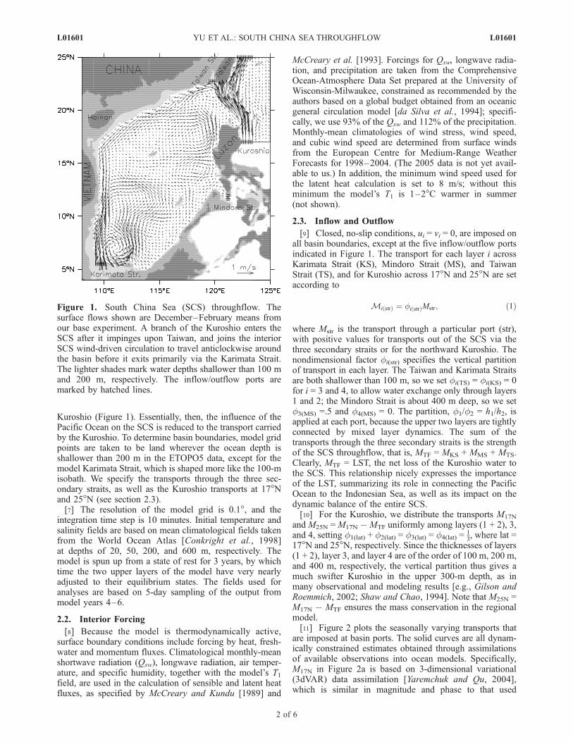
17�N and 25�N, respectively. Since the thicknesses of layers(1 + 2), layer 3, and layer 4 are of the order of 100 m, 200 m,and 400 m, respectively, the vertical partition thus gives amuch swifter Kuroshio in the upper 300-m depth, as inmany observational and modeling results [e.g., Gilson andRoemmich, 2002; Shaw and Chao, 1994]. Note that M25N =M17N � MTF ensures the mass conservation in the regionalmodel.[11] Figure 2 plots the seasonally varying transports that

are imposed at basin ports. The solid curves are all dynam-ically constrained estimates obtained through assimilationsof available observations into ocean models. Specifically,M17N in Figure 2a is based on 3-dimensional variational(3dVAR) data assimilation [Yaremchuk and Qu, 2004],which is similar in magnitude and phase to that used

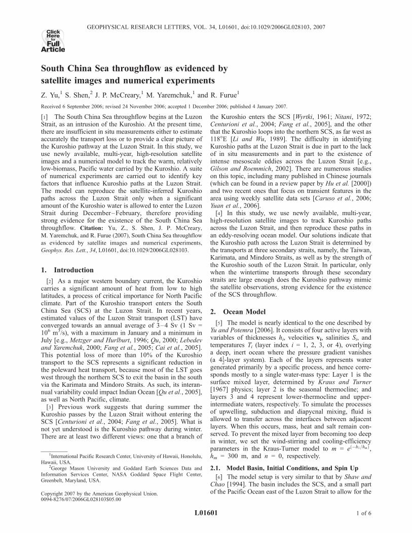
Figure 1. South China Sea (SCS) throughflow. Thesurface flows shown are December–February means fromour base experiment. A branch of the Kuroshio enters theSCS after it impinges upon Taiwan, and joins the interiorSCS wind-driven circulation to travel anticlockwise aroundthe basin before it exits primarily via the Karimata Strait.The lighter shades mark water depths shallower than 100 mand 200 m, respectively. The inflow/outflow ports aremarked by hatched lines.

L01601 YU ET AL.: SOUTH CHINA SEA THROUGHFLOW L01601

2 of 6

by Shaw and Chao [1994]. The three solid curvesin Figure 2b are based on 4dVAR data assimilation(M. Yaremchuk, unpublished data, 2005); their sum inwintertime (summertime) is similar to (much smaller than)that used by Shaw and Chao [1994], which is based on anearly estimate from Wyrtki [1961]. We use the two curvesfor the Karimata and Mindoro Straits as MKS and MMS,respectively. Although the magnitude of the Taiwan Straittransport from the 4dVAR agrees well with the availabledata, its phase differs from observation-based estimates,which suggest a maximum in summer and minimum in

winter [e.g., Fang et al., 1991]. For this reason, we willuse a synthetic curve for MTS, which has the same annualmean as the 4dVAR curve but with its minimum shifted toDecember (dashed curve in Figure 2b). The sensitivity ofour solutions to the magnitude of these transport estimatesis discussed in section 3.[12] Temperature and salinity of water associated with

M17N are (T1, T2, T3, T4) = (T1obs, 26, 18.3, 8.4)�C and (S1,S2, S3, S4) = (S1obs, 34.6, 34.78, 34.4) psu, selected accord-ing to Boyer et al. [2002] and Qu et al. [2000]. Boundaryconditions at the other ports are zero normal derivatives.

3. Results

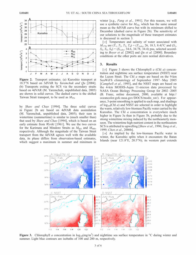
[13] Figure 3 shows the Chlorophyll a (Chl a) concen-tration and nighttime sea surface temperature (NSST) nearthe Luzon Strait. The Chl a maps are based on the 9-kmSeaWiFS climatology of September 1997–May 2005[Campbell et al., 1995], and the NSST maps are based onthe 4-km MODIS-Aqua 11-micron data processed byNASA Ocean Biology Processing Group for 2002–2005(B. Franz, online document, 2000, available at http://oceancolor.gsfc.nasa.gov/DOCS/modis_sst/). For appear-ance, 3-point smoothing is applied to each map, and shadingsof log10(Chl a) and NSST are selected in order to highlightthe warm, relatively low-biomass Pacific water carried by theKuroshio. The Chl a concentration is everywhere muchhigher in Figure 3a than in Figure 3b, probably due to thestrong wintertime mixing induced by the northeasterly mon-soon. The wintertime high-nutrient content in the northeasternSCS is attributed to upwelling [Shaw et al., 1996; Tang et al.,1999; Chen et al., 2006b].[14] As implied by the low-biomass Pacific water in

winter, the Kuroshio splits when it encounters the BatanIslands (near 121.8�E, 20.5�N); its western part extends

Figure 2. Transport estimates. (a) Kuroshio transport at18.5�N based on 3dVAR by Yaremchuk and Qu [2004].(b) Transports exiting the SCS via the secondary straitsbased on 4dVAR (M. Yaremchuk, unpublished data, 2005)are shown in solid curves. The dashed curve is the shiftedTaiwan Strait transport, to be used as MTS.

Figure 3. Chlorophyll a concentration in log10(mg/m3) and nighttime sea surface temperature in �C during winter andsummer. Light blue contours are isobaths of 100 and 200 m, respectively.

L01601 YU ET AL.: SOUTH CHINA SEA THROUGHFLOW L01601

3 of 6

north-northwestward toward the southern tip of Taiwan andthen seems to continue westward following the 200-misobath. The low-biomass tongue west of Luzon resultsfrom the well-known wintertime anticlockwise circulationof the SCS, as shown by Liu et al. [2004]. Tongues of warmNSSTs in Figure 3c suggest a similar Kuroshio pathway aswell as a cyclonic SCS circulation. The low-biomass tongueeast of 120�E is not well defined in summer (Figure 3b), butseems to take a more northward path after passing the BatanIslands. Note that there is a region of high Chl a east ofTaiwan (white-out zone) associated with coastal upwellingand offshore Ekman drift during the southwesterly mon-soon. The offshore cooling east of Taiwan in Figure 3dconfirms the existence of the coastal upwelling.[15] To support our interpretation of the inferred Kur-

oshio pathways from Figure 3, we carried out a suite ofnumerical experiments using the eddy-resolving regionalmodel described in section 2. Figures 4a and 4b show

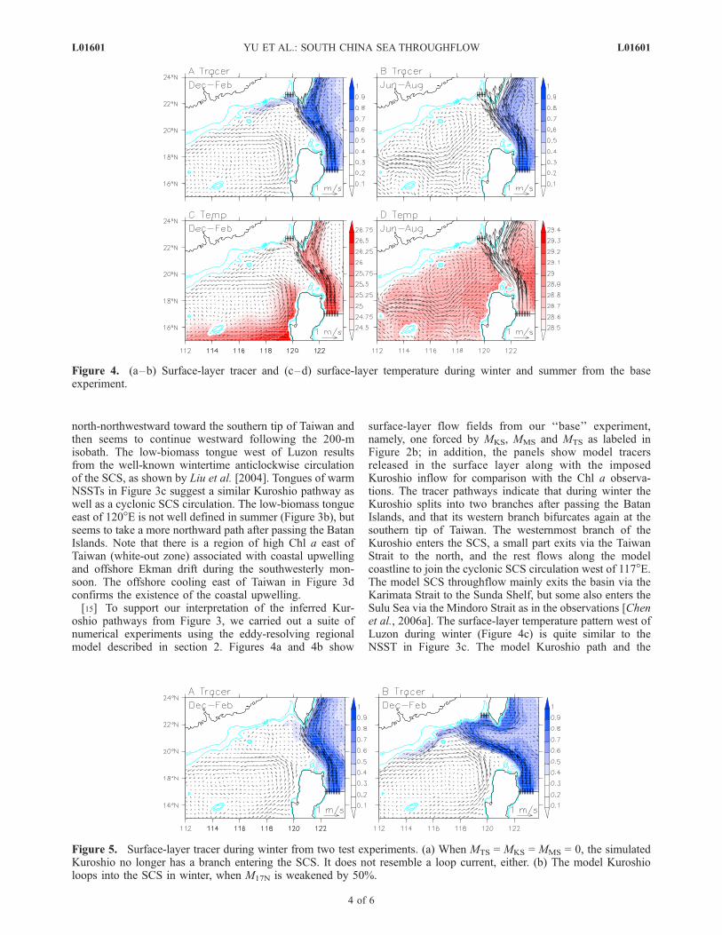
surface-layer flow fields from our ‘‘base’’ experiment,namely, one forced by MKS, MMS and MTS as labeled inFigure 2b; in addition, the panels show model tracersreleased in the surface layer along with the imposedKuroshio inflow for comparison with the Chl a observa-tions. The tracer pathways indicate that during winter theKuroshio splits into two branches after passing the BatanIslands, and that its western branch bifurcates again at thesouthern tip of Taiwan. The westernmost branch of theKuroshio enters the SCS, a small part exits via the TaiwanStrait to the north, and the rest flows along the modelcoastline to join the cyclonic SCS circulation west of 117�E.The model SCS throughflow mainly exits the basin via theKarimata Strait to the Sunda Shelf, but some also enters theSulu Sea via the Mindoro Strait as in the observations [Chenet al., 2006a]. The surface-layer temperature pattern west ofLuzon during winter (Figure 4c) is quite similar to theNSST in Figure 3c. The model Kuroshio path and the

Figure 4. (a–b) Surface-layer tracer and (c–d) surface-layer temperature during winter and summer from the baseexperiment.

Figure 5. Surface-layer tracer during winter from two test experiments. (a) When MTS = MKS = MMS = 0, the simulatedKuroshio no longer has a branch entering the SCS. It does not resemble a loop current, either. (b) The model Kuroshioloops into the SCS in winter, when M17N is weakened by 50%.

L01601 YU ET AL.: SOUTH CHINA SEA THROUGHFLOW L01601

4 of 6

circulation west of Luzon during summer (Figure 4b) areconsistent with the Chl a pattern in Figure 3b: Most ofthe Kuroshio water bypasses the SCS, and an eastwardflow in the SCS between 16–18�N approaches Luzonand turns northeastward. Note that the model tracersduring summer are not attached to the east coast of Taiwan(Figure 4b), and the surface-layer temperature there iscooler (Figure 4d), similar to the satellite observations(Figures 3b and 3d).[16] The Kuroshio branching at the Luzon Strait depends

on the MTF. In a test case with the three outflows set to50% of their values in Figure 2b, the Kuroshio still clearlybranches into the SCS (not shown). In contrast, in a testcase like the base experiment but with no throughflow(MTS = MKS = MMS = 0) there is no branching (Figure 5a).[17] Finally, none of the preceding model Kuroshio path-

ways appear as a loop current that penetrates deep into thenorthern SCS. A recent study by Sheremet [2001] showsthat a western boundary current ‘‘jumps’’ across a gap (likethe Luzon Strait) when it is sufficiently strong, but pene-trates into the gap as a loop current when it is weak. Our testexperiments show that M17N needs to be weakened by 50%for a loop current to appear (Figure 5b), and that the Kuroshiopath changes very little whenM17N is weakened by 30% (notshown). Since the mean Kuroshio transport south of Taiwanis of the order of 20 Sv [Gilson and Roemmich, 2002], it isunlikely to be weak enough to form a loop under normalconditions. A loop could form, however, under the influenceof a strong eddy or when there is a significant reduction in theKuroshio transport (say during a strong El Nino year). Sinceno loop current is hinted at by either Chl a or NSST monthlymaps, we conclude that the monthly-averaged Kuroshio doesnot loop across the Luzon Strait.

4. Discussion

[18] We note that Rossby waves and eddies that propa-gate into the SCS from the Pacific Ocean are not consideredin this study. Some observations suggest that Pacific waterenters the SCS in the form of warm core eddies [Li et al.,1997, 1998]. A natural extension of our study is to includesuch eddies and to understand their interactions with themonthly-mean Kuroshio. More in situ observations andmodeling studies are needed to understand the importanceof high-frequency variability from the Pacific Ocean.

[19] Acknowledgments. This study was supported by NASA throughgrant NAG 5-10045 and by the Japan Agency for Marine-Earth Science andTechnology (JAMSTEC) through its sponsorship of the InternationalPacific Research Center (IPRC). The Goddard Earth Sciences Data andInformation Services Center’s Web-based visualization tool, Giovanni, isgreatly appreciated for the initial data exploration. The assistance of theFerret group at NOAA/PMEL, and of Sharon DeCarlo and Jan Hafner, isgreatly appreciated. Discussions with Gisela Speidel, Guohong Fang, andJianping Xu were helpful. ZY would like to thank the South China SeaInstitute of Oceanology for providing partial support for her to attend the2005 Guilin Meeting on the South China Sea. This paper is IPRCcontribution #425 and SOEST #7028.

ReferencesBoyer, T. P., C. Stephens, J. I. Antonov, M. E. Conkright, R. A. Locarnini,T. D. O’Brien, and H. E. Garcia (2002), World Ocean Atlas 2001, vol. 2,Salinity, NOAA Atlas NESDIS, vol. 50, NOAA, Silver Spring, Md.

Cai, S., H. Liu, W. Li, and X. Long (2005), Application of LICOM to thenumerical study of the water exchange between the South China Sea andits adjacent oceans, Acta Oceanol. Sin., 24, 10–19.

Campbell, J. W., J. M. Blaisdell, and M. Darzi (1995), Level-3 SeaWiFSdata products: Spatial and temporal binning algorithms, NASA Tech.Memo, TM-104566, 32, 1–73.

Caruso, M. J., G. G. Gawarkiewicz, and R. C. Beardsley (2006), Interann-ual variability of the Kuroshio intrusion in the South China Sea,J. Oceanogr., 62, 559–575.

Centurioni, L. R., P. P. Niiler, and D. K. Lee (2004), Observations of inflowof Philippine Sea surface water into the South China Sea through theLuzon Strait, J. Phys. Oceanogr., 34, 113–121.

Chen, C. A., W. Hou, T. Gamo, and S. Wang (2006a), Carbonate-relatedparameters of subsurface waters in the West Philippine, South China, andSulu Seas, Mar. Chem., 99, 151–161.

Chen, C., F. Shiah, S. Chung, and K. Liu (2006b), Winter phytoplanktonblooms in the shallow mixed layer of the South China Sea enhanced byupwelling, J. Mar. Syst., 59, 97–110.

Conkright, M., S. Levitus, T. O’Brien, T. Boyer, J. Antonov, and C. Stephens(1998), World Ocean Atlas 1998 CD-ROM data set documentation, Tech.Rep. 15, 16 pp., Natl. Oceanogr. Data Cent., Silver Spring, Md.

da Silva, A., A. C. Young, and S. Levitus (1994), Atlas of Surface MarineData 1994, vol. 1, Algorithms and Procedures, NOAA Atlas NESDIS,vol. 6, NOAA, Silver Spring, Md.

Fang, G., B. Zhao, and Y. Zhu (1991), Water volume transports through theTaiwan Strait and the continental shelf of the East China Sea measuredwith current meters, in Oceanography of Asian Marginal Seas, edited byK. Takano, pp. 345–358, Elsevier, New York.

Fang, G., D. Susanto, I. Soesilo, Q. Zheng, F. Qiao, and Z. Wei (2005), Anote on the South China Sea shallow interocean circulation, Adv. Atmos.Sci., 22, 946–954.

Gilson, J., and D. Roemmich (2002), Mean and temporal variability inKuroshio geostrophic transport south of Taiwan (1993–2001), J. Ocea-nogr., 58, 183–195.

Hu, J., H. Kawamura, H. Hong, and Y. Qi (2000), A review on the currentsin the South China Sea: Seasonal circulation, South China Sea warmcurrent and Kuroshio intrusion, J. Oceanogr., 56, 607–624.

Kraus, E. B., and J. S. Turner (1967), A one-dimensional model of theseasonal thermocline: II. The general theory and its consequences, Tellus,19, 98–106.

Lebedev, K. V., and M. I. Yaremchuk (2000), A diagnostic study of theIndonesian throughflow, J. Geophys. Res., 105, 11,243–11,258.

Li, L., and B. Y. Wu (1989), Kuroshio’s loop in the South China Sea (inChinese with English abstract), Taiwan Strait, 8, 89–95.

Li, L., J. L. Su, and J. P. Xu (1997), Detached Kuroshio rings in the SouthChina Sea, Trop. Oceanol., 16, 42–57.

Li, L., W. D. Nowlin, and J. L. Su (1998), Anticyclonic rings from theKuroshio in the South China Sea, Deep Sea Res., Part I, 45, 1469–1482.

Liu, Q., X. Jiang, S.-P. Xie, and W. T. Liu (2004), A gap in the Indo-Pacificwarm pool over the South China Sea in boreal winter: Seasonal devel-opment and interannual variability, J. Geophys. Res., 109, C07012,doi:10.1029/2003JC002179.

McCreary, J. P., Jr., and P. K. Kundu (1989), A numerical investigation ofsea surface temperature variability in the Arabian Sea, J. Geophys. Res.,94, 16,097–16,114.

McCreary, J. P., P. K. Kundu, and R. L. Molinari (1993), A numericalinvestigation of dynamics, thermodynamics, and mixed-layer processesin the Indian Ocean, Prog. Oceanog., 31, 181–224.

Metzger, E. J., and H. E. Hurlburt (1996), Coupled dynmics of the SouthChina Sea, the Sulu Sea, and the Pacific Ocean, J. Geophys. Res., 101,12,331–12,352.

Nitani, H. (1972), Beginning of the Kuroshio, in Kuroshio: Its PhysicalAspects, edited by H. Stommel and K. Yoshida, pp. 129–163, Univ. ofWash. Press, Seattle, Wash.

Qu, T. (2000), Upper-layer circulation in the South China Sea, J. Phys.Oceanogr., 30, 1450–1460.

Qu, T., H. Mitsudera, and T. Yamagata (2000), Intrusion of the NorthPacific waters into the South China Sea, J. Geophys. Res., 105, 6415–6424.

Qu, T., Y. Du, G. Meyers, A. Ishida, and D. Wang (2005), Connecting thetropical Pacific with Indian Ocean through South China Sea, Geophys.Res. Lett., 32, L24609, doi:10.1029/2005GL024698.

Shaw, P.-T., and S.-Y. Chao (1994), Surface circulation in the South ChinaSea, Deep Sea Res., 40, 1663–1683.

Shaw, P.-T., S.-Y. Shao, K.-K. Liu, S.-C. Pai, and C.-T. Liu (1996), Winterupwelling off Luzon in the northeastern South China Sea, J. Geophys.Res., 101, 16,435–16,448.

Sheremet, V. (2001), Hysteresis of a western boundary current leapingacross a gap, J. Phys. Oceanogr., 31, 1259–1274.

Tang, D.-L., I.-H. Ni, D. R. Kester, and F. E. Muller-Karger (1999),Remote sensing observations of winter phytoplankton blooms southwestof the Luzon Strait in the South China Sea, Mar. Ecol. Prog. Ser., 191,43–51.

L01601 YU ET AL.: SOUTH CHINA SEA THROUGHFLOW L01601

5 of 6

Wyrtki, K. (1961), Physical oceanography of the Southeast Asian waters:Scientific results of marine investigations of the South China Sea and theGulf of Thailand, Naga Rep., 2, 1–195.

Yaremchuk, M., and T. Qu (2004), Seasonal variability of the large-scalecurrents near the coast of the Philippines, J. Phys. Oceanogr., 34, 844–855.

Yu, Z., and J. Potemra (2006), Generation mechanism for the intraseasonalvariability in the Indo-Australian basin, J. Geophys. Res., 111, C01013,doi:10.1029/2005JC003023.

Yuan, D., W. Han, and D. Hu (2006), Surface Kuroshio path in the LuzonStrait area derived from satellite remote sensing data, J. Geophys. Res.,111, C11007, doi:10.1029/2005JC003412.

�����������������������R. Furue, J. P. McCreary, M. Yaremchuk, and Z. Yu, International Pacific

Research Center, SOEST, University of Hawaii, 1680 East-West Road,Honolulu, HI 96822, USA. (zuojun@hawaii.edu)S. Shen, George Mason University and GES Data and Information

Services Center, NASA/GSFC, Code 610.2, Greenbelt, MD 20771, USA.

L01601 YU ET AL.: SOUTH CHINA SEA THROUGHFLOW L01601

6 of 6