i

Sous vide Lamb Shank

Modelling and Process Improvement

Wen Yan

A thesis submitted to the

Auckland University of Technology

in Partial fulfilment of the requirements for the degree of

Master of Applied Science (MAppSci)

March 2011

Faculty of Health and Environmental Sciences

Primary Supervisor: Associate Professor Owen Young

ii

TABLE OF CONTENTS

Title Page i

Table of contents ii

List of Figures vi

List of Tables viii

Acknowledgements x

Attestation of Authorship xi

Confidential Material xii

Abstract xiii

1 INTRODUCTION 1

2 LITERATURE REVIEW 2

2.1 NEW ZEALAND RED MEAT INDUSTRY 2

2.1.1 History and current situation 2

2.1.2 Cooked sheepmeat products 5

2.1.3 Lamb shank 6

2.2 THE COMPOSITION OF MEAT AND LAMB SHANK 7

2.2.1 Contractile tissue 8

2.2.2 Connective tissue 9

2.2.3 Fat 12

2.2.4 Bone 13

2.2.5 The nature of lamb shank 14

2.3 THE CHANGES OF MEAT DURING THERMAL PROCESS 15

2.4 SHANK PROCESSED BY TITAN MEATS 16

2.4.1 Sous vide technology 17

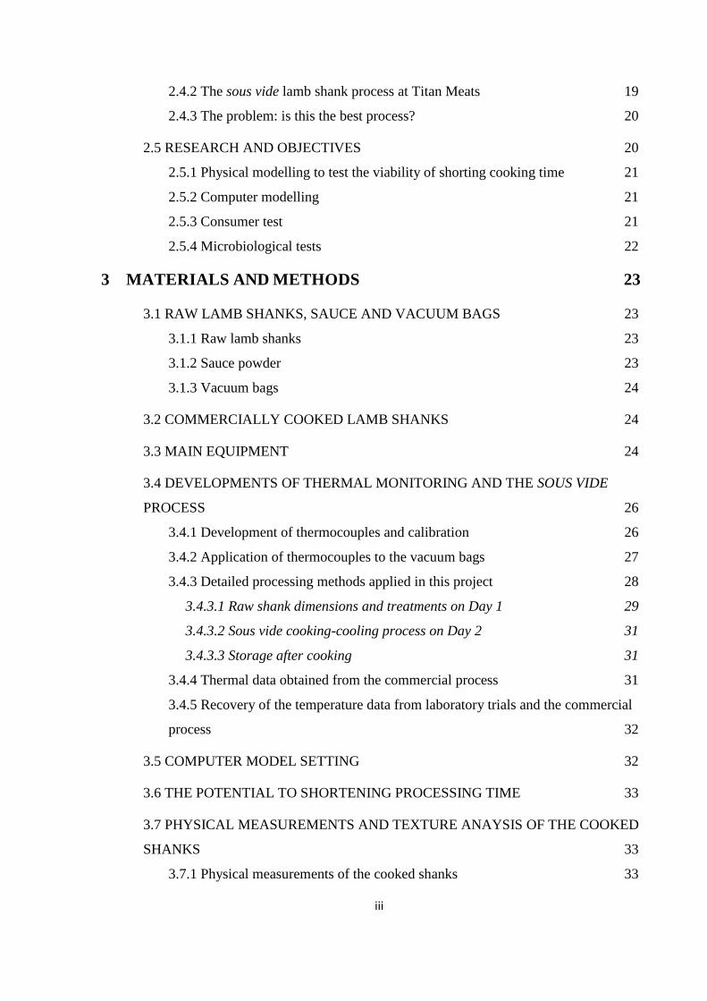
iii

2.4.2 The sous vide lamb shank process at Titan Meats 19

2.4.3 The problem: is this the best process? 20

2.5 RESEARCH AND OBJECTIVES 20

2.5.1 Physical modelling to test the viability of shorting cooking time 21

2.5.2 Computer modelling 21

2.5.3 Consumer test 21

2.5.4 Microbiological tests 22

3 MATERIALS AND METHODS 23

3.1 RAW LAMB SHANKS, SAUCE AND VACUUM BAGS 23

3.1.1 Raw lamb shanks 23

3.1.2 Sauce powder 23

3.1.3 Vacuum bags 24

3.2 COMMERCIALLY COOKED LAMB SHANKS 24

3.3 MAIN EQUIPMENT 24

3.4 DEVELOPMENTS OF THERMAL MONITORING AND THE SOUS VIDE

PROCESS 26

3.4.1 Development of thermocouples and calibration 26

3.4.2 Application of thermocouples to the vacuum bags 27

3.4.3 Detailed processing methods applied in this project 28

3.4.3.1 Raw shank dimensions and treatments on Day 1 29

3.4.3.2 Sous vide cooking-cooling process on Day 2 31

3.4.3.3 Storage after cooking 31

3.4.4 Thermal data obtained from the commercial process 31

3.4.5 Recovery of the temperature data from laboratory trials and the commercial

process 32

3.5 COMPUTER MODEL SETTING 32

3.6 THE POTENTIAL TO SHORTENING PROCESSING TIME 33

3.7 PHYSICAL MEASUREMENTS AND TEXTURE ANAYSIS OF THE COOKED

SHANKS 33

3.7.1 Physical measurements of the cooked shanks 33

iv

3.7.1.1 Cooking loss 33

3.7.1.2 Shrinkage 33

3.7.1.3 Physical measurements of three major muscle groups 34

3.7.2 Texture Analysis 35

3.8 MEASUREMENTS ON COMMERCIAL COOKED LAMB SHANK 37

3.9 TEXTURAL COMPARSION OF THE LABORATORY- AND COMMERICAL-

PROCESSED SHANKS 38

3.10 CONSUMER PREFERENCE TEST OF LABORATORY-PROCESSED

SHANK 38

3.11 MICROBIOLOGICAL TESTS 38

4 RESULTS AND DISCUSSION 41

4.1 THERMAL DATA FOR THE 5.5-HOUR PROCESS 41

4.1.1 Water temperature during process 41

4.1.2 Shank surface and core temperatures during laboratory process 45

4.2 COMPUTER MODEL OUTCOMES OF THE THERMAL DATA FOR THE 5.5-

HOUR PROCESS 45

4.2.1 Food product modellerTM

(FPMTM

) 45

4.2.2 FlexPDE 3TM

47

4.3 PHYSICAL MEASUREMENTS AND TEXTURE ANALYSIS OF THE

COOKED SHANKS 50

4.3.1 Physical measurements results 51

4.3.1.1 Cooking loss 51

4.3.1.2 Shrinkage 52

4.3.2 Texture analysis results 52

4.3.3 Main outcomes of texture analysis 65

4.4 CONSUMER PREFERNCE TEST OF LABORATORY-PROCESSED SHANK

67

4.5 MICROBIOLOGICAL TESTS 71

5 CONCLUSION AND RECOMMENDATIONS 75

v

REFERENCE 78

Appendix 1 The 7-point hedonic scales used in the consumer test to judge the tenderness,

juiciness and overall impression of the sous vide shanks 82

Appendix 2 Temperature profiles of lamb shank surface and core during 5.5-hour sous vide

cooking, modelled using FlexPDE 3 84

Appendix 3 Calculation of energy consumption 85

vi

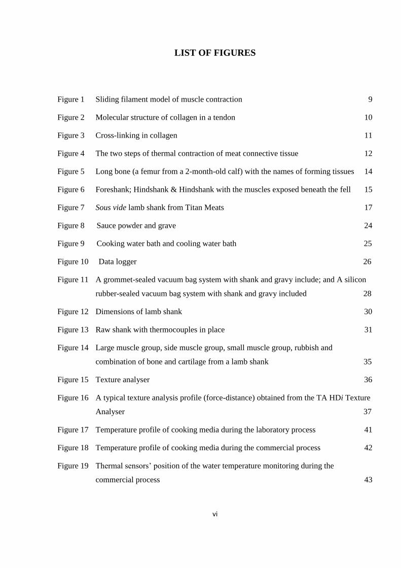
LIST OF FIGURES

Figure 1 Sliding filament model of muscle contraction 9

Figure 2 Molecular structure of collagen in a tendon 10

Figure 3 Cross-linking in collagen 11

Figure 4 The two steps of thermal contraction of meat connective tissue 12

Figure 5 Long bone (a femur from a 2-month-old calf) with the names of forming tissues 14

Figure 6 Foreshank; Hindshank & Hindshank with the muscles exposed beneath the fell 15

Figure 7 Sous vide lamb shank from Titan Meats 17

Figure 8 Sauce powder and grave 24

Figure 9 Cooking water bath and cooling water bath 25

Figure 10 Data logger 26

Figure 11 A grommet-sealed vacuum bag system with shank and gravy include; and A silicon

rubber-sealed vacuum bag system with shank and gravy included 28

Figure 12 Dimensions of lamb shank 30

Figure 13 Raw shank with thermocouples in place 31

Figure 14 Large muscle group, side muscle group, small muscle group, rubbish and

combination of bone and cartilage from a lamb shank 35

Figure 15 Texture analyser 36

Figure 16 A typical texture analysis profile (force-distance) obtained from the TA HDi Texture

Analyser 37

Figure 17 Temperature profile of cooking media during the laboratory process 41

Figure 18 Temperature profile of cooking media during the commercial process 42

Figure 19 Thermal sensors‟ position of the water temperature monitoring during the

commercial process 43

vii

Figure 20 Temperature profile of cooking media during the commercial process (highlight of

water temperature between 72 and 92°C) 44

Figure 21 Core and surface temperature profiles of lamb shank during commercial and lab

processes, modelled by FPM 46

Figure 22 The boundary conditions of shank and the temperature profile inside a shank at 5.5

hours 50

Figure 23 Hardness, fracturability and chewiness of laboratory- and commercial-processed

shanks in large, side and small muscle groups 56

Figure 24 Ratios of hardness, fracturability and chewiness to muscle thickness of laboratory-

and commercial-processed shanks in large, side and small muscle groups 58

Figure 25 The liking scores of laboratory-processed shank tenderness, juiciness and overall

impression 67

viii

LIST OF TABLES

Table 1 New Zealand meat exports at year ended 30 September 2008 3

Table 2 New Zealand livestock numbers at the end of June in 1997 and 2007 4

Table 3 Chemical composition of typical adult mammalian muscle after rigor mortis but

before degradative changes post-mortem 8

Table 4 Collagen content in longissimus of ovine which slaughtered at 2, 4, 6, 8 and 10

months of age 12

Table 5 Sequence of vacuum packing, cooking and cooling of lamb shanks, and physical

measurements and texture analysis after processing 29

Table 6 Sequence of sampling, dilution series preparation, plating, colonies counting, and

results calculation 39

Table 7 Cooking loss and muscle shrinkage of lamb shanks cooked for different time 51

Table 8 Correlations between chewiness (muscle compression work) and shank physical

properties 53

Table 9 Textural properties of the large muscle from shanks cooked for different time in three

weight ranges 60

Table 10 Textural properties of the side muscle from shanks cooked for different time in three

weight ranges 62

Table 11 Textural properties of the small muscle from shanks cooked for different time in

three weight ranges 64

Table 12 FPM model setup for the calculation of energy saving from water bath immersion

prior to cooking 66

Table 13 Comments on texture from the consumer test 69

Table 14 Comments on overall impression from the consumer test 70

Table 15 Aerobic and anaerobic plate counts, Enterobacteriaceae counts, fastidious anaerobe

counts (log10 CFU/cm2 or log10 CFU/g), and the presence of viable Clostridia and

their spores in raw materials and the package after the sous vide process and further

refreezing 73

ix

Table 16 Total within-package aerobic and anaerobic plate counts, Enterobacteriaceae counts,

fastidious anaerobes counts (log10), and the presence of viable Clostridia and their

spores before and after the sous vide process and further refreezing 74

x

ACKNOWLEDGEMENTS

I would like to acknowledge the Foundation of Research, Science and Technology for

providing the funding that went towards this project. I also acknowledge Titan Meats Company

Limited for the support in granting me a scholarship to complete this thesis.

Acknowledges go to Ms Leeanne Cuming and the staff of Titan Meats Ltd. in the

Takapau plant for welcoming me into their plant and assisting me in the data collection.

Thanks go to Dr Marlon dos Reis for assistance in the statistical analyses of the data that

were collected. My thanks also go to Dr Katja Rosenvold and the Meat science team at MIRINZ

for the great support in this project. Thank you for making me a place here, as a student. You

have all been so nice and I have really enjoyed working here.

A special thank you goes to my supervisors Dr Owen Young and Mr Robert Kemp for

their support, guidance, feedback, and encouragement throughout my study.

Finally, big thanks go to my parents and my boyfriend for the encouragement and support

during the past years.

xi

ATTESTATION OF AUTHORSHIP

I hereby declare that this submission is my own work and that, to the best of my

knowledge and belief, it contains no materials previously published or written by another person

(except where explicitly defined in the acknowledgments), nor material which to a substantial

extent has been submitted for the award of any other degree or diploma of a university or other

institution of higher learning.

Signed: _______________________________ Date: ________________

Wen Yan

xii

This image has been removed by the author of this thesis for copyright reasons.

xiii

ABSTRACT

The optimum production is important for the manufacture companies as it allows the

optimistic using of capital and ensures the competitiveness of product in market. This thesis

explores the options to optimise the existing sous vide lamb shank process, and subsequently, the

product quality.

The thermal history of a model laboratory process and the existing commercial process

were profiled by physical and computer models. The measured results showed that a higher

temperature variation present in the commercial process, compared to the well controlled model

laboratory process. The temperature variation impacted the textural properties of the products,

as there was no significant difference between the commercial-processed shanks in different

weight ranges, whereas the size effect was marked in the laboratory-processed equivalents,

where the heavier shanks were more difficult to chew.

FPM and FlexPDE were used to model the cooking-cooling process. The FPM model

showed that the shank temperature was generally lower in the commercial products, and caused

these products was more difficult to chew. The FlexPDE model was a poor predictor of the

temperature profile of lamb shank during the cooking process, due to the failure to the thermal

conductivity of bone in the model. However, the model pointed the importance of bone as a

conductor of heat from the ends of the shank to the meat surround.

The cooking time was shortened to 4.5 hours from the standard 5.5 hours, to explore the

potential of shortening cooking time. The physical measurements on shanks cooked in the

laboratory for the two different times showed that longer time caused higher cooking loss,

however, the cooking time did not affect the mean muscle shrinkage, and the variations were low.

The commercial products had similar mean shrinkage value to the laboratory shanks, but the

variation was much higher, which again suggested the higher temperature variation in the

commercial process. In addition, the comparison of texture between these three shanks showed

that the textural values of the commercial-processed shanks were similar to the 4.5-hour

laboratory-processed shanks, which were higher (more difficult to chew) than the 5.5-hour

laboratory equivalents.

The consumer test suggested that the 4.5-hour laboratory-processed shanks were preferable

to the 5.5-hour equivalents, and the over-tenderisation may be the main reason for the less

attractiveness of the 5.5-hour shanks.

xiv

The microbiological tests showed that the existing start-point of the material, the existing

cooking-cooling process and the subsequent frozen storage could effectively reduce the bacterial

loads inside the product package.

Recommendations were discussed that aim to reduce the temperature variation in the

existing commercial process. The first recommendation was reducing the product heat load by

increasing the mean temperature of the shanks prior to loading. This could be achieved by

tempering the packed shanks in an equilibration bath that contains mains supply water for a

certain time. This would ensure a more even temperature distribution when the products are

loaded into the cooking bath, consequently reduce the required cooking time/energy

consumption. Improving the heating capacity of the cooking system was another way to reduce

the temperature variation, which could be achieved by increasing the heating capacity of the

cooking bath and increasing the circulation of the bath fluid. The heating capacity of the

cooking bath could be improved by redesigning the heating system of the bath and increasing the

effectiveness of the insulation surround. And the circulation could be increased by applying

either pump recirculation or mechanical stirrer. A more detailed evaluation of the cooking bath

was also recommended, as it would profile the temperature history in the bath more accurately.

1

CHAPTER 1

INTRODUCTION

Sous vide is a French word means “under vacuum” (Baldwin 2009). The sous vide cooking

technology is originated in France in the 1970s, and nowadays, it has become a popular method

in the catering and food processing industries worldwide, because it can bring benefits on both

storage life and eating quality to the food products (Church and Parsons 1993).

Titan Meats company Limited is a meat and seafood products manufacturer and exporter,

and the sous vide cooked meat is their main product category.

Sous vide lamb shank is one of the most successful products in the company. Shanks are

cooked in a water bath with a set-point of 85 to 90°C for 5 to 5.5 hours, followed by 2 hours

cooling in a water bath with a set-point of 4.2°C. This temperature-time protocol was largely

developed empirically, and the temperature endpoints were set to satisfy the demands of food

safety authorities. With respect to cooking time and temperature, Titan Meats wants to optimise

the existing process and the product quality, with an optimistic view of shortening the processing

time, but attaining desired shank tenderness. A shorter cooking time would make better use of

capital, potentially saving energy and money, and in turn enhancing the competitiveness of sous

vide lamb shank product in international markets.

In this thesis, physical and computer models were set up to profile the temperature changes

in a model laboratory process and the existing commercial process. The texture properties of the

resulting shanks were analysed and compared, to explore ways to improve the existing process.

A consumer test of laboratory-processed shanks was included in this thesis to find out consumer

preference for the tenderness and juiciness of shanks cooked in the laboratory process for

different times. Microbiological tests were also carried out to confirm the safety of the sous vide

lamb shank product.

After a literature review in Chapter 2, Chapter 3 describes the materials and methods used

in this study. This is followed by the presentation of results and discussion in Chapter 4, where

results consisting of temperature-time profiles, textural properties, consumer preference, and

microbiological status. Conclusions drawn from the results are presented in Chapter 5, and

recommendations for improving the existing commercial process are also discussed.

2

CHAPTER 2

LITERATURE REVIEW

2.1 NEW ZEALAND RED MEAT INDUSTRY

2.1.1 History and current situation

The New Zealand red meat industry is largely a supply chain from sheep, beef and deer

farms producing slaughter animals, through abattoirs yielding carcasses and a wide range of

derived meat products, through refrigerated transport to local and international destinations,

ending in a range of wholesale and retail markets. The export industry was developed in 1800s

with the advent of commercial freezing technology in ships (Investment New Zealand 2007) and

aimed at the British Isles market. The export trade has expanded to service a diverse array of

markets and cultures, each with their individual requirements.

Eighty to ninety percent of New Zealand sheep and beef meats are processed for export,

and as such the meat and associated products make significant contributions to the national

economy. According to MIA (2009), in 2007/08, the meat industry generated NZ$4.6 billion in

exporting earnings, which was 15% of New Zealand‟s total merchandise export value.

Sheepmeat and beef are the two main export meat products from New Zealand. Table 1

shows the quantity and price of meat exports in the meat industry‟s financial year to end

September 2008 (Meat and Wool New Zealand 2009). During this period, 426,000 tonne of

sheepmeat products were exported, comparing with 351,000 tonne of beef products. Moreover,

the unit price of sheepmeat was higher than that of beef. Thus, sheepmeat dominates New

Zealand‟s red meat industry, and has always done so. New Zealand continues to be the largest

sheepmeat exporter in the world (MIA 2009).

3

Table 1. New Zealand meat exports at year ended 30 September 2008 (Meat and

Wool New Zealand 2009)

Type Total shipped

(tonne)

Free on board value

($000)

Price

($ tonne-1)

Lamb

Carcasses

Cuts

Boneless

329,949

15,940

268,772

44,237

2,246,748

80,906

1,703,259

462,582

6,830

5,076

6,337

10,457

Mutton

Carcasses

Cuts

Boneless

95,897

17,779

42,730

35,388

390,711

48,258

119,862

222,590

4,074

2,714

2,805

6,290

Beef

Carcasses

Cuts

Boneless

351,375

99

27,149

324,127

1,712,863

449

110,534

1,601,880

4,875

4,544

4,071

4,942

Bobby

Carcasses

Cuts

Boneless

11,854

440

977

10,437

62,145

1,264

6,910

53,971

5,243

2,871

7,076

5,171

Goat 895 5,738 6,408

Offal 71,801 221,049 3,079

Total 860,770 4,639,253 5,390

Sheep, comprising three age categories – lamb, hogget, and mutton – are very nearly all

raised free range on pasture. Pasture comprises largely grasses and legumes which grow nearly

all year around in New Zealand‟s temperate climate. While this way of production has

implications in meat flavour (Schreurs and others 2008), and seasonality, the free-range pastoral

production system is very much cheaper than alternatives such as grain feeding (MAF 2009).

Moreover, New Zealand as an island nation with vigilant biological border controls is fortunately

free of diseases such as spongiform encephalopathy, typified by the trivially-named „mad cow

disease‟, and foot-and-mouth disease. The disease-free environment allows New Zealand meat

products to be exported worldwide to the most demanding markets.

The New Zealand meat industry is different from most of its international competitors,

because there are very few market-distorting price supports, subsidies and other interventions

from the government (Investment New Zealand 2007). Therefore, the farmers and exporters

concentrate only on markets and their requirements. The price signals from these markets have

4

resulted in a continually shifting pattern of agricultural land use and consequently animal

numbers. Thus, during the period June 1997 to June 2007, total stock units in New Zealand

declined from 95.9 million to 92.2 million. The reduction was almost entirely due to sheep

number decline (17%) in response to market signals that included the better returns from dairy

(Table 2) and also land use change to forestry. However, in spite of the reduction in sheep

numbers, the tonnes of sheepmeat exported remained at the similar quantity (MIA 2009) because

slaughter weights were higher, presumably in response to market signals that specified larger

cuts (Meat and Wool New Zealand 2009).

Table 2. New Zealand livestock numbers at the end of June in 1997 and 2007

(Investment New Zealand 2007)

1997 (million) 2007 (million) % change

Sheep 46.1 38.5 - 17

Beef cattle 4.76 4.39 - 8

Dairy cattle 4.39 5.26 20

Deer 1.27 1.40 10

Total stock units 95.9 92.2 - 4

Over all red meat categories, the proportion of further processed meat products has

increased particularly during the last 20 years. The red meat industry has developed from

exporting frozen whole carcasses to higher-value meat products, such as chilled meat cuts, and to

some extent, cooked meat products. In 2006, 97% of export meat products were in a cut form

rather than carcass, a major increase from 64% in 1989 (Investment New Zealand 2007).

New Zealand export meat is cut according to objective specifications, and every cut has an

exact definition. In the case of lamb, for example, there are five primal (primary) cuts based on

muscle distribution, which are full leg, flap, mid-loin, rib-loin, and forequarter. The primal cuts

are further divided to smaller cuts for different markets requirements. For instance, full leg may

be divided into shank, silverside, knuckle, topside and rump, each destined for a different style of

cooking with different textural outcomes. Meat cuts are chilled and packed by modern

packaging methods, such as vacuum pack and controlled atmosphere pack, which can extend the

storage life of chilled meat to about 8 to12 weeks and 16 to 20 weeks, respectively (Meat New

Zealand 2000).

5

Cooking is another method that can add value to meat products exported or otherwise, and

according to the common predictions, cooked or partially cooked meat products will become the

dominant products in international meat trading markets (Xiong and Mikel 2001; North and

Carson 2003; Lynn 2006). However to date, the New Zealand red meat industry has added every

little export value by cooking. Even in the domestic trade, very little red meat is sold cooked,

which is in marked contrast to the activity in the domestic chicken meat industry. In the year

ended May 2009, the prepared and preserved meat products export revenue was only NZ$128

million, which including cooked meats, canned meats, and sausages. This can be contrasted with

the total revenue of about NZ$6.4 billion in a similar year, representing only 2.8% of export

revenue (MIA 2009).

The exact and detailed reasons for this low adoption of adding value by cooking are

beyond the scope of this review. However, reasons are likely to include the following. Post

farm gate the export meat industry is inherently highly financially geared, with minimal capital

input from the farmer owners through cooperative structures. Development of cooked meat

products and their international marketing would require large amounts of capital that farmers

are reluctant to divert from their farms. The meat industry is moreover inherently conservative.

The industry has little experience beyond acquisition of stock, slaughter, processing and

distribution to established markets. Also, beyond the scope of this review is the issue of tariffs,

which are likely to vary with country and cooked meat category. Superimposed on these likely

reasons is the uncertainty of returns due to the exchange rate of the New Zealand dollar. In the

year ending May 2009, the New Zealand dollar exchange rate against both the US dollar and

Euro was at lower levels compared with its historical average. The favourable exchange rate

assisted the red meat industry to generate 17% higher export profit than the previous year (MIA

2009). In an unsubsidised meat market such as New Zealand‟s, the growth or otherwise of the

cooked meat categories, will ultimately depend on returns. Those products that are being

currently prepared and sold internationally are presumably profitable and these are now

discussed in respect to sheepmeat.

2.1.2 Cooked sheepmeat products

Several red meat processors in New Zealand prepare cooked sheepmeat products for the

domestic and export trades. Silver Fern Farms is New Zealand‟s largest red meat processor. Its

main focus is clearly raw meat products, but the cooperative‟s website shows that Silver Fern

offers a range of cooked meat products from sheepmeat, beef and venison. There is no particular

6

species focus, and it is clear that the products are manufactured in response to demand from the

food service trade. There is no advertising directed at the retail consumer. Angel Bay

Australasia is a subsidiary of ANZCO Food Group, a meat processor with a history of successful

trade with Japan and other South East Asian countries. Their products catalogue includes 12

cooked meat products dominates by beef, and mostly aimed at the food service trade. Of the

three cooked lamb products (Gourmet Lamb Bites, Part-cooked Lamb 110g rissole, Bite-sized

Lamb Portions), the former two are for food service and the last one is for retail sale. There may

be other food companies in New Zealand that produce cooked sheepmeat products, but a

thorough search of the internet has failed to reveal clear examples.

One smaller food company, Titan Meats Company Limited (previously named National

Meats), is a joint venture between National Meats New Zealand Limited and Silver Fern Farms.

The factory of Titan Meats is based in Takapau, and produces a range of cooked meat products

from lamb, beef, and veal using sous vide cooking technology. Sous vide is a French culinary

term meaning under vacuum, and its advantages are described in a later section. Their sous vide

products including Cooked Lamb Shanks, Cooked Lamb Charlottes, Cooked Boneless Lamb

Roll, and Cooked Diced Lamb, Lamb and Veal Meatloaves, Cooked Beef Blade Steaks, Cooked

Beef Short Ribs, Cooked Roast Beef. Most of the products are exported, destined for food

service and retail customers.

Sous vide Cooked Lamb Shank is the core product of Titan Meats. Lamb foreshank or

hindshank is sealed in a plastic pouch with a sauce and slow cooked in a water bath for a

specified cooking time. This product is mainly exported to the U.K. and Australia, where it is re-

heated and served in hotels, bars, etc. as „pub (or bar) food‟.

2.1.3 Lamb shank

Lamb shank has become one of the more popular meat products in last 10 to 15 years.

Whereas lamb shank was a popular food decades ago, the obligatory long cooking time made

this product less attractive to those with busy lifestyles. Thus 20 years or so ago shank was

considered little better than dog food. In response to the real or perceived dangers of fast food,

an affluent section of the community has developed an interest in traditional foods and foods

from other cultures. When some well-known celebrity chefs brought the slow-cooked lamb

shank to restaurant dining tables, the product‟s reputation grew markedly (Food reference n.d.;

Grill and Foodservice 2010). With its historical roots, lamb shank is also often regarded as

„comfort food‟. At the same time, comparing with other meat cuts, the unit price of shank is

7

lower than other meats (Gourmet Direct 2005) probably because of the high proportion of bone.

Given that the cooked shank can be sold at a high price in export markets, lamb shank is a raw

material well-suited to adding value.

According to Meat New Zealand (2000), there are three shank cuts processed in New

Zealand, defined as foreshank (knuckle tip off), hindshank (knuckle tip off), and shank frenched

(trimmed shank). In New Zealand, the chilled and frozen lamb shanks are for local and export

trade. Fresh chilled lamb shanks are sold in a variety of packages, including cling-film overwrap

packaging (local markets only), vacuum packaging and controlled atmosphere packaging, while

frozen lamb shanks are preferably vacuum packed in freezer-quality barrier bags.

2.2 THE COMPOSITION OF MEAT AND LAMB SHANK

Before examining lamb shank and its thermal processing in more detail, it is useful to

discuss the nature of the components that dominate meat in general and their thermal changes

during heating.

Meat muscle mainly composed five constituents: water, protein, lipid, carbohydrate and

non-protein nitrogenous compounds (Table 3). Water is the largest constituent, and the content

is approximately 75% of muscle weight. Protein is the second largest component, which makes

up an average of 18.5% of muscle weight. Protein has many functions in muscle, including

maintaining the structure, organization muscle and muscle cell, and supporting the contractile

process. The content of lipid in muscle varies in the range between 1% and about 13%, and

inverses to the water content. Carbohydrate and non-protein nitrogenous compounds present in

small amounts, approximately 1% to 2.6% in weight.

8

Table 3. Chemical composition of typical adult mammalian muscle after

rigor mortis but before degradative changes post-mortem (Adapted

from Lawrie 2006)

Components Average % of muscle weight

Water 75.0

Protein

- Contractile tissue

myofibrillar

sarcoplasmic

- Connective tissue

collagen

elastin

mitoehondrial etc.

19.0

17.0

11.5

5.5

2.0

1.0

0.05

0.95

Lipid 3.0

Carbohydrate 1.0

Non-protein nitrogenous compounds 2.0

In this project, the components of principal interest are contractile tissue, connective tissue,

fat and bone. These components are the most important factors influencing the sous vide lamb

shank cooking process and the texture of the final products. For this reason, the next section

discusses these four components in more detail.

2.2.1 Contractile tissue

As the name indicates, contractile tissue is the proteinaceous tissue that generates muscular

force as dictated by the motor neurone system (Mann 2008).

The two most abundant proteins in the contractile mechanism are myosin and actin, which

are arranged in parallel filaments (the so-called thick and thin, respectively). They interdigitate

reversibly as the muscle cell contract and relax in response to the neurone signals. In the

myofibrils, the thin filaments (actin) appear in cross section as regular hexagonal arrays and a

thick filament (myosin) appears at the centre of each array. During muscle contraction, the thin

and thick filaments slide past each other. As the sliding filament model showing in Figure 1,

when muscle is relaxed, there is no or little overlap of the filaments, whereas, as muscle

contracts, the overlap becomes greater until the filaments fully overlapped (Mann 2008). Thus

muscle is a linear biological motor. The filaments in the muscle are organised in a regular

9

pattern that is held in place by a group of structural proteins such as desmin, filamin and

connectin (Lawrie 2006). The force from myosin and actin contraction is transmitted to the

surface of the muscle cell where the cell membrane is surrounded by a “mesh” of connective

tissue in the form of collage. This mesh permeates the muscle such that if the cells contents were

somehow removed, the resulting structure would resemble a sponge where the cavities were

fusiform rather than spherical. Muscles all have a so-called origin and an insertion on bone, and

all acts over one or over two joints (Mann 2008).

Figure 1. Sliding filament model of muscle contraction. A. no or little overlap between

thick and thin filaments; B. greater overlap; C. complete overlap; D. extremely

shortened with buckled thin filament (Mann 2008).

When contractile tissue is heated to above 45°C, the myosin and actin begin to irreversibly

denature to form a gel (Bejerholm and Aaslyng 2004) that is effectively called cooked meat.

This gel is nonetheless fibrous in nature because the arrangement of muscle fibres is obviously

fibrous. Thus, whole cooked meat – as opposed to finely minced emulsion sausages – has a

fibrous texture.

2.2.2 Connective tissue

The relative proportion of connective tissue varies between muscles and, in part, account

for the relative toughness of meat (Lawrie 2006). As noted above, the role of connective tissue

10

is to transmit force and to do this it must have minimal elasticity. However, it can be arranged in

muscles in different ways as will be described later.

Collagen is the main type of protein fibre in muscle connective tissue, the amount in

muscle is from 1.5% to about 10% of dry weight (Lepetit 2008). The content of connective

tissue is higher in muscles which are in the distal parts of the limbs, such as foreshanks,

compared with other types. In meat connective tissue frameworks, collagen is present in a

highly fibrillar structure, which contains a regularly oriented array of polypeptide chains. The

collagen fibres are densely packed and have high tensile strength (Davies 2004). The molecular

structure of collagen in a tendon is shown in Figure 2. To construct a tendon from the

polypeptide chains, these chains are arranged in a triple helix to form collagen molecules, and

then linked to form collagen fibrils, which in turn to form collagen fibres. Cross-linking within

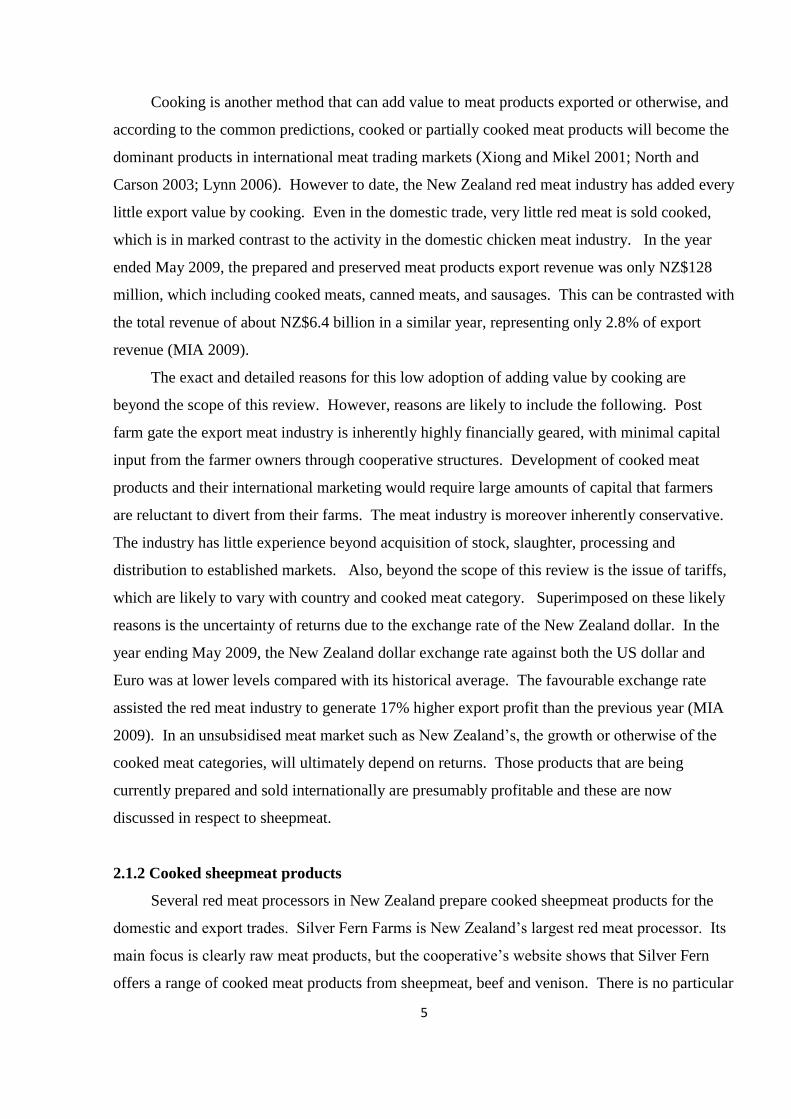
and between individual collagen molecules is pivotal to creation of collagen fibrils (Figure 3).

The cross-links are easily broken in young animals, since they most are intermolecular head-to-

tail cross-links (Figure 3a). However, as the animals age, the collagen fibres become more stable,

due to the increase in the number of interfibril cross-links (Figure 3b) (Davies 2004). Collagen

is an important source of meat texture through the quantity and quality of the various cross-links

(Lepetit 2008).

Figure 2. Molecular structure of collagen in a tendon (Davies 2004).

11

Figure 3. Cross-linking in collagen. a. intermolecular head-to-tail cross-links in a

immature connective tissue; b. interfibril cross-links in a mature collagen

fibre (Davies 2004).

Importantly for this project, thermal processes have a significant effect on meat collagen.

Collagen originally exhibits a quasi-crystalline structure and converts to a random amorphous

structure when heated up to a temperature of 58°C (Lepetit 2008). The thermal transition of

collagen is progressive, and starts with collagen denaturation at temperatures 56°C to 65°C,

followed by gelatinization at up to temperature of 80°C, at which stage collagen fibres finally

convert to gelatines (Palka 2004), where the collagen molecules are arranged as random coils.

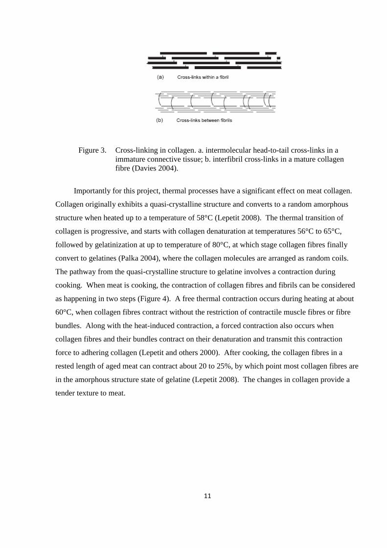
The pathway from the quasi-crystalline structure to gelatine involves a contraction during

cooking. When meat is cooking, the contraction of collagen fibres and fibrils can be considered

as happening in two steps (Figure 4). A free thermal contraction occurs during heating at about

60°C, when collagen fibres contract without the restriction of contractile muscle fibres or fibre

bundles. Along with the heat-induced contraction, a forced contraction also occurs when

collagen fibres and their bundles contract on their denaturation and transmit this contraction

force to adhering collagen (Lepetit and others 2000). After cooking, the collagen fibres in a

rested length of aged meat can contract about 20 to 25%, by which point most collagen fibres are

in the amorphous structure state of gelatine (Lepetit 2008). The changes in collagen provide a

tender texture to meat.

12

Figure 4. The two steps of thermal contraction of meat connective tissue (Lepetit and

others 2000).

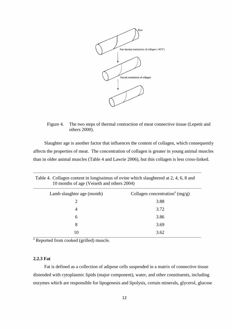
Slaughter age is another factor that influences the content of collagen, which consequently

affects the properties of meat. The concentration of collagen is greater in young animal muscles

than in older animal muscles (Table 4 and Lawrie 2006), but this collagen is less cross-linked.

Table 4. Collagen content in longissimus of ovine which slaughtered at 2, 4, 6, 8 and

10 months of age (Veiseth and others 2004)

Lamb slaughter age (month) Collagen concentrationa (mg/g)

2 3.88

4 3.72

6 3.86

8 3.69

10 3.62

a Reported from cooked (grilled) muscle.

2.2.3 Fat

Fat is defined as a collection of adipose cells suspended in a matrix of connective tissue

distended with cytoplasmic lipids (major component), water, and other constituents, including

enzymes which are responsible for lipogenesis and lipolysis, certain minerals, glycerol, glucose

13

and glycogen, and nerves (Kauffman 2001). During cooking, fat starts to melt and drip out when

the temperature increases to 40 to 50°C (Bejerholm and Aaslyng 2004).

2.2.4 Bone

Bone is responsible for structural support and locomotion in animals. It starts to form early

in the fetal development period through the transformation of collagenous tissue, and continues

to grow after birth through net addition of collagen and mineral until the animal grows to the

mature size (Beermann 2004). There are three commonly recognised types of bone present in

the animal body, but only long bone will be discussed here since it is the main type found in

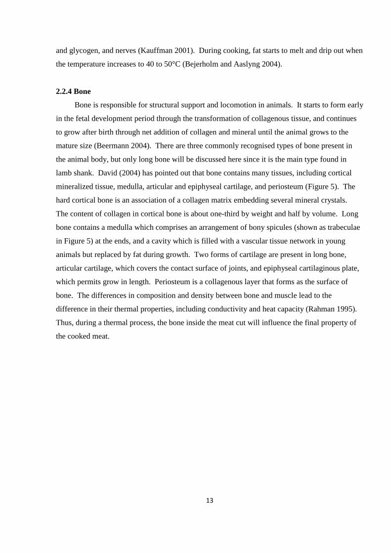
lamb shank. David (2004) has pointed out that bone contains many tissues, including cortical

mineralized tissue, medulla, articular and epiphyseal cartilage, and periosteum (Figure 5). The

hard cortical bone is an association of a collagen matrix embedding several mineral crystals.

The content of collagen in cortical bone is about one-third by weight and half by volume. Long

bone contains a medulla which comprises an arrangement of bony spicules (shown as trabeculae

in Figure 5) at the ends, and a cavity which is filled with a vascular tissue network in young

animals but replaced by fat during growth. Two forms of cartilage are present in long bone,

articular cartilage, which covers the contact surface of joints, and epiphyseal cartilaginous plate,

which permits grow in length. Periosteum is a collagenous layer that forms as the surface of

bone. The differences in composition and density between bone and muscle lead to the

difference in their thermal properties, including conductivity and heat capacity (Rahman 1995).

Thus, during a thermal process, the bone inside the meat cut will influence the final property of

the cooked meat.

14

Figure 5. Long bone (a femur from a 2-month-old calf) with the names of forming

tissues (David 2004).

2.2.5 The nature of lamb shank

Lamb shank is either the lower section of the fore leg or the hind leg with knuckle tips

removed, and generally referred to as foreshank and hindshank, respectively. The foreshank

(Figure 6a) (which was used for processing in this project) is cut through the arm bone joint

(elbow) of the forequarter, while the hindshank (Figure 6b) is cut through the stifle (knee) joint

of the hind leg. Lamb shank is covered by a thin layer of fat and fell (Figure 6c), which appears

as a sheath that surrounds the muscles of shank, therefore, making the shank a whole meat cut.

The shank fell is recognized as a layer of collagenous tissue.

15

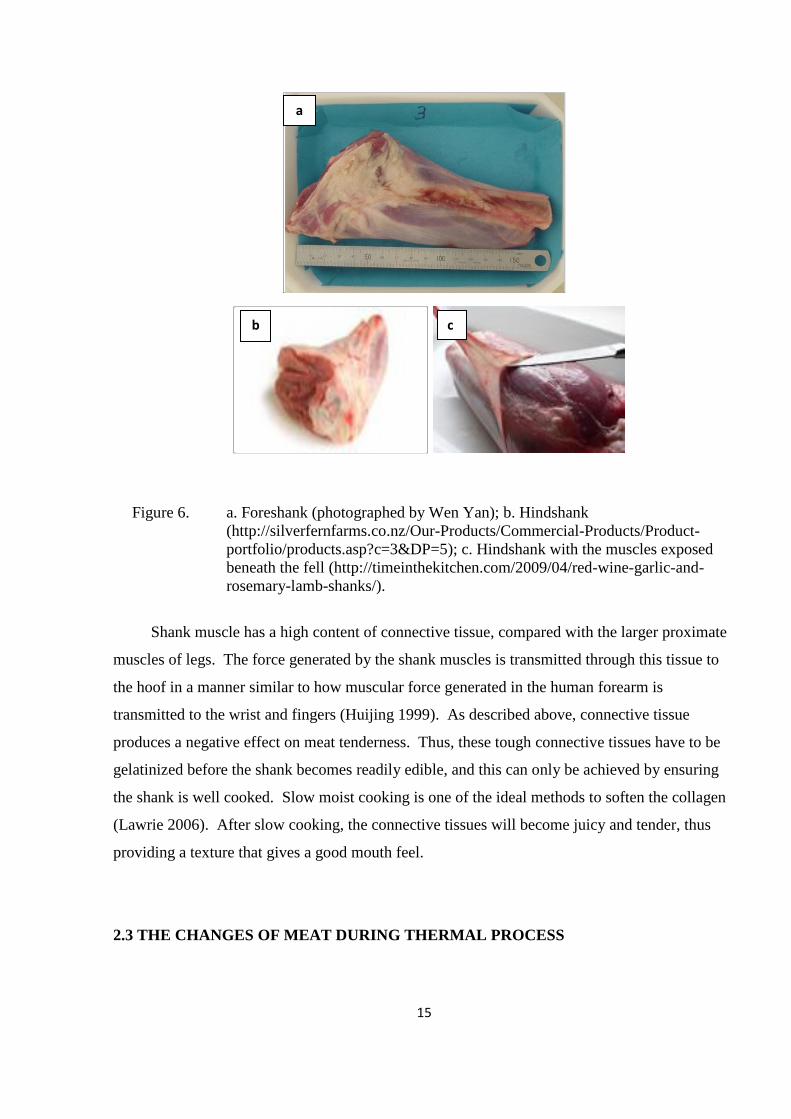
Figure 6. a. Foreshank (photographed by Wen Yan); b. Hindshank

(http://silverfernfarms.co.nz/Our-Products/Commercial-Products/Product-

portfolio/products.asp?c=3&DP=5); c. Hindshank with the muscles exposed

beneath the fell (http://timeinthekitchen.com/2009/04/red-wine-garlic-and-

rosemary-lamb-shanks/).

Shank muscle has a high content of connective tissue, compared with the larger proximate

muscles of legs. The force generated by the shank muscles is transmitted through this tissue to

the hoof in a manner similar to how muscular force generated in the human forearm is

transmitted to the wrist and fingers (Huijing 1999). As described above, connective tissue

produces a negative effect on meat tenderness. Thus, these tough connective tissues have to be

gelatinized before the shank becomes readily edible, and this can only be achieved by ensuring

the shank is well cooked. Slow moist cooking is one of the ideal methods to soften the collagen

(Lawrie 2006). After slow cooking, the connective tissues will become juicy and tender, thus

providing a texture that gives a good mouth feel.

2.3 THE CHANGES OF MEAT DURING THERMAL PROCESS

a

b c

16

The perceived textural changes (e.g. hardness, fracturability and chewiness) of meat that

occur through thermal process are generally related to heat-induced alternations of the primary

structure components (mainly connective tissue and myofibrillar proteins) in muscle tissue. The

heat solubilisation of collagen leads to meat tenderisation, but the denaturation of myofibrillar

proteins (myosin and actin) induces meat toughening (Seideman and Durland 1984; Bertola and

others 1994; Califano and others 1997). Protein denaturation is the combination results of

cooking time and temperature. Generally, connective tissue solubilisation depends more on

cooking time, and myofibrillar toughening relates more to cooking temperature (Lawrie 2006).

The textural changes occurring in the core of a meat cut obviously depend on the temperature

history at the surface (Rinaldi and others 2010). During processing, heat acts first at the meat

surface, and induces a dynamic temperature gradient to the core of the meat (Bole 2010). Along

this changing gradient, the pattern of changes in meat texture can be divided into three steps.

First, the meat becomes tough when heat to a temperature of 40 to 50°C, followed by a decrease

to about 60°C. The first rise is apparently due to the denaturation of contractile proteins (mainly

myosin), where myofibrils begin to shrink transversely, and the subsequent decrease between 50

and 60°C can be explained by the denaturation and shrinkage of collagen fibres of intramuscular

connective tissue. The second step occurs between 60 to 75°C, where the meat gets tougher

again, due to the denaturation of cytoskeletal protein titin, which begins at 60°C, and the later

denaturation of actin at 70 to 80°C. The third step occurs when temperature above 75°C. With

increasing cooking time, the toughness of meat decreases, especially in meat high in connective

tissue, as the result of collagen gelatinization (Bejerholm and Aaslyng 2004; Lawrie 2006).

Collagen gelatinization also increases with temperature, as Ranken (2000), Tornberg (2005) and

Lawrie (2006) reported, particularly at the higher end of the range 60 to 98°C and especially

when moist cooked.

2.4 SHANK PROCESSED BY TITAN MEATS

Titan Meats services both ready meal manufactures and retail customers. They produce

sous vide fully cooked entrees, intermediate meat products, raw, marinated and cooked meats

using lamb, mutton, beef and veal. Sous vide meats is one of the most popular product

categories, and lamb shank (Figure 7) as a main product in this category. Lamb shank is

17

exported to the U.K. and other countries for food service in public bars and hotels, and also for

retail sale in the supermarkets.

Figure 7. Sous vide lamb shank from Titan Meats

(http://www.nationalmeats.co.nz/index.cfm?pagecall=content&ContentTypeID

=18343&MenuItemID=57006).

2.4.1 Sous vide technology

The Sous vide cooking method originated in France in the 1970s (Key 2009). Today, this

technology has been applied in the catering and food processing industries worldwide, because it

has been shown to improve both storage life and eating quality of the food products (Church and

Parsons 1993). Sous vide is a French word, means under vacuum (Baldwin 2009). Sous vide

cooking is defined as: “raw materials or raw materials with intermediate foods that are cooked

under controlled conditions of temperature and time inside heat-stable vacuumized pouches”

(Schellekens 1996). Compared with traditional cooking method, sous vide applies well

controlled heating on food materials that are vacuum sealed in plastic pouch. Foods are cooked

at lower temperatures (usually under 100°C) for a longer time than traditional methods. The

cooking temperature and time depend on the composition and size of the materials and the

desired final eating quality. During processing, the food materials are cooked in a water bath at a

temperature just above the desired final core temperature of the products. By using this

temperature setting, the products are prevented from overcooking (Baldwin 2009). In the food

processing industry, sous vide technology is generally applied as a cook-chill process, since the

food packages are chilled rapidly after cooking (usually to 0 to 8°C), and then either chilled or

18

frozen for storage until reheating before serving (Schellekens 1996). In processing, chilling is

usually achieved with cold water either by immersion in a bath or by spraying with cold water in

a chiller (Church and Parsons 1993). Seasonings and marinades are added prior to sous vide

cooking, however, compared with traditional cooking, the level of seasonings should be lower,

since flavours are intensified under a sous vide vacuum packaging system (Key 2009).

To ensure a good sous vide process, the plastic pouch used to vacuum pack and then cook

the raw material must be food grade, and be able to use at high temperatures with minimal

migration of polymer component(s) –to– food, and have low gas permeability (O2 and water

vapour). In addition, the pouch must be mechanically strong enough to be handled, especially

when hot (Schellekens 1996).

Both a water bath and a convection steam oven are suitable for sous vide cooking, but a

water bath appears to be more acceptable. It can provide very uniform heating with a

temperature variance as low as 0.05°C, which is difficult to attain using steam oven, especially

when it is fully loaded (Baldwin 2009).

Sous vide technology brings many benefits to food products. The use of a vacuum package

prevents losses of favourable flavour and odour volatiles, moisture, and vitamins from the food

material. The vacuum environment also removes air inside the bag, therefore reducing oxidation

of the food components (Creed n.d.), and the growth of aerobic bacteria. Moreover, the vacuum

sealing prevents the occurrence of re-contamination (Baldwin 2009). Also, low cooking

temperature lessens the breakdown of flavour and odour volatiles, and of vitamins (Creed n.d).

Sous vide technology not only improves the products quality, but also provides economic

advantages. Immersion (water or steam) cooking provides a very efficient means of transferring

heat directly to the product (Baldwin 2009), and reduces the use of flavour enhancers. It can also

ensure better use of labour and equipment through centralized production (Schellekens 1996).

Sous vide technology is currently widely used for cooking vegetables and protein materials,

especially secondary meat cuts, such as shanks, since it can ensure tenderness in meat material,

while retaining moisture (Key 2009). The low cooking temperature in water bath with longer

cooking time maximises the transformation of collagen to gelatine in meat materials, which can

significantly enhance the tenderness of meat product, particular in meat having high content of

connective tissue. Moreover, sous vide cooking can minimize shrinkage and moisture loss of the

meat, which improve the succulence of the meat (Church and Parsons 1993).

There are some concerns related to microbiological safety due to the temperature abuse

that may occur between manufacturing and consumption. The potential survival and growth of

19

psychrotolerant obligate and facultative anaerobes such as Clostridium botulinum, Listeria

monocytogenes, Yersinia enterocolitica and Aeromonas hydrophila are the main categories of

interest. C. botulinum, which is potentially fatal, has had most attention, due to it being the most

heat resistant spore form and may grow at as low as 3°C. Other heat resistant spore formers such

as Bacillus cereus, also causes hazards with sous vide foods (Church and Parsons 1993). To

prevent these potential health threats, high quality food materials, specialized equipment and

packaging are essential, as well as trained staff with an understanding of food safety and

temperature control. In addition, specialised refrigerated distribution, retail display, and careful

re-heating and presentation for consumption are important (Beauchemin 1990).

2.4.2 The sous vide lamb shank process at Titan Meats

In Titan Meats‟s protocol, both foreshank and hindshank are cooked in three weight ranges,

small (240 to 300 g), medium (300 to 350 g), and large (350 to 450 g). These shanks are frozen

to below -12°C when delivered to the plant and are stored at that temperature for an average of 3

to 4 months. The sous vide process principally involves three steps, which are shank preparation

and packing, cooking and cooling, and chilled storage. Shanks are taken from the freezer prior

to cooking, and placed into individual vacuum bags. One hundred grams of viscous gravy mix is

added into each bag, which is then evacuated and sealed by heat weld. The gravy mix is

prepared by adding 30 g of gravy powder to 70 g of tap water. The cooking and cooling

processes respectively are carried out in two large covered water baths. The shanks are arranged

in wire baskets that are totally immersed in the water bath. In each batch of cooking, shanks in

different size categories are separated by layering in the basket, and all shanks are subjected to

the same heating profile with acceptance of the likelihood of some temperature variation at

different sites within the tank. (This variation is discussed in much more detail in later chapters).

The standard cooking time is 5 to 5.5 hours, and depends on the required doneness of the shanks,

with a target water temperature of 87°C. An informal texture test is done directly after cooking –

with one shank randomly selected from the top of a basket – to ensure the muscles are easily

removed, and the shank core temperature is also measured to confirm the 82°C endpoint has

been reached. The baskets are then immediately immersed in the cooling tank where the water

temperature is set to the target of 4.2°C. The shanks remain in that tank for 2 hours, at which

point the core temperature is checked to confirm that it has dropped to below 4.5°C. After that,

the cooled shanks were stored in a 0°C chiller until the retail packing phase.

20

The sous vide lamb shanks are retail packed 24 hour before freezing to -12°C and

despatched. The frozen temperature is recommended for transport and storage prior to reheating.

The shanks need to be reheated for consumption, either from a thawed or a frozen state.

The company recommends three reheating methods, which are microwave oven heating, boiling

in bag, and conventional oven heating. Using the microwave method, the shank is cooked in the

bag, with a top corner cut off to allow ventilation. The bagged product is firstly cooked on full

power for either 4 minutes (the thawed state) or 6 minutes (the frozen state). After 2 minutes

standing, it is cooked for a further 2 to 3 minutes and finally after a further minute standing and

stirring the sauce, the shank is ready for serving. The boiling method reheats the shank within

the pouch. The bag with shank is cooked in uncovered boiling water for 45 minutes from the

frozen state or 30 minutes from the thawed state. The shank is ready for serving after 2 minutes

standing. For the reheating in a conventional oven, the shank is removed from the bag and

placed in an ovenproof dish with the sauce, then roasted on the middle shelf of the oven

preheated to 180°C, for 1 hour and 20 minutes from the frozen state or 30 minutes from the

thawed state. Finally the shank is basted with the sauce and cooked for an additional 15 to 20

minutes in the oven at 200°C before serving.

2.4.3 The problem: is this the best process?

As described above, the lamb shanks are cooked in a water bath with set-point range

between 85 and 90°C, typically at 87°C, for 5 to 5.5 hours, to reach a final core temperature of

82°C, and to achieve the textural quality that the meat is easily to be removed from the bone.

The set-point of cooling bath is 4.2°C, which allows the core of cooked shanks decrease to below

4.5°C in 2 hours. The existing processing set-points can meet the demands of food safety

authorities, and to date, no known complaints about texture have been made by consumers.

Thus, there is no doubt that for lamb shank, which has high content of connective tissue,

the existing cooking time-temperature protocol is in the right range. However, this protocol was

developed empirically, and therefore, the company wants to explore the options which may be

able to optimise the existing process and the product quality.

2.5 RESEARCH AND OBJECTIVES

This thesis project was carried out to explore the options to optimise the existing sous vide

lamb shank process and the product quality. This objective was achieved through modelling the

21

process physically by using real lamb shanks and sauce to record the thermal history of the

shanks and water bath during the entire process, and mathematically by applying Food Product

ModellerTM

and FlexPDE 3TM

to model the thermal history of the shanks. The effect variables

that were included in the physical model were cooking loss of the lamb shanks, muscle shrinkage

and the resulting textural properties of the cooked shanks. The textural quality of laboratory

processed shanks was also judged by a consumer test. In addition, the microbial status of the

shanks was also monitored to ensure the safety of the products.

2.5.1 Physical modelling to test the viability of shorting cooking time

Texture (tenderness/toughness) is considered as one of the most important determinants for

eating quality of cooked meat (Farouk and others 2009). An adequate texture means acceptance

by consumers. However meat products with an excessive tough or mushy texture will be

rejected (Martinez and others 2004).

Therefore, in this project, the physical and textural properties of 4.5-hour and 5.5-hour

laboratory processed shanks were compared with the commercial processed shanks in three

weight ranges. The shorter time of 4.5 hours was arbitrarily chosen but represented an 18%

reduction in cooking time and an unknown but measurable reduction in energy use. The cooking

effects on shanks were analysed on the basis of cooking loss, muscle shrinkage, and muscle

textural properties.

2.5.2 Computer modelling

Both Food product modellerTM

(FPMTM

) and FlexPDE 3TM

were applied to model the

temperature-time profiles of the both 5.5-hour laboratory and commercial sous vide cooking-

cooling processes. Food product modeller (FPM) is modelling software developed by the Meat

Industry Research Institute of N.Z. (MIRINZ), now part of AgResearch Ltd, N.Z., and marketed

internationally since 1994. This model has been widely used to model heating and cooling

processes for food products, etc. and proven to give results accurate to +/- 10% or better

(Technology Innovations Group 2003).

FlexPDE is registered by PDE Solutions Inc. (U.S.A.). FlexPDE can provide numerical

solutions to partial deferential equations in 2 or 3 dimensions, based on the problem description

script written by the user, and present the results in a graphical form (PDE Solutions Inc. 2001).

2.5.3 Consumer test

22

Understanding the eating qualities of Titan‟s sous vide lamb shanks is fundamentally

important for the success of this product. The eating quality can be defined by either trained

sensory panelists or untrained consumers. The trained sensory panelists can rate the eating

quality differences, whereas the consumer panelists usually provide information on the

acceptance or otherwise of the product, or degree of liking of the eating quality (Miller 1998). A

consumer preference evaluation was included in this project, to judge the tenderness, juiciness

and overall impression of shanks cooked in laboratory for 4.5 and 5.5 hours.

2.5.4 Microbiological tests

The vacuum sealing in sous vide process produces an anaerobic condition inside the

package, which creates a suitable environment for the growth of facultative and anaerobic

organisms. Also, the potential existence of aerobic bacteria in vacuum package cannot be

neglected, due to the presence of residual air (and hence O2), which also increases with the

addition of sauce (Schellekens 1996).

The microbiological tests in this project aim to determine the numbers of bacteria on the

frozen shank surface, arisen from nearly all microorganisms on or near the surface (MIRINZ,

2009) and the sauce. As well the effects of sous vide cooking-cooling process and further frozen

storage on the microbiological status of the cooked shank products were determined.

23

CHAPTER 3

MATERIALS AND METHODS

3.1 RAW LAMB SHANKS, SAUCE AND VACUUM BAGS

3.1.1 Raw lamb shanks

Four cartons of raw lamb shanks were provided by Titan Meats. Only foreshanks (both

left and right sides) in weight range from 240 to 450 g were used in this project. This is the

weight range typically used in the commercial process of lamb shanks. Shanks were delivered

frozen to the MIRINZ Centre at AgResearch Ltd., Ruakura, Hamilton and stored at -12°C after

arrival. Before cooking, the weight of each shank was recorded. The shanks were then divided

into three weight ranges: 240 to 300 g, 300 to 350 g, and 350 to 450 g, according to Titan

Meats‟s advice.

3.1.2 Sauce powder

The sauce was provided by Titan Meats in a powdered form. This powder was orange

coloured with green flecks (Figure 8a), and contains sugar, modified starch (E1422), salt, acidity

regulators (E262, E330), rosemary, mint, yeast, dehydrated garlic, spice extracts and malt extract.

The sauce was prepared by adding tap water to the powder in a 3:7 ratio by weight (sauce

powder : tap water), which producing a thick, dark red and very aromatic gravy (Figure 8b).

This gravy was used for all sous vide lamb shank cooking trails. Sufficient gravy was prepared

and stored in a 5°C chiller for 5 days of sous vide processing.

24

Figure 8. a. Sauce powder; b. Gravy.

3.1.3 Vacuum bags

The plastic vacuum bags used were also supplied by Titan Meats. The information about

these bags was incomplete, described as comprising a 90 μm top web and a 150 μm bottom web

poly film. During the sous vide cooking-cooling process, each lamb shank was vacuum packed

in a single vacuum bag with a 100 g portion of gravy. This did not vary with shank weight range.

3.2 COMMERCIALLY COOKED LAMB SHANKS

Thirty eight cooked lamb shanks that cover the three weight ranges were sent by Titan

Meats. None temperature-time data were supplied with these shanks, nor original weight data.

These shanks were delivered frozen and stored at -12°C for later comparison with the laboratory-

processed samples.

3.3 MAIN EQUIPMENT

The sous vide vacuum packing of the prepared sauce and shank in vacuum bag was achieved

using a commercial double chamber vacuum packing machine made by Webomatic

Maschinenfabrik GmbH (West Germany). The packer bore no model number and no

information relating to this machine could be sourced from the internet. In its application, a

a b

25

vacuum of 0.99 atmosphere was achieved in 30 seconds after which the thermal weld was

applied.

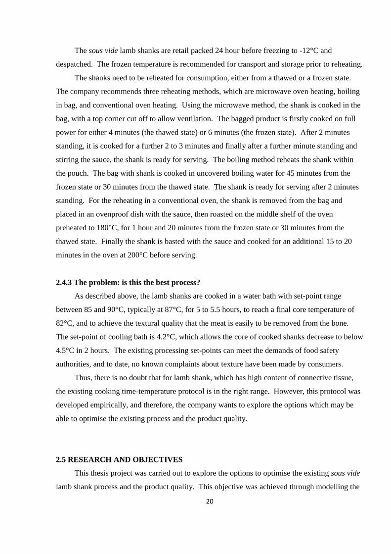
Two similar water baths were used in this project (Figure 9), one for the cooking process

(FP40-HC, Julabo Labortechnik, Gemany) and the other for the cooling process (FP40-HE).

Both of these units were capable of heating or cooling, but using each exclusively for either

heating or cooling respectively maintained consistency throughout the trials. The liquid capacity

for each of these baths was 20 L.

Figure 9. a. Cooking water bath; b. Cooling water bath.

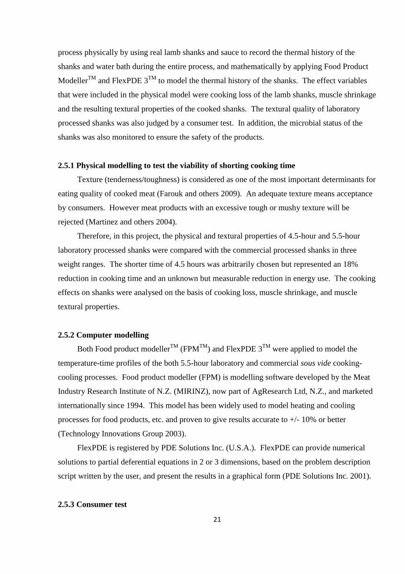
The temperature profiles of shank surface and core (see later) and each of the water baths

during process were monitored and recorded using a 1000 Series Squirrel data logger by Eltek

(U.K.) (Figure 10).

.

a b

26

Figure 10. Data logger.

The texture of the cooked shanks was analysed using a TA HDi Texture Analyser, by

Stable Micro Systems (U.K.).

3.4 DEVELOPMENTS OF THERMAL MONITORING AND THE SOUS VIDE

PROCESS

3.4.1 Development of thermocouples and calibration

To accurately monitor shank temperature changes during cooking and cooling, two

thermocouples were inserted into each shank – one at the core of a muscle group and the other

just under the surface collagen layer (see next section for details). Each of the thermocouples

used were made from lengths of Teflon-insulated twin-twist wire, 0.2 mm in diameter,

designated T-type (Farnell, New Zealand). The thermocouple was prepared by exposing a short

section of wire at each end of each strand and twisting the two wires at one end prior to soldering.

The exposed wires at the other end were connected to a plug according to their electrical

polarities. Each probe, typically measuring 1 m, was identified by a unique number so that the

calibration of each probe could be traced and the probes linked to a given shank during each trial.

27

The thermocouples were calibrated in an ice reference (a water and ice slurry in a thermos

flask to give a solution close to 0°C). For the calibration check, the thermocouple sensors were

tied to a reference thermometer probe. This was an electronic thermometer, model RT200,

manufactured by Industrial Research Ltd. (New Zealand), with a platinum resistance probe,

manufactured by Sensing Devices Ltd. (U.K.). Each thermocouple sensor tip was immediately

adjacent to the sensor of the reference thermometer. The thermocouples were connected to the

data logger, and the temperatures were recorded every 30 seconds. This process confirmed that

the accuracy of the combination of thermocouple sensors and logger was within 0.5°C.

3.4.2 Application of thermocouples to the vacuum bags

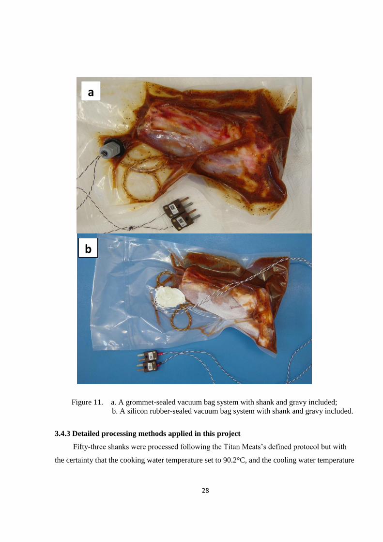
To allow the sensors to be fitted to the vacuum packed product, two methods were tried.

The first involved the use of a grommet (Figure 11a) to provide a sealed access for the

thermocouple wires in the vacuum bag. Whereas this method did work, the grommets were

bulky and a better solution was found simply using a silicon rubber sealant. A 14-gauge

hypodermic needle was used to poke a strategically-placed hole in the surface of the vacuum bag.

For each sous vide shank preparation, two thermocouple wires were passed through the small

hole, such that typically 15 cm of wire was able to reach the required sensing point in shank

muscle. The hole, now partially blocked by the two wires, was then sealed by a copious external

layer of white Specialist Silicone Sealant (Sika, New Zealand) (Figure 11b). The bags were left

in at normal room temperature for 2 or 3 days to cure the sealant before being used for the sous

vide process. Preliminary experiments showed that no leakage was found with the seals during

the cooking and cooling of the sous vide process.

28

Figure 11. a. A grommet-sealed vacuum bag system with shank and gravy included;

b. A silicon rubber-sealed vacuum bag system with shank and gravy included.

3.4.3 Detailed processing methods applied in this project

Fifty-three shanks were processed following the Titan Meats‟s defined protocol but with

the certainty that the cooking water temperature set to 90.2°C, and the cooling water temperature

a

b

29

set to 4.2°C. The laboratory trial process was divided into three main steps that followed a

defined time sequence (Table 5).

Table 5. Sequence of vacuum packing, cooking and cooling of lamb shanks, and

physical measurements and texture analysis after processing

Time Actions in temporal order Time taken

(hour)

Day 1 Measured and recorded dimensions of three frozen

weighed shanks

0.3

Drilled a hole into the thermal centre of the largest

muscle group1, and a hole on the surface of the same

muscle, positioned directly above the thermal centre

0.3

Placed the prepared (frozen) shank into a vacuum bag

fitted with sealed thermocouple wires, and inserted the

thermocouple sensors into the end of the holes. Filled

remaining airspace in the holes with water drops using a

hypodermic needle

0.3

Stored the prepared shanks in a -12°C freezer Overnight

Day 2 Added 100 g prepared gravy into the bottom of each

shank bag. Vacuum sealed the bags

0.3

Connected the thermocouple plugs to the data logger,

started the data logger and placed three vacuum-packed

shanks plus a water temperature thermocouple into the

cooking water bath, with the temperature set at 90.2°C.

Cooked for 5.5 hours, then transferred the cooked

shanks and the water temperature thermocouple to the

cooling water bath, with a temperature set-point of

4.2°C, and cooled for 2 hours

7.6

Day 3 and

later

Stored the cooked shanks at -12°C until further analysis As required

3.4.3.1 Raw shank dimensions and treatments on Day 1

Three shanks were taken from the -12°C freezer for each cooking trial. The number

cooked was limited by the size/capacity of the water bath. Seven dimensions were recorded for

each shank, including the length, width and cross-section, tagged x, y, z, a, b, m, n, respectively

1 The largest muscle group comprises the foreshank extensor and flexors, including M. Extensor carpi ulnaris, M.

flexor carpi ulnaris, and M. flexor digitorum profundus

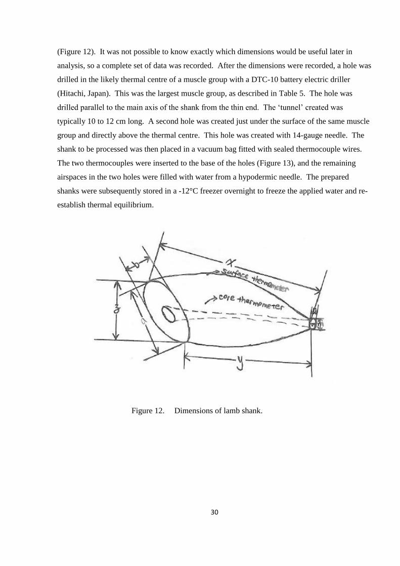
30

(Figure 12). It was not possible to know exactly which dimensions would be useful later in

analysis, so a complete set of data was recorded. After the dimensions were recorded, a hole was

drilled in the likely thermal centre of a muscle group with a DTC-10 battery electric driller

(Hitachi, Japan). This was the largest muscle group, as described in Table 5. The hole was

drilled parallel to the main axis of the shank from the thin end. The „tunnel‟ created was

typically 10 to 12 cm long. A second hole was created just under the surface of the same muscle

group and directly above the thermal centre. This hole was created with 14-gauge needle. The

shank to be processed was then placed in a vacuum bag fitted with sealed thermocouple wires.

The two thermocouples were inserted to the base of the holes (Figure 13), and the remaining

airspaces in the two holes were filled with water from a hypodermic needle. The prepared

shanks were subsequently stored in a -12°C freezer overnight to freeze the applied water and re-

establish thermal equilibrium.

Figure 12. Dimensions of lamb shank.

31

Figure 13. Raw shank with thermocouples in place.

3.4.3.2 Sous vide cooking-cooling process on Day 2

On Day 2, the three prepared shank bags were removed from the -12°C freezer. One

hundred grams of the prepared gravy was added into the bottom of each bag, and then the bags

were sealed using the vacuum packer. The thermocouple probes were then connected to the data

logger, and once all three vacuum-packed shanks were prepared, they were placed into the

cooking water bath, along with a temperature sensor to measure the bath temperature. The bath

temperature set at 90.2°C. The cooking process was for 5.5 hours, after which the cooked shank

packs were transferred, along with the water temperature sensor, to the cooling bath, which was

set at 4.2°C. The cooling process was for 2 hours.

3.4.3.3 Storage after cooking

The individual cooked shank packs were then stored in a -12°C freezer, until further

analysis.

32

3.4.4 Thermal data obtained from the commercial process

To allow a comparison to be made to the commercial process, the water temperature

during a commercial run was recorded on a visit to the processing plant at Takapau, Hawkes Bay.

The size (4.5 x 1.5 x 1.5 m) of the commercial steam-jacketed cooking bath was considered

when determining the required number and placement of the thermocouple probes. It was

decided that 13 probes would give an overview of the bath‟s temperature profile. Accordingly,

the 13 sensors were wire-tied to the cooking baskets at selected locations, to be described in

detail in the next chapter. These selected locations included the middle and both ends of the bath,

just below the surface of water, and at middle and bottom depths. The air temperature in the

processing room was also recorded. Unfortunately, it was not possible to record the surface and

core temperature of any shank during commercial processing, due to the requirement to fit in

with a dedicated process (and to hygiene regulations). Moreover, no thermocouple was tied to a

shank(s) at the likely thermal centre of a basket full of shanks. It was not realistically possible

to do this in a time constrained one-off industrial trial.

3.4.5 Recovery of the temperature data from laboratory trials and the commercial process

As described above, two thermocouple probes were inserted into each shank to monitor

changes in the muscle‟s core and surface temperature during the cooking-cooling process. This

temperature data was recorded by the data logger at 30 second intervals during the entire process.

The temperature variation in the cooking and cooling water baths was also recorded using the

additional thermocouple sensor described above. In the case of the commercial temperature

logging, data were recorded every 5 minutes.

The temperature data were downloaded from the data logger to computer, and reviewed

using Microsoft Excel.

3.5 COMPUTER MODEL SETTING

Both Food product modellerTM

(FPMTM

) and FlexPDE3 (PDE Solutions, Inc.) were used to

model the temperature history of shanks during the sous vide process.

FPMTM

modelled the shank as a finite cylinder of lean meat, with a dimension of 12 cm

length and 3 cm radius. The dimensional data using here were collected and calculated from the

33

experimental trials. The shank surface and core temperatures during cooking-cooling process

were calculated using the cooking and cooling water temperature data recorded from both

laboratory and commercial trials, and the heat transfer coefficient (HTC) value was set as 500 W

m-2

°K-1

.

FlexPDE3 used the dimensional data that was collected from the laboratory trials to draw a

2-dimensional model of lamb shank, then created a temperature profile of the shank core and

surface by applying the laboratory setting of the sous vide cooking-cooling process.

3.6 THE POTENTIAL TO SHORTENING PROCESSING TIME

Cooking is the most time and energy intensive stage in a sous vide process. Therefore,

reducing the cooking time, if possible, would be an effective and efficient way to shorten the

process and cut the cost of production.

For this trial, the cooking time was reduced to 4.5 hours from the standard 5.5 hours.

Shanks selected by weight were treated in exactly the same way as for the standard 5.5-hour

process. A total of 30 shanks were processed for 4.5 hours.

3.7 PHYSICAL MEASUREMENTS AND TEXTURE ANAYSIS OF THE COOKED

SHANKS

3.7.1 Physical measurements of the cooked shanks

Cooked lamb shanks (three from each trial) were taken from the -12°C freezer one day

prior to physical tests and left in the texture analysis room overnight (room temperature set at

15°C) to equilibrate samples to the room temperature. The next day, the thawed shank sample

was removed from the plastic bag, the marinade was rinsed off using tap water, and the shank

was patted dry with a paper towel.

3.7.1.1 Cooking loss

After patting dry, the cooked shank was weighted. The cooking loss was calculated as the

difference between raw and cooked mass as a percentage of initial (raw) mass, which can be

expressed by the following equation:

34

Cooking loss (%) = [(Raw weight – cooked weight) / Raw weight] x 100%

3.7.1.2 Shrinkage

The muscle shrinkage was expressed as the muscle length reduction, which was measured

from the length of bone that was exposed at the end of the cooked shank after process compared

to that before.

3.7.1.3 Physical measurements of three major muscle groups

Three major muscle groups, named Large muscle (the largest muscle group mentioned in

Section 3.4.3), Side muscle, and Small muscle (Figure 14), were removed from each shank based

on their distribution. The large muscle group comprises foreshank extensor and flexors,

including M. Extensor carpi ulnaris, M. flexor carpi ulnaris, and M. flexor digitorum profundus;

the side muscle group is the foreshank flexor M. flexor carpi radialis; and the small muscle

group comprises M. biceps brachii and M. extensor carpi radialis. These three muscle groups

were kept in snap lock bag for later texture analysis after the measurements of weights and

multiple dimensions. In addition, the weights of the remaining muscle on the shank, called

„rubbish‟, and combination of bone and cartilage (Figure 14) were also recorded.

35

Figure 14. Large muscle group, side muscle group, small muscle group, rubbish and

combination of bone and cartilage from a lamb shank.

3.7.2 Texture Analysis

Texture analysis was carried out at room temperature (15°C) with a TA HDi Texture

Analyser which was fitted with a square probe of 1 cm on edge. A coarse abrasive cloth strip

held in place with clamps was used to cover the instrument‟s base plate (Figure 15). This strip

provided a surface that would resist sliding of wet cooked muscle. In this way all the force

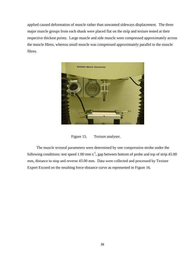
36

applied caused deformation of muscle rather than unwanted sideways displacement. The three

major muscle groups from each shank were placed flat on the strip and texture tested at their

respective thickest points. Large muscle and side muscle were compressed approximately across

the muscle fibres, whereas small muscle was compressed approximately parallel to the muscle

fibres.

Figure 15. Texture analyser.

The muscle textural parameters were determined by one compression stroke under the

following conditions: test speed 1.00 mm s-1

, gap between bottom of probe and top of strip 45.00

mm, distance to stop and reverse 43.00 mm. Data were collected and processed by Texture

Expert Exceed on the resulting force-distance curve as represented in Figure 16.

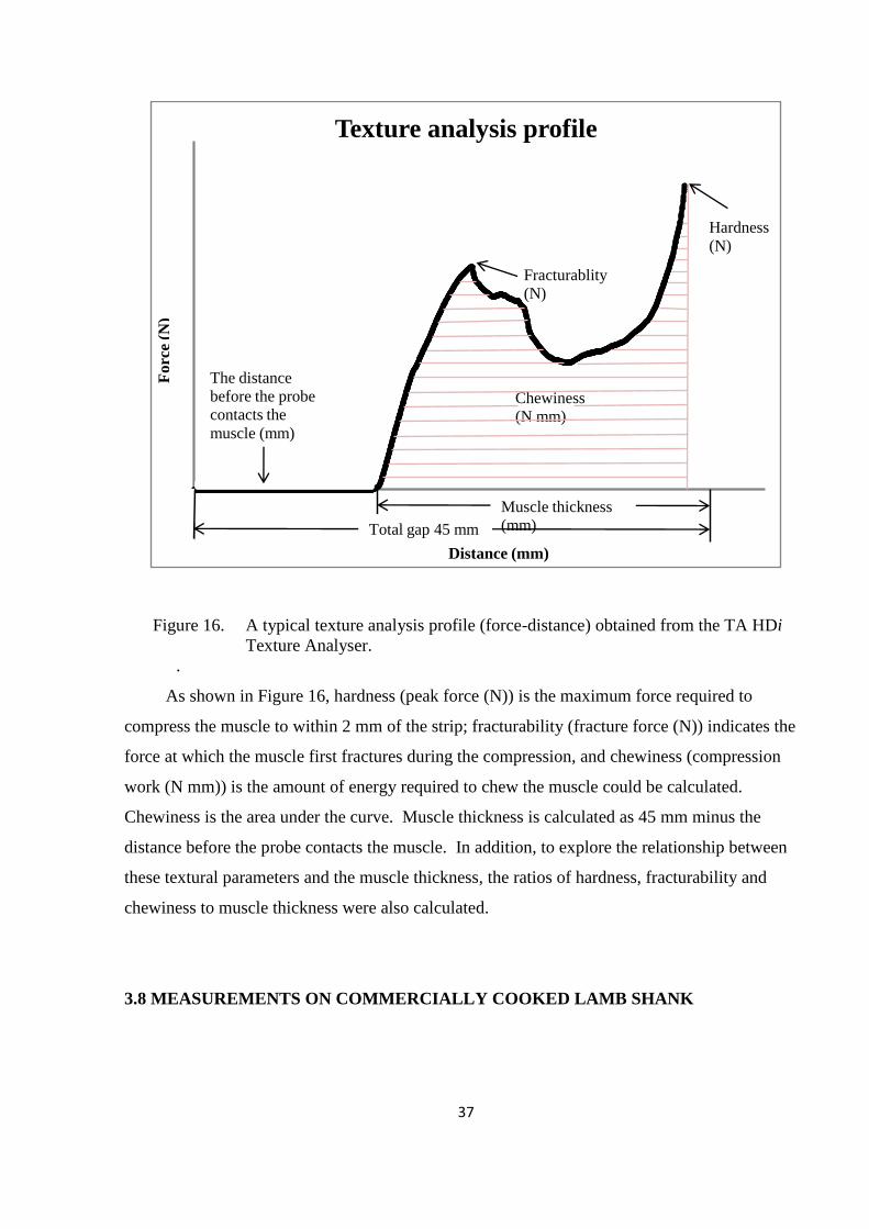
37

Figure 16. A typical texture analysis profile (force-distance) obtained from the TA HDi

Texture Analyser.

.

As shown in Figure 16, hardness (peak force (N)) is the maximum force required to

compress the muscle to within 2 mm of the strip; fracturability (fracture force (N)) indicates the

force at which the muscle first fractures during the compression, and chewiness (compression

work (N mm)) is the amount of energy required to chew the muscle could be calculated.

Chewiness is the area under the curve. Muscle thickness is calculated as 45 mm minus the

distance before the probe contacts the muscle. In addition, to explore the relationship between

these textural parameters and the muscle thickness, the ratios of hardness, fracturability and

chewiness to muscle thickness were also calculated.

3.8 MEASUREMENTS ON COMMERCIALLY COOKED LAMB SHANK

-5

0

5

10

15

20

25

30

35

0 5 10 15 20 25 30 35 40 45 50

Fo

rce

(N)

Distance (mm)

Texture analysis profile

Fracturablity

(N)

Hardness

(N)

The distance

before the probe

contacts the

muscle (mm)

Chewiness

(N mm)

Muscle thickness

(mm)Total gap 45 mm

38

Thirty eight cooked shanks provided by Titan Meats were measured following the same

procedure of physical measurements and texture analysis that applied to the laboratory-processed

shanks.

3.9 TEXTURAL COMPARSION OF THE LABORATORY- AND COMMERICAL-

PROCESSED SHANKS

The textural properties of shanks cooked laboratory for 4.5 hours and 5.5 hours were

compared with the commercial products based on three muscle groups. The compared

parameters included hardness (peak force), fracturability (fracture force), chewiness

(compression work), and the ratios of these three parameters to muscle thickness.

3.10 CONSUMER PREFERENCE TEST OF LABORATORY-PROCESSED SHANK

A limited consumer test was done to evaluate the consumer preference of shanks cooked in

the laboratory process for 4.5 hours and 5.5 hours. Twenty-eight consumers took part to judge

the tenderness, juiciness and overall impression of the large muscle using 7-point hedonic scales

(Appendix 1) to explain the degrees of tenderness, juiciness and over liking of the shanks

cooked for the two times.

Twenty medium-size shanks were processed in the laboratory (three shanks per day), ten

were cooked for 4.5 hours, and the others for 5.5 hours. The cooked shanks were frozen stored

(-12°C) for at least 1 week before the consumer test.

These cooked shanks were reheated in microwave from the frozen state before serving,

following Titan Meats‟s recommend reheating method (see Section 2.4.2). The method used

here was believed to be similar to the reheating method used in the pubs. Three meat pieces

(about 2 cm in length) were cut from each shank large muscle. Two meat pieces (with gravy on)

that were cooked for the two times were served to each consumer and each identified by a unique

3-digit code. The consumers could taste in any order.

3.11 MICROBIOLOGICAL TESTS

39

The microbiological tests were carried out in three stages. In the first stage the counts of

initial bacterial loads on the surface of the frozen shank and in the sauce (separately) before

vacuum packing were made. In the second stage the counts of survival bacteria loads were made

in the sauce after the sous vide cooking-cooling process. In the third stage, counts were made in

the sauce after further frozen storage at -12°C for a week. The tests were divided into five steps,

sampling, dilution series preparation, plating, colonies counting, and results calculation. The

whole procedure followed a defined time sequence (Table 6).

Table 6. Sequence of sampling, dilution series preparation, plating, colonies

counting, and results calculation

Time Actions in temporal order

Day 1 Collected three 12 mm diameter samples (each weight approx 0.5 g) from

each shank by using borer, scalpel and forceps (washed in drum ethanol and

flamed before sampling). Samples were kept in 24-oz Whirl-Pak® write-one

bag (NASCO, U.S.) with nine times weight dilution fluid (0.1% peptone +

0.85% NaCl). Three shanks were sampled each day. Then collected 2 g of

sauce gravy sample which would be used for the cooking, and treated as the

meat samples

Processed the three sampled shanks using the sous vide protocol introduced

above

Transported the collected shank and sauce samples to the microbiological

lab, prepared the ten-fold sample dilutions, then inoculated the serially

diluted sample homogenates onto specific medias and incubated the medias

at certain conditions and temperatures as required

After 7.5 hours cooking-cooling process, collected 2 g sauce from the

cooked shank package, then sealed the sample in a 24-oz Whirl-Pak® write-

one bag with nine times weight dilution fluid (0.1% peptone + 0.85% NaCl)

and stored in a 5°C chiller

Day 2 Transported the cooked sauce sampling bag from the chiller to the

microbiological lab, prepared the sample homogenates, then plated and

incubated at certain conditions and temperatures as required

Day 3 and

later

Counted the numbers of colonies on the incubated agar plates, and calculated

the results

Day 7 Repeat the five steps sequence on frozen sauce

The microbiological tests included aerobic and anaerobic plate counts, Enterobacteriaceae

count, mesophilic and psychrophilic anaerobe counts and analysis for the presence of viable

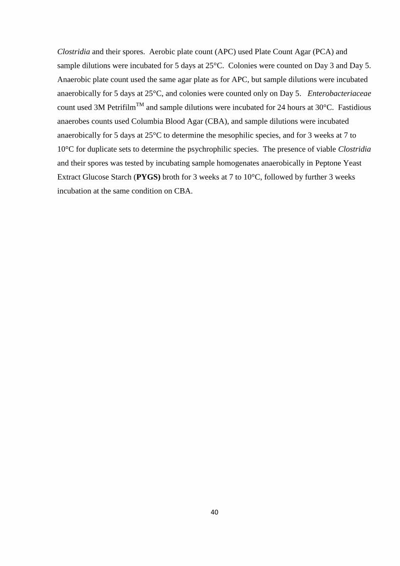
40

Clostridia and their spores. Aerobic plate count (APC) used Plate Count Agar (PCA) and

sample dilutions were incubated for 5 days at 25°C. Colonies were counted on Day 3 and Day 5.

Anaerobic plate count used the same agar plate as for APC, but sample dilutions were incubated

anaerobically for 5 days at 25°C, and colonies were counted only on Day 5. Enterobacteriaceae

count used 3M PetrifilmTM

and sample dilutions were incubated for 24 hours at 30°C. Fastidious

anaerobes counts used Columbia Blood Agar (CBA), and sample dilutions were incubated

anaerobically for 5 days at 25°C to determine the mesophilic species, and for 3 weeks at 7 to

10°C for duplicate sets to determine the psychrophilic species. The presence of viable Clostridia

and their spores was tested by incubating sample homogenates anaerobically in Peptone Yeast

Extract Glucose Starch (PYGS) broth for 3 weeks at 7 to 10°C, followed by further 3 weeks

incubation at the same condition on CBA.

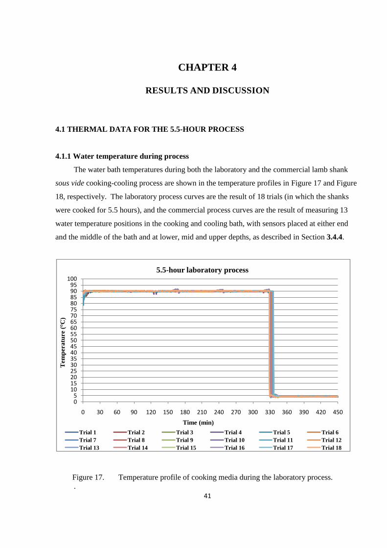
41

CHAPTER 4

RESULTS AND DISCUSSION

4.1 THERMAL DATA FOR THE 5.5-HOUR PROCESS

4.1.1 Water temperature during process

The water bath temperatures during both the laboratory and the commercial lamb shank

sous vide cooking-cooling process are shown in the temperature profiles in Figure 17 and Figure

18, respectively. The laboratory process curves are the result of 18 trials (in which the shanks

were cooked for 5.5 hours), and the commercial process curves are the result of measuring 13

water temperature positions in the cooking and cooling bath, with sensors placed at either end

and the middle of the bath and at lower, mid and upper depths, as described in Section 3.4.4.

Figure 17. Temperature profile of cooking media during the laboratory process.

.

05

101520253035404550556065707580859095

100

0 30 60 90 120 150 180 210 240 270 300 330 360 390 420 450

Tem

pera

ture (°C

)

Time (min)

5.5-hour laboratory process

Trial 1 Trial 2 Trial 3 Trial 4 Trial 5 Trial 6

Trial 7 Trial 8 Trial 9 Trial 10 Trial 11 Trial 12

Trial 13 Trial 14 Trial 15 Trial 16 Trial 17 Trial 18

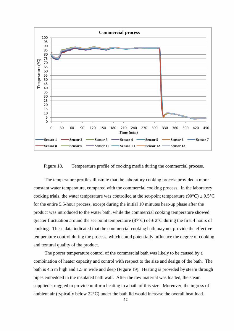
42

Figure 18. Temperature profile of cooking media during the commercial process.

The temperature profiles illustrate that the laboratory cooking process provided a more

constant water temperature, compared with the commercial cooking process. In the laboratory

cooking trials, the water temperature was controlled at the set-point temperature (90°C) ± 0.5°C

for the entire 5.5-hour process, except during the initial 10 minutes heat-up phase after the

product was introduced to the water bath, while the commercial cooking temperature showed

greater fluctuation around the set-point temperature (87°C) of ± 2°C during the first 4 hours of

cooking. These data indicated that the commercial cooking bath may not provide the effective

temperature control during the process, which could potentially influence the degree of cooking

and textural quality of the product.

The poorer temperature control of the commercial bath was likely to be caused by a

combination of heater capacity and control with respect to the size and design of the bath. The

bath is 4.5 m high and 1.5 m wide and deep (Figure 19). Heating is provided by steam through

pipes embedded in the insulated bath wall. After the raw material was loaded, the steam

supplied struggled to provide uniform heating in a bath of this size. Moreover, the ingress of

ambient air (typically below 22°C) under the bath lid would increase the overall heat load.

05

101520253035404550556065707580859095

100

0 30 60 90 120 150 180 210 240 270 300 330 360 390 420 450

Tem

per

atu

re (°C

)

Time (min)

Commercial process

Sensor 1 Sensor 2 Sensor 3 Sensor 4 Sensor 5 Sensor 6 Sensor 7

Sensor 8 Sensor 9 Sensor 10 Sensor 11 Sensor 12 Sensor 13

43

Figure 19. Thermal sensors‟ position for water temperature monitoring during the

commercial process.

Based on information initially provided by Titan Meats, the laboratory cooking

temperature was set at 90°C, compared to the actual commercial cooking temperature which

ranged between 85 and 90°C, nominally a set-point of 87°C. With the high connective tissue

content, lamb shank is inherently tough and required extended cooking to achieve a tender

product (Lawrie 2006). Therefore, given that a higher cooking temperature is likely to give

better results, the textural results obtained from a 90°C set-point are arguably likely to be better

than those from a lower temperature set-point. In addition, based on initial information provided

by Titan Meats, the laboratory cooking time was defined at 5.5 hours, which turned out to be

different from that for the industrial cooking process, which uses 5 to 5.5 hours, depending on

the required doneness of shanks.

During the laboratory cooking process, the water temperature dropped to approx 85°C after

three frozen shanks were placed into the bath, but recovered to the set-point temperature of 90°C

within 10 minutes. By comparison, during the commercial cooking process, the bath

temperature dropped to below 75°C when the baskets of shanks were loaded, and it took 1 hour

for the water temperature to recover to the set-point temperature of 87°C. The greater

temperature drop in the commercial cooking process and much longer recovery time were likely

due to the limited heating capacity of the bath from the initial product load (about 660 frozen

shanks).

When monitoring the bath temperature in the commercial process, the two baskets

(referred to as Basket 1 and Basket 2) were loaded into the cooking bath, and 13 sensors (copper

constantan thermocouples) were held on the baskets at different positions by domestic tie-wires

44

(Figure 19). The temperature variations between these 13 sensor locations can be seen in Figure

20. Sensors 8, 9, 10, 11, and 12 all recorded a temperature of 1.5°C higher than those recorded

by Sensors 1, 2, 3 and 4 during the first three hours cooking, and temperatures at Sensors 5, 6, 7

and 13 were between the extremes. These data showed that the temperature at the sides of

Basket 2 was higher than that at the equivalent locations on Basket 1. The likely reason is the

difference in lamb shank loading between Baskets 1 and 2, with Basket 1 fully loaded, and

Basket 2 partially loaded. Therefore, this produced variation in heat load on the heating system

in different area of the bath. This would be exacerbated by the lack of forced circulation within

the bath and tends agreed with the discussion in the previous paragraph comparing the

commercial and laboratory situations.

Figure 20. Temperature profile of cooking media during the commercial process

(highlight of water temperature between 72 and 92°C). Sensors 1and 2 were

secured at one end of Basket 1, and were close to the bath wall; Sensors 3 and 4

were secured on the front side of Basket 1, and near to the bath wall; Sensors 5,

6 and 7 were secured to the opposite end of Basket 1, which was close to the

middle of cooking bath. Sensors 8, 9, and 10 were secured on the end of

Basket 2, and were close to the bath wall; Sensors 11 and 12 – like 3 and 4 –

were secured on the front side of Basket 2, also near to the bath wall, and

72

74

76

78

80

82

84

86

88

90

92

0 30 60 90 120 150 180 210 240 270 300 330

Tem

per

atu

re (°C

)

Time (min)

72 to 92°C - Commercial process

Sensor 1 Sensor 2 Sensor 3 Sensor 4 Sensor 5 Sensor 6 Sensor 7

Sensor 8 Sensor 9 Sensor 10 Sensor 11 Sensor 12 Sensor 13

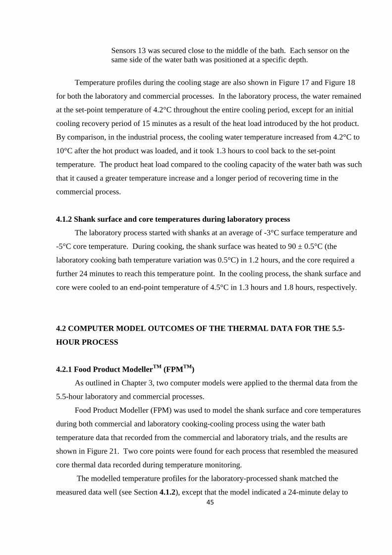
45

Sensors 13 was secured close to the middle of the bath. Each sensor on the

same side of the water bath was positioned at a specific depth.

Temperature profiles during the cooling stage are also shown in Figure 17 and Figure 18

for both the laboratory and commercial processes. In the laboratory process, the water remained

at the set-point temperature of 4.2°C throughout the entire cooling period, except for an initial

cooling recovery period of 15 minutes as a result of the heat load introduced by the hot product.

By comparison, in the industrial process, the cooling water temperature increased from 4.2°C to

10°C after the hot product was loaded, and it took 1.3 hours to cool back to the set-point

temperature. The product heat load compared to the cooling capacity of the water bath was such

that it caused a greater temperature increase and a longer period of recovering time in the

commercial process.

4.1.2 Shank surface and core temperatures during laboratory process

The laboratory process started with shanks at an average of -3°C surface temperature and

-5°C core temperature. During cooking, the shank surface was heated to 90 ± 0.5°C (the

laboratory cooking bath temperature variation was 0.5°C) in 1.2 hours, and the core required a

further 24 minutes to reach this temperature point. In the cooling process, the shank surface and

core were cooled to an end-point temperature of 4.5°C in 1.3 hours and 1.8 hours, respectively.

4.2 COMPUTER MODEL OUTCOMES OF THE THERMAL DATA FOR THE 5.5-

HOUR PROCESS

4.2.1 Food Product ModellerTM

(FPMTM

)

As outlined in Chapter 3, two computer models were applied to the thermal data from the

5.5-hour laboratory and commercial processes.

Food Product Modeller (FPM) was used to model the shank surface and core temperatures

during both commercial and laboratory cooking-cooling process using the water bath

temperature data that recorded from the commercial and laboratory trials, and the results are

shown in Figure 21. Two core points were found for each process that resembled the measured

core thermal data recorded during temperature monitoring.

The modelled temperature profiles for the laboratory-processed shank matched the

measured data well (see Section 4.1.2), except that the model indicated a 24-minute delay to

46

reach 90 ± 0.5°C at both the core and surface of the shank, compared to measured 72 and 96

minutes, respectively. In addition, FPM indicated that for the shank surface temperature during

the laboratory cooling process it took 1.8 hours to reduce to 4.5°C, which was 27 minutes longer

than the measured time. The shank core temperature reduced to 4.7°C by the end of the

modelled cooling process.

These differences could be due to the shank description used in the model. The shank was

modelled as a cylinder of lean meat, as FPM is unable to deal with irregular shapes. In addition,

a lamb shank consists of a significant section of bone with meat plus connective tissue and a

small amount of fat cover unevenly distributed over its surface (their effects on shank cooking

are described in a later section). These factors would all impact on the accuracy of the modelling

outcomes, but it is likely that the model could be finely „tuned‟ to account for these factors,

therefore be a useful tool for future decision making regarding to the shank processing time and

temperature. As it was, the current FPM model still provided a reasonable prediction on shank

temperature changes during thermal process.

Figure 21. Core and surface temperature profiles of lamb shank during commercial and lab

processes, modelled by FPM.

-10-505

101520253035404550556065707580859095

0 30 60 90 120 150 180 210 240 270 300 330 360 390 420 450

Tem

per

atu

re (°C

)

Time (min)

Model of lamb shank core and surface temperature profile during

commercial and laboratory processes

Core 1 - commericial shank Core 2 - commericial shank Surface - commericial shank

Core 1 - Lab-processed shank Core 2 - Lab-processed shank Surface - Lab-processed shank

47

The FPM model results are shown in Figure 21. These curves indicate that the surface

temperatures of both the commercial- and laboratory-processed shank were predicted to increase

to 50°C in the first 3 minutes cooking (the initial temperature of the shank was

-5°C), but following the initial period, the temperature of the laboratory-processed shank

increased more rapidly than that of the commercial shank.

The model also indicates that at Core 1 and Core 2, both the commercial- and laboratory-

processed shanks went through a similar temperature change during the first 9 and 6 minutes of

cooking, respectively, and after that, the temperature of the laboratory-processed shank rose up

faster than that for the commercial shank. The commercial process required about 15 minutes

more to heated up the shank to a mean temperature above 75°C (when collagen starts to

gelatinize), compared to the laboratory process. In addition, the temperature of the laboratory

shank retained at 90°C (the cooking temperature) in a ± 0.5°C variation after heated to the point,

whereas, the temperature of the commercial shank fluctuated around 87°C (the cooking

temperature) in a ± 2°C variation.

For the cooling process, the FPM model indicates that the cooked shank surface was

cooled to 4.5°C in 108 minutes for the laboratory process and in 102 minutes for the commercial

process. The shank core temperatures (Core 1 and 2) dropped to below 5°C by the end of

cooling process, as shown by the converging curves (Figure 21).

The outcomes of the FPM model suggest the cooking effectiveness of the commercial

process was not as good as that of the laboratory process, as the former required a longer time to

heat up the shank. However, the cooling process model shows there was no significant

difference between the two processes.

The measured difference in heating rate between the commercial and laboratory cooking

processes is due to the difference in total heat load of the processes with respect to the heating

capacity and volume of the respective cooking water baths. The total heat load is the amount of

heat that is required to be transferred to the raw material (packages of part-frozen lamb shanks

with sauce) to increase the temperature to a required endpoint plus the heat energy required to

overcome heat infiltration through the external surfaces of the water bath (Serrallach 1987). The

mass of the material is the most significant factor in terms of heat load and to match the

laboratory process in terms of temperature recovery after product loading would require

significantly more heat energy than is currently provided.

4.2.2 FlexPDE 3TM

48

The second computer model applied to the 5.5-hour processes was FlexPDE 3. The results

of 2-dimensional modelling of the cooking process using FlexPDE 3 did not match the measured

temperature profiles of the shank core and surface as well as those from the FPM model. There

were several reasons that could explain this, for example, the variation of the shank dimensions,

the proportion of shank muscle to bone, and the selection of thermal references, including

thermal conductivity and specific heating capacity of the shank muscle and bone that were used

to set up the model.

Nonetheless, Figure 22a shows a 2-dimensional diagram of a lamb shank entered into

FlexPDE. This illustrates a slice across a lamb shank at the greatest circumference with the

narrow yellow circle2 indicating the shank bone, which was covered by muscle (the outer

perimeter blue line). The dimensions used were the average values derived from the measured

data collected from 32 of medium-size lamb shanks. The shape of lamb shank was irregular, and

the dimension of bone was also variable, thus this graphical illustration as used for the model did

not provide an exact description of the shank shape, the position of the bone, and the proportion

of muscle to bone, all of which would influence the accuracy of the model outcomes, but could

be potentially „tuned‟ for.

Figure 22b illustrates the modelled temperatures inside the lamb shank after 5.5 hours of

immersion cooking. The conditions surrounding the shank model were set at 90.2°C (this was

required to achieve 90°C at the surface) with a heat transfer co-efficient appropriate for water

immersion. This was equivalent to the water bath conditions used. The diagram illustrates the

outer temperature at or close to the water bath temperature with the central temperatures

understandably cooler. The model indicated two low temperature zones around the bone. The

zone above was lowest at 83.2°C, and was 1.1°C colder than the opposite side of the bone. The

temperature difference between these two points was due to the thickness of muscle on the top

and bottom side of the bone.

Importantly, the FlexPDE 3 model indicates that the shank internal temperature was lower

than the surface temperature during the entire cooking process (graph shown in Appendix 2),

which differed from the measured results. This is entirely possible because no heat transfer from

the bone to the surrounding muscle, as assumed in the model. In the real world situation, heat

would flow into the bone from the exposed end, and be transmitted to muscle. Generally bone

has a higher thermal conductivity than that of lean meat (Morley 1966), thus the recommended

2 The yellow colour of this line could not be changed in FlexPDE 3, and is unfortunately hard to see.

49

cooking time (min kg-1

) for bone-in lamb leg roast is shorter than that of boneless leg roast

(Griffin and others 1985).

Although the FlexPDE 3 model did not match the measured thermal results well, it output

(Figure 22) shows the potential of this program to graphically illustrate a temperature profile

within a shank. However, the thermal references chosen were clearly inadequate. The core

temperature in the laboratory process unquestionably reached 90°C, as measured (see Section

4.1.2), but only about 83°C indicated in the model. It was outside the scope of this project to

pursue this matter further.

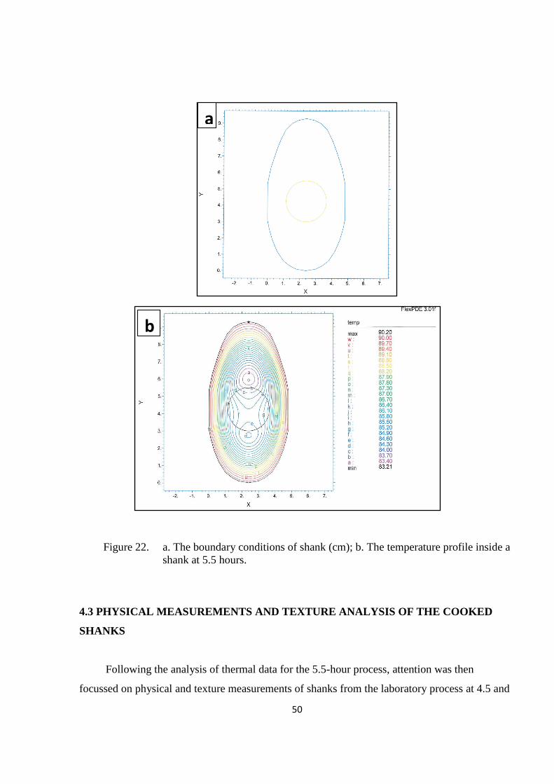
50

Figure 22. a. The boundary conditions of shank (cm); b. The temperature profile inside a

shank at 5.5 hours.

4.3 PHYSICAL MEASUREMENTS AND TEXTURE ANALYSIS OF THE COOKED

SHANKS

Following the analysis of thermal data for the 5.5-hour process, attention was then

focussed on physical and texture measurements of shanks from the laboratory process at 4.5 and

a

b

51

5.5 hours, and the commercial process at nominally 5.5 hours. The word „nominally‟ is used

because the cooked shanks provided by Titan Meats were not accompanied by process

information.

4.3.1 Physical measurements results

4.3.1.1 Cooking loss

For shanks of all weight ranges, the 5.5-hour laboratory process caused an average 18.8%

weight loss in shanks, which was significantly greater (P ≤ 0.05) than the 17.6% weight loss in

the 4.5-hour laboratory process (Table 7). However, both cooking times showed low standard

deviations, 1.8% and 1.9%, respectively, indicating that all shanks cooked laboratory for same

period of time had similar cooking losses.

Table 7. Cooking loss and muscle shrinkage of lamb shanks cooked for different time

Cooking time Cooking loss (%) Shrinkage (cm)

Mean StDev Mean StDev

4.5 h 17.6a ± 1.8 4.1

a ± 0.6

5.5 h 18.8b ± 1.9 4.1

a ± 0.5

Commercial Unavailable Unavailable 4.3a ± 0.8

Means within a column and treated with different letters differ significantly (P ≤ 0.05).

StDev = standard deviation.

As discussed in Chapter 2 the cooking loss is reported as mostly occurring between a

temperature of 65°C and 70°C, as a result of changes in charges and unfolding of proteins. Both

cooking time and meat temperature affect the cooking loss (Bole 2010). The results showed a

significantly higher cooking loss for 5.5 hours, compared to that for the 4.5 hours, which agrees

with previous studies that longer cooking time leads to higher cooking loss when meat is cooked

at a single temperature (Laakkonen and others 1970; Hostetler and others 1982; Griffin and

others 1984; Hamm 1986; Bole and Swan 2002; Bejerholm and Aaslyng 2004; Vasanthi and

others 2007). Moreover, the low standard deviations in both laboratory trials showed that the

laboratory process provided excellent temperature control during the entire project over four

months.

Cooking loss of the commercial products could not be calculated due to the original shank

mass data not being available.

52

4.3.1.2 Shrinkage

Both the 5.5-hour and 4.5-hour laboratory processes resulted in a mean of 4.1 cm reduction

in shank muscle length, which was statistically similar with the 4.3 cm shrinkage in the

commercial products (Table 7). This similarity was probably due to the cooking temperature

used in both cases. Previous studies showed that muscle shrinkage is the combined result of

water loss from both between and within muscle fibres, and shrinkage and shortening of the

fibres (Ritchey and Hostetler 1964; Obuz and Dikeman 2003; Bole 2010). When meat is

cooking, loss of water holding capacity happens between 60 and 90°C, and collagen shrinkage

occurs at about 70°C. As a result, cooking above 70°C promotes water loss and muscle

shrinkage (Bouton and others 1976; Boles and Swan 2002), and shrinkage increased only

slightly after cooking at temperature above 70°C (Bouton and others 1976). Because the heating

temperatures used in both laboratory and commercial processes were quite comparable (90 and

about 87°C, respectively), the difference in the resulting shrinkage values was small.

The standard deviation of shrinkage for commercial products was 0.8 cm, which was about

30% and 60% higher than the 4.5-hour and 5.5-hour laboratory-processed products, respectively.

This greater variability in commercial products was perhaps due to the greater temperature

variation in the cooking bath (Figure 20). This temperature variation would cause variability of

the meat dehydration, and therefore muscle shrinkage (Perez and Calvelo 1984), and thus the

cause of the variability. In addition, variation of heat transfer of the plastic bags used for

vacuum packing the shanks and sauce could be another reason. During the cooking process, the

bag acts as an insulation layer for heat transfer, its conductibility would consequently influence

the effectiveness of heating on the sample (Drummond and Sun 2006; Cheng and Sun 2007).

Considering the difference between the bags provided for the experimental work and those used

for commercial products, a variation in heat transfer may exist.

4.3.2 Texture analysis results

To determine the eating quality (tenderness/toughness) of the cooked shanks, the three

main muscle groups that were described in Chapter 3, named large muscle, side muscle and

small muscle were analysed. These three muscle groups were represented likely fractions of

cooked shank that would be selected during eating because they were easily/naturally separable.

The textural analysis was based on the hardness (peak force (N)), fracturability (fracture

force (N)), and chewiness (compression work (N mm)). These three parameters are believed to

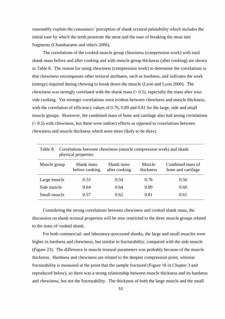
53

reasonably explain the consumers‟ perception of shank textural palatability which includes the

initial ease by which the teeth penetrate the meat and the ease of breaking the meat into

fragments (Chandraratne and others 2006).

The correlations of the cooked muscle group chewiness (compression work) with total

shank mass before and after cooking and with muscle group thickness (after cooking) are shown

in Table 8. The reason for using chewiness (compression work) to determine the correlations is

that chewiness encompasses other textural attributes, such as hardness, and indicates the work

(energy) required during chewing to break down the muscle (Lyon and Lyon 2000). The

chewiness was strongly correlated with the shank mass (> 0.5), especially the mass after sous

vide cooking. Yet stronger correlations were evident between chewiness and muscle thickness,

with the correlation of efficiency values of 0.76, 0.89 and 0.81 for the large, side and small

muscle groups. Moreover, the combined mass of bone and cartilage also had strong correlations

(> 0.5) with chewiness, but these were indirect effects as opposed to correlations between

chewiness and muscle thickness which were more likely to be direct.

Table 8. Correlations between chewiness (muscle compression work) and shank

physical properties

Muscle group Shank mass

before cooking

Shank mass

after cooking

Muscle

thickness

Combined mass of

bone and cartilage

Large muscle 0.53 0.54 0.76 0.56

Side muscle 0.64 0.64 0.89 0.60

Small muscle 0.57 0.62 0.81 0.61

Considering the strong correlations between chewiness and cooked shank mass, the

discussion on shank textural properties will be now restricted to the three muscle groups related

to the mass of cooked shank.

For both commercial- and laboratory-processed shanks, the large and small muscles were

higher in hardness and chewiness, but similar in fracturability, compared with the side muscle

(Figure 23). The difference in muscle textural parameters was probably because of the muscle

thickness. Hardness and chewiness are related to the deepest compression point, whereas

fracturability is measured at the point that the sample fractured (Figure 16 in Chapter 3 and

reproduced below), so there was a strong relationship between muscle thickness and its hardness

and chewiness, but not the fracturability. The thickness of both the large muscle and the small

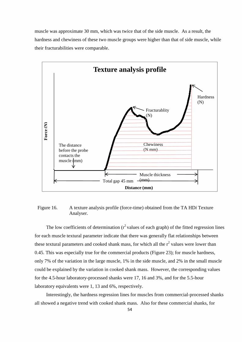
54

muscle was approximate 30 mm, which was twice that of the side muscle. As a result, the

hardness and chewiness of these two muscle groups were higher than that of side muscle, while

their fracturabilities were comparable.

Figure 16. A texture analysis profile (force-time) obtained from the TA HDi Texture

Analyser.

The low coefficients of determination (r2

values of each graph) of the fitted regression lines

for each muscle textural parameter indicate that there was generally flat relationships between

these textural parameters and cooked shank mass, for which all the r2 values were lower than

0.45. This was especially true for the commercial products (Figure 23); for muscle hardness,

only 7% of the variation in the large muscle, 1% in the side muscle, and 2% in the small muscle

could be explained by the variation in cooked shank mass. However, the corresponding values

for the 4.5-hour laboratory-processed shanks were 17, 16 and 3%, and for the 5.5-hour

laboratory equivalents were 1, 13 and 6%, respectively.

Interestingly, the hardness regression lines for muscles from commercial-processed shanks

all showed a negative trend with cooked shank mass. Also for these commercial shanks, for

-5

0

5

10

15

20

25

30

35

0 5 10 15 20 25 30 35 40 45 50

Forc

e (N

)

Distance (mm)

Texture analysis profile

Fracturablity

(N)

Hardness

(N)

The distance

before the probe

contacts the

muscle (mm)

Chewiness

(N mm)

Muscle thickness

(mm)Total gap 45 mm

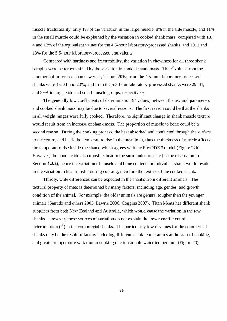
55

muscle fracturability, only 1% of the variation in the large muscle, 8% in the side muscle, and 11%

in the small muscle could be explained by the variation in cooked shank mass, compared with 18,

4 and 12% of the equivalent values for the 4.5-hour laboratory-processed shanks, and 10, 1 and

13% for the 5.5-hour laboratory-processed equivalents.

Compared with hardness and fracturability, the variation in chewiness for all three shank

samples were better explained by the variation in cooked shank mass. The r2

values from the

commercial-processed shanks were 4, 12, and 20%; from the 4.5-hour laboratory-processed

shanks were 45, 31 and 20%; and from the 5.5-hour laboratory-processed shanks were 29, 41,

and 39% in large, side and small muscle groups, respectively.

The generally low coefficients of determination (r2

values) between the textural parameters

and cooked shank mass may be due to several reasons. The first reason could be that the shanks

in all weight ranges were fully cooked. Therefore, no significant change in shank muscle texture

would result from an increase of shank mass. The proportion of muscle to bone could be a

second reason. During the cooking process, the heat absorbed and conducted through the surface

to the centre, and leads the temperature rise in the meat joint, thus the thickness of muscle affects

the temperature rise inside the shank, which agrees with the FlexPDE 3 model (Figure 22b).

However, the bone inside also transfers heat to the surrounded muscle (as the discussion in

Section 4.2.2), hence the variation of muscle and bone contents in individual shank would result

in the variation in heat transfer during cooking, therefore the texture of the cooked shank.

Thirdly, wide differences can be expected in the shanks from different animals. The

textural property of meat is determined by many factors, including age, gender, and growth

condition of the animal. For example, the older animals are general tougher than the younger

animals (Sanudo and others 2003; Lawrie 2006; Coggins 2007). Titan Meats has different shank

suppliers from both New Zealand and Australia, which would cause the variation in the raw

shanks. However, these sources of variation do not explain the lower coefficient of

determination (r2) in the commercial shanks. The particularly low r

2 values for the commercial

shanks may be the result of factors including different shank temperatures at the start of cooking,

and greater temperature variation in cooking due to variable water temperature (Figure 20).

56

Large muscle (L)

200 250 300 350

Hard

ness (

Peak f

orc

e (

N))

0

20

40

60

80

100

120

140

160

180

r2 = 0.17

r2 = 0.01

r2 = 0.07

Side muscle (E)

200 250 300 350

r2 = 0.16

r2 = 0.13

r2 = 0.01

Small muscle (S)

Mass of cooked shank (g)200 250 300 350

r2 = 0.03

r2 = 0.06

r2 = 0.02

Large muscle (L)

200 250 300 350

Fra

ctu

rab

ilit

y (

Fra

ctu

re F

orc

e (

N))

0

10

20

30

40

50

60

70

80

r2 = 0.18

r2 = 0.10

r2 = 0.01

Side muscle (E)

Mass of cooked shank (g)200 250 300 350

r2 = 0.04

r2 = 0.01

r2 = 0.08

Small muscle (S)

200 250 300 350

r2 = 0.12

r2 = 0.13

r2 = 0.11

Large muscle (L)

200 250 300 350

Ch

ew

iness (

Co

mp

ressio

n w

ork

(N

mm

))

0

100

200

300

400

500

600

700

r2

= 0.45

r2

= 0.29

r2

= 0.04

Side muscle (E)

Mass of cooked shank (g)200 250 300 350

r2

= 0.31

r2

= 0.41

r2

= 0.12

Small muscle (S)

200 250 300 350

r2 = 0.20

r2 = 0.39

r2 = 0.20

● 4.5-hour laboratory process; ● 5.5-hour laboratory process; ▼ Commercial process

Figure 23. Hardness, fracturability and chewiness of laboratory- and commercial-

processed shanks in large, side and small muscle groups.

57

Intuitively, muscle thickness should have an effect on texture, generally, when muscle

thickness increases along with shank mass, textural parameters should and do tend to increase in

many cases (Figure 23). If this is true, it follows that of the ratio of these textural parameters is

adjusted for muscle thickness (i.e. texture parameter divided by thickness), the slopes against

shank mass and therefore the r2

values should both be reduced (Figure 24). Comparison of the

two figures shows that the slopes are subtly lower in Figure 24, and 23 of the 27 r2 values are

also lower in Figure 24. This tends to confirm that muscle thickness is an important variable in

final product eating quality.

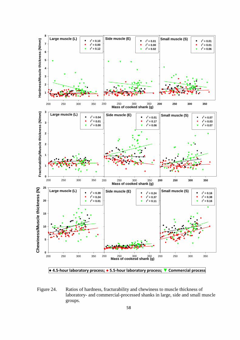
58

Large muscle (L)

200 250 300 350

Hard

ne

ss

/Mu

sc

le t

hic

kn

ess

(N

/mm

)

1

2

3

4

5

6

7

8

r2 = 0.10

r2 = 0.00

r2 = 0.12

Side muscle (E)

Mass of cooked shank (g)200 250 300 350

r2 = 0.01

r2 = 0.00

r2 = 0.02

Small muscle (S)

200 250 300 350

r2 = 0.01

r2 = 0.01

r2 = 0.06

Large muscle (L)

200 250 300 350

Fra

ctu

rab

ilit

y/M

us

cle

th

ickn

ess

(N

/mm

)

0

1

1

2

2

3

3

r2 = 0.04

r2 = 0.01

r2 = 0.00

Side muscle (E)

200 250 300 350

r2 = 0.01

r2 = 0.17

r2 = 0.06

Small muscle (S)

Mass of cooked shank (g)200 250 300 350

r2 = 0.07

r2 = 0.03

r2 = 0.07

Large muscle (L)

200 250 300 350

Ch

ew

iness/M

uscle

th

ickn

ess (

N)

0

5

10

15

20

25

r2 = 0.39

r2 = 0.24

r2 = 0.01

Side muscle (E)

200 250 300 350

r2 = 0.24

r2 = 0.37

r2 = 0.11

Small muscle (S)

Mass of cookesd shank (g)200 250 300 350

r2 = 0.16

r2 = 0.38

r2 = 0.16

● 4.5-hour laboratory process; ● 5.5-hour laboratory process; ▼ Commercial process

Figure 24. Ratios of hardness, fracturability and chewiness to muscle thickness of

laboratory- and commercial-processed shanks in large, side and small muscle

groups.

59

To compare the commercial-processed shanks with the laboratory-processed shanks in

further detail, cooked shanks were divided into three weight ranges, 200 to 250 g, 250 to 290 g,

and 290 to 380 g. These ranges were chosen as a result of 17 to 18.8% cooking losses. For

example, the raw weight range of 240 to 300 g was reduced to 200 to 250 g, and so on for the

other weight ranges. The different weight ranges were compared for various textural parameters

and analysed statistically (Table 9, Table 10 and Table 11).

For the large muscle group (Table 9), the commercial-processed shanks had significantly

greater (P ≤ 0.05) hardness and ratio of hardness to muscle thickness in all three cooked weight

ranges, compared to the laboratory-processed shanks. This may be important in the eating

experience.

In the medium weight range the commercial shanks had statistically similar fracturability

and fracturability ratio with both the laboratory-processed shanks. In the other two weight

ranges there were significant differences, but the means were quite similar, which may not

influence the eating experience.

For chewiness, the data show that the 4.5-hour laboratory-processed shanks were chewier

than the 5.5-hour equivalents (P ≤ 0.05), but similar to the commercial-processed shanks. This

difference extended to the chewiness ratio.

Generally speaking, the large muscle from the commercial-processed shanks was generally

tougher than that from the 5.5-hour laboratory-processed shanks, but similar to that from the 4.5-

hour laboratory-processed shanks.

The weight range effects on the large muscle are also shown in Table 9. For the 4.5-hour

laboratory-processed shanks, all textural parameters were numerically higher in the large weight

range (290 to 380 g) than in the small and medium weight ranges, but the differences were often

not statistically significant. This, of course, is consistent with the close-to-flat regression lines in

Figure 23 and Figure 24. At 5.5-hour, only some parameters were numerically higher in the

large weight range, and again differences were often not statistically significant, for the same

reason as for the 4.5-hour comparisons. In the commercial shanks there was no any increasing

trend in textural parameters with weight ranges and the differences with weight ranges were not

significant.

Thus for the large muscle group, the major effect on textural properties arise from time of

laboratory cooking and the effect of commercial production.

60

Table 9. Textural properties of the large muscle from shanks cooked for different time in three weight ranges. These properties

are hardness, fracturability and chewiness, and the ratio of those parameters to muscle thickness

Textural parameter Cooked shank weight

range

Cooking Time

4.5 h 5.5 h Commercial

Hardness

(Peak force - N)

Small (200-250 g)

Medium (250-290 g)

Large (290-380 g)

25.4 ± 7.7bβ

26.7 ± 7.2bβ

34.2 ± 10.2abα

23.2 ± 7.6bα

27.2 ± 8.4bα

28.1 ± 8.3bα

60.9 ± 48.8aα

60.1 ± 43.5aα

43.9 ± 17.2aα

Fracturability

(Fracture force - N)

Small (200-250 g)

Medium (250-290 g)

Large (290-380 g)

20.4 ± 3.1aβ

20.9 ± 4.3aβ

24.3 ± 2.1aα

17.4 ± 2.4bβ

18.6 ± 2.7aαβ

19.7 ± 2.4bα

18.4 ± 5.3abα

17.1 ± 6.3aα

20.7 ± 7.1abα

Chewiness

(Compression work – N mm)

Small (200-250 g)

Medium (250-290 g)

Large (290-380 g)

252.8 ± 58.1aβ

294.2 ± 59.5aβ

377.4 ± 66.9aα

211.9 ± 38.9bβ

227.9 ± 37.0bβ

288.0 ± 35.6bα

310.9 ± 85.9aα

293.4 ± 109.5aα

361.8 ± 129.9aα

Hardness/muscle thickness (N mm-1

) Small (200-250 g)

Medium (250-290 g)

Large (290-380 g)

0.9 ± 0.2bα

0.9 ± 0.2bα

1.1 ± 0.3abα

0.8 ± 0.3bα

0.9 ± 0.3bα

0.9 ± 0.3bα

2.0 ± 1.6aα

1.9 ± 1.3aα

1.3 ± 0.5aα

Fracturability/muscle thickness (N mm-1

) Small (200-250 g)

Medium (250-290 g)

Large (290-380 g)

0.7 ± 0.1aα

0.7 ± 0.2aα

0.8 ± 0.1aα

0.6 ± 0.1bα

0.6 ± 0.1aα

0.6 ± 0.1bα

0.6 ± 0.2abα

0.6 ± 0.2aα

0.6 ± 0.2abα

Chewiness/muscle thickness (N) Small (200-250 g)

Medium (250-290 g)

Large (290-380 g)

8.5 ± 1.5aβ

9.5 ± 1.9aβ

11.6 ± 1.7aα

7.1 ± 1.0bβ

7.5 ± 1.0bβ

8.9 ± 0.9bα

10.1 ± 2.6aα

9.2 ± 3.3abα

10.9 ± 3.5aα

Means ± standard deviation.

Different letters (a, b, c) in the same row indicate significant difference between means (p ≤ 0.05).

Different letter (α, β, γ) in the same column for each parameter indicate significant differences between means (p ≤ 0.05).

61

For the side muscle group (Table 10), the commercial-processed shanks had significantly

greater (P ≤ 0.05) hardness and hardness ratio than the 5.5-hour laboratory-processed shanks in

all three cooked weight ranges, and the medium-size 4.5-hour equivalents. However, these

subtleties of significance should not obscure the fact that the means of these two parameters in

the commercial-processed shanks were remarkable numerically higher than both laboratory-

processed shanks.

The side muscle from the commercial-processed shanks had similar fracturability and

fracturability ratio to the 4.5-hour laboratory-processed shanks in all the three weight ranges.

Both parameters for the commercial-processed and the 4.5-hour laboratory-processed shanks

were numerically and statistically greater (P ≤ 0.05) than for the 5.5-hour laboratory-processed

shanks.

For chewiness and the chewiness ratio, the commercial-processed shanks were closer to

the 4.5-hour laboratory-processed shanks than the 5.5-hour equivalents. The latter were less

chewy (P ≤ 0.05).

Overall, the side muscle from the commercial-processed shanks was definitely tougher

than the 5.5-hour laboratory-processed shanks, but rather similar to the 4.5-hour equivalents.

The weight range effects on the side muscle were also showed in Table 10. For the 4.5-

hour laboratory-processed shanks, all textural parameters were nearly always numerically higher

in the large weight range (290 to 380 g), but often not statistically significant. For the 5.5-hour

laboratory-processed shanks, hardness, chewiness and chewiness ratio were significantly higher

(P ≤ 0.05) in the large weight range. But for the commercial shanks, there was no increasing

trend with weight range and no differences were significant.

Thus for the side muscle group, the laboratory cooking time and the difference with the

commercial production were still the main reasons for the differences on muscle textural

properties.

62

Table 10. Textural properties of the side muscle from shanks cooked for different time in three weight ranges. These

properties are hardness, fracturability and chewiness, and the ratio of those parameters to muscle thickness

Textural parameter Cooked shank weight

range

Cooking time

4.5 h 5.5 h Commercial

Hardness

(Peak force - N)

Small (200-250 g)

Medium (250-290 g)

Large (290-380 g)

15.2 ± 3.2aβ

13.6 ± 2.2bβ

18.7 ± 3.4aα

11.3 ± 2.8bβ

13.6 ± 3.5bα

14.3 ± 3.6bα

27.0 ± 20.9aα

34.9 ± 27.0aα

24.8 ± 9.7aα

Fracturability

(Fracture force - N)

Small (200-250 g)

Medium (250-290 g)

Large (290-380 g)

14.1 ± 2.8aα

12.6 ± 2.5abα

15.4 ± 4.0aα

11.6 ± 1.9bα

10.8 ± 2.4bα

11.6 ± 3.1bα

14.8 ± 6.4abα

13.9 ± 3.9aα

19.2 ± 6.7aα

Chewiness

(Compression work – N mm)

Small (200-250 g)

Medium (250-290 g)

Large (290-380 g)

30.8 ± 6.9aβ

33.3 ± 8.1aβ

46.4 ± 16.3aα

24.1 ± 6.1bβ

26.4 ± 7.1bβ

39.8 ± 8.8aα

30.9 ± 12.9abα

31.5 ± 10.5abα

42.1 ± 13.3aα

Hardness/muscle thickness (N mm-1

) Small (200-250 g)

Medium (250-290 g)

Large (290-380 g)

1.1 ± 0.2aα

0.9 ± 0.2bβ

1.2 ± 0.2bα

0.8 ± 0.2bα

0.9 ± 0.4bα

0.8 ± 0.2cα

2.0 ± 1.4aα

2.5 ± 1.8aα

1.8 ± 0.7aα

Fracturability/muscle thickness (N mm-1

) Small (200-250 g)

Medium (250-290 g)

Large (290-380 g)

1.0 ± 0.2aα

0.8 ± 0.2abβ

1.0 ± 0.2bαβ

0.8 ± 0.2bα

0.7 ± 0.2bαβ

0.7 ± 0.2cβ

1.1 ± 0.5aα

1.0 ± 0.3aα

1.4 ± 0.5aα

Chewiness/muscle thickness (N) Small (200-250 g)

Medium (250-290 g)

Large (290-380 g)

2.2 ± 0.4aβ

2.1 ± 0.4aβ

2.9 ± 0.8aα

1.7 ± 0.3bβ

1.7 ± 0.3bβ

2.3 ± 0.4bα

2.3 ± 0.9aα

2.3 ± 0.7aα

3.0 ± 0.9aα

Means ± standard deviation.

Different letters (a, b, c) in the same row indicate significant difference between means (p ≤ 0.05).

Different letter (α, β, γ) in the same column for each parameter indicate significant differences between means (p ≤ 0.05).

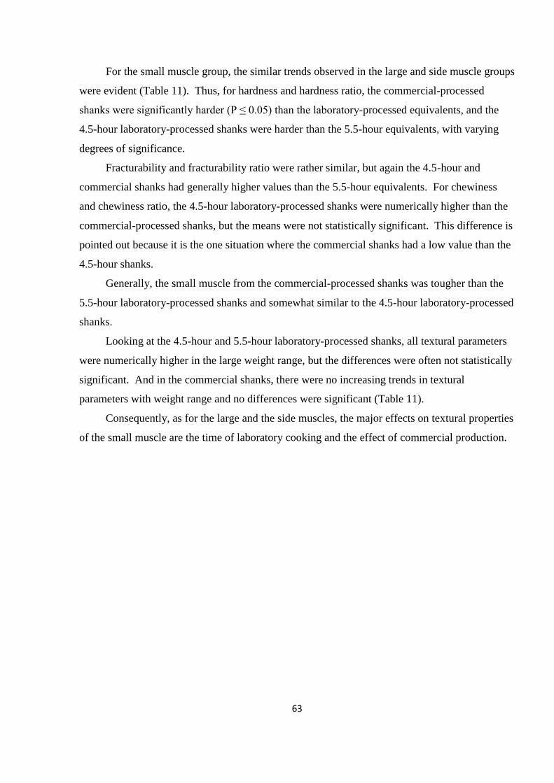
63

For the small muscle group, the similar trends observed in the large and side muscle groups

were evident (Table 11). Thus, for hardness and hardness ratio, the commercial-processed

shanks were significantly harder (P ≤ 0.05) than the laboratory-processed equivalents, and the

4.5-hour laboratory-processed shanks were harder than the 5.5-hour equivalents, with varying

degrees of significance.

Fracturability and fracturability ratio were rather similar, but again the 4.5-hour and

commercial shanks had generally higher values than the 5.5-hour equivalents. For chewiness

and chewiness ratio, the 4.5-hour laboratory-processed shanks were numerically higher than the

commercial-processed shanks, but the means were not statistically significant. This difference is

pointed out because it is the one situation where the commercial shanks had a low value than the

4.5-hour shanks.

Generally, the small muscle from the commercial-processed shanks was tougher than the

5.5-hour laboratory-processed shanks and somewhat similar to the 4.5-hour laboratory-processed

shanks.

Looking at the 4.5-hour and 5.5-hour laboratory-processed shanks, all textural parameters

were numerically higher in the large weight range, but the differences were often not statistically

significant. And in the commercial shanks, there were no increasing trends in textural

parameters with weight range and no differences were significant (Table 11).

Consequently, as for the large and the side muscles, the major effects on textural properties

of the small muscle are the time of laboratory cooking and the effect of commercial production.

64

Table 11. Textural properties of the small muscle from shanks cooked for different time in three weight ranges. These

properties are hardness, fracturability and chewiness, and the ratio of those parameters to muscle thickness

Textural parameter Cooked shank weight

range

Cooking time

4.5 h 5.5 h Commercial

Hardness

(Peak force - N)

Small (200-250 g)

Medium (250-290 g)

Large (290-380 g)

37.8 ± 8.2bα

35.9 ± 10.4bα

45.5 ± 14.7aα

28.5 ± 6.8cβ

36.2 ± 14.2bα

34.1 ± 7.8bα

61.8 ± 27.5aα

52.5 ± 22.1aα

49.3 ± 15.1aα

Fracturability

(Fracture force - N)

Small (200-250 g)

Medium (250-290 g)

Large (290-380 g)

17.7 ± 4.8aα

18.7 ± 4.8aα

23.1 ± 8.8aα

15.0 ± 3.3aβ

12.7 ± 3.1bγ

18.2 ± 3.7aα

17.5 ± 12.6aα

17.4 ± 5.8aα

25.1 ± 13.4aα

Chewiness

(Compression work – N mm)

Small (200-250 g)

Medium (250-290 g)

Large (290-380 g)

235.6 ± 42.9aβ

237.1 ± 59.3aβ

319.6 ± 65.3aα

179.8 ± 41.3bβ

181.5 ± 41.6bβ

283.6 ± 86.5aα

215.2 ± 73.7abαβ

190.1 ± 52.0abβ

282.3 ± 95.5aα

Ratio of

Hardness/muscle thickness (N mm-1

)

Small (200-250 g)

Medium (250-290 g)

Large (290-380 g)

1.4 ± 0.3bα

1.3 ± 0.4bα

1.5 ± 0.5aα

1.0 ± 0.2cβ

1.3 ± 0.5bα

1.1 ± 0.3bαβ

2.4 ± 1.2aα

2.1 ± 0.9aαβ

1.8 ± 0.5aβ

Ratio of

Fracturability/muscle thickness (N mm-1

)

Small (200-250 g)

Medium (250-290 g)

Large (290-380 g)

0.7 ± 0.2aα

0.7 ± 0.2aα

0.8 ± 0.4abα

0.5 ± 0.1aαβ

0.5 ± 0.1bβ

0.6 ± 0.1bα

0.7 ± 0.5aα

0.7 ± 0.3aα

0.9 ± 0.5aα

Ratio of

Chewiness /muscle thickness (N)

Small (200-250 g)

Medium (250-290 g)

Large (290-380 g)

8.6 ± 1.4aβ

8.2 ± 1.7aβ

10.7 ± 1.8aα

6.2 ± 1.1bβ

6.4 ± 1.4bβ

8.8 ± 2.0bα

8.3 ± 3.3aα

7.5 ± 2.2abα

10.0 ± 3.0abα

Means ± standard deviation.

Different letters (a, b, c) in the same row indicate significant difference between means (p ≤ 0.05).

Different letter (α, β, γ) in the same column for each parameter indicate significant differences between means (p ≤ 0.05).

65

4.3.3 Main outcomes of texture analysis

The results for the laboratory trials indicated that shanks cooked for 4.5 hours were tougher

than those cooked for 5.5 hours, which confirmed the effect of cooking time on meat texture.

Prolonged cooking time promotes gelatinization of collagen, consequently increasing the

tenderness of the meat (Seideman and Durland 1984; Bejerholm and Aaslyng 2004; Lawrie

2006). Tenderness of meat is an extremely important attribute of eating quality, but over-

tenderisation and consequent loss of „bite‟ is not desirable (Farouk and others 2009).

Although the cooking time of the commercial-processed shanks was nominally 5.5 hours,

the hardness was generally greater than the 4.5-hour laboratory-processed shanks, and even

compared with the 5.5-hour laboratory-processed equivalents, the commercial-processed shanks

was significantly tougher as judged by the textural parameters as a group. The differences

between the commercial- and laboratory-processed shanks were considered to be mainly due to

the product thermal history and possibly the nature of sous vide bags used, as discussed earlier.

Between-animal effects are also a possible cause but cannot be formally considered because the

supply history of the raw shanks and cooked shanks was not available.

The thermal history includes many factors, such as the initial temperature of the shank, the

water bath temperature set-point, the product loading on the heating capacity throughout the

process (Figure 20), and the heat transfer rate during cooking. Since collagen in sheep meat

starts to denature after heating for 10 minutes at 64°C (Snowden and Weidemann 1978) and the

solubility degree increases with temperature (Lawrie 2006), the difference in final temperature

between the commercial- and laboratory-processed shanks would relate to the muscle tenderness.

This result agrees with previous studies that in the 80 to 90°C range, where meat tenderness

increased (shear force decreased) with temperature (Machlik and Draudt 1963; Bouton and

others 1981; Robertson and others 1984; Seideman and Durland 1984; Combes and others 2004).

The results also indicated that weight range had no significant effect on textural properties

in commercial shanks, whereas, there were often noticeable differences in the texture of

laboratory shanks due to weight range. One reason for this would probably be the temperature

variability within the commercial cooking bath. Thus reduction of the variability of the

commercial process would provide a more consistent product textural quality.

A related way of minimizing the temperature variability would to have all shanks at a same

starting temperature. This might be accomplished with a thaw process, by first immersing the

shanks in a water bath maintained around 15°C. This pre-cook process would not only bring all

shanks to the same temperature but also should save on energy costs in the cooking process as

66

such. The energy saving was calculated based on the output of an FPM model. The FPM model

used the settings shown in Table 12. The shank dimensions and thermal property used here were

the same as those used in the earlier FPM modelling exercise (see Section 3.5).

Table 12. FPM model setup for the calculation of energy saving from water bath

immersion prior to cooking

Shank dimension Shank was modelled as a finite cylinder

Length: 0.12 m

Radius: 0.03 m

Thermal property Shank was considered as lean meat

Heat transfer coefficient: 500 W m-² °K

-1

Initial shank temperature -12°C

Immersion temperature 15°C

Immersion time 2 hours

Results from the FPM model showed that shank mean temperature after 2 hours immersion

was 13°C, but clearly this requires maintaining the water bath at or near 15°C (see below). The

energy saving was calculated as the difference between the energy required for cooking a batch

of shanks (300 kg) from the frozen state (-12°C) and the energy used for cooking an equivalent

batch of shanks after the 2 hour immersion (13°C). The calculations (Appendix 3) indicated that

the energy consumption of cooking shanks from frozen was 33.9 kWh, and cooking from pre-

heated was 19.1 kWh. The energy saving was mainly due to the fact that shanks have been

thawed, using „free‟ energy from water at ambient temperature. Assuming 20c per Kwh, the

energy saving is trivial $3, and clearly not worth the effort considering that maintaining the

water bath at or near 15°C may itself require some energy input and/or water cost, and labour

cost. The tempering water may be reusable, if there was no leakage from the vacuum packages,

but the hygiene need be confirmed before reuse. In addition, the use of an equilibrating water

bath would also require a capital outlay unless idle water baths are available, and the process

room has enough space.

However, there are two important advantages that could be gained from thaw immersion

prior to cooking. First, the shanks will all be at the same starting temperature, and that is likely

to result in more consistent texture. Second, the cooking time can be shorter, but would have to

be determined by experiment and the modelling has not been extended to that level of detail.

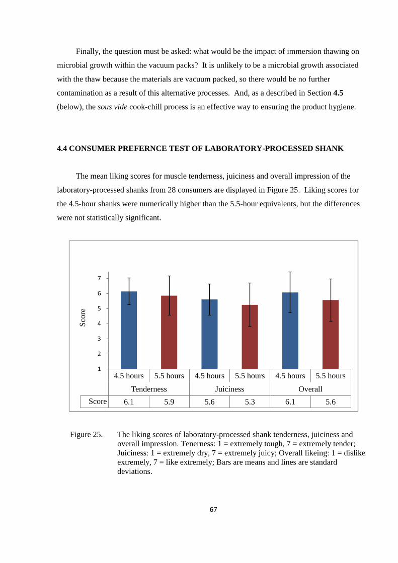
67

Finally, the question must be asked: what would be the impact of immersion thawing on

microbial growth within the vacuum packs? It is unlikely to be a microbial growth associated

with the thaw because the materials are vacuum packed, so there would be no further

contamination as a result of this alternative processes. And, as a described in Section 4.5

(below), the sous vide cook-chill process is an effective way to ensuring the product hygiene.

4.4 CONSUMER PREFERNCE TEST OF LABORATORY-PROCESSED SHANK

The mean liking scores for muscle tenderness, juiciness and overall impression of the

laboratory-processed shanks from 28 consumers are displayed in Figure 25. Liking scores for

the 4.5-hour shanks were numerically higher than the 5.5-hour equivalents, but the differences

were not statistically significant.

Figure 25. The liking scores of laboratory-processed shank tenderness, juiciness and

overall impression. Tenerness: 1 = extremely tough, 7 = extremely tender;

Juiciness: 1 = extremely dry, 7 = extremely juicy; Overall likeing: 1 = dislike

extremely, 7 = like extremely; Bars are means and lines are standard

deviations.

4.5 hours 5.5 hours 4.5 hours 5.5 hours 4.5 hours 5.5 hours

Tenderness Juiciness Overall

Score 6.1 5.9 5.6 5.3 6.1 5.6

1

2

3

4

5

6

7

8

9

Sco

re

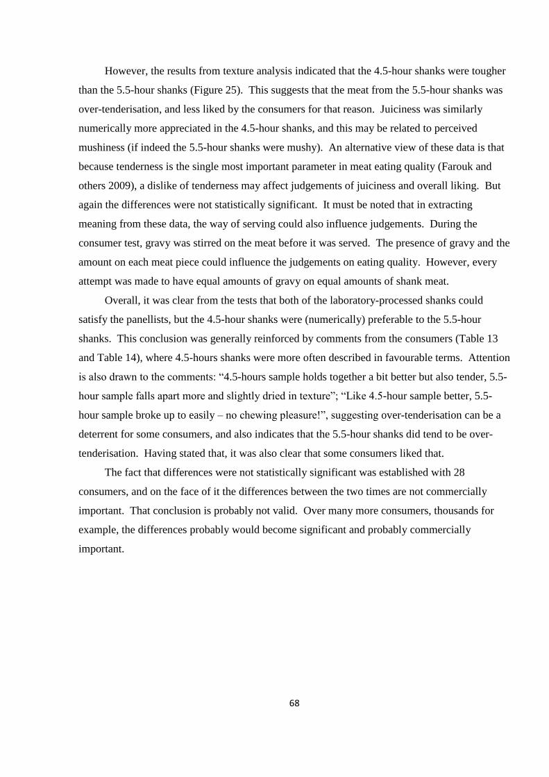
68

However, the results from texture analysis indicated that the 4.5-hour shanks were tougher

than the 5.5-hour shanks (Figure 25). This suggests that the meat from the 5.5-hour shanks was

over-tenderisation, and less liked by the consumers for that reason. Juiciness was similarly

numerically more appreciated in the 4.5-hour shanks, and this may be related to perceived

mushiness (if indeed the 5.5-hour shanks were mushy). An alternative view of these data is that

because tenderness is the single most important parameter in meat eating quality (Farouk and

others 2009), a dislike of tenderness may affect judgements of juiciness and overall liking. But

again the differences were not statistically significant. It must be noted that in extracting

meaning from these data, the way of serving could also influence judgements. During the

consumer test, gravy was stirred on the meat before it was served. The presence of gravy and the

amount on each meat piece could influence the judgements on eating quality. However, every

attempt was made to have equal amounts of gravy on equal amounts of shank meat.

Overall, it was clear from the tests that both of the laboratory-processed shanks could

satisfy the panellists, but the 4.5-hour shanks were (numerically) preferable to the 5.5-hour

shanks. This conclusion was generally reinforced by comments from the consumers (Table 13

and Table 14), where 4.5-hours shanks were more often described in favourable terms. Attention

is also drawn to the comments: “4.5-hours sample holds together a bit better but also tender, 5.5-

hour sample falls apart more and slightly dried in texture”; “Like 4.5-hour sample better, 5.5-

hour sample broke up to easily – no chewing pleasure!”, suggesting over-tenderisation can be a

deterrent for some consumers, and also indicates that the 5.5-hour shanks did tend to be over-

tenderisation. Having stated that, it was also clear that some consumers liked that.

The fact that differences were not statistically significant was established with 28

consumers, and on the face of it the differences between the two times are not commercially

important. That conclusion is probably not valid. Over many more consumers, thousands for

example, the differences probably would become significant and probably commercially

important.

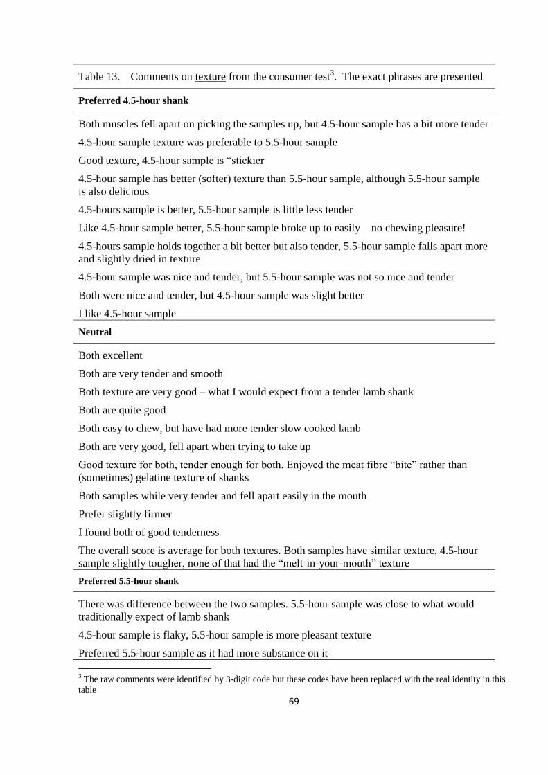
69

Table 13. Comments on texture from the consumer test3. The exact phrases are presented

Preferred 4.5-hour shank

Both muscles fell apart on picking the samples up, but 4.5-hour sample has a bit more tender

4.5-hour sample texture was preferable to 5.5-hour sample

Good texture, 4.5-hour sample is “stickier

4.5-hour sample has better (softer) texture than 5.5-hour sample, although 5.5-hour sample

is also delicious

4.5-hours sample is better, 5.5-hour sample is little less tender

Like 4.5-hour sample better, 5.5-hour sample broke up to easily – no chewing pleasure!

4.5-hours sample holds together a bit better but also tender, 5.5-hour sample falls apart more

and slightly dried in texture

4.5-hour sample was nice and tender, but 5.5-hour sample was not so nice and tender

Both were nice and tender, but 4.5-hour sample was slight better

I like 4.5-hour sample

Neutral

Both excellent

Both are very tender and smooth

Both texture are very good – what I would expect from a tender lamb shank

Both are quite good

Both easy to chew, but have had more tender slow cooked lamb

Both are very good, fell apart when trying to take up

Good texture for both, tender enough for both. Enjoyed the meat fibre “bite” rather than

(sometimes) gelatine texture of shanks

Both samples while very tender and fell apart easily in the mouth

Prefer slightly firmer

I found both of good tenderness

The overall score is average for both textures. Both samples have similar texture, 4.5-hour

sample slightly tougher, none of that had the “melt-in-your-mouth” texture

Preferred 5.5-hour shank

There was difference between the two samples. 5.5-hour sample was close to what would

traditionally expect of lamb shank

4.5-hour sample is flaky, 5.5-hour sample is more pleasant texture

Preferred 5.5-hour sample as it had more substance on it

3 The raw comments were identified by 3-digit code but these codes have been replaced with the real identity in this

table

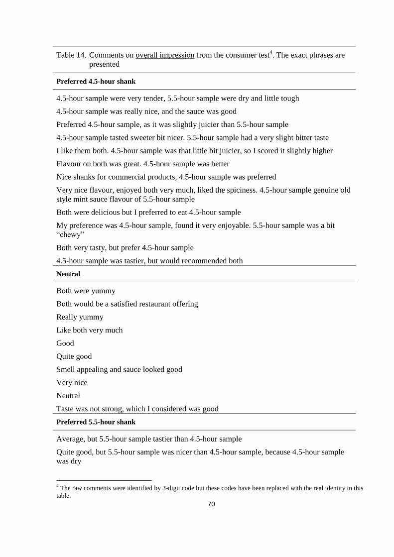
70

Table 14. Comments on overall impression from the consumer test4. The exact phrases are

presented

Preferred 4.5-hour shank

4.5-hour sample were very tender, 5.5-hour sample were dry and little tough

4.5-hour sample was really nice, and the sauce was good

Preferred 4.5-hour sample, as it was slightly juicier than 5.5-hour sample

4.5-hour sample tasted sweeter bit nicer. 5.5-hour sample had a very slight bitter taste

I like them both. 4.5-hour sample was that little bit juicier, so I scored it slightly higher

Flavour on both was great. 4.5-hour sample was better

Nice shanks for commercial products, 4.5-hour sample was preferred

Very nice flavour, enjoyed both very much, liked the spiciness. 4.5-hour sample genuine old

style mint sauce flavour of 5.5-hour sample

Both were delicious but I preferred to eat 4.5-hour sample

My preference was 4.5-hour sample, found it very enjoyable. 5.5-hour sample was a bit

“chewy”

Both very tasty, but prefer 4.5-hour sample

4.5-hour sample was tastier, but would recommended both

Neutral

Both were yummy

Both would be a satisfied restaurant offering

Really yummy

Like both very much

Good

Quite good

Smell appealing and sauce looked good

Very nice

Neutral

Taste was not strong, which I considered was good

Preferred 5.5-hour shank

Average, but 5.5-hour sample tastier than 4.5-hour sample

Quite good, but 5.5-hour sample was nicer than 4.5-hour sample, because 4.5-hour sample

was dry

4 The raw comments were identified by 3-digit code but these codes have been replaced with the real identity in this

table.

71

Preferred 5.5-hour sample as it had more flavour, did not like the sauce, it made it difficult

taste the meat

Both were delicious. I preferred 5.5-hour sample because it held more moisture

4.5 MICROBIOLOGICAL TESTS

The microbiological results are shown in Table 15. In the frozen shank, the aerobic plate

count was 2.56 log10 CFU/cm2 on Day 3, and slightly numerically increased to 2.72 log10

CFU/cm2 after 2 more days‟ incubation. The anaerobic plate count on Day 5 was 2.19 log10

CFU/cm2. The counts of anaerobic mesophilic (25°C) bacteria, anaerobic psychrophilic (7°C)

bacteria, and Enterobacteriaceae were 2.56, 1.44, and below 0.11 log10 CFU/cm

2, respectively.

(The expression below 0.11 log10 – <0.11 in the table – means that several replicate plates were

devoid of colonies, but the bacterium was not necessarily absent.)

In the sauce, the aerobic plate counts were 3.56 and 3.58 log10 CFU/g on Day 3 and Day 5.

The anaerobic plate count on Day 5 was 3.12 log10 CFU/g. The counts of anaerobic mesophilic

(25°C) bacteria, anaerobic psychrophilic (7°C) bacteria, and Enterobacteriaceae were 3.37,

below 1.75, and below 1.13 log10 CFU/g, respectively. Neither the raw shank nor the sauce

contained Clostridia or their spores.

After the sous-vide cooking-cooling process, the total aerobic and anaerobic plate counts

decreased to 2.64 and 2.04 log10 CFU/g, respectively. The counts of anaerobic mesophilic (25°C)

bacteria and anaerobic psychrophilic (7°C) bacteria dropped to below 2.30 and 2.03 log10 CFU/g.

The Enterobacteriaceae count was below 1.03 log10 CFU/g inside the product package.

The subsequent refreezing process provided a further reduction of the microbiological

populations inside the vacuum package. The total aerobic and anaerobic plate counts decreased

slightly to 2.26 and 2.12 log10 CFU/g, respectively. The numbers of anaerobic mesophilic (25°C)

bacteria dropped to below 2.05 log10 CFU/g. Anaerobic psychrophilic (7°C) bacteria and

Enterobacteriaceae were eliminated. (not detected in any replicate plates.)

The total numbers of bacteria inside each vacuum package were calculated (Table 16)

based on the results in Table 15, assuming the average surface area for each shank was 313 cm2,

and the average mass of raw shank was 350 g, the sauce in each pouch weighed 100 g. This

analysis provides a more direct description of the microbial population within the product

package before and after processing.

72

The total aerobic plate counts in initial (unprocessed) sous vide package after 3 and 5 days

incubation was 5.75 and 5.84 log10, which were decreased to 5.30 log10 after the sous vide

cooking-cooling process and to 4.92 log10 after the further freezing. The total anaerobic plate

count was 5.35 log10, which reduced to 4.96 and 4.77 log10 after the sous vide process and further

freezing. The number of anaerobic mesophilic (25°C) bacteria was 5.64 log10 before the process,

and reduced to below 4.96 log10 after the cooking-cooling process and further dropped to below

4.71 log10 after refreezing. In addition, the number of anaerobic psychrophilic (7°C) bacteria and

Enterobacteriaceae in the initial package was below 4.34 and 3.27 log10, respectively, and the

number slightly increased to 4.86 and 3.69 log10 after the cooking-cooling process, but eliminated

after further refreezing.

It is clear from the results that the bacteria present preferred to grow under aerobic

conditions rather than anaerobic conditions, and that they appeared to grow faster rates at the

higher temperature (25°C) compared with the lower temperature (7°C).

The plate counts results also indicated that the sous vide process (cooking at 90°C for 5.5

hours, following cooling at 4.2°C for 2 hours) could reduce the total bacteria load inside the

product package, and the subsequent frozen storage produce a further reduction.

This limited microbiological study shows that product is hygienic, according to the

microbiological reference criteria for food (Ministry of Health 1995).

73

Table 15. Aerobic and anaerobic plate counts, Enterobacteriaceae counts, fastidious anaerobe counts (log10 CFU/cm2 or log10 CFU/g), and the

presence of viable Clostridia and their spores in raw materials and the package after the sous vide process and further refreezing

Sample APC AnPC Enterobacteriaceae

count

CBA Presence of viable

Clostridia and/or their

spores Day 3 Day 5 Day 5 25°C 7°C

Pre-process

Shanka

2.56 ± 0.50 2.72 ± 0.57 2.19 ± 0.68 < 0.11 ± 0.18 2.56 ± 0.79 1.44 ± 1.05 Not detected

Sauceb 3.56 ± 0.16 3.58 ± 0.17 3.12 ± 0.24 < 1.13 ± 0.32 3.37 ± 0.26 < 1.75 ± 0.12 Not detected

Post-process

Cook-cooled packagec Unavailable 2.64 ± 0.83 2.04 ± 0.75 < 1.03 ± 0.10 < 2.30 ± 0.72 < 2.03 ± 0.67 Not detected

Refrozen packaged Unavailable 2.26 ± 0.63 2.12 ± 0.88 Not detected < 2.05 ± 0.90 Not detected Not detected

Value of mean ± standard deviation aLog10 CFU/cm

2;

b,c,dLog10 CFU/g

APC = Aerobic plate counts; AnPC = Anaerobic plate counts; CBA = Anaerobe counts incubated in Columbia Blood Agar

Cook-cooled package = processed shank with sauce; refrozen package = refrozen shank with sauce

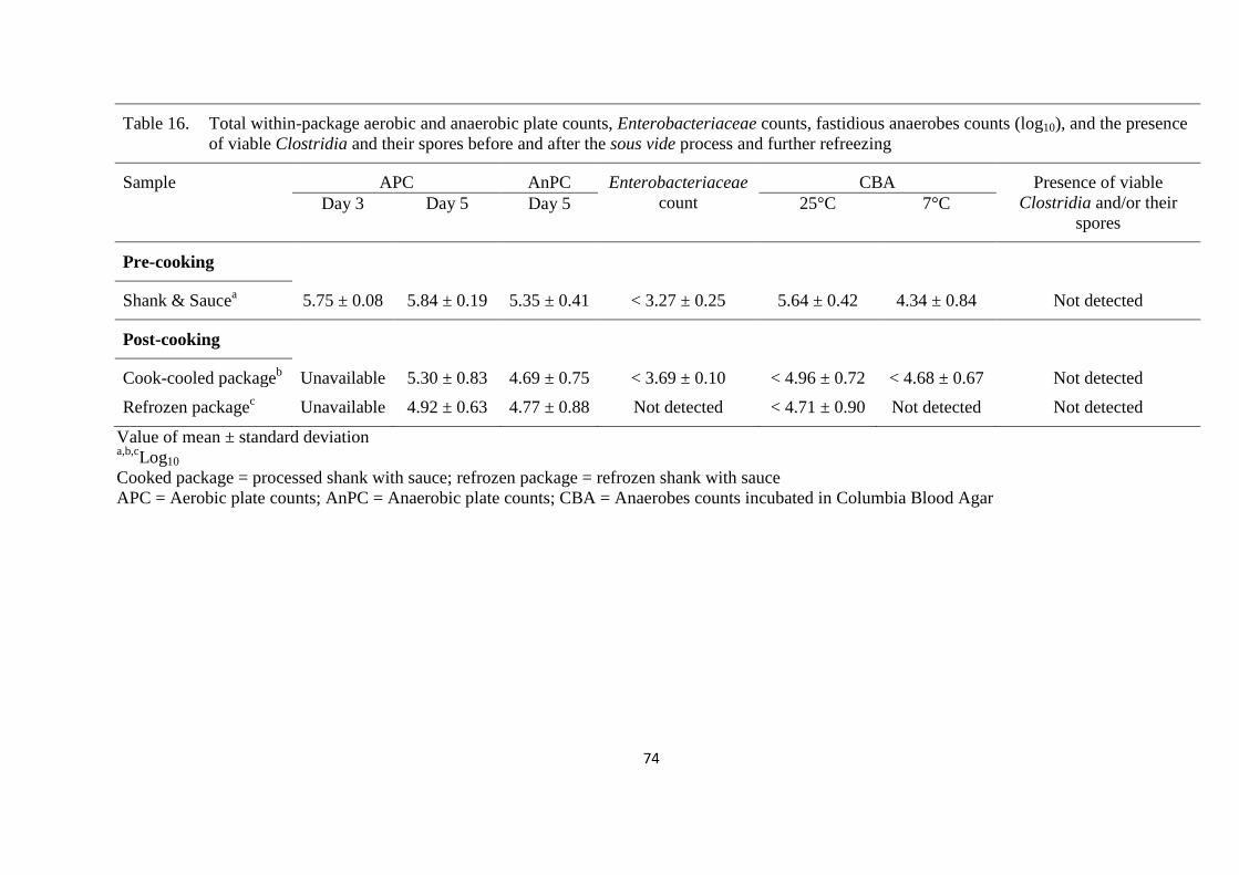
74

Table 16. Total within-package aerobic and anaerobic plate counts, Enterobacteriaceae counts, fastidious anaerobes counts (log10), and the presence

of viable Clostridia and their spores before and after the sous vide process and further refreezing

Sample APC AnPC Enterobacteriaceae

count

CBA Presence of viable

Clostridia and/or their

spores Day 3 Day 5 Day 5 25°C 7°C

Pre-cooking

Shank & Saucea

5.75 ± 0.08 5.84 ± 0.19 5.35 ± 0.41 < 3.27 ± 0.25 5.64 ± 0.42 4.34 ± 0.84 Not detected

Post-cooking

Cook-cooled packageb

Unavailable 5.30 ± 0.83 4.69 ± 0.75 < 3.69 ± 0.10 < 4.96 ± 0.72 < 4.68 ± 0.67 Not detected

Refrozen packagec

Unavailable 4.92 ± 0.63 4.77 ± 0.88 Not detected < 4.71 ± 0.90 Not detected Not detected

Value of mean ± standard deviation a,b,c

Log10

Cooked package = processed shank with sauce; refrozen package = refrozen shank with sauce

APC = Aerobic plate counts; AnPC = Anaerobic plate counts; CBA = Anaerobes counts incubated in Columbia Blood Agar

75

CHAPTER 5

CONCLUSIONS AND RECOMMENDATIONS

The temperature in the laboratory process was well controlled as could be expected from

a water bath with good heating capacity, circulation and insulation. The measured temperature

variation was higher in the commercial process, and the measurements did not include those in

the likely thermal centre of a cooking basket, which intuitively would be the coldest locale in the

entire bath. The exact thermal history of the 38 commercial shanks was unknown, but assuming

it was representative of the Titan‟s product, it can be concluded that in spite of temperature

variation, the commercial product has good textural properties on average, although there is

scope to reduce variation, provided this can be done cost effectively. Moreover, weight range

had no significant effect on textural properties in commercial shanks. The key data that supports

this conclusion is in Table 9, Table 10 and Table 11, where the absolute textural values and the

ratios of textural values to muscle thickness were segregated into small, medium and large shank

groups. There were no significant differences between the groups. However, there were often

marked differences in the texture of laboratory shanks due to size. Overall, textural values were

higher (more difficult to chew) where the shanks were heavier, even when expressed as the ratios

of textural values to muscle thickness. It is very likely that the failure to detect a shank-size

effect in commercial shanks can be traced to temperature variation within the commercial

cooking bath.

Physical measurements of laboratory cooked shanks showed that shanks cooked for the

longer time of 5.5 hours had a higher cooking loss, indicating the collagen was not completely

gelatinised at 4.5 hours.

Laboratory cooking time did not affect mean muscle shrinkage and variation was low.

However, while the mean shrinkage of the commercial-processed shanks was similar to that of

the laboratory shanks, the variation was much higher, which again points to more variation in

temperature during the commercial process.

The computer models of the cooking-cooling process did not address variation. The FPM

model showed that the shank muscle temperature were generally lower in the commercial

76

product as might be inferred from the Figure 17 and Figure 18, and leading to more difficult

chewing summarised in Table 9, Table 10 and Table 11. The Flex PDE 3 model was a poor

predictor of the temperature profile of the lamb shank during the cooking process. This could be

traced to a failure to including the thermal conductivity of bone in the model. Without bone the

core of the shank was predicted to be much cooler than the surface, which measurement showed

was not the case. The results indicate the importance of bone as a conductor of heat from the

ends of the shank to the meat immediately surrounding the bone. Thus in the real life situation

the meat cut is being cooked from the inside and the outside.

The consumer trial suggested that the 4.5-hour laboratory-processed shanks were

preferable to the 5.5-hour equivalents, and the feedbacks from the consumers also supported the

likelihood that the 5.5-hour cooked shanks were over-tenderised. Because the commercial

shanks have a mean textural profile more similar to the 4.5-hour laboratory-processed shanks

than the 5.5-hour equivalents, it is proposed that the existing Titan process is fundamentally

sound. However, the issue of variability remains and is further discussed below.

The microbiological tests showed that the existing frozen starting shanks, existing

cooking-cooling process and the subsequent frozen storage effectively reduced the bacterial

loads inside the product package. This confirmed the hygiene of the lamb shank products.

Several recommendations can be drawn from these conclusions. Temperature variation

was identified as the cause of undesirable textural variation. This temperature variation was

mainly due to the total heat load of the process, the heating capacity, and to the size and design

of the water baths. Therefore, the existing commercial process can be improved by reducing the

product heat load and/or increasing the heating capacity of the cooking system.

One way of reducing the product heat load is to increase the mean temperature of the

shanks prior to loading. This could be achieved by first placing the baskets containing the

uncooked, vacuum packed lamb shanks into a water bath containing cold water at typically 14 to

18°C, as discussed in Section 4.3.3. This water may flow by trickle-feed to maintain the bath

temperature above 10°C, for example. This would speed up the thawing of packed shanks and

most importantly, ensure a more even temperature distribution when the products are loaded into

the cooking bath. The thawing process would also reduce the required cooking energy

consumption, without any significant impact on the colour, juiciness and tenderness of the final

product (Ferger and others 1972; Griffin and others 1985; Obuz and Dikeman 2003). However,

the 44% reduction in energy cost resulted in only a trivial cost saving. But as was pointed out

the main advantage would be the even shank starting temperature, and the shorter cooking time.

77

Two suggestions can be thought for improving the heating capacity of the cooking bath.

The first one is increasing the heating capacity of the steam cooking system. The heating system

appears to be built into the walls of the bath, so any redesign is likely to be a major undertaking.

However, it may be possible to ensure the maximum heating is improved by increasing the

effectiveness of insulation round the cooking bath that including the lid. The second one is

increasing the circulation of the bath fluid. Better circulation would ensure more even

distribution of temperature in the bath and therefore more even cooking of the product in the

baskets. This could be achieved by either pump recirculation or mechanical stirrer.

The heating curve for the commercial process (Figure 20) indicated that a better heating

system could not only improve the initial heating of the shanks loaded into the bath, but also the

control of the set-point cooking temperature once it is achieved. However, a more detailed

evaluation of the cooking immersion bath would be required before undertaking any of the

suggestion on heating capacity improvement. The further examination of the temperature

profiles in the cooking bath will including better understanding of the design and insulation of

the commercial cooking bath, more probes inside the cooking baskets, perhaps the thermal centre,

and a random shank tests (about 20 shanks) in each batch.

When the temperature variation was limited, shanks in small and medium weight ranges

would require shorter cooking time than those in large weight range, as indicated from the

laboratory trials. The question turns out the large-size shanks need to be separated from the

smaller shanks before the commercial cooking, which may complicate the process. The knowing

differences of textural properties between shanks in large weight range and small and medium

ranges may be significant, but is it commercially important? However, there is no doubt that this

size segregation will provide a more consistent final products textural quality.

78

REFERENCE

Baldwin DE. 2009. A practical guide to sous vide cooking. Availiable from

http://amath.colorado.edu/~baldwind/sous-vide.html

Beauchemin M. 1990. Sous-vide technology. Reciprocal Meat Conference Proceedings 43: 103-7.

Beermann DH. 2004. Physiology. In: Jensen WK, editor. Encyclopedia of Meat Science.

Elsevier Ltd. p 511-8.

Bejerholm C, Aaslyng MD. 2004. Cooking of meat. In: Jensen WK, editor. Encyclopedia of

Meat Science. Elsevier Ltd. p 343-9.

Bertola NC, Bevilacqua AE, Zaritzky NE. 1994. Heat treatment effect on texture changes and

thermal denaturation of proteins in beef muscle. Journal of Food Processing and

Preservation, 18(1): 31-46.

Bole JA, Swan JE. 2002. Heating method and final temperature affect processing characteristics

of beef semimembranosus muscle. Meat Science 62(1): 107-12.

Bole JA. 2010. Thermal processing. In: Fidel Toldra, editor. Handbook of Meat Processing.

Ames, Iowa: Wiley-Blackwell. p. 169-84.

Bouton PE, Harris PV, Shorthose WR. 1976. Dimensional changes in meat during cooking.

Journal of Texture Studies 7(2): 179-92.

Bouton PE, Harris PV, Ratcliff D. 1981. Effect of cooking temperature and time on the shear

properties of meat. Journal of Food Science 46(4): 1082-7.

Califano AN, Bertola NC, Bevilacqua AE, Zaritzky NE. 1997. Effect of processing conditions

on the hardness of cooked beef. Journal of Food Engineering 34(1): 41-54.

Chandraratne MR, Samarasinghe S, Kulasiri D, Bickerstaffe R. 2006. Prediction of lamb

tenderness using image surface texture features. Journal of Food Engineering 77(3): 492-

9.

Cheng QF, Sun DW. 2007. Effect of cooking bag and netting packaging on the quality of pork

ham during water cooking. Meat Science 75(2): 243-7.

Church IJ, Parsons AL. 1993. Review: sous vide cook-chill technology. International Journal of

Food Science and Technology 28(6): 563-74.

Coggins PC. 2007. Attributes of muscle foods: colour, texture, flavour. In: Nollet LEL editor.

Handbook of meat, poultry and seafood quality. Ames, Iowa: Blackwell Publishing. p 89-

97.

Combes S, Lepetit J, Darche B, Lebas F. 2004. Effect of cooking temperature and cooking time

on Warner-Bratzler tenderness measurement and collagen content in rabbit meat. Meat

Science 66(1): 91-6.

Creed PG. n.d.. Sous vide: an overview of the process. U.K.: Bournemouth University.

Davies AS. 2004. Muscle structure and contraction. In: Jensen WK, editor. Encyclopedia of

Meat Science. Elsevier Ltd. p 882-901.

Drummond LS, Sun DW. 2006. Feasibility of water immersion cooking of beef joints: effect on

product quality and yield. Journal of Food Engineering 77(2): 289-94.

Farouk MM, Wiklund E, Rosenvold K. 2009. Carcass interventions and meat tenderness. In:

Kerry JP, Ledward D. editors. Improving the sensory and nutritional quality of fresh meat:

new technologies. Cambridge: Woodhead Publishing Ltd. p 561-84.

Ferger DC, Harrison DL, Anderson LL. 1972. Lamb and beef roasts cooked from the frozen state

by dry and moist heat. Journal of Food Science 37(2): 226-9.

Foodreference.com (n.d.). Food facts and history. Lamb. Available from

http://www.foodreference.com/html/artlamb.html

79

Gourmet Direct (2005). Gourmet Direct Lamb Online. Available from

http://www.gourmetdirect.com/0800-TASTE-IT/Online-Shop/Lamb/

Griffin CL, Savell JW, Rhee KS, Johnson HK. 1985. Cooking time, cooking losses and energy

used for cooking lamb roasts. Journal of Food Quality 8(2-3): 69-79.

Grill and Foodservice. 2010. Offal: The Best Bits. Available from

http://www.grill.co.nz/index.php/tastings/49-winetestings/77-

offalanewchallengeforchefs-getthemtoeatoffal

Hamm R. 1986. Functional properties of the myofibrillar system and their measurements. In:

Bechtel PJ. editor. Muscle as Food. New York: Academic Press. p 135-99.

Hostetler RL, Dutson TR, Smith GC. 1982. Effect of electrical stimulation and steak temperature

at the beginning of cooking on meat tenderness and cooking loss. Journal of Food

Science, 47(2): 687-8.

Huijing PA. 1999. Muscle as a collagen fibre reinforced composite: a review of force

transmission in muscle and whole limb. Journal of Biomechanics 32(4): 329-45.

Investment New Zealand. 2007. New Zealand Red Meat Industry: from pasture to plate. New

Zealand Trade and Enterprise.

Kauffman RG. 2001. Meat composition. In Hui YH, Nip W-K, Rogers RW, Young OA, editors.

Meat Science and Application. New York: Marcel Dekker, Inc. p 1-19.

Key RA. 2009. Sous vide: slow and delicious. Available from

http://www.foodproductdesign.com/articles/2009/02/sous-vide-slow-and-delicious.aspx

Laakkonen E, Wellington GH, Sherbon JW. 1970. Low-temperature, long-time heating of

bovine muscle 1. Changes in tenderness, water-binding capacity, pH and amount of

water-soluble components. Journal of Food Science 35(2): 175-7.

Lawrie RA. 2006. The structure and growth of muscle. In: Lawrie RA. editor. Lawrie‟ Meat

Science 7th ed. Cambridge: Woodhead Publishing Ltd. p 41-74.

Lawrie RA. 2006. Chemical and biochemical constitution of muscle. In: Lawrie RA. editor.

Lawrie‟ meat science. 7th ed. Cambridge: Woodhead Publishing Ltd. p 75-127.

Lawrie RA. 2006. The eating quality of meat. In: Lawrie RA. editor. Lawrie‟ Meat Science 7th

ed. Cambridge: Woodhead Publishing Ltd. p 279-341.

Lepetit J, Grajales A, Favier R. 2000. Modelling the effect of sarcomere length on collagen

thermal shorting in cooked meat: consequence on meat toughness. Meat Science 54(3):

239-50.

Lepetit J. 2008. Review: collagen contribution to meat toughness: theoretical aspects. Meat

Science 80(4): 960-7.

Lynn P. 2006. Cooked products ring the register: the retail meat case, freezer and service deli

make way for a plethora of cooked meat and poultry items. Available from

http://www.allbusiness.com/sector-44-45-retail-trade/food-beverage-stores/1183108-

1.html

Lyon CE, Lyon BG. 2000. Sensory differences in broiler breast meat due to electrical stimulation,

deboning time, and marination. The Journal of Applied Poultry Research 9: 234-41.

Machlik SM, Draudt HN. 1963. The effect of heating time and temperature on the shear of beef

semitendinosus muscle. Journal of Food Science 28(6): 711-8.

[MAF] Ministry of Agriculture and Forestry. 2009. Meat: the future opportunities and challenges

for the New Zealand sheep meat and beef sector over the next 10 to 15 years: 2009.

Wellington: Ministry of Agriculture and Forestry.

[MAF] Ministry of Agriculture and Forestry. 2009. Meat Industry. Available from

http://www.investmentnz.govt.nz/common/files/NZTE%20Meat%20Brochure_Low%20

Res%20Final%20Apr07.pdf

80

Mann MD. 2008. The Nervous System in Action. Available from

http://www.unmc.edu/physiology/Mann/mann14.html

Martinez O, Salmeron J, Guillen MD, Casas C. 2004. Texture profile analysis of meat products

treated with commercial liquid smoke flavourings. Food Control 15(6): 457-61.

Meat and Wool New Zealand. 2009. Compendium of New Zealand farm facts. Wellington: Meat

and Wool New Zealand Economic Service.

Meat New Zealand. 2000. The New Zealand meat specifications guide.

[MIA] Meat Industry Association. 2009. Meat industry association of New Zealand (Inc.):

annual report 2009. Wellington: Meat Industry Association.

Miller R. 1998. Sensory evaluation of pork. U.S.A.: National Pork Board.

Ministry of Health 1995. Microbiological reference criteria for food. Wellington: Ministry of

Health.

MIRINZ. 2009. Meat industry microbiological methods. 4th ed. Hamilton.

Morley MJ. 1966. Thermal conductivities of muscles, fats, and bones. Journal of Food

Technology 1(4): 303-11.

North MF, Carson JK. 2003. Industry workshop: cooked meat research. Hamilton: AgResearch

and Meat New Zealand.

Obuz E, Dikeman ME. 2003. Effects of cooking beef muscles from frozen or thawed states on

cooking traits and palatability. Meat Science 65(3): 993-7.

Palka K. 2004. Heat effects on meat: physics and chemistry. In: Jensen WK, editor.

Encyclopedia of Meat Science. Elsevier Ltd. p 567-70.

Ranken MD. 2000. Cooking. In Ranken MD. editor. Handbook of Meat Product Technology.

Oxford: Blackwell Science Ltd. p 105-115.

PDE Solutions Inc. 2001. FlexPDE 3 user guide (version 3.00).

Perez MGR, Calvelo A. 1984. Modeling the thermal conductivity of cooked meat. Journal of

Food Science 49(1): 152-6.

Rahman S. 1995. Thermal conductivity of foods. In Rahman S. editor. Food properties handbook.

Boca Raton, Florida: CRC Press. p 275-336.

Rinaldi M, Chiavaro E, Massini R. 2010. Apparent thermal diffusivity estimation for the heat

transfer modelling of pork loin under air/steam cooking treatment. International Journal

of Food Science and Technology, 45(9): 1909-17.

Ritchey SJ, Hostetler RL. 1964. Relationships of free and bound water to subjective scores for

juiciness and softness and to changes in weight and dimensions of steaks from two beef

muscles during cooking. Journal of Food science 29(4): 413-9.

Robertson J, Ratcliff D, Bouton PE, Harris PV, Shorthose WR. 1984. Effect of cooking

temperature and animal age on the shear properties of beef and buffalo meat. Journal of

Food Science 49(4): 1163-6.

Sanudo C, Alfonso M, Sanchez P, Berge P, Dransfield E, Zygoyiannis D, Stamataris C,

Thorkelsson G, Valdimarsdottir T, Piasentier E, Mills C, Nute GR, Fisher AV. 2003.

Meat texture of lambs from different European production systems. Australian Journal of

Agricultural Research 54: 551-60.

Schellekens M. 1996. New research issues in sous-vide cooking. Trends in Food Science and

Technology 7(8): 256-62.

Schreurs NM, Lane GA, Tavendale MH, Barry TN, McNabb WC. 2008. Pastoral flavour in meat

products from ruminants fed fresh forages and its amelioration by forage condensed

tannins. Animal Feed Science and Technology 146(3): 193-221.

Seideman SC, Durland PR. 1984. The effect of cook on muscle proteins and meat palataility: a

review. Journal of Food Quality 6(4): 291-314.

81

Serrallach GF. 1987. The role of the specification in heat load determination for plant sizing. In:

Cleland AC, Cleland DJ, Earle RL, Serrallach GF, Paterson AHJ. Editors. Cost-effective

refrigeration (Session 3). Biotechnology Department, Massy University.

Snowden LM, Weidemann JF. 1978. A morphological and biochemical examination of the

hydrothermal denaturation of collagen. Meat Science 2(1): 1-18.

Technology Innovations Group 2003. Food product modeller user guide (version 2.01).

MIRINZ Centre, AgResearch.

Tornberg E. 2005. Effects of heat on meat proteins – implications on structure and quality of

meat products. Meat Science 70(3): 493-508.

Vasanthi C, Venkataramanujam V, Dushyanthan K. 2007. Effect of cooking temperature and

time on the physico-chemical, histological and sensory properties of female carabeef

(buffalo) meat. Meat science 76(2): 274-80.

Veiseth E, Shackelford SD, Wheeler TL, Koohmaraie M. 2004. Factors regulating lamb

longissimus tenderness are affected by age at slaughter. Meat Science 68(4): 635-40.

Xiong YL, Mikel WB. 2001. Meat and meat products. In Hui YH, Nip W-K, Rogers RW, Young

OA, editors. Meat Science and Application. New York: Marcel Dekker, Inc. p 351-69.

82

Appendix 1. The 7-point hedonic scales used in the consumer test to judge the tenderness,

juiciness and overall impression of the sous vide shanks.

Consumer test

Sous-vide lamb shank

Have a drink of water before you start.

Please answer the questions on both sides.

1. Please rate each sample for tenderness by placing a mark in a box that best describes your

evaluation.

Sample

231

Extremely

tough

Tough

Slightly

tough

Neutral Slightly

tender

Tender

Extremely

tender

Sample

434

Extremely

tough

Tough

Slightly

tough

Neutral Slightly

tender

Tender

Extremely

tender

2. Please rate each sample for juiciness by placing a mark in a box that best describes your

evaluation.

Sample

231

Extremely

dry

Dry

Slightly

dry

Neutral Slightly

juicy

juicy

Extremely

juicy

Sample

434

Extremely

dry

Dry

Slightly

dry

Neutral Slightly

juicy

juicy

Extremely

juicy

83

3. Please rate each sample for overall like/dislike by placing a mark in a box that best describes

your evaluation.

Sample

231

Dislike

extremely

Dislike

Dislike

slightly

Neutral

Like

slightly

Like

Like

Extremely

Sample

434

Dislike

extremely

Dislike

Dislike

slightly

Neutral

Like

slightly

Like

Like

Extremely

4. Have you had lamb shanks before?

Yes No

5. What is your overall impression of the two samples‟ texture?

6. What is your overall impression of the two samples?

Please hand in this score sheet. Thank you!

84

Appendix 2. Temperature profiles of lamb shank surface and core during 5.5-hour sous vide

cooking, modelled by FlexPDE 3.

Shank surface

temperature profile

at position „a‟ (as

shown in the

diagram below).

Shank core

temperature profile

at position „a‟ (as

shown in the

diagram below).

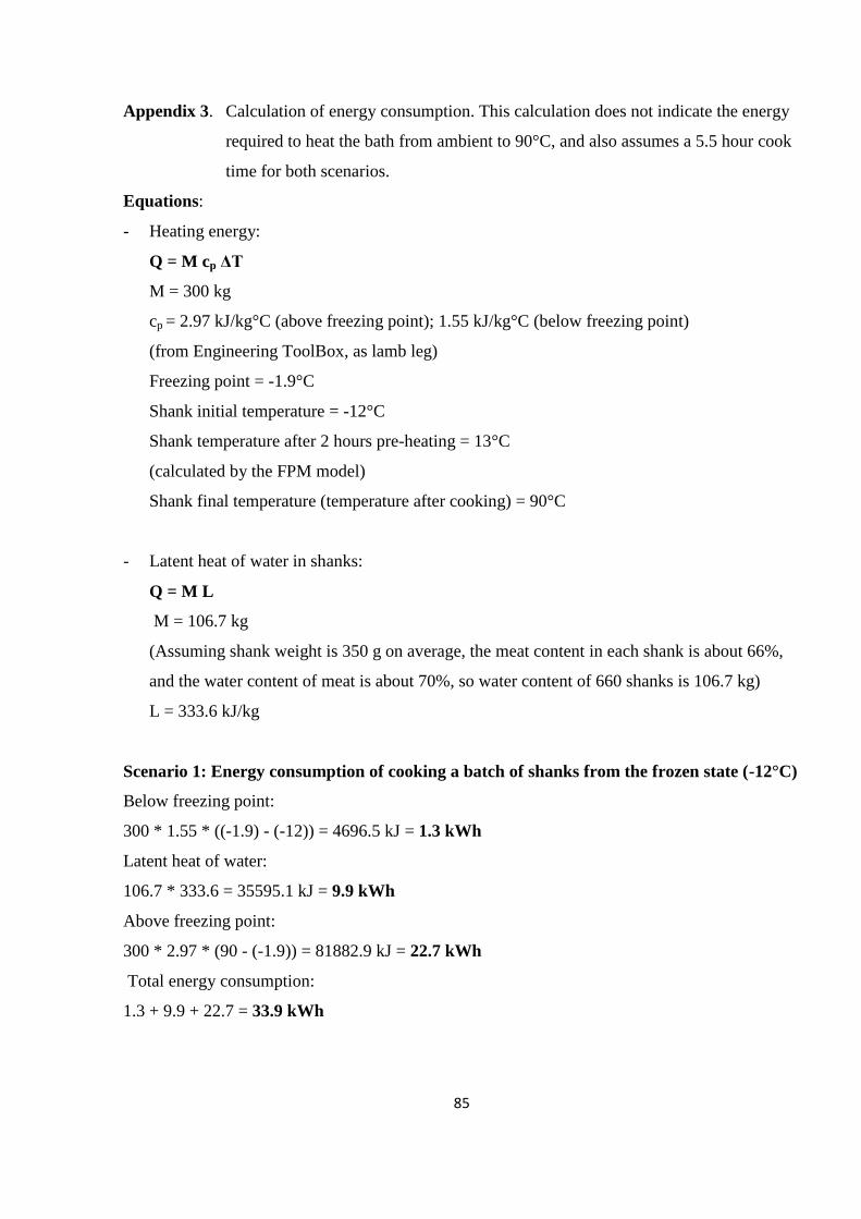
85

Appendix 3. Calculation of energy consumption. This calculation does not indicate the energy

required to heat the bath from ambient to 90°C, and also assumes a 5.5 hour cook

time for both scenarios.

Equations:

- Heating energy:

Q = M cp ΔT

M = 300 kg

cp = 2.97 kJ/kg°C (above freezing point); 1.55 kJ/kg°C (below freezing point)

(from Engineering ToolBox, as lamb leg)

Freezing point = -1.9°C

Shank initial temperature = -12°C

Shank temperature after 2 hours pre-heating = 13°C

(calculated by the FPM model)

Shank final temperature (temperature after cooking) = 90°C

- Latent heat of water in shanks:

Q = M L

M = 106.7 kg

(Assuming shank weight is 350 g on average, the meat content in each shank is about 66%,

and the water content of meat is about 70%, so water content of 660 shanks is 106.7 kg)

L = 333.6 kJ/kg

Scenario 1: Energy consumption of cooking a batch of shanks from the frozen state (-12°C)

Below freezing point:

300 * 1.55 * ((-1.9) - (-12)) = 4696.5 kJ = 1.3 kWh

Latent heat of water:

106.7 * 333.6 = 35595.1 kJ = 9.9 kWh

Above freezing point:

300 * 2.97 * (90 - (-1.9)) = 81882.9 kJ = 22.7 kWh

Total energy consumption:

1.3 + 9.9 + 22.7 = 33.9 kWh

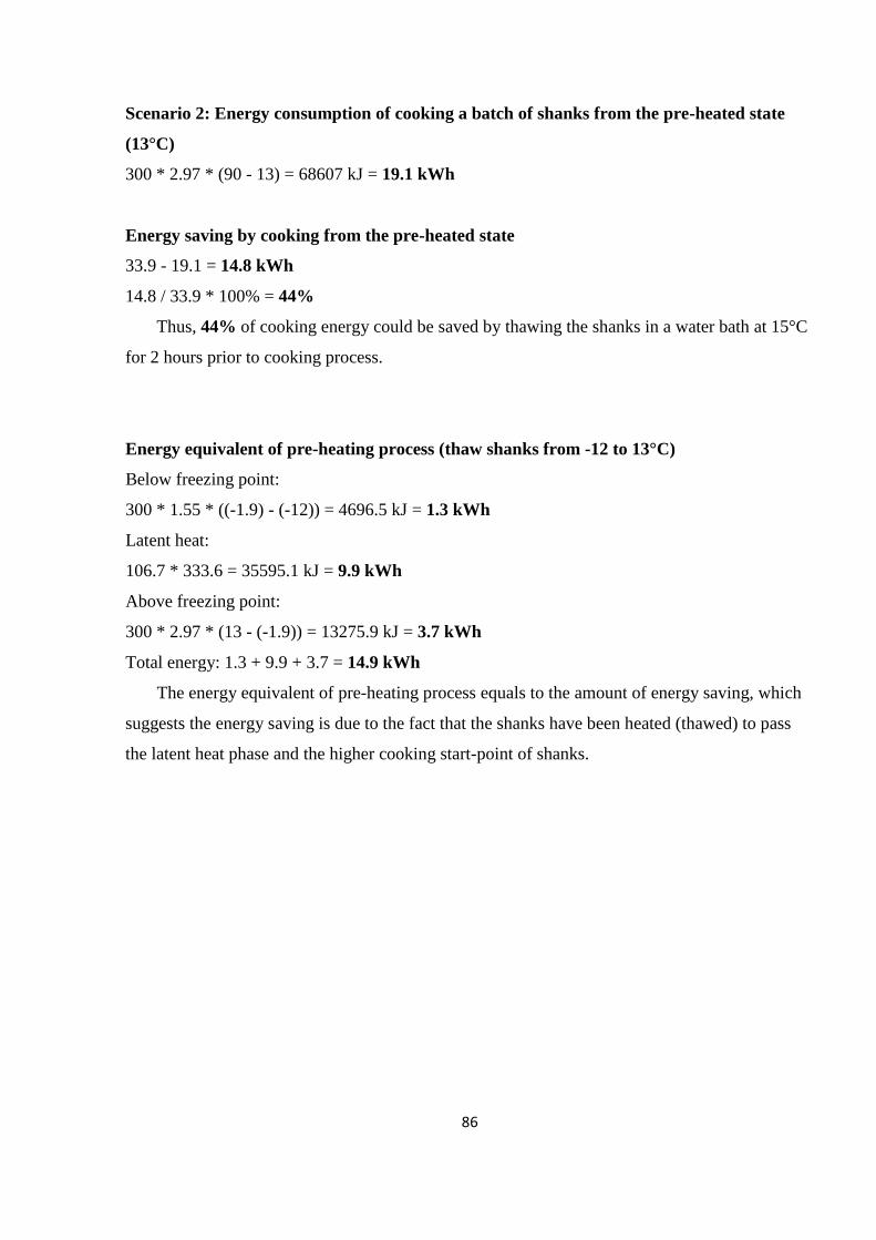
86

Scenario 2: Energy consumption of cooking a batch of shanks from the pre-heated state

(13°C)

300 * 2.97 * (90 - 13) = 68607 kJ = 19.1 kWh

Energy saving by cooking from the pre-heated state

33.9 - 19.1 = 14.8 kWh

14.8 / 33.9 * 100% = 44%

Thus, 44% of cooking energy could be saved by thawing the shanks in a water bath at 15°C

for 2 hours prior to cooking process.

Energy equivalent of pre-heating process (thaw shanks from -12 to 13°C)

Below freezing point:

300 * 1.55 * ((-1.9) - (-12)) = 4696.5 kJ = 1.3 kWh

Latent heat:

106.7 * 333.6 = 35595.1 kJ = 9.9 kWh

Above freezing point:

300 * 2.97 * (13 - (-1.9)) = 13275.9 kJ = 3.7 kWh

Total energy: 1.3 + 9.9 + 3.7 = 14.9 kWh

The energy equivalent of pre-heating process equals to the amount of energy saving, which

suggests the energy saving is due to the fact that the shanks have been heated (thawed) to pass

the latent heat phase and the higher cooking start-point of shanks.