Geophys. J. Int. (2000) 140, 311–323

Source ambiguity from an estimation of the scaling exponent ofpotential field power spectra

Tatiana Quarta,1 Maurizio Fedi2 and Angelo De Santis31Dipartimento di Scienza dei Materiali, via per Arnesano, 73100 L ecce, Italy

2Dipartimento di Geofisica e Vulcanologia, L .go S. Marcellino 10, 80138 Napoli, Italy

3 Istituto Nazionale di Geofisica, Dip. Geomagnetismo, V ia di V igna Murata 605, 00143 Roma, Italy. E-mail: desantisag@ing750.ingrm.it

Accepted 1999 September 16. Received 1999 January 1; in original form 1997 September 1

SUMMARYAn analysis of the field scaling power spectrum yields useful information about thesource distribution, but it is uncertain whether deterministic, random, fractal or mixedapproaches have to be used for the interpretation. To this end, the scaling propertiesof potential field spectra are analysed for a number of different source models ofgeological interest. Besides the models of Naidu (purely random sources) and Spectorand Grant (gross block statistical ensembles) we consider other types of density andmagnetization distributions with spectral exponents in the fractal range, such as asingle homogeneous body with a random white source distribution. Spectral slopes inthe fractal range are obtained.

We also study the effects of important natural sources, such as salt domes andsedimentary basins, representing them with simple Gaussians or combinations ofGaussian signals. The same spectral slopes as for gravity signals generated by 3-Dfractal source distributions are found for them. Hence the power law decay of the fieldis not a characteristic only of fractal source models.

If a 3-D fractal source distribution is assumed a priori, a way of verifying thegoodness of the model is to examine the whitened field at source level. The probabilitythat the whitened field derives from a random white population is estimated forsynthetic and real anomalies by applying the usual statistical tests.

Key words: fractals, potential field, spectral analysis.

scaling noise. Mandelbrot (1983) and Huang & Turcotte (1989)INTRODUCTION

showed that its power spectrum P is proportional to some

negative power of frequency,Spectral analysis is widely applied to gravity and geomagnetic

field data since it provides information about the averageP3 f −b , (1)values of the main parameters characterizing the source distri-

bution. The more meaningful information is normally related where b is related to the fractal dimension Df of the scalingto the decay properties of the field power spectra. noise as b=5−2Df with 1<Df≤2 for a 1-D random process

Two main spectral approaches are used, namely those of (e.g. Turcotte 1992), or as b=8−2Df with 2<Df≤3 for aNaidu (1968) and of Spector & Grant (1970). Naidu’s model 2-D random process, the latter being valid when a radial(Appendix A) is based on randomly distributed sources and power spectrum is considered (e.g. Goff 1990). Therefore,is appropriate for describing a shallow and highly variable 1≤b<3 for 1-D stochastic processes (Huang & Turcottemagnetization or mass density distribution. Spector and 1989; Fox 1989; Hough 1989) and 2≤b<4 for 2-D onesGrant’s model (Appendix B) regards statistical ensembles of (Goff 1990).blocks of various sizes and magnetization, and is suitable for Recently, the concepts of fractal geometry have been used torepresenting sources sketched as gross homogeneous bodies, analyse geophysical phenomena such as the Earth’s topographysuch as, for instance, intrusions. (Huang & Turcotte 1989; Gilbert 1989), seafloor roughness

In the last 10 years, fractal theory has become very popular (Fox & Hayes 1985; Malinverno 1989), rock fractures (Brown1987; Kumar & Bodvarsson 1990), the level of geomagneticin many physical fields. The simplest fractal model is the

311© 2000 RAS

312 T . Quarta, M. Fedi and A. De Santis

activity (De Santis & Chiappini 1992), and the topography

of the geomagnetic potential at the core–mantle boundary(De Santis & Barraclough 1997).

Fractal theory has also been applied to magnetic and gravity

anomalies, since the decay properties of the field power spectrum(at source level ) are strictly related to the power spectrum ofthe sources (Appendices A and B). Gregotski et al. (1991)

found a scaling exponent bfield#3 for the power spectra of aero-magnetic data from some areas in the Canadian Shield; theyshowed that this result is consistent with a fractal stochastic

model for the near-surface magnetic susceptibility of thatregion. Pilkington & Todoeschuck (1993) showed that thepower spectra of magnetic susceptibility logs from boreholes

in Bells Corners (Ontario) exhibit a scaling behaviour (b#2)

in the fractal range. Subsequently, Pilkington et al. (1994),

examining aeromagnetic radial power spectra from variousareas of the Canadian Shield (bfield#3), argued a fractal

distribution for the near-surface magnetic sources (bsource=4).

Maus & Dimri (1994) established important relations between

the scaling exponents of gravity and magnetic power spectraand the isotropic scaling exponents of their corresponding

sources. Later, the same authors (1996), assuming an a priori3-D isotropic fractal source distribution, found a scaling

exponent bfield#4.6 for the radially averaged 2-D power

spectrum of gravity data from Paradox Basin, and, applyingtheir relations, found a scaling exponent bsource=3.6 of the

corresponding sources.

On the other hand, Zhou & Thybo (1998) have shown that

the spectral slope of power spectra from aeromagnetic data, inan area of the southeast North Sea with a thick sediment

cover, is likely to be significantly different from the expected

value bfield=3 (they found bfield=2.3). Furthermore, the

analysis of susceptibility data from boreholes shows differentvalues of the scaling exponent at different depths.

(a)

(b)

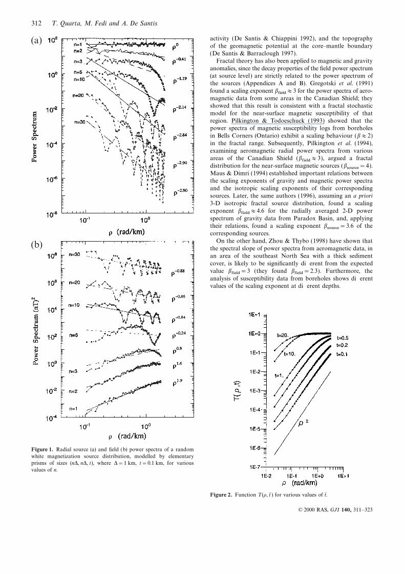
Figure 1. Radial source (a) and field (b) power spectra of a random

white magnetization source distribution, modelled by elementary

prisms of sizes (nD, nD, t), where D=1 km, t=0.1 km, for various

values of n.

Figure 2. Function T (r, t: ) for various values of t:.

© 2000 RAS, GJI 140, 311–323

Source ambiguity from power spectra 313

In all the above cases, the authors attributed a random to take into account the correlation lengths present in the

observational data (e.g. Dolan et al. 1998). Moreover, Fedifractal noise nature to the near-surface source distributions ofdensity or magnetization in the crust. Although the fractal et al. (1997) have shown that non-fractal sources (in a strict

sense), such as those pertinent to the Spector and Grant model,point of view with all it implies (i.e. scale-invariance, self-

affinity and non-differentiability) is a powerful approach for may also give a scaling exponent bfield#3 in the magneticcase, which corresponds to bfield#5 in the gravity case. Withanalysing complex media, most of the time it needs to be

properly tuned to the particular situation, in order, for instance, this in mind, we assume that different models are compatible

(a)

(b)

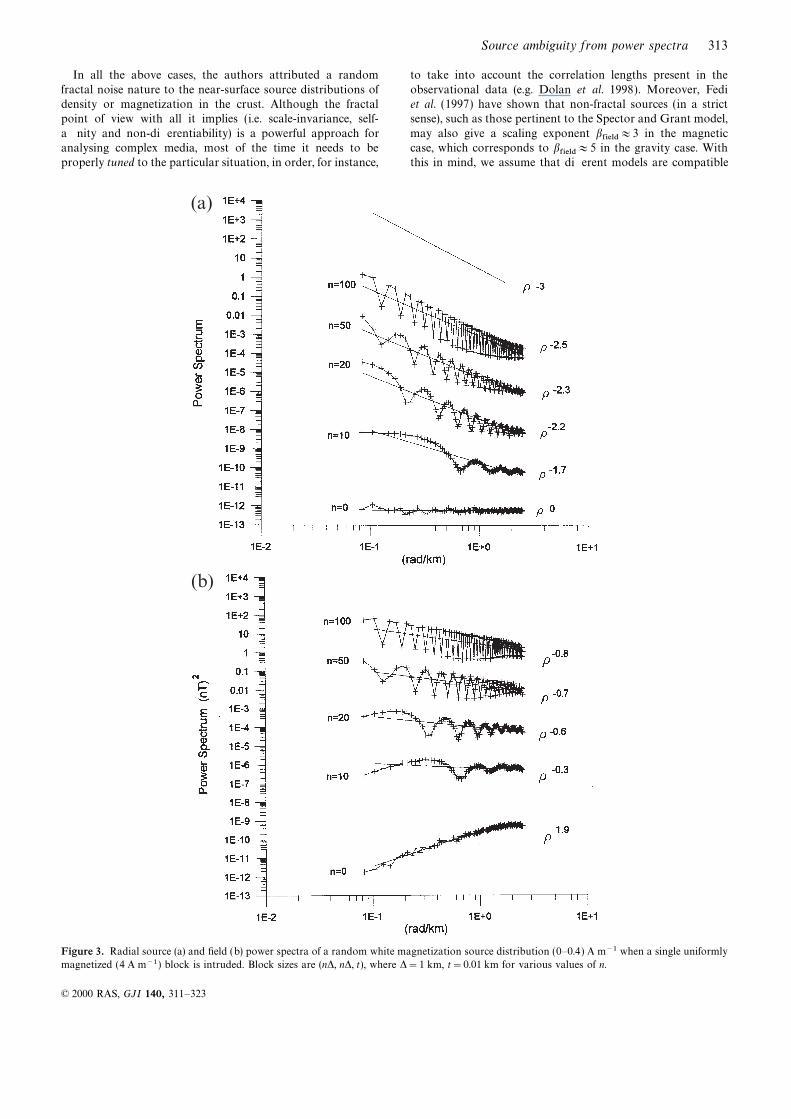
Figure 3. Radial source (a) and field (b) power spectra of a random white magnetization source distribution (0–0.4) A m−1 when a single uniformly

magnetized (4 A m−1 ) block is intruded. Block sizes are (nD, nD, t), where D=1 km, t=0.01 km for various values of n.

© 2000 RAS, GJI 140, 311–323

314 T . Quarta, M. Fedi and A. De Santis

with the same power law decay in the field power spectrum. spectral decay properties of these models are presently not

well known. Thus, in this paper, we study such properties forHough (1989) asserted that the presence of a power law decayin the spectrum is not sufficient to identify a fractal distribution. a number of source models of particular interest in geology.She showed that the spectral slope b#2 (1-D case) can be

obtained by concatenating time series of different amplitudesTHE SCALING EXPONENT OF THE POWER

and frequencies. Fox & Hayes (1985), analysing long non-SPECTRUM OF POTENTIAL FIELDS

stationary bathymetric profiles, suggested a general tendency

towards a self-similar model, characterized by a spectral slope The spectral approaches of Naidu, and Spector and Grant(Appendices A and B, respectively) deal with only two typesb#2. Owing to the Earth’s real geology and to inaccuracies

in data representations of the field measurements (interpolation of geological models, namely purely random sources and gross

homogeneous blocks, respectively. Such models are, however,and so on), complex cases arise which do not match therequirements of Naidu’s or of Spector and Grant’s model. The inadequate to describe more complex structures, the simplest

Figure 4. Synthetic signals obtained by combining different Gaussian functions and their power spectra: different spectral slopes are obtained if

the signals are not tapered (box-car window), tapered (Hanning window) or the power is calculated using the maximum entropy method. All the

ordinates have arbitrary units; power spectra are plotted against angular frequencies.

© 2000 RAS, GJI 140, 311–323

Source ambiguity from power spectra 315

of them being a few, relatively homogeneous blocks buried note that in the discrete case the concepts of homogeneous

blocks and random sources are relative. For example, a homo-in an ensemble of random sources. Generalizing this kind ofsituation, some authors (e.g. Wu et al. 1994) have argued that geneous source will be detected only if the sampling interval

D is appropriate with respect to the horizontal dimension ofthe crustal heterogeneity is composed of two components: a

deterministic part and a stochastic part. For this reason it is the field anomaly. Therefore, the ratio n=a/D, where a is thehorizontal extent of the source, becomes a relevant parameteroften suggested that a trend should be removed from the data

records (e.g. Bracewell 1965). As this way of proceeding in linking the spectral properties of the field measurements to

those of the sources.is rather subjective, we prefer here to analyse a number ofparticular cases in order to understand better the relation In the following cases, we will investigate the dependence of

the scaling exponent b on n.between deterministic and random sources. First of all, let us

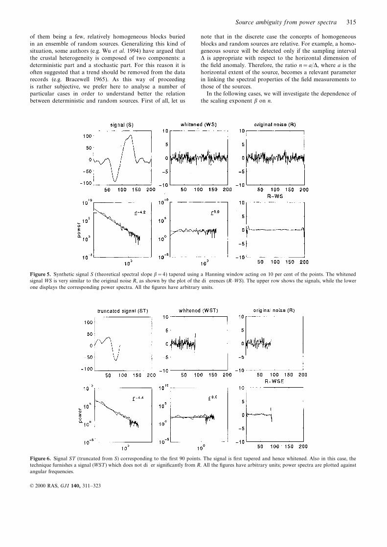
Figure 5. Synthetic signal S (theoretical spectral slope b=4) tapered using a Hanning window acting on 10 per cent of the points. The whitened

signal WS is very similar to the original noise R, as shown by the plot of the differences (R–WS). The upper row shows the signals, while the lower

one displays the corresponding power spectra. All the figures have arbitrary units.

Figure 6. Signal ST (truncated from S) corresponding to the first 90 points. The signal is first tapered and hence whitened. Also in this case, the

technique furnishes a signal (WST ) which does not differ significantly from R. All the figures have arbitrary units; power spectra are plotted against

angular frequencies.

© 2000 RAS, GJI 140, 311–323

316 T . Quarta, M. Fedi and A. De Santis

a general random distribution of background sources. WeCase (a)

now want to study how the presence of a homogeneous bodycan modify the power decay of the surrounding randomWe consider several sets of homogeneous blocks with different

ratios n. For all sets, a uniformly random magnetization is magnetization sources.

For the homogeneous source we assume a simple model,assumed. When n=1 our model practically reduces to Naidu’smodel, while for a sufficiently large value of n it corresponds to namely a single uniformly magnetized block represented by a

thin prismatic body of size (nD, nD, 0.1) km3, with D=1 kma Spector and Grant source distribution. We will see later that

in practice this threshold corresponds to n#10. Although such and a 4 A m−1 magnetization. The surrounding background isassumed to be in the form of a plate of (300, 300, 0.1) km3 withextreme models have been studied extensively, intermediate

cases (i.e. when 1<n<10) have not been investigated so far. white random magnetization in the interval [0, 0.4] A m−1.Figs 3(a) and (b) show the radially averaged source andThe starting model that mimics Naidu’s model is formed

by N×N (with N=300) uniformly magnetized prisms, each field power spectra, respectively, for increasing values of n(the value n=0 identifies the white source power spectrumof size (a, a, t) where a=1 km, the thickness t=0.1 km and

the sampling interval of the anomaly field D=1 km; the and the corresponding field power spectrum). The results aresummarized in Table 2.magnetization intensity values attributed to the elementary

prisms are randomly and uniformly distributed in the interval

[0, 4] A m−1. The case n=1 identifies the power spectra ofTable 2. Results of Case (b).

this kind of source and its relative field in Figs 1(a) and (b),respectively. Other sets of models are produced by changing n 0 10 20 50 100the size a of the elementary prisms. In practice, each model isobtained by dividing the thin plate into (N/n×N/n) equal bsource 0.0 1.7 2.2 2.3 2.5elementary prisms of size (a, a, t), where a=nD, t=0.1 km, and bfield −1.9 0.3 0.6 0.7 0.8

n is a positive integer in the interval [2, N]. The magnetizationvalues are again random numbers uniformly distributed in the

interval [0, 4] A m−1. The sources and the radially averagedfield power spectra are calculated using, for all the models, thesame sampling interval D=1 km. Figs 1(a) and (b) show the

power spectra of the sources and fields, respectively, for variousvalues of n.

The results are summarized in Table 1. Note that for n>10

we have bsource#2.9 and bfield#0.9. These latter values charac-terize the Spector and Grant model for small values of meanthickness t: and for large values of a. In fact, Fig. 2 shows that,

for a small thickness (t:=0.1), the factor T (r, t: )3r2, and henceeq. (B8) in Appendix B becomes E(r)3r2−b, where b#2.9.

It is worth noting that the source power spectrum calculated

using the (N/n×N/n) matrix is always white-like, while thatcalculated using the (N×N ) matrix becomes red as n increases.Thus the field sampling interval D assumes an important role

in inferring the power decay. In fact, if the randomness of thesources has a scale a>D, the field scaling exponent is affectedby the correlation existing between the magnetization values

in each elementary prism.Obviously, when t increases, for high values of n, bfield� 2.9,

which is the typical Spector and Grant exponent value (Fedi

et al. 1997). Hence bfield can assume values in the fractalrange too.

Case (b)

A completely random distribution of magnetization is rare innature. A more realistic case is represented by one or morelocalized homogeneous magnetization sources together with

Table 1. Results of Case (a).

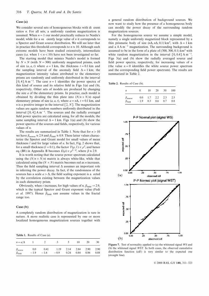
n=a/D 1 2 3 5 10 20 30Figure 7. Test of normality applied to (a) the whitened signal WS and

(b) the whitened signal WST . In both cases, the observed cumulativebsource 0.0 0.41 1.19 2.14 2.84 2.90 2.90distribution function (cdf ) is very similar to the expected onebfield −1.9 −1.6 −0.9 0.24 0.84 0.86 0.88(straight line).

© 2000 RAS, GJI 140, 311–323

Source ambiguity from power spectra 317

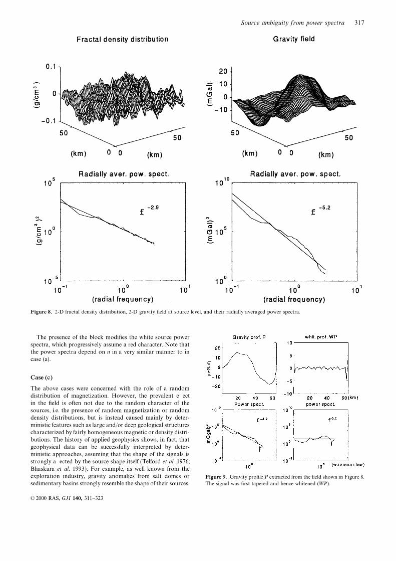
Figure 8. 2-D fractal density distribution, 2-D gravity field at source level, and their radially averaged power spectra.

The presence of the block modifies the white source power

spectra, which progressively assume a red character. Note thatthe power spectra depend on n in a very similar manner to incase (a).

Case (c)

The above cases were concerned with the role of a randomdistribution of magnetization. However, the prevalent effect

in the field is often not due to the random character of thesources, i.e. the presence of random magnetization or randomdensity distributions, but is instead caused mainly by deter-

ministic features such as large and/or deep geological structurescharacterized by fairly homogeneous magnetic or density distri-butions. The history of applied geophysics shows, in fact, that

geophysical data can be successfully interpreted by deter-ministic approaches, assuming that the shape of the signals isstrongly affected by the source shape itself (Telford et al. 1976;

Bhaskara et al. 1993). For example, as well known from theexploration industry, gravity anomalies from salt domes or Figure 9. Gravity profile P extracted from the field shown in Figure 8.

The signal was first tapered and hence whitened (WP).sedimentary basins strongly resemble the shape of their sources.

© 2000 RAS, GJI 140, 311–323

318 T . Quarta, M. Fedi and A. De Santis

In such cases, the anomalies have a typically medium-long wave- bining various Gaussian functions and their associated power

length spectral content which is fundamental for the description spectra. If the signals are not tapered, which is equivalent toof the sources. This must not be confused with the presence of applying a box-car window, the power spectra of symmetricalexternal trends, usually removed before any spectral analysis. signals show scaling exponents b in the range [3.7–3.8], while

To understand the behaviour of the spectral scaling exponent the power spectra of asymmetrical signals show scalingof such deterministic models, we analysed the power spectra exponents b in the range [1.9–2.0]. The lower value of bof simple theoretical signals which have most of their energy obtained for asymmetrical signals is due to the presence ofat medium-long wavelengths. Here we report only the most periods greater than the length of the data window. In thismeaningful results. Fig. 4 shows the signals obtained by com- case there is strong spectral leakage, and the energy of the

signal is linearly distributed with respect to f −2 . The leakage

can be reduced by applying tapered windows, but the spectral

slope will depend on the function used to taper the signal.

If a Hanning window tapering only 10 per cent of the points

is applied to the signals, the power spectra show a scaling

exponent b in the range [3.7–4.3] (Fig. 4). Similar results are

obtained if the same tapered window is applied to the whole

data window. In the following, tapering will indicate the above

procedure.

The power spectra of the signals (not tapered) are also

calculated using the maximum entropy method and p=10

poles. In this case the spectral slope b shows a more limited

range [3.7–3.8], and the power spectra appear very smoothed.

Using a larger number of poles does not affect the results.

In conclusion, deterministic signals obtained by combining

a few Gaussian functions show a spectral slope b in the range

[3–5], the same as gravity profiles generated by a 3-D fractal

source distribution. This fact confirms the intrinsic non-uniqueness of field anomaly interpretations. The results areFigure 10. Test of normality applied to the whitened gravity profile

WP. summarized in Table 3.

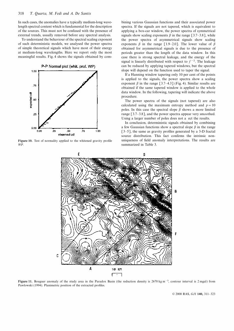
Figure 11. Bouguer anomaly of the study area in the Paradox Basin (the reduction density is 2670 kg m−3, contour interval is 2 mgal ) from

Pawlowski (1994). Planimetric position of the extracted profiles.

© 2000 RAS, GJI 140, 311–323

Source ambiguity from power spectra 319

Table 3. Results of Case (c). power spectral exponents of an n-dimensional field and lower-

dimensional subsets (Table 4). In particular, in the gravitySignal 1 2 3 4 case, the spectral slope of a gravity profile must have the same

spectral slope as the 3-D fractal source distributions.b (box-car) 3.8 3.7 2.0 1.9

However, as with any theory, the basic hypotheses need tob (Hanning) 4.2 3.7 4.3 3.9be validated; that is, we need to test how close our observationsb (Max.-Entr.) 3.7 3.7 3.8 3.7are to our assumed model.

As Maus & Dimri (1996) state, at source level the field

power spectrum is dominated by the scaling properties of theWhitening technique and non-parametric tests

source distribution. In this case we expect that if the field is

whitened, i.e any existing correlation among the amplitudes atMaus & Dimri (1994), assumed a 3-D fractal isotropic sourcedistribution and established important relations amongst the different wavenumbers is removed, the signal obtained will be

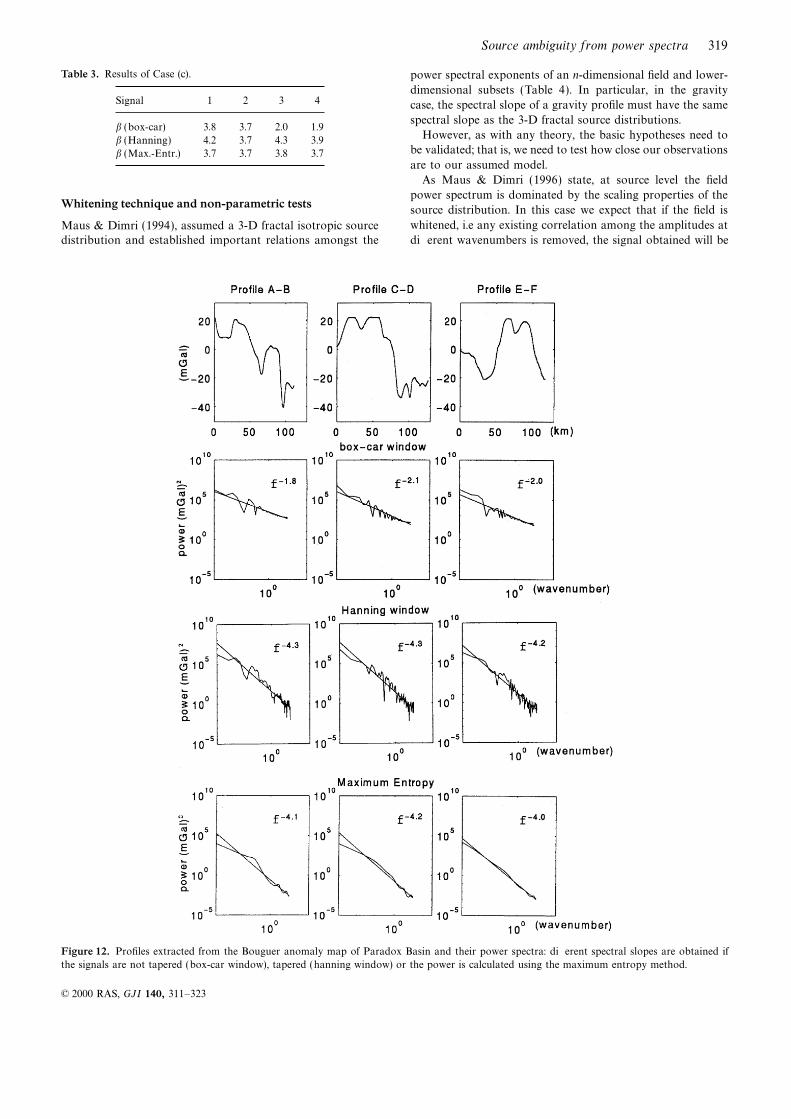
Figure 12. Profiles extracted from the Bouguer anomaly map of Paradox Basin and their power spectra: different spectral slopes are obtained if

the signals are not tapered (box-car window), tapered (hanning window) or the power is calculated using the maximum entropy method.

© 2000 RAS, GJI 140, 311–323

320 T . Quarta, M. Fedi and A. De Santis

Table 4. Relations amongst scaling exponents of potential field spectra both cases the points cluster closely about the theoreticalwith various dimensionalities. straight line, not showing significant departures from normality.

The package SPSS (1998) was employed to perform the K–SSource Field test and to produce the P–P plots.

As already stated (see also Table 4), the spectral scaling3-D 2-D 1-D XY 1-D

properties of a 3-D fractal source distribution are the same asthose associated with a profile of the gravity anomaly fieldGravity b b−1 b−2 b+1 bobserved at the surface. To verify whether whitening the gravityMagnetic b b−1 b−2 b−1 b−2profiles produces random white signals, a synthetic 3-D fractalsource was generated by extending the method proposed by

Feder (1988) to the 3-D case. Feder showed that a 2-D triadica white noise. The procedure of whitening is performed by: Koch surface, generated by sliding the Koch curve along a(1) dividing the Fourier transform of the signal by the square direction perpendicular to the plane of the Koch curve forroot of f −b , and (2) antitransforming. a distance l, has a fractal dimension D2=D1+1, where D1 is

We now want to test whether the method is able to recover the original fractal dimension of the Koch curve.white random signals when a tapered window is applied. To We have generated a 2-D fractal density set (64×64this end, a synthetic 1-D signal is generated using the technique elements, spectral slope b2-Dsource=3, range of density valuessuggested by Huang & Turcotte (1989). The algorithm generates [−0.1, 0.1]), again using the technique of Huang & Turcottea signal S, having a specific spectral slope b, by starting with a (1989), but for the 2-D case. The fractal densities were assignedGaussian random white noise R and then colouring it. to 64×64 prisms, each sized (1, 1, 20) km3, with expected

Fig. 5 shows a synthetic signal S of 200 points having the spectral slope b3-Dsource=b2-Dsource+1=4. The corresponding gravitytheoretical spectral slope b=4. If the signal is not tapered, the field was computed at the (64×64) points, at 1 km steps andwhitening technique perfectly recovers the random noise R. close to the sources (at 1 m elevation). Fig. 8 shows the 2-DTapering of the signal causes a slight increase of the spectral fractal density distribution, the 2-D gravity field at sourceslope (b=4.2), and little difference (about 20 per cent) of the level, and their radially averaged power spectra computed afterwhitened signal with respect to the true random noise R, tapering. Fig. 9 shows a profile extracted from the 2-D gravityexcept for few points at the ends of the data window. If only field, the whitened signal WP, and their power spectra com-part of the signal is analysed, with the same procedure (signal puted after tapering. The K–S test, applied to the whitenedST in Fig. 6), the results are still satisfactory. signal WP stripped of the first and last eight points, gives a

In real cases, the whiteness of the signal can be validated 98 per cent probability that the signal belongs to a Gaussianby the non-parametric test of Kolmogorov–Smirnov (e.g. Box white noise population. Furthermore, the associated P–P normal& Jenkins 1976), which verifies whether the signal derives from plot does not show significant departures from normalitya random white noise population. The K–S test has been (Fig. 10).applied to the whitened signal WS (resulting from the case inFig. 5), with the first and last 10 points removed in order toavoid the introduction of artificial features as a result of the

APPLICATION TO REAL CASEStapering operation. The test yields a 97 per cent probabilitythat the signal is a sample of a Gaussian white noise population. Having shown for synthetic cases that the whiteness of the

signal can be validated by statistical analysis, we now discussThe K–S test applied to the truncated whitened signal WST

(resulting from the case of Fig. 6), again stripped of the first an application of such tests to three profiles (Fig. 11) extractedfrom a gravity anomaly map (120 km×120 km) of Paradoxand last 10 points, yields 72 per cent probability.

Another sensitive indicator of departure from a Gaussian Basin (Pawlowski 1994). Paradox Basin is a salt anticline

region in southeastern Utah (USA), characterized by a strongrandom white noise is the P–P normal plot (e.g. Box & Jenkins1976), where the cumulative distribution function (cdf ) of the regional gravity field of deep origin and more localized gravity

anomalies caused by shallower salt anticlines and structures.data is plotted against the theoretical normal one. Fig. 7 shows

P–P normal plots for the whitened signals WS and WST ; in Pawlowski (1994) used the Spector and Grant method and

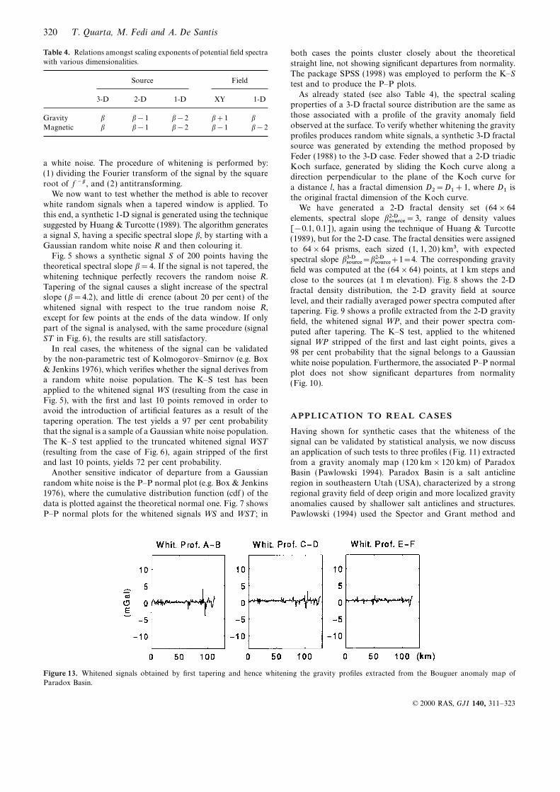
Figure 13. Whitened signals obtained by first tapering and hence whitening the gravity profiles extracted from the Bouguer anomaly map of

Paradox Basin.

© 2000 RAS, GJI 140, 311–323

Source ambiguity from power spectra 321

derived source depths at 5 and 54 km from the radial power

spectrum of the anomaly field. He used these depth estimatesto separate the effects caused by shallow and deep-seatedsources by means of Wiener filtering, assuming that long- and

short-wavelength anomalies originate from deep-seated andshallow sources, respectively. Maus & Dimri (1996) fitted thesame radial power spectrum by the function

Pmodel (r)=C exp(−2tr)r−bfield

, (8)

where r=2p(u2+v2 )1/2, and assumed that bfield=bsource+1,

where bsource is the scaling isotropic exponent of the 3-D sourcedistribution. Applying a non-linear best-fit technique, theauthors found ln(C)=0.93, and bfield=4.5 and 0.054 km for

the source depth. They concluded that the density variationscaused by the structures in Paradox Basin are scaling withbsource=3.6.

The central part of the map in Fig. 11 shows a localmaximum and strong anomalies of various wavelengths,stretched in the NW–SE direction. We selected three profiles

(indicated by AB, CD, and EF in Fig. 11) crossing anomaliesof variable wavelength and gradient. For each profile, a discreteset of anomaly values has been digitized from the map and

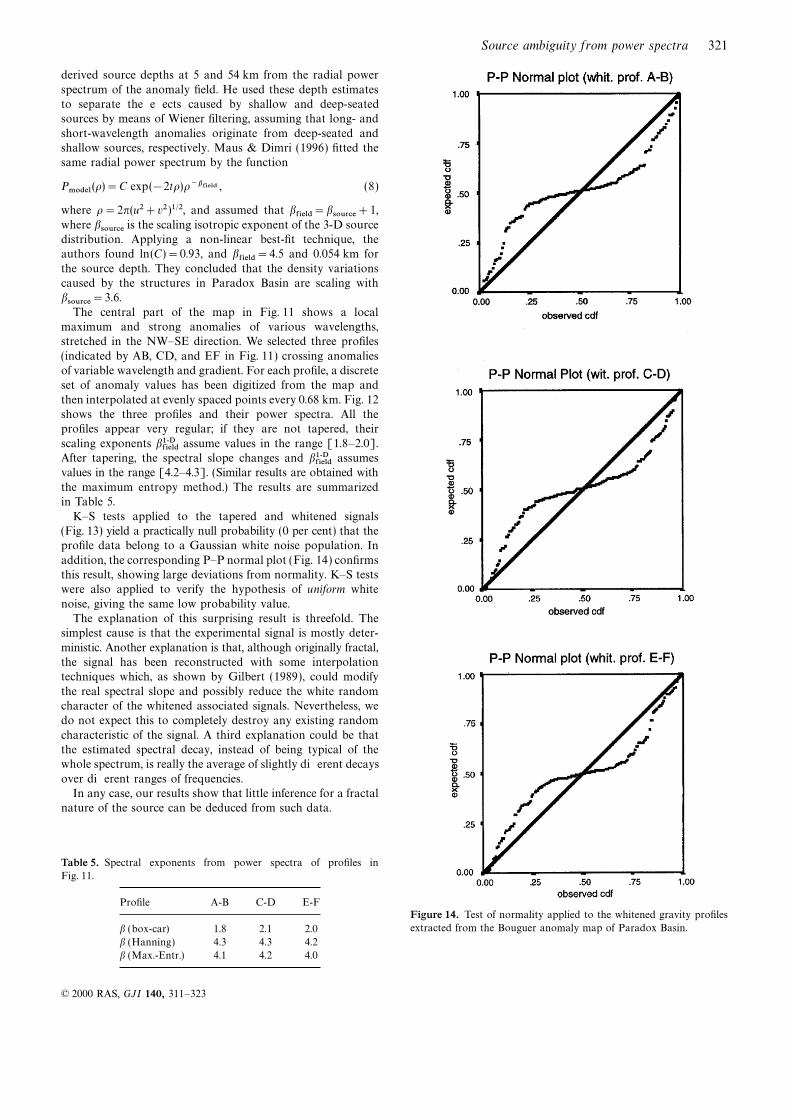
then interpolated at evenly spaced points every 0.68 km. Fig. 12shows the three profiles and their power spectra. All theprofiles appear very regular; if they are not tapered, their

scaling exponents b1-Dfield assume values in the range [1.8–2.0].After tapering, the spectral slope changes and b1-Dfield assumesvalues in the range [4.2–4.3]. (Similar results are obtained with

the maximum entropy method.) The results are summarizedin Table 5.

K–S tests applied to the tapered and whitened signals(Fig. 13) yield a practically null probability (0 per cent) that theprofile data belong to a Gaussian white noise population. In

addition, the corresponding P–P normal plot (Fig. 14) confirmsthis result, showing large deviations from normality. K–S testswere also applied to verify the hypothesis of uniform white

noise, giving the same low probability value.The explanation of this surprising result is threefold. The

simplest cause is that the experimental signal is mostly deter-

ministic. Another explanation is that, although originally fractal,the signal has been reconstructed with some interpolationtechniques which, as shown by Gilbert (1989), could modify

the real spectral slope and possibly reduce the white randomcharacter of the whitened associated signals. Nevertheless, wedo not expect this to completely destroy any existing random

characteristic of the signal. A third explanation could be thatthe estimated spectral decay, instead of being typical of thewhole spectrum, is really the average of slightly different decays

over different ranges of frequencies.In any case, our results show that little inference for a fractal

nature of the source can be deduced from such data.

Table 5. Spectral exponents from power spectra of profiles in

Fig. 11.

Profile A-B C-D E-FFigure 14. Test of normality applied to the whitened gravity profiles

extracted from the Bouguer anomaly map of Paradox Basin.b (box-car) 1.8 2.1 2.0

b (Hanning) 4.3 4.3 4.2

b (Max.-Entr.) 4.1 4.2 4.0

© 2000 RAS, GJI 140, 311–323

322 T . Quarta, M. Fedi and A. De Santis

Dolan, S.S., Bean, C.J. & Riollet, B., 1998. The broad-band fractalCONCLUSIONS nature of heterogeneity in the upper crust from petrophysical logs,

Geophys. J. Int., 132, 489–507.In this work we have shown that the spectral scaling exponentFeder, J., 1988. Fractals, Plenum Press, New York.of the field can assume values in the so-called fractal range,Fedi, M., Quarta, T. & De Santis, A., 1997. Improvements to the

even though the corresponding sources are not fractal. SourcesSpector and Grant method of source depth estimation using the

with intermediate characteristics between Naidu’s and Spectorpower law decay of magnetic field power spectra, Geophysics, 62,

and Grant’s models produce fields whose power spectra scaling 1143–1150.exponent bfield depends on the ratio n between the horizontal Fox, C.G., 1989. Empirically derived relationships between fractalextent of the source and the field sampling interval. Moreover, dimension and power law form frequency spectra, Pageoph, 131,

211–239.a single large block, uniformly magnetized and intruded into aFox, C.G. & Hayes, D.E., 1985. Quantitative methods for analysingrandom white magnetization source distribution, shows similar

the roughness of the seafloor, Rev. Geophys., 23, 1–48.characteristics. In the above cases, the scaling exponent of theGilbert, L.E., 1989. Are topographic data sets fractal?, Pageoph,field power spectra may be incorrectly related to the source

131, 241–254.power spectra with a fractal scaling exponent.Goff, J.A., 1990. Comment on ‘Fractal mapping of digitized images,

Simple signals obtained by combinations of a few Gaussianapplication to the topography of Arizona and comparison with

functions show a spectral slope in the range [3–5]; that is, thesynthetic images’ by J. Huang and D. L. Turcotte, J. geophys. Res.,

same as gravity signals generated by a 3-D fractal source 95, 5159.distribution. The estimated value of the spectral slope may Gregotski, M.E., Jensen, O. & Arkani-Hamed, J., 1991. Fractaldepend on the method used to calculate the spectra (e.g. stochastic modelling of aeromagnetic data, Geophysics, 56,

1706–1715.Fourier, maximum entropy) or on the windows used to taperHough, S.E., 1989. On the use of spectral methods for the determinationthe data.

of fractal dimension, Geophys. Res. L ett., 16, 673–676.In order to verify the goodness of a fractal source model forHuang, J. & Turcotte, D.L., 1989. Fractal mapping of digitized images,experimental data, we suggest examining the properties of the

application to the topography of Arizona and comparisons withwhitened field at source level, since it must be random whensynthetic images, J. geophys. Res., 94, 7491–7495.

any correlation is removed in the amplitude spectrum.Kumar, S. & Bodvarsson, G.S., 1990. Fractal study and simulation of

The Kolmogorov–Smirnov (K–S) test applied to taperedfracture roughness, Geophys. Res. L ett., 17, 701–704.

and whitened gravity profiles yields a high probability value Malinverno, A., 1989. Testing linear models of sea-floor topography,in the synthetic cases, and a nearly null value for three profiles Pageoph, 131, 139–155.extracted from the gravity anomaly map of Paradox Basin. Mandelbrot, B.B., 1983. The Fractal Geometry of Nature,

W. H. Freeman, New York.Finally, we note that if the available data from densityMaus, S. & Dimri, V.P., 1994. Scaling properties of potential fieldsand magnetic susceptibility borehole logs show power spectra

due to scaling sources, Geophys. Res. L ett., 21, 891–894.compatible with fractal shallow sources, their extension to largerMaus, S. & Dimri, V., 1996. Depth estimation from the scaling powerdepths can be an incorrect extrapolation. This is confirmed

spectrum of potential fields?, Geophys. J. Int., 124, 113–120.by many seismic, gravity and petrological models that showNaidu, P., 1968. Spectrum of the potential field due to randomly

that the density generally increases with depth. Consequently,distributed sources, Geophysics, 33, 337–345.

any realistic fractal model should be constrained accordingly;Pawlowski, R.S., 1994. Green’s equivalent-layer concept in gravity

otherwise, the results will be physically unacceptable. band-pass filter design, Geophysics, 59, 69–76.

Pilkington, M. & Todoeschuck, J.P., 1993. Fractal magnetization of

continental crust, Geophys. Res. L ett., 20, 627–630.ACKNOWLEDGMENTS

Pilkington, M., Gregotski, M.E. & Todoeschuck, J.P., 1994. Using

fractal crustal magnetization models in magnetic interpretation,The paper was presented at session SE29/NP1.1 of the EGSGeophys. Prospect., 42, 677–692.22nd General Assembly Vienna, Austria, 21–25 April 1997.

Spector, A. & Grant, S.F., 1970. Statistical models for interpretingWe would like to thank S. Maus and an unknown referee for

aeromagnetic data, Geophysics, 35, 293–302.their valuable comments and suggestions that improved the

SPSS for Windows, 1998. Version 7.5, Copyright (c) SPSS Inc.original version of the paper. Telford, W.M., Geldart, L.P., Sheriff, R.E. & Keys, D.A., 1976. Applied

Geophysics, Cambridge University Press, Cambridge.

Turcotte, D.L., 1992. Fractals and Chaos in Geology and Geophysics,REFERENCES

Cambridge University Press, Cambridge.

Wu, R.S., Xu, Z. & Li, X.P., 1994. Heterogeneity spectrum and scale-Bhaskara Rao, D., Prakash, M.J. & Ramesh Babu, N., 1993. Gravityanisotropy in the upper crust revealed by the German Continentalinterpretation using Fourier transform and simple geometricalDeep-Drilling (KTB) Holes, Geophys. Res. L ett., 21, 911–914.models with exponential density contrast, Geophysics, 58,

Zhou, S. & Thybo, H., 1998. Power spectra analysis of aeromagnetic1074–1083.data and KTB susceptibility logs, and their implication for fractalBox, G.E.P. & Jenkins, G.M., 1976. T ime Series Analysis Forecastingbehavior of crustal magnetization, Pageoph, 151, 147–159.and Control, Holden-Day, San Francisco.

Bracewell, R., 1965. T he Fourier T ransform and its Applications,

McGraw-Hill Book Company, New York.APPENDIX A: NAIDU’S MODELBrown, S.R., 1987. A note on the description of surface roughness

using fractal dimension, Geophys. Res. L ett., 14, 1095–1098.A relation connecting the spectrum of a random gravity field

De Santis, A. & Barraclough, D.R., 1997. A fractal interpretation ofSgz

(u, v) (or magnetic field SYz

(u, v) ) to the spectrum of randomthe topography of the scalar geomagnetic potential at the core–gravity density S

r(or intensity of magnetization S

j) thatmantle boundary, Pure appl. Geophys., 149, 747–759.

produces it has been established by Naidu (1968). If theDe Santis, A. & Chiappini, M., 1992. Automatic K, determination by

means of fractal and harmonic analysis, Ann. Geophys., 10, 597–602. homogeneous random density sources are assumed to be

© 2000 RAS, GJI 140, 311–323

Source ambiguity from power spectra 323

confined to a thin infinite sheet or a thick semi-infinite medium, parallelepipeds. Each ensemble is characterized by a joint

frequency distribution for depth (h), width (a), length (b), depththe relations are, respectively:extent (t), magnetization intensity (k/ab) and direction cosinesof magnetization (L , M, N). Under the hypotheses that the para-S

gz

(u, v)=4s2

p2Sr(u, v) exp(−2sd) , (A1)

meters vary independently one from another and that they arerandomly and uniformly distributed about their average values(h: , a: , b: , t:, k: ), the authors provided the following expression forS

gz

(u, v, d1)=

4s2

p2 P2

−2

sr(u, v, w)

u2+v2+w2exp(−2sd

1)dw , (A2)

the radial power spectrum E(r) of the magnetic anomaly field,reduced to the north magnetic pole:where

u, v, w are angular frequencies;E(r)=Am

02 B2k: 2C(r, a: , b: )T (r, t: )H(r, h: ) , (B1)s= (u2+v2 )1/2 is the radial frequency;

s is a constant;d is the depth of the sheet; whered1 is the depth of the upper face of the semi-infinite medium;

r= (u2+v2)1/2 is the radial frequency ; (B2)sr(u, v) is the power spectrum of the random density of

the sheet; k: 2= k2� ; (B3)sr(u, v, w) is the power spectrum of the random density of

the semi-infinite medium; C(r, a: , b: )=1

p P p0 S2(r, h, a, b)�dh ; (B4)

Sgz

(u, v) and Sgz

(u, v, d1 ) are the power spectra of thegravitational fields observed on the plane z=0.

S(r, h, a, b)=sin(ar cos h)

ar cos h

sin(br sin h)

br sin h; (B5)

In the magnetic case, the relations are

T (r, t: )= (1−e−tr)2�=1−(3−e−2t:r ) (1−e−2t:r)

4t:r; (B6)S

Yz

(u, v)=8s2

p2s2S

j(u, v) exp (−2sd) , (A3)

H(r, h: )= (e−hr)2�=e−2h:r sinh (2rDh)

2rDh. (B7)S

Yz

(u, v, d1)=

8s2

p2 P2

−2s2

sr(u, v, w)

u2+v2+w2exp(−2sd

1)dw , (A4)

The symbol � denotes the ensemble average.where

The shape of the spectrum given by eq. (B1) is dominatedSj(u, v) is the power spectrum of the random magnetization

by the factor H(r, h: )3e−2h:r for Dh≤(h/2), eq. (B7). Pilkingtonon the sheet;

& Todoeschuck (1993) and Maus & Dimri (1996) stated thatSj(u, v) is the power spectrum of the random magnetization

the Spector and Grant approach implicitly assumes that theof the semi-infinite medium;

power spectral density of 2-D potential fields is constant (white)SYz

(u, v) and SYz

(u, v, d1) are the power spectra of the

at source level (h:=0). Fedi et al. (1997) showed instead that,random magnetic fields observed on the plane z=0.

at h:=0 and for most values of (a: , b: , t: ), the power spectrum ischaracterized by a power law decay:Eqs (A1)–(A4) show that, at d=0 or d1=0, the decaying

properties of the gravity or magnetic field spectra are dueexclusively to the decaying properties of the sources spectra. E(r)=Am

02 B2k: 2C(r, a: , b: )T (r, t: )3r−b , (B8)

where b#2.9. Such a decay is also present in the powerAPPENDIX B: SPECTOR AND GRANT’S

spectrum of the field generated by a single prismatic bodyMODEL

uniformly magnetized.Therefore Spector and Grant’s model has a red spectrum asSpector & Grant (1970) modelled the susceptibility distri-

bution of independent ensembles of rectangular, vertical-sided an intrinsic limit.

© 2000 RAS, GJI 140, 311–323