Sorting It Out:

Technical Barriers to Trade and Industry Productivity∗

Gabriel J. Felbermayr and Benjamin Jung†

Eberhard Karls University, Tubingen, Germany

December, 2007

Abstract

The focus of theoretical trade policy analysis traditionally is on variable trade costs. How-

ever, in the political discussion, technical barriers to trade (TBT), i.e., the regulatory costs of

foreign market access have become increasingly important. We study TBT liberalization in

a heterogeneous firms model with variable degrees of scale economies on the aggregate level.

TBT reform affects equilibrium input diversity and the productivity distribution. Compared

to lower variable trade costs, TBT deregulation may have very different reallocation effects.

Industry productivity improves only if the scale effect and the productivity dispersion are

strong enough. A simple calibration suggests that this condition may not be met in some

industries.

Keywords: Heterogeneous firms, international trade, single European market, technical bar-

riers to trade, regulatory costs.

JEL-Codes: F12, F13, F15

∗We are grateful to David Greenaway, Julien Prat, Davide Sala, and seminar participants at the OeNB Work-

shop 2007 on International Trade and Domestic Growth and at Tubingen university for comments and discussion.

All remaining errors are ours. This is a preliminary draft; please do not circulate.†E-mail: gabriel.felbermayr@uni-tuebingen.de; benjamin.jung@uni-tuebingen.de. Address: Economics De-

partment, Eberhard Karls University Tubingen, Nauklerstrasse 47, 72074 Tubingen, Germany.

1 Introduction

In the last fifty years, import duties on most relevant manufacturing goods have fallen substan-

tially, at least in developed countries. A rising fraction of total trade is covered by free trade

agreements and hence totally exempt from tariffs. Yet, even within the European Union, in 2003,

on average only 10% of spending falls on products from other EU15 countries (Delgado, 2006).

Chen (2004) explains this striking fact by the existence of non-tariff barriers to trade. Indeed,

the World Trade Organization (WTO) and the European Commission, have since long identified

technical barriers to trade (TBT) as potential obstacles towards goods market integration, but

progress towards eliminating those barriers has been slow.

TBTs impose additional costs on firms willing to export to some foreign market. Those costs

arise when producers must customize their goods to meet national technical standards, or norms

relating to human health and the safety of the environment. They are associated to product

labeling and conformity assessment procedures.

Both the European Union (EU) and the WTO acknowledge that entry regulation may serve

a multitude of legitimate goals; however, entry rules that effectively protect incumbent domestic

firms against foreign competition are deemed discriminatory and are hence illegal.1 The EU

champions mutual recognition of technical standards. However, Ilzkovitz, Dierx, Kovacs, and

Sousa (2007) argue that while about 20% of industrial production and about 26% of intra EU

manufacturing trade are covered by mutual recognition, “practical implementation [...] is often

hampered by legal uncertainty, administrative hassle and lack of awareness both from the side

of the companies and of the Member States’ authorities” (p. 61).

Discriminatory use of regulation is notoriously hard to detect; nevertheless, the number of

TBT-related complaints notified to the WTO has grown from 365 in 1995 to almost 900 in1The EU tackles TBTS under its Single Market Programme (SMP) which essentially champions the principle

of mutual recognition: a product that is lawfully marketed in one EU country should be allowed to be marketed

in any other EU country even when the product does not fully comply with the technical rules in the destination

country. However, there is the option of refusing the marketing for protection of public safety, health, and the

environment. (Articles 28 and 30 of the EC Treaty, similar regulation appears in the WTO TBT Agreement in

Article 2.)

2

2006 (WTO, 2007). Similarly, Conway, Janod, and Nicoletti (2005) document the persistence

of discriminatory regulation in the OECD. The stringency of regulatory barriers to trade has

increased in many EU countries from 1995-2005, according to the Fraser Institute (see Gwartney,

Lawson, Sobel, and Leeson, 2007).

In this paper, we analyze the effects of TBT liberalization on industry productivity. We

consider two scenarios. In the first, we assume that any good sold in a market needs to undergo

some costly licensing procedure, but there is no discrimination between imported and domestic

goods. We then study the effects of lower licensing costs. In the second scenario, there is

discriminatory regulation and we analyze the reduction of those costs. Following Baldwin and

Forslid (2006), these scenarios are called domestic de-regulation and lower fixed-cost protection.

As a modeling shell, we use a version of the Melitz (2003) model. Producers of intermediate

inputs (components) differ with respect to their productivity and interact in monopolistic com-

petition. They face fixed distribution costs on domestic and foreign markets. TBTs increase

foreign market access costs. We deviate from Melitz and allow for a more general CES aggrega-

tor that allows the degree of Ethier (1982)-type external scale effects to vary, thereby relaxing

the often made implicit assumption that the marginal productivity gain from components is

completely pinned down by the elasticity of substitution (e.g., Krugman, 1980; Melitz, 2003).2

In recent work, Corsetti, Martin, and Pesenti (2007) find that welfare effects of variable trade

cost liberalization strongly hinge on the parametrization of love for variety in a standard dy-

namic general-equilibrium model with homogeneous firms. Ardelean (2006) provides convincing

empirical evidence that the scale effect (which is, of course, isomorphic to the love-for-variety

effect) exhibits important cross-industry variation and is, in general, lower than the implicitly

assumed value in Krugman (1980) or Melitz (2003) type models. This, in turn, has important

implications for the productivity effect of input diversity.

We show that lowering TBTs has different productivity implications than reducing variable

trade costs, and that the effect can actually be negative. Our argument contrasts with claims in2Actually, the flexible parametrization of the external scale effect goes back to the working paper version of the

seminal work by Dixit and Stiglitz (1975). The critique of the arbitrary link between the elasticity of substitution

and the marginal productivity gain from components has been put forward by Benassy (1996).

3

the literature, that TBT reform and variable trade cost reductions lead to qualitatively similar

results (Baldwin and Forslid, 2006; Baller, 2007).

TBT reform potentially affects industry productivity through four channels. First, lower

discriminatory costs of market access induce more firms to enter the foreign market. This

induces a reallocation of market shares and resources away from inefficient (selection effect) and

efficient firms (adverse export selection effect) to new exporters. Depending on the shape of

the productivity distribution, the adverse export selection effect offsets the selection effect, thus

potentially lowering the productivity of the average firm in response to a TBT reform.3 Variable

trade cost reduction, in contrast, unambiguously reallocates resources towards the most efficient

producers.

Second, to the extent that there are economies of scale at the industry level, industry pro-

ductivity depends not only on the average input producer’s productivity but also on the number

of available input varieties. TBT liberalization tends to increase the number of available vari-

eties. When the scale effect is strong enough, the ambiguity related to the average producer’s

productivity is resolved. In Melitz (2003), the scale effect is implicitly fixed, so that improved

input diversity always overcompensates lower industry productivity.

Third, there is a potential direct resource saving effect of lower regulatory costs which may

increase the amount of final output per worker in the industry. However, in our model, the

resource-saving effect is exactly offset by additional entry so that TBT does not affect produc-

tivity through this channel.

Fourth, additional entry may increase competition and reduce the dead-weight loss associated

to the existence of monopoly power. In our framework with constant elasticity of substitution

between varieties, markups are constant and TBT reform does not lead to pro-competitive pro-

ductivity gains.4

3These effects rely on firm heterogeneity. Firms select themselves into exporting according to their productivity.

There is overwhelming empirical evidence that this is indeed the case, see the survey by Helpman (2006).4There are a number of interesting papers that address pro-competitive effects with heterogeneous firms, e.g.,

the work by Melitz and Ottaviano (2007). In that framework, there is no natural role for fixed foreign market

access costs (and hence TBT), since the partitioning of firms into exporters and domestic sellers is achieved by

4

We derive the conditions under which TBT reform improves industry productivity, assuming

that the sampling distribution of firm productivities is Pareto.5 TBT liberalization improves

productivity if and only if the degree of external economies of scale and the dispersion of firm-

level productivity are both sufficiently large. Drawing on recent estimates of those two key

parameters (Corcos, Del Gatto, Mion, and Ottaviano, 2007, and Ardelean, 2006), we provide

a simple numerical exercise which shows that the average productivity of component producers

is likely to decrease in response to a TBT reform, while the effect on industry productivity

crucially hinges on the importance of the external scale effect.

Our paper is related to a number of studies, most of them inspired by the SMP. Smith and

Venables (1988) simulate the abolishment of trade barriers in terms of tariff equivalents between

European countries, and predict substantial welfare gains for several industries. The simulation

is based on a Krugman (1979) model of international trade with homogeneous firms. A similar

simulation is done by Francois, Meijl, and van Tongeren (2005). They analyze a simultaneous

cut in tariffs and TBTs, and obtain an additional real income of 0.3% to 0.5% of global GDP,

depending on the country coverage. More recently, Del Gatto, Mion, and Ottaviano (2006)

and Corcos, Del Gatto, Mion, and Ottaviano (2007) focus on the productivity effects of intra-

EU variable trade costs reduction under quasi-linear preferences with heterogeneous firms and

provide simulation results. Our paper complements their work, as we use the Melitz (2003)

model as a point of departure and relate TBT to fixed costs.

The remainder of the paper falls into five chapters. Chapter 2 introduces the analytical

framework, while Chapter 3 solves for general equilibrium and derives a first lemma on the non-

existence of a resource saving effect. Chapter 4 theoretically analyzes the productivity effects

of TBT reforms, and Chapter 5 provides a numerical exercise to illustrate the size of the effects

for different industries. Finally, Chapter 6 concludes.

the linearity of the demand system.5This is a common assumption which receives satisfactory empirical support, see, e.g., Helpman, Melitz, and

Yeaple (2004).

5

2 Theoretical framework

2.1 Demand for components

We study a single market (such as the EU) with n + 1 identical countries. Each country is

populated by a representative consumer who has Cobb-Douglas preferences for final consump-

tion goods produced by H industries. Final output producers in each industry h are perfectly

competitive. They assemble their output using a continuum of components q(ω) according to

the same constant elasticity of substitution (CES) production function

yh = M

ηh−1

σh−1

h

∫ω∈Ωh

q (ω)σh−1

σh dω

σh

σh−1

, σh > 1, ηh ≥ 0. (1)

The set Ωh represents the mass of available components in industry h, and σh is the elasticity of

substitution between any two varieties in that industry. Mh is the measure of Ωh and gives the

number of differentiated components available. The generalized CES aggregator parametrizes

industry externalities: component producers do not internalize the effect of their entry decisions

on industry productivity. ηh/ (σh−1) measures the final output producer’s marginal productivity

gain from spreading a given amount of expenditure over a basket that includes one additional

component.6

For ηh = 1, expression (1) is analogous to the standard CES production function (as used

in Melitz, 2003), where the industry externality is completely pinned down by the elasticity

of substitution σh. If ηh = 0, variation in the number of available components leaves pro-

ductivity completely unaffected. This generalization is already discussed in the working paper

version of the Dixit-Stiglitz (1977) paper and has been revived by Benassy (1996). Variants of

it have been adopted by Blanchard and Giavazzi (2003), Egger and Kreickemeier (2008), and

Corsetti, Martin, and Pesenti (2007), as the more general CES aggregator turns out to yield

theoretical predictions which are more in line with empirical observations. Recently, Ardelean

(2006) provides empirical estimates for ηh and shows that ηh ∈ [0, 1], thereby rejecting the usual6To see this, assume that all inputs have the same price p and that industry spending on inputs equals Rh.

Then, q (ω) = Rh/Mhp. Evaluating the integral in (1), one has yh = Mηh/(σh−1)h Rh/p.

6

assumption ηh = 1.

The optimal demand quantity for each component ω is

q (ω) = Mηh−1h

Rh

Ph

(p (ω)Ph

)−σh

, (2)

where Rh is aggregate industry spending on inputs, p(ω) is the price charged by a composite

producer to the final output producers, and

Ph = M− ηh−1

σh−1

h

∫ω∈Ωh

p (ω)1−σh dω

1

1−σh

. (3)

is the price index dual to (1).

2.2 Components production

Differentiated components are produced by a continuum of monopolistically competitive firms,

who disregard the effect of their actions on the overall price level Ph and their externality on

industry productivity. Each industry draws on a single industry-specific input Lh, which is

inelastically supplied in equal quantities to all industries in all countries. Industry specificity of

inputs and the Cobb-Douglas utility function make sure that trade reforms generate only within

rather than between-industry resource reallocation.7

Component producers differ with respect to their productivity ϕ, but share the same domestic

and foreign market entry costs, fdh and fx

h , respectively, and the same variable trade costs τh ≥ 1,

which we assume to have the usual iceberg form. All fixed costs have to be incurred in terms

of the industry-specific resource. Fixed market costs have a technological component fh that

reflect distribution costs, and a regulatory component fh that capture costs of approval and

conformity assessment. The latter is set by national authorities, but differs from a tax since it

does not generate revenue.

Let Th = fxh/fd

h measure the competitive disadvantage of importers relative to domestic

component producers and consider the following scenarios. In the first, both domestic and7Allowing for between-industry mobility of factors of production would require a different theoretical frame-

work, see Bernard, Redding, and Schott (2007).

7

imported components have to meet national requirements, but are treated equally in the approval

procedure. Then fdh = fx

h . If, moreover, both types of firms share the same distribution costs,

fdh = fx

h , we have Th = 1, and entry into production and exporting are purely driven by

national regulation. In the second, like under mutual recognition each product that is approved

domestically can be exported. However, there are regulatory costs from gathering information

and redundant testing and certification procedures. If

τσh−1

h Th > 1, (4)

not all domestic producers find it optimal to engage in exports, since revenues – diminished by

the existence of variable trace costs – do not suffice to pay for fixed regulatory and distribution

costs.

Following Melitz (2003), productivity levels are drawn prior to entry from a cumulative

distribution Gh (ϕ) at a cost feh in terms of labor. Not all firms that have paid the entry fee

feh are efficient enough to even bear domestic distribution costs. Hence, there will be cut-off

productivities ϕ∗h < (ϕxh)∗, which partition the distribution of component producers into inactive

firms, purely domestic ones, and exporters.

We choose a distribution function for ϕ which does not feature mass points, so that we can

identify each differentiated component by the productivity level of the firm which produces that

component. The production function is linear: q(ϕ) = ϕlh(ϕ), where lh(ϕ) denotes the number

of industry-h specific workers employed by firm ϕ.

Profit maximization of component producers results in the standard rule for determining the

ex-factory (f.o.b.) price

ph (ϕ) =wh

ρhϕ, (5)

where ρh = 1 − 1/σh. Since the description of technology (1) is identical over all countries, we

may pick the factor price specific to some industry, wh, as the numeraire. In the following, we

focus on that industry.

Using optimal demand (2) and the pricing rule (5), one obtains that revenues earned on the

8

domestic market are given by

rdh (ϕ) = Rh (Phρhϕ)σ−1 /Mη

h , (6)

where Rh denotes aggregate revenue. It follows from (6) that the ratio of any two firms’ revenues

only depends on the ratio of their productivity levels

rdh (ϕ1)

rdh (ϕ2)

=(

ϕ1

ϕ2

)σh−1

. (7)

A component producer generates revenue depending on her export status

rh (ϕ) =

rdh (ϕ) if the firm does not export

rdh (ϕ) + nrx

h (ϕ) = rdh (ϕ)

(1 + nτ1−σ

h

)if the firm exports.

(8)

Clearly, if the firm ϕ finds it optimal to sell in one market, by symmetry it finds it optimal to

sell in all n foreign markets. Similarly, profits can be stated as

πh (ϕ) =

rdh(ϕ)σh

− fdh if the firm does not export

rdh(ϕ)σh

(1 + nτ1−σ

h

)− fd

h (1 + nTh) if the firm exports.(9)

2.3 Within-industry aggregation

Recall that any component producer with productivity draw ϕ < ϕ∗h immediately exits and

never produces. Then the ex-ante probability of successful entry into component production is

given by pinh = 1−Gh (ϕ∗h) . Analogously, px

h =1−G[(ϕx

h)∗]

1−G(ϕ∗h)represents the ex-ante (and ex-post)

probability that one of these successful entrants will export. Let Mdh be the equilibrium mass of

domestic component producers. Then the mass of exporters is given by Mxh = px

hMdh , and the

mass of totally available components is Mh = Mdh + nMx

h = Mdh (1 + npx

h) .

The entry cutoff ϕ∗h defines the average productivity level of domestic component producers

ϕdh

(ϕd

h

)σh−1=

11−G

(ϕ∗h) ∞∫ϕ∗h

ϕσ−1gh (ϕ) dϕ; (10)

9

ϕxh is defined analogously. Then the weighted average productivity level of component producers

is given by

ϕσh−1h =

11 + npx

h

[(ϕd

h

)σh−1+ npx

h

(τ−1ϕx

d

)σh−1]

. (11)

Note that ϕh does not depend on masses Mdh and Mx

h . The choice of weights implies that q (ϕh) =

RhM− ηh+σh−1

σh−1

h /Ph. In the absence of industry externalities, i.e., if η = 0, the weighting implies

that the output quantity of the average firm is identical to the average output Rh/ (PhMh).

As in Melitz (2003), the weighted average ϕh determines aggregate variables in the industry.

Applying the definition of ϕh (11) to the dual industry price index in (3) implies

Ph = M− ηh

σh−1

h p (ϕh) . (12)

Clearly, if η = 0, then Ph = p (ϕh), so that the price index is equal to the price chosen by the

average firm.

Aggregate revenue is given by Rh = Mhrd (ϕh) , which implies an expression for the number

of available components

Mh =Rh

rd (ϕh). (13)

The industry productivity level Ah is just the inverse of its price level. Using the expression

for the price index (12) together with optimal pricing of components (5), we may write

Ah = Mηh

σh−1

h /p (ϕh) = Mηh

σh−1

h ρϕh. (14)

The industry productivity level Ah depends on both, the average productivity level of com-

ponent producers ϕh and the mass of available components Mh. However, the mass is scaled by

the degree of the industry externality. The productivity elasticity of Mh is given by ηh/ (σh − 1) ;

both, changes in the parameter ηh and in the elasticity of substitution σh, shape the productivity

effects of increased diversity. The larger σh, the smaller the degree of concavity in each compo-

nents’ contribution to total production q (ω)1−1/σh , and the weaker it the direct productivity

advantage of increased availability of different components. If ηh = 0, industry productivity is

independent of Mh and is fully determined by ϕh. If ηh = 1, (14) is formally equivalent to the

10

expression describing total welfare in Melitz (2003). In the following, we solve for the equilib-

rium mass of available components and the average productivity level of component producers,

and analyze how Mh and ϕh respond to TBT liberalization.

3 Equilibrium

We need to determine the equilibrium values of the average productivity of component produc-

ers, ϕh, and the total number of components available Mh. The equilibrium is well defined for

a very large class of productivity distribution functions. However, since the comparative statics

with respect to TBTs turn out to be potentially ambiguous in general, we follow Melitz, Help-

man, and Yeaple (2004), or Egger and Kreickemeier (2008) and use the Pareto distribution to

obtain algebraic expressions for the interesting endogenous variables. The Pareto distribution is

characterized by two parameters: a shape parameter γh > σh−1 which controls the skewness of

the distribution8, and a scale parameter ϕ0h which captures the lower bound of productivity lev-

els. Larger values of γh characterize industries in which the productivity distribution is skewed

towards inefficient component producers. The scale parameter ϕ0h captures the lower bound of

productivity levels.9

Equilibrium is characterized by four conditions:

Zero cutoff profit conditions (ZPCs). The first two conditions identify the productivity

levels of the firm that just finds it optimal to take up production ϕ∗h, and of the marginal exporter

(ϕxh)∗

πdh (ϕ∗h) = 0, πx

h [(ϕxh)∗] = 0. (15)

Making use of (7), the zero cutoff profit conditions imply that (ϕxh)∗ can be written as a function

of ϕ∗hrx [(ϕx

h)∗]rd(ϕ∗h) = τ1−σh

h

((ϕx

h)∗

ϕ∗h

)σh−1

= T ⇔ (ϕxh)∗ = ϕ∗hτT

1σh−1 . (16)

8The assumption γh > σh − 1 makes sure that the equilibrium sales distribution has finite variance.

9The Pareto distribution is empirically motivated by Axtell (2001) and takes the form Gh (ϕ) = 1−(

ϕ0h

ϕ

)γh

.

11

Moreover, the zero cutoff profit conditions along with (7) yield an expression for revenues earned

on the domestic market

rdh (ϕ) =

(ϕ

ϕ∗h

)σh−1

σhfdh . (17)

Free entry. The free entry condition ensures that ex ante expected profits πh cover entry

costs feh :

feh =

pinh

δhπh, (18)

where πh = πdh

(ϕd

h

)+ npx

xπxh (ϕx

h), and δh is the exogenous Poisson destruction rate at which

component producers are forced to exit. Recall that pinh = 1 − G (ϕ∗h) denotes the ex-ante

probability of successful entry. Along with the zero cutoff profit conditions (15), the free entry

condition determines the entry cutoff productivity level ϕ∗h

ϕ∗h = ϕ0h

σh − 1

γh − (σh − 1)fd

h

δhfeh

(1 + nτ

−γhh T

− γh−(σh−1)σh−1

h

) 1γh

. (19)

The fraction of component producers that export pxh is given by

pxh = τ

−γhh T

− γhσh−1

h , (20)

and the export cutoff productivity level immediately follows from (16)

(ϕxh)∗ = (px

h)−1

γh ϕ∗h. (21)

The cutoff productivity levels directly translate into the average productivity level of all firms

and exporters, respectively,

ϕdh =

(γh

γh − (σh − 1)

) 1σh−1

ϕ∗h, (22)

ϕxh = τhT

1σh−1

h ϕdh. (23)

Moreover, one can compute ϕh using its definition in (11)

ϕh = ϕdh

(1 + npx

hTh

1 + npxh

) 1σh−1

. (24)

12

Stationarity condition. Finally, the fourth equilibrium condition relates the mass of entrants

to the number of domestically produced varieties of components by the stationarity condition

pinh M e

h = δhMdh , (25)

which mandates that the mass of successful entrants pinh M e

h exactly replaces the mass δhMdh of

component producers that are hit by a bad shock. Thus, aggregate revenue Rh is exogenously

fixed by the size of the labor force Lh. Then, making use of (13) and (17), we obtain the

equilibrium mass of components available

Mh =Lh

σhfdh

(ϕ∗hϕh

)σh−1

. (26)

4 Productivity effects of TBT reform

With heterogeneous firms, variable trade cost liberalization generally has implications for the

intensive and the extensive margin: when trade costs costs fall, additional firms will start

to export (extensive margin), and existing exporters and purely domestic firms will see their

sales change (intensive margin). Crucially, while reductions in variable trade costs and TBT

liberalization have qualitatively similar implications for the cut-off productivity levels ϕ∗h and

(ϕxh)∗ (see the discussion in Baldwin and Forslid, 2006), they imply different patterns of within-

industry resource reallocation and may yield opposite results concerning the productivity of the

average producer. The literature has not yet fully recognized this point yet.

A reduction in regulatory fixed costs can come in different guises. In the simplest scenario,

we assume that imported and domestic components have to meet national requirements, but

that there is neither discriminatory regulation nor higher foreign distribution costs that drives

foreign market access costs above the domestic levels. Hence, Th is fixed to 1, and a relaxation

of national requirements can be considered as a reduction in fdh . Following Baldwin and Forslid

(2006), this scenario is called domestic deregulation. In the second scenario, we analyze a TBT

reform that comes through a reduction in fxh , whereas domestic regulation costs fd

h are hold

constant. Thus, we consider a cut in discriminatory technical requirements or, once the mutual

13

recognition principle applies, a reduction in costs of gathering information and redundant testing

and conformity assessment (lower fixed-cost protection).

A priori, the effect of TBT reform on productivity and hence welfare is ambiguous. The

decentralized equilibrium does not necessarily feature the efficient amount of components pro-

ducers if ηh 6= 1.10 Neither do producers internalize the effect of entry on the external economies

of scale in the industry nor on the profits of incumbent producers. If ηh < 1, there is over-supply

of varieties, if ηh > 1 (which is empirically implausible) there is under-supply. Only in the spe-

cial case where ηh = 1 does the planner solution coincide with the decentralized equilibrium.

Hence, the potential negative effect of TBT reform on the average input producer’s productivity

therefore appear as a straight-forward application of second-best theory. Higher regulatory costs

reduce entry and thereby mitigate the distortion due to external economies of scale. However,

TBTs are not the first-best policy instrument to cope with industry externalities. They are

always dominated by entry taxes to regulate input diversity, which would generate tax revenue

instead of imposing wasteful red tape.

Before moving to a detailed analysis of within-industry resource reallocation along the two

scenarios outlined above, it is worthwhile to inquire about potential resource savings from lower

regulatory fixed costs (TBTs). Let Fh denote the number of workers11 devoted to fixed costs of

entry feh, fixed domestic costs fd

h , and fixed foreign market costs fxh . Making use of the stationar-

ity condition (25), the free entry condition (18), the expression for profits (9), and the definition

of the mass of components available (13), one obtains Fh = Lh/σh. Hence, irrespectively of the

absolute size of feh,fd

h , and fxh , a constant share of the industry-specific labor force is used for

the payment of fixed costs. Clearly, this result is specific to the CES production function with

constant elasticity of substitution. In this case, the resource saving effect associated to a TBT

reform is completely offset by additional entry. The result is summarized in Lemma 1.

Lemma 1 In a stationary equilibrium, the number of workers devoted to fixed costs of entry,

domestic regulation, and fixed costs associated with the foreign market is a constant share 1/σh

10Note that the results of Benassy (1996) on the comparison between the decentralized economy outcome and

the planner solution continue to hold even in the presence of heterogeneous firms.11Recall: by choice of numeraire, wh = 1.

14

of the industry-specific labor force.

Proof. In the text.

From Lemma 1 it follows that lower regulatory fixed costs obtained either from domestic

deregulation or lower fixed-cost protection does not induce resource saving since the share of

workers devoted to the payment of fixed costs is constant.

4.1 Domestic deregulation

We shall now turn to the within-industry reallocation of market shares as a response to domestic

deregulation. It immediately follows from log-linearizing equation (14) that the response of

industry productivity to relaxation of national requirements is composed of changes in the

number of inputs available (scale effect) and in the average productivity level of component

producers:

Ah

fdh

=ηh

σh − 1Mh

fdh

+ϕh

fdh

, (27)

where a ‘hat’ denotes an infinitesimally small deviation of a variable from its initial level (x =

dx/x).

Differentiating (26), the direct effect on the mass of available inputs, Mh, is

Mh

fdh

= −1 + (σh − 1)

(ϕ∗h

fdh

−ϕh

fdh

). (28)

Domestic de-regulation makes it easier for unproductive firms to survive; equation (19) implies

ϕ∗h/fdh = 1/γh. Hence, domestic deregulation weakens the selection effect associated to fixed

costs. With Th = 1, the ex ante probability of exporting remains unchanged as fdh falls (see

(20)). It follows from (21) that the change in the entry cutoff productivity level ϕ∗h is exactly

offset by the change in average productivity ϕh. Hence, the second term in (28) is equal to zero,

and the mass of inputs available unambiguously rises (Mh/fdh = −1).

15

Inserting these results into (27), for any γh, the effect of a change in fdh is given by

Ah

fdh

= −(

ηh

σh − 1− 1

γh

). (29)

The following proposition is a direct implication.

Proposition 1 The productivity of the final output good producer only increases in response to

a domestic de-regulation, if the marginal gain from an additional component is larger than the

inverse dispersion measure of the Pareto

ηh

σh − 1>

1γh

. (30)

Proof. Follows from (29).

The elasticity of ϕh with respect to fdh is given by −1/γh (see equation (10) and (24)).

Hence, the productivity of the average component producer falls. The larger γh, the more the

distribution is skewed towards inefficient component producers, and the smaller is the claim on

resources of these small producers when they take up exporting or start production. Hence, the

smaller is the adverse effect on the average producer’s productivity. To understand the adverse

effect on ϕh note that deregulation makes it easier for inefficient firms to start production

and/or export. Industry resources being in limited supply, there must be some reallocation from

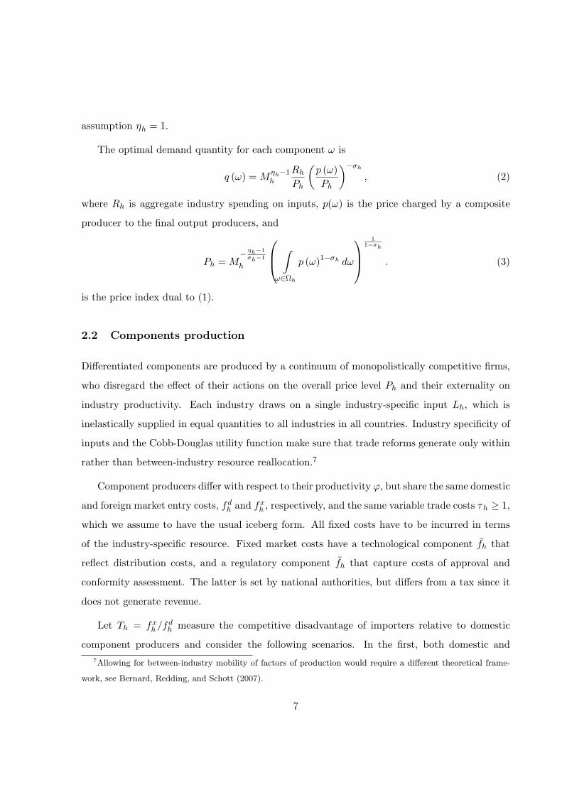
more existing firms no start-ups and from incumbent exporters to new ones; see Figure 1 for

illustration.12 Hence, deregulation reduces average productivity ϕh.

However, the number of available components goes up, which enhances aggregate productiv-

ity; see (28). Input diversity Mh rises one-to-one as fdh falls. Hence, the aggregate productivity

effect – which combines the beneficial diversity effect and the adverse effect on input producers’

productivity – depends on the comparison between the marginal gain from increased variety,

ηh/ (σh − 1) and the loss of input producers’ average productivity −1/γh.

In the case of ηh ≥ 1, the above inequality always holds (as we have assumed γh > σh − 1).

Hence, domestic deregulation always makes the final goods producer more productive. However,

this result is not general: in the empirically relevant case, where ηh < 1, the sign of Ah is

ambiguous.12Melitz (2003) uses this kind of representation from autarky to trade.

16

Figure 1: Within-industry reallocation of market shares as a response to domestic deregulation

4.2 Lower fixed-cost protection

As above, the change in industry productivity in response to lower fixed-cost protection is driven

by two channels, and (27) becomes

Ah

Th

=ηh

σh − 1Mh

Th

+ϕh

Th

. (31)

Recall that in this scenario we analyze a TBT reform that comes through a reduction in fxh ,

whereas domestic regulation costs fdh are hold constant. The mass of component producers

responds to changes in the entry cutoff productivity level. Also, the average productivity level

of component producers adjusts to changes in the cutoff productivity levels and to the probability

of exporting. It turns out from our analysis that lower fixed-cost protection is certain to improve

industry productivity only if ηh ≥ 1. In the empirically relevant case of ηh < 1, however, the

effect is ambiguous.

Average productivity of component producers. Although the less productive compo-

nent producers are forced to exit, the within-industry reallocation mechanism towards more

productive firms in case of a TBT reform is different from that operating under variable trade

17

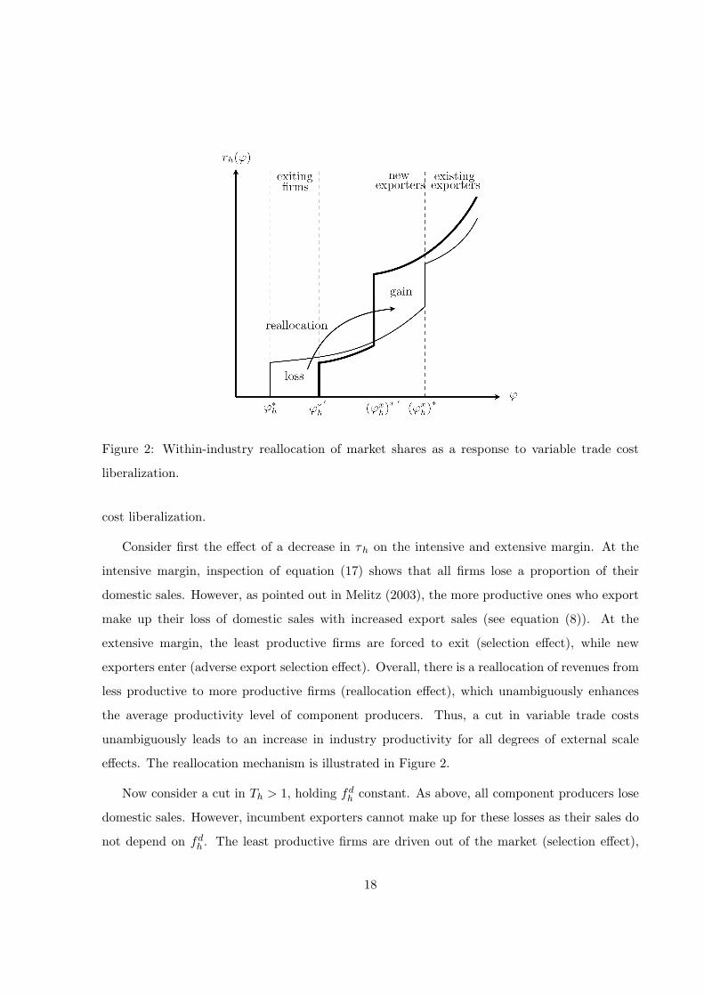
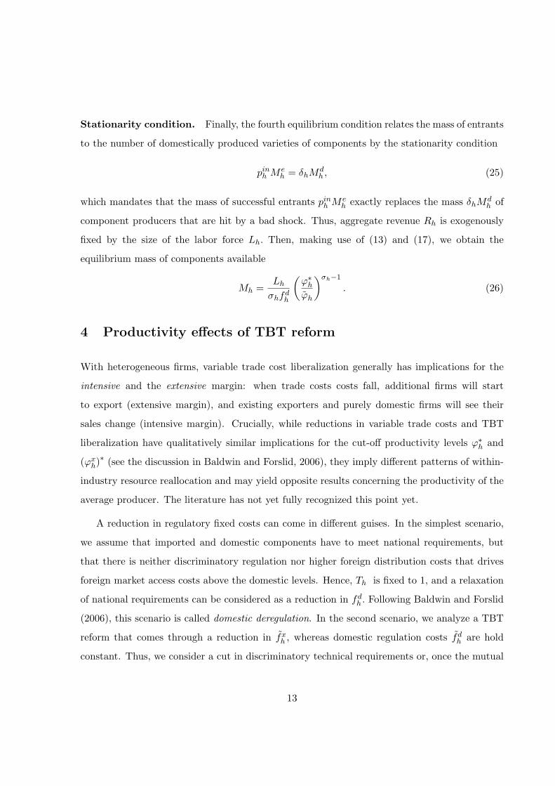
Figure 2: Within-industry reallocation of market shares as a response to variable trade cost

liberalization.

cost liberalization.

Consider first the effect of a decrease in τh on the intensive and extensive margin. At the

intensive margin, inspection of equation (17) shows that all firms lose a proportion of their

domestic sales. However, as pointed out in Melitz (2003), the more productive ones who export

make up their loss of domestic sales with increased export sales (see equation (8)). At the

extensive margin, the least productive firms are forced to exit (selection effect), while new

exporters enter (adverse export selection effect). Overall, there is a reallocation of revenues from

less productive to more productive firms (reallocation effect), which unambiguously enhances

the average productivity level of component producers. Thus, a cut in variable trade costs

unambiguously leads to an increase in industry productivity for all degrees of external scale

effects. The reallocation mechanism is illustrated in Figure 2.

Now consider a cut in Th > 1, holding fdh constant. As above, all component producers lose

domestic sales. However, incumbent exporters cannot make up for these losses as their sales do

not depend on fdh . The least productive firms are driven out of the market (selection effect),

18

Figure 3: Within-industry reallocation of market shares as a response to TBT liberalization.

and some firms start exporting (adverse export selection effect). Only this group gains from a

TBT reform. However, in this scenario there is reallocation of revenues from more productive to

less productive firms (adverse reallocation effect). The overall effect on the average productivity

level ϕh then depends on the the countervailing effects of reallocation of revenues from the

exiting firms to new exporters and reallocation from existing exporters to new exporters. Figure

3 visualizes the reallocation of market shares. ϕh only increases in response to a cut in Th > 1 if

the shape parameter γh is large enough. The intuition is straightforward: The larger the shape

parameter γh, the more mass is given to low productive firms, thus giving a high potential for

reallocation from the low productive, exiting firms to the new exporters.

If the initial level of competitive disadvantage of importers is smaller than 1, ϕh never

increases in response to a TBT reform regardless of the shape parameter γh.

Let θ(Th) ≡ 1/ [1 + npxh] be the weight that is attached to the average domestic firm ϕd

h in

the calculation of the average productivity level of component producers (11). Then we may

summarize the result in Lemma 2.

19

Lemma 2 Fix fdh and reduce fx

h . The productivity level of the component producer ϕh increases

in response to a cut in fxh if and only if the initial level Th > 1 and the shape parameter of the

Pareto distribution γh is large enough, i.e.

1γh

<1γ

h

≡ 1σh − 1

√θh

Th − 1Th

. (32)

Proof. Follows immediately from totally differentiating (24).

External economies of scale. A decrease in the productivity level of the component producer

ϕh can potentially be offset by an increase in the mass of components available, and vice versa.

However, for the scale effect to be positive, it is required that the shape parameter γh is not too

large. The intuition is the following: the higher γh, the more mass is given to low productive

firms, and the higher the mass of component producers that are forced to exit in response to

a TBT reform. However, if T < 1, the mass of components available unambiguously increases.

We summarize the result in Lemma 3.

Lemma 3 Fix fdh and reduce Th. The mass of available components Mh increases in response

to a cut in Th if and only if the shape parameter of the Pareto distribution γh is not too large,

i.e.1γh

>1γh

≡ 1σh − 1

θhTh − 1

Th. (33)

Proof. Follows immediately from totally differentiating (26).

Clearly, industry productivity increases in response to a TBT reform, if the shape parameter

γh falls into the bracket

γh > γh > γh. (34)

We now distinguish two cases: in the first case, condition (32) is violated. Then γh is too small

or the initial level of Th < 1 is such that the average productivity level of component producers

decreases, while the mass of available components increases. It follows from Melitz (2003) that

Ah/Th < 0 for the special case ηh = 1. Moreover, inspection of (31) shows that Ah/Th > 0 for

ηh = 0. For the overall effect on industry productivity to be positive (Ah/Th < 0 ), the scale of

the mass effect has to be sufficiently large.

20

Consider now the case, where condition (33) is violated. Then the scale of the mass effect is

required to be small enough to be completely offset by the average productivity effect. It turns

out that this condition always holds if ηh ≤ 1.

These results are summarized in the following Proposition

Proposition 2 Define υ∗ as

υ∗ ≡ 1γh − γh

(γh

σh − 1− γh

γh

).

(i) Under the assumption that condition (32) is violated, industry productivity increases in re-

sponse to a TBT reform, if and only if the industry externality is large enough, and decreases

otherwise, i.e.ηh

σh − 1> υ∗, (35)

where 0 < υ∗ < 1/ (σh − 1) .

(ii) Under the assumption that condition (33) is violated, industry productivity increases in

response to a TBT reform, if and only if the industry externality is not too large, i.e.

ηh

σh − 1< υ∗, (36)

where υ∗ > 1/ (σh − 1) .

Proof. The conditions follow from equation (27).

4.3 Comparing tariff and TBT liberalization

Recall the crucial mechanism that drives the difference between tariff and TBT liberalization.

Tariff liberalization (or any reduction in variable trade costs) has a direct effect on inframarginal

exporters’ revenue: export sales go up, and so does the weight of existing exporters in the

average productivity calculation. The movement on this intensive margin is strengthened by the

fact that the marginal producer becomes more productive, but weakened by the fact that the

marginal exporter is now less efficient than before. However, these extensive margin effects are

21

second-order relative to the intensive margin. The net effect on ϕh is therefore unambiguously

positive.

Lower TBT-related costs, however, have a first-order effect on the extensive margin as new

firms start exporting. Existing exporters – the most efficient firms in the industry – do not see

increased sales. Quite the contrary, to make the expansion of low-productivity exporters possible,

there must be reallocation of resources away from existing exporters and purely domestic firms.

However, it can be shown that total export sales always increase in response to lower fixed

cost production.13 Hence, the correlation between an increase in trade volume and industry

productivity is ambiguous: If the increase comes about due to variable trade cost reduction, it

is clearly associated with higher industry productivity. However, if the increase in trade volume

is driven by a TBT reform, the effect on industry productivity depends on the strength of the

external economies of scale as stated in conditions (35) and (36). This theoretical result rational-

izes the empirical result by Baller (2007), who finds mixed evidence on the correlation between

industry productivity and trade volume. It is also important for cross-country regressions which

explain TFP by some measure of trade openness defined as export sales over GDP.14

Anecdotal evidence suggests that there is important resistance against TBT reform. Indeed,

Gwartney, Lawson, Sobel, and Leason (2007) provide evidence that suggests that the EU25

countries have failed on average to decrease regulatory costs to importers. Our paper allows

two interpretations of this result. First, based on efficiency considerations, TBT reform is not

necessarily recommendable. Second, TBT reform – even if it leads to industry productivity gains

– inflicts losses to the vast majority of firms due to the implied reallocation of resources towards

new exporters, by nature a relatively small fraction out of all domestic firms. Hence, it may

not be overly surprising that total resistance against TBT reform is strong, and, in particular,

stronger than against trade liberalization that involves lower variable trade costs.

13Total sales abroad are given by Xcifh = nMx

h rx (ϕxh) . Recall that Mx

h = pxhMd

h . Using (8), (25) and (26) one

finds that Xcifh = Lhnpx

hTh/ (1 + npxhTh) , and ∂Xcif

h /∂Th < 0.14Moreover, Gibson (2006) shows that the theoretical measures of industry productivity are not necessarily

reflected in the data-based measure of productivity (e.g., value added per worker).

22

5 Numerical exercise at the industry level

In this chapter, we draw on estimates of the key parameters of our model from the literature,

and calibrate the model accordingly. The numerical exercise serves several purposes. First, it

allows to calibrate the degree of industry externalities ηh/ (σh − 1) and the level of competitive

disadvantage of importers Th. Second, it enables us to check the inequalities derived in the

theoretical section of this paper and to sort out the ambiguous effects associated to domestic

deregulation and lower fixed-cost protection on industry productivity. Finally, the exercise allows

to compute the productivity gain relative to status quo achieved by setting Th to the level which

maximizes industry productivity Ah.

We find that average productivity of component producers is likely to fall in almost all of

the 19 industries in response to lower fixed cost protection. While this finding is rather robust,

the effect of TBT reform on industry productivity crucially depends on the strength of industry

externalities.15

5.1 Calibration

In order to develop a rough understanding of the quantitative behavior of the model, we need to

put numbers to the parameters. The key parameters are the strength of the external scale effect

(ηh), the elasticity of substitution (σh) and the parameter governing productivity dispersion

(γh). While Ardelean (2006) provides some convincing evidence on ηh for different industries,

there do not exist estimates of elasticities of substitution and productivity dispersion on industry

level that are estimated in a unified empirical framework and separately identified.

There are independent estimates on industry-level shape parameters, e.g., those suggested by

Corcos, Del Gatto, Mion, and Ottaviano (2007)16, and estimates of the elasticity of substitution,15In the very different context of their open macro model, Corsetti, Martin, and Pesenti (2007) detect a similar

lack of robustness.16Corcos, Del Gatto, Mion, and Ottaviano (2007) use European firm-level data to estimate the within-industry

productivity distribution, applying the Levinsohn and Petrin (2003) estimator, and fit a Pareto distribution for

each industry. For all industries the regression fit (the adjusted R squared) is close to 1, suggesting that the

Pareto is a good approximation of the productivity distribution.

23

e.g., Hummels (2001). Estimates of Pareto shape parameters γh on the two-digit industry level

are on average close to 2, while those for the elasticity of substitution are usually much larger,

ranging from σh = 3.53 for iron and steel to σh = 11.02 for electric machinery.17 Unfortunately,

comparing γh and σh reveals that the regularity condition that guarantees a finite variance of

the truncated productivity distribution γh > σh − 1 only holds for a small subset of industries.

Without having alternative data at hand, we deal with this problem by using the following

specifications. In a first specification we take the shape parameters from Corcos, Del Gatto,

Mion, and Ottaviano (2007), and calibrate the elasticity of substitution to the industry sales

dispersion measure disph = γh − (σh − 1) obtained from Helpman, Melitz, and Yeaple (2004).

Since disph is close to 1 for all industries, we end up with σh ≈ 2, which seems to be very small

as compared to Hummels’ (1999) estimates. Hence, this specification is referred to as the low-σh

specification.

In the high-σh specification, we take the elasticity of substitution from Hummels (1999)

and calibrate the shape parameters, again using the dispersion measure disph obtained from

Helpman, Melitz, and Yeaple (2004). Table 1 reports the parameters taken from the literature

and the calibrated parameters for several industries.18

Corsetti, Martin, Pesenti (2007, p. 109) argue that there is no obvious benchmark value for

ηh available. However, in a working paper Ardelean (2006) provides some convincing evidence on

that parameter for different industries. She estimates the average US love of variety parameter

(isomorphic to our ηh) is 42% lower than in the standard Dixit-Stiglitz case. Estimates are

identified by decomposing the price index into a traditional part and the extensive margin,

following the Feenstra (1994) method, and exploiting cross-importer variation. As the strength

of the external scale effect is given by ηh/(σ−1), it is substantially larger under the low-σh than

under the high-σh specification.

We take data on industry transport costs from Hanson and Xiang (2004). Using data on17These data have been used extensively in the literature, e.g., by Hanson and Xiang (2004).18We find neither significant correlation between the shape parameters obtained from Corcos, Del Gatto, Mion,

and Ottaviano (2007) and those imputed from the elasticities of substitution nor between the elasticities of

substitution from Hummels (2001) and their imputed counterparts.

24

freight rates for U.S. imports from Feenstra (1996), they identify the implicit U.S. industry

freight rate (insurance and freight charges/import value), and regress it on log distance to the

origin country. Transport cost for an industry are reported as projected industry freight rate

from these coefficient estimates evaluated at median distance in their sample of importers and

exporters.19

Finally, we derive values for the competitive disadvantage of importers Th from calibrating

the model to the export participation rate by industry obtained from Eaton, Kortum, and

Kramarz (2004).20 Using the expression for the export participation rate (20) and information

on the shape parameter, the elasticity of substitution, and transport cost, one obtains values

for Th by industry.21 The calibrated values of Th vary between figures close to 1 and close to

4. This is well in line with the result of the calibration exercise by Ghironi and Melitz (2005),

who argue that Th is substantially above unity for the US. The correlation between the levels of

competitive disadvantage of importers Th obtained under the low- and high-σh specification is

0.76 and significant at the 1 percent level.

Table 1 summarizes the parameters taken from the literature and the calibrated parameters

for several industries. It is, however, crucial to bear in mind that the parameter estimates used

in the numerical exercise come from different sources, that cover different countries, and that

are – judged by the theoretical requirements of our model – at least partially incompatible.

Hence, for a more elaborate understanding of trade liberalization using approaches based on the

Melitz (2003) model, we urgently need more econometric work aimed at structural estimation

and identification of the key parameters.19We are grateful to Gordon Hanson for providing their estimated freight rates and the elasticities of substitu-

tion.20They report figures for France for 1986, based on Customs and BRN-SUSE data sources.21We also use information on openness (40%), the average transportation costs, and the average Th to calibrate

the number of trading partners n.

25

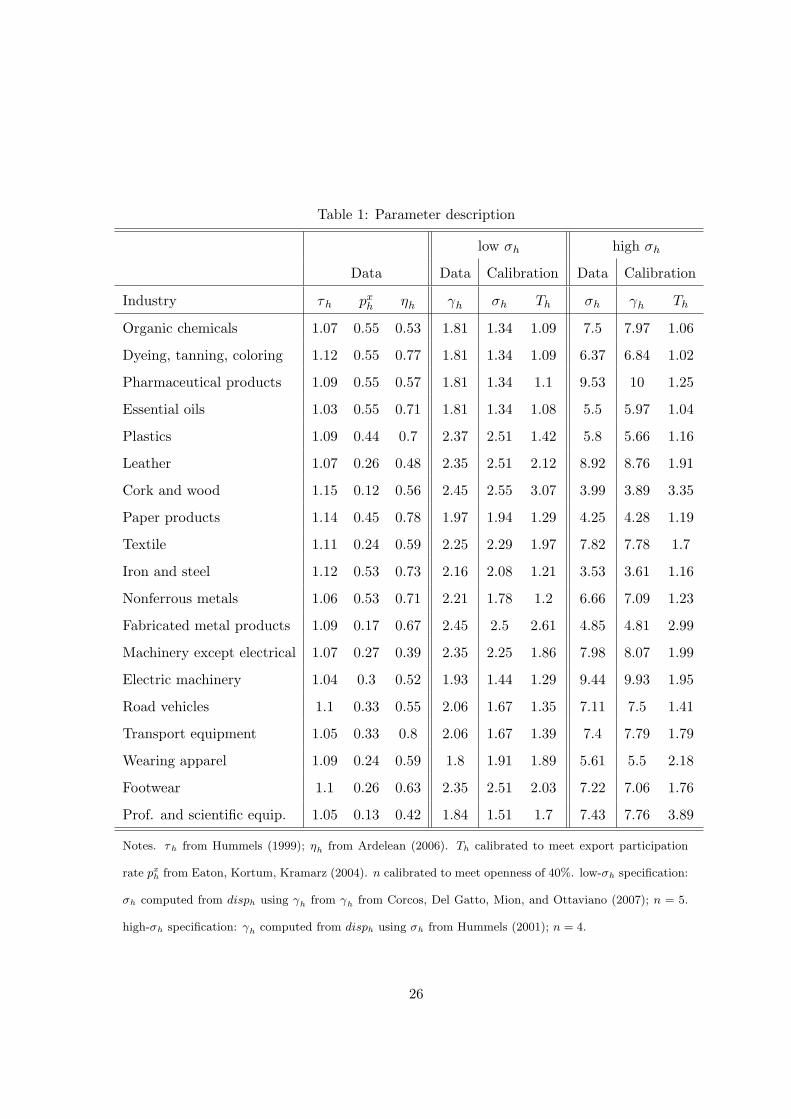
Table 1: Parameter description

low σh high σh

Data Data Calibration Data Calibration

Industry τh pxh ηh γh σh Th σh γh Th

Organic chemicals 1.07 0.55 0.53 1.81 1.34 1.09 7.5 7.97 1.06

Dyeing, tanning, coloring 1.12 0.55 0.77 1.81 1.34 1.09 6.37 6.84 1.02

Pharmaceutical products 1.09 0.55 0.57 1.81 1.34 1.1 9.53 10 1.25

Essential oils 1.03 0.55 0.71 1.81 1.34 1.08 5.5 5.97 1.04

Plastics 1.09 0.44 0.7 2.37 2.51 1.42 5.8 5.66 1.16

Leather 1.07 0.26 0.48 2.35 2.51 2.12 8.92 8.76 1.91

Cork and wood 1.15 0.12 0.56 2.45 2.55 3.07 3.99 3.89 3.35

Paper products 1.14 0.45 0.78 1.97 1.94 1.29 4.25 4.28 1.19

Textile 1.11 0.24 0.59 2.25 2.29 1.97 7.82 7.78 1.7

Iron and steel 1.12 0.53 0.73 2.16 2.08 1.21 3.53 3.61 1.16

Nonferrous metals 1.06 0.53 0.71 2.21 1.78 1.2 6.66 7.09 1.23

Fabricated metal products 1.09 0.17 0.67 2.45 2.5 2.61 4.85 4.81 2.99

Machinery except electrical 1.07 0.27 0.39 2.35 2.25 1.86 7.98 8.07 1.99

Electric machinery 1.04 0.3 0.52 1.93 1.44 1.29 9.44 9.93 1.95

Road vehicles 1.1 0.33 0.55 2.06 1.67 1.35 7.11 7.5 1.41

Transport equipment 1.05 0.33 0.8 2.06 1.67 1.39 7.4 7.79 1.79

Wearing apparel 1.09 0.24 0.59 1.8 1.91 1.89 5.61 5.5 2.18

Footwear 1.1 0.26 0.63 2.35 2.51 2.03 7.22 7.06 1.76

Prof. and scientific equip. 1.05 0.13 0.42 1.84 1.51 1.7 7.43 7.76 3.89

Notes. τh from Hummels (1999); ηh from Ardelean (2006). Th calibrated to meet export participation

rate pxh from Eaton, Kortum, Kramarz (2004). n calibrated to meet openness of 40%. low-σh specification:

σh computed from disph using γh from γh from Corcos, Del Gatto, Mion, and Ottaviano (2007); n = 5.

high-σh specification: γh computed from disph using σh from Hummels (2001); n = 4.

26

5.2 Sorting out the ambiguities

Before quantifying the effects of TBT reform, we use the parameters discussed above to check

the inequalities derived in the theoretical section of the paper. We find that the effect of TBT

reform on industry productivity strongly depends on the calibration of γh and σh. The low-

σh specification implies a larger degree of industry externalities, enabling the scale effect to

overcompensate a deterioration in the average productivity level of component producers in

more cases than under the high-σh specification.

Domestic deregulation. We have shown analytically that domestic deregulation always lead

to a fall in the average productivity of component producers unambiguously declines and to a

rise in the mass of available components. As a result, industry productivity rises (Ah/fdh < 0)

if and only if the strength of the industry externality is large enough as compared to the degree

of dispersion of the productivity distribution. The strength of the scale effect is calibrated to

be higher under the low-σh than under the high-σh specification. Moreover, under the low-

σh specification the productivity distribution is assumed to be more skewed towards the less

productive firms than under the high-σh specification. Both facts together rationalize that

domestic deregulation is likely to increase industry productivity in most industries under the

first specification, while the scale effect is not efficient to offset the deterioration in the average

productivity level of component producers under the second (see Table 2). However, in industries

with relatively low value for ηh (leather, cork and wood, and machinery except electrical), the

scale effect is not sufficiently large. Moreover, footware barely misses the inequality check.

Lower fixed-cost protection. In this scenario, also the directions of the effects on the mass

and the average productivity of component producers are ambiguous from a theoretical point of

view. However, under both of our specifications we find that both effects pretty much work like

under domestic deregulation: the average productivity of component producers deteriorates in

most industries in response to lower fixed-cost protection (ϕh/Th > 0), whereas more components

become available (Mh/Th < 0, see Table 2).

Again, the effect on industry productivity hinges on the relationship between the degree of

27

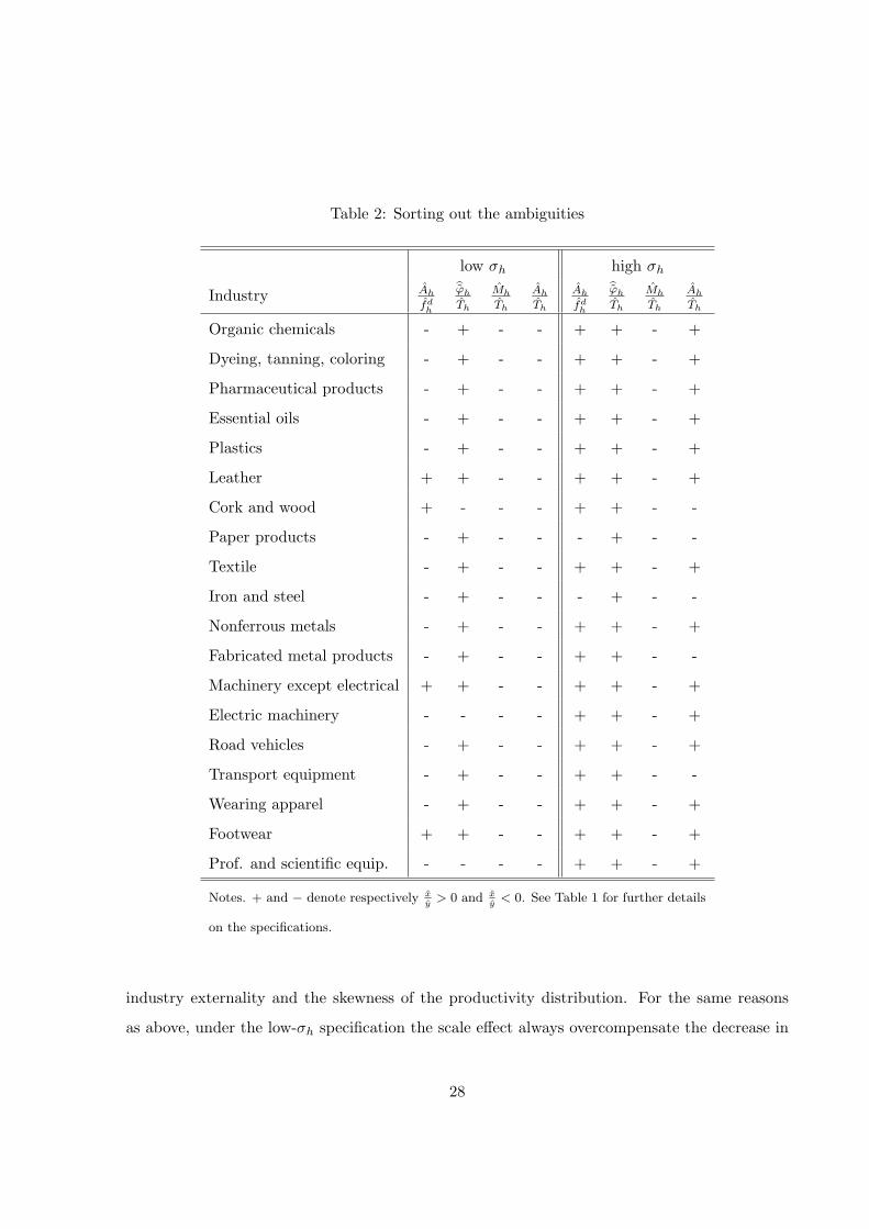
Table 2: Sorting out the ambiguities

low σh high σh

Industry Ah

fdh

ϕh

Th

Mh

Th

Ah

Th

Ah

fdh

ϕh

Th

Mh

Th

Ah

Th

Organic chemicals - + - - + + - +

Dyeing, tanning, coloring - + - - + + - +

Pharmaceutical products - + - - + + - +

Essential oils - + - - + + - +

Plastics - + - - + + - +

Leather + + - - + + - +

Cork and wood + - - - + + - -

Paper products - + - - - + - -

Textile - + - - + + - +

Iron and steel - + - - - + - -

Nonferrous metals - + - - + + - +

Fabricated metal products - + - - + + - -

Machinery except electrical + + - - + + - +

Electric machinery - - - - + + - +

Road vehicles - + - - + + - +

Transport equipment - + - - + + - -

Wearing apparel - + - - + + - +

Footwear + + - - + + - +

Prof. and scientific equip. - - - - + + - +

Notes. + and − denote respectively xy

> 0 and xy

< 0. See Table 1 for further details

on the specifications.

industry externality and the skewness of the productivity distribution. For the same reasons

as above, under the low-σh specification the scale effect always overcompensate the decrease in

28

average productivity of component, whereas under the high-σh specification this is not the case

(see Table 2).

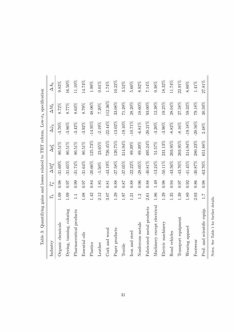
5.3 Quantifying the effects of TBT reform

We now strive at quantifying the gains and losses related to TBT reform. In order to fix

ideas, consider that the competitive disadvantage of importer relative to domestic component

producers is set to the level T ∗h which maximizes industry productivity Ah. Recall that in the

light of the externalities at work this is not a first-best policy. We find that under the low-σh

specification Th is mostly set to its minimum value that guarantees partitioning T ∗h = τσh−1h ,

except for industries with low values of ηh (leather and machinery except electrical).

The effects are the following (see Table 3). First, all component producers start to export,

thereby driving the fraction of exporters towards 1, implying ∆pxh > 0. Second, since less pro-

ductive firms start to export, this comes along with a deterioration of their average productivity

level (∆ϕh < 0). The drop amounts to approximately 20% in industries with high initial values

of Th (cork and wood, fabricated metal products, wearing apparel, and footwear). Third, due

to increased competition the least productive component producers are forced to exit, thereby

decreasing the mass of firms operating domestically (∆Mdh < 0). However, the mass of compo-

nents available clearly increases (∆Mh > 0). Again, the increase is large in industries with high

initial values of Th.22 Finally, the total effect on industry productivity is dominated by the scale

effect and amounts to more than 10%, except for the industries with low values of ηh, which do

not value input diversity much.

Under the high-σh scenario, the effects are rather different. We find that TBTs may be used

to cope with over-supply of components. For most of the industries (except cork and wood,

paper products, iron and steel, fabricated metal products, and transport equipment), the level

T ∗h which maximizes industry productivity Ah is higher than the initial level (see Table 4).23

Clearly, higher regulatory fixed costs force some component producers to exit the export markets22From a social planner’s perspective, there is over-supply of varieties also under T ∗

h as ηh < 1. However, even

if ∆Mh > 0, the over-supply of varieties relative to the planner’s solution is smaller for T ∗h than for Th.

23Note that if one of the conditions (32) and (33) is violated, T ∗h is implicitly defined by υ∗ (T ∗

h ) = ηh/ (σh − 1).

29

(∆pxh < 0), thereby increasing their average productivity level (∆ϕh > 0). However, the latter

effect is rather small and lies in the range of 3% to 8%. Lower competition allows more firms to

operate domestically (∆Mdh > 0), whereas overall input diversity falls (∆Mh < 0). The loss in

varieties sums up to approximately 30%. After all, the total effect on industry productivity is

positive (∆Ah < 1%), but modest, since some of component producers’ productivity gains are

offset by the scale effect.

30

Tab

le3:

Qua

ntify

ing

gain

san

dlo

sses

rela

ted

toT

BT

refo

rm.

Low

-σh

spec

ifica

tion

Indu

stry

Th

T∗ h

∆M

d h∆

px h

∆ϕ

h∆

Mh

∆A

h

Org

anic

chem

ical

s1.

090.

98-3

1.69

%80

.51%

-3.7

0%8.

72%

9.83

%

Dye

ing,

tann

ing,

colo

ring

1.09

0.97

-31.

65%

80.5

1%-3

.86%

8.77

%16

.50%

Pha

rmac

euti

calpr

oduc

ts1.

10.

99-3

1.74

%80

.51%

-3.4

2%8.

63%

11.1

0%

Ess

enti

aloi

ls1.

080.

97-3

1.64

%80

.51%

-3.9

2%8.

79%

14.7

4%

Pla

stic

s1.

420.

84-2

0.66

%12

5.73

%-1

4.95

%48

.06%

1.99

%

Lea

ther

2.12

1.85

-5.5

0%23

.65%

-2.1

9%7.

20%

0.01

%

Cor

kan

dw

ood

3.07

0.81

-43.

19%

726.

45%

-22.

44%

112.

36%

1.74

%

Pap

erpr

oduc

ts1.

290.

88-2

7.58

%12

0.75

%-1

3.02

%33

.08%

10.2

2%

Tex

tile

1.97

0.87

-37.

05%

314.

94%

-19.

10%

71.2

9%3.

52%

Iron

and

stee

l1.

210.

88-2

2.22

%89

.39%

-10.

71%

28.2

0%5.

60%

Non

ferr

ous

met

als

1.2

0.96

-28.

05%

89.3

9%-6

.81%

18.6

0%8.

92%

Fabr

icat

edm

etal

prod

ucts

2.61

0.88

-40.

81%

495.

24%

-20.

21%

93.0

0%7.

14%

Mac

hine

ryex

cept

elec

tric

al1.

861.

49-1

3.24

%51

.57%

-3.2

0%12

.38%

0.38

%

Ele

ctri

cm

achi

nery

1.29

0.98

-50.

11%

231.

13%

-3.9

0%19

.25%

18.3

2%

Roa

dve

hicl

es1.

350.

94-4

3.56

%20

3.95

%-8

.82%

28.0

4%11

.74%

Tra

nspo

rteq

uipm

ent

1.39

0.97

-43.

76%

203.

95%

-8.1

6%27

.58%

22.9

1%

Wea

ring

appa

rel

1.89

0.92

-41.

45%

314.

94%

-19.

18%

59.3

3%8.

89%

Foot

wea

r2.

030.

86-3

0.87

%28

0.23

%-2

0.56

%79

.18%

1.41

%

Pro

f.an

dsc

ient

ific

equi

p.1.

70.

98-6

3.76

%65

1.88

%2.

48%

30.5

9%27

.81%

Note

s.See

Table

1fo

rfu

rther

det

ails.

31

Tab

le4:

Qua

ntify

ing

gain

san

dlo

sses

rela

ted

toT

BT

refo

rm.

Hig

h-σ

hsp

ecifi

cati

on

Indu

stry

Th

T∗ h

∆M

d h∆

px h

∆ϕ

h∆

Mh

∆A

h

Org

anic

chem

ical

s1.

063.

6820

.83%

-78.

23%

6.86

%-4

4.31

%1.

88%

Dye

ing,

tann

ing,

and

colo

ring

mat

eria

ls1.

021.

172.

66%

-16.

24%

1.34

%-8

.82%

0.01

%

Med

ical

and

phar

mac

euti

calpr

oduc

ts1.

255.

1518

.99%

-81.

06%

5.98

%-4

7.47

%1.

52%

Ess

enti

aloi

ls1.

041.

46.

89%

-32.

50%

3.08

%-1

7.05

%0.

09%

Pla

stic

s1.

162.

9711

.61%

-66.

87%

7.67

%-3

6.10

%0.

86%

Lea

ther

1.91

8.75

11.0

5%-8

1.38

%4.

39%

-35.

28%

1.68

%

Cor

kan

dw

ood

3.35

2.58

-4.8

1%40

.45%

-1.2

2%7.

74%

0.17

%

Pap

erpr

oduc

ts1.

190.

77-9

.17%

77.6

7%-7

.02%

36.2

9%0.

16%

Tex

tile

1.7

4.83

9.29

%-6

9.69

%3.

76%

-28.

10%

0.84

%

Iron

and

stee

l1.

160.

75-1

2.70

%86

.73%

-8.7

5%38

.69%

0.28

%

Non

ferr

ous

met

als

1.23

2.03

9.43

%-4

6.76

%3.

96%

-25.

30%

0.22

%

Fabr

icat

edm

etal

prod

ucts

2.99

2.44

-3.3

4%28

.86%

-1.2

6%7.

88%

0.06

%

Mac

hine

ryex

cept

elec

tric

al1.

996.

6213

.23%

-75.

10%

3.80

%-3

0.77

%1.

69%

Ele

ctri

cm

achi

nery

1.95

5.25

12.7

1%-6

8.89

%3.

03%

-29.

77%

0.81

%

Roa

dve

hicl

es1.

413.

2912

.89%

-64.

69%

3.98

%-2

8.61

%0.

87%

Tra

nspo

rteq

uipm

ent

1.79

1.34

-4.3

5%42

.03%

-2.0

6%18

.50%

0.04

%

Wea

ring

appa

rel

2.18

3.99

8.05

%-5

1.32

%3.

26%

-19.

16%

0.51

%

Foot

wea

r1.

764.

939.

21%

-68.

94%

4.44

%-2

9.39

%0.

83%

Pro

fess

iona

lan

dsc

ient

ific

equi

pmen

t3.

895.

143.

93%

-28.

48%

0.53

%-6

.35%

0.10

%

Note

s.See

Table

1fo

rfu

rther

det

ails.

32

6 Conclusion

This paper analyzes the reallocation and industry productivity effects of TBT reform in a single

market with heterogeneous firms and variable and fixed trade costs. The model goes beyond the

Melitz (2003) model by explicitly parameterizing external scale effects. Our framework allows

to disentangle the effect of a TBT reform on the average productivity of component producers

ϕh and the mass of available components Mh, thereby making the industry productivity effect

dependent on the strength of the external economies of scale.

We find that both, domestic deregulation and lower fixed-cost protection, lead to reallocation

of market shares from more to less productive firms, potentially negatively affecting industry

productivity for a wide range of parameter constellations, while input diversity is usually en-

hanced. Referring to recent evidence on love for variety, we show that industry productivity is

likely to deteriorate in many industries. As we rule out resource and market share reallocation

across industries, changes in one industry directly translate into the average productivity of the

economy.

Both, variable trade cost and TBT liberalization increase the volume of trade. However,

in case of TBT reform this increase in trade may come along with a deterioration of industry

productivity. Then, inferring productivity changes from changes in trade volumes would require

dissection of the margins of trade.

Regarding further research, the present paper motivates to aim at structural estimation

and identification of the key parameters in trade models with heterogeneous firms: the shape

parameter, the elasticity of substitution, and the degree of external economies of scale.

33

References

[1] Ardelean, A. (2006). How Strong is Love of Variety? Mimeo: Purdue University.

[2] Axtell, R. (2001). Zipf Distribution of U.S. Firm Sizes. Science 293: 1818-20.

[3] Baldwin, R.E., and R. Forslid (2006). Trade Liberalization with Heterogeneous Firms.

NBER Working Paper 12192.

[4] Baller, Silja (2007). Trade effects of regional standards: A heterogeneous firms approach.

World Bank Policy Research Working Paper 4124.

[5] Benassy, J.-P. (1996). Taste for Variety and Optimum Production Patterns in Monopolistic

Competition. Economics Letters 52: 41-47.

[6] Bernard, A., J.S. Redding, and P.K. Schott (2007). Comparative Advantage and Heteroge-

neous Firms. Review of Economic Studies 74(1): 31-66.

[7] Blanchard, O., and F. Giavazzi (2003). Macroeconomic Effects of Regulation and Deregu-

lation in Goods and Labor Markets. The Quarterly Journal of Economics 118(3): 879-907.

[8] Chen, N. (2004). Intra-national versus International Trade in the European Union: Why

do National Borders Matter? Journal of International Economics 63: 93-118.

[9] Conway, P., V. Janod, G. Nicoletti (2005). Product Market Regulation in OECD Countries:

1998 To 2003. OECD Economics Department Working Paper No. 419.

[10] Corcos, G., M. Del Gatto, G. Mion, and G.I.P. Ottaviano (2007). Productivity and Firm

Selection: Intra- vs International Trade. CORE Discussion Paper No. 2007/60

[11] Corsetti, G., P. Martin, and P. Pesenti (2007). Productivity, Terms of Trade and the ’Home

Market Effect’. Journal of International Economics 73:99-127.

[12] Delgado, J. (2006). Single Market Trails Home Bias. Bruegel Policy Brief 2006/05. Brussels.

[13] Del Gatto, M., G. Mion, and G.I.P. Ottaviano (2006). Trade Integration, Firm Selection

and the Costs of Non-Europe. CEPR Discussion Paper No. 5730.

34

[14] Dixit, A.K., and J.E. Stiglitz (1975). Monopolistic Competition and Optimum Product

Diversity. Warwick Economic Research Paper No. 64.

[15] Dixit, A.K., and J.E. Stiglitz (1977). Monopolistic Competition and Optimum Product

Diversity. American Economic Review : 67(3): 297-308.

[16] Eaton, J., S. Kortum, and F. Kramarz (2004). Dissecting Trade: Firms, Industries, and

Export Destinations. American Economic Review 94(2): 150-154.

[17] Egger, H., and U. Kreickemeier (2008). Firm Heterogeneity and the Labour Market Effects

of Trade Liberalisation. International Economic Review, forthcoming.

[18] Ethier, W.J. (1982). National and International Returns to Scale in the Modern Theory of

International Trade. American Economic Review 72(3): 950-959.

[19] Feenstra, R. (1996). U.S. Imports, 1972-1994: Data and Concordances. NBER Working

Paper 5515.

[20] Francois, J., H. van Meijl, and F. van Tongeren (2005). Trade Liberalization in the Doha

Development Round. Economic Policy 20(42): 349-391.

[21] Ghironi, F., and M.J. Melitz (2005). International Trade and Macroeconomic Dynamics

with Heterogeneous Firms. Quarterly Journal of Economics 120(3): 865-915.

[22] Gwartney, J., R. Lawson, R.S. Sobel, and P.T. Leeson (2007). Economic Freedom of the

World 2007 Annual Report. Fraser Institute, Vancouver.

[23] Hanson, G., and C. Xiang (2004). The Home-Market Effect and Bilateral Trade Patterns.

American Economic Review 94(4): 1108-1129.

[24] Helpman, E., M.J. Melitz, and S.R. Yeaple (2004). Export Versus FDI with Heterogeneous

Firms. American Economic Review 94(1): 300-316.

[25] Hummels, D. (2001). Towards a Geography of Trade Costs. Mimeo: University of Chicago.

35

[26] Ilzkovitz, F., A. Dierx, V. Kovacs, and N. Sousa (2007). Steps. Towards a Deeper Economic

Integration: The Internal Market in the 21st Century. European Economy, Economic Papers

No. 271, European Commission.

[27] Krugman, P.R. (1980). Increasing Returns, Monopolistic Competition and International

Trade. Journal of International Economics 9(4): 469-479.

[28] Krugman, P.R. (1980). Scale Economies, Product Differentiation, and the Pattern of Trade.

American Economic Review 70(5): 950-959.

[29] Levinsohn, J., and A. Petrin (2005). Estimating Production Functions Using Inputs to

Control for Unobservables. Review of Economic Studies 70: 317-342.

[30] Melitz, M.J. (2003). The Impact of Trade on Intra-Industry Reallocations and Aggregate

Industry Productivity. Econometrica 71(6): 1695-1725.

[31] Melitz, M.J., and G.I.P Ottaviano (2007). Market Size, Trade, and Productivity. Review of

Economic Studies, forthcoming.

[32] Smith, A., and A.J. Venables (1988). Completing the Internal Market in the European

Community. Some Industry Simulations. European Economic Review 32: 1501-1521.

[33] World Trade Organization (2007). Twelfth Annual Review of the Implementation and Op-

eration of the TBT Agreement. Geneva

36