Solving the strong-correlation problem in materials - JuSER
44
La Rivista del Nuovo Cimento (2021) 44:597–640 https://doi.org/10.1007/s40766-021-00025-8 REVIEW PAPER Solving the strong-correlation problem in materials Eva Pavarini 1 Received: 24 March 2021 / Accepted: 11 June 2021 / Published online: 14 July 2021 © The Author(s) 2021 Abstract This article is a short introduction to the modern computational techniques used to tackle the many-body problem in materials. The aim is to present the basic ideas, using simple examples to illustrate strengths and weaknesses of each method. We will start from density-functional theory (DFT) and the Kohn–Sham construction—the standard computational tools for performing electronic structure calculations. Leaving the realm of rigorous density-functional theory, we will discuss the established practice of adopting the Kohn–Sham Hamiltonian as approximate model. After recalling the triumphs of the Kohn–Sham description, we will stress the fundamental reasons of its failure for strongly-correlated compounds, and discuss the strategies adopted to overcome the problem. The article will then focus on the most effective method so far, the DFT+DMFT technique and its extensions. Achievements, open issues and possible future developments will be reviewed. The key differences between dynamical (DFT+DMFT) and static (DFT+U ) mean-field methods will be elucidated. In the conclusion, we will assess the apparent dichotomy between first-principles and model- based techniques, emphasizing the common ground that in fact they share. Keywords Many-body problem · Strongly-correlated systems · Transition-metal oxides · Metal–insulator transition · Static mean-field theory · Dynamical mean-field theory · DFT · DFT+U · DFT+DMFT Contents 1 Introduction ............................................. 598 2 The quantum many-body problem .................................. 600 3 The standard model: density-functional theory ........................... 602 4 Strongly-correlated compounds ................................... 605 5 It is not all about the gap ....................................... 607 6 Static mean-field theory and the DFT+U approach ......................... 611 7 Model Hamiltonians ......................................... 615 B Eva Pavarini [email protected] 1 Institute for Advanced Simulation, Forschungszentrum Jülich GmbH, Jülich, Germany 123
-
Upload
khangminh22 -
Category
Documents
-
view
1 -
download
0
Transcript of Solving the strong-correlation problem in materials - JuSER
La Rivista del Nuovo Cimento (2021) 44:597–640https://doi.org/10.1007/s40766-021-00025-8
REVIEW PAPER
Solving the strong-correlation problem in materials
Eva Pavarini1
Received: 24 March 2021 / Accepted: 11 June 2021 / Published online: 14 July 2021© The Author(s) 2021
AbstractThis article is a short introduction to the modern computational techniques used totackle the many-body problem in materials. The aim is to present the basic ideas,using simple examples to illustrate strengths and weaknesses of each method. We willstart from density-functional theory (DFT) and the Kohn–Sham construction—thestandard computational tools for performing electronic structure calculations. Leavingthe realmof rigorous density-functional theory,wewill discuss the established practiceof adopting the Kohn–Sham Hamiltonian as approximate model. After recalling thetriumphs of the Kohn–Sham description, we will stress the fundamental reasons ofits failure for strongly-correlated compounds, and discuss the strategies adopted toovercome the problem. The article will then focus on the most effective method sofar, the DFT+DMFT technique and its extensions. Achievements, open issues andpossible future developmentswill be reviewed.Thekeydifferences betweendynamical(DFT+DMFT) and static (DFT+U ) mean-field methods will be elucidated. In theconclusion, wewill assess the apparent dichotomy between first-principles andmodel-based techniques, emphasizing the common ground that in fact they share.
Keywords Many-body problem · Strongly-correlated systems · Transition-metaloxides · Metal–insulator transition · Static mean-field theory · Dynamical mean-fieldtheory · DFT · DFT+U · DFT+DMFT
Contents
1 Introduction . . . . . . . . . . . . . . . . . . . . . . . . . . . . . . . . . . . . . . . . . . . . . 5982 The quantum many-body problem . . . . . . . . . . . . . . . . . . . . . . . . . . . . . . . . . . 6003 The standard model: density-functional theory . . . . . . . . . . . . . . . . . . . . . . . . . . . 6024 Strongly-correlated compounds . . . . . . . . . . . . . . . . . . . . . . . . . . . . . . . . . . . 6055 It is not all about the gap . . . . . . . . . . . . . . . . . . . . . . . . . . . . . . . . . . . . . . . 6076 Static mean-field theory and the DFT+U approach . . . . . . . . . . . . . . . . . . . . . . . . . 6117 Model Hamiltonians . . . . . . . . . . . . . . . . . . . . . . . . . . . . . . . . . . . . . . . . . 615
B Eva [email protected]
1 Institute for Advanced Simulation, Forschungszentrum Jülich GmbH, Jülich, Germany
123
598 E. Pavarini
8 DMFT and DFT+DMFT . . . . . . . . . . . . . . . . . . . . . . . . . . . . . . . . . . . . . . . 6179 Quantum-impurity solvers . . . . . . . . . . . . . . . . . . . . . . . . . . . . . . . . . . . . . . 62210 Lessons from a toy model: the two-site Hubbard model . . . . . . . . . . . . . . . . . . . . . . 62311Non-local Coulomb terms . . . . . . . . . . . . . . . . . . . . . . . . . . . . . . . . . . . . . . 62912 Linear response functions . . . . . . . . . . . . . . . . . . . . . . . . . . . . . . . . . . . . . . 63013Methods for non-local correlations . . . . . . . . . . . . . . . . . . . . . . . . . . . . . . . . . 63414Conclusion . . . . . . . . . . . . . . . . . . . . . . . . . . . . . . . . . . . . . . . . . . . . . . 635References . . . . . . . . . . . . . . . . . . . . . . . . . . . . . . . . . . . . . . . . . . . . . . . . 636
1 Introduction
Strong electron–electron correlations can give rise to surprising co-operative phenom-ena, typically very hard to explain and even harder to predict. Paradigmatic examplesare high-temperature superconductivity in the cuprates, other types of unconventionalsuperconductivity, Mott insulating or heavy fermion behavior, spin and orbital order-ing, spin and orbital liquid phenomena. Understanding many-body effects in materialsis, by all means, a grand challenge since the early days of quantum mechanics. Andyet, what are, exactly, strong electronic correlations? In principle, one could say thatcondensed matter physics is all about electron–electron interactions. Indeed, the gen-eral electronic Hamiltonian that describes all possible systems, in the non-relativisticlimit and the Born–Oppenheimer approximation, is
He =Ne∑
i
(Ti +
Nn∑
α
Viα
)
︸ ︷︷ ︸Te+Ven
+ 1
2
Nn∑
α �=α′Vαα′
︸ ︷︷ ︸Vnn
+ 1
2
Ne∑
i �=i ′Vii ′
︸ ︷︷ ︸Vee
, (1)
where Ne is the number of electrons, Nn the number of nuclei, Te the kinetic energyof the electrons, Ven the electron–nuclei attraction, Vnn the nuclei–nuclei repulsion,and Vee the electron–electron repulsion. If the latter could be neglected (Vee = 0),the Hamiltonian would be separable, and the electrons independent. In this case thesolution of the many-body problem would be straightforward. For a single electron,eigenvalues and eigenvectors could be found solving the equation
H0i φn(ri ) = εnφn(ri ), (2)
where
H0i = Ti +
Nn∑
α
Viα + 1
2
Nn∑
α �=α′Vαα′ . (3)
The many-electron states would then be single Slater determinants, trivially con-structed from the complete basis {φn(r)} just obtained. For example, in the case ofa half-filled band described by the dispersion relation ε(k) and Bloch states φk↑(r),
123
Solving the strong-correlation problem in materials 599
such a Slater determinant has the form
Ψ (r1, r2, . . . , rNe ) = 1√Ne!
φk1↑(r1) φk1↑(r2) . . . φk1↑(rNe )
φk1↓(r1) φk1↓(r2) . . . φk1↓(rNe )...
......
...
φk Ne2
↑(r1) φk Ne2
↑(r2) . . . φk Ne2
↑(rNe )
φk Ne2
↓(r1) φk Ne2
↓(r2) . . . φk Ne2
↓(rNe )
. (4)
In real materials, however, the electronic Coulomb repulsion is both large and longranged, and there is no obvious reason to neglect it. This can be already seen from theaverage bare Coulomb energy (Hartree term)
EH = 1
2
∫dr
∫dr′ n(r)n(r′)
|r − r′| , (5)
where n(r) is the electron density.1 Even if electronic charges are localized at differentatomic sites (labeled with Rα), i.e., if
n(r) ≈∑
α
δ(r − Rα), (6)
the integrand still decays as the inverse of the nuclei–nuclei distance. Since theelectron–electron repulsion cannot be neglected, a many-body eigenstate can be, inprinciple, a combination of infinite Slater determinants. It is thus remarkable that,de facto, for understanding several phenomena, Hamiltonian (1) can be replaced to agood approximation with an effective non-interacting model for quasi electrons
He → H0e =
Ne∑
i
H0i , (7)
whose eigenstates are single Slater determinants. The independent-electron approxi-mation is, e.g., sufficient to explain the key differences between transition metals (Ni,Cu, Ag, …), alkali metals (Li, Na, K,…), semiconductors (Si, Ge, GaAs, …) andband insulators (diamond,…). It is so successful that modern solid-state physics textbooks still devote a substantial volume to results obtained starting from it. Remark-ably, an independent–electron model is also used in a different context. This is theKohn–Sham (KS) construction in density-functional theory (DFT), the most populartool for electronic-structure calculations. In DFT, the KS Hamiltonian is, however,merely an auxiliary model, instrumental in obtaining the exact ground-state energyand density—it has, in principle, no physical meaning. Nevertheless, the practice ofusing it as an effective model has proven successful for entire categories of systemsand problems. The KS band-structure is thus an established tool for studying, under-standing and predicting the electronic properties of materials. In the light of such an
1 Here and in the rest of the manuscript we adopt Hartree atomic units.
123
600 E. Pavarini
unexpected success, stepping outside the rigorous principles of DFT, one could viewalso the KS Hamiltonian as a (very effective) mean-field mapping of type (7).
Mapping a complicated many-body Hamiltonian into a simpler effective auxil-iary problem has by and large proven a powerful technique in physics. Mean-fieldapproaches capture, e.g., essential features of magnetic broken symmetry phases,although the problem of quantum magnetism is vastly more complex. It is thus tempt-ing to conclude that, if the mapping in Eq. (7) is an excellent approximation in manycases, it should work for all systems, once we found the correct non-interacting effec-tive particles. Strong correlation phenomena are those for which such an Ansatzepically fails, and a simple effective non-interacting model is not expected to be foundfor reasons of principle.
The article is organized as follows. First we will briefly discuss the nature of thestrong correlation problem.We will then recall the basics of density-functional theory,the standard method used to perform electronic structure calculations in materials. Inthis context wewill discuss the Kohn–Sham construction and, leaving aside the princi-ples of DFT, the strength and the advantages of the Kohn–Sham picture. We will stressthe fundamental reasons for its failure for strongly-correlated compounds, illustratingthe two main strategies used for overcoming the problem. The first consists in improv-ing the approximation of the exchange–correlation functional—even if at the priceof introducing ad hoc corrections or free parameters, and thus operating outside thestrict principles of density-functional theory. This scheme is used, e.g., in the DFT+Uapproach. The limitations of such a tactic will be emphasized. The second strategyconsist in using the KS orbital as a basis for building materials-specific many-bodymodels. This is the most effective strategy so far, and the one used in the DFT+DMFTapproach. Successes and open problems will be reviewed. The differences betweenstatic (DFT+U ) and dynamical (DFT+DMFT) mean-field methods will be elucidated.Towards the end of the article we will take a glimpse to extensions of the DFT+DMFTapproach and future developments.
2 The quantummany-body problem
In the reductionist viewpoint, knowing the fundamental interactions, here given inEq. (1), is alone sufficient to reconstruct the behavior of any system. There is no doubtthat reductionism led to crucial advances in science. It also harbors a key misunder-standing, however, as Anderson pointed out in thewell-known articleMore is different.[1]. Taking it to the extreme, reductionism implies that solving the many-body prob-lem described by Hamiltonian (1) is a mere exercise, perhaps a complicated one, anenterprise however from which nothing fundamentally new can be learned. If this wastrue, phenomena like superconductivity should have been predicted, rather that foundexperimentally, to be understood only several decades later. Even more, in the era ofsupercomputers, all phenomena in chemistry and condensed matter physics would beunraveled. Saying it with Anderson [1]
The constructionist hypothesis breaks down when confronted with the twin dif-ficulties of scale and complexity. The behavior of large and complex aggregates
123
Solving the strong-correlation problem in materials 601
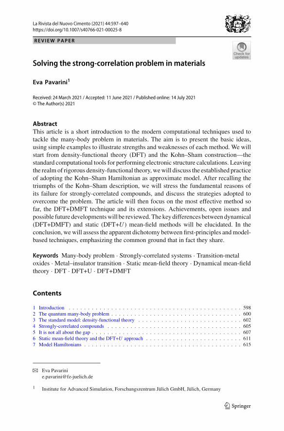
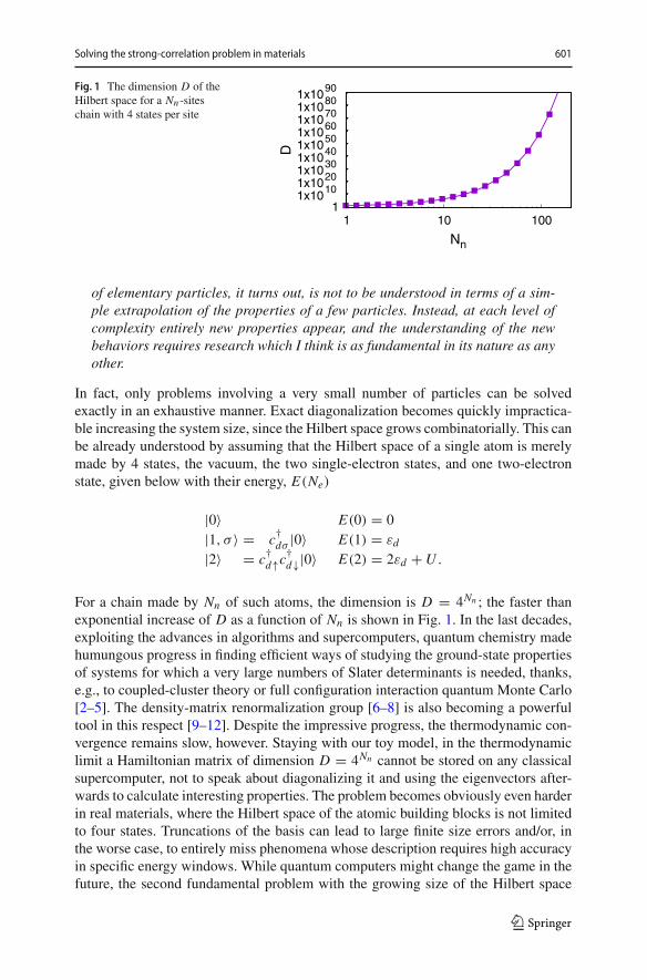
Fig. 1 The dimension D of theHilbert space for a Nn -siteschain with 4 states per site
1 1x10¹⁰ 1x10²⁰ 1x1030 1x1040 1x1050 1x1060 1x1070 1x1080 1x1090
1 10 100
D
Nn
of elementary particles, it turns out, is not to be understood in terms of a sim-ple extrapolation of the properties of a few particles. Instead, at each level ofcomplexity entirely new properties appear, and the understanding of the newbehaviors requires research which I think is as fundamental in its nature as anyother.
In fact, only problems involving a very small number of particles can be solvedexactly in an exhaustive manner. Exact diagonalization becomes quickly impractica-ble increasing the system size, since the Hilbert space grows combinatorially. This canbe already understood by assuming that the Hilbert space of a single atom is merelymade by 4 states, the vacuum, the two single-electron states, and one two-electronstate, given below with their energy, E(Ne)
|0〉 E(0) = 0|1, σ 〉 = c†dσ |0〉 E(1) = εd
|2〉 = c†d↑c†d↓|0〉 E(2) = 2εd +U .
For a chain made by Nn of such atoms, the dimension is D = 4Nn ; the faster thanexponential increase of D as a function of Nn is shown in Fig. 1. In the last decades,exploiting the advances in algorithms and supercomputers, quantum chemistry madehumungous progress in finding efficient ways of studying the ground-state propertiesof systems for which a very large numbers of Slater determinants is needed, thanks,e.g., to coupled-cluster theory or full configuration interaction quantum Monte Carlo[2–5]. The density-matrix renormalization group [6–8] is also becoming a powerfultool in this respect [9–12]. Despite the impressive progress, the thermodynamic con-vergence remains slow, however. Staying with our toy model, in the thermodynamiclimit a Hamiltonian matrix of dimension D = 4Nn cannot be stored on any classicalsupercomputer, not to speak about diagonalizing it and using the eigenvectors after-wards to calculate interesting properties. The problem becomes obviously even harderin real materials, where the Hilbert space of the atomic building blocks is not limitedto four states. Truncations of the basis can lead to large finite size errors and/or, inthe worse case, to entirely miss phenomena whose description requires high accuracyin specific energy windows. While quantum computers might change the game in thefuture, the second fundamental problem with the growing size of the Hilbert space
123

602 E. Pavarini
is that it becomes rapidly impossible to make sense of the results. Indeed, the finalaim of all simulations is not to merely reproduce experiments, but to give us answerto the truly interesting questions. Why does a systems behave the way it does? Withan exponentially large number of degrees of freedom, even if we had the means ofobtaining the exact solution, we might be left with an ocean of information impossibleto disentangle. Having the solution would then not necessary lead to real scientificprogress. An example of this paradox comes from the classical gravitational N -bodyproblem. In this case, an exact solution in terms of power series has been obtained.First it was done for the three-body problem [13] and later on it was extended to theN -body case [14]. Nevertheless, limited progress in understanding the N -body prob-lem comes from power-series solutions themselves. This is due to the fact that theyconverge slowly and simulations can become quickly impossibly long [15]. In a sim-ilar way, most progress in unravelling the quantum many-body problem in materialscomes from methods which construct minimal effective models capturing the essenceof a given phenomenon with sufficient degree of sophistication, and from solutionsof such models, perhaps approximate, but allowing us to answer to essential “why”questions. This category includes a whole range of techniques, from those for solvingparadigmatic models (describing only the generic features of a given phenomenon)all the way, I will argue, to the so-called first-principles methods, discussed in the nextsection.
3 The standardmodel: density-functional theory
Density-functional theory [16,17] has revolutionized the way we deal with the many-electron problem. For this reason, DFT can be to some extent viewed as the standardmodel of condensed-matter physics. Given such a status, there aremany reviews and/orbooks devoted to DFT, covering the principles, the applications, the history, or all ofthis together. A selection—definitely non-exhausting—can be found in Refs. [18–24].Here I will merely recall the aspects most relevant for strongly-correlated systems.DFT shifts the focus from the electronic wave-function, which depends on Ne threedimensional coordinates, Ψ (r1, . . . rNe ), to the electron density n(r), a function of asingle coordinate. This changes completely the perspective. For this reason, in 1998,in his Nobel lecture [18], Walter Kohn described the most important contributions ofDFT starting as follows
[..] The first is in the area of fundamental understanding. Theoretical chemistsand physicists, following the path of the Schrödinger equation, have becomeaccustomed to think in a truncated Hilbert space of single particle orbitals.The spectacular advances achieved in this way attest to the fruitfulness of thisperspective. However, when very high accuracy is required, so many Slaterdeterminants are required (in somecalculations up to∼ 109) that comprehensionbecomes difficult. DFT provides a complementary perspective. It focuses onquantities in the real, three-dimensional coordinate space, principally on theelectron density n(r) of the ground state. [..] These quantities are physical,independent of representation and easily visualisable even for large systems.
123
Solving the strong-correlation problem in materials 603
Decades later this conclusion remains unchallenged. Still, the rise of DFT as thestate-of-the art approach for describing actual materials is to a large extent due toa second step, the Kohn–Sham construction. In practical implementations, the elec-tronic ground-state density n(r) is typically calculated by mapping the many-bodyHamiltonian onto an auxiliary non-interacting KS Hamiltonian, HKS
e , with the sameelectronic ground-state density,
n(r) = n0(r) =occ∑
l
|φKSl (r)|2.
Here {φl(r)} are Kohn–Sham orbitals; the associated Kohn–Sham eigenvalues areLagrange multipliers, obtained solving the equation
h0e(r) φKSl (r) = ( − 1
2∇2 + vKS(r)
)φKSl (r) = εlφ
KSl (r) (8)
with effective potential given by
vKS(r) = −∑
α
Zα
|r − Rα|︸ ︷︷ ︸
ven(r)
+∫
dr′ n(r′)|r − r′|︸ ︷︷ ︸
vH(r)
+ δExc[n]δn(r)︸ ︷︷ ︸vxc(r)
. (9)
In this expression the first term (ven(r)) is the external potential, the second and thirdare the Hartree (vH(r)) and the exchange-correlation (vxc(r)) potential; Exc[n] is theexchange-correlation functional. The exact ground-state energy of the system can beexpressed as
EG[n] =occ∑
l
εl − EH [n] + Exc[n] −∫
drδExc[n]δn(r)
n(r), (10)
where
EH [n] = 1
2
∑
ll ′
∫dr1
∫dr2 φKS
l (r1)φKSl ′ (r2)
1
|r1 − r2|φKSl (r1)φKS
l ′ (r2) (11)
= 1
2
∫dr
∫dr′ n(r)
1
|r − r′|n(r′). (12)
is theHartree energy.Themaindifficulty is tofindgoodapproximations to the unknownfunctional Exc[n]. One of the best known is the local-density approximation (LDA),in which Exc[n] is replaced by its expression for a homogeneous interacting electrongas (HEG) with electron density equal to n(r)
Exc[n] ∼∫
dr εHEGxc (n(r)) n(r). (13)
123
604 E. Pavarini
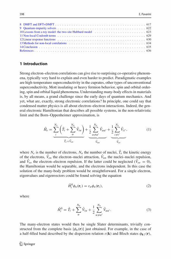
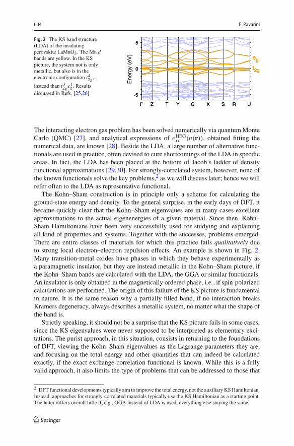
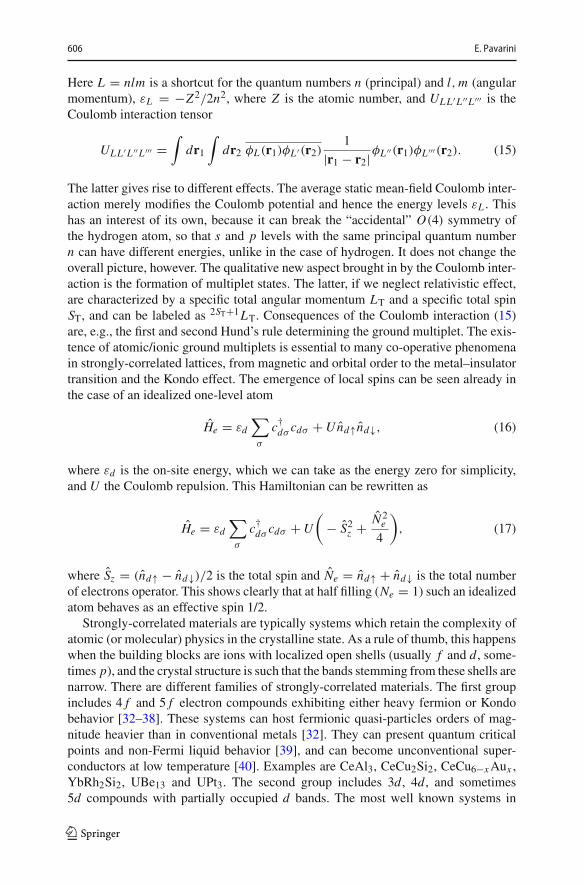
Fig. 2 The KS band structure(LDA) of the insulatingperovskite LaMnO3. The Mn dbands are yellow. In the KSpicture, the system not is onlymetallic, but also is in theelectronic configuration t42g ,
instead than t32ge1g . Results
discussed in Refs. [25,26] -5
0
5
Γ Z T Y G X S R U
t2g
eg
-5
0
5
Γ Z T Y G X S R U
t2g
eg
Ene
rgy
(eV
)The interacting electron gas problem has been solved numerically via quantumMonteCarlo (QMC) [27], and analytical expressions of εHEGxc (n(r)), obtained fitting thenumerical data, are known [28]. Beside the LDA, a large number of alternative func-tionals are used in practice, often devised to cure shortcomings of the LDA in specificareas. In fact, the LDA has been placed at the bottom of Jacob’s ladder of densityfunctional approximations [29,30]. For strongly-correlated system, however, none ofthe known functionals solve the key problems,2 as we will discuss later; hence we willrefer often to the LDA as representative functional.
The Kohn–Sham construction is in principle only a scheme for calculating theground-state energy and density. To the general surprise, in the early days of DFT, itbecame quickly clear that the Kohn–Sham eigenvalues are in many cases excellentapproximations to the actual eigenenergies of a given material. Since then, Kohn–Sham Hamiltonians have been very successfully used for studying and explainingall kind of properties and systems. Together with the successes, problems emerged.There are entire classes of materials for which this practice fails qualitatively dueto strong local electron–electron repulsion effects. An example is shown in Fig. 2.Many transition-metal oxides have phases in which they behave experimentally asa paramagnetic insulator, but they are instead metallic in the Kohn–Sham picture, ifthe Kohn–Sham bands are calculated with the LDA, the GGA or similar functionals.An insulator is only obtained in the magnetically ordered phase, i.e., if spin-polarizedcalculations are performed. The origin of this failure of the KS picture is fundamentalin nature. It is the same reason why a partially filled band, if no interaction breaksKramers degeneracy, always describes a metallic system, no matter what the shape ofthe band is.
Strictly speaking, it should not be a surprise that the KS picture fails in some cases,since the KS eigenvalues were never supposed to be interpreted as elementary exci-tations. The purist approach, in this situation, consists in returning to the foundationsof DFT, viewing the Kohn–Sham eigenvalues as the Lagrange parameters they are,and focusing on the total energy and other quantities that can indeed be calculatedexactly, if the exact exchange-correlation functional is known. While this is a fullyvalid approach, it also limits the type of problems that can be addressed to those that
2 DFT functional developments typically aim to improve the total energy, not the auxiliary KSHamiltonian.Instead, approaches for strongly-correlated materials typically use the KS Hamiltonian as a starting point.The latter differs overall little if, e.g., GGA instead of LDA is used, everything else staying the same.
123
Solving the strong-correlation problem in materials 605
can be solved by calculating the total energy and electron density of the ground state.Thus this strategy will not be discussed further in this article.
Here we will focus instead on less rigorous but more flexible methods. The beautyand simplicity of the KS picture and its great successes create indeed hope that theKS eigenvalues and eigenvectors represent a good starting point, even when they arenot sufficient alone. In this view, it should be possible to describe the missing effectsas corrections of some kind. Which, however? There are two different strategies thatcan be adopted to make progress. The first consists in finding, even stepping outsidethe rigorous principles of DFT, corrections to the exchange-correlation functional, forexample in order to obtain a KS gap in Mott insulators; this approach is adopted,e.g., to the DFT+U technique, which we will discuss in Sect. 6. This choice has theadvantage that the mapping to an effective one-electron model, with all its simplicity,is preserved. If it works, it is very effective. Unfortunately only some aspects of strongcorrelations can be recast into an independent quasi-electron problem. The secondstrategy consists in interpreting the KS orbitals as an optimal basis for constructingthe general many-body Hamiltonian. The crucial step is building from it minimalmany-body models, approximate but as realistic as possible, that can be solved withstate-of-the-art many-body methods.3 This is the viewpoint taken in the DFT+DMFTmethod and its extensions, illustrated in Sects. 8 and 13.
4 Strongly-correlated compounds
In his Lectures on Physics [31], Feynman writes
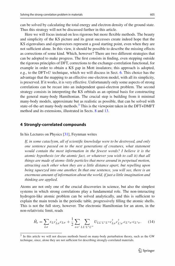
If, in some cataclysm, all of scientific knowledge were to be destroyed, and onlyone sentence passed on to the next generations of creatures, what statementwould contain the most information in the fewest words? I believe it is theatomic hypothesis (or the atomic fact, or whatever you wish to call it) that allthings are made of atoms–little particles that move around in perpetual motion,attracting each other when they are a little distance apart, but repelling uponbeing squeezed into one another. In that one sentence, you will see, there is anenormous amount of information about the world, if just a little imagination andthinking are applied.
Atoms are not only one of the crucial discoveries in science, but also the simplestsystems in which strong correlations play a fundamental role. The non-interactinghydrogen-like atomic problem can be solved analytically, and this is sufficient toexplain the main trends in the periodic table, progressively filling the atomic shells.This is not the full story, however. The electronic Hamiltonian for an atom, in thenon-relativistic limit, reads
He =∑
Lσ
εLc†Lσ cLσ + 1
2
∑
σσ ′
∑
LL ′L ′′L ′′′ULL ′L ′′L ′′′c†Lσ c
†L ′σ ′cL ′′′σ ′cL ′′σ . (14)
3 In this article we will not discuss methods based on many-body perturbation theory, such as the GWtechnique, since, alone they are not sufficient for describing strongly-correlated materials.
123
606 E. Pavarini
Here L = nlm is a shortcut for the quantum numbers n (principal) and l,m (angularmomentum), εL = −Z2/2n2, where Z is the atomic number, and ULL ′L ′′L ′′′ is theCoulomb interaction tensor
ULL ′L ′′L ′′′ =∫
dr1
∫dr2 φL(r1)φL ′(r2)
1
|r1 − r2|φL ′′(r1)φL ′′′(r2). (15)
The latter gives rise to different effects. The average static mean-field Coulomb inter-action merely modifies the Coulomb potential and hence the energy levels εL . Thishas an interest of its own, because it can break the “accidental” O(4) symmetry ofthe hydrogen atom, so that s and p levels with the same principal quantum numbern can have different energies, unlike in the case of hydrogen. It does not change theoverall picture, however. The qualitative new aspect brought in by the Coulomb inter-action is the formation of multiplet states. The latter, if we neglect relativistic effect,are characterized by a specific total angular momentum LT and a specific total spinST, and can be labeled as 2ST+1LT. Consequences of the Coulomb interaction (15)are, e.g., the first and second Hund’s rule determining the ground multiplet. The exis-tence of atomic/ionic ground multiplets is essential to many co-operative phenomenain strongly-correlated lattices, from magnetic and orbital order to the metal–insulatortransition and the Kondo effect. The emergence of local spins can be seen already inthe case of an idealized one-level atom
He = εd∑
σ
c†dσ cdσ +Und↑nd↓, (16)
where εd is the on-site energy, which we can take as the energy zero for simplicity,and U the Coulomb repulsion. This Hamiltonian can be rewritten as
He = εd∑
σ
c†dσ cdσ +U
(− S2z + N 2
e
4
), (17)
where Sz = (nd↑ − nd↓)/2 is the total spin and Ne = nd↑ + nd↓ is the total numberof electrons operator. This shows clearly that at half filling (Ne = 1) such an idealizedatom behaves as an effective spin 1/2.
Strongly-correlated materials are typically systems which retain the complexity ofatomic (or molecular) physics in the crystalline state. As a rule of thumb, this happenswhen the building blocks are ions with localized open shells (usually f and d, some-times p), and the crystal structure is such that the bands stemming from these shells arenarrow. There are different families of strongly-correlated materials. The first groupincludes 4 f and 5 f electron compounds exhibiting either heavy fermion or Kondobehavior [32–38]. These systems can host fermionic quasi-particles orders of mag-nitude heavier than in conventional metals [32]. They can present quantum criticalpoints and non-Fermi liquid behavior [39], and can become unconventional super-conductors at low temperature [40]. Examples are CeAl3, CeCu2Si2, CeCu6−xAux ,YbRh2Si2, UBe13 and UPt3. The second group includes 3d, 4d, and sometimes5d compounds with partially occupied d bands. The most well known systems in
123
Solving the strong-correlation problem in materials 607
this class are high-temperature superconducting cuprates. Other representative casesare titanates, manganites, cuprates, and ruthenates, among which LaTiO3, LaMnO3,KCuF3 and Sr2RuO4. Additional systems of this kind are iron-based superconduc-tors, iridates and nichelates. All these materials exhibit fingerprints of Mott physics,ranging from enhanced quasi-particle masses to a fully blown Mott insulating phase[41–44]. They can show in addition Hund’s metal behavior, spin, charge and orbitalorder, spin and orbital frustration, spin- and orbital-liquid phenomena. Finally, a thirdgroup of correlated systems collects molecular crystals, such as C60 compounds [45];here the narrow bands stem from the small inter-molecular hopping integrals. Thethree families of systems just described have in common the fact that their unexpectedelectronic properties arise from the competition between hopping integrals, favoringelectron delocalization, and on-site Coulomb interaction, fostering atomic-like behav-ior. The anomalous properties of correlated materials are usually very sensitive tosmall changes in external parameters, such as temperature and pressure. In the rest ofthe article we will focus on the representative class of transition-metal compounds.
5 It is not all about the gap
Aclassical example of strong-correlation effects is theMottmetal–insulator transition,characteristic feature of many transition–metal compounds. From the point of viewof the mechanism, the Mott transition is well captured by the single-band Hubbardmodel
He = −∑
σ
∑
i i ′t i,i
′c†iσ ci ′σ +U
∑
i
ni↑ni↓, (18)
where t i,i′are the hopping integrals andU is the on-site Coulomb term. At half filling,
for U = 0, this model describes a conventional metal with band-width W . Increasingthe ratio U/W , the system becomes a strongly-correlated electron liquid. When theon-site Coulomb repulsion U is large with respect to W the electrons tend to stayas far apart as possible and the expectation value of double occupations, 〈ni↑ni↓〉,correspondingly decreases. Eventually, for U larger than a critical Uc, the systembecomes an insulator. When W=0, the model describes an insulating collection ofdecoupled atoms.
Since the most remarkable effect described by (18) is the formation, for U >
Uc and at half filling, of a paramagnetic insulating state in a system which, in theindependent-electron picture, should be metallic, the focus of the discussion oftengoes to the gap in the spectral function. The emphasis on the charge gap can be,however, misleading. Indeed, the gap is only one of the very surprising electronicproperties characterizing a system described by Hamiltonian (18). At half filling,the list includes low-energy quasi-particles with enhanced masses and short lifetimes,alongwith their co-existencewithHubbard bands. It extends to local-moment behaviorand low-temperature super-exchange-driven magnetic order, and the presence of bothatomic and delocalized electron signatures in response functions. Away from half-filling, a dopedMott insulator is ametallic systemwith unusual transport andmagnetic
123
608 E. Pavarini
0
0.05
0.1
0.15
0.2
0.25
1.75 1.8 1.85 1.9 1.95 2 2.05 2.1
Ene
rgy
Bar
rier
smin
E(s
) −
E(s
min
) (e
V p
er f.
u.)
s (Å)
KCuF3, Rb volRbCuF3
900 K600 K300 K
0.8 GPa10 K
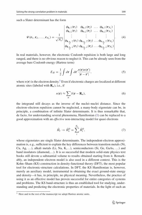
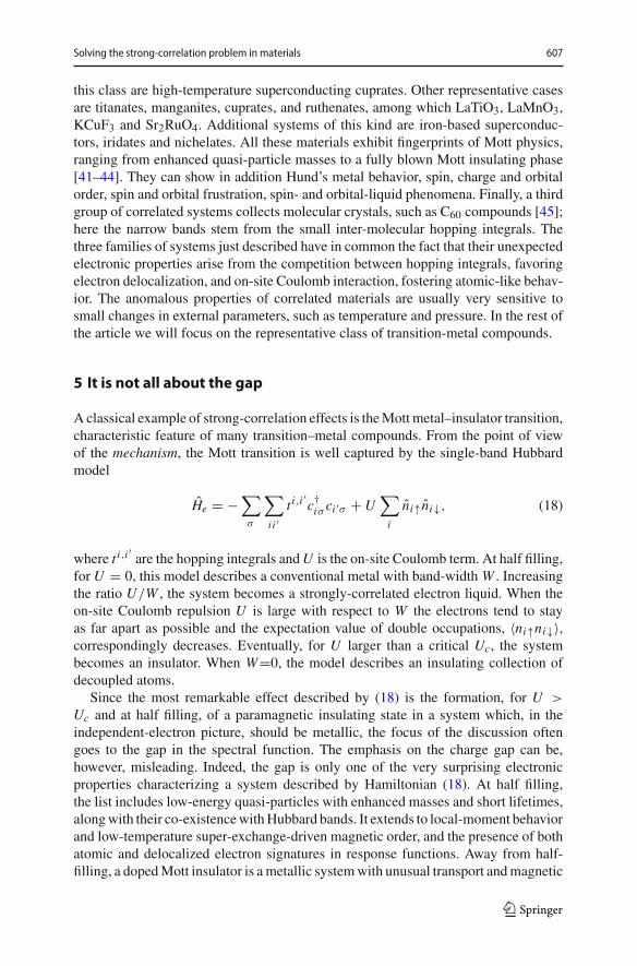
Fig. 3 The Born–Mayer repulsion is key for understanding the orbitally-ordered structure of KCuF3. Sym-bols indicate structures at specific temperatures, pressures or for different cations. The figure shows thechange in total energy as a function of the short Cu–F bond (s) for structures with different lattice constantsa. The minimum smin is practically independent of the temperature so that the experimentally observedincrease in Δ = (l − s)/2, where l is the long Cu–F bond, is merely an effect of thermal expansion.Reprinted figure with permission from Sims et al. [46]. Copyright (2017) by the American Physical Society
properties, it can exhibit superconductivity, Nagaoka-like ferromagnetism, and muchmore. Although we cannot solve (18) in the general case, we know from approximatesolutions in specific regimes and/or limit cases that the complex behavior emergingfrom it is quite different from the one expected for a simple band metal or from aconventional doped band insulator.
The properties of real correlated systems are, of course, in general not captured bythe simple version of the Hubbard model given in Eq. (18). First, in a given mate-rial there can be more than one strongly correlated band. Second, other interactionsbeside the on-site Coulomb repulsion can play an important role. The behavior actu-ally observed in experiments is typically the result of the interplay of several of them:electron–lattice coupling, crystal-field splittings, spin–orbit interaction, just tomentiona few. This is of course not a surprise—it is true for any material, independently on thedegree of correlation. For weakly correlated systems, such a complexity can typicallybe taken into account and disentangled in full, however, exploiting the Kohn Sham pic-ture. In a correlated system, where the Kohn Sham picture fails at the qualitative level,it is instead often very tricky to identify the true causes of a specific phenomenon and/orto explain a given observation. A metal–insulator transition could, for example, arisefrom a pure Mott mechanism, but could also be driven by lattice distortion reducingthe symmetry, or could be the co-operative effect of all this together. An example is thecase of single layered ruthenates [47–49]. Often chicken-and-egg problems arise, asin the case of orbital-ordering. For the latter, it was long debated if the ordering arisesfrom the electron–lattice interaction (Jahn–Teller coupling) or from a purely electronicmany-body super-exchange mechanism. This riddle was solved only recently, afterdecades of hot discussions [25,46,50–52]. It was shown that super-exchange yields a
123

Solving the strong-correlation problem in materials 609
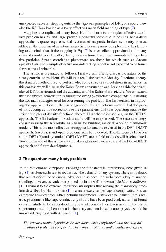
Fig. 4 Quasiparticles and Hubbard bands in the doped 2D Hubbard model (square lattice) with dispersionε(k) = −2t(cos kx + cos ky) + 4t ′ cos kx cos ky , obtained with the dynamical mean-field theory approach[53,54]. The special points are Γ = (0, 0, 0), X = (0, π/a, 0), M = (π/a, π/a, 0), and Z = (0, 0, π/a).Left panels: t ′/t = 0.2. Right panels: t ′/t = 0.4. Calculations were performed for U = 7 eV, t = 0.4 eV,290 K. The quantum impurity solver adopted is the Hirsch–Fye quantum Monte Carlo [55] method in theimplementation of Ref. [53]. The number of holes is indicated with x
large transition temperature, but is not sufficient to explain alone the persistence ofdistortions till very high temperatures; in the case of ionic systems such as KCuF3,a new mechanism was identified [46], with the Born–Mayer repulsion playing a keyrole in determining the actual experimental structure (Fig. 3). Given this complexity,the classification of a system as strongly correlated is justified not by a single obser-vation, e.g., the mere existence of a Mott-like gap, but via a series of experimentalresults which coherently fit within the phenomena described by the Hubbard model orits generalizations. It is this coherent picture, built, e.g., collecting strong-correlationfingerprints in families of similar compounds or in different energy and temperatureregimes, which makes it clear that it is necessary to take the local Coulomb interactionexplicitly into account—not the fact that one specific isolated experiment in a specificsystem does not agree with calculations based on the KS Hamiltonian. This makesalso clear that descriptions trying to circumvent the introduction of the Hubbard U ,in order to become valid alternatives, must, of course, satisfy the same requirements,and capture the global picture.
The complexity ofHubbard-U effects is illustrated, e.g., in Fig. 4 for the single-bandHubbard model. The figure shows the evolution of the k-resolved spectral functionas a function of hole doping for the 2-dimensional square lattice. The non-interactingdispersion adopted is
εk = −2t(cos kx + cos ky) + 4t ′ cos kx cos ky . (19)
123
610 E. Pavarini
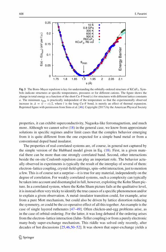
This is a good approximation of the generic x2− y2 band stemming fromCuO2 planesin high-temperature superconducting cuprates [56,57]. The figure shows the effect ofintroducing x holes in the CuO2 planes. For x 1 the spectral function shows a quasi-particle band close to the Fermi level as well as Hubbard bands at higher energy; thelatter lose intensity with increasing x . The finite lifetime of quasi-particles is reflectedin the intensity of the lines.
Going back to rigorous DFT, the theory gives in principle the exact ground-stategap, the difference between ionization energy and electron affinity
Egap = E(Ne + 1) + E(Ne − 1) − 2E(Ne), (20)
if the exact exchange-correlation functional is used. The Kohn–Sham picture does not,however. The KS gap is defined as
EKSgap = εγ+1(Ne) − εγ (Ne), (21)
where γ labels the highest occupied Kohn–Sham orbital and γ + 1 the lowest unoc-cupied Kohn–Sham orbital. It has been shown long ago [58,59] that the KS gap candiffer sizably from the exact value, due to the discontinuities in the reference potential.In fact
Egap = EKSgap + δExc
δn
∣∣∣∣Ne+δ
− δExc
δn
∣∣∣∣Ne−δ︸ ︷︷ ︸
ΔVxc
. (22)
The extra term ΔVxc is large in semiconductors [60], and can be the dominant contri-bution in strongly correlated systems, as it was shown explicitly for, e.g., a chain ofidealized hydrogen atoms [61] or the two-site Hubbard model [62]. A characteristic ofMott insulators is that EKS
gap = 0 in the LDA, the GGA, or similar approximations. Thegap is zero even for the exact exchange-correlation functional –if Kramers degeneracyis not broken in the ground state. In discussing the KS gap, it is in fact important toremember that Mott insulators have typically a magnetically ordered ground state. Inbroken symmetry phases, a finite KS gap, even if often too small, is typically alreadyobtained in calculations based on the local-spin-density approximation (LSDA) orother spin-density functionals, and thus it is likely to be obtained also with the exactfunctional. Hence, if one focuses on the broken symmetry ground-state only, the KSHamiltonian, calculated with a well chosen or corrected functional, can give an insu-lator; this is the basis of the success of the DFT+U approach, discussed in the nextsection. In order to understand the complex electronic properties of Mott insulatorsthis is not sufficient, however. In the KS description the gap is present only in the bro-ken symmetry phase; furthermore the effects of hole/electron doping are the same asin regular band insulators and the magnetic excitation spectrum is qualitatively wrong.The real problem is thus the fact that the Kohn–Sham description fails to provide theglobal picture; the absence of a gap in the paramagnetic phase is not the only issue, itis merely a paradigmatic example of this failure, the one to which is perhaps simplerto point to.
123
Solving the strong-correlation problem in materials 611
6 Static mean-field theory and the DFT+U approach
The DFT+Umethod [63–67] is one of the approaches based on the strategy of improv-ing the effective Kohn–Sham potential, given in Eq. (9). The correction is based onthe physical insight that the shortcomings of the KS Hamiltonian, calculated withLDA, its spin-polarized extension, LSDA, or similar functionals arise from the inad-equate treatment of the local Coulomb interaction, the Hubbard U . In this view, theKS Hamiltonian HKS
e should be augmented by a Hubbard-like correction
HKSe −→ HKS
e + ΔHUe (23)
where ΔHUe is a Hubbard-like augmentation operator. Assuming for simplicity that
the latter acts only on the electrons with quantum numbers m in, e.g., shell d,
ΔHUe = 1
2U
∑
i
∑
mσ �=m′σ ′nimσ nim′σ ′
︸ ︷︷ ︸HU
−∑
i
H iDC. (24)
The term HDC is a double-counting (DC) correction, subtracting the effects of HU
already included in HKSe via the Hartree and exchange-correlation potential. Here, for
simplicity, we approximate it with the fully localized limit (FLL) expression
H iDC ∼ 1
2UNd Nid − μAT Nid , (25)
where Nid = ∑mσ nimσ yields Nd , the number of d electrons at site i , μAT = U/2
is the atomic chemical potential at half filling and the expectation value 12UNdNd is
the Hartree energy.In DFT+U , the many-body Hubbard term in Eq. (23) is approximated with an
effective single-electron operator, i.e., a modification of the parameters of the KSHamiltonian. This is done via static mean-field decoupling.4 The static mean-fieldHamiltonian obtained from Eqs. (23) and (24) in this way is
HMFe = HKS
e +∑
imσ
Δεimσ nimσ , with Δεimσ = U
(1
2− 〈nimσ 〉
). (26)
In HMFe the original levels εimσ are shifted by Δεimσ , and
Δεimσ ={
−U2 if 〈nimσ 〉 = 1
+U2 if 〈nimσ 〉 = 0.
(27)
4 The expression static mean field decoupling indicates here the replacement of the two-body operatorni↑ni↓ with the single-body operator ni↑〈ni↓〉 + ni↓〈ni↑〉-〈ni↑〉〈ni↓〉.
123
612 E. Pavarini
Assuming that one spin state is empty and the other full, the associated shifts corre-spond to the poles of the atomic Green function at half filling
E(N )−E(N−1) − μ = −U/2 (28)
E(N+1)−E(N ) − μ = +U/2, (29)
and thus to the center of the Hubbard bands. The modified (U -dependent) total energy“functional” giving Eq. (26) is
ELDA+U[n] = ELSDA[n] +∑
i
⎡
⎣1
2U
∑
mσ �=m′σ ′〈nimσ 〉〈nim′σ ′ 〉 − EDC
⎤
⎦ , (30)
where
EDC = 1
2UNd(Nd − 1). (31)
One can verify with Janak’s theorem [68] that indeed
εLDA+Uimσ = ∂ELDA+U
∂〈nimσ 〉 = εLSDAimσ +U
(1
2− 〈nimσ 〉
)= εLSDAimσ + Δεimσ . (32)
SinceU is a parameter, not determined univocally by the density, calculations based onthe DFT+U approach are not fully ab initio and do not follow rigorously the principlesof DFT. The correction yields however a better KS description of the magnetic groundstate of Mott insulators, with respect to the one obtained via more rigorous DFT-basedapproaches. In DFT+U the gap calculated from the eigenvalues of themodified Kohn–Sham Hamiltonian (26) increases linearly with U as in the exact solution in the largeU/W limit; thus the term ΔVxc in Eq. (22) is less relevant. The DFT+U approachhas been generalized to account for additional elements of the Coulomb-interactiontensor, e.g., the Hund’s rule coupling J or the coupling between first neighbors, V .Furthermore, different types of DC corrections are used in different regimes/situations[69–75]. Hence, in practice, the name DFT+U collects a plethora of different Hartree–Fock-like corrections to the LSDA or similar functionals, all sharing however theprinciples just outlined.
The main strength of DFT+U , the ability of taking into account key effects ofthe local Coulomb repulsion via a mere modification of the parameters of the KSHamiltonian, is also its main limit. The correction corresponds to a static mean fieldtreatment of the Hubbard U . Thus, while it well describes the magnetic ground stateof correlated materials, is not suitable for studying the metal-insulator transition itself.This failure can be understood in a simple way. In the absence of static local spin andorbital polarization, i.e., if
〈nimσ 〉 = ni2Nd
, (33)
123
Solving the strong-correlation problem in materials 613
the DFT+U correction is merely a level shift, identical for all d electrons. Hence, ifthe original KS Hamiltonian describes a metal, everything else remaining the same(in particular space group, magnetic group and primitive cell), so does the DFT+UHamiltonian. Conversely, when an insulating state is obtained in DFT+U , it is ofSlater- (and not of Mott) type. It requires a reduction of symmetry, e.g., via spin orcharge disproportionation, and/or, dependingon the system, orbital disproportionation,long-range spin and orbital order or, generalizing, spin-glass-like behavior.
As we have already pointed out, Mott insulators have typically a magneticallyordered ground state; it is perfectly justified to use DFT+U to describe it. Problemsarise if the approach is used to analyze the behavior of a Mott insulator above themagnetic transition temperature, usually a paramagnetic insulating phase. An (ideal)local-moment paramagnet is a system in which local magnetic moments fluctuate intime. Hence 〈Siz〉 = 〈Six 〉 = 〈Siy〉 = 0 at each site, but at the same time 〈Si · Si 〉 ∼S(S+1); the latter is the local moment appearing, e.g., in the expression of the Curie-Weiss susceptibility. A static potential, even if orbital, site and spin dependent, failsto capture this behavior (and several associated phenomena). In fact, a paramagneticinsulator is very different from, e.g., a system characterized by spatial fluctuations of〈Siz〉 in a supercell (nomatter how large this cell is or howquasi-random the fluctuationsare).5 This remains true even if
∑i 〈Siz〉 = 0 for the unit cell.6 Furthermore, an ideal
paramagnet and an ideal disordered spin system can be distinguished experimentally.While disordered systems do exist also among strongly-correlated materials, in orderto capture the correct behavior of a paramagnetic insulator one needs a method whichcan explicitly account for dynamical fluctuations.
Let us now examine the interplay between the DC correction and charge self-consistency. In order to keep it simple, always with transition-metal oxides in mind,we consider a toy model with two sites, the first representing a transition metal ionand the second an oxygen ion. The model is
He =H0 + HU
H0 =εd∑
σ
c†dσ cdσ + εp∑
σ
c†pσ cpσ − tpd∑
σ
(c†dσ cpσ + c†pσ cdσ )
HU =Und↑nd↓ (34)
with εp = εd − Δpd . The difference Δpd > 0 is the charge-transfer energy. For threeelectrons the exact ground doublet of this Hamiltonian is
|G, σ 〉 = a1 c†dσ c
†p↑c
†p↓|0〉 + a2 c
†d↑c
†d↓c
†pσ |0〉, (35)
5 This representation is adopted, e.g., in polymorphous DFT calculations. See, e.g., J. Varignon, M. Bibesand A. Zunger, Nat. Comm. 10, 1658 (2019).6 A trivial example is the ideal antiferromagnet in a bipartite lattice.
123
614 E. Pavarini
where a22 + a21 = 1 and
a21 = t2pd
t2pd +(
Δpd+U2 −
√(Δpd+U2
)2 + t2pd
)2 . (36)
Its energy is
EG(3) = 3εd − 2Δpd + Δpd +U
2−
√(Δpd +U
2
)2
+ t2pd , (37)
and the total number of d electrons is
nd = 1 +
(Δpd+U
2 −√(Δpd+U
2
)2 + t2pd
)2
t2pd +(
Δpd+U2 −
√(Δpd+U2
)2 + t2pd
)2 . (38)
ForU = 0, the total number of d electrons takes the value n0d = 1+ x0, where x0 is apositive number, which can be determined by setting U = 0 in right term in Eq. (38);for U → ∞, we find instead n∞
d = 1.Let us now analyze the effect of the DC correction in a mean-field treatment of the
Coulomb term. In the first step we calculate the KS Hamiltonian. For simplicity weassume that this yields εd −→ εKSd = εd + UKS nd . When UKS = U , the correctionis the Hartree term for the Hubbard model. From Eq. (38) one may see that, ifU = 0,the exact ground state density for finite U is recovered by merely replacing εd withεd + U ; indeed, this N = 3 electron problem is an uncorrelated system in the hole
representation. In the second step, we augment ˆHKSe with Δ ˆHU∗
e = HU∗e − HDC,
and solve the problem in the static mean-field approximation; we replace U with U∗,since, in general, we do not know the exact value of U included in the Hartree term.Thus
Δpd −→Δ∗pd(nd) = Δpd +Und + U
2
∗(nd − n∗
d). (39)
The choice of n∗d defines the DC correction. The self-consistent condition for the
number of d electrons is obtained setting U = 0 in Eq. (38) and replacing Δpd withΔ∗
pd via Eq. (39). In the FLL limit, i.e., when the double-counting energy is givenby Eq. (31), for nd > 1 we obtain nd < n∗
d ; hence, the double-counting term tendsto slightly increase the self-consistent value of nd . The opposite happens if, e.g., weset n∗
d = 1. The example shows that the largest effect can arise, however, from theuncertainty in the value of U∗, rather than from the specific choice of n∗
d .Besides DFT+U , there are many attempt to address the problem of strong
correlation by correcting the functional [28,76–84]. Examples are, e.g., the self-interaction-correction approach [28,77,78] or the hybrid functional method [79–84].
123
Solving the strong-correlation problem in materials 615
Other approaches try instead to propose schemes alternative to the Kohn–Sham con-struction, such as the strictly-correlated-electron approach [85,86] and/or focus on thetotal energy [87].
7 Model Hamiltonians
In this section, we will discuss the second family of approaches, the one that usesthe Kohn–Sham states as the optimal one electron basis for constructing many-bodymodels. The Hamiltonian (1), with all terms explicitly written, has the form
He = −1
2
∑
i
∇2i −
∑
i
∑
α
Zα
|ri−Rα| +∑
i> j
1
|ri−r j | +∑
α>α′
ZαZα′
|Rα−Rα′ | , (40)
where {ri } are electron coordinates, {Rα} nuclear coordinates and Zα the nuclearcharges.Using a complete one-electron basis {φa(r)}, where {a} are quantumnumbers,we can rewrite it in second quantization as
He = −∑
ab
tabc†acb
︸ ︷︷ ︸H0
+ 1
2
∑
aa′bb′Uaa′bb′ c†ac
†a′cb′cb
︸ ︷︷ ︸HU
.
The hopping integrals are given by
tab = −∫dr φa(r)
(−1
2∇2 −
∑
α
Zα
|r−Rα|︸ ︷︷ ︸
ven(r)
)φb(r),
while the elements of the Coulomb tensor are
Uaa′bb′ =∫dr2
∫dr2 φa(r1) φa′(r2)
1
|r1−r2| φb′(r2) φb(r1).
All complete one-electron bases are of course equivalent in theory. In practice,since, in the general case, we cannot solve the Ne-electron problem exactly, somebases are better than others. In this spirit, the Kohn–Sham orbitals {φKS
a (r)} havemany advantages, since they provide KS spectra reasonably in line with experimentsfor weakly correlated systems. Even for strongly-correlated systems, they are oftensufficiently accurate for empty and fully occupied states. In order to use theKS orbitalsas a basis, we first rewrite ven(r) in terms of the effective KS potential, vKS(r). Thelatter differs from ven(r) via the Hartree term vH(r) and the (approximate) exchange-correlation contribution, vxc(r)
ven(r) = vKS(r) − vH(r) − vxc(r). (41)
123
616 E. Pavarini
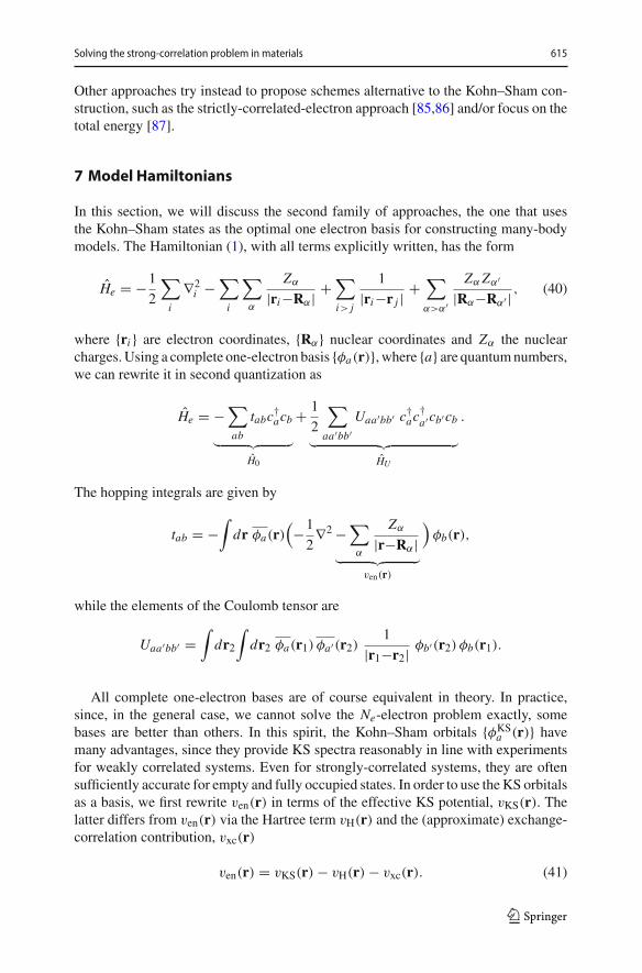
Fig. 5 (Color online) NMTOWannier functions showingorbital-order in TbMnO3, asobtained by LDA+DMFTcalculations. Reprinted figurewith permission from Flesch etal. [51]. Copyright (2012) by theAmerican Physical Society
We thus introduce the Kohn–Sham hopping integrals
tab = −∫dr φKS
a (r)(−1
2∇2 + vKS(r)
)φKSb (r). (42)
With this definition, the total Hamiltonian, in the KS basis, is
He = −∑
ab
tab c†acb
︸ ︷︷ ︸H0=HKS
e
+ 1
2
∑
aba′b′Uaa′bb′ c†ac
†a′cb′cb − HDC
︸ ︷︷ ︸ΔHU
, (43)
where HDC is the double-counting correction. TypicallyΔHU is a short range operatorsince long-range effects are already well captured by the KS potential, and strongcorrelation effects are a manifestation of a large local U .
The key step for studying correlation effects in materials is building, starting fromthe general Hamiltonian (43), minimal material-specific models containing all essen-tials degrees of freedom and interactions. This was made possible by the developmentof methods for constructing Kohn–Sham localized Wannier functions spanning spe-cific bands [88,89] and/or projection schemeswith similar capabilities.7 An example ofaWannier-like state is shown in Fig. 5. These approaches yield single-electron Hamil-tonians which very accurately reproduce the Kohn–Sham bands in specific energywindows. A quite different story is the estimate of screened Coulomb integrals. Cal-culating exact screening effects is in principle as hard as solving the full many-body
7 The more localized the Wannier functions, the more short range ΔHU is expected to be. Althoughdifferent localization schemes have been explored [88,89], the results obtained are very similar. A way forworking with substantially more localized functions is to use, instead ofWannier functions, orbitals definedin an atomic sphere. The latter are however ill defined and do not build a complete one-electron basis. Infact, alone, they do not even span the bands. Wannier functions remain therefore the basis of choice.
123
Solving the strong-correlation problem in materials 617
0
2
4
6
-4 -2 0 2 4
A(ω
)
ω (eV)
0
2
4
6
-4 -2 0 2 4
A(ω
)
ω (eV)
0
2
4
6
-4 -2 0 2 4
A(ω
)
ω (eV)
0
2
4
6
-4 -2 0 2 4
A(ω
)
ω (eV)
0
2
4
6
-4 -2 0 2 4
A(ω
)
ω (eV)
-4 -2 0 2 4
ω (eV)
-4 -2 0 2 4
ω (eV)
-4 -2 0 2 4
ω (eV)
-4 -2 0 2 4
ω (eV)
-4 -2 0 2 4
ω (eV)
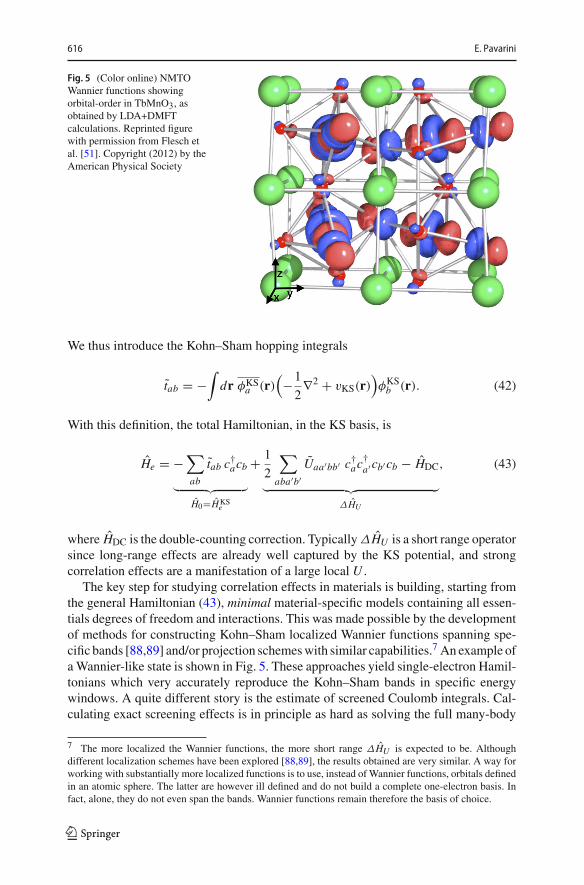
Fig. 6 LDA+DMFT spectral function for the single band systems VOMoO4 (left) and Li2VOSiO4 (right)at 380 K and for 1 < U < 5 eV. The linewidth increases with increasing U in steps of 1 eV. Rearrangedfrom Ref. [53]
Hamiltonian. Commonly adopted schemes are the constrained local-density approx-imation (cLDA) [90,91], linear-response methods [67,92,93], and the constrainedrandom-phase approximation (cRPA) [94,95]. They have been successfully used forbuilding models and understanding the properties of several families of correlatedmaterials. Still, screened Coulomb parameters are only known within relatively largeerror bars.
It is important to underline that the model construction is not a mechanical proce-dure.Althoughmodern techniques provide the tools, identifying the relevant degrees offreedom and interactions remains bound to our physical understanding of the problemand system analyzed. A model is typically a work in progress, a compromise betweenwhat one would like to include and what can be included in actual calculations. Itevolves with time, when new facts come to light. For most transition-metal oxides,typical low-energy starting models, augmented with Coulomb corrections, have theform He = HKS
e + ΔHU of a generalized Hubbard Hamiltonian, with
HKSe = −
∑
i i ′
∑
σ
∑
mm′t i,i
′mσ,m′σ ′ c
†imσ ci ′m′σ ′ (44)
ΔHU = 1
2
∑
i
∑
σσ ′
∑
mm′
∑
pp′Umpm′ p′ c†imσ c
†i pσ ′cip′σ ′cim′σ − HDC, (45)
with m belonging to the d shell or to a subset of crystal-field states.
8 DMFT and DFT+DMFT
The essential step forward for the theoretical description of the Mott metal-insulatortransition in the Hubbard model came with the development of the dynamical mean-field theory (DMFT) [96–103]. The central idea consists in mapping the HubbardHamiltonian onto an auxiliary quantum-impurity model. The latter can be solvedexactly, differently from the original lattice model. A typical QIM is the Anderson
123
618 E. Pavarini
Γ X M Γ Z
-4
-2
0
2
4
ω (
eV)
VOMoO4
-4 -2 0 2 4
Re Σ11/eV
Im Σ11/eV
Γ X M Γ Z
-4
-2
0
2
4
ω (
eV)
Li2VOSiO4
-4 -2 0 2 4
Re Σ11/eV
Im Σ11/eV
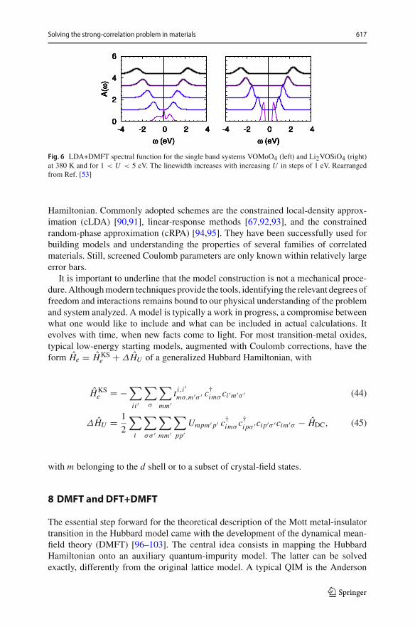
Fig. 7 Left: correlated band structure of VOMoO4 and Li2VOSiO4 for a realistic U = 5 eV, calculated at∼ 200 K. The dots are the poles of the Green function and yield the energy dispersion. Right: correspondingreal-axis self-energyΣ(ω). Reprintedfigurewith permission fromKiani andPavarini [53].Copyright (2016)by the American Physical Society
Hamiltonian
HQIM =∑
kσ
εsknkσ
︸ ︷︷ ︸Hbath
+∑
kσ
(V sk c
†kσ cdσ + h.c.
)
︸ ︷︷ ︸Hhyb
+ εd∑
σ
ndσ +Und↑nd↓︸ ︷︷ ︸
Himp
.
It describes a single correlated d impurity in a bath of non-interacting electrons s.The Anderson model was originally introduced to describe the Kondo effect in dilutedmetallic alloys [104–106]. Solution methods, approximated and numerically exact,were therefore already available when DMFT was introduced. The main differencewith respect to the single-impurity case is that inDMFT the parameters of the quantum-impurity model are not known from the start, but obtained via the self-consistencycondition, requiring that the quantum impurity self-energy is as close as possible tothe local self-energy of the original model. Non-local self-energy terms are neglected.DMFT is exact for U = 0, in the atomic limit, in the single-impurity limit, and, mostremarkably, in the infinite coordination number limit [96–99]. For realistic three-dimensional lattices it is an excellent approximation.
The success ofDMFT relies on the fact that it describes theMott paramagneticmetalto paramagnetic insulator transition, differently from all static mean-field approaches.This is shown in a representative case in Fig. 6 for two systems well described by
123
Solving the strong-correlation problem in materials 619
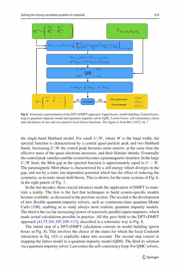
Fig. 8 Schematic representation of theDFT+DMFT approach. Upper boxes: model building. Central boxes:map to quantum impurity model and quantum impurity solver (QIS). Lower boxes: self-consistency checkand calculation of one and two-particle local Green functions. The figure is from Ref. [107], ch. 7
the single-band Hubbard model. For small U/W , where W is the band width, thespectral function is characterized by a central quasi-particle peak and two Hubbardbands. Increasing U/W the central peak becomes more narrow; at the same time theeffective mass of the quasi-electrons increases, and their lifetime shrinks. Eventuallythe central peak vanishes and the systembecomes a paramagnetic insulator. In the largeU/W limit, the Mott gap in the spectral function is approximately equal to U − W .The paramagnetic Mott phase is characterized by a self-energy which diverges in thegap, and not by a static site-dependent potential which has the effect of reducing thesymmetry, as in static mean-field theory. This is shown, for the same systems of Fig. 6,in the right panels of Fig. 7.
In the last decades, three crucial advances made the application of DMFT to mate-rials a reality. The first is the fact that techniques to build system-specific modelsbecame available, as discussed in the previous section. The second is the developmentof new flexible quantum-impurity solvers, such as continuous-time quantum MonteCarlo [108], enabling us to study always more realistic quantum impurity models.The third is the (so-far increasing) power of massively parallel supercomputers, whichmade actual calculations possible in practice. All this gave birth to the DFT+DMFTapproach [41,75,101,107,109–113], described in a schematic way in Fig. 8.
The initial step of a DFT+DMFT calculation consists in model building (greenboxes in Fig. 8). This involves the choice of the states for which the local Coulombinteraction in Eq. (43) is explicitly taken into account. The second step consist inmapping the lattice model to a quantum impurity model (QIM). The third its solutionvia a quantum impurity solver. Last comes the self-consistency loop. ForQMCsolvers,
123
620 E. Pavarini
0 500 1000
90o
150o
60o
180o
θ (D
MF
T)
T/K
R0
I0 R2.4800K
R6
R11
0 500 1000
90o
150o
60o
180o
θ (D
MF
T)
T/K
R0
I0 R2.4800K
R6
R11
0 500 1000
90o
150o
60o
180o
θ (D
MF
T)
T/K
R0
I0 R2.4800K
R6
R11
0 500 1000
90o
150o
60o
180o
θ (D
MF
T)
T/K
R0
I0 R2.4800K
R6
R11
0 500 1000
90o
150o
60o
180o
θ (D
MF
T)
T/K
R0
I0 R2.4800K
R6
R11
0 500 1000
90o
150o
60o
180o
θ (D
MF
T)
T/K
R0
I0 R2.4800K
R6
R11
0 500 1000
90o
150o
60o
180o
θ (D
MF
T)
T/K
R0
I0 R2.4800K
R6
R11
0 500 1000
90o
150o
60o
180o
θ (D
MF
T)
T/K
R0
I0 R2.4800K
R6
R11
0
1
0 500 1000
p (D
MF
T)
T/K
I0I0
I0I0 R0
R2.4800K
R6R11
0
1
0 500 1000
p (D
MF
T)
T/K
I0I0
I0I0 R0
R2.4800K
R6R11
0
1
0 500 1000
p (D
MF
T)
T/K
I0I0
I0I0 R0
R2.4800K
R6R11
0
1
0 500 1000
p (D
MF
T)
T/K
I0I0
I0I0 R0
R2.4800K
R6R11
0
1
0 500 1000
p (D
MF
T)
T/K
I0I0
I0I0 R0
R2.4800K
R6R11
0
1
0 500 1000
p (D
MF
T)
T/K
I0I0
I0I0 R0
R2.4800K
R6R11
0
1
0 500 1000
p (D
MF
T)
T/K
I0I0
I0I0 R0
R2.4800K
R6R11
0
1
0 500 1000
p (D
MF
T)
T/K
I0I0
I0I0 R0
R2.4800K
R6R11
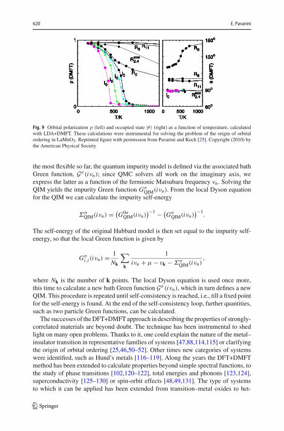
Fig. 9 Orbital polarization p (left) and occupied state |θ〉 (right) as a function of temperature, calculatedwith LDA+DMFT. These calculations were instrumental for solving the problem of the origin of orbitalordering in LaMnO3. Reprinted figure with permission from Pavarini and Koch [25]. Copyright (2010) bythe American Physical Society
the most flexible so far, the quantum impurity model is defined via the associated bathGreen function, Gσ (iνn); since QMC solvers all work on the imaginary axis, weexpress the latter as a function of the fermionic Matsubara frequency νn . Solving theQIM yields the impurity Green function Gσ
QIM(iνn). From the local Dyson equationfor the QIM we can calculate the impurity self-energy
ΣσQIM(iνn) = (
G0σQIM(iνn)
)−1 − (Gσ
QIM(iνn))−1
.
The self-energy of the original Hubbard model is then set equal to the impurity self-energy, so that the local Green function is given by
Gσi,i (iνn) = 1
Nk
∑
k
1
iνn + μ − εk − ΣσQIM(iνn)
,
where Nk is the number of k points. The local Dyson equation is used once more,this time to calculate a new bath Green function Gσ (iνn), which in turn defines a newQIM. This procedure is repeated until self-consistency is reached, i.e., till a fixed pointfor the self-energy is found. At the end of the self-consistency loop, further quantities,such as two particle Green functions, can be calculated.
The successes of theDFT+DMFTapproach in describing the properties of strongly-correlated materials are beyond doubt. The technique has been instrumental to shedlight on many open problems. Thanks to it, one could explain the nature of the metal–insulator transition in representative families of systems [47,88,114,115] or clarifyingthe origin of orbital ordering [25,46,50–52]. Other times new categories of systemswere identified, such as Hund’s metals [116–119]. Along the years the DFT+DMFTmethod has been extended to calculate properties beyond simple spectral functions, tothe study of phase transitions [102,120–122], total energies and phonons [123,124],superconductivity [125–130] or spin-orbit effects [48,49,131]. The type of systemsto which it can be applied has been extended from transition–metal oxides to het-
123
Solving the strong-correlation problem in materials 621
-2
0
2
Γ X M Γ
mU=0
-2
0
2
Γ X M Γ
ener
gy (
eV)
mU=0
Γ X M Γ
mU=0.5t
Γ X M Γ
mU=0.5t
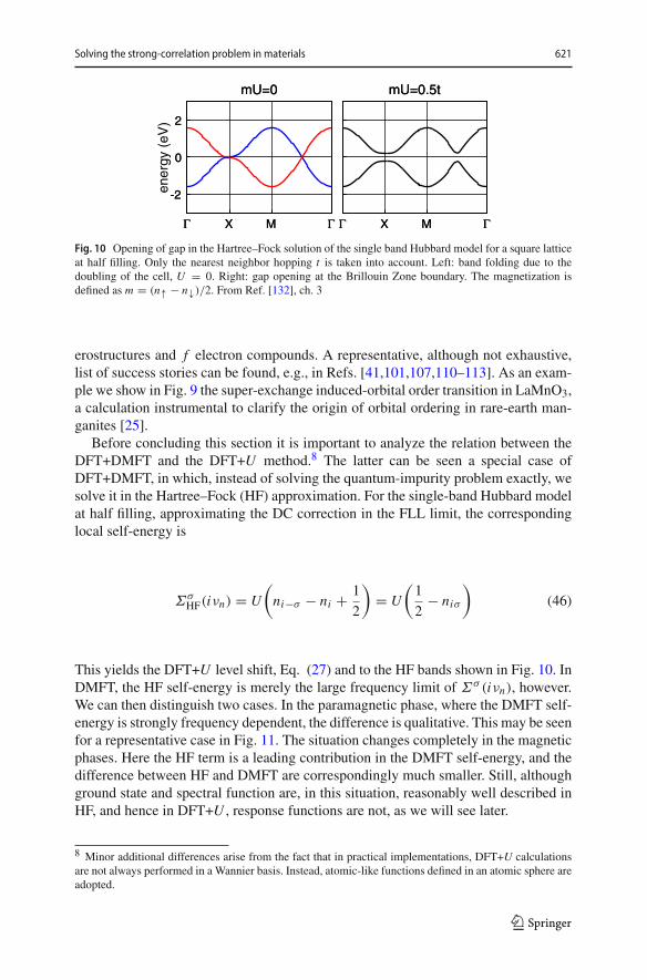
Fig. 10 Opening of gap in the Hartree–Fock solution of the single band Hubbard model for a square latticeat half filling. Only the nearest neighbor hopping t is taken into account. Left: band folding due to thedoubling of the cell, U = 0. Right: gap opening at the Brillouin Zone boundary. The magnetization isdefined as m = (n↑ − n↓)/2. From Ref. [132], ch. 3
erostructures and f electron compounds. A representative, although not exhaustive,list of success stories can be found, e.g., in Refs. [41,101,107,110–113]. As an exam-ple we show in Fig. 9 the super-exchange induced-orbital order transition in LaMnO3,a calculation instrumental to clarify the origin of orbital ordering in rare-earth man-ganites [25].
Before concluding this section it is important to analyze the relation between theDFT+DMFT and the DFT+U method.8 The latter can be seen a special case ofDFT+DMFT, in which, instead of solving the quantum-impurity problem exactly, wesolve it in the Hartree–Fock (HF) approximation. For the single-band Hubbard modelat half filling, approximating the DC correction in the FLL limit, the correspondinglocal self-energy is
ΣσHF(iνn) = U
(ni−σ − ni + 1
2
)= U
(1
2− niσ
)(46)
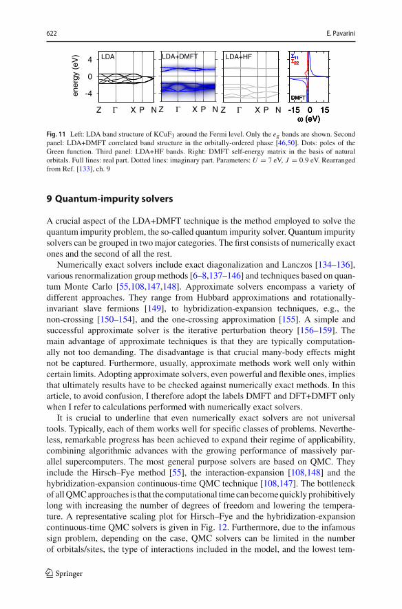
This yields the DFT+U level shift, Eq. (27) and to the HF bands shown in Fig. 10. InDMFT, the HF self-energy is merely the large frequency limit of Σσ (iνn), however.We can then distinguish two cases. In the paramagnetic phase, where the DMFT self-energy is strongly frequency dependent, the difference is qualitative. This may be seenfor a representative case in Fig. 11. The situation changes completely in the magneticphases. Here the HF term is a leading contribution in the DMFT self-energy, and thedifference between HF and DMFT are correspondingly much smaller. Still, althoughground state and spectral function are, in this situation, reasonably well described inHF, and hence in DFT+U , response functions are not, as we will see later.
8 Minor additional differences arise from the fact that in practical implementations, DFT+U calculationsare not always performed in a Wannier basis. Instead, atomic-like functions defined in an atomic sphere areadopted.
123
622 E. Pavarini
-4
0
4
Z Γ X P N
LDA
ene
rgy
(eV
)
Z Γ X P N
LDA+HF
Z Γ X P N
LDA+DMFT
-15 0 15
Σ11Σ22
DMFT
ω (eV)-15 0 15
Σ11Σ22
DMFT
ω (eV)-15 0 15
Σ11Σ22
DMFT
ω (eV)-15 0 15
Σ11Σ22
DMFT
ω (eV)
Fig. 11 Left: LDA band structure of KCuF3 around the Fermi level. Only the eg bands are shown. Secondpanel: LDA+DMFT correlated band structure in the orbitally-ordered phase [46,50]. Dots: poles of theGreen function. Third panel: LDA+HF bands. Right: DMFT self-energy matrix in the basis of naturalorbitals. Full lines: real part. Dotted lines: imaginary part. Parameters: U = 7 eV, J = 0.9 eV. Rearrangedfrom Ref. [133], ch. 9
9 Quantum-impurity solvers
A crucial aspect of the LDA+DMFT technique is the method employed to solve thequantum impurity problem, the so-called quantum impurity solver. Quantum impuritysolvers can be grouped in two major categories. The first consists of numerically exactones and the second of all the rest.
Numerically exact solvers include exact diagonalization and Lanczos [134–136],various renormalization groupmethods [6–8,137–146] and techniques based on quan-tum Monte Carlo [55,108,147,148]. Approximate solvers encompass a variety ofdifferent approaches. They range from Hubbard approximations and rotationally-invariant slave fermions [149], to hybridization-expansion techniques, e.g., thenon-crossing [150–154], and the one-crossing approximation [155]. A simple andsuccessful approximate solver is the iterative perturbation theory [156–159]. Themain advantage of approximate techniques is that they are typically computation-ally not too demanding. The disadvantage is that crucial many-body effects mightnot be captured. Furthermore, usually, approximate methods work well only withincertain limits. Adopting approximate solvers, even powerful and flexible ones, impliesthat ultimately results have to be checked against numerically exact methods. In thisarticle, to avoid confusion, I therefore adopt the labels DMFT and DFT+DMFT onlywhen I refer to calculations performed with numerically exact solvers.
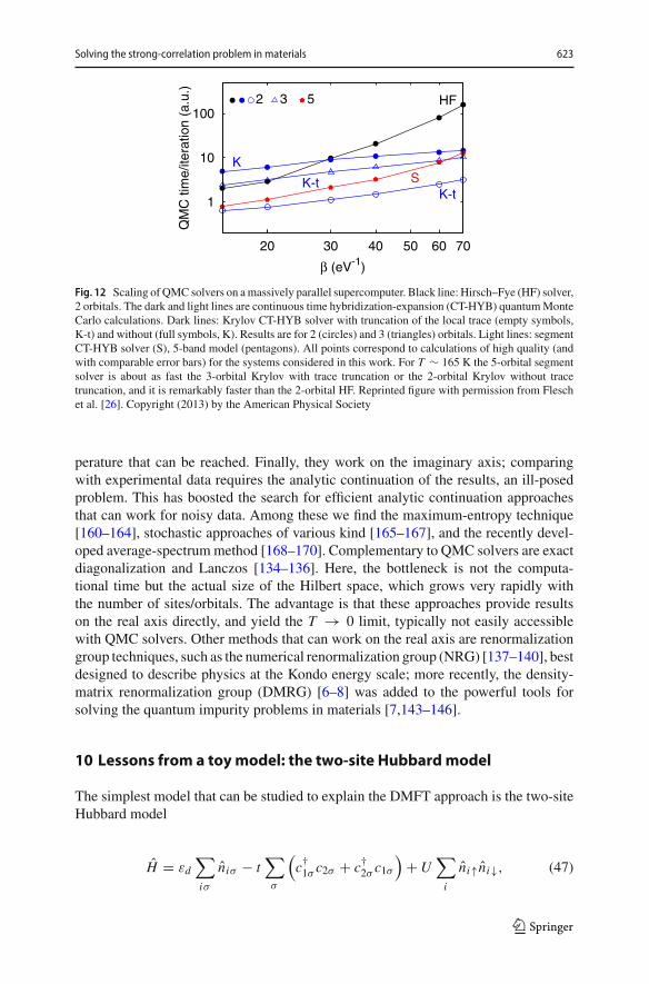
It is crucial to underline that even numerically exact solvers are not universaltools. Typically, each of them works well for specific classes of problems. Neverthe-less, remarkable progress has been achieved to expand their regime of applicability,combining algorithmic advances with the growing performance of massively par-allel supercomputers. The most general purpose solvers are based on QMC. Theyinclude the Hirsch–Fye method [55], the interaction-expansion [108,148] and thehybridization-expansion continuous-time QMC technique [108,147]. The bottleneckof allQMCapproaches is that the computational time canbecomequickly prohibitivelylong with increasing the number of degrees of freedom and lowering the tempera-ture. A representative scaling plot for Hirsch–Fye and the hybridization-expansioncontinuous-time QMC solvers is given in Fig. 12. Furthermore, due to the infamoussign problem, depending on the case, QMC solvers can be limited in the numberof orbitals/sites, the type of interactions included in the model, and the lowest tem-
123
Solving the strong-correlation problem in materials 623
1
10
100
20 30 40 50 60 70
QM
C ti
me/
itera
tion
(a.u
.)
β (eV-1)
HF
KS
2 3 5
K-tK-t
Fig. 12 Scaling of QMC solvers on amassively parallel supercomputer. Black line: Hirsch–Fye (HF) solver,2 orbitals. The dark and light lines are continuous time hybridization-expansion (CT-HYB) quantumMonteCarlo calculations. Dark lines: Krylov CT-HYB solver with truncation of the local trace (empty symbols,K-t) and without (full symbols, K). Results are for 2 (circles) and 3 (triangles) orbitals. Light lines: segmentCT-HYB solver (S), 5-band model (pentagons). All points correspond to calculations of high quality (andwith comparable error bars) for the systems considered in this work. For T ∼ 165 K the 5-orbital segmentsolver is about as fast the 3-orbital Krylov with trace truncation or the 2-orbital Krylov without tracetruncation, and it is remarkably faster than the 2-orbital HF. Reprinted figure with permission from Fleschet al. [26]. Copyright (2013) by the American Physical Society
perature that can be reached. Finally, they work on the imaginary axis; comparingwith experimental data requires the analytic continuation of the results, an ill-posedproblem. This has boosted the search for efficient analytic continuation approachesthat can work for noisy data. Among these we find the maximum-entropy technique[160–164], stochastic approaches of various kind [165–167], and the recently devel-oped average-spectrummethod [168–170]. Complementary to QMC solvers are exactdiagonalization and Lanczos [134–136]. Here, the bottleneck is not the computa-tional time but the actual size of the Hilbert space, which grows very rapidly withthe number of sites/orbitals. The advantage is that these approaches provide resultson the real axis directly, and yield the T → 0 limit, typically not easily accessiblewith QMC solvers. Other methods that can work on the real axis are renormalizationgroup techniques, such as the numerical renormalization group (NRG) [137–140], bestdesigned to describe physics at the Kondo energy scale; more recently, the density-matrix renormalization group (DMRG) [6–8] was added to the powerful tools forsolving the quantum impurity problems in materials [7,143–146].
10 Lessons from a toymodel: the two-site Hubbardmodel
The simplest model that can be studied to explain the DMFT approach is the two-siteHubbard model
H = εd∑
iσ
niσ − t∑
σ
(c†1σ c2σ + c†2σ c1σ
)+U
∑
i
ni↑ni↓, (47)
123

624 E. Pavarini
0
10
-5 0 5
exact H
A(ω
)
ω /t
d2→ d1+
d2→ d1-
d3+→ d2
d3-→ d2
-5 0 5
k=πk=0
ω /t-5 0 5
k=πk=0
ω /t
Fig. 13 Spectral function of the Hubbard dimer (H) forU/t = 3. Local (left), k = 0, π (right). It is obtainedfromEq. (52), setting νn −→ ω+iδ, where δ → 0. The spectral function exhibits four peaks, correspondingto the four poles of the Green function. The associated weights are: w+ = (1 + w(t,U ))/4 for the pole atenergies EG (2)−E−(1)−μ and the one at energy E−(3)−EG (2)−μ, and w− = (1− w(t,U ))/4 for theremaining two, at energies EG (2)−E+(1)−μ and E+(3)−EG (2)−μ. Figure rearranged from Ref. [107],ch. 7
with i = 1, 2. For N = 2 electrons (half filling) the ground state of this Hamiltonianis the singlet
|G〉H = a2(t,U )√2
(c†1↑c
†2↓ − c†1↓c
†2↑
)|0〉 + a1(t,U )√
2
(c†1↑c
†1↓ + c†2↑c
†2↓
)|0〉 (48)
The prefactors are given by
a21(t,U ) = 1
Δ(t,U )
Δ(t,U ) −U
2, a22(t,U ) = 4t2
Δ(t,U )
2
Δ(t,U ) −U, (49)
where
Δ(t,U ) =√U 2 + 16t2. (50)
The associated ground-state energy is
EG(2) = 2εd + 1
2
(U − Δ(t,U )
). (51)
The eigenvalues for Ne = 1 and Ne = 3 electrons are instead
E±(1) = εd ± t
E±(3) = 3εd ± t +U
In the T → 0 limit, the local Matsubara Green function for spin σ (see Fig. 13 for theassociated spectral function) is then the sum of four terms
Gσi,i (iνn)=
w+iνn − (EG(2) − E−(1)−μ)
+ w−iνn − (
EG(2) − E+(1)−μ)
+ w−iνn−
(− EG(2)+E+(3)−μ)+ w+
iνn−(− EG(2)+E−(3)−μ
) , (52)
123

Solving the strong-correlation problem in materials 625
where νn = π(2n+1)/β are fermionic Matsubara frequencies, the chemical potentialis μ = εd +U/2, and
w± = 1 ± w(t,U )
4(53)
w(t,U ) = 2a1(t,U )a2(t,U ). (54)
This can be rewritten as the average of the Green function for the bonding (k = 0)and the anti-bonding (k = π) state, i.e.,
Gσi,i (iνn) = 1
2
(1
iνn + μ − εd + t − Σσ (0, iνn)︸ ︷︷ ︸Gσ (0,iνn)
+ 1
iνn + μ − εd − t − Σσ (π, iνn)︸ ︷︷ ︸Gσ (π,iνn)
).
(55)
The k-dependent self-energy is given by
Σσ (k, iνn) =U
2+ U 2
4
1
iνn + μ − εd − U2 − eik 3t
. (56)
The local self-energy is, by definition, the k-average
Σσl (iνn) = Σσ
i,i (iνn) = 1
2
(Σσ (π, iνn)+Σσ (0, iνn)
)
= U
2+U 2
4
iνn + μ − εd − U2
(iνn + μ − εd − U2 )2 − (3t)2
. (57)
The difference
ΔΣσl (iνn) = 1
2
(Σσ (π, iνn)−Σσ (0, iνn)
)
= U 2
4
3t
(iνn + μ − εd − U2 )2 − (3t)2
, (58)
is the non-local part of the self-energy. The local Green function can then be expressedin the form
Gσi,i (iνn) = 1
iνn + μ − εd − Fσ (iνn) − Σσl (iνn)
, (59)
where
Fσ (iνn) =(t + ΔΣσ
l (iνn))2
iνn + μ − εd − Σσl (iνn)
(60)
123
626 E. Pavarini
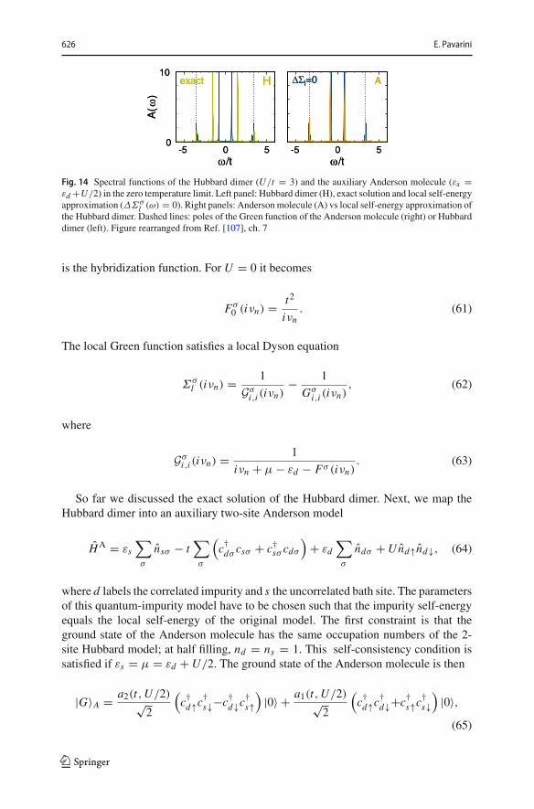
0
10
-5 0 5
exact H
A(ω
)ω /t
0
10
-5 0 5
exact H
A(ω
)ω /t
-5 0 5
AΔΣl=0
ω /t-5 0 5
AΔΣl=0
ω /t
Fig. 14 Spectral functions of the Hubbard dimer (U/t = 3) and the auxiliary Anderson molecule (εs =εd +U/2) in the zero temperature limit. Left panel: Hubbard dimer (H), exact solution and local self-energyapproximation (ΔΣσ
l (ω) = 0). Right panels: Andersonmolecule (A) vs local self-energy approximation ofthe Hubbard dimer. Dashed lines: poles of the Green function of the Anderson molecule (right) or Hubbarddimer (left). Figure rearranged from Ref. [107], ch. 7
is the hybridization function. For U = 0 it becomes
Fσ0 (iνn) = t2
iνn. (61)
The local Green function satisfies a local Dyson equation
Σσl (iνn) = 1
Gσi,i (iνn)
− 1
Gσi,i (iνn)
, (62)
where
Gσi,i (iνn) = 1
iνn + μ − εd − Fσ (iνn). (63)
So far we discussed the exact solution of the Hubbard dimer. Next, we map theHubbard dimer into an auxiliary two-site Anderson model
HA = εs∑
σ
nsσ − t∑
σ
(c†dσ csσ + c†sσ cdσ
)+ εd
∑
σ
ndσ +Und↑nd↓, (64)
where d labels the correlated impurity and s the uncorrelated bath site. The parametersof this quantum-impurity model have to be chosen such that the impurity self-energyequals the local self-energy of the original model. The first constraint is that theground state of the Anderson molecule has the same occupation numbers of the 2-site Hubbard model; at half filling, nd = ns = 1. This self-consistency condition issatisfied if εs = μ = εd +U/2. The ground state of the Anderson molecule is then
|G〉A = a2(t,U/2)√2
(c†d↑c
†s↓−c†d↓c
†s↑
)|0〉 + a1(t,U/2)√
2
(c†d↑c
†d↓+c†s↑c
†s↓
)|0〉,(65)
123
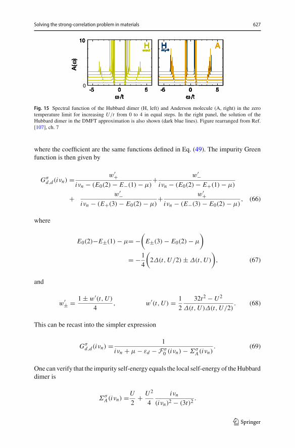
Solving the strong-correlation problem in materials 627
0
10
-5 0 5
exactH
A(ω
)
ω /t
10
-5 0 5
exactH
A(ω
)
ω /t
10
-5 0 5
exactH
A(ω
)
ω /t
10
-5 0 5
exactH
A(ω
)
ω /t
10
-5 0 5
exactH
A(ω
)
ω /t
10
-5 0 5
exactH
A(ω
)
ω /t-5 0 5
AHΔΣl=0
ω /t-5 0 5
AHΔΣl=0
ω /t-5 0 5
AHΔΣl=0
ω /t-5 0 5
AHΔΣl=0
ω /t-5 0 5
AHΔΣl=0
ω /t-5 0 5
AHΔΣl=0
ω /t-5 0 5
AHΔΣl=0
ω /t-5 0 5
AHΔΣl=0
ω /t-5 0 5
AHΔΣl=0
ω /t-5 0 5
AHΔΣl=0
ω /t-5 0 5
AHΔΣl=0
ω /t-5 0 5
AHΔΣl=0
ω /t
Fig. 15 Spectral function of the Hubbard dimer (H, left) and Anderson molecule (A, right) in the zerotemperature limit for increasing U/t from 0 to 4 in equal steps. In the right panel, the solution of theHubbard dimer in the DMFT approximation is also shown (dark blue lines). Figure rearranged from Ref.[107], ch. 7
where the coefficient are the same functions defined in Eq. (49). The impurity Greenfunction is then given by
Gσd,d(iνn) = w′+
iνn − (E0(2) − E−(1) − μ)+ w′−iνn − (E0(2) − E+(1) − μ)
+ w′−iνn − (E+(3) − E0(2) − μ)
+ w′+iνn − (E−(3) − E0(2) − μ)
, (66)
where
E0(2)−E±(1) − μ= −(E±(3) − E0(2) − μ
)
= −1
4
(2Δ(t,U/2) ± Δ(t,U )
), (67)
and
w′± = 1 ± w′(t,U )
4, w′(t,U ) = 1
2
32t2 −U 2
Δ(t,U )Δ(t,U/2). (68)
This can be recast into the simpler expression
Gσd,d(iνn) = 1
iνn + μ − εd − Fσ0 (iνn) − Σσ
A(iνn). (69)
One can verify that the impurity self-energy equals the local self-energy of theHubbarddimer is
ΣσA(iνn) =U
2+ U 2
4
iνn(iνn)2 − (3t)2
.
123
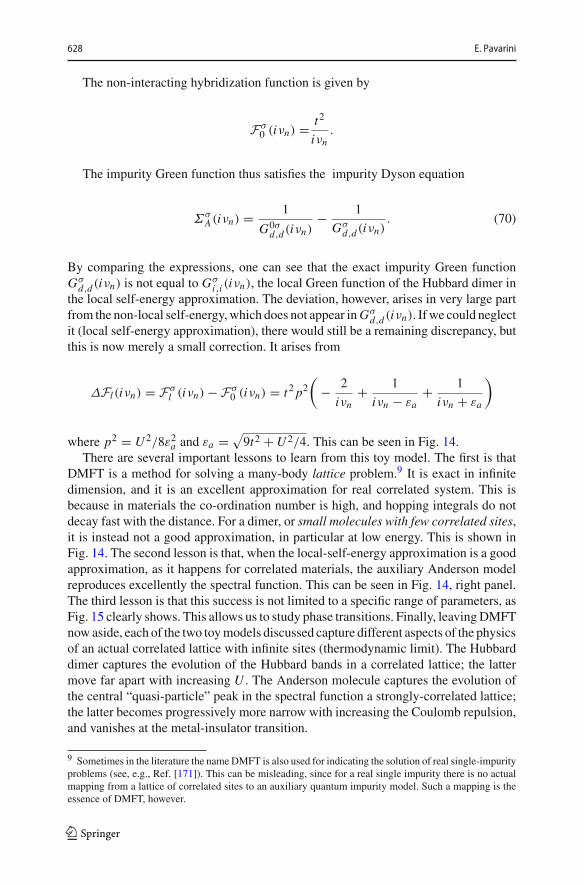
628 E. Pavarini
The non-interacting hybridization function is given by
Fσ0 (iνn) = t2
iνn.
The impurity Green function thus satisfies the impurity Dyson equation
ΣσA(iνn) = 1
G0σd,d(iνn)
− 1
Gσd,d(iνn)
. (70)
By comparing the expressions, one can see that the exact impurity Green functionGσ
d,d(iνn) is not equal to Gσi,i (iνn), the local Green function of the Hubbard dimer in
the local self-energy approximation. The deviation, however, arises in very large partfrom the non-local self-energy,which does not appear inGσ
d,d (iνn). If we could neglectit (local self-energy approximation), there would still be a remaining discrepancy, butthis is now merely a small correction. It arises from
ΔFl(iνn) = Fσl (iνn) − Fσ
0 (iνn) = t2 p2(
− 2
iνn+ 1
iνn − εa+ 1
iνn + εa
)
where p2 = U 2/8ε2a and εa = √9t2 +U 2/4. This can be seen in Fig. 14.
There are several important lessons to learn from this toy model. The first is thatDMFT is a method for solving a many-body lattice problem.9 It is exact in infinitedimension, and it is an excellent approximation for real correlated system. This isbecause in materials the co-ordination number is high, and hopping integrals do notdecay fast with the distance. For a dimer, or small molecules with few correlated sites,it is instead not a good approximation, in particular at low energy. This is shown inFig. 14. The second lesson is that, when the local-self-energy approximation is a goodapproximation, as it happens for correlated materials, the auxiliary Anderson modelreproduces excellently the spectral function. This can be seen in Fig. 14, right panel.The third lesson is that this success is not limited to a specific range of parameters, asFig. 15 clearly shows. This allows us to study phase transitions. Finally, leavingDMFTnowaside, each of the two toymodels discussed capture different aspects of the physicsof an actual correlated lattice with infinite sites (thermodynamic limit). The Hubbarddimer captures the evolution of the Hubbard bands in a correlated lattice; the lattermove far apart with increasing U . The Anderson molecule captures the evolution ofthe central “quasi-particle” peak in the spectral function a strongly-correlated lattice;the latter becomes progressively more narrow with increasing the Coulomb repulsion,and vanishes at the metal-insulator transition.
9 Sometimes in the literature the name DMFT is also used for indicating the solution of real single-impurityproblems (see, e.g., Ref. [171]). This can be misleading, since for a real single impurity there is no actualmapping from a lattice of correlated sites to an auxiliary quantum impurity model. Such a mapping is theessence of DMFT, however.
123
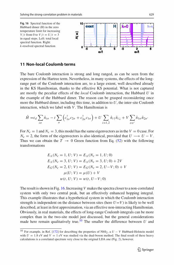
Solving the strong-correlation problem in materials 629
Fig. 16 Spectral function of theHubbard dimer (H) in the zerotemperature limit for increasingV /t from 0 to V /t = U/t = 3in equal steps. Left: total localspectral function. Right:k-resolved spectral function 0
10
-5 0 5
exact H
A(ω
)
ω /t 0
10
-5 0 5
exact H
A(ω
)
ω /t 0
10
-5 0 5
exact H
A(ω
)
ω /t 0
10
-5 0 5
exact H
A(ω
)
ω /t 0
10
-5 0 5
exact H
A(ω
)
ω /t 0
10
-5 0 5
exact H
A(ω
)
ω /t 0
10
-5 0 5
exact H
A(ω
)
ω /t-5 0 5
k=πk=0
ω /t-5 0 5
k=πk=0
ω /t-5 0 5
k=πk=0
ω /t-5 0 5
k=πk=0
ω /t-5 0 5
k=πk=0
ω /t-5 0 5
k=πk=0
ω /t-5 0 5
k=πk=0
ω /t-5 0 5
k=πk=0
ω /t-5 0 5
k=πk=0
ω /t-5 0 5
k=πk=0
ω /t-5 0 5
k=πk=0
ω /t-5 0 5
k=πk=0
ω /t-5 0 5
k=πk=0
ω /t-5 0 5
k=πk=0
ω /t
11 Non-local Coulomb terms
The bare Coulomb interaction is strong and long ranged, as can be seen from theexpression of the Hartree term. Nevertheless, in many systems, the effects of the long-range part of the Coulomb interaction are, to a large extent, well described alreadyin the KS Hamiltonian, thanks to the effective KS potential. What is not capturedare mostly the peculiar effects of the local Coulomb interaction, the Hubbard U inthe example of the Hubbard dimer. The reason can be grasped reconsidering oncemore the Hubbard dimer, including this time, in addition toU , the inter-site Coulombinteraction, which we label with V . The Hamiltonian is
H =εd∑
iσ
niσ − t∑
σ
(c†1σ c2σ + c†2σ c1σ
)+U
∑
i=1,2
ni↑ni↓ + V∑
σσ ′n1σ n2σ ′
For Ne = 1 and Ne = 3, thismodel has the same eigenvectors as in the V = 0 case. ForNe = 2, the form of the eigenvectors is also identical, provided that U −→ U − V .Thus we can obtain the T → 0 Green function from Eq. (52) with the followingtransformations
E±(Ne = 1,U ; V ) = E±(Ne = 1,U ; 0)E±(Ne = 3,U ; V ) = E±(Ne = 3,U ; 0) + 2V
EG(Ne = 2,U ; V ) = EG(Ne = 2,U−V ; 0) + V
μ(U ; V ) = μ(U ) + V
w(t,U ; V ) = w(t,U−V ; 0)
The result is shown inFig. 16. IncreasingV makes the spectra closer to a non-correlatedsystem with only two central peak, but an effectively enhanced hopping integral.This example illustrates that a hypothetical system in which the Coulomb interactionstrength is independent on the distance between sites (here U=V ) is likely to be welldescribed, at least in first approximation, via an effective non-interacting Hamiltonian.Obviously, in real materials, the effects of long-range Coulomb integrals can be morecomplex than in the two-site model just discussed, but the general considerationsmade here remain qualitatively true.10 The smaller the difference between U and
10 For example, in Ref. [172] for describing the properties of NbS2, a U − V Hubbard-Holstein modelwith U = 1.8 eV and V = 1 eV was studied via the dual-boson method. The final result of these heavycalculations is a correlated spectrum very close to the original LDA one (Fig. 2), however.
123
630 E. Pavarini
longer range terms, the less strongly-correlated the system is. V-type Coulomb termscan be taken into account in DMFT, e.g., via the E-DMFT extension [173,174].
12 Linear response functions
Linear response functions can be obtained in DFT+DMFT in two steps. First the localsusceptibility χ(iωm) is calculated solving the quantum-impurity problem. This canbe done at the end of the self-consistency loop, as shown in Fig. 8. Calculating χ(iωm)
is a much harder task than calculating single-particle Green functions, in particularbecause one needs to compute the full three-frequency tensor χ(iωm; iνn, iνn′). Oncethis is done, the Bethe–Salpeter (BS) equation has to be solved
χ(q; iωm) = χ0(q; iωm) + χ0(q; iωm)Γ (q; iωm)χ(q; iωm). (71)
TheBS equation is known from standardmany-body perturbation theory. InDMFT the“bubble” term χ0(q; iωm) is obtained however using the DMFT Green function as thepropagator. The next step consist in finding approximations for the vertex Γ (q; iωm),which is unknown. In the infinite coordination limit, the vertex can however be replacedby a local quantity [102,103,175]
Γ (q; iωm) −→ Γ (iωm).
This leads to the modified BS equation
χ(q; iωm) = χ0(q; iωm) + χ0(q; iωm)Γ (iωm)χ(q; iωm). (72)
By solving Eq. (72) we find, formally
χ−1(q; iωm) = χ−10 (q; iωm) − Γ (iωm). (73)
The local vertex can be obtained from Eq. (73), however replacing all quantities withtheir local counterparts
Γ (iωm) = χ−10 (iωm) − χ−1(iωm). (74)
Despite its apparent simplicity, solving the BS equation, even in the local vertexapproximation, is a delicate task in practice. It involves the inversion of, in principle,infinite-dimensionmatrices. This can be seen from the analytic formula of themagneticsusceptibility of the Hubbard model in the atomic limit [53,176,177]
χzz(iωm; 0) =∑
σσ ′σσ ′ χn,n′
iσσ,iσ ′σ ′(0)
= Mn′dMn
dy+ Mn
dMn′
dy
123
Solving the strong-correlation problem in materials 631
− βn(y)
[δn,n′ + δn,−n′
]dMn
dy+ βn(−y)MnMn′
− 1
y
{Mn′ − β
[n(y)δn,−n′ − n(−y)δn,n′
]}Mn (75)
where
Mn = 1
iνn − y− 1
iνn + y, (76)
and n, n′ are fermionic Matsubara frequencies. The expression (75) evidences theslow decay in the fermionic frequencies, in particular along the diagonals n = n′ andn = −n′. Only summing up all fermionic Matsubara frequencies one recovers theexpression
χzz(iωm) = δm,0n(−U/2)
4kBT(77)
where n(x) is the Fermi distribution function. To complicate thematter, in actual mate-rials the susceptibility tensor depends on the flavors (spin, site, orbitals) associatedwith the four (creation and annihilation) operators entering the expression of the gen-eralized correlation function [176]. It is thus important to exploit symmetries and findcompact representations, in order to reduce both truncation errors and computationaltime. More compact representation are based on polynomial expansions, for exampleLegendre polynomials [178].
In order to better explain how susceptibilities are calculated in DMFT we makefurther use of the toy model previously introduced, the two-site Hubbard model, andcalculate themagnetic susceptibility in this case. For simplicity we perform in advanceall sums over fermionic Matsubara frequencies, so that only the bosonic frequencyωm remains. The site-dependent components, defined in imaginary time as
χi jzz(τ ) =〈T Siz(τ )S j
z (0)〉 − 〈T Siz(τ )〉〈T S jz (0)〉, (78)
where T is the time-ordering operator and τ the imaginary time. The total magneticsusceptibility is
χzz(q; iωm) = 1
Ns
∑
i j
∫ β
0dτeiωmτ χ
i jzz(τ )e−iq·(Ri−R j ) (79)
whereRi are vectors identifying the Ns = 2 atomic sites; the only possibleq values arehere 0 andπ , as we have already seen. The first step consists in calculating the impuritysusceptibility for the (self-consistent) auxiliarymodel, theAndersonmolecule. For thisis necessary to consider not only the ground state, Eq. (65), but also the excited triplet
123
632 E. Pavarini
states, with energy ET . They are given by
|1, 0〉A = 1√2
[c†d↑c
†s↓ − c†d↓c
†s↑
]|0〉 (80)
|1, 1〉A =c†d↑c†s↑|0〉 (81)
|1,−1〉A =c†d↓c†s↓|0〉. (82)
At sufficiently low temperature higher energy states can be neglected. We define theenergy difference ET = EG + EX with
EX = −1
4
[U − 2Δ(t,U/2)
]= U
4
[− 1 +
√1 + 16ΓSE
U
]. (83)
For sufficiently small ΓSE/U one then finds
χzz(iωm) ∼ 1 − e−βEX
4Z
(1
iωm + EX− 1
iωm − EX
)+ δm,0β
e−βEX
2Z
where Z ∼ 1 + 3e−βEX . At high temperature this becomes
χzz(0) ∼ 1
4βδm,0, (84)
which is the atomic limit susceptibility. Next we have to calculate the DMFT bubbleterm. The latter can be written as
χ0zz(q; iωm) = −(gμB)2
1
4
∑
σ
1
β
∑
n
1
Nk
∑
k
Gkσ (iνn)Gkσ (iνn + iωm), (85)
where Gkσ (iνn) is the DMFT Green function. Decomposing all the products of polesin sums of single poles, this can be recast into [53,176,177,179]
χ0zz(iωm;q) = (gμB)2
1
2
1
Nk
∑
k
(− I++
k,q − I−−k,q + I+−
k,q + I−+k,q
). (86)
The addends are defined as
I αγ
k,q = Eαk E
γ
k+q
(E+k − E−
k )(E+k+q − E−
k+q)
n(Eαk ) − n(Eγ
k+q)
Eαk − Eγ
k+q + iωm. (87)
The energies are
E±k = 1
2εk ± 1
2
√ε2k +U 2, (88)
123
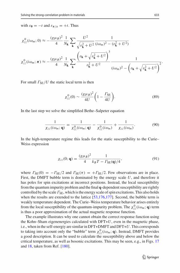
Solving the strong-correlation problem in materials 633
with ε0 = −t and επ/a = +t . Thus
χ0zz(iωm; 0) ≈ − (gμB)2
4
1
Nk
∑
k
U 2√
ε2k +U 2
1
(iωm)2 − (ε2k +U 2)
χ0zz(iωm;π) ≈ − (gμB)2
4
1
Nk
∑
k
(εk +
√ε2k +U 2
)3
ε2k +U 2
1
(iωm)2 −(
εk +√
ε2k +U 2
)2 .
For small ΓSE/U the static local term is then
χ0zz(0) ∼ (gμB)2
4U
(1 − ΓSE
4U
). (89)
In the last step we solve the simplified Bethe–Salpeter equation
1
χzz(iωm;q)= 1
χ0zz(iωm;q)
− 1
χ0zz(iωm)
+ 1
χzz(iωm). (90)
In the high-temperature regime this leads for the static susceptibility to the Curie–Weiss expression
χzz(0;q) = (gμB)2
4
1
kBT − ΓSE(q)/4, (91)
where ΓSE(0) = −ΓSE/2 and ΓSE(π) = +ΓSE/2. Few observations are in place.First, the DMFT bubble term is dominated by the energy scale U , and therefore ithas poles for spin excitations at incorrect positions. Instead, the local susceptibilityfrom the quantum impurity problem and the finalq-dependent susceptibility are rightlycontrolledby the scaleΓSE,which is the energy scale of spin excitations.This alsoholdswhen the results are extended to the lattice [53,176,177]. Second, the bubble term isweakly temperature dependent. The Curie–Weiss temperature behavior arises entirelyfrom the local susceptibility of the quantum-impurity problem. The χ0
zz(iωm;q) termis thus a poor approximation of the actual magnetic response function.
The example illustrates why one cannot obtain the correct response function usingthe Kohn–Sham eigenenergies calculated with DFT+U , even in the magnetic phase,i.e., when in the self-energiy are similar inDFT+DMFTandDFT+U . This correspondsto taking into account only the “bubble” term χ0
zz(iωm;q). Instead, DMFT providesa good description. It can be used to calculate the susceptibility above and below thecritical temperature, as well as bosonic excitations. This may be seen, e.g., in Figs. 17and 18, taken from Ref. [180].
123
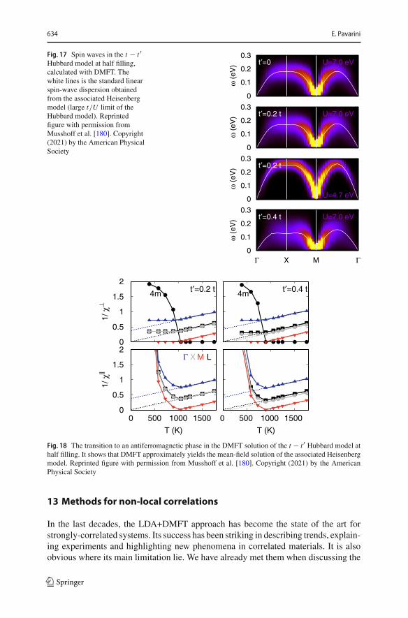
634 E. Pavarini
Fig. 17 Spin waves in the t − t ′Hubbard model at half filling,calculated with DMFT. Thewhite lines is the standard linearspin-wave dispersion obtainedfrom the associated Heisenbergmodel (large t/U limit of theHubbard model). Reprintedfigure with permission fromMusshoff et al. [180]. Copyright(2021) by the American PhysicalSociety
t′=0 U=7.0 eV
0
0.1
0.2
0.3
ω (
eV) t′=0 U=7.0 eV
t′=0.2 t U=7.0 eV
0
0.1
0.2
0.3
ω (
eV) t′=0.2 t U=7.0 eV
t′=0.2 t
U=4.7 eV 0
0.1
0.2
0.3
ω (
eV) t′=0.2 t
U=4.7 eV
t′=0.4 t U=7.0 eV
Γ X M Γ 0
0.1
0.2
0.3
ω (
eV) t′=0.4 t U=7.0 eV
0
0.5
1
1.5
2 t′=0.2 t4m
1/ χ
⊥
t′=0.4 t4m
0
0.5
1
1.5
2
0 500 1000 1500
Γ LX M
1/ χ
||
T (K)
0 500 1000 1500
T (K)
Fig. 18 The transition to an antiferromagnetic phase in the DMFT solution of the t − t ′ Hubbard model athalf filling. It shows that DMFT approximately yields the mean-field solution of the associated Heisenbergmodel. Reprinted figure with permission from Musshoff et al. [180]. Copyright (2021) by the AmericanPhysical Society
13 Methods for non-local correlations
In the last decades, the LDA+DMFT approach has become the state of the art forstrongly-correlated systems. Its success has been striking in describing trends, explain-ing experiments and highlighting new phenomena in correlated materials. It is alsoobvious where its main limitation lie. We have already met them when discussing the
123
Solving the strong-correlation problem in materials 635
toy model, the two-site Hubbard model. Non-local correlations are not captured by alocal self-energy. Still, here one should make a distinction. Long-range ordered phasesthemselves can be well described in single-site DMFT, simply using supercells. A dif-ferent story is the description of non-local effects in phase transitions. In such a case,DMFT gives basically the static mean-field critical exponents, i.e., the Curie–Weisslaw. This is shown for a representative case in Fig. 18. Straightforward extensionsthat go beyond DMFT are cellular dynamical mean-field theory and the dynamicalcluster approximation [122].With cluster approaches it is possible to recover the exactcritical behavior, but the cluster size required might be very large, depending on theproblem analyzed and the type of clusters used. This is shown in Refs. [122,181] forthe two-dimensional Hubbard model. The example chosen is an extreme case sincethe exact TN is zero due to the Mermin–Wagner theorem, while at the same time theco-ordination number is relatively small. Still, even in three-dimensional materials alarge cluster sizemight be necessary, depending on the case, for accurately reproducingthe details of phase transitions. Alternatives to cluster approaches are diagrammaticmethods, such as the GW+DMFT approach [182], the dynamical-vertex approxima-tion [183,184], or the dual-fermion technique [185–187].
14 Conclusion
In this short article, I introduced some of the modern methods for studying strongcorrelations in materials. I emphasized successes and shortcomings of the currentstate-of-the art approaches, and briefly discussed developments that could play animportant role in the future. The article is a personal view of a field in evolution, ofwhich snapshots have been captured. More detailed descriptions of specific aspects,solvers and applications can be found, e.g., in Refs. [41,107,108,110–113,122].
In this conclusion, I would like to underline few points. The impressive progressachieved in the last decades in the description of correlation effects in materials relieson schemes which, instead of solving the full many-body Hamiltonian, solve low-energy materials-specific models. The latter are built to capture both the essence ofthe mechanisms at play and the key specific characteristics which distinguish a sys-tem from the others. Furthermore, these models are solvable, if not exactly withinvery good approximations. This successful strategy combines the best of many-bodyphysics and ab-initio approaches—overcoming the historical dichotomy between thetwo. Anderson, had once coined the ironical expression “the great solid-state physicsdream machine” when referring to DFT-based first principlesmethods [24]. The maincriticism was that, in a many-body system, it is extremely hard to predict truly novelemergent properties—and indeed it rarely happens. Methods like DFT+DMFT andits extensions, although not fully ab-initio, give us the impression that eventuallyreductionism could win.
Even in the best case scenario, this will always be true only in a limited sense,however. Traditional ab-initio methods show us the nature of the restriction. UsingKohn–Shameigenvalues for interpreting experiments implies a stark assumptionon theform of the model and on the type of phenomena described. State-of-the-art methodsfor correlated systems allow us to study a vast variety of new systems and phenomena,
123
636 E. Pavarini
and have been instrumental to clarify several open problems. They are becomingprogressively more powerful, slowly but steadily approaching predictive power. Still,they suffer from the same core problem—they do not exhaust all the possibilitiesin a many-electron system. If something truly new is found, we have to return to thebasics—trying first to guess and solve the basicmodel, and only thenmake itmaterials-specific. In fact, despite all progress, even old fundamental problems remain unsettled,not least the nature of superconductivity in cuprates.
Finally, we have seen that together with theoretical progress and algorithmicadvances, the advent of massively parallel supercomputers was crucial to study real-istic models in practice. And yet, the exponential growth of the Hilbert space poseslimit on what can be done with a classical computer. In the future, quantum computershold the promise to bring a new revolution for the description of strongly correlatedsystems. If this promise is realized, we will be able to tackle always more complexproblems. Still, numerical calculations alone will never be sufficient. A simulationthat exactly reproduce the world will not give us, alone, more information then exper-iments themselves. The final frontier will always be the understanding, disentanglingthe crucial aspects from all the rest. In that respect, the many-body problem and itsemergent phenomena should keep us busy for a long time to come.
Acknowledgements ComputationalGrants on JURECAand JUWELSat the JülichSupercomputingCentreand the RWTH Aachen computer cluster are acknowledged. This article is based on several lectures I gavefor the Autumn School on Correlated Electrons at the Forschungszentrum Jülich along the years. Moredetails on specific topics as well as derivations of formulas can be found in the lecture notes of the school.
Funding Open Access funding enabled and organized by Projekt DEAL.
OpenAccess This article is licensedunder aCreativeCommonsAttribution 4.0 InternationalLicense,whichpermits use, sharing, adaptation, distribution and reproduction in any medium or format, as long as you giveappropriate credit to the original author(s) and the source, provide a link to the Creative Commons licence,and indicate if changes were made. The images or other third party material in this article are includedin the article’s Creative Commons licence, unless indicated otherwise in a credit line to the material. Ifmaterial is not included in the article’s Creative Commons licence and your intended use is not permittedby statutory regulation or exceeds the permitted use, you will need to obtain permission directly from thecopyright holder. To view a copy of this licence, visit http://creativecommons.org/licenses/by/4.0/.
References
1. P.W. Anderson, Science 177, 393 (1972)2. R.J. Bartlett, M. Musiał, Rev. Mod. Phys. 79, 291 (2007)3. G.H. Booth, A.J.W. Thom, A. Alavi, J. Chem. Phys. 131, 054106 (2009)4. A.A. Holmes, N.M. Tubman, C.J. Umrigar, J. Chem. Theory Comput. 12, 3674 (2016)5. I.Y. Zhang, A. Grüneis, Front. Mater. 6, 123 (2019)6. S. White, Phys. Rev. Lett. 69, 2863 (1992)7. K. Hallberg, Adv. Phys. 55, 477 (2006)8. U. Schollwöck, Ann. Phys. 326, 96 (2011)9. S.R. White, R.L. Martin, J. Chem. Phys. 110, 4127 (1999)10. S. Woutersa, D. Van Neck, Eur. Phys. J. D 68, 272 (2014)11. T. Yanai, Y. Kurashige, W. Mizukami, J. Chalupsk, T. Nguyen Lan, M. Saitow, Int. J. Quant. Chem.
115, 283 (2015)12. G.K.-L. Chan, S. Sharma, Ann. Rev. Phys. Chem. 62, 465 (2011)13. K.F. Sundman, Acta Math. 36, 105 (1912)
123
Solving the strong-correlation problem in materials 637
14. Q. Wang, Celest. Mech. 50, 73 (1991)15. F. Diacu, Math. Intell. 18, 66 (1996)16. P. Hohenberg, W. Kohn, Phys. Rev. 136, B864 (1964)17. W. Kohn, L.J. Sham, Phys. Rev. 140, A1133 (1965)18. W. Kohn, Nobel lecture: electronic structure of matter, wave functions and density functionals. Rev.
Mod. Phys. 71, 1253 (1998)19. U. von Barth, Phys. Scr. 109, 9 (2004)20. R.M. Dreizler, E.K.U. Gross, Density-Functional Theory (Springer, Berlin, 1990)21. R.G. Parr, Y. Weitao, Density-Functional Theory of Atoms and Molecules (Oxford University Press,
Oxford, 1994)22. R.M.Martin,Electronic Structure, Basic Theory andPracticalMethods (CambridgeUniversity Press,
Cambridge, 2004)23. R.O. Jones, O. Gunnarsson, Rev. Mod. Phys. 61, 689 (1989)24. R.O. Jones in Ref. [188]25. E. Pavarini, E. Koch, Phys. Rev. Lett. 104, 086402 (2010)26. A. Flesch, E. Gorelov, E. Koch, E. Pavarini, Phys. Rev. B 87, 195141 (2013)27. D.M. Ceperley, B.J. Alder, Phys. Rev. Lett. 45, 566 (1980)28. J.P. Perdew, A. Zunger, Phys. Rev. B 23, 5048 (1981)29. J.P. Perdew, K. Schmidt, AIP Conf. Proc. 577, 1 (2001)30. J.P. Perdew, A. Ruzsinszky, J. Tao, V.N. Staroverov, G.E. Scuseria, J. Chem. Phys. 123, 062201 (2005)31. R.P. Feynman, R.B. Leighton,M. Sands,TheFeynmanLectures onPhysics, Vol. 1 (California Institute
of Technology, California, 2010)32. K. Andres, J.E. Graebner, H.R. Ott, Phys. Rev. Lett. 35, 1779 (1975)33. F. Steglich, S. Wirth, Rep. Prog. Phys. 79 (2016)34. Q. Si, F. Steglich, Science 329, 326 (2005)35. P. Coleman, Ann. Henri Poincaré 4, 1161 (2010)36. P. Coleman in Ref. [132]37. P.S. Riseborough, J.M. Lawrence, Rep. Prog. Phys. 79, 084501 (2016)38. P. Coleman, in Handbook of Magnetism and Advanced Magnetic, Vol 1: Fundamentals and Theory-
Materials, ed. by H. Kronmuller, S. Parkin (Wiley, New York, 2007), p. 9539. H.V. Löhneysen, T. Pietrus, G. Portisch, H.G. Schlager, A. Schröder, M. Sieck, T. Trappmann, Phys.
Rev. Lett. 72, 3262 (1994)40. F. Steglich, J. Aarts, C.D. Bredl, W. Lieke, D. Meschede, W. Franz, H. Schäfer, Phys. Rev. Lett. 43,
1892 (1979)41. E. Pavarini, E. Koch, A. Lichtenstein, D. Vollhardt (Eds.), DMFT at 25: Infinite Dimensions, Reihe
Modeling and Simulation, Vol. 4 (Forschungszentrum Jülich, Jülich, 2014)42. M. Imada, A. Fujimori, Y. Tokura, Rev. Mod. Phys. 70, 1039 (1998)43. E. Dagotto, Y. Tokura, MRS Bull. 33, 1037 (2008)44. Y. Tokura, Phys. Today 56, 50 (2003)45. O. Gunnarsson, Alkali-Doped Fullerides Narrow-Band Solids with Unusual Properties (World Sci-
entific, Singapore, 2004)46. H. Sims, E. Pavarini, E. Koch, Phys. Rev. B 96, 054107 (2017)47. E. Gorelov, M. Karolak, T.O.Wehling, F. Lechermann, A.I. Lichtenstein, E. Pavarini, Phys. Rev. Lett.
104, 226401 (2010)48. G. Zhang, E. Pavarini, Phys. Rev. B 95, 075145 (2017)49. G. Zhang, E. Pavarini, Phys. Rev. B 101, 205128 (2020)50. E. Pavarini, E. Koch, A.I. Lichtenstein, Phys. Rev. Lett. 101, 266405 (2008)51. A. Flesch, G. Zhang, E. Koch, E. Pavarini, Phys. Rev. B 85, 035124 (2012)52. C. Autieri, E. Koch, E. Pavarini, Phys. Rev. B 89, 155109 (2014)53. A. Kiani, E. Pavarini, Phys. Rev. B 94, 075112 (2016)54. A. Kiani, E. Pavarini (to be published)55. J.E. Hirsch, R.M. Fye, Phys. Rev. Lett. 56, 2521 (1986)56. E. Pavarini, I. Dasgupta, T. Saha-Dasgupta, O. Jepsen, O.K. Andersen, Phys. Rev. Lett. 87, 047003
(2001)57. E. Pavarini, I. Dasgupta, T. Saha-Dasgupta, O.K. Andersen, Phys. Rev. Lett. 124, 109701 (2020)58. J.P. Perdew, M. Levy, Phys. Rev. Lett. 51, 1884 (1983)59. L.J. Sham, M. Schluter, Phys. Rev. Lett. 51, 1888 (1983)
123
638 E. Pavarini
60. W. Knorr, R.W. Godby, Phys. Rev. B 50, 1779 (1994)61. E.M. Stoudenmire, L.O. Wagner, S.R. White, K. Burke, Phys. Rev. Lett. 109, 056402 (2012)62. D.J. Carrascal, J. Ferrer, J.C. Smith, K. Burke, J. Phys. Condens. Matter 27, 393001 (2015)63. A.I. Lichtenstein, M.I. Katsnelson, V.A. Gubanov, J. Phys. F 14, L125 (1984)64. A.I. Lichtenstein, M.I. Katsnelson, V.A. Gubanov, Solid State Commun. 54, 327 (1985)65. A.I. Lichtenstein, M.I. Katsnelson, V.P. Antropov, V.A. Gubanov, J. Magn. Magn. Mater. 67, 65
(1987)66. M.I. Katsnelson, A.I. Lichtenstein, Phys. Rev. B 61, 8906 (2000)67. B. Himmetoglu, A. Floris, S. de Gironcoli, M. Cococcioni, Int. J. Quantum Chem. 114, 14 (2014)68. J.F. Janak, Phys. Rev. B 18, 7165 (1978)69. V.I. Anisimov, J. Zaanen, O.K. Andersen, Phys. Rev. B 44, 943 (1991)70. M.T. Czyžyk, G.A. Sawatzky, Phys. Rev. B 49, 14211 (1994)71. A.G. Petukhov, I.I. Mazin, L. Chioncel, A.I. Lichtenstein, Phys. Rev. B 67, 153106 (2003)72. A.I. Lichtenstein, V.I. Anisimov, J. Zaanen, Phys. Rev. B 52, R5647 (1995)73. S.L. Dudarev, G.A. Botton, S.Y. Savrasov, C.J. Humphreys, A.P. Sutton, Phys. Rev. B 57, 1505 (1998)74. V.I. Anisimov, I.V. Solovyev, M.A. Korotin, M.T. Czyžyk, G.A. Sawatzky, Phys. Rev. B 48, 16929
(1993)75. V.I. Anisimov, F. Aryasetiawan, A.I. Lichtenstein, J. Phys. Condens. Matter 9, 767 (1997)76. F. Malet, P. Gori-Giorgi, Phys. Rev. Lett. 109, 246402 (2012)77. E. Fermi, E. Amaldi, Accad. Ital. Rome 6, 119 (1934)78. T. Tsuneda, K. Hirao, J. Chem. Phys. 140, 18A513 (2014)79. A.D. Becke, J. Chem. Phys. 98, 1372 (1993)80. J.P. Perdew, K. Burke, M. Ernzerhof, Phys. Rev. Lett. 77, 3865 (1996)81. J.P. Perdew, M. Ernzerhof, K. Burke, J. Chem. Phys. 105, 9982 (1996)82. J. Heyd, G.E. Scuseria, M. Ernzerhof, J. Chem. Phys. 118, 8207 (2003)83. T.M. Henderson, B.G. Janesko, G.E. Scuseria, J. Phys. Chem. A 112, 12530 (2008)84. C. Franchini in Ref. [132]85. M. Seildl, Phys. Rev. A 60, 4387 (1999)86. C.B. Mendl, F. Malet, P. Gori-Giorgi, Phys. Rev. B 89, 125106 (2014)87. P. Gori-Giorgi, M. Seildl, G. Vignale, Phys. Rev. Lett. 103, 166402 (2009)88. E. Pavarini, A. Yamasaki, J. Nuss, O.K. Andersen, New J. Phys. 7, 188 (2005)89. N. Marzari, A.A. Mostofi, J.R. Yates, I. Souza, D. Vanderbilt, Rev. Mod. Phys. 84, 1419 (2012)90. P.H. Dederichs, S. Blügel, R. Zeller, H. Akai, Phys. Rev. Lett. 53, 2512 (1984)91. O. Gunnarsson, O.K. Andersen, O. Jepsen, J. Zaanen, Phys. Rev. B 39, 1708 (1989)92. M. Cococcioni, S. de Gironcoli, Phys. Rev. B 71, 035105 (2005)93. W.E. Pickett, S.C. Erwin, E.C. Ethridge, Phys. Rev. B 58, 1201 (1998)94. F. Aryasetiawan, M. Imada, A. Georges, G. Kotliar, S. Biermann, A.I. Lichtenstein, Phys. Rev. B 70,
195104 (2004)95. F. Aryasetiawan in Ref. [107]96. W. Metzner, D. Vollhardt, Phys. Rev. Lett. 62, 324 (1989)97. E. Müller-Hartmann, Z. Phys, B 74, 507 (1989)98. E. Müller-Hartmann, Z. Phys. B 76, 211 (1989)99. E. Müller-Hartmann, Int. J. Mod. Phys. B 3, 2169 (1989)
100. A. Georges, G. Kotliar, Phys. Rev. B 45, 6479 (1992)101. G. Kotliar, D. Vollhardt, Phys. Today 57, 53 (2004)102. M. Jarrell, Phys. Rev. Lett. 69, 168 (1992)103. A. Georges, G. Kotliar, W. Krauth, M.J. Rozenberg, Rev. Mod. Phys. 68, 13 (1996)104. J. Kondo, J. Phys. Soc. Jpn. 74, 1 (2005)105. P.W. Anderson, Phys. Rev. 124, 41 (1961)106. A.C. Hewson, TheKondoProblem toHeavy Fermions (CambridgeUniversity Press, NewYork, 2003)107. E. Pavarini, E. Koch, A. Lichtenstein, D. Vollhardt (Eds.): DMFT: From Infinite Dimensions to Real
Materials, Reihe Modeling and Simulation, Vol. 8 (Forschungszentrum Jülich, 2018)108. E. Gull, A.J. Millis, A.I. Lichtenstein, A.N. Rubtsov, M. Troyer, P. Werner, Rev. Mod. Phys. 83, 349
(2011)109. A.I. Lichtenstein, M.I. Katsnelson, Phys. Rev. B 57, 6884 (1998)110. G. Kotliar, S.Y. Savrasov, K. Haule, V.S. Oudovenko, O. Parcollet, C.A. Marianetti, Rev. Mod. Phys.
78, 865 (2006)
123
Solving the strong-correlation problem in materials 639
111. P.R.C. Kent, G. Kotliar, Science 361, 348 (2018)112. G. Kotliar, J. Phys. Soc. Jpn. 74, 147 (2005)113. E. Pavarini, E. Koch, D. Vollhardt, A. Lichtenstein (Eds.): The LDA+DMFT approach to
strongly-correlated materials, Reihe Modeling and Simulation, Vol. 1 (ForschungszentrumJülich, 2011).https://www.cond-mat.de/events/correl11/manuscripts/correl11.pdf, http://hdl.handle.net/2128/7348
114. E. Pavarini, S. Biermann, A. Poteryaev, A.I. Lichtenstein, A. Georges, O.K. Andersen, Phys. Rev.Lett. 92, 176403 (2004)
115. S. Biermann, A. Poteryaev, A.I. Lichtenstein, A. Georges, Phys. Rev. Lett. 94, 026404 (2005)116. Z.P. Yin, K. Haule, G. Kotliar, Nat. Mater. 10, 932 (2011)117. J. Mravlje, M. Aichhorn, T. Miyake, K. Haule, G. Kotliar, A. Georges, Phys. Rev. Lett. 106, 096401
(2011)118. T. Kondo, M. Ochi, M. Nakayama, H. Taniguchi, S. Akebi, K. Kuroda, M. Arita, S. Sakai, H.
Namatame, M. Taniguchi, Y. Maeno, R. Arita, S. Shin, Phys. Rev. Lett. 117, 247001 (2016)119. A. Georges, L. Medici, J. Mravlje, Annu. Rev. Condens. Matter Phys. 4, 137 (2013)120. K. Held in Ref. [107] and references therein121. A.I. Lichtenstein, M.I. Katsnelson, G. Kotliar, Phys. Rev. Lett. 87, 067205 (2001)122. T. Maier, M. Jarrell, T. Pruschke, M.H. Hettler, Rev. Mod. Phys. 77, 1027 (2005)123. I. Leonov, A.I. Poteryaev, V.I. Anisimov, D. Vollhardt, Phys. Rev. Lett. 106, 106405 (2011)124. I. Leonov, A.I. Poteryaev, V.I. Anisimov, D. Vollhardt, Phys. Rev. B 85, R020401 (2012)125. D. Sénéchal, A.G.R. Day, V. Bouliane, A.-M.S. Tremblay, Phys. Rev. B 87, 075123 (2013)126. A.M.S. Tremblay, B. Kyung, D. Sénéchal, Low Temp. Phys. 32, 424 (2006)127. G. Sordi, P. Sémon, K. Haule, A.-M.S. Tremblay, Phys. Rev. Lett. 108, 216401 (2012)128. T. Maier, M. Jarrell, T. Pruschke, J. Keller, Phys. Rev. Lett. 85, 1524 (2000)129. M. Jiang, U.R. Hähner, T.C. Schulthess, T.A. Maier, Phys. Rev. B 97, 184507 (2018)130. T.A. Maier, J. Supercond. Nov. Magn. 25, 1307 (2012)131. G. Zhang, E. Gorelov, E. Sarvestani, E. Pavarini, Phys. Rev. Lett. 116, 106402 (2016)132. E. Pavarini, E. Koch, P. Coleman (Eds.):Many-Body Physics: From Kondo to Hubbard, Reihe Mod-
eling and Simulation, Vol. 5 (Forschungszentrum Jülich, 2015). https://www.cond-mat.de/events/correl15/manuscripts/correl15.pdf, http://hdl.handle.net/2128/9255
133. E. Pavarini, E. Koch, R. Scalettar, R. Martin (Eds.): The Physics of Correlated Insulators, Metals, andSuperconductors, Reihe Modeling and Simulation, Vol. 7 (Forschungszentrum Jülich, 2017). https://www.cond-mat.de/events/correl17/manuscripts/correl17.pdf, http://hdl.handle.net/2128/15283
134. J. Jaklic, P. Prelovšek, Phys. Rev. B 49, 5065(R) (1994)135. P. Prelovšek, in Ref. [133] and references therein136. E. Koch in Ref. [113] and references therein137. K.G. Wilson, Rev. Mod. Phys. 47, 773 (1975)138. R. Bulla, A.C. Hewson, Th Pruschke, J. Phys. Cond. Mat. 10, 8365 (1998)139. R. Bulla, Phys. Rev. Lett. 83, 136 (1999)140. R. Bulla, T.A. Costi, Th Pruschke, Rev. Mod. Phys. 80, 395 (2008)141. S. White, Phys. Rev. B 48, 10345 (1993)142. U. Schollwöck, Rev. Mod. Phys. 77, 259 (2005)143. K. Hallberg, in Ref. [190], and references therein144. H. G. Evertz, in Ref. [107], and references therein145. D. Bauernfeind, M. Zingl, R. Triebl, M. Aichhorn, H.G. Evertz, Phys. Rev. X 7, 031013 (2017)146. D. Bauernfeind, R. Triebl, M. Zingl, M. Aichhorn, H.G. Evertz, Phys. Rev. B 97, 115156 (2018)147. P. Werner, A. Comanac, L. de’ Medici, M. Troyer, A.J. Millis, Phys. Rev. Lett. 97, 076405 (2006)148. A.N. Rubtsov, V.V. Savkin, A.I. Lichtenstein, Phys. Rev. B 72, 035122 (2005)149. F. Lechermann, A. Georges, G. Kotliar, O. Parcollet, Phys. Rev. B 76, 155102 (2007)150. Y. Kuramoto, Z. Phys. B 53, 37 (1983)151. H. Kojima, Y. Kuramoto, M. Tachiki, Z. Phys. B 54, 29 (1984)152. N. Grewe, Z. Phys. B 53, 271 (1983)153. N.E. Bickers, Rev. Mod. Phys. 59, 845 (1987)154. Th Pruschke, D.L. Cox, M. Jarrell, Phys. Rev. Lett. 47, 3553 (1993)155. K. Haule, S. Kirchner, J. Kroha, P. Wölfle, Phys. Rev. B 64, 155111 (2001)156. E. Muller-Hartmann, Int. J. Mod. Phys. 3, 2169 (1989)157. D. Vollhardt, Phys. B 169, 277 (1991)
123
640 E. Pavarini
158. H. Kajueter, G. Kotliar, Phys. Rev. Lett. 77, 131 (1996)159. G. Kotliar, E. Lange, M.J. Rozenberg, Phys. Rev. Lett. 84, 5180 (2000)160. M. Jarrell, J.E. Gubernatis, Phys. Rep. 269, 133 (1996)161. R.N. Silver, D.S. Sivia, J.E. Gubernatis, Phys. Rev. B 41, 2380 (1990)162. R. Bryan, Eur. Biophys. J. 18, 165 (1990)163. J.E. Gubernatis, M. Jarrell, R.N. Silver, D.S. Sivia, Phys. Rev. B 44, 6011 (1991)164. M. Jarrell, in Ref. [189]165. A.S. Mishchenko, N.V. Prokof’ev, A. Sakamoto, B.V. Svistunov, Phys. Rev. B 62, 6317 (2000)166. A. S. Mishchenko, in Ref. [189]167. O. Goulko, A.S. Mishchenko, L. Pollet, N. Prokof’ev, B. Svistunov, Phys. Rev. B 95, 014102 (2017)168. E. Koch, in Ref. [107]169. K. Ghanem, E. Koch, Phys. Rev. B 101, 085111 (2020)170. K. Ghanem, E. Koch, Phys. Rev. B 102, 035114 (2020)171. C. Weber, D.D. O’Regan, N.D.M. Hine, P.B. Littlewood, G. Kotliar, M.C. Payne, Phys. Rev. Lett.
110, 106402 (2013)172. E.G.C.P. van Loon, M. Rösner, G. Schönhoff, M.I. Katsnelson, T.O. Wehling, Quant. Mat. 3, 32
(2018)173. Q. Si, J.L. Smith, Phys. Rev. Lett. 77, 3391 (1996)174. R. Chitra, G. Kotliar, Phys. Rev. Lett. 84, 3678 (2000)175. V. Slatic, B. Horvatic, Solid Stat. Commun. 75, 263 (1990)176. For a pedagogical introduction see E. Pavarini in Ref. [41] and reference therein177. E. Pavarini in Ref. [188]178. L. Boehnke, H. Hafermann, M. Ferrero, F. Lechermann, O. Parcollet, Phys. Rev. B 84, 075145 (2011)179. J. Musshoff, G. Zhang, E. Koch, E. Pavarini, Phys. Rev. B 100, 045116 (2019)180. J. Musshoff, A. Kiani, E. Pavarini, Phys. Rev. B 103, 075136 (2021)181. M. Jarrell, T. Maier, C. Huscroft, S. Moukouri, Phys. Rev. B 64, 195130 (2001)182. S. Biermann, F. Aryasetiawan, A. Georges, Phys. Rev. Lett. 90, 086402 (2003)183. A. Toschi, A.A. Katanin, K. Held, Phys. Rev. B 75, 045118 (2007)184. K. Held, in Ref. [107]185. A.N. Rubtsov, M.I. Katsnelson, A.I. Lichtenstein, Phys. Rev. B 77, 033101 (2008)186. A. Lichtenstein, in Ref. [188]187. H. Hafermann, in Ref. [107]188. E. Pavarini andE.Koch (Eds.):Topology,Entanglement, andStrongCorrelations, ReiheModeling and
Simulation, Vol. 10 (Forschungszentrum Jülich, 2020). https://www.cond-mat.de/events/correl20/manuscripts/correl20.pdf, http://hdl.handle.net/2128/25605
189. E. Pavarini, E. Koch, F. Anders, M. Jarrell (eds): Correlated Electrons: From Models to Materials,Reihe Modeling and Simulation, Vol. 2 (Forschungszentrum Jülich, 2012). https://www.cond-mat.de/events/correl12/manuscripts/correl12.pdf, http://hdl.handle.net/2128/4611
190. E. Pavarini, E. Koch, S. Zhang (eds.), Many-Body Methods for Real Materials Modeling andSimulation Vol. 9, Forschungszentrum Jülich (2019). https://www.cond-mat.de/events/correl19/manuscripts/correl19.pdf, http://hdl.handle.net/2128/22740
123