arX

iv:2

105.

0273

0v1

[cs

.LG

] 6

May

202

1

Solve routing problems with a residual edge-graph attention neural

network

Kun LEIa, Peng GUOa,b,∗, Yi WANGc, Xiao WUa,b, Wenchao ZHAOa

aDepartment of Industrial Engineering, School of Mechanical Engineering, Southwest Jiaotong University,

Chengdu, 610031 ChinabTechnology and Equipment of Rail Transit Operation and Maintenance Key Laboratory of Sichuan Province,

Chengdu, 610031 ChinacDepartment of Mathematics and Computer Science, Auburn University at Montgomery, Montgomery, AL

36124-4023 USA

Abstract

For NP-hard combinatorial optimization problems, it is usually difficult to find high-quality solu-tions in polynomial time. The design of either an exact algorithm or an approximate algorithmfor these problems often requires significantly specialized knowledge. Recently, deep learningmethods provide new directions to solve such problems. In this paper, an end-to-end deep re-inforcement learning framework is proposed to solve this type of combinatorial optimizationproblems. This framework can be applied to different problems with only slight changes of input(for example, for a traveling salesman problem (TSP), the input is the two-dimensional coordi-nates of nodes; while for a capacity-constrained vehicle routing problem (CVRP), the input issimply changed to three-dimensional vectors including the two-dimensional coordinates and thecustomer demands of nodes), masks and decoder context vectors. The proposed framework isaiming to improve the models in literacy in terms of the neural network model and the trainingalgorithm. The solution quality of TSP and the CVRP up to 100 nodes are significantly improvedvia our framework. Specifically, the average optimality gap is reduced from 4.53% (reported best[1]) to 3.67% for TSP with 100 nodes and from 7.34% (reported best [1]) to 6.68% for CVRPwith 100 nodes when using the greedy decoding strategy. Furthermore, our framework usesabout 1/3∼3/4 training samples compared with other existing learning methods while achiev-ing better results. The results performed on randomly generated instances and the benchmarkinstances from TSPLIB and CVRPLIB confirm that our framework has a linear running timeon the problem size (number of nodes) during the testing phase, and has a good generalizationperformance from random instance training to real-world instance testing.

Keywords: Combinatorial optimization, Deep reinforcement learning, Residual edge-graphattention model, Routing problems

1. Introduction

Combinatorial optimization problems as basic problems in computer science and operationsresearch have received extensive attention from the theory and algorithm design communitiesin the past few decades. TSP and vehicle routing problem (VRP) are two representatives of

∗Corresponding authorEmail address: pengguo318@swjtu.edu.cn (Peng GUO)

Preprint submitted to Elsevier May 7, 2021

classic combinatorial optimization problems, and have been studied in the fields of logisticstransportation, genetics, express delivery, and dispatching [2, 3, 4, 5]. Generally, TSP is definedon a graph with a number of nodes, and it is necessary to search among the permutation sequencesof nodes for finding an optimal one with the shortest traveling distance. CVRP is a basic variantof VRP, which finds the route with the lowest cost while not violating vehicle capacity constraintsand meeting all customer needs [6]. Even in the case of two-dimensional Euclid, it is difficult tofind an optimal solution for a TSP or CVRP due to their intractability of NP-hardness [7]. Ingeneral, such a NP-hard problem can be expressed as sequential decision tasks on a graph dueto its highly structured nature [8].

Traditional methods for solving graph optimization problems with NP-hardness include ex-act algorithms, approximate algorithms, and heuristic algorithms [9]. Exact algorithms withthe branch and bound framework can obtain optimal solutions, but they are not suitable forlarge-sized problems due to their NP-hardness. Polynomial-time approximation algorithms canusually obtain quality-guaranteed solutions, but they possess weaker optimality warrants com-pared to exact algorithms. In particular, for problems that are not amenable to a polynomialapproximation algorithm, the optimality guarantee may not exist at all. In addition, heuristicalgorithms are widely used due to their good computational performance, but usually requirecustomizations and domain expertise knowledge for a specific problem. Besides, heuristic algo-rithms often lack theoretical support. All the above three groups of algorithms seldomly takeadvantage of the common features among optimization problems, and thus often need to designa new algorithm to solve a different instance of an even similar problem that is based on the samecombinatorial structure, of which the coefficient values in the objective function or constraintsmay be deemed as samples from the same basic distributions [10]. The idea of using machinelearning approaches has cast a silver lining to provide a scalable method to solve combinatorialproblems with similar combinatorial structures.

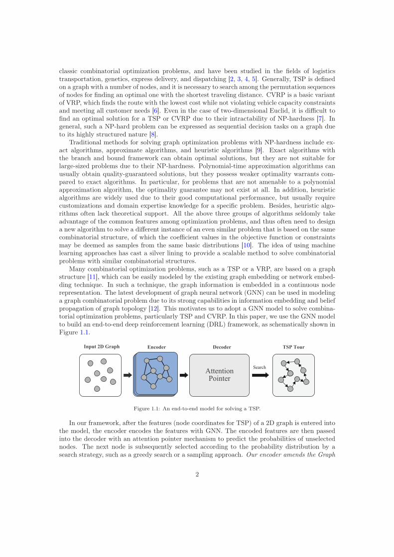
Many combinatorial optimization problems, such as a TSP or a VRP, are based on a graphstructure [11], which can be easily modeled by the existing graph embedding or network embed-ding technique. In such a technique, the graph information is embedded in a continuous noderepresentation. The latest development of graph neural network (GNN) can be used in modelinga graph combinatorial problem due to its strong capabilities in information embedding and beliefpropagation of graph topology [12]. This motivates us to adopt a GNN model to solve combina-torial optimization problems, particularly TSP and CVRP. In this paper, we use the GNN modelto build an end-to-end deep reinforcement learning (DRL) framework, as schematically shown inFigure 1.1.

Encoder

Attention

Pointer

DecoderInput 2D Graph TSP Tour

Search

Figure 1.1: An end-to-end model for solving a TSP.

In our framework, after the features (node coordinates for TSP) of a 2D graph is entered intothe model, the encoder encodes the features with GNN. The encoded features are then passedinto the decoder with an attention pointer mechanism to predict the probabilities of unselectednodes. The next node is subsequently selected according to the probability distribution by asearch strategy, such as a greedy search or a sampling approach. Our encoder amends the Graph

2

Attention Network (GAT) [13] by taking into consideration the edge information in the graph

structure and residual connections between layers. We shall call the designed networka residual edge-graph attention network (residual E-GAT). Our decoder is designed based on aTransformer model, which is used primarily in the field of natural language processing [14]. Theentire network is optimized using either a proximal policy optimization algorithm (PPO) or animproved baseline REINGORCE algorithm.

For demonstrating the performance of the proposed framework, a serial of random instancesof TSP and CVRP with nodes of 20, 50, and 100 are used to train and test our algorithm.Besides, the complexity of the model running time during the testing phase is analyzed. Tohave a fair comparison to the current literature, we have tested the generalization ability of theframework using the standard benchmark instances from TSPLIB and CVRPLIB.

The main contributions of this paper can be summarized below:

• An improved DRL framework is proposed for the routing problems. In this framework,a residual E-GAT is introduced for the encoder in which, are taken into considerationthe edge information and residual connections between layers. The edge information andresidual connections are not considered in GAT in the literature. It is demonstrated thatthe residual E-GAT is powerful to capture information of graph structures directly. Inaddition, the transformer model is used to design the decoder.

• In the training phase, we adopted two actor-critic algorithms: PPO and improved baselineREINGORCE algorithm. Some techniques of "code-level optimization" are used for furtherimproving the performance of the two algorithms.

• The proposed algorithm is efficient and has strong generalization power. The efficiency ofthe proposed framework is evaluated on randomly generated instance datasets of TSP andCVRP. Besides, the standard benchmark instances from TSPLIB and CVRPLIB are usedto verify the generalization capacity of our framework.

The rest of the paper is organized as follows. Section 2 summarizes the relevant literature.Section 3 describes our encoder-decoder model in detail. Section 4 introduces two deep reinforce-ment learning algorithms and decoding strategies. Section 5 gives the experimental results anddiscussions are made. Finally, conclusions and prospects are listed in Section 6. Appendix Aanalyzes the sensitivities of hyper-parameters. Appendix B shows solution examples of randominstances with 100 nodes. Appendix C demonstrates examples of standard benchmark instances.

2. Literature Review

Recently, supervised learning (SL) and reinforcement (RL) learning have been widely usedto solve combinatorial optimization problems [11, 15, 16, 17, 18], especially in routing problems.Table 2.1 summarizes various existing methods for solving routing problems based on super-vised learning and reinforcement learning. Reinforcement learning can be further divided intomodel-based and model-free methods. Finally, model-free reinforcement learning methods canbe divided into Value-Based and Policy-Based methods or a combination of both (actor-critic).

Vinyals et al. [19] introduced a supervised learning framework with sequence-to-sequencepointer network (PtrNet) to train and solve a Euclidean TSP and other combinatorial optimiza-tion problems. Their model uses the softmax probability distribution as a ’pointer’ to selecta member from the input sequence as the output. Bello et al. [20] introduced an actor-criticreinforcement learning algorithm to train PtrNet to solve the TSP in an unsupervised manner.They considered each instance as a training sample and used the cost (tour length) of a sampled

3

Table 2.1: Survey of deep/reinforcement learning methods in solving routing problems

Routing Problem Authors Network Structure Learning Type

TSP

[Vinyals et al.,2015][19] LSTM+Attention Supervised Learning, Approximation[Bello et al.,2016][20] LSTM+Attention RL-Model Free, Actor-Critic[Joshi et al.,2019][8] GCN Supervised Learning, Approximation[Dai et al.,2017][10] GNN RL-Model Free, Deep Q-Learning[Nazari et al.,2018][21] LSTM+Attention RL-Model Free, Actor-Critic[Deudon et al.,2018][22] GRU RL-Model Free, Actor-Critic[Emami et al.,2018][23] Transformer RL-Model Free, Actor-Critic[Kool et al.,2019][1] Transformer RL-Model Free, Actor-Critic[Malazgirt et al.,2019][24] NN RL-Model Free, Policy-Based[Ma et al.,2020][25] GPN Hierarchical RL-Model Free, Policy-Based[Cappart et al.,2020][26] GAT RL-Model Free, Actor-Critic[P. Felix et al.,2020][27] GCN RL-Model Based, Given Model[Drori et al.,2020][28] GAT+ Attention RL-Model Free, Actor-Critic[Zhang et al.,2020][29] Transformer RL-Model Free, Policy-Based[Hu et al., 2020][30] GNN RL-Model Free, Policy-Based

VRP

[Nazari et al.,2018][21] LSTM+Attention RL-Model Free, Actor-Critic[Chen et al.,2019][31] LSTM RL-Model Free, Actor-Critic[Kool et al.,2019][1] Transformer RL-Model Free, Actor-Critic[Zhao et al. 2020][32] LSTM+Attention RL-Model Free, Actor-Critic[Lu et al.,2020][33] NN RL-Model Free, Actor-Critic[Gao et al.,2020][34] GAT+GRU RL-Model Free, Actor-Critic[Drori et al.,2020][28] GAT+ Attention RL-Model Free, Actor-Critic[Chen et al.,2020][12] GAT+GRU RL-Model Free, Actor-Critic[zhang et al., 2020][35] Transformer RL-Model Free, Actor-Critic

Note: In the Network Structure column, LSTM: long short-term memory; NN: neural networks; GRU: gate recurrentunit; GPN: graph pointer network.

solution for an unbiased Monte-Carlo estimate of the policy gradient, and showed the perfor-mance of their algorithms on TSP with up to 100 nodes is better than most previous approximatealgorithms. Nazari et al. [21] extended the structure of PtrNet to solve more complex combina-torial optimization problems, such as the VRP with batch delivery and random variables. Gu etal. [36] used the PtrNet combined with supervised learning and DRL to solve an unconstrainedbinary quadratic programming problem. However, the neural network structure used in the aboveworks does not fully consider the relationship of the edges between vertexes in a graph, which isactually very important for many routing problems.

GNN as a powerful tool for processing non-Euclidean data and capturing graphical informa-tion has been widely researched in recent years. Specifically, once a GNN-based approximatesolver has been trained, its time complexity to solve a problem is significantly better than thatof an OR algorithm. In this case, the trained GNN is very suitable for real-time decision-makingproblems such as TSP and related vehicle routing problems. Li et al. [37] applied graph con-volutional network (GCN) model proposed by Kipf et al. [38] and guided tree search algorithmto solve graph-based combinatorial optimization problems, such as maximum independent setand minimum vertex cover problems. Dai et al. [10] used GNN to encode a problem instanceand demonstrated a GNN preserves node order and performs better in reflecting the combina-torial structure of TSP, when compared with the sequence-to-sequence model. They used deepQ-networks (DQN) to train a structure2vec (S2V) graph embedding model [39]. Motivated bythe Transformer architecture [14], Kool et al. [1] proposed an attention model (AM) to solve aserial of combinatorial optimization problems, and used rollout baseline in the policy gradientalgorithm to significantly improve the results of small-sized routing problems. Nowak et al. [40]used deep GCN in a supervised learning manner to construct an effective TSP graph repre-sentation and output itineraries through a highly parallel beam search using non-autoregressiveapproaches. Ma et al. [25] proposed a Graph Pointer Network (GPN), which trains a network tosolve TSP with time window constraints (TSPTW) through hierarchical reinforcement learning.They claimed that the model can be extended from small-sized problems to large-sized prob-lems. Drori et al. [28] used the GAT to solve many graph combinatorial optimization problems.Their results showed that the GAT framework has a generalization performance from trainingon random graphs to testing on a real-world graph. Hu et al. [41] introduced a bidirectionalGNN trained by imitation learning to solve an arbitrary symmetric TSP.

4

The previous works used GNN and reinforcement learning to solve combinatorial optimizationproblems without considering the dependency between edges in a graph structure. Motivated bythe above researches, our work considers the role of edges in a graph structure and considersconnecting residuals between layers to remedy the model degradation due to vanishing gradients ina deep model to further improve the GAT. Besides, most existing methods combine GNN, searchmethods, and reinforcement learning. Our model is based on an encoder built-upon the improvedGAT and a decoder built-upon the Transformer model. The proposed framework uses two deepreinforcement learning algorithms in training, i.e., PPO and improved baseline REINFORCEalgorithm. These differences make the proposed model different from the existing ones.

3. Graph-attention model

In this section, we will formally introduce our residual edge-graph-attention model (ResidualE-GAT). We define the model through a 2D Euclidean and symmetric TSP. The model is alsoapplicable to other graph-based routing problems, and only needs to change accordingly theinput, masks and decoder context vectors. TSP is defined on an undirected graph G = (V,E,W )where node i is represented by features ni, i ∈ V = {1, · · · ,m}. Here m is the number of nodesand ni denotes the coordinates of node i. And aij ∈ E, i, j ∈ V represents the edge from nodei to node j, further eij ∈ W is the distance information of aij . Solution π = (π1, · · · , πm) isintroduced to express a permutation of all the nodes, πt ∈ {1, · · · ,m} and πt 6= πt′ , ∀t 6= t′. Ourgoal is to find a solution π given a problem instance s so that each node can be visited exactlyonce and the total tour length is minimized. The length of a tour is defined for permutation πas:

L(π|s) = ||nπm− nπ1 ||2 +

m−1∑

t=1

||nπt− nπt+1 ||2, (3.1)

where || · ||2 denotes the L2 norm. Our graph-attention model defines a stochastic policy p(π|s)for instance s. Based on the chain rule of probability, the selection probability for sequence πcan be calculated based on a parameter set θ of the graph-attention model:

pθ(π|s) =m∏

t=1

pθ(πt|s, πt′ ∀t′ < t). (3.2)

The encoder makes embeddings of all input nodes. The decoder produces a permutation π ofinput nodes by generating a node at each time step and masks (will be introduced in Section3.2) that node out to prevent the model from visiting the node again.

Our encoder is designed based on the GAT, which is a neural network architecture thattransmits node information through an attention mechanism and has a powerful graph topologyrepresentation capability. For the TSP problem with an undirected graph G = (V,E,W ), GAT[13] only updates the information of each node by assigning new weights to its neighbors. How-ever, this update method ignores the information of the edge in the graph structure. Inspired bythe work of Gao et al. [34], the residual E-GAT proposed in this paper integrates the edge in-formation into the node information and updates them simultaneously, instead of only updatingthe node information in the original GAT. In addition, each sub-layer of E-GAT adds a residualconnection for avoiding vanishing gradient and model degradation [42]. The decoder is based onan attention mechanism, in which the next node is selected through either sampling or a greedydecoding. We will refine the encoder-decoder model in detail below.

5

3.1. The encoder

Our encoder model takes a graph G = (V,E,W ) as input, as shown in Figure 3.2. TakingTSP as an example, the input node features are the two-dimensional coordinates ni, and theinput edge features are the Euclidean distances eij , i, j ∈ {1, · · · ,m}.

The above two features are embedded in dx and de dimension features through a fully con-nected layer (FC Layer in Figure 2(b)) before they are fed into the residual E-GAT. Equation3.3 and Equation 3.4 below describe the node and edge embeddings respectively, where, thesuperscript 0 indicates that the embedding is before entering the residual E-GAT.

x(0)i = BN(A0ni + b0), ∀i ∈ {1, · · · ,m}, (3.3)

eij = BN(A1eij + b1), ∀i, j ∈ {1, · · · ,m}, (3.4)

where A0 and A1 represent learnable weight matrixes, and BN(·) represents batch normal-

ization [43]. We next use layer index ℓ ∈ {1, · · · , L} to represent the node embeddings x(ℓ)i

of the ℓ-th layer obtained in the residual E-GAT. The inputs of the first layer of the resid-

ual E-GAT are the node features x(0) = {x(0)1 ,x

(0)2 , · · · ,x(0)

m },x(0)i ∈ R

dx and edge featurese = {e11, e12, · · · , emm}, eij ∈ R

de . The first layer of the residual E-GAT produces a new set of

node features x(1) = {x(1)1 ,x

(1)2 , · · · ,x(1)

m },x(1)i ∈ R

dx as its output, while the edge features eijremain unchanged.

)1-(

ix ije)1-(

jx

g

)1-(

1x

)1-(

jx

)1-(

mx

ij

11

j1

m1

)1-(

1x)(

,1 Rx

11e

je1

me1

(W )

Softm

ax

LeakyReLU

)(

,1

)1-(

1 Rxx

)(

1x

(a) Edge and node fusion and update method.

Batch Normalization

FC Layer FC Layer

11e 12e mme

)(

1

Lx

)(

2

Lx

)(L

mx

2n1n mn

Add

Input

Embedding

L

Single Residual

E-GAT

Encoder Output

Mean x

(b) Encoder network structure.

Figure 3.2: The Encoder structure with multi-layer residual E-GAT.

Figure 2(a) describes how a single-layer residual E-GAT integrates the information of nodesand edges and updates the information of each node. The attention coefficient αℓ

ij indicates theimportance of node i and node j(i, j ∈ {1, · · · ,m}) at the ℓ-th layer:

αℓij =

exp(σ(gℓT [W ℓ(x(ℓ−1)i ||x(ℓ−1)

j ||eij)]))∑m

z=1 exp(σ(gℓT [W ℓ(x

(ℓ−1)i ||x(ℓ−1)

z ||eiz)]))(3.5)

where (·)T represents transposition, ·||· is the concatenation operation, gℓ and W ℓ are learnableweight vectors and matrices respectively, and σ(·) is the LeakyReLU activation function (asadopted in GAT [13]). Figure 2(b) shows the encoder model structure with multi-layer residualE-GAT. Each layer of the residual E-GAT updates the feature vector of every node throughthe attention mechanism described by Equation (3.5). We have employed a residual connectionbetween every two layers. That is, the output of layer ℓ is calculated as:

xℓi = x

(ℓ)i,R + x

(ℓ−1)i , (3.6)

6

where x(ℓ)i,R is a function implemented by layer ℓ itself, which can be expressed as:

x(ℓ)i,R =

m∑

j=1

αℓijW

ℓ1x

(ℓ−1)j , (3.7)

here W ℓ1 represents a learnable weight matrix. Our residual E-GAT contains L layers. The L-th

residual E-GAT outputs the node embeddings x(L)i . Subsequently, they are used to compute the

final graph embedding (as in [1]) x = {x1, · · · , xdx}, xj ∈ R, ∀j ∈ {1, 2, · · · , dx} by Equation

(3.8)

xj =1

m

m∑

i=1

(x(L)i )

j, j = 1, · · · , dx (3.8)

3.2. The decoder

Our decoder uses an attention mechanism similar to Kool et al. [1], and is based on thedecoder part of a Transformer model [14]. A Transformer model uses a multi-head attentionmechanism rather than the commonly used loop layer in an encoder-decoder architecture.

However, a Transformer cannot directly be applied to solve combinatorial optimization prob-lems, because its output dimension is fixed in advance and cannot be varied according to theinput dimension. On the other hand, the PtrNet, proposed by Vinyals et al. [19], uses an at-tention mechanism to select a member from the input sequence as the output at each decodingstep based on a softmax probability distribution. The PtrNet enables a Transformer model toapply to combinatorial optimization problems, where the length of an output sequence is de-termined by the source sequence. With this idea in our mind, our decoder follows the PtrNetway to output nodes, in which each node is related to a probability value as a "pointer" at eachdecoding time step by using the softmax probability distribution. Different from a Transformerdecoder in structure though, we do not use residual connections, batch normalization, and fullyconnected layers. Instead, our decoder contains two attention sub-layers. Figure 3.3 illustratesthe decoding process in our decoder.

Multi-Head

Attention

Single-Head

Attention

Context Vector }1,0{},,...,1{,)(Nmtc

N

tNode Embedding: },...,1{,)(

mixL

i },...,1{ˆ,', 'ˆ 'mttx tt

Masked Node:

)1(

1c

)0(

1c

Softmax

Pointer

1p 1mpmp

Multi-Head

Attention

Single-Head

Attention

)1(

2c

)0(

2c

Softmax

Pointer

1p 1mp mp

Decoder Step t =1 Decoder Step t =2

Multi-Head

Attention

Single-Head

Attention

)1(

mc

)0(

mc

Softmax

Pointer

1p 1mpmp

Decoder Step t =m

Output Probability:tp

Figure 3.3: The decoder structure for TSP.

7

The first layer computes a context vector through a multi-head attention mechanism [14],and the second layer outputs the probability distribution of the nodes to be selected. Decodinghappens sequentially, and at time step t ∈ {1, · · · ,m} the decoder outputs the node πt basedon the embeddings from the encoder and the previous outputs πt

′ generated at timestep t′

< t.

The decoder context vector c(0)t at time step t is calculated using the graph embedding x, the

last selected node πt−1 and the fist selected node π1. For t = 1, the decoder context vector isobtained from the graph embedding x and a learnable dx-dimensional parameter vector −→v :

c(0)t =

{

x+Wx(x(L)π1

||x(L)πt−1

), t > 1

x+−→v , t = 1. (3.9)

where Wx is a learnable weight matrix. The input of the first layer of the decoder is the context

vector c(0)t , and this layer produces a new context vector c

(1)t which is obtained through a multi-

head (with H number of heads) attention mechanism. We next describe in detail the multi-headattention mechanism.

Generally, we define the dimension dv to compute the key vectors ki ∈ Rdv , value vectors

vi ∈ Rdv , and query vector q ∈ R

dv through the node embeddings and the context vector c(0)t :

q = WQc(0)t ,vi = W V x

(L)i ,ki = WKx

(L)i , i ∈ {1, 2, · · · ,m}. (3.10)

where WK ∈ Rdv×dx ,WQ ∈ R

dv×dx and W V ∈ Rdv×dx(dv = dx/H) are learnable weight

matrices.In this paper, the context vector c

(0)t is used to compute a single query vector q. The

key vectors k = {k1, · · · ,km} and value vectors v = {v1, · · · ,vm} are computed using the

encoder output node embeddings x(L)i , i ∈ {1, 2, · · · ,m}. Then query vector q and key vectors

k = {k1, · · · ,km} are used to compute the attention coefficient u(1)i,t ∈ R, i ∈ {1, · · · ,m} of the

first decoder layer at time step t via Equation 3.11:

u(1)i,t =

qTki√dv

, if i 6= πt′ ∀t′ < t,

−∞, otherwise.

(3.11)

In Equation 3.11, the nodes that have been selected before timestep t are masked out by setting

their attention coefficients to −∞. We then normalize the attention coefficient u(1)i,t through a

softmax activation function by using Equation 3.12:

u(1)i,t = softmax(u

(1)i,t ) (3.12)

Next, H-head independent attentions are performed according to Equation 3.13, where the

h-th (h ∈ {1, · · · , H}) normalized attention coefficient is denoted by (u(1)i,t )

hfor 1 ≤ i ≤ m. The

vectors computed by each head are connected in series, and then the final context vector c(1)t is

obtained through a fully connected layer:

c(1)t = Wf · (||Hh=1

m∑

i=1

(u(1)i,t )

hvhi ), (3.13)

where Wf is a learnable weight matrix. The multi-head attention mechanism lends itself toenhance the stability of the attention learning process [13].

8

The input to the second decoder layer with a single attention head is the context vector c(1)t .

We then compute the attention coefficient u(2)i,t ∈ R, i ∈ {1, · · · ,m} of the second decoder layer at

timestep t using Equation 3.14. Referring to the work proposed by Bello et al. [18], we clippedthe result within [−C,C] (we used C = 10 in this paper) using tanh. Then the probability pi,t,for each node,i ∈ {1, · · · ,m}, is obtained through a softmax activation function using Equation3.15:

u(2)i,t =

C · tanh(c(1)t

Tki√

dv), if i 6= πt

′ ∀t′ < t

−∞, otherwise

. (3.14)

pi,t = pθ(πt|s, πt′ ∀t′ < t) = softmax(u

(2)i,t ). (3.15)

Finally, according to the probability distribution pi,t, we shall use either a sampling strategyor a greedy decoding strategy (to be introduced in Section 4.3) to predict the next node to visit.

4. DRL algorithm based on policy gradient

In this section, we present our implementation of two DRL algorithms: PPO and an Improvedbaseline REINFORCE algorithm. Both algorithms will be used in the proposed model.

4.1. PPO for solving routing problems

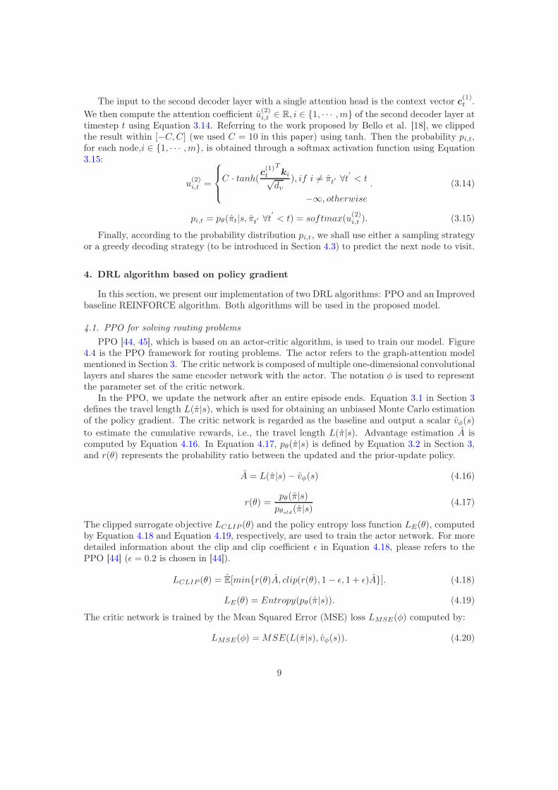
PPO [44, 45], which is based on an actor-critic algorithm, is used to train our model. Figure4.4 is the PPO framework for routing problems. The actor refers to the graph-attention modelmentioned in Section 3. The critic network is composed of multiple one-dimensional convolutionallayers and shares the same encoder network with the actor. The notation φ is used to representthe parameter set of the critic network.

In the PPO, we update the network after an entire episode ends. Equation 3.1 in Section 3defines the travel length L(π|s), which is used for obtaining an unbiased Monte Carlo estimationof the policy gradient. The critic network is regarded as the baseline and output a scalar vφ(s)

to estimate the cumulative rewards, i.e., the travel length L(π|s). Advantage estimation A iscomputed by Equation 4.16. In Equation 4.17, pθ(π|s) is defined by Equation 3.2 in Section 3,and r(θ) represents the probability ratio between the updated and the prior-update policy.

A = L(π|s)− vφ(s) (4.16)

r(θ) =pθ(π|s)pθold(π|s)

(4.17)

The clipped surrogate objective LCLIP (θ) and the policy entropy loss function LE(θ), computedby Equation 4.18 and Equation 4.19, respectively, are used to train the actor network. For moredetailed information about the clip and clip coefficient ǫ in Equation 4.18, please refers to thePPO [44] (ǫ = 0.2 is chosen in [44]).

LCLIP (θ) = E[min{r(θ)A, clip(r(θ), 1− ǫ, 1 + ǫ)A}]. (4.18)

LE(θ) = Entropy(pθ(π|s)). (4.19)

The critic network is trained by the Mean Squared Error (MSE) loss LMSE(φ) computed by:

LMSE(φ) = MSE(L(π|s), vφ(s)). (4.20)

9

Actor Parameter

Training

Data

Behavior Actor Parameter

Muti-Layer Residual E-GAT

Encoder

Decoder

Action

State

Probability

Rewards

Memory Buffer Muti-Layer Residual E-GAT

Encoder

Decoder

Test

Data

Muti-Layer Residual E-GAT

Encoder

Decoder

Trained Model

Critic Parameter

Gradient

Actor-Critic

Update

Update

Old

Old Old

via Adam

TSP Tour

CVRP Tour

Figure 4.4: The DRL framework based on PPO.

Then the total loss function of the actor-critic model can be expressed as:

Loss(θ, φ) = cpLCLIP (θ) + cvLMSE(φ)− ceLE(θ), (4.21)

which is composed of three parts, including LCLIP (θ), LMSE(φ), and LE(θ). And their weightsare coordinated by parameters cp, cv, and ce. The objective is to reduce the LCLIP (θ) andthe LMSE(φ) and to increase the LE(θ) through gradient descent [44]. Table 4.2 shows theinstantiations of the reinforcement learning framework for the two routing problems.

Table 4.2: Definition of reinforcement learning components for routing problems.

Problem State Action Reward Termination

TSP Partial tour Grow tour by one node Change in tour cost Tour includes all nodesCVRP Partial tour and vehicle inventory Grow tour by one node or depot Change in tour cost All needs are met

However, getting such an actor-critic algorithm to work is non-trivial. Engstrom et al. [46]believes that the success of the PPO algorithm comes from minor modifications to the corealgorithm Trust Region Policy Optimization [47]. They called these modifications "code-leveloptimization" and proved the effectiveness of these modifications. This paper adopts some partsof "code-level optimization" when using the PPO algorithm to train our encoder-decoder model.The following tricks sourced from the "code-level optimization" are used in our framework:

• Normalization of the reward in each mini-batch: In a standard PPO implementation,rather than feeding the reward directly from the environment into the objective, it performsa certain discount-based scaling scheme. We did not perform this discount-based scaling

10

scheme. Instead, we normalize reward L(π|s) by subtracting the mean and dividing by thestandard deviation in each mini batch.

• Adam optimizer learning rate annealing: We used learning rate decay during training,and update the learning rate at the end of each epoch:

lnew = lold · (β)epoch, (4.22)

where lnew and lold are the learning rate before and after each update, and β is a learningrate annealing coefficient.

• Orthogonal initialization: Instead of using the default weight initialization scheme forthe actor and critic networks, we used an orthogonal initialization following Engstrom etal. [46].

• Global Gradient Clipping: After computing the loss function gradient with respect tothe actor and the critic networks, we clip the concatenated gradient of all parameters suchthat the "global L2 norm" does not exceed 2 following the recommendation in Bello et al.[20].

The whole PPO algorithm is listed in Algorithm 1.

4.2. Improved baseline REINFORCE algorithm

In addition to the PPO algorithm described earlier, we also used an improved baselineREINFORCE algorithm to train our model. To that end, we defined the loss function asLoss(θ|s) = Eπ∼pθ(π|s)[L(π|s)]. The parameters θ is optimized by gradient descent using theREINFORCE [48] algorithm with rollout baseline b:

∇θLoss(θ|s) = Eπ∼pθ(π|s)[(L(π|s)− b)∇θlogpθ(π|s)]. (4.23)

REINFORCE algorithm with rollout baseline was proposed by Kool et al. [1] in solving routingproblems. The critic network in the actor-critic algorithm was replaced by the so-called baselineactor (policy) network, which can be described as a double actor structure. This replacingstrategy freezes the parameters θBL of the baseline policy network πθBL in each epoch, somewhatsimilar to freezing the target Q-network in DQN [49]. At the end of each epoch, a greedydecoding is used to compare the results of the current training policy and the baseline policy.Then the parameters of the baseline policy network are updated only when an improvement issignificant according to a paired t-test (significance level α = 5%) on 10000 evaluation instancesas done in existing studies [8, 20, 21, 22, 1]. In the training process, "code-level optimization"including Adam optimizer learning rate annealing and normalization of the reward functionis used to improve the performance of the baseline REINFORCE algorithm. We dubbed themodified algorithm improved baseline REINFORCE algorithm (Rollout algorithm). The stepsare described in Algorithm 2.

4.3. Decoding strategy

Effective search algorithms for combinatorial optimization problems include beam search,neighborhood search and tree search. Bello et al. [20] proposed search strategies such as samplingand Active Search. We used the following two decoding strategies:

11

Algorithm 1 PPO for Combinatorial Optimization

Input: number of total epochs Et, PPO epochs Ep, PPO steps Ts, steps per total epoch Pe, batch sizeB; actor network πθ and behaviour actor network πθold with trainable parameters θ and θold; criticnetwork vφ with trainable parameters φ; policy loss coefficient cp; value function loss coefficient cv;entropy loss coefficient ce; clipping ratio ǫ.

1: Initialization:Orthogonal initialization θ;φ, θold ← θ

2: for each total epoch = 1, · · ·, Et do

3: for each step = 1, · · · , Pe do

4: si ∼ RandomInstance() ∀i ∈ {1, · · · , B}5: πi ∼ SampleSolution(pθold(πi|si)) ∀i ∈ {1, · · · , B}6: Compute L(πi|si) via si, πi

7: Put si, πi, L(πi|si), pθold(πi|si) into Memory Buffer8: if step%Ts == 0 then

9: for each PPO epoch = 1, · · · , Ep do

10: for each PPO step = 1, · · · , Ts do

11: vφ(si)← Vφ(si) ∀i ∈ {1, · · · , B}12: L(πi|si)← Reward Normalization L(πi|si) ∀i ∈ {1, · · · , B}13: Compute advantage estimates Ai = L(πi|si)− vφ(si)

14: ri(θ) =pθ(πi|si)

pθold(πi|si)

15: LiCLIP (θ) = E[min{ri(θ)Ai, clip(ri(θ), 1− ǫ, 1 + ǫ)Ai}]

16: LiMSE(φ) = MSE(L(πi|si), vφ(si))

17: LiE(θ) = Entropy(pθ(πi|si))

18: Lossi(θ, φ) =1B

∑B

i=1{cpLiCLIP (θ) + cvL

iMSE(φ)− ceL

iE(θ)}

19: Update θ, φ by a gradient method w.r.t. Lossi(θ, φ)20: end for

21: end for

22: θold ← θ

23: Clear Memory Buffer24: end if

25: end for

26: end for

Output: Trained parameters set θ of the actor

12

Algorithm 2 Improved baseline REINFORCE Algorithm

Input: number of epochs E, steps per epoch Pe, batch size B, significance level α; actor network πθ

with trainable parameters θ; Baseline policy network πθBL with trainable parameters θBL.1: Initialization:Xavier initialization θ, θBL ← θ

2: for each epoch = 1, · · ·, Et do

3: for each step = 1, · · · , Pe do

4: si ∼ RandomInstance() ∀i ∈ {1, · · · , B}5: πi ∼ SampleSolution(pθ(πi|si)) ∀i ∈ {1, · · · , B}6: πBL

i ∼ GreedySolution(pθBL(πi|si)) ∀i ∈ {1, · · · , B}7: Compute L(πi|si), L(π

BLi |si) via si, πi, π

BLi

8: L(πi|si)← Reward Normalization L(πi|si)9: L(πBL

i |si)← Baseline Reward Normalization L(πBLi |si)

10: Compute advantage estimates Ai = L(πi|si)− L(πBLi |si))

11: ∇θLoss(θ|si) =1B

∑B

i=1 Eπ∼pθ(π|s)[Ai∇θlogpθ(πi|si)]12: θ ← Adam(θ,∇θLoss(θ|si))13: end for

14: if OneSidedPairedTTest(pθ, pθBL) < α then

15: θBL ← θ

16: end if

17: end for

Output: Trained parameters set θ of the actor

• Greedy Decoding: Generally, a greedy algorithm selects a local optimal solution andprovides a fast approximation of the global optimal solution. In each decoding step, thenode with the highest probability is selected greedily, and the visited nodes are maskedout. For the TSP problem, the search is terminated when all nodes have been visited.For CVRP, the search is terminated when the requirements of all nodes are satisfied toconstruct an effective solution.

• Stochastic Sampling: In each decoding timestep t ∈ {1, · · · ,m}, the random policypθ(πt|s, πt

′ ∀t′ < t) samples the nodes to be selected according to the probability distribu-tion to construct an effective solution. During testing, Bello et al. [20] used temperaturehyperparameters λ ∈ R to modify Equation 3.15 to ensure the diversity of sampling. Themodified Equation is as follows:

pi,t = pθ(πt|s, πt′ ∀t′ < t) = softmax(

u(2)i,t

λ) (4.24)

Through grid search of the temperature hyperparameters, we found that the temperatureof 2, 2.5, 1.5 provide best results for TSP20, TSP50, and TSP100, respectively. In addi-tion, the temperature of 2.5, 1.8, 1.2 supply the best results for CVRP20, CVRP50, andCVRP100, respectively.

In the training process, stochastic sampling is usually needed to explore the environmentto obtain a better model performance. In the testing process, we used the greedy decoding.Moreover, we sampled 1280 solutions (following the existing studies [8, 20, 21, 22, 1]) by usingstochastic sampling with a selected temperature hyperparameters λ and listed the best one inTable 5.4 (the row indicated by "Ours (Sampling)") and Table 5.5 (the row indicated by "Ours(Sampling)") .

13

5. Computational Experiment

Our framework is suitable for many combinatorial optimization problems. For different op-timization problems, only the input, masks and decoder context vectors need to be adjusted.This paper mainly focuses on the routing problems TSP and CVRP. We trained the proposedgraph-attention model for both TSP and CVRP instances with the number of nodes m = 20, 50and 100, respectively. Instances were generated with batch sizes of 512, 128, 128 (affected bymemory) for the three different numbers of nodes, respectively. Each epoch of the PPO algorithmcontains 800, 3000, and 3000 batches respectively, and for the Rollout algorithm each contains1600, 6000, and 6000 batches correspondingly. We trained 100 epochs using instances randomlygenerated from the unit square [0, 1] × [0, 1]. And 10,000 test instances following the existingstudies [8, 20, 21, 22, 1] are generated with the same data distribution. As the testing processdoes not update the model parameters, a larger batch size can be used. We used a Nvidia GeForceRTX2070 GPU to complete the training of TSP and CVRP with sizes of m = 20 and 50. Sincethe memory of GPU in the personal computer is limited, the training process with instances ofm = 100 and all testing processes are performed on an Nvidia Tesla V100 GPU. The values ofother related hyper-parameters for the training process are listed in Table 5.3. Furthermore, weanalyzed the sensitivities of hyper-parameters in Appendix A. The hyper-parameter values forTSP and CVRP of the same size are identical. The model is constructed by PyTorch [50], andthe code is implemented by using Python 3.7.

Table 5.3: The values of the hyper-parameters used in our framework.

Parameters Value Parameters Value

Number of encoder layers ℓ 4 PPO steps Ts 1

Learning rate decay β 0.96 Heads of attention H 8

PPO learning rate l 3 × 10−4(m = 20) PPO epochs Ep 3

1 × 10−4(m = 50, 100) Optimizer Adam [51]

Rollout learning rate l 1 × 10−3(m = 20) Node embedding dimension dx 128

3 × 10−4(m = 50, 100) Edge embedding dimension de 64

5.1. TSP results

The test results of TSP instances for difference sizes are reported in Table 5.4. The comparisonbenchmark method is the Gurobi solver. The optimization solver Gurobi [52] can obtain anexact solution of TSP via mixed integer programming within a reasonable running time. TheGoogle OR tools are developed based on local search and can be generally used to judge non-learned algorithms, such as heuristics with greedy search strategies. The listed results cover threegroups of solution techniques, including exact solver, greedy approaches, and sampling/searchapproaches. Except for Gurobi and our results (both shown in bold) in the Table 5.4, all othersare taken from Table 1 [1] and Table 1 [8]. For more detailed information about non-learnedalgorithms (Nearest Insertion, Random Insertion, Farthest Insertion, Nearest Neighbor), pleaserefer to Appendix B of Kool et al. [1]. All the results are expressed by the average travel lengthL(π|s) of Ntest (here Ntest = 10, 000) test instances. And Opt. Gap denotes the average optimalgap between a result and the optimal solution L(π|s) delivered by the optimization solver Gurobi,as shown in the following Equation:

Opt. Gap =1

Ntest

Ntest∑

i=1

L(π|s)− L(π|s)L(π|s) (5.25)

14

Table 5.4: Performance of our framework compared to non-learned algorithms and state-of-the-art methods forTSP instances.

Method TypeTSP20 TSP50 TSP100

Length Gap Time Length Gap Time Length Gap Time

Gurobi Solver 3.829 0.00% 1m 5.698 0.00% 20m 7.763 0.00% 3h

Nearest Insertion H,G 4.33 12.91% 1s 6.78 19.03% 2s 9.46 21.82% 6sRandom Insertion H,G 4.00 4.36% 0s 6.13 7.65% 1s 8.52 9.69% 3sFarthest Insertion H,G 3.93 2.36% 1s 6.01 5.53% 2s 8.35 7.59% 7sNearest Neighbor H,G 4.50 17.23% 0s 7.00 22.94% 0s 9.68 24.73% 0sPtrNet [19] SL,G 3.88 1.15% 7.66 34.48% -PtrNet [20] RL,G 3.89 1.42% 5.95 4.46% 8.30 6.90%S2V [10] RL,G 3.89 1.42% 5.99 5.16% 8.31 7.03%GAT [22] RL,G 3.86 0.66% 2m 5.92 3.98% 5m 8.42 8.41% 8mGAT [22] RL,G,2OPT 3.85 0.42% 4m 5.85 2.77% 26m 8.17 5.21% 3hAM [1] RL,G 3.85 0.34% 0s 5.80 1.76% 2s 8.12 4.53% 6sGCN [8] SL,G 3.86 0.60% 6s 5.87 3.10% 55s 8.41 8.38% 6mOurs (Greedy) RL,G 3.832 0.06% 1s 5.755 0.98% 4s 8.048 3.67% 11s

OR Tools H,S 3.85 0.37% 5.80 1.83% 7.99 2.90%Chr.f. + 2OPT H,2OPT 3.85 0.37% 5.79 1.65% -PtrNet [20] RL,S - 5.75 0.95% 8.00 3.03%GNN [40] SL,BS 3.93 2.46% - -GAT [22] RL,S 3.84 0.11% 5m 5.77 1.28% 17m 8.75 12.70% 56mGAT [32] RL,S,2OPT 3.84 0.09% 6m 5.75 1.00% 32m 8.12 4.64% 5hAM [1] RL,S 3.84 0.08% 5m 5.73 0.52% 24m 7.94 2.26% 1hGCN [8] SL,BS 3.84 0.10% 20s 5.71 0.26% 2m 7.92 2.11% 10mGCN [40] SL,BS* 3.84 0.01% 12m 5.70 0.01% 18m 7.87 1.39% 40mOurs (Sampling) RL,S 3.830 0.01% 10m 5.738 0.70% 55m 7.896 1.71% 2h

Note: DL/DRL approaches are named according to the type of neural network used. In the Type column, H: heuristic method;SL: supervised learning; S: sample search; G: greedy search; BS: beam search; BS*: beam search and shortest path heuristics;2OPT: 2OPT local search.

In Table 5.4, our results are obtained by applying our trained graph attention model to theTSP testing instances. The applied model is trained by using the Rollout algorithm introduced inSection 4.2, as the PPO algorithm performs slightly less well. We point out that, for our trainedmodel, the greedy decoding strategy can obtain almost the same solution quality as that by thesampling strategy, for example, 3.67% vs. 1.71% Opt. Gap for TSP100 instances. Furthermore,for our model, the running time of the greedy decoding strategy is much faster compared to thesampling strategy, for example, 11s vs. 2h for TSP100 instances.

Compared with other learning-based methods, our method has a significant improvement inthe quality of solutions when adopting the greedy decoding strategy. This is clearly shown inthe row indicated by "Ours (Greedy)" in Table 5.4. Our results using the sampling strategy(indicated by "Ours (Sampling)" in Table 5.4 are at least compatible to other results. Table5.4 lists also the solution time (from test instances) of some methods. Due to the difference inimplementation language and hardware, it is not meaningful for direct comparison of runningtime.

Figure B.10 in Appendix B shows the visualization of the solutions to the random TSPinstances with 100 nodes through sampling and greedy decoding, respectively. Figure 5.5 showsthe convergency of the PPO and Rollout two algorithms training the graph-attention model.Both use a validation set of size 10000 with greedy decoding. It can be seen from Figure 5.5that the convergence trends are almost the same for the two methods. It is worth noting thatthe PPO only uses half of the training data used by the Rollout, but the Rollout converges faster.In the TSP50 and TSP100 problems, the model proposed by Kool et al. [1] needs more than onemillion training samples. Our PPO and Rollout only use 384,000 and 768,000 training samplesrespectively, nevertheless the performance of our trained model is better than that of Kool et al.[1].

5.2. CVRP results

CVRP is defined through an undirected graph G = (V,E,W ) where node i = {0, 1, · · · ,m}is represented by features ni. The index i = 0 represents the depot node, and i(i > 0) representsthe i-th customer node. The vehicle has capacity D > 0 and each customer node i = {1, · · · ,m}

15

(a) TSP20 (b) TSP50 (c) TSP100

Figure 5.5: The Opt. Gap convergency curves of PPO and Rollout on the validation set.

has a demand δi, 0 < δi < D. It is assumed that the depot demand δ0 = 0. Both depot andcustomer nodes are randomly generated from the unit square [0, 1] × [0, 1]. We generated 21,51, and 101 nodes (the first node is the depot) for problems with a size of m = 20, 50, and 100,and the corresponding vehicle capacities are 30, 40, and 50, respectively. The customer nodedemands are sampled uniformly from {1, · · · , 9}. And we normalized the customer node demandto [0, 1] through δ

′

i =δi10 , so the vehicle capacity D is transformed into 3, 4, and 5 accordingly.

The input, masks and decoder context vectors are adjusted for CVRP:

• Input: Switching to CVRP only needs to expand the node feature ni to a three-dimensionalinput n

′

i that includes the normalized demand δ′

i and node feature ni:

n′

i = ni||δ′

i (5.26)

• Vehicle remaining capacity update: We masked out the customer nodes that have beenserved, so there is no need to update the needs of served customer nodes. The decoderselects the customer node πt at timestep t, and the remaining capacity of the vehicle isrepresented by D

′

t. It is assumed that the vehicle starts at the depot when the decodingtimestep t = 1 and the vehicle is fully loaded (with vehicle remaining capacity D

′

1 = D).The remaining vehicle capacity is updated by using the following Equation:

D′

t =

{

D′

t−1 − δ′

πt, πt = i, i ∈ {1, · · · ,m}

D, πt = 0. (5.27)

• Decoder context vector: The context vector c(0)t of the decoder at timestep t ∈ {1, · · · ,m}

consists of three parts: graph embedding x, embedding of node πt and vehicle remainingcapacity D

′

t−1:

c(0)t =

x+Wx(x(L)πt−1

||D′

t−1), t > 1

x+Wx(x(L)0 ||D′

t), t = 1. (5.28)

• Mask update: For CVRP, our mask consists of two parts: the customer node mask andthe depot node mask. For the customer node mask, we mask out a customer node that hasbeen served or when the demand of a customer node is greater than the remaining capacity

of the vehicle. That is, customer node i’s attention coefficients u(0)i,t , u

(1)i,t = −∞ (introduced

in Section 3.2) when δ′

i > D′

t−1 or i 6= πt′ ∀t′ < t, i ∈ {1, · · · ,m}. For the depot mask, as

the depot will not be the next chosen node when the vehicle leaves the depot, the depot

node 0’s attention coefficients u(0)0,t , u

(1)0,t = −∞ for t = 1 or πt−1 = 0, when the vehicle is at

the depot.

16

The test results of CVRP instances with various sizes are listed in Table 5.5. Our resultsagain are obtained by applying our trained graph attention model to the CVRP testing instancesusing the Rollout Algorithm due to the same reason. Except for ours, the results in this Tableare taken from Table 1 [1]. The structure and symbol description in the Table are identical tothose introduced in Table 5.4 in Section 5.1. Our solution approaches outperform other listedlearning based algorithms in terms of solution quality. Figure B.11 in Appendix B shows thevisualization of the solutions to the random CVRP instances with 100 nodes through samplingand greedy decoding, respectively.

Table 5.5: Performance of our framework versus state-of-the-art methods for CVRP instances with various sizes.

Method TypeVRP20 VRP50 VRP100

Length Gap Time Length Gap Time Length Gap Time

Gurobi Solver 6.10 0.00% - -LKH3 Solver 6.14 0.58% 2h 10.38 0.00% 7h 15.65 0.00% 13h

PtrNet [21] RL, G 6.59 8.03% 11.39 9.78% 17.23 10.12%AM [1] RL, G 6.40 4.97% 1S 10.98 5.86% 3S 16.80 7.34% 8sOurs (Greedy) RL, G 6.26 2.60% 2s 10.80 4.05% 7s 16.69 6.68% 17s

OR Tools H, S 6.43 5.41% 11.31 9.01% 17.16 9.67%PtrNet [21] SL, BS 6.40 4.92% 11.15 7.46% 16.96 8.39%AM [1] RL, S 6.25 2.49% 6m 10.62 2.40% 28m 16.23 3.72% 2hOurs (Sampling) RL, S 6.19 1.47% 14m 10.54 1.54% 1h 16.16 3.25% 4h

Note: DL/DRL approaches are named according to the type of neural network used. In the Type column, H: heuristicmethod; SL: supervised learning; S: sample search; G: greedy search; BS: beam search; BS*: beam search and shortestpath heuristics; 2OPT: 2OPT local search.

5.3. Testing running time complexity analysis

We next report the running times of the entire encoder-decoder model (graph-attentionmodel) and the decoder model only when the graph size (number of nodes) increases from 1to 500. Each test is run with a single batch (batch size=1). Figure 5.6 shows that our frameworkhas linear testing time complexity on graph size (number of nodes). The running time mainlyis consumed by the decoder. The encoder generally completes the embedding of nodes quickly(within 1ms). Table 5.6 summarizes the running time complexity, running time (average), ac-celeration factor, and optimal gap of exact algorithms, heuristic algorithms, and learning-basedmethods for TSP with 100 nodes. All those results except ours are taken from Table 1 of Droriet al. [28]. Our results are listed in bold. The running time of exact algorithms, approximatealgorithms, and heuristic algorithms increases at least squarely in the graph size. S2V-DQN [10]and GPN [25] are both reinforcement learning methods, and their running time complexity isO(n2) and O(nlogn) respectively. In particular, they have a large Opt. Gap (8.4% and 8.6%respectively). The running time complexity of our method is O(n), and both the running timeand the Opt. Gap are significantly improved. GAT [28] has the same running time complexityas our method, but its Opt. Gap is larger.

Table 5.6: Comparison of running time for TSP.

Method Runtime Complexity Runtime (ms) Speedup Opt. Gap

Gurobi (Exact) NA 3, 220 2, 752.1 0.00%Concorde (Exact) NA 254.1 217.2 0.00%

Christofifides O(n3) 5, 002 4, 275.2 2.90%

LKH O(n2.2) 2, 879 2460.7 0.00%

2-opt O(n2) 30.08 25.7 9.70%

Farthest O(n2) 8.35 7.1 7.50%

Nearest O(n2) 9.35 8 24.50%

S2V-DQN [Dai et al., 2017][10] O(n2) 61.72 52.8 8.40%GPN [Ma et al., 2019][25] O(nlogn) 1.537 1.3 8.60%GAT [Drori et al., 2020][28] O(n) 1.17 1 7.40%Ours (Greedy) O(n) 1.06 1 3.70%

17

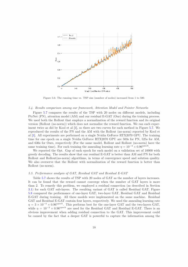
Figure 5.6: The running time vs. TSP size (number of nodes) increased from 1 to 500.

5.4. Results comparison among our framework, Attention Model and Pointer Networks

Figure 5.7 compares the results of the TSP with 20 nodes on different models, includingPtrNet (PN), attention model (AM) and our residual E-GAT (Our) during the training process.We used both the Rollout that employs a normalization of the reward function and its originalversion (Rollout (no-norm)) which does not normalize the reward function. We ran each exper-iment twice as did by Kool et al [1], so there are two curves for each method in Figure 5.7. Wereproduced the results of the PN and the AM with the Rollout (no-norm) reported by Kool etal [1]. All experiments are performed on a single Nvidia GeForce RTX2070 GPU. The trainingtime for one epoch on a single Nvidia GeForce RTX2070 GPU are 503s for PN, 525s for AM,and 636s for Ours, respectively (For the same model, Rollout and Rollout (no-norm) have thesame training time). For each training the annealing learning rate η = 10−3 × 0.96epoch.

We reported the Opt. Gap of each epoch for each model on a validation set of 10000 withgreedy decoding. The results show that our residual E-GAT is better than AM and PN for bothRollout and Rollout(no-norm) algorithms, in terms of convergence speed and solution quality.We also overserve that the Rollout with normalization of the reward function is better thanRollout (no-norm).

5.5. Performance analysis of GAT, Residual GAT and Residual E-GAT

Table 5.7 shows the results of TSP with 20 nodes of GAT as the number of layers increases.It can be found that the reward cannot converge when the number of GAT layers is morethan 2. To remedy this problem, we employed a residual connection (as described in Section3.1) for each GAT sub-layers. The resulting variant of GAT is called Residual GAT. Figure5.8 compared the performance of one-layer GAT, two-layer GAT, Residual GAT and ResidualE-GAT during training. All these models were implemented on the same machine. ResidualGAT and Residual E-GAT contain four layers, respectively. We used the annealing learning rateη = 3 × 10−4 × 0.96epoch. This performs best for the one-layer GAT and the two-layers GAT,while η = 10−3 × 0.96epoch are used for the Residual GAT and Residual E-GAT. There is anobvious improvement when adding residual connection to the GAT. This improvement couldbe caused by the fact that a deeper GAT is powerful to capture the information among the

18

Figure 5.7: The validation Opt. Gap convergency curves of the attention model (AM), PtrNet (PN) and ourmodel (Our).

graphs but more difficult to train. Therefore, we introduced the residual connection to ease thetraining of the deeper GAT, a different approach than those used previously [42]. Furthermore,the Residual E-GAT has a further improvement relative to Residual GAT. Compared to the bestresult of the GAT, the Residual E-GAT reduces the Opt. Gap from 0.85% to 0.06%.

Table 5.7: The results of GAT using different layers.

Number of Layers 1 2 3 5 8

Length (Opt. Gap)

3.86(0.86%) 3.87(1.09%) 10.41(171%) 10.41(171%) 10.41(171%)

3.86(0.85%) 3.88(1.31%) 10.41(171%) 10.41(171%) 10.41(171%)

5.6. The generalization performance of our framework

We used small and medium-sized instances from the public libraries TSPLIB [53] and CVR-PLIB [54] to verify the generalization performance from random instance training to real-worldinstance testing. The instance suffix for an instance in TSPLIB indicates the number of nodes.Table 5.8 shows the results of exact algorithm, reinforcement learning methods and approximatealgorithms. Except for ours, the results in this Table are taken from Table C.2 [9]. S2V-DQN[10] is a reinforcement learning method that uses the Active Search proposed by Bello et al.[20] to solve the instance problems in TSPLIB. Its generalization performance does not dependon the distribution of the training data. Different than greedy decoding with a fixed model,Active Search can refine the parameters of the stochastic policy pθ during testing on a single testdata. Therefore, solving through Active Search consumes a lot of time. Instead of using ActiveSearch, we used greedy decoding in training our model with the 100-node random instances forthe purpose of testing the instances in TSPLIB. We saved the model parameters at the end ofeach epoch, which constitute a set of 100 models (epoch = 100). For each instance, the tourfound by each individual model is collected and the shortest tour is chosen. We refer to thisapproach as trained-greedy100.

For small sized instances (customer m < 75) and medium size instances (customer m ≥ 75)in CVRLIB, we used the trained models by 50 and 100 nodes random instances to test them,

19

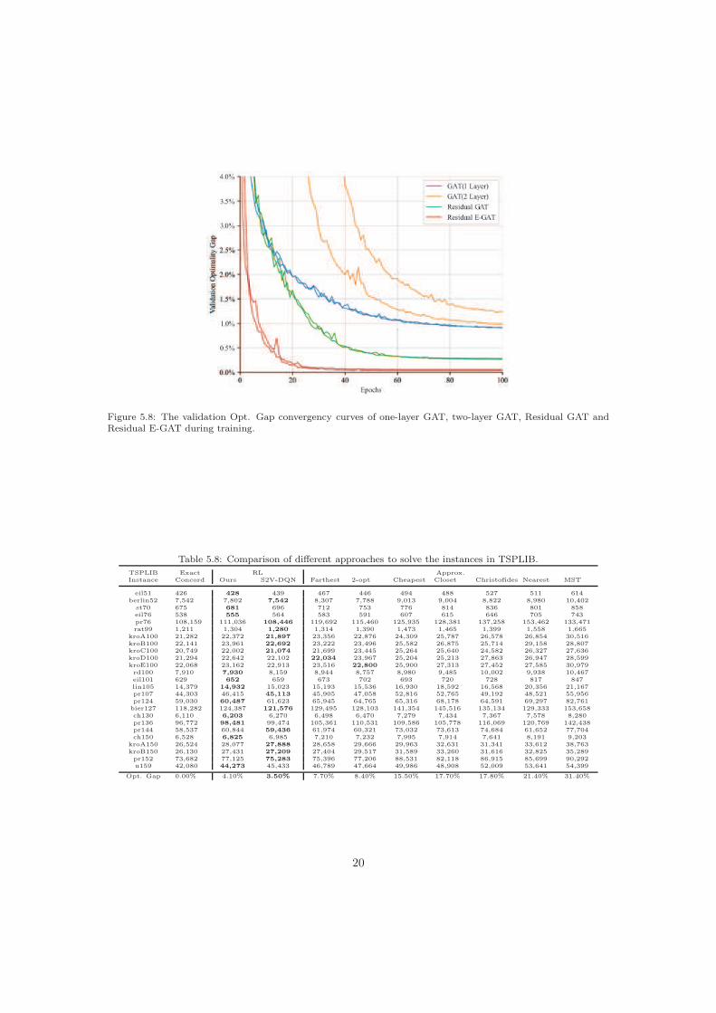
Figure 5.8: The validation Opt. Gap convergency curves of one-layer GAT, two-layer GAT, Residual GAT andResidual E-GAT during training.

Table 5.8: Comparison of different approaches to solve the instances in TSPLIB.

TSPLIB Exact RL Approx.Instance Concord Ours S2V-DQN Farthest 2-opt Cheapest Closet Christofides Nearest MST

eil51 426 428 439 467 446 494 488 527 511 614berlin52 7,542 7,802 7,542 8,307 7,788 9,013 9,004 8,822 8,980 10,402

st70 675 681 696 712 753 776 814 836 801 858eil76 538 555 564 583 591 607 615 646 705 743pr76 108,159 111,036 108,446 119,692 115,460 125,935 128,381 137,258 153,462 133,471rat99 1,211 1,304 1,280 1,314 1,390 1,473 1,465 1,399 1,558 1,665

kroA100 21,282 22,372 21,897 23,356 22,876 24,309 25,787 26,578 26,854 30,516kroB100 22,141 23,961 22,692 23,222 23,496 25,582 26,875 25,714 29,158 28,807kroC100 20,749 22,002 21,074 21,699 23,445 25,264 25,640 24,582 26,327 27,636kroD100 21,294 22,642 22,102 22,034 23,967 25,204 25,213 27,863 26,947 28,599kroE100 22,068 23,162 22,913 23,516 22,800 25,900 27,313 27,452 27,585 30,979rd100 7,910 7,930 8,159 8,944 8,757 8,980 9,485 10,002 9,938 10,467eil101 629 652 659 673 702 693 720 728 817 847lin105 14,379 14,932 15,023 15,193 15,536 16,930 18,592 16,568 20,356 21,167pr107 44,303 46,415 45,113 45,905 47,058 52,816 52,765 49,192 48,521 55,956pr124 59,030 60,487 61,623 65,945 64,765 65,316 68,178 64,591 69,297 82,761

bier127 118,282 124,387 121,576 129,495 128,103 141,354 145,516 135,134 129,333 153,658ch130 6,110 6,203 6,270 6,498 6,470 7,279 7,434 7,367 7,578 8,280pr136 96,772 98,481 99,474 105,361 110,531 109,586 105,778 116,069 120,769 142,438pr144 58,537 60,844 59,436 61,974 60,321 73,032 73,613 74,684 61,652 77,704ch150 6,528 6,825 6,985 7,210 7,232 7,995 7,914 7,641 8,191 9,203

kroA150 26,524 28,077 27,888 28,658 29,666 29,963 32,631 31,341 33,612 38,763kroB150 26,130 27,431 27,209 27,404 29,517 31,589 33,260 31,616 32,825 35,289pr152 73,682 77,125 75,283 75,396 77,206 88,531 82,118 86,915 85,699 90,292u159 42,080 44,273 45,433 46,789 47,664 49,986 48,908 52,009 53,641 54,399

Opt. Gap 0.00% 4.10% 3.50% 7.70% 8.40% 15.50% 17.70% 17.80% 21.40% 31.40%

20

respectively. Table 5.9 and Table 5.10 show the optimal solutions and our graph-attention modelresults for instances in CVRPLIB. We listed the Opt. Gap for each instance and the average ofall instances.

The average Opt. Gap are 4.1%, 6.39% and 10.45% for TSP, small and medium sized CVRPbenchmark instances, respectively. The results verify that our framework has generalizationperformance from random instance training to real-world instance testing. Finally, Figure C.12and Figure C.13 in Appendix C show the visualized solutions of instances in TSPLIB andCVRPLIB with different sizes.

Table 5.9: Trained by random instances with 50 nodes and solved the instances with different sizes in CVRPLIBby trained-greedy100.

No. Problem Nodes Capacity Routes Optimal

Ours (Greedy)

Opt. GapRoutes Distance

1 A-n32-k5 31 100 5 784 5 789 0.63%2 A-n36-k5 35 100 5 799 5 839 5.00%3 A-n37-k5 36 100 5 669 5 710 6.12%4 A-n38-k5 37 100 5 730 5 751 2.87%5 A-n39-k5 38 100 5 822 5 838 1.94%6 A-n44-k6 43 100 6 937 6 984 5.01%7 A-n45-k6 44 100 6 944 6 984 4.23%8 A-n46-k7 45 100 7 914 7 999 9.29%9 A-n48-k7 47 100 7 1,073 7 1,123 4.65%10 A-n63-k10 62 100 10 1,314 12 1,519 15.60%11 A-n64-k9 63 100 9 1,401 12 1,659 18.40%12 A-n65-k9 64 100 9 1,174 10 1,246 6.13%13 A-n69-k9 68 100 9 1,159 10 1,264 9.05%14 B-n34-k5 33 100 5 788 5 812 3.04%15 B-n35-k5 34 100 5 955 5 986 3.24%16 B-n45-k6 44 100 6 678 7 729 7.52%17 B-n50-k7 49 100 7 741 7 798 7.69%18 B-n51-k7 50 100 7 1,032 8 1,045 1.25%19 B-n52-k7 51 100 7 747 7 762 2.00%20 B-n56-k7 55 100 7 707 7 755 6.79%21 B-n57-k9 56 100 9 1,598 9 1,638 2.50%22 B-n63-k10 62 100 10 1,496 12 1,667 11.43%23 B-n64-k9 63 100 9 861 11 989 14.86%24 B-n66-k9 65 100 9 1,316 9 1,381 4.93%25 B-n68-k9 67 100 9 1,272 9 1,397 9.82%26 E-n30-k3 29 4500 3 534 5 585 9.55%27 E-n51-k5 50 160 5 521 6 553 6.14%28 P-n50-k8 49 120 8 631 9 655 3.80%29 P-n51-k10 50 80 10 741 10 811 9.44%30 P-n55-k10 56 115 10 694 10 726 4.61%31 P-n60-k10 59 120 10 744 10 776 4.30%32 P-n65-k10 64 130 10 792 10 826 4.29%33 P-n70-k10 69 135 10 827 11 865 4.59%

Average 6.39%

6. Conclusion

In this research, a general deep reinforcement learning framework for solving routing problemsis introduced. An encoder based on an improved GAT, which forms a graph-attention model withthe Transformer decoder, is proposed. Two deep reinforcement learning algorithms: PPO andimproved baseline REINFORCE algorithm, are used to train the model. The PPO has higherefficiency of sample utilization compared with the improved baseline REINFORCE algorithm,and both algorithms can achieve better performance with less than one million training data.Our framework significantly improves the results of solving TSP and CVRP problems using fewertraining data compared with existing studies. Moreover, it can be found that our framework haslinear running time complexity during the testing process. For real-world instances of TSPLIBand CVRPLIB, our framework exhibits similar performance as it does in random instances. Thisindicates our framework has generalization performance from random instance training to actualproblem testing, even using fewer instances for training.

For the future research, PPO and improved baseline REINFORCE algorithm may be com-bined for finding a better DRL framework. Furthermore, the proposed framework is also possible

21

Table 5.10: Trained by random instances 100 nodes and solved the instances with different sizes in CVRPLIB bytrained-greedy100.

No. Problem Nodes Capacity Routes Optimal

Ours (Greedy)

Opt. GapRoutes Distance

1 A-n80-k10 79 100 10 1,763 10 1,890 7.20%2 B-n78-k10 77 100 10 1,221 10 1,333 9.17%3 E-n76-k10 75 140 10 830 10 870 4.81%4 E-n101-k14 100 112 14 1,067 14 1,163 8.96%5 M-n101-k10 100 200 10 820 10 873 6.46%6 M-n121-k7 120 200 7 1,034 8 1,144 10.63%7 M-n151-k12 150 200 12 1,015 12 1,106 8.96%8 M-n200-k17 199 200 17 1,275 17 1,414 10.90%9 P-n76-k5 75 280 5 627 5 690 10.04%10 P-n101-k4 100 400 4 681 4 820 20.41%11 X-n106-k14 105 600 14 26,362 14 28,085 6.53%12 X-n125-k30 124 188 30 55,539 30 59,147 6.49%13 X-n134-k13 133 643 13 10,916 13 12,342 13.06%14 X-n148-k46 147 18 46 43,448 46 50,462 16.14%15 X-n157-k13 156 12 13 16,876 13 20,273 20.12%16 X-n181-k23 180 8 23 25,569 23 28,566 11.72%17 X-n200-k36 199 402 36 58,578 36 63,276 8.02%18 X-n223-k34 222 836 34 40,437 37 43,508 7.59%19 X-n251-k28 250 69 28 38,684 28 42,965 11.06%20 X-n266-k58 265 35 58 75,478 62 83,155 10.17%21 X-n298-k31 297 55 31 34,231 32 38,023 11.07%

Average 10.45%

to solve more complex VRP problems with extra constraints or other complex combinatorial op-timization problems, such as job shop scheduling problems and flexible job shop schedulingproblems.

CRediT authorship contribution statement

Kun LEI: Conceptualization, Methodology, Investigation, Writing-original draft, Editing.Peng GUO: Conception and design of study, Analysis and interpretation of data, Writing -original draft, Writing - review & editing. Yi WANG: Validation, Writing - review & editing.Xiao WU: Writing - review & editing. Wenchao ZHAO: Methodology, Writing-original draft.

Declaration of Competing Interest

The authors declare that they have no known competing financial interests or personal rela-tionships that could have appeared to influence the work reported in this paper.

Acknowledgments

The research of this paper is supported by the National Key Research and DevelopmentPlan (grant number 2020YFB1712200) and the Fundamental Research Funds for the CentralUniversities (grant number 2682018CX09).

Data availability

The associated source code and the computational results are available at the Github website:https://github.com/pengguo318/RoutingProblemsGANN.

22

References

References

[1] W. Kool, H. Van Hoof, M. Welling, Attention, learn to solve routing problems!, arXivpreprint arXiv:1803.08475.

[2] D. L. Applegate, R. E. Bixby, V. Chvatal, W. J. Cook, The traveling salesman problem: acomputational study, Princeton university press, 2006.

[3] G. Perboli, M. Rosano, Parcel delivery in urban areas: Opportunities and threats for themix of traditional and green business models, Transportation Research Part C: EmergingTechnologies 99 (2019) 19–36.

[4] Y. Li, F. Chu, C. Feng, C. Chu, M. Zhou, Integrated production inventory routing plan-ning for intelligent food logistics systems, IEEE Transactions on Intelligent TransportationSystems 20 (3) (2019) 867–878.

[5] B. D. Brouer, J. F. Alvarez, C. E. M. Plum, D. Pisinger, M. M. Sigurd, A base integerprogramming model and benchmark suite for liner-shipping network design, TransportationScience 48 (2) (2014) 281–312.

[6] P. Toth, D. Vigo, Vehicle routing: problems, methods, and applications, SIAM, 2014.

[7] G. Kim, Y.-S. Ong, C. K. Heng, P. S. Tan, N. A. Zhang, City vehicle routing problem (cityvrp): A review, IEEE Transactions on Intelligent Transportation Systems 16 (4) (2015)1654–1666.

[8] C. K. Joshi, T. Laurent, X. Bresson, An efficient graph convolutional network technique forthe travelling salesman problem, arXiv preprint arXiv:1906.01227.

[9] B. Golden, L. Bodin, T. Doyle, W. Stewart Jr, Approximate traveling salesman algorithms,Operations research 28 (3-part-ii) (1980) 694–711.

[10] H. Dai, E. B. Khalil, Y. Zhang, B. Dilkina, L. Song, Learning combinatorial optimizationalgorithms over graphs, arXiv preprint arXiv:1704.01665.

[11] Y. Bengio, A. Lodi, A. Prouvost, Machine learning for combinatorial optimization: amethodological tour d’horizon, European Journal of Operational Research.

[12] M. Chen, L. Gao, Q. Chen, Z. Liu, Dynamic partial removal: A neural network heuristicfor large neighborhood search, arXiv preprint arXiv:2005.09330.

[13] P. Veličković, G. Cucurull, A. Casanova, A. Romero, P. Lio, Y. Bengio, Graph attentionnetworks, arXiv preprint arXiv:1710.10903.

[14] A. Vaswani, N. Shazeer, N. Parmar, J. Uszkoreit, L. Jones, A. N. Gomez, L. Kaiser, I. Polo-sukhin, Attention is all you need, arXiv preprint arXiv:1706.03762.

[15] P. Sun, Y. Hu, J. Lan, L. Tian, M. Chen, Tide: Time-relevant deep reinforcement learningfor routing optimization, Future Generation Computer Systems 99 (2019) 401–409.

[16] F. Rasheed, K.-L. A. Yau, Y.-C. Low, Deep reinforcement learning for traffic signal controlunder disturbances: A case study on sunway city, malaysia, Future Generation ComputerSystems 109 (2020) 431–445.

23

[17] J. Ruan, Z. Wang, F. T. Chan, S. Patnaik, M. Tiwari, A reinforcement learning-basedalgorithm for the aircraft maintenance routing problem, Expert Systems with Applications169 (2021) 114399.

[18] J. Faigl, Gsoa: growing self-organizing array-unsupervised learning for the close-enoughtraveling salesman problem and other routing problems, Neurocomputing 312 (2018) 120–134.

[19] O. Vinyals, M. Fortunato, N. Jaitly, Pointer networks, arXiv preprint arXiv:1506.03134.

[20] I. Bello, H. Pham, Q. V. Le, M. Norouzi, S. Bengio, Neural combinatorial optimization withreinforcement learning, arXiv preprint arXiv:1611.09940.

[21] M. Nazari, A. Oroojlooy, L. V. Snyder, M. Takáč, Reinforcement learning for solving thevehicle routing problem, arXiv preprint arXiv:1802.04240.

[22] M. Deudon, P. Cournut, A. Lacoste, Y. Adulyasak, L.-M. Rousseau, Learning heuristicsfor the tsp by policy gradient, in: International conference on the integration of constraintprogramming, artificial intelligence, and operations research, Springer, 2018, pp. 170–181.

[23] P. Emami, S. Ranka, Learning permutations with sinkhorn policy gradient, arXiv preprintarXiv:1805.07010.

[24] G. A. Malazgirt, O. S. Unsal, A. C. Kestelman, Tauriel: Targeting traveling sales-man problem with a deep reinforcement learning inspired architecture, arXiv preprintarXiv:1905.05567.

[25] Q. Ma, S. Ge, D. He, D. Thaker, I. Drori, Combinatorial optimization by graph pointernetworks and hierarchical reinforcement learning, arXiv preprint arXiv:1911.04936.

[26] Q. Cappart, T. Moisan, L.-M. Rousseau, I. Prémont-Schwarz, A. Cire, Combining reinforce-ment learning and constraint programming for combinatorial optimization, arXiv preprintarXiv:2006.01610.

[27] P. Felix, I. Darius, Alphatsp: Learning a tsp heuristic using the alphazero methodology,JHU Technical Report.

[28] I. Drori, A. Kharkar, W. R. Sickinger, B. Kates, Q. Ma, S. Ge, E. Dolev, B. Dietrich, D. P.Williamson, M. Udell, Learning to solve combinatorial optimization problems on real-worldgraphs in linear time, arXiv preprint arXiv:2006.03750.

[29] R. Zhang, A. Prokhorchuk, J. Dauwels, Deep reinforcement learning for traveling salesmanproblem with time windows and rejections, in: 2020 International Joint Conference onNeural Networks (IJCNN), IEEE, 2020, pp. 1–8.

[30] Y. Hu, Y. Yao, W. S. Lee, A reinforcement learning approach for optimizing multiple trav-eling salesman problems over graphs, Knowledge-Based Systems 204 (2020) 106244.

[31] X. Chen, Y. Tian, Learning to perform local rewriting for combinatorial optimization, arXivpreprint arXiv:1810.00337.

[32] J. Zhao, M. Mao, X. Zhao, J. Zou, A hybrid of deep reinforcement learning and local searchfor the vehicle routing problems, IEEE Transactions on Intelligent Transportation Systems.

24

[33] H. Lu, X. Zhang, S. Yang, A learning-based iterative method for solving vehicle routingproblems, in: International Conference on Learning Representations, 2019.

[34] L. Gao, M. Chen, Q. Chen, G. Luo, N. Zhu, Z. Liu, Learn to design the heuristics for vehiclerouting problem, arXiv preprint arXiv:2002.08539.

[35] K. Zhang, F. He, Z. Zhang, X. Lin, M. Li, Multi-vehicle routing problems with soft timewindows: A multi-agent reinforcement learning approach, Transportation Research Part C:Emerging Technologies 121 (2020) 102861.

[36] S. Gu, T. Hao, H. Yao, A pointer network based deep learning algorithm for unconstrainedbinary quadratic programming problem, Neurocomputing 390 (2020) 1–11.

[37] Z. Li, Q. Chen, V. Koltun, Combinatorial optimization with graph convolutional networksand guided tree search, arXiv preprint arXiv:1810.10659.

[38] T. N. Kipf, M. Welling, Semi-supervised classification with graph convolutional networks,arXiv preprint arXiv:1609.02907.

[39] H. Dai, B. Dai, L. Song, Discriminative embeddings of latent variable models for structureddata, in: International conference on machine learning, PMLR, 2016, pp. 2702–2711.

[40] A. Nowak, S. Villar, A. S. Bandeira, J. Bruna, A note on learning algorithms for quadraticassignment with graph neural networks, stat 1050 (2017) 22.

[41] Y. Hu, Z. Zhang, Y. Yao, X. Huyan, X. Zhou, W. S. Lee, A bidirectional graph neuralnetwork for traveling salesman problems on arbitrary symmetric graphs, Engineering Ap-plications of Artificial Intelligence 97 (2021) 104061.

[42] K. He, X. Zhang, S. Ren, J. Sun, Deep residual learning for image recognition, in: Pro-ceedings of the IEEE conference on computer vision and pattern recognition, 2016, pp.770–778.

[43] S. Ioffe, C. Szegedy, Batch normalization: Accelerating deep network training by reducinginternal covariate shift, in: International conference on machine learning, PMLR, 2015, pp.448–456.

[44] J. Schulman, F. Wolski, P. Dhariwal, A. Radford, O. Klimov, Proximal policy optimizationalgorithms, arXiv preprint arXiv:1707.06347.

[45] N. Heess, D. TB, S. Sriram, J. Lemmon, J. Merel, G. Wayne, Y. Tassa, T. Erez, Z. Wang,S. Eslami, et al., Emergence of locomotion behaviours in rich environments, arXiv preprintarXiv:1707.02286.

[46] L. Engstrom, A. Ilyas, S. Santurkar, D. Tsipras, F. Janoos, L. Rudolph, A. Madry, Imple-mentation matters in deep policy gradients: A case study on ppo and trpo, arXiv preprintarXiv:2005.12729.

[47] J. Schulman, S. Levine, P. Abbeel, M. Jordan, P. Moritz, Trust region policy optimization,in: International conference on machine learning, PMLR, 2015, pp. 1889–1897.

[48] R. J. Williams, Simple statistical gradient-following algorithms for connectionist reinforce-ment learning, Machine learning 8 (3-4) (1992) 229–256.

25

[49] V. Mnih, K. Kavukcuoglu, D. Silver, A. A. Rusu, J. Veness, M. G. Bellemare, A. Graves,M. Riedmiller, A. K. Fidjeland, G. Ostrovski, et al., Human-level control through deepreinforcement learning, nature 518 (7540) (2015) 529–533.

[50] A. Paszke, S. Gross, S. Chintala, G. Chanan, E. Yang, Z. DeVito, Z. Lin, A. Desmaison,L. Antiga, A. Lerer, Automatic differentiation in pytorch.

[51] D. P. Kingma, J. Ba, Adam: A method for stochastic optimization, arXiv preprintarXiv:1412.6980.

[52] G. Optimization, Gurobi optimizer reference manual (2020).

[53] G. Reinelt, Tsplib-a traveling salesman problem library, ORSA journal on computing 3 (4)(1991) 376–384.

[54] E. Uchoa, D. Pecin, A. Pessoa, M. Poggi, T. Vidal, A. Subramanian, New benchmarkinstances for the capacitated vehicle routing problem, European Journal of OperationalResearch 257 (3) (2017) 845–858.

Appendix A. Sensitivity Analyses

(a) Dimension of initial node/edge embedding (b) Number of encoder layers

Figure A.9: Sensitivity analyses of hyperparameters in our graph-attention model.

In this section, we analyzed the sensitivities of hyper-parameters in the proposed framework,which could greatly influence the solution quality of our graph-attention model. Studied are threehyper-parameters including the dimension of the initial node embedding (dx), the dimensionof the initial edge embedding (de) and the number of the encoder layers (L). First, we re-trained the network by setting the embedding dimension of the node to be 64 or 128, and theembedding dimension of the edge as 8 or 16, respectively. Figure 9(a) shows the Opt. Gapconvergency curves for TSP with 20 nodes. It can be found that the results tend to get betterwith increased embedding dimensions of the node and the edge. This finding arises becausesome useful information will be neglected in lower dimensional space, which leads to deterioratedalgorithm output. Similarly, we tested the sensitivity of the encoder layers L(L = [3, 4, 5, 6]),and the Opt. Gap convergency curves are demonstrated in Figure 9(b). The training time of anepoch on a single Nvidia GeForce RTX2070 GPU are 536s, 632s, 712s, and 805s, respectively.It can be seen that the model with three encoder layers achieved the worst performance. Thisfinding confirmed that a shallow model makes it difficult to capture the information among thenodes and the edges in a graph structure. We found L = 4 is a good trade-off between qualityof the results and computational complexity (training time) of the model.

26

Appendix B. Solutions of random instances

Figure B.10 and B.11 show instance solutions for the TSP and the CVRP with 100 nodesobtained by our model compared with the optimal solutions. Our solutions were obtained bya single construction using the trained model with either greedy decoding or sampling 1280solutions (following the existing studies [8, 20, 21, 22, 1]) with the best one reported.

Figure B.10: testing a random TSP instance problem with 100 nodes through sampling and greedy decoding.

Appendix C. Solutions of standard benchmark instances

Figure C.12 and Figure C.13 show the solution of the standard benchmark instance forthe TSP and CVRP using our method. The solutions were obtained by trained-greedy100 asdescribed in Section 5.6.

27

Figure B.11: Solving a random CVRP instance problem with 100 nodes through sampling and greedy decoding,where, R: Route; N: nodes included in the path; C: all demand of the path/vehicle capacity; and D: the length ofthe path. Edges from and to depot omitted for clarity.

Figure C.12: Instances of TSPLIB solutions obtained by our method through trained-greedy100.

28

Figure C.13: Instances of CVRPLIB solutions obtained by our method through trained-greedy100, where, R:Route; N: nodes included in the path; C: all demand of the path/vehicle capacity; and D: the length of the path.Edges from and to depot omitted for clarity.

29