Solar photo-Fenton treatment—Process parameters and process control

W. Gernjak a,b,*, M. Fuerhacker b, P. Fernandez-Ibanez a, J. Blanco a, S. Malato a

a Plataforma Solar de Almerıa-CIEMAT, Carretera Senes km 4, 04200 Tabernas (Almerıa), Spainb University of Applied Life Sciences, Department of Water, Air and Environment, Muthgasse 18, 1190 Vienna, Austria

Received 3 August 2005; received in revised form 29 November 2005; accepted 1 December 2005

Available online 6 January 2006

Abstract

Photo-Fenton experiments were performed using alachlor as a model compound (initial concentration 100 mg/L) in a compound parabolic

collector solar pilot-plant. Three process parameters were varied following a central composite design without star points (temperature 20–50 8C,

iron concentration 2–20 mg/L, illuminated volume 11.9–59.5% of total).

Under all experimental conditions, complete alachlor degradation, mineralisation of chloride and 85–95% mineralisation of dissolved organic

carbon (DOC) was achieved. An increase in temperature, iron concentration and illuminated volume from minimum to maximum value reduced

the time required for 80% degradation of initial DOC by approximate factors of 5, 6 and 2, respectively. When process parameter changes were

made simultaneously, these factors multiplied each other, resulting in degradation times between 20 and 1250 min.

Models were designed to predict the time necessary to degrade 50 or 80% of the initial DOC applying response surface methodology (RSM).

Another model based on the logistic dose response curve was also designed, which predicted the whole DOC degradation curve over time very well.

The three varied process parameters (temperature, iron concentration and illuminated volume) were independent variables in all the models.

Mass balances of hydrogen peroxide consumption showed that the same amount of hydrogen peroxide was always needed to degrade a certain

amount of DOC regardless of variations in the process parameters within the range applied.

Possible applications of the models developed for automatic process control are discussed.

# 2005 Elsevier B.V. All rights reserved.

Keywords: Photo-Fenton; Advanced oxidation processes; Wastewater treatment; Solar energy; Response surface methodology

www.elsevier.com/locate/apcatb

Applied Catalysis B: Environmental 64 (2006) 121–130

1. Introduction

Although adopted as the best available technology, bio-

logical treatment can only be partially employed to treat waste

water. In the case of non-biodegradable or toxic wastewater

sources, alternative treatments have to be employed. Among

the chemical oxidative treatments, advanced oxidation pro-

cesses (AOP) are well known for their capacity for oxidising

and mineralising almost any organic contaminant. Compen-

dium reviews of these technologies are available [1–4], but

most of the research reported has been performed at laboratory

scale, not very much at pilot-plant scale and practically none at

full scale.

What keeps AOPs from going commercial are their

comparatively high costs, although, generally, valid cost

figures are difficult to provide, as they are subject to case-

by-case differences depending on the particular waste problem,

* Corresponding author. Tel.: +34 950387957; fax: +34 950365015.

E-mail address: wolfgang.gernjak@psa.es (W. Gernjak).

0926-3373/$ – see front matter # 2005 Elsevier B.V. All rights reserved.

doi:10.1016/j.apcatb.2005.12.002

possible process integration and uncertainties inherent in such

estimations for not fully developed processes. Attempts have

been made to assess and compare AOPs on the basis of defined

figures-of-merit, chemical parameters such as reaction con-

stants [5,6], electrical energy per order [7] and financial

parameters [6,8].

Although quantitative process assessment is difficult, several

promising cost-cutting approaches have been proposed:

(1) U

sing renewable energy instead electrical energy to drive

the process [9–12]. Heterogeneous semiconductor photo-

catalysis and homogeneous photo-Fenton are the only

AOPs which can use sunlight to produce hydroxyl radicals.

Of the two, photo-Fenton is known to have higher reaction

rates [13]. Furthermore, it uses non-toxic, easy-to-handle

reagents.

(2) I

ntegration of the AOP as part of a sequence of various

treatments, in which the AOP would typically be a pre-

treatment of non-biodegradable or toxic waste water. Once

biodegradability has been achieved, the effluent can be

W. Gernjak et al. / Applied Catalysis B: Environmental 64 (2006) 121–130122

transferred to a cheaper biological treatment. The key is to

minimise residence time and reagent consumption in the

more expensive AOP stage by applying an optimised

coupling strategy [14,15].

(3) M

aximising AOP reaction rates, which leads to higher

throughput and lower capital costs because of the smaller

plant size needed [10,14,16].

(4) I

mprovement of plant components, e.g., the solar collector.

The use of non-concentrating compound parabolic collec-

tors (CPC) for this purpose was proposed in the early

nineties [17], and this set-up has been tested successfully

for solar photo-Fenton [12,18] as well as for heterogeneous

photocatalysis [19–21]. Requirements for the solar collec-

tor have also been discussed [11,21,22].

(5) I

mprovement of plant operation and control strategies

leading to more automation and lower operating costs.

This study focuses on solar photo-Fenton degradation of

alachlor as a model contaminant. Several previous studies have

discussed the influence of iron concentration and its catalytic

behaviour [10,14,16] and temperature [10,23]. However, to our

knowledge, only one study examines the result of alternating

time intervals with and without illumination [24]. To determine

the effect of these process parameters on the degradation of

alachlor, a central composite design without star points varying

three factors (temperature, iron concentration and collector

area) was performed, and the results were analysed by the

response surface methodology [14,16,25].

Alachlor is soluble in water (240 mg/L, 25 8C) and

moderately toxic to aquatic organisms: EC50 (48 h) water flea

(Daphnia magna) 10 mg/L; TL50 (72 h) algae (Selenastrum

capricornutum) 0.012 mg/L. Furthermore, it is a persistent

herbicide with a half-life in soil and water of over 70 and 30

days, respectively. Its main application is grass and weed

control for corn, cabbage, cotton and several other crops [26].

Alachlor is classified by the US Environmental Protection

Agency (USEPA) as Type III, that is, toxic and slightly

hazardous, and a priority substance (PS) by the European

Commission (EC) within the scope of the Water Framework

Directive (WFD, Directive 2000/60/EC). Furthermore, ala-

chlor’s molecular structure can be regarded as that of a rather

typical non-biodegradable contaminant, having an aromatic

ring structure, aliphatic carbon and organically bound chlorine

and nitrogen. Therefore, in addition to its importance as a

contaminant, its use as a model compound in a generic study on

the influence of process parameters is further justified.

Finally, several parameters, which can be easily measured

on-line, are correlated to process progress. Suggestions for the

use of such data in improved process operation strategies are

provided.

2. Experimental

2.1. Analysis

All measurements were performed from samples filtered

through 0.2 mm syringe-driven filters (Millipore Millex-GN).

Dissolved organic carbon (DOC) and inorganic carbon (IC)

were measured by a Shimadzu model 5050A TOC analyser.

Ammonium concentrations were determined with a Dionex

DX-120 ion chromatograph equipped with a Dionex Ionpac

CS12A 4 mm � 250 mm column. Chloride and nitrate con-

centrations were measured with a Dionex DX-600 ion chro-

matograph using a Dionex Ionpac AS11-HC 4 mm � 250 mm

column. Alachlor concentration was analysed using reverse-

phase liquid chromatography with UV detector in an Agilent

Technologies, series 1100 HPLC-UV with C-18 column

(Phenomenex LUNA 5 mm, 3 mm � 150 mm). Complete

alachlor degradation means degradation below the detection

limit of 0.1 mg/L. All other parameters are measured much

above the quantification limit.

For photometric measurements and recording of UV spectra,

a Unicam-2 spectrophotometer was used. Iron determination was

done by colorimetry with 1,10-phenantroline [27]. Hydrogen

peroxide concentrations were analysed by iodometric titration.

pH, oxidation reduction potential (ORP), temperature (T)

and dissolved oxygen (DO) were measured on-line in the pilot-

plant by the corresponding WTW Sensolyt system electrodes.

Global UV (300–400 nm) irradiation in the solar plant was

recorded by a Kipp&Zonen CUV3 detector at the same 378inclination as the reactor modules. That way incident UV-

radiation could be evaluated as a function of time of day taking

into account cloudiness and other environmental variations.

Experiments could thus be compared using a corrected

illumination time t30W (Eq. (1)) [18].

t30W;n ¼ t30W;n�1 þ DtnUV

30; Dtn ¼ tn � tn�1 (1)

where tn is the experimental time for each sample and UV is the

average solar ultraviolet radiation measured during Dtn. In this

case, t30W refers to a constant solar UV power of 30 W/m2

(typical solar UV power on a perfectly sunny day around noon).

All measured parameters have an estimated relative error of

about 2% (on-line analysis) to 5% (laboratory measurements).

However, standard deviation of experiments repeated under the

same experimental conditions (compare Table 1 and Fig. 2a) is

10–11% of the corresponding value with regard to t30W. This

error can be attributed to the fact that the experiments are pilot-

plant experiments under solar conditions. While experimental

conditions such as iron concentration can be replicated well, the

intensity of solar radiation cannot, as it varies with time of day.

So, the use of the corrected illumination time t30W partly

compensates the effect of changing radiation, but it cannot

completely avoid its influence.

2.2. Pilot-plant

The pilot-plant, consisting of compound parabolic collectors

exposed to sunlight, a reservoir tank, a recirculation pump and

connecting tubing, was operated in batch mode. The collector

consists of 20 Pyrex absorber tubes with an inner diameter of

46.4 mm. The reflectors are made of aluminium with a

concentration factor of one. Collector area is 4.16 m2,

W. Gernjak et al. / Applied Catalysis B: Environmental 64 (2006) 121–130 123

Table 1

Central composite design without star points

Experiment Process variables Measured Model 1

cFe (mg/L) T (8C) A (m2) tDOC50%30W (min) tDOC80%

30W (min) tDOC50%30W (min) tDOC80%

30W (min)

Centre 1 11 35 2.50 45 75 38 62

Centre 2 11 35 2.50 54 92 38 62

Centre 3 11 35 2.50 46 77 38 62

Cube 1 2 50 0.83 141 252 140 254

Cube 2 2 20 0.83 703 1060 703 1058

Cube 3 2 50 4.16 50 77 61 91

Cube 4 2 20 4.16 308 375 307 378

Cube 5 20 50 0.83 12 35 22 46

Cube 6 20 20 0.83 110 181 111 192

Cube 7 20 50 4.16 5.9 18 10 17

Cube 8 20 20 4.16 39 69 49 69

Set-up, main DOC and regression results for tDOC50%30W and tDOC80%

30W calculated with Model 1. Initial alachlor concentration was always 100 mg/L. A = 0.83, 2.50 and

4.16 m2 means that 11.9, 35.7 and 59.5% of the total volume were illuminated.

illuminated volume (Vi) when the collector is completely

exposed to sunlight is 44.6 L and total volume (VT) 70–82 L,

depending on how full the tank is. Total volume was 75 L for all

experiments in this study. The pilot-plant is equipped with on-

line measurement sensors for T, pH, ORP and DO. The plant

also incorporates heating and cooling devices to control

reaction solution temperatures during an experiment. A flow

diagram of the plant is depicted in Fig. 1.

2.3. Experimental set-up and statistical evaluation

Photo-Fenton experiments were performed as follows:

alachlor was homogeneously dissolved in the pilot-plant with

the collectors covered, the pH was adjusted to 2.7 with

Fig. 1. Flow diagram

sulphuric acid, pre-dissolved ferrous sulphate was added and

the first sample was taken after 15 min of homogenisation.

Then hydrogen peroxide was added, and after 30 min of dark

Fenton reaction, a zero-illumination-time sample was taken,

and illumination began. After the start of illumination, periodic

samples were taken and hydrogen peroxide concentration was

kept between 200 and 400 mg/L by addition simultaneously

compensating consumption.

The experimental set-up of the experiments performed

within a central composite design without star points and main

DOC results are given in Table 1. Apart from the central

composite design, a dark Fenton control experiment was

performed in a magnetically stirred, temperature-controlled, 5-

L flask with 20 mg/L iron at 50 8C.

of pilot-plant.

W. Gernjak et al. / Applied Catalysis B: Environmental 64 (2006) 121–130124

All statistical evaluation and calculations were done by

multivariate linear regression and Levenberg–Marquardt non-

linear curve fitting using Origin v7.03 software. tDOC50%30W and

tDOC80%30W values given in Table 1 were obtained by linear

interpolation between the two points adjacent to the limit value.

For Cube 2 and Cube 4 experiments, tDOC80%30W was obtained by

linear extrapolation from the last three measured points. This

method provides sufficient accuracy (relative error 3–5%)

compared to the overall repeatability of the experiments as

detected by the repetition of the centre points of the factorial

design (relative error 10–11%, compare Fig. 2a and Table 1).

3. Results and discussion

3.1. Degradation of alachlor

Fig. 2a–c show the DOC degradation of alachlor versus t30W

for the experiments performed (for experiment details refer to

Table 1). Several qualitative points can be deduced from these

graphics.

First of all, DOC degradation was confirmed under all the

experimental conditions tested in the photo-Fenton experi-

ments, even at the rather low iron concentration of 2 mg/L (see

Fig. 2b). Repeatability of the results is confirmed (see Fig. 2a).

Fig. 2. (a–c) DOC degradation curves measured and predicted with Model 2;

cube points.

Referring to the values for 50 and 80% degradation given in

Table 1 for the centre experiments, the standard deviations are

4.9 and 9.3 min, respectively, which corresponds to 10 and 11%

of the mean values. The beneficial effect of increased

temperature and iron concentration is confirmed as well (see

Fig. 2b and c).

Furthermore, Fig. 2b and c show that by reducing the

illuminated area from 4.16 to 0.83 m2 (uncovering only part of

the CPC) the reaction rate decreases with respect to t30W. But

while the illuminated area is reduced five times, the real

treatment time increases only by a factor of 2.5 instead of 5, as

might be expected if all the reactions were to be induced by

photochemical processes (at least as a rate-limiting step

involved in the recycling of ferrous iron). Observing Eq. (1),

this means that only about half the photons are necessary with

less illuminated area. This suggests that an important part of the

reactions are thermally induced in the dark. Several possibi-

lities could explain the difference in the number of photons

needed for degradation depending on the relationship between

dark and illuminated reactor volume. Either intermediates are

formed under illumination, which boost the reaction further

after leaving the illuminated reactor zones (e.g., hydroqui-

nones/quinones maintaining the catalytic iron cycle [28]), or

intermediates are formed in the dark, which then react quickly

under illumination (e.g., organic acids forming photo-active

complexes with ferric iron). A combination of both explana-

tions is also possible. A dark Fenton control experiment

performed at 20 mg/L iron and 50 8C yielded the highest

reaction rates in the experimental region investigated. Fig. 2b

shows that although degradation was confirmed, the reaction

was considerably slower than the corresponding experiments

under illumination. Furthermore, it seems that DOC degrada-

tion cannot be achieved to the same extent as under illumination

and intermediates produced in the degradation process slowed

down the reaction further. Therefore, it may be concluded that

illumination is necessary for high DOC degradation to be

achieved.

From a practical point of view, this means that lowering the

ratio of illuminated to total volume is beneficial because fewer

photons are required, meaning smaller collector area and lower

capital costs. The limitations of this approach to optimise the

effect of promoting incident photons would depend on the

residence time in dark and illuminated zones in the reactor

system. Quantification of the effects of temperature, iron

concentration and variation of collector area will be dealt with

later in this paper.

The stoichiometric demand for hydrogen peroxide necessary

to completely oxidise 100 mg/L of alachlor can be calculated

with Eq. (2) as 12.6 mM. As can be seen in Fig. 7, hydrogen

peroxide consumption had to be two to three times higher if

80% DOC degradation was to be achieved. The dark Fenton

experiment consumed even more hydrogen peroxide in

accordance with Eqs. (3)–(9), where reactions involved in

the catalytic iron cycle are described. Sychev and Isaak [29]

have reported the reaction rates given. The dark reactions

reducing ferric iron consume hydrogen peroxide molecules and

produce only a less active peroxyl radical instead of a hydroxyl

W. Gernjak et al. / Applied Catalysis B: Environmental 64 (2006) 121–130 125

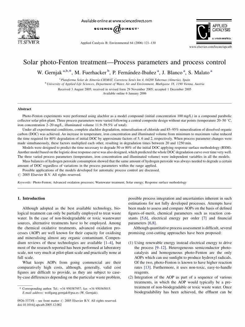
Fig. 4. Typical degradation experiment (Cube 6). HPLC chromatograms at

225 nm wavelength of detection showing the formation of intermediates.

Alachlor is the chromatogram before H2O2 addition and 0 min refers to the

chromatogram after the Fenton reaction in the dark.

radical (Eq. (4)). This peroxyl radical can reduce another ferric

iron ion forming oxygen (Eq. (6)). So all together, two ferrous

iron ions would be recycled at the expense of one hydrogen

peroxide molecule, but without generating any oxidising

species.

C14H20ClNO2þ 34H2O2 ! 14CO2þNH4Cl þ 42H2O (2)

Fe2þ þH2O2 ! Fe3þ þ �OH þ OH� ð53�76 M�1 s�1Þ(3)

Fe3þ þH2O2 ! Fe2þ þ �HO2þHþ ð1�2 � 10�2 M�1 s�1Þ(4)

Fe2þ þ �HO2 ! Fe3þ þHO2� ð0:72�1:5 � 106 M�1 s�1Þ

(5)

Fe3þ þ �HO2! Fe2þ þO2þHþ ð0:33�2:1 � 106 M�1 s�1Þ(6)

Fe2þ þ �OH ! Fe3þ þOH� ð2:6�5 � 108 M�1 s�1Þ (7)

½Fe3þðOH�ÞxðH2OÞy� þ hn

! Fe2þ þ ðx� 1ÞOH� þ yH2O þ �OH (8)

½Fe3þðRCO2�Þ�þ hn ! Fe2þ þ �R þ CO2 " (9)

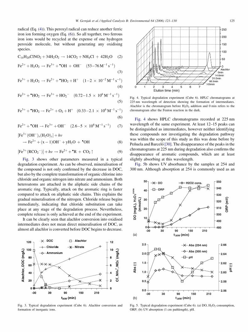
Fig. 3 shows other parameters measured in a typical

degradation experiment. As can be observed, mineralisation of

the compound is not only confirmed by the decrease in DOC,

but also by the complete transformation of organic chlorine into

chloride and organic nitrogen into nitrate and ammonium. Both

heteroatoms are attached in the aliphatic side chains of the

aromatic ring. Typically, attack on the aromatic ring is faster

compared to attack on aliphatic side chains. This explains the

gradual mineralisation of the nitrogen. Chloride release begins

immediately, indicating that chloride substitution can take

place at any stage of the degradation process. Nevertheless,

complete release is only achieved at the end of the experiment.

It can be clearly seen that alachlor conversion into oxidised

intermediates does not mean direct mineralisation of DOC, as

almost all alachlor is converted before DOC begins to decrease.

Fig. 3. Typical degradation experiment (Cube 6). Alachlor conversion and

formation of inorganic ions.

Fig. 4 shows HPLC chromatograms recorded at 225 nm

wavelength of the same experiment. At least 12–15 peaks can

be distinguished as intermediates, however neither identifying

these compounds nor investigating the degradation pathway

was within the scope of this study as this was done before by

Penuela and Barcelo [30]. The disappearance of the peaks in the

chromatograms at 225 nm during degradation also confirms the

disappearance of aromatic compounds, which are at least

slightly absorbing at this wavelength.

Fig. 5b shows UV absorbance by the samples at 254 and

300 nm. Although absorption at 254 is commonly used as an

Fig. 5. Typical degradation experiment (Cube 6). (a) DO, H2O2 consumption,

ORP; (b) UV absorption (1 cm pathlength), pH.

W. Gernjak et al. / Applied Catalysis B: Environmental 64 (2006) 121–130126

indicator for the content of aromatic compounds (DIN 38404-

C3), in the case of photo-Fenton, this is not the only cause of

absorption at 254 nm, which is also due to dissolved iron and

hydrogen peroxide. So to avoid at least the interference of

hydrogen peroxide, it is advisable to observe absorption at

300 nm. The drop in the aromatic compound content correlates

to the absorption of the solution as depicted in Fig. 5. Conversion

of aromatic compounds to oxidised molecule fragments, which

then lose their aromaticity, can usually lead to detoxification

without need of complete mineralisation. Typical early inter-

mediate degradation products, such as phenols, hydroquinones

and quinones, are also known to be considerably toxic and light

absorbing in the ultraviolet region. Consequently, the increasing

absorption at the beginning of the reaction can most probably be

attributed to such intermediates, while subsequent decreasing

absorption reflects the dearomatisation of these compounds. In

another previous study by our group, we showed that acute

toxicity determined with the Vibrio Fischeri bioluminescence

test showed a profile similar to absorption at 300 nm. First,

toxicity rose higher than the toxicity of alachlor itself, and then

decreased as DOC began to decrease [31].

3.2. Influence of process parameters—Model 1

To ensure effective detoxification, wastewater detoxification

must intrinsically involve process assessment. Measurements

of biodegradability enhancement, decrease in toxicity, chemi-

cal oxygen demand or dissolved organic carbon are among the

most frequently applied figures-of-merit. In this work, DOC

degradation was chosen for process evaluation, because other

figures-of-merit can be estimated based upon this measure, if

empirically determined values are available for the given waste

water and oxidation process [12,31].

DOC degradation curves are usually sigmoidal because in

the initial degradation stages, the pollutant is transformed into

oxygenised intermediates but without a loss of carbon dioxide

resulting in initially stable DOC. When degradation proceeds,

DOC decrease accelerates until it slows down again in the final

stages. This particular behaviour impedes calculating rate

constants based on simple rate equations. Alternatively, process

efficiency can be compared based on a given DOC decrease

[9,12]. According to a previous study [31], detoxification of an

alachlor solution can be ensured once DOC degradation reaches

50–80% of the initial value. It was therefore attempted to

develop a model that could predict the time (tDOC50%30W ; tDOC80%

30W )

required for these levels of degradation.

Response surface methodology (RSM) [25] has recently been

applied by several authors to modelling tasks related to photo-

Fenton [14,16]. We attempted the same mathematical approach

in our work, but fitting degradation to second order polynomial

equations was unsuccessful. If all parameters were included, the

resulting models were over-fitted and the response surfaces

folded, and gave local minima and maxima where their

occurrence was not logical from a physical–chemical perspec-

tive. If the number of parameters were limited by forward and

backward selection of parameters, the models simply were not

able to predict the target variables satisfactorily.

One disadvantage was that the model target values have very

high relative errors for fast experiments. This is due to least

square minimisation, which also takes into account absolute

differences. To counter this effect, the model calculation was

directly weighted with the target value (tDOC50%30W ; tDOC80%

30W ) to put

additional weight on the fast experiments, but the approach

yielded poor results nevertheless.

The main reason for the failure of this methodological

approach is probably the wide range of results that the model

must cover. For the fastest experiment tDOC50%30W and tDOC80%

30W

were 6 and 18 min, respectively, for the slowest one 703 and

1060 min. Therefore, the polynomial function approach to the

problem proved invalid.

We then tried a search for functions which seemed

appropriate to describe the problem in a mechanistic approach,

given the knowledge existing about the photo-Fenton process

and the expected influence of T, Fe and the relationship of

collector surface (or illuminated volume) to total volume.

After carefully examining the data and attempting several

types of functions, we decided that the target function should be

a product of functions of the process parameter. To be able to

model the curvature in the n-dimensional space we selected the

potential function. The resulting equation was Eq. (10), where

C, pFe, pT and pA are the four parameters that have to be

optimised, while cFe, T and A are the iron concentration, the

temperature and the collector surface. This equation was then

used to model tDOC50%30W and tDOC80%

30W .

tDOC50%30W or tDOC80%

30W ¼ C � cPFe

Fe � T pT � A pA (10)

A second degree polynomial for three factors, including

linear, quadratic, cross-product terms and offset, has 10

parameters that have to be adjusted. The advantage in this

aspect of Eq. (10) is obvious, as for a given data set for n

observations it leaves more degrees of freedom, which for a

given Pearson’s coefficient results in a higher Fisher’s value in

ANOVA analyses, i.e., a more plausible model. Furthermore,

polynomial functions tend to have poor extrapolation qualities,

which is another reason for searching for alternative functions

more closely related to the physical–chemical behaviour of the

system.

To distinguish this approach from another described later,

we refer to these results as Model 1. The results of parameter

optimisation are given in Eqs. (11) and (12). The results of the

model applied to the experimental results are given in Table 1.

The model results are accurate, except that the relative error is

considerable in very fast experiments. Note that the effect of

changing a process factor can be estimated directly when the

value of the exponent is known.

tDOC50%30W ¼ 220; 200 � c�0:800

Fe � T�1:765 � A�0:515 (11)

tDOC80%30W ¼ 167; 000 � c�0:740

Fe � T�1:558 � A�0:638 (12)

As described, the results of these models are valid for

constant process variables, i.e., those which do not change,

such as temperature, iron concentration and collector area.

The latter would not change in a real case plant either, of

W. Gernjak et al. / Applied Catalysis B: Environmental 64 (2006) 121–130 127

Fig. 6. DOC/DOCi values calculated by logistic dose response curve modelling

of the real data for each experiment against measured DOC/DOCi from all

experiments (see text).

course, while temperature obviously changes in a solar

collector, if no external temperature control is applied. The

same is possible for the iron concentration, if there should be

precipitation due to high pH or the presence of phosphate, for

example.

3.3. Influence of process parameters—Model 2

It would be desirable to have a dynamic model which is

capable of predicting the reaction speed at every moment of the

degradation process. As mentioned, DOC degradation curves

have a sigmoidal form. Of the common curves fitting sigmoidal

tendencies, the Boltzmann function and the logistic dose

response curve are outstanding for their simplicity. Both have

only four parameters to adjust. The problem with the

Boltzmann function is that its curvature is symmetric at both

sides of the inflexion point, which is not necessarily the case in

a DOC degradation curve. So this function must be discarded in

favour of the logistic dose response curve, which is commonly

used to describe dose response curves in pharmacology. The

four parameters of the equation (Eq. (13)) are A1 and A2, which

are the initial and the final DOC values (DOCi, DOCf), t1/2, the

time when degradation is half-way between DOCi and DOCf

and p, an exponent largely determining the curvature and the

slope of the curve. DOC in Eq. (13) refers to the measured DOC

value at any time during degradation.

DOC

DOCi¼ A1 � A2

1þ ðt30W=t1=2Þ p þ A2 (13)

As we used normalised values (DOC/DOCi), A1 was always

one, except for the experiments in which 20 mg/L iron was used

at 50 8C because these were the only ones in which DOC

degradation during the Fenton reaction before illumination was

remarkable. Consequently, A1 was set at 0.82, the average value

of both experiments at zero illumination time (see Fig. 2c). At

the same time, it was assumed that the DOCf is always 5% of

DOCi and A2 is 0.05, thus resulting a non-linear fitting problem

with only two parameters. This assumption was made to

optimise modelling between 20 and 80% DOC degradation,

Table 2

Logistic dose response curve parameters modelled from experimental data

Experiment Fitted values Fitted valu

t1/2 (min) p t1/2 (min)

Centre 1 42 3.02 36

Centre 2 53 3.39 36

Centre 3 45 3.13 36

Cube 1 139 2.93 140

Cube 2 689 4.27 688

Cube 3 48 3.86 55

Cube 4 272 4.91 272

Cube 5 15 1.77 22

Cube 6 107 3.51 110

Cube 7 5.1 1.26 8.9

Cube 8 37 2.82 44

These parameters were modelled from process parameters as described in the text

which is considered the most relevant region because

detoxification takes place somewhere in this phase of

degradation.

We then fitted each experiment, which gave an excellent

coefficient of determination (square of Pearson’s coefficient) of

higher than 0.99 for each experiment and also when all

measured samples were plotted against their calculated value

(see Fig. 6). This confirms the adequacy of the equation for this

problem. The fitted parameters are given in Table 2.

Then we fitted t1/2 the same way as described above for

tDOC50%30W and tDOC80%

30W (see Eq. (10)) and the result was Eq. (14).

No logical reason for any correlation between p and the

influencing process variables could be found. So we started out

again with a second degree polynomial including cross-

products of the variables. This time the results of the regression

were logical and consistent. Forward selection was applied to

find the optimum selection of parameters in the multivariate

linear regression process [32] based on the criteria of

maximising not only coefficient of determination (square of

es with Model 2

p tDOC50%30W (min) tDOC80%

30W (min)

3.17 38 62

3.17 38 62

3.17 38 62

2.95 145 247

4.24 706 1022

3.86 57 85

4.92 278 383

1.76 24 58

3.55 114 177

1.27 9.6 33

2.82 45 79

and regression results for tDOC50%30W and tDOC80%

30W calculated with Model 2.

W. Gernjak et al. / Applied Catalysis B: Environmental 64 (2006) 121–130128

Pearson’s coefficient), but also the Fisher’s value. Eq. (15) was

the result (Fisher’s value of 135). Regression results for

Eqs. (14) and (15) are given in Table 2. It also lists the values

calculated with Model 2 for tDOC50%30W and tDOC80%

30W :

t1=2 ¼ 197; 000 � c�0:795Fe � T�1:740 � A�0:576 (14)

p ¼� 0:0431 � T þ 0:203 � A� 0:000929 � cFe � T � 0:0235

� cFe � Aþ 0:00237 � T � Aþ 4:97 (15)

Model 2, the final equation for the DOC degradation curve as

a function of illumination time, temperature, iron concentra-

tion, collector surface and irradiation intensity implicitly

included in the illumination time (see Eq. (1)), results from

inserting Eqs. (14) and (15) into Eq. (13). The results calculated

for all samples measured are plotted against the measured

values in Fig. 2. The fit is very good for most experiments,

except, similar to the above modelling problems, in fitting very

fast experiments, probably due to the extremely wide intervals

of the reaction rates observed.

The partial derivative with respect to illumination time of

the resulting equation represents the DOC degradation rate

when the other parameters are constant (except changes in

irradiation intensity, which are taken into account). If the

other parameters are not constant, the degradation curve can

be calculated by parts. A complete degradation curve can thus

be reconstructed for varying process parameters. This would

present no problem should online prediction of the degrada-

tion curve be necessary, as long as temperature and radiation

intensity are measured on-line and information about changes

in iron concentration is made available to the control system.

So, this is a possibility for on-line prediction of process

progress and for making decisions about when to end the

process and whether to transfer or discharge the treated

effluent.

3.4. Determination of process progress by easy-to-measure

on-line parameters

As mentioned above, detoxification semantically implies

that at one point of the degradation process the waste water is no

longer toxic and can be disposed of to a subsequent treatment or

the environment. Measuring chemical oxygen demand, DOC or

toxicity is expensive, time-consuming and slow. This justifies

the search for alternative assessment criteria that are cheaper

and faster.

One approach is to model the process based on process

variables describing the system as above. Another approach is

to measure alternative parameters directly. We measured the

absorbance at various wavelengths and hydrogen peroxide

consumption off-line, and DO, ORP and pH on-line. Fig. 5

shows the same parameters for the experiment shown in Fig. 3,

which may be considered paradigmatic.

ORP measurements gave little information in this first

screening because of their many influencing parameters. The

most interesting effect was that the ORP reflects whether iron

ions present are ferric or ferrous very well (see Fig. 5 for the

step between �150 and 00, where Fenton reaction takes place

converting ferrous in ferric iron). This could be an indirect

indicator of a lack of hydrogen peroxide as in this case the

ferric/ferrous iron relationship is changed by Eqs. (8) and (9)

from equilibrium in the presence of hydrogen peroxide, while

Eq. (3) cannot take place.

pH measurements are mainly useful because depending

upon initial pollutant concentrations and the mineralisation

processes taking place (acids or bases produced), the pH can

be modified during treatment. So on-line pH measurement

can avoid precipitation of iron, if pH tends to rise in a

particular system. In our experiments, pH changed only

slightly during the treatment reflecting the formation of

chloride, inorganic nitrogen species and carboxylic acids as

intermediates.

DO measurements were of interest, as several different

phenomena were present in the DO profile. First, DO decreased,

indicating the incorporation of DO in the reaction mechanism

by Eqs. (16) and (17) (Dorfman mechanism) [33]. The resulting

peroxyl radical can then further participate in the reaction

mechanism, e.g., by Eq. (5) generating an additional hydrogen

peroxide molecule. When degradation proceeded, the ratio of

reactants (particularly hydrogen peroxide) to pollutant changed

and the reaction of the radicals generated (by Eq. (3)) with

hydrogen peroxide (Eq. (18)) was favoured, leading to the mere

decomposition of hydrogen peroxide into water and oxygen

(Eq. (19)). Consequently, the DO profile is a reaction progress

indicator. Furthermore, at the stage at which massive oxygen

production took place, a lack of hydrogen peroxide can again be

perceived in the DO profile, because DO concentration

decreases from its supersaturation range by degassing to the

atmosphere, if no new oxygen is supplied into the solution

simultaneously by the reaction:

�R þ O2 ! �RO2 (16)

�RO2þH2O ! ROH þ �HO2 (17)

�OH þ H2O2 ! H2O þ �HO2 (18)

2H2O2 ! 2H2O þ O2 (19)

Light absorbance by the solution at 254 nm can be used in

wastewater treatment to estimate the content of aromatic

substances (DIN 38404-C3). However, this approximation is

applicable to waste water with a rather constant composition

such as urban waste water, as it depends largely on the

molecular extinction coefficient of the present organic

substances at the chosen wavelength. In the particular case

of photo-Fenton, it is advisable to measure at somewhat higher

wavelengths for two reasons. First, if hydrogen peroxide is

present, its absorption influences measurement below 300 nm,

and second, if the treated waste water contains aromatics many

of the typical quinone/hydroquinone reaction intermediates

formed can be detected by measurement at higher wavelengths

as that is where they typically absorb. Indication of these

intermediates is especially desirable, as they are known to be

highly toxic. Fig. 5 clearly shows that the value again has a

W. Gernjak et al. / Applied Catalysis B: Environmental 64 (2006) 121–130 129

Fig. 7. H2O2 consumption vs. the measured DOC/DOCi values of all experi-

ments performed, including the Fenton experiment. The curve fits show the

H2O2 consumption for photo-Fenton and Fenton (a) points are marked accord-

ing to temperature; (b) points are marked according to iron concentration.

typical profile that could be used to estimate process progress.

The remnant absorption is due to iron complexes. Depending

on pH, ferric iron forms different aquo complexes involving

more or fewer hydroxyl radicals. These iron complexes differ in

their light absorption properties [4], which interferes with this

parameter, making it a qualitative measure.

Hydrogen peroxide was measured off-line but could

theoretically be measured on-line. Such sensors exist (Alldos

Eichler GmbH, Prominent Dosiertechnik GmbH), although

they are not very commonly employed. Fig. 7 shows DOC

degradation as a function of hydrogen peroxide consumption.

It can clearly be seen that the amount of degradation is strongly

correlated to the amount of hydrogen peroxide consumed. It

should be remarked that within the range of the parameters

investigated, no influence of any of the selected process

variables (iron concentration, temperature and collector area)

on the amount of hydrogen peroxide consumption needed for

degradation could be detected. On the contrary, Fig. 7 shows

that Fenton degradation needed more hydrogen peroxide to

reach the same degradation level. This is in accordance with the

fact that, contrary to the dark Fenton reaction (Eq. (4)), in

photo-Fenton, transformation of ferric to ferrous iron takes

place mainly without hydrogen peroxide consumption (Eqs. (8)

and (9)). The consumption of hydrogen peroxide (mmol/L) as a

function of DOC degradation (between 0 and 1) can be

estimated with a polynomial function (Eq. (20), coefficient of

determination (square of Pearson’s coefficient) of 0.94,

standard deviation of error 5.1 mmol/L), where H2O2cons

represents the hydrogen peroxide consumption and %DOC the

share of initial DOC degraded (between 0 and 1).

H2Ocons2 ¼ 1110 �%DOC5 � 2100 �%DOC4 þ 1430 �%DOC3

� 400 �%DOC2 þ 58:9 �%DOC� 0:0325 (20)

The theoretical hydrogen peroxide consumption for com-

plete mineralisation of 100 mg/L Alachlor is 12.6 mmol/L

(Eq. (2)). Calculated with Eq. (20), 55% of DOC mineralisation

takes place before this. This correlation could be used for

process control. It should be noted that the data and correlation

shown are only valid for the case in hand, because hydrogen

peroxide consumption depends on many parameters, mainly the

type and amount of wastewater contamination. So similar

empirical data will have to be obtained for different cases

before such a correlation can be established.

Fig. 7 shows furthermore, that extensive DOC degradation

needs considerably higher amounts of hydrogen peroxide than

moderate DOC degradation (e.g., 11.3, 25.2, 46.5 and

66.2 mmol/L for 50, 80, 90 and 95% DOC degradation,

calculated with Eq. (20)). So apart from merely extending

treatment time (and associated costs) increased reagent

consumption has to be included in the economic considerations

for making a decision as to when to stop treatment and/or with a

view to possible combination of AOPs with subsequent

biological treatment.

4. Conclusions

Hundred milligrams per litre of alachlor solutions were

mineralised with solar photo-Fenton treatment over a wide

range of varying process variables for iron concentration,

temperature and collector area per volume.

Response surface methodology was applied to assess the

influence of process parameters on the reaction rate. The use of

second degree polynomials, including cross-product terms,

yielded invalid results. Consequently, mechanistic modelling

was attempted and the equation employed for modelling DOC

degradation became a potential function. Prediction was further

improved by modelling the DOC degradation curve as a

function of illumination time with the ‘‘logistic dose response’’

curve. This produced an analytical expression as a function of

time, irradiation intensity, iron concentration, temperature and

solar collector area per volume. Given the analytical

expression, the DOC degradation rate (first derivative) can

be calculated for any moment of a real process with changing

process variables, as long as feed waste water and process

variable values are available. If on-line process parameter

information is available, an on-line control system can be

automated based on this information.

Further parameters measurable on-line were also investi-

gated. ORP, DO, pH and UV absorption of the solution

produced only qualitative information about the degradation

process progress. On the contrary, hydrogen peroxide

measurements revealed that DOC degradation could be

predicted by a polynomial relationship with hydrogen peroxide

consumption as the only independent variable. That means that

W. Gernjak et al. / Applied Catalysis B: Environmental 64 (2006) 121–130130

none of the process variables varied changed the amount of

oxidising reagent necessary to reach a certain level of DOC

decrease. Furthermore, it was shown that a multiple of the

amount of reagent necessary for high DOC degradation levels

must be added compared to what is required for moderate

levels. This is important to process economic assessment and

the possibility of a subsequent biological treatment.

It should be noted that the models and correlations employed

here were calculated for these experimental data and serve only

as a model case. Due to the complexity of the system and

depending on the waste water, the correlations are likely to be

somewhat different in other cases. Nevertheless, the modelling

approach is proposed as a methodology for obtaining models

also useful for other cases.

Acknowledgements

The authors wish to thank the European Commission for

financial support through the CADOX Project (contract no.

EVK1-CT-2002-00122). Mr. Gernjak wants to thank the

Austrian Academy of Sciences for a grant under the DOC

Programme. The authors wish to express their gratitude to Mrs.

Eva Augsten for the laboratory analysis and Mrs. Deborah

Fuldauer for the correction of the English style.

References

[1] P.R. Gogate, A.B. Pandit, Adv. Environ. Res. 8 (2004) 501.

[2] P.R. Gogate, A.B. Pandit, Adv. Environ. Res. 8 (2004) 553.

[3] O. Legrini, E. Oliveros, A.M. Braun, Chem. Rev. 93 (1993) 671.

[4] A. Safarzadeh-Amiri, J.R. Bolton, S.R. Cater, J. Adv. Oxid. Technol. 1

(1996) 18.

[5] V. Augugliaro, C. Baiocchi, A. Bianco Prevot, E. Garcıa-Lopez, V. Loddo,

S. Malato, G. Marcı, L. Palmisano, M. Pazzi, E. Pramauro, Chemosphere

49 (2002) 1223.

[6] S. Esplugas, J. Gimenez, S. Contreras, E. Pascual, M. Rodrıguez, Water

Res. 36 (2002) 1034.

[7] M.E. Sigman, A.C. Buchanan III, S.M. Smith, J. Adv. Oxid. Technol. 2

(1997) 415.

[8] A. Goi, M. Trapido, Chemosphere 46 (2002) 913.

[9] H. Fallmann, T. Krutzler, R. Bauer, S. Malato, J. Blanco, Catal. Today 54

(1999) 309.

[10] T. Krutzler, H. Fallmann, P. Maletzky, R. Bauer, S. Malato, J. Blanco,

Catal. Today 54 (1999) 321.

[11] S. Malato, J. Blanco, A. Vidal, C. Richter, Appl. Catal. B: Environ. 37

(2002) 1.

[12] S. Malato, J. Blanco, A. Vidal, D. Alarcon, M.I. Maldonado, J. Caceres, W.

Gernjak, Sol. Energy 75 (2003) 329.

[13] R. Bauer, H. Fallmann, Res. Chem. Intermed. 23 (1997) 341.

[14] V. Sarria, S. Kenfack, O. Guillod, C. Pulgarin, J. Photochem. Photobiol. A

159 (2003) 89.

[15] S. Esplugas, D.F. Ollis, J. Adv. Oxid. Technol. 2 (1997) 197.

[16] E. Oliveros, O. Legrini, M. Hohl, T. Muller, A.M. Braun, Chem. Eng.

Proc. 36 (1997) 397.

[17] E.K. May, R. Gee, D.T. Wickham, L.A. Lafloon, J.D. Wright, Design and

Fabrication of a Prototype Solar Receiver/Reactors for the Solar Detox-

ification of Contaminated Water, NREL Report, Industrial Solar Technol-

ogy Corp., Golden, Colorado, USA, 1991.

[18] S. Malato, J. Caceres, A.R. Fernandez-Alba, L. Piedra, M.D. Hernando, A.

Aguera, J. Vial, Environ. Sci. Technol. 37 (2003) 2516.

[19] M. Kositzi, I. Poulios, S. Malato, J. Caceres, A. Campos, Water Res. 38

(2004) 1147.

[20] S. Malato, J. Blanco, M.I. Maldonado, P. Fernandez-Ibanez, A. Campos,

Appl. Catal. B: Environ. 28 (2000) 163.

[21] S. Malato, J. Blanco, M.I. Maldonado, P. Fernandez, D. Alarcon, M.

Collares, J. Farinha, J. Correia, Sol. Energy 77 (2004) 513.

[22] J. Blanco, S. Malato, P. Fernandez, A. Vidal, A. Morales, P. Trincado,

J.C. Oliveira, C. Minero, M. Musci, C. Casalle, M. Brunotte,

S. Tratzky, N. Dischinger, K.H. Funken, C. Sattler, M. Vincent, M.

Collares-Pereira, J.F. Mendes, C.M. Rangel, Sol. Energy 67 (2000) 317.

[23] G. Sagawe, A. Lehnard, M. Lubber, G. Rochendorf, D. Bahnemann, Helv.

Chim. Acta 84 (2001) 3742.

[24] F. Herrera, C. Pulgarin, V. Nadtochenko, J. Kiwi, Appl. Catal. B: Environ.

17 (1998) 141.

[25] G.E.P. Box, Statistics for Experimenters, John Wiley & Sons, New York,

USA, 1978.

[26] C.D.S. Tomlin, The Pesticide Manual, 11th ed., British Crop Protection

Council, Farnham, UK, 1997.

[27] APHA, AWWA, WEF, Standard Methods for the Examination of Water

and Waste Water, 20th ed., United Book Press Inc., Maryland, USA,

1998 .

[28] R. Chen, J.J. Pignatello, Environ. Sci. Technol. 31 (1997) 2399.

[29] A.Y. Sychev, V.G. Isaak, Russ. Chem. Rev. 64 (1995) 1105.

[30] G.A. Penuela, D. Barcelo, J. Chromatogr. A 754 (1996) 187.

[31] M. Hincapie, M.I. Maldonado, I. Oller, W. Gernjak, J.A. Sanchez-Perez,

M.M. Ballesteros, S. Malato, Catal. Today 101 (2005) 203.

[32] J.F. Hair, R.E. Anderson, R.L. Tatham, W.C. Black, Multivariate Data

Analysis, Prentice Hall International, New Jersey, USA, 1998.

[33] C. von Sonntag, P. Dowideit, X. Fang, R. Mertens, X. Pan, M.N.

Schuchmann, H.P. Schuchmann, Water Sci. Technol. 35 (4) (1997) 9.