Software packages performance evaluation of basic radar ...
81
University of Cape Town Software packages performance evaluation of basic radar signal processing techniques Presented by: Xavier Frantz Prepared for: Associate Professor Daniel O’Hagan Dept. of Electrical Engineering University of Cape Town Submitted to the Department of Electrical Engineering at the University of Cape Town in partial fulfilment of the academhic requirements for a Master of Engineering specialising in Radar and Electronic Defence January 26, 2019
-
Upload
khangminh22 -
Category
Documents
-
view
0 -
download
0
Transcript of Software packages performance evaluation of basic radar ...
Univers
ity of
Cap
e Tow
n
Software packages performance evaluation ofbasic radar signal processing techniques
Presented by:Xavier Frantz
Prepared for:Associate Professor Daniel O’Hagan
Dept. of Electrical EngineeringUniversity of Cape Town
Submitted to the Department of Electrical Engineering at the University of Cape Townin partial fulfilment of the academhic requirements for a Master of Engineering
specialising in Radar and Electronic Defence
January 26, 2019
Univers
ity of
Cap
e Tow
nThe copyright of this thesis vests in the author. Noquotation from it or information derived from it is to bepublished without full acknowledgement of the source.The thesis is to be used for private study or non-commercial research purposes only.
Published by the University of Cape Town (UCT) in termsof the non-exclusive license granted to UCT by the author.
Declaration
I know the meaning of plagiarism and declare that all the work in the document, savefor that which is properly acknowledged, is my own. This thesis/dissertation has beensubmitted to the Turnitin module (or equivalent similarity and originality checking soft-ware) and I confirm that my supervisor has seen my report and any concerns revealed bysuch have been resolved with my supervisor.
Signature:X. Frantz
Date: 10 September 2018

Acknowledgments
I would like to thank the following people who helped with the completion of this project:
Darryn Jordan, for assisting with the implementation of pulse compression and Dopplerprocessing algorithms.
Francois Schoken and Lerato Mohapi, for being available to brainstorm ideas for perfor-mance analysis.
Colleagues in the RRSG Radar Lab, for helping with setting up equipment, sharingresources and perfecting the implementation of algorithms.
My supervisor, Professor Daniel O’Hagan for patience and guidance during the comple-tion of the project.
My family, for constant encouragement and motivation.
I would like to thank ARMSCOR and the CSIR for their generous funding of my studies.
The Almighty God, for always giving me the strength and motivation for life.
i
Abstract
This dissertation presents a radar signal processing infrastructure implemented on script-ing language platforms. The main goal is to determine if any open source scripted pack-ages are appropriate for radar signal processing and if it is worthwhile purchasing the moreexpensive MATLAB, commonly used in industry. Some of the most common radar signalprocessing techniques were considered, such as pulse compression, Doppler processing andadaptive filtering for interference suppression. The scripting languages investigated werethe proprietary MATLAB, as well as open source alternatives such as Octave, Scilab,Python and Julia.
While the experiments were conducted, it was decided that the implementations shouldhave algorithmic fairness across the various software packages. The first experimentwas loop based pulse compression and Doppler processing algorithms, where Julia andPython outperformed the rest. A further analysis was completed by using vectors to indexmatrices instead of loops, where possible. This saw a significant improvement in all of thelanguages for Doppler processing implementations. Although Julia performed extremelywell in terms of speed, it utilized the most memory for the processing techniques. This wasdue to its garbage collector not automatically clearing the memory heap when required.The adaptive LMS (least mean squares) filter designs were a different form of analysis,as a vector of data was required instead of a matrix of data. When processing a vectoror one dimensional array of data, Julia outperformed the rest of the software packagessignificantly, approximately a 10 times speed improvement.
The experiments indicated that Python performed satisfactorily in terms of speed andmemory utilization. Physical RAM of computer systems is, however, constantly improv-ing, which will mitigate the memory issue for Julia. Overall, Julia is the best open sourcesoftware package to use, as its syntax is similar to MATLAB compared with Python, andit is improving rapidly as Julia developers are constantly updating it. Other disadvantageof Python is that the mathematical signal processing is an add-on realized by modulessuch as NumPy.
ii
Contents
1 Introduction 1
1.1 Objectives of this study . . . . . . . . . . . . . . . . . . . . . . . . . . . 2
1.1.1 Problems to be investigated . . . . . . . . . . . . . . . . . . . . . 2
1.1.2 Purpose of the study . . . . . . . . . . . . . . . . . . . . . . . . . 2
1.2 Scope and limitations . . . . . . . . . . . . . . . . . . . . . . . . . . . . . 2
1.3 Plan of development . . . . . . . . . . . . . . . . . . . . . . . . . . . . . 3
2 Literature review 4
2.1 Radar theory . . . . . . . . . . . . . . . . . . . . . . . . . . . . . . . . . 4
2.1.1 Radar signals . . . . . . . . . . . . . . . . . . . . . . . . . . . . . 4
2.2 RSP techniques . . . . . . . . . . . . . . . . . . . . . . . . . . . . . . . . 6
2.2.1 NetRAD data . . . . . . . . . . . . . . . . . . . . . . . . . . . . . 6
2.2.2 Matched filter . . . . . . . . . . . . . . . . . . . . . . . . . . . . . 7
2.2.3 Pulse compression . . . . . . . . . . . . . . . . . . . . . . . . . . . 8
2.2.4 Doppler processing . . . . . . . . . . . . . . . . . . . . . . . . . . 10
iii
2.2.5 Adaptive noise cancellation . . . . . . . . . . . . . . . . . . . . . 11
2.3 Programming languages . . . . . . . . . . . . . . . . . . . . . . . . . . . 14
2.3.1 MATLAB . . . . . . . . . . . . . . . . . . . . . . . . . . . . . . . 15
2.3.2 Julia . . . . . . . . . . . . . . . . . . . . . . . . . . . . . . . . . . 15
2.3.3 Scilab . . . . . . . . . . . . . . . . . . . . . . . . . . . . . . . . . 15
2.3.4 Octave . . . . . . . . . . . . . . . . . . . . . . . . . . . . . . . . . 16
2.3.5 Python . . . . . . . . . . . . . . . . . . . . . . . . . . . . . . . . . 16
2.3.6 Additional features for interpreted languages . . . . . . . . . . . . 17
2.3.7 Memory principles . . . . . . . . . . . . . . . . . . . . . . . . . . 20
2.3.8 FFT library . . . . . . . . . . . . . . . . . . . . . . . . . . . . . . 23
2.3.9 Floating point operations per second (FLOPS) . . . . . . . . . . . 24
3 Implementation of radar signal processing (RSP) techniques 26
3.1 Fairness . . . . . . . . . . . . . . . . . . . . . . . . . . . . . . . . . . . . 26
3.2 Pulse compression implementation . . . . . . . . . . . . . . . . . . . . . . 27
3.3 Doppler processing implementation . . . . . . . . . . . . . . . . . . . . . 29
3.4 Adaptive LMS filter implementation . . . . . . . . . . . . . . . . . . . . . 31
4 Results and discussion 36
4.1 Performance of RSP algorithm designs . . . . . . . . . . . . . . . . . . . 37
4.1.1 Computation time for pulse compression design . . . . . . . . . . 37
iv
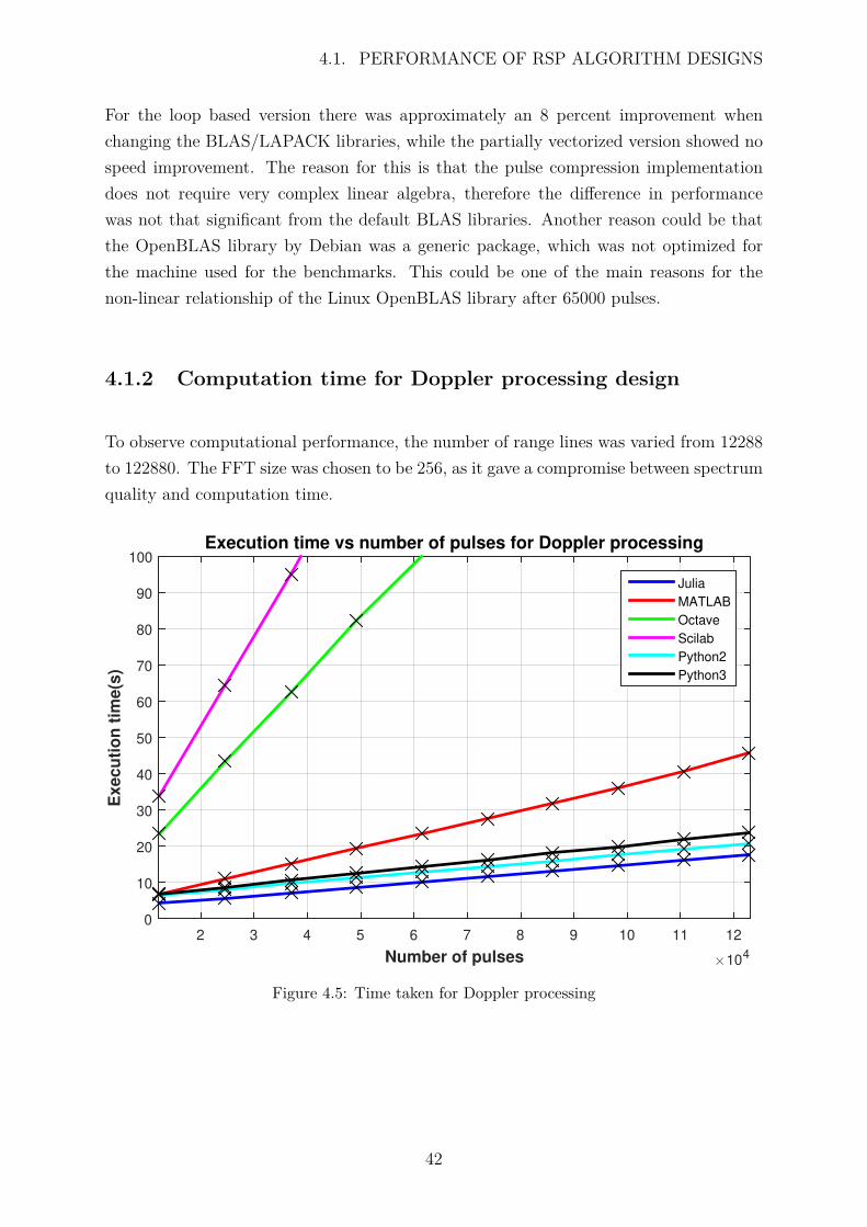
4.1.2 Computation time for Doppler processing design . . . . . . . . . . 42
4.2 FLOPS for different RSP algorithms . . . . . . . . . . . . . . . . . . . . 46
4.2.1 FLOPS for pulse compression algorithm design . . . . . . . . . . 46
4.2.2 FLOPS for Doppler processing algorithm design . . . . . . . . . . 48
4.3 Memory handling for pulse compression andDoppler processing . . . . . . . . . . . . . . . . . . . . . . . . . . . . . . 50
4.4 Performance of adaptive LMS filter algorithm design . . . . . . . . . . . 53
5 Conclusions and recommendations 58
5.1 Improved performance with spatial locality . . . . . . . . . . . . . . . . . 58
5.2 Adequate performance of pulse compression . . . . . . . . . . . . . . . . 58
5.3 Lack of JIT during Doppler processing for Octave and Scilab . . . . . . . 59
5.4 Impact of large vectors on adaptive LMS filter design . . . . . . . . . . . 60
5.5 Impact of memory utilization on various language packages . . . . . . . . 60
5.6 Lack of implicit parallelism in Scilab . . . . . . . . . . . . . . . . . . . . 60
5.7 Suitable alternatives to MATLAB . . . . . . . . . . . . . . . . . . . . . . 61
5.8 Recommendations . . . . . . . . . . . . . . . . . . . . . . . . . . . . . . . 61
A Additional Procedures 62
A.1 Changing BLAS/LAPACK libraries for Scilab . . . . . . . . . . . . . . . 62
A.2 FFTW procedures . . . . . . . . . . . . . . . . . . . . . . . . . . . . . . 62
A.3 Vectorization procedures . . . . . . . . . . . . . . . . . . . . . . . . . . . 63
v
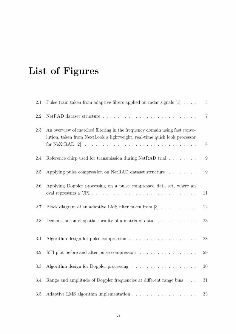
List of Figures
2.1 Pulse train taken from adaptive filters applied on radar signals [1] . . . . 5
2.2 NetRAD dataset structure . . . . . . . . . . . . . . . . . . . . . . . . . . 7
2.3 An overview of matched filtering in the frequency domain using fast convo-lution, taken from NextLook a lightweight, real-time quick look processorfor NeXtRAD [2] . . . . . . . . . . . . . . . . . . . . . . . . . . . . . . . 8
2.4 Reference chirp used for transmission during NetRAD trial . . . . . . . . 9
2.5 Applying pulse compression on NetRAD dataset structure . . . . . . . . 9
2.6 Applying Doppler processing on a pulse compressed data set, where anoval represents a CPI . . . . . . . . . . . . . . . . . . . . . . . . . . . . . 11
2.7 Block diagram of an adaptive LMS filter taken from [3] . . . . . . . . . . 12
2.8 Demonstration of spatial locality of a matrix of data. . . . . . . . . . . . 23
3.1 Algorithm design for pulse compression . . . . . . . . . . . . . . . . . . . 28
3.2 RTI plot before and after pulse compression . . . . . . . . . . . . . . . . 29
3.3 Algorithm design for Doppler processing . . . . . . . . . . . . . . . . . . 30
3.4 Range and amplitude of Doppler frequencies at different range bins . . . 31
3.5 Adaptive LMS algorithm implementation . . . . . . . . . . . . . . . . . . 33
vi
3.6 Simulated fixed frequency pulse radar signals before and after LMS adap-tive filtering . . . . . . . . . . . . . . . . . . . . . . . . . . . . . . . . . . 35
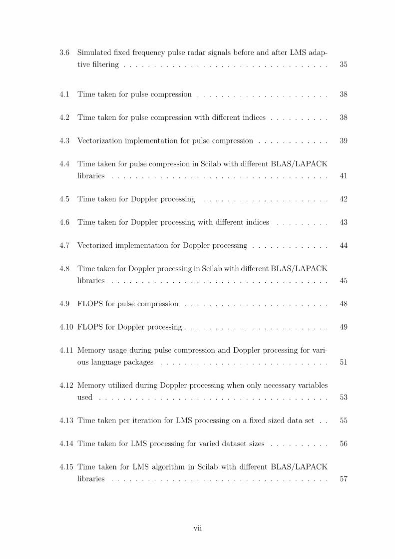
4.1 Time taken for pulse compression . . . . . . . . . . . . . . . . . . . . . . 38
4.2 Time taken for pulse compression with different indices . . . . . . . . . . 38
4.3 Vectorization implementation for pulse compression . . . . . . . . . . . . 39
4.4 Time taken for pulse compression in Scilab with different BLAS/LAPACKlibraries . . . . . . . . . . . . . . . . . . . . . . . . . . . . . . . . . . . . 41
4.5 Time taken for Doppler processing . . . . . . . . . . . . . . . . . . . . . 42
4.6 Time taken for Doppler processing with different indices . . . . . . . . . 43
4.7 Vectorized implementation for Doppler processing . . . . . . . . . . . . . 44
4.8 Time taken for Doppler processing in Scilab with different BLAS/LAPACKlibraries . . . . . . . . . . . . . . . . . . . . . . . . . . . . . . . . . . . . 45
4.9 FLOPS for pulse compression . . . . . . . . . . . . . . . . . . . . . . . . 48
4.10 FLOPS for Doppler processing . . . . . . . . . . . . . . . . . . . . . . . . 49
4.11 Memory usage during pulse compression and Doppler processing for vari-ous language packages . . . . . . . . . . . . . . . . . . . . . . . . . . . . 51
4.12 Memory utilized during Doppler processing when only necessary variablesused . . . . . . . . . . . . . . . . . . . . . . . . . . . . . . . . . . . . . . 53
4.13 Time taken per iteration for LMS processing on a fixed sized data set . . 55
4.14 Time taken for LMS processing for varied dataset sizes . . . . . . . . . . 56
4.15 Time taken for LMS algorithm in Scilab with different BLAS/LAPACKlibraries . . . . . . . . . . . . . . . . . . . . . . . . . . . . . . . . . . . . 57
vii
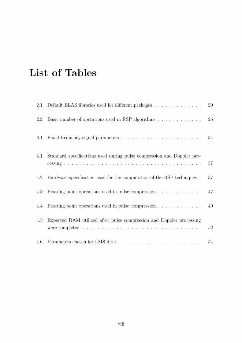
List of Tables
2.1 Default BLAS libraries used for different packages . . . . . . . . . . . . . 20
2.2 Basic number of operations used in RSP algorithms . . . . . . . . . . . . 25
3.1 Fixed frequency signal parameters . . . . . . . . . . . . . . . . . . . . . . 34
4.1 Standard specifications used during pulse compression and Doppler pro-cessing . . . . . . . . . . . . . . . . . . . . . . . . . . . . . . . . . . . . . 37
4.2 Hardware specification used for the computation of the RSP techniques . 37
4.3 Floating point operations used in pulse compression . . . . . . . . . . . . 47
4.4 Floating point operations used in pulse compression . . . . . . . . . . . . 49
4.5 Expected RAM utilized after pulse compression and Doppler processingwere completed . . . . . . . . . . . . . . . . . . . . . . . . . . . . . . . . 52
4.6 Parameters chosen for LMS filter . . . . . . . . . . . . . . . . . . . . . . 54
viii
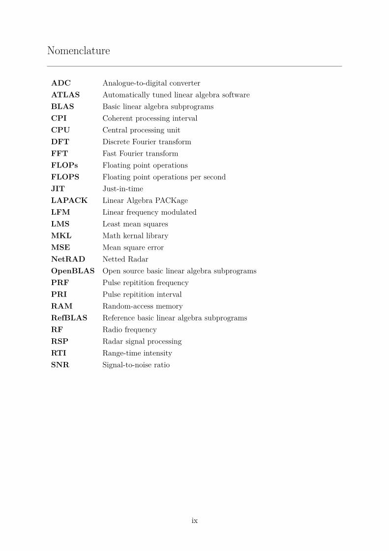
Nomenclature
ADC Analogue-to-digital converterATLAS Automatically tuned linear algebra softwareBLAS Basic linear algebra subprogramsCPI Coherent processing intervalCPU Central processing unitDFT Discrete Fourier transformFFT Fast Fourier transformFLOPs Floating point operationsFLOPS Floating point operations per secondJIT Just-in-timeLAPACK Linear Algebra PACKageLFM Linear frequency modulatedLMS Least mean squaresMKL Math kernal libraryMSE Mean square errorNetRAD Netted RadarOpenBLAS Open source basic linear algebra subprogramsPRF Pulse repitition frequencyPRI Pulse repitition intervalRAM Random-access memoryRefBLAS Reference basic linear algebra subprogramsRF Radio frequencyRSP Radar signal processingRTI Range-time intensitySNR Signal-to-noise ratio
ix
Chapter 1
Introduction
The signal processor will take the raw radar data from the receiver, and perform a numberof common signal processing operations on the data. These include pulse compression,Doppler processing and adaptive filtering. When performing the above algorithms, op-erations such as correlation, fast Fourier transforms (FFT) and matrix-vector algebraicoperations are typically required [4].
Scientific computing is typically used for designing radar signal processing (RSP) so-lutions. Using compiled languages like C++ for processing will be time consuming asdevelopment time is longer. Its syntax is not simple; libraries have to be integratedmanually or own functions have to be written, and memory has to be handled manually.Interpreted languages are much simpler and easier for engineers to use. Syntax is almostlike writing mathematical expressions on paper and memory handling is automatic. Themost common interpreted language used in research and industry is MATLAB. However,it is costly and extra funding would be needed for purchasing additional toolboxes. Thereis, therefore, a need for suitable open source alternatives to MATLAB that can provideacceptable, or even superior, performance.
1
1.1. OBJECTIVES OF THIS STUDY
1.1 Objectives of this study
1.1.1 Problems to be investigated
The main problem to be investigated in this study is the fair comparison of differentscripted language packages, in the context of common RSP operations. The objectivesof this report are to:
• design RSP algorithms in such a manner that performance is not decremented, butstill gives algorithmic fairness across various language packages;
• compare scripting language platforms in terms of memory usage and execution time;
• draw conclusions to determine which open source software packages are viable forRSP; and
• recommend strategies to improve performance for all of the language packages suchthat further comparisons can be made.
1.1.2 Purpose of the study
The main purpose is to determine which of the several scripted languages are appropriatefor RSP. In engineering, MATLAB is widely used in research and industry to design RSPtechniques. Therefore, a requirement is to determine how open source software packagescompare with the more accomplished and expensive MATLAB, as well as which of theopen source packages would be recommended for various RSP techniques.
1.2 Scope and limitations
This report is limited to the implementation of pulse compression, Doppler processingand adaptive filter algorithms in MATLAB, Julia, Python, Octave and Scilab. Thealgorithms are designed in such a way that they can be used in various other radarapplications besides the datasets used in these experiments.
In this paper the following limitations occurred:
2
1.3. PLAN OF DEVELOPMENT
• A fair algorithmic comparison was made across all of the software packages. Firstly,a loop based algorithm was written, implying that code was not written for maxi-mum performance for each language package. Secondly, code was optimized wherepossible in order to give faster execution time. In both scenarios, performance wasmeasured for identical algorithmic implementation and code patterns, correspond-ing to each software package.
• Memory utilization analysis was only considered for the pulse compression andDoppler processing algorithms, because Netted Radar (NetRAD) datasets consumelarge amounts of memory. The dataset used for the adaptive LMS processing algo-rithms was approximately 6 megabytes (MB), for which it was not worthwhile todo a thorough memory analysis. It was decided to avoid redundancy as memorywould be handled in the same way as in large datasets.
• The default linear algebra libraries were used for all the software packages, with onlyScilab’s linear algebra libraries being altered for analysis and clarification purposes.
1.3 Plan of development
The rest of the report is organized in the following way:
Chapter 2 provides a literature review of the basics of radar, different RSP techniques, andsoftware packages used in the study. It also describes important techniques that mustbe considered when implementing different RSP algorithms on the different languagepackages.
In Chapter 3 the manner in which the RSP algorithms were designed is described indetail.
Chapter 4 describes how the RSP algorithms were executed. Performance results arepresented for all three RSP algorithms across all investigated software platforms, afterwhich an analysis and comparison will follow.
Chapter 5 presents the conclusions based on the progression of the study and discusseswhich software packages are suitable for RSP design. Chapter 5 also has a list of recom-mendations that can be used for future work to build on the results of this study.
3
Chapter 2
Literature review
2.1 Radar theory
RADAR is an acronym for radio detection and ranging. It’s two most basic functions areto detect an object and to determine it’s distance from the radar system. Radar systemshave improved over the years, with the ability to track, identify, and image detectedtargets. A radar system typically transmits radio frequency (RF) electromagnetic (EM)waves towards a region of interest. In this region of interest, the EM waves are reflectedfrom the objects, creating echoes. These echoes are received by the radar system and areprocessed to determine important information about the target [4].
2.1.1 Radar signals
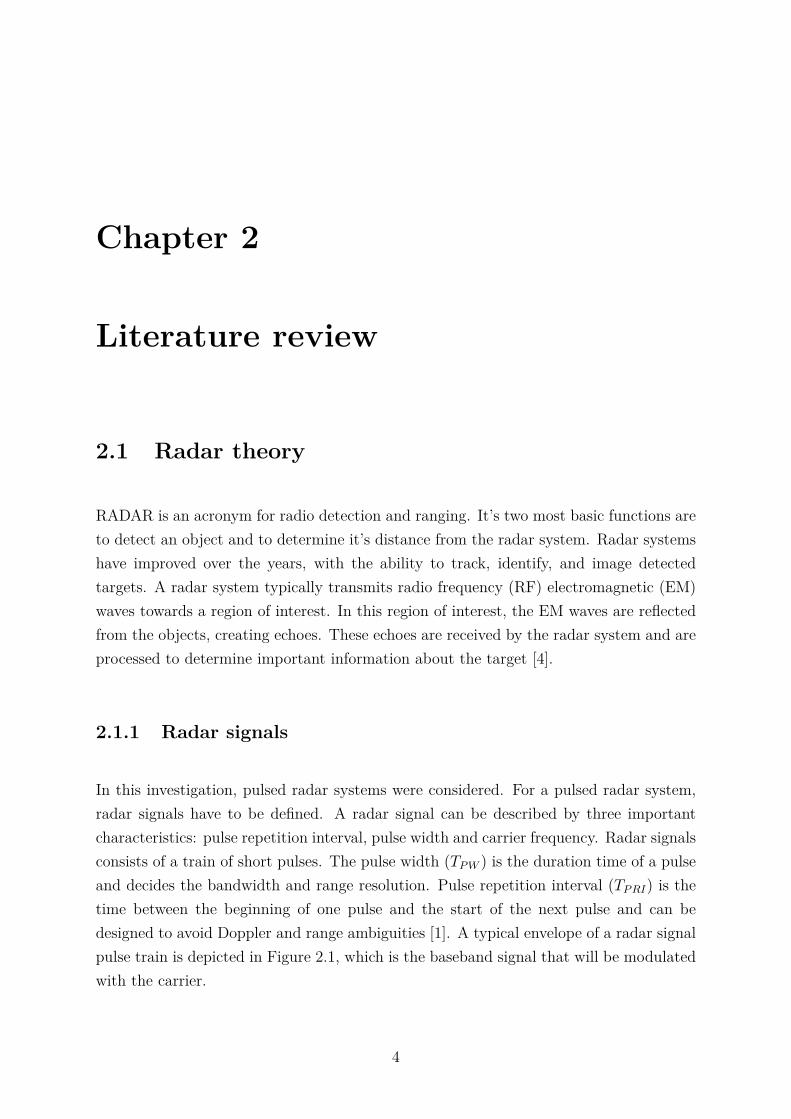
In this investigation, pulsed radar systems were considered. For a pulsed radar system,radar signals have to be defined. A radar signal can be described by three importantcharacteristics: pulse repetition interval, pulse width and carrier frequency. Radar signalsconsists of a train of short pulses. The pulse width (TP W ) is the duration time of a pulseand decides the bandwidth and range resolution. Pulse repetition interval (TP RI) is thetime between the beginning of one pulse and the start of the next pulse and can bedesigned to avoid Doppler and range ambiguities [1]. A typical envelope of a radar signalpulse train is depicted in Figure 2.1, which is the baseband signal that will be modulatedwith the carrier.
4
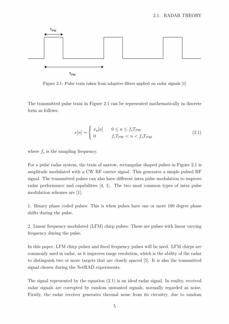
2.1. RADAR THEORY
Figure 2.1: Pulse train taken from adaptive filters applied on radar signals [1]
The transmitted pulse train in Figure 2.1 can be represented mathematically in discreteform as follows:
x[n] =
xp[n] 0 ≤ n ≤ fsTP W
0 fsTP W < n < fsTP RI
(2.1)
where fs is the sampling frequency.
For a pulse radar system, the train of narrow, rectangular shaped pulses in Figure 2.1 isamplitude modulated with a CW RF carrier signal. This generates a simple pulsed RFsignal. The transmitted pulses can also have different intra pulse modulation to improveradar performance and capabilities [4, 1]. The two most common types of intra pulsemodulation schemes are [1]:
1. Binary phase coded pulses: This is when pulses have one or more 180 degree phaseshifts during the pulse.
2. Linear frequency modulated (LFM) chirp pulses: These are pulses with linear varyingfrequency during the pulse.
In this paper, LFM chirp pulses and fixed frequency pulses will be used. LFM chirps arecommonly used in radar, as it improves range resolution, which is the ability of the radarto distinguish two or more targets that are closely spaced [5]. It is also the transmittedsignal chosen during the NetRAD experiments.
The signal represented by the equation (2.1) is an ideal radar signal. In reality, receivedradar signals are corrupted by random unwanted signals, normally regarded as noise.Firstly, the radar receiver generates thermal noise from its circuitry, due to random
5
2.2. RSP TECHNIQUES
electron motion. There is also environmental noise, clutter, unwanted echoes from theenvironment and jamming that could interfere with the desired signal. So the datacollected is not perfect, as these unwanted signals might mask the signal of interest [4].
The radar signal processor becomes important, as it takes the raw radar signal andapplies signal processing techniques to it, improving the ability to detect targets andextract useful information from raw radar echoes. In this study the most common RSPtechniques were considered. These include pulse compression, which improves rangeresolution and SNR, as well as Doppler processing, which measures Doppler shift andthus radial velocity. Adaptive filtering is also used to suppress thermal noise from rawradar data [4].
2.2 RSP techniques
2.2.1 NetRAD data
NetRAD, is a three node coherent multistatic radar system, consisting of one transmit-receive node and two receive-only nodes. In other words, there is only one monostaticnode and two bistatic nodes [6]. This system was originally developed at the UniversityCollege of London in 2000 as a cable synchronized, multi-node radar system. However,due to the limitations of the 50m cable used to connect the nodes, the University of CapeTown joined the project in 2003 by developing a distributed global positioning systemsynchronized set of clocks. Control software was also developed such that different nodescan be controlled over a wireless network from a central control computer. This enablednodes to be separated many kilometres apart and improved synchronization problems.The main purpose of the NetRAD system was making raw data available, with theintention that individuals and organizations process this multistatic data, and understandsea clutter and vessel properties in a multistatic configuration [7].
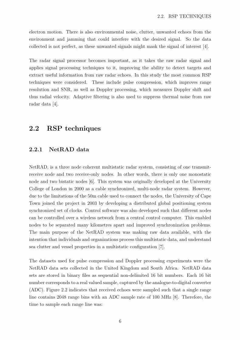
The datasets used for pulse compression and Doppler processing experiments were theNetRAD data sets collected in the United Kingdom and South Africa. NetRAD datasets are stored in binary files as sequential non-delimited 16 bit numbers. Each 16 bitnumber corresponds to a real valued sample, captured by the analogue-to-digital converter(ADC). Figure 2.2 indicates that received echoes were sampled such that a single rangeline contains 2048 range bins with an ADC sample rate of 100 MHz [8]. Therefore, thetime to sample each range line was:
6
2.2. RSP TECHNIQUES
2048 · 1100 MHz = 20.48 µs (2.2)
During the experiments, a total of 130000 pulses were transmitted at a PRF of 1 kHz [8].This resulted in the experiment lasting for:
130000 · 11kHz = 130 s (2.3)
Figure 2.2: NetRAD dataset structure
2.2.2 Matched filter
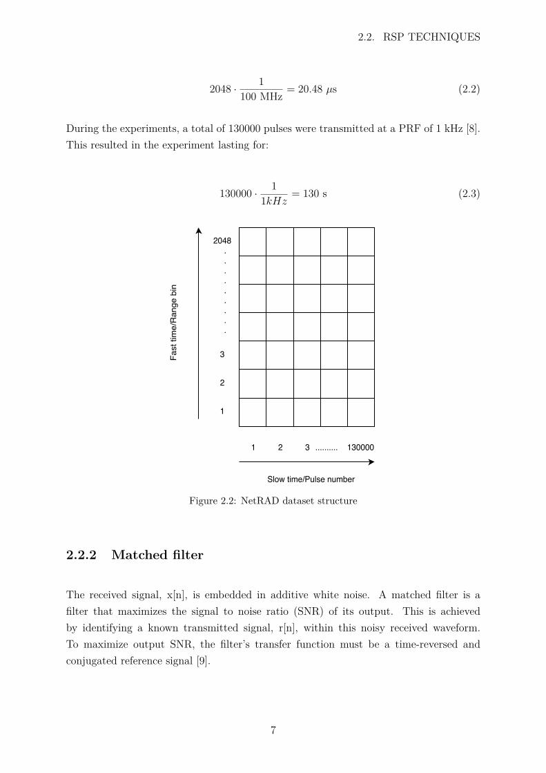
The received signal, x[n], is embedded in additive white noise. A matched filter is afilter that maximizes the signal to noise ratio (SNR) of its output. This is achievedby identifying a known transmitted signal, r[n], within this noisy received waveform.To maximize output SNR, the filter’s transfer function must be a time-reversed andconjugated reference signal [9].
7
2.2. RSP TECHNIQUES
h[n] = r∗[−n] ⇐⇒ H[k] = R∗[k] (2.4)
Matched filtering is normally implemented digitally by using fast convolution. Fast con-volution is a correlation operation implemented using the FFT, thus the discrete timesamples can be efficiently transformed into discrete-time Fourier transform samples [4].The fast convolution technique is illustrated in Figure 2.3.
FFT
FFT Conjugation
IFFTx[n]
r[n]
X[k]
R[k]
Y[k]
H[k]
y[n]
Figure 2.3: An overview of matched filtering in the frequency domain using fast con-volution, taken from NextLook a lightweight, real-time quick look processor for NeX-tRAD [2]
2.2.3 Pulse compression
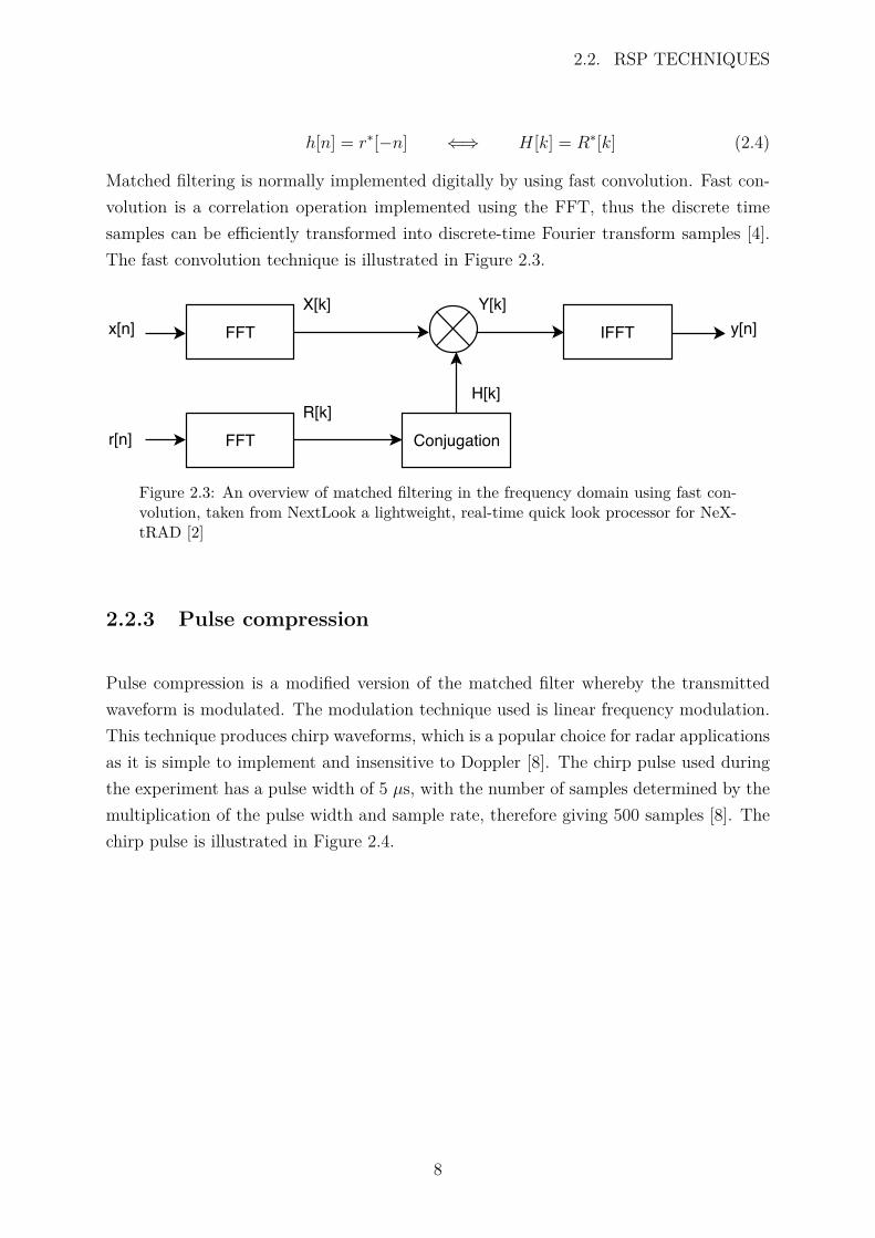
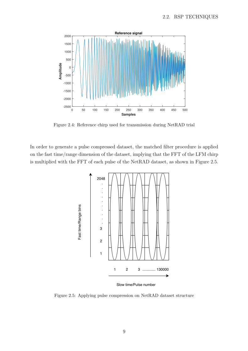
Pulse compression is a modified version of the matched filter whereby the transmittedwaveform is modulated. The modulation technique used is linear frequency modulation.This technique produces chirp waveforms, which is a popular choice for radar applicationsas it is simple to implement and insensitive to Doppler [8]. The chirp pulse used duringthe experiment has a pulse width of 5 µs, with the number of samples determined by themultiplication of the pulse width and sample rate, therefore giving 500 samples [8]. Thechirp pulse is illustrated in Figure 2.4.
8
2.2. RSP TECHNIQUES
Samples
0 50 100 150 200 250 300 350 400 450 500
Am
pli
tud
e
-2500
-2000
-1500
-1000
-500
0
500
1000
1500
2000
Reference signal
Powered by TCPDF (www.tcpdf.org)
Powered by TCPDF (www.tcpdf.org)
Figure 2.4: Reference chirp used for transmission during NetRAD trial
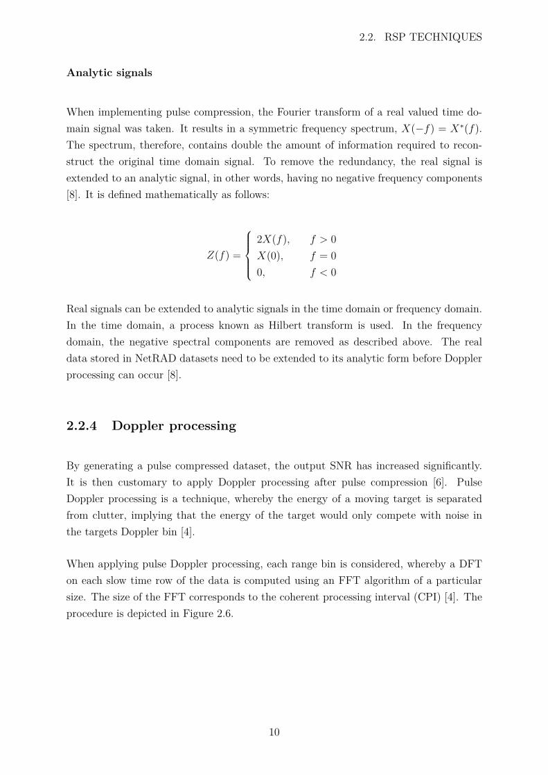
In order to generate a pulse compressed dataset, the matched filter procedure is appliedon the fast time/range dimension of the dataset, implying that the FFT of the LFM chirpis multiplied with the FFT of each pulse of the NetRAD dataset, as shown in Figure 2.5.
Figure 2.5: Applying pulse compression on NetRAD dataset structure
9
2.2. RSP TECHNIQUES
Analytic signals
When implementing pulse compression, the Fourier transform of a real valued time do-main signal was taken. It results in a symmetric frequency spectrum, X(−f) = X∗(f).The spectrum, therefore, contains double the amount of information required to recon-struct the original time domain signal. To remove the redundancy, the real signal isextended to an analytic signal, in other words, having no negative frequency components[8]. It is defined mathematically as follows:
Z(f) =
2X(f), f > 0X(0), f = 00, f < 0
Real signals can be extended to analytic signals in the time domain or frequency domain.In the time domain, a process known as Hilbert transform is used. In the frequencydomain, the negative spectral components are removed as described above. The realdata stored in NetRAD datasets need to be extended to its analytic form before Dopplerprocessing can occur [8].
2.2.4 Doppler processing
By generating a pulse compressed dataset, the output SNR has increased significantly.It is then customary to apply Doppler processing after pulse compression [6]. PulseDoppler processing is a technique, whereby the energy of a moving target is separatedfrom clutter, implying that the energy of the target would only compete with noise inthe targets Doppler bin [4].
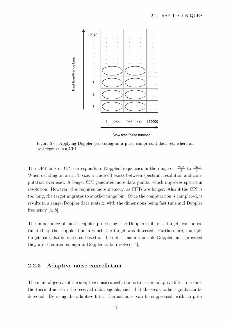
When applying pulse Doppler processing, each range bin is considered, whereby a DFTon each slow time row of the data is computed using an FFT algorithm of a particularsize. The size of the FFT corresponds to the coherent processing interval (CPI) [4]. Theprocedure is depicted in Figure 2.6.
10
2.2. RSP TECHNIQUES
..........
..........
..........
...........
1300001 255 256....
Slow time/Pulse number
Fast
tim
e/Ra
nge
bins
2048
2
3
1
.
.
.
.
.
.
.
.
.
.
.
.
.
.
.
.
.
.
.
.
.
.
.
.
.
.
.
.
.
.
.
.
.
.
.
.
.
.
.
.
.
.
.
.
.
.
.
.
.
.
...... 511......
Powered by TCPDF (www.tcpdf.org)
Powered by TCPDF (www.tcpdf.org)
Figure 2.6: Applying Doppler processing on a pulse compressed data set, where anoval represents a CPI
The DFT bins or CPI corresponds to Doppler frequencies in the range of -P RF2 to P RF
2 .When deciding on an FFT size, a trade-off exists between spectrum resolution and com-putation overhead. A longer CPI generates more data points, which improves spectrumresolution. However, this requires more memory, as FFTs are longer. Also if the CPI istoo long, the target migrates to another range bin. Once the computation is completed, itresults in a range/Doppler data matrix, with the dimensions being fast time and Dopplerfrequency [4, 8].
The importance of pulse Doppler processing, the Doppler shift of a target, can be es-timated by the Doppler bin in which the target was detected. Furthermore, multipletargets can also be detected based on the detections in multiple Doppler bins, providedthey are separated enough in Doppler to be resolved [4].
2.2.5 Adaptive noise cancellation
The main objective of the adaptive noise cancellation is to use an adaptive filter to reducethe thermal noise in the received radar signals, such that the weak radar signals can bedetected. By using the adaptive filter, thermal noise can be suppressed, with no prior
11
2.2. RSP TECHNIQUES
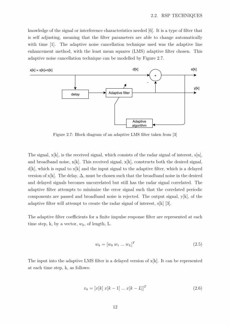
knowledge of the signal or interference characteristics needed [6]. It is a type of filter thatis self adjusting, meaning that the filter parameters are able to change automaticallywith time [1]. The adaptive noise cancellation technique used was the adaptive lineenhancement method, with the least mean squares (LMS) adaptive filter chosen. Thisadaptive noise cancellation technique can be modelled by Figure 2.7.
delay Adaptive filter
Adaptivealgorithm
+x[k] = s[k]+n[k] d[k] e[k]
y[k]-
Figure 2.7: Block diagram of an adaptive LMS filter taken from [3]
The signal, x[k], is the received signal, which consists of the radar signal of interest, s[n],and broadband noise, n[k]. This received signal, x[k], constructs both the desired signal,d[k], which is equal to x[k] and the input signal to the adaptive filter, which is a delayedversion of x[k]. The delay, ∆, must be chosen such that the broadband noise in the desiredand delayed signals becomes uncorrelated but still has the radar signal correlated. Theadaptive filter attempts to minimize the error signal such that the correlated periodiccomponents are passed and broadband noise is rejected. The output signal, y[k], of theadaptive filter will attempt to create the radar signal of interest, s[k] [3].
The adaptive filter coefficients for a finite impulse response filter are represented at eachtime step, k, by a vector, wk, of length, L.
wk = [w0 w1 ... wL]T (2.5)
The input into the adaptive LMS filter is a delayed version of x[k]. It can be representedat each time step, k, as follows:
xk = [x[k] x[k − 1] ... x[k − L]]T (2.6)
12
2.2. RSP TECHNIQUES
The radar signal of interest, s[k], is embedded in noise. The output of the adaptive filter,y[k], attempts to create this radar signal of interest and is denoted by Equation (2.7):
y[k] = wTk · xk (2.7)
At each time step, the adaptive filter coefficients, wk, are updated by an adaptive algo-rithm. The adaptive filter algorithm consists of a mean square error (MSE) objectivefunction. The MSE is a function of the error signal, e[k].
e[k] = d[k]− y[k] (2.8)
Since y[n] goes towards the signal of interest, s[n], the error signal will be approximatethermal noise.
e[k] = d[k]− y[k] = s[n] + n[n]− s[n] ≈ n[n] (2.9)
To minimize the MSE, the adaptive filter coefficients are altered recursively as follows:
wk+1 = wk + 2µ · e∗(k) · xk (2.10)
where ∗ represents complex conjugate.
The step size, µ, is also known as the convergence factor. This determines the changeof the filter coefficients in each time step. By using a small step size, changes to thefilter parameters are small in each time step. This results in a high convergence time,as steps towards the minimum of the performance surface are short. The advantage isthat, the steady state MSE will be small. However, a large step size is the opposite, as itgives a fast convergence time and an increase in steady state MSE. Therefore, choosingan appropriate step size becomes a tradeoff between having a fast convergence time or asmall steady state MSE [10].
The other important parameter needed for the LMS filter is the filter length. Thisdetermines the best SNR performance that the adaptive filter can achieve. A smallnumber of filter coefficients will give a low SNR gain, while a large number of filter
13
2.3. PROGRAMMING LANGUAGES
coefficients generate a high SNR gain. Having many filter coefficients requires moresamples, resulting in a longer time to converge [10].
2.3 Programming languages
Users design algorithms in high-level languages, consisting of basic English words andphrases, arithmetic operators and punctuation. A program written in a high level lan-guage is known as source code. Computers will not be able to execute source code;therefore it needs to be converted to machine code. Machine code is written in binary,0’s and 1’s, which is understandable by a computer. In order to convert source code tomachine code, either compilers or interpreters are used [11].
Compiled programming languages: These are programming languages that goesthrough a compiling step during which all of the source code is converted to machinecode. The machine code generated is then executed directly on the target hardware. Inother words, during runtime, only machine code is executed. Compiled languages alsooptimize generated code to achieve faster execution [12].
Interpreted programming languages: When using interpreted languages, source codeis not converted to machine code prior to runtime. There is no explicit compile step.During runtime, interpreted languages are executed one command at a time by anotherprogram, known as an interpreter program. It therefore interprets the source code andthen executes previously compiled functions based on that source code during runtime andnot before runtime as for compiled languages. For this very reason interpreted languagescan be considered slower than compiled languages [12].
All of the investigated packages contain interpreted languages and RSP algorithms aredeveloped on a Linux system. The open source packages are all available from the Linuxdistribution packaging system. However, the up-to-date versions might not be available,therefore, for certain languages, the binary version of the packages was used. A binaryversion of a software package is a pre-compiled version that can be read by the computerand used for execution.
14
2.3. PROGRAMMING LANGUAGES
2.3.1 MATLAB
MATLAB stands for MATrix LABoratory. It is a high performance language, used fortechnical computing, and has been commercially available since 1984 [13]. It has grownto be considered as a standard tool used by most universities and industries. There arenumerous powerful built-in science and engineering toolboxes available, used for a varietyof computations. These comprise signal processing, control theory, symbolic computationand many more [13]. MATLAB 2014 was the licenced version used for RSP designs. Toget a MATLAB licence is expensive, which is why free, open source alternatives need tobe considered.
2.3.2 Julia
Julia is a high-level language that achieves high performance for numerical computing.It also provides a just-in-time (JIT) compiler, numerical accuracy and a comprehensivemathematical function library. Julia’s base library is mostly written in Julia, integratingC and FORTRAN libraries for linear algebra and signal processing. Currently, the Juliadeveloper community is rapidly contributing numerous external packages through Julia’sbuilt-in package. Julia 0.5.2, which was updated in May 2017, was used in the develop-ment of RSP algorithms. A new, much improved version, Julia 0.6.0, is available but stillin its infant stage, with algorithms on Julia 0.5.2 completed before Julia 0.6 was released[14].
2.3.3 Scilab
Scilab is a free, open source software package provided under the Cecill licence. It isused for numerical computations, as it provides a powerful computing environment forengineering and scientific applications. It includes various functionalities such as signalprocessing, control system design and analysis, and many more [15]. On the Linux systemused for the experiments, the packaging system is distributed with Scilab. The up-to-date version, Scilab 6.0.0, was, however, not available on that particular Linux version,therefore the binary version of Scilab 6.0.0 was used. Reasons for using Scilab 6.0.0were that memory was dynamically allocated and previous versions of Scilab only acceptapproximately 2GB of memory. This was not sufficient when large datasets need to beprocessed. Algorithms were also implemented on Linux systems because the Windows
15
2.3. PROGRAMMING LANGUAGES
version of Scilab 6.0.0 immediately shuts down for unknown reasons when processing thedatasets. This happened on multiple Windows systems. The latest version of Scilab 6.0.0was downloaded and installed in June 2017.
2.3.4 Octave
Octave was initially developed in 1988 as a companion software, for an undergraduate-level textbook on chemical reactor design. It was later decided to build a more flexibletool which, that was more than just courseware package. Today it is a high level language,intended for numerical computations. Octave is convenient as its syntax is compatiblewith MATLAB, which is commonly used in industry and academia. Today it is used bythousands of people for numerous activities that include teaching, research and commer-cial applications. It is currently being developed under the leadership of Dr J.W. Eatonand released under the GNU General Public Licence [16]. In the designing of the RSPalgorithms Octave 4.0.0 was used as it was initially installed from the Linux distribu-tion package. There are no substantial changes from Octave 4.0.0 to the latest Octavepackage.
2.3.5 Python
Guido van Rossum invented Python around 1990 while working with the Amoeba dis-tributed operating system and the ABC language. Initially, Python was created as anadvanced scripting language for the Amoeba system. Later it was realized that Python’sdesign was very general, such that it could be used in numerous domains. Today it isa general purpose open source language used for numerous applications [17]. The im-plementation of Python used is the default version, CPython. It is both a compiler andinterpreter that comes with standard packages and modules written in standard C [18].
Two versions of Python are currently being used, Python2 and Python3. Python2 ismostly used, it is stable, with no changes being made to it as its life cycle will endapproximately in 2020 [19]. Python3 is an improvement on Python2 and will be the futureof Python. At the moment it is still growing and updated regularly. The motivation forPython3 was to fix old design mistakes, requiring backward compatibility to be brokenfrom Python2. There would be a few changes in both languages and its libraries, asmajor Python packages were ported to Python3. This implies that many skills gained bylearning Python2 can be transferred to Python3 [20]. The versions of Python used during
16
2.3. PROGRAMMING LANGUAGES
this investigation are Python 2.7.12 and Python 3.5.2, which are the default installationson UbuntuMATE 17.04.
Python also has many specialized modules that can be used for solving numerical prob-lems with fast array operations. The Numeric Python (NumPy) package was used in thisinvestigation, as it is an open source numeric programming extension module for Pythonthat consists of a flexible multidimensional array for fast and concise mathematical cal-culations. The internals of this array is based on C arrays, which will give performanceimprovements, as well as the ability to interface with the existing C and FORTRANroutines. NumPy provides a large library of fast precompiled functions for mathematicaland numerical routines that effectively turn Python into a scientific programming tool,allowing for efficient computations on multi-dimensional arrays and matrices [17, 21, 22].NumPy’s speed is achieved through vectorization, which will be elaborated on in furthersections [23].
2.3.6 Additional features for interpreted languages
JIT compiler
When using interpreted languages, faster code can be generated by using a JIT compiler.A JIT compiler uses both the interpreter and compiler, whereby each line is compiledand executed to generate machine code. By doing this, the application can be optimizedfor target hardware [12].
MATLAB and Julia have introduced a JIT, one of the most important factors in howcode is executed faster. Currently, Octave’s JIT compiler is in its experimental stage,while CPython and Scilab do not have such a feature. However, Python makes use ofthe CPython compiler, which is not optimized for numerical processing. This compilercould be replaced with the Numba compiler that would give CPython JIT capabilitiesbut it is not compatible with all the existing Python libraries (mainly Pyfftw) and someof the language features [24]. Another Python implementation known as PyPy imple-ments a standard JIT compiler, this also has the libraries issues that Numba does [25].The disadvantage of languages with a JIT compiler is that the first run is always slowerthan subsequent runs because of the compilation process. Therefore, when performingbenchmarks, always use the second runs [12]. A JIT compiler also performs optimiza-tion techniques, such as vectorization on for loops in the background, resulting in loopoverhead being minimized. MATLAB’s JIT compiler has been improved significantly in
17
2.3. PROGRAMMING LANGUAGES
newer versions, speeding up for loops without the user’s attempt to vectorize them [26].
Python JIT compiler
Implicit parallelism
There are several forms of parallelism that can be implemented in algorithms. Thesecan be classified into either implicit or explicit parallelization. The former is where theuser’s code is parallelized without any modification to the algorithm, while the latter isa transformation of the user’s algorithm to achieve parallelization [27, 28]. During thisinvestigation, implicit parallelization was constantly used, as it occurs without the usersknowledge. There are two types of implicit parallelism: vectorization and linear algebracomputations.
Vectorization: This is a programming technique whereby vector operations are used,instead of element-by-element loop-based operations. Vectorized operations are implic-itly parallelized. This means that the internal implementations are optimized by beingmulti threaded behind the scenes in optimized, pre-compiled C code. When possible, italso makes use of the hardware’s vector instructions or performs other optimizations insoftware that accelerates everything. A JIT compiler is important as one of its featuresis vectorizing for loops in the background, such that loop overhead is minimized. Thethree main advantages of vectorized code are [29, 30]:
1. Appearance of the code is neater, which is easier to understand.
2. It is faster than loop based code, as its operations are optimized for matrices andvectors.
3. It is typically shorter than loop-based code, which is less prone to errors.
In most scenarios vectorized code achieves a massive speed up compared to loop basedcode [31]. All of the above languages have operations which are optimized for matricesand vectors.
Linear algebra computations: Implicit parallelization also shows up in linear algebracomputations, such as matrix multiplication, linear algebra and performing the sameoperation on a set of numbers [28, 32]. The building blocks for linear algebra is the basic
18
2.3. PROGRAMMING LANGUAGES
linear algebra subprograms (BLAS) and Linear Algebra PACKage (LAPACK) libraries[33].
• LAPACK: This is the library responsible for linear algebra computations. It con-sists of a collection of FORTRAN routines, used for solving high level linear algebraproblems [33]. All of the above packages make use of this library.
• BLAS: It is a collection of FORTRAN routines that provide low level operationssuch as vector addition, dot products and matrix-matrix multiplications [33]. LA-PACK relies on this library for its internal computations [34].
There are four major implementations of the BLAS libraries that can be used. Theseare reference basic linear algebra subprograms (RefBLAS), automatically tuned linearalgebra software (ATLAS), open source basic linear algebra subprograms (OpenBLAS)and intel math kernel library (MKL).
• ATLAS: It provides optimized routines for BLAS, as well as a small subset ofLAPACK. The procedure is based on empirical techniques to provide portable per-formance and improvements over the reference BLAS/LAPACK libraries [33].
• Intel MKL: This is a library developed by Intel. It consists of highly optimized,heavily threaded math routines for Intel processors. This implies that on Intelprocessors, maximum performance would be achieved [34, 33]. For computers withIntel CPU’s, these MKL libraries can be obtained for free. If installed correctly,all of the language packages investigated can make use of it for complex matrixoperations [35, 36, 37, 38].
• OpenBLAS: For several processor architectures, optimized implementations oflinear algebra kernels are provided [39].
• RefBLAS: Reference BLAS library is a single threaded implementation of BLAS.For particularly complex linear algebra, this library will be slower than optimizedmulti-threaded versions [34].
The key difference between these libraries is that RefBLAS is a single threaded implemen-tation and the others are highly optimized, multi-threaded versions of BLAS [34]. IntelMKL is a proprietary library, while RefBLAS, ATLAS and OpenBLAS are open sourcelibraries, all available from the Ubuntu Linux distribution package system [34]. The bi-nary packages of ATLAS and OpenBLAS distributed by Debian are generic packages
19

2.3. PROGRAMMING LANGUAGES
which are not optimized for a particular machine [39]. To achieve optimal performance,ATLAS and OpenBLAS must be recompiled locally for optimal performance, which isrecommended for advanced Linux users seeking maximum performance. If the hardwareused is amd64 or x86, there is no need to recompile OpenBLAS, as the binary includesoptimized kernels for several CPU micro-architectures [39].
The default version of BLAS and LAPACK libraries was used for each of the packagesand is outlined in Table 2.1. Note that Octave uses OpenBLAS from Linux distributionpackage by default.
Table 2.1: Default BLAS libraries used for different packages
Software BLAS libraryMATLAB Intel MKL
Julia OpenBLASOctave OpenBLASScilab RefBLAS
Python2 OpenBLASPython3 OpenBLAS
There is a necessity to also have a fair performance comparison. This means that forScilab, the OpenBLAS library from the Linux distribution package, as well as the defaultversion were considered during the experiment. This was encouraged in order to havemulti-threaded BLAS/LAPACK libraries for all software packages, not necessarily beingoptimized for specific hardware. Note that on Windows, Scilab uses Intel MKL linearalgebra libraries by default, instead of the reference linear algebra libraries as with Linuxmachines.
2.3.7 Memory principles
Memory heap
In any programming language, heap memory management is important. The heap is amassive space where memory is dynamically allocated. In other words, when a programis in execution, it will continuously allocate memory to the heap until algorithms arecompleted. If the space used on the heap is not freed, that space will never be availableagain while the program continues to execute. Normally, two scenarios might happen
20
2.3. PROGRAMMING LANGUAGES
when this occurs. Firstly, the heap will fill up and the program will abnormally terminate.Secondly, the program would continue to run, but the performance of the system willdeteriorate [40].
There are two ways to free space on the heap: manually, whereby programmers mustremember to free space that was allocated on the heap or it can be done automatically.Many interpreted languages do the latter. This is accomplished by using a garbagecollector which runs as part of the interpreter and checks for space that can be freed onthe heap. Garbage collectors will ensure that space on the heap is allocated and accessedcorrectly. This allows for programmers to allocate space on the heap, without concerningthemselves about freeing that space [40].
Virtual memory
Processing datasets that require a significant amount of memory might cause the process-ing procedure to fail or performance might deteriorate, as explained in the memory heapsection. To compensate for this, computer systems automatically use virtual memorywithout the user’s control. Virtual memory is a technique whereby the hardware uses aportion of the hard disk, called a swap file, that extends the amount of available mem-ory. This is completed by treating main memory as cache for most recently used data,the inactive RAM contents are stored onto disk and only active contents are allowed tobe situated in main memory. This process is continued as needed by the computer bycontinuously swapping from disk to memory, eventually causing the system performanceto deteriorate [41].
Principle of locality
Over the years, memory performance has not increased at the same rate as CPU perfor-mance. When processing large datasets, generating fast algorithms could be troublesome,as performance will be limited by the time it takes to access memory. Code is thus mem-ory bound, which means that processing is decided by the amount of memory required tohold the datasets. However, there are measures that can overcome memory bound code,such as avoiding inefficient memory usages [42].
Principal of locality is an important concept for cache friendly code, which is when thesame or related storage locations are being accessed regularly [43, 4]. It allocates data
21
2.3. PROGRAMMING LANGUAGES
such that it is aligned close in memory. There are two types:
Temporal locality: When data in a specific memory location is accessed and cached -data that is accessed can be used again for a short time period.
Spatial locality: Relevant when manipulating datasets, the data in a particular datasetare aligned in memory locations that are close to each other. When accessing elementsin matrices, elements adjacent/next to it will also be fetched.
When the user generates code to manipulate data, both forms of locality are likely tooccur. By considering spatial locality, datasets can be manipulated to ensure that ithandles contiguous memory effectively. This will lead to fewer memory accesses andfaster code [43].
Contiguous memory
When processing 2-D or an N-D array, try accessing data that transverses monotonicallyincreasing memory locations [42]. This means either accessing rows or columns, dependingon how data is stored in contiguous memory. When accessing memory, data is not directlyread from it, some of the data is initially stored from memory to cache, and then readfrom cache to the processor. If data needed is not in cache, the required data will befetched from memory. This process can be referred to as spatial locality: when fetchingan element, the elements next to it are cached. To ensure spatial locality occurs for theRSP algorithms, row major or column major ordering needs to be considered [44].
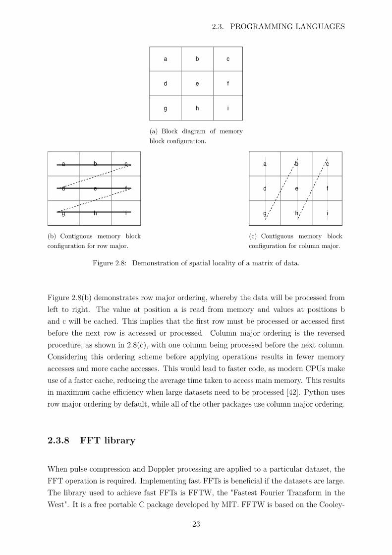
Figure 2.8 demonstrates spatial locality using a simple 3x3 matrix with data for row andcolumn major ordering schemes.
22
2.3. PROGRAMMING LANGUAGES
a b c
d e f
g h i
(a) Block diagram of memoryblock configuration.
a b c
d e f
g h i
(b) Contiguous memory blockconfiguration for row major.
a b c
d e f
g h i
(c) Contiguous memory blockconfiguration for column major.
Figure 2.8: Demonstration of spatial locality of a matrix of data.
Figure 2.8(b) demonstrates row major ordering, whereby the data will be processed fromleft to right. The value at position a is read from memory and values at positions band c will be cached. This implies that the first row must be processed or accessed firstbefore the next row is accessed or processed. Column major ordering is the reversedprocedure, as shown in 2.8(c), with one column being processed before the next column.Considering this ordering scheme before applying operations results in fewer memoryaccesses and more cache accesses. This would lead to faster code, as modern CPUs makeuse of a faster cache, reducing the average time taken to access main memory. This resultsin maximum cache efficiency when large datasets need to be processed [42]. Python usesrow major ordering by default, while all of the other packages use column major ordering.
2.3.8 FFT library
When pulse compression and Doppler processing are applied to a particular dataset, theFFT operation is required. Implementing fast FFTs is beneficial if the datasets are large.The library used to achieve fast FFTs is FFTW, the "Fastest Fourier Transform in theWest". It is a free portable C package developed by MIT. FFTW is based on the Cooley-
23
2.3. PROGRAMMING LANGUAGES
Tukey fast Fourier transform, that takes real data and computes the complex discreteFourier transforms (DFT) in N log(N) time. This library is considered to be much fasterthan available DFT software, as well as being on par with proprietary, highly tunedlibraries [8, 45].
The user also has the ability to interact with the FFTW library through the plannermethod which helps the FFTW to adapt its algorithm to the hardware of the ma-chine. FFTW is thus optimized by the planner during runtime. FFTW’s performance isportable, as the same code can be used to achieve good performance on various hardwaretypes. Different types of planner methods can be used. The user can decide on a plannerthat runs all tests, including ones that are not optimal, to determine the best transformalgorithm for the dataset. This type of planner would result in a higher computationalcost, however the least computational cost algorithm would be used for the experimentsin this investigation [8]. The planner that can accomplish this scenario is the estimateplanner, which will give the best guess transform algorithm based on the size of theproblem [46].
When using the FFTW, the number of operations is proposed to be 2.5N log(N) and5N log(N) [47]. This is for the real and complex transforms respectively, where N is thenumber of values to be transformed. It is not an actual flop count, but a convenient scalingbased on the radix-2 Cooley-Tukey algorithm and it is based on Big O notation. BigO notation describes the performance or complexity of an algorithm, giving informationabout the rate of growth of an algorithm as the size of the input increases [48]. This meansthat as N increases, the runtime will be proportional to 2.5N log(N) and 5N log(N) forreal and complex transforms respectively [47, 48]. The proposed values are viable forthis investigation, because it was used in many scenarios to generate benchmark testsfor performance analysis [49]. All of the languages use FFTW by default apart fromPython which requires the Pyfftw library. The procedure for Pyfftw is mentioned in theAppendix section.
2.3.9 Floating point operations per second (FLOPS)
A floating point number is one where the position of the decimal point can float ratherthan being in a fixed position within a number [50]. When mathematical operations areapplied on floating point numbers, these operations are called floating point operations.In scientific computing, a common procedure is to count the number of floating pointoperations carried out by an algorithm [51]. The floating point operations used in this
24
2.3. PROGRAMMING LANGUAGES
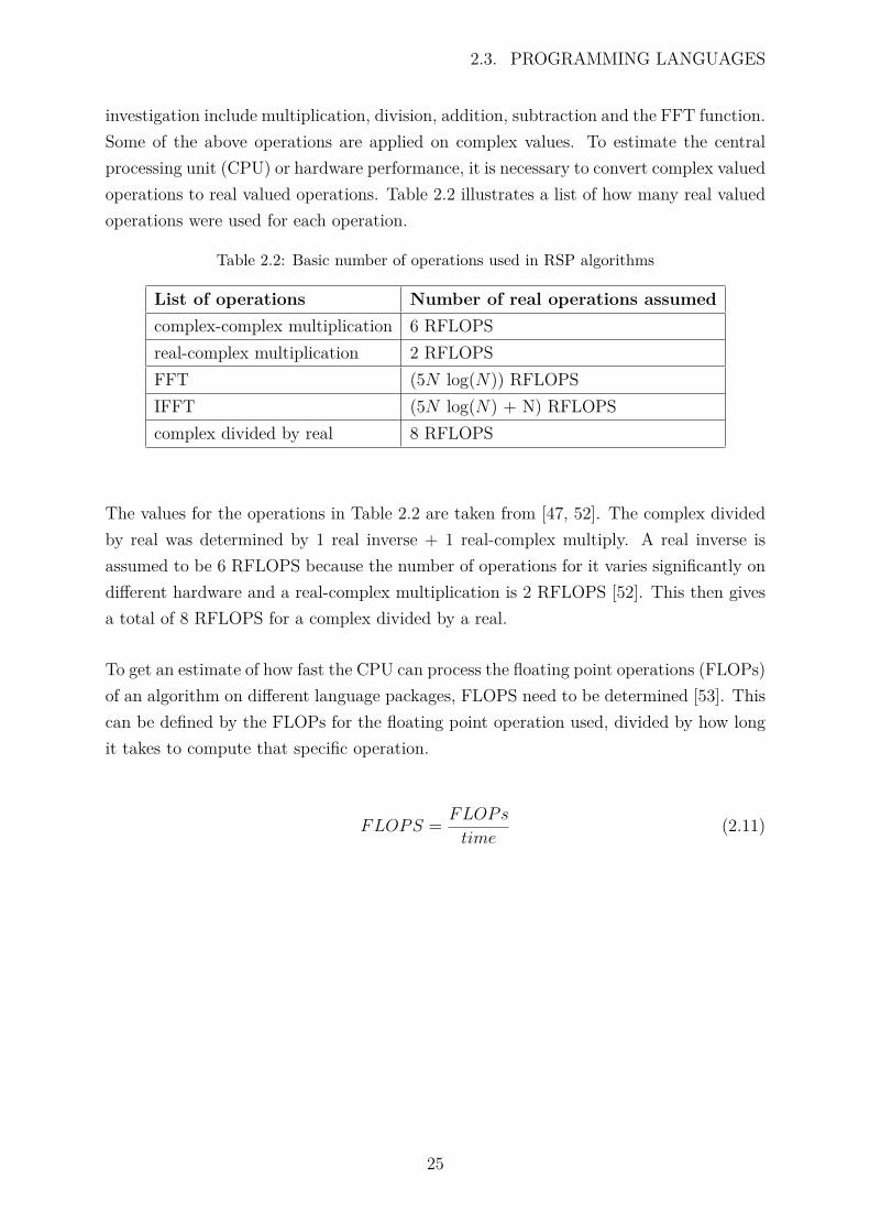
investigation include multiplication, division, addition, subtraction and the FFT function.Some of the above operations are applied on complex values. To estimate the centralprocessing unit (CPU) or hardware performance, it is necessary to convert complex valuedoperations to real valued operations. Table 2.2 illustrates a list of how many real valuedoperations were used for each operation.
Table 2.2: Basic number of operations used in RSP algorithms
List of operations Number of real operations assumedcomplex-complex multiplication 6 RFLOPSreal-complex multiplication 2 RFLOPSFFT (5N log(N)) RFLOPSIFFT (5N log(N) + N) RFLOPScomplex divided by real 8 RFLOPS
The values for the operations in Table 2.2 are taken from [47, 52]. The complex dividedby real was determined by 1 real inverse + 1 real-complex multiply. A real inverse isassumed to be 6 RFLOPS because the number of operations for it varies significantly ondifferent hardware and a real-complex multiplication is 2 RFLOPS [52]. This then givesa total of 8 RFLOPS for a complex divided by a real.
To get an estimate of how fast the CPU can process the floating point operations (FLOPs)of an algorithm on different language packages, FLOPS need to be determined [53]. Thiscan be defined by the FLOPs for the floating point operation used, divided by how longit takes to compute that specific operation.
FLOPS = FLOPs
time(2.11)
25
Chapter 3
Implementation of radar signalprocessing (RSP) techniques
3.1 Fairness
In the design process of the algorithms, four main considerations were taken into accountto ensure a fair algorithmic comparison across the different languages.
• Float64 numbers: This is to achieve maximum accuracy and precision whencomputations take place. Double precision numbers also occupy more memory thanFloat32 numbers, indicating how well the software packages handle algorithms thatuse maximum computer resources. This could be considered as a worst case scenarioin terms of computer resource usage.
• Spatial locality: This ensures that the contiguous memory block is used effectivelyfor each of the language packages. It makes sure that one language is not given anadvantage over another language - all software packages will have the same amountof memory accesses and the same amount of data will be cached.
• Same libraries: The only library used was the FFTW library and all of the lan-guages made use of the estimate planner. No additional libraries were used duringthe actual design of the algorithms, with the exception of Python. For Python, theNumPy library is encouraged because it gives Python scripting language capabili-ties such as vectorization. During the actual experiment to get speed results, thefile I/O, graphics was ignored as it is not part of the actual signal processing of the
26

3.2. PULSE COMPRESSION IMPLEMENTATION
algorithms.
• Similar implementation: All of the RSP algorithms across all of the softwarepackages will have the same algorithmic implementation.
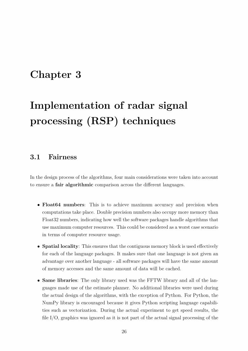
3.2 Pulse compression implementation
The pulse compression algorithm is basically the matched filter implementation describedin the previous chapter. Figure 3.1 illustrates the procedure followed to implement thepulse compression on the NetRAD dataset.
1. The dataset is read into memory as a two dimensional matrix of size N, where N =number of range bins × number of pulses. In Python, it is read in the reversed direction(number of pulses × number of range lines). This is because its contiguous memory blockis in row major ordering instead of column major ordering.
2. Reference signal or transmitted pulse is read from a text file into a one dimensionalmatrix. The reference signal was windowed by applying a Hanning window [54]. Since thereference signal has only 500 samples, it was zero padded such that it has 2048 samples.This ensures that it has the same amount of samples as a single pulse in the datamatrix.The reference signal was also transposed.
3. The FFT of the reference signal is multiplied with the FFT of each line of the data-matrix. This is done sequentially in a for loop for a specific number of pulses stipulatedby the user. The output is then stored in the MF2 matrix.
4. Analytic signal is formed by taking the completed MF2 matrix and zeroing the negativehalf of it. Since the MF2 matrix has 2048 samples, the first 1024 samples were zeroed,leaving only the positive half of the spectrum.
5. Inverse FFT is applied on each pulse of the modified MF2 matrix with the resultstored in pulseCompressData matrix.
27
3.2. PULSE COMPRESSION IMPLEMENTATION
Load data set, window andzero padded reference
signal, and indicatenumber of pulses.
Initialize matrices:
REF: To store result from FFT of reference signal.MF2: To store result from frequency domain. pulseCompressData: To store result from time domain.
FFT reference signal andtake complex conjugate to
form matched filter.
Loop through data set andapply FFT on single pulse.
All pulsesprocessed?
Multiply reference signalFFT with single pulse FFT..
Store result into MF2matrix.
No
Zero pad and formanalytic signal matrix from
MF2 matrix.
Loop through modifiedMF2 matrix and applyIFFT on each pulse.
All pulsesprocessed?
No
Done
Yes
Yes
Store result intopulseCompressData
matrix.
Figure 3.1: Algorithm design for pulse compression
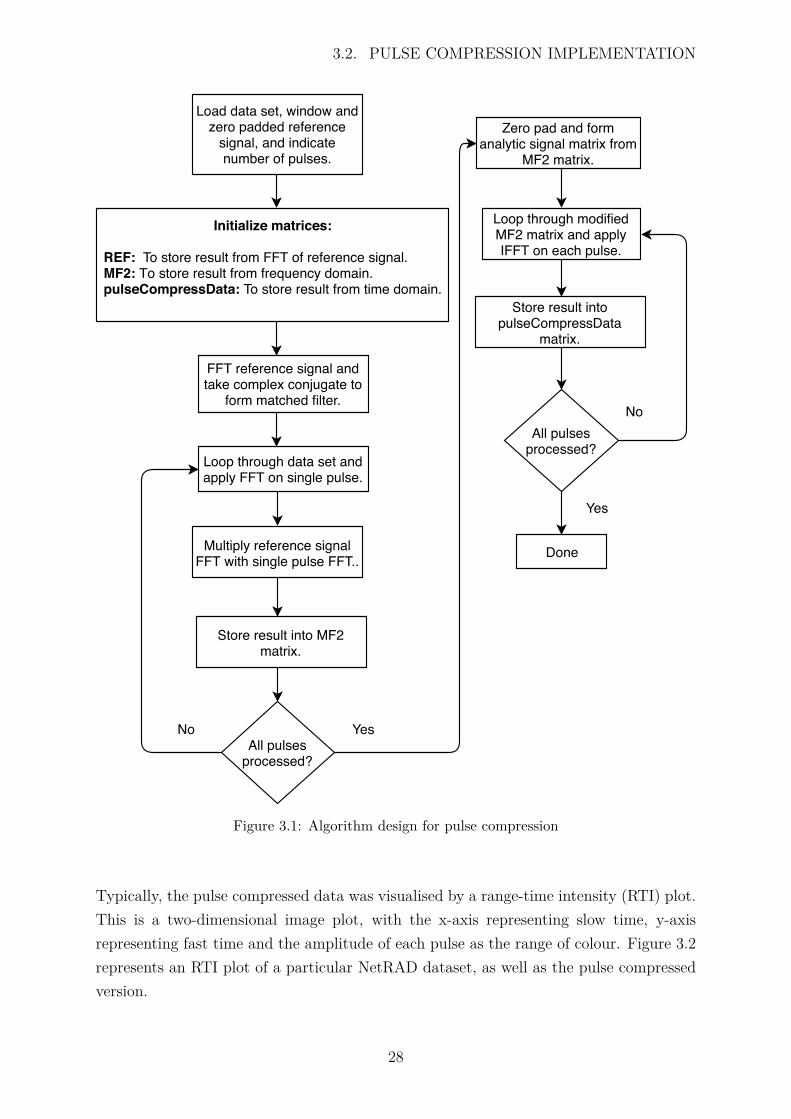
Typically, the pulse compressed data was visualised by a range-time intensity (RTI) plot.This is a two-dimensional image plot, with the x-axis representing slow time, y-axisrepresenting fast time and the amplitude of each pulse as the range of colour. Figure 3.2represents an RTI plot of a particular NetRAD dataset, as well as the pulse compressedversion.
28
3.3. DOPPLER PROCESSING IMPLEMENTATION
0 20000 40000 60000 80000 100000 120000Pulse number
0
500
1000
1500
2000
Range b
ins
Before pulse compression
(a) RTI plot of raw NetRAD radar data.
0 20000 40000 60000 80000 100000 120000Pulse number
0
500
1000
1500
2000
Range b
ins
After pulse compression
(b) RTI plot of pulse compressed NetRAD dataset.
Figure 3.2: RTI plot before and after pulse compression
It is important to note that the dataset is a scene of the ocean. In (b) the pulse compressedversion of (a) shows high intensity curves. This illustrates that ocean waves are movingtowards the radar over time. This also indicates that SNR has improved, as more valuableinformation can be interpreted from the pulse compressed dataset. To get even moreinformation from this dataset Doppler processing can now be applied.
3.3 Doppler processing implementation
To perform Doppler processing, the output data matrix from the pulse compression wasused. Figure 3.3 displays the procedure followed to generate range Doppler matrix.
1. The data matrix from pulse compression algorithm was loaded and then transposed.This gives the data matrix with dimensions of (number of pulses × number of range lines)for column major ordering and (number of range lines × number of pulses) for row majorordering. This allows for the exploitation of contiguous memory storage of each languagepackage. In other words, there will be more cache accesses and fewer memory accesseswhen the FFT operations are applied.
2. To produce a Doppler spectrum, CPI needs to be defined. This is the FFT size whichis applied to all pulses of each range bin. During the experiment, the FFT size was de-termined empirically. An FFT size of 256 was chosen, as it gave a compromise betweencomputation time and spectrum resolution. The result was stored in the pulseDoppler-Data matrix.
29

3.3. DOPPLER PROCESSING IMPLEMENTATION
Load data set frompulse compression
step.
Indicate how manypulses and the FFTsize to be applied on
each range bin.
Loop through all pulses ofrange dimension considered,and apply FFT on specified
number of pulses.
All pulsesprocessed?
All range binsprocessed?
Loop through eachrange dimension of
data set.
No Yes
No
Done
Initialization:
pulseDopplerData: To storeresult from main dopplerprocessing procedure.
Yes
Store result intopulseDopplerData
matrix
Figure 3.3: Algorithm design for Doppler processing
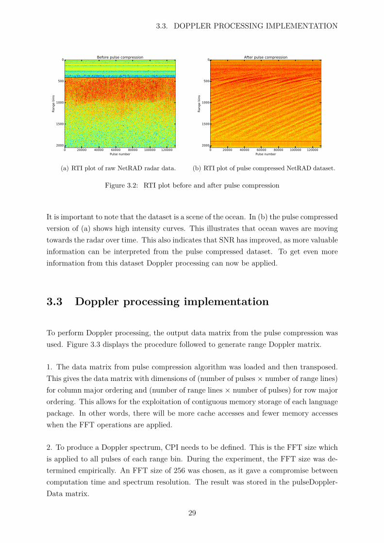
Figure 3.4 shows a range Doppler plot for the first 256 pulses, illustrating Doppler shiftsof targets for a specific range, over short instance in time.
30
3.4. ADAPTIVE LMS FILTER IMPLEMENTATION
Range Doppler plot of a NetRAD dataset
DFT bins50 100 150 200 250
Ran
ge
bin
s
200
400
600
800
1000
1200
1400
1600
1800
2000
Figure 3.4: Range and amplitude of Doppler frequencies at different range bins
Figure 3.4 shows several targets that were detected at positive Doppler frequencies asDoppler bins from 0 to 256 represent Doppler frequencies from -0.5 kHz to 0.5 kHz.
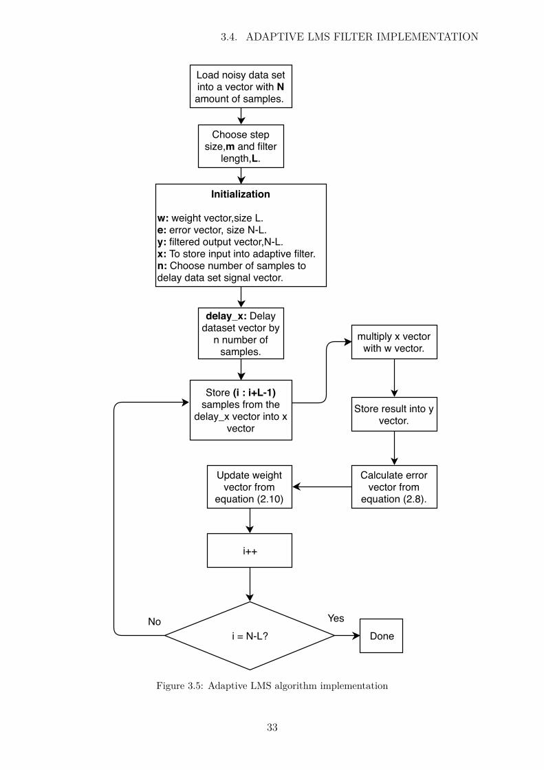
3.4 Adaptive LMS filter implementation
The adaptive LMS filter is identical to the implementation that was described in theprevious chapter. Figure 3.5 shows the procedure that was followed to implement theadaptive LMS filter on a simulated dataset.
1. The noisy dataset is read into memory as a one dimensional array/vector. A onedimensional array/vector is stored in a contiguous block of memory by default.
2. Step size and filter length were chosen, that gave a reasonable convergence rate witha small MSE, and a suitable SNR.
3. The (delay_x) signal is the noisy dataset signal vector that is delayed by five samplesto ensure the noise is uncorrelated from it. Five samples was chosen because there areabout 2.5 samples per signal period. This shifting of the vector is completed by addingzeros to the beginning of the vector.
4. The filter length of 80 was chosen. This means that 80 samples of the delay_x signalwere stored into vector x.
31

3.4. ADAPTIVE LMS FILTER IMPLEMENTATION
5. A weight vector of length 80 is multiplied with the x vector, with the result storedinto array/vector y.
6. Error vector is calculated by using equation (2.8) , the parameters inserted were thenoisy dataset vector from Step 1 and y vector from Step 4.
7. Weight vector is updated from equation (2.10) by using the step size as well as theweight, error and the x vector from the above results.
8. The process is repeated until all samples have been processed from the delay_x vector.
32
3.4. ADAPTIVE LMS FILTER IMPLEMENTATION
Load noisy data setinto a vector with Namount of samples.
delay_x: Delaydataset vector by
n number ofsamples.
Choose stepsize,m and filter
length,L.
i = N-L?
Store (i : i+L-1)samples from the
delay_x vector into xvector
i++
multiply x vectorwith w vector.
Store result into yvector.
Calculate errorvector from
equation (2.8).
Update weightvector from
equation (2.10)
NoDone
Yes
Initialization
w: weight vector,size L.e: error vector, size N-L.y: filtered output vector,N-L.x: To store input into adaptive filter.n: Choose number of samples todelay data set signal vector.
Figure 3.5: Adaptive LMS algorithm implementation
33
3.4. ADAPTIVE LMS FILTER IMPLEMENTATION
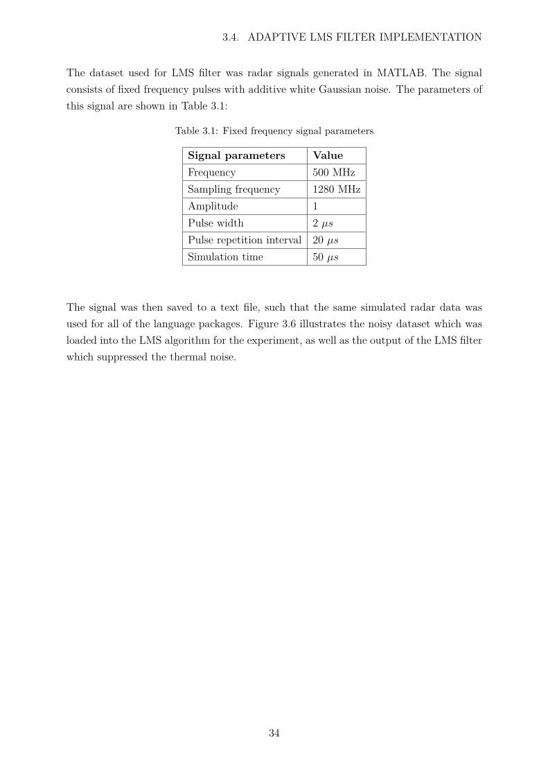
The dataset used for LMS filter was radar signals generated in MATLAB. The signalconsists of fixed frequency pulses with additive white Gaussian noise. The parameters ofthis signal are shown in Table 3.1:
Table 3.1: Fixed frequency signal parameters
Signal parameters ValueFrequency 500 MHzSampling frequency 1280 MHzAmplitude 1Pulse width 2 µsPulse repetition interval 20 µsSimulation time 50 µs
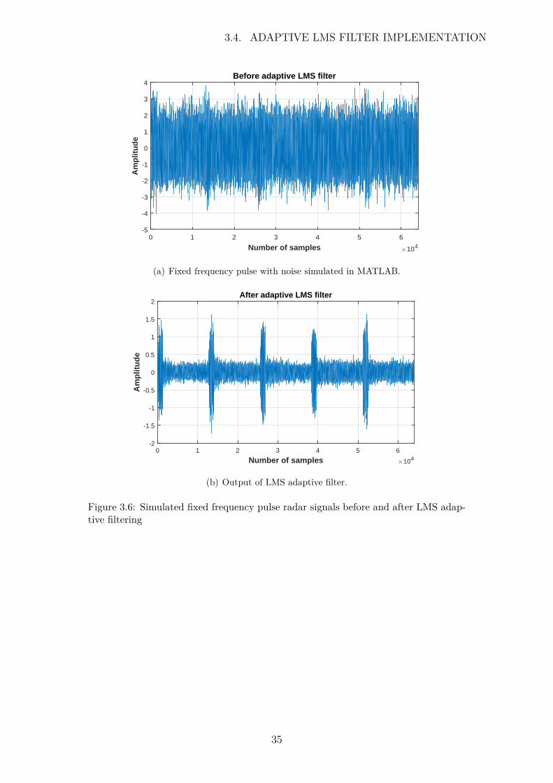
The signal was then saved to a text file, such that the same simulated radar data wasused for all of the language packages. Figure 3.6 illustrates the noisy dataset which wasloaded into the LMS algorithm for the experiment, as well as the output of the LMS filterwhich suppressed the thermal noise.
34
3.4. ADAPTIVE LMS FILTER IMPLEMENTATION
Number of samples #104
0 1 2 3 4 5 6
Am
plit
ud
e
-5
-4
-3
-2
-1
0
1
2
3
4Before adaptive LMS filter
(a) Fixed frequency pulse with noise simulated in MATLAB.
Number of samples #1040 1 2 3 4 5 6
Am
plit
ud
e
-2
-1.5
-1
-0.5
0
0.5
1
1.5
2After adaptive LMS filter
(b) Output of LMS adaptive filter.
Figure 3.6: Simulated fixed frequency pulse radar signals before and after LMS adap-tive filtering
35
Chapter 4
Results and discussion
In this chapter, the performance related results will be shown for three RSP algorithms.These are pulse compression, Doppler processing and LMS filter. In order to evaluate theperformance of pulse compression and Doppler processing on all packages, three differentexperiments were undertaken:
1.) Computation time: Determines the wall clock time for the RSP algorithms invarious language packages. Wall clock time is the actual time taken, from the start ofthe RSP algorithms to the end. This determines which software package would completethe quickest.
2.) Memory handling: Gives an indication of how memory is used for all of the languagepackages, by considering if the calculated memory or extra memory was used duringprocessing. This was completed only for pulse compression and Doppler processing, asthe NetRAD datasets required a lot of memory. It was not worthwhile completing thisfor small sets of data that was used for the adaptive LMS filter.
3.) FLOPS: This gives an indication of how many mathematical operations are per-formed for different RSP algorithms on various language packages.
By evaluating the performance of the experiments and comparing it with all the lan-guage packages under investigation, the objectives of the study can be met. Note: thesisalgorithms can be found on bitbucket (https://bitbucket.org/ExtremesExtreme/thesis-code/src/master/)
36
4.1. PERFORMANCE OF RSP ALGORITHM DESIGNS
4.1 Performance of RSP algorithm designs
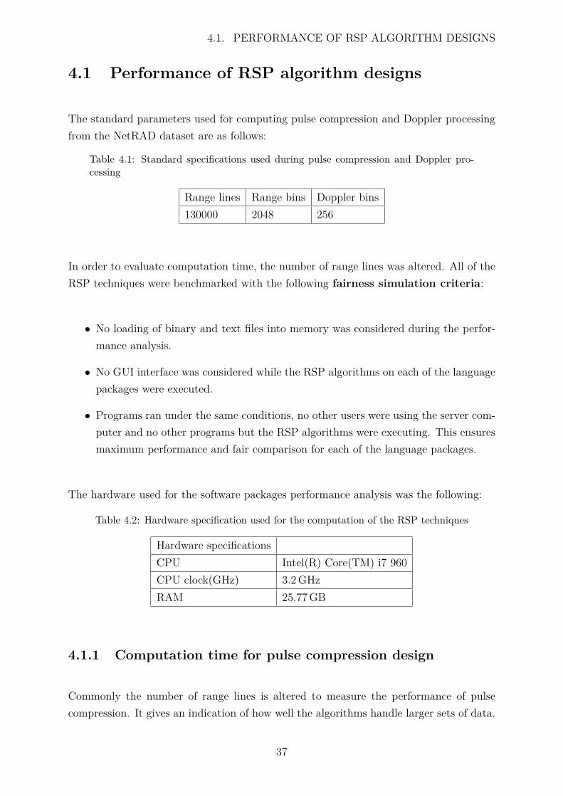
The standard parameters used for computing pulse compression and Doppler processingfrom the NetRAD dataset are as follows:
Table 4.1: Standard specifications used during pulse compression and Doppler pro-cessing
Range lines Range bins Doppler bins130000 2048 256
In order to evaluate computation time, the number of range lines was altered. All of theRSP techniques were benchmarked with the following fairness simulation criteria:
• No loading of binary and text files into memory was considered during the perfor-mance analysis.
• No GUI interface was considered while the RSP algorithms on each of the languagepackages were executed.
• Programs ran under the same conditions, no other users were using the server com-puter and no other programs but the RSP algorithms were executing. This ensuresmaximum performance and fair comparison for each of the language packages.
The hardware used for the software packages performance analysis was the following:
Table 4.2: Hardware specification used for the computation of the RSP techniques
Hardware specificationsCPU Intel(R) Core(TM) i7 960CPU clock(GHz) 3.2GHzRAM 25.77GB
4.1.1 Computation time for pulse compression design
Commonly the number of range lines is altered to measure the performance of pulsecompression. It gives an indication of how well the algorithms handle larger sets of data.
37
4.1. PERFORMANCE OF RSP ALGORITHM DESIGNS
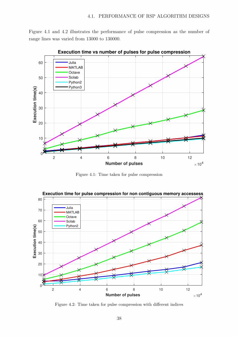
Figure 4.1 and 4.2 illustrates the performance of pulse compression as the number ofrange lines was varied from 13000 to 130000.
Number of pulses #104
2 4 6 8 10 12
Exe
cu
tio
n t
ime
(s)
0
10
20
30
40
50
60
Execution time vs number of pulses for pulse compression
Julia
MATLAB
Octave
Scilab
Python2
Python3
Powered by TCPDF (www.tcpdf.org)
Powered by TCPDF (www.tcpdf.org)Powered by TCPDF (www.tcpdf.org)
Figure 4.1: Time taken for pulse compression
Number of pulses #104
2 4 6 8 10 12
Execu
tio
n t
ime(s
)
0
10
20
30
40
50
60
70
80
Execution time for pulse compression for non contiguous memory accessess
Julia
MATLAB
Octave
Scilab
Python2
Powered by TCPDF (www.tcpdf.org)
Powered by TCPDF (www.tcpdf.org)Powered by TCPDF (www.tcpdf.org)
Figure 4.2: Time taken for pulse compression with different indices
38
4.1. PERFORMANCE OF RSP ALGORITHM DESIGNS
Figure 4.1 illustrates a nearly linear relationship between the number of pulses and com-putation time. The trend was expected, as more data is processed the longer the programtakes to execute. The most important observation: the same algorithm ran on numerouslanguage packages but the computation times varied. MATLAB, Julia and Python allhad similar results, varying from 9 to 12 seconds, with Python being the fastest. Octaveand Scilab were the slowest at 28 and 63 seconds respectively. Figure 4.1 trends are muchfaster than Figure 4.2, because it is cache friendlier, as it does not have non-contiguousmemory accesses.
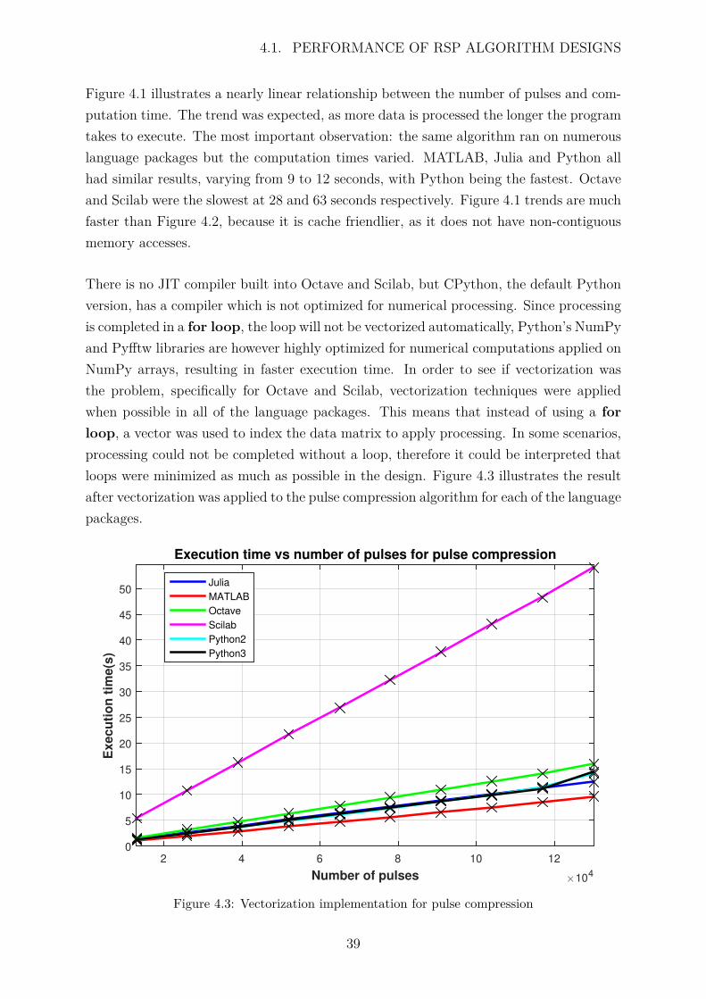
There is no JIT compiler built into Octave and Scilab, but CPython, the default Pythonversion, has a compiler which is not optimized for numerical processing. Since processingis completed in a for loop, the loop will not be vectorized automatically, Python’s NumPyand Pyfftw libraries are however highly optimized for numerical computations applied onNumPy arrays, resulting in faster execution time. In order to see if vectorization wasthe problem, specifically for Octave and Scilab, vectorization techniques were appliedwhen possible in all of the language packages. This means that instead of using a forloop, a vector was used to index the data matrix to apply processing. In some scenarios,processing could not be completed without a loop, therefore it could be interpreted thatloops were minimized as much as possible in the design. Figure 4.3 illustrates the resultafter vectorization was applied to the pulse compression algorithm for each of the languagepackages.
Number of pulses #104
2 4 6 8 10 12
Execu
tio
n t
ime(s
)
0
5
10
15
20
25
30
35
40
45
50
Execution time vs number of pulses for pulse compression
Julia
MATLAB
Octave
Scilab
Python2
Python3
Powered by TCPDF (www.tcpdf.org)
Powered by TCPDF (www.tcpdf.org)Powered by TCPDF (www.tcpdf.org)
Figure 4.3: Vectorization implementation for pulse compression
39
4.1. PERFORMANCE OF RSP ALGORITHM DESIGNS
Figure 4.3 emphasizes that there was an improvement in MATLAB, Octave and Scilab.Octave computed processing in approximately 16 seconds, while Scilab was still signifi-cantly slower than the rest of the packages.
Another reason for the discrepancy in Scilab’s computation time could be from implicitparallelization. Scilab employed the reference BLAS library by default, which used onecore when doing matrix multiplication. To investigate if this was the problem, a differentBLAS library was used, namely OpenBlas library from the Linux distribution package.This library was applied to the loop based and semi-vectorized code, with the resultsdepicted in Figure 4.4
40
4.1. PERFORMANCE OF RSP ALGORITHM DESIGNS
Number of pulses #104
2 4 6 8 10 12
Exe
cuti
on
tim
e(s)
0
10
20
30
40
50
60
Execution time for pulse compression using different BLAS libraries on Scilab
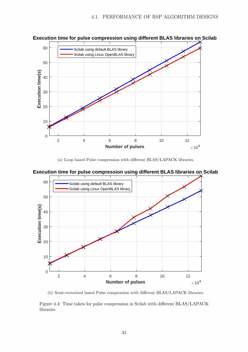
Scilab using default BLAS libraryScilab using Linux OpenBLAS library
(a) Loop based Pulse compression with different BLAS/LAPACK libraries.
Number of pulses #1042 4 6 8 10 12
Exe
cuti
on
tim
e(s)
0
10
20
30
40
50
60
Execution time for pulse compression using different BLAS libraries on Scilab
Scilab using default BLAS libraryScilab using Linux OpenBLAS library
(b) Semi-vectorized based Pulse compression with different BLAS/LAPACK libraries.
Figure 4.4: Time taken for pulse compression in Scilab with different BLAS/LAPACKlibraries
41
4.1. PERFORMANCE OF RSP ALGORITHM DESIGNS
For the loop based version there was approximately an 8 percent improvement whenchanging the BLAS/LAPACK libraries, while the partially vectorized version showed nospeed improvement. The reason for this is that the pulse compression implementationdoes not require very complex linear algebra, therefore the difference in performancewas not that significant from the default BLAS libraries. Another reason could be thatthe OpenBLAS library by Debian was a generic package, which was not optimized forthe machine used for the benchmarks. This could be one of the main reasons for thenon-linear relationship of the Linux OpenBLAS library after 65000 pulses.
4.1.2 Computation time for Doppler processing design
To observe computational performance, the number of range lines was varied from 12288to 122880. The FFT size was chosen to be 256, as it gave a compromise between spectrumquality and computation time.
Number of pulses #104
2 3 4 5 6 7 8 9 10 11 12
Ex
ecu
tio
n t
ime(s
)
0
10
20
30
40
50
60
70
80
90
100Execution time vs number of pulses for Doppler processing
Julia
MATLAB
Octave
Scilab
Python2
Python3
Powered by TCPDF (www.tcpdf.org)
Powered by TCPDF (www.tcpdf.org)Powered by TCPDF (www.tcpdf.org)
Figure 4.5: Time taken for Doppler processing
42
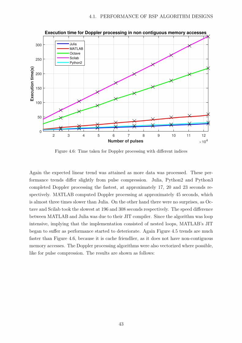
4.1. PERFORMANCE OF RSP ALGORITHM DESIGNS
Number of pulses #104
2 3 4 5 6 7 8 9 10 11 12
Execu
tio
n t
ime(s
)
0
50
100
150
200
250
300
Execution time for Doppler processing in non contiguous memory accesses
Julia
MATLAB
Octave
Scilab
Python2
Powered by TCPDF (www.tcpdf.org)
Powered by TCPDF (www.tcpdf.org)
Figure 4.6: Time taken for Doppler processing with different indices
Again the expected linear trend was attained as more data was processed. These per-formance trends differ slightly from pulse compression. Julia, Python2 and Python3completed Doppler processing the fastest, at approximately 17, 20 and 23 seconds re-spectively. MATLAB computed Doppler processing at approximately 45 seconds, whichis almost three times slower than Julia. On the other hand there were no surprises, as Oc-tave and Scilab took the slowest at 196 and 308 seconds respectively. The speed differencebetween MATLAB and Julia was due to their JIT compiler. Since the algorithm was loopintensive, implying that the implementation consisted of nested loops, MATLAB’s JITbegan to suffer as performance started to deteriorate. Again Figure 4.5 trends are muchfaster than Figure 4.6, because it is cache friendlier, as it does not have non-contiguousmemory accesses. The Doppler processing algorithms were also vectorized where possible,like for pulse compression. The results are shown as follows:
43
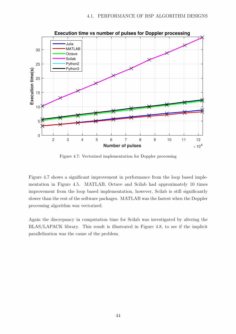
4.1. PERFORMANCE OF RSP ALGORITHM DESIGNS
Number of pulses #104
2 3 4 5 6 7 8 9 10 11 12
Exe
cu
tio
n t
ime(s
)
0
5
10
15
20
25
30
Execution time vs number of pulses for Doppler processing
Julia
MATLAB
Octave
Scilab
Python2
Python3
Powered by TCPDF (www.tcpdf.org)
Powered by TCPDF (www.tcpdf.org)Powered by TCPDF (www.tcpdf.org)
Figure 4.7: Vectorized implementation for Doppler processing
Figure 4.7 shows a significant improvement in performance from the loop based imple-mentation in Figure 4.5. MATLAB, Octave and Scilab had approximately 10 timesimprovement from the loop based implementation, however, Scilab is still significantlyslower than the rest of the software packages. MATLAB was the fastest when the Dopplerprocessing algorithm was vectorized.
Again the discrepancy in computation time for Scilab was investigated by altering theBLAS/LAPACK library. This result is illustrated in Figure 4.8, to see if the implicitparallelization was the cause of the problem.
44
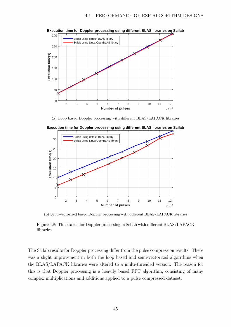
4.1. PERFORMANCE OF RSP ALGORITHM DESIGNS
Number of pulses #104
2 3 4 5 6 7 8 9 10 11 12
Exe
cuti
on
tim
e(s)
0
50
100
150
200
250
300
Execution time for Doppler processing using different BLAS libraries on Scilab
Scilab using default BLAS libraryScilab using Linux OpenBLAS library
(a) Loop based Doppler processing with different BLAS/LAPACK libraries
Number of pulses #104
2 3 4 5 6 7 8 9 10 11 12
Exe
cuti
on
tim
e(s)
0
5
10
15
20
25
30
Execution time for Doppler processing using different BLAS libraries on Scilab
Scilab using default BLAS libraryScilab using Linux OpenBLAS library
(b) Semi-vectorized based Doppler processing with different BLAS/LAPACK libraries
Figure 4.8: Time taken for Doppler processing in Scilab with different BLAS/LAPACKlibraries
The Scilab results for Doppler processing differ from the pulse compression results. Therewas a slight improvement in both the loop based and semi-vectorized algorithms whenthe BLAS/LAPACK libraries were altered to a multi-threaded version. The reason forthis is that Doppler processing is a heavily based FFT algorithm, consisting of manycomplex multiplications and additions applied to a pulse compressed dataset.
45
4.2. FLOPS FOR DIFFERENT RSP ALGORITHMS
4.2 FLOPS for different RSP algorithms
The main interest was only in RSP algorithms, as stated previously in the benchmarkcriteria. Therefore, the number of FLOPs would only be determined for RSP techniquesand not for the file input and output. The basic number of FLOPs used for a specificfloating point operation is stated in 2.2. This will be deployed as a reference to estimatethe number of FLOPS that was processed by the CPU for various RSP algorithms.Note: FLOPS were estimated using the loop based implementation, not thevectorized implementation.
4.2.1 FLOPS for pulse compression algorithm design
The main computations happened during the correlation process, whereby matched fil-tering was computed by the fast convolution implementation from Figure 2.3. Table 4.3depicts the major mathematical operations used during pulse compression, as well as anapproximation of the number of floating point operations used for each operation.
46
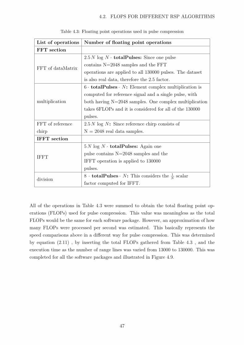
4.2. FLOPS FOR DIFFERENT RSP ALGORITHMS
Table 4.3: Floating point operations used in pulse compression
List of operations Number of floating point operationsFFT section
FFT of dataMatrix
2.5N log N · totalPulses: Since one pulsecontains N=2048 samples and the FFToperations are applied to all 130000 pulses. The datasetis also real data, therefore the 2.5 factor.
multiplication
6 · totalPulses · N : Element complex multiplication iscomputed for reference signal and a single pulse, withboth having N=2048 samples. One complex multiplicationtakes 6FLOPs and it is considered for all of the 130000pulses.
FFT of referencechirp
2.5N log N : Since reference chirp consists ofN = 2048 real data samples.
IFFT section
IFFT
5N log N · totalPulses: Again onepulse contains N=2048 samples and theIFFT operation is applied to 130000pulses.
division8 · totalPulses · N : This considers the 1
Nscalar
factor computed for IFFT.
All of the operations in Table 4.3 were summed to obtain the total floating point op-erations (FLOPs) used for pulse compression. This value was meaningless as the totalFLOPs would be the same for each software package. However, an approximation of howmany FLOPs were processed per second was estimated. This basically represents thespeed comparisons above in a different way for pulse compression. This was determinedby equation (2.11) , by inserting the total FLOPs gathered from Table 4.3 , and theexecution time as the number of range lines was varied from 13000 to 130000. This wascompleted for all the software packages and illustrated in Figure 4.9.
47
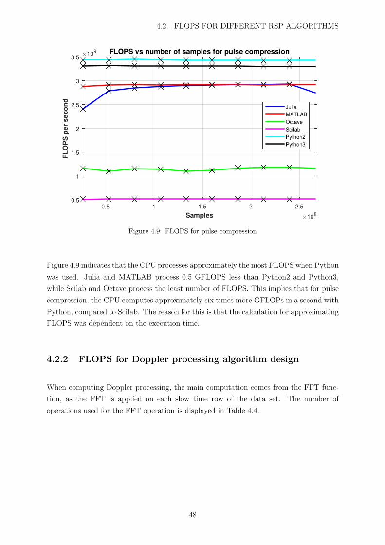
4.2. FLOPS FOR DIFFERENT RSP ALGORITHMS
Samples #108
0.5 1 1.5 2 2.5
FL
OP
S p
er
seco
nd
#109
0.5
1
1.5
2
2.5
3
3.5FLOPS vs number of samples for pulse compression
Julia
MATLAB
Octave
Scilab
Python2
Python3
Powered by TCPDF (www.tcpdf.org)
Powered by TCPDF (www.tcpdf.org)Powered by TCPDF (www.tcpdf.org)
Figure 4.9: FLOPS for pulse compression
Figure 4.9 indicates that the CPU processes approximately the most FLOPS when Pythonwas used. Julia and MATLAB process 0.5 GFLOPS less than Python2 and Python3,while Scilab and Octave process the least number of FLOPS. This implies that for pulsecompression, the CPU computes approximately six times more GFLOPs in a second withPython, compared to Scilab. The reason for this is that the calculation for approximatingFLOPS was dependent on the execution time.
4.2.2 FLOPS for Doppler processing algorithm design
When computing Doppler processing, the main computation comes from the FFT func-tion, as the FFT is applied on each slow time row of the data set. The number ofoperations used for the FFT operation is displayed in Table 4.4.
48
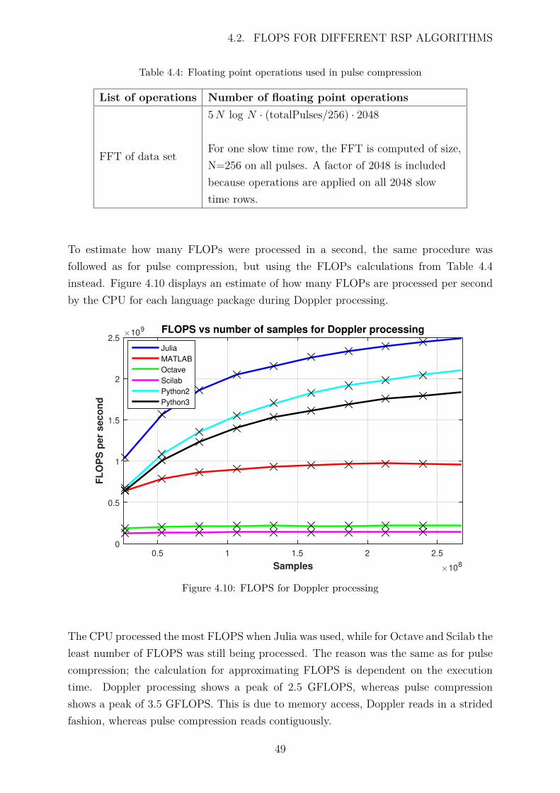
4.2. FLOPS FOR DIFFERENT RSP ALGORITHMS
Table 4.4: Floating point operations used in pulse compression
List of operations Number of floating point operations
FFT of data set
5N log N · (totalPulses/256) · 2048
For one slow time row, the FFT is computed of size,N=256 on all pulses. A factor of 2048 is includedbecause operations are applied on all 2048 slowtime rows.
To estimate how many FLOPs were processed in a second, the same procedure wasfollowed as for pulse compression, but using the FLOPs calculations from Table 4.4instead. Figure 4.10 displays an estimate of how many FLOPs are processed per secondby the CPU for each language package during Doppler processing.
Samples #108
0.5 1 1.5 2 2.5
FL
OP
S p
er
seco
nd
#109
0
0.5
1
1.5
2
2.5FLOPS vs number of samples for Doppler processing
Julia
MATLAB
Octave
Scilab
Python2
Python3
Powered by TCPDF (www.tcpdf.org)
Powered by TCPDF (www.tcpdf.org)Powered by TCPDF (www.tcpdf.org)
Figure 4.10: FLOPS for Doppler processing
The CPU processed the most FLOPS when Julia was used, while for Octave and Scilab theleast number of FLOPS was still being processed. The reason was the same as for pulsecompression; the calculation for approximating FLOPS is dependent on the executiontime. Doppler processing shows a peak of 2.5 GFLOPS, whereas pulse compressionshows a peak of 3.5 GFLOPS. This is due to memory access, Doppler reads in a stridedfashion, whereas pulse compression reads contiguously.
49
4.3. MEMORY HANDLING FOR PULSE COMPRESSION ANDDOPPLER PROCESSING
4.3 Memory handling for pulse compression andDoppler processing
The requirement was to observe how much memory was handled during the actual pro-cessing. Memory utilization was difficult to determine, but as stated in the previoussections, all of the above languages are interpreted languages. This means that it is notnecessary to free memory space as it is done automatically with the garbage collector. Agood estimate was then to determine peak memory performance during processing. Con-sidering the above, two scenarios were taken to evaluate how memory is handled duringthe actual processing:
1. When no unnecessary variables are cleared: This determines how well the garbagecollector of each language automatically handles memory deallocation.
2. Clearing unnecessary variables before processing begins: To examine if the measuredmemory consumption corresponds to theoretical memory.
Memory observations were gathered from HTOP software from the Linux distributionpackage while the pulse compression and Doppler processing algorithms were process-ing. Many runs of the algorithms were completed in order to make sure that the valuesrecorded correlate with each other. Note that changing the BLAS library for Scilab dur-ing the memory analysis was not considered, as it only improves performance in terms ofspeed.
Figure 4.11 illustrates peak memory consumption, handling of memory from garbagecollector, and memory consumption once unnecessary variables are cleared. This wascompleted for all of the language packages.
50
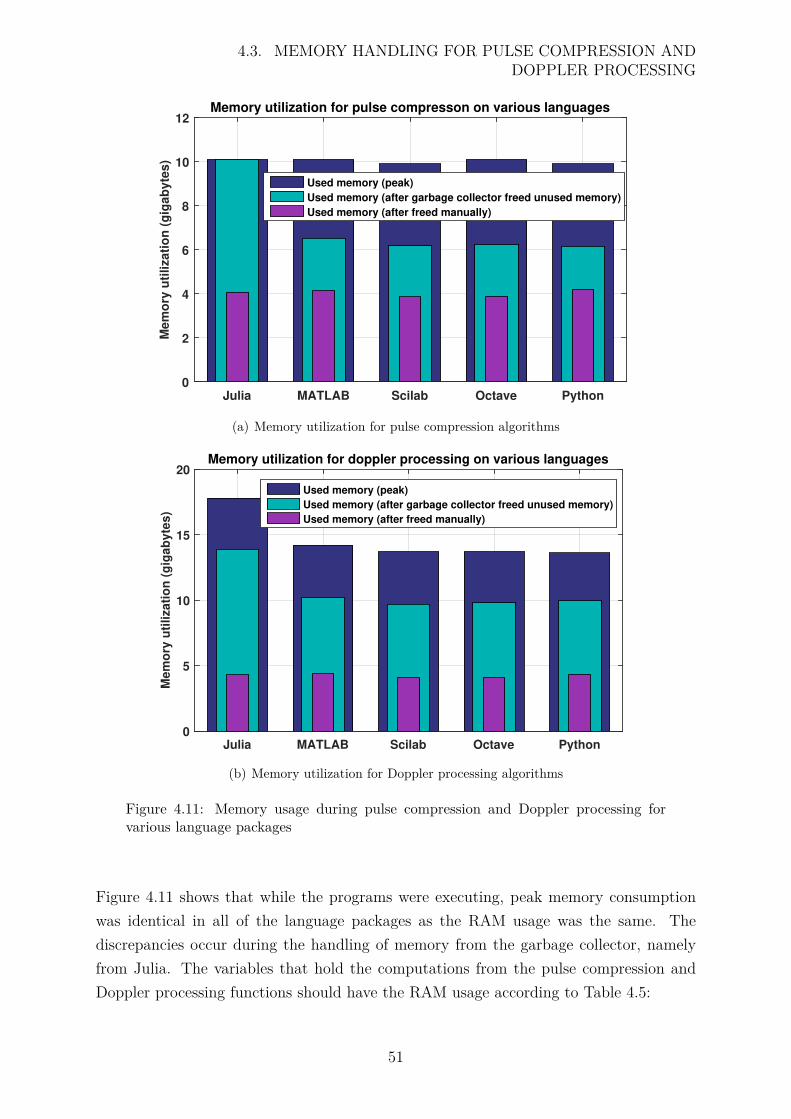
4.3. MEMORY HANDLING FOR PULSE COMPRESSION ANDDOPPLER PROCESSING
Julia MATLAB Scilab Octave Python
Mem
ory
uti
lizati
on
(g
igab
yte
s)
0
2
4
6
8
10
12Memory utilization for pulse compresson on various languages
Used memory (peak)
Used memory (after garbage collector freed unused memory)
Used memory (after freed manually)
Powered by TCPDF (www.tcpdf.org)
Powered by TCPDF (www.tcpdf.org)Powered by TCPDF (www.tcpdf.org)
(a) Memory utilization for pulse compression algorithms
Julia MATLAB Scilab Octave Python
Mem
ory
uti
lizati
on
(g
igab
yte
s)
0
5
10
15
20Memory utilization for doppler processing on various languages
Used memory (peak)
Used memory (after garbage collector freed unused memory)
Used memory (after freed manually)
Powered by TCPDF (www.tcpdf.org)
Powered by TCPDF (www.tcpdf.org)Powered by TCPDF (www.tcpdf.org)
(b) Memory utilization for Doppler processing algorithms
Figure 4.11: Memory usage during pulse compression and Doppler processing forvarious language packages
Figure 4.11 shows that while the programs were executing, peak memory consumptionwas identical in all of the language packages as the RAM usage was the same. Thediscrepancies occur during the handling of memory from the garbage collector, namelyfrom Julia. The variables that hold the computations from the pulse compression andDoppler processing functions should have the RAM usage according to Table 4.5:
51
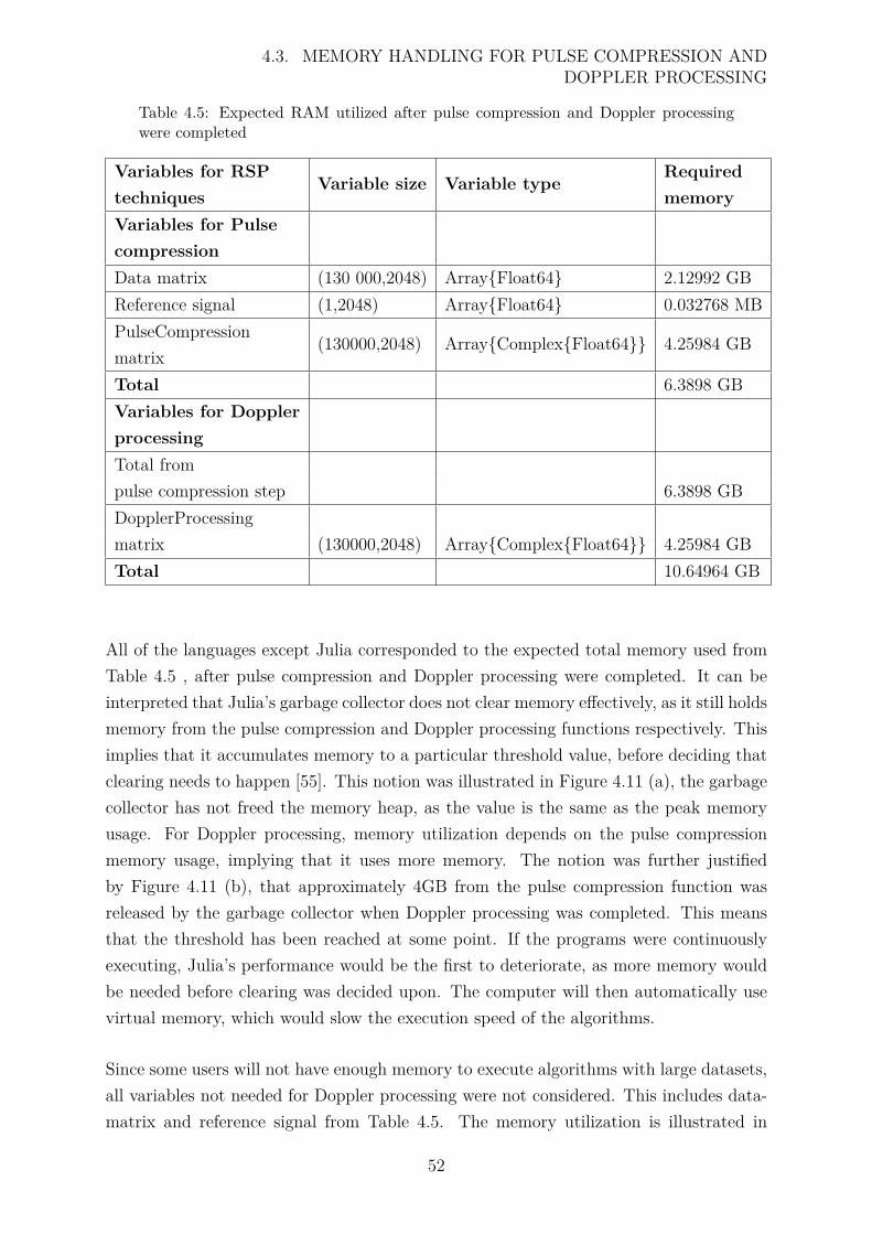
4.3. MEMORY HANDLING FOR PULSE COMPRESSION ANDDOPPLER PROCESSING
Table 4.5: Expected RAM utilized after pulse compression and Doppler processingwere completed
Variables for RSPtechniques
Variable size Variable typeRequiredmemory
Variables for PulsecompressionData matrix (130 000,2048) Array{Float64} 2.12992 GBReference signal (1,2048) Array{Float64} 0.032768 MBPulseCompressionmatrix
(130000,2048) Array{Complex{Float64}} 4.25984 GB
Total 6.3898 GBVariables for DopplerprocessingTotal frompulse compression step 6.3898 GBDopplerProcessingmatrix (130000,2048) Array{Complex{Float64}} 4.25984 GBTotal 10.64964 GB
All of the languages except Julia corresponded to the expected total memory used fromTable 4.5 , after pulse compression and Doppler processing were completed. It can beinterpreted that Julia’s garbage collector does not clear memory effectively, as it still holdsmemory from the pulse compression and Doppler processing functions respectively. Thisimplies that it accumulates memory to a particular threshold value, before deciding thatclearing needs to happen [55]. This notion was illustrated in Figure 4.11 (a), the garbagecollector has not freed the memory heap, as the value is the same as the peak memoryusage. For Doppler processing, memory utilization depends on the pulse compressionmemory usage, implying that it uses more memory. The notion was further justifiedby Figure 4.11 (b), that approximately 4GB from the pulse compression function wasreleased by the garbage collector when Doppler processing was completed. This meansthat the threshold has been reached at some point. If the programs were continuouslyexecuting, Julia’s performance would be the first to deteriorate, as more memory wouldbe needed before clearing was decided upon. The computer will then automatically usevirtual memory, which would slow the execution speed of the algorithms.
Since some users will not have enough memory to execute algorithms with large datasets,all variables not needed for Doppler processing were not considered. This includes data-matrix and reference signal from Table 4.5. The memory utilization is illustrated in
52
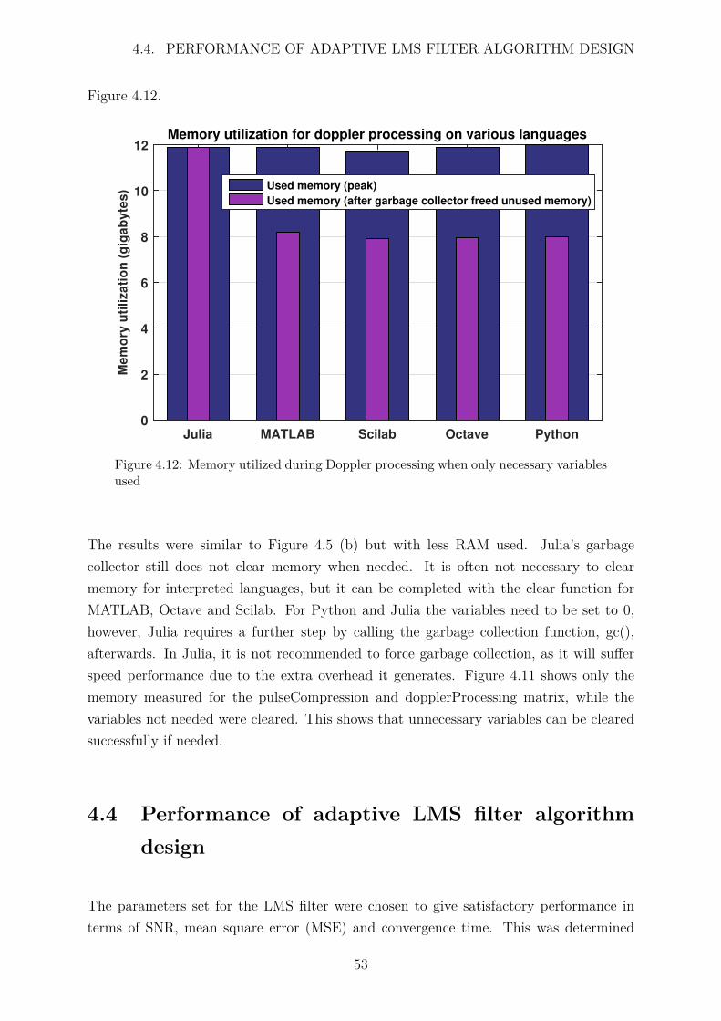
4.4. PERFORMANCE OF ADAPTIVE LMS FILTER ALGORITHM DESIGN
Figure 4.12.
Julia MATLAB Scilab Octave Python
Me
mo
ry u
tili
za
tio
n (
gig
ab
yte
s)
0
2
4
6
8
10
12Memory utilization for doppler processing on various languages
Used memory (peak)
Used memory (after garbage collector freed unused memory)
Powered by TCPDF (www.tcpdf.org)
Powered by TCPDF (www.tcpdf.org)Powered by TCPDF (www.tcpdf.org)
Figure 4.12: Memory utilized during Doppler processing when only necessary variablesused
The results were similar to Figure 4.5 (b) but with less RAM used. Julia’s garbagecollector still does not clear memory when needed. It is often not necessary to clearmemory for interpreted languages, but it can be completed with the clear function forMATLAB, Octave and Scilab. For Python and Julia the variables need to be set to 0,however, Julia requires a further step by calling the garbage collection function, gc(),afterwards. In Julia, it is not recommended to force garbage collection, as it will sufferspeed performance due to the extra overhead it generates. Figure 4.11 shows only thememory measured for the pulseCompression and dopplerProcessing matrix, while thevariables not needed were cleared. This shows that unnecessary variables can be clearedsuccessfully if needed.
4.4 Performance of adaptive LMS filter algorithmdesign
The parameters set for the LMS filter were chosen to give satisfactory performance interms of SNR, mean square error (MSE) and convergence time. This was determined
53
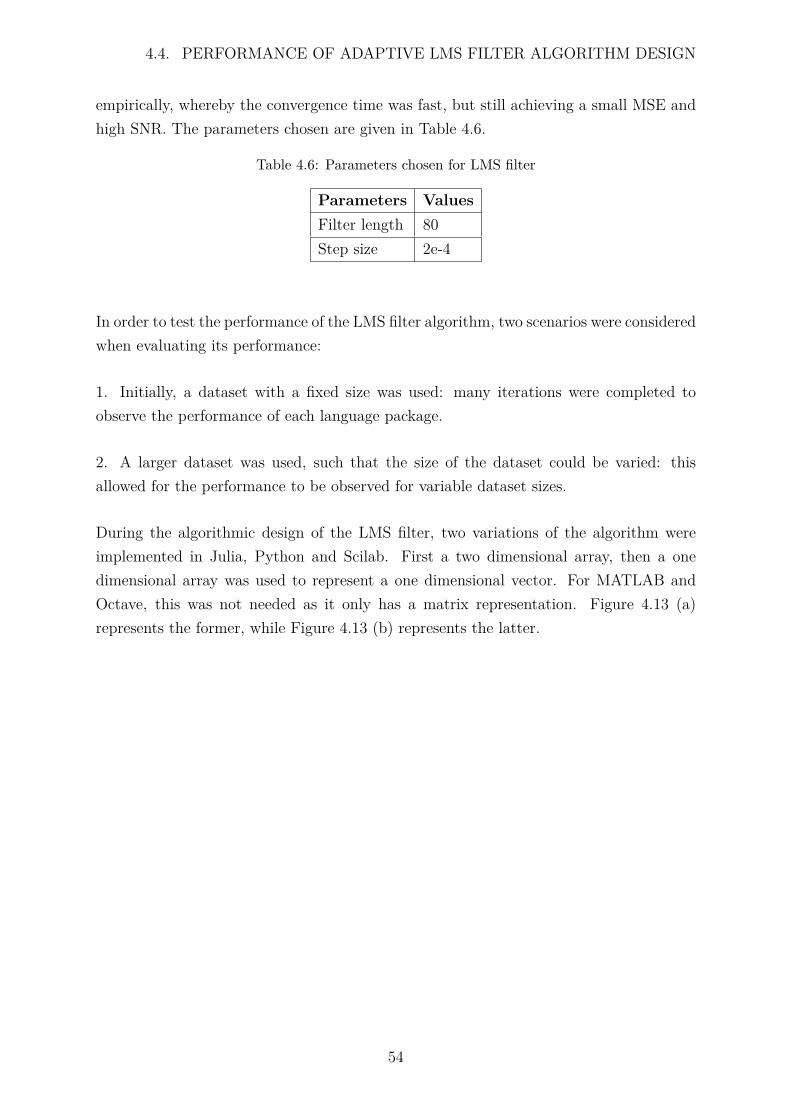
4.4. PERFORMANCE OF ADAPTIVE LMS FILTER ALGORITHM DESIGN
empirically, whereby the convergence time was fast, but still achieving a small MSE andhigh SNR. The parameters chosen are given in Table 4.6.
Table 4.6: Parameters chosen for LMS filter
Parameters ValuesFilter length 80Step size 2e-4
In order to test the performance of the LMS filter algorithm, two scenarios were consideredwhen evaluating its performance:
1. Initially, a dataset with a fixed size was used: many iterations were completed toobserve the performance of each language package.
2. A larger dataset was used, such that the size of the dataset could be varied: thisallowed for the performance to be observed for variable dataset sizes.
During the algorithmic design of the LMS filter, two variations of the algorithm wereimplemented in Julia, Python and Scilab. First a two dimensional array, then a onedimensional array was used to represent a one dimensional vector. For MATLAB andOctave, this was not needed as it only has a matrix representation. Figure 4.13 (a)represents the former, while Figure 4.13 (b) represents the latter.
54
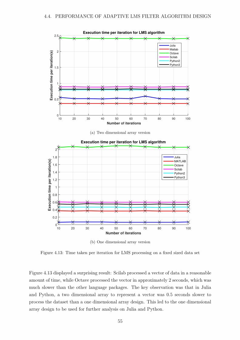
4.4. PERFORMANCE OF ADAPTIVE LMS FILTER ALGORITHM DESIGN
Number of iterations
10 20 30 40 50 60 70 80 90 100
Ex
ec
uti
on
tim
e p
er
ite
rati
on
(s)
0
0.5
1
1.5
2
2.5Execution time per iteration for LMS algorithm
Julia
Matlab
Octave
Scilab
Python2
Python3
Powered by TCPDF (www.tcpdf.org)
Powered by TCPDF (www.tcpdf.org)Powered by TCPDF (www.tcpdf.org)Powered by TCPDF (www.tcpdf.org)Powered by TCPDF (www.tcpdf.org)Powered by TCPDF (www.tcpdf.org)Powered by TCPDF (www.tcpdf.org)Powered by TCPDF (www.tcpdf.org)
(a) Two dimensional array version
Number of iterations
10 20 30 40 50 60 70 80 90 100
Ex
ec
uti
on
tim
e p
er
ite
rati
on
(s)
0
0.2
0.4
0.6
0.8
1
1.2
1.4
1.6
1.8
2
Execution time per iteration for LMS algorithm
Julia
MATLAB
Octave
Scilab
Python2
Python3
Powered by TCPDF (www.tcpdf.org)
Powered by TCPDF (www.tcpdf.org)Powered by TCPDF (www.tcpdf.org)
(b) One dimensional array version
Figure 4.13: Time taken per iteration for LMS processing on a fixed sized data set
Figure 4.13 displayed a surprising result: Scilab processed a vector of data in a reasonableamount of time, while Octave processed the vector in approximately 2 seconds, which wasmuch slower than the other language packages. The key observation was that in Juliaand Python, a two dimensional array to represent a vector was 0.5 seconds slower toprocess the dataset than a one dimensional array design. This led to the one dimensionalarray design to be used for further analysis on Julia and Python.
55

4.4. PERFORMANCE OF ADAPTIVE LMS FILTER ALGORITHM DESIGN
The dataset was now increased from 64000 to 640000 samples. Figure 4.14 depicts theperformance of the LMS algorithm, as the number of samples was varied from 64000 to640000. This determines how the algorithm scales for larger datasets.
Number of samples #105
1 1.5 2 2.5 3 3.5 4 4.5 5 5.5 6
Ex
ecu
tio
n t
ime(s
)
0
5
10
15
20
Execution time vs number of samples for LMS algorithm
Julia
MATLAB
Octave
Scilab
Python2
Python3
Powered by TCPDF (www.tcpdf.org)
Powered by TCPDF (www.tcpdf.org)Powered by TCPDF (www.tcpdf.org)
Figure 4.14: Time taken for LMS processing for varied dataset sizes
Figure 4.14 shows that Julia processed a vector of data approximately 10 times faster thanany of the other language packages. Octave processed the entire dataset in 20 seconds,which was far slower than any of the other languages. Scilab processed the dataset ina similar time range to most of the languages. The BLAS/LAPACK libraries for Scilabwere altered to OpenBLAS from the Linux distribution package, and this was comparedwith the default version. The results can be observed in Figure 4.15.
56
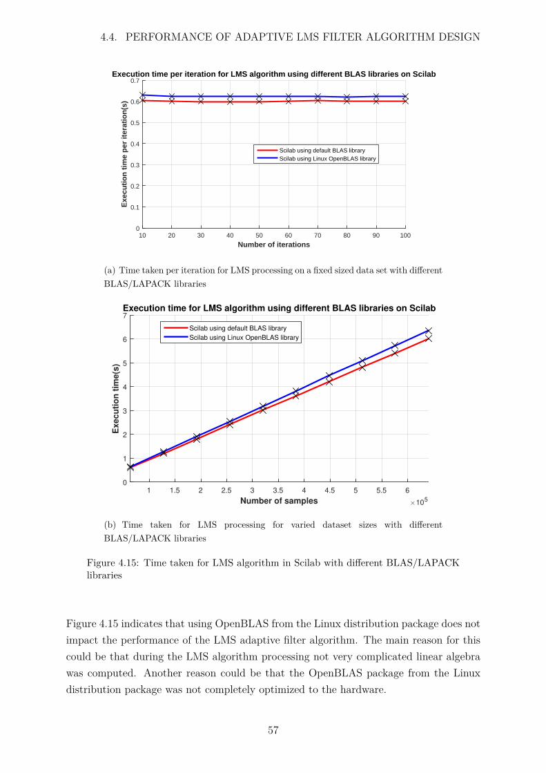
4.4. PERFORMANCE OF ADAPTIVE LMS FILTER ALGORITHM DESIGN
Number of iterations10 20 30 40 50 60 70 80 90 100
Exe
cuti
on
tim
e p
er it
erat
ion
(s)
0
0.1
0.2
0.3
0.4
0.5
0.6
0.7Execution time per iteration for LMS algorithm using different BLAS libraries on Scilab
Scilab using default BLAS libraryScilab using Linux OpenBLAS library
(a) Time taken per iteration for LMS processing on a fixed sized data set with differentBLAS/LAPACK libraries
Number of samples #105
1 1.5 2 2.5 3 3.5 4 4.5 5 5.5 6
Ex
ec
uti
on
tim
e(s
)
0
1
2
3
4
5
6
7Execution time for LMS algorithm using different BLAS libraries on Scilab
Scilab using default BLAS library
Scilab using Linux OpenBLAS library
Powered by TCPDF (www.tcpdf.org)
Powered by TCPDF (www.tcpdf.org)
(b) Time taken for LMS processing for varied dataset sizes with differentBLAS/LAPACK libraries
Figure 4.15: Time taken for LMS algorithm in Scilab with different BLAS/LAPACKlibraries
Figure 4.15 indicates that using OpenBLAS from the Linux distribution package does notimpact the performance of the LMS adaptive filter algorithm. The main reason for thiscould be that during the LMS algorithm processing not very complicated linear algebrawas computed. Another reason could be that the OpenBLAS package from the Linuxdistribution package was not completely optimized to the hardware.
57
Chapter 5
Conclusions and recommendations
Scripting languages are constantly improving. When designing algorithms for the purposeof a fair algorithmic comparison across different software packages, several factors needto be considered such that suitable performance can also be achieved. These include howdata is stored in memory and to maintain implicit parallelism when possible. Based onthe results obtained, the following conclusions can be drawn.
5.1 Improved performance with spatial locality
Algorithms that process large datasets, can result in code that is inefficient, as most usershardly consider spatial locality. Knowing how data is ordered in each of the languagepackages would result in cache-friendly code. Taking this into account the efficiency ofthe algorithms can be improved and, hence, the processing time can be reduced. Thisis one mechanism that can be used in any of the software packages to improve efficiencyand performance of any algorithms, not just RSP algorithms.
5.2 Adequate performance of pulse compression
Algorithm speed was the most important factor when comparing performance of varioussoftware packages. It was also an essential component when estimating the number ofFLOPS, which represents how efficient the program language can translate the ’numericalexpression’ into machine code. Initially, the algorithms were written with loops that
58
5.3. LACK OF JIT DURING DOPPLER PROCESSING FOR OCTAVE ANDSCILAB
iterate over matrices with data. All of the language packages achieved performancesunder the real time constraint of 130 seconds, implying that the external FFTW libraryof all the software packages gave acceptable performances, as most of the processingcompleted with pulse compression was completed with this library. The for-loop basedalgorithm implemented in MATLAB, Julia and Python obtained the best performancecompared to Octave and Scilab, with Scilab resulting in the slowest execution speed. Itwas realized that Scilab used the reference BLAS/LAPACK libraries by default, whichwas a single core implementation. Implicit parallelism was then further investigated byaltering the Scilab BLAS/LAPACK libraries to a multi core OpenBLAS library from theLinux distribution package. This resulted in an 8 percent improvement from the referenceBLAS library, which was not significant enough for the default BLAS/LAPACK librariesto be changed. When implementing pulse compression, the best performance would beobtained by MATLAB, Python and Julia, as they would complete the processing in theshortest amount of time.
5.3 Lack of JIT during Doppler processing for Oc-tave and Scilab
When applying Doppler processing, a nested loop-based algorithm was implemented.Since Scilab and Octave do not have a JIT compiler, performance was significantly worsethan the other software packages. Although CPython compiler is not optimized fornumerical processing, the efficiency and optimization of the NumPy and Pyfttw librariesallowed it to achieve good performance. Julia’s JIT compiler was extremely useful, as itmaximized the performance of for loops. MATLAB’s JIT compiler was not as advancedbut still attempts to vectorize for loops, obtaining execution times of approximately fivetimes slower than Python and Julia.
In order to determine if vectorization was the problem for Scilab and Octave, the nestedfor loops were vectorized, where possible. There was a massive improvement in per-formance with MATLAB, Octave and Scilab having approximately a 10 times speedimprovement, but Scilab was still significantly slower than the rest of the languages.The partially vectorized implementations resulted in MATLAB performing better thanthe rest of the packages. Since all of the languages are vectorizable, using vectors toindex a data matrix would improve the performance. This proves that using scientificlanguages as they were intended, results in maximum performance for heavily loop basedalgorithms.
59
5.4. IMPACT OF LARGE VECTORS ON ADAPTIVE LMS FILTER DESIGN
5.4 Impact of large vectors on adaptive LMS filterdesign
The analysis of the adaptive LMS algorithm was different to that of the pulse compressionand Doppler processing algorithms. It required a vector of data as opposed to a matrixof data. When using vectors or one dimensional arrays, Octave performed 50 percentworse than the rest of the packages. This implies that when a vector of data is required,Octave should be avoided, as it does not handle vectors as well as matrices of data. Juliasignificantly outperformed all of the language packages, as there was a 50 percent speedimprovement compared to MATLAB, which was the next best.
5.5 Impact of memory utilization on various languagepackages
Working memory size is important when dealing with large datasets. Algorithms withlarge datasets require larger hardware memories. All of the language packages accumulatesimilar peak memory usages, with no extra memory overhead. The only concern wasJulia’s garbage collector, which does not initially clear unnecessary variables but waitsuntil a particular threshold has occurred before it clears memory from the heap. Julia’sperformance would be the first to suffer, as virtual memory would be needed first from allof the language packages. Overall, when using Julia for processing large datasets, ensurethat a computer with enough physical RAM is used, such that performance would notsuffer.
5.6 Lack of implicit parallelism in Scilab
The default installation of Scilab does not benefit from implicit parallelism as it usesthe reference linear algebra packages. It also does not have a JIT, meaning that forloops are not automatically vectorized. All of the other languages benefit from implicitparallelism by the default installation. This means that on Linux machines, more workhas to be done by the user to obtain satisfactory performance from Scilab. This includesmanually switching or generating optimized linear algebra libraries, while no extra effortwas needed by the other packages to achieve the required performance.
60
5.7. SUITABLE ALTERNATIVES TO MATLAB
5.7 Suitable alternatives to MATLAB
All of the software languages are constantly improving. Newer versions of MATLAB hasa new execution engine which has improved its JIT compiler to work better with nestedloops. However, all of the open source packages are also making significant refinements,as they are still in development. Although Julia is the youngest language, it is competingand outperforming MATLAB in some scenarios. During the experiments, whether thealgorithms were loop based or vectorized, Python and Julia’s performances were the bestamongst the open source packages. Python performed better than Julia with extremelylarge data sets on computers with minimal physical RAM. However, Julia has a smoothertransition than Python in terms of syntax comparability to MATLAB. Python is also ageneral programming language which is able to perform very well in the scientific areawith specific modules such as NumPy. That means it also offers the possibility to easilybuild a module for interacting with other instruments, building GUI’s, processing otherdata and not only numbers. When choosing between Julia and Python, the user wouldneed to consider what they want in terms of syntax comparability to MATLAB, speedand their RAM constraints. Whichever one is chosen would give the user a satisfactoryperformance when implementing RSP techniques.
5.8 Recommendations
On the basis of the above conclusions, the following recommendations are made:
• Implement suitable multi-core implementations of various RSP algorithms. Thiswould allow for performance comparisons of the single core with a multi core im-plementation. There is also a chance to compare multi core implementations of thevarious language packages. This would determine if it is possible and reasonable todo a multi core implementation of the RSP algorithms on various languages.
• Investigate methods that change the linear algebra libraries for various softwarepackages, not just Scilab. Furthermore, determine procedures that optimize theselibraries, without using the versions from the Linux distribution package. Thiswould verify whether altering the default BLAS libraries to a more optimized versionwould affect the performance significantly.
61
Appendix A
Additional Procedures
The Appendix consists of the procedures followed to change the BLAS/LAPACKlibraries for Scilab as well as the basic commands used for FFTW and vectorizationprocedures:
A.1 Changing BLAS/LAPACK libraries for Scilab
This is the procedure followed in order to use the OpenBLAS library from the Linuxdistribution package (this assumes that the binary version of Scilab is used):
1. Enter the directory where Scilab was downloaded.
2. Enter the lib directory and then open the thirdparty folder.
3. Search for and delete libblas.so.3 and liblapack.so.3.
4. Once the above steps are completed the OpenBLAS library from Linux distri-bution will be used.
5. To check if OpenBLAS was actually used by Linux distribution package, openScilab and then the terminal.
6. Then enter the command "ps aux" into the terminal and record the pid of Scilab.
7. Finally enter the command lsof -p pid | grep ′blas\ | lapack′.
8. This should give the result, "/usr/lib/openblas-base/libblas.so.3", which impliesthat openBLAS from Linux is used.
A.2 FFTW procedures
By default, all of the software packages used the FFTW library apart from Python.To interact with the FFTW library, the pyFFTW module must be used. The
62
A.3. VECTORIZATION PROCEDURES
pyFFTW provides a unified interface for the different types of transforms thatFFTW can perform [56]. To interface with this pyfftw module, the pyfftw.buildersor pyfftw.interfaces package is recommended. The former consists of a set of func-tions that returns pyfftw.FFTW objects. In other words, it doesn’t return the re-sult of the FFT but instead returns a pyfftw.FFTW object that performs the FFToperation when it is called [57]. The latter provides interfaces to pyfftw modulethat implements the API of other commonly used FFT libraries such as numpy.fft[58]. The command used to apply FFT operations on a particular dataset usingpyfftw.builders and pyfftw.interfaces packages respectively is defined as follows:
pyfftw.builders.fft(dataMatrix, planner_effort = ′FFTW_ESTIMATE′,auto_align_input=True)
pyfftw.interfaces.numpy_fft.fft(dataMatrix, planner_effort =′FFTW_ESTIMATE′, auto_align_input=True, auto_contiguous=True)
The arguments of the above functions are given below:
– dataMatrix: This is the data set required for processing.
– planner_effort: By default, the FFTW_MEASURE is used, thereforeFFTW_ESTIMATE has to be set as the planner method.
– auto_align_input: It correctly byte aligns the dataMatrix for optimal usageof vector instructions. It is set to true by default. This means it does not haveto be included in the function.
– auto_contiguous: Makes sure the dataMatrix is contiguous in memory beforeperforming the transform on it. It is set to true by default. This means it doesnot have to be included in the function.
A.3 Vectorization procedures
These were the important operations used in order to partially vectorize the algo-rithms:
1. To index an array or matrix of data without loops use:
i = 1:step size:totalNumber
This method was used for all languages investigated except Python. Python usedthe NumPy library with the indexing command being:
i = numpy.arange(totalNumber).
The parameters of the above operations are given below:
63

A.3. VECTORIZATION PROCEDURES
– totalNumber is the number of elements that needs to be accessed in a vector.
– step size is the increment between these elements.
2. The next step was to make sure that the FFT was computed in the correctdimension to ensure Step 1 could occur correctly and without any errors. MAT-LAB, Octave and Python automatically give the proper dimension for the FFTcomputation, with Scilab and Julia requiring extra steps.
For Scilab and Julia, the following commands are used:
fft(data matrix, sign, size(data matrix,1), 1) = This is used in Scilab to applyFFT.
fft(data matrix,1) = This is used in Julia to apply FFT.
plan_fft(data matrix,1), plan_ifft(data matrix,1) = These are optional func-tions in Julia that can be used to determine an optimal FFT implementation for aspecific data set [6].
The arguments of the above functions are given below:
– dataMatrix: this is the data set required for processing.
– sign: this is either 1 or -1, indicating the direct and inverse transform respec-tively.
– size(data matrix,1): this is the size of the data matrix that requires a FFToperation with ’1’ indicating that it will be a one dimensional vector.
– the parameter ’1’ indicates applying a one dimensional FFT operation.
To ensure that Doppler processing produces the correct output, the fftshift functionwas needed. The fftshift function rearranges the Fourier transform of dataMatrixby shifting the zero-frequency component to the center of the array. The commandused to apply fftshift is written as follows:
fftshift(dataMatrix,dim): Swaps halves of each column or row of the dataMatrixdepending on the value of dim. If dim is set to 1: this swaps halves of each columnof dataMatrix for all of the software packages except Python, as the halves of eachrow of dataMatrix would be swapped.
64
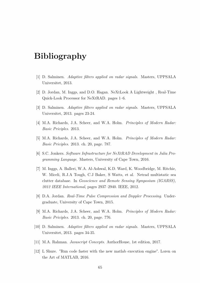
Bibliography
[1] D. Salminen. Adaptive filters applied on radar signals. Masters, UPPSALAUniversitet, 2013.
[2] D. Jordan, M. Inggs, and D.O. Hagan. NeXtLook A Lightweight , Real-TimeQuick-Look Processor for NeXtRAD. pages 1–6.
[3] D. Salminen. Adaptive filters applied on radar signals. Masters, UPPSALAUniversitet, 2013. pages 23-24.
[4] M.A. Richards, J.A. Scheer, and W.A. Holm. Principles of Modern Radar:Basic Priciples. 2013.
[5] M.A. Richards, J.A. Scheer, and W.A. Holm. Principles of Modern Radar:Basic Priciples. 2013. ch. 20, page. 787.
[6] S.C. Jonkers. Software Infrastructure for NeXtRAD Development in Julia Pro-gramming Language. Masters, University of Cape Town, 2016.
[7] M. Inggs, A. Balleri, W.A. Al-Ashwal, K.D. Ward, K. Woodbridge, M. Ritchie,W. Miceli, R.J.A Tough, C.J Baker, S Watts, et al. Netrad multistatic seaclutter database. In Geoscience and Remote Sensing Symposium (IGARSS),2012 IEEE International, pages 2937–2940. IEEE, 2012.
[8] D.A. Jordan. Real-Time Pulse Compression and Doppler Processing. Under-graduate, University of Cape Town, 2015.
[9] M.A. Richards, J.A. Scheer, and W.A. Holm. Principles of Modern Radar:Basic Priciples. 2013. ch. 20, page. 776.
[10] D. Salminen. Adaptive filters applied on radar signals. Masters, UPPSALAUniversitet, 2013. pages 34-35.
[11] M.A. Rahman. Javascript Concepts. AuthorHouse, 1st edition, 2017.
[12] L Shure. "Run code faster with the new matlab execution engine". Loren onthe Art of MATLAB, 2016.
65
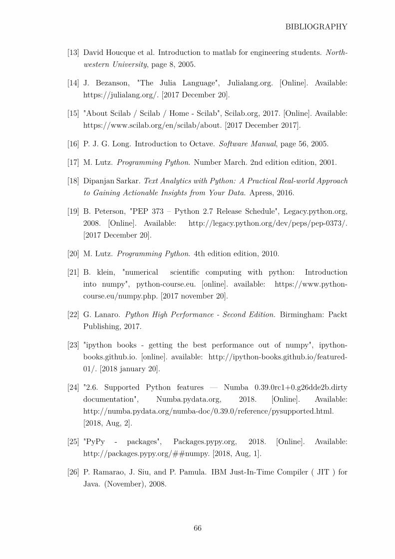
BIBLIOGRAPHY
[13] David Houcque et al. Introduction to matlab for engineering students. North-western University, page 8, 2005.
[14] J. Bezanson, "The Julia Language", Julialang.org. [Online]. Available:https://julialang.org/. [2017 December 20].
[15] "About Scilab / Scilab / Home - Scilab", Scilab.org, 2017. [Online]. Available:https://www.scilab.org/en/scilab/about. [2017 December 2017].
[16] P. J. G. Long. Introduction to Octave. Software Manual, page 56, 2005.
[17] M. Lutz. Programming Python. Number March. 2nd edition edition, 2001.
[18] Dipanjan Sarkar. Text Analytics with Python: A Practical Real-world Approachto Gaining Actionable Insights from Your Data. Apress, 2016.
[19] B. Peterson, "PEP 373 – Python 2.7 Release Schedule", Legacy.python.org,2008. [Online]. Available: http://legacy.python.org/dev/peps/pep-0373/.[2017 December 20].
[20] M. Lutz. Programming Python. 4th edition edition, 2010.
[21] B. klein, "numerical scientific computing with python: Introductioninto numpy", python-course.eu. [online]. available: https://www.python-course.eu/numpy.php. [2017 november 20].
[22] G. Lanaro. Python High Performance - Second Edition. Birmingham: PacktPublishing, 2017.
[23] "ipython books - getting the best performance out of numpy", ipython-books.github.io. [online]. available: http://ipython-books.github.io/featured-01/. [2018 january 20].
[24] "2.6. Supported Python features — Numba 0.39.0rc1+0.g26dde2b.dirtydocumentation", Numba.pydata.org, 2018. [Online]. Available:http://numba.pydata.org/numba-doc/0.39.0/reference/pysupported.html.[2018, Aug, 2].
[25] "PyPy - packages", Packages.pypy.org, 2018. [Online]. Available:http://packages.pypy.org/##numpy. [2018, Aug, 1].
[26] P. Ramarao, J. Siu, and P. Pamula. IBM Just-In-Time Compiler ( JIT ) forJava. (November), 2008.
66
BIBLIOGRAPHY
[27] "documentation/parallelcomputinginscilab - scilabwiki", wiki.scilab.org. [online]. Available:https://wiki.scilab.org/Documentation/ParallelComputingInScilab. [2017October 18].
[28] "ITaP Research Computing -", Rcac.purdue.edu, [Online]. Available:.https://www.rcac.purdue.edu/knowledge/rice/run/examples/apps/matlab/implicit_parallelism. [2018, Aug, 13].
[29] "vectorization-matlab & simulink-mathworks unitedkingdom", mathworks.com. [online]. available:https://www.mathworks.com/help/matlab/matlab_prog/vectorization.html.[2017 december 20].
[30] "What is NumPy? — NumPy v1.12 Manual", Docs.scipy.org, 2017. [Online].Available: https://docs.scipy.org/doc/numpy-1.12.0/user/whatisnumpy.html.[2018 January 16].
[31] "GNU Octave Vectorization and Faster Code Execution", Gnu.org. [Online].Available:https://www.gnu.org/software/octave/doc/interpreter/Vectorization-and-Faster-Code-Execution.html [2017, October, 20].
[32] "Optimal Number of Workers for Parallel Julia - Stochastic Lifestyle", Stochas-tic Lifestyle, [Online]. Available:. http://www.stochasticlifestyle.com/236-2/. [2018, July, 30].
[33] M. Baudin. Programming in SCILAB. pages 129–130, 2011.
[34] R. Baudin. Run time comparison of MATLAB , Scilab and GNU Octave onvarious benchmark programs. pages 1–20, 2016.
[35] "Julia with Intel R© Math Kernel Library for Improved Performance| Intel R© Software", Software.intel.com, 2018. [Online]. Available:https://software.intel.com/en-us/articles/julia-with-intel-mkl-for-improved-performance. [2018, Aug, 5].
[36] "Using Intel R© MKL in GNU Octave | Intel R© Software", Software.intel.com,2018. [Online]. Available: https://software.intel.com/en-us/articles/using-intel-mkl-in-gnu-octave. [2018, Aug, 5].
[37] "Numpy/Scipy with Intel R© MKL and Intel R© Compilers | Intel R© Software",Software.intel.com, 2018. [Online]. Available: https://software.intel.com/en-us/articles/numpyscipy-with-intel-mkl. [Accessed: 05- Aug- 2018].
67
BIBLIOGRAPHY
[38] "File : Details", Fileexchange.scilab.org, 2018. [Online]. Available:https://fileexchange.scilab.org/toolboxes/MKL/5.5.2. [2018, Aug, 5].
[39] "debianscience/linearalgebralibraries-debian wiki", wiki.debian.org, 2017. [on-line]. available: http://wiki.debian.org/DebianScience/LinearAlgebraLibraries.[2017 december 23].
[40] K.D. Lee. Programming languages: An Active Learning Approach, page 15.2008.
[41] MathWorks. Memory Management Guide. pages 1–9, 2002.
[42] S. McGarrity, "Programming Patterns: Maximizing Code Performance byOptimizing Memory Access", Mathworks.com, 2007. [Online]. Available:https://www.mathworks.com/company/newsletters/articles/programming-patterns-maximizing-code-performance-by-optimizing-memory-access.html.[2017,October,20].
[43] "Principle of Locality", Codingfreak.blogspot.com, 2009. [Online]. Available:http://codingfreak.blogspot.com/2009/03/principle-of-locality.html. [2017 De-cember 20].
[44] "Row-major vs Column-major confusion", Stackoverflow.com. [Online]. Avail-able: https://stackoverflow.com/questions/33862730/row-major-vs-column-major-confusion. [2017 December 20].
[45] M. Frigo and S.G. Johnson. The Fastest Fourier Transform in the West (MIT-LCS-TR-728). Materials Research, page 1, 1997.
[46] "define method for determining fft algorithm - matlab fftw -mathworks united kingdom", mathworks.com. [online]. available:https://www.mathworks.com/help/matlab/ref/fftw.html. [2017 december20].
[47] M. Frigo and S. Johnson, "FFT Benchmark Methodology", fftw.org. [Online].Available: http://www.fftw.org/speed/method.html. [2017 December 20].
[48] "Big-Oh", [Online]. Available: https://www.cs.cmu.edu/ mrmiller/15-121/Lectures/14-bigOh.pdf. [2018 July 18].
[49] M. Frigo and S. Johnson, "FFT Benchmark Results", fftw.org. [Online]. Avail-able: http://www.fftw.org/speed/. [2017 December 20].
[50] "What is a Floating-point?", Computerhope.com, 2018. [Online]. Available:https://www.computerhope.com/jargon/f/floapoin.htm. [2018, Aug, 1.
68
BIBLIOGRAPHY
[51] M. Baudin. Programming in SCILAB. page 137, 2011.
[52] M.A. Richards, J.A. Scheer, and W.A. Holm. Principles of Modern Radar:Basic Priciples. 2013. ch. 13, page. 466.
[53] "flops (floating point operations per second) definition", techterms.com, 2009.[online]. available: https://techterms.com/definition/flops. [2017 decemember20].
[54] "HANNING", Northstar-dartmouth.edu, 2018. [Online]. Available:http://northstar-www.dartmouth.edu/doc/idl/html_6.2/HANNING.html.[2018, Aug, 2].
[55] T Holy. "Julia Users - How does garbage collection really work in Julia?",Julia-programming-language.2336112.n4.nabble.com, 2018. [Online]. Avail-able: http://julia-programming-language.2336112.n4.nabble.com/How-does-garbage-collection-really-work-in-Julia-td46829.html. [2018 January 19].
[56] H. gomersall, "welcome to pyfftw’s documentation! — pyfftw0.10.4 documentation", hgomersall.github.io, 2016. [online]. available:https://hgomersall.github.io/pyFFTW/. [2018 january 3].
[57] H. gomersall, "pyfftw.builders - get fftw objects using a numpy.fft like interface— pyfftw 0.10.4 documentation", hgomersall.github.io, 2016. [online]. available:https://hgomersall.github.io/pyFFTW/pyfftw/builders/builders.html#module-pyfftw.builders. [2018 january 3].
[58] "pyfftw.interfaces - drop in replacements for other fft implementations —pyfftw 0.10.4 documentation", hgomersall.github.io, 2016. [online]. available:https://hgomersall.github.io/pyFFTW/pyfftw/interfaces/interfaces.html#module-pyfftw.interfaces. [2018 january 7].
69