Social Context and Network Formation: Experimental Studies

1

Social Context and Network Formation: Experimental Studies

Martijn Burger1 Vincent Buskens2

April 22, 2006

Word Count: 12,668 (Including References)

Abstract Recently, there has been an increasing interest in how strategic action influences network structure. Motivated by the widespread belief that ‘networks matter’ in the process of reaching personal objectives, it is a natural assumption that rational actors will try to strategically arrange their ties in order to optimize their expected utility. Starting from the notion that there exist rival theories on what is the best strategy to form linkages and that the applicability of these theories varies across social contexts, we will examine how (groups of) actors change their networks in order to get better positions. Theoretical results predict that emerging networks are to a large extent contingent on the social context and the adjacent strategy actors follow to choose their relations. Experiments will be used to test this conjecture. Keywords: Social Networks, Network Formation, Game Theory, Experimental Sociology

1 Faculty of Social Sciences, Utrecht University, Email: [email protected] 2 Department of Sociology/ICS, Utrecht University, Heidelberglaan 1, 3584 CS Utrecht, The Netherlands, Email: [email protected] We thank Jeroen Weesie, … for useful comments.

2

1. Introduction

Over the past decades, there has been a growing interest in the effect of networks on

individual achievement and group performance. Driven by the belief that actors should not be

regarded as atomized individuals, but are embedded in social relationships (Polanyi, 1957;

Granovetter, 1985), many studies have shown that social structure affects important aspects

of social and economic life (Granovetter, 2005). Examples include personal health (House et

al., 1988), educational attainment (Coleman & Hoffer, 1987), finding a job (Granovetter,

1974), buyer satisfaction (DiMaggio & Louch 1998), the performance of companies (Uzzi,

1996), closing deals (Mizruchi & Stearns, 1999), the enforcement of social norms (Raub &

Weesie, 1990), and the promotion of civic engagement (Putnam, 2000).

With the focus on social structure and achievement, most of the network literature has been

concentrating on the questions what the good positions are within a network (at the

individual level) and how network structure relates to the performance of groups (at the

collective level). Although these studies imply that individuals will attempt to maneuver

themselves in beneficial positions, the mechanisms underlying those processes have only

been made explicit to a limited extent. Given the strategic importance of networks, it is

however essential to understand how they are formed (Jackson, 2005a). In other words,

approaching the subject matter from a dynamic point of view, we can shed some light on

how actors form ties and network structure evolves, given the benefits or externalities

networks can provide (Jackson & Wolinsky, 1996). As some network positions are more

beneficial to actors than others, it is expected that actors will attempt to maneuver themselves

in a better position (Flap, 1999). Hence, the focus shifts from network as an independent

variable (‘consequences of networks’) to networks as a dependent variable (‘causes of

networks’). Naturally, new questions will arise. How will people change their networks in

order to get better positions? And when is a network stable, or when does no more change

occur?

Lately, several strategic dynamic models based on cooperative and non-cooperative game

theory that deal with the emergence of networks have been developed (e.g., Myerson, 1977,

1991; Jackson & Wolinsky, 1996; Bala & Goyal, 2000; Johnson & Gilles, 2000; Gould,

3

2002; Goyal & Vega-Redondo, 2004; Buskens & Van de Rijt, 2005; Goyal & Joshi 2005).3

Drawing on micro-economic theory, it is assumed that 1) actors derive utility from their

network and the position they occupy within this network and 2) actors are able to

strategically arrange their ties in order to optimize their expected utility (Jackson, 2005b).

Most of these strategic models of network formation face however a number of major

drawbacks. First of all, the connection with ‘classic’ theories on network structure and

performance, developed in the static literature, is often nonexistent. This deficiency can be

attributed to the fact that dynamic and static network literatures have their roots in different

disciplines. Whereas static network analysis has its foundations in sociology, dynamic

network analysis is an emerging field not only in sociology, but also in economics, computer

science and physics. Although the degree of integration of these subfields is low, noteworthy

examples of cross-fertilization are recent work by Cálvo-Armengol (2004), Goyal and Vega-

Redondo (2004) and Buskens and Van den Rijt (2005). Second, many dynamic models suffer

from being undercontextualised accounts of network formation. Although in most cases a

hypothetical situation to which the model applies is sketched, the potential effect of social

context on the emergence of networks remains often unaddressed. Third, few empirical tests

of dynamic network models have been conducted so far. Exceptions are in this respect

experiments conducted by Falk and Kosfeld (2003), Berninghaus et al. (2004), Deck and

Johnson (2004), and Callander and Plott (2005).4

The main contribution of this article is an attempt to overcome the above-mentioned

quandaries by implementing static theoretical accounts and the notion of social context in

dynamic models of network formation. By addressing theories on network structure derived

from the static literature, we will conjecture what is the best strategy to form linkages given

the social context in which the network is embedded. We will here introduce three network

formation strategies for three different contexts, being 1) a neutral setting, 2) a competitive

setting, and 3) a cooperative setting. Analytic calculations and computer simulations,

including the characterization of stable states in each context, will be used to further develop

the theoretical framework and draw our hypotheses. Experiments will be carried out to assess

whether emerging networks are to a large extent contingent on the social context and the

adjacent strategy actors follow to choose their relations.

3 A survey of the dynamic network literature can be found in Dutta & Jackson (2003) and Jackson (2005a) 4 For a more extensive overview see Kosfeld (2004)

4

2. Rival Theories of Network Formation

In his seminal work on the social structure of competition, Ronald Burt (1992) constructs a

theory that envisages which positions in a social network are most beneficial (e.g., in order to

obtain higher profits, to gain exclusive information, or to produce good ideas). Burt

hypothesizes in this respect that brokerage positions or ‘structural holes’ within a social

network create competitive advantage as they offer access and control benefits. Access

benefits encompass the availability of information and are based on the idea of redundancy or

the extent to which ties procure the same information benefits. Contacts of ego that also share

ties among each other are very likely to share the same information and for this reason

provide a repetitious or redundant advantage to a particular actor. Control benefits constitute

advantages based on the fact that bringing together non-redundant contacts (i.e., occupying a

structural hole) gives an exorbitant arbitrage over whose interests are served when the ties

flock together. Burt (2001: 36) notes in this respect that “… the holes between his contacts

mean that [an actor] can broker communication while displaying different beliefs and

identities to each contact.” For these reasons, individuals rich in structural holes are then the

ones who have more social capital or higher returns on their social relationships.

Although Burt’s notion of structural entrepreneurship implies that individuals will attempt to

maneuver themselves in beneficial positions, the mechanism underlying this process is hardly

specified in his work. A translation to strategic behavior of actors in the formation process is

however not difficult. Given that there are apparently advantageous structural positions

within a network, actors will not create relationships at random, but will attempt to

strategically arrange their ties in order to optimize their position. In other words, it is

assumed that actors will deliberately manipulate links to increase their stock of social capital

and improve their opportunity structure created by social relationships.5 In the “Burtian”

sense, actors strive for having non-redundant ties, brokerage positions and bridging structural

holes. In other words, actors will maximize their utility by trying to create ties with

unconnected alters

5 Network change can also be extrinsic through factors external to the network (see Willer & Willer, 2000). This article will however only deal with intrinsic network change.

5

In contrast to Burt, Coleman (1988; 1990) argues that not structural holes, but network

closure should be regarded as the most important source of social capital. According to

Coleman, dense and cohesive networks reduce the costs of information search and achieving

norms. In line with Burt (1992), Coleman likewise focuses on both access and control

benefits. Access benefits are however not related to brokerage positions here, but merely to

the idea that full closure decreases the costs of information search. As the quality of

information tends to decay over ties, it is better to obtain this information with a minimum

amount of intermediaries. Control benefits are here related to the fact that network closure

makes it easier to impose sanctions and come to agreements (through amplification of

existing opinion), hereby promoting trust and norms. In other words, cohesion also reduces

the risk and uncertainty associated with transactions by reducing the chance that actors will

behave opportunistically. From a dynamic point of view, actors should strive for having

redundant ties and closed triads. To put it different: in the “Colemanian” sense, the optimal

strategy is to form ties with alters that are connected.

Whereas Burt (1992) argues that full closure networks are often related to dreadful

performance at the individual and group level, Coleman (1990) evaluates striving for

bridging structural holes and brokerage positions as very risky. At a first glance, Burt and

Coleman seem to point out two opposing views of what is the best strategy to form linkages.

However, one can seriously question the validity of this contradistinction, since the context-

dependency of the respective strategies is often overlooked when comparing their strengths

and weaknesses. As network effects are ostensibly goal-specific, structural advantage may

vary over situations (Flap & Völker, 2001). Accordingly, the effects of network structure on

social and economic outcomes can be perceived as being context-dependent. When your

main objective is to enforce norms and promote safety, this might work better in a dense local

structure than in a local structure rich in structural holes. On the other hand, job attainment

clear example in which ‘weak ties’ are ought to be more beneficial than ‘strong ties’

(Granovetter, 1973). This is a clear example of how systemic-level phenomena (social

contexts) influence systemic outcomes (network structure) through their effect on individual

orientations and actions (networking strategy and behavior) (Coleman 1990, see Figure 1).

Nevertheless, network formation should be perceived here as strictly interdependent due to

the non-atomic character of networks (Buskens & Van de Rijt, 2005). Accordingly, it can be

argued that networks evolve as an unintended consequence of goal-directed actions. In other

6

words, the resulting network structure should not be perceived as a direct result, but merely

as a byproduct of individual rational behavior and therefore non-trivial.

INSERT FIGURE 1 ABOUT HERE

This tempting significance of the macro-micro link is corresponding to the notion of

Stinchcombe (1989) and Flap (1999; 2002) that network effects are conditional upon certain

institutional and social factors. Applying a methodological and positivist perspective, it can

be derived that a rationale for both strategies is present, albeit the applicability and success of

these strategies depend on the context in which they are utilized. Drawing on

psychoanalytical theory developed by Greenberg (1991) and Haidt & Rodin (1999),

Kadushin (2002) links the Burtian and Colemanian network formation strategies to two

adversarial intrinsic motivations present in human beings. On the one hand, there exists the

drive towards individual effectiveness, competitiveness and control, while, on the other hand,

there is the drive towards support, trust and feelings of safety. Kadushin (2002) argues that

despite the fact both drives are present in mankind, their relative amounts may vary across

social settings. This is in line with Burt’s argument (2005a), who argues that brokerage

revolves around the strategic importance and uniqueness of information, while closure is

focused on safety and verification of information. Hence, brokerage is about the value of non-

redundant information, whereas closure is about the value of redundant information. People

that strive for bridging structural holes are therefore expected to be merely found in contexts,

in which it is very important to obtain non-redundant, first-hand information to get ahead.

Granovetter (1973) also speaks of the ‘strength of weak ties’. One can here think of the news-

reporting business, finding a job in difficult times, or leadership functions. These are

situations in which a vision advantage is important (Burt, 2005a) and you have to be quicker

and smarter than everybody else. Also being in control of the information flowing in the

network is considered to be of importance here. On the contrary people that strive for a

closed local structure are expected to be found in contexts in which safety, stability, and

continuity is considered to be of utmost importance. This can be denoted as the ‘strength of

strong ties’ (Krackhardt, 1992). One can here think of getting help when being ill

(community care in particular), checking the trustworthiness of sellers in risky transactions

with a high problem potential, or promoting certain group standards. In sum, closure

promotes cooperation, voluntarily or involuntarily. Consequently, it can be argued that

7

Burtian strategies are mainly to be found in competitive and entrepreneurial settings, whereas

Colemanian strategies are thought to be more prevalent within the context of cooperation and

collaboration (Flap 1999). Brokerage is often found in contexts where the good individuals

strive for is rival (consumption by one individual leads to less benefits for other individuals)

and excludable (an individual to which the good is supplied can exclude other individuals

from consumption) as in these situations it is very important to get ahead of others. Closure,

on the other hand, is often found in contexts where there is a potential problem of collective

action to produce the common good and cooperation of the rest of the network is strictly

necessary. From an economic point of view, it can therefore be argued that brokerage is

mainly concerned with the acquisition of private goods, whereas closure is more prevalent for

the production of collective goods. In sum, Burtian and Colemanian strategies seem to be

both appropriate strategies, but in different contexts.

3. Theoretical Framework and Hypotheses: Network Formation and Stability

Network Formation Contexts, Strategies and Utility Functions

In this section, we will turn to a formalization of our general model by linking each network

strategy s to a numerical value in terms of a utility function ui(s). For the matter of simplicity,

we will start off with the neutral situation in which actors establish ties at random, or more

specifically, do not have any preferences on the relationship between alters. Later on, the

model will be expanded to situations in which 1) actors prefer ties with unconnected alters

(Burtian network formation context) and 2) actors prefer ties with alters that are connected

(Colemanian network formation context). Note that preferential attachment is here

considered only to be based on the ties of alters. In all other respects, actors are assumed to

be homogeneous within a given network, in the sense that other actor characteristics (such as

the amount of resources an actor possesses) are neglected in the network formation process,

the costs and benefits are the same for each tie, and individual strategies only vary across

network formation contexts. It should be noted that in reality one is likely to find

heterogeneity of strategies within the same social context. However, the composition of this

strategy mix may still highly vary across contexts.

From a graph-theoretic point of view, a network g is composed of actors, represented by n

nodes, and the relationships between these actors, represented by t ties (or edges). Let N = {1,

8

2,…, n} be the finite set of actors, n = 2 the minimum amount of actors present in the

network, and tij the strength of the tie between actor i and j. In our research, we consider ties

to be non-reflexive (tii = 0 for all i), non-directed (tij = tji for all i, j), and non-

weighted ( {0,1})ijt ∈ . Given these conditions, the set of all possible networks is then

( 1) / 2{ | {0,1}n ng g −⊆ . We denote the tie between i and j by ij. If ij∈g then actor i and j are

directly connected in the network, when ij∉g this is however not the case. The addition of a

tie ij in a network g can be denoted by g + ij, while the deletion of a tie ij results in the

creation of the network g – ij. Based on models by Myerson (1991) and Gould (2002), we

consider actors simultaneously propose and discard ties. The pure strategy of actor i is then ( 1){0,1} n

is −∈ with the utility function ui(s) connected to it, where s is the strategy profile of

all actors. We assume here that there has to be (simultaneous) mutual consent about the

creation of a tie in the network, so that for the graph g induced by s holds:

1ij jiij g s s∈ ⇔ = = . We also assume that utility is solely conditional upon the structure of g

and not on the proposals made. Therefore, ui(s’) = ui(s’’), whenever s’ and s’’ are two

strategy profiles inducing the same network g. Thus if g is the network induced by s, it can be

stated that ui(s) = ui(g).

Below we will distinguish three utility functions on networks. First, we assume the number

of ties an actor i has: ui(g) = ui(ti). An actor is willing to form or hold a tie if and only if the

marginal benefits (b1) of that tie outweigh its marginal costs (c1). This context we will call

the neutral network formation context. When actors form ties in a neutral network formation

context and do not have any preferential attachment, an actor’s costs (C) and benefits (B) are

only comprised of having t (direct) ties.6 The utility of an actor i networking in a neutral

network formation context can therefore be presented by the following formula (1):

(1) ( ) ( ) ( )i i i iu t B t C t= −

Assuming that the costs and benefits of ties are linear and that indirect ties do not yield any

benefits, this would always lead to either a full-closure network or an empty network (if

c1>b1). An addition to this basic utility function might therefore include the following. As

6 We assume here that indirect ties do not yield any benefits.

9

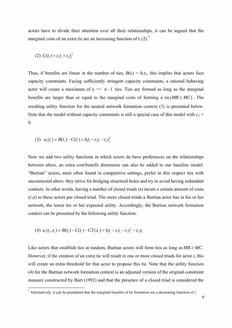
actors have to divide their attention over all their relationships, it can be argued that the

marginal costs of an extra tie are an increasing function of ti (2).7

(2) 21 2( )i i iC t c t c t= +

Thus, if benefits are linear in the number of ties, B(ti) = b1t1, this implies that actors face

capacity constraints. Facing sufficiently stringent capacity constraints, a rational behaving

actor will create a maximum of ti << 1n − ties. Ties are formed as long as the marginal

benefits are larger than or equal to the marginal costs of forming a tie ( )MB MC≥ . The

resulting utility function for the neutral network formation context (3) is presented below.

Note that the model without capacity constraints is still a special case of this model with c2 =

0.

(3) 21 1 2( ) ( ) ( )i i i i i i iu t B t C t b t c t c t= − = − −

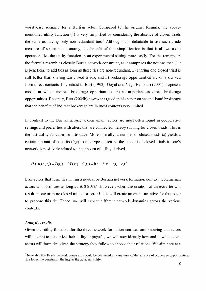
Now we add two utility functions in which actors do have preferences on the relationships

between alters, an extra cost/benefit dimension can also be added to our baseline model.

“Burtian” actors, most often found in competitive settings, prefer in this respect ties with

unconnected alters: they strive for bridging structural holes and try to avoid having redundant

contacts. In other words, having a number of closed triads (z) incurs a certain amount of costs

(c3z) to these actors per closed triad. The more closed triads a Burtian actor has in his or her

network, the lower his or her expected utility. Accordingly, the Burtian network formation

context can be presented by the following utility function:

(4) 21 1 2 3( , ) ( ) ( ) ( )i i i i i i i i i iu t z B t C t CT z b t c t c t c z= − − = − − −

Like actors that establish ties at random, Burtian actors will form ties as long as .MB MC≥

However, if the creation of an extra tie will result in one or more closed triads for actor i, this

will create an extra threshold for that actor to propose this tie. Note that the utility function

(4) for the Burtian network formation context is an adjusted version of the original constraint

measure constructed by Burt (1992) and that the presence of a closed triad is considered the 7 Alternatively, it can be postulated that the marginal benefits of tie formation are a decreasing function of t.

10

worst case scenario for a Burtian actor. Compared to the original formula, the above-

mentioned utility function (4) is very simplified by considering the absence of closed triads

the same as having only non-redundant ties.8 Although it is debatable to use such crude

measure of structural autonomy, the benefit of this simplification is that it allows us to

operationalize the utility function in an experimental setting more easily. For the remainder,

the formula resembles closely Burt’s network constraint, as it comprises the notions that 1) it

is beneficial to add ties as long as these ties are non-redundant, 2) sharing one closed triad is

still better than sharing ten closed triads, and 3) brokerage opportunities are only derived

from direct contacts. In contrast to Burt (1992), Goyal and Vega-Redondo (2004) propose a

model in which indirect brokerage opportunities are as important as direct brokerage

opportunities. Recently, Burt (2005b) however argued in his paper on second-hand brokerage

that the benefits of indirect brokerage are in most contexts very limited.

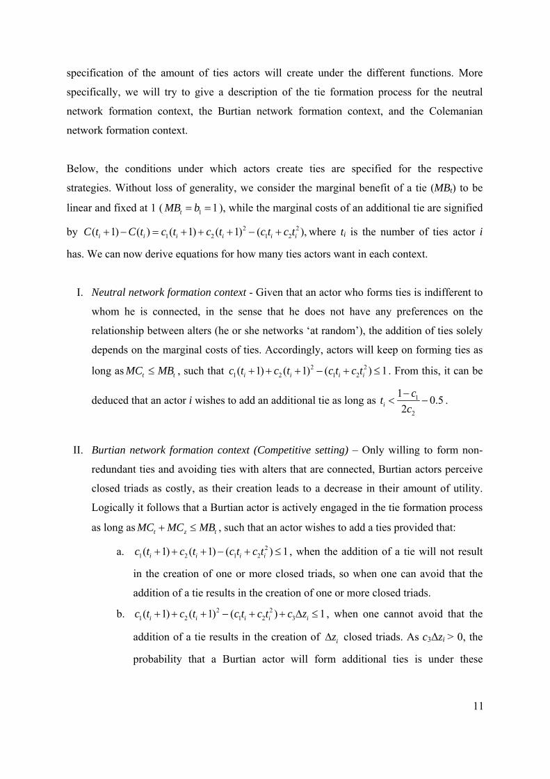
In contrast to the Burtian actors, “Colemanian” actors are most often found in cooperative

settings and prefer ties with alters that are connected, hereby striving for closed triads. This is

the last utility function we introduce. More formally, a number of closed triads (z) yields a

certain amount of benefits (b2z) to this type of actors: the amount of closed triads in one’s

network is positively related to the amount of utility derived.

(5) 21 2 1 2( , ) ( ) ( ) ( )i i i i i i i i i iu t z B t CT z C t b t b z c t c t= + − = + − +

Like actors that form ties within a neutral or Burtian network formation context, Colemanian

actors will form ties as long as .MB MC≥ However, when the creation of an extra tie will

result in one or more closed triads for actor i, this will create an extra incentive for that actor

to propose this tie. Hence, we will expect different network dynamics across the various

contexts.

Analytic results

Given the utility functions for the three network formation contexts and knowing that actors

will attempt to maximize their utility or payoffs, we will now identify how and to what extent

actors will form ties given the strategy they follow to choose their relations. We aim here at a

8 Note also that Burt’s network constraint should be perceived as a measure of the absence of brokerage opportunities: the lower the constraint, the higher the adjacent utility.

11

specification of the amount of ties actors will create under the different functions. More

specifically, we will try to give a description of the tie formation process for the neutral

network formation context, the Burtian network formation context, and the Colemanian

network formation context.

Below, the conditions under which actors create ties are specified for the respective

strategies. Without loss of generality, we consider the marginal benefit of a tie (MBt) to be

linear and fixed at 1 ( 1 1tMB b= = ), while the marginal costs of an additional tie are signified

by 2 21 2 1 2( 1) ( ) ( 1) ( 1) ( ),i i i i i iC t C t c t c t c t c t+ − = + + + − + where ti is the number of ties actor i

has. We can now derive equations for how many ties actors want in each context.

I. Neutral network formation context - Given that an actor who forms ties is indifferent to

whom he is connected, in the sense that he does not have any preferences on the

relationship between alters (he or she networks ‘at random’), the addition of ties solely

depends on the marginal costs of ties. Accordingly, actors will keep on forming ties as

long as t tMC MB≤ , such that 2 21 2 1 2( 1) ( 1) ( ) 1i i i ic t c t c t c t+ + + − + ≤ . From this, it can be

deduced that an actor i wishes to add an additional tie as long as 1

2

1 0.52i

ctc−

< − .

II. Burtian network formation context (Competitive setting) – Only willing to form non-

redundant ties and avoiding ties with alters that are connected, Burtian actors perceive

closed triads as costly, as their creation leads to a decrease in their amount of utility.

Logically it follows that a Burtian actor is actively engaged in the tie formation process

as long as t z tMC MC MB+ ≤ , such that an actor wishes to add a ties provided that:

a. 21 2 1 2( 1) ( 1) ( ) 1i i i ic t c t c t c t+ + + − + ≤ , when the addition of a tie will not result

in the creation of one or more closed triads, so when one can avoid that the

addition of a tie results in the creation of one or more closed triads.

b. 2 21 2 1 2 3( 1) ( 1) ( ) 1i i i i ic t c t c t c t c z+ + + − + + ∆ ≤ , when one cannot avoid that the

addition of a tie results in the creation of iz∆ closed triads. As c3∆zi > 0, the

probability that a Burtian actor will form additional ties is under these

12

circumstances smaller than when the addition of a tie does not result in the

creation of one or more closed triads.

Accordingly, it can be argued that a Burtian actor i is willing to create an additional

tie on the condition that 3 1

2

1 min0.5

2j i

i

c z ct

c− ∆ −

< − ties. Note that this, ceteris

paribus, implies that the Burtian actor will on average form less ties than an actor

creating ties in a neutral network formation context.

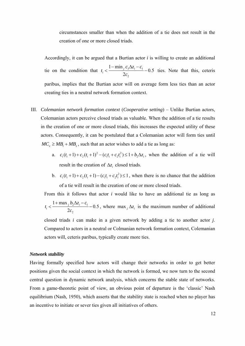
III. Colemanian network formation context (Cooperative setting) – Unlike Burtian actors,

Colemanian actors perceive closed triads as valuable. When the addition of a tie results

in the creation of one or more closed triads, this increases the expected utility of these

actors. Consequently, it can be postulated that a Colemanian actor will form ties until

z t zMC MB MB≥ + , such that an actor wishes to add a tie as long as:

a. 2 21 2 1 2 2( 1) ( 1) ( ) 1i i i i ic t c t c t c t b z+ + + − + ≤ + ∆ , when the addition of a tie will

result in the creation of iz∆ closed triads.

b. 21 2 1 2( 1) ( 1) ( ) 1i i i ic t c t c t c t+ + + − + ≤ , when there is no chance that the addition

of a tie will result in the creation of one or more closed triads.

From this it follows that actor i would like to have an additional tie as long as

2 1

2

1 max0.5

2j i

i

b z ct

c+ ∆ −

< − , where max j iz∆ is the maximum number of additional

closed triads i can make in a given network by adding a tie to another actor j.

Compared to actors in a neutral or Colmanian network formation context, Colemanian

actors will, ceteris paribus, typically create more ties.

Network stability

Having formally specified how actors will change their networks in order to get better

positions given the social context in which the network is formed, we now turn to the second

central question in dynamic network analysis, which concerns the stable state of networks.

From a game-theoretic point of view, an obvious point of departure is the ‘classic’ Nash

equilibrium (Nash, 1950), which asserts that the stability state is reached when no player has

an incentive to initiate or sever ties given all initiatives of others.

13

Definition 1: Nash Equilibrium

A network g* is considered Nash stable if there exists strategy combination s* inducing g*: (I) * *( ) ( , )i i i i iu s u s s−≥ for all i and si

Applications of the Nash equilibrium in the dynamic network literature can be found in

Myerson (1991) and Gould (2002). Since our model subsumes that ties are non-directed and

mutual consent is needed to form a link, it is however unsatisfactory to use Nash as

equilibrium concept because coordination problems may arise (Gilles & Sarangi, 2004; Van

de Rijt & Buskens, 2005). As one-sided proposals do not alter an actor’s utility, two-sided

link formation games often result in numerous Nash equilibria. The empty network is for

instance always a Nash equilibrium network: if no one is proposing a tie, actors do not have

an incentive to propose ties because mutual consent is needed to establish a link. For these

reasons, Gilles and Sarangi (2004) denote networks resulting from Nash equilibria as

individually stable networks, but not necessarily as collectively stable networks, in the sense

that Nash is a strategy-based stability concept. Understandably, we require a suitable

alternative to the Nash equilibrium.

As an alternative, Jackson and Wolinsky (1996) proposed the concept of pairwise stability.

Opposed to Nash networks, all pairwise stable networks are considered both link deletion and

link addition proof. In other words, there is no actor who desires to sever a tie (II) and no pair

of actors that would like to add a tie between themselves (III). In general, we refer to these

conditions as link deletion proofness (II) and link addition proofness (III).

Definition 2: Pairwise stability

A network is considered pairwise stable if:

(II) For all i and ij g∈ , ( ) ( )i iu g u g ij≥ −

(III) For all ij g∉ , if ( ) ( )i iu g u g ij< + then ( ) ( )ju g u g ij> +

Given that that tie deletion is considered to be unilateral and tie addition bilateral, the concept

of pairwise stability is robust to one-tie deviations (Calvó-Armengol & Ilkiliç, 2005), in the

sense that if the creation of a certain tie would beneficial to both actors involved, a given

14

network is considered unstable (Buskens & Van de Rijt, 2005; Jackson, 2005b). In

accordance, pairwise stability accounts for coordination problems that may arise in the

process of network formation. Note that in contrast to Nash stability, pairwise stability is

defined in terms of a network property (local condition) rather than in terms of strategic

considerations of actors (Gilles & Sarangi, 2004). Therefore, pairwise stability should be

primarily characterized as an indicator of collective stability rather than an indicator of

individual stability. Consequently, it can be perceived as a network-based stability concept.

Although there exist more strict network-based stability concepts, including strong pairwise

stability (Gilles & Sarangi, 2004) and unilateral stability (Van de Rijt & Buskens, 2005),

these will not be utilized in this article as they do not add much explanatory value to the

evolving network structures and their characteristics.

4. Computer Simulations

Simulation design

Having introduced the context-specific utility functions and a suitable stability concept, we

will now identify the stability states of networks across the various contexts using computer

simulations. In order to do so, all possible non-isomorphic networks ranging from 3 to 8

actors, containing in total 13,595 different network configurations, will be surveyed in the

three network formation contexts. In this simulation, b1 and c1 are respectively fixed at 1 and

0.2, while we vary the degree in which actors face capacity constraints (c2) when forming

ties. These ‘quadratic costs of forming ties’ can take a value between 0.00 (no capacity

constraints) and 0.20 (actors only want one tie). These values are chosen in such way that we

have a value for each possible number of ties actors can have. The cut-off points are here

based on tie formation in a neutral network formation context. With respect to the Burtian

and Colemanian network formation context, respectively the costs and benefits of an

additional closed triad are considered to be linear and fixed at 0.2 ( 2 0.2zMB b= = ,

3 0.2zMC c= = ). Remember that this means that an additional tie that results in one or more

additional closed triad is of less value for an actor networking in the Burtian context,

compared to an additional tie that does not result in the creation of a closed triad. On the

contrary, for an actor networking in the Colemanian context, the opposite is true.

15

In order to draw hypotheses on the effects of context and to uniquely identify evolving

network structures, a number of main network characteristics are estimated for stable

networks. These include measures of structure, density, centralization and segmentation. A

detailed overview of these indicators is listed below in Table 1.

INSERT TABLE 1 ABOUT HERE

The analyses are performed using a two-step procedure. First of all, we check for each

network formation context under the various capacity constraints using each of the 13,595

non-isomorphic networks with size n=3 to 8, which networks are pairwise stable. In addition,

we evaluated the network structure for the stable networks in the respective network

formation contexts by network size and the degree of capacity constraint. Although, this

analysis provided us with an overview of all stable networks, it does not indicate which

equilibrium networks are more likely to occur than others. For this reason, it is impossible to

draw exact hypotheses with respect to the predicted network structures across the various

network formation contexts and cost functions.

In network formation the convergence to some equilibrium depends on the starting network..

For these reasons, we examine in a second simulation the network formation process by

starting from an empty network (i.e., a network in which no ties are formed yet) and letting a

process in which actors are allowed to sever and add ties continue until convergence, so

when a pairwise stable state is reached. By letting this simulation run 200 times under each

condition (which are defined by network formation context and capacity constraint; the tested

conditions will be specified below), we are able to deduce the probability that a network will

converge to a pairwise stable network contingent on the network formation context. In

particular, we focus here on networks with size n=6 in all three network formation contexts

in order to be able to draw and test exact hypotheses on the emerging network structures. We

decided to focus specifically on the networks of size 6 because this magnitude can be

considered ‘a size reflecting a trade-off between capturing network complexity while

maintaining manageability’ (Callander & Plott, 2005: 1473). On the one hand a network

should be large enough (in terms of actors and potential number of ties) in order to observe

differences between conditions and network formation contexts, while on the other hand

testing hypotheses based on a relatively large network size might lead to the situation in

16

which subjects have difficulties to gain a clear view of the ‘physical’ network during the

experimental test, resulting in coordination problems and non-random error. With respect to

the quadratic costs, we focus here on two levels: low 2( 0.10)c = and high

2( 0.20)c = capacity constraints. Whereas under high capacity constraints actors want to form

maximally 2 ties in the neutral network formation context, this amounts to 4 ties under low

capacity constraints. The choice for these two specific levels of quadratic costs

2 2( 0.10 | 0.20)c c= = is based on the premise to scrutinize two significantly different

conditions, in which there is under each of the constraints, in each network formation

context, at least more than one equilibrium network. We control for ‘random error’ in goal-

directed behavior by running the simulations at different levels of ‘noise’ as this can explain

the discrepancies between the expected and observed network structures. This ‘noise’ can be

interpreted as the degree of random mistakes made by the actors in the network and can take

a value between 0.00 (very low) and 0.80 (very high) in our simulation. In general, we

assume an average noise level (α=0.40) and hypotheses will be drawn under this assumption.

However, possible discrepancies between the expected and observed probabilities of

convergence toward a particular equilibrium network will be analyzed by looking at different

levels of random error.


Simulation Results and Hypotheses

From the first analysis it could be deduced that the number of stable networks is very small

compared to the number of existing networks with size 3 through 8 (13,595 networks).

Moreover, the number of stable networks generally increases with network size, but not

monotonically so. On the contrary, the relationship between the number of stable networks

and the degree of capacity constraints is non-monotonic, as we find the largest number of

stable networks under medium capacity constraints. Table 3 shows the network

characteristics of the pairwise stable networks for n=6 by capacity constraint and network

formation context. Figure 2A and 2B display the ‘physical structure’ of these networks.

Some equilibrium networks can be found in more than one network formation context.

Nevertheless, their expected probability of occurrence might still fluctuate across contexts

and conditions (as we will show later). Under the low capacity constraint condition, there are

17

eight different pairwise stable networks. For the neutral network formation context, there are

four pairwise stable networks: the tailed full pentagon, single-crossed 3-prism, octahedron,

and the full pentagon with one actor isolated. For the Burtian network formation context

under low capacity constraints, there are three pairwise stable networks: the 2,4-complete

bipartite network, 3,3-complete bipartite network, and the 3-prism. For the Colemanian

network formation context, there are only two pairwise stable networks: the full hexagon and

the full pentagon with one actor isolated. Under the high capacity constraint condition, there

are six different pairwise stable networks. Surprisingly, we find under this cost condition

often similar equilibrium networks across the three network formation contexts. For the

neutral formation context, there are again four pairwise stable networks: the two triangles,

the square and dyad, the pentagon and isolate, and the hexagon. In the competitive (Burtian)

setting, there are three pairwise stable networks: the square and dyad, the pentagon and

isolate, and the hexagon. In the cooperative (Colemanian) setting, there are even five

pairwise stable networks: the full pentagon (with one actor isolated), the full square and

dyad, two triangles, the pentagon and isolate, and the hexagon.


INSERT FIGURE 2A AND 2B ABOUT HERE

We do not only want an overview of all stable networks, but also wish to know which game-

theoretic equilibria are more likely to occur than others as their characteristics differ. These

predictions are derived from the simulation by the procedure described above. Table 4 shows

the probability of convergence toward a particular equilibrium by capacity constraint and

network formation context. Note that we assume here an average ‘noise’ level of 0.40. It is

unreasonable that actors never make mistakes. However, the variation in probabilities is

limited for different noise levels (see Table 4).


Basing ourselves on table 3 and 4, we can hypothesize to which extent the emerging network

structures and the resulting network characteristics are contingent on the social context and

18

the adjacent strategy actors follow to choose their relations. This can be done by comparing

the mean network characteristics across the six network formation conditions. These

predicted mean network characteristics are derived from the characteristics of the identified

pairwise stable networks times the probability of convergence to a particular equilibrium

network in a given network formation context, assuming a 40% noise level. For example, in

the Colemanian network formation context under low capacity constraints, the full hexagon

accounts for 86% of the mean network characteristics and the full pentagon for 14% (based

on their probability of occurrence). Table 5 shows the predicted mean density, proportion of

full triads, centralization, and segmentation by capacity constraint and network formation

context. The standard deviations are presented between parentheses.


Equality of means for the selected network characteristics (density, proportion of full triads,

centralization, and segmentation) across the three network formation contexts by capacity

constraint was tested by means of a Wald test. In other words, we tested for the uniqueness of

the expected contextual mean scores (denoted by E(x)) related to density, proportion of full

triads, centralization, and segmentation within both the high capacity constraints and low

capacity constraints condition. Accordingly, we were able to rank each network formation

context (by the degree of capacity constraints) for each of the four network characteristics.

Table 8 presents these rankings by capacity constraint and network characteristic. The

resulting hypothesized differences between network formation contexts are described below.

It should be noted that some hypotheses (and related results) are more self-evident than

others. The proportion of full triads can be perceived as a direct product of goal-directed or

rational behavior. ‘If actors want bananas, they buy bananas (if they are able to pay them and

recognize what bananas are)’. In other words, given that Colemanian actors strive for full

triads, it is not surprising when we find in the emerging network structures a high proportion

of full triads. On the contrary, the degree of centralization, the degree of segmentation and

network density, are merely a byproduct of these actions. In other words, they are unintended

consequences of goal-directed behavior.

19

Density

We hypothesize that under low capacity constraints, the density (d) will be larger in

Colemanian networks (E(d)=.953) compared to networks created within the neutral

(E(d)=.753, F=1338, p=.004) and Burtian (E(d)=.595, F=4235, p<.001) network formation

context. Moreover, it is predicted that under this condition the density will be larger in

networks emerging from a neutral network formation than in networks emerging from a

Burtian context (F=835, p<.001). Under high capacity constraints, the density in Colemanian

(E(d)=.400) networks is predicted to be larger than in neutral (E(d)=.380, F=13.39, p<.001)

and Burtian (E(d)=.376, F=19.82, p<.001) networks. The density across the emerging

networks in the latter two contexts is not expected to differ (F=.63, p=.43). Not surprisingly,

the density under low capacity (E(d)=.767) constraints is hypothesized to be higher than

under high capacity constraints (E(d)=.385, F=3178, p<.001). This general trend can be

observed when looking at the average density scores over all computed capacity constraints

(uncorrected for probability of convergence) for network size n=6. This conjecture also holds

for networks of different sizes.

Hypothesis 1

We predict that the network density in the different conditions is ordered as follows:

• Low capacity constraints: d(Burtian, low) < d(Neutral, low) < d(Colemanian, low)

• High capacity constraints: d(Burtian, high) = d(Neutral, high) < d(Colemanian, high)

• Low vs. high capacity constraints: d(high) < d(low)

Proportion of full triads

Under low capacity constraints, it can be hypothesized that the proportion of full triads (ft) is

higher in Colemanian networks (E(ft)=.930) than in neutral (E(ft)=.362, F=4905, p<.001) and

Burtian (E(ft)=.031, F=12297, p<.001) networks. Comparing the emerging network

structures in the Burtian and neutral network formation context, it is expected that networks

created in the latter setting contain a higher proportion of full triads (F=1665, p<.001). Under

high capacity constraints, we predict again the proportion of full triads to be larger in

Colemanian networks (E(ft)=.081) than in networks related to the neutral (E(ft)=.014,

F=67.23, p<.001) and Burtian (E(ft)=.000, F=98.52, p<.001) network formation contexts.

Furthermore, it is hypothesized that that there will be no differences with respect to the

proportion of full triads between the Burtian and neutral network formation context (F=2.98,

20

p=.084). Evidently, the proportion of full triads is predicted to be larger under low capacity

constraints (E(ft)=.441) than under high capacity constraints (E(ft)=.032, F=660.2, p<.001).

Hypothesis 2

We predict that the proportion of full triads in the different conditions is ordered as follows:

• Low capacity constraints: ft(Burtian, low) < ft(Neutral, low) < ft(Colemanian, low)

• High capacity constraints: ft(Burtian, high) = ft(Neutral, high) < ft(Colemanian, high)

• Low vs. high capacity constraints: ft(high) < ft(low)

Centralization

Under low capacity constraints it is expected that the degree of centralization (c) is higher in

neutral networks (E(c) =.310) than in networks created within the Colemanian (E(c) =.140,

F=48.97, p<0.001) and Burtian (E(c) =.044, F=119.6, p<0.001) network formation context.

Moreover, it is predicted that under this condition the degree of segmentation will be larger

in networks embedded in a Colemanian network formation context than in networks

embedded in a Burtian context (F=15.51, p<.001). This prediction seems to be

counterintuitive as all actors that strive for bridging structural holes wish to be in the center

of the network. However, if all actors want to be in center, there is no center (Buskens & Van

de Rijt, 2005). This is obviously an unintended consequence of goal-directed behavior. We

do not expect a difference in centralization scores between the three network formation

contexts under high capacity constraints (F=1.04, p=.354). Differences in centralization

scores across the capacity constraint conditions are also hypothesized to be less pronounced

as both extremes are here located within the low capacity constraints conditions. This

proposition holds when controlling at different capacity constraints and networks of different

sizes. However, the degree of centralization is still expected to be significantly larger under

low capacity constraints (E(ft)=.165) than under high capacity constraints (E(ft)=.134,

F=4.370, p=.037).

Hypothesis 3

We predict that the degree of centralization in the different conditions is ordered as follows:

• Low capacity constraints: c(Burtian, low) < c(Colemanian, low) < c(Neutral, low)

• High capacity constraints: c(Colemanian, high) = c(Neutral, high) = c(Burtian, high)

• Low vs. high capacity constraints: c(high) < c(low)

21

Segmentation

Under low capacity constraints, it is predicted that the degree of segmentation (s) is lower in

Colemanian networks (E(s) = -.720) than in networks created within the Burtian (E(s) =.000,

F=385.7, p<0.001) and neutral (E(s) =.004, F=429.7, p<0.001) network formation context.

We do not expect a difference in segmentation scores here between networks created in the

Burtian and neutral network formation context (F=1.19, p=.28). On the contrary, under high

capacity constraints, we expect the degree of segmentation to be higher in Colemanian (E(s)

= .870) networks than in Burtian (E(s) = .577, F=64.03, p<.001) and neutral networks (E(s) =

.627, F=44.06, p<.001). Again, we do not predicted a differences in the degree of

segmentation between neutral and Burtian networks (F=1.86, p=0.17). Overall, it can be

hypothesized that the degree of density will be higher under high capacity constraints

(F=1243, p<.001). These predictions are robust for different network sizes and capacity

constraints.

Hypothesis 4

We predict that the degree of segmentation in the different conditions is ordered as follows:

• Low capacity constraints: s(Colemanian, low) < s(Burtian, low) = s(Neutral, low)

• High capacity constraints: s(Burtian, high) = s(Neutral, high) < s(Colemanian, high)

• Low vs. high capacity constraints: s(low) < s(high)


5. Experimental Design and Method of Analysis

Experiments as Method to Analyze the Process of Network Formation

The aim of this research is to evaluate which stable networks will emerge and how actors behave in reaching respectively staying in stable networks contingent on the network formation context in which they are embedded. In other words, the main theoretical construct of interest is here to examine the effect of social context on the evolving network structure. While many models of network formation have only remained at a theoretical level, our study attempts to overcome this deficiency by means of an experimental test. In this respect,

22

our research accumulates to the existing knowledge of the experiments conducted by Falk and Kosfeld (2003), Berninghaus et al. (2004), Deck and Johnson (2004), and Callander and Plott (2005). Whereas computer simulations in the previous section were used to predict which (stable) network structures are most likely to emerge, we now closely monitor the formation of networks by letting subjects participate in a computerized network experiment. An obvious advantage of using laboratory experiments is the possibility to control your environment, such as actors’ strategies and the benefits and costs of tie formation, increasing the internal validity of the study. Deck and Johnson (2005) stress notwithstanding the importance of keeping the task understandable and undemanding for subjects, in order to safeguard the construct validity. This need for comprehensibility certifies our choice for the relatively straightforward utility functions, earlier presented in section 3. However, also other measures were taken to facilitate a valid interpretation of the experimental data. The instruction manual contained for instance an extensive task description, including examples and hints. Likewise, payoff matrices were included to give a brief synopsis of the costs and benefits per network formation context by the amount of ties created (see Appendix A). In addition, four rounds were included in which subjects could practice. All the same, it should be noted that making tasks oversimplified would also have a negative impact on the construct validity of the research as it induces a sphere of artificiality (Judd et al., 1990). When conducting a laboratory experiment, it is important to keep in mind that what we measure is really what we intend to measure. To what extent are the constructs of theoretical interest successfully operationalized? To put it different, are subjects to a respectable degree aware they are involved in a network formation process and act like this, or are they just occupied with maximizing payoffs (whether or not due to trial and error)? The latter can be the case when the task to be executed in the laboratory is too difficult or too easy. Our study tries to find a compromise between incomprehension and oversimplification by presenting subjects a simplified, but abstract environment in which the formulated hypotheses on network formation will be tested. Experimental Setting: Treatments and Conditions In the experiment, subjects had to play network games in the designated network formation contexts (in the neutral, Burtian (competitive), and Colemanian (cooperative) setting) under one of the two capacity constraints conditions (low capacity constraint (c1=0.20, c2=0.10) or high capacity constraint (c1=0.20, c2=0.20)). In every context, subjects had to interact with 5

23

other participants. Starting from an empty network, they add and delete ties for a limited amount of time in order to improve their network position and maximize their utility. Table 4 gives a detailed overview of the experimental design, including the costs and benefits of ties and triads in each network formation context under each experimental condition. Under the low capacity constraint, the marginal benefits of ties were set equal to 100 ECU (experimental currency units), whereas costs were increasing more than proportional: 20t + 10t2, in which t represents the number of ties an actor has formed. The marginal benefits of triads in the cooperative setting amounted to 20 ECU, as did the costs of triads in the competitive setting. Under the high capacity constraint, the marginal benefits of ties equated 200 ECU, whilst the costs were set at 40t + 40t2. In this condition, the marginal benefits of triads in the cooperative setting equalled 40 ECU. Likewise, the marginal costs of triads in the competitive setting also totalled 40 ECU. Besides the marginal costs and benefits of ties and triads, Table 4 indicates the maximum amount of benefits and costs for triad formation, given the amount of triads actors can form. Although the composition and absolute magnitude of the payoffs varied across conditions and contexts, these were always in accordance, in terms of relative magnitude, with the utility functions used in the computer simulations.


From the information presented in Table 5 it can be derived, that the optimal periodical profit

lies between 160 ECU and 350 ECU in each unique network formation context. As already

presented in the computer simulations, it is evident that the amount of preferred ties highly

fluctuates over contexts and conditions. Whereas in the Colemanian setting under low

capacity constraints the optimal amount of ties equals 5, this amount is in the Burtian setting

under high capacity constraints only 2.

Experimental Procedures

The computerized experiment was designed using the software program z-tree 3.0

(Fischbacher, 1999) and conducted in the Experimental Laboratory for Sociology and

Economics (ELSE) at Utrecht University. In total, six experimental sessions of

approximately one-and-a-half hours were scheduled and completed, three using each

condition (low or high capacity constraint). Using the ORSEE recruitment system, over 250

24

potential subjects were approached by e-mail to participate in the experiment. Eventually, 18

students participated in each session for a total of 108 separate subjects, as it was allowed to

take part in only one session.9 Altogether, the emergence of 216 networks was surveyed.

During the experiment, participants were subjected to all treatments (i.e., one of the network

formation contexts) consisting and created networks in the 1) neutral network formation

context, 2) Burtian network formation context (competitive setting) and 3) Colemanian

network formation context (cooperative setting). The capacity constraint to which

participants were subjected was session-dependent. Also the order in which the contexts were

presented to the subjects differed across sessions, to separate the ordering effects from the

condition and contextual effects. Before the start of each treatment, subjects had to read the

context-specific instructions. General instructions were given before the start of the

experiment. Each treatment was similarly structured and consisted of four cycles.

At the beginning of each cycle, subjects were randomly allocated to a group together with 5

other participants and assigned a label (D1, D2…D6), in order to accumulate statistically

independent observations (Falk & Kosfeld, 2004). Hence, every subject operated in 3

contexts in 12 different groups. Each cycle had the same structure and was divided in 10

periods of 30 seconds each. Starting from an empty network in the first period of every cycle,

subjects indicated simultaneously on their computer terminals with whom they wanted to

establish or break a connection. As assumed in our models, mutual consent was needed to

form a link, while subjects could unilaterally delete ties. Established connections appeared

red and double-arrowed on the screen. Full information about the network was continuously

provided, as tie proposals and created links of other participants could instantly be tracked.

After each period, an update of the entire network was displayed at the bottom of the screen.

In addition, subjects were informed about the amount of points earned in the previous period.

A screenshot of the subject screen is displayed in Figure 2.

INSERT FIGURE 3 ABOUT HERE

The magnitude of a subject’s payoff depended on his decisions and the decisions of the other

participants. Subjects were honoured points after each period. Consequently, participants

who managed to form their ‘ideal’ ego-network (given the network formation context) rather 9 Enrollment was based on a first come, first serve basis

25

quickly during a particular cycle were usually awarded more points in that cycle. The

maximum expected payoff was 19800 ECU for actors under the low capacity constraint

condition and 16500 ECU for subjects under the high capacity constraint condition. At the

end of the experiment, the earned experimental currency units were converted to euros at an

average rate of 1000 ECU = 0.92 euro.10 In addition, subjects received €2.50 (5000 ECU)

participation fee. The maximum salient payoff (that is, excluding participation fee) earned by

a subject was €15.80, while the minimum amount equalled €10.80. On average subjects

obtained €14.20.

Data Analysis

The acquired data from the experiment comprises the realized equilibrium network structures

for maximally 162 cycles (that is, 27 per possible combination of network formation context

and degree of capacity constraint. More specifically, in our analysis we assumed that during

each cycle only one equilibrium network could be reached. In line with the experiment

conducted by Callander and Plott (2005), a network is defined to have converged to some

equilibrium if the same configuration was chosen in three consecutive periods within the

same cycle. Note that this configuration does necessarily have to be like one of the game-

theoretic equilibria as predicted from the simulations. The analysis consisted of two parts.

First of all, it is tested to what extent the network characteristics of the stable networks

obtained from the simulations bear a resemblance to the network characteristics of the stable

networks obtained from the experiment (hypothesis 7-10). This is at the outset done by an

examination of the rank order as predicted from the simulation (see Table 7) and on which

our hypotheses were based. Here, we compare the observed network characteristics across the

six network formation contexts using Wald tests in order to assess whether we find the same

rank order for the four distinguished network characteristics (density, full triads,

centralization, and segmentation11). Secondly, a more rigid test (one-sample z-test) was

conducted to examine whether the network characteristics of the equilibria in the experiment

exactly matched the network characteristics of the pairwise stable networks derived from the

computer simulations as stated in Table 6. Overall model fit by network characteristic was

assessed using an adjacent chi-square test. It should be noted that, contrary to the rank order

10 As the maximum amount of points that could be earned differed across conditions, this was corrected for in the exchange rate 11 Explanations of these concepts can be found in the previous section

26

test, the equality of means tests have a very stringent nature and assess whether the expected

probability/mean accurately resembles the observed probability/mean.

6. Experimental Results

Description of the general results

Table 10 shows the proportion of networks that converged to an equilibrium network by

network formation context and capacity constraint condition. Note that an equilibrium

network is here defined as (the first) network configuration12 that was chosen in three

consecutive rounds and does not necessarily imply one of the game-theoretic equilibrium

structures as identified in the simulations. Overall, 130 of the 162 networks (80.2%)

converged to a stationary configuration. Convergence was more likely to happen under high

capacity constraints (85.2%) than under low capacity constraints (75.3%). This is not

surprising, as the number of ties actors wish to have is essentially lower under high capacity

constraints, which makes coordination among actors easier. Moreover, there was a clear

learning effect as reaching a stable state was more probable to occur in 1) treatments that

were played during a later stage of the experiment and 2) network games that were played

during a later stage within the same treatment. To illustrate the differences: the mean

percentage of networks that converged to a stationary configuration equaled 63.0% over all

treatments that were played first during a experimental session, whilst this percentage is on

average 93.5% for all treatments played during a later stage of the experiment. In addition, in

network games played during the first cycle of a treatment 77.8% reached an equilibrium

state, compared to 86.1% for the network games played during a later stage within the same

treatment. More importantly, also across network formation contexts we observed some

differences: the probability of convergence seems to be higher in the neutral (88.9%) and

Colemanian (85.2%) network formation context than in the Burtian network formation

context (66.7%). Particularly, in the Burtian network formation context, under low capacity

constraints, reaching an equilibrium state appeared to be difficult as this only happened in

51.9% of the cases. These differences can be explained by the fact that the Burtian network

formation context is conceptually perhaps the most difficult setting to grasp for subjects.

12 Only in two cycles more than one equilibrium network appeared. The first stable configuration was here denoted as being the equilibrium network.

27

Moreover, it is particularly a hard setting to coordinate in when everyone wants to make a lot

of ties, but also tries to avoid the creation of full triads.

Most of the equilibrium networks (114 out of 130 networks, 87.7%) were one of the game-

theoretic equilibria as specified in the simulations. In the neutral setting and in the Burtian

setting under high capacity constraints even in 100% of the cases the stationary configuration

was also (at least) a pairwise stable network. Only in the Colemanian network formation

context under low capacity constraints the proportion of equilibria that were also a game-

theoretic equilibrium was relatively low (only 60.0%). These non-game-theoretic equilibria

differed often (in 93.8% of the cases) only one tie from one of the context-specific pairwise

stable networks. For example, in the Colemanian setting under low capacity constraints, in 9

out of 10 non-pairwise stable stationary networks, there was always one of the six actors who

did not see that making the last tie, which would complete the full hexagon, would result in

the creation of 4 additional full triads (instead of for example one full triad). This ‘bounded

rationality’ (the inability to identify bananas) of actors in the real world would obviously be

one of the most important reasons why in these cycles convergence to one of the pairwise

stable networks did not happen.


Results related to the Comparison of Network Characteristics across Social Contexts

In this section, we compare the network characteristics of the stationary configurations with

the predicted network characteristics of the predicted structures. We begin with examining

whether the predicted rank order (as presented in Table 6) is correct (an overview is

presented in Table 9). Later, we will scrutinize whether the observed mean density (d),

proportion of full triads (ft), and the amount of centralization (c) and segmentation (s) exactly

matches the predicted means. Note that O(x) refers below to the observed mean of a

particular network characteristic under a given condition.

Density (Hypothesis 1)

Our hypothesis that under low capacity constraints the average density will be larger in

Colemanian networks than in neutral networks and Burtian networks is confirmed. The

observed mean density in Colemanian (O(d)=.968) network is significantly larger than in

28

neutral (O(d)=.785, F=557.7, p<.001) and Burtian (O(d)=.600, F=1727, p<.001) networks.

Also, neutral networks are generally denser than networks created within a Burtian setting

(F=415.4, p<.001). Our hypotheses under high capacity constraints are only partly confirmed

as there appear to be no significant differences in density between the three network

formation contexts, whereas it was predicted that the density in Colemanian context would be

slightly higher than in the other two settings (F=1.29, p=.279). However, as the predicted

differences were already small and the hypothesis is tested under a small sample size, the lack

of confirmation for this hypothesis is not surprising because the power to find it is low.

Overall, it is indeed confirmed that the density of networks is higher under low capacity

constraints (O(d)=.817) than under high capacity constraints (O(d)=.402, F=533.6, p<.001).

Proportion of full triads (Hypothesis 2)

With respect to the proportion of full triads, our expectations hold under both low and high

capacity constraints. Under low capacity constraints, the average proportion of full triads is as

predicted higher in networks embedded in the Colemanian network formation context (O(ft)=

.908) than in networks embedded in the neutral (O(ft)=.395, F=825.1, p<.001) and Burtian

(O(ft)=.000, F=1993, p<.001) network formation context. Also the difference between the

Burtian and neutral setting under low capacity constraints with respect to the mean proportion

of full triads is as predicted statistically significant (F=361.9, p<.001). Under high capacity

constraints we also find in line with our hypotheses a higher proportion of full triads in the

Colemanian network formation context (O(ft)=.114) compared to the neutral (O(ft)=.012,

F=33.18, p<.001) and Burtian(O(ft)=.000, F=37.96, p<.001) network formation context. As

predicted there are however no significant differences between the Burtian and neutral setting

(F=.43, p=.514). Unsurprisingly, the proportion of full triads is higher under low capacity

constraints (O(ft)=.514) than under high capacity constraints (O(ft)=.514, F=110.2, p<.001).

Centralization (Hypothesis 3)

With respect to the amount of centralization, which can, opposed to the previous two network

characteristics, be merely perceived as a byproduct of goal-directed behavior (instead of a

direct consequence), part of our hypothesis are confirmed. Under low capacity constraints, it

was predicted that the highest average degree of centralization was to be found in the neutral

network formation context, followed by 2) the Colemanian and 3) the Burtian setting. In line

with our expectations, we find a significantly lower centralization score in the Burtian

29

network formation context (O(c)=.000) than in the neutral (O(c)=.105), F=2.75, p<.10)13 and

Colemanian O(c)=.134), F=4.66, p=.033) network formation context. However, there is no

significant difference with respect to the amount of centralization between Colemanian and

neutral networks (F=.28, p=.600). Contrary to our predictions, the mean degree of

centralization is even somewhat higher in the Colemanian setting. Under high capacity

constraints, the hypothesis that the degree of centralization is equal across all three network

formation context does not hold (F=3.62, p=.030). Instead, we find again the highest degree

of centralization in the Colemanian (O(c)=.156) network formation context, although the

difference with Burtian networks is only significant at the p=0.10 level (O(c)=.053, F=3.33,

p=.070). This finding can at least partly be contributed to the high proportion of equilibrium

networks that were not game-theoretic equilibria. Often these equilibrium networks were

missing a ‘final tie’, which resulted in a higher degree of inequality between actors compared

to when this equilibrium (full hexagon) would have been reached. With respect to the overall

picture, there is, contrary to our expectations, no observed difference in degree of

centralization for the two different capacity constraints (F=.500, p=0.480).

Segmentation (Hypothesis 4)

With respect to the amount of segmentation (which can also be strictly perceived as an

unintended consequence of rational behavior) the expected rank orders are confirmed for both

capacity constraints. Under low capacity constraints, the mean degree of segmentation is

indeed significantly lower in Colemanian networks (O(s)=-.600) than in networks embedded

in the neutral (O(s)=.045, F=71.49, p<.001) and Burtian (O(s)=.000, F=47.37, p<.001)

environment. As expected, the degree of segmentation does not significantly differ between

the latter two context (F=.26, p-.612). Under high capacity constraints, we observe as

predicted the reverse order: the mean degree of segmentation is found to be higher in

Colemanian networks (O(s)= -.972) than in neutral (O(s)=.428, F=50.29, p<.001) and Burtian

(O(s)=.000, F=65.19, p<.001) networks. Again, no significant difference between the Burtian

and neutral context is observed (F=1.74, p=.189). Evidently, these results show that in the

Colemanian setting actors tend to cluster. However, if the costs of ties become too high, this

results in the partition of the larger network (full hexagon) into segmented clusters of a

smaller size (two triangles or square and dyad). Overall, the amount of segmentation is as

13 As the sample size is relatively, the p=0.10 level is accepted as a reasonable threshold here

30

expected lower under low capacity constraints (O(s)=-.230) than under high capacity

constraints (O(s)=.562, F=133.2, p<.001).


In sum, most of our hypotheses with respect to differences in network characteristics as

expressed in the predicted rank order are confirmed or at least partly confirmed. From this it

can be concluded that in terms of network characteristics, the emerging networks are to a

large extent contingent on the social context and the adjacent strategy actors follow to choose

their relations. However, are the observed mean network characteristics also exactly the same

as the predicted ones? Table 12 shows the predicted (from the simulations) and observed

average density, proportion of full triads and degree of centralization and segmentation by

capacity constraint and network formation context. The predicted and observed average

scores by network characteristic, network formation context and capacity constraint were

compared using a one-sample z-test. An overall chi-square test is conducted for each network

characteristic. It should be noted that this test is very rigid and can be perceived as a very

strict test of the hypotheses related to differences in the network characteristics across

network formation contexts.

Although, the observed average density in each network formation context (under both

capacity constraints) resemble closely the predicted ones, the observed density does not

exactly match the expected density for all conditions (χ2=41.39, df=6, p<.001). In the neutral

setting (under both capacity constraints) and the Burtian setting (under high capacity

constraints) the observed average density score significantly differs from the predicted

density score, despite the fact that this difference is at maximum .032 (in the Burtian network

formation context, under high capacity constraints). In general, it can be postulated that the

observed degree is higher than the expected one. In other words, actors make more ties than

is predicted from the simulations. The same type of results can be observed for the other

network characteristics: the observed scores are very close to the predicted ones, but they do

not exactly match. Concerning the proportion of full triads, we find an underprediction of this

network characteristic in the Colemanian setting and an overprediction in the Burtian setting.

This can be contributed to the fact that actors were made explicitly aware of the fact that

triads are respectively beneficial or costly. With respect to the degree of centralization and

31

segmentation, we suffer in general from overpredictions as we observe in some cases a lower

mean than expected. Tentative conclusions might lead us in the direction of social efficiency

and inequality aversion. This indication will be further discussed in the concluding section.


7. Discussion and Conclusion

In this paper, we analyzed the context-dependency of evolving network structures. Network

formation was examined in a neutral setting, a competitive setting (Burtian network

formation context), and a cooperative setting (Colemanian network formation context). On

the basis of rank orders, computerized simulations predicted that networks are to a large

extent determined by the social context in which they are embedded. Experimental results

confirmed this conjecture as most of the predicted rank orders were verified: network

characteristics often significantly differ across social contexts. Networks emerging from in

cooperative settings (Colemanian network formation context) can be characterized as dense

networks, which tend to segment when the costs of ties are becoming high. On the contrary,

networks evolving in competitive settings (Burtian network formation context) are usually

sparse and highly decentralized, especially when the costs of ties are relatively low: when

everyone wants to be in the center, there is no center (or this develops by chance). These

differences should be predominantly perceived as a byproduct of rational behavior, as they

are only indirect results of preferential attachment of actors within a given network formation

context. Actors do not directly strive for a dense, centralized or segmented network, but these

network features are an unintended consequence of goal-directed behavior. In other words,

they are the uncoordinated aggregate of individuals’ actions, originating from the

optimalization of each actor’s local structure.

Although we found a highly significant effect of social context on network structure, the

observed network characteristics did not exactly equal the predicted network characteristics.

Explanations for this incongruity have to be found in the fact that the predicted network

configurations did not match the observed network configurations. We tested whether the

predicted distribution of equilibrium networks exactly resembled the observed distribution of

equilibrium networks by means of a Fisher’s exact test (a chi-square test which accounts for

32

low frequencies) and found that this is often not the case. The dominant network structure is

often more dominant than we would predict from the simulations. This can, first of all, be

explained by the fact that there is a learning effect and subjects tend to replicate network

structures that have proven to be stable configurations during earlier cycles within a

particular network formation context. Evidence for this conjecture can be found in the fact

that the observed standard deviations of the mean network characteristics are overall lower

(in 19 out of the 24 cases, see table 10) than the predicted standard deviations. Secondly, this

can be attributed to a certain degree of fairness within the emerging networks. All dominant

networks have in common that they are inequality adverse, in the sense that all subjects are

equally well off. During the experiment, we saw actors who where initially isolated, let in the

network again. Also Falk and Kosfeld (2003) have shown that fairness considerations are

ought to play an important role in the network formation process. Future research, which not

only compares the features of the stationary configurations, but also observes tie changes of

individual subjects, should further investigate this conjecture.

Throughout this article, we have attempted to integrate the static and dynamic theoretical

framework on networks, apply the dynamic models of network formation to real-life

situations, and tested our dynamic model by means of an experiment. Much work remains to

be done in order to model reality more accurately. This article has been mainly concerned

with situations in which all actors use the same strategy contingent on the social context.

These situations are very rare and usually it is beneficial to use rely both on strong and weak

ties. Gargiulo and Benassi (2000) for example conclude that there is a trade-off between the

safety of cooperation within cohesive networks and the flexibility provided by networks rich

in structural holes. Uzzi (1996) defines this as the paradox of embeddedness: individual

networks should have at least some degree of cohesion, but overembeddedness (a network

that is too dense) saturates the network. In line with Uzzi’s argument, Brandenburger and

Nalebuff (1998) suggest a mix between competitive and cooperative strategies (‘co-

opetition’) as optimal strategic planning method. In addition, there is within networks often a

certain degree of heterogeneity among actors. Differences in actor characteristics might lead

to a different valuation and utilization of the various network strategies. The result is a

network in which a mixture of strategies is employed. As a consequence, the optimization of

network position and finite network structure becomes inherently intertwined with specific

actor properties. Further research should scrutinize these propositions.

33

References

Baerveldt, C., Snijders, T., 1994. Influences on and from the segmentation of networks:

hypotheses and tests. Social Networks 16, 213-232.

Bala, V., Goyal, S., 2000. A non-cooperative model of network formation. Econometrica 68,

1181-1229.

Berninghaus, S., Ott, M., Vogt, B., 2004. Searching for Stars: Recent Experimental Results

on Network Formation. Working Paper no. 04-34, Universität Mannheim.

Burt, R., 1992. Structural Holes: The Social Structure of Competition. Harvard University

Press, Cambridge, MA.

Burt, R., 2001. Social capital versus network closure. In: Lin, N., Cook, K., Burt, R., Social

Capital: Theory and Research. Aldine de Gruyter, New York, pp. 31-56.

Burt, R., 2005a. Brokerage and Closure: An Introduction to Social Capital. Oxford

University Press, Oxford.

Burt, R., 2005b. Second-Hand Brokerage. Paper presented at the 2005 annual meetings of the

Academy of Management

Buskens, V., Corten, R., Weesie, J., 2005. Consent or Conflict: Co-evolution of Coordination

and Networks. ISCORE Paper 231, Utrecht University.

Buskens, V., Van de Rijt, A., 2005. Dynamics of Networks if Everyone Strives for Structural

Holes. ISCORE Paper 227, Utrecht University.

Callander, S., Plott, C., 2005. Principles of network development and evolution: an

experimental study. Journal of Public Economics 89, 1469-1495.

34

Cálvo-Armengol, A., 2004. Job contact networks. Journal of Economic Theory 115, 191-206.

Coleman, J.S., Hoffer, T., 1987. Public and Private Schools: The Impact of Communities.

Basic Books, New York.

Coleman, J.S., 1988. Social capital in the creation of human capital. American Journal of

Sociology 94, S95-SA120.

Coleman, J.S., 1990. Foundations of Social Theory. Harvard University Press, Cambridge,

MA.

Deck, C., Johnson, C., 2004. Link bidding in laboratory networks. Review of Economic

Design 8, 359-372.

DiMaggio, P., Louch, H., 1998. Socially embedded consumer transactions: for what kind of

purchases do people most often use networks? American Sociological Review 63, 619-637.

Dutta, B., Jackson, M., 2003. Networks and Groups: Models of Strategic Network

Formation. Springer Verlag, Berlin.

Falk, A., Kosfeld, M., 2003. It’s All about Connections: Evidence on Network Formation.

Institute for Empirical Research in Economics, University of Zurich, IEW Working Paper no.

146.

Fischbacher, U., 1999. Z-Tree: Toolbox for Readymade Economic Experiments, University

of Zurich, IEW Working Paper no. 21.

Flap, H., 1999. Creation and returns of social capital. A new research program. La Revue

Tocqueville 20, 1-22.

Flap, H., 2002. No man is an island. In: Favereu, O., Lazega, E. (eds), Conventions and

Structures in Economic Organizations: Markets, Networks, and Hierarchies. Edgar Elgar,

Cheltenham, UK, pp. 384-432.

35

Flap, H., Völker, B., 2001. Goal specific social capital and job satisfaction. Effects of

different types of social capital on instrumental and social aspects of work. Social Networks

23, 297-320.

Gargiulo, M., Benassi, M., 2000. Trapped in your own net? Network cohesion, structural

holes and the adaptation of social capital. Organization Science 11, 183-196.

Gilles, R., Sarangi, S., 2004. Social Network Formation with Consent. CEnter Discussion

Paper 2004-70.

Gould, R., 2002. The origins of status hierarchies: a formal theory and empirical test.

American Journal of Sociology 107, 1143-1178.

Goyal, S., Joshi, S., 2005. Unequal Connections. Working Paper.

Granovetter, M., 1974. Getting a Job. University of Chicago Press, Chicago.

Granovetter, M., 1985. Economic action and social structure: the problem of embeddedness.

American Journal of Sociology 81, 481-510.

Granovetter, M., 2005. The impact of social structure on economic outcomes. Journal of

Economic Perspectives 19, 33-50.

Greenberg, J., 1991. Oedipus and Beyond: A Clinical Theory. Harvard University Press,

Cambridge, MA.

Goyal, S., Vega-Redondo, F. (2004), Structural Holes in Social Networks. Paper in Progress.

Haidt, J., Rodin, J., 1999. Control and efficacy as interdisciplinary bridges. Review of

General Psychology 3, 317-337.

36

House, J., Landis, K., Umberson, D., 1988. Social relationship and health. Science 241, 540-

545.

Jackson, M., 2005a. A survey of models of network formation. Stability and efficiency. In:

Demange, G., Wooders, M. (eds), Group Formation in Economics: Networks, Clubs and

Coalitions. Cambridge University Press, Cambridge, UK, pp. 11-57.

Jackson, M., 2005b, The economics of social networks. In: Blundell, R., Newey, W.,

Persson, T. (eds), Proceedings of the 9th World Congress of the Econometric Society

(forthcoming).

Jackson, M., Wolinsky, A., 1996. A strategic model of social and economic models. Journal

of Economic Theory 71, 44-74.

Johnson, C., Gilles, R., 2000. Spatial social networks. Review of Economic Design 5, 273-

299.

Judd, Ch., Smith, E., Kidder, L. (1990), Research Methods in Social Relations, Harcourt

Brace, Orlando.

Kadushin, C., 2002. The motivational foundation of social networks. Social Networks 24, 77-

91.

Kosfeld, M., 2005. Economic networks in the laboratory: a survey. Review of Network

Economics 3, 20-41.

Krackhardt, D., 1992. The strength of strong ties: the importance of philos in organizations.

In: Nohria, N., Eccles, R. (eds), Networks and Organizations: Structure, Form and Action,

Boston: Harvard Business School Press. Pp. 216-239.

Mizruchi, M., Stearns, L., 2001. Getting deals done: the use of social networks in bank

decision making. American Sociological Review 66, 647-671.

37

Myerson, R., 1977. Graphs and cooperation in games. Mathematics of Operations Research

2, 225-229.

Myerson, R., 1991. Game Theory: Analysis of Conflict. Harvard University Press,

Cambridge, MA.

Brandenburger, A., Nalebuff, B., 1998. Co-opetition. Profile Business: London.

Nash, J., 1950. Equilibrium points in n-person games. Proceedings of the National Academy

of the USA 36, 48-49.

Polanyi, K., 1957. The economy as instituted process. In: Polanyi, K., Arensberg, C.,

Pearson, H. (eds), Trade and Markets in the Early Empires. Free Press, Glencoe, pp. 243-269.

Putnam, R., 2000. Bowling Alone. The Collapse and Revival of American Community.

Simon & Schuster, New York.

Raub, W., Weesie, J., 1990. Reputation and efficiency in social interactions. American

Journal of Sociology 96, 626-654.

Snijders, T., 1981. The degree variance: an index of graph heterogeneity. Social Networks 3,

163-174.

Stinchcombe, A., 1989. An outsider’s view of network analysis of power. In: Perrucci, R.,

Potter, H., Networks of Power, Aldine de Gruyter, New York, pp. 119-133.

Uzzi, B., 1996. The sources and consequences of embeddedness for the economic

performance of organizations: the network effect. American Sociological Review 61, 674-

698.

Van de Rijt, A., Buskens, V., 2005. A Nash Equilibrium Refinement for Myerson’s Network

Formation Game. ISCORE Paper 230, Utrecht University.

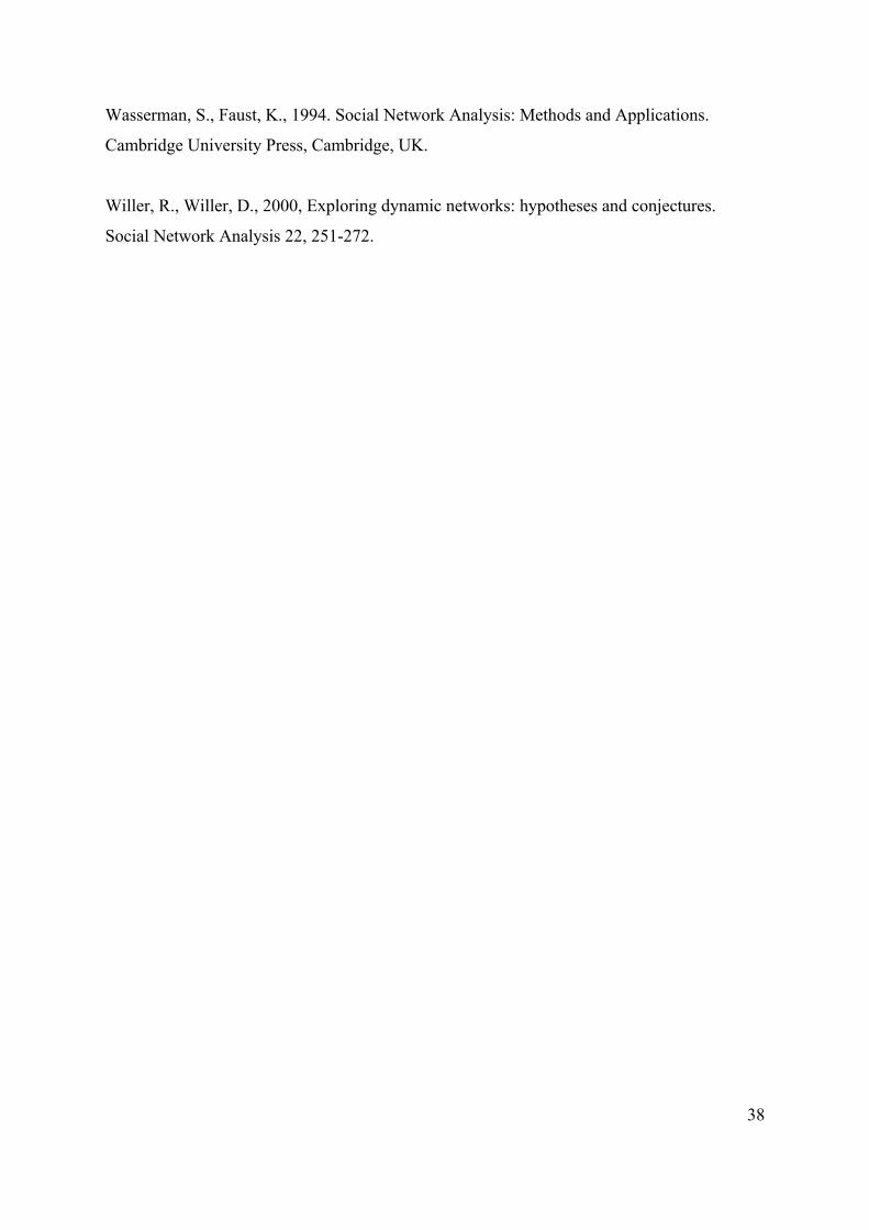
38

Wasserman, S., Faust, K., 1994. Social Network Analysis: Methods and Applications.

Cambridge University Press, Cambridge, UK.

Willer, R., Willer, D., 2000, Exploring dynamic networks: hypotheses and conjectures.

Social Network Analysis 22, 251-272.

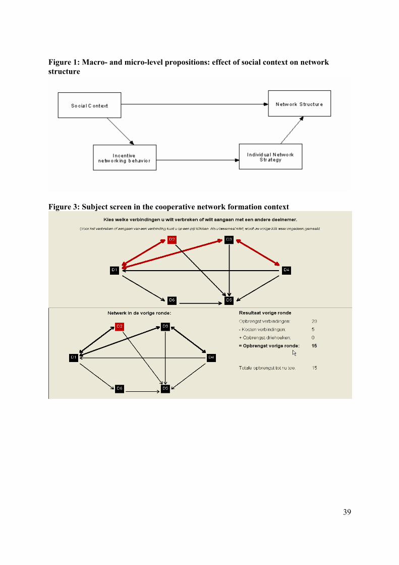
39

Figure 1: Macro- and micro-level propositions: effect of social context on network structure

Figure 3: Subject screen in the cooperative network formation context

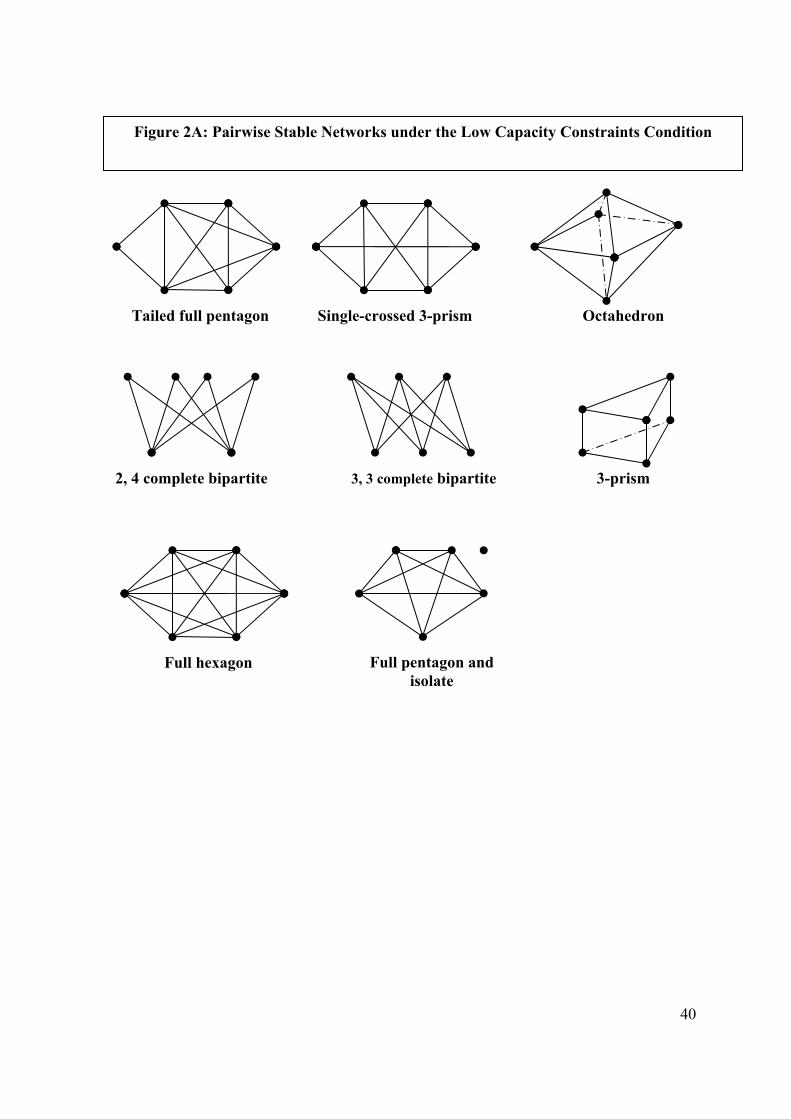
40

3, 3 complete bipartite 3-prism 2, 4 complete bipartite

Full hexagon Full pentagon and isolate

Figure 2A: Pairwise Stable Networks under the Low Capacity Constraints Condition

Single-crossed 3-prism Octahedron Tailed full pentagon

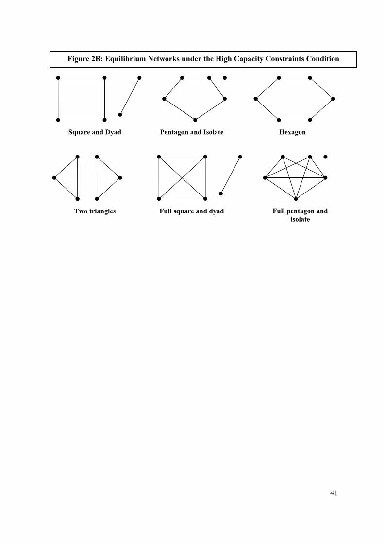
41

Figure 2B: Equilibrium Networks under the High Capacity Constraints Condition

Square and Dyad

Two triangles Full pentagon and isolate

Pentagon and Isolate Hexagon

Full square and dyad

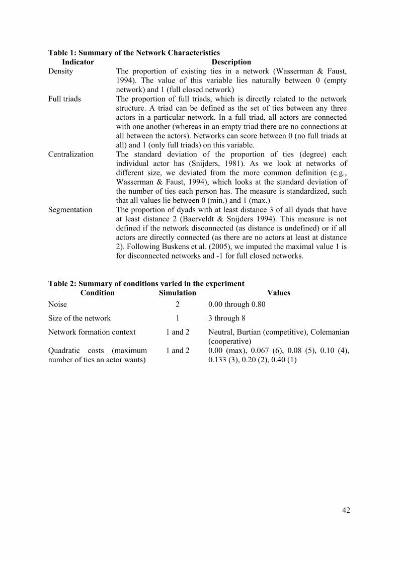
42

Table 1: Summary of the Network Characteristics Indicator Description

Density The proportion of existing ties in a network (Wasserman & Faust, 1994). The value of this variable lies naturally between 0 (empty network) and 1 (full closed network)

Full triads The proportion of full triads, which is directly related to the network structure. A triad can be defined as the set of ties between any three actors in a particular network. In a full triad, all actors are connected with one another (whereas in an empty triad there are no connections at all between the actors). Networks can score between 0 (no full triads at all) and 1 (only full triads) on this variable.

Centralization The standard deviation of the proportion of ties (degree) each individual actor has (Snijders, 1981). As we look at networks of different size, we deviated from the more common definition (e.g., Wasserman & Faust, 1994), which looks at the standard deviation of the number of ties each person has. The measure is standardized, such that all values lie between 0 (min.) and 1 (max.)

Segmentation The proportion of dyads with at least distance 3 of all dyads that have at least distance 2 (Baerveldt & Snijders 1994). This measure is not defined if the network disconnected (as distance is undefined) or if all actors are directly connected (as there are no actors at least at distance 2). Following Buskens et al. (2005), we imputed the maximal value 1 is for disconnected networks and -1 for full closed networks.

Table 2: Summary of conditions varied in the experiment

Condition Simulation Values Noise 2 0.00 through 0.80

Size of the network 1 3 through 8

Network formation context 1 and 2 Neutral, Burtian (competitive), Colemanian (cooperative)

Quadratic costs (maximum number of ties an actor wants)

1 and 2 0.00 (max), 0.067 (6), 0.08 (5), 0.10 (4), 0.133 (3), 0.20 (2), 0.40 (1)

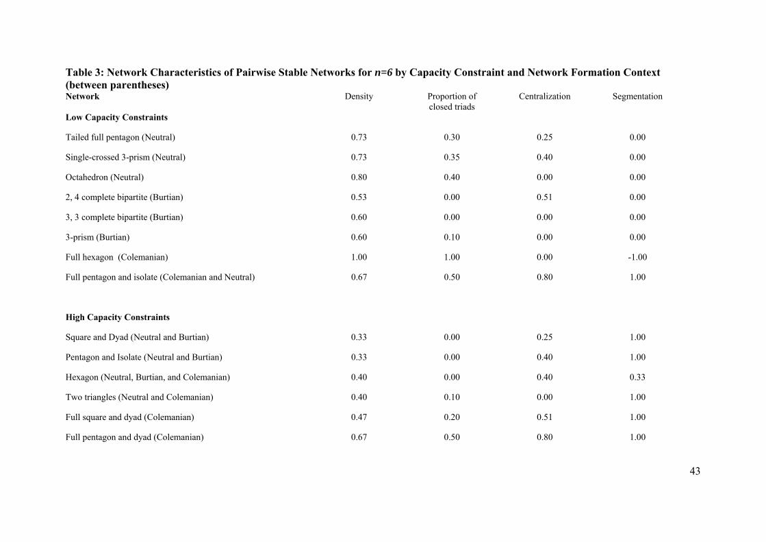
43

Table 3: Network Characteristics of Pairwise Stable Networks for n=6 by Capacity Constraint and Network Formation Context (between parentheses) Network

Density Proportion of closed triads

Centralization Segmentation

Low Capacity Constraints

Tailed full pentagon (Neutral) 0.73 0.30 0.25 0.00

Single-crossed 3-prism (Neutral) 0.73 0.35 0.40 0.00

Octahedron (Neutral) 0.80 0.40 0.00 0.00

2, 4 complete bipartite (Burtian) 0.53 0.00 0.51 0.00

3, 3 complete bipartite (Burtian) 0.60 0.00 0.00 0.00

3-prism (Burtian) 0.60 0.10 0.00 0.00

Full hexagon (Colemanian) 1.00 1.00 0.00 -1.00

Full pentagon and isolate (Colemanian and Neutral) 0.67 0.50 0.80 1.00

High Capacity Constraints

Square and Dyad (Neutral and Burtian) 0.33 0.00 0.25 1.00

Pentagon and Isolate (Neutral and Burtian) 0.33 0.00 0.40 1.00

Hexagon (Neutral, Burtian, and Colemanian) 0.40 0.00 0.40 0.33

Two triangles (Neutral and Colemanian) 0.40 0.10 0.00 1.00

Full square and dyad (Colemanian) 0.47 0.20 0.51 1.00

Full pentagon and dyad (Colemanian) 0.67 0.50 0.80 1.00

44

Table 4: Probability of convergence to particular equilibrium network by capacity constraint, network formation context and noise level

Network

Probability of convergence (α=0.40)

1. Low Capacity Constraint Neutral Context Tailed full pentagon * 0.220 Single-crossed 3-prism* 0.400 Octahedron * 0.340 Full pentagon and isolate* 0.040 Burtian Context 2, 4 complete bipartite 0.070 3, 3 complete bipartite * 0.620 3-prism * 0.310 Colemanian Context Full hexagon * 0.860 Full pentagon and isolate 0.140 2. High Capacity Constraint Neutral Context Two triangles * 0.140 Square and dyad * 0.110 Pentagon and isolate * 0.190 Hexagon * 0.560 Burtian Context Square and dyad * 0.160 Pentagon and isolate * 0.205 Hexagon * 0.635 Colemanian Context Full pentagon and isolate * 0.000 Full square and dyad 0.105 Two triangles 0.595 Hexagon * 0.195 Pentagon and Isolate * 0.105

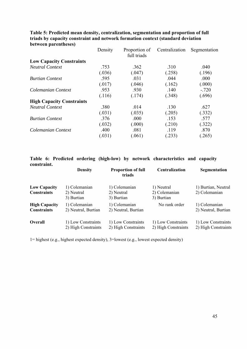
45

Table 5: Predicted mean density, centralization, segmentation and proportion of full triads by capacity constraint and network formation context (standard deviation between parentheses) Density Proportion of

full triads Centralization Segmentation

Low Capacity Constraints Neutral Context .753

(.036) .362

(.047) .310

(.258) .040

(.196) Burtian Context .595

(.017) .031

(.046) .044

(.162) .000

(.000) Colemanian Context .953

(.116) .930

(.174) .140

(.348) -.720 (.696)

High Capacity Constraints Neutral Context .380

(.031) .014

(.035) .130

(.205) .627

(.332) Burtian Context .376

(.032) .000

(.000) .153

(.210) .577

(.322) Colemanian Context .400

(.031) .081

(.061) .119

(.233) .870

(.265) Table 6: Predicted ordering (high-low) by network characteristics and capacity constraint.

Density Proportion of full triads

Centralization Segmentation

Low Capacity Constraints

1) Colemanian 2) Neutral 3) Burtian


1) Neutral 2) Colemanian 3) Burtian

1) Burtian, Neutral 2) Colemanian


1) Colemanian 2) Neutral, Burtian


No rank order 1) Colemanian 2) Neutral, Burtian

Overall 1) Low Constraints 2) High Constraints

1) Low Constraints 2) High Constraints



1= highest (e.g., highest expected density), 3=lowest (e.g., lowest expected density)

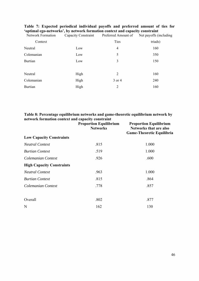
46

Table 7: Expected periodical individual payoffs and preferred amount of ties for ‘optimal ego-networks’, by network formation context and capacity constraint

Network Formation

Context

Capacity Constraint Preferred Amount of

Ties

Net payoffs (including

triads)

Neutral Low 4 160

Colemanian Low 5 350

Burtian Low 3 150

Neutral High 2 160

Colemanian High 3 or 4 240

Burtian High 2 160

Table 8: Percentage equilibrium networks and game-theoretic equilibrium network by network formation context and capacity constraint Proportion Equilibrium

Networks Proportion Equilibrium Networks that are also

Game-Theoretic Equilibria Low Capacity Constraints

Neutral Context .815 1.000

Burtian Context .519 1.000

Colemanian Context .926 .600


Neutral Context .963 1.000

Burtian Context .815 .864

Colemanian Context .778 .857

Overall .802 .877

N 162 130

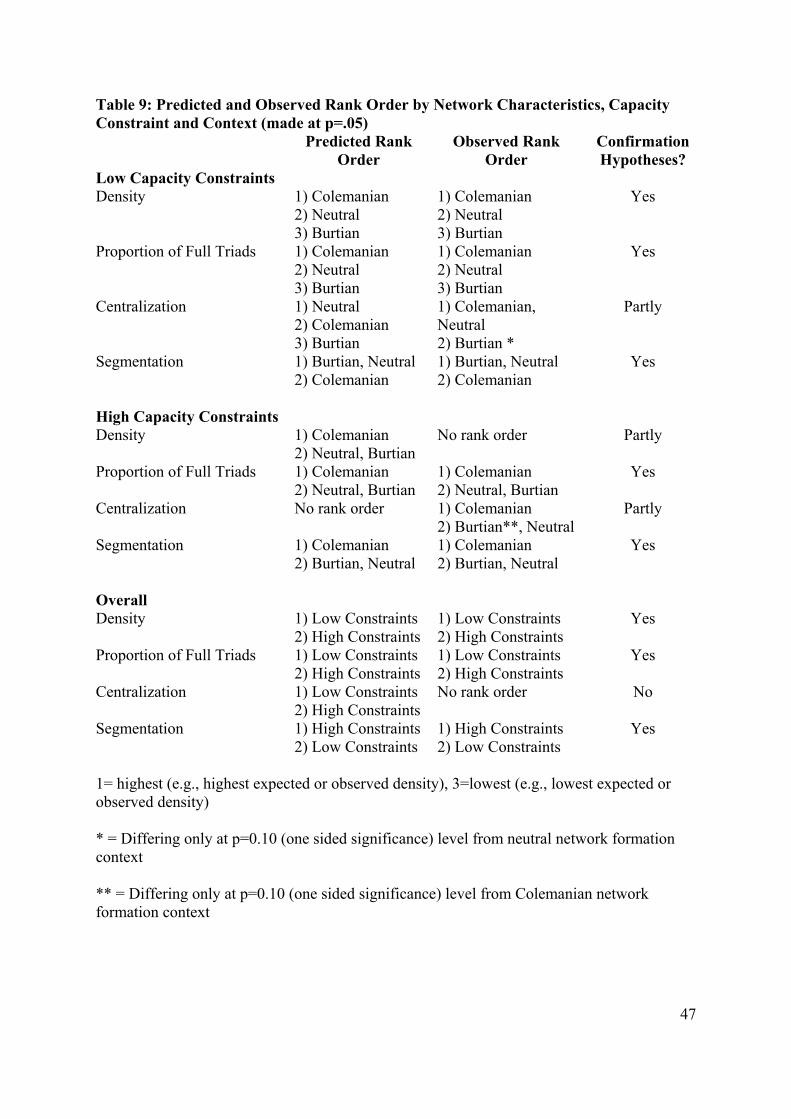
47

Table 9: Predicted and Observed Rank Order by Network Characteristics, Capacity Constraint and Context (made at p=.05) Predicted Rank

Order Observed Rank

Order Confirmation Hypotheses?

Low Capacity Constraints Density 1) Colemanian

2) Neutral 3) Burtian


Yes

Proportion of Full Triads 1) Colemanian 2) Neutral 3) Burtian


Yes

Centralization 1) Neutral 2) Colemanian 3) Burtian

1) Colemanian, Neutral 2) Burtian *

Partly

Segmentation 1) Burtian, Neutral 2) Colemanian

1) Burtian, Neutral 2) Colemanian

Yes

High Capacity Constraints Density 1) Colemanian

2) Neutral, Burtian No rank order Partly

Proportion of Full Triads 1) Colemanian 2) Neutral, Burtian


Yes

Centralization No rank order 1) Colemanian 2) Burtian**, Neutral

Partly

Segmentation 1) Colemanian 2) Burtian, Neutral

1) Colemanian 2) Burtian, Neutral

Yes

Overall Density 1) Low Constraints

2) High Constraints 1) Low Constraints 2) High Constraints

Yes

Proportion of Full Triads 1) Low Constraints 2) High Constraints


Yes

Centralization 1) Low Constraints 2) High Constraints

No rank order No

Segmentation 1) High Constraints 2) Low Constraints

1) High Constraints 2) Low Constraints

Yes

1= highest (e.g., highest expected or observed density), 3=lowest (e.g., lowest expected or observed density) * = Differing only at p=0.10 (one sided significance) level from neutral network formation context ** = Differing only at p=0.10 (one sided significance) level from Colemanian network formation context

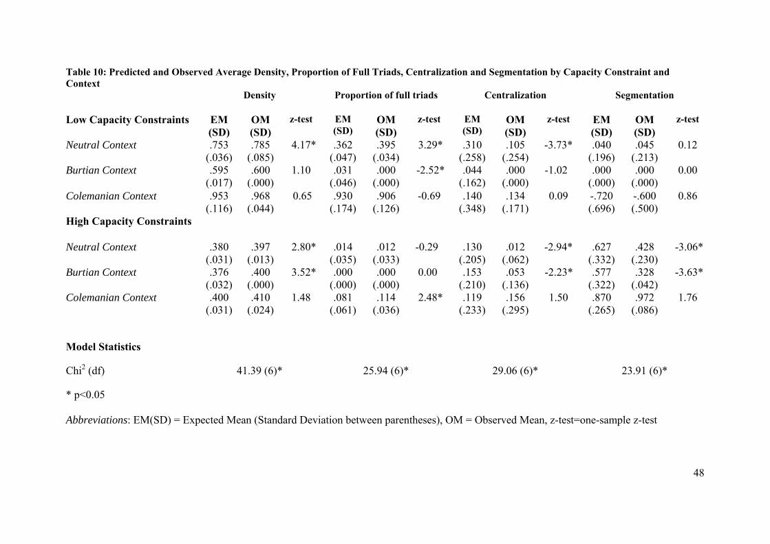
48

Table 10: Predicted and Observed Average Density, Proportion of Full Triads, Centralization and Segmentation by Capacity Constraint and Context Density Proportion of full triads Centralization Segmentation

Low Capacity Constraints EM (SD)

OM (SD)

z-test EM (SD)

OM (SD)

z-test EM (SD)

OM (SD)

z-test EM (SD)

OM (SD)

z-test

Neutral Context .753 (.036)

.785 (.085)

4.17* .362 (.047)

.395 (.034)

3.29* .310 (.258)

.105 (.254)

-3.73* .040 (.196)

.045 (.213)

0.12

Burtian Context .595 (.017)

.600 (.000)

1.10 .031 (.046)

.000 (.000)

-2.52* .044 (.162)

.000 (.000)

-1.02

.000 (.000)

.000 (.000)

0.00

Colemanian Context .953 (.116)

.968 (.044)

0.65 .930 (.174)

.906 (.126)

-0.69 .140 (.348)

.134 (.171)

0.09 -.720 (.696)

-.600 (.500)

0.86


Neutral Context .380 (.031)

.397 (.013)

2.80* .014 (.035)

.012 (.033)

-0.29 .130 (.205)

.012 (.062)

-2.94* .627 (.332)

.428 (.230)

-3.06*

Burtian Context .376 (.032)

.400 (.000)

3.52* .000 (.000)

.000 (.000)

0.00 .153 (.210)

.053 (.136)

-2.23* .577 (.322)

.328 (.042)

-3.63*

Colemanian Context .400 (.031)

.410 (.024)

1.48 .081 (.061)

.114 (.036)

2.48* .119 (.233)

.156 (.295)

1.50 .870 (.265)

.972 (.086)

1.76

Model Statistics

Chi2 (df) 41.39 (6)* 25.94 (6)* 29.06 (6)* 23.91 (6)*

* p<0.05 Abbreviations: EM(SD) = Expected Mean (Standard Deviation between parentheses), OM = Observed Mean, z-test=one-sample z-test

Social Context and Network Formation: Experimental Studies

Documents

Transcript of Social Context and Network Formation: Experimental Studies