SLITA: A new SLim Towed Array for AUV applications

A. Maguer, R. Dymond, M. Mazzi, S. Biagini, S. Fioravanti and P. Guerrini

NURC Nato Undersea Research Centre, Viale San Bartolomeo 400, 19026 La Spezia, Italymaguer@nurc.nato.int

Acoustics 08 Paris

141

The typical 70mm diameter towed array was developed for blue-water detection at long range and low frequencies in the 1960s. Since then, there has been a need for towed arrays that are lighter and less expensive, especially since the maturing field of autonomous vehicles has expanded the potential of such arrays. The marriage of AUVs and lightweight towed arrays is a natural progression in the development of littoral autonomous sensing networks for applications such Anti-Submarine Warfare, marine mammals or ambient noise measurements. In August 2007, NURC began to design and build a new thin diameter (31 mm) High-frequency (up to 20 kHz) nested towed array for ASW purposes. An Engineering at-sea trial of the array towed by OEX-C AUV was performed beginning of November 07. The flow noise level of the array while towed and the potential influence of the AUV self noise on the acoustic array were also measured. This paper will first describe the array design, its acquisition system and its integration on the OEX-C AUV. Then, the results obtained from the data analysis are presented. It is shown that the SLITA array has performance that will make it easily fit requirements of the applications previously mentioned.

1 Introduction

This paper analyzes acoustic data collected during the Engineering Test of the Ocean Explorer AUV, version C (OEX-C) towing the Slim Line Towed Array (SLITA) and during the Trail CCLNet08. The Engineering Test was carried out between 07-15 November 2007, while the CCLNet08 Trial was performed at the end of January 2008 and in particular the SLITA has been operated during the period 23-25 January. Objectives of the paper are to assess the performance of the array in terms of noise level (both electrical/electronic, generated by the AUV, and mechanical) and array shape during navigation, and To this aim both passive acoustic data and data collected during active experiments with a towed sound source have been processed. Between November 2007 and January 2008, some minor problems identified during data analysis have been fixed and are no longer present in the updated version used during CCLNet08.

2 SLITA array technical details

The SLITA array (see Figure 1) is a towed array derived from the SLIVA Vertical Line Array developed at NURC.

Figure 1- SLITA Array deployment and OEX-C

It features:

• 48 hydrophones in total

• 2 x 32 hydrophones o octaves spacing 0.211 and 0.422 m o array apertures are named Octave 2 (3550

Hz), and Octave 3 (1780 Hz) o cylindrical hydrophones (sensitivity -201

dB ref. to 1 Volt per µPa) o total gain 33.8 dB

• Acquisition performances o A/D board simultaneously samples 32

channels of sensor data o 24 bit Delta-Sigma A/D o continuous acquisition o On-board processing

The analog to digital acquisition board is a General Standards PCI-24DSI32 with 24 bits resolution. the following electrical characteristics

The Benthos AQ-4 hydrophones (Sh=-201 dBV re 1 μPa ±1dB) used are designed to compensate for noise generated from array movement, commonly know as acceleration noise. Noise is substantially reduced by symmetrically supporting the active element inside the mounting structure.

Figure 2 – Benthos AQ-4 hydrophones

The mechanical design is shown below.

Acoustics 08 Paris

142

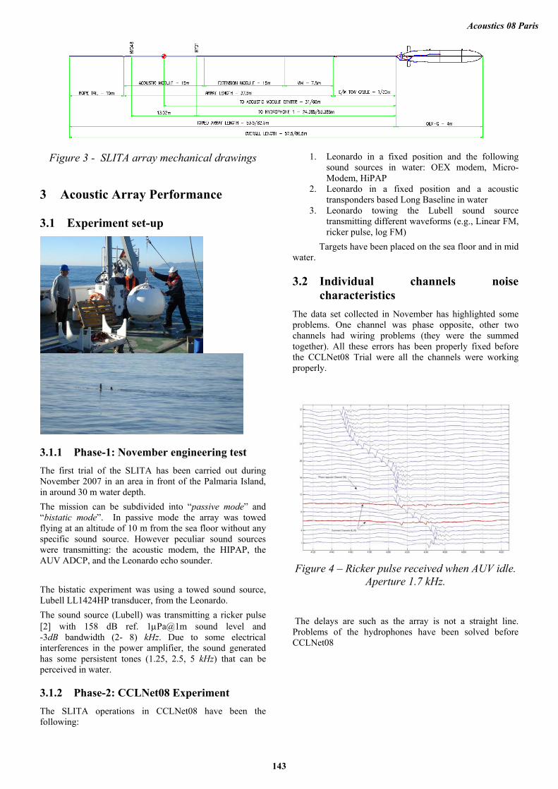
Figure 3 - SLITA array mechanical drawings

3 Acoustic Array Performance

3.1 Experiment set-up

3.1.1 Phase-1: November engineering test The first trial of the SLITA has been carried out during November 2007 in an area in front of the Palmaria Island, in around 30 m water depth. The mission can be subdivided into “passive mode” and “bistatic mode”. In passive mode the array was towed flying at an altitude of 10 m from the sea floor without any specific sound source. However peculiar sound sources were transmitting: the acoustic modem, the HIPAP, the AUV ADCP, and the Leonardo echo sounder. The bistatic experiment was using a towed sound source, Lubell LL1424HP transducer, from the Leonardo. The sound source (Lubell) was transmitting a ricker pulse [2] with 158 dB ref. 1μPa@1m sound level and -3dB bandwidth (2- 8) kHz. Due to some electrical interferences in the power amplifier, the sound generated has some persistent tones (1.25, 2.5, 5 kHz) that can be perceived in water.

3.1.2 Phase-2: CCLNet08 Experiment The SLITA operations in CCLNet08 have been the following:

1. Leonardo in a fixed position and the following sound sources in water: OEX modem, Micro-Modem, HiPAP

2. Leonardo in a fixed position and a acoustic transponders based Long Baseline in water

3. Leonardo towing the Lubell sound source transmitting different waveforms (e.g., Linear FM, ricker pulse, log FM)

Targets have been placed on the sea floor and in mid water.

3.2 Individual channels noise characteristics

The data set collected in November has highlighted some problems. One channel was phase opposite, other two channels had wiring problems (they were the summed together). All these errors has been properly fixed before the CCLNet08 Trial were all the channels were working properly.

Figure 4 – Ricker pulse received when AUV idle. Aperture 1.7 kHz.

The delays are such as the array is not a straight line. Problems of the hydrophones have been solved before CCLNet08

Acoustics 08 Paris

143

3.3 Noise analysis with wavenumber-frequency diagrams

3.3.1 Wave-number-frequency diagrams theory

In order to differentiate between acoustic and non-acoustic noise, e.g., mechanical noise, one tool is provided by the wave-number-frequency diagrams (also called k-ω transform). These diagrams allow the identification of the speed of the pressure waves measured by the array. The wave-number-frequency diagram is a double Fourier transform, both in time and in space, where the positive time frequencies are plotted in the Y axis and the X axes represent the spatial frequency k, where the positive and negative values discriminate signals coming from the two end-fires side of the array.

k = 2π/λ

Given d the array spacing, the maximum k value is the following:

kmax = π/d

For an acoustic wave traveling with sound speed C, the variation of the wave-number with frequency f and angle of arrival θ is given by the following:

k(f, θ) = 2π f/C * cos θ

Figure 5 – linear array and planar acoustic waves

Varying f and θ the will produce the classical V-shape plots. The acoustic energy is confined within the V-area of the k-f diagrams. Energy outside this V will highlight non-acoustic energy (e.g., mechanical vibrations, flow noise, etc.), or other array artifacts. The borders of the V-shape represent the end fire beams energy, and therefore the energy coming, on one side, from the AUV propeller.

Figure 6 – k-f diagram and V-shape

3.3.2 Experimental results Wave-number-frequency diagrams for real data do not shows significant artifacts which could be produced by mechanical vibrations or array distortions. Figure 7 shows the k-f diagrams when the AUV was still and the array was folded and not a straight line. The energy is not focused within the V-shape. Figure 8 presents the same results during AUV navigation. The V-shape is well characterized, and the array gain is around 30 dB as expected. The residual energy outside the V-area is due to sidelobes effects.

θ

A ti

f

d/π

)2/( dC

k

Acoustic Energy

Non acoustic Energy

Figure 7 – k-f diagrams when AUV was not navigating; duration 4 seconds

(a) MF aperture, 211 mm, (b) LF aperture 422 mm

π2∗

Tail side Vehicle side

Acoustics 08 Paris

144

Figure 8 – k-f diagrams during navigation; duration 4 seconds

(a) MF aperture, 211 mm, (b) LF aperture 422 mm

3.4 Noise considerations Both during the November engineering test, both in passive configuration and using an active source, the noise levels are considerable high. A more in thorough analysis has proved that the noise sound source is the Leonardo itself. The thundering cavitation noise as the propeller begins to spin behaves as a broad band white source in a range at least up to 15-20 kHz.

Figure 9 – Leonardo turbulence and noise spectra (ship distance around 30 m)

The noise, more than by the propellers itself, it seems to be produced by the combination of cavitations and of the water flow and waves that the Leonardo creates even at low speed, which has a wide spectrum.

Figure 10 – (a) Typical ambient sea noise levels (b) Example of measured noise level during

CCLNet08

Under these conditions, it is difficult to assess in details the noise performances of the array, as the ship noise is predominant. However, due to the wide spectrum of the Leonardo noise, it is evident in the power spectra the hydrophones resonant behavior at 17 kHz (see Figure 9).

2 1010 3 104 10560

65

70

75

80

85

90

95

100

dB re 1μPa

105

110

Acoustics 08 Paris

145

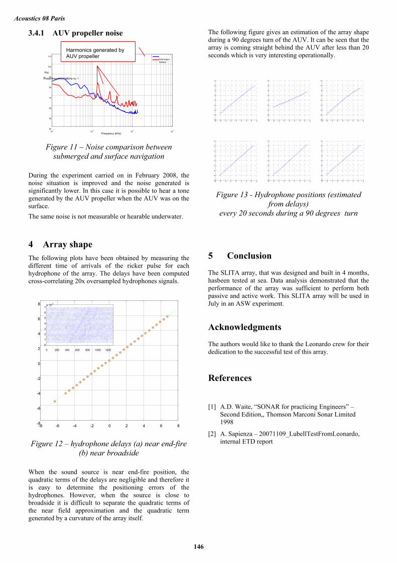
3.4.1 AUV propeller noise

Figure 11 – Noise comparison between submerged and surface navigation

During the experiment carried on in February 2008, the noise situation is improved and the noise generated is significantly lower. In this case it is possible to hear a tone generated by the AUV propeller when the AUV was on the surface. The same noise is not measurable or hearable underwater.

4 Array shape The following plots have been obtained by measuring the different time of arrivals of the ricker pulse for each hydrophone of the array. The delays have been computed cross-correlating 20x oversampled hydrophones signals.

Figure 12 – hydrophone delays (a) near end-fire (b) near broadside

When the sound source is near end-fire position, the quadratic terms of the delays are negligible and therefore it is easy to determine the positioning errors of the hydrophones. However, when the source is close to broadside it is difficult to separate the quadratic terms of the near field approximation and the quadratic term generated by a curvature of the array itself.

The following figure gives an estimation of the array shape during a 90 degrees turn of the AUV. It can be seen that the array is coming straight behind the AUV after less than 20 seconds which is very interesting operationally.

102

103

104

105

40

50

60

70

80

90

100

110

Frequency (kHz)

Power/frequency (dB/Hz re. 1 μ Pa)

SubmergedSurface

Harmonics generated by AUV propeller

-8 -6 -4 -2 0 2 4 6 8-8

-6

-4

-2

0

2

4

6

8

-8 -6 -4 -2 0 2 4 6 8-8

-6

-4

-2

0

2

4

6

8

-8 -6 -4 -2 0 2 4 6 8-8

-6

-4

-2

0

2

4

6

8

-8 -6 -4 -2 0 2 4 6 8-8

-6

-4

-2

0

2

4

6

8

-8 -6 -4 -2 0 2 4 6 8-8

-6

-4

-2

0

2

4

6

8

-8 -6 -4 -2 0 2 4 6 8-8

-6

-4

-2

0

2

4

6

8

Figure 13 - Hydrophone positions (estimated from delays)

every 20 seconds during a 90 degrees turn

5 Conclusion

The SLITA array, that was designed and built in 4 months, hasbeen tested at sea. Data analysis demonstrated that the performance of the array was sufficient to perform both passive and active work. This SLITA array will be used in July in an ASW experiment.

-8 -6 -4 -2 0 2 4 6 8-8

-6

-4

-2

0

2

4

6

8

0 200 400 600 800 1000 1200 0 1 2 3 4 5 6 7 x 10 -3

Acknowledgments

The authors would like to thank the Leonardo crew for their dedication to the successful test of this array.

References

[1] A.D. Waite, “SONAR for practicing Engineers” – Second Edition,, Thomson Marconi Sonar Limited 1998

[2] A. Sapienza – 20071109_LubellTestFromLeonardo, internal ETD report

Acoustics 08 Paris

146