Slip Power Loss and Fuel Consumption Control in 4x4 Terrain Vehicle Applications

Proceedings of the Joint 9th Asia-Pacific ISTVS Conference and

Annual Meeting of Japanese Society for Terramechanics

Sapporo, Japan, September 27 to 30, 2010

Slip Power Loss and Fuel Consumption Control in 4x4 Terrain Vehicle Applications

Barys Shyrokau

Ilmenau University of Technology, Germany

Vladimir Vantsevich

Lawrence Technological University, USA

Klaus Augsburg


Valentin Ivanov


Abstract. 4x4 terrain vehicle applications widely use positively locked power dividing units (PDU) in the transfer case. Such PDUs considerably improve vehicle mobility by keeping identical rotational velocities of the front and rear wheels and re-distributing the torque between the driving axles as terrain conditions require. The mentioned equality of the angular speeds leads to kinematic discrepancy in linear velocities of the driving axles when a vehicle undertakes turns. The paper presents an analytical method to evaluate this discrepancy and analytically demonstrates its influence on extra power losses on slippage of the front and rear tires and thus on extra fuel consumption. To avoid these extra power losses and fuel consumption, the paper presents a method for controlling the kinematic discrepancy by reducing it to zero values. This was done without negative impacts on vehicle dynamics. The theoretical propositions are illustrated by computer simulations of a 4x4 heavy-duty truck turning in terrain. A comparative analysis is presented with regard to the same truck but without kinematic discrepancy control. The results proved the proposed approach to managing the kinematic discrepancy in 4x4 vehicles with positive engagement of the driving axles to improve vehicle energy efficiency.

Keywords. Kinematic discrepancy, power loss, fuel consumption.

1 Introduction

The phenomenon of kinematic discrepancy is an inherent property of all-wheel drive (AWD) vehicles with positive engagement of the drive axles (locked up axles). By this effect is meant the difference of theoretical velocities of the front and rear wheels. At that it is considered that wheels roll without slipping. Kinematic discrepancy influences significantly power distribution between the driving axles and wheels and as consequence fuel consumption, mobility, and stability. A methodology for analytical description of kinematic discrepancy of vehicle with any given number of the driving axles and steering system and the influence of kinematic discrepancy on the vehicle operational properties are presented in (Andreev et al., 2010).

Proceedings of the 9th

Asia-Pacificl ISTVS Conference, Sapporo, Japan, September 27 to 30, 2010

2

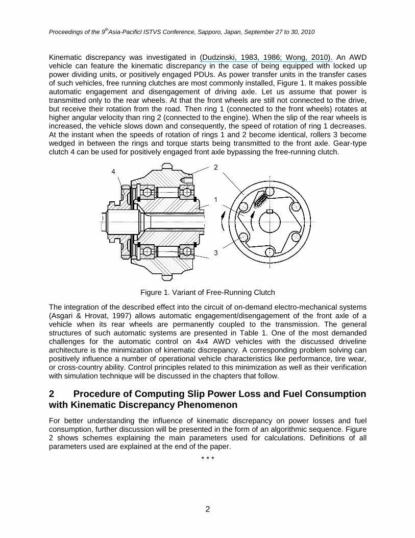
Kinematic discrepancy was investigated in (Dudzinski, 1983, 1986; Wong, 2010). An AWD vehicle can feature the kinematic discrepancy in the case of being equipped with locked up power dividing units, or positively engaged PDUs. As power transfer units in the transfer cases of such vehicles, free running clutches are most commonly installed, Figure 1. It makes possible automatic engagement and disengagement of driving axle. Let us assume that power is transmitted only to the rear wheels. At that the front wheels are still not connected to the drive, but receive their rotation from the road. Then ring 1 (connected to the front wheels) rotates at higher angular velocity than ring 2 (connected to the engine). When the slip of the rear wheels is increased, the vehicle slows down and consequently, the speed of rotation of ring 1 decreases. At the instant when the speeds of rotation of rings 1 and 2 become identical, rollers 3 become wedged in between the rings and torque starts being transmitted to the front axle. Gear-type clutch 4 can be used for positively engaged front axle bypassing the free-running clutch.

Figure 1. Variant of Free-Running Clutch

The integration of the described effect into the circuit of on-demand electro-mechanical systems (Asgari & Hrovat, 1997) allows automatic engagement/disengagement of the front axle of a vehicle when its rear wheels are permanently coupled to the transmission. The general structures of such automatic systems are presented in Table 1. One of the most demanded challenges for the automatic control on 4x4 AWD vehicles with the discussed driveline architecture is the minimization of kinematic discrepancy. A corresponding problem solving can positively influence a number of operational vehicle characteristics like performance, tire wear, or cross-country ability. Control principles related to this minimization as well as their verification with simulation technique will be discussed in the chapters that follow.

2 Procedure of Computing Slip Power Loss and Fuel Consumption with Kinematic Discrepancy Phenomenon

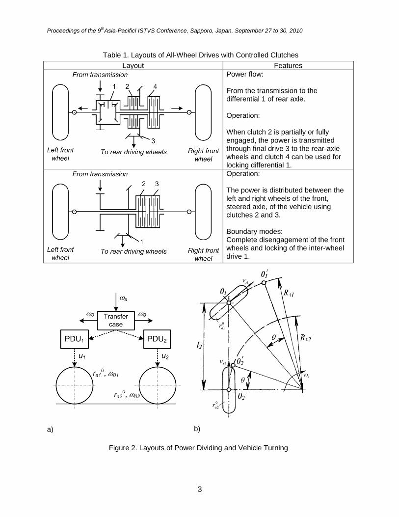
For better understanding the influence of kinematic discrepancy on power losses and fuel consumption, further discussion will be presented in the form of an algorithmic sequence. Figure 2 shows schemes explaining the main parameters used for calculations. Definitions of all parameters used are explained at the end of the paper.

* * *

https://www.researchgate.net/publication/256275134_Problems_of_turning_process_in_articulated_terrain_vehicles?el=1_x_8&enrichId=rgreq-1e2c7b71-02dc-41d3-af61-6d5e2df8b29e&enrichSource=Y292ZXJQYWdlOzIzMTQ0MDA0NjtBUzoxMDIyMjE0NzU3NDU3OTNAMTQwMTM4MjkwNzExMg==



3

Table 1. Layouts of All-Wheel Drives with Controlled Clutches

Layout Features

Power flow: From the transmission to the differential 1 of rear axle. Operation: When clutch 2 is partially or fully engaged, the power is transmitted through final drive 3 to the rear-axle wheels and clutch 4 can be used for locking differential 1.

Operation: The power is distributed between the left and right wheels of the front, steered axle, of the vehicle using clutches 2 and 3. Boundary modes: Complete disengagement of the front wheels and locking of the inter-wheel drive 1.

a)

b)

Figure 2. Layouts of Power Dividing and Vehicle Turning



4

2.1 Step 1: Estimation of Kinematic Discrepancy

The condition of kinematic conformity by straight-line motion of a 4x4 AWD vehicle can be written in accordance with Fig. 2a as:

0 0 0 00 001 1 02 2 1 2

1 2

or (1)a a a ar r r ru u

By turning, Fig. 2b, when only one axle is steered and the centers of axles move over curves of different radii then, conversely, kinematic agreement of the traveled path and angular velocities of the front and rear wheels requires that the linear velocities of the axle centers should not be equal. In such a case the condition of kinematic conformity is as follows:

0 0

2 1 1 2 2 2 (2)a t a tr u R r u R

The situations that the theoretical velocities from conditions (2) are not equal can be described through the kinematic discrepancy factor:

0 0

2 1 1 1 2 2

0

2 1 1

(3)a t a t

a t

r u R r u Rm

r u R

2.2 Step 2: Slippage Factor of Axle with Inter-wheel Open Differential

The generalized rolling radius, Fig 2a, of the axle in the driven mode is:

0' 0 ''0

0 ' 0 ''

2, 1,2 (4)wi wi

ai

wi wi k

r rr i

r r u

Then the generalized slippage factor of the axle that represents the loss of axle velocity and loss of power in wheel slippage, when the slippages of the left and right wheels are different, can be given by the expression:

0' 0 '' '' '

'' 0 ' ' ' 0 '' ''

1 11 , 1,2

1 1 (5)

ti wi wi i i

ai

ti wi i ti wi i

R r r s ss i

R r s R r s

2.3 Step 3: Generalized Slippage Factor by Kinematic Discrepancy

The generalized rolling radius at the vehicle turning in the driven mode takes into account the

longitudinal stiffness factors of axles Kai and turning angle and can be described as

0 00 1 1 1 2 2 2

1 1 2

/ /

sec (6)a a a a

a

a a

K r u K r ur

K K

Then the kinematic discrepancy factors can be expressed both for the front and rear axles:

0 0

1 1 1 2 2 2

0

1 1 2

sec / /1 , 1,2

sec (7)i i a a a a

i

ai a a

u K r u K r um i

r K K

As a consequence, the generalized slippage factor of the vehicle is given by the expression:

1 , 1,2ai i i as m m s i (8)



5

2.4 Step 4: Mechanical Efficiency

Consider a vehicle with two driving axles. The flows of power from the transfer case to the driving wheels shall be termed positive. In certain cases there occur negative power flows from the wheels to the transfer case. Negative torque on the front wheels of a 4x4 vehicle that causes power to flow from the front axle to the transfer case can be caused by the effect of kinematic discrepancy.

Let p1 be the number of driving axles with positive power flow and p2 – the number of axles with negative power flow, and

1 2 (9)p p n

For a 4x4 vehicle n=2.

The power fed to the driving axles is designated as

1

(10)n

in in

w wi

i

P P

If PM is the power fed from the transmission to the driveline system then the mechanical power loss in the driveline system Pdrl can be assessed using the overall mechanical efficiency:

1 (11)

nin

wiinM drl w i

M

M M M

PP P P

P P P

The components in the right-hand side of formula shall be determined by writing the coefficient of distribution of power to the axle as:

1

(12)in in

wi wii nin

inwwi

i

P Pq

PP

where Pwiin is the power supplied to the axle.

Power PM in Eq. (11) is defined as:

1 2

1 1

(13)p p

pos neg

M Mi Mi

i i

P P P

where PMipos and PMi

neg are the components of power PM. These components are defined as:

1

1

and (14)

nin

in i wi npos neg in neg in negwi i

Mi Mi wi Mi i wi Mipos posiMi Mi

q PP

P P P q P

where Mipos and Mi

neg are the efficiencies of the branches of the driveline system with positive and negative power flows.

The expression for the total efficiency M from Eq. (11) becomes finally:

1 2

1 1

1 (15)M p p

negii Mipos

i iMi

qq



6

2.5 Step 5: Power Balance

The effective power of the engine is dissipated in several energy flows:

(16)out turn

e trm drl fP P P P P P P

The components of Eq. (16) can be presented as follows.

The loss of mechanical power in the driveline:

(1 ) / (17)in

drl w M MP P

The slip power:

1 (18)in

wP P

In Eqs. (17) and (18) the power supplied to the driving wheels is

'('') '('') '('') '('')

1 1

(19)n n

in

w wi wi xi ti

i i

P T F v

Hence Eq. (16) can be transformed to

(1 ) / 1 (20)in in out turn

e trm w M M w fP P P P P P P

2.6 Step 6: Fuel Consumption

The fuel economy of the vehicle can be characterized by the fuel consumption referred to the distance traveled by the vehicle:

, g/km (21)h e es

x x

Q g PQ

V V ,

where Qh is fuel consumption in g/h, Vx is the vehicle velocity in km/h, ge is the specific fuel consumption in g/kWh.

Using Eq. (20) the fuel consumption can be

'('') '('') '('') '('')

1 1

(1 ) / 1 (21)n n

out turnes trm wi wi M M wi i f

i ix

gQ P T T w P P P

V

Important remarks: The second and third terms in the square brackets of Eq. (21) define the direct effect of the vehicle's driveline system on the fuel consumption. In fact, different driveline systems bring about different distributions of power to the driving wheels which, in its turn,

affects the total mechanical efficiency M and the power loss in slipping. This means that the

efficiencies M and should be the objects of attention in assessing the effect of driveline systems on the fuel economy of vehicles. To provide for minimal fuel consumption the driveline system should ensure such distribution of power among the wheels that provide for maximum

values of M and under the given travel conditions. The contribution of each of these efficiencies on the fuel consumption is different. At positive power flows from the transfer case to the driving wheels the effect is commonly commensurable or sometimes the power losses Pdrl

may exceed P in all-wheel drive vehicles. On a deformable surface the effect of P may be more perceptible and depends on the type of the driveline system.



7

* * *

The procedures of the calculations of power losses and fuel consumption given above allow to propose the control technique aimed at power balance improvement through the minimization of kinematic discrepancy. This matter is further discussed.

3 Control on Kinematic Discrepancy

Consider a 4x4 AWD vehicle with front steered wheels and positively engaged inter-axle power-dividing unit, which does not have a design kinematic discrepancy (m = 0). When this vehicle takes a turn there arises the kinematic discrepancy that is caused by differences in the turning

radii of the front and rear axles, Rt1 ≠ Rt2 and calculated from Eq. (3).

The numerical value of m is positive and increases with the angle of turn δ of the front wheels.

The increase in m brings about an increase in the tangential force Fx2 of the rear wheels and

reduction in tangential force Fx1 of the front wheels. At large δ, m attains substantial values,

which may cause parasitic power circulation, i.e., negative values of Fx1. This changes the

direction and increases the numerical value of the lateral reaction Fl1 and simultaneously

increases vehicle understeering. If the gear ratios u1 or u2 in the drives of the axles are changed

in the course of the turn, then the kinematic discrepancy m may be reduced to zero and the increase in understeering of the vehicle can be avoided. The changing of gear ratios shall be in accordance with

2 1 cosu u or 1 2 cosu u (22)

Gear ratios u1 and u2 are in general determined by the gear ratios uf1 and uf2 of the final drives

and the gear ratios of the wheel-hub reduction gears uk1 and uk2:

1 1 1f ku u u and 2 2 2f ku u u (23)

By installing power transmitting units with variable gear ratios uPTU1 and uPTU2 , Fig. 2a, in the

axle drives, the equations are:

)/(cos 11221 kfkfPTU uuuuu , (24)

)cos/( 22112 kfkfPTU uuuuu (25)

The use of the additional power-transmitting unit in the drive of either the rear axle or of the front

axle will cause differences in the mechanical power loss in the drives, i.e., ηM1 ≠ ηM2. To provide

for equality of these two efficiencies it is necessary to simultaneously control the values of u1

and u2. The corresponding control formula is as follows:

0/ 112211 ttt RuRuRu (26)

It follows from the turning geometry of a vehicle:

cos12 tt RR and cos21 uu (27)

i.e., when simultaneously controlling the values of u1 and u2 their ratio must be maintained

equal to cos δ. To achieve this, u1 should decrease when the vehicle turns and u2 should

increase. Note that Eq. (27) corresponds to the particular cases when either u1 or u2 are

assumed to be constant.



8

Hence conformance to Eqs. (22) and (27) ensures zero kinematic discrepancy in the turning of a 4x4 AWD vehicle.

4 Validation of Kinematic Discrepancy Control and Discussion of Results

To estimate effects that can be achieved by the control on the kinematic discrepancy, several vehicle manoeuvres were simulated in accordance with equations proposed in Chapters 2 and 3. The technical data of the vehicle are given in Table 2.

Table 2. Technical Data of Vehicle

Parameter Value

Vehicle gross weight, kg 25 150

Yaw inertia, kgm2 48 704

Vehicle base, mm 4 900

Distance between the vehicle gravity center and the front axle, mm 3 508

Distance between the vehicle gravity center and the road, mm 1 392

Track, mm 2 032

Final front gear ratio 6.59

Final rear gear ratio 6.59

Moment of wheel inertia, kgm2

front / rear

5.6 / 11.2

Wheel rolling radius, mm 638

Initial velocity, km/h 20

Consider dynamics of 4x4 off-road dump truck with blocked inter-wheel drive. Two test conditions are:

1. Dry soil, thrust: 0.65, initial rolling resistance factor: 0.025;

2. Wet soil, thrust: 0.4, initial rolling resistance factor: 0.05.

In both test modes the vehicle drives on 20 km/h and begins turning with the turn velocity 0.05 rad/s.

In addition the vehicle is controlled in two control modes:

Control Mode 1. Keeping constant velocity through permanent fuel feed control;

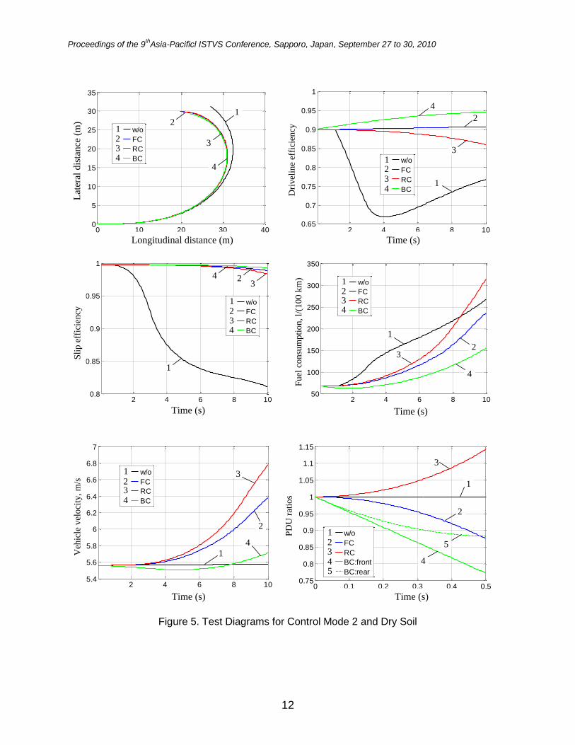
Control Mode 2. Keeping constant velocity without minimization of kinematic discrepancy but with recording of fuel feed level; then all test cases are repeated in accordance with this recorded level.

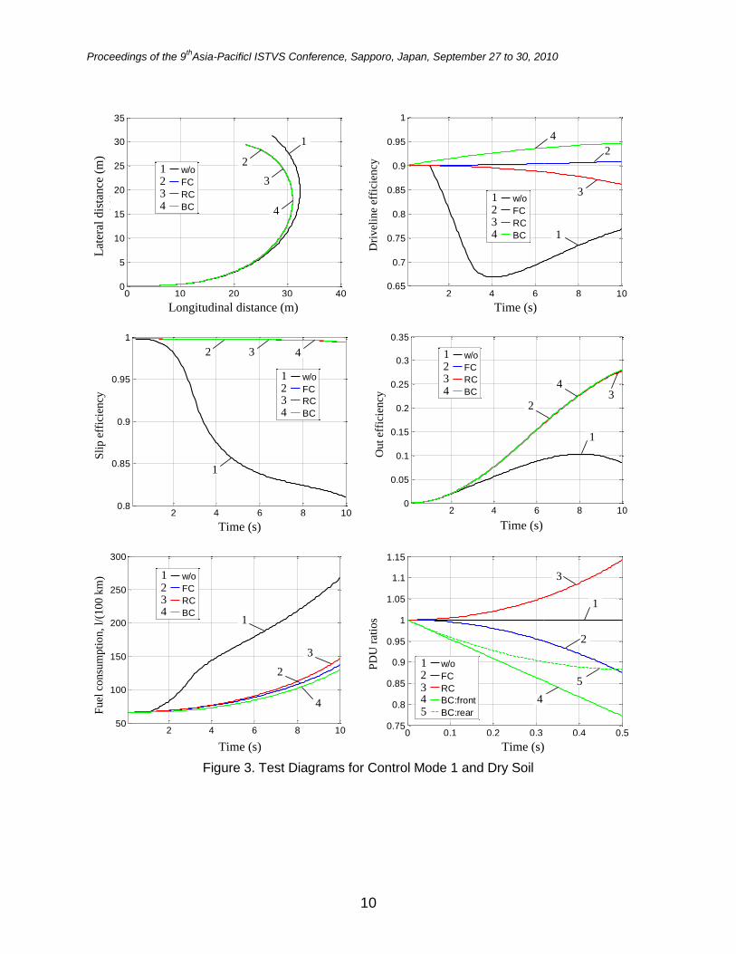
Figure 3 shows computing results for the first control mode on dry soil. The minimization of kinematic discrepancy is being achieved by way of three variants:

1. Control on transfer ratio from PDU to front axis only (FC - front control);

2. Control on transfer ratio from PDU to rear axis only (RC - rear control);

3. Control on both transfer ratios (BC – bi-control).

To reach null value of kinematic discrepancy, in these three cases the system must follow the dependencies:



9

2

1

1

cos (28)f

PDU

f

uu

u

1

1

2

1

cos (29)

f

PDU

f

uu

u

Figures 3-6 presents results obtained for both control modes on both types of grounds. The detailed results of power balance, efficiencies, and fuel consumptions are summarized in Tables 3-4.

An analysis of results allows to make a number of observations:

It can be seen from the diagram of vehicle trajectory that the understeering is being decreased due to the minimization of kinematic discrepancy as compared to non-controlled motion.

The highest performance index is obtained for bi-control variant.

The slip efficiency and the driveline efficiency are also kept on high level during the process of kinematic discrepancy minimization.

The lowest fuel consumption has been obtained in bi-control mode.

5 Conclusion

The presented paper discussed an effect of kinematic discrepancy on slip loss and fuel consumption. It was showed that kinematic discrepancy can cause parasitic power by turning of an AWD vehicle. To avoid this negative phenomenon, the control on power dividing units of the AWD driveline system has been proposed. Case study analyzed such control procedures as applied to the individual control on either front or rear axle as well as on simultaneous control on two axles. The obtained results corroborated the proposed control strategy, and it can be used in by designing mechatronic driveline control systems for AWD vehicles.

Acknowledgements

The authors would like to thanks the German Research Foundation for support in framework of the DFG-Program "Initiierung und Intensivierung bilateraler Kooperationen".

References

Andreev, A.F., Kabanau, V., and V. Vantsevich. 2010. Driveline Systems of Ground Vehicles: Theory and Design (Ground Vehicle Engineering), CRC-Press.

Asgari, J., and D. Hrovat. 1997. On-Demand Four Wheel-Drive Transfer Case Modeling, SAE Technical Paper Series, paper No. 970969.

Dudzinski, P.A. 1983. Problems of turning process in articulated terrain vehicles, Journal of Terramechanics, 19(4): 243-256.

Dudzinski, P.A. 1986. The problems of multi-axle vehicle drives, Journal of Terramechanics, 23(2): 85-93.

Wong, J.Y. 2010. Terramechanics and off-road vehicle engineering, Butterworth-Heinemann.



10

2 4 6 8 100.65

0.7

0.75

0.8

0.85

0.9

0.95

1

Time (s)

Effic

iency (

drivelin

e)

w/o

FC

RC

BC

0 10 20 30 400

5

10

15

20

25

30

35

xa (m)

ya (

m)

w/o

FC

RC

BC

Longitudinal distance (m)

Lat

eral

dis

tance

(m

)

Time (s)

Dri

vel

ine

effi

cien

cy

234

12

3

4

1

234

1

2

3

4

1

2 4 6 8 100

0.05

0.1

0.15

0.2

0.25

0.3

0.35

Time (s)

Effic

iency (

out)

w/o

FC

RC

BC

2 4 6 8 100.8

0.85

0.9

0.95

1

Time (s)

Effic

iency (

slip

)

w/o

FC

RC

BC

Time (s)

Sli

p e

ffic

ien

cy

Time (s)

Ou

t ef

fici

ency

234

1

2

234

1

23

4

1

3 4

1

0 0.1 0.2 0.3 0.4 0.50.75

0.8

0.85

0.9

0.95

1

1.05

1.1

1.15

Steer angle (rad)

Gear

ratio

w/o

FC

RC

BC:front

BC:rear

2 4 6 8 1050

100

150

200

250

300

Time (s)

Fule

consum

ptio

n (

l/100km

)

w/o

FC

RC

BC

Time (s)

Fuel

consu

mpti

on

, l/

(10

0 k

m)

Time (s)

PD

U r

atio

s

234

1

2 234

1

2

3

1

3

4

1

54

5

Figure 3. Test Diagrams for Control Mode 1 and Dry Soil



11

2 4 6 8 100.82

0.84

0.86

0.88

0.9

0.92

0.94

0.96

Time (s)

Effic

iency (

drivelin

e)

w/o

FC

RC

BC

0 10 20 30 400

5

10

15

20

25

30

35

xa (m)

ya (

m)

w/o

FC

RC

BC


Lat

eral

dis

tance

(m

)

Time (s)

Dri

vel

ine

effi

cien

cy

234

12

3

4

1

234

1

2

3

4

1

2 4 6 8 100

0.02

0.04

0.06

0.08

0.1

0.12

Time (s)

Effic

iency (

out)

w/o

FC

RC

BC

2 4 6 8 100.92

0.93

0.94

0.95

0.96

0.97

0.98

0.99

1

Time (s)

Effic

iency (

slip

)

w/o

FC

RC

BC

Time (s)

Sli

p e

ffic

iency

Time (s)

Ou

t ef

fici

ency

234

1

2234

1

23

4

1

34

1

0 0.1 0.2 0.3 0.4 0.50.75

0.8

0.85

0.9

0.95

1

1.05

1.1

1.15

Steer angle (rad)

Gear

ratio

w/o

FC

RC

BC:front

BC:rear

2 4 6 8 10120

140

160

180

200

220

240

Time (s)

Fule

consum

ptio

n (

l/100km

)

w/o

FC

RC

BC

Time (s)

Fu

el c

on

sum

pti

on,

l/(1

00

km

)

Time (s)

PD

U r

atio

s

234

1

2

234

1

2

3

1

3

4

1

5

4

5

Figure 4. Test Diagrams for Control Mode 1 and Wet Soil



12

2 4 6 8 100.65

0.7

0.75

0.8

0.85

0.9

0.95

1

Time (s)

Effic

iency (

drivelin

e)

w/o

FC

RC

BC

0 10 20 30 400

5

10

15

20

25

30

35

xa (m)

ya (

m)

w/o

FC

RC

BC


Lat

eral

dis

tance

(m

)

Time (s)

Dri

vel

ine

effi

cien

cy

234

12

3

4

1

234

1

2

3

4

1

2 4 6 8 1050

100

150

200

250

300

350

Time (s)

Fule

consum

ptio

n (

l/100km

)

w/o

FC

RC

BC

2 4 6 8 100.8

0.85

0.9

0.95

1

Time (s)

Effic

iency (

slip

)

w/o

FC

RC

BC

Time (s)

Sli

p e

ffic

iency

Time (s)

Fu

el c

onsu

mpti

on, l/

(10

0 k

m)

234

1

2

234

1

23

4

1

34

1

0 0.1 0.2 0.3 0.4 0.50.75

0.8

0.85

0.9

0.95

1

1.05

1.1

1.15

Steer angle (rad)

Gear

ratio

w/o

FC

RC

BC:front

BC:rear

2 4 6 8 105.4

5.6

5.8

6

6.2

6.4

6.6

6.8

7

Time (s)

Ve

locity (

m/s

)

w/o

FC

RC

BC

Time (s)

Veh

icle

vel

oci

ty, m

/s

Time (s)

PD

U r

atio

s

234

1

2

234

1

2

3

13

4

1

54

5

Figure 5. Test Diagrams for Control Mode 2 and Dry Soil



13

2 4 6 8 100.82

0.84

0.86

0.88

0.9

0.92

0.94

0.96

Time (s)

Effic

iency (

drivelin

e)

w/o

FC

RC

BC

0 10 20 30 400

5

10

15

20

25

30

35

xa (m)

ya (

m)

w/o

FC

RC

BC


Lat

eral

dis

tance

(m

)

Time (s)

Dri

vel

ine

effi

cien

cy

234

1

2

3

4

1

234

1

2

3

4

1

2 4 6 8 10100

150

200

250

300

350

400

Time (s)

Fule

consum

ptio

n (

l/100km

)

w/o

FC

RC

BC

2 4 6 8 100.88

0.9

0.92

0.94

0.96

0.98

1

Time (s)

Effic

iency (

slip

)

w/o

FC

RC

BC

Time (s)

Sli

p e

ffic

ien

cy

Time (s)

Fu

el c

on

sum

pti

on

, l/

(10

0 k

m)

234

1

2234

1

2

3

4

1

3

4

1

2 4 6 8 10

5

5.2

5.4

5.6

5.8

6

6.2

6.4

Time (s)

Ve

locity (

m/s

)

w/o

FC

RC

BC

0 0.1 0.2 0.3 0.4 0.50.75

0.8

0.85

0.9

0.95

1

1.05

1.1

1.15

Steer angle (rad)

Gear

ratio

w/o

FC

RC

BC:front

BC:rear

Time (s)

Veh

icle

vel

oci

ty, m

/s

Time (s)

PD

U r

atio

s

234

1

2

234

1

2

3

1

3

4

1

54

5

Figure 6. Test Diagrams for Control Mode 2 and Wet Soil



14

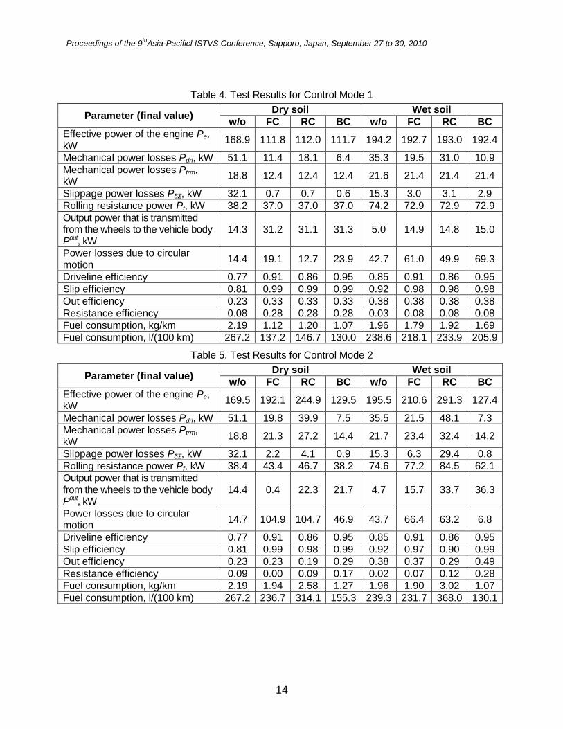
Table 4. Test Results for Control Mode 1

Parameter (final value) Dry soil Wet soil

w/o FC RC BC w/o FC RC BC

Effective power of the engine Pe, kW

168.9 111.8 112.0 111.7 194.2 192.7 193.0 192.4

Mechanical power losses Pdrl, kW 51.1 11.4 18.1 6.4 35.3 19.5 31.0 10.9

Mechanical power losses Ptrm, kW

18.8 12.4 12.4 12.4 21.6 21.4 21.4 21.4

Slippage power losses PδΣ, kW 32.1 0.7 0.7 0.6 15.3 3.0 3.1 2.9

Rolling resistance power Pf, kW 38.2 37.0 37.0 37.0 74.2 72.9 72.9 72.9

Output power that is transmitted from the wheels to the vehicle body Pout, kW

14.3 31.2 31.1 31.3 5.0 14.9 14.8 15.0

Power losses due to circular motion

14.4 19.1 12.7 23.9 42.7 61.0 49.9 69.3

Driveline efficiency 0.77 0.91 0.86 0.95 0.85 0.91 0.86 0.95

Slip efficiency 0.81 0.99 0.99 0.99 0.92 0.98 0.98 0.98

Out efficiency 0.23 0.33 0.33 0.33 0.38 0.38 0.38 0.38

Resistance efficiency 0.08 0.28 0.28 0.28 0.03 0.08 0.08 0.08

Fuel consumption, kg/km 2.19 1.12 1.20 1.07 1.96 1.79 1.92 1.69

Fuel consumption, l/(100 km) 267.2 137.2 146.7 130.0 238.6 218.1 233.9 205.9

Table 5. Test Results for Control Mode 2

Parameter (final value) Dry soil Wet soil

w/o FC RC BC w/o FC RC BC

Effective power of the engine Pe, kW

169.5 192.1 244.9 129.5 195.5 210.6 291.3 127.4

Mechanical power losses Pdrl, kW 51.1 19.8 39.9 7.5 35.5 21.5 48.1 7.3

Mechanical power losses Ptrm, kW

18.8 21.3 27.2 14.4 21.7 23.4 32.4 14.2

Slippage power losses PδΣ, kW 32.1 2.2 4.1 0.9 15.3 6.3 29.4 0.8

Rolling resistance power Pf, kW 38.4 43.4 46.7 38.2 74.6 77.2 84.5 62.1

Output power that is transmitted from the wheels to the vehicle body Pout, kW

14.4 0.4 22.3 21.7 4.7 15.7 33.7 36.3

Power losses due to circular motion

14.7 104.9 104.7 46.9 43.7 66.4 63.2 6.8

Driveline efficiency 0.77 0.91 0.86 0.95 0.85 0.91 0.86 0.95

Slip efficiency 0.81 0.99 0.98 0.99 0.92 0.97 0.90 0.99

Out efficiency 0.23 0.23 0.19 0.29 0.38 0.37 0.29 0.49

Resistance efficiency 0.09 0.00 0.09 0.17 0.02 0.07 0.12 0.28

Fuel consumption, kg/km 2.19 1.94 2.58 1.27 1.96 1.90 3.02 1.07

Fuel consumption, l/(100 km) 267.2 236.7 314.1 155.3 239.3 231.7 368.0 130.1



15

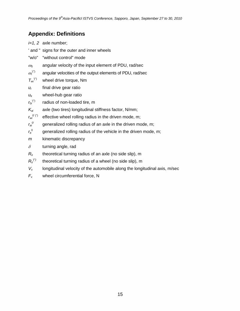
Appendix: Definitions

i=1, 2 axle number;

' and '' signs for the outer and inner wheels

"w/o" "without control" mode

0 angular velocity of the input element of PDU, rad/sec

i'('') angular velocities of the output elements of PDU, rad/sec

Twi'('') wheel drive torque, Nm

ui final drive gear ratio

uk wheel-hub gear ratio

r0i'('') radius of non-loaded tire, m

Kai axle (two tires) longitudinal stiffness factor, N/mm;

rwi0' ('') effective wheel rolling radius in the driven mode, m;

rai0' generalized rolling radius of an axle in the driven mode, m;

ra0 generalized rolling radius of the vehicle in the driven mode, m;

m kinematic discrepancy

turning angle, rad

Rti theoretical turning radius of an axle (no side slip), m

Rti'('') theoretical turning radius of a wheel (no side slip), m

Vx longitudinal velocity of the automobile along the longitudinal axis, m/sec

Fx wheel circumferential force, N

Slip Power Loss and Fuel Consumption Control in 4x4 Terrain Vehicle Applications

Documents

Transcript of Slip Power Loss and Fuel Consumption Control in 4x4 Terrain Vehicle Applications