Slime Mold Inspired Path Formation Protocol

for Wireless Sensor Networks�

Ke Li1, Kyle Thomas2, Claudio Torres3, Louis Rossi3, and Chien-Chung Shen1

1 Computer & Info. Sciences2 Chemical Engineering3 Mathematical Sciences

University of Delaware, Newark, DE, USA{kli,cshen}@cis.udel.edu, kcthomas@udel.edu, {torres,rossi}@math.udel.edu

Abstract. Many biological systems are composed of unreliable compo-nents which self-organize efficiently into systems that can tackle complexproblems.One such example is the true slimemoldPhysarum polycephalumwhich is an amoeba-like organism that seeks food sources and efficientlydistributes nutrients throughout its cell body. The distribution of nutri-ents is accomplished by a self-assembled resource distribution network ofsmall tubeswith varyingdiameter which can evolve with changing environ-mental conditions without any global control. In this paper, we use a phe-nomenological model for the tube evolution in slime mold and map it to apath formation protocol for wireless sensor networks. By selecting certainevolution parameters in the protocol, the network may evolve toward singlepaths connecting data sources to a data sink. In other parameter regimes,the protocol may evolve toward multiple redundant paths. We present de-tailed analysis of a small model network. A thorough understanding of thesimple network leads to design insights into appropriate parameter selec-tion. We also validate the design via simulation of large-scale realistic wire-less sensor networks using the QualNet network simulator.

1 Introduction

One fundamental design issue in wireless sensor networks (WSNs) is, given anarbitrary deployment of sensor nodes, how to connect the source nodes to thesinks so that data collected by the source nodes flow efficiently and reliably to thesinks. To facilitate such data transfer, a path formation protocol becomes essen-tial that will determine multi-hop routes between source nodes and sink nodes.We avoid strategies that rely upon global coordination and optimization becausesuch approaches will not scale well in large networks or networks where nodesare added or deleted dynamically, or where connections form or break easily. Toseek sound solutions that rely upon local interactions, we borrow mechanismsfrom similar problems in the natural world and adapt them to suit the challengesof sensor networks. The natural world is full of resource distribution networks� Preliminary work of the paper appeared as a 2-page poster in the 3rd IEEE Int.

Conf. on Self-Adaptive and Self-Organizing Systems (SASO 2009).

M. Dorigo et al. (Eds.): ANTS 2010, LNCS 6234, pp. 299–311, 2010.c© Springer-Verlag Berlin Heidelberg 2010

300 K. Li et al.

such as circulatory, respiratory and nervous systems in animals that are elegantsolutions to very specific and complex problems. We draw our inspiration fromtrue slime mold Physarum polycephalum, a biological system that has propertiesmore aligned with the requirements of sensor networks. In particular, the dy-namics of Physarum polycephalum constructs resource distribution networks inresponse to environmental conditions. This is distinct from circulatory systemswhich are hard-wired for a particular physiology.

Slime mold Physarum polycephalum is a multinuclear, single-celled organismthat has properties making it ideal for the study of resource distribution net-works [1]. While the organism is a single cell, slime mold can grow to tens ofcentimeters in size so that it can be studied and manipulated with modest lab-oratory facilities. The presence of nutrients in the cell body triggers a sequenceof chemical reactions leading to oscillations along the cell body [5]. Tubes self-assemble which are perpendicular to the oscillatory waves to create networkslinking nutrient sources throughout the cell body. There are two key mecha-nisms in the slime mold life cycle that transfer readily to WSNs. First, duringthe growth cycle, the slime mold will explore its immediate surroundings withpseudopodia via chemotaxis to discover new food sources. We have applied thismechanism successfully to WSNs in a previous work treating data sources andsinks as singular potentials [2]. In this current work, we exploit the second keymechanism which is the temporal evolution of existing routes through nonlinearfeedback to efficiently distribute nutrients throughout the organism. In slimemold, it can be shown experimentally that the diameters of tubes carrying largefluxes of nutrients grow to expand their capacity, and tubes that are not useddecline and can disappear entirely.In the context of WSNs, the diameter of atube may be used to denote the Quality of Service (QoS) of a wireless channel.

To evaluate the merits of path formation, we focus on three metrics that di-rectly measure the network performance: expected hop count, fault tolerance,and node degree distribution. The expected hop count denotes the efficiency ofdata flow in a network by measuring the expected number of nodes a data packetmust traverse to reach the sink. We compute the expectation because the proto-col may construct topologies with multiple disjoint routes. The fault tolerance isa gross indicator of network robustness measured by the probability that a nodefailure will disconnect at least one source from the network. Finally, we measurethe node degree distribution for the network as an indicator of connectivity.

This paper is structured as follows. In Section 2, we describe the model ofTero et al. for solutions of Physarum polycephalum to mazes and map it to thepath formation problems of WSNs. In Section 3, we describe the path formationprotocol based on the slime mold model. In Section 4, we verify our model byindependently computing all possible stationary states and their stability on avery small network. In Section 5, we perform large scale simulations and measurethe protocol performance with quantitative metrics of expected hop count, faulttolerance, and node degree distribution as functions of network parameters.

Slime Mold Inspired Path Formation Protocol for Wireless Sensor Networks 301

2 A Phenomenological Model for Slime Mold

We base our path formation protocol for WSNs on the phenomenological modelproposed by Tero et al. for tube evolution in Physarum polycephalum to repro-duce the slime mold maze solving experiments [3,6]. In recent article on appli-cations of their slime-inspired algorithm, Tero et al. independently acknowledgethe suitability of this type of model for sensor networks [7]. The model capturesthe evolution of tube capacities in an existing network through a dynamical sys-tem as follows. The original model consists of a set of nodes representing eithera food source or a junction in the maze connected by a set of edges. Along eachedge, the flow of nutrients from node i to node j is represented as qij , whichis directional and qij = −qji. Flow through the network is driven by a pres-sure at each node pi. The cross-sectional size of each tube is represented by Dij

(Dij = Dji). At each node, a Kirchhoff law is required to enforce conservationof nutrient flux at each junction. All above variables evolve in time as follows:

qij =Dij

Lij(pi − pj), (1a)

∑

j∈Ni

qij =mi, (1b)

dDij

dt=f (|qij |)− rDij , (1c)

where Lij is the length of the tube, Ni represents the set of neighbors for nodei, mi is the amount of nutrient flux into the network from i, f(x) is either anexponential or sigmoidal function describing the rate of growth of the tube sizein response to nutrient flow rate, and r is a tube size linear decay rate. Thesystem (1) contains a continuity equation (Kirchhoff Law) (1b) balancing theflow out of a node with the source value. In Tero et al. [6], nutrient sources weredesignated to be mi = 1 at the entrance or mi = −1 at the exit to drive flowthrough a maze. At junctions within the maze, mi = 0.

We use the Tero model as a foundation for the path formation protocol forWSNs. While the distinction of identical nutrient sources as either mi = +1 ormi = −1 in the slime mold seems arbitrary, this aspect of algorithm maps well toWSNs which have sensors that are data sources and sinks that represent highlycapable nodes collecting source data. The set Ni of neighbors denotes the set ofnodes within the transmission radius of node i. Thus, there is a communicationlink between node i and all members of Ni. In the proposed protocol, we assumesymmetric links with all identical transmission radii. While the tube length Lij

could be a useful tuning parameter mappable to special restrictions on networkconnections, we do not pursue these issues in this paper and simply assume equalLij ’s throughout the network. We represent f(x) as sigmoid function slightlydifferently from Tero et al. as

f(x) = rDmaxa|x|μ

1 + a|x|μ , (2)

302 K. Li et al.

Δ tsync

Δ tsync

Δ tsync

Δ tsync

Δ tsync

Δ tsync

Δ tsync

Δ tsync

Δ tsync

Solve ODE

Solve for p

1

t=0

Solve ODE

Solve for p

Send p , D

Node 1 time

t=0

Send

p ,

D

2 2

Real time

Node 2 time

1

2

Send p , D1

Send

p ,

D

12

21 21

12

Fig. 1. Schematic diagram of local computation followed by synchronization of protocolvariables. Nodes 1 and 2 perform computations independently within a fixed cycle ofΔtsync, and share information afterward.

where Dmax specifies the upper limit on Dij ’s. The exponent μ plays a criticalrole in the behavior of this model, which will be discussed later. The parameter adescribes the shape of the sigmoid and has little impact on network performance.Without loss of generality, we simply select all Lij ’s, r, Dmax, and a to be 1when calculating numerical solutions to the model as well as simulating thepath formation protocol.

Like ant colony optimization (ACO), the slime mold model includes dynamicpositive and negative feedback mechanisms (1c). The key distinction is that themodel permits nearly simultaneous coordination through flow continuity (1a,1b),which provides both the advantage that more information is available, and thedisadvantage that the pressure equation must be solved iteratively as will bediscussed in Section 3.2. The solution to this system may be used to move datafrom sources to data sink(s) in WSNs following a multi-path routing scheme. Theoutward fluxes from a node i guide how packets are routed through the network.If we denote Oi to be the subset of k ∈ Ni such that qik > 0, Oi then representsthe next-hop neighbors of node i on a route toward the sink. We define the ratio

wij =qij∑

k∈Oiqik

. (3)

If node i has C data packets to send, Cwij packets (rounding as necessary) wouldbe sent to node j for each j ∈ Oi. While the wij ’s do not necessarily representprobabilities, we could pose a stochastic routing protocol by routing each packetarriving at node i to node j with probability wij .

3 Protocol Description

Although model (1) is globally coupled via the pressure field, the inspired pathformation protocol solves the model in a distributed manner. Each node i main-tains its local states of own pressure pi, perceived neighbor pressures pj’s, and

Slime Mold Inspired Path Formation Protocol for Wireless Sensor Networks 303

tube size Dij ’s for all j ∈ Ni. We initialize pressures uniformly as 1.0 (except forthe sink as 0), with Dij ’s randomly selected between 0 and Dmax. Each node thenperforms local computations in a fixed cycle of Δtsync, solving model (1b,1c) forpressure and link diameters. At the end of each Δtsync cycle, a node broadcastsits latest computing results to neighbors, which allows globally coupled infor-mation to propagate across the network. Meanwhile, each node keeps updatingperceived neighbor pressures to be used in future local computation. The loop oflocal computation followed by states synchronization at fixed interval of Δtsync

is demonstrated in Figure 1. Notice that the localized path formation protocolsolves model (1) cooperatively among neighboring nodes and in real time with-out explicit clock synchronization across the network. All that is required is thatclocks run forward at approximately the same rate in every node.

3.1 Local Data Structures

Each node i locally maintains a node type (nodeType i), a net flux (netFlux i), apressure value (pi), and a neighbor table (nTabi). The value of nodeType i couldbe SINK, SOURCE, or OTHER (as potential relays). The netFlux i specifies thepure flux mi flowing out of node i into the network, which is positive at any datasource, negative at the data sink, and zero at any other node. The pressure valueof each node other than the sink starts with 1.0 and evolves based on model (1),while the sink’s pressure remains 0 at all time. The neighbor table entry nTabi(j)corresponds to the 1-hop neighbor j of node i, with the form of 〈pj , Dij , qij , Lij〉.The neighbor table keeps track of local dynamics of the evolving system and thusforms the basis for solving model (1).

3.2 Local Computation

Between synchronizations of pressures and link diameters with neighbors, eachnode i performs local computation in R rounds to solve model (1) for pressure pi,neighbor link flux qij ’s, and diameter Dij ’s, based on the following mathematicalmethods.

To solve for pi locally, we substitute the flow model (1a) into the pressureequation (1b):

pi ←mi +

∑j∈Ni

Dij

Lijpj

∑j∈Ni

Dij

Lij

. (4)

Similar to the Jacobi algorithm for solving diagonally dominant linear systems,the above method of solving Kirchhoff law (1b) in terms of pressure is translationinvariant, meaning that one can take a pressure solution and add the sameconstant to all pressures to obtain another solution. Therefore, we fix the pressureto be 0 at the sink node which does not satisfy Kirchhoff’s law. Conservationof flux is already imposed and fixing the pressure at the sink node guarantees aunique pressure solution. With (1b) satisfied at all nodes except for the sink, we

304 K. Li et al.

then numerically solve the evolution equation for Dij iteratively using the firstorder implicit scheme proposed by Tero:

Dn+1ij =

Dnij + Δtf(|qn

ij |)1 + Δtr

, (5)

where the fluxes qij are determined from the solved pressures pi, Δt is theduration of one discrete time step (or iteration), and Dn

ij is the value of Dij atthe nth iteration.

Each round of the local computation works as follows. First, every node i ex-cept for the sink calculates its pressure pi by solving the linear equation (Kirch-hoff’s law), given neighbors’ pj ’s and Dij ’s based on (4), while the sink remainszero pressure as the minimum pressure level. Next, for each of its neighbor j,node i determines the corresponding flux qij with the freshly calculated pi. Thenit solves the adaptive system (1c) for Dij based on (5) in S iterations, with eachiteration’s result based on the previous one and fed into the next. Since eachiteration signifies Δt time, the total time for R rounds of S iterations is thusT = R× S ×Δt before the next synchronization. We require that Δtsync ≥ T .

3.3 Synchronization

Before each cycle of local computation, every node i shares its pressure pi andsynchronizes Dij ’s with neighbors by broadcasting a one-hop synchronization(Sync) packet. The Sync packet contains the sender’s id and current pressure,together with the latest neighbor-diameter table, including the total number ofentries (#entries) followed by each entry 〈nj , Did,nj 〉. In particular, Did,nj repre-sents the diameter of link to its neighbor nj , retrieved from the sender’s neighbortable. The initial synchronization also serves as a hello packet for neighbor dis-covery, whose neighbor-diameter table is empty with #entries == 0.

Upon receiving a Sync packet, each node tries to synchronize its neighbortable in terms of neighbor pressure and link diameter based on information fromthe packet. In case of the first time to hear from sender j, node i will insertin its neighbor table a new entry for j. Specifically, Dij in the new entry iseither assigned as the corresponding Dji from the packet’s neighbor-diametertable if it exists, or otherwise initialized as a random value rand(i + j) within[0, Dmax]. Notice that the latter case applies when receiving the initial batch ofSync packets which also serve for neighbor discovery, and the random diameteruniquely dependent on (i+j) ensures that Dij = Dji at the start. In case senderj already exists in node i’s neighbor table, pj is updated and Dij synchronizedas the mean of itself and Dji from the packet.

3.4 Issue of Asymmetric Neighborhood

Due to unreliability of wireless communications, synchronization packets mayget lost or corrupted. This is annoying when lost packets assist in neighbordiscovery, which could cause “asymmetric neighborhood”, e.g., node i can hear(sometimes) from node j thus recording j in its neighbor table and counting pj

Slime Mold Inspired Path Formation Protocol for Wireless Sensor Networks 305

q(0.40,0.40)

n2p(1.69,1.69)

D(0.31,0.31)n3

p(1.03,1.03)

q(0.20,0.20)D(0.31,0.31)

n4p(1.69,1.69)

D(0.47,0.47)q(0.80,0.80)D(0.47,0.47)

D(0.38,0.38)

q(0.80,0.80)

n1p(0.00,0.00)

q(0.20,0.20)

D(0.50,0.50)

D(0.00,0.00)q(0.00,0.00)

p(2.00,2.00)

p(0.00,0.00)

n4n3

n1

q(0.00,0.00)D(0.00,0.00)

q(0.00,0.00)D(0.00,0.00)

q(1.00,1.00) q(1.00,1.00)D(0.50,0.50)

p(0.22,1.24)p(2.00,2.00)

n2

(a) (b)

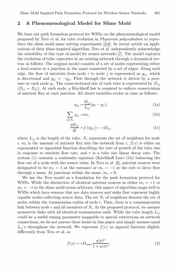
Fig. 2. Comparison between steady states from numerical solutions (left value) andQualNet simulations (right value) on the 4-node network under different μ values. (a)μ = 0.5, (b) μ = 2.

and Dij during its local computations, while node j could not receive successfullyfrom i thus never taking i as its neighbor. This problem is aggravated when nodei decides through local computation to send majority of its outgoing flux to itsseeming neighbor j, while node j is ignorant of the large flux from node i,which could potentially disrupt the global flow continuity (1b) and render theprotocol unable to converge. Asymmetric neighborhood becomes widespread asthe number of nodes within transmission range increases which causes severerchannel contentions.

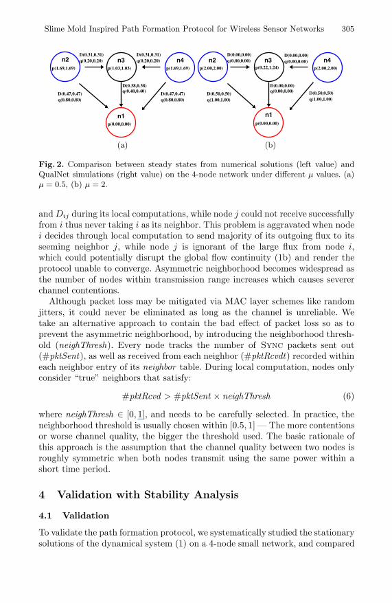
Although packet loss may be mitigated via MAC layer schemes like randomjitters, it could never be eliminated as long as the channel is unreliable. Wetake an alternative approach to contain the bad effect of packet loss so as toprevent the asymmetric neighborhood, by introducing the neighborhood thresh-old (neighThresh). Every node tracks the number of Sync packets sent out(#pktSent), as well as received from each neighbor (#pktRcvdt) recorded withineach neighbor entry of its neighbor table. During local computation, nodes onlyconsider “true” neighbors that satisfy:

#pktRcvd > #pktSent × neighThresh (6)

where neighThresh ∈ [0, 1], and needs to be carefully selected. In practice, theneighborhood threshold is usually chosen within [0.5, 1] — The more contentionsor worse channel quality, the bigger the threshold used. The basic rationale ofthis approach is the assumption that the channel quality between two nodes isroughly symmetric when both nodes transmit using the same power within ashort time period.

4 Validation with Stability Analysis

4.1 Validation

To validate the path formation protocol, we systematically studied the stationarysolutions of the dynamical system (1) on a 4-node small network, and compared

306 K. Li et al.

exact numerical solutions with results from distributed calculations in realisticQualNet [4] simulations. Details on calculating exact solutions are discussed inSection 4.2.

The 4-node network consists of one sink n1, two sources n2 and n4 eachwith 1 unit of flux to be sent to the sink, and one potential relay n3, withnetwork layout shown in Figure 2. By numerically solving the model, we found9 steady states for μ = 0.5 (demonstrated in Figure 3 inside ovals), and 6 forμ = 2.We ran QualNet simulations under same set of parameters with differentrandom seeds. For μ = 0.5, all trials converged to the same single steady stateshown in Figure 2(a), the reason of which will be discussed in Section 4.2. Forμ = 2, different steady states were found by simulations. Figure 2 comparesone corresponding steady state between the solution of numerical method andQualNet simulation for each μ value. We find that the exact numerical solutionsand the realistic QualNet simulation results agree on Dij ’s and qij ’s. So do theyon almost all pressure p values except for node n3 when μ = 2, in which stateboth sources n2 and n4 send all fluxes directly to the sink n1 without passingthrough n3. Therefore n3 has the “freedom” of choosing any positive value aspressure, since it will not be used for relay. This “freedom” doesn’t impact theprotocol because it only happens when the flux through the node is zero. Fromthe mathematical point of view, this case corresponds to the existence of anontrivial, homogeneous solution when we solve (1a) and (1b) for the pressure.

4.2 Linear Stability Analysis

To understand the stability of solutions to model (1), we analyze solutions tothe nonlinear system of equation F(Dij) = f (|qij |) − rDij = 0 when settingdDij

dt = 0 in (1). The stationary solution to F(Dij) = 0 is defined as an im-plicit nonlinear system, where the implicit part (qij) is obtained by solving anested linear system for pressure values using system (1). After calculating so-lutions to F(Dij) = 0, we then compute the Jacobian matrix

[∂Fij

∂Dkl

]evaluated

at the stationary point of interest. The eigenvalues and eigenvectors of each so-lution determine the stability of the system. If all eigenvalues are negative, the

Fig. 3. Stability diagram for the 4-node network with μ = 0.5. The topology of each ofthese 9 steady solutions is shown inside the oval, with solid lines indicating links withDij �= 0 and dotted lines for links with Dij = 0. Each pair of arrows represents thegrowth of a small positive and negative amplitude perturbation along an eigenvector.

Slime Mold Inspired Path Formation Protocol for Wireless Sensor Networks 307

solution is a stable steady state. Otherwise when there are any positive eigenval-ues, the solution is unstable, which will evolve to a different steady state, withthe linear evolution described by the eigenvector corresponding to the positiveeigenvalue.

The complete understanding of small problems gives us useful insights intohow parameter values affect the behavior of the whole network. In particular,the parameter μ dominates the evolution of links in the network. Generallyspeaking, for μ = 2 (in general μ > 1) all single route solutions with positiveDij values are stable. On the other hand, for μ = 0.5 (in general μ < 1) only thesolution where all links are used is stable, which corresponds to the single steadystate reached by QualNet simulations. Since there are both stable and unstablenumerical solutions when μ = 0.5, we also built the stability diagram over all 9solutions shown in Figure 3, where the perturbations were computed using theeigenvectors related to the positives eigenvalues. We find that for μ = 0.5 theinitialization does not affect the final stable state at all, which should alwaysbe the all-link solution illustrated by Figure 2(a). This mathematical analysisalso explains why all QualNet simulations converged to this stable solution whenμ = 0.5. Finally, these general properties transfer to larger networks.

5 QualNet Simulation

We performed QualNet simulations on 100 and 300-node networks with onesink and varying numbers of sources. All nodes were random distributed over aterrain of size 1000×1000 m2. Each node in the network was equipped with aradio transceiver capable of transmitting signals up to approximately 80 meters.The underlying wireless channel had a data rate of 2 Mbps, using the two-raypath loss model without fading. IEEE 802.11 DCF was used as the MAC layerprotocol, and IP as the network layer on top of which our protocol ran. Noapplication traffic was employed since the sole purpose was to connect sourcenodes to the data sink. The neighborhood threshold is 0.8 to avoid neighborhoodasymmetry. For each cycle of local computation, the number of round R = 10,iteration S = 1, and Δtsync = 0.01 sec. The following three quantitative metricsare designed to measure qualities of resulting network connectivity under μ = 0.5and μ = 2 with different portions of sources:

– Expected hop count: indicates the efficiency of the connectivity in termsof hop count distance between a source and the sink. The smaller the hopcount, the higher the efficiency. Let W = [wij ]

T be the Markov transitionmatrix with wij defined in Equation (3). Let el be a unit vector consistingof all zeros except at element l. Then Wel is a vector whose jth elementdenotes the probability of a data packet starting from node l and arrivingat node j in one hop. Similarly, W kel is a vector of probabilities for k hops.Therefore, the expected hop count from source node l to sink node s is

E(l, s) =∞∑

k=1

kW kel. (7)

308 K. Li et al.

Table 1. Fault tolerance of a 300-node network with 1 sink and varying numbers ofsources

source 10% 20% 30% 40% 50%

μ 0.5 2 0.5 2 0.5 2 0.5 2 0.5 2

1-fault 1 .9851 .9916 .9874 .9856 .9761 .9832 .9609 .9799 .9530

2-fault .9998 .9700 .9826 .9739 .9709 .9616 .9659 .9222 .9595 .9070

– Fault tolerance: indicates the robustness of the connectivity. We define thex-fault tolerance to be the probability that removing x relay nodes will notyet result in any source being disconnected from the sink. The higher theprobability, the better the robustness.

– Degree distribution: defines P (d) as the probability of a node in thenetwork having a degree of d. The presence of a small number of high degreenodes may indicate a greater dependence on a few “gateway nodes” fornetwork connectivity.

Figure 4 shows snapshots of steady state connectivity under μ = 0.5 and μ = 2over a 100-node randomly generated network with one data sink and three datasources. Figure 5 depicts a 300-node network with one data sink and thirtydata sources. The width and color of a link signify the value of correspondingflow qij . The arrow of the link shows the direction of the flow. We find thatthe network with μ < 1 (e.g., μ = 0.5) evolves towards multi-route robustconnectivity, whereas the network with μ > 1 (e.g., μ = 2) evolves into single-route efficient topology. This verifies that the exponent μ is a critical parameter

0 0.1 0.2 0.3 0.4 0.5 0.6 0.7 0.8 0.9 10

0.1

0.2

0.3

0.4

0.5

0.6

0.7

0.8

0.9

1

0.05

0.1

0.15

0.2

0.25

0.3

0.35

0.4

0.45

0 0.1 0.2 0.3 0.4 0.5 0.6 0.7 0.8 0.9 10

0.1

0.2

0.3

0.4

0.5

0.6

0.7

0.8

0.9

1

0.1

0.2

0.3

0.4

0.5

0.6

0.7

0.8

0.9

1

(a) (b)

Fig. 4. Steady states obtained by QualNet for a 100-node network, including 1 sink(the star near the center) and 3 sources (the bold circles) with link color and widthsignifying the flux value under (a) μ = 0.5 and (b) μ = 2

Slime Mold Inspired Path Formation Protocol for Wireless Sensor Networks 309

0 0.1 0.2 0.3 0.4 0.5 0.6 0.7 0.8 0.9 10

0.1

0.2

0.3

0.4

0.5

0.6

0.7

0.8

0.9

1

1

2

3

4

5

6

0 0.1 0.2 0.3 0.4 0.5 0.6 0.7 0.8 0.9 10

0.1

0.2

0.3

0.4

0.5

0.6

0.7

0.8

0.9

1

1

2

3

4

5

6

(a) (b)

Fig. 5. Steady states obtained by QualNet for a 300-node network, including 1 sink(the star near the center) and 30 sources under (a) μ = 0.5 and (b) μ = 2

0 5 10 15 20μ=0.5

0

5

10

15

20

μ=2

10% sources20% sources30% sources40% sources50% sources

Expected hop count

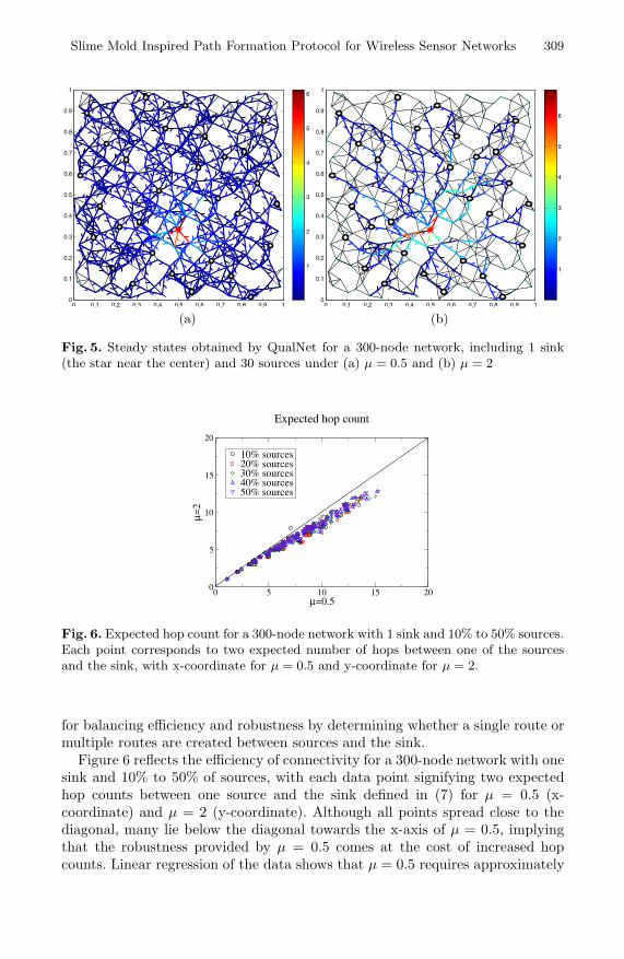
Fig. 6. Expected hop count for a 300-node network with 1 sink and 10% to 50% sources.Each point corresponds to two expected number of hops between one of the sourcesand the sink, with x-coordinate for μ = 0.5 and y-coordinate for μ = 2.

for balancing efficiency and robustness by determining whether a single route ormultiple routes are created between sources and the sink.

Figure 6 reflects the efficiency of connectivity for a 300-node network with onesink and 10% to 50% of sources, with each data point signifying two expectedhop counts between one source and the sink defined in (7) for μ = 0.5 (x-coordinate) and μ = 2 (y-coordinate). Although all points spread close to thediagonal, many lie below the diagonal towards the x-axis of μ = 0.5, implyingthat the robustness provided by μ = 0.5 comes at the cost of increased hopcounts. Linear regression of the data shows that μ = 0.5 requires approximately

310 K. Li et al.

1 2 3 4 5 6 7 8 9 10 110

0.1

0.2

0.3

0.4

0.5

Node Degree (d)

P(d

)

μ = 0.5μ = 2

1 2 3 4 5 6 7 8 9 10 110

0.1

0.2

0.3

0.4

Node Degree (d)

P(d

)

μ = 0.5μ = 2

1 2 3 4 5 6 7 8 9 10 110

0.1

0.2

0.3

0.4

Node Degree (d)

P(d

)

μ = 0.5μ = 2

(a) (b) (c)

Fig. 7. Distribution of node degree for (a) 10%, (b) 30%, and (c) 50% sources on a300-node network with 1 sink

10% more hops than μ = 2. Table 1 presents the 1 and 2-fault tolerances for thesame networks, showing that μ = 0.5 achieves better robustness against nodefailure than μ = 2, and that the network becomes less fault tolerant with moresources added. Figure 7 presents the distribution of node degree. As we wouldexpect, μ = 0.5 leads to a higher proportion of high degree nodes in a multi-routeconnectivity, whereas μ = 2 leads to a greater proportion of low degree nodes ina single-route topology. The distinction blurs as more sources join the network.

6 Conclusion

In this paper, we design a slime mold inspired, self-organizing path formationprotocol for WSNs. The localized protocol is effective in iteratively solving theunderlying mathematical model which is globally coupled through the pressurefield. The critical parameter μ controls whether single (μ > 1) or multi-route(μ < 1) connections emerge. We validate the protocol through linear stabilityanalysis on a small model network, as well as via simulations on large realisticWSNs with one sink and varying numbers of sources. Future work will focuson extending the protocol to deal with real network traffic, exploring Lij as ameasure of link quality, and modifying the biologically inspired model to addressWSNs with coordinated routing to multiple sinks.

Acknowledgements. This work is supported in part by National Science Foun-dation under grants CCF-0726556 and CNS-0347460.

References

1. Ben-Jacob, E., Cohen, I.: Cooperative organization of bacterial colonies: From geno-type to morphotype. Annual Review of Microbiology 52, 779–806 (1998)

2. Li, K., Thomas, K., Rossi, L.F., Shen, C.C.: Slime-mold inspired protocol forwireless sensor networks. In: Proc. of the 2nd IEEE International Conference onSelf-Adaptive and Self-Organizing Systems (SASO), pp. 319–328. IEEE Press, LosAlamitos (2008)

Slime Mold Inspired Path Formation Protocol for Wireless Sensor Networks 311

3. Nakagaki, T., Yamada, H., Toth, A.: Maze-solving by an amoeboid organism. Na-ture 407(6803), 470–470 (2000)

4. Scalable Network Technologies, Inc.: QualNet Simulator,http://www.scalable-networks.com

5. Stewart, P.A.: The organization of movement in slime mold plasmodia. In: PrimitiveMotile Systems in Cell Biology, pp. 69–78. Academic Press, London (1964)

6. Tero, A., Kobayashi, R., Nakagaki, T.: A mathematical model for adaptive transportnetwork in path finding by true slime mold. J. Theor. Biol. 244, 553–564 (2007)

7. Tero, A., Takagi, S., Saigusa, T., Ito, K., Bebber, B.P., Fricker, M.D., Yumiki, K.,Kobayashi, R., Nakagaki, T.: Rules for biologically inspired adaptive network design.Science 327, 439–442 (2010)