
SKI Report 96:36 - International Atomic Energy Agency
698
SKI Report 96:36 Deep Repository Performance Assessment Project December 1996 ISSN 1104-1374 ISRN SKI-R-96/36-SE STATENS KARNKRAFTINSPEKTION Swedish Njctear Power Inspectorate
-
Upload
khangminh22 -
Category
Documents
-
view
0 -
download
0
Transcript of SKI Report 96:36 - International Atomic Energy Agency
SKI Report 96:36
Deep Repository Performance Assessment Project
December 1996
ISSN 1104-1374ISRN SKI-R-96/36-SE
STATENS KARNKRAFTINSPEKTIONSwedish Njctear Power Inspectorate
SKI Report 96:36
Deep Repository Performance Assessment Project
Volume I
December 1996

NORSTEDTS TRYCKERI ABStockholm 1997
PREFACE
The Swedish Industry program for deep geological disposal of spent nuclear fuel and high-levelradioactive waste is now in the early stages of the site selection process, with feasibility studiesunderway in 5 to 10 municipalities. According to the Swedish Nuclear Fuel and WasteManagement Co., SKB (SKB RD&D Programme, 1995), the ongoing siting process involvesselection of two sites for surface-based investigations by around the year 1998, and submissionof a licence application for detailed underground investigations and for commencement ofconstruction of a deep repository, at one of these sites, in the first years of the next century.
In preparation for upcoming reviews of licence applications, the Swedish Nuclear PowerInspectorate, SKI, has developed an independent expertise for conducting performanceassessments. The foundation for SKI's capability was laid in SKI's previous performance-assessment exercise, Project-90, published in 1991. SITE-94, which commenced in 1992, buildson the methodology developed in Project-90, but is focused on further development in specificareas, such as handling of site-specific data and analysis of systems and scenarios. Thedevelopments in SITE-94 have provided SKI with expertise and analysis tools that, with limitedupdating, can be applied as a regulatory tool in SKI's future work. This report summarises theresults of the four-year SITE-94 programme.
The work with SITE-94 has involved staff members of the Office of Nuclear Waste at SKI, ledby the office head, Soren Norrby, and a number of Swedish and foreign consultants. The SKIproject group consisted of:
Johan Andersson1
Bjorn DverstorpFritz KautskyChristina LiljaRolf Sjoblom2
Benny SundstromOivind ToverudStig Wingefors
(project manager 1992-1995; scenarios)(project manager 1995-1997; hydrogeology, data management)(geology, rock mechanics)(near-field radionuclide release and transport, canister)(canister)(far-field radionuclide transport, graphics)(disposal concept)(geochemistry, radionuclide chemistry, bentonite)
1) now at QuantiSci2) now at AF Energi Stockholm
For the project, a steering committee (within SKI) and an advisory expert group were formed.The members of the expert group were Mick Apted, Neil Chapman (QuantiSci) and GhislaindeMarsily (Universite de Paris).
A large number of external consultants, as cited throughout this report, have contributed to thesuccessful completion of the project. Karin Pers (Kemakta) assisted with near-field radionucliderelease and transport calculations at SKI. The final report was written by the SKI project group,assisted by Neil Chapman and Joel Geier (Golder Associates/Clearwater Hardrock Consulting).Technical reviews of the manuscript by Timo Vieno (Technical Research Center of Finland) andPhilip Maul (QuantiSci) helped greatly in the final editing of the report.
Stockholm, December 30, 1996
HogbergDirector General Bjorn Dverstorp
Project Manager
OVERVIEW OF CHAPTERS
1 Introduction
2 Performance Assessment Methodology
3 Properties of Spent Nuclear Fuel
4 The Aspo Site
5 Outline of the Disposal System
6 Basic Data for the Site Evaluation
7 Site Evaluation
8 The Engineered Barrier System
9 Scenario Identification
10 Predictions of Geosphere Evolution
11 Evolution of the Near-field
12 Chemistry and Behaviour of Radionuclides
13 Modelling Radionuclide Release and Transport
14 Biosphere Modelling and Radiation Exposure
15 Formulation of Release and Transport Calculation Cases
16 Results of Radionuclide Transport Calculations
17 Implications for Safety Assessments of the Studied Repository Concept
18 Conclusions
CONTENTS
Volume IPage
1 INTRODUCTION 1
1.1 BACKGROUND TO THE SITE-94 PROJECT 11.1.1 SITE-94 and the Overall Regulatory Duties of SKI 11.1.2 SITE-94 in the Context of Swedish Nuclear Industry Plans for a Deep Geological
Repository 21.1.3 Use of Previous Experience in Formulating the Objectives of SITE-94 4
1.1.3.1 SKI Conclusions from Project-90 41.1.3.2 Review of Project-90 by an OECD/NEA Team of Experts 5
1.2 OBJECTIVES, SCOPE AND ORGANISATION OF SITE-94 51.2.1 Objectives Concerning Development Needs 5
1.2.1.1 Site Evaluation 61.2.1.2 Performance Assessment Methodology 61.2.1.3 Canister Integrity 7
1.2.2 Objectives Concerning Training of SKI Staff 71.2.3 Project Organisation 7
1.2.3.1 Analysis of a Hypothetical Repository 71.2.3.2 SITE-94 Sub-projects 8
1.3 STRUCTURE OF THE SITE-94 REPORT 9
2 PERFORMANCE ASSESSMENT METHODOLOGY 13
2.1 SAFETY REQUIREMENTS AND ACCEPTANCE CRITERIA 132.1.1 General Performance Criteria for the Repository 132.1.2 Technical Criteria 15
2.2 PERFORMANCE ASSESSMENT ELEMENTS 162.2.1 Output from a Performance Assessment 162.2.2 Systems Analysis Approach to Performance Assessment 172.2.3 System Identification 17
2.2.3.1 General 172.2.3.2 The System Boundary 182.2.3.3 The SITE-94 Process System 18
2.2.4 Scenario Identification 202.2.5 Model Selection and Consequence Analysis 21
2.3 TREATMENT OF UNCERTAINTIES AT THE DIFFERENTANALYSIS LEVELS 21
2.3.1 Classification of Uncertainty 2123.1.1 Categories of Uncertainties 212.3.1.2 Completeness 222.3.1.3 Quantification 222.3.1.4 Approach to Treatment of Uncertainties 23
2.3.2 System Uncertainty 232.3.3 Scenario Uncertainty 242.3.4 Conceptual Model Uncertainty and Validation 25
2.3.5 Parameter Uncertainty and Variability 262.3.6 Propagation of Uncertainties 26
2.4 IMPLEMENTATION OF THE ANALYSIS LEVELS 282.4.1 System Identification - The Process Influence Diagram 28
2.4.1.1 The FEPs Audit 282.4.1.2 Constructing the General Version of the PID 292.4.1.3 Importance Levels Expert Assessment of the PID and Adjustment
to Different Scenarios 332.4.2 Scenario Identification 362.4.3 Model Selection - The Assessment Model Flowchart (AMF) 37
2.4.3.1 The Assessment Model Flowchart 382.4.3.2 Structure of the AMF 382.4.3.3 Mapping the PID onto the AMF 422.43 A Information Transfer and Representation of Conceptual Uncertainty 422.4.3.5 Adjusting the AMF to Different PIDs 43
2.4.4 Formulation of Calculations Cases 44
2.5 QUALITY ASSURANCE 44
3 PROPERTIES OF SPENT NUCLEAR FUEL 47
3.1 INTRODUCTION 473.1.1 Quantities of Spent Fuel 473.1.2 Types of Spent Fuel and Their General Characteristics 48
3.2 COMPOSITION OF FUEL COMPONENTS 503.2.1 Fuel Material 503.2.2 Metal Parts 50
3.3 RADIONUCLIDE INVENTORY 503.3.1 Burn-up Calculations 503.3.2 The SITE-94 Inventory 51
3.4 CHEMICAL AND PHYSICAL FORM OF SPENT FUEL 533.4.1 Chemical Composition and Structure 533.4.2 Physical Properties 55
4 THE ASPO SITE 57
4.1 INTRODUCTION 57
4.2 ASPO HARD ROCK LABORATORY 58
4.3 REGIONAL DESCRIPTION 584.3.1 Bedrock and Structural Geology 584.3.2 Seismic Activity 594.3.3 Topography and Quaternary Deposits 604.3.4 Surface Hydrology 61
4.4 SURFACE ENVIRONMENT 614.4.1 Society 61
Ill
4.4.2 Land Use 614.4.3 Nuclear Facilities 61
5 OUTLINE OF THE DISPOSAL SYSTEM 63
5.1 INTRODUCTION 63
5.2 TRANSPORT 635.2.1 Present System for Transport of Spent Nuclear Fuel 635.2.2 Future System for Transport of Spent Nuclear Fuel 64
5.3 INTERMEDIATE STORAGE 65
5.4 CANISTER DESIGN AND ENCAPSULATION 655.4.1 Canister Design 655.4.2 Encapsulation 66
5.5 REPOSITORY CONSTRUCTION AND DESIGN 685.5.1 Introduction 685.5.2 Principal Repository Design 685.5.3 Construction, Operation and Closure ot the Repository 70
6 BASIC DATA FOR THE SITE EVALUATION 73
6.1 INTRODUCTION 73
6.2 SITE INVESTIGATION PROGRAMME 73
6.3 METHODS AND INSTRUMENTS 74
6.4 AVAILABLE DATA AND USED DATA 79
6.5 AVAILABILITY AND QUALITY OF DATA 856.5.1 Documentation 856.5.2 Positional Information 866.5.3 Geochemical Sampling Procedures 876.5.4 Borehole Hydraulic Measurement Data 876.5.5 Geological Data 886.5.6 Configuration of Boreholes and Measurements (Measurement Strategy) 89
6.6 CONCLUSIONS 90
6.7 SOURCES OF BASIC DATA 91
7 SITE EVALUATION 97
7.1 INTRODUCTION 977.1.1 The Geosphere as a Part of the SITE-94 Process System 977.1.2 Site Evaluation 100
IV
7.2 BEDROCK AND STRUCTURAL GEOLOGY: THE SKI STRUCTURALMODEL 100
7.2.1 Introduction 1007.2.2 The Regional and Subregional Scale Models 102
7.2.2.1 Bedrock Geology 1027.2.2.2 Regional Structural History and Future Evolution 1027.2.2.3 Regional (35 x 25 km) Structural Environment Model 1047.2.2.4 Subregional (10x12 km) Structural Environment Model 105
7.2.3 The Local Scale Models 1077.2.3.1 Bedrock Geology of Aspo 1077.2.3.2 Local Structural Geology and Fracturing 1077.2.3.3 The 2D Local Scale Structural Model 1117.2.3.4 The 3D Fracture Zone Model of Aspo 113
7.2.4 Verification of the SKI 3D Structural Model 1177.2.5 Comparison of the SKI Structural Model with Other Models 119
7.2.5.1 Data and Models 1197.2.5.2 SKB Structural Model of Aspo 1197.2.5.3 SKN Structural Model of Aspo 1207.2.5.4 Similarities Between the Structural Models 1217.2.5.5 Differences Between the Structural Models 1227.2.5.6 General Implications for Structural Modelling 124
7.2.6 Uncertainties Underlying Structural Models 1247.2.6.1 The Extrapolation of Geological Data 1267.2.6.2 Identifying Discrete Rock Volumes within a Model 1277.2.6.3 Precision in the Location of Structures 1277.2.6.4 Approximations Made in Structural Modelling 1287.2.6.5 Relative Age of Rocks and Structures 1297.2.6.6 Restoration of Faulting 129
7.2.7 Fitting a Hypothetical Repository Into the Aspo Structure 1317.2.7.1 Introduction 1317.2.7.2 Overall Constraints on Location 1317.2.7.3 Repository Layout 1337.2.7.4 Final Remarks 134
7.2.8 Implications for Site Characterisation Programmes 1357.2.8.1 Implications for Other Parts of the Assessment 1357.2.8.2 Implications for Site Characterisation Programmes 135
7.3 HYDROGEOLOGY 1377.3.1 Introduction 137
7.3.1.1 Hydrogeological FEPs and Influences in the PID 1377.3.1.2 Specific Objectives of the Hydrogeological Site Evaluation 1387.3.1.3 Summary of Approach 138
7.3.2 Hydrogeological Setting of Aspo 1427.3.3 Models for Regional Hydrogeology 145
7.3.3.1 Regional Flow of Variable Density Groundwaterin the Fennoscandian Shield 146
7.3.3.2 Two-dimensional Sensitivity Analysis of Semi-regionalGroundwater Flow 151
7.3.3.3 Interpreted Hydrogeological Evolution of the Site 1537.3.3.4 Implications for Site-scale Modelling of Groundwater Flow 155
7.3.4 Uncertainty in the Site Characterisation Data—First Order Analysis 1567.3.4.1 GRF-analysis of Hydraulic Borehole Packer Tests 1567.3.4.2 Multivariate Analysis of Borehole Data 160
7.3.5 Simple Evaluation 163
7.3.6 Qualitative Hydrogeological Assessment of Site Data and the SITE-94Structural Model — Basis for Detailed Models 1637.3.6.1 Introduction 1637.3.6.2 Aspo Hydrogeological Base Data 1657.3.6.3 Correlation of Subsurface Flow with Geological Factors 1667.3.6.4 Structural Model Correlation with Subsurface Flow 1677.3.6.5 Testing the Hydrogeological Value of the SITE-94 Structural Model 1707.3.6.6 Structural Model Correlation with Paths of Pressure Propagation 1717.3.6.7 Correlation of Flowing- and Pressure-transmissive Structures 1737.3.6.8 Structural Model Correlation with Aspo Geochemistry 1737.3.6.9 Integrated Hydrogeological Interpretation of All Data Types 1757.3.6.10 Assessment of the Structural Model as a Hydrogeological Explanation 1767.3.6.11 Bias and Uncertainty in Data and Interpretation 1777.3.6.12 Conclusions - Implications for the Formulation of Detailed
Quantitative Models 1787.3.7 Development of a Discrete Feature Hydrogeological Site Model 179
7.3.7.1 Introduction 1797.3.7.2 Semi-regional and Site-scale Model of Fractures and Fracture Zones 1817.3.7.3 Discrete-Fracture Network Model for the Repository Rock Block 1837.3.7.4 Integrated Discrete Feature Model of the Aspo Site 185
7.3.8 Development of a Stochastic Continuum Hydrogeological Site Model 1887.3.8.1 Introduction 1887.3.8.2 Data Used 1887.3.8.3 Stochastic Generation of Conditioned 3D Hydraulic Conductivity Fields 1897.3.8.4 Discussion of Model Validity 192
7.3.9 Variable Aperture Discrete-Fracture Network Modelling 1937.3.10 Summary and Implications for Other Parts of the Assessment 195
7.4 GEOCHEMISTRY 2017.4.1 Introduction 2017.4.2 Rock Properties and Mineralogy 202
7.4.2.1 Rock Mineralogy 2027.4.2.2 Physico-chemical Properties 2037.4.2.3 Fracture Infillings 205
7.4.3 Ground water Chemistry 2077.4.4 Rock-ground water Interactions 213
7.4.4.1 Identified Groundwater Interactions 2137.4.4.2 Simulation of Aspo Groundwaters 218
7.4.5 Conclusions and Implications for Other Parts of the Assessment 222
7.5 ROCK MECHANICS 2247.5.1 Introduction 2247.5.2 Far-field Rock Mechanical Model 225
7.5.2.1 Model Size and Geometry 2257.5.2.2 Material Models and Properties 2267.5.2.3 Model Orientation and Boundary Conditions 229
7.5.3 Near-field (repository scale) Rock Mechanical Model 2307.5.3.1 Three-dimensional DEM Models 230
7.5.4 Discussion on the Validity of the Rock Mechanical Models 2337.5.5 Conclusions and Implications for Other Parts of the Assessment 236
7.5.5.1 Conclusions Regarding the Validity of the Rock Mechanical Model 2367.5.5.2 Implications for Other Parts of the Assessment 236
VI
8 THE ENGINEERED BARRIER SYSTEM 237
8.1 INTRODUCTION 2378.1.1 The Engineered Barrier System as a Part of the SITE-94 Process System 2378.1.2 Assessing the Properties of the Engineered Barrier System 237
8.2 THE CANISTER 2398.2.1 Introduction 2398.2.2 Objectives and Requirements 2418.2.3 Manufacturing, Sealing and Testing 241
8.2.3.1 Manufacturing 2418.2.3.2 Sealing 2428.2.3.3 Testing and Quality Inspection 243
8.2.4 Mechanical Properties 2448.2.5 Chemical Properties 246
8.2.5.1 Introduction 2468.2.5.2 Copper Chemistry 2478.2.5.3 Copper Corrosion 2488.2.5.4 Steel Corrosion 252
8.2.6 Conclusions and Implications for Other Parts of the Assessment 253
8.3 THE BENTONITE BUFFER 2548.3.1 Introductory Remarks 2548.3.2 Composition of the Buffer 2558.3.3 Transport Properties 256
8.3.3.1 Hydraulic Conductivity 2568.3.3.2 Diffusivity 2568.3.3.3 Sorption in Bentonite 2598.3.3.4 Gas Transport 259
8.4 THE BACKFILL AND SEALS 2598.4.1 Introduction 2608.4.2 Excavation, Reinforcement and Grouting 2618.4.3 The Backfill 2628.4.4 Seals and Plugs 264
8.5 TEMPERATURES IN THE REPOSITORY 265
9 SCENARIO IDENTIFICATION 267
9.1 INTRODUCTION 2679.1.1 Practical Approach to Handling Scenario Uncertainty 2679.1.2 Identification of Scenario-initiating EFEPs 2679.1.3 Further Specification of the EFEPs Selected 2689.1.4 Probability of Scenario Occurrence 269
9.2 THE REFERENCE CASE 2709.2.1 Definition of the Reference Case 2709.2.2 Developing Influence Diagrams, Models and Calculation Cases
for the Reference Case 271
9.3 THE CENTRAL (CLIMATE EVOLUTION) SCENARIO 2719.3.1 Introduction 271

Vll
9.3.2 Climate Prediction 2729.3.3 Specification of PID Impact Points and Construction of the PID
for the Central Scenario 2759.3.4 Specification of Quantitative Data for Performance Assessment Modelling 2769.3.5 Adjustment of the AMF to Evaluate the Central Scenario 277
9.4 SELECTION OF INTERESTING COMBINATIONSOF REMAINING EFEPs 278
9.4.1 Screening the EFEPs 2789.4.2 Lumping EFEPs and Finding PID Impact Points 2799.4.3 Combining EFEPs to Form Scenario Initiators 2799.4.4 Comments on the Scenario Selection Methodology 280
9.5 CONCLUSIONS 281
REFERENCES TO CHAPTERS 1 - 9 283
Volume II
10 PREDICTIONS OF GEOSPHERE EVOLUTION 305
10.1 INTRODUCTION 30510.1.1 The Assessment Model Flowchart 30510.1.2 Structure of the Chapter 306
10.2 TEMPERATURES AND MECHANICAL STABILITYIN THE FAR-FIELD ROCK 306
10.2.1 Introduction 30610.2.2 Temperatures 307
10.2.2.1 Source Term and Boundary Conditions - Reference Case 30710.2.2.2 Calculated Temperatures for the Reference Case 30710.2.2.3 Temperature Loads Assumed for Central Scenario 30810.2.2.4 Temperature for the Central Scenario 309
10.2.3 Mechanical Stability for the Reference Case 31110.2.3.1 Introduction 31110.2.3.2 Loadings and Boundary Conditions 31110.2.3.3 Results 311
10.2.4 Mechanical Stability for the Central Scenario 31210.2.4.1 Loadings 31210.2.4.2 Results 313
10.2.5 Uncertainties 31610.2.5.1 Consistency with PID FEPs and Links 31610.2.5.2 Conceptual Model and Parameter Uncertainty 317
10.2.6 Conclusions 31810.2.6.1 Implications for Other Parts of the Assessment 31810.2.6.2 Implications for Repository Design and Further Work 320
10.3 HYDROGEOLOGY 32010.3.1 Introduction 32010.3.2 Strategy for Evaluation Calculations 321
10.3.2.1 Hydrogeological Aspects of the Reference Case 32110.3.2.2 Modelling the Central Scenario 321
V l l l
10.3.2.3 General Procedure for Estimation of HydrogeologicalTransport Parameters 321
10.3.2.4 Quantification of Uncertainty and Variability 32310.3.2.5 Model-Dependent Parameters and Representative Transport Parameters 324
10.3.3 Simple Evaluation of Flow and Transport for the Reference Case 32510.3.3.1 Setup and Results of the Analysis of Groundwater Flux 32510.3.3.2 Analysis of Reactive Transport Parameters 32710.3.3.3 Applicability of Results 328
10.3.4 Discrete Feature Site Model—Reference Case Results 33110.3.4.1 Introduction 33110.3.4.2 Variants 33310.3.4.3 Base Case Results 33710.3.4.4 Impact of Different Conceptual Variants on the Far-field Radionuclide
Transport Properties 34110.3.5 Stochastic Continuum Site Model—Reference Case Results 346
10.3.5.1 Introduction 34610.3.5.2 Uncertainties in the Hydraulic Conductivity Field 34710.3.5.3 Variants 34910.3.5.4 Base Case Results 35110.3.5.5 Impact of Different Conceptual Variants on the Far-Field Radionuclide
Transport Properties 35310.3.6 Flow-wetted Surface Area Estimates 358
10.3.6.1 Introduction 35810.3.6.2 The VAPFRAC and DISCFRAC Discrete-Fracture Network Models 35810.3.6.3 The SITE-94 Geological Structure Model 35910.3.6.4 The Discrete Feature Hydrogeological Site Model 36010.3.6.5 Geochemical Model 36010.3.6.6 Simple Evaluation 36010.3.6.7 Implications for Radionuclide Transport Evaluation 361
10.3.7 Central Scenario: Regional Scale Analysis 36210.3.7.1 Evolving Boundary Conditions 36310.3.7.2 Setup of the Analyses 36410.3.7.3 Variants 36510.3.7.4 Results 366
10.3.8 Central Scenario: Site-Scale Analysis 37210.3.8.1 Introduction 37210.3.8.2 Set-up of the Analysis 37210.3.8.3 Results 374
10.3.9 Discussion and Overall Conclusions 37510.3.9.1 Main Results for Reference Case 37510.3.9.2 Impact of Climate Evolution—Results for Central Scenario 37610.3.9.3 Treatment of System Uncertainty in the Hydrogeological Evaluation 37710.3.9.4 Scenario Uncertainty 37810.3.9.5 Conceptual Model and Parameter Uncertainty 37910.3.9.6 Simplification Errors 38510.3.9.7 Implications for Other Parts of the Assessment 38610.3.9.8 Implications for Future Work 386
10.4 GEOCHEMISTRY 38810.4.1 Introduction 38910.4.2 Groundwater Properties 39010.4.3 Scenario-related Changes of Groundwater Chemistry 39210.4.4 Conclusions and Implications for Other Parts of the Assessment 394
IX
11 EVOLUTION OF THE NEAR-FIELD 395
11.1 INTRODUCTION 39511.1.1 Near-field Interactions 39511.1.2 Modelling Near-field Processes and the AMF 396
11.2 NEAR-FIELD ROCK 39611.2.1 Rock Mechanical Impacts in the Near-field 396
11.2.1.1 Introduction 39711.2.1.2 The Effects of Loading for the Reference Case 39711.2.1.3 The Effect of Loads for the Central Scenario 40211.2.1.4 Uncertainties 40311.2.1.5 Conclusions 404
11.2.2 Hydrogeology 40611.2.2.1 Discrete Feature Model: Reference Case Results 40611.2.2.2 Stochastic Continuum Model: Reference Case Results 41011.2.2.3 Central Scenario Results 41211.2.2.4 Conclusions and Implications for Other Parts of the Assessment 413
11.2.3 Chemical Conditions and Perturbations 41411.2.3.1 Effects of Aeration and Other Phenomena During the Operational Phase 41511.2.3.2 Thermochemical Effects 41611.2.3.3 Effects from Long-Term Alteration of the Engineered Barriers 41611.2.3.4 Possible Future Changes in Chemical Conditions of the Rock 417
11.3 THE BUFFER 41811.3.1 Introductory Remarks 41811.3.2 Mechanical Stability 41911.3.3 Chemical Alterations and Conditions 420
11.3.3.1 General 42011.3.3.2 Chemical Conditions in the Porewater 421
11.3.4 Possible Future Changes in Buffer Properties - Implications for OtherParts of the Assessment 423
11.4 BACKFILLS AND SEALS 42311.4.1 Evolution of Backfill and Seals 42311.4.2 Evolution of Grouted Rock 424
11.5 THE CANISTER 42511.5.1 Introduction 42511.5.2 Mechanical Integrity 426
11.5.2.1 Evolution of the Mechanical Loads 42611.5.2.2 Effects on the Canister 426
11.5.3 Chemical Integrity 42711.5.3.1 Evolution of the Chemical Conditions 42711.5.3.2 Effects on the Canister 429
11.5.4 Chemical Conditions in a Failed Canister 43211.5.5 Conclusions and Implications for Other Parts of the Assessment 435
11.6 RADIOLYSIS 436
11.7 REDOX CONDITIONS 43811.7.1 Initial Redox Conditions 43 811.7.2 Formation and Propagation of Redox Fronts 43811.7.3 Modelling Near-field Redox Conditions in SITE-94 439

11.8 FUEL DISSOLUTION 44111.8.1 General 44111.8.2 Thermodynamic Modelling of Spent Fuel Oxidation 44311.8.3 Implications for the Assessment - Modelling of Time Dependence
for Fuel Dissolution in SITE-94 443
12 CHEMISTRY AND BEHAVIOUR OF RADIONUCLIDES 445
12.1 INTRODUCTION 445
12.2 MODELLING RADIONUCLIDE SPECIATION AND SOLUBILITY 44512.2.1 General 44512.2.2 Thermodynamic Data 44712.2.3 Chemical Models of Near-field Evolution 450
453454454455455455456456457457458458459459460460461461461465
12.4 SORPTION OF RADIONUCLIDES 465
12.5 CONCLUSIONS AND IMPLICATIONS FOR OTHER PARTSOF THE ASSESSMENT 468
13 MODELLING RADIONUCLIDE RELEASEAND TRANSPORT 471
13.1 INTRODUCTION 47113.1.1 Transport Processes 47113.1.2 Calculational Tools for Consequence Modelling and
the Assessment Model Flowchart 47113.1.3 Scoping Calculations 473
12.3
12.3.112.3.212.3.312.3.412.3.512.3.612.3.712.3.812.3.912.3.1012.3.1112.3.1212.3.1312.3.1412.3.1512.3.1612.3.1712.3.1812.3.19
DISCUSSION OF RADIONUCLIDE SPECIATION-SOLUBILITYCALCULATIONSAmericiumCesiumIodineLanthanidesNickelNeptuniumNiobiumPalladiumPlutoniumRadiumSeleniumStrontiumTechnetiumThoriumTinUraniumZirconiumNature and Crystallinity of Solid PhasesConclusions Regarding Solubilities and Speciation
XI
13.2 RELEASE FROM THE FUEL 47313.2.1 Overview 47313.2.2 Gap Release 47413.2.3 Grain Boundary Release 47513.2.4 Matrix Release 47513.2.5 Release From Metal Parts 47513.2.6 Solubility Limitations 47613.2.7 Mathematical Model and Solution Using the CALIBRE Code 476
133 NEAR-FBELD TRANSPORT 47713.3.1 Transport in the Failed Canister 47713.3.2 Transport in the Bentonite 47813.3.3 Transport in the Near-field Rock 47813.3.4 Redox Front 47813.3.5 Mathematical Model and Solution Using the CALIBRE Code 479
13.3.5.1 Transport in the Waste-form 47913.3.5.2 Transport in the Bentonite 48113.3.5.3 Transport in the Near-field Rock 48213.3.5.4 Redox Front 486
13.4 TRANSPORT IN THE FAR-FIELD ROCK 48713.4.1 General Description 48713.4.2 Mathematical Model and Solution Using the CRYSTAL Code 488
13.5 SCOPING CALCULATIONS WITH THE CONSEQUENCE CODES 49113.5.1 Near-field Results 491
13.5.1.1 Sensitivity to Some Parameters 49113.5.1.2 Direct Release to a Tunnel 49513.5.1.3 Pin-hole Release 495
13.5.2 Far-field Results 496
14 BIOSPHERE MODELLING AND RADIATION EXPOSURE 501
14.1 INTRODUCTION 501
501501502502
505
15 FORMULATION OF RELEASE AND TRANSPORTCALCULATION CASES 509
15.1 INTRODUCTION 509
15.2 VARIANTS IN THE REFERENCE CASE 51115.2.1 Hydrogeological Variants 511
15.2.1.1 Introduction 51115.2.1.2 The Hydrogeology Zero Variant 51415.2.1.3 Near-field Variants 515
14.214.2.14.2.14.2.
14.3
123
BIOSPHERE MODELGeneralReference CaseCentral Scenario
RESULTS

Xll
15.2.1.4 Far-field Variants 51715.2.1.5 Combined Near-field and Far-field Variants 52515.2.1.6 Potential Model Simplification Errors 528
15.2.2 Chemical Variants 52815.2.2.1 Redox Conditions Variants 52915.2.2.2 Solubility Variants 52915.2.2.3 Sorption Variants 53115.2.2.4 Buffer Variants 53215.2.2.5 Physical Properties 53215.2.2.6 Combinations of Chemical Variants 534
15.2.3 Canister Failure Variants 53415.2.4 Biosphere Variants 53515.2.5 Inventory, Fuel Degradation and Radionuclide Release from Fuel 53615.2.6 Combination of Variants from Different Clearing Houses
to form Calculation Cases 53615.2.6.1 Total Number of Variant Combinations 53615.2.6.2 Calculation Cases Selected for the Near-field Analyses 53715.2.6.3 Calculation Cases Selected for Integrated Near-field
and Far-field Transport 540
15.3 VARIANTS FOR THE CENTRAL (CLIMATE EVOLUTION) SCENARIO 54415.3.1 Possibilities for Central Scenario Variants 54415.3.2 Evolution of Conditions Affecting Radionuclide Release and Transport 544
15.3.2.1 Hydrogeology 54415.3.2.2 Geochemistry 54515.3.2.3 Canister Life-time 54615.3.2.4 Biosphere 546
15.3.3 Central Scenario Consequence Analysis 54715.3.3.1 Near-field Release and Transport 54715.3.3.2 Integration with Far-field Transport 548
16 RESULTS OF RADIONUCLIDE TRANSPORT
CALCULATONS 549
16.1 INTRODUCTION 549
16.2 NEAR-FIELD TRANSPORT RESULTS 55016.2.1 Overview of Calculation Cases 55016.2.2 Reference Case: Near-field 550
16.2.2.1 Near-field Zero Variant Case (A3) 55016.2.2.2 Other Calculation Cases for the Reference Case 56016.2.2.3 Conclusions for Near-field Reference Case Calculations 577
16.2.3 Central Scenario: Near-field 57816.3 INTEGRATED NEAR-FIELD AND FAR-FIELD TRANSPORT RESULTS 58316.3.1 Overview of Calculation Cases 58316.3.2 Reference Case: Integrated Near- and Far-fields 585
16.3.2.1 Integrated Zero Variant Case 58516.3.2.2 Other Integrated Calculation Cases for the Reference Case 590
16.3.3 Central Scenario: Integrated Near- and Far-fields 59916.3.4 Summary of Integrated Calculations 602

X l l l
16.4 CONCLUSIONS 60416.4.1 The Reference Case 604
16.4.1.1 Zero Variant Case 60416.4.1.2 Variability and Uncertainty of Hydrogeological Parameters 60416.4.1.3 Uncertainty in Geochemical Parameters 60616.4.1.4 Buffer Properties 60716.4.1.5 Uncertainty in Canister Life-time 60716.4.1.6 Overview 608
16.4.2 Central Scenario 61016.4.3 Biosphere 61216.4.4 Combining Single-canister Variants Into Full Repository Analyses 612
17 IMPLICATIONS FOR SAFETY ASSESSMENTS
OF THE STUDIED REPOSITORY CONCEPT 615
17.1 INTRODUCTION 615
17.2 SYSTEM UNDERSTANDING 61517.2.1 System Description 61517.2.2 Scenario Completeness 61617.2.3 Consistency Between PID and Actual Modelling 61617.3 ENGINEERED BARRIER PERFORMANCE 61717.3.1 Spent Fuel 61717.3.2 Radionuclide Solubilities 61817.3.3 Canister 61817.3.4 Buffer 61917.3.5 Backfill and Sealing System 620
17.4 GEOSPHERE PERFORMANCE 62017.4.1 Site Characterisation, Uncertainties and Understanding of the Site 621
17.4.1.1 Site Characterisation Data Usage 62117.4.1.2 Uncertainties 62217.4.1.3 The Nature of Crystalline Sites - Results from Integrated Evaluations 623
17.4.2 Hydrogeology 62417.4.2.1 Long Term Evolution of Groundwater Flow 62417.4.2.2 Groundwater Flow as Input to Models for Radionuclide Migration 625
17.4.3 Geomechanical Environment of the Repository 62617.4.3.1 Long Term Stability 62717.4.3.2 Uncertainties 627
17.4.4 Geochemical Environment of the Repository 62817.4.5 Radionuclide Migration 629
17.4.5.1 Near-field Rock 62917.4.5.2 Far-field Rock 630
17.5 QUALITY ASSURANCE 63117.5.1 Recording of Decisions, Judgements and Routes of Information Transfer 63217.5.2 Traceability of Site Specific Information 632
XIV
18 CONCLUSIONS 635
18.1 MAJOR TECHNICAL ADVANCES 63518.1.1 Methods for Site Evaluation and Treatment of Uncertainty 635
18.1.1.1 Traceability of Site Specific Information 63618.1.1.2 Handling Data and Model Uncertainty 636
18.1.2 Performance Assessment Methodology 63718.1.2.1 A Systems Approach Capable of Developing Scenarios
of Future System Evolution 637
18.2 IMPORTANT OUTSTANDING SAFETY ISSUES 638
18.3 THE POSITION OF SKI AT THE CLOSE OF SITE-94 639
18.4 FUTURE R&D AND APPLICATION WORK 640
REFERENCES TO CHAPTERS 10 - 18 641
APPENDIX 1: SITE-94 BACKGROUND REPORTS 657
1 INTRODUCTIONThis report concerns the SITE-94 repository Performance Assessment research project,conducted by the Swedish Nuclear Power Inspectorate (SKI) between 1992 and 1996. Thefunction of SITE-94 is to provide SKI with the capacity and supporting knowledge neededfor reviewing the Swedish nuclear industry's research and development programmes andfor reviewing license applications, as stipulated in Swedish legislation. It is SKI policy thatconducting independent Performance Assessment is a fruitful means of attaining thenecessary competence for these tasks. The project is based on information (regarding sitedata and disposal concept) that was available in 1992; more recent information has not beentaken into account.
The SITE-94 report is structured as a Performance Assessment exercise of the type whoseresults would be expected to provide input to decisions regarding repository safety, but theSITE-94 project is not a safety assessment or a model for future assessments to beundertaken by the Swedish Nuclear Fuel and Waste Management Company, SKB. Thefocus is on building institutional competence and expertise and on the methodologydevelopment deemed necessary to fulfill future needs. The specific project objectives ofSITE-94, which were derived from the regulatory needs of SKI and from experiences fromprevious Performance Assessments, comprise site evaluation, Performance Assessmentmethodology and canister integrity.
The report gives a detailed description of the many inter-related studies undertaken as partof the research project. It is hoped that it will be of interest to Performance Assessmentprofessionals in Sweden and other countries with programmes for the development of deeprepositories for radioactive waste. In Section 1.1 the background to the project is given,leading into a description of the project's objectives, scope and organisation in Section 1.2.Section 1.3 gives reading instructions and describes the way in which the report isstructured.
1.1 BACKGROUND TO THE SITE-94 PROJECT
In order to judge the role of the project properly, as well as the conclusions drawn from it,it is necessary to understand some aspects of Swedish legislation concerning nuclear wasteand the plans of the Swedish nuclear industry for development of a final repository for thespent nuclear fuel from the Swedish nuclear programme. The project has built on past SKIresearch experience, in particular the preceding Performance Assessment exercise,Project-90.
1.1.1 SITE-94 and the Overall Regulatory Duties of SKI
In Sweden, the nuclear power utilities are responsible for the safe operation of the nuclearpower plants. The utilities are also responsible for the safe handling and final disposal ofspent nuclear fuel and radioactive waste. SKI is the authority which ensures that the nuclearpower utilities actually assume their responsibility. SKI is the Swedish governmentregulatory body under the 'Nuclear Activities Act' (SFS 1984:3) and the 'Financing of
Future Expenses for Spent Nuclear Fuel Act (etc)' (SFS 1981:669). It should be noted thatradiation protection matters are not handled by SKI; the Swedish Radiation ProtectionInstitute (SSI), under the 'Radiation Protection Act' (SFS 1988:220), is the competentradiation protection authority.
SKI examines and evaluates the nuclear power utilities' research and developmentprogramme for the handling and final disposal of spent nuclear fuel and thedecommissioning of nuclear power plants. When the utilities submit their application toconstruct a repository for the final disposal of spent nuclear fuel (or other nuclear facilities),SKI will also have the task of examining the application according to the Nuclear ActivitiesAct and advising the Government of its recommendations on the matter, before theGovernment makes a decision.
In order to be able to carry out its tasks, SKI conducts research on nuclear waste safety.SITE-94 is such a research project. In general, the main purpose of the SKI researchprogramme is to provide SKI with sufficient competence to fulfill its regulatory duties. Itis not intended to assist in the development of safe disposal solutions, a task that is the soleresponsibility of the utilities. It is important to view the SITE-94 report in this context.
1.1.2 SITE-94 in the Context of Swedish Nuclear Industry Plans fora Deep Geological Repository
According to the requirements of the Nuclear Activities Act, the reactor owners have thefull responsibility for the safe handling and disposal of spent nuclear fuel and other nuclearwaste. The utilities have formed a joint company, the Swedish Nuclear Fuel and WasteManagement Co., SKB, to meet this requirement. Since the 1992 SKB Research,Development and Demonstration Programme (SKB, 1992), SKB work on final disposal ofspent fuel has moved from a stage dominated by research and entered a phase of pre-siting,design and engineering. SKB has presented plans for an Encapsulation Plant and a DeepGeological Repository. An important step in the latter plan is the identification of sites for'Site Investigations'. According to the SKB plans, two sites will be explored by surface-based investigation methods, including various borehole tests. After completion of theseSite Investigations, SKB plans to submit an application to conduct 'DetailedInvestigations', including shafts and exploratory tunnels, at one of these sites.
Many aspects of the Encapsulation Plant lie outside the scope of STTE-94. SKI (1995) hasformulated stipulations, confirmed by Government decision (1995-05-19), which state,among other things, that a license application for the Encapsulation Plant must include asafety assessment of the complete repository concept. The Detailed Investigation (seeabove) will be seen as a first step in the development of the Deep Repository and is thusseen as an integral part of a nuclear facility. Both applications will be reviewed under theManagement of Natural Resources Act (SFS 1987:12) and the Nuclear Activities Act, aswell as other acts. The licensing decisions are made by the Government, which takes advicefrom SKI. SKI will thus need to review a license application to construct a DeepRepository, where the site-specific information is based on surface-based siteinvestigations. According to present plans (SKB, 1995), such an application will besubmitted by 2003.
In order to fulfill its duties as a licensing authority, SKI has decided to develop independentcompetence and capacity to conduct Performance Assessments. This work started with thereview of the KBS-3 project (SKI, 1984). In 1991 SKI completed its first independentPerformance Assessment, Project-90 (SKI, 1991), which had been initiated in 1986.
The main reason for SKI to develop its own competence in Performance Assessment, ratherthan simply following the development of that of the implementor, is that a PerformanceAssessment is complex and involves many judgmental aspects. By gaining its ownexperience, SKI's capabilities to review judgements made by SKB in their assessmentsincrease substantially. Other regulatory agencies, notably the USNRC and the UKDOE(now the UK Environment Agency), have adopted similar approaches to PerformanceAssessment (e.g. Coplan et al., 1992). The NRC issued an in-house PerformanceAssessment of a repository at Yucca Mountain in 1991 and a second iteration of thisassessment was presented in 1995 (NRC, 1995).
The present project, SITE-94, builds on SKI's experiences from Project-90, but there is amuch stronger emphasis on developing an adequate tool for reviewing future licenseapplications. SITE-94 has a strong emphasis on the evaluation of surface-based siteinvestigation data and its use in the Performance Assessment as this is the type of site-specific information that is likely to be part of the license application for the DeepRepository, as discussed previously.
The specific objectives and set-up of SITE-94 are described in Section 1.2. In practice,SITE-94 is set up as a post-closure Performance Assessment of a repository for spentnuclear fuel constructed according to the methodology outlined in the KBS-3 project(SKBF/KBS, 1983) and in the SKB 1992 RD&D plan. The repository is hypothetical^placed at the Aspo Hard Rock Laboratory (Wikberg et al., 1991), which is operated bySKB.
At the present time no decisions have been made on the methods which will eventually beused for the final disposal of the spent fuel or where to locate a repository. Aspo is aresearch facility and not a proposed repository site. Clearly, the KBS-3 method, or avariation of it, is still the focus of the industry and both SKI (1993) and the SwedishGovernment (M93/2225/6, 1993-12-16) have accepted the KBS-3 method as the mainoption in the ongoing research and development work. However, further development workis needed and the industry has to show, in a license application, that the method and the sitefinally selected will constitute a safe solution. Consequently, SITE-94 is not a safetyevaluation of an existing or well defined technical facility, but it can explore safety-relatedissues relevant to the technical concept which is being developed. It is expected that theknowledge and competence gained by SITE-94 will also be of great value for SKI whenreviewing the research and development programmes of the industry, although it does notaddress several issues which would be of importance in a license application by theindustry, such as system and site selection.

1.1.3 Use of Previous Experience in Formulating the Objectives ofSITE-94
One source of information used in formulating the objectives and scope of SITE-94 isSKI's past research experience in Performance Assessment. In particular, Project-90highlighted a range of issues for future consideration.
1.1.3.1 SKI Conclusions from Project-90
Project-90 involved an assessment of a hypothetical repository system with KBS-3(SKBF/KBS, 1983) features (i.e. spent fuel stored in copper canisters surrounded by abentonite buffer emplaced at approximately 500 m depth in saturated crystalline rock)located at a synthetic reference site. The reference site was purely hypothetical and wasdescribed by a data set that was meant to represent 'typical Swedish crystalline rock'.
A large part of the effort was to identify and characterise the underlying uncertainties andscenarios involved in evaluating repository behaviour. This evaluation covered geology,hydrogeology, mechanical stability, geochemistry, coupled near-field effects, near-fieldtransport, far-field transport and the biosphere. Project-90 indicated that, in most situations,only small amounts of radionuclides will be released from a KBS-3 type repository, but italso indicated that potentially important uncertainties remained.
The analyses indicated that only a few geosphere parameters influence repositoryperformance, but this conclusion was built partly upon ad hoc assumptions on the structureof the Project-90 reference site. Thus, a serious limitation of Project-90 was that it wasbased on a hypothetical site. It was understood that future analyses would need to includeinterpretation of real site-specific data.
Only very limited efforts were devoted to analyses of mechanisms that could potentiallylead to canister failure and no aspects of canister manufacturing or quality control wereconsidered. Of the processes studied, no mechanism leading to early canister failure wasidentified in Project-90, but it was noted that the distribution of the times for canisterfailures may be of great importance for the assessment. For this reason, further efforts inexploring possible mechanisms leading to canister failure were thought to be highlydesirable.
The scenario analysis in Project-90 started with an identification of individual features,events, and processes (FEPs) that may affect a repository. Based on this analysis, a suite ofpotentially important external impacts leading to scenarios covering climate changes,human actions and canister defects were identified and analysed. It was felt, however, thatfurther development in the scenario and system analyses technique would be necessary.
Very limited efforts were devoted to biosphere evaluation in Project-90, this being aradiation protection issue, where SKI is not the competent authority. Clearly, this was anundesirable limitation which prompted closer co-operation with the Swedish RadiationProtection Institute in SITE-94.
Finally, Project-90 also showed that there is a need to develop methods for QualityAssurance within a Performance Assessment.
1.1.3.2 Review of Project-90 by an OECD/NEA Team of Experts
After the conclusion of Project-90, SKI asked the OECD/NEA to set up an internationalteam of experts to review the project. After reading the report, this review team also metwith SKI staff. In summary, the reviewers stated (NEA, 1992) that Project-90 was a goodpiece of work but some problems and development requirements were identified. Ingeneral, the reviewers thought that the report should have a clearer formulation ofobjectives and a better description of the relations between objectives, actual work, andconclusions drawn. In SITE-94, the obvious ambition is to improve upon these points.
The reviewers felt that Project-90 was over-pessimistic regarding the barrier properties ofthe far-field and stated that a site-specific assessment was needed. On the other hand, thereviewers thought that Project-90 was too optimistic regarding canister integrity. SKI didnot necessarily agree with all these views, but acknowledged the need for a site-specificassessment and the need to explore different mechanisms that could potentially lead tocanister failure.
The reviewers noted that the scenario analysis in Project-90 was a good first step, but thatfurther developments were needed. They thought that the Project-90 scenarios should moreproperly be termed useful 'what-if calculations.
When structuring and conducting SITE-94, SKI's ambition has been to take care of all therelevant points raised during the NEA review.
1.2 OBJECTIVES, SCOPE AND ORGANISATION OF SITE-94
Based on the principal reason for carrying out SITE-94, that it should provide SKI with thecapacity and supporting knowledge needed for its regulatory duties, two types of objectivesare derived for SITE-94.
The first type concerns development needs in SKI's capability to conduct PerformanceAssessments and covers issues such as Performance Assessment methodology, methods forsite evaluation and methods for evaluating canister integrity. These issues are identifiedfrom the forthcoming regulatory needs of SKI and from deficiencies in previous work. Theother type of objective concerns training of SKI staff and general guidance to SKB. Aspreviously stated, evaluating the safety of a site or a concept are not objectives of SITE-94.
1.2.1 Objectives Concerning Development Needs
The development needs identified in SKI's capability to conduct Performance Assessmentsconcern site evaluation, Performance Assessment methodology and canister integrity.
1.2.1.1 Site Evaluation
The main focus and the principal objective of SITE-94 is to determine how site-specificdata should be assimilated into the Performance Assessment process and to evaluate howuncertainties inherent in site characterisation will influence Performance Assessmentresults. Specifically, the intention is to:
• Improve traceability of site-specific information: A considerable amount ofinformation is gathered during any site investigation, but the way in which any ofthis (from general descriptive information to specific data and parameter values) issifted, evaluated and translated into the Performance Assessment could probably bemuch better defined. Furthermore, a lack of traceability makes it difficult to reviewthe data assimilation process.
• Suggest and test means of handling data and model uncertainty: A critical reviewof the data available from site characterisation is the starting point for estimatinguncertainties in the form of parameter ranges or alternative models of site propertiesor behaviour. These uncertainties need to be identified and their effect accounted forand propagated through the assessment process.
• Strive for consistency between geology, hydrogeology, rock mechanics andgeochemistry in describing the long-term evolution of the site: The long-termevolution of the surface environment and the deep system is of primary interest inrepository performance and, in particular, the geochemical and rock mechanicalinteraction with the near-field; understanding the long-term evolution is necessaryin order to achieve a satisfactory understanding of the present state of the site. Thelong-term evolution depends on couplings between geology, hydrogeology, rockmechanics and geochemistry and this makes it necessary to strive for consistencybetween description and predictions of these processes.
The site evaluation objectives are motivated both by the forthcoming demand for the reviewof license applications, which will be based on site-specific data, and the fact that SKI didnot have any earlier experience of its own. The issues listed should also be of interest to awider technical community.
1.2.1.2 Performance Assessment Methodology
Another objective of SITE-94 is to develop Performance Assessment methodology.Specific sub-objectives are to:
• develop and test a rigorous systems approach on which to base a safety assessmentcapable of both generating scenarios of future system evolution and tackling theassociated uncertainties,
• develop an approach to safety assessments that allows traceability of information,decisions and activities in a way that can eventually be incorporated into a qualityassurance plan.
The motivation for these sub-objectives may be found in SKI's previous experience fromProject-90 and reviewing other Performance Assessments. A Performance Assessment isa complex undertaking and means of improving the logic and traceability are judged to beimportant, both in SKI's own assessments and in order to allow for a focused review ofassessments carried out by others.
1.2.1.3 Canister Integrity
The last development objective of SITE-94 is to identify and, as far as currently possible,to analyse mechanisms influencing canister integrity. The motivation for this objective isbased both on the potential importance of the canister and the need to increase knowledgeon potential canister failure mechanisms in order to make judgements on canister longevity.The knowledge base, as presented in Project-90, is regarded as being clearly insufficient forthis purpose.
1.2.2 Objectives Concerning Training of SKI Staff
A further objective of SITE-94 concerns training. The intention is to:
• gain experience in conducting or supervising the various activities included in aPerformance Assessment,
• test further the SKI capability of carrying out radionuclide release and transportcalculations, as they form the core of any assessment and the results of suchcalculations are also useful in determining the relevance of uncertainties identifiedin other subtasks and,
• document the project in a format that follows the SKI general advice to SKBconcerning the content of a safety assessment and assess whether this is feasible.
1.2.3 Project Organisation
The project is set up as a Performance Assessment of a hypothetical repository as this isbelieved to be the only practical way of judging the success of the developments within thecontext of actual assessments. In order to meet the specific objectives, different sub-projectsare organised.
1.2.3.1 Analysis of a Hypothetical Repository
In order to work with a concrete example, and to be able to work with real and relevantfield data, SITE-94 is set up as an assessment of a repository for spent nuclear fuelhypothetically placed at the Aspo Hard Rock Laboratory.
The Aspo laboratory is a research facility operated by SKB and has been extensivelyexplored (Wikberg et al., 1991). In reality, this site will not be considered for wastedisposal, but it is, and will be, used by SKB for investigating groundwater flow and radio-nuclide transport in crystalline rock, development of tunnel construction methods anddevelopment of canister handling and emplacement methods. All tests are made withinactive material. Consequently, the data assembled at Aspo are considered to represent agood example of the kind of data that will be available at the time for the review of a reallicense application for detailed site investigations. As a courtesy of the Swedish NuclearWaste Management Co. both raw data and interpretations of raw data (Almen and Zellman,1991, Wikberg et al., 1991 and Gustafsson et al., 1991) from the pre-excavation phase ofthe Aspo Laboratory have been made available to the SITE-94 project. Most of these dataare, however, independently re-interpreted by SKI as part of the project.
The hypothetical repository is constructed according to a KBS-3 design, where the spentfuel is placed in the composite copper/steel canister described by SKB (1992). It should bemade clear that this is still a research concept under development. In reviewing the SKBR&D Programme 1992 (SKB, 1992), SKI (1993) accepted that a 'KBS-3 type' canister wasused as the main alternative in the ongoing research and development work. This view wasalso confirmed by the Swedish Government in its decision (M93/2225/6, 1993-12-16) onthe SKB 1992 R&D Programme. However, no decision has been taken by the authoritiesthat such a canister can be used in a repository. In reviewing SKB's amendment (SKB,1994) to the R&D Programme 1992, SKI (1995) concluded that substantial developmentwork still lies ahead and that this may lead to design changes. These facts, as well as otherunresolved issues with regard to the system design, have also had a direct impact on whattype of analyses could be done within SITE-94.
The SITE-94 analyses do not consider a specific size of the repository, but when evaluatingspatial variability of rock mass properties or in discussing issues such as the evolution ofthe Engineered Barriers and the near-field rock, there is sometimes a need to refer to thesize of the repository as well as to the repository emplacement in the rock mass. This meansthat different sections in the report will evaluate different sizes of the repository (seeSection 5.5.1). In particular, the radionuclide release and transport calculations in SITE-94(Chapter 16) only consider single canister releases, implying that the size of the repositorydoes not directly enter into these calculations.
1.2.3.2 SITE-94 Sub-projects
In order to fulfill the project objectives SITE-94 is organised into four different subprojects,addressing site evaluation, Performance Assessment methodology, canister evaluation andradionuclide release and transport calculations, respectively. Each sub-project had adesignated leader who formulated a sub-project plan and ensured that activities within thesub-project were integrated and that the interfaces with other subprojects were taken careof.
1.3 STRUCTURE OF THE SITE-94 REPORT
The full documentation of the SITE-94 project consists of this report, two summary reports,in English and Swedish respectively, and a suite of supporting SKI reports (for acompilation see Appendix 1, at the end of Volume II of this report). References to thesesupporting reports are made in many places.
Chapter 2 contains a detailed description of the Performance Assessment methodologywhich was developed within the project. It discusses objectives of Performance Assess-ments and the relationship between Performance Assessment and acceptance criteria. Inaddition, it describes the system analysis approach adopted, the classification and treatmentof uncertainties, including scenarios and the practical techniques developed in order todescribe and analyse the system. Concrete examples of how the technique was used in theproject are found elsewhere in the report. The general Performance Assessmentmethodology in SITE-94, explained in Chapter 2, consists of System Identification,Scenario Identification, Modelling and Consequence Analysis. The SITE-94 report alsofollows this structure.
Chapters 3 to 8 cover System Identification and contain a description of the full repositorysystem, starting out with the characteristics of spent nuclear fuel (Chapter 3) and endingwith a description of the site characteristics (Chapter 7) and the Engineered Barriers(Chapter 8). These latter chapters, in particular, contain a considerable amount ofevaluation and analysis. This is a reflection of the fact that one important uncertainty inassessing the performance of a repository is that the system (particularly the geologicalbarrier) will ever be only partially observed and described.
Chapter 9 covers Scenario Identification and defines the external conditions of therepository system that are analysed. Such scenario-generating conditions, together withprocesses inside the system, result in different potential evolutions of the disposal system.
Chapters 10 to 15 cover Modelling and describe the evolution of the system with time (thebiosphere, far-field rock, the near-field rock and the Engineered Barriers) for the scenariosidentified in Chapter 9. The chapters describe how different processes interact and how theyaffect the conditions for release of radionuclides and their transport from the repository,through the rock and into the biosphere. Limitations and uncertainties are evaluated anddocumented or, at least, discussed. The chapters define a suite of calculation cases for theactual evaluation of radionuclide release and transport.
Chapter 16 covers Consequence Analysis and reports on the radionuclide release andtransport calculations defined by Chapters 10 to 15.
Discussion of project results and their implications for different important issues is foundin Chapter 17. Chapter 18 contains the overall project conclusions.
Some sections of this report (for example on 'repository design') were not part of theSITE-94 project, but have been included where information is needed for the studies thatwere undertaken. The most detailed sections of the report are generally those wheresubstantial new work has been conducted; a particular example is the parts of the report

10
concerned with hydrogeological modelling. The amount of detail given does not reflect therelative importance for a safety assessment.
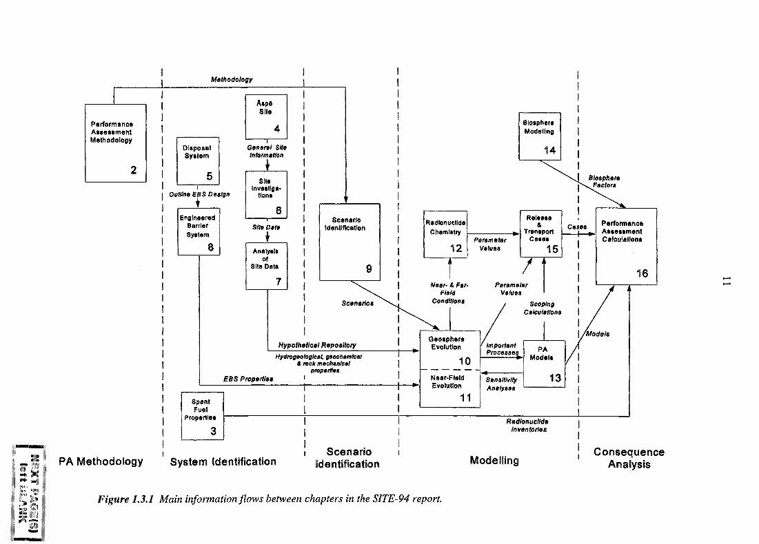
The report contains descriptions of a large number of inter-related pieces of work, andanother way of looking at its structure is to consider the main information flows betweenreport chapters. These flows are shown schematically in Figure 1.3.1. For example, acentral part of the SITE-94 project involves the calculation of the evolution of the near- andfar-fields at the Aspo site in Chapters 10 and 11; this depends upon the scenarios identifiedin Section 9, information on the engineered barrier systems given in Chapter 8 and thehydrogeological, geochemical and rock mechanical models developed in Chapter 7. Theinformation obtained from these calculations is used in the studies of radionuclidechemistry in Chapter 12, defining the important processes to be modelled in the per-formance assessment models in Chapter 13 and in the definition of the release and transportcalculations to be undertaken in Chapter 15. Similarly, the performance assessmentcalculations undertaken in Chapter 16 require the models described in Chapter 13, thecalculation^ cases defined in Chapter 15, the biosphere factors calculated in Chapter 14and various detailed items of information including the radionuclide inventories given inSection 3.
For readers who wish to study particular parts of the SITE-94 project and who do not wishto read the whole report, Figure 1.3.1 can be used to help indicate the relevant chapters andtheir inter-relationships.
PerformanceAssessmentMethodology
Methodology
DisposalSystem
Outline EBS Design
EngineeredBarrierSystem
8
RadlonuctldeChemistry
12
Near- & Far-Field
Conditions
Hydrogeologlcal, geochemlcal& rock mechanical
propertiesEBS Properties '
SpentFuel
Properties
GeosphereEvolution
Near-ReidEvolution
BiosphereModelling
14
| BiosphereFactors
ParameterValues
ScopingCalculations
SensitivityAnalyses
PAModels
13
RadlonuclldeInventories
PA Methodology System IdentificationScenario
PerformanceAssessmentCalculations
16
ConsequenceAnalysis
Figure 1.3.1 Main information flows between chapters in the SITE-94 report.
13
2 PERFORMANCE ASSESSMENTMETHODOLOGY
Performance Assessment (PA) provides a basis for decisions on issues related to repositorysafety. The demands on Performance Assessment may differ among the parties involvedin the development and siting of a repository, but common to all is that PA is a tool to helpdecision makers. PA should thus be open to scientific review and fulfill stringent criteriafor scientific and technical quality. However, when it comes to the focus of PA, it servesthe need of the decision maker, not the scientific community. These aspects are kept inmind when developing the SITE-94 Performance Assessment Methodology, outlined in thepresent chapter.
Owing to the fact that development of Performance Assessment methodology is part of theSITE-94 project objectives, all aspects of the methodology described in this chapter are notapplied in full in SITE-94. However, the principle aspects of the methodology are appliedand shown to work.
2.1 SAFETY REQUIREMENTS AND ACCEPTANCECRITERIA
The general safety objective for SKI's nuclear waste regulatory programme, as specifiedby the government in their annual Letter of Appropriation, is that spent nuclear fuel andnuclear waste should be emplaced in a disposal system that aims at containing theradioactive substances indefinitely and where the potential for releases of those that cannotbe contained is below acceptable levels. When assessing safety, Performance Assessmentresults are related to general performance criteria and safety requirements.
2.1.1 General Performance Criteria for the Repository
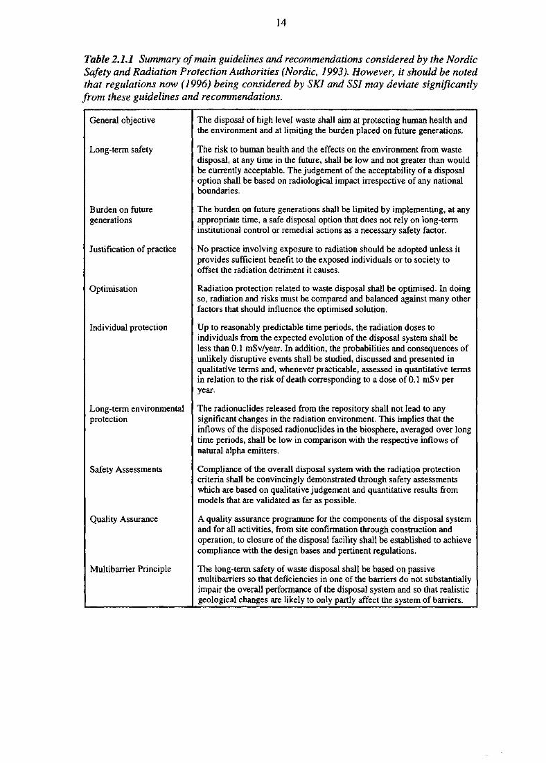
The Nuclear Safety and Radiation Protection authorities in Sweden are currently developingregulations for the disposal of spent nuclear fuel and other nuclear waste. These regulationswill build on the general safety and radiation protection requirement in the Act of NuclearActivities (SFS 1984:3) and the Radiation Protection Act (SFS 1988:220). Although theregulations are still in a developing stage, considerable guidance can be obtained from adocument issued by The Nordic Safety and Radiation Protection Authorities (Nordic,1993). This document considers criteria for disposal of high-level nuclear waste. As abackground its main guidelines and recommendations are summarised in Table 2.1.1.However, it must be clearly stated that the regulations which finally will be adopted by theSwedish authorities may deviate significantly from some of these guidelines andrecommendation s.
14
Table 2.1.1 Summary of main guidelines and recommendations considered by the NordicSafety and Radiation Protection Authorities (Nordic, 1993). However, it should be notedthat regulations now (1996) being considered by SKI and SSI may deviate significantlyfrom these guidelines and recommendations.
General objective
Long-term safety
Burden on futuregenerations
Justification of practice
Optimisation
Individual protection
Long-term environmentalprotection
Safety Assessments
Quality Assurance
Multibarrier Principle
The disposal of high level waste shall aim at protecting human health andthe environment and at limiting the burden placed on future generations.
The risk to human health and the effects on the environment from wastedisposal, at any time in the future, shall be low and not greater than wouldbe currently acceptable. The judgement of the acceptability of a disposaloption shall be based on radiological impact irrespective of any nationalboundaries.
The burden on future generations shall be limited by implementing, at anyappropriate time, a safe disposal option that does not rely on long-terminstitutional control or remedial actions as a necessary safety factor.
No practice involving exposure to radiation should be adopted unless itprovides sufficient benefit to the exposed individuals or to society tooffset the radiation detriment it causes.
Radiation protection related to waste disposal shall be optimised. In doingso, radiation and risks must be compared and balanced against many otherfactors that should influence the optimised solution.
Up to reasonably predictable time periods, the radiation doses toindividuals from the expected evolution of the disposal system shall beless than 0.1 mSv/year. In addition, the probabilities and consequences ofunlikely disruptive events shall be studied, discussed and presented inqualitative terms and, whenever practicable, assessed in quantitative termsin relation to the risk of death corresponding to a dose of 0.1 mSv peryear.
The radionuclides released from the repository shall not lead to anysignificant changes in the radiation environment. This implies that theinflows of the disposed radionuclides in the biosphere, averaged over longtime periods, shall be low in comparison with the respective inflows ofnatural alpha emitters.
Compliance of the overall disposal system with the radiation protectioncriteria shall be convincingly demonstrated through safety assessmentswhich are based on qualitative judgement and quantitative results frommodels that are validated as far as possible.
A quality assurance programme for the components of the disposal systemand for all activities, from site confirmation through construction andoperation, to closure of the disposal facility shall be established to achievecompliance with the design bases and pertinent regulations.
The long-term safety of waste disposal shall be based on passivemultibarriers so that deficiencies in one of the barriers do not substantiallyimpair the overall performance of the disposal system and so that realisticgeological changes are likely to only partly affect the system of barriers.
15
2.1.2 Technical Criteria
Safety requirements and acceptance criteria set up demands for the performance of thedisposal system as a whole. In a licensing process, they are the principles that guide thedecision on repository safety. However, they are not operational, i.e. there are noinstructions on how they should be turned into verifiable criteria for the performance ofspecific components of a specific repository at a specific site. Verifiable criteria, ortechnical criteria, are criteria that can be proven to be satisfied or not satisfied through afinite series of physical operations such as testing, observations and experiments. Examplesof technical criteria would be acceptable ranges of chemical parameters for the site ormaximum size of grains in the copper canister.
The technical criteria are of great importance in specifying the requirements on therepository components in the licensing process. They may also provide important guidancein concept development and siting processes. They will, however, be site and conceptspecific and cannot necessarily be transferred between sites or concepts. In addition, theymust never be dissociated from total system performance. Experience shows that too greata reliance on technical criteria may be counter-productive.
The safety of the repository is based on the multibarrier concept. The criteria for onecomponent cannot be specified without considering the functions of other components, i.e.the total safety of the repository cannot be compartmentalised. This raises the questionabout the links between the general safety requirements and acceptance criteria on the onehand and technical criteria on the other hand. Even if an extended discussion on thesematters lies outside the scope of SITE-94, it is important to recognise that PerformanceAssessment techniques and results have an important role if such a linking is to besuccessful. PA is not used only for assessing the overall safety of the system, but also toassess the relevance of proposed technical criteria for safety requirements and consistencywith acceptance criteria.
Although a detailed description of the legal situation lies outside the scope of SITE-94, itis necessary to re-emphasise the different roles of the regulatory authorities and theimplementor. As already mentioned, Swedish legislation states that it is the soleresponsibility of the waste producer to provide the means for safe disposal of nuclear wasteand to demonstrate that the suggested solutions are safe, whereas the authorities formulategeneral safety requirements (based on the legislation) as well as making sure that thesolutions suggested by industry are indeed safe.
Accordingly, it is not the role of SKI to formulate technical criteria, as this would restrictthe design options available to the implementor. However, SKI needs to make sure that theimplementor develops feasible and justified technical criteria. SKI should be able to answerthe question as to whether technical criteria suggested by the waste producer will complywith the general safety requirements. It is also foreseen that the implementor will discusstechnical criteria during different phases of the development work. At present (1995) suchdiscussions are part of the SKI guidance to SKB when evaluating their research anddevelopment programme, but more detailed discussions are expected during the pre-licensing and licensing process. Eventually, technical criteria will form a background tostipulations in a potential license for a repository. Consequently, the PerformanceAssessment of SITE-94 will not address technical criteria, but the results may potentially

16
be used for discussing safety aspects of the different repository barriers. This is covered inpart in the concluding assessment of Chapter 17.
2.2 PERFORMANCE ASSESSMENT ELEMENTS
The previous section pointed out some design and regulatory decisions for which PAprovides a basis. They include overall safety of the repository at a specific site andverifiable technical criteria as a means of ensuring that safety is maintained. A decisionmaker involved directly in the actual design of a repository would need other foci for PA,such as a detailed hydrological description to decide on alternative layouts of canisterpositions. Decisions on alternative technical concepts for a repository need yet another typeof PA, with a broad scope.
2.2.1 Output from a Performance Assessment
The idea common to all versions of PA is to describe the repository and its surroundingenvironment as an integrated system in order to evaluate circumstances under whichradionuclides disposed in the repository may be released and transported to the environmentand to people. The problem is complicated by the fact that the state of the system, as wellas its future evolution, is subject to uncertainty. Therefore, treatment of uncertainty andmodels for description of complex systems have prominent positions in PA methodology.These two issues are discussed in Sections 2.3 and 2.4.
A PA decision basis is structured according to the needs of the decision maker. A typicalbasis may include:
• a description of how the system constituting the repository and its surroundingenvironment may evolve in time and how that affects radionuclide release andtransport,
• a description of how the system may release and transport radionuclides as afunction of time,
• estimates of various safety indicators, such as potential radiation doses or risks ofadverse health effects to individuals or groups of people over different periods oftime in the future in a deterministic or a probabilistic framework,
• ranking of factors that contribute negatively to (enhance) radionuclide release andtransport,
• ranking of different design or siting options.
17
2.2.2 Systems Analysis Approach to Performance Assessment
In order to provide the desired decision basis, it should be recognised that a PerformanceAssessment is a systems analysis and, as such, can be performed on different analysislevels. The SITE-94 the analysis levels are:
• LEVEL 1: System Identification and Definition• LEVEL 2: Scenario Definition
LEVEL 3: Model Selection• LEVEL 4: Consequence Analysis
Each level involves different activities and has its own associated types of uncertainty. Thetreatment of the four analysis levels and the associated categories of uncertainty withinSITE-94 is thoroughly discussed by Chapman et al. (1995) and is outlined in the followingsections.
2.2.3 System Identification
2.2.3.1 General
Identifying the relevant system, or System Identification, is an important initialising activityin using systems engineering methods for problem solving. PA uses such methods toinvestigate the behaviour of a complex of natural and engineered components which are leftunmanaged to interact with each other over a long period of time. System Identificationinvolves defining the boundary of the relevant system and identifying the componentswithin the system boundary and their relations among themselves and to the systemenvironment (see, for instance, Churchman, 1968; Flood and Carson, 1988). Everythingoutside the system boundary, by definition, belongs to the system environment.
System Identification is called an 'initialising activity' in order to indicate that, althoughit seems a natural starting point for a formal PA, it is an ongoing process which leads tomore stringent identification of the relevant system. Defining the system boundary requiresconsiderable knowledge about both the problem and the system and appropriatemethodological tools. In most earlier studies, system identification has been informal andimplicit through the selection of analysis models.
In SITE-94, system identification is a formalised, defensible level of analysis. Thisimproves the control over model linking, model use and scenario generation. FormalisedSystem Identification is possible through two methodological landmarks: the use ofFeatures Events and Processes (FEPs) to define the Process System (SKI, 1991) andintroducing a Process Influence Diagram (PID) to identify relations (Sumerling et al.,1993).
The conceptual basis for the System Identification in SITE-94 is that the repository can bedescribed as a system of interdependent FEPs (Cranwell et al, 1990) that directly, orindirectly, influence the release and transport of radionuclides from the repository to theenvironment and to man. Following the vocabulary introduced in Project-90 (SKI, 1991),
18
the system is called the Process System (PS). The list of FEPs explicitly included in theProcess System then defines the system boundary. The ambition in SITE-94 is to describe,and include in the analysis on the modelling level, all internal FEPs and theirinterdependencies. Outside the Process System, only those FEPs which directly influencethe Process System will be described. Such FEPs are called External FEPs (EFEPs).
The primary interest in the analysis is to determine the evolution of the Process System. Thesystem may evolve as a consequence of processes within the Process System, but also asa consequence of direct influences from the external FEPs. This implies that the SystemIdentification with the definition of the Process System will affect the classification andtreatment of uncertainty. This aspect is elaborated further in Section 2.3.
2.2.3.2 The System Boundary
It is very important to set a clear system boundary. The appropriate size of the system isdecided by the PA analyst, based on the specific purpose of the assessment. It is importantthat the setting of the boundary is openly documented and reviewed from differentperspectives, for example:
• Legal and other pre-specified requirements: Clearly, analyses can only be made forthe part of system contained within the system boundaries. This factor may influencethe time frames studied, the need for biosphere modelling, sub-system analyses (e.g.the US subsystem criteria, 10CFR60), etc.
• Defensibility of analysis: Even if predictions are only needed for a limited system,it may be a strong motivation to analyse a larger system, as the part of the systemwhere predictions are needed will be less sensitive to external influence or tocorrelations between external FEPs.
• Complexity of the analysis: A large system is obviously more complex and containsa large number of internal uncertainties.
The judgemental aspect of the placement of the system boundaries may also be illustratedby the actual choices made in different previously published assessments. For example,HMIP in the UK have advocated full integration of the future climate evolution in theanalysis (Sumerling, 1992). The TVO-92 assessment (TVO, 1992) puts most of itsemphasis on the near-field and tends to treat changes in the geosphere as differentscenarios, in contrast, the SKB 91 exercise (SKB, 1992) is largely concentrated on thegeosphere and deliberately adopts a simplified source term description.
2.2.3.3 The SITE-94 Process System
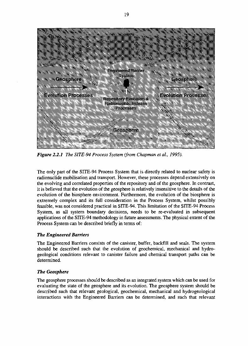
The SITE-94 Process System comprises FEPs in the geosphere and the repository, whichdirectly or indirectly affect radionuclide mobilisation and transport within these regions, asdepicted in Figure 2.2.1.
19
Figure 2.2.1 The SITE-94 Process System (from Chapman et al, 1995).
The only part of the SITE-94 Process System that is directly related to nuclear safety isradionuclide mobilisation and transport. However, these processes depend extensively onthe evolving and correlated properties of the repository and of the geosphere. In contrast,it is believed that the evolution of the geosphere is relatively insensitive to the details of theevolution of the biosphere environment. Furthermore, the evolution of the biosphere isextremely complex and its full consideration in the Process System, whilst possiblyfeasible, was not considered practical in SITE-94. This limitation of the SITE-94 ProcessSystem, as all system boundary decisions, needs to be re-evaluated in subsequentapplications of the SITE-94 methodology in future assessments. The physical extent of theProcess System can be described briefly in terms of:
The Engineered Barriers
The Engineered Barriers consists of the canister, buffer, backfill and seals. The systemshould be described such that the evolution of geochemical, mechanical and hydro-geological conditions relevant to canister failure and chemical transport paths can bedetermined.
The Geosphere
The geosphere processes should be described as an integrated system which can be used forevaluating the state of the geosphere and its evolution. The geosphere system should bedescribed such that relevant geological, geochemical, mechanical and hydrogeologicalinteractions with the Engineered Barriers can be determined, and such that relevant
20
transport paths and transport processes of both near-field and far-field geosphere aredetermined in space and time.
The Biosphere
In principle, biosphere processes could be described as an integrated system to be used forevaluating the state of the biosphere and its evolution, as has been developed within theBIOMOVS n project (BIOMOVS XT, 1994). SITE-94 has adopted a simplified descriptionof the biosphere. For evaluation of radionuclide transport, the boundary of the generalProcess System was set at the interface between the far-field rock and the biosphere.However, a few biosphere phenomena were identified as having direct impacts oncomponents of the Process System, and were consequently included within it. Furthermore,a few biosphere pathways (Chapter 14) have been evaluated in order to calculate doses fromthe calculated releases.
Near-field Transport
Near-field transport describes the transport of radionuclides from the spent fuel in near-field(fuel dissolution, etc.) to the near-field interface with the far-field. The near-field transportincludes transport in the near-field geosphere, i.e. the part of the geosphere which is directlyinfluenced by the existence of the repository.
Far-field Transport
Far-field transport describes the transport of radionuclides from the near-field interface tothe biosphere interface or other relevant endpoints.
2.2.4 Scenario Identification
The definition of a scenario has to be made in relation to the definition of the system.Chapman et al. (1995) discuss various approaches to scenario identification and treatment.In SITE-94, the concept of the Process System, introduced by Andersson et al. (1989), hasbeen used to generate 'top-down' scenarios by letting Features, Events and Processesoutside the Process System (EFEPs) act on the Process System. The attached EFEP, or aset of EFEPs and the consequential development of the Process System, then constitutesa scenario and the EFEPs are thus scenario-generating elements.
When an EFEP acts on the Process System, the interaction is spread through different FEPsand links in the Process System. For example, the EFEP permafrost directly affectstemperature, which in turn affects water mobility (ultimately the water will freeze), etc.Such interactions may eventually be modelled. In addition, by attaching an EFEP onto theProcess System, FEPs and links in it which were thought to be of little importance (e.g.freezing of water) may change in importance. The SITE-94 experiences in applying thistechnique to the Process Influence Diagram are discussed in Section 2.4.
21
2.2.5 Model Selection and Consequence Analysis
Models are tools that can provide quantitative numbers in an assessment. Evidently, modelselection implies identification or development of models, identification of differentsources of information, as well as the establishment of the information transfer betweenthese in a manner that reflects the defined system and its evolution. Consequence analysisimplies the selection of input numbers for the models and subsequent quantitative analysis.In practice, and traditionally, most of the effort in a Performance Assessment, includingSITE-94, is devoted to these two analysis levels.
An important example of model selection concerns site evaluation and the selection ofstructure models. This step should be formally separated from assigning parameter valuesfor a given site structure model, which is part of the consequence analysis.
2.3 TREATMENT OF UNCERTAINTIES AT THE DIFFERENTANALYSIS LEVELS
There are many uncertainties associated with a Performance Assessment. Uncertainties cannever be avoided but if a PA is to serve as a useful decision basis, it is necessary to identifyuncertainties, clarify, quantify and reduce them as far as possible, and put them intoperspective. In treating uncertainties, it is important to realise that there are different kindsof uncertainties and that these differences may affect how the uncertainty should be treatedin the assessment as well as the impact it will have on the decision basis.
2.3.1 Classification of Uncertainty
2.3.1.1 Categories of Uncertainties
In the nuclear waste community, it is common to distinguish between scenario uncertainty,conceptual model uncertainty and parameter uncertainty. The three categories reflect thethree levels of analysis usually employed in Performance Assessment: measuring/evaluatingthe properties of the components of the Process System (parameter uncertainty),representing and modelling the components and their relations (conceptual modeluncertainty), and speculation about external influences on the modelled components andrelations (scenario uncertainty). The distinction between these kinds of uncertainties is notalways clear, depending on how well an analysis manages to uphold the hierarchy ofanalysis levels. However, it is important to be able to associate one category of uncertainteswith each level of analysis. The terminology (language) and activities used to obtain andprocess information is distinctly different for each level. The categories of uncertainty mustbe sufficiently well-defined to reflect these differences.
Two comments should be made about classification according to analysis levels in thePerformance Assessment. First, if more levels of analysis are needed, it is necessary toextend the set of uncertainty categories. For this reason, SITE-94 introduces the concept ofsystem uncertainty, which is the uncertainty in the System Identification concerning whichFEPs and influences inside the system boundary really need to be considered. This will be
22
further discussed in Section 2.3.2. Second, an uncertainty may be re-interpreted at anotherlevel of analysis. For example, uncertainty about rock permeability (parameter uncertainty)may be re-interpreted as conceptual model uncertainty (porous medium or channelnetwork). Such re-interpretations are to be expected in a hierarchical analysis and re-emphasise the need to record and track the origins of uncertainty within each differentanalyses level. For example, two different conceptual models may produce the same resultin a certain application, but may yield very different results in another.
2.3.1.2 Completeness
A general uncertainty underlying all analyses is the problem of completeness, i.e. 'have wethought of everything?'. The completeness problem exists for all four types of uncertaintydiscussed above. It is particularly evident for scenario uncertainty, as it is impossible toprove that all relevant EFEPs that directly influence the Process System have beenidentified, but completeness is also an issue inside the system. On a system descriptionlevel, the completeness concerns whether all relevant FEPs, and links between FEPs, havebeen identified. With regard to the conceptual model uncertainty level, completenessconcerns the possible existence of unidentified, alternative conceptual models. At theparameter uncertainty level, there is always an uncertainty as to whether the parameterranges consider all the desired uses of the model in question.
In treating the completeness problem, it should be made absolutely clear that it isimpossible to reach completeness in an absolute sense. This lack of absolute proof isgeneral to most decision making problems, but should, of course, always be made veryclear to all decision makers. As stated earlier, Performance Assessments are conducted inorder to assist decisions. The primary ambition level in a Performance Assessment withregard to completeness is thus to facilitate the judgement as to whether more efforts areneeded in order to support the decision. Within SITE-94, it is believed that traceable andwell-documented procedures for handling uncertainties are important in this respect.Clearly, any assessment should also have the ambition to reduce the incompleteness, butthe question of how much effort is needed for this is always judgemental.
2.3.1.3 Quantification
Another important aspect of uncertainty is whether it can be quantified and how.Performance Assessment should be used to prepare a decision basis by putting differentuncertainties into perspective. This is clearly facilitated if the uncertainties are quantified,as this provides a means of at least ranking different problems. A simple example of aquantified uncertainty is a frequentistic-based probability of canister failure during a certaintime period (even though difficult to estimate). A more complex uncertainty is a 'degree-of-belief that a certain feature in the rock mass exists or that certain chemical processes willoccur in the near-field. In this case it may, for example, be irrelevant to discuss meanvalues. Consequently, care must be taken when propagating impacts of uncertainty throughan assessment, such that the relevant aspects of the uncertainty are maintained.
When dealing with several uncertain quantities, it is also necessary to treat properly theissue of statistical dependence or correlations. For example, if a postulated fracture zone
23
exists in the rock or if particular chemical processes do occur, this may have directimplications on the status of other uncertain phenomena in the repository system. Omittingstatistical dependence can have dramatic impacts on estimates of the likelihood of coupledevents and phenomena.
It should also be noted that many geosphere properties (in particular) show considerablespatial variability and that many processes or conditions will change with time. However,variability is not uncertainty—it is a property of the system. It does, however, often makeit difficult to evaluate measurements, thus contributing to overall uncertainty.
2.3.1.4 Approach to Treatment of Uncertainties
The SITE-94 approach to uncertainty, including the completeness problem, is to developa methodology for the systematic use of expert judgement for identification purposes andto document these judgements in a traceable and transparent form which would allow forreview and potential updates of decisions made. Furthermore, the way an uncertainty isdescribed, as well as its correlation with other phenomena, both affect how to estimate theuncertainty and how to propagate the impact of the uncertainty through the assessment.Consequently, the Performance Assessment Methodology has to acknowledge these factsand treat them properly. In developing and adopting a methodology for system analysis,scenario development and treatment of uncertainty within SITE-94, the ambition is toadvance the capability of handling these matters by:
• Developing a new technique for System Identification through expert judgement (theProcess Influence Diagrams) which allows for a systematic search for systemcomponents (FEPs) and their couplings as well as making it possible to handle awide system boundary.
• Adopting procedures for reflecting expert opinion on the importance of differentFEPs and their interactions. This contributes to a quantification of the systemuncertainty, although not in a frequentistic sense.
• Developing a new technique for describing the quantitative modelling of theevolution of the Process System (the Assessment Model Flowchart) that can berelated to the Process Influence Diagram and which provides a framework forpropagating uncertainties in a manner that ensures that the known dependencies areproperly treated.
These techniques are described in Section 2.4. In developing this approach, the concept ofa Performance Assessment involving a number of levels of analysis, as discussed above,was adopted.
2.3.2 System Uncertainty
System uncertainty is the uncertainty in the System Identification, made in a specificProcess Influence Diagram. It refers to the fact that the Process System is not fully known:

24
FEPs may be missing in the PED, improperly linked to other FEPs, or the importance of alinking may be misjudged.
The need to introduce system uncertainty arises from the wide system boundaries adoptedin SITE-94. Many of the features, events and processes that in earlier studies wereconsidered as generators of scenario uncertainties, are now found inside the ProcessSystem. This makes it easier to test and document hypotheses about causes andconsequences of different uncertainties but at the price of a new category of uncertainty tohandle. Formally, it could also be argued that one category of uncertainty should beassociated with each level of analysis. A more thorough elaboration on this is given byChapman etal. (1995).
Assessment of system uncertainty is clearly subjective. Much system uncertainty is non-quantifiable and can only be treated by open documentation and expert judgement.However, once a system is documented, such as the PID in SITE-94, it is open tosystematic expert review, as described in more detail in Section 2.4. Experts can provideanswers to the question of how many FEPs and links must be considered by assessing howunreasonable it would be to ignore a specific link or FEP. This does not allow for acategorisation of influences in terms of probabilities, but rather in terms of possibilities. Assuch, the rules for combining separate decisions to produce a final categorisation are thoseof fuzzy set theory. Specifically, the category assigned to a combination of separate choicesis the widest category of the component choices.
2.3.3 Scenario Uncertainty
For the sake of simplicity, the definition of scenario uncertainty adopted in SITE-94 is theuncertainty related to the EFEPs. This uncertainty concerns both the completeness problem(concerning whether all relevant EFEPs have been found) as well as different quantitativemeasures of the EFEP, such as the quantification of the impact at the system boundary andprobability of occurrence. The SITE-94 approach to identifying EFEPs is discussed inSection 2.4 and Chapter 9. It is evident that much uncertainty still remains, even afterprecise definition of the EFEPs, since the Process System is subject to system uncertainty,its models are subject to conceptual model uncertainty and the parameters may be subjectto parameter uncertainty.
When modelling the scenario generated by the EFEP, the EFEP needs to be quantified. Thequantification concerns both different measures of likelihood for the EFEP, such asestimates of when the EFEP will occur over a certain time period, as well as quantitativeestimates of the magnitude of the impact. For permafrost, an example of the latter could beestimates of surface temperature as a function of time. The quantified model of the EFEPcan then be attached to the different quantitative models that describe the Process System.Application of this technique within SITE-94 is discussed in Section 2.4.
The Process System will evolve internally without changes in the environment to theProcess System, as the system itself contains many evolving processes. This warrantsanalyses of a Reference Case, which concerns how the system evolves 'internally' (seefurther discussion in Chapter 9). In fact, the wide system boundaries adopted in SITE-94are chosen in order to make the system relatively insensitive to outside disturbances, even
25
if major external changes may have an impact on the system. The wide system boundariesmay consequently minimise the scenario uncertainty, but at the price of increased systemuncertainty.
2.3.4 Conceptual Model Uncertainty and Validation
A model of a process, group of processes, or of the behaviour of a particular region of therepository, represents one or several FEPs and their links in the PID. Conceptual modeluncertainty is connected with model validation, but includes more than uncertainty aboutwhether a model is properly validated or not. Conceptual model uncertainty also concernswhether all relevant processes have been identified.
Model validation should answer the question: how well do the proposed relationshipsbetween physical entities describe (predict) phenomena in the real world? A model isvalidated by proving that it has been properly derived from natural laws or previouslyvalidated models, or by comparison of model results with experiments and observations.It is useful to view the result of validation, not as proving that the model is true or false, butas establishing the applicability of the model. That is, we interpret the expression 'Howwell...' in the validation question as meaning 'Under what circumstances ...'.
Model validation is an iterative process, progressively testing and refining the applicabilityof models and is, consequently, always provisional. It depends on the experiments andobservations that have made to date. New experiments or observations may reduce theapplicability of the model or the model from which it has been derived. There are alsoexamples where successful models have increased their applicability. For the presentdiscussion, it can be concluded that there is always some validation uncertainty about theproper range of application of a model. The reader is also referred to the SKI/NRC staffposition paper on validation (Eisenberg et al., 1994) and the conclusions from theinternational INTRAVAL project (NEA/SKI, 1996), which advocate similar ideas.
Validation of alternative conceptual models may show that they have overlapping rangesof application. That is, although the models propose alternative relations and alternativemeasurable entities, they describe the relevant experiments or observations equally well.The alternative models may seem mutually exclusive but, with available experiments andobservations, it is not possible to rule any of them out. Assume that the models canrepresent the same FEPs in the Process System. If they always produce similarconsequences for the Process System, the apparent uncertainties in validation of thesemodels do not give rise to any conceptual model uncertainty. However, if the models yielddifferent results, there is a genuine case of conceptual model uncertainty.
Conceptual model uncertainty due to model overlap is generated by the models and the lackof precision in their validation, that is, it originates at the modelling level of analysis. Thereis also a type of conceptual model uncertainty which is a re-interpretation of systemuncertainty. Instead of an uncertainty about whether a model can be applied under thespecified conditions, there may be uncertainty about the conditions themselves. This maylead to uncertainty about the applicability of a model, in spite of very precise validation.Such a situation may occur when there is uncertainty about FEPs or links within the areaof the PID represented by the model, or about links to this area.
26
An important example of conceptual model uncertainty originates from site evaluation,where there is often uncertainty about the relevant geological structure models. In STTE-94,such conceptual model uncertainty is, to a large extent, treated by formulating alternativeconceptual site models (such as a discrete or a continuum representation of geometry). Inother instances, the conceptual model uncertainty is treated by selecting 'conservative'models.
2.3.5 Parameter Uncertainty and Variability
Parameter uncertainty refers to parameters with unknown values, but where a unique valuecould, in principle, be inferred from measurements or observations. The definition of theparameter is usually model dependent. If conceptual model uncertainty exists, thispropagates and is re-interpreted on the measurement level.
Parameter uncertainty has been extensively investigated in radioactive waste programmesin Canada, Sweden, the UK and elsewhere (see, for example, Goodwin et al, 1994a).Usually, the parameter uncertainties are described by distribution functions and theconsequences for the Process System are calculated using a range of values sampled fromthe distribution, in some instance using Monte Carlo technique.
Parameter uncertainty should not be confused with parameter variability. In the formercase, the parameter has a single, but unknown value; in the latter case, the parameteractually has different values depending on space and time. The probability of finding aspecific value is given by a distribution function. Variability is not uncertainty but aproperty of a component or of the system. In general, however, variability increasesparameter uncertainty.
2.3.6 Propagation of Uncertainties
The overall aim of treating uncertainties in SITE-94 is to follow their effects through theProcess System. Figure 2.3.1 illustrates the methodology chosen. As it is important toquantify the role of uncertainties, their propagation through models and chains of modelsis of primary interest. The propagation of uncertainties has to be followed in twodimensions: in the logical space set up by the four levels of analysis described above(systems analysis, scenario analysis, model development/selection and consequenceanalysis), and in the Process System itself. In order to avoid double-counting the effects ofuncertainty, it is necessary to keep track both of the level of origin (or source level) of aparticular uncertainty and the re-interpretation of the uncertainty on the subsequent levelsof analysis. Such a tracking is also necessary to handle correlations between differentuncertainties.
On the System Identification level, all uncertainties originate from the identification of therelevant system through the Process Influence Diagram. But for each of the other threelevels, there are two types of uncertainties: those which originate on the level and thosewhich are re-interpretations of uncertainties from previous levels. Propagation through theProcess System can be followed on those levels where there is a complete representation
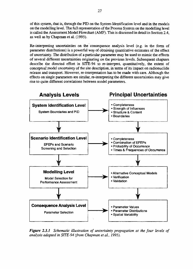
27
of this system, that is, through the PID on the System Identification level and in the modelson the modelling level. The full representation of the Process System on the modelling levelis called the Assessment Model Flowchart (AMF). This is discussed in detail in Section 2.4,as well as by Chapman et al. (1995).
Re-interpreting uncertainties on the consequence analysis level (e.g. in the form ofparameter distributions) is a powerful way of obtaining quantitative estimates of the effectof uncertainty. The distribution of a particular parameter may be used to mimic the effectsof several different uncertainties originating on the previous levels. Subsequent chaptersdescribe the directed effort in SITE-94 to re-interpret, quantitatively, the extent ofconceptual model uncertainty of the site description, in terms of its impact on radionucliderelease and transport. However, re-interpretation has to be made with care. Although theeffects on single parameters are similar, re-interpreting the different uncertainties may giverise to quite different correlations between model parameters.
Analysis Levels
System Identification LevelSystem Boundaries and PID
Principal Uncertainties
CompletenessStrength of InfluencesStructure & ContentBoundaries
Scenario Identification LevelEFEPs and Scenario
Screening and Selection>-
• Completeness• Combination of EFEPs• Probability of Occurrence• Times & Frequencies of Occurrence
Modelling LevelModel Selection for
Performance Assessment
Consequence Analysis Level
Parameter Selection
1 Alternative Conceptual Models1 VerificationValidation
\
Parameter ValuesParameter DistributionsSpatial Variability
Figure 2.3.1 Schematic illustration of uncertainty propagation at the four levels ofanalysis adopted in SITE-94 (from Chapman et al., 1995).
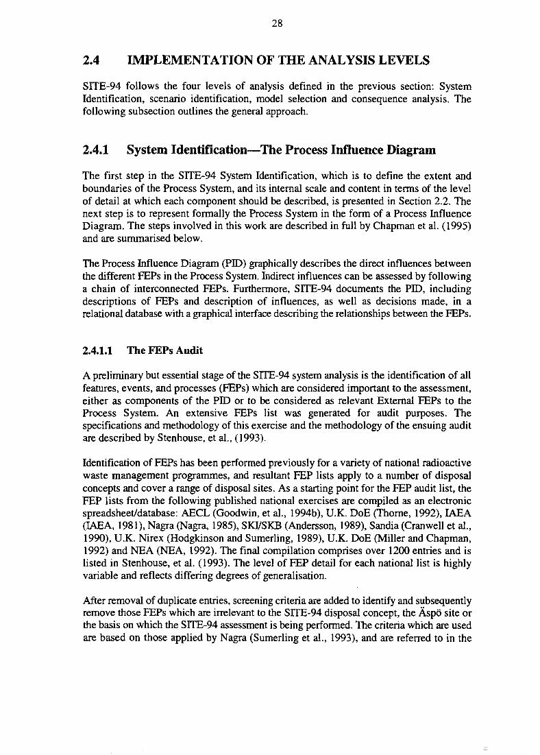
28
2.4 IMPLEMENTATION OF THE ANALYSIS LEVELS
SITE-94 follows the four levels of analysis defined in the previous section: SystemIdentification, scenario identification, model selection and consequence analysis. Thefollowing subsection outlines the general approach.
2.4.1 System Identification—The Process Influence Diagram
The first step in the SITE-94 System Identification, which is to define the extent andboundaries of the Process System, and its internal scale and content in terms of the levelof detail at which each component should be described, is presented in Section 2.2. Thenext step is to represent formally the Process System in the form of a Process InfluenceDiagram. The steps involved in this work are described in full by Chapman et al. (1995)and are summarised below.
The Process Influence Diagram (PID) graphically describes the direct influences betweenthe different FEPs in the Process System. Indirect influences can be assessed by followinga chain of interconnected FEPs. Furthermore, SITE-94 documents the PID, includingdescriptions of FEPs and description of influences, as well as decisions made, in arelational database with a graphical interface describing the relationships between the FEPs.
2.4.1.1 The FEPs Audit
A preliminary but essential stage of the SITE-94 system analysis is the identification of allfeatures, events, and processes (FEPs) which are considered important to the assessment,either as components of the PID or to be considered as relevant External FEPs to theProcess System. An extensive FEPs list was generated for audit purposes. Thespecifications and methodology of this exercise and the methodology of the ensuing auditare described by Stenhouse, et al., (1993).
Identification of EEPs has been performed previously for a variety of national radioactivewaste management programmes, and resultant FEP lists apply to a number of disposalconcepts and cover a range of disposal sites. As a starting point for the FEP audit list, theFEP lists from the following published national exercises are compiled as an electronicspreadsheet/database: AECL (Goodwin, et al., 1994b), U.K. DoE (Thome, 1992), IAEA(IAEA, 1981), Nagra (Nagra, 1985), SKI/SKB (Andersson, 1989), Sandia (Cranwell et al.,1990), U.K. Nirex (Hodgkinson and Sumerling, 1989), U.K. DoE (Miller and Chapman,1992) and NEA (NEA, 1992). The final compilation comprises over 1200 entries and islisted in Stenhouse, et al. (1993). The level of FEP detail for each national list is highlyvariable and reflects differing degrees of generalisation.
After removal of duplicate entries, screening criteria are added to identify and subsequentlyremove those FEPs which are irrelevant to the SITE-94 disposal concept, the Aspo site orthe basis on which the SITE-94 assessment is being performed. The criteria which are usedare based on those applied by Nagra (Sumerling et al., 1993), and are referred to in the
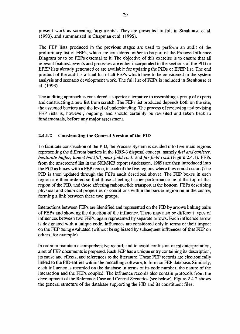
29
present work as screening 'arguments'. They are presented in full in Stenhouse et al.(1993), and summarised in Chapman et al. (1995).
The FEP lists produced in the previous stages are used to perform an audit of thepreliminary list of FEPs, which are considered either to be part of the Process InfluenceDiagram or to be FEPs external to it. The objective of this exercise is to ensure that allrelevant features, events and processes are either incorporated in the sections of the PID orEFEP lists already generated or are available for updating the PIDs or EFEP list. The endproduct of the audit is a final list of all FEPs which have to be considered in the systemanalysis and scenario development work. The full list of FEPs is included in Stenhouse etal. (1993).
The auditing approach is considered a superior alternative to assembling a group of expertsand constructing a new list from scratch. The FEPs list produced depends both on the site,the assumed barriers and the level of understanding. The process of reviewing and revisingFEP lists is, however, ongoing, and should certainly be revisited and taken back tofundamentals, before any major assessment.
2.4.1.2 Constructing the General Version of the PID
To facilitate construction of the PID, the Process System is divided into five main regionsrepresenting the different barriers in the KBS-3 disposal concept, namely fuel and canister,bentonite buffer, tunnel backfill, near-field rock, and far-field rock (Figure 2.4.1). FEPsfrom the unscreened list in the SKI/SKB report (Andersson, 1989) are then introduced intothe PID as boxes with a FEP name, in each of the five regions where they could occur. (ThePID is then updated through the FEPs audit described above). The FEP boxes in eachregion are then ordered so that those affecting barrier performance lie at the top of thatregion of the PID, and those affecting radionuclide transport at the bottom. FEPs describingphysical and chemical properties or conditions within the barrier region lie in the centre,forming a link between these two groups.
Interactions between FEPs are identified and represented on the PID by arrows linking pairsof FEPs and showing the direction of the influence. There may also be different types ofinfluences between two FEPs, again represented by separate arrows. Each influence arrowis designated with a unique code. Influences are considered only in terms of their impacton the FEP being evaluated (without being biased by subsequent influences of that FEP onothers, for example).
In order to maintain a comprehensive record, and to avoid confusion or misinterpretation,a set of FEP documents is prepared. Each FEP has a unique entry containing its description,its cause and effects, and references to the literature. These FEP records are electronicallylinked to the PID entries within the modelling software, to form an FEP database. Similarly,each influence is recorded on the database in terms of its code number, the nature of theinteraction and the FEPs coupled. The influence records also contain protocols from thedevelopment of the Reference Case and Central Scenarios (see below). Figure 2.4.2 showsthe general structure of the database supporting the PID and its constituent files.
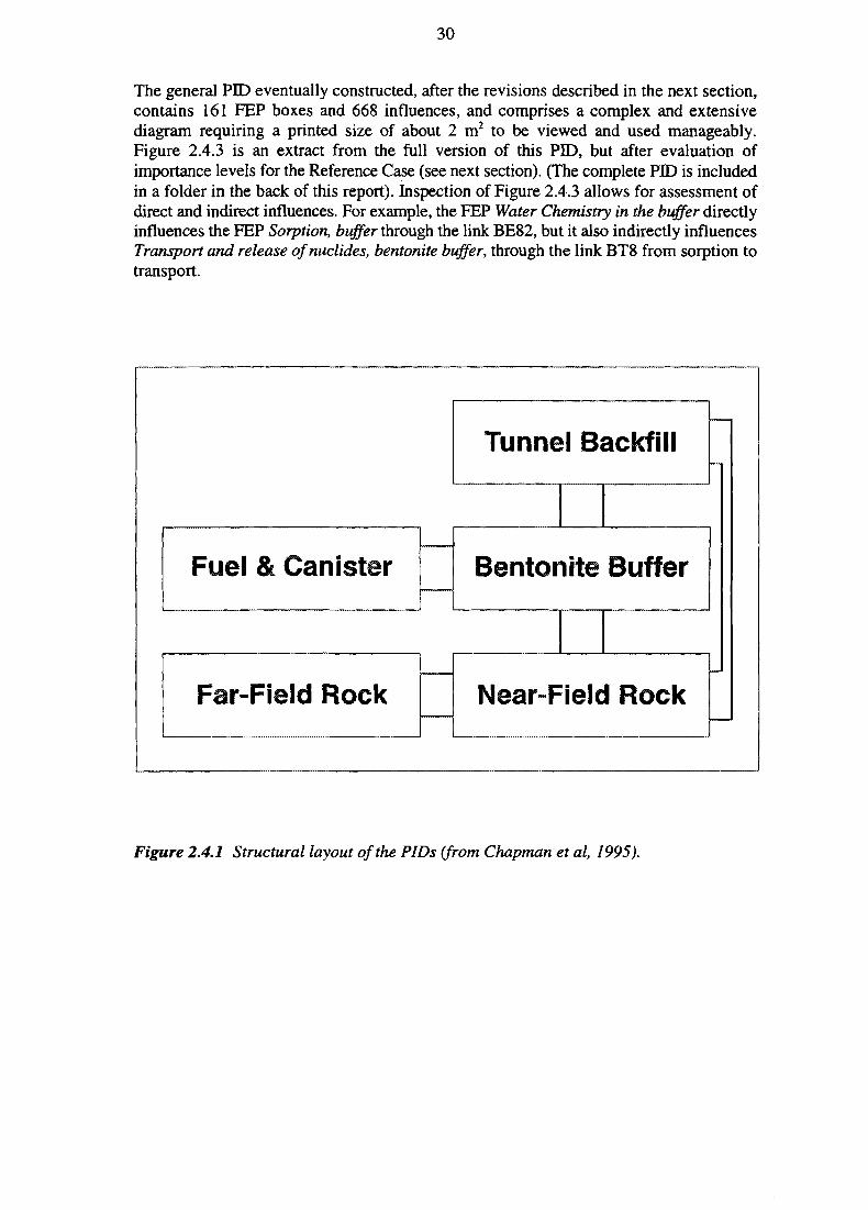
30
The general PID eventually constructed, after the revisions described in the next section,contains 161 FEP boxes and 668 influences, and comprises a complex and extensivediagram requiring a printed size of about 2 m2 to be viewed and used manageably.Figure 2.4.3 is an extract from the full version of this PID, but after evaluation ofimportance levels for the Reference Case (see next section). (The complete PID is includedin a folder in the back of this report). Inspection of Figure 2.4.3 allows for assessment ofdirect and indirect influences. For example, the FEP Water Chemistry in the buffer directlyinfluences the FEP Sorption, buffer through the link BE82, but it also indirectly influencesTransport and release ofnuclides, bentonite buffer, through the link BT8 from sorption totransport.
Fuel & Canister
Far»Field Rock
Tunnel Backfill
Bentonite Buffer
Near-Field Rock
Figure 2.4.1 Structural layout of the PIDs (from Chapman et al, 1995).
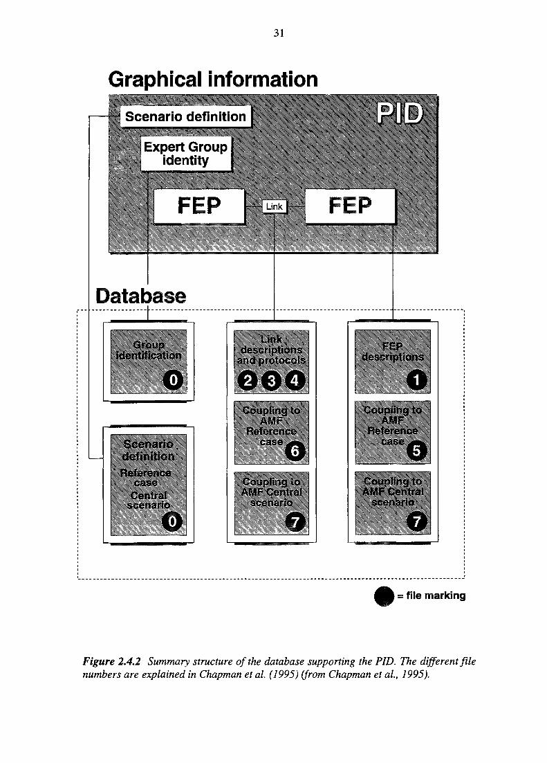
31
Graphical information
Scenario definition I
fcxpcrt Groupidentity
u
HP f FP
Database
™ file marking
Figure 2.4.2 Summary structure of the database supporting the PID. The different filenumbers are explained in Chapman et al. (1995) (from Chapman et al., 1995).
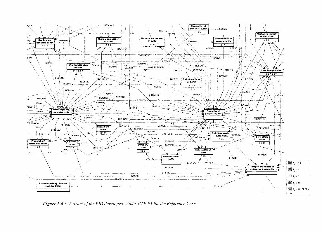
\ y \ ; iBE33<10) X \ \ • •
\ \ \ nBE35(8) X \\U(
;./i^ _ _ : BE99(10) : +~
-- BE112(2) :-
Figure 2.4.3 Extract of the PID developed within S1TK-94 for the Reference Case.
33
2.4.1.3 Importance Levels Expert Assessment of the PID and Adjustment toDifferent Scenarios
The original PID, which was developed within a very small group of people, contained alot of judgements which needed to be reviewed. Furthermore, importance levels have to beassociated with the influences between the FEPs. These revisions are made by expertjudgment as described below. However, since the importance of an influence may bescenario dependent, the scenario premises must be defined before judging the importanceof the links.
The evaluation of the importance of an influence is described with the help of importancelevels. Importance levels are obtained by asking the question whether the influence shouldbe included in the assessment or if its influence is negligible. An importance level, or IL-value, (taken as an integer in the range 0-10) is assigned to each influence. An influencewith an importance level of 10 is one which it would be completely unreasonable to ignorein an assessment. The other categories are defined as follows:
\L Value Importance of an influence on a full-system PA
10 Total loss of confidence in PA if influence is excluded.8 Considerable loss of confidence if it is not considered.6 It should be included but effect on confidence marginal.
Influences scoring below this line will normally be omitted from any assessment.
4 PA would be just acceptable without the influence.2 It may be interesting to include the influence.0 No loss in confidence in the PA if it is excluded.
In practice, the steps of reviewing the structure of the general PID are combined withassigning importance levels to the PID influences for specific scenarios. The first step inthis process is to define a Reference Case. The main purpose of the SFTE-94 ReferenceCase, which is described in Chapter 9, is to make it possible to describe the system and itsinternal couplings without a need to consider all possible EFEPs. In addition, the ReferenceCase can be seen as a means to evaluate the 'internal evolution' of the repository systemwhen it is not affected by changing external influences. The definition of the SITE-94Reference Case is that the repository is constructed according to the Design Basis, withuncertainties, that present day climate and surface environment persist indefinitely and thatthere is no human interference with the system. The SITE-94 repository system DesignBasis is defined in Chapters 3 to 8 and is not reiterated here.
Using this definition it is then possible to convert the PID for the general Process Systeminto one which describes the Reference Case. A formal symbolic notation is adopted andthis version is denoted as the PID(RF). The mechanism for making this conversion is viaa series of expert group meetings, whose objectives are to:
34
• check the structure of the diagram and the details of the influences between FEPs,thus carrying out an audit of the constructed general PHD,
• prepare the PID(RF) by attributing 'importance levels' (IL values) to each of theinfluences in the general PID for the Reference Case assumptions. This will laterallow further versions of the diagram to be produced at various levels ofsimplification, reflecting 'degrees of belief in the validity of the overall ProcessSystem model, as discussed in Section 2.3.
The basic steps in the evaluation process are to:
• check that the influences charted between each FEP are comprehensive,• add or redirect influences if necessary,• attribute IL values to each influence for the Reference Case assumptions,• record briefly the basis on which these values are attributed.
From this record, it is then possible to construct various versions of the PDD(RF) whichincorporate only those influences relevant to different IL degrees of belief. The review andauditing of the general PID and the construction of the PID(RF) effectively take placesimultaneously. The complete PID(RF) is provided in a folder at the end of this report. Amore detailed record of the procedure adopted, and other examples of PIDs, are presentedin Chapman etal. (1995).
Following the meetings, reduced versions of the PID(RF) are prepared for two importancelevels: 6 and 10, denoted PED(RF, 1^) and PID(RF, I ^ Q ) respectively. This is done simplyby removing all influences with lower IL values and all FEPs which thereby becomecompletely disconnected. These diagrams contain substantially less information than thefull PID. Whilst the full PID(RF) contains 668 influences, the PID(RF, I^6) contains 469,and the PID(RF, IU1O) only has 257, consequently being substantially more manageable.Both the PID(RF, 1^) and the PID(RF, I^10) are presented in full in Chapman et al. (1995).The same extract of the PID for the Reference Case, as shown in Figure 2.4.3 is depictedin Figure 2.4.4 for the importance level 10. A comparison of Figure 2.4.3 with Figure 2.4.4illustrates the effects of removing influences.
After identifying a set of EFEPs to form scenarios, these EFEPs need to be applied to thePID in order to check for potential changes in influence levels, etc. The implementation ofthat step is discussed in the next section and in Chapter 9.
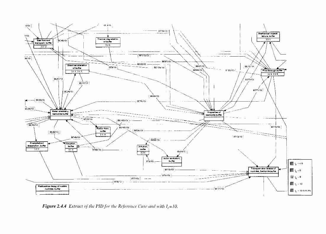
Figure 2.4.4 Extract of the FID for the Reference Case and with 1, = 10.
36
2.4.2 Scenario Identification
The principal procedures adopted in SITE-94 for identification of future external events andconditions (EFEPs) that may have a relevant impact in the analysed system are as follows.
A list of EFEPs relevant to SITE-94 is obtained through the FEPs audit described above.The FEPs audit results in 81 EFEPs listed by Stenhouse et al. (1993). As already noted byAndersson (1989) and further elaborated by Chapman et al. (1995), it is not possible toexplore all permutations of a large number (such as 81) of EFEPs. They also note thecomplexity of time sequences, i.e. that the order of occurrence of EFEPs, as well as the timein relation to the evolutionary processes in the repository, can potentially be very importantto the scenario consequences. Other means of selecting EFEPs and EFEP combinations,rather than simple permutations, are needed. The SITE-94 approach to resolving this issueis the following:
Establishment of a Design Basis (DB)
One set of EFEPs concern deviations from the proposed repository design and operation,including the effects of poor QA on the wastes or near-field Engineered Barriers. However,due to the development work that still lies ahead in particular (Chapter 5) and to the roleof SKI with respect to the industry (Chapter 1), such deviations are not evaluated inSITE-94. In the SITE-94 repository design (Chapters 3 to 8), there is room for uncertaintiessuch as those regarding canister quality. However, such uncertainties, which maypotentially lead to relatively early canister failure, are treated as properties of the analysedsystem, not as EFEPs. Evidently, analysing the system dependence on design issues,including its sensitivity to deviations from the desired design, would be an importantexercise but, following the discussion in Chapter 1 on the role of SKI with respect to thenuclear utilities, such issues should primarily be treated in the SKB RD&D Programme.
Definition of a Reference Case (RF)
The repository constructed according to the Design Basis will start to evolve even withoutexternal influences. There are processes that may lead to canister failure and, onceradioactive elements are released into the buffer, they will migrate through the geosphere.Clearly, canister lifetimes can be very long, failure rates may be very small and theretardation so effective that a substantial level of containment is achieved but, in order tomake such statements, analyses of the processes involved are needed. It could be arguedthat such 'internally generated' evolution dominates evolution caused by externalinfluences. For this reason, one important (in fact, the main) class of analyses carried outin SITE-94 concerns a Reference Case which represents a hypothetical situation of nofuture changes in the external influences on the Process System. When evaluating theReference Case, it is understood that the Design Basis potentially also allows for earlycanister failures, meaning that all processes affecting radionuclide mobilisation andtransport would be effective in the Reference Case.
Definition of a Central Climate Evolution Scenario (CS)
A large group of the EFEPs identified in SITE-94 relates to climate change, its effects onthe surface environment and thence on the disposal system. In the light of today'sknowledge (Chapter 9) it is evident that the stable climate, implying steady-state system
37
boundary conditions, which is assumed for the Reference Case, in fact, is unlikely. For thisreason, in the SITE-94 analysis, full account is taken of predicted changes in the climateof Sweden, and the impact of a deterministic description of the most likely sequence ofclimatic events on the repository evolution is analysed. It was decided to develop a 'CentralScenario' which incorporates the large group of EFEPs concerning the expected climatechange (e.g. permafrost, glaciation, sea-level changes, etc.) in Sweden. The CentralScenario conditions are specified such that their influence on the Process System can beevaluated. Furthermore, it is assumed that any additional external impacts (i.e. theremaining EEEPs) are superimposed on the Central Scenario conditions.
Selection of interesting combinations of remaining EFEPs
The EFEPs not considered for the Central Scenario form the basis for the selection of otherscenario initiators, to be applied singly, or in groups, to the Central Scenario. The followingguidelines are used for this selection:
1. The aim should be to try to test the envelope of possible futures, even though it isdifficult to demonstrate rigorously that this has been done.
2. A set of scenarios should stress each part of the disposal system, so that the responseof the whole system to adverse conditions is tested.
3. A careful search should be made for EFEPs which are likely to occur at 'early' times(i.e. before 100 000 years).
4. Combinations of EFEPs should be considered, as well as single ones, together withpositive correlations between EFEPs. Time sequencing and time of impact withrespect to the Central Scenario should also be taken into account.
The general version of the PID(RF) is taken as the starting point for development ofinfluence diagrams resulting from impacts by External FEPs. The modus operandi is thesame as that described in the previous section for the production of the PID(RF), usingsmall expert working groups and documenting each decision on protocol sheets as the workprogressed. In SITE-94, only the FEPs representing the Central Scenario are applied to thePID. Whilst a set of supplementary scenarios resulting from the evaluation of the remainingEEEPs is developed, these are not taken as far as producing scenario-specific PIDs. Specificresults of the overall exercise are presented in Chapter 9.
2.4.3 Model Selection - The Assessment Model Flowchart (AMF)
The PID expresses the processes and links that should be considered in the PerformanceAssessment for a certain importance level, IL, and is thus a structured approach to treatingsystem uncertainty. However, the PED does not directly describe how to model the system,which calculation cases should be considered, or how these calculation cases, representingdifferent scenarios, should be generated. Specifically, the next analysis levels concernlinking the FEPs and links of the PID with the actual assessment modelling. Themethodology must also be able to incorporate parameter uncertainty into the definition ofcalculation cases for consequence analysis.
38
2.4.3.1 The Assessment Model Flowchart
In order to address these issues the concept of the Assessment Model Flowchart (AMF) isdeveloped. The AMF is devised as a tool which will organise the models, ideas,elaborations or computer codes that are used within the assessment in the form of aflowchart, showing how information is transferred between models and other means ofprocessing information. In SITE-94 the issues raised above are addressed by:
• mapping the FEPs and links of the PID onto the relevant parts of the AMF,
• documenting explicitly the uncertainties, alternative conceptual models andparameter in the AMF and,
• sampling calculation cases (variants) from the large number of potential variantsidentified by using the AMF.
An additional motivation is to use the AMF to define the practical limitations oninformation treatment that constrain the assessment. As developed in SITE-94, the AMFthus essentially describes available tools, techniques and experts. Clearly, this approachcould introduce unacceptable bias into an assessment if it meant that the assessment onlytreated issues for which it had techniques or information available. Any assessment,particularly a scenario-based assessment, must be able to identify all the areas which havebeen defined as potentially important, but which it has not been possible to addressquantitatively. Mapping the information from the PIDs onto the AMF proves an ideal toolfor identifying modelling needs. In addition, the AMF is a good tool for designinginformation processing. In SITE-94, the AMF-concept is used for such design purposes andthe final AMF used is the result of an iterative process.
2.4.3.2 Structure of the AMF
As with the PID, the AMF is represented as a relational database with a graphical interface.Information processing can take place in models or Clearing Houses (Wene, 1995). Someinformation is obtained from information sources. The information transfers betweenmodels, Clearing Houses and information sources are represented by links. The finalversion of the SITE-94 AMF is shown in Figure 2.4.5.
• A model is a quantitative tool that processes information in a formal and welldefined manner. Typical examples of models are analytical equations or computercodes. Clearly, some FEPs and links in the PID are well represented by models.
• A Clearing House (Wene, 1995), is a less formal means of processing information.It represents a situation where input to a model is not made according to a pre-defined protocol, but involves judgement and compilation of data from differentsources. A Clearing House has instructions and experts as members and, aftermapping the PID elements onto the AMF, a list of FEPs or influences with whichit must deal.
39
In developing the AMF for SITE-94, it is acknowledged that there is a substantial amountof information processing that is not made by computer models, but rather by expertopinion or simplistic ('back-of-the-envelope'; conservative assumption) evaluation. Thesemethods of information processing have both limitations and strengths. They may be morecost-effective and more transparent. They may also be the only way to combine the resultsof very different model concepts and, from them, derive parameters for other modelcalculations.
The major drawback of the Clearing House is the potential for less stringent quality control,which may result in oversimplifications. From a QA point of view, a Clearing House is lessdefensible than a formal information transfer link, in that it processes and simplifies databefore passing them on, rather than allowing the recipient full access to raw information.However, there may be a series of good reasons for using a Clearing House, includingresources available in relation to the importance of the subject, too simplistic recipientquantitative models and the openness of information transfer. Where Clearing Housesinteract with other Clearing Houses, there is found to be a risk of blurring information toan unacceptable level. Fortunately, there are only a few such links in the AMF developedfor SITE-94.
An information source includes the scientific literature, previous work,experiments, technical specifications, etc. However, the use of the information in theinformation sources usually has to be defined in the Clearing House.
A link indicates that information is sent from an information source, model orClearing House to a model or a Clearing House. What is being sent is defined by themodel or the Clearing House.
The graphical description of the AMF displays the information transfer between theinformation processors. The links represent the transmitted information. The graphicalpicture in the database is supplemented with text in the database attached to each AMFelement. The documentation serves three purposes:
1. It discusses how links and FEPs in the PID are handled in the assessment.
2. It describes how to obtain information (usually numerical values) that should betransferred to another part of the AMF.
3. It identifies the people responsible for decisions.
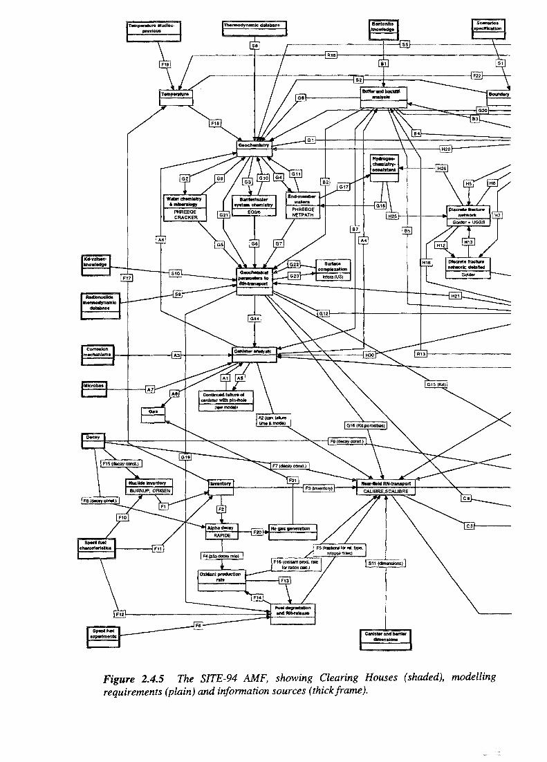
Temperature studies'previous
Canister and barrtordimensions
Figure 2.4.5 The SITE-94 AMF, showing Clearing Houses (shaded), modellingrequirements (plain) and information sources (thick frame).
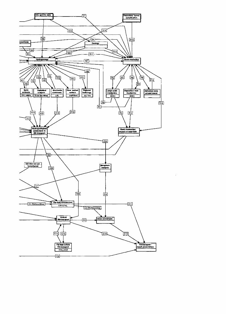
Repository layoutspecification
Earlyanalysis
Ecole des Moss
Regionalhydrology
SUTRA
Large seals Deposition hoismechanics
Disturbed zonearound turmel
Far-field coRotdRN-transport
RN-trartsport -result presentation
42
2.4.3.3 Mapping the PID onto the AMF
One purpose of the AMF is to ensure either a systematic treatment or, at the least, adiscussion of each of the FEPs and links on a PID that have been identified at a certain IL
value. This problem is addressed by mapping the FEPs and links in the PID onto the AMF.
The mapping is achieved through a series of documented meetings with experts within theSITE-94 project. For practical reasons, the mapping exercise conducted within SITE-94was limited to the PID(RF, IL=10).
The procedure for the mapping is as follows. As each EEP, or link of the PID, is evaluated,a check is made as to whether it is an obvious component of either a model or a ClearingHouse in the AMF. If this is the case, then the FEP/link is mapped to this AMF element.If it is not, then the FEP/link is mapped to the most appropriate Clearing House and a shortdiscussion is included in the documentation on the possibility of improving the treatmentof the FEP/link. For each decision made, a protocol sheet is completed which includessuggestions on how best to address the influence/FEP in the assessment phase of SITE-94.The items not included in the AMF models (or Clearing Houses), and for which no obviouseasy assumption or scoping calculations can be suggested for use in the SITE-94assessment, then require specific attention. Once outlined on the diagram, it is intuitivelyclear that these areas cover Performance Assessment issues which are widely acknowledgedto be problematic, poorly understood or, generally, rarely analysed. The followingprocedure is adopted to handle these issues:
• A protocol sheet is completed for each item, explaining the nature of the problem(no conceptual model available, no data available, understanding inadequate, etc.)plus some discussions as to the likely effect of omitting analysis from an assessmentand the types of uncertainty that this will incur.
• Decisions are made by the relevant Clearing House as to how the issue is to beaddressed, either within SITE-94 (i.e. either ignored, or by a simplifying assumptionafter further discussion) or after SITE-94 by further research.
The actual decisions made in SITE-94 are discussed at the relevant sections in this reportand documented in the AMF database.
2.4.3.4 Information Transfer and Representation of Conceptual Uncertainty
The AMF is a tool for documenting the information transfer between various parts of theassessment. This can provide explicit documentation of conceptual model uncertainty,including alternative conceptual models and parameter uncertainty. A specific role is givento the Clearing Houses. Clearing Houses represent people, who specifically examine theresults or data and make judgments and decisions before transferring the information toanother level. This is also a potentially useful QA-function, as mistakes or doubtful datawould not be automatically passed on to new models. The Clearing House documentationshould include the following information:
43
• text describing how the information entering the Clearing House is used forproducing the output information,
• uncertainty estimates of the output information, when possible in the form ofpotential variants that may be considered for analyses by receiving models orClearing Houses and,
• a discussion of the quality of the information delivered.
Conceptual model uncertainty is described graphically directly on the AMF if there arealternative conceptual models that are intended to provide the same information. In thissituation, the information (i.e. the AMF links) leaving the different alternative models hasto enter a Clearing House. A typical example of such a case is the different hydrogeologicalmodels that all deliver information to the same Clearing House (Figure 2.4.5). The ClearingHouse then has to decide how to transmit the results of the alternative models furtherthrough the AMF. One possibility is to produce a suite of parameter variants representingranges of the different conceptual models.
When there are no good models available, the Clearing House has to provide the outputparameter ranges based on reasoning, previous information and simplistic calculations. Avariant of this situation is where one or more models exist that described some of theprocesses that need to be considered, but not enough to provide a full output. In such cases,the Clearing House may both deliver information to, and receive information from, a modeland then produce output ranges from reasoning (see, for example, how the SurfaceComplexation models interact with the geochemical parameters to RN-transport ClearingHouse in Figure 2.4.5).
For specific details and application the reader is referred to Chapters 10 to 15 in this report.
2.4.3.5 Adjusting the AMF to Different PIDs
In SITE-94, the only Process Influence Diagram formally mapped to the Assessment ModelFlowchart is for the Reference Case with the most important influences (IL=10). Mappinga PID which also includes less important influences would potentially lead to modificationsof the AMF. Some of the new influences may correspond to models already in the AMF.The models may actually contain more influences than the most important ones. Mappingmay also make it necessary to add links in the AMF. However, the main effect is likely tobe more influences mapped to different Clearing Houses. In such a case, if there are manyinfluences mapped to Clearing Houses, the AMF may be a poor representation of the PIDand model development would be necessary.
Adjustments to the AMF are also necessary for the PID developed for different scenarios.Such adjustments are made in SITE-94 for the Central Scenario, as further discussed inChapter 9.
44
2.4.4 Formulation of Calculations Cases
The fourth level of analysis concerns selecting parameter values for the consequenceanalysis models. The parameter selection should reflect the different analysis levels, suchthat the suite of consequence model results could be used for a quantitative re-interpretationof system uncertainty, scenario uncertainty, conceptual model uncertainty and parameteruncertainty and variability. The quantitative assessment is based on the concept of variantsand calculation cases. Each Clearing House that should deliver parameters to the codes forconsequence analyses formulates different setups of parameter values for potential use inconsequence analyses. A single parameter setup from Clearing House is called a variant.The suite of variants from a Clearing House represents a parameterisation of scenariouncertainty, conceptual model uncertainty, parameter uncertainty and variability. Thereby,the information on the origin of the uncertainty (or variability) is directly tied to the variant.However, the consequence codes require input from many Clearing Houses. This input isobtained by combining variants from different Clearing Houses. Each single combinationanalysed is denoted a calculation case.
For a given System Identification and scenario, the AMF displays the sources ofinformation to any assessment code used. In trivial cases, input can be determined uniquely,but the more interesting parameter deliveries to an assessment is usually processed in aClearing House. Consequently, the Clearing Houses are given responsibility for deliveringsets of variants that reflect the uncertainties in the different analysis levels.
When the Clearing House needs to deliver many parameters, or when many ClearingHouses deliver parameters to the same model, this task is complicated by the need to assurethat the parameter values in a single variant and in the calculation cases are internallyconsistent and not in conflict with known functional relations or other correlations.Furthermore, the number of calculation cases could easily grow to unmanageable numbersand there is then a need to sample an illustrative subset of combinations of variants. Thisproblem is particularly acute when formulating calculation cases for the SITE-94 near-fieldand far-field radionuclide transport codes, which receive input from many different sources.
In order to handle this situation, an overall approach is developed (Chapman et al., 1995)which identifies a relevant and manageable set of calculation cases for each SystemIdentification and scenario selected. The actual application of this approach in SITE-94 isdescribed in Chapter 15.
2.5 QUALITY ASSURANCE
Quality is defined by the International Standards Organisation (ISO) as the totality offeatures and characteristics of a product and service that bear on its ability to satisfy statedor implied needs. Quality assurance (QA) is then simply the activity of ensuring that qualityis achieved.
The principles and concepts of QA have mainly been developed and applied within themanufacturing industry, for which purpose generally accepted standards (e.g., ISO 9000)have been developed. However, a more or less direct translation from manufacturing to
45
services is often possible without too much difficulty. In fact, scientific decision aids arementioned explicitly as examples of a service to which the standard ISO 9004-2 may beapplied.
Quality requirements are most logically derived based on the needs of the user of a productor service. For Performance Assessments undertaken by a licensing authority, there areseveral such users with somewhat different needs, e.g., decision makers, the public,management, PA staff and peers. From an analysis of these needs, it is evident that thefocus is on the following issues, which may then be described as the main objectives of QAfor Performance Assessments:
• transparency and logic in arguments and their derivation,
• comprehensiveness,
• validity in application of models and data,
• traceability of assumptions, models, data.
Clearly, most of these requirements concern how the assessment is documented. Anotherimportant point is the scientific quality of a Performance Assessment (validity,comprehensiveness, etc.).
SITE-94 includes a subproject with the original aim of developing a plan for QualityAssurance of Performance Assessments and of applying this plan to relevant parts ofSITE-94. It should be stated from the outset that, for various reasons, this aim has not beenachieved. Thus, soon after the start of SITE-94 it was realised that the development ofquality assurance for Performance Assessments would involve much more than justestablishing the procedures relevant for a particular Performance Assessment project. Infact, such project-oriented procedures must, in one way or another, be integrated or linkedwith the Quality System of the host organisation. At present, a formal Quality System hasnot yet been established within SKI. At the start of SITE-94, it was thought possible todevelop a stand-alone Quality Plan for Performance Assessment, based on a standard suchas ISO 9004-2. However, the necessity to link such a plan to the overall SKI QualitySystem became apparent and this approach was abandoned. Instead, the AMF methodologywithin the scenario subproject eventually evolved into a very promising answer to the needsof a set of practical and useful QA tools, although by the time these tools were ready forpractical use, time and resources were insufficient to have them applied to SITE-94.However, an audit of the relevant parts of the project using this methodology appears to bea promising exercise.
- Xi
47
3 PROPERTIES OF SPENT NUCLEAR FUEL
This chapter discusses the quantities, the radionuclide inventory and the properties of thewaste-form analysed in STTE-94, i.e. spent nuclear fuel. Of this information, theradionuclide inventory is directly used in the radionuclide release and transport calculationspresented in Chapter 16, whereas the quantities of spent fuel more is given as backgroundinformation, since in most cases SITE-94 evaluates consequences from a single canisterfailure. The discussion of the properties of the spent fuel is an input to the discussion of fueldissolution in Section 11.8 and the modelling of radionuclide release as described inSection 13.2.
3.1 INTRODUCTION
3.1.1 Quantities of Spent Fuel
The twelve nuclear power reactors in operation in Sweden produce spent nuclear fuel at arate of about 250 tonnes per year. If all of these stay in operation until the year 2010 theywill have produced 7000 to 8000 tonnes of spent fuel. The precise amount will depend ona number of factors, e.g. utilisation of reactors and burn-up of the fuel. In its most recentplan (SKB, 1995) for costs of nuclear waste management, SKB has calculated the fuelquantity to be 7840 tonnes U for the same scenario. The inventory of radionuclides forSITE-94 has been calculated (Liljenzin, 1990) assuming a higher burn-up than in SKB'sestimate, resulting in a lower total quantity of spent fuel of 6820 tonnes IHM (Initial HeavyMetal). The data used for the inventories for SITE-94 and Project-90 are identical.
With 1.6 tonnes IHM per canister, the SITE-94 inventory corresponds to about 4300canisters. As will be explained in Chapter 7.2, it was not found possible to emplace morethan about 400 canisters at the evaluated portion of the Aspo site. This limitation and lackof realism is judged to be of little importance for SITE-94 and it should be kept in mind thatSITE-94 is not Performance Assessment of a real site or repository (see Chapter 1). As willbe discussed further in subsequent chapters (Chapters 5, 8, 11 and 15), the radionuclidemigration calculations in SITE-94 are confined to analysing releases from a single failedcanister under different conditions. Due to the development stage of the canister(Chapter 5), it has not been judged meaningful to provide estimates of the number of failedcanisters at any given time after repository closure.
Some types of spent fuel are not considered in SITE-94. These include small amounts ofvery low burn-up, natural uranium fuel from the first Swedish research and prototype powerreactors. Damaged fuel and waste from examinations of spent fuel will also need to bedisposed of, but are not considered here. Some mixed-oxide fuel (24 tonnes of Germanorigin) is a cause for more concern, primarily due to its higher concentrations of heavynuclides. Separate studies on this type of fuel may be necessary.
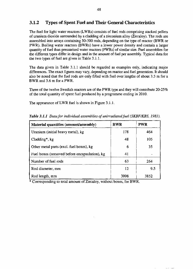
48
3.1.2 Types of Spent Fuel and Their General Characteristics
The fuel for light water reactors (LWRs) consists of fuel rods comprising stacked pelletsof uranium dioxide surrounded by a cladding of a zirconium alloy (Zircaloy). The rods areassembled into arrays containing 50-300 rods, depending on the type of reactor (BWR orPWR). Boiling water reactors (BWRs) have a lower power density and contain a largerquantity of fuel than pressurised water reactors (PWRs) of similar size. Fuel assemblies forthe different types differ in design and in the amount of fuel per assembly. Typical data forthe two types of fuel are given in Table 3.1.1.
The data given in Table 3.1.1 should be regarded as examples only, indicating majordifferences. The exact figures may vary, depending on reactor and fuel generation. It shouldalso be noted that the fuel rods are only filled with fuel over lengths of about 3.5 m for aBWR and 3.6 m for a PWR.
Three of the twelve Swedish reactors are of the PWR type and they will contribute 20-25%of the total quantity of spent fuel produced by a programme ending in 2010.
The appearance of LWR fuel is shown in Figure 3.1.1.
Table 3.1.1 Data for individual assemblies of unirradiated fuel (SKBF/KBS, 1983).
Material quantities (amount/assembly)
Uranium (initial heavy metal), kg
Cladding*, kg
Other metal parts (excl. fuel boxes), kg
Fuel boxes (removed before encapsulation), kg
Number of fuel rods
Rod diameter, mm
Rod length, mm
BWR
178
48
6
41
63
12
3998
PWR
464
105
35
264
9.5
3852
* Corresponding to total amount of Zircaloy, without boxes, for BWR.
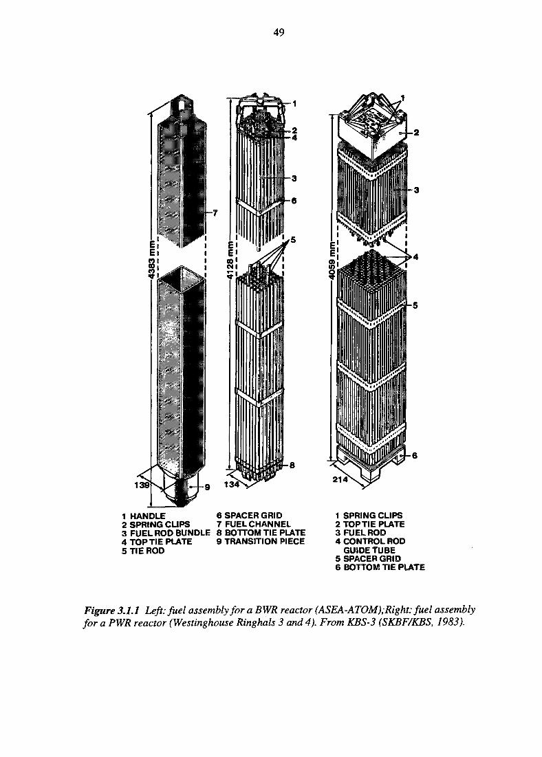
49
1 HANDLE2 SPRING CLIPS3 FUEL ROD BUNDLE4 TOP TIE PLATE5 TIE ROD
6 SPACER GRID7 FUELCHANNEL8 BOTTOM TIE PLATE9 TRANSITION PIECE
88-5
214s
1 SPRING CLIPS2 TOP TIE PLATE3 FUEL ROD4 CONTROLROD
GUIDE TUBE5 SPACER GRID6 BOTTOM TIE PLATE
Figure 3.1.1 Left: fuel assembly for a BWR reactor (ASEA-ATOM);Right: fuel assemblyfor a PWR reactor (Westinghouse Ringhals 3 and 4). From KBS-3 (SKBF/KBS, 1983).
50
3.2 COMPOSITION OF FUEL COMPONENTS
3.2.1 Fuel Material
The composition of spent fuel depends on the bum-up and on the initial enrichment of thefuel. Modern fuel for LWRs has an enrichment in the range of 3-4% 235U. Higherenrichments and, thus, higher burn-ups are attainable by the addition of a few tens ofpercent of a so-called burnable absorber (BNA, Burnable Neutron Absorber), which lowersthe reactivity of the fresh fuel. Eventually this absorber (typically a lanthanide such as Gd,with an extremely high neutron capture cross-section) is burnt up by neutron capture,thereby balancing the bum-up of 235U. The influence on radionuclide inventory is probablyof minor importance and has not been considered further in SITE-94.
3.2.2 Metal Parts
The amount and composition of metal parts in the fuel vary depending on the type of fueland reactor. For SITE-94, data for the metal parts of BWR fuel are used (TVO, 1992).Thus, the following average values are assumed in calculations of radionuclide inventory:
Zircaloy-2Zircaloy-4Inconel X-750Stainless steel
27556
20
kg/tlHMkg/tlHMkg/tlHMkg/tlHM
3.3 RADIONUCLIDE INVENTORY
3.3.1 Burn-up Calculations
The inventory for SITE-94 is based on the same calculations as for Project-90 (SKI, 1991;Liljenzin, 1990). Thus, the bum-up history of each batch of fresh fuel has been followedfor each reactor. Known or predicted changes in enrichment, recirculation of uranium andbum-up have been accounted for. Calculations have been performed for three shut-downscenarios. The scenario chosen for the SITE-94 calculations is the same as in Project-90,namely:
• All reactors are assumed to have been operated until 2010 and shut downsimultaneously. Fuel for two large boiling water reactors, Forsmark 3 andOskarshamn 3, is assumed to be based mainly on re-enriched uranium fromreprocessed LWR fuel after 1995.
Some recirculated (reprocessed) uranium might be present due to the mixing of uraniumfeeds from different (foreign) sources when enrichment services are bought outsideSweden. Inclusion of reprocessed uranium in the inventory is of some importance, since itgives an increased content of U-236 and Np-237 in the spent fuel.
51
The maximum bum-up assumed in the calculations is for a small part of the PWR fuel with62 GWd/t IHM. The heat load per canister is restricted, however, which means that fuelelements with a high bum-up will be packaged together with low bum-up fuel. Thus, theaverage bum-up per canister will probably not vary as much as the bum-up for fuel batches.
The radionuclide data presented in the next section are averages based on the total quantityof fuel produced. A significant proportion of fuel batches should not be far from thiscomposition and it is considered to be a good approximation to the average compositionin a canister.
Radionuclide activities are calculated for the year 2100. Thus, these data compare ratherwell with data for 100 years cooling time, such as those presented in KBS-3 and TVO-92.
3.3.2 The SITE-94 Inventory
The SITE-94 inventory used in the calculations is given in Table 3.3.1. In comparison toProject-90, the inventory is more comprehensive, e.g. it includes a few more fissionproducts, activation products (TVO, 1992) and data for some higher actinides. Data forinactive isotopes are also given (Table 3.3.2) in order to allow calculations of isotopicdilution effects on radionuclide solubilities (Chapter 12). For a more detailed listing ofradionuclide data, see Liljenzin (1990).
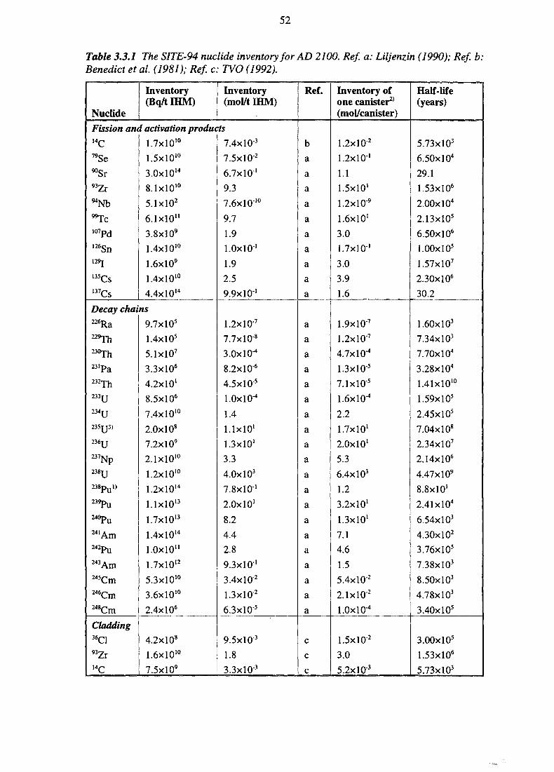
52
Table 3.3.1 The SITE-94 nuclide inventory for AD 2100. Ref a: Liljenzin (1990); Ref b:Benedict et al. (1981); Ref c: TWO (1992).
Nuclide
Inventory(Bq/t I H M )
Inventory(mol/t IHM)
Fission and activation products14C79Se
^Sr93Zr9 4Nb
"Tc107pd
126Sn129T
135Cs137Cs
1.7x10'°
1.5x10'°
3.0xl014
8.1xl010
5.1xl02
6.1x10"
3.8xl09
1.4x10'°
1.6xlO9
1.4x10'°
4.4xlO14
Decay chains22fiRa2 2 9 ^
230Th231pa
232 T h
2 3 3 U
2 3 4 u2 3 5 u 3 )2 3 6 u237Np238U238pul)
239Pu240pu
241Am242pu
243 A m
^ C m246Cm
"•CmCladding36C193Zr1 4 C
9.7xl05
1.4xlO5
5.1xlO7
3.3xlO6
4.2x10'
8.5xl06
7.4x10'°
2.0xl08
7.2xlO9
2.1x10'°
1.2x10'°
1.2xlO14
l.lxlO13
1.7xlO13
1.4xlO14
1.0x10"
1.7xlO12
5.3x10'°
3.6x10'°
2.4xlO6
4.2x10⁸
1.6x10'°
7.5xlO9
7.4x10³
7.5xlO"2
6.7x10'
9.3
7.6x10'°
9.7
1.9
l.OxlO"1
1.9
2.5
9.9x10'
1.2xlO7
7.7xlO"8
3.0X10"4
8.2xlO"6
4.5xlO"5
l.OxlO"4
1.4
1.1x10'
1.3x10'
3.3
4.0x10³
7.8x10'
2.0x10'
8.2
4.4
2.8
9.3x10'
3.4xlO"2
1.3xlO"2
6.3xlO"5
9.5x10°
1.8
3.3xlO"3
Ref.
b
a
a
a
a
a
a
a
a
a
a
a
a
a
a
a
a
a
a
a
a
a
a
a
a
a
a
a
a
a
a
c
c
c
Inventory ofone canister2*(mol/canister)
1.2xlO"2
1.2x10'
1.1
1.5x10'
1.2xlO"9
1.6x10'
3.0
1.7x10'
3.0
3.9
1.6
1.9xlO"7
1.2xlO"7
4.7X10"4
1.3xlO'5
7.1xlO"5
1.6X10"4
2.2
1.7x10'
2.0x10'
5.3
6.4x10³
1.2
3.2x10'
1.3x10'
7.1
4.6
1.5
5.4x10'2
2.1xlO"2
l.OxlO"4
1.5xlO"2
3.0
5.2xlO'3
Half-life(years)
5.73xlO3
6.50xl04
29.1
1.53xlO6
2.00xl04
2.13xlO5
6.50x10⁶
l.OOxlO5
1.57xlO7
2.30xl06
30.2
1.60xl03
7.34xlO3
7.70xl04
3.28xlO4
1.41x10'°
1.59xlO5
2.45xlO5
7.04xl08
2.34xlO7
2.14xlO6
4.47xlO9
8.8x10'
2.41xlO4
6.54xlO3
4.30xl02
3.76xlO5
7.38xlO3
8.50xl03
4.78xlO3
3.40xl05
3.00xl05
1.53xlO6
5.73xlO3
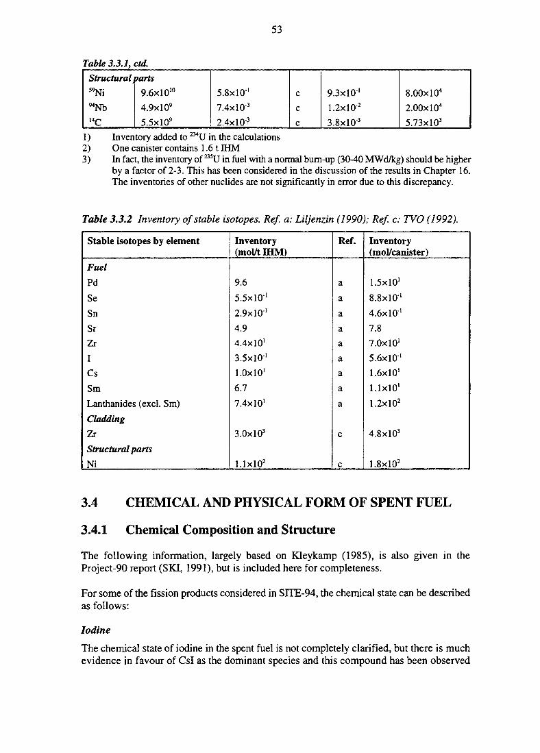
53
Table 3.3.1,Structural59Ni
^Nb14C
ctd.
larts
9.6x10'°
4.9x10⁹
5.5xlO9
5.8x10'
7.4x10³
2.4xlO"3
c
c
c
9.3x10'
1.2xlO"2
3.8xlO3
8.00xl04
2.00x10⁴
5.73xlO3
1) Inventory added to 234U in the calculations2) One canister contains 1.6 t IHM3) In fact, the inventory of 235U in fuel with a normal burn-up (30-40 MWd/kg) should be higher
by a factor of 2-3. This has been considered in the discussion of the results in Chapter 16.The inventories of other nuclides are not significantly in error due to this discrepancy.
Table 3.3.2 Inventory of stable isotopes. Ref. a: Liljenzin (1990); Ref. c: TVO (1992).
Stable isotopes by element
Fuel
Pd
Se
Sn
Sr
Zr
I
Cs
Sm
Lanthanides (excl. Sm)
Cladding
Zr
Structural parts
Ni
Inventory(mol/t IHM)
9.6
5.5x10'
2.9x10'
4.9
4.4x10'
3.5x10'
1.0x10'
6.7
7.4x10'
3.0xl03
l . lxlO2
Ref.
a
a
a
a
a
a
a
a
a
c
c
Inventory(mol/canister)
1.5x10'
8.8x10'
4.6x10'
7.8
7.0x10'
5.6x10'
1.6x10'
1.1x10'
1.2xlO2
4.8xlO3
1.8xl02
3.4 CHEMICAL AND PHYSICAL FORM OF SPENT FUEL
3.4.1 Chemical Composition and Structure
The following information, largely based on Kleykamp (1985), is also given in theProject-90 report (SKI, 1991), but is included here for completeness.
For some of the fission products considered in SITE-94, the chemical state can be describedas follows:
Iodine
The chemical state of iodine in the spent fuel is not completely clarified, but there is muchevidence in favour of Csl as the dominant species and this compound has been observed
54
in the fuel-cladding gap. On the other hand, the mobility of I is higher than that of Cs,which seems to contradict the assumption of Csl formation and it might also be taken asevidence for I occurring in the elemental form. However, the thermodynamic equilibriaduring burn-up suggest the formation of Csl, the equilibrium pressure of elemental iodineand I2 being negligibly small (Imoto, 1986). Together with other volatile fission products,iodine mainly occurs in voids along the grain boundaries and, to some extent, within thegrains.
Cesium
The amount of Cs not present as Csl (or CsBr) forms mixed oxide phases, e.g. uranates andmolybdates, located in the fuel-cladding gap, in cracks and at grain boundaries. To someextent, it may also be dissolved in the matrix.
Technetium
The major part of the Tc inventory seems to occur in the so-called 'white inclusions', i.e.particles of metal alloys. The constituents of these precipitates are Mo, Tc, and the noblemetals Ru, Rh and Pd, with Mo and Ru as the main components. The inclusions formseparate phases of about 10 urn size, almost comparable to that of the fuel grains (about 10-50 fim).
Tin
This element is present in another kind of intermetallic compound, with Pd as the majorcomponent. Other constituents in these phases are Te, Sb, Ag, and Cd and they tend toaccumulate in the centre of the fuel.
Zirconium
The Zr-oxide is only soluble to a limited extent in the oxide matrix. Therefore, Zr alsoforms a separate oxide phase (a so-called 'grey phase') together, primarily with Ba, Mo andU.
Strontium
According to Kleykamp (1985), Sr is predominantly dissolved as an oxide in the fuelmatrix. This is at variance with some earlier assumptions based on fuel leachingexperiments. However, a fraction of Sr is found in the grey oxide phase.
Lanthanides
Due to the close chemical similarity, lanthanides should form a solid solution with actinidesin the fuel matrix.
A major portion of the transuranium elements is also dissolved in the fuel matrix.
The spent fuel is a multi-component, multi-phase system of great complexity. In addition,many of the compounds and phases formed under reactor operation are metastable at thetemperatures of a repository. Therefore, it will be difficult, if not impossible, to base arealistic model of the fuel on thermodynamic calculations. On the other hand, achievements
55
have been made in simulating the chemical state of fission products in irradiated fuel, i.e.by calculations for high temperatures (Imoto, 1986).
In the SITE-94 inventory, the stable isotopes of the radioactive elements have been given(Table 3.3.2) in order to allow for a more complete analysis of potential isotopic dilutioneffects and formation of solid solutions. For solubility limited release mechanisms, therelease rate for each single radionuclide should be proportional to its isotopic fraction in thewaste form. However, the isotopic effect is only valid over volumes with homogeneousisotopic composition. For that reason, it is probably questionable and non-conservative toinclude isotopes from regions far apart in the waste form. Nevertheless, in SITE-94 the Zrin the cladding has been assumed to share solubility with 93Zr in the fuel (Chapters 13 and16).
A great potential for a similar solubility reduction is probably present for elements formingsolid solutions. In the first place, this should be the case for Am and Cm and also for thesetwo together with the lanthanides. However, this beneficial feature has not been taken intoaccount in SITE-94 and, in most cases, it seems that the potential reduction in radionuclidereleases would have little effect on the total radiological consequences.
3.4.2 Physical Properties
Spent nuclear fuel is a highly heterogeneous material, a factor which must be consideredin attempts to describe release mechanisms for radionuclides. Apart from the phaseheterogeneities, described in Section 3.4.1, the physical form is also of importance. The fuelstructure changes with burn-up and thermal load and transients, resulting in geometricaldistortion, e.g. swelling and cracking of the fuel pellets.
This cracking may be of particular concern when defining the contact surface area betweenfuel and water, e.g. for estimation of oxidant production (Section 11.6) The upper limit ofthis surface area, as determined by the grain size, is larger than the geometrical area of theintact fuel pellets by a factor of several hundred.
The structure of spent fuel has been studied extensively in connection with tests of fuelunder reactor operation, but little is known of how this structure will change in the long-or very long-term in contact with groundwater. For example, it is not known whether thegrain boundaries will dissolve at a faster rate than the grains, or whether reprecipitatedoxides will seal the pores in fuel particles.
The appearance of spent fuel, typical for Swedish LWRs, is shown in Figure 3.4.1.
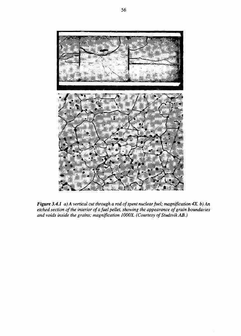
56
Figure 3.4.1 a) A vertical cut through a rod of spent nuclear fuel; magnification 4X. b) Anetched section of the interior of a fuel pellet, showing the appearance of grain boundariesand voids inside the grains; magnification 1000X. (Courtesy of Studsvik AB.)
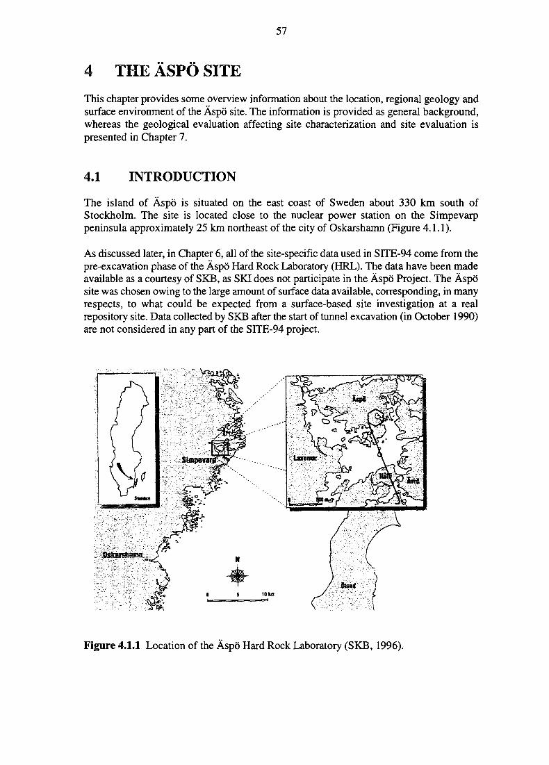
57
4 THE ASPO SITE
This chapter provides some overview information about the location, regional geology andsurface environment of the Aspo site. The information is provided as general background,whereas the geological evaluation affecting site characterization and site evaluation ispresented in Chapter 7.
4.1 INTRODUCTION
The island of Aspo is situated on the east coast of Sweden about 330 km south ofStockholm. The site is located close to the nuclear power station on the Simpevarppeninsula approximately 25 km northeast of the city of Oskarshamn (Figure 4.1.1).
As discussed later, in Chapter 6, all of the site-specific data used in SITE-94 come from thepre-excavation phase of the Aspo Hard Rock Laboratory (HRL). The data have been madeavailable as a courtesy of SKB, as SKI does not participate in the Aspo Project. The Asposite was chosen owing to the large amount of surface data available, corresponding, in manyrespects, to what could be expected from a surface-based site investigation at a realrepository site. Data collected by SKB after the start of tunnel excavation (in October 1990)are not considered in any part of the SITE-94 project.
Figure 4.1.1 Location of the Aspo Hard Rock Laboratory (SKB, 1996).
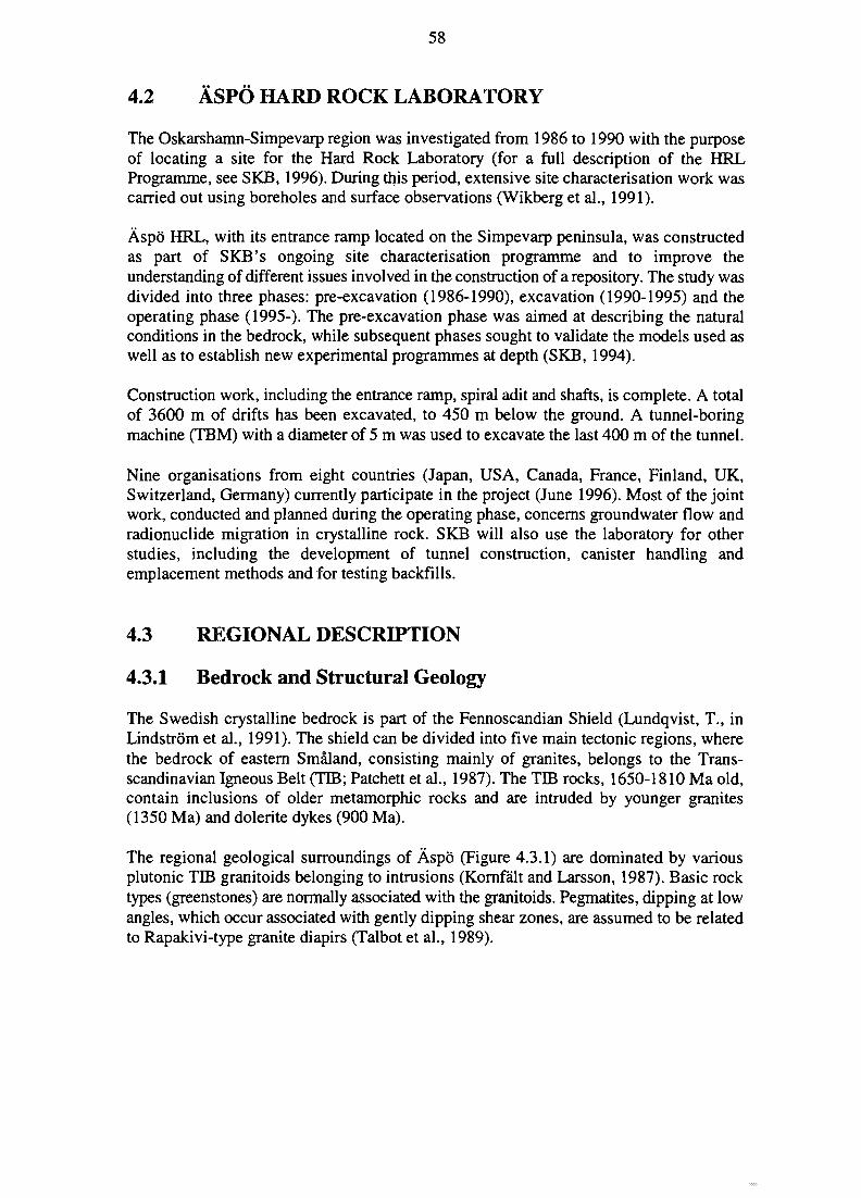
58
4.2 ASPO HARD ROCK LABORATORY
The Oskarshamn-Simpevarp region was investigated from 1986 to 1990 with the purposeof locating a site for the Hard Rock Laboratory (for a full description of the HRLProgramme, see SKB, 1996). During this period, extensive site characterisation work wascarried out using boreholes and surface observations (Wikberg et al., 1991).
Aspo HRL, with its entrance ramp located on the Simpevarp peninsula, was constructedas part of SKB's ongoing site characterisation programme and to improve theunderstanding of different issues involved in the construction of a repository. The study wasdivided into three phases: pre-excavation (1986-1990), excavation (1990-1995) and theoperating phase (1995-). The pre-excavation phase was aimed at describing the naturalconditions in the bedrock, while subsequent phases sought to validate the models used aswell as to establish new experimental programmes at depth (SKB, 1994).
Construction work, including the entrance ramp, spiral adit and shafts, is complete. A totalof 3600 m of drifts has been excavated, to 450 m below the ground. A tunnel-boringmachine (TBM) with a diameter of 5 m was used to excavate the last 400 m of the tunnel.
Nine organisations from eight countries (Japan, USA, Canada, France, Finland, UK,Switzerland, Germany) currently participate in the project (June 1996). Most of the jointwork, conducted and planned during the operating phase, concerns groundwater flow andradionuclide migration in crystalline rock. SKB will also use the laboratory for otherstudies, including the development of tunnel construction, canister handling andemplacement methods and for testing backfills.
4.3 REGIONAL DESCRIPTION
4.3.1 Bedrock and Structural Geology
The Swedish crystalline bedrock is part of the Fennoscandian Shield (Lundqvist, T., inLindstrom et al., 1991). The shield can be divided into five main tectonic regions, wherethe bedrock of eastern Smaland, consisting mainly of granites, belongs to the Trans-scandinavian Igneous Belt (TIB; Patchett et al., 1987). The TIB rocks, 1650-1810 Ma old,contain inclusions of older metamorphic rocks and are intruded by younger granites(1350 Ma) and dolerite dykes (900 Ma).
The regional geological surroundings of Aspo (Figure 4.3.1) are dominated by variousplutonic TIB granitoids belonging to intrusions (Kornfalt and Larsson, 1987). Basic rocktypes (greenstones) are normally associated with the granitoids. Pegmatites, dipping at lowangles, which occur associated with gently dipping shear zones, are assumed to be relatedto Rapakivi-type granite diapirs (Talbot et al., 1989).
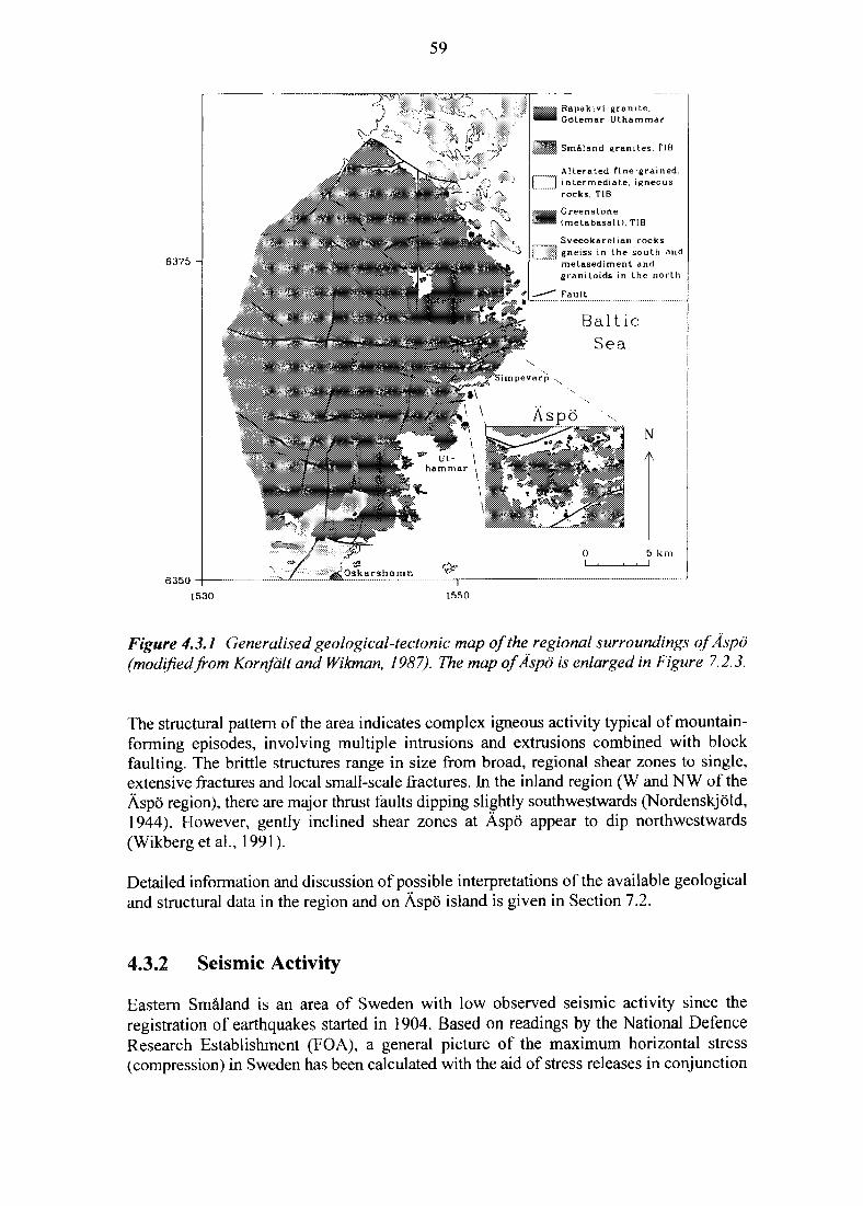
59
6375 -
6350
Rapakivi granite,GOtemarUthammar
Smaland granites, TIB
Alterated fine grainedintermediate, igneousrocks, TIB
Greenstone(metabasalt), TIB
Svecokarelian rocksgneiss in the south andmetasediment andgranitoids in the north
1530
^Oskarshamn *>""~I
1550
Figure 4.3.1 Generalised geological-tectonic map of the regional surroundings of Aspo(modified from Kornfalt and Wikman, 1987). The map ofAspo is enlarged in Figure 7.2.3.
The structural pattern of the area indicates complex igneous activity typical of mountain-forming episodes, involving multiple intrusions and extrusions combined with blockfaulting. The brittle structures range in size from broad, regional shear zones to single,extensive fractures and local small-scale fractures. In the inland region (W and NW of theAspo region), there are major thrust faults dipping slightly southwestwards (Nordenskjold,1944). However, gently inclined shear zones at Aspo appear to dip northwestwards(Wikberg et al., 1991).
Detailed information and discussion of possible interpretations of the available geologicaland structural data in the region and on Aspo island is given in Section 7.2.
4.3.2 Seismic Activity
Eastern Smaland is an area of Sweden with low observed seismic activity since theregistration of earthquakes started in 1904. Based on readings by the National DefenceResearch Establishment (FOA), a general picture of the maximum horizontal stress(compression) in Sweden has been calculated with the aid of stress releases in conjunction
60
with registered earthquakes (Slunga, 1990). A northwesterly principal maximum stressdirection is indicated and this has been confirmed by some actual rock mechanical stressmeasurements (Stephansson et al., 1991 andBjarnasson et al, 1989).
4.3.3 Topography and Quaternary Deposits
Aspo is located east of the South Swedish Highland and is characterised by a gentlyundulating topography (Figure 4.3.2). The highest (100 m) late glacial shoreline is locatedabout 25-30 km west of Aspo. The highest elevation of Aspo island is 13 m above presentsea level.
Glacial till, mostly influenced by earlier wave activity, dominates the area with anincreasing amount of overlying peat bogs (and clay) inland. In moderately exposed areas,the till cover does not normally exceed 5 metres. Several metres of glacial clay can befound overlain by a few metres of postglacial clay and mudded clay, especially in thecultivated low land (Svensson, 1989).
+- -A -:
• MEkipaa'!"' -piin.yrT0
' - 1 / - M ' " » )
N
1km
Topographic con-tour intervals, 5 m
Figure 4.3.2 Topographic map ofAspo Island and its surroundings. Published with thepermission of National Land Survey of Sweden. (Copyright © National Land Survey ofSweden, Licens no. 96.0340)

61
4.3.4 Surface Hydrology
The Simpevarp area contains parts of two larger drainage basins with two major streamsflowing into the Baltic. Average annual precipitation for the area is 675 mm. Potential andactual annual evaporation is calculated to be 616 and 490 mm, respectively. Groundwaterrecharge has been determined from this data, and shows mean values from 128 to 218 mmper year (Svensson, 1987).
4.4 SURFACE ENVIRONMENT
The information presented in the following sections gives only a brief introduction to thesurface environment and should not be considered a complete account. In a realPerformance Assessment for licensing purposes, considerably more information would berequired as it would be coupled to the Environmental Impact Statement (EIS).
4.4.1 Society
The Oskarshamn Municipality, with an area of 1050 km2, has a population of 27 000people, most of them living in the town of Oskarshamn. It is one of twelve municipalitiesin the County of Kalmar.
4.4.2 Land Use
Seventy-five percent of the Municipality area is covered by forest, with 7% used forcultivation (arable and pasture land), 13% covered by development, 4% taken in populationcentres and 1 % used for power transmission lines. Over recent years, the forested area hasincreased and cultivated land decreased.
4.4.3 Nuclear Facilities
Sweden has twelve nuclear power reactors generating approximately 50% of the electricityconsumed in Sweden. Three of the reactors are Pressurised Water Reactors (PWRs) andnine are Boiling Water Reactors (BWRs).
The Simpevarp peninsula is one of four sites in Sweden where nuclear power plants arelocated. The Oskarshamn I, II and in BWRs have currently a total net output of 2295 MW,generating approximately 22% of the total nuclear power production in Sweden. Theunderground facility for intermediate storage of spent fuel (CLAB) is located close to thenuclear power plant.
63
5 OUTLINE OF THE DISPOSAL SYSTEMThis chapter, which deals with the disposal system design, is included largely for the sakeof completeness. No new work in this area has been undertaken within SITE-94; indeed,it is not the role of SKI to suggest design solutions as explained in Chapter 1. A full safetysubmission for an encapsulation or disposal facility would, consequently, be expected tocontain considerably more information than the brief outline presented below.
5.1 INTRODUCTION
In a licensing report, the systems description should be comprehensive and can be expectedto comprise a large part of the submission. Full accounts should be given of systemsdevelopment and systems selection issues providing the rationale, particularly from a safetypoint of view, for the selection of the proposed system and subsystems, as well as therationale for the selection of the proposed site. The report should also include analyses ofsafety during plant operation as well as during transport. For the reasons stated above, noneof these issues is treated in the SITE-94 report.
Many safety issues are, however, closely related to the system description and even todetails within it. Therefore, even for the purposes of SITE-94, a relatively detailed systemsdescription would be desirable. When conducting SITE-94 no such detailed descriptionexisted, which created difficulties in at least two ways: first, different parts of the disposalsystem had to be treated differently depending on how far the SKB (or SKI) work hadadvanced in different areas (e.g., canister longevity issues are dealt with only in aqualitative manner). Second, since technical solutions are still being developed, potentialinadequacies can be identified quite readily. They should not be overemphasised, however,since further work, even in the short term, may prove them manageable (possibly with somemodification of the system).
In order to make any analyses possible within SITE-94, it was necessary to select areference system. The reference system used is the one presented as the reference systemin SKB's Programme 92 for research, development and demonstration (SKB, 1992a), i.e.spent nuclear fuel is encapsulated in copper/steel canisters, which are deposited in a deeprepository in crystalline basement rock. This system has been accepted by SKI (in its reviewof the SKB Programme; SKI, 1993) as an appropriate reference system for the furtherdevelopment work to be carried out by SKB. The fact that this system has also beenselected as the reference system for the SITE-94 project has no further implications.
5.2 TRANSPORT
5.2.1 Present System for Transport of Spent Nuclear Fuel
In the existing transport system for spent nuclear fuel, the fuel is transported in a dedicatedship called SIGYN, from the four nuclear power plant sites to the central storage facility,CLAB.
64
After removal from the reactor core, the spent fuel is stored in on-site pool storage in waterfor about a year. This allows for the fuel to 'cool', that is, for the short-lived activation andfission products in the fuel to decay and thereafter give rise to a considerably smaller heatoutput.
After on-site interim storage, the spent fuel is put in transport containers. The transportcontainers are hoisted onto supports, which, in turn, are lifted hydraulically by a dedicatedtruck and transferred to the dedicated roll on/roll off ship, SIGYN. A similar procedure isused for unloading the spent fuel at the CLAB interim storage facility.
The transport containers provide shielding from alpha, beta and gamma radiation as wellas from neutrons. The containers are supplied with flanges on the outside in order toimprove the cooling and to keep the temperature down. The containers also providemechanical protection as well as protection from any contamination.
The transport of spent fuel is not a trivial task since spent fuel is highly radioactive.Considerable international experience exists, however, regarding transport of spent fuel bysea as well as by railway. The experience includes international procedures and rules.Sweden has accepted the IAEA (International Atomic Energy Agency, a United Nationsorganisation) recommendations as rules.
5.2.2 Future System for Transport of Spent Nuclear Fuel
According to the 1992 plans of the Swedish nuclear industry (SKB, 1992a), two newnuclear facilities will be required for the management of spent nuclear fuel: anencapsulation plant and a final repository.
In the encapsulation facility, the spent fuel is put in containers (see below) of copper andsteel which are then sealed. It is intended that these sealed canisters will be deposited in therepository. The industry plans to co-locate the encapsulation plant with CLAB (i.e.construct it as an extension to CLAB).
The scheme of transportation for the spent fuel will, to a large extent, depend on the choiceof site. At present, no specific site has been identified to host the final repository. Over longdistances the spent fuel can be transported by ship and/or by rail and, over short distances,by road.
The transport containers will be similar to those used today for the transport of fuel that hasnot been encapsulated. The main difference is that the cooling flanges will no longer beneeded and that the diameter will be different. It can be expected that the safety analysiswill be facilitated by the fact that the radioactivity of the spent fuel decreases rapidly withtime and the fact that the spent fuel is actually kept in a canister inside the transportationcontainer. It is assumed that encapsulation takes place no sooner than 40 years after the fuelhas been removed from the reactor core.
Loading and unloading procedures are assumed to be similar to those described for SIGYNin Section 5.2.1 above.
65
5.3 INTERMEDIATE STORAGE
In the CLAB interim wet storage facility, the unencapsulated spent fuel is kept in largepools of water which provide cooling as well as shielding of the radiation. The water is alsoa contamination barrier. Radionuclides continuously leave the surface of the fuel pins andalso, at some points, the interior of the pins and enter the pool water which is continuouslycleaned by mechanical and ion exchange filters.
The unloading and inspection area of the CLAB facility is situated at ground level. In thispart of the facility, the fuel is unloaded from the transportation container and put in boronsteel boxes. Boron has a high cross-section for neutrons and improves the subcriticalitycharacteristics of the storage.
The actual storage area is located in crystalline basement rock under a rock cover of about30 metres. The pools are made of concrete, lined on the inside with sheets of stainless steel.
Transfer of the steel boxes containing spent fuel from the surface part of the facility to thepools is achieved by means of a dedicated elevator.
The present capacity of CLAB is 5000 metric tonnes of spent fuel (figured as uraniummetal). This capacity is not regarded to be sufficient for the Swedish programme and,therefore, an extension is foreseen. A second rock cavern with another pool is planned andthe total capacity is intended to be 8000 metric tonnes of uranium.
5.4 CANISTER DESIGN AND ENCAPSULATION
5.4.1 Canister Design
The canister used in the SITE-94 project is shown in Figure 5.4.1. This canister waspresented as the reference canister in SKB's RD&D Programme 1992. It contains eithereight fuel elements from a boiling water reactor or four fuel elements from a pressurisedwater reactor. The dimensions are apparent from the figure.
The empty canister weighs about 11.3 tonnes and the copper accounts for about 55% of thisweight. The fuel boxes in a loaded canister weigh about 3.6 tonnes. A high-purity, oxygen-free copper, which can be obtained commercially, has been selected for fabricatingcanisters. A high-strength mild steel, also available commercially in the form of pipe withsuitable dimensions, forms the other canister component.
It is apparent from Figure 5.4.1 that the copper/steel canister consists of two vessels, oneinside the other. The inner steel vessel provides mechanical strength while the outer coppervessel provides long-term chemical integrity and corrosion resistance. Both the steel andthe copper vessels provide shielding which reduces the radiation at the canister surface inthe repository. The reduced dose rate gives rise to only a low rate of radiolysis of water(decomposition into oxygen and hydrogen). Thus, the canister is designed to provide long-term containment in the repository (Chapter 8 discusses mechanisms that should beconsidered when evaluating long-term containment).
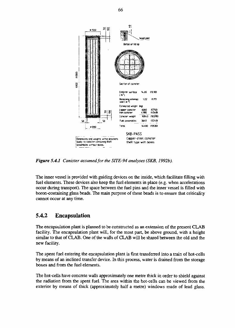
66
14.65 (13.90)
1.22 U17)
Estimated weight (J«j)Capper canister 6060Iron canister 4780
Canister weight 10840 (10290)
Fuel assemblies 3640 I3240I
(5750)(4S40)
Total 14480 1135301
| Dimensions and weights within brackets'apply to canister containing BWRi assemblies without boxes.
SKB-PASSCopper-steel canisterBWR type with boxes
Figure 5.4.1 Canister assumed for the SITE-94 analyses (SKB, 1992b).
The inner vessel is provided with guiding devices on the inside, which facilitate filling withfuel elements. These devices also keep the fuel elements in place (e.g. when accelerationsoccur during transport). The space between the fuel pins and the inner vessel is filled withboron-containing glass beads. The main purpose of these beads is to ensure that criticalitycannot occur at any time.
5.4.2 Encapsulation
The encapsulation plant is planned to be constructed as an extension of the present CLABfacility. The encapsulation plant will, for the most part, be above ground, with a heightsimilar to that of CLAB. One of the walls of CLAB will be shared between the old and thenew facility.
The spent fuel entering the encapsulation plant is first transferred into a train of hot-cellsby means of an inclined transfer device. In this process, water is drained from the storageboxes and from the fuel elements.
The hot-cells have concrete walls approximately one metre thick in order to shield againstthe radiation from the spent fuel. The area within the hot-cells can be viewed from theexterior by means of thick (approximately half a metre) windows made of lead glass.

67
Manipulation of objects can be performed remotely either by 'hand-driven' or computerisedmanipulators. There are also 'hand-driven' power manipulators.
The drained fuel elements (still in the storage box) are then transferred by a hoist to adrying station where they are dried in a stream of hot air. At this point, the fuel is stillemitting some decay heat which aids in the drying.
It is expected that very little water would remain on the surfaces after such drying.However, in the course of reactor operation, some of the fuel pins might have becomedamaged and may have small holes, fractures or fissures. In such cases, a certain amountof water (at most, a few tens of grams) might remain on the inside of a pin after drying.
The dried fuel elements are then lifted out of the storage box and transferred to an emptycopper/steel canister. The canister rests on a trolley with vertical guides and a hydraulicdevice which makes it possible to elevate and lower the canister. When the canister is inits lowest position, the trolley can be transferred to new positions among the train of hot-cells.
In the bead fill and steel lid welding station, the canister is evacuated and filled with aninert gas, such as argon. Then, the space between the fuel pins is filled with an inert fillingmaterial.
After filling, the canister is closed with a steel lid which is joined to the inner vessel, alsomade of steel, by laser beam welding. The depth of the weld is only of the order of a fewmillimetres. The purpose of this weld is to keep the lid in place during handling and toseparate the atmosphere inside the canister from that outside. Thus, the weld provides abarrier against contamination. The weld is not intended to contribute substantially to themechanical strength.
After the steel lid has been put in place, the canister is moved to the copper lid weldingstation. Here, a vacuum is applied and a copper lid is joined to the outer copper canister byelectron beam welding. In this process, the weld depth is the same thickness as the coppercanister and the lid.
When the copper lid has been welded to the copper canister, the canister is moved to thenon-destructive testing and machining station. At this station, the weld is machined to aneven surface and inspected using x-rays and ultrasound techniques.
Non-destructive testing is an important part of the scheme for qualifying a canister for thefinal repository. If the measurements for a weld are found to be outside some range ofacceptance, the canister will not be taken to the repository. Instead, an appropriate remedialprocess will be carried out.
If a canister has been found to be acceptable for the repository, it is transferred to thedecontamination station where any potential surface contamination is removed. Finally, thecanister is transferred to a buffer storage at the encapsulation facility.
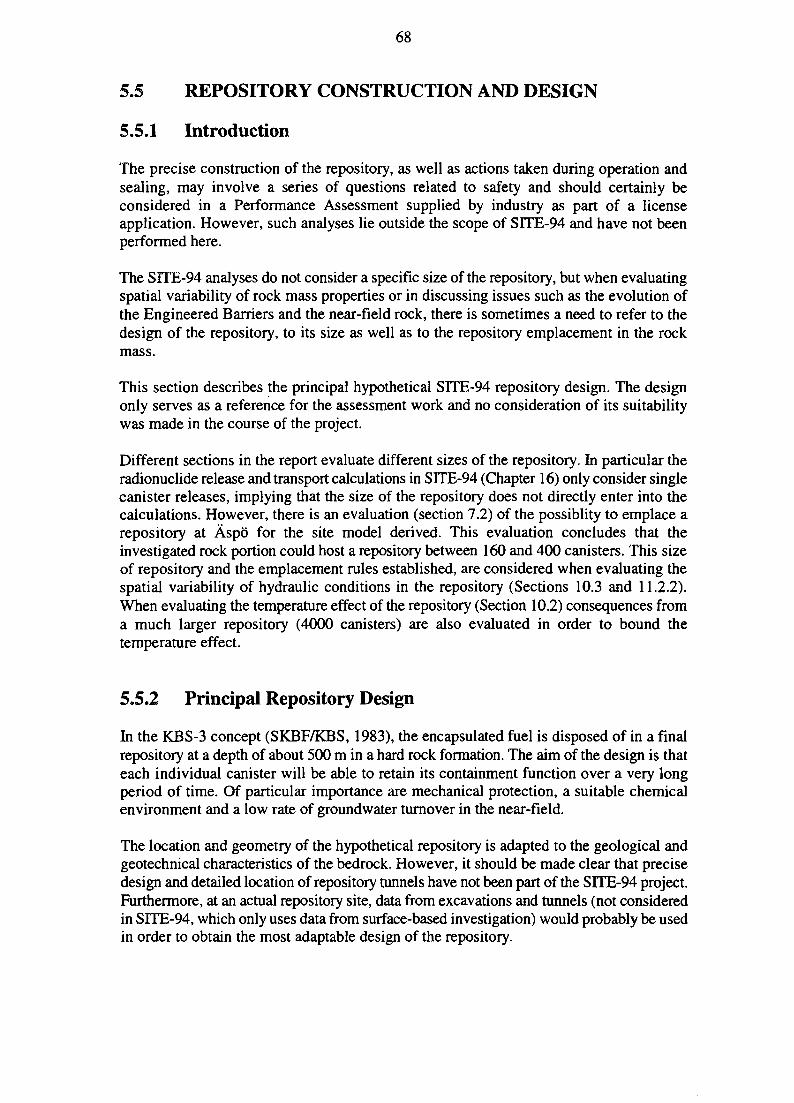
68
5.5 REPOSITORY CONSTRUCTION AND DESIGN
5.5.1 Introduction
The precise construction of the repository, as well as actions taken during operation andsealing, may involve a series of questions related to safety and should certainly beconsidered in a Performance Assessment supplied by industry as part of a licenseapplication. However, such analyses lie outside the scope of SITE-94 and have not beenperformed here.
The SITE-94 analyses do not consider a specific size of the repository, but when evaluatingspatial variability of rock mass properties or in discussing issues such as the evolution ofthe Engineered Barriers and the near-field rock, there is sometimes a need to refer to thedesign of the repository, to its size as well as to the repository emplacement in the rockmass.
This section describes the principal hypothetical SITE-94 repository design. The designonly serves as a reference for the assessment work and no consideration of its suitabilitywas made in the course of the project.
Different sections in the report evaluate different sizes of the repository. In particular theradionuclide release and transport calculations in SITE-94 (Chapter 16) only consider singlecanister releases, implying that the size of the repository does not directly enter into thecalculations. However, there is an evaluation (section 7.2) of the possiblity to emplace arepository at Aspo for the site model derived. This evaluation concludes that theinvestigated rock portion could host a repository between 160 and 400 canisters. This sizeof repository and the emplacement rules established, are considered when evaluating thespatial variability of hydraulic conditions in the repository (Sections 10.3 and 11.2.2).When evaluating the temperature effect of the repository (Section 10.2) consequences froma much larger repository (4000 canisters) are also evaluated in order to bound thetemperature effect.
5.5.2 Principal Repository Design
In the KBS-3 concept (SKBF/KBS, 1983), the encapsulated fuel is disposed of in a finalrepository at a depth of about 500 m in a hard rock formation. The aim of the design is thateach individual canister will be able to retain its containment function over a very longperiod of time. Of particular importance are mechanical protection, a suitable chemicalenvironment and a low rate of groundwater turnover in the near-field.
The location and geometry of the hypothetical repository is adapted to the geological andgeotechnical characteristics of the bedrock. However, it should be made clear that precisedesign and detailed location of repository tunnels have not been part of the SITE-94 project.Furthermore, at an actual repository site, data from excavations and tunnels (not consideredin SITE-94, which only uses data from surface-based investigation) would probably be usedin order to obtain the most adaptable design of the repository.
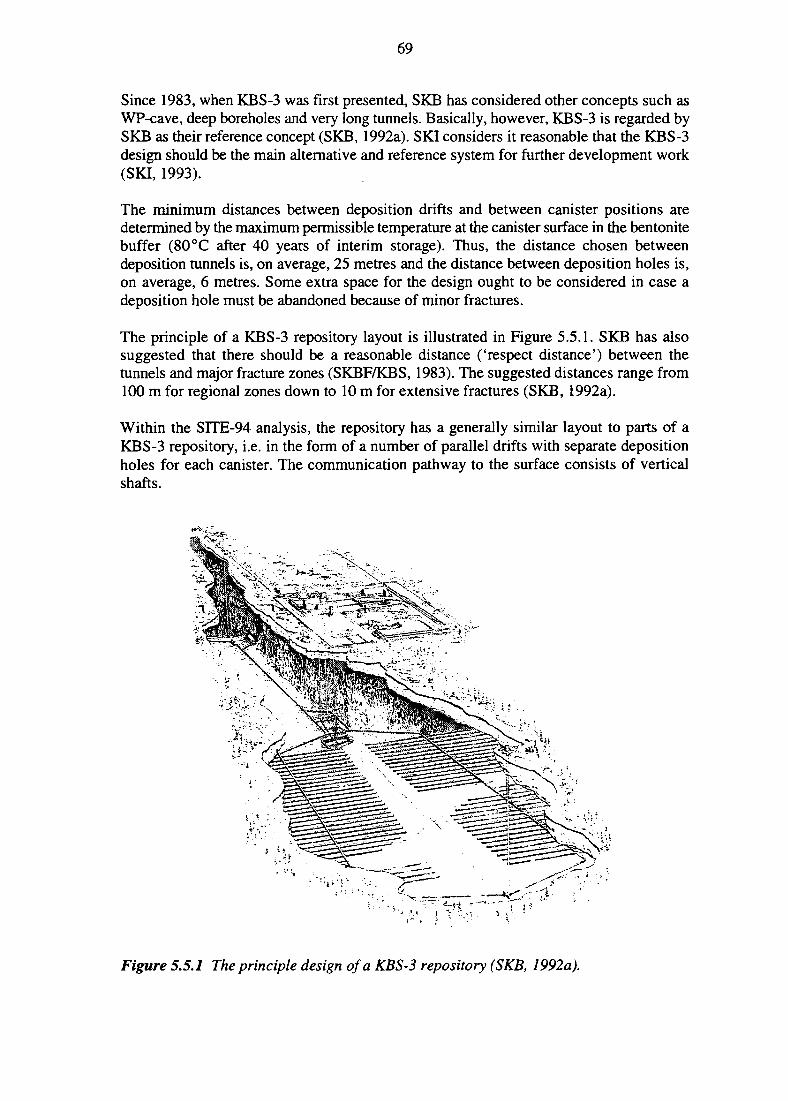
69
Since 1983, when KBS-3 was first presented, SKB has considered other concepts such asWP-cave, deep boreholes and very long tunnels. Basically, however, KBS-3 is regarded bySKB as their reference concept (SKB, 1992a). SKI considers it reasonable that the KBS-3design should be the main alternative and reference system for further development work(SKI, 1993).
The minimum distances between deposition drifts and between canister positions aredetermined by the maximum permissible temperature at the canister surface in the bentonitebuffer (80°C after 40 years of interim storage). Thus, the distance chosen betweendeposition tunnels is, on average, 25 metres and the distance between deposition holes is,on average, 6 metres. Some extra space for the design ought to be considered in case adeposition hole must be abandoned because of minor fractures.
The principle of a KBS-3 repository layout is illustrated in Figure 5.5.1. SKB has alsosuggested that there should be a reasonable distance ('respect distance') between thetunnels and major fracture zones (SKBF/KBS, 1983). The suggested distances range from100 m for regional zones down to 10 m for extensive fractures (SKB, 1992a).
Within the SITE-94 analysis, the repository has a generally similar layout to parts of aKBS-3 repository, i.e. in the form of a number of parallel drifts with separate depositionholes for each canister. The communication pathway to the surface consists of verticalshafts.
Figure 5.5.1 The principle design of a KBS-3 repository (SKB, 1992a).
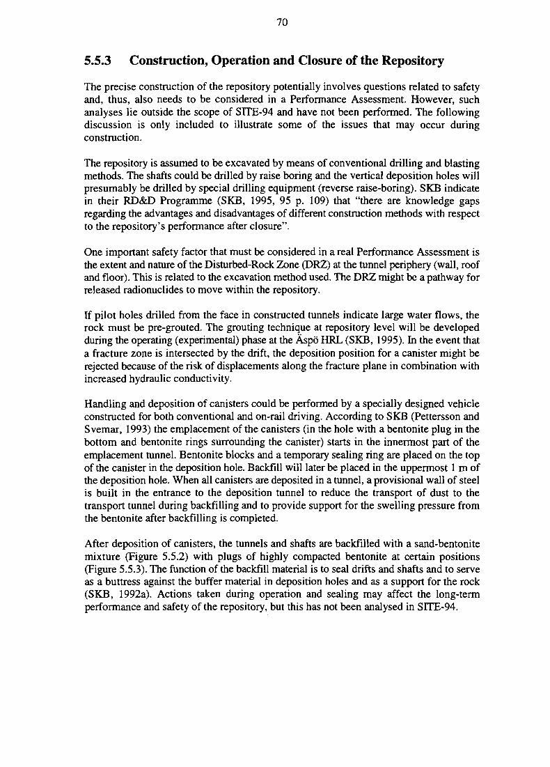
70
5.5.3 Construction, Operation and Closure of the Repository
The precise construction of the repository potentially involves questions related to safetyand, thus, also needs to be considered in a Performance Assessment. However, suchanalyses lie outside the scope of SITE-94 and have not been performed. The followingdiscussion is only included to illustrate some of the issues that may occur duringconstruction.
The repository is assumed to be excavated by means of conventional drilling and blastingmethods. The shafts could be drilled by raise boring and the vertical deposition holes willpresumably be drilled by special drilling equipment (reverse raise-boring). SKB indicatein their RD&D Programme (SKB, 1995, 95 p. 109) that "there are knowledge gapsregarding the advantages and disadvantages of different construction methods with respectto the repository's performance after closure".
One important safety factor that must be considered in a real Performance Assessment isthe extent and nature of the Disturbed-Rock Zone (DRZ) at the tunnel periphery (wall, roofand floor). This is related to the excavation method used. The DRZ might be a pathway forreleased radionuclides to move within the repository.
If pilot holes drilled from the face in constructed tunnels indicate large water flows, therock must be pre-grouted. The grouting technique at repository level will be developedduring the operating (experimental) phase at the Aspo HRL (SKB, 1995). In the event thata fracture zone is intersected by the drift, the deposition position for a canister might berejected because of the risk of displacements along the fracture plane in combination withincreased hydraulic conductivity.
Handling and deposition of canisters could be performed by a specially designed vehicleconstructed for both conventional and on-rail driving. According to SKB (Pettersson andSvemar, 1993) the emplacement of the canisters (in the hole with a bentonite plug in thebottom and bentonite rings surrounding the canister) starts in the innermost part of theemplacement tunnel. Bentonite blocks and a temporary sealing ring are placed on the topof the canister in the deposition hole. Backfill will later be placed in the uppermost 1 m ofthe deposition hole. When all canisters are deposited in a tunnel, a provisional wall of steelis built in the entrance to the deposition tunnel to reduce the transport of dust to thetransport tunnel during backfilling and to provide support for the swelling pressure fromthe bentonite after backfilling is completed.
After deposition of canisters, the tunnels and shafts are backfilled with a sand-bentonitemixture (Figure 5.5.2) with plugs of highly compacted bentonite at certain positions(Figure 5.5.3). The function of the backfill material is to seal drifts and shafts and to serveas a buttress against the buffer material in deposition holes and as a support for the rock(SKB, 1992a). Actions taken during operation and sealing may affect the long-termperformance and safety of the repository, but this has not been analysed in SITE-94.
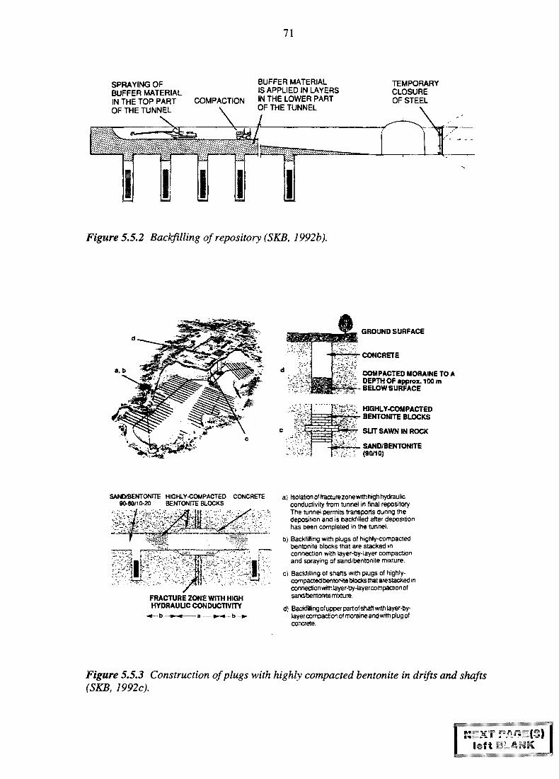
71
SPRAYING OF BUFFER MATERIALBUFFER MATERIAL IS APPLIED IN LAYERSIN THE TOP PART COMPACTION IN THE LOWER PARTOF THE TUNNEL \ OF THE TUNNEL
TEMPORARYCLOSUREOF STEEL
Figure 5.5.2 Backfilling of repository (SKB, 1992b).
GROUND SURFACE
r CONCRETE
l ^ . COMPACTED MORAINE TO A^•r. DEPTH OF approx. 100 mS ^ ~ BELOW SURFACE
WS
i^.<-
HIGHLY-COMPACTEDBENTONTTE BLOCKS
SLIT SAWN IN ROCK
SAND/BENTONITEr&\\ (90/10)
SANOraENTONlTE HIGHLY-COMPACTED CONCRETE90-80/10-20 BENTONITE BLOCKS
FRACTURE ZONE WITH HIGHHYDRAULIC CONDUCTIVITY
b --*
a) Isolation of fracture zone with high hydraulicconductivity from tunnel in final repository.The tunnel permits transports during thedeposition and is backfilled after depositionhas been completed in the tunnel.
b) Backfilling with plugs of htghly-compactedbentonite blocks that are stacked inconnection with layer-by-layer compactionand spraying of sand/bentonite mixture.
c) Backfilling of shafts with plugs of highly-compacted bentonite blocks that are stacked inconnection with layer-by-layer compaction ofsandtoentonite mixture.
d) Backfillingofupperpartofshaftwittiiayer-by-layer compaction of moraine and with plug ofconcrete.
Figure 5.5.3 Construction of plugs with highly compacted bentonite in drifts and shafts(SKB, 1992c).
loft--11
73
6 BASIC DATA FOR THE SITE EVALUATION
This chapter describes the available basic data and summarises the utilisation of these datawithin the SITE-94 Performance Assessment. Section 6.2 describes SKB's preliminary siteinvestigation for the Aspo Hard Rock Laboratory (HRL), which is the source of the site-specific data used within SITE-94. Section 6.3 gives an overview of the field methods andinstrumentation used in the preliminary site investigation. The available site data and theirutilisation within SITE-94 are described in Section 6.4. Data quality, availability andaccessibility are discussed in Section 6.5.
6.1 INTRODUCTION
In order to ensure traceability within a Performance Assessment, careful documentation ofbasic data and their utilisation is essential. An important aspect of SITE-94 is thedevelopment and application of procedures for ensuring traceability. This exercise providespractical experience in working with types and quantities of data such as would beencountered in a Performance Assessment for an actual repository. This experiencefacilitates appraisal of the adequacy, accessibility and quality of data that the sitecharacterisation methodologies provide.
Data for the SITE-94 project were generously provided by SKB, from the Aspo HRL siteinvestigations. In order to make SITE-94 representative of a preliminary PerformanceAssessment, such as would be required prior to commencement of underground activitiesat a candidate repository site, SITE-94 utilises only data that were gathered in the HRLpreliminary investigation phase, which preceded the excavation and construction phase ofthe HRL. This preliminary investigation phase is henceforth referred to as the 'pre-investigation' phase.
6.2 SITE INVESTIGATION PROGRAMME
The major objectives of the preliminary stage of a site investigation include (SKB, 1992):
• definition of the specific position of a rock volume for a repository,
• planning of the surface and subterranean facilities, to be carried out in parallel with,and largely based on the results of the geoscientific pre-investigations,
• providing a basis for a preliminary, site-specific Performance Assessment, asrequired to carry out further, detailed site investigations.
The aims of SKB's investigation programme at Aspo (Stanfors et al., 1991) differed insome respects from these objectives, since the emphasis was on constructing a researchfacility rather than an actual repository. In particular, the HRL pre-investigations were notplanned with the aim of providing a basis for a Performance Assessment exercise.Therefore, some deficiencies are to be expected in applying these data to the SITE-94Performance Assessment.
74
The research objectives of the HRL may also have led to the investigations being moreintensively focused on a few major hydrogeological structures than would be likely to bethe case for a repository pre-investigation. Although proximity to a few major structuresmay be desirable for a research facility (e.g. to test methods for the characterisation of suchstructures), in the siting of a repository an effort would presumably be made to locate rockvolumes at a distance from such features, in as much as possible.
Despite these differences, in many respects the scope of the HRL pre-investigations wassimilar to what can be expected for a real disposal site. The stated objectives of the pre-investigation phase are: site selection for the HRL, description of the natural conditions inthe bedrock and predictions of changes that would occur during construction. All of theseare of concern for an actual repository. Moreover, a general aim of the current HRL workis the "verification of pre-investigation methods and development of the detailedinvestigation methodology" (SKB, 1994), which implies that the pre-investigation methodsbeing verified should be representative of those envisioned for an actual repository site.
The pre-investigations for the HRL were carried out between late 1986 and October 1990,in three main stages (Stanfors et al., 1991):
• Siting stage (late 1986 - 1987): A regional survey over a 25 km x 35 km area,roughly centred on Simpevarp, based on airborne geophysics, digital terrain models,geological mapping and regional hydrological data.
• Site description stage (1987 - 1988): Site investigations in the vicinity of Avro,Aspo and Laxemar, including geological, hydrogeological and geochemicalinvestigations in boreholes (percussion- and core-drilled), and detailed surfaceinvestigations on Aspo including geophysical profiles and mapping of bedrock typesand fracturing.
• Prediction stage (late 1988 - 1990): The HRL site was chosen in southern Aspo.Additional core-drilled holes were directed toward 'zones of geological andhydraulic importance'. Hydrogeological evaluation and/or changes in the layout ofthe HRL prompted a third drilling campaign (Stanfors et al., 1991; Wikberg et al.,1991). Short-term interference tests and two long-term pumping tests (LPT1 andLPT2) were performed.
An overview of these investigations is given by Stanfors et. al. (1991). Particular aspectsof the HRL site investigation programme, including the relevance of different types ofmeasurements, are discussed in relevant sections of this report.
6.3 METHODS AND INSTRUMENTS
The following is a brief summary of the data collection methods that provided the basicdata for SITE-94. Table 6.3.1 lists the main types of methods and indicates the coverageand type of information sought and/or provided with each method. This information isdrawn mainly from three SKB reports summarising the HRL pre-investigations:
75
• a comprehensive tabulation of the investigation methods by Stanfors et al. (1991),
• summary descriptions of the field methods and instrumentation by Almen andZellman(1991),
• a description of how the results were evaluated by Wikberg et al. (1991).
A list of over 80 HRL progress reports, which contain more detailed descriptions of the pre-investigation methods and analyses, is given by Stanfors et al (1991).
Remote sensing and survey data for the Simpevarp area were produced by Swedishgovernmental agencies, independent of the HRL investigations. Supplementary work wascommissioned by SKB to establish a single elevation database for the Simpevarp area.Lineament interpretations based on these data were produced during the HRL siting stage.
Geophysical surveys include airborne surveys that were conducted on a regional (about50 km) scale during the HRL siting stage, and subsequent ground-based surveys. Ground-based surveys during the siting stage were performed on about 20 profiles across specificregional structures. More detailed ground-based surveys were subsequently conducted onsemi-regional (about 10 km) and local (2-5 km) scales. Borehole geophysical logging wasperformed in a majority of the cored and percussion-drilled holes at the HRL site.
Geological investigations include field studies, based on outcrop mapping on regional andlocal scales and mapping of cleared trenches on the local scale. Borehole geologicallogging consists of lithologic and fracture mapping on core from the 12 deepest holes onAspo (KAS02-08 & 11-14) plus KBH02 and KLX01, plus logging of drill cuttings (rockchips) in the percussion-drilled holes. Detailed petrologic analyses (thin-section andchemical) were performed on selected rock samples and fracture coatings/fillings from core.
Geomechamcal investigations include in-situ stress measurements and laboratory tests oncore samples. The latter included measurements of the mechanical properties of joints.Petrophysical measurements were performed both on rock samples gathered over theregional scale, in support of the airborne geophysical surveys, and on core samples fromboreholes KAS02 and KLX01.
Hydrogeochemical analyses were performed on groundwater samples collected at severalstages of the pre-investigations. Major element analyses were performed on 'first-strike'groundwater samples collected during drilling of the core-drilled holes and on samples fromthe percussion-drilled holes. More comprehensive suites of chemical analyses (includingminor element chemistry, stable-isotope compositions, 3H and 14C activities, and drilling-water content) are performed on samples drawn from water-bearing sections of boreholeHAS 13 and six core-drilled boreholes, generally after sustained pumping. The groundwateranalyses were supplemented by analyses of fracture minerals in core.
Hydrogeological measurements in boreholes were performed using a variety of single-hole and cross-hole techniques, as listed in Table 6.3.1. Additional regional well andgroundwater chemistry data were available from well records maintained by the SwedishGeological Survey. The cross-hole testing included short-term (2- or 3-day) pumping testsin single boreholes or packed-off sections of boreholes, with monitoring of groundwater
76
pressures/levels in adjacent boreholes, and long-term (3-month) pumping tests LPT1 andLPT2 in boreholes KAS07 and KAS06, respectively. In both LPT1 and LPT2, the flowrates of groundwater passing the observation boreholes are estimated based on tracerdilution measurements. A 3D convergent tracer test was conducted in conjunction withLPT2, with four distinct types of tracers being introduced in packed-off sections of thepassive boreholes and arrivals monitored in sections of the pumped hole.
Within SITE-94, a critical review (Andersson et al., 1993) was commissioned of theborehole hydraulic measurement methods used by SKB at Aspo. This review discussesvarious uncertainties and potential sources of errors related to the measurement methods,including:
• ordinary measurement errors due to instrument resolution, equipment compliance,borehole survey errors, and test procedures,
• uncertainty in measurements due to wellbore storage (fluid and packercompressibility) and skin effects (e.g. plugging of fractures by drilling fines),
• potential measurement errors due to deviations from the boundary conditions thatare supposed to be imposed during a test (e.g. leakage around packers for injectiontests and short-circuiting of multiple hydraulic units during dilution tests),
• conceptual uncertainties and scale effects due to the heterogeneous nature of thefractured rock (e.g. flow geometry and volume of rock characterised for packer tests;distinct multiple pathways for tracer tests) and,
• bias of the Aspo measurements toward the horizontal component of hydraulicconductivity (or horizontal fractures), due to the combination of predominantly near-vertical boreholes and testing methods that primarily measure lateral conductivity.
The conceptual uncertainty due to rock-mass heterogeneity is likely to be the dominantsource of uncertainty for any single measurement. Furthermore, the presence ofheterogeneity may diminish the comparability of hydraulic measurements when the testingequipment and/or procedures are modified during the course of a site investigation, sincesuch changes may affect the volume of the rock that is actually characterised by theinterpretable response.
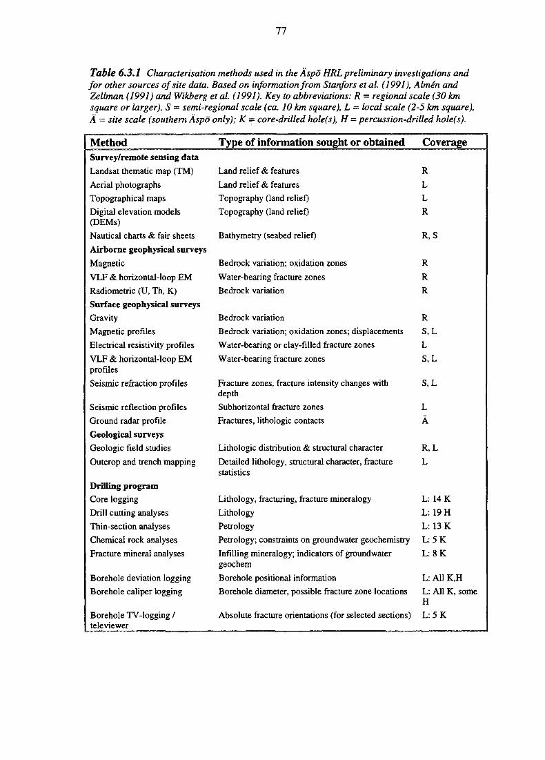
77
Table 6.3.1 Characterisation methods used in the Aspo HRL preliminary investigations andfor other sources of site data. Based on information from Stanfors et al. (1991), Almen andZellman (1991) and Wikberg et al. (1991). Key to abbreviations: R = regional scale (30 kmsquare or larger), S — semi-regional scale (ca. 10 km square), L — local scale (2-5 km square),A = site scale (southern Aspo only); K = core-drilled hole(s), H = percussion-drilled hole(s).
MethodSurvey/remote sensing data
Landsat thematic map (TM)
Aerial photographs
Topographical maps
Digital elevation models(DEMs)
Nautical charts & fair sheets
Airborne geophysical surveys
Magnetic
VLF & horizontal-loop EM
Radiometric (U, Th, K)
Surface geophysical surveys
Gravity
Magnetic profiles
Electrical resistivity profiles
VLF & horizontal-loop EMprofiles
Seismic refraction profiles
Seismic reflection profiles
Ground radar profile
Geological surveys
Geologic field studies
Outcrop and trench mapping
Drilling programCore logging
Drill cutting analyses
Thin-section analyses
Chemical rock analyses
Fracture mineral analyses
Borehole deviation logging
Borehole caliper logging
Borehole TV-logging /televiewer
Type of information sought or obtained
Land relief & features
Land relief & features
Topography (land relief)
Topography (land relief)
Bathymetry (seabed relief)
Bedrock variation; oxidation zones
Water-bearing fracture zones
Bedrock variation
Bedrock variation
Bedrock variation; oxidation zones; displacements
Water-bearing or clay-filled fracture zones
Water-bearing fracture zones
Fracture zones, fracture intensity changes withdepth
Subhorizontal fracture zones
Fractures, lithologic contacts
Lithologic distribution & structural character
Detailed lithology, structural character, fracturestatistics
Lithology, fracturing, fracture mineralogy
Lithology
Petrology
Petrology; constraints on groundwater geochemistry
Infilling mineralogy; indicators of groundwatergeochem
Borehole positional information
Borehole diameter, possible fracture zone locations
Absolute fracture orientations (for selected sections)
Coverage
R
L
L
R
R, S
R
R
R
R
S,L
L
S,L
S,L
L
A
R,L
L
L: 14 K
L: 19 H
L: 13 K
L:5K
L:8K
L: All K,H
L: All K, someH
L:5K
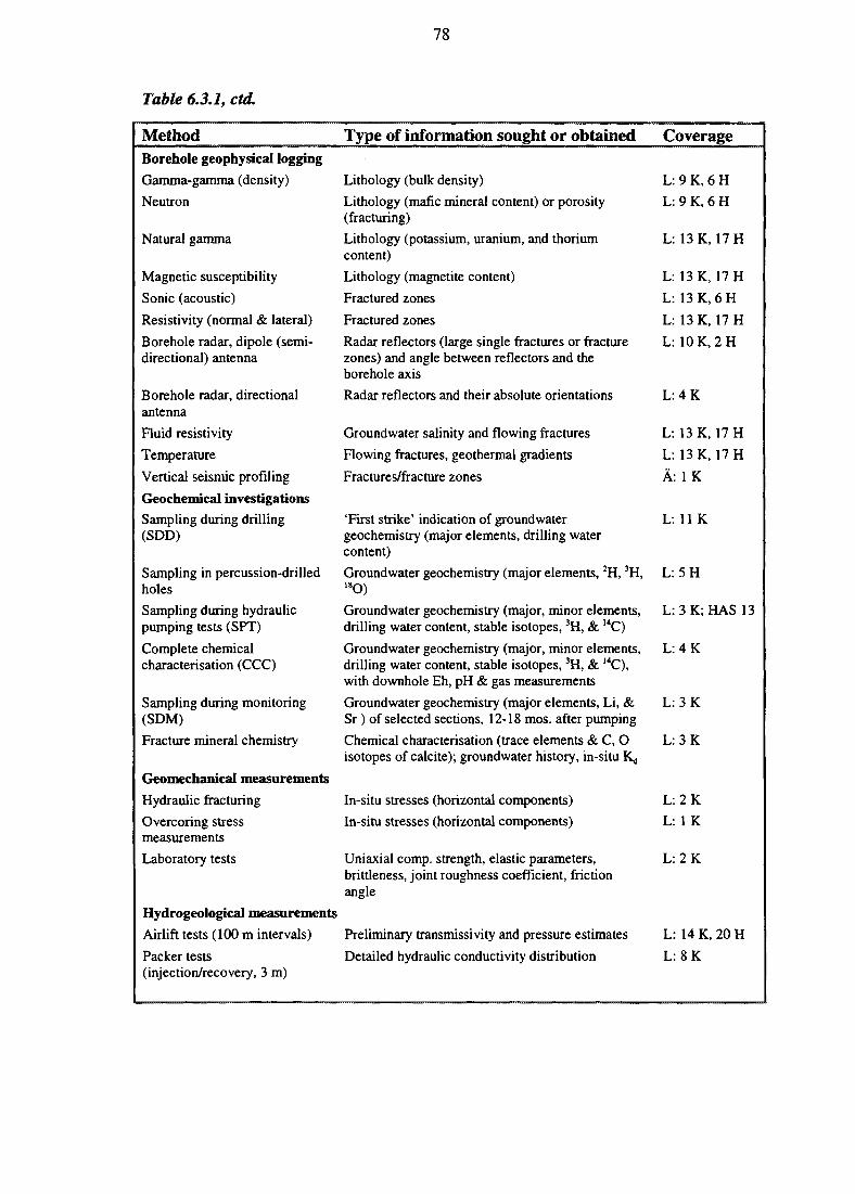
78
Table 6.3.1, ctd.
MethodBorehole geophysical logging
Gamma-gamma (density)
Neutron
Natural gamma
Magnetic susceptibility
Sonic (acoustic)
Resistivity (normal & lateral)
Borehole radar, dipole (semi-directional) antenna
Borehole radar, directionalantenna
Fluid resistivity
Temperature
Vertical seismic profiling
Geochemical investigationsSampling during drilling(SDD)
Sampling in percussion-drilledholes
Sampling during hydraulicpumping tests (SPT)
Complete chemicalcharacterisation (CCC)
Sampling during monitoring(SDM)
Fracture mineral chemistry
Geomechanical measurements
Hydraulic fracturing
Overcoring stressmeasurements
Laboratory tests
Hydrogeological measurements
Airlift tests (100 m intervals)
Packer tests(injection/recovery, 3 m)
Type of information sought or obtained
Lithology (bulk density)
Lithology (mafic mineral content) or porosity(fracturing)
Lithology (potassium, uranium, and thoriumcontent)
Lithology (magnetite content)
Fractured zones
Fractured zones
Radar reflectors (large single fractures or fracturezones) and angle between reflectors and theborehole axis
Radar reflectors and their absolute orientations
Groundwater salinity and flowing fractures
Flowing fractures, geothermal gradients
Fractures/fracture zones
'First strike' indication of groundwatergeochemistry (major elements, drilling watercontent)
Groundwater geochemistry (major elements, 2H, 3H,18O)
Groundwater geochemistry (major, minor elements,drilling water content, stable isotopes, 3H, & 14C)
Groundwater geochemistry (major, minor elements,drilling water content, stable isotopes, 3H, & 14C),with downhole Eh, pH & gas measurements
Groundwater geochemistry (major elements, Li, &Sr ) of selected sections, 12-18 mos. after pumping
Chemical characterisation (trace elements & C, 0isotopes of calcite); groundwater history, in-situ K,j
In-situ stresses (horizontal components)
In-situ stresses (horizontal components)
Uniaxial comp. strength, elastic parameters,brittleness, joint roughness coefficient, frictionangle
Preliminary transmissivity and pressure estimates
Detailed hydraulic conductivity distribution
Coverage
L: 9 K, 6 H
L: 9 K, 6 H
L: 13 K, 17 H
L: 13 K, 17 H
L: 13K,6H
L: 13 K, 17 H
L: 10K,2H
L:4K
L:13 K, 17 H
L: 13 K, 17 H
A: I K
L: 11 K
L:5H
L:3K;HAS 13
L:4K
L:3K
L:3K
L:2K
L: 1 K
L:2K
L: 14 K, 20 H
L:8K
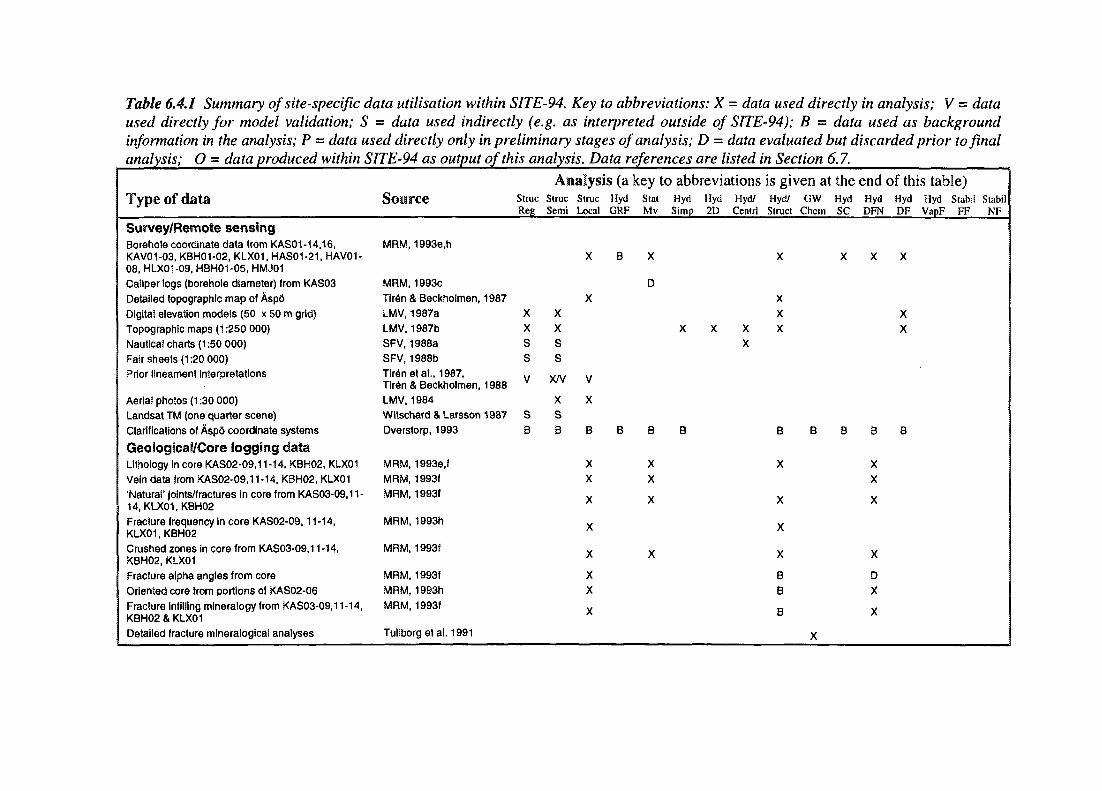
Table 6.4.1 Summary of site-specific data utilisation within SITE-94. Key to abbreviations: X = data used directly in analysis; V = dataused directly for model validation; S - data used indirectly (e.g. as interpreted outside of SITE-94); B = data used as backgroundinformation in the analysis; P - data used directly only in preliminary stages of analysis; D - data evaluated but discarded prior to finalanalysis; O = data produced within SITE-94 as output of this analysis. Data references are listed in Section 6.7.
Type of data
Survey/Remote sensingBorehole coordinate data from KAS01-14.16,KAV01-03, KBH01-02, KLX01, HAS01-21, HAV01-08, HLX01-09, HBH01-05, HMJ01Caliper logs (borehole diameter) from KAS03Detailed topographic map of Asp6Digita! elevation models (50 x 50 m grid)Topographic maps (1:250 000)Nauticai charts (1:50 000)Fair sheets (1:20 000)Prior lineament interpretations
Aeria! photos (1:30 000)Landsat TM (one quarter scene)Clarifications of Asp6 coordinate systems
GeoiogScaS/Core logging dataLithology in core KAS02-09.11-14, KBH02, KLX01Vein data from KAS02-09.11-14, KBH02, KLX01'Natural' joints/fractures in core from KAS03-09.11-14, KLX01.KBH02Fracture frequency in core KAS02-09,11-14,KLX01.KBH02Crushed zones in core from KAS03-09.11-14,KBH02, KLX01Fracture alpha angles from coreOriented core from portions of KAS02-06Fracture infilling mineralogy from KAS03-09.11-14,KBH02 & KLX01Detailed fracture mineraiogical analyses
Source
MRM, 1993e,h
MRM, 1993cTiren & BeckhoSmen, 1987LMV, 1987aLMV, 1987bSFV, 1988aSFV, 1988bTiren eta!., 1987,Tiren & Beckholmen, 1988LMV, 1984Witschard & Larsson 1987Dverstorp, 1993
MRM, 1993e,fMRM, 1993fMRM, 19931
MRM, 1993h
MRM, 1993f
MRM, 1993fMRM, 1993hMRM, 19931
Tullborg et al. 1991
StnicReg
XXSS
v
sB
Analysis (aStrucSemi
XXSS
XA//V V
XsB
Struc HydLocal GRF
X B
X
vV
X
B B
XX
x
x
yA
XXY/ \
key to abbreviationsStat Hyd Hyd Hyd/Mv Simp 2D Centrl
X
D
X X X
X
B B
XX
Y/ \
yA
is given atHyd/ GWStruct Chem
X
XXX
B B
X
yA
x
vA
BBQO
X
theHydSC
X
B
endHydDFN
X
B
XX
yA
VA
DXvA
of this table)Hyd Hyd Stabil StabilDF VapF FF NF
X
XX
B
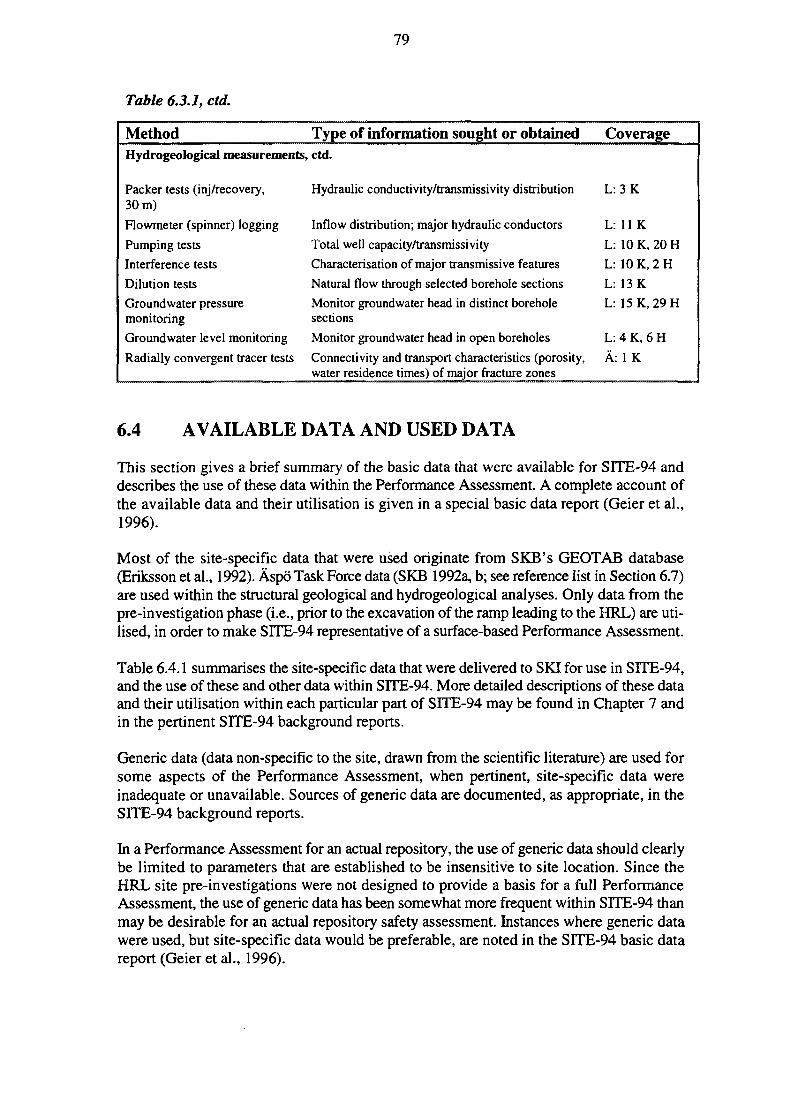
79
Table 6.3.1, ctd.
Method Type of information sought or obtainedHydrogeological measurements, ctd.
Packer tests (inj/recovery,30 m)
Flowmeter (spinner) logging
Pumping tests
Interference tests
Dilution tests
Groundwater pressuremonitoringGroundwater level monitoring
Radially convergent tracer tests
Hydraulic conductivity/transmissivity distribution
Inflow distribution; major hydraulic conductors
Total well capacity/transmissivity
Characterisation of major transmissive features
Natural flow through selected borehole sections
Monitor groundwater head in distinct boreholesectionsMonitor groundwater head in open boreholes
Connectivity and transport characteristics (porosity,water residence times) of major fracture zones
Coverage
L:3K
L: U K
L: 10 K, 20 H
L: 10 K, 2 H
L: 13 K
L: 15 K, 29 H
L: 4 K, 6 H
A: 1 K
6.4 AVAILABLE DATA AND USED DATA
This section gives a brief summary of the basic data that were available for SITE-94 anddescribes the use of these data within the Performance Assessment. A complete account ofthe available data and their utilisation is given in a special basic data report (Geier et al.,1996).
Most of the site-specific data that were used originate from SKB's GEOTAB database(Eriksson et al., 1992). Aspo Task Force data (SKB 1992a, b; see reference list in Section 6.7)are used within the structural geological and hydrogeological analyses. Only data from thepre-investigation phase (i.e., prior to the excavation of the ramp leading to the HRL) are uti-lised, in order to make SITE-94 representative of a surface-based Performance Assessment.
Table 6.4.1 summarises the site-specific data that were delivered to SKI for use in SITE-94,and the use of these and other data within SITE-94. More detailed descriptions of these dataand their utilisation within each particular part of SITE-94 may be found in Chapter 7 andin the pertinent SITE-94 background reports.
Generic data (data non-specific to the site, drawn from the scientific literature) are used forsome aspects of the Performance Assessment, when pertinent, site-specific data wereinadequate or unavailable. Sources of generic data are documented, as appropriate, in theSITE-94 background reports.
In a Performance Assessment for an actual repository, the use of generic data should clearlybe limited to parameters that are established to be insensitive to site location. Since theHRL site pre-investigations were not designed to provide a basis for a full PerformanceAssessment, the use of generic data has been somewhat more frequent within S1TE-94 thanmay be desirable for an actual repository safety assessment. Instances where generic datawere used, but site-specific data would be preferable, are noted in the SITE-94 basic datareport (Geier et al., 1996).
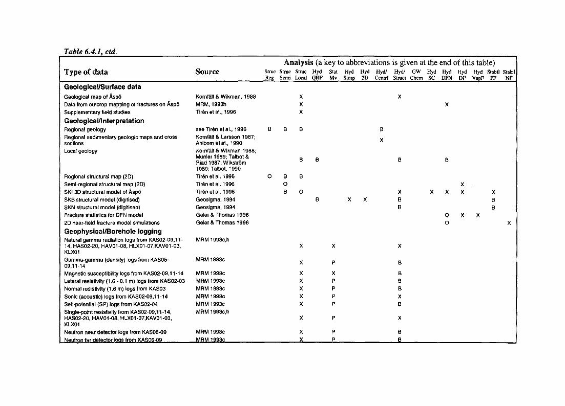
Table 6.4.1, ctd.
Type of dataV A.
Geological/Surface dataGeological map of Asp6Data from outcrop mapping of fractures on AspoSupplementary field studies
Geological/interpretationRegional geologyRegional sedimentary geologic maps and crosssectionsLocal geology
Regional structural map (2D)Semi-regional structural map (2D)SKI 3D structural model of Asp6SKB structural model (digitised)SKN structural model (digitised)Fracture statistics for DFN model2D near-field fracture model simulations
GeophysicaS/Boreho9e loggingNatural gamma radiation logs from KAS02-09.11-14, HAS02-20, HAV01-08, HLX01-07.KAV01-03,KLX01Gamma-gamma (density) logs from KAS05-09,11-14Magnetic susceptibility logs from KAS02-09.11-14Lateral resistivity (1.6 - 0.1 m) logs from KAS02-03Normal resistivity (1.6 m) logs from KAS03Sonic (acoustic) logs from KAS02-09.11-14Self-potential (SP) logs from KAS02-04Single-point resistivity from KAS02-09.11-14,HAS02-20, HAV01-08, HLX01-07.KAV01-03,KLX01Neutron near detector logs from KAS06-09
Neutron far detector ioas from KAS06-09
Source
Komfalt & Wikman, 1988MRM, 1993hTir6netal, 1996
seeTlren eta!., 1996Kornfaii & Larsson 1987;Ahlbometal., 1990Kornfait & Wikman 1988;Munier1989;Talbot&Riad1987;Wikstrom1989;Talbot, 1990Tireneial. 1996Tir6netal. 1996TirSnetal. 1996Geosigma, 1994Geosigma, 1994Geier& Thomas 1996Geier& Thomas 1996
MRM 1993c,h
MRM 1993c
MRM 1993cMRM 1993cMRM 1993cMRM 1993cMRM 1993cMRM 1993c,h
MRM 1993cMRM 1993c
Analysis (a key to abbreviationsStruc StrucReg Semi
8 B
O BOB
Struc HydLocal GRF
XXX
B
D OO O
B
0B
X
x
XXXXX
X
XX
Stat Hyd Hyd Hyd/Mv Simp 2D Centrl
B
y
X X
X
p
Xp
ppp
p
pp
is given atHyd/ GWStruct Chem
X
b
XBB
X
B
BBBXB
X
8B
the endHyd HydSC DFN
X
oD
X X
0
o
of this table)HydDF
XX
X
Hyd Stabil StabilVapF FF NF
XBB
XX
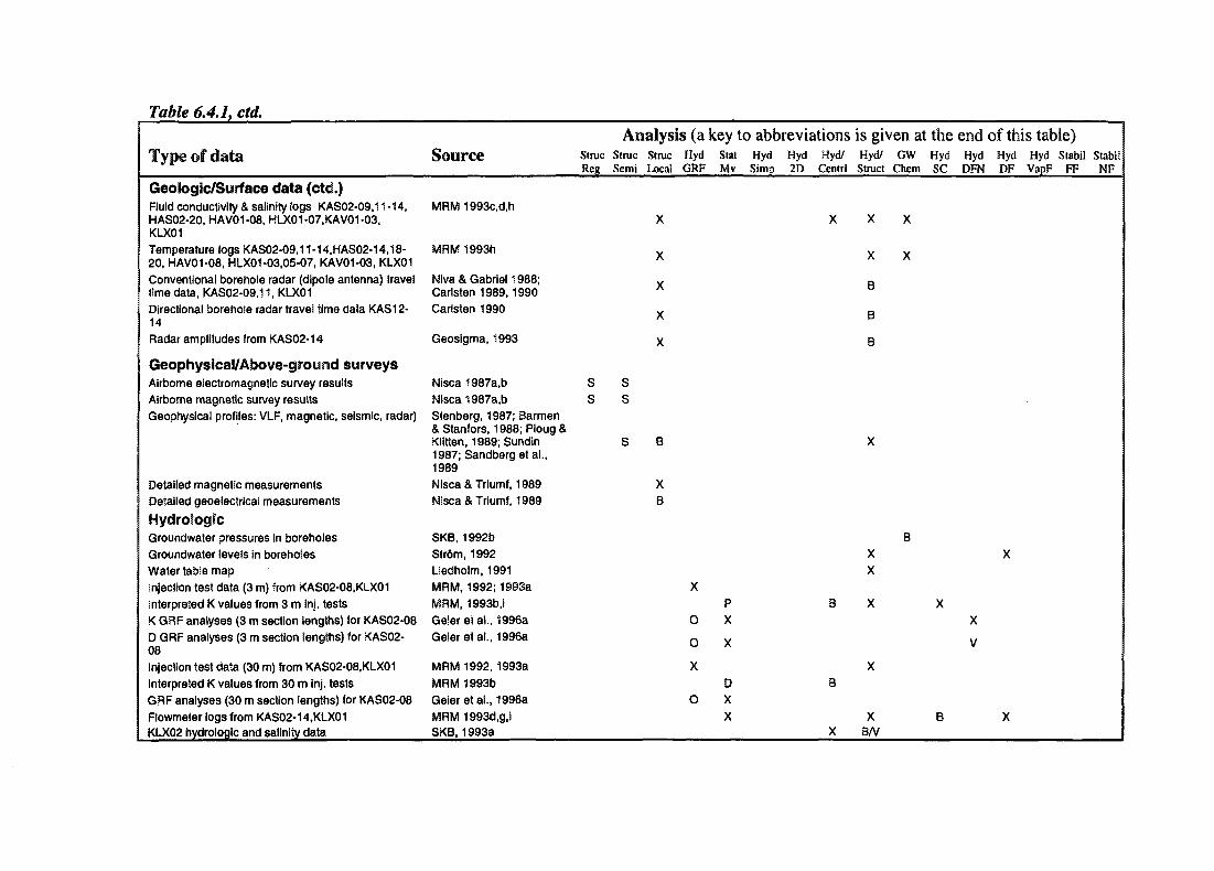
Table 6.4.1, ctd.
Type of data
Geologic/Surface data (ctd.)Fluid conductivity & salinity logs KAS02-09.11-14,HAS02-20, HAV01-08, HLX01-07.KAV01-03,KLX01Temperature logs KAS02-09,11-14,HAS02-14,18-20, HAV01-08, HLX01-03,05-07, KAV01-03, KLX01Conventional borehole radar (dipole antenna) traveltime data, KAS02-09.11, KLX01Directional borehole radar travel time data KAS12-14Radar amplitudes from KAS02-14
Geophysical/Above-ground! surveysAirborne electromagnetic survey resultsAirborne magnetic survey resultsGeophysical profiles: VLF, magnetic, seismic, radar)
Detailed magnetic measurementsDetailed geoelectricai measurements
HydiroiogicGroundwater pressures in boreholesGroundwater levels in boreholesWater table mapInjection test data (3 m) from KAS02-08.KLX01Interpreted K values from 3 m inj. testsK GRF analyses (3 m section lengths) for KAS02-08D GRF analyses (3 m section lengths) for KAS02-08Injection test data (30 m) from KAS02-08.KLX01
Interpreted K values from 30 m inj. testsGRF analyses (30 m section lengths) for KAS02-08Flowmeter logs from KAS02-14.KLX01KLX02 hydrologic and salinity data
Source
MRM 1993c,d,h
MRM 1993h
Niva& Gabriel 1988;Carlsten 1989,1990Carlsten 1990
Geosigma, 1993
Nisca 1987a,bNisca 1987a,bStenberg, 1987; Barmen& Stanfors, 1988; Ploug &Klitten, 1989; Sundin1987; Sandberg et a!.,1989Nisca &Triumf, 1989Nisca &Triumf, 1989
SKB, 1992bStr6m, 1992Uedholm, 1991MRM, 1992; 1993aMRM, 1993b,iGeiereta!., 1996aGeieretai., 1996a
MRM 1992, 1993aMRM 1993bGeieretai., 1996aMRM 1993d,g,iSKB, 1993a
Analysis (a keyStruc Struc StrucReg Semi Local
X
yA
yA
X
X
s ss s
S B
XB
HydGRF
X
O
O
X
O
StatMv
PX
X
DXX
to abbreviationsHyd Hyd Hyd/Simp 2D Centrl
X
B
8
X
is given at theHyd/ GW HydStruct Chem SC
X X
x yA A
R
B
CD
X
BXX
X X
X
X BB/V
end of this table)Hyd Hyd Hyd Stabil StabilDFN DF VapF FF NF
X
X
V
X
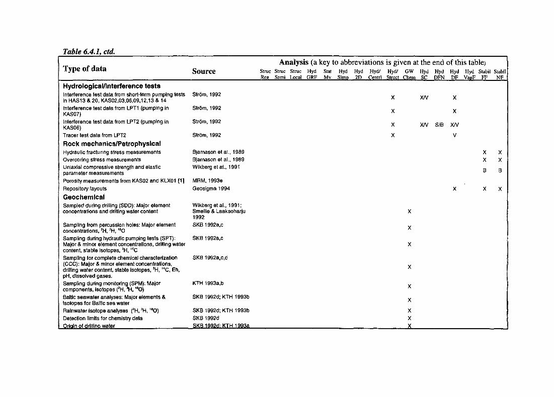
Table 6.4.1, ctd.
Type of data SourceAnalysis (a key to abbreviations is given at the end of this table)
Struc Struc Struc Hyd Stat Hyd Hyd Hyd/ Hyd/ GW Hyd Hyd Hyd Hyd Stabil Stabi!Reg Semi Local GRF Mv Simp 2D Centrl Struct Chem SC DFN DF VaoF FF NF
Hydrological/lnferference testsInterference test data from short-term pumping testsin HAS13 & 20, KAS02,03,06,09,12,13 & 14Interference test data from LPT1 (pumping inKAS07)interference test data from LPT2 (pumping inKAS06)Tracer test data from LPT2
Rock mechanics/PetrophysicaiHydraulic fracturing stress measurementsOvercoring stress measurementsUniaxiai compressive strength and elasticparameter measurements
Porosity measurements from KAS02 and KLX01 [1]Repository layouts
GeochemicaSSampled during drilling (SDD): Major elementconcentrations and driliing water content
Sampling from percussion holes: Major elementconcentrations, 2H, 3H, 18OSampling during hydraulic pumping tests (SPT):Major & minor element concentrations, drilling watercontent, stable isotopes, 3H, 14CSampling for complete chemical characterization(CCC): Major & minor element concentrations,drilling water content, stable isotopes, 3H, MC, Eh,pH, dissolved gases.Sampling during monitoring (SPM): Majorcomponents, isotopes (2H, 3H, 18O)Baltic seawater analyses: Major elements &isotopes for Baltic sea waterRainwater isotope analyses (2H, 3H, 18O)Detection limits for chemistry dataOriain of drillina water
Str6m,1992
Str&m, 1992
Str6m, 1992
Strom, 1992
Bjarnason etal., 1989Bjarnason etal., 1989Wikberg et a!., 1991
MRM, 1993e
Geosigma 1994
Wikberg et a!., 1991;Smellie & Laaksoharju1992SKB1992a,c
SKB1992a,c
SKB1992a,c,d
KTH 1993a,b
SKB1992d;KTH 1993b
SKB1992d;KTH 1993bSKB 1992dSKB1992d:KTH 1993a
X
X
X
X
X/V
X/V
X
X
S/B X/V
V
X
X
X
X
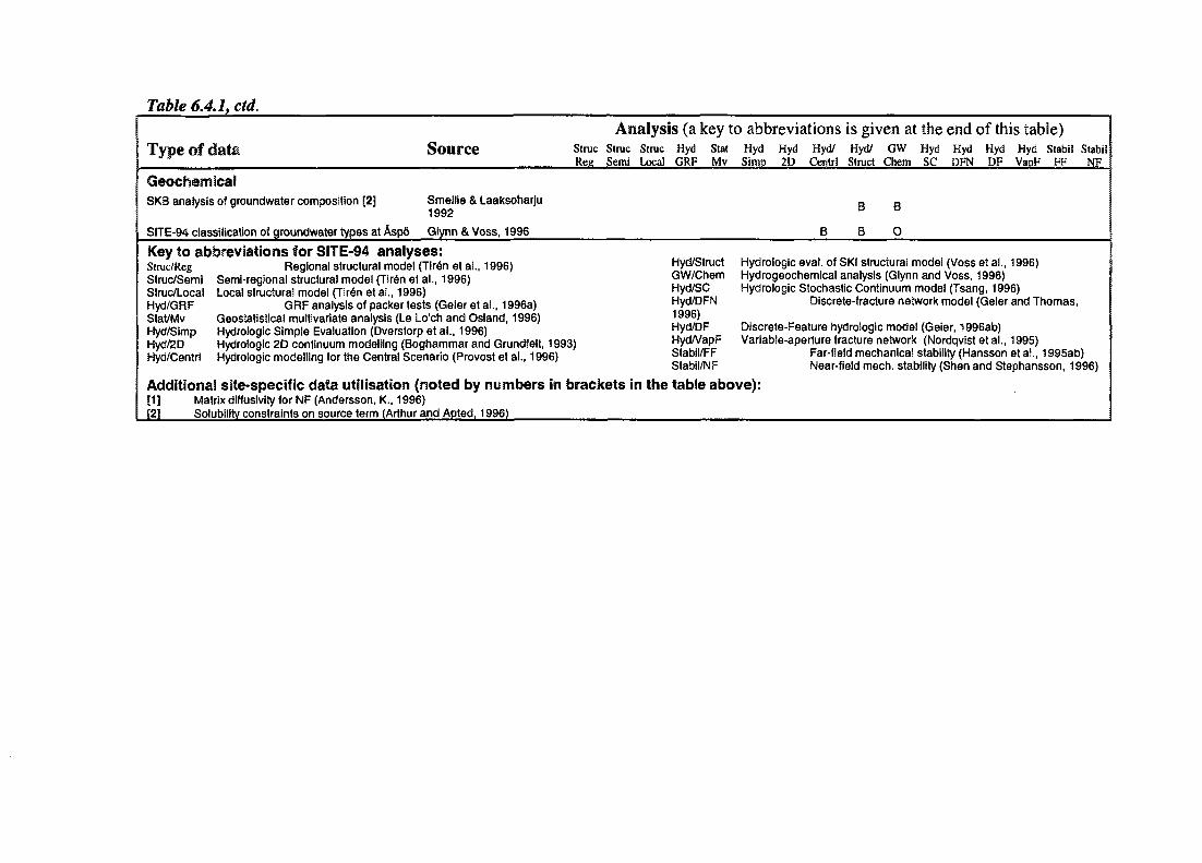
Table 6.4.1, ctd.
Type of dataAnalysis (a key to abbreviations is given at the end of this table)
Struc StnicReg Semi
StrucLocal
HydGRF
StatMv
HydSimp 2D
Hyd/Centrl
Hyd/ GWStruct Chem
HydSC
HydDFN
Hyd Hyd Stabil StabiSV a o F F F N F
GeochemiicalSKB analysis of groundwater composition [2] Smeiiie & Laaksoharju
1992
SITE-94 classification of groundwater types at Asp6 Glynn & Voss, 1996 B B
Key to abbreviations for SITE-94 analyses:Struc/Reg Regional structural model (Tir6n et al., 1996)Struc/Semi Semi-regional structural mode! (Tiren et al., 1996)Struc/Local Local structural model (Tir6n et al., 1996)Hyd/GRF GRF analysis of packer tests (Geier et a!., 1996a)Stat/Mv Geostatisticaj multivariate analysis (Le Lo'ch and Osland, 1996)Hyd/Simp Hydroiogic Simple Evaluation (Dverstorp et a!., 1996)Hyd/2D Hydroiogic 2D continuum modelling (Boghammar and Grundfelt, 1993)Hyd/Centrj Hydroiogic modelling for the Central Scenario (Provost et al., 1996)
Hyd/Struct Hydroiogic evai. of SKI structural mode! (Voss et a!., 1996)GW/Chem Hydrogeochemical analysis (Glynn and Voss, 1996)Hyd/SC Hydroiogic Stochastic Continuum model (Tsang, 1996)Hyd/DFN Discrete-fracture network model (Geier and Thomas,1996)Hyd/DF Discrete-Feature hydroiogic model (Geier, 1996ab)Hyd/VapF Variable-aperture fracture network (Nordqvistetal., 1995)Stabi!/FF Far-field mechanical stability (Hansson et a!., 1995ab)Stabil/NF Near-field mech. stability (Shen and Stephansson, 1996)
Additional site-specific data utilisation (noted by numbers in brackets in the table above):[1] Matrix diffusivity for NF (Andersson, K., 1996)[2] Solubility constraints on source term (Arthur and Apted, 1996)
85
6.5 AVAILABILITY AND QUALITY OF DATA
The following is a summary of observations concerning data quality and availability for theAspo HRL site. A more detailed discussion of these issues is given by Geier et al. (1996).
It should be emphasised that SKB's establishment of the GEOTAB database is in itself ofgreat value. The collection of primary geoscientific data in a unified database creates thepotential to investigate relationships among different properties/attributes of the bedrockand groundwater, using flexible querying techniques. SKB's considerable efforts inpreparing the site data and in providing these to SKI for SITE-94, are also very muchappreciated. In most cases, the data requested were delivered expediently, together withsupporting information which facilitated the analysis of these data within SITE-94.
Regarding the observations that follow, it should be noted that, within SITE-94, these dataare utilised in ways that may not have been foreseen during acquisition. The task oforganising and conducting a major site investigation, such as that at Aspo, is formidable,requiring the coordination of diverse logistical, geoscientific and construction activities.The HRL pre-investigations provide a valuable learning experience as to how such aninvestigation should be conducted in order to acquire and preserve the essential, high-quality data that will be required for Performance Assessment.
SITE-94 may be seen as a part of this learning experience, in that it tests the sufficiency ofthe site database as the basis for an independent Performance Assessment. The commentssummarised below should be viewed as constructive suggestions for future siteinvestigations. A few of the problems noted have been independently identified andcorrected by the Aspo investigators. It should be noted that, following the HRL pre-investigations, SKB has established a new database to replace GEOTAB and has devotedconsiderable effort to improving procedures for handling site data.
6.5.1 Documentation
Clear and comprehensive documentation of the basic data is an important requirement foran independent, site-specific Performance Assessment. In several cases, documentationdescribing the collection of specific data appears to be lacking. In other cases (as describedby Geier et al., 1996), the data that have been stored are not clearly defined, or the methodsof measurement are not sufficiently described, to allow a full, independent assessment ofthe data.
It is essential that, together with each piece of archived data, information should be readilyaccessible concerning:
• how measurements and sampling were performed,
• what equipment was used,
86
• what detection limits and accuracy levels are associated with the equipment andprocedures and,
• if interpretations or corrections were performed, how these were done.
When equipment or procedures are modified during the course of an investigation, thedocumentation, archiving and retrieval systems must provide for clear distinction amongthe resulting data. A good, general description of the field investigation methods is givenby Almen and Zellman (1991), but this is incomplete as a record of which particularmethods were used in which portions of the pre-investigations. In a few cases, methods aredescribed that apparently were not actually used at Aspo, but were part of a broaderresearch and development programme.
A related problem, from the standpoint of analysts engaged in an independent PerformanceAssessment such as SITE-94, is the lack of a single document describing the specific datathat were available for the HRL site. The overview report for the HRL pre-investigations(Stanfors et al., 1991) was valuable as a record of what types of studies were performed atthe site, but it did not provide a comprehensive index to the data that were actuallyavailable from the site database. In some cases, the basic data produced by individualstudies were not available from GEOTAB, while in other cases the availability of particulardata was only discovered fortuitously, from HRL progress reports or unpublished sources.The lack of a single document giving an index to all available data led to some unnecessaryeffort, on the part of both SKI and SKB, and is a hindrance to a thorough analysis.
6.5.2 Positional Information
A second basic requirement for Performance Assessment is to establish a consistent frameof reference (spatial coordinates) for the measurements that have been performed. This isparticularly important for structural geological and geostatistical analysis. In the HRL pre-investigations, several different coordinate systems (the Swedish Land Survey's RAK-38system, an OKG system for Simpevarp, and a local system on Aspo) are used forobservations at the surface. Unfortunately, the relationships between these systems are notfully documented. Inaccurate map scales are also an occasional problem, particularly forcertain geological data that are only presented on maps. For measurements withinindividual boreholes, the points of reference are not always consistent. Also, it is notconsistently made clear whether and how corrections have been made to borehole loggingdata, e.g. for cable stretch. These inconsistencies introduce unnecessary uncertainty into theinterpretations.
Furthermore, it is essential that the database contains sufficient information to establish theposition and geometric configuration of each measurement. For the geochemical samplingin core-drilled holes on Avro, the specific borehole sections from which samples weredrawn were not adequately documented. For the fracture mapping on outcrops, informationconcerning the geometry of the mapped areas is insufficient for evaluation of directionalsampling bias.
87
6.5.3 Geochemical Sampling Procedures
The characterisation of the undisturbed groundwater chemistry at Aspo is limited in someways by the sequence in which the borehole investigations were performed. The mostcomplete chemical analyses are performed on groundwater samples that were drawn afterdrilling, sustained pumping and, in some cases, hydrogeological testing. The samplingduring drilling (SDD), despite being heavily contaminated by drilling water, is in manyways more representative of the initial groundwater distribution. After correcting fordrilling water content, the SDD samples reveal a salinity gradient twice as steep as thatindicated by later sampling, which suggests that substantial dilution of the originalgroundwaters, by fresher, shallower waters, resulted from the pumping and hydrogeologicaltesting activities (Glynn and Voss, 1996).
The usefulness of the SDD samples is, however, limited by uncertainty regarding drilling-water content. A drilling-water marker, Uranine, which was used during the HRLinvestigations, provides a basis for estimating drilling-water content. However, use of asecond tracer would have been desirable as a check on the accuracy of these estimates. Agreater problem is that, for several of the boreholes on Avro and Aspo, the source ofdrilling water is not reported.
Several practical problems may also be noted regarding sampling procedures. First, in atleast some cases, the samples were not filtered and, in other cases, the type of filtering hasnot been recorded with the analysis data. Inadequate filtering may have been the cause ofhigh iron concentrations in some samples. Second, ambient downhole temperatures werenot consistently recorded for each sample and, hence, must sometimes be estimated forinterpretation. Third, the pH was not measured downhole for all types of samples. Judgingfrom cases in which pH was measured both downhole and later in the lab, for the deepersamples there tends to be a decrease in pH after sampling. Finally, it is not clear that anadequate assessment has been made of the possible effects of temperature and pressurechanges (ingassing, degassing, precipitation or dissolution of particulates) which can occurwhile retrieving samples from deep boreholes. More consistent use of measures such asdownhole filtering, downhole temperature measurements and downhole (or at least in-line)measurement of pH, could reduce the uncertainty due to these effects.
6.5.4 Borehole Hydraulic Measurement Data
A complete re-evaluation of the transient, constant-pressure packer-test data fromGEOTAB was conducted for SITE-94 (Geier et al., 1996a). Several problems are notedregarding the hydraulic conductivity data in GEOTAB. First, the comparability of data fromdifferent boreholes is substantially affected by improvements made to the testingequipment/procedures during the pre-investigations, which may have led to artificialcontrasts in estimated hydraulic properties, between the boreholes sampled earlier and thosesampled later in the pre-investigations. Second, the flow geometry assumed by the originalinterpretation methods is contra-indicated by the transient data in a substantial number ofcases (although in most cases the interpretations are satisfactory). Third, various practicalproblems were apparent from the transient data, such as severe injection pressure
oscillations, insufficient test duration (for the specified resolution) and equipmentcompliance effects.
The ready availability of the primary data in GEOTAB was instrumental to the re-evaluation of these tests and greatly facilitated the identification of these problems.However, a more thorough description of the equipment and procedures, for each testingsequence, ought to be included in the site database. Preferably, this should includecalibration data for the test equipment (especially compliance measurements) to facilitatesubsequent corrections, if necessary.
Practical problems were also encountered in working with spinner (flowmeter) profiles ofthe boreholes at Aspo. First, the data in GEOTAB contained false anomalies due to anequipment malfunction. Apparently this problem was investigated at the time and a methodfor correction was found. Unfortunately, this correction was not applied to the data asstored, nor was the need for correction noted in the database. Second, the spinnermeasurements contain localised increases with depth, which would indicate negativeinflows to the pumped well (Le Loc'h and Osland, 1996). Corrections for such problemsshould preferably be made by analysts familiar with the equipment and included in the sitedatabase.
6.5.5 Geological Data
The quality of geological data from Aspo is diminished by inconsistencies in nomenclatureand logging conventions. First, the rock-type classification scheme was revised during theborehole investigations, but this revision was not carried over to those boreholes previouslylogged, nor to the surface mapping during the pre-investigation phase (the surface mappingwas more recently updated to reflect the current nomenclature). This inconsistency has ledto misconceptions in previous analyses regarding trends in lithology with depth, especiallysince the earlier boreholes happened to be the deepest on Aspo.
Second, the procedures for the logging of rock fabric (structural style), fracture minerals,veins, joints, crush zones and core losses appear to have varied considerably from point topoint. A more thorough standardisation of logging procedures and nomenclature, togetherwith clear documentation of these, would be desirable.
Third, the procedures by which geological data are transformed for entry into the loggingsoftware and GEOTAB may result in a loss of information. A particular problem is thehierarchical preservation of information, i.e. preferential recording of certain characteristicswhen multiple characteristics (e.g. mylonite, red staining and brecciation) are observedtogether in a given length of core. The hierarchical discarding of data in such cases canrender later statistical analyses practically meaningless.
With the exception of detailed fracture mapping data, information from the geologicalmapping was available for SITE-94 only as interpreted, rather than as primary field data(Tiren et al., 1996). A similar situation exists for some of the above-ground geophysicalsurveys, for which only processed maps are available. There is a critical need to implementmethods for storage of all primary geological data, from surface mapping as well as corelogging, so that subsequent full retrieval and re-interpretation are possible.
89
Besides these practical issues, there is a general need to assess whether the geologicallogging and data-storage procedures preserve the information that is essential forPerformance Assessment. The emphasis at Aspo appears to have been on recording datathat relate to the present-day hydrogeology of the site, as opposed to data that indicate thetectonic/geochemical history of the site (e.g. mineral zonation in fractures). An under-standing of the site history is essential for predictions of long-term site evolution, which arerequired for a Performance Assessment. Also, it should be assessed whether an adequatesurvey is being made of the fracture minerals that are likely to control sorption.
6.5.6 Configuration of Boreholes and Measurements(Measurement Strategy)
The layout of boreholes and subsurface measurements at Aspo appears to have beenmotivated largely by an interest in particular fracture zones, which were identified early inthe pre-investigations (Stanfors et al., 1991; Wikberg et al., 1991). Most subsurfacemeasurements are clustered under the southern peninsula of Aspo and all of themeasurements in deep and cored boreholes on Aspo lie within 180 m of a single verticalplane.
This sampling pattern leads to a restricted understanding of the site-scale structural geologyand hydrogeology. A relatively high density of structural features (fracture zones andextensive single fractures) is inferred for southern Aspo, but it is not clear to what extentthis is a consequence of the much higher sampling density in that area (Tiren et al., 1996).For the calibration of a site-scale hydrogeological model, the effect of this clusteredsampling is high uncertainty in the estimated hydrogeological properties over much of thesite-scale model, and poor characterisation of the effective boundary conditions (Geier,1996a). For the SITE-94 Stochastic Continuum model of Aspo (Tsang, 1996) specifically,it was demonstrated that, for the given sampling configuration, the possibility of large-scalecorrelation of high-conductivity rock can neither be confirmed nor disproved.
Furthermore, the emphasis on characterising specific fracture zones can lead to a biasedsample, in which the rock within or adjacent to fracture zones is disproportionatelysampled. Thus anomalies are over-represented relative to the general properties of the site,which increases the uncertainty in a geostatistical analysis (Le Loc'h and Osland, 1996).
It should be noted that these comments regarding data clustering and sampling bias arisewithin the specific context of a repository site evaluation such as SITE-94, where the aimis to predict relatively large-scale and long-duration phenomena (e.g. the long-termhydrogeochemical evolution of the site and radionuclide transport under the influence ofambient, regional hydraulic gradients). For the smaller geometrical scales, shorter temporalscales (years or tens of years) and typically stronger hydraulic gradients of the HRLexperiments, a more restricted and focused site investigation may, in some respects, beviewed as being of greater value.
In any site investigation, there is likely to be a conflict among the needs of different analysismethods. For geostatistical analysis, an unbiased sample based on regular sampling ispreferred. For a structural geological investigation, boreholes may be designed to intercept
90
specific features indicated by previous boreholes and/or above-ground geophysics, orconfigured so as to optimise sampling for the inferred, site-specific distribution of structureorientations. For a hydrogeological investigation, the optimal sampling scheme may differgreatly from that normally preferred by geostatisticians, due to the strong dependence of thevolume of rock characterised on local values of hydraulic conductivity.
Since the high costs of drilling (and, for an actual repository, sealing requirements) precludesatisfying all competing objectives, these conflicts are not easily resolved. However, for thepurposes of geostatistical analysis, it would be useful to distinguish between boreholes thatwere drilled as part of a structured sampling programme and boreholes that were drilledspecifically to investigate particular geological features.
6.6 CONCLUSIONS
The HRL site pre-investigations produced a large quantity of data, mostly of the type andquality that are essential for a Performance Assessment. SKB's GEOTAB databaseprovides a system for the orderly archiving and retrieval of site data, which has proved tobe effective, in many respects, in support of SITE-94. The SITE-94 project benefitted fromSKB's usually expedient delivery of the data that were requested by SKI.
In working with the HRL data, some problems were encountered regarding quality control,procedural consistency, positional accuracy and documentation of the measurements. Theconsequences of these problems included:
• redundant effort in tracking down information and sources of inconsistencies,
• difficulty in making a conclusive multivariate geostatistical analysis,
• unnecessary residual uncertainty in the structural geological and hydrogeologicalmodels and,
• under-utilisation of the data acquired at Aspo.
Although not specifically an objective of SITE-94, it is evident that the SITE-94 exerciseprovides several lessons that are applicable to the gathering and handling of data fromfuture site investigations.
First, thorough documentation of observations and measurements is essential. This shouldinclude a comprehensive index of all data available for the site, a clearly defined,standardised nomenclature and, for each instance of primary site data, backgroundinformation on sampling/measurement procedures, sources of error and corrections.
Second, to support independent evaluations, the primary site data and backgroundinformation must be preserved in an accessible form, distinct from interpretations andsynthesis; more effective archiving methods are needed for geological and surfaceobservations, in particular.
91
Third, positional data based on a consistent coordinate system must be available for allobservations.
Finally, the sequence of borehole investigations should emphasise geochemicalcharacterisation of groundwaters prior to disturbance by other testing, and the value of the'first-strike' samples should be enhanced by improved procedures for characterisation andtagging of drilling waters. A detailed discussion of these and other points can be found inthe SITE-94 basic data report (Geier et al., 1996).
6.7 SOURCES OF BASIC DATA
The following is a listing of references for the basic data described in Table 6.4.1. For thesake of traceability, reference is given to all original Aspo data delivered by SKB to theSITE-94 project. Some of these data were compiled specifically for the SITE-94 project andhave not been published in the form in which they were delivered; however, the bulk of theinformation has been presented by SKB in the form of analyses, figures and tables, innumerous reports. Any questions or requests concerning the original Aspo data should bedirected to the Swedish Nuclear Fuel and Waste Management Co. (SKB).
Ahlbom, K., Andersson, J-E., Carlsson, L., Tiren, S., Winberg, A., Sedimentar berggrundsom hydraulisk barriar: Fbrstudie. SGAB report IRAP 89264, Sveriges Geologiska AB,Uppsala, 1990.
Barmen, G. and Stanfors, R., Ground level geophysical measurements on the island ofAspo. SKB Swedish Hard Rock Laboratory PR 25-88-16, Swedish Nuclear Fuel and WasteManagement Co., Stockholm, 1988.
Bjarnasson, B., Klasson, H., Leijon, B., Strindell, L., and Ohman, T., Rock stressmeasurements in boreholes KAS02, KAS03, and KAS05 on Aspo, Sweden, Aspo HardRock Laboratory PR 25-89-17, Swedish Nuclear Fuel and Waste Management Co.,Stockholm, 1989.
Carlsten, S., Results from borehole radar measurements in KAS05, KAS06, KAS07 andKAS08 at Aspo—-Interpretations of fracture zones by including radar measurements fromKAS02 and KAS04, SKB Swedish Hard Rock Laboratory PR 25-89-10, Swedish NuclearFuel and Waste Management Co., Stockholm, 1989.
Carlsten, S., Borehole radar measurements at Aspo, Boreholes KAS09, KAS10, KAS11,KAS12, KAS13 and KAS14, SKB Swedish Hard Rock Laboratory PR 25-89-10, SwedishNuclear Fuel and Waste Management Co., Stockholm, 1990.
Dverstorp, B., Some clarifications regarding coordinate systems and depth coordinates forborehole measurements at Aspo, Memorandum 1993-05-12, unpublished internal SITE-94document, Swedish Nuclear Power Inspectorate, Stockholm, 1993.
92
Geier, J.E., Doe, T.W., Benabderrahman, A., and Hassler, L., Generalised radial flowinterpretation of well tests for the SITE-94 project, SKI Report 96:4, Swedish NuclearPower Inspectorate, Stockholm, 1996a.
Geier, J.E., and Thomas, A.L., Discrete-feature modelling of the Aspo site: 1. Discrete-fracture network models for the repository scale (SITE-94), SKI Report 96:5, SwedishNuclear Power Inspectorate, Stockholm, 1996.
Geosigma, Borehole radar amplitudes from KAS02 - KAS14 (Report no. 1993-05-05;unpublished SKB material), Swedish Nuclear Fuel and Waste Management Co.,Stockholm, 1993.
Geosigma, Digitised SKI, SKB and SKN models, Report no. 1994-05-27 (unpublishedSITE-94 working material), Swedish Nuclear Power Inspectorate, Stockholm, 1994.
Kornfalt, K-A. and Wikman, H., The rocks of Aspo island, Description to the detailed mapsof solid rocks including maps of 3 uncovered trenches, SKB Swedish Hard RockLaboratory PR 25-88-12, Swedish Nuclear Fuel and Waste Management Co., Stockholm,1988.
Kornfalt, K. A., and Wikman, H., Description to the map of solid rocks around Simpevarp,SKB PR 25-87-02, Swedish Nuclear Fuel and Waste Management Co., SKB, Stockholm,1987.
KTH, Geochemistry data including sampling during monitoring and origin of drilling water(unpublished Report No: 1993-10-04 to SKB), 1993a.
KTH, Geochemistry data including sampling during monitoring, isotopes for Balticseawater and rainwater (unpublished Report No: 1993-11-01 to SKB), 1993b.
Liedholm, M. (ed.), Technical notes 18-32, SKB Swedish Hard Rock LaboratoryPR 25-90-16b, Swedish Nuclear Fuel and Waste Management Co., Stockholm, 1991.
LMV, Aerial photographs, black and white prints 844 05699 6-10 84-06-03 and 844 067202-5 84-06-03, National Land Survey of Sweden, Gavle, 1984.
LMV, Digital elevation model of Sweden, 50 m x 50 m grid (unpublished LMV material,presented by Tiren et al. 1987a), National Land Survey of Sweden, Gavle, 1987a.
LMV, Relief karta 'Oskarshamn,' 1:250 000 scale (unpublished LMV material, presentedby Tiren et al. 1987a), National Land Survey of Sweden, Gavle, 1987b.
MRM, Utdrag ur SKBs databas GEOTAB till Golder Geosystem AB, Mark Radon Miljo(MRM) MRAP 92061, unpublished SKB material, 1992.
MRM, Utdrag ur SKBs databas GEOTAB: Data fran injektionstester i KAS03, KAS04,KAS06, KAS08, KLX01. Mark Radon Miljo (MRM) MRAP 93006, unpublished SKBmaterial, 1993a.
93
MRM, Utdrag ur SKBs databas GEOTAB: Utvarderade konduktivitetsvarden franinjektionstester i KAS02-08 och KLX01. Mark Radon Miljo (MRM) MRAP 93011,unpublished SKB material, 1993b.
MRM, Geophysical logging data delivery. Mark Radon Miljo (MRM) 1993-02-10,unpublished SKB material, 1993c.
MRM, Utdrag ur SKBs databas GEOTAB: Geohydrology: Spinner och fluid conductivity.Mark Radon Miljo (MRM) MRAP 93015, unpublished SKB material, 1993d.
MRM, Data delivered from the GEOTAB tables: BHCOORD, PETROD and ROCKTYPE(update). Mark Radon Miljo (MRM) MRAP 93017, unpublished SKB material, 1993e.
MRM, Data delivered from the GEOTAB tables: ROCKTYPE, VEIN, NJOINT, andCRUSH. Mark Radon Miljo (MRM) MRAP 93022, April 8, 1993, unpublished SKBmaterial, 1993f.
MRM, Flow measurements from KLX01 in the SKB GEO database GEOTAB. MarkRadon Miljo (MRM) MRAP 93063, October, 1993, unpublished SKB material, 1993g.
MRM, Data delivery from GEOTAB: Geological core logging, geophysical boreholelogging and background data. Mark Radon Miljo (MRM) MRAP 93064, September 27,1993, unpublished SKB material, 1993h.
MRM, Corrections to geophysical logging data, spinner, and KAS injection data, MarkRadon Miljo (MRM) 1993-04-28, unpublished SKB material, 1993i.
Munier, R., Brittle tectonics on Aspo, SE Sweden, SKB Swedish Hard Rock LaboratoryPR 25-89-17, Swedish Nuclear Fuel and Waste Management Co., Stockholm, 1989.
Nisca, D., Aerogeophysical interpretation, SKB Swedish Hard Rock LaboratoryPR 25-87-04, Swedish Nuclear Fuel and Waste Management Co., Stockholm, 1987a.
Nisca, D., Aeromagnetic interpretation 6G Vimmerby, 6H Krakelund NW. SW. SKBSwedish Hard Rock Laboratory PR 25-87-23, Swedish Nuclear Fuel and WasteManagement Co., Stockholm, 1987b.
Nisca, D. and Triumf, C-A., Detailed geomagnetic and geoelectrical mapping of Aspo,SKB Swedish Hard Rock Laboratory PR 25-89-01, Swedish Nuclear Fuel and WasteManagement Co., Stockholm, 1989.
Niva, B., and Gabriel, G., Borehole radar measurements at Aspo and Laxemar—BoreholesKAS02, KAS03, KAS04, KLX01, HAS02, HAS03 and HAS07, SKB Swedish Hard RockLaboratory PR 25-89-10, Swedish Nuclear Fuel and Waste Management Co., Stockholm,1988.
Ploug, C. and Klitten, K., Shallow reflection seismic profiles from Aspo, Sweden, SKBSwedish Hard Rock Laboratory PR 25-89-02, Swedish Nuclear Fuel and WasteManagement Co., Stockholm, 1989.
94
Sandberg, E., Forslund, O., and Olsson, O., Ground surface radar measurements at Aspo,SKB Swedish Hard Rock Laboratory PR 25-89-12, Swedish Nuclear Fuel and WasteManagement Co., Stockholm, 1989.
SFV, Hydrographic Office of the Swedish Administration of Shipping and Navigation,1:50 000 navigation charts for the Simpevarp area (unpublished SFV material, presentedby Tiren and Beckholmen, 1988), Sjofartsverket, Stockholm, 1988a.
SFV, Hydrographic Office of the Swedish Administration of Shipping and Navigation,1:20 000 fair sheets for the Simpevarp area (unpublished SFV material, presented by Tirenand Beckholmen, 1988), Sjofartsverket, Stockholm, 1988b.
SKB, Groundwater geochemical data, SKB 1992-10-09 (unpublished SKB material),Swedish Nuclear Fuel and Waste Management Co., Stockholm, 1992a.
SKB, Groundwater pressures in boreholes, SKB 1992-11-06 (unpublished SKB material),Swedish Nuclear Fuel and Waste Management Co., Stockholm, 1992b.
SKB, Isotope data, SKB 1992-11-19 (unpublished SKB material), Swedish Nuclear Fueland Waste Management Co., Stockholm, 1992c.
SKB, Geochemical data including Eh, pH, dissolved gases, isotope analyses of Baltic seawater and rain water, detection limits for chemistry data, and origin of drilling water, SKB1992-12-18 (unpublished SKB material), Swedish Nuclear Fuel and Waste ManagementCo., Stockholm, 1992d.
SKB, Preliminary data from KLX02, SKB 1993-09-24 (unpublished SKB material),Swedish Nuclear Fuel and Waste Management Co., Stockholm, 1993a.
Smellie, J. and Laaksoharju, M., The Aspo Hard Rock Laboratory: Final evaluation of thehydrochemical pre-investigations in relation to existing geologic and hydraulic conditions,SKB TR 92-31, Swedish Nuclear Fuel and Waste Management Co., Stockholm, 1992.
Stenberg, L., Underground research laboratory: Geophysical profile measurements, SKBSwedish Hard Rock Laboratory PR 25-87-01, Swedish Nuclear Fuel and WasteManagement Co., Stockholm, 1987.
Strom, A., Data delivery No. 1 for Task No. 1, SKB Project Memorandum 25.1078 to theAspo HRL Task Force (unpublished SKB material), Swedish Nuclear Fuel and WasteManagement Co., Stockholm, 1992.
Sundin, S., Seismic refraction investigation at Aspo, SKB Swedish Hard Rock LaboratoryPR 25-87-15, Swedish Nuclear Fuel and Waste Management Co., Stockholm, 1987.
Talbot, C , and Riad, L., Natural fractures in the Simpevarp area, SKB Swedish Hard RockLaboratory PR 25-87-03, Swedish Nuclear Fuel and Waste Management Co., Stockholm,1987.
95
Talbot, C , Some clarification of the tectonics of Aspo and its surroundings, SKB SwedishHard Rock Laboratory PR 25-90-15, Swedish Nuclear Fuel and Waste Management Co.,Stockholm, 1990.
Tiren, S., Beckholmen, M., and Isaksson, H., Structural analysis of digital terrain models,Simpevarp area, Southeastern Sweden, Method study EBBA n, SKB Swedish Hard RockLaboratory PR 25-87-21, Swedish Nuclear Fuel and Waste Management Co., Stockholm,1987.
Tiren, S., and Beckholmen, M., Structural analysis of contoured maps, Aspo and Avro,Southeastern Sweden, SKB Swedish Hard Rock Laboratory PR 25-87-22, Swedish NuclearFuel and Waste Management Co., Stockholm, 1987.
Tiren, S., and Beckholmen, M, Structural analysis of the Simpevarp sea area, SoutheasternSweden. Lineaments and rock blocks, SKB Swedish Hard Rock Laboratory PR 25-88-01,Swedish Nuclear Fuel and Waste Management Co., Stockholm, 1988.
Tullborg, E-L, Wallin, B., and Landstrom, O., Hydrogeochemical studies of fractureminerals from water-conducting fractures and deep groundwaters at Aspo, SKB SwedishHard Rock Laboratory PR 25-90-01, Swedish Nuclear Fuel and Waste Management Co.,Stockholm, 1991.
Wikberg, P. (ed.), Gustafson, G., Rhen, L, and Stanfors, R., Aspo Hard Rock Laboratory,Evaluation and conceptual modelling based on the pre-investigations 1986-1990,SKB TR 91-22, Swedish Nuclear Fuel and Waste Management Co., Stockholm, 1991.
Wikstrom, A., General geological-tectonic study of the Simpevarp area with specialattention to the Aspo island, SKB Swedish Hard Rock Laboratory PR 25-89-06, SwedishNuclear Fuel and Waste Management Co., Stockholm, 1989.
Witschard, F., and Larsson, J., Landsat TM imagery processing and SPE interpretationVastervik-Oskarshamn region, SKB Swedish Hard Rock Laboratory PR 25-87-25, SwedishNuclear Fuel and Waste Management Co., Stockholm, 1987.
X*

97
7 SITE EVALUATION
This chapter describes the analysis of interdisciplinary site data and the development of sitemodels that were used to evaluate the present-day conditions and future evolution of theAspo site. The development of site models involves selection of conceptual models forvarious processes and for rock heterogeneity and fitting/calibrating these models with theavailable data. Attempts to validate the site models are discussed in this chapter.
The results of the actual evaluation calculations are presented in Chapters 10 and 11. Thischapter does not cover background knowledge on the different features, events andprocesses in the geosphere, except where specifically necessary in order to select or justifya particular model. The reader is referred to other documents, such as the Project-90 report(SKI, 1991), for such background information.
7.1 INTRODUCTION
7.1.1 The Geosphere as a Part of the SITE-94 Process System
The geosphere comprises an important part of the SITE-94 process system. Forconvenience, it is considered to consist of two parts, the far-field and the near-field. Ingeneral the near-field is the part of the geosphere that interacts directly with the EngineeredBarriers, but the precise division between far-field and near-field is somewhat model-dependent.
As discussed in Chapter 2, part of the SITE-94 assessment involves the production of aProcess Influence Diagram (PID) displaying the interactions between the different FEPs inthe Process System. The procedure for development of the PID is discussed in Chapter 2and described fully in Chapman et al. (1995). Figure 7.1.1 shows an extract of the SITE-94PID, covering the most important (IL=10) FEPs and links in the far-field region of thegeosphere. Figure 7.1.2 displays an extract of the same PID for such links and FEPs in thenear-field rock. The PID, as shown, reflects the fact that the thermal, mechanical,hydrogeological and chemical processes in the geosphere all interact. The importance ofthese interactions vary and the magnitude of the interactions also depends on the propertiesof the rock mass. The state of the geosphere will consequently affect the thermal,mechanical, hydrogeological and chemical state of the Engineered Barriers, as well as theradionuclide transport properties of the geosphere itself.
At this point it should be emphasised that the main use of the SITE-94 PID is to illustratethe interactions which were thought to be important in the assessment. There will benumerous references to Figures 7.1.1 and 7.1.2 in this and subsequent chapters.
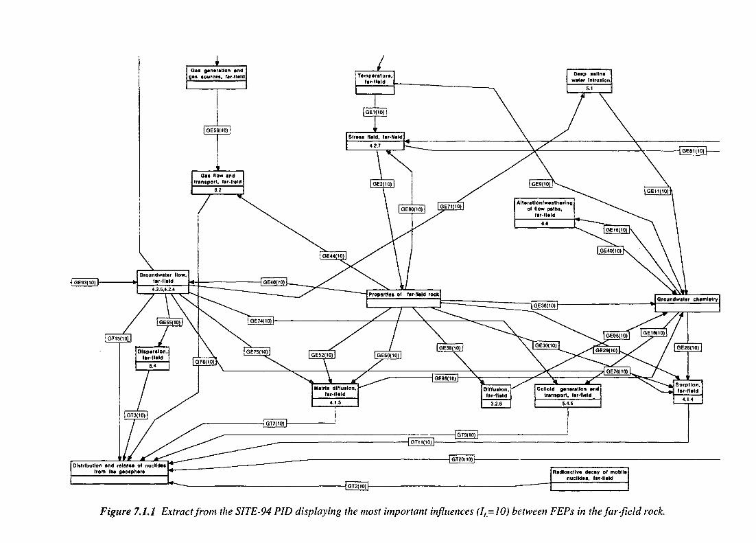
Gas generation andgas sources, far-field Deep saline
water Intrusion
Colloid generation andtransport, far-field
Distribution and release of nuclldesfrom the geosphere
Figure 7.1.1 Extract from the SITE-94 PID displaying the most important influences (IL-10) between FEPs in the far-field rock.
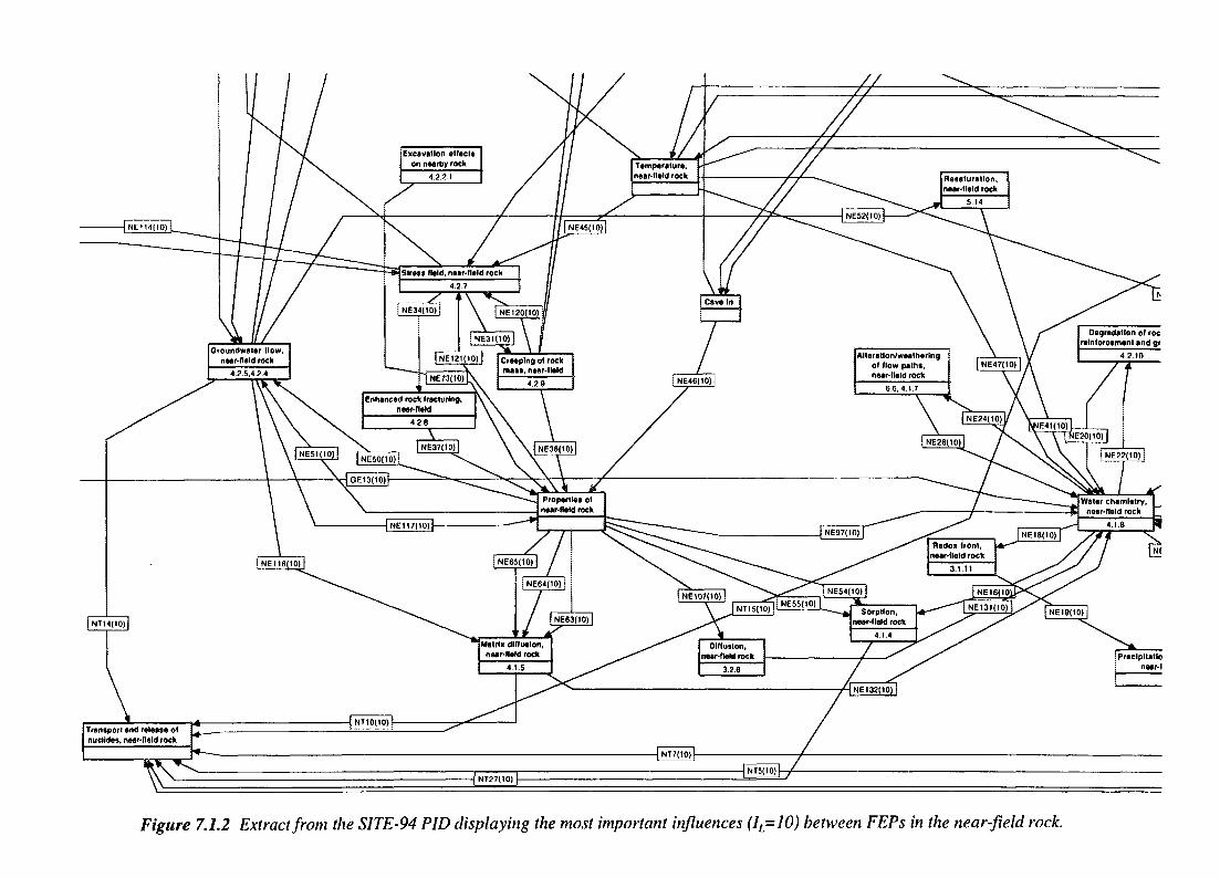
Degradation of rocreinforcement and gr
Transport and release ofnuclldes, near-field rock
Figure 7.1.2 Extract from the SITE-94 PID displaying the most important influences (IL=I0) between FEPs in the near-field rock.
100
7.1.2 Site Evaluation
Evidently, the geosphere is a natural system. The properties of the geosphere are not knowna priori, but have to be measured or estimated during the site characterisation andevaluation.
The objectives of the site evaluation in SITE-94 are to deliver parameters for calculationsof degradation of the Engineered Barriers, radionuclide release and transport in the near-field rock and radionuclide transport through the geosphere, under different scenarios. Inaddition, the site evaluation must develop an understanding of the structures and processesat the site and their evolution in time, in order to give credibility to the predictions madeby the site models and the Performance Assessment results. A key to such confidence-building is a systematic and transparent evaluation of uncertainties and their impact on thePerformance Assessment.
Although separate models are developed for the geochemical, hydrogeological and rockmechanical evaluation, an integrated interpretation of all data types is crucial to determinewhether different types give a consistent picture of the site and to explore potentialcorrelations.
7.2 BEDROCK AND STRUCTURAL GEOLOGY: THE SKISTRUCTURAL MODEL
This section describes the development of a bedrock and structural geologic model of theAspo site, based on the available geological information. The uncertainties in the model arediscussed. The model, with uncertainties, provides a common baseline for subsequenthydrogeological, geochemical and rock mechanical models of the site as will be discussedin Sections 7.3 to 7.5.
7.2.1 Introduction
The objective of producing a bedrock and structural model of the Aspo site is to providea geological framework for all the hydrogeological and geomechanical modelling studiescarried out in SITE-94. Every aspect of the design, positioning and safety assessment of arepository at a specific site will require a common 'baseline' 3D model defining the keylithologies and structures of the rock. Onto this can be superimposed, as required,information on hydraulically active features, geomechanical properties and geochemicaland hydrochemical variations. The baseline model is built using surface and boreholeobservations from a wide variety of geological and geophysical techniques. The model ofAspo is developed by means of a stepwise analysis of data from regional to local scale andalso from outcrop scale to local scale.
The model produced describes the geological setting of the Aspo area, in terms of itsgeological evolution and, in particular, the distribution of tectonic discontinuities and otherfeatures which could act as possible pathways for circulating groundwater or regions of
101
low rock mechanical strength which might be of concern in some scenarios of future siteevolution.
The intention in producing the model is to use only primary geological data. However, thisdid not prove possible as most field observations of the site are not reported in a primaryform (maps, diaries, etc.), but as processed data in the SKB Progress Reports series (cf.Stanfors et al., 1991). The information used is described by Tiren et al. (1996), who alsodescribe the complete structural modelling programme in detail. The SKB database(GEOTAB, containing surface fracture mapping, core logs and geophysical boreholemeasurements) was available to SITE-94. In addition, some short field trips were made toAspo to obtain 'unfiltered' general information. It should be noted, however, that thepresent SKI model does not consider information other than that available to SKB in theirmodelling.
The general approach of the study comprises three steps:
1. Literature studies of the geological and structural history of the area are performedin order to evaluate the types of geological features expected.
2. The structural setting is defined by outlining the distribution of structures within aregional, then a subregional, area, each defined by hydrogeological models and eachwith Aspo in their centres. This results in the production of a regional (35 x 25 km)and a subregional (10 x 12 km) 2D model. This is followed by detailed 2Dgeological modelling of the Aspo area, on the assumption that what can be seen ona large-scale can also be seen on a local scale and vice versa. A local-scale 2Dstructural and fracture-zone model is produced.
3. A detailed 3D structural model is developed which describes the structuralconfiguration of fracture zones within a 2 x 2 x 1 km rock volume (including thewhole of Aspo island) using, as far as possible, only primary data (field notes, corelogs, surface geophysical data, borehole measurements, airborne geophysicalmeasurements, aerial photos, topographical maps, terrain models, etc.). This modelis the ultimate objective of the work described in the present section and comprisesthe baseline model discussed above.
The structural interpretation is constrained by the fact that Aspo is an island and importantinformation on the character of low angle fracture zones, as well as other NW and NEtrending structures, are hidden below the sea. The location of boreholes, which is restrictedto a relative narrow NNW trending corridor from the southernmost part of Aspo to thecentre of the island, makes it difficult to obtain unique determinations of the trends of NEto NW dipping fractures and fracture zones at the southern tip of Aspo. This is an exampleof uncertainties in the geological model, which are dealt with in Section 7.2.6.
102
7.2.2 The Regional and Subregional Scale Models
7.2.2.1 Bedrock Geology
The oldest rocks in the county of Smaland, in the southeastern-most part of Sweden, arestrongly metamorphosed, Svecokarelian metasediments, metavolcanics, and granitoids,older than 1800 Ma (metamorphic age). These rocks were intruded by a suite of Smalandgranites and associated volcanic rocks (Lundqvist, 1991) between 1770-1810 Ma ago(Mansfeld, 1991). These intrusions compose the main part of the bedrock in the region,forming part of the Trans-Scandinavian Igneous Belt (TIB; Patchett et al., 1987),comprising 1650-1810 Ma old rocks.
The Smaland granites are intruded by several generations of dykes (e.g. porphyries ofgranitic-granodioritic-monzonitic composition, trending N-S and E-W) older thanc. 1420 Ma. In marginal areas, these intrusions occur as composite dykes with frequentbasaltic intrusions. The Smaland granite suite is also intruded at a few localities (e.g.Karlshamn and along the coast at Oskarshamn), by reddish, massive and often coarse-grained 1350-1400 Ma old granites of Rapakivi type. The youngest intrusive rocks(960-980 Ma) are N-S trending dolerite dykes (Figure 4.3.1.). For further information, seeTirenet. al. (1996).
7.2.2.2 Regional Structural History and Future Evolution
The bedrock of the Aspo region is composed of TIB rocks that were emplaced within a vastbelt of volcanics on the edge (margin) of a continental plate, which may have beensubducted by oceanic crust from the west.
The present ground surface at Aspo represents a plane which was at a depth of about 10 kmin the former TIB mountain belt. At such a depth, ascent and emplacement of plutonicrocks through older and shallower intrusions or supracrustal rock is typical. The bedrockis divisible into regional blocks and the passage from one block to the next may wellexhibit a change in lithologies, while the block boundaries are wide, oxidised zones,possibly containing intrusions. Examples of the latter are NW to N-S (NNW and NNE) andE-W trending intrusions which are older than 1420 Ma.
The later intrusions of Rapakivi granites (e.g. the Gotemar granite), not related to the TIBrocks, were probably formed by either magmatism initiated in the mantle in a NNE trendingdomain of crustal tension, or possibly by subcrustal melting along deep faults. Largerbodies of Rapakivi granites occur to the east, below the Baltic Sea.
Since the intrusion of the Gotemar granite about 1400 Ma ago, about 7 km of the TIB rockshave been eroded. The related isostatic elevation of the rock was probably caused bydifferential movements along existing fault planes, but could also result from formation ofnew faults, as, in some cases, existing faults may have been arrested. The magnitude ofvertical displacement along individual faults may well have been on the order of a fewkilometres during the formation and denudation of the TIB mountain range. For example,in the Gotemar granite, relative vertical displacement of about 500 m along a N-S trendingfault has occurred.
103
Extensional collapse of the TIB mountain belt may have initiated low-angle faults, whichcould be reactivated as thrusts in a later compressional regime. At Aspo, low-angle faultsgenerally dip northwestward and, on the mainland just west of Aspo, SW-dipping thrustfaults have been identified (Nordenskjold, 1944). Westward dipping thrusts are found inthe TIB rocks along the tectonic contact zone with the gneiss complex of southwesternSweden in the 20-30 km wide, N-S trending, ca. 1.0 Ga old Protogine Zone (locatedc. 130 km west of Aspo).
Active periods of regional denudation, as indicated by sedimentation, occurred at 1200 Maago and 700 Ma ago. At the end of the Precambrian, a peneplain was formed and the areais characterised by cratonic conditions as part of the present Fennoscandian Shield. Thevariation in altitude within the sub-Cambrian peneplain was, at that time, only a few tensof metres (Rudberg, 1954).
Displacement along vertical faults on the order of some tens of metres occurred during thedeposition of 2-3 km of Palaeozoic to Mesozoic platform sediments upon the sub-Cambrianpeneplain. The displacement along individual faults was caused both by loading due tosedimentation, and by extensional distortion of the craton. NNW-SSE extension isindicated by clastic Cambro-Ordovician dikes dominated by ENE-trending filled fractures,and minor NE and N-S trending clastic veins which opened in the direction perpendicularto the extension. This pile of Palaeozoic sediments loaded the continental platform for atleast 100 Ma (Larsson and Tullborg, 1993).
Regional tectonic influences on the Fennoscandian Shield during mountain-buildingepisodes (e.g. Caledonian and Hercynian orogenies) in the marginal zones of theFennoscandian Shield also resulted in tilting and uplift of the sub-Cambrian peneplain,causing denudation in some areas and sedimentation in other parts. The erosion of theplatform sediments started c. 280 Ma ago, due to deformation along the southern border ofthe Fennoscandian Shield, located c. 250 km southwest of Aspo. A regional denudationsurface was formed, discordant with the sub-Cambrian peneplain and cutting down into thePrecambrian bedrock (Lidmar-Bergstrom, 1991).
By late Cretaceous times (c. 80 Ma ago), the basement rocks had become exposedc. 100 km southwest of Aspo. However, the present ground surface in the main part ofsoutheastern Sweden coincides with the sub-Cambrian peneplain. The last remnants ofsediments were presumably eroded during the Quaternary or, possibly, during late Tertiarytime. About 18 000 to 20 000 years ago, during the Weichselian glaciation (the last of atleast three glaciations), the region was covered by approximately 2-2.5 km of ice cover.This ice cap melted c. 12 000 years ago.
The inclination of the sub-Cambrian peneplain following post-glacial uplift is c. 0.2°toward the ESE. The present rate of uplift in the Aspo region is c. 0.001 m/year. It isaseismic and affected by a regional compressive stress oriented NW-SE.
On Aspo, a few open NNW and EW trending fractures are found, possibly indicating verylate dilation (cf. Morner, 1989). Neotectonic deformation is indicated by displaced sea bed,but it is always restricted to old structures in the basement rocks (Floden, 1984). For moredetails see Tiren et al., 1996.
104
Over the next few millions of years, future deformation of the bedrock at Aspo, based onits structural history and offsets in the topography (cf. Tiren and Beckholmen, 1989), willprobably be very limited, with deformation accommodated preferentially along N-Strending fracture zones (due to continued glacial loading and unloading in the next105 years) and NE to NNE trending fracture zones (where the most recent lateraldisplacements have occurred). In the region, NW to WNW trending structures may also bereactivated, but the Aspo bedrock will probably be shielded by the Gotemar granite.Deformation along E-W to NNE trending structures appears less probable.
7.2.2.3 Regional (35 x 25 km) Structural Environment Model
The regional structural pattern showing the dominant lineaments is illustrated inFigure 7.2.1, with Aspo (shaded area) located in the centre. In this study, the principallineaments considered have a trace length greater than about 1.5 km. The dominantlineament orientations are E-W, NW, N-S and NE.
The E-W trending lineaments may either appear as shear zones up to at least a hundredmetres wide, or as subvertical fracture zones, some 50 m wide. During the late stages ofpast ice ages 'meltwater canyons' up to 50 m deep, 100 m wide and 5 km long have beenformed locally along subvertical fracture zones trending N-S and NW and c. EW in theinland region (Olvmo, 1989). The most prominent structure in the regional area is a 50 mdeep NW trending submarine canyon, Strupdjupet, about 11 km NNE of Aspo, which maybe a meltwater canyon. The existence of meltwater canyons is considered in developing theCentral Scenario (see Chapter 9 and King-Clayton et al., 1995).
The NW-trending lineaments overprint the E-W structures, with many of those in the inlandregion representing the surface expressions of gently southwestward-dipping thrusts.NE-trending lineaments are also relatively frequent and occur as extensive and distincttopographical features. The NW-trending lineaments dominate in the northern part of thearea investigated, whereas the NE-trending lineaments are more topographicallypronounced in the southern parts.
The most prominent topographical features in the region are the N-S trending lineaments,which are typical of those found in most parts of Sweden. They are often extensive andconstitute subvertical fault planes.
The intersections of the E-W, NW, N-S and NE-trending sets of fracture zones gives riseto triangular, rectangular and polyhedral rock blocks. Rock blocks of different orders orgeometrical forms may overprint each other.
In summary, Aspo is a triangular island outlined in the north by an extensive E-W shearzone, in the east by a N-S trending fracture zone and to the west by a NW-trending fracturezone. Rock blocks similar to those of Aspo are common and occur on various scales, forexample, to the west of Aspo.
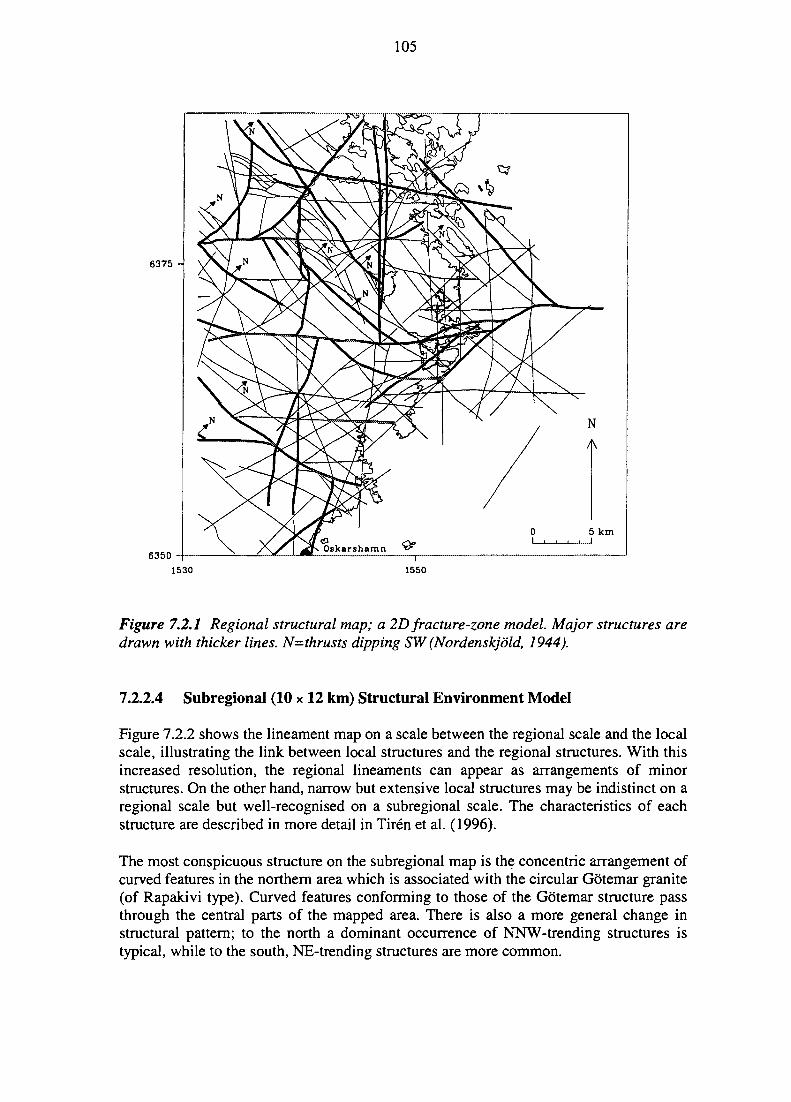
105
6375 -
6350
1530 1550
Figure 7.2.1 Regional structural map; a 2D fracture-zone model. Major structures aredrawn with thicker lines. N=thrusts dipping SW (Nordenskjold, 1944).
7.2.2.4 Subregional (10 x 12 km) Structural Environment Model
Figure 7.2.2 shows the lineament map on a scale between the regional scale and the localscale, illustrating the link between local structures and the regional structures. With thisincreased resolution, the regional lineaments can appear as arrangements of minorstructures. On the other hand, narrow but extensive local structures may be indistinct on aregional scale but well-recognised on a subregional scale. The characteristics of eachstructure are described in more detail in Tiren et al. (1996).
The most conspicuous structure on the subregional map is the concentric arrangement ofcurved features in the northern area which is associated with the circular Gotemar granite(of Rapakivi type). Curved features conforming to those of the Gotemar structure passthrough the central parts of the mapped area. There is also a more general change instructural pattern; to the north a dominant occurrence of NNW-trending structures istypical, while to the south, NE-trending structures are more common.
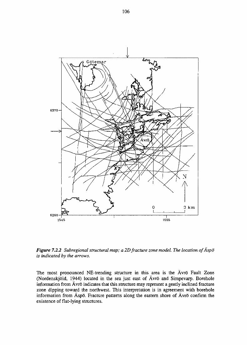
106
6360
1545 1555
Figure 7.2.2 Subregional structural map; a 2D fracture zone model. The location ofAspois indicated by the arrows.
The most pronounced NE-trending structure in this area is the Avro Fault Zone(Nordenskjold, 1944) located in the sea just east of Avro and Simpevarp. Boreholeinformation from Avro indicates that this structure may represent a gently inclined fracturezone dipping toward the northwest. This interpretation is in agreement with boreholeinformation from Aspo. Fracture patterns along the eastern shore of Avro confirm theexistence of flat-lying structures.
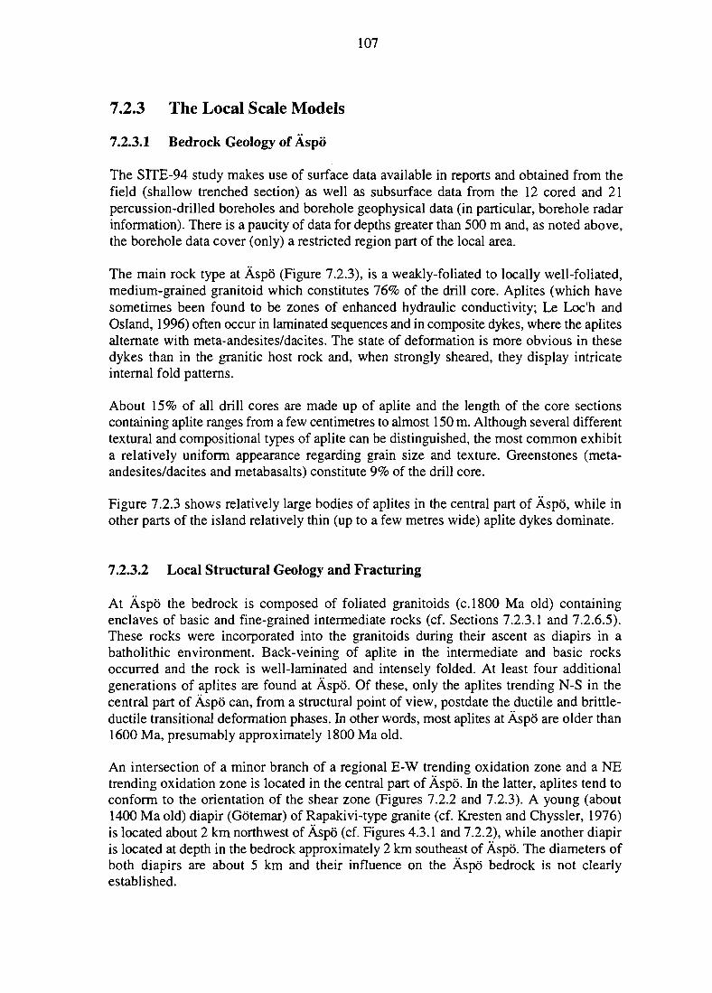
107
7.2.3 The Local Scale Models
7.2.3.1 Bedrock Geology of Aspo
The SITE-94 study makes use of surface data available in reports and obtained from thefield (shallow trenched section) as well as subsurface data from the 12 cored and 21percussion-drilled boreholes and borehole geophysical data (in particular, borehole radarinformation). There is a paucity of data for depths greater than 500 m and, as noted above,the borehole data cover (only) a restricted region part of the local area.
The main rock type at Aspo (Figure 7.2.3), is a weakly-foliated to locally well-foliated,medium-grained granitoid which constitutes 76% of the drill core. Aplites (which havesometimes been found to be zones of enhanced hydraulic conductivity; Le Loc'h andOsland, 1996) often occur in laminated sequences and in composite dykes, where the aplitesalternate with meta-andesites/dacites. The state of deformation is more obvious in thesedykes than in the granitic host rock and, when strongly sheared, they display intricateinternal fold patterns.
About 15% of all drill cores are made up of aplite and the length of the core sectionscontaining aplite ranges from a few centimetres to almost 150 m. Although several differenttextural and compositional types of aplite can be distinguished, the most common exhibita relatively uniform appearance regarding grain size and texture. Greenstones (meta-andesites/dacites and metabasalts) constitute 9% of the drill core.
Figure 7.2.3 shows relatively large bodies of aplites in the central part of Aspo, while inother parts of the island relatively thin (up to a few metres wide) aplite dykes dominate.
7.2.3.2 Local Structural Geology and Fracturing
At Aspo the bedrock is composed of foliated granitoids (c.1800 Ma old) containingenclaves of basic and fine-grained intermediate rocks (cf. Sections 7.2.3.1 and 7.2.6.5).These rocks were incorporated into the granitoids during their ascent as diapirs in abatholithic environment. Back-veining of aplite in the intermediate and basic rocksoccurred and the rock is well-laminated and intensely folded. At least four additionalgenerations of aplites are found at Aspo. Of these, only the aplites trending N-S in thecentral part of Aspo can, from a structural point of view, postdate the ductile and brittle-ductile transitional deformation phases. In other words, most aplites at Aspo are older than1600 Ma, presumably approximately 1800 Ma old.
An intersection of a minor branch of a regional E-W trending oxidation zone and a NEtrending oxidation zone is located in the central part of Aspo. In the latter, aplites tend toconform to the orientation of the shear zone (Figures 7.2.2 and 7.2.3). A young (about1400 Ma old) diapir (Gotemar) of Rapakivi-type granite (cf. Kresten and Chyssler, 1976)is located about 2 km northwest of Aspo (cf. Figures 4.3.1 and 7.2.2), while another diapiris located at depth in the bedrock approximately 2 km southeast of Aspo. The diameters ofboth diapirs are about 5 km and their influence on the Aspo bedrock is not clearlyestablished.
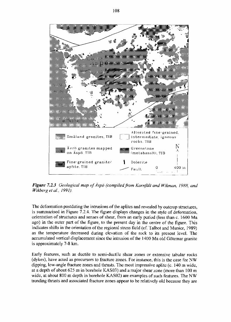
108
Smaland granites, TIB
Avro granites mappedon Aspo, TIB
Fine-grained granite/aplite, TIB
Alterated fine-grained,intermediate, igneousrocks, TIB
- Greenstone ^(metabasalt), TIB
\ Dolerite
Fault 400 m
Figure 7.2.3 Geological map of Aspo (compiled from Kornfalt and Wikman, 1988, andWikbergetal, 1991).
The deformation postdating the intrusions of the aplites and revealed by outcrop structures,is summarised in Figure 7.2.4. The figure displays changes in the style of deformation,orientation of structures and senses of shear, from an early period (less than c. 1600 Maago) in the outer part of the figure, to the present day in the centre of the figure. Thisindicates shifts in the orientation of the regional stress field (cf. Talbot and Munier, 1989)as the temperature decreased during elevation of the rock to its present level. Theaccumulated vertical displacement since the intrusion of the 1400 Ma old Gotemar graniteis approximately 7-8 km.
Early features, such as ductile to semi-ductile shear zones or extensive tabular rocks(dykes), have acted as precursors to fracture zones. For instance, this is the case for NWdipping, low-angle fracture zones and thrusts. The most impressive aplite (c. 140 m wide,at a depth of about 625 m in borehole KAS03) and a major shear zone (more than 100 mwide, at about 800 m depth in borehole KAS02) are examples of such features. The NWtrending thrusts and associated fracture zones appear to be relatively old because they are
109
overprinted (cut?) by NE and ENE trending fracture zones in the central part of Aspo (cf.text above). These zones have, in their turn, been reactivated several times and thestructures have alternately distorted each other. It is, however, obvious from the fieldobservations and structural analysis of topographical information, that the latest distortionof any significance took place along a NE trending structure in the central parts of Aspo(see cf. Figures 7.2.4, 7.2.6 and 7.2.14).
There are relatively few N-S trending faults and fracture zones. Field observations showthat deformation along N-S trending structures has occurred during a relatively long timeinterval, as indicated by occurrence of ductile shear zones, mylonites, faulting and doleritedykes (c. 960-980 Ma).
Minor brittle structures (i.e. fractures) manifest themselves in a number of ways. In'unfoliated' rocks, these generally occur in more or less the same directions as the systemof aplitic dikes. In ductile shear zones, the fracture density is generally enhanced bydeformation along zones. However, later deformation may cause fractures to overprint thezones in other directions. In brittle shear zones, the fracturing is related to the history ofmotion along the zones. At Aspo, most sets of aplites have locally been technicallydistorted by ductile to semi-ductile deformation (at sufficiently high temperature andpressure), indicating that they were emplaced before the general deformation in the rockbecame brittle. When this occurred is not clear, and most of the aplites in the Aspo bedrockmay well have been intruded before the intrusion of the Rapakivi granites and in associationwith the Aspo granitoids. However, the Aspo bedrock has been penetrated by swarms offractures of variable lengths, spacings and orientations that are parts of regional fracturedomains. The most frequent direction of these structures is between WNW and NW. OnAspo, these brittle structures regionally overprint the NE and EW trending ductile to semi-ductile shear zones (see above and Figure 7.2.2). Other examples of brittle structures areswarms of extensive and widely-spaced NNW (central Aspo) and NNE (eastern Aspo)trending fractures. Some of these nearly N-S trending structures in the Aspo region containdolerites about 1000 Ma old (see also Tiren et al., 1996).
Outcrop fracture data are used in SITE-94 for the analysis of structures. A new approachusing outcrop data to define the geometry of the rock blocks and, from this, to definepossible transport paths for groundwater, is introduced and applied in a preliminary mannerin the overall analyses. A detailed discussion is given in Tiren et al. (1996).
The subsurface configuration and distribution of fractures are shown in the fracture logs ofthe cored boreholes. In the northern part of Aspo, borehole information indicates agenerally higher degree of fracturing in the upper parts of the borehole, compared to thefracturing in the southern part of Aspo. Hematite and epidote, as infilling minerals, aretypical for the gently inclined fracture zones.
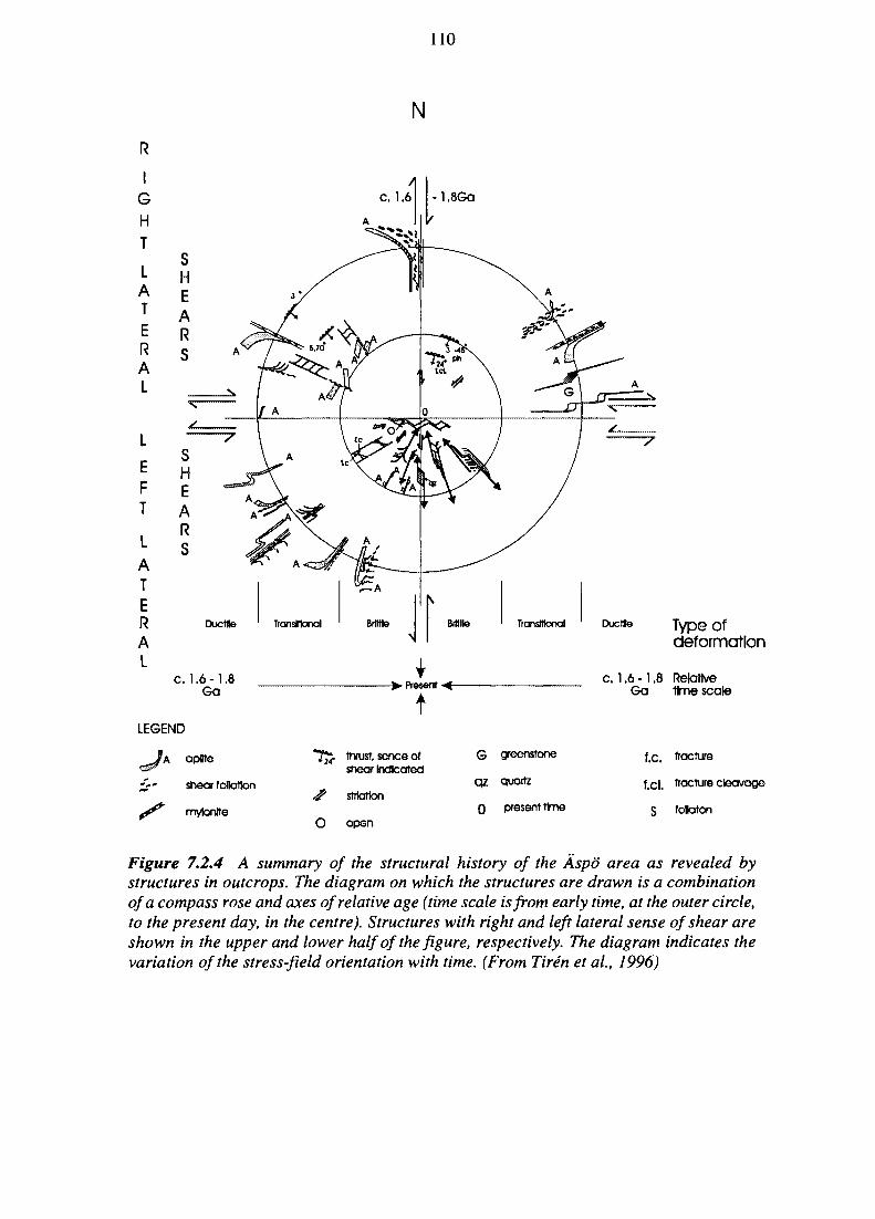
110
N
R
IGHT
LATERAL
L
EFT
LATERAL
Ductile
c. 1.6 -1.8Go
Transitional Ductile Type ofdeformation
IPresent
tLEGEND
apDte
shear fetation
mytonlteO
thrust, sence ofshear Indicated
stitatlon
open
G greenstone
qz quartz
0 present time
c. 1.6 -1.8 RelativeGa time scale
f.C. fracture
f.cl. fracture cleavage
S follaton
Figure 7.2.4 A summary of the structural history of the Aspo area as revealed bystructures in outcrops. The diagram on which the structures are drawn is a combinationof a compass rose and axes of relative age (time scale is from early time, at the outer circle,to the present day, in the centre). Structures with right and left lateral sense of shear areshown in the upper and lower half of the figure, respectively. The diagram indicates thevariation of the stress-field orientation with time. (From Tiren et ah, 1996)
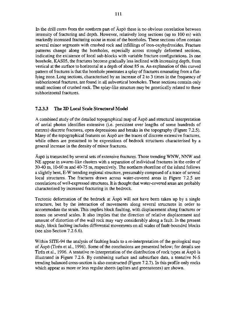
I l l
In the drill cores from the southern part of Aspo there is no obvious correlation betweenintensity of fracturing and depth. However, relatively long sections (up to 100 m) withmarkedly increased fracturing occur in most of the boreholes. These sections often containseveral minor segments with crushed rock and infillings of iron-oxyhydroxides. Fracturepatterns change along the boreholes, especially across strongly deformed sections,indicating the existence of local sub-blocks with variable fracture configurations. In oneborehole, KAS05, the fractures become gradually less inclined with increasing depth, fromvertical at the surface to horizontal at a depth of about 85 m. An explanation of this curvedpattern of fractures is that the borehole penetrates a splay of fractures emanating from a flat-lying zone. Long sections, characterised by an increase of 2 to 3 times in the frequency ofsubhorizontal fractures, are found in all subvertical boreholes. These sections contain onlysmall sections of crushed rock. The splay-like structure may be genetically related to thesesubhorizontal fractures.
7.2.3.3 The 2D Local Scale Structural Model
A combined study of the detailed topographical map of Aspo and structural interpretationof aerial photos identifies extensive (i.e. persistent over lengths of some hundreds ofmetres) discrete fractures, open depressions and breaks in the topography (Figure 7.2.5).Many of the topographical features on Aspo are the traces of discrete extensive fractures,while others are presumed to be expressions of bedrock structures characterised by ageneral increase in the density of minor fractures.
Aspo is transected by several sets of extensive fractures. Those trending WNW, NNW andNE appear in swarm-like clusters with a separation of individual fractures in the order of30-40 m, 10-60 m and 40-75 m, respectively. The northern shoreline of the island followsa slightly bent, E-W trending regional structure, presumably composed of a trace of severallocal structures. The fractures drawn across water-covered areas in Figure 7.2.5 arecorrelations of well-expressed structures. It is thought that water-covered areas are probablycharacterised by increased fracturing in the bedrock.
Tectonic deformation of the bedrock at Aspo will not have been taken up by a singlestructure, but by the interaction of movements along several structures in order toaccommodate the strain. This implies block faulting, with displacement along fractures orzones on several scales. It also implies that the direction of relative displacement andamount of distortion of the wall rock may vary considerably along a fault. In the presentstudy, block faulting includes differential movements on all scales of fault-bounded blocks(see also Section 7.2.6.6).
Within SITE-94 the analysis of faulting leads to a re-interpretation of the geological mapof Aspo (Tiren et al., 1996). Some of the conclusions are presented below; for details seeTiren et al., 1996. A tentative re-interpretation of the distribution of rock types at Aspo isillustrated in Figure 7.2.6. By combining surface and subsurface data, a tentative N-Strending balanced cross-section is also constructed (Figure 7.2.7). In this profile only rockswhich appear as more or less regular sheets (aplites and greenstones) are shown.

112
Figure 7.2.5 2D structural model ofAspd, showing extensive (i.e. persistent over distancesof some hundreds of metres) discrete fractures and topographical lows (yellow).
ft J
ASPOTi-nl.ilivi- zoological map
<OOrn
Figure 7.2.6 Tentative geological map ofAspd. The distribution pattern of the lithologieson the map mimic the appearance of the rock types exposed in outcrops (Figure 7.2.4).Most faults displacing the lithologies, although they are very short, coincide with extensivelineaments seen on aerial photos (cf Figure 7.2.5).
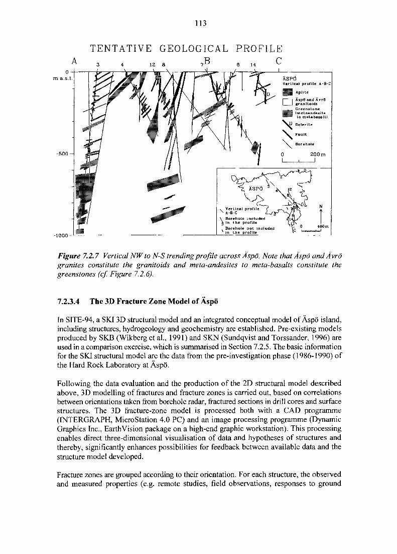
113
TENTATIVE GEOLOGICAL PROFILEA
Borehole includedin the profileBorehole not includedin the profile
-1000
Figure 7.2.7 Vertical NW to N-S trending profile across Aspo. Note that Aspo and Avrogranites constitute the granitoids and meta-andesites to meta-basalts constitute thegreenstones (cf. Figure 7.2.6).
7.2.3.4 The 3D Fracture Zone Model of Aspo
In SITE-94, a SKI 3D structural model and an integrated conceptual model of Aspo island,including structures, hydrogeology and geochemistry are established. Pre-existing modelsproduced by SKB (Wikberg et al., 1991) and SKN (Sundqvist and Torssander, 1996) areused in a comparison exercise, which is summarised in Section 7.2.5. The basic informationfor the SKI structural model are the data from the pre-investigation phase (1986-1990) ofthe Hard Rock Laboratory at Aspo.
Following the data evaluation and the production of the 2D structural model describedabove, 3D modelling of fractures and fracture zones is carried out, based on correlationsbetween orientations taken from borehole radar, fractured sections in drill cores and surfacestructures. The 3D fracture-zone model is processed both with a CAD programme(INTERGRAPH, MicroStation 4.0 PC) and an image processing programme (DynamicGraphics Inc., EarthVision package on a high-end graphic workstation). This processingenables direct three-dimensional visualisation of data and hypotheses of structures andthereby, significantly enhances possibilities for feedback between available data and thestructure model developed.
Fracture zones are grouped according to their orientation. For each structure, the observedand measured properties (e.g. remote studies, field observations, responses to ground
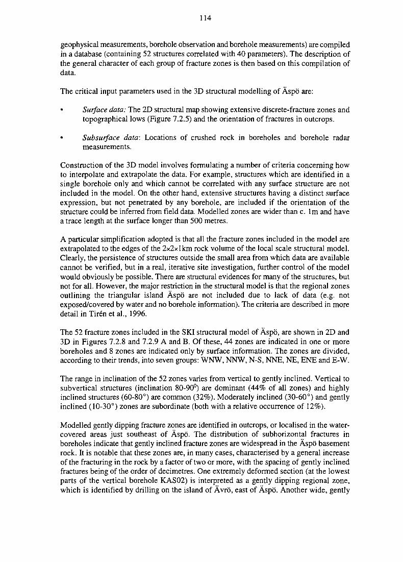
114
geophysical measurements, borehole observation and borehole measurements) are compiledin a database (containing 52 structures correlated with 40 parameters). The description ofthe general character of each group of fracture zones is then based on this compilation ofdata.
The critical input parameters used in the 3D structural modelling of Aspo are:
• Surface data: The 2D structural map showing extensive discrete-fracture zones andtopographical lows (Figure 7.2.5) and the orientation of fractures in outcrops.
• Subsurface data: Locations of crushed rock in boreholes and borehole radarmeasurements.
Construction of the 3D model involves formulating a number of criteria concerning howto interpolate and extrapolate the data. For example, structures which are identified in asingle borehole only and which cannot be correlated with any surface structure are notincluded in the model. On the other hand, extensive structures having a distinct surfaceexpression, but not penetrated by any borehole, are included if the orientation of thestructure could be inferred from field data. Modelled zones are wider than e l m and havea trace length at the surface longer than 500 metres.
A particular simplification adopted is that all the fracture zones included in the model areextrapolated to the edges of the 2x2x1 km rock volume of the local scale structural model.Clearly, the persistence of structures outside the small area from which data are availablecannot be verified, but in a real, iterative site investigation, further control of the modelwould obviously be possible. There are structural evidences for many of the structures, butnot for all. However, the major restriction in the structural model is that the regional zonesoutlining the triangular island Aspo are not included due to lack of data (e.g. notexposed/covered by water and no borehole information). The criteria are described in moredetail in Tiren et al., 1996.
The 52 fracture zones included in the SKI structural model of Aspo, are shown in 2D and3D in Figures 7.2.8 and 7.2.9 A and B. Of these, 44 zones are indicated in one or moreboreholes and 8 zones are indicated only by surface information. The zones are divided,according to their trends, into seven groups: WNW, NNW, N-S, NNE, NE, ENE and E-W.
The range in inclination of the 52 zones varies from vertical to gently inclined. Vertical tosub vertical structures (inclination 80-90°) are dominant (44% of all zones) and highlyinclined structures (60-80°) are common (32%). Moderately inclined (30-60°) and gentlyinclined (10-30°) zones are subordinate (both with a relative occurrence of 12%).
Modelled gently dipping fracture zones are identified in outcrops, or localised in the water-covered areas just southeast of Aspo. The distribution of subhorizontal fractures inboreholes indicate that gently inclined fracture zones are widespread in the Aspo basementrock. It is notable that these zones are, in many cases, characterised by a general increaseof the fracturing in the rock by a factor of two or more, with the spacing of gently inclinedfractures being of the order of decimetres. One extremely deformed section (at the lowestparts of the vertical borehole KAS02) is interpreted as a gently dipping regional zone,which is identified by drilling on the island of Avro, east of Aspo. Another wide, gently
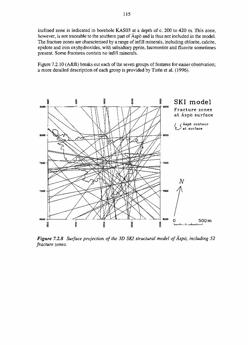
115
inclined zone is indicated in borehole KAS03 at a depth of c. 200 to 420 m. This zone,however, is not traceable to the southern part of Aspo and is thus not included in the model.The fracture zones are characterised by a range of infill minerals, including chlorite, calcite,epidote and iron oxyhydroxides, with subsidiary pyrite, laumontite and fluorite sometimespresent. Some fractures contain no infill minerals.
Figure 7.2.10 (A&B) breaks out each of the seven groups of features for easier observation;a more detailed description of each group is provided by Tiren et al. (1996).
8500
SKI modelFracture zonesat Aspo surface
) r AspO contour<_/ at surface
8000
500 m
Figure 7.2.8 Surface projection of the 3D SKI structural model of Aspo, including 52fracture zones.
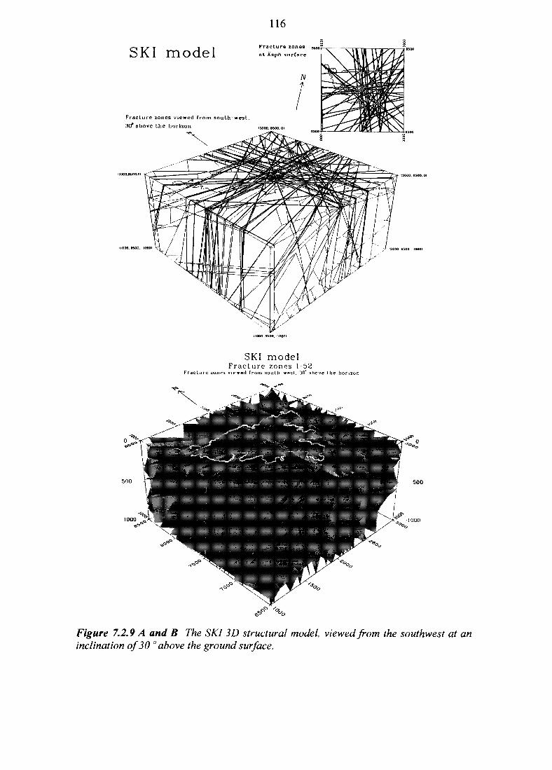
116
SKI modelFracture zones
at Aspd surface
Fracture zones viewed from south west,
30° above the horizon IMOO.85OO.OI
IIOOO. 8400. 10001
SKI modelF r a c t u r e z o n e s 1 5 2
F r a c t u r e z o n e s v i e w e d f r o m s o u t h w e s t . 30' a b o v e I h e h u r i z u
500
Figure 7.2.9 A and B The SKI 3D structural model, viewed from the southwest at aninclination of 30 ° above the ground surface.
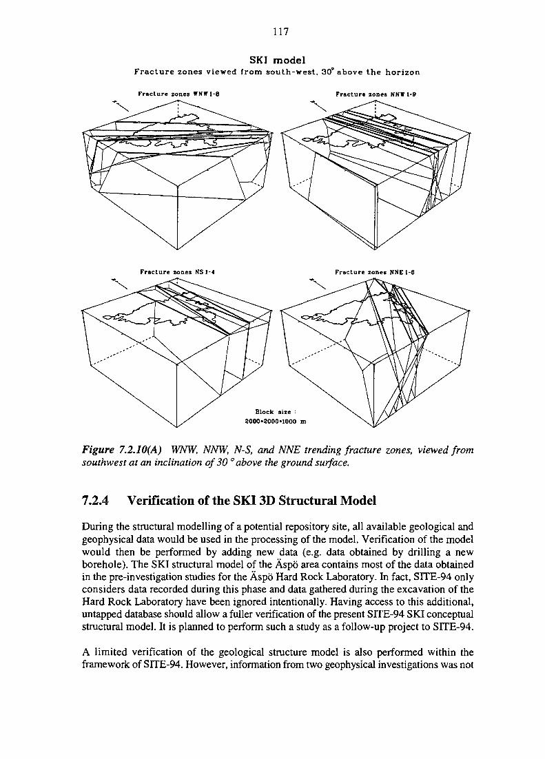
117
SKI modelFracture zones viewed from south-west. 30° above the horizon
Fracture zones WNW1-B Fracture zones NNW 1-9
Fracture zones NS 1-4 Fracture zones NNE 1-6
Figure 7.2.10(A) WNW, NNW, N-S, and NNE trending fracture zones, viewed fromsouthwest at an inclination of 30 ° above the ground surface.
1.2A Verification of the SKI 3D Structural Model
During the structural modelling of a potential repository site, all available geological andgeophysical data would be used in the processing of the model. Verification of the modelwould then be performed by adding new data (e.g. data obtained by drilling a newborehole). The SKI structural model of the Aspo area contains most of the data obtainedin the pre-investigation studies for the Aspo Hard Rock Laboratory. In fact, SITE-94 onlyconsiders data recorded during this phase and data gathered during the excavation of theHard Rock Laboratory have been ignored intentionally. Having access to this additional,untapped database should allow a fuller verification of the present SITE-94 SKI conceptualstructural model. It is planned to perform such a study as a follow-up project to SITE-94.
A limited verification of the geological structure model is also performed within theframework of Sllb-94. However, information from two geophysical investigations was not
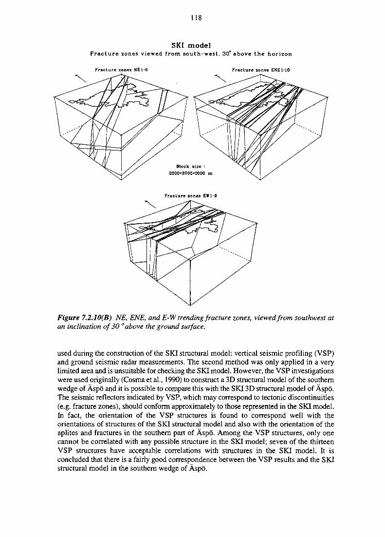
118
SKI modelFracture zones viewed from south-west, 30° above the horizon
Fracture zones NE1-6 Fracture zones ENE1-10
Fracture zones EW1-9
Figure 7.2.10(B) NE, ENE, and E-W trending fracture zones, viewed from southwest atan inclination of 30 ° above the ground surface.
used during the construction of the SKI structural model: vertical seismic profiling (VSP)and ground seismic radar measurements. The second method was only applied in a verylimited area and is unsuitable for checking the SKI model. However, the VSP investigationswere used originally (Cosma et al., 1990) to construct a 3D structural model of the southernwedge of Aspo and it is possible to compare this with the SKI 3D structural model of Aspo.The seismic reflectors indicated by VSP, which may correspond to tectonic discontinuities(e.g. fracture zones), should conform approximately to those represented in the SKI model.In fact, the orientation of the VSP structures is found to correspond well with theorientations of structures of the SKI structural model and also with the orientation of theaplites and fractures in the southern part of Aspo. Among the VSP structures, only onecannot be correlated with any possible structure in the SKI model; seven of the thirteenVSP structures have acceptable correlations with structures in the SKI model. It isconcluded that there is a fairly good correspondence between the VSP results and the SKIstructural model in the southern wedge of Aspo.
119
7.2.5 Comparison of the SKI Structural Model with Other Models
7.2.5.1 Data and Models
Different geologists may take different approaches to the analysis and interpretation of data.The effect of this on structural modelling can be illustrated by comparing different modelsdescribing the same area. Similarities in the models could indicate that the interpretationshave a relatively high degree of correctness. Differences in models can be attributed tochoice of methodology and interpretation of data, but can also indicate errors in themodelling procedure.
In this context, a comparison is made between the SKI structural model and two additionalmodels describing the structural framework of Aspo, the SKB structural model1 (Wikberget al., 1991) and the SKN structural model2 (Sundqvist and Torssander, 1996). As statedabove, the comparison of the quality of models depends on the data and the interpretationprocess. However, the relative quality of the different models is not judged in the presentcomparison, but the similarities and differences of the three structural models areemphasised.
The collected Aspo data are summarised by Stanfors et al. (1991) in a report whichconstitutes the basis for the structural interpretations made by SKI, SKB and SKN,respectively. The comparison of the three different model approaches are discussed in detailinTiren(1996).
7.2.5.2 SKB Structural Model of Aspo
The SKB structural model, Figure 7.2.11, is developed by interpolating structures identifiedat the ground surface with sections of increased fracturing in boreholes. The main surfacedata used in the analysis are geological and structural observations, detailed geophysicalmeasurements (resistivity and magnetic) and refraction seismic profile measurements. Thecorresponding main subsurface (borehole) data include core logs (lithological and fracturemapping), borehole radar measurements and vertical seismic profiling (VSP).
The SKB structural model is processed as a series of vertical sections, working in two-dimensional sections using a CAD system (INTERGRAPH, MicroStation 3.0 PC).
1 A structural model produced to predict structures which was developed during the pre-investigationphase (1986-1990) of the construction of the SKB Hard Rock Laboratory at Aspo.
Initially an independent model performed partly in parallel with the SKB model, but modified later on(see text).
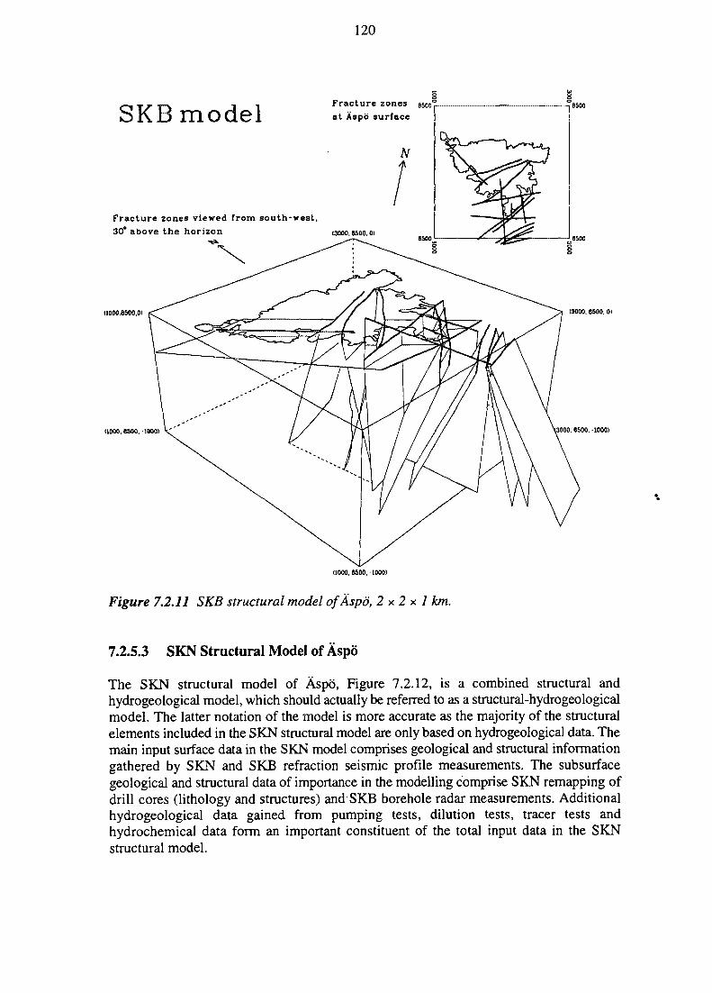
120
SKB modelFracture zones 850<rat Aspo surface
Fracture zones viewed from south-west,30* above the horizon oooo. 8500, oi
11000.8500.0)
(1000. 6500. -1000)
(3000. 6500. 0)
13000.6500.-1000)
(1000. 6500. -1000)
Figure 7.2.11 SKB structural model ofAspo, 2 x 2 x 1 km.
7.2.5.3 SKN Structural Model of Aspo
The SKN structural model of Aspo, Figure 7.2.12, is a combined structural andhydrogeological model, which should actually be referred to as a structural-hydrogeologicalmodel. The latter notation of the model is more accurate as the majority of the structuralelements included in the SKN structural model are only based on hydrogeological data. Themain input surface data in the SKN model comprises geological and structural informationgathered by SKN and SKB refraction seismic profile measurements. The subsurfacegeological and structural data of importance in the modelling comprise SKN remapping ofdrill cores (lithology and structures) and SKB borehole radar measurements. Additionalhydrogeological data gained from pumping tests, dilution tests, tracer tests andhydrochemical data form an important constituent of the total input data in the SKNstructural model.
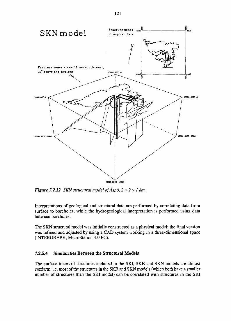
SKNmodel
121
Fracture zonesat Aspb surface
Fracture zones viewed from south-west,
30° above the horizon 0000, BSOO. o>
11000.8500.0)
(1000. 8500. -1000)
(3000. 6500. 0)
V (3O00. 6500. -1000)
(1000. 6500. -1000)
Figure 7.2.12 SKN structural model ofAspo, 2 x 2 x 1 km.
Interpretations of geological and structural data are performed by correlating data fromsurface to boreholes, while the hydrogeological interpretation is performed using databetween boreholes.
The SKN structural model was initially constructed as a physical model; the final versionwas refined and adjusted by using a CAD system working in a three-dimensional space(INTERGRAPH, MicroStation 4.0 PC).
7.2.5.4 Similarities Between the Structural Models
The surface traces of structures included in the SKI, SKB and SKN models are almostconform, i.e. most of the structures in the SKB and SKN models (which both have a smallernumber of structures than the SKI model) can be correlated with structures in the SKI
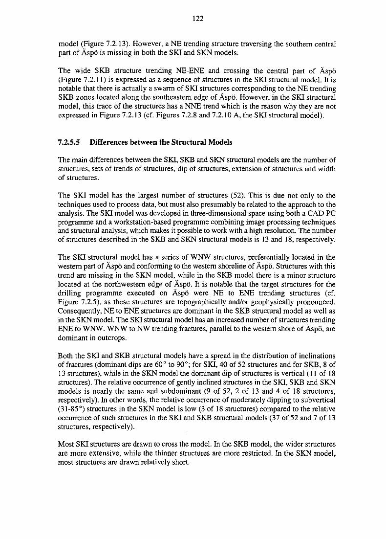
122
model (Figure 7.2.13). However, a NE trending structure traversing the southern centralpart of Aspo is missing in both the SKI and SKN models.
The wide SKB structure trending NE-ENE and crossing the central part of Aspo(Figure 7.2.11) is expressed as a sequence of structures in the SKI structural model. It isnotable that there is actually a swarm of SKI structures corresponding to the NE trendingSKB zones located along the southeastern edge of Aspo. However, in the SKI structuralmodel, this trace of the structures has a NNE trend which is the reason why they are notexpressed in Figure 7.2.13 (cf. Figures 7.2.8 and 7.2.10 A, the SKI structural model).
7.2.5.5 Differences between the Structural Models
The main differences between the SKI, SKB and SKN structural models are the number ofstructures, sets of trends of structures, dip of structures, extension of structures and widthof structures.
The SKI model has the largest number of structures (52). This is due not only to thetechniques used to process data, but must also presumably be related to the approach to theanalysis. The SKI model was developed in three-dimensional space using both a CAD PCprogramme and a workstation-based programme combining image processing techniquesand structural analysis, which makes it possible to work with a high resolution. The numberof structures described in the SKB and SKN structural models is 13 and 18, respectively.
The SKI structural model has a series of WNW structures, preferentially located in thewestern part of Aspo and conforming to the western shoreline of Aspo. Structures with thistrend are missing in the SKN model, while in the SKB model there is a minor structurelocated at the northwestern edge of Aspo. It is notable that the target structures for thedrilling programme executed on Aspo were NE to ENE trending structures (cf.Figure 7.2.5), as these structures are topographically and/or geophysically pronounced.Consequently, NE to ENE structures are dominant in the SKB structural model as well asin the SKN model. The SKI structural model has an increased number of structures trendingENE to WNW. WNW to NW trending fractures, parallel to the western shore of Aspo, aredominant in outcrops.
Both the SKI and SKB structural models have a spread in the distribution of inclinationsof fractures (dominant dips are 60° to 90°; for SKI, 40 of 52 structures and for SKB, 8 of13 structures), while in the SKN model the dominant dip of structures is vertical (11 of 18structures). The relative occurrence of gently inclined structures in the SKI, SKB and SKNmodels is nearly the same and subdominant (9 of 52, 2 of 13 and 4 of 18 structures,respectively). In other words, the relative occurrence of moderately dipping to subvertical(31-85°) structures in the SKN model is low (3 of 18 structures) compared to the relativeoccurrence of such structures in the SKI and SKB structural models (37 of 52 and 7 of 13structures, respectively).
Most SKI structures are drawn to cross the model. In the SKB model, the wider structuresare more extensive, while the thinner structures are more restricted. In the SKN model,most structures are drawn relatively short.
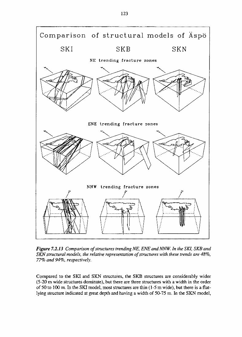
123
Comparison of s t r u c t u r a l models of Aspo
SKI SKB SKN
NE trending fracture zones
ENE trending fracture zones
NNW trending fracture zones
/
Figure 7.2.13 Comparison of structures trending NE, ENE and NNW. In the SKI, SKB andSKN structural models, the relative representation of structures with these trends are 48%,77% and 94%, respectively.
Compared to the SKI and SKN structures, the SKB structures are considerably wider(5-20 m wide structures dominate), but there are three structures with a width in the orderof 50 to 100 m. In the SKI model, most structures are thin (1-5 m wide), but there is a flat-lying structure indicated at great depth and having a width of 50-75 m. In the SKN model,
124
most zones are thin (0.2-10 m; 9 structures are 0.2 to 0.5 m wide) and four zones are wider(10-20 m).
In the SKN structural model, which focuses on hydrogeological data, 17 out of 18 structureshave hydrogeological significance.
7.2.5.6 General Implications for Structural Modelling
The brief comparison and analysis of the variations between the different structural modelsindicate that two separate components may be important in explaining the differencesbetween them.
One component, which is related to the difference in the number, extension and widths ofstructures, is fundamentally related to the nomenclature and definitions used (e.g. what isa fracture zone?). In addition, the methodology (direct observation, remote studies,statistical analysis, etc.) used to identify structures (at surface) or anomalous deformation(in boreholes) and the tools used to visualise the data and the model (e.g. a physical model,CAD drawings in two or three dimensions or three-dimensional image processing) areimportant. The other important component is related to the basis for extrapolation of data(one or two-dimensional data giving three-dimensional structures), that is, the argumentsand technique used for combining surface structures with locations of increaseddeformation in boreholes or analogue extrapolation between boreholes.
To conclude, the extrapolation of structural data is not a simple geometrical exercise. Thesimulated structural model should be in agreement with the general structural context, bothin a macroscopic (regional scale) and mesoscopic (outcrop to hand specimen scale) sense.This is discussed in more detail in Tiren (1996).
7.2.6 Uncertainties Underlying Structural Models
As with all aspects of Performance Assessment modelling, understanding and identificationof the uncertainties involved in constructing the geological structural model of a site is animportant task, not least because many of the hydrogeological and geotechnical and designconsiderations are based upon it.
Structural models traditionally deal with the characterisation of individual structures or setsof structures and how these interact with or affect each other (Section 7.2.6.5). The resultof the modelling is, for example, restricted by physical limitations (input data and computertools), expert judgements and constraints in the modelling procedure. Uncertaintiesregarding these aspects, the accuracy and precision of locations of structural elements andthe existence of 'black holes' (areas with no information) in the model are often notdiscussed in depth, although, for the last five years or so, SKB has been using a guidelinefor modelling discrete-fracture zones which classifies the probability of the existence of astructure (Backblom, 1989). However, the validity of the interpretation produced in relationto the general structural pattern in the rock is not considered in the SKB guideline.
125
A comprehensive treatment of all the categories of uncertainty in structural modelling is acomplex problem. For the purposes of the SITE-94 study, a limited number of subjects isselected for treatment. The two main physical limitations to structural modelling are thecontrol of geometrical relationships (orientations of sets of structures comprising thestructural system) and the volume (spatial location of structures). Specific questions toaddress are:
• Control of geometry: The identification of orientations of all sets of structurescomprising the system of fracture zones in the rock. Does the configuration oforientations of structures within the modelled volume mimic geometries inneighbouring areas, where independent investigations may have been performed?
• Control of volume: Does the spatial distribution of available data give a uniformcontrol of the volume modelled and with what degree of certainty will existingstructural elements be detected by the types of survey performed?
A third physical limitation is uncertainty in the detailed descriptions of individual structures(width/thickness, internal structure, alteration, infilling, etc.). The character of a fracture orfracture zone may also change along its length. Expert knowledge of the structuralrelationships in an area is generally one of the most important inputs for building anunderstanding. This is especially true in complex areas with few easily identifiablecharacteristics for individual structures. The extent to which the geologist's reading andinterpretation of diffuse observations can contribute to uncertainties in the model is,however, hard to quantify. Direct observations and characterisation of structures on thesurface or in tunnels are essential for the correlation of structures in boreholes. This typeof information is very limited in the SITE-94 study.
A three-dimensional model of a domain is a way to visualise the structural framework ofthe domain, even though the model may not explain all the observations made in thedomain. Approximations are often made in order to be able to formulate and present amodel, often comprising some form of weighting in the importance of different types ofstructures in relation to the complexity of the model. For example, it is clearly not possibleto include structures of all sizes and widths. The approximations should not, however,change the impression of the overall character of the domain. The approximations appliedin the modelling procedure are generally well defined (see Section 7.2.3.3), but theirconsequences may not be well understood in some cases. Consequently, approximationsmay, if not fully controlled, introduce systematic errors in the model. In spite of the fact thatthe approximations are apparently well defined, decisions based on them may introducesubtle uncertainties. For example, why is a certain structure included whilst other similarstructures are excluded? To illustrate the effect of some of the approximations, two testsare carried out in SITE-94:
• What percentage of the mapped section of crushed rock can be explained by the SKI3D structural model of Aspo?
• What is the relationship between selected structural input parameters and indicationsof groundwater flow in the bedrock, indicated by borehole spinner measurements?
126
The first of these tests is described in Tiren et al., 1996 and the second in Section 7.3.6. Itshould also be noted here that one should not expect a one-to-one correlation between flowmeasurements and structures as i) some of the observed structures may be tight at the pointof intersection with the measuring borehole and ii) there certainly exist structures(individual fractures etc.) that are too small to be included in the structure model, but whichstill could be significant water conductors.
The modelled area comprises a 2 x 2 x 1 km rock volume. Most boreholes are located in thesouth-central part of Aspo where borehole coverage is best. The objective of the verticalboreholes is to investigate the distribution of rock types, while the inclined boreholes areintended to characterise structures trending NE to ENE. However, three other sets ofstructures exist, deformed by or overprinted by the NE to ENE trending structures. Thequestion asked is whether or not the present configuration of boreholes at Aspo would beable to detect and characterise these other sets of structures that may exist.
A statistical approach is applied to test if the configuration of the cored boreholes on Aspois able to reveal any arbitrary orientation of fracture zones. For example, as a simple test,only the angular relationships between orientations of boreholes and orientations ofdifferent sets of structures is considered. This poses the question as to whether the systemof boreholes will allow any structure to pass through the investigated space without beingintersected by any of them, which implies that the structure has to be parallel to theboreholes. Introducing the fact that boreholes have finite length further reduces theobservation probability. Ain addition, the borehole system will preferentially detectstructures of certain orientations.
The results of the analysis (see Tiren et al., 1996, for details) imply that the representationof structures oriented in certain directions may be suppressed in the structural model ofAspo compared to other directions. The same test can be applied to determine whether theborehole configuration at a site is able to detect all possible orientations of structures andcan obviously be used in the planning of borehole investigations in future sitecharacterisation programmes.
7.2.6.1 The Extrapolation of Geological Data
The connection of structures between boreholes and surface observations is often performedby correlating structures with similar characteristics. In areas where no significantcharacteristics are attributable to a specific set of fracture zones, correlation becomesuncertain.
Many of the fracture zones mapped on Aspo are vertical to steeply dipping. The boreholesare inclined approximately 60-90° to the horizontal. The angle of intersection betweenboreholes and the steeply dipping fracture zones is less than 60° and, in many cases, theboreholes are subparallel to the fracture zones. The number of fractured sections in theboreholes are frequent. The average separation of borehole radar reflections and sectionsmapped as crushed rock is about 15 m. The effects of these relationships on theinterpretations of orientations of structures are discussed by Tiren et al. (1996), who alsodeal with uncertainties of extrapolations over distances, using geometrical analyses of corefracture and borehole radar data to illustrate the potential uncertainties involved. The
127
authors conclude that the borehole configuration at Aspo favours the detection (by boreholeradar investigations) of structures trending c. NNE, E-W and NW with a gently dip(30-60°) to the north. Flat-lying to gently inclined structures are also detected in severalboreholes. Vertical structures trending NE - EW are detected in boreholes. The samplingis poor for vertical to subvertical structures trending NNW to NW and for structures steeplydipping west to southwestward.
An additional method of checking whether the structural system identified within an areacorresponds to the existing population is to compare the set of structures in the area withthose in other areas within the same tectonic region. Independent surveys in the Simpevarparea have identified the orientation of structures in different scales. The structuralinformation of the subregional area surrounding Aspo (Section 7.2.2.4) and the mappingof fractures which determine the morphology of outcrops in the local scale, show that theresemblance between the orientations of structures identified on the three different scalesare convincing.
7.2.6.2 Identifying Discrete Rock Volumes within a Model
The representation of the spatial distribution of structures in a model of any rock volumegenerally depends on a combination of structural information (homogeneous or hetero-geneous sampling) and approximations applied during the structural modelling, which caninduce systematic errors.
It is important to realise that structures do not form random configurations (unsystematicarrangements) in the rock. The degrees of freedom for the interpretation of the structuralframework in the rock are thus limited. It can also be stated that the uncertainties in thestructural model increase with depth due to lack of input data, but also because it may notbe possible to correlate structures located at depth with any observed surface structure. Ina structural model of a specific rock volume, confidence in the existence and location ofstructures are generally not equal in all parts of the model, due to uneven data distribution.Furthermore, the ability to detect structures in different parts of the rock volume is also afunction of the orientation of the structures. Uncertainties regarding the location ofstructures and especially the existence of volumes where there is a low degree of confidencein detecting structures ('black holes') should, therefore, be analysed and presentedseparately for each group/set of structures constituting the structural system in the rock.This type of check can be performed by graphical visualisation techniques and can also beused as an aid in the design of a drilling programme. This can also give important input tothe interpretations of, for example, hydraulic measurements and their correlations withgeological structures.
7.2.6.3 Precision in the Location of Structures
In structural modelling, a very important input parameter is the location of data points. Theaccuracy in location of structures interpreted on aerial photos and reproduced on maps arein the order of ±10-20 m. Due to technical processing during modelling, the averageaccuracy in locating the fracture zones on the top surface of the model is estimated to be±10-25 m or less in the central part of the Aspo model. A further point to address is the
128
approximation involved in extrapolation of structural elements included in the model, bothsurface and subsurface. The minimum surface extension of a structure produced in theSITE-94 study corresponds with the length of the interpreted lineament representing thestructure. This implies that the extension of structures to the boundary of the structuremodel in areas covered by water is not documented and such extrapolations are performedonly in order to get a better visualisation of the structural system of the area.
A generic uncertainty underlying all structural modelling is the conceptual identificationof structures (for example, the definition of fracture zones and how to choose and apply thedefinition). In order to be able to identify what is anomalous regarding fracturing (i.e. thefracture zones), an area of 'normal' averagely fractured rock should be documented as abaseline. This is discussed in more detail in Tiren et al., 1996.
7.2.6.4 Approximations Made in Structural Modelling
The structural model is a reflection of the input parameters, which was intentionallyrestricted to geological and geophysical surface-based investigations for the purposes ofSITE-94. It is important to consider the degree to which the SKI 3D structural modelsucceeds in explaining the existence of all mapped sections of crushed rock and identifiedoriented borehole radar reflections. A second question is whether the approximations willinfluence understanding of the transport of water in the bedrock. Tiren et al. (1996)concluded that the SKI structural model had succeeded in outlining a structural frameworkof fracture zones which appears to consider a relatively large fraction of the more extensivezones in the area (more than 50%). The local zones (larger than 50 m) may be of the orderof one to two times more frequent than the extensive zones included in the SKI structuralmodel.
To address the second question, the locations of potential groundwater flow paths inboreholes (cf. Section 7.3.6) are identified according to rock type and occurrence of zonescontaining crushed rock. About 50% of all flow indications are located in borehole sectionswhich contain a single rock type and which are located 3 m or more away from anylithological contact (measured along the drill core). In the granitoids, 50% of the indicatedpotential flow paths are located in sections with crushed rock. In the aplite, about 80% ofthe flow indications are located in sections with crushed rock. Slightly more than 50% ofall indicated flow points in the boreholes are located close to lithological contacts. Therelative proportion of groundwater flow paths associated with sections of crushed rockappears to be more pronounced at lithological contacts compared to flow paths in sectionscontaining a single rock type. Mylonites, fine-grained microbreccias resulting fromfracturing or deformation, appear to be potential pathways for groundwater flow if they arestrongly fractured. Correlation between spinner measurements and borehole radarmeasurements shows that about 70% of all indications of water inflow were detected by theborehole radar measurement (directional antenna).
The SKI structural model of Aspo uses data on sections of crushed rock as one of the maininputs. Out of all potential groundwater flow paths found in boreholes, about 40% are notassociated with sections containing crushed rock. This implies that the model, based ongeological and geophysical data, will only, at best, include less than 60% of all potentialgroundwater flow paths identified by spinner measurements and temperature/salinity logs.
129
The implications of this are discussed in detail in Tiren et al. (1996) and in Voss et al.(1996).
Again it should be noted here that one should not expect a one-to-one correlation betweenflow measurements and structures as i) some of the observed structures may be tight at thepoint of intersection with the measuring borehole and ii) there certainly exist structures(individual fractures etc.) that are too small to be included in the structure model, but whichstill could be significant water conductors. The percentages of flow explained by thestructure model could thus be seen as an indication of how significant smaller scalestructures are for the groundwater flow through the rock.
7.2.6.5 Relative Age of Rocks and Structures
An appropriate understanding of the geological and structural evolution of an area is the keyto defining the character of the area and making a prediction of the future stability of thearea. The geological and structural history represents a continuous record of events whichhave affected the area. It also shows how the character of the different structures haschanged with time. In this perspective, the different sets of structures in the area can beidentified and estimates can be made concerning how future mechanical, chemical andhydraulic stresses on the system might be accommodated in the rock.
Because relative ages can be judged by overprinting criteria (before 1991 absolute agedeterminations were not available for the Aspo area) and the character of the structures, agood knowledge of the field appearance of rocks and structures is critical for understandingthe site-specific geological evolution. However, this is not always a straight-forwardmethod as, in the Aspo case, obvious multiple reactivations and partial reactivations ofstructures may locally obscure the impression of the overprinting relationships. The resultcould be an inconsistent cross-cutting relationship among different sets of fractures.
The basic information for any interpretation of the evolution is different types ofobservations made on various scales. In this case, a review of geological and structuraldescriptions of the geological terrain is made and then compared with the geoscientificinformation gathered in the area and vice versa. This infers that the regional surroundingsof the target area, as well as the outcrops within the area, constitute reference areas.Detection of late crustal movements, which may have occurred in the last 600 million yearsor after the latest ice age, is not a trivial topic. This is why datum surfaces for calibrationare needed. Representative datum surfaces are, in this case, the sub-Cambrian peneplain andQuaternary strata. Such surfaces may often not be conveniently found in the actual site, butin its regional surroundings.
7.2.6.6 Restoration of Faulting
A part of the interpretation of the structural history of an area is sequential reconstructionof deformation, e.g. displacements (faulting) which have taken place in the rock. This helpswith the correlation of displaced structures and the extrapolation of geochemical,mechanical and hydrogeological properties from one structural location to another. In areascharacterised by partial reactivation, reconstruction will be troublesome for early phases of
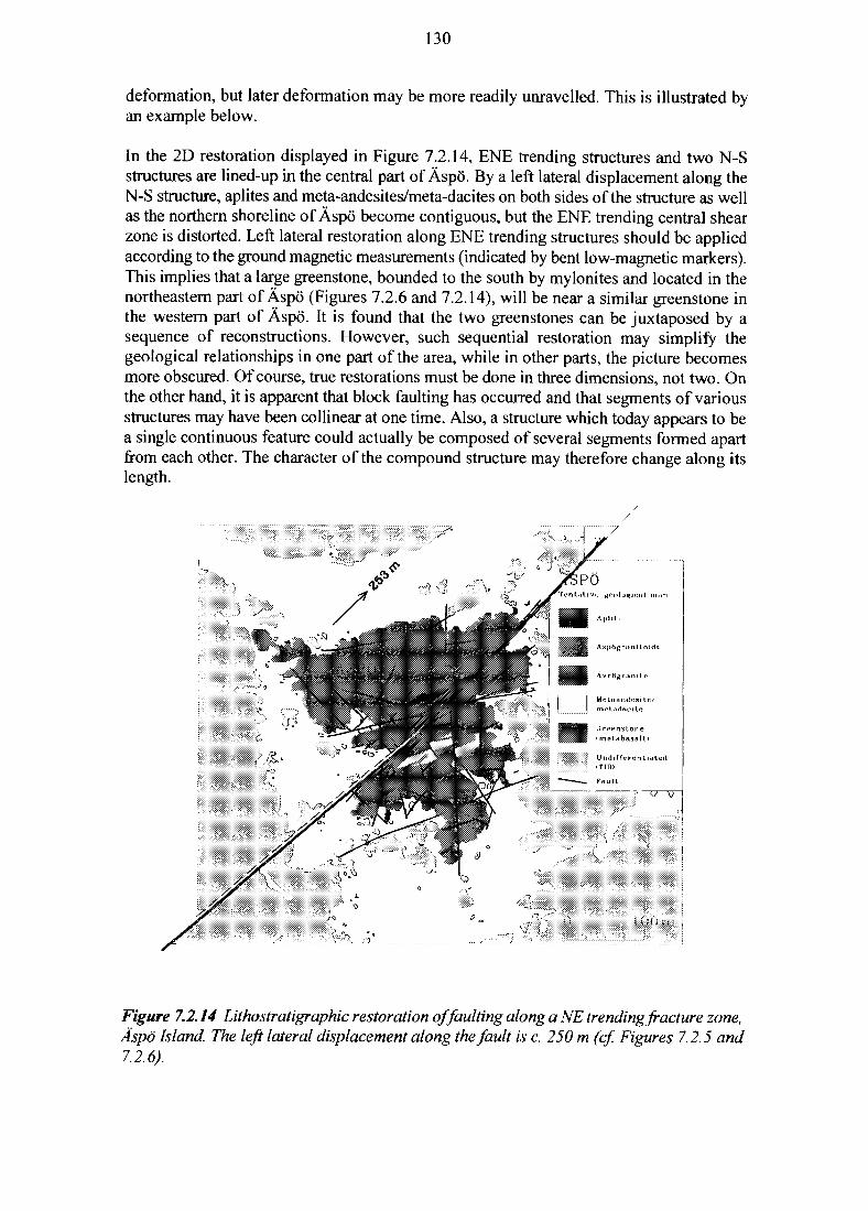
130
deformation, but later deformation may be more readily unravelled. This is illustrated byan example below.
In the 2D restoration displayed in Figure 7.2.14, ENE trending structures and two N-Sstructures are lined-up in the central part of Aspo. By a left lateral displacement along theN-S structure, aplites and meta-andesites/meta-dacites on both sides of the structure as wellas the northern shoreline of Aspo become contiguous, but the ENE trending central shearzone is distorted. Left lateral restoration along ENE trending structures should be appliedaccording to the ground magnetic measurements (indicated by bent low-magnetic markers).This implies that a large greenstone, bounded to the south by mylonites and located in thenortheastern part of Aspo (Figures 7.2.6 and 7.2.14), will be near a similar greenstone inthe western part of Aspo. It is found that the two greenstones can be juxtaposed by asequence of reconstructions. However, such sequential restoration may simplify thegeological relationships in one part of the area, while in other parts, the picture becomesmore obscured. Of course, true restorations must be done in three dimensions, not two. Onthe other hand, it is apparent that block faulting has occurred and that segments of variousstructures may have been collinear at one time. Also, a structure which today appears to bea single continuous feature could actually be composed of several segments formed apartfrom each other. The character of the compound structure may therefore change along itslength.
Figure 7.2.14 Lithostratigraphic restoration of faulting along a NE trending fracture zone,Aspo Island. The left lateral displacement along the fault is c. 250 m (cf Figures 7.2.5 and7.2.6).
131
7.2.7 Fitting a Hypothetical Repository Into the Aspo Structure
7.2.7.1 Introduction
One exercise conducted within SITE-94 has been to investigate how readily a repositorycould be fitted into the developed detailed 3D structural model of the site, taking accountof simple guidelines on avoiding significant fracture zones. This fitting of the repositoryto the rock at Aspo is made considering only the geological structures. Obviously, takingaccount of this factor alone is not sufficient to achieve a satisfactory design in a sitingexercise for a real repository, which would need to be based on a wide range of detailedinformation not available to SITE-94. In particular, some large size geometrical structuresmay have mechanical and hydrological properties, which would be allowable within, orclose to, a repository. On the other hand small scale structures, not necessarily included inthe model, may in fact cause significant problem for the repository emplacement. Thegeneral outline of the disposal system used in the present exercise is given in Chapter 5.
7.2.7.2 Overall Constraints on Location
The location and geometry of the hypothetical repository are adapted to take into accountthe geological and geotechnical characteristics of the bedrock. However, it should be madeclear that precise design and detailed location of repository tunnels are not part of theSITE-94 project. Furthermore, data from excavations and tunnels would clearly be essentialin order to achieve a more adaptable layout of the repository.
Based on the available information, it appears that the repository can be positioned indifferent ways below Aspo island: in the northern or in the southern block. A location atthe southeast, in the southern block, is chosen because more data (boreholes) are availablein this area.
As discussed earlier, the SKI interpretation of Aspo contains a large number (52) of fracturezones, which means that there is only room for a limited number of canisters out of themore than 4000 that may be needed to dispose of the spent nuclear fuel that will beproduced up to the year 2010 (Chapter 3).
For the purposes of this exercise, the repository is connected to the surface by two verticalshafts placed at a distance of greater than 100 m from the repository and with a separationof at least 300 m.
Large horizontal stresses and stress gradients may be harmful to the stability of a repository.With regard to practical constructability and mechanical stability of the repository, theorientation of the deposition tunnels has been chosen approximately parallel to theorientation of the maximum horizontal principal stress direction at Aspo (N 400° W) andperpendicular to the SKB fracture zone NE-1 (Wikberg et al., 1991).
Owing to the low hydraulic gradient at depth on the island the importance of the orientationof the drifts in relation to the hydraulic gradient can be ignored.
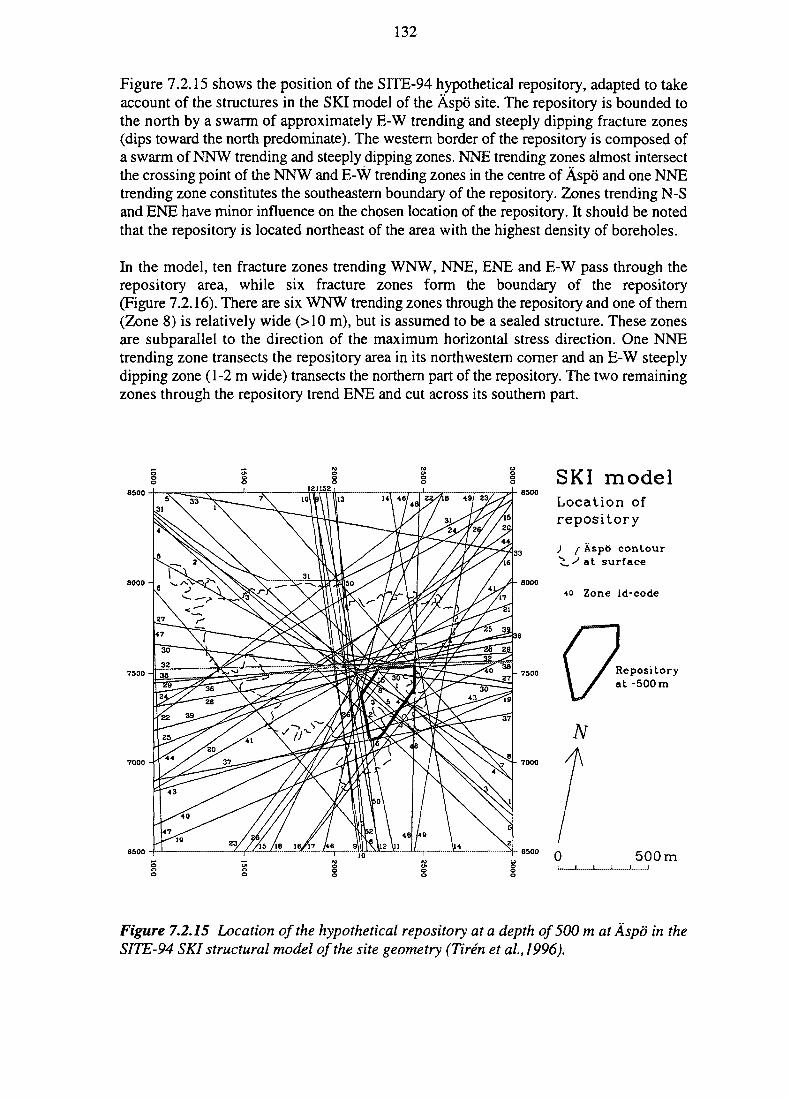
132
Figure 7.2.15 shows the position of the SITE-94 hypothetical repository, adapted to takeaccount of the structures in the SKI model of the Aspo site. The repository is bounded tothe north by a swarm of approximately E-W trending and steeply dipping fracture zones(dips toward the north predominate). The western border of the repository is composed ofa swarm of NNW trending and steeply dipping zones. NNE trending zones almost intersectthe crossing point of the NNW and E-W trending zones in the centre of Aspo and one NNEtrending zone constitutes the southeastern boundary of the repository. Zones trending N-Sand ENE have minor influence on the chosen location of the repository. It should be notedthat the repository is located northeast of the area with the highest density of boreholes.
In the model, ten fracture zones trending WNW, NNE, ENE and E-W pass through therepository area, while six fracture zones form the boundary of the repository(Figure 7.2.16). There are six WNW trending zones through the repository and one of them(Zone 8) is relatively wide (>10 m), but is assumed to be a sealed structure. These zonesare subparallel to the direction of the maximum horizontal stress direction. One NNEtrending zone transects the repository area in its northwestern corner and an E-W steeplydipping zone (1-2 m wide) transects the northern part of the repository. The two remainingzones through the repository trend ENE and cut across its southern part.
SKI modelLocation ofrepository
; f Asp6 contour> y> at surface
40 Zone id-code
Repositoryat -500 m
500m
Figure 7.2.15 Location of the hypothetical repository at a depth of 500 m atAspo in theSITE-94 SKI structural model of the site geometry (Tiren et al.,1996).
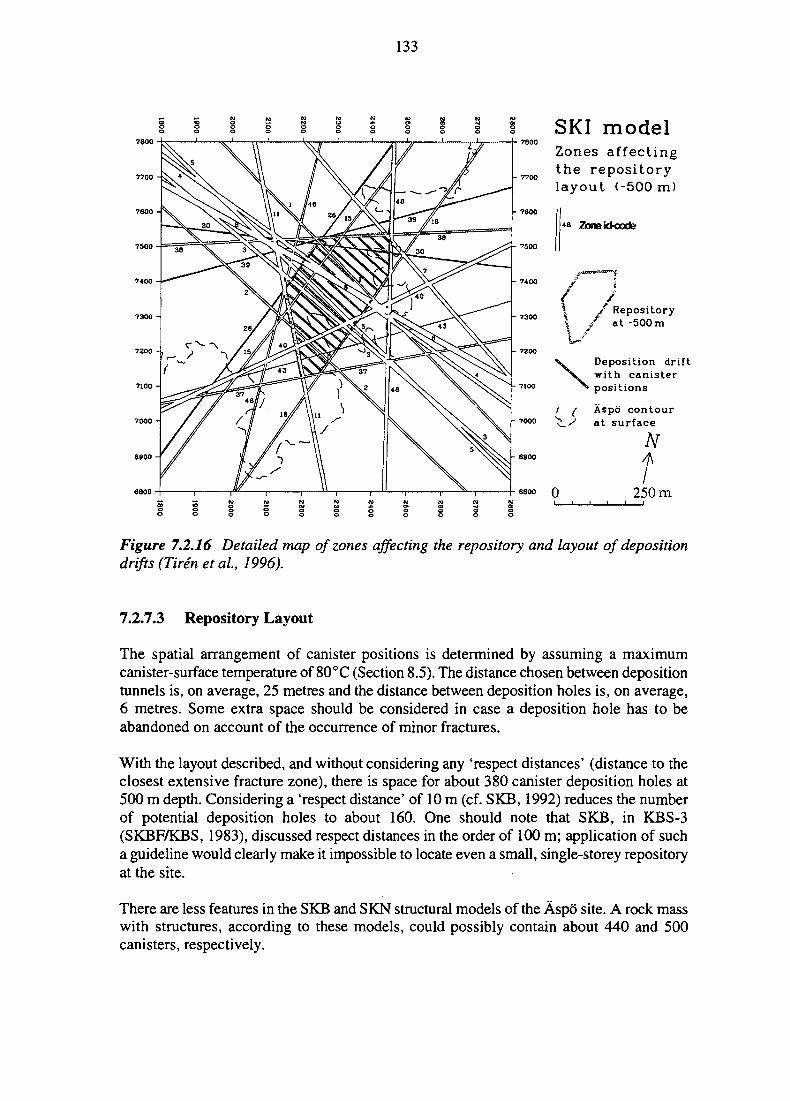
133
SKI modelZones affectingthe repositorylayout (-500 m)
Zonekkxxle
/ Repositoryat -500m
Deposition driftwith canisterpositions
Aspo contourat surface
250 m
Figure 7.2.16 Detailed map of zones affecting the repository and layout of depositiondrifts (Tiren et al, 1996).
7.2.7.3 Repository Layout
The spatial arrangement of canister positions is determined by assuming a maximumcanister-surface temperature of 80°C (Section 8.5). The distance chosen between depositiontunnels is, on average, 25 metres and the distance between deposition holes is, on average,6 metres. Some extra space should be considered in case a deposition hole has to beabandoned on account of the occurrence of minor fractures.
With the layout described, and without considering any 'respect distances' (distance to theclosest extensive fracture zone), there is space for about 380 canister deposition holes at500 m depth. Considering a 'respect distance' of 10 m (cf. SKB, 1992) reduces the numberof potential deposition holes to about 160. One should note that SKB, in KBS-3(SKBF/KBS, 1983), discussed respect distances in the order of 100 m; application of sucha guideline would clearly make it impossible to locate even a small, single-storey repositoryat the site.
There are less features in the SKB and SKN structural models of the Aspo site. A rock masswith structures, according to these models, could possibly contain about 440 and 500canisters, respectively.
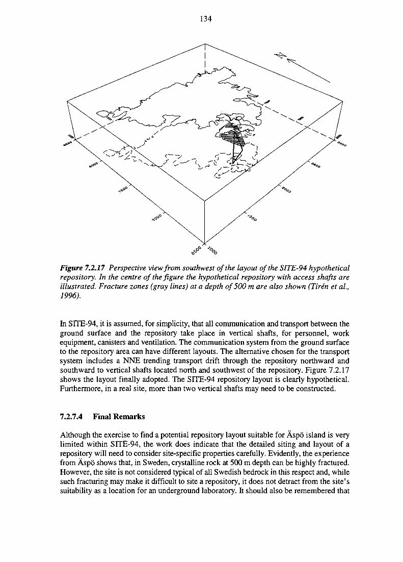
134
Figure 7.2.17 Perspective view from southwest of the layout of the SITE-94 hypotheticalrepository. In the centre of the figure the hypothetical repository with access shafts areillustrated. Fracture zones (gray lines) at a depth of 500 m are also shown (Tiren et al,1996).
In SITE-94, it is assumed, for simplicity, that all communication and transport between theground surface and the repository take place in vertical shafts, for personnel, workequipment, canisters and ventilation. The communication system from the ground surfaceto the repository area can have different layouts. The alternative chosen for the transportsystem includes a NNE trending transport drift through the repository northward andsouthward to vertical shafts located north and southwest of the repository. Figure 7.2.17shows the layout finally adopted. The SITE-94 repository layout is clearly hypothetical.Furthermore, in a real site, more than two vertical shafts may need to be constructed.
7.2.7.4 Final Remarks
Although the exercise to find a potential repository layout suitable for Aspo island is verylimited within SITE-94, the work does indicate that the detailed siting and layout of arepository will need to consider site-specific properties carefully. Evidently, the experiencefrom Aspo shows that, in Sweden, crystalline rock at 500 m depth can be highly fractured.However, the site is not considered typical of all Swedish bedrock in this respect and, whilesuch fracturing may make it difficult to site a repository, it does not detract from the site'ssuitability as a location for an underground laboratory. It should also be remembered that
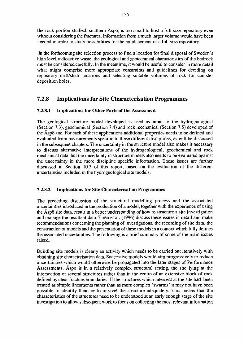
135
the rock portion studied, southern Aspo, is too small to host a full size repository evenwithout considering the fractures. Information from a much larger volume would have beenneeded in order to study possibilities for the emplacement of a full size repository.
In the forthcoming site selection process to find a location for final disposal of Sweden'shigh level radioactive waste, the geological and geotechnical characteristics of the bedrockmust be considered carefully. In the meantime, it would be useful to consider in more detailwhat might comprise more appropriate constraints and guidelines for deciding onrepository drift/shaft locations and selecting suitable volumes of rock for canisterdeposition holes.
7.2.8 Implications for Site Characterisation Programmes
7.2.8.1 Implications for Other Parts of the Assessment
The geological structure model developed is used as input to the hydrogeological(Section 7.3), geochemical (Section 7.4) and rock mechanical (Section 7.5) developed ofthe Aspo site. For each of these applications additional properties needs to be defined andevaluated from measurements specific to these different disciplines, as will be discussedin the subsequent chapters. The uncertainty in the structure model also makes it necessaryto discuss alternative interpretations of the hydrogeological, geochemical and rockmechanical data, but the uncertainty in structure models also needs to be evaluated againstthe uncertainty in the more discipline specific information. These issues are furtherdiscussed in Section 10.3 of this report, based on the evaluation of the differentuncertainties included in the hydrogeological site models.
7.2.8.2 Implications for Site Characterisation Programmes
The preceding discussion of the structural modelling process and the associateduncertainties introduced in the production of a model, together with the experience of usingthe Aspo site data, result in a better understanding of how to structure a site investigationand manage the resultant data. Tiren et al. (1996) discuss these issues in detail and makerecommendations concerning the planning of investigations, the recording of site data, theconstruction of models and the presentation of these models in a context which fully definesthe associated uncertainties. The following is a brief summary of some of the main issuesraised.
Building site models is clearly an activity which needs to be carried out iteratively withobtaining site characterisation data. Successive models would aim progressively to reduceuncertainties which would otherwise be propagated into the later stages of PerformanceAssessments. Aspo is in a relatively complex structural setting, the site lying at theintersection of several structures rather than in the centre of an extensive block of rockdefined by clear fracture boundaries. If the structures which intersect at the site had beentreated as simple lineaments rather than as more complex 'swarms' it may not have beenpossible to identify them or to unravel the structure adequately. This means that thecharacteristics of the structures need to be understood at an early enough stage of the siteinvestigation to allow subsequent work to focus on collecting the most relevant information
136
to allow their mapping. This can best be done by compiling regional data from the largerstructures in the area surrounding the site, as these often reflect the characteristics of thesmaller scale structures which will later be identified at the site scale. The need for iterativeinvestigations is clear.
SITE-94 clearly showed the importance of high quality surface mapping at an early stageof site investigation. In areas with good exposure a detailed surface map provides the bestcontinuous coverage possible and allows well-controlled extrapolation to depth at lesseffort and expense than geophysical methods. There is not always enough emphasis placedon this approach in site investigation. As noted above, an important issue is knowing theparticular characteristics to seek during mapping and exploratory exercises to relategeological and structural features to particular surface manifestations can thus be valuable.
During the course of modelling the structure of a site the methods of recording informationwill change with increasing resolution of information and increasing or changingunderstanding. Nomenclature may be revised (e.g of fracture zones and their structuralsignificance) and the weighting given to certain data will change, with consequent changesin the relative precision and quantity of observations. The impacts of this evolution in datacollection need to be kept under constant review, both by the structural modelling groupand by those using different iterations of the model (e.g. for hydrogeological modellingpurposes).
Many of the geological data collected during mapping and core analysis will prove not tobe diagnostic of particular features of the site. At a superficial level the data may thusappear to contain much 'noise' and it may take some time to identify properties (bothstructural and mineralogical) which are sufficiently distinctive of, for example, particulargroups of fractures.
Borehole numbers, location, angling and spacing are clearly of considerable significancein planning a site investigation. The boreholes on Aspo are very closely spaced in terms ofproducing a geological and structural model and more data from outlying parts of the localscale model area would have been very useful: investigations for a real candidate siteshould not concentrate solely inside the site boundary. In addition, the limitations ofworking at a coastal or island site need careful planning.
There is a tendency in site investigation to concentrate boreholes on particular features or'conceptual' blocks of rock rather than on obtaining a wide enough areal coverage and abroad enough sampling of 'average' or apparently featureless rock. There is a rational casefor having an early suite of boreholes spaced on a regular grid pattern. Initial boreholesshould focus on establishing the broad geological and tectonic setting of the site and region.Subsequent establishment of the main structural features as well as the geology of the sitewill provide information on the optimum location and orientation of further boreholeswhich will provide the best 'view' for geophysical techniques aimed at characterising thesefeatures. In this respect, the more oriented borehole geophysical data available the better.In addition, information from greater depths than usually sampled would be valuable inconstraining geological and structural models. Actually a certain amount of data from therock mass below the repository level is required in order to be able to claim that the modelsproduced are valid.
137
Finally, it is clear that very simplified 'block' models of a site are unlikely adequately toexplain all the geological data obtained. Significant structural patterns (from the viewpointof hydrogeology and rock mechanics) are likely to found at much smaller scales and onlybecome evident during the later stages of site investigation. The need to keep the structuralmodel under review as more site investigation data emerge is evident. In this respect, itshould be borne in mind that SITE-94 did not progress to the next logical step of tying-inthe models based on surface and borehole data alone, to data from undergroundexcavations.
7.3 HYDROGEOLOGY
This rather detailed section describes analysis of hydrogeological data and the developmentand calibration of conceptual site models for the hydrogeology of the Aspo site. It alsodiscusses the data which support the conceptual models tested. Model predictions forfurther use in the assessment are presented in Sections 10.3 and 11.2.2, together with anevaluation of the validity of these predictions. Readers primarily interested in theapplication of the hydrogeological models are thus referred to these latter sections.
7.3.1 Introduction
7.3.1.1 Hydrogeological FEPs and Influences in the PID
Groundwater flow is of major importance to repository performance. It constitutes themajor pathway of radionuclide migration and affects the chemical environment of therepository. Figures 7.1.1 and 7.1.2 show the SITE-94 assessment of which FEPs affect andare affected by groundwater flow, as determined through the procedure presented byChapman et al. (1995), and as outlined in Chapter 2.
In the far-field, the PID illustrates that the FEP Far-field groundwater flow is driven by theFEP External flow boundary conditions and that it depends on the FEP Properties of far-field rock (Figure 7.1.1). In addition, there are important indirect influences. For example,the FEP 'Stress field' affects the hydraulic properties of the rock directly throughdeformation of fractures and indirectly through fracturing and faulting (should these eventsoccur). The well-known influences from Temperature and density effects fromGroundwater chemistry are considered less important for overall performance (see e.g. thediscussion of these influences in Project-90, SKI, 1991). At the highest level of importance,Far-field groundwater flow primarily affects radionuclide migration FEPs and the near-field groundwater flow, but there are many other influences at lower importance levels.
In the near-field, the PID reflects that, at the highest importance level, the FEP Near-fieldgroundwater flow is driven by the FEP Far-field groundwater flow, and that it depends onthe FEP Properties of the near-field rock, together with the FEP Properties ofbentonitebuffer, see Figure 7.1.2 and the complete PID (folded at the end of the report). Again, thereare indirect influences as well as other direct influences at lower importance levels.
138
7.3.1.2 Specific Objectives of the Hydrogeological Site Evaluation
The specific objectives of the hydrogeological evaluation in SITE-94 are:
• to develop quantitative, hydrogeological site models consistent with the site data, tobe used for prediction of hydrogeological conditions and their future evolution underdifferent external boundary conditions,
• to develop a general understanding of site hydrogeology and to build confidence inthe detailed hydrogeological prediction models,
• to document how the different FEPs and influences of the PID have been treated.
Formally, these tasks were assigned to the Hydrogeology Clearing House in the SITE-94Assessment Model Flowchart (Chapman et al., 1995). Ideally, quantitative models shouldbe developed for all hydrogeology-related FEPs and influences in the PID. In practice,however, it is not possible to treat each FEP and influence with the same level of detail. Insome cases (e.g. groundwater flow in the far-field), several well-established conceptualapproaches are available, which make it possible to develop detailed, quantitative sitemodels. In other cases, where process uncertainties and lack of data restrict the possibilitiesfor developing detailed quantitative models (for example, regarding the influence of rockstresses on the groundwater flow in the near-field), it is necessary to rely upon expertjudgement or simple scoping calculations.
Model development comprises calibration of the selected conceptual hydrogeological sitemodels and validation efforts, to ascertain that the models are consistent with the availablehydrogeological site data. The models build on hydrogeological test data and the SITE-94geological structural model, described in Section 7.2. Application of the hydrogeologicalsite models developed to evaluate effective parameters for the radionuclide transportcalculations is described in Sections 10.3 and 11.2.2.
Special efforts are also made to analyse the consistency between interdisciplinary sitemodels. These efforts include an integrated interpretation of geological, hydrogeologicaland geochemical site data, as well as a series of workshops with interdisciplinary site-evaluation teams. These efforts are discussed in Section 7.3.6.
The influence of rock mechanical processes on groundwater flow, which is of potentialimportance for the near-field environment in particular, is discussed in Sections 10.2 and11.2.1. However, no attempt is made to incorporate these influences directly into thehydrogeological site models.
7.3.1.3 Summary of Approach
The hydrogeological site evaluation comprises analyses of a large amount of site-specificdata and development and testing of several alternative site models (i.e. integrateddescriptions of the hydrogeological processes and structures). Each site model may consistof a number of subsidiary models. The SITE-94 approach to this rather complex task issummarised below.
139
1) Assessment of hydrological setting and regional hydrogeological modelling
Groundwater flow is driven by the external boundary conditions. One important boundaryto be described is the hydrological setting of the surface environment. The boundaries inother directions are more artificial as the hydrogeological models are, for practical reasons,confined mainly to the Aspo region. In order to assess the justification of the boundaryconditions applied to the site models and to assess the impact of changes in the large-scaleboundary conditions that may occur, e.g., if the climate changes, the SITE-94 analyses alsoinclude some regional hydrogeological modelling.
2) Assessment of uncertainties in the site characterisation data
As discussed in Chapter 6, site-characterisation data are associated with several sources ofpotential errors and uncertainty regarding equipment, measurement techniques,representativity, etc. Many of the parameters used in the site evaluation (e.g. hydraulicconductivity) cannot be measured directly, but need to be estimated indirectly withinterpretation models. The assumptions associated with such interpretations introduceadditional uncertainties. To estimate a portion of this uncertainty, detailed analyses of themeasured borehole data are performed. These analyses include a multivariate analysis ofdata from hydraulic, geological and geophysical measurements in boreholes, as well as are-interpretation of all hydraulic packer-test data, using the Generalised Radial Flow (GRF)theory. In addition, the correlation between hydraulic and other borehole data isqualitatively assessed by direct inspection of the data and by use of a 3D visualisationtechnique. The aim in SITE-94 is to evaluate the impact of the quantified uncertainties bymeans of parameter-sensitivity analyses in the hydrogeological site models.
3) Simple scoping calculations
Site data suggest that the crystalline rock that underlies Aspo is highly heterogeneous, withfracture properties and small-scale hydraulic conductivities that vary over many orders ofmagnitude. Detailed modelling of the flow requires both that this complex information beassigned to various structures and that a fully three-dimensional solution be obtained forthe flow field.
Before embarking on these ambitious tasks, a set of scoping analyses is performed, basedon simple hypotheses concerning the flow-field structure and hydraulic driving forces. Suchsimple, scoping calculations and sensitivity analyses are ways to estimate wide bounds onthe system behaviour and to identify the critical uncertainties that must be addressed withthe more complex, detailed site models. Thus, these simple calculations may aid in theselection of conceptual approaches for modelling site hydrogeology. Such calculations arealso valuable for assessing the reasonableness of the results of the detailed site models,which often build on conceptual assumptions that cannot be directly verified by the site data(Sections 10.3 and 11.2.2). However, it should also be kept in mind that the types ofscoping analyses used here do not fully exploit the information that is present in the data.Moreover, they do not yield estimates of the variability of flow and transport parameters,but rather just bounds on their ranges.
140
4) Development of a hydrogeological model based on the SITE-94 structural model andintegrated interpretation of different hydrogeological and interdisciplinary site data
Groundwater flow depends directly on the site properties. In general, it is assumed thatthere is some correlation between hydrogeological structures and geological structures, andbetween the evolution of the groundwater flow and the geochemistry at the site.Interdisciplinary data give information on potential correlations and provide informationfor discrimination between alternative site models. Integration of this information isimportant for building confidence in the site evaluation.
The SITE-94 approach is to develop a hydrogeological structure model based on thegeological structural model (Tiren et al., 1996; see Section 7.2). This model is then adaptedto geophysical, hydrogeological and geochemical data by means of a 3D visualisationtechnique, which makes it possible to visualise large, complex data sets and test differenthypotheses of correlation between, e.g., geological features and hydrogeological andgeochemical properties.
5) Development of quantitative hydrogeology models and multiple interpretations
The hydrogeological evaluation comprises development of a suite of groundwater flowmodels on different scales, ranging from the largest regional scale of the Baltic Shield,down to the scale of the repository rock block at Aspo. Table 7.3.1 gives an overview ofthe conceptual models selected on the various scales.
The quantitative predictions of the spatially varying hydrogeology for the site-scale (far-field) radionuclide transport evaluations are all derived from detailed, three-dimensionalmodels of the Aspo site. On the smallest scale, corresponding to the repository rock block(length scale less than 50 m), detailed fracture-network models are developed, consistentwith the site-scale models, to evaluate hydrogeological properties of the near-field rock. Tovarying degrees, the site-scale models are based on the analysis of regional flow, estimatesof data uncertainty, the scoping calculations and the integrated, hydrogeological structuremodel.
Due to the pronounced heterogeneity of crystalline rock and limitations of the site data, itis often possible to formulate alternative conceptual models that fit the site characterisationdata equally well. To some extent, the validity of alternative conceptual models can beevaluated by calibration using one data set and validation using another data set. Analysisof consistency between different site models (e.g. for hydrogeology and geochemistry) mayyield additional information for model discrimination. However, in many cases the sitecharacterisation data do not contain sufficient information for conclusive discriminationamong alternative conceptual models. The envelope of alternative models is thus a measureof conceptual uncertainty in the description of the site.
Such conceptual uncertainty is a concern if different models predict different behaviour ofthe site, when extrapolated to the temporal and spatial scales that are being considered inthe safety assessment. Furthermore, it is often difficult to determine, a priori, whether acertain conceptual model is realistic, or even conservative, in terms of its net impact on theconsequence calculations. Therefore, the strategy adopted in SITE-94 is to developalternative conceptual site models for site hydrogeology, and to propagate the resultsthroughout the assessment.
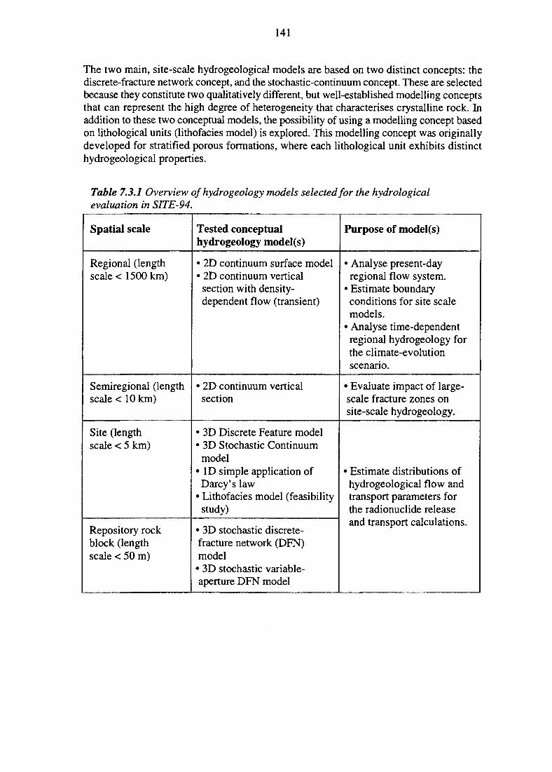
141
The two main, site-scale hydrogeological models are based on two distinct concepts: thediscrete-fracture network concept, and the stochastic-continuum concept. These are selectedbecause they constitute two qualitatively different, but well-established modelling conceptsthat can represent the high degree of heterogeneity that characterises crystalline rock. Inaddition to these two conceptual models, the possibility of using a modelling concept basedon lithological units (lithofacies model) is explored. This modelling concept was originallydeveloped for stratified porous formations, where each lithological unit exhibits distincthydrogeological properties.
Table 7.3.1 Overview of hydro geology models selected for the hydrologicalevaluation in SITE-94.
Spatial scale
Regional (lengthscale < 1500 km)
Semiregional (lengthscale < 10 km)
Site (lengthscale < 5 km)
Repository rockblock (lengthscale < 50 m)
Tested conceptualhydrogeology model(s)
• 2D continuum surface model• 2D continuum verticalsection with density-dependent flow (transient)
• 2D continuum verticalsection
• 3D Discrete Feature model• 3D Stochastic Continuummodel
• ID simple application ofDarcy's law
• Lithofacies model (feasibilitystudy)
• 3D stochastic discrete-fracture network (DFN)model• 3D stochastic variable-aperture DFN model
Purpose of model(s)
• Analyse present-dayregional flow system.
• Estimate boundaryconditions for site scalemodels.
• Analyse time-dependentregional hydrogeology forthe climate-evolutionscenario.
• Evaluate impact of large-scale fracture zones onsite-scale hydrogeology.
• Estimate distributions ofhydrogeological flow andtransport parameters forthe radionuclide releaseand transport calculations.
142
7.3.2 Hydrogeological Setting of Aspo
General
The climate of southeastern Sweden is humid-continental with cool summers. Annualprecipitation is about 675 mm (including snow cover of about 125 mm/a) with mostrecharge occurring during snow melt (Svensson, 1987). Evapotranspiration is about490 mm/a, leaving about 185 mm/a for runoff and recharge of the groundwater systems(Svensson, 1987).
Soil layers and regolith are thin or nonexistent in many places, with regolith dominated byglacial drift. Granodioritic and related basement rocks of the Fennoscandian shield (agesabout 1400 Ma to >1700 Ma) are at or near the ground surface in all locations. Flora areprimarily of boreal forest type, but are adapted to thin soils and near-coastal conditions.
The topography of the area is relatively flat and mildly undulating, with occasional steeperfeatures associated with major fracture zones that traverse the area. The water-tablegenerally mimics the topography. On Aspo, water-table elevation varies from 0 masl(metres above sea level) to about 4 masl. (Liedholm, 1991) with typical elevation of 1 to2 masl. The normal, annual variation of water-table elevation in the area is about one metre(Nyberg et al., 1992). In the immediate vicinity of Aspo, elevations are at most a few tensof metres; however, the regional groundwater flow system of the southern Swedishhighlands has maximal elevations over 300 m near its centre, south of Lake Vattern.
Aspo is a small (less than 2 km across), triangular, crystalline-bedrock island, bounded tothe north by an extensive, E-W trending shear zone, to the east by a N-S trending fracturezone, and to the west by a NW trending fracture zone. Aspo is adjacent to the mainland ina narrow archipelago of similarly sized islands, along the southeastern coast of Sweden.Relief on Aspo is low (less than 14 m), as it is in the nearby region.
Groundwater in the Fennoscandian Shield
As a result of the regional deformation history (as discussed in Section 7.2), theFennoscandian Shield is heavily fractured in this area. Tectonic structures such as fracturezones, which are more highly fractured than the surrounding rock, tend to be more easilyweathered/eroded, and hence appear as topographic valleys. Because they often occur asdepressions, regional structures tend to be focal areas for groundwater flow, recharge anddischarge, and often contain surface-water bodies.
In the shield rocks, groundwater flow occurs almost exclusively through fractures andfracture zones. Hydraulic conductivity of the shield rock varies over many orders ofmagnitude, and most of the groundwater flux occurs in connected segments of structureshaving the highest conductivity, while almost none occurs through regions of intactcrystalline rock. Such flow paths below Aspo may be associated with structures orientedin any direction, including subhorizontal zones that do not outcrop at the surface.
Groundwater flow systems in Sweden's crystalline basement occur at a variety of scales.Path lengths of groundwater flow from point of entry into the subsurface to point of exitfrom the subsurface vary from as little as a few hundred metres to a few hundred kilometresor more. The length of subsurface travel of water depends mainly on the pattern of ground
143
surface (and thus water-table) elevation, as well as on the transmissivity and connectivityof the more-conductive subsurface structures in the bedrock. Another control on flow-pathlength is the fluid density distribution, especially for saline deep waters. As in allgroundwater flow systems, water usually enters the subsurface at higher elevations andexits at lower elevations.
Groundwater below Aspo
The largest scale flow system in the Aspo area consists of water that recharges in the southSwedish highlands and discharges near the Baltic Sea coast (Figure 7.3.1). The coastalzone, including Aspo, is the major discharge zone for deep groundwater flow. This mustbe the case irrespective of the transmissivity distribution of bedrock structures and fluiddensity distribution. The only role the latter play is in controlling the depth of the flow pathsin this regional flow system before the flow exits the subsurface near the coast. Ground-water recharged on the mainland is likely to discharge from permeable structures thatoutcrop in the straits surrounding the coastal islands and in the deeper waters immediatelyeast of the islands.
At shallower depths in the subsurface, smaller flow systems exist at a variety of scalesdependent on the topography and transmissivity distribution of bedrock structures, of less-fractured bedrock and of local sedimentary cover. The exact location, extent and depth ofthe smaller flow systems is much more difficult to predict than the large regional systembecause there is a great dependence on the above-mentioned controlling factors. Localelevation highs may be either recharge or discharge areas for smaller systems dependingon all of the controlling factors. On Aspo, it would appear reasonable to expect that becauseof the 14 m relief, some recharge of fresh water would occur. However, depending on therelation of the local topography, transmissivity and density distributions to the same factorsat larger scales, Aspo may be purely a discharge area for deeper fluids occurring in a largerflow system.
The narrow straits of shallow Baltic Sea water surrounding Aspo are only a few metresdeep. Hydrologically, these straits have little effect on groundwater conditions below theisland. Below the island, there is a small fresh-water body. Below, groundwaters consist ofmixtures of shield brines. Very little subsurface intrusion of Baltic Sea water occurs undernatural conditions (i.e. without pumping wells drawing in the seawater).
The main hydrological feature of Aspo is that, due to its present-day coastal location, it isin the primary discharge area for the regional flow system of the south Swedish highlands.Owing to the discharge, shallow shield brines are found in the area. Moreover, dischargefrom the regional system is a major control on groundwater flow below the island.
Geochemical evidence of regional flow
There are few deep boreholes that allow characterisation of geochemical distributions inthe southern Swedish highlands regional flow system. Boreholes at the Klipperas researchsite (Gentzschein, 1986) intercept relatively fresh waters of less than 50 ppm Cl to theirmaximum depth of 900 m (Figure 7.3.2). At the Baltic coast, boreholes associated with theAspo Laboratory, KLX01, KAS02, KAS03 and KAV01, all intercept more saline waters(from 5000 ppm Cl to 12 300 ppm Cl) at depths between 500 m and 1000 m. Brines con-
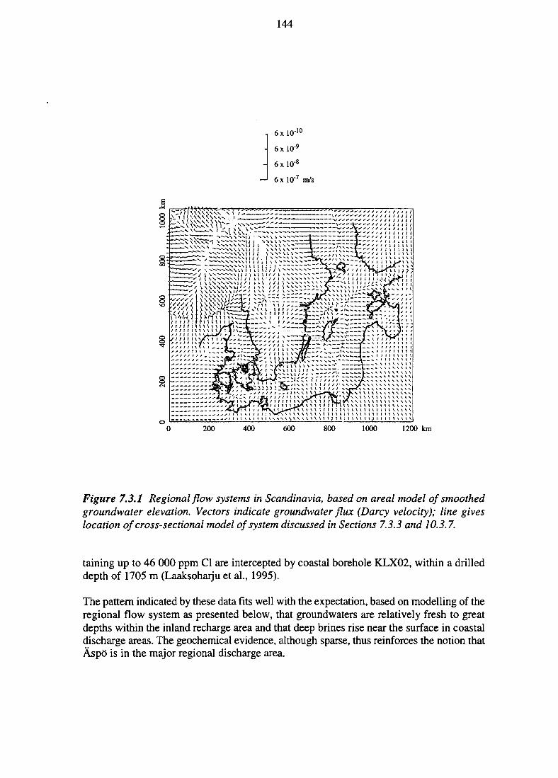
144
6xlO- 1 0
6 x 1(T9
6 x l O 8
6 x 10'7 m/s
200 400 600 800 1000 1200 km
Figure 7.3.1 Regional flow systems in Scandinavia, based on areal model of smoothedgroundwater elevation. Vectors indicate groundwater flux (Darcy velocity); line giveslocation of cross-sectional model of system discussed in Sections 7.3.3 and 10.3.7.
taining up to 46 000 ppm Cl are intercepted by coastal borehole KLX02, within a drilleddepth of 1705 m (Laaksoharju et al., 1995).
The pattern indicated by these data fits well with the expectation, based on modelling of theregional flow system as presented below, that groundwaters are relatively fresh to greatdepths within the inland recharge area and that deep brines rise near the surface in coastaldischarge areas. The geochemical evidence, although sparse, thus reinforces the notion thatAspo is in the major regional discharge area.
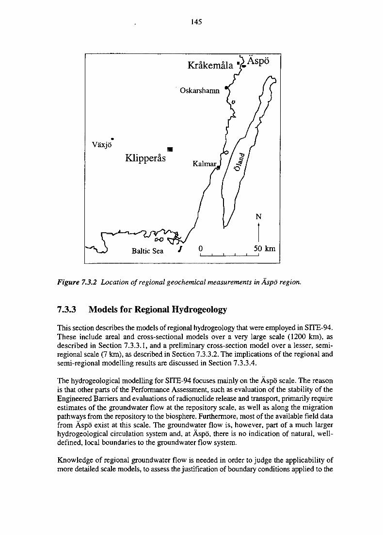
145
•Vaxjo
Klipperas
\ *° K^\J> Baltic Sea
Krakemala %'
>Oskarshamn *)
V
KalmarJ / / /
/ o1 1 1 t I
Aspo
/ /
IN
5 3 km
Figure 7.3.2 Location of regional geochemical measurements in Aspo region.
7.3.3 Models for Regional Hydrogeology
This section describes the models of regional hydrogeology that were employed in SITE-94.These include areal and cross-sectional models over a very large scale (1200 km), asdescribed in Section 7.3.3.1, and a preliminary cross-section model over a lesser, semi-regional scale (7 km), as described in Section 7.3.3.2. The implications of the regional andsemi-regional modelling results are discussed in Section 133 A.
The hydrogeological modelling for SITE-94 focuses mainly on the Aspo scale. The reasonis that other parts of the Performance Assessment, such as evaluation of the stability of theEngineered Barriers and evaluations of radionuclide release and transport, primarily requireestimates of the groundwater flow at the repository scale, as well as along the migrationpathways from the repository to the biosphere. Furthermore, most of the available field datafrom Aspo exist at this scale. The groundwater flow is, however, part of a much largerhydrogeological circulation system and, at Aspo, there is no indication of natural, well-defined, local boundaries to the groundwater flow system.
Knowledge of regional groundwater flow is needed in order to judge the applicability ofmore detailed scale models, to assess the justification of boundary conditions applied to the
146
detailed models and to assess the impact of changes in large-scale boundary conditions onthe groundwater flow and groundwater chemistry (salinity), which may occur if the climatechanges. In order to obtain such knowledge, the SITE-94 analyses also include someregional hydrogeological modelling.
The regional modelling is, to a large extent, generic, being based on the generalunderstanding of hydrogeology in the crystalline basement rock in Sweden. The results ofmodelling present-day hydrogeology are presented here, as they should be regarded as'input data' rather than actual predictions in the Performance Assessment. Changes in flowdue to changed regional boundary conditions, as well as the impact of the potentialuncertainty in regional flow on the detailed flow predictions are discussed in Section 10.3.
7.3.3.1 Regional Flow of Variable Density Groundwater in the FennoscandianShield
The most extensive regional flow analysis in SITE-94 concerns a very large area, includingsouthern Sweden and the Baltic Sea, and considers both areal and cross-sectional flowgeometries. A complete description of this analysis, including data and assumptions, isgiven by Provost et al. (1996).
The regional model is simply a reproduction of the groundwater flow field driven by thetopography of the water-table and indicates general areal flow patterns. The steady-stateflow field shown in Figure 7.3.3a, for the upper 10 km of rock in a region extending fromNorway through southern Sweden and across the Baltic Sea, is calculated on the basis ofspecifying hydraulic head everywhere on the surface equal to the local elevation. Thechoice of a 10km thickness for the model is somewhat arbitrary but reflects the sort ofdepth at which groundwater flow is thought to be practically negligible, owing to theeffective closure of fracture porosity by the high lithostatic load. The Baltic Sea bathymetryis also specified and the groundwater flow shown in these areas is equivalent to that whichwould occur if there were no water in the Baltic Sea. Inclusion of the Baltic Sea wouldimply no groundwater flow beneath it. However, this would not affect mainland flow at allin this model, because all hydraulic heads are specified a priori.
Major regional flow systems are more easily apparent in Figure 7.3.3b, which is thecalculated flow field 2000 years after recharge is stopped everywhere. This causessmoothing of local flow cells and only large-scale features are visible. Note the eastwardflowing system in the southern Swedish highlands including Aspo. A detail of this area,with actual steady-state flow as in Figure 7.3.3a, is shown in Figure 7.3.3c.
Aspo is not surrounded by natural hydrogeological boundaries and, as such, much of thegroundwater flow that occurs below Aspo is part of the regional flow system. Analyses ofthe regional flow system were done to determine the status of flow below Aspo in the largesystem. Cross-sectional simulation of groundwater flow in the Fennoscandian shield ofsouthern Sweden was carried out along a line extending from offshore of the westernNorway coast to Aspo and across the Baltic Sea to Poland. The particular line of sectionselected is somewhat arbitrary, but follows the average regional groundwater flowdirections under present-day conditions (Figure 7.3.1) along a large part of its extent. Thelength of the section is based on boundary conditions that occur at the maximum extent of
147
Scandinavian ice sheets, discussed later (Section 10.3.7.1) in the context of climateevolution.
The analysis takes into account the effects of the following physical processes:
• the formation of deep shield brines,
• variations in density and viscosity due to temperature, pressure and concentrationgradients and,
• groundwater flow driven by topographic gradients and fluid density imbalances.
The flow of variable-density groundwater and the transport of dissolved solids under theinfluence of pressure and density gradients were modelled numerically using a version ofthe U.S. Geological Survey computer code, SUTRA (Voss, 1984) modified to generateshield brine. In this approach, brine is formed by rock-water interaction and the totaldissolved solid content (TDS) of a parcel of fluid increases with time of travel through thesubsurface.
In the simulation, brine generation occurs according to a simple kinetic model wherein thebrine generation rate is linearly dependent on the difference between TDS content of thegroundwater at any point in the shield, and the TDS of saturated brine. The rate of brinegeneration is thus:
rate = kn t(C i a t-C)
where C is the concentration of TDS, Csat is the concentration at saturation (i.e. thesolubility) of the dissolved solids, and kmt is a mass transfer constant, estimated bycalibration.
Variations in hydraulic conductivity with rock type and depth are represented in thesimulations by a stratified conductivity profile (Figure 7.3.4a). The effects of fracture zoneson flow field are considered to be well-represented in an average sense for the regionalanalysis by homogeneous conductivity distributions. Conductivity in the Caledonides isassumed, for lack of information, to be equivalent to the shield rock, although the thrustfaults may be more transmissive than surrounding rock. The sedimentary sequenceoverlying the Precambrian basement southeast of Aspo is modelled in a simplified formthat captures the major vertical variations in hydraulic conductivity.
Groundwater flow and fresh-water recharge are generated in the model by assuming thatthe elevation of the water-table is near the surface of the ground. On portions of the surfaceof the simulated section not covered by the sea, the pressure is ambient (atmospheric).Portions of the shield covered by sea are subjected to additional pressure associated withthe weight of the seawater.
Figure 7.3.4b shows the simulated present-day steady-state distributions of fluid velocityand concentration of shield brine for the "base case" of Provost et al. (1996). This "basecase" consists of shield rock with homogeneous permeability that is ten times greaterhorizontally than vertically, and a stratified sedimentary sequence extending south-eastward
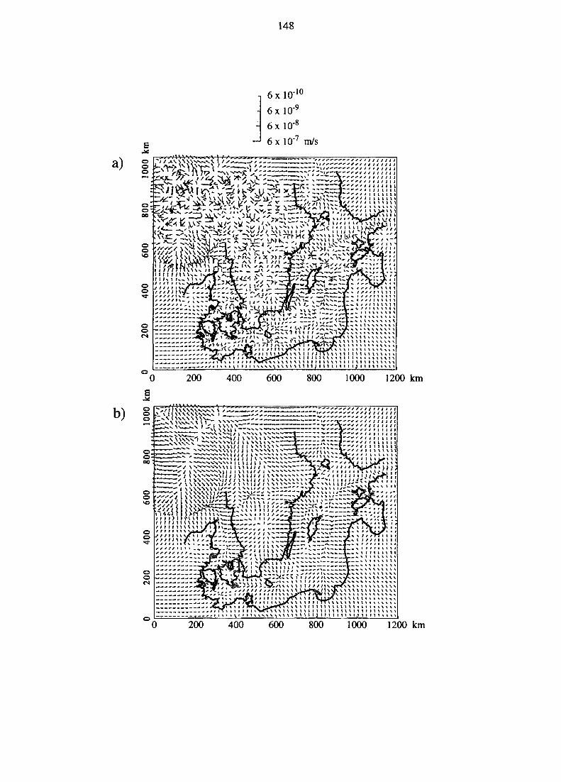
148
a)sOOo
6xlO-10
6xlO-9
6x 10'8
6xlQ-7 m/s
oooo
T"~JC/"' N
oo
oo
oo
^VM.
:<.«-. / /
cs
I I I t J M \ \I1 r% i i \
1000 1200 km
^
b)-^iy/WV''>«>>W«t»gK^"i''yii»!WJ'^>".s.'ai'
200 400 600 800 1000 1200 km
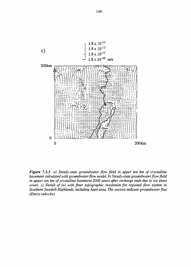
149
C)
1.8 x l O 1 3
1.8 xl(T1 2
1.8 xicr11
1.8 xlO"10 m/s
200km xr^r^
f.\ > / / / ] } \ J / ^ t . v Y / / / - -—Z?
0 200 km
Figure 7.3.3 a) Steady-state groundwater flow field in upper ten km of crystallinebasement calculated with groundwater flow model, b) Steady-state groundwater flow fieldin upper ten km of crystalline basement 2000 years after recharge ends due to ice sheetcover, c) Detail of (a) with finer topographic resolution for regional flow system inSouthern Swedish Highlands, including Aspd area. The vectors indicate groundwater flux(Darcy velocity).
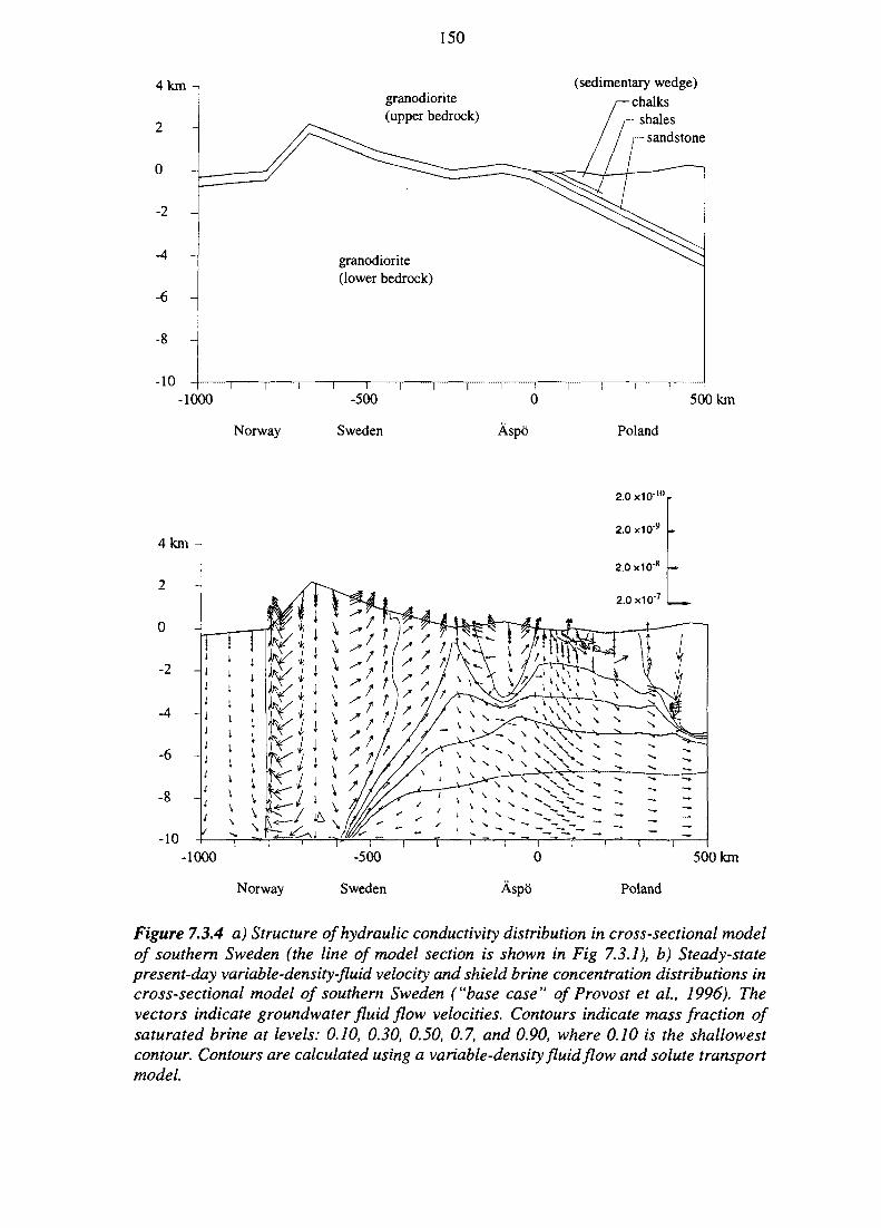
150
4 km -
2
0
-2 -
-4 -
-6 -
Q
-o -
-10
granodiorite(upper bedrock)
granodiorite(lower bedrock)
1 1 I 1 1 1 1 1 !
(sedimentary wedge)/— chalks
/ /—shales/ / r-sandstone
^ ^
1 I I 1 1-1000
Norway
-500
Sweden
500 km
Aspo Poland
4 km -
-2
-4
-6
-10-1000
Norway
-500
Sweden
500 km
Aspo Poland
Figure 7.3.4 a) Structure of hydraulic conductivity distribution in cross-sectional modelof southern Sweden (the line of model section is shown in Fig 7.3.1), b) Steady-statepresent-day variable-density-fluid velocity and shield brine concentration distributions incross-sectional model of southern Sweden ("base case" of Provost et al., 1996). Thevectors indicate groundwater fluid flow velocities. Contours indicate mass fraction ofsaturated brine at levels: 0.10, 0.30, 0.50, 0.7, and 0.90, where 0.10 is the shallowestcontour. Contours are calculated using a variable-density fluid flow and solute transportmodel.
151
from the Baltic Coast near Aspo. In the shallow portion of the cross-section, the velocityfield exhibits the typical pattern of recharge at topographic highs and discharge attopographic lows. As a result, lenses of fresh water develop beneath the southern Swedishhighlands and the Caledonides. Aspo is situated in an area of natural discharge from thesouthern Swedish highlands.
As initially fresh water travels through the bedrock, its salinity increases due to rock-waterinteraction. Within each fresh water lens, the increase in density is not sufficient to preventthe recharge water from flowing upward and ultimately discharging. However, water at theperiphery of a lens travels a longer path at a slower velocity and becomes too dense to bedriven to the surface. At the right-hand margin of the lens beneath the Caledonides, thisdense water settles, forming a clockwise, regional flow circulation in the model.
In the simulation, the major regional discharge area for deep fluids at the lower margin ofthe southern Swedish highlands' semi-regional system is at the coast and, as a result, shieldbrine occurs near the surface at Aspo. Further inland, shield brine is found only at greaterdepths. This is exactly the pattern found in actual field data in the area (e.g. deep freshwater at the Klipperas field site and shallow brine in the Laxemar boreholes and belowAspo).
Simulated flow at Aspo is generally eastward and upward. Some of the fresher groundwaterthat discharges at the coast near Aspo was recharged near the centre of the southernSwedish highlands. It thus travels in the subsurface for 100 km at depths up to a fewkilometres in the shield before discharging. For the "base case" in this analysis (with aporosity of 10'3), the typical velocity at 500 m depth below Aspo is 3xl0"8m/s. The generalflow through the coastal area, including Aspo, and the water chemistry in this dischargearea, are strongly dependent on regional conditions and driving forces.
The general patterns of regional groundwater flow and the status of Aspo in the regionalflow field are similar to those described above in all of the variations considered by Provostet al. (1996), including variations with layered shield-rock permeability and with highervertical than horizontal permeability. However, local correlation between undulations intopography and exceptionally transmissive subsurface structures, which would cause localdisturbances in the flow field, was not considered in the regional model. Near Aspo, thetopography is not unusual and no exceptionally transmissive structure has been identified.Thus, the flow field predicted from regional analysis should be a good averagerepresentation of local flow.
7.3.3.2 Two-dimensional Sensitivity Analysis of Semi-regional Groundwater Flow
The present-day, semi-regional flow system is analysed by means of semi-genericsimulations in a 2D cross-section across Aspo (Boghammar and Grundfelt, 1993). Theobjectives of this study were to illustrate the impact of large-scale fracture zones and therelative importance of semi-regional versus local topographical driving forces on thegroundwater flow pattern at Aspo. The simulations do not take the density effects fromdifferences in salinity into account.
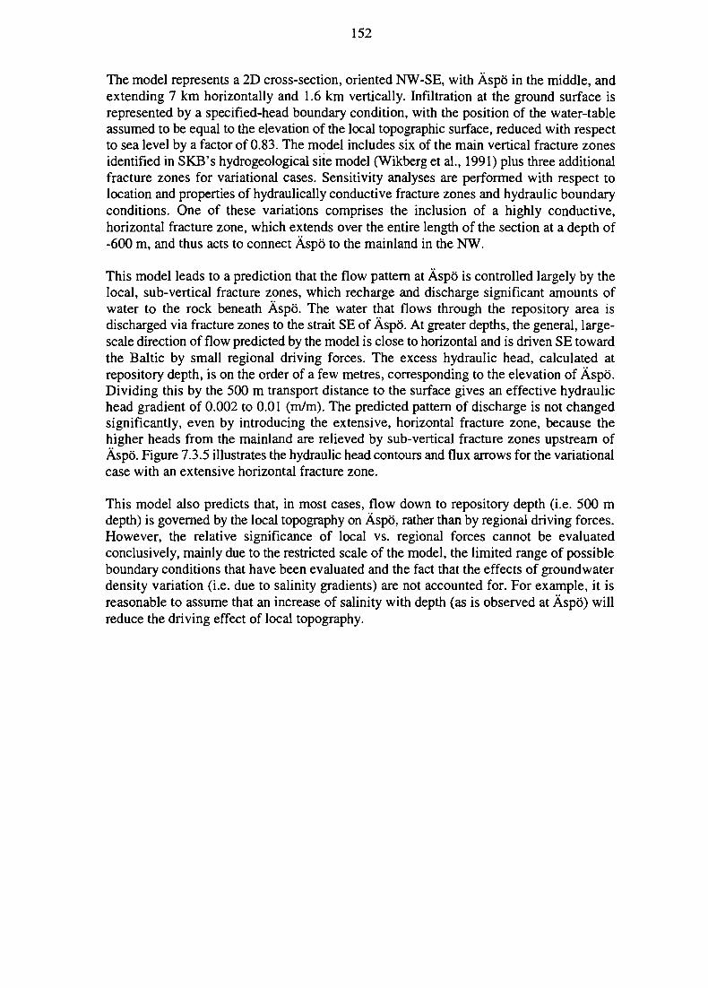
152
The model represents a 2D cross-section, oriented NW-SE, with Aspo in the middle, andextending 7 km horizontally and 1.6 km vertically. Infiltration at the ground surface isrepresented by a specified-head boundary condition, with the position of the water-tableassumed to be equal to the elevation of the local topographic surface, reduced with respectto sea level by a factor of 0.83. The model includes six of the main vertical fracture zonesidentified in SKB's hydrogeological site model (Wikberg et al., 1991) plus three additionalfracture zones for variational cases. Sensitivity analyses are performed with respect tolocation and properties of hydraulically conductive fracture zones and hydraulic boundaryconditions. One of these variations comprises the inclusion of a highly conductive,horizontal fracture zone, which extends over the entire length of the section at a depth of-600 m, and thus acts to connect Aspo to the mainland in the NW.
This model leads to a prediction that the flow pattern at Aspo is controlled largely by thelocal, sub-vertical fracture zones, which recharge and discharge significant amounts ofwater to the rock beneath Aspo. The water that flows through the repository area isdischarged via fracture zones to the strait SE of Aspo. At greater depths, the general, large-scale direction of flow predicted by the model is close to horizontal and is driven SE towardthe Baltic by small regional driving forces. The excess hydraulic head, calculated atrepository depth, is on the order of a few metres, corresponding to the elevation of Aspo.Dividing this by the 500 m transport distance to the surface gives an effective hydraulichead gradient of 0.002 to 0.01 (m/m). The predicted pattern of discharge is not changedsignificantly, even by introducing the extensive, horizontal fracture zone, because thehigher heads from the mainland are relieved by sub-vertical fracture zones upstream ofAspo. Figure 7.3.5 illustrates the hydraulic head contours and flux arrows for the variationalcase with an extensive horizontal fracture zone.
This model also predicts that, in most cases, flow down to repository depth (i.e. 500 mdepth) is governed by the local topography on Aspo, rather than by regional driving forces.However, the relative significance of local vs. regional forces cannot be evaluatedconclusively, mainly due to the restricted scale of the model, the limited range of possibleboundary conditions that have been evaluated and the fact that the effects of groundwaterdensity variation (i.e. due to salinity gradients) are not accounted for. For example, it isreasonable to assume that an increase of salinity with depth (as is observed at Aspo) willreduce the driving effect of local topography.
153
S94V3 - FH1, FV2
-16001000 2000 3000 4000 5000 6000 7000
0.00
•1600.003000 3500 4000 4500 5000 5500
Figure 7.3.5 Hydraulic head contours and flux arrows calculated with the 2D semi-regional groundwater flow model, for a case with an extensive horizontal fracture zonetransmitting high heads from the mainland.
7.3.3.3 Interpreted Hydrogeological Evolution of the Site
Based on the observations presented in Section 7.3.2 and the results of the modellingpresented above, a picture emerges of the likely hydrogeological evolution of the site.
The major water type found below Aspo today, in various admixtures, is shield brine(Section 7.4). Shield brines are deep fluids with long residence times and long flow pathsbetween source areas and discharge areas. These fluids would be found at depth in theFennoscandian shield, irrespective of climatic influences at the surface. Surface conditionscan force the brines to flow in various directions and to mix with and discharge with morerecent recharge waters in various proportions The present-day distribution of groundwaterand brines below Aspo can be explained in such terms.
154
The ages of discharging regional groundwater/brines found below Aspo may be on theorder of a few million years, assuming that they recharged in the central portion of the southSwedish highlands. A flow velocity on the order of 0.1 m/yr along a flow path about100 km long is implied, if recharge area elevation above the coast is 100 m, regionaleffective porosity is 10'3 and regional effective hydraulic conductivity is 10'9 m/s. Regionalgroundwater/brines found today, at about 500 m below Aspo, can thus discharge upwardto the surface in about 5000 years.
Before the onset of the glaciation 20 to 30 ka BP, Aspo was probably, hydrologically, muchas it appears today; whether the coast was to the east or to the west of Aspo is of littleconsequence for the present discussion. As the ice sheet advanced over the area, firstcutting off recharge and then providing excess meltwater as recharge, the waters belowAspo began to change. Oxygenated, glacial meltwater is likely to have replaced existingfluids to depths of more than one kilometre below the glacier (which may have reachedthicknesses of 2 of 3 km locally). Some meltwater remains below Aspo today (based ongeochemical evidence as described in Section 7.4), but most has been flushed out bysubsequent regional discharge.
As the ice sheet receded, the precursor of the Baltic sea followed at the ice margin, leavingAspo submerged approximately 200 m beneath the sea at about 10 ka BP, due to isostaticdepression of the crust. Some of the shallower saline waters found today might derive frominundation of parts of the Fennoscandian shield by post-glacial seas (Lindewald, 1981).However, due to the low salinity of these seas, the density contrast with the existinggroundwater was small and, apart from molecular diffusion, there was no other impetus forsubmarine intrusion of seawater. Groundwater flow was probably dominated by slowdischarge of the meltwater that had been stored due to high pressures below the ice sheet.Hence little of the pre-Baltic seawater is found today in the bedrock, although some maybe found in isolated pockets of unconsolidated, glacial sediments.
Eventually, post-glacial, crustal rebound caused relative sea level to fall (this processcontinues today, albeit more slowly), and Aspo emerged from the Baltic Sea a few thousandyears ago. At this time, rainwater and snow meltwater began to infiltrate the island, andsoils stabilised through growth of vegetation. Owing to the low relief, there was littledriving force for infiltration and recharge only slowly proceeded to flush the shallow glacialmeltwater from the subsurface. As the ice sheet receded inland, a regional-scale flowpattern developed, with rain and snow melt inland and discharge near the Baltic coast.Thus, while Aspo received a small amount of recharge from above, it also became situatedin the discharge area for the regional flow system. Deeper glacial meltwaters in the uplandarea began to discharge at local topographic lows and to the coast and meltwaters belowAspo discharged into the Baltic.
Today, only a small amount of glacial meltwater is still found in the subsurface(Section 7.4). For the most part, glacial meltwater has been replaced in the upper 100 m byrecent recharge water, and below this, by admixtures of discharging shield brine and watersrecharged further inland. The degree to which meltwaters have been replaced gives somemeasure of the regional discharge rate during the few thousand years since Aspo emergedfrom the sea.
155
7.3.3.4 Implications for Site-scale Modelling of Groundwater Flow
The regional groundwater modelling, as described in Section 7.3.3.1, is used in SXTE-94mainly to gain an understanding of regional flow patterns and their evolution over time.This understanding provides a basis for assessing the applicability of particular sets ofboundary conditions, for the site-scale models and the reasonableness of the flow fieldspredicted by the site-scale models. Due to the fact that the regional and site-scale modelswere developed concurrently, the regional flow predictions are generally not used to defineexternal boundary conditions for the site-scale models. An exception is for two calculationcases of the Discrete Feature site-scale model related to the Central Scenario, in whichboundary conditions are taken directly from the regional model (see Section 10.3.8).
The semi-regional, 2D groundwater model is used for a preliminary assessment of theinfluence of major fracture zones on groundwater flow patterns at Aspo. The results are notused directly in the subsequent, site-scale modelling, but are used for qualitativecomparisons in terms of the predicted pattern of discharge from the repository. The DiscreteFeature hydrogeological model of Aspo for SITE-94, as described in Section 7.3.7, includesa 3D, semi-regional submodel that explicitly accounts for coupling between the 3D site-scale submodel and the conditions imposed at the boundary of the semi-regional domain.However, with the exception of the Central Scenario calculation cases, as mentioned above,the effective boundary conditions for the semi-regional domain are not drawn from theregional-scale simulations.
The regional and semi-regional cross-section models (as described in Sections 7.3.3.1 and7.3.3.2, respectively) yield different conclusions regarding the relative significance ofregional vs. local driving forces. Whereas the 2D semi-regional model predicts that flowat repository depth is controlled by heads directly above on the island, the regional modelindicates that a larger-scale flow system dominates at repository depth. This difference maywell be due to artificial limitations of the 2D semi-regional model (the limited scale of thecross-section, the omission of salinity/density effects, and the fact that boundary conditionswere not drawn from a larger-scale model), rather than due to the more detailed resolutionof structures in the 2D semi-regional model. These artificial limitations are, in manyrespects, shared by the 3D, semi-regional submodel of the Discrete Feature model forSITE-94.
The regional simulations indicate that the depth of penetration of the local flow systembelow Aspo depends upon the anisotropy of the system (vertical vs. horizontal effectiveconductivity). With higher vertical conductivity, the local flow system reaches greaterdepths but, nevertheless, Aspo remains within the regional discharge area. However, therepository may intercept either locally recharged water or regionally discharging, deepbrines, depending on the effective connectivity, geometry and transmissivity of the localnetwork of transmissive structures.
The lack of direct coupling between the regional and lesser-scale models in SITE-94 onlyallows for a qualitative assessment of the influence of the regional flow system. However,the regional, semi-regional, and site-scale models all predict discharge in roughly the samedirection (upward and southeastward), with roughly similar values of excess hydraulic head(a few metres). The semi-regional and site-scale models both predict that the direction offlow is more steeply upward and, consequently, discharge paths to the biosphere will be
156
shorter than predicted by the regional model. Therefore, for the purposes of the SITE-94Performance Assessment, the results from the smaller-scale models may be taken asconservative.
7.3.4 Uncertainty in the Site Characterisation Data—First OrderAnalysis
The site-characterisation data give rise to various uncertainties, as discussed in theintroduction. An attempt to estimate part of this uncertainty has been done by performingdetailed quantitative analyses of the measured bore-hole data.
7.3.4.1 GRF-analysis of Hydraulic Borehole Packer Tests
As a basis for further hydrogeological model development, SKI initiated a complete re-evaluation of hydraulic borehole packer tests performed at Aspo (Geier et al., 1996a). Theinitial interpretations by SKB use classical methods for estimating hydraulic conductivityfrom lugeon (constant-pressure) tests and subsequent pressure recovery tests (Moye, 1967;Cooper and Jacob, 1946). These methods are based on assumptions of essentially two-dimensional flow geometry around the test section and require attainment of certainconditions by the end of the test. In SKI's re-evaluation, the transient flow data from eachpacker test are analysed to:
1. test the assumptions of the original evaluation,
2. produce an alternative database for hydraulic conductivity and transmissivity, basedon a less restrictive set of assumptions,
3. assess the suitability of particular conceptual models for specific geological unitswithin the site.
The SKI re-evaluation is based on an alternative model for transient packer-test analysis,the Generalised Radial-Flow (GRF) model (Barker, 1988; Doe and Geier, 1990). For eachtest section, this model yields an estimate of the effective flow dimension for each test, aswell as the hydraulic conductivity. Flow dimension is related to the small-scalehydrogeological structure of fracture networks connecting to the test section (Figure 7.3.6).Although this relationship is non-unique, the combined estimates of flow dimension andhydraulic conductivity provide a more complete characterisation than does hydraulicconductivity alone and can be used to discriminate among alternative conceptual modelsfor rock mass hydrology.
A complete reanalysis is performed, working from the original, transient logs of flow rateand pressure variation during each test (Geier et al., 1996b). Results show that assumptionsmade with regard to flow geometry may affect the hydraulic conductivity estimates byseveral orders of magnitude. Figure 7.3.7 compares the GRF estimates of hydraulicconductivity with values from the SKB database, for one of the boreholes at Aspo. Thenumbers in the plot indicate the GRF estimates of flow dimension. The most significant
157
differences are for sub-cylindrical conduits (flow dimension less than 2), where the GRFmethod gives more conservative (higher) estimates of conductivity.
The hydraulic conductivity estimates are utilised in several of the hydrogeological analyses.In the Discrete Feature model for Aspo (Geier, 1996a, b), the GRF estimates are used:
1. to estimate the transmissivity distribution for fractures in the repository block,
2. as a database for comparison with the behaviour predicted by simulation of packertests for different discrete-fracture models,
3. for preliminary estimates of major structure transmissivities.
In the Stochastic Continuum (SC) model of Aspo (Section 7.3.8), the SKB conductivitydatabase is used:
1. to estimate the percentage of values in each conductivity class for indicatorsimulation,
2. for conditioning of stochastic realisations.
Discrepancies between GRF and SKB estimates are discussed in terms of SC modelsensitivity.
The SKB and GRF data sets are also utilised in the comprehensive geostatistical analysisof the site data, as described in the following section.
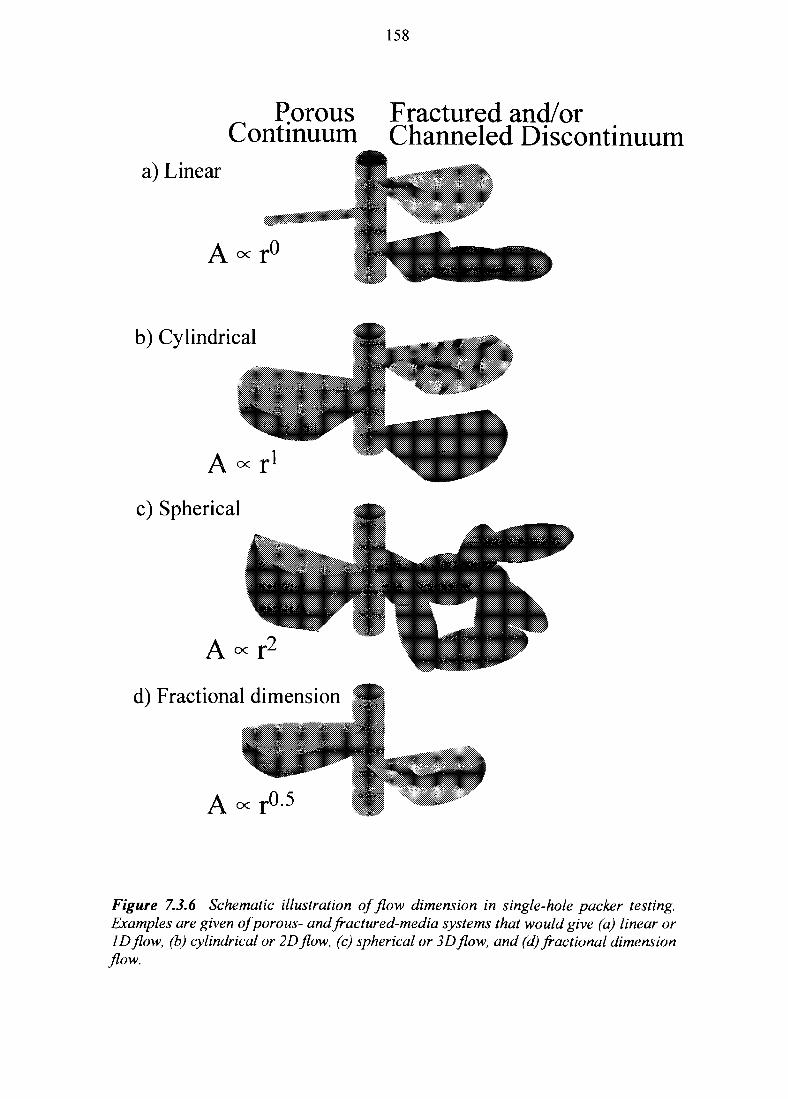
158
Porous Fractured and/orContinuum Channeled Discontinuum
a) Linear
A 0
b) Cylindrical^ " V s
A <* r 1
c) Spherical
d) Fractional dimension
" ™ ^ ; "
A oc r0.5
Figure 7.3.6 Schematic illustration of flow dimension in single-hole packer testing.Examples are given of porous- and fractured-media systems that would give (a) linear orID flow, (b) cylindrical or 2D flow, (c) spherical or 3D flow, and (d) fractional dimensionflow.
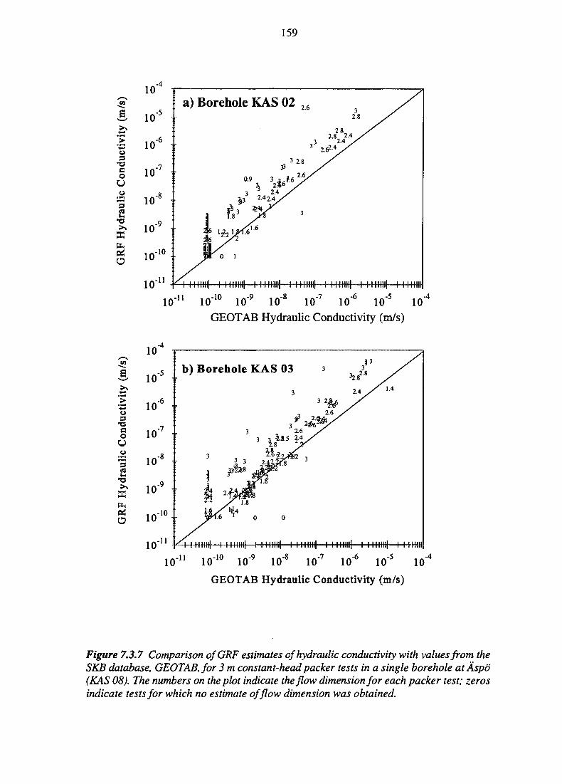
159
o
aoU
a
Oao
Uo"3S3»
X
a
1U
-5
-6
lO7
10'8
io - 9 •
10 1 0 1
1 0 " •
a) Borehole KAS
0.9 3 „
,' U
. IK?M ii mill i IImill -1 ninn
02
333
2.6
3
IIIHIll f-
2.8 /
2>y/
WHHl-H-t-fHmi-4+HtiH
I O 1 1 i o 1 0 io"7 io"6
GEOTAB Hydraulic Conductivity (m/s)
-410
i o J -
TJ 1 0 •
10
-5
-6
-7
-8
-9
-10 '
-11
b) Borehole
3
J4
?!
II mil
3
-333*8
Xia46 »
KAS
3 3 ^
0 ft
r0
-{ II inn
03
3
3
0
H-
22.6
X
444
3
3 2&£2.6 ,
X
mil i in
§3 ^ X
328238 /
24 ^X ' 4
X
mil i II imi| i II mil
10
10
1 0 ' v
1 0 l u v
10"11 10"10 10"9 10"8 10"7 10"6 1O"5 10"4
GEOTAB Hydraulic Conductivity (m/s)
Figure 7.3.7 Comparison ofGRF estimates of hydraulic conductivity with values from theSKB database, GEOTAB, for 3 m constant-head packer tests in a single borehole at Aspo(KAS 08). The numbers on the plot indicate the flow dimension for each packer test; zerosindicate tests for which no estimate of flow dimension was obtained.
160
7.3.4.2 Multivariate Analysis of Borehole Data
Introduction
The general objective of the multivariate analysis of borehole data (Le Loc'h and Osland,1996) is to provide a better understanding of the distribution and spatial variability of thehydraulically highly conductive zones in the fractured rock at Aspo. In most of thehydrogeological models developed in SITE-94, the implicit assumption is that the hydraulicconductivity is associated with the fractures and that a good 'model' of the hydraulicconductivity of the medium should be based on a good prior description of the fractures.This assumption may be tested by analysing the available data, with three questions inmind:
1. Is there clear statistical evidence that hydraulic conductivity data are only linked tothe fracturing or are other data, such as rock type, or other geophysical data that havebeen recorded in the boreholes by logging, also relevant?
2. If some other geophysical data are found relevant to estimate the hydraulicconductivity of the rock, is it possible to build an alternative geostatistical modelthat would estimate or simulate the hydraulic conductivity at unmeasured locations,based on all the relevant information (rock type, geophysical logs, etc)? Note thatthe geostatistical model that was used for the Stochastic Continuum approach(Section 7.3.8) is solely based on the hydraulic conductivity data.
3. Can the spatial variability of the hydraulic conductivity within transmissivestructures be described? This information is important to estimate the longitudinaldispersion along the dominant flow paths.
Data used
The borehole data that were available for this study from the site database (Chapter 6)include:
• detailed core descriptions from 14 boreholes, including lithology and fracturing,
• hydraulic conductivities derived from injection tests (3 and 30 m packed sections),using the Jacob method of interpretation (data from SKB), the GRF method (fromSITE-94, see above) and also the borehole flow (spinner) data,
• geophysical logs with 10 cm spacing including caliper, natural-gamma, gamma-gamma, neutron, near and far magnetic-susceptibility, sonic, lateral and normalelectric-resistivity, single-point electric-resistance, and self-potential logs.
Analysis tools
The approaches used to analyse the data are based on single-variable geostatistical analysis,multivariate correlation analysis and multivariate geostatistical analysis. The first approachdescribes the spatial variability of each parameter in space (tests of stationarity, mean,variance and spatial autocorrelation using the variogram). The second approach investigateswhether, statistically, there is a link between the value of a variable at a given point in space
161
and the value of another variable at the same point. The third approach combines spatialvariability and correlation and may thus detect whether a variable is correlated in space withanother, but with a possible systematic lag. For instance, the hydraulic conductivity at agiven location might be correlated with the value of the lateral electric conductivitymeasured a few metres above that location, due to the physical laws governing themeasurement method, or due to measurement errors such as a systematic shift in themeasurement positions. This approach is thus much more powerful than a simple, point-to-point correlation analysis.
Results
The analysis shows that the fracturing data (density of fractures) is, as expected, the majorfactor controlling hydraulic conductivity. However, rock type is also a variable thatinfluences many other properties and, in particular, the hydraulic conductivity. Geier et al.(1996a) made a similar observation from the GRF analysis of injection test data, concludingthat lithological contacts (between aplites/'fine-grained granite' and the host rock) may bezones of high hydraulic conductivity. Comprehensive modelling of the distribution of thehydraulic conductivity in the medium should thus be based not only on the fracture system,but also on the distribution of rock type.
It is found in general that, along the boreholes, the spatial autocorrelation of all thevariables studied is very weak; the correlation length is, in general, on the order of 3 m (e.g.for the hydraulic conductivity and fracture frequency) and up to 80% of the variance isspatially uncorrelated. Only on rare occasions, and for some variables (e.g. fracturefrequency in granodiorite, hydraulic conductivity in aplite), does the correlation lengthextend up to 50 m. Given that the available information was obtained essentially alongnearly vertical boreholes, and that the average distance between boreholes is on the orderof 100 m or more, it is not feasible to attempt a horizontal or even three-dimensionalgeostatistical analysis of the data. However, this does not necessarily exclude the possibilitythat the data might be differently (perhaps better) correlated in the horizontal direction. Asno boreholes were drilled such that a significant length lies within a single fracture zone,the data do not permit an analysis of the spatial variability of hydraulic conductivity withinany given, conductive fracture zone.
Although the correlation between some of the geophysical variables is sometimes good,their ability to predict hydraulic conductivity is found to be very weak. This is partly dueto the fact that, although fractures can be detected by geophysical (e.g. sonic or electrical)logging tools, the existence of fracture filling can make the hydraulic conductivity verypoorly correlated with fracturing. Only the single-point electric resistance shows a small,negative correlation with hydraulic conductivity, probably because pervious fractures carrywater that has an electric resistivity lower than that of the medium or the infilling.
The only successful attempt at building a multivariate geostatistical model is based on thenatural logarithm of the 3 m section GRF hydraulic conductivities, in conjunction with fourother explanatory variables, when they are made representative of a 3 m section. Thesevariables include:
• the GRF flow dimension of the same 3 m section,• the total number of fractures in the same 3 m section,
162
• the presence of aplite in the 3 m section, at any position,• the existence of a change of rock type within the 3 m section.
The last two variables are less important than the first two, thus confirming theoverwhelming importance of fracturing on hydraulic conductivity. A linear model ofcoregionalisation is fitted on these data, using a nugget effect and three exponentialvariograms, with ranges of 18, 27 and 300 m. With this model, it is possible to estimate orto simulate the distribution of hydraulic conductivity in the medium (in one dimension)using all five variables, with a smaller variance than if the explanatory variables wereomitted.
An attempt to incorporate the spinner data in this model showed that these data need to becorrected for bias and that their correlation with hydraulic conductivity is rather weak. Thespinner data are, however, better correlated with some other variables. Natural gamma log,sonic log and, perhaps, magnetic susceptibility and single point electric resistance are alsoweakly correlated with the hydraulic conductivity.
Conclusions and recommendations
The fact that correlations are found between hydraulic conductivity, spinner data and othervariables measured in the boreholes and, in particular, rock type, suggests that there is apotential for a more comprehensive use of measurement data that, in SITE-94, are notincluded in hydrogeology models. However, the observed correlations are, in most cases,rather weak and do not support development of an alternative conceptual site model forgroundwater flow. Instead, the good correlation that is found between fracturing andhydraulic conductivity lends some credibility to the use, for this site, of the Discrete Featureconceptual model that is adopted as one of the main models for analysing hydrogeology.
The study gives a list of recommendations to improve the data-collection design and dataprocessing, for use in a geostatistical framework. A key aspect of data quality for boreholemeasurements concerns the accuracy of the coordinates of measurement locations along theboreholes. For example, in many cases it is not clear how, or with what accuracy, differentborehole measurements had been corrected for bias due to cable extension. As a result itis difficult to judge whether a weak correlation between two variables that were measuredwith different probes, or directly on the core, is a true result, or just an artifact of systematicor random shift in measurement position. An associated problem concerns therepresentativity of different types of measurements. To be able to account for the fact thatdifferent measurements represent different volumes of rock, it is also essential that a gooddescription of the measurement tools is supplied with the data.
It is emphasised that, for a geostatistical analysis in particular, randomly spaced or regularlyspaced boreholes provide the best data, whereas, for a geological reconnaissance, boreholesmight in general be located in areas where anomalies have been detected or are expected.In the latter case, the data tend to over-sample anomalies compared to the general propertiesof the medium, thus making a geostatistical model more uncertain.
163
7.3.5 Simple Evaluation
As a complement to the detailed hydrogeological site models developed in SITE-94,hydrogeological behaviour is assessed with simple scoping calculations of groundwater fluxand transport parameters. These scoping calculations are based on a ID application ofDarcy's law, simple assumptions regarding flow-field structure and pore geometry andbounding values of hydraulic driving forces (Dverstorp et al., 1996). The objectives are toestimate ranges of the hydrogeological behaviour, and to identify critical factors for thedetermination of groundwater fluxes and transport parameters, as guidance for thedevelopment of detailed hydrological site models. The analysis considers the Aspo site andseven other study sites in crystalline rock in Sweden, employing SKB's interpretation ofhydrogeological structures and hydraulic conductivities.
The results for the Aspo site are presented in detail in Section 10.3.3. However, animportant inference that can be noted here is that connectivity and spatial structure ofhydraulic conductivity are key uncertainties for the determination of groundwater flux. Thedetailed pore geometry within conductive structures (which defines the relation betweenDarcy velocity and flow wetted surface area available for sorption and matrix diffusion) isan additional key source of uncertainty for transport parameters. The variability of hydraulicconductivity estimates at the sites studied, including Aspo, is very large (up to 5 orders ofmagnitude), both in fracture zones and in the less fractured parts of the rock. However,limited or no direct information is available in the existing site characterisation dataregarding how conductive elements in the rock mass and fracture zones connect in space,as most hydraulic measurements represent only a small volume of rock. The properties ofa calibrated flow model will thus, to a large extent, depend on conceptual assumptions thatcannot be directly supported from the site characterisation data. This finding is an importantmotivation for evaluating site hydrogeology with alternative conceptual models.
7.3.6 Qualitative Hydrogeological Assessment of Site Data and theSITE-94 Structural Model - Basis for Detailed Models
This (long) section makes a qualitative assessment of the available hydrogeological datafrom Aspo together with the geological structure model and relevant geochemicalinformation. This assessment forms the basis for the formulation of the detailed quantitativehydrogeological models to be used as input in subsequent consequence analysis, itconstitutes parts of the justification for the use of these models an thus represent animportant element of integration between overall site evaluation and specialised modelling.
7.3.6.1 Introduction
The structural geological analysis resulting in the SITE-94 structural model (Tiren et al.,1996, and Section 7.2), the geochemical analysis (Glynn and Voss, 1996, and Section 7.4)and a hydrogeological analysis of the data (Voss et al., 1996) are integrated in this sectionto yield a qualitative hydrogeological characterisation of Aspo to about one kilometredepth. This hydrogeological characterisation is of a qualitative nature and consists primarilyof inspection of the available data and attempts to express, in simple terms, any basic
164
hydrogeological relationships observed in the data. The integration requires simultaneousconsideration of many data types and is accomplished, in part, with the aid of three-dimensional visualisation on graphic workstations.
The following approach is taken in this hydrogeological characterisation. First, thestructural model of the site (Section 7.2) is developed on the basis of geological andgeophysical information collected on the surface and in boreholes only. No hydrogeologicalor geochemical information is used, either to generate or to constrain the structural model.Next, the completed structural model is evaluated hydrogeologically to determine its abilityto describe the locations of flow measured in the subsurface and its power to delineate pathsof subsurface pressure propagation. Finally, the structural model is compared with thesubsurface distribution of water types based on geochemical analysis (Glynn and Voss,1996) to explore whether the structures contained in the model explain the location ofdistinct water bodies or chemically uniform flow paths. In summary then, the followingtypes of test are performed to assess the SITE-94 structural model:
• correlation of subsurface flow indications with geological factors• correlation of the structural model and subsurface flow indications• comparison of the effectiveness of the SITE-94 geological model and a random
structural model in explaining the hydrogeological data• correlation of the structural model and observations of pressure propagation• correlation of structures which have indications of flow and structures which act as
pathways for pressure propagation• correlation of the structural model with geochemical patterns.
These tests, as discussed below, lead to an overall assessment of the hydrogeological valueof the structural model.
It would also have been possible to use the hydrogeological and geochemical data togetherwith the geological-geophysical data at an early stage to develop the structural model.However, in this study, such early data synthesis is avoided in order to allow for anindependent check on the structural model and its capability to predict site hydrogeology.
The SITE-94 structural model is based primarily on surface data, consisting of a map ofextensive discrete-fracture zones and topographical lows and data on orientation offractures in outcrops, as well as subsurface data consisting mainly of locations of crushedrock in boreholes and borehole radar measurements. These data provide a basis for findingfracture zones, but not simple discrete fractures. Simple discrete fractures cannot be reliablyconnected through the subsurface volume given the data available for model construction.Unfortunately, both fracture zones and simple fractures may act as fluid conduits of equalimportance. The clear result is that subsurface flow paths associated with simple fractureswill not be included in the SITE-94 structural model. Notwithstanding, it is assumed thatthe type of structures that are included in the model (semi-planar fracture zones) are indeedamong the major hydrogeological features controlling subsurface flow below Aspo. No apriori assumption is made concerning the distribution of flow (e.g. uniform or channelled)within any structure.
165
7.3.6.2 Aspo Hydrogeological Base Data
The water-table on Aspo rises to a maximum height above the Baltic Sea of about 4 m nearthe island centre and decreases to about zero elevation at shores. Some fresh water rechargeoccurs in the island interior, with discharge near the shores. Geochemical evidence,described later, indicates that this recharge water remains shallow, penetrating only theupper tens of metres below the island surface. As measured in most boreholes, the water-table responds quickly to recharge events on the island. Pressure response at great depth isalso swift, which indicates that there are permeable structures throughout the island thatconnect the surface to the water-table and greater depths and that storage is low.
Borehole flow indications
Direct evidence of conductive structures in the subsurface is given by boreholemeasurements with the borehole flowmeter in 11 cored boreholes on Aspo. There are61 flow points measured where water enters boreholes through a conductive structure and23 ranges where water enters the borehole diffusely over the entire range. Owing to thenature of the measurement in this test, the structures discharging water to a boreholenecessarily conduct fluid over some distance and should be considered as 'well-connected,conductive structures.'
Geophysical borehole logs
Indirect evidence of conductive structures may be based on indications obtained from anumber of geophysical logs: single-point resistivity, acoustic, fluid conductivity and fluidtemperature. Taken together with resistivity and acoustic indication of an intersectingstructure, an abrupt shift in fluid conductivity and temperature logs gives strong indicationthat the structure is well-connected and conductive. Outside the borehole ranges whereborehole flow measurements were made, geophysical indications of conductive structuresare used to augment the collection of subsurface points where flow occurs. There are35 geophysically-indicated flow points, making a total of 119 indications of flow atborehole points or within borehole ranges observed under Aspo.
Pumping tests
Single-hole pressure tests with straddle packers at 3 m distance were conducted along largereaches of most cored boreholes and interpreted by two methods. These short-term testsgive indications of locally conductive structures. There are many more indications of high-permeability structures indicated by these tests than by direct (borehole flow) and indirect(geophysical) flow measurements. However, because of their brief duration, well-connectedconductive structures are not distinguished from 'dead-end' conductive structures by thesetests. Existence of a subsurface flow, as indicated by a measured flow point in a borehole,requires that a relatively high conductivity also be measured at that point. However, a highmeasured conductivity is no guarantee that fluid can flow.
A large number of tests was conducted where one open borehole or packed-off boreholesection was pumped and sections of many other boreholes were monitored for pressurechanges at various depths separated by packers. Most of these tests lasted about one week,one test lasted a few weeks (LPT1) and the longest test lasted about three months (LPT2).There were many monitored sections providing a large amount of data. The early time
166
portions of these tests are extremely useful in locating conductive structures. Much of theearly drawdown propagation occurs along planar paths indicating pressure propagationalong near-planar structures. Later time data are less useful for locating specific, conductivestructures because so many intersecting structures participate in drawdown transmissionthat unambiguous interpretation is very difficult.
Tracer tests
Tracer tests were conducted at the site by SKB but little information on natural flow paths,of interest to the current analysis, is obtained from such data. Further, the choice ofinjection and withdrawal locations was based on SKB's interpretation of hydrogeologicalsite data and this type of interpretive information is excluded from the SITE-94 analysis.
7.3.6.3 Correlation of Subsurface Flow with Geological Factors
Local geological factors such as rock type, contacts between different rock types(lithological contacts) and mechanical alteration of rocks such as crushing and fracturing,may be major controls on the ability of fluid to migrate through the rock. Some of thesefactors may be determined directly by inspection of cores from boreholes, while somefactors may be determined indirectly by geophysical measurements.
Correlation with geophysical logs
A complete set of geophysical borehole logs collected for the Aspo site was compared withthe 119 points/ranges of indicated subsurface flow in the boreholes to determine whetherthere is any correlation of flow location with geological factors. Four of these logs exhibitvery high correlation with the locations of flow indications: natural gamma radiation of therock, single-point resistivity of the rock, borehole radar measurements and the sonic log.
Correlation with rock type
The detailed, manually-mapped core logs of each cored borehole (KAS series) werecompared with the borehole flow indications to determine whether there is any correlationof flow location with geological factors at the Aspo site. It was found that the 119 locationsof indicated flow are distributed throughout the rock volume with no apparent preferencefor any rock type. The cores/boreholes consist of: granites: 72% by volume containing 70%of flow indications, aplites: 18% by volume containing 20% of flow indications, and basicrocks: 9% by volume containing 9% of flow indications. Hydraulic conductivity, on theother hand, appears to be correlated with rock type, as described in Section 7.3.4.2.
Correlation with crushed rock
In total, flow indications occur twice as often (66%) in crushed rock as in uncrushed rock(34%). Because there is only 4.2% crushed rock in the whole rock volume, and 66% of flowindications occur there, 44 times more flow indications occur in crushed rock than inuncrushed rock. In aplites, 91% of flow indications occur in crushed rock. Of flowindications that occur wholly within aplite, 71 % are near the aplite contacts with the hostrock.
167
Correlation with fractured rock
Of the 34% of flow indications that do not occur in crushed rock, about one third (or 11 %of all flow indications) occur at locations with notable enhancement of fracture frequency.The local enhancement of fracture frequency is often two to three or more times thebackground frequency (of 2 to 3 fractures/m) and has a width of about 1 m along aborehole. The remaining two thirds of flow indications in uncrushed rock (about 23% ofall flow indications) occur at points with low to moderate fracture frequency and may beassociated with single fractures. Note, again, that the structural model does not includesingle fractures or regions of enhanced fracture frequency as a structure type. Thus, it maybe expected that the 23% to 34% of borehole flow indications associated with thesegeological factors will not occur within any of the structures included in the model.
Summary
The above facts have the following implications regarding the dependence of subsurfaceflow on local geological factors.
1. Flowing structures are uniformly distributed among rock types. There is noenhancement of flowing structures in any particular rock type.
2. The existence of crushed rock, in general, is a major factor allowing fluid flow.About two thirds of all flowing structures are composed of crushed rock.
3. The flows in the remaining third of flow indications occur in discrete fractures orclusters of fractures, but fractures control only half as many points of measurablesubsurface flow as crushed rock structures.
4. Nearly all flow paths in aplite are encountered in crushed rock, and the majority ofthese occur near the contact with the host rock.
5. Subsurface flow locations have a high correlation with geophysical anomaliesmeasured by four borehole logs: natural gamma, single-point resistivity, boreholeradar and sonic. Of these, only the borehole radar is directly used to construct theSITE-94 structural model.
Note that some of the crushed-rock zones may have been caused by drilling (and notdistinguished by SKB in the GEOTAB database from pre-existing crushed rock), falselyenhancing the correlation between crushed rock and flow (see also Section 6.5).
7.3.6.4 Structural Model Correlation with Subsurface Flow
To test the power of the SITE-94 structural model to predict paths of subsurface flow, themost discriminating parameter is arguably the location of flow indications in boreholes.This parameter, described earlier as 'direct and indirect flow indications', is compared herewith the structural model. The hydrogeological predictive capacity of the structural modelis measured simply, by direct comparison of spatial location of flow indications with thelocation of all structures (Figure 7.3.8a). Three-dimensional measurement of the shortestdistance between flow indications and structure gives a true measure of the spatial
168
correlation of all structures with all flow indications. As pointed out earlier (seeSection 7.2) one cannot expect a one-to-one correspondence between flow indications andthe structure model since some large scale features may be poor conductors and sincenetworks of small scale features may constitute significant flow paths. Consequently, theevaluation partly provides information on the need to include conductive features below thescale of the geological structure model.
Intersection tolerance
To decide whether a given distance between a structure and a flow indication in 3D issignificant, for the purposes of this test, an intersection tolerance was specified in terms ofthe radius of a sphere around each flow indication point. Any structure that crosses thatsphere is considered to coincide with the flow indication. The sphere radius may beconsidered as the maximum distance in which errors in spatial location of flow indicationsor structures are ignored, for the purpose of finding intersections. Alternatively, the use ofsuch an intersection tolerance may be viewed as taking into account the finite thickness ofthe structures. A tabular structure with a thickness of twice the intersection tolerance wouldcoincide with the flow indication even if the plane through the centre of the structure didnot coincide exactly.
Analyses are given for intersection tolerances (sphere radii) of 1 m, 2 m, 3 m, 5 m, and10 m, in Voss et al. (1996). A tolerance of 1 m is a very stringent requirement for thecloseness of acceptable intersections, while a tolerance of 10 m implies generousacceptance of less proximity at intersections. Here, results are described for an intermediateintersection tolerance of 3 m.
Flowing structures in S1TE-94 structural model
For this simple analysis, it is assumed that, if a structure intersects at least one point orrange of indicated flow, it is at least conductive over part of its extent. These structures aretermed 'flowing structures.' There is a different count of flowing structures for eachassumed value of intersection tolerance. For a 3 m tolerance, there are 34 flowing structuresand 11 structures that are not tested (i.e., do not pass within 3 m of any logged borehole).Thus, of 52 total structures in the SITE-94 structural model, only 7 structures are found tohave no indication of internal flow. Here, these are termed 'non-flowing structures.' Theaverage number of flow indications intersecting any flowing structure is 2.5. The numberof flow indications occurring in each structure ranges from one to eight. It should be notedthat a large fraction of the tested structures in the SITE-94 structural model are found to be'flowing' for all of the intersection-tolerance values that were considered (Voss et al.,1996).
Subsurface flow indications explained by SITE-94 structural model
Using a similarly simple approach, the points and ranges of indicated flow in boreholes areconsidered to be 'explained' when they coincide with a borehole-structure intersection anda flow indication. For an intersection tolerance of 3 m, there are 55 explained flowindications of a total of 119 indications. Thus, 54% of all flow indications are unexplainedand 46% are explained by structures in the SITE-94 structural model.

169
Figure 7.3.8 a) SITE-94 structural model of Aspd containing 52 structures (view fromsoutheast), b) Structures in SITE-94 structural model found to be flowing' on the basis ofboth borehole flow indications and borehole pressure tests (29 structures), c) Randomstructure set for Aspd with same density of structures throughout model block as within thebest-characterised region of the southern portion of Aspd (includes 80 structures).
170
7.3.6.5 Testing the Hydrogeological Value of the SITE-94 Structural Model
A series of tests, as described by Voss et al. (1996), are conducted to appraise thesignificance of the observed correlation between the SITE-94 structural model and flowindications. The objective of these tests is to determine how much of the observedcorrelation is due to pure chance and how much is due to information built into thestructural model. Below is a summary of one of these tests, which compares how well arandom structural model and the SITE-94 structural model explain the locations of flowindications in the boreholes.
Structure density in the SITE-94 structural model
For a fair comparison between the SITE-94 structural model and a random set of structures,the random model should have the same intensity (total structure area per unit volume),throughout the simulation region, as in the central portion of the SITE-94 model, wheremost boreholes are concentrated and, hence, a larger number of structures have beeninferred. The average intensity of structures was determined by sampling the SITE-94model within cubical measurement boxes of varying size, located at various points in themodel. An average intensity of 0.065 m2/m3 is obtained consistently for box side lengthsof 50 to 500 m (Note that only the surface area of one face of each structure, rather than ofboth faces, is included in these intensity estimates).
Generation of random structural model
One hundred realisations of the 'random' structural model are generated by Monte Carlosimulation. Each structure was generated as a plane through three independent, randompoints, each of which was generated by a 3D Poisson process within the 2 x 2 x 1 km deepblock (This method of generation may have resulted in a somewhat higher proportion ofgently vs. steeply dipping structures in the random model, relative to a spherically uniformdistribution of orientations). In each realisation, a sufficient number of structures isgenerated to attain the intensity of 0.065 m2/m3, corresponding to the intensity of structuresin the SITE-94 structural model. An example of one realisation, containing 80 randomstructures, is shown in Figure 7.3.8c.
For each realisation, the intersections between structures and boreholes are compared withthe measured flow indications in boreholes and the percentages of 'flowing structures' and'explained flow indications' are calculated, as described above for the SITE-94 model.Stable running means and variances are obtained after 50 realisations.
Results of test
For an intersection tolerance of 3 m, the SITE-94 structural model explains no moresubsurface flow indications than do random sets of structures (46%). However, moreSITE-94 model structures are found to be flowing (65%) than in random structure sets(51%). Furthermore, the maximum and average numbers of flow indications that coincidewith at least one structure are higher for the SITE-94 model, than for the random structures.Thus, a higher fraction of structures in the SITE-94 model are flowing than in a random setof structures, and each SITE-94 structure, on average, coincides with more flow indicationsthan does a random structure that is flowing.
171
Thus, each flow indication, on average, coincides with more SITE-94 structures thanrandom structures, which indicates that SITE-94 structures tend to intersect each other moreoften near boreholes than do random structures. This largely explains why the SITE-94model contains more 'flowing' structures than a random model. If the SITE-94 model werecorrect, these results would imply that subsurface flow is most likely to occur alongstructure intersections. However, as noted above, the SITE-94 structural model does notexplain a greater number of flow indications than does a set of random structures with thesame intensity.
This observation is not surprising in terms of the alternative view of intersection tolerance.For an intersection tolerance of 3 m, which corresponds to tabular structures 6 m thick, andfor an intensity of 0.065 m1, about 39% of the total model volume is filled with structures.Any random or model set of tabular structures having this volume should roughly coincidewith 39% of point flow indications. Considering that some flow indications occur overborehole sections of finite length, the percentage of coincidence should be somewhathigher. Indeed, both the random sets and SITE-94 model coincide with just a slightly higherpercentage of flow indications. This result neither confirms nor contradicts the correctnessof the SITE-94 structural model.
7.3.6.6 Structural Model Correlation with Paths of Pressure Propagation
An important test of the ability of the structural model to represent important paths of fluidmigration below Aspo is its ability to predict paths of fluid pressure propagation. It may beexpected that fluid pressure changes will propagate most readily along structures thatconduct fluid flow. While many of the structures in the SITE-94 structural model conductfluid flow in at least part of the structure, according to the correlation with flow indications,it remains to be seen whether these structures transmit changes in pressure. The datacollected in the multiple-hole, pressure-transmission tests on Aspo are used to determinethe capacity of the structural model to predict such paths, as follows.
Visualisation
The 19 pressure transmission tests (not including the LPT2 test which repeats tests inKAS 06 for a longer time period) were each represented in a 3D visualisation; boreholesand packers were visible. At each elapsed time in a given test for which data were provided,the measured borehole sections were coloured according to the logarithm of drawdown(pressure drop due to pumping). Thus the 3D propagation of drawdown through thesubsurface at Aspo is represented as a sequence of snapshots in time. By visuallycomparing each of the 52 structures with the pumped borehole section and the sections ofother boreholes that experience drawdown, it is determined which, if any, of the structuresact to connect these sections.
Inspection of the 3D drawdown patterns makes it clear that, immediately following theonset of pumping, the pressure drop propagates along planar features, causing drawdownat measurement sections in nearby boreholes (Figure 7.3.9). At later times, drawdownpropagates along more complex paths, possibly 'turning corners' where structures intersect.Later in each test, drawdown spreads through other structures intersecting the firststructures, to many of the borehole sections that were monitored, at all distances from the
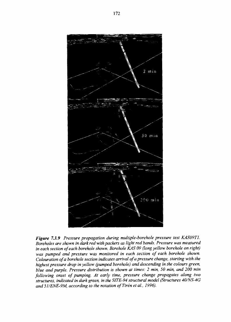
172
Figure 7.3.9 Pressure propagation during multiple-borehole pressure test KAS09T1.Boreholes are shown in dark red with packers as light red bands. Pressure was measuredin each section of each borehole shown. Borehole KAS 09 (long yellow borehole on right)was pumped and pressure was monitored in each section of each borehole shown.Colouration of a borehole section indicates arrival of a pressure change, starting with thehighest pressure drop in yellow (pumped borehole) and descending in the colours green,blue and purple. Pressure distribution is shown at times: 2 min, 50 min, and 200 minfollowing onset of pumping. At early time, pressure change propagates along twostructures, indicated in dark green, in the SITE-94 structural model (Structures 40/NS-4Gand 51/ENE-9M, according to the notation ofTiren et al, 1996).
173
pumped section. After about one day, many borehole sections on Aspo indicate somedrawdown and thus, at least, an indirect connection to the pumped section.
Interpretation of the initial, planar paths in terms of some of the 52 structures in the model,is straightforward, while interpretation of the secondary paths of propagation that evolveafter drawdowns 'turn corners' is difficult, if not practically impossible. 'Early time' for allof these tests ends after one-half to one hour, depending on the test. Complete results of thevisual inspection for 'early-time' pressure propagation are given by Voss et al. (1996).
Results
The structural model contains structures that explain nearly all of the 'early-time' pressurepropagation in tests on the southern part of Aspo. However, relatively few pressurepropagation paths in tests conducted in the northern part (in KAS03) are explained bymodel structures. This is due to both the lack of nearby boreholes and the sparsity of modelstructures in the area. In total, 30 model structures match (counting both exact and near-connections) the apparent paths of 'early-time' pressure propagation in the tests and may,therefore, be considered to transmit pressure changes in the fluid. Eighteen model structuresare not in the vicinity of any pumped sections of boreholes and are thus not checked bythese tests. Four of the structures that are checked do not transmit pressure. The structuresappear as active pressure conduits in one to seven of these tests. Because of the clarity andsparseness of the paths of pressure propagation at early time, it is unlikely that the goodspatial correlation found between SITE-94 model structures and these paths is accidental.The 30 structures are considered to be definite pressure conductors below Aspo.
7.3.6.7 Correlation of Flowing- and Pressure-transmissive Structures
Of the 30 structures that are found to transmit pressure, 29 are also found to be 'flowing'by comparison with flow indications, for an intersection tolerance of 3 m or less(Figure 7.3.8b). For a given one of these 30 structures, an average of 2.5 flow indicationscoincide with structure (with a tolerance of 3 m or less), and an average of 3 multiple-well,pressure-transmission tests indicate that the structure transmits pressure. This is strongevidence that these 30 structures act as subsurface fluid conduits, at least in the measuredportion of their extent in the modelled area.
7.3.6.8 Structural Model Correlation with Aspo Geochemistry
Visualisation and water types
The correlation of geochemical distributions and the Aspo structural model are investigatedby inspection of a three-dimensional computer graphic visualisation. The geochemically-sampled borehole sections are coloured according to the water type found in each section.Overlapping sampling sections are placed alongside the borehole to the east and samplescollected at later times in each section are placed alongside the borehole section in sequencetowards the north. This three-dimensional water-type visualisation, showing both spatialdistribution and temporal trends, is compared individually with each of the flowingstructures in the model and with surface features such as the coast of Aspo. Moreover, the
174
number of borehole locations sampled is relatively few, making it difficult to draw generalconclusions concerning distribution of water compositions in individual structures.
Groundwaters from Aspo and nearby areas (Laxemar and the island of Avro) may beclassified into five different water types based on their chemical and stable isotopiccharacteristics. The five different water types are:
1. 'recent waters',2. waters with close to 5 g/1 chloride,3. 'deep waters',4. glacial meltwaters,5. 'seawater imprint' waters.
These waters are explained in Section 7.4.
Results
Generally, salinity stratification of the three-dimensional geochemical distribution isobserved, even within individual structures. More dilute, 'recent' waters are found inshallow borehole sections, the more saline '5 g/1 chloride' waters are found at intermediatedepths near 500 m and the most saline 'deep' waters are found between 500 m and 1000 mdepth.
The 'seawater imprint' waters are found only in structures crossing sampled boreholesections near the perimeter of Aspo and each of the waters could be explained by thepresence of at least one or more SITE-94 model structures outcropping into the Baltic Sea.Most Aspo groundwaters, however, do not show any 'seawater imprint'. This indicates thatthe Aspo area is a discharge area for most of the saline groundwaters present. The seawatercharacter of fluid in these structures increased as more water was pumped from thestructures. Deeper portions of structures contain shield brine. Recharged dilute waters withisotopic compositions close to modern precipitation (part of the 'recent' water group) onlyoccur at shallow depth (less than 100 m).
Samples collected early (during drilling) have higher salinity than waters collected in thesame locations at later time. This indicates a major reorganisation of water types during thefield testing program, leading to some uncertainty concerning spatial interpretation of thegeochemical data (see also Section 6.5).
A few locations at shallower depths contain glacial meltwater. The glacial meltwater occursin both structures identified as flowing and non-flowing. The reason for its persistence inthe subsurface may be that it occurs in poorly conductive structures with relatively slowmovement, or it may occur in flowing structures if there is an extensive reservoir of suchwater along the flow path.
175
Hydrogeological implications of geochemical distributions
There is apparently no single structure that separates large regions of waters of differenttype in the subsurface. Also, the distribution of water types is too complex to be explainedby the existence of one (or a few) major flowing structure(s) below Aspo. Many structuresseem to participate in producing the observed geochemical distribution.
Because, in any given borehole, there are discrete changes in water type from onepenetrated structure to the next, it appears as if each structure has a distinct watercomposition. Careful inspection of the available data, however, reveals that no modelstructure has uniform fluid chemical composition. Each structure sampled more than oncecontains more than one type of water, and chemical composition of fluid in the structureappears to be depth-stratified. This implies that flow through each structure may not beuniform and/or that flow paths consist of a chain of segments occurring in a number ofstructures. Both of these circumstances would lead to mixing of water types within oramong structure segments at intersections.
A conjecture consistent with the above observations is that each segment of a structure(portion of structure between intersections with other structures) contains a unique uniformwater composition. With the available data, however, it is not possible to test this. It maybe that the borehole activities and sampling process have so thoroughly rearrangedgeochemical distributions that the original distribution is totally obscured in the collecteddata and that few specific conclusions concerning correlation of model structures withwater types may be fairly drawn. On the other hand, this rearrangement of waters couldserve as useful information for testing hydraulic connectivity, had the initial groundwaterdistribution been more thoroughly characterised, for example by first-strike groundwatersamples.
7.3.6.9 Integrated Hydrogeological Interpretation of All Data Types
Taken together, the geological, geophysical, hydrogeological and geochemicalmeasurements give a strong description of Aspo hydrogeology. The granodioriticsubsurface rock has undergone complex deformation resulting in zones of weakness, orstructures cutting across all rock types. Subsurface flow occurs in these structures andprimarily in portions of structures consisting of crushed rock. Flow occurs somewhat lessoften in structures consisting of individual fractures or clusters of simple fractures. Theremay be some preference for flow to occur along intersections of structures. Subsurface flowbelow Aspo is evenly distributed among rock types. However, most flow is associated withportions of deformation structures containing crushed rock. Aplites do not contain morelocations of subsurface flow than other rock types, but flow in aplites most often occurs inportions that are crushed near contacts with other rock types.
The pattern of subsurface pressure transmission gives the impression of planar pressuretransmitters, in agreement with the assumption of semi-planar structures in the model.Spatial distribution of flow indication in boreholes and paths of subsurface pressurepropagation agree that there are discrete conductive features and they agree on whichstructures are hydraulically active. Both the relatively homogeneous nature of the spatialdistribution of chemical water types and the pressure propagation data at late time,
176
following onset of pumping in a borehole, indicate a highly complex flow system, notdominated by any particular structure. Thus, interconnection of structures (rather thanlocation of individual structures) controls both pressure propagation and flow field.
No dominant and extensive hydraulic structures could be identified below Aspo. Mostextensive structures identified in the model are conductive at least in some sections. Moststructures are hydraulically well-connected (for flow and pressure transmission). There isno evidence of uniform flow within any structure or segment, indicating that flow may bechannelled within structures. Also, there is no evidence of a long flow path in any singlestructure under natural conditions.
Most flow paths apparently consist of a connected chain of segments belonging to differentstructures. Fluid may move through a segment in a uniform or channelled manner and mixwith flows from other contiguous segments at an intersection, finally continuing in the samestructure, turning into a segment of another structure, or diverging into a number ofintersecting structures.
On the local scale, this highly complex flow field is very difficult to characterise in detailwith any field data collection programme. On a larger scale, this flow field may, perhaps,be amenable to representation by homogeneous descriptions with relatively constantparameter values, although this has not been positively demonstrated in SITE-94.
7.3.6.10 Assessment of the Structural Model as a Hydrogeological Explanation
What the SITE-94 model explains
Of 52 structures in the SITE-94 model, 11 are neither tested for pressure transmission, norby borehole flow measurements, geophysical salinity or temperature logging. Thus, thereare 41 structures tested for occurrence of flow and pressure transmission. Of these 41, 34(allowing an intersection distance of 3 m), have segments that conduct fluid flow, and 30of these structures transmit pressure changes. Thus, about 3/4 of identified and testedstructures in the model are definite fluid conductors. It is believed that these structuresactually exist and conduct fluid, at the very least in the southern area of Aspo, in the areaof greatest borehole density.
What the SITE-94 model does not explain
The model explains only part of the flow found in the subsurface; 34% of flow indicationsare in structures such as simple fractures that are not included as structures in the model.Thus, there are 66% of measured flow indications that the model could possibly explain.In actuality, the model explains only 46% (for an intersection radius of 3 m). Thisapparently poor performance of the structural model may be blamed in part on the fact thatnot all locations with mechanical deformation of bedrock (in other words, locations withcrushed rock or radar indication) are possible to correlate between boreholes as structures.Although these indications may be the local expression of conductive structures, thesecould not be included in the model. Still, only about two-thirds of all flow indications thatshould be possible to explain with the model are actually explained by the model. Finally,sets of structures with purely random locations having no basis in field data explain asmany of the flow indications as does the SITE-94 structural model. This does not show that
177
the SITE-94 model is incorrect, but gives no clear proof that the model containshydrogeological information on flow at the site. The only certain check on the model wouldbe correlation of flowing model structures with flowing structures actually found in theHard Rock Laboratory tunnels below Aspo. Such a comparison may, perhaps, be possibleat a later time.
Missing structures in the SITE-94 model
Allowing that the 30 'definitely conductive' structures correctly explain half of allmeasured flow indications, what explains the other half? Rather than an inaccuracy in theexisting model structures, there is likely to be a simple lack of structures in the model.Some of those missing may be of the extensive site-scale type already included, whileothers may be of a local inter-borehole scale and not discernable in the data employed. Itis certain that the SITE-94 model is missing many single, discrete, fluid-conductivefractures in the rock mass. These exhibit little or no geophysically-measurable anomaly andcannot generally be correlated over inter-borehole distances.
This lack of structures in the model is due in part to the limited time and resources allowedfor model construction, and to the early date at which the model was finalised in order toallow other SITE-94 groups to proceed with their analyses. Some of the subsurface flowat Aspo can indeed be explained using a hydrogeological site model, and other aspects mayhave been possible to explain given more time and resources.
Implications of results
The SITE-94 model explains about half of the measured flow locations and much of thepressure transmission in the area of maximum borehole density. The implication is that,within the area covered by this already complex structural model, there are additional,hydrogeologically significant structures that have not been characterised. The impressiveamount of data collected by SKB on Aspo suffices to explain only partly the geologicalstructure and groundwater flow within a relatively small volume of rock. To characterisethe entire 2 x 2 x 1 km deep volume of the SITE-94 structural model would requirecollection of an immense amount of data. Even if this were done, there would, in allprobability, still be uncharacterised structures within the volume. It must be concluded that,given the state of the art in site characterisation methods, any attempt at a detailedcharacterisation of fluid flow and solute transport through fractured bedrock, similar to thatat Aspo, will lack sufficient data for a unique explanation.
7.3.6.11 Bias and Uncertainty in Data and Interpretation
Because of the complexity of the data, many uncertainties are inherent in any interpretationof the data. The boreholes are clustered in one area of Aspo so the resultant structuredensity must be greatest and the structure locations most accurate, within the boreholecluster. Conversely, structure location is less certain away from boreholes and surficiallineaments. Locations are noticeably poor where structures cross borehole KAS03, the onlydeep borehole that provides data in the northern part of the island.
The SITE-94 structural model includes only extensive structures (< 500 m), which areassumed to go through the modelled rock domain. There were many smaller-size features
178
that could possibly have been used as structures; however, these were not included due totime constraints and the great complexity of the data, even for just the extensive structures.Many smaller-size structures have the same geological character as the 'flowing' extensivestructures in the model and, therefore, the subsurface points of flow associated with theseare unexplained by the model.
The most highly sampled structures are the nearly horizontal ones, because they arepenetrated by the most boreholes per structure. However, there is poor recognition of near-horizontal structures because of their lack of surface expression and difficulties incorrelating indicative properties among the boreholes. Hence there are few near-horizontalstructures in the model. Difficulty in recognising these structures may lead tounderestimation of horizontal transmissivity and connectivity of the bedrock. For the samereasons, there is poor recognition of structures outcropping below water. The result isundoubtedly that many structures are missed outside the main borehole cluster on southernAspo and many structures under southern Aspo that do not outcrop are also missed.
In this study, all structures were assumed to be approximately planar and continuousthroughout the Aspo model area, in order to make the problem tractable in the short timeavailable for the work. This is certainly an over-simplification for many of the structuresfound. In order to maintain simplicity, structure planes were not allowed to be offset atblock boundaries by movements along other structures. There is evidence of verticalmovement and hundreds of metres of lateral movement along structures (see Section 7.2and Tiren, et al. 1996). Thus, many of the structures cannot be continuous as has beenassumed. This can cause significant error in location of some structure segments and shouldbe kept in mind when assessing the above results.
In testing the power of the SITE-94 structural model to explain the movement ofgroundwater, it is likely that even random structures, or structures included in error or atthe wrong locations, will intersect with some flow indications, giving a false indication ofa flowing structure. The available geological data for identification of structures exist onlyalong the boreholes, and measured flow necessarily also occurs at points in boreholesconstrained to be very near those from which structures are generated by collection of datain a borehole. Thus there is a high likelihood of coincidence between structures and flowindications, as demonstrated above.
The apparent complexity of the subsurface transmissivity distribution and flow field belowAspo makes detailed hydrogeological characterisation of the site ambiguous and manyspecific interpretations are possible. This situation motivates the analysis of multiple,alternative models in the Performance Assessment.
7.3.6.12 Conclusions - Implications for the Formulation of Detailed QuantitativeModels
The qualitative assessment of the available hydrogeological data from Aspo together withthe geological structure model and relevant geochemical information serve two coupledpurposes:
179
• it forms the basis for the formulation of the detailed quantitative hydrogeologicalmodels to be used as input in subsequent consequence analysis,
• it constitutes parts of the justification for the use of these models.
From the evalution the following main conclusions can be made:
• the geological structure model contains a considerable amount of the features thatmakes up the flow paths of the site and this fact should be acknowledged in anydetailed quantitative model,
• there is a significant degree of uncertainty regarding which features in the structuremodels which account for the flow, several hypotheses are possible,
• there is a significant amount of the flow at the site which cannot be explained by theflow in features of the structure model, a detailed flow model needs to include flowpaths below the scale of the identified structures.
In SITE-94 these observations are taken care of in the formulation of two conceptuallydifferent approaches to the flow modelling Discrete Feature modelling and StochasticContinuum modelling. Within these two main concepts different variants are developed.The models are fully described in the following two sections (7.3.7 and 7.3.8).
Consequently, the detailed quantitative hydrogeological models used in SITE-94 are basedon an integrated assessment of all soft and hard data available from the site and a thoroughevaluation of part of the hard data. Such integration between overall site evaluation andapplications of specialised models is probably key for making performance assessmentstruly site specific. In retrospect it is clear that even further integration would have improvedthe models and the justification for them. Careful planning of such integration, well aheadof the work, appear to be of vital importance for a succesful evaluation of site specific data.
7.3.7 Development of a Discrete Feature Hydrogeological Site Model
7.3.7.1 Introduction
The SITE-94 structural model also serves directly as the basis for a hydrogeological modelbased on the discrete feature concept (Geier, 1996a, b), which is used in SITE-94 to predictsite-scale groundwater flow and effective hydrogeological parameters for PerformanceAssessment calculations. The Discrete Feature model is based on a three-dimensional,deterministic representation of the fracture zones in the SITE-94 geological structuremodel, plus a stochastic representation of smaller-scale fractures within the repository. Asshown in Figure 7.3.10, the Discrete Feature model integrates structural data on a range ofscales, becoming progressively more detailed closer to the repository and individualcanister sites.
The basic concept of discrete-feature modelling is to represent conductive structures interms of a collection of discrete, planar, transmissive features, which interconnect to form
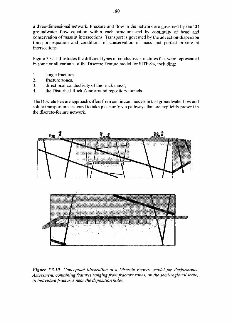
180
a three-dimensional network. Pressure and flow in the network are governed by the 2Dgroundwater flow equation within each structure and by continuity of head andconservation of mass at intersections. Transport is governed by the advection-dispersiontransport equation and conditions of conservation of mass and perfect mixing atintersections.
Figure 7.3.11 illustrates the different types of conductive structures that were representedin some or all variants of the Discrete Feature model for SITE-94, including:
1. single fractures,2. fracture zones,3. directional conductivity of the 'rock mass',4. the Disturbed-Rock Zone around repository tunnels.
The Discrete Feature approach differs from continuum models in that groundwater flow andsolute transport are assumed to take place only via pathways that are explicitly present inthe discrete-feature network.
Figure 7.3.10 Conceptual illustration of a Discrete Feature model for PerformanceAssessment, containing features ranging from fracture zones, on the semi-regional scale,to individual fractures near the deposition holes.
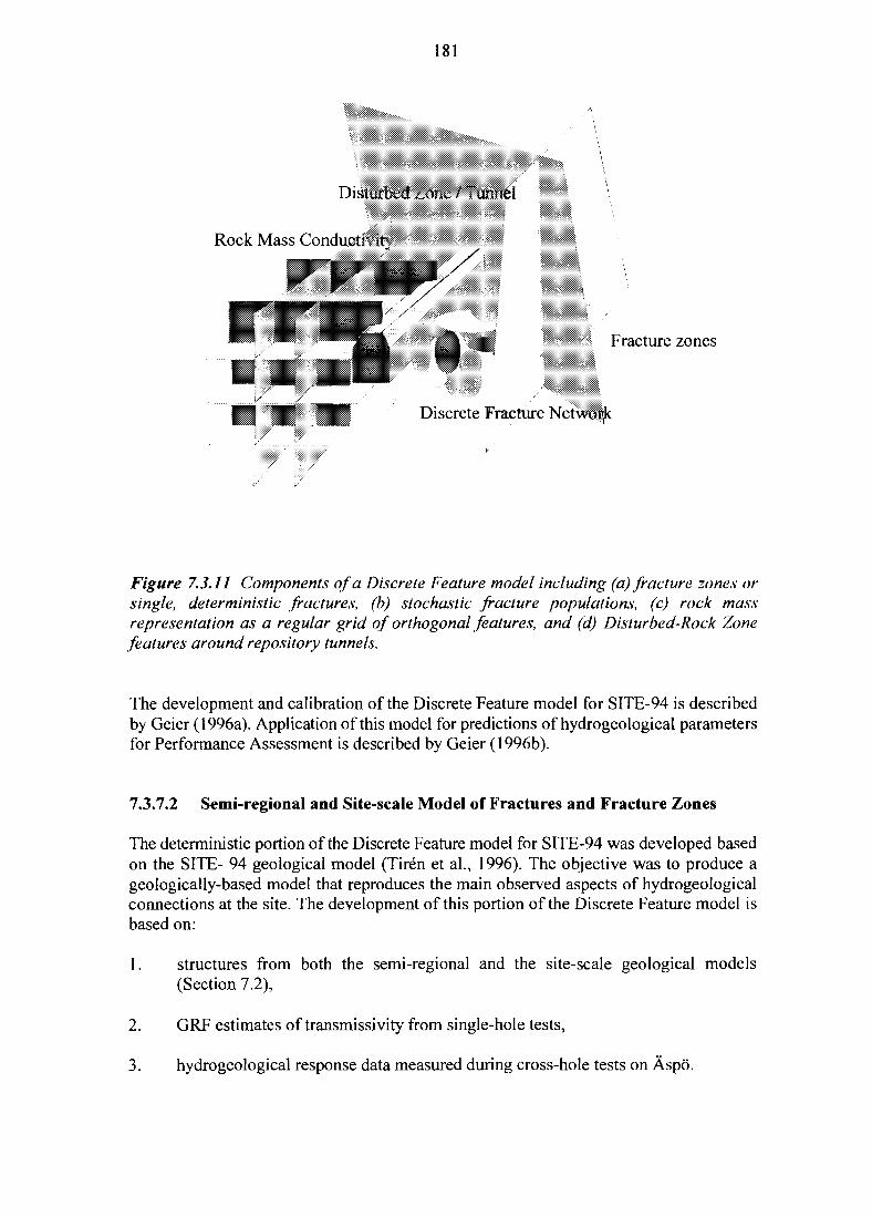
181
Disturbed Zone / Tunnel
Rock Mass Conductivity
Fracture zones
Discrete Fracture Netwoijk
Figure 7.3.11 Components of a Discrete Feature model including (a) fracture zones orsingle, deterministic fractures, (b) stochastic fracture populations, (c) rock massrepresentation as a regular grid of orthogonal features, and (d) Disturbed-Rock Zonefeatures around repository tunnels.
The development and calibration of the Discrete Feature model for SITE-94 is describedby Geier (1996a). Application of this model for predictions of hydrogeological parametersfor Performance Assessment is described by Geier (1996b).
7.3.7.2 Semi-regional and Site-scale Model of Fractures and Fracture Zones
The deterministic portion of the Discrete Feature model for SITE-94 was developed basedon the SITE- 94 geological model (Tiren et al., 1996). The objective was to produce ageologically-based model that reproduces the main observed aspects of hydrogeologicalconnections at the site. The development of this portion of the Discrete Feature model isbased on:
1. structures from both the semi-regional and the site-scale geological models(Section 7.2),
2. GRF estimates of transmissivity from single-hole tests,
3. hydrogeological response data measured during cross-hole tests on Aspo.
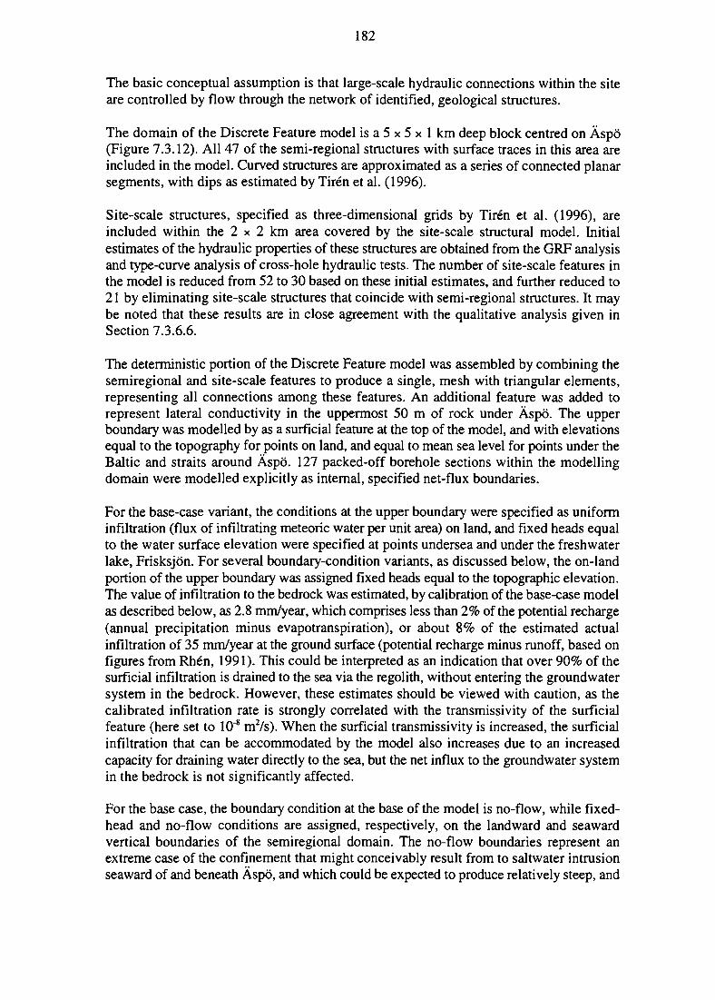
182
The basic conceptual assumption is that large-scale hydraulic connections within the siteare controlled by flow through the network of identified, geological structures.
The domain of the Discrete Feature model is a 5 x 5 x 1 km deep block centred on Aspo(Figure 7.3.12). All 47 of the semi-regional structures with surface traces in this area areincluded in the model. Curved structures are approximated as a series of connected planarsegments, with dips as estimated by Tiren et al. (1996).
Site-scale structures, specified as three-dimensional grids by Tiren et al. (1996), areincluded within the 2 x 2 km area covered by the site-scale structural model. Initialestimates of the hydraulic properties of these structures are obtained from the GRF analysisand type-curve analysis of cross-hole hydraulic tests. The number of site-scale features inthe model is reduced from 52 to 30 based on these initial estimates, and further reduced to21 by eliminating site-scale structures that coincide with semi-regional structures. It maybe noted that these results are in close agreement with the qualitative analysis given inSection 7.3.6.6.
The deterministic portion of the Discrete Feature model was assembled by combining thesemiregional and site-scale features to produce a single, mesh with triangular elements,representing all connections among these features. An additional feature was added torepresent lateral conductivity in the uppermost 50 m of rock under Aspo. The upperboundary was modelled by as a surficial feature at the top of the model, and with elevationsequal to the topography for points on land, and equal to mean sea level for points under theBaltic and straits around Aspo. 127 packed-off borehole sections within the modellingdomain were modelled explicitly as internal, specified net-flux boundaries.
For the base-case variant, the conditions at the upper boundary were specified as uniforminfiltration (flux of infiltrating meteoric water per unit area) on land, and fixed heads equalto the water surface elevation were specified at points undersea and under the freshwaterlake, Frisksjon. For several boundary-condition variants, as discussed below, the on-landportion of the upper boundary was assigned fixed heads equal to the topographic elevation.The value of infiltration to the bedrock was estimated, by calibration of the base-case modelas described below, as 2.8 mm/year, which comprises less than 2% of the potential recharge(annual precipitation minus evapotranspiration), or about 8% of the estimated actualinfiltration of 35 mm/year at the ground surface (potential recharge minus runoff, based onfigures from Rhen, 1991). This could be interpreted as an indication that over 90% of thesurficial infiltration is drained to the sea via the regolith, without entering the groundwatersystem in the bedrock. However, these estimates should be viewed with caution, as thecalibrated infiltration rate is strongly correlated with the transmissivity of the surficialfeature (here set to 10'8 m2/s). When the surficial transmissivity is increased, the surficialinfiltration that can be accommodated by the model also increases due to an increasedcapacity for draining water directly to the sea, but the net influx to the groundwater systemin the bedrock is not significantly affected.
For the base case, the boundary condition at the base of the model is no-flow, while fixed-head and no-flow conditions are assigned, respectively, on the landward and seawardvertical boundaries of the semiregional domain. The no-flow boundaries represent anextreme case of the confinement that might conceivably result from to saltwater intrusionseaward of and beneath Aspo, and which could be expected to produce relatively steep, and
183
hence conservative discharge paths for radionuclides. Based upon the results of thevariable-density regional modelling, as described in Section 7.3.3, such conditions may notbe regarded as most probable. Several variants of the discrete-feature were developed toanalyse the effects of other configurations of boundary effects, including a case withlinearly varying, fixed heads on all external boundaries.
The initial estimates of hydraulic properties for the site-scale and semi-regional structuresare refined by calibration in the Discrete Feature model. First, the infiltration rate and thesurface-layer transmissivity are calibrated with respect to the steady-state head distributionon Aspo. Next, the initial estimates are calibrated with respect to the observed, long-termdrawdowns in cross-hole hydraulic tests. Short-term cross-hole tests are simulated in themodel, the simulated drawdowns are compared with observations and hydraulic propertiesof the discrete features are adjusted to improve the fit. The calibrations of infiltration anddiscrete-feature properties are accomplished by an algorithm for automated optimisationwith respect to the total absolute discrepancy in simulated vs. observed heads ordrawdowns.
The calibration is successful in producing a model that reproduces the undisturbed headdistribution within a few decimetres at most points on Aspo. The final drawdownspredicted by the model for long-term pumping tests in boreholes KAS06 and KAS07 tendto be much too high, particularly in the northwestern part of Aspo. However, predicted andobserved final drawdowns in the vicinity of the SITE-94 repository generally agree withina factor of 2 or 3.
Several variations are analysed to assess the effects of uncertainties in the deterministicportion of the model with respect to the predicted hydrogeological parameters forPerformance Assessment. A structural variation is performed by assigning an alternativeestimate of dip to structures in the Avro fracture zone. Hydrogeological variations includea change in the relative transmissivities of steeply-dipping and gently-dipping fracturezones and introduction of stochastic variability of transmissivity within individualstructures. Hydrogeological variations are also performed with respect to the effectiveboundary conditions on the seaward boundary, upper surface and base of the model.Besides these variations, discrete feature implementations of two independently developedgeological/hydrogeological site models are evaluated. The variational cases are discussedin Section 10.3.4.2.
7.3.7.3 Discrete-Fracture Network Model for the Repository Rock Block
Stochastic models for the rock within the repository are developed based on a statisticalanalysis of fracture data from core drilling and outcrop fracture mapping (Geier andThomas, 1996). A separate geometrical DFN model is derived for each of the four mainrock types found at Aspo. Alternative statistical forms (types of models) are considered foreach of the following fracture population properties: location (clustering), orientation, sizeand fracture transmissivity. Data utilised in the analysis include fracture frequency in cores,fracture orientations from core and outcrop mapping, fracture trace lengths on outcrops and3 m packer test transmissivities as evaluated by GRF analysis.
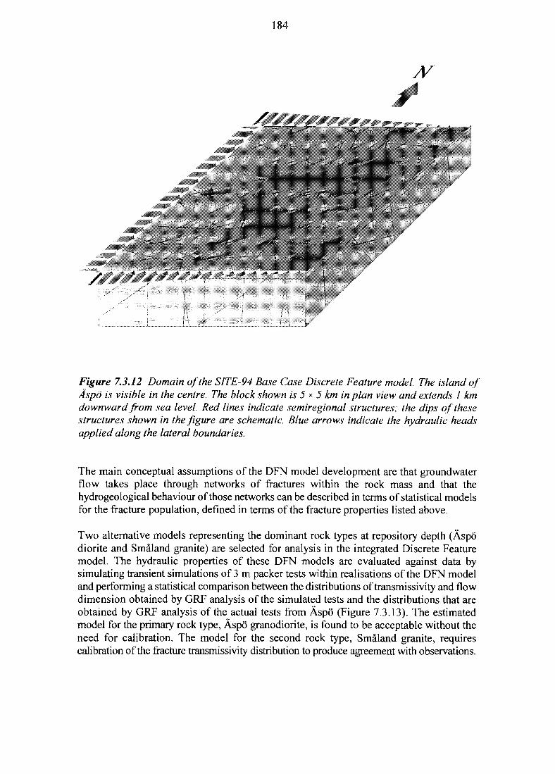
184
Figure 7.3.12 Domain of the SITE-94 Base Case Discrete Feature model. The island ofAspo is visible in the centre. The block shown is 5 * 5 km in plan view and extends I kmdownward from sea level. Red lines indicate semiregional structures; the dips of thesestructures shown in the figure are schematic. Blue arrows indicate the hydraulic headsapplied along the lateral boundaries.
The main conceptual assumptions of the DFN model development are that groundwaterflow takes place through networks of fractures within the rock mass and that thehydrogeological behaviour of those networks can be described in terms of statistical modelsfor the fracture population, defined in terms of the fracture properties listed above.
Two alternative models representing the dominant rock types at repository depth (Aspodiorite and Smaland granite) are selected for analysis in the integrated Discrete Featuremodel. The hydraulic properties of these DFN models are evaluated against data bysimulating transient simulations of 3 m packer tests within realisations of the DFN modeland performing a statistical comparison between the distributions of transmissivity and flowdimension obtained by GRF analysis of the simulated tests and the distributions that areobtained by GRF analysis of the actual tests from Aspo (Figure 7.3.13). The estimatedmodel for the primary rock type, Aspo granodiorite, is found to be acceptable without theneed for calibration. The model for the second rock type, Smaland granite, requirescalibration of the fracture transmissivity distribution to produce agreement with observations.
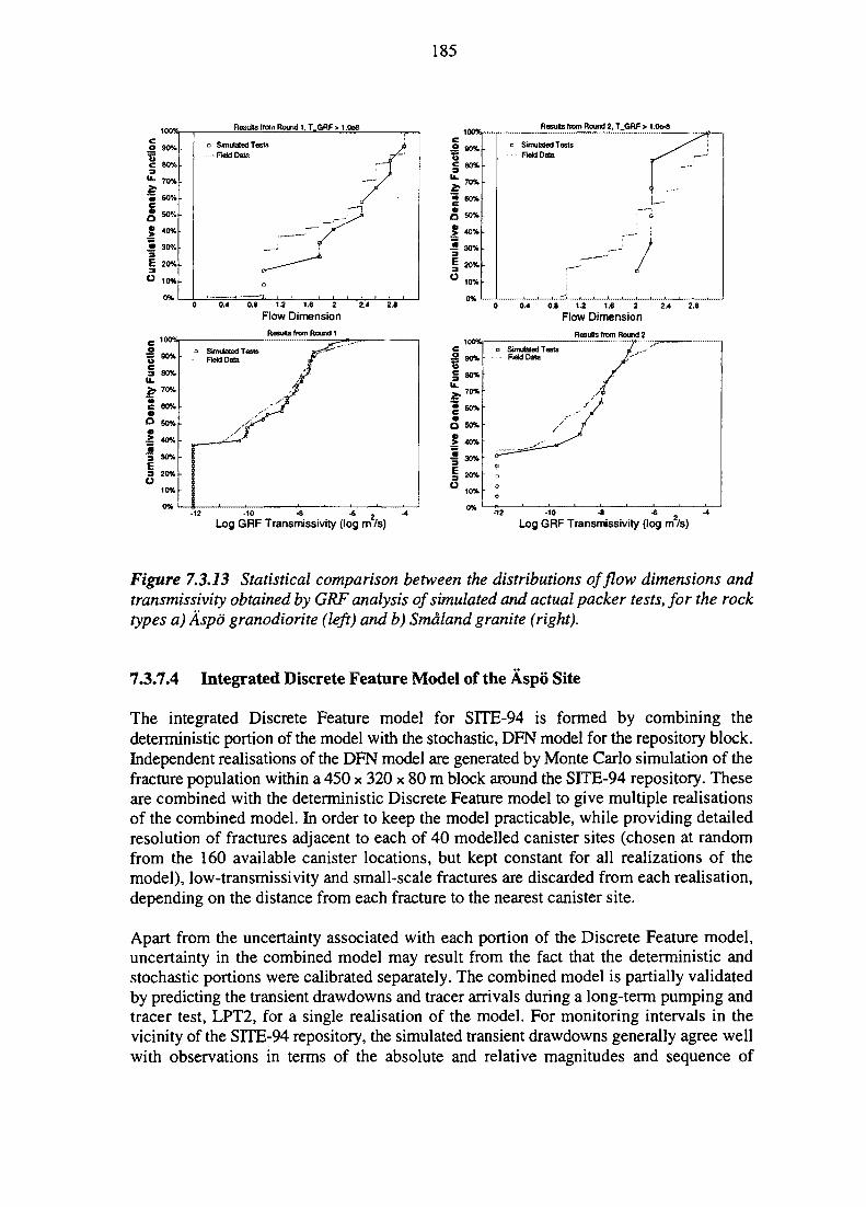
185
Results trotn Round 1. T.GRF > 1.0e8 Results from Round 2. T_GRF > 1 Oe-8
0 0.4 0.8 1.2 1.6 2 2.4 2.8
Flow DimensionResults from Round 1
0 0.4 0.8 1.2 1.6 2 2.4 2.8
Flow Dimension
Results from Round 2
Log GRF Transmissivity (log m /s)-10 -8 -6 -4
Log GRF Transmissivity (log m /s)
Figure 7.3.13 Statistical comparison between the distributions of flow dimensions andtransmissivity obtained by GRF analysis of simulated and actual packer tests, for the rocktypes a) Aspo granodiorite (left) and b) Smdland granite (right).
1.3.7.4 Integrated Discrete Feature Model of the Aspo Site
The integrated Discrete Feature model for SITE-94 is formed by combining thedeterministic portion of the model with the stochastic, DFN model for the repository block.Independent realisations of the DFN model are generated by Monte Carlo simulation of thefracture population within a 450 x 320 x 80 m block around the SITE-94 repository. Theseare combined with the deterministic Discrete Feature model to give multiple realisationsof the combined model. In order to keep the model practicable, while providing detailedresolution of fractures adjacent to each of 40 modelled canister sites (chosen at randomfrom the 160 available canister locations, but kept constant for all realizations of themodel), low-transmissivity and small-scale fractures are discarded from each realisation,depending on the distance from each fracture to the nearest canister site.
Apart from the uncertainty associated with each portion of the Discrete Feature model,uncertainty in the combined model may result from the fact that the deterministic andstochastic portions were calibrated separately. The combined model is partially validatedby predicting the transient drawdowns and tracer arrivals during a long-term pumping andtracer test, LPT2, for a single realisation of the model. For monitoring intervals in thevicinity of the SITE-94 repository, the simulated transient drawdowns generally agree wellwith observations in terms of the absolute and relative magnitudes and sequence of
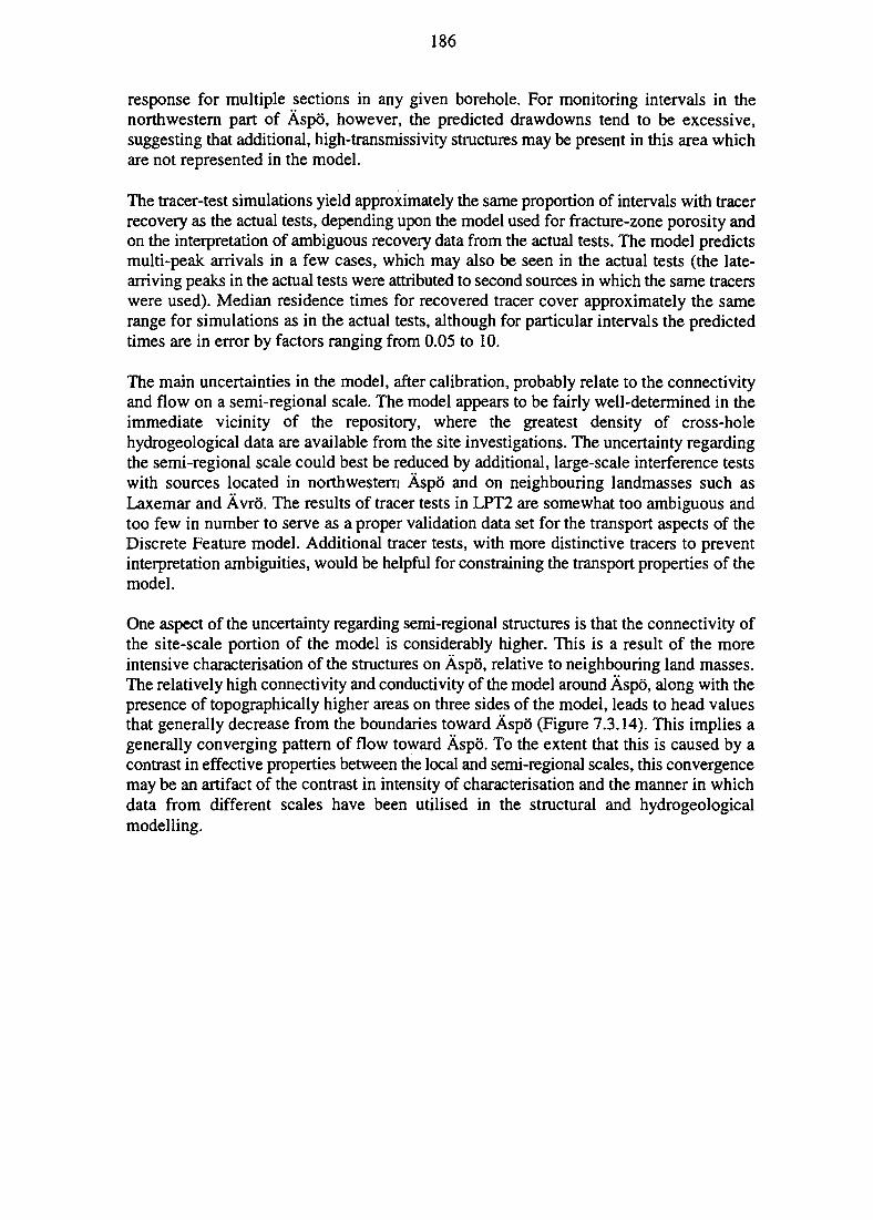
186
response for multiple sections in any given borehole. For monitoring intervals in thenorthwestern part of Aspo, however, the predicted drawdowns tend to be excessive,suggesting that additional, high-transmissivity structures may be present in this area whichare not represented in the model.
The tracer-test simulations yield approximately the same proportion of intervals with tracerrecovery as the actual tests, depending upon the model used for fracture-zone porosity andon the interpretation of ambiguous recovery data from the actual tests. The model predictsmulti-peak arrivals in a few cases, which may also be seen in the actual tests (the late-arriving peaks in the actual tests were attributed to second sources in which the same tracerswere used). Median residence times for recovered tracer cover approximately the samerange for simulations as in the actual tests, although for particular intervals the predictedtimes are in error by factors ranging from 0.05 to 10.
The main uncertainties in the model, after calibration, probably relate to the connectivityand flow on a semi-regional scale. The model appears to be fairly well-determined in theimmediate vicinity of the repository, where the greatest density of cross-holehydrogeological data are available from the site investigations. The uncertainty regardingthe semi-regional scale could best be reduced by additional, large-scale interference testswith sources located in northwestern Aspo and on neighbouring landmasses such asLaxemar and Avro. The results of tracer tests in LPT2 are somewhat too ambiguous andtoo few in number to serve as a proper validation data set for the transport aspects of theDiscrete Feature model. Additional tracer tests, with more distinctive tracers to preventinterpretation ambiguities, would be helpful for constraining the transport properties of themodel.
One aspect of the uncertainty regarding semi-regional structures is that the connectivity ofthe site-scale portion of the model is considerably higher. This is a result of the moreintensive characterisation of the structures on Aspo, relative to neighbouring land masses.The relatively high connectivity and conductivity of the model around Aspo, along with thepresence of topographically higher areas on three sides of the model, leads to head valuesthat generally decrease from the boundaries toward Aspo (Figure 7.3.14). This implies agenerally converging pattern of flow toward Aspo. To the extent that this is caused by acontrast in effective properties between the local and semi-regional scales, this convergencemay be an artifact of the contrast in intensity of characterisation and the manner in whichdata from different scales have been utilised in the structural and hydrogeologicalmodelling.
187
Horizontal sectionthrough vicinityof the repository(Z = -495 m)
Vertical Section (Y = 2200 m)-
Hydraulic Head in Cross SectionsHorizontal Section (Z = -495 m)
Z =-1000 m
Vertical Section (X = 7300 m)
Z = 0 m
greater than 7 m6 to 7 m5 to 6 m4 to 5 m3 to 4 m2 to 3 m1 to 2 mOto 1 mless than 0 m, orhydraulically isolated
Darcy Velocity through Cross SectionHorizontal section (Z = -495 m) Vertical component:
Z = -1000 m
Magnitude of vector:
3x10"9m/s_g
1x10 m/s
3x10"1°m/s
1x10~1°m/s
_g
more than 10 m/s10"10to 10"9m/s10"11to10"10m/sless than 10~11rn/sless than 10~11rn/s10"11to 10~10m/s10"10to10"9m/smore than 10" m/s
DWG0161
Figure 7.3.14 Cross sections showing the distributions of groundwater head and Darcyvelocity within the Discrete Feature model for the Reference Case (Base Case modelvariant - see Section 10.3). Coloured line segments in plots (a) and (c) representintersections between the discrete features and the plane of each cross section; the linecolours indicate the magnitude of hydraulic head. Coloured arrows in plot (b) representthe magnitude and direction of Darcy velocity through the plane of the repository; thearrow colours indicate the magnitude of the vertical component of Darcy velocity.Coordinates (X, Y,Z values) are in the OKG system for Aspo.
188
7.3.8 Development of a Stochastic Continuum HydrogeologicalSite Model
7.3.8.1 Introduction
The second of the main hydrogeological site-scale models is based on the stochasticcontinuum concept. In contrast to the Discrete Feature site-scale model, where water flowsonly in permeable discrete fractures or fracture zones, the Stochastic Continuum site modeltreats the rock as a random, equivalent porous continuum that is hydraulically connectedeverywhere. The model generates conditioned stochastic realisations of the 3D hydraulicconductivity field using a non-parametric technique. The input data consist exclusively ofthe values and distribution of hydraulic conductivity interpreted from borehole packer tests.Apart from that, no attempt was made to calibrate the model on the hydraulic interferencetest data or any other site data, other than in a qualitative sense.
Uncertainties related to the hydraulic conductivity structure are explored by constructingseveral alternative hydraulic conductivity fields with different correlation structures andconnectivity properties. For example, geological evidence on the existence of major fracturezones is taken into account by constructing hydraulic conductivity fields with long rangecorrelation features in the major fracturing directions.
The Stochastic Continuum model is used to estimate effective hydrogeological parameters,including near-field and far-field Darcy velocities and far-field dispersion, for the radio-nuclide release and transport calculations by means of steady-state flow and particletracking calculations in a similar way as for the Discrete Feature site model (Section 10.3).The development of the Stochastic Continuum site model is described in detail by Tsang(1996).
7.3.8.2 Data Used
The Stochastic Continuum model uses 844 hydraulic conductivity (K) values interpretedfrom injection tests performed in 3 m packed-off sections along 7 cored boreholes (KAS02through KAS08) at Aspo. The data used are the K estimates interpreted by classicalmethods based on 2D flow geometry, as obtained from the SKB database (Section 6.4). Thehydraulic conductivities were divided into six classes, separated by indicators, eachspanning about one order of magnitude. Figure 7.3.15 shows the frequency histogram ofthese hydraulic conductivity classes (log10 scale). These data are used for generating three-dimensional conditioned stochastic hydraulic conductivity fields.
A geostatistical analysis shows that the hydraulic conductivity data are very poorly spatiallycorrelated and appear mostly as randomly distributed. However, this finding is based ondata along boreholes that are predominantly in the vertical direction. The large spacingbetween the boreholes (on the order of 100 m) does not allow for a meaningful search fora 3D correlation structure. Furthermore, as no boreholes were drilled along a major fracturezone, this analysis is also unable to determine whether strong connectivity and correlationexist along the planes of major fracture zones. That is, even if long-range correlations werepresent in the data, they would be difficult to detect. This was verified by estimating
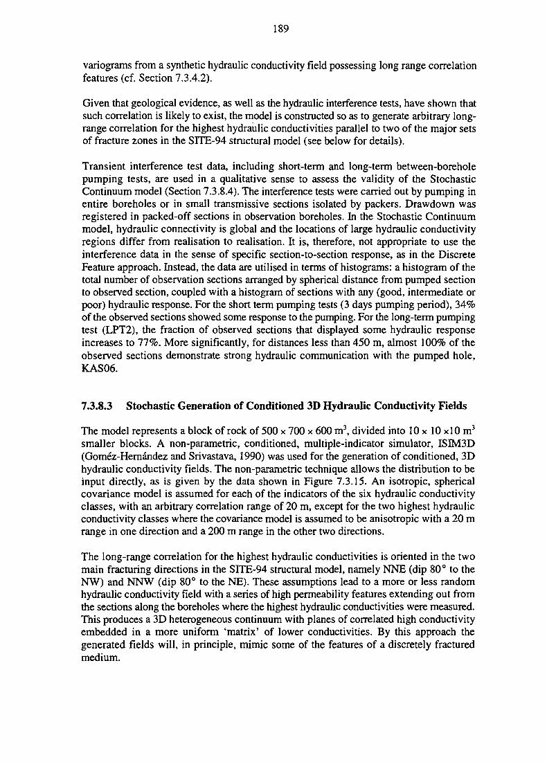
189
variograms from a synthetic hydraulic conductivity field possessing long range correlationfeatures (cf. Section 7.3.4.2).
Given that geological evidence, as well as the hydraulic interference tests, have shown thatsuch correlation is likely to exist, the model is constructed so as to generate arbitrary long-range correlation for the highest hydraulic conductivities parallel to two of the major setsof fracture zones in the S1TE-94 structural model (see below for details).
Transient interference test data, including short-term and long-term between-boreholepumping tests, are used in a qualitative sense to assess the validity of the StochasticContinuum model (Section 7.3.8.4). The interference tests were carried out by pumping inentire boreholes or in small transmissive sections isolated by packers. Drawdown wasregistered in packed-off sections in observation boreholes. In the Stochastic Continuummodel, hydraulic connectivity is global and the locations of large hydraulic conductivityregions differ from realisation to realisation. It is, therefore, not appropriate to use theinterference data in the sense of specific section-to-section response, as in the DiscreteFeature approach. Instead, the data are utilised in terms of histograms: a histogram of thetotal number of observation sections arranged by spherical distance from pumped sectionto observed section, coupled with a histogram of sections with any (good, intermediate orpoor) hydraulic response. For the short term pumping tests (3 days pumping period), 34%of the observed sections showed some response to the pumping. For the long-term pumpingtest (LPT2), the fraction of observed sections that displayed some hydraulic responseincreases to 77%. More significantly, for distances less than 450 m, almost 100% of theobserved sections demonstrate strong hydraulic communication with the pumped hole,KAS06.
7.3.8.3 Stochastic Generation of Conditioned 3D Hydraulic Conductivity Fields
The model represents a block of rock of 500 x 700 x 600 m3, divided into 10 x 10 xlO m3
smaller blocks. A non-parametric, conditioned, multiple-indicator simulator, ISIM3D(Gomez-Hernandez and Srivastava, 1990) was used for the generation of conditioned, 3Dhydraulic conductivity fields. The non-parametric technique allows the distribution to beinput directly, as is given by the data shown in Figure 7.3.15. An isotropic, sphericalcovariance model is assumed for each of the indicators of the six hydraulic conductivityclasses, with an arbitrary correlation range of 20 m, except for the two highest hydraulicconductivity classes where the covariance model is assumed to be anisotropic with a 20 mrange in one direction and a 200 m range in the other two directions.
The long-range correlation for the highest hydraulic conductivities is oriented in the twomain fracturing directions in the SITE-94 structural model, namely NNE (dip 80° to theNW) and NNW (dip 80° to the NE). These assumptions lead to a more or less randomhydraulic conductivity field with a series of high permeability features extending out fromthe sections along the boreholes where the highest hydraulic conductivities were measured.This produces a 3D heterogeneous continuum with planes of correlated high conductivityembedded in a more uniform 'matrix' of lower conductivities. By this approach thegenerated fields will, in principle, mimic some of the features of a discretely fracturedmedium.
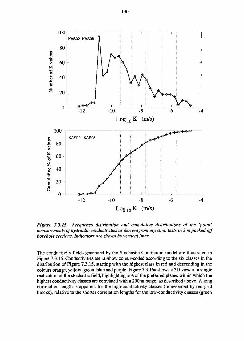
190
100
80
> 60 H
fc 40
I 20
0
!KAS02 -KAS08 i
i
\
i
1
V
i
1
1 i
1 1
-12 -10 -8
Log10K (m/s)-6 _4
-12 -10 -8Log10K (m/s)
Figure 7.3.15 Frequency distribution and cumulative distributions of the 'point'measurements of hydraulic conductivities as derived from injection tests in 3 m packed offborehole sections. Indicators are shown by vertical lines.
The conductivity fields generated by the Stochastic Continuum model are illustrated inFigure 7.3.16. Conductivities are rainbow colour-coded according to the six classes in thedistribution of Figure 7.3.15, starting with the highest class in red and descending in thecolours orange, yellow, green, blue and purple. Figure 7.3.16a shows a 3D view of a singlerealization of the stochastic field, highlighting one of the preferred planes within which thehighest conductivity classes are correlated with a 200 m range, as described above. A longcorrelation length is apparent for the high-conductivity classes (represented by red gridblocks), relative to the shorter correlation lengths for the low-conductivity classes (green
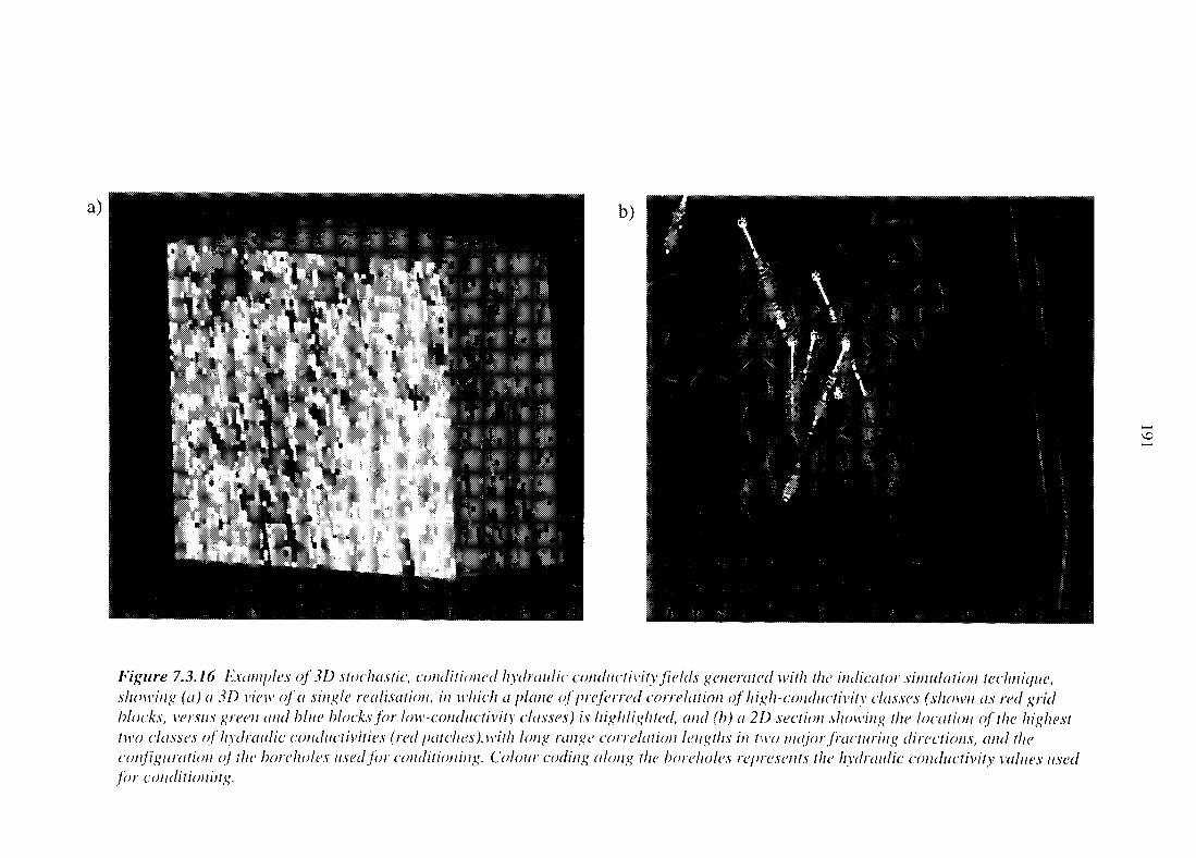
Figure 7.3.16 Examples of 3D stochastic, conditioned hydraulic conductivity fields generated with the indicator simulation technique,showing (a) a 3D view of a single realisation, in which a plane of preferred correlation of high-conductivity classes (shown as red gridblocks, versus green and blue blocks for low-conductivity classes) is highliglited, and (b) a 2D section showing the location of the highesttwo classes of hydraulic conductivities (red patches),with long range correlation lengths in two major fracturing directions, and theconfiguration of the boreholes used for conditioning. Colour coding along the boreholes represents the hydraulic conductivity values usedfor conditioning.
192
and blue blocks). Figure 7.3.16b shows a stochastic realization together with theexperimental configuration of the boreholes. Each block with a hydraulic conductivity valuethat falls into the highest class is indicated by a red dot. The colour coding along theboreholes represents the "measured" hydraulic conductivities used for conditioning. Thethin, orange lines bracketing the small sections of the boreholes represent locations ofwater-bearing fractures, as indicated by spinner flow measurements (according to Stanforset al., 1991, Figures 3.7 - 3.8). As result of the long range correlation, the highestconductivities congregate in NNE and NNW orientated planes. It should be noted that thepreferred orientations indicated in Figure 7.3.16a are not represented by a constant, highhydraulic conductivity. Instead they contain a wide range of conductivity values, althoughfavouring the high conductivities (red grid blocks) and longer correlation length.
7.3.8.4 Discussion of Model Validity
An important strength of the Stochastic Continuum model is that it honours the location andvalues of the interpreted hydraulic conductivities by means of conditioning. This is incontrast to the Discrete Feature model where such conditioning is difficult. However, it isimportant to remember that the block conductivities in the Stochastic Continuum model arean idealised representation of the packer test measurements. Thus, if transient simulationsof packer tests were run in this model, quite disparate results may be obtained. Because theStochastic Continuum model is constrained only by the values and correlation structure ofhydraulic conductivities, it is possible to construct a variety of alternative stochastic fields,with different flow and transport properties, that do not contradict the data. Theincorporation of long-range correlation structures, guided by 'soft' geological information,is one such example. These structural features are not supported by the hydraulic test databut do not contradict the data. In order to address how such and other conceptualuncertainties affect the predicted flow and transport properties, a number of variantsreflecting different assumptions on hydraulic conductivity structure are evaluated inSection 10.3.5.
The validity of the Stochastic Continuum model is assessed in a qualitative sense byperforming transient simulations of the short-term interference tests in hydraulicconductivity fields generated by the model and comparing the results with the actual testsperformed at Aspo. The model calculates response (pressure drawdown) as a function ofdistance from the pumping well at the end of the (3 days) pumping period for 20 arbitrarilyselected pumping well sites. The simulations are performed for two alternative stochastichydraulic conductivity fields, one with the long range correlation features and one isotropicwith the short correlation length (20 m) for all hydraulic conductivity classes. Forcomparison, each simulation is also performed for a homogeneous field of hydraulicconductivity where the constant hydraulic conductivity is taken as the geometric mean ofthe values in the stochastic field.
The results of these simulations indicate that the Stochastic Continuum model capturesimportant characteristics of the field tests. Figure 7.3.17 shows the simulated pressureresponse to pumping in an arbitrarily selected highly conductive well site. The dotsrepresent the response at different grid blocks for the stochastic field with long rangecorrelation structures and the solid curve shows the result for a homogeneous conductivityfield. At this short duration of pumping, as a result of flow channelling, the pressure
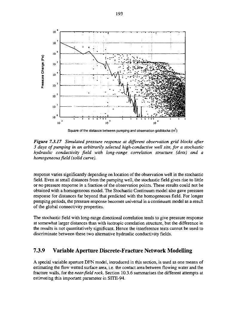
193
oratca
Oo
S
10 10
Square of the distance between pumping and observation gridblocks (m2)
Figure 7.3.17 Simulated pressure response at different observation grid blocks after3 days of pumping in an arbitrarily selected high-conductive well site, for a stochastichydraulic conductivity field with long-range correlation structure (dots) and ahomogeneous field (solid curve).
response varies significantly depending on location of the observation well in the stochasticfield. Even at small distances from the pumping well, the stochastic field gives rise to littleor no pressure response in a fraction of the observation points. These results could not beobtained with a homogeneous model. The Stochastic Continuum model also gave pressureresponse for distances far beyond that predicted with the homogeneous field. For longerpumping periods, the pressure response becomes universal in a continuum model as a resultof the global connectivity properties.
The stochastic field with long-range directional correlation tends to give pressure responseat somewhat larger distances than with isotropic correlation structure, but the difference inthe results is not quantitatively significant. Hence the interference tests cannot be used todiscriminate between these two alternative hydraulic conductivity fields.
7.3.9 Variable Aperture Discrete-Fracture Network Modelling
A special variable aperture DFN model, introduced in this section, is used as one means ofestimating the flow wetted surface area, i.e. the contact area between flowing water and thefracture walls, for the near-field rock. Section 10.3.6 summarises the different attempts atestimating this important parameter in SITE-94.
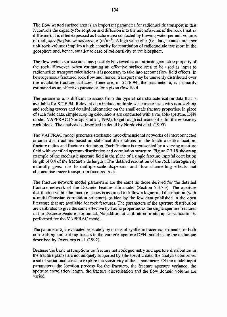
194
The flow wetted surface area is an important parameter for radionuclide transport in thatit controls the capacity for sorption and diffusion into the microfissures of the rock (matrixdiffusion). It is often expressed as fracture area contacted by flowing water per unit volumeof rock, specific flow-wetted area, a, (m2/m3). A high value of a,, (i.e., large contact area perunit rock volume) implies a high capacity for retardation of radionuclide transport in thegeosphere and, hence, smaller release of radioactivity to the biosphere.
The flow wetted surface area may possibly be viewed as an intrinsic geometric property ofthe rock. However, when estimating an effective surface area to be used as input toradionuclide transport calculations it is necessary to take into account flow field effects. Inheterogeneous fractured rock flow and, hence, transport may be unevenly distributed overthe available fracture surfaces. Therefore, in SITE-94, the parameter a,, is primarilyestimated as an effective parameter for a given flow field.
The parameter a,, is difficult to assess from the type of site characterisation data that isavailable for SITE-94. Relevant data include multiple-scale tracer tests with non-sorbingand sorbing tracers and detailed information on the small-scale fracture properties. In placeof such field data, simple scoping calculations are conducted with a variable-aperture, DFNmodel, VAPFRAC (Nordqvist et al., 1992), to get rough estimates of a, for the repositoryrock block. The analysis is described in detail by Nordqvist et al. (1995).
The VAPFRAC model generates stochastic three-dimensional networks of interconnectedcircular disc fractures based on statistical distributions for the fracture centre location,fracture radius and fracture orientation. Each fracture is represented by a varying aperturefield with specified aperture distribution and correlation structure. Figure 7.3.18 shows anexample of the stochastic aperture field in the plane of a single fracture (spatial correlationlength of 0.4 of the fracture side length). This detailed resolution of the rock heterogeneitynaturally gives rise to multiple-scale dispersion and flow channelling effects thatcharacterise tracer transport in fractured rock.
The fracture network model parameters are the same as those derived for the detailedfracture network of the Discrete Feature site model (Section 7.3.7.3). The aperturedistribution within the fracture planes is assumed to follow a lognormal distribution (witha multi-Gaussian correlation structure), guided by the few data published in the openliterature that are available for rock fractures. The parameters of the aperture distributionare calibrated to give the same effective hydraulic properties as the single aperture fracturesin the Discrete Feature site model. No additional calibration or attempt at validation isperformed for the VAPFRAC model.
The parameter a,, is evaluated separately by means of synthetic tracer experiments for bothnon-sorbing and sorbing tracers in the variable-aperture DFN model using the techniquedescribed by Dverstorp et al. (1992).
Because the basic assumptions on fracture network geometry and aperture distribution inthe fracture planes are not uniquely supported by site-specific data, the analysis comprisesa set of variational cases to explore the sensitivity of the a,, parameter. Of the model inputparameters, the location process for the fractures, the fracture aperture variance, theaperture correlation length, the fracture discretisation and the flow domain volume arevaried.
195
Figure 7.3.18 Illustration of a variable aperture field used to represent individual fractureplanes in the VAPFRAC 3D Discrete-Fracture Network model (from Moreno et ai, 1988).
The results of the VAPFRAC simulations and the use of the results in the radionuclidetransport calculations are presented in Section 10.3.6.
7.3.10 Summary and Implications for Other Parts of the Assessment
The hydrogeological analyses for SITE-94, as described above, have considered processeson scales ranging from continental-scale groundwater flow to heterogeneity withinindividual fractures. The main steps in the analysis included:
1. assessment of the regional hydrogeological setting and regional hydrogeologicalmodelling,
2. assessment of uncertainties in the site characterisation data,
3. simple scoping calculations of flow,
4. a qualitative, integrated hydrogeological interpretation of diverse, interdisciplinarydata from Aspo,
196
5. development of quantitative hydrogeological models, based upon multipleconceptual models, for scales ranging from the repository block scale (<50 m) toseveral kilometres.
Each of these steps typically involve multiple variants of two or more distinct types ofmodels.
Taken as a whole, the hydrogeological analyses for SITE-94 incorporate a very largeportion of the available site data. The models are partly calibrated and tested to ensureconsistency with the hydrogeological field tests that were performed at the Aspo site.However, each particular model or analysis emphasises a different subset of the site dataand not all aspects of the database are treated with an equal degree of quantitative rigour.Furthermore, in no particular model are all of the site data fully integrated, nor is it possibleto validate fully any particular conceptual model. Therefore substantial conceptualuncertainty can be said to persist. On the other hand, large efforts are made to evaluatesystematically various sources of uncertainty by formulating alternative conceptual modelsand conceptual variants. A discussion of the importance of these model uncertaintiesrequires an understanding of how these affect effective transport parameters and theconsequence analysis calculations and, therefore, appears in Chapters 10 and 17.
Regional hydrogeological modelling
The regional hydrogeological modelling include three separate, 2D continuum models.
A 1200 x 1200 km areal model of steady-state, topographically-driven groundwater flowin the uppermost 10 km of crust is used to gain a general understanding of regional flowpatterns. The results indicate that Aspo lies within an eastward-flowing, regional systemthat extends from the southern Swedish highlands toward the Baltic coast.
A 1500 km long by 10 km deep, vertical cross-section model is used to evaluate thecombined effects of topographic gradients and fluid density imbalances on regional flow,taking into account variations in density and viscosity due to temperature, pressure anddissolved-solids concentration gradients. The model includes a simplified, kinematicsubmodel for generation of deep shield brines by rock-water interaction. Besidestopographic and bathymetric data, this model makes use of regional geologicalinterpretations and information on the present-day distribution of groundwater salinity.
The results indicate that Aspo lies within the primary discharge zone for the regional flowsystem of the southern Swedish highlands. This discharge is a major control ongroundwater flow at repository depths below Aspo and is responsible for the shallowoccurrence of shield brines in the area. The results of the large-scale cross-section modelare used to assess the appropriateness of different sets of boundary conditions that areapplied to the site-scale models for present-day conditions (the same basic model is alsoapplied to assess the impact of long-term climate changes on effective, large-scale boundaryconditions, as described in Section 10.3.7.1).
A smaller-scale, 7 km long by 1.6 km deep, vertical cross-section model is applied toinvestigate the impact of large-scale fracture zones on site-scale hydrogeology. Densityeffects are not taken into account in this model and both the regional hydraulic conductivity
197
structure and effective boundary conditions in this model are simplified. However, themodel predicts a pattern of discharge to the strait SE of Aspo and effective hydraulicgradients of 0.002 to 0.01 m/m, which are comparable with the results from the moredetailed site models.
Assessment of uncertainties and correlations in the site characterisation data
Uncertainty in the hydraulic conductivity data from Aspo, which provide the main basis forassigning hydrogeological properties in the site-scale models, is appraised by a completere-evaluation of the transient, hydraulic packer test data from boreholes on Aspo, using theGeneralised Radial Flow (GRF) methodology. This yields both new estimates of hydraulicconductivity and estimates of the effective dimensionality of flow in each packer test. Bothconductivity and flow dimension estimates are used directly in the multivariate analysis ofborehole data and in the construction and validation of DFN models for the detailed(<50 m) scale. The most significant differences with the prior estimates of hydraulicconductivity are for tests exhibiting low flow dimension, where the GRF analysis giveshigher estimates than the prior conductivity database.
The sensitivity of the site-scale Stochastic Continuum (SC) model to the evaluateduncertainty in hydraulic conductivity is not evaluated directly, but is argued to be minor asthe low-dimension tests account for a minority of the database. The flow dimensionestimates also provide indications regarding the appropriateness of conceptual models forparticular rock type. However, these indications are not conclusive, due to the fact thatmany different physical systems can give rise to a given, effective flow dimension, in asingle-hole packer test. Resolution of this non-uniqueness would require additional typesof hydraulic test data, which were not available from Aspo.
Interrelationships among the various hydraulic, geological and geophysical measurementdata from boreholes are investigated systematically, by a series of univariate andmultivariate geostatistical analyses. These analyses examine the spatial variability of eachtype of observation, taken separately, correlations between different types of observationsat any given point in space, and combined spatial variability and correlation betweendifferent types of observations. Most correlations are found to be weak and thus do notmotivate the development of additional types of hydrogeological conceptual models withinS1TE-94. A notable exception is a correlation between hydraulic conductivity and fractureintensity, which is in agreement with the conceptual assumptions of the DFN model.
The geostatistical analyses indicate that there are also correlations between hydraulicconductivity and other variables such as rock type and the GRF flow dimension. Inparticular, transitions between aplite and granite or granodiorite are indicated to behydrogeologically significant at this site, which agrees with qualitative findings of the GRFanalysis. Such findings suggest a potential for more comprehensive use of these data in theconstruction of hydrogeological site models (e.g. using the lithofacies approach). However,such possibilities are not developed within SITE-94. The resolution of the geostatisticalanalysis is limited by several aspects of the site database, including positional inaccuracyfor measurements in boreholes, clustering of measurements along mainly near-verticalboreholes and clustering of boreholes at the site.
198
Simple scoping calculations
A simple model for scoping calculations, consisting of a one-dimensional application ofDarcy's law, simple assumptions regarding flow field structure and bounding values ofhydraulic driving forces, is applied early in SITE-94 to develop widely bounding estimatesof possible system behaviour and to identify critical uncertainties to be addressed with themore detailed, 3D site models. One important inference, which is obtained directly fromthe process of formulating this model, is that a key uncertainty concerns the connectivityand spatial structure of hydraulic conductivity. Since, in general, particular conceptualassumptions regarding these factors cannot be verified directly from the available site data,this is treated in SITE-94 as a key conceptual uncertainty and addressed by the paralleldevelopment of multiple conceptual models. The simple model is also used directly, aspresented in Section 10.3.3, to predict Darcy velocity and effective transport parameters forthe consequence calculations.
Integrated hydrogeological/structural model
A qualitative, integrated hydrogeological interpretation of the various hydrogeological,geochemical and geophysical data from site characterisation is produced based on thegeometrical framework provided by the geological structural model. All available data fromboreholes on Aspo are considered in this analysis. The integrated interpretation can beviewed as a possible basis for defining the hydrogeological character of the site and, inparticular, the sufficiency of the structural geological model for explaining thehydrogeology. However, due to the fact that this interpretation was carried out in parallelwith the development of other site models, the results are used only to appraise theapplicability of the other models to the site, rather than as a basis for deciding how thosemodels should be developed.
A comparison of borehole flow indications (flowmeter anomalies and/or geophysicalindicators of flow) with geological factors indicate that:
1. the volumetric frequency of flow indications is independent of rock type,
2. about two-thirds of all flowing indications occur in crushed rock, with the remainderoccurring in discrete fractures or clusters of fractures,
3. flow indications in aplite are predominantly associated with crushed rock and, ofthese, a majority occurs near the contact with the host rock.
A comparison between flow indications and points where structures in the geological modelintersect boreholes shows that a slight majority of the flow indications are not explained bystructures in the model. This implies that a substantial number of connected, transmissivefeatures at the site have not been included in the geological structural model. The nature ofthese 'missing' features can only be speculated upon but, possibly, they include somefracture zones that could not be correlated among boreholes (due to limitations of the sitecharacterisation programme) as well as transmissive, discrete fractures. This result confirmsthe necessity of including a stochastic aspect in the detailed site models.
Furthermore, it is found that the geological structure model does not explain a greaterproportion of the flow indications than does a random set of structures with the same
199
volumetric density. However, structures in the model are more frequently associated withflow indications than are a random set of structures, due to a tendency for a larger numberof structures to share a given flow point, in the case of the geological structure model.While these results do not necessarily imply that the geological structural modelcorresponds poorly to the actual set of hydrogeologically active structures, on the otherhand they do not give any clear confirmation of the hydrogeological value of this model.
Observed pressure drawdowns during 19 pumping tests are compared with the geologicalstructures, using 3D visualisation software, to visually identify which structures participatein the transmission of pressure between boreholes. Of the 52 structures, 18 are interpretedas uncharacterised, with respect to the drawdown data. Of the remaining 34, four clearlydo not transmit pressure changes. The other 30 coincide with pressure propagationpathways and are considered in the integrated interpretation to be 'definite' pressureconductors. When the indications of cross-hole pressure transmission are consideredalongside the indications of flow in boreholes, just 11 of the 52 structures are stilluncharacterised. Of the remaining 41 structures, 34 are found to conduct ground water oversome portion of their area, including 29 of the 30 'definite' pressure conductors. Thecombined flow and pressure-transmission indications give strong evidence that these 29structures act as distinct, subsurface conduits, at least within the area sampled by the sitecharacterisation programme.
A comparison between hydrogeochemical groundwater types and the structural model, alsousing 3D visualisation, shows that variation of groundwater type is present in all structuresfor which more than one sample is available. Salinity stratification with depth occurs evenwithin individual structures. Groundwater with a glacial meltwater imprint is found in a fewlocations at shallow depths, within structures that have been interpreted either as flowingor non-flowing. A complex flow field with no particular, dominant structure and withmixing at intersections within the network of structures and/or heterogeneous flow withinindividual structures, is suggested by the available data. The sparsity of sampling locationsand questions as to what degree the groundwater samples represent undisturbed conditions,make any detailed interpretation of this flow field highly speculative.
Development of quantitative hydrogeology models and multiple interpretations
Due to the apparent complexity of the site-scale flow system and the conceptual uncertaintyregarding the connectivity and spatial structure of hydraulic conductivity, multiple modelsfor the site-scale and detailed-scale hydrogeology are developed in parallel. The site-scalemodels include 3D models based on two different concepts, namely the Discrete Feature(DF) and Stochastic Continuum (SC) concepts. The detailed-scale models include both anordinary, discrete fracture network (DFN) model that is embedded in the site-scale DFmodel, and a variable-aperture version of the DFN model that is used for separate, block-scale modelling. A limitation shared by all of these models is that hydrogeochemicalinformation is not utilised directly.
The DF site model for SITE-94 consists of a site-scale, 3D network of deterministic,discrete, transmissive features, representing semi-regional and local-scale structures withina 5 x 5 x 1 km deep block around Aspo, combined with a stochastic DFN model for therock mass within and around the SITE-94 repository. The site-scale portion of the modelrepresents a quantitative synthesis of geometrical information from the SITE-94 geological
200
structural model and hydrogeological data, including single-hole transmissivity profiles,hydraulic head measurements, pressure transmission data from pumping tests and tracer testresults. The base case DF model and numerous conceptual and parametric variants, areapplied directly in SITE-94 to predict hydrogeological parameters for the near-field and far-field Performance Assessment. Limitations of the DF modelling include the facts thatvariants other than the base case were not calibrated separately (which limits the accuracywith which these variants address the true uncertainty) and that the stochastic portion of themodel is not conditioned on observations in boreholes. Some elements of the model are notwell constrained by the available site data, most importantly the effective transportparameters for the site-scale structures, the connectivity of the semi-regional-scale portionof the model and the effective boundary conditions on the exterior of this domain.
The DFN models for the repository scale and more detailed scales consist of statisticaldescriptions of the 3D populations of discrete fractures, for each of the major lithologicalcategories in the rock mass. These models represent a synthesis of geological data fromsurface mapping and core logging, plus hydrogeological data interpreted from packer testsin boreholes. The models for the two main rock types, Aspo granodiorite and Smalandgranite, are partly validated by a statistical comparison between GRF interpretations, forthe actual packer tests and for tests simulated in stochastic realisations of the DFN models.The DFN models are applied in several ways within SITE-94, including:
1. for prediction of far-field and near-field parameters in the integrated DF model,
2. as a stochastic, geometrical framework for the variable-aperture DFN modelling,
3. in the form of 2D cross-sections, for detailed-scale geomechanical modelling.
A key aspect of the DFN models, which is poorly constrained by the data available fromAspo, concerns the large-scale connectivity of the fracture networks. Furthermore, it shouldbe noted that the DFN models do not take mechanical effects (e.g. depth-dependent stressdistribution and stress concentrations near the repository tunnels) into account, but thisdeficiency is probably rather insignificant compared to other uncertainties.
The variable-aperture DFN (VAPFRAC) model for detailed-scale flow and transportconsists of stochastic realisations of the DFN model, within a 30 m cube, for thepredominant rock type, granodiorite. Within each fracture, aperture varies according to ageostatistical model based on generic single-fracture data. The effective flow-wettedsurface for transport, ar, is estimated from synthetic, block-scale tracer experiments forboth sorbing and non-sorbing tracers. The key uncertainties, which arise from the fact thatfracture network geometry and aperture variation are not fully constrained by site-specificdata, are addressed through sensitivity studies.
The SC site model for SITE-94 consists of a 500 x 700 x 600 m block, with a stochastichydraulic conductivity field defined in terms of a geostatistical model for six classes ofhydraulic conductivity. For the two highest-conductivity classes, an anisotropic covarianceis assumed to be aligned with two of the most prominent sets of structures in the geologicalstructural model, which results in a tendency for tabular, relatively high-conductivitystructures to occur in realisations of the model, parallel to these two sets of geologicalstructures.
201
Each realisation of the SC model is conditioned upon the hydrogeological packer test data,which means that the hydraulic conductivity value assigned to each 10 m cube in the modelis equal to the conductivity interpreted from packer tests, if any, at the same location, whilepreserving the estimated or assumed correlation structure among 10 m cubes. The large-scale connectivity properties of the SC model are partly validated by a statisticalcomparison of transient responses in simulated and observed pumping tests.
The base case SC model, and several variants, are applied directly in SITE-94 to predict apartial set of the hydrogeological parameters for the near-field and far-field PerformanceAssessment. Limitations of the SC modelling include the use of highly idealised boundaryconditions for the flow domain, the limited utilisation of geological information and the factthat the model does not yield a full set of hydrogeological parameters for the PerformanceAssessment (in particular, flow-wetted surface), which necessitates this model beingcomplemented by other types of models. A key conceptual uncertainty, which is addressedby the use of model variants, is that the available site data do not support discriminationwith respect to the large-scale correlation structure.
7.4 GEOCHEMISTRY
This section describes the geochemistry of the Aspo site under the present, naturalconditions, undisturbed by the influences of a hypothetical repository. In relevant sectionsin Chapters 10,11 and 12, this information is used to extract the parameter values and otherinformation which are required for the subsequent analysis of chemical features andprocesses in the assessment.
7.4.1 Introduction
The focus of the geochemical evaluation presented here are on those characteristics thatmay be of importance for barrier stability and performance and which may influence thebehaviour of radionuclides after canister failure. The rock and its mineralogy are describedin Section 7.4.2. The characteristics of groundwater are presented in Section 7.4.3 and thoseprocesses that influence groundwater chemistry in Section 7.4.4.
Inspecting the PID in Figures 7.1.1 and 7.1.2 reveals that there are many FEPs that affectthe water chemistry and that many FEPs are affected by it. The water chemistry affects thetransport properties of the rock mass (mainly precipitation/dissolution and sorption) as wellas the water chemistry in the buffer. Primary influences affecting the chemistry include rockmineralogy, weathering processes, temperature and the chemistry of surroundinggroundwaters, as well as different transport processes (making groundwater flow an indirectinfluence).
202
7.4.2 Rock Properties and Mineralogy
7.4.2.1 Rock Mineralogy
The bulk rock matrix (between fractures) takes part (along with fracture infill minerals) ingeochemical rock-water interaction processes which determine groundwater composition.It is also the medium in which matrix diffusion and sorption of radionuclides occurs. Themineral composition of the rock matrix must be known in order to allow an evaluation ofthese processes in a Performance Assessment.
Section 7.2 discusses the lithology and structural relationships of Aspo and itssurroundings, while a full account of these matters and the mineralogy of rocks and fractureinfillings is given by Tiren et al. (1996).
The Aspo bedrock (Kornfalt and Wikman, 1988; Wikman et al., 1988) is mainly composedof granitoids, which constitute about 76% of the bedrock. Aplites, about 15% of thebedrock, form networks of dykes or elongate bodies. Greenstones, about 9% of the bedrock,occur as single dykes or intercalated in laminated sequences together with aplite.
The granitoids (granodiorites dominate, but there is a range in composition from granite toquartz monzodiorite) are mainly composed of plagioclase, quartz, K-feldspar and biotite(42, 20, 17 and 12 volume %, respectively. Modal analyses of 29 samples show standarddeviations of 5-7 vol. %). Epidote is a minor mineral (4 vol. %), and minerals with anoccurrence of less than one volume percentage include chlorite (altered biotite), muscovite,sphene, apatite and opaque minerals. Petrochemical analysis shows that the Aspo granitoidsconsist of two groups of rocks. One group consists of intermediate rocks with a mean SiO2
content of ~ 61 wt % and the other group consists of acid rocks with a mean SiO2 contentof ~ 68 wt %. The intermediate group of Aspo granitoids is reddish grey, while rocks of theacid group are greyish red in colour. The intermediate group of Aspo granitoids has a highercontent of total iron oxides (FeO+Fe2O3), MgO, CaO and TiO2 compared to the acid group,while the acid group has an increased content of K2O and is also slightly more oxidised (ahigher Fe2O3/FeO ratio).
The aplites (true granitic composition) have a uniform mineralogical composition. Themain minerals are K-feldspar, quartz and plagioclase (38, 31 and 21 volume %,respectively). Minor minerals are epidote (4 vol. %), muscovite (3 vol. %), biotite(2 vol. %). Minerals with an occurrence of less than one volume percentage includechlorite, opaque minerals, calcite and fluorite. The petrochemistry of aplites sampled fromoutcrops and drillcores is relatively uniform. However, the distribution of less mobileelements such as titanium and iron indicate that the aplites can be separated into twogroups. Aplites with a low TiO2-content (0.10-0.15 wt % TiO2) generally have a lowercontent of total iron (0.83-1.60 wt % FeO+Fe2O3), while aplites with a higher TiO2-content(0.33-0.37 wt % TiO2) also have an increased content of total iron oxides (2.0-2.8 wt %FeO+Fe2O3). The content of total iron appears not to be related to the state of oxidation(Fe2O3/FeO-ratio) in the rock. The higher Fe2O3/FeO ratio and CaO content in aplitessampled at the surface indicate shallow alteration of the aplite.
In SITE-94, all compact dark-green rock types at Aspo are called greenstones. Thegreenstones form a relatively inhomogeneous group of rocks (ranging in composition from
203
dacite to basalt) and comprise intrusive rocks, different types of hybridic/mixed dark rocksand altered basic rocks. The main minerals of the greenstones are plagioclase, biotite andamphibole (37, 19 and 18 volume %, respectively). Minor minerals are pyroxene(0-14 vol. %), epidote (11 vol. %), quartz (8 vol. %), K-feldspar (0-4 vol. %), chlorite(2 vol. %). Minerals with an occurrence less than one volume percentage include opaqueminerals, apatite, sphene, and calcite. Surface samples appear to be slightly oxidised.
7.4.2.2 Physico-chemical Properties
SITE-94 takes account of radionuclide transport and retardation by matrix diffusion. Toevaluate this, the porosity and diffusivity of the rock matrix are clearly key factors.However, transport properties of the rock matrix from the Aspo site were not investigatedin the original site characterisation programme. Nevertheless, some measurements of theporosity (and the redox capacity) of Aspo samples have been performed in Finland. Basedon these and other data, values for these parameters and matrix diffusivity are discussedbelow.
Other transport/retardation processes in the rock matrix which can be found on the PID arenot evaluated in SITE-94. For example, anion exclusion, a mechanism whereby theelectrostatic properties of structured water layers on the mineral surfaces comprising porewalls repels anions, is not evaluated in the present study. Anion exclusion effectivelyreduces the diffusivity and the available porosity into which anions can diffuse, thusreducing the efficiency of matrix diffusion as a retardation mechanism for these species. Itsomission from SITE-94 is thus non-conservative and a complete safety assessment wouldneed to address this issue.
Conversely, the omission of surface diffusion, a mechanism whereby cations migrate withinthe electric double layer adjacent to mineral surfaces and might thus diffuse deeper into thematrix, thereby increasing the retarding effect of matrix diffusion, is regarded asconservative.
The following information is a condensed form of a compilation of physico-chemical datafor the parameters discussed above, prepared for use in SITE-94 by Andersson (1996a).
Matrix porosity
The total porosity of a rock mass may be divided into several different porosities,such asflow porosity and matrix porosity. The latter might be further divided into connectingporosity, dead-end porosity and non-accessible porosity. In modelling of migration withmatrix diffusion, the porosity values should cover connecting and dead-end porosity. Thesum of such porosities has been determined to be 0.09 and 0.18% for two samples fromAspo (Andersson, 1996a; Valkiainen, 1992).
Based on this information, a matrix porosity of 0.1% is suggested for SITE-94, arepresentative value for this type of rock. Information on the correlation between porosityand other transport/retardation parameters and of its spatial variability is still lacking,however.

204
Matrix diffusivity
Experimental evidence shows that crystalline rock has a more or less continuous poresystem in the rock matrix (SKI, 1991; Skagius and Neretnieks, 1985). Radionuclidesadvecting in a fracture system may then diffuse into the matrix porosity and sorb on theinner surfaces of the mineral grains. This mechanism has an enormous potential forretardation of sorbing radionuclides and could be a decisive factor in the PerformanceAssessment of a repository (Neretnieks, 1980; cf. also SKI, 1991). For a more detaileddiscussion of this phenomenon, the reader is referred to the recent review by Neretnieks(1996).
No determination of matrix diffusivities has been made on samples from Aspo. Based oncomparisons with other studies and estimation by an empirical relationship betweendiffusivity and porosity, Andersson (1996a) has suggested a value of 3.10"14 m/s2 for theeffective diffusivity of the rock matrix. Generally, data for crystalline rock seem to fall inthe range 1014 to 1013 m/s2 (Neretnieks, 1996).
The question of the extent of a continuous pore system through the rock is not yet resolved.A limitation in matrix penetration depth would have the greatest impact on the retardationof elements with small to intermediate sorption coefficients. Based on recent studies ofnatural analogues (Montoto et al., 1992; Neretnieks, 1996) the range of observed matrixdiffusion distance from fracture surfaces in granite is about 2-10 cm. Consequently, apenetration depth of 5 cm is used for the calculations in SITE-94. However, it should benoted that such relatively small penetration depths are observed mainly for species withrelatively high sorption coefficients, such as the natural decay series radionuclides. Thus,as a variation, a value of 25 cm is used in SITE-94 as an upper limit variant. Whilst thismay be optimistic for strongly sorbing radionuclides, it may be unduly conservative forweakly sorbing, anionic species. This issue requires more detailed consideration andjustification in an eventual safety case submission.
Redox capacity
The available reducing capacity of the rock is determined not only by the concentration ofFe(II) in the rock matrix (and pyrite in fractures), but also by other factors, e.g.:
• the chemical form of Fe(II), which determines its availability for both kinetic andthermodynamic reasons,
• the distribution of Fe(lT) in the matrix and the texture of corresponding mineralswhich, for given contact times, will limit the available capacity.
Thus, effective reducing capacities are generally a small portion, down to a few percent, ofthe total amount of Fe(II) in the rock. Measured capacities fall in the range about0.03-1 keq/m3 (Andersson, 1996a). Two samples from Aspo provide values of 0.036 and0.056 keq/m3 which, in fact, seem to be lower than normal. In this context, it may be ofinterest to note the similarly abnormally low concentrations of Fe(II) in the groundwatersat Aspo. Based on this evidence, Andersson (1996a) recommends a value of 0.04 keq/m3
for the SITE-94 calculations, although this value might well be on the low side incomparison to most other sites.
205
7.4.2.3 Fracture Infillings
Fracture infillings are defined as any solid material situated on and/or between the walls ofa fracture. Fracture infillings can be magmatic intrusions, minerals precipitated fromaqueous solutions, fragmented rock/cataclastic products, redistributed clastic/cataclasticmaterial and altered wallrock or infilling materials. The geological history determines thecharacter of fracture infillings.
Talbot and Munier (1989) present a succession of fracture infillings related to thedeformation history of Aspo. Early epidote-quartz veins were formed along myloniticshears trending N to NW. Epidote was also an index mineral in early faults trending NWto NE and in NNW-trending thrusts. Epidote+chlorite formed later and occur preferentiallyin structures trending c. E-W, comprising steep faults and northwards dipping thrusts.Subsequently, the principle fracture infilling was chlorite, which is typical for NW trendingfractures. Post-chlorite distortion in the rock is accommodated by pre-existing structures.
However, the formation of fracture infillings does not necessarily take place as a singleevent. Existing fractures, open/closed and/or connected/isolated, are all affected duringdeformation of the bedrock. Fractures may be reactivated one or several times and thecharacter of the resultant fracture infilling will be more or less complex. However, theSITE-94 study clearly indicates that old fractures may reactivate and that new fractures mayalso be formed (Tiren et al., 1996). Fracture infillings within a given set of fractures maydiffer, as some fractures may have been connected (formed flowpaths for groundwater),while others have not. This implies that the character of the fracture infillings of everystructure included in a model may have to be considered separately.
Fracture minerals such as calcite, chlorite, ± epidote, ± hematite/Fe-oxyhydroxide aretypical for fractures forming the flowpaths of groundwater in the rock, while in sealed orhydraulically unconnected fractures, minerals such as pyrite, laumontite and fluorite mayalso occur (Tullborg, 1989).
The mineralogical characteristics of fracture zones identified in the 3D model of Aspo areshown in Table 7.4.1. These and similar data will be important for an integrated descriptionof groundwater flowpaths and potential transport paths for radionuclides in a real sitecharacterisation exercise. In SITE-94, this information is not analysed further, owing totime constraints.
A more detailed presentation of the above is found in Tiren et al. (1996).
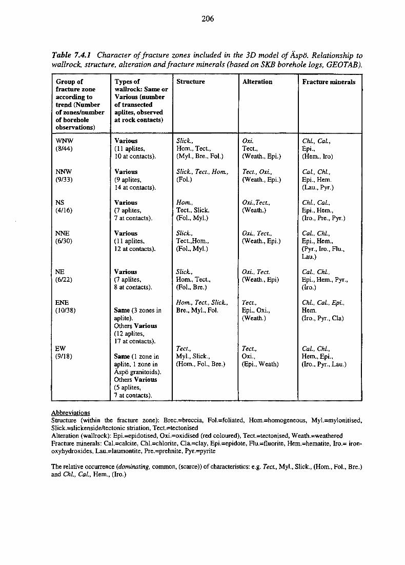
206
Table 7.4.1 Character of fracture zones included in the 3D model of Aspd. Relationship towallrock, structure, alteration and fracture minerals (based on SKB borehole logs, GEOTAB).
Group offracture zoneaccording totrend (Numberof zones/numberof boreholeobservations)
WNW(8/44)
NNW(9/33)
NS(4/16)
NNE(6/30)
NE(6/22)
ENE(10/38)
EW(9/18)
Types ofwallrock: Same orVarious (numberof transectedaplites, observedat rock contacts)
Various(11 aplites,10 at contacts).
Various(9 aplites,14 at contacts).
Various(7 aplites,7 at contacts).
Various(11 aplites,12 at contacts).
Various(7 aplites,8 at contacts).
Same (3 zones inaplite).Others Various(12 aplites,17 at contacts).
Same (1 zone inaplite, 1 zone inAspo granitoids).Others Various(5 aplites,7 at contacts).
Structure
Slick.,Horn., Tect.,(Myl., Bre., Fol.)
Slick., Tect., Horn.,(Fol.)
Horn.,Tect., Slick.(Fol., Myl.)
Slick.,Tect.,Hom.,(Fol., Myl.)
Slick.,Horn., Tect.,(Fol., Bre.)
Horn., Tect., Slick.,Bre., Myl., Fol.
Tect.,Myl., Slick.,(Horn., Fol., Bre.)
Alteration
Oxi.Tect.,(Weath., Epi.)
Tect., Oxi.,(Weath., Epi.)
Oxlject.,(Weath.)
Oxi., Tect.,(Weath., Epi.)
Oxi., Tect.(Weath., Epi)
Tect.,Epi., Oxi.,(Weath.)
Tect.,Oxi.,(Epi., Weath)
Fracture minerals
Chi, Cal,Epi.,(Hem., Iro)
Cal, Chi,Epi., Hem.(Lau., Pyr.)
Chi, Cal,Epi., Hem.,(Iro., Pre., Pyr.)
Cal, Chi,Epi., Hem.,(Pyr., Iro., Flu.,Lau.)
Cal, Chi,Epi., Hem., Pyr.,(Iro.)
Chi, Cal, Epi.,Hem.(Iro., Pyr., Cla)
Cal, Chi,Hem., Epi.,(Iro., Pyr., Lau.)
AbbreviationsStructure (within the fracture zone): Brec.=breccia, Fol.=foliated, Hom.=homogeneous, Myl.=mylonitised,Slick.=slickenside/tectonic striation, Tect.=tectonisedAlteration (wallrock): Epi.=epidotised, Oxi.=oxidised (red coloured), Tect.=tectonised, Weath.=weatheredFracture minerals: Cal.=calcite, Chl.=chlorite, Cla.=clay, Epi.=epidote, Flu.=fluorite, Hem.=hematite, Iro.= iron-oxyhydroxides, Lau.=laumontite, Pre.=prehnite, Pyr.=pyrite
The relative occurrence (dominating, common, (scarce)) of characteristics: e.g. Tect., Myl., Slick., (Horn., Fol., Bre.)and Chi, Cal, Hem., (Iro.)
207
Investigations of fracture minerals at Aspo, mainly performed by Tullborg et al. (1991) arealso discussed by Andersson (1996b) with the following conclusions:
• Zones of hematite are observed in the granite. They were probably formed underhydrothermal conditions over 100 Ma ago and not by more recent oxidation ofmagnetite in contact with water.
• Clay minerals, e.g. of the illite/smectite type, are found together with crushed rockin zones of up to 1 m width. Kaolinite is not common. Ingrowth of pyrite in thesehas probably occurred during the last 300 Ma and this age correlates with the latesthydrothermal episode. An important question is whether these zones are highlyconductive, or whether the clays have sealed the fractures.
• Goethite is probably better correlated to groundwater flow than hematite, whilesiderite is not found.
• Calcite, which is definitely correlated with flow, has a low content of iron.
• Fluorite is common, explaining the presence of fluoride in the groundwater.
• Epidote, quartz and chlorite (iron-rich) are most likely of hydrothermal origin andof the same age as the Gotemar granite (1400 Ma). Epidote is present in largeamounts close to the fracture surfaces, which indicates that it has been formed veryearly in the fracture history, and probably does not contribute to the watercomposition.
• Zeolites like laumontite and prehnite are of more recent hydrothermal origin.
• Calcite, chlorite and epidote have been found to dominate the filling mineralogy ofconductive fractures (not zones) in 'fine-grained granite', Aspo diorite and Smalandgranite. There are very few observations of pure iron minerals (e.g. hematite,hydroxides, etc.)
7.4.3 Groundwater Chemistry
The geochemical characterisation of groundwaters near the Aspo Hard Rock Laboratorywithin the context of the SITE-94 project is described in detail by Glynn and Voss (1996).The principal objectives of this study are to use the available geochemical and isotopic datafrom Aspo boreholes, provided by SKB, to determine:
• the origins of groundwaters in the vicinity of Aspo• the processes responsible for the hydrochemical evolution of these waters• residence times of different waters in the rock• the structural and hydrogeological implications of variations in groundwater
chemistry and isotopic compositions• the implications of mineralogical distributions for past groundwater environments.
208
The approach used is to carry out a detailed hydrochemical and isotopic evaluation of 'firststrike' and well-characterized groundwaters, relating this to the location of groundwatersamples with respect to rock structure and mineralogy. An important aid to this evaluationis thermodynamic modelling of rock-water chemical equilibria to establish how theseinteractions have controlled the evolution of different bodies of groundwater within therock.
Groundwaters from Aspo island and from the surrounding areas (Laxemar, Avro) areclassified into five different water types based on their chemical and stable isotopecharacteristics:
(1) 'recent waters',(2) waters with close to 5 g/1 chloride,(3) 'deep waters',(4) glacial meltwaters,(5) 'seawater imprint' waters.
Deuterium contents and chloride concentrations are the primary variables used to classifymost of the groundwaters (Figure 7.4.1). Isotope data are only available for CCC and SPTdata types and for shallow percussion-drilled boreholes. (CCC and SPT are SKB'snomenclature for 'completely characterised' water samples and for waters 'sampled duringpumping tests'.)
Waters 'sampled during drilling' (SDD waters following SKB's nomenclature) and mostwater samples taken during later groundwater monitoring were not analysed for stableisotopes and are therefore classified using different variables, although this secondaryclassification is consistent with the first. Chloride concentrations are used as the primaryvariable to separate water Types 1, 2 and 3. 'Seawater imprint' waters are determined onthe basis of their Mg/Ca and K/Na ratios. The 'glacial meltwaters' (Type 4) in the CCC andSPT data groups do not have any distinctive chemical characteristics and, lacking isotopicdata, none of the SDD and monitoring waters can be classified into water Type 5.
All groundwaters considered were sampled before the start of the excavation of the Aspotunnel in October 1990. The excavation of the tunnel is shown by Glynn and Voss (1996)to have had a significant effect on groundwater chemistry, lowering chloride concentrationsin many borehole sections (Figure 7.4.2).
Similarly, hydrogeological testing (pump tests, interference tests, etc.) and groundwatersampling activities also appear to have had a significant dilution effect on the overallsalinity of the groundwaters. Chloride concentrations in SDD samples, corrected fordilution by drilling waters, are estimated to have been about two times higher on averageat any given depth than chloride concentrations for 'representative ground-water samples'(SKB's terminology) in the CCC and SPT data groups (Figures 7.4.3 and 7.4.4). SDDsamples also exhibit a wider spread of chloride concentrations at given depths, comparedto the CCC and SPT samples. Although sample section lengths are usually significantlygreater for SDD samples than for CCC and SPT samples, these latter samples show a muchsmoother distribution of chloride concentrations with depth, as if the groundwaters hadbeen partially 'homogenised' by the pumping and sampling activities.
209
The distribution of the five water-chemistry Types is investigated in relation to thedistribution of fracture surfaces (structures) in the structural model built by Voss et al.(1996). No correlation is found between water types and individual structures. Eachstructure is found to contain more than one type of groundwater, implying that flowpathsconsist of a series of segments through multiple structures. Pressure propagation datacollected during hydrogeological interference testing also offer support for complex multi-fracture flowpaths. Generally, salinity stratification is observed, even within individualstructures. More dilute, 'recent' waters are found in shallow borehole sections, the moresaline '5 g/L chloride' waters are found at intermediate depths near or at less than 500 mdepth and the most saline 'deep' waters are found between 500 m and 1000 m depth.
The 'seawater imprint' waters are all found near the perimeter of Aspo and each of thewaters could be explained by the presence of at least one or more structures which extendinto the Baltic sea floor. Most Aspo groundwaters, however, do not show any 'seawaterimprint'. This indicates that the Aspo area is a discharge area for most of the salinegroundwaters present. Recharge of dilute waters (part of the 'recent' water group) onlyoccurs at shallow depth (less than 100 metres).
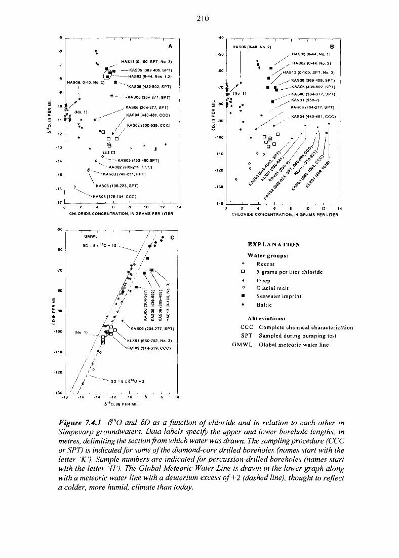
210
HAS06, 0-40, No. 2)
(No. 1)
*D
HAS13 (0-100, SPT. No. 3)
—KAS06 (389-406, SPT)
- HAS02 (0-44, Nos. 1,2)
"~~KAS06 (439-602, SPT)
-KAS06 (304-377, SPT)
KAS06 (204-277, SPT)
KAS04 (440-481, CCC)
KAS02 (530-535, CCC)
D D
CD D0
0 ——- KAS03 (453-480.SPT)
^ " ^ KAS02 (202-215, CCC)
""""""" KAS03 (248-251, SPT)
KAS03 (196-223, SPT)
KAS03 (129-134, CCC)
2 4 6 8 10 12
CHLORIDE CONCENTRATION, IN GRAMS PER LITER
BHAS02 (0-44, No. 1)
HAS02 (0-44, No. 2)
HAS13 (0-100, SPT, No. 3)
KAS06 (389-406, SPT)KAS06 (439-602, SPT)
KAS06 (304-377, SPT)
KAV01 (558?)
KAS06 (204-277, SPT)
KAS04 (440-481, CCC)
10 12
CHLORIDE CONCENTRATION, IN GRAMS PER LITER
(No 1)
KLX01 (680-702, No. 3)
KAS02 (314-319, CCC)
6D = 8 x 8 " O + 2
/
-16 -12 -10
EXPLANATION
Water groups:* RecentQ 5 grams per liter chloride
* Deep0 Glacial melt• Seawater imprint
* Baltic
Abreviations:
CCC Complete chemical characterization
SPT Sampled during pumping test
GMWL Global meteoric water line
6 O, IN PER MIL
Figure 7.4.1 6IHO and 5D as a function of chloride and in relation to each other inSimpevarp groundwaters. Data labels specify the upper and lower borehole lengths, inmetres, delimiting the section from which water was drawn. The sampling procedure (CCCor SPT) is indicated for some of the diamond-core drilled boreholes (names start with theletter 'K'). Sample numbers are indicated for percussion-drilled boreholes (names startwith the letter 'H'). The Global Meteoric Water Line is drawn in the lower graph alongwith a meteoric water line with a deuterium excess of +2 (dashed line), thought to reflecta colder, more humid, climate than today.
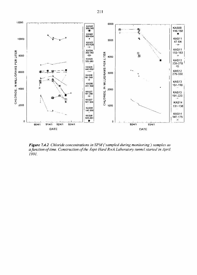
211
12000
KAS02309-345
KAS02800-854
KAS03533-626
• • • • * -
KAS04332-392
-B-
KAS05320-380
KAS05440-550
KAS06191-249
o
KAS06431-500
KAS07191-290
KAS07501-604
KAS08140-200
KAS08503-601
MS
PE
R L
ITE
R-L
fGR
A
I
RID
E, !
CH
LO
6000
5000
4000
3000
; 2000
1000
KAS09116-150
-B--
KAS1147-64
KAS11153-183
KAS12235-278
KAS12279-330
KAS13151-190
KAS13191-220
KAS14
131-138
KAS14147-175
x
90/4/1 91/4/1 92/4/1 93/4/1
DATE
92/4/1 93/4/1
DATE
Figure 7.4.2 Chloride concentrations in SPM ('sampled during monitoring') samples asa function of time. Construction of the Aspo Hard Rock Laboratory tunnel started in April1991.
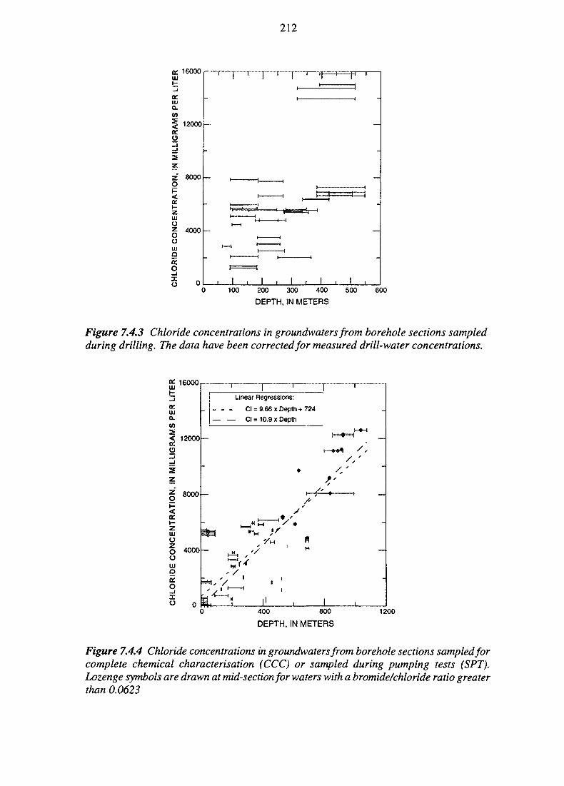
212
£ 16000W
200 300 400 500
DEPTH, IN METERS
600
Figure 7.4.3 Chloride concentrations in groundwaters from borehole sections sampledduring drilling. The data have been corrected for measured drill-water concentrations.
UJ
a.w
16000
12000-
o<a:zUJ
oooUJ2tco_JXo
8000 -
4 0 0 0 -
_ _ .
-
-
- x
H^
1 1 'Linear Regressions:
Cl = 9.66 x Depth +
— Cl = 10.9 x Depth
1 |I
H l l1 1 i
724
RH
1 '
—-
-
400 800
DEPTH, IN METERS1200
Figure 7.4.4 Chloride concentrations in groundwaters from borehole sections sampled forcomplete chemical characterisation (CCC) or sampled during pumping tests (SPT).Lozenge symbols are drawn at mid-section for waters with a bromide/chloride ratio greaterthan 0.0623
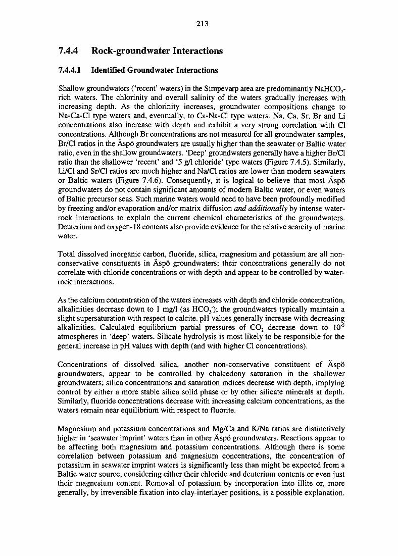
213
7.4.4 Rock-groundwater Interactions
7.4.4.1 Identified Groundwater Interactions
Shallow groundwaters ('recent' waters) in the Simpevarp area are predominantly NaHCO3-rich waters. The chlorinity and overall salinity of the waters gradually increases withincreasing depth. As the chlorinity increases, groundwater compositions change toNa-Ca-Cl type waters and, eventually, to Ca-Na-Cl type waters. Na, Ca, Sr, Br and Liconcentrations also increase with depth and exhibit a very strong correlation with Clconcentrations. Although Br concentrations are not measured for all groundwater samples,Br/Cl ratios in the Aspo groundwaters are usually higher than the seawater or Baltic waterratio, even in the shallow groundwaters. 'Deep' groundwaters generally have a higher Br/Clratio than the shallower 'recent' and '5 g/1 chloride' type waters (Figure 7.4.5). Similarly,Li/Cl and Sr/Cl ratios are much higher and Na/Cl ratios are lower than modern seawatersor Baltic waters (Figure 7.4.6). Consequently, it is logical to believe that most Aspogroundwaters do not contain significant amounts of modern Baltic water, or even watersof Baltic precursor seas. Such marine waters would need to have been profoundly modifiedby freezing and/or evaporation and/or matrix diffusion and additionally by intense water-rock interactions to explain the current chemical characteristics of the groundwaters.Deuterium and oxygen-18 contents also provide evidence for the relative scarcity of marinewater.
Total dissolved inorganic carbon, fluoride, silica, magnesium and potassium are all non-conservative constituents in Aspo groundwaters; their concentrations generally do notcorrelate with chloride concentrations or with depth and appear to be controlled by water-rock interactions.
As the calcium concentration of the waters increases with depth and chloride concentration,alkalinities decrease down to 1 mg/1 (as HCO3"); the groundwaters typically maintain aslight supersaturation with respect to calcite. pH values generally increase with decreasingalkalinities. Calculated equilibrium partial pressures of CO2 decrease down to 10"5
atmospheres in 'deep' waters. Silicate hydrolysis is most likely to be responsible for thegeneral increase in pH values with depth (and with higher Cl concentrations).
Concentrations of dissolved silica, another non-conservative constituent of Aspogroundwaters, appear to be controlled by chalcedony saturation in the shallowergroundwaters; silica concentrations and saturation indices decrease with depth, implyingcontrol by either a more stable silica solid phase or by other silicate minerals at depth.Similarly, fluoride concentrations decrease with increasing calcium concentrations, as thewaters remain near equilibrium with respect to fluorite.
Magnesium and potassium concentrations and Mg/Ca and K/Na ratios are distinctivelyhigher in 'seawater imprint' waters than in other Aspo groundwaters. Reactions appear tobe affecting both magnesium and potassium concentrations. Although there is somecorrelation between potassium and magnesium concentrations, the concentration ofpotassium in seawater imprint waters is significantly less than might be expected from aBaltic water source, considering either their chloride and deuterium contents or even justtheir magnesium content. Removal of potassium by incorporation into illite or, moregenerally, by irreversible fixation into clay-interlayer positions, is a possible explanation.
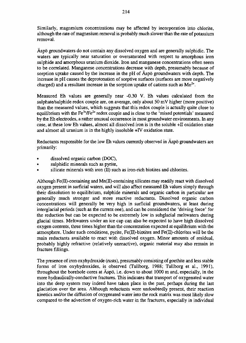
214
Similarly, magnesium concentrations may be affected by incorporation into chlorite,although the rate of magnesium removal is probably much slower than the rate of potassiumremoval.
Aspo groundwaters do not contain any dissolved oxygen and are generally sulphidic. Thewaters are typically near saturation or oversaturated with respect to amorphous ironsulphide and amorphous uranium dioxide. Iron and manganese concentrations often seemto be correlated. Manganese concentrations decrease with depth, presumably because ofsorption uptake caused by the increase in the pH of Aspo groundwaters with depth. Theincrease in pH causes the deprotonation of sorptive surfaces (surfaces are more negativelycharged) and a resultant increase in the sorption uptake of cations such as Mn2+.
Measured Eh values are generally near -0.30 V. Eh values calculated from thesulphate/sulphide redox couple are, on average, only about 50 mV higher (more positive)than the measured values, which suggests that this redox couple is actually quite close toequilibrium with the Fe37Fe2+ redox couple and is close to the 'mixed potentials' measuredby the Eh electrodes, a rather unusual occurrence in most groundwater environments. In anycase, at these low Eh values, almost all dissolved iron is in the soluble +n oxidation stateand almost all uranium is in the highly insoluble +FV oxidation state.
Reductants responsible for the low Eh values currently observed in Aspo groundwaters areprimarily:
• dissolved organic carbon (DOC),• sulphidic minerals such as pyrite,• silicate minerals with iron (II) such as iron-rich biotites and chlorites.
Although Fe(II)-containing and Mn(H)-containing silicates may readily react with dissolvedoxygen present in surficial waters, and will also affect measured Eh values simply throughtheir dissolution to equilibrium, sulphide minerals and organic carbon in particular aregenerally much stronger and more reactive reductants. Dissolved organic carbonconcentrations will generally be very high in surficial groundwaters, at least duringinterglacial periods (such as the current one), and can be considered the 'driving force' forthe reduction but can be expected to be extremely low in subglacial meltwaters duringglacial times. Meltwaters under an ice cap can also be expected to have high dissolvedoxygen contents, three times higher than the concentration expected at equilibrium with theatmosphere. Under such conditions, pyrite, Fe(II)-biotites and Fe(II)-chlorites will be themain reductants available to react with dissolved oxygen. Minor amounts of residual,probably highly refractive (relatively unreactive), organic material may also remain infracture fillings.
The presence of iron oxyhydroxide (rusts), presumably consisting of goethite and less stableforms of iron oxyhydroxides, is observed (Tullborg, 1988; Tullborg et al., 1991),throughout the borehole cores at Aspo, i.e. down to about 1000 m and, especially, in themore hydraulically-conductive fractures. This indicates that transport of oxygenated waterinto the deep system may indeed have taken place in the past, perhaps during the lastglaciation over the area. Although reductants were undoubtedly present, their reactionkinetics and/or the diffusion of oxygenated water into the rock matrix was most likely slowcompared to the advection of oxygen-rich water in the fractures, especially in individual

215
fractures (as opposed to 'fracture zones' or wide 'crushed-rock' structures). The occurrenceof such oxygenated waters is discussed further and modelled in Section 10.4.
Although dissolved uranium concentrations are usually low in sampled groundwaters(between 0.1 and 0.7 mg/1), the concentration of uranium in fracture fillings (average15 ppm) is about three times higher than its concentration in the parent rocks. Uraniumconcentrations, together with dissolved radon measurements, allow an estimation of theaverage effective surface area of 3.1 m2 per litre of fluid, or an 'average' fracture apertureof 0.65 mm, for the Aspo groundwater system. These estimates are based on previouscalculations made for groundwaters from the Stripa mine in Sweden, and from theCarmenellis granite in Cornwall (Andrews et al., 1988). The effective surface area can beused for estimation of the specific surface area parameter a,, i.e. the flow-wetted surfacearea per volume of rock (see Section 10.3.6).
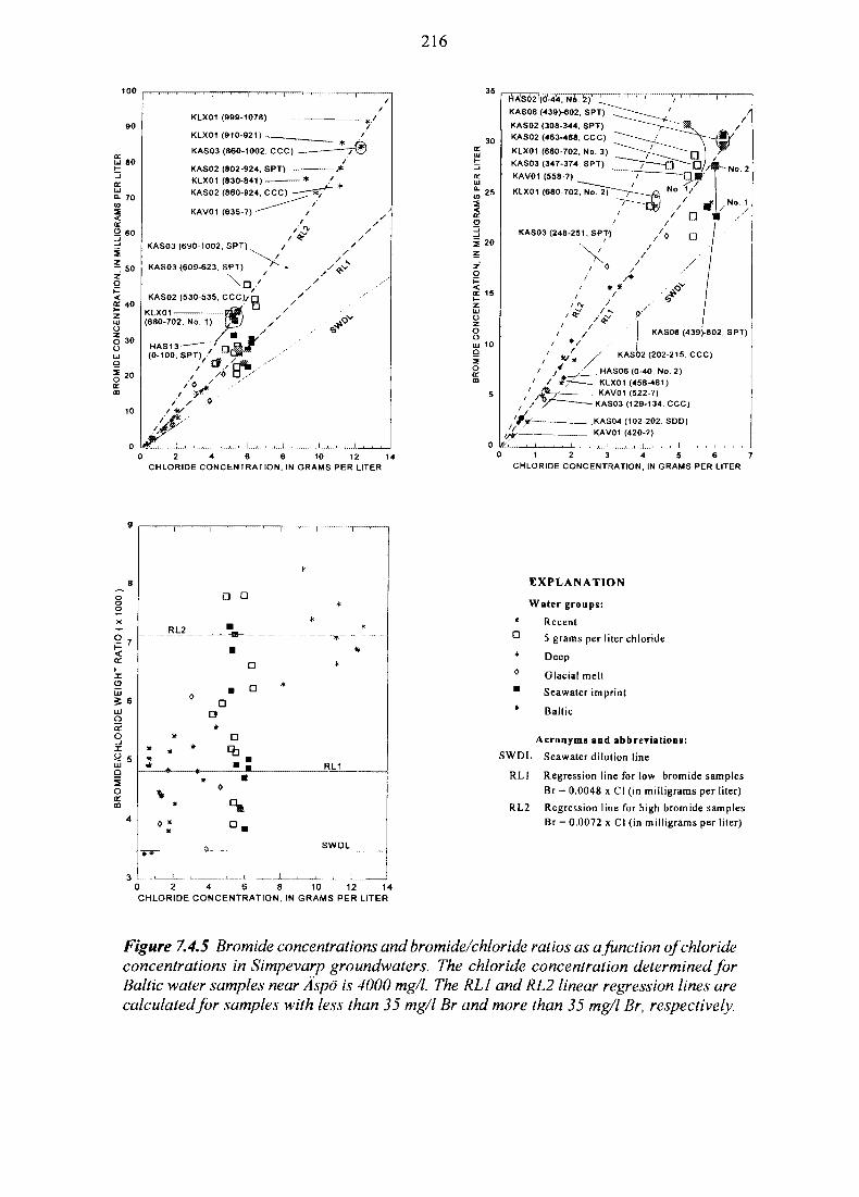
216
100
KLX01 (999-1078)
KLX01 (910-921)
KAS03 (860-1002, CCC)
KAS02 (802-924, SPT)
KLX01 (830-841) — — *
KAS02 (860-924, CCC) — - —
KAS06 (439)-602, SPT)
KAS02 (308-344, SPT)
KAS02 (463-468, CCC)
KLX01 (680-702, No. 3)
KAS03 (347-374, SPT)
KAV01 (558-?)
KLX01 (680-702, No. 2)
KAS03 (248-251, SPT4
KAS06 (439)-602, SPT)
KAS02 (202-215. CCC)
HAS06 (0-40, No 2)
KLX01 (456-461)
KAV01 (522-?)
KAS03 (129-134, CCC)
KAS04 (102-202. SDD)
KAV01 (420-?)
CHLORIDE CONCENTRATION, IN GRAMS PER LITER CHLORIDE CONCENTRATION, IN GRAMS PER LITER
¥ 7RL2
D D
D
D
* * **
o *
RL1
SWDL
0 2 4 6 8 10 12 14CHLORIDE CONCENTRATION, IN GRAMS PER LITER
EXPLANATION
Water groups:
* Recent
^ 5 grams per liter chloride+ Deep0 Glacial meltm Seawater imprint
* Baltic
Acronyms and abbreviations:
SWDL Seawater dilution line
RLI Regression line for low bromide samplesBr = 0.0048 x Cl (in milligrams per liter)
RL2 Regression line for high bromide samplesBr = 0.0072 x Cl (in milligrams per liter)
Figure 7.4.5 Bromide concentrations and bromide/chloride ratios as a function of chlorideconcentrations in Simpevarp groundwaters. The chloride concentration determined forBaltic water samples near Aspo is 4000 mg/l. The RLI and RL2 linear regression lines arecalculated for samples with less than 35 mg/l Br and more than 35 mg/l Br, respectively.
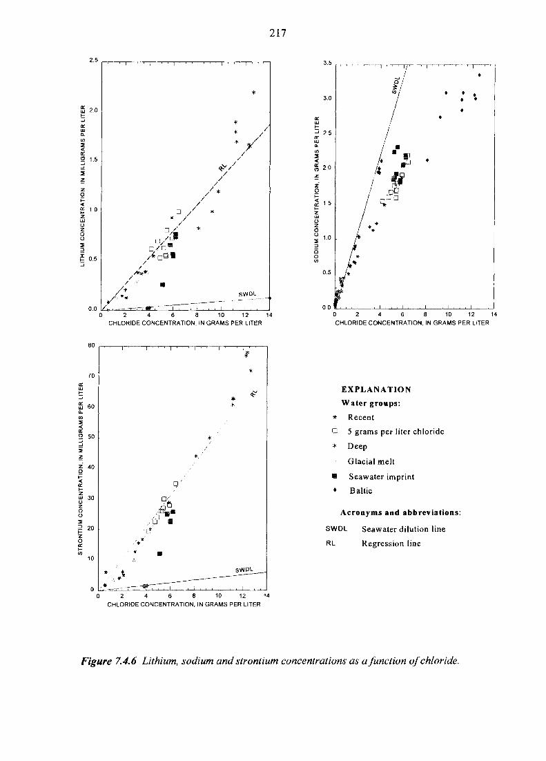
217
0.0
CHLORIDE CONCENTRATION, IN GRAMS PER LITER0 2 4 6 8 10 12 14CHLORIDE CONCENTRATION. IN GRAMS PER LITER
EXPLANATION
Water groups:
* Recent
d 5 grams per liter chloride
* Deep
Glacial melt
s Seawater imprint
* Baltic
Acronyms and abbreviations:
SWDL Seawater dilution line
RL Regression line
0 2 4 6 8 10 12 14CHLORIDE CONCENTRATION, IN GRAMS PER LITER
Figure 7.4.6 Lithium, sodium and strontium concentrations as a function of chloride.

218
7.4.4.2 Simulation of Aspo Groundwaters
Geochemical modelling can be used for prediction of possible future changes and theconsistent description of the variability in geochemical parameters needed for estimationof barrier performance and radionuclide behaviour. For a given site, this modelling mustbe based on an understanding of how observed geochemical phenomena have developeddue to past and present processes and, in particular, regarding which solids are reactive onthe relevant timescales. Part of this understanding can be obtained by attempting thesimulation of the observed concentrations of important constituents in the groundwater.This section presents the results of such simulations for the conditions at Aspo.
The waters sampled from boreholes at Aspo have been formed by complicated processesoccurring during extended time intervals. The different waters have been present in fracturesystems for a long time and might be assumed to have reached equilibrium with respect toat least some of the fracture minerals. This also holds for the Type waters, as defined inSection 7.4.3. However, as a consequence of the natural flow and of the forced flow frompumping during boring, rinsing and sampling, the Type waters have been mixed to formthe waters sampled from the boreholes. This might explain linear relationships as shownin Figure 7.4.7, where the waters from KAS03 down to 600 m may be interpreted asmixtures of waters from 130 and 600 m. As is discussed above, a choice of five types ofwaters is enough to describe the D and Cl concentrations observed in a large number ofsampled waters.
Although groundwater models which only take mixing into account may be successful inexplaining concentrations of some elements, the concentrations of most elements cannotbe explained in this simple way. An example is seen in Figure 7.4.8, where it is obviousthat the iron concentrations at intermediate levels cannot be obtained simply by mixingwaters from levels 130 and 600 m. The same holds for several other elements, e.g. K, C,Ca, Mg as well as for parameters such as pH and pE. Obviously, reactions between theaqueous species and with fracture minerals play an important role in the formation ofgroundwaters at different levels from Type waters. For simulation of this process bothmixing and reactions have to be considered.
For this purpose an extended version of the PHREEQE geochemical code (Parkhurst et al.,1985) is used. This code is incorporated in the CRACKER code, which simulates themixing process over different scales along transport paths for groundwater (Emren, 1993;Emren, 1996a). In CRACKER, fracture minerals are assumed to be distributed randomlyacross a fracture plane in accordance with observed or reasonable abundances. Waterflowing in a fracture between two surfaces is supposed to equilibrate locally with mineral(s)within diffusion distance at the time scale considered. While the water moves, it is mixedwith water from the neighbourhood. Since the mineral sets found in nature normally containincompatible minerals, i.e. Gibb's phase rule is violated, global equilibrium is rarelypossible. This does not prevent a local equilibrium with respect to a small subset ofminerals.
The process of sampling is simulated by mixing about 900 equilibrium waters fromdifferent locations in the fracture. No mineral-water reactions are allowed to occur in thesimulation of this mixing process, but speciation reactions in the mixed water are supposedto be fast enough and are thus modelled by the CRACKER code.
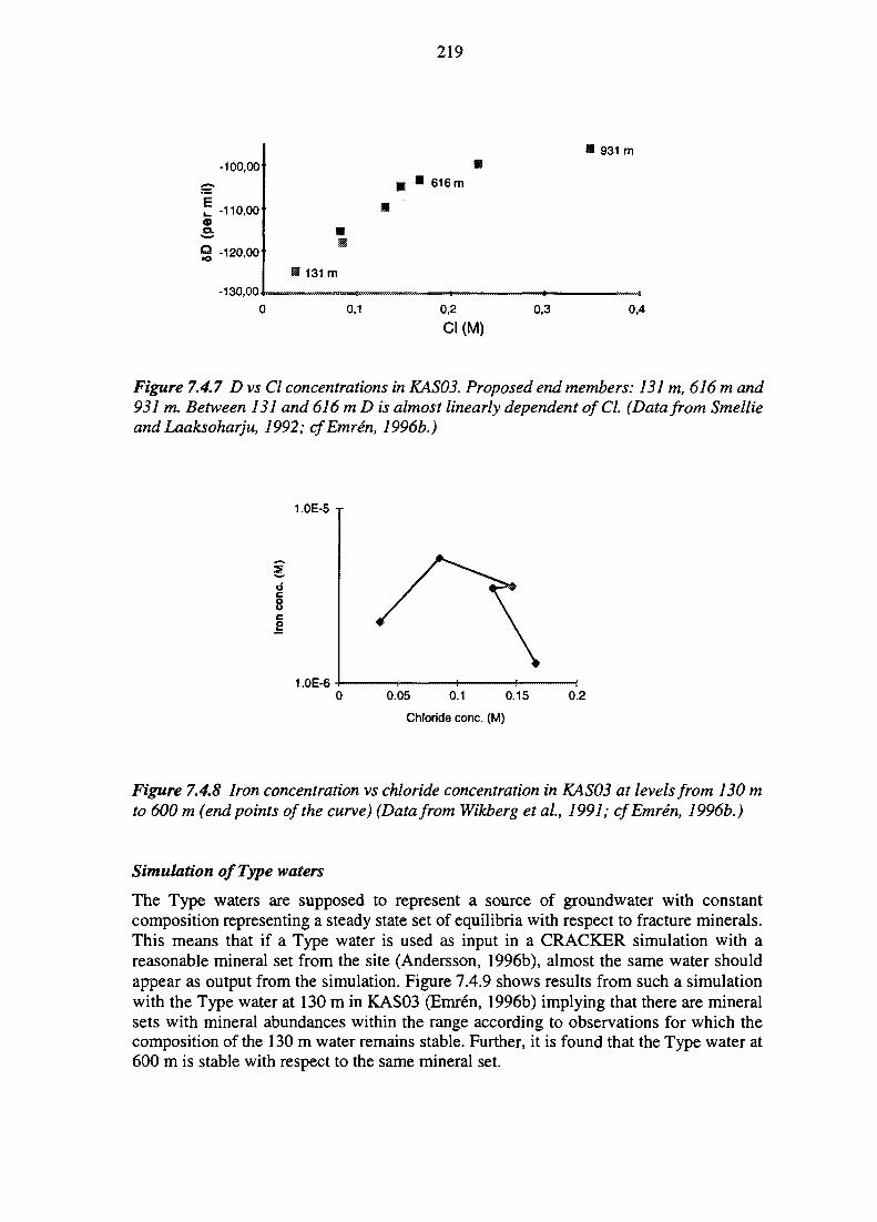
219
-100,00
-110,0003g -120,00
-130,00
931 m
616 m
131 m
0 0,1 0,2
CI(M)0,3 0,4
Figure 7.4.7 D vs Cl concentrations in KAS03. Proposed end members: 131 m, 616 m and931 m. Between 131 and 616 m D is almost linearly dependent of Cl. {Data from Smellieand Laaksoharju, 1992; cfEmren, 1996b.)
1.0E-5 T
1.0E-60.05 0.1 0.15
Chloride cone. (M)
0.2
Figure 7.4.8 Iron concentration vs chloride concentration in KAS03 at levels from 130 mto 600 m (end points of the curve) (Data from Wikberg et al, 1991; cfEmren, 1996b.)
Simulation of Type waters
The Type waters are supposed to represent a source of groundwater with constantcomposition representing a steady state set of equilibria with respect to fracture minerals.This means that if a Type water is used as input in a CRACKER simulation with areasonable mineral set from the site (Andersson, 1996b), almost the same water shouldappear as output from the simulation. Figure 7.4.9 shows results from such a simulationwith the Type water at 130 m in KAS03 (Emren, 1996b) implying that there are mineralsets with mineral abundances within the range according to observations for which thecomposition of the 130 m water remains stable. Further, it is found that the Type water at600 m is stable with respect to the same mineral set.
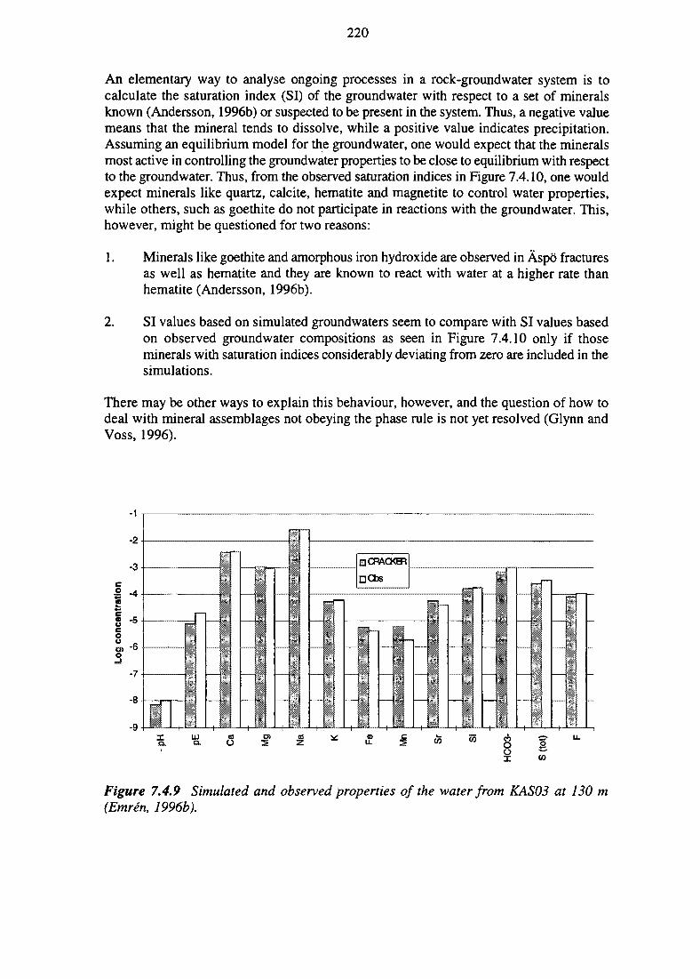
220
An elementary way to analyse ongoing processes in a rock-groundwater system is tocalculate the saturation index (SI) of the groundwater with respect to a set of mineralsknown (Andersson, 1996b) or suspected to be present in the system. Thus, a negative valuemeans that the mineral tends to dissolve, while a positive value indicates precipitation.Assuming an equilibrium model for the groundwater, one would expect that the mineralsmost active in controlling the groundwater properties to be close to equilibrium with respectto the groundwater. Thus, from the observed saturation indices in Figure 7.4.10, one wouldexpect minerals like quartz, calcite, hematite and magnetite to control water properties,while others, such as goethite do not participate in reactions with the groundwater. This,however, might be questioned for two reasons:
1. Minerals like goethite and amorphous iron hydroxide are observed in Aspo fracturesas well as hematite and they are known to react with water at a higher rate thanhematite (Andersson, 1996b).
2. SI values based on simulated groundwaters seem to compare with SI values basedon observed groundwater compositions as seen in Figure 7.4.10 only if thoseminerals with saturation indices considerably deviating from zero are included in thesimulations.
There may be other ways to explain this behaviour, however, and the question of how todeal with mineral assemblages not obeying the phase rule is not yet resolved (Glynn andVoss, 1996).
Figure 7.4.9 Simulated and observed properties of the water from KAS03 at 130 m(Emren, 1996b).
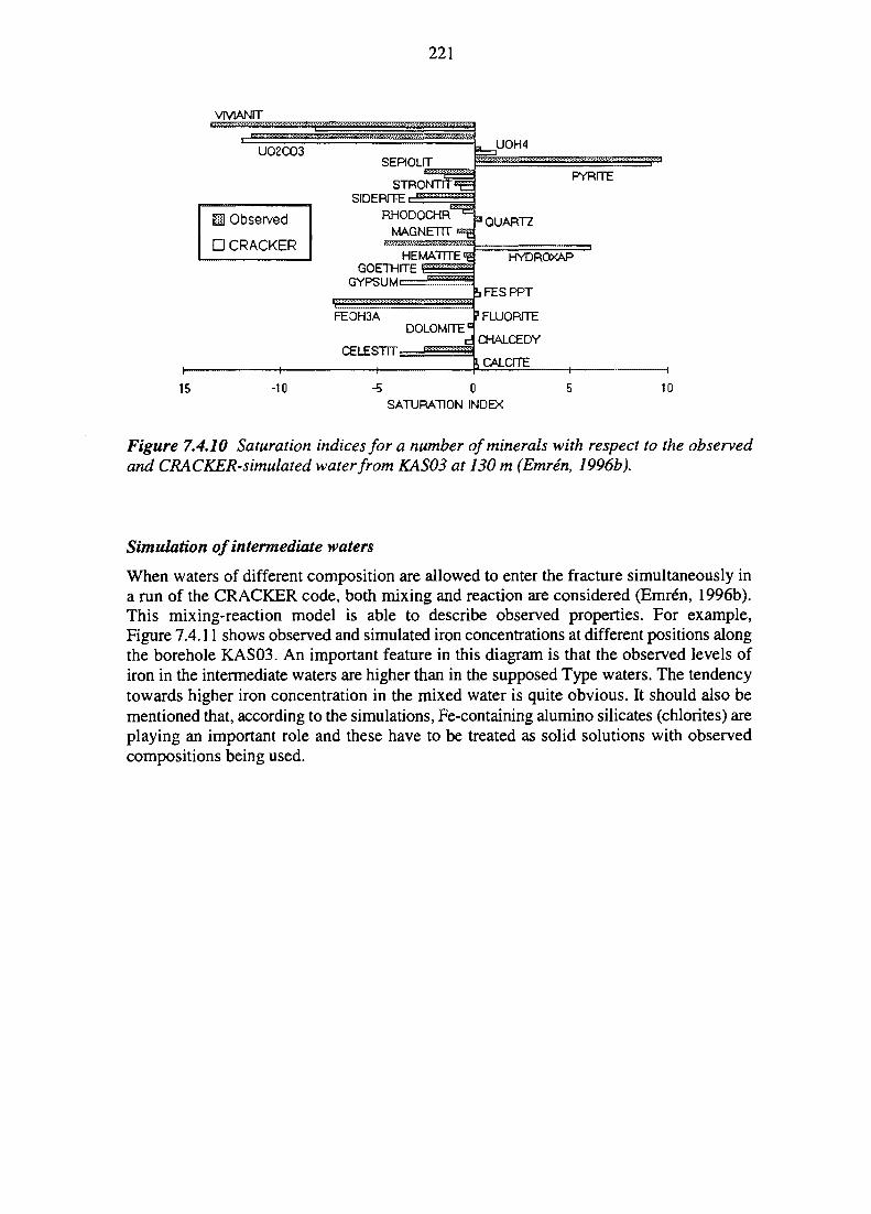
221
VMANIT
UO2CO3
H Observed
• CRACKER
SEPI0L1T
STRONTTT^SIDER1TE t
RHODOCHRMAGNETTT^
HEMATITE 1GOETHITE EJgggSS
GYPSUM t = ^ ^ ^
FEOH3A
CELESTIT:
DOLOMITE1
UOH4
PYRITE
3 QUARTZ
HYDROXAP
b FES PPT
1 FLUORITE
CHALCEDY
!, CALCITE
15 -10 -5 0SATURATION INDEX
10
Figure 7.4.10 Saturation indices for a number of minerals with respect to the observedand CRACKER-simulated water from KAS03 at 130 m (Emren, 1996b).
Simulation of intermediate waters
When waters of different composition are allowed to enter the fracture simultaneously ina run of the CRACKER code, both mixing and reaction are considered (Emren, 1996b).This mixing-reaction model is able to describe observed properties. For example,Figure 7.4.11 shows observed and simulated iron concentrations at different positions alongthe borehole KAS03. An important feature in this diagram is that the observed levels ofiron in the intermediate waters are higher than in the supposed Type waters. The tendencytowards higher iron concentration in the mixed water is quite obvious. It should also bementioned that, according to the simulations, Fe-containing alumino silicates (chlorites) areplaying an important role and these have to be treated as solid solutions with observedcompositions being used.
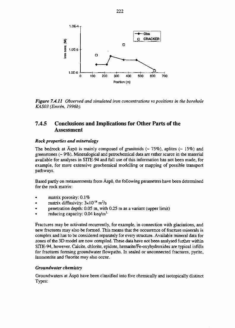
222
LOE-4-r
-4—Obs• CRACKER
1.0E-6100 200 300
Position (m)
400 500 600 700
Figure 7.4.11 Observed and simulated iron concentrations vs positions in the boreholeKAS03 (Emren, 1996b).
7.4.5 Conclusions and Implications for Other Parts of theAssessment
Rock properties and mineralogy
The bedrock at Aspo is mainly composed of granitoids (~ 75%), aplites (~ 15%) andgreenstones (~ 9%). Mineralogical and petrochemical data are rather scarce in the materialavailable for analyses in SITE-94 and full use of this information has not been made, forexample, for more extensive geochemical modelling or mapping of possible transportpathways.
Based partly on measurements from Aspo, the following parameters have been determinedfor the rock matrix:
• matrix porosity: 0.1 %• matrix diffusivity: 3xl0'14 m2/s• penetration depth: 0.05 m, with 0.25 m as a variant (upper limit)• reducing capacity: 0.04 keq/m3
Fractures may be activated recurrently, for example, in connection with glaciations, andnew fractures may also be formed. This means that the occurrence of fracture minerals iscomplex and has to be considered separately for every structure. Available mineral data forzones of the 3D model are now compiled. These data have not been analysed further withinSITE-94, however. Calcite, chlorite, epidote, hematite/Fe-oxyhydroxides are typical infillsfor fractures forming groundwater flowpaths. In sealed or unconnected fractures, pyrite,laumontite and fluorite may also occur.
Groundwater chemistry
Groundwaters at Aspo have been classified into five chemically and isotopically distinctTypes:
223
1. 'recent' waters2. '5 g/1 chloride waters'3. 'deep' waters4. 'seawater imprint' waters5. 'glacial meltwaters'.
The classification is made primarily on the basis of chloride and deuterium content, and,when impossible because of missing stable isotope analyses, the classification is made onthe basis of chloride concentrations and Mg/Ca and K/Na ratios.
Rock-water interaction processes
Shallow waters are predominantly of the NaHCO3 type. The chlorinity/salinity increaseswith depth to around 5 g Cl/1 at 500 m depth and the groundwater composition graduallychanges to Na-Ca-Cl and Ca-Na-Cl. Most Aspo groundwaters do not contain significantamounts of modern Baltic water and they do not contain any dissolved oxygen. The watersare typically near saturation or oversaturated with respect to amorphous iron sulphide andamorphous uranium dioxide. Measured Eh values are generally near -0.30 V and fall closeto both the sulphate/sulphide and the ferric/ferrous redox couples. The following reductantsare primarily responsible for the currently observed low Eh values:
• dissolved organic carbon (DOC)• sulphidic minerals such as pyrite• silicate minerals with ferrous iron such as iron-rich biotites and chlorites.
The presence of 'rusts' (iron oxyhydroxides) has been observed along all the boreholescores, i.e. down to about 1000 m. This may be taken as an indication of the ingress ofoxygenated waters at these depths in the past, probably in connection with glaciations.
Geochemical simulations have shown that the analysed groundwater compositions arecompatible with observed mineral abundances. These simulations also indicate that chloriteand iron oxyhydroxides are important reactive solids in the geochemical system at Aspo.
Implications for other parts of the assessment
The geochemical site evaluation presented in this section is used as input to Section 10.4,which extracts the parameter values and other information which are relevant for thesubsequent analysis of chemical features and processes in the assessment. This information,in turn, is used as one of the inputs in the evaluation of canister stability, bufferperformance, fuel dissolution and radionuclide migration discussed primarily in Chapters11 and 12.
Implications for site investigation
The majority of chemical and isotopic data were collected as part of the "CompleteChemical Characterisation" (CCC) and "Sampling during Pumping Test" (SPT) samplingefforts. The data measured at these efforts show a comprehensive characterisation.
Unfortunately, most of the "CCC" and "SPT" samples were collected after extensivepumping had been conducted either in the same borehole or in its vicinity. The pumping
224
activities appear to have resulted in significant dilution and homogenisation of the Aspogroundwaters. Extensive pumping was needed to reduce the oxygenated drilling watercontent of the groundwaters as to be able to obtain meaningful concentrations of redox-acti ve minor constituents and of other constituents affected by the mixing of high alkalinity,high DOC, high pCO2 drilling waters with deeper native groundwaters. Nevertheless, manyconstituents (such as Na, Ca, Mg, and K) appear to have been relatively unaffected by theadmixture of shallow dilute drilling waters, but were affected by pumping activities. Indeed,once corrected for their drilling water content, the waters "Sampled During Drilling" (SDD)proved very useful in identifying some of the characteristics of the groundwaters originallypresent in the system.
In future drilling programmes it would be beneficial with a greater effort at characterisingthe waters sampled during drilling. Deuterium and 18O analyses, along with Br, Li and Srshould be conducted so at to better understand the origin of the waters and of their solutes.Identifying the amount of drilling water present in the SDD samples would be essential inthis effort and it is therefore recommended that a second and easily measurable taggingcompound (in addition to uranine) is used. Additionally, a complete characterisation of thedrilling waters used and full identification of their provenance should be ensured. Furtherrecommendations are given by Glynn and Voss (1996) and by Geier et al., (1996).
7.5 ROCK MECHANICS
This section presents the derivation of a rock mechanical model of the Aspo site anddiscusses its validity. An important input to this model is the geological structure modelpresented in Section 7.2. Using the rock mechanical model developed, Section 10.2evaluates the mechanical stability of the far-field rock and Section 11.2.1 evaluates themechanical stability of the near-field rock for the scenarios specified in Chapter 9.
7.5.1 Introduction
An important aspect of the repository integrity is its mechanical stability. Fractures canopen, close or shear and the rock mass may fail, forming new fractures due to changes inthe rock stress distribution, as shown in the Process Influence Diagram in Figure 7.1.1.These changes may, in turn, affect groundwater flow as well as the mechanical stability ofthe Engineered Barriers. Processes that may affect the stress field include external andinternal mechanical loads (such as an ice-cover or excavations), changes in the temperaturefield as well as the groundwater pressure. Consequently, rock mechanics is fully coupledto hydrogeology and temperature (Tsang, 1987), although omitting these couplings maycertainly be justified in many circumstances. In addition, lack of data or lack of knowledgemay make it necessary to make simplifications also for situations where indeed thecouplings could be more significant.
Rock mechanical analyses in SITE-94 build on previous studies related to this field (Shenand Stephansson, 1990, and Rosengren and Stephansson, 1990). The analyses provideinformation on the rock stress distribution, rock mass movement, fracture initiation andfracture propagation with respect to mechanical perturbations and heat load. Numerical
225
analyses are performed by the three-dimensional distinct element code 3DEC (ITASCA,1994) and models based on the boundary element method (Shen, 1993). Neither of thesemodels considers the full hydro-mechanical coupling. A fully coupled hydro-mechanicalanalysis of the 'rock excavation damaged zone' was performed by Noorishad et al. (1996;see also Section 11.2.1.2). However, the analysis was preliminary and the results are notused further in SITE-94.
The SITE-94 rock mechanical analyses, which are fully described by Hanson et al. (1995a,b) and Shen and Stephansson (1996a, b), have been carried out at two different scales:
• The far-field scale, approximately the size of Aspo island.
• The near-field scale, the size of a tunnel and deposition hole.
The far-field model builds on the structural model of fractures and faults at Aspo, describedin Section 7.2. The near-field model is based on the detailed fracture network modelsdefined in Section 7.3.
This section describes how the rock mechanical models are set up based on the availablefield information from Aspo. The loads applied are based on different scenarios which aredefined in Chapter 9 and concern the effects of excavation, heat release of spent fuel, andfuture glaciations. The results of the analyses are presented in Sections 10.2 (far-field) and11.2.1 (near-field).
7.5.2 Far-field Rock Mechanical Model
The conceptual far-field rock mechanical model, contained in the computer code 3DEC(ITASCA, 1994), is a rock mass consisting of a 3D assemblage of rigid or deformableblocks. The boundaries between the blocks constitute the fracture zones and can beassigned various deformation characteristics. The rock mass may transfer heat throughthermal conduction. Stress and temperature are coupled through the thermal expansion ofthe rock. A special model is set up for calculations of propagation of permafrost (King-Clayton et al., 1995). The behaviour of the model is discussed in Section 10.2.
On the basis of information from surface mapping, drill cores, drill holes and seismicsurveys of Aspo island, a structural model of fracture zones is established (Tiren et al.,1996) as described in Chapter 7.2. The structural model, which contains 52 differentfractures, is used as geometrical input to the rock mechanical model. Alternative modelsof the rock structure are not analysed, although the uncertainty in the structure model couldwell have motivated such variants.
7.5.2.1 Model Size and Geometry
Hansson et al. (1995a) describe the details of how the SKI structural model is adapted tothe rock mechanical analysis. The size of the far-field model is 4x4x4 km. An inner regionof size 1.5 x 1.5 x 1.5 km is defined and contains Aspo and the repository area. The inner
226
region is discretised with a finer mesh than the rest of the model, so that more detailedresults in the vicinity of the hypothetical repository can be obtained.
Due to limitations of computer capacity, it is difficult to include all the existing 52 fracturezones and major faults of the SKI structural model into the computational model.Consequently, several structures are removed or merged to nearby structures, using a setof criteria described by Hansson et al. (1995a, b). The criteria aim at removing onlystructures that would not significantly affect the stress distribution.
After the reduction process, 23 fracture zones (out of 52) remained, as shown inFigure 7.5.1. Figure 7.5.2 shows the representation of the selected structures in the 3DECmodel, Figure 7.5.2a illustrating a global view and 7.5.2b showing the inner region. Forcomparison, Hansson et al (1995a, b) also carry out further reductions of the number offracture zones and analyse two models with only 15 fracture zones.
7.5.2.2 Material Models and Properties
Elastic and isotropic material behaviour is assigned to the intact rock in the far-field study.For the fracture zones, the deformability is assumed to be elastic/plastic with a Mohr-Coulomb failure criterion.
The dominant rock types in the Aspo area are Aspo diorite and Smaland granite. Theirmechanical properties were tested in the laboratory and were found to be similar (Wikberget al., 1991). The mean uniaxial compressive strength of the Aspo diorite is 183.5 MPa andfor Smaland granite, 188.7 MPa. For both the Aspo diorite and Smaland granite theYoung's modulus is about 60 GPa and Poisson's ratio is 0.23 and 0.24 respectively.Therefore, to simplify the calculations, a common set of mechanical properties is assignedto both rock types. Table 7.5.1 lists the properties of intact rock which are used in the far-field modelling.
The mechanical properties of fracture zones for the far-field modelling are:
1. normal stiffness2. shear stiffness (Ks)3. friction angle (()))4. cohesion (C).
These properties can only be determined using small-scale laboratory tests. For large-scalefracture zones, no laboratory data exist. Therefore, the properties of the fracture zones areestimated based on assumptions of the Young's modulus and Poisson's ratio of thefractured rock and the width of fracture zones, as explained by Hansson et al. (1995a, b).From a compilation of a large number of laboratory experiments and the results ofnumerical modelling, Shen and Stephansson (1990) estimate that the friction angle (4>) islikely to be in the range 15° to 30° and the cohesion (C) is likely to be in the range 0 to 20MPa for faults and fracture zones. Based on the results of this study and additionalsensitivity analyses with SKI structural model, Hansson et al. (1995a, b) decided to use<)) = 20° and C = 5 MPA in the far-field model (Table 7.5.1).

-500 m -500 m
-1000 m
to
-1000 m
Figure 7.5.1 Distribution of fracture zones in the SKI model (Tiren el al., 1996) after the reduction process in theAspd area (after Hansson et al, 1995a, b).
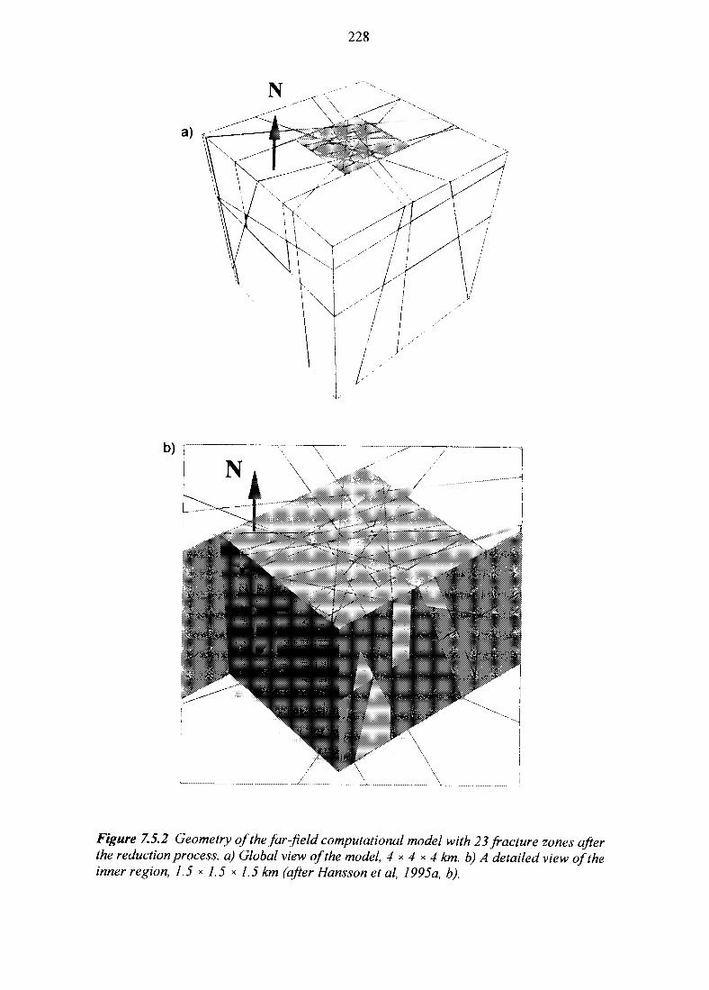
228
a)
Figure 7.5.2 Geometry of the far-field computational model with 23 fracture zones afierthe reduction process, a) Global view of the model, 4 * 4 * 4 km. b) A detailed view of theinner region, 1.5 * 1.5 * 1.5 km (afier Hans son et al, 1995 a, b).
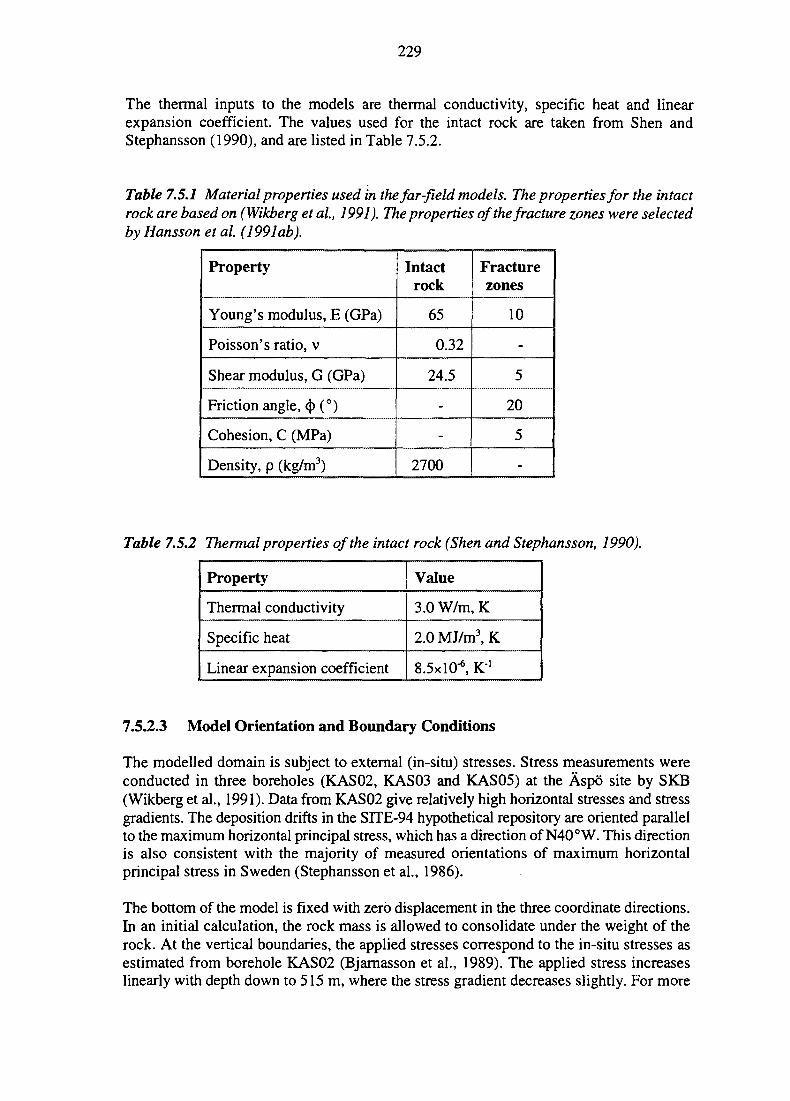
229
The thermal inputs to the models are thermal conductivity, specific heat and linearexpansion coefficient. The values used for the intact rock are taken from Shen andStephansson (1990), and are listed in Table 7.5.2.
Table 7.5.1 Material properties used in the far-field models. The properties for the intactrock are based on (Wikberg et al, 1991). The properties of the fracture zones were selectedby Hansson et al (199lab).
Property
Young's modulus, E (GPa)
Poisson's ratio, v
Shear modulus, G (GPa)
Friction angle, (J> (°)
Cohesion, C (MPa)
Density, p (kg/m3)
Intactrock
65
0.32
24.5
-
-
2700
Fracturezones
10
-
5
20
5
-
Table 7.5.2 Thermal properties of the intact rock (Shen and Stephansson, 1990).
Property
Thermal conductivity
Specific heat
Linear expansion coefficient
Value
3.0W/m,K
2.0MJ/m3,K
8.5xl06, K1
7.5.2.3 Model Orientation and Boundary Conditions
The modelled domain is subject to external (in-situ) stresses. Stress measurements wereconducted in three boreholes (KAS02, KAS03 and KAS05) at the Aspo site by SKB(Wikberg et al., 1991). Data from KAS02 give relatively high horizontal stresses and stressgradients. The deposition drifts in the SITE-94 hypothetical repository are oriented parallelto the maximum horizontal principal stress, which has a direction of N40°W. This directionis also consistent with the majority of measured orientations of maximum horizontalprincipal stress in Sweden (Stephansson et al., 1986).
The bottom of the model is fixed with zero displacement in the three coordinate directions.In an initial calculation, the rock mass is allowed to consolidate under the weight of therock. At the vertical boundaries, the applied stresses correspond to the in-situ stresses asestimated from borehole KAS02 (Bjarnasson et al., 1989). The applied stress increaseslinearly with depth down to 515 m, where the stress gradient decreases slightly. For more
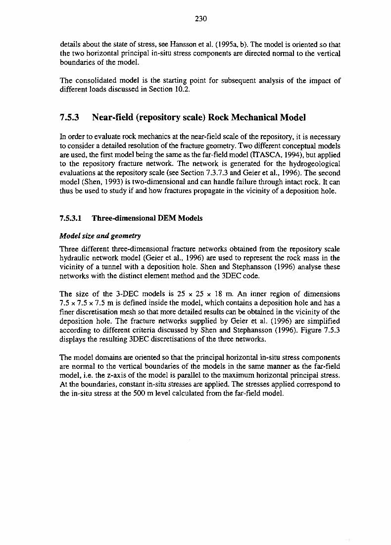
230
details about the state of stress, see Hansson et al. (1995a, b). The model is oriented so thatthe two horizontal principal in-situ stress components are directed normal to the verticalboundaries of the model.
The consolidated model is the starting point for subsequent analysis of the impact ofdifferent loads discussed in Section 10.2.
7.5.3 Near-field (repository scale) Rock Mechanical Model
In order to evaluate rock mechanics at the near-field scale of the repository, it is necessaryto consider a detailed resolution of the fracture geometry. Two different conceptual modelsare used, the first model being the same as the far-field model (TTASCA, 1994), but appliedto the repository fracture network. The network is generated for the hydrogeologicalevaluations at the repository scale (see Section 7.3.7.3 and Geier et al., 1996). The secondmodel (Shen, 1993) is two-dimensional and can handle failure through intact rock. It canthus be used to study if and how fractures propagate in the vicinity of a deposition hole.
7.5.3.1 Three-dimensional DEM Models
Model size and geometry
Three different three-dimensional fracture networks obtained from the repository scalehydraulic network model (Geier et al., 1996) are used to represent the rock mass in thevicinity of a tunnel with a deposition hole. Shen and Stephansson (1996) analyse thesenetworks with the distinct element method and the 3DEC code.
The size of the 3-DEC models is 25 x 25 x 18 m. An inner region of dimensions7.5 x 7.5 x 7.5 m is defined inside the model, which contains a deposition hole and has afiner discretisation mesh so that more detailed results can be obtained in the vicinity of thedeposition hole. The fracture networks supplied by Geier et al. (1996) are simplifiedaccording to different criteria discussed by Shen and Stephansson (1996). Figure 7.5.3displays the resulting 3DEC discretisations of the three networks.
The model domains are oriented so that the principal horizontal in-situ stress componentsare normal to the vertical boundaries of the models in the same manner as the far-fieldmodel, i.e. the z-axis of the model is parallel to the maximum horizontal principal stress.At the boundaries, constant in-situ stresses are applied. The stresses applied correspond tothe in-situ stress at the 500 m level calculated from the far-field model.
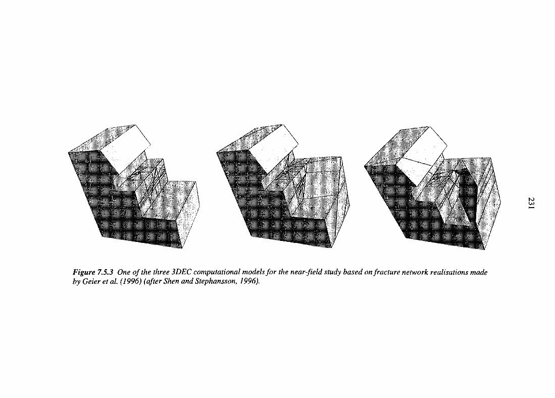
to
Figure 7.5.3 One of the three 3DEC computational models for the near-field study based on fracture network realisations madeby Geier et al. (1996) (after Shen and Stephansson, 1996).
232
Material models and properties
The material properties used in the 3DEC near-field model are the same as those used inthe far-field, i.e. a Mohr-Coulomb plastic material for the intact rock and a Coulombfriction law for the fractures, with constant normal and shear stiffness. Table 7.5.3 lists thematerial properties used for the 3DEC near-field study. The thermal properties of the intactrocks are the same as those in the far-field model, see Table 7.5.2.
Table 7.5.3 The mechanical properties for intact rock and rock fractures for the near-field3DEC modelling (Shen, 1993).
Properties of intactrock:
DensityYoung's modulusShear modulusCohesionTensile strengthInner friction angleDilation angle
Properties of fractures
Normal stiffnessShear stiffnessFriction angleCohesion
Elastic/plasticMohr-Coulomb
p=2700 kg/m3
E=35.71 GPaG=24.59 GPaG=10MPaat=10MPa<|)=40o
K.-50 GPa/mK^50 GPa/mcf>=30°C=5 MPa
Two-dimensional BEM models
The three-dimensional 3DEC code cannot handle failure through the intact rock. In thevicinity of a deposition hole such failures may be an issue, as the mechanical stability andthe hydraulic properties of the rock around the deposition holes are directly related to therepository barrier properties. Furthermore, the stress situation is governed both by theimpact from local loads such as the excavation itself, the swelling pressure from thebentonite and the heat from the waste, as well as from external loads.
To study this problem Shen and Stephansson (1996) performed a study with a BEM(Boundary Element Method) code, which was designed to simulate fracture propagationand fracture coalescence in two dimensions (Shen, 1993). It sought to study if and howfractures propagate in the vicinity of the deposition hole due to rock excavation and theloads from swelling pressure, thermal loading and glaciation.
At present, only a few fractures can be considered in the model owing to the limitation ofcomputer capacity. The material properties used are defined by Shen and Stephansson(1996). The boundary element code was applied to different fracture geometries for ahorizontal and a vertical cross-section of a deposition hole, as is discussed inSection 11.2.1.2
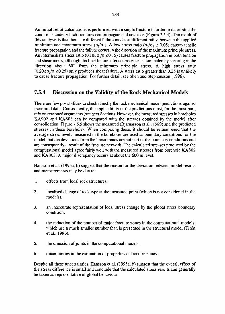
233
An initial set of calculations is performed with a single fracture in order to determine theconditions under which fractures can propagate and coalesce (Figure 7.5.4). The result ofthis analysis is that there are different failure modes at different ratios between the appliedminimum and maximum stress {o3lox). A low stress ratio (o3/ol < 0.05) causes tensilefracture propagation and the failure occurs in the direction of the maximum principle stress.An intermediate stress ratio (0.10<o3/Oj<0.15) causes fracture propagation in both tensionand shear mode, although the final failure after coalescence is dominated by shearing in thedirection about 60° from the minimum principle stress. A high stress ratio(0.20<a3/Oj<0.25) only produces shear failure. A stress ratio greater than 0.25 is unlikelyto cause fracture propagation. For further detail, see Shen and Stephansson (1996).
7.5.4 Discussion on the Validity of the Rock Mechanical Models
There are few possibilities to check directly the rock mechanical model predictions againstmeasured data. Consequently, the applicability of the predictions must, for the most part,rely on reasoned arguments (see next Section). However, the measured stresses in boreholesKAS02 and KAS03 can be compared with the stresses obtained by the model afterconsolidation. Figure 7.5.5 shows the measured (Bjarnasson et al., 1989) and the predictedstresses in these boreholes. When comparing these, it should be remembered that theaverage stress levels measured in the boreholes are used as boundary conditions for themodel, but the deviations from the linear trends are not part of the boundary conditions andare consequently a result of the fracture network. The calculated stresses produced by thecomputational model agree fairly well with the measured stresses from borehole KAS02and KAS03. A major discrepancy occurs at about the 600 m level.
Hansson et al. (1995a, b) suggest that the reason for the deviation between model resultsand measurements may be due to:
1. effects from local rock structures,
2. localised change of rock type at the measured point (which is not considered in themodels),
3. an inaccurate representation of local stress change by the global stress boundarycondition,
4. the reduction of the number of major fracture zones in the computational models,which use a much smaller number than is presented in the structural model (Tirenetal., 1996),
5. the omission of joints in the computational models,
6. uncertainties in the estimation of properties of fracture zones.
Despite all these uncertainties, Hansson et al. (1995a, b) suggest that the overall effect ofthe stress difference is small and conclude that the calculated stress results can generallybe taken as representative of global behaviour.
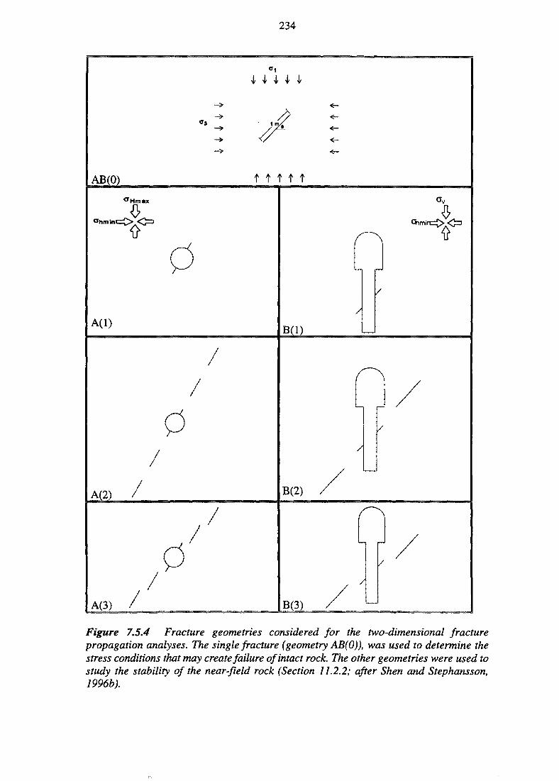
234
V • V V V
AB(O)A A A A A
^ X X
A(2) B(2)
A(3) B(3)
Figure 7.5.4 Fracture geometries considered for the two-dimensional fracturepropagation analyses. The single fracture (geometry AB(0)), was used to determine thestress conditions that may create failure of intact rock. The other geometries were used tostudy the stability of the near-field rock (Section 11.2.2; after Shen and Stephansson,1996b).
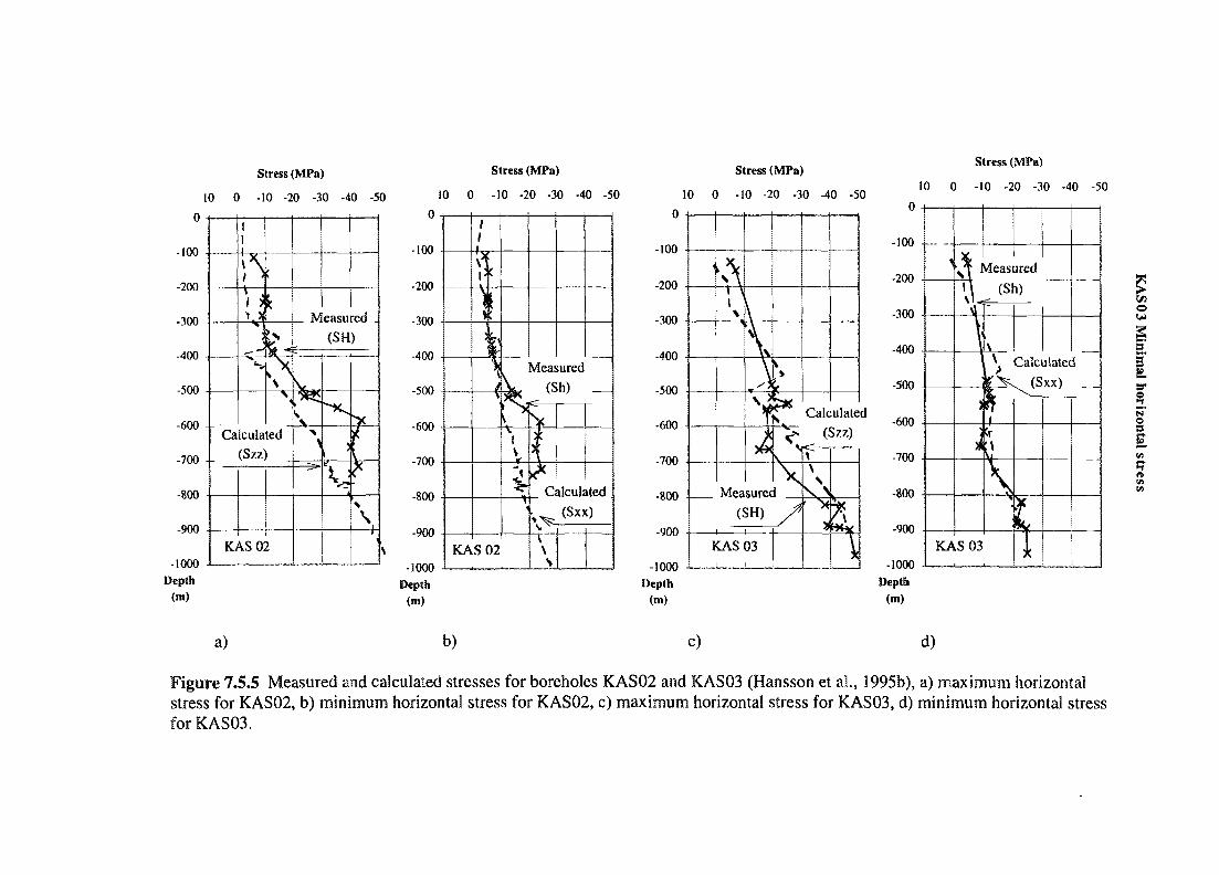
Stress (MPa)
10 0 -10 -20 -30 -40 -50
0
-100
-200
-300
-400
-500
-600
-700 4-
-800
-900
-1000i)epth(m)
11
\ \
1 iM
:
k
\\ *
Calculated
(Szz')
KAS02
Measured -
(SH)
\•v
. )f
y
\
a)
Stress (MPa)
10 0 -10 -20 -30 -40 -50
Stress (MPa)
10 0 -10-20 -30 -40 -50
Stress (MPa)
10 0 -10 -20 -30 -40 -50
c) d)
Figure 7.5.5 Measured and calculated stresses for boreholes KAS02 and KAS03 (Hansson et al, 1995b), a) maximum horizontalstress for KAS02, b) minimum horizontal stress for KAS02, c) maximum horizontal stress for KAS03, d) minimum horizontal stressfor KAS03.
3 #
SLB"O
236
7.5.5 Conclusions and Implications for Other Parts of theAssessment
7.5.5.1 Conclusions Regarding the Validity of the Rock Mechanical Model
Sections 10.2 and 11.2.1 present an extended discussion on uncertainty in the modellingapproaches. Evidently, a major uncertainty in the rock mechanical models concerns theproperties of large fractures and fracture zones at the Aspo site. Laboratory experiments canonly determine, at best, the properties of rock joints; the normal and shear stiffness offracture zones are estimated by extrapolation, with little prospect of validation. Sensitivityanalysis, performed in order to derive mechanical properties of fracture zones, is anapproach at overcoming the problem of limited data on the mechanics of fracture zones. Inaddition, Hansson et al. (1995a, b) discuss several potential uncertainties and problems ofthe far-field model approach adopted. For example:
• In the current geological structural model provided by SKI (Tiren et al., 1996), thefracture zones are infinite in size and planar in geometry. The finite dimension andlarge-scale undulations of the fracture zones are ignored and this will significantlyaffect the resulting stress field.
• The fracture zone geometry has a major influence on the stress state in the modelsand stress concentration artifacts may occur at sharp corners which, in reality, wouldfail.
• Time effects on the fracture mechanical properties (creep) are not considered. Thismay be a serious shortcoming owing to the long times over which model predictionsare to be made.
• Failure of rock matrix and fractures is most likely to occur when excavation ofrepository and emplacement of waste canisters are performed, but failuremechanisms are probably complicated and the validity of the material modelspresently used can be questioned for such applications.
Despite all these shortcomings, Hansson et al. (1995a, b) conclude that their modelprobably provides reasonable general stress levels, but the validity of detailed predictionsof the stress and shear displacement of individual fracture zones, or the impact ofexcavations, could be questioned. For a more elaborate discussion, see Hansson et al.(1995a, b).
7.5.5.2 Implications for Other Parts of the Assessment
The rock mechnical models developed in this section is used as input to the evaluation ofthe rock mechanical stability of the far-field rock (in Section 10.2) and the evaluation of themechanical stability of the near-field rock (in Section 11.2.2), for the scenarios specifiedin Chapter 9.
237
8 THE ENGINEERED BARRIER SYSTEM
The canister, the buffer, the shafts and tunnels, and the backfill and seals constitute theengineered part of the repository. This chapter describes the initial properties of theEngineered Barrier System (EBS), processes that may potentially change these propertiesand, when applicable, the models used to evaluate their evolution. The outline of thedisposal system as well as the design of the canister are described in Chapter 5. The resultsof the actual evaluation calculations are presented in Chapter 11.
8.1 INTRODUCTION
8.1.1 The Engineered Barrier System as a Part of the SITE-94Process System
The SITE-94 Process System consists of the geosphere and the EBS. Features, events andprocesses affecting, in particular, the spent fuel, the canister, the buffer and the tunnels willdirectly determine whether radionuclides will be released from the repository. Theinfluences between these FEPs are described in the STTE-94 Process Influence Diagram(PID) in the same way as the geosphere FEPs (see Chapters 2 and 7), using themethodology described in Chapman et al. (1995). Figure 8.1.1 displays an extract of theSITE-94 PUD covering the most important (IL=10) FEPs and links for the canister andbuffer. The PID reflects the fact that the thermal, mechanical, hydrogeological, radiologicaland chemical processes in the engineered barriers all interact and that these FEPs are linked,in turn, to the geosphere. The importance of these interactions varies and the magnitude ofthe interactions depends on the properties of the EBS.
It should be noted that a potentially important region of the PID which is not considered inthe SITE-94 analysis of EBS performance concerns the generation and impacts of gas inthe near-field. Hydrogen gas may form as a result of anaerobic corrosion of the inner steelcanister and this issue, not treated in the following text, would need to be considered in afull safety assessment.
8.1.2 Assessing the Properties of the Engineered Barrier System
As stated in Chapters 1 and 5, the reference disposal system used in this report is the so-called KBS-3 system. This system is still under development by the Swedish nuclearindustry. It is therefore inappropriate to describe the canister or the other engineeredcomponents in a way similar to that of a safety analysis supporting an application to builda nuclear facility. Furthermore, SITE-94 is a learning exercise and is not intended for thedevelopment of disposal designs or techniques.
At the time of the completion of SITE-94, full-scale tests are in progress in order to developcanister design as well as processes for manufacturing, sealing and non-destructive testingof canisters in the programme managed by the industry. Similar developments are alsounderway concerning buffer material, tunnel backfill, etc. Consequently, it is considered
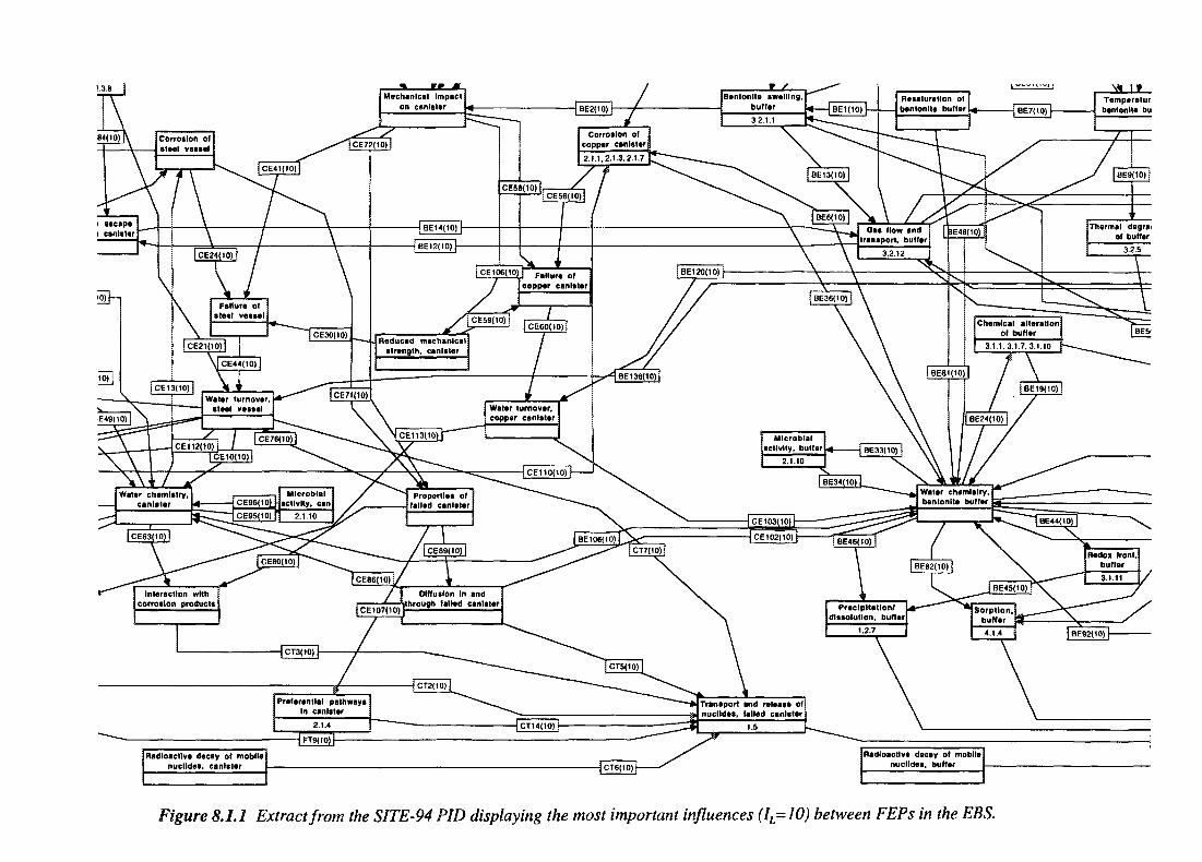
Radioactive decay of mobilenuclldes, canister
Radioactive decay of mobilenuclldes, buffer
Figure 8.1.1 Extract from the SITE-94 PID displaying the most important influences (IL=I0) between FEPs in the EBS.
239
premature to make any detailed conclusions which may depend on which fabricationprocesses will eventually be used or which properties an actual 'as-produced' canister mayhave.
At the time of writing, however, interesting results are appearing from the SKBdevelopment programme at a rapid rate. These initial results make it possible to identifyprocesses which might conceivably give rise to canister malfunctioning. Mechanismsrelated to canister longevity are of particular interest in the Swedish programme since, inthe KBS-3 system, the canister is the component of the system that is expected to providethe initial containment of the radionuclides in the spent nuclear fuel and earlier assessmentshave shown canister failure rate (in terms of the distribution of failure times) to be asensitive parameter in estimating overall system safety. It should be borne in mind,however, that any potential weaknesses identified in the present report might be overcomeor circumvented by the industry in the near future. Similar reasoning can also be appliedto the other engineered components.
8.2 THE CANISTER
This section discusses factors of relevance for judging the stability of the canister. Suchfactors include aspects of manufacture, testing and sealing, and the mechanical andchemical properties of the canister. The potential for copper and steel corrosion are mainaspect of these chemical properties. The information provided in this section is used asinput to the evaluation of canister stability discussed in Section 11.5.
8.2.1 Introduction
The anticipated canister design includes an outer copper canister to assure long-termcontainment and an inner steel canister to provide mechanical support. The longevity of thecopper canister is potentially a very important safety feature. Indeed, if full containment byall canisters is assumed for the projected time of 106 years or greater, the performancebehaviour and response of all other engineered and natural barriers becomes largelyirrelevant. The potential for canister failure is influenced by mechanical impacts on thecanister and by corrosion, which is generally shown in the PID (Figure 8.1.1). The effectof these impacts depends on the canister properties which, in turn, strongly depend on thetechniques used for manufacturing, sealing and testing. For this reason, these latterconditions will also be addressed in this section.
One important objective of performing an integrated safety analysis is to provide a similarlevel of integration in the research and development programme, as well as in the systemsdesign (Sjoblom et al., 1994). Integration is particularly important when the containmentbehaviour of a canister is to be analysed. In this case, integration is required between manyareas of research and fabrication (or processing) development. Even details in themanufacturing process might have significant implications for canister failure mechanismsin the repository.
240
A systematic and transparent approach to the identification of scenarios and to thecompilation of links in the Process System (cf. Chapters 2 and 9) is particularly valuablewhen a structured and comprehensive description of the future functioning of the canisteris to be compiled. For the reasons given above, it is not possible to include a comprehensiveand integrated description of all the factors affecting canister behaviour in SITE-94.Analysis at an early stage is useful, however, in order to identify which factors might besignificant. Furthermore, such analyses are necessary as learning exercises in the area ofsafety analysis (and may also provide a tool for directing further research and developmentwork into the pertinent areas). The first analysis in a particular area cannot be expected tobe evenly balanced when compared to other areas or barriers that have been more fullystudied. It does, however, serve as a necessary starting point for further and morecomprehensive work.
In order to facilitate analysis of the fully integrated repository system in the STTE-94project, different conceivable defects and deficiencies are assumed to exist from the outsetin some of the canisters. This ad hoc assumption is justified in the SITE-94 analysisbecause it enables a fuller investigation of the complex interactions and performance of thesite and of each subsystem of the repository. These postulated deficiencies can be attributedto uncertainties in the canister design, manufacturing and sealing process and the testingmethods, etc., put forward by the industry.
In most cases, it is not possible to make any reliable quantification of such uncertainties,nor is it justified, since the canister system is still under development. This caution mayseem surprising in view of the considerable experience that exists regarding design andconstruction of canisters made of metal. It should be recognised, however, that more or lesspure copper is not a standard construction material (it is mainly used for electricalconductors where mechanical properties are less of an issue) and that much of the processdevelopment work is either in progress or remains to be done.
Almost pure metals are rarely, if ever, used as construction materials for a number ofreasons, some of which may be related to the very properties desired for a waste canister.For example, no mechanism has been identified that would lead to diminution of the grainsize once the canister has been formed into its final shape. This is contrary to the situationin certain other materials such as steel, where diminution can be obtained through cyclingaround a phase transition temperature. Moreover, in less pure metal, there may be little orno build-up of alloying elements on the grain surfaces and subsequent hindrance of thedevelopment of large grains. More full scale experiments, such as those presently beingcarried out by the industry, are needed before conclusions can be drawn regarding thesignificance of such effects.
Another feature that deserves specific mention is the requirement that the canister functionover a very long period of time and the consequent need for verification of the relevanceof the testing and quality assurance procedures. These time scales extend much further thanthe service lives tested in other industrial applications. In materials testing, extrapolationinto areas far outside those of the test conditions is typically carried out with greatreluctance, if at all. In the present case, it is not possible to perform tests of duration similarin magnitude to the anticipated service life. Thus, a thorough understanding of the pertinentphenomena in combination with relevant experimental data of sufficient quality appears tobe needed.
241
8.2.2 Objectives and Requirements
The role of the canister
Given that the KBS-3 method will actually be selected for the final repository, the Swedishnuclear industry have to ensure that the canister will be designed, manufactured, sealed,tested and quality-assured in such a manner that it can be shown that the canister willfunction in the anticipated manner in the encapsulation plant, during transport and in therepository (during the operational phase as well as after closure).
During transportation and handling, the canister will provide a contamination barrier, aradiation shield, mechanical integrity and protection and a suitable geometry for lifting andfor securing the fuel elements. In the repository, after closure, the canister should providecontainment of the radionuclides.
The canister should also be suitable for control and quality inspection so that its properfunctioning can be assured.
The requirements of the canister
The functional requirements describe the requirements regarding the function of thecanister. They can be derived from the role (described above) that the canister has to playin the repository after closure and during handling and transportation. Functionalrequirements include the following:
• resistance to corrosion,• mechanical resistance to external load (isostatic as well as non-uniform),• radiation shielding (e.g. in order to minimise gamma-radiolysis),• suitable geometry from a criticality point of view.
In most cases, the functional requirements cannot be confirmed directly. Instead,requirements have to be placed on properties or processes (e.g. manufacturing and sealing).Since the latter requirements are related to the manufacturing of the sealed canisters theymight be referred to as manufacturing specifications. In order for the manufacturingspecifications to be used to ensure the function of the canister, it is necessary that the linksbetween manufacturing specifications and functional requirements are fully established andproven.
8.2.3 Manufacturing, Sealing and Testing
8.2.3.1 Manufacturing
Copper canister
It is assumed that the canisters are manufactured through a process of rolling, bending andwelding. The rolling process starts with a cast ingot, with large grains (a cast structure withe.g. dendrites) as well as fissures. During the forging process, including rolling, work isapplied and the fissures are closed. The cast structure is broken down and, as a result, thematerial recrystallises to a smaller grain size with a uniform structure.
242
The size of the ingot in relation to the size of the rolls may imply, however, that the sizereduction (of the ingot) and the work applied is less than desirable (Bowyer, 1995). Inparticular, the interior of the copper plate produced may still contain a coarse grain structureas well as pores.
Such effects not only affect mechanical strength and corrosion but also the possibility ofnondestructive testing (see Section 8.2.3.3). Further comments regarding the welding of thebent copper plates are made in Section 8.2.3.2 .
Steel canister
In the case of the steel canister, a solid knowledge base exists regarding both the materialsscience aspects and the engineering aspects of this material. The steel canister is made froma rolled plate of carbon manganese steel (OX520DM), with a minimum thickness of50 mm. The top and bottom lids are made from another carbon manganese steel(SS 2103-0) with a thickness of 100 mm. The bottom lid is intended to be welded onto thecylinder. The manufacturing procedures are well-known standards.
The qualities of this material provide a high mechanical strength and a good stability. Thestability of the material emanates from the small grain size together with the way in whichthis grain structure is stabilised. The fine-grained structure in these types of materials isproduced through alloying small amounts of e.g. niobium, titanium and vanadium. Theseelements form high-temperature carbides and/or nitrides that are very stable at lowtemperature. The nitrides and/or carbides precipitate at the grain boundaries of the materialand thereby prevent the fine-grain structure from coarsening. The yield strength isproportional to the grain size and can therefore be engineered and optimised.
8.2.3.2 Sealing
It is assumed that the sealing of the copper canister would be carried out by electron beamwelding (EBM). The EBM technology is well developed for a number of industrialapplications, including the sealing of nuclear fuel rods. In the case of copper canisters, thenovel aspects for EBM include the thickness of the canister in combination with the highthermal conductivity of copper. Thus, even if the volume to be kept molten is as small asa cylinder of 50 mm length and a diameter of only two or a few mm, a substantial amountof power (100 - 150 kW) is required for the beam.
One of the main issues to consider in EBM welding is the stability of the beam (Bowyer,1995). The beam is sensitive to disturbances (e.g. stray magnetic fields or gas molecules)and can change character very rapidly. In order to regulate the beam, an efficient and veryfast feed-back system of a very low impedance has to be used. Typically, a vacuum has tobe applied over the object to be welded.
Degassing of the copper may occur during the welding operation. Such degassing may takeplace if the copper contains some oxygen and may cause formation of pores. Anothermechanism for pore formation is through shrinkage when molten copper metal solidifies.
243
The welding process is also likely to affect the grain structure in such a manner thatcolumnar grains are formed, (Bowyer, 1995). Such grains may form in the direction of thewelding. They are thus parallel to the canister surface and may therefore not be observedunless explicitly sought. These grains may be larger in size than those in the bulk material,which might affect the mechanical properties, as well as the possibility of inspection usingnon-destructive testing.
The welding process may also lead to segregation of matter, since a molten zone propagatesthrough the material. Such a zone may bring impurities along with the melt and theseimpurities may concentrate at the end of the weld.
The steel canister is assumed to be sealed by laser-beam welding. A penetration of only acouple of millimetres is required since the canister will be designed in such a manner thatlittle mechanical strength is required in the weld region. The purpose of this weld is to keepthe lid in place (e.g. during the subsequent operations in the encapsulation plant), topreserve the dry atmosphere inside the steel canister and to prevent contamination of theoutside by activity from the inside.
There are concerns with respect to steel canister welds. For example, when laser-beamwelding is performed in a fine grain steel alloy like OX520DM, the heat-affected zone(HAZ) may become brittle (due to the formation of martensite) and thus need to be heat-treated (Bowyer, 1995).
8.2.3.3 Testing and Quality Inspection
Testing of the canisters will probably involve all stages of manufacturing, including thesealing process. Testing during manufacturing will probably be both destructive and non-destructive, while testing of the sealed canisters is only non-destructive. For the purpose ofSITE-94, only non-destructive testing will be discussed.
The main methods considered for non-destructive testing (NDT) are ultrasonic inspectionand radiography. Both may be utilised during canister manufacturing, as well as after thecanister has been sealed. In the present report, they are discussed mainly from the point ofview of testing the sealed canisters.
Ultrasound can be used to detect irregularities in the refractive properties of a solid.Fissures and pores give rise to reflections, if the orientation is favourable. Pores may notbe detected, however, if the wavelength is somewhat larger than the diameter of the pores.In copper, the sound velocity (for longitudinal waves) is of the order of 5xlO3 metres persecond. It can thus be expected that frequencies of the order of a megahertz, or higher, arerequired in order for pores having a diameter of a few millimetres to be detected.
The ultrasonic waves may also interact with the copper itself if the grain size is of the sameorder of magnitude as the wavelength, or larger. The interaction is quite complex since therefractive properties of copper vary with the orientation of the grain as well as with the typeof wave (transverse or longitudinal). Thus, the waves may change direction as well ascharacter at the interfaces between the grains. The phenomenon leads to dispersion and toabsorption of the waves. Pores located deep in a copper specimen having a large grain size
244
may therefore be very difficult, or even impossible, to detect. In such a case, the absenceof echoes does not indicate any absence of pores but merely that the signal is beingattenuated. The dependence of the grain size on the manufacturing and sealing processesis discussed in Sections 8.2.3.1 and 8.2.3.2 respectively.
It appears that when ultrasonic inspection is carried out, more detail can be expected fromthe region near the surface than from the interior of the copper canister. Also, the weldregions may be more difficult to inspect than the bulk material.
For radiography applied to a canister, only transmission of the rays is considered. Importantconstraints include the thickness of the material and the resolution needed. This implies thatthe rays will have to have a high intensity as well as high energy. In an accelerator, a targetis bombarded with particles and as a result x-rays are emitted. The x-ray beam is collimatedand there is a trade-off between collimation and intensity. A proper balance between thetwo will, ideally, provide the resolution needed within the time available. The collimatedbeam is scanned through the weld region of the canister and differences in the detectorsignal level may reflect irregularities in the material tested.
One important aspect concerning testing of the sealed canister, valid for ultrasonicinspection as well as for radiography, is the question of how the data from testing are usedwith regard to statistics. Under ideal conditions, many properties can be controlled andmeasured. During actual plant operation, a limit must, typically, be set on the effort spenton testing. Understanding of the process and a pertinent testing strategy are probablyimportant prerequisites for success. Nevertheless, when the future behaviour of the canistersis to be assessed, it should be recognised how various deviations from expectedcharacteristics may arise, their statistical distributions and the implications of suchdeviations on the long-term integrity of the canisters. Such analyses may be of particularinterest in the realms of low probability, where early failures might occur.
8.2.4 Mechanical Properties
Design and manufacture have important implications for the mechanical properties. Thus,the steel canister inside the copper canister provides a mechanical load-bearing function,and the outer copper canister, protection against corrosion.
The canister is subjected to and affected by internal as well as external stresses. However,in the SITE-94 canister analysis, only the external stresses are analysed.
Copper is a soft material and can be highly deformed without cracking at ordinarydeformation rates. For loads that correspond to stresses well below the yield strength andwhich are applied for a long time, copper will creep.
After manufacturing (especially the welding operation), residual stresses will be present inthe empty canister. These stresses might be partially relaxed before encapsulation. Duringthe welding of the lid, new stresses will be introduced. These latter stresses might also bepartially relaxed before disposal.
245
After closure of the repository, water will enter and a significant pressure from hydrostaticloading and swelling of the bentonite buffer will build up (see Section 11.5.2). The pressurewill cause the copper to creep onto the steel canister until the space between the canistersis essentially eliminated. (Initially, there has to be a space between the canisters in order toput one inside the other.)
During creep, copper will be less ductile than during ordinary deformations. The creepbehaviour of copper depends on composition, grain structure and temperature. It isimportant to ensure that copper has the creep ductility required, even for very slow creepat comparatively low temperatures (Bowyer, 1995).
In order for the creep to take place at rates that can be measured, the experiments performedhave been carried out at elevated temperatures. These creep data are then used inextrapolations to the range of interest (25 to 80 °C). In these extrapolations, an Arrheniustype of equation is assumed. In this expression, the activation energy obtained in the hightemperature range is used for the entire extrapolation.
Such extrapolations are only justified in cases where the same mechanism persists over theentire temperature range. It is, therefore, of interest to determine what mechanism iseffective within what temperature range (e.g. migration of dislocations or diffusion).
A necessary condition for a creep failure to occur, regardless of mechanism, is the presenceof tensile stresses. The creep behaviour of the canister can thus be altered and improved byappropriate design.
When the mechanical properties of a canister are considered within the context ofPerformance Assessments, the analysis should include canisters that have defects. In spiteof the testing, and due to different effects, some of which are discussed above, defects ofvarying sizes, shapes and frequency can be expected to be present in the canisters (Bowyer,1995).
Defects may give rise to considerable changes in local distribution of stresses and therebyalso to plastic deformation and/or cracking. The low yield strength of copper implies thatcopper has a low resistance against such deformations. On the other hand, the high ductilitymay imply that cracking will take place only at very large deformations.
Another aspect of defects is that they could be of importance for the feasibility of lifting andretrieving canisters. This has not been analysed in detail, but the present judgment is thatthe critical defect size is large in comparison with what might pass inspection.
The long-term behaviour of the canisters in the repository is discussed further inSection 11.5.

246
8.2.5 Chemical Properties
8.2.5.1 Introduction
A first prerequisite for the long service life of a canister is that it can be shown to have asufficiently low rate of general corrosion. Estimates of life-times with regard to generalcorrosion of copper are usually based on estimates of the supply of reacting species underreducing conditions. This supply, in turn, is normally limited by diffusion resistance in thebentonite, possibly in combination with limits to the concentrations of reactive species atthe outside of the bentonite buffer.
If the lifetime of a canister is limited by localised corrosion, the lifetime will depend on acombination of the supply of reactive species, the intensity of initiating factors and themechanism of the attack.
Thus, when the corrosion behaviour of a copper canister in a repository for spent nuclearfuel is to be evaluated, it is necessary to understand:
• the chemistry of the water contacting the canister,• the reactions that take place at the copper surface,• the properties of the reactants formed,• the migration of reactive species to the canister,• the migration of reactants away from the canister surface (including the rates),• the mechanism(s) for the corrosion process(es).
These aspects are discussed in the following sections.
Evaluations should also be made for the potential effects of microbes, stress corrosion(including stress state and initial defects) and corrosion from the inside. However, thesethree aspects are not dealt with in the SITE-94 project.
The reactions that might take place at the copper surface depend on the composition of thesurrounding groundwater and of the bentonite buffer. The composition of the groundwatercan vary considerably with chemical buffering properties, location, depth and time. Long-term changes in climate or regional hydrogeology may impose sustained changes in thechemical composition of groundwater at repository depth, as described in Chapter 9.Furthermore, it can be expected that the redox potential, the iron(II) content and the reducedsulphur content of the groundwater can be further modified by interaction with thebentonite buffer.
Typically, groundwaters contain calcium and sodium cations and chloride, sulphate andcarbonate anions. Oxidising water also contains dissolved oxygen, and reducinggroundwater may contain iron(II) and reduced sulphur (in the form of sulphide andpolysulphide). The reduced sulphur is usually present in low concentrations only, but is ofinterest in connection with copper corrosion because it reacts with copper under sufficientlyreducing conditions.
The composition of the groundwater at Aspo is described and discussed in Sections 10.4and 11.5.3. Changes in the composition of the groundwater during the post-operational
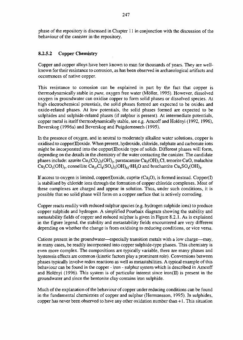
247
phase of the repository is discussed in Chapter 11 in conjunction with the discussion of thebehaviour of the canister in the repository.
8.2.5.2 Copper Chemistry
Copper and copper alloys have been known to man for thousands of years. They are well-known for their resistance to corrosion, as has been observed in archaeological artifacts andoccurrences of native copper.
This resistance to corrosion can be explained in part by the fact that copper isthermodynamically stable in pure, oxygen free water (Moller, 1995). However, dissolvedoxygen in groundwater can oxidise copper to form solid phases or dissolved species. Athigh electrochemical potentials, the solid phases formed are expected to be oxides andoxide-related phases. At low potentials, the solid phases formed are expected to besulphides and sulphide-related phases (if sulphur is present). At intermediate potentials,copper metal is itself thermodynamically stable, see e.g. Amcoff and Holenyi (1992, 1996),Beverskog (1996a) and Beverskog and Puigdomenech (1995).
In the presence of oxygen, and in neutral to moderately alkaline water solutions, copper isoxidised to copper(II)oxide. When present, hydroxide, chloride, sulphate and carbonate ionsmight be incorporated into the copper(II)oxide type of solids. Different phases will form,depending on the details in the chemistry of the water contacting the canister. The candidatephases include: azurite Cu3(CO3)2(OH)2, paratacamite Cu2(OH)3Cl, tenorite CuO, malachiteCu2CO3(OH)2, connellite Cu37Cl8(SO4)2(OH)62-8H2O and brochantite Cu4SO4(OH)6.
If access to oxygen is limited, copper(I)oxide, cuprite (Cu2O), is formed instead. Copper(I)is stabilised by chloride ions through the formation of copper chloride complexes. Most ofthese complexes are charged and appear in solution. Thus, under such conditions, it ispossible that no solid phase will form on a copper surface that is actively corroding.
Copper reacts readily with reduced sulphur species (e.g. hydrogen sulphide ions) to producecopper sulphide and hydrogen. A simplified Pourbaix diagram showing the stability andmetastability fields of copper and reduced sulphur is given in Figure 8.2.1. As is explainedin the figure legend, the stability and metastability fields encountered are very differentdepending on whether the change is from oxidising to reducing conditions, or vice versa.
Cations present in the groundwater—especially transition metals with a low charge—may,in many cases, be readily incorporated into copper sulphide-type phases. This chemistry iseven more complex. The compositions are typically variable, there are many phases andhysteresis effects are common (kinetic factors play a prominent role). Conversions betweenphases typically involve redox reactions as well as metastabilities. A typical example of thisbehaviour can be found in the copper - iron - sulphur system which is described in Amcoffand Holenyi (1996). This system is of particular interest since iron(II) is present in thegroundwater and since the bentonite clay contains iron sulphide.
Much of the explanation of the behaviour of copper under reducing conditions can be foundin the fundamental chemistries of copper and sulphur (Hermansson, 1995). In sulphides,copper has never been observed to have any other oxidation number than +1. This situation
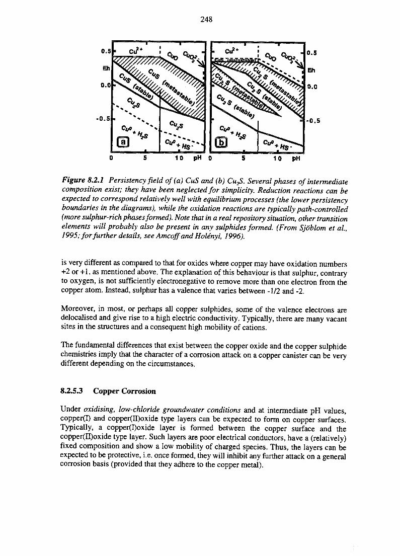
248
-0.5
10 pH 0
0.5
-0.5
10 pK
Figure 8.2.1 Persistency field of (a) CuS and (b) Cu2S. Several phases of intermediatecomposition exist; they have been neglected for simplicity. Reduction reactions can beexpected to correspond relatively well with equilibrium processes (the lower persistencyboundaries in the diagrams), while the oxidation reactions are typically path-controlled(more sulphur-rich phases formed). Note that in a real repository situation, other transitionelements will probably also be present in any sulphides formed. (From Sjoblom et ai,1995; for further details, see Amcoff and Holenyi, 1996).
is very different as compared to that for oxides where copper may have oxidation numbers+2 or +1, as mentioned above. The explanation of this behaviour is that sulphur, contraryto oxygen, is not sufficiently electronegative to remove more than one electron from thecopper atom. Instead, sulphur has a valence that varies between -1/2 and -2.
Moreover, in most, or perhaps all copper sulphides, some of the valence electrons aredelocalised and give rise to a high electric conductivity. Typically, there are many vacantsites in the structures and a consequent high mobility of cations.
The fundamental differences that exist between the copper oxide and the copper sulphidechemistries imply that the character of a corrosion attack on a copper canister can be verydifferent depending on the circumstances.
8.2.5.3 Copper Corrosion
Under oxidising, low-chloride groundwater conditions and at intermediate pH values,copper(I) and copper(II)oxide type layers can be expected to form on copper surfaces.Typically, a copper(I)oxide layer is formed between the copper surface and thecopper(H)oxide type layer. Such layers are poor electrical conductors, have a (relatively)fixed composition and show a low mobility of charged species. Thus, the layers can beexpected to be protective, i.e. once formed, they will inhibit any further attack on a generalcorrosion basis (provided that they adhere to the copper metal).
249
This situation is a comparatively favourable one from the point of canister longevity underoxidising conditions. The oxygen available reacts only slowly with the canister, thusproviding time for reactions with other species that can be oxidised e.g. the iron sulphidein the bentonite. Moreover, since the attack is uniform, a considerable amount of oxygenwill have to diffuse to the canister surface and react before any penetration can take place.
The layers on the copper surface are protective in the sense that they hinder reactions thatwould otherwise take place (actually slowing down the rate). Under certain circumstances,local chemistries, different from those in the bulk of the groundwater, may develop in theclose vicinity of and on isolated parts of the copper surface (Hermansson and Beverskog,1996). The microchemistry at the copper surface may be separated into anodic and cathodicareas, perhaps related to faults in the passive film. At such localised areas, pits can formand, once initiated, they might propagate, since the chemical conditions in a pit will inhibitrestoration of the local protective film. The mechanism is illustrated in Figure 8.2.2.
The possibilities for pit formation, as well as the pitting factor, can be expected to dependstrongly on the details of the chemical environment. The pitting factor is the ratio betweenthe depth of the deepest pit and the depth of the average corrosion. Pitting has beenobserved on many metals. In cases where the metal surface is passivated by an oxide layer,certain general patterns can be identified. Thus, at low electrochemical potentials, a metaltypically shows immunity towards corrosion. At high electrochemical potentials, incombination with acidic conditions, no protective layer is formed and a rapid generalcorrosion can be observed. At high electrochemical potentials, together with moderate tohigh pH-values, 'perfect' passivation might occur (with associated slow uniform corrosion).In between the latter two areas, and above a minimum electrochemical potential (theprotective potential), pitting might take place. The location of the pitting area in thePourbaix diagram is typically heavily dependent on details in the chemistry, e.g. thechloride concentration. The pits are typically shallow on the acidic side and deep on thealkaline side.
cu 2*Cu+ -complex
Bentoniteclay
Passivatingcopper oxidetype layers
Copper metal
Figure 8.2.2 Mechanism for pitting corrosion of copper. (From Sjdblom et al, 1995).
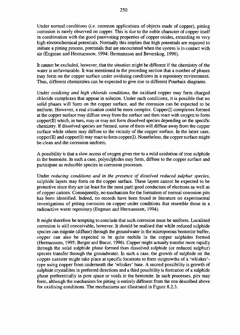
250
Under normal conditions (i.e. common applications of objects made of copper), pittingcorrosion is rarely observed on copper. This is due to the noble character of copper itselfin combination with the good passivating properties of copper oxides, extending to veryhigh electrochemical potentials. Normally this implies that high potentials are required toinitiate a pitting process, potentials that are encountered when the system is in contact withair (Engman and Hermansson, 1994; Hermansson and Beverskog, 1996).
It cannot be excluded, however, that the situation might be different if the chemistry of thewater is unfavourable. It was mentioned in the preceding section that a number of phasesmay form on the copper surface under oxidising conditions in a repository environment.Thus, different chemistries can be expected to give rise to different Pourbaix diagrams.
Under oxidising and high chloride conditions, the oxidised copper may form chargedchloride complexes that appear in solution. Under such conditions, it is possible that nosolid phases will form on the copper surface, and the corrosion can be expected to beuniform. However, a real situation could be more complex. Copper(I) complexes formedat the copper surface may diffuse away from the surface and then react with oxygen to formcopper(II) which, in turn, may or may not form dissolved species depending on the specificchemistry. If dissolved species are formed, some of them will diffuse away from the coppersurface while others may diffuse to the vicinity of the copper surface. In the latter case,copper(II) and copper(O) may react to form copper(I). Nonetheless, the copper surface mightbe clean and the corrosion uniform.
A possibility is that a slow access of oxygen gives rise to a mild oxidation of iron sulphidein the bentonite. In such a case, polysulphides may form, diffuse to the copper surface andparticipate as reducible species in corrosion processes.
Under reducing conditions and in the presence of dissolved reduced sulphur species,sulphide layers may form on the copper surface. These layers cannot be expected to beprotective since they are (at least for the most part) good conductors of electrons as well asof copper cations. Consequently, no mechanism for the formation of normal corrosion pitshas been identified. Indeed, no records have been found in literature on experimentalinvestigations of pitting corrosion on copper under conditions that resemble those in aradioactive waste repository (Engman and Hermansson, 1994).
It might therefore be tempting to conclude that such corrosion must be uniform. Localisedcorrosion is still conceivable, however. It should be realised that while reduced sulphidespecies can migrate (diffuse) through the groundwater in the microporous bentonite buffer,copper can also be expected to be quite mobile in the copper sulphides formed(Hermansson, 1995; Berger and Bucur, 1996). Copper might actually transfer more rapidlythrough the solid sulphide phase formed than dissolved sulphide (or reduced sulphur)species transfer through the groundwater. In such a case, the growth of sulphide on thecopper canister might take place at specific locations to form outgrowths of a 'whisker'-type using copper from underneath the 'whisker' base. A second possibility is growth ofsulphide crystallites in preferred directions and a third possibility is formation of a sulphidephase preferentially in pore space or voids in the bentonite. In such processes, pits mayform, although the mechanism for pitting is entirely different from the one described abovefor oxidising conditions. The mechanisms are illustrated in Figure 8.2.3.
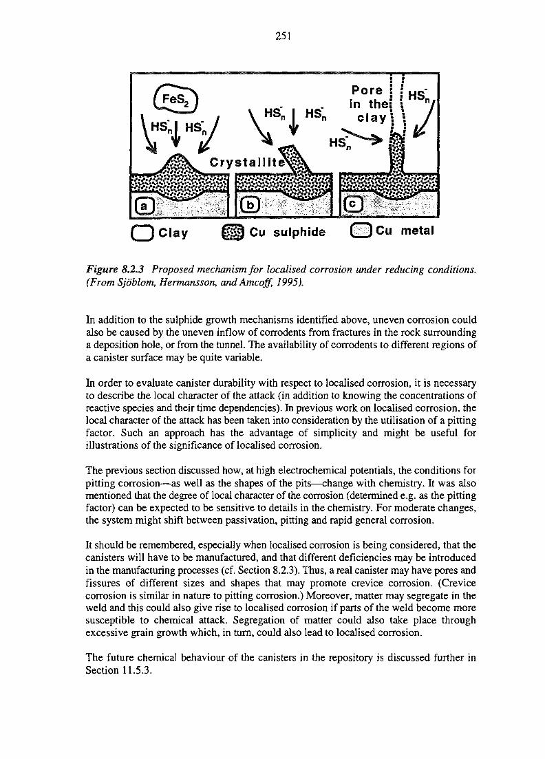
251
m^ Crystallite^
Cu metal
Figure 8.2.3 Proposed mechanism for localised corrosion under reducing conditions.(From Sjoblom, Hermansson, andAmcoff, 1995).
In addition to the sulphide growth mechanisms identified above, uneven corrosion couldalso be caused by the uneven inflow of corrodents from fractures in the rock surroundinga deposition hole, or from the runnel. The availability of corrodents to different regions ofa canister surface may be quite variable.
In order to evaluate canister durability with respect to localised corrosion, it is necessaryto describe the local character of the attack (in addition to knowing the concentrations ofreactive species and their time dependencies). In previous work on localised corrosion, thelocal character of the attack has been taken into consideration by the utilisation of a pittingfactor. Such an approach has the advantage of simplicity and might be useful forillustrations of the significance of localised corrosion.
The previous section discussed how, at high electrochemical potentials, the conditions forpitting corrosion-~as well as the shapes of the pits—change with chemistry. It was alsomentioned that the degree of local character of the corrosion (determined e.g. as the pittingfactor) can be expected to be sensitive to details in the chemistry. For moderate changes,the system might shift between passivation, pitting and rapid general corrosion.
It should be remembered, especially when localised corrosion is being considered, that thecanisters will have to be manufactured, and that different deficiencies may be introducedin the manufacturing processes (cf. Section 8.2.3). Thus, a real canister may have pores andfissures of different sizes and shapes that may promote crevice corrosion. (Crevicecorrosion is similar in nature to pitting corrosion.) Moreover, matter may segregate in theweld and this could also give rise to localised corrosion if parts of the weld become moresusceptible to chemical attack. Segregation of matter could also take place throughexcessive grain growth which, in turn, could also lead to localised corrosion.
The future chemical behaviour of the canisters in the repository is discussed further inSection 11.5.3.
252
8.2.5.4 Steel Corrosion
In several countries, the reference alternative includes disposal canisters made of steel, avery well known construction material. Consequently, the corrosion behaviour of steel hasbeen studied extensively, and a wealth of knowledge is available.
Under oxidising conditions (and in the presence of water), the corrosion of carbon steelsis relatively rapid since passivation is usually inefficient. Pitting corrosion is less of aproblem, in comparison, since the rate of general corrosion is high.
Under reducing conditions, with favourable chemistries and in the absence of galvaniceffects, passivating layers may form and the rate of corrosion becomes relatively slow.
In the SITE-94 project, corrosion of the steel canister is investigated in one pre-study(Beverskog, 1996b). No calculations or estimates are made of the rate of corrosion. In theReference Case studied, it is assumed that—for whatever reason—a hole exists in thecopper canister. The hole is cylindrical with a cross-sectional surface area of 5 mm2. Thisis small enough to simulate credibly the effect of an undetected welding defect that verysoon develops into a hole of dimensions significant for the release of radionuclides (SKB,1992).
For such a geometry the following would be essential in order for galvanic corrosion to takeplace:
• Iron dissolves to iron(II) at a rate sufficiently high to maintain a low pH and tohinder passivation (extremely geometry-dependent).
• There is a reducible species available at the surface of the copper canister.
• The metallic canisters should be good electrical conductors.
• The porewater of the bentonite should contain sufficiently high concentrations ofionic species to make it a reasonably good electrical conductor by diffusion of ions.
It would seem that the most important limiting factor would be the supply of reduciblespecies at the copper surface. Obviously, immediately after closure, residual oxygen willdiffuse to the copper surface and become reduced, thus taking up the electrons generatedwhen iron is converted to iron(II):
Vi O2 + H2O + 2e" * 2OH'
Fe * Fe2+ + 2e"
Another possibility would be if oxygen reacts with copper to form an oxide-type surfacelayer on the copper. Subsequently, when the oxygen has been consumed, the copper oxidemight sustain galvanic corrosion by converting the copper oxide back to copper metal.However, all these effects have not been considered for the evolution of the near-fieldchemistry in SITE-94.
253
8.2.6 Conclusions and Implications for Other Parts of theAssessment
The information provided in this section is used as input to the evaluation of canisterstability discussed in Section 11.5. The main findings are as follows.
A critical issue with the copper material is the structure and size of the grains achieved. Itwill be influenced by the manufacturing and locally by the welding of the lid, and willaffect mechanical strength and corrosion, as well as the possibilities for nondestructivetesting.
An inevitable kind of deformation is the creep of the copper canister onto the steel canisterdue to the external pressure from the swelling bentonite. The creep behaviour of the coppertogether with analysis of defects in the material are the most crucial features to assessregarding mechanical properties of the copper canister.
A first prerequisite for a long service life of a canister is that it can be shown to have a lowrate of general corrosion, which is generally regarded as limited by availability of thereactive species, as is in turn limited by diffusion in the bentonite. If the lifetime of acanister is limited by localised corrosion, the lifetime will depend on a combination of theavailability of reactive species, the intensity of initiating factors and the mechanism of theattack.
The nature of the copper oxides and sulphides that can form on the surface provides muchof the key to the corrosion behaviour of copper. The copper oxides formed under oxidisingand low-chloride groundwater conditions can be expected to be protective, since they arepoor electrical conductors and have a low mobility for charged species. Differentmicrochemistries in different areas might, however, give separate anodic and cathodicareas, which could create pits.
Under oxidising and high-chloride groundwater conditions it is possible that no solidphases will form on the copper surface, due to the formation of charged copper complexes.The corrosion can then be expected to be uniform.
Under reducing conditions and in the presence of dissolved reduced sulphur species,sulphide layers may form on the copper surface. These layers cannot be expected to beprotective since they are (at least for the most part) good conductors of electrons as well asof copper cations. Such corrosion would then be uniform. However, it cannot be totallyexcluded with a 'whisker'-type of localised corrosion. This would have the effect of coppermoving more rapidly in the solid copper sulphide than dissolved sulphide would move inthe groundwater in the bentonite. In such a case, the growth of sulphide on the coppersurface might give whisker-like outgrowths, while pits are formed under the outgrowth, dueto copper depletion.
Besides the influence of the chemical conditions (including separated microchemistries),defects and deficiencies in the material are important determinants of the possibilities forlocalised corrosion.
254
The qualitative analysis of the canister in SITE-94 highlights some critical issues regardingthe mechanical and chemical properties of the copper canister. Since there is a more solidknowledge base for the use of steel as a canister construction material, only minor effortsare made in SITE-94 to evaluate it.
8.3 THE BENTONITE BUFFER
This section describes the initial properties of the bentonite buffer surrounding the wastecontainers and the material models that are relevant for evaluating its function andperformance in the repository.
8.3.1 Introductory Remarks
The buffer consists of highly-compacted bentonite clay emplaced as tightly interlockedblocks filling the annulus of the deposition holes around the waste canisters, as well asabove and below them. It constitutes a key part of the Engineered Barrier System. Ideallythe buffer should:
• contribute to conditioning the chemical environment of the canister and the spentfuel once the canister fails,
• provide mechanical protection of the canister against any movements in the rock,
• protect the canister and, eventually, the exposed spent fuel from advectivegroundwater flow,
• retard the migration of radionuclides released from the spent fuel.
In SITE-94 little effort is devoted to new analysis of the buffer and the subsequent text isthus given largely as background. However, this does not detract from the importance ofthe buffer. Many of the issues discussed below would need close scrutiny in a PerformanceAssessment connected to a license application. Here, the focus is on those transportproperties that are used in the subsequent radionuclide migration calculations. Importantsections that are not included in SITE-94, but which would be essential in an eventualPerformance Assessment submission, are:
• swelling properties• rheology• thermal conductivity• pretreatment and application methods• quality control.
An example of how many of the important issues can be covered in more detail is providedin a recent report by Pusch (1995).
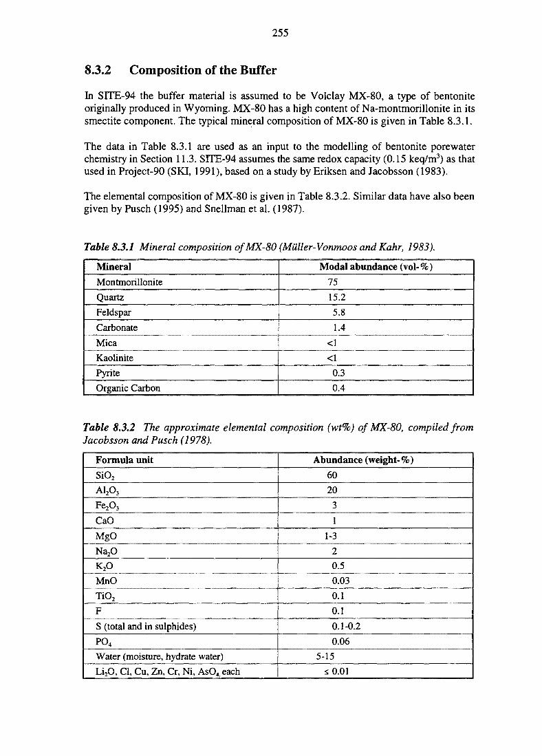
255
8.3.2 Composition of the Buffer
In SITE-94 the buffer material is assumed to be Volclay MX-80, a type of bentoniteoriginally produced in Wyoming. MX-80 has a high content of Na-montmorillonite in itssmectite component. The typical mineral composition of MX-80 is given in Table 8.3.1.
The data in Table 8.3.1 are used as an input to the modelling of bentonite porewaterchemistry in Section 11.3. SITE-94 assumes the same redox capacity (0.15 keq/m3) as thatused in Project-90 (SKI, 1991), based on a study by Eriksen and Jacobsson (1983).
The elemental composition of MX-80 is given in Table 8.3.2. Similar data have also beengiven by Pusch (1995) and Snellman et al. (1987).
Table 8.3.1 Mineral composition of MX-80 (Miiller-Vonmoos and Kahr, 1983).
Mineral
Montmorillonite
Quartz
Feldspar
Carbonate
Mica
Kaolinite
Pyrite
Organic Carbon
Modal abundance (vol-%)
75
15.2
5.8
1.4
<1
<1
0.3
0.4
Table 8.3.2 The approximate elemental composition (wt%) of MX-80, compiled fromJacobsson and Pusch (1978).
Formula unit
SiO2
A12O3
FeA
CaO
MgO
Na2O
K2O
MnO
TiO2
F
S (total and in sulphides)
PO4
Water (moisture, hydrate water)
Li,O, Cl, Cu, Zn, Cr, Ni, AsO4 each
Abundance (weight-%)
60
20
3
1
1-3
2
0.5
0.03
0.1
0.1
0.1-0.2
0.06
5-15
<0.01
256
8.3.3 Transport Properties
Much of the text in this section is derived from an earlier report by the OECD/NEA (NEA,1993).
8.3.3.1 Hydraulic Conductivity
A conceptual model for transport in dense bentonites proposed by Pusch and Hokmark(1987) describes compacted and dry clays as consisting of dense aggregates that, uponhydration, swell and fill the residual pore spaces left by the dry compaction process. Thematerial in the pores is less dense than the initial aggregates of clay platelets and, therefore,is assumed to be less mechanically stable. The low hydraulic conductivity (K) of compactedbentonite backfill assures that transport through such materials will be dominated bydiffusion, with possible minor transport arising from non-Darcy flow such as thermal- orconcentration-osmotic effects (Dixon et al., 1992).
Traditional determinations of K for compacted bentonite have used high-pressure apparatusto decrease the time required to induce measurable flow through the bentonite (e.g., Pusch,1980). The results of these studies give K values in compacted bentonite of about 10'13 m/s.These studies show that flow does not occur until the pressures applied exceed, or comeclose to, the swelling pressures of the bentonite and conclude that the interlayer structureis being affected by high water pressures, e.g., collapsing of the structure, allowing flow tooccur. Follow-on studies (Pusch et al., 1985; Neretnieks, 1985) acknowledge that theseapplied pressures (in the tens of MPa range) are not relevant to the repository situation andthat initial measurements K values may be overestimated. Use of much smaller appliedpressures (tens of kPa range) led to drops in measured K values to about 10"14 m/s (Puschet al., 1985). Even so, applied pressure gradients of this magnitude could still have anunnatural affect on the bentonite, and high point-pressures within the bentonite could resultin local collapse of the interlayer structure or enlargement of intergranular channels.
Alternative techniques have recently been employed to address the difficulties andlimitations inherent in high-pressure gradient permeability tests. These include applicationof low-pressure gradient techniques (e.g., Dixon et al., 1992) and ultracentrifuge technology(e.g., Conca et al., 1993a). These studies claim that compacted bentonite shows hydraulicconductivities below a detection limit of 10"16 m/s, a factor of a thousand lower than thatinitially measured by high-pressure techniques.
In any case, the hydraulic conductivity of an undamaged buffer seems to be sufficiently lowto ensure that transport will be dominated entirely by diffusion.
8.3.3.2 Diffusivity
For low permeability buffers, diffusion will control the transport of radionuclides from thefailed waste canister to the host rock. The extensive literature on diffusion in clay-basedmaterials, including bentonite, has been summarised recently (NEA, 1993).
257
Diffusive transport, represented by Fick's second law of diffusion for a stable species, isgiven by:
aC(x,t) D „- f ^ = ^V2C(x,t)
at a. J
a. = cR. = e + PbKdj
where Cj(x,t) is the concentration of species j , De is the effective diffusion coefficient, ande is the porosity of the medium available for diffusive transport, ctj is the capacity factor forradionuclide j , Rj is the retardation factor for radionuclide j , pb is the bulk density of thematerial, and Kd j is the distribution coefficient for radionuclide j between the solute andsolid phases.
A standard approach to determining radionuclide specific values of the effective diffusioncoefficient, De (also referred to as the so-called simple diffusion coefficient, Ds, see, e.g.NEA, 1993) in compacted bentonite, for use in near-field Performance Assessment (e.g.,Skagius and Neretnieks, 1985; Cho and Oscarson, 1992) is based on the relationship:
in which radionuclide-specific values of the apparent diffusivity, Da, are measured forcompacted bentonite with known e and pb values. Several different techniques involvingradio-chemical tracers may be used, including half-cell/in-diffusion, through-diffusion, andtime-lag approaches in compacted materials (e.g., Cho and Oscarson, 1992; Oscarson et al.,1992; Sato et al., 1992). If retardation processes significantly affect the migration of aspecies in a porous medium, the measured Da will be markedly lower than De.
In conventional, indirect determinations of De, Da values for various radionuclides aremeasured for intact, compacted bentonite samples. Separate batch sorption tests are usedto measure Kd-values for the same radionuclides on disaggregated bentonite samples. Theseconventional determinations of De give values typically in the range 5xlO"13 to 5xlO"M m2/sfor non-sorbing species (SKI, 1991). Indirect measurements for sorbing radionuclides giveDe values for most metals, which are within this range. This includes the actinides, whichfall in the upper part of the range. The alkali and alkaline earth cations behave abnormally,however, with values higher by about one order of magnitude. This phenomenon is ascribedto surface diffusion (see below).
An alternative method for direct determination of De for different materials is electricalconductivity in a potentiostatic or galvanostatic mode, which provides reliable estimatesof diffusion coefficients in electrolyte solutions (Miller 1972; Robinson and Stokes 1959;Conca et al., 1991). Based on electrical conductivity measurements, De in compacted
258
bentonite ranges from 6.5x10¹³ m2/s to l.lxl0"9 m2/s, depending on the volumetric watercontent of the sample (Conca et al., 1993b).
Surface diffusion has been postulated as a theoretically important mechanism in thetransport of radionuclides within bentonite (e.g., Rasmuson and Neretnieks, 1983; Bradburyet al., 1986; Jahnke and Radke, 1987; Cheung, 1990). This transport is assumed to occurwithin the electric double-layer adjacent to mineral surfaces and is sometimes invoked asa significant contributor to the overall diffusion coefficient in experiments in geologicalsystems, especially where model predictions underestimate the extent of tracer diffusion.This kind of behaviour is shown by, e.g., Cs and Sr.
An alternative to the surface diffusion concept as an interpretation of experimental data hasbeen suggested recently. If surface diffusion were dominant, or even of equal magnitudeto bulk porewater diffusion, then increased compaction in bentonite would increasemeasured diffusion by enhancing the linkages between electric double-layers anddecreasing overall surface-diffusion path length. However, through-cell measurements ofDe in compacted bentonite for a variety of radionuclides show that there is a consistent,albeit irregular, decrease in measured diffusion coefficients with increasing compactiondensity (Oscarson et al., 1992). The same systematic decrease in measured diffusion withincreasing compaction is observed in ultracentrifuge tests (Conca et al., 1993b). From thisreasoning, it appears that surface diffusion might be an artifact of the data-fitting procedurein which De for an intact bentonite sample is indirectly inferred by combining Da for anintact bentonite sample with Kd measured on a disaggregated sample. An important reasonfor these difficulties is that all three parameters (De, e and Kd) depend on both the diffusingspecies and the density of the compacted clay (Wanner et al., 1994). This question is notyet resolved.
From the above discussion, it follows that the values of the transport parameters should bechosen conservatively, in order not to underestimate the rate of diffusion through the bufferwhich is due to conceptual uncertainty. For SITE-94, however, no thorough investigationis made and the same non-radionuclide specific values for De and e are employed as thoseused in Project-90 (SKI, 1991). Thus, transport in the buffer is described by analogy withtransport in the rock matrix (see section 7.4.2.2) and surface diffusion is not considered.The effective diffusivity is chosen as suggested by Andersson (1991), i.e. 4xlO'u m2/s, andE is set to 0.36. The former value may be non-conservative for Cs, Sr and Ra. In fact, amore realistic value may be an order of magnitude greater (for example, if surface diffusionwere to be taken into account) and it should be noted that other recent assessments haveused effective diffusivities for cations which are up to three orders of magnitude moreconservative. The choice of De value thus represents an uncertainty within the SITE-94analysis. However, a preliminary analysis shows that with the conceptual model used forradionuclide transport in the near-field in SITE-94, release to the far-field, of at least Cs,is governed by release from the waste-form rather than diffusion in the bentonite.
It should be noted that, in the discussion above, as with the rock matrix, the effects of anionexclusion are not considered. In the bentonite buffer the potential impact of anion exclusionon radionuclide releases is the opposite to that in the rock matrix (see Section 7.4.2.2) inthat, in the buffer, reduced diffusivities caused by anion exclusion will reduce the releaserate of anionic species. Its omission is thus conservative, in this case.
259
8.3.3.3 Sorption in Bentonite
Radionuclide species are retarded as they diffuse through the pore pathways of compactedbentonite owing to sorption onto mineral surfaces. Sorption of radionuclides is discussedin Section 12.4, where the bentonite data selected for SITE-94 are also presented.
The conceptual difficulties experienced in modelling diffusion in bentonite are describedin the previous sub-section. Usually, it is assumed that Kj-values are the same for intact,compacted bentonite and for disaggregated samples. Distribution coefficients for intact,compacted bentonite may be obtained from the relationship described previously betweenDe, Kd and 6. These results, derived from direct measurements on compacted bentonite(Sato et al., 1992; Conca et al., 1991), indicate the possibility of significant differencesbetween batch and intact Kd-values. In some cases, the batch Kd-values are as much as 100times higher (i.e., less conservative) than Kd-values obtained from intact samples ofbentonite. Again, these differences challenge the assumption previously made innormalisation of Da values with batch Kd-values in order to derive De.
8.3.3.4 Gas Transport
Due to the presence of iron in the canister the issue of gas transport through the bentonitehas gained importance. No specific work on gas in the bentonite has been done in SITE-94so the information provided in this subsection is given as a reference only.
According to the SKB RD&D Programme 1995 hydrogen gas will be formed by anaerobiccorrosion of iron. A study supported by SKB (Wikramaratna et al., 1993) have made thefollowing conclusions:
• The long term effect of gas generation is primarily dependent on the gas generationrate and the capacity of the bentonite to permit gas to escape.
• The quantity of gas that can be dissolved in water and is transported away bydiffusion is small compared to the expected generation rate, which means that thegas flow through the bentonite is expected to be the dominant transport mechanism.
• Once the gas has passed through the bentonite, there are enough transport pathwaysto enable the gas to continue on through the rock towards the ground surface.
Evidently, these conclusions have not been checked or by any means evaluated withinSITE-94. However, the conclusions suggest that it will be worthwhile to pay continuedattention to the problem of gas migration through the bentonite.
8.4 THE BACKFILL AND SEALS
The way in which the repository is backfilled and sealed and the long-term performance ofthe materials used may influence the safety of the repository. These issues will thus needto be addressed in an eventual Performance Assessment and safety submission. SITE-94does not treat this subject, however, as it lies outside the general scope of the project, as

260
defined in Chapter 1, and no new work is presented here. The following text is thus anindication of the issues which may arise and need to be evaluated in a full safetysubmission.
8.4.1 Introduction
The construction activities and repository components which need to be considered underthe general heading of 'backfill and seals' comprise:
• the excavation technique, which affects the rock properties and the consequent needfor (and designs of) seals or remedial rock engineering,
• rock reinforcement, including cement grouts, rock bolts and other roof supportmethods,
• tunnel and shaft mass backfill materials,
• seals and flow cut-offs in tunnels, shafts and exploratory boreholes.
The description of the repository system in a full Performance Assessment report will needto comment on each of these activities and components in detail, giving information onissues such as:
• which excavation methods will be used in which regions of the rock/repository andhow these techniques will influence the types of support or sealing required,including information on response to encountering different conditions in the rockduring construction,
• criteria for deciding on the use of different possible rock engineering support orsealing methods, what these methods are, the materials they will introduce into therepository and how the decision criteria may vary, depending on the zone of therepository being excavated,
• the proposed functional requirements of seals, backfills and supports (e.g. temporarysupport during operation, sealing only until closure, long-term support and sealing,etc.),
• detailed descriptions of the properties and long-term behaviour of all materials used(cements, grouts, concretes, mass backfills, seals, bolts, etc.), including the long-term behaviour of material, rock bonding and the development of models of futurematerials performance (chemical alteration, behaviour during resaturation,mechanical stability, hydraulic properties, etc.),
• quality assurance methods to be used during construction and emplacement of seals,including NDT techniques to verify performance.
SITE-94 does not address any of these issues, with the exception of the mechanical impactsof bentonite swelling (Section 11.2.1) on the rock (which is largely aimed at evaluating
261
buffer/rock interactions rather than backfill/rock interactions) and the initiation of somegroundwater flow calculations which explore the impacts of the presence or absence of anExcavation Disturbed Zone (EDZ) in the rock around disposal tunnels and the effects ofhaving no shaft seals (Section 10.3.4).
8.4.2 Excavation, Reinforcement and Grouting
Current assumptions
The proposals at present (SKB, 1992a and 1995a) are that the shaft and tunnels will beconstructed using known technology (raise-boring, drilling/blasting) and the depositionholes can be drilled using a reverse raise-boring method. The possibility of using full-faceboring for the tunnels is also being considered, as this probably reduces the EDZ.
The use of rock support systems is not discussed in detail by SKB (SKB, 1992b) althoughit is noted that the use of concrete as a support may have to be limited owing to the high pHconditions it may introduce locally. SKB note that "other methods must be available for useas a complement to, or substitute for, concrete when needed". It is inevitable that steel-reinforced concrete, rock bolts and associated grouts and resins, and sprayed concrete andsteel netting would need to be used in some parts of a repository during its operational life,as roof or wall supports and as structural platforms and floors. The amounts and locationsof such materials that might be acceptable will need to be considered and justified in thevarious stages of repository licensing.
During excavation, water-bearing fracture zones may be encountered which require sealingin order to allow continued work in the repository. Sealing is likely to be by the injectionof cement grouts. Experience at Aspo indicates that more work is required to developflexible and successful techniques for grouting zones where large volumes of water inflowunder high hydraulic heads (SKB, 1992b and 1995a). It may be that such structures onlyrequire temporary sealing during the operational life of the repository; again, this wouldneed to be considered and any proposals justified. Grouting may also be required to reduceinflows of groundwater if they have a high radon content, as this will lower the ventilationrequirements for the operating repository (SKB, 1995a).
Small fractures can be sealed successfully with either cement or bentonite grouts (SKB,1992b). There may be a need to grout small, water-bearing fractures in some of thedeposition holes (SKB, 1995a).
Safety-related factors
Important safety-related aspects of excavation, reinforcing and grouting include thefollowing:
• The nature and extent of the EDZ in various parts of the repository and whether thiswill influence groundwater flow in the near-field to such an extent that remedialaction (e.g. in the form of flow cut-offs) would be required. Any potential forproducing high-conductivity pathways, connecting deposition zones along the lengthof tunnels, or connecting deeper regions of the rock with shallower regions, via shaftwalls, has clear safety implications. There is already a large amount of information
262
on this issue from the Stripa and Aspo projects, as well as other undergroundlaboratories internationally (SKB, 1992b, 1995a). The Aspo project ZEDEX andother experiments suggest (Pusch and Borgesson, 1992) that hydraulic conductivityof blasted tunnels increases by 100-1000 times in the blast-disturbed zone (onaverage 100 times in a 1 m thick zone) and about 10 times in the stress-redistributedzone beyond this, out to about one tunnel diameter. Full-face boring has less impactand may only induce changes in porosity a few centimetres from the tunnel wall(SKB, 1995b).
The significance of the long-term structural stability of tunnels: how long doesreinforcement need to function in the post-closure and resaturation period?
Geochemical changes, which may be introduced locally by reinforcement andgrouting. The location and mobility of high-pH groundwaters which have been incontact with these materials will need to be evaluated. The possibilities for suchwaters interacting with deposition holes or with radionuclides released from thenear-field over the longer term, together with the times at which such interactionsmight happen, will require analysis.
Cement additives, in the form of plasticisers used to improve the fluidity and theability to pump the grouts, may introduce organic complexants into the repository.
The potential extent of grout sheets injected into highly conductive fracture zoneswill require evaluation. Grout may find its way into regions distant from theinjection points. The need to evaluate and predict the impacts of grouting isacknowledged in the stepped grouting process presented by SKB (SKB, 1995a).
8.4.3 The Backfill
Current assumptions
SKB proposes to backfill the tunnels immediately above the deposition holes with amixture of sand and bentonite, the lower part of which would be compacted in layers andthe upper sections using vibrators. Sprayed mixtures of 20% bentonite with 80% sand weretested in the Stripa project, but the swelling pressure of the bentonite proved too small tobe able to support the tunnel roof and prevent creep deformation (SKB, 1992b). Thisdemonstrates the need for compaction of the material, as mentioned above, or for a higherbentonite content.
Shafts (and, presumably, remote, non-deposition regions of the repository) would be filledwith different materials at various locations, depending on the rock structure and sitehydrogeology. SKB (1992a) suggest using compacted moraine, with localised use of a90/10 sand-bentonite mix, highly compacted bentonite block seals (see Section 8.4.4) andconcrete plugs (e.g. in the upper 100 m to the surface). Clearly, the less conductivematerials and seals would be placed in hydraulically more active zones, at tunnelintersections, or in other parts of the repository to which the results of groundwater flowmodelling proved to be sensitive.
263
Recently, SKB have been evaluating the use of crushed and uncrushed rock debris (muck),produced by the full-face tunnel boring machine used at the Aspo HRL, the crushed muckbeing mixed with various proportions (10, 20 and 30%) of bentonite (SKB, 1995a). Pre-formed blocks which use the higher bentonite content may be emplaced against the tunnelroof zone.
Safety-related factors
The choice and performance of backfill materials raises different safety-related questions,depending on location in the repository. The following are considered to be among theimportant issues which would need to be addressed in a licensing submission:
• The long-term development of bentonite properties influencing the evolution andstability of the hydraulic properties of the backfill, the mechanical stress distributionaround tunnels and shafts and the consequent time-dependent evolution of the EDZhydraulic properties.
• The interaction between swelling of the highly compacted bentonite in thedeposition holes and swelling of the tunnel backfill. The former may extrude into thelatter, causing a certain heterogeneity in buffer/backfill properties at the tops ofdeposition holes.
• Any concrete in the base of tunnels may interact chemically with the backfill (SKB,1995b) and account must also be taken of other cement or concrete reinforcementsor structures which impinge on bentonite-containing backfill.
• Long-term chemical alteration of backfill containing crushed rock may affect theproperties of the bentonite component. Crushed rock presents fresh, active mineralsurfaces to the porewaters present in the backfill at the time of deposition and onresaturation. Components leached from these surface may react with the bentoniteto affect its swelling behaviour and hydraulic properties. In addition, the overalltransport properties of the backfill will evolve with time and this may need to beaccounted for if radionuclide transport in the tunnels is considered relevant to anassessment.
• The hydraulic properties of the interface between backfill materials and the rock isimportant, as a poor bond may lead to preferential pathways for water movementover long distances in the repository.
• A safety analysis will be required to justify the selection of alternative backfillmaterials for different positions in the repository by quantitative evaluations of theirimpacts of groundwater movement in and around the shafts and deposition holes andtunnels. For example, the decision as to the lengths of shafts to fill with relativelyunprocessed material, such as crushed rock or moraine as opposed to concrete orbentonite-based materials, will need a clear rationale based on understanding of thelong-term hydraulic behaviour of the shaft region.
• The behaviour of backfills under the hydraulic and chemical stresses imposed byglaciation will also need to be analysed, particularly in respect to the upper regions
264
of shafts, which are most likely to be subject to elevated hydraulic gradients andpermafrost.
8.4.4 Seals and Plugs
Current assumptions
Seals may be required to isolate fracture zones with high hydraulic conductivity whichintersect deposition tunnels and the repository access shafts and adits. In addition, seals maybe emplaced at strategic points where tunnels intersect each other, or join shafts, and inexploratory boreholes, both vertical from the surface and radiating out from the repository,where the latter have not been 'excavated out' already.
SKB propose (SKB, 1992a, b) to use seals comprising either concrete or highly compactedbentonite blocks, or both, emplaced both within the excavation and within slots cut out intothe rock to cut off the EDZ or isolate fracture zones. Grout shields may also be injected intothe rock around seal zones. Over the next six years, SKB plan to carry out practicalevaluations of concrete seals, which use a bentonite O-ring against the rock, and swellingconcrete seals (SKB, 1995a).
The Stripa project developed various methods to carry out sealing tests in tunnels and inboreholes and there is already a reasonable amount of experience in this field.
The repository will finally be isolated by emplacement of a concrete plug over a length ofabout 100 m at the top of access shafts, possibly incorporating some form of asphalt seal(SKB, 1995a).
Safety-related factors
The safety-related factors for plugs and seals are much the same as those for the backfillmaterials, involving knowledge of mechanical, hydraulic and chemical stability and thelongevity of bonding properties. The choice of materials and emplacement locations will,again, need to be justified quantitatively. These factors are not reiterated in total here. Someadditional points which will need to be considered include:
• The period over which each type and location of seal will be expected to functionand contribute to repository performance needs to be defined. As with rock supportsystems, some seals may only be required to function over the operational, pre-closure period, while others may be required to function, albeit possibly withreduced levels of performance, for thousands of years or more. These factors willrequire quantification and justification.
• Near-surface seals and plugs will be subject to strong impacts of climate change,particularly during glaciations. Freezing and thawing, mechanical erosion, high-pressure water fluxes and oxidising conditions are all to be expected. Thequantitative extent to which shaft plugs are anticipated to resist these impacts needsto be assessed and presented in a safety submission.

265
8.5 TEMPERATURES IN THE REPOSITORY
The thermal output of the spent fuel can influence the geomechanical and geochemicalevolution of the near-field as well as having an impact on the response of the far-field toclimate change. This section summarises how temperatures have been considered indifferent SITE-94 analyses.
In SITE-94, repository-induced temperatures have been analysed (Hansson et al, 1995; seeSection 10.2) in order to study the far-field rock mechanical responses to repository heatingfollowed by the mechanical load from ice in the Central Scenario (Chapter 9). In addition,the Central Scenario description has evaluated far-field temperatures when estimatingthicknesses of permafrost above the repository (King-Clayton et al., 1995; seeSection 10.2). This work builds on the earlier modelling work of McEwen and de Marsily(1991) which established that the repository will not freeze as a result of permafrost,although the heat output of the spent fuel has only a limited impact on the depth ofpenetration of permafrost directly above the repository.
In the near-field, estimates of decay-heat induced temperatures have been taken intoaccount when considering both the geomechanical evolution of the rock (Hansson et al.1995, Section 11.2.1) and the geochemical evolution of the system (Section 11.2.3).
All the temperature modelling work mentioned above has been based on the thermalanalysis of a KBS-3 type repository carried out by Tarandi (1983) and the data presentedin that report. It should, however, be pointed out at this stage that the repositorytemperatures, which have been estimated in each of these studies, vary somewhat accordingto the type of model used, the assumptions made and the intended end-use of thetemperature values calculated. In all studies, where new temperatures are calculated the heatgenerated at the repository level by the waste is modelled with a source term, decaying overtime. The amount of heat, decay rate and density of waste (which is a function of repositorydesign) are taken from Tarandi (1983), but the number of canisters assumed varies betweenstudies. The original work of Tarandi (1983) produced estimates of repository temperaturesas shown in Table 8.5.1.
The Central Scenario study (King-Clayton et al., 1995; Chapter 10.2) used a simple one-dimensional heat-flow model and estimated the maximum bulk repository temperature tobe about 55 °C, occurring shortly after repository closure and dropping to about 15°Cwithin 20 000 years. Repository temperature then lies within the range 5-10°C for the next100 000 years as a result of the climate change scenario. Within 50 000 years of closure,heat from the waste has negligible impact on repository rock temperatures.
The study of far-field geomechanical impacts (Hansson et al., 1995; Section 10.2) used a3D model of a repository containing 4000 canisters of waste and assumed a somewhatdifferent geothermal gradient and Earth surface temperature to those of King-Clayton et al.,1995. This study produced a maximum repository rock temperature of about 48 °C,occurring about 200 years after closure. For a 400 canister repository the maximumtemperature was 35 °C. One should note that these temperatures refer to rock block volumearound the repository and thus are lower than the values given by Tarandi (1983) whichrefer to the temperature at the canister edge.
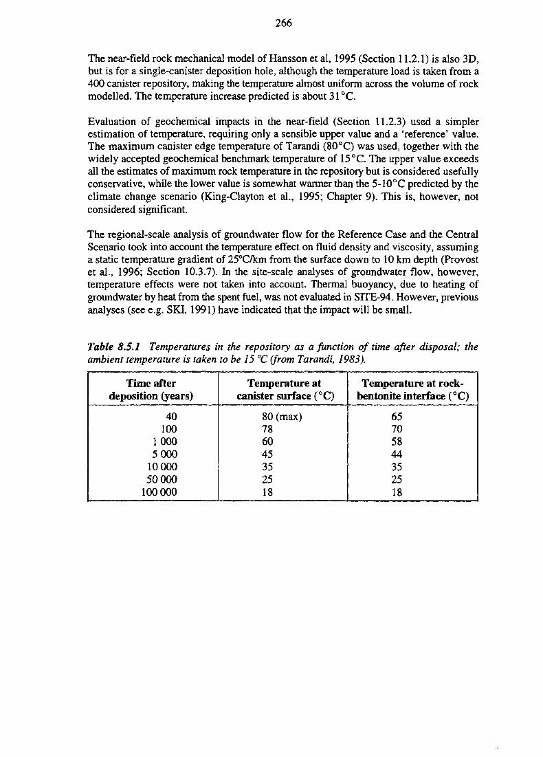
266
The near-field rock mechanical model of Hansson et al, 1995 (Section 11.2.1) is also 3D,but is for a single-canister deposition hole, although the temperature load is taken from a400 canister repository, making the temperature almost uniform across the volume of rockmodelled. The temperature increase predicted is about 31 °C.
Evaluation of geochemical impacts in the near-field (Section 11.2.3) used a simplerestimation of temperature, requiring only a sensible upper value and a 'reference' value.The maximum canister edge temperature of Tarandi (80 °C) was used, together with thewidely accepted geochemical benchmark temperature of 15°C. The upper value exceedsall the estimates of maximum rock temperature in the repository but is considered usefullyconservative, while the lower value is somewhat warmer than the 5-10°C predicted by theclimate change scenario (King-Clayton et al., 1995; Chapter 9). This is, however, notconsidered significant.
The regional-scale analysis of groundwater flow for the Reference Case and the CentralScenario took into account the temperature effect on fluid density and viscosity, assuminga static temperature gradient of 25°C/km from the surface down to 10 km depth (Provostet al., 1996; Section 10.3.7). In the site-scale analyses of groundwater flow, however,temperature effects were not taken into account. Thermal buoyancy, due to heating ofgroundwater by heat from the spent fuel, was not evaluated in SITE-94. However, previousanalyses (see e.g. SKI, 1991) have indicated that the impact will be small.
Table 8.5.1 Temperatures in the repository as a function of time after disposal; theambient temperature is taken to be 15 °C (from Tarandi, 1983).
Time afterdeposition (years)
40100
10005 000
10 00050 000
100 000
Temperature atcanister surface (°C)
80 (max)786045352518
Temperature at rock-bentonite interface (°C)
65705844352518
267
9 SCENARIO IDENTIFICATION
The previous Chapters (3 to 8) describe the Process System analysed in SITE-94. The stateof the Process System directly affects the potential mechanisms of radionuclide release andtransport. Both the processes inside the system and the external FEPs that interact with thesystem determine the state of the system at any given time. This chapter defines the externalfuture events and conditions that are analysed in SITE-94. The chapter also describes howthese EFEPs are specified in order to allow for analysis of their impact on the repositorysystem (i.e. the Process System). Following the vocabulary established in Chapter 2(Section 2.3), this chapter defines the scenario-generating EFEPs that are analysed. Theevolution of the Process System under the scenarios selected is analysed in the subsequentchapters.
9.1 INTRODUCTION
The SITE-94 general approach to scenarios and scenario uncertainty is discussed inChapter 2 and is described in detail by Chapman et al. (1995). Chapman et al. (1995) havealso made an extensive literature survey, the findings of which strongly influenced theapproach finally adopted.
9.1.1 Practical Approach to Handling Scenario Uncertainty
Essential to the SITE-94 approach are the concepts of System Boundary which defines theextent of the Process System (i.e. the 'repository and surrounding rock') and the SystemEnvironment which concerns future events or conditions outside the system (EFEPs) thatmay affect evolution inside the system. A scenario concerns the evolution of the ProcessSystem under the influence of an EFEP or a combination of EFEPs. The EFEPs are denotedscenario-initiating elements.
As discussed in Section 2.3.3, scenario uncertainty is the uncertainty related to the EFEPs.This uncertainty concerns both the completeness problem (have all relevant EFEPs beenfound?) and the quantification of the impact at the System Boundary, probability or otherrelevant measures of the identified EFEPs. Even with an exact specification of the externalimpact, the system evolution may still be uncertain due to uncertainties inside the system.These aspects of the uncertainty of the evolution of a scenario are, however, classified asuncertainties in the Process System in terms of system uncertainty, conceptual modeluncertainty, parameter uncertainty and variability and are discussed in subsequent chapters.This chapter demonstrates how identification of scenario-initiating elements and scenariouncertainty is handled in practice in SITE-94.
9.1.2 Identification of Scenario-initiating EFEPs
The principal procedures for identification of EFEPs that may have a relevant impact onthe analysed system are discussed in Chapter 2. Chapter 2 also describes the principal
268
procedures for treating the impact of EFEPs on the system analysed through the use ofProcess Influence Diagrams (PIDs) and the Assessment Model Flowchart (AMF).
A list of EFEPs relevant to SITE-94 is obtained through the FEP audit procedure describedby Stenhouse et al. (1993). Even if it is clearly impossible to claim that such a list wouldbe complete (see, e.g. Section 2.3), this list is judged to be sufficiently comprehensive forpresent purposes for two reasons. First, the SITE-94 system boundaries are wide, whichshould make the system less sensitive to external influences. Second, the FEP audit is basedon several international FEPs lists and is documented such that it can be reviewed.
The FEPs audit resulted in 81 EFEPs, listed by Stenhouse et al. (1993). Chapter 2 describesthe rationale for avoiding the need to analyse all permutations of these EFEPs and thecomplexities this would involve. The following steps are taken:
• SITE-94 does not analyse deviation from the repository design basis as this liesoutside the scope of the project. Such issues should primarily be treated in the SKBR&D Programme.
• The main class of analyses carried out in SITE-94 concerns a Reference Case whichrepresents a hypothetical situation of no future changes in the external influences onthe Process System. When evaluating the Reference Case, it is understood that theDesign Basis potentially also allows for early canister failures, meaning that allprocesses affecting radionuclide mobilisation and transport would be effective in theReference Case.
• The impact of a deterministic description of the most likely sequence of climaticevents on the repository evolution is analysed by developing a 'Central Scenario'which incorporates the large group of EFEPs concerning expected climate change(e.g. permafrost, glaciation, sea-level changes, etc.) in Sweden.
• Selection of other scenario initiators from the remaining EFEPs is made by applyingthem singly or in groups to the Central Scenario conditions. Whilst a set ofsupplementary scenarios resulting from the evaluation of the remaining EFEPs isdeveloped, these are not taken as far as producing scenario-specific PIDs.
9.1.3 Further Specification of the EFEPs Selected
Once the EFEPs or combinations of EFEPs are defined, it is possible to start evaluatingtheir interaction with the system. In doing this, the EFEPs must be further specifiedcompared to the rather general description usually found in the EFEPs list. A glaciationmay, for example, interact through stress impact from the ice cover, changed hydraulicconditions or changes in temperature. Furthermore, in order to assess these impactsnumerically, quantitative estimates of factors such as time of occurrence, ice thickness,hydraulic conditions in the ice, etc., are needed. The SITE-94 approach to these issuesinvolves a series of steps:
269
• The first step, after specification of which EFEPs to analyse, is to specify theselected set of EFEPs and their time sequence in order to make it possible to applyit to the PID. This step involves identification of where the EFEP influenced the PID(impact points) and a specification of the time sequence, which is detailed enoughto determine if the EFEPs in the selected set could occur in sequence orsimultaneously.
• The next principal step is to modify the PID for the set of selected EFEPs such thatit can handle the influences implied by the EFEPs in a correct manner. The practicalapproach to this in SITE-94 is to develop the PID for the Reference Case, (includingthe Design Basis) as already described in Chapter 2. The resulting PID(RF) is thenadjusted such that it also encompasses the influences highlighted by the CentralScenario, whereas the PID is not adjusted to the remaining EFEPs. Application ofEFEPs, such as those in the Central Scenario, should in principle only change thePID importance level IL as well as the nature of some the PID internal influences.
• The final principal step is a quantitative analysis of the scenario consequences,which first require quantitative specification of the EFEP interactions with theProcess System. The extent of these impacts, as well as the identification of new PIDlinks that need to be considered, may make it necessary to update the calculationmodels (i.e. update the mapping of the PID onto the AMF as described inChapter 2). Finally, actual consequence calculations are performed. In practice suchanalyses are heavily concentrated on the Reference Case in SITE-94, but withillustration of impacts during the Central Scenario.
The subsequent sections in this chapter cover specification of EFEPs for the PID update,the PID update and the specification of the EFEPs to make quantitative analysis possible.The actual modelling details of PID mapping onto the AMF, as well as the results, arecovered in Chapters 10 to 16.
9.1.4 Probability of Scenario Occurrence
The likelihood of occurrence of any specified combination of EFEPs which comprises ascenario needs to be taken into account by the decision-maker who is considering theestimated consequences of a scenario. Chapman et al. (1995) evaluated the issue of scenarioprobability and went back to some of the seminal work on scenarios (Kahn and Wiener,1967).
Kahn and Wiener did not advocate scenarios as predictive devices. Instead, they were seenas one of many devices for stimulating and disciplining the imagination. Whilst it is helpfulto aim for plausibility in constructing scenarios, 'unrealistic' scenarios may be equallyuseful aids to discussion and it is pointed out that many sequences of events only appearplausible after they have happened. Cooke (1991) reinforces this view, stating that "...it iseasy to be misled into believing that scenario analysis yields predictions". Referring to theearlier work of Kahn, he also suggests that no particular scenario is any more likely thananother. This idea is extended to have relevance to the type of probabilistic analyses carriedout in a Performance Assessment. Because any given 'future' is only part of an infinite setof possible futures, it is not appropriate to assign conditional probabilities to any scenario
270
within a set selected for analysis. Thus, whilst it may be possible to estimate the probabilityof a given event occurring and to build a scenario based upon that event, the fullprobabilistic treatment of a comprehensive scenario set is not considered possible.
Kahn's approach of defining a 'surprise-free scenario' based on basic long-term trends andthen defining 'alternative futures' or 'canonical variations' by varying key parameterswithin it is closely parallelled by SITE-94's formulation of a Reference Case and then aCentral Scenario upon which all other scenarios are based. The surprise-free scenario ofKhan serves a key purpose by being salient, because of its relation to basic trends, notbecause it is any more probable than any of the alternative futures.
Making decisions based on a set of analysed scenarios will thus, unavoidably, require aconsiderable degree of judgement concerning the relative significance of poorly quantifiedprobabilities and the proper weighting to give to each scenario presented. This simplyreinforces the view that scenarios are simply:
• a means of illustrating possible future behaviour of a system,• a means of defining how such behaviour might arise.
Scenario analysis, on the premises of its original proponents, categorically does not try topredict the future. The emphasis is on having salient scenarios, acting as illustrations toassist in the making of decisions.
These points need to be considered in practical decision making. It is clear that a systemthat usually behaves well ('robust') under a set of salient scenarios is normally viewed tobe superior to a system which behaves less well under these conditions. The practicaldecision is probably to favour the first system. This may be a wise decision policy, butshould not be misinterpreted as a prediction of what actually will happen.
9.2 THE REFERENCE CASE
9.2.1 Definition of the Reference Case
The main purpose of the Reference Case is to set up conditions which make it possible toevaluate the 'internal evolution' of the repository system when it is not under the impactof changing external influences. The definition of the SITE-94 Reference Case is that therepository is constructed according to the Design Basis and with uncertainties, thatpresent-day climate and surface environment persist indefinitely and that there is no humaninterference with the system. The SITE-94 repository system Design Basis is defined inChapters 3 to 8 and is not reiterated here.
In SITE-94 it was decided not to view the Reference Case as a realistic example of externalconditions (i.e. a scenario), thereby avoiding discussions on whether it should include the'known' time evolution of climate or other external conditions. Instead, the effect ofclimate evolution is handled by the Central Scenario. The evolution of the repositorybarriers under the Reference Case assumptions may deviate little from their evolution underthe Central Scenario. In fact, the difference between the evolution of the repository under
271
the Reference Case and under climate evolution gives information on how sensitive therepository would be to external influences. If the system is robust, the relevant differenceshould be small.
9.2.2 Developing Influence Diagrams, Models and CalculationCases for the Reference Case
The Reference Case is the starting point in defining and describing the SITE-94 ProcessSystem, as well as its formal representation in the Process Influence Diagram, PID(RF).The PID is then used to develop and audit the consequence modelling described in theAMF. Chapters 10 to 16 include descriptions of the AMF assessments of the evolution ofthe Process System for the Reference Case conditions and discussions on whether themodelling actually performed is consistent with the modelling as designed in the AMF.
9.3 THE CENTRAL (CLIMATE EVOLUTION) SCENARIO
9.3.1 Introduction
The Central Scenario describes the impact of the most likely sequence of climatic eventson repository evolution. Consequently, full account is taken of predicted changes in theclimate of Sweden. A specification of the external impact during the Central Scenario thusrequires the following main components:
• a deterministic description of the most probable climate state for Sweden, withspecial reference to the Aspo area,
• a description of the likely nature of the surface environment in the site area at eachstage of the climate sequence selected,
• quantitative information on how these changes might affect the disposal system,such that impact points on the PID for the Reference Case could be identified andimpacts tracked quantitatively through the influence diagram to produce a PID forthe Central Scenario.
It was decided that the timescale of the Central Scenario should be about 100 000 years, asa justifiable description of climate sequence beyond this would become more difficult.Also, this order of magnitude of time falls in well with the principal period of concern ina repository safety assessment. In the event, as the climate sequence model was developed,the actual timescale of the Central Scenario was most conveniently fixed at 120 000 yearsinto the future, with a description which also extended some 10 000 years into the past (seeKing-Clayton et al., 1995).
272
9.3.2 Climate Prediction
The SlTE-94 description of the most probable climate evolution is made in general for thewhole of Scandinavia and, more specifically, for the Stockholm and Aspo regions. Thebasis for the development of the SITE-94 climate change scenario is the ACLIN(Astronomical CLimate INdex), Imbrie and Imbrie (1980) and the Paleoclimate Model(PCM) (Berger et al., 1990) climate models, all of which consider the Milankovitch orbitalparameters. From these models, changes in the global amount of ice and correspondingeustatic sea-level are estimated. The prediction of future glaciations in Fennoscandia isbased on parallels with the last glaciation.
It is now recognised that a period of glaciations, which had particularly significant impactsin the Northern Hemisphere, started some 2.3 million years ago. During the Quaternaryperiod (the last 1.8 million years), a considerable number of glaciations, interrupted bywarmer interglacials, have been documented. The periodicity of the glacial/interglacialsequence approaches a 100 000 year cycle during the middle and late Pleistocene(approximately the last million years). This knowledge of Quaternary glaciations is helpfulin making a preliminary prognosis of a future glaciation. The last (Eemian) interglacial,about 100 000 to 120 000 years ago, lasted about 10 000 years. As the present warm period,the Holocene, has lasted about this long and as the Holocene climatic optimum passedseveral thousand years ago, it is possible that the cooling of the next glaciation has alreadybegun. The great uncertainty in this simple prediction is that it does not consider the causesof the glacial/interglacial cycles.
More elaborate prognoses of future climate use a climate model based on the variableswhich regulate the glacial/interglacial cycles. The general acceptance of the Milankovitch(1941) theory of the forcing of climate as a result of cycling and fluctuations in the Earth'sorbital parameters and its confirmation through oxygen isotope stratigraphy in deep-seasediments, makes it the best tool available for climate predictions within the time spanrelevant for disposal of spent nuclear fuel. The Central Scenario description thus usesinformation on Milankovitch forcing of climate to describe likely implications for futureglacial-interglacial cycles, sea-level changes and crustal movements of glaciated regions.
In the prediction of future climate changes for the Central Scenario, the possible effects ofhuman activities (e.g. greenhouse warming) are not considered, as they are difficult toassess quantitatively in detail. Human effects could prolong the present state of climate orresult in global warming, but this effect is not considered to hinder the next cold phase,merely delay it in the perspective of the next 120 000 years. As discussed in Section 9.4,a separate Scenario is envisaged to handle this issue.
The climate models used for this study suggest glaciations at about 5000, 20 000, 60 000and 100 000 years from now. The scenario is mainly based on the SKB/TVO scenario(Ahlbom et al. 1991) and Bjorck and Svensson (1992), with some modifications due toinput from McEwen and de Marsily (1991) and Svensson (1989). The proposed evolutionof the future climate is as follows:
0 -10 000 years. The climate in Sweden will gradually change to cooler conditions withgrowth of an ice sheet in the Scandinavian Caledonides. Ice sheet thickness in the centralmountains will be about 1000 m, with no ice in Stockholm or southwards. Crustal down-
273
warping of about 300 m will occur in the central mountainous part. Sea-level will graduallydrop to -20 to -40 m below present day sea-level in the Stockholm region as well as in theAspo region. During the colder parts of this period, permafrost will occur in northernSweden. The water in the Baltic will gradually become fresher as the straits to the oceansdecrease.
10 000 - 30 000 years. After a minor, somewhat warmer, period the climate will get colderand fully glacial conditions will prevail around 20 000 years from now. The glacial peakwill last approximately 5000 years. The ice sheet is estimated to reach the Stockholm areabut probably not the Aspo region. Ice thickness in the central part of the ice sheet will beabout 1500 m, while the ice sheet thickness in the Stockholm region will be about 800 m.Crustal downwarping of about 500 m will occur in the central part of the ice sheet withabout 60 m taking place in the latitude of Stockholm. During deglaciation, when the icefront is located in the Stockholm region, the sea-level is estimated to be about 25 m belowpresent day sea-level. At Aspo, sea-level will drop to about -50 m below present day sea-level. The total effect of the glacial loading at Aspo is difficult to evaluate, but probablywill not be large. Permafrost conditions will be present as far south as southern Sweden.The water in the Baltic will be fresh and probably at the same level as the oceans, due toerosion at its outlets.
30 000 - 50 000 years. Conditions will be interstadial with a dry, cold climate (like theclimate of Greenland today). Glaciers will be present in the Swedish mountains andpermafrost will be present in northern Sweden. In the Stockholm region, the eustatic riseof sea-level and decreasing isostatic uplift will result in a sea-level about 30-40 m belowpresent day sea-level. At Aspo there will not be much isostatic uplift but a eustatic sea-levelrise of about 10-20 m. Thus a sea-level at about 30-40 m below present day level is likely.The Baltic will be mainly fresh but some saline water will probably enter it.
50 000 - 70 000 years. Full glacial conditions will prevail. Due to the previous coldconditions, the ice sheet will respond more rapidly. The glacial culmination will occuraround 60 000 years. The ice sheet will cover the whole of Sweden as far south as northernGermany, comparable to the maximum of the Weichselian glaciation. Ice sheet thicknessin the central part will be about 3000 m. In the Stockholm region the ice thickness will beabout 2500 m. The Stockholm region will probably be covered by the ice sheet for at least10 000 years and, possibly, longer. Downwarping of the ground will be about 700 m in thecentral part of the ice sheet, about 600 m in the Stockholm area and, at Aspo, could beabout 500 m. During deglaciation, when the ice front is located in the Stockholm region,the sea-level is estimated to be about 150 m at Stockholm and, at the same time, about 80 mabove present day coastline at Aspo. There could also be a damming of the Baltic to10-30 m above ocean level. The Baltic will be mainly fresh but during deglaciation salinewater may enter the Baltic through isostatically depressed areas. Permafrost will be presentin large areas of Europe.
70 000 - 80 000 years. A rapid deglaciation will lead to and culminate in interglacialconditions at 75 000 years. Total crustal uplift is estimated to be about 700 m in the centralparts of the previous ice sheet, about 600 m at Stockholm and 500 m at Aspo. This will bea relatively 'warm' period with a climate in the Stockholm region similar to the presentclimate in northern Sweden. Small mountain glaciers and permafrost will occur in the verynorth. Parts of southern Sweden could be resettled and farming might be possible. Sea-level
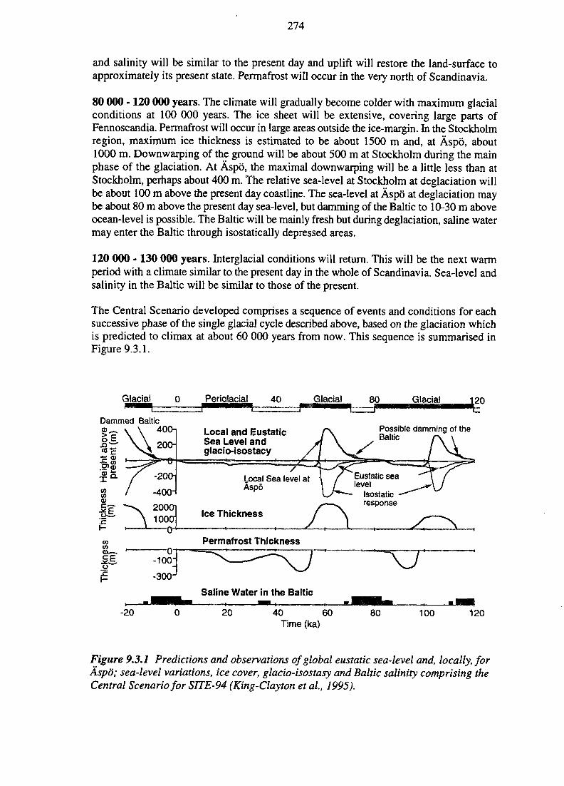
274
and salinity will be similar to the present day and uplift will restore the land-surface toapproximately its present state. Permafrost will occur in the very north of Scandinavia.
80 000 -120 000 years. The climate will gradually become colder with maximum glacialconditions at 100 000 years. The ice sheet will be extensive, covering large parts ofFennoscandia. Permafrost will occur in large areas outside the ice-margin. In the Stockholmregion, maximum ice thickness is estimated to be about 1500 m and, at Aspo, about1000 m. Downwarping of the ground will be about 500 m at Stockholm during the mainphase of the glaciation. At Aspo, the maximal downwarping will be a little less than atStockholm, perhaps about 400 m. The relative sea-level at Stockholm at deglaciation willbe about 100 m above the present day coastline. The sea-level at Aspo at deglaciation maybe about 80 m above the present day sea-level, but damming of the Baltic to 10-30 m aboveocean-level is possible. The Baltic will be mainly fresh but during deglaciation, saline watermay enter the Baltic through isostatically depressed areas.
120 000 -130 000 years. Interglacial conditions will return. This will be the next warmperiod with a climate similar to the present day in the whole of Scandinavia. Sea-level andsalinity in the Baltic will be similar to those of the present.
The Central Scenario developed comprises a sequence of events and conditions for eachsuccessive phase of the single glacial cycle described above, based on the glaciation whichis predicted to climax at about 60 000 years from now. This sequence is summarised inFigure 9.3.1.
Glacial Periqlacial 40 Glacial 80 Glacial 120
Dammed Baltic400-i
-20
Local and EustaticSea Level andglacio-isostacy
Possible damming of theBaltic
Local Sea level atAspo
Ice Thickness
Eustatic sealevel
Isostaticresponse
Permafrost Thickness
\7Saline Water in the Baltic
20 40 60Time (ka)
80 100 120
Figure 9.3.1 Predictions and observations of global eustatic sea-level and, locally, forAspo; sea-level variations, ice cover, glacio-isostasy and Baltic salinity comprising theCentral Scenario for SITE-94 (King-Clayton et al, 1995).
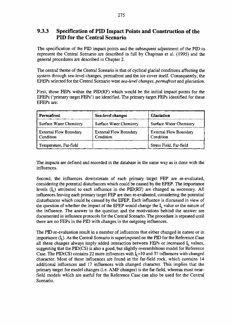
275
9.3.3 Specification of PID Impact Points and Construction of thePID for the Central Scenario
The specification of the PJD impact points and the subsequent adjustment of the PID torepresent the Central Scenario are described in full by Chapman et al. (1995) and thegeneral procedures are described in Chapter 2.
The central theme of the Central Scenario is that of cyclical glacial conditions affecting thesystem through sea-level changes, permafrost and the ice cover itself. Consequently, theEFEPs selected for the Central Scenario were sea-level changes, permafrost and glaciation.
First, those FEPs within the PID(RF) which would be the initial impact points for theEFEPs ('primary target FEPs') are identified. The primary target FEPs identified for theseEFEPs are:
Permafrost
Surface Water Chemistry
External Flow BoundaryCondition
Temperature, Far-field
Sea-level changes
Surface Water Chemistry
External Flow BoundaryCondition
Glaciation
Surface Water Chemistry
External Flow BoundaryCondition
Stress Field, Far-field
The impacts are defined and recorded in the database in the same way as is done with theinfluences.
Second, the influences downstream of each primary target FEP are re-evaluated,considering the potential disturbances which could be caused by the EFEP. The importancelevels Qn) attributed to each influence in the PID(RF) are changed as necessary. Allinfluences leaving each primary target FEP are then re-evaluated, considering the potentialdisturbances which could be caused by the EFEP. Each influence is discussed in view ofthe question of whether the impact of the EFEP would change the IL value or the nature ofthe influence. The answer to the question and the motivations behind the answer aredocumented in influence protocols for the Central Scenario. The procedure is repeated untilthere are no FEPs in the PID with changes in the outgoing influences.
The PID re-evaluation result in a number of influences that either changed in nature or inimportance (IJ. As the Central Scenario is superimposed on the PID for the Reference Caseall these changes always imply added interaction between FEPs or increased IL values,suggesting that the PID(CS) is also a good, but slightly overambitious model for ReferenceCase. The PID(CS) contains 22 more influences with IL=10 and 37 influences with changedcharacter. Most of these influences are found in the far-field rock, which contains 14additional influences and 17 influences with changed character. This implies that theprimary target for model changes (i.e. AMF changes) is the far-field, whereas most near-field models which are useful for the Reference Case can also be used for the CentralScenario.
276
Clearly, this re-evaluation is strongly influenced by expert judgement based on the assumedmagnitude of the EFEP impact. Increased detail in the Central Scenario description refinedthis judgement. For example, a judgement that the repository will never freeze, based onevaluations of the maximum thickness of permafrost made by McEwen and de Marsily(1991), make it possible to disregard influences that would be very important if therepository did, in fact, freeze.
9.3.4 Specification of Quantitative Data for PerformanceAssessment Modelling
The Central Scenario, described fully in King-Clayton et al. (1995), contains an initialdescription of the climate model developed for the Aspo area with an accompanying broad-scale outline of the predicted surface conditions. As predictions of future climate areultimately uncertain, it is the intention of the Central Scenario to provide an indication ofthe potential degree of variability and significance of future climatic changes on theevolution of a deep repository site.
The research supporting the Central Scenario is not intended to be exhaustive, but ratherto produce basic support for the Performance Assessment models used in SITE-94.Wherever possible, direct observations and measurements of features are sought to provideinformation. However, in many cases only model predictions are available from theliterature for many of the features and processes of interest.
The general description of the climate evolution is extended to produce a more detaileddescription of the surface conditions at the site at each stage of the climate sequence, withparticular emphasis on the passage of ice (especially the ice-front) across the site. Thisinvolves evaluating issues such as the existence of free water under ice sheets, hydraulicconnection between free water in, on and under the ice with groundwater in the underlyingrock, the rate of ice build-up and decay at a site-scale and evidence for the geometry of theice front.
Following the construction of the scenario description, quantitative estimates of the time-dependent changes are made for:
• ice sheet thickness (excess hydraulic head),• ice sheet thickness gradient (excess hydraulic gradient),• supraglacial and subglacial discharge (approximate),• permafrost thickness,• glacial meltwater chemistry,• surface (meteoric) water chemistry,• deep, very saline water chemistry,• marine water chemistry,• regional saline/dense water chemistry (incorporating both deep saline and marine
components),• regional fresh/dilute water chemistry (incorporating both meteoric and glacial
water),
277
the distribution of organic accumulations at the surface (affecting the chemistry ofinfiltrating waters).
9.3.5 Adjustment of the AMF to Evaluate the Central Scenario
The PID(CS) at IL=10 is formally mapped onto the AMF developed for the Reference Case.Due to resource limitations there is no formal exercise in SITE-94 where this AMF isthoroughly evaluated in order to find out if the Central Scenario would imply additionalmodelling needs and not just changed input to the AMF models. Clearly such an exercisecould be done and would not require tremendous efforts. At any rate, knowledge of thechanged importance and character of some of the PID links for the Central Scenario led tothe identification of some modelling needs on a less formal basis.
Most of the modelling needs for the Central Scenario are known before the developmentof the PID(CS), but the PID helps in Quality Assurance terms as a reminder of theirimportance and highlighted aspects such as the connection between long-termhydrogeology and geochemistry. The Central Scenario PID indicate that, apart from themodels needed to describe the evolution under the Reference Case, the following modellingcapabilities are necessary:
Rock Mechanics
The rock mechanical impact of the ice-load is evidently one of the major phenomena toevaluate during the Central Scenario. The glacial load also highlights the coupling betweenhydrology and rock mechanics.
Regional Hydrogeology and Geochemistry
Sea-level changes, permafrost and the ice sheet all imply large-scale (regional) changes ofthe hydrogeological boundary conditions at the site. Furthermore, these large-scale changespotentially affect deep saline water with high density. Consequently, a proper analysis ofhydrogeology and changes in geochemistry during the Central Scenario would requirehydrological analysis of density-dependent flow at a regional scale.
Repository Scale Hydrology and Geochemistry
It is also evident that the changing boundary conditions will result in time-varying flow andgeochemistry at the repository. The flow variation may potentially be rather rapid duringevents such as glacial retreat. Migration of groundwaters with different chemistry,particularly highly oxidising surface waters, may also be important.
Radionuclide Release and Transport
The Central Scenario implies that the hydrogeological and geochemical conditions thataffect radionuclide release and transport will change with time. Such temporal changes maypotentially lead to accumulation followed by more rapid releases.
278
Biosphere
The Central Scenario has obvious implications for the local biosphere as a function of time.The modelling needs identified above are also realised in some modelling exercisesspecially designed for the Central Scenario; these are discussed in Chapters 10 to 16.However, the ambition level for the actual consequence analyses of the Central Scenariois lower than for the Reference Case. In particular, the predictions for radionuclide releaseand transport should be seen as examples of differences of system behaviour within theCentral Scenario as compared to the Reference Case. S1TE-94 does not claim to analysesystem evolution comprehensively, with uncertainties, for the Central Scenario.
9.4 SELECTION OF INTERESTING COMBINATIONS OFREMAINING EFEPS
The Central Scenario only covers a few of the potentially important scenario-generatingEFEPs identified in SITE-94. The other EFEPs form the basis for the selection of otherscenario initiators by applying them singly or in groups to the Central Scenario followinga set of guidelines for selection. Whilst a set of supplementary scenarios resulting from theevaluation of the remaining EFEPs is developed, these are not taken as far as producingscenario-specific PIDs. Only EFEP identification and grouping is done in SITE-94, noqualitative or quantitative consequence analyses are performed. In some cases qualitativearguments would suffice for showing that such analyses would be unnecessary, but someof the scenario-initiating events identified in SITE-94 would eventually need to be analysedfurther. The reader is also referred to SKI Project-90 (SKI, 1991) which included analysesof a number of scenarios formulated 'ad-hoc'. Chapman et al. (1995) describe in full theSITE-94 work using the remaining EFEPs and the following sections summarise this.
9.4.1 Screening the EFEPs
The 81 EFEPs from the SITE-94 FEP audit list (Stenhouse et al., 1993) are re-evaluated.They are first screened, using the following three screening decisions:
• Design Basis: Deviations from the proposed repository design and operation,including the effects of poor QA on the wastes or near-field Engineered Barriers, arenot evaluated in SITE-94 although some account is taken of the latter issues in termsof the variability in material properties used in the assessment.
• Human Intrusion: As in SKI Project-90, human intrusion is not considered inSITE-94, as it is considered to be fundamentally different in nature from all other PAanalyses and a matter on which a separate position needs eventually to beestablished.
• Relevance: EFEPS which could be identified as having no relevance to therepository or to the Aspo site (improbable effects which had survived the initial FEPaudit, such as tsunamis and landslides), to have negligible identifiable impact, or tobe related only to biosphere uncertainties (which are not addressed in SITE-94) arererr: ;ved.
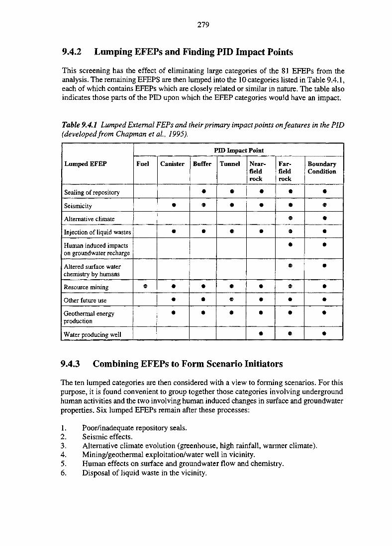
279
9.4.2 Lumping EFEPs and Finding PID Impact Points
This screening has the effect of eliminating large categories of the 81 EFEPs from theanalysis. The remaining EFEPS are then lumped into the 10 categories listed in Table 9.4.1,each of which contains EFEPs which are closely related or similar in nature. The table alsoindicates those parts of the PID upon which the EFEP categories would have an impact.
Table 9.4.1 Lumped External FEPs and their primary impact points on features in the PID(developedfrom Chapman etal., 1995).
Lumped EFEP
Sealing of repository
Seismicity
Alternative climate
Injection of liquid wastes
Human induced impactson groundwater recharge
Altered surface waterchemistry by humans
Resource mining
Other future use
Geothermal energyproduction
Water producing well
PID Impact Point
Fuel Canister
«
•
m
9
Buffer
#
9
%
9
Tunnel
*
$
$
$
#
Near-fieldrock
9
9
9
#
$
$
Far-fieldrock
9
9
m
9
9
9
9
9
9
9
BoundaryCondition
9
9
9
9
9
9
9
9
9
9
9.4.3 Combining EFEPs to Form Scenario Initiators
The ten lumped categories are then considered with a view to forming scenarios. For thispurpose, it is found convenient to group together those categories involving undergroundhuman activities and the two involving human induced changes in surface and groundwaterproperties. Six lumped EFEPs remain after these processes:
1. Poor/inadequate repository seals.2. Seismic effects.3. Alternative climate evolution (greenhouse, high rainfall, warmer climate).4. Mining/geothermal exploitation/water well in vicinity.5. Human effects on surface and groundwater flow and chemistry.6. Disposal of liquid waste in the vicinity.
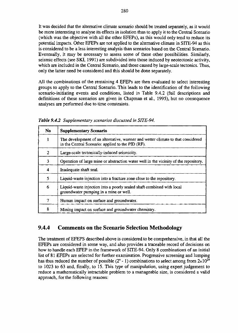
280
It was decided that the alternative climate scenario should be treated separately, as it wouldbe more interesting to analyse its effects in isolation than to apply it to the Central Scenario(which was the objective with all the other EFEPs), as this would only tend to reduce itspotential impacts. Other EFEPs are not applied to the alternative climate in SUE-94 as thisis considered to be a less interesting analysis than scenarios based on the Central Scenario.Eventually, it may be necessary to assess some of these other possibilities. Similarly,seismic effects (see SKI, 1991) are subdivided into those induced by neotectonic activity,which are included in the Central Scenario, and those caused by large-scale tectonics. Thus,only the latter need be considered and this should be done separately.
All the combinations of the remaining 4 EFEPs are then evaluated to select interestinggroups to apply to the Central Scenario. This leads to the identification of the followingscenario-initiating events and conditions, listed in Table 9.4.2 (full descriptions anddefinitions of these scenarios are given in Chapman et al., 1995), but no consequenceanalyses are performed due to time constraints.
Table 9.4.2 Supplementary scenarios discussed in SITE-94.
No
1
2
3
4
5
6
7
8
Supplementary Scenario
The development of an alternative, warmer and wetter climate to that consideredin the Central Scenario: applied to the PID (RF).
Large-scale tectonically-induced seismicity.
Operation of large mine or abstraction water well in the vicinity of the repository.
Inadequate shaft seal.
Liquid-waste injection into a fracture zone close to the repository.
Liquid-waste injection into a poorly sealed shaft combined with localgroundwater pumping in a mine or well.
Human impact on surface and groundwater.
Mining impact on surface and groundwater chemistry.
9.4.4 Comments on the Scenario Selection Methodology
The treatment of EFEPS described above is considered to be comprehensive, in that all theEFEPs are considered in some way, and also provides a traceable record of decisions onhow to handle each EFEP in the framework of STTE-94. Only 8 combinations of an initiallist of 81 EFEPs are selected for further examination. Progressive screening and lumpinghas thus reduced the number of possible (2n -1) combinations to select among from 2xlO24
to 1023 to 63 and, finally, to 15. This type of manipulation, using expert judgement toreduce a mathematically intractable problem to a manageable size, is considered a validapproach, for the following reasons:
281
• Large classes of EFEPs can be relegated from analysis from the viewpoint ofassessment philosophy (e.g. human intrusion EFEPs), provided the position adoptedis acceptable to all reviewers and decision makers.
• The breadth and comprehensivity of the PID(RF) effectively 'mop up' a largenumber of EFEPs into the Process System and the Central Scenario so thatinteractions are considered via an influence diagram.
• Slavish adherence to mathematical completeness is eliminated from the objectivesof a scenario definition programme at the outset, as discussed in Chapter 2. Theobjective, instead, is to use the assembly of EFEPs to allow intelligent interrogationof the PID, with expert judgement being used to ensure that important confluencesof impacts are not overlooked and to identify topical scenarios for further study.
In general, it is felt that it is possible to follow, reasonably closely, the guidelines forscenario selection introduced at the beginning of this chapter. A residual criticism,however, is that the approach developed may overlook some obscure combination ofEFEPs which could have a reasonable likelihood of occurrence and a significantconsequence. Nevertheless, it is thought that this could occur whatever technique is used,and the best defence against this possibility is the repeated application of the methodologyin sequential assessments, by as diverse a range of expert groups as possible.
Inevitably then, the final selection of scenarios must be rather subjective, reflecting theneeds and interests of the moment. The approach adopted does allow any group now toadopt a different attitude to particular issues and EFEPs, and to use the same approach tobuild their own scenarios, testing and stressing the system in different ways.
9.5 CONCLUSIONS
SITE-94 demonstrates an approach to handling scenario uncertainty. The wide SystemBoundary and the open procedure for identifying EFEPs outside the system are means ofhandling the completeness problem. This approach also makes it possible to put lessemphasis on scenario probability as, in fact, most of the quantifiable uncertainties arereclassified into conceptual model or parameter uncertainty.
The Reference Case and the Central Scenario together represent external conditions basedon assessment of long-term trends. Even if it is hard to quantify whether these conditionswill occur or not, it is nevertheless natural to assess the consequences of these conditionsin some detail and include the results in the decision basis.
Throughout this chapter, emphasis is placed on the illustrative nature of the scenarioanalysis process. The group of supplementary scenarios described above reflects issues,events and mechanisms which are currently of interest within SKI and elsewhere. Inparticular, they are mostly concerned with the future activities of people. This reflects adominant concern that it is these activities which are most likely to affect a repository andalso to have the greatest impact, consequently being of most interest in safety andregulatory terms. In a few years time, other scenarios may be suggested which are of moreconcern and some of those currently evaluated may no longer be of interest. Scenario

282
generation should be seen as a dynamic process, responding to the needs and the state ofdevelopment of a waste disposal programme.
The list of supplementary scenarios is thus not meant to be exhaustive. Nevertheless, evenat this stage, a number of additional important issues have already been identified, butomitted from study. It is not SKI's intention to give the impression that these should berelegated in importance. Future evaluations are needed. The PDD-based approach adoptedin this study would form a sensible basis for such evaluations.
283
REFERENCES TO CHAPTERS
CHAPTER 1
Almen, K-E and Zellman, O., Aspo Hard Rock Laboratory. Field investigation metho-dology and instruments used in the pre-investigation phase, 1986-1990, SKB TR 91-21,Swedish Nuclear Fuel and Waste Management Co., Stockholm, 1991.
Coplan, S.M., Eisenberg, N.A., Federline, M.V. and Randal, J.D., Current perspectives onPerformance Assessment at the NRC, Proceedings of the Third International Conferenceon High Level Radioactive Waste Management, Las Vegas, Nevada, April 12-16, 1992,American Nuclear Society - American Society of Civil Engineers, 1992.
Gustafsson, G., Liedholm, M., Rhen, I., Stanfors, R., and Wikberg, P., Aspo Hard RockLaboratory, Predictions prior to excavation and the process of their validation, SKBTR 91-23, Swedish Nuclear Fuel and Waste Management Co., Stockholm, 1991.
NEA, SKI Project-90, A review carried out by an OECD/NEA team of experts, Organi-sation for Economic Co-operation and Development, Nuclear Energy Agency, Paris, 1992.
Nordic Document, Disposal of high level radioactive waste, Consideration of some basiccriteria, The Radiation Protection and Nuclear Safety Authorities in Denmark, Finland,Iceland, Norway and Sweden, 1993.
NRC, Iterative Performance Assessment Phase 2: Development of capabilities for reviewof a Performance Assessment for a High-Level Waste Repository, NUREG-1464,U. S. Nuclear Regulatory Commission, Washington, 1995.
SKB RD&D-Programme 92, Treatment and final disposal of nuclear waste, Programme forresearch, development, demonstration and other measures, Swedish Nuclear Fuel andWaste Management Co., Stockholm, 1992.
SKB RD&D-Programme 92 Supplement, Swedish Nuclear Fuel and Waste ManagementCo., Stockholm, 1994.
SKBF/KBS, Final Storage of Spent Nuclear Fuel—KBS-3, report, Swedish Nuclear FuelSupply Co./Div. KBS, Stockholm, 1983.
SKI, Review of the KBS-3 report, SKI Technical Report 84-5, Swedish Nuclear PowerInspectorate, Stockholm, 1984.
SKI, Project-90, Volumes I and n, SKI TR 91:23, Swedish Nuclear Power Inspectorate,Stockholm, 1991.
SKI, Review of SKB RD&D-Programme 92, SKI Technical Reports 93:13 and 93:14,Swedish Nuclear Power Inspectorate, Stockholm, 1993.
284
SKI, Review of SKB RD&D-Programme 95, SKI Technical Report 95:1, Swedish NuclearPower Inspectorate, Stockholm, 1995.
Wikberg, P. (ed.), Gustafson, G., Rhen, I., and Stanfors, R., Aspo Hard Rock Laboratory,Evaluation and conceptual modelling based on the pre-investigations 1986-1990, SKBTR 91-22, Swedish Nuclear Fuel and Waste Management Co., Stockholm, 1991.
CHAPTER 2
Andersson, J. (ed), Carlsson, T., Eng, T., Kautsky, F., Soderman, E., and Wingefors, S.,The joint SKI/SKB scenario development project, SKI TR 89:14, Swedish Nuclear PowerInspectorate, Stockholm, 1989.
BIOMOVS H, Reference biospheres: Report of a subgroup meeting to examine the applica-bility of the 'RES' methodology to scenario development in the biosphere component ofPerformance Assessment for radioactive waste repositories, 14-15th September 1994,Langholmen Stockholm, (available from the BIOMOVS E Secretariat, Intera, Henley, U.K.),1994.
Chapman, N.A., Andersson, J., Robinson, P., Skagius, K., Wene, C-O., Wiborgh, M., andWingefors, S., Systems analysis, scenario construction and consequence analysis definitionfor SITE-94, SKI Report 95:26, Swedish Nuclear Power Inspectorate, Stockholm, 1995.
Churchman, C.W., The systems approach, Dell Publishing Co., Inc, New York, 1968.
Cranwell, R.M., Guzowki, R.V., Campbell, J.E., and Ortiz, N.R., (revised from an originaldocument produced in 1982) Risk methodology for geologic disposal of radioactive waste:Scenario selection procedure, Report of US NRC, NUREG/CR-1667 (SAND80-1429),NRC Washington D.C., 1990.
Eisenberg, N., Federline, M., Sagar, B., Wittmeyer, G., Andersson, J., and Wingefors, S.,Model validation from a regulatory perspective: A summary, in Proceedings of GEOVAL-94,OECD/NEA, 421-434, Paris, 1994.
Flood, R.L., and Carson, E.R., Dealing with complexity: an introduction to the theory andapplication of systems science, Plenum Press, New York, 1988.
Goodwin, B.W., McConnell, D.B., Andres, T.H., Hajas, W.C., LeNeveu, D.M., Melnyk,T.W., Sherman, G.R., Stephens, M.E., Szekely, J.G., Bera, P.C, Cosgrove, CM., Dougan,K.D., Keeling, S.B., Kitson, C.L, Kummen, B.C., Oliver, S.E., Witzke, K.,Wojciechowski, L., and Wikjord, A.G., The disposal of Canada's nuclear fuel waste: post-closure assessment of a reference system., Atomic Energy of Canada Ltd, Report NoAECL-10717,COG-93-7, 1994a.
Goodwin, B.W., Stephens, M.E., Davison, C.C., Johnson, L.H., and Zach, R., Scenarioanalysis for the postclosure assessment of the Canadian concept for nuclear fuel wastedisposal, Atomic Energy of Canada Ltd., Report AECL-10969, 1994b.

285
Hodgkinson, D.P. and Sumerling, T.J., A review of approaches to scenario analysis forrepository safety assessment, in Safety assessment of radioactive waste repositories, OECDNuclear Energy Agency, Paris, 1989.
IAEA, Safety assessment for the underground disposal of radioactive wastes, InternationalAtomic Energy Agency, Vienna, Safety Series Report No 56, 1981.
Miller, W.M. and Chapman, N.A. (eds.), Identification of relevant processes, Systemconcept group report., U.K. DoE/HMBP Technical Report TR-ZI-11, Department of theEnvironment, London, 1992.
Nagra, Project Gewahr, Nuclear waste management in Switzerland: feasibility studies andsafety analyses, Nagra Project Report NGB 85-09, Nagra, Baden, 1985.
NEA, SKI Project-90, A review carried out by an OECD/NEA team of experts, Organi-sation for Economic Co-operation and Development, Nuclear Energy Agency, Paris, 1992.
NEA/SKI, Developing groundwater flow and transport models for radioactive wastedisposal: Six years of experience from INTRAVAL project, OECD Nuclear EnergyAgency, Paris/Swedish Nuclear Power Inspectorate, Stockholm, 1996.
Nordic Document, Disposal of high level radioactive waste, Consideration of some basiccriteria, The Radiation Protection and Nuclear Safety Authorities in Denmark, Finland,Iceland, Norway and Sweden, 1993.
SKB, SKB 91, Final disposal of spent nuclear fuel, Importance of the bedrock for safety,SKB TR 92-20, Swedish Nuclear Fuel and Waste Management Co., Stockholm, 1992.
SKI, Project-90, SKI TR 91:23, Swedish Nuclear Power Inspectorate, Stockholm, 1991.
Stenhouse, M., Chapman., N.A., and Sumerling, T., Scenario development FEP audit listpreparation: methodology and presentation, SKI TR 93:27, Swedish Nuclear PowerInspectorate, Stockholm, 1993.
Sumerling, T.J. (ed), Dry Run 3, A trial assessment of underground disposal of radioactivewastes based on probabilistic risk analysis, Overview, Her Majesty's Inspectorate ofPollution, UK Department of the Environmental Report DOE/HMDP/RR/92.039, HMIP,London, 1992.
Sumerling, T.J., Zuidema, P., Grogan, H., and van Dorp, F., Scenario development forsafety demonstration for deep geological disposal in Switzerland, in High Level Radio-active Waste Management, Proceedings of the 4th Annual International Conference,Las Vegas, 1993.
Thorne, M.C., Dry Run 3, A trial assessment of underground disposal of radioactive wastesbased on probabilistic risk analysis, Volume 8: Uncertainty and Bias Audit, U.K. DoEReport No DoE/HMIP/RR/92.040, Department of the Environment, London, 1992.
286
TVO, TVO-92 safety analysis of spent fuel disposal, Report YJT-92-33E, Nuclear WasteCommission of Finnish Power Companies, Helsinki, 1992.
Wene, C-O., Energy-Economy Analysis: Linking the macroeconomic and systemengineering approaches, HAS A Working Paper (in press), 1995.
CHAPTER 3
Benedict, M., Pigford, T.H., and Levi, H.W., Nuclear Chemical Engineering 2nd ed.McGraw-Hill, New-York, 1981.
Imoto, S., Chemical State of Fission products in Irradiated UO2, J. Nucl. Mat. 140, p. 19-27,1986.
Kleykamp, H., The Chemical state of the fission products in oxide fuels, J. Nucl. Mat. 131,221-246, 1985.
Liljenzin, J.O., Some estimates of the total nuclide inventory in the year 2100 from Swedishnuclear power production, SKI TR 90:18, Swedish Nuclear Power Inspectorate, Stockholm,1990.
SKBF/KBS, Final Storage of Spent Nuclear Fuel—KBS-3, report, Swedish Nuclear FuelSupply Co./Div. KBS, Stockholm, 1983.
SKB RD&D-Programme 95, Treatment and final disposal of nuclear waste, Programme forencapsulation, deep geological disposal and research, development and demonstration,Swedish Nuclear Fuel and Waste Management Co., Stockholm, 1995.
SKI, Project-90, SKI TR 91:23, Swedish Nuclear Power Inspectorate, Stockholm, 1991.
TVO, TVO-92 Safety analysis of spent fuel disposal, Report YJT-92-33 E, Nuclear WasteCommission of Finnish Power Companies, Helsinki, 1992.
CHAPTER 4
Bjarnasson, B., Klasson, H., Leijon, B., Strindell, L., and Ohman, T., Rock stress measure-ments in boreholes KAS02, KAS03, and KAS05 on Aspo, Sweden, Aspo Hard RockLaboratory PR 25-89-17, Swedish Nuclear Fuel and Waste Management Co., Stockholm,1989.
Kornfalt, K-A. and Larsson, K., Geologic maps and cross-sections of southern Sweden,SKB TR 87-24, Swedish Nuclear Fuel and Waste Management Co., Stockholm, 1987.
Kornfalt, K. A., and Wikman, H., Description to the map of solid rocks around Simpevarp,SKB PR 25-87-02, Swedish Nuclear Fuel and Waste Management Co., SKB, Stockholm,1987.
287
Lundqvist, J. in Lindström, M., Lundqvist, J., and Lundqvist, Th., Sveriges geologi frånurtid till nutid (The geology of Sweden from early to recent time; in Swedish),Studentlitteratur, Lund, 1991.
Nordenskjöld, C-E., Morfologiska studier inom övergångsområdet mellan Kalmarslättenoch Tjust (Morphological studies in the transition area between the Kalmar plain and Tjust;in Swedish), Carl Bloms Boktryckeri, 216 pps., Lund, 1944.
Patchett, P.J., Todt, W., and Gorbatschev. R., Origin of continental crust of 1.9-1.7 Ga age:Nd-isotopes in the Svecofennian orogenic terrains of Sweden, PreCambrian Research 35,145-160, 1987.
SKB, Äspö Hard Rock Laboratory, 10 Years of Research, Swedish Nuclear Fuel and WasteManagement Co., Stockholm, 1996.
SKB, Annual Report 1994, SKB TR 94-33, Swedish Nuclear Fuel and Waste ManagementCo., Stockholm, 1995.
Slunga, R., The earthquakes of the Baltic shield, SKB TR 90-30, Swedish Nuclear Fuel andWaste Management Co., Stockholm, 1990.
Stephansson, O., Ljunggren, C , and Jing, L., Stress measurements and tectonic implicationfor Fennoscandia, Tectonophysics, 189,317-322, 1991.
Svensson, N-O., Late Weichselian and early Holocene shore displacement in the centralBaltic, based on stratigraphical and morphological records from eastern Småland andGotland, Sweden, Lundqua Thesis 25, 195pp, 1989.
Svensson, U., Hydrological conditions in the Simpevarp area, SKB PR 25-87-09, SwedishNuclear Fuel and Waste Management Co., Stockholm, 1987.
Talbot, C, and Munier, R., Faults and fracture zones in Äspö, SKB PR 25-89-11, SwedishNuclear Fuel and Waste Management Co., Stockholm, 1989.
Wikberg, P. (ed.), Gustafson, G., Rhén, L, and Stanfors, R., Äspö Hard Rock Laboratory,Evaluation and conceptual modelling based on the pre-investigations 1986-1990, SKBTR 91-22, Swedish Nuclear Fuel and Waste Management Co., Stockholm, 1991.
CHAPTER 5
Pettersson, S., and Svemar, C , Kortfattad preliminär anläggningsbeskrivning (Shortlypreliminary facility description; in Swedish), SKB Work Report 44-93-008, SwedishNuclear Fuel and Waste Management Co., Stockholm, 1993.
SKBF/KBS, Final Storage of Spent Nuclear Fuel—-KBS-3, report, Swedish Nuclear FuelSupply Co./Div. KBS, Stockholm, 1983.
288
SKB RD&D-Programme 92, Treatment and final disposal of nuclear waste, Programme forresearch, development, demonstration and other measures, Swedish Nuclear Fuel andWaste Management Co., Stockholm, 1992a.
SKB, Background Report to R&D-Programme 92, Treatment and final disposal of nuclearwaste, Detailed R&D-Programme 1993-1998, Swedish Nuclear Fuel and Waste ManagementCo., Stockholm, 1992b.
SKB, SKB 91, Final disposal of spent nuclear fuel, Importance of the bedrock for safety,SKB TR 92-20, Swedish Nuclear Fuel and Waste Management Co., Stockholm, 1992c.
SKB RD&D-Programme 95, Treatment and final disposal of nuclear waste, Programme forencapsulation, deep geological disposal and research, development and demonstration,Swedish Nuclear Fuel and Waste Management Co., Stockholm, 1995.
SKI, SKI's Evaluation of SKB's RD&D-Programme 92, SKI Technical Report 93:24,Swedish Nuclear Power Inspectorate, Stockholm, 1993.
CHAPTER 6
Almen, K-E and Zellman, O., Aspo Hard Rock Laboratory. Field investigation methodo-logy and instruments used in the pre-investigation phase, 1986-1990, SKB TR 91-21,Swedish Nuclear Fuel and Waste Management Co., Stockholm, 1991.
Andersson, K., Chemical and physical transport parameters for SITE-94, SKI Report 96:2,Swedish Nuclear Power Inspectorate, Stockholm, 1996.
Andersson, P., Andersson, J-E., Gustafsson, E., Nordqvist, R., and Voss, C , Site charac-terisation in fractured crystalline rock: A critical review of geohydraulic measurementmethods (SITE-94), SKI Technical Report 93:23, Swedish Nuclear Power Inspectorate,Stockholm, 1993.
Arthur, R., and Apted, M., Radionuclide solubilities for SITE-94, SKI Report 96:30,Swedish Nuclear Power Inspectorate, Stockholm, 1996.
Boghammar, A., and Grundfelt, B., Initial two-dimensional groundwater flow calculationsfor SITE-94, SKI TR 93:25, Swedish Nuclear Power Inspectorate, Stockholm, 1993.
Dverstorp, B., Geier, J., and Voss, C , Simple evaluation of groundwater flux and radio-nuclide transport at Aspo (SITE-94), SKI Report 96:14, Swedish Nuclear PowerInspectorate, Stockholm, 1996.
Eriksson, E., Johansson, B., Gerlach, M., Magnusson, S., Nilsson, A-C, Sehlstedt, S., andStark, T., GEOTAB Overview, SKB 92-01, Swedish Nuclear Fuel and Waste ManagementCo., Stockholm, 1992.
289
Geier, J.E., Discrete-feature modelling of the Aspo site: 2. Development of the integratedsite-scale model (SITE-94), SKI Report 96:6, Swedish Nuclear Power Inspectorate,Stockholm, 1996a.
Geier, J.E., Discrete-feature modelling of the Aspo site: 3. Predictions of hydrogeologicalparameters for performance assessment (SITE-94), SKI Report 96:7, Swedish NuclearPower Inspectorate, Stockholm, 1996b.
Geier, J.E., Tiren, S., Dverstorp, B., and Glynn, P., Site-specific base data for the perfor-mance assessment (SITE-94), SKI Report 96:10, Swedish Nuclear Power Inspectorate,Stockholm, 1996.
Glynn, P., and Voss, C , Geochemical characterisation of Simpevarp groundwaters near theAspo Hard Rock Laboratory (SITE-94), SKI Report 96:29, Swedish Nuclear PowerInspectorate, Stockholm, 1996.
Hansson, H., Stephansson, O., and Shen, B., Far-field rock mechanics modelling fornuclear waste disposal (SITE-94), SKI Report 95:40, Swedish Nuclear Power Inspectorate,Stockholm, 1995a.
Hansson, H., Shen, B., Stephansson, O., and Jing, L., Rock mechanics modelling for thestability and safety of a nuclear waste repository, Executive summary (SITE-94), SKIReport 95:41, Swedish Nuclear Power Inspectorate, Stockholm, 1995b.
Le Loc'h, G. and Osland, R., Preliminary analysis of geostatistical structure of Aspoborehole data (SITE-94), SKI Report 96:15, Swedish Nuclear Power Inspectorate,Stockholm, 1996.
Nordqvist, W., Dverstorp, B., and Andersson, J., On the specific surface area parameter:a sensitivity study with a Discrete Fracture network model (SITE-94), SKI Report 95:30,Swedish Nuclear Power Inspectorate, Stockholm, 1995.
Provost, A., Voss, C , and Neuzil, C , Glaciation and regional groundwater flow in theFennoscandian shield (SITE-94), SKI Report 96:11, Swedish Nuclear Power Inspectorate,Stockholm, 1996.
SKB, Treatment and final disposal of nuclear waste, Siting of a deep repository,Background report to RD&D-programme 92, Swedish Nuclear Fuel and WasteManagement Co., Stockholm, 1992.
SKB, SKB Annual Report 1993, Technical Report 93-34, Swedish Nuclear Fuel and WasteManagement Co., Stockholm, 1994.
Stanfors, R., Erlstrom, M., and Markstrom, L, Aspo Hard Rock Laboratory: Overview ofthe investigations 1986-1990, SKB TR 91-20, Swedish Nuclear Fuel and WasteManagement Co., Stockholm, 1991.

290
Tiren, S., Beckholmen, M., Voss, C , and Askling, P., Development of a geological andstructural model of Aspo, southeastern Sweden (SITE-94), SKI Report 96:16, SwedishNuclear Power Inspectorate, Stockholm, 1996.
Tsang, Y.W., Stochastic Continuum hydrological model of Aspo (SITE-94), SKI Report 96:9,Swedish Nuclear Power Inspectorate, Stockholm, 1996.
Voss, C , Tiren, S., and Glynn, P., Hydrogeology of Aspo Island, Simpevarp, Sweden(SITE-94), SKI Report 96:13, Swedish Nuclear Power Inspectorate, Stockholm, 1996.
Wikberg, P. (ed.), Gustafson, G., Rhen, L, and Stanfors, R., Aspo Hard Rock Laboratory,Evaluation and conceptual modelling based on the pre-investigations 1986-1990, SKBTR 91-22, Swedish Nuclear Fuel and Waste Management Co., Stockholm, 1991.
CHAPTER 7
Section 7.1
Chapman, N.A., Andersson, J., Robinson, P., Skagius, K., Wene, C-O., Wiborgh, M., andWingefors, S., Systems analysis, scenario construction and consequence analysis definitionfor SITE-94, SKI Report 95:26, Swedish Nuclear Power Inspectorate, Stockholm, 1995.
SKI, Project-90, SKI TR 91:23, Swedish Nuclear Power Inspectorate, Stockholm, 1991.
Section 7.2
Backblom, G., Guidelines for use of nomenclature on fractures, fracture zones and othertopics. SKB TPM 25-89-007. Swedish Nuclear Fuel and Waste Management Co.,Stockholm, 1989.
Cosma, C , Heikkinen, P., Keskinen, J., and Korhonen, R., VSP-survey including 3Dinterpretation in Aspo, Sweden, borehole KAS07, SKB PR 25-90-07, Swedish Nuclear Fueland Waste Management Co., Stockholm, 1990.
Floden, T., Der Strukturbau im Seegebiet von Schweden, Zeitschrift fur AngewandteGeologie30, 1-16,1984.
King-Clayton, L.M., Chapman, N.A., Kautsky, F., Svensson, N.O., de Marsily, G., andLedoux, E., The central scenario for SITE-94, SKI Report SKI 95:42, Swedish NuclearPower Inspectorate, Stockholm, 1995.
Kornfalt, K-A. and Wikman, H., The rocks of Aspo island, Description to the detailed mapsof solid rocks including maps of 3 uncovered trenches, SKB Swedish Hard RockLaboratory PR 25-88-12, Swedish Nuclear Fuel and Waste Management Co., Stockholm,1988.
291
Kresten, P., and Chyssler, J., The Gotemar massif in southeastern Sweden: Areconnaissance study, Geologiska Foreningens i Stockholm Forhandlingar, GFF, vol. 98,155-161, 1976.
o
Larsson, S.A., and Tullborg, E.L., Tectonoc regimes in the Baltic Shield during the last1200Ma- A review, SKB Technical report 94-05, Swedish Nuclear Fuel and WasteManagement Co., Stockholm, 1993.
Le Loc'h, G. and Osland, R., Preliminary analysis of geostatistical structure of Aspoborehole data (SITE-94), SKI Report 96:15, Swedish Nuclear Power Inspectorate,Stockholm, 1996.
Lidmar-Bergstrom, K., Phanerozoic tectonics in southern Sweden, Zeitschrift fur.Geomorphologie. Neue .Folge. Supplementband. 82, 1-16, 1991.
Lundqvist, T., De prekambriska bildningarna (urberget), in Lindstrom, M., Lundqvist, J.,and Lundqvist, T., Sveriges geologi fran urtid till nutid, (The geology of Sweden from earlyto recent time; in Swedish), Studentlitteratur, Lund, 398 pps., 1991.
Mansfeld, J., U-Pb age determination of Smaland-Varmland granitoids in Smaland,southeastern Sweden, Geologiska Foreningens i Stockholm Forhandlingar, GFF, vol.113,113-119,1991.
Morner, N-A., Postglacial faults and fractures on Aspo, SKB PR 25-89-24, SwedishNuclear Fuel and Waste Management Co., Stockholm, 1989.
Nordenskjold, C-E., Morfologiska studier inom overgangsomradet mellan Kalmarslattenoch Tjust (Morphological studies in the transition area between the Kalmar plain and Tjust;in Swedish), Carl Bloms Boktryckeri, 216 pps., Lund, 1944.
Olvmo, M., Meltwater canyons in Sweden, Ph.D. Thesis, Dep. of Physical Geography,Univ. of Goteborg, Sweden, GUNI Rapport 17, 133 pps, 1989.
Patchett, P.J., Todt, W., and Gorbatschev. R., Origin of continental crust of 1.9-1.7 Ga age:Nd-isotopes in the Svecofennian orogenic terrains of Sweden, PreCambrian Research 35,145-160, 1987.
Rudberg, S., Vasterbottens berggrundsmorfologi, ett forsok till rekonstruktion av preglacialerosionsgenerationer i Sverige (Bedrock morphology in Vasterbotten County, an effort toreconstruction of preglacial erosion generations in Sweden; in Swedish), GeographicaNr 25, Skrifter fran Uppsala Universitets Geografiska Institution, Appelbergs boktryckeri,1954.
SKBF/KBS, Final Storage of Spent Nuclear Fuel—KBS-3, report, Swedish Nuclear FuelSupply Co./Div. KBS, Stockholm, 1983.
SKB, SKB 91, Final disposal of spent nuclear fuel, Importance of the bedrock for safety,SKB TR 92-20, Swedish Nuclear Fuel and Waste Management Co., Stockholm, 1992.
292
Stanfors, R., Erlstrom, M., and Markstrom, L, Aspo Hard Rock Laboratory: Overview of theinvestigations 1986-1990, SKB TR 91-20, Swedish Nuclear Fuel and Waste ManagementCo., Stockholm, 1991.
Sundquist, U., and Torssander, P., The SKN conceptual model of Aspo (SITE-94), SKIReport SKI 95:44, Swedish Nuclear Power Inspectorate, Stockholm, 1996.
Talbot, C, and Munier, R., Faults and fracture zones in Aspo, SKB PR 25-89-11, SwedishNuclear Fuel and Waste Management Co., Stockholm, 1989.
Tiren, S. A., Comparison of the SKI, SKB and SKN geological and structural models of theAspo area (SITE-94), SKI Report SKI 96:19, Swedish Nuclear Power Inspectorate,Stockholm, 1996.
Tiren, S. A., and Beckholmen, M., Block faulting in southeastern Sweden interpreted fromdigital terrain models, Geologiska Foreningens i Stockholm Forhandlingar, GFF, 111,171-179, 1989.
Tiren, S.A., Beckholmen, M., Voss, C, and Askling, P., Development of a geological andstructural model of Aspo, southeastern Sweden (SITE-94), SKI Report 96:16, SwedishNuclear Power Inspectorate, Stockholm, 1996.
Voss, C , Tiren, S., and Glynn, P., Hydrogeology of Aspo Island, Simpevarp, Sweden(SITE-94), SKI Report 96:13, Swedish Nuclear Power Inspectorate, Stockholm, 1996.
Wikberg, P. (ed.), Gustafson, G., Rhen, I., and Stanfors, R., Aspo Hard Rock Laboratory,Evaluation and conceptual modelling based on the pre-investigations 1986-1990, SKBTR 91-22, Swedish Nuclear Fuel and Waste Management Co., Stockholm, 1991.
Section 7.3
Barker, J.A., A generalized radial-flow model for pumping tests in fractured rock. WaterResources Research, Vol. 24; pp. 1796-1804, 1988.
Boghammar, A., and Grundfelt, B., Initial two dimensional groundwater flow calculationsfor SITE-94, SKI Technical Report 93:25, Swedish Nuclear Power Inspectorate,Stockholm, 1993.
Chapman, N., Andersson, J., Robinson, P., Skagius, K., Wene, C-O., Wiborgh, M., andWingefors, S., Systems analysis, scenario construction and consequence analysis definitionfor SITE-94, SKI Report 95:26, Swedish Nuclear Power Inspectorate, Stockholm, 1995.
Cooper, H.H., Jr. and Jacob, C.E., A generalized graphical method for evaluating formationconstants and summarizing well-field history, Transactions of the American GeophysicalUnion, Vol. 27, No. 1, pp. 239-269, 1946.
293
Doe, T.W. and Geier, J.E., Interpreting fracture system geometry using well test data. StripaProject Technical Report 91-03, Swedish Nuclear Fuel and Waste Management Co.,Stockholm, 1990.
Dverstorp, B., Andersson, J., and Nordqvist, W., Discrete fracture network interpretationof field tracer migration in sparsely fractured rock, Water Resources Research Vol. 28,No. 9, pp. 2327-2343, September 1992.
Dverstorp, B., Geier, J., and Voss, C , Simple evaluation of groundwater flux and radio-nuclide transport at Aspo (SITE-94), SKI Report 96:14, Swedish Nuclear PowerInspectorate, Stockholm, 1996.
Geier, J.E., Discrete-feature modelling of the Aspo site: 2. Development of the integratedsite-scale model (SITE-94), SKI Report 96:6, Swedish Nuclear Power Inspectorate,Stockholm, 1996a.
Geier, J.E., Discrete-feature modelling of the Aspo site: 3. Predictions of hydrogeologicalparameters for performance assessment (SITE-94), SKI Report 96:7, Swedish NuclearPower Inspectorate, Stockholm, 1996b.
Geier, J.E., and Thomas, A.L., Discrete-feature modelling of the Aspo site: 1. Discrete-fracture network models for the repository scale (SITE-94), SKI Report 96:5, SwedishNuclear Power Inspectorate, Stockholm, 1996.
Geier, J.E., Doe, T.W., Benabderrahman A., and Hassler, L., Generalized radial flow inter-pretation of well tests for the SITE-94 project, SKI Report 96:4, Swedish Nuclear PowerInspectorate, Stockholm, 1996a.
Geier, J.E., Tiren, S., Dverstorp, B., and Glynn, P., Site-specific base data for the per-formance assessment (SITE-94), SKI Report 96:10, Swedish Nuclear Power Inspectorate,Stockholm, 1996b.
Gentzschein, B., Hydrogeological investigations at the Klipperas study site. SKB TechnicalReport 86-08, Swedish Nuclear Fuel and Waste Management Co., Stockholm, 1986.
Glynn, P., and Voss, C , Geochemical characterization of Simpevarp ground waters nearthe Aspo Hard Rock Laboratory (SITE-94), SKI Report 96:29, Swedish Nuclear PowerInspectorate, Stockholm, 1996.
Gomez-Hernandez, J.J., and Srivastava, R.M., ISIM3D: An ANSI-C three-dimensionalmultiple indicator conditional simulation program, Computer and Geosciences, 16(4),395-440, 1990.
Laaksoharju, M., Smellie, J., Nilsson, A-C, and Skarman, C , Groundwater sampling andchemical characterisation of the Laxemar deep borehole KLX02, SKB TR 95-05, SwedishNuclear Fuel and Waste Management Co., Stockholm, 1995.
294
Le Loc'h, G. and Osland, R., Preliminary analysis of geostatistical structure of Aspoborehole data (SHE-94), SKI Report 96:15, Swedish Nuclear Power Inspectorate,Stockholm, 1996.
Liedholm, M. (ed), Technical notes 18-32. SKB Swedish Hard Rock Laboratory ProgressReport 25-90-16b, Swedish Nuclear Fuel and Waste Management Co., Stockholm, 1991.
Lindewald, H., Salt grundvatten i Sverige (Saline groundwater in Sweden; in Swedish),Geological Survey of Sweden Report No. 27, 24-32, Uppsala, Sweden, 1981.
Moreno, L., Y.W. Tsang, C.F. Tsang, F.V. Hale, and I. Neretnieks, Flow and transport ina single fracture: A stochastic model and its relation to some field observations, WaterResources Research 24(12), 2033-2048, 1988.
Moye, D.G., Diamond drilling for foundation exploration, Civil Engineering Transactions,Inst. Eng. Australia, Vol. CE9, pp. 95-100, 1967.
Nordqvist, A.W., Tsang, Y.W., Tsang, C.F., Dverstorp, B., and Andersson, J., A variable-aperture fracture network model for flow and transport in crystalline rocks at differentscales. Water Resources Research, Vol. 28, pp. 1703-1713, 1992.
Nordqvist, W., Dverstorp, B., and Andersson, J., On the specific surface area parameter:a sensitivity study with a Discrete Fracture network model (SITE-94), SKI Report 95:30,Swedish Nuclear Power Inspectorate, Stockholm, 1995.
Nyberg, G., Jonsson, S., and Ekman, L., Groundwater level program report for 1991, SKBHard Rock Laboratory Progress Report 25-92-16, Swedish Nuclear Fuel and WasteManagement Co., Stockholm, 1992.
Provost, A., Voss, C , and Neuzil, C , Glaciation and regional ground-water flow in theFennoscandian shield (SITE-94), SKI Report 96:11, Swedish Nuclear Power Inspectorate,Stockholm, 1996.
Rhen, I. (ed.), Information for numerical modelling 1990. Calibration cases. Aspo HardRock Laboratory Progress Report 25-90-17b, Swedish Nuclear Fuel and WasteManagement Co., Stockholm, 1991.
SKI, Project-90, SKI TR 91:23, Swedish Nuclear Power Inspectorate, Stockholm, 1991.
Stanfors, R., Erlstrom, M., and Markstrom, L, Aspo Hard Rock Laboratory. Overview ofthe investigations 1986-1990, SKB TR 91-20, Swedish Nuclear Fuel and WasteManagement Co., Stockholm, 1991.
Svensson, T., Hydrological conditions in the Simpevarp area, SKB Hard Rock LaboratoryProgress Report 25-87-09, Swedish Nuclear Fuel and Waste Management Co., Stockholm,1987.
295
Tiren, S., Beckholmen, M., Voss, C , and Askling, P., Development of a geological andstructural model of Aspo, southeastern Sweden (SITE-94), SKI Report 96:16, SwedishNuclear Power Inspectorate, Stockholm, 1996.
Tsang, Y.W., Stochastic Continuum hydrological model of Aspo (SITE-94), SKI Report 96:9,Swedish Nuclear Power Inspectorate, Stockholm, 1996.
Voss, C.I., SUTRA - A finite-element simulation model for saturated-unsaturated, fluid-density-dependent ground-water flow with energy transport or chemically-reactive single-species solute transport, U.S. Geological Survey Water-Resources Investigations Report84-4369, U.S. Geological Survey, Reston, Virginia, 1984.
Voss, C , Tiren, S., and Glynn, P., Hydrogeology of Aspo Island, Simpevarp, Sweden(SITE-94), SKI Report 96:13, Swedish Nuclear Power Inspectorate, Stockholm, 1996.
Wikberg, P. (ed.), Gustafson, G., Rhen, I., and Stanfors, R., Aspo Hard Rock Laboratory.Evaluation and conceptual modelling based on the pre-investigations 1986-1990. SKBTechnical Report 91-22, Swedish Nuclear Fuel and Waste Management Co., Stockholm,1991.
Section 7.4
Andersson, K., Chemical and physical transport parameters for SITE-94, SKI Report 96:2,Swedish Nuclear Power Inspectorate, Stockholm, 1996a.
Andersson, K., Mineralogy at the Aspo site (SITE-94), SKI Report 96:33, Swedish NuclearPower Inspectorate, Stockholm 1996b.
Andrews, J., Fontes, J.-C, Fritz, P., and Nordstrom, K., Hydrogeochemical assessment ofcrystalline rock for radioactive waste disposal: The Stripa experience, SKB StripaTechnical Report 88-05, Swedish Nuclear Fuel and Waste Management Co., Stockholm,1988.
Emren, A., CRACKER - A program coupling chemistry and transport. Version 92-11. SKITechnical Report 93:6, Swedish Nuclear Power Inspectorate, Stockholm, 1993.
Emren, A., CRACKER - A program coupling inhomogeneous chemistry and transport.Computers and Geosciences, submitted, 1996a.
Emren, A., Modelling of groundwater chemsitry at Aspo Hard Rock Laboratory (SITE-94),SKI Report 96:32, Swedish Nuclear Power Inspectorate, Stockholm 1996b.
Geier, J.E., Tiren, S., Dverstorp, B., and Glynn, P., Site-specific base data for the per-formance assessment (SITE-94), SKI Report 96:10, Swedish Nuclear Power Inspectorate,Stockholm, 1996.
296
Glynn, P., and Voss, C, Geochemical characterisation of Simpevarp groundwaters near theAspo Hard Rock Laboratory (SITE-94), SKI Report 96:29, Swedish Nuclear PowerInspectorate, Stockholm, 1996.
Kornfalt, K-A. and Wikman, H., The rocks of Aspo island, Description to the detailed mapsof solid rocks including maps of 3 uncovered trenches, SKB Swedish Hard RockLaboratory PR 25-88-12, Swedish Nuclear Fuel and Waste Management Co., Stockholm,1988.
Montoto, M., Heath, M.J., Rodriguez Rey, A., Ruiz de Argandona, V.G., Calleja, L., andMenendez, B., Natural analogue and microstructural studies in relation to radionuclideretardation by rock matrix diffusion in granite. Final report. EUR 14352 EN, CEC, 1992.
Neretnieks, I., Diffusion in the rock matrix: An important factor in radionuclideretardation? J. Geophys. Res. 85, p. 4379-4397, 1980.
Neretnieks, I., Matrix diffusion. How confident are we ? In Sixth EC Natural AnalogueWorking Group Meeting, Proc. Int. Workshop in Santa Fe, 12-16 September 1994, (H. vonMaravic and J. Smellie, eds.), EUR 16762 En, European Commission, Luxembourg, 1996.
Parkhurst, D.L., Thorstenson, D.C., and Plummer, L.N., PHREEQE - A computer programfor geochemical calculations. U.S. Geol. Surv. Water Res. Invest. Rept. 80-96 (2nd rev.),1985.
Skagius, K., and Neretnieks, I , Diffusion measurements of caesium and strontium in biotitegneiss, SKB TR 85-15, Swedish Nuclear Fuel and Waste Management Co., Stockholm,1985.
SKI, Project-90, SKITR 91:23, Swedish Nuclear Power Inspectorate, Stockholm, 1991.
Smellie, J., and Laaksoharju, M., The Aspo Hard Rock Laboratory. Final evaluation of thehydrogeochemical pre-investigations in relation to existing geologic and hydraulicconditions. SKB Technical Report 92-31, Swedish Nuclear Fuel and Waste ManagementCo., Stockholm, 1992.
Talbot, C , and Munier, R., Faults and fracture zones in Aspo, SKB PR 25-89-11, SwedishNuclear Fuel and Waste Management Co., Stockholm, 1989.
Tiren, S.A., Beckholmen, M., Voss, C, and Askling, P., Development of a geological andstructural model of Aspo, southeastern Sweden (SITE-94), SKI Report 96:16, SwedishNuclear Power Inspectorate, Stockholm, 1996.
Tullborg, E-L., Fracture fillings in the drillcores KAS05-KAS08 from Aspo, southeasternSweden, SKB PR 25-89-16, Swedish Nuclear Fuel and Waste Management Co.,Stockholm, 1989.
297
Tullborg, E-L., Wallin, B., and Landstrdm, O., Hydrogeochemical studies of fractureminerals from water-conducting fractures and deep groundwaters at Aspo, SKB SwedishHard Rock Laboratory PR 25-90-01, Swedish Nuclear Fuel and Waste Management Co.,Stockholm, 1991.
Valkiainen, M., Diffusion in the rock matrix - A review of laboratory tests and field studies.Report YJT-92-04, Nuclear Waste Commission of Finnish Power Companies, Helsinki,1992.
Voss, C , Tiren, S., and Glynn, P., Hydrology of Aspo Island, Simpevarp, Sweden. SKIReport 96:13, Swedish Nuclear Power Inspectorate, Stockholm, 1996.
Wikberg, P. (ed.), Gustafson, G., Rhen, L, and Stanfors, R., Aspo Hard Rock Laboratory.Evaluation and conceptual modelling based on the pre-investigations 1986-1990. SKBTechnical Report 91-22, Swedish Nuclear Fuel and Waste Management Co., Stockholm,1991.
Wikman, H., Kornfalt, K-A., Riad, L., Minier, R., and Tullborg, E-L., Detailed investi-gation of the drillcores KAS02, KAS03 and KAS04 on Aspo island and KLX01 atLaxemar, SKB PR 25-88-11, Swedish Nuclear Fuel and Waste Management Co.,Stockholm, 1988.
Section 7.5
Bjarnasson, B., Klasson, H., Leijon, B., Strindell, L., and Ohman, T., Rock stress measure-ments in boreholes KAS02, KAS03, and KAS05 on Aspo, Sweden, Aspo Hard RockLaboratory PR 25-89-17, Swedish Nuclear Fuel and Waste Management Co., Stockholm,1989.
Geier,J.E., and Thomas, A.L., Discrete-feature modelling of the Aspo site: Discrete-fracturenetwork models for the repository scale (SITE-94), SKI Report 96:5, Swedish NuclearPower Inspectorate, Stockholm, 1996.
Hansson, H., Stephansson, O., and Shen, B., Far-field rock mechanics modelling fornuclear waste disposal (SITE-94), SKI Report 95:40, Swedish Nuclear Power Inspectorate,Stockholm, 1995a.
Hansson, H., Shen, B., Stephansson, O., and Jing, L., Rock mechanics modelling for thestability and safety of a nuclear waste repository, Executive summary (SITE-94), SKIReport 95:41, Swedish Nuclear Power Inspectorate, Stockholm, 1995b.
ITASCA, 3D Distinct Element Code, Version 1.50 User's Manual, ITASCA ConsultingGroup, INC. Minneapolis, U.S.A, 1994.
King-Clayton, L.M., Chapman, N.A., Kautsky, F., Svensson, N.O., de Marsily, G., andLedoux, E., The central scenario for SITE-94, SKI Report SKI 95:42, Swedish NuclearPower Inspectorate, Stockholm, 1995.
298
Noorishad, J., Mojtahedi, S., and Tsang, C.F., Development of 3D thermohydroelasticsimulator ROCMAS m, application to modeling of SCV experiments (SITE-94), SKIReport 96:59, Swedish Nuclear Power Inspectorate, Stockholm, 1996.
Rosengren, L., and Stephanson, O., Distinct elements modelling of the rock mass responseto glaciation at Finnsjbn, central Sweden, SKB TR 90-12, Swedish Nuclear Fuel and WasteManagement Co., Stockholm, 1990.
Shen, B., Mechanics of fractures and intervening bridges in hard rocks, Ph.D. Thesis,Engineering Geology, Royal Institute of Technology, Stockholm, ISBN 91-7170-140-0.,1993.
Shen, B., and Stephansson, O., Modelling of rock mass response to repository excavations,thermal loading from radioactive waste and swelling pressure of buffer material, SKITechnical Report TR 90:12, Swedish Nuclear Power Inspectorate, Stockholm, 1990.
Shen, B., and Stephansson, O., Near-field rock mechanics modelling for nuclear wastedisposal (SITE-94), SKI Report 96:17, Swedish Nuclear Power Inspectorate, Stockholm,1996a.
Shen, B., and Stephansson, O., Modelling of rock fracture propagation for nuclear wastedisposal (SITE-94), SKI Report 96:18, Swedish Nuclear Power Inspectorate, Stockholm,1996b.
Stephansson, O., Sarkaa, P., and Myrvang, A., State of Stress in Fennoscandia, In Proc. Int.Symp. on Rock Stress and Rock Stress Measurements, Ove Stephansson (ed.), Stockholm,CENTER Publ., Lulea, 1986.
Thunvik, R., and Braester, C , Heat propagation from a radioactive waste repository, SKB 91Reference canisters, SKB TR 91-61, Swedish Nuclear Fuel and Waste Management Co.,Stockholm, 1991.
Tiren, S.A., Beckholmen, M., Voss, C, and Askling, P., Development of a geological andstructural model of Aspo, southeastern Sweden (SITE-94), SKI Report 96:16, SwedishNuclear Power Inspectorate, Stockholm, 1996.
Tsang, C.F. (ed.), Coupled processes associated with nuclear waste repositories, AcademicPress, San Diego CA, 1987.
Wikberg, P. (ed.), Gustafson, G., Rhen, L, and Stanfors, R., Aspo Hard Rock Laboratory,Evaluation and conceptual modelling based on the pre-investigations 1986-1990, SKBTR 91-22, Swedish Nuclear Fuel and Waste Management Co., Stockholm, 1991.
299
CHAPTER 8
Section 8.1
Chapman, N.A., Andersson, J., Robinson, P., Skagius, K., Wene, C-O., Wiborgh, M., andWingefors, S., Systems analysis, scenario construction and consequence analysis definitionfor SITE-94, SKI Report 95:26, Swedish Nuclear Power Inspectorate, Stockholm, 1995.
Section 8.2
Amcoff, O., and Holenyi, K., Stability of metallic copper in the near surface environment,SKN Report 57, National Board for Spent Nuclear Fuel, Stockholm, 1992.
Amcoff, 6., and Holenyi, K., Mineral formation on metallic copper in a 'future repositorysite environment', SKI Report 96:38, Swedish Nuclear Power Inspectorate, Stockholm,1996.
Berger, R., and Bucur, R.V., Diffusion in copper sulphides, An experimental study ofchalcocite, chalcopyrite and bornite, SKI Report 96:3, Swedish Nuclear Power Inspectorate,Stockholm, 1996.
Beverskog, B., Kopparforeningar—en litteraturstudie (Copper compounds—a literaturestudy; in Swedish), SKI Report 96:54, Swedish Nuclear Power Inspectorate, Stockholm,1996a.
Beverskog, B., Korrosionsscenarier for koppar-jarnkapseln vid slutforvar av anvant karn-bransle (Corrosion scenarios for the copper/iron canister at final disposal of spent nuclearfuel; SITE-94; in Swedish), SKI Report 96:55, Swedish Nuclear Power Inspectorate,Stockholm, 1996b.
Beverskog, B., and Puigdomenech, I., Revised Pourbaix Diagrams for Copper at 5-150degrees C, SKI Report 95:73, Swedish Nuclear Power Inspectorate, Stockholm, 1995.
Bowyer, W.H., Design basis for the copper canister, Stage One, SKI Report 95:9, SwedishNuclear Power Inspectorate, Stockholm, 1995.
Engman, U., and Hermansson, H-P., Korrosion av kopparmaterial for inkapsling av radio-aktivt avfall—En litteraturstudie (Corrosion of copper materials for encapsulation of radio-active waste—a literature study; SITE-94; in Swedish), SKI Report 94:6, Swedish NuclearPower Inspectorate, Stockholm, 1994.
Hermansson, H-P., Some properties of copper and selected heavy metal sulfides; a limitedliterature review (SITE-94), SKI Report 95:29, Swedish Nuclear Power Inspectorate,Stockholm, 1995.
300
Hermansson, H-R, and Beverskog, B., Gropfratning pa kopparkapsel (Pitting corrosion ofa copper canister; in Swedish), SKI Report 96:25, Swedish Nuclear Power Inspectorate,Stockholm, 1996.
Mbller, K., Kopparkorrosion i rent syrefritt vatten (Copper corrosion in pure oxygen-freewater; in Swedish), SKI Report 95:72, Swedish Nuclear Power Inspectorate, Stockholm,1995.
Sjoblom, R., Dverstorp, B., and Wingefors, S., Objectives and limitations of scientificstudies with reference to the Swedish RD&D Programme 1992 for handling and finaldisposal of nuclear waste, Scientific Basis for Nuclear Waste Management XVII, MaterialsResearch Soc, 209-216, 1994.
Sjoblom, R., Hermansson, H-P. and Amcoff, O., Chemical durability of copper canistersunder crystalline bedrock repository conditions, Scientific Basis for Nuclear WasteManagement XVm, Materials Research Soc, 687-694, 1995.
SKB, SKB 91, Final disposal of spent nuclear fuel, Importance of the bedrock for safety,SKB TR 92-20, Swedish Nuclear Fuel and Waste Management Co., Stockholm, 1992.
Section 8.3
Andersson, K., Project-90: Chemical data. SKI TR 93:21, Swedish Nuclear PowerInspectorate, Stockholm, 1991.
Bradbury, M.H., Green, A., Lever, D., and Stephen, I.G., Diffusion and permeability basedsorption measurements in sandstone, anhydrite and upper magnesian limestone samples,UKAEA Report AERE - R 11995, UK Atomic Energy Agency, Oxfordshire, 1986.
Cheung, S.C.H., A new interpretation of measured ionic diffusion coefficients in compactedbentonite-based materials. Engineering Geology, Vol. 28, p. 369-378, 1990.
Cho, W.J., and Oscarson, D.W., Comparison of methods to determine diffusion coefficientsin dense clays, Proc. of the 1992 Annual Conf. of the Canadian Soc. for Civil Engineers,May 27-29, p. 227, 1992.
Conca, J.L., Apted, M., and Arthur, R., Direct determination of transport parameters inrepository materials, Scientific Basis for Nuclear Waste Management XVI, Materials Res.Soc., Pittsburgh, Pa, 1993a.
Conca, J.L., Apted, M., and Arthur, R., Aqueous diffusion in repository and backfillenvironments, Scientific Basis for Nuclear Waste Management XVI, Materials Res. Soc,Pittsburgh, Pa, 1993b.
Conca, J.L., Ashida, T., and Sato, H., Apparent and simple diffusion coefficients incompacted bentonite, in Proceedings of the Second International Conference on High LevelRadioactive Waste Management, Am. Nuclear Society, La Grange Park, IL, 1382-1389,1991.
301
Dixon, D.A., Ranjan, R.S., and Graham, J., Applicability of Darcy's law in laboratorymeasurements of water flow through low permeability clays, Proc. of 48th CanadianGeotechnical Society meeting, Toronto, Ontario, 1992.
Eriksen, T., and Jacobsson, A., Radiation effects on the chemical environment in aradioactive waste repository, SKBF/KBS TR 83-27, Swedish Nuclear Fuel Supply CoVDiv.KBS, Stockholm, 1983.
Jacobsson, A., and Pusch, R., Egenskaper hos bentonitbaserat buffertmaterial (Propertiesof bentonite based buffer material; in Swedish), KBS TR 32, Swedish Nuclear Fuel SupplyCo., Stockholm, 1978.
Jahnke, F.M., and Radke, C.J., Electrolyte diffusion in compacted montmorilloniteengineered barriers, in Coupled Processes Associated with Nuclear Waste Repositories(C. Tsang, ed.), Academic Press, New York, 287-297, 1987.
Miller, D.G., Estimation of tracer diffusion coefficients of ions in aqueous solution.UCRL-53319, Lawrence Livermore National Laboratory, Livermore, Ca., 1972.
Miiller-Vonmoos, M., and Kahr, G., Mineralogische Untersuchungen von WyomingBentonite MX-80 und Montigel, Nagra Report NTB 83-12, Nagra, Baden, 1983.
NEA, Nuclear Energy Agency, The status of near-field modelling, Proc. TechnicalWorkshop, Cadarache, France, 11-13 May, 1993 OECD/NEA, Paris, 1993.
Neretnieks, L, Diffusivities of some constituents in compacted wet bentonite clay and theimpact on radionuclide migration in the buffer. Nuclear Technology, Vol. 71, p. 458, 1985.
Oscarson., D. W., Hume, H.B., Sawatsky, N.G., and Cheung, S.C.H., Diffusion of iodinein compacted bentonite, Soil Science Society of America Journal 56, 1400-1406, 1992.
Pusch, R., Permeability of highly compacted bentonite, SKBF/KBS TR 80-16, SwedishNuclear Fuel Supply Co., Stockholm, 1980.
Pusch, R., Selection of buffer materials with special respect to their performance in a long-term perspective, SKB AR 95-21, Swedish Nuclear Fuel and Waste Management Co.,Stockholm, 1995.
Pusch, R., and Hbkmark, H., Outline of models of water and gas flow through smectite claybuffers, SKB TR 87-10, Swedish Nuclear Fuel and Waste Management Co., Stockholm,1987.
Pusch, R., Ranhagen, L., and Nilsson, K, Gas migration through MX-80 bentonite, NagraNTB TR 85-36, Nagra, Baden, Switzerland, 1985.
Rasmuson, A., and Neretnieks, I., Surface migration in sorption processes, SKB TR 83-37,Swedish Nuclear Fuel and Waste Management Co., Stockholm, 1983.
302
Robinson, R.A., and Stokes, R.H., Electrolyte Solutions, 2nd ed., Butterworths Publ.,London, 1959.
Sato, H., Ashida, T., Kohara, Y., Yui, M, and Sasaki, N., Effect of dry density on diffusionof some radionuclides in compacted sodium bentonite, J. Nucl. Sei. Techn., Vol 29, p. 873,1992.
Skagius, K., and Neretnieks, L, Diffusion measurements of caesium and strontium in biotitegneiss, SKB TR 85-15, Swedish Nuclear Fuel and Waste Management Co., Stockholm,1985.
SKI, Project-90, SKITR 91:23, Swedish Nuclear Power Inspectorate, Stockholm, 1991.
Snellman, M , Uotila, H., and Rantanen, J., Laboratory and modelling studies of sodiumbentonite—groundwater interaction, Scientific Basis for Nuclear Waste Management X,Materials Res. Soc, 781-790, 1987.
Wanner, H., Albinsson, Y., and Wieland, E., Project caesium—An ion exchange model forthe prediction of distribution coefficients of caesium in bentonite, SKB TR 94-10, SwedishNuclear Fuel and Waste Management Co., Stockholm, 1994.
Wikramaratna R.S, Goodfield M., Rodwell W.R., Nash P.J., Agg P.J., A preliminaryassessment of gas migration from the copper/steel canister., SKB TR 93-31, SwedishNuclear Fuel and Waste Management Co., Stockholm, 1993.
Section 8.4
Pusch, R. and Börgesson, L., PASS—-Project on Alternative Systems Study, PerformanceAssessment of bentonite clay barrier in three repository concepts: VDH, KBS-3 and VLH,SKB TR 92-40, Swedish Nuclear Fuel and Waste Management Co., Stockholm, 1992.
SKB RD&D-Programme 92, Treatment and final disposal of nuclear waste, Programme forresearch, development, demonstration and other measures, Swedish Nuclear Fuel andWaste Management Co., Stockholm, 1992a.
SKB, Background Report to R&D-Programme 92, Treatment and final disposal of nuclearwaste, Detailed R&D-Programme 1993-1998, Swedish Nuclear Fuel and WasteManagement Co., Stockholm, 1992b.
SKB RD&D-Programme 95, Treatment and final disposal of nuclear waste, Programme forencapsulation, deep geological disposal and research, development and demonstration,Swedish Nuclear Fuel and Waste Management Co., Stockholm, 1995a.
SKB SR 95, Mall för säkerhetsanalyser med beskrivande exempel (Template for reportingof safety assessments with examples; in Swedish), Swedish Nuclear Fuel and WasteManagement Co., Stockholm, 1995b.
303
Section 8.5
Hansson, H., Shen, B., Stephansson, O., and Jing, L., Rock mechanics modelling for thestability and safety of a nuclear waste repository, Executive summary (SITE-94), SKIReport 95:41, Swedish Nuclear Power Inspectorate, Stockholm, 1995.
King-Clayton, L.M., Chapman, N.A., Kautsky, R, Svensson, N.O., de Marsily, G., andLedoux, E., The central scenario for SITE-94, SKI Report SKI 95:42, Swedish NuclearPower Inspectorate, Stockholm, 1995.
McEwen, T., and de Marsily, G., The potential significance of permafrost to the behaviourof a deep radioactive waste repository, SKI TR 91:8, Swedish Nuclear Power Inspectorate,Stockholm, 1991.
Provost, A., Voss, C , and Neuzil, C , Glaciation and regional groundwater flow in theFennoscandian shield (SITE-94), SKI Report 96:11, Swedish Nuclear Power Inspectorate,Stockholm, 1996.
SKI, Project-90, SKI TR 91:23, Swedish Nuclear Power Inspectorate, Stockholm, 1991.
Tarandi, T., Calculated temperature field in and around a repository for spent nuclear fuel,SKBF/KBS TR 83-22, Swedish Nuclear Fuel Supply CoVDiv. KBS, Stockholm, 1983.
CHAPTER 9
Ahlbom, K., Aikas, T., and Ericsson, L.O., SKB/TVO Ice age scenario, SKB TR 91-32,Swedish Nuclear Fuel and Waste Management Co., Stockholm, 1991.
Berger, A., Gallee, H., Fichefet, T., Marsiat, I., and Tricot, C , Testing the astronomicaltheory with a coupled climate-ice sheet model, in Geochemical Variability in the Oceans,Ice and Sediments, Palaeogr., Palaeoclimatol., Palaeoecol., L.D. Labeyrie and C. Jeandel(eds)., Global and Planetary Change, 1990.
Bjorck, S., and Svensson, N-O., Climatic change and uplift patterns—past, present andfuture, SKB TR 92-38, Swedish Nuclear Fuel and Waste Management Co., Stockholm,1992.
Chapman, N.A., Andersson, J., Robinson, P., Skagius, K., Wene, C-O., Wiborgh, M., andWingefors, S., Systems analysis, scenario construction and consequence analysis definitionfor SITE-94, SKI Report 95:26, Swedish Nuclear Power Inspectorate, Stockholm, 1995.
Cooke, R. M., Experts in uncertainty: Opinion and subjective probability in science, OxfordUniversity Press, 1991.
Imbrie, I., and Imbrie, J.Z., Modelling the climate response to orbital variations, Science,207,943-953, 1980.

304
Kahn, H., and Wiener, A. J. The Year 2000: A Framework for speculation on the nextthirty-three years, Macmillan, New York, 1967.
King-Clayton, L.M., Chapman, N.A., Kautsky, R, Svensson, N.O., de Marsily, G., andLedoux, E., The central scenario for SITE-94, SKI Report SKI 95:42, Swedish NuclearPower Inspectorate, Stockholm, 1995.
McEwen, T., and deMarsily, G., The potential significance of permafrost to the behaviourof a deep radioactive waste repository, SKI TR 91:8, Swedish Nuclear Power Inspectorate,Stockholm, 1991.
Milankovitch, M.M., Kanon der Erdbestrahlung und seine Anwendung auf das Eiszeit-problem. Acad. Roy. Serbe, Ed. spec. 133, 633 pp, 1941.
SKI, Project-90, SKI TR 91:23, Swedish Nuclear Power Inspectorate, Stockholm, 1991.
Stenhouse, M., Chapman., N.A., and Sumerling, T., Scenario development FEP audit listpreparation: methodology and presentation, SKI TR 93:27, Swedish Nuclear PowerInspectorate, Stockholm, 1993.
Svensson, N-O., Late Weichselian and early Holocene shore displacement in the centralBaltic, based on stratigraphical and morphological records from eastern Smaland andGotland, Sweden, Lundqua Thesis 25, 195 pp, 1989.

STATENS KARNKRAFTINSPEKTIONSwedish Nuclear Power Inspectorate
Postadress/Postal address Telefon/Telephone Telefax
SKIS-106 58 STOCKHOLM
Nat 08-698 84 00Int +46 8 698 84 00
Nat 08-661 90 86Int +46 8 661 90 86
Telex
11961 SWEATOMS
SKI Report 96:36 SE9700100
Deep Repository Performance Assessment Project
m$irfkbibH Volume II
December 1996
ISSN 1104-1374ISRN SKI-R-96/36-SE
STATENS KARNKRAFTINSPEKTIONSwedish Nuclear Power Inspectorate
SKI Report 96:36
'i
LJ LIDeep Repository Performance Assessment Project
Volume II
December 1996

NORSTEDTS TRYCKERI ABStockholm 1997

OVERVIEW OF CHAPTERS
1 Introduction
2 Performance Assessment Methodology
3 Properties of Spent Nuclear Fuel
4 The Aspo Site
5 Outline of the Disposal System
6 Basic Data for the Site Evaluation
7 Site Evaluation
8 The Engineered Barrier System
9 Scenario Identification
10 Predictions of Geosphere Evolution
11 Evolution of the Near-field
12 Chemistry and Behaviour of Radionuclides
13 Modelling Radionuclide Release and Transport
14 Biosphere Modelling and Radiation Exposure
15 Formulation of Release and Transport Calculation Cases
16 Results of Radionuclide Transport Calculations
17 Implications for Safety Assessments of the Studied Repository Concept
18 Conclusions
CONTENTS
Volume IPage
1 INTRODUCTION 1
1.1 BACKGROUND TO THE SITE-94 PROJECT 11.1.1 SITE-94 and the Overall Regulatory Duties of SKI 11.1.2 SITE-94 in the Context of Swedish Nuclear Industry Plans for a Deep Geological
Repository 21.1.3 Use of Previous Experience in Formulating the Objectives of SITE-94 4
1.1.3.1 SKI Conclusions from Project-90 41.1.3.2 Review of Project-90 by an OECD/NEA Team of Experts 5
1.2 OBJECTIVES, SCOPE AND ORGANISATION OF SITE-94 51.2.1 Objectives Concerning Development Needs 5
1.2.1.1 Site Evaluation 61.2.1.2 Performance Assessment Methodology 61.2.1.3 Canister Integrity 7
1.2.2 Objectives Concerning Training of SKI Staff 71.2.3 Project Organisation 7
1.2.3.1 Analysis of a Hypothetical Repository 71.2.3.2 SITE-94 Sub-projects 8
1.3 STRUCTURE OF THE SITE-94 REPORT 9
2 PERFORMANCE ASSESSMENT METHODOLOGY 13
2.1 SAFETY REQUIREMENTS AND ACCEPTANCE CRITERIA 132.1.1 General Performance Criteria for the Repository 132.1.2 Technical Criteria 15
2.2 PERFORMANCE ASSESSMENT ELEMENTS 162.2.1 Output from a Performance Assessment 162.2.2 Systems Analysis Approach to Performance Assessment 172.2.3 System Identification 17
2.2.3.1 General 172.2.3.2 The System Boundary 182.2.3.3 The SITE-94 Process System 18
2.2.4 Scenario Identification 202.2.5 Model Selection and Consequence Analysis 21
2.3 TREATMENT OF UNCERTAINTIES AT THE DIFFERENTANALYSIS LEVELS 21
2.3.1 Classification of Uncertainty 212.3.1.1 Categories of Uncertainties 212.3.1.2 Completeness 222.3.1.3 Quantification 222.3.1.4 Approach to Treatment of Uncertainties 23
2.3.2 System Uncertainty 232.3.3 Scenario Uncertainty 242.3.4 Conceptual Model Uncertainty and Validation 25
11
2.3.5 Parameter Uncertainty and Variability 262.3.6 Propagation of Uncertainties 26
2.4 IMPLEMENTATION OF THE ANALYSIS LEVELS 282.4.1 System Identification - The Process Influence Diagram 28
2.4.1.1 The FEPs Audit 282.4.1.2 Constructing the General Version of the PID 292.4.1.3 Importance Levels Expert Assessment of the PID and Adjustment
to Different Scenarios 332.4.2 Scenario Identification 362.4.3 Model Selection - The Assessment Model Flowchart (AMF) 37
2.4.3.1 The Assessment Model Flowchart 382.4.3.2 Structure of the AMF 382.4.3.3 Mapping the PID onto the AMF 422.4.3.4 Information Transfer and Representation of Conceptual Uncertainty 422.4.3.5 Adjusting the AMF to Different PIDs 43
2.4.4 Formulation of Calculations Cases 44
2.5 QUALITY ASSURANCE 44
3 PROPERTIES OF SPENT NUCLEAR FUEL 47
3.1 INTRODUCTION 473.1.1 Quantities of Spent Fuel 473.1.2 Types of Spent Fuel and Their General Characteristics 48
3.2 COMPOSITION OF FUEL COMPONENTS 503.2.1 Fuel Material 503.2.2 Metal Parts 50
3.3 RADIONUCLEDE INVENTORY 503.3.1 Burn-up Calculations 503.3.2 The SITE-94 Inventory 51
3.4 CHEMICAL AND PHYSICAL FORM OF SPENT FUEL 533.4.1 Chemical Composition and Structure 533.4.2 Physical Properties 55
4 THE ASPO SITE 57
4.1 INTRODUCTION 57
4.2 ASPO HARD ROCK LABORATORY 58
5858596061
6161
4.34.3.14.3.24.3.34.3.4
4.44.4.1
REGIONAL DESCRIPTIONBedrock and Structural GeologySeismic ActivityTopography and Quaternary DepositsSurface Hydrology
SURFACE ENVIRONMENTSociety
Ill
4.4.2 Land Use 614.4.3 Nuclear Facilities 61
5 OUTLINE OF THE DISPOSAL SYSTEM 63
5.1 INTRODUCTION 63
5.2 TRANSPORT 635.2.1 Present System for Transport of Spent Nuclear Fuel 63
5.2.2 Future System for Transport of Spent Nuclear Fuel 64
5.3 INTERMEDIATE STORAGE 65
5.4 CANISTER DESIGN AND ENCAPSULATION 655.4.1 Canister Design 655.4.2 Encapsulation 665.5 REPOSITORY CONSTRUCTION AND DESIGN 685.5.1 Introduction 685.5.2 Principal Repository Design 685.5.3 Construction, Operation and Closure ot the Repository 70
6 BASIC DATA FOR THE SITE EVALUATION 73
6.1 INTRODUCTION 73
6.2 SITE INVESTIGATION PROGRAMME 73
6.3 METHODS AND INSTRUMENTS 74
6.4 AVAILABLE DATA AND USED DATA 79
6.5 AVAILABILITY AND QUALITY OF DATA 856.5.1 Documentation 856.5.2 Positional Information 866.5.3 Geochemical Sampling Procedures 876.5.4 Borehole Hydraulic Measurement Data 876.5.5 Geological Data 886.5.6 Configuration of Boreholes and Measurements (Measurement Strategy) 89
6.6 CONCLUSIONS 90
6.7 SOURCES OF BASIC DATA 91
7 SITE EVALUATION 97
7.1 INTRODUCTION 977.1.1 The Geosphere as a Part of the SITE-94 Process System 977.1.2 Site Evaluation 100
IV
7.2 BEDROCK AND STRUCTURAL GEOLOGY: THE SKI STRUCTURALMODEL 100
7.2.1 Introduction 1007.2.2 The Regional and Subregional Scale Models 102
7.2.2.1 Bedrock Geology 1027.2.2.2 Regional Structural History and Future Evolution 1027.2.2.3 Regional (35 x 25 km) Structural Environment Model 1047.2.2.4 Subregional (10x12 km) Structural Environment Model 105
7.2.3 The Local Scale Models 1077.2.3.1 Bedrock Geology of Aspo 1077.2.3.2 Local Structural Geology and Fracturing 1077.2.3.3 The 2D Local Scale Structural Model 1117.2.3.4 The 3D Fracture Zone Model of Aspo 113
7.2.4 Verification of the SKI 3D Structural Model 1177.2.5 Comparison of the SKI Structural Model with Other Models 119
7.2.5.1 Data and Models 1197.2.5.2 SKB Structural Model of Aspo 1197.2.5.3 SKN Structural Model of Aspo 1207.2.5.4 Similarities Between the Structural Models 1217.2.5.5 Differences Between the Structural Models 1227.2.5.6 General Implications for Structural Modelling 124
7.2.6 Uncertainties Underlying Structural Models 1247.2.6.1 The Extrapolation of Geological Data 1267.2.6.2 Identifying Discrete Rock Volumes within a Model 1277.2.6.3 Precision in the Location of Structures 1277.2.6.4 Approximations Made in Structural Modelling 1287.2.6.5 Relative Age of Rocks and Structures 1297.2.6.6 Restoration of Faulting 129
7.2.7 Fitting a Hypothetical Repository Into the Aspo Structure 1317.2.7.1 Introduction 1317.2.7.2 Overall Constraints on Location 1317.2.7.3 Repository Layout 1337.2.7.4 Final Remarks 134
7.2.8 Implications for Site Characterisation Programmes 1357.2.8.1 Implications for Other Parts of the Assessment 1357.2.8.2 Implications for Site Characterisation Programmes 135
7.3 HYDROGEOLOGY 1377.3.1 Introduction 137
7.3.1.1 Hydrogeological FEPs and Influences in the PID 1377.3.1.2 Specific Objectives of the Hydrogeological Site Evaluation 1387.3.1.3 Summary of Approach 138
7.3.2 Hydrogeological Setting of Aspo 1427.3.3 Models for Regional Hydrogeology 145
7.3.3.1 Regional Flow of Variable Density Groundwaterin the Fennoscandian Shield 146
7.3.3.2 Two-dimensional Sensitivity Analysis of Semi-regionalGroundwater Flow 151
7.3.3.3 Interpreted Hydrogeological Evolution of the Site 1537.3.3.4 Implications for Site-scale Modelling of Groundwater Flow 155
7.3.4 Uncertainty in the Site Characterisation Data—First Order Analysis 1567.3.4.1 GRF-analysis of Hydraulic Borehole Packer Tests 1567.3.4.2 Multivariate Analysis of Borehole Data 160
7.3.5 Simple Evaluation 163
7.3.6 Qualitative Hydrogeological Assessment of Site Data and the SITE-94Structural Model - Basis for Detailed Models 1637.3.6.1 Introduction 1637.3.6.2 Aspo Hydrogeological Base Data 1657.3.6.3 Correlation of Subsurface Flow with Geological Factors 1667.3.6.4 Structural Model Correlation with Subsurface Flow 1677.3.6.5 Testing the Hydrogeological Value of the SHE-94 Structural Model 1707.3.6.6 Structural Model Correlation with Paths of Pressure Propagation 1717.3.6.7 Correlation of Flowing- and Pressure-transmissive Structures 1737.3.6.8 Structural Model Correlation with Aspo Geochemistry 1737.3.6.9 Integrated Hydrogeological Interpretation of All Data Types 1757.3.6.10 Assessment of the Structural Model as a Hydrogeological Explanation 1767.3.6.11 Bias and Uncertainty in Data and Interpretation 1777.3.6.12 Conclusions - Implications for the Formulation of Detailed
Quantitative Models 1787.3.7 Development of a Discrete Feature Hydrogeological Site Model 179
7.3.7.1 Introduction 1797.3.7.2 Semi-regional and Site-scale Model of Fractures and Fracture Zones 1817.3.7.3 Discrete-Fracture Network Model for the Repository Rock Block 1837.3.7A Integrated Discrete Feature Model of the Aspo Site 185
7.3.8 Development of a Stochastic Continuum Hydrogeological Site Model 1887.3.8.1 Introduction 1887.3.8.2 Data Used 1887.3.8.3 Stochastic Generation of Conditioned 3D Hydraulic Conductivity Fields 1897.3.8.4 Discussion of Model Validity 192
7.3.9 Variable Aperture Discrete-Fracture Network Modelling 1937.3.10 Summary and Implications for Other Parts of the Assessment 195
7.4 GEOCHEMISTRY 2017.4.1 Introduction 2017.4.2 Rock Properties and Mineralogy 202
7.4.2.1 Rock Mineralogy 2027.4.2.2 Physico-chemical Properties 2037.4.2.3 Fracture Infillings 205
7.4.3 Ground water Chemistry 2077.4.4 Rock-groundwater Interactions 213
7.4.4.1 Identified Groundwater Interactions 2137.4.4.2 Simulation of Aspo Ground waters 218
7.4.5 Conclusions and Implications for Other Parts of the Assessment 222
7.5 ROCK MECHANICS 2247.5.1 Introduction 2247.5.2 Far-field Rock Mechanical Model 225
7.5.2.1 Model Size and Geometry 2257.5.2.2 Material Models and Properties 2267.5.2.3 Model Orientation and Boundary Conditions 229
7.5.3 Near-field (repository scale) Rock Mechanical Model 2307.5.3.1 Three-dimensional DEM Models 230
7.5.4 Discussion on the Validity of the Rock Mechanical Models 2337.5.5 Conclusions and Implications for Other Parts of the Assessment 236
7.5.5.1 Conclusions Regarding the Validity of the Rock Mechanical Model 2367.5.5.2 Implications for Other Parts of the Assessment 236
VI
8 THE ENGINEERED BARRIER SYSTEM 237
8.18.1.18.1.2
8.28.2.18.2.28.2.3
8.2.48.2.5
8.2.6
8.38.3.18.3.28.3.3
8.48.4.18.4.28.4.38.4.4
INTRODUCTIONThe Engineered Barrier System as a Part of the SITE-94 Process SystemAssessing the Properties of the Engineered Barrier System
THE CANISTERIntroductionObjectives and RequirementsManufacturing, Sealing and Testing8.2.3.1 Manufacturing8.2.3.2 Sealing8.2.3.3 Testing and Quality InspectionMechanical PropertiesChemical Properties8.2.5.1 Introduction8.2.5.2 Copper Chemistry8.2.5.3 Copper Corrosion8.2.5.4 Steel CorrosionConclusions and Implications for Other Parts of the Assessment
THE BENTONITE BUFFERIntroductory RemarksComposition of the BufferTransport Properties8.3.3.1 Hydraulic Conductivity8.3.3.2 Diffusivity8.3.3.3 Sorption in Bentonite8.3.3.4 Gas Transport
THE BACKFILL AND SEALSIntroductionExcavation, Reinforcement and GroutingThe BackfillSeals and Plugs
237237237
239239241241241242243244246246247248252253
254254255256256256259259
259260261262264
8.5 TEMPERATURES IN THE REPOSITORY 265
9 SCENARIO IDENTIFICATION 267
9.1 INTRODUCTION 2679.1.1 Practical Approach to Handling Scenario Uncertainty 2679.1.2 Identification of Scenario-initiating EFEPs 2679.1.3 Further Specification of the EFEPs Selected 2689.1.4 Probability of Scenario Occurrence 269
9.2 THE REFERENCE CASE 2709.2.1 Definition of the Reference Case 2709.2.2 Developing Influence Diagrams, Models and Calculation Cases
for the Reference Case 271
9.3 THE CENTRAL (CLIMATE EVOLUTION) SCENARIO 2719.3.1 Introduction 271
Vll
9.3.2 Climate Prediction 2729.3.3 Specification of PID Impact Points and Construction of the PID
for the Central Scenario 2759.3.4 Specification of Quantitative Data for Performance Assessment Modelling 2769.3.5 Adjustment of the AMF to Evaluate the Central Scenario 277
9.4 SELECTION OF INTERESTING COMBINATIONSOF REMAINING EFEPs 278
9.4.1 Screening the EFEPs 2789.4.2 Lumping EFEPs and Finding PID Impact Points 2799.4.3 Combining EFEPs to Form Scenario Initiators 2799.4.4 Comments on the Scenario Selection Methodology 280
9.5 CONCLUSIONS 281
REFERENCES TO CHAPTERS 1 - 9 283
Volume II
10 PREDICTIONS OF GEOSPHERE EVOLUTION 305
10.1 INTRODUCTION 30510.1.1 The Assessment Model Flowchart 30510.1.2 Structure of the Chapter 306
10.2 TEMPERATURES AND MECHANICAL STABILITYIN THE FAR-FIELD ROCK 306
10.2.1 Introduction 30610.2.2 Temperatures 307
10.2.2.1 Source Term and Boundary Conditions ~ Reference Case 30710.2.2.2 Calculated Temperatures for the Reference Case 30710.2.2.3 Temperature Loads Assumed for Central Scenario 30810.2.2.4 Temperature for the Central Scenario 309
10.2.3 Mechanical Stability for the Reference Case 31110.2.3.1 Introduction 31110.2.3.2 Loadings and Boundary Conditions 31110.2.3.3 Results 311
10.2.4 Mechanical Stability for the Central Scenario 31210.2.4.1 Loadings 31210.2.4.2 Results 313
10.2.5 Uncertainties 31610.2.5.1 Consistency with PID FEPs and Links 31610.2.5.2 Conceptual Model and Parameter Uncertainty 317
10.2.6 Conclusions 31810.2.6.1 Implications for Other Parts of the Assessment 31810.2.6.2 Implications for Repository Design and Further Work 320
10.3 HYDROGEOLOGY 32010.3.1 Introduction 32010.3.2 Strategy for Evaluation Calculations 321
10.3.2.1 Hydrogeological Aspects of the Reference Case 32110.3.2.2 Modelling the Central Scenario 321
V l l l
10.3.2.3 General Procedure for Estimation of HydrogeologicalTransport Parameters 321
10.3.2.4 Quantification of Uncertainty and Variability 32310.3.2.5 Model-Dependent Parameters and Representative Transport Parameters 324
10.3.3 Simple Evaluation of Flow and Transport for the Reference Case 32510.3.3.1 Setup and Results of the Analysis of Groundwater Flux 32510.3.3.2 Analysis of Reactive Transport Parameters 32710.3.3.3 Applicability of Results 328
10.3.4 Discrete Feature Site Model—Reference Case Results 33110.3.4.1 Introduction 33110.3.4.2 Variants 33310.3.4.3 Base Case Results 33710.3.4.4 Impact of Different Conceptual Variants on the Far-field Radionuclide
Transport Properties 34110.3.5 Stochastic Continuum Site Model—Reference Case Results 346
10.3.5.1 Introduction 34610.3.5.2 Uncertainties in the Hydraulic Conductivity Field 34710.3.5.3 Variants 34910.3.5.4 Base Case Results 35110.3.5.5 Impact of Different Conceptual Variants on the Far-Field Radionuclide
Transport Properties 35310.3.6 Flow-wetted Surface Area Estimates 358
10.3.6.1 Introduction 35810.3.6.2 The VAPFRAC and DISCFRAC Discrete-Fracture Network Models 35810.3.6.3 The SITE-94 Geological Structure Model 35910.3.6.4 The Discrete Feature Hydrogeological Site Model 36010.3.6.5 Geochemical Model 36010.3.6.6 Simple Evaluation 36010.3.6.7 Implications for Radionuclide Transport Evaluation 361
10.3.7 Central Scenario: Regional Scale Analysis 36210.3.7.1 Evolving Boundary Conditions 36310.3.7.2 Setup of the Analyses 36410.3.7.3 Variants 36510.3.7.4 Results 366
10.3.8 Central Scenario: Site-Scale Analysis 37210.3.8.1 Introduction 37210.3.8.2 Set-up of the Analysis 37210.3.8.3 Results 374
10.3.9 Discussion and Overall Conclusions 37510.3.9.1 Main Results for Reference Case 37510.3.9.2 Impact of Climate Evolution—Results for Central Scenario 37610.3.9.3 Treatment of System Uncertainty in the Hydrogeological Evaluation 37710.3.9.4 Scenario Uncertainty 37810.3.9.5 Conceptual Model and Parameter Uncertainty 37910.3.9.6 Simplification Errors 38510.3.9.7 Implications for Other Parts of the Assessment 38610.3.9.8 Implications for Future Work 386
10.4 GEOCHEMISTRY 38810.4.1 Introduction 38910.4.2 Groundwater Properties 39010.4.3 Scenario-related Changes of Groundwater Chemistry 39210.4.4 Conclusions and Implications for Other Parts of the Assessment 394
IX
11 EVOLUTION OF THE NEAR-FIELD 395
11.1 INTRODUCTION 39511.1.1 Near-field Interactions 39511.1.2 Modelling Near-field Processes and the AMF 396
11.2 NEAR-FIELD ROCK 39611.2.1 Rock Mechanical Impacts in the Near-field 396
11.2.1.1 Introduction 39711.2.1.2 The Effects of Loading for the Reference Case 39711.2.1.3 The Effect of Loads for the Central Scenario 40211.2.1.4 Uncertainties 40311.2.1.5 Conclusions 404
11.2.2 Hydrogeology 40611.2.2.1 Discrete Feature Model: Reference Case Results 40611.2.2.2 Stochastic Continuum Model: Reference Case Results 41011.2.2.3 Central Scenario Results 41211.2.2.4 Conclusions and Implications for Other Parts of the Assessment 413
11.2.3 Chemical Conditions and Perturbations 41411.2.3.1 Effects of Aeration and Other Phenomena During the Operational Phase 41511.2.3.2 Thermochemical Effects 41611.2.3.3 Effects from Long-Term Alteration of the Engineered Barriers 41611.2.3.4 Possible Future Changes in Chemical Conditions of the Rock 417
11.3 THE BUFFER 41811.3.1 Introductory Remarks 41811.3.2 Mechanical Stability 41911.3.3 Chemical Alterations and Conditions 420
11.3.3.1 General 42011.3.3.2 Chemical Conditions in the Pore water 421
11.3.4 Possible Future Changes in Buffer Properties - Implications for OtherParts of the Assessment 423
11.4 BACKFILLS AND SEALS 42311.4.1 Evolution of Backfill and Seals 42311.4.2 Evolution of Grouted Rock 424
11.5 THE CANISTER 42511.5.1 Introduction 42511.5.2 Mechanical Integrity 426
11.5.2.1 Evolution of the Mechanical Loads 42611.5.2.2 Effects on the Canister 426
11.5.3 Chemical Integrity 42711.5.3.1 Evolution of the Chemical Conditions 42711.5.3.2 Effects on the Canister 429
11.5.4 Chemical Conditions in a Failed Canister 43211.5.5 Conclusions and Implications for Other Parts of the Assessment 435
11.6 RADIOLYSIS 436
11.7 REDOX CONDITIONS 43811.7.1 Initial Redox Conditions 43811.7.2 Formation and Propagation of Redox Fronts 43811.7.3 Modelling Near-field Redox Conditions in SITE-94 439
11.8 FUEL DISSOLUTION 44111.8.1 General 44111.8.2 Thermodynamic Modelling of Spent Fuel Oxidation 44311.8.3 Implications for the Assessment ~ Modelling of Time Dependence
for Fuel Dissolution in SITE-94 443
12 CHEMISTRY AND BEHAVIOUR OF RADIONUCLIDES 445
12.1 INTRODUCTION 445
12.2 MODELLING RADIONUCLIDE SPECIATION AND SOLUBILITY 44512.2.1 General 44512.2.2 Thermodynamic Data 44712.2.3 Chemical Models of Near-field Evolution 450
453454454455455455456456457457458458459459460460461461461465
12.4 SORPTION OF RADIONUCLIDES 465
12.5 CONCLUSIONS AND IMPLICATIONS FOR OTHER PARTSOF THE ASSESSMENT 468
13 MODELLING RADIONUCLIDE RELEASEAND TRANSPORT 471
13.1 INTRODUCTION 47113.1.1 Transport Processes 47113.1.2 Calculational Tools for Consequence Modelling and
the Assessment Model Flowchart 47113.1.3 Scoping Calculations 473
12.3
12.3.112.3.212.3.312.3.412.3.512.3.612.3.712.3.812.3.912.3.1012.3.1112.3.1212.3.1312.3.1412.3.1512.3.1612.3.1712.3.1812.3.19
DISCUSSION OF RADIONUCLIDE SPECIATION-SOLUBELITYCALCULATIONSAmericiumCesiumIodineLanthanidesNickelNeptuniumNiobiumPalladiumPlutoniumRadiumSeleniumStrontiumTechnetiumThoriumTinUraniumZirconiumNature and Crystallinity of Solid PhasesConclusions Regarding Solubilities and Speciation
XI
13.2 RELEASE FROM THE FUEL 47313.2.1 Overview 47313.2.2 Gap Release 47413.2.3 Grain Boundary Release 47513.2.4 Matrix Release 47513.2.5 Release From Metal Parts 47513.2.6 Solubility Limitations 47613.2.7 Mathematical Model and Solution Using the CALIBRE Code 476
13.3 NEAR-FIELD TRANSPORT 47713.3.1 Transport in the Failed Canister 47713.3.2 Transport in the Bentonite 47813.3.3 Transport in the Near-field Rock 47813.3.4 Redox Front 47813.3.5 Mathematical Model and Solution Using the CALIBRE Code 479
13.3.5.1 Transport in the Waste-form 47913.3.5.2 Transport in the Bentonite 48113.3.5.3 Transport in the Near-field Rock 48213.3.5.4 Redox Front 486
13.4 TRANSPORT IN THE FAR-FEELD ROCK 48713.4.1 General Description 48713.4.2 Mathematical Model and Solution Using the CRYSTAL Code 488
13.5 SCOPING CALCULATIONS WITH THE CONSEQUENCE CODES 49113.5.1 Near-field Results 491
13.5.1.1 Sensitivity to Some Parameters 49113.5.1.2 Direct Release to a Tunnel 49513.5.1.3 Pin-hole Release 495
13.5.2 Far-field Results 496
14 BIOSPHERE MODELLING AND RADIATION EXPOSURE 501
14.1 INTRODUCTION 501
501501502502
505
15 FORMULATION OF RELEASE AND TRANSPORTCALCULATION CASES 509
15.1 INTRODUCTION 509
15.2 VARIANTS IN THE REFERENCE CASE 51115.2.1 Hydrogeological Variants 511
15.2.1.1 Introduction 51115.2.1.2 The Hydrogeology Zero Variant 51415.2.1.3 Near-field Variants 515
14.214.214.214.2
14.3
.1
.2
.3
BIOSPHERE MODELGeneralReference CaseCentral Scenario
RESULTS
Xll
15.2.1.4 Far-field Variants 51715.2.1.5 Combined Near-field and Far-field Variants 52515.2.1.6 Potential Model Simplification Errors 528
15.2.2 Chemical Variants 52815.2.2.1 Redox Conditions Variants 52915.2.2.2 Solubility Variants 52915.2.2.3 Sorption Variants 53115.2.2.4 Buffer Variants 53215.2.2.5 Physical Properties 53215.2.2.6 Combinations of Chemical Variants 534
15.2.3 Canister Failure Variants 53415.2.4 Biosphere Variants 53515.2.5 Inventory, Fuel Degradation and Radionuclide Release from Fuel 53615.2.6 Combination of Variants from Different Clearing Houses
to form Calculation Cases 53615.2.6.1 Total Number of Variant Combinations 53615.2.6.2 Calculation Cases Selected for the Near-field Analyses 53715.2.6.3 Calculation Cases Selected for Integrated Near-field
and Far-field Transport 540
15.3 VARIANTS FOR THE CENTRAL (CLIMATE EVOLUTION) SCENARIO 54415.3.1 Possibilities for Central Scenario Variants 54415.3.2 Evolution of Conditions Affecting Radionuclide Release and Transport 544
15.3.2.1 Hydrogeology 54415.3.2.2 Geochemistry 54515.3.2.3 Canister Life-time 54615.3.2.4 Biosphere 546
15.3.3 Central Scenario Consequence Analysis 54715.3.3.1 Near-field Release and Transport 54715.3.3.2 Integration with Far-field Transport 548
16 RESULTS OF RADIONUCLIDE TRANSPORTCALCULATONS 549
16.1 INTRODUCTION 549
16.2 NEAR-FIELD TRANSPORT RESULTS 55016.2.1 Overview of Calculation Cases 55016.2.2 Reference Case: Near-field 550
16.2.2.1 Near-field Zero Variant Case (A3) 55016.2.2.2 Other Calculation Cases for the Reference Case 56016.2.2.3 Conclusions for Near-field Reference Case Calculations 577
16.2.3 Central Scenario: Near-field 578
16.3 INTEGRATED NEAR-FIELD AND FAR-FDELD TRANSPORT RESULTS 58316.3.1 Overview of Calculation Cases 58316.3.2 Reference Case: Integrated Near-and Far-fields 585
16.3.2.1 Integrated Zero Variant Case 58516.3.2.2 Other Integrated Calculation Cases for the Reference Case 590
16.3.3 Central Scenario: Integrated Near-and Far-fields 59916.3.4 Summary of Integrated Calculations 602
X l l l
16.4 CONCLUSIONS 60416.4.1 The Reference Case 604
16.4.1.1 Zero Variant Case 60416.4.1.2 Variability and Uncertainty of Hydrogeological Parameters 60416.4.1.3 Uncertainty in Geochemical Parameters 60616.4.1.4 Buffer Properties 60716.4.1.5 Uncertainty in Canister Life-time 60716.4.1.6 Overview 608
16.4.2 Central Scenario 61016.4.3 Biosphere 61216.4.4 Combining Single-canister Variants Into Full Repository Analyses 612
17 IMPLICATIONS FOR SAFETY ASSESSMENTSOF THE STUDIED REPOSITORY CONCEPT 615
17.1 INTRODUCTION 615
17.2 SYSTEM UNDERSTANDING 61517.2.1 System Description 61517.2.2 Scenario Completeness 61617.2.3 Consistency Between PID and Actual Modelling 616
17.3 ENGINEERED BARRIER PERFORMANCE 61717.3.1 Spent Fuel 61717.3.2 Radionuclide Solubilities 61817.3.3 Canister 61817.3.4 Buffer 61917.3.5 Backfill and Sealing System 620
17.4 GEOSPHERE PERFORMANCE 62017.4.1 Site Characterisation, Uncertainties and Understanding of the Site 621
17.4.1.1 Site Characterisation Data Usage 62117.4.1.2 Uncertainties 62217.4.1.3 The Nature of Crystalline Sites - Results from Integrated Evaluations 623
17.4.2 Hydrogeology 62417.4.2.1 Long Term Evolution of Groundwater Flow 62417.4.2.2 Groundwater Flow as Input to Models for Radionuclide Migration 625
17.4.3 Geomechanical Environment of the Repository 62617.4.3.1 Long Term Stability 62717.4.3.2 Uncertainties 627
17.4.4 Geochemical Environment of the Repository 62817.4.5 Radionuclide Migration 629
17.4.5.1 Near-field Rock 62917.4.5.2 Far-field Rock 630
17.5 QUALITY ASSURANCE 63117.5.1 Recording of Decisions, Judgements and Routes of Information Transfer 63217.5.2 Traceability of Site Specific Information 632
XIV
18 CONCLUSIONS 635
18.1 MAJOR TECHNICAL ADVANCES 63518.1.1 Methods for Site Evaluation and Treatment of Uncertainty 635
18.1.1.1 Traceability of Site Specific Information 63618.1.1.2 Handling Data and Model Uncertainty 636
18.1.2 Performance Assessment Methodology 63718.1.2.1 A Systems Approach Capable of Developing Scenarios
of Future System Evolution 637
18.2 IMPORTANT OUTSTANDING SAFETY ISSUES 638
18.3 THE POSITION OF SKI AT THE CLOSE OF SITE-94 639
18.4 FUTURE R&D AND APPLICATION WORK 640
REFERENCES TO CHAPTERS 10 - 1 8 641
APPENDIX 1: SITE-94 BACKGROUND REPORTS 657
305
10 PREDICTIONS OF GEOSPHERE EVOLUTION
Chapter 7 describes the analysis of site data and the development of conceptual models forsite geology, hydrogeology, geochemistry and rock mechanics. This chapter describes howthese models are employed to make predictions of site conditions and their future evolution.Predictions of the near-field evolution are given in Chapter 11. The results of this modellingis used as input to the radionuclide release and transport calculations defined in Chapter 15and presented in Chapter 16.
10.1 INTRODUCTION
As discussed in Chapter 9, the predictions of geosphere evolution are made for twodifferent sets of external conditions, the Reference Case and the Central Scenario. TheReference Case assumes steady state surface conditions, corresponding to the present daysituation. In the Central Scenario, the future surface boundary conditions at the site changeaccording to a specified climate evolution model, including permafrost, sea-level changesand glaciations.
10.1.1 The Assessment Model Flowchart
The quantitative assessment of the geosphere status and evolution for the Reference Caseand the Central Scenario are introduced with the different models of rock mechanics,hydrogeology and geochemistry described in Chapter 7. However, recalling the interactionsbetween these different processes (e.g. as described in the Process Influence Diagrams inFigures 7.1.1 and 7.1.2), makes it necessary to transfer information from one analysis to theother. There is frequently uncertainty in the information that need to be transmitted.Furthermore, this information transfer usually includes subjective judgements. Suchjudgements occur in Clearing Houses. The logic for information transfer between modelsand Clearing Houses is displayed in the SITE-94 Assessment Model Flowchart (AMF)shown in Figure 2.4.5. This AMF is constructed through the methodology outlined inChapter 2 and described fully by Chapman et al. (1995).
Inspecting the upper part of the AMF, which largely concerns the geosphere, reveals a muchsimpler structure than the PID for the geosphere (cf. Figures 7.1.2 and 7.1.1). Most linksand FEPs are mapped to the different models and Clearing Houses in the AMF, leavingonly few explicit information transfer channels in the AMF. The information transferusually takes place between the Clearing Houses.
The AMF, in contrast to the PID, depicts the actual modelling undertaken. The rockmechanical analyses utilises different models for different problem scales. Thehydrogeological analysis recognises different conceptual models describing the flow. Thegeochemical analysis considers different processes and assumptions in different models.The Clearing Houses Geochemistry, Hydrology and Rock mechanics all have the role ofhandling the information transfer between the different geosphere processes. Furthermore,the Clearing Houses Rock mechanical impact on near-field, Hydrological parameters toRN-transport and Geochemical parameters to RN transport assess the results of model
306
evaluations and then deliver information to near-field models (Chapter 11) and theradionuclide release and transport models.
10.1.2 Structure of the Chapter
The main sections in the present chapter concern rock mechanics and thermal evolution,hydrogeology and geochemistry. The content of the sections generally reflects theinformation needed for the Clearing Houses concerning these processes. The modelling andthe predictions for the Reference Case and the Central Scenario are presented. Theuncertainties in the predictions and their origin are assessed. Links or FEPs that should havebeen treated according to the PID, but which have been omitted, are identified. Each mainsection also specifies which information is transmitted to the other parts of the assessment.
10.2 TEMPERATURES AND MECHANICAL STABILITY INTHE FAR-FIELD ROCK
This section describes the far-field rock mechanical and temperature evaluations made forthe Reference Case and the Central Scenario. The rock mechanical evaluation uses themodels described in Section 7.5.
10.2.1 Introduction
The mechanical state of the rock in the repository area may evolve both for the ReferenceCase and for the Central Scenario. Even if the Reference Case does not imply any externalloads on the system, the excavation of the repository, the swelling of the buffer material andthe heat produced from the waste will affect the mechanical state of the rock (see also thefull PID, enclosed at the end of the report). The Central Scenario implies that external loadssuch as surface temperature changes and the weight of the ice will be superimposed on thesystem and the internal system loads.
The present section describes the far-field rock mechanical and temperature evaluationsmade for the Reference Case and the Central Scenario. Two sets of calculations areperformed. One set (Hansson et al., 1995a, b) concerns the coupled temperature and rockmechanical response due to repository heat and the weight of the ice during glaciation. Theother set, discussed in King-Clayton et al. (1995) concerned only the temperature evolutionduring the Central Scenario. The two sets of calculations, which overlap somewhat, are notcombined.
The section concludes by stating how the results of these evaluations are transmitted toother evaluations in the assessment. The conclusions also contain a discussion onuncertainties, including an evaluation on the extent to which the rock mechanical andtemperature analyses are consistent with the system description contained in the PID.
307
10.2.2 Temperatures
The rock temperature affects the mechanical state of the rock through thermal expansionand is thus indirectly an important mechanical load on the system. For this reason the rockmechanical evaluation by Hansson et.al., (1995a, b) evaluate temperatures fully coupledwith the mechanical analysis. However, in order to study the evolution of temperatures forthe Central Scenario, Clayton-King et al., (1995) performed a set of calculationsindependent from the calculations made by Hansson et al., (1995ab), and with somedifferences in assumptions. In order to avoid confusion this subsection presents thecalculated temperatures from both these studies, although only the temperatures ascalculated by Hansson et al. (1995a, b) were used in the rock mechanical evaluation. Thevarious treatments of thermal data in SITE-94 are discussed in Section 8.5.
10.2.2.1 Source Term and Boundary Conditions - Reference Case
The heat release of spent fuel as a function of time is based on the heat data provided byTarandi (1983). The initial heat effect from a canister at the time of emplacement is1066 W. The heat production decays exponentially, in steps related to the half-lives of thedifferent temperature-generating radionuclides (see Hansson et al., 1995b, for actualequations and parameter values). After 1000 years, each canister generates 73.3 W and after10 000 years, only 16 W.
As stated in Section 7.2.7, the SITE-94 repository can only contain around 400 canisters.A repository that would contain all the spent fuel produced in Sweden up to the year 2010would contain in the order of 4000 canisters. In order to evaluate the full potential of theheat impact, the heat evaluation is based on a repository with 4000 canisters. Forcomparison, Hansson et al. (1995a, b) perform a reduced set of evaluations with 400canisters and are thereby able to confirm that the heat impact would be significantly lesspronounced in such a case. In the hypothetical repository with 4000 canisters, the canistersare evenly distributed over a square of 825 m x 825 m. The heat release intensity at the timeof emplacement is 6.1 MW/km2.
The temperature during the first 1000 years of the repository lifetime is considered to beof great interest, therefore the top boundary is assumed to have a constant temperature of6°C and all other boundaries have natural boundary conditions at infinity. According toKing-Clayton et al. (1995) the surface temperature at Aspo is approximately 7°C anddecreases during the next 20 000 years to -4°C. The thermal gradient used for themodelling is 16°C per kilometre of depth. This value is probably too high for the Aspoarea. King-Clayton et al. (1995) suggest a thermal gradient of 9°C per kilometre for presentconditions in the Aspo area.
10.2.2.2 Calculated Temperatures for the Reference Case
Figure 10.2.1 displays the thermal response of the rock mass 200, 400, 1000 and 60 000years after emplacement calculated by Hansson et al., (1995b) along a vertical profilethrough the hypothetical repository. The temperatures given in the figure are averaged overthe mesh size and thus represent average values over a length scale of about 50 m. The
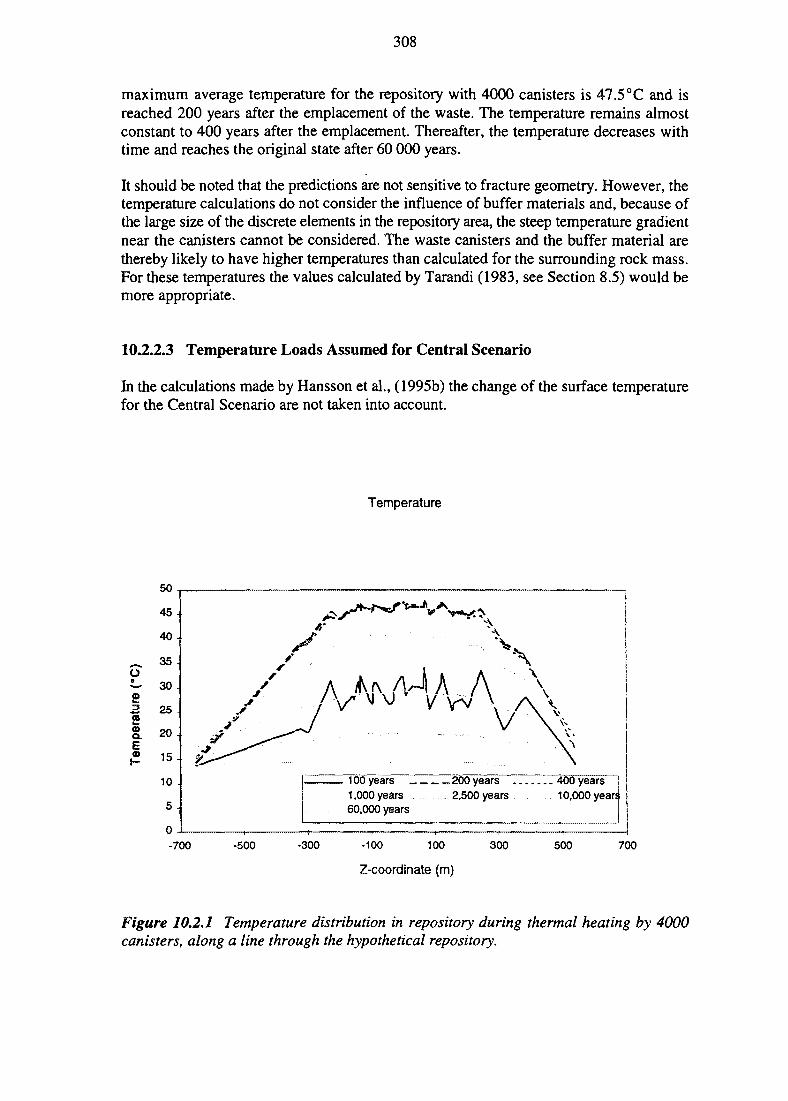
308
maximum average temperature for the repository with 4000 canisters is 47.5°C and isreached 200 years after the emplacement of the waste. The temperature remains almostconstant to 400 years after the emplacement. Thereafter, the temperature decreases withtime and reaches the original state after 60 000 years.
It should be noted that the predictions are not sensitive to fracture geometry. However, thetemperature calculations do not consider the influence of buffer materials and, because ofthe large size of the discrete elements in the repository area, the steep temperature gradientnear the canisters cannot be considered. The waste canisters and the buffer material arethereby likely to have higher temperatures than calculated for the surrounding rock mass.For these temperatures the values calculated by Tarandi (1983, see Section 8.5) would bemore appropriate.
10.2.2.3 Temperature Loads Assumed for Central Scenario
In the calculations made by Hansson et al., (1995b) the change of the surface temperaturefor the Central Scenario are not taken into account.
Temperature
o
©
E©
50 -,
45 -
40-
35-
30 -
25 -
20 -
15 -
10Iv -
5 -
o
/
rs
s f'' 1
-700 -500 -300
V ^
— 100 years _ .1,000 years60,000 years
(- . _ i
-100
v-x\ \ A \\ A A v
_ 200 years . . . .2,500 years
100 300
Z-coordinate (m)
V-
400 years10,000 year;
" !L.|_ . . „ „ „ — - ..JULJ.
500 7C
Figure 10.2.1 Temperature distribution in repository during thermal heating by 4000canisters, along a line through the hypothetical repository.
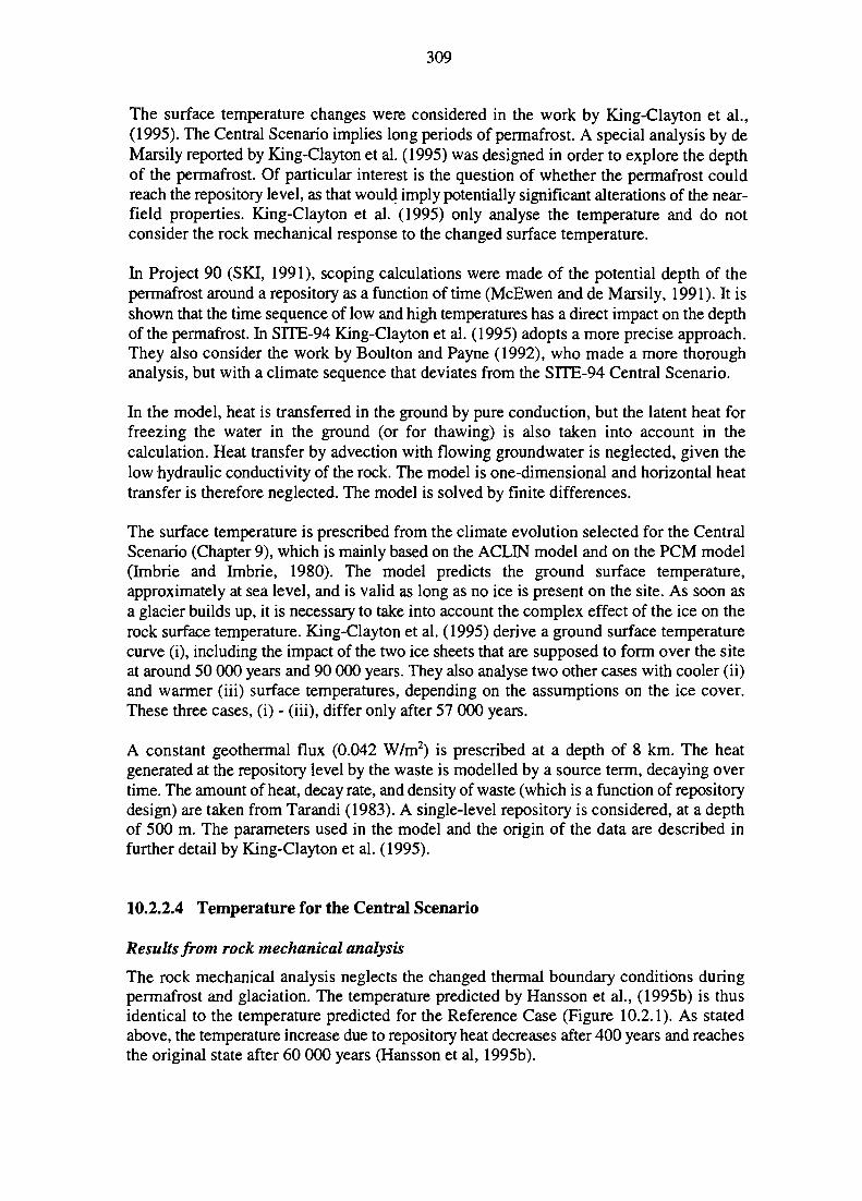
309
The surface temperature changes were considered in the work by King-Clayton et al.,(1995). The Central Scenario implies long periods of permafrost. A special analysis by deMarsily reported by King-Clayton et al. (1995) was designed in order to explore the depthof the permafrost. Of particular interest is the question of whether the permafrost couldreach the repository level, as that would imply potentially significant alterations of the near-field properties. King-Clayton et al. (1995) only analyse the temperature and do notconsider the rock mechanical response to the changed surface temperature.
In Project 90 (SKI, 1991), scoping calculations were made of the potential depth of thepermafrost around a repository as a function of time (McEwen and de Marsily, 1991). It isshown that the time sequence of low and high temperatures has a direct impact on the depthof the permafrost. In SITE-94 King-Clayton et al. (1995) adopts a more precise approach.They also consider the work by Boulton and Payne (1992), who made a more thoroughanalysis, but with a climate sequence that deviates from the SITE-94 Central Scenario.
In the model, heat is transferred in the ground by pure conduction, but the latent heat forfreezing the water in the ground (or for thawing) is also taken into account in thecalculation. Heat transfer by advection with flowing groundwater is neglected, given thelow hydraulic conductivity of the rock. The model is one-dimensional and horizontal heattransfer is therefore neglected. The model is solved by finite differences.
The surface temperature is prescribed from the climate evolution selected for the CentralScenario (Chapter 9), which is mainly based on the ACLIN model and on the PCM model(Imbrie and Imbrie, 1980). The model predicts the ground surface temperature,approximately at sea level, and is valid as long as no ice is present on the site. As soon asa glacier builds up, it is necessary to take into account the complex effect of the ice on therock surface temperature. King-Clayton et al. (1995) derive a ground surface temperaturecurve (i), including the impact of the two ice sheets that are supposed to form over the siteat around 50 000 years and 90 000 years. They also analyse two other cases with cooler (ii)and warmer (iii) surface temperatures, depending on the assumptions on the ice cover.These three cases, (i) - (iii), differ only after 57 000 years.
A constant geothermal flux (0.042 W/m2) is prescribed at a depth of 8 km. The heatgenerated at the repository level by the waste is modelled by a source term, decaying overtime. The amount of heat, decay rate, and density of waste (which is a function of repositorydesign) are taken from Tarandi (1983). A single-level repository is considered, at a depthof 500 m. The parameters used in the model and the origin of the data are described infurther detail by King-Clayton et al. (1995).
10.2.2.4 Temperature for the Central Scenario
Results from rock mechanical analysis
The rock mechanical analysis neglects the changed thermal boundary conditions duringpermafrost and glaciation. The temperature predicted by Hansson et al., (1995b) is thusidentical to the temperature predicted for the Reference Case (Figure 10.2.1). As statedabove, the temperature increase due to repository heat decreases after 400 years and reachesthe original state after 60 000 years (Hansson et al, 1995b).
310
Results from evaluation of permafrost depth
Figure 10.2.2 displays the permafrost depth, as predicted by King-Clayton et al. (1995), asa function of time from -120 000 to +120 000 years, with and without a repository for thethree cases (i)-(iii) discussed previously. The permafrost depth reaches three peaks ataround 25 000, 50 000 and 90 000 years, with values of 210, 340 and 250 m, respectively,for the main scenario with two ice sheets and no repository (model (i)).
With no ice sheet at 90 000 years (model (ii)), the permafrost depth is similar, but thepermafrost melts faster, at around 100 000 years. With warm-based ice (model (iii)), thepermafrost under both ice sheets melts much faster, around 10 000 years earlier. This latterscenario appears to be more consistent with qualitative descriptions of subglacialpermafrost development (e.g. Boulton, 1991; Ahlbom et al., 1991) and quantitative models(e.g. Boulton and Payne, 1992) which consider that permafrost is only present beneath theouter edge and centre of an ice sheet. Compared to the situation with no repository, the heatgenerated by the waste reduces the permafrost depth by 75 m for the peak at 25 000 years,and by 35 m and 10 m for the peaks at 50 000 and 90 000 years, respectively. The resultsfrom the different cases, which in fact show little difference between each other, supportthe assumption that the permafrost would not reach repository depth. Permafrost may,however, have an effect on shaft and tunnel seals closer to the surface.
Permafrost Depth
(i) two ice sheets
(ii) one ice sheet (c.6()ka) with repository
(iii) warmer-based ice
(i) two ice sheets without repository
-120.00 -100.00 -ao.oo -#>.oo -40.00 -20.00 0.00 20.00 40.00 eo.00 100.00 120.00
Time in 1000 years
Figure 10.2.2 Predicted permafrost depths as a function of time, from 120 Ka BP to+ 120 Kafor three different glaciation cycles (i), (ii) and (iii) and with no repository present(From King-Clayton et al., 1995).
311
10.2.3 Mechanical Stability for the Reference Case
10.2.3.1 Introduction
As noted in Chapter 9, the Reference Case assumes that there are no external mechanicalloads on the system apart from the present day tectonic stress field. However, processesinternal to the Process System, such as the weight of the rock mass, the excavation, theswelling of the buffer and the repository heat, will affect the mechanical response of therock mass.
The far-field rock mechanical evaluations in SITE-94, reported by Hansson et al. (1995a, b)consider the weight of the rock and the temperature, whereas the other potential influencesare regarded to be less important for the far-field, as is further discussed in the conclusionof Section 10.2. The actual modelling is done with the model described in Section 7.5.
10.2.3.2 Loadings and Boundary Conditions
The temperature load is evaluated directly from the tempertures calculated by Hansson etal., (1995b), see Section 10.2.2. In fact, the temperature and the mechanical calculations arefully coupled.
The bottom of the model is fixed in all stress directions. In order to initiate calculations, therock mechanical model is first allowed to consolidate under the weight of the rock mass andthe in-situ stress applied on the vertical boundaries, as described in Section 7.5. For thetemperature (and the consecutive ice-load) calculations, the vertical boundaries are fixedin the normal direction, but free in the shear directions.
10.2.3.3 Results
The rock mechanical analyses by Hansson et al. (1995a, b) do not explicitly differentiatebetween the Reference Case and the Central Scenario. Instead, they analyse the thermalload from the repository and the glacial load in a single suite. For clarity, the present sectiononly discusses the part of their analysis that is also relevant for the Reference Case (i.e. thethermal load), although reference will be made to figures and tables that contain results forboth Reference Case and Central Scenario. Furthermore, most results shown here representa point in the centre of the hypothetical repository. For more detailed results the reader isreferred to Hansson et al. (1995a, b).
The calculated peak stresses during thermal loading appear after approximately 200 years(Figure 10.2.3). During the thermal loading, the horizontal stresses are strongly increased,while the vertical stresses are only slightly increased (Hansson et al., 1995a, b). Accordingto Shen and Stephansson (1996) fractures can start to propagate through intact rock whenthe ratio between the minimum and the maximum stresses is less than 0.25. This does, infact, occur in some areas near fracture zones, when the impact of the temperature load isat its maximum, approximately 200 years after emplacement.
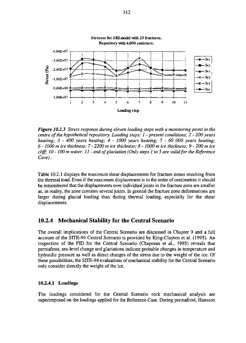
312
-4.00E+07
-3.O0E+O7
{£ -2.00E+O7
C/3
-1.00E+07
0,00E+00 X s
1.00E+07
Stresses for SKI model with 23 fractures.Repository with 4,000 canisters.
T T T ~ T 71 2 3 4 5 6 7
Loading step
10 11
Figure 10.2.3 Stress response during eleven loading steps with a monitoring point in thecentre of the hypothetical repository. Loading steps: 1 - present conditions; 2 - 200 yearsheating; 3 - 400 years heating; 4 - 1000 years heating; 5-60 000 years heating;6 -1000 m ice thickness; 7 - 2200 m ice thickness; 8 - 1000 m ice thickness; 9 - 200 m icecliff; 10 -100 m water; 11 - end of glaciation (Only steps 1 to 5 are valid for the ReferenceCase).
Table 10.2.1 displays the maximum shear displacements for fracture zones resulting fromthe thermal load. Even if the maximum displacement is in the order of centimetres it shouldbe remembered that the displacements over individual joints in the fracture zone are smalleras, in reality, the zone contains several joints. In general the fracture zone deformations arelarger during glacial loading than during thermal loading, especially for the sheardisplacements.
10.2.4 Mechanical Stability for the Central Scenario
The overall implications of the Central Scenario are discussed in Chapter 9 and a fullaccount of the SITE-94 Central Scenario is provided by King-Clayton et al. (1995). Aninspection of the PID for the Central Scenario (Chapman et al., 1995) reveals thatpermafrost, sea-level change and glaciations indicate probable changes in temperature andhydraulic pressure as well as direct changes of the stress due to the weight of the ice. Ofthese possibilities, the SlTJbi-94 evaluations of mechanical stability for the Central Scenarioonly consider directly the weight of the ice.
10.2.4.1 Loadings
The loadings considered for the Central Scenario rock mechanical analysis aresuperimposed on the loadings applied for the Reference Case. During permafrost, Hansson
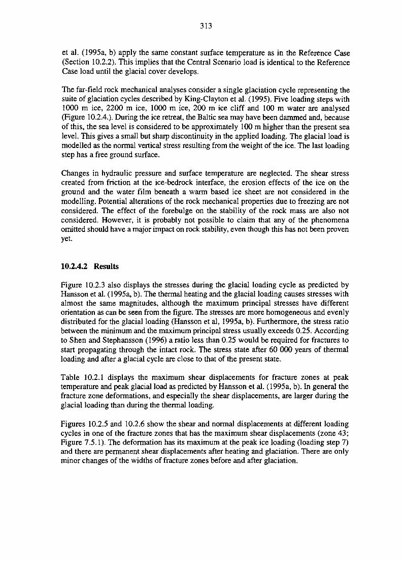
313
et al. (1995a, b) apply the same constant surface temperature as in the Reference Case(Section 10.2.2). This implies that the Central Scenario load is identical to the ReferenceCase load until the glacial cover develops.
The far-field rock mechanical analyses consider a single glaciation cycle representing thesuite of glaciation cycles described by King-Clayton et al. (1995). Five loading steps with1000 m ice, 2200 m ice, 1000 m ice, 200 m ice cliff and 100 m water are analysed(Figure 10.2.4.). During the ice retreat, the Baltic sea may have been dammed and, becauseof this, the sea level is considered to be approximately 100 m higher than the present sealevel. This gives a small but sharp discontinuity in the applied loading. The glacial load ismodelled as the normal vertical stress resulting from the weight of the ice. The last loadingstep has a free ground surface.
Changes in hydraulic pressure and surface temperature are neglected. The shear stresscreated from friction at the ice-bedrock interface, the erosion effects of the ice on theground and the water film beneath a warm based ice sheet are not considered in themodelling. Potential alterations of the rock mechanical properties due to freezing are notconsidered. The effect of the forebulge on the stability of the rock mass are also notconsidered. However, it is probably not possible to claim that any of the phenomenaomitted should have a major impact on rock stability, even though this has not been provenyet.
10.2.4.2 Results
Figure 10.2.3 also displays the stresses during the glacial loading cycle as predicted byHansson et al. (1995a, b). The thermal heating and the glacial loading causes stresses withalmost the same magnitudes, although the maximum principal stresses have differentorientation as can be seen from the figure. The stresses are more homogeneous and evenlydistributed for the glacial loading (Hansson et al, 1995a, b). Furthermore, the stress ratiobetween the minimum and the maximum principal stress usually exceeds 0.25. Accordingto Shen and Stephansson (1996) a ratio less than 0.25 would be required for fractures tostart propagating through the intact rock. The stress state after 60 000 years of thermalloading and after a glacial cycle are close to that of the present state.
Table 10.2.1 displays the maximum shear displacements for fracture zones at peaktemperature and peak glacial load as predicted by Hansson et al. (1995a, b). In general thefracture zone deformations, and especially the shear displacements, are larger during theglacial loading than during the thermal loading.
Figures 10.2.5 and 10.2.6 show the shear and normal displacements at different loadingcycles in one of the fracture zones that has the maximum shear displacements (zone 43;Figure 7.5.1). The deformation has its maximum at the peak ice loading (loading step 7)and there are permanent shear displacements after heating and glaciation. There are onlyminor changes of the widths of fracture zones before and after glaciation.
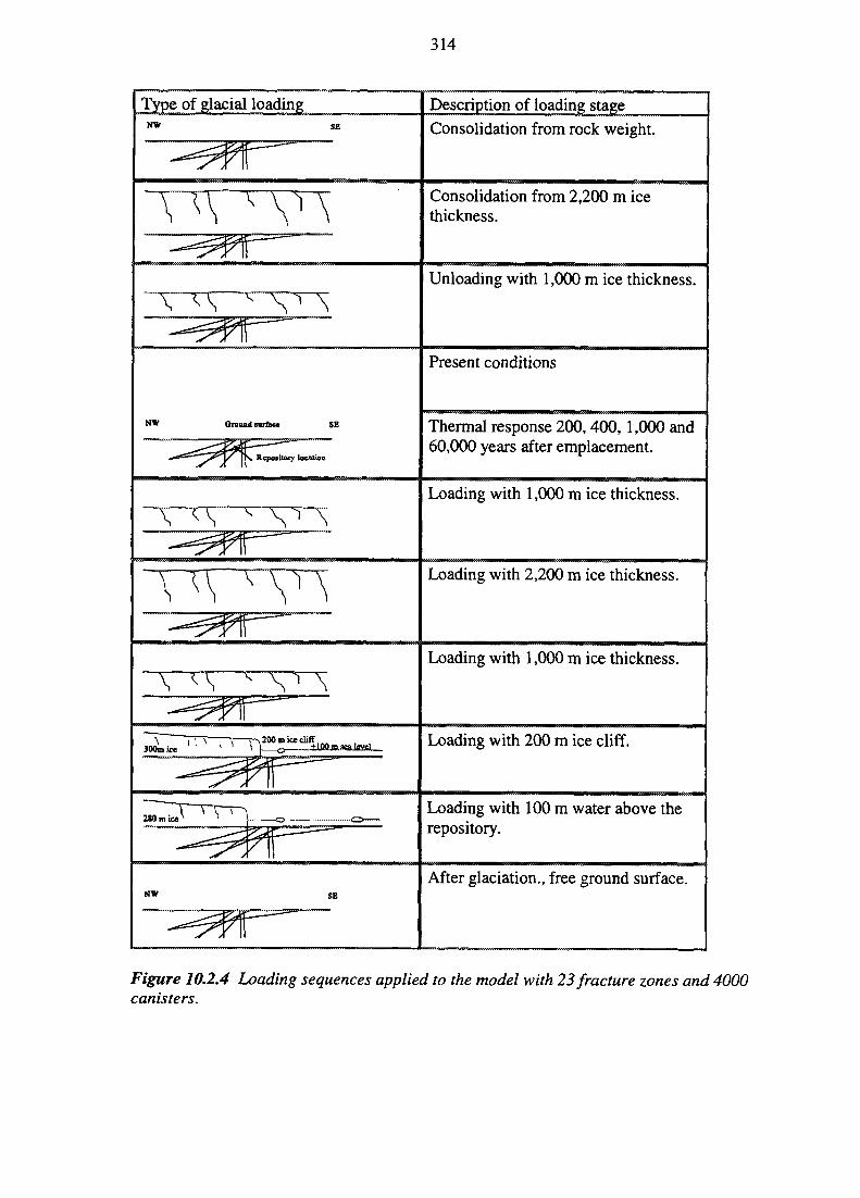
314
Type of glacial loadingNW SE
\ \ ' V \
— ^ t
NW Ground surface SE
• " * s S = " : ^ ^ ^ P ' | K depository locatioD
\ <A " V \
\ ~Tp\—r-^ p . 200 m ice cliff300m ice \ } o _±lMjB.sraJsa«J—
28oJic^ ^ " V " ^
NW S E
Description of loading stageConsolidation from rock weight.
Consolidation from 2,200 m icethickness.
Unloading with 1,000 m ice thickness.
Present conditions
Thermal response 200,400, 1,000 and60,000 years after emplacement.
Loading with 1,000 m ice thickness.
Loading with 2,200 m ice thickness.
Loading with 1,000 m ice thickness.
Loading with 200 m ice cliff.
Loading with 100 m water above therepository.
After glaciation., free ground surface.
Figure 10.2.4 Loading sequences applied to the model with 23 fracture zones and 4000canisters.
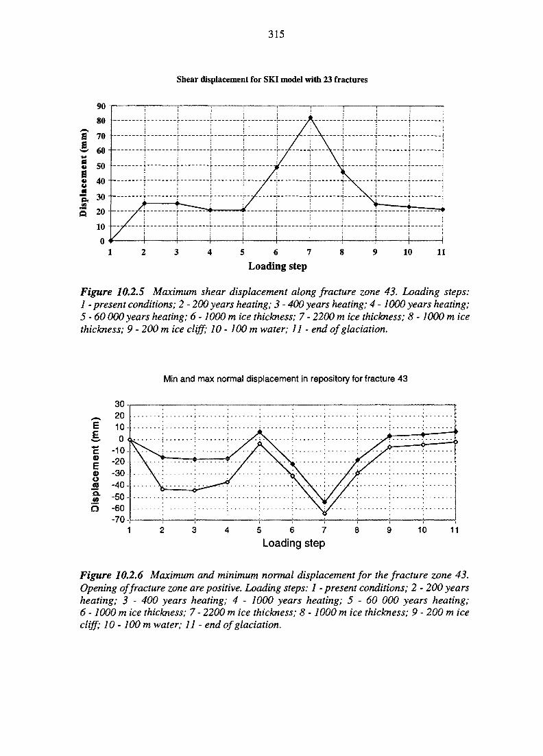
315
Shear displacement for SKI model with 23 fractures
5 6 7
Loading step
Figure 10.2.5 Maximum shear displacement along fracture zone 43. Loading steps:1 - present conditions; 2 - 200 years heating; 3 - 400 years heating; 4 -1000 years heating;5-60 000 years heating; 6 -1000 m ice thickness; 7 - 2200 m ice thickness; 8 -1000 m icethickness; 9 - 200 m ice cliff; 10 - 100 m water; 11 - end of glaciation.
Min and max normal displacement in repository for fracture 43
oJSa.CO
302010
& 0c -10£ -20
-30-40-50
Q -60-70
\
\
• - — - — ^
> — <
^™_—4/ /
/ /
/
\ \
\ \
N>s,....:Vv
*• / .
/ / •
/ /
V
>
/ >
> — <
It
I
> - ' " - " ^
i
|
5 6 7
Loading step10 11
Figure 10.2.6 Maximum and minimum normal displacement for the fracture zone 43.Opening of fracture zone are positive. Loading steps: 1 - present conditions; 2 - 200 yearsheating; 3 - 400 years heating; 4 - 1000 years heating; 5-60 000 years heating;6 -1000 m ice thickness; 7 - 2200 m ice thickness; 8 - 1000 m ice thickness; 9 - 200 m icecliff; 10 - 100 m water; 11 - end of glaciation.
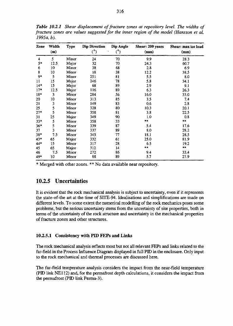
316
Table 10.2.1 Shear displacement of fracture zones at repository level. The widths offracture zones are values suggested for the inner region of the model (Hansson et al,1995a, b).
Zone
45*689*
1114*17*18*20212527*3133*36*3738*43*44*454649*
Width(m)
512.510105
151512.53
10355
255537.5
651565
7.510
Type
MinorMajorMinorMinorMinorMajorMajorMajorMinorMinorMinorMinorMinorMajorMinorMinorMinorMinorMajorMinorMajorMinorMinor
Dip Direction
(°)
24323818
251246
68116284313149328358349358339337345332317312272
88
Dip Angle
(°)
7070683881788989568583808190338789776128148689
Shear: 200 years(mm)
9.924.32.8
12.25.55.82.96.3
16.03.50.6
10.33.81.0
**5.48.0
18.125.0
6.5**9.45.7
Shear: max ice load(mm)
28.360.7
6.938.5
8.034.19.1
26.333.0
7.42.8
20.122.50.8
**17.628.228.581.919.2**33.427.9
Merged with other zones. ** No data available near repository.
10.2.5 Uncertainties
It is evident that the rock mechanical analysis is subject to uncertainty, even if it representsthe state-of-the art at the time of SITE-94. Idealisations and simplifications are made ondifferent levels. To some extent the numerical modelling of the rock mechanics poses someproblems, but the serious uncertainty stems from the uncertainty of site properties, both interms of the uncertainty of the rock structure and uncertainty in the mechanical propertiesof fracture zones and other structures.
10.2.5.1 Consistency with PID FEPs and Links
The rock mechanical analysis reflects most but not all relevant FEPs and links related to thefar-field in the Process Influence Diagram displayed in full PID in the enclosure. Only inputto the rock mechanical and thermal processes are discussed here.
The far-field temperature analysis considers the impact from the near-field temperature(PID link NE112) and, for the permafrost depth calculations, it considers the impact fromthe permafrost (PID link Perma-3).
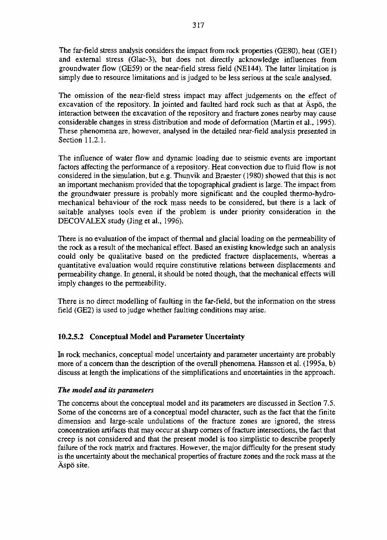
317
The far-field stress analysis considers the impact from rock properties (GE80), heat (GE1)and external stress (Glac-3), but does not directly acknowledge influences fromgroundwater flow (GE59) or the near-field stress field (NE144). The latter limitation issimply due to resource limitations and is judged to be less serious at the scale analysed.
The omission of the near-field stress impact may affect judgements on the effect ofexcavation of the repository. In jointed and faulted hard rock such as that at Aspo, theinteraction between the excavation of the repository and fracture zones nearby may causeconsiderable changes in stress distribution and mode of deformation (Martin et al., 1995).These phenomena are, however, analysed in the detailed near-field analysis presented inSection 11.2.1.
The influence of water flow and dynamic loading due to seismic events are importantfactors affecting the performance of a repository. Heat convection due to fluid flow is notconsidered in the simulation, but e.g. Thunvik and Braester (1980) showed that this is notan important mechanism provided that the topographical gradient is large. The impact fromthe groundwater pressure is probably more significant and the coupled thermo-hydro-mechanical behaviour of the rock mass needs to be considered, but there is a lack ofsuitable analyses tools even if the problem is under priority consideration in theDECOVALEX study (Jing et al., 1996).
There is no evaluation of the impact of thermal and glacial loading on the permeability ofthe rock as a result of the mechanical effect. Based an existing knowledge such an analysiscould only be qualitative based on the predicted fracture displacements, whereas aquantitative evaluation would require constitutive relations between displacements andpermeability change. In general, it should be noted though, that the mechanical effects willimply changes to the permeability.
There is no direct modelling of faulting in the far-field, but the information on the stressfield (GE2) is used to judge whether faulting conditions may arise.
10.2.5.2 Conceptual Model and Parameter Uncertainty
In rock mechanics, conceptual model uncertainty and parameter uncertainty are probablymore of a concern than the description of the overall phenomena. Hansson et al. (1995a, b)discuss at length the implications of the simplifications and uncertainties in the approach.
The model and its parameters
The concerns about the conceptual model and its parameters are discussed in Section 7.5.Some of the concerns are of a conceptual model character, such as the fact that the finitedimension and large-scale undulations of the fracture zones are ignored, the stressconcentration artifacts that may occur at sharp corners of fracture intersections, the fact thatcreep is not considered and that the present model is too simplistic to describe properlyfailure of the rock matrix and fractures. However, the major difficulty for the present studyis the uncertainty about the mechanical properties of fracture zones and the rock mass at theAspo site.
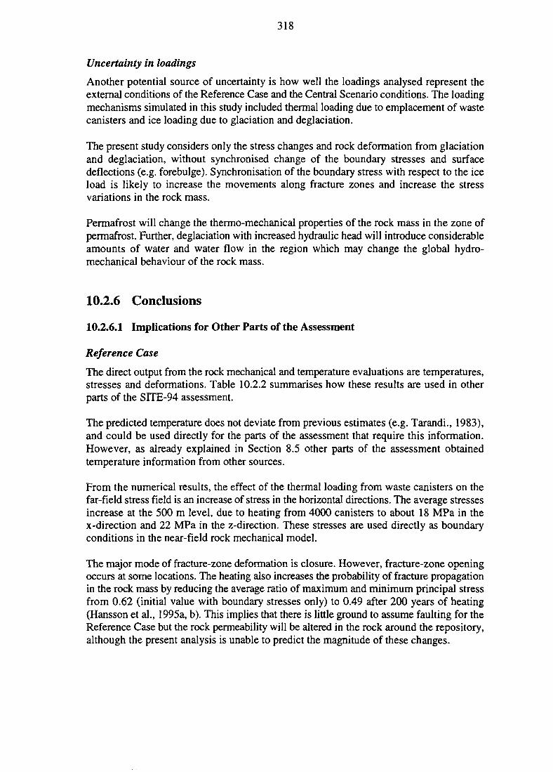
318
Uncertainty in loadings
Another potential source of uncertainty is how well the loadings analysed represent theexternal conditions of the Reference Case and the Central Scenario conditions. The loadingmechanisms simulated in this study included thermal loading due to emplacement of wastecanisters and ice loading due to glaciation and deglaciation.
The present study considers only the stress changes and rock deformation from glaciationand deglaciation, without synchronised change of the boundary stresses and surfacedeflections (e.g. forebulge). Synchronisation of the boundary stress with respect to the iceload is likely to increase the movements along fracture zones and increase the stressvariations in the rock mass.
Permafrost will change the thermo-mechanical properties of the rock mass in the zone ofpermafrost. Further, deglaciation with increased hydraulic head will introduce considerableamounts of water and water flow in the region which may change the global hydro-mechanical behaviour of the rock mass.
10.2.6 Conclusions
10.2.6.1 Implications for Other Parts of the Assessment
Reference Case
The direct output from the rock mechanical and temperature evaluations are temperatures,stresses and deformations. Table 10.2.2 summarises how these results are used in otherparts of the SITE-94 assessment.
The predicted temperature does not deviate from previous estimates (e.g. Tarandi., 1983),and could be used directly for the parts of the assessment that require this information.However, as already explained in Section 8.5 other parts of the assessment obtainedtemperature information from other sources.
From the numerical results, the effect of the thermal loading from waste canisters on thefar-field stress field is an increase of stress in the horizontal directions. The average stressesincrease at the 500 m level, due to heating from 4000 canisters to about 18 MPa in thex-direction and 22 MPa in the z-direction. These stresses are used directly as boundaryconditions in the near-field rock mechanical model.
The major mode of fracture-zone deformation is closure. However, fracture-zone openingoccurs at some locations. The heating also increases the probability of fracture propagationin the rock mass by reducing the average ratio of maximum and minimum principal stressfrom 0.62 (initial value with boundary stresses only) to 0.49 after 200 years of heating(Hansson et al., 1995a, b). This implies that there is little ground to assume faulting for theReference Case but the rock permeability will be altered in the rock around the repository,although the present analysis is unable to predict the magnitude of these changes.
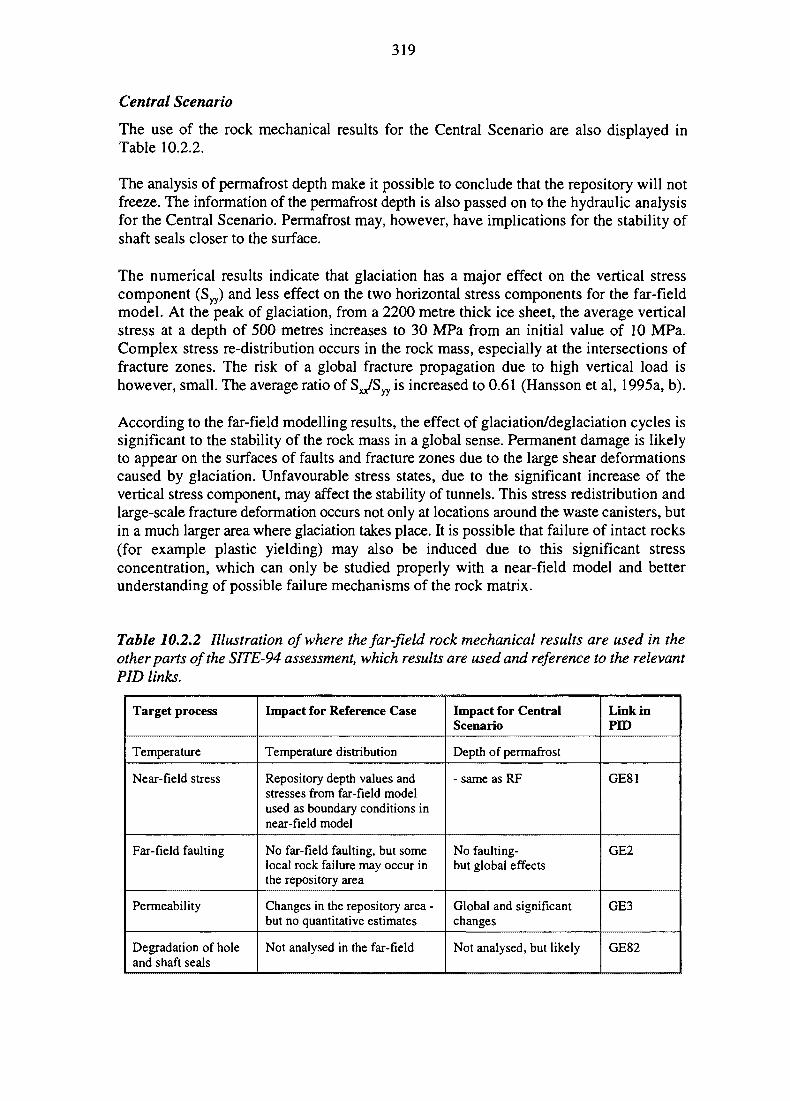
319
Central Scenario
The use of the rock mechanical results for the Central Scenario are also displayed inTable 10.2.2.
The analysis of permafrost depth make it possible to conclude that the repository will notfreeze. The information of the permafrost depth is also passed on to the hydraulic analysisfor the Central Scenario. Permafrost may, however, have implications for the stability ofshaft seals closer to the surface.
The numerical results indicate that glaciation has a major effect on the vertical stresscomponent (Syy) and less effect on the two horizontal stress components for the far-fieldmodel. At the peak of glaciation, from a 2200 metre thick ice sheet, the average verticalstress at a depth of 500 metres increases to 30 MPa from an initial value of 10 MPa.Complex stress re-distribution occurs in the rock mass, especially at the intersections offracture zones. The risk of a global fracture propagation due to high vertical load ishowever, small. The average ratio of Sxx/Syy is increased to 0.61 (Hansson et al, 1995a, b).
According to the far-field modelling results, the effect of glaciation/deglaciation cycles issignificant to the stability of the rock mass in a global sense. Permanent damage is likelyto appear on the surfaces of faults and fracture zones due to the large shear deformationscaused by glaciation. Unfavourable stress states, due to the significant increase of thevertical stress component, may affect the stability of tunnels. This stress redistribution andlarge-scale fracture deformation occurs not only at locations around the waste canisters, butin a much larger area where glaciation takes place. It is possible that failure of intact rocks(for example plastic yielding) may also be induced due to this significant stressconcentration, which can only be studied properly with a near-field model and betterunderstanding of possible failure mechanisms of the rock matrix.
Table 10.2.2 Illustration of where the far-field rock mechanical results are used in theother parts of the SITE-94 assessment, which results are used and reference to the relevantPID links.
Target process
Temperature
Near-field stress
Far-field faulting
Permeability
Degradation of holeand shaft seals
Impact for Reference Case
Temperature distribution
Repository depth values andstresses from far-field modelused as boundary conditions innear-field model
No far-field faulting, but somelocal rock failure may occur inthe repository area
Changes in the repository area -but no quantitative estimates
Not analysed in the far-field
Impact for CentralScenario
Depth of permafrost
- same as RF
No faulting-but global effects
Global and significantchanges
Not analysed, but likely
Link inPID
GE81
GE2
GE3
GE82
320
10.2.6.2 Implications for Repository Design and Further Work
The SITE-94 analyses are not designed to evaluate different repository designs, butHansson et al. (1995a, b) make the following comments on this subject.
The design of tunnels and deposition holes will affect not only the mechanical stability, butalso the temperature in the repository and its surroundings. A greater heat load per squarekilometre will increase the temperature in the repository and the stress level will increase.
The underground openings will undergo several loading paths during construction and later,followed by the heat loading and loading from glaciation. Hence, the stress concentrationsat corners and fracture intersections are areas for local failure. Although the stressconcentration/relief appears at isolated small areas at fracture intersections and is less likelyto effect the stress behaviour globally, it may be a problem for repository design. Thestability of tunnels and deposition holes close to fracture intersections may be affected.These intersections may also be conduits for water flow.
In order to study these phenomena properly, Hansson et al. (1995a, b) suggest detailed fullyT-H-M coupled near-field modelling that should include improved constitutive models forthe fracture zones and single fractures and groundwater flow through the fracture networks.It is suggested that such models, which would require some amount of research anddevelopment, be used to perform a series of sensitivity analyses, a study of dynamic effectsfrom seismic or neotectonic events and modelling of large-scale tunnel excavations.
10.3 HYDROGEOLOGY
This section concerns the evolution of flow and transport paths and the provision of datafor estimation of effective hydrogeological transport parameters for the consequencecalculations in the Reference Case and in the Central (climate evolution) Scenario.
10.3.1 Introduction
The hydrogeological evaluation calculations, reflected in the Assessment Model Flowchart(AMF) in Figure 2.4.5, comprise scoping calculations and detailed simulations, using thealternative site models established in Section 7.3. This section describes the methodologyand results for the far-field. The results for the near-field, to be used for evaluation of theEngineered Barrier System, are described in detail in Section 11.2.2. Chapter 15 describeshow the results of the hydrogeological evaluation are used to define calculation cases forthe radionuclide release and transport calculations.
321
10.3.2 Strategy for Evaluation Calculations
The evaluation calculations yield predictions of groundwater flow and transport, in termsof parameters that can be used as input to the consequence models described in Chapter 13.The models developed for the regional hydrogeology provide general information on large-scale groundwater movement and its evolution during the Central Scenario. The detailedhydrogeological site-scale models provide quantitative parameters for the calculations ofradionuclide release and transport in the geosphere. Finally, a set of alternative conceptualmodels are used to estimate rough bounds on the specific flow-wetted area.
10.3.2.1 Hydrogeological Aspects of the Reference Case
The Reference Case refers to a situation where present-day hydrological surface boundaryconditions, considered to be at steady-state, prevail into the future (see Chapter 9). For thehydrogeological evaluation, this means that the present-day flow field is assumed to be atsteady-state. The main emphasis of the evaluation calculations for the Reference Case ison quantifying conceptual and parameter uncertainties associated with the development ofhydrogeological models for the heterogeneous rock at the Aspo site. However, to a largeextent, the results for the Reference Case are also applicable to the Central Scenario.
The models used for making quantitative predictions of site hydrogeology for the ReferenceCase include:
• the Simple Evaluation (Sections 7.3.5 and 10.3.3),• the Discrete Feature site model (Sections 7.3.7 and 10.3.4),• the Stochastic Continuum site model (Sections 7.3.8 and 10.3.5),• the VAPFRAC variable aperture Discrete-Fracture Network model (Sections 7.3.9
and 10.3.6).
10.3.2.2 Modelling the Central Scenario
The Central Scenario specifies a sequence of time-dependent boundary conditions as aclimate-evolution scenario that includes glaciation cycles, sea-level changes and permafrostevents over the next 120 000 years, as discussed in Chapter 9. Large-scale hydrogeologicalmodels are developed to simulate the long-term evolution of the groundwater flow field anddistribution of fresh and saline waters (Section 7.3.3). The evaluation and results aredescribed in Section 10.3.7. Certain aspects of the Central Scenario are also evaluated withthe Discrete Feature site model (see Section 10.3.8). The site-scale hydrogeologicalevolution is inferred both from the large-scale models and from the detailed-scale resultsfor the Reference Case, as will be discussed further in Chapter 15.
10.3.2.3 General Procedure for Estimation of Hydrogeological TransportParameters
Figure 10.3.1 illustrates the general procedure for estimation of hydrogeological transportparameters from the detailed site models, which comprises the following steps:
322
• Solution of steady-state flow for each model realisation.
• Sampling near-field parameters on a single canister scale.
• Particle tracking (discrete-particle random-walk, DPRW) calculations for eachcanister site in the repository.
• Interpretation of each calculated canister release curve in terms of an equivalent one-dimensional homogeneous porous medium giving effective far-field parameters tobe used in CRYSTAL.
The hydrogeological parameters that are determined for the near-field radionuclide releaseand transport model, CALIBRE, are Darcy velocity, fracture spacing, fracture aperture,specific surface area (see Chapter 13). Each realization of a flow field provides adistribution of the near-field parameters reflecting the spatially varying properties amongdifferent canister sites in the repository rock block. However, the full set of near-fieldparameters was not provided by all models.
As radionuclide transport in the geosphere is calculated with a coupled, but simple one-dimensional transport model (CRYSTAL; see Chapter 13), the results of the three-dimensional site models have to be interpreted in terms of a few effective hydrogeologicaltransport parameters including Darcy velocity, longitudinal dispersion coefficient, transportpath length, flow porosity and specific surface area.
In SITE-94 this is done by dividing the flow field into a set of equivalent stream tubes, eachrepresenting flow and transport from a single canister site to the biosphere. For eachrealization of the flow field and for each canister source the DPRW method of particletracking provides a distribution of residence times (breakthrough curve) at the biosphereinterface. The DPRW method differs from deterministic particle tracking (that is sometimesused to trace streamlines) in that it uses multiple particles to simulate dispersion from asingle (canister) source. An estimate of effective far-field fluid velocity and dispersioncoefficient that characterise the transport (multiple particle tracks) from a given canistersource, is obtained by fitting the ID advection-dispersion solution to the spatiallyintegrated, mass break-through recorded at the surface. In the Discrete Feature model, theparticle-tracking results are also used to estimate flow porosity, specific surface area andtransport path length (see Section 10.3.4).
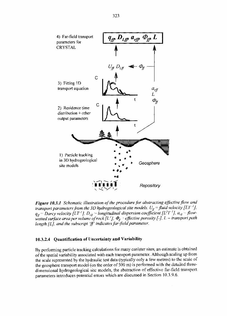
323
4) Far-field transportparameters forCRYSTAL
^ffDLffi
3) Fitting IDtransport equation
2) Residence timedistribution + otheroutput parameters
1) Particle trackingin 3D hydrogeologicalsite models Geosphere
Repository
Figure 10.3.1 Schematic illustration of the procedure for abstracting, effective flow andtransport parameters from the 3D hydrogeological site models. Ujf = fluid velocity [LT1],qff = Darcy velocity [LT'J, DLj] = longitudinal dispersion coefficient [L2T''J, arff = flow-wetted surface area per volume ofrock[L~'], <Pfj = effective porosity [-], L = transport pathlength [L], and the subscript ff' indicates far-field parameter.
10.3.2.4 Quantification of Uncertainty and Variability
By performing particle tracking calculations for many canister sites, an estimate is obtainedof the spatial variability associated with each transport parameter. Although scaling up fromthe scale represented by the hydraulic test data (typically only a few metres) to the scale ofthe geosphere transport model (on the order of 500 m) is performed with the detailed three-dimensional hydrogeological site models, the abstraction of effective far-field transportparameters introduces potential errors which are discussed in Section 10.3.9.6.
324
In addition to the alternative hydrogeological site models, a number of variational cases(variants) are defined to explore different types of uncertainties within each site model. Thevariants are selected to reflect uncertainties related to the conceptual description of the rockheterogeneity and permeability structure as well as parameter (property) values of differentmodel features.
The distinction between uncertainty and spatial variability, discussed in Chapter 2, hasspecial relevance to hydrogeology. Spatial variability refers to the natural variability of ahydrogeological property, which arises from the rock heterogeneity. This variability is afunction of the parameter studied and the scale or rock volume it represents. In general, thespatial variability decreases with averaging volume. Although the exact value of a certainhydrogeological parameter may be unknown at different positions in the rock, one mayobtain a good estimate of the range and nature of its variability. Uncertainty, on the otherhand, implies that there are insufficient data or models to make precise predictions of themean and spatial variability of the parameter studied. Uncertainty could arise from a varietyof sources, including lack of knowledge regarding processes and spatial structures(conceptual model uncertainty), uncertainty in measurements and data, or even lack ofrelevant data.
10.3.2.5 Model-Dependent Parameters and Representative Transport Parameters
The hydrogeological component of the far-field radionuclide transport model is an idealisedrepresentation of the more complex detailed hydrogeological site models. Consequently,the interpreted far-field transport parameters should not be seen as physical properties ofthe rock. The relationship between the interpreted hydrogeological far-field parameters andtheir absolute values is specific for the conceptual hydrogeology model or conceptualvariant from which they are derived. Therefore a single parameter value (for example Darcyvelocity) is not meaningful unless it is combined with the other transport parameters (forexample flow wetted surface area) estimated from the same conceptual hydrogeologymodel. Hence, a comparison between different conceptual models or conceptual variantsin terms of the individual far-field transport parameters is not meaningful.
To facilitate a direct evaluation of, and comparison between, the hydrogeological sitemodels, two parameter groups are defined as hydrogeological performance measures forthe far-field transport from a single canister source, namely the F-ratio, F, and the Pecletnumber, Pe:
F ^ a ^ x L / q t f (Eq. 10.3.1)
Pe = U f fxL/DU f (Eq. 10.3.2)
where a^ = flow-wetted surface area per volume of rock (m2/m3), L = transport path length(m), qff =Uff x Off = Darcy velocity (m/s), Uff = fluid velocity (m/s), <3>ff = effective porosity(dimensionless) and D ^ = longitudinal dispersion coefficient (m2/s). The index *ffindicates a parameter estimate for the far-field.
The F-ratio parameter group appears in the solution to the advection-dispersion-matrixdiffusion equation (e.g. Tang et al., 1981 and Moreno and Neretnieks, 1993) and has
325
dimension (s/m), i.e. an inverse velocity, and is a measure of the capacity for retardationby sorption and matrix diffusion in the rock fractures. The Peclet number (dimensionless)is the ratio between advective to dispersive groundwater transport. It appears that these twoparameter groups encompass the primary hydrogeological influence on radionuclidetransport, and that different combinations of the individual far-field parameter values willnot affect transport as long as the F-ratio and the Pe-number are held constant(Section 13.5.2). Accordingly, comparison of the different model predictions are basedprimarily on these two parameter groups.
Chapter 13 discusses the sensitivity of radionuclide transport on the F-ratio and the Pecletnumber. A low F-ratio implies little retardation and a potential for high far-field releases.A low Peclet number implies high dispersion and in some cases a potential for high far-field releases; however, the precise impact of the Peclet number on radionuclide releasedepends upon the shape of the input pulse from the near-field as well as on the F-ratio andthe radiochemical properties of the nuclide.
10.3.3 Simple Evaluation of Flow and Transport for the ReferenceCase
The first attempt at quantifying the groundwater flow at Aspo comprised simple scopingcalculations of groundwater flux, based on a ID application of Darcy's law, simpleassumptions regarding flow-field structure and bounding values of hydraulic driving forces.The Simple Evaluation of groundwater flux was later extended (Dverstorp et al., 1996) toevaluate critical transport parameters, based upon a range of generic models for porestructure in fractures and fracture zones. Although the latter part of the Simple Evaluationis in fact performed later in SITE-94, in principle the entire Simple Evaluation could havebeen accomplished at the outset of SITE-94.
The objectives of the Simple Evaluation are to determine uncertainty ranges for Darcyvelocity (groundwater flux) and the F-ratio, as defined above, along idealised pathwaysfrom the hypothetical repository to the biosphere. The analysis considers eight study sitesin crystalline rock in Sweden, but only the results for Aspo are summarised here.
10.3.3.1 Setup and Results of the Analysis of Groundwater Flux
Figure 10.3.2 shows the idealised flow and transport paths analysed, which representdifferent assemblages of 'good rock', fracture zones, rock disturbed by excavation, andpoorly sealed access shafts and tunnels. Hydraulic conductivity data for the rock mass andfracture zones are taken from SKB's interpretation of the injection test data (Wikberg et al.,1991).
The first and most optimistic case (Pathway 1 in Figure 10.3.2) represents a situation wheretransport takes place in 600 m of moderately fractured rock, using SKB's estimate ofhydraulic conductivity (K = lxlO"10 m/s) for the rock volume where the SITE-94 repositoryis located (Wikberg et al., 1991). An intermediate case (Pathway 2) assumes transportthrough 10 m of moderately fractured rock in the repository rock block, with discharge into

326
Fracture zone ©Transport pathin moderatelyfractured rock
Repository
Disturbedzone
Figure 10.3.2 Schematic illustration of the transport pathways analysed in the SimpleEvaluation of groundwater flow at the Aspo site.
a major discharging fracture zone (resistance to flow in the fracture zone is taken to benegligible). Pathway 3 is a highly pessimistic case of 600 m of transport directly to thebiosphere, via a highly conductive, excavation-disturbed zone and a major dischargingfracture zone. For this case, two values of fracture zone conductivities (cases 3a and 3b) areanalysed, corresponding to the most conductive (K = 2xlO"5 m/s) fracture zone and a lessconductive (K - 5xlO'7 m/s) fracture zone in the SKB hydrogeological site model (Wikberget al., 1991). The hydraulic conductivity of the disturbed zone is assumed to be the sameas that in the fracture zone.
For each case, analyses are performed for a low and a high value of hydraulic head gradient,corresponding to excess hydraulic heads of+1 m and +10 m between repository depth andthe outlet at the surface, respectively. The lower value is based on the local water-tableelevation at Aspo. The higher value represents a rather pessimistic situation where anextensive, subhorizontal fracture zone is present to transmit regional high heads from themainland west of Aspo to the rock beneath Aspo.
Table 10.3.1 shows the calculated Darcy velocities together with the input parameters forthe analysed cases. The resulting Darcy velocities range from SxlO^m/year to 10 m/year.This very wide range makes it difficult to confirm the effectiveness of the geological barrierfunction for a repository in crystalline rock (e.g. SKI, 1991). Because the hydraulic headgradient is fairly well determined (within an order of magnitude), the high uncertainty inthe calculated Darcy velocities simply reflects the wide range (5 orders of magnitude) ofestimated hydraulic conductivities.
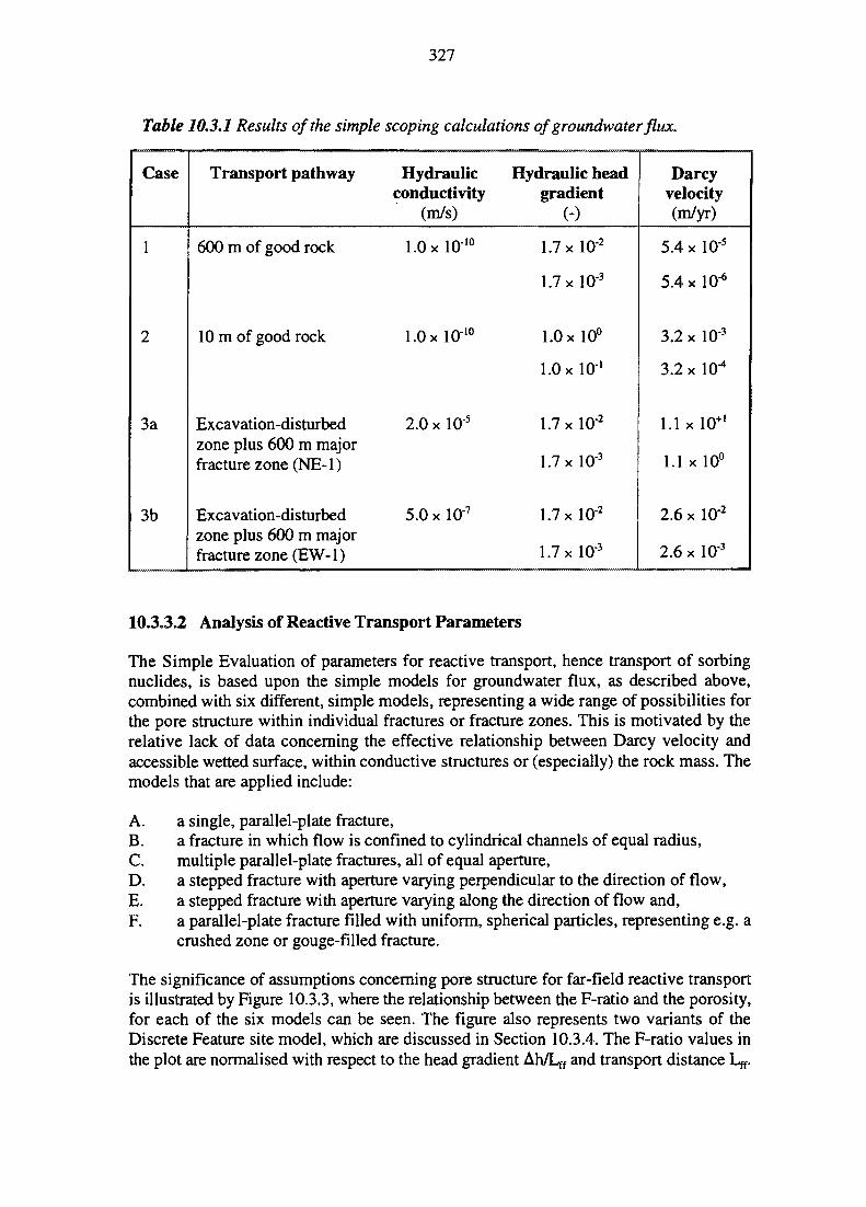
327
Table 10.3.1 Results of the simple scoping calculations of groundwater flux.
Case
1
2
3a
3b
Transport pathway
600 m of good rock
10 m of good rock
Excavation-disturbedzone plus 600 m majorfracture zone (NE-1)
Excavation-disturbedzone plus 600 m majorfracture zone (EW-1)
Hydraulicconductivity
(m/s)
1.0x10'°
1.0x10'°
2.0 xlO"5
5.0 x lO"7
Hydraulic headgradient
(-)
1.7 xlO"2
1.7 x lO 3
1.0x10°
l.Ox 10'
1.7 xlO"2
1.7 xlO"3
1.7 x 10"2
1.7 x l O 3
Darcyvelocity(m/yr)
5.4 x 10"5
5.4 xlO'6
3.2 x 10"3
3.2 x 10"*
1.1 x 10+I
1.1x10°
2.6 x 10"2
2.6 x 10"3
10.3.3.2 Analysis of Reactive Transport Parameters
The Simple Evaluation of parameters for reactive transport, hence transport of sorbingnuclides, is based upon the simple models for groundwater flux, as described above,combined with six different, simple models, representing a wide range of possibilities forthe pore structure within individual fractures or fracture zones. This is motivated by therelative lack of data concerning the effective relationship between Darcy velocity andaccessible wetted surface, within conductive structures or (especially) the rock mass. Themodels that are applied include:
A. a single, parallel-plate fracture,B. a fracture in which flow is confined to cylindrical channels of equal radius,C. multiple parallel-plate fractures, all of equal aperture,D. a stepped fracture with aperture varying perpendicular to the direction of flow,E. a stepped fracture with aperture varying along the direction of flow and,F. a parallel-plate fracture filled with uniform, spherical particles, representing e.g. a
crushed zone or gouge-filled fracture.
The significance of assumptions concerning pore structure for far-field reactive transportis illustrated by Figure 10.3.3, where the relationship between the F-ratio and the porosity,for each of the six models can be seen. The figure also represents two variants of theDiscrete Feature site model, which are discussed in Section 10.3.4. The F-ratio values inthe plot are normalised with respect to the head gradient Ah/Lff and transport distance Lff.
328
The parameters of all models are chosen to give the same average transmissivity of10"6 m2/s (representative of site-scale fracture zones). Porosity values are calculated basedon a 10 m thickness of rock (a typical fracture-zone thickness). The lowest values of bothF and porosity occur with Model B, the cylindrical channel model, whereas the highestvalues of both F and porosity are given by Model F, the 'crushed-zone' model. Model Cgives increasing values of F and porosity, depending on the number of parallel fractures.
For realistic values of aperture, the specific surface in Models D and E is nearly the sameas in Model A, and hence F does not vary appreciably. However, effective values ofporosity can vary widely in these models, depending on the magnitude of the variation inaperture and on whether the aperture varies parallel to or perpendicular to the direction offlow.
Figure 10.3.4 (a-c) shows the results of applying these pore-structure models to calculateF-ratios for each of the cases analysed in the Simple Evaluation of Darcy flux, as describedabove. For each hydrogeological case and each pore-structure model, a physicallyreasonable range of parameters is estimated, as described by Dverstorp et al. (1996), andapplied to predict wide bounds on the F-ratio.
The lowest values of F are produced by Model B, which represents the case of extremechannelling. However, this model is found to be incompatible with reasonable ranges ofporosity for a rock mass or fracture zone composed entirely of such channels. Hence ModelB can be viewed as representative only of isolated, extreme channels. The incidence of suchchannels would be nearly impossible to estimate at the stage of site characterisationrepresented by S1TE-94, therefore Model B is not shown in these figures. The lowest valuesof F, excluding Model B, are produced by Model D which represents more moderatechannelisation of conductive fractures, with channels running parallel to the flow direction.The highest values of the F-ratio are produced by Model F, which represents the somewhatextreme case in which all fracture zones consist of crushed zones with very high flow-wetted surface area.
The predicted F-ratios for Aspo span an extremely wide range, from about 108 to 1018 s/m(3xl0'2 to 3xl010 year/m). Thus uncertainty regarding pore structure introduces more than4 orders of magnitude of uncertainty in the F-ratio, in addition to the uncertainty that isexpressed in the range for Darcy velocity.
10.3.3.3 Applicability of Results
The Simple Evaluation is not conditioned on the data and uses only a small portion of it,so it should be expected to give an overestimate of the uncertainty in Darcy velocities andF-ratio. For a Performance Assessment based on a 'worst case' analysis, the results forDarcy velocity are probably reasonable, as the worst case (a high continuous permeabilityvalue between the repository and the surface) could occur in some realisations of both theDiscrete Feature site model and the Stochastic Continuum site model (see Sections 10.3.4and 10.3.5).
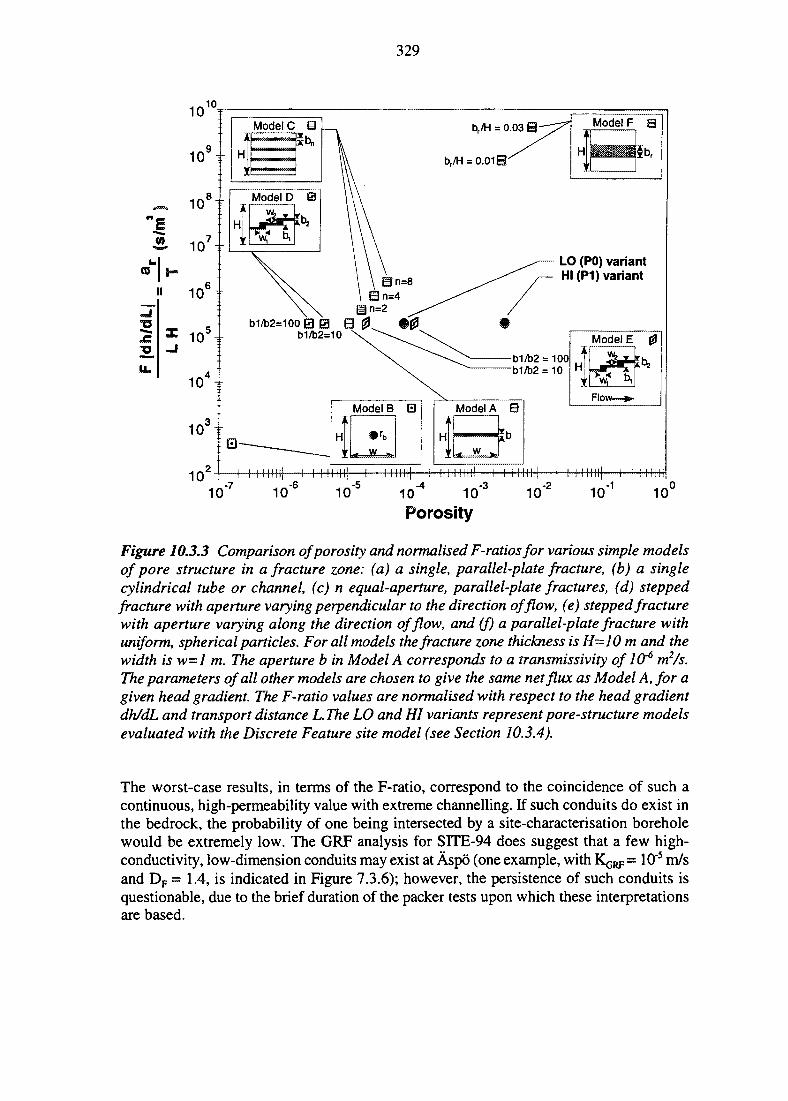
(D
U,,
329
1010
~ 10'
'I 10
105 +
104 +
10
i
H
Model CEta5
Iv
HV
Model D
iffe
b1/b2=100 B B Bb1/b2=10
Model F ei
H1
fbr
LO (P0) variantHI (P1) variant
Model B
H
i
r <*—W.—»•
E) Model A Bi
Hr
Model E 0
H
:Flow—^
10-7
10-6
10-5 -4
10 10Porosity
-310
-210"
Figure 10.3.3 Comparison of porosity and normalised F-ratiosfor various simple modelsof pore structure in a fracture zone: (a) a single, parallel-plate fracture, (b) a singlecylindrical tube or channel, (c) n equal-aperture, parallel-plate fractures, (d) steppedfracture with aperture varying perpendicular to the direction of flow, (e) stepped fracturewith aperture varying along the direction of flow, and (f) a parallel-plate fracture withuniform, spherical particles. For all models the fracture zone thickness is H-10 m and thewidth is w=l m. The aperture b in Model A corresponds to a transmissivity of 10'6 m2/s.The parameters of all other models are chosen to give the same net flux as Model A, for agiven head gradient. The F-ratio values are normalised with respect to the head gradientdh/dL and transport distance LThe LO and HI variants represent pore-structure modelsevaluated with the Discrete Feature site model (see Section 10.3.4).
The worst-case results, in terms of the F-ratio, correspond to the coincidence of such acontinuous, high-permeability value with extreme channelling. If such conduits do exist inthe bedrock, the probability of one being intersected by a site-characterisation boreholewould be extremely low. The GRF analysis for SFTE-94 does suggest that a few high-conductivity, low-dimension conduits may exist at Aspo (one example, with K Q ^ = 105 m/sand DF = 1.4, is indicated in Figure 7.3.6); however, the persistence of such conduits isquestionable, due to the brief duration of the packer tests upon which these interpretationsare based.
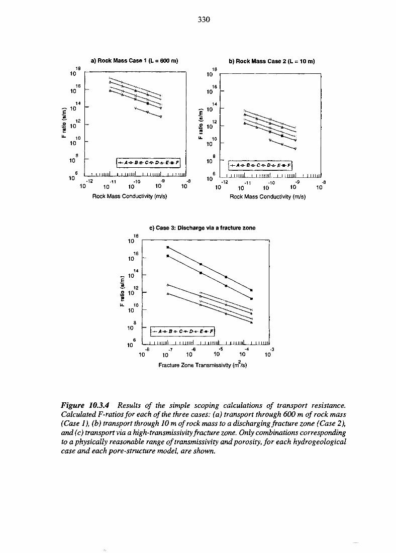
330
a) Rock Mass Case 1 (L = 600 m) b) Rock Mass Case 2 (L = 10 m)
10
10 10 10 10
Rock Mass Conductivity (m/s)
10 10 10 10 10
Rock Mass Conductivity (m/s)10
c) Case 3: Discharge via a fracture zone
Fracture Zone Transmissivity (m /s)
Figure 10.3.4 Results of the simple scoping calculations of transport resistance.Calculated F-ratios for each of the three cases: (a) transport through 600 m of rock mass(Case 1), (b) transport through 10 m of rock mass to a discharging fracture zone (Case 2),and (c) transport via a high-transmissivity fracture zone. Only combinations correspondingto a physically reasonable range of transmissivity and porosity, for each hydro geologicalcase and each pore-structure model, are shown.
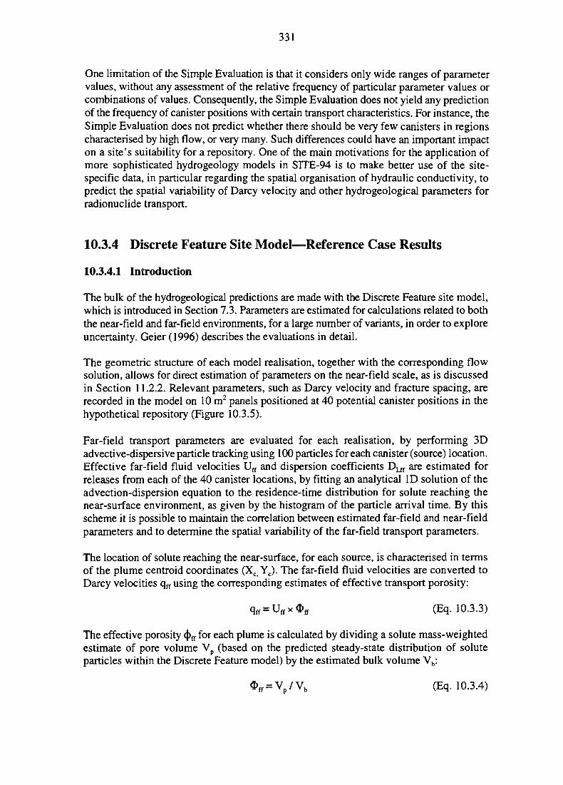
331
One limitation of the Simple Evaluation is that it considers only wide ranges of parametervalues, without any assessment of the relative frequency of particular parameter values orcombinations of values. Consequently, the Simple Evaluation does not yield any predictionof the frequency of canister positions with certain transport characteristics. For instance, theSimple Evaluation does not predict whether there should be very few canisters in regionscharacterised by high flow, or very many. Such differences could have an important impacton a site's suitability for a repository. One of the main motivations for the application ofmore sophisticated hydrogeology models in SITE-94 is to make better use of the site-specific data, in particular regarding the spatial organisation of hydraulic conductivity, topredict the spatial variability of Darcy velocity and other hydrogeological parameters forradionuclide transport.
10.3.4 Discrete Feature Site Model—Reference Case Results
10.3.4.1 Introduction
The bulk of the hydrogeological predictions are made with the Discrete Feature site model,which is introduced in Section 7.3. Parameters are estimated for calculations related to boththe near-field and far-field environments, for a large number of variants, in order to exploreuncertainty. Geier (1996) describes the evaluations in detail.
The geometric structure of each model realisation, together with the corresponding flowsolution, allows for direct estimation of parameters on the near-field scale, as is discussedin Section 11.2.2. Relevant parameters, such as Darcy velocity and fracture spacing, arerecorded in the model on 10 m2 panels positioned at 40 potential canister positions in thehypothetical repository (Figure 10.3.5).
Far-field transport parameters are evaluated for each realisation, by performing 3Dadvective-dispersive particle tracking using 100 particles for each canister (source) location.Effective far-field fluid velocities Uff and dispersion coefficients D ^ are estimated forreleases from each of the 40 canister locations, by fitting an analytical ID solution of theadvection-dispersion equation to the residence-time distribution for solute reaching thenear-surface environment, as given by the histogram of the particle arrival time. By thisscheme it is possible to maintain the correlation between estimated far-field and near-fieldparameters and to determine the spatial variability of the far-field transport parameters.
The location of solute reaching the near-surface, for each source, is characterised in termsof the plume centroid coordinates (Xc Yc). The far-field fluid velocities are converted toDarcy velocities qff using the corresponding estimates of effective transport porosity:
qff = U f fx0 f f (Eq. 10.3.3)
The effective porosity 4)ff for each plume is calculated by dividing a solute mass-weightedestimate of pore volume Vp (based on the predicted steady-state distribution of soluteparticles within the Discrete Feature model) by the estimated bulk volume Vb:
*ff = Vp /Vb (Eq. 10.3.4)
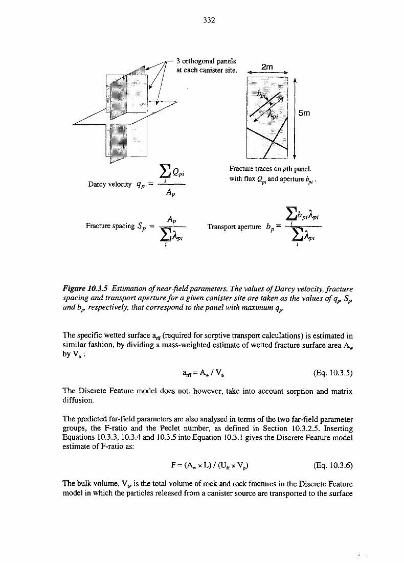
332
3 orthogonal panelsat each canister site. 2m
5m
Darcy velocity qp = - l
Fracture traces on pth panel,with flux Q . and aperture b •
pFracture spacing Sp = ••^^ Transport aperture bD~ l
Figure 10.3.5 Estimation of near-field parameters. The values ofDarcy velocity, fracturespacing and transport aperture for a given canister site are taken as the values of qp, 5^and bp, respectively, that correspond to the panel with maximum qp.
The specific wetted surface a^ (required for sorptive transport calculations) is estimated insimilar fashion, by dividing a mass-weighted estimate of wetted fracture surface area A^byVb :
arif = Aw /Vb (Eq. 10.3.5)
The Discrete Feature model does not, however, take into account sorption and matrixdiffusion.
The predicted far-field parameters are also analysed in terms of the two far-field parametergroups, the F-ratio and the Peclet number, as defined in Section 10.3.2.5. InsertingEquations 10.3.3, 10.3.4 and 10.3.5 into Equation 10.3.1 gives the Discrete Feature modelestimate of F-ratio as:
= (AwxL)/(U f fxVp) (Eq. 10.3.6)
The bulk volume, Vb, is the total volume of rock and rock fractures in the Discrete Featuremodel in which the particles released from a canister source are transported to the surface
333
(for details see Geier, 1996). It represents the volume of an equivalent stream-tube in theCRYSTAL radionuclide transport model.
Because the calculation of Vb involves a somewhat arbitrary assumption regarding whatfraction of the rock between discrete features should be included, the absolute values of qff,3>ff and a^ should not be overinterpreted. However, as can be seen from Equations 10.3.2and 10.3.6, the far-field parameter groups (F-ratio and Peclet number) which are used fordefining the input to the far-field radionuclide transport model, are independent of the bulk-volume assumption and may thus be used for comparisons among Discrete Feature modelvariants and with other hydrogeological models.
The statistics of the estimated effective hydrogeological transport parameters, as presentedbelow, are based upon the pooled results of 40 canister positions and all realisations (10-20,in most cases, but in two cases just 5). Combining results from all realisations provides alarger basis for analysis than analysing each variant separately, particularly for the far-fieldestimates where results are obtained for only a few, connective sites per realisation.
However, to do so, the assumption must be introduced that the differences betweenstochastic realisations are insignificant in comparison with the variability within a singlerealisation. If this were not so, and the mean value of a given parameter varied significantlybetween realisations, the pooled results would give an exaggerated estimate of spatialvariability. This assumption is difficult to justify, for precisely the same reasons that suchan assumption is required.
However, statistical tests that are performed for the Discrete Feature model base-caseresults (a multivariate, multi-sample likelihood ratio test of complete homogeneity, andWilks' multivariate, multi-sample likelihood ratio test for equality of means) indicate thatthis assumption is most likely to be valid, as described by Geier (1996). Therefore it isconcluded that the variability expressed in the pooled results is predominantly anexpression of true spatial variability.
10.3.4.2 Variants
The variation cases that are investigated for the Discrete Feature model are chosen so as toaddress major aspects of uncertainty regarding:
1. the geological structural model,2. hydrogeological properties of the major structures,3. effective boundary conditions,4. rock type within the repository,5. hydrogeological properties of the discrete-fracture network and,6. effects of the Disturbed-Rock Zone.
By using variants of the Discrete Feature model to estimate effective near-field and far-fieldparameters for each of these cases, the effect of each of these components of uncertaintyon the overall Performance Assessment could be evaluated.
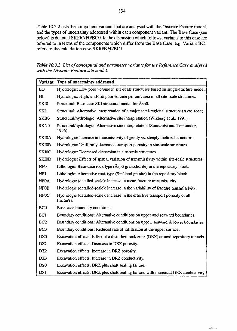
334
Table 10.3.2 lists the component variants that are analysed with the Discrete Feature model,and the types of uncertainty addressed within each component variant. The Base Case (seebelow) is denoted SKI0/NF0/BC0. In the discussion which follows, variants to this case arereferred to in terms of the components which differ from the Base Case, e.g. Variant BC1refers to the calculation case SKI0/NF0/BC1.
Table 10.3.2 List of conceptual and parameter variants for the Reference Case analysedwith the Discrete Feature site model.
Variant Type of uncertainty addressed
LO Hydrologic: Low pore volume in site-scale structures based on single-fracture model.
HI Hydrologic: High, uniform pore volume per unit area in all site-scale structures.
SKIO Structural: Base-case SKI structural model for Aspo.
SKI1 Structural: Alternative interpretation of a major semi-regional structure (Avro zone).
SKBO Structural/hydrologic: Alternative site interpretation (Wikberg et al., 1991).
SKNO Structural/hydrologic: Alternative site interpretation (Sundquist and Torssander,1996).
SKIOA Hydrologic: Increase in transmissivity of gently vs. steeply inclined structures.
SKIOB Hydrologic: Uniformly decreased transport porosity in site-scale structures.
SKIOC Hydrologic: Decreased dispersion in site-scale structures.
SKIOD Hydrologic: Effects of spatial variation of transmissivity within site-scale structures.
NFO Lithologic: Base-case rock type (Aspo granodiorite) in the repository block.
NF1 Lithologic: Alternative rock type (Smaland granite) in the repository block.
NFOA Hydrologic (detailed-scale): Increase in mean fracture transmissivity.
NFOB Hydrologic (detailed-scale): Increase in the variability of fracture transmissivity.
NFOC Hydrologic (detailed-scale): Increase in the effective transport porosity of allfractures.
BCO Base-case boundary conditions.
BC1 Boundary conditions: Alternative conditions on upper and seaward boundaries.
BC2 Boundary conditions: Alternative conditions on upper, seaward & lower boundaries.
BC3 Boundary conditions: Reduced rate of infiltration at the upper surface.
DZO Excavation effects: Effect of a disturbed rock zone (DRZ) around repository tunnels.
DZ1 Excavation effects: Decrease in DRZ porosity.
DZ2 Excavation effects: Increase in DRZ porosity.
DZ3 Excavation effects: Increase in DRZ conductivity.
DSO Excavation effects: DRZ plus shaft sealing failure.
DS1 Excavation effects: DRZ plus shaft sealing failure, with increased DRZ conductivity.
335
The Base Case and calibration of variants
The Base Case for calculations consists of the component variants SKI0/NF0/BC0 usedwhen calibrating the Discrete Feature site model, as described in Section 7.3. Partly due totime and resource limitations, no attempt is made to recalibrate the other model variants.This means that the uncertainty associated with some variants, such as the alternative far-field boundary conditions, to some extent reflects different assumptions rather than trueuncertainty. However, for several variants, strict re-calibration is not possible. Thisobviously holds for the variants representing the Excavation Disturbed Zone and shaftsealing failure, but also for many of the variants representing different transport models forfractures and fracture zones, since relevant data for calibration (e.g. small-scale tracer tests)were not available. The variants representing the alternative geological/hydrogeologicalstructure models (variants SKBO and SKNO) use their own hydraulic properties as reportedfor each model, although some simplification and adjustment is required to adapt thesemodels into the discrete-fracture network concept.
Uncertainty in geological I hydrogeological structure model
Uncertainty in the geological structural model is a key concern with the Discrete Featuremodel, because this model makes more direct use of the geological interpretation than doother detailed site models. The structural variant SKI1 is analysed to test an alternativeinterpretation for a particular feature. To address the more profound uncertainty whichrelates to the likelihood that independent groups of experts, working with a single sitedatabase, will produce disparate models, Discrete Feature models (variants SKBO andSKNO) are constructed and analysed based on the two alternative, geological/hydro-geological structure models as described in Section 7.2.
Hydraulic and transport properties of major structures
The second major type of uncertainty arises in the assignment of hydrogeological propertiesto the structures in a given structural model. In particular, this concerns the parameterswhich determine Darcy velocity and wetted surface area within each structure.
Whereas a considerable quantity of hydraulic test data are available for calibration ofstructure transmissivities, the only data relating to transport porosity are a few (5) tracertests, in all of which non-sorbing tracers are used. There are no independent data regardingthe spatial structure of porosity, which governs non-reactive transport, or the specificsurface, which governs reactive (i.e. sorption or matrix-diffusion dominated) transport.
The importance of assumptions concerning the structure of pore space is illustrated byFigure 10.3.3, in terms of the F-ratio (which is a measure of the reactive transportproperties) and the porosity for each of a range of simple models. The two main pore-structure variants that are used in the Discrete Feature analysis, the LO (P0) and HI (PI)variants, are also represented in the figure, in terms of the local values of F and porositywhich these models give for structures with the same net transmissivity as Model A.
The contrasting assumptions in the LO and HI variants address conceptual uncertaintyregarding the detailed geometry of flow and transport within transmissive structures, whichdetermines the inter-relationships among Darcy velocity, advective transport, and flow-wetted surface area. In a discrete-fracture network model, the governing assumptions
336
concerning pore geometry are specified explicitly in terms of the relationship betweenfracture transmissivity and transport aperture, whereas in a continuum model theseassumptions are applied indirectly, as functional relationships among larger-scalehydrogeological properties.
In the LO variant, the pore volume within each structure is assumed to be positivelycorrelated to structure transmissivity, with pore volume at a given point being equivalentto that of a single, dominant fracture accounting for all flow through the structure. The LOvariant has F and porosity values similar to those for a variable-aperture (Model E), whichmay be expected since the model for transport aperture in the LO variant is based onempirical data from single-fracture transport experiments in natural fractures.
In the second case (HI variant), all structures are assumed to have a uniform, effective porevolume per unit area (in the plane of the structure) of 0.03 mVm2. This is based on fracture-zone porosity estimates from tracer tests in relatively diffuse fracture zones at the Aspo site,and a generic zone thickness of 30 m. The porosity of the HI variant is high in relation tothe single-fracture models, but comparable to the 'crushed-zone' model (Model F).However, the wetted surface area in the HI variant is taken to be the same as for the LOvariant, i.e. just twice the planar area of each structure. This is very low in relation to pore-structure models which could reasonably yield the high porosity-to-transmissivity ratios ofthe HI variant, and thus the HI variant is likely to give conservative F-ratios.
Variants SKIOA-D reflect additional parameter uncertainty regarding transmissivitydistribution, effective transport porosity and dispersion in the site-scale structures (seeTable 10.3.2).
Alternative Boundary Conditions
Uncertainty with regard to the semi-regional hydrogeological setting, due to the limitedamount of data from depth and form outside Aspo, is expressed in the Discrete Featuremodel as uncertainty with regard to effective boundary conditions. Variants BC1-3 areanalysed to assess the effects of alternative sets of boundary conditions on performance-assessment parameters, including: topographic heads at the upper surface (rather than fixedinfiltration), hydrostatic heads at the seaward boundary (rather than confinement due tosaltwater intrusion) and fixed, declining heads at the base (rather than no flow due to tightrock), such as could effectively be produced by a highly transmissive, subhorizontal,regional fracture zone just below the base of the model.
Properties of the repository scale fracture network
Additional uncertainty arises from the spatial variability of lithology in the vicinity of therepository, and variability of the fracture system within a given rock type. These aspects ofuncertainty are addressed by variations of the repository-scale, discrete-fracture networkmodel with respect to rock type (NF1) and the hydrogeological properties of the fracturepopulation (NFOA-C).
The excavation disturbed-rock zone
Uncertainty related to the Disturbed-Rock Zone (DRZ) around the repository is assessedby additional variations. Although the DRZ is considered to be present in the Reference

337
Backfilled access drift
Primary DRZ
Backfilleddeposition drift
Canister in backfilleddeposition hole
DRZ features
Radionuclide source
boundaries
Figure 10.3.6 Discrete Feature representation of the disturbed-rock-zone. The upperfigure is a schematic illustration of the DRZ around the access drift and deposition drift.The lower figure shows the discrete features that represent the DRZ, and the internal modelboundaries, representing the canister deposition holes, which are the sources forradionuclide release into the DF network.
Case, for practical reasons its effects are investigated within specific variational cases,rather than by including the DRZ in all calculation cases. The DRZ around all depositionand access tunnels within the repository is represented by a special set of connected,discrete features (Figure 10.3.6), with base-case hydrogeological properties as evaluated byWinberg (1991; variant DZO). Additional variants are analysed to evaluate uncertaintyregarding the hydrogeological properties of the DRZ itself (variants DZl-3), and of theDRZ in the event of a shaft sealing failure (variants DSO and DS1).
10.3.4.3 Base Case Results
Results from the Discrete Feature model are obtained as estimates of near-field and far-fieldparameters, for each canister site within each realisation of the model. Analysis of thesedata (Geier, 1996) yields information concerning the variability of the parameters,correlations between parameters, and the principle effects of the variants. The main resultsfor the far-field are summarised in the following paragraphs; specific results for the near-field are discussed in Section 11.2.2.
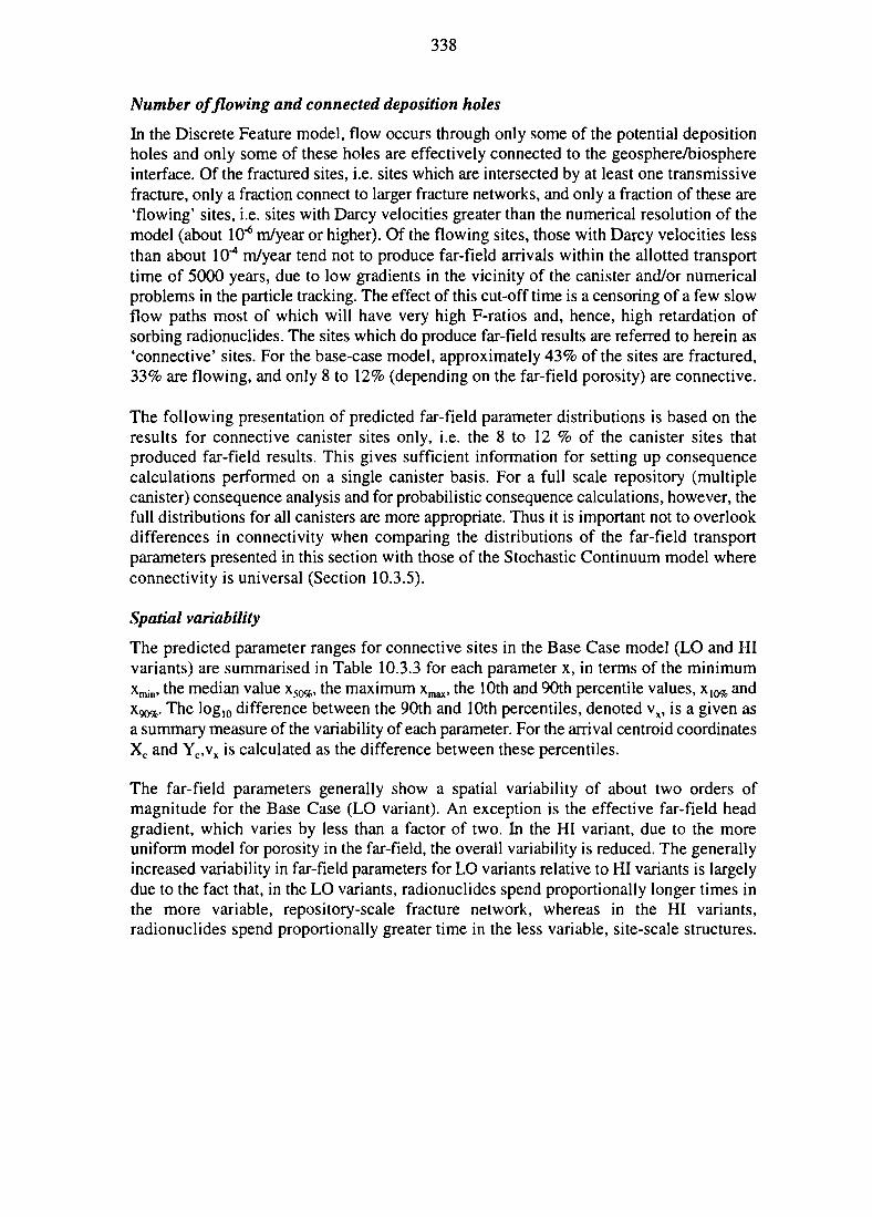
338
Number of flowing and connected deposition holes
In the Discrete Feature model, flow occurs through only some of the potential depositionholes and only some of these holes are effectively connected to the geosphere/biosphereinterface. Of the fractured sites, i.e. sites which are intersected by at least one transmissivefracture, only a fraction connect to larger fracture networks, and only a fraction of these are'flowing' sites, i.e. sites with Darcy velocities greater than the numerical resolution of themodel (about 10"6 m/year or higher). Of the flowing sites, those with Darcy velocities lessthan about 10"4 m/year tend not to produce far-field arrivals within the allotted transporttime of 5000 years, due to low gradients in the vicinity of the canister and/or numericalproblems in the particle tracking. The effect of this cut-off time is a censoring of a few slowflow paths most of which will have very high F-ratios and, hence, high retardation ofsorbing radionuclides. The sites which do produce far-field results are referred to herein as'connective' sites. For the base-case model, approximately 43% of the sites are fractured,33% are flowing, and only 8 to 12% (depending on the far-field porosity) are connective.
The following presentation of predicted far-field parameter distributions is based on theresults for connective canister sites only, i.e. the 8 to 12 % of the canister sites thatproduced far-field results. This gives sufficient information for setting up consequencecalculations performed on a single canister basis. For a full scale repository (multiplecanister) consequence analysis and for probabilistic consequence calculations, however, thefull distributions for all canisters are more appropriate. Thus it is important not to overlookdifferences in connectivity when comparing the distributions of the far-field transportparameters presented in this section with those of the Stochastic Continuum model whereconnectivity is universal (Section 10.3.5).
Spatial variability
The predicted parameter ranges for connective sites in the Base Case model (LO and HIvariants) are summarised in Table 10.3.3 for each parameter x, in terms of the minimumxmin, the median value \50%, the maximum xmax, the 10th and 90th percentile values, \lWh andx90%. The log10 difference between the 90th and 10th percentiles, denoted vx, is a given asa summary measure of the variability of each parameter. For the arrival centroid coordinatesXc and Yc,vx is calculated as the difference between these percentiles.
The far-field parameters generally show a spatial variability of about two orders ofmagnitude for the Base Case (LO variant). An exception is the effective far-field headgradient, which varies by less than a factor of two. In the HI variant, due to the moreuniform model for porosity in the far-field, the overall variability is reduced. The generallyincreased variability in far-field parameters for LO variants relative to HI variants is largelydue to the fact that, in the LO variants, radionuclides spend proportionally longer times inthe more variable, repository-scale fracture network, whereas in the HI variants,radionuclides spend proportionally greater time in the less variable, site-scale structures.
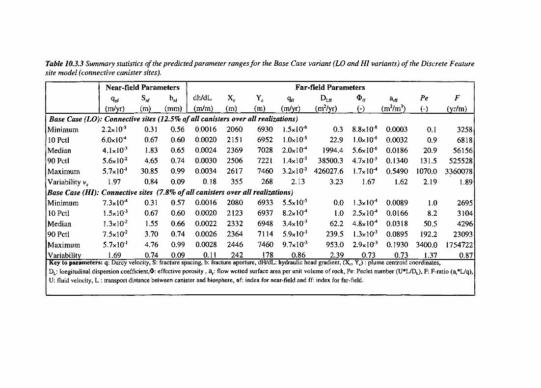
Table 10.3.3 Summary statistics of the predicted parameter ranges for the Base Case variant (LO and HI variants) of the Discrete Featuresite model (connective canister sites).
Near-fie1
(m/yr)
Id Parameters
s n f(m) (mm)
dh/dL(m/m)
xc(m)
Yc
(m)
Far-i
%(m/yr)
Base Case (LO): Connective sites (12.5% of all canisters over all realizations)Minimum 2.2x10⁵
lOPctl 6.0x10"4
Median 4.1xlO3
90Pctl 5.6x!02
Maximum 5.7x10'Variability v, 1.97
0.310.671.834.65
30.850.84
0.560.600.650.740.990.09
0.00160.00200.00240.00300.0034
0.18
20602151236925062617
355
69306952702872217460
268
1.5xl0"6
l.OxlO5
2.0x10^
1.4xlO"3
3.2xl0"2
2.13
Base Case (HI): Connective sites (7.8% of all canisters over all realizations)Minimum 7.3x10^lOPctl 1.5xlO3
Median 1.3xlO2
90Pctl 7.5xlO"2
Maximum 5.7x10'Variability 1.69
0.310.671.553.704.760.74
0.570.600.660.740.990.09
0.00160.00200.00220.00260.0028
0.11
20802123233223642446
242
69336937694871147460
178Key to parameters: q: Darcy velocity, S: fracture spacing, b: fracture aperture, dH/dL:DL: longitudinal dispersion coefficient,®: effective porosity , ar: flow wetted
5.5xlO"5
8.2X10"4
3.4xl03
5.9xlO3
9.7x10"3
0.86
leld Param
Bur(mVyr)
0.322.9
1994.438500.3
426027.63.23
0.01.0
62.2239.5953.0
2.39
teters
(-)
8.8xlO8
l.Oxi a6
5.6xlO"6
4.7xl0"5
l.lxlO-4
1.67
OxlO-4
2.5X10"4
4.8X10⁻⁴
1.3x1 Or3
2.9x10³
0.73
arff
(m2/m3)
0.00030.00320.01860.13400.5490
1.62
0.00890.01660.03180.08950.1930
0.73
Pe
(-)
0.10.9
20.9131.5
1070.02.19
1.08.2
50.5192.2
3400.01.37
hydraulic head gradient, (Xc, Yc): plume centroid coordinates,surface area per unit volume of rock, ]
F(yr/m)
32586818
56156525528
33600781.89
269531044296
230931754722
0.87
Pe: Peclet number (U*L/DL), F: F-ratio (a^L/q),U: fluid velocity, L : transport distance between canister and biosphere, nf: index for near-field and ff: index for far-field.
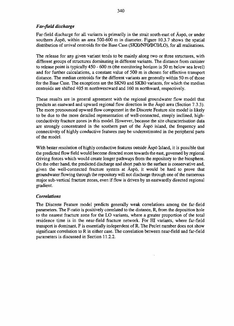
340
Far-field discharge
Far-field discharge for all variants is primarily in the strait south-east of Aspo, or undersouthern Aspo, within an area 500-600 m in diameter. Figure 10.3.7 shows the spatialdistribution of arrival centroids for the Base Case (SKI0/NF0/BC0/LO), for all realisations.
The release for any given variant tends to be mainly along two or three structures, withdifferent groups of structures dominating in different variants. The distance from canisterto release point is typically 450 - 600 m (the monitoring horizon is 50 m below sea level)and for further calculations, a constant value of 500 m is chosen for effective transportdistance. The median centroids for the different variants are generally within 50 m of thosefor the Base Case. The exceptions are the SKN0 and SKB0 variants, for which the mediancentroids are shifted 405 m northwestward and 160 m northward, respectively.
These results are in general agreement with the regional groundwater flow model thatpredicts an eastward and upward regional flow direction in the Aspo area (Section 7.3.3).The more pronounced upward flow component in the Discrete Feature site model is likelyto be due to the more detailed representation of well-connected, steeply inclined, high-conductivity fracture zones in this model. However, because the site characterisation dataare strongly concentrated in the southern part of the Aspo island, the frequency andconnectivity of highly conductive features may be underestimated in the peripheral partsof the model.
With better resolution of highly conductive features outside Aspo Island, it is possible thatthe predicted flow field would become directed more towards the east, governed by regionaldriving forces which would create longer pathways from the repository to the biosphere.On the other hand, the predicted discharge and short path to the surface is conservative and,given the well-connected fracture system at Aspo, it would be hard to prove thatgroundwater flowing through the repository will not discharge through one of the numerousmajor sub-vertical fracture zones, even if flow is driven by an eastwardly directed regionalgradient.
Correlations
The Discrete Feature model predicts generally weak correlations among the far-fieldparameters. The F-ratio is positively correlated to the distance, R, from the deposition holeto the nearest fracture zone for the LO variants, where a greater proportion of the totalresidence time is in the near-field fracture network. For HI variants, where far-fieldtransport is dominant, F is essentially independent of R. The Peclet number does not showsignificant correlation to R in either case. The correlation between near-field and far-fieldparameters is discussed in Section 11.2.2.
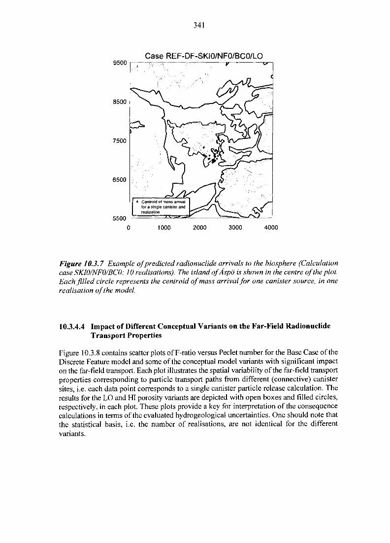
341
Case REF-DF-SKIO/NFO/BCO/LO9500
8500
7500
6500
5500
• Centroid of mass arrivalfor a single canister andrealization
1000 2000 3000 4000
Figure 10.3.7 Example of predicted radionuclide arrivals to the biosphere (Calculationcase SKI0/NF0/BC0; 10 realisations). The island of A spo is shown in the centre of the plot.Each filled circle represents the centroid of mass arrival for one canister source, in onerealisation of the model.
10.3.4.4 Impact of Different Conceptual Variants on the Far-Field RadionuclideTransport Properties
Figure 10.3.8 contains scatter plots of F-ratio versus Peclet number for the Base Case of theDiscrete Feature model and some of the conceptual model variants with significant impacton the far-field transport. Each plot illustrates the spatial variability of the far-field transportproperties corresponding to particle transport paths from different (connective) canistersites, i.e. each data point corresponds to a single canister particle release calculation. Theresults for the LO and HI porosity variants are depicted with open boxes and filled circles,respectively, in each plot. These plots provide a key for interpretation of the consequencecalculations in terms of the evaluated hydrogeological uncertainties. One should note thatthe statistical basis, i.e. the number of realisations, are not identical for the differentvariants.

342
10 4 1
10 '"I
J> 10 2 -rE3
©a,10
10
10
Base CaseD
a D
CD
D
••<"! i iinij'—i"i'>-m«j i t nim|—i"<-nmt|
10 10 10 11 10 " 10 1J 10a ) F-ratio (s/m)
10
EC©
10 4 f
10 '10 " 10 " 10 " 10 M 10 14 10
b) F-ratio (s/m)
c)10 10 10 " 10
F-ratio (s/m)10 14 10
0)
10
10
10
10 ° y
10 "
1 J» : fl.SD
= B^. *§ • •: i
l-l<-HHl| 1-! t)mi|
eD
• D
0D
»
SKIOBD
• D
•t"H'H»|" 1 1 1 Mill
d)10 10 10 " 10 " 10 " 10 14 10
F-ratio (s/m)
©
©
10 1
10 J l
10 2 1
10 ' 1
10 ° "
1 0 • ' - ' '"""I
•
SKBO
» l • > > » » • • { ' ' " • • • •
10 10 10 " 10 " 10 " 10e) F-ratio (s/m)
10
©JO
E
©a.
f)10 10 " 10 " 10 " 10
F-ratio (s/m)10
Figure 10.3.8 Scatter plots of the hydrogeological far-field parameter groups, F-ratioand Peclet number, evaluated from particle tracking calculations in the main modelvariants of the Discrete Feature hydrogeological site model. Each data point representsthe far-field transport properties of the transport paths originating from a single canistersource location. The result for the LO and HI porosity variants are depicted with openboxes and filled circles, respectively, in each plot.
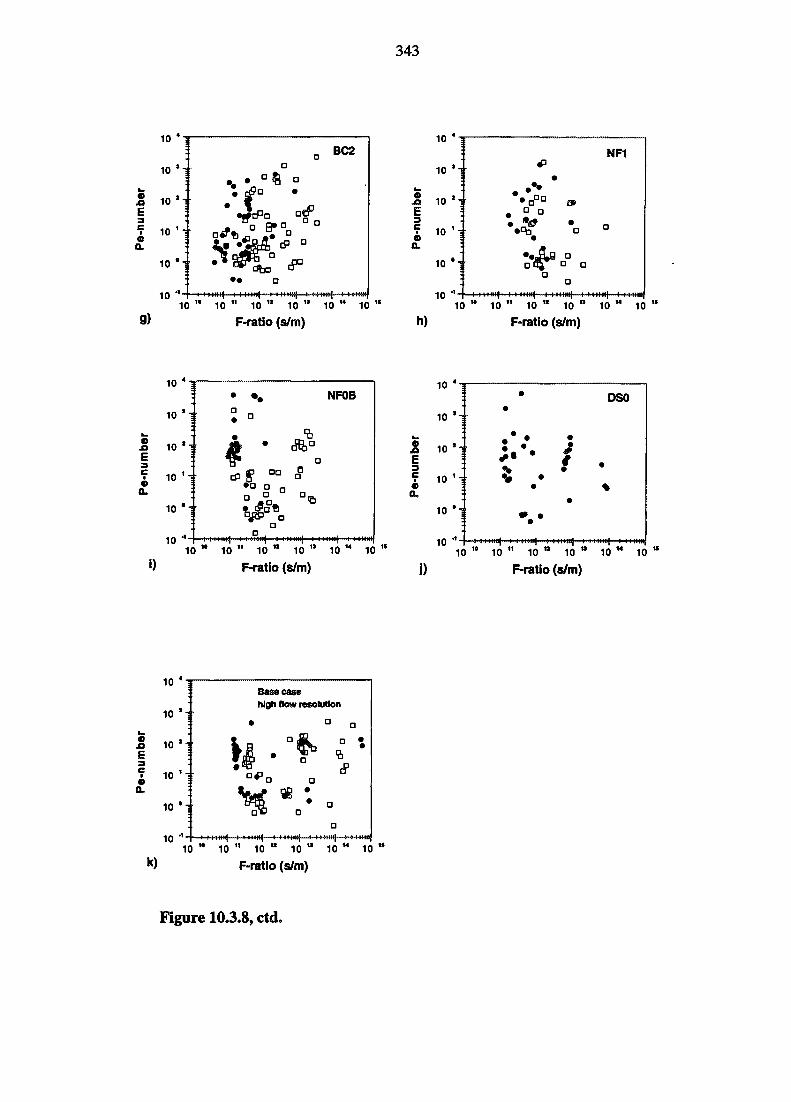
343
F-ratio (s/m)
sJOEc9
a*
i)
10 41
10 ' ]
10 *1
10 ' ]
10 °1
10 1-
• • •
• 5 °•
aa
D
D
10 M 10 " 10 " 10 tt
F-ratio (s/m)
NFOB
10 u 10
0
E3Ca>
a ,
10 10 10 10 10
j) F-ratio (s/m)
F-ratio (s/m)
Figure 10.3.8, ctd.
344
Impact of hydraulic and transport properties of major structures
The hydrogeological properties of the site-scale structures, and particularly the assumptionsconcerning pore structure, the LO and HI variants, have a direct impact on the effectivetransport properties for Performance Assessment. Although both variants have identicalflux distributions within the Discrete Feature network, the assumption of lower porosityvalues in the LO variant results in higher advective velocities in the site-scale structures.The HI variant predicts significantly lower F values (i.e. reduced potential for retardation),but also less spatial variability (see Figure 10.3.8a). The low F values predicted by the HIvariant are largely due to a conservative assumption regarding the ratio of wetted surfacearea to porosity, as discussed in Section 10.3.4.2. The reason for the reduced spatialvariability in the HI variant is partly due to the net transport being dominated by the site-scale structures, in which the advective velocities are relatively uniform, due to the uniformeffective transport aperture. In the LO variant, the net transport is more strongly affectedby the heterogeneous fracture network in the repository rock block, due to the shorterresidence times in the site-scale structures.
It should be noted that the magnitudes of these effects are, to some degree, a function ofhow the effective transport properties are calculated from the model based on weightedsummations of local pore volumes and surface areas, weighted with respect to soluteresidence time (for details see Geier, 1996). The use of weighted estimates is necessary sothat the property estimates are representative of the pore volume and surface area that areactually encountered by radionuclides travelling from the repository, rather than the totalporosity and surface area of the hydrogeological network. However, a different weightingscheme could give somewhat different results. The significance of the weighting methodis one aspect of the parameter-abstraction uncertainty, which derives from the differencesbetween three-dimensional transport in a discrete network, and the simplified, one-dimensional models used for the final consequence calculations.
As can be seen in Figure 10.3.8b, the relative increase of transmissivity of subhorizontalfar-field structures (SKIOA) results in the lowest F-ratios obtained for any variant, whichis due to higher effective Darcy velocities. This variant reflects uncertainty related to non-uniqueness in the calibration of the Discrete Feature site model. Given the large number ofinterconnected conductive features, it will always be possible to distribute transmissivitiesin slightly different ways and still obtain the same overall fit to the drawdown data.
Introducing transmissivity variability within the deterministic, site-scale structures (SKIOD,Figure 10.3.8c) enhances the variability of the predicted far-field performance for the HIporosity model, as expected, with a fraction of the pathways having very low F-ratios andPeclet numbers. The variant with uniformly decreased porosity in the site-scale structures(SKIOB, Figure 10.3.8d) has a similar impact resulting from the decreased residence timesin the site-scale structures which, due to the weighting, increase the relative influence ofthe stochastic fracture network in the repository block.
Impact of alternative geological I hydrogeological structural model
Figures 10.3.8e and f show the results for the alternative geological/hydrogeologicalstructure models, SKBO and SKNO, respectively. Although the statistical basis is poor forthese variants (a limited number of particle release calculations in combination with a lowpercentage of connective sites), it is clear that the SKBO variant predicts occasional
345
pathways with very low F-ratios compared to the SKIO Base Case variant. The SKBOvariant also predicts significantly higher near-field Darcy velocities (see Section 11.2.2.1).Both variants give relatively low Peclet numbers, hence high dispersion compared to theBase Case.
Despite the above differences, the overall effects of the alternative structure models on thepredicted far-field radionuclide transport properties are surprisingly small in relation to theinternal conceptual and parameter uncertainties in the SITE-94 Base Case model. Thisresult may be taken as an indication that the exact number and locations of the major site-scale structures is not a critical uncertainty for a well-connected fractured rock such as atAspo. Uncertainty related to the hydraulic and transport properties within fractures andfracture zones appears to be more important.
Impact of Boundary Conditions
The effect of the boundary condition variants (BC1-3) that represent different ways ofconnecting regional hydraulic driving forces to the site scale Discrete Feature model, arerelatively small in relation to other uncertainties. The main effects are small shifts in thepredicted distributions of the Darcy velocity (less than about a factor of 5).
Variant BC2, where declining head boundary conditions are imposed on the bottom faceof the model to simulate an upward component of regional groundwater flow, predicts thehighest effective hydraulic head gradient (0.008 compared to 0.002 for the Base Case). Inrelation to the Base Case, this variant has a portion of transport pathways characterised bycomparatively low F-ratio and Peclet number as can be seen in Figure 10.3.8g. This is likelyto be due to a combination of the increased effective head gradient and a slightly alteredselection of transport paths.
Impact of the repository scale fracture network
The structural and hydraulic properties in the near repository environment also has animpact on the far-field transport properties. In particular, variant NF1, representing thealternative small-scale fracture network model for the Smaland granite, has a significanteffect on the percentages of connective sites. This model reduces the number of canistersites with connection to the site-scale structures to about half of that in the Base Case (seealso Section 11.2.2.1). The NF1 variant also gives significantly higher F-ratios(Figure 10.3.8h) and, consequently, more effective retardation of the radionuclide transport.
Increased transmissivity variability in the repository scale fracture network (NF0B,Figure 10.3.8i) results in a wider range of effective Peclet numbers. Otherwise, the simplevariations of hydrogeological properties in the repository scale fracture network (variantsNF0A and C) have a limited impact, indicating that the far-field transport is dominated bythe site-scale structures.
Impact of excavation disturbed zone
Introduction of the Disturbed-Rock Zone (Variants DZ0-3) produces a significant increasein the percentage of connective sites (42% instead of 33%). The effects of the disturbedzone on estimated F-ratios are, however, relatively small. Figure 10.3.8J shows the resultsfor variant DS0 that represents a situation with enhanced transmissivity along the
346
deposition tunnels as well as the access tunnels and shafts (DRZ plus shaft sealing failure).The main effect is an increased fraction of canister positions that produces far-field resultsand these generally have a high F-ratio. In the Base Case variant, these canister sites do notexperience a sufficiently high Darcy velocity to produce far-field results.
The DRZ variants are analysed only in combination with the HI variant for far-fieldporosity and could possibly produce a more significant effect in combination with a lessporous or more variable far-field model. Furthermore, it is important to note that theeffective far-field parameters that are evaluated from the particle tracking simulationscaptured the effects of the DRZ poorly. The DRZ variants give wider ranges of flow pathvelocities, resulting in more irregular multiple peak breakthrough curves, i.e. both fasterand slower transport paths. When fitting the ID advection-dispersion equation to suchbreakthrough curves, the estimated effective dispersion coefficient becomes higher,whereas the effective Darcy velocity is not much affected.
Impact of numerical resolution
The effect of refining the numerical resolution is also analysed and the results, in terms ofF-ratio and Pe-number, are displayed in Figure 10.3.8k. Apart from a better resolution oflow transmissivities and small fractures, this variant is identical to the Base Case variant(Figure 10.3.8a). The main effect is the occurrence of a number of additional pathways(data points) with a high capacity for radionuclide transport retardation (high F-ratios) thatdid not show up with the lower resolution in the Base Case variant.
10.3.5 Stochastic Continuum Site Model—Reference Case Results
10.3.5.1 Introduction
The procedure for estimating effective hydrogeological parameters from the StochasticContinuum site model is similar to the one described for the Discrete Feature model.However, the Stochastic Continuum model only provides a subset of the effectivehydrogeological parameters required for the consequence calculations, namely: near-fieldDarcy velocity, q^, effective far-field Darcy velocity, %, and (longitudinal) far-fielddispersion coefficient, D^ . Details of the evaluation calculations are described by Tsang(1996).
The flow and transport calculations are performed in an idealised orthorhombic domain of700 x 500 x 600 m. The repository horizon is assumed to be at the bottom face at anelevation of -600m. Owing to the relatively small and idealised model domain, no attemptis made to simulate realistic boundary conditions. A 'no- flow' condition is imposed on thevertical model boundaries. The top and bottom boundaries are of prescribed hydraulic headtype. The hydraulic head difference between these boundaries is rescaled to give aneffective hydraulic head gradient of 0.0025, which corresponds to the typical head gradientcalculated with the Discrete Feature model. This configuration of boundary conditionsimplies that the hydraulic head gradient and flow direction are always directed upwards inthe Stochastic Continuum model.

347
The effective hydraulic head gradient at Aspo is fairly well established; the regional flowmodels (Provost et al., 1996 and Boghammar and Grundfelt, 1993), the Simple Evaluation(Dverstorp et al., 1996), the Discrete Feature site model (Geier, 1996) all predict values ofthe hydraulic head gradient within the range 0.002 to 0.02. The uncertainty associated withthe scaling for hydraulic head gradient is therefore not judged to be critical.
For each realisation of the hydraulic conductivity field, the model calculates the local (near-field) Darcy velocity at several hundred positions, representing canister sites at the bottomface of the model. Then particle tracking calculations are performed by releasing 1000particles from each of these canister sites, thus producing a temporal and spatial massbreakthrough at the top surface, for each canister source. These mass breakthrough curvesare interpreted in the same way as for the Discrete Feature site model by fitting the one-dimensional solution to the advection-dispersion equation to obtain estimates of theeffective far-field hydrogeological parameters qff and D^ , one set of parameters for eachcanister release calculation.
Due to flow channelling in the heterogeneous rock, tracer breakthrough curves often displaymultiple peaks, in which case a multiple peak fit with respective % and Dyj for each peak,as well as a fit to the whole curve with one set of qg and D ^ (single peak fit), are carriedout. Figure 10.3.9 gives a sample of calculated tracer breakthrough histogramscorresponding to releases of particles from different canister sites. The multiple peak fittingscheme gives a wider range of Darcy velocities and smaller dispersion coefficientscompared to the single peak solution, where all peaks are represented by a single effectiveDarcy velocity and dispersion coefficient. However, the difference between the two fittingschemes is small in comparison to other uncertainties associated with this model. Thefollowing presentation of results is based exclusively on the single peak fitting procedureto make the results comparable with the Discrete Feature site model.
The flow and transport calculations in the Stochastic Continuum model are performed foran arbitrarily chosen unit bulk porosity. This means that the fluid velocity (Uff), that isactually determined from the curve fitting, is identical to the Darcy velocity (q^ that isrequired for the radionuclide transport model. The calculated dispersion coefficients(DyjXon the other hand, are related to the fluid velocities. (Uff) and, therefore, need to bescaled for a realistic (site-specific) porosity value. For the following presentation, the valuesof Dyf obtained from the curve fitting have been divided by a constant porosity of 5x10"*.This is a typical porosity value determined by the Discrete Feature site model, and isconsistent with interpretations of the LPT-2 tracer test. The need to introduce an arbitraryporosity may appear to be very unsatisfactory, but the selected porosity value cancels outfor the F-ratio and the Pe-number. However, the stochastic continuum methods do notprovide any estimates of the a^ parameter — it has to be estimated from other sources.
10.3.5.2 Uncertainties in the Hydraulic Conductivity Field
The Stochastic Continuum site model is constrained through conditioning on 844 hydraulicconductivity values estimated from hydraulic packer tests in seven cored boreholes at theAspo site. However, as discussed in Section 7.3.8, the hydraulic conductivity data onlycontain limited information on the spatial structure of the hydraulic conductivity field in therock between the boreholes.
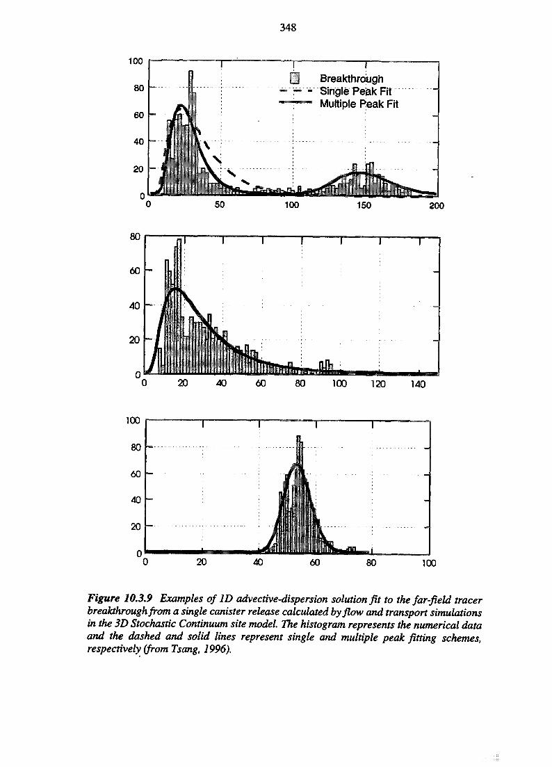
348
Breakthrough- SinglesPeakFit
Multiple Peak Fit
100
0 20 40 60 80 100 120 140
100
80
60
40
20
0
r
1i
i81H||SL. jws
20 40 60 80 100
Figure 10.3.9 Examples of ID advective-dispersion solution fit to the far-field tracerbreakthrough from a single canister release calculated by flow and transport simulationsin the 3D Stochastic Continuum site model The histogram represents the numerical dataand the dashed and solid lines represent single and multiple peak fitting schemes,respectively (from Tsang, 1996).
349
A geostatistical analysis indicates that the hydraulic conductivities are more or lessrandomly distributed and are very poorly spatially correlated, but it is also shown that, evenif a more complex structure were to be present, it would not show up in the analysis due tothe configuration of the boreholes. There are also different possibilities for generation ofthe stochastic hydraulic conductivity field.
One possibility is to assume that the distribution function of the log hydraulic conductivityis Gaussian, i.e. assuming the experimental histogram of the log of all the measuredhydraulic conductivity values to be normal, and that the joint distribution of any numberof values is also multigaussian. The multigaussian distribution is fully defined by a singlevariogram of the hydraulic conductivity data. However, this does not necessarily mean thatthe model is a valid representation of the true correlation structure, i.e. if the realdistribution is not multigaussian. Such an assumption is very difficult to confirm withouthaving a very large amount of data. Furthermore, because hydraulic conductivity fields withvery different connectivity properties (and hence different transport properties) may bedescribed by the same variogram, in the Gaussian assumption, there is no guarantee thattransport predictions based on this model are conservative (e.g. Journel and Deutsch, 1993and Schafmeister and de Marsily, 1994).
The indicator simulation method is an alternative to the Gaussian model (Gomez-Hernandez and Srivastava, 1990) is based on the use of indicators. In this approach, thehistogram of the experimental hydraulic conductivity distribution is divided into a numberof classes (6 in this case), where the covariance structure of the extreme classes can differfrom the rest. This approach is more flexible and makes it possible to represent morecomplex structures of the hydraulic structure as shown in the variants presented below. Forthis reason the indicator method is selected for the majority of variants analysed.
In general, a single or only a few realisations of each stochastic field is generated andanalysed, as preliminary tests showed that there is no significant difference amongrealisations with respect to the effective parameters estimated for the consequence analysis(see further Section 10.3.5.4).
10.3.5.3 Variants
In the light of the previous discussion, it is possible to construct alternative hydraulicconductivity fields with different transport properties that do not contradict the hydraulicdata. The variants of the Stochastic Continuum site model are chosen so as to address majoraspects of uncertainty regarding:
1. orientation of the hydraulic head gradient,2. correlation structure and,3. type of distribution for the hydraulic conductivity.
Table 10.3.4 lists all the variants that are analysed.
350
Table 10.3.4 Conceptual model variants analysed with the Stochastic Continuum sitemodel.
Variants)
REF-DIP80(Base Case)
LNG-DIP80
REF-DIP40REF-DIP90
REF-ISO
NEW-ISO
NEW-DIP80
GAU-ISO
Hydraulicconductivity (K)
distribution
Indicator
Indicator
Indicator
Indicator
Indicator, skewedtoward low Kvalues in each class
Same as NEW-ISO
Gaussian(lognormal)
Correlation structure / model
Planes of long-range correlation forthe highest 11 % of K values.Short, isotropic correlation for theremaining K values.
High percentage (60%) of K valueswith long-range correlation.
Alternative dip angles for thecorrelated planes of high K.
Isotropic correlation for all K values.
Same as REF-ISO
Same as REF-D1P80 (Base Case)
Isotropic multi-Gaussian
Correlationlength(s)
200 m / 20 m
200 m / 20 m
200 m / 20 m
20 m
20 m
200 m / 20 m
20 m
Base Case variant
The Base Case for all the variants in Table 10.3.4 is the one denoted REF-DIP80. The BaseCase model has an anisotropic correlation structure (200 m correlation length in twoorthogonal directions, representing the orientation of a major fracture zone set, and 20 mcorrelation length in the third direction, orthogonal to the fracture orientation) for thehighest two hydraulic conductivity classes and an isotropic short (20 m) correlation lengthfor the remaining hydraulic conductivity classes. Orientations of two sets of major fracturezones are represented simultaneously by superposing two such models, with differentorientations of the fracture zones.
This model produces two sets of planes of correlated high, but not constant, conductivity,extending out from each borehole section where high hydraulic conductivities have beenmeasured, imbedded in a more variable and less connected field of lower hydraulicconductivity. The rationale for these features is the geological evidence of extensivefracture zones at the site. The planes of long range correlation are oriented along the majorNNE and NNW fracturing directions with a dip angle of 80°, guided by the SITE-94geological structure model. Due to the better connectivity of the high conductivity zones,this variant is potentially more conservative with regard to far-field transport compared tothe classical Gaussian model.
351
Different correlation structures
In the Base Case, an arbitrary small fraction (11%) of the highest conductivity values areassigned anisotropic long range correlation in two directions. To explore the sensitivity ofthis assumption another variant (LNG-DIP80) is constructed, where a very high portion (thetop 60%) of the hydraulic conductivities are assigned the anisotropic 200 m correlationlength in the same two directions. Although not in conflict with the packer test data, thisvariant is considered to be rather extreme, as it has no support from any site data.
The variants REF-DIP40 and REF-DIP90, representing alternative dip angles, are includedto evaluate the sensitivity of transport to the orientation of the hydraulic head gradient withrespect to the orientation of major fracture zones. A dip angle of 90° implies that the planesof correlated high conductivity are parallel to the hydraulic head gradient.
In the variant denoted REF-ISO, a short (20 m) isotropic correlation length is assumed forall hydraulic conductivity classes. This model generates more or less random hydraulicconductivity fields, and would be the appropriate choice if no data other than the packer testhydraulic conductivities were taken into account.
Types of distribution for the hydraulic conductivity
The NEW-ISO and NEW-DIP80 variants have the same structural properties as those ofREF-ISO and REF-DIP80, respectively, but in the 'NEW' variants an alternative methodis used for assigning random hydraulic conductivities to the individual hydraulicconductivity classes. Instead of generating conductivity values to conform to a randomdistribution within each class, in the 'NEW' variants, conductivity values are generated toconform with a random distribution in the logarithmic scale. This method puts more of thehydraulic conductivity on the lower end of each class thus enhancing the conductivitycontrast between the different classes. This also broadens the range of the hydraulicconductivities generated towards lower values, which enhances the heterogeneity. Thesevariants are an example of conceptual uncertainty, specific for the indicator simulationmethod.
Different correlation model
The final variant, denoted GAU-ISO, represents the parametric (Gaussian) method ofgenerating hydraulic conductivity fields. As in the above variants, the fields generated areconditioned on the packer test hydraulic conductivity data. However, only the isotropic case(with the 20 m correlation length) is considered, as the parametric geostatistics only allowone correlation length for all conductivity values.
10.3.5.4 Base Case Results
Results from the Stochastic Continuum model are obtained as estimates of near-field Darcyvelocity (q^), far-field Darcy velocity (%) and far-field longitudinal dispersion coefficient(Duj) for each canister site or canister release calculation within each realisation of themodel. The Pe-number is obtained directly from these values, whereas calculation of theF-ratio requires an independent estimate of the specific flow-wetted surface (aj. The
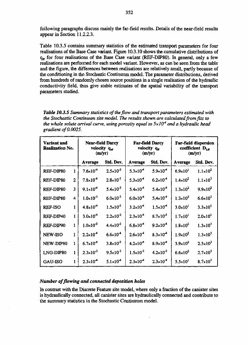
352
following paragraphs discuss mainly the far-field results. Details of the near-field resultsappear in Section 11.2.2.3.
Table 10.3.5 contains summary statistics of the estimated transport parameters for fourrealisations of the Base Case variant. Figure 10.3.10 shows the cumulative distributions ofqff for four realisations of the Base Case variant (REF-DIP80). In general, only a fewrealisations are performed for each model variant. However, as can be seen from the tableand the figure, the differences between realisations are relatively small, partly because ofthe conditioning in the Stochastic Continuum model. The parameter distributions, derivedfrom hundreds of randomly chosen source positions in a single realisation of the hydraulicconductivity field, thus give stable estimates of the spatial variability of the transportparameters studied.
Table 10.3.5 Summary statistics of the flow and transport parameters estimated withthe Stochastic Continuum site model. The results shown are calculated from fits tothe whole solute arrival curve, using porosity equal to 5x1 (X4 and a hydraulic headgradient of 0.0025.
Variant andRealization No.
REF-DIP80
REF-DIP80
REF-DIP80
REF-DIP80
REF-ISO
REF-DIP40
REF-DIP90
NEW-ISO
NEW-DIP80
LNG-DIP80
GAU-ISO
1
2
3
4
1
1
1
1
1
1
1
Near-field Darcyvelocity q^
(m/yr)
Average
7.6x10"*
7.8x10"*
9.1x10"*
LOxlO0
4.8x10"*
3.0x10"*
l.OxlO-3
2.2x10"*
6.7x10"*
2.3xl0"3
2.3x10"*
Std. Dev.
2.5xlO3
2.8xl03
5.4xlO3
6.0xl0"3
1.5xl0-3
2.2xlO"3
4.4xlO"3
6.6x10"*
3.8xl03
9.5xlO"3
5.1x10"*
Far-field Darcyvelocity qff
(m/yr)
Average
5.3x10"*
5.3x10"*
5.4x10"*
6.0x10"*
3.2x10"*
2.3x10"*
6.8x10"*
2.6x10"*
4.2x10"*
1.5xl0-3
2.3x10"*
Std. Dev.
5.9x10"*
6.2x10"*
5.4x10"*
5,4x10"*
1.5x10"*
8.7xl0-5
9.2x10"*
8.3x10"*
8.9x10"*
4.2xlO-3
2.3x10"*
Far-field dispersioncoefficient D ^
(m/yr)
Average
6.9X101
1.4xlO2
1.3xlO2
1.3xlO2
3.0X101
UxlO1
1.8xl02
1.9xlO2
3.9xl02
6.6xlO2
5.5X101
Std. Dev.
l.lxlO2
l.lxlO3
9.9xlO2
6.6xlO2
3.3X101
2.0x10'
1.3xl03
1.3xl03
2.3xlO3
2.7xlO3
8.7xlO2
Number of flowing and connected deposition holes
In contrast with the Discrete Feature site model, where only a fraction of the canister sitesis hydraulically connected, all canister sites are hydraulically connected and contribute tothe summary statistics in the Stochastic Continuum model.
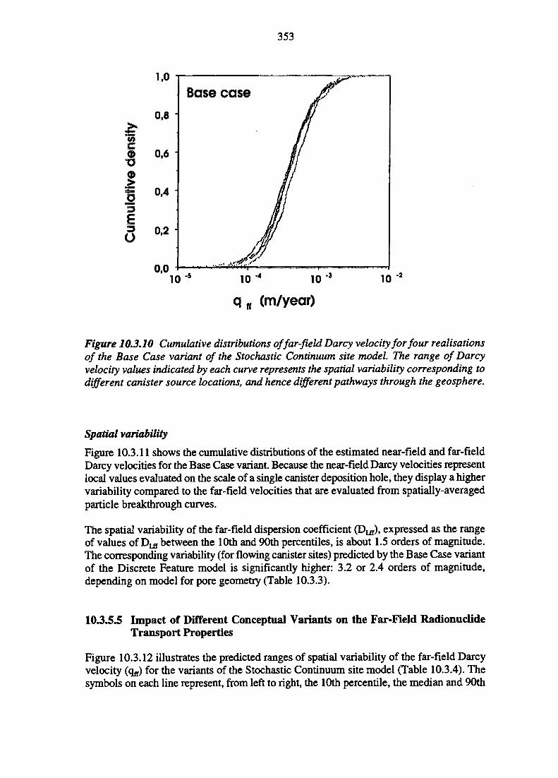
353
10 -5 •410 '* 10 *3
q n (m/y@ar)
10 -2
Figure 10.3.10 Cumulative distributions of far-field Darcy velocity for four realisationsof the Base Case variant of the Stochastic Continuum site model The range of Darcyvelocity values indicated by each curve represents the spatial variability corresponding todifferent canister source locations, and hence different pathways through the geosphere.
Spatial variability
Figure 10.3.11 shows the cumulative distributions of the estimated near-field and far-fieldDarcy velocities for the Base Case variant. Because the near-field Darcy velocities representlocal values evaluated on the scale of a single canister deposition hole, they display a highervariability compared to the far-field velocities that are evaluated from spatially-averagedparticle breakthrough curves.
The spatial variability of the far-field dispersion coefficient (D^), expressed as the rangeof values of D ^ between the 10th and 90th percentiles, is about 1.5 orders of magnitude.The corresponding variability (for flowing canister sites) predicted by the Base Case variantof the Discrete Feature model is significantly higher: 3.2 or 2.4 orders of magnitude,depending on model for pore geometry (Table 10.3.3).
10.3.5.5 Impact of Different Conceptual Variants on the Far-Field RadionuclideTransport Properties
Figure 10.3.12 illustrates the predicted ranges of spatial variability of the far-field Darcyvelocity (%) for the variants of the Stochastic Continuum site model (Table 10.3.4). Thesymbols on each line represent, from left to right, the 10th percentile, the median and 90th
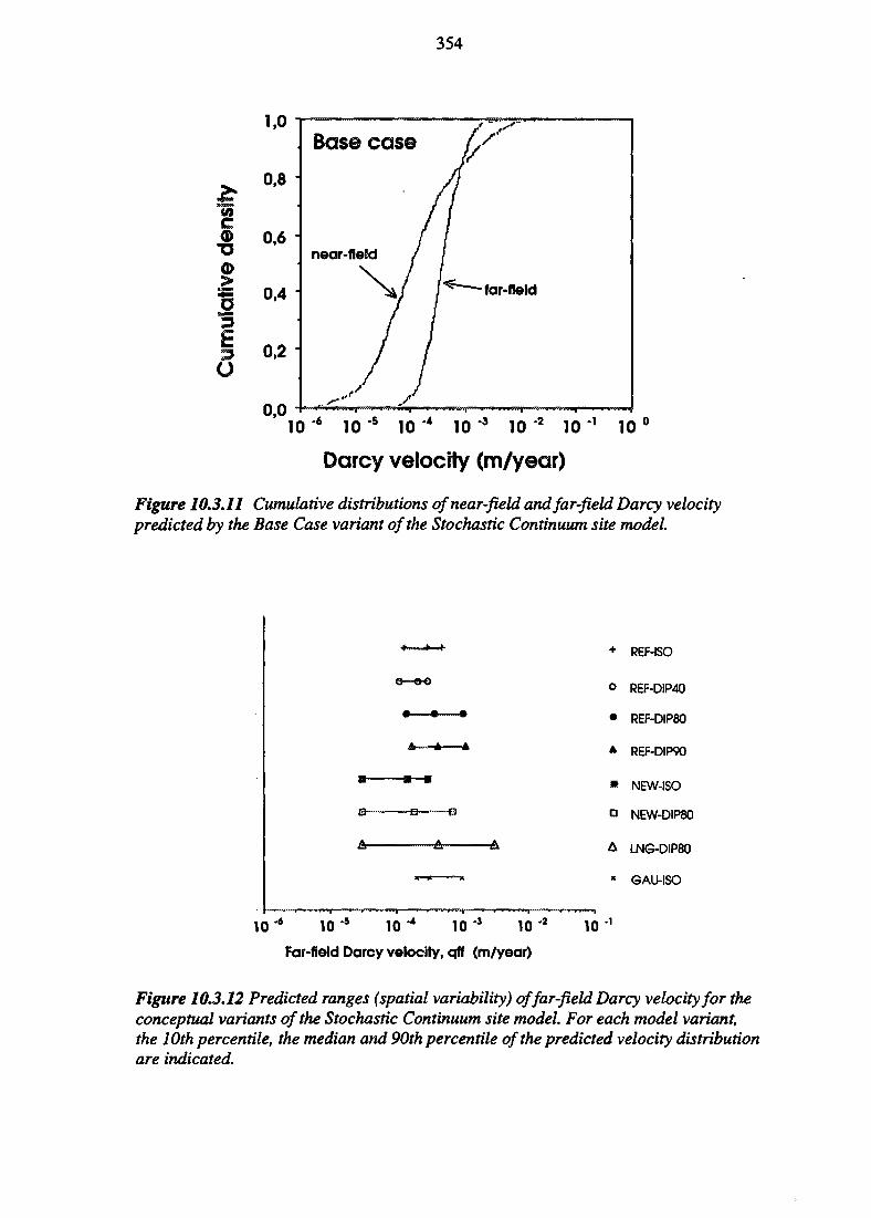
354
I
1,0
0,8
0,6 "
0,4 "
3 0,2o
0,0
Base case
near-field
far-field
10 '6 10 '5 10 •* 10 '3 10 *2 10 -1 10
Darcy velocity (m/year)
Figure 10.3.11 Cumulative distributions of near-field and far-field Darcy velocitypredicted by the Base Case variant of the Stochastic Continuum site model.
9 «..,„ 9
10 *6 10 *5 10 ** 10 "3 10 '2
Far-field Darcy velocity, qff (m/year)
10
+ REF-ISO
o REF-DIP40
• REF-DIP80
* REF-DIP90
s NEW-ISO
a NEW-DIP80
A LNG-DIP80
« GAU-ISO
Figure 10.3.12 Predicted ranges (spatial variability) of far-field Darcy velocity for theconceptual variants of the Stochastic Continuum site model. For each model variant,the 10th percentile, the median and 90th percentile of the predicted velocity distributionare indicated.
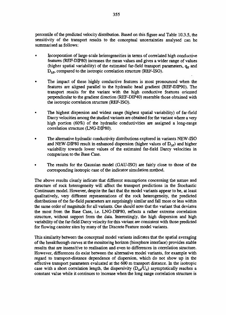
355
percentile of the predicted velocity distribution. Based on this figure and Table 10.3.5, thesensitivity of the transport results to the conceptual uncertainties analysed can besummarised as follows:
• Incorporation of large-scale heterogeneities in terms of correlated high conductivefeatures (REF-DIP80) increases the mean values and gives a wider range of values(higher spatial variability) of the estimated far-field transport parameters, % andD ^ , compared to the isotropic correlation structure (REF-ISO).
• The impact of these highly conductive features is most pronounced when thefeatures are aligned parallel to the hydraulic head gradient (REF-DIP90). Thetransport results for the variant with the high conductive features orientedperpendicular to the gradient direction (REF-DEP40) resemble those obtained withthe isotropic correlation structure (REF-ISO).
• The highest dispersion and widest range (highest spatial variability) of far-fieldDarcy velocities among the studied variants are obtained for the variant where a veryhigh portion (60%) of the hydraulic conductivities are assigned a long-rangecorrelation structure (LNG-DIP80).
• The alternative hydraulic conductivity distributions explored in variants NEW-ISOand NEW-DIP80 result in enhanced dispersion (higher values of D^) and highervariability towards lower values of the estimated far-field Darcy velocities incomparison to the Base Case.
• The results for the Gaussian model (GAU-ISO) are fairly close to those of thecorresponding isotropic case of the indicator simulation method.
The above results clearly indicate that different assumptions concerning the nature andstructure of rock heterogeneity will affect the transport predictions in the StochasticContinuum model. However, despite the fact that the model variants appear to be, at leastqualitatively, very different representations of the rock heterogeneity, the predicteddistributions of the far-field parameters are surprisingly similar and fall more or less withinthe same order of magnitude for all variants. One should note that the variant that deviatesthe most from the Base Case, i.e. LNG-DIP80, reflects a rather extreme correlationstructure, without support from the data. Interestingly, the high dispersion and highvariability of the far-field Darcy velocity for this variant are consistent with those predictedfor flowing canister sites by many of the Discrete Feature model variants.
This similarity between the conceptual model variants indicates that the spatial averagingof the breakthrough curves at the monitoring horizon (biosphere interface) provides stableresults that are insensitive to realisation and even to differences in correlation structure.However, differences do exist between the alternative model variants, for example withregard to transport-distance dependence of dispersion, which do not show up in theeffective transport parameters evaluated at the 600 m transport distance. In the isotropiccase with a short correlation length, the dispersivity (D^/L^) asymptotically reaches aconstant value while it continues to increase when the long range correlation structure is
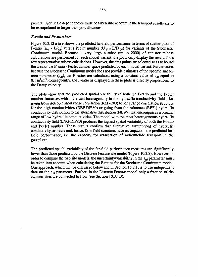
356
present. Such scale dependencies must be taken into account if the transport results are tobe extrapolated to larger transport distances.
F-ratio and Pe-numbers
Figure 10.3.13 a to e shows the predicted far-field performance in terms of scatter plots ofF-ratio (a^ x L/qff) versus Peclet number (U ff x L/D yj) for variants of the StochasticContinuum model. Because a very large number (up to 2000) of canister releasecalculations are performed for each model variant, the plots only display the results for afew representative release calculations. However, the data points are selected so as to boundthe area of the F-ratio - Peclet number space predicted by each model variant. Furthermore,because the Stochastic Continuum model does not provide estimates of the specific surfacearea parameter (a^), the F-ratios are calculated using a constant value of a^ equal to0.1 mVm3. Consequently, the F-ratio as displayed in these plots is directly proportional tothe Darcy velocity.
The plots show that the predicted spatial variability of both the F-ratio and the Pecletnumber increases with increased heterogeneity in the hydraulic conductivity fields, i.e.going from isotropic short range correlation (REF-ISO) to long range correlation structurefor the high conductivities (REF-DIP80) or going from the reference (REF-) hydraulicconductivity distribution to the alternative distribution (NEW-) that encompasses a broaderrange of low hydraulic conductivities. The model with the most heterogeneous hydraulicconductivity field (LNG-DIP80) produces the highest spatial variability of both the F-ratioand Peclet number. These results confirm that alternative assumptions of hydraulicconductivity structure and, hence, flow field structure, have an impact on the predicted far-field performance, i.e. the capacity for retardation of radionuclide transport in thegeosphere.
The predicted spatial variability of the far-field performance measures are significantlylower than those predicted by the Discrete Feature site model (Figure 10.3.8). However, inprder to compare the two site models, the uncertainty/variability in the a^ parameter mustbe taken into account when calculating the F-ratios for the Stochastic Continuum model.One approach, which will be discussed below and in Section 15.2.1, is to use independentdata on the a^ parameter. Further, in the Discrete Feature model only a fraction of thecanister sites are connected to flow (see Section 10.3.4.3).
357
a)101 0 1 6 " 1 0 " 1 0 " 101 4 10
F-ratio (s/m)
S; 10
b)
101 0 1 0 " 101 2 10 1S 101 4 10
F-ratio (s/m)
10 S
10
c)
101 0 1 0 " 1012 1 0 " 101 4 10
F-ratio (s/m)
10 S
10 3 -
5 io2iEf 101
0,
10 0 _ ,
NEW-ISO
1010 1 0 " 101 2 1 0 " 1 0 " 10
F-ratio (s/m)
e)
1010 1 0 " 1 0 " 1013 1 0 " 10
F-ratio (s/m)
Figure 10.3.13 Scatter plots of the hydrogeological far-field parameter groups, F-ratioand Peclet number, evaluated from particle tracking calculations in the main modelvariants of the Stochastic Continuum hydrogeological site model. Each data pointrepresents the far-field transport properties of the transport paths originating from aselected single canister source location. A constant value of the flow-wetted surface areaparameter (a^ -0.1 m1) is used for the calculation of the F-ratios.
358
10.3.6 Flow-wetted Surface Area Estimates
10.3.6.1 Introduction
This section describes analyses of the specific surface area parameter a i.e. the flow-wettedsurface area per volume of rock. This parameter strongly affects the efficiency ofretardation processes such as sorption and matrix diffusion and is, therefore, an importantinput parameter to the radionuclide transport models employed in SITE-94. As describedin Section 10.3.4 the a, parameter is estimated together with Darcy velocity from flow andtransport calculations in the Discrete Feature site model. This ensures that potential flowfield effects on the a, parameter are taken into account, i.e. the effect of an unevendistribution of flow and transport on the available fracture surfaces. However, independentestimates of a, are required for two purposes: (1) for evaluation of far-field radionuclidetransport based on the flow and transport results from the Stochastic Continuum site model(which does not provide estimates of a,.), and (2) for near-field radionuclide release andtransport model. In addition, the independent estimates provide a check of the predictionsmade with the Discrete Feature model, which build on geometrical assumptions on the porestructure within conductive fractures.
The surface-based site characterisation at Aspo" produced very limited information forestimation of a,. There are, for example, no data from field tracer tests in which sorbingtracers are used and the detailed pore structure in individual fractures and fracture zones isessentially unknown. In place of such data, a, is evaluated from synthetic transportexperiments performed with a detailed discrete-fracture network model (Nordqvist et al.,1995) and as part of the evaluation of the Discrete Feature hydrogeological site model(Geier, 1996). Additional estimates are derived from the SITE-94 geological structuremodel (Voss et al., 1996), from geochemical data (Glynn and Voss, 1996), and from theSimple Evaluation.
Evaluation of the parameter a,, is intrinsically difficult, since the values obtained are ingeneral dependent upon assumptions (explicit or implicit) regarding the effective porosity(or bulk volume) for a given transport pathway. For example, in the Discrete Feature model,each estimated value of a, depends directly upon the essentially arbitrary volume ofadjacent, unfractured rock that is associated with the given transport path. On the otherhand, this ambiguity does not affect most of the transport calculations in SITE-94, wherea, is incorporated in the F-ratio. As discussed in Section 10.3.4, the porosity dependenceof a, is exactly cancelled out, in the F-ratio, by a corresponding porosity dependence ofDarcy velocity, provided that identical assumptions are used in calculating flow-wettedsurface area and Darcy velocity.
10.3.6.2 The VAPFRAC and DISCFRAC Discrete-Fracture Network Models
The VAPFRAC discrete-fracture network model is employed to estimate the specificsurface area (a,) for the moderately fractured rock (i.e. excluding fracture zones) at thedepth of the hypothetical repository at Aspo. The model uses the same stochastic fracture-network parameters that are estimated for the detailed-scale fracture network in the DiscreteFeature hydrogeological site model, but includes additional parameters to define thespatially varying aperture within the individual fracture planes (see Section 7.3.9).
359
Because the basic assumptions regarding fracture network geometry and, in particular, theaperture field in the fracture planes, are not uniquely supported by site-specific data, theanalysis included a set of variational cases to explore the sensitivity of a, to the locationprocess for fractures, the variance of fracture aperture, the correlation length for apertureand the fracture discretisation.
For each combination of input parameters, 12 realisations of 3D fracture networks aregenerated with the VAPFRAC model. For each realisation, the specific surface area isevaluated from synthetic tracer experiments, for both non-sorbing and sorbing tracers, usingthe method described by Dverstorp et al. (1992). This method takes into account potentialflow field effects, such as dynamic (flow field dependent) channelling, that may influencethe proportion of the total fracture surface area that is accessible to a migrating solute.
The estimated values of a, for the different realisations fall within the range 0.1 to 10 m2/m3,with a median value around 2-3 m2/m3, for all input-parameter combinations. Of the variedparameters, the largest impact on a, is produced by changing the variance of aperture withinfracture planes. An increased variance results in more pronounced flow channelling, i.e.preferential transport paths, and a lower flow-wetted surface area,
When judging the results of the VAPFRAC model, it is important to recall that the entireplane of each fracture is assumed to be accessible to advective transport, and that theaperture field is assumed to be described by a lognormal distribution. This model producesa channelised flow field in the fracture planes but, due to numerical problems, moreextreme assumptions of flow channelling could not be evaluated. If, for example, flow andtransport occur within narrow channels within the fracture planes, as suggested byNeretnieks et al. (1987), the specific surface area might be significantly reduced.
From a purely geometrical point of view, a system of one-dimensional tubular flowchannels gives the lowest value of the specific surface area. In an earlier analysis, Dverstorpet al. (1992) used a discrete-fracture network model, DISCFRAC, to evaluate the specificsurface area for a set of idealised fracture channel geometries, including parallel plate andtubular channels. The fracture network properties are estimated by calibration on fractureand flow data from the Stripa-3D flow and migration experiment (Abelin et al., 1991a, b).The results of this evaluation suggested values of a,, on the order of 0.2 m2/m3 for a networkof parallel plate flow channels with a width of 0.2 m, and as low as 0.001 m2/m3 for anetwork of tubular flow channels. However, the tubular flow channel model could beinvalidated because it does not provide a consistent description of both the experimentalflow and tracer test data.
10.3.6.3 The SITE-94 Geological Structure Model
A rough geometrical estimate of the flow-wetted surface area parameter can be obtaineddirectly from the SITE-94 geological structure model. Voss et al. (1996) found that the totalarea of water conducting structures per volume of rock in that model, takes on a constantmean value of 0.065 m2/m3 for a large range of averaging volumes (see Section 7.3.6.5).Assuming that all structure surfaces are accessible to flow and counting each structure areatwice to account for the two sides of the fracture planes, gives an effective specific surfacearea of 0.12 m2/m3. This value is about one order of magnitude lower than the median value
360
(a, equal to 2 m2/m3) determined with the VAPFRAC discrete-fracture network model. Hiereason for this difference is likely to be that the geological structure model only includessite-scale structures, whereas the VAPFRAC model represents a network of small-scalefractures.
10.3.6.4 The Discrete Feature Hydrogeological Site Model
The Discrete Feature site model (Geier, 1996) contains a simple model for estimation ofthe specific surface area from site scale particle tracking calculations as discussedabove. The median values of the specific surface area (a^) predicted by this model verybetween 0.01 and 0.1 m2/m3 with a spatial variability, reflecting transport paths fromdifferent canister sites, of 1 - 2 orders of magnitude. The lower values (and lowervariability) are obtained for the model variants where a constant transport aperture of 3 cmis assumed for the deterministic fracture zones (the 'HI' variants). However, as noted inSection 10.3.4.1, the abstraction of effective transport parameters for the far-field (includinga^, % and <3>ff) from the Discrete Feature site model involves a somewhat arbitraryassumption of a bulk or averaging volume, corresponding to the volume of an equivalentstream tube between the source canister and the biosphere. The choice of averaging volumeaffects the magnitude of the individual transport parameters but not the parameter groups(F-ratio and the Peclet number) that control far-field transport. This means that the valuesof aj, as presented above, are only meaningful when combined with the correspondingtransport parameters estimated from the Discrete Feature site model.
10.3.6.5 Geochemical Model
Glynn and Voss (1996) presented an independent estimate of the flow-wetted surface areabased on geochemical data. The estimate builds on the assumption that the 222Rn contentof the groundwater can be related to the uranium content in the rock and the contact areabetween the groundwater and the rock. The higher the uranium content and the larger thecontact area, the greater the source of ^Rn. Using Aspo data on the uranium content in therock and the ^ R n content in the groundwater, Glynn and Voss (1996) obtained an averageflow-wetted surface area of 3100 m2 per m3 of fluid. The surface area per volume of rock(a,) is obtained by multiplying this value by the porosity of the rock. Analyses of the LPT-2tracer test suggested porosities in the range of 10"4 to 10"2 for some of the major fracturezones at Aspo (Rhen et al., 1992, pp 54-56). Assuming that the lower end of this range (10"4
to 103) is a reasonable average porosity for the rock at Aspo, would give values of a^between 0.31 and 3.1m2 per m3 of rock. Although this estimate involves several uncertainassumptions it is interesting to note that it agrees with the range of values predicted by theVAPFRAC detailed fracture network model.
10.3.6.6 Simple Evaluation
Although prediction of flow-wetted surface area is not a specific objective of the SimpleEvaluation of flow and transport parameters, values of a, are readily calculated for the pore-structure models that are shown in Figure 10.3.3, for each of the idealised transportpathways shown in Figure 10.3.2. Excluding Model B, which (as discussed in
361
Section 10.3.3) is interpreted as being representative only of isolated, extreme channels, therange of values of a, thus calculated extends from 0.0014 to 140 m2/m3. This range is verywide in comparison with the ranges estimated by other techniques, which is to be expecteddue to the fact that broad ranges of uncertainty in the underlying parameters, and in themodels for pore structure, have been taken into account.
103.6.7 Implications for Radionuclide Transport Evaluation
Given the limited amount of supporting data and the large conceptual model uncertaintiesin the above analyses, the results should be regarded as rough indications on the range ofpossible values of the specific surface area. Furthermore, the validity of using a singleeffective specific surface area to represent the spatially varying flow-wetted fracture area,both within and between fractures, could be questioned.
For the reasons stated above, the specific surface area estimated with the Discrete Featuresite model (a^) are used exclusively in combination with the other far-field transportparameters estimated with that model. In this way the correlations between, and spatialvariability of, Darcy velocity, porosity and specific surface area are automatically taken intoaccount. Because the hydrogeological transport parameters estimated with this model areall internally consistent, the predictions of far-field radionuclide transport based on thismodel can be directly related to the original assumptions on transport geometry in thefractures and fracture zones.
For analyses of far-field radionuclide transport based upon the predictions of the StochasticContinuum site model, and for near-field radionuclide release and transport modelling,three values of the specific surface area (a, equal to 0.01,0.1 and 1.0 m2/m3) are selectedto represent the uncertainty in this parameter (see also Section 15.2.1). As shown inFigure 10.3.14, these values approximately cover the range of median values calculated bythe various techniques. The highest and most optimistic value is close to the median valuepredicted by the VAPFRAC discrete-fracture network model, and is thus representative ofa moderately fractured rock volume consisting of connected small-scale fractures that arecompletely open to flow. The middle value (a, equal to 0.1 mVm3), which represents thelower bound of a, predicted by the VAPFRAC model, is selected as a conservativereference value. The lowest value (a, equal to 0.01) could be considered as ratherpessimistic, judging from the above analysis and discussion.
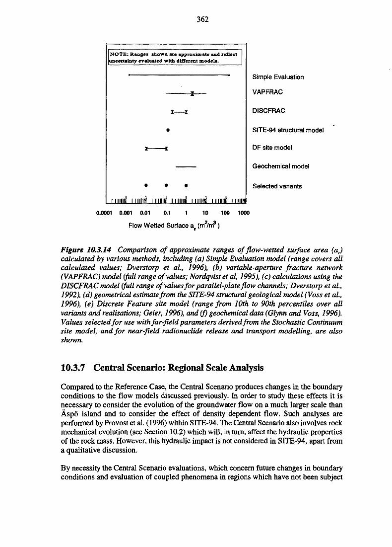
362
NOTE: Ranges shown are approximate and reflectuncertainty evaluated with different models.
Simple Evaluation
VAPFRAC
DISCFRAC
SITE-94 structural model
DF site model
Geochemical model
Selected variants
iiiiiifl i IIIIIHI I i mini iniiiiil 11 mill! i m i l
0.0001 0.001 0.01 0.1 10 100 1000
Flow Wetted Surface ar (m2/m3)
Figure 10.3.14 Comparison of approximate ranges of flow-wetted surface area (ar)calculated by various methods, including (a) Simple Evaluation model (range covers allcalculated values; Dverstorp et al, 1996), (b) variable-aperture fracture network(VAPFRAC) model (full range of values; Nordqvist et al, 1995), (c) calculations using theDISCFRAC model (full range of values for parallel-plate flow channels; Dverstorp et al.,1992), (d) geometrical estimate from the SITE-94 structural geological model (Voss et at,1996), (e) Discrete Feature site model (range from 10th to 90th percentiles over allvariants and realisations; Geier, 1996), and (f) geochemical data (Glynn and Voss, 1996).Values selected for use with far-field parameters derived from the Stochastic Continuumsite model, and for near-field radionuclide release and transport modelling, are alsoshown.
10.3.7 Central Scenario: Regional Scale Analysis
Compared to the Reference Case, the Central Scenario produces changes in the boundaryconditions to the flow models discussed previously. In order to study these effects it isnecessary to consider the evolution of the groundwater flow on a much larger scale thanAspb" island and to consider the effect of density dependent flow. Such analyses areperformed by Provost et al. (1996) within SITE-94. The Central Scenario also involves rockmechanical evolution (see Section 10.2) which will, in turn, affect the hydraulic propertiesof the rock mass. However, this hydraulic impact is not considered in SITE-94, apart froma qualitative discussion.
By necessity the Central Scenario evaluations, which concern future changes in boundaryconditions and evaluation of coupled phenomena in regions which have not been subject
363
to a detailed site evaluation in a sense need to be rather speculative. On the other hand, theobjective of the evaluations is not to give a precise prediction of what is going to happeneverywhere. The evaluations are done in order to establish plausible external impacts onthe repository as consequence of the Central Scenario.
10.3.7.1 Evolving Boundary Conditions
As stated in Chapter 9, the SITE-94 Central Scenario, which builds upon the Milankovictheory of climate changes, assumes the occurrence of three glacial periods in the northernhemisphere at about 10 ka after present (AP), 60 ka AP and 80 ka AP. In Scandinavia, thelatter two glaciations are expected to be major, with continental ice sheets reaching northernEurope. During this period, there will be alternating periods of present-day temperateconditions, permafrost, cold-based glacial ice, warm-based glacial ice with sub-ice meltingand sea incursion and regression due to glacial-isostatic depression and rebound of theshield. Each of these conditions may affect regional flow of groundwater in significantways.
Extension of Boundary Conditions to the Fennoscandian shield
For the regional-scale analysis, the evolution of surface conditions at Aspo, defined inKing-Clayton et al. (1995), is extended in a simple manner to the Fennoscandian shield ofsouthern Sweden, to represent changes expected along a line extending from offshore ofthe western coast of Norway to Aspo and across the Baltic Sea to Poland, as shown inFigure 10.3.15. This line covers the region of the maximum expected extent of the glaciers.The particular line selected is somewhat arbitrary, but follows the regional groundwaterflow direction under present-day conditions along a large part of its extent. On portions ofthe surface not covered by ice or sea, the pressure is ambient (atmospheric). Portions of theshield covered by sea are subjected to additional pressure associated with the weight of theseawater.
Permafrost
It is assumed that permafrost acts primarily to reduce permeability in portions of the near-surface domain. In certain areas, particularly in areas of natural discharge, the permafrostmay be punctuated with open taliks that provide a path for fluid flow from deep, unfrozenrock to the surface.
The ice sheet
The ice sheet, where present, is assumed to control the pressure and/or groundwaterrecharge at the surface of the shield. It is assumed that the ice sheet forms a barrier to theflow of water, except in regions of basal melting, where meltwater can be a source ofrecharge. Furthermore, the recharge could not continue once the sub-ice pressure reachesthe pressure exerted by the weight of the overlying ice; any further increase in this basalpressure is precluded by the release of excess water which may occur through fissures inthe stressed ice or by basal flow through films, cavities and channels.
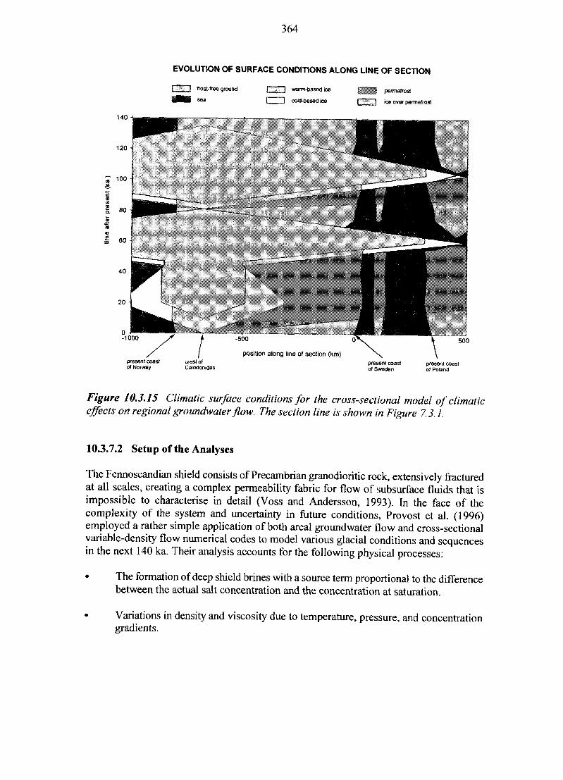
364
EVOLUTION OF SURFACE CONDITIONS ALONG LINE OF SECTION
r7'"'~_3 frost-free ground
sea
warm-based ice
I I cold-based ice
\j&%£2$ permafrost
I HI l c e o v e r permafrost
140
120
100
£ 80
•S 60
-500
position along line of section (km)
500
present coastof Poland
Figure 10.3.15 Climatic surface conditions for the cross-sectional model of climaticeffects on regional groundwater flow. The section line is shown in Figure 7.3.1.
10.3.7.2 Setup of the Analyses
The Fennoscandian shield consists of Precambrian granodioritic rock, extensively fracturedat all scales, creating a complex permeability fabric for flow of subsurface fluids that isimpossible to characterise in detail (Voss and Andersson, 1993). In the face of thecomplexity of the system and uncertainty in future conditions, Provost et al. (1996)employed a rather simple application of both areal groundwater flow and cross-sectionalvariable-density flow numerical codes to model various glacial conditions and sequencesin the next 140 ka. Their analysis accounts for the following physical processes:
The formation of deep shield brines with a source term proportional to the differencebetween the actual salt concentration and the concentration at saturation.
• Variations in density and viscosity due to temperature, pressure, and concentrationgradients.
365
• Groundwater flow driven by topographic gradients, recharge and fluid densityimbalances.
• Changes in total stress in the subsurface due to glacial loading.
The major classes of flow-field phenomena that are likely to occur are thus identified andtaken into account. This is true regardless of the details of the rock fabric structure, climaticconditions or uncertainty therein.
A static temperature distribution is assumed for the calculation of local density andviscosity of the groundwater. Two values of the vertical temperature gradient are tested:15°C/km and 25°C/km. However, because the simulation results are insensitive to theexact value of the temperature gradient, a single value (25°C/km) is used for allsimulations. Advective heat transport is determined to be insignificant so that the stableconductive temperature regime assumed is a reasonable assumption during interglacialperiods. Porosity of the rock is assumed to be 10'3.
10.3.7.3 Variants
In the evaluation of possible future behaviours of the groundwater flow system and of thephysical controls on these behaviours, Provost et al. (1995) simulated a large number ofsituations. These included combinations of the following variations:
• sub-ice melting rate (low and high),
• sedimentary sequence overlying shield rocks east of Aspo (with and without),
• permeability distribution of shield rocks (constant and vertically stratified),
• anisotropy (horizontal permeability:vertical permeability) of shield rocks torepresent regional effect of fracture zones (100:1, 10:1 and 1:10),
• loading efficiency of shield rocks (0,0.5, and 1; where 0 implies that the rock bearsthe entire weight of the glacier and 1 implies that the water bears the weight of theglacier),
• permafrost (many taliks: generally open to flow; taliks only in areas of present-daydischarge; and no taliks: closed to flow).
For each situation, a coefficient controlling the rate of generation of shield-brine solute inthe simulation is adjusted to reproduce, in a general fashion, the available (but very sparse)data on regional solute distribution found today. Thus, each situation is simulated for a140-ka period into the future, with the climate change conditions described above,beginning from a roughly calibrated steady-state condition representing the system as itappears today. It should be noted, however, that although today's system may not be in atrue steady-state condition following the previous glaciation, this is still considered areasonable starting point for future evolution.
366
10.3.7.4 Results
Base Case results
Figure 10.3.16 shows the Darcy velocity and solute concentration fields for groundwatersat selected times during the first major glacial cycle in the Base Case simulation of Provostet al. (1996). The Base Case assumes the presence of a sedimentary wedge east of Aspo anda uniform bedrock permeability with a horizontal permeability 10 times greater than verticalpermeability. The loading efficiency is assumed to be zero. The permafrost, where present,is assumed to decrease the permeability by ten orders of magnitude and to be continuous(no open taliks), except beneath the sea or melting ice, where there is no permafrost. Thesub-ice melting rate is assumed to be 0.5 cm/year.
Figure 10.3.17 shows the time evolution of Darcy velocity and solute concentration forgroundwaters at the SITE-94 repository position (500 m below the surface) for the entire140 ka sequence. Sequences for the other combinations of variables may be found inProvost et al. (1996), but the general evolution described below is similar for all cases, withsome variation in the magnitude and timing of certain flow events.
Under today's conditions, Aspo is in the regional discharge area for water recharged in thesouthern Swedish highlands. Flow is generally eastward and upward (Figure 10.3.17b).
During periods of permafrost (10 ka, Figure 10.3.16b), which effectively block rechargeand discharge of groundwater, flow velocities decrease only slightly, but the directions offlow may change significantly. Regions below cold-based glacial ice do not experience anyadditional change in flow compared with regions overlain by permafrost, but one shouldnote that stress-related fluid redistribution is not considered here. If taliks occur in the samearea where groundwater presently discharges, there is effectively no change from today'slocal flow conditions in these areas during periods of permafrost.
The advent of warm-based glacial ice with sub-ice melting on the Fennoscandian shield isof major importance to the regional groundwater flow system. Meltwater recharge occursat a high angle and can reach depths of a few kilometres in a few thousand years of recharge(Figure 10.3.16c and d). Compare the velocity of infiltrating water of around 1 m/year herewith 7 m/year (500 m per 70 years) in the Discrete Feature model (Section 10.3.8). Thedifference reflects discrete versus equivalent continuum properties and the more detailedrepresentation of site-scale heterogeneity in the Discrete Feature site model.
Meltwater may also bring oxygen to great depths in an otherwise reducing chemical systemin as little as one thousand years (Glynn and Voss, 1996; see also Section 10.4) causingsignificant geochemical changes in addition to a decrease of total dissolved solids (TDS)content. Glacial meltwater, over 20 ka old and no longer oxidising, is indeed found in therocks below Aspo Island (Glynn and Voss, 1996; see also Section 7.4).
For a large range of likely melting rates, there is significantly more meltwater availablebelow the ice than that which can recharge the shield rocks. If an arbitrarily high pressureare allowed to build up below the ice, all of the available meltwater could be recharged.However, the maximum sub-ice pressure cannot exceed the weight of the ice withoutcausing the ice to lift or fracture. Thus, local ice thickness controls the maximum local
367
recharge rate and excess meltwater must drain away in sub-ice channels, fractures or films,or upwards through fissures. These large quantities of excess fluid may be associated withthe development of eskers and possible scouring of fracture zones below their originalsurface. Under the condition where ice weight controls the recharge rate, recharge changesto discharge as soon as the ice thickness begins to decrease during glacial regression(Figure 10.3.16e).
Discharge also occurs nearly vertically. However, it is not likely that deep shield brines willenter subsurface regions where they are not already found today. Flow rates in areas ofbasal melting may exceed present-day rates by about one order of magnitude.
The largest groundwater flow rate in the Central Scenario sequence occurs at the ice marginduring advance and regression. Discharge occurs to the sea in the area where the seafollows the ice margin inland (Figure 10.3.16f) and otherwise to the ground surface. Thisflow is also about one order of magnitude greater than present-day rates, but lasts only aslong as the ice margin is in the vicinity of a particular point (Figure 10.3.17a). Givensufficient time following a glacial cycle (on the order of 50 ka), the regional flow systemapproaches steady conditions for interglacial (present-day) conditions (Figure 10.3.16g).
Combined results of Base Case and the other variants
The combined results of the Base Case and the cases which consider other combinationsof variables are as follows. Regional groundwater flow in the Fennoscandian shield isindeed strongly affected by surface conditions associated with climatic change andglaciation. The changes in subsurface conditions near Aspo Island due to the glacial-climatic cycle are primarily controlled by the changes in surface conditions directly above.However, the general flow through the area and water chemistry are always stronglydependent on regional conditions and driving forces.
Under periglacial conditions and where permafrost is impermeable, permafrost locally orextensively impedes the free recharge and discharge of groundwater. Below cold-basedglacial ice, no recharge or discharge of groundwater occurs.
Below warm-based ice with sub-ice melting, the potential for groundwater recharge ratesgreater than the present rate is large, with recharging meltwater flowing downward at a highangle. When the glacier begins to recede, large flows may occur upwards, at a high anglebelow the ice sheet, due to pressure release, although there is still potential sub-ice rechargedue to the existence of meltwater. Excess meltwater must exit from below the glacier insub-ice channels or upwards through fissures. Sub-ice groundwater flow rates may be oneorder of magnitude greater than flow under present-day conditions. There is significantincrease in groundwater discharge at the receding ice margin, but it is generally less thanone order of magnitude greater than sub-ice flow rates and lasts only as long as the icemargin is in the vicinity.
Major increases in solute concentration in the groundwaters above present-day levels, dueto the rise of deep shield brine, is not likely. However, glacial meltwater may penetrate thesubsurface to depths of a few kilometres (especially if loading efficiency is low) duringglacial advance (possibly inducing oxidising conditions, see Section 10.4) and may residein the shallow subsurface for periods exceeding 10 ka. The depth of such meltwater pene-
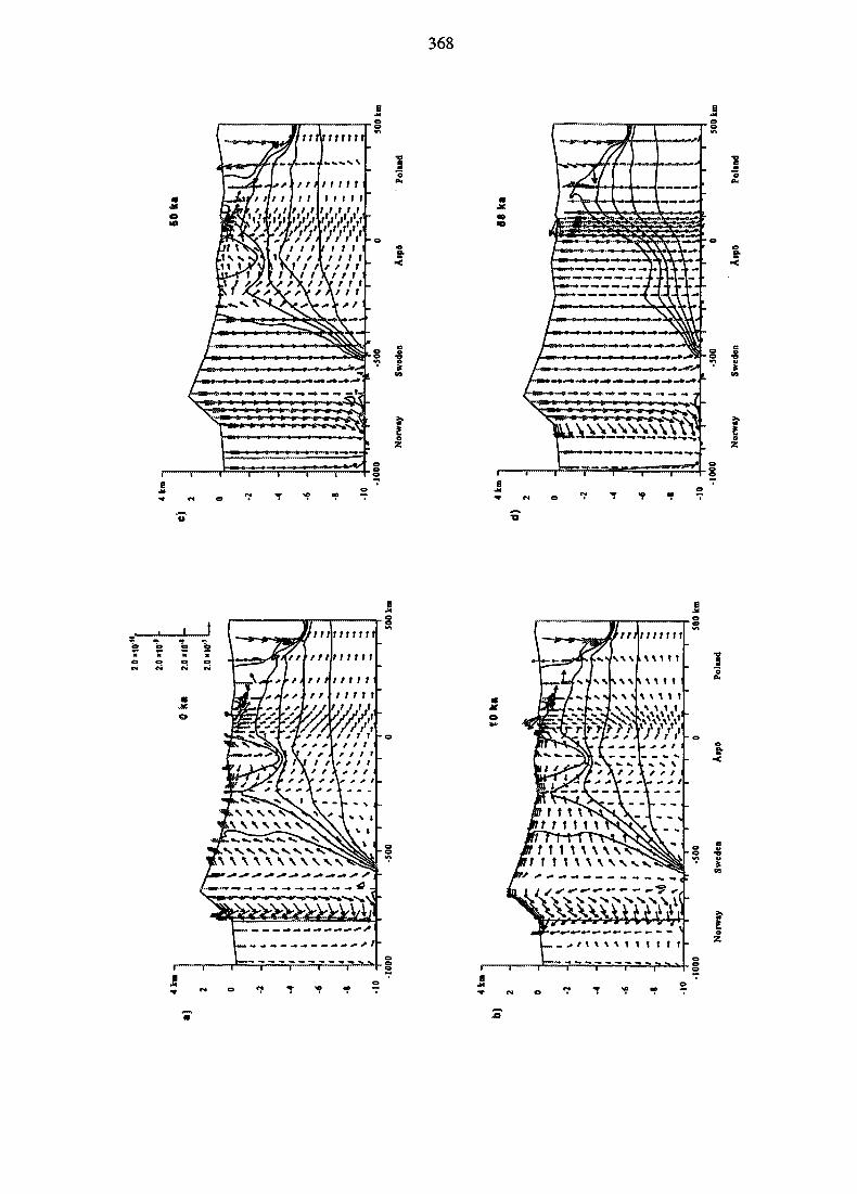
368
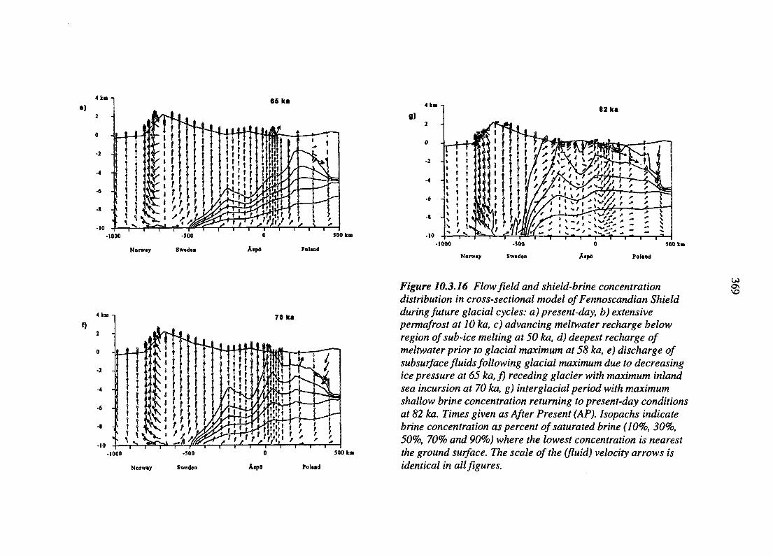
4 km
-10• 1000
Norway
•500
Sweden
500 km
AfpO Poland• 1000
82 ka
Norway AipO
500 km
Poland
•10
70 9ta
• 1000 500 km
Norway AipO Poland
Figure 10.3.16 Flow field and shield-brine concentrationdistribution in cross-sectional model of Fennoscandian Shieldduring future glacial cycles: a) present-day, b) extensivepermafrost at 10 ka, c) advancing meltwater recharge belowregion of sub-ice melting at 50 ka, d) deepest recharge ofmeltwater prior to glacial maximum at 58 ka, e) discharge ofsubsurface fluids following glacial maximum due to decreasingice pressure at 65 ka, f) receding glacier with maximum inlandsea incursion at 70 ka, g) interglacial period with maximumshallow brine concentration returning to present-day conditionsat 82 ka. Times given as After Present (AP). Isopachs indicatebrine concentration as percent of saturated brine (10%, 30%,50%, 70% and 90%) where the lowest concentration is nearestthe ground surface. The scale of the (fluid) velocity arrows isidentical in all figures.
uONo
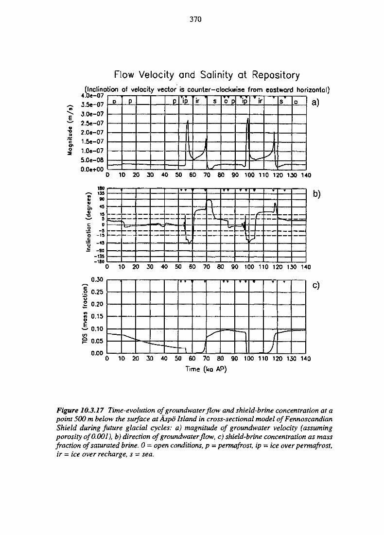
370
V
3
Flow Velocity and Salinity at Repository(Inclination of velocity vector is counter-clockwise from eastward horizontal)
4.0e-073.5e-073.0«-07
0)
— 2.5e-072.0e-07
c 1.5e-071.0e-075.0e-080.0e+00
0 p p 'p
\
s
\AIs-
0 p •p 'ir
1A
*
1jA
{
s 0 a)
10 20 30 40 50 60 70 80 90 100 110 120 130 140
180->->. 135
S 90V£b 45
C 0•2 "5o -15
| -45
£ -90-135-180
— •
" — -
i i 1 i r",..iiL—-•.
L__1
\
_ —
V T T
_ _ _
„
b)
0 10 20 30 40 50 60 70 80 90 100 110 120 130 140
0.
•I °2 0.
iP o.
0.
.30
.25
.20
.15
.10
.05
.00~~- , 1——~
T T ' V
;
T
c)
0 10 20 30 40 50 60 70 80 90 100 110 120 130 140
Time (ko AP)
Figure 10.3.17 Time-evolution of groundwaterflow and shield-brine concentration at apoint 500 m below the surface atAspo Island in cross-sectional model of FennoscandianShield during future glacial cycles: a) magnitude of groundwater velocity (assumingporosity of 0.001), b) direction of groundwaterflow, c) shield-brine concentration as massfraction of saturated brine. 0 — open conditions, p ~ permafrost, ip = ice over permafrost,ir ~ ice over recharge, s - sea.
371
tration can be less for higher loading efficiency of the shield rock. This is due to the factthat meltwater recharge slows or stops when subsurface pressures reach the ice weight (asdescribed above), while subsurface pressures increase faster when the ice weight itself hasa direct effect on subsurface fluid pressure through loading. Thus, depending on themechanical properties of the shield rock, loading can affect the amount and penetration ofglacial recharge in the subsurface.
Flow at the ice front
Very sharp changes in pressure, equivalent to hundreds of metres of hydraulic head at theice margin, may cause extremely high flows locally. An example is the presence of ice-dammed lakes. However, these are not considered here owing to the regional nature of theanalysis. Such an extreme situation would serve to increase the local hydraulic gradient andgroundwater fluxes below Aspo would increase proportionately.
Sudden meltwater breakouts may be the cause of deep scouring of fracture zones to depthsin the order of 100 m, as found in a number of locations in Sweden (Olvmo, 1989). Suddenunloading due to ice melting may result in rock-block motion along new or existing faultsand concomitant changes in the transmissivity of structures. Neither this extreme effect, norchanges in transmissivity due to glacial loading and unloading of the bedrock, have beenconsidered in the regional analysis.
The likelihood of combined high-consequence circumstances, such as a high-elevation icelake at the ice margin discharging large quantities of fluid through a fracture zone (withscouring) which is recently made transmissive due to local unloading, which, in turn,connects to a discharge area directly through the SITE-94 repository, must be consideredto be exceptionally small. However, in such a case, extremely high fluid fluxes (105 timesnormal) can be calculated through the SITE-94 repository, given up to 100 times highergradient and 1000 times greater transmissivity.
Because a variety of rock fabric structures and climatic conditions have been consideredgenerically at the regional scale, the ranges of flow behaviours modelled are consideredindicative of what will generally occur in the next 140 ka. Exceptional and specificcircumstances such as described above will, however, result in exceptional groundwaterflow conditions, not considered in detail here.
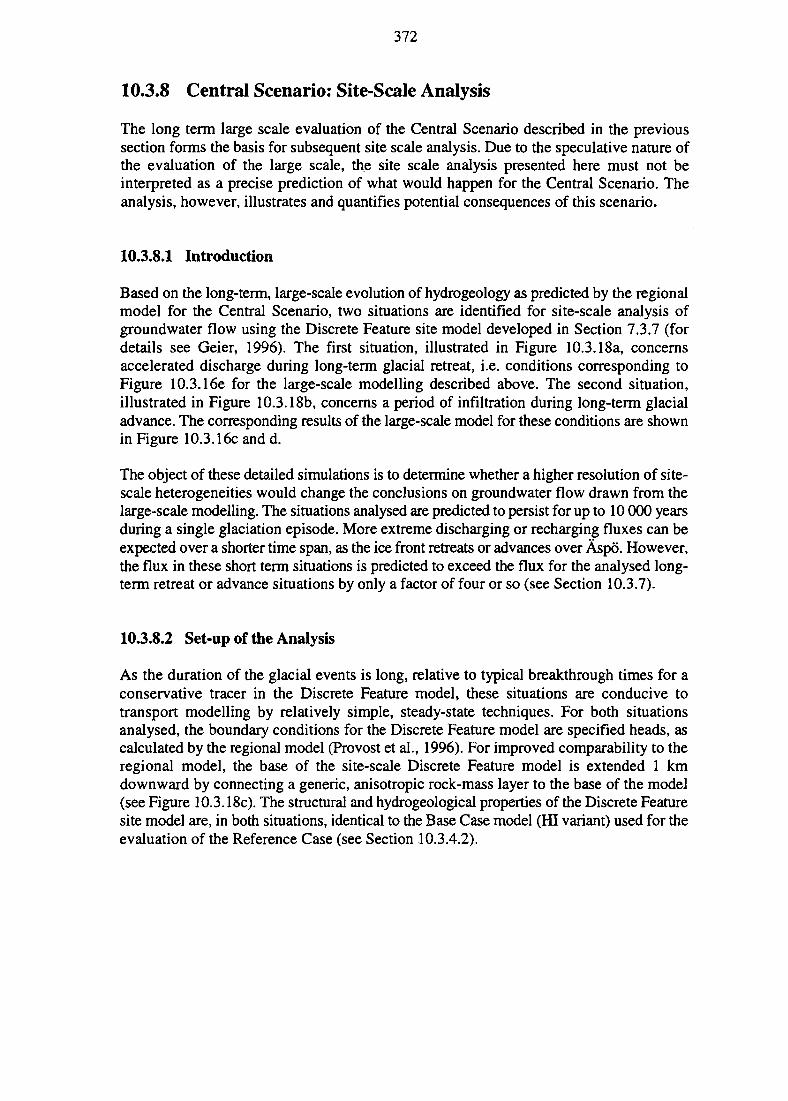
372
10.3.8 Central Scenario: Site-Scale Analysis
The long term large scale evaluation of the Central Scenario described in the previoussection forms the basis for subsequent site scale analysis. Due to the speculative nature ofthe evaluation of the large scale, the site scale analysis presented here must not beinterpreted as a precise prediction of what would happen for the Central Scenario. Theanalysis, however, illustrates and quantifies potential consequences of this scenario.
10.3.8.1 Introduction
Based on the long-term, large-scale evolution of hydrogeology as predicted by the regionalmodel for the Central Scenario, two situations are identified for site-scale analysis ofgroundwater flow using the Discrete Feature site model developed in Section 7.3.7 (fordetails see Geier, 1996). The first situation, illustrated in Figure 10.3.18a, concernsaccelerated discharge during long-term glacial retreat, i.e. conditions corresponding toFigure 10.3.16e for the large-scale modelling described above. The second situation,illustrated in Figure 10.3.18b, concerns a period of infiltration during long-term glacialadvance. The corresponding results of the large-scale model for these conditions are shownin Figure 10.3.16c and d.
The object of these detailed simulations is to determine whether a higher resolution of site-scale heterogeneities would change the conclusions on groundwater flow drawn from thelarge-scale modelling. The situations analysed are predicted to persist for up to 10 000 yearsduring a single glaciation episode. More extreme discharging or recharging fluxes can beexpected over a shorter time span, as the ice front retreats or advances over Aspo. However,the flux in these short term situations is predicted to exceed the flux for the analysed long-term retreat or advance situations by only a factor of four or so (see Section 10.3.7).
10.3.8.2 Set-up of the Analysis
As the duration of the glacial events is long, relative to typical breakthrough times for aconservative tracer in the Discrete Feature model, these situations are conducive totransport modelling by relatively simple, steady-state techniques. For both situationsanalysed, the boundary conditions for the Discrete Feature model are specified heads, ascalculated by the regional model (Provost et al., 1996). For improved comparability to theregional model, the base of the site-scale Discrete Feature model is extended 1 kmdownward by connecting a generic, anisotropic rock-mass layer to the base of the model(see Figure 10.3.18c). The structural and hydrogeological properties of the Discrete Featuresite model are, in both situations, identical to the Base Case model (HI variant) used for theevaluation of the Reference Case (see Section 10.3.4.2).
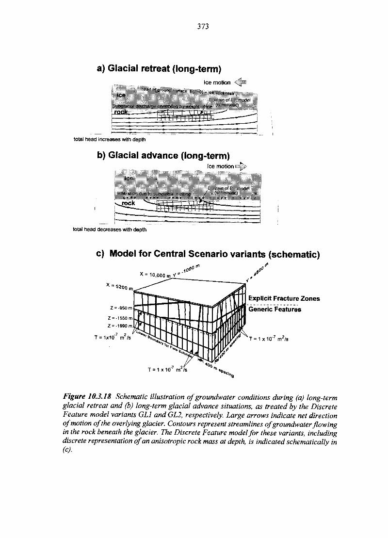
373
a) Glacial retreat (long-term)Ice motion '
total head increases with depth
b) Glacial advance (long-term)Ice motion'
total head decreases with depth
c) Model for Central Scenario variants (schematic)
x = 10,000jooo"
X = 5200
T=1x10"7 m2/s
T = 1 x10"7 m2/s
Explicit Fracture Zones
Generic Features
T= 1x10'7 m2/s
Figure 10.3.18 Schematic illustration of groundwater conditions during (a) long-termglacial retreat and (b) long-term glacial advance situations, as treated by the DiscreteFeature model variants GLl and GL2, respectively. Large arrows indicate net directionof motion of the overlying glacier. Contours represent streamlines of groundwater flowingin the rock beneath the glacier. The Discrete Feature model for these variants, includingdiscrete representation of an anisotropic rock mass at depth, is indicated schematically in(c).
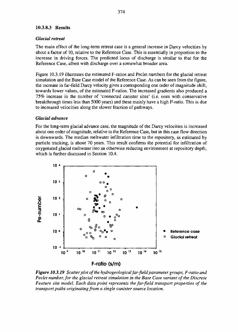
374
10.3.8.3 Results
Glacial retreat
The main effect of the long-term retreat case is a general increase in Darcy velocities byabout a factor of 10, relative to the Reference Case. This is essentially in proportion to theincrease in driving forces. The predicted locus of discharge is similar to that for theReference Case, albeit with discharge over a somewhat broader area.
Figure 10.3.19 illustrates the estimated F-ratios and Peclet numbers for the glacial retreatsimulation and the Base Case model of the Reference Case. As can be seen from the figure,the increase in far-field Darcy velocity gives a corresponding one order of magnitude shift,towards lower values, of the estimated F-ratios. The increased gradients also produced a75% increase in the number of 'connected canister sites' (i.e. ones with conservativebreakthrough times less than 5000 years) and these mainly have a high F-ratio. This is dueto increased velocities along the slower fraction of pathways.
Glacial advance
For the long-term glacial advance case, the magnitude of the Darcy velocities is increasedabout one order of magnitude, relative to the Reference Case, but in this case flow directionis downwards. The median meltwater infiltration time to the repository, as estimated byparticle tracking, is about 70 years. This result confirms the potential for infiltration ofoxygenated glacial meltwater into an otherwise reducing environment at repository depth,which is further discussed in Section 10.4.
t
10 *
10 3
10 2
10
10 -
* Reference case° Glacial retreat
F-ratio (s/m)
Figure 10.3.19 Scatter plot of the hydrogeological far-field parameter groups, F-ratio andPeclet number, for the glacial retreat simulation in the Base Case variant of the DiscreteFeature site model. Each data point represents the far-field transport properties of thetransport paths originating from a single canister source location.
375
10.3.9 Discussion and Overall Conclusions
The hydrogeological evaluation presented in Section 10.3 gives qualitative and quantitativepredictions of groundwater flow and radionuclide transport paths through the repository,both for present-day conditions (the Reference Case) and for evolving climatic conditions(the Central Scenario). Calculations for the Reference Case are performed for scalesranging from regional (1500 km) to detailed (10-20 m). Calculations for the CentralScenario are performed mainly on the regional scale, with a few site-scale calculations toevaluate the effects of specific hydrogeological situations that are predicted to arise. Theresults of these calculations are summarised below, followed by a discussion of differenttypes of uncertainty in the hydrogeological evaluations.
10.3.9.1 Main Results for Reference Case
Regional hydrogeology
The general character of the flow system (average flow direction and magnitude of fluxes)at Aspo is reasonably well understood from the regional groundwater flow modellingpresented in Section 7.3.3. Aspo is situated in an area of natural discharge from thesouthern Swedish highlands with a generally upward and eastward flow direction. Theregional flow simulations indicate that the major discharge area for deep groundwaters isat the coast, and consequently deep shield brines should occur near the surface at Aspo.Further inland, shield brine should be found only at greater depths. This is exactly thepattern found in the field data.
The local flow distribution is affected by local heterogeneity, including small-scalefractures and major fracture zones and, at shallow depths, also by local topographicaldriving forces. The detailed flow field beneath Aspo is therefore complex, with significantlocal variations in both flow direction and flow magnitude. However, both the regionalmodel and the more detailed models (including the semi-regional 2D continuum model andthe Discrete Feature hydrogeological site model), which incorporate local heterogeneity,predict a generally upward direction of flow, with discharge of deep waters to southernAspo or the strait southeast of Aspo. The pattern of discharge is not very sensitive to thefar-field boundary conditions that are tested for the Reference Case.
Site-scale hydrogeology
Both the qualitative hydrogeological assessment of site data (Section 7.3.6) and the SimpleEvaluation of groundwater flow (Section 10.3.3) indicate that the Aspo site is highlyheterogeneous, and that geological structures such as fracture zones and single fractures aremajor controls on groundwater flow. By representing the heterogeneity of the site explicitlyin the detailed hydrogeological site models, i.e. the Discrete Feature and StochasticContinuum models, quantitative estimates of hydrogeological transport parameters and theirspatial variability are obtained, as described in Sections 10.3.4 and 10.3.5.
Although the parameter and conceptual uncertainties associated with the detailed sitemodels are large (see below), both models consistently predict a high spatial variability ofthe hydrogeological transport parameters for the far-field rock. This variability should beviewed as an intrinsic property of the site, rather than an expression of uncertainty in site
376
characterisation. The parameterisation of the model results in terms of the far-fieldperformance measures, F-ratio and Peclet number, give a direct indication that thisvariability is critical for the overall far-field performance. The estimated F-ratio, which isa measure of the capacity for retardation of migrating radionuclides in the rock, in manycases, can vary by several orders of magnitude depending on the release point in therepository area.
10.3.9.2 Impact of Climate Evolution—Results for Central Scenario
The main hydrogeological effects of the variations in surface conditions, which arepredicted to occur during the Central Scenario, comprise changes in discharge area location,alteration of flow directions and moderate changes of flow magnitude.
Effects of climate evolution on discharge area
Under present-day conditions, Aspo is interpreted as being a discharge area for regionalgroundwater flow. Permafrost and the onset of cold-based glaciers could locally orextensively block groundwater discharge, leading to longer transport paths for radionuclidesfrom the repository. With the advance of warm-based glacial ice, meltwaters formed at thebase of the glacier will infiltrate due to increasing pressure buildup below the ice, and thedischarge area will advance with the glacial front. However, when recharge rates arecontrolled by the basal pressure due to ice thickness, the onset of glacial retreat willproduce a switch to discharge conditions, due to the release of groundwater that will havebeen stored in the rock under previous, higher basal pressures.
Effects of climate evolution on magnitude and direction of flow
During periods of permafrost or in the event of a cold-based glacial ice covering Aspo, theflow directions may change to produce longer transport paths in the geosphere, but themagnitude of flow rates is of the same order as in the Reference Case. The highestgroundwater flow rates occur as recharge or discharge at the ice-margin, during periods ofglacial advance and regression, and below melting ice. These high flow rates, which maypersist over several thousands of years, are about one order of magnitude greater than theflow rates in the Reference Case. In the event of a warm-based glacier covering Aspo, thereis a potential for meltwater recharge that may penetrate to a depth of several kilometres.The time for these meltwaters to infiltrate to the repository may be as little as 70 years,which implies a potential for oxygenated waters reaching the otherwise reducingenvironment in the repository.
More extreme groundwater flow rates could be envisaged as occurring during short timeperiods, at the ice margin, as a result of a combination of several extreme situations. Forexample, a high-elevation, ice-dammed lake at the ice margin could discharge largequantities of fluid via a fracture zone (with scouring) that has recently been madetransmissive due to local unloading, and which in turn connects directly through theS1TE-94 repository to a discharge area. The likelihood that all of these extreme situationswould occur simultaneously, and at Aspo, is judged to be extremely small.
377
10.3.9.3 Treatment of System Uncertainty in the Hydrogeological Evaluation
The hydrogeological analyses considered most of the FEPs and influences that areidentified in the system description, i.e. in the Process Influence Diagram (PJD) as shownin Figures 7.1.1 and 7.1.2. Uncertainty in the PID itself is discussed in Chapter 2. Thefollowing is a discussion of the consistency between the hydrogeological analyses and thePID, i.e. of how well relevant FEPs and influences are treated in the hydrogeologicalevaluation.
The main FEPs analysed within the hydrogeological evaluation are Groundwater Flow Far-Field Rock (GWFF) and Groundwater Flow Near-Field Rock (GWNF). Most of theinfluences to these EEPs are addressed in the above analysis, although the thoroughness oftreatment varies among these influences.
Coupling between GWFF and GWNF (Influence GE65) is accounted for implicitly by thedetailed site-scale models. Effects of the FEP External flow boundary conditions (InfluenceGE93) on GWFF are evaluated in various ways using the regional hydrogeological model,the Simple Evaluation of groundwater flow and the detailed site-scale models (ClearingHouse Hydrogeology in the AMF).
Effects of the FEPs Properties of far-field rock and Properties of near-field rock on GWFFand GWNF (Influences GE46, NE50 and NE51) are evaluated in the derivation of thedetailed site models (Discrete Feature and Stochastic Continuum). However, coupledeffects stemming from possible influence of GWNF on the rock properties (InfluenceNE117) are not considered explicitly, as discussed below.
Effects of GWFF and GWNF on far-field and near-field radionuclide transport processes(dispersion, matrix diffusion, etc.) are explicitly considered, by estimating parameters forthe consequence-calculation models, CRYSTAL and CALIBRE (Clearing HouseHydrogeological parameters to RN-transport in the AMF).
FEPs and influences that are not fully evaluated
Potentially important influences that are identified in the PID, but are insufficientlyevaluated, or simply not evaluated, are mostly related to coupled Thermo-Hydro-Mechanical (T-H-M) or Thermo-Hydro-Mechanical-Chemical (T-H-M-C) processes. Atpresent there is a lack of models and data for evaluating many of the above coupledphenomena in a quantitative fashion. However, intensive, ongoing research in the field ofT-H-M processes (for example Jing et al., 1996) will probably yield a better basis foranalyses in future Performance Assessments.
The effects of a Disturbed-Rock Zone (DRZ) around tunnels and shafts, due to excavationdamage and mechanical stress concentrations, are evaluated in a simplified manner with theDiscrete Feature hydrogeological site model. However, some potentially important T-H-Mcouplings in the near-field rock are not considered in the hydrogeological site models (e.g.,the combined effects on the stress field of heat from the spent fuel and swelling pressurein the bentonite, which could in turn affect the transmissivity of existing fractures). Theeffect on the FEP GWNF of thermal buoyancy, due to heating of groundwater by heat from

378
the spent fuel, is not evaluated in SITE-94. However, previous analyses (see e.g. SKI, 1991)have indicated that the impact will be small.
The hydrogeological model for the Central Scenario accounts explicitly for a number ofFEPs and influences, including the effects of permafrost, formation of shield brine,variations in density and viscosity due to temperature, pressure and concentration gradientsand time-varying hydrological boundary conditions. The Central Scenario also implies asignificant mechanical load, due to the overburden of glacial ice, which could potentiallyaffect fracture apertures and the flow and transport properties of major fracture zones in thefar-field. The variations of permeability anisotropy in the Central Scenario hydrogeologicalmodel provide some indication of the potential impacts of such effects. However, a betterhydrogeological evaluation is needed regarding the combined effects of extreme hydraulicgradients and enhanced transmissivity of large-scale fractures, particularly in conjunctionwith recharge of oxygenated glacial meltwater, since these factors could reasonably beexpected to coincide in the Central Scenario.
Other links in the PID that are not evaluated in SITE-94 include Influence GE74 (effectsof GWFF on colloid generation and transport) and Influences GE86 and GE87 (effects ofEarth Tides on far-field groundwater flow and matrix diffusion). The entire sets of FEPsand influences relating to resaturation of near-field rock, backfill and bentonite buffer, andrelating to gas generation, gas flow and transport are also not evaluated.
Couplings between chemical and hydrogeological processes are not adequately evaluatedin SITE-94. Of particular interest are the effects of dissolution and precipitation of fracturefilling minerals on the hydraulic and transport properties in fractures and fracture zones.These processes are affected both by the natural, long-term evolution of groundwaterchemistry at the site and by the geochemical disturbance that occurs with the constructionof an underground repository, which may significantly affect the near-field rock propertiesat early times after closure. The potential impact of altered fracture mineralogy ongroundwater flow needs to be better understood, although it may be expected that the mainimpact is on the potential for chemical retardation of reactive radionuclide transport.
10.3.9.4 Scenario Uncertainty
Site hydrogeology is evaluated primarily for the Reference Case and for the CentralScenario, as specified in Chapter 9. Within the hydrogeological evaluations for theReference Case, the main emphasis is on quantifying the impact of rock heterogeneity ongroundwater flow and transport, whereas, for the Central Scenario, the main focus is onevaluating the impact of evolving hydrological boundary conditions.
Scenario completeness
The supplementary scenarios for SITE-94, as listed in Table 9.4.2, are mostly not used asthe basis for detailed hydrogeological evaluations; an exception is the supplementaryscenario Deficient Shaft Seal, which is evaluated as a variant of the Discrete Featurehydrogeological site model.
379
Uncertainty in scenario specification
Uncertainty in the specification of the Central Scenario is evaluated by means of multiplevariants in the regional hydrogeological model for the Central Scenario, includingalternative specifications of permafrost conditions (presence or absence of taliks), sub-icemelting rates, and regional system boundaries (the effects of a sedimentary sequenceoverlying the shield rocks east of Aspo).
Uncertainty in scenario implementation
Major physical processes that are taken into account quantitatively by the regionalhydrogeological model for the Central Scenario include density-dependent groundwaterflow coupled with diffusion, shield-brine generation, and hydraulic conditions induced atthe ground surface by the advance and regression of continental glaciers. Somesimplifications have been made in adapting the Central Scenario specifications to themodel, but the effects of the major events in the Central Scenario have been evaluatedquantitatively. Extreme effects (e.g. local conditions at ice margins) have been discussedqualitatively.
10.3.9.5 Conceptual Model and Parameter Uncertainty
Conceptual and parameter uncertainties have been evaluated through multipleinterpretations of the hydrogeological site data, i.e. a suite of alternative conceptualhydrogeological site models, each consistent with the available site data. With eachconceptual model, multiple variants have been used to evaluate conceptual and parameteruncertainty specific to the model.
Ranking of evaluated uncertainties for Reference Case
The detailed hydrogeological site models predict water residence times, hence mediantravel times from a canister to the biosphere, ranging from a few years to 10 000 years,depending on conceptual model variant and position of the source canister. Uncertaintyrelated to the water residence time primarily affects the travel time of non-sorbing orweakly sorbing radionuclides. However, the overall impact on the far-field barrier functionis not that critical because the dominating non-sorbing nuclide, 129I, has a very long half-lifecompared with these groundwater residence times. Hence, potential releases of 129I from thenear-field will be delayed in the geosphere, but will not have time to decay before theyreach the biosphere. The following ranking of uncertainties is therefore based primarily ontheir impact on the F-ratio, which is a better measure of the capacity of the far-field forreducing radioactive releases to the biosphere.
The most significant conceptual uncertainties, as evaluated by the Discrete Feature model,concern the spatial distributions of flow wetted surface area and transmissivity withintransmissive features, both of which strongly affect the retardation potential for aradionuclide travelling through the far-field hydrogeological system. Conceptual andparametric uncertainties of secondary importance include those pertaining to the effectivesemi-regional boundary conditions for the model and those pertaining to the geologicalstructure model (i.e. uncertainties in the interpretation of the number of fracture zones and
380
their exact position and orientation). These uncertainties affect non-reactive transportproperties, but are of lesser importance for the predicted F-ratios.
The main impact of the detailed-scale fracture network, representing the rock in the near-repository environment, is to control the percentage of canister sites that are hydraulicallyconnected to a site-scale structure. Otherwise the distribution of far-field transportproperties for connective sites is not strongly affected by the properties of the detailed-scalefracture network, within the evaluated ranges of parametric uncertainty.
The most critical uncertainty, as evaluated with the Stochastic Continuum site model,concerns assumptions regarding the distribution and spatial correlation of the hydraulicconductivity. This uncertainty affects the predicted distributions of far-field Darcy velocityand thereby the F-ratios. However, the main uncertainty associated with the predictedF-ratios is associated with the specific surface area, which is not estimated with this model.
The issue of connectivity is discussed in Section 11.2.2.4.
Comparison between the Simple Evaluation and the detailed site models
One purpose of the Simple Evaluation is to assess the reasonableness of the results fromthe detailed, 3D hydrogeological site models. The following comparisons among modelsare based on the near-field Darcy velocity and the far-field F-ratio.
Figure 10.3.20 illustrates the ranges of predicted near-field Darcy velocities for the SimpleEvaluation and three variants each of the Stochastic Continuum site model (SC) and theDiscrete Feature site model (DF). The figure includes the Base Case and the variants thatgive the lowest and the highest median Darcy velocity for the respective site model. Therange of Darcy velocities for the Simple Evaluation corresponds to the results inTable 10.3.1. For the detailed site models, the ranges of Darcy velocity correspond to the10th percentile, the median and the 90th percentile of the estimated velocity distribution.Note that for the DF model the velocity distributions are based only on a fraction of thecanister sites, i.e. the 33% flowing canister sites.
Disregarding the two highest Darcy velocities of the Simple Evaluation, which representa highly pessimistic case with a direct connection between the repository and the biospherevia the most conductive fracture zone (NE-1, according to SKB nomenclature), thecombined uncertainty range predicted by the two detailed site models (approximately10"6 m/year to 10"2 m/year) covers essentially the whole uncertainty range predicted in theSimple Evaluation (Figure 10.3.20). In this respect, the more comprehensive use of site datain the detailed 3D hydrogeological site models does not reduce the prediction uncertaintyfor near-field Darcy velocity, but merely confirms the results of the simple scopingcalculations.
However, the detailed site models provide additional information on the spatial variabilityof the Darcy velocity in terms of probability distributions. The Discrete Feature site modelalso provides estimates of connectivity, i.e. the number of canisters that are hydraulicallyconnected to flow. Such information is essential for evaluating the performance of a fullrepository. The detailed site models also provide information on parameter correlations,which are not given directly by the simple scoping calculations.
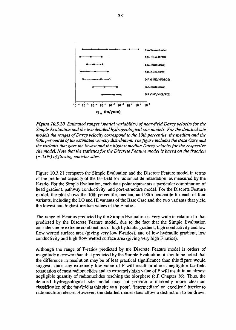
381
Simple evaluation
• • 9 S.C. (NEW-DIP80)
• *—« s.C. (base case)
• • • S.C. ONG-DIP80)
a •• — E3——D D.F. (SKN0/NF0/BC0)
B- a - a D.F. (base case)
Q B~—-a D.F. (SKW/NFOB/BCO)
1 0 •* i o s i o •* i o - 3 i o 2 i o ' i o ° i o ' i o 2
q nf (m/year)
Figure 10.3.20 Estimated ranges (spatial variability) of near-field Darcy velocity for theSimple Evaluation and the two detailed hydro geological site models. For the detailed sitemodels the ranges of Darcy velocity correspond to the 10th percentile, the median and the90th percentile of the estimated velocity distribution. The figure includes the Base Case andthe variants that gave the lowest and the highest median Darcy velocity for the respectivesite model. Note that the statistics for the Discrete Feature model is based on the fraction(~ 33%) of flowing canister sites.
Figure 10.3.21 compares the Simple Evaluation and the Discrete Feature model in termsof the predicted capacity of the far-field for radionuclide retardation, as measured by theF-ratio. For the Simple Evaluation, each data point represents a particular combination ofhead gradient, pathway conductivity, and pore-structure model. For the Discrete Featuremodel, the plot shows the 10th percentile, median, and 90th percentile for each of fourvariants, including the LO and HI variants of the Base Case and the two variants that yieldthe lowest and highest median values of the F-ratio.
The range of F-ratios predicted by the Simple Evaluation is very wide in relation to thatpredicted by the Discrete Feature model, due to the fact that the Simple Evaluationconsiders more extreme combinations of high hydraulic gradient, high conductivity and lowflow wetted surface area (giving very low F-ratios), and of low hydraulic gradient, lowconductivity and high flow wetted surface area (giving very high F-ratios).
Although the range of F-ratios predicted by the Discrete Feature model is orders ofmagnitude narrower than that predicted by the Simple Evaluation, it should be noted thatthe difference in resolution may be of less practical significance than this figure wouldsuggest, since any extremely low value of F will result in almost negligible far-fieldretardation of most radionuclides and an extremely high value of F will result in an almostnegligible quantity of radionuclides reaching the biosphere (c.f. Chapter 16). Thus, thedetailed hydrogeological site model may not provide a markedly more clear-cutclassification of the far-field at this site as a 'poor', 'intermediate' or 'excellent' barrier toradionuclide release. However, the detailed model does allow a distinction to be drawn
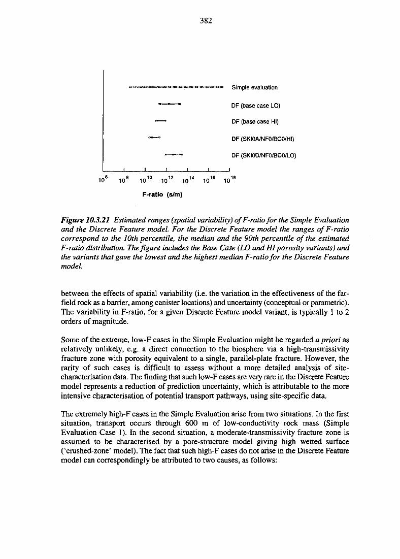
382
Simple evaluation
DF (base case LO)
DF (base case HI)
DF (SKIOA/NFO/BCO/HI)
DF (SKI0D/NF0/BC0/LO)
106 108 i o 1 0 1012 1014 i o 1 6 i o 1 8
F-ratio (s/m)
Figure 10.3.21 Estimated ranges (spatial variability) of F-ratio for the Simple Evaluationand the Discrete Feature model. For the Discrete Feature model the ranges of F-ratiocorrespond to the 10th percentile, the median and the 90th percentile of the estimatedF-ratio distribution. The figure includes the Base Case (LO and HI porosity variants) andthe variants that gave the lowest and the highest median F-ratio for the Discrete Featuremodel.
between the effects of spatial variability (i.e. the variation in the effectiveness of the far-field rock as a barrier, among canister locations) and uncertainty (conceptual or parametric).The variability in F-ratio, for a given Discrete Feature model variant, is typically 1 to 2orders of magnitude.
Some of the extreme, low-F cases in the Simple Evaluation might be regarded a priori asrelatively unlikely, e.g. a direct connection to the biosphere via a high-transmissivityfracture zone with porosity equivalent to a single, parallel-plate fracture. However, therarity of such cases is difficult to assess without a more detailed analysis of site-characterisation data. The finding that such low-F cases are very rare in the Discrete Featuremodel represents a reduction of prediction uncertainty, which is attributable to the moreintensive characterisation of potential transport pathways, using site-specific data.
The extremely high-F cases in the Simple Evaluation arise from two situations. In the firstsituation, transport occurs through 600 m of low-conductivity rock mass (SimpleEvaluation Case 1). In the second situation, a moderate-transmissivity fracture zone isassumed to be characterised by a pore-structure model giving high wetted surface('crushed-zone' model). The fact that such high-F cases do not arise in the Discrete Featuremodel can correspondingly be attributed to two causes, as follows:
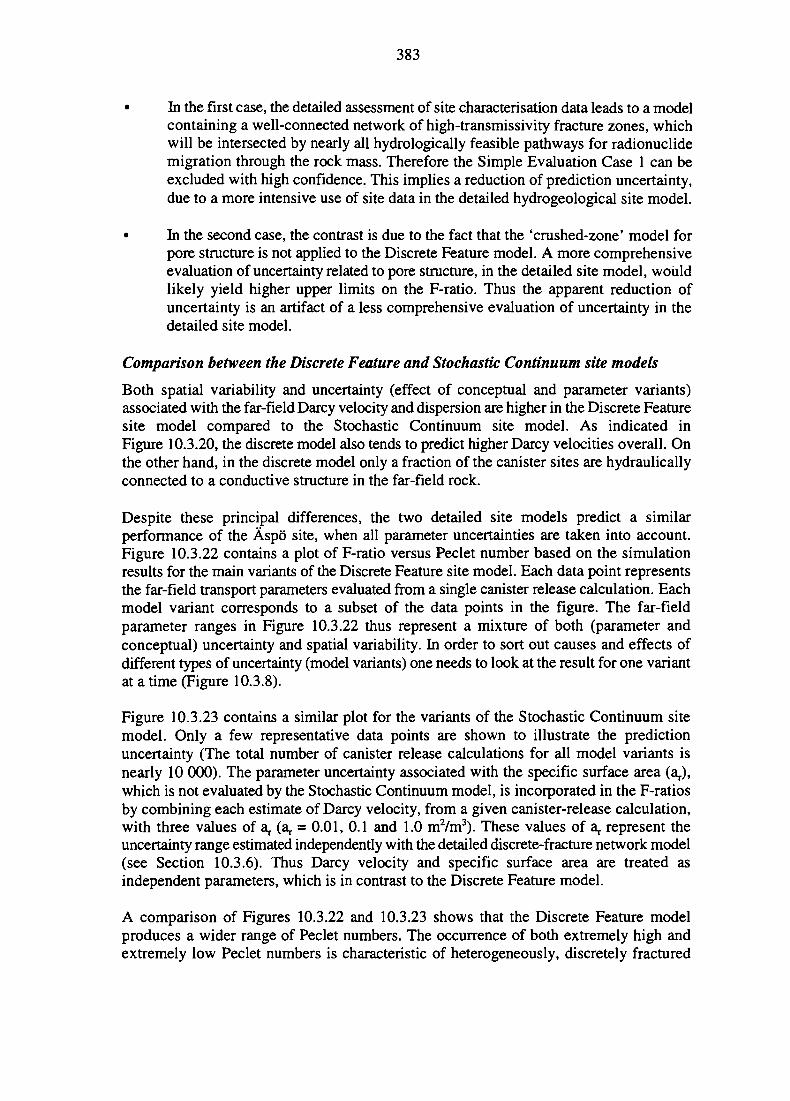
383
• In the first case, the detailed assessment of site characterisation data leads to a modelcontaining a well-connected network of high-transmissivity fracture zones, whichwill be intersected by nearly all hydrologically feasible pathways for radionuclidemigration through the rock mass. Therefore the Simple Evaluation Case 1 can beexcluded with high confidence. This implies a reduction of prediction uncertainty,due to a more intensive use of site data in the detailed hydrogeological site model.
• In the second case, the contrast is due to the fact that the 'crushed-zone' model forpore structure is not applied to the Discrete Feature model. A more comprehensiveevaluation of uncertainty related to pore structure, in the detailed site model, wouldlikely yield higher upper limits on the F-ratio. Thus the apparent reduction ofuncertainty is an artifact of a less comprehensive evaluation of uncertainty in thedetailed site model.
Comparison between the Discrete Feature and Stochastic Continuum site models
Both spatial variability and uncertainty (effect of conceptual and parameter variants)associated with the far-field Darcy velocity and dispersion are higher in the Discrete Featuresite model compared to the Stochastic Continuum site model. As indicated inFigure 10.3.20, the discrete model also tends to predict higher Darcy velocities overall. Onthe other hand, in the discrete model only a fraction of the canister sites are hydraulicallyconnected to a conductive structure in the far-field rock.
Despite these principal differences, the two detailed site models predict a similarperformance of the Aspo site, when all parameter uncertainties are taken into account.Figure 10.3.22 contains a plot of F-ratio versus Peclet number based on the simulationresults for the main variants of the Discrete Feature site model. Each data point representsthe far-field transport parameters evaluated from a single canister release calculation. Eachmodel variant corresponds to a subset of the data points in the figure. The far-fieldparameter ranges in Figure 10.3.22 thus represent a mixture of both (parameter andconceptual) uncertainty and spatial variability. In order to sort out causes and effects ofdifferent types of uncertainty (model variants) one needs to look at the result for one variantat a time (Figure 10.3.8).
Figure 10.3.23 contains a similar plot for the variants of the Stochastic Continuum sitemodel. Only a few representative data points are shown to illustrate the predictionuncertainty (The total number of canister release calculations for all model variants isnearly 10 000). The parameter uncertainty associated with the specific surface area (a,.),which is not evaluated by the Stochastic Continuum model, is incorporated in the F-ratiosby combining each estimate of Darcy velocity, from a given canister-release calculation,with three values of a,, (a,, - 0.01, 0.1 and 1.0 mVm3). These values of a,, represent theuncertainty range estimated independently with the detailed discrete-fracture network model(see Section 10.3.6). Thus Darcy velocity and specific surface area are treated asindependent parameters, which is in contrast to the Discrete Feature model.
A comparison of Figures 10.3.22 and 10.3.23 shows that the Discrete Feature modelproduces a wider range of Peclet numbers. The occurrence of both extremely high andextremely low Peclet numbers is characteristic of heterogeneously, discretely fractured
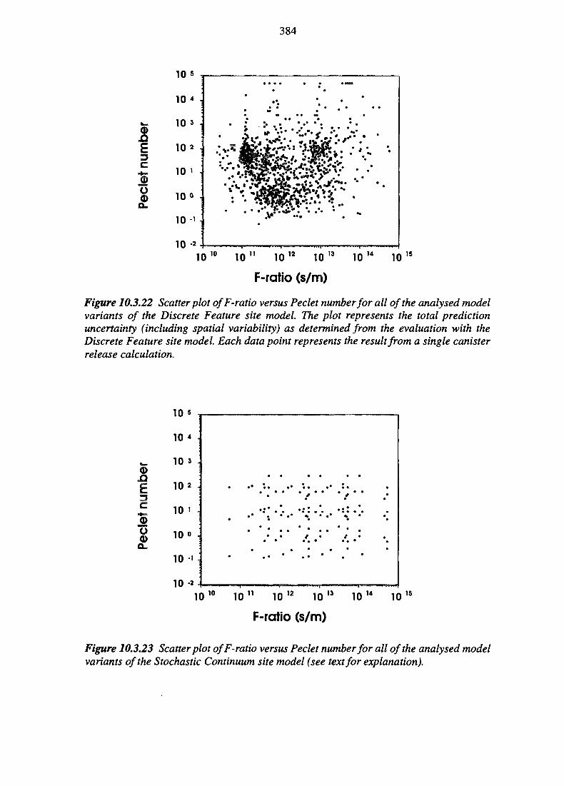
384
3C
2o
10 5
10
F-ratio (s/m)
Figure 10.3.22 Scatter plot ofF-ratio versus Peclet number for all of the analysed modelvariants of the Discrete Feature site model. The plot represents the total predictionuncertainty (including spatial variability) as determined from the evaluation with theDiscrete Feature site model. Each data point represents the result from a single canisterrelease calculation.
10 5
£C
£
10
10
10
10
10
10
10
4 ,
3 .
2 ,
1 .
0 .
-1 .
10 i i1 0 " 10 12 10 13
F-ratio (s/m)10
1410 1 5
Figure 10.3.23 Scatter plot ofF-ratio versus Peclet number for all of the analysed modelvariants of the Stochastic Continuum site model (see text for explanation).

385
systems in which large variations of velocities and limited mixing between flow paths mayoccur (e.g. Dverstorp et al., 1992). The Stochastic Continuum model predicts a narrowerrange of Peclet numbers which is consistent with the concept that a continuum model ingeneral induces more mixing than a discrete model. The Discrete Feature site model alsopredicted a lower bound for the F-ratio, indicating the occurrence of pathways with lesscapacity for retardation of radionuclide transport in the geosphere. However, the overallimpression from these plots is a striking similarity in the predicted uncertainty ranges of thefar-field performance.
Water residence times
The Discrete Feature site model variants predict water residence times, hence median traveltimes from a canister to the biosphere, between 1 and 1500 years (10th and 90th percentilesrespectively). The corresponding range of water residence times predicted by the StochasticContinuum model variants is 100 to 10 000 years (assuming a constant porosity of 5X10"4).Because the residence times for the Discrete Feature site model only represent a subset ofcanister release points that had sufficiently high fluid velocity to allow particle tracking, theupper limits are not directly comparable.
10.3.9.6 Simplification Errors
A potentially important uncertainty, which is not addressed in SITE-94, is related to thesimplifications involved in the abstraction of effective far-field transport parameters fromthe detailed three-dimensional hydrogeology models. For example, the occurrence of bothextremely high and low Peclet numbers may be taken as indications that transport throughthe three-dimensional, heterogeneous, Discrete Feature model is poorly approximated bya one-dimensional, homogeneous advection-dispersion model. Very low values of thePeclet number (less than unity) can result from fitting solutions of the ID advective-dispersive transport equation to particle tracking data for multiple, distinct flow paths withstrongly contrasting velocities. Very high values of the Peclet number (greater than 100),corresponding to essentially plug flow in the ID transport equation, can occur due to acombination of poor fits and an under-representation of small-scale dispersion in the far-field model. The transport distance dependence of the estimated dispersivities in theStochastic Continuum site model is another indication of a discrepancy between thedetailed site models and the simple one-dimensional transport equation adopted for the far-field radionuclide transport calculations.
The estimated values of the F-ratio represent averages of the spatially varying Darcyvelocities and flow-wetted surface areas along the transport paths from a canister to thebiosphere. If the local variability of Darcy velocity and flow-wetted surface area along thetransport paths is high, the use of constant parameter values for calculating reactiveradionuclide transport could be questioned. The potential errors associated with thissimplification are difficult to predict, as reactive radionuclide transport is a non-linearfunction of Darcy velocity and flow-wetted surface area.
386
10.3.9.7 Implications for Other Parts of the Assessment
The direct impact of the hydrogeological evaluation on other parts of the assessment isindicated schematically in the Assessment Model Flowchart (AMF), Figure 2.4.5. Allevaluations described in this Chapter provide data to the Clearing House Hydrogeologicalparameters to RN transport. One of the main functions of this Clearing House is to analysethe modelling results and formulate hydrogeological parameter variants for the radionuclidetransport calculations (as indicated by the arrows to the Clearing Houses Near-field RNTransport and Far-field RN Transport). This is described in Chapter 15.
The AMF also indicates additional deliveries of information to the Clearing HousesGeochemistry, Geochemical parameters to RN-transport and Canister analysis. Thecalculated infiltration rate of oxygenated groundwater during the Central Scenario is anexample of data that are delivered to the geochemistry Clearing Houses (Section 10.4).
10.3.9.8 Implications for Future Work
Several lessons pertinent to future Performance Assessments can be drawn from thehydrogeological evaluations for SITE-94, in particular regarding:
1. the assessment of spatial variability versus other sources of uncertainty,2. the need for further development of hydrogeological models,3. data requirements for future site characterisation,4. methods for discriminating among alternative models and,5. treatment of simplification errors.
Spatial variability and uncertainty
The parameterisation of the far-field in terms of F-ratio and Peclet number is a promisingapproach for describing uncertainty and spatial variability. For the Aspo site, spatialvariability is found to be high in relation to most other evaluated sources of uncertainty, interms of the hydrogeological parameters for calculations of radionuclide transport. The highspatial variability is predicted despite a repository layout that avoids major fracture zonesinsofar as possible. For sites similar to Aspo, spatial variability between canister sites willbe one of the dominant aspects of the hydrogeological influences on overall performance.
The hydrogeological analysis has not taken into account the possibility of reducingvariability between canister sites by active canister emplacement (i.e., selection or rejectionof canister sites based upon detailed characterisation of the rock around each depositionhole). The predicted existence of effectively unconnected sites (in the Discrete Featuremodel) and a weak, negative correlation between F-ratio and near-field Darcy velocity (seeSection 11.2.2), suggests that such techniques could be effective for the Aspo site. Morework is needed to define methods for active canister emplacement, and for evaluation ofthe consequences in hydrogeological models for Performance Assessment.
387
Development of hydrogeological models
The multiple-interpretations approach is used in the hydrogeological evaluations to interpretdata at different stages, from the interpretation of hydraulic packer test data to thedevelopment of 3D, detailed site models. This approach is found to be an effective meansof quantifying the relative importance of different types of parameter and conceptual modeluncertainties, particularly those uncertainties that cannot be evaluated with a particularmodel.
The different types of hydrogeological models that have been used can be viewed ascomplementary, both in that they represent a variety of conceptual assumptions, and in thatthey utilise different subsets of the available data. The latter is important because neitherof the detailed site models used for quantitative predictions (Discrete Feature or StochasticContinuum) is able to utilise all of the available data. The Discrete Feature model is ableto assimilate more structural geological data in comparison with the Stochastic Continuummodel. On the other hand, the Stochastic Continuum model made more intensive use ofhydraulic measurements in boreholes, through conditional simulations.
The most comprehensive use of site-characterisation data is in the integrated interpretationof hydrogeological and other site data, using 3D-visualisation techniques. This has provedto be a valuable technique for building a qualitative understanding of site hydrogeology andfor assessing the significance of different data types. Although such integrated analyses areresource-intensive, they provide essential information for selection and validation ofquantitative groundwater flow models. Partly due to constraints on resources, and partly dueto the fact that the techniques for integrated interpretation are developed in the course ofSITE-94, the findings from the integrated interpretation are not fully utilised for theabstraction of quantitative site models.
In future Performance Assessments, integrated interpretations should be performed at anearlier stage, so that the results can be applied to the development of and discriminationamong alternative detailed, quantitative hydrogeology models. Further development of thedetailed, quantitative models is desirable to improve data utilisation, especially with regardto geochemistry. Links between these models and other types of models should also bedeveloped, in order to account for potentially important coupling effects (e.g. thermal-hydrogeological-mechanical-chemical couplings) as discussed in Section 10.3.9.3.
Data needs
From the discussion throughout this section it is also clear that the hydrogeologicalevaluation provided feedback for site characterisation, regarding the need for specific typesof data and the relative importance of different hydrogeological parameters. The dominantsources of uncertainty in the hydrogeological evaluation are mainly related to the spatialdistribution and interrelationships of hydrogeological and transport properties. In theStochastic Continuum model, these uncertainties are expressed in terms of the spatialcorrelation of hydraulic conductivity and assumptions regarding its relationship to porosityand wetted surface. In the Discrete Feature model, the same uncertainties are expressed interms of models for heterogeneity of, and correlations among hydrogeological and transportproperties, within major fracture zones and individual fractures.
388
Tracer tests on a range of scales could provide useful data for addressing theseuncertainties. Limitations on the characterisation of detailed flow geometries within suchexperiments will, in general, lead to residual uncertainty in the estimated relationshipsamong hydraulic conductivity, porosity, and wetted surface. These uncertainties canperhaps be addressed through expert judgement and further data analysis, in combinationwith data from detailed characterisation studies of single, transmissive features.
Model discrimination
To some extent, the importance of conceptual uncertainty as evaluated by the multiple-interpretations may be exaggerated, due to inadequate discrimination among alternativeconceptual models, model variants, and stochastic realisations. For example, the individualvariants of the Discrete Feature model are not recalibrated or systematically checked forconsistency with the site-characterisation database, except for the Base Case variants. Theevaluated uncertainty would most likely be reduced if all realisations of all variants areconditioned on borehole measurements and recalibrated with respect to cross-hole(hydraulic interference and tracer) data. Similarly, the evaluated uncertainty in theStochastic Continuum model and variants could likely be reduced by a more comprehensivecalibration with respect to cross-hole data. Methods such as co-simulation could also beused for incorporating the type of correlations between hydraulic conductivity and othervariables such as fracture density and lithology that are found in the multivariate analysis(Le Loc'h and Osland, 1996).
Further development of the respective modelling methodologies is needed to produce a setof model variants that more accurately reflect the true, residual uncertainty at the site. Apartfrom conditioning and calibrating with respect to hydraulic and tracer test data, techniquesshould be developed to discriminate among alternative models on the basis of geochemicaldata.
Simplification errors
Errors arising from the use of simplified models for analysis of site characterisation data,and in extraction of effective parameters from heterogeneous, 3D hydrogeological modelsto homogeneous transport models of lesser dimension, should be explored more thoroughlythan is possible in SlTB-94. Where the effects of such simplifications on overallPerformance Assessment cannot be established as negligible, more sophisticated modelsmight be needed. For example, radionuclide transport models capable of handling spatialvariability of hydrogeological properties along streamlines, and/or network effects, mayneed to be developed.
10.4 GEOCHEMISTRY
The purpose of Section 10.4 is to extract, from the geochemical site evaluation presentedin Section 7.4, those parameters and other information which are relevant for thesubsequent analysis of chemical features and processes in a Performance Assessmentgenerally described by the AMF. This section therefore discusses and motivates thedifferent groundwater composition variants that will be used later on in the assessment. Inparticular, this section deals with the geochemical properties of the far-field, i.e. thosevolumes of rock which will be relatively undisturbed by the excavation and the presence

389
of the repository. This disturbance may be extensive, however, and will differ in scale andextent depending on the phenomenon in question and with time. It is, therefore, useful toconsider the far-field as those parts of the site, where, apart from early transient effects, anassumption of natural conditions in the long-term is justified. Nevertheless, much of thisdiscussion of geochemistry will also be relevant for the near-field rock, discussed in moredetail in Chapter 11, since the near-field geochemistry is always influenced directly by thefar-field chemistry by groundwater transport and since most changes in chemistry in thenear-field rock can be regarded as perturbations from undisturbed far-field conditions in theabsence of a repository.
10.4.1 Introduction
The task is to define ranges of geochemical conditions of importance, directly or indirectly,for an assessment of barrier stability and the prediction of radionuclide behaviour in the far-field or, indirectly, of their behaviour in the near-field. This has to be done for theReference Case and for those external conditions or scenarios identified in the scenariodevelopment (see Chapter 9).
No significant changes in the far-field bulk rock mineralogy are expected over the nextmillions of years, as evidenced by the fact that no such changes have occurred in the pastover much longer times. This is not the case for fracture-coating mineralogy at depth, wheresome redistribution of easily dissolved minerals like calcite may occur. There is also thepossibility of oxidation of fracture surfaces, even at depth, due to ingress of oxidisingsurface waters (see Section 10.4.3). However, as a first approximation, it can be assumedthat the chemical conditions of groundwater pathways, including pathways forradionuclides, will be influenced mainly by externally driven changes in groundwatercomposition and temperature. Consequently it will probably be sufficient to concentrate ongroundwater composition. It should be noted, however, that this assumption is a hypothesisneeding further confirmation. This may be achieved by an iterative procedure where resultsfrom the first geochemical and hydrogeological analyses are integrated together with resultsfrom structural geology, etc. Such a procedure is not possible within SITE-94, however,owing to time constraints.
In a full Performance Assessment, the physical properties of the rock would also beanalysed further, in particular, matrix diffusivities and penetration depths and their possiblecorrelation with groundwater chemistry and fracture/bulk rock mineralogy. The scarcity ofconsistent site-specific data of this kind does not allow such an evaluation in SITE-94.
390
10.4.2 Groundwater Properties
Based on the discussion in the preceding section, the following properties of groundwaterare of primary interest:
• redox properties (content of divalent iron, sulphides and other reduced species; Eh;pH),
• concentration of components that may influence copper corrosion (oxygen,sulphide/sulphate, chloride, carbonate),
• contents of pH-buffering components (carbon dioxide/carbonate, calcium),
• constituents aggressive to bentonite, such as potassium, low/high pH, calcium,high/low salinity.
The groundwater composition for the Zero Variant of the Reference Case should berelevant for the major part of the flowpaths into and out from the repository location (i.e.the near-field in a geometrical sense). This variant should reflect conditions prevailing formost of the next million years. Obviously, these requirements are difficult or impossibleto fulfill, not least as a result of the limited knowledge available at the time of data selectionin this project. Instead, data for groundwater at repository depth, near the most probablelocation of a repository, are used. This choice would be relevant for present day (and thenext thousands of years, at least) for the groundwater entering the repository area and forthe near-field rock. Potentially diverging groundwater compositions for the flowpaths fromthe repository area out to the biosphere are difficult to define, owing to lack of knowledgeabout correlations between flow and geochemistry in the system.
However, it is possible to define ranges of compositions encompassing the groundwaterTypes observed today at different depths and locations, as described in Section 7.4.3.Representative groundwaters are selected as representative of conditions relevant to someof the scenarios discussed in Chapter 9 and in Section 10.3. These waters constitutedifferent variants in the assessment.
The reference (Zero Variant) composition is based on a complete chemical characterisationof multiple groundwater samples from the 530-535 m sampling interval in borehole KAS02at the Aspo site (Smellie and Laaksoharju, 1992). A deep, high-salinity groundwater fromLaxemar borehole KLX02 and a shallow, low-salinity groundwater from Laxemar boreholeHLX01 reflect the range in salinities observed at the site. Both the KAS02 and KLX02waters are reducing and alkaline. The shallow groundwater, however, is slightly acidic,relatively oxidising and enriched in dissolved organic carbon. All the water samples arenearly pristine, that is, they contain a very low content of contaminating drilling fluid. (Notethat these waters are not the same as the Type waters identified and discussed inSection 7.4.3).
Thus, the following water is defined for the Zero Variant:
Medium salinity and reducing water are assumed to flow more or less horizontallyin the W-E direction. The composition is based on data from KAS02 (530-535m,
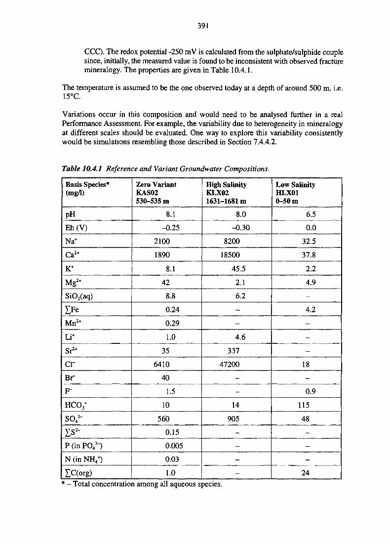
391
CCC). The redox potential -250 mV is calculated from the sulphate/sulphide couplesince, initially, the measured value is found to be inconsistent with observed fracturemineralogy. The properties are given in Table 10.4.1.
The temperature is assumed to be the one observed today at a depth of around 500 m, i.e.15°C.
Variations occur in this composition and would need to be analysed further in a realPerformance Assessment. For example, the variability due to heterogeneity in mineralogyat different scales should be evaluated. One way to explore this variability consistentlywould be simulations resembling those described in Section 7.4.4.2.
Table 10.4.1 Reference and Variant Groundwater Compositions.
Basis Species*(mg/I)
pH
Eh(V)
Na+
Ca2+
K+
Mg2+
SiO2(aq)
EFe
Mn 2 +
Li+
Si2*
ci-
Br"
F
HCO3-
SO42"
Zs2-P (in PO^)
N (in NH4+)
EC(org)
Zero VariantKAS02530-535 m
8.1
-0.25
2100
1890
8.1
42
8.8
0.24
0.29
1.0
35
6410
40
1.5
10
560
0.15
0.005
0.03
1.0
High SalinityKLX021631-1681m
8.0
-0.30
8200
18500
45.5
2.1
6.2
-
-
4.6
337
47200
—
-
14
905
-
-
Low SalinityHLX010-50 m
6.5
0.0
32.5
37.8
2.2
4.9
_
4.2
-
—
-
18
-
0.9
115
48
-
—
24
- Total concentration among all aqueous species.
392
10.4.3 Scenario-related Changes of Groundwater Chemistry
The Central Scenario described in Chapter 9 and Section 10.3 affects the direction ofgroundwater flow and, thus, the groundwater chemistry at the repository location as wellas along flowpaths towards the biosphere. The flow conditions are described in detail inSection 10.3. The flow will be about the same in magnitude and direction for the next55 ka. After that, during advance of the ice-sheet at the site, the flow direction will changeto downwards for about 5000 years, followed by a return to upward flow at 60-70 ka. After70 ka, the flow will be about the same as at present, until the next glaciation at about 95 ka.
For a large part of the next 50 ka, permafrost conditions will prevail at Aspo and impedefree recharge and discharge of groundwater. Below cold-based ice, no recharge or dischargewill occur. Below warm-based melting ice, there is a large potential for greater rechargesthan today as a result of meltwater flowing downwards. When the ice-sheet recedes at thesite, large upward flow may occur. Sub-ice groundwater flow rates will generally be oneorder of magnitude greater than at present.
A major increase in the salinity above present levels, due to the rise of deep brines at thereceding ice margin, is not deemed likely in this analysis (Section 10.3.7.4). If such achange is ever to occur, however, it is reasonable to assume that it will occur at about thistime. Glacial meltwater may penetrate to depths of a few kilometres during glacial advance,possibly causing oxidising conditions.
A timetable for illustration of possible geochemical changes at Aspo would then be:
10-55 ka: Several occurrences of permafrost conditions; salinity decreased toabout half of present day values; possibly a high organic content; 0°Cas an extreme variation in temperature.
55-60 ka: Advance of ice-sheet, eventually sub-ice melting and recharge ofmeltwater to great depths; low salinity water with properties similar tothose of present near-surface waters; oxidising conditions are possible.
70-95 ka: Although not very likely, this would be the time for ingress ofgroundwater at repository depth with a (much) higher salinity than atpresent.
This leads to the definition of the following groundwaters for application in analysis of theCentral Scenario:
High salinity and reducing water from the deep sections of KLX02. Thisgroundwater composition would only be possible under more or less upward flowconditions, e.g. some time during 70-95 ka after repository closure. The propertiesare given in Table 10.4.1.
Low salinity, weakly oxidising and high TOC water. More or less downward flow.The properties are given in Table 10.4.1.
393
Waters representing highly oxidising conditions, as more extreme variations, were assumedfor some calculations, as described in Chapter 12.
The somewhat lower salinity that might occur at 10-55 ka is encompassed by the othervariations in this parameter. Only the effect of oxidising conditions is analysed further inSITE-94, e.g. in the analysis of near-field chemistry (Section 12.2.3) and in the choice ofsorption coefficients.
The possibilities for oxidising groundwater to penetrate down to repository depth (see alsoSections 7.4.3 and 10.3.7.4) are analysed by Arthur (1996). Flow properties of individualfracture zones have to be used in this approach. In the major conductive zones the Darcyvelocities may be in the order of 10 m/y as can be seen from the results of the simpleevaluation and similar high Darcy velocities occur in the conductive zones of the DiscreteFeature Models, although the flow in the rock of the hypothetical repository is lower (atmost 0.1 m/y) as can be seen from Figure 10.3.20. The high Darcy velocities in theconductive zones are also confirmed by tracer-dilution tests in packed-off intervals ofboreholes at Aspo. Evaluation of these test suggest a range of Darcy velocity of 0.3 - 30 m/y(Wikberg et al., 1991, p. 147; Rhen et al., 1992). During the event of a downward flow offresh meltwaters due to a warm-based glacial ice with sub-ice melting will create adownward flow of these waters, whereas the magnitude of the flows are expected to befairly similar to the present under natural boundary conditions (see Section 10.3.7.4).
The quasi-stationary state approximation to coupled mass transport and water-rockinteraction (Lichtner, 1988) is used to derive analytical expressions for the rate of redoxfront migration as a function of the modal abundances of ferrous silicate, oxide andsulphide minerals in unaltered and hydrothermally altered granites and in fractures.Mineralogical data from the Aspo site are used in the calculations. If the relevant reactionsare assumed to be instantaneous, the retardation of redox front migration is considerableand would not seem to be a cause for concern but for the most pessimistic combinations ofmineralogy and groundwater flow (see Table 10.4.2).
However, there are at least two significant uncertainties associated with this conclusion.First, knowledge about the availability of reducing minerals along groundwater flowpathsand on reaction kinetics is not yet sufficient. Assuming, for example, that only ten percentof the minerals are available for redox reactions would directly decrease the migration timewith a factor of 10. Second, ingress of oxidising waters to considerable depth has occurredseveral times in the past and, therefore, significant amounts of reducing minerals mayalready have been consumed along major flowpaths. In addition, the flow rates might beeven higher than those employed in the calculations depending on assumptions regardingthe cross sectional area of the conducting zones.
Calculations with similar conclusions are presented independently by Glynn and Voss(1996); see also Sections 7.4.3 and 10.3.7.4. Together with the growing understanding ofthe effect of glaciations on hydrogeology described in Section 10.3, these findings seem toindicate an area where more knowledge is needed, not the least from field observations.
Consequences of oxidising groundwater penetrating down to the repository have beenillustrated in radionuclide transport calculation cases for the Central Scenario presented inSections 15.3.2.2, 15.3.3, 16.2.3 and 16.3.3.
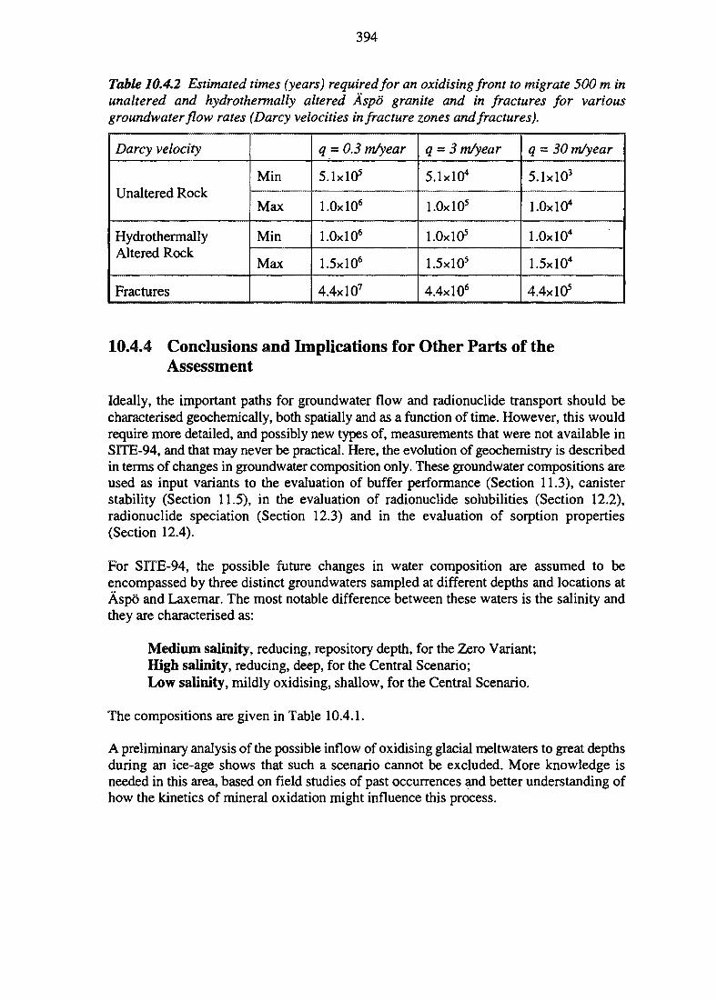
394
Table 10.4.2 Estimated times (years) required for an oxidising front to migrate 500 m inunaltered and hydrothermally altered Aspo granite and in fractures for variousgroundwater flow rates (Darcy velocities in fracture zones and fractures).
Darcy velocity
Unaltered Rock
HydrothermallyAltered Rock
Fractures
Min
Max
Min
Max
q ~ 0.3 m/year
5.1xlO5
l.OxlO6
l.OxlO6
1.5xlO6
4.4xlO7
q = 3 m/year
5.1xlO4
l.OxlO5
l.OxlO5
1.5xlO5
4.4xlO6
q ^ 30 m/year
5.1xlO3
l.OxlO4
l.OxlO4
1.5xlO4
4.4x10⁵
10.4.4 Conclusions and Implications for Other Parts of theAssessment
Ideally, the important paths for groundwater flow and radionuclide transport should becharacterised geochemically, both spatially and as a function of time. However, this wouldrequire more detailed, and possibly new types of, measurements that were not available inSITE-94, and that may never be practical. Here, the evolution of geochemistry is describedin terms of changes in groundwater composition only. These groundwater compositions areused as input variants to the evaluation of buffer performance (Section 11.3), canisterstability (Section 11.5), in the evaluation of radionuclide solubilities (Section 12.2),radionuclide speciation (Section 12.3) and in the evaluation of sorption properties(Section 12.4).
For SITE-94, the possible future changes in water composition are assumed to beencompassed by three distinct groundwaters sampled at different depths and locations atAspo and Laxemar. The most notable difference between these waters is the salinity andthey are characterised as:
Medium salinity, reducing, repository depth, for the Zero Variant;High salinity, reducing, deep, for the Central Scenario;Low salinity, mildly oxidising, shallow, for the Central Scenario.
The compositions are given in Table 10.4.1.
A preliminary analysis of the possible inflow of oxidising glacial meltwaters to great depthsduring an ice-age shows that such a scenario cannot be excluded. More knowledge isneeded in this area, based on field studies of past occurrences and better understanding ofhow the kinetics of mineral oxidation might influence this process.
395
11 EVOLUTION OF THE NEAR-FIELD
This chapter describes the modelling of the near-field evolution for the Reference Case andfor the Central Scenario. The modelling builds on the description of the spent fuel andEngineered Barrier System in Chapters 3 and 8 respectively and the modelling of thegeosphere described in Chapter 10. The results of this modelling is used as input to thecalculations of radionuclide speciation and solubilities in Chapter 12, as well as thetransport calculations defined in Chapter 15 and presented in Chapter 16.
11.1 INTRODUCTION
The near-field is usually defined as including the Engineered Barrier System (EBS) and thatpart of the geosphere which will undergo changes due to the emplacement of the EBS, butthis is not a strict definition, as some EBS-induced influences may spread throughout thegeosphere to variable distances. Nevertheless, it is clear that modelling degradation of theEBS and the eventual radionuclide release and migration through the barriers requireshigher resolution, both in terms of scale and in terms of which interactions of processesneed to be considered, than modelling migration of radionuclides far out in the geosphere.In SITE-94, the near-field was defined as encompassing the canister containing the spentnuclear fuel, surrounded by a compacted clay backfill, a portion of the immediatelysurrounding rock and the tunnels in the vicinity of the deposition holes.
11.1.1 Near-field Interactions
The disturbances and interactions within the near-field are primarily of thermal,mechanical, chemical and hydraulic nature. Couplings between these disturbances mightgive rise to other, more complex, phenomena, e.g. fracturing, heat convection, canisterfailure or change in the redox state. In SITE-94, special effort is devoted to linking thefeatures, events and processes (FEPs) of the near-field within the Process InfluenceDiagram (PDDs; see Chapter 2 and Chapman et al., 1995). Inspection of the PIDs inFigures 7.1.1, 7.1.2 and 8.1.1 reveals that the majority of Process System FEPs and linksconsidered in SITE-94 concern the near-field, but that the near-field FEPs also are linkedto the far-field.
The excavation, construction, operation and sealing of the repository may alter the state ofthe near-field rock. In the Reference Case and Central Scenario, changes in the near-fieldare also caused by interactions through the far-field/near-field interface. For example, thestresses will adjust to the local geometry of features and excavation geometries in the near-field and thereby result in local deformations of the near-field rock mass. Stress inducedfrom swelling of the buffer and from the repository heat will also cause deformation of therock mass. In another example, the groundwater flow in the vicinity of an individualcanister is driven by the overall far-field flow, but is highly influenced by the localconductive features. A third example is that the chemistry of the groundwater, whicheventually reaches the canister and spent fuel, may change as a result of contact with thebuffer material.
396
The changing state of the near-field rock may affect the buffer properties, both chemicallyand mechanically. The mechanical and chemical loads on the canister affect canisterlongevity. Once a canister is breached, water may reach the spent fuel, which startsprocesses such as radiolysis, fuel degradation, radionuclide release and other subsequentchanges of the near-field chemistry.
11.1.2 Modelling Near-field Processes and the AMF
The modelling of the near-field evolution in SITE-94 is shown in the Assessment ModelFlowchart already introduced in Chapter 2 (Figure 2.4.5). The following subsectionsprovide the details about the modelling undertaken. However, much of the informationtransfer between disciplines is manual, through a relatively large number of ClearingHouses.
This chapter reports on SITE-94 analyses of thermal evolution, near-field rock mechanics,near-field hydrogeology, near-field geochemistry, buffer evolution, tunnel evolution,canister evolution, radiolysis, fuel degradation and redox conditions. The analyses are basedon the far-field impacts for the Reference Case and the Central Scenario as reported inChapter 10. In addition, possible intrinsic processes are analysed.
Chapter 12 describes radionuclide behaviour, such as dissolution/precipitation and sorption.The radionuclide behaviour clearly depends on the state of the barriers, but in SITE-94 itis assumed that there is no influence in the other direction, apart from the potentialmovement of the redox front, i.e. that radionuclide transport does not affect the barrierproperties. This separation of the evolution of the barriers and the radionuclide behaviouris justified since the radionuclides can be regarded as micro, or tracer, components in theProcess System. As such, they are assumed not to influence the behaviour of the macrocomponents, i.e. the barriers and other chemical components occurring in much largeramounts than the radionuclides. On the other hand, the mutual influence of isotopes of thesame elements (including, stable isotopes of some elements, such as Zr present in the fuelelements) are accounted for, e.g., in the sharing of solubilities as described in Chapter 13.
11.2 NEAR-FIELD ROCK
11.2.1 Rock Mechanical Impacts in the Near-field
This section describes the modelling of the mechanical stability of the near-field rock forthe Reference Case and the Central Scenario. The mechanical model is described inSection 7.5. According to the AMF (Figure 2.4.5) the result of this analysis should affectthe evaluation of the canister stability (Section 11.5) and the evaluation of the near-fieldgroundwater flow (Section 11.2.2).
397
11.2.1.1 Introduction
The mechanical state of the near-field rock is of primary importance for the integrity andstability of the repository barriers. The PID covering the near-field rock (Figure 7.1.2)shows that the near-field rock stress is influenced by the far-field stress, the excavation, theswelling of the buffer, the temperature and the groundwater flow. These influences areimportant both for the rock mass response of the Reference Case and the Central Scenario.External stresses and temperatures will differ for the two cases as has already beendiscussed in Section 10.2.
A rock mechanical analysis of the near-field provides information on the rock stressdistribution, rock mass movement, fracture initiation and fracture propagation. Theseresults can be used as a direct estimate of the mechanical stability of the repository and alsoas input to discussion of the hydrogeology of the near-field. More specifically, the resultsaddress the potential for:
• rock instability in the near-field,
• shearing of fractures at the wall of the canister deposition hole,
• fracture displacement, shearing, opening/closure and fracture propagation whichmight affect the near-field water flow.
This section focuses on the results of the SITE-94 near-field rock mechanical analyses(Shen and Stephansson, 1996a, b). Two model approaches are used, as discussed inSection 7.5. Modelling in 2D of simple fracture geometries, focuses on the propagation andcoalescence of existing fractures in the near-field, using a code developed by Shen (1993).Modelling in 3D of three different fracture networks, all consistent with the hydraulic near-field fracture networks (Geier et al., 1996), focuses on the intact rock stability and the shearand normal displacement of existing fractures using the three-dimensional distinct elementcode 3DEC (ITASCA, 1994).
11.2.1.2 The Effects of Loading for the Reference Case
Models and boundary conditions
The 3D, near-field analysis of the Reference Case considers the impacts from
• the excavation of the tunnel and deposition hole,• the bentonite swelling pressure and,• the thermal loading at given times after waste disposal.
This modelling is done in sequence. Due to the small size of the model domain, applicationof constant stress boundary conditions estimated by the far-field analyses is considered tobe justified.
The first step is to perform a consolidation calculation by applying an assumed, constant,in-situ stress level at the 500 m level as a boundary condition. Excavation is then modelled
398
by removing the rock mass in the tunnels and the deposition holes from the consolidatedmodel. The effect of the swelling pressure is modelled using the excavated model, byapplying 10 MPa as a boundary stress around the wall of the deposition hole and byapplying zero displacement on the external boundaries.
The temperature load is applied to this last model, by calculating the temperatures resultingfrom the heat of a repository of 400 canisters. This temperature calculation is not equal tothe temperature calculations made for the far-field (see Section 10.2) and are only relevantfor assessing the rock mechanical impact of temperature changes. The temperaturespredicted are not adjusted for ambient temperatures or the geothermal gradient, but this isof minor significance for the rock mechanical evaluation. (For further details see Shen andStephansson, 1996a, and Hansson et al., 1995a, b).
The three-dimensional 3DEC code, used for analysing the rock mechanics, can handlecomplex fracture geometries and loads, but cannot directly model fracture propagation andcoalescence. Instead, Shen (1993) developed a special boundary element code to analysethese phenomena in order to find out when stress conditions predicted by the three-dimensional analysis could lead to such failures. Using this code, which can only handlea few fractures, SITE-94 analyses the rock mass stability in a vertical and a horizontalplane, through a deposition hole, for six different idealised fracture geometries (Shen andStephansson 1996a).
The applied boundary stresses simulate the stress state with the same loading events andthe same in-situ stresses as those used in the 3DEC near-field models. Thermal loading isconsidered by increasing the boundary stresses and is estimated from previous studies (Shenand Stephansson, 1990) to be about 2.5 times greater than the in-situ stresses. Shen andStephansson (1996a) also present limited sensitivity analyses of the impact of the appliedboundary stresses. A case with a 50% increase of the maximum principal stress and a 50%decrease of the minimum principal stress is considered an extreme external stress condition.
Excavation
In the 2D analysis, the excavation does not cause any fracture propagation or coalescencefor the applied standard boundary stresses. However, fracture propagation and coalescencedo occur for some geometries when extreme boundary stresses are applied.
In the 3D analysis, excavation causes a major stress redistribution of the rock mass. Theprinciple stresses in the vicinity of the tunnel and the deposition hole are oriented in theradial and tangential directions. Near the walls, the tangential stress is high (30 to 50 MPa)and the radial stress is less (10 to 20 MPa). Stress redistribution due to the excavationcauses the occurrence of yield zones in a few locations near the walls of the tunnel anddeposition hole. At a few locations, where the stress is even higher, local intact rock failureis found to have occurred.
Even though the analysis does not demonstrate it, rock wedges may form in the tunnel roofand fall down during excavation or at a later stage during repository operation. Later, whenthe repository is backfilled, this local instability is of minor importance. Rockreinforcement can prevent rock fall and enhance stability during the operational phase.
399
Fractures intersecting the tunnel will close with a maximum closure of 0.14 mm due to theincrease of normal stress. Fractures located in the tunnel walls, but not intersecting thetunnel, will open, partly due to decrease of normal stress. The opening displacement isnormally very small (less than 0.02 mm) and only takes place over a limited length. Theopening and closing of fractures, which occur in the immediate vicinity of the excavation,will affect the hydraulic conductivity of the rock mass in this region.
The maximum fracture shear displacement caused by excavation is found to be about 1 mm(Shen and Stephansson, 1996a,b). Fracture dilation caused by shearing will increase theconductivity of the fractures, but the 1 mm shearing is believed to be too small to have anyeffect on the groundwater flow regime. Gouge material, resulting from shearing, mayreduce fracture conductivity.
Swelling of the buffer
According to the 2D analyses, the swelling pressure may enhance or prevent fracturepropagation, depending on the fracture geometry. As the impact is limited to the immediatevicinity of the deposition hole, the swelling pressure has an influence only when thefractures are short. Outside ranges which are larger than one borehole diameter, fracturesare barely affected by the swelling pressure.
The 3D analysis results show that swelling pressure in the deposition hole has a minorinfluence on the stability of the rock mass. In fact, with swelling pressure of 10 MPa actingon the wall of the deposition hole, the stress concentration caused by the excavation isreduced. Swelling bentonite appears to function like a rock support, preventing majordisturbances and collapse of the deposition hole.
No significant fracture movement is found due to the swelling pressure of the buffer.
Thermal load
In the 3D analysis of thermal loading, the rock temperature in the repository reaches itsmaximum at about 200 years after waste deposition. The temperature increase is almostevenly distributed in the model, ranging from 25°C to 31 °C. The high temperature increasecauses high stresses in the rock mass, more than twice those present prior to thermalloading. High stresses cause additional yielding in the foot- and sidewalls of the tunnel anddeposition hole. The maximum shear displacement of fractures increases to 0.47 mm. Allfractures in the model are closed, with average closure of 0.4 mm. After 10 000 years, therepository has nearly reached the ambient temperature. The stresses return to their originalmagnitude in most regions, except where rock yielding has occurred earlier. Unrecoverablefracture shear displacement remains along the inclined joints; some fractures which wereopen prior to thermal loading, open again after the cooling of the repository.
The 2D analysis, representing the thermal load with the extreme external stress boundaryconditions discussed above, result in major fracture propagation and coalescence for allfracture geometries considered. Since the loading stress is high (50-90 MPa), shearfractures extend long distances (more than 5 m). Fracture coalescence is found to increasethe shear displacement of fractures by more than 100%. Within the limited size of themodels, fracture shear displacement is small (less than 1-2 mm). Long fractures, whichcould be a result of fracture coalescence, are expected to produce larger shear displacement.
400
The fracture shear displacement at peak thermal loading is about twice that caused byexcavation. The amount of shear displacement predicted by both 3DEC models and BEMmodels is only about 1 mm. The shear displacement is, however, roughly proportional tothe fracture length. Consequently, Shen and Stephansson (1996b) note that fracturepropagation and coalescence, which result in longer fractures, may significantly increasethe fracture shear displacement. It may be possible that fracture coalescence can occur ina wider region than has been simulated by the BEM models.
Most fractures in the near-field region close due to the temperature increase, which willreduce their hydraulic conductivity considerably. This effect is, however, reversed when therock starts to cool after the temperature peak about 200 years after waste deposition (cf.KBS-3). Fracture propagation and coalescence may, however, result in remnant, long-termeffects on the hydraulic conductivity of the near-field rock mass. Because the high adversestresses only appear in the repository and its immediate region, such remnant permeabilitychanges are only likely to develop in the immediate area of the repository.
The Disturbed-Rock Zone
The Disturbed-Rock Zone is not treated extensively within SITE-94. Geier et al. (1996)evaluates the effects of enhanced hydraulic conductivity along deposition tunnels in theDiscrete Feature site model, as reported in Section 10.3.4. In addition, Lawrence BerkeleyLaboratories (Noorishad et al., 1996) have started to analyse the SCV experiment at Stripa(see below).
The extent of the disturbance of rocks adjacent to an excavation is dependent on the specificproperties of the site and the design and engineering of the excavation. A wide range ofpossible changes in mechanical and fluid flow behaviour of the rock mass can be expectedas a result of the excavation (Jing et al., 1996). Experiences from the SCV experiment atthe Stripa mine (Olsson et al.,1992) showed a major reduction of inflow once the SCVtunnel was constructed. One suggested explanation was degassing of dissolved gasses in thegroundwater, which may have resulted in reduced permeability due to gas blockage.However, there may also be rock mechanical explanations.
In a case such as the SCV experiment, local variations of hydraulic conductivity in theDisturbed-Rock Zone can be expected to occur as the rock deforms in shear and normalmodes; the magnitude of the effect depends on the orientation of existing fracture sets.Because flow through the system is very sensitive to flow connectivity, critical changes inthe overall flow rate into the tunnel may occur due to local, seemingly unimportant changesin the conductivity, if such changes affect flow connectivity. This fact points to the need forcareful consideration in a proper analysis. The complexity of the coupled hydromechanicaleffects in a task of this nature requires development of an appropriate 3D-coupled hydro-mechanical simulator.
Some efforts within SITE-94 to address these needs are described by the team from LBL(Noorishad et al., 1996). The work starts with the development of a computer simulatorutilising continuum macro-constitutive models of the rock material. Inclusion of majordiscontinuities are then superimposed on the continuum models. The underlying philosophyfor this approach emanates from the fact that consideration of all controlling parameters isusually beyond practical means and various approximations have to be made. A continuum
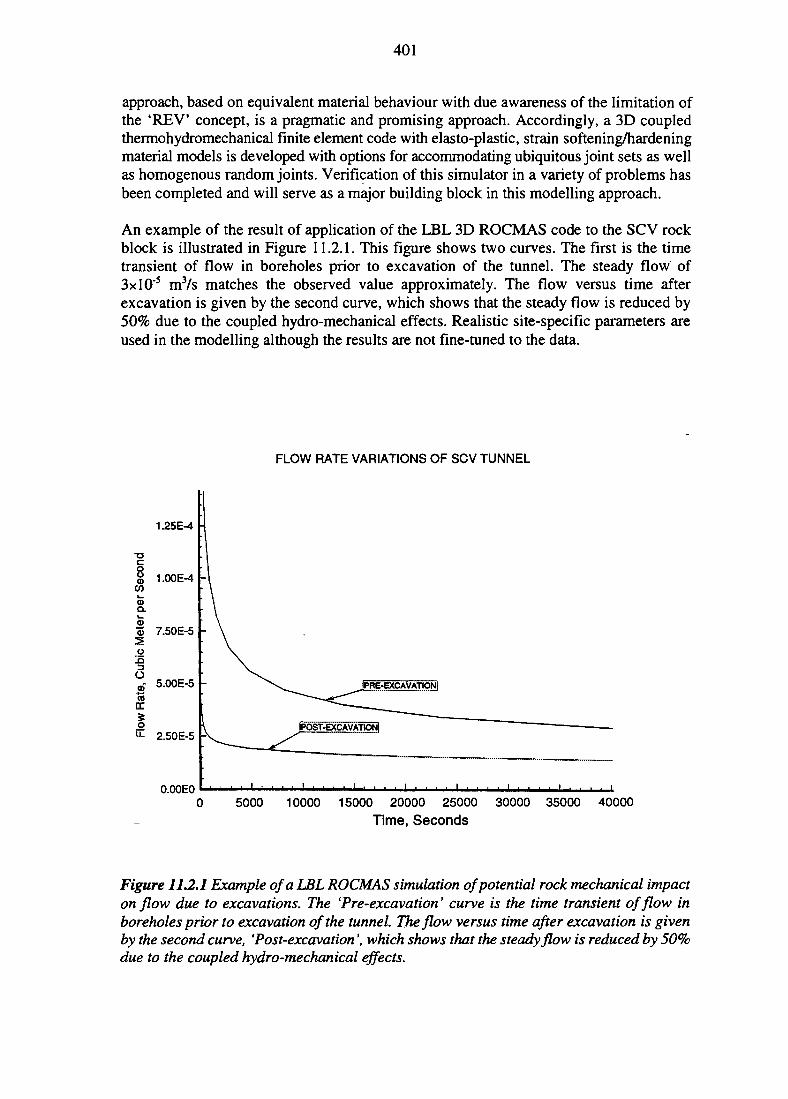
401
approach, based on equivalent material behaviour with due awareness of the limitation ofthe 'REV concept, is a pragmatic and promising approach. Accordingly, a 3D coupledthermohydromechanical finite element code with elasto-plastic, strain softening/hardeningmaterial models is developed with options for accommodating ubiquitous joint sets as wellas homogenous random joints. Verification of this simulator in a variety of problems hasbeen completed and will serve as a major building block in this modelling approach.
An example of the result of application of the LBL 3D ROCMAS code to the SCV rockblock is illustrated in Figure 11.2.1. This figure shows two curves. The first is the timetransient of flow in boreholes prior to excavation of the tunnel. The steady flow of3xl0"5 m3/s matches the observed value approximately. The flow versus time afterexcavation is given by the second curve, which shows that the steady flow is reduced by50% due to the coupled hydro-mechanical effects. Realistic site-specific parameters areused in the modelling although the results are not fine-tuned to the data.
FLOW RATE VARIATIONS OF SCV TUNNEL
-acooQ
COl _<Da.
o
3
o©•"co£E
1
1.25E-4
1.00E-4
7.50E-5
5.00E-5
2.50E-5
0.00E05000 10000 15000 20000 25000 30000 35000 40000
Time, Seconds
Figure 11.2.1 Example of a LBL ROCMAS simulation of potential rock mechanical impacton flow due to excavations. The lP re-excavation' curve is the time transient of flow inboreholes prior to excavation of the tunnel. The flow versus time after excavation is givenby the second curve, 'Post-excavation', which shows that the steady flow is reduced by 50%due to the coupled hydro-mechanical effects.
402
11.2.1.3 The Effect of Loads for the Central Scenario
The Central Scenario involves changes to the far-field stress and temperature due topermafrost and glaciation which would be superimposed on the effects defined by theReference Case rock mechanical analysis.
Permafrost
The effect of permafrost on near-field rock mechanics in SITE-94 is approximated tocoincide with Reference Case conditions. From the analysis of the permafrost depth (King-Clayton et al., 1995) discussed in Section 10.2, it is concluded that permafrost will not reachthe repository level. Consequently, it is not necessary to analyse the effect of freezing of thenear-field rock in SITE-94. The temperature effect from glaciation on the stress field isalready neglected in the far-field analyses.
Glaciation
In order to represent the ice load in the 3D near-field rock mechanical analyses, Shen andStephansson (1996a) apply a vertical boundary stress, equivalent to the weight of 2200 mice, at the top surface of the model after it has been subjected to the effect of the swellingpressure. In the two-dimensional model, the boundary stresses caused by 2200 m ice loadare calculated theoretically (see Shen and Stephansson, 1990 and 1996a).
The vertical 2D geometries analysed show an enhanced fracture propagation andcoalescence for the more extreme stress conditions. The far-field analysis (Hansson et al.,1995a) shows that such extreme stress conditions may occur. Fractures propagate roughlyalong the 60° dip plane. This may trigger a major shear rupture or faulting in this direction.In the horizontal geometries, no fracture propagation, or only limited fracture propagation,occurs during glaciation.
In the 3D analysis, the vertical and sub-vertical principle stresses increase in magnitude inthe whole region as ice loading is mainly vertical. Due to differences in stress magnitude,there will be intact rock failures (yielding) in the deposition hole wall and the tunnel walls.Intact rock yielding is also found near some joints intersections. The volume of intact rockfailure caused by glaciation is found to be similar to that caused by thermal loading.Glaciation causes a major increase of shear displacement of inclined fractures with amaximum of 0.33 mm, (Shen and Stephansson, 1996a, b). Larger shear displacements canbe expected if longer fractures are modelled. Rock fractures close when ice load is applied.The maximum closure occurs in horizontal fractures which have the highest normal stress.Deglaciation releases the vertical stresses. However, the yield zones and most of the fractureshear displacement in the vicinity of the tunnel and deposition hole are unrecoverable andremain as long-term consequences of the glaciation cycle.
With the short joints used in the near-field models, for both 3DEC and BEM models (Shenand Stephansson, 1996a, b), fracture shear displacement is limited to 1 mm, which is smallenough to be neglected. However, fracture shear displacement is proportional to the lengthof a fracture. Considering longer fractures (or the possibility that short fractures connect andcoalesce due to fracture propagation and become a long fracture or even a minor fault)would result in greater shear displacements. If the strength and stiffness of the fracture zoneare reduced, the displacements can be even greater (Hansson et al., 1995a, b). Shen and
403
Stephansson (1996a, b) suggest that fracture coalescence caused by glaciation may extendover large areas because the glaciation is a large-scale event. Large-scale fracturepropagation and coalescence can create minor faults, or can trigger movement of existingfaults.
Glaciation will close most of the joints and hence reduce the hydraulic aperture.Reactivation of existing faults or development of new fractures are other factors which willenhance their hydraulic conductivity.
11.2.1.4 Uncertainties
Consistency with PID FEPs and links
The near-field rock mechanical analysis considers most of the FEPs and links related to thenear-field rock Process Influence Diagram displayed in Figure 7.1.2 (IL=10) and the full PIDin enclosure. (All these FEPs and links are also associated to the Rock Mechanics ClearingHouse, see Figure 2.4.5). However, some of the links are only treated qualitatively, as willbe discussed in the next section.
The near-field rock stress analysis in SITE-94 considers the impact from properties of near-field rock (NE121), creeping of near-field rock (NE120), near-field temperature (NE45),bentonite swelling (BE 129) as well as the far-field stress field (GE81). The analysis alsodirectly considers the impact on creeping of the rock mass (NE31) and enhanced near-fieldrock fracturing (NE34). The SITE-94 analysis does not acknowledge the influence ofgroundwater flow (NE48). Furthermore, there is no quantitative evaluation of the changesin rock permeability due to the deformation of the rock mass.
The omission of the hydraulic coupling with rock mechanics is a limitation, as noted incurrent research and development work such as the DECOVALEX study (Jing et al., 1996).
Conceptual model and parameter uncertainty
Most of the discussion on conceptual model and parameter uncertainty for the far-field rockmechanical analysis (Section 10.2.6) is also valid for the near-field.
Clearly, the analysis is subject to significant conceptual model uncertainty. The joint systemat Aspo is not known in reality and will only be partially known even after excavation ofthe test rooms. The intact rock is assumed to be linearly elastic (in BEM models) or elasto-plastic (in 3DEC models) and joints are assumed to have linear stiffness and to followMohr-Coulomb failure criteria.
Apart from conceptual model uncertainty, there is also parameter uncertainty owing to thelack of measured data. Most of the mechanical properties of the intact rock and joints arebased on experience or extracted from other published data. These data have greatuncertainties when they are applied to the Aspo site. In spite of this, as Shen andStephansson (1996a) study some different variants (three different 3D networks, differentexternal stresses in the 2D model and two alternative values for the fracture toughness inthe 2D model), they are able to draw the following conclusions:
404
• When sufficient numbers of fractures are considered, different fracture networkrealisations from the same fracture distribution model have minor influence on theresults.
• Different stress states have a significant effect on fracture propagation andcoalescence. Fractures do not propagate under the in-situ stresses measured at Aspo.However, with a variation of 50%, they can propagate during different loadingevents. Fracture propagation is very sensitive to the ratio of minimum and maximumprinciple stresses.
• Fracture roughness value is another parameter controlling fracture propagation andcoalescence. The modelling results are sensitive to fracture roughness but not asmuch as to the stress state.
In addition, due to code and resource limitations in the analysis, only one tunnel and onedeposition hole are considered for the near-field study. The influences from other tunnelsor deposition holes are neglected. The region analysed is relatively small, which does notallow for long (and potentially significant) structural features to form. The far-field stressesresulting from the large-scale features are not properly transmitted to the near-field analysis.Instead, average stress values are used as boundary conditions. The fracture networkobtained from the hydraulic analysis is simplified. The fracture propagation analysis is onlymade in two dimensions. Clearly, it is not easy to judge the effect of all thesesimplifications at the present stage, but this will have to be considered in future analyses.
11.2.1.5 Conclusions
Implications for other parts of the assessment
The direct outputs from the near-field rock mechanical evaluations are stresses anddeformations of the near-field rock mass. Table 11.2.1 summarises how these results areused in other parts of the SITE-94 assessment.
The modelling conducted by Shen and Stephansson (1996a, b) shows that both thermalloading and glaciation may create local instability of intact rocks in the walls of the tunneland deposition hole, possible fracture propagation and coalescence at some locations nearmajor faults or fracture zones and changes of water flow pathways caused by such fracturecoalescence. The swelling pressure in the deposition hole is found to have minor effects onthe rock stability and fracture deformation.
The fracture propagation and coalescence is found to be controlled by the ratio of minor andmajor principal stresses and their magnitude. A ratio less than 0.20 is the essential conditionfor any fracture propagation. The 2D BEM analysis of fracture coalescence finds that anextremely low stress ratio (less than 0.05) is unlikely to occur in the repository area and thata stress ratio of less that 0.20 is only found in some locations. This means that tensilefracture propagation (rock splitting) will not occur and shear failure only occurs in thoselimited locations where the stress ratio is less than 0.20.
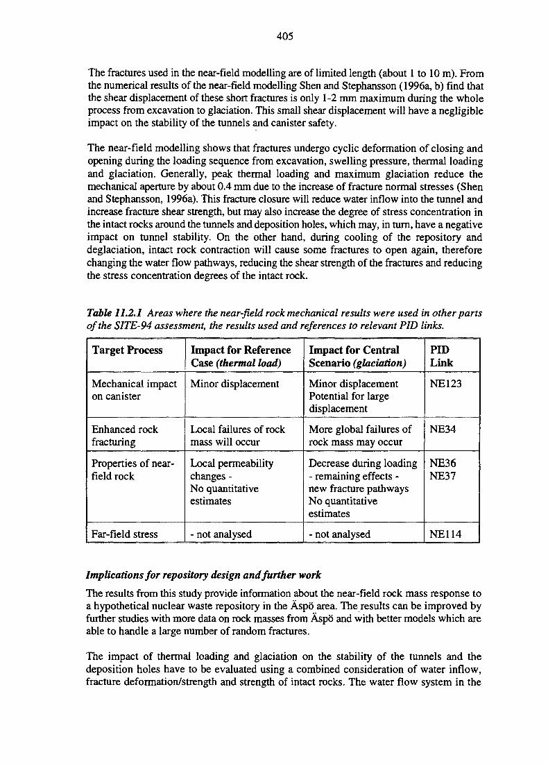
405
The fractures used in the near-field modelling are of limited length (about 1 to 10 m). Fromthe numerical results of the near-field modelling Shen and Stephansson (1996a, b) find thatthe shear displacement of these short fractures is only 1-2 mm maximum during the wholeprocess from excavation to glaciation. This small shear displacement will have a negligibleimpact on the stability of the runnels and canister safety.
The near-field modelling shows that fractures undergo cyclic deformation of closing andopening during the loading sequence from excavation, swelling pressure, thermal loadingand glaciation. Generally, peak thermal loading and maximum glaciation reduce themechanical aperture by about 0.4 mm due to the increase of fracture normal stresses (Shenand Stephansson, 1996a). This fracture closure will reduce water inflow into the tunnel andincrease fracture shear strength, but may also increase the degree of stress concentration inthe intact rocks around the tunnels and deposition holes, which may, in turn, have a negativeimpact on tunnel stability. On the other hand, during cooling of the repository anddeglaciation, intact rock contraction will cause some fractures to open again, thereforechanging the water flow pathways, reducing the shear strength of the fractures and reducingthe stress concentration degrees of the intact rock.
Table 11.2.1 Areas where the near-field rock mechanical results were used in other partsof the SITE-94 assessment, the results used and references to relevant PID links.
Target Process
Mechanical impacton canister
Enhanced rockfracturing
Properties of near-field rock
Far-field stress
Impact for ReferenceCase (thermal load)
Minor displacement
Local failures of rockmass will occur
Local permeabilitychanges -No quantitativeestimates
- not analysed
Impact for CentralScenario (glaciation)
Minor displacementPotential for largedisplacement
More global failures ofrock mass may occur
Decrease during loading- remaining effects -new fracture pathwaysNo quantitativeestimates
- not analysed
PIDLink
NE123
NE34
NE36NE37
NE114
Implications for repository design and further work
The results from this study provide information about the near-field rock mass response toa hypothetical nuclear waste repository in the Aspo area. The results can be improved byfurther studies with more data on rock masses from Aspo and with better models which areable to handle a large number of random fractures.
The impact of thermal loading and glaciation on the stability of the tunnels and thedeposition holes have to be evaluated using a combined consideration of water inflow,fracture deformation/strength and strength of intact rocks. The water flow system in the
406
vicinity of the repository is expected to be especially affected by thermal loading andglaciation, due mainly to changes of fracture aperture and to changes in the connectivity ofthe fracture network by fracture propagation and coalescence.
11.2.2 Hydrogeology
The details of the hydrogeological evaluation calculations are described in Section 10.3,together with the results for the far-field. This section briefly summarises thehydrogeological parameters estimated for the near-field rock. This division of thepresentation corresponds to different data delivery paths from the Clearing HouseHydrogeological parameters to RN-transport in the AMF (Figure 2.4.5). The resultsdescribed in this section constitute the basis for the delivery to the Canister analysis andNear-field RN-transport Clearing Houses. However, in the hydrogeological site models, thenear-field rock is modelled as an integrated part of the far-field rock, to enable thedetermination of correlations between local hydrogeological parameters on the scale of acanister deposition hole and the effective far-field flow and transport parameters describingtransport in the geosphere.
Note that the term 'significant' is used below in the sense of significance for the overallperformance of the rock as a barrier, rather than in the sense of statistical significance forparticular parameters.
11.2.2.1 Discrete Feature Model: Reference Case Results
Introduction
Hydrogeological parameters for the near-field model, CALIBRE, are estimated by samplingthe predicted steady-state flow fields for each realisation of the Discrete Feature model, asdescribed in Section 10.3.4.1. The predicted near-field parameters include fracture spacing,Snf, mean transport aperture , bnf, and near-field Darcy velocity, qnf.
Connectivity: Base Case
A minority of the canister sites die fractured (intersected by transmissive fractures), andonly a fraction of these can be described as flowing sites, in consideration of the numericalresolution of the model (see Section 10.3.4.3). For the Base Case model, in which the near-field rock type is considered to be Aspo granodiorite, approximately 43% of the canistersites are fractured and only 33% are flowing sites. In the following, the results for theDiscrete Feature site model are presented in terms of the canister sites that are experiencingflow (flowing sites). Partly because it facilitates the evaluation of different model variantsand partly because the consequence calculations are performed on a single canister basis inSITE-94. The implication of connectivity for the results interpretation is discussed inSection 11.2.2.4.
Spatial variability: Base Case
The distribution of near-field parameters for flowing sites in the Base Case model,SKI0/NF0/BC0, is summarised in Table 11.2.2. The variability, vx of each parameter is

407
defined in terms of the log10 difference between the 90th and 10th percentiles of thepredicted distribution, as in Section 10.3.4.3. The highest spatial variability is seen for qnf,which varies by more than two orders of magnitude. Snf varies by about one order ofmagnitude, while b^ varies by less than a factor of two. The effective far-field head gradientAh/L (which is actually a far-field parameter, but is obtained for all flowing sites) alsoshows relatively little spatial variability.
Table 11.2.2 Summary statistics of the near-field hydrogeological parameters for flowingcanister sites, determined with the Base Case model variant of the Discrete Feature sitemodel.
qnf
(m/yr)snf(m)
Base Case: All flowing sites (33% of all canisters)MinimumlOPercentileMedian90th PercentileMaximumVariability
3.2xlO6
9.7xlO"5
1.7xlO3
3.8xlO"2
5.7x10'
2.59
0.280.672.085.50
30.850.91
bnf
(mm)
0.400.580.650.750.990.11
M/L(rn/m)
<0.00020.00180.00240.00280.00360.19
Correlations: Base Case
Near-field Darcy velocity qnf shows, at best, a weak correlation to the far-field Darcyvelocity, qff and to the far-field performance measure, F-ratio, discussed in Section 10.3.Figure 11.2.2 is a cross-plot of near-field Darcy velocity estimated for different canisterpositions versus the corresponding estimates of the far-field F-ratio (a^LA^), for the BaseCase variant (SKI0/NF0/BC0/LO). Note that the plot only contains data for the connectivefraction of canister sites that produced far-field results. As can be seen from the figure, thenear-field Darcy velocity is negatively correlated with the F-ratio, indicating a lowerpotential for far-field retardation if the local Darcy velocity is high. However, thecorrelation is rather weak, hence a low Darcy velocity at a certain canister site does notguarantee high retardation in the far-field. For the 'HI' far-field variant (Section 10.3),where transport is dominated by the far-field geological structures, the far-field retardationis essentially independent of the local near-field Darcy velocity.
A weak negative correlation is also seen between near-field Darcy velocity, qnf, and thedistance to the nearest deterministic feature, R (Figure 11.2.3). However, high near-fieldfluxes do occur at sites with R>40 m from the nearest fracture zone; thus a location far froma fracture zone does not guarantee a low near-field Darcy velocity. Recalling Section 10.3,a similar result is obtained for the correlation between the far-field F-ratio and R.
Among near-field parameters, a weak negative correlation is seen between qnf and Snf, i.e.higher flux values are more likely to occur in more intensely fractured intervals, where thefracture spacing is lower. However, many well-fractured canister sites have negligible Darcyvelocities, which illustrates the importance of network connectivity effects for the near-fieldat the Aspo site.
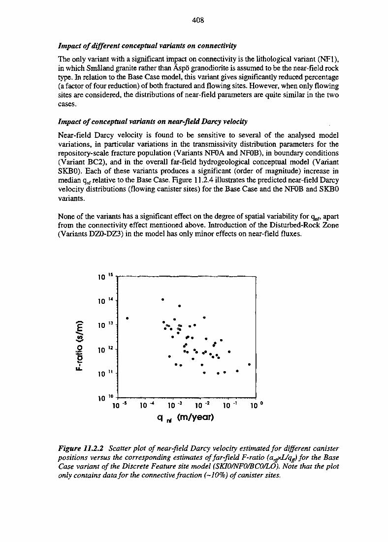
408
Impact of different conceptual variants on connectivity
The only variant with a significant impact on connectivity is the lithological variant (NF1),in which Smaland granite rather than Aspo granodiorite is assumed to be the near-field rocktype. In relation to the Base Case model, this variant gives significantly reduced percentage(a factor of four reduction) of both fractured and flowing sites. However, when only flowingsites are considered, the distributions of near-field parameters are quite similar in the twocases.
Impact of conceptual variants on near-field Darcy velocity
Near-field Darcy velocity is found to be sensitive to several of the analysed modelvariations, in particular variations in the transmissivity distribution parameters for therepository-scale fracture population (Variants NFOA and NFOB), in boundary conditions(Variant BC2), and in the overall far-field hydrogeological conceptual model (VariantSKBO). Each of these variants produces a significant (order of magnitude) increase inmedian q^ relative to the Base Case. Figure 11.2.4 illustrates the predicted near-field Darcyvelocity distributions (flowing canister sites) for the Base Case and the NFOB and SKBOvariants.
None of the variants has a significant effect on the degree of spatial variability for qnf, apartfrom the connectivity effect mentioned above. Introduction of the Disturbed-Rock Zone(Variants DZ0-DZ3) in the model has only minor effects on near-field fluxes.
10 '4 10 "3 10 2 10
q nf (m/year)
Figure 11.2.2 Scatter plot of near-field Darcy velocity estimated for different canisterpositions versus the corresponding estimates of far-field F-ratio (a^>dJqff) for the BaseCase variant of the Discrete Feature site model (SKI0/NF0/BC0/LO). Note that the plotonly contains data for the connective fraction (-10%) of canister sites.
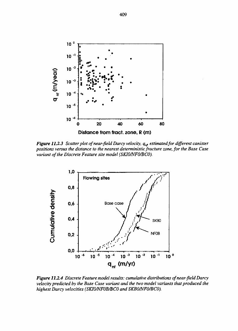
409
0 20 40 60 80
Distance from tract, zone, R (m)
Figure 11.2.3 Scatter plot of near-field Darcy velocity, qnj> estimated for different canisterpositions versus the distance to the nearest deterministic fracture zone, for the Base Casevariant of the Discrete Feature site model (SKI0/NF0/BC0).
™
o
1,0
0,8 -
0,6 -
0,4 -
0,2 -
0,0
Flowing sites
Base case4 SKBO
NFOB
J.rl<?•;> '
10 '6 10 "5 1 0 ' 4 1 0 ' 3 10 "2 10 "' 1 0 °
qnf (m/yr)
Figure 11.2.4 Discrete Feature model results: cumulative distributions of near-field Darcyvelocity predicted by the Base Case variant and the two model variants that produced thehighest Darcy velocities (SKI0/NF0B/BC0 and SKB0/NF0/BC0).
410
Impact of conceptual variants on fracture spacing
Fracture spacing is not affected by most of the variations considered, with the exception ofthe lithological variant, NFL The main effect of this variant is a decrease in the number offractured sites. However, when only the flowing sites are considered, the distribution offracture spacing is quite similar between lithological variants.
Impact of conceptual variants on near-field transport aperture
Fracture transport aperture estimates from the Discrete Feature model are quite consistentbetween variants, due to the fact that all variants use the same relationship between fracturetransmissivity and transport aperture, except the variant NFOC which specifically considersa uniform, order of magnitude increase in fracture transport apertures.
Summary: effects of variants
In summary, Darcy velocity qnf is predicted to be the most sensitive of the near-fieldparameters, with respect to the uncertainties which have been considered for the DiscreteFeature model. Key factors are:
• the influence of lithology on the connectivity of canister sites to the far-field,
• the effect of the fracture transmissivity distribution on fluxes through connected sites.
Near-field fluxes are also influenced by a few of the variations with respect to the far-fieldhydrogeological model, but are not significantly affected in most cases.
It should be noted that uncertainty regarding conceptual models for the detailed poregeometry within the near-field fracture network is not investigated with the Discrete Featuremodel in SITE-94. More heterogeneous conceptual models for pore geometry could beexpected to yield greater variability of bnf and q^.
11.2.2.2 Stochastic Continuum Model: Reference Case Results
Introduction
The Stochastic Continuum site model is only used to provide estimates of Darcy velocity,qnf, for the near-field rock. For each realisation of the hydraulic conductivity field, Darcyvelocity is evaluated for a large number of uniformly distributed 'canister' positions(approximately 600) at repository depth. Because the model does not explicitly representthe location and geometry of the site-scale fracture zones used to define the lateralboundaries of the hypothetical repository, the selected canister positions are not confinedto a particular region in the repository horizon.
Connectivity
As noted above, connectivity is universal in the Stochastic Continuum model which impliesthat all canister sites are connected to flow. The distributions of near-field Darcy velocitypresented below thus represent all of the canister positions evaluated, and are thus not
411
directly comparable to the corresponding plots for the Discrete Feature site model that arebased on a limited fraction of flowing canister sites.
Spatial variability: Base Case
The estimated spatial variability of q^ for the Base Case of the Stochastic Continuum modelis about 2 orders of magnitude, expressed as the log10 difference between the 90th and 10thpercentiles of the velocity distribution. The corresponding variability associated withflowing sites for the Base Case of the Discrete Feature model (for the 33% flowing canistersites) is about 2.6 orders of magnitude (Figure 10.3.20). The median of the predicted near-field Darcy velocity distribution is about 10"4 m/year compared to 10'3 m/year for theDiscrete Feature model.
Correlations: Base Case
As in the Discrete Feature model, a weak positive correlation is found between the near-field and far-field Darcy velocities. The far-field residence times are, however, essentiallyindependent of local hydraulic conductivity of the rock at the source canister. In otherwords, a small, local hydraulic conductivity at the radionuclide release site does not ensurethat the mean residence time for transport is long, over the 500 m transport distance to thebiosphere. These results are to be expected in a continuum model where connectivity isuniversal. Over large transport distances, the hydraulic conductivity along the pathway willbe averaged out so that the local hydraulic conductivity at a particular point, even if anextreme value, will play an insignificant role.
Impact of conceptual variants on near-field Darcy velocity
Table 10.3.5 contains summary statistics of q^for all of the analysed variants (Table 10.3.4)of the Stochastic Continuum site model. Figure 11.2.5 illustrates the cumulativedistributions of q^ for the Base Case and some of the conceptual variants. As can be seen,the calculated near-field Darcy velocity distributions are very similar, both in terms of meanvalues and variability. The only exception is the variant with rather extreme assumptionson correlation (LNG-DIP80) that results in a wider distribution.
These results indicate that the predictions of near-field Darcy velocity are rather insensitiveto the details within the Stochastic Continuum model, be it correlation structure or detailsof the point hydraulic conductivity distribution. This is an important difference between theStochastic Continuum and Discrete Feature site models.
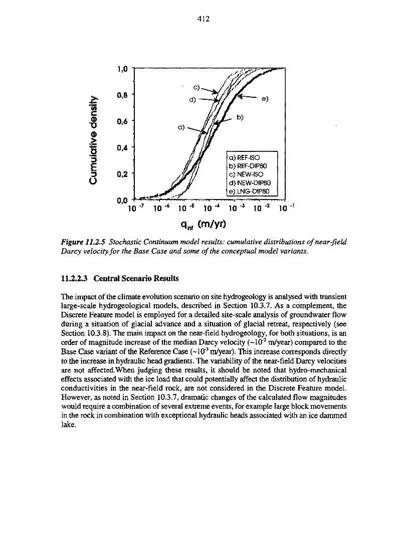
412
(A
c
1,0
0,8
0,6
0,4
0,0
a) REF-ISOb) REF-DIP80c) NEW-ISOd) NEW-DIP80e) LNG-DIP80
10 "7 10 "* 10 "5 10 '* 10 "3 10 '2 10 ''
qnf (m/yr)
Figure 11.2.5 Stochastic Continuum model results: cumulative distributions of near-fieldDarcy velocity for the Base Case and some of the conceptual model variants.
11.2.2.3 Central Scenario Results
The impact of the climate evolution scenario on site hydrogeology is analysed with transientlarge-scale hydrogeological models, described in Section 10.3.7. As a complement, theDiscrete Feature model is employed for a detailed site-scale analysis of groundwater flowduring a situation of glacial advance and a situation of glacial retreat, respectively (seeSection 10.3.8). The main impact on the near-field hydrogeology, for both situations, is anorder of magnitude increase of the median Darcy velocity (~102 m/year) compared to theBase Case variant of the Reference Case (~103 m/year). This increase corresponds directlyto the increase in hydraulic head gradients. The variability of the near-field Darcy velocitiesare not affected.When judging these results, it should be noted that hydro-mechanicaleffects associated with the ice load that could potentially affect the distribution of hydraulicconductivities in the near-field rock, are not considered in the Discrete Feature model.However, as noted in Section 10.3.7, dramatic changes of the calculated flow magnitudeswould require a combination of several extreme events, for example large block movementsin the rock in combination with exceptional hydraulic heads associated with an ice dammedlake.
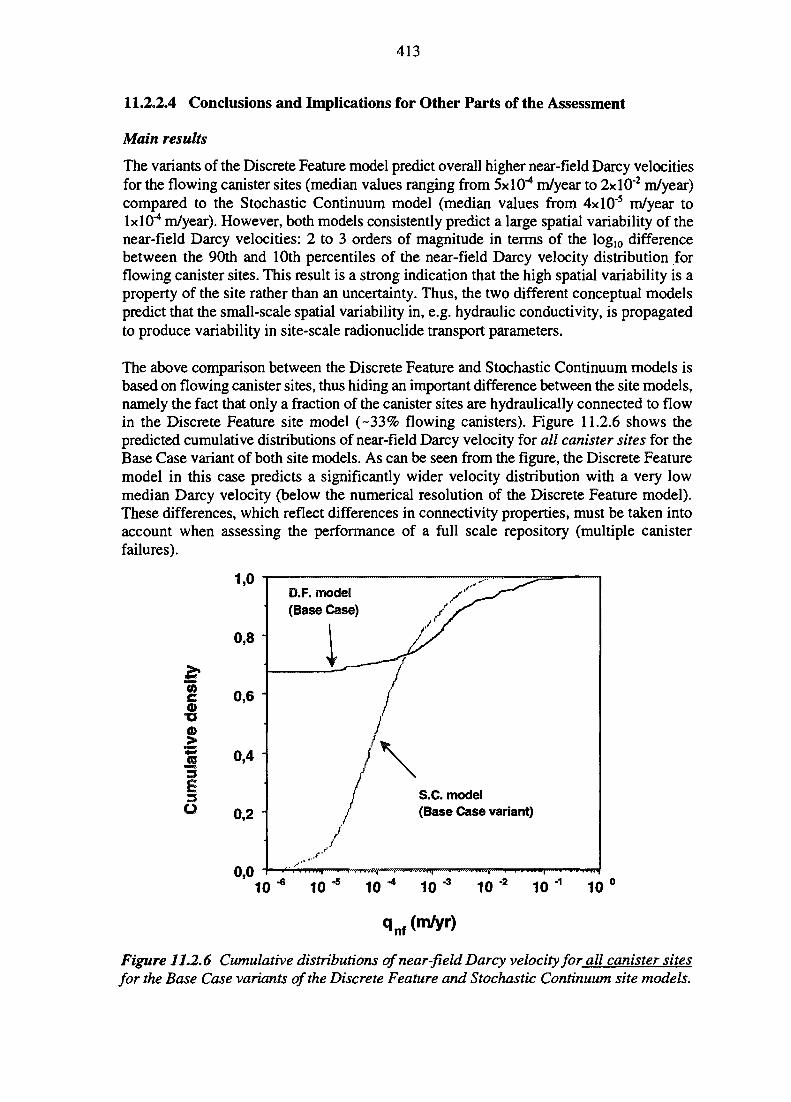
413
11.2.2.4 Conclusions and Implications for Other Parts of the Assessment
Main results
The variants of the Discrete Feature model predict overall higher near-field Darcy velocitiesfor the flowing canister sites (median values ranging from 5X10"4 m/year to 2xlO"2 m/year)compared to the Stochastic Continuum model (median values from 4xlO'5 m/year tolxlO"4 m/year). However, both models consistently predict a large spatial variability of thenear-field Darcy velocities: 2 to 3 orders of magnitude in terms of the log10 differencebetween the 90th and 10th percentiles of the near-field Darcy velocity distribution forflowing canister sites. This result is a strong indication that the high spatial variability is aproperty of the site rather than an uncertainty. Thus, the two different conceptual modelspredict that the small-scale spatial variability in, e.g. hydraulic conductivity, is propagatedto produce variability in site-scale radionuclide transport parameters.
The above comparison between the Discrete Feature and Stochastic Continuum models isbased on flowing canister sites, thus hiding an important difference between the site models,namely the fact that only a fraction of the canister sites are hydraulically connected to flowin the Discrete Feature site model (-33% flowing canisters). Figure 11.2.6 shows thepredicted cumulative distributions of near-field Darcy velocity for all canister sites for theBase Case variant of both site models. As can be seen from the figure, the Discrete Featuremodel in this case predicts a significantly wider velocity distribution with a very lowmedian Darcy velocity (below the numerical resolution of the Discrete Feature model).These differences, which reflect differences in connectivity properties, must be taken intoaccount when assessing the performance of a full scale repository (multiple canisterfailures).
C0)
Im
3O
1,0 T
0,8
0,6
0,4
0,2 1
0,0
D.F. model(Base Case)
I
S.C. mode!(Base Case variant)
10 '210 "* 10 ~ 10 "* 10
qnf(m/yr)
10
Figure 11.2.6 Cumulative distributions of near-field Darcy velocity for all canister sitesfor the Base Case variants of the Discrete Feature and Stochastic Continuum site models.
414
Applicability of the Reference Case results for the Central Scenario
The only impact of the Central Scenario on the near-field Darcy velocities is an order ofmagnitude shift of the flow distribution towards higher velocities. The results on spatialvariability for the Reference Case are thus also applicable for the Central Scenario, withreservation for potential T-H-M-C effects that are not considered in the hydrogeologicalmodels (see discussion in Section 10.3.9).
Uncertainties
As noted in Section 10.3 (Figure 10.3.20) the combined uncertainty plus variability rangeof the near-field Darcy velocities, associated with the detailed site models, is as great as thatdetermined by the simple 'back-of-the-envelope' calculations of groundwater flow.
However, in the detailed models part of the uncertainty has been transferred into spatialvariability. Further reduction of the uncertainty is thus a question of model discrimination(i.e. to be able to rank the validity of the tested conceptual site models and their variants)but high spatial variability appears to be an intrinsic property of the site.
Although the predicted variability of flow for flowing canister sites is similar in both sitemodels, there are significant differences in the predicted connectivity properties in the near-field rock. These differences reflect conceptual differences in the two modelling approachesrather than data uncertainties. The integrated analysis of hydrogeological borehole datadescribed in Section 7.3.6 indicates a high degree of non-uniformity and the discrete natureof flow, which are more consistent with the Discrete Feature modelling results. TheStochastic Continuum model encompasses a wide distribution of hydraulic conductivities,but does not account for the fact that some deposition holes may be located in unfracturedrock with no (or extremely small) Darcy velocities.
Implications for other parts of the assessment
The predictions of near-field hydrogeology provide the basis for defining hydrogeologicalparameter variants for the radionuclide release calculations, as described in Section 15.2.1.The weak correlations found between the near-field and far-field hydrogeologicalparameters imply that the parameter variants for the near-field and far-field cannot betreated as completely independent. However, restrictions on which near-field parameterscan be combined with a given set of far-field parameters are relatively small.
11.2.3 Chemical Conditions and Perturbations
This section discusses the chemical conditions in the near-field rock and perturbations ofthese conditions as a consequence of the existence of the repository and of changesconsidered in the Central Scenario. These conditions also correspond to some of theevaluations necessary within the Clearing House Geochemical parameters to RN-transportin the AMF (Figure 2.4.5). The results described in this section constitute part of the basisfor the delivery to the Canister analysis and Near-field RN-transport Clearing Houses,mainly discussed in Chapter 15.
415
11.2.3.1 Effects of Aeration and Other Phenomena During the Operational Phase
Regions of the host rock will be in continuous contact with air during the construction andmuch of the operational phase of the repository, because ventilation and drainage will beneeded to sustain viable working conditions underground. Natural gases, such as Rn,CH4(g) and H2(g), will have to be removed from underground workings, as will gasesgenerated by blasting or exhausted from drilling and excavation equipment. Excess waterentering excavations will be pumped to the surface.
Oxygen may diffuse into partially-drained regions of the host rock under such conditionsand this would promote oxidation of Fe(II) minerals such as pyrite and ferrous silicates(McKinley, 1985). The development of partially-saturated conditions in the host rock isdifficult to evaluate quantitatively but estimates for the case of crystalline host rocks suggestthat such conditions could be generated near borehole surfaces (Winberg, 1991). Oxidationreactions could generate acidic solutions and cause hydrous ferric oxide or other Fe(III)minerals (e.g., jarosite), to precipitate. Hydrolysis of aluminosilicate minerals andcarbonates would minimise the overall amount of acid generated, but if such reactions wereto occur for extended periods of time the porosity and permeability of the host rock couldbe altered.
Changes in hydrogeological conditions and groundwater chemistry may also result fromperturbations in fluid pressure (NEA, 1993). The hydraulic pressure within excavations willbe roughly equal to that at the Earth's surface (c. 0.1 MPa), whereas fluid pressures outwardinto the host rock would eventually approach hydrostatic conditions (c. 5 MPa at 500 mdepth). A range of transitional pressures could therefore exist between the excavations andunperturbed regions of the host rock. Groundwater will flow towards regions of reducedpressure and dissolved gases will exsolve as the lower pressures are encountered.Exsolution of volatile, weak electrolytes (e.g. CO2(g) and H2S(g)) could increase pH,possibly by as much as several pH units (Arthur and Murphy, 1989). Increasing pH wouldinduce heterogeneous reactions (Winberg, 1991) that could alter the porosity and permea-bility of the host rock. Larger volumes of the host rock could experience the effects ofdepressurisation than would be affected by O2(g) diffusion.
Repository construction and operation could also introduce exotic materials to the naturalenvironment. Blasting gases could, for example, permeate the host rock and locally enrichgroundwaters in nitrate/nitrite. Human activity will inevitably introduce bacteria and othermicro-organisms underground. The longevity of microbial populations following closureof the repository may be short, however, because their viability would be limited by theavailability of nutrients.
Many of these effects will be transient in nature. Some chemicals introduced or foundduring construction and the operational phase are soluble and thus will be removed asgroundwater resaturates the repository. Others are present naturally and will not changegeochemical conditions significantly. Residual amounts of oxygen and other reactive gasesremaining in the repository after closure will eventually be consumed by reactions withhost-rock minerals or the Engineered Barriers.
Many of these early chemical disturbances will probably have little effect on the long-termfunction of the host rock in providing a stable physical and geochemical environment

416
enveloping the repository. The extent of host-rock oxidation caused by O2(g) diffusion andpossible mineralogical changes accompanying groundwater depressurisation may, however,require further analysis because these phenomena could affect long-term redox conditionsand groundwater flow patterns in localised regions near the repository. A potential openquestion in this regard concerns whether reactions generating such changes are reversible(NEA, 1993). The possible effect of remaining oxygen on canister corrosion is consideredin Section 11.5.3.
11.2.3.2 Thermochemical Effects
The heat dissipation from spent fuel causes a significant increase in temperature lasting formany thousands of years. According to the KBS-3 concept, the maximum temperature atthe canister surface of 80°C will be reached within a hundred years after disposal. The usein SITE-94 of the work by Tarandi (1983) is discussed in Section 8.5, and Table 8.5.1 givesthe temperatures within the Engineered Barriers as a function of time after disposal.
It is evident from Table 8.5.1 that the initial temperature gradient across the buffer(0.375 m) declines relatively 'quickly'; after a few thousand years, it decreases to values inthe order of a few °C and less. After 1000 years, the average temperature within therepository will be only a few degrees below the temperature at the canister surface. Themaximum gradient outside the repository will be less than 0.1 °C/m after a few thousandyears (Tarandi, 1983). This will clearly be influenced by changes in ambient temperaturein the rock, as discussed for the circumstances of permafrost in the Central Scenario (seeSection 10.2).
Equilibria which may be influenced by an increase in rock temperature include:
• A decrease of calcite solubility, which may cause a net deposition of calcite in thenear-field, possibly leading to decreased fracture transmissivity and water flow;however, it is conservative to assume that the overall transmissivity is not affected.
• An increase of silicate solubility, which might give rise to a slight increase of rockporosity, but probably more than counteracted by the effects of calcite deposition.
For the reasons given above, in SITE-94 these thermochemical effects on the host rock areneglected.
11.2.3.3 Effects from Long-Term Alteration of the Engineered Barriers
Dissolved species and reaction products from alteration of the Engineered Barriers mightsignificantly change the chemical conditions in the host rock. A more detailed account ofsuch phenomena was presented in SKI Project-90 (SKI, 1991) and no new work isundertaken in SITE-94. Examples of relevant processes are:
• Release of impurities in the bentonite comprising buffer and backfill: sulphide,sulphate, carbonate and organic materials. The latter is considered to be a minorproblem since the clay acts as an effective 'filter' for passage of large molecules
417
(such as humic substances, colloids and microbes). The inorganic components occurnaturally and would have generally the most significant impact on the canister andspent fuel.
• In theory, bentonite may form colloidal dispersions when in contact with pure water,or water with extremely low salinity. If such conditions should ever occur, theywould most probably be of a transient nature, e.g. in connection with glaciations (seeSections 10.3.7 and 10.3.8).
• Corrosion of the metal components, notably the copper canister, will release heavymetals, toxic in the conventional sense. However, the solubility of copper in therepository environment is extremely low and cannot add to the hazards of therepository more than would a natural orebody of copper minerals.
• Concrete will most probably be used as a material for injection, rock reinforcementand other construction in the repository (see Section 8.4). The reactive componentscalcium and hydroxide will eventually be leached out and then be able to react withrock minerals to form laumontite. Bentonite might react to form zeolites such asanalcime (Bolt, 1982). From a chemical point of view these reactions are notunfavourable, since such minerals are good sorbents for radionuclides. However,alkaline attack on clay minerals can lead to loss of their plasticity (Pusch andKarnland, 1988) which could affect the effectiveness of the bentonite buffer as adiffusion barrier.
None of these processes are addressed quantitatively in SITE-94.
11.2.3.4 Possible Future Changes in Chemical Conditions of the Rock
The host rock should provide a stable geochemical environment for the repository, whoseevolution can be predicted in terms of probable ranges in the values of parameters thataffect the performance of the Engineered Barriers. Accurate prediction of possible futurechanges in host-rock geochemistry may not be possible, however, because:
• it is extremely difficult to characterise heterogeneities in host rock propertiescontrolling groundwater flow and mixing processes that could affect mineral-waterequilibria,
• rates and mechanisms of many heterogeneous and homogeneous reactions areunknown, particularly over the range of temperatures and groundwater compositionsthat could be of importance,
• physical processes, including possible future changes in the character of atmosphericdeposition, temperature variations, and the effects of glaciation, are difficult toquantify (e.g. SKI, 1991).
Despite these difficulties, in a Performance Assessment it is necessary to account forpossible future changes in geochemical conditions in the host rock.
418
In SITE-94 it is assumed that the evolution in site conditions would produce variations inmineralogy and groundwater chemistry similar to those presently observed at Aspo. Thisimplies that the physical and chemical processes occurring in the future will be the same asthose that have occurred in the past. This is a reasonable assumption for natural phenomenasuch as glaciation and water-rock interaction, but it may be questionable for human-inducedeffects (e.g. acid rain, global warming or intrusion into the repository by people in thefuture).
The range in groundwater compositions observed at Aspo (Section 7.4.3) is thereforeevaluated to define bounding estimates of initial chemical conditions in groundwaters thatcould come into contact with the repository. The selected groundwaters are discussed inSection 10.4, where a reference composition (Zero Variant), as well as low-salinity andhigh-salinity variants are defined.
An important objective in SITE-94 is to determine how natural variations in sitegroundwater chemistry can best be assimilated into the Performance Assessment processand to evaluate how associated uncertainties could influence Performance Assessmentresults. The chemical evolution of the near-field is approximated in SITE-94 in terms oflimiting conditions at equilibrium, or steady state, in three closed systems representing fullysaturated bentonite, iron corrosion products of the canister and spent fuel. The model is areaction-path model contacting a reference amount of site groundwater with bentonite,canister corrosion products and spent fuel, one after the other. The model is presented inSection 11.3.3.2 and 12.2, and described in full in Arthur and Apted (1996a, b).
11.3 THE BUFFER
This section discusses the chemical and mechanical stability of the buffer, although theambition level in this discussion is low compared to what should be expected in aPerformance Assessment being part of a license application. The radionuclide transportproperties of the buffer are discussed in Section 8.3 and the sorption properties arediscussed in Section 12.4. These discussions correspond to some of the evaluationsnecessary within the Clearing House Buffer and backfill analysis in the AMF (Figure 2.4.5).The results described in this section constitute part of the basis for the delivery to theCanister analysis and Near-field RN-transport Clearing Houses, mainly discussed inChapter 15.
11.3.1 Introductory Remarks
The mechanical and chemical stability of the buffer is important because of its ability tolimit groundwater flow and radionuclide transport and to provide a stable and beneficialchemical environment, as well as a physical protection for the embedded waste packages.In a full Performance Assessment, the following issues would have to be addressed withrespect to alterations of the buffer materials and the possible subsequent change ordeterioration of safety-related functions:
419
1. The initial state of the buffer (mechanical and physico-chemical properties, includingredox buffering capacity and their variations), which includes consideration of QAin pretreatment of materials and during emplacement. Some of these aspects havealready been covered in Section 8.3.
2. Consideration of phenomena that might occur during both the operational phase andthe resaturation phase, i.e. after sealing the repository and during ingress ofgroundwater into the (at least partially) dried out and hot components of therepository.
3. Mechanical effects on of the buffer due to the behaviour of the surrounding media,host rock and canister. The fact that mechanical properties of the buffer aredetermined by its evolving mineralogical and chemical condition must be considered.
4. Alteration of chemical conditions in the buffer (e.g. porewater chemistry, mineralogy,redox state, etc.) as a possible consequence of chemical interactions withgroundwater components, reactions with corrosion and radiolysis products and theeffect of temperature on such reactions.
5. Effects on the physico-chemical properties, e.g. swelling ability, plasticity (rheology),porosity, diffusivity, sorptivity and hydraulic conductivity of the clay as a result ofmineral alteration, variation in salinity and mechanical behaviour of adjoiningbarriers (rock and canister).
6. Behaviour during and after disruptive events (e.g. mechanical and thermomechanicaleffects) in the repository for different timeframes. Effects of gas transport through thebuffer also belong to this category.
It should be recognised that many of the processes mentioned above may need to beconsidered in combination.
For SITE-94, independent work has only been performed on the fourth item listed above.However, mechanical degradation of the buffer is also discussed separately in this sectiondue to its importance in the evaluation of some scenarios.
11.3.2 Mechanical Stability
The bentonite intended for use as a buffer has a high potential for water uptake andswelling. Thus, it tends to fill fractures that intersect the deposition holes. When subjectedto rock movement, its plasticity and swelling ability, in combination, act to prevent theformation of voids and volumes with increased hydraulic conductivity.
Thus, the most important mechanical properties are the ability of the buffer to keep thecanister in place and to accommodate rock deformation such as dilation and shearing ofjoints so that open fractures are not propagated into the canister surface. The buffer materialshould, therefore, have a suitable plasticity (related to mineralogy, density, etc.) to allow itto seal off fractures crossing the deposition hole.
420
It is hard to imagine a purely mechanical process that could remove or severely degrade thebuffer in these respects. Anticipated rock movements along fractures are of a magnitude(mm - cm) that should only disturb the buffer temporarily (Section 11.2.1). However,fractures along a deposition hole may affect the buffer if fracture widths significantlygreater than 0.1 mm are common. The bentonite can then swell out into the fracturescausing a decrease in density. A similar effect has been suggested as a result of voids in theKBS-3 lead-filled canister. This is now believed to be a minor problem for present designsof the canister which have an inner steel structure that will not yield to the external pressure(hydrostatic plus bentonite swelling pressure is about 15 MPa, but may exceed 30 MPaduring glaciations; Section 11.5.2.1). After failure of the steel construction, however, anyinner void volume will be available for swelling of bentonite, unless the corrosion productsof iron give rise to an increase in volume of about the same extent. Such a volumeexpansion due to corrosion products must not, however, increase the compaction and theback-pressure of the buffer to levels that might endanger the surrounding host-rock.
It is evident that more careful analysis of the mechanical processes influencing bufferfunctions will be necessary when the design of the canister is finalised.
The mechanical properties of the buffer after chemical degradation are unclear. This is alsotrue for degradation due to a combined chemical and mechanical attack on the buffer. Anexample of the latter is piping, which might occur as a result of gas transport through thebuffer (Tsang and Mangold, 1984).
11.3.3 Chemical Alterations and Conditions
11.3.3.1 General
The buffer material will undergo chemical reactions, either between components initiallypresent, or with reactants transported from the host rock or from the waste package. Thesereactions may cause changes in the ability of the buffer to fulfill its functions as a barrier.In addition, the chemical conditions in the buffer will govern the behaviour of radionuclidesdiffusing through it after canister failure. An attempt to simulate these conditions isdescribed in the next section.
In the relatively calcium-rich Aspo groundwaters, the most obvious alteration of the buffermaterial would probably be ion exchange of sodium for calcium. This process results insome loss of plasticity and of swelling ability, although the latter may be a minor problemfor highly compacted bentonite. Results from coupled modelling of ion exchange andtransport of calcium are available (Jacobson and Camahan, 1988) as well as from modellingbased on a mixing tank concept (Wieland et al., 1994), but they are not conclusive on thetime scale of this alteration process. Such results are not generic, since initial conditions inthe actual buffer and site-specific groundwater compositions must be employed in thecalculations.
The high initial temperature in the vicinity of the canister might lead to dissolution of silicafrom the laminar layers of the montmorillonite structure and replacement of silicon byaluminum, e.g. from the clay plate edges (see, e.g., Pusch and Karnland, 1988). The silicais precipitated at the edges, leading to a decrease in plate mobility and subsequent loss of
421
plasticity (so-called cementation). The aluminium-substituted montmorillonite, i.e.beidellite, may transform into Mite, when sodium ions in the interlaminar layers areexchanged for potassium. Ulitisation means a collapse of the interlaminar layers, with theresult that the swelling ability of the clay is lost. Both beidellite and illite may be presentinitially in bentonite in significant amounts.
According to present understanding, alteration due to illitisation will be small, even after100 000 years (Pusch, 1995). Temperatures elevated enough to be of importance are ofcomparatively short duration, about 5000 to 10 000 years (Section 8.5). In addition, the ionexchange takes place in an environment dominated by sodium and calcium ions and withlow potassium concentrations.
11.3.3.2 Chemical Conditions in the Porewater
A change in buffer porewater chemistry starts when the bentonite is initially contacted withgroundwater. It might also occur later, in connection with transport of reactants and reactionproducts after canister failure. Chemical gradients will develop and might influence thebehaviour of radionuclides when they diffuse through the buffer. Thus, the chemistryobserved under non-evolving conditions may not be relevant. Full coupling of chemistryand transport in modelling will be difficult, however. In the following, a semi-quantitativeattempt to determine possible changes in the porewater chemistry is described.
The chemical evolution of the near-field was modelled in terms of limiting conditions atequilibrium (or steady state) in three closed systems representing bentonite, iron corrosionproducts of the canister, and spent fuel. Groundwater (Sections 10.4 and 11.2.3.4) wasassumed to equilibrate first with bentonite, then with the canister corrosion products(Section 11.5.4) and, finally, with spent fuel (Section 11.8). The bentonite model andcalculated results are summarised in this section and are described further by Arthur andApted (1995a, b). Background information on bentonite composition is provided inSection 8.3.
A reaction-path model was used to simulate bentonite-water interactions and resultantporewater compositions at equilibrium. Such models enable calculation of variations inmineral abundances and aqueous solution compositions resulting from the cumulativeeffects of reversible and irreversible reactions. Each reaction contributes to progress inadvancing the system from initial, non-equilibrium conditions to a final state of overallequilibrium. The theoretical foundations of reaction-path modelling are described byHelgeson (1968). A reaction-path model in version 7.2 of the EQ3/6 geochemical softwarepackage (Wolery, 1992) was used in SITE-94.
Initial conditions that must be specified in such models include the temperature, solutionchemistry and mineralogy. Because a key objective of SITE-94 is to evaluate howuncertainties inherent in site properties could influence Performance Assessment results,three groundwaters representing the range in groundwater compositions observed at theAspo HRL were considered. Bentonite mineralogy was assumed to be similar to that ofMX-80 bentonite according to Table 8.3.1. Smectite was modelled as an ideal solid solutionof Na, K, Ca, and Mg -montmorillonite, -nontronite, and -beidellite end members, initiallywith 69 mol% Na-montmorillonite, 23 mol% Ca-montmorillonite, 6 mol% Mg-mont-
422
morillonite, 1 mol% K-montmorillonite and 0.125 mol% each of the other components. Aninitial porosity of 30% was assumed.
Bentonite-water interactions at 15°C and/or 80°C were simulated for each of the initialgroundwater compositions. It was assumed that redox conditions were controlled by theseinteractions. An alternative constraint of fixed O2(g) partial pressure (= 0.2 bar assumed forconservative, strongly oxidising conditions) was also adopted in some cases, in order tosimulate conditions that could be generated by alpha radiolysis, or by contact of the bufferwith oxidising groundwaters. These temperatures, initial groundwater compositions andredox constraints represent conditions that could be generated in the Reference Case orCentral Scenario. Seven conceptual models of near-field evolution were defined accordingly(Section 12.2.3) and radionuclide solubilities in the corresponding equilibrated solutions(Section 12.3) were used in the consequence calculations (Chapter 16).
Some results of the calculations are presented in Chapter 12 and are discussed further byArthur and Apted (1995a, b). The general conclusions from these results, mainly withrespect to the effects of uncertainties inherent in site properties (groundwater chemistry) onPerformance Assessment results (radionuclide speciation-solubility behaviour), aresummarised in the following paragraphs. It should be emphasised, however, that theseconclusions are preliminary and are based on very limited analyses. Moreover, severalalternative conceptual models to that adopted in SITE-94 have been proposed (e.g., Wanner,1987; Meunier et al., 1992; Arthur et al., 1993), but cross-comparison of the models wasnot attempted, as this is beyond the scope of SITE-94.
The results suggest that bentonite-water interactions will buffer the aqueous solutionparameters that control radionuclide speciation-solubility behaviour. For example, Eh andpH are buffered to relatively alkaline and reducing values (e.g., pH: 7.7 to 9.3; Eh: -0.25 to-0.33 V) compared to the Eh-pH range of the initial groundwaters (see e.g. Table 12.3.1).Pyrite oxidation lowers pH to 3.5 under oxidising conditions, but subsequent hydrolysis ofthe smectite clays and calcite raises the final, equilibrium pH to the mildly alkaline range.Such buffering could be important because the redox potential and pH dominate theaqueous speciation and solubility behaviour of most of the radionuclides released fromspent fuel, and because radionuclide solubilities are often minimised under alkaline andreducing conditions (Section 12.3). These results support the approach in the Swiss, Finnishand Japanese HLW programmes, in which radionuclide solubilities are evaluated in relationto evolved bentonite porewater compositions. The rationale for this approach is that suchsolutions are better defined and are more likely to be time-invariant than are solutionscoexisting with other components of the Engineered Barrier System and near-field host rock(McKinley and Savage, 1994).
The results also suggest that bentonite-water interactions could control the concentrationsof anions that form complexes with several radionuclides. The calculations indicate thatincorporation of Ca2+ in smectite and solubility equilibrium with calcite, for example, willeffectively limit dissolved carbonate concentrations. These reactions increase carbonateconcentrations in the near-field by approximately one order of magnitude under bothreducing and oxidising conditions and at 80°C as well as 15°C, compared to initialconcentrations in the reference, saline and dilute groundwaters. Carbonate complexes makeup greater than 10% of Pu and U concentrations under oxidising conditions. Suchcomplexes also dominate Am speciation (Section 12.3).
423
Dissolved sulphate concentrations are predicted to increase by up to several orders ofmagnitude under oxidising conditions, as the trace amounts of pyrite in bentonite areoxidised. Sulphate complexes of Ni2+, Si"2* and Am3+ are important under such conditions(Section 12.3). Differences in salinity among the groundwaters appear to have little effecton calculated bentonite-water interactions. Chloride concentrations are unaffected byreactions in bentonite. Similarly, the results suggest that F and PO4
3" concentrations will belimited by the relatively high Ca2+ concentrations and solubility control by fluorapatite,Ca5(PO4)3F.
11.3.4 Possible Future Changes in Buffer Properties - Implicationsfor Other Parts of the Assessment
Ideally, changes and degradation of buffer properties should be described as functions oftime and, for a range of cases, covering uncertainties in data and models, as well as thevariability in geochemical conditions. However, no attempt to reach this goal was madewithin the scope of SITE-94. Instead, calculations have been performed to illustrate theeffects of what is believed to be a worst case of buffer degradation.
Loss in plasticity and swelling ability are the major threats to the barrier functions of thebuffer. Even after such a transformation the material will still be present, but will be moresimilar in properties to a fractured hard rock than a clay. This situation would be the sameas if the canister had been put in a deposition hole without buffer and in direct contact withthe rock. This an example of a scenario with extreme buffer degradation. For the results ofthis evaluation, see Chapter 16.
Oxidation of the buffer due to radiolysis is described further in Section 11.7.
11.4 BACKFILLS AND SEALS
The long-term evolution of the drift backfill, drift and shaft seals, and any localised zonesof grouted rock may affect both the flux and the composition of groundwaters in theEngineered Barrier System.
No new work is carried out in this area in SITE-94 and this section simply provides acompilation of potentially significant issues that would need to be considered in a full safetyassessment. The issues are divided between those concerning the backfill and seals, andthose concerning grouted rock.
11.4.1 Evolution of Backfill and Seals
Degradation and possible complete or partial loss of function of backfill and seals mayoccur as a result of a number of processes. The main impact on repository performance isconsidered to be on groundwater fluxes in the vicinity of deposition holes, as a result ofenhancements in transmissivity of drifts and shafts, predominantly at the seal-backfillinterface with the rock. This 'short-circuiting' of flow through the rock may have the added

424
effect of allowing waters of different composition to move more easily and quickly torepository depths. Topics that will eventually need review and consideration include:
• possible displacement of the buffer-backfill interface (at the top of deposition holes)caused by the higher swelling pressure of the highly compacted bentonite bufferwhich may, in turn, lead to reduction in buffer density and performance as a diffusionbarrier,
• localised variations in groundwater flux within backfilled shafts and drifts and insurrounding rock resulting from anticipated heterogeneities in emplaced backfill andseals (including potential for channelling),
• long-term degradation of hydraulic properties in clay-containing backfill arising fromchemical interactions with cement-based grouts,
• erosion of seals (particularly in the upper regions of shafts) because of possible highhydraulic gradients and groundwater flow rates (e.g. resulting from ice loading),
• possible disruption and loss of physical integrity of backfill and seals by rockdisplacements and permafrost as a result of climate change,
• field-scale confirmation of the performance of backfills and seals, both as emplacedand after a period of saturation.
11.4.2 Evolution of Grouted Rock
The long-term chemical stability of high-performance, cement-based grouts remains to beestablished. The impact on stability of the addition of performance enhancing agents suchas superplasticiser and pozzolanic material (finely divided particulates and amorphoussilica) needs to be considered. While natural and archaeological analogues to theenvironmental stability of normal cements and concretes (or their constituent phases) canbe useful, confirmation of the chemical stability of these high-performance grouts needs tobe established more directly.
In addition to its own stability, the long-term chemical compatibility of cement-based groutswith granitic host rock and clay-based backfill and buffers must be considered. Highlyalkaline groundwater, generated by reaction with cements in grouted rock zones, may leadto rapid mineralogical alteration of the granite or backfill. Conversely, groundwatersbuffered by granitic minerals may react with the phases of the cement. The compositionalgradients between these dissimilar materials are likely to sustain chemical reactions, and thepossible degradation of physical and chemical properties of rock, buffer/backfill materialsand cement-based grouts over a long time period needs to be explored.
One aspect of the study of grouted rock interaction with Engineered Barriers would needto be the potential region of influence. This may be restricted to zones where grout isactually in direct contact with other Engineered Barriers or there may be a potential forsmall localised, high-pH plumes around intensively grouted volumes of rock. The potential
425
significance of such interactions on actual repository performance may be small, but thisneeds to be established by scoping studies.
This is an important issue in terms of design and construction flexibility since, if suchinteractions can be demonstrated to be of little significance to overall system performance,the volume of potentially useable rock at a site (after allowing engineering of weak orflowing zones using grouts and concretes) might be extended.
11.5 THE CANISTER
This section discusses the stability of the canister and thus correspond to the Clearing HouseCanister Analysis in the AMF (Figure 2.4.5). The discussion builds on information providedin previous sections. The design of the canister is described in Section 5.4.1 and theconstruction, manufacture, sealing and testing of the canister, in Section 8.2.3. Themechanical and chemical properties are described in Sections 8.2.4 and 8.2.5, respectively.
11.5.1 Introduction
As discussed earlier, technical development work of the canister is in progress (1996) in anumber of crucial areas, e.g.:
• full scale test of manufacturing and sealing of canisters,• testing for identification of defects,• modelling of localised corrosion,• evolution of the chemical and mechanical load environment.
Therefore, it is at present not reasonable, or even possible to derive estimates of the canisterfailure rates at different times after closure of the repository.
However, for the purposes of SITE-94 it is still pertinent to discuss conceivablemechanisms for canister deterioration and to use this discussion as a basis for postulatingfailure rates for use in the subsequent analyses. It is intended that these postulates shouldfall withing a credible range, although they may be considered realistic, pessimistic or evenhighly pessimistic. As mentioned earlier (Section 8.1.2), it should be borne in mind that anypotential weakness identified as a basis for canister failure might yet be overcome orcircumvented by the industry as a result of the ongoing R&D work.
On a general, qualitative sense all high importance canister related FEPs and influences inthe SITE-94 Process Influence Diagram are assessed. However, on account of thequalitative treatment of the canister in SITE-94, it is not considered appropriate to relate theanalyses to specific FEPs and links in the PID.
426
11.5.2 Mechanical Integrity
The canister will have to be designed and manufactured to withstand the mechanical forcesencountered during transportation and handling as well as in the repository after closure (cf.Section 8.2.3). For the purposes of S1TE-94, only the function in the repository after closureis considered.
11.5.2.1 Evolution of the Mechanical Loads
The hydrogeological and rock mechanical analyses described in Section 11.2, and theevaluation of the buffer in Section 11.3, provide estimates of the uniform mechanical loadson the canister, for both the Reference Case and the Central Scenario.
Reference Case loads
As water enters the bentonite during resaturation, the bentonite swells and exerts a pressureonto the canister, as described in Section 11.3. This pressure can be expected to be mainlyisostatic. SITE-94 makes no calculations on the degree of non-uniformity of the pressurein the bentonite. It is conceivable, however, that such a non-uniform pressure may build upif the access of water to the bentonite around a canister is unevenly distributed, e.g. froma fracture.
Non-uniform pressures on the canister can also arise in the unlikely event of faulting.However, the rock mechanical analysis (see Section 11.2.1) only suggests minordisplacements (a few mm) across the deposition hole for the Reference Case loadings.
A repository located at a depth of 500 metres will experience a maximum hydrostaticpressure of about 5 MPa (in the case of no ice sheet). The maximum uniform swellingpressure of the bentonite may be of the order of 10 MPa.
Central Scenario loads
The glaciation phases of the Central Scenario implies additional loadings on the canister.During certain phases of the glaciation, when the bottom of the ice is wet, the ice cover willbe in hydraulic contact with the groundwater in the rock mass. This could result in anadditional pressure build-up corresponding to the thickness of the ice, as discussed inSection 10.3.7. A conservative estimate of the maximum additional hydrostatic pressureduring a glaciation would be in the region of 30 MPa, which corresponds to an overburdenof ice that is three kilometres thick.
The ice cover also affects the rock mechanical stability. The SITE-94 evaluations (seeSection 11.2.1) only suggest minor displacements across the deposition hole, but do notfully exclude the possibility of more general failures, or even faulting.
11.5.2.2 Effects on the Canister
The uniform external pressure will build up slowly, and this pressure will probably causethe copper to creep onto the steel canister until the space between the canisters is essentially
427
eliminated (see Section 8.2.4). The non-uniform part of the external pressure might causefurther creep. In such a process, the copper might become thinner where the pressure is thehighest, and thicker where the pressure is the lowest. A canister thus flattened on twoopposite sides would experience a somewhat peculiar stress situation and it cannot readilybe assessed whether or not all these stresses will be compressive. Tensile stresses may besignificant for the long-term mechanical behaviour (including creep) as well as for anypossibility for stress corrosion (cf. Section 8.2.5).
When a canister is subjected to an external load, the associated stresses (in addition to anyinternal stresses present) may concentrate in the vicinity of defects having unfavourableshape and location. For the purpose of SITE-94, it is postulated that such situations,possibly in combination with other effects mentioned above, might lead to the loss ofcanister integrity for a small fraction of the canisters after 1000 years, but before 50 000years after closure. The number of canisters which will fail will depend on the eventualdesign specification for the canister. The possibility of this process representing a commoncause failure for a large number of canisters has not been addressed in SITE-94.
In Section 11.5.3 below, it is postulated that adverse conditions leading to considerablelocalised corrosion on a few of the canisters might occur later than 1000 years after closure,but before the next glaciation. For the Reference Case, it is assumed that some canistershave initial defects that could potentially lead to penetration of the copper canister bycorrosion. This would also impair the steel canister so that it will eventually becomesufficiently weakened in order to succumb to the external pressure.
11.5.3 Chemical Integrity
11.5.3.1 Evolution of Chemical Conditions
The development of rock-groundwater geochemistry is described in Section 10.4 and theevolution of the chemistry in the buffer in Section 11.3. This section discusses somefeatures pertinent to copper corrosion.
As described in Section 8.2.5, the reactions that take place at the copper surface depend onboth the composition of the porewater in the bentonite and the surrounding groundwater.For a long time, the composition of the porewater near the canister surface will be verysimilar to the initial groundwater composition. The oxygen content might be an exception,e.g. due to reactions with reducing materials (see Section 11.2.3).
The composition of the groundwater can vary significantly, even within a limited rockvolume. In particular, the composition varies with depth and variations can also be expectedto appear with time.
The transport of aqueous species between the rock and the zone nearest to the canistersurface can be expected to take place by diffusion (see Section 8.3.3) and is thus assumedto be driven by differences in concentration.
428
Evolution for the Reference Case
During the operational phase, and for some time after closure of the repository, oxygenoriginating from air may be present in the water contacting the canister. The availability ofsuch residual oxygen for canister corrosion depends on a number of factors, amongst others:
• the initial degree of water saturation in the backfill as well as the manner in whichthe bentonite absorbs water,
• the rate and the distribution of groundwater inflow to the bentonite,
• the rate and the mechanism for oxidation of the iron sulphide in the bentonite,
• the extent of diffusion of the dissolved oxygen.
It can be expected that, once the atmospheric oxygen has been consumed, the redoxpotential, the iron(II) content and the reduced sulphur content (sulphides and polysulphides)will correspond to equilibria with the bentonite.
As time elapses, the most abundant ions in the inflowing groundwater (chloride and sodiumions, but also carbonate, sulphate and iron(IT) ions) will modify the composition of the waterin contact with the canister (cf. Section 11.3.3).
No example has been found where groundwater sulphate ions are reduced without the actionof microorganisms. The direct reduction of sulphate ions by copper is not thermo-dynamically possible. Sulphidation of copper by sulphate is, however, thermodynamicallypossible if iron(II) is present. It has been found that even deep fracture systems in crystallinebedrock may host significant microbiological populations (including sulphur-reducingbacteria) although their activity is nutrient-limited.
At present, relatively little is known about the condition of the bentonite when it is put inplace (development work is still in progress, see the discussion in Section 8.1). Thefollowing possibility is mentioned as an example. In order to facilitate the pressing of theblocks by reducing the internal friction, water is added to the powdered bentonite. There arelimits to the amount of water that can be added since pressing beyond the point where thepores are totally filled with water provides no improvement in the compaction. The pre-pressed blocks can, therefore, be expected to contain open pores, partially filled with air.When exposed to the temperature gradient between the canister and the rock in therepository, the water in the bentonite may distill across to the cold side and leave a relativelyconcentrated groundwater ('brine') on the surface of the canister. The presence of such abrine may strongly enhance certain corrosion processes, e.g. formation of copper chloridecomplexes.
Another pessimistic, but conceivable, situation would appear if the residual oxygen in thetunnel backfill were to concentrate onto one or a few canisters. Such a concentration wouldappear to be possible if resaturation initially occurs predominantly in one region of adisposal tunnel. At present, the procedure for backfilling is still under development.
429
Central Scenario
During the later phases of a glaciation, it is possible that surface water containing oxygenmight reach repository depth (cf. Sections 10.3.7, 10.3.8 and 10.3.9). Such oxygen is notlikely ever to reach the canister since it can be expected to react with (and becomeconsumed by) the pyrite that is present in the bentonite. Nevertheless, if it is postulated thatthe bentonite contains no pyrite, or that the pyrite has been consumed previously duringresaturation, the oxygen will access the canister surface at a very slow rate (provided thatthe bentonite is physically intact).
11.5.3.2 Effects on the Canister
Corrosion failures may occur as a result of general corrosion or localised corrosion. Theprerequisites for corrosion of the copper canister in a repository environment are given inSection 8.2.5. Some comments were also made regarding corrosion of the steel canister.
Modelling corrosion of the copper canister
The chemical durability of a canister depends on the availability of reactive species and themechanism of attack. Evaluations of the availability of reactive species can usually beconverted, in a relatively straightforward manner, to general corrosion lifetimes. They arealso necessary when localised corrosion is to be evaluated.
Several calculations of general corrosion have been reported for KBS-3 type repositories.In most cases, it has been assumed that residual oxygen introduced during repositoryconstruction and waste emplacement will react within a short time, at most a few hundredyears. Consequently, previous work has concentrated on general corrosion under reducingconditions.
In SITE-94, calculations of general corrosion are carried out for three cases (Worgan andApted, 1996; Worgan et. al. 1995):
• diffusive mass-transport of sulphide through the bentonite to the canister surfaceunder reducing conditions (the sulphide originates from the groundwater as well asfrom the iron sulphide in the bentonite),
• diffusive mass-transport of oxygen from the surrounding groundwater to the canistersurface,
• diffusive mass-transport of copper chloride species away from the canister surfaceunder comparatively highly oxidising conditions.
The CALIBRE finite-difference code, previously developed for near-field radionuclidetransport analysis by SKI has been modified to perform mass-transport analysis of generalcorrosion of copper under a range of repository conditions. This modified code, calledCAMEO (Worgan and Apted, 1996), represents the Engineered Barrier System andsurrounding host rock, and is two-dimensional with radial and axial symmetry. The time ofcontainment failure is constrained either by (King et. al., 1994):
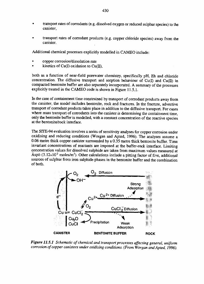
430
• transport rates of corrodants (e.g. dissolved oxygen or reduced sulphur species) to thecanister,
• transport rates of corrodant products (e.g. copper chloride species) away from thecanister.
Additional chemical processes explicitly modelled in CAMEO include:
• copper corrosion/dissolution rate• kinetics of Cu(I) oxidation to Cu(II),
both as a function of near-field porewater chemistry, specifically pH, Eh and chlorideconcentration. The diffusive transport and sorption behaviour of Cu(I) and Cu(II) incompacted bentonite buffer are also separately incorporated. A summary of the processesexplicitly treated in the CAMEO code is shown in Figure 11.5.1.
In the case of containment time constrained by transport of corrodant products away fromthe canister, the model includes bentonite, rock and fractures. In the fracture, advectivetransport of corrodant products takes place in addition to the diffusive transport. For caseswhere mass transport of corrodants into the canister is determining the containment time,only the bentonite buffer is modelled, with a constant concentration of the reactive speciesat the bentonite/rock interface.
The SITE-94 evaluation involves a series of sensitivity analyses for copper corrosion underoxidising and reducing conditions (Worgan and Apted, 1996). The analyses assume a0.06 metre thick copper canister surrounded by a 0.35 metre thick bentonite buffer. Timeinvariant concentrations of reactants are imposed at the buffer-rock interface. Limitingconcentration values for dissolved sulphide are taken from maximum values measured atAspo (3.12xl02 moles/m3). Other calculations include a pitting factor of five, additionalsources of sulphur from iron sulphide phases in the bentonite buffer and the combinationof both.
f~ Q ^ 0 2 Diffusion
StrongAdsorption
o^ Cu2+Diffusion .•
CuCI 2 DiffusionCuCQ ~ • " » " ;
ICu2° J>I CuCI ^^"^ Precipitation W e a k
Adsorption
CANISTER BENTONITE BUFFER ROCK
Figure 11.5.1 Schematic of chemical and transport processes affecting general, uniformcorrosion of copper canisters under oxidising conditions. (From Worgan and Apted, 1996).
431
Predicted containment times for general corrosion of copper under diffusion-limitedtransport of reactants (either dissolved oxygen or reduced sulphur species) are in the orderof 107 years or greater. These results are in agreement with earlier analyses, such as KBS-3(SKBF/KBS, 1983). Inclusion of sulphur from iron sulphides in the buffer has negligibleimpact on containment times.
Two exceptional cases can be identified. First, dissolved sulphate (which can be as muchas three orders of magnitude higher than dissolved sulphide species in Aspo waters) candiffuse through the buffer and might be reduced (perhaps microbially) at the copper surface.For such a condition, predicted containment times for general corrosion decrease to about104 years. Second, if extremely oxidising conditions (Eh=0.4 V, pH=9) can be sustained atthe copper surface, then the diffusive transport rate of copper chloride complexes maybecome the rate-limiting step in general corrosion of copper. Under such extremelyoxidising conditions, predicted failure times by general corrosion also decrease toapproximately 104 years.
The canister design assumed for the SllJb-94 analyses is presented in Figure 5.4.1, and hasa copper thickness of 0.05 m. Despite the slightly greater copper thickness used in theseconservative bounding calculations performed with the CAMEO code, the results are stillare considered sound. The results should not, however, be accepted as likely containmenttimes without a careful analysis of the assumptions and uncertainties. Some topics wheresuch caution needs to be observed may be the following:
• the process for resaturation of the repository with groundwater after closure,
• the attack on the canister by uniform corrosion, which can be expected to take placeat different rates on different parts of the surface due e.g. to differences in access tooxygen,
• possible significant reduction of the effective thickness of the canister if large poresof unfavourable shapes are present (e.g. defects from manufacturing),
• changes in groundwater chemistry with time:- intrusion of oxygenated water (e.g. in connection with a glaciation)- cyclic variations
• changes in the properties of the bentonite with time, including possibilities ofchannelling,
• reduction of sulphate ions through the action of microorganisms.
An interesting feature of the general corrosion calculations is that they indicate thesignificance of intact bentonite barriers and the importance of understanding phenomenathat might be detrimental to the functions of that low permeability, diffusion-control barrier.
General corrosion might be strongly enhanced if the chemistry becomes unfavourable, asdescribed above. Since the precise condition of the bentonite in the long-term is not known,no calculations have yet been made. However, it appears unlikely that even veryunfavourable chemistries would give rise to early failures by this mechanism.
432
In other fields of technology, where materials are used in corroding environments, a generalpattern can be observed. When comparatively rapidly corroding materials are used(thermodynamically unstable materials with little or no protecting layers), the lifetime isusually limited by general corrosion, perhaps with some localised character. When moresophisticated materials are used (highly protective layers are formed), corrosion failuretypically takes place as a result of localised corrosion, if it occurs at all.
The prerequisites for localised corrosion were discussed in Section 8.2.5. At present,essentially no calculation^ tools are available for simulation of localised corrosion oncopper under repository conditions. Therefore, only a general discussion can take place.
Section 8.2.4 noted that very few data exist regarding the frequency, size, shape andlocation of fissures in the copper canister. Such fissures might provide sites for crevicecorrosion. Moreover, for larger grain sizes, material may segregate to the grain boundariesand make such regions more susceptible to localised corrosion.
Corrosion of the steel canister
For the steel canister, only corrosion from the outside is considered in S1TE-94. Suchcorrosion is possible only if there is a penetration of the copper canister. In such a case,galvanic corrosion of the steel in contact with the copper canister is assumed to be thedominating mechanism for oxidising as well as reducing conditions (cf. Section 8.2.5). Forthe purpose of SITE-94, it is postulated that the lifetime of the steel canister is 1000 years,subsequent to failure of the copper canister. This postulate should not be interpreted as animplication that the life-time of the steel canister inside a penetrated copper canister isactually 1000 years under fully oxidising conditions.
Canister failures for the Reference Case and the Central Scenario
It should be clear from the above discussions that the number and character of canisterdefects will be distributed among the canisters and that the canisters will experience adistribution of chemical environments. This implies that canister failures will be distributedin time and that there will also be a distribution of the types of failure. Common causefailures have not been addressed.
In view of the conceivable effects discussed above, and for the purpose of SITE-94, it ispostulated (cf. Section 15.2.3) that a few of the canisters will lose their full integrity within100 000 years. The effect of an initial defect going all the way through steel and copper isinvestigated by postulating a pin-hole from the time of deposition (one calculation case, seefurther Section 15.2.3).
11.5.4 Chemical Conditions in a Failed Canister
The chemical evolution of the near-field is approximated in SITE-94, in terms of limitingconditions at equilibrium, or steady state, in three closed systems representing bentonite,iron corrosion products of the canister and spent fuel. In essence, this approximation ismade using a reaction-path model which contacts a reference amount of site groundwater(Section 10.4 and 11.2.3.4) with bentonite, canister corrosion products and spent fuel, one
433
after the other. The model is presented in Section 11.3.3.2 and described in full in Arthurand Apted (1996a, b). The canister part of the model and the calculated results aresummarised in this section.
The initial conditions that must be specified in the model include the temperature, solutionchemistry and mineralogy. Calculations are carried out for near-field temperatures of 15°Cand/or 80°C (see Section 12.2.3). Irreversible reactions among corrosion products of thecanister and solutions generated by prior reactions in bentonite (Section 11.3.3.2) aresimulated. As described in Section 5.4.1, the canister consists of an inner shell of carbonsteel and an outer shell of copper. Copper and its corrosion products are not explicitlymodelled, however. Copper has been selected, in part, because of its thermodynamicstability in water over a large range of mildly oxidising to mildly reducing conditions thatare similar to the redox conditions of many Swedish groundwaters.
In contrast to Cu°, Fe° in contact with water is thermodynamically unstable at alltemperatures and hydrostatic pressures expected in the near-field. Under anaerobicconditions, corrosion is induced by reactions involving H2O. It is assumed that increases inferrous ion concentration and the formation of corrosion-product layers would reducecorrosion to a low, steady-state value until all the Fe° in the canister is altered to corrosionproducts. It is also assumed, as a first approximation, that magnetite (Fe3O4) is the onlycorrosion-product mineral formed. After the metallic iron has completely corroded, thecomposition of the water in contact with the canister would therefore be controlled in thelong-term by an approach to equilibrium with magnetite.
Magnetite may react with mildly reducing to mildly oxidising near-field solutions to formone or more of several possible Fe(III) oxides, hydroxides, or silicate minerals (includingclay minerals). Studies of analogous conditions in geological systems indicate that ametastable Fe(III) solid, such as amorphous ferric oxyhydroxide (Fe(OH)3), wouldprecipitate initially, and that it would subsequently transform over geological time scalesinto more stable minerals such as goethite (a-FeOOH) and, finally, hematite (a-Fe2O3). Toevaluate the effects on near-field evolution of the formation of ferric-bearing alterationphases under oxidising conditions (see below), the conceptual model is constrained by twoalternative assumptions: (1) hematite is allowed to form, and (2) hematite is not allowed toform. In both cases, other ferric-bearing phases precipitate if conditions lead to theirstability. In SITE-94, radionuclide speciation-solubility behaviour is calculated only forcanister solutions generated in the absence of hematite. The effect of this conceptual-modeluncertainty on radionuclide behaviour is discussed in Arthur and Apted (1996a), and theresults are summarised below.
Redox conditions are assumed to be determined by magnetite reactions at 15°C and/or80 °C with solutions evolved from bentonite. An alternative constraint of fixed O2(g) partialpressure (= 0.2 bar assumed for conservative, strongly oxidising conditions) is also adoptedin some cases, to simulate conditions that could be generated by a-radiolysis, or by contactof the buffer and canister with oxidising groundwaters. These temperatures, initial solutioncompositions and redox constraints represent conditions that could be generated in theReference Case or Central Scenario.
Seven conceptual models of near-field evolution are defined accordingly (Section 12.2.3)and representative results of the calculations are shown in Tables 12.3.1 and 12.3.2.
434
Radionuclide solubilities in the canister-equilibrated solutions corresponding to thesemodels (Section 12.3) are then used in the radionuclide transport calculations (seeChapter 15).
The general conclusions from these results, mainly with respect to the effects ofuncertainties inherent in site properties (groundwater chemistry) on PerformanceAssessment results (radionuclide speciation-solubility behaviour), are summarised in thefollowing paragraphs. It should be emphasised, however, that these conclusions are basedon very limited analyses.
Reaction of magnetite with bentonite porewaters is predicted to have minor effects onsolution chemistry and virtually no effect on aqueous-phase parameters that are importantdeterminants of radionuclide speciation-solubility behaviour. Dissolved Al concentration(which is relatively low in unreacted groundwater) is calculated to decrease by as much as9 orders of magnitude, however, and Fe concentration increases by factors of between 10and 100. The concentrations of other constituents are nevertheless virtually unchanged, asare pH and Eh.
Such minor changes in calculated solution compositions indicate that bentonite-equilibratedporewaters are close to equilibrium with magnetite under reducing conditions and inequilibrium with magnetite alteration phases when both bentonite and the canisterexperience strongly oxidising conditions. Magnetite equilibrates with goethite and anontronitic smectite (i.e., Fe3+ is the principal cation occupying octahedral sites) underreducing conditions at 15°C. A similar assemblage is generated at 80 °C, but pyrite, ratherthan goethite, coexists at equilibrium. Magnetite is unstable under the strongly oxidisingconditions assumed in some calculations. It dissolves completely in such instances and isreplaced by goethite and nontronitic smectite. It is important to note that aqueous-phaseredox potentials are then controlled by the assumed fixed-fugacity constraint on O2(g) andthe equilibrium reaction:
and not by the Fe-bearing alteration phases.
The speciation and solubility behaviour of radionuclides in solutions contacting the canistercorrosion products are similar to those in corresponding bentonite-equilibrated solutions(for one example, see Table 12.3.1 showing the results from Model 1). This is becausesolution parameters controlling radionuclide speciation-solubility behaviour are nearlyidentical in both cases, which further underscores the possible importance of buffering ofnear-field chemistry by bentonite-water interactions.
Solution compositions generated by magnetite-water reactions differ significantly fromthose discussed above if hematite is assumed to be a possible reaction product. Hematiteis more stable than goethite and nontronitic smectite, but its formation may be kineticallyhindered over geological timescales. Nevertheless, if conditions permit hematiteprecipitation (e.g., given sufficient time and/or increasing temperature), calculations suggestthat solution compositions in the above models would be controlled by reactions leadingto a stable assemblage of magnetite + pyrite + hematite (Arthur and Apted, 1996b).Predicted equilibrium conditions are strongly reducing (<-0.5V) and hyperalkaline
435
(>pH 12), and calculated solubilities of several radionuclides differ by orders of magnitudecompared to solubilities shown in Tables 12.3.1 and 12.3.2. This suggests that uncertaintiesin conceptual models of near-field evolution of chemistry could be of similar importanceto uncertainties in site properties.
11.5.5 Conclusions and Implications for Other Parts of theAssessment
The SITE-94 assessment of canister longevity is, to a large extent, of a qualitative nature.It appears that both mechanical and chemical mechanisms can be identified which wouldpotentially lead to failure. Common cause failures have not been addressed. In light of thesequalitative results and the intended purpose of SITE-94 to evaluate site characterisation andsite performance issues, it is concluded:
• SITE-94 will assess the consequence of a complete canister failure after 1000 years,10 000 years and 100 000 years, knowing that such failure may in fact occur for onlya few canisters at any of these times.
• SITE-94 should not assess the consequences of a multiple canister failure, as anyestimate of the number failed would be highly uncertain. Instead, the consequenceanalyses should be performed for single canister failures, knowing that the overallimpact of a full repository would be to superimpose the effect of few such failures.
Chapter 15 discusses how these general conclusions are used to formulate actual radio-nuclide transport calculation cases.
The general conclusions drawn from modelling the evolution of the conditions in a failedcanister must be regarded as preliminary, with respect to the limited analysis. Theconclusions mainly concern the effects of uncertainties inherent in site properties(groundwater chemistry) on Performance Assessment results (radionuclide speciation-solubility behaviour).
Reaction of magnetite (used as a model for the canister corrosion products) with bentoniteporewaters is predicted to have minor effects on solution chemistry and virtually no effecton aqueous-phase parameters that are important determinants of radionuclide speciation-solubility behaviour. This underscores the possible importance of buffering of near-fieldchemistry by bentonite-water interactions.
With other phases included, e.g. if hematite is assumed to be a possible reaction product,quite different solution compositions are generated. This suggests that uncertainties inconceptual models of near-field evolution of chemistry could be of similar importance touncertainties in site properties.
436
11.6 RADIOLYSIS
This section discusses radiolysis and thus corresponds to part of the discussion necessarywithin the Fuel Degradation and RN-release Clearing House in the AMF (Figure 2.4.5).Fuel dissolution mechanisms is discussed in Section 11.8 and redox front formation inSection 11.7.
Ionising radiation from the spent fuel can decompose water present in the inner regions ofthe EBS into hydrogen and oxidants, mainly hydrogen-peroxide and oxygen. For thecopper-steel canister concept, it is possible that water may be present in the canister at thetime of manufacture. In that case, radiolysis will start immediately on encapsulation.Radiolysis can also occur in the water surrounding the canister in the deposition hole, butonly gamma radiation can penetrate out through the canister wall and it will be attenuatedconsiderably. Therefore, the effects and the consequences of gamma radiolysis are notconsidered in detail in SITE-94.
The most significant radiolysis, from the Performance Assessment point of view, will takeplace via alpha radiation, when water reaches the fuel surface after canister failure. Thisprocess is important for understanding and modelling the oxidation of the fuel matrix andthe subsequent release of radionuclides (see Section 11.8). In addition, oxygen speciesformed by alpha radiolysis might migrate through oxidised parts of the canister, reach thebentonite buffer and rock and form a redox front in the otherwise reducing environment (seeSection 11.7).
Alpha radiolysis as a source for oxidants in the near-field was treated in detail in theProject-90 report (SKI, 1991). It was concluded that a very simple, but reasonable, modelfor the rate of oxidant production (Gox, e.g. moles/tonne, year) would be a directproportionality with the alpha activity (A, e.g. GBq/tonne),
GoxW^Att ) (Eq. 11.6.1)
This relation gives the time-dependence of oxidant production rate. The proportionalityconstant k^ depends on a range of factors. As shown by, e.g., Christensen and Bjergbakke(1982), the most important of these is the chemical environment at the fuel surface, e.g. thepresence or absence of iron species acting as 'catalysts' for recombination of reducing andoxidising radiolysis products . Another factor is the physical state of the fuel, in particularits specific surface area, which depends on the sizes of fuel fragments. In SITE-94, the valueon kox used in Project-90 has been retained.
When it is assumed that part or all of the produced oxidant reacts with the fuel, causing itsdissolution, this process occurs at a rate proportional to the alpha decay rate (seeSection 11.8).
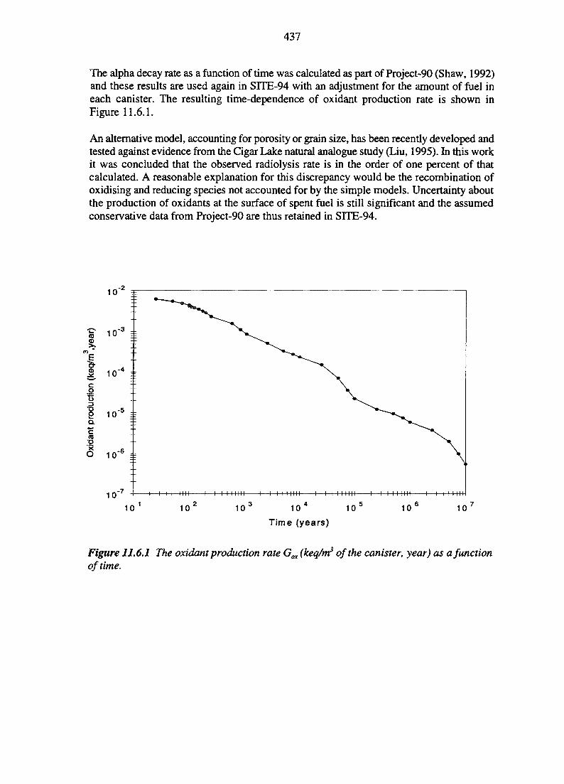
437
The alpha decay rate as a function of time was calculated as part of Project-90 (Shaw, 1992)and these results are used again in SITE-94 with an adjustment for the amount of fuel ineach canister. The resulting time-dependence of oxidant production rate is shown inFigure 11.6.1.
An alternative model, accounting for porosity or grain size, has been recently developed andtested against evidence from the Cigar Lake natural analogue study (Liu, 1995). In this workit was concluded that the observed radiolysis rate is in the order of one percent of thatcalculated. A reasonable explanation for this discrepancy would be the recombination ofoxidising and reducing species not accounted for by the simple models. Uncertainty aboutthe production of oxidants at the surface of spent fuel is still significant and the assumedconservative data from Project-90 are thus retained in SITE-94.
n
*3 --3
1 0 " " EE
1 10-5 *acCO
O 10"6 n
10 -7 l i l t Mil 1—I I4HIII 1—h-H-t HII 1—h-H Hill 1—I I-H-H--H 1—1-4- I H
10 1 102 103 104 105 106 107
Time (years)
Figure 11.6.1 The oxidant production rate Gox (keq/m3 of the canister, year) as a functionof time.
438
11.7 REDOX CONDITIONS
This section discusses redox conditions and formation and propagation of redox fronts. Theresulting input to consequence calculations are discussed in Chapter 15.
Different oxidation states of some of the radionuclides (Tc, Np and Se) behave chemicallyquite differently, which makes it important to determine the redox state of the migrationpath. The redox state is governed by the initial barrier conditions as well as by any redoxreactions causing changes in the redox state of solids. The redox capacity of thegroundwater may also play a role, in particular by scavenging oxidants being transportedby flow, along fractures.
11.7.1 Initial Redox Conditions
The redox state of the predominantly granitic, aplitic and dioritic rocks at Aspo is largelycontrolled by their content of iron-bearing minerals, e.g. magnetite, biotite and pyrite. Thegroundwater at Aspo shows low concentrations of Fe(II). Direct measurements of the redox-potential in the deep groundwaters give values generally close to -0.30 V (seeSection 7.4.4). Experimental data for the Aspo rocks shows reducing capacities whichsupport the selection of a redox capacity of 0.04 keq/m3, see further Section 7.4.2 andAndersson (1996).
The mineralogy of the bentonite in the EBS is similar to that of an MX-80 type (seeSection 8.3.2). The redox condition in the bentonite buffer, after resaturation, is reducingand the redox potential has been calculated to be -0.25 to -0.33 V (see Section 11.3.3). Thesame redox capacity is selected for the bentonite as that used in Project-90, i.e. 0.15 keq/m3
(Ericsen and Jacobsson, 1983) since no new literature data were found (Andersson, 1996).
The redox potential inside the canister will probably be reducing due to the large contentof iron. Although oxidants are produced inside the canister, conditions will remainreducing, except for certain parts, which may be oxidised by migrating oxidants.
11.7.2 Formation and Propagation of Redox Fronts
The redox-front concept has been accepted as an important part of near-field PerformanceAssessment since its first presentation in connection with KBS-3 (Neretnieks, 1982;Neretnieks and Aslund, 1983). A redox front in the system may be caused by three possibleeffects:
1. The possible establishment of oxidising conditions due to radiolysis in the closevicinity of the fuel and the change to reducing conditions further out in the near-field.
2. Formation of an oxidised zone around the repository before closing and resaturation.
3. The change of water chemistry when oxidising surface water enters the system.
439
The first cause is seen as the principal reason for inclusion of a redox front in the analysisand requires an estimate of the extent and consequence of an oxidised zone surrounding abreached canister. The importance of the second cause has not been analysed. The thirdcause may be of importance in case of glaciation in the Central Scenario, but has not beenconsidered likely for the Reference Case.
The oxidants produced by radiolysis of water (see Section 11.6) at the fuel surface maymigrate out from the surface, through the broken canister wall, through the bentonite bufferand penetrate the rock matrix and its fractures. The oxidant production rate exhibitsconsiderable uncertainty, over several orders of magnitude. A further uncertainty concernsthe migration distance of the oxidants, since the original metal content in the canister couldbe sufficient to preclude any propagation of the front (Shaw, 1992). Reducing agents,primarily ferrous iron, in the barriers and rock consume the oxidants as they migratethrough the barriers and decrease their migration rate. Since oxidants can only migrate inan oxidised environment, any available reductants present along the transport path must firstbe oxidised. This means that the propagation rate and extent of the front decrease inproportion to the availability of reductants in the barriers.
11.7.3 Modelling Near-field Redox Conditions in SITE-94
The uncertainties in the propagation of oxidants through the near-field barriers and the near-field rock are reflected in the selection of four redox variants in the consequence analysis,which cover the full range, from fully oxidising to fully reducing conditions in the near-field. These variants are:
• the zero variant, which assumes reducing conditions everywhere, except on the fuelsurface
• a variant which assumes oxidising conditions throughout the near-field,
• a variant which calculates the propagation of a redox front, as will be describedbelow (corresponds to (a) in Figure 11.7.1),
• a variant which assumes a redox front is present a few metres into the rock, withoxidising conditions inside the front (corresponds to (c) in Figure 11.7.1, as anextreme of the case (b) in Figure 11.7.1).
These variants are further specified in Section 15.2.2.
The migration of the redox-front in the near-field (including near-field rock), i.e. the thirdvariant above, can be calculated with the near-field transport code CALIBRE (Worgan andRobinsson, 1995). In the model, once the container has failed, the oxidants diffuse throughthe canister and buffer and reach the rock matrix and a water-filled fracture. The oxidantproduction rate, expressed as a time series in moles per cubic metre of canister, is specified,together with the redox capacities of the waste form (canister, fuel, filler and cladding),bentonite and rock. The radionuclide transport calculations take account of the calculatedredox potential throughout the system by adjusting the values of elemental solubility limitsand retardation properties. In modelling the redox-front in the present version of CALIBRE,
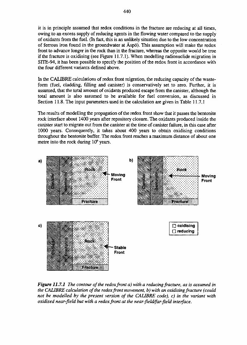
440
it is in principle assumed that redox conditions in the fracture are reducing at all times,owing to an excess supply of reducing agents in the flowing water compared to the supplyof oxidants from the fuel. (In fact, this is an unlikely situation due to the low concentrationof ferrous iron found in the groundwater at Aspo). This assumption will make the redoxfront to advance longer in the rock than in the fracture, whereas the opposite would be trueif the fracture is oxidising (see Figure 11.7.1). When modelling radionuclide migration inSITE-94, it has been possible to specify the position of the redox front in accordance withthe four different variants defined above.
In the CALIBRE calculations of redox front migration, the reducing capacity of the waste-form (fuel, cladding, filling and canister) is conservatively set to zero. Further, it isassumed, that the total amount of oxidants produced escape from the canister, although thetotal amount is also assumed to be available for fuel conversion, as discussed inSection 11.8. The input parameters used in the calculation are given in Table 11.7.1
The results of modelling the propagation of the redox front show that it passes the bentoniterock interface about 1400 years after repository closure. The oxidants produced inside thecanister start to migrate out from the canister at the time of canister failure, in this case after1000 years. Consequently, it takes about 400 years to obtain oxidising conditionsthroughout the bentonite buffer. The redox front reaches a maximum distance of about onemetre into the rock during 106 years.
a)
Fracture
b)
MovingFront
MovingFront
c) H oxidisingG reducing
Figure 11.7.1 The contour of the redox front a) with a reducing fracture, as is assumed inthe CALIBRE calculation of the redox front movement, b) with an oxidising fracture (couldnot be modelled by the present version of the CALIBRE code), c) in the variant withoxidised near-field but with a redox front at the near-field/far-field interface.

441
Table 11.7.1 Input parameters for the calculation of redox front migration.
Parameter
Reducing capacity, 'waste-form'
Reducing capacity, bentonite
Reducing capacity, rock
Proportion of oxidants produced that are madeavailable for redox front migration
Oxidant production rate as a function ofcanister failure time
Value
0
0.15
0.04
100
See Table 11.8.1
Unit
keq/m3
keq/m3
keq/m3
%
11.8 FUEL DISSOLUTION
This section discusses fuel dissolution mechanisms and thus corresponds to part of thediscussion necessary within the Fuel Degradation and RN-release Clearing House in theAMF (Figure 2.4.5). The radionuclide release mechanisms are discussed in Section 13.2 andthe resulting input to consequence calculations are discussed in Chapter 15.
11.8.1 General
One of the major mechanisms believed to determine the release rate of radionuclides fromspent fuel is a release congruent with the dissolution/conversion of the fuel matrix into anoxide of uranium in a higher valency state. Other important mechanisms are a partial butrapid (instantaneous) release of some soluble elements present in cracks and in the gapbetween fuel and cladding (e.g. Cs, I) and also an intermediate rate of release for someelements from, for example, grain boundaries (e.g. Cs, I, Sb, Mo, Tc and, possibly, Sr). Thissection describes briefly the mechanism(s) for fuel conversion; for a more detaileddiscussion, see SKI (1991).
Although not yet experimentally confirmed, it might be expected that (alpha) radiolysis ofwater causes oxidation of uranium (matrix conversion). As explained in Section 11.6, theuncertainty in the prediction of oxidant production rate is great. The maximum amount ofuranium that can be oxidised depends on when radiolysis starts (the time of canister failure).The rate of oxidation decreases from the start, due to decay of the alpha emittingradionuclides, giving the fastest matrix conversion for immediate canister failure times.
The concepts for fuel dissolution and matrix release mentioned in the literature mostly dealwith explanations of results from leaching experiments. This rather limits consideration ofthe availability and behaviour of oxidants under conditions relevant for the long-term in arepository. These difficulties must be kept in mind when reviewing the literature forconcepts of importance for a predictive release model. Fuel dissolution and related subjectshave been reviewed by Grambow (1989; 1990) and Johnson and Shoesmith (1988).
442
The redox condition of the aqueous phase adjacent to the fuel surface is determined by thebalance of various rate processes, e.g.:
• production rate of oxidant,
• transport rate of oxidant away from the surface,
• rate of uranium oxidation,
• rates of other reactions consuming oxidant (including recombination, e.g. as catalysedby surface reactions),
• transport rate of (oxidised) uranium from the surface,
• transport rates of other reactants.
Evidently, it is a non-trivial task to model the combined effect of these processes even forwell-defined (laboratory) conditions. It is currently not possible, given our present levelsof understanding, to analyse the effect for conditions relevant to a breached canister in arepository. Thus, it is necessary to rely on bounding assumptions, in particular for regulatorypurposes.
The redox condition determines which oxide phase is stable. For slow oxidant production,U4O9 or U3O7 might be stable. When the 4-9 oxide is the stable phase, the attack on thesurface will come to a halt as soon as a protective layer of this oxide has formed. The matrixdissolution is then controlled by the rate of uranium transport from the surface, with thesolubility of the 4-9 oxide as an inner boundary condition. It is not certain that the 3-7 oxidewill form a similar protective layer, but this uncertainty in stoichiometry should be ofnegligible importance, considering all other uncertainties.
For higher production rates of oxidant, the 3-8 oxide will form, which also means a definitedisruption of the matrix structure since this oxide cannot be incorporated in the dioxidecrystalline structure. Thus, the oxidation and conversion will propagate through the layerof 3-8 oxide and this rate will depend only on the supply of oxidant at the corroding surface.
In its highest state of oxidation, uranium will probably occur as schoepite (UO3*2H2O orUO2(OH)2-H2O). From the viewpoint of all other uncertainties, the different stoichiometryof schoepite and the 3-8 oxide may be neglected in the mass balance of oxidant.
In SITE-94, the rate of fuel matrix conversion is assumed to correspond to the oxidantproduction rate and the most conservative assumption for the rate of matrix conversion isthat all the oxidant produced will oxidise the fuel. Likewise, and also conservatively, it hasbeen assumed that all the oxidant produced is available in the case of a redox front forming(see Section 11.7).
A similar approach, i.e. a direct proportionality between alpha decay rate and rate of fueldegradation, was used in SKB 91 (SKB, 1992) and in TVO 92 (TVO, 1992), although withless conservative assumptions regarding the degradation rate based on results from leachingexperiments.
11.8.2 Thermodynamic Modelling of Spent Fuel Oxidation
The chemical evolution of the near-field is approximated in SITE-94 in terms of limitingconditions at equilibrium, or steady state, in three closed systems representing bentonite,iron corrosion products of the canister and spent fuel. The model is a reaction-path modelcontacting a reference amount of site groundwater (Sections 10.4 and 11.2.3.4) withbentonite, canister corrosion products and spent fuel, one after the other. The model ispresented in Section 11.3.3.2 and described in full in Arthur and Apted (1996a, b).
The results from the speciation-solubility calculations reveal the complexity of the spentfuel/water interaction and the difficulty of modelling it as a closed system. The treatmentof carbon is an illustrative example. The CO2 fugacities are assumed to be fixed in order tominimise the effects of acidification from release of carbon from the fuel. Since the CO3
2*is an important complexing agent, this assumption will influence the speciationunacceptably. It is concluded that realistic models that treat the spent fuel/water interactionswill need to have transport included.
For the SITE-94 radionuclide transport calculations, the solubility limits in the 'waste-form'part of the near-field code CALIBRE are taken as the lowest from the water interaction witheither spent fuel or canister corrosion products, see Table 12.3.2. (The CALIBRE code doesnot distinguish between the real waste form, spent fuel, and the interior of the canister, seeChapter 13.)
11.8.3 Implications for the Assessment - Modelling of TimeDependence for Fuel Dissolution in SITE-94
The oxidant production rate as a function of time is derived from the alpha radiolysis, asdescribed in Section 11.6. By integrating Equation 11.6.1, the accumulated amount ofoxidants produced can be derived as a function of time. The integration starts at canisterfailure time, when water reaches the fuel surface. In Figure 11.8.1, the amount of oxidantsproduced is shown as a function of time for different canister failure times. As the oxidantproduction rates are only available for time intervals, the integration is performed as astepwise summation.
With the dissolution of the fuel matrix seen as a transformation of UO2 into U3O8
(Section 11.8.1) and the oxidants as hydrogen peroxide, 2 moles of oxidant transform3 moles of uranium. The total amount of uranium oxide to be oxidised is given in theSITE-94 inventory (Section 3.3.2) and, hence, the required amount of oxidants can becalculated. This is shown in Figure 11.8.1 as a horizontal line.
It is clear that linearisation of these curves would be reasonable, considering all otheruncertainties in the model. The resulting oxidant production rates and durations of fuelmatrix dissolution obtained after linearisation are presented in Table 11.8.1.
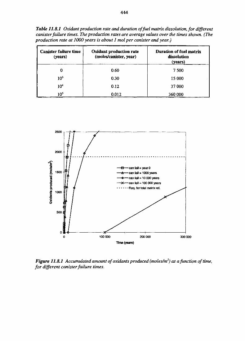
444
Table 11.8.1 Oxidant production rate and duration of fuel matrix dissolution, for differentcanister failure times. The production rates are average values over the times shown. (Theproduction rate at 1000 years is about 1 mol per canister and year.)
Canister failure time(years)
0
103
104
1O5
Oxidant product ion rate(moles/canister, year)
0.60
0.30
0.12
0.012
Duration of fuel matrixdissolution
(years)
7 500
15 000
37 000
360 000
2500
D can fail = year 0
-can fail = 1000 years
-can fail = 10 000 years
-can fail = 100 000 years
• Req. for total matrix re!.
100 000 200 000 300 000
Time (years)
Figure 11.8.1 Accumulated amount ofoxidants produced (moles/m3) as a function of time,for different canister failure times.
445
12 CHEMISTRY AND BEHAVIOUR OFRADIONUCLIDES
12.1 INTRODUCTION
When describing the rate of transport of radionuclides it is not only necessary to considergroundwater flow and diffusion processes, but also to take into account the mobility of thedifferent radionuclides. The mobility of an element is determined by its partition betweensolids and solution, i.e. by its solubility and its tendency to sorb onto solid surfaces.
This chapter describes how the chemical behaviour of radionuclides is predicted based oninformation on the geochemical conditions in various parts of the repository ProcessSystem and for different time frames. The discussion covers all high importance FEPs andinfluences in the SITE-94 Process Influence Diagram. The general aspects of modellingradionuclide chemistry, in particular speciation and solubility, are described in Section 12.2,together with the assumptions made for the calculations in SITE-94. The results ofcalculations in terms of solubilities and speciation are presented and discussed inSection 12.3. Sorption mechanisms and different approaches to evaluate sorption onmineral surfaces are discussed in Section 12.4, where sorption data for the bentonite andthe rock also are given.
12.2 MODELLING RADIONUCLIDE SPECIATION ANDSOLUBILITY
12.2.1 General
The low solubility of many radionuclides is an important constraint limiting theirconcentration and, hence, their transport rate. Here, the term solubility refers to the totalaqueous concentration of a radioactive element among all isotopes and species that are inequilibrium with each other and with a solid phase comprising the element. Solubilities canbe calculated with the aid of chemical thermodynamic models and standard-statethermodynamic data. The models describe the state of an aqueous solution in terms of theconcentrations and activity coefficients of simple ions, ion pairs and complexes. Solubilitiesare calculated in such models on the basis of heterogeneous-equilibrium constraints (i.e.,specification of solubility-controlling phases) for each element considered. Becauseaqueous speciation and solubility are interrelated, the models are often referred to asspeciation-solubility models.
Radionuclide solubilities may constitute credible upper bounds on the source term inPerformance Assessment models if solubility-controlling phases are selected such that theyare:
446
• well-defined thermodynamically,
• conservative choices in the sense that resultant equilibrium concentrations aregreater than might realistically be expected.
Radionuclide solubilities then represent deliberately maximised estimates for givenconditions of temperature, pressure and solution composition. Radionuclide concentrationscontrolled by other possible reactions, such as sorption, must be less than or equal toconcentrations limited by solubility equilibrium. Similarly, the solubility of a solidcomposed dominantly or partially of a radionuclide component in solid solution should beless than that of the corresponding pure component (e.g., SKI, 1991; Anderson and Crerar,1993). (Examples exists, however, which seem to contradict this important basicassumption).1
Radionuclide solubilities can be calculated for systems in which charge balance,mass-action and mass-balance constraints among relevant components and phases can bequantified (e.g., Anderson and Crerar, 1993). Computer programs are required to solve theresultant sets of nonlinear equations when dealing with complex multicomponent,multiphase systems such as will exist in the near-field. More than 80 speciation-solubilityprograms are described by Andersson (1987). EQ3/6 (Wolery et al., 1992), PHREEQE(Parkhurst et al., 1985), MINEQL (Morel and Morgan, 1972) and MINTEQA2 (Allison etal., 1993) are among the most widely used codes supporting the development of geologicaldisposal systems for radioactive wastes.
A number of limitations must be recognised, however, when thermodynamic models areused to calculate radionuclide solubilities.
Given relevant thermodynamic data, the total aqueous concentration of a radioelement ina water of specified and constant properties is easily calculated. This simple approach isoften used and it gives correct results if the water properties (pE, pH and ligandconcentrations) are appropriately buffered. If this is not the case, the direction of reactionand the availability of reacting components, solids and solutes within a specified systemmust be considered. It should be noted here that the available reactants are not onlydetermined by initial conditions but also depend on possible mass transfer to and from thesurroundings. This is the same as admitting that only a coupling of chemistry and transportwill give useful results.
This problem is highlighted in particular when it is not assumed that the radioelement is amicrocomponent and, thus, that its presence does influence the macrosystem. It isemphasised even more when it is simultaneously recognised that the radionuclide behaviouris governed by a range of different microenvironments due to the heterogeneous character
1 Such behaviour may be reversed, however, if excess free energy of mixing is positive. Bricker and Garrels(1967; see also Stumm and Morgan, 1981) showed, for example, that the equilibrium concentration of Ca2+
in aqueous solutions coexisting with magnesian calcites increases with increasing concentrations of MgCO3
in these non-ideal solid solutions. High-Mg calcites (i.e., > 6 mol%) are metastable relative to pure CaCO3,but this metastability evidently persists over geological timescales. Similar experimental studies of solid-solution behaviour among radionuclide-containing solids are few (Bruno and Sandino, 1987; Bruno et al.,1985), however, and it is therefore unclear at present whether pure radionuclide solids are necessarily moresoluble than solid-solution phases in all cases.
447
of the geochemical system. Conversely, in an homogeneous system, and with an assumedimmediate access to unlimited amounts of reactants, and thus where the radioelement maybe considered as a microcomponent, this conceptual uncertainty should be of minorimportance. This is the simplified approach used in the calculations described below.
Deficiencies in the availability, accuracy and consistency of thermodynamic data aredescribed in Section 12.2.2. An approach to evaluate the effects on radionuclide solubilitiesof:
• uncertainties associated with natural variations in site groundwater chemistry,
• uncertainties inherent in models of the chemical evolution of the near-field,
• uncertainties in radionuclide speciation-solubility behaviour
is described in Section 12.2.3. Owing to these uncertainties, a number of simplifications aremade in deriving a radionuclide solubility database for SITE-94. The general approach isoutlined in the following paragraphs and is described further by Arthur and Apted (1996a).
12.2.2 Thermodynamic Data
This section discusses the thermodynamic data needed to model radionuclidespeciation-solubility behaviour and to document potential sources of uncertainty in thesedata. Sources of thermodynamic data supporting SITE-94 calculations are identified byArthur and Apted (1996a).
The primary data needed in most speciation-solubility models include equilibrium constantsfor formation of aqueous species and for heterogeneous reactions involving solubility-controlling solids. These data are temperature-dependent and reaction enthalpies and partialmolal quantities, such as isobaric heat capacities, are required to calculate equilibriumconstants at a given temperature of interest. Other thermodynamic data needed inspeciation-solubility models include temperature-dependent parameters for calculation ofactivity coefficients and water activity in electrolyte solutions. A detailed evaluation of datarequirements in thermodynamic models is given by Johnson et al. (1992) and Anderson andCrerar(1993).
An important source of uncertainty in the results of radionuclide speciation-solubilitymodels stems from inadequacies in the availability, accuracy or consistency ofthermodynamic data for formation of solubility-controlling solids and aqueous species. Thestatus of these potential limitations in thermodynamic data supporting SITE-94speciation-solubility calculations is described below.
An evaluation of the inorganic solution chemistry of actinide and fission product ionsprovides insight concerning thermodynamic data that should be included inspeciation-solubility models for these elements. Thus, thermodynamic data for hydrolysisreactions are likely to be of primary importance in such models. Hydrolysis of theseelements is probable because many of them occur in high valency states (+III or higher) andbecause the acidity of these ions generally increases with increasing oxidation state (e.g.,
448
Baes and Mesmer, 1976; Stumm and Morgan, 1981). Also, because precipitation of oxides,hydrous oxides and hydroxide minerals represents the final stage of formation ofpolynuclear complexes from mononuclear hydrolysis species (Stumm and Morgan, 1981),it is reasonable to assume that many radionuclide solubilities could be controlled by theseminerals under near-neutral to alkaline conditions.
However, it is important to reiterate that, in reality, such solubilities are more likely to becontrolled by solid-solution phases than by pure solids.
The relatively low oxidation states of the aqueous ions of some radionuclides, such as Ni2+
and Sr2"1", may limit the effects of hydrolysis to strongly alkaline conditions, and othercomplexes may dominate the aqueous speciation of these elements over a broad pH range.Carbonate species are particularly important complexing ligands because they form strongcomplexes with some important radionuclides and because their concentrations in naturalgroundwaters are generally greater than concentrations of other possible ligands, such asphosphate and fluoride. Other common anionic constituents of groundwaters, such assulphate, chloride and bromide, do not form strong complexes with actinides and mostfission-product cations. In an analogous way to the behaviour of oxide precipitates ofhydrolysis species, carbonate minerals may be solubility-controlling in cases whereradionuclide speciation is dominated by carbonate complexes. Carbonate minerals arefrequently less soluble than corresponding oxides/hydroxides (Stumm and Morgan, 1981),but are more soluble than other minerals, such as silicates or aluminosilicates.Consequently, they are moderately conservative choices as solubility-controlling phases.
For these reasons, oxides and carbonates are assumed as a first approximation to bepossible solubility-controlling solids in SITE-94. The primary aqueous species of interestare the radionuclide hydroxy and/or carbonate complexes. Thermodynamic data for thesesolids and aqueous species are available for most of the radionuclides considered (Am, Np,Pu, Tc, Th, U, Ni, Sn, Sr and Zr). In the absence of appropriate thermodynamic data (i.e.Ra and Se), other phases are selected, as noted below, or source-term concentrations areassumed to be unlimited by solubility constraints (i.e. Cs and I).
A complicating factor in this approach is the tendency among (primarily) the actinides toform amorphous hydrous oxides on initial precipitation from aqueous solutions (Rai et al.,1990; SKI, 1991; Grenthe et al., 1992). Further complications arise from self-irradiationeffects, which can cause initially crystalline solids to become amorphous with time (Rai andRyan, 1982). These effects are mitigated to some extent by the tendency for amorphoussolids to re-crystallise with ageing (Strickert et al., 1984; Yui, 1993). Consequently, it isuncertain whether solubility-controlling actinide phases should be considered as crystallineor amorphous solids. The solubilities of the amorphous solids may be of primary interestin Performance Assessments, however, because metastable supersaturations wouldcorrespond to higher solubilities and thus to conservative constraints on source-termconcentrations.
The solubilities of both crystalline oxides and amorphous hydrous oxides of U(IV), Np(IV),Pu(IV), Th(IV) and Ni(IT) are therefore calculated in SITE-94. Comparison of calculatedsolubilities between crystalline and amorphous solids of these radionuclides underconditions that could be generated in the near-field provides insight concerning the effects
449
of uncertainty in the crystallinity of solubility-controlling phases on radionuclideconcentrations that constrain the source term in Performance Assessment calculations.
The solubility-controlling phases for other radionuclides, for which thermodynamic datafor amorphous solids are unavailable, are assumed to be crystalline oxides (Sn, Zr, U(VI)),elemental solids (Se°), carbonates (Sr, Np(V)), hydroxy carbonates (Am), or sulphates (Ra).Calculations are carried out to determine differences in solubilities when other phases (e.g.sulphides, selenides, silicates) more stable than these crystalline solids are assumed to besolubility-controlling.
Potential radionuclide species other than hydroxy and carbonate complexes are alsoconsidered in these calculations. Many of the radionuclides may be strongly complexed byphosphate or fluoride ligands, for instance, although experimental determinations ofrelevant formation constants are lacking (Andersson, 1988). Nevertheless, availableestimates of formation constants for fluoride and phosphate complexes of Am(HT),Np(IV/V), Pu(IV/V), Sr(II), Th(IV) and U(IV/VI) are adopted in the calculations. Estimatedformation constants for fluoride complexes of Sn(II) and Zr(IV) are also utilised.
The effects on radionuclide solubility of organic complexes are not considered in S1TE-94because measured or estimated thermodynamic data are lacking or are of questionablerelevance. Organic ligands in deep groundwaters are primarily humates and fulvates, whichmay be particularly important for trivalent radionuclides (e.g. Andersson, 1988). Humicacids are also known to complex Np(V) species (Moriyama et al., 1995). Modelling theeffects of these ligands on radionuclide solubilities is complicated, however, because theircomplexing behaviour is influenced by ionic strength, the presence of other cations and bythe degree of protonation of functional groups comprising these high molecular weightligands. Further study is needed to evaluate the potential importance of organic complexeson radionuclide solubilities.
A problem related to the availability of thermodynamic data for radionuclide complexes isthe presence in databases of data for potential solubility-controlling solids that are notrelevant to the conditions of interest. For example, Ca and Sr uranates and zirconates(CaUO4, CaZrO3, a-SrUO4 and SrZrO3) are calculated to be extremely insoluble, but theyare not observed in experiments, possibly for kinetic reasons. Similarly, the calculatedsolubilities of spinel minerals such as trevorite (NiF^OJ are extremely low, but suchminerals are not observed in experimental or natural systems at relatively low temperatures(Bruno et al., 1991). These solids are therefore excluded in SITE-94 to avoid calculationof potentially non-conservative solubilities for U, Sr, Zr and Ni.
In addition to the availability of thermodynamic data, uncertainty in speciation-solubilitymodels may also result from inaccuracies in existing thermodynamic data. Evaluating theaccuracy of thermodynamic data is a complex and time-consuming task, as evidenced bythe recent NEA/OECD effort in compiling a selected set of consistent thermodynamic datafor inorganic aqueous species and solid phases of uranium (Grenthe et al., 1992; see alsoSKI, 1991, Wanner, 1990 and Nordstrom and Munoz, 1985).
Because such evaluations are presently unavailable for many radionuclides and are outsidethe scope of SITE-94, the results of the speciation-solubility calculations must be
450
considered with regard to possible inaccuracies in the thermodynamic data supporting thecalculations.
The approach to dealing with this problem in SITE-94 is to compare calculatedradionuclide solubilities to the results of experiments conducted under conditions that aresimilar to those expected in the near-field (Arthur and Apted, 1996a). This is analogous toan approach by Puigdomenech and Bruno (1991; 1988) to develop thermodynamicdatabases for Pu and U, respectively. In the absence of experimental data, expert judgementis used to define speciation-solubility models that are representative of the knowngeochemical behaviour of stable isotopes of the radionuclides in environments that areanalogous to expected near-field conditions. The approach is useful in identifyingthermodynamic data for solids and aqueous species that are clearly inconsistent withobserved solubility behaviour. It does not, however, constitute a test of the accuracy ofthermodynamic data supporting the model, nor should it imply confidence in model resultsfor conditions that are outside an experimental range.
In SITE-94, ensuring the availability, accuracy and consistency of thermodynamic data inspeciation-solubility calculations is not a subject of separate investigation. A detailedreview of thermodynamic data will be necessary for licensing purposes, however, and thecompleteness, quality and consistency of the data will then be of critical importance.
12.2.3 Chemical Models of Near-field Evolution
A key objective in SITE-94 is to determine how site specific data can best be assimilatedinto the Performance Assessment process and to evaluate how uncertainties inherent in siteproperties could influence Performance Assessment results. In this section, models aredescribed that account, in some measure, for the variability in groundwater compositionsobserved at Aspo and the effects of these variations on the chemical evolution of thenear-field (Arthur and Apted, 1996b). The results of calculations using these models definesolution compositions that constrain calculations of radionuclide solubilities, the results ofwhich are described by Arthur and Apted (1996a) and are summarised in Section 12.3.
The chemical evolution of the near-field will be controlled by reaction diffusionphenomena, driven by the inherent thermodynamic instability of some barrier materials(spent fuel and Fe°) and by irreversible reactions leading to equilibrium among othermaterials, their alteration products and the ambient environment (e.g. bentonite and Cu°).
The chemical evolution of the near-field is approximated in SITE-94 in terms of limitingconditions at equilibrium, or steady state, in three closed systems representing fullysaturated bentonite (Section 11.3.3.2), iron corrosion products of the canister(Section 11.5.4) and spent fuel (Section 11.8). In essence, this approximation is made usinga reaction-path model which contacts a reference amount of site groundwater (Sections 10.4and 11.2.3.4) with bentonite, canister corrosion products and spent fuel, one after the other.The model is presented in Section 11.3.3.2 and described in full in Arthur and Apted(1996a, b).
A maximum near-field temperature of 80°C and a minimum temperature of 15°C is alsoassumed in these models. The minimum temperature is most realistic because the thermal
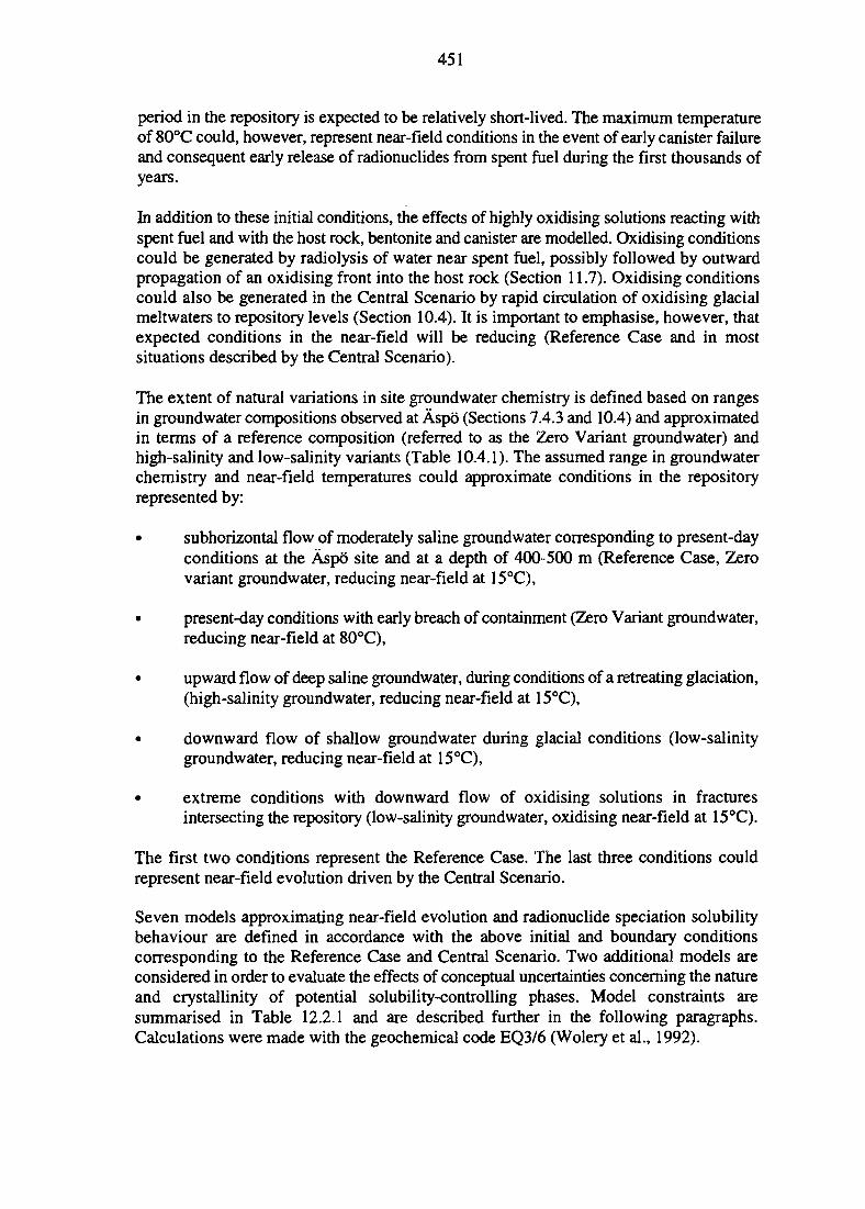
451
period in the repository is expected to be relatively short-lived. The maximum temperatureof 80°C could, however, represent near-field conditions in the event of early canister failureand consequent early release of radionuclides from spent fuel during the first thousands ofyears.
In addition to these initial conditions, the effects of highly oxidising solutions reacting withspent fuel and with the host rock, bentonite and canister are modelled. Oxidising conditionscould be generated by radiolysis of water near spent fuel, possibly followed by outwardpropagation of an oxidising front into the host rock (Section 11.7). Oxidising conditionscould also be generated in the Central Scenario by rapid circulation of oxidising glacialmeltwaters to repository levels (Section 10.4). It is important to emphasise, however, thatexpected conditions in the near-field will be reducing (Reference Case and in mostsituations described by the Central Scenario).
The extent of natural variations in site groundwater chemistry is defined based on rangesin groundwater compositions observed at Aspo (Sections 7.4.3 and 10.4) and approximatedin terms of a reference composition (referred to as the Zero Variant groundwater) andhigh-salinity and low-salinity variants (Table 10.4.1). The assumed range in groundwaterchemistry and near-field temperatures could approximate conditions in the repositoryrepresented by:
• subhorizontal flow of moderately saline groundwater corresponding to present-dayconditions at the Aspo site and at a depth of 400-500 m (Reference Case, Zerovariant groundwater, reducing near-field at 15°C),
• present-day conditions with early breach of containment (Zero Variant groundwater,reducing near-field at 80°C),
• upward flow of deep saline groundwater, during conditions of a retreating glaciation,(high-salinity groundwater, reducing near-field at 15°C),
• downward flow of shallow groundwater during glacial conditions (low-salinitygroundwater, reducing near-field at 15°C),
• extreme conditions with downward flow of oxidising solutions in fracturesintersecting the repository (low-salinity groundwater, oxidising near-field at 15°C).
The first two conditions represent the Reference Case. The last three conditions couldrepresent near-field evolution driven by the Central Scenario.
Seven models approximating near-field evolution and radionuclide speciation solubilitybehaviour are defined in accordance with the above initial and boundary conditionscorresponding to the Reference Case and Central Scenario. Two additional models areconsidered in order to evaluate the effects of conceptual uncertainties concerning the natureand crystallinity of potential solubility-controlling phases. Model constraints aresummarised in Table 12.2.1 and are described further in the following paragraphs.Calculations were made with the geochemical code EQ3/6 (Wolery et al., 1992).

452
Model 1 represents possible Reference Case conditions in which the Zero Variantground water (Table 10.4.1) is assumed to equilibrate at 15°C with bentonite(Section 11.3.3.2). The resultant solution is then equilibrated with magnetite corrosionproducts of the canister (Section 11.5.4). The solution equilibrated with these corrosionproducts is then reacted with spent fuel (Section 11.8). Reducing conditions are assumedin the host rock, bentonite and canister. Reducing conditions in the host rock are definedby the redox potential assumed for the Zero Variant groundwater. Reducing conditions inthe bentonite and canister are determined by irreversible reactions leading to equilibriumin these systems. Oxidising conditions are assumed during reactions involving spent fuel.In this and all other models in which oxidising conditions are assumed, redox potentials areconstrained by assuming a fixed O2(g) partial pressure of 0.21 bar. This represents stronglyoxidising conditions corresponding to equilibration of the aqueous solution with ambientair - a highly unrealistic situation. Solubility-controlling phases in Model 1 are assumed tobe amorphous oxide or carbonate solids. The full results for Model 1 are shown inTable 12.3.1.
Model 2 is similar to Model 1. A near-field temperature of 80°C is assumed, however, inorder to simulate conditions possibly resulting from early canister failure.
Models 3 and 4 represent conditions that could be generated in the Central Scenario.Near-field interactions involving saline (deep) and dilute (shallow) variants of the ZeroVariant groundwater are considered in these models (Table 10.4.1). Equilibration of thesegroundwaters with bentonite is considered in the models, but not subsequent reactions withcorrosion products of the canister or spent fuel.
The effects on near-field evolution and radionuclide speciation-solubility behaviour ofoxidising conditions generated, for example, by radiolysis, are considered for the ReferenceCase in Models 5 and 6. The existence of a redox front at the bentonite-host rock interfaceis considered in Model 5, whereas in Model 6, oxidising conditions are assumed throughoutthe Engineered Barrier System and near-field host rock.
Model 7 is similar to Model 6, but evaluates conditions that could be generated in theCentral Scenario. Oxidising conditions simulated in this model could be generated bymigration of a shallow, dilute and oxidising solution to repository levels.
Models 8 and 9 are defined to evaluate the effects of conceptual model uncertainty forReference Case conditions. Uncertainty concerning the nature of solubility-controllingphases is addressed in Model 8, where non-oxide/non carbonate solids are assumed to besolubility limiting (in cases where appropriate thermodynamic data are available) ratherthan amorphous oxide/carbonate phases. The results of calculations simulating Model 8 arecompared to those for Model 1. In Model 9, crystalline oxides/carbonates are assumed tobe solubility-controlling rather than the amorphous isochemical solids considered underidentical conditions in Model 1.
For full results of Models 2-9, see Arthur and Apted (1996a). The essential results arepresented in the next Section, 12.3.
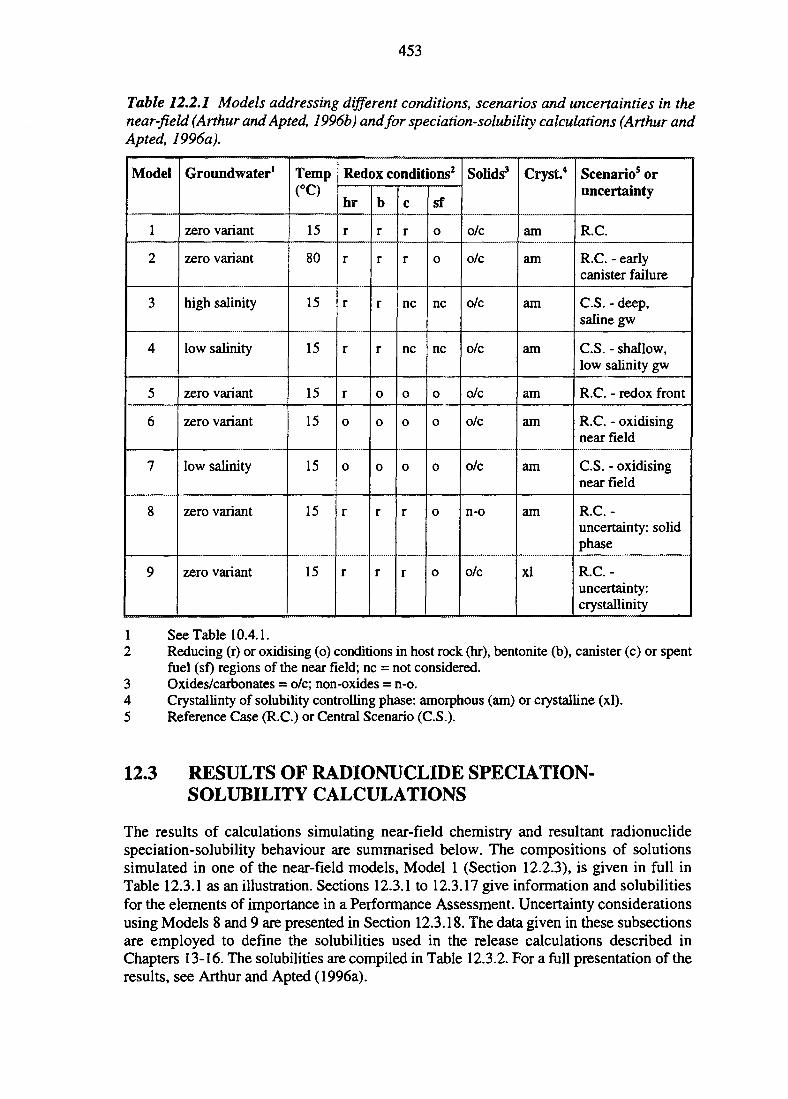
453
Table 12.2.1 Models addressing different conditions, scenarios and uncertainties in thenear-field (Arthur andApted, 1996b) and for speciation-solubility calculations (Arthur andApted, 1996a).
Model
1
2
3
4
5
6
7
8
9
Groundwater1
zero variant
zero variant
high salinity
low salinity
zero variant
zero variant
low salinity
zero variant
zero variant
Temp(°C)
15
80
15
15
15
15
15
15
15
Redox conditions2
hr
r
r
r
r
r
0
0
r
r
b
r
r
r
r
0
0
0
r
r
c
r
r
nc
nc
0
0
0
r
r
sf
0
0
nc
nc
0
0
0
0
o
Solids3
o/c
o/c
o/c
o/c
o/c
o/c
o/c
n-o
o/c
Cryst4
am
am
am
am
am
am
am
am
xl
Scenario5 oruncertainty
R.C.
R.C. - earlycanister failure
C.S. - deep,saline gw
C.S. - shallow,low salinity gw
R.C. - redox front
R.C. - oxidisingnear field
C.S. - oxidisingnear field
R.C.-uncertainty: solidphase
R.C. -uncertainty:crystallinity
1 See Table 10.4.1.2 Reducing (r) or oxidising (o) conditions in host rock (hr), bentonite (b), canister (c) or spent
fuel (sf) regions of the near field; nc = not considered.3 Oxides/carbonates = o/c; non-oxides = n-o.4 Crystallinty of solubility controlling phase: amorphous (am) or crystalline (xl).5 Reference Case (R.C.) or Central Scenario (C.S.).
12.3 RESULTS OF RADIONUCLIDE SPECIATION-SOLUBILITY CALCULATIONS
The results of calculations simulating near-field chemistry and resultant radionuclidespeciation-solubility behaviour are summarised below. The compositions of solutionssimulated in one of the near-field models, Model 1 (Section 12.2.3), is given in full inTable 12.3.1 as an illustration. Sections 12.3.1 to 12.3.17 give information and solubilitiesfor the elements of importance in a Performance Assessment. Uncertainty considerationsusing Models 8 and 9 are presented in Section 12.3.18. The data given in these subsectionsare employed to define the solubilities used in the release calculations described inChapters 13-16. The solubilities are compiled in Table 12.3.2. For a full presentation of theresults, see Arthur and Apted (1996a).
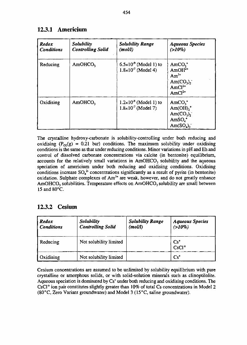
454
12.3.1 Americium
RedoxConditions
Reducing
Oxidising
SolubilityControlling Solid
AmOHCO3
AmOHCO3
Solubility Range(moUl)
6.5xlO'9 (Model 1) to1.8xlO"7(Model4)
1.2xlO"8 (Model 1) to1.8*10-7(Model7)
Aqueous Species(>10%)
AmCO3+
AmOH2+
Am3+
Am(CO3)2*AmCl2+
AmCl2+
AmCO3+
Am(OH)2+
Am(CO3)2"AmSO4
+
Am(SO4)2-
The crystalline hydroxy-carbonate is solubility-controlling under both reducing andoxidising (P02(g) ~ 0.21 bar) conditions. The maximum solubility under oxidisingconditions is the same as that under reducing conditions. Minor variations in pH and Eh andcontrol of dissolved carbonate concentrations via calcite (in bentonite) equilibrium,accounts for the relatively small variations in AmOHCO3 solubility and the aqueousspeciation of americium under both reducing and oxidising conditions. Oxidisingconditions increase SO4
2" concentrations significantly as a result of pyrite (in bentonite)oxidation. Sulphate complexes of Am3+ are weak, however, and do not greatly enhanceAmOHCO3 solubilities. Temperature effects on AmOHCO3 solubility are small between15and80°C
12.3.2 Cesium
RedoxConditions
Reducing
Oxidising
SolubilityControlling Solid
Not solubility limited
Not solubility limited
Solubility Range(moUl)
Aqueous Species(>10%)
Cs+
CsCl°
Cs+
Cesium concentrations are assumed to be unlimited by solubility equilibrium with purecrystalline or amorphous solids, or with solid-solution minerals such as clinoptilolite.Aqueous speciation is dominated by Cs+ under both reducing and oxidising conditions. TheCsCl° ion pair constitutes slightly greater than 10% of total Cs concentrations in Model 2(80°C, Zero Variant groundwater) and Model 3 (15°C, saline groundwater).
455
12.3.3 Iodine
RedoxConditions
Reducing
Oxidising
SolubilityControlling Solid
Not solubility limited
Not solubility limited
Solubility Range(mol/l)
Aqueous Species(>10%)
r
io3-
Iodine concentrations are unconstrained by solubility equilibrium under all conditions.Aqueous speciation is calculated to be dominated by the iodide anion, I\ in reducingsolutions and iodate, IO3", in oxidising waters.
12.3.4 Lanthanides
The solubilities of lanthanide elements are not calculated because relevant thermodynamicdata are scarce and not available in the database used. As a first approximation, thespeciation-solubility behaviour of the lanthanides, including Ce and Sm, might be assumedto be the same as for trivalent actinides such as Am (SKI, 1991).
12.3.5 Nickel
RedoxConditions
Reducing
Oxidising
SolubilityControlling Solid
NiO-H2O(am)
NiO-H2O(am)
Solubility Range(mol/l)
4.9x10-* (Model 2) tol.lxl<r l(Model3)
5.8xlO-3(Model6)to7.4xlO"2(Model6)
Aqueous Species(>10%)
Ni2+
Ni4(OH)44+
Ni2+
NiSO4°Ni^OH)/*
Thermodynamic data for Ni(OH)2 are assumed to approximate data for amorphous hydrousNi oxide, NiO-H2O(am), and this phase is assumed to be solubility-controlling under bothreducing and oxidising conditions. This phase is not solubility-controlling, however, in therelatively acidic dilute groundwater (Models 4 and 7, respectively). The polynuclearhydrolysis species, Ni4(OH)4
4+, makes up slightly greater than 10% of total Niconcentrations in some cases and nearly 40% in bentonite solutions generated byinteractions with the saline groundwater. Pyrite oxidation increases SO4
2" concentrationsunder oxidising conditions, thereby increasing NiSO4° concentrations up to about 40% oftotal dissolved Ni.
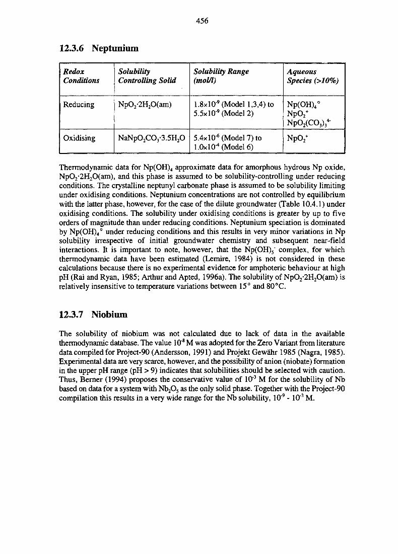
456
12.3.6 Neptunium
RedoxConditions
Reducing
Oxidising
SolubilityControlling Solid
NpO2-2H2O(am)
NaNpO2CO3-3.5H2O
Solubility Range(mol/l)
1.8xlO"9 (Model 1,3,4) to5.5xlO-9(Model2)
5.4x10* (Model 7) tol.OxlO^CMode^)
AqueousSpecies (>10%)
Np(OH)4°NpO2
+
NpCyCO^
NpO2+
Thermodynamic data for Np(OH)4 approximate data for amorphous hydrous Np oxide,NpO2-2H2O(am), and this phase is assumed to be solubility-controlling under reducingconditions. The crystalline neptunyl carbonate phase is assumed to be solubility limitingunder oxidising conditions. Neptunium concentrations are not controlled by equilibriumwith the latter phase, however, for the case of the dilute groundwater (Table 10.4.1) underoxidising conditions. The solubility under oxidising conditions is greater by up to fiveorders of magnitude than under reducing conditions. Neptunium speciation is dominatedby Np(OH)4° under reducing conditions and this results in very minor variations in Npsolubility irrespective of initial groundwater chemistry and subsequent near-fieldinteractions. It is important to note, however, that the Np(OH)5" complex, for whichthermodynamic data have been estimated (Lemire, 1984) is not considered in thesecalculations because there is no experimental evidence for amphoteric behaviour at highpH (Rai and Ryan, 1985; Arthur and Apted, 1996a). The solubility of NpO2-2H2O(am) isrelatively insensitive to temperature variations between 15° and 80°C.
12.3.7 Niobium
The solubility of niobium was not calculated due to lack of data in the availablethermodynamic database. The value 10"8 M was adopted for the Zero Variant from literaturedata compiled for Project-90 (Andersson, 1991) and Projekt Gewahr 1985 (Nagra, 1985).Experimental data are very scarce, however, and the possibility of anion (niobate) formationin the upper pH range (pH > 9) indicates that solubilities should be selected with caution.Thus, Berner (1994) proposes the conservative value of 10"3 M for the solubility of Nbbased on data for a system with Nb2O5 as the only solid phase. Together with the Project-90compilation this results in a very wide range for the Nb solubility, 10"9 - 10'3 M.
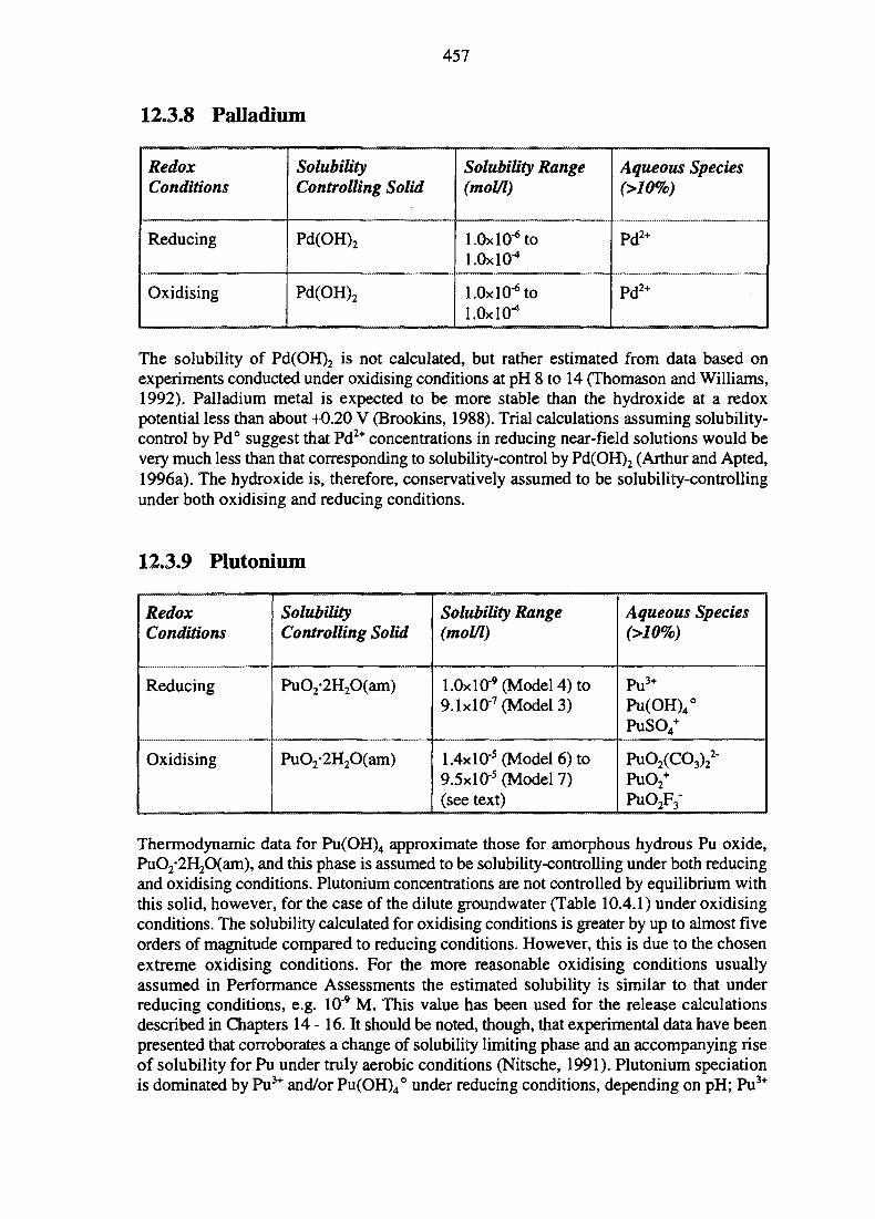
457
123.8 Palladium
RedoxConditions
Reducing
Oxidising
SolubilityControlling Solid
Pd(OH)2
Pd(OH)2
Solubility Range(mol/l)
l.OxlO^tol.OxlO-4
l.OxlO^tol.OxlO"4
Aqueous Species(>10%)
Pd2+
Pd2+
The solubility of Pd(OH)2 is not calculated, but rather estimated from data based onexperiments conducted under oxidising conditions at pH 8 to 14 (Thomason and Williams,1992). Palladium metal is expected to be more stable than the hydroxide at a redoxpotential less than about +0.20 V (Brookins, 1988). Trial calculations assuming solubility-control by Pd° suggest that Pd2+ concentrations in reducing near-field solutions would bevery much less than that corresponding to solubility-control by Pd(OH)2 (Arthur and Apted,1996a). The hydroxide is, therefore, conservatively assumed to be solubility-controllingunder both oxidising and reducing conditions.
12.3.9 Plutonium
RedoxConditions
Reducing
Oxidising
SolubilityControlling Solid
PuO2-2H2O(am)
PuO2-2H2O(am)
Solubility Range(mol/l)
1.0xlO"9(Model4)to9.1xl0-7(Model3)
1.4xlO-5(Model6)to9.5xlO"5(Model7)(see text)
Aqueous Species(>10%)
Pu3+
Pu(OH)4°PuSO4
+
PuO2(CO3)22-
PuO2+
PuO2F3-
Thermodynamic data for Pu(OH)4 approximate those for amorphous hydrous Pu oxide,PuO2-2H2O(am), and this phase is assumed to be solubility-controlling under both reducingand oxidising conditions. Plutonium concentrations are not controlled by equilibrium withthis solid, however, for the case of the dilute groundwater (Table 10.4.1) under oxidisingconditions. The solubility calculated for oxidising conditions is greater by up to almost fiveorders of magnitude compared to reducing conditions. However, this is due to the chosenextreme oxidising conditions. For the more reasonable oxidising conditions usuallyassumed in Performance Assessments the estimated solubility is similar to that underreducing conditions, e.g. 10'9 M. This value has been used for the release calculationsdescribed in Chapters 14 -16 . It should be noted, though, that experimental data have beenpresented that corroborates a change of solubility limiting phase and an accompanying riseof solubility for Pu under truly aerobic conditions (Nitsche, 1991). Plutonium speciationis dominated by Pu3+ and/or Pu(OH)4° under reducing conditions, depending on pH; Pu3+
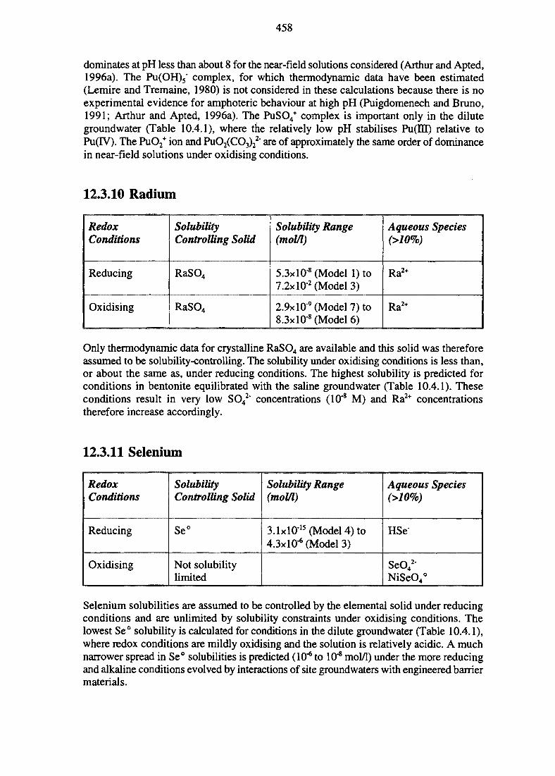
458
dominates at pH less than about 8 for the near-field solutions considered (Arthur and Apted,1996a). The Pu(OH)5" complex, for which thermodynamic data have been estimated(Lemire and Tremaine, 1980) is not considered in these calculations because there is noexperimental evidence for amphoteric behaviour at high pH (Puigdomenech and Bruno,1991; Arthur and Apted, 1996a). The PuSO4
+ complex is important only in the dilutegroundwater (Table 10.4.1), where the relatively low pH stabilises Pu(IH) relative toPu(IV). The PuO2
+ ion and PuO2(CO3)22" are of approximately the same order of dominance
in near-field solutions under oxidising conditions.
12.3.10 Radium
RedoxConditions
Reducing
Oxidising
SolubilityControlling Solid
RaSO4
RaSO4
Solubility Range(mol/l)
5.3xl0"8 (Model l)to7.2xl0'2(Model3)
2.9xl09(Model7)to8.3xl0-8(Model6)
Aqueous Species(>10%)
Ra2+
Ra2+
Only thermodynamic data for crystalline RaSO4 are available and this solid was thereforeassumed to be solubility-controlling. The solubility under oxidising conditions is less than,or about the same as, under reducing conditions. The highest solubility is predicted forconditions in bentonite equilibrated with the saline groundwater (Table 10.4.1). Theseconditions result in very low SO4
2' concentrations (10"8 M) and Ra2+ concentrationstherefore increase accordingly.
12.3.11 Selenium
RedoxConditions
Reducing
Oxidising
SolubilityControlling Solid
Se°
Not solubilitylimited
Solubility Range(mol/l)
3.1xl015(Model4)to4.3x10* (Model 3)
Aqueous Species(>10%)
HSe
SeO42"
NiSeO4°
Selenium solubilities are assumed to be controlled by the elemental solid under reducingconditions and are unlimited by solubility constraints under oxidising conditions. Thelowest Se° solubility is calculated for conditions in the dilute groundwater (Table 10.4.1),where redox conditions are mildly oxidising and the solution is relatively acidic. A muchnarrower spread in Se° solubilities is predicted (10"6 to 10"8 mol/l) under the more reducingand alkaline conditions evolved by interactions of site groundwaters with engineered barriermaterials.
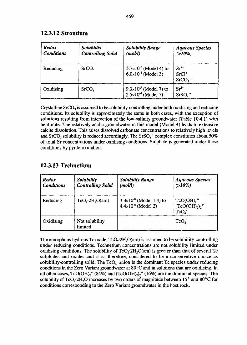
459
12.3.12 Strontium
RedoxConditions
Reducing
Oxidising
SolubilityControlling Solid
SrCO3
SrCO3
Solubility Range(mol/l)
5.7xlO'8(Model4)to6.0x10" (Model 3)
9.3xl0"5(Model7)to2.5x10" (Model 7)
Aqueous Species(>10%)
Sr2*SrCl+
SrCO3°
Sr2*SrSO4°
Crystalline SrCO3 is assumed to be solubility-controlling under both oxidising and reducingconditions. Its solubility is approximately the same in both cases, with the exception ofsolutions resulting from interaction of the low-salinity groundwater (Table 10.4.1) withbentonite. The relatively acidic groundwater in this model (Model 4) leads to extensivecalcite dissolution. This raises dissolved carbonate concentrations to relatively high levelsand SrCO3 solubility is reduced accordingly. The SrSO4° complex constitutes about 50%of total Sr concentrations under oxidising conditions. Sulphate is generated under theseconditions by pyrite oxidation.
12.3.13 Technetium
RedoxConditions
Reducing
Oxidising
SolubilityControlling Solid
TcO2-2H2O(am)
Not solubilitylimited
Solubility Range(mol/l)
3.3xl0*8 (Model 1,4) to4.4xlO-6(Model2)
Aqueous Species(>10%)
TcO(OH)2°(TcO(OH)2)2°TcO4-
TcO4"
The amorphous hydrous Tc oxide, TcO2-2H2O(am) is assumed to be solubility-controllingunder reducing conditions. Technetium concentrations are not solubility limited underoxidising conditions. The solubility of TcO2-2H2O(am) is greater than that of several Tcsulphides and oxides and it is, therefore, considered to be a conservative choice assolubility-controlling solid. The TcO4" anion is the dominant Tc species under reducingconditions in the Zero Variant groundwater at 80 °C and in solutions that are oxidising. Inall other cases, TcO(OH)2° (84%) and (TcO(OH)J2° (16%) are the dominant species. Thesolubility of TcO2-2H2O increases by two orders of magnitude between 15° and 80 °C forconditions corresponding to the Zero Variant groundwater in the host rock.
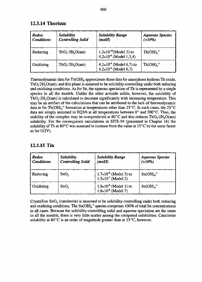
460
12.3.14 Thorium
RedoxConditions
Reducing
Oxidising
SolubilityControlling Solid
ThO2-2H2O(am)
ThO2-2H2O(am)
Solubility Range(mol/l)
1.3xl010(Model2)to4.2X10"6 (Model 1,3,4)
4.2xlO"6 (Model 6,7) to4.2x10-* (Model 6,7)
Aqueous Species(>10%)
Th(OH)4°
Th(OH)4°
Thermodynamic data for Th(OH)4 approximate those data for amorphous hydrous Th oxide,ThO2-2H2O(am), and this phase is assumed to be solubility-controlling under both reducingand oxidising conditions. As for Sn, the aqueous speciation of Th is represented by a singlespecies in all the models. Unlike the other actinide solids, however, the solubility ofThO2*2H2O(am) is calculated to decrease significantly with increasing temperature. Thismay be an artifact of the calculations that can be attributed to the lack of thermodynamicdata in for Th(OH)4° formation at temperatures other than 25 °C. In such cases, the 25 °Cdata are simply assumed in EQ3/6 at all temperatures between 0° and 300°C. Thus, thestability of the complex may be overpredicted at 80°C and this reduces ThO2-2H2O(am)solubility. For the consequence calculations in SITE-94 (presented in Chapter 16) thesolubility of Th at 80 °C was assumed to increase from the value at 15°C by the same factorasforU(IV).
12.3.15 Tin
RedoxConditions
Reducing
Oxidising
SolubilityControlling Solid
SnO2
SnO2
Solubility Range(mol/l)
1.7xl0-8(Model3)to1.5xlO'7(Model2)
1.8xl0"8 (Model 1) to1.8xl0"8(Model7)
Aqueous Species(>10%)
Sn(OH)4°
Sn(OH)4°
Crystalline SnO2 (cassiterite) is assumed to be solubility-controlling under both reducingand oxidising conditions. The Sn(OH)4° species comprises 100% of total Sn concentrationsin all cases. Because the solubility-controlling solid and aqueous speciation are the samein all the models, there is very little scatter among the computed solubilities. Cassiteritesolubility at 80°C is an order of magnitude greater than at 15°C, however.
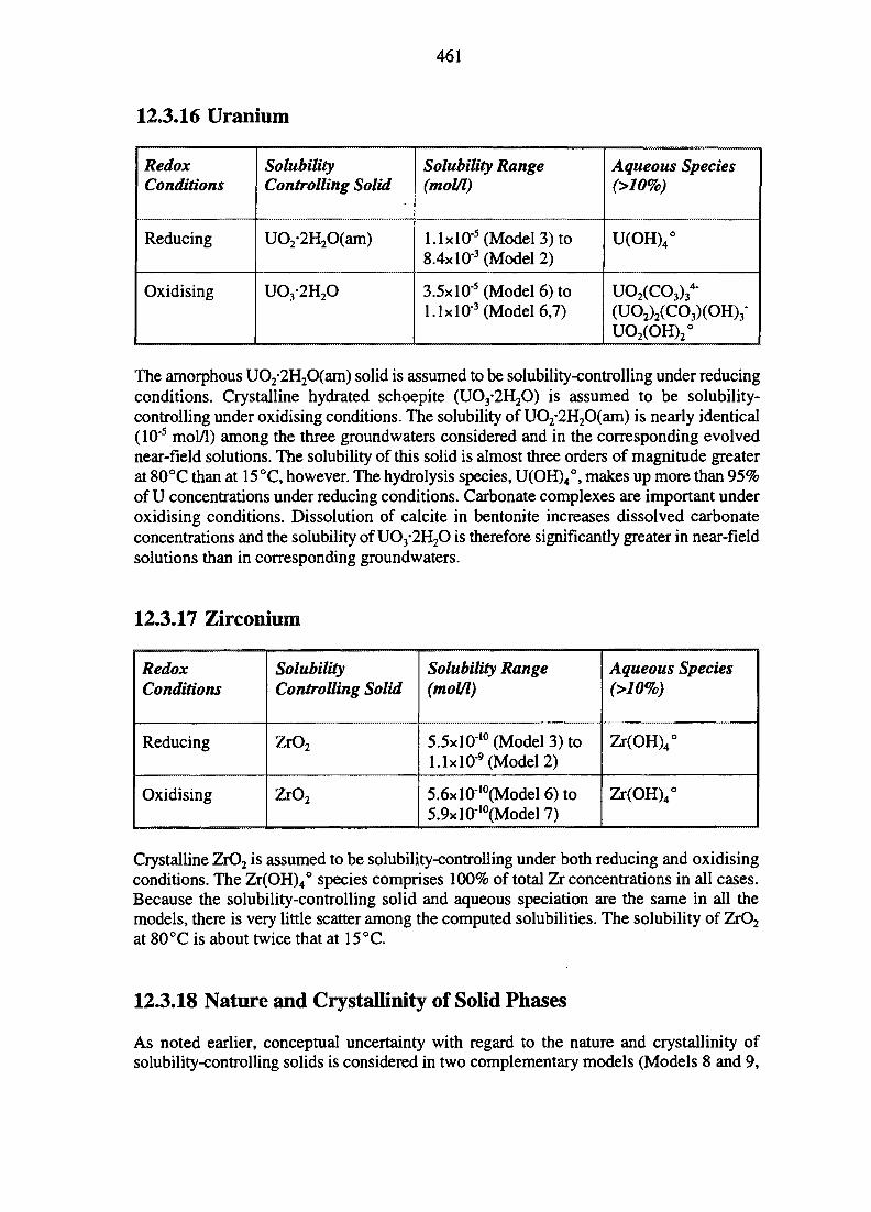
461
12.3.16 Uranium
RedoxConditions
Reducing
Oxidising
SolubilityControlling Solid
UO2-2H2O(am)
UO3-2H2O
Solubility Range(mol/l)
LlxlO-5(Model3)to8.4xlO"3 (Model 2)
3.5xlO"5(Model6)tol.lxHT3 (Model 6,7)
Aqueous Species(>10%)
U(OH)4°
UO2(CO3)34-
(UO2)2(CO3)(OH)3-UO2(OH)2°
The amorphous UO2*2H2O(am) solid is assumed to be solubility-controlling under reducingconditions. Crystalline hydrated schoepite (UO3*2H2O) is assumed to be solubility-controlling under oxidising conditions. The solubility of UO2-2H2O(am) is nearly identical(105 mol/l) among the three groundwaters considered and in the corresponding evolvednear-field solutions. The solubility of this solid is almost three orders of magnitude greaterat 80°C than at 15°C, however. The hydrolysis species, U(OH)4°, makes up more than 95%of U concentrations under reducing conditions. Carbonate complexes are important underoxidising conditions. Dissolution of calcite in bentonite increases dissolved carbonateconcentrations and the solubility of UO3-2H2O is therefore significantly greater in near-fieldsolutions than in corresponding groundwaters.
123.17 Zirconium
RedoxConditions
Reducing
Oxidising
SolubilityControlling Solid
ZrO2
ZrO2
Solubility Range(mol/l)
5.5xl010(Model3)tol.lxlO-9(Model2)
5.6xl010(Model6)to5.9xlO-10(Model7)
Aqueous Species(>10%)
Zr(OH)4°
Zr(OH)4°
Crystalline ZrO2 is assumed to be solubility-controlling under both reducing and oxidisingconditions. The Zr(OH)4° species comprises 100% of total Zr concentrations in all cases.Because the solubility-controlling solid and aqueous speciation are the same in all themodels, there is very little scatter among the computed solubilities. The solubility of ZrO2
at 80°C is about twice that at 15°C.
123.18 Nature and Crystallinity of Solid Phases
As noted earlier, conceptual uncertainty with regard to the nature and crystallinity ofsolubility-controlling solids is considered in two complementary models (Models 8 and 9,
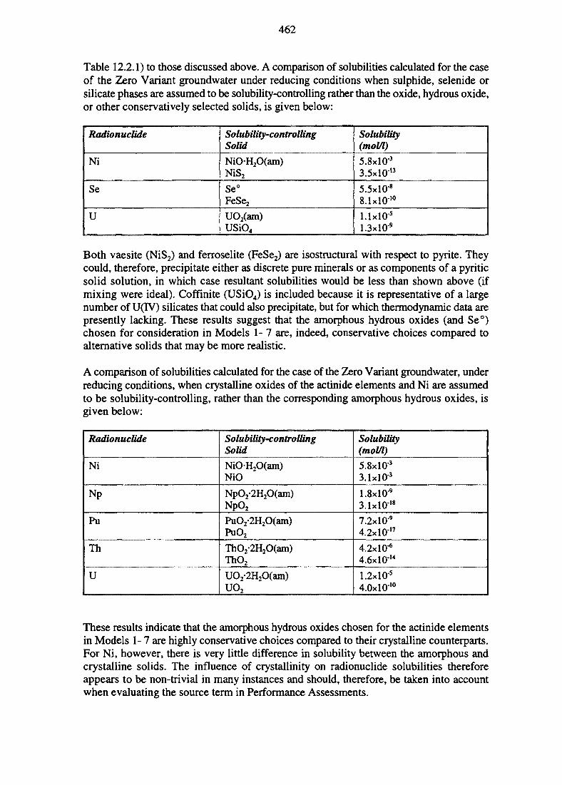
462
Table 12.2.1) to those discussed above. A comparison of solubilities calculated for the caseof the Zero Variant groundwater under reducing conditions when sulphide, selenide orsilicate phases are assumed to be solubility-controlling rather than the oxide, hydrous oxide,or other conservatively selected solids, is given below:
Radionuclide
Ni
Se
U
Solubility-controllingSolid
NiOH20(am)NiS2
Se°FeSej
UO2(am)USiO4
Solubility(mol/l)
5.8xlO'3
3.5xlO13
5.5xlO8
8.1xlOl°
l.lxlO"5
1.3xlO"9
Both vaesite (NiS2) and ferroselite (FeSe2) are isostructural with respect to pyrite. Theycould, therefore, precipitate either as discrete pure minerals or as components of a pyriticsolid solution, in which case resultant solubilities would be less than shown above (ifmixing were ideal). Coffinite (USiO4) is included because it is representative of a largenumber of U(IV) silicates that could also precipitate, but for which thermodynamic data arepresently lacking. These results suggest that the amorphous hydrous oxides (and Se°)chosen for consideration in Models 1-7 are, indeed, conservative choices compared toalternative solids that may be more realistic.
A comparison of solubilities calculated for the case of the Zero Variant groundwater, underreducing conditions, when crystalline oxides of the actinide elements and Ni are assumedto be solubility-controlling, rather than the corresponding amorphous hydrous oxides, isgiven below:
Radionuclide
Ni
Np
Pu
Th
U
Solubility~controllingSolid
NiOH20(am)NiO
NpO2-2H2O(am)NpO2
PuO2-2H2O(am)PuO2
ThO2-2H2O(am)ThO2
UO2-2H2O(am)UO2
Solubility(mol/l)
5.8xlO"3
3.1xlO"3
1.8xlO'9
3.1xlO18
7.2xlO9
4.2xlO17
4.2x10-*4.6xlO14
1.2xlO"5
4.0xl01 0
These results indicate that the amorphous hydrous oxides chosen for the actinide elementsin Models 1- 7 are highly conservative choices compared to their crystalline counterparts.For Ni, however, there is very little difference in solubility between the amorphous andcrystalline solids. The influence of crystallinity on radionuclide solubilities thereforeappears to be non-trivial in many instances and should, therefore, be taken into accountwhen evaluating the source term in Performance Assessments.
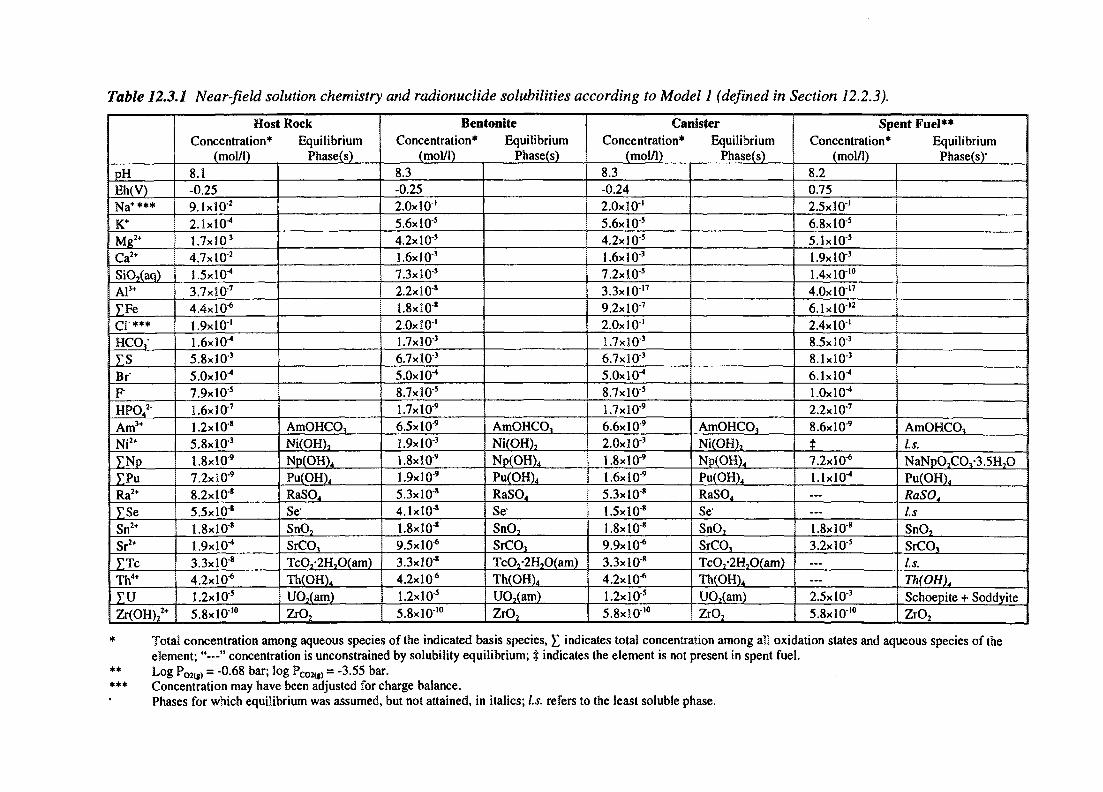
Table 12.3.1 Near-field solution chemistry
pHEh(V)Na+***
K+
Mg2+
Ca2+
SiO2(aq) i
Al3+
]TFe
cr***HCO,YSBrFHPO4
2
Am3+
Ni2+
ENpEPURa2+
£SeSn2+
Sr2+
ETcTh4+
TVZr(OH)2
2*
Host RockConcentration* Equilibrium
(mol/I) Phase(s)8.1-0.259.1xlO2
2.1xl04
1.7x303
4.7xlO2
l.SxlQ-4 j
3.7xl07 14.4x10 6
1.9x10'1.6x10^5.8xlO3
5.0x10^7.9x10'1.6x!0"7
1.2x10'5.8xl03
1.8xlO"9
7.2xlO9
8.2x10'5.5x10'1.8x10'1.9x10^3.3x10'4.2x10⁶
1.2x10'5.8x10'°
AmOHCO,Ni(OH)2
Np(OH),Pu(OH)4
RaSO4
SeSnO2
SrCO3
Tc02^H2O(am)Th(OH)4
U02(am)ZrO2
and radionuclide solubilities according to Model 1 (defined in Section 12.2.3).
BentonlteConcentration* Equilibrium
(mol/1) Phase(s)8.3 !-0.252.0x10'5.6xl05
4.2x10'3.6xlO3
L 7.3x10'2.2x10'1.8x10'2.0x10'1.7x3O-3
6.7xl0"3
5.0x10^8.7x10"'1.7xl0"9
6.5xl0"9
1.9xl0"3
1.8xl0"9
1.9xlO9
5.3x10'4.1x10'1.8xl0-8
9.5X10"6
3.3x10'4.2X10"6
1.2x10'5.8x10'°
AmOHCO,Ni(OH)2
Np(OH)4
Pu(OH)4
RaSO4
SeSnO,SrCO,TcO,-2H2O(am)Th(OH)4
UO,(am)ZrO2
CanisterConcentration* Equilibrium
(mol/1) Phase(s)8.3 |-0.242.0x10'5.6x10'4.2x30'1.6xl03
7.2x10'3.3xl0'7
9.2xl0"7
2.0x10'1.7xl0"3
6.7x10"3
5.0X10"4
8.7x10'1.7xlO"9
6.6x10⁹
2.0x10³
1.8xlO"9
1.6xlO9
5.3x30"'1.5x10'1.8x10"'9.9x10 6
3.3x10'4.2x10"6
1.2x10'5.8x10'°
AmOHCO,Ni(OH)2
Np(OH)4
Pu(OH)4
RaSO4
SeSnO2
SrCO,TcO2-2H2O(am)Th(OH)4
U02(am)ZrO2
Spent Fuel**Concentration* Equilibrium
(mol/1) Phase(s)*8.20.752.5x10'6.8x10'5.3x10'1.9xlO"3
1.4x10'°4.0xl017
6.1xlO12
2.4x10'8.5xlO3
8.1xlO"3
6.1x10^1.0x10^2.2xlO7
8.6x10⁹
t7.2xlO6
l.lxlO"4
——
1.8xlO"8
3.2x10'——
2.5xlO3
5.8x10'°
AmOHCO,is.NaNpO7COv3.5H,OPu(OH)4
RaS04
l.sSnO2
SrCO,is.Th(0H)4
Schoepite + SoddyiteZrO2
Total concentration among aqueous species of the indicated basis species, £ indicates total concentration among all oxidation states and aqueous species of theelement; "—" concentration is unconstrained by solubility equilibrium; t indicates the element is not present in spent fuel.
*****
Log P02(g) = - ° - 6 8 pco2(g) = -3.55 bar.d
g g
Concentration may have been adjusted for charge balance.Phases for which equilibrium was assumed, but not attained, in italics; l.s. refers to the least soluble phase.
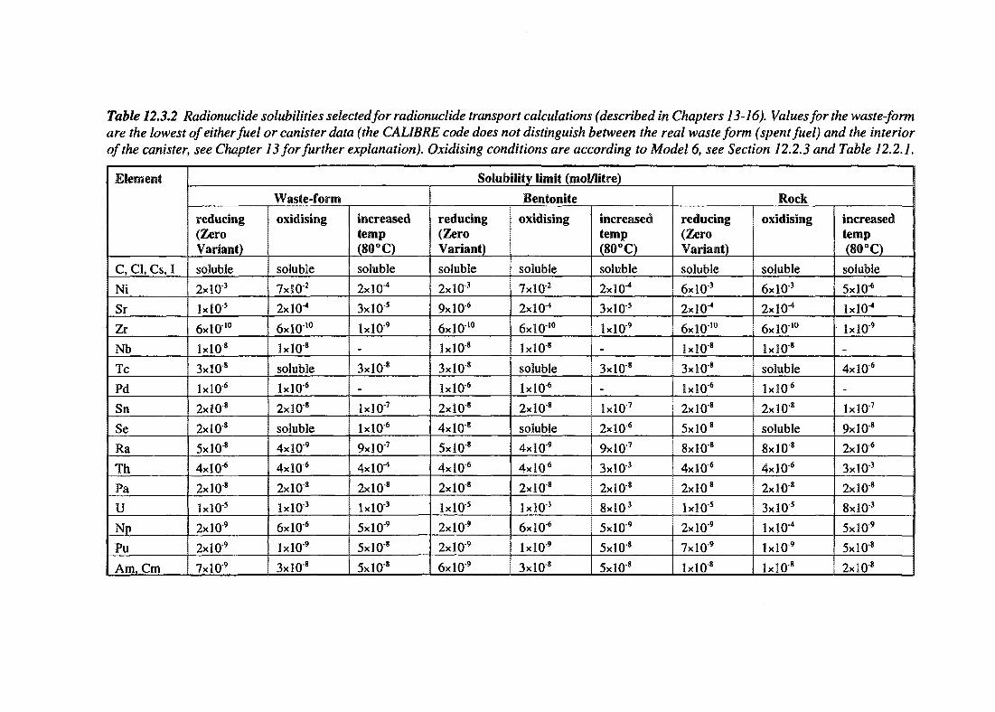
Table 12.3.2 Radionuclide solubilities selected for radionuclide transport calculations (described in Chapters 13-16). Values for the waste-formare the lowest of either fuel or canister data (the CALIBRE code does not distinguish between the real waste form (spent fuel) and the interiorof the canister, see Chapter 13 for further explanation). Oxidising conditions are according to Model 6, see Section 12.2.3 and Table 12.2.1.
Element
C, Cl, Cs, I
Ni
Sr
Zr
Nb
Tc
Pd
Sn
Se
Ra
Th
Pa
U
Np
Pu
Am, Cm
Waste-form
reducing(ZeroVariant)
soluble
2xlO'3
IxlO5
6xlO10
1x10*
3x10*
IxlO-6
2x10*
2x10*
5x10*
4xlO"6
2x10*
ixlO5
2x10 '
2x10'
7x10'
oxidising
soluble
7xlO"2
2x10^
6xlO10
1x10*
soluble
ix lO 6
2x10*
soluble
4x10"'
4xlO6
2x10*
IxlO3
6xlO"6
ixlO9
3x10*
increasedtemp(80°C)
soluble
2x10^
3xlO5
ixlO9
-
3x10*
MO"7
lxlO"6
9xlO7
4XI0-4
2x10*
ixlO 3
5x10"'
5x10*
5x10*
Solubility limit (mo! litre)
Bentonite
reducing(ZeroVariant)
soluble
2xlO3
9xlO6
6xlO10
1x10*
3x10*
IxlO6
2x10*
4x10*
5x10*
4xlO6
2x10*
IxlO5
2x10 '
2x10'
6x10'
oxidising
soluble
7xlO2
2xlO"4
6xlO10
1x10*
soluble
IxlO6
2x10*
soluble
4x10 '
4xlO6
2x10*
IxlO 3
6x10⁶
1x10"'
3x10*
increasedtemp(80°C)
soluble
2X10⁻⁴
3xlO"5
1x10'
-
3x10*
-
!xlO'7
2xlO"6
9xlO"7
3xlO3
2x10*
8xlO3
5x10 '
5x10*
5x10"*
Rock
reducing(ZeroVariant)soluble
6xlO3
2x!0'4
6xlO"10
1x10*
3x10*
ixlO"6
2x10*
5x10*
8x10*
4xlO"6
2x10*
ixlO"5
2x10 '
7x10 '
1x10"*
oxidising
soluble
6xlO3
2X10"4
6xlO10
1x10*
soluble
IxlO 6
2x10*
soluble
8x10*
4xlO"6
2x10*
3xlO"5
IxlO-4
1x10'
1x10*
increasedtemp(80°C)
soluble
5xlO6
1x10^
ixlO'9
_
4xlO"6
_
lxlO"7
9x10*
2xlO"6
3xlO"3
2x10*
8xlO"3
5x10"'
5x10*
2x10*
465
12.3.19 Conclusions Regarding Solubilities and Speciation
In terms of the main objectives of SITE-94, it is concluded that chemical models ofnear-field evolution combined with thermodynamic models of radionuclidespeciation-solubility behaviour can assist efforts to assimilate site characterisation data intothe Performance Assessment process and to deal with uncertainties that are inherent in bothsite properties and in concepts of near-field chemistry. It is essential, however, that expertjudgement should be exercised, such that model results are conservative with respect toacknowledged (and documented) uncertainties. Most importantly, it must be recognised thatit is not possible to specify radionuclide solubilities precisely given the complex chemicalenvironments and long timescales involved in the disposal of radioactive wastes. ForPerformance Assessment, however, only bounding values are needed. Technical peerreview and cross-comparisons of solubility databases adopted in other PerformanceAssessments might provide a basis for building confidence in the results of suchassessments (McKinley and Savage, 1996).
Models of near-field evolution and radionuclide speciation-solubility behaviour couldprovide an important link between Performance Assessment and site characterisation. Theabove results suggest, for example, that understanding the redox buffering behaviour ofnear-field materials could simplify efforts to assess repository performance in relation tosite characterisation data. The aqueous speciation and solubility behaviour of the actinidesand many fission products are primarily Eh-pH dependent. Although complexes involvingligands such as CO3
2* and SO42" do contribute to the aqueous speciation of some
radionuclides under some conditions, model results suggest they are often of secondaryimportance compared to hydrolysis species. Consequently, it would appear most importantto characterise the Eh and pH of site groundwaters and to focus attention on reactions thatcould effectively buffer Eh-pH conditions in the near-field.
The relation between Performance Assessment and site characterisation should be iterativein nature. The need for more realistic models of solubility-controlling solids (alternativesto Ni(OH)2, for example, and for most actinides) may be indicated by initial results ofPerformance Assessment calculations. Refined models, perhaps based on a more realisticsolid-solution approach (e.g., NiS2 in pyritic solid solution), may then make it necessary tocharacterise certain groundwater parameters in more detail (e.g., concentration ranges ofdissolved Fe and S). Similarly, integration of Performance Assessment models withchemical models of near-field evolution and radionuclide speciation-solubility behaviourcould be useful in prioritising phenomena needing additional laboratory study. A possibleexample from the results discussed above would be to clarify the factors which control thecrystalline/amorphous nature of the phases limiting actinide solubilities.
12.4 SORPTION OF RADIONUCLIDES
Sorption is the collective term for processes whereby solutes or particles attach to thesurfaces of solids. Sorption onto mineral surfaces might depend on a variety of processes,often difficult to distinguish from each other (physical adsorption, electrostatic adsorption,chemisorption and chemical substitution). In fact, the same element might well be sorbedby more than one mechanism under the same conditions. A more detailed description of
466
sorption phenomenon is found in the Project-90 report (SKI, 1991) and a review by Serneand Muller (1987). SITE-94 contains no new work on conceptual models of sorptionmechanisms and simply selects relevant literature data for the performance assessmentcalculations.
Sorption on mineral surfaces is a dominant retardation mechanism in the transport of mostradionuclides through the EBS and the geosphere. Sorption is element specific and dependsboth on radionuclide speciation, the solid phase composition and surface characteristics.
To obtain a parameter suitable for describing sorption in mathematical modelling of thetransport of radionuclides, a distribution coefficient (K,,) has been defined, as thedistribution of an element between aqueous and mineral phases at equilibrium.
K -ELd c .
where Cs is the concentration of the element on the solid phase (mol/kg) and Ca is theconcentration of the element in solution (mol/m3). The coefficient describes an observeddistribution of an element between the two phases under certain physico-chemicalconditions. Sorption can also be modelled with surface-complexation models whichdescribe sorption more mechanistically, where chemical reactions, speciation, etc. areincluded in the model. The latter approach has limitations owing to the availability ofmeasured data and may be used as a complement to the use of distribution coefficients inPerformance Assessment.
Distribution coefficients for use in the SITE-94 radionuclide transport calculations areselected from literature review for rocks relevant to the hypothetical repository at Aspo, aswell as for the bentonite buffer (Andersson, 1996). The review covers three main sourcesof information:
• journal articles and technical reports published after 1989,• the OECD/NEA 'ISIRS' sorption database, which contains some 11 000 data fields,• previous safety assessment studies, including KBS-3 (SKBF/KBS, 1983), Project-90
(SKI, 1991), Gewahr (Nagra, 1985), SKB 91 (SKB, 1992) and TVO-92 (TVO,1992).
The site contains a number of different rock types, including granite, aplite and diorite. Forthe selection of sorption data, representative rocks have been chosen from among thegranite-granodiorite suite. The data are valid for a non-saline groundwater that can beoxidising or reducing, defined by either being in contact with air or having an Eh of-0.25 V. The distribution coefficients selected for use in the radionuclide transportcalculations are presented in Table 12.4.1.
In future assessments it may be useful to consider potential variations in far-field sorptionproperties in circumstances where specific water types can be correlated with specific bulkor fracture mineralogies in different regions of the rock. Apart from providing the bulk rockand bentonite sorption data, Andersson (1996) also proposed a range of sorption values for
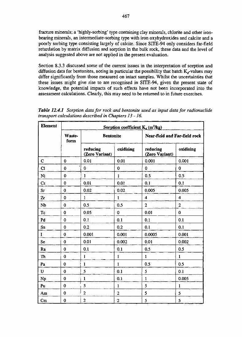
467
fracture minerals; a 'highly-sorbing' type containing clay minerals, chlorite and other iron-bearing minerals, an intermediate-sorbing type with iron oxyhydroxides and calcite and apoorly sorbing type consisting largely of calcite. Since SITE-94 only considers far-fieldretardation by matrix diffusion and sorption in the bulk rock, these data and the level ofanalysis suggested above are not applied in the present evaluation.
Section 8.3.3 discussed some of the current issues in the interpretation of sorption anddiffusion data for bentonites, noting in particular the possibility that batch Kd-values maydiffer significantly from those measured on intact samples. Whilst the uncertainties thatthese issues might give rise to are recognised in STTE-94, given the present state ofknowledge, the potential impacts of such effects have not been incorporated into theassessment calculations. Clearly, this may need to be returned to in future exercises.
Table 12.4.1 Sorption data for rock and bentonite used as input data for radionuclidetransport calculations described in Chapters 13-16.
Element
C
Cl
Ni
Cs
Sr
Zr
Nb
Tc
Pd
Sn
I
Se
Ra
Th
Pa
U
Np
Pu
Am
Cm
Waste-form
0
0
0
0
0
0
0
0
0
0
0
0
0
0
0
0
0
0
0
0
Sorption coefficient Kd (m3/kg)
Bentonite
reducing(Zero Variant)0.01
0
1
0.01
0.02
1
0.5
0.05
0.1
0.2
0.001
0.01
0.1
1
1
5
1
5
2
2
oxidising
0.01
0
1
0.01
0.02
1
0.5
0
0.1
0.2
0.001
0.002
0.1
1
1
0.1
0.1
1
2
2
Near-field and Far-field rock
reducing(Zero Variant)0.001
0
0.5
0.1
0.005
4
2
0.01
0.1
0.1
0.0005
0.01
0.5
1
0.5
5
1
5
5
5
oxidising
0.001
0
0.5
0.1
0.005
4
2
0
0.1
0.1
0.001
0.002
0.5
1
0.5
0.1
0.005
1
5
5

468
The empirical Kd approach has been criticised because data are only valid under theexperimental conditions at which they were measured and extrapolation to other conditionsis not scientifically defensible. This may be an especially important limitation for modelssimulating radionuclide transport in repository systems where the geochemical environmentmay vary significantly in both space and time. A methodology for adapting mechanisticsorption models for use in Performance Assessments, using a surface-film concept forsorption of neptunium, is tested for the SITE-94 study (Arthur, 1994). Surface acidityparameters in a generalised two-layer surface complexation model are combined withsurface complexation constants for Np(V) sorption on hydrous ferric oxide to derive ananalytical model enabling calculation of corresponding intrinsic distribution coefficientsas a function of pH and calcium, chloride and bicarbonate concentrations. The surface filmconcept is then used to calculate a whole-rock distribution for Np(V) sorption fromoxidised groundwater. The limited amount of measured input data restricts the conditionsfor which the calculations can be performed, but it is concluded, from this parallel study,that the Kd-value selected by Andersson (1996) for oxidising conditions is reasonablyrealistic. The results also show that sorption capacity is very dependent on the pH.
12.5 CONCLUSIONS AND IMPLICATIONS FOR OTHERPARTS OF THE ASSESSMENT
As discussed in Chapter 11, the chemical evolution of the near-field is approximated usinga sequential interaction modelling approach, in which site groundwater (Section 11.23.4)is assumed to equilibrate first with bentonite (Section 11.3.3.2) and then with corrosionproducts of the canister (Section 11.5.4). Irreversible reactions involving solutions evolvedfrom the canister and spent fuel are also modelled (Section 11.8). Initial groundwatercompositions and near-field conditions are defined in accordance with the Reference Caseand Central scenarios (Sections 9.2 and 9.3, respectively). Radionuclide solubilities arecalculated for the initial groundwaters and for near-field solutions resulting frombentonite - water, canister - water and spent fuel - water interactions.
To deal with uncertainties in radionuclide speciation-solubility behaviour, model results arecompared to published experimental data appropriate for the reducing and moderatelyalkaline solutions expected in the near-field. The purpose of the comparisons is to establishconfidence that model results are in reasonable agreement with the available data, or, wherethere are discrepancies, to evaluate whether the calculated solubilities are conservative withrespect to experimental results. Good, or conservative, agreement between calculated andexperimental solubilities is determined for Am, Np, Pu, Tc, Th and U (Arthur and Apted,1996a).
In cases where such experimental data are lacking (Ni, Se, Sn, Sr, Zr and Ra),speciation-solubility models are constrained by the observed geochemical behaviour ofstable isotopes of these elements in natural systems. Solubility-controlling solids are chosensuch that calculated solubilities are greater than the average analysed concentrations ofthese elements in natural waters, according to published reviews such as Hem (1970). Insome cases (Sn and Zr), limited thermodynamic data on solid phases are available and themost soluble solid among these is assumed to be solubility-controlling.
469
Solubility limits for a range of pure mineral phases for each radionuclide in solutionsgenerated by reactions in each subregion of the near-field are calculated using the evaluatedspeciation-solubility models (Arthur and Apted, 1996a). The solubility of the most solublephase among these possibilities is assumed to represent a conservative upper bound onnear-field radionuclide concentrations. Solubilities are calculated for U, Pu, Np, Th, Am,Tc, Ni, Se, Sn, Sr, Zr and Ra (Section 12.3). In cases where appropriate thermodynamic orgeochemical data are unavailable (Pd and lanthanide elements, such as Ce and Sm),radionuclide concentrations are estimated based on a review of the literature (Section 12.3).Near-field Cs and I concentrations are assumed to be unlimited by solubility constraints.Available thermodynamic data for Cs solubility-control by a zeolite (clinoptilolite) solidsolution are not considered in order to maintain conservatism in the calculations.
The results of the calculations are evaluated for the purposes of selecting radionuclidesolubilities for the SITE-94 consequence analyses. The results are summarised inSection 16.2.
SITE-94 uses conventional Kd-values to describe sorption of radionuclides onto thebentonite and the rock. A sorption database is compiled from the available literature,relevant to non-saline, oxidising or reducing groundwaters. A surface-film model for Npsorption is also tested and concludes that the conventional Kd-value selected for oxidisingconditions is reasonably realistic.
xi
471
13 MODELLING RADIONUCLIDE RELEASEAND TRANSPORT
This chapter describes the mechanisms involved in release and transport of the radio-nuclides and how these processes are modelled in SITE-94. In some instances, the chapteralso discusses which parameters most affect the transport by drawing upon the results ofcalculations for some idealised cases. In Chapter 15, the calculation cases for near-fieldrelease and transport, far-field transport and potential biosphere release are formulated,while the results are presented in Chapter 16. The biosphere factors used in the radionuclidetransport calculations are described in Chapter 14.
13.1 INTRODUCTION
13.1.1 Transport Processes
When a canister fails and its contents are exposed to water, the spent fuel degrades and itsinventory of radionuclides starts to be released into the water. Once released, theradionuclides may be partitioned between the water and other phases through processessuch as precipitation/dissolution and sorption. They may be transported by processes suchas diffusion and advection through the various repository barriers and eventually end up inthe biosphere. These processes, in turn, are influenced by the water chemistry, water flowand physical properties such as porosity. The state and evolution of these conditions dependon the state and evolution of the near-field and far-field, as described in previous chapters.These general mechanisms are also displayed in the Process Influence Diagram coveringthe different barriers in the repository; see Figures 7.1.1 (far-field rock), 7.1.2 (near-fieldrock) and 8.1.1 (canister and buffer).
In SITE-94, as in most other assessments, the radionuclides are usually treated as microcomponents, i.e. their presence does not influence the environment. In SITE-94 there are,however, two exceptions: the formation of oxidants due to radiolysis of water within thecanister and the sharing of solubilities among isotopes of the same element. Otherwise, theradionuclides are treated as micro components; that is, they are assumed not to influencethe behaviour of the other radionuclides.
13.1.2 Calculations! Tools for Consequence Modelling andthe Assessment Model Flowchart
Quantitative assessment of radionuclide release and transport has been made with twocomputer codes: CALIBRE, representing near-field transport, and CRYSTAL, representingfar-field transport. The following sections discuss how these codes model radionuclidetransport. However, the transport analyses also require input from other parts of theassessment. This information transfer is captured in the Assessment Model Flowchart(AMF), the function of which is explained in Chapter 2. The AMF is shown in Figure 2.4.5.
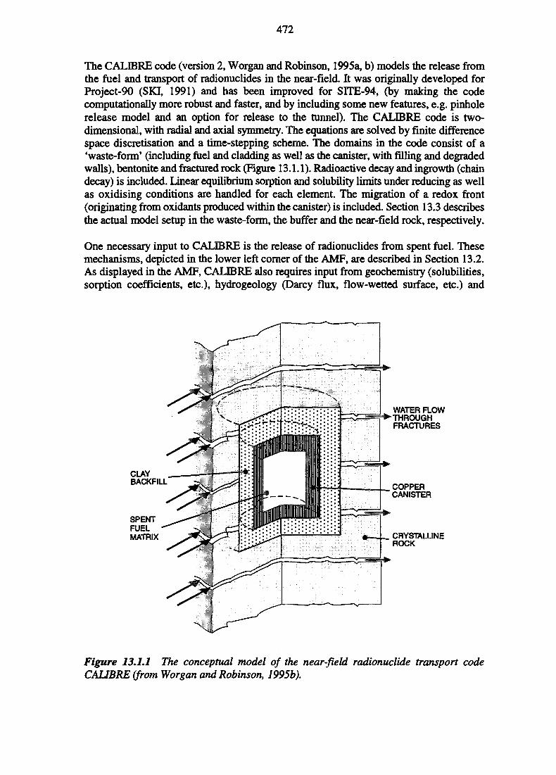
472
The CALIBRE code (version 2, Worgan and Robinson, 1995a, b) models the release fromthe fuel and transport of radionuclides in the near-field. It was originally developed forProject-90 (SKI, 1991) and has been improved for S1TE-94, (by making the codecomputationally more robust and faster, and by including some new features, e.g. pinholerelease model and an option for release to the tunnel). The CALIBRE code is two-dimensional, with radial and axial symmetry. The equations are solved by finite differencespace discretisation and a time-stepping scheme. The domains in the code consist of a'waste-form' (including fuel and cladding as well as the canister, with filling and degradedwalls), bentonite and fractured rock (Figure 13.1.1). Radioactive decay and ingrowth (chaindecay) is included. linear equilibrium sorption and solubility limits under reducing as wellas oxidising conditions are handled for each element. The migration of a redox front(originating from oxidants produced within the canister) is included. Section 13.3 describesthe actual model setup in the waste-form, the buffer and the near-field rock, respectively.
One necessary input to CALIBRE is the release of radionuclides from spent fuel. Thesemechanisms, depicted in the lower left corner of the AMF, are described in Section 13.2.As displayed in the AMF, CALIBRE also requires input from geochemistry (solubilities,sorption coefficients, etc.), hydrogeology (Darcy flux, flow-wetted surface, etc.) and
CLAYBACKFILL
SPENTFUELMATRIX
WATER FLOWTHROUGHFRACTURES
COPPERCANISTER
CRYSTALLINEROCK
Figure 13,1.1 The conceptual model of the near-field radionuclide transport codeCALIBRE (from Worgan and Robinson, 1995b).
473
canister analysis (canister failure time and mode of failure). Dimensions (height, radius,etc.) are derived from the system description in Chapter 5.
The far-field transport is modelled with the CRYSTAL code (Worgan, 1995; Worgan andRobinson 1995c), which is one-dimensional with advection and diffusion in a fracture.Diffusion into the rock matrix is perpendicular to the fracture. Longitudinal dispersion inthe fracture is included. Linear equilibrium sorption is treated for the rock matrix, or assurface sorption (or both). Radioactive decay and ingrowth (chain decay) are included.Apart from simple source terms, CRYSTAL can also handle a source term produced byCALIBRE, in terms of the near-field release rate as a function of time.
13.1.3 Scoping Calculations
Chapter 15 will describe the formulation of calculation cases for CALIBRE andCRYSTAL. The calculation cases are based on the evaluation of the barriers discussed inprevious chapters.
In advance of the evaluation of the calculation cases, a sensitivity analysis, with a simplifiedsource term, was performed. The knowledge of sensitivity derived is later used in order toeconomise the number of calculation cases analysed. The results of these scopingcalculations are presented in Section 13.5.
13.2 RELEASE FROM THE FUEL
13.2.1 Overview
The following fuel release concepts have been incorporated into the near-field codeCALIBRE (Worgan and Robinson, 1995a, b):
• Gap release: release of those radionuclides that are present in soluble form betweenthe cladding and fuel pellets and, to some extent, in fissures (cracks) within thepellets.
• Grain boundary release: release of radionuclides present in solid phases betweenthe UO2 (matrix) grains in spent fuel.
• Matrix release: release of radionuclides incorporated within the grains of fuel.
• In addition, the release of activation products by corrosion of metal parts has beenmodelled in a similar way to grain boundary release.
A lucid review of the subject has been presented by Grambow (1990). An outline of the fuelrelease processes is shown in Figure 13.2.1.
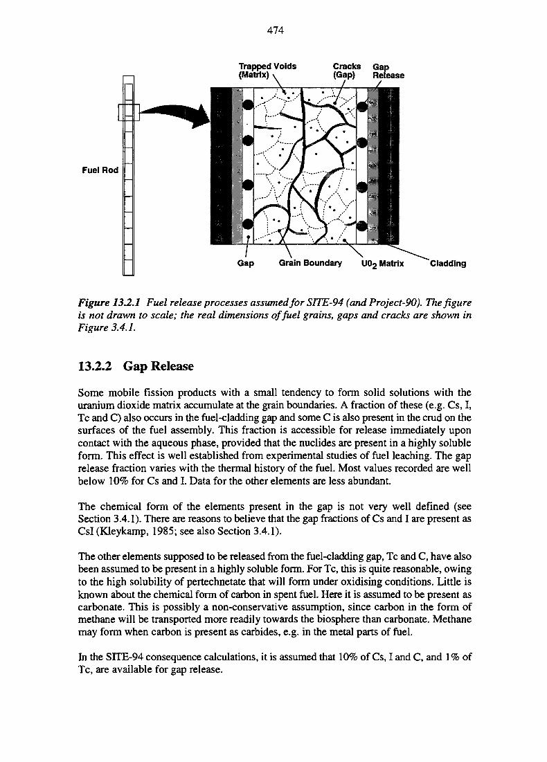
474
Trapped Voids(Matrix)
Cracks Gap(Gap) Release
Fuel Rod
Cladding
Figure 13.2.1 Fuel release processes assumed for SITE-94 (and Project-90). The figureis not drawn to scale; the real dimensions of fuel grains, gaps and cracks are shown inFigure 3.4.1.
13.2.2 Gap Release
Some mobile fission products with a small tendency to form solid solutions with theuranium dioxide matrix accumulate at the grain boundaries. A fraction of these (e.g. Cs, I,Tc and C) also occurs in the fuel-cladding gap and some C is also present in the crud on thesurfaces of the fuel assembly. This fraction is accessible for release immediately uponcontact with the aqueous phase, provided that the nuclides are present in a highly solubleform. This effect is well established from experimental studies of fuel leaching. The gaprelease fraction varies with the thermal history of the fuel. Most values recorded are wellbelow 10% for Cs and I. Data for the other elements are less abundant.
The chemical form of the elements present in the gap is not very well defined (seeSection 3.4.1). There are reasons to believe that the gap fractions of Cs and I are present asCsl (Kleykamp, 1985; see also Section 3.4.1).
The other elements supposed to be released from the fuel-cladding gap, Tc and C, have alsobeen assumed to be present in a highly soluble form. For Tc, this is quite reasonable, owingto the high solubility of pertechnetate that will form under oxidising conditions. Little isknown about the chemical form of carbon in spent fuel. Here it is assumed to be present ascarbonate. This is possibly a non-conservative assumption, since carbon in the form ofmethane will be transported more readily towards the biosphere than carbonate. Methanemay form when carbon is present as carbides, e.g. in the metal parts of fuel.
In the SITE-94 consequence calculations, it is assumed that 10% of Cs, I and C, and 1% ofTc, are available for gap release.
475
13.2.3 Grain Boundary Release
Observed leach rates of Sr and Tc (and of Cs for longer times) have earlier been ascribedto release from grain boundaries, i.e. as an explanation why the leach rates were higher forthese elements than for the observed leach rate of uranium. This assumption may bedoubtful according to more recent studies (TVO, 1992). Technetium and some of the noblemetals form metallic inclusions together with Mo. Parts of these accumulations of Tc maywell be subject to oxidative dissolution along grain boundaries. No separate study of howto model these phenomena has been done for SITE-94. Therefore, the same assumptionsand model is used here as in Project-90 (SKI, 1991).
An uncertainty related to grain boundary release is the possibility for an increase with timeof the corroding surface of oxide grains. This is an intricate question which has bearing onmatters such as oxidant production and the relative rates of grain boundary release andmatrix release.
In the SITE-94 consequence calculations it is assumed that 100% of Sr, 90% of Cs, I andC, and 10% of Tc, are available for grain boundary release. The release rate chosen is 10"7
per day (3.65xl0'5 per year), based on experimental leaching data for Sr (i.e. disregardingthe present belief that Sr is dissolved in the fuel). Modelling of this release is very uncertainfor the long-term, due to insufficient knowledge about the structural degradation of spentfuel.
13.2.4 Matrix Release
Radionuclides present in the uranium dioxide matrix (i.e. within the fuel grains) areassumed to be released at the rate of oxidative conversion of the matrix (congruent release;see Section 11.8). After release, they are transported away at the same rate or theyaccumulate within the canister due to limited solubility (cf. Section 12.3). In the latter case,the transport rate is governed by the solubility limit as an inner boundary condition.
13.2.5 Release From Metal Parts
Activation products in the Zircaloy cladding of the fuel rods and the structural parts of thefuel assembly are released due to corrosion. The release of radionuclides from the metalparts in SITE-94 is based on the assumptions made for the Finnish safety analysis, TVO-92(TVO, 1992).
The corrosion of the Zircaloy is relatively slow, less than 0.01 urn/year, and the corrosionof the Zircaloy then takes more than 100 000 years (TVO, 1992). In S1TE-94, the activationproducts in the Zircaloy are assumed to be evenly released over 10 000 years, which is thesame approach as the one used in TVO-92.
The other structural parts are of stainless steel and Inconel. The corrosion rates of thesematerials are higher than for Zircaloy. The modelling assumption in TVO-92 is that the
476
activity in these materials is released at an even rate over 1000 years (TVO, 1992), and thesame approach is used in SITE-94.
13.2.6 Solubility Limitations
The radionuclides which might reach their solubility limit within the canister are primarilyisotopes of Th, U and Pu. When comparisons are made against a solubility limit all isotopes(including stable isotopes) of the element in question are considered. The resultingcompositions of the solid and aqueous phases are based on an assumption of completeisotopic exchange. This principle is applied for all calculations for all radionuclides.
13.2.7 Mathematical Model and Solution Using the CALIBRE Code
The release of radionuclides from the spent fuel and metal parts in a failed canister iscalculated within the CALIBRE code. The starting point for fuel dissolution is the time ofcanister failure, although decay and ingrowth during the containment phase are included.When the canister fails, it is conservatively assumed that water is immediately in contactwith the fuel and the process of oxidant production by radiolysis and fuel dissolutionbegins.
In the CALIBRE code, release from the fuel and metal parts means that the radionuclidesbecome available in the 'waste-form' (the logical unit in CALIBRE representing fuel,cladding, filler and canister material) for transport by diffusion, for sorption and forconsideration of solubility constraints.
Gap release
The inventories in the gaps between the fuel and cladding are released to the 'waste-form'in a single time-step of the CALIBRE calculations. This release mechanism is applied to1% of "Tc, and 10% of 1291,135Cs, 137Cs and 14C.
Grain boundary release
Elements present at the grain boundaries are released at a fraction that remains constant at10'7 per day, meaning that grain boundary release continues at an even rate until 27 400years after canister failure. This release mechanism is applied to 100% of ^Sr, 90% of 14C,135Cs, 137Cs and 129I, and 10% of "Tc.
For early canister failure times (canister failure at 103 years and less), the fuel matrixdissolution is faster than would be accounted for using this model of grain boundary release(cf. Table 11.8.1). To avoid the radionuclides assigned to grain boundary release beingreleased more slowly than the fuel matrix is actually dissolving, they are in these casesassigned to be released at the same rate as the fuel matrix release.
Fuel matrix release
The remaining fuel inventory (not released by gap or grain boundary release) is releasedcongruently with the fuel matrix dissolution, as described in Section 11.8.1. As the release
477
is assumed to occur linearly with time, the input to CALIBRE is simply the starting timefor dissolution and the time when the full matrix is dissolved. The duration of fuel dis-solution as a function of canister failure time is shown in Table 11.8.1.
Release from metal parts
The activation products in cladding (Zircaloy) and in structural parts (stainless steel andInconel) are released at an even rate over 10 000 and 1000 years, respectively. Themodelling approach in the code is the same as for grain boundary release.
Solubility limitations
In the CALIBRE code, the total concentration of an isotope released from the solid waste(fuel or metal parts) is partitioned into the amount dissolved in the porewater, the amountsorbed on solid material and the amount precipitated. In SITE-94, sorption on the canisteror other solid materials inside the canister is not accounted for (see also Section 15.2.2.3).If the solubility limit for an element is exceeded inside the canister, the dissolvedconcentration of each isotope is proportional to the ratio of the total isotope concentrationto the total element concentration, including stable isotopes (see Equation 13.3.4.)
For the dissolution of precipitate, the CALIBRE code uses the same equation for thepartitioning between precipitated, sorbed and dissolved, while the time dependency gets aless straightforward treatment, as the timescale of dissolution of precipitate is related to themovement of the redox front (although in reality it might be subject to more subtle control).Further, it can be noted that the code treats daughter radionuclides that arise in precipitatesas being immediately available in the water—this can be justified as being conservative but,again, the real situation is much more complicated.
13.3 NEAR-FIELD TRANSPORT
13.3.1 Transport in the Failed Canister
In SITE-94, transport within the canister is assumed to take place by diffusion.Dissolution/precipitation is considered, while no sorption onto the waste-form is takenaccount of. In reality, the canister, cladding and other metal materials (as well as any fillingmaterial) could affect the release and transport of radionuclides, as these could act asphysical barriers and also affect the chemistry by buffering or otherwise changing thechemical environment. Referring to the PBD (Figure 8.1.1), all influences affecting transportin the canister are considered either by including them or by making conservativeassumptions that allow the influence to be neglected.
The water chemistry will primarily affect speciation and solubilities. In preparation for therelease and transport calculations, the water chemistry and the solubilities are calculated byequilibrating the specified far-field groundwater with bentonite, corrosion products (fromthe steel canister) and fuel, one after the other (see Section 11.3.3.2.) In addition, the effectof a moving redox front resulting from the formation of oxidants is considered whenapplicable.
478
The other PID influences, which basically act to reduce transport through the waste-formand out of the canister, are handled by the generally conservative assumptions of nosorption and full contact between the waste-form and the buffer (apart from the possibilityof analysing diffusion through a pinhole in the canister). The approach is consideredgenerally conservative, in that any physical hindrance is neglected. However, this may notbe true in all cases as the assumption of full contact results in an effective dilution ofreleases in the bentonite, through sorption. If there were to be preferential pathways throughthe buffer, this assumption would clearly underestimate releases from the bentonite.
13.3.2 Transport in the Bentonite
The dominating transport mechanism in highly compacted bentonite is diffusion. Advectivetransport can be neglected due to the low hydraulic conductivity (about 10"13 m/s for purewater and 10"12 m/s for saline water, according to SKI, 1991; possibly even down to1016 m/s according to OECD/NEA, 1993). Precipitation/dissolution and sorption in thebentonite are both considered. They are functions of the groundwater chemistry and themineral compositions, including the redox state of the system. The bentonite properties andtheir expected evolution for the Reference Case and the Central Scenario are discussed inSections 8.3 and 11.3.
13.3.3 Transport in the Near-field Rock
In SITE-94, the near-field rock is modelled as a fractured medium, with transport byadvection and diffusion in fractures, and diffusion in the rock matrix (matrix diffusion).Sorption and precipitation/dissolution (see the bottom of the PID, Figure 7.1.2) are alsoconsidered. These latter processes depend on the geochemistry, including the redox state.
Although it is generally recognised that these are the main processes that govern transportin the near-field rock, there is another uncertainty introduced by the unknown and spatiallyvarying structure of the rock itself. For example, matrix diffusion depends on both theporous structure of the rock mass and the effective contact between the rock matrix and theflowing groundwater. Furthermore, the fractures intersecting the deposition hole havespatially varying properties and may be coated with fracture minerals with varying chemicalproperties.
13.3.4 Redox Front
The redox state affects both solubilities and sorption coefficients. The potential formationand migration of a redox front owing to the migration of oxidants produced from radiolysisin the fuel is described in Section 11.7.
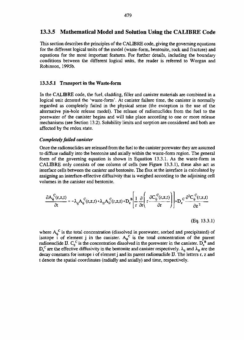
479
13.3.5 Mathematical Model and Solution Using the CALIBRE Code
This section describes the principles of the CALIBRE code, giving the governing equationsfor the different logical units of the model (waste-form, bentonite, rock and fracture) andequations for the most important features. For further details, including the boundaryconditions between the different logical units, the reader is referred to Worgan andRobinson, 1995b.
13.3.5.1 Transport in the Waste-form
In the CALIBRE code, the fuel, cladding, filler and canister materials are combined in alogical unit denoted the 'waste-form'. At canister failure time, the canister is normallyregarded as completely failed in the physical sense (the exception is the use of thealternative pin-hole release model). The release of radionuclides from the fuel to theporewater of the canister begins and will take place according to one or more releasemechanisms (see Section 13.2). Solubility limits and sorption are considered and both areaffected by the redox state.
Completely failed canister
Once the radionuclides are released from the fuel to the canister porewater they are assumedto diffuse radially into the bentonite and axially within the waste-form region. The generalform of the governing equation is shown in Equation 13.3.1. As the waste-form inCALIBRE only consists of one column of cells (see Figure 13.3.1), these also act asinterface cells between the canister and bentonite. The flux at the interface is calculated byassigning an interface-effective diffusivity that is weighed according to the adjoining cellvolumes in the canister and bentonite.
aA>(r,z,t)at
I.JLr dr
aCy(r,z,t)ar
+Dca
2C>(r,z,t)
az:
(Eq. 13.3.1)
where AyC is the total concentration (dissolved in porewater, sorbed and precipitated) ofisotope i of element j in the canister. AuC is the total concentration of the parentradionuclide D. C^ is the concentration dissolved in the porewater in the canister. DC
B andDe
c are the effective diffusivity in the bentonite and canister respectively. kl} and Xu are thedecay constants for isotope i of element j and its parent radionuclide IJ. The letters r, z andt denote the spatial coordinates (radially and axially) and time, respectively.
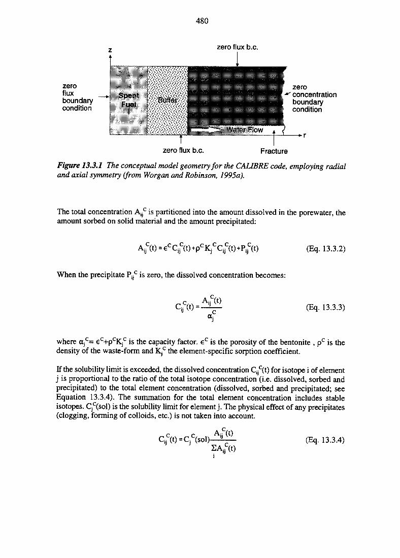
480
zero flux b.c.
zerofluxboundarycondition
zeroconcentrationboundarycondition
zero flux b.c. Fracture
Figure 13.3.1 The conceptual model geometry for the CALIBRE code, employing radialand axial symmetry (from Worgan and Robinson, 1995a).
The total concentration Af is partitioned into the amount dissolved in the porewater, theamount sorbed on solid material and the amount precipitated:
A>(t)=ecCif(t)+PcKj
cC> (Eq. 13.3.2)
When the precipitate PyC is zero, the dissolved concentration becomes:
Ajfrt)
" o f(Eq. 13.3.3)
where ajC= ec+pcKjC is the capacity factor. e c is the porosity of the bentonite , p c is thedensity of the waste-form and KjC the element-specific sorption coefficient.
If the solubility limit is exceeded, the dissolved concentration C^t) for isotope i of elementj is proportional to the ratio of the total isotope concentration (i.e. dissolved, sorbed andprecipitated) to the total element concentration (dissolved, sorbed and precipitated; seeEquation 13.3.4). The summation for the total element concentration includes stableisotopes. CjC(sol) is the solubility limit for element j . The physical effect of any precipitates(clogging, forming of colloids, etc.) is not taken into account.
s i (0
ii CO(Eq. 13.3.4)
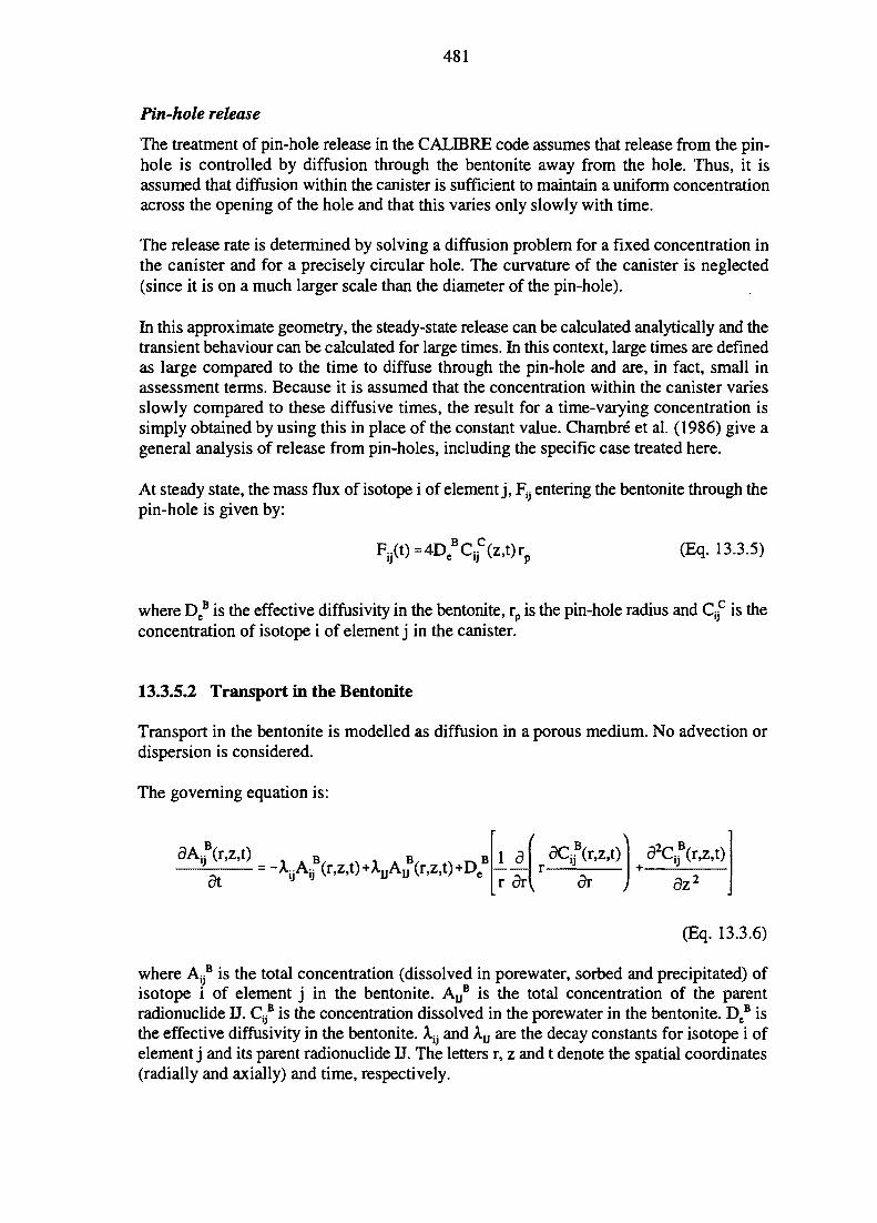
481
Pin-hole release
The treatment of pin-hole release in the CALIBRE code assumes that release from the pin-hole is controlled by diffusion through the bentonite away from the hole. Thus, it isassumed that diffusion within the canister is sufficient to maintain a uniform concentrationacross the opening of the hole and that this varies only slowly with time.
The release rate is determined by solving a diffusion problem for a fixed concentration inthe canister and for a precisely circular hole. The curvature of the canister is neglected(since it is on a much larger scale than the diameter of the pin-hole).
In this approximate geometry, the steady-state release can be calculated analytically and thetransient behaviour can be calculated for large times. In this context, large times are definedas large compared to the time to diffuse through the pin-hole and are, in fact, small inassessment terms. Because it is assumed that the concentration within the canister variesslowly compared to these diffusive times, the result for a time-varying concentration issimply obtained by using this in place of the constant value. Chambre et al. (1986) give ageneral analysis of release from pin-holes, including the specific case treated here.
At steady state, the mass flux of isotope i of element j , F^ entering the bentonite through thepin-hole is given by:
Fa(t)=4DeBCa
c(z,t)r (Eq. 13.3.5)
where DCB is the effective diffusivity in the bentonite, rp is the pin-hole radius and
concentration of isotope i of element j in the canister.is the
13.3.5.2 Transport in the Bentonite
Transport in the bentonite is modelled as diffusion in a porous medium. No advection ordispersion is considered.
The governing equation is:
6A:: (r,Z,t)u LJL
r dv
dC°(T,z,t)
dv
d2C::B(r,z,t)
dz
(Eq. 13.3.6)
where Ai3B is the total concentration (dissolved in porewater, sorbed and precipitated) of
isotope i of element j in the bentonite. ADB is the total concentration of the parent
radionuclide IJ. C* is the concentration dissolved in the porewater in the bentonite. DCB is
the effective diffusivity in the bentonite. X^ and Xu are the decay constants for isotope i ofelement j and its parent radionuclide IJ. The letters r, z and t denote the spatial coordinates(radially and axially) and time, respectively.
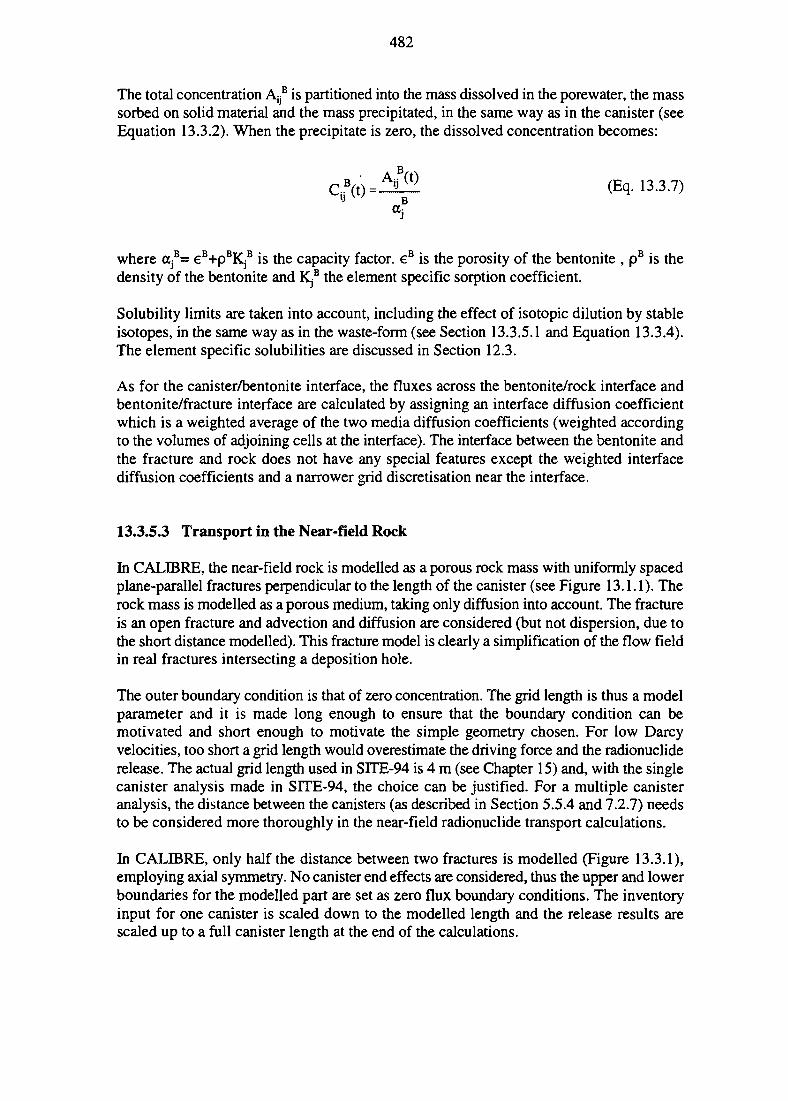
482
The total concentration A^8 is partitioned into the mass dissolved in the porewater, the masssorbed on solid material and the mass precipitated, in the same way as in the canister (seeEquation 13.3.2). When the precipitate is zero, the dissolved concentration becomes:
(Eq. 13.3.7)
where otjB= eB+pBKjB is the capacity factor. eB is the porosity of the bentonite , pB is thedensity of the bentonite and KjB the element specific sorption coefficient.
Solubility limits are taken into account, including the effect of isotopic dilution by stableisotopes, in the same way as in the waste-form (see Section 13.3.5.1 and Equation 13.3.4).The element specific solubilities are discussed in Section 12.3.
As for the canister/bentonite interface, the fluxes across the bentonite/rock interface andbentonite/fracture interface are calculated by assigning an interface diffusion coefficientwhich is a weighted average of the two media diffusion coefficients (weighted accordingto the volumes of adjoining cells at the interface). The interface between the bentonite andthe fracture and rock does not have any special features except the weighted interfacediffusion coefficients and a narrower grid discretisation near the interface.
13.3.5.3 Transport in the Near-field Rock
In CALIBRE, the near-field rock is modelled as a porous rock mass with uniformly spacedplane-parallel fractures perpendicular to the length of the canister (see Figure 13.1.1). Therock mass is modelled as a porous medium, taking only diffusion into account. The fractureis an open fracture and advection and diffusion are considered (but not dispersion, due tothe short distance modelled). This fracture model is clearly a simplification of the flow fieldin real fractures intersecting a deposition hole.
The outer boundary condition is that of zero concentration. The grid length is thus a modelparameter and it is made long enough to ensure that the boundary condition can bemotivated and short enough to motivate the simple geometry chosen. For low Darcyvelocities, too short a grid length would overestimate the driving force and the radionucliderelease. The actual grid length used in S1TE-94 is 4 m (see Chapter 15) and, with the singlecanister analysis made in SITE-94, the choice can be justified. For a multiple canisteranalysis, the distance between the canisters (as described in Section 5.5.4 and 7.2.7) needsto be considered more thoroughly in the near-field radionuclide transport calculations.
In CALIBRE, only half the distance between two fractures is modelled (Figure 13.3.1),employing axial symmetry. No canister end effects are considered, thus the upper and lowerboundaries for the modelled part are set as zero flux boundary conditions. The inventoryinput for one canister is scaled down to the modelled length and the release results arescaled up to a full canister length at the end of the calculations.
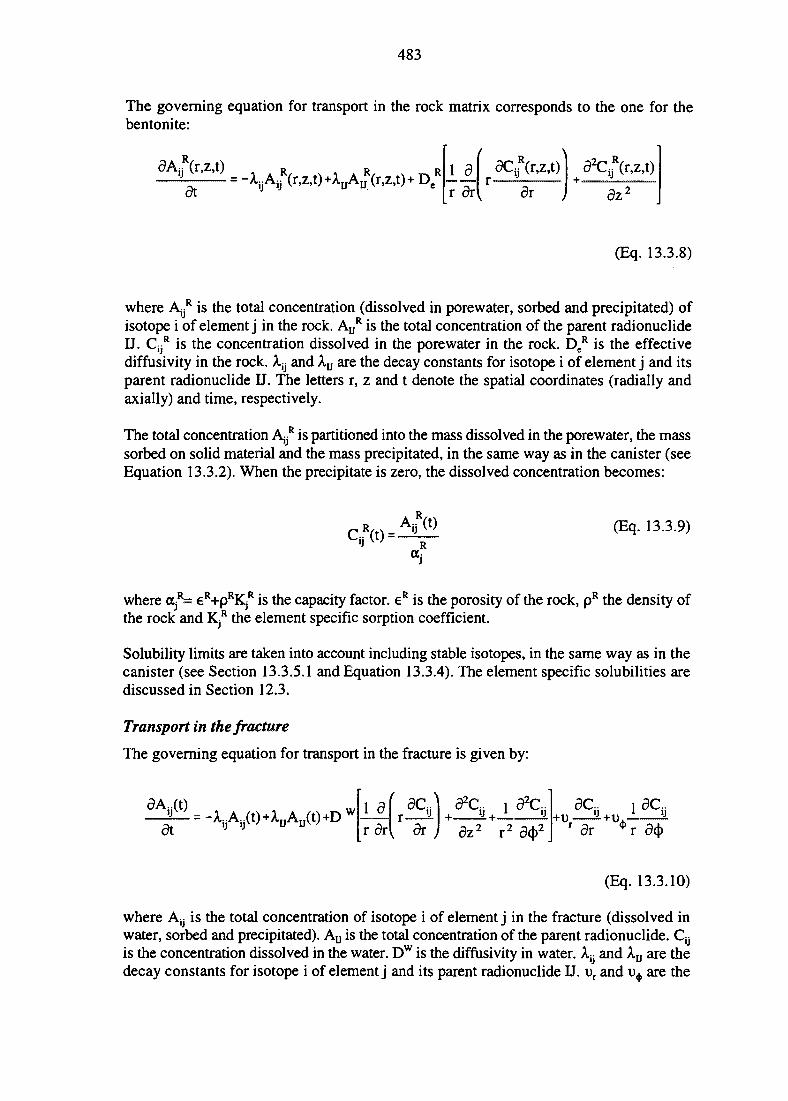
483
The governing equation for transport in the rock matrix corresponds to the one for thebentonite:
atDe LJL
r dr dz
(Eq. 13.3.8)
where AyR is the total concentration (dissolved in porewater, sorbed and precipitated) of
isotope i of element j in the rock. AUR is the total concentration of the parent radionuclide
IJ. CijR is the concentration dissolved in the porewater in the rock. DeR is the effective
diffusivity in the rock. X-^ and Xu are the decay constants for isotope i of element j and itsparent radionuclide IJ. The letters r, z and t denote the spatial coordinates (radially andaxially) and time, respectively.
The total concentration A^ is partitioned into the mass dissolved in the porewater, the masssorbed on solid material and the mass precipitated, in the same way as in the canister (seeEquation 13.3.2). When the precipitate is zero, the dissolved concentration becomes:
RC (Eq. 13.3.9)
where 0 *= €R+pRKjR is the capacity factor. eR is the porosity of the rock, pR the density ofthe rock and KjR the element specific sorption coefficient.
Solubility limits are taken into account including stable isotopes, in the same way as in thecanister (see Section 13.3.5.1 and Equation 13.3.4). The element specific solubilities arediscussed in Section 12.3.
Transport in the fracture
The governing equation for transport in the fracture is given by:
~L wr6rl dr az
I2 r2 ) _
(Eq. 13.3.10)
where Ay is the total concentration of isotope i of element j in the fracture (dissolved inwater, sorbed and precipitated). AD is the total concentration of the parent radionuclide. Cyis the concentration dissolved in the water. Dw is the diffusivity in water. Xi} and A-u are thedecay constants for isotope i of element j and its parent radionuclide IJ. i>r and u^ are the
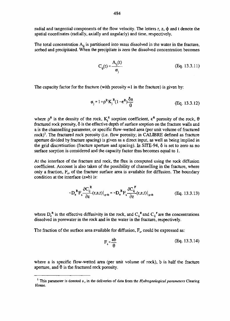
484
radial and tangential components of the flow velocity. The letters r, z, (|> and t denote thespatial coordinates (radially, axially and angularly) and time, respectively.
The total concentration A^ is partitioned into mass dissolved in the water in the fracture,sorbed and precipitated. When the precipitate is zero the dissolved concentration becomes
(Eq. 13.3.11)a}
The capacity factor for the fracture (with porosity ~1 in the fracture) is given by:
Oj-l^KjVe*^ (Eq. 13.3.12)
where pR is the density of the rock, KjR sorption coefficient, eR porosity of the rock, 0fractured rock porosity, 6 is the effective depth of surface sorption on the fracture walls anda is the channelling parameter, or specific flow-wetted area (per unit volume of fracturedrock)1. The fractured rock porosity (i.e. flow porosity; in CALIBRE defined as fractureaperture divided by fracture spacing) is given as a direct input, as well as being implied inthe grid discretisation (fracture aperture and spacing). In SITE-94, 6 is set to zero as nosurface sorption is considered and the capacity factor thus becomes equal to 1.
At the interface of the fracture and rock, the flux is computed using the rock diffusioncoefficient. Account is also taken of the possibility of channelling in the fracture, whereonly a fraction, Fs, of the fracture surface area is available for diffusion. The boundarycondition at the interface (z=b) is:
-D eRF s-^-(r,z,t) | z ,b = -De
RF s-^-(r,z,t) |2 ,b (Eq. 13.3.13)
where DeR is the effective diffusivity in the rock, and C^and Cij
Fare the concentrationsdissolved in porewater in the rock and in the water in the fracture, respectively.
The fraction of the surface area available for diffusion, Fs, could be expressed as:
F = ^ (Eq. 13.3.14)s 6
where a is specific flow-wetted area (per unit volume of rock), b is half the fractureaperture, and 8 is the fractured rock porosity.
1 This parameter is denoted a r in the deliveries of data from the Hydrogeological parameters ClearingHouse.

485
In Project-90 (SKI, 1991) the radionuclide transport calculations indicated that using thesame value of specific flow-wetted area in the near-field code (CALIBRE) and the far-fieldcode (CRYSTAL) produced more effective matrix diffusion in the near-field. The reasonwas that the matrix diffusion occurs in two dimensions in CALIBRE while only in one inCRYSTAL.
In an attempt to overcome this and to reflect more accurately the concept of channellingwithin the fracture, a parameter called channel connection length (CCL-parameter) is nowintroduced in the CALIBRE code. The basis for this concept is that a few large channelsin the fracture will have a greater separation distance than many small channels, even if thetotal surface areas are equal. The opportunity for matrix diffusion is less the bigger theseparation distance.
In the CALIBRE code, the grid discretisation distance between the fracture cell and theadjacent rock cell is generally small (on the same order as the fracture aperture) and doesnot represent the channelling situation very well. In practice, the average diffusion distancefrom the channels to the rock adjacent to the fracture plane is controlled by the distancebetween channels so, in the CALIBRE code, the value of CCL-parameter is used insteadof the grid discretisation distance when calculating the diffusive transfer rate. Thus, matrixdiffusion becomes more restricted the larger the channel connection length that is chosen.However, it must be remembered that the treatment of transport in the fracture in theCALIBRE code is approximate (in terms of orientation, dimensionality, etc., as well as inthe interface between rock matrix and fracture) and the model of the fracture in CALIBREis thus best regarded as a way to get better boundary conditions than would be obtainedwith a more simplistic mixing tank with zero-concentration.
The influence of the CCL-parameter is evaluated in the simple scoping calculationspresented in Section 13.5.1.
For flow around a cylinder, the radial and tangential components of the flow velocity, ur andi^, could be written:
= UCOS(J) (Eq. 13.3.15)
= -usincj) 1+- (Eq. 13.3.16)
where r2 is the radius of the interface of the bentonite and rock, and u is the flow velocityin the fracture far from the cylinder. The flow velocity is derived from the Darcy velocityq (input parameter to CALIBRE) and the fractured rock porosity 0 by:
6(Eq. 13.3.17)
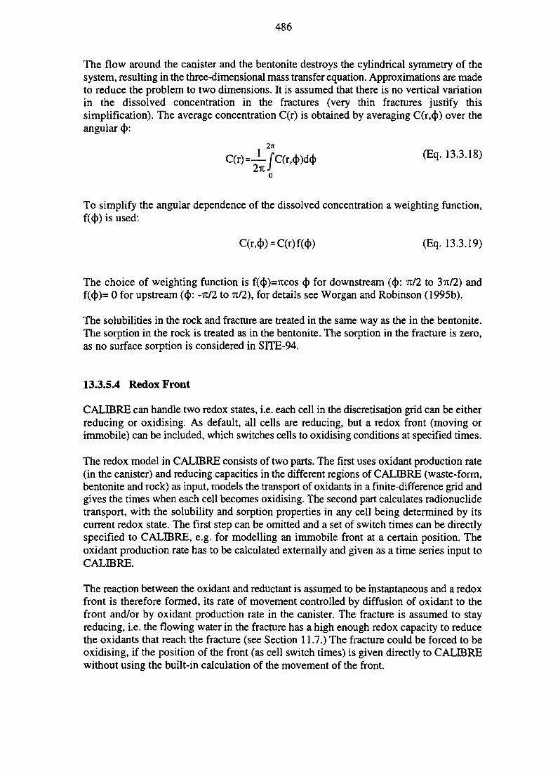
486
The flow around the canister and the bentonite destroys the cylindrical symmetry of thesystem, resulting in the three-dimensional mass transfer equation. Approximations are madeto reduce the problem to two dimensions. It is assumed that there is no vertical variationin the dissolved concentration in the fractures (very thin fractures justify thissimplification). The average concentration C(r) is obtained by averaging C(r,(j)) over theangular (():
C(r)=-LjC(r,<t»dci> (Eq- 1 3 - 3 1 8 )
To simplify the angular dependence of the dissolved concentration a weighting function,is used:
C(r,<t>)=C(r)f(<J>) (Eq. 13.3.19)
The choice of weighting function is f((j>)=7i:cos <|) for downstream ($: it/2 to 3it/2) andf((j))= 0 for upstream (4>: -ft/2 to %/2), for details see Worgan and Robinson (1995b).
The solubilities in the rock and fracture are treated in the same way as the in the bentonite.The sorption in the rock is treated as in the bentonite. The sorption in the fracture is zero,as no surface sorption is considered in SITE-94.
13.3.5.4 Redox Front
CALIBRE can handle two redox states, i.e. each cell in the discretisation grid can be eitherreducing or oxidising. As default, all cells are reducing, but a redox front (moving orimmobile) can be included, which switches cells to oxidising conditions at specified times.
The redox model in CALIBRE consists of two parts. The first uses oxidant production rate(in the canister) and reducing capacities in the different regions of CALIBRE (waste-form,bentonite and rock) as input, models the transport of oxidants in a finite-difference grid andgives the times when each cell becomes oxidising. The second part calculates radionuclidetransport, with the solubility and sorption properties in any cell being determined by itscurrent redox state. The first step can be omitted and a set of switch times can be directlyspecified to CALIBRE, e.g. for modelling an immobile front at a certain position. Theoxidant production rate has to be calculated externally and given as a time series input toCALIBRE.
The reaction between the oxidant and reductant is assumed to be instantaneous and a redoxfront is therefore formed, its rate of movement controlled by diffusion of oxidant to thefront and/or by oxidant production rate in the canister. The fracture is assumed to stayreducing, i.e. the flowing water in the fracture has a high enough redox capacity to reducethe oxidants that reach the fracture (see Section 11.7.) The fracture could be forced to beoxidising, if the position of the front (as cell switch times) is given directly to CALIBREwithout using the built-in calculation of the movement of the front.
487
With the stepwise (cellwise) movements of the front in CALIBRE, the changes of solubilitylimits and sorption properties may be very abrupt. In the case of a moving front, theproperties of a cell are allowed to start changing as soon as any of the nearest cells becomefully oxidised. Thus, the properties may change from reducing to oxidising linearly over anumber of time steps, depending on how quickly the front moves.
13.4 TRANSPORT IN THE FAR-FIELD ROCK
13.4.1 General Description
Radionuclide migration and retardation in the far-field rock are assumed to take place byadvection/dispersion of the radionuclides dissolved in the flowing groundwater, matrixdiffusion into the rock mass and sorption. Precipitation/dissolution is, conservatively,neglected as the concentrations are assumed to be very low. Colloids could constitute analternative transport mechanism, but their impacts are not analysed within SITE-94. Allthese processes are also displayed at the bottom of the PID (see Figure 7.1.1.)
For a continuous Darcy velocity field the transport mechanisms above could be describedby the advection-dispersion Equation 13.4.1 coupled to the diffusion equation inside therock matrix (Equation 13.4.2). Equation 13.4.1 takes into account radionuclide transportby groundwater flow in a fracture, but subject to instantaneous linear sorption on thefracture surface, diffusion out of the fracture into the matrix porosity, and radioactive decay.The three terms on the left hand side of the equation describe impacts on radionuclideconcentration in the water of retardation by fracture surface sorption, of flow rate and ofdispersion, respectively. The first two terms on the right hand side of the equation takeaccount of radioactive decay (including chain decay) whilst the final term defines theimpact on concentration of radionuclides in the matrix pore waters as a result of diffusionout from the wetted fracture surface area (in the w direction assumed to be orthogonal tothe fracture) into the rock matrix.
Equation 13.4.2 accounts for diffusion in one direction orthogonal to the fracture and forsorption of radionuclides inside the rock matrix, again taking account of chain decay.
Finally, Equations 13.4.3 and 13.4.4 describe how the two retardation factors (surface andmatrix) used in the transport equations are derived from the relationship between sorptioncoefficient and fracture or matrix porosity, respectively. The surface sorption equation(13.4.3) includes a term to account for the size of the wetted surface area of the fracture andthe amount ('depth') of rock available for immediate surface sorption. Note that this isdistinct from the penetration depth for diffusion and sorption in the matrix which is definedas the maximum distance in the w direction where there is connected pore space.
The velocity field and the specific flow-wetted area are subject both to spatial variabilityand to uncertainty, as discussed in Chapter 10. The appropriateness of Equation 13.4.2could be questioned, particularly the assumption of spatially invariant properties and thegeometrical simplifications. The uncertainties in the treatment of sorption are discussed inSection 12.4.
488
l C j . ) + V(qc.) - V(6DVCi) =dt
-i - AjORjC, + a6 r a D m - | - ( c J | w , 0
4&m*J - D-"r^ c- |) + V i ^ - i ^ - i - V ^ - (Eq- 13-4.2)dt 5w^
K r i Q m ( l -8 ja6. - I + - — (Eq. 13.4.3)
R = i + K d ^ Q m ( L e J (Eq. 13.4.4)mi 0mi
where:Cj = concentration of radionuclide i in the fracture water [moles/m3]cmi = concentration of radionuclide i in the matrix water [moles/m3]w = distance into matrix orthogonal to fracture surface [m]q = groundwater flow (Darcy velocity) [m3/m2/s]D = dispersion [m2/s]a = specific flow-wetted area of fractures (per volume of rock mass) [m1]Kdi = sorption coefficient for radionuclide i for fracture surfaces [m3/kg]Kd.mi ™ sorption coefficient for radionuclide i inside rock matrix [m3/kg]6 = 'depth ' of surface sorption [m]D m = matrix diffusivity [m2/s]0 = rock mass ( 'flowing') porosity6 m = matrix porosityXi = decay constant for radionuclide i [s 1]Qm = bulk density of rock matrix [kg/m3]Rj = retardation for radionuclide i due to surface sorption
retardation for radionuclide i due to sorption in rock matrix
13.4.2 Mathematical Model and Solution Using the CRYSTAL Code
Far-field transport in SITE-94 is evaluated using a computer code, CRYSTAL version 2.1,developed by Worgan and Robinson (1995c). The code implements a one-dimensional formof Equation 13.4.2. This is a considerable simplification of the true velocity field discussedin Sections 10.3.9 and 15.2.1.6. The following physical and chemical processes areincluded:
489
• Advection of radionuclides occurs in the groundwater, which is assumed to have alaminar flow at constant velocity through a set of parallel fractures. The shape of thematrix blocks are either planar, cylindrical or combinations of both. Figure 13.4.1outlines the planar shape of the matrix blocks. This is the shape used in all thecalculations in SITE-94.
• Longitudinal dispersion spreads dissolved radionuclides along the direction of flow.Transverse dispersion is not considered, since the required results are total fluxesintegrated in the transverse direction. It is assumed that molecular diffusionequalises the concentration across the aperture. Note that the fracture aperture shownin Figure 13.4.1 is not used as a direct variable in CRYSTAL, which instead uses thesurrogate value of flow porosity, from which aperture can be back-calculated ifrequired.
• Diffusion in the rock matrix occurs perpendicular to the fracture walls and can occurup to a symmetry boundary of specified penetration distance. The 'fracture spacing'shown in Figure 13.4.1 defines a 'slab thickness' in CRYSTAL which clearlydefines the upper limit of diffusion into the rock matrix. This parameter is notdetermined in the SITE-94 hydrogeological analysis and is not used as a variable inCRYSTAL in the current analysis. This is because it is set at a single, sufficientlylarge value in CRYSTAL (1 m) that it exceeds twice the maximum diffusionpenetration distance variant (0.25 m).
• The contact area between the rock and fracture is controlled by the specific flow-wetted area parameter1. This restricts the amount of rock into which diffusion canoccur. Figure 13.4.2 illustrates diffusion into the planar type of matrix blocks usedby CRYSTAL.
• Linear equilibrium sorption on fracture surfaces and in the bulk matrix retards themovement of radionuclides. In the application for SITE-94, only the matrix sorptionwas used. Linear equilibrium sorption in the matrix or on the fracture walls orcombinations of both are possible in the code.
• Radioactive decay and ingrowth occur throughout.
Note that the geometrical simplifications are made on the assumption that the overallbehaviour of the system depends largely on averaged properties of the detailed geometry.For example, the specific surface area of contact between flowing and non-flowing wateris sufficient to model the system without knowledge of the real, highly complex structures.Thus, it is not implied that a real system has such a simple geometry, only that its behaviourcan be well enough reproduced by working with the simple geometry.
This parameter is denoted a r in the deliveries of data from the Hydrogeological parameters ClearingHouse.
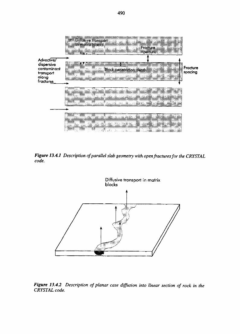
490
JJLJLV*~
Advedive?dispersivecontaminanttransportalongfradures
Fracturespacing
Figure 13.4.1 Description of parallel slab geometry with open fractures for the CRYSTALcode.
Diffusive transport in matrixblocks
Figure 13.4.2 Description of planar case diffusion into linear section of rock in theCRYSTAL code.
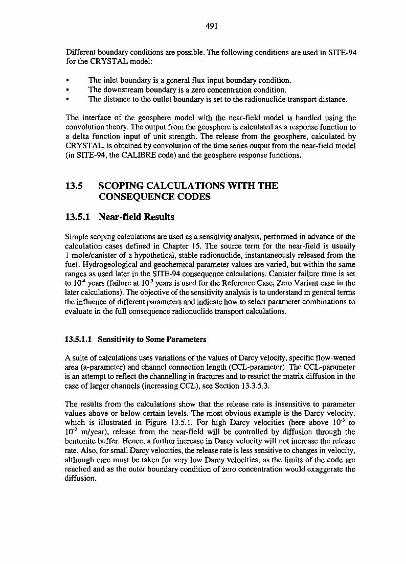
491
Different boundary conditions are possible. The following conditions are used in SITE-94for the CRYSTAL model:
• The inlet boundary is a general flux input boundary condition.• The downstream boundary is a zero concentration condition.• The distance to the outlet boundary is set to the radionuclide transport distance.
The interface of the geosphere model with the near-field model is handled using theconvolution theory. The output from the geosphere is calculated as a response function toa delta function input of unit strength. The release from the geosphere, calculated byCRYSTAL, is obtained by convolution of the time series output from the near-field model(in SITE-94, the CALIBRE code) and the geosphere response functions.
13.5 SCOPING CALCULATIONS WITH THECONSEQUENCE CODES
13.5.1 Near-field Results
Simple scoping calculations are used as a sensitivity analysis, performed in advance of thecalculation cases defined in Chapter 15. The source term for the near-field is usually1 mole/canister of a hypothetical, stable radionuclide, instantaneously released from thefuel. Hydrogeological and geochemical parameter values are varied, but within the sameranges as used later in the SITE-94 consequence calculations. Canister failure time is setto W4 years (failure at 10"3 years is used for the Reference Case, Zero Variant case in thelater calculations). The objective of the sensitivity analysis is to understand in general termsthe influence of different parameters and indicate how to select parameter combinations toevaluate in the full consequence radionuclide transport calculations.
13.5.1.1 Sensitivity to Some Parameters
A suite of calculations uses variations of the values of Darcy velocity, specific flow-wettedarea (a-parameter) and channel connection length (CCL-parameter). The CCL-parameteris an attempt to reflect the channelling in fractures and to restrict the matrix diffusion in thecase of larger channels (increasing CCL), see Section 13.3.5.3.
The results from the calculations show that the release rate is insensitive to parametervalues above or below certain levels. The most obvious example is the Darcy velocity,which is illustrated in Figure 13.5.1. For high Darcy velocities (here above 10'3 to10"2 m/year), release from the near-field will be controlled by diffusion through thebentonite buffer. Hence, a further increase in Darcy velocity will not increase the releaserate. Also, for small Darcy velocities, the release rate is less sensitive to changes in velocity,although care must be taken for very low Darcy velocities, as the limits of the code arereached and as the outer boundary condition of zero concentration would exaggerate thediffusion.
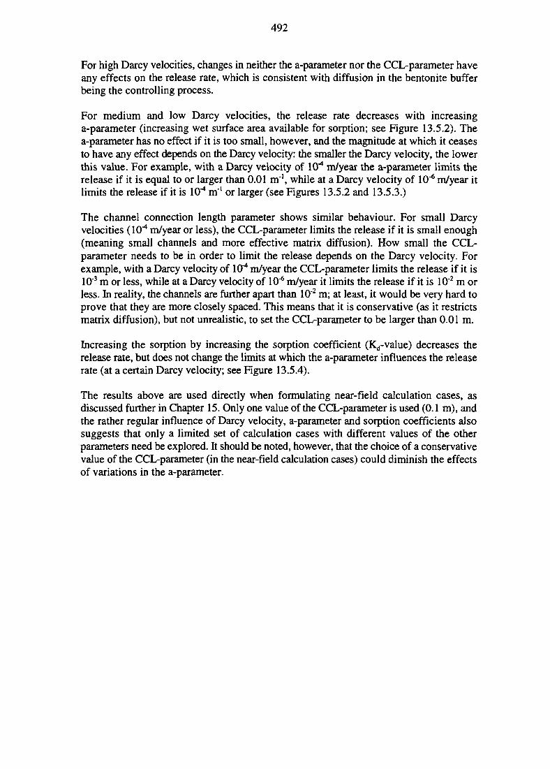
492
For high Darcy velocities, changes in neither the a-parameter nor the CCL-parameter haveany effects on the release rate, which is consistent with diffusion in the bentonite bufferbeing the controlling process.
For medium and low Darcy velocities, the release rate decreases with increasinga-parameter (increasing wet surface area available for sorption; see Figure 13.5.2). Thea-parameter has no effect if it is too small, however, and the magnitude at which it ceasesto have any effect depends on the Darcy velocity: the smaller the Darcy velocity, the lowerthis value. For example, with a Darcy velocity of 10*4 m/year the a-parameter limits therelease if it is equal to or larger than 0.01 m"1, while at a Darcy velocity of 10"6 m/year itlimits the release if it is 10"4 m'1 or larger (see Figures 13.5.2 and 13.5.3.)
The channel connection length parameter shows similar behaviour. For small Darcyvelocities (10^ m/year or less), the CCL-parameter limits the release if it is small enough(meaning small channels and more effective matrix diffusion). How small the CCL-parameter needs to be in order to limit the release depends on the Darcy velocity. Forexample, with a Darcy velocity of 10^ m/year the CCL-parameter limits the release if it is10'3 m or less, while at a Darcy velocity of 10"6 m/year it limits the release if it is 10'2 m orless. In reality, the channels are further apart than 10"2 m; at least, it would be very hard toprove that they are more closely spaced. This means that it is conservative (as it restrictsmatrix diffusion), but not unrealistic, to set the CCL-parameter to be larger than 0.01 m.
Increasing the sorption by increasing the sorption coefficient (Kd-value) decreases therelease rate, but does not change the limits at which the a-parameter influences the releaserate (at a certain Darcy velocity; see Figure 13.5.4).
The results above are used directly when formulating near-field calculation cases, asdiscussed further in Chapter 15. Only one value of the CCL-parameter is used (0.1 m), andthe rather regular influence of Darcy velocity, a-parameter and sorption coefficients alsosuggests that only a limited set of calculation cases with different values of the otherparameters need be explored. It should be noted, however, that the choice of a conservativevalue of the CCL-parameter (in the near-field calculation cases) could diminish the effectsof variations in the a-parameter.
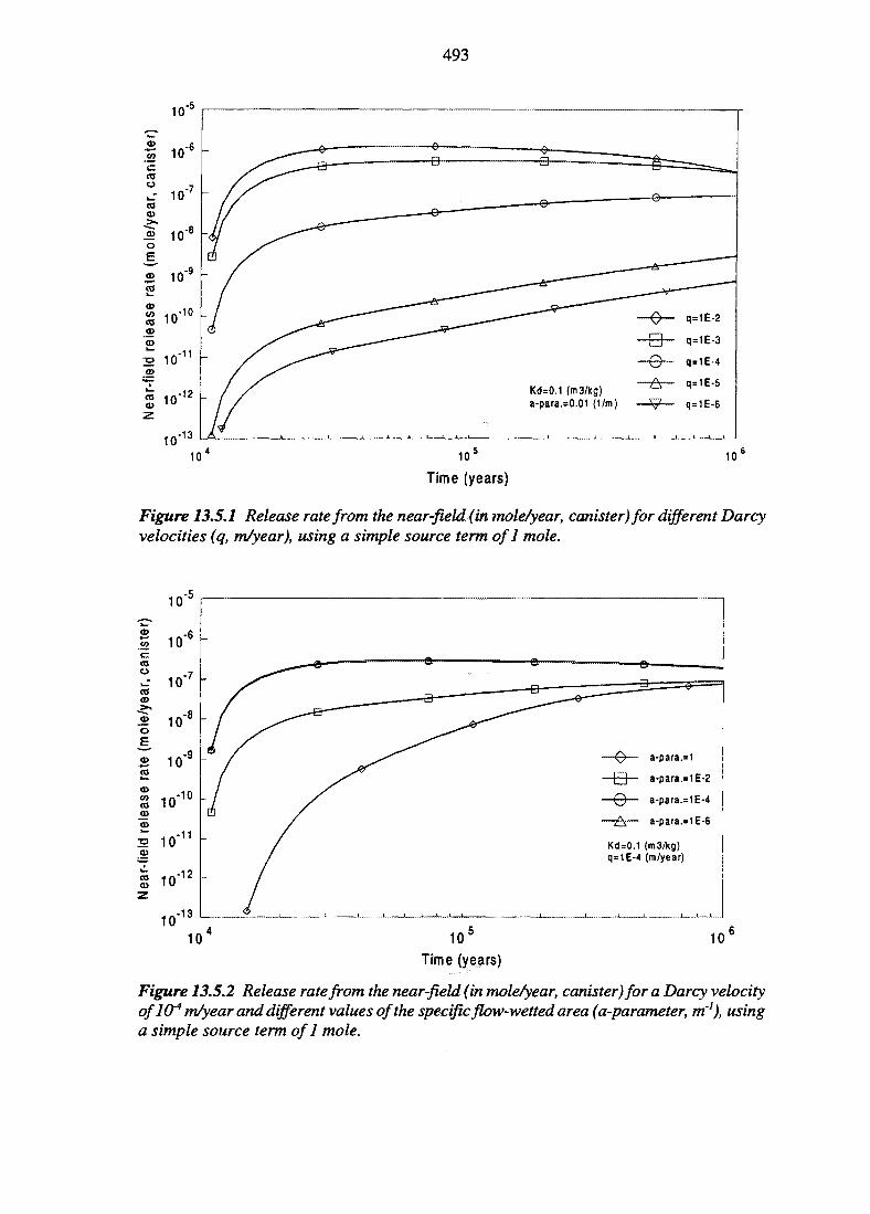
493
10 10
Time (years)
Figure 13.5.1 Release rate from the near-field (in mole/year, canister) for different Darcyvelocities (q, m/year), using a simple source term of 1 mole.
a-para.=1
a-para.=1E-2
a-para.= iE-4
a-para.=1E-6
Kd=0.1 (m3/kg)q=1 E-4 (m/year)
10 10Time (years)
Figure 13.5.2 Release rate from the near-field (in mole/year, canister) for a Darcy velocityoflO4 m/year and different values of the specific flow-wetted area (a-parameter, m1), usinga simple source term of 1 mole.
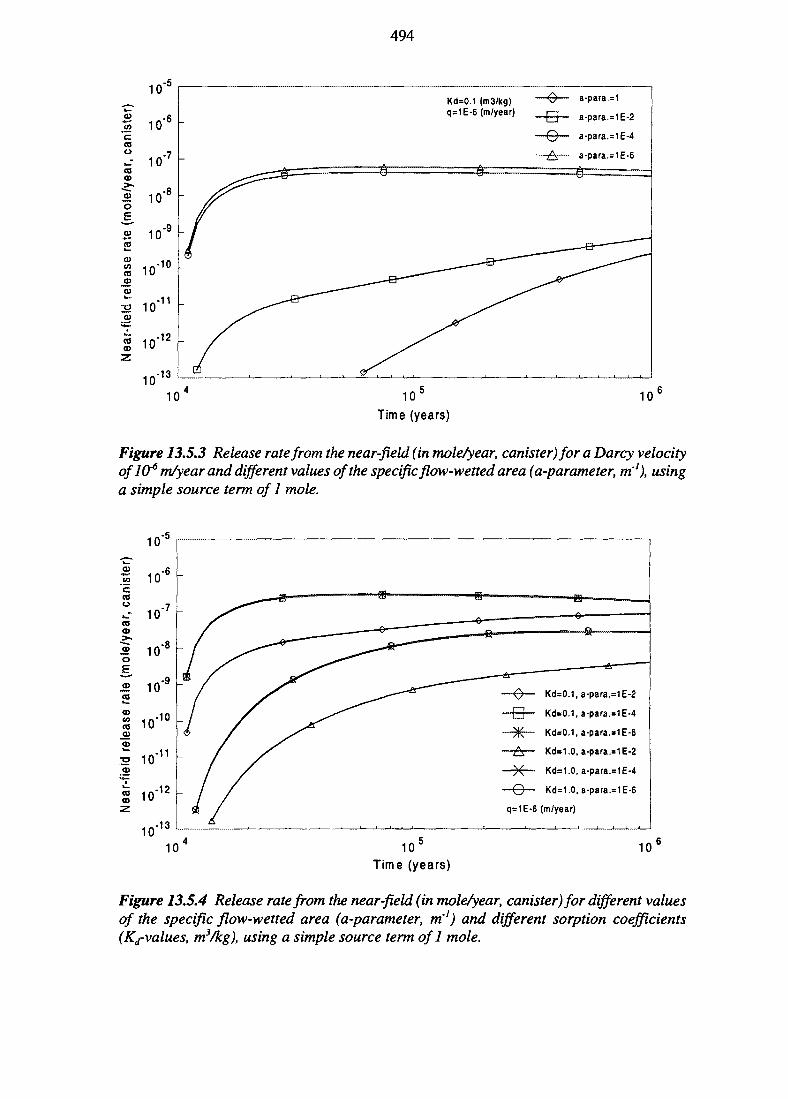
CO0)
a>
10'
10-6
w 10-7
10-8
.2 10-9
CD
i 10
"510
•10
•11
v-12
10-13
10
494
Kd=0.1 (m3/kg)q=1E-6 (m/year)
a-para.=1
a-para.=1E-2
a-para.=1E-4
a-para.=1E-6
- § — = =
103
Time (years)10
Figure 13.5.3 Release rate from the near-field (in mole/year, canister) for a Darcy velocityoflCt6 m/year and different values of the specific flow-wetted area (a-parameter, m'1), usinga simple source term of 1 mole.
Kd=0.1,a-para.=1E-2
Kd=0.1,a-para.=1E-4
Kd=0.1, a-para.=1E-6
Kd=1.0.a-para.=
Kd=1.0,a-para.=1E-4
Kd=1.0, a-para.=1E-6
q=1E-6 (m/year)
10Time (years)
Figure 13.5.4 Release rate from the near-field (in mole/year, canister) for different valuesof the specific flow-wetted area (a-parameter, m'1) and different sorption coefficients(Kd-values, m3/kg), using a simple source term of 1 mole.
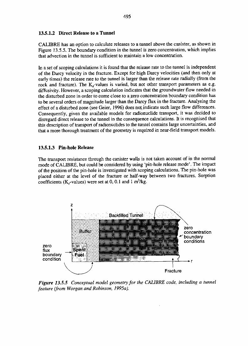
495
13.5.1.2 Direct Release to a Tunnel
CALIBRE has an option to calculate releases to a tunnel above the canister, as shown inFigure 13.5.5. The boundary condition in the tunnel is zero concentration, which impliesthat advection in the tunnel is sufficient to maintain a low concentration.
In a set of scoping calculations it is found that the release rate to the tunnel is independentof the Darcy velocity in the fracture. Except for high Darcy velocities (and then only atearly times) the release rate to the tunnel is larger than the release rate radially (from therock and fracture). The Kd-values is varied, but not other transport parameters as e.g.diffusivity. However, a scoping calculation indicates that the groundwater flow needed inthe disturbed zone in order to come close to a zero concentration boundary condition hasto be several orders of magnitude larger than the Darcy flux in the fracture. Analysing theeffect of a disturbed zone (see Geier, 1996) does not indicate such large flow differences.Consequently, given the available models for radionuclide transport, it was decided todisregard direct release to the tunnel in the consequence calculations. It is recognised thatthis description of transport of radionuclides to the tunnel contains large uncertainties, andthat a more thorough treatment of the geometry is required in near-field transport models.
13.5.1.3 Pin-hole Release
The transport resistance through the canister walls is not taken account of in the normalmode of CALIBRE, but could be considered by using 'pin-hole release mode'. The impactof the position of the pin-hole is investigated with scoping calculations. The pin-hole wasplaced either at the level of the fracture or half-way between two fractures. Sorptioncoefficients (Kd-values) were set at 0, 0.1 and 1 mVkg.
zerofluxboundarycondition
zeroconcentrationboundaryconditions
Fracture
Figure 13.5.5 Conceptual model geometry for the CALIBRE code, including a tunnelfeature (from Worgan and Robinson, 1995a).
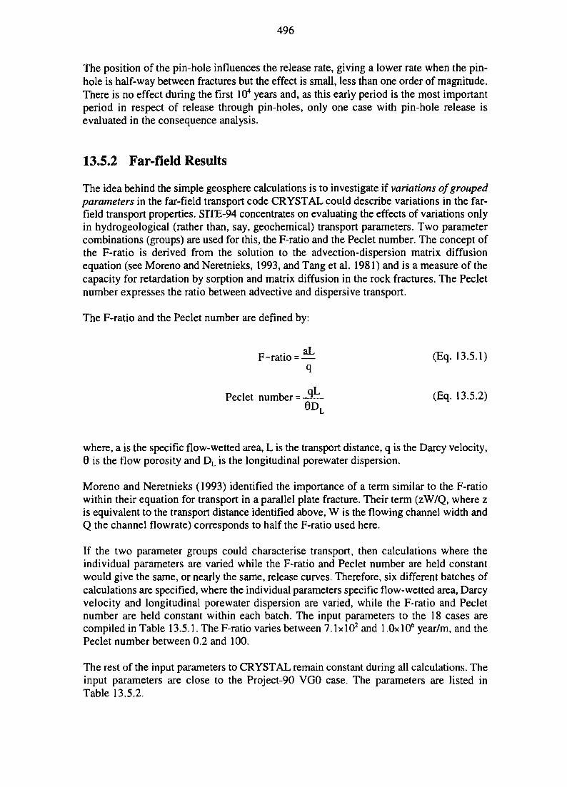
496
The position of the pin-hole influences the release rate, giving a lower rate when the pin-hole is half-way between fractures but the effect is small, less than one order of magnitude.There is no effect during the first 104 years and, as this early period is the most importantperiod in respect of release through pin-holes, only one case with pin-hole release isevaluated in the consequence analysis.
13.5.2 Far-field Results
The idea behind the simple geosphere calculations is to investigate if variations of groupedparameters in the far-field transport code CRYSTAL could describe variations in the far-field transport properties. S1TE-94 concentrates on evaluating the effects of variations onlyin hydrogeological (rather than, say, geochemical) transport parameters. Two parametercombinations (groups) are used for this, the F-ratio and the Peclet number. The concept ofthe F-ratio is derived from the solution to the advection-dispersion matrix diffusionequation (see Moreno and Neretnieks, 1993, and Tang et al. 1981) and is a measure of thecapacity for retardation by sorption and matrix diffusion in the rock fractures. The Pecletnumber expresses the ratio between advective and dispersive transport.
The F-ratio and the Peclet number are defined by:
F-ratio = — (Eq. 13.5.1)
Peclet number = -S t - (Eq. 13.5.2)0D,
where, a is the specific flow-wetted area, L is the transport distance, q is the Darcy velocity,0 is the flow porosity and DL is the longitudinal porewater dispersion.
Moreno and Neretnieks (1993) identified the importance of a term similar to the F-ratiowithin their equation for transport in a parallel plate fracture. Their term (zW/Q, where zis equivalent to the transport distance identified above, W is the flowing channel width andQ the channel flowrate) corresponds to half the F-ratio used here.
If the two parameter groups could characterise transport, then calculations where theindividual parameters are varied while the F-ratio and Peclet number are held constantwould give the same, or nearly the same, release curves. Therefore, six different batches ofcalculations are specified, where the individual parameters specific flow-wetted area, Darcyvelocity and longitudinal porewater dispersion are varied, while the F-ratio and Pecletnumber are held constant within each batch. The input parameters to the 18 cases arecompiled in Table 13.5.1. The F-ratio varies between 7.1xlO2 and l.OxlO6 year/m, and thePeclet number between 0.2 and 100.
The rest of the input parameters to CRYSTAL remain constant during all calculations. Theinput parameters are close to the Project-90 VGO case. The parameters are listed inTable 13.5.2.
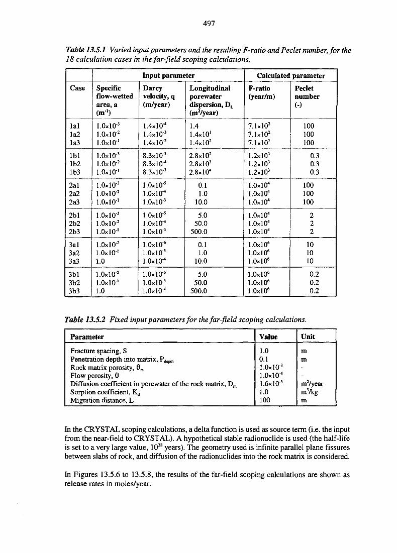
497
Table 13.5.1 Varied input parameters and the resulting F-ratio and Peclet number, for the18 calculation cases in the far-field scoping calculations.
Case
lalIa2Ia3
lblIb2Ib3
2al2a22a3
2bl2b22b3
3al3a23a3
3bl3b23b3
Input parameter
Specificflow-wettedarea,a(m1)
1.0x10"'1.0x10'1.0x10'
1.0x10'1.0x10'1.0x10'
1.0x10'1.0x10"'l.OxlO-1
1.0x10'1.0x10"'1.0x10'
1.0x10'l.OxlO"1
1.0
1.0x10-'1.0x10'1.0
Darcyvelocity, q(m/year)
1.4x10"*1.4xlO3
1.4x10'
8.3xlO5
8.3x10"*8.3x10'
l.OxlO'5
1.0x10"*l.OxlO-3
l.OxlO"5
1.0x10"*1.0x10'
l.OxlO-6
l.OxlO"5
l.OxlO"4
l.OxlO-6
l.OxlO"5
1.0x10"*
Longitudinalporewaterdispersion, DL
(mVyear)
1.41.4x10'1.4x10'
2.8x10'2.8x10'2.8x10'
0.11.0
10.0
5.050.0
500.0
0.11.0
10.0
5.050.0
500.0
Calculated parameter
F-ratio(year/m)
7.1x10'7.1x10'7.1x10'
1.2x10'1.2x10'1.2x10'
1.0x10'1.0x10'1.0x10'
1.0x10'1.0x10'1.0x10'
l.OxlO6
l.OxlO6
l.OxlO6
l.OxlO6
l.OxlO6
l.OxlO6
Pecletnumber
100100100
0.30.30.3
100100100
222
101010
0.20.20.2
Table 13.5.2 Fixed input parameters for the far-field scoping calculations.
Parameter
Fracture spacing, SPenetration depth into matrix, P ^Rock matrix porosity, 6m
Flow porosity, 0Diffusion coefficient in porewater of the rock matrix, Dm
Sorption coefficient, Kd
Migration distance, L
Value
1.00.11.0x10'l.OxlO-4
1.6x10"'1.0100
Unit
mm--m'/yearm'/kgm
In the CRYSTAL scoping calculations, a delta function is used as source term (i.e. the inputfrom the near-field to CRYSTAL). A hypothetical stable radionuclide is used (the half-lifeis set to a very large value, 1038 years). The geometry used is infinite parallel plane fissuresbetween slabs of rock, and diffusion of the radionuclides into the rock matrix is considered.
In Figures 13.5.6 to 13.5.8, the results of the far-field scoping calculations are shown asrelease rates in moles/year.
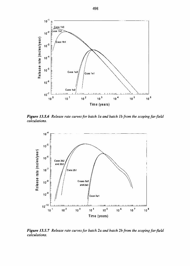
498
10'
10
CD
.2CO
- Case 1b3
Case 1b2
- /Case
10-4
CDtn .5«$ 10
10'6 N
10-7
Case 1a2I I I I I I I I ! I I ' I [ I I I I I I [ I I I I I I I I I I I I I I I I I I I I I I I I I | \ I I I I I I
10 10 10 10 10
Time (years)
10 10
Figure 13.5.6 Release rate curves for batch la and batch lbfrom the scoping far-fieldcalculations.
10"
10-5
10-6
JCD
O
-73 101ov_
CD
S i o 8
JCDCD
10-9
10
Case2b2
and 2b3
- 1 0 l i i i 11 n i l i i i i i , m i i i i 1 1 j i i i i i i 1 i 1 1 m i i_ 1 1 i i n n 1 1 1
101 102 103 104 105 106 107 10
Time (years)
Figure 13.5.7 Release rate curves for batch 2a and batch 2b from the scoping far-fieldcalculations.
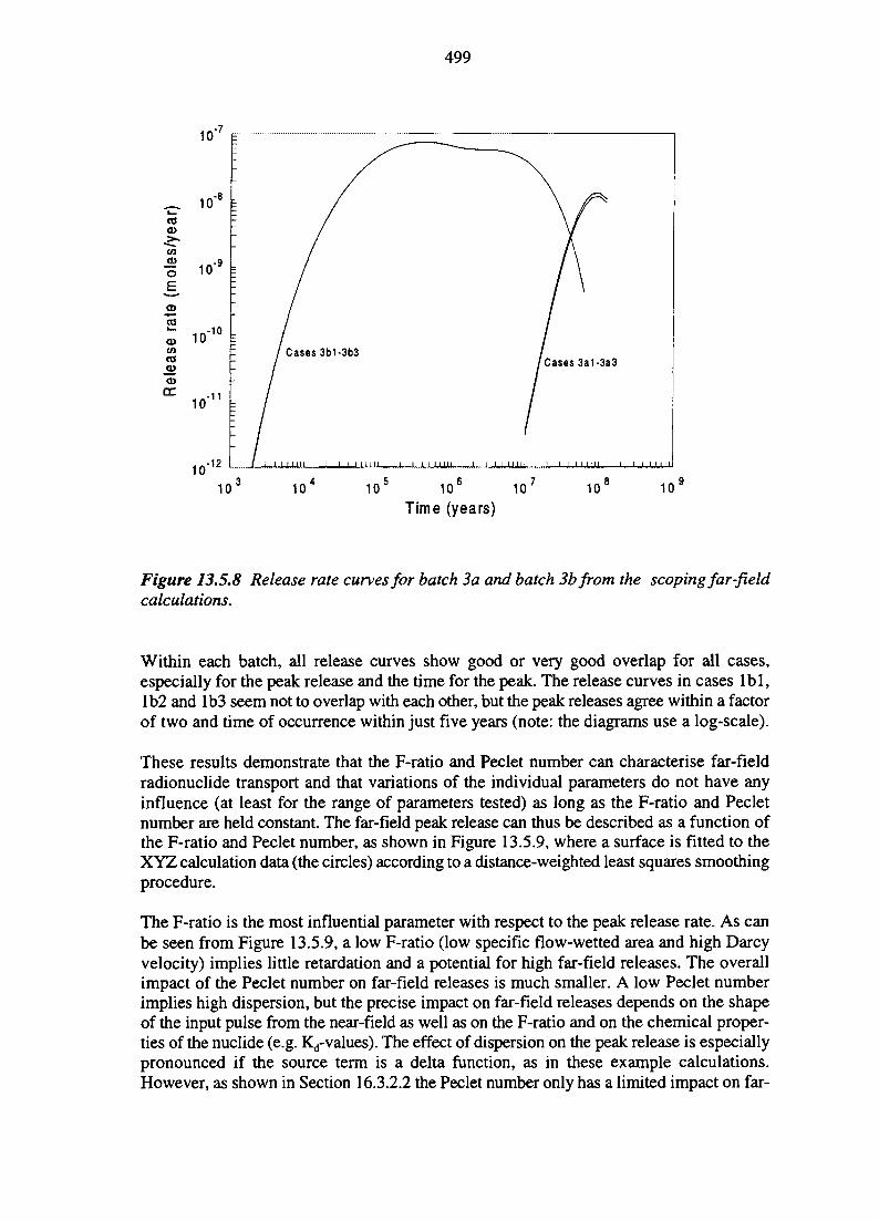
499
10 10 10 10° 10Time (years)
10 10
Figure 13.5.8 Release rate curves for batch 3 a and batch 3b from the scoping far-fieldcalculations.
Within each batch, all release curves show good or very good overlap for all cases,especially for the peak release and the time for the peak. The release curves in cases lbl ,Ib2 and Ib3 seem not to overlap with each other, but the peak releases agree within a factorof two and time of occurrence within just five years (note: the diagrams use a log-scale).
These results demonstrate that the F-ratio and Peclet number can characterise far-fieldradionuclide transport and that variations of the individual parameters do not have anyinfluence (at least for the range of parameters tested) as long as the F-ratio and Pecletnumber are held constant. The far-field peak release can thus be described as a function ofthe F-ratio and Peclet number, as shown in Figure 13.5.9, where a surface is fitted to theXYZ calculation data (the circles) according to a distance-weighted least squares smoothingprocedure.
The F-ratio is the most influential parameter with respect to the peak release rate. As canbe seen from Figure 13.5.9, a low F-ratio (low specific flow-wetted area and high Darcyvelocity) implies little retardation and a potential for high far-field releases. The overallimpact of the Peclet number on far-field releases is much smaller. A low Peclet numberimplies high dispersion, but the precise impact on far-field releases depends on the shapeof the input pulse from the near-field as well as on the F-ratio and on the chemical proper-ties of the nuclide (e.g. Kj-values). The effect of dispersion on the peak release is especiallypronounced if the source term is a delta function, as in these example calculations.However, as shown in Section 16.3.2.2 the Peclet number only has a limited impact on far-
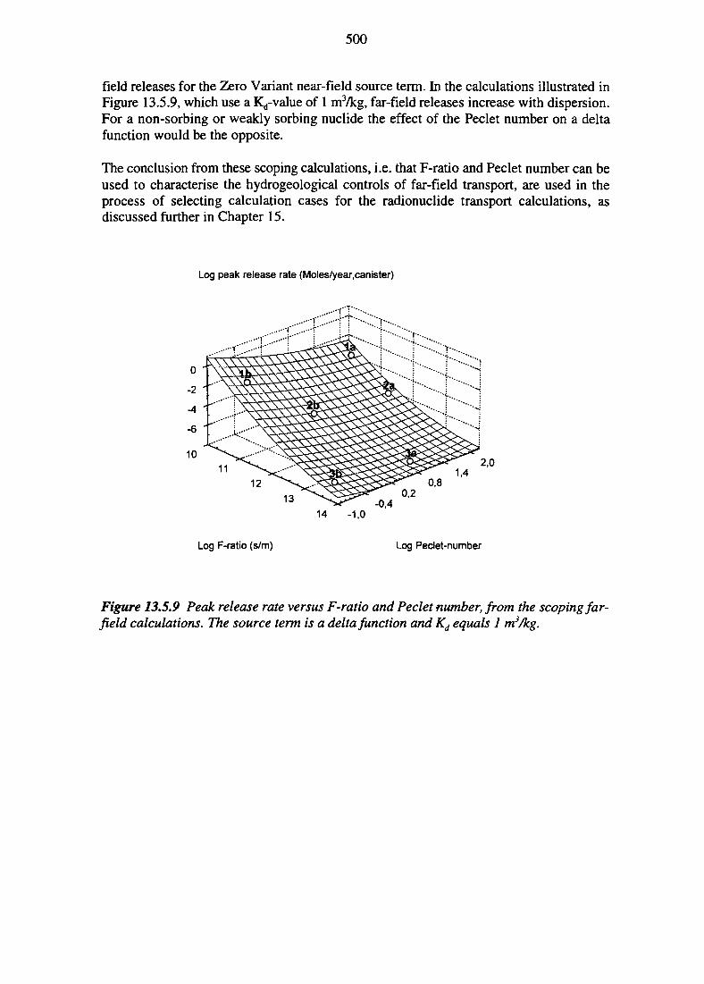
500
field releases for the Zero Variant near-field source term. In the calculations illustrated inFigure 13.5.9, which use a K^-value of 1 mVkg, far-field releases increase with dispersion.For a non-sorbing or weakly sorbing nuclide the effect of the Peclet number on a deltafunction would be the opposite.
The conclusion from these scoping calculations, i.e. that F-ratio and Peclet number can beused to characterise the hydrogeological controls of far-field transport, are used in theprocess of selecting calculation cases for the radionuclide transport calculations, asdiscussed further in Chapter 15.
Log peak release rate (Moles/year.canister)
10
...-••"•T"'---"i"T'""--.l!""f"--..• • • - . ' • • - .
0 '
-2 '
-4 ' '
-6 '"
\\v
1112
1314 -1,0
Log F-ratio (s/m) Log Peclet-number
Figure 13.5.9 Peak release rate versus F-ratio and Peclet number, from the scoping far-field calculations. The source term is a delta function and Kd equals 1 m3/kg.
501
14 BIOSPHERE MODELLING AND RADIATIONEXPOSURE
This chapter describes the model used for calculations of the biosphere factors, later usedin the radionuclide transport calculations (formulated in Chapter 15 and presented inChapter 16). The models for release and transport of radionuclides in the near-field and far-field are described in Chapter 13.
14.1 INTRODUCTION
The simple biosphere model used in SITE-94 was developed specifically for the project bythe Swedish Radiation Protection Institute (SSI) in co-operation with the SKI (Barrdahl,1996). SITE-94 is concerned with safety aspects of a hypothetical repository, and employsmore conservative assumptions and estimates than are sometimes used in radiationprotection. A biosphere model is needed to provide estimates of the radiological impactsresulting from the flux of any repository-derived radionuclides which enter the biospherefrom the geosphere. The biosphere model can calculate both annual individual andcollective (50 year integrated) radiation doses to people, and doses to fish. In this chapterconsideration will be restricted to radiation doses to people.
Calculations are generally undertaken for a unit input flux to the biosphere of 1 Bq/year foreach radionuclide; the biosphere model calculations can then be scaled by the calculatedradionuclide fluxes from the geosphere in order to provide estimates of radiologicalimpacts. It should be stressed that radiation doses calculated using the biosphere model areentirely hypothetical and illustrative. Pessimistic parameter values are often chosen in ordernot to underestimate the resulting radiation exposures.
In the biosphere model calculations dose factors for ingestion and inhalation are taken fromthe current SSI regulation (SSI, 1989), and for external exposure from Kocher (1983). Criticalgroup consumption rates and exposure times are taken from Sundblad et al. (1983a; 1983b).
14.2 BIOSPHERE MODEL
14.2.1 General
The model includes a non-evolving ('stationary') biosphere for the Reference Case, and atime dependent climate evolution biosphere for the Central Scenario. Both the stationaryand the time dependent biospheres contain, as primary biosphere receptors, a well and thebay of Borholmsfjarden, the waters surrounding the island of Aspo. In addition, the timedependent biosphere incorporates the Baltic Sea as a biosphere receptor in the remote future.
Transport of radionuclides within the model system is assumed to be essentiallyinstantaneous, except in the case of sediments subject to land rise. Apart from that pathway,radioactive decay and ingrowth is not included in the model, and corrections have to bemade outside the biosphere model. For the land rise pathway, activity in the sediments is
502
modelled to allow for radioactive decay from the time at which the sediment no longerconstitutes the sea bottom until the desired time for dose calculations.
The use of a constant flux of 1 Bq/year of each radionuclide considered into the variousbiosphere receptors can be justified on the following grounds:
• The time scale for variations of radionuclide flux from the geosphere is much longerthan one year; variations in the biosphere model on shorter time scales will havenegligible influence on the results.
• Turnover rates in the biosphere receptors are usually much higher than once peryear, with the exception of the Baltic Sea.
The modelling of radionuclides entering the Baltic Sea is undertaken on a different basisfrom that for the other biosphere receptors, as described in Section 14.2.3.
14.2.2 Reference Case
The Reference Case assumes stationary (non-evolving) present-day conditions. Thefollowing biosphere receptors are considered:
• A well on Aspo island: The well provides potentially contaminated drinking waterfor people and is also used for irrigation of agricultural land, leading to externalexposure, inhalation of contaminated dust and ingestion of contaminated vegetablesand soil. The well is assumed to have an extraction rate of 10 000 m3 per year,generally considered sufficient water to support about 100 people. This well is abouta factor of 2 larger than the one considered in Project-90 (SKI, 1991).
• The bay of Borholmsfjarden, i.e. the brackish waters surrounding the Aspo island:Some fraction of the radionuclides in the bay sorbs on sediment and will not beaccessed by pathways considered here. Fish in the bay accumulate radionuclides andare consumed by people.
The exposure pathways in the Reference Case are illustrated in Figure 14.2.1. Theequations describing the transfer between the compartments in the biosphere model and themodel parameter values employed are given in Barrdahl (1996).
14.2.3 Central Scenario
A simplification of the climate evolution in the Central Scenario was adopted for thebiosphere analysis. In short, it was assumed that the climate will gradually become colderand, in parallel, the sea-level will first start to fall locally. Between 50 000 and 100 000years in the future the climate will be glacial and too cold for people. Aspo island will belocated below sea-level during the last part of this period. After 100 000 years in the future,climate and sea-level will be restored to present values, except that the Baltic Sea ismodelled as having no outlet.
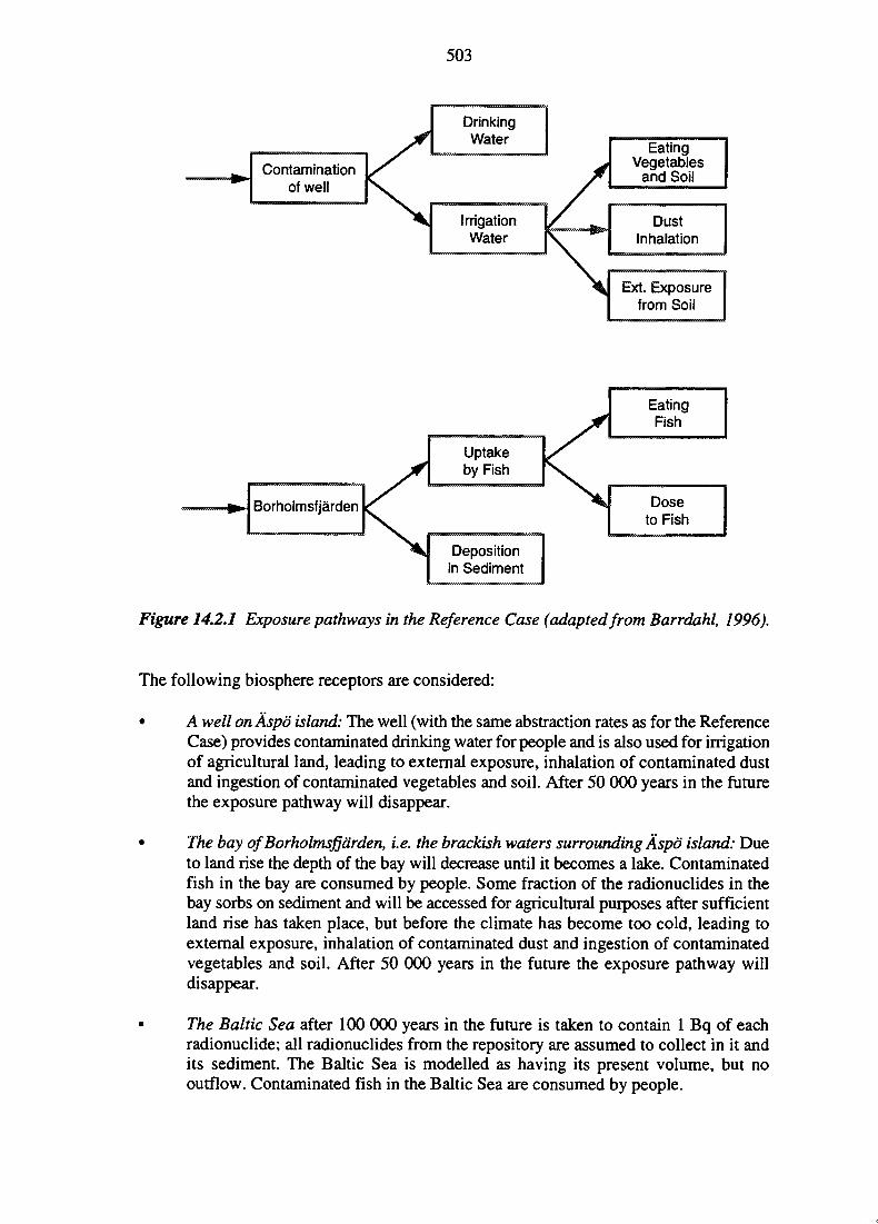
503
Contaminationof well
DrinkingWater
IrrigationWater
EatingVegetables
and Soil
DustInhalation
Ext. Exposurefrom Soil
Borholmsfjarden
Uptakeby Fish
Doseto Fish
Depositionin Sediment
Figure 14.2.1 Exposure pathways in the Reference Case (adapted from Barrdahl, 1996).
EatingFish
The following biosphere receptors are considered:
• A well on Aspd island: The well (with the same abstraction rates as for the ReferenceCase) provides contaminated drinking water for people and is also used for irrigationof agricultural land, leading to external exposure, inhalation of contaminated dustand ingestion of contaminated vegetables and soil. After 50 000 years in the futurethe exposure pathway will disappear.
• The bay of Borholmsfjarden, i.e. the brackish waters surrounding Aspd island: Dueto land rise the depth of the bay will decrease until it becomes a lake. Contaminatedfish in the bay are consumed by people. Some fraction of the radionuclides in thebay sorbs on sediment and will be accessed for agricultural purposes after sufficientland rise has taken place, but before the climate has become too cold, leading toexternal exposure, inhalation of contaminated dust and ingestion of contaminatedvegetables and soil. After 50 000 years in the future the exposure pathway willdisappear.
• The Baltic Sea after 100 000 years in the future is taken to contain 1 Bq of eachradionuclide; all radionuclides from the repository are assumed to collect in it andits sediment. The Baltic Sea is modelled as having its present volume, but nooutflow. Contaminated fish in the Baltic Sea are consumed by people.
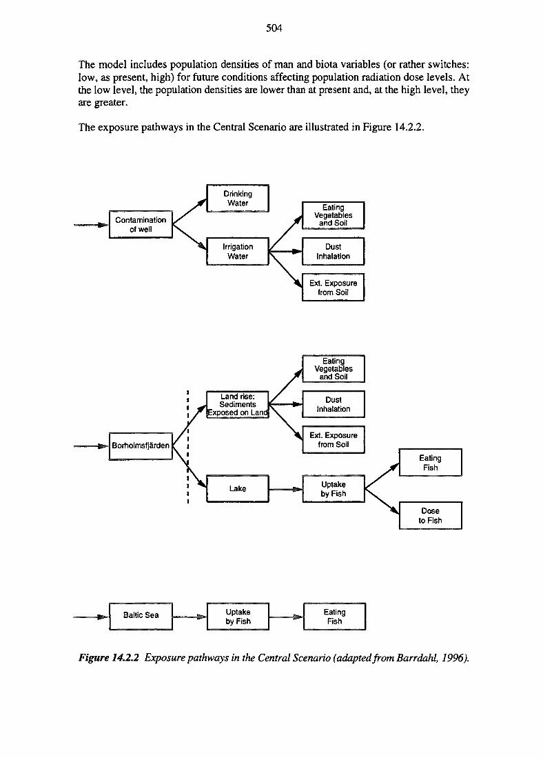
504
The model includes population densities of man and biota variables (or rather switches:low, as present, high) for future conditions affecting population radiation dose levels. Atthe low level, the population densities are lower than at present and, at the high level, theyare greater.
The exposure pathways in the Central Scenario are illustrated in Figure 14.2.2.
Contaminationof well
DrinkingWater
IrrigationWater
EatingVegetables
and Soil
DustInhalation
Ext. Exposurefrom Soil
Borholmsfjarden
Land rise:Sediments
Exposed on Land
Lake
//
/ »
\ *
EatingVegetables
and Soil
DustInhalation
Ext. Exposurefrom Soil
Uptakeby Fish
EatingFish
Doseto Fish
Baltic Sea Uptakeby Fish
EatingFish
Figure 14.2.2 Exposure pathways in the Central Scenario (adapted from Barrdahl, 1996).
505
In the land rise sediment calculations, a correction for radioactive decay (but not daughteringrowth) is made in an approximate manner, taking into account the delay from the timeof land rise until the time of calculated doses. For this pathway it is important to note thatthe radionuclide flux scaling factor is evaluated at a time representative of the build-up ofcontamination in the sediment (about 1000 years) and not at the time of dose evaluation,unless that time is earlier than 1000 years.
For the Baltic Sea pathway, the complete inventory of radionuclides, corrected for decayand daughter ingrowth, is multiplied by the calculated dose impact in order to yield apessimistic upper bound for the scaled dose impact. This pathway is only considered in theremote future.
14.3 RESULTS
Calculated doses for unit 1 Bq/year fluxes from the geosphere for the Reference Case aregiven in Table 14.3.1. For the time dependent Central Scenario, corresponding calculationsare shown for 25 000 years in the future in Table 14.3.2. A full account of dose impacts at0, 5000, 25 000 and 125 000 years in the future is given in Barrdahl (1996).
For the Central Scenario doses from the fish pathway asymptotically reaches a constantvalue after about 3200 years. With the exception of the land rise sediment pathway, allother pathways provide constant doses up to 50 000 years in the future, after which theydisappear. After the glaciation period, 100 000 years in the future, the only remainingpathway is consumption of fish from the Baltic.
For the majority of radionuclides, the drinking-water pathway produces the highestindividual doses in both scenarios, and the calculated individual doses for the well receptorpathway are used throughout in the radionuclide transport calculations in SITE-94. Theconservative nature of this choice is discussed in Section 15.2.4. It should be borne in mindthat there are significant uncertainties associated with these biosphere dose calculations, butthey do provide indicative values that can be compared with calculations from otherbiosphere models.
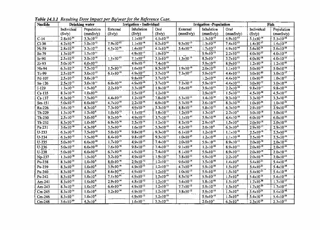
Table 14.3.1Nuclide
C-14Cl-36Ni-59Se-79Sr-90Zr-93Nb-94Tc-99Pd-107Sn-126I-129Cs-135Cs-137Sm-151Ra-226Th-229Th-230Th-232Pa-231U-233U-234U-235U-236U-238Np-237Pu-238Pu-239Pu-240Pu-242Am-24!Am-243Cm-245Cm-246Cm-248
Resulting Dose Impact per Bq/yearfor the Reference Case.Drinking water
Individual(Sv/y)2.8xlO14
4.2xlO14
2.8xlO15
1.3xlO13
2.5xlO12
5.0xl014
6.3xlO14
2.5xI014
2.5xlO15
2.5xlO13
1.3x10"8.3xlO14
6.3xl013
5.0xl015
3.6x10"1.3x10'°2.5x10"8.3x10"3.6xl010
6.3xl012
6.3xl012
5.0xl012
5.0xl012
5.0xl012
1.3x10'°8.3x10"8.3x10"8.3x10"8.3x10"8.3x10"8.3x10"8.3x10"8.3x10"3.6x10'°
Population(manSv/y)3.3xl012
5.0xl012
3.3xl013
1.5x10"3.0x10'°6.0xl012
7.5xl012
3.OxlO12
3.OxlO13
3.0x10"1.5xlO9
1.0x10"7.5x10"6.0xl013
4.3xlO9
1.5xlO8
3.0x10"9
l.OxlO8
4.3xlO8
7.5x10'°7.5x10'°6.0x10'°6.0x10'°6.0x10'°1.5xlO8
1.0x10⁸
l.OxlO8
l.OxlO"8
l.OxlO8
1.0x!0"8
l.OxlO-8
l.OxlO-8
l.OxlO-8
4.3xlO"8
Irrigation - IndividualExternal(Sv/y)
7.9xlO15
4.5xlO16
UxJO 1 5
1.5xlO12
6.1xlO19
6.0xl014
2.2xlO14
4.4xlO13
4.7xlO18
7.3xlO15
LOxlO13
9.2xlO16
6.9xlO16
3.5xlO14
5.0xl016
8.4xlO16
L7xlO13
7.6xlO16
6.7x!016
3.2x10'4
8.0xl016
3.9xlO16
8.6xlO16
7.1xlO16
2.9xlO14
6.4xlO14
3.2xlO14
Inhalation(Sv/y)l.lxlO'7
LlxlO16
1.4xlO17
4.9xlO17
7.1xlO15
4.9xlO15
1.6xlO15
4.9xlO17
9.8xlO17
4.9xlO16
3.3xlO15
2.5xlO17
L2xlO16
2.2xlO16
4.9xlO14
1.1x10"4.9xlO12
2.5x10"1.6x10"9.8xlO13
9.8xlO13
4.9xlO13
9.8xlO13
4.9xlO13
4.9xlO12
2.9xlO12
4.9xlO12
4.9xlO12
4.9xlO12
4.8xlO12
4.9xlO12
4.9xlO'2 _^4.9xlO12
1.6x10"
Oral(Sv/y) |4.1xlO15
6.2xlO15
4.1xlO16
1.9xlO'4
3.1xlO13
7.4xlO'5
9.3xlO15
3.7xlO'5
3.7x3O16
3.7xlO14
I.9xlO12
1.2xlO14
7.8xlO14
6.9xlO16
5.3xlO12
1.8x10"3.7xlO12
1.2x10"5.3x10"9.3xlO'3
9.3xlO13
7.4xlO13
7.4xlO13
7.4xlO13
1.9x10"1.2x10"1.2x10"3.2x10"1.2x10"1.2x10"1.2x10"1.2x10"1.2x30"5.3x10"
IrriExternal(manSv/y)
9.5xlO13
5.4xlO14
1.3xlO'3
1.9x10'°7.3xlO17
7.2xlO12
2.6xlO12
5.3x10"5.7xlO16
8.8xlO13
1.2x10"l.lxlO13
8.2xlO14
4.2xlO12
6.1xlO14
LOxlO13
2.0x10"9.1xlO'4
8.1xlO14
3.8xlO12
9.6xlO14
4.7xlO14
1.0x10'3
8.5xlO14
3.4xlO12
7.7xlO12
3.8xlO12
gation -PopulationInhalation(manSv/y)1.3xlO15
1.3xlO14 !1.7xlO15
5.9xlO15
8.5xlO13
5.9xlO13
2.0x10¹³
5.9xlO15
1.2xlO14
5.9xlO14
3.9xlO13
2.9xlO15
1.4xlO14
2.6xlO14
5.8xlO12
1.3xlO9
5.9x10'°2.9x10"9
2.0x10"9
1.2x10'°1.2x10'°5.9x10"1.2x10'°5.9x10"5.9x10'°3.5x10'°5.9x10'°5.9x10'°5.9x10'°5.8x10'°5.9x10'°5.9x10'°5.9x10'°2.0x10"9
Oral(manSv/y)4.9xlO13
7.4xlO'3
4.9xlO'4
2.2xlO'2
3.7x10"8.9xlO'3
l . lxlO'2
4.4xlO13
4.4xlO14
4.4xlO12
2.2x10'°1.5xI012
9.3xlO12
8.3xlO14
6.3x10'°2.2x10⁹
4.4x10'°1.5x!0"9
6.3x10⁹
1.1x10'°1.1x10'°8.9x10"8.9x10"8.9x10"2.2x10⁹
1.4xlO-9
1.5xlO9
1.5xlO"9 i1.5x!09
1.5xlO"9
1.5xlO9
1.5xlO"9
1.5xlO"9
6.3x10⁹
FishIndividual(Sv/y)5.1xlO19
1.4xlO17
5.6xlO21
4.0xl017
4.0xl018
3.2xlO19
5.0xl019
3.0xl0-2°I.OxlO'20
3.0xl017
9.8xlO17
4.5xlO"20
3.3xlO19
l.OxlO-24
2.9xlO17
3.0xl018
6.0xl019
2.0xl018
2.9xlO17
2.5xlO19
2.5xiO19
2.0x10¹⁹
2.0x10¹⁹
2.0xl019
2.0xl018
5.4xlO"21
5.4xlO-21
5.4xlO21
5.4xlO"21
1.7xlO2°IJxlO"20
5.4xlO"2'5.4xlO2'2.3xlO-20
Population(manSv/y)5.1xlO16
1.4xlO14
5.6xlO18
4.0xl014
4.0xl015
1.2xlO16
5.0xl016
3.0xl017
l.OxlO17
3.0xl014
9.8xlO14
4.5xlO'7
3.3xlO16
1.0x10²¹
2.9xlO14
3.0xl015
6.0xl016
2.0xl015
2.9xlO14
2.5xlO16
2.5xlO16
2.0x10'6
2.0xl0'6
2.0xl016
2.0x!015
5.4xlO'8
5.4xlO18
5.4xlO18
5.4xlO18
L7xlO'7
IJxlO 1 7
5.4xlO18
5.4xlO18
2.3xlO17
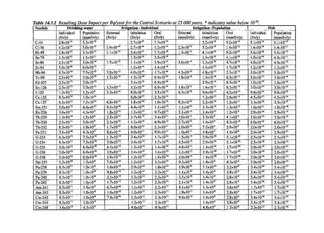
Table 14.3.2Nuclide
C-14Cl-36Ni-59Se-79Sr-90Zr-93Nb-94Tc-99Pd-107Sn-1261-129Cs-135Cs-137 iSm-151 !Ra-226Th-229Th-230Th-232Pa-231U-233U-234U-235U-236U-238
_Np-237Pu-238Pu-239Pu-240Pu-242Am-241Am-243Cm-245Cm-246Cm-248
Resulting Dose Impact per Bq/yearfor the Central Scenario at 25 000 years. * indicates value belonDrinking water
Individual(Sv/y)2.8xlO14
4.2xlO14
2.8x10"1.3xlO-13
2.5xlO12
5.0xl0M
6.3xlO14
2.5xlO14
2.5x10"2.5xlO13
1.3x10"8.3xlO14
6.3xlO13
5.0x10"3.6x10"1.3x10'°2.5x10"8.3x10"3.6x10-'°6.3xlO12
6.3xl012
5.0xl012
5.0xl012
5.0xl012
1.3x10'°8.3x10"8.3x10"8.3x10"8.3x10"8.3x10"8.3x10"8.3x10"8.3x10"3.6x10'°
Population(manSv/y)3.3xlO12
5.0xl0'2
3.3xl013
1.5x10"3.0x10'°6.0xl012
7.5xl012
3.OxlO12
3.OxlO13
3.0x10"1.5xlO9
1.0x!0"7.5x10"6.0x10'3
4.3xlO"9
1.5xlO8
3.0xl09
l.OxlO8
4.3xlO8
7.5x10'°7.5x10'°6.0x10'°6.0x10'°6.0x10'°1.5xlO"8
l.OxlO8
1.0x10⁸
I.OxlO"8
l.OxlO8
l.OxlO8
3.0xl0"8
l.OxlO-8
l.OxlO8
4.3xlO"8
IrrijExternal(Sv/y)
1.9xlO14
l . lx lO' 1 5
1.7x10"
3.8xlO12
1.5x10-"
1.5xlO13
5.3xlO14
6.8xlO13
9.5xlO18
1.8xlO14
2.5xlO13
2.3xlO15
1.7xlO15
8.6xlO14
1.2xlO15
2.0xl015
4.1xlO13
1.9xlO15
1.6xlO15
7.8xlO'4
1.6xlO15
9.6xlO16
2.1xlO15
1.7xlO15
6.7xlO14
1.6xlO13
7.8xlO14
;ation - IndividualInhalation(Sv/y)2.7xlO17
2.7xlO16
3.4xlO17
1.2x!016
l .lxlO'4 I1.2xlO14
4.0xl015
1.2xlO16
2.4xlO16
1.2xlO15
8.OxlO15
6.0xl017
1.8xlO16
4.4xlO16
1.2xlO13
2.7x10"1.2x10"6.0x10"4.0x10"2.4xlO12 ,2.4xlO12
1.2xlO12
2.4xlO12
1.2xlO12
1.2x10"5.9xlO12
.2x10"1.2x10"1.2x10"1.1x10"1.2x10"1.2x10"1.2x10"4.0x10"
Oral(Sv/y)7.7xlO15
1.2xlO14
7.7xlO16
3.5xlO14
3.9xlO13
1.4xlO14 j1.7x3O14 !6.9xlO15 !6.9xlO16
6.9xlO14
3.5xlO12
2.3x3O14
l.OxlO-13
l.lxlO15
9.7xlO12 i3.4x10" j6.9xlO12
2.3x10"9.9x10"1.7xlO12
1.7xlO12
I.4xlO12
1.4xlO12
1.4xlO12
3.5x10"1.8x10"2.3x10"2.3x10"2.3x10"2.2x10"2.3x10"2.3x10"2.3x10"9.9x10"
Irrigation -PopulationExternal(manSv/y)
2.3xlO12
1.3x!O13
2.0x10'3 !
4.5x10'°1.8xlO16
1.8x10"6.3xlO12
8.2x10"l . l x l O " 1 5
2.1xlO12
3.0x10"2.7xlO13
2.0xl013
1.0x10"1.5xlO"13
2.5xlO13
4.9x10"2.2xlO13
2.0xl013
9.3xlO'2
1.9x10-"l.lxlO13
2.5xlO13
2.1xlO13
8.1xlO12
1.9x10"9.4xlO'2
Inhalation(manSv/y)3.2xlO15
3.2xlO14
4.1xlO15
1.4xlO14
1.3xlO12
1.4xlO12
4.8xlO13
1.4xlO14
2.9xlO14
1.4xlO13
9.6xlO13
7.2xlO15
2.2x3O14
5.3xlO14
1.4x10"3.2x10⁹
1.4xlO9
7.2xlO9
4.8xlO"9
2.9x10'°2.9x10'°1.4x10'°2.9x10'°1.4x10'°1.4xlO9
7.1x10'°1.4xlO9
1.4xlO9
1.4xlO9
1.3xlO9
1.4xlO"9
1.4xlO"9
1.4xlO9
4.8xlO9
Oral(manSv/y)9.2xlO13
1.4x3O12 |9.2xlO14
4.1xlO12
4.7x10"1.7xlO12
2.1xlO12
8.3xlO'3
8.3xlO14
8.3xlO'2
4.2x10'°2.8xlO12
1.2x10"1.3xlO13
1.2x3O9
4.1xlO"9
8.3x10'°2.8x10"9
1.2xlO-8
2.1x10'°2.1x10'°1.7x10'°1.7x10'°1.7x10'°4.2x10"9
2.2xlO9
2.8xlO9
2.8xlO9
2.8xlO"9
2.6x10⁹
2.8xlO9
2.8xlO9
2.8xlO"9
1.2x10⁸
' 10 •".Fish
Individual(Sv/y)5.1xlO16
3.4xlO14
5.6xlO'8
4.0xl014
4.0xl015
1.2xlO16
5.0x10'6
3.0xl017
l.OxlO-17
3.0xl014
9.8xlO14
4.5xlO17
3.3xlO16
l.OxlO-2'2.9xlO14
3.0xl015 16.0x10¹⁶ !2.0xl015 |2.9xlO14
2.5xlO16
2.5xlO16 |2.0xl016
2.0xl016
2.0x10'6
2.0x10"5.4xlO18
5.4xlO18
5.4xlO18
5.4xlO18
1.7xlO17
3.7xlO17
5.4xlO18
5.4x3O'8
2.3xlO17
Population(manSv/y)5.1xlO13
1.4x10"5.6x10"4.0x10"4.0xl012
1.2xlO13
5.0xl013
3.0xl014
l.OxlO'14
3.0x10"9.8x10"4.5xlO14
3.3xlO13
l.OxlO'18
2.9x10"3.0xl012
6.0xl013
2.0xl012
2.9x10"2.5xlO13
2.5xlO13
2.0xl013
2.0xl013
2.0xl013
2.0xl012
5.4x10"5.4x10"5.4x10"5.4x10"1.7xlO14
1.7xlO14
5.4x10"5.4x10"2.3xlO14
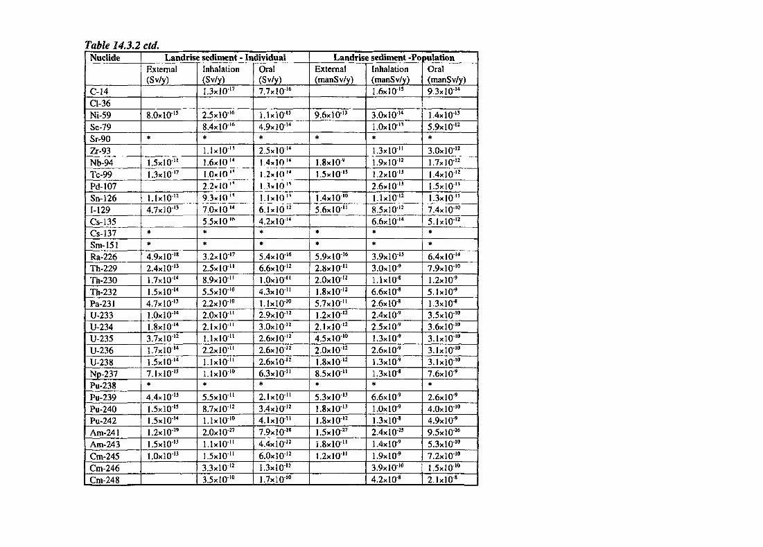
Table 14.3.2Nuclide
C-14CI-36Ni-59Se-79Sr-90Zr-93Nb-94Tc-99Pd-107Sn-1261-129Cs-135Cs-137Sm-151Ra-226Th-229Th-230Th-232Pa-231U-233U-234U-235U-236U-238Np-237Pu-238Pu-239Pu-240Pu-242Am-241Am-243Cm-245Cm-246Cm-248 !
ctd.Landrise sediment - Individual
External(Sv/y)
8.OxlO15
*
3.5x10"1.3xl017
l.lxlO12
4.7xlO13
*4.9xlO18
2.4xlO13
I.7xlO14
1.5x10l4
4.7xlO13
l.OxlO'4
1.8xlO14 !3.7xlO12
1.7x!014
1.5xlO14
7.1xlO13
*4.4xlO15
1.5xlO15
1.5xlO14
1.2x30"1.5xlO13
l.OxlO13
Inhalation(Sv/y)1.3xlO17
2.5xlO16
8.4x10¹⁶
*
LlxlO13
1.6x10 l4
1.0x10"2.2x30 "9.3x10"7.0xl014
5.5x3O16
**3.2xlO17
2.5x10"8.9x10"5.5xlO10
2.2x10'°2.0x10"2.1x10"1.1x10"2.2x10"1.1x10"1.1x10'°*5.5x10"8.7x3O12
l.lxlO10
2.0x1027
l.lxlO"11
1.5x10"3.3xlO12
3.5x10'°
Oral(Sv/y)7.7xlO16
l.lxlO'15
4.9xlO14
*
2.5xSO14
I 4xS014
1.2*10t4
I .3- I0"1.1x10"6.1xlO12
4.2xlO14
*
5.4xiO16
6.6xI012
3.0x10"4.3x10"l.lxlO10
2.9xlO12
3.OxlO12
2.6xlO12
2.6xI012 |2.6xlO12
6.3x10" 1
2.1x10"3.4xlO12
4.1x10"7.9xlO28
4.4xlO12
6.0x3012
1.3xlO'2
1.7x10'°
Landrise sediment -PoExternal(manSv/y)
9.6xlO13
*
1.8x10"1.5x10"
3.4x10 l0
5.6x10"
*
5.9xlO16
2.8x10"2.0xl012
1.8xlO12
5.7x10"1.2xlO12
2.1xlO12
4.5x10'°2.0xI012
1.8xlO12
8.5x10"*5.3xlO13
1.8xlO13
1.8xlO12
1.5xlO27
1.8x10"1.2x10"
Inhalation(manSv/y) !1.6xlO15
3.0xl014
I.OxlO13
*
1.3x10"1.9xlO12
1.2xlO13
2.6xlO13
l.lxlO12
8.5xlO12
6.6xlO14
**3.9xlO15
3.0x10⁹
l.lxlO8
6.6x10"2.6x10⁸
2.4x10⁹
2.5xlO9
1.3xlO9 I
2.6xlO"9
1.3xlO9
UxlO 8
*6.6x10"9
l.OxlO9
1.3xlO8
2.4x1025
1.4xlO9
1.9xI09
3.9x10'°4.2xlO8
pulationOral(manSv/y)9.3xlO14
1.4xlO13
5.9xlO12
*
3.OxlO12
1.7xlO12
1.4xlO12
1.5x!O13
1.3x10"7.4x30'°5.1xlO12
**6.4xlO14
7.9x10'°1.2xlO9
5.1xlO-9
1.3xlO"8
3.5x10'°3.6x10'°3.1x10'°3.1x10'°3.1x10'°7.6xlO9
2.6xlO"9
4.0x10'°4.9x10"9
9.5xlO"26
5.3x10'°7.2x10'°1.5x10'°2.1xlO"8
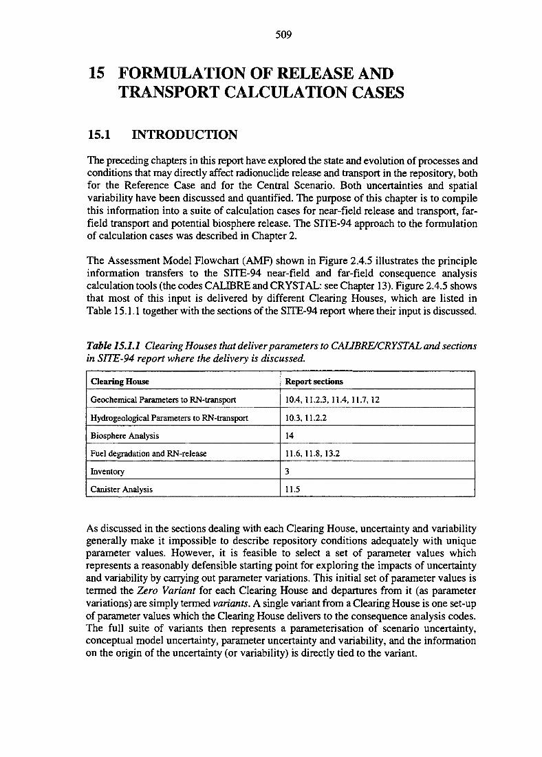
509
15 FORMULATION OF RELEASE ANDTRANSPORT CALCULATION CASES
15.1 INTRODUCTION
The preceding chapters in this report have explored the state and evolution of processes andconditions that may directly affect radionuclide release and transport in the repository, bothfor the Reference Case and for the Central Scenario. Both uncertainties and spatialvariability have been discussed and quantified. The purpose of this chapter is to compilethis information into a suite of calculation cases for near-field release and transport, far-field transport and potential biosphere release. The SITE-94 approach to the formulationof calculation cases was described in Chapter 2.
The Assessment Model Flowchart (AMF) shown in Figure 2.4.5 illustrates the principleinformation transfers to the SITE-94 near-field and far-field consequence analysiscalculation tools (the codes CALIBRE and CRYSTAL: see Chapter 13). Figure 2.4.5 showsthat most of this input is delivered by different Clearing Houses, which are listed inTable 15.1.1 together with the sections of the SITE-94 report where their input is discussed.
Table 15.1.1 Clearing Houses that deliver parameters to CALIBRE/CRYSTAL and sectionsin SITE-94 report where the delivery is discussed.
Clearing House
Geochemical Parameters to RN-transport
Hydrogeological Parameters to RN-transport
Biosphere Analysis
Fuel degradation and RN-release
Inventory
Canister Analysis
Report sections
10.4,11.2.3,11.4,11.7,12
10.3,11.2.2
14
11.6,11.8,13.2
3
11.5
As discussed in the sections dealing with each Clearing House, uncertainty and variabilitygenerally make it impossible to describe repository conditions adequately with uniqueparameter values. However, it is feasible to select a set of parameter values whichrepresents a reasonably defensible starting point for exploring the impacts of uncertaintyand variability by carrying out parameter variations. This initial set of parameter values istermed the Zero Variant for each Clearing House and departures from it (as parametervariations) are simply termed variants. A single variant from a Clearing House is one set-upof parameter values which the Clearing House delivers to the consequence analysis codes.The full suite of variants then represents a parameterisation of scenario uncertainty,conceptual model uncertainty, parameter uncertainty and variability, and the informationon the origin of the uncertainty (or variability) is directly tied to the variant.
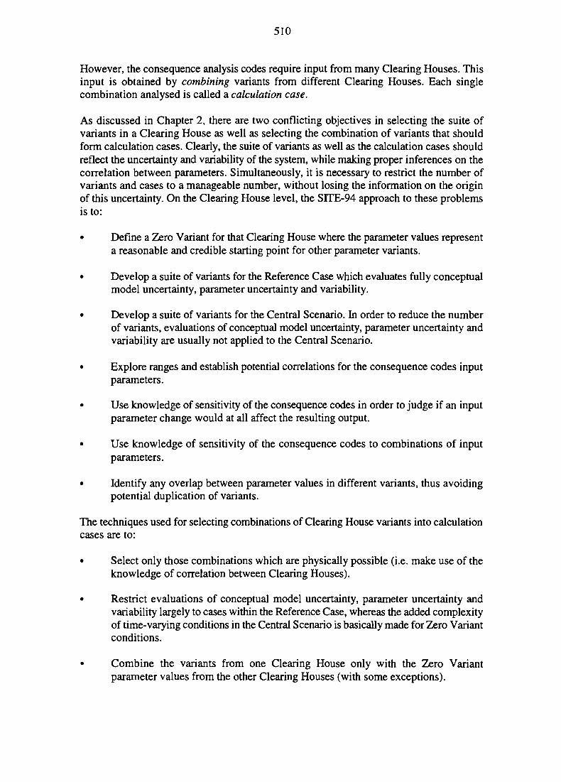
510
However, the consequence analysis codes require input from many Clearing Houses. Thisinput is obtained by combining variants from different Clearing Houses. Each singlecombination analysed is called a calculation case.
As discussed in Chapter 2, there are two conflicting objectives in selecting the suite ofvariants in a Clearing House as well as selecting the combination of variants that shouldform calculation cases. Clearly, the suite of variants as well as the calculation cases shouldreflect the uncertainty and variability of the system, while making proper inferences on thecorrelation between parameters. Simultaneously, it is necessary to restrict the number ofvariants and cases to a manageable number, without losing the information on the originof this uncertainty. On the Clearing House level, the SITE-94 approach to these problemsis to:
• Define a Zero Variant for that Clearing House where the parameter values representa reasonable and credible starting point for other parameter variants.
• Develop a suite of variants for the Reference Case which evaluates fully conceptualmodel uncertainty, parameter uncertainty and variability.
• Develop a suite of variants for the Central Scenario. In order to reduce the numberof variants, evaluations of conceptual model uncertainty, parameter uncertainty andvariability are usually not applied to the Central Scenario.
• Explore ranges and establish potential correlations for the consequence codes inputparameters.
• Use knowledge of sensitivity of the consequence codes in order to judge if an inputparameter change would at all affect the resulting output.
• Use knowledge of sensitivity of the consequence codes to combinations of inputparameters.
• Identify any overlap between parameter values in different variants, thus avoidingpotential duplication of variants.
The techniques used for selecting combinations of Clearing House variants into calculationcases are to:
• Select only those combinations which are physically possible (i.e. make use of theknowledge of correlation between Clearing Houses).
• Restrict evaluations of conceptual model uncertainty, parameter uncertainty andvariability largely to cases within the Reference Case, whereas the added complexityof time-varying conditions in the Central Scenario is basically made for Zero Variantconditions.
• Combine the variants from one Clearing House only with the Zero Variantparameter values from the other Clearing Houses (with some exceptions).
511
• Select only those combinations which will produce different output when there isdirect or indirect overlap between parameter values in logically different variants(for example, two different hydraulic conceptual models may in fact producetransport parameters that give very similar far-field retardation and there would thenbe little point in keeping both variants).
• Select manually a few 'illustrative' combinations such as the most pessimistic andthe most optimistic parameter combinations.
These techniques make it possible to reduce the number of combinations considerably, butthere are a number of drawbacks. First, there is always a risk that an important combinationis overlooked, but this can be overcome if the selection is made carefully. Second, and moreimportant, is that the set of calculation cases may provide a skewed picture of theuncertainties in the system as some cases may contain many pooled variants, whereas othercases represent much more extreme situations or assumptions. Consequently, in this typeof non-probabilistic analysis, it is not possible to draw inferences on the likelihood of acertain output based on the number of calculation cases that produce this or similar outputs.In order to draw such inferences, or to track the origin of the uncertainty that motivates thecase, it is necessary to go back to the Clearing House level.
15.2 VARIANTS IN THE REFERENCE CASE
15.2.1 Hydrogeological Variants
15.2.1.1 Introduction
This section describes the selection of hydrogeological parameter variants for the ReferenceCase radionuclide release and transport (consequence) calculations, based on thepredictions of site hydrogeology described in Sections 10.3 and 11.2.2. This task wasformally assigned to the Clearing House Hydrogeological parameters to RN-transport inthe AMF (Figure 2.4.5).
The ambition is to propagate all conceptual and other uncertainties that could not beresolved by the site characterisation data and to evaluate their impact on repository safety.However, there is not a direct connection for information to pass between thehydrogeological site evaluation and the consequence calculations. The importantintermediate step, represented by this chapter, is to compile and organise results of the siteevaluation in such a way that different sources of uncertainty can be evaluated. Thisinvolves book-keeping of uncertainties and spatial variability, and a systematic approachto defining parameter variants for the consequence calculations. Another important aspectis to ensure consistency between parameters, taking correlations into account. Theradionuclide release and transport calculations (Chapter 16) was also used to providefeedback regarding the importance of different hydrogeological uncertainties for theperformance of the site.
512
The key hydrogeological parameters for the near-field delivered by the Hydrogeologicalparameters Clearing House are:
• Darcy velocity, q^,• fracture spacing, Snf,• fracture aperture, b^,• flow-wetted surface area, a^,
and for the far-field:
• Darcy velocity, qff,• dispersion coefficient, DUf,• effective porosity, <j>ff,• flow-wetted surface area, a^,• transport distance, L.
As discussed in Section 10.3, the far-field parameters are usually inter-correlated such thatthey are better described by the F-ratio and Pe-number.
In common with all the Clearing Houses, some parameters were not varied and theseinclude, in the near-field, the CCL-parameter and in the far-field, the penetration depth, thefracture spacing and the path length.
The need to analyse many variants
The hydrogeological site evaluation, presented in Sections 10.3 and 11.2.2, concludes thata single set-up of the hydrogeological parameters values will not adequately represent thesite hydrogeology. Apart from the temporal changes during the Central Scenario, which willbe further discussed in Section 15.3, the hydrogeology at a canister position and along apotential transport pathway:
• can be described with alternative conceptual models and different conceptualvariants of these models,
• is uncertain due to uncertainty in boundary conditions and parameter (or property)values within any given conceptual model,
• exhibits spatial variability.
The hydrogeological parameter variants for the consequence calculations are selected insuch a way that the impact of all types of uncertainty as well as spatial variability can bequantified. Because the hydrogeological site evaluation comprises a large number of modelvariants for each uncertainty category, the number of possible parameter variants becomesvery large. Further, additional variants are needed to evaluate the correlated ranges ofparameter values reflecting spatial variability for each model realisation. Therefore, astrategy for selecting a manageable number of parameter variants is needed.
513
Iteration with the consequence analysis models
The problem of selecting a limited number of representative parameter variants for theconsequence analysis models is addressed by iteration between them and thehydrogeological evaluation. Simple sensitivity analyses with the CALIBRE near-fieldrelease and transport code show that the release rates are insensitive to the hydrogeologicalparameter values above or below certain values (Section 13.5.1). For example, for highDarcy velocities (above 10"3 - 102 m/year) the release from the near-field is controlled bydiffusion through the bentonite buffer, hence a further increase in Darcy velocity will notaffect the release rate. These type of sensitivity analyses make it possible to sort outhydrogeological parameter variants that give similar results, thus reducing the number ofnear-field parameter variants that need to be combined with the far-field variants.
As discussed in Section 10.3, the results of both mathematical analysis and simplesensitivity analyses with the CRYSTAL radionuclide transport code (Section 13.5.2) showthat variation of the individual hydrogeological far-field parameter values does not affect(reactive) transport, as long as the parameter groups F-ratio (a^ x L/qff) and Peclet number(Uff x L/Dyf) are held constant. Thus, for the far-field, it is sufficient to explore the F-ratio -Peclet number parameter space predicted by each hydrogeological model and model variant(see Figures 10.3.8 and 10.3.13).
It is possible to get a rough estimate of the impact of the different hydrogeologicalconceptual model variants using simple scoping calculations with the CRYSTAL code(Section 13.5.2). Figure 13.5.9 contains a simple illustration of the sensitivity of far-fieldradionuclide transport (response surface for the peak release rate) as a function of thehydrogeological parameter groups. The ranges of F-ratio and Pe-number in the figurecorrespond to the total uncertainty and spatial variability evaluated with the hydrogeologicalsite models (see Figures 10.3.22 and 10.3.23). The exact shape of the response surfacevaries for different radionuclides and for different source terms (in this simple example adelta function) but the general behaviour is the same, i.e. high release rates for low F-ratiosand low Pe-numbers. The plots of F-ratio versus Pe-number in Figures 10.3.8 and 10.3.13provide a link between the original conceptual model or parameter uncertainty and theresults of the consequence calculations.
Treatment of correlation between near-field and far-field hydrogeology
Near-field and far-field transport are calculated separately by the CALIBRE and CRYSTALcodes (Chapter 13), thus the release from the near-field constitutes the source term for far-field transport. When combining near-field and far-field parameter variants it is thusessential that any correlation is taken into account.
In the hydrogeological site models the near-field parameters are evaluated as an integratedpart of the far-field (Section 10.3). The only observed correlation between the near-fieldand far-field is through near-field and far-field Darcy velocity or near-field Darcy velocityand far-field F-ratio (using data only for the Discrete Feature hydrogeology model).Canister positions with low Darcy velocity tend to be associated with high retardationcapacity in the far-field rock, but the correlation is, in general, weak or non-existent.Therefore, near-field and far-field parameter variants are developed separately. However,when combining near-field and far-field parameter variants a check needs to be made thateach parameter variant is consistent with the conceptual model variant it represents.
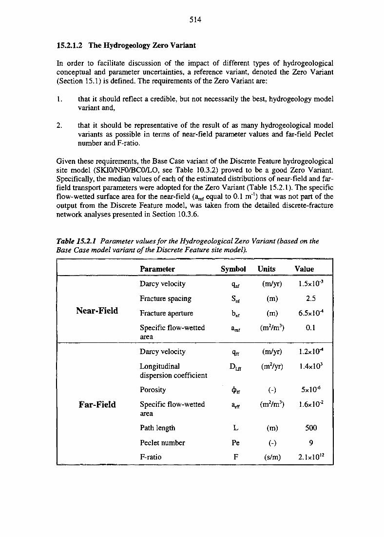
514
15.2.1.2 The Hydrogeology Zero Variant
In order to facilitate discussion of the impact of different types of hydrogeologicalconceptual and parameter uncertainties, a reference variant, denoted the Zero Variant(Section 15.1) is defined. The requirements of the Zero Variant are:
1. that it should reflect a credible, but not necessarily the best, hydrogeology modelvariant and,
2. that it should be representative of the result of as many hydrogeological modelvariants as possible in terms of near-field parameter values and far-field Pecletnumber and F-ratio.
Given these requirements, the Base Case variant of the Discrete Feature hydrogeologicalsite model (SKI0/NF0/BC0/LO, see Table 10.3.2) proved to be a good Zero Variant.Specifically, the median values of each of the estimated distributions of near-field and far-field transport parameters were adopted for the Zero Variant (Table 15.2.1). The specificflow-wetted surface area for the near-field (a^ equal to 0.1 m"1) that was not part of theoutput from the Discrete Feature model, was taken from the detailed discrete-fracturenetwork analyses presented in Section 10.3.6.
Table 15.2.1 Parameter values for the Hydrogeological Zero Variant (based on theBase Case model variant of the Discrete Feature site model).
Near-Field
Far-Field
Parameter
Darcy velocity
Fracture spacing
Fracture aperture
Specific flow-wettedarea
Darcy velocity
Longitudinaldispersion coefficient
Porosity
Specific flow-wettedarea
Path length
Peclet number
F-ratio
Symbol
s n f
b n f
«nrf
qff
Diif
4>ff
Srff
L
Pe
F
Units
(m/yr)
(m)
(m)
(m2/m3)
(m/yr)
(rnVyr)
(-)
(m2/m3)
(m)
(-)
(s/m)
Value
1.5xl0"3
2.5
6.5X10"4
0.1
1.2X10"4
1.4xlO3
5x10"*
1.6xlO2
500
9
2.1xlO12
515
15.2.1.3 Near-field Variants
Table 15.2.2 contains a compilation of 25 selected hydrogeological parameter variants forthe near-field release and transport calculations. Each of the selected variants represents theparameters determined at an actual canister position, in a specific realisation in one of thehydrogeological site models. This ensures that the range of possible correlations are takeninto account. However, as noted above, the results for the different hydrogeology modelsoften overlap which means that many of the parameter combinations in Table 15.2.2 couldrepresent several model variants.
The general idea is to vary one or two parameters at a time and to use the Zero Variantvalues for the remaining near-field parameters. However, in some cases the remainingparameters have to be adjusted to comply with the observed correlations (see Section 10.3).For example, in the Discrete Feature site model, it is not possible to find a canister positionwith both very high Darcy velocity and the Zero Variant values of fracture spacing andfracture aperture, which is why the low value of fracture spacing and high value of fractureaperture are used in variant 5.
Flux variants
The first 11 variants reflect uncertainty and spatial variability of the near-field Darcyvelocity. These Darcy velocity variants are selected from Figure 10.3.20, as follows. Foreach of the two main hydrogeological site models, the Discrete Feature and the StochasticContinuum models, five parameter variants are selected, variants 1-5 and 6-10, respectively.Three of these represent the spatial variability of the Base Case variants in respectivehydrogeology site models. The other two represent the lower end (10th percentile Darcyvelocity) of the hydrogeology variant that produces the lowest median Darcy velocity andthe upper end (90th percentile Darcy velocity) of the hydrogeology variant that producesthe highest median Darcy velocity. In addition, a variant based on the Simple Evaluationis included to cover a highly pessimistic estimate of Darcy velocity derived for a case witha direct connection between a canister and the biosphere via a major fracture zone.Together, these variants cover the full range of estimated Darcy velocities for the near-field.The density of intermediate Darcy velocity variants within this range is sufficient to allowdiscussion of the impact of the other hydrogeological variants, through interpolation.
Fracture property variants
The second group of variants, 12-17, which are based on the Discrete Feature site model,are set up to explore the impact of the other near-field parameters, namely flow-wettedsurface area, fracture aperture and fracture spacing. The median values and spatialvariability of the latter two parameters are similar for most of the analysed variants of theDiscrete Feature site model. Therefore, three values of each parameter (10th, 50th and 90thpercentiles), reflecting the spatial variability for most variants, are evaluated. Similarly,three values of flow-wetted surface area, artf= 0.01, 0.1 and 1.0 m"1, are evaluated. Thesevalues reflect uncertainty (regarding data and conceptual model for estimation) and thereis no information on correlation with the other near-field parameters. Each parameter isvaried one at the time about the Zero Variant. All parameter combinations are consistentwith the Base Case variant of the Discrete Feature hydrogeology model.

516
Table 15.2.2 Hydro geological near-field parameter variants for the Reference Case. Shadedparameter values are equal to the values specified for the Zero Variant, in Table 15.2.1. Thefollowing abbreviations are used: DF = Discrete Feature hydrology model; SC = StochasticContinuum hydrology model; SE = Simple Evaluation; pctl. = percentile.
Near-Field Variant:
ID Description
0 Zero Variant:
Flux variants (DF-based):1 Lowest-qnf DF variant (1 Oth pctl. qnf)
2 DF Base Case (10th pctl. qnf)
3 DF Base Case (median qnf)
4 DF Base Case (90th pctl. qnf)
5 Highest-qnf DF case (90th pctl. qnf)
Flux variants (SC-based):6 L o w e s t ^ SC case (10th pctl. qnf)
7 SC Base Case (1 Oth pctl. qnf)
8 SC Base Case (median qnf)
9 SC Base Case (90th pctl. qnf)
10 Highest-qnf SC case with (90th pctl. qnf)
Flux variants (SE-based):11 Highest-qnf SE Case (low gradient)
Flow-wetted surface variants:12 Zero Variant + Iowa,.nf
13 Zero Variant + high a ^
Fracture aperture variants:14 Zero Variant + low bnf
15 Zero Variant + high bnf
Fracture spacing variants:16 Zero Variant + low Snf
17 Zero Variant + high Snf
High-flux variants:18 Highest-qnf DF case (90th pctl. qnf); low a ^
19 Highest-q^ DF case (90th pctl. qnf); high a^f
20 DF Base Case (90th pctl. qnf); low a ^
21 DF Base Case (90th pctl. qnf); high a,.nf
Low-flux variants:22 Lowest-flux DF case (10th pctl. qnf); low a,.nf
23 Lowest-flux DF case (10th pctl. qnf); high a ^
24 DF Base Case (10th pctl. qnf) and low a,.nf
25 DF Base Case (10th pctl. qnf) and high a,,,.
Correspondinghydrogeologicalmodel variant
DF: SKIO/NFO/BCO
DF: SKNO/NFO/BCO
DF: SKIO/NFO/BCO
DF: SKIO/NFO/BCO
DF: SKIO/NFO/BCO
DF: SKIO/NFOB/BCO
SC: NEW-DIP80
SC: REF-DIP80
SC: REF-DIP80
SC: REF-DIP80
SC: LNG-DIP80
SE: Case 3a
DF: SKIO/NFO/BCO
DF: SKIO/NFO/BCO
DF: SKIO/NFO/BCO
DF: SKIO/NFO/BCO
DF: SKIO/NFO/BCO
DF: SKIO/NFO/BCO
DF: SKIO/NFOB/BCO
DF: SKIO/NFOB/BCO
DF: SKIO/NFO/BCO
DF: SKIO/NFO/BCO
DF: SKNO/NFO/BCO
DF: SKNO/NFO/BCO
DF: SKIO/NFO/BCO
DF: SKIO/NFO/BCO
Parameter Values
<lnf
(m/year)
1.5xiO*3
6.0X10"6
8.0xl0"5
1.5x10?4.0x10"2
1.2X10'1
3.0xl0"6
1.8xlO"5
l .lxlO"4
l.OxlO"3
4.0x10'3
1.05x10°
t.5xlO*3
L5xlG"3
1.5xlO'3
I.5xlO*3
I.5xlO"3
1.5x10*
1.2X10"1
1.2X10"1
4.0x10'2
4.0x10"2
6.0xl0"6
6.0X10"6
8.OxlO"5
8.0x10"5
s n f(m)
2.5
8.02.52.5Z50.8
2.52.52.52.52.5
2.5
2.5
2.5
2.5
2.5
0.88.0
0.80.82.52.5
8.0
8.0
2.52.5
Kt(m)
6.5X10"4
6.5X10"4
6.5x10"4
6.5x10"4
6.5X10"4
l.OxlO"3
6.5X10*4
6.5X10"4
6.5X10"4
6.5x10^
6.5X10"4
6.5x10"4
6.5X10"4
6.5x10"*
4.0x10^
l.OxlO"3
6.5X10"4
6.5XHGT4
l.OxlO"3
l.OxlO"3
6.5X10"4
6.5X10"4
6:5x10"*
6.5X10"4
6.5X10⁻⁴
6.5X10"4
arnf
(1/m)
0.1
0.10.10.10.10.1
0.10.10.10.10.1
0.1
0.011
0.10.1
0.10.1
0.0110.011
0.0110.011
517
Extreme combinations ofDarcy velocity and flow-wetted surface
Finally, variants 18-25 are defined to evaluate some extreme combinations of Darcyvelocity (estimated with the Discrete Feature site model) and specific flow-wetted surface.In variants 18-21, high flux is combined with the high and low value of flow-wetted surfacearea. The first two use the 90th percentile Darcy velocity of the hydrogeology variant thatproduces the highest median Darcy velocity and the last two use the 90th percentile Darcyvelocity of the Base Case variant. Similarly, in variants 22-25, low Darcy velocities arecombined with the low and high values of flow-wetted surface area. These parametervariants thus reflect both extremes of uncertainty as well as spatial variability of Darcyvelocity for the Base Case variant of the Discrete Feature model. However, it is importantto recall that the flow-wetted surface area (for the near-field) is estimated independentlywith the VAPFRAC discrete-fracture network model (see Section 10.3.6). Thus, potentialcorrelation between the flow-wetted surface area and the other near-field parameters isdisregarded.
15.2.1.4 Far-field Variants
As outlined above, the far-field performance is evaluated by defining radionuclide transportparameter variants that cover the F-ratio - Pe-number parameter space estimated with thehydrogeology site models. In the context of the far-field radionuclide transport model,Figures 10.3.22 and 10.3.23 constitute a complete parameterisation of the hydrogeologicalevaluation performed with the Discrete Feature site model and the Stochastic Continuumsite model, respectively. All that remains is to select a sufficient number of data points (ortransport parameter variants) so that different types of uncertainties and spatial variabilitycan be evaluated, either directly or through interpolation.
The density of points (hence parameter variants) should ideally be higher in regions of theF-ratio - Pe-number parameter space where transport is more sensitive to perturbations ofthe F-ratio and Pe-number. However, different radionuclides may be more or less sensitivein different areas, which makes it difficult to realise such an approach. A more simplisticapproach is to cover the most extreme points, as well as some regularly spaced intermediatepoints in the F-ratio - Pe-number space.
Figure 15.2.1 illustrates a subset of 44 far-field parameter variants selected for evaluationof the Discrete Feature model results (Figure 10.3.22). The selected parameter variants(data points) in Figure 15.2.1 are based on the Base Case variant (filled circles) and someadditional model variants to cover the extremes of the F-ratio - Pe-number parameter spacepredicted by the Discrete Feature hydrogeology model variants. Table 15.2.3 lists thecomplete set of far-field transport parameters corresponding to the variants depicted inFigure 15.2.1. However, the exact origin of each data point is not an issue, as radionuclidetransport is insensitive to parameter variations for a given set of values of the F-ratio andthe Pe-number. Different hydrogeological model variants may produce the same value ofthe F-ratio and Pe-number through different combinations of the individual far-fieldparameters (%, Dyj, cj)ff, a^ and L). The Zero Variant is indicated with a large filled box inthe central portion of Figure 15.2.1.
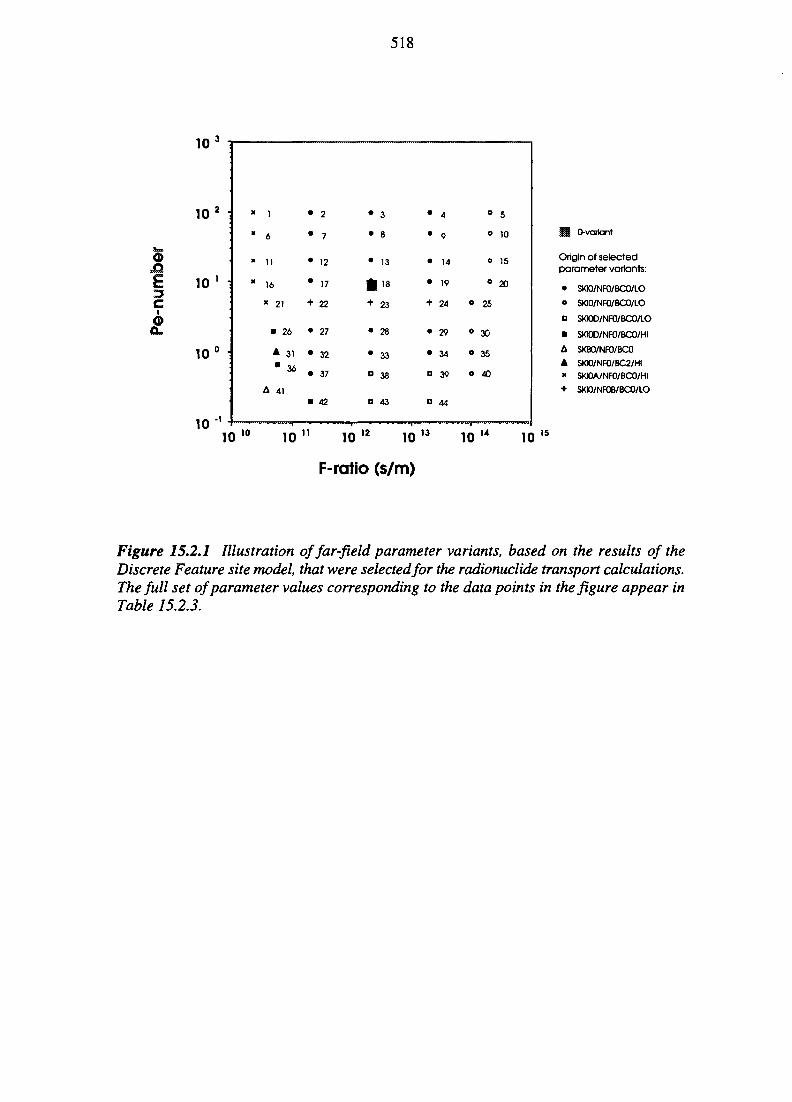
518
n
C
10
10
10
10
10
2 .
1 .
0 .
-1
* 1
* 6
* 11
" 16
* 21
• 26
A 31
" 36
A 41
• 2
• 7
• 12
• 17
+ 22
• 27
• 32
• 37
• 42
• 3
• 8
• 13
in*+ 23
• 28
• 33
° 38
• 43
• 4
• 9
• 14
• 19
+ 24
• 29
• 34
a 39
O 44
o
0
0
o
o
0
0
o
25
30
35
40
5
10
15
20
10 10
2 0-variant
Origin of selectedparameter variants:
• SKI0/NF0/BC0/LO
o SKIO/NFO/BCO/LO
D SKIOD/NfO/BCO/LO
• SK10D/NF0/BC0/HI
A SKBO/NFO/BCO
• SK10/NF0/BC2/HI* SKIOA/NFO/BCO/HI+ SKIO/NFOB/BCO/LO
10 10 12 10 13 10 14 10 15
F-ratio (s/m)
Figure 15.2.1 Illustration of far-field parameter variants, based on the results of theDiscrete Feature site model, that were selected for the radionuclide transport calculations.The full set of parameter values corresponding to the data points in the figure appear inTable 15.2.3.
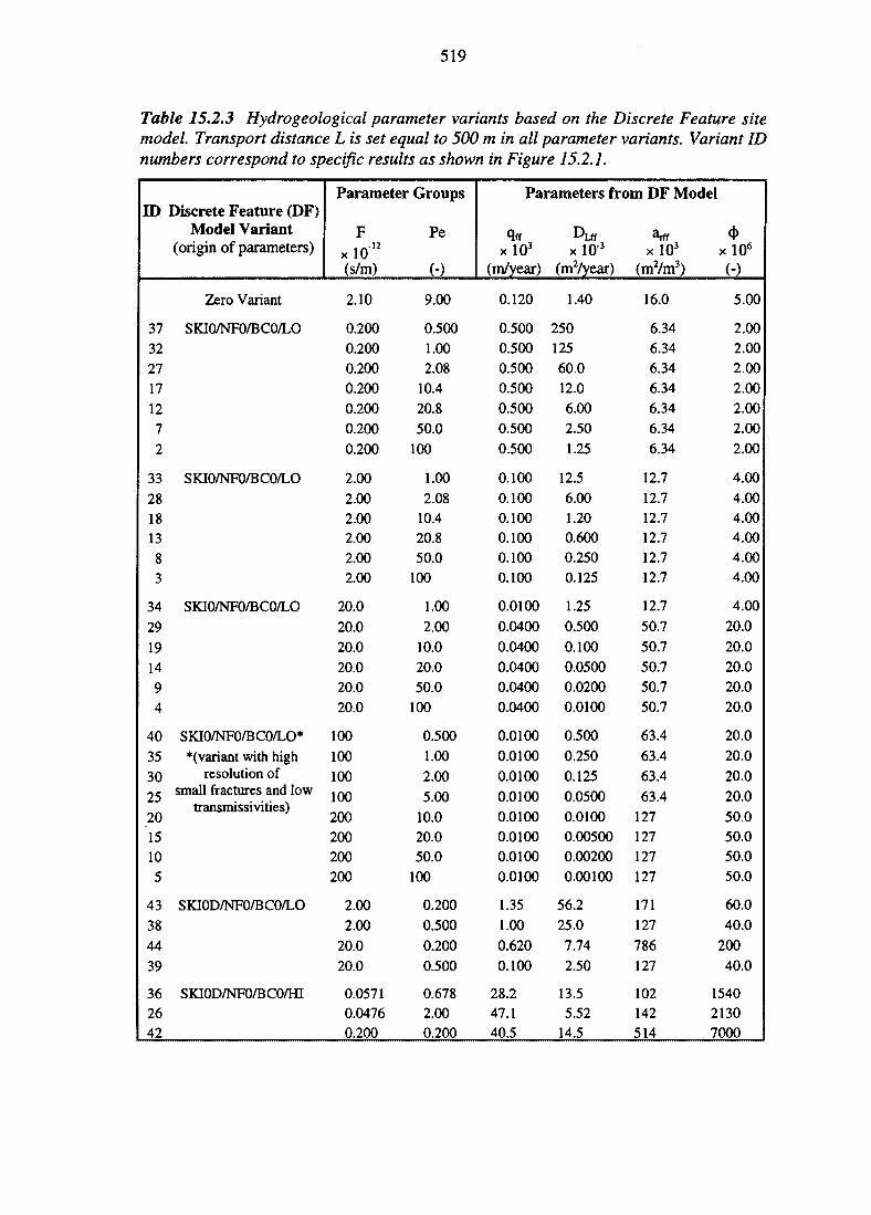
519
Table 15.2.3 Hydrogeological parameter variants based on the Discrete Feature site
model. Transport distance L is set equal to 500 m in all parameter variants. Variant ID
numbers correspond to specific results as shown in Figure 15.2.1.
ID
373227171272
3328181383
34
29191494
403530252015105
43384439
362642
Discrete Feature (DF)Model Variant
(origin of parameters)
Zero Variant
SKI0/NF0/BC0/LO
SKI0/NF0/BC0/LO
SKI0/NF0/BC0/LO
SKI0/NF0/BC0/LO**(variant with high
resolution ofsmall fractures and low
transmissivities)
SKI0D/NF0/BC0/LO
SKI0D/NF0/BC0/HI
Parameter Groups
F
x 10 1 2
(s/m)
2.10
0.2000.2000.2000.2000.2000.2000.200
2.002.002.002.002.002.00
20.0
20.020.020.020.020.0
100100100100200200200200
2.002.00
20.020.0
0.05710.04760.200
Pe
(-)
9.00
0.5001.002.08
10.4
20.850.0
100
1.002.08
10.420.850.0
100
1.002.00
10.020.050.0
100
0.5001.002.005.00
10.020.050.0
100
0.2000.500
0.2000.500
0.6782.000.200
Parameters from DF Model
xlO3
(m/year)
0.120
0.5000.5000.5000.5000.5000.5000.500
0.1000.1000.1000.1000.1000.100
0.01000.04000.04000.04000.04000.0400
0.01000.01000.01000.01000.01000.01000.01000.0100
1.351.000.6200.100
28.247.140.5
DLffxlO'3
(mVyear)
1.40
25012560.012.06.002.501.25
12.56.001.200.6000.2500.125
1.250.5000.1000.05000.02000.0100
0.5000.2500.125
0.05000.01000.005000.002000.00100
56.225.07.742.50
13.55.52
14.5
3rffxlO3
(mVm3)
16.0
6.346.346.346.346.346.346.34
12.712.712.712.712.712.7
12.7
50.750.750.750.750.7
63.463.463.4
63.4127127127127
171127
786127
102142514
<i>xlO 6
(-)
5.00
2.002.002.002.002.002.002.00
4.004.004.004.004.004.00
4.00
20.020.020.020.020.0
20.020.020.020.050.050.050.050.0
60.040.0
20040.0
154021307000
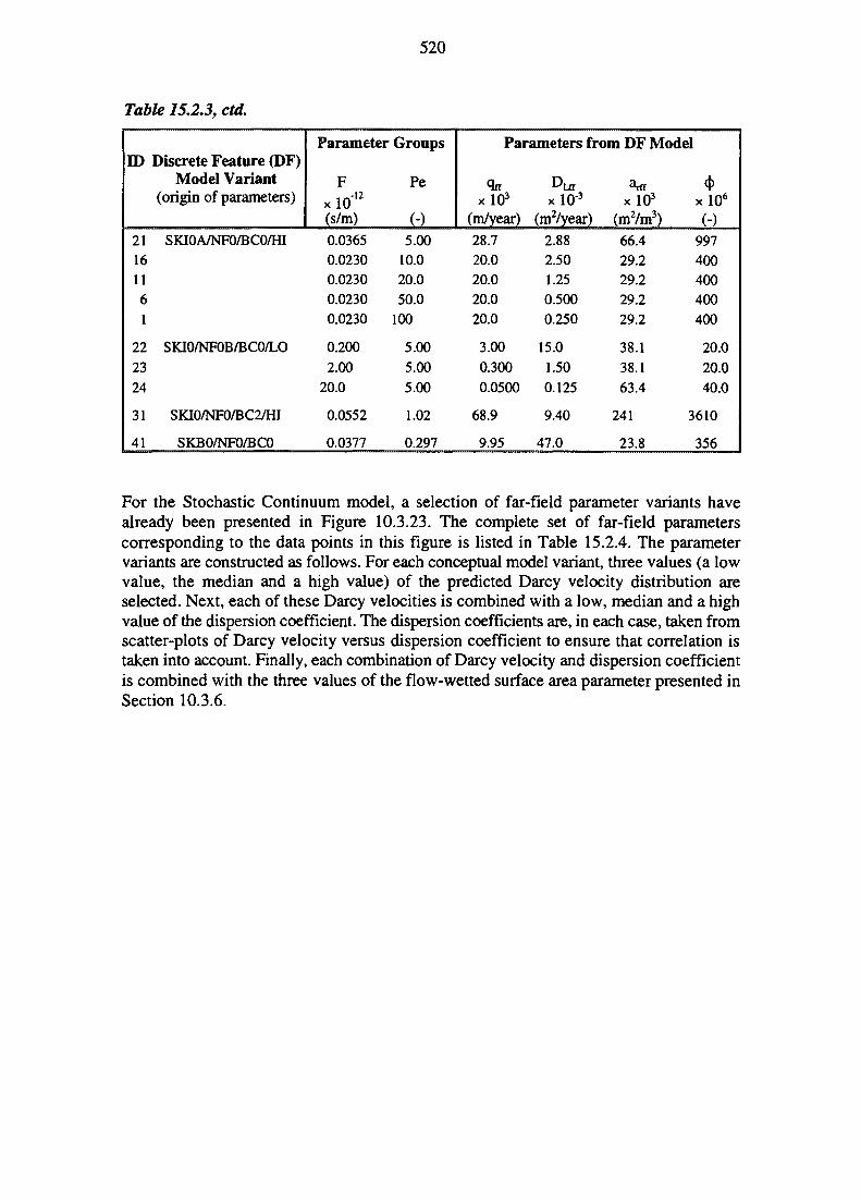
520
Table 15.2.3, ctd.
YD
211611
61
22
2324
31
41
Discrete Feature (DF)Model Variant
(origin of parameters)
SKI0A/NF0/BC0/HI
SKI0/NF0B/BC0/LO
SKI0/NF0/BC2/HI
SKB0/NF0/BC0
Parameter Groups
F Pex 1012
(s/m) (-)0.03650.02300.02300.02300.0230
0.200
2.0020.0
0.0552
0.0377
5.0010.020.050.0
100
5.005.005.00
1.02
0.297
Parameters from DF Model
qff DLfr arff <|>
x 103 x 10 3 x 103 x 106
(m/year) (mVyear) (m2/m3) (-)28.720.020.020.020.0
3.00
0.3000.0500
68.9
9.95
2.882.501.250.5000.250
15.0
1.500.125
9.40
47.0
66.429.229.229.229.2
38.138.163.4
241
23.8
997400400400400
20.020.040.0
3610
356
For the Stochastic Continuum model, a selection of far-field parameter variants havealready been presented in Figure 10.3.23. The complete set of far-field parameterscorresponding to the data points in this figure is listed in Table 15.2.4. The parametervariants are constructed as follows. For each conceptual model variant, three values (a lowvalue, the median and a high value) of the predicted Darcy velocity distribution areselected. Next, each of these Darcy velocities is combined with a low, median and a highvalue of the dispersion coefficient. The dispersion coefficients are, in each case, taken fromscatter-plots of Darcy velocity versus dispersion coefficient to ensure that correlation istaken into account. Finally, each combination of Darcy velocity and dispersion coefficientis combined with the three values of the flow-wetted surface area parameter presented inSection 10.3.6.
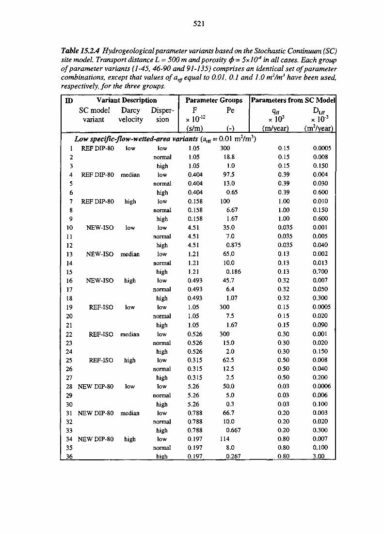
521
Table 15.2.4 Hydrogeological parameter variants based on the Stochastic Continuum (SC)site model. Transport distance L - 500 m and porosity (p- 5-KKX4 in all cases. Each groupof parameter variants (1-45, 46-90 and 91-135) comprises an identical set of parametercombinations, except that values of a^ equal to 0.01, 0.1 and 1.0 m2/m3 have been used,respectively, for the three groups.
ID
1
2
34
5678
9
101112
13
14
1516
17
18
19
20
21
222324252627
28
29
303132333435
36
Variant DescriptionSC model
variantDarcy
velocityDisper-
sion
Parameter
Fx 10-12
(s/m)Low specific-flow-wetted-area variants (a^ =
REF DIP-80
REF DIP-80
REF DIP-80
NEW-ISO
NEW-ISO
NEW-ISO
REF-ISO
REF-ISO
REF-ISO
NEW DIP-80
NEW DIP-80
NEW DIP-80
low
median
high
low
median
high
low
median
high
low
median
high
low
normal
highlow
normal
highlow
normal
highlow
normalhigh
low
normalhighlow
normal
high
low
normal
high
low
normalhighlow
normal
highlow
normal
highlow
normalhighlow
normal
high
1.051.05
1.050.404
0.404
0.404
0.1580.1580.158
4.51
4.514.51
1.21
1.211.210.493
0.493
0.493
1.05
1.05
1.05
0.5260.5260.5260.3150.3150.315
5.26
5.26
5.260.7880.7880.7880.1970.197
0.197
GroupsPe
(-)0.01 mVrr300
18.8
1.0
97.5
13.0
0.65
1006.671.67
35.0
7.0
0.875
65.0
10.0
0.18645.7
6.4
1.07
300
7.5
1.67
30015.02.0
62.512.5
2.550.0
5.0
0.366.710.00.667
1148.0
0.267
Parameters from
QffxlO3
(m/year)
i3)0.150.15
0.150.39
0.39
0.39
1.001.001.00
0.035
0.0350.035
0.13
0.130.130.32
0.32
0.32
0.15
0.15
0.15
0.300.300.300.500.50
0.50
0.03
0.03
0.030.200.200.200.800.80
0.80
SC Model
Diifx l O 3
^rnVyear)
0.00050.0080.1500.004
0.030
0.600
0.0100.1500.600
0.001
0.0050.040
0.002
0.0130.7000.007
0.050
0.300
0.0005
0.020
0.0900.0010.0200.1500.008
0.0400.200
0.0006
0.006
0.1000.0030.020
0.3000.0070.100
3.00
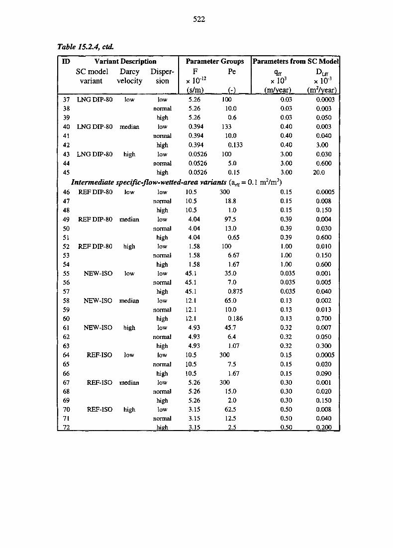
522
Table
ID
3738394041
42434445
15.2.4, cta\
Variant DescriptionSC model
variant
LNG DIP-80
LNG DIP-80
LNG DIP-80
Darcyvelocity
low
median
high
Disper-sion
lownormal
highlow
normal
highlow
normalhigh
Parameter GroupsF
x 1012
(s/m)5.265.265.260.3940.394
0.394
0.05260.05260.0526
Pe
(-)100
10.00.6
13310.0
0.133
1005.00.15
Intermediate specific-flow-wetted-area variants (a^ =46474849
50515253545556
5758596061626364
65
66676869707172
REF DIP-80
REF DIP-80
REF DIP-80
NEW-ISO
NEW-ISO
NEW-ISO
REF-ISO
REF-ISO
REF-ISO
low
median
high
low
median
high
low
median
high
low
normalhighlow
normalhighlow
normalhighlow
normalhighlow
normalhighlow
normalhighlow
normalhighlow
normalhighlow
normalhigh
10.510.510.54.04
4.044.041.581.581.58
45.145.1
45.112.112.112.14.93
4.934.93
10.5
10.510.55.265.265.263.153.153.15
30018.81.0
97.513.00.65
1006.671.67
35.07.0
0.87565.010.00.186
45.76.41.07
300
7.51.67
30015.02.0
62.512.52.5
Parameters from
QffxlO3
(m/year)0.030.030.030.400.40
0.40
3.003.003.00
0.1 m2/m3)0.150.150.15
0.390.390.391.001.001.000.0350.0350.035
0.130.130.130.32
0.320.32
0.15
0.15
0.150.300.300.300.500.500.50
SC ModelE>Lff
xlO"3
(mVyear)0.00030.0030.0500.0030.040
3.000.0300.600
20.0
0.00050.0080.150
0.0040.0300.6000.0100.1500.6000.0010.0050.0400.0020.0130.7000.007
0.0500.3000.0005
0.020
0.0900.0010.0200.1500.0080.0400.200
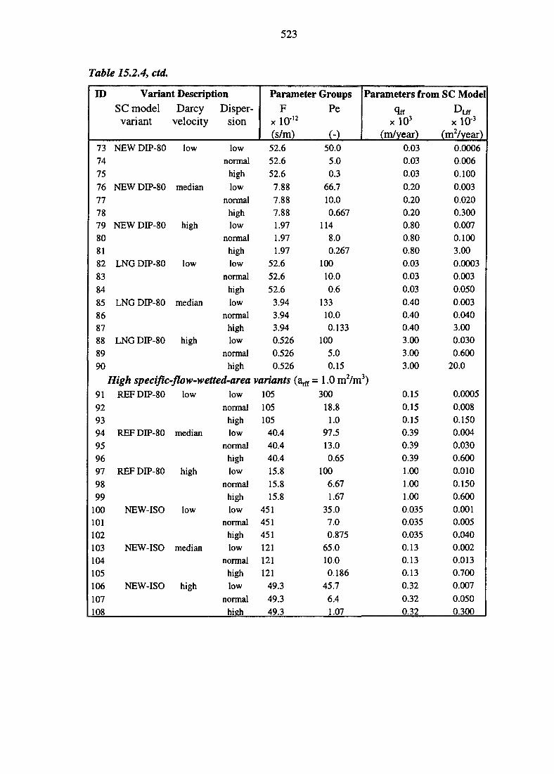
523
Table 15.2.4, ctd.
ID
7374
75
767778798081828384
858687888990
91929394959697
9899
100101102103104105
106107108
Variant DescriptionSC modelvariant
NEW DIP-80
NEW DIP-80
NEW DIP-80
LNG DIP-80
LNG DIP-80
LNG DIP-80
Darcyvelocity
low
median
high
low
median
high
Disper-sion
lownormal
high
low
normalhighlow
normalhighlow
normal
highlow
normalhighlow
normalhigh
High specific-flow-wetted-areaREF DIP-80
REF DIP-80
REF DIP-80
NEW-ISO
NEW-ISO
NEW-ISO
low
median
high
low
median
high
low
normalhighlow
normalhighlow
normalhighlow
normalhighlow
normalhighlow
normalhigh
Parameter GroupsF
x 1012
(s/m)52.652.652.6
7.887.887.881.971.971.97
52.652.6
52.63.943.943.940.5260.5260.526
variants (a^ =105
105105
40.440.440.4
15.815.815.8
451451451121121121
49.3
49.349.3
Pe
(-)50.05.00.3
66.710.00.667
1148.00.267
10010.00.6
13310.00.133
1005.00.15
1.0m2/m300
18.81.0
97.513.00.65
1006.671.67
35.07.00.875
65.010.00.186
45.7
6.41.07
Parameters from
xlO3
(m/year)0.030.030.03
0.200.200.200.800.800.800.030.03
0.030.400.400.403.003.003.00
3)0.15
0.150.150.390.390.391.001.001.000.0350.0350.0350.130.130.130.32
0.320.32
SC Model
DiifxlO"3
(mVyear)0.00060.0060.100
0.0030.0200.3000.0070.1003.000.00030.003
0.0500.0030.0403.000.0300.600
20.0
0.00050.0080.1500.0040.0300.6000.0100.1500.6000.0010.0050.0400.0020.0130.7000.007
0.0500.300
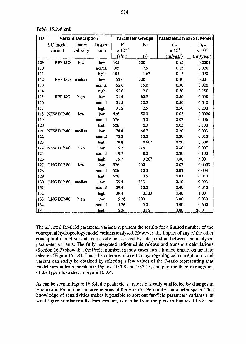
524
Table 15.2.4, ctd.
ID
109110111
112113114
115
116117118119120121122123124125126127128129130131
132133134135
Variant DescriptionSC modelvariant
REF-ISO
REF-ISO
REF-ISO
NEW DIP-80
NEW DIP-80
NEW DIP-80
LNG DIP-80
LNG DIP-80
LNG DIP-80
Darcyvelocity
low
median
high
low
median
high
low
median
high
Disper-sion
lownormal
highlow
normalhighlow
normalhighlow
normalhighlow
normalhighlow
normalhighlow
normalhighlow
normal
highlow
normalhigh
Parameter GroupsF
x 1012
(s/m)105105105
52.652.652.6
31.5
31.531.5
526526526
78.878.878.819.719.719.7
526
526526
39.439.4
39.45.265.265.26
Pe
(")300
7.51.67
30015.02.0
62.5
12.52.5
50.05.00.3
66.710.00.667
1148.00.267
10010.00.6
133
10.0
0.133100
5.00.15
Parameters from
OffxlO3
(m/year)0.150.150.150.300.300.300.50
0.500.500.030.030.030.200.200.200.800.800.800.030.030.030.40
0.40
0.403.003.003.00
SC Mode!
xlO"3
(mVyear)0.00050.0200.0900.0010.0200.150
0.008
0.0400.2000.00060.0060.1000.0030.0200.3000.0070.1003.000.0003
0.0030.0500.003
0.040
3.000.0300.600
20.0
The selected far-field parameter variants represent the results for a limited number of theconceptual hydrogeology model variants analysed. However, the impact of any of the otherconceptual model variants can easily be assessed by interpolation between the analysedparameter variants. The fully integrated radionuclide release and transport calculations(Section 16.3) show that the Peclet number, in most cases, has a limited impact on far-fieldreleases (Figure 16.3.4). Thus, the outcome of a certain hydrogeological conceptual modelvariant can easily be obtained by selecting a few values of the F-ratio representing thatmodel variant from the plots in Figures 10.3.8 and 10.3.13, and plotting them in diagramsof the type illustrated in Figure 16.3.4.
As can be seen in Figure 16.3.4, the peak release rate is basically unaffected by changes inF-ratio and Pe-number in large regions of the F-ratio - Pe-number parameter space. Thisknowledge of sensitivities makes it possible to sort out far-field parameter variants thatwould give similar results. Furthermore, as can be from the plots in Figures 10.3.8 and
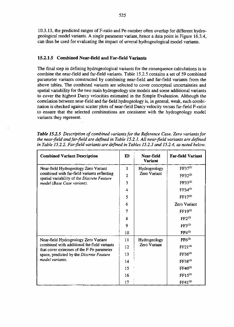
525
10.3.13, the predicted ranges of F-ratio and Pe-number often overlap for different hydro-geological model variants. A single parameter variant, hence a data point in Figure 16.3.4,can thus be used for evaluating the impact of several hydrogeological model variants.
15.2.1.5 Combined Near-field and Far-field Variants
The final step in defining hydrogeological variants for the consequence calculations is tocombine the near-field and far-field variants. Table 15.2.5 contains a set of 59 combinedparameter variants constructed by combining near-field and far-field variants from theabove tables. The combined variants are selected to cover conceptual uncertainties andspatial variability for the two main hydrogeology site models and some additional variantsto cover the highest Darcy velocities estimated in the Simple Evaluation. Although thecorrelation between near-field and far-field hydrogeology is, in general, weak, each combi-nation is checked against scatter plots of near-field Darcy velocity versus far-field F-ratioto ensure that the selected combinations are consistent with the hydrogeology modelvariants they represent.
Table 15.2.5 Description of combined variants for the Reference Case. Zero variants forthe near-field and far-field are defined in Table 15.2.1. All near-field variants are definedin Table 15.2.2. Far-field variants are defined in Tables 15.2.3 and 15.2.4, as noted below.
Combined Variant Description
Near-field Hydrogeology Zero Variantcombined with far-field variants reflectingspatial variability of the Discrete Featuremodel (Base Case variant).
Near-field Hydrogeology Zero Variantcombined with additional far-field variantsthat cover extremes of the F-Pe parameterspace, predicted by the Discrete Featuremodel variants.
ID
1
2
3
4
5
6
7
8
9
10
11
12
13
14
15
16
17
Near-fieldVariant
HydrogeologyZero Variant
HydrogeologyZero Variant
Far-field Variant
FF37(2)
FF32(2)
FF33(2)
FF34(2)
F F 1 7 (2)
Zero Variant
FF19(2)
FF2(2)
FF3(2)
FF4(2)
FF6(2)
FF21(2)
FF36(2)
FF38(2)
FF40(2)
FF15(2)
FF41(2)
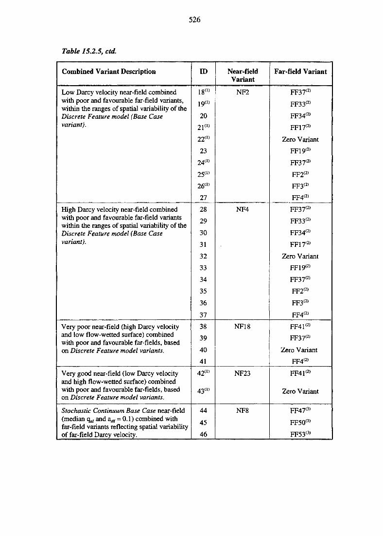
526
Table 15.2.5, ctd.
Combined Variant Description
Low Darcy velocity near-field combinedwith poor and favourable far-field variants,within the ranges of spatial variability of theDiscrete Feature model (Base Casevariant).
High Darcy velocity near-field combinedwith poor and favourable far-field variantswithin the ranges of spatial variability of theDiscrete Feature model (Base Casevariant).
Very poor near-field (high Darcy velocityand low flow-wetted surface) combinedwith poor and favourable far-fields, basedon Discrete Feature model variants.
Very good near-field (low Darcy velocityand high flow-wetted surface) combinedwith poor and favourable far-fields, basedon Discrete Feature model variants.
Stochastic Continuum Base Case near-field(median qnf and a^ = 0.1) combined withfar-field variants reflecting spatial variabilityof far-field Darcy velocity.
ID
18 ( 1 )
19(D
20
2i(D
22(1)
23
24(1)
25(1)
26(1)
27
28
29
30
31
32
33
34
35
36
37
38
39
40
41
42(1)
43(1)
44
45
46
Near-fieldVariant
NF2
NF4
NF18
NF23
NF8
Far-field Variant
FF37(2)
FF33(2)
FF34(2)
FF17(2)
Zero Variant
FF19(2)
FF37(2)
FF2<2)
FF3(2)
FF4(2)
FF37(2)
FF33(2)
FF34(2)
FF17(2)
Zero Variant
FF19(2)
FF37(2)
FF2(2)
FF3(2)
FF4(2)
FF41 (2)
FF37(2)
Zero Variant
FF4(2)
FF41 (2)
Zero Variant
FF47(3)
FF50(3)
FF53(3)
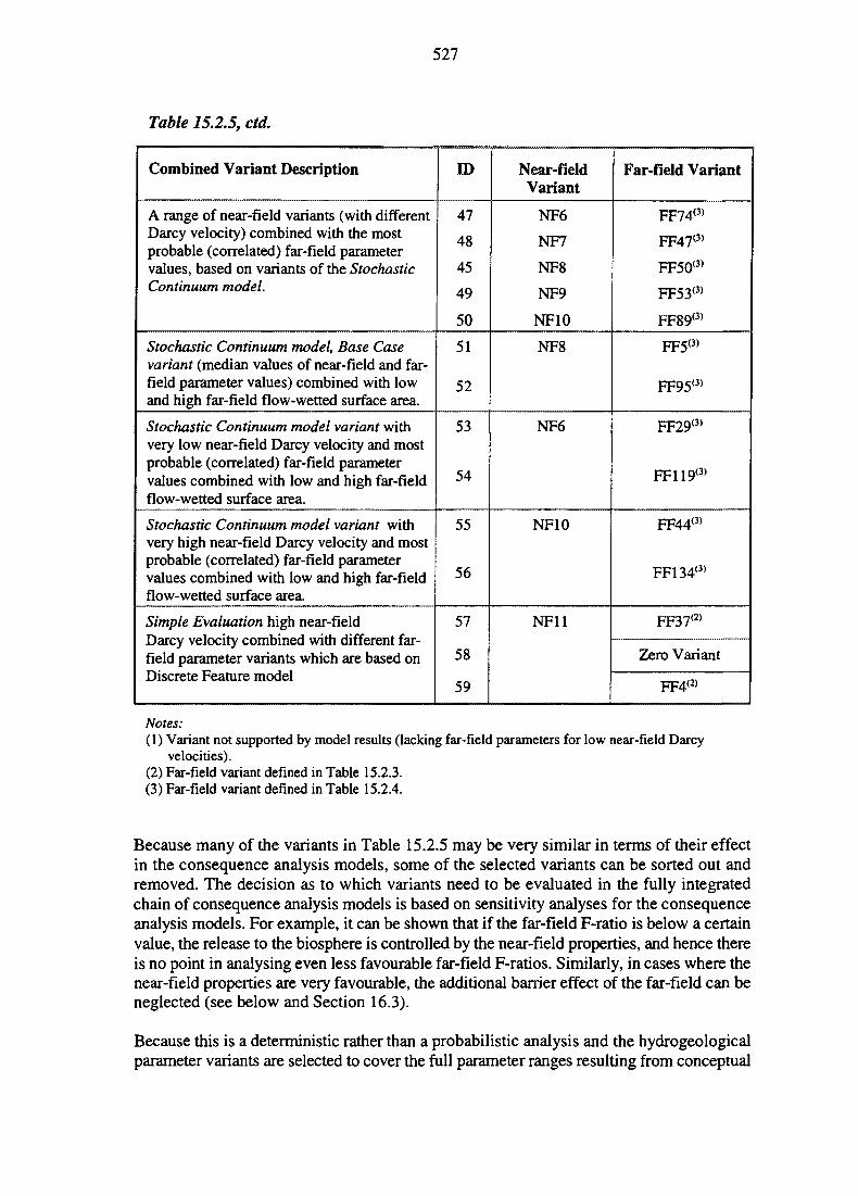
527
Table 15.2.5, ctd.
Combined Variant Description
A range of near-field variants (with differentDarcy velocity) combined with the mostprobable (correlated) far-field parametervalues, based on variants of the StochasticContinuum model.
Stochastic Continuum model, Base Casevariant (median values of near-field and far-field parameter values) combined with lowand high far-field flow-wetted surface area.
Stochastic Continuum model variant withvery low near-field Darcy velocity and mostprobable (correlated) far-field parametervalues combined with low and high far-fieldflow-wetted surface area.
Stochastic Continuum model variant withvery high near-field Darcy velocity and mostprobable (correlated) far-field parametervalues combined with low and high far-fieldflow-wetted surface area.
Simple Evaluation high near-fieldDarcy velocity combined with different far-field parameter variants which are based onDiscrete Feature model
ID
47
48
45
49
50
51
52
53
54
55
56
57
58
59
Near-fieldVariant
NF6
NF7
NF8
NF9
NF10
NF8
NF6
NF10
NF11
Far-field Variant
FF74(3)
FF47(3)
FF50(3)
FF53(3)
FF89(3)
FF5(3)
FF95(3)
FF29(3)
FF119(3)
FF44(3)
FF134<3)
FF37(2)
Zero Variant
FF4<2)
Notes:(1) Variant not supported by model results (lacking far-field parameters for low near-field Darcy
velocities).(2) Far-field variant defined in Table 15.2.3.(3) Far-field variant defined in Table 15.2.4.
Because many of the variants in Table 15.2.5 may be very similar in terms of their effectin the consequence analysis models, some of the selected variants can be sorted out andremoved. The decision as to which variants need to be evaluated in the fully integratedchain of consequence analysis models is based on sensitivity analyses for the consequenceanalysis models. For example, it can be shown that if the far-field F-ratio is below a certainvalue, the release to the biosphere is controlled by the near-field properties, and hence thereis no point in analysing even less favourable far-field F-ratios. Similarly, in cases where thenear-field properties are very favourable, the additional barrier effect of the far-field can beneglected (see below and Section 16.3).
Because this is a deterministic rather than a probabilistic analysis and the hydrogeologicalparameter variants are selected to cover the full parameter ranges resulting from conceptual

528
uncertainties and spatial variability, they do not reflect the likelihood of a certain outcomein the consequence analysis models. In order to draw such inferences, or to track the originof a particular uncertainty, it would be necessary to go back to the hydrogeological modelvariant in Section 10.3 from which the parameter variant is derived. The references in theparameter variant tables in this chapter provide the necessary link for this analysis.
15.2.1.6 Potential Model Simplification Errors
As mentioned in Section 10.3, the procedure for estimation of effective transport para-meters for the idealised, near-field radionuclide release and, in particular, far-field transportcodes involves simplifications that may generate uncertainty. For the far-field,simplification errors arise because the simplistic one-dimensional transport code(CRYSTAL) is not compatible with the three-dimensional heterogeneous hydrogeology sitemodels. In the 3D heterogeneous hydrogeology models the local transport properties varyin a complex fashion, both along a given transport path and between different pathwaysbetween a source canister and the biosphere. The resulting residence time distributions are,in some cases, characterised by multiple peak structures and non-Gaussian tailing(Section 10.3), which are poorly represented by an effective Darcy velocity and dispersioncoefficient in the ID CRYSTAL code. The fact that both very high (MOO) and very low(<1) Peclet numbers are obtained for some of the transport paths in the Discrete Featuremodel is a direct indication that the ID advection-dispersion equation (in CRYSTAL) isa poor model of a three-dimensional, spatially varying flow field.
The potential magnitude of the simplification errors depends on the heterogeneity and flowfield structure in the hydrogeological site models. However, because the coupled radio-nuclide transport (as modelled in CRYSTAL, Chapter 13) is a non-linear function of thehydrogeological transport parameters, e.g. Darcy velocity and specific flow-wetted area,without further research it is difficult to foresee exactly how the simplification errors wouldaffect the radionuclide transport results.
SITE-94 did not include a detailed analysis of simplification errors. However, in com-parison with the large parameter and conceptual uncertainties evaluated in the SITE-94hydrogeological evaluation, the additional uncertainties introduced by the above modelsimplifications are likely to be negligible. As shown in Section 16.3.1, the evaluateduncertainty in the far-field F-ratio covers the whole range from essentially no retardationto complete containment in the far-field rock.
15.2.2 Chemical Variants
The key chemical parameters for the radionuclide release and transport calculations whichare delivered by the Geochemical parameters to radionuclideKN-transport Clearing Houseare solubility limits and sorption coefficients (Kj-values) for the different elements. Theseproperties depend on the groundwater chemistry which, in turn, depends on the history ofthe groundwater and the properties of the solid phases, as discussed in Sections 7.4 and10.4. The sorption properties also depend directly upon the properties of the solid phases.This Clearing House also delivers buffer properties and physical parameters of theEngineered Barriers and the rock.
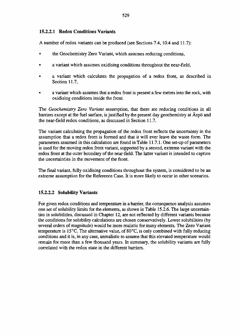
529
15.2.2.1 Redox Conditions Variants
A number of redox variants can be produced (see Sections 7.4, 10.4 and 11.7):
• the Geochemistry Zero Variant, which assumes reducing conditions,
• a variant which assumes oxidising conditions throughout the near-field,
• a variant which calculates the propagation of a redox front, as described inSection 11.7,
• a variant which assumes that a redox front is present a few metres into the rock, withoxidising conditions inside the front.
The Geochemistry Zero Variant assumption, that there are reducing conditions in allbarriers except at the fuel surface, is justified by the present day geochemistry at Aspo andthe near-field redox conditions, as discussed in Section 11.7.
The variant calculating the propagation of the redox front reflects the uncertainty in theassumption that a redox front is formed and that it will ever leave the waste form. Theparameters assumed in this calculation are found in Table 11.7.1. One set-up of parametersis used for the moving redox front variant, supported by a second, extreme variant with theredox front at the outer boundary of the near-field. The latter variant is intended to capturethe uncertainties in the movement of the front.
The final variant, fully oxidising conditions throughout the system, is considered to be anextreme assumption for the Reference Case. It is more likely to occur in other scenarios.
15.2.2.2 Solubility Variants
For given redox conditions and temperature in a barrier, the consequence analysis assumesone set of solubility limits for the elements, as shown in Table 15.2.6. The large uncertain-ties in solubilities, discussed in Chapter 12, are not reflected by different variants becausethe conditions for solubility calculations are chosen conservatively. Lower solubilities (byseveral orders of magnitude) would be more realistic for many elements. The Zero Varianttemperature is 15°C. The alternative value, of 80°C, is only combined with fully reducingconditions and it is, in any case, unrealistic to assume that this elevated temperature wouldremain for more than a few thousand years. In summary, the solubility variants are fullycorrelated with the redox state in the different barriers.
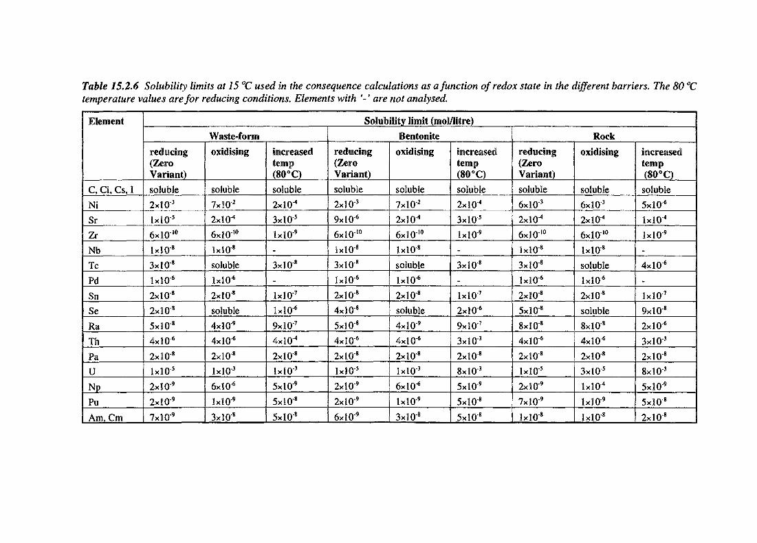
Table 15.2.6 Solubility limits at 15 °C used in the consequence calculations as a function ofredox state in the different barriers. The 80 °Ctemperature values are for reducing conditions. Elements with '-' are not analysed.
Element
C, CI, Cs, I
Ni
Sr
Zr
Nb
Tc
Pd
Sn
Se
Ra
Th
Pa
U
Np
Pu
Am, Cm
Solubility limit (mol/Iitre)
Waste-form
reducing(ZeroVariant)
soluble
2xlO"3
ixlO"5 I
6x10'°
1x10'
3x10'
1x10'
2x10'
2x10"'
5x10' 1
4 x 1 0 '
2x10 '
Ix lO 5
2x10 '
2x10"'
7 x 1 0 '
oxidising
soluble
7xlO"2
2X10"4
6x10'°
1x10'
soluble
1x10'
2x10"'
soluble
4x10 '
4x10 '
2x10"'
ixlO"3
6x10"'
1x10'
3x10 '
increasedtemp(80°C)
soluble
2X10"4
3 x l 0 5
1x10'
3x10 '-
IxlO-7
1x10'
9xlO7
4xlO"4
2x10 '
IxlO 3
5x10 '
5x10 '
5x10 '
Bentonite
reducing(ZeroVariant)
soluble
2xiO"3
9x10 '
6xlO10
1x10'
3x10 '
1x10"'
2x10 '
4x10 '
5x10 '
4x10 '
2x10 '
IxlO5
2x10"'
2x10 '
6x10 '
oxidising
soluble
7xlO2
2xlO"4
6xlO10
ixlO"8
soluble
1x10"'
2x10 '
soluble
4x10 '
4x10"'
2x10 '
MO"3
6x10 '
1x10 '
3x10"'
increasedtemp(80°C)
soluble
2x10⁴
3 x l 0 5
1x10'-
3x10 '_
IxlO 7
2x10 '
9xlO7
3xlO"3
2x10 '
8x10³
5x10"'
5x10 '
5x10"'
Rock
reducing(ZeroVariant)
soluble
6 x l 0 3
2xlO4
6xlO10
1x10-'
3x10 '
1x10'
2x10 '
5x10"'
8x10 '
4x10 '
2x10 '
IxlO5
2x10 '
7x10 '
ix lO 8
oxidising
soluble
6xlO3
2xlO4
6xl0 1 0
1x10'
soluble
1x10'
2x10 '
soluble
8x10 '
4x10 '
2x10 '
3xl0"5
IxlO4
1x10'
ix lO 8
increasedtemp(80°C)
soluble
5x10 '
IxlO-4
1x10 '
4x10"'
lxl0"7
9 x 1 0 '
2 x 1 0 '
3xlO 3
2x10 '
8xlO"3
5x10"'
5x10"'
2x10 '
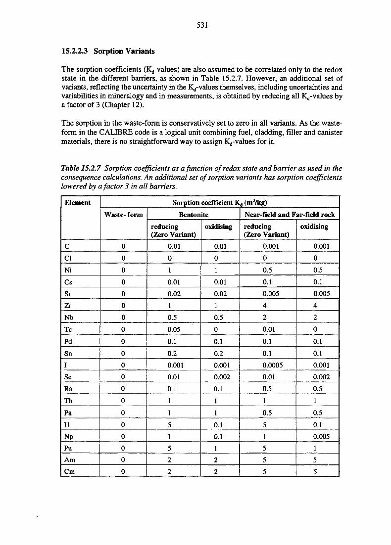
531
15.2.2.3 Sorption Variants
The sorption coefficients (Kd-values) are also assumed to be correlated only to the redoxstate in the different barriers, as shown in Table 15.2.7. However, an additional set ofvariants, reflecting the uncertainty in the K^-values themselves, including uncertainties andvariabilities in mineralogy and in measurements, is obtained by reducing all Kd-values bya factor of 3 (Chapter 12).
The sorption in the waste-form is conservatively set to zero in all variants. As the waste-form in the CALIBRE code is a logical unit combining fuel, cladding, filler and canistermaterials, there is no straightforward way to assign Kd-values for it.
Table 15.2.7 Sorption coefficients as a function of redox state and barrier as used in theconsequence calculations. An additional set ofsorption variants has sorption coefficientslowered by a factor 3 in all barriers.
Element
C
Cl
Ni
Cs
Sr
Zr
Nb
Tc
Pd
Sn
I
Se
Ra
Th
Pa
U
Np
Pu
Am
Cm
Sorption coefficient Kd (mVkg)
Waste- form
0
0
0
0
0
0
0
0
0
0
0
0
0
0
0
0
0
0
0
0
Bentonite
reducing(Zero Variant)
0.01
0
1
0.01
0.02
1
0.5
0.05
0.1
0.2
0.001
0.01
0.1
1
1
5
1
5
2
2
oxidising
0.01
0
1
0.01
0.02
1
0.5
0
0.1
0.2
0.001
0.002
0.1
1
1
0.1
0.1
1
2
2
Near-field and Far-field rock
reducing(Zero Variant)
0.001
0
0.5
0.1
0.005
4
2
0.01
0.1
0.1
0.0005
0.01
0.5
1
0.5
5
1
5
5
5
oxidising
0.001
0
0.5
0.1
0.005
4
2
0
0.1
0.1
0.001
0.002
0.5
1
0.5
0.1
0.005
1
5
5
532
15.2.2.4 Buffer Variants
An alternative buffer variant is produced by assuming the very unlikely event that thebentonite loses its plasticity such that cracks form, connecting the canister with the fracturein the rock. This variant is clearly a 'what-if assumption, but reflects, in an extremefashion, the uncertainties in the long-term degradation of the bentonite (Section 11.3). Inpractice, this variant is modelled by moving the rock/bentonite interface in CALIBRE veryclose to the canister. As the assumption is extreme, it is considered inappropriate tocombine it with anything but the Geochemistry Zero Variant redox conditions.
15.2.2.5 Physical Properties
In the consequence analysis, there is no variation in a number of the physical properties ofthe Engineered Barriers and rock (diffusivity, density, porosity, redox capacity). In theSITE-94 calculations, this is justified by the fact that no information about the variabilityin site-specific data is available. In a real Performance Assessment, the effects of all thesevariations will have to be considered.
In Tables 15.2.8 and 15.2.9 parameters that have not been varied in the SITE-94 conse-quence analyses are given for CALIBRE and CRYSTAL, respectively. The canister anddeposition hole dimensions are taken as design parameters (outlined in Chapter 5). The gridlength is a modelling parameter in CALIBRE (see Chapter 13). The diffusivities are takenfrom Project-90 (SKI, 1991) for the bentonite, and as for pure water for the fracture and thewaste-form. The rock diffusivity and matrix porosity is discussed in Section 7.4.4.2, whilethe rock density is a typical value for granite. The bentonite density and porosity is derivedfrom KBS-3 data (SKBF/KBS, 1983). Porosity and density of the waste-form is an attemptto give averages for the logical unit 'waste-form' in CALIBRE, and the values given areestimations based on design data from e.g. Benedict et. al. (1981), TVO-92 (TVO, 1992)and SKB 91 (SKB, 1992). The CCL-parameter and the chosen value is discussed inSection 13.5.1. Parameter values for redox capacity, used in calculating the movement ofa redox front, are found in Table 11.7.1.
The far-field parameter fracture spacing is discussed in Section 13.4.2. The penetrationdepth into matrix is given in Section 7.4.2.2. The diffusivity, matrix porosity and densityof the rock are the same as for the near-field, and given in 7.4.2.2. The migration distanceis given in Section 15.2.1 (Table 15.2.1).
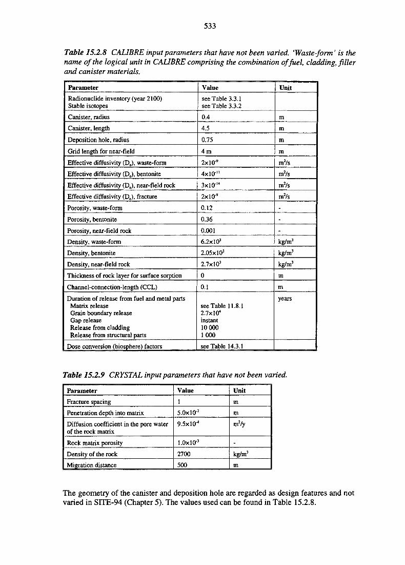
533
Table 15.2.8 CALIBRE input parameters that have not been varied. 'Waste-form' is thename of the logical unit in CALIBRE comprising the combination of fuel, cladding, fillerand canister materials.
Parameter
Radionuclide inventory (year 2100)Stable isotopes
Canister, radius
Canister, length
Deposition hole, radius
Grid length for near-field
Effective diffusivity (DJ, waste-form
Effective diffusivity (De), bentonite
Effective diffusivity (De), near-field rock
Effective diffusivity (Dc), fracture
Porosity, waste-form
Porosity, bentonite
Porosity, near-field rock
Density, waste-form
Density, bentonite
Density, near-field rock
Thickness of rock layer for surface sorption
Channel-connection-length (CCL)
Duration of release from fuel and metal partsMatrix releaseGrain boundary releaseGap releaseRelease from claddingRelease from structural parts
Dose conversion (biosphere) factors
Value
see Table 3.3.1see Table 3.3.2
0.4
4.5
0.75
4m
2xlO9
4x10"
3xlO14
2xlO"9
0.12
0.36
0.001
6.2x10³
2.05xl03
2.7xl03
0
0.1
see Table 11.8.12.7x104
instant10 0001000
see Table 14.3.1
Unit
m
m
m
m
m2/s
m2/s
m2/s
mVs
-
-
-
kg/m3
kg/m3
kg/m3
m
m
years
Table 15.2.9 CRYSTAL input parameters that have not been varied.
Parameter
Fracture spacing
Penetration depth into matrix
Diffusion coefficient in the pore waterof the rock matrix
Rock matrix porosity
Density of the rock
Migration distance
Value
1
5.0xl0-2
9.5X10⁻⁴
l.OxlO3
2700
500
Unit
m
m
m2/y
-
kg/m3
m
The geometry of the canister and deposition hole are regarded as design features and notvaried in SITE-94 (Chapter 5). The values used can be found in Table 15.2.8.
534
15.2.2.6 Combinations of Chemical Variants
The chemical parameters of solubility limit and sorption are both implicitly determined bywhich redox variant is chosen (4 variants) and could, in addition, be varied independently(high temperature solubility variant and low sorption variant). The variants with hightemperature solubility limits and with low sorption are, however, only combined withreducing conditions (Zero Variant redox conditions), because this is the most pessimisticcombination. As noted above (Section 15.2.2.4), the degraded buffer variant is judged tobe such an extreme condition that it is only considered for fully reducing conditions.
Far-field chemistry variants are reduced to two redox variants (reducing and oxidising) andtwo sorption variants (normal and low sorption), as solubility limits and redox fronts arenot considered in the modelling of far-field radionuclide transport. Calculations with thenear-field CALIBRE code (see Section 11.7) which suggest that a redox front wouldprobably never leave the near-field and that no radionuclides would be precipitated far outin the rock, indicate why omitting solubility constraints and redox fronts is not a seriouslimitation. For the same reason as for the near-field, the low sorption variant is onlycombined with reducing redox conditions.
The far-field geochemistry is treated as fully correlated to the near-field geochemistry in theintegrated near-field and far-field analysis, such that the far-field is oxidised only when thenear-field is oxidised throughout (as the front is assumed to originate from oxidant pro-duction in the fuel) and low sorption in the far-field is only considered together with a near-field which has low sorption.
15.2.3 Canister Failure Variants
When analysing a single canister, the relevant input to the consequence analysis is the timeof failure and the mode of failure, i.e. if the canister fails completely or if there is releasethrough a 'pin-hole' (Section 13.3). For a full repository analysis it would be necessary tohave the probability distribution function for the number of canisters failed as a functionof time. However, as stated in Section 11.5, no attempt is made to estimate canister failurefrequency in SITE-94. The reason for this is the uncertainty in the spread of canisterproperties, which makes any prediction of canister failure rates rather speculative. Thismeans that the parameters in the canister failure variants are restricted to the time and themode of failure for one single canister.
As discussed in the canister analysis (Section 11.5) it is very difficult to make estimates ofthe canister life time, particularly as design, manufacturing methods and means of qualitycontrol are still under development. Nevertheless, it is concluded that under Reference Caseconditions, even though they do not imply large mechanical or chemical disturbances in thenear-field, a few canisters may still fail during the first 100 000 years and that the firstfailure may be as early as 1000 years after disposal, although most canisters may survivefor much longer times. The canister analysis also concludes that, even if early canisterfailures probably start as a very localised failure of the copper canister, subsequentcorrosion of the steel vessel may lead to general failure within a time period in the order of1000 years. Furthermore, it is suggested that, for the Reference Case, there is only a veryweak coupling between failure and geochemical or hydrogeological conditions.
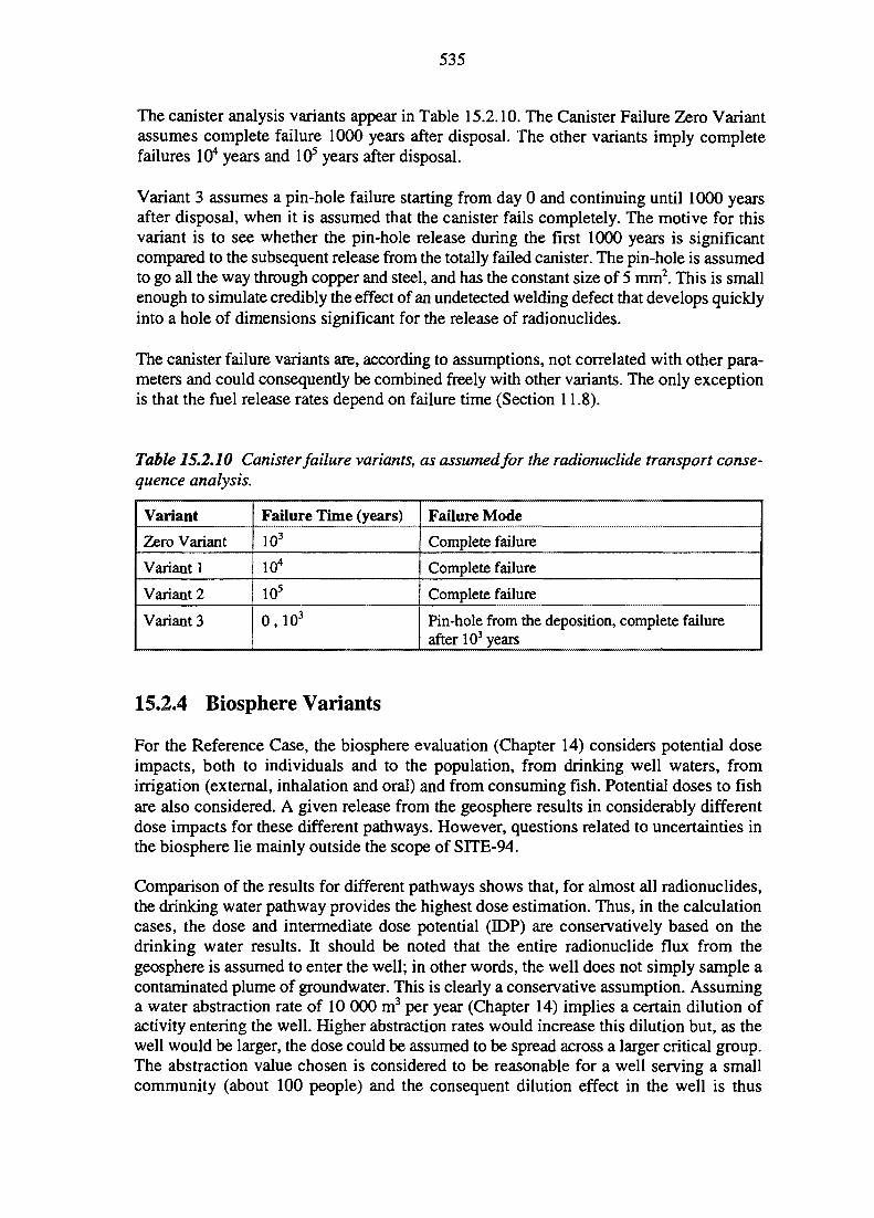
535
The canister analysis variants appear in Table 15.2.10. The Canister Failure Zero Variantassumes complete failure 1000 years after disposal. The other variants imply completefailures 104 years and 105 years after disposal.
Variant 3 assumes a pin-hole failure starting from day 0 and continuing until 1000 yearsafter disposal, when it is assumed that the canister fails completely. The motive for thisvariant is to see whether the pin-hole release during the first 1000 years is significantcompared to the subsequent release from the totally failed canister. The pin-hole is assumedto go all the way through copper and steel, and has the constant size of 5 mm2. This is smallenough to simulate credibly the effect of an undetected welding defect that develops quicklyinto a hole of dimensions significant for the release of radionuclides.
The canister failure variants are, according to assumptions, not correlated with other para-meters and could consequently be combined freely with other variants. The only exceptionis that the fuel release rates depend on failure time (Section 11.8).
Table 15.2.10 Canister failure variants, as assumed for the radionuclide transport conse-quence analysis.
Variant
Zero Variant
Variant 1
Variant 2
Variant 3
Failure Time (years)
103
104
105
0, 103
Failure Mode
Complete failure
Complete failure
Complete failure
Pin-hole from the deposition, complete failureafter 103 years
15.2.4 Biosphere Variants
For the Reference Case, the biosphere evaluation (Chapter 14) considers potential doseimpacts, both to individuals and to the population, from drinking well waters, fromirrigation (external, inhalation and oral) and from consuming fish. Potential doses to fishare also considered. A given release from the geosphere results in considerably differentdose impacts for these different pathways. However, questions related to uncertainties inthe biosphere lie mainly outside the scope of SITE-94.
Comparison of the results for different pathways shows that, for almost all radionuclides,the drinking water pathway provides the highest dose estimation. Thus, in the calculationcases, the dose and intermediate dose potential (IDP) are conservatively based on thedrinking water results. It should be noted that the entire radionuclide flux from thegeosphere is assumed to enter the well; in other words, the well does not simply sample acontaminated plume of groundwater. This is clearly a conservative assumption. Assuminga water abstraction rate of 10 000 m3 per year (Chapter 14) implies a certain dilution ofactivity entering the well. Higher abstraction rates would increase this dilution but, as thewell would be larger, the dose could be assumed to be spread across a larger critical group.The abstraction value chosen is considered to be reasonable for a well serving a smallcommunity (about 100 people) and the consequent dilution effect in the well is thus
536
considered to be realistic. It should, in any case, be re-emphasised that calculated doses areindicators only, not accurate predictors of radiological impact.
Using a single set of factors from one biosphere receptor (the well) has the additionaladvantage of simplifying inter-comparison of results. The biosphere factors used, therefore,are those given under the 'Drinking water, Individual' heading in Table 14.3.1. The poten-tial impact of other pathways is discussed in Section 16.4.3.
15.2.5 Inventory, Fuel Degradation and Radionuclide Release fromFuel
As discussed in Chapter 3 and Sections 11.6 and 13.2, it was decided that SITE-94 wouldnot analyse any uncertainties or deviations in radionuclide inventory, mechanisms and ratesof fuel degradation or mechanisms and rates of radionuclide release from the fuel. The onlyexception is that the oxidant production rate in the canister, and hence the canister releaserate, is dependent on canister failure time. These sections point out that uncertainties doexist, but an analysis of their impact lies outside the scope of SITE-94. Consequently, thereis only a single variant for these inputs.
The inventory values actually used are found in Tables 3.3.1 (radionuclides) and 3.3.2(stable nuclides). The transport calculations for all variants are not performed for wNb and107Pd (due to late delivery of data) but, as these radionuclides are not strong contributors tothe total dose, this is not considered to be a serious drawback.
Values for oxidant production rate and duration of matrix release as functions of canisterfailure time are found in Table 11.8.1. The duration of other release mechanisms are foundin Table 15.2.8. The allocation of radionuclides from the fuel to gap release, grain boundaryrelease and matrix release is described in Section 13.2. For modelling purposes, for casesinvolving immediate canister failure or a lifetime of only 1000 years, grain boundary releaseis set to the same rate as matrix release (to avoid a grain boundary release slower than thematrix release).
15.2.6 Combination of Variants from Different Clearing Houses toform Calculation Cases
15.2.6.1 Total Number of Variant Combinations
After internal reduction within each Clearing House, 25 near-field hydrology variants, 17far-field hydrology variants, 7 geochemical variants and 4 canister variants remain to beanalysed. The remaining Clearing Houses only produce Zero Variant parameter sets. Sincethe consequence analysis is performed for 14 individual radionuclides and the 4 actinidechains, this would involve over 200 000 individual computer runs if all combinations ofvariants have to be analysed. For the purposes of the present exercise it was decided toreduce the number to a more manageable set of combinations.
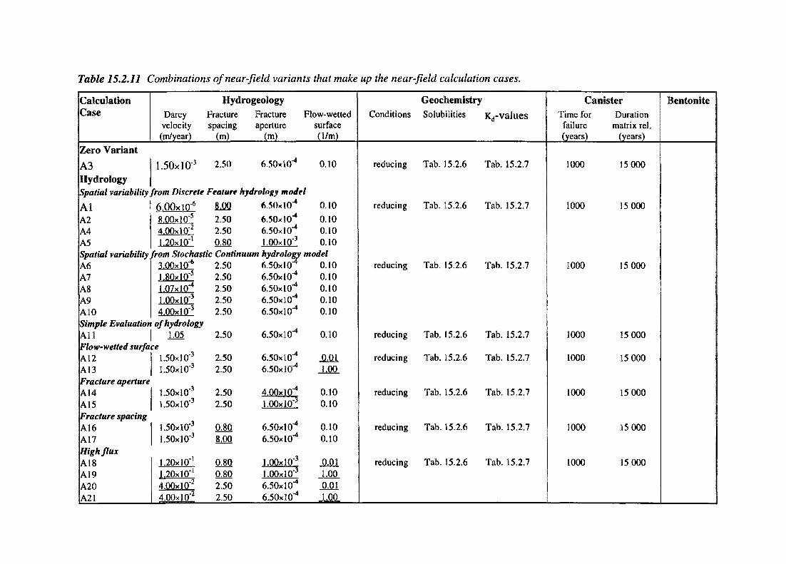
Table 15.2.11 Combinations of near-field variants that make
CalculationCase
Zero Variant
A3Hydrology
Darcyvelocity(m/year)
1.5OxlO-3
Spatial variability from Discrete
AIA2A4A5
6.00x10⁶
8.00x10'5
4.00x10'2
1.20x10''
HydrogeologyFracturespacing
(m)
2.50
Fractureaperture
(m)
6.5Ox! 0"4
Flow-wettedsurface(1/m)
0.10
Feature hydrology model
8.00
2.502.500.80
6.50* I0"4
6.50x10^*6.50x10"4
l.OOxlO'3
Spatial variability from Stochastic Continuum hydrologyA6A7A8A9A10
3.00x10'°1.8OxlO"5
1.07X10"4
l.OOxlO"3
4.00xl0"3
Simple Evaluation of hydrologyAll .IQ5Flow-wetted surfaceA12A13Fracture apertureA14A15Fracture spacingA16A17High fluxA18A19A20A21
3.5Ox!O"J
1.50xl0"3
1.50xl0"3
1.5OxlO"3
1.50xl0'3
1.5OxlO'3
1.20xl0'!
1.20x10"'4.00x10*2
4.00x10'2
2.502.502.502.502.50
2.50
2.502.50
2.502.50
0.808.00
0.800.802.502.50
6.50x10"^6.50x10"4
6.50X10*4
6.50X10"4
6.50XI0"4
A
6.50XI0"4
6.50x10"4
6.50X10"4
4.00X10⁻⁴
l.OOxlO"3
6.50X10"4
6.50X10"4
l.OOxlO"3
l.OOxlO"3
6.50x10"4
6.50x10"4
0.10
0.100.100.10
model0.100.100.100.100.10
0.10
0.011.00
0.100.10
0.100.10
0.011.000.011.00
up the near-field calculation cases.
Conditions
reducing
reducing
reducing
reducing
reducing
reducing
reducing
reducing
GeochemistrySolubilities
Tab. 15.2.6
Tab. 15.2.6
Tab. 35.2.6
Tab. 15.2.6
Tab. 15.2.6
Tab. 15.2.6
Tab. 15.2.6
Tab. 15.2.6
Krf-values
Tab. 35.2.7
Tab. 15.2.7
Tab. 15.2.7
Tab. 15.2.7
Tab. 15.2.7
Tab. 15.2.7
Tab. 15.2.7
Tab. 15.2.7
CanisterTime for
failure(years)
1000
1000
1000
1000
1000
1000
1000
1000
Durationmatrix rel.
(years)
15 000
15 000
35 000
35 000
15 000
35 000
15 000
15 000
Betntonite
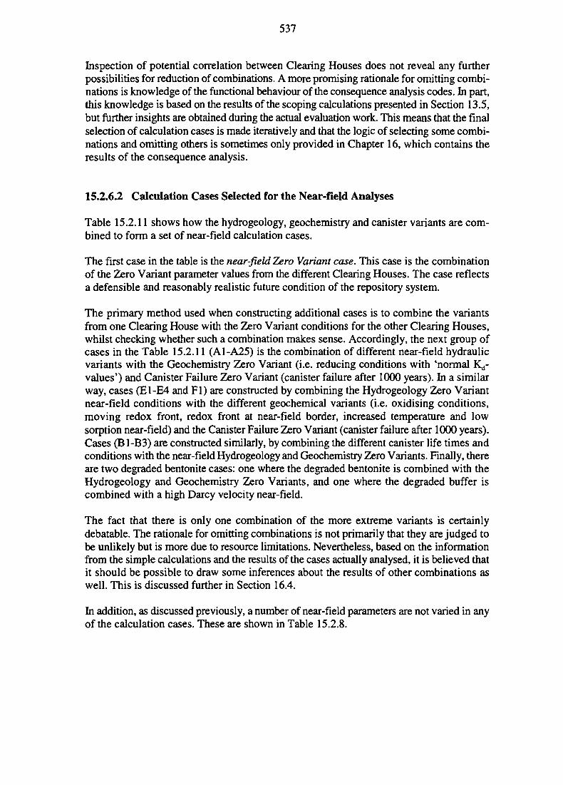
537
Inspection of potential correlation between Clearing Houses does not reveal any furtherpossibilities for reduction of combinations. A more promising rationale for omitting combi-nations is knowledge of the functional behaviour of the consequence analysis codes. In part,this knowledge is based on the results of the scoping calculations presented in Section 13.5,but further insights are obtained during the actual evaluation work. This means that the finalselection of calculation cases is made iteratively and that the logic of selecting some combi-nations and omitting others is sometimes only provided in Chapter 16, which contains theresults of the consequence analysis.
15.2.6.2 Calculation Cases Selected for the Near-field Analyses
Table 15.2.11 shows how the hydrogeology, geochemistry and canister variants are com-bined to form a set of near-field calculation cases.
The first case in the table is the near-field Zero Variant case. This case is the combinationof the Zero Variant parameter values from the different Clearing Houses. The case reflectsa defensible and reasonably realistic future condition of the repository system.
The primary method used when constructing additional cases is to combine the variantsfrom one Clearing House with the Zero Variant conditions for the other Clearing Houses,whilst checking whether such a combination makes sense. Accordingly, the next group ofcases in the Table 15.2.11 (A1-A25) is the combination of different near-field hydraulicvariants with the Geochemistry Zero Variant (i.e. reducing conditions with 'normal Kd-values') and Canister Failure Zero Variant (canister failure after 1000 years). In a similarway, cases (E1-E4 and Fl) are constructed by combining the Hydrogeology Zero Variantnear-field conditions with the different geochemical variants (i.e. oxidising conditions,moving redox front, redox front at near-field border, increased temperature and lowsorption near-field) and the Canister Failure Zero Variant (canister failure after 1000 years).Cases (B1-B3) are constructed similarly, by combining the different canister life times andconditions with the near-field Hydrogeology and Geochemistry Zero Variants. Finally, thereare two degraded bentonite cases: one where the degraded bentonite is combined with theHydrogeology and Geochemistry Zero Variants, and one where the degraded buffer iscombined with a high Darcy velocity near-field.
The fact that there is only one combination of the more extreme variants is certainlydebatable. The rationale for omitting combinations is not primarily that they are judged tobe unlikely but is more due to resource limitations. Nevertheless, based on the informationfrom the simple calculations and the results of the cases actually analysed, it is believed thatit should be possible to draw some inferences about the results of other combinations aswell. This is discussed further in Section 16.4.
In addition, as discussed previously, a number of near-field parameters are not varied in anyof the calculation cases. These are shown in Table 15.2.8.
Table 15.2.11, ctd.
CalculationCase
Low fluxA22A23A24A25GeochemistryElE2E3
E4FtDlD2CanisterBlB2B3
Darcyvelocity(m/year)
6.00x10'6
6.00x10"6
8.00x10"5
8.OOxlO'5
1.50x10'3
1.5OxlO'3
1.5OxlO'3
1.5OxlO"3
1.5OxlO"3
1.50x10'1.20x10'
1.50x10'1.50x10'1.50x10'
Hydi
Fracturespacing
(m)
8.008.002.502.50
2.50
2.502.50
2.502.502.500.80
2.502.502.50
•ogeoSogy
Fractureaperture
(m)
6.50X10"4
6.50x10"4
6.50X10"4
6.50X10"4
6.50x10"*
6.50XI0"4
6.50XI0"4
6.50x10"4
6.50X10"4
6.50x10^1.00x10'
6.50X10"4
6.50x10^6.50x10⁻⁴
Flow-wettedsurface(1/m)
0.011.000.011.00
0.10
0.100.10
0.100.100.100.10
0.100.100.10
Geochemistry
Conditions Solubilities
reducing
oxidising
moving frontIncr. temp,reducing
front at NF borderlow sorp, reducing
reducing
reducing
Tab. 15.2.6
Tab. 15.2.6
Tab. 15.2.6Tab. 35.2.6
Tab. 15.2.6Tab. 15.2.6Tab. 15.2.6
Tab. 15.2.6
Kd-va!ues
Tab. 15.2.7
Tab. 15.2.7
Tab. 15.2.7Tab. 15.2.7
Tab. 15.2.7i)Tab. 15.2.7
Tab. 15.2.7
Canister
Time for Durationfailure matrix rel.(years) (years)
1000
1000
10001000
1000100010001000
10 000100 000pinhole 2)
15 000
15 000
15 00015 000
15 00015 00015 00015 000
37 000360 000
7 500
Bentoitite
2121
1)2)3)
Factor 3 lower than in Zero Variant case.Pinhole, 5 mm2 0-1000 years, thereafter canister failure.Highly degraded bentonite with the same properties as the rock.Underlined area indicates input values different from the Zero Variant case.
540
15.2.6.3 Calculation Cases Selected for Integrated Near-field and Far-fieldTransport
Table 15.2.12 shows the combinations of near-field calculation cases and far-field variantsselected for the Reference Case integrated calculation cases. The integrated cases aredivided into groups depending on which of the input parameters that are varied.
The first case in the table is the overall near-field Zero Variant Case (A3), which is thecombination of the near-field Zero Variant case and Zero Variant far-field parameter valuesfrom the different Clearing Houses. Again, it is emphasised that this case should not beviewed as the most likely state of the repository system, but merely a sensible starting pointfor exploring the variants.
An important component of the strategy to follow when constructing the integrated casesis to make use of the fact that far-field transport, as it is formulated, could only act to reducethe releases from the near-field (the near-field intermediate dose potential, or IDP; seeSection 16.1). This means that there is no point in combining far-field variants with near-field conditions that are more favourable than the Zero Variant near-field case, as the near-field release is already quite small for the Zero Variant near-field (Section 16.2.2.1). Thespecial case of a sudden release of sorbed material in the far-field which could exceed thenear-field IDP is discussed in connection with the Central Scenario in the next section.
With the exception of sorption, the other far-field parameters originate from the hydro-geological analysis. The impact of uncertainty and variability in the far-field hydrogeologyis generally explored by combining the near-field Zero Variant case with a suite of far-fieldhydrogeological variants. From this suite of analyses, it is possible to draw rather qualifiedinferences on the result of combing these far-field variants with other near-field cases.
The remaining suite of far-field cases are all designed to explore the extent to which the far-field could reduce the release from a 'poor' near-field by combining a poor near-field witha 'good' far-field as well as with a far-field with properties fully correlated to the assumednear-field. The following cases are analysed:
• Two 'worst hydrogeology' cases are constructed by combining very poor near-fieldhydraulic conditions with poor far-field hydraulic conditions. The extent to whichfavourable far-field conditions may reduce the release from a poor near-field is alsoexplored.
• The analyses of the impacts of uncertainty in the geochemical parameters arerestricted to the effect of oxidising conditions and of lowered sorption. The near-field case with oxidising conditions is combined with an oxidising far-field withdifferent hydraulic conditions (varying from poor to favourable). The near-field casewith lowered sorption is combined with a low sorption far-field with differenthydraulic conditions (varying from poor to favourable).
Using the results of the cases listed in Tables 15.2.11 and 15.2.12, it is possible to makerather good estimates of other, unanalysed combinations. However, it must be re-emphasised strongly that this suite of cases does not directly reflect the likelihood of certainoutcomes. Many potentially possible combinations are not analysed at all and some of the

541
analysed combinations are probably much more likely than others. In order to say anythingabout likelihood it would be necessary to go back to the origin of the variants.
As discussed previously, a number of far-field parameters are not varied in any of thecalculation cases; these are listed in Table 15.2.9.
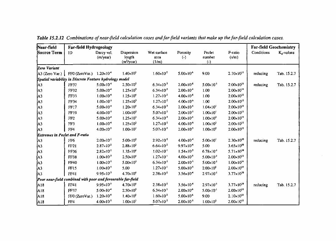
Table 15.2.12
Near-fieldSource Term
Zero VariantA3 (Zero Var.)
Combinations of near-field calculation cases and far-field variants
Far-fieSd HydrogeologyID
FFO (ZeroVar.)
Darcy vel.(m/year)
1.20X10"4
Dispersionlength
(m'/year)
1.40x10'
Spatial variability in Discrete Feature hydrology modelA3A3A3A3A3A3A3A3A3
FF37FF32FF33FF34FF17FF19FF2FF3FF4
Extremes in Peclet and F-ratioA3A3A3A3A3A3A3
FF6FF21FF36FF38FF40FF15FF41
5.00x10^
5.00X10⁻⁴
1.00x10^
LOOxlO"5
5.00x10^
4.00x10"5
5.00x10^
l.OOxlO-4
4.00x10⁵
2.00x10'
2.87x10'
2.82x10"'
1.00x10'
l.OOxlO5
l.OOxlO"5
9.95x10'
2.5OxlO5
1.25xlO5
1.25xlO4
1.25x10'
1.20xl04
1.00x10'
1.25x10'
1.25x10'
1.00x10'
5.00x10'
2.88x10'
1.35x10"
2.50x10⁴
5.00x10'
5.00
4.70x10"
Poor near-field combined with poor and favourable far-field
A18A18A18
A18
FF41FF37FFO (ZeroVar.)FF4
9.95x10'
5.00x10^
1.20X10"4
4.00x10⁵
4.70x10"
2.50x10⁵
1.40x10'
1.00x10'
Wet surfacearea
(1/m)
1.60x10'
6.34x10'
6.34x10'
1.27x10-'
1.27x10'
6.34x10'
5.07x10'
6.34x10'
1.27x10'
5.07x10'
2.92x10'
6.64xlO2
1.02x10'
1.27x10'
6.34x10'
1.27x10'
2.38x10'
2.38x10-'
6.34x10"'
1.60x10'
5.07x10'
Porosity
(-)
5.00xl0 6
2.00x10⁶
2.00x10⁶
4.00xl0 6
4-OOxlO-6
2.00x10⁶
2.00x10⁵
2.00x10⁶
4.00x10⁶
2.00x10⁵
4.00x10^
9.97x10^
1.54x10"'
4.00xI0"5
2.00x10⁵
5.00x10"5
3.56x10^
3.56x10""
2.00x10"6
5.00x10⁶
2.00x10"5
that make up
Pecletnumber
(-)
9.00
5.00x10"'1.001.001.001.04x10'1.00x10'1.00x10'l.OOxlO2
1.00x10'
5.00x10'5.006.78x10"'5.00x30"'5.00x10'2.00x10'2.97x10'
2.97x10"'5.00x10'9.00
1.00x10'
the far-field calculation cases.
F-ratio(s/m)
2.10x10"
2.00x10"2.00x10"2.00x10"2.00x10"2.00x10"2.00x10"2.00x10"2.00x10"2.00x10"
2.30x10'°3.65x10'°5.71x30'°2.00x10"1.00x10'"2.00x10'"3.77x10'°
3.77x10'°2.00x10"2.10x10"2.00x10"
Far-field GeochemistryConditions
reducing
reducing
reducing
reducing
Kj-values
Tab. 15.2.7
Tab. 15.2.7
Tab. 35.2.7
Tab. 15.2.7

Table 15.2.12,
Near-HeldSource Term
Oxidised near-fi
ElElElElLow sorption
FlFlFlFl
ctd.
Far-field HydiID
eld combined with
FF4!
FF37
FFO(ZeroVar.)
FF4
FF41
FF37
FFO (ZeroVar.)
FF4
•ogeologyDarcy vel.
(m/year)
Dispersion
length(m /year)
Wet surface
area(1/m)
oxidiied poor and favourable far-field
9.95«IO '
5.00* 10 4
1.2OXKT4
4.00x10'5
9.95x10'3
5.00x!0 4
1.20X10"4
4.00x10'5
4 70x10
2.50x10⁵
1.40x10*
LOOxlO1
4.70x10⁴
2.50x10⁵
1.4OxlO3
l.OOxlO1
2.38x10"z
6.34x10'3
1.60xlO'2
5.07xl0'2
2.38xlO'2
6.34xlO"3
1.60xl0"2
5.07xl0"2
Porosity
(-)
3.56x10^
2.00x10'6
5.00x10"6
2.00x10'5
3.56X10"4
2.00x10*6
5.00xI0"6
2.00x10'5
Peclet
number
(-)
2.97x10"'
5.00x30"'
9.00
l.OOxlO2
2.97x10''
5.00x30"'
9.00
l.OOxlO2
F-ratio
(s/m)
3.77xlO10
2.00x10"
2.10xI012
2.00xl013
3.77xlO10
2.00x10"
2.10xl012
2.00xl013
Far-field G«Conditions
oxidising
reducing
jochemSstryKd-values
Tab. S5.2.7
3)
I) Factor three lower than in the Zero Variant case.
544
15.3 VARIANTS FOR THE CENTRAL (CLIMATE EVOLUTION)SCENARIO
15.3.1 Possibilities for Central Scenario Variants
The Central Scenario is designed to analyse the effects of the time-varying SystemBoundary conditions at the site caused by the expected climate evolution over the next100 000 years. The climate evolution includes periods of sea-level changes, permafrost andglaciations. Sections 10.3.7, 10.3.8 and 11.2.2 discuss how these conditions affect radio-nuclide release and transport and how they may evolve during the Central Scenario. TheCentral Scenario affects the evolution of groundwater chemistry, the groundwater flow andthe biosphere conditions, compared to the Reference Case. It may also affect canister failuretimes.
The SITE-94 analysis of repository system performance during the Central Scenario maybe divided into two steps.
The first step is to establish appropriate time sequence descriptions of the evolution ofgeochemical, hydrogeological and other conditions that directly affect radionuclide releaseand transport during the Central Scenario. The ambition level is not, however, to make fullpredictions of the potential evolution of the repository. It is, rather, to find examples thatillustrate the impact of the large-scale climate changes imposed through the CentralScenario.
The second step is to explore how the consequence analysis models available within theSITE-94 project can be used to handle the time-varying conditions and to formulate a setof variants for quantitative analysis. Evidently, most of the uncertainties and spatialvariability of the Reference Case are also valid for the Central Scenario. However, theconsequence calculation cases for the Central Scenario concentrate on the time-varyingaspects. The impact of conceptual model and parameter uncertainty for the Central Scenariois only assessed qualitatively, based on results of the Central Scenario and Reference Casevariants actually analysed. It should also be noted that the adjustment of variants to thetools actually available is rather arbitrary but is, indeed, a practical necessity.
15.3.2 Evolution of Conditions Affecting Radionuclide Release andTransport
15.3.2.1 Hydrogeology
During the Central Scenario, groundwater flow changes both in magnitude and in direction(Section 10.3.7). Figure 10.3.17 provides a general overview. However, as alreadydiscussed in Section 10.3.9 and as is evident from this figure, the impact of the time-varying boundary conditions is relatively moderate. This is also true at the repository scale.In summary, present day groundwater flow prevails, for the most part, until the firstglaciation, 55 000 years after disposal. During the next 5000 years (55-60 ka), groundwaterflow changes from upward to downward. Flow increases, but less than one order ofmagnitude. During the following 10 000 years (60-70 ka), the flow direction reverses to
545
upward flow again, with the magnitude increased by as much as ten times present day flow.At 70 ka, the magnitude of the flow is back to present day conditions. This flow sequenceis repeated during a second glaciation with change in flow direction and magnitude at95 ka, reversed flow direction at 105 ka, and back to present day conditions at 120 ka. Theconditions during the first glaciation are summarised in Table 15.3.1. Finally, a special setof analyses with the Discrete Feature hydrogeology model (Section 10.3.8; Geier, 1996)also shows that a conservative tracer released at the repository will discharge almost at thesame points for both glacial and non-glacial conditions.
15.3.2.2 Geochemistry
The modelling of the evolution of the hydrogeology also gives information on the coupledevolution of the geochemistry. As can be seen in Figure 10.3.17, present day groundwatersalinity will prevail up to glaciation, though with a slight decrease (a factor of 2) during theperiod with permafrost (10-55 ka). As flow is nearly horizontal during this period, there isa possibility of water with high organic content (surficial water) reaching the repository.
The downward flow during the first part of the glaciation (55-60 ka) transports glacialmeltwater, with very low salinity, to the repository (Figure 10.3.17). The glacial meltwateris oxidising, but the possibility of a breakthrough of oxidising waters to the EngineeredBarriers depends on the availability of reducing minerals in the rock, as discussed inSection 10.4. For part of the time, the glacial meltwater will have upward flow but, fromabout 70 ka, the salinity will increase to a level slightly above present day conditions. Apossible variant would be to have water with high salinity during the period after theglaciation up to the next permafrost (70-95 ka). The variants of geochemical time sequencesare summarised in Table 15.3.1.
As modelling of the hydrogeology for the Central Scenario is performed on a regional scale,the detailed scale hydrogeology and geochemistry are not considered. For the analysis ofradionuclide transport, knowledge of the redox conditions in the different parts of the near-field (waste, bentonite, near-field rock) is very important, as it determines solubility limitsand sorption for most radionuclides. The likelihood of an oxidising groundwater break-through in the near-field depends on the redox capacities in the different barriers (minera-logy in rock and bentonite; canister materials, etc.) as well as on the transport processes.With an intact bentonite buffer, the intrusion of meltwater components (into the bentoniteand waste-form) must be the consequence only of diffusion and, with the limited timeduring which glacial meltwater may surround the repository, it is questionable whether thenear-field will be fully oxidised. In the analysis of radionuclide transport, two variants areconsidered: the conservative approach of allowing oxidised conditions to extend all the wayinto the waste-form and a variant where bentonite and rock are oxidised, but not the waste-form, (i.e. the canister corrosion products; the spent fuel is oxidised by radiolysis all thetime after canister failure, see Chapter 12).
The evolution of the geochemistry is not considered for a second glaciation cycle, althoughit is noted that the salinity shows behaviour similar to that during the first glaciation cycle(Figure 10.3.17).
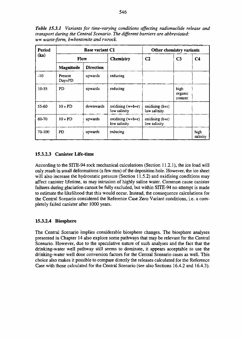
546
Table 15.3.1 Variants for time-varying conditions affecting radionuclide release andtransport during the Central Scenario. The different barriers are abbreviated:w= waste-form, b—bentonite and r=rock.
Period(ka)
-10
10-55
55-60
60-70
70-100
Base variant Cl
Flow
Magnitude
PresentDay=PD
PD
lOxPD
lOxPD
PD
Direction
upwards
upwards
downwards
upwards
upwards
Chemistry
reducing
reducing
oxidising (w+b+r)low salinity
oxidising (w+b+r)low salinity
reducing
Other chemistry variants
C2
oxidising (b+r)low salinity
oxidising (b+r)low salinity
C3
highorganiccontent
C4
highsalinity
15.3.2.3 Canister Life-time
According to the SITE-94 rock mechanical calculations (Section 11.2.1), the ice load willonly result in small deformations (a few mm) of the deposition hole. However, the ice sheetwill also increase the hydrostatic pressure (Section 11.5.2) and oxidising conditions mayaffect canister lifetime, as may intrusion of highly saline water. Common cause canisterfailures during glaciation cannot be fully excluded, but within SITE-94 no attempt is madeto estimate the likelihood that this would occur. Instead, the consequence calculations forthe Central Scenario considered the Reference Case Zero Variant conditions, i.e. a com-pletely failed canister after 1000 years.
15.3.2.4 Biosphere
The Central Scenario implies considerable biosphere changes. The biosphere analysespresented in Chapter 14 also explore some pathways that may be relevant for the CentralScenario. However, due to the speculative nature of such analyses and the fact that thedrinking-water well pathway still seems to dominate, it appears acceptable to use thedrinking-water well dose conversion factors for the Central Scenario cases as well. Thischoice also makes it possible to compare directly the releases calculated for the ReferenceCase with those calculated for the Central Scenario (see also Sections 16.4.2 and 16.4.3).
547
15.3.3 Central Scenario Consequence Analysis
A full analysis of the consequences of the Central Scenario would require further develop-ments of the consequence analysis codes. In particular, the far-field analyses would needto be able to handle at least two dimensions and time-varying properties and boundaryconditions. Such code development is though not included in SITE-94. However, theproblem is recognised and some supporting exploratory 2D calculations are made using theLAPLACE-2D code in time-stepping mode to investigate and illustrate the potentialimpacts of a time-dependent flow field on releases of both sorbing and non-sorbing radio-nuclides (King-Clayton and Smith, 1996). This work is discussed further in Section 16.3.3.For the purposes of the SITE-94 release calculations however, only a few calculation casesare formulated for the Central Scenario using the existing CALIBRE and CRYSTAL conse-quence analysis codes. This route is followed in order to maintain consistency with, andallow comparison with, the Reference Case modelling.
15.3.3.1 Near-field Release and Transport
In principle, there are no problems in directly applying the time-varying conditions inTable 15.3.1 to the CALIBRE near-field model. It is possible to run the code with one set-up of conditions up to a certain time, stop the calculation and then restart with newconditions. For the hydrogeological changes, which are in fact boundary conditions, thisapproach is straightforward. For the geochemical changes, however, the approach is moredebateable. A simplistic and, possibly, conservative approach would be to change solubilitylimits and sorption coefficients in accordance with the groundwater chemistry changesgiven in Table 15.3.1, but this is not realistic. Even if the groundwater in the fracture inter-secting the deposition hole becomes oxidising during the glaciation period, it will take timeuntil the oxidising conditions have propagated through the buffer and into the vicinity ofthe fuel matrix.
In the event, only two of the calculation cases shown in Table 15.3.1 are set up for radio-nuclide transport in the near-field, with the aim of showing how time-dependent processescan influence releases. The variants analysed are the base variant (Cl) and the case wherebentonite and rock are oxidised (C2). For 'present day' hydrogeological conditions, thenear-field Zero Variant case for the Reference Case (A3) is used. During the glaciationperiod (55-70 ka) the Darcy velocity is increased by one order of magnitude (Table 15.3.2)The direction of flow is not modelled in CALIBRE and needs thus not be considered.
The analysis is made on a subset of radionuclides: I29I (as it dominates at early times) and"Tc and the actinide chains (as they have redox sensitive solubility limits and sorption).The solubility limits and sorption distribution coefficients are varied with time, but thevalues are the same as in the Reference Case for reducing and oxidising conditions(Table 15.3.2)
The calculations are performed for a period up to 105 years in the future, which is approxi-mately the time for the onset of a new glaciation cycle. All other parameters are set as inthe near-field Zero Variant case for the Reference Case (A3). A rather crude method ofchanging the parameter values instantaneously at each climate sequence change is used.
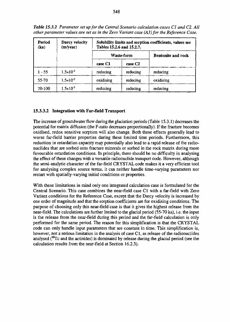
548
Table 15.3.2 Parameter set up for the Central Scenario calculation cases Cl and C2. Allother parameter values are set as in the Zero Variant case (A3) for the Reference Case.
Period(ka)
1 -55
55-70
70-100
Darcy velocity(m/year)
1.5xlO"3
1.5xl02
1.5xlO"3
Solubility limits and sorption coefficients, values seeTables 15.2.6 and 15.2.7.
Waste-form
case Cl
reducing
oxidising
reducing
caseC2
reducing
reducing
reducing
Bentonite and rock
reducing
oxidising
reducing
15.3.3.2 Integration with Far-field Transport
The increase of groundwater flow during the glaciation periods (Table 15.3.1) decreases thepotential for matrix diffusion (the F-ratio decreases proportionally). If the fracture becomesoxidised, redox sensitive sorption will also change. Both these effects generally lead toworse far-field barrier properties during these limited time periods. Furthermore, thisreduction in retardation capacity may potentially also lead to a rapid release of the radio-nuclides that are sorbed onto fracture minerals or sorbed in the rock matrix during morefavourable retardation conditions. In principle, there should be no difficulty in analysingthe effect of these changes with a versatile radionuclide transport code. However, althoughthe semi-analytic character of the far-field CRYSTAL code makes it a very efficient toolfor analysing complex source terms, it can neither handle time-varying parameters norrestart with spatially-varying initial conditions or properties.
With these limitations in mind only one integrated calculation case is formulated for theCentral Scenario. This case combines the near-field case Cl with a far-field with ZeroVariant conditions for the Reference Case, except that the Darcy velocity is increased byone order of magnitude and that the sorption coefficients are for oxidising conditions. Thepurpose of choosing only this near-field case is that it gives the highest release from thenear-field. The calculations are further limited to the glacial period (55-70 ka), i.e. the inputis the release from the near-field during this period and the far-field calculation is onlyperformed for the same period. The reason for this simplification is that the CRYSTALcode can only handle input parameters that are constant in time. This simplification is,however, not a serious limitation in the analysis of case Cl, as release of the radionuclidesanalysed ("Tc and the actinides) is dominated by release during the glacial period (see thecalculation results from the near-field at Section 16.2.3).
549
16 RESULTS OF RADIONUCLIDE TRANSPORTCALCULATIONS
This chapter presents the results of the near- and far-field calculations evaluated for theReference Case and the Central Scenario. The formulation of the calculation cases buildson combinations of variants presented in Chapter 15.
16.1 INTRODUCTION
The calculations for the Reference Case, focussing on the near-field and far-field ZeroVariant cases, include a wide range of variant cases which are chosen with the aim ofcovering scenario uncertainties, system uncertainties, conceptual model uncertainties andparameter uncertainties. Calculations for the Central Scenario are performed for two variantcases for the purpose of illustrating the impact of changing water flow and redox conditionsduring a glaciation. The derivation of all the calculation cases was presented in Chapter 15.
The calculations for radionuclide release to the biosphere are performed using the near-fieldcode CALIBRE version 2.0 (Worgan and Robinson, 1995a, b) and the geosphere codeCRYSTAL version 2.1 (Worgan and Robinson 1995c; Worgan 1995). These codes havealready been discussed in Chapter 13. The results from the CALIBRE calculations arediscussed in the near-field transport Section (16.2). The release results from the near-fieldare used as the source term for the geosphere transport calculations. These latter integratedresults are discussed in Section 16.3.
The results from the near-field and the far-field calculations are presented as the flux ofradionuclides from a single canister (Bq/year, canister). The far-field flux from one canister(Bq/year, canister) is converted to individual dose rate (Sv/year, canister) by applying theReference Case well on Aspo (i.e. a well with an extraction rate of 10 000 mVyear, seeChapter 14). This well receptor is applied both for the Reference Case and the CentralScenario as explained in Chapter 15. In addition, the results from the near-field arepresented as Intermediate Dose Rate Potentials (IDPs) as was done in Project-90 (SKI,1991). The BDP (Sv/year, canister) is obtained by assuming direct release from the near-field into the reference biosphere and thereby describes the effect of having no geosphereretardation or dispersion.
As already explained in Chapter 15, there are no analyses of the consequence of multiplecanister failures in SITE-94. The reason for this is the uncertainty in canister lifetimes,which makes any prediction of canister failure rates quite speculative. However, the singlecanister results may usually be superimposed in order to describe the effect of multiplefailures. This aspect will be discussed in the conclusions section of this chapter(Section 16.4).
550
16.2 NEAR-FIELD TRANSPORT RESULTS
16.2.1 Overview of Calculation Cases
Near-field transport depends on a number of properties both in the EBS (Engineered BarrierSystem) and in the near-field rock, as already discussed in Section 13.3. Some of theseproperties are either variable or uncertain and, in order to reflect this, a set of near-fieldcalculation cases representing different near-field conditions is identified, as presented inChapter 15. Tables 16.2.1 and 16.2.2 list the analysed cases for the Reference Case and theCentral Scenario respectively. The rationale behind these different cases is provided inChapter 15.
16.2.2 Reference Case: Near-field
16.2.2.1 Near-field Zero Variant Case (A3)
The evaluation is centred around the near-field Zero Variant calculation case. The para-meters for this case are obtained by combining the Zero Variant near-field hydrogeological,geochemical and canister failure times parameters as explained in Chapter 15. The caseshould not be taken as a best estimate; instead, it reflects a combination of credible, non-extreme parameter values.
The canister is assumed to fail at 1000 years after deposition, and reducing redox conditionsprevail in the near-field barriers during the calculation period (103 - 106 year). The Darcyvelocity in the near-field rock is 1.5x10³ m/year and the fracture spacing is 2.5 m. The fuel,cladding and structural parts contain both active and stable isotopes. For further details seeChapter 15.
Results for each radionuclide
The resulting radionuclide fluxes for the near-field Zero Variant case (A3) are given inFigures 16.2.1-16.2.2. The figures show the time evolution of the flux from the near-fieldto the far-field in (Bq/year, canister) and the Intermediate Dose Rate Potentials, IDPs(Sv/year, canister). The diagrams show fluxes higher than 102 Bq/year, canister and IDPshigher than 10"9 Sv/year. canister. The figures are complemented by Table 16.2.3, where themaximum release rales (Bq/year, canister) and IDPs (Sv/year, canister) for times up to 106
years are given, as well as the time in the future at which fluxes or IDPs reach a maximum.The behaviour of each radionuclide is discussed below. Note that the assumptionsassociated with the following descriptions are stated factually, without discussion, in orderto simplify the presentation.
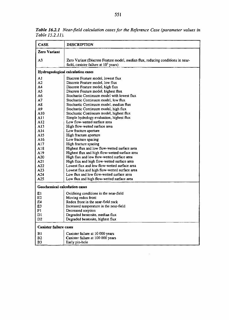
551
Table 16.2.1 Near-field calculation cases for the Reference Case (parameter values inTable 15.2.11).
CASE
Zero Variant
A3
DESCRIPTION
Zero Variant (Discrete Feature model, median flux, reducing conditions in near-field, canister failure at 103 years)
Hydrogeological calculation cases
AlA2A4A5A6A7A8A9A10Al lA12A13A14A15A16A17A18A19A20A21A22A23A24A25
Discrete Feature model, lowest fluxDiscrete Feature model, low fluxDiscrete Feature model, high fluxDiscrete Feature model, highest fluxStochastic Continuum model with lowest fluxStochastic Continuum model, low fluxStochastic Continuum model, median fluxStochastic Continuum model, high fluxStochastic Continuum model, highest fluxSimple hydrology evaluation, highest fluxLow flow-wetted surface areaHigh flow-wetted surface areaLow fracture apertureHigh fracture apertureLow fracture spacingHigh fracture spacingHighest flux and low flow-wetted surface areaHighest flux and high flow-wetted surface areaHigh flux and low flow-wetted surface areaHigh flux and high flow-wetted surface areaLowest flux and low flow-wetted surface areaLowest flux and high flow-wetted surface areaLow flux and low flow-wetted surface areaLow flux and high flow-wetted surface area
Geochemical calculation cases
ElE2E4E3FlDlD2
Oxidising conditions in the near-fieldMoving redox frontRedox front in the near-field rockIncreased temperature in the near-fieldDecreased sorptionDegraded bentonite, median fluxDegraded bentonite, highest flux
Canister failure cases
BlB2B3
Canister failure at 10 000 yearsCanister failure at 100 000 yearsEarly pin-hole
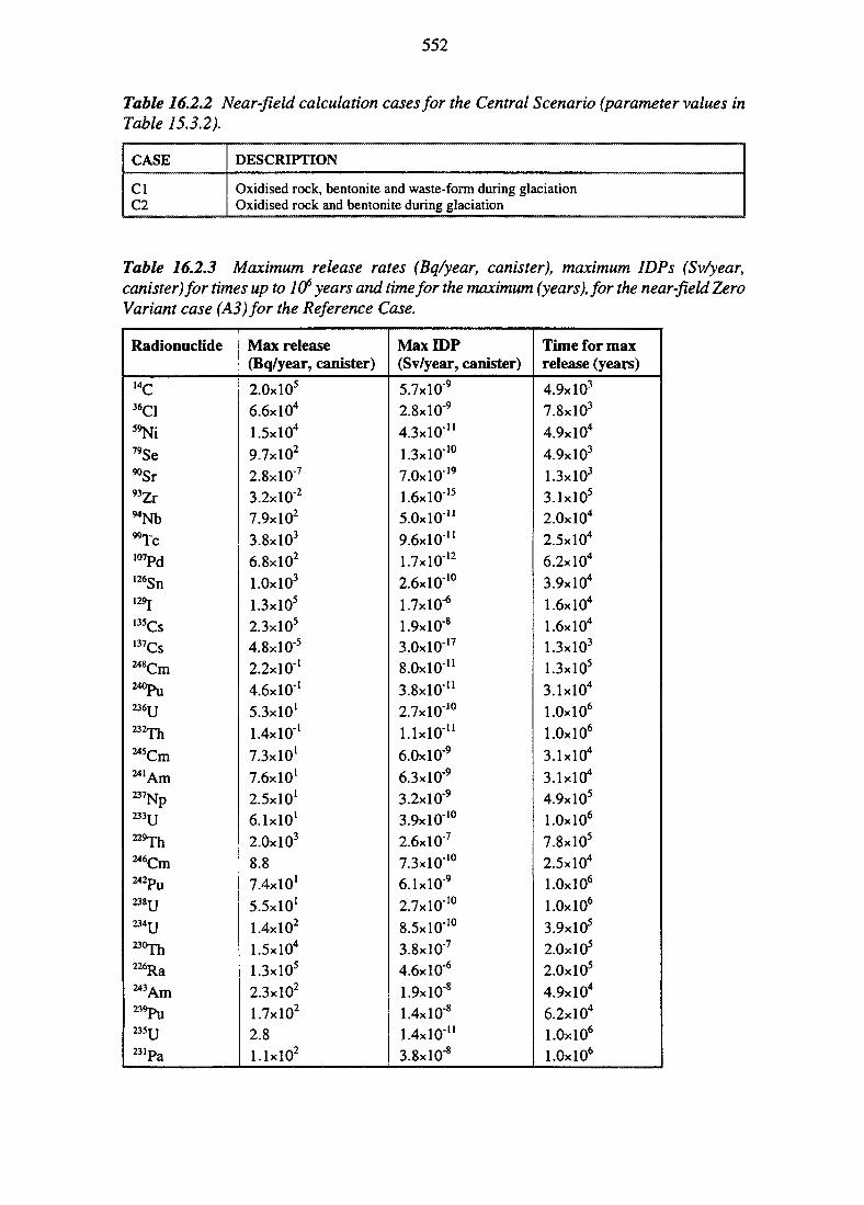
552
Table 16.2.2 Near-field calculation cases for the Central Scenario (parameter values inTable 15.3.2).
CASE DESCRIPTION
ClC2
Oxidised rock, bentonite and waste-form during glaciationOxidised rock and bentonite during glaciation
Table 16.2.3 Maximum release rates (Bq/year, canister), maximum IDPs (Sv/year,canister) for times up to 10s years and time for the maximum (years), for the near-field ZeroVariant case (A3) for the Reference Case.
Radionucl ide
14C36C159Ni79Se^Sr93ZrMNb"Tc107pd
126Sn129J
135Cs137Cs""Cm240pu
236U232Thw C m^ A m237Np233U229ThM 6Cm242pu
mu2 3 4 u
2 3 0 ^
226Ra
239pu
2 3 5 u231Pa
Max release(Bq/year, canister)
2.0x10⁵
6.6xlO4
1.5x10"*9.7x10²
2.8xlO7
3.2xl0'2
7.9x10²
3.8xl03
6.8xlO2
l.OxlO3
1.3xl05
2.3xl05
4.8xl05
2.2x10-'4.6x10'5.3x10'1.4x10"'7.3x10'7.6x10'2.5x10'6.1x10'2.0x10³
8.8
7.4x10'5.5x10'1.4xlO2
1.5xlO4
1.3xl05
2.3xlO2
1.7xlO2
2.8
l.lxlO2
Max IDP(Sv/year, canister)
5.7xlO"9
2.8xlO-9
4.3x10"1.3x10'°7.0xl0"'9
1.6xl0-'5
5.0x10"9.6x10"1.7xlO12
2.6x10'°lJxlO"6
1.9xlO"8
3.0xl017
8.0x10"3.8x10-"2.7x10-'°1.1x10-"6.0xl0"9
6.3xlO"9
3.2xlO"9
3.9x10''°2.6xl07
7.3x10-'°6.1xlO"9
2.7x10"'°8.5x10"'°3.8xl0"7
4.6x10"6
1.9xl0"8
1.4xlO"8
1.4x10-"3.8xl0'8
Time for maxrelease (years)
4.9xlO3
7.8xl03
4.9x10"*4.9xlO3
1.3xl03
3.1xl05
2.0xl04
2.5x10"*6.2xlO4
3.9x10"*1.6x10"*1.6x10"*1.3xlO3
1.3xl05
3.1xl04
l.OxlO6
l.OxlO6
3.1x10"*3.1x10"*4.9xlO5
l.OxlO6
7.8xl05
2.5x10"*l.OxlO6
l.OxlO6
3.9xl05
2.0x10⁵
2.0xl05
4.9x10"*6.2x10"*l.OxlO6
l.OxlO6
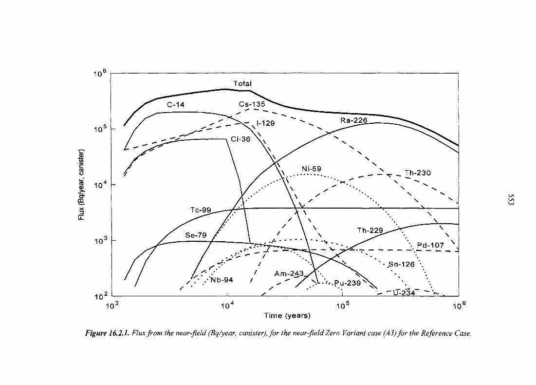
10'
10° -
&
§S 10'
X
1010 10 10 10'
Time (years)
Figure 16.2.1. Flux from the near-field (Bq/year, canister), for the near-field Zero Variant case (A3) for the Reference Case.
U)
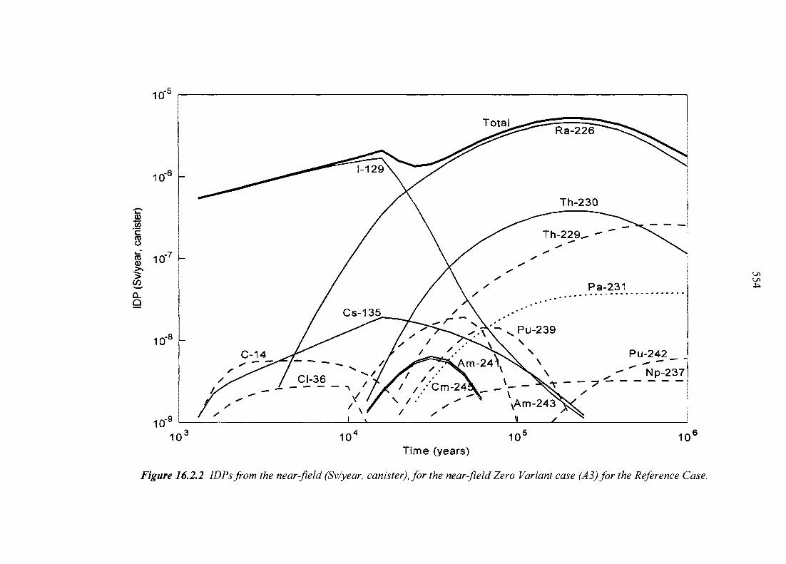
10"
10"6h
"to
3
CO,
Q
10'
10
10'10
Tota!
10 10'Time (years)
Figure 16.2.2 IDPsfi-om the near-field (Sv/year, canister), for the near-field Zero Variant case (A3) for the Reference Case.
555
14C is present in the fuel (90% in grain boundaries and 10% in gaps, see Section 13.2.3for details of how the grain boundary is modelled), but also in cladding andstructural parts. Carbon is fully soluble and sorbs weakly in the barriers. The highestflux of 14C is obtained from the structural parts, although the maximum release ratesfrom the three sources are of the same order.
36C1 is present in the cladding. Chloride is fully soluble and does not sorb in thenear-field. The breakthrough of 36C1 into the far-field is fast. The total mass of 36C1is released and the decrease in flux at 104 years is due to depletion of the source.
59Ni is present in the structural parts. Nickel is moderately sorbed in the barriers. Therelease is not limited by solubility although there are stable nickel isotopes. Theintegrated mass of 59Ni that leaves the near-field before it decays is about 15% of theoriginal inventory. (Not shown in Figure 16.2.2.)
79Se is present in the fuel matrix. The concentration of selenium in the waste-formreaches the solubility limit. The solubility of 79Se is decreased (by a factor of 10) dueto isotopic dilution with stable isotopes. Selenium precipitates are present through-out the calculation. In total, only 5% of the initial mass of the weakly sorbed 79Seleaves the near-field during 106 years. (Not shown in Figure 16.2.2.)
^Sr is present at the grain boundaries (see Section 13.2.3). Although strontium is onlyweakly sorbed in the near-field, the amount released from the near-field is of noimportance since ^Sr has a short half-life and decays in the near-field. (Not shownin Figures 16.2.1 and 16.2.2.)
93Zr is present both in the fuel matrix and in the cladding. The cladding also containslarge amounts of stable zirconium isotopes and the solubility of the active isotopeis therefore decreased (by a factor of 400) due to isotopic dilution. The concentrationof zirconium reaches the solubility limit both in the waste-form and in the bentonite.Zirconium is strongly sorbed in the near-field. More than 60% of 93Zr is precipitatedin the waste-form at the end of the calculation and less than 1 % of the initial masshas left the near-field at 106 years. (Not shown in Figures 16.2.1 and 16.2.2.)
wNb is present in the fuel matrix and in structural parts. Niobium is moderately sorbedin the bentonite, but sorbs strongly in the rock. Niobium does not precipitate in thenear-field. Of the initial mass of wNb, 25% leaves the near-field before it decays.(Not shown in Figure 16.2.2.)
"Tc is present in the fuel matrix, at the grain boundaries and in gaps between fuel andcladding, (89%, 10% and 1% of the inventory, respectively, see Section 13.2). Thesolubility limit of technetium is reached in the waste-form and bentonite andprecipitates are left at the end of the calculation, although a considerable amount hasdecayed at that time. Technetium is poorly sorbed in the near-field; despite this only3% of the mass inventory has left the near-field at the end of the calculation at 106
years. (Not shown in Figure 16.2.2.)
107Pd is present in the fuel matrix. Palladium is moderately sorbed in the bentonite androck. It precipitates in the waste-form and the solubility-limited concentration for

556
107Pd is decreased (by a factor of 6) due to isotopic dilution with stable isotopes. Atthe end of the calculation, 90% of the initial mass is left in the near-field. (Notshown in Figure 16.2.2.)
126Sn is present in the fuel matrix. Tin is moderately sorbed in the near-field. The con-centration of tin in the waste-form is limited by the solubility, and the solubility ofthe active isotope is further decreased (by a factor of 4) due to isotopic dilution.There are precipitates in the waste-form after 106 years. In total, 8% of the initialmass of 126Sn leaves the near-field during 106 years. (Not shown in Figure 16.2.2)
129I is at the grain boundaries (90% of the inventory, Section 13.2) and in the gapsbetween cladding and fuel (10% of the inventory). Iodine is fully soluble and sorbsweakly in the bentonite and rock. The activity in the gaps is released immediatelyafter canister failure and results in a fast breakthrough into the far-field. At 106 years,99% of the initial mass of iodine has left the near-field.
135Cs is present at the grain boundaries (90% of the inventory, Section 13.2) and in thegaps between fuel and cladding (10% of the inventory). The concentration of cesiumin the pores does not reach the solubility limit. Cesium sorbs poorly in the bentoniteand moderately in the rock. The flux decreases as soon as the source is depleted. Atthat time, 80% of the initial mass has left the near-field.
137Cs is present at the grain boundaries (90% of the inventory, Section 13.2) and in thegaps (10% of the inventory). Cesium decays in the near-field and very little activityis released into the far-field. (Not shown in Figures 16.2.1 and 16.2.2).
The radionuclides in the natural decay chains are strongly sorbed in the bentonite and rockat the prevailing reducing conditions, except for moderate sorption of protactinium in therock and radium in the bentonite and rock. All radionuclides in the natural decay chains,except uranium and thorium, have solubility limits lower than 10'7 moles/litre at theprevailing redox conditions. The solubility of uranium is 10"5 moles/litre and of thorium,ixlO"6 moles/litre in all barriers (waste-form, bentonite and rock). The concentration ofplutonium, neptunium, uranium and americium in the waste-form reaches the solubilitylimit. The concentration of plutonium and neptunium also reaches the solubility limit in thebentonite porewater.
Decay chain 4N248Cm is relatively short-lived and the flux falls off due to decay after reaching a maximum
at lxlO5 years. Curium is strongly sorbed in the near-field. The curium isotopeconcentrations do not reach the solubility limit in the near-field. (Not shown inFigures 16.2.1 and 16.2.2). (Curium 248 is part of the 4N chain but is treated as asingle nuclide in the calculations since its daughter, 244Pu, is long lived, with a half-life of 8.3x10⁵ years).
240Pu is relatively short-lived and decays in the near-field without any considerable releaseto the far-field. Plutonium is strongly sorbed in the barriers. The solubility limit of
557
plutonium is reached both in the waste-form and in the bentonite. (Not shown inFigures 16.2.1 and 16.2.2.)
236U The uranium isotope concentration reach the solubility limit in the waste-form.Uranium is strongly sorbed in the near-field. The flux is still increasing at the endof the calculations at 106 years. (Not shown in Figures 16.2.1 and 16.2.2)
232Th The thorium isotope concentrations do not reach the solubility limit in any barrierin the near-field. Thorium is strongly sorbed in the near-field and the flux is stillincreasing at 106 years. (Not shown in Figures 16.2.1 and 16.2.2)
Decay chain 4N+1245Cm is relatively short-lived and the flux falls off due to decay after a peak at 3xlO4 years.
Curium is strongly sorbed in the near-field. The curium isotope concentrations donot reach the solubility limit in the near-field. (Not shown in Figure 16.2.1.)
241 Am is short-lived and the flux follows that of the parent nuclide (245Cm). The initialinventory of 241Am has decayed by the time of release from the near-field. (Notshown in Figure 16.2.1.)
237Np Neptunium is strongly sorbed in the near-field and concentrations reach thesolubility limit both in the waste-form and in the bentonite. (Not shown inFigure 16.2.1.)
233U This uranium isotope has a low initial inventory compared to the other isotopes.Since uranium concentrations reach the solubility limit in the waste-form, thefraction of mobile ^ U is relatively small. (Not shown in Figures 16.2.1 and 16.2.2.)
229Th Thorium is strongly sorbed in the near-field. The solubility-limited concentration isnot reached in the near-field. The flux is still increasing at 106 years, but appears tobe levelling out.
Decay chain 4N+2246Cm is relatively short-lived and the flux falls off due to decay after a peak at 3x10⁴ years.
Curium is strongly sorbed in the near-field. The curium isotope concentrations donot reach the solubility limit in the near-field. (Not shown in Figures 16.2.1 and16.2.2.)
242Pu Plutonium is strongly sorbed in the near-field and concentrations reach the solubilitylimit in the waste-form and in the bentonite. The release of 242Pu is limited by theshare of the solubility with other isotopes, but increases slightly as the more short-lived isotopes (239Pu and 240Pu) decay. The flux is still increasing at 106 years. (Notshown in Figure 16.2.1.)
238U is the dominating uranium isotope. Uranium concentration reaches the solubilitylimit in the waste-form. Uranium is strongly sorbed and the flux is still increasingslightly at 106 years. (Not shown in Figures 16.2.1 and 16.2.2.)
558
234U Uranium is strongly sorbed in the near-field and concentrations reach the solubilitylimit in the waste-form. The flux of 234U reaches a peak at 3x10 5years and fallsthereafter, due to the decay of the initial inventory. The release will then be deter-mined by the release of the parent nuclide. (Not shown in Figure 16.2.2.)
230Th Thorium is strongly sorbed in the near-field. The solubility-limited concentration isnot reached in the near-field. The flux reaches a peak at 2x10⁵ years.
226Ra Radium is relatively short-lived but also rather mobile in the near-field. The releaseof radium is not controlled by the solubility limit and a maximum flux is reached at2xlO5 years; thereafter the flux decreases due to decay of the grandparent, 234U.
Decay chain 4N+3243Am is relatively short-lived and decays in the near-field. Americium is strongly sorbed
in the near-field and the solubility-limited concentration of americium is reached inthe waste-form.
239Pu is strongly sorbed in the barriers and decays in the near-field without any consider-able release to the far-field. The solubility-limited concentration of plutonium isreached both in the waste-form and in the bentonite.
235U Uranium is strongly sorbed in the near-field and concentrations reach the solubilitylimit in the waste-form. The flux of 235U levels off after 2xlO5 years and continuesbeyond 106 years, since 235U is very long-lived and precipitates of uranium are leftin the waste-form at the end of the calculation (106 years). As was mentioned inChapter 3 (see Table 3.3.1) the inventory of this nuclide should, in fact, have beenhigher by a factor of 2-3. However, the relative importance of this discrepancydecreases after some tens of thousands of years due to in-growth from decay of theparent nuclide 239Pu. (Not shown in Figures 16.2.1 and 16.2.2.)
231Pa is relatively short-lived and sorbs moderately in the near-field. The initial amountof 231Pa is not sufficient to reach the solubility limit in the waste-form. The fluxreaches a steady-state after 2X10⁵ years, which is largely determined by decay andrelease of the parent nuclide (235U). Note the comment on the inventory of the latterabove. (Not shown in Figure 16.2.1.)
The flux from the near-field given as IDPs (Figure 16.2.2) is totally dominated by 129I until20 000 years, when 226Ra becomes dominant. The peak value for 129I is 2x10 "* Sv/year,canister at 16 000 years and for 226Ra the peak value is 5x10"* Sv/year, canister at 200 000years. Second after 20 000 years, is 23OTh (4xlO'7 Sv/year, canister), followed by 229Th(3xl07 Sv/year, canister).
A histogram showing the mass balance (in moles, normalised to initial inventory) for someradionuclides at 10\ 105 and 106 years is given in Figure 16.2.3. Each bar consists of threeparts: one representing the fraction of the initial content that is left in the near-field, onerepresenting the amount released into the far-field and one representing the amount that hasdecayed to stable isotopes at the specified time. The mass that has decayed in the near-field
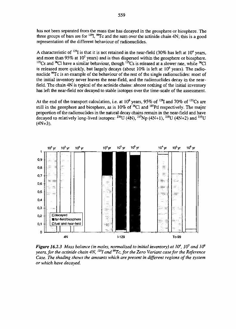
559
has not been separated from the mass that has decayed in the geosphere or biosphere. Thethree groups of bars are for 129I, "Tc and the sum over the actinide chain 4N; this is a goodrepresentation of the different behaviour of radionuclides.
A characteristic of 129I is that it is not retained in the near-field (30% has left at 104 years,and more than 95% at 105 years) and is thus dispersed within the geosphere or biosphere.135Cs and 36C1 have a similar behaviour, though 135Cs is released at a slower rate, while 36C1is released more quickly, but largely decays (about 10% is left at 106 years). The radio-nuclide "Tc is an example of the behaviour of the rest of the single radionuclides: most ofthe initial inventory never leaves the near-field, and the radionuclides decay in the near-field. The chain 4N is typical of the actinide chains: almost nothing of the initial inventoryhas left the near-field nor decayed to stable isotopes over the time-scale of the assessment.
At the end of the transport calculation, i.e. at 106 years, 95% of 129I and 70% of 135Cs arestill in the geosphere and biosphere, as is 10% of 36C1 and 107Pd respectively. The majorproportion of the radionuclides in the natural decay chains remain in the near-field and havedecayed to relatively long-lived isotopes: 236U (4N), 237Np (4N+1), 238U (4N+2) and 235U(4N+3).
1 -p
0,9
0,8
0,7
0,6
0,5-
0,4
0,3 -
0,2-
0,1 -
0--
104yr 105yr 106yr
• decayedM far-field/biosphere•fuel and near-fieid
104yr 105yr 106yr
4N 1-129 Tc-99
Figure 16.2.3 Mass balance (in moles, normalised to initial inventory) at 10*, 105 andyears, for the actinide chain 4N, I29I and "Tc, for the Zero Variant case for the ReferenceCase. The shading shows the amounts which are present in different regions of the systemor which have decayed.
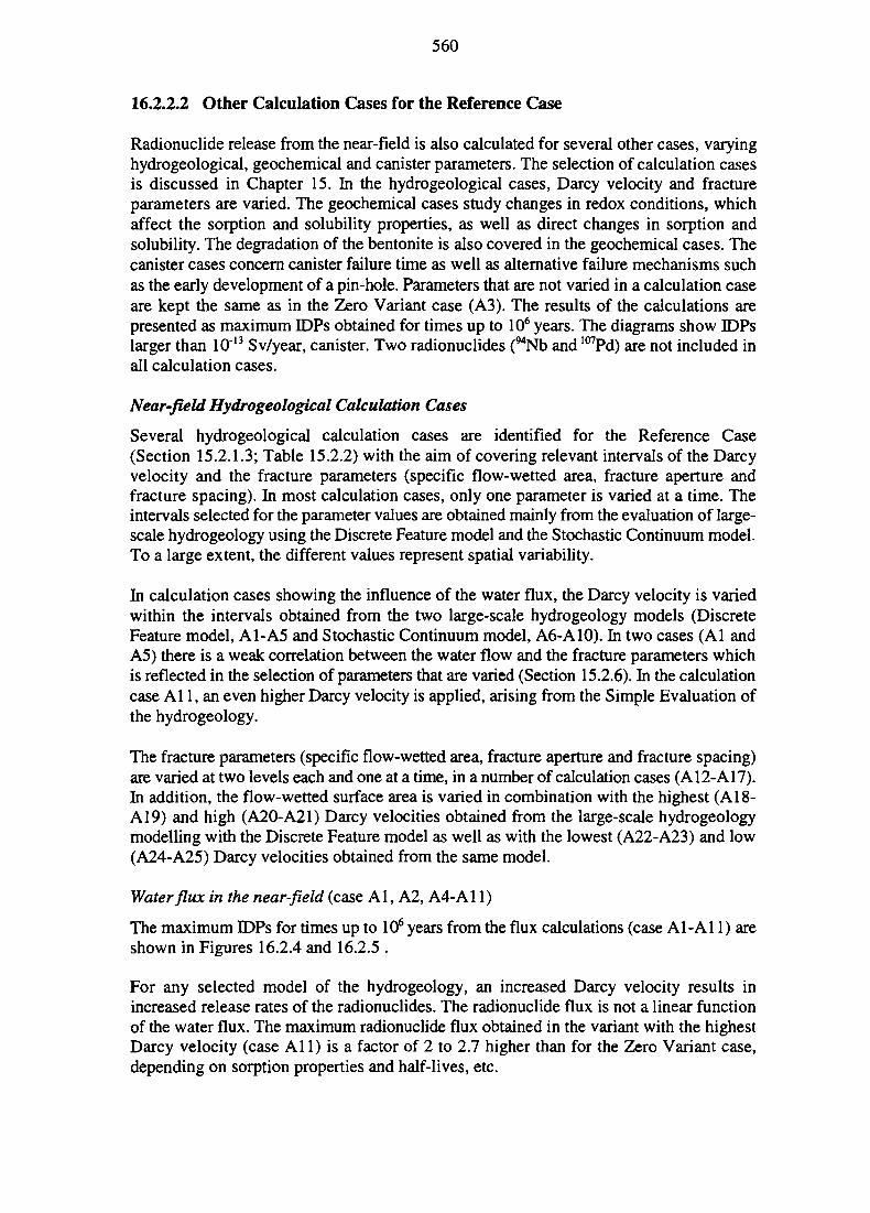
560
16.2.2.2 Other Calculation Cases for the Reference Case
Radionuclide release from the near-field is also calculated for several other cases, varyinghydrogeological, geochemical and canister parameters. The selection of calculation casesis discussed in Chapter 15. In the hydrogeological cases, Darcy velocity and fractureparameters are varied. The geochemical cases study changes in redox conditions, whichaffect the sorption and solubility properties, as well as direct changes in sorption andsolubility. The degradation of the bentonite is also covered in the geochemical cases. Thecanister cases concern canister failure time as well as alternative failure mechanisms suchas the early development of a pin-hole. Parameters that are not varied in a calculation caseare kept the same as in the Zero Variant case (A3). The results of the calculations arepresented as maximum IDPs obtained for times up to 106 years. The diagrams show IDPslarger than 10"13 Sv/year, canister. Two radionuclides (94Nb and 107Pd) are not included inall calculation cases.
Near-field Hydrogeological Calculation Cases
Several hydrogeological calculation cases are identified for the Reference Case(Section 15.2.1.3; Table 15.2.2) with the aim of covering relevant intervals of the Darcyvelocity and the fracture parameters (specific flow-wetted area, fracture aperture andfracture spacing). In most calculation cases, only one parameter is varied at a time. Theintervals selected for the parameter values are obtained mainly from the evaluation of large-scale hydrogeology using the Discrete Feature model and the Stochastic Continuum model.To a large extent, the different values represent spatial variability.
In calculation cases showing the influence of the water flux, the Darcy velocity is variedwithin the intervals obtained from the two large-scale hydrogeology models (DiscreteFeature model, A1-A5 and Stochastic Continuum model, A6-A10). In two cases (Al andA5) there is a weak correlation between the water flow and the fracture parameters whichis reflected in the selection of parameters that are varied (Section 15.2.6). In the calculationcase Al 1, an even higher Darcy velocity is applied, arising from the Simple Evaluation ofthe hydrogeology.
The fracture parameters (specific flow-wetted area, fracture aperture and fracture spacing)are varied at two levels each and one at a time, in a number of calculation cases (A12-A17).In addition, the flow-wetted surface area is varied in combination with the highest (A 18-A19) and high (A20-A21) Darcy velocities obtained from the large-scale hydrogeologymodelling with the Discrete Feature model as well as with the lowest (A22-A23) and low(A24-A25) Darcy velocities obtained from the same model.
Water flux in the near-field (case Al, A2, A4-A11)
The maximum IDPs for times up to 106 years from the flux calculations (case Al-Al 1) areshown in Figures 16.2.4 and 16.2.5 .
For any selected model of the hydrogeology, an increased Darcy velocity results inincreased release rates of the radionuclides. The radionuclide flux is not a linear functionof the water flux. The maximum radionuclide flux obtained in the variant with the highestDarcy velocity (case Al l ) is a factor of 2 to 2.7 higher than for the Zero Variant case,depending on sorption properties and half-lives, etc.
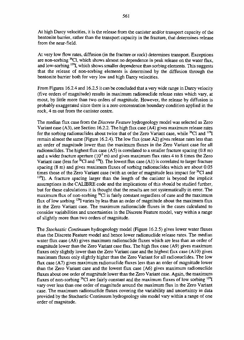
561
At high Darcy velocities, it is the release from the canister and/or transport capacity of thebentonite barrier, rather than the transport capacity in the fracture, that determines releasefrom the near-field.
At very low flow rates, diffusion (in the fracture or rock) determines transport. Exceptionsare non-sorbing 36C1, which shows almost no dependence in peak release on the water flux,and low-sorbing l29l, which shows smaller dependence than sorbing elements. This suggeststhat the release of non-sorbing elements is determined by the diffusion through thebentonite barrier both for very low and high Darcy velocities.
From Figures 16.2.4 and 16.2.5 it can be concluded that a very wide range in Darcy velocity(five orders of magnitude) results in maximum radionuclide release rates which vary, atmost, by little more than two orders of magnitude. However, the release by diffusion isprobably exaggerated since there is a zero concentration boundary condition applied in therock, 4 m out from the canister centre.
The median flux case from the Discrete Feature hydrogeology model was selected as ZeroVariant case (A3), see Section 16.2.2. The high flux case (A4) gives maximum release ratesfor the sorbing radionuclides about twice that of the Zero Variant case, while 36C1 and 129Iremain almost the same (Figure 16.2.4). The low flux (case A2) gives release rates less thanan order of magnitude lower than the maximum fluxes in the Zero Variant case for allradionuclides. The highest flux case (A5) is correlated to a smaller fracture spacing (0.8 m)and a wider fracture aperture (10'3 m) and gives maximum flux rates 4 to 8 times the ZeroVariant case (less for 36C1 and 129I). The lowest flux case (Al) is correlated to larger fracturespacing (8 m) and gives maximum fluxes of sorbing radionuclides which are about 0.05times those of the Zero Variant case (with an order of magnitude less impact for 36C1 and129I). A fracture spacing larger than the length of the canister is beyond the implicitassumptions in the CALIBRE code and the implications of this should be studied further,but for these calculations it is thought that the results are not systematically in error. Themaximum flux of non-sorbing 36C1 is fairly constant regardless of case and the maximumflux of low sorbing 129I varies by less than an order of magnitude about the maximum fluxin the Zero Variant case. The maximum radionuclide fluxes in the cases calculated toconsider variabilities and uncertainties in the Discrete Feature model, vary within a rangeof slightly more than two orders of magnitude.
The Stochastic Continuum hydrogeology model (Figure 16.2.5) gives lower water fluxesthan the Discrete Feature model and hence lower radionuclide release rates. The medianwater flux case (A8) gives maximum radionuclide fluxes which are less than an order ofmagnitude lower than the Zero Variant case flux. The high flux case (A9) gives maximumfluxes only slightly lower than the Zero Variant case and the highest flux case (A 10) givesmaximum fluxes only slightly higher than the Zero Variant for all radionuclides. The lowflux case (A7) gives maximum radionuclide fluxes less than an order of magnitude lowerthan the Zero Variant case and the lowest flux case (A6) gives maximum radionuclidefluxes about one order of magnitude lower than the Zero Variant case. Again, the maximumfluxes of non-sorbing 36C1 are fairly constant and the maximum fluxes of low sorbing 129Ivary over less than one order of magnitude around the maximum flux in the Zero Variantcase. The maximum radionuclide fluxes covering the variability and uncertainty in dataprovided by the Stochastic Continuum hydrogeology site model vary within a range of oneorder of magnitude.
C-14
CI-36
Ni-59
Se-79
Nb-94
Tc-99
Pd-107
Sn-126
1-129
Cs-135
Cm-248
Pu-240
U-236
Th-232
Cm-245
Am-241
Np-237
U-233
Th-229
Cm-246
Pu-242
U-238
U-234
Th-230
Ra-226
Am-243
Pu-239
U-235
Pa-231
10
562
a o
D O
o
B-
D O I & O
o e
O O
-e-o——-e- O
O i &r-O
Q O 1 AS-
D O
Q-
G - O—I £< O
O
Q O U O
B O | A< O
a o ! x o-e—H£-o
-e—| A< o
O
B—-e-D O |
XD0i
A0
A11
A1
A2
A3,ZeroVar.
A4
A5
C3- o o
O O
-e o
13 1 0 " 1 2 10"10 10"9 10" 10'7 10"6 10"5 10-410
-3
Maximum IDP (Sv/year, canister)
Figure 16.2.4 Comparison of maximum IDPs from the near-field between calculationcases of the Discrete Feature hydrogeology model and the Simple Evaluation of hydro-geology (All), for all the different radionuclides.
563
C-14
CI-36
Ni-59
Se-79
Nb-94
Tc-99
Pd-107
Sn-126
1-129
Cs-135
Cm-248
Pu-240
U-236
Th-232
Cm-245
Am-241
Np-237
U-233
Th-229
Cm-246
Pu-242
U-238
U-234
Th-230
Ra-226
Am-243
Pu-239 h
U-235
Pa-231
DO X
CD X
DO X 40
DO X 40
DO X 40
DO X 40
DO X 40
DO X 40
D0XA0I
A6
A7
A8
A9
A10
A3,ZeroVar.
10"13 10-'2 10"11 ,-10 v-71 0 l u 1 0 ' 1 0 " 1 0 ' 10
Maximum IDP (Sv/year, canister)
-6 10-5 10-4 10-3
Figure 16.2.5 Comparison of maximum IDPs from the near-field between calculationcases of the Stochastic Continuum hydrogeology model, for the different radionuclides.
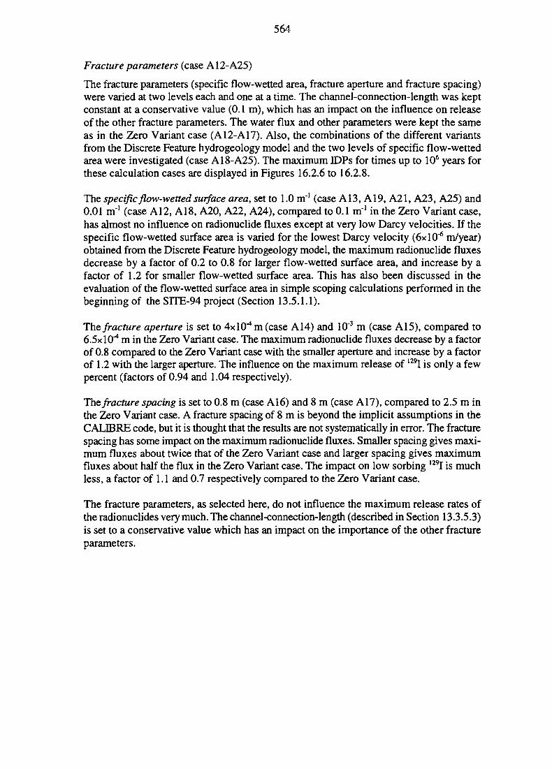
564
Fracture parameters (case A12-A25)
The fracture parameters (specific flow-wetted area, fracture aperture and fracture spacing)were varied at two levels each and one at a time. The channel-connection-length was keptconstant at a conservative value (0.1 m), which has an impact on the influence on releaseof the other fracture parameters. The water flux and other parameters were kept the sameas in the Zero Variant case (A12-A17). Also, the combinations of the different variantsfrom the Discrete Feature hydrogeology model and the two levels of specific flow-wettedarea were investigated (case A18-A25). The maximum IDPs for times up to 106 years forthese calculation cases are displayed in Figures 16.2.6 to 16.2.8.
The specific flow-wetted surface area, set to 1.0 m"1 (case A13, A19, A21, A23, A25) and0.01 m"1 (case A12, A18, A20, A22, A24), compared to 0.1 m*1 in the Zero Variant case,has almost no influence on radionuclide fluxes except at very low Darcy velocities. If thespecific flow-wetted surface area is varied for the lowest Darcy velocity (6x10"* m/year)obtained from the Discrete Feature hydrogeology model, the maximum radionuclide fluxesdecrease by a factor of 0.2 to 0.8 for larger flow-wetted surface area, and increase by afactor of 1.2 for smaller flow-wetted surface area. This has also been discussed in theevaluation of the flow-wetted surface area in simple scoping calculations performed in thebeginning of the SITE-94 project (Section 13.5.1.1).
The fracture aperture is set to 4x1 O^m (case A14) and 10'3 m (case A15), compared to6.5x10^ m in the Zero Variant case. The maximum radionuclide fluxes decrease by a factorof 0.8 compared to the Zero Variant case with the smaller aperture and increase by a factorof 1.2 with the larger aperture. The influence on the maximum release of 129I is only a fewpercent (factors of 0.94 and 1.04 respectively).
The fracture spacing is set to 0.8 m (case A16) and 8 m (case A17), compared to 2.5 m inthe Zero Variant case. A fracture spacing of 8 m is beyond the implicit assumptions in theCALIBRE code, but it is thought that the results are not systematically in error. The fracturespacing has some impact on the maximum radionuclide fluxes. Smaller spacing gives maxi-mum fluxes about twice that of the Zero Variant case and larger spacing gives maximumfluxes about half the flux in the Zero Variant case. The impact on low sorbing 129I is muchless, a factor of 1.1 and 0.7 respectively compared to the Zero Variant case.
The fracture parameters, as selected here, do not influence the maximum release rates ofthe radionuclides very much. The channel-connection-length (described in Section 13.3.5.3)is set to a conservative value which has an impact on the importance of the other fractureparameters.
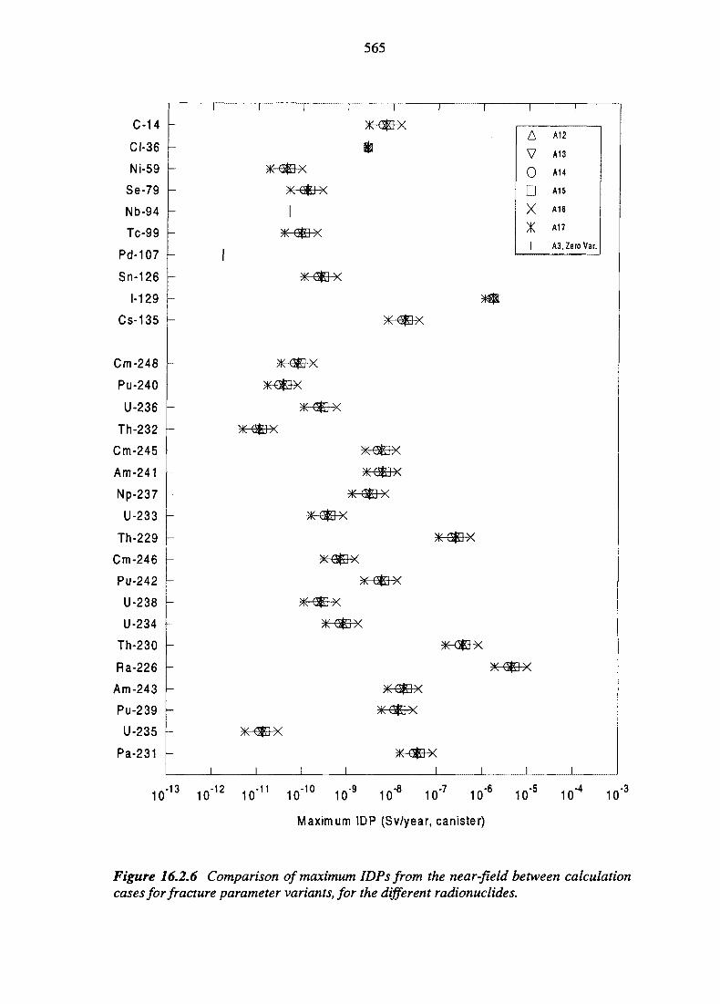
565
C-14
CI-36
Ni-59
Se-79
Nb-94
Tc-99
Pd-107
Sn-126
1-129
Cs-135
Cm-248
Pu-240
U-236
Th-232 h
Cm-245
Am-241
Np-237
U-233
Th-229
Cm-246
Pu-242
U-238
U-234
Th-230
Ra-226
Am-243
Pu-239
U-235
Pa-231
10-13
X
X
X
X
-X
X
X
x-x-
10•11 v-10 .-8 k-7
AV0DXXI
A12
A13
A14
A15
A16
A17
A3, Zero Var.
10 10 10 10 10
Maximum IDP (Sv/year, canister)
10-5 10-4
10"
Figure 16.2.6 Comparison of maximum IDPs from the near-field between calculationcases for fracture parameter variants, for the different radionuclides.
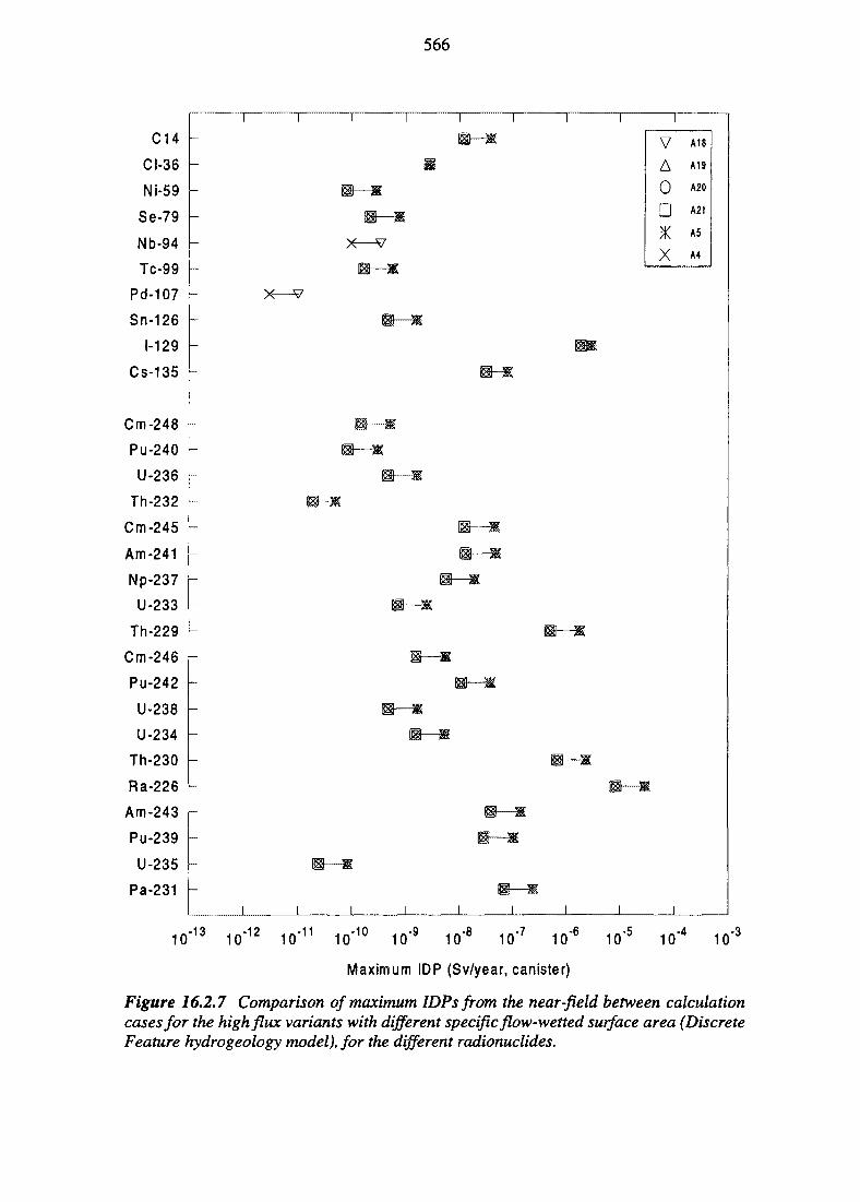
566
C14
CI-36
Ni-59
Se-79
Nb-94
Tc-99
Pd-107
Sn-126
1-129
Cs-135
Cm-248
Pu-240
U-236
Th-232
Cm-245
Am-241
Np-237
U-233
Th-229
Cm-246
Pu-242
U-238
U-234
Th-230
Ra-226
Am-243
Pu-239
U-235
Pa-231
BI-
Bt
i i i
BH-B
m
n—-B
BH-B
m—«
m—8
m—a
m-~-8
n—8H—8
e—8^—8
HI—8
H—8
Bh-B
—8
i i i
V A18
A A19
0 A20
D A21
* A5
X A4
10-1310-12 10-11 ,-10 -8 ,-7
10" l w 10 10 1 0 ' 10
Maximum IDP (Sv/year, canister)
-6 10' 10-4 10-3
Figure 16.2.7 Comparison of maximum IDPs from the near-field between calculationcases for the high flux variants with different specific flow-wetted surface area (DiscreteFeature hydrogeology model), for the different radionuclides.
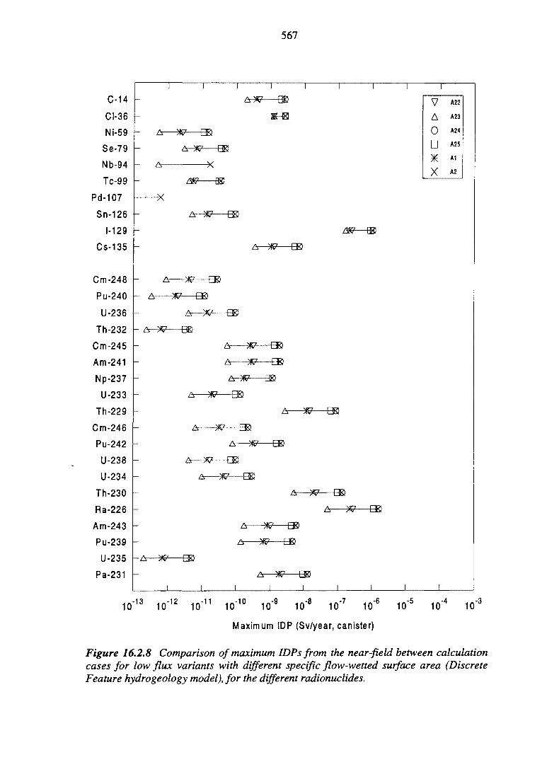
567
C-14
CI-36
Ni-59
Se-79
Nb-94
Tc-99
Pd-107
Sn-126
1-129
Cs-135
Cm-248
Pu-240
U-236
Th-232
Cm-245
Am-241
Np-237
U-233
Th-229
Cm-246
Pu-242
U-238
U-234
Th-230
Ra-226
Am-243
Pu-239
U-235
Pa-231
A
A X
A EK
A- W-
A
A-
w—asA W
aa
A-
A-
A asA
A
A-as
BE)
.-10 .-710 1W 10 10 10 10
Maximum IDP (Sv/year, canister)
-6 10"
VA0D*X
A22
A23
A24
A25
A1
A2
10-4 10-3
Figure 16.2.8 Comparison of maximum IDPs from the near-field between calculationcases for low flux variants with different specific flow-wetted surface area (DiscreteFeature hydrogeology model), for the different radionuclides.
568
Geochemical Calculation Cases
The geochemical calculation cases are defined and described in Chapter 15. In the ZeroVariant (case A3), reducing conditions prevail in the whole near-field. In the first geo-chemical calculation case (El), the flux from the near-field has been calculated for oxi-dising conditions in the near-field. The impact on the release of a redox front in the near-field has been evaluated in two cases, one with a moving redox front (E2) and one with aredox front at the edge of the near-field (E4). The oxidants are assumed to be produced inthe canister due to radiolysis. The redox conditions impact both on the solubilities andsorption of many radionuclides. The effect of a higher temperature (80°C) in the near-field,which influences the solubilities of some elements, has also been investigated (case E3) aswell as the influence of lower sorption capacities (Fl). In addition, the effects of a highlydegraded bentonite buffer have also been investigated in two calculation cases (Dl and D2).
The maximum BDPs for times up to 106 years for all these cases are shown in Figures 16.2.9and 16.2.10.
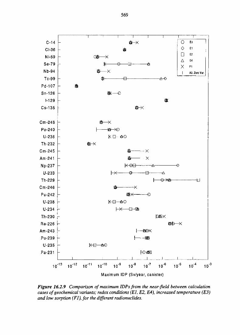
569
C-14
CI-36
Ni-59
Se-79
Nb-94
Tc-99
Pd-107
Sn-126
1-129
Cs-135
Cm-248
Pu-240 -
U-236 -
Th-232 -
Cm-245
Am-241 -
Np-237 -
U-233
Th-229
Cm-246
Pu-242
U-238
U-234
Th-230
Ra-226
Am-243
Pu-239
U-235
Pa-231
(3$ X
-e—B-
-B
-X
-x
h-x -a-
-B-9&
I—HKX
00DAXI
E3
E1
E2
E4
F1
A3, Zero Var.
-o
-B
10"13 10"12 10"11 10"10 10'9-8 .-7
1 0 " 1 0 ' 10
Maximum IDP (Sv/year, canister)
10-5
10-4
10-3
Figure 16.2.9 Comparison of maximum IDPs from the near-field between calculationcases of geochemical variants; redox conditions (El, E2, E4), increased temperature (E3)and low sorption (Fl), for the different radionuclides.
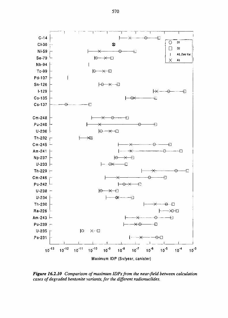
570
C-14
CI-36
Ni-59
Se-79 h
Nb-94
Tc-99
Pd-107
Sn-126
1-129
Cs-135
Cs-137
Cm-248 -
Pu-240 -
U-236
Th-232
Cm-245
Am-241
Np-237
U-233
Th-229
Cm-246
Pu-242
U-238
U-234
Th-230
Ra-226
Am-243
Pu-239
U-235
Pa-231
10"13
-e-
10'12
-e- -e
-x- -e-je—x—e
-Q
he—x
-B
-e- -Q
-X- -e-x—o
ah- o>< •
xh-O-X E3
|O X D
E3
0Di
X
D1
D2
A3, Zero Var.
A5
-e--B
-e
-e——Q
-Q
-0 —Q
o a-e
O DD
>< e-s
10"10 10'9 10'8 10'7 10*6 10'5 10'4 10'3
Maximum IDP (Sv/year, canister)
Figure 16.2.10 Comparison of maximum IDPsfrom the near-field between calculationcases of degraded bentonite variants, for the different radionuclides.
571
Oxidising conditions throughout the near-field (El)
In this calculation, the whole near-field is assumed to be in an oxidising state. This influ-ences the solubilities and sorption properties of many elements in the near-field barriers.The distribution coefficients of selenium, technetium, uranium, plutonium and neptuniumin the bentonite and the rock decrease compared to the Zero Variant case (A3). Technetiumand selenium are soluble under oxidising conditions. The solubilities of neptunium anduranium increase in all barriers compared to reducing conditions, whereas the solubilitiesof nickel, strontium, americium and curium increase in the waste-form and bentonite, butthe solubility in the rock does not change. The solubility of plutonium decreases slightlyin all barriers, and the solubility of radium decreases in the waste-form and bentonite.
The maximum release rate of "Tc and 79Se is increased considerably compared to the ZeroVariant case (A3), since these elements are soluble and less sorbing under the oxidisingconditions. The release rate of "Tc increases more than 4 orders of magnitude and therelease rate of 79Se increases by almost 3 orders of magnitude. The release of the othersingle radionuclides is unaffected by the oxidising conditions.
The maximum release rate of 237Np increases considerably (more than 3 orders of magni-tude), compared to the Zero Variant case, although the solubility limit is still reached in thewaste-form. The maximum release rates for uranium increase 7 to 27 times compared tothe Zero Variant case. A factor of less than 10 is due to changed solubility and sorption,whereas effects larger than this are due to the effect of earlier breakthrough and changedmobility of parent radionuclides. The maximum release of short-lived plutonium isotopes(239Pu and 240Pu) increases due to earlier breakthrough, although the solubility decreases.The maximum release of 242Pu decreases as an effect of the decreased solubility. Thesolubility concentration of the plutonium isotopes is reached both in the waste-form and thebentonite. The limited effects on the release of radionuclides in the natural decay chainswhose properties do not change with the redox conditions (thorium and protactinium) orwhich does not reach the solubility limits (radium and curium), is due to the changedmobility of parent radionuclides.
The H)Ps (Figure 16.2.9) are dominated by 129I and "Tc at a level of 1 - 2x10^ Sv/year,canister, 79Se at a level of lxlO'7 Sv/year, canister and radionuclides from the natural decaychains. The latter are dominated by 237Np at a level of lxlO"5 Sv/year, canister, followed by229Th and 226Ra (3x10^ Sv/year, canister). The results from this calculation case show thatradionuclides other than I29I and 226Ra may reach high dose levels under certain conditions.
Redox-front a few metres into the near-field rock (E4)
In this calculation, oxidising redox conditions prevail throughout the near-field with theexception of the last 0.1 m of rock, which is reducing. This simulates the presence of aredox front a few metres out from the rock/bentonite interface.
The release from the near-field is similar to the release from a completely oxidised near-field (El) except for the release of technetium and neptunium, which decrease sinceprecipitates occur in the fracture where the front is. The maximum release of "Tc increases8000 times compared to the Zero Variant case, but is less than in the case with oxidisingconditions throughout. The maximum release of 237Np is 70 times the release in the ZeroVariant case, but much less than in the case with oxidising conditions. A secondary effect
572
of the precipitation of neptunium at the redox front is that the release of its daughters (233Uand 229Th) increase compared both to the Zero Variant case and the case with oxidisingconditions throughout. The increase in maximum release rate is 3000 times for 233U and 10times for 229Th, compared to the Zero Variant case. This, presumably, is an effect of in-growth from the precipitate of 237Np in the fracture close to the redox front.
Moving redox-front (E2)
Oxidants are produced in the canister as a result of decomposition of water due to radio-lysis. The oxidants may migrate and form a moving redox front. The redox front passes outof the bentonite into the rock after about 1400 years which means that it takes about 400years for the oxidants to diffuse through the bentonite. Following this, it takes a furthermillion years for the redox front to penetrate a metre into the near-field rock (seeSection 11.7).
The result from this calculation is similar to the one with oxidising conditions throughoutthe whole near-field (El), except for the release of some elements that precipitate in thefracture at the redox-front, i.e. neptunium, technetium and selenium. The maximum releaseof 79Se is 50 times larger than in the Zero Variant case, the release of "Tc is 30 times largerand the release of 237Np is 4 times larger. The maximum release of all these radionuclidesis, however, lower than in the calculation case with a front at the border of the near-field.An additional effect due to the precipitation of 237Np is an increased maximum release ofits daughters (233U and 229Th) compared to both the Zero Variant case and the calculationcase with oxidising conditions throughout.
Increased temperature (80 °C) (E3)
In this calculation case, reducing conditions are used, but the temperature in the canisterand close surroundings is assumed to have increased from 15 °C in the near-field ZeroVariant (A3) to 80°C, which influences the solubilities of many elements. Other potentialtemperature effects on radionuclide transport, such as increased diffusivities in thebentonite and reduced fluid viscosities, are not considered in SITE-94. The increasedtemperature is maintained throughout the calculation (103 to 106 years), which is an un-realistic exaggeration of this effect (Section 15.2.2.2).
The release from the near-field of soluble radionuclides (14C, 36C1,135Cs and 129I) is equalto the near-field Zero Variant case (A3). In the calculation, the solubility limit oftechnetium in the waste-form and bentonite is not changed and the release of "Tc is equalto the Zero Variant case.
The increase in maximum release rates of 93Zr and 126Sn are proportional to the increase insolubility in the waste-form where the concentration reaches the solubility limit, i.e. a factorof about 2 for 93Zr and about 5 for 126Sn.
The solubility of nickel decreases due to the temperature increase. The lowest solubility isin the rock, where nickel precipitates. The maximum release rate of 59Ni decreases by afactor of 0.7 compared to the Zero Variant case, where it does not precipitate. The solubilityof selenium increases in all barriers. The lowest solubility is in the rock, where seleniumprecipitates. The maximum release rate of 79Se increases by about one order of magnitudecompared to the Zero Variant case.
573
The solubilities of the radionuclides in the natural decay chains increase due to the rise intemperature, with one exception, protactinium, whose solubility is not changed, againowing to lack of data. The concentration of curium, thorium and radium is not limited bythe solubility in the Zero Variant case and consequently not in this calculation either.Therefore, the release rates of the curium isotopes, which are all in the beginning of thedecay chains, are equal to the release rates obtained in the Zero Variant case. The maximumrelease rate of 226Ra and thorium isotopes increases by a factor of about 1 to 5 compared tothe Zero Variant case, as an effect of the decreased solubility of their parent radionuclides.
Uranium does not precipitate and the maximum flux increases by about 10-20 timescompared to the Zero Variant case, where uranium precipitates in the waste-form. The con-centrations of plutonium and neptunium reach the solubility limit. The maximum fluxincreases 2 to 28 times compared to the Zero Variant case.
Among the IDPs (Figure 16.2.9) 129I still has a dominant role, at the same level as in theZero Variant case (2X10"6 Sv/year, canister) since the release rate of this nuclide was notinfluenced by the temperature increase and none of the other nuclides affected bytemperature reach such a high dose level. The maximum IDPs from the natural decaychains are 5X10"6 Sv/year, canister from ^ R a (equal to the Zero Variant case), followed by229Th (lxlO-6 Sv/year, canister), 230Th (5xlO*7 Sv/year, canister) and 242Pu and 243Am(1 x 10'7 Sv/year, canister).
Low sorption (Fl)
The aim of this calculation case is to show the consequences of uncertainties/variabilitiesin mineralogy, water chemistry and measurements of the sorption properties of the barriermaterials. AH distribution coefficients are lowered by a factor of three, compared to thenear-field Zero Variant case (A3) and, consequently, the maximum release rates of the allradionuclides except the non-sorbing elements increase compared to the Zero Variant case.
The effects of a decreased sorption capacity on the radionuclide flux from the near-field issmall for long-lived, poorly sorbed radionuclides (129I); the effect is also small forsolubility-limited radionuclides (93Zr, 126Sn, "Tc and 79Se). For the other single radio-nuclides, the maximum flux increases about 2 to 4 times compared to the Zero Variant case.The fluxes of the very short-lived radionuclides ^Sr and 137Cs increase by 14 and 6 times,respectively, due to the faster breakthrough.
The increase in maximum release rates is, for most of the radionuclides in the natural decaychains, 1 to 8 times compared to the Zero Variant case results. The effect is small forelements that are solubility limited (Pu, Np, U and Am), apart from the maximum releaseof the short-lived isotopes (without long-lived parent nuclides), i.e. 240Pu, 241Am, 245Cm,246Cm and 243Am, which increase 8 to 22 times.
The maximum IDPs (Figure 16.2.9) are still dominated by 129I, at the same level as in theZero Variant case (2X10"6 Sv/year, canister) and by226Ra, at a level of 1.6xlO"5 Sv/year,canister and 229Th, at a level of 2X10"6 Sv/year, canister.
574
Degraded bentonite (Dl, D2)
Two cases were formulated with the aim of investigating the radionuclide flux from thenear-field if the bentonite barrier is degraded and fractured, so that the opening of a fractureinto the rock is situated close to the canister. The bentonite was given rock properties. Twohydrogeology cases were selected, one equal to the Zero Variant hydrogeological conditions(A3) giving variant Dl, and one equal to the highest flux obtained in the Discrete Featurehydrogeology model (A5) giving variant D2, see Table 15.2.11. The maximum IDPs aredisplayed in Figure 16.2.10.
The breakthrough of radionuclides arrives earlier with the degraded bentonite barrier thanin the Zero Variant case. The release of the mobile radionuclides in the gaps between thefuel and the cladding (135Cs, 137Cs, 129I, Tc and 14C) is very fast, almost instantaneous. Themaximum release rate, which occurs very early, is rather difficult to calculate since theselection of time-stepping in the calculations becomes important, especially in the calcu-lation case with the highest flux. The IDPs from the single radionuclides is dominated by129I at a level about two to three orders of magnitude above the maximum dose in the ZeroVariant case, depending on the water flux rate.
The earlier breakthrough results in a larger contribution from short-lived isotopes. For awater flux equal to the Zero Variant case, some relatively short-lived isotopes,241 Am, 229Th,2i0Th and 231Pa, give doses higher than was obtained for 226Ra (2X10"6 Sv/year, canister) inthe Zero Variant case calculation. The highest dose is from 229Th, Ax\0A Sv/year, canister.At the highest water flux, most of the radionuclides in the natural decay chains give IDPshigher than those obtained from ^ R a in the Zero Variant case. The maximum IDP fromthe natural decay chains at the highest flux is above 10"4 Sv/year, canister from 229Th and241Am.
Canister Calculation Cases for the Reference Case
Late canister failure (B1, B2)
In the Zero Variant case, canister failure occurs at 1000 years. Radionuclide release has alsobeen calculated for later canister failure, occurring at 104 (B1) and 105 (B2) years. The timefor canister failure has an impact on the fuel matrix dissolution rate (Section 13.2.7). Fueldissolution is initiated when the canister fails and proceeds with a rate that is fairly constantwith time, but the rate is dependent on the failure time. This gives a longer duration ofmatrix release for later canister failure times. The maximum IDPs for times up to 106 yearsfor these cases are shown in Figure 16.2.11.
Examination of Figure 16.2.11 shows that canister failure at 104 years (Bl) results in adecreased maximum release rate of relatively short-lived isotopes. The maximum flux of14C decreases to 30%, 240Pu and241 Am decrease to 50% and 25% respectively, of the peakflux in the Zero Variant case. Iodine in the gaps (10%) is released instantaneously from thefuel after canister failure but the 90% of iodine at the grain boundaries is released at a rateslower than in the Zero Variant (in the Zero Variant the grain boundary release rate wastaken to be equal to the matrix dissolution for canister failure at 103 years, as this was fasterthan the default grain boundary release rate). The maximum flux of 129I is half the ZeroVariant case flux. The decrease in fuel dissolution rate has a very small impact on the

575
release of radionuclides that are solubility limited (79Se, "Tc and 93Zr) or long-lived andstrongly retarded in the near-field (actinides).
An even further delayed canister failure, 105 years (B2), causes 14C, 240Pu, 241Am, 243Am,245Cm, and 246Cm to decay in the canister. The maximum release rate of 129I is not furtherinfluenced by this even later canister failure, since the grain boundary release rate is thesame for canister failures at 104 and 105 years. The maximum releases of 226Ra and 23OThdecrease to 0.7 times the Zero Variant case results.
The late failure cases do not result in reduced total maximum IDPs (Figure 16.2.11)compared to the Zero Variant case. The IDP for 129I is 7xl0"7 - 10"6 Sv/year, canister and theIDP for 226Ra is 3-5x10⁶ Sv/year, canister.
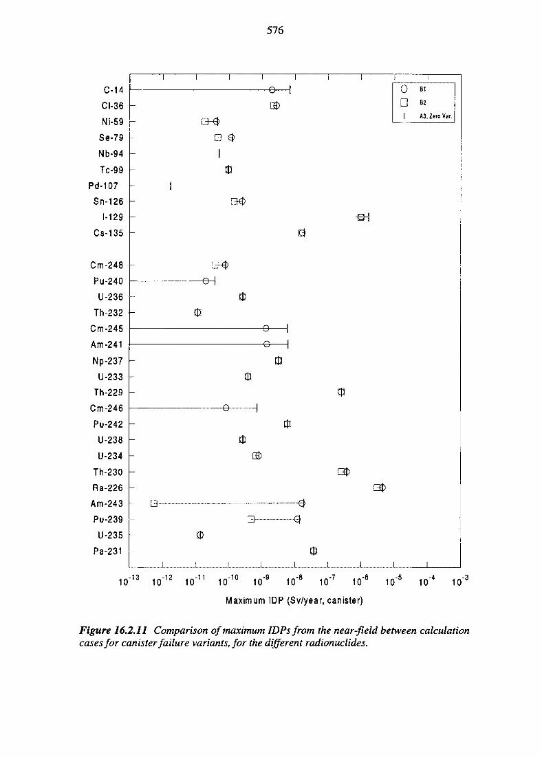
576
Cm-248
Pu-240
U-236
Th-232
Cm-245
Am-241
Np-237
U-233
Th-229
Cm-246
Pu-242
U-238
U-234
Th-230
Ra-226
Am-243
Pu-239
U-235
Pa-231
10 13 10"12 10'11 10 10 10 10 10
Maximum IDP (Sv/year, canister)
-610
-510' 10
-3
Figure 16.2.11 Comparison of maximum IDPsfrom the near-field between calculationcases for canister failure variants, for the different radionuclides.
577
Early pin-hole in the canister (B3)
This is a case in which a pin-hole (area 5 mm2) already exists through both the copper andsteel canisters at the time of deposition. It is positioned close to the fracture opening in therock (Section 13.3.5.1). Releases occur through the pinhole from time zero, over whichperiod an enhanced fuel matrix dissolution rate is assumed (time to total dissolution of 7500years). Pinhole release continues for 1000 years, at which time the canister is assumed tofail completely. After total failure, matrix dissolution rate and other conditions revert tothose of the Zero Variant case. Radionuclide migration through the pin-hole will not causea radionuclide flux that exceeds the maximum fluxes obtained in the Zero Variant case,except for the very short-lived radionuclides ^Sr and 137Cs, which will give release ratesorders of magnitude higher than in the Zero Variant case. However, the faster and earliermatrix release which has occurred during the time when the pinhole is open may, to someextent, influence the radionuclide flux after total canister failure. This is not considered inSITE-94.
16.2.2.3 Conclusions for Near-field Reference Case Calculations
For all calculation cases, the release of radionuclides from the near-field is dominated by129I at early times. The IDP from 129I is 10'MO"6 Sv/year, canister and does not show muchspread across the range of parameter variations performed. At later times, the dose-dominating radionuclides are 226Ra, 23OTh and 229Th, but other radionuclides also becomeimportant under certain circumstances (241 Am, 239Pu, 245Cm and237Np) depending on solu-bilities, time for maximum release, half-lives, etc. The maximum IDPs obtained beyond 105
years are within the interval of lO^-lO'5 Sv/year, canister. Considerably higher IDPs areobtained if the bentonite is degraded. Very redox sensitive radionuclides ("Tc, 79Se) causeIDPs almost as high as 129I if there are oxidising conditions or a redox front far out in thenear-field.
The results from the Discrete Feature hydrogeology site model cover the full range ofreleases, from the situation with a zero concentration boundary in the fracture to the otherextreme with pure diffusion, not only in the rock matrix, but also in the fracture. Theinterval in release rate spans about two orders of magnitude, with the near-field ZeroVariant case somewhere in the middle of the interval.
The Stochastic Continuum hydrogeology site model provides a smaller span in parameteruncertainties and, consequently, the range in releases is smaller than for the DiscreteFeature model. The IDP results from the Stochastic Continuum model fall within theintervals resulting from the Discrete Feature model. The major reason for the smaller rangeis that the specific flow-wetted surface area parameter is not evaluated in this model, butestimated separately.
The uncertainties/variabilities in specific flow-wetted surface area, fracture aperture andfracture spacing are not shown to be crucial parameters for the release of radionuclides inthe selected calculation cases. The channel-connection-length parameter (Section 13.3.5.3)was not varied but set to a conservative value, which influences the impact of the otherfracture parameters. The fracture spacing has a small impact, as well as the specific flow-wetted surface area, at very low Darcy velocities.
578
The redox state of conditions in the near-field is an important parameter since the solu-bilities of many elements change by orders of magnitude and the flux of radionuclides isdirectly correlated to the solubilities. The maximum release of "Tc varies by four ordersof magnitude (1010-106 Sv/year, canister).
Decreased sorption has less influence on elements with low distribution coefficients sincea relatively large fraction of these elements is already in the aqueous phase. Decreasedsorption results in a faster breakthrough from the near-field and this has an impact on themaximum release of short-lived radionuclides (e.g.241 Am).
The bentonite provides important resistance to radionuclide transport, especially for short-lived radionuclides which decay in the bentonite. Not surprisingly, a highly degradedbentonite causes an increase in the flux of the radionuclides. The largest increase isobtained for the initially mobile radionuclides in the gaps between fuel and cladding (14C,135Cs, 137Cs and 129I). These species cause an early release and a rather high flux. Thebentonite is also important for strongly sorbed nuclides, such as many of the actinides.
The time for canister failure has a very large effect on short-lived radionuclides which, forlate failure, would have decayed inside the canister. The reason for the limited effect offailure time on the other elements is due to the dissolution rate, which limits the release ofradionuclides from the waste.
16.2.3 Central Scenario: Near-field
Calculations for the Central Scenario are performed for variant cases Cl and C2 (definedin Chapter 15) to illustrate the impact of changing water flow and redox conditions duringa glaciation. Case Cl conservatively assumes that oxidising conditions reach all the wayinto the waste-form, while in C2 the bentonite and rock are oxidised, but not the waste-form. The calculations are performed for a subset of representative nuclides: 129I, "Tc andthe actinide chains and for a period up to 105 years (i.e. one glaciation cycle). The dose con-version factors (Sv/Bq) used to calculate IDPs are the same as for the Reference Case, i.e.a drinking-water well at Aspo (see also the conclusion section to this chapter).
Figures 16.2.12 and 16.2.13 show the time evolution of the sum of IDPs, as well as themost important contributing radionuclides for cases Cl and C2 respectively. Figure 16.2.14shows a comparison between the maximum IDPs (for times up to 105 years) for theactinides, for the cases Cl, C2 and the near-field Zero Variant case in the Reference Case(A3).
The release of radionuclides (in Sv/year, canister) during the glaciation period (55-70 kaAP), is about a factor of 2 higher than the release in the Zero Variant case for the ReferenceCase, during the same period. However, the maximum release in case Cl during theglaciation period is not higher than the overall maximum (at about 200 000 years) in theZero Variant case for the Reference Case.
The dominant radionuclides are 129I (early times) and 226Ra (later times), as in the ReferenceCase. For the Cl case, the largest differences in maximum release are for "Tc and 237Np,which have drastically increased solubility and decreased sorption under oxidising condi-
579
tions. The effect for "Tc and237Np in case C2 is much less, as solubility in the waste-form,where the precipitates occur, remains low.
As in the Zero Variant case in the Reference Case, 229Th and 230Th are strong contributorsto the sum of IDPs, both in Cl and C2. However, thorium has no change in solubility orsorption in going from reducing to oxidising conditions. Uranium and plutonium haveincreased solubility and decreased sorption for oxidising conditions, but the changes aresmaller than for "Tc and 237Np. The peak releases for the uranium isotopes change by 2 to3 orders of magnitude, while the plutonium change is more moderate: up to one order ofmagnitude (Figure 16.2.14).
For the actinides, the amount released in moles at 105 years (summed over all actinidechains) is 300 times larger in Cl than in the Zero Variant case for the Reference Case (A3),while C2 is 30 times larger, as can be seen in Table 16.2 A. Despite this increased releaseof radionuclides, the amount of the actinides retained in the near-field is hardly affected.
For "Tc, with its extreme sensitivity to redox conditions, an intrusion of oxidising water(all the way into the waste-form) releases essentially the whole amount that is in thenear-field during the 15 000 years of glaciation (about 16 % of the initial inventory of "Tchas decayed at 55 000 years). For the case with oxidising conditions only in the bentoniteand rock (C2), the amounts released are much the same as in the Reference Case (as "Tcprecipitates in the waste-form), see Table 16.2.4 .
The results could be summarised by noting the total BDP, with 129I and 226Ra as theimportant contributors, is not much affected by the Central Scenario, whereas the maximumIDPs for some radionuclides increase by orders of magnitude. A sudden intrusion ofoxidising water also has the potential to mobilise redox-sensitive radionuclides, even witha short duration period of oxidising conditions.
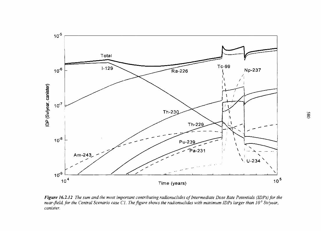
10'.-5
&cCOo
CD I f ) "
CLQ
Total
o
Time (years)
Figure 16.2.12 The sum and the most important contributing radionuclides of Intermediate Dose Rate Potentials (IDPs) for thenear-field, for the Central Scenario case Cl. The figure shows the radionuclides with maximum IDPs larger than 10'9 Sv/year,canister.
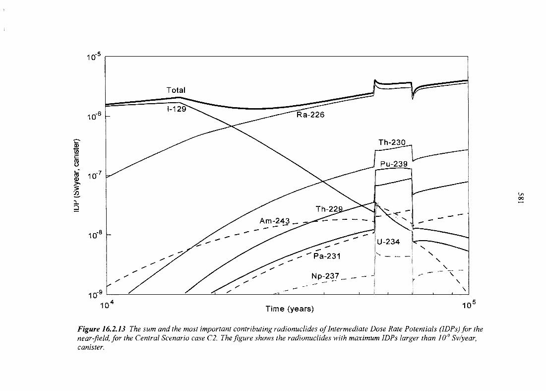
10'
10"
§3 io"
10"8h
10"
Total"
1-129"^^ -— -
^ ^ Am-243
^^a^226
T h - 2 2 9 ^ > <
Np-237_ _ -- -
i i
S———s
Pu-239
U-234
i
^ — —
1
N
>
: 1
- " " '
\
\1
10 Time (years) 10
0 0
Figure 16.2.13 The sum and the most important contributing radionuclides of Intermediate Dose Rate Potentials (IDPs) for thenear-field, for the Central Scenario case C2. The figure shows the radionuclides with maximum IDPs larger than 10'9 Sv/year,canister.
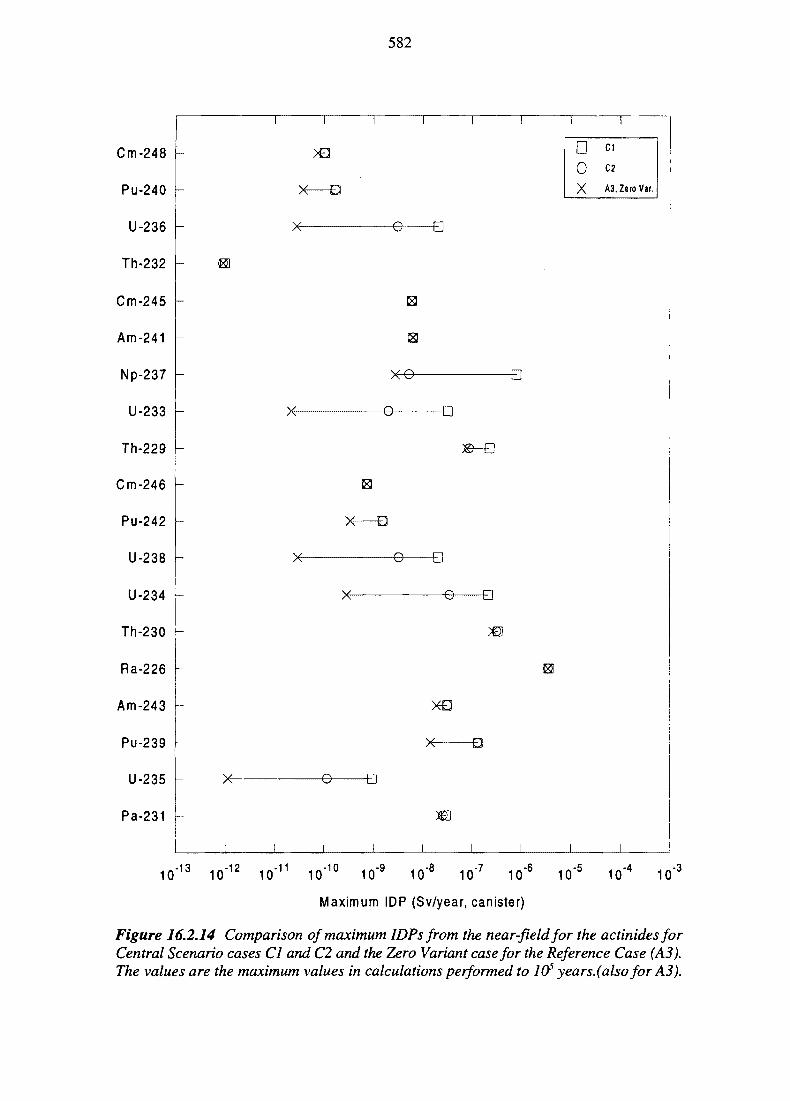
582
Cm-248
Pu-240
U-236
Th-232
Cm-245 -
Am-241 -
Np-237
U-233
Th-229 -
Cm-246 -
Pu-242
U-238
U-234
Th-230
Ra-226 h
Am-243
Pu-239
U-235
Pa-231
X-
x-
x-
-e-
x-o-
-e-
-B
-e—-a
x-
-e- -o
-e
-o a
D0X
Cl
C2
A3, Zero Var.
10"1 3 10"1 2 10 ' 1 1 10"1 0 10"9 10" 10"7 10 ' 6 10 ' 5 10"4 10*3
Maximum IDP (Sv/year, canister)
Figure 16.2.14 Comparison of maximum IDPsfrom the near-field for the actinides forCentral Scenario cases Cl and C2 and the Zero Variant case for the Reference Case (A3).The values are the maximum values in calculations performed to 1O5 years, (also for A3).
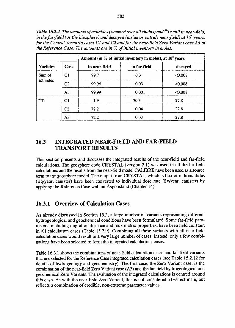
583
Table 16.2.4 The amounts ofactinides (summed over all chains) and "Tc still in near-field,in the far-field (or the biosphere) and decayed (inside or outside near-field) at 105 years,for the Central Scenario cases Cl and C2 and for the near-field Zero Variant case A3 ofthe Reference Case. The amounts are in % of initial inventory in moles.
Nuclides
Sum ofactinides
"Tc
Case
Cl
C2
A3
Cl
C2
A3
Amount (in % of initial inventory in moles), at 10s years
in near-Held
99.7
99.96
99.99
1.9
72.2
72.2
in far-field
0.3
0.03
0.001
70.3
0.04
0.03
decayed
<0.008
<0.008
<0.008
27.8
27.8
27.8
16.3 INTEGRATED NEAR-FIELD AND FAR-FIELDTRANSPORT RESULTS
This section presents and discusses the integrated results of the near-field and far-fieldcalculations. The geosphere code CRYSTAL (version 2.1) was used in all the far-fieldcalculations and the results from the near-field model CALIBRE have been used as a sourceterm to the geosphere model. The output from CRYSTAL, which is flux of radionuclides(Bq/year, canister) have been converted to individual dose rate (Sv/year, canister) byapplying the Reference Case well on Aspo island (Chapter 14).
16.3.1 Overview of Calculation Cases
As already discussed in Section 15.2, a large number of variants representing differenthydrogeological and geochemical conditions have been formulated. Some far-field para-meters, including migration distance and rock matrix properties, have been held constantin all calculation cases (Table 15.2.9). Combining all these variants with all near-fieldcalculation cases would result in a very large number of cases. Instead, only a few combi-nations have been selected to form the integrated calculations cases.
Table 16.3.1 shows the combinations of near-field calculation cases and far-field variantsthat are selected for the Reference Case integrated calculation cases (see Table 15.2.12 fordetails of hydrogeology and geochemistry). The first case, the Zero Variant case, is thecombination of the near-field Zero Variant case (A3) and the far-field hydrogeological andgeochemical Zero Variants. The evaluation of the integrated calculations is centred aroundthis case. As with the near-field Zero Variant, this is not considered a best estimate, butreflects a combination of credible, non-extreme parameter values.
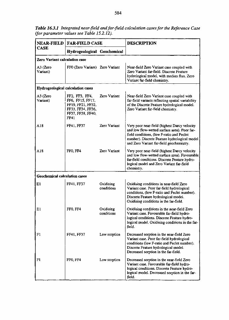
584
Table 16.3.1 Integrated near-field and far-field calculation cases for the Reference Case(for parameter values see Table 15.2.12).
NEAR-FIELDCASE
FAR-FIELD CASE
Hydrogeological Geochemical
Zero Variant calculation case
A3 (ZeroVariant)
FFO (Zero Variant) Zero Variant
Hydrogeological calculation cases
A3 (ZeroVariant)
A18
A18
FF2, FF3, FF4, Zero VariantFF6, FF15,FF17,FF19,FF21,FF32,FF33, FF34, FF36,FF37, FF38, FF40,FF41
FF41,FF37 Zero Variant
FFO, FF4 Zero Variant
Geochemical calculation cases
El
El
Fl
Fl
FF41,FF37 Oxidisingconditions
FFO, FF4 Oxidisingconditions
FF41.FF37 Lowsorption
FFO, FF4 Low sorption
DESCRIPTION
Near-field Zero Variant case coupled withZero Variant far-field. Discrete Featurehydrological model, with median flux. ZeroVariant far-field chemistry.
Near-field Zero Variant case coupled withfar-field variants reflecting spatial variabilityof the Discrete Feature hydrological model.Zero Variant far-field chemistry.
Very poor near-field (highest Darcy velocityand low flow-wetted surface area). Poor far-field conditions, (low F-ratio and Pecletnumber). Discrete Feature hydrological modeland Zero Variant far-field geochemistry.
Very poor near-field (highest Darcy velocityand low flow-wetted surface area). Favourablefar-field conditions. Discrete Feature hydro-logical model and Zero Variant far-fieldchemistry.
Oxidising conditions in near-field ZeroVariant case. Poor far-field hydrologicalconditions, (low F-ratio and Peclet number).Discrete Feature hydrological model.Oxidising conditions in the far-field.
Oxidising conditions in the near-field ZeroVariant case. Favourable far-field hydro-logical conditions. Discrete Feature hydro-logical model. Oxidising conditions in the far-field.
Decreased sorption in the near-field ZeroVariant case. Poor far-field hydrologicalconditions (low F-ratio and Peclet number).Discrete Feature hydrological model.Decreased sorption in the far-field.
Decreased sorption in the near-field ZeroVariant case. Favourable far-field hydro-logical conditions. Discrete Feature hydro-logical model. Decreased sorption in the far-field.
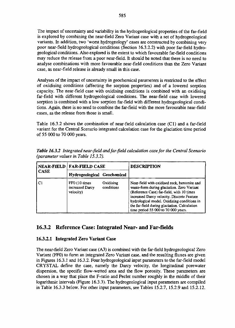
585
The impact of uncertainty and variability in the hydrogeological properties of the far-fieldis explored by combining the near-field Zero Variant case with a set of hydrogeologicalvariants. In addition, two 'worst hydrogeology' cases are constructed by combining verypoor near-field hydrogeological conditions (Section 16.3.2.2) with poor far-field hydro-geological conditions. Also explored is the extent to which favourable far-field conditionsmay reduce the release from a poor near-field. It should be noted that there is no need toanalyse combinations with more favourable near-field conditions than the Zero Variantcase, as near-field release is already small in this case.
Analyses of the impact of uncertainty in geochemical parameters is restricted to the effectof oxidising conditions (affecting the sorption properties) and of a lowered sorptioncapacity. The near-field case with oxidising conditions is combined with an oxidisingfar-field with different hydrogeological conditions. The near-field case with loweredsorption is combined with a low sorption far-field with different hydrogeological condi-tions. Again, there is no need to combine the far-field with the more favourable near-fieldcases, as the release from those is small.
Table 16.3.2 shows the combination of near-field calculation case (Cl) and a far-fieldvariant for the Central Scenario integrated calculation case for the glaciation time periodof 55 000 to 70 000 years.
Table 16.3.2 Integrated near-field and far-field calculation case for the Central Scenario(parameter values in Table 15.3.2).
NEAR-FBELDCASE
Cl
FAR-FIELD CASE
Hydrogeological Geochemical
FF0 (10 times Oxidisingincreased Darcy conditionsvelocity)
DESCRIPTION
Near-field with oxidised rock, bentonite andwaste-form during glaciation. Zero Variant(Reference Case) far-field, with 10 timesincreased Darcy velocity. Discrete Featurehydrological model. Oxidising conditions inthe far-field during glaciation. Calculationtime period 55 000 to 70 000 years.
16.3.2 Reference Case: Integrated Near- and Far-fields
16.3.2.1 Integrated Zero Variant Case
The near-field Zero Variant case (A3) is combined with the far-field hydrogeological ZeroVariant (FF0) to form an integrated Zero Variant case, and the resulting fluxes are givenin Figures 16.3.1 and 16.3.2. Four hydrogeological input parameters to the far-field modelCRYSTAL define the case, namely the Darcy velocity, the longitudinal porewaterdispersion, the specific flow-wetted area and the flow porosity. These parameters arechosen in a way that place the F-ratio and Peclet number roughly in the middle of theirlogarithmic intervals (Figure 16.3.3). The hydrogeological input parameters are compiledin Table 16.3.3 below. For other input parameters, see Tables 15.2.7, 15.2.9 and 15.2.12.

586
Figures 16.3.1 and 16.3.2. give the time evolution of the fluxes from the far-field to thebiosphere in (Bq/year, canister) and the dose rates in (Sv/year, canister); fluxes higher than102 Bq/year, canister and dose rates higher than 10"12 Sv/year, canister are shown. Thefigures are complemented by Table 16.3.4, where the maximum release rates (Bq/year,canister) and dose rates (Sv/year, canister) for times up to 106 years are given, as well as thetime in the future at which fluxes or dose rates reach a maximum.
Comparing Figure 16.3.2 with the release (as IDPs) from the near-field alone (seeFigure 16.2.2, but note the different scales on the y-axis), it can be seen that the poorlysorbed 129I (Kd = 5.0x10"4 rnVkg) and the non-sorbing 36C1 are practically unaffected bypassage through the geosphere. The geosphere has a large influence on radionuclides whichare dominant at later times, notably 230Th and 226Ra, belonging to the 4N+2 decay chain.Their maximum releases have dropped by several orders of magnitude. The radionuclide23OTh is retarded by sorption in the rock matrix. And ^ R a is also sorbed in the rock matrix,but its behaviour is governed by the sorption of its parent, 23<>Th.
The radionuclide giving the highest maximum dose rate for times up to 106 years is 129I(1.6X10"6 Sv/year, canister). The radionuclides giving the second and third highestmaximum dose rate up to 106 years are 226Ra (3.5xl0'9 Sv/year, canister) and 14C(3.3xl09 Sv/year, canister).
The solid line in Figure 16.3.2 indicates the sum of all radionuclides as a function of time.Its maximum value is \.6xW6 Sv/year, canister, at about 104 years. The contribution to thismaximum value is totally dominated by 129I up to about 105 years. The contribution to thesecond, later peak is mainly from 226Ra, 135Cs and 23(>Th.
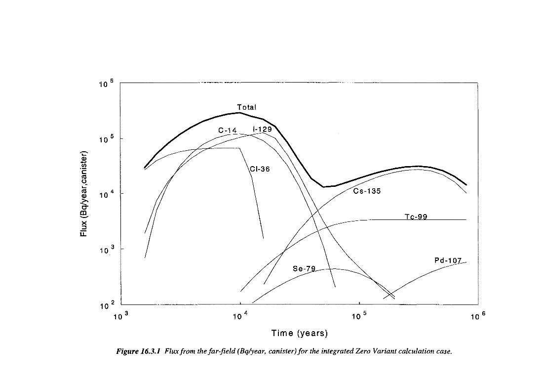
0
10
c03
CD 1 0
X
E10 3 _
1010° 10" 10°
Time (years)
Figure 16.3.1 Flux from the far-field (Bq/year, canister) for the integrated Zero Variant calculation case.
10
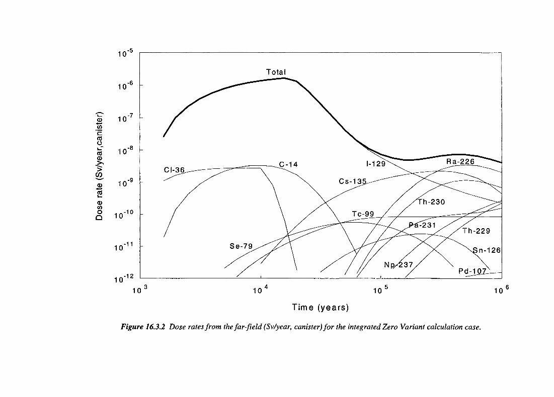
4en'c(0o0
Q>
CO
0
°Q
10
10
10
10
10
-5
-6
-7
-8 _
•9 _
.-10 _
-11
10-12
10 10 10
Time (years)
Figure 16.3.2 Dose rates from the far-field (Sv/year, canister) for the integrated Zero Variant calculation case.
10
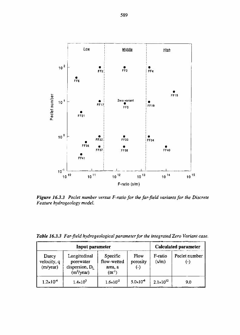
589
10
E
<DOCD
10
100 _
10'
Low
-
FF6
FF21
9FF36
FF41
I
FF2
ft
FF17
FF32
9FF37
: Middle
9FF3
Zero variant9FFO
FF33
*FF38
I . I ;
FF4
FF19
FF34
High
9FF15
FF4O
I
1010
1011 1012 10
F-ratio (s/m)
1310
14 10 15
Figure 16.3.3 Peclet number versus F-ratio for the far-field variants for the DiscreteFeature hydrogeology model.
Table 16.3.3 Far-field hydrogeological parameter for the integrated Zero Variant case.
Input parameter
Darcyvelocity, q(m/year)
1.2x10^
Longitudinalporewater
dispersion, DL
(mVyear)
1.4xlO3
Specificflow-wetted
area, a(m-1)
1.6xlO"2
Flowporosity
(-)
5.0xl0'6
Calculated parameter
F-ratio(s/m)
2.1xlO12
Peclet number(-)
9.0
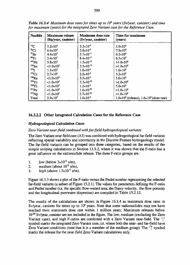
590
Table 16.3.4 Maximum dose rates for times up to 1O6 years (Sv/year, canister) and timefor maximum (years) for the integrated Zero Variant case for the Reference Case.
Nuclide
14C36C179Se"Tci o 7 p d
126Sn129T
135Cs2 2 6Ra2 2 9Th2 3 0 ^
B 1 P a^NpTotal
Maximum release(Bq/year, canister)
1.2x10'6.6xlO4
4.4x10²
3.4xlO3
5.8xlO2
<1.0xl02
1.3x10'2.7x10⁴
<1.0xl02
<1.0xl02
<1.0xl02
<1.0xl02
<1.0xl02
2.9x10'
Maximum dose rate(Sv/year, canister)
3.3xlO9
2.8xlO"9
5.7x10-"8.4x10-"1.5xlO12
3.3xlO12
1.6xlO6
2.2xlO"9
3.5xlO"9
2.2xlO10
1.2xlO"9
1.6xlO10
2.7xlO10
1.6xlO"6
Time for maximum(years)
l.OxlO4
7.9xlO3
6.3xlO4
6.3x10'>1.0xl06
>1.0xl06
1.6xlO4
3.2x10'5.0x10'>1.0xl06
5.0x10'>1.0xl06
>1.0xl06
1 .Ox 104 (release), 1.6x 10⁴ (dose rate)
16.3.2.2 Other Integrated Calculation Cases for the Reference Case
Hydrogeological Calculation Cases
Zero Variant near-field combined with far-field hydrogeological variants
The Zero Variant near-field case (A3) was combined with hydrogeological far-field variantsreflecting spatial variability and uncertainty in the Discrete Feature hydrogeology model.The far-field variants can be grouped into three categories, based on the results of thesimple scoping calculations in Section 13.5.2, where it was shown that the F-ratio has agreat influence on the radionuclide release. The three F-ratio groups are:
1. low (below 3xl0ns/m),2. medium (about 1012 s/m),3. high (above 1.5xlO13 s/m).
Figure 16.3.3 shows a plot of the F-ratio versus the Peclet number representing the selectedfar-field variants (a subset of Figure 15.2.1). The values for parameters defining the F-ratioand Peclet number (i.e. the specific flow-wetted area, the Darcy velocity, the flow porosityand the longitudinal porewater dispersion) are compiled in Table 15.2.12.
The results of the calculations are shown in Figure 16.3.4 as maximum dose rates inSv/year, canister for times up to 106 years. Note that some radionuclides may not havereached their maximum dose rate within 1 million years. Maximum releases below10-20 Sv/year, canister are not included in the figure. The low, medium (excluding the ZeroVariant case), and high F-ratios are combined with a Zero Variant near-field. The ' | 'symbol marks the integrated Zero Variant case, i.e. where both the near- and far-field haveZero Variant conditions (note that it is a member of the medium group). The *"]' symbolmarks the release for the near-field Zero Variant calculations only.
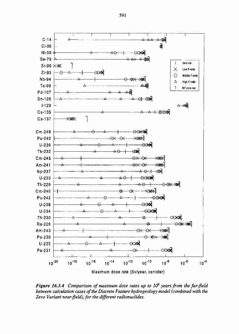
591
C-14
CI-36
Ni-59
Se-79
Sr-90
Zr-93
Nb-94
Tc-99
Pd-107
Sn-126
1-129
Cs-135
Cs-137
Cm-248
Pu-240
U-236
Th-232
Cm-245
Am-241
Np-237
U-233
Th-229
Cm-246
Pu-242
U-238
U-234
Th-230
Ra-226
Am-243
Pu-239
U-235
Pa-231
10
A- A.-A- A^
•A0-
O
A-
A AA A
A A A
•A- A -A—0}-
.A.- •A A—.A-
ox ex-9.
ox cx-ox ex
-e- -eee
-e--e-
-e-
I
X0A
1
zero var.
Low F-ratio
Middle F-ratio
High F-ratio
NF zero var.
-e-
-20 10-18 -16 .-14 .-1010 1W 1 0 ' " 10 ' 10 10
Maximum dose rate (Sv/year, canister)
-8 10-6 10-4
Figure 16.3.4 Comparison of maximum dose rates up to l(f years from the far-fieldbetween calculation cases of the Discrete Feature hydrogeology model (combined with theZero Variant near-field), for the different radionuclides.
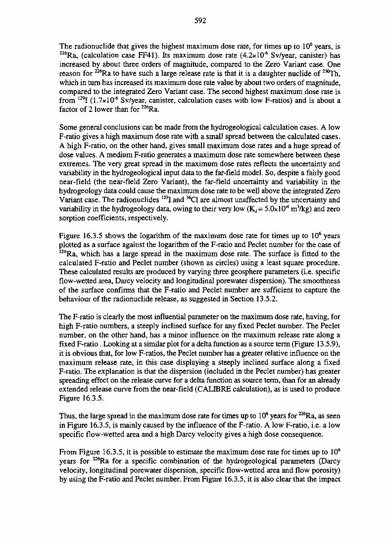
592
The radionuclide that gives the highest maximum dose rate, for times up to 106 years, is226Ra, (calculation case FF41). Its maximum dose rate (4.2x10"6 Sv/year, canister) hasincreased by about three orders of magnitude, compared to the Zero Variant case. Onereason for 226Ra to have such a large release rate is that it is a daughter nuclide of 230Th,which in turn has increased its maximum dose rate value by about two orders of magnitude,compared to the integrated Zero Variant case. The second highest maximum dose rate isfrom 129I (1.7X10"6 Sv/year, canister, calculation cases with low F-ratios) and is about afactor of 2 lower than for 226Ra.
Some general conclusions can be made from the hydrogeological calculation cases. A lowF-ratio gives a high maximum dose rate with a small spread between the calculated cases.A high F-ratio, on the other hand, gives small maximum dose rates and a huge spread ofdose values. A medium F-ratio generates a maximum dose rate somewhere between theseextremes. The very great spread in the maximum dose rates reflects the uncertainty andvariability in the hydrogeological input data to the far-field model. So, despite a fairly goodnear-field (the near-field Zero Variant), the far-field uncertainty and variability in thehydrogeology data could cause the maximum dose rate to be well above the integrated ZeroVariant case. The radionuclides 129I and 36C1 are almost unaffected by the uncertainty andvariability in the hydrogeology data, owing to their very low (Kd= 5.0x10"4 mVkg) and zerosorption coefficients, respectively.
Figure 16.3.5 shows the logarithm of the maximum dose rate for times up to 106 yearsplotted as a surface against the logarithm of the F-ratio and Peclet number for the case of226Ra, which has a large spread in the maximum dose rate. The surface is fitted to thecalculated F-ratio and Peclet number (shown as circles) using a least square procedure.These calculated results are produced by varying three geosphere parameters (i.e. specificflow-wetted area, Darcy velocity and longitudinal porewater dispersion). The smoothnessof the surface confirms that the F-ratio and Peclet number are sufficient to capture thebehaviour of the radionuclide release, as suggested in Section 13.5.2.
The F-ratio is clearly the most influential parameter on the maximum dose rate, having, forhigh F-ratio numbers, a steeply inclined surface for any fixed Peclet number. The Pecletnumber, on the other hand, has a minor influence on the maximum release rate along afixed F-ratio. Looking at a similar plot for a delta function as a source term (Figure 13.5.9),it is obvious that, for low F-ratios, the Peclet number has a greater relative influence on themaximum release rate, in this case displaying a steeply inclined surface along a fixedF-ratio. The explanation is that the dispersion (included in the Peclet number) has greaterspreading effect on the release curve for a delta function as source term, than for an alreadyextended release curve from the near-field (CALIBRE calculation), as is used to produceFigure 16.3.5.
Thus, the large spread in the maximum dose rate for times up to 106 years for 226Ra, as seenin Figure 16.3.5, is mainly caused by the influence of the F-ratio. A low F-ratio, i.e. a lowspecific flow-wetted area and a high Darcy velocity gives a high dose consequence.
From Figure 16.3.5, it is possible to estimate the maximum dose rate for times up to 106
years for 226Ra for a specific combination of the hydrogeological parameters (Darcyvelocity, longitudinal porewater dispersion, specific flow-wetted area and flow porosity)by using the F-ratio and Peclet number. From Figure 16.3.5, it is also clear that the impact
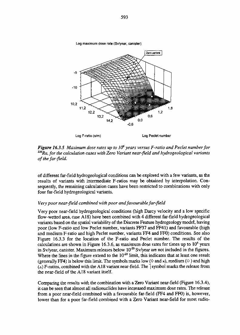
593
Log maximum dose rate (Sv/year, canister)
-5
-10
10,2
Log F-ratio (s/m) Log Peclet number
Figure 16.3.5 Maximum dose rates up to l(f years versus F-ratio and Peclet number for226Ra, for the calculation cases with Zero Variant near-field and hydro geological variantsof the far-field.
of different far-field hydrogeological conditions can be explored with a few variants, as theresults of variants with intermediate F-ratios may be obtained by interpolation. Con-sequently, the remaining calculation cases have been restricted to combinations with onlyfour far-field hydrogeological variants.
Very poor near-field combined with poor and favourable far-field
Very poor near-field hydrogeological conditions (high Darcy velocity and a low specificflow-wetted area, case A18) have been combined with 4 different far-field hydrogeologicalvariants based on the spatial variability of the Discrete Feature hydrogeology model, havingpoor (low F-ratio and low Peclet number, variants FF37 and FF41) and favourable (highand medium F-ratio and high Peclet number, variants FF4 and FFO) conditions. See alsoFigure 16.3.3 for the location of the F-ratio and Peclet number. The results of thecalculations are shown in Figure 16.3.6, as maximum dose rates for times up to 106 yearsin Sv/year, canister. Maximum releases below 10'20 Sv/year are not included in the figures.Where the lines in the figure extend to the 10'20 limit, this indicates that at least one result(generally FF4) is below this limit. The symbols marks low (0 and x), medium (o) and high(A) F-ratios, combined with the A18 variant near-field. The ~| symbol marks the release fromthe near-field of the A18 variant itself.
Comparing the results with the combination with a Zero Variant near-field (Figure 16.3.4),it can be seen that almost all radionuclides have increased maximum dose rates. The releasefrom a poor near-field combined with a favourable far-field (FF4 and FFO) is, however,lower than for a poor far-field combined with a Zero Variant near-field for most radio-
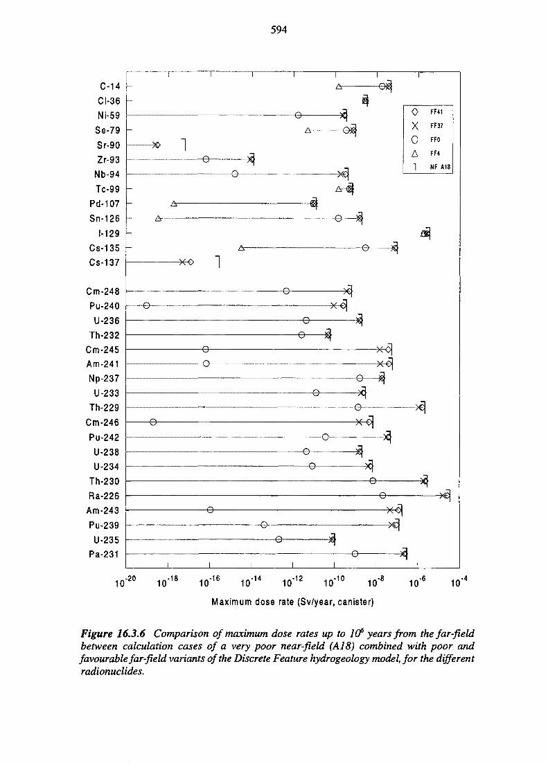
594
C-14
CI-36
Ni-59
Se-79
Sr-90
Zr-93
Nb-94
Tc-99
Pd-107
Sn-126
1-129
Cs-135
Cs-137
Cm-248
Pu-240
U-236
Th-232
Cm-245
Am-241
Np-237
U-233
Th-229
Cm-246
Pu-242
U-238
U-234
Th-230
Ra-226
Am-243
Pu-239
U-235
Pa-231
-eif
-e-
-e--e-
-e-xo
-e--e-
-e--e-
_©_
o
-e- -x-e)-e-
-e--e-
-e--e-
-e--e-
-e--e-
10-20
10"18 "16 "14 .-12 .-1010 10 10 10 10
Maximum dose rate (Sv/year, canister)
-8
0X0A1
FF41
FF37
FFO
FF4
NF A18
10-6
10-4
Figure 16.3.6 Comparison of maximum dose rates up to l(f years from the far-fieldbetween calculation cases of a very poor near-field (A18) combined with poor andfavourable far-field variants of the Discrete Feature hydrogeology model, for the differentradionuclides.
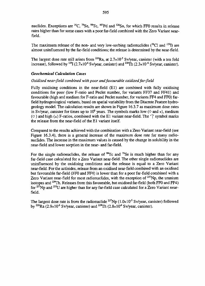
595
nuclides. Exceptions are 14C, 79Se, "Tc, 107Pd and 126Sn, for which FFO results in releaserates higher than for some cases with a poor far-field combined with the Zero Variant near-field.
The maximum release of the non- and very low-sorbing radionuclides (36C1 and 129I) arealmost uninfluenced by the far-field conditions; the release is determined by the near-field.
The largest dose rate still arises from 226Ra, at 2.7xlO'5 Sv/year, canister (with a ten foldincrease), followed by 129I (2.7X10"6 Sv/year, canister) and 23aTh (2.3x10^ Sv/year, canister).
Geochemical Calculation Cases
Oxidised near-field combined with poor and favourable oxidised far-field
Fully oxidising conditions in the near-field (El) are combined with fully oxidisingconditions for poor (low F-ratio and Peclet number, for variants FF37 and FF41) andfavourable (high and medium for F-ratio and Peclet number, for variants FF4 and FFO) far-field hydrogeological variants, based on spatial variability from the Discrete Feature hydro-geology model. The calculation results are shown in Figure 16.3.7 as maximum dose ratesin Sv/year, canister for times up to 106 years. The symbols marks low (0 and x), medium(o) and high (A) F-ratios, combined with the El variant near-field. The ' ] ' symbol marksthe release from the near-field of the El variant itself.
Compared to the results achieved with the combination with a Zero Variant near-field (seeFigure 16.3.4), there is a general increase of the maximum dose rate for many radio-nuclides. The increase in the maximum values is caused by the change in solubility in thenear-field and lower sorption in the near- and far-field.
For the single radionuclides, the release of "Tc and 79Se is much higher than for anyfar-field case calculated for a Zero Variant near-field. The other single radionuclides areuninfluenced by the oxidising conditions and the release is equal to a Zero Variantnear-field. For the actinides, release from an oxidised near-field combined with an oxidisedbut favourable far-field (FFO and FF4) is lower than for a poor far-field combined with aZero Variant near-field for most radionuclides, with the exception of 237Np, the uraniumisotopes and 229Th. Releases from this favourable, but oxidised far-field (both FFO and FF4)for 237Np and 233U are higher than for any far-field case calculated for a Zero Variant near-field.
The largest dose rate is from the radionuclide 237Np (l.OxlO"5 Sv/year, canister) followedby 226Ra (2.9xlO"6 Sv/year, canister) and 229Th (2.8X10"6 Sv/year, canister).
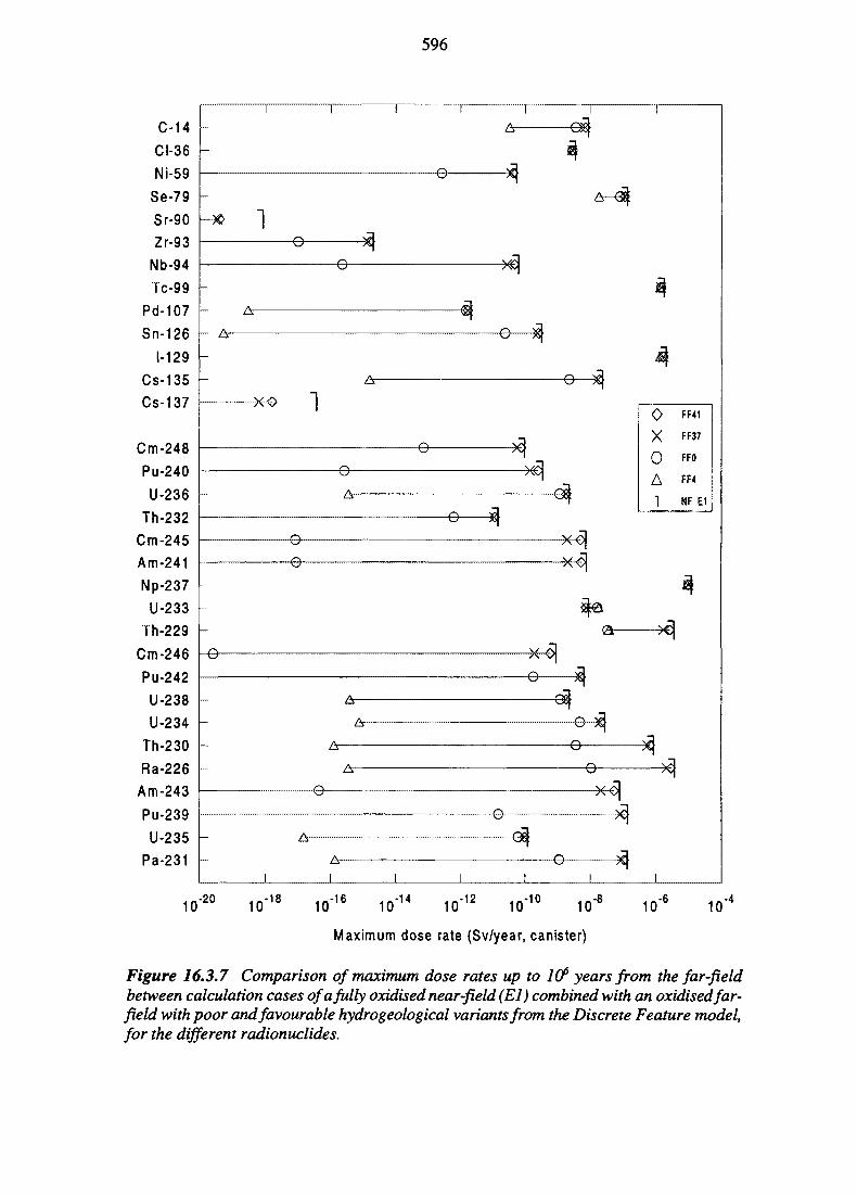
596
0 FF41
X FF37
0A FF4
1 NF E1
10-20 10-18 .-16 -14 ,-12 ,-1010 1W 1 0 " " 1 0 " " 10 1W 10
Maximum dose rate (Sv/year, canister)
-8 10-6 10-4
Figure 16.3.7 Comparison of maximum dose rates up to 10^ years from the far-fieldbetween calculation cases of a fully oxidised near-field (El) combined with an oxidised far-field with poor and favourable hydrogeological variants from the Discrete Feature model,for the different radionuclides.
597
Low sorption near-field combined with low sorption for poor and favourable far-field
The near-field variant case (Fl), with low sorption conditions (sorption lowered by a factorof three) is combined with a far-field with low sorption conditions (sorption also loweredby a factor of three) for poor (low F-ratio and Peclet number, for variants FF37 and FF41)and favourable (high and medium for F-ratio and Peclet number, for variants FF4 and FFO)far-field hydrogeological variants, based on spatial variability in the Discrete Feature hydro-geology model. The results are shown in Figure 16.3.8 as maximum dose rates in Sv/year,canister for times up to 106 years. The symbols marks low (0 and x), medium (o ) and high(A) F-ratios, combined with the Fl variant near-field. The ~| symbol marks the release fromthe near-field of the Fl variant itself.
Compared to the results achieved with the combination with a Zero Variant near-field(Figure 16.3.4.), there is a general increase of the maximum dose rate for all sorbing radio-nuclides. Release from a low sorbing near-field combined with a low sorbing but favour-able far-field (FFO and FF4) is, however, lower than for a poor far-field combined with aZero Variant near-field, for most radionuclides.
The largest dose rate is from 226Ra (1.5xlO'5 Sv/year, canister), followed by 229Th(2.0X10"6 Sv/year, canister) and 129I (1.9xlO"6 Sv/year, canister).
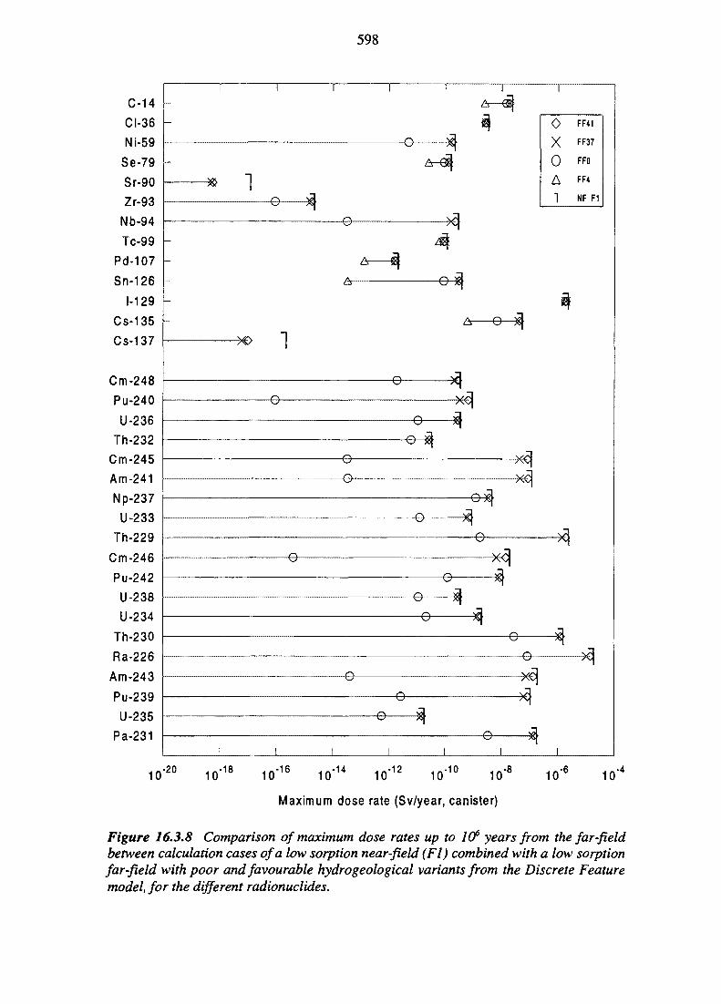
598
C-14
CI-36
Ni-59
Se-79
Sr-90
Zr-93
Nb-94
Tc-99
Pd-107
Sn-126
1-129Cs-135
Cs-137
Cm-248
Pu-240
U-236
Th-232
Cm-245
Am-241
Np-237
U-233
Th-229
Cm-246
Pu-242
U-238
U-234
Th-230
Ra-226
Am-243
Pu-239
U-235
Pa-231
10 -20
-e
-e-
0X0A1
FF41
FF37
FFO
FF4
NF F1
-e-
-e—$
• e -
• e -
-e-
-e--e-
-e-
-e--e-
-e-e-
-e--e-
-e--e-
io18 "16 "14 "12 '10
10 IW 10 in 10 lfc 10 IM 10
Maximum dose rate (Sv/year, canister)
-8 10 -610
-4
Figure 16.3.8 Comparison of maximum dose rates up to ltf years from the far-fieldbetween calculation cases of a low sorption near-field (Fl) combined with a low sorptionfar-field with poor and favourable hydrogeological variants from the Discrete Featuremodel, for the different radionuclides.
599
16.3.3 Central Scenario: Integrated Near- and Far-fields
The integrated calculations for the Central Scenario are limited to the Base Case variant C1,for the near-field, where glacial meltwater permeates all of the near-field, including thewaste-form. The calculation is further limited to the time period 55 000 to 70 000 years,which is only part of the whole climate sequence. This limitation is necessary, as theCRYSTAL code can only handle input parameters that are constant in time(Section 15.3.3.2). By choosing a time period within the glaciation climate sequence shortenough to have conditions constant in time, it is possible for the CRYSTAL code to analysereleases to the biosphere. The chosen time period in the Cl case gives the greatest releasefrom the near-field during the whole glacial sequence. During this time period, the Darcyvelocity is increased by a factor of ten (compared to the Zero Variant case for the ReferenceCase). Oxidising conditions prevail in the far-field. The sorption values for oxidisingcondition are used.
As in the near-field Central Scenario calculations, only a subset of nuclides is chosen: "Tc,129I and the actinide chains. The dose conversion factors (Sv/Bq) used to calculate doses arethe same as for the Reference Case, i.e. a drinking-water well on Aspo (see also the con-clusion section of this chapter). This must be seen as a hypothetical well case and the solemotivation for this is that it makes it possible to compare the results with the ReferenceCase calculations.
Releases occurring before the glaciation are simply obtained from the Reference Caseresults, as the conditions are the same before the glaciation period (55 000 to 70 000 years)as in the integrated Zero Variant case for the Reference Case. The radionuclide 129I has itsmaximum release at 1.6xlO4 year and is the dominating radionuclide at early times for theZero Variant in the Reference Case. Before the glaciation period, l29I releases havediminished by two orders of magnitude and it is no longer the dominant radionuclide.Therefore, no additional calculation is performed for 129I during the glaciation.
The integrated calculation results for the Central Scenario case Cl (• symbol) are shownin Figure 16.3.9, for the maximum dose rates between 55 000 and 70 000 years. As acomparison, the Reference Case for the integrated Zero Variant (*|* symbol in figure,near-field/far-field A3/FF0 combination) is included in the figure. The maximum dose ratesin the Central Scenario have increased by several orders of magnitude compared to the inte-grated Zero Variant case for the Reference Case. This is the result of the increased releasefrom the near-field, increased Darcy velocity and the change to oxidising conditions (whichreduces the sorption for some radionuclides).
During the glaciation period the near-field IDP is dominated by 226Ra for both near-fieldcases Cl and C2. In the case of Cl, there is also a substantial contribution from "Tc and237Np to the total IDP. These radionuclides also have the largest maximum dose rates(besides 129I) for times up to 70 000 years in the integrated analysis of the Cl case.
As discussed in Section 15.3.3, the limitations of the existing consequence analysis codesfor analysing the highly time-dependent evolution of the repository system under theconditions of the Central Scenario are well-understood, so some exploratory work investi-gates the biases that might be introduced by the simple treatment outlined above. This work(King-Clayton & Smith, 1996) uses a 2D flow and transport code (LAPLACE-2D) and
600
evaluates local scale (a 10 km wide, 1500 m deep section) responses of the system underthe transient flow conditions for the whole period of the Central Scenario. Releases to thesurface of the 2D model are calculated for poorly sorbing 129I and 79Se, which has 'average'sorption properties, applying a constant release rate source from a repository situated at500 m depth.
The objective of the exercise is to investigate variations in release at the surface during eachclimate episode of the Central Scenario, examining in particular the impacts of varying thecontinuity of permafrost cover and the rate of basal melting and associated groundwaterrecharge under the ice sheet. These are compared with releases calculated using a non-time-varying flow estimation for the same model system. As the model uses an equivalent porousmedium approach, the calculated releases are not directly comparable with those outlinedpreviously in this chapter and are thus not reported quantitatively here.
However, as can be seen from Figure 16.3.10, considerable variation in releases of 79Se isindicated, when compared with non-evolving conditions. The episodic nature of releasesis evident, with greatest releases ocurring as a result of partial or complete flushing out ofradionuclides from the geosphere by the high, upwardly-directed groundwater flows thathave been assumed to occur at the ice-sheet margins during the period of ice retreat. Suchflows may persist for around 2000 years, sufficient time to flush out most of the non-sorbing radionuclides which would be passing through the far-field at this time, butinsufficient to have a marked impact on sorbing species. Clearly, associated hydrochemicalperturbations, not assessed in this exercise, would modify this latter finding.
In general terms, this work identifies periods in the next 130 000 years where releases couldbe several orders of magnitude higher or lower than those calculated assuming fixedparameter values and fixed flow boundary conditions. In this respect, the study providessupport to the findings of the CALIBRE and CRYSTAL Central Scenario modellingdescribed above. The most significant uncertainties identified in the study relates to themagnitude of basal melting under the ice-sheet and to the anisotropy of the hydraulicconductivity of the rock. The presence or absence of breaks in the permafrost cover (taliks)are less significant with respect to maximum and cumulative radinuclide fluxes to thesurface.
Clearly, there are sufficient indicators of important safety impacts of time-dependencywithin both the LAPLACE-2D sensitivity study and the general integrated Central Scenarioconsequence analyses to motivate a more detailed evaluation of potential release variationsfor a variable climate future.
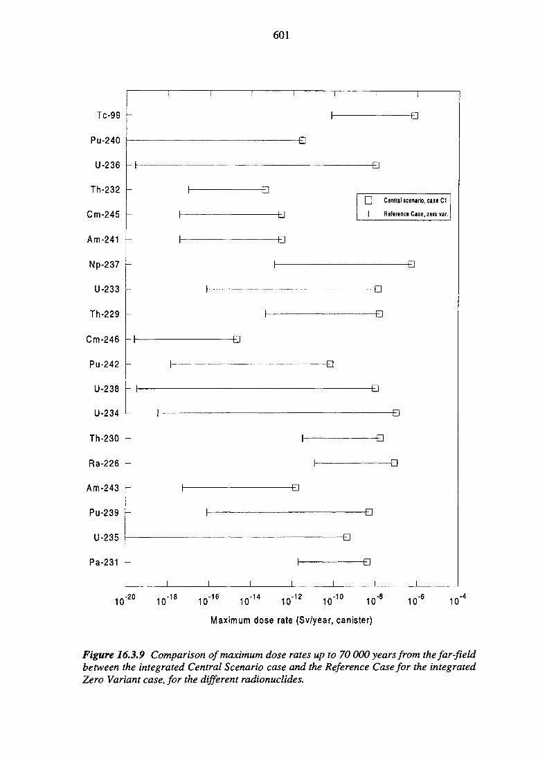
601
Tc-99
Pu-240
U-236
Th-232
Gm-245
Am-241
Np-237
U-233
Th-229
Cm-246
Pu-242
U-238
U-234
Th-230
Ra-226
Am-243
Pu-239 f-
U-235
Pa-231
10-20
10-18
-a
-e
~Q
-B
-a
-a
[ j Central scenario, case C1
I Reference Case, zero var.
• a
•a
• a
• a
• a
•B
-a
-a
-a
.-16 .-14 .-12 .-1010 "'" 10" " 1 0 " 10"'" 10
Maximum dose rate (Sv/year, canister)
-810
-610
-4
Figure 16.3.9 Comparison of maximum dose rates up to 70 000 years from the far-fieldbetween the integrated Central Scenario case and the Reference Case for the integratedZero Variant case, for the different radionuclides.
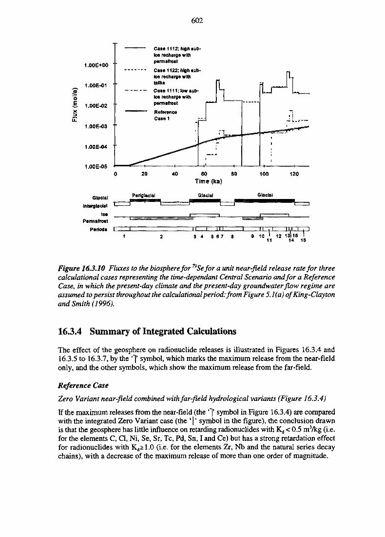
602
1.00E+00
1.00E-01 ' •
1.00E-02 ' "
1.00E-03
1 .OOE-04
1.00E-05
Glacial
Interglacial
Ice
Permafrost
Periods
Case 1112; high sub-ice recharge withpermafrost
Case 1122; high sub-ice recharge withtalik*
Case 1111; low sub-tee recharge withpermafrost
ReferenceCasei
20
Periglacla!
40 60Time (ka)
Glacial
80 100
Glacial
120
1L SL I III3 4 5 67 8 9 10 > 12 13)15 I
11 14 16
Figure 16.3.10 Fluxes to the biosphere for 79Sefor a unit near-field release rate for threecalculational cases representing the time-dependant Central Scenario and for a ReferenceCase, in which the present-day climate and the present-day groundwater flow regime areassumed to persist throughout the calculational period: from Figure 5.1 (a) of King-Claytonand Smith (1996).
16.3.4 Summary of Integrated Calculations
The effect of the geosphere on radionuclide releases is illustrated in Figures 16.3.4 and16.3.5 to 16.3.7, by the ' ] ' symbol, which marks the maximum release from the near-fieldonly, and the other symbols, which show the maximum release from the far-field.
Reference Case
Zero Variant near-field combined with far-field hydrological variants (Figure 16.3.4)
If the maximum releases from the near-field (the '~|' symbol in Figure 16.3.4) are comparedwith the integrated Zero Variant case (the * | ' symbol in the figure), the conclusion drawnis that the geosphere has little influence on retarding radionuclides with Kj < 0.5 mVkg (i.e.for the elements C, Cl, Ni, Se, Sr, Tc, Pd, Sn, I and Ce) but has a strong retardation effectfor radionuclides with Kd^1.0 (i.e. for the elements Zr, Nb and the natural series decaychains), with a decrease of the maximum release of more than one order of magnitude.
603
This situation is dramatically altered for cases with low F-ratio, i.e. with a large Darcyvelocity and small specific flow-wetted area (the V symbols in Figure 16.3.4), where theimportance of the geosphere in retarding radionuclides has diminished, for almost all theradionuclides, compared to the maximum releases from the near-field (the ' ] ' symbol).
On the other hand, for calculation cases with high F-ratios, i.e. with a small Darcy velocityand a large specific flow-wetted area ('A' symbol in the figure) and radionuclides withKd ^ 1.0 mVkg, (i.e. for the elements Zr, Nb and the natural series decay chains) the geo-sphere has major retardation influence.
Thus, the geosphere can act as a 'good' barrier to transport under hydrogeologicalconditions with a high F-ratios and for radionuclides with a large Kd and as a 'bad' barrierfor hydrogeological cases with a low F-ratios, almost regardless of the Kd-value. Theexceptions are 36C1 and 129I, with zero and very small (Kd = 5.0X10"4 mVkg) Kd-valuesrespectively, where the geosphere does not has any significant barrier function.
Very poor near-field combined with poor and favourable far-field (Figure 16.3.6)
If the near-field is 'very poor' (highest flux and low specific flow-wetted area; case A18,the *~|* symbol in Figure 16.3.6) from the beginning, only medium and high F-ratioconditions ('o' and V symbols, respectively) in the far-field can reduce radionuclidereleases from the near-field, to varying extents. Again, the exceptions are 36C1 and 129I,which have zero and very small (5.0x10^ mVkg) Kd-values, respectively.
Oxidised near-field combined with poor and favourable oxidised far-field (Figure 16.3.7)
In this calculation case, the oxidising conditions in both the near- and far-field, have theeffect of reducing the Kd-values for some of the radionuclides (Np, Pu, Se, Tc and U)compared to the integrated Zero Variant case. Of the radionuclides with reduced sorptioncoefficient, far-field releases of "Tc and 237Np show that the far-field has almost no effectin reducing releases from the near-field. The same arguments also holds for the radio-nuclides 36C1 and 129I. For most of the rest of radionuclides, only medium and high F-ratioconditions ('o' and 'A' symbols, respectively) in the far-field can, to varying extents, reduceradionuclide releases compared to those from the near-field (]).
Low sorption near-field combined with low sorption for poor and favourable far-field(Figure 16.3.8)
In contrast to the previous calculation case, all radionuclides have their Kj-values reducedby a factor of three. For all radionuclides, except 36C1 and 129I, only medium and high F-ratioconditions ('o' and 'A' symbols, respectively) in the far-field can, to varying extents, reduceradionuclide releases compared those release from the near-field (']' symbol). ^Cl and 129I,with their zero and very small (UxlO"4) Kd-values respectively, give almost the samerelease, with or without the far-field barrier.
Central Scenario
Compared to the integrated Zero Variant of the Reference Case ( ' | ' symbol inFigure 16.3.8), the Central Scenario case Cl calculations ( ' • ' symbol in Figure 16.3.9)increase the maximum dose rate by several orders of magnitude. The receptor, in bothcalculation cases, is a well, but the land-rise sediment pathway may be an alternative and,
604
in this case, the dose rate would be decreased by a factor of two for the three dominantradionuclides in the Central Scenario calculations, i.e. "Tc, 237Np and 234U.
16.4 CONCLUSIONS
The calculation cases analysed in this chapter all build on variants formulated to describescenario uncertainty, conceptual hydrogeological model uncertainty, parameter uncertaintyand variability in the conditions that affect radionuclide release and transport. This sectionsummarises the impact of these uncertainties and variability by connecting the major resultsof the consequence calculations with the rationale for the cases evaluated. More generalconclusions follow in the two subsequent chapters.
16.4.1 The Reference Case
In the five sub-sections that follow, the main conclusions that can be drawn from thevarious calculations that have been undertaken are summarised. These sub-sections includea description of how the most important radionuclides are affected by the various processesunder consideration. The dependence of the final dose calculations on these processesinevitably remains complex, and it is not possible to summarise all the important issues ina few simple conclusions. Nevertheless, some of the key issues can be illustrated by con-sidering the magnitude and timing of the total peak doses calculated, and a simplified over-view of the calculations is presented in Section 16.4.1.6 by considering these quantities.
16.4.1.1 Zero Variant Case
Release for the near-field Zero Variant case is dominated by 129I, which, owing to itschemistry, is readily released and transported once initial physical containment in thecanister has broken down. At later times (about 105 years after canister failure, which failsat 103 years after disposal, see Table 15.2.10) there is significant release of some daughterradionuclides in the actinide chains (226Ra, 230Th and 229Th), whereas most other radio-nuclides have decayed or are significantly retarded by solubility limitations and sorption inthe near-field barriers. The far-field Zero Variant conditions imply a significant retardationof sorbing radionuclides, leaving the 129I release to dominate doses. Section 15.2 gives theparameters used for the Zero Variant calculations.
Evidently, both the near-field and the far-field are significant barriers if a canister failsunder Zero Variant conditions. However, when evaluating the consequence of multiplecanister failures, it would not be acceptable to assume that all canisters failed under ZeroVariant conditions.
16.4.1.2 Variability and Uncertainty of Hydrogeological Parameters
The results show that near-field release is sensitive to local Darcy velocity, whereas theuncertainties/variabilities in specific flow-wetted surface area, fracture aperture and fracture
605
spacing are not very crucial parameters, apart from a small impact at very low Darcyvelocities. Furthermore, there is no simple relationship between Darcy velocity and near-field release. For high Darcy velocities, near-field release is insensitive to the Darcyvelocities (i.e. the concentration in the fracture is close to zero) such that it is the releasefrom the canister and the transport capacity of the bentonite barrier, rather than the transportcapacity in the fracture, that determines releases from the near-field. At very low water flowrates, diffusion through the rock and in the fractures determine the transport. In summary,it can be noted that a very wide range in Darcy velocity (five orders of magnitude) resultsin maximum radionuclide release rates which only vary by about two orders of magnitude.Consequently, uncertainty in the hydrogeological parameters alone does not imply releasesthat deviate too much from the Zero Variant case.
Recalling the origin of the variants reveals (Chapter 11) that there are some differencesbetween the conceptual variants. The results from the Discrete Feature hydrogeology sitemodel cover the full range of releases, from the situation with a zero concentrationboundary in the fracture, to the other extreme with pure diffusion, not only in the rockmatrix but also in the fracture. The results from the Stochastic Continuum model fall withinthe intervals provided by the Discrete Feature model. However, it is spatial variability thataccounts for most of the differences in near-field Darcy velocity. This is a deterministicallyunmeasured and, probably, a largely unmeasurable property of the site. This implies thatsome canisters must be assumed to fail at favourable, and others at unfavourable, positionsin the rock mass. This variability must be taken into account when evaluating a fullrepository.
In the far-field, the impact of the hydrogeological and fracture parameters, captured as theF-ratio, are very important for sorbing radionuclides. A low F-ratio provides no retardationand a high F-ratio results in many orders of magnitude reduction of far-field release. Thefar-field Zero Variant F-ratio is sufficient to retard the sorbing radionuclides released fromall near-field hydrogeological cases, such that their far-field release will be insignificantcompared to the release of 129I. This implies that the far-field acts as a good barrier as longas the F-ratio is at the far-field Zero Variant value or higher. For considerably lowerF-ratios, the barrier function of the far-field disappears and releases will be dominated bythe sorbing radionuclides (226Ra, etc.) released from the near-field. Figure 16.3.4 alsoreveals that the far-field release of relatively short-lived and strongly-sorbing radionuclidessuch as 239Pu and 243Am increases by several orders of magnitude. In the example, theseradionuclides are still insignificant contributors to dose, compared to 129I and 226Ra, but afurther increase of the near-field release of these radionuclides would be transmitteddirectly as an increase in far-field release for the low F-ratio cases.
As discussed in Chapter 15, differences in F-ratio originate not only from conceptual modeluncertainty and uncertainty in flow-wetted surface geometry, but also quite strongly fromspatial variability. Figures 10.3.8 and 10.3.13 show that the lowest F-ratios overall wereobtained for the variants of the Discrete Feature site model with a small flow-wetted surfacearea in the far-field fracture zones. However, low F-ratios occur in most of the conceptualmodels analysed as a result of the pronounced rock heterogeneity and the high spatialvariability of the hydrogeological transport properties. Consequently, it must be concludedthat, regardless of the interpretation method applied, some migration pathways in the rockin fact have very limited barrier effect at all, whereas other migration pathways will be verysignificant barriers. The likelihood that a release from a failed canister would enter a
606
favourable or a non-favourable pathway differ between the conceptual model variants. Thepossibilities of reducing this prediction uncertainty is discussed in Chapter 17.
16.4.1.3 Uncertainty in Geochemical Parameters
The redox conditions in the near-field are very important for near-field releases, since thesolubilities of many elements change by orders of magnitude and the flux of radionuclidesis usually directly correlated to the solubilities. Sorption is also affected. The maximumrelease of "Tc varies by four orders of magnitude (lO'^-lO"6 Sv/year, canister). With fullyoxidising conditions, the XDP is dominated by 237Np (lxlO5 Sv/year, canister), followed by229Th and 226Ra (3xl06 Sv/year, canister). These high releases from"Tc and237Np arereduced if there is a redox front present, either with a prescribed or a calculated position(within CALIBRE) in the near-field, where these elements precipitate.
Combining the oxidising near-field with an oxidising far-field also results in significantincreases of releases. For elements with almost negligible sorption under oxidisingconditions, such as Tc and Np, this increase occurs regardless of the far-field hydrogeology(i.e. also for the high F-ratio cases) and 237Np dominates, at a dose rate of 10 "5Sv/year,canister. The release of elements with significant sorption under oxidising conditions (suchas Pu and Am) is significantly reduced for the favourable far-field hydrogeology cases.
Increasing the temperature in the canister and the closest surroundings in the BBS to 80°Cinfluences the solubilities of most elements. Consequently, releases increase for elementswith solubilities that increase with temperature such as 79Se, 93Zr and 126Sn and most of theactinides, but the effect is moderate.
Decreased sorption has less influence on elements with low distribution coefficients, sincea relatively large fraction of these elements is already in the aqueous phase. The effect isalso small for elements with limited solubility. Decreased sorption results in a faster break-through from the near-field and this has an impact on the maximum release of relativelyshort-lived radionuclides (e.g. 241Am, 240Pu, ^Cm, ^Cm, which can be considerably largerthan the change in the sorption coefficient. Combining decreased sorption in the near-fieldwith decreased sorption in the far-field has obvious effects. For small F-ratios, there is noreduction of the near-field release, whereas high F-ratios result in considerable reductionsof releases of the sorbing radionuclides.
In summary, it is evident that redox conditions are very important for the barrier propertiesof the system as they affect both solubilities and sorption. Fully oxidising conditions resultin significant releases, which might approach unacceptable levels in relation to the criteriadiscussed in Chapter 2. If conditions in the near-field should be such that a redox frontdevelops, this would reduce the releases, especially if combined with a high F-ratio far-fieldmigration pathway. Following the discussion in Chapter 15, it appears that fully oxidisingconditions are improbable for the Reference Case and their potential occurrence would,instead, be scenario driven. Also, the presence of the iron in the canister would makeoxidising conditions in the near-field rather unrealistic.
The impact of uncertainty in sorption values for a given geochemistry appears to bemoderate, although a factor of three reduction in Kd may not fully cover the uncertainty
607
range. There is also considerable uncertainty in solubilities for a given water chemistry, asdiscussed in Chapter 12, but the values selected for the consequence calculations are, again,on the conservative side.
16.4.1.4 Buffer Properties
The bentonite provides important resistance to radionuclide transport, especially for short-lived species which decay in the bentonite. For the cases assuming degraded bentonite,which would allow for fracture flow in the vicinity of the canister, the largest increase isobtained for the initially mobile radionuclides in the gaps between fuel and cladding (14C,135Cs, 137Cs and 129I). The bentonite is also an important barrier for strongly sorbed radio-nuclides, e.g. many of the actinides. For a water flux equal to that in the near-field ZeroVariant case, some relatively short-lived isotopes, 241Am, 229Th and 230Th reach doses higherthan was obtained for 226Ra. In the near-field Zero Variant case at the highest water flux,most of the actinides cause IDPs higher than those obtained from 226Ra in the near-fieldZero Variant case. For example, the flux of 229Th and 241Am is above 10"4 Sv/year, canister.
The degraded buffer cases have not been combined with the far-field. The results of theflow variants nevertheless indicate that a far-field Zero Variant would retard most of theincreased near-field release (not, however, 129I) as the radionuclides in question are bothsorbing and relatively short-lived. Combinations with a low F-ratio far-field would notcause such a reduction.
As discussed in Chapter 15, the buffer cases analysed are hypothetical, but demonstrate theneed for multiple barriers in the repository. A canister failure in the situation where thenear- and far-field have high flow, combined with a degraded bentonite buffer, only leavessolubility limit in the waste-form as a barrier. The resulting releases may approachunacceptable levels and would do so even more if the 'solubility barrier' was also short-circuited (i.e. oxidising conditions). Consequently, the Engineered Barriers and the siteproperties need to be such that such a combination could not occur.
16.4.1.5 Uncertainty in Canister Life-time
The time to canister failure has a limited effect on releases, except for the short-lived radio-nuclides which decay inside the canister at later failure times. The case of a small pin-holealready existing in the canister at the time of deposition, which develops into completefailure at 1000 years, would not result in much larger releases than from an intact canisterthat fails after 1000 years.
The canister is a unique barrier in the system as there will be no release at all as long as itis not breached. Providing the canister is intact for at least 1000 years, which allows fordecay of the shortest-lived, highly active radionuclides, the consequence is relativelyinsensitive to the exact canister lifetime. Of more importance is the number of canisters thatfail within the same time span. Aspects of multiple failures is discussed in Section 16.4.4.
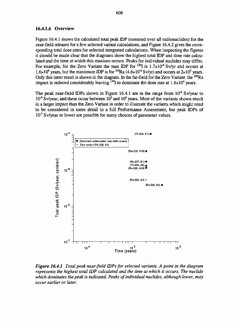
608
16.4.1.6 Overview
Figure 16.4.1 shows the calculated total peak IDP (summed over all radionuclides) for thenear-field releases for a few selected variant calculations, and Figure 16.4.2 gives the corre-sponding total dose rates for selected integrated calculations. When inspecting the figuresit should be made clear that the diagrams show the highest total IDP and dose rate calcu-lated and the time at which this maxium occurs. Peaks for individual nuclides may differ.For example, for the Zero Variant the max IDP for 129I is 1.7xlO"6 Sv/yr and occurs at1.6xlO4 years, but the maximum IDP is for ^ R a (4.6x10"6 Sv/yr) and occurs at 2x10⁵ years.Only this latter result is shown in the diagram. In the far-field for the Zero Variant the 226Raimpact is reduced considerably leaving 129I to dominate the dose rate at 1.6xlO4 years.
The peak near-field IDPs shown in Figure 16.4.1 are in the range from 10"6 Sv/year to10"4 Sv/year, and these occur between 105 and 106 years. Most of the variants shown resultin a larger impact than the Zero Variant in order to illustrate the variants which might needto be considered in more detail in a full Performance Assessment, but peak IDPs of10"7 Sv/year or lower are possible for many choices of parameter values.
10"4n
3
« 10*o
CO
a,Q
i o " 6 z
10'
(Th-229.D1)«
(Dominant radionuclide, near-field variant)+ Zero variant (Ra-226, A3)
(Ra-226,A18)»
(Np-237, E1)«(Th-230, A5) «
(Ra-226, A16)«
(Ra-226, A3) +
(Ra-226, B2) <
TTTTT
10
i—r i i i n —
105
Time (years)
i—\i T i i
10
Figure 16.4.1 Total peak near-field IDPs for selected variants. A point in the diagramrepresents the highest total IDP calculated and the time at which it occurs. The nuclidewhich dominates the peak is indicated. Peaks of individual nuclides, although lower, mayoccur earlier or later.
609
The timing of the peak IDP depends on the dominant radionuclide, but for all the variantsshown in the figure, the timing was similar. For most variants 226Ra is the dominant radio-nuclide, but when oxidising conditions prevail (El variant), 237Np can be dominant, and ifa degraded buffer (Dl variant) is considered 229Th can be dominant.
Consideration of the change in the magnitude of the peak IDP from the Zero Variant case(A3) gives an indication of the sensitivity of the near-field performance to the differentprocesses that have been considered.
The performance of the near-field is quite sensitive to the water flux, and in the case of ahigh flux of water through the system (A5 and A18 variants), the peak IDP may beincreased by a factor of around 3 and 7 respectively. The performance appears less sensitiveto the properties of the fracturing of the near-field rock (A 16 variant), with increases in thepeak IDP compared with the Zero Variant of less than a factor of around three in unfavour-able cases. Changes in the geochemistry of the system can greatly affect the performanceof the system. For example, if oxidising conditions occur in the near-field (El variant) theredox-sensitive radionuclides such as 237Np can become dominant. If the buffer becomesdegraded, even higher IDPs may result; in the variant shown in the figure (Dl variant),229Th becomes the dominant radionuclide with a peak IDP over one order of magnitudeabove the Zero Variant. This emphasises the importance of the buffer in the overall per-formance of the near-field barrier. Finally, the peak IDP is not very sensitive to changes inthe timing of canister failure (Figure 16.2.11).
The peak dose rates for the integrated calculations shown in Figure 16.4.2 are in the rangefrom 10"7 Sv/year to 1(T* Sv/year, and these occur between 104 and 106 years. As before,most of the variants shown result in a larger impact than the Zero Variant in order to illu-strate the variants which might need to be considered in more detail in a full assessment,but peak dose rates of much less than 10'7 Sv/year are possible for many choices of para-meter values.
The range of peak dose rates is similar to that shown for the near-field IDPs, because forsome parameter combinations the far-field does not significantly reduce the peak fluxreleased from the near-field. There are two clusters of points in the Figure depending onwhich radionuclides are dominant. For the Zero Variant (A3+FF0) 129I dominates, and thepeak dose rate generally occurs between 104 and 105 years. For variants where the geo-sphere performs well 129I continues to dominate, but many of the variants shown relate toparameter combinations where the geosphere performs poorly, and then ^ R a or other chaindecay radionuclides dominate and the peak generally occurs between 105 and 106 years.
Consideration of the change in magnitude and timing of the peak dose rate from the ZeroVariant case gives an indication of the sensitivity of the far-field performance to thedifferent processes considered. The transport of radionuclides which may be significantlysorbed in the far-field depend upon the hydrogeology (as represented by the F-ratio para-meter), and so overall performance of the geosphere may be sensitive to hydrogeologicalvariants. Low F-ratio variants do not result in much change to the 129I fluxes (not shown infigure), but 226Ra fluxes may increase by as much as three orders of magnitude, resultingin the total peak dose rate increasing by up to around one order of magnitude.
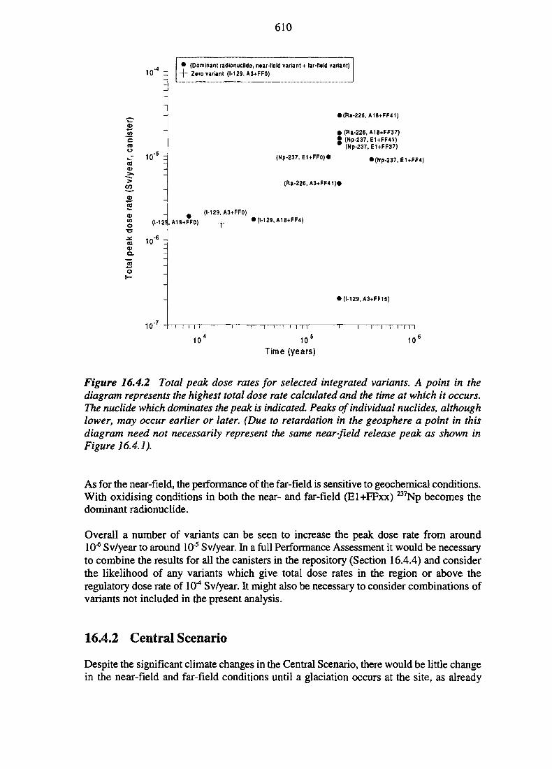
610
10" 4 n
CO
o
CO
>•»
>
CO
<DCOO
T 3
COa>a.
(1-12$
10'
* (Dominant radionuclide, near-field variant + far-field variant)- j ~ Zero variant (1-129. A3+FF0)
>(Ra-226, A18+FF41)
• (Ra-226, A18+FF37)• (Np-237, E1+FF41)
(Np-237. E1+FF37)
(Np-237, E1+FF0)*
(Ra-226, A3+FF41)*
• (Np-237, E1+FF4)
(1-129, A3+FF0)
.A1B+FF0) • (1-129, A18+FF4)
1 (1-129, A3+FF15)
I I I I I
10
"1 1—I I I T 1
105
Time (years)
i—i—i—i i i i i
10
Figure 16.4.2 Total peak dose rates for selected integrated variants. A point in thediagram represents the highest total dose rate calculated and the time at which it occurs.The nuclide which dominates the peak is indicated. Peaks of individual nuclides, althoughlower, may occur earlier or later. (Due to retardation in the geosphere a point in thisdiagram need not necessarily represent the same near-field release peak as shown inFigure 16.4.1).
As for the near-field, the performance of the far-field is sensitive to geochemical conditions.With oxidising conditions in both the near- and far-field (El+FFxx) 237Np becomes thedominant radionuclide.
Overall a number of variants can be seen to increase the peak dose rate from around10"6 Sv/year to around 10"5 Sv/year. In a full Performance Assessment it would be necessaryto combine the results for all the canisters in the repository (Section 16.4.4) and considerthe likelihood of any variants which give total dose rates in the region or above theregulatory dose rate of 10"4 Sv/year. It might also be necessary to consider combinations ofvariants not included in the present analysis.
16.4.2 Central Scenario
Despite the significant climate changes in the Central Scenario, there would be little changein the near-field and far-field conditions until a glaciation occurs at the site, as already
611
noted in Chapter 15. This means that the Reference Case results are also valid for theCentral Scenario, up to 55 000 years into the future. The subsequent glaciation periods,however, imply significant changes deep in the rock mass.
In the near-field results for the glaciation period, the most significant effect is themobilisation of "Tc and 237Np following oxidising water reaching the repository. However,the releases are significantly reduced for the assumption that the oxidising water does nothave time to penetrate through the bentonite to the interior of the canister.
The far-field peak release to the biosphere for these radionuclides increases by severalorders of magnitude compared to the integrated Zero Variant case in the Reference Case,but the dose rate would not exceed the peak for 129I, which occurs before the glaciation.This is to be expected considering the increased near-field release, the increase in Darcyvelocity and the oxidising redox conditions (which affect the Kd-values for some radio-nuclides).
In the calculations, "Tc and the 237Np in the near-field are released suddenly, because thesolubility limits increase and precipitated material becomes mobilised. In the light of this,it is worth considering whether there are any similar effects in the geosphere. In the far-field, a similar increase in mobility could occur through a reduction in sorption and/orincreases of groundwater flux. Consideration of the far-field sorption data (Table 15.2.7)shows that 237Np has a much lower sorption coefficient under oxidising conditions thanunder reducing conditions. This raises the possibility of 237Np in the far-field becomingmobile and being released at a high rate for a short time. However, the effect may not bedramatic, as only a limited amount of 237Np (and parent radionuclides) is released from thenear-field before the start of the glaciation period.
In conclusion, it appears that the main issue associated with future climate change may bethe effect on groundwater chemistry. A few thousands of years of fully oxidising conditionsappear to be sufficient to mobilise redox-sensitive radionuclides with potentiallydetrimental effects on calculated doses. Even without this geochemical effect, transientincreases in Darcy velocities may 'flush' radionuclides out of the far-field at an increasedrate and this would affect any radionuclides already present in the geosphere as a result ofearlier releases prior to glaciation. The present CRYSTAL analyses do not address thistime-dependent effect. Furthermore, the glaciation period implies a significant rockmechanical load and, even if the calculations made (Chapter 11) indicate stable conditions,this load could still be responsible for common cause failures of many canisters. However,there are numerous arguments that can be put against these concerns. The glacial load isexpected to occur in the far future (55 000 years). The possibility of oxidising watersreaching repository depths rests on speculative assumptions and the release is significantlyreduced if the oxidising conditions do not reach the interior of the canister. The biospherereceptor is probably water under the ice or sea water which provides additional dilution.Nevertheless, the results from the evaluation of the Central Scenario, in particular thelimited 2D time-dependant modelling, reflect the need to be cautious about predictions ofrepository performance in the far future.
612
16.4.3 Biosphere
For simplicity, and to facilitate the inter-comparison of results, the calculated doses andIDPs in this chapter have all been obtained using the drinking-water pathway. The bio-sphere results presented in Chapter 14 are based on an equilibrium assumption, leading tofactors for conversion from Bq/year released to doses (or IDPs) in Sv/year. It is, therefore,straightforward to rescale the drinking-water results to give doses for other pathways. Inmost cases, the drinking-water pathway is dominant. In particular, this is true for 129I and226Ra, which are the dominant radionuclides. In fact, the only radionuclide with a higherdose factor for an alternative pathway is ^Nb, but this is never significant in the calculatedresults. Thus for the Reference Case, the biosphere factors used dominate the other path-ways considered, although there is clearly room for discussion on the most appropriatedilution factors to assume for the well water.
In the Central Scenario, the biosphere results are more complicated, but the generalconclusion is the same — the drinking-water pathway is dominant. The question, then, iswhether this pathway is available at a particular time in the future. The most significantresult from the Central Scenario calculations was the potential for a sudden release of "Tcfollowing oxidising water reaching the repository. The drinking-water pathway could beunavailable because the surface is under water and, in this case, the land-rise sedimentpathway would become important. This is a factor of two lower than the drinking-waterresults (this is true for the three dominating radionuclides in the Central Scenariocalculations, i.e. 99Tc, 237Np and 234U), indicating that the drinking-water pathway stilldominates, without being over-pessimistic. It should also be noted that, since SITE-94 isnot a complete safety analysis, the selection of a well as receptor was chosen largely for thesake of simplicity and to make it directly comparable with the Reference Case calculations.
16.4.4 Combining Single-canister Variants Into Full RepositoryAnalyses1
As already explained in Chapter 15, there are no analyses of the consequences of multiplecanister failures in SITE-94. The reason for this is the uncertainty in canister properties(some of which are because the canister is still under development), which makes anyprediction of canister failure rates quite speculative. However, the release from one canisteris usually insensitive to the release from other canisters. This means that results of singlecanister analyses can usually be superimposed in order to describe the effect of multiplefailures, if there is information on the canister failure frequency.
Lacking information on the canister failure frequency, it is still possible to draw someinferences on its importance. Inspection of the results of the calculations reveals that, inmost variants analysed for the Reference Case, many canisters would need to fail between103 years and 105 years if there is to be any possibility that the overall consequence wouldbe in conflict with the radiation protection criteria discussed in Chapter 2. The exact time
1 It should be noted that the discussion in this section is limited by the fact that SITE-94 is not a completesafety analysis.
613
distribution of failures is also relatively unimportant, as most releases take place overrelatively long times.
Far fewer canister failures would be admissible if the canisters failed under oxidisingconditions at a location discharging into a low F-ratio far-field pathway. Only very fewfailures (one or two) are admissible if a degraded buffer is combined with a low F-ratiofar-field. These extreme cases would also be sensitive to a large number of early failures.
Until there is a glaciation, such an unfavourable environment for the canister is judged tobe very unlikely (but not fully impossible as discussed above) and the likelihood of itsoccurrence has to be weighed against the understanding of the canister failure mechanisms.The results of the Central Scenario analysis reveal that the risk of unfavourable conditionsincreases during a glaciation.
tut
615
17 IMPLICATIONS FOR SAFETY ASSESSMENTSOF THE STUDIED REPOSITORY CONCEPT
17.1 INTRODUCTION
The analysis of site data and the systematic way in which this and other information isorganised and accounted for, leading up to the Performance Assessment calculations ofSITE-94, have clear implications for future safety assessments of similar disposal systems.These concern the means of structuring the assessment, identification of key safety issues,site characterisation, evaluation of site specific data, and research and development needs.The detailed lessons learned will influence the way in which SKI will manage its ownevaluations of SKB safety submissions, and the guidance it will give to SKB on issueswhich it would expect to see treated in such submissions.
This chapter discusses some of the top-level technical findings of the whole of the SITE-94exercise, taking different perspectives on how they may affect future safety assessments:
• The first perspective (Section 17.2) concerns the non-quantifiable aspects of systemunderstanding and addresses questions such as the appropriateness of the systemdescription and the completeness of scenarios.
• The second perspective (Sections 17.3 and 17.4) concerns quantifiable aspects of thedifferent barriers within the system as defined in SITE-94. The discussion buildsprincipally upon the analysis of site data and the quantitative consequence modellingresults but also upon other information sources described in preceeding chapters.The discussion is organised to cover:
the features and processes that contribute most to contain the waste or toretard migration of radionuclides,
the support for concepts and parameter values relevant to these criticalphenomena that can be obtained from site characterisation and evaluation, aswell as from non site-specific sources of information, and
unquantified uncertainties of barrier performance, including judgements oninadequate models.
• The third perspective (Section 17.5) concerns Quality Assurance in a safety assess-ment.
17.2 SYSTEM UNDERSTANDING
17.2.1 System Description
The Process Influence Diagram developed within the project is believed to identify all ofthe FEPs and links that are currently considered relevant to the problem. Although this
616
picture may change with increased knowledge, only moderate revisions are likely to beneeded in the future. Clearly, the PID can never be complete, and any statement concerningthis must be judgemental. Confidence in the system description stems from the fact that thePID has been audited against a variety of international FEP lists, and considerable effortwas spent in constructing it and using it in the development of the Reference Case and theCentral Scenario.
The PID also includes an assessment, based on expert judgement, of the importance of thedifferent PID links. The adequacy of these importance levels (IJ is less defendable. Mostdecisions were made by a small number of individuals, and judgements were made bypeople working entirely within the project. A fresh perspective brought by additionalexpertise might result in substantial modifications in this area, especially in some regionsof the PID where work is currently taking place. Furthermore, no quantitative checks weremade to assess whether the omission of a particular link was indeed as unimportant asbelieved by the experts, although this could have been done if analyses had been made onversions of the PID with IL <10. Nevertheless, the open documentation of all decisions, aswell as the reasoning behind them, is intended to cope with exactly such shortcomings byfacilitating the review and updating of the importance levels. In fact, such a future reviewis considered important, as mainly links with high importance levels are considered in theSITE-94 analysis.
Another judgemental aspect in describing the system is identification of the extent of thesystem boundaries (see Chapter 2). However, during the course of the project there havenot been any grounds for reconsidering the choices made, and the wide system boundariesadopted seem to be appropriate.
V7.2.2 Scenario Completeness
In SITE-94 only limited efforts have been made to identify EFEPs that may interact signifi-cantly with the system studied. The main emphasis has been on analyses of repositoryevolution for Reference Case conditions, as well as for the time varying boundary condi-tions imposed by the Central Scenario. A shortlist of additional EFEPs which are poten-tially worth analysing has been identified (see Chapter 9). Consequently, further efforts inidentifying EFEPs and in specifying their potential impact on the system are consideredworthwhile. Many of the EFEPs suggested will only change repository evolution marginallycompared with the evolution considered in the Reference Case or the Central Scenario.Nevertheless, a qualitative assessment of potential EFEP impacts needs to be undertaken,and this would probably lead to the identification of a few additional EFEPs requiringquantitative analysis.
17.2.3 Consistency Between PID and Actual Modelling
The PID for the Reference Case, IL=10, was mapped onto the SITE-94 quantitative analysistools in the form of the Assessment Model Flowchart (AMF), in order to check to whatextent FEPs or links in the PID were taken care of in the quantitative analysis. Thismapping revealed that there were PID FEPs and links that were not properly considered.
617
In particular, issues connected with gas evolution, microbially mediated chemical processesand long-term physico-chemical behaviour of bentonite received very little attention inSITE-94, although these were attributed high importance levels in some regions of the PID.More work is needed here, at least in justifying whether or not these phenomena may bedisregarded.
There was no formal mapping between the Central Scenario PID and the associated AMF,although changes were made in the quantitative models, in order to enable phenomenaimportant for the Central Scenario to be represented. The quantitative analyses indicateimportant changes resulting from the glacial load, although most consequences are rathertransient. These results still motivate a more thorough analysis of the Central Scenario,including a revision of the AMF using the Central Scenario PID.
17.3 ENGINEERED BARRIER PERFORMANCE
In theory, the EBS, being a man-made system, should be well defined, but even with a fullyspecified manufacturing process and quality assurance procedures there will always remainuncertainties. These uncertainties may be assessed through analyses of the manufacturingprocess and the quality assurance procedures. In addition, the long term performance of theEBS will partly depend on its interaction with the geosphere. However, at the time whenSITE-94 was being conducted, neither the design of the Engineered Barriers nor the qualityassurance procedures to be put in place were fully defined and, as clearly stated inChapter 1, analyses of different designs or QA-schemes were outside the scope of the work.This is true also for the construction and operational phases and the resaturation period andtheir potential impact on the repository conditions. Consequently, SITE-94 statements onthe properties of the Engineered Barriers are provisional.
17.3.1 Spent Fuel
The rate of congruent dissolution/conversion of the spent fuel matrix controls the releaserate of many radionuclides from the EBS. In particular, the late dose peak from naturaldecay series radionuclides depends directly on the this factor. The earlier the canister fails,the more rapidly is the fuel converted by radiolytically generated oxidants. Under ReferenceCase assumptions (failure at 1000 years), the fuel is assumed to be converted completelyin 15 000 years, whereas failure after 105 years is assumed to result in a much longer con-version period of 360 000 years.
There are considerable uncertainties in modelling the combined processes of radiolyticproduction of hydrogen and oxidants, their recombination and transport, fuel oxidation anddissolution and radionuclide mobilisation, and it is currently not possible to carry out fullycoupled modelling which describes the overall effect. In SITE-94 no variants were analysedwhich reflect these uncertainties in release mechanisms or rates, although the values usedare judged to be conservative. This conclusion is also considered to be valid for the CentralScenario, as changes in the redox state of groundwaters would not change the releasemechanisms or rates from the spent fuel.
618
17.3.2 Radionuclide Solubilities
Once mobilised from the degrading fuel, the subsequent transport of radionuclides isstrongly dependent on their solubility in the various regions of the EBS. For example, underReference Case reducing conditions "Tc is largely retained in this region until it hasdecayed, owing to its limited solubility and tendency to precipitate as an oxide phase in thebuffer. The consequence analyses of Chapter 16 clearly indicate the orders of magnitudechanges in release rates for some radionuclides when hydrochemical conditions are changedto increase or decrease their solubilities. Such changes (e.g. in oxidation state of thegroundwaters in the EBS) may occur under Central Scenario conditions.
The details of how soluble a particular radionuclide may be, whether it will co-precipitateand whether it can be remobilised by changes in groundwater composition, all depend onlocal geochemical properties of the system which are expected to change with time in boththe Reference Case and the Central Scenario. In SITE-94 the need to evaluate the com-plexity of this issue has been avoided, in most cases, by adopting conservative boundingvalues of solubilities. However, the use of more tightly constrained and realistic valueswould clearly be motivated under circumstances where high releases are predicted (e.g.oxidising conditions in the EBS). Consequently, there is an impetus to refine the thermo-dynamic models (and databases) used to model solubilities and an associated need tounderstand the extent to which groundwater chemistry may change with time and scenario.
It is important to note that SITE-94 has not evaluated supplementary Scenarios (seeChapter 9) and that several of these would imply potentially significant hydrochemicalchanges. There is thus a number of reasons which give good motivation for ftirther refine-ment of geochemical models for radionuclide solubility and speciation.
17.3.3 Canister
Evaluation of the integrity of the canister shows that it is conceivable that it can have a verylong lifetime. A long canister lifetime is a key safety element for three reasons:
• it reduces the risk of multiple failures in any given time period, thereby spreadingthe distribution of failure times and reducing peak releases,
• if containment can be assured for more than about 1000 years it substantially reducesthe risk from short-lived radionuclides,
• if containment can be assured for very long times (on the order of a million years orlonger) much of the potentially hazardous inventory would have decayed andreleases would be largely dominated by natural decay series radionuclides, althoughsome very long-lived artificial radionuclides, such as 129I, 135Cs and 237Np, wouldremain in the waste.
For individual canisters the exact time of failure in the intermediate range from 1000 yearsto 100 000 years is not very crucial for the peak release rate. However, it is not acceptablefor all the containers to fail simultaneously or for many of the containers to fail early, in
619
particular if all failures happen to occur at unfavourable positions in the repository (seeChapter 16). SITE-94 has not specifically addressed the question of common-cause canisterfailures, but, as noted by SKB in their RD&D Programme 95 (SKB, 1995), the question ofhow well canisters should withstand the increased pressures resulting from glacial loadingis an outstanding design issue. Clearly, such a mechanism has the potential to producecommon-cause failures unless canisters are designed to withstand these pressures.
Evaluation of copper corrosion supports the view that general corrosion of the canister willtake a very long time. However, a number of uncertainties surround the performance of thecanister, not least of which is the lack of information on its final design and properties aswell as details of the techniques to be used for emplacement and buffer application. Untilthese issues are resolved, and quality-controlled specimens and the results of full-scale testsare available, much of the discussion on container behaviour will remain incomplete.
Other uncertainties concern the hydrochemical environment and how this will change,particularly under the conditions of the Central Scenario and alternative localised corrosionmechanisms. Various possible geochemical equilibria in the buffer porewaters could affectcorrosion rates and mechanisms.
Much of the previous understanding of anticipated canister performance relates to thecopper canister of the KBS-3 concept, and little is known about the changes in behaviourof the copper/steel container. The performance of the canister will remain a significantsource of uncertainty in any assessment of this disposal concept at the present time. InSITE-94 this has been mitigated by making bounding, pessimistic assumptions in theReference Case. However, given that this is a single canister analysis and given theuncertainties surrounding failure time distributions, a wide range of potential 'fullrepository' impacts could easily be presented. Given present knowledge it would bedifficult to demonstrate which of these ought to be considered pessimistic. This arearequires more development work and closer analysis.
17.3.4 Buffer
The buffer is a key component of the EBS, controlling the migration of corrodents to thecanister, the rate of migration of radionuclides into the rock and providing mechanicalprotection for the waste package. However, one should note that, at least for some radio-nuclides, the release from the near-field is governed more by the release rate from the fuelthan by diffusion in the bentonite buffer.
In the SITE-94 consequence analysis a large part of the retardation of transport through thesystem is provided by the EBS and the buffer in particular. The mass balance calculationssummarised in Figure 16.2.3 demonstrate how many significant radionuclides effectivelynever leave the EBS and the near-field rock (modelled with the CALIBRE code). Forexample, under Reference Case Zero Variant conditions only about \%o of the "Tcinventory and the 4N natural decay series chain have been released from the near-field. Thehigh near-field releases of many important radionuclides, for example 240Pu, 241Am and229Th, for the degraded buffer variants illustrate the high relative importance of the bufferin the EBS (see Figure 16.2.10).
620
Uncertainties in buffer performance concern the most appropriate values of effectivediffusivity (Dc). In SITE-94 there is discussion (see Section 8.3.3.2) as to whether thevalues used in the consequence analyses are sufficiently conservative. Similar uncertaintysurrounds the choice of values for sorption parameters; for example, whether these shouldbe derived from batch disaggregated samples or intact material. However, the mostimportant migration controlling property of the buffer is that it provides an effective barrierto advective flow close to the fuel elements. Release from the near-field would increase bymany orders of magnitude for many radionuclides, if such flows could occur.
SITE-94 looked at some aspects of the internal chemical evolution of the bentonite and itsporewaters, but no work has been done on its mechanical evolution and interaction with thecanister, on gas migration, or on its behaviour under the changing hydrochemical and rockstress conditions which would be experienced under Central Scenario conditions. Further-more, there has not been any assessment of the engineering aspects of buffer emplacementand the resulting swelling sequences. To some extent these uncertainties have been circum-vented in the consequence analyses by addressing the degraded buffer variants (seeSection 15.2.2.4). As noted in Section 16.4.1.4, the high radionuclide fluxes produced whenthe degraded buffer variants are combined with certain far-field flow situations indicatesthat these uncertainties in buffer evolution need to be resolved.
17.3.5 Backfill and Sealing System
SFTE-94 presents no new evaluation of the performance of the backfill and sealing systemsor of the associated uncertainties. However, it is possible to draw attention to a few recog-nised safety-related issues where further work is required:
• the extent and hydraulic properties of the excavation damaged zone caused indifferent regions of the repository by the excavation techniques eventually used,
• the local impacts of cementitious materials if they are used close to or within thedisposal tunnels,
• the long-term geochemical and hydraulic evolution of bentonite-crushed rockbackfill,
• the behaviour of seals and plugs under the high rock stress and hydraulic gradientconditions associated with the Central Scenario.
17.4 GEOSPHERE PERFORMANCE
In general, SITE-94 results support the view expressed by SKB in their RD&D Programmesthat the main safety features of the geosphere are to provide a stable and suitable chemicaland mechanical environment for the waste and the EBS and to provide significant retentionfor the radionuclides eventually released from the EBS. In order to determine which geo-sphere processes and properties are the most important to provide these desired functionsit is necessary to assess the extent to which they can be supported by common knowledge
621
and site specific data. For this reason this section starts with a discussion of lessons learnedfrom the site data evaluation, in particular where sources of uncertainty were identifiedwhich would feed through into consequence analysis. Following this is an evaluation of theimportance of the geosphere from different perspectives.
17A.I Site Characterisation, Uncertainties and Understanding ofthe Site
The overall aim of the site data analysis and model development has been to obtain thenecessary support for the basic assumptions regarding geosphere stability and, morespecifically, to provide support for the conceptual models and parameter values thatdescribe the system components. In order to meet this aim a key aspect of site evaluationis to seek an understanding of the geosphere system at the site based on integrated inter-pretations of the structural geology, hydrogeology and geochemistry. However, an overallunderstanding of the site would usually not be sufficient for abstracting conceptual modelsand parameters for the consequence analysis; direct evaluations of data and uncertainty aregenerally needed.
17.4.1.1 Site Characterisation Data Usage
In SITE-94 analysis of all the measured data from the surface-based site investigation wasattempted, considering simultaneously issues affecting geology, rock mechanics, hydro-geology and geochemistry. The following observations can be made:
• The practicability of handling the large amount of information involved was sub-stantially improved by the application of three-dimensional graphical presentationsoftware. Such software made it possible to visualise measurement values andlocations, and thereby to test hypotheses for different structures.
• It was possible to produce a site model that was consistent with most data, but it wasalso clear that despite the large amount of information used, it was not possible toarrive at a unique representation. In terms of field evidence, it appears that the linksbetween geology, rock mechanics, hydrogeology and geochemistry are rather weak.
• Large scale regional hydrogeological modelling of past groundwater flow (palaeo-hydrogeology) provided plausible explanations for the salinity distribution of the siteand also provided plausible boundary conditions for the more detailed scalemodelling.
• A successful search was made for the origins of different groundwaters. The use ofchemical imprints enabled the formulation of a plausible model for different ground-water compositions at the site which were not in conflict with the general conceptof past groundwater movement. These analyses increased the confidence in thegroundwater composition used as input (to solubility and Kd-values) for the radio-nuclide release and transport calculations.
622
• A large quantity of basic hydrogeological data including pressure and water-levelmonitoring data, packer-test data, flowmeter logging data and interference test datawere available and were used intensively in the construction, calibration and testingof the various hydrogeological models. Despite this, considerable uncertaintyremains regarding the hydraulic connectivity between different positions in the rock,which had to be addressed by using different conceptual models. In addition, theclustering of measurements within a relatively small area results in significantuncertainties on the semi-regional scale, which had to be addressed by analysingmultiple model variants.
• In essence there was no information regarding the local relationships amonghydrogeological parameters ('permeability distribution', 'flow paths', 'flow wettedsurface') and the retention properties of the rock (matrix porosity, diffusivity andsorption properties), leading to a major uncertainty in the estimation of the effectiveretention properties ('F-values') along the leading migration paths in the geosphere.
• There were no measurements of large scale rock mechanical properties (strength anddeformation characteristics). These had to be estimated making inferences fromsmall scale data (i.e. pure extrapolation).
• In the groundwater flow modelling SITE-94 assessed the non-sorbing tracer testscarried out in the Aspo project and thereby confirmed some of the hydraulic connec-tions in the Discrete Feature model. However, the judgement was made that thesetracer tests could not provide essential information (or possibility for validation) formodels of radionuclide retention in the geosphere.
Although nearly all of the available and relevant site data have been taken into account insome part of the SITE-94 analysis, no single model or line of analysis leading to quanti-tative predictions of geosphere performance has made comprehensive use of all the relevantdata.
It should also be noted that in some cases mentioned above, there is a lack of relevant site-specific information, and in other cases uncertainties in site properties were impossible toexplore due to lack of any relevant field information. Given the central importance of someof these properties, as will be further discussed in the following subsections, this is asignificant residual issue for both site characterisation and Performance Assessment whichneeds to be resolved by further work or at least fully factored into the analysis. Conse-quently, the lessons learned in SITE-94 should have implications for the planning of futuresite characterisation programmes. Even if feedback from Performance Assessment may notindicate precisely what to search for at a site, it clearly identifies important information thatcould not be obtained from the analysis of the data available in SITE-94.
17.4.1.2 Uncertainties
When making detailed predictions of the state and evolution of the geosphere it is necessaryto acknowledge the uncertainties in such predictions. Uncertainty arises due to
623
the (partly) unknown past evolution of the site and the future development ofboundary conditions,
the spatial variability over many scales of important site structures and properties,
the inability to quantify some processes, parameters or structures because they arenot captured or because the spatial resolution of the measurement is unsuitable.
These uncertainties manifest themselves in the form of conceptual model uncertainty andparameter uncertainty.
Due to the pronounced heterogeneity in crystalline rock and the limitations of the site data,it is often possible to formulate alternative conceptual models that fit the site characteri-sation data. To some extent, the validity of alternative conceptual models can be evaluatedby calibration using one data set and validation using another data set. Analysis of con-sistency between different site models, e.g. for hydrogeology and geochemistry, may addadditional information for model discrimination. However, in many cases the site charac-terisation data do not contain critical information for conclusive discrimination betweenalternative conceptual models. The envelope of alternative models is thus a measure ofconceptual uncertainties in the description of the site.
Such conceptual uncertainty is a concern if different models predict different behaviour ofthe site when extrapolated to the temporal and spatial scales that are being considered inthe safety assessment. Furthermore, it is often difficult to determine, a priori, whether acertain conceptual model is realistic, or even conservative, in terms of impact on the conse-quence calculations. The strategy adopted in SITE-94 has therefore been to developalternative conceptual site models for site hydrogeology and to propagate the resultsthrough the assessment.
17.4.1.3 The Nature of Crystalline Sites - Results from Integrated Evaluations
The following is a summary of the main findings regarding the nature of the site that arerelevant to the Performance Assessment. Although derived from the analysis of the Asposite, they are presented in a generic manner, as they are likely to be applicable to mostpotential repository sites in the Swedish basement.
• The regional groundwater flow field and its temporal variation is a key to under-standing the overall groundwater flow regime and the geochemical conditions at asite. For example, Aspo appears to lie in a regional discharge area, with waterflowing generally eastward and upward. The water chemistry is stratified, fromrecharge water near the surface to brines at depth, with local pockets of relict glacialmeltwater, and seawater near the periphery of the island. A thorough understandingof how this system has arisen and what has controlled its evolution is a pre-requisitefor site scale flow and hydrochemical modelling.
• The hydrogeological analyses indicate that many site-scale fractures and fracturezones act as distinct, significant hydraulic conductors (for pressure propagation andflow), giving rise to a complex hydrogeological system which is only partially
624
defined by the site-investigation data, Transport pathways for radionuclidestravelling from failed canisters to the biosphere will most likely follow portions ofone or several of these structures over most of the path length.
• The bedrock, excluding these site-scale fractures and fracture zones, is variablyfractured on a range of scales and includes a substantial population of extensive,interconnected water conducting discrete fractures. Heterogeneity, with respect tofracture intensity and network connectivity, is present both within and betweenlithological types. Site-characterisation data may not be sufficient to ascertain theeffects of this heterogeneity on hydraulic connectivity on the scale of tens of metres(the relevant scale for radionuclide migration from a single canister failure). Thiswas the case in S1TE-94, and multiple conceptual models were used to address thisissue and to analyse the consequences of alternative assumptions regarding connec-tivity.
These overall findings form the basis for the more detailed modelling of geochemistry, rockmechanics, hydrology and retention properties, which are needed for the consequenceanalysis. However, as stated in Chapter 7, an integrated assessment of all available soft andhard data in an overall site evaluation, combined with applications of specialised quanti-tative models, is a key to making Performance Assessments truly site specific.
17.4.2 Hydrogeology
Predictions of groundwater flow have two major functions in Performance Assessment.Understanding the overall, regional, groundwater flow is necessary for defining the longterm stability (and evolution) of the geochemical conditions at the site and for definingboundary conditions for site-scale models of groundwater flow. Groundwater flow is alsothe main, and in SITE-94 the only considered, potential migration pathway for radio-nuclides from the repository to the biosphere.
17.4.2.1 Long Term Evolution of Groundwater Flow
The S1TE-94 analyses demonstrate the importance of a regional, chemically coupled andtransient analysis of the long term evolution of the groundwater flow at a site. Under-standing of regional connective structures, past and present boundary conditions, presentsalinity distributions and the origin of salt in the groundwater are key to successfulmodelling. Details of the hydraulic properties of a site are here of less significance.
The information available for SITE-94 made it possible to undertake plausible regionalscale hydrogeological modelling, which indicated rather stable hydrogeological (and geo-chemical) conditions at the site over very long times, but with important deviations fromthese stable conditions in the event of glaciations. It must be borne in mind, however, thatassumptions on the origin of the salt, on hydraulic properties on a regional scale, and onpast and future changes in boundary conditions are speculative; in many cases there wereno data available to provide quantitative support for the predictions made. If more reliablequantitative predictions were needed it would be necessary to obtain hydrogeological and
625
geochemical data at depth on a semi-regional and regional scale, although the need fordetailed spatial resolution would be far less than for the repository region.
17.4.2.2 Groundwater Flow as Input to Models for Radionudide Migration
In order to specify hydrogeological input parameters for radionuclide release and transportmodels it is necessary to deal with the problem of spatial variability. Not unexpectedly,field data strongly suggest significant spatial variability in the groundwater flow at the scaleof individual deposition holes, and modelling suggests a strong variability between flowproperties in streamtubes (on this scale) from the repository to the environment.
The site data are sufficient to define a large number of large structures (fracture zones) inthe vicinity of the SlTJa-94 repository, where the sampling density was relatively high.However, the geological and hydrogeological analyses indicate that there are additionalstructures in this vicinity, which have not been identified. Moreover, due to the lowerdensity of information over the remainder of the site, it can be assumed, that a large numberof structures have been missed within 1-2 km of the repository. Thus, the actual configu-ration of structures is likely to be even more complex than has been represented in theSITE-94 structural model. This uncertainty in the structural model has been addressedthrough the use of specific variants in the hydrogeological modelling.
Data on fracturing and hydraulic conductivity (mainly based on injection test data) aresufficient to estimate the high degree of heterogeneity (spatial variability) which is present.However, the types of data that were available did not give much information on the spatialorganization of this heterogeneity. This leads to crucial uncertainties regarding connectivity,and hence to the properties of potential radionuclide transport pathways, in the far-fieldrock. Due to lack of specific information about hydraulic connectivity within the fracturedrock outside the designated structures (fracture zones), the variability had to be describedwith different conceptual structure models. Rough estimates of the variability anduncertainty may be obtained from simplistic reasoning, but more complex model analysesare also needed. The SITE-94 analysis shows how different concepts such as DiscreteFeature models and Stochastic Continuum models may be successfully applied to field data.
The full range of uncertainty and variability did not differ too much between the morecomplex site models or the first, simplistic uncertainty estimates. However, the potentialadvantage of the complex models is that they describe the spatial variability separately fromthe uncertainty. Judging from the Aspo data it is clear that pronounced spatial variabilityin hydraulic conductivity might be encountered at a potential repository site. In analysingconsequences from a single canister failure such information may be of little more use thanjust knowing that the flow is uncertain. However, in the case of multiple failures it may bepossible to make use of the information of spatial variability, since the number of "poor"canister positions is limited. In addition, the information could potentially be used as aninput to design and engineering. Consequently, information on spatial variability may beimportant for judging the suitability of a site. Furthermore, application of the complexmodels provides a means to explore whether other types of field measurements wouldreduce uncertainty.
626
The Discrete Feature site model tends to produce higher near-field flows and moreuncertainty than the Stochastic Continuum site model, but the two models generally predictrather similar flow variability and variability in the far-field performance measure, F-ratio,when all parameter uncertainty is taken into account. However, when comparing these twomodelling concepts one should keep in mind that in the Discrete Feature model only afraction of the canister sites are hydraulically connected to flow. Hence, the higher near-field flows in this model may be of less significance , at least for multiple canister failureanalyses, than the fact that a large number of canisters are predicted to be hydraulicallyisolated.
The Discrete Feature site model utilises most of the available hydraulic and structural dataof the site. In addition, it has the advantage that it can be used to extrapolate transportproperties in a way which is consistent with the assumptions made on fracture geometry.In comparison the Stochastic Continuum model incorporates less of the fundamental sitespecific data on hydraulic structure, but has a principal advantage in the ease with whichdifferent realisations can be conditioned on the measured 'point' hydraulic data. However,because the hydraulic data alone were incapable of providing reliable information on thecorrelation structure, this was inferred (i.e. postulated) by a qualitative assessment of thestructure data. Data needed to reduce the prediction uncertainty is discussed in conjunctionwith the discussion of far-field radionuclide transport (Section 17.4.5).
In transferring the uncertainty and the variability in the hydrogeological site description toparameters of interest for radionuclide release and transport it became clear that a criticalparameter, showing significant variation between different migration paths, is the ratiobetween the flow wetted surface area and the groundwater flow rate (the F-ratio). Thisvariability (and uncertainty) has important implications for making meaningful predictionsof the retention properties of the site (see Section 17.4.5). However, many site uncertaintiesseem to be of minor significance for these predictions. For example, different structuremodels were tried but did not really result in different retention properties of the far-field.
There are simplifications made in the abstraction process from complex three-dimensionalmodels to the simplistic one-dimensional models used for radionuclide migration, and itmay for example be questioned whether the spatial variability of flow and chemicalproperties along the streamlines are properly averaged. However, given satisfactory hydro-geological and geochemical models for the site, abstraction of parameters for radionucliderelease and transport calculations is a minor problem, at least if attention is given to makingestimates at the relevant scales (i.e. deposition hole scale and not repository scale) and todistinguishing between spatial variability and uncertainty. The methods used in SITE-94are considered appropriate although, if resources were available, an evaluation of theabstraction errors would be possible and worthwhile.
17.4.3 Geomechanical Environment of the Repository
The main reason for evaluating the mechanical stability of the rock in the repository regionis to ensure the mechanical stability of the canister deposition hole in the future. Indeed theresults of rock mechanical analyses also suggest that the canister deposition holes willremain mechanically stable both for the Reference Case and the Central Scenarioconditions, but there are uncertainties regarding the site properties that need attention. In
627
addition, rock mechanical effects may change the state of the geosphere and consequentlythe conditions for groundwater flow. A rock mechanical analysis needs to ensure that suchchanges would not be significant for the assumptions made in the consequence analysis.
17.4.3.1 Long Term Stability
In the future the rock will experience events that may affect mechanical stability. On a largescale SITE-94 includes an evaluation of the impact of repository heat, permafrost andglacial loads. On the near-field scale, the additional effects of excavation and bufferswelling are considered.
The analyses do not suggest significant deformation of the deposition holes or the reposi-tory during any of the analysed events, although there is a need to pay attention to thelocally increased stress levels due to repository heat, which occurs rather soon (200 years)after emplacement, and the significant glacial load. Furthermore, the quality of the stabilitypredictions may be questioned because of significant uncertainties in the rock mechanicalproperties of the site (see Section 17.4.3.2 ).
The analysis of permafrost depth in the Central Scenario made it possible to conclude thatthe repository will not freeze. Permafrost may, however, have implications for the stabilityof shaft seals close to the surface.
The rock mechanical modelling showed that both thermal loading and glaciation may createlocal instability of intact rock in the walls of the tunnels and deposition holes, possiblefracture propagation and coalescence at some locations near major faults or fracture zonesand changes of water flow pathways. The predicted shear displacements were small,however, and they will have a negligible impact on the stability of the tunnels and thedeposition holes.
Complex stress states and stress orientation occur in the rock during a glaciation, especiallyat the intersections of fracture zones. The risk of a global fracture propagation due to highvertical ice load is however small.
Fractures undergo cyclic deformation involving closing and opening during the loadingsequence starting with excavation, followed by the swelling pressure of bentonite, thermalloading and, finally, glaciation, but the modelling results indicated that the effects arerelatively small. Nevertheless, such changes directly affect the permeability distribution ofthe rock, implying that the potential migration paths will change location as the rockdeforms. However, there will probably not be any significant changes in the overall magni-tude of the permeability.
17.4.3.2 Uncertainties
There are uncertainties associated with the rock mechanical analysis of SITE-94,concerning system definition, the conceptual models and the parameter values selected.Some links in the Process Influence Diagram relevant to rock mechanics are not analysed.Both the far-field and the near-field analysis omit the hydraulic coupling. The importance
628
of such an omission is being evaluated in current research and development work such asthe international DECOVALEX study.
Examples of concerns regarding the rock mechanical modelling include the fact that thefinite dimension and large scale undulations of the fracture zones were ignored, that stressconcentration artefacts could occur at sharp corners of fracture intersections, that creep wasnot considered and that the model used was too simplistic to describe properly the failureof the rock matrix and fractures. However, the major difficulty for the study was theuncertainty about the properties of fracture zones and the rock mass at the Aspo site. Inparticular, there was no analysis of the potential significance of spatial variability of suchproperties. For example, increasing the strength of major structures may have the effect ofenhancing failure of less pronounced features.
There may also be scope for further work on dynamically coupled processes, for examplehydromechanical impacts of high ice loads combined with high hydraulic heads andenhanced flows at depth in the Central Scenario. The overall impact of this scenario ondeep fracture behaviour is not yet well understood.
17.4.4 Geochemical Environment of the Repository
The geosphere is predicted to provide stable groundwater chemical conditions in theReference Case. Aspo groundwaters are generally low in dissolved oxygen and high insulphides, which implies reducing conditions. As already mentioned, the regional scalehydrogeological modelling has provided support for the assertion that groundwaters foundat depth at Aspo today are a good representation of the future geochemical conditions at thesite. However, calculations for the Central Scenario indicate a possibility for oxygenated,glacial meltwaters to infiltrate to repository depths during future glaciations, which mighthave a number of deliterious effects on the performance of the EBS and on the mobility ofsome important radionuclides.
Geochemical redox conditions are very important for the barrier properties, as they affectboth solubilities and sorption. Variations in redox conditions in the near-field may lead toorders-of-magnitude changes in solubilities, which correlate directly with radionuclide flux.The influence of redox conditions on distribution coefficients (Kd) has a moderatelysignificant effect on the retardation of the more strongly sorbing and relatively short-livednuclides, e.g.241 Am, 240Pu, 245Cm, and 246Cm. No analysis was made of the geochemicaleffects of desaturation (drawdown) and resaturation during the repository constructionphase.
Characterisation of the 'undisturbed' distribution of geochemical groundwater types islimited to some extent by the sampling methodology that was employed at Aspo. Most ofSKB's efforts in gathering (and interpreting) chemical and isotopic data were focussed onsamples obtained either after extensive pumping had been conducted or even duringpumping tests. This extensive pumping, conducted for hydrogeological testing purposes andfor the removal of drilling water, resulted in a significant in-situ dilution and homo-genisation of the groundwaters. Although extensive pumping was clearly needed in orderto offer meaningful interpretation of measured Eh and pH values and of measured concen-trations of redox-active minor constituents (Fe, Mn, HS"), the concentrations of many
629
relatively unreactive constituents such as sodium, calcium, magnesium and potassium wererelatively unaffected by the admixture of shallow dilute drilling waters. The concentrationsof these elements, once corrected for drilling-water content, were very useful in identifyingsome characteristics of the groundwaters originally present in the system. More thoroughidentification and analysis of drilling water sources and content would be helpful inextending the scope of such analyses.
Deuterium and 18O analyses were valuable in identifying the origins of the groundwaters.However, such identification could potentially be made much better had these data beensampled very early and to a larger extent. Such data, bromide, and perhaps lithium andstrontium concentrations, in combination with the chloride concentrations that wereactually measured, would have revealed much more about the origin of solutes in thegroundwaters.
17.4.5 Radionuclide Migration
17.4.5.1 Near-field Rock
All conceptual models and variants used to predict groundwater flows in the near-field rocksuggest that there will be large spatial variability in Darcy velocities in the rock surroundingthe canister deposition holes. This may be an intrinsic property of many sites in similargeological environments. This variability will clearly affect the relative performance of theEBS in individual deposition holes. Also the flow wetted area, fracture aperture andfracture spacing in deposition holes are subject to spatial variability. However, these varia-bilities have been shown not to be crucial for near-field radionuclide migration, althoughthis may be a consequence of the simplifications made in the near-field transport models.
The two other key uncertainties affecting radionuclide migration in the near-field are thelong-term evolution of buffer properties and the lifetime of the canisters, both of whichhave been discussed earlier in this chapter.
The Central Scenario implies potential transient changes to both near-field water flux andchemistry. Depending on assumptions about how much of the EBS is exposed tooxygenated waters, these conditions may have only small impacts (relative to the ReferenceCase) or very marked impacts, specifically on releases of "Tc and 237Np. If the canisters areexposed to oxygenated waters then the whole Tc inventory might be released from the near-field during the period of a glaciation. This suggests that further work on understanding theextent to which the EBS might be buffered from such effects would be well motivated.
Two aspects of the PID that were not addressed in S1TE-94, and which may affect near-field radionuclide migration, are gas generation and colloids. The former may affect thephysical properties of the buffer and potentially lead to advective transport through thebentonite or gas bubble entrainment of solutes. Colloid transport through the buffer isunlikely, except in the circumstances just described. However, colloidal species whichcould complex with radionuclides might be formed at the buffer-rock interface, particularlyin the event that a redox front is present in this region. Both these issues require furtherstudy.

630
17.4.5.2 Far-field Rock
For weakly- or non-sorbing radionuclides such as 36C1 and 129I, the retention time afterescaping from the EBS is essentially determined by groundwater transit times from therepository to the surface. Due to the regional discharge under present-day conditions,groundwater travel times for the Reference Case tend to be short. Depending uponconceptual and parametric uncertainties and spatial variability within the site, groundwatertransit times may range anywhere from millennia down to a few decades.
For the more strongly sorbing elements such as Pu and Th the geosphere provides apotentially significant barrier to migration. For the set of conditions corresponding to theReference Case Zero Variant, both the near-field and far-field portions of the geosphere arepredicted to be significant barriers, due to the retardation of radionuclide migration by thecombined mechanisms of sorption and matrix diffusion. However, the effectiveness of thegeosphere as a barrier, in this respect, is critically sensitive to various uncertainties thathave been evaluated in the hydrogeological models and will also strongly depend upon thelocation of the failed canisters.
As shown in Section 13.5.2, this sensitivity can be discussed in terms of two parameters,the Peclet number and F-ratio (defined in Section 10.3.2.5), which summarise the essential,non-chemical characteristics of a given hydrogeological variant and pathway for far-fieldradionuclide migration. Of the two parameters, the Peclet number is of secondary import-ance. Variants and individual pathways with high F-ratios represent cases in which the far-field acts as a very significant barrier, while those with low F-ratios represent cases inwhich the far field provides an insignificant barrier. According to the hydrogeologicalanalyses described in Sections 7.3 and 10.3, a very wide range of F-ratios can result withinthe evaluated bounds of system uncertainty. This wide range results from the variability anduncertainty in the distribution of flow paths, as described by the hydrogeological models,and the lack of data on the detailed fracture characteristics, which affect the relationbetween Darcy velocity and flow wetted surface along these flow paths.
The spatial variability of hydrogeological properties within the Aspo site is a majorinfluence on prediction uncertainty with respect to geosphere performance. Despite the highdensity of fracture zones in the SITE-94 geological structural model, hydrogeologicalanalysis (Section 7.3.6) indicates that uncharacterised, conductive structures account for amajor proportion of the points where significant flow is observed in boreholes. Thismotivates the use of semi-stochastic, hydrogeological models which can estimate the conse-quences of incompletely characterised spatial variability. Two general types of such modelshave been employed in the hydrogeological analyses for SITE-94: stochastic-continuum anddiscrete-fracture-network models. Both types of models predict that the spatial variabilityof the Aspo site results in variability of migration-path hydrogeological properties, whichis comparable to the effects of the evaluated sources of uncertainty. The consequence is thatthe effectiveness of the geosphere as a barrier to radionuclide release will be highlyvariable, depending upon the location of a failed canister within the repository.
A key conceptual uncertainty, which is addressed by use of the stochastic model variants,is that the available site data do not support discrimination with respect to the large-scalecorrelation structure as well as the interrelationships between hydrogeological and transportproperties. In the Stochastic Continuum model these uncertainties are expressed in terms
631
of the spatial correlation of hydraulic conductivity and assumptions regarding its relation-ship to flow wetted surface area and porosity. In the Discrete Feature model the sameuncertainties are expressed in terms of models for heterogeneity and correlations betweenhydrogeological properties within major fracture zones and individual fractures. Despitethese apparently different data needs the two model approaches would, in fact, need verysimilar data in order to reduce the prediction uncertainty. In particular, tracer tests, withsorbing and non-sorbing tracers on a range of scales, in combination with data from detailedcharacterisation studies of single transmissive features, appear to be an important com-ponent in order to achieve such reductions.
The Sllb-94 analysis concentrated entirely on sorption in combination with matrix diffu-sion as a far-field retardation mechanism and did not evaluate sorption on the spatiallyvarying mineralogy of fracture surfaces. Whilst this may be conservative, the case is notstrong, as there may be circumstances in which fracture coatings 'armour' the flow wettedsurface and prevent matrix penetration.
Matrix porosity, diffusivity coefficients and data on mineral assemblages (to support valuesfor sorption coefficients) are fairly well known from generic data, and are supported byanalyses of Aspo cores. However, a more complete database of these parameters, whichwould allow determination of their spatial variability and ideally of their correlation withthe actual flow paths in the rock, should be developed during site investigations of potentialrepository sites.
Colloids may affect far-field radionuclide migration much more effectively than in the near-field and, as noted in the previous section, analysis of this issue was omitted in SITE-94.
Finally, it is recognised that far-field radionuclide transport and release under CentralScenario conditions is considerably enhanced over that for the Reference Case. The limitedtime-dependent analysis carried out in SITE-94, suggesting episodic releases, changingbiosphere receptors and 'knock-on' transient effects on the amounts of radionuclides 'intransit' through the far-field, points to the necessity for more detailed studies of this type.
17.5 QUALITY ASSURANCE
Good Quality Assurance will be an important aspect of the design, construction, operationand closure of a repository. It is also an important foundation of safety assessment, ensuringthat analyses are comprehensive, traceable, repeatable and credible. Any regulatory sub-mission would be expected to be supported by a well tried and tested QA system,particularly allowing reviewers to assess the quality and validity of all the data used by theapplicant and required for use in any independent assessment by SKI. It is important torealise that the 'audit trail' would need to extend back in time to cover all data that mightbe used in an assessment, and it will thus not be adequate to apply QA at a late stage of theprogramme. Information abstracted from early projects where no QA was applied must betreated in a qualified manner. Where such information relates to clearly sensitive aspectsof a submission, it is unlikely that it would be regarded as adequate without properly QA'dsupporting data.
632
There was no formal work in SITE-94 directed at setting in place a QA procedure for usein an assessment. However, the PA methodology developed, and the enhancement of thetraceability of information flow from site characterisation data to consequence calculations,will form a useful basis for data management and decision tracking. The major advancesin these areas are briefly discussed here. SITE-94 has thus begun to contribute someimportant Quality Assurance tools.
17.5.1 Recording of Decisions, Judgements and Routesof Information Transfer
With regard to the PA-methodology developed the following activities were particularlyuseful:
• Development of the Process Influence Diagram which allows for an explicitdocumentation of the system identification. This explicit procedure should enhancecomprehensiveness as it enables communication between different experts. Further-more the PID could be used to audit existing analysis tools.
• Development of the Assessment Model Flowchart, AMF, which allowed an explicitdescription of the information flow between models and expert interpretationgroups. The AMF could be audited with the PID. Evaluation of the AMF structurecould potentially be used to identify bottlenecks in the information transfer. TheAMF identifies suppliers and users of data in terms of Clearing Houses and therebyhighlights the need for interaction and even negotiations between suppliers andreceivers of information.
• Meetings within the Clearing Houses that had the main responsibility to supplyparameters to the radionuclide release and transport calculations. This work, whichis documented in Chapter 15, should ensure consistency between delivered andreceived data.
17.5.2 Traceability of Site Specific Information
Major efforts have been made to improve the link between measured data and the use ofthese data in Performance Assessment. The following lessons have been learnt with respectto Quality Assurance:
• Care has been taken to record data sources and to document analyses as well as morejudgmental assessments of these data. This effort, however tedious, highlightedthose data that were really used, those data that were not used and areas where thereis little information to support judgements. Such information appears to be crucialfor the planning of a site characterisation programme and for SKI when evaluatingthe adequacy of such programmes.

633
• Assessing the SKB field data bases also revealed problems in how to represent suchdata in an efficient and reproducible form for users other than SKB staff. Suchlessons have been passed on to SKB during the course of the project.
• Joint meetings between the experts in geology, rock mechanics, hydrogeology andgeochemistry were conducted in order to develop a model of the site which wasconsistent for all these disciplines.
In summary, it was found that careful documentation of the actual use of data is certainlyworthwhile.
."XT'left
635
18 CONCLUSIONS
The SITE-94 project has run for three years from August 1992 to 1995, with the final inte-gration and reporting taking place during 1996. Besides the technical findings and develop-ment, SITE-94 has given SKI valuable experiences regarding management of a fullPerformance Assessment. Although the basis for SKI's Performance Assessment capabilitywas founded on SKI's previous Performance Assessment project, Project-90 (SKI, 1991),the step to a site-specific Performance Assessment, like SITE-94, has involved a great dealof time consuming development work. Any organisation going from generic to site specificassessments is likely to face similar challenges, which points to a need for applying andevaluating Performance Assessment methodology using site specific data at the early stagesof a waste disposal programme.
Whilst by no means a complete safety assessment of a repository system, the exercise ofcarrying out and reporting the SITE-94 project has provided SKI with some importantbenefits. In particular, it has:
• Permitted some major technical advances in Performance Assessment methodology,i.e. evaluation and assimilation of site characterisation information and the treatmentof uncertainties and scenarios. These have provided SKI with methodologies (theProcess Influence Diagramme and the Assessment Model Flowchart) which werenot previously available either in the Swedish national programme or from otherradioactive waste management projects abroad.
• Identified clearly some of the most significant issues in preparing and justifying asafety case. This will assist in defining what SKI expects of SKB in a future licenseapplication and the emphasis which will need to be placed on each issue.
• Clarified the capabilities of SKI and the tools which it has available, in terms of itsability to respond to a regulatory safety submission.
• Identified topics where further work is required either by SKI or SKB to sort outresidual technical issues.
These four concluding topics are discussed in the following sections.
18.1 MAJOR TECHNICAL ADVANCES
18.1.1 Methods for Site Evaluation and Treatment of Uncertainty
A key theme of the project has been to determine how site specific data should beassimilated into the Performance Assessment process and to evaluate how uncertaintiesinherent in site characterisation will influence Performance Assessment results. In part thishas been an in-house learning exercise, as SKI did not have any experience of handlingfield data, but several conclusions can be made which should be of interest to a widertechnical community.
636
18.1.1.1 Traceability of Site Specific Information
Major efforts have been made to improve the link between measured data and the use ofthese data in Performance Assessment. It is evident that only on rare occasions are fielddata used directly in radionuclide release and transport calculations. Instead, the 'raw' dataare interpreted by experts in geology, rock mechanics, hydrogeology and geochemistry, whothen provide interpreted or manipulated parameters for the consequence analysis calcula-tions. Care has been taken to record data sources and to document analyses as well as morejudgmental assessments of these data. Such information appears to be crucial for the plan-ning of a site characterisation programme and for SKI, when evaluating the adequacy ofsuch programmes.
18.1.1.2 Handling Data and Model Uncertainty
The site evaluation of SITE-94 has shown major achievements in how to handle geospherevariability and the model and data uncertainty resulting from this. The approach developedwas adopted in full in the hydrogeological evaluation and consists of several steps.
Field data are usually interpretations of measurements for specific (often simplified) con-ceptual models. In order to use field data for other conceptual models the field measure-ments usually need to be re-interpreted for the new models. For example, such re-inter-pretation of packer injection test resulted in an increase of permeability values by an orderof magnitude. Re-interpretation of data is also an important quality check.
Attempts at analysing all data, to evaluate time history, to analyse the problem in multiplescales and to consider geology, rock mechanics, hydrogeology and geochemistry jointly,increase confidence in detailed models and predictions in a general sense. The use of 3Dgeological modelling tools to develop a model based on integration of diverse types of datahas proved very powerful both for developing understanding and visualising and presentinginformation. An attempt was made to treat all geological and geophysical data systemati-cally and to develop estimates of uncertainties in the structural model.
For a full integration of geology, hydrogeology, geochemistry and rock mechanics severalinteractions are necessary. For example, a full integration of flow and geochemistry shouldbe based on geological structure models with distribution of minerals. The necessity forsuch interactions have been recognized in SITE-94, but have not been pursued in full, partlybecause much of the analyses were performed in parallell.
For the detailed modelling of groundwater flow the analyses demonstrate how to applymultiple conceptual models in order to handle conceptual model uncertainty. The analysisalso demonstrate that the detailed models enable distinction between spatial variability anduncertainty in the derivation of effective parameters for the consequence calculations.
637
18.1.2 Performance Assessment Methodology
18.1.2.1 A Systems Approach Capable of Developing Scenarios of Future SystemEvolution
The STTE-94 project has resulted in the development of a comprehensive methodology forstructuring and guiding Performance Assessments, for constructing scenarios and fordefining calculation cases for consequence analysis which takes full account of the un-certainties involved. Although the exercise began with the objective of rationalizing vague-ness and inconsistency in scenario methodology, the largest part of this development workhas actually been focused on producing a consistent systems approach to designing andmanaging a safety assessment exercise.
The major advances of this work has been the development of:
• a rigorous methodology for defining and managing all the FEPs and their inter-actions, which any assessment must account for, for evaluating these FEPs andassigning them to relevant parts of the PA exercise by the tools FEPs auditing andProcess Influence Diagrams,
• a quantitative technique for incorporating expert judgement of uncertainty into thestructure of the system being assessed through the process of assigning importancelevels to influences between FEPs,
• a procedure which integrates all the activities in the structuring and completion ofan assessment exercise (data selection, model definition, calculation case produc-tion, uncertainty management etc.), through the concept of an Assessment ModelFlowchart,
• a comprehensive documentation system for all the decisions made in building thePA, which ensures that the way in which all FEPs have been incorporated, orrelegated from the assessment are recorded.
In doing this, the project has moved a long way forward from the position at the end ofProject-90. Over the same period, other organisations, notably SKB, have also developedtheir Performance Assessment and scenario analysis methodology. The RES matrixmethodology currently applied by SKB (Eng et al., 1994), has many resemblances to themethodology developed within S1TE-94, but there are also important differences. For thisreason, it appears that the Process Influence Diagrams developed within SITE-94 shouldbe highly relevant tools for reviewing future SKB assessments.
Owing to the rapid developments in concepts and technique, it has not, by any means, beenpossible to test all aspects of the methodology developed within SITE-94. As a result, thereare a number of issues which must be followed up before the total approach can be said tobe in a suitable state for application. These include:
• The PIDs and AMFs developed need further review. This concerns both the level ofdetail on the diagram and the importance levels assigned to different influences. Thiswould provide a good QA and consistency check.
638
Developing and reviewing PIDs and AMFs has been very time and resource con-suming. Evidently, revisions of these diagrams, or even complete redrafts wouldrequire less resources, but there is a need for further simplification of the methodsand for development of more user-friendly presentations of the PIDs.
A number of issues, including supplementary Scenarios or the nature of less impor-tant influences, were not analysed within SITE-94.
18.2 IMPORTANT OUTSTANDING SAFETY ISSUES
The SITE-94 consequence analysis, whilst incomplete, has highlighted a number of keyissues for safety assessments and, consequently for disposal system design. These areidentified briefly below:
• Canister performance. Further generic progress in this area is possible, but definitiveanswers to some of the issues involved will only be possible once the design isfinalised and full-scale specimens are available and tested.
• Derived parameters of geosphere retention properties. The key parameter control-ling the geosphere retention is the F-ratio (flow wetted surface divided by the Darcyvelocity of groundwater), which is a derived geological parameter (i.e. that cannotbe measured directly). It will become increasingly important to ensure that there isadequate understanding of how these parameters relate to alternative conceptualmodels of flow and transport, how they may be derived with confidence from fielddata and how the quality of these data may influence the outcome of a safetyanalysis.
• Spatial variability. Spatial variability of groundwater flow and geochemistry ofmigration paths is a property of the site and there is a risk that near-field releasesfrom a few deposition holes would not be further retained by the geosphere.Techniques to identify and evaluate potential fast pathways need to be developedand applied.
• Time dependency. It is clear that the disposal system will respond to significantchanges in the surface environment on a timescale of tens of thousands of years andthat these changes will be repeated, perhaps many times over the next million years.Future assessments will have to put more emphasis on transient, time-dependentprocesses.
• Buffer Evolution. Given the core retardation role of the buffer in the whole disposalsystem, understanding of the long-term evolution of its properties in a changingstress and hydrochemical environment is currently not fully adequate.
Finally, it should be borne in mind that in specific areas there will always be uncertaintiesand there will always exist means of reducing these uncertainties, but this does not auto-matically imply that all R&D needs are equally important.
639
18.3 THE POSITION OF SKI AT THE CLOSE OF SITE-94
The methodology developed in SITE-94 as well as the knowledge gained have significantlyadvanced SKI's capability of reviewing Performance Assessments. Thereby SITE-94 hasgenerally contributed to the overall aims of the SKI research programme as they are statedin the introduction to this report. The following observations can be made:
• The effort to carry out an extensive suite of radionuclide release and transportcalculation using SKI staff has been very successful. Through the SITE-94 efforts,workable procedures have been developed within the organisation to plan, carry outand document such calculations with sufficient quality and efficiency. It is likely thatSKI will draw upon this competence both in potential new Performance Assessmentprojects, but also as a means of checking results when reviewing other assessments.
• The effort to document the project in a format that follows the SKI general adviceto SKB concerning the content of a safety assessment has indeed been difficult. Inpart, this is due to the mass of information that needs to be compiled, but mostimportantly it is due to the fact that SITE-94 was a research project and not a trueperformance or safety assessment. It is generally felt that the information providedin the SITE-94 report belongs to a Performance Assessment report, but the level ofdetail of some sections is evidently too deep (e.g. hydrogeology), whereas others arerelatively brief (e.g. geochemistry) or plainly too superficial (e.g. treatment of back-fills and seals, gas, colloids and the biosphere).
• At the close of Project-90, SKI noted that the earlier conclusion by the government(following the review of KBS-3) that safe final disposal of spent nuclear fuel isfeasible in Sweden remained valid. The work carried out in SITE-94 has identifiednothing to alter this general conclusion. SKI remains confident that the KBS-3disposal concept is a realistic main alternative for SKB's further research anddevelopment work. However, as discussed above, SKI notes that several importantuncertainties still need to be resolved, both with respect to the long-term per-formance of the engineered barriers and with respect to the evolution of thegeosphere. Recurrent up-dated Performance Assessments will play an important rolein directing and integrating future research and technical development work. Thefinal test will be in fitting the selected disposal concept to site specific properties anddeveloping a fully integrated site-specific Performance Assessment for the selectedsite.
SKI has developed a useful toolkit for carrying out assessment calculations, both in termsof numerical and scoping analyses. This clearly needs to be kept under review and a simpleaudit of the AMF will identify where the toolkit is, even now, insufficient. The content ofthe SITE-94 report will serve as an important input to SKI when providing directions toSKB on what needs to be included in a Performance Assessment in a license application.
640
18.4 FUTURE R&D AND APPLICATION WORK
In the near future SKI will focus its efforts on some of the specific issues identified inSection 18.2 above. Canister and buffer properties will clearly be an important componentof future work, as will extension of the site evaluation approach to take account of datafrom underground excavations. The PA methodology set up in SITE-94 requires furtherrefinement and advantage will be taken of recent advances in other programmes which havebuilt on the original SKI approach. Certain aspects of the SITE-94 Performance Assess-ment, including the validity of the geological and hydrogeological site models, will betested by analysing the additional underground data now available from the excavations atthe Aspo Hard Rock Laboratory.
Over the coming years SKI will be called upon to carry out reviews and technical analysesof both generic and site specific assessments prepared by SKB as part of the RD&D and siteselection programmes. These latter reviews will involve exercises similar to SITE-94, usingsite specific data. SKI will thus have to implement reviews on both of the main componentsof SITE-94; the site evaluation and the PA systems methodology.
Having established a methodology, future exercises will build upon the findings describedearlier in this chapter. In particular, the following can be noted:
• Even if the PID and AMF, with associated databases, of SITE-94 are not complete,future efforts would not have to repeat the time-consuming work involved in estab-lishing them. Future efforts can be devoted to review and updating.
• If SKI were to review data sets similar to the ones analysed from Aspo, it would notbe necessary to perform all the different kinds of analyses conducted withinSITE-94, even if some of the analyses should certainly be undertaken. Only fewdifferent conceptual models differ with respect to their implications for radionucliderelease and transport and even fewer are sensitive to the kind of measurementscurrently undertaken in site investigations.
• Basic processes affecting canister integrity have been identified and evaluated.Future review work will proceed with studies of the different canister conceptsactually suggested by SKB.
• SKI has a good in-house capacity for conducting independent radionuclide releaseand transport calculations.
In light of the significant reviewing tasks that SKI will have to face relatively soon, SKIwill primarily strive for the improvement of aspects of the above methodologies developedand to support directed research on properties of the different barriers.
641
REFERENCES TO CHAPTERS 10 -18
CHAPTER 10
Section 10.1
Chapman, N.A., Andersson, J., Robinson, P., Skagius, K., Wene, C-O., Wiborgh, M., andWingefors, S., Systems analysis, scenario construction and consequence analysis definitionfor SITE-94, SKI Report 95:26, Swedish Nuclear Power Inspectorate, Stockholm, 1995.
Section 10.2
Ahlbom, K., Aikas, T., and Ericsson, L.O., SKB/TVO Ice age scenario, SKB TR 91-32,Swedish Nuclear Fuel and Waste Management Co., Stockholm, 1991.
Boulton, G.S., Proposed approach to time-dependent or 'event-scenario' modelling offuture glaciation in Sweden, SKB arbetsrapport SKB AR 91-27, Swedish Nuclear Fuel andWaste Management Co., Stockholm, 1991.
Boulton, G.S., and Payne, A., Simulation of the European ice sheet through the last glacialcycle and prediction of future glaciation, SKB TR 93-14, Swedish Nuclear Fuel and WasteManagement Co., Stockholm, 1992.
Chapman, N.A., Andersson, J., Robinson, P., Skagius, K., Wene, C-O., Wiborgh, M., andWingefors, S., Systems analysis, scenario construction and consequence analysis definitionfor SITE-94, SKI Report 95:26, Swedish Nuclear Power Inspectorate, Stockholm, 1995.
Hansson, H., Stephansson, O., and Shen, B., Far-field rock mechanics modelling fornuclear waste disposal (SITE-94), SKI Report 95:40, Swedish Nuclear Power Inspectorate,Stockholm, 1995a.
Hansson, H., Shen,B., Stephansson, O., and Jing, L., Rock mechanics modelling for thestability and safety of a nuclear waste repository, Executive summary (SITE-94), SKIReport 95:41, Swedish Nuclear Power Inspectorate, Stockholm, 1995b.
Lnbrie, J., and Imbrie, J.Z., Modelling the climate response to orbital variations, Science,207, 943-953, 1980.
Jing, L., Stephansson, O., Tsang, C.-F, and Kautsky, F., DECOVALEX - Mathematicalmodels of coupled T-H-M processes for nuclear waste repositories - Executive summaryfor phases LII, and IE, SKI Report 96:58, Swedish Nuclear Power Inspectorate, Stockholm,1996.
King-Clayton, L.M., Chapman, N.A., Kautsky, F., Svensson, N.O., de Marsily, G., andLedoux, E., The central scenario for SITE-94, SKI Report SKI 95:42, Swedish NuclearPower Inspectorate, Stockholm, 1995.
642
Martin, D., Read, R. S., and Dzick, E. J., Near-face cracking and strength around under-ground openings, Proceedings: Mechanics of jointed and faulted rocks, Vienna, Balkema,Rotterdam, 1995.
McEwen, T., and deMarsily, G., The potential significance of permafrost to the behaviourof a deep radioactive waste repository, SKI TR 91:8, Swedish Nuclear Power Inspectorate,Stockholm, 1991.
Shen, B., and Stephansson, O., Modelling of rock fracture propagation for nuclear wastedisposal (SITE-94), SKI Report 96:18, Swedish Nuclear Power Inspectorate, Stockholm,1996.
Tarandi, T., Calculated temperature field in and around a repository for spent nuclear fuel,SKBF/KBS TR 83-22, Swedish Nuclear Fuel Supply Co./Div. KBS, Stockholm, 1983.
Thunvik, R., and Braester, C, Hydrothermal conditions around a radioactive wasterepository, Part 1 & Part 2, SKBF/KBS TR 80-19, Swedish Nuclear Fuel Supply Co.,Stockholm, 1980.
Section 10.3
Abelin, H., Birgersson, L., Gidlund, J., and Neretnieks, I., A large-scale flow and tracerexperiment in granite, 1. Experimental design and flow distribution, Water Resour. Res.,27,3107-3117, 1991a.
Abelin, H., Birgersson, L., Moreno, L., Widen, H., Agren, T., and Neretnieks, L, A large-scale flow and tracer experiment in granite, 2. Results and interpretation, Water Resour.Res., 27, 3119-3135, 1991b.
Boghammar, A., and Grundfelt, B., Initial two-dimensional groundwater flow calculationsfor SITE-94, SKI TR 93:25, Swedish Nuclear Power Inspectorate, Stockholm, 1993.
Dverstorp, B., Andersson, J., and Nordqvist, W., Discrete-fracture network interpretationof field tracer migration in sparsely fractured rock, Water Resour. Res., Vol. 28, No. 9,2327-2343, 1992.
Dverstorp, B., Geier, J., and Voss, C , Simple evaluation of groundwater flux and radio-nuclide transport at Aspo (SITE-94), SKI Report 96:14, Swedish Nuclear PowerInspectorate, Stockholm, 1996.
Geier, J.E., Discrete-feature modelling of the Aspo site: 3. Predictions of hydrogeologicalparameters for performance assessment (SITE-94), SKI Report 96:7, Swedish NuclearPower Inspectorate, Stockholm, 1996.
Glynn, P., and Voss, C , Geochemical characterisation of Simpevarp groundwaters near theAspo Hard Rock Laboratory (SITE-94), SKI Report 96:29, Swedish Nuclear PowerInspectorate, Stockholm, 1996.
643
Gomez-Hernandez, J.J., and Srivastava, R.M., ISIM3D: An ANSI-C three-dimensionalmultiple indicator conditional simulation program, Computer and Geosciences, 16(4),395-440, 1990.
Jing, L., Stephansson, O., Tsang, C.-R, and Kautsky, F., DECOVALEX - Mathematicalmodels of coupled T-H-M processes for nuclear waste repositories—Executive summaryfor phases I, II and HI, SKI Report 96:58, Swedish Nuclear Power Inspectorate, Stockholm,June 1996.
Journel, A.G., and Deutsch. C.V., Entropy and spatial disorder, Mathematical Geology, 25(3), 329-355, 1993.
King-Clayton, L.M., Chapman, N.A., Kautsky, R, Svensson, N.O., de Marsily, G., andLedoux, E., The central scenario for SITE-94, SKI Report SKI 95:42, Swedish NuclearPower Inspectorate, Stockholm, 1995.
Le Loc'h, G. and Osland, R., Preliminary analysis of geostatistical structure of Aspoborehole data (SITE-94), SKI Report 96:15, Swedish Nuclear Power Inspectorate,Stockholm, 1996.
Moreno, L., and Neretnieks, L, How and nuclide transport in fractured media: Theimportance of the flow-wetted surface for radionuclide migration, Journal of ContaminantHydrology, 13 (1993), 49-71, 1993.
Neretnieks, I., Channelling effects in flow and transport in fractured rocks—some recentobservations and models, Swedish Nuclear Power Inspectorate, Proceedings of GEOVAL-87,Stockholm, Sweden, 1987.
Nordqvist, W., Dverstorp, B., and Andersson, J., On the specific surface area parameter:a sensitivity study with a Discrete Fracture network model (SITE-94), SKI Report 95:30,Swedish Nuclear Power Inspectorate, Stockholm, 1995.
Olvmo, M., Meltwater canyons in Sweden, Ph.D. Thesis, Dep. of Physical Geography,Univ. of Goteborg, Sweden, GUNI Rapport 17, 133 pps, 1989.
Provost, A., Voss, C , and Neuzil, C , Glaciation and regional groundwater flow in theFennoscandian shield (SITE-94), SKI Report 96:11, Swedish Nuclear Power Inspectorate,Stockholm, 1996.
Rhen, L, Svensson, U., Andersson, J.-E., Andersson, P., Eriksson, C.-O., Gustafsson, E.,Ittner, T., Nordqvist, R., Aspo Hard Rock Laboratory: Evaluation of the combined long-term pumping and tracer test (LPT2) in borehole KAS06, SKB TR 92-32, Swedish NuclearFuel and Waste Management Co., Stockholm, 1992.
Schafmeister, M.T., and deMarsily, G., The influence of correlation length of highlyconductive zones in alluvial media on the transport behaviour, IntAssoc. of Hydraulic Res.,Symposium on Transport of Reactive Processes in Aquifers, Zurich, April 11-15, Dracos,T., Stauffer, S. (Eds), Baalkema, 1994.
644
SKI, Project-90, SKI TR 91:23, Swedish Nuclear Power Inspectorate, Stockholm, 1991.
Sundquist, U., and Torssander, P., The SKN conceptual model of Aspo (SITE-94), SKIReport SKI 95:44, Swedish Nuclear Power Inspectorate, Stockholm, 1996.
Tang, G.H., Frind, E.O., and Sudicky, E.A., Contaminant transport in fractured porousmedia— An analytical solution for a single fracture, Water Resour. Res., 17, 555-564,1981.
Tsang, Y.W., Stochastic Continuum hydrological model of Aspo (SITE-94), SKIReport 96:9, Swedish Nuclear Power Inspectorate, Stockholm, 1996.
Voss, C , Tiren, S., and Glynn, P., Hydrogeology of Aspo Island, Simpevarp, Sweden(SITE-94), SKI Report 96:13, Swedish Nuclear Power Inspectorate, Stockholm, 1996.
Voss, C. I , and Andersson, J., Regional flow in the Baltic shield during Holocene coastalregression, Ground Water, Vol. 31, No. 6, 989-1006, 1993.
Wikberg, P. (ed.), Gustafson, G., Rhen, L, and Stanfors, R., Aspo Hard Rock Laboratory,Evaluation and conceptual modelling based on the pre-investigations 1986-1990, SKBTR 91-22, Swedish Nuclear Fuel and Waste Management Co., Stockholm, 1991.
Winberg, A., The role of the disturbed rock zone in radioactive waste safety andPerformance Assessment, A topical discussion and international overview, SKB TR 91-25,Swedish Nuclear Fuel and Waste Management Co., Stockholm, 1991.
Section 10.4
Arthur, R., Estimated rates of redox-front migration in granitic rocks (SITE-94), SKIReport 96:35, Swedish Nuclear Power Inspectorate, Stockholm 1996.
Glynn, P., and Voss, C , Geochemical characterisation of Simpevarp groundwaters near theAspo Hard Rock Laboratory (SITE-94), SKI Report 96:29, Swedish Nuclear PowerInspectorate, Stockholm, 1996.
Lichtner, P.C., The quasi-stationary state approximation to coupled mass transport and fluidrock interaction in a porous medium, Geochim. Cosmochim. Acta, 52, 143-165, 1988.
Rhen, I. (ed.), Svensson, U. (ed.), Andersson, J.-E., Andersson, P., Eriksson, C.-O.,Gustafsson, E., Ittner, T., and Nordqvist, R., Aspo Hard Rock Laboratory: Evaluation of thecombined longterm pumping and tracer test (LPT2) in borehole KAS06, SKB TR 92-32,Swedish Nuclear Fuel and Waste Management Co., Stockholm, 1992.
Smellie, J. and Laaksoharju, M., The Aspo Hard Rock Laboratory: Final evaluation of thehydrochemical pre-investigations in relation to existing geologic and hydraulic conditions,SKB TR 92-31, Swedish Nuclear Fuel and Waste Management Co., Stockholm, 1992.
645
Wikberg, P. (ed.), Gustafson, G., Rhen, I., Stanfors, R., Aspo Hard Rock Laboratory.Evaluation and conceptual modelling based on the pre-investigations 1986-1990, SKBTR 91-22, Swedish Nuclear Fuel and Waste Management Co., Stockholm, 1991.
CHAPTER 11
Section 11.1
Chapman, N.A., Andersson, J., Robinson, P., Skagius, K., Wene, C-O., Wiborgh, M., andWingefors, S., Systems analysis, scenario construction and consequence analysis definitionfor SITE-94, SKI Report 95:26, Swedish Nuclear Power Inspectorate, Stockholm, 1995.
Section 11.2.1
Geier, J.E., and Thomas, A.L., Discrete-feature modelling of the Aspo site: 1. Discrete-fracture network models for the repository scale (SITE-94), SKI Report 96:5, SwedishNuclear Power Inspectorate, Stockholm, 1996.
Hansson, H., Stephansson, O., and Shen, B., Far-field rock mechanics modelling fornuclear waste disposal (SITE-94), SKI Report 95:40, Swedish Nuclear Power Inspectorate,Stockholm, 1995a.
Hansson, H., Shen, B., Stephansson, O., and Jing, L., Rock mechanics modelling for thestability and safety of a nuclear waste repository, Executive summary (SITE-94), SKIReport 95:41, Swedish Nuclear Power Inspectorate, Stockholm, 1995b.
ITASCA, 3D Distinct Element Code, Version 1.50 User's Manual, TTASCA ConsultingGroup, INC. Minneapolis, U.S.A, 1994.
Jing, L., Stephansson, O., Tsang, C-F., and Kautsky, F., DECOVALEX—mathematicalmodels of coupled T-H-M- processes for nuclear waste repositories - Executive summaryfor phases 1,11, and HI, SKI Report 96:58 .Swedish Nuclear Power Inspectorate, SKI,Stockholm, 1996.
King-Clayton, L.M., Chapman, N.A., Kautsky, F., Svensson, N.O., de Marsily, G., andLedoux, E., The central scenario for SITE-94, SKI Report SKI 95:42, Swedish NuclearPower Inspectorate, Stockholm, 1995.
Noorishad, J., Mojtahedi, S., and Tsang, C.F., Development of 3D thermohydroelasticsimulator ROCMAS HI, application to modeling of SCV experiments, SKI Report 96:59,Swedish Nuclear Power Inspectorate, Stockholm, 1996.
Olsson, O.(Editor) Site characterization and validation report - final report, Stripa Project,Technical Report TR 92-22, Swedish Nuclear Fuel and Waste Management Co., Stockholm1992.
646
Shen, B., and Stephansson, O., Modelling of rock mass response to repository excavations,thermal loading from radioactive waste and swelling pressure of buffer material, SKITechnical Report TR 90:12, Swedish Nuclear Power Inspectorate, Stockholm, 1990.
Shen, B., Mechanics of fractures and intervening bridges in hard rocks, Ph.D. Thesis,Engineering Geology, Royal Institute of Technology, Stockholm, ISBN 91-7170-140-0,1993.
Shen, B., and Stephansson, O., Near-field rock mechanics modelling for nuclear wastedisposal (SITE-94), SKI Report 96:17, Swedish Nuclear Power Inspectorate, Stockholm,1996a.
Shen, B., and Stephansson, O., Modelling of rock fracture propagation for nuclear wastedisposal (SITE-94), SKI Report 96:18, Swedish Nuclear Power Inspectorate, Stockholm,1996b.
Section 11.2.2
No references.
Section 11.2.3
Arthur, R., and Apted, M., Radionuclide solubilities for SITE-94, SKI Report 96:30,Swedish Nuclear Power Inspectorate, Stockholm, 1996a.
Arthur, R., and Apted, M., Modelling of near-field chemistry for SITE-94, SKI Report96:31, Swedish Nuclear Power Inspectorate, Stockholm, 1996b.
Arthur, R.C. and Murphy, W.M., An analysis of gas-water-rock interactions during boilingin partially saturated tuff, Intl.symp. Thermo. Natural Processes (TNP-88), SciencesGeologiques, Bull., 42,4, Strasbourg, 1989.
Bolt, G.H. (Ed.), Soil Chemistry: B. Physico-chemical Models (Developments in SoilScience 5B). Elsevier, Amsterdam 1982.
McKinley, I.G., The geochemistry of the near field, TR 84-48, Nagra, Baden, Switzerland,1985.
NEA, Nuclear Energy Agency, The status of near-field modelling, Proc. TechnicalWorkshop, Cadarache, France, 11-13 May, 1993 OECD/NEA, Paris, 1993.
Pusch, R. and Karnland, O., Hydrothermal effects on montmorillonite: a preliminary study,SKB TR 88-15, Swedish Nuclear Fuel and Waste Management Co., Stockholm, 1988.
SKI, Project-90, SKI TR 91:23, Swedish Nuclear Power Inspectorate, Stockholm, 1991.
647
Tarandi, T., Calculated temperature field in and around a repository for spent nuclear fuel,SKBF/KBS TR 83-22, Swedish Nuclear Fuel Supply CoVDiv. KBS, Stockholm, 1983.
Winberg, A., The role of the disturbed rock zone in radioactive waste safety andPerformance Assessment, A topical discussion and international overview, SKB TR 91-25,Swedish Nuclear Fuel and Waste Management Co., Stockholm, 1991.
Section 11.3
Arthur, R., and Apted, M., Radionuclide solubilities for SITE-94, SKI Report 96:30,Swedish Nuclear Power Inspectorate, Stockholm, 1996a.
Arthur, R., and Apted, M., Modelling of near-field chemistry for SITE-94, SKI Report96:31, Swedish Nuclear Power Inspectorate, Stockholm, 1996b.
Arthur, R.C., Apted, M.J, and Conca, J.L., Dealing with uncertainty in the chemicalenvironment in bentonite backfill, in Scientific Basis for Nuclear Waste Management XVI,ed. C. Interrante, Materials Research Society, Pittsburgh, PA, 1993.
Helgeson, H.C., Evaluation of irreversible reactions in geochemical processes involvingminerals and aqueous solutions, Thermodynamic relations, Geochim, Cosmochim. Acta5
Vol. 32, pp. 853-877, 1968.
Jacobsen, J.S. and Carnahan, C.L., Numerical simulations of cesium and strontiummigration through sodium bentonite altered by cation exchange with groundwatercomponents, Scientific Basis for Nuclear Waste Management XI, Materials Res. Soc,p. 415, 1988.
McKinley, I.G., and Savage, D., Comparison of solubility databases used for HLWPerformance Assessment, Fourth International Conference on the Chemistry and MigrationBehaviour of Actinides and Fission Products in the Geosphere, 657-665, 1994.
Meunier, A., Proust, D., Beaufort, D., Lajudie, A., and Pertit, J-C, Heterogenous reactionsof dioctahedral smectities in illite-smectite and kaolinite-smectite mixed-layers:applications to clay materials for engineered barriers, Applied Geoch., Supple. Issue No. 1,143-150, 1992.
Pusch, R., Selection of buffer materials with special respect to their performance in a long-term perspective, SKB AR 95-21, Swedish Nuclear Fuel and Waste Management Co.,Stockholm,1995.
Pusch, R. and Karnland, O., Hydrothermal effects on montmorillonite: a preliminary study,SKB TR 88-15, Swedish Nuclear Fuel and Waste Management Co., Stockholm, 1988.
Tsang, C.-F., and Mangold, D.C., Panel report on coupled thermo-mechanical-hydro-chemical processes associated with a nuclear waste laboratory, from a Panel meeting,Lawrence Berkeley Laboratory, January 25-27, 1984, LBL-18250, Lawrence BerkeleyLaboratory, University of California Berkeley, Ca., 1984.
648
Wanner, H., Modelling interaction of deep groundwaters with bentonite and radionuclidespeciation, Nucl. Technol., Vol. 79, 338-347, 1987.
Wieland, E., Wanner, H., Albinsson, Y., Wersin, P., and Karnland, O., A surface chemicalmodel of the bentonite-water interface and its implications for modelling the near-fieldchemistry in a repository for spent fuel, SKB TR 94-26, Swedish Nuclear Fuel and WasteManagement Co., Stockholm, 1994.
Wolery, T. J., Jackson K. J., Bourcier W. L., Bruton, C. J., Viani, B. E. Knauss, K. G., andDelany, J., M., Current status of the EQ3/6 software package for geochemical modelling,In Chemical Modelling of Aqueous Systems n, (D.C. Melchior and R.L. Bassests, eds),ACS Symp. Sen, 416, Am., Chem., Soc., Washington D.C., 1992.
Section 11.4
No references.
Section 11.5
Arthur, R., and Apted, M., Radionuclide solubilities for S1TE-94, SKI Report 96:30,Swedish Nuclear Power Inspectorate, Stockholm, 1996a.
Arthur, R., and Apted, M., Modelling of near-field chemistry for SITE-94, SKI Report96:31, Swedish Nuclear Power Inspectorate, Stockholm, 1996b.
King., R, LeNeveu, D.M., and Jobe, D.J., Modelling the effects of evolving redox condi-tions on the corrosion of copper canisters, Scientific Bases for Nuclear Waste ManagementXVII, Materials Res. Soc, 901-8, 1994.
SKBF/KBS, Final Storage of Spent Nuclear Fuel—KBS-3, report, Swedish Nuclear FuelSupply Co./Div. KBS, Stockholm, 1983.
Worgan, K., and Apted, M., CAMEO: A model of mass-transport limited general corrosionof copper canisters, SKI Report 96:46, Swedish Nuclear Power Inspectorate, Stockholm,1996.
Worgan, K., Apted, M., and Sjoblom, R., Performance analysis of copper canister corrosionunder oxidising and reducing conditions, Scientific Basis for Nuclear Waste ManagementXVm, Materials Res. Soc, 695-702, 1995.
Section 11.6
Christensen, H., and Bjergbakke, E., Radiolysis of groundwater from spent fuel,SKBF/KBS TR 82-18, Swedish Nuclear Fuel Supply CoVDiv. KBS, Stockholm, 1982.
649
Liu, J., Development and test of models in the natural analogue studies of the Cigar Lakeuranium deposit, Ph. D. Thesis, Department of Chemical Engineering and Technology,Royal Institute of Technology, Stockholm, 1995.
Shaw, W.T., The oxidation state of the near-field environment in the CALIBRE sourceterm model: Further remarks, SKI TR 91:20, Swedish Nuclear Power Inspectorate,Stockholm, 1992.
SKI, Project-90, SKI TR 91:23, Swedish Nuclear Power Inspectorate, Stockholm, 1991.
Section 11.7
Andersson, K., Chemical and physical transport parameters for SITE-94, SKI Report 96:2,Swedish Nuclear Power Inspectorate, Stockholm, 1996.
Eriksen, T., and Jacobsson, A., Radiation effects on the chemical environment in aradioactive waste repository, SKBF/KBS TR 83-27, Swedish Nuclear Fuel Supply Co./Div.KBS, Stockholm, 1983.
Neretnieks, I , Difrusivities of some dissolved constituents in compacted wet bentonite clayMX80 and the impact of radionuclide migration in the buffer, SKBF/KBS TR 82-27,Swedish Nuclear Fuel Supply CoVDiv. KBS, Stockholm, 1982.
Neretnieks, L, and Aslund B., The movement of radionuclides past a redox front,SKBF/KBS TR 83-66, Swedish Nuclear Fuel Supply CoVDiv. KBS, Stockholm, 1983.
Shaw, W.T., The oxidation state of the near-field environment in the CALIBRE sourceterm model: Further remarks, SKI TR 91:20, Swedish Nuclear Power Inspectorate,Stockholm, 1992.
Worgan, K., and Robinson, P., The CALIBRE Source-Term Code: TechnicalDocumentation for Version 2, SKI Report 95:13, Swedish Nuclear Power Inspectorate,Stockholm, 1995.
Section 11.8
Arthur, R., and Apted, M., Radionuclide solubilities for SITE-94, SKI Report 96:30,Swedish Nuclear Power Inspectorate, Stockholm, 1996a.
Arthur, R., and Apted, M., Modelling of near-field chemistry for SITE-94, SKI Report96:31, Swedish Nuclear Power Inspectorate, Stockholm, 1996b.
Grambow, B., Spent fuel, Dissolution and oxidation: An evaluation of literature data, SKBTR 89-13, Swedish Nuclear Fuel and Waste Management Co., Stockholm, 1989.
650
Grambow, B., Status in understanding and modelling radionuclide release from high levelwaste glass and spent fuel, in Proc. Symp. Safety Assessment of Radioactive WasteRepositories, Paris 1989; OECD, Paris, 1990.
Johnson, L.H., and Shoesmith, D.W., Spent fuel, Chapter 11 in: Lutze, W., and Ewing,R.C. (eds), Radioactive waste forms for the future, Elsevier Science Publishers B.V., 1988.
SKI, Project-90, SKI TR 91:23, Swedish Nuclear Power Inspectorate, Stockholm, 1991.
SKB, SKB 91, Final disposal of spent nuclear fuel, Importance of the bedrock for safety,SKB TR 92-20, Swedish Nuclear Fuel and Waste Management Co., Stockholm, 1992.
TVO, TVO-92 Safety analysis of spent fuel disposal, Report YJT-92-33 E, Nuclear WasteCommission of Finnish Power Companies, Helsinki, 1992.
CHAPTER 12
Allison, J.D., Brown, D.S., and Novo-Gradac, K.J., MINTEQA2/PRODEFA2, a geo-chemical assessment model for environmental systems: Version 3.0 user's manual.EPA/600/3-91/021, U.S.EPA, Athens, GA, 1991.
Anderson, G.M., and Crerar, D.A., Thermodynamics in Geochemistry. Oxford UniversityPress, New York, 1993.
Andersson, K., Geochemical computer codes. A review. Studsvik Technical NoteNP-87/86. Studsvik Energiteknik AB, Nykoping, 1987.
Andersson, K., Complexation of actinides with phosphate and organic complex formers indeep groundwaters. SKI TR 88:10, Swedish Nuclear Power Inspectorate, Stockholm, 1988.
Andersson, K., SKI Project-90: Chemical data, SKI TR 91:21, Swedish Nuclear PowerInspectorate, Stockholm, 1991.
Arthur, R., Adaption of mechanistic sorption models for performance assessmentcalculations. SKI Report 96:34, Swedish Nuclear Power Inspectorate, Stockholm, 1996.
Arthur, R., and Apted, M., Radioelement solubilities for SITE-94. SKI Report 96:30,Swedish Nuclear Power Inspectorate, Stockholm, 1996a.
Arthur, R., and Apted, M., Modelling of near-field chemistry for SITE-94, SKI Report96:31, Swedish Nuclear Power Inspectorate, Stockholm, 1996b.
Baes, C.F.Jr, and Mesmer, R.E., The hydrolysis of cations. John Wiley and Sons, NewYork, 1976.
Berner, U., Kristallin-I. Estimates of solubility limits for safety relevant radionuclides.Nagra Technical Report 94-08, Nagra, Wettingen, 1994.

651
Brookins, D.G., Eh-pH diagrams for geochemistry. Springer Verlag, New York, 1988.
Bruno, I , Cross, J.E., Eikenberg, J., McKinley, I.G., Read, D., Sandino, A., and Sellin, P.,Testing of geochemical models in the Pocos de Caldas analogue study. Nagra, NTB 90-29,Baden, 1991.
Grenthe, L, Fuger, J., Konings, R.J.M., Lemire, R.J., Muller, A.B., Nguyen-Trung, C , andWanner, H., Chemical Thermodynamics, Volume 1: Chemical thermodynamics of uranium.(NEA) North-Holland, Amsterdam, 1992.
Hem, J.D., Study and interpretation of the chemical characteristics of natural water. U.S.Geol. Surv., Water-Supply Paper 1473 (2nd ed.), 1970.
Johnson, J.W., Oelkers, E.H., and Helgeson, H.C., SUPCRT92: A software package forcalculating the standard molal thermodynamic properties of minerals, gases, aqueousspecies, and reactions from 1 to 5000 bars and 0 °C to 1000 °C, Computers andGeosciences, 18, 899-947, 1992.
Lemire, R.J., An assessment of the thermodynamic behaviour of neptunium in water andmodel groundwater from 25 to 150 °C. AECL-7817, Atomic Energy of Canada Ltd,Pinawa, Manitoba, 1984.
Lemire, R.J., and Tremaine, P.R., Uranium and plutonium equilibria in aqueous solutionsto 200 °C. J. Chem. Eng. Data, 25, 361-370, 1980.
McKinley, I., and Savage, D., Comparison of solubility databases used for HLWperformance assessment, J. Contaminant Hydrology, Vol. 21, p. 335-350, 1996.
Morel, F., and Morgan, J.J., A numerical method for computing equilibria in aqueoussystems. Environ. Sci. Tech., 6, 58-67, 1972.
Moriyama, H., Nakata, Y., and Higashi, K., Humate complexation of neptunium(V) and itsmodelling. In Scientific Basis for Nuclear Waste Management (XVIII) (T. Murakami andR.C. Ewing, eds.), Mat. Res. Soc. Symp. Ser., 353(2), 1129-1136, 1995.
Nagra, Projekt Gewahr 1985. Endlager fiir hochaktive Abfalle: Sicherheitsbericht. NagraNGB 85-05, Nagra, Baden, 1985.
Nitsche, H., Basic research for assessment of geologic nuclear waste repositories: Whatsolubility and speciation studies of transuranium elements can tell us. MRS Symp. Proc.Vol. 212, p. 517-529. Materials Research Society, Pittsburgh, PA, 1991.
Nordstrom, D.K., and Munoz, J.L., Geochemical Thermodynamics. Benjamin/CummingsPubl. Co., 477p, Menlo Park, 1985.
Parkhurst, D.L., Thorstenson, D.C., and Plummer, L.N., PHREEQE - A computer programfor geochemical calculations. U.S. Geol. Surv. Water Res. Invest. Rept. 80-96 (2nd rev.),195 p., 1985.
652
Puigdomenech, L, and Bruno, J., Plutonium solubilities. SKB TR 91-04, Swedish NuclearFuel and Waste Management Co., Stockholm, 1991.
Puigdomenech, I., and Bruno, J., Modeling uranium solubilities in aqueous solutions:Validation of a thermodynamic data base for the EQ3/6 geochemical codes, SKB TR 88-21,Swedish Nuclear Fuel and Waste Management Co., Stockholm, 1988.
Rai, D., Felmy, A.R., and Ryan, J.L., Uranium (IV) hydrolysis constants and solubilityproduct of UO2-xH2O(am). Inorg. Chem., 29, 260-264, 1990.
Rai, D., and Ryan, J.L., Neptunium(IV) hydrous oxide solubility under reducing andcarbonate conditions. Inorg. Chem., 24, 247-251, 1985.
Rai, D, and Ryan, J.L., Crystallinity and solubility of Pu(IV) oxide and hydrous oxide inaged aqueous solutions. Radiochim. Acta, 30, 213-216, 1982.
SKB, SKB 91, Final disposal of spent nuclear fuel, Importance of the bedrock for safety,SKB TR 92-20, Swedish Nuclear Fuel and Waste Management Co., Stockholm, 1992.
SKBF/KBS, Final Storage of Spent Nuclear Fuel—KBS-3, report, Swedish Nuclear FuelSupply Co./Div. KBS, Stockholm, 1983.
SKI, Project-90, SKITR 91:23, Swedish Nuclear Power Inspectorate, Stockholm, 1991.
Strickert, R.G., Rai, D., and Fulton, R.W., Effect of aging on the solubility and crystallinityof Np(TV) hydrous oxide. In Geochemical Behaviour of Disposed radioactive Waste (G.S.Barney, J.D. Navratil and W.W. Schultz, eds.), ACS Symp. Sen, 245, Am. Chem. Soc,Washington D.C., 1984.
Stumm, W., and Morgan, J.J., Aquatic Chemistry. Wiley-Interscience, 780 p., 1981.
Thomason, H.P., and Williams, S.J., Near-field solubility studies. NSS/R128, UK NirexLtd., Oxfordshire, 1992.
TVO, TVO-92 Safety analysis of spent fuel disposal, Report YJT-92-33 E, Nuclear WasteCommission of Finnish Power Companies, Helsinki, 1992.
Wanner, H., The NEA thermochemical data base project. TDB-0.1 (revison 1),OECD/NEA Data bank, Gif-sur-Yvette, France, 13 p., 1990.
Wolery, T.J., Jackson, K.J., Bourcier, W.L., Bruton, C.J., Viani, B.E., Knauss, K.G., andDelany, J.M., Current status of the EQ3/6 software package for geochemical modeling. InChemical Modelling of Aqeous Systems n, (D.C. Melchior and R.L. Bassett, eds.) ACSSymp. Sen, 416, Am. Chem. Soc., Washington D.C., 1992.
Yui, M., A kinetic study on the transformation of U02(am) to UO2(cr). Proc. Int. Workshopon Research and Development of geological Disposal, Nov. 15-18, Tokai, Japan, PNC-RWMP, 1-41 -1-50, 1993.
653
CHAPTER 13
Chambre, P.L., Lee, W.W-L., Kim, C.L., and Pigford T.H., Steady-state and transientradionuclide transport through penetrations in nuclear waste containers, LBL-21806, 1986.
Geier, J.E., Discrete-feature modelling of the Aspo site: 3. Predictions of hydrogeologicalparameters for performance assessment (SITE-94), SKI Report 96:7, Swedish NuclearPower Inspectorate, Stockholm, 1996.
Grambow, B., Status in understanding and modelling radionuclide release from high levelwaste glass and spent fuel, in Proc. Symp. Safety Assessment of Radioactive WasteRepositories, Paris 1989; OECD, Paris, 1990.
Kleykamp, H., The Chemical state of the fission products in oxide fuels, J. Nucl. Mat. 131,221-246, 1985.
Moreno, L., and Neretnieks, L, Flow and nuclide transport in fractured media: Theimportance of flow-wetted surface for radionuclide migration, Journal of ContaminantHydrology, 13, p. 49-71, 1993.
OECD/NEA, The status of near-field modelling, Proceeding of a Technical Workshop,Cadarache 11-13 May, 1993, OECD/NEA, Paris, 1993.
SKI, Project-90, SKI TR 91:23, Swedish Nuclear Power Inspectorate, Stockholm, 1991.
Tang, G.H., Frind, E.O., and Sudicky, E.A., Contaminant transport in fractured porousmedia—An analytical solution for a single fracture, Water Resour. Res., 17,555-564,1981.
TVO, TVO-92 Safety analysis of spent fuel disposal, Report YJT-92-33 E, Nuclear WasteCommission of Finnish Power Companies, Helsinki, 1992.
Worgan, K., User Guide for CRYSTAL, Version 2.1, SKI Report 95:56, Swedish NuclearPower Inspectorate, Stockholm, 1995.
Worgan , K., and Robinson, P., User Guide For CALIBRE, Version 2, SKI Report 95:12,Swedish Nuclear Power Inspectorate, Stockholm, 1995a.
Worgan, K., and Robinson, P., The CALIBRE Source-Term Code: TechnicalDocumentation for Version 2, SKI Report 95:13, Swedish Nuclear Power Inspectorate,Stockholm, 1995b.
Worgan, K., and Robinson, P., The CRYSTAL Geosphere Transport Model: TechnicalDocumentation, Version 2.1, SKI Report 95:55, Swedish Nuclear Power Inspectorate,Stockholm 1995c.
654
CHAPTER 14
Barrdahl, R., A biosphere model for use in SITE-94, SKI Report 96:62, Swedish NuclearPower Inspectorate, Stockholm, 1996.
Kocher D. C , Dose-rate conversion factors for external exposure to photons and electrons,Health Phys, vol 45:3, 665-686, 1983.
SKI, Project-90, SKITR 91:23, Swedish Nuclear Power Inspectorate, Stockholm, 1991.
SSI, Regulation of the Swedish Radiation Protection Institute, SSI FS 1989:1,ISSN 0347-5468, 1989.
Sundblad, B., Appelgren, A., Bergstrom, U., Edlund, O., and Wilkens, A-B., Referencedischarges for the Oskarshamn Nuclear Power Plant, Studsvik Report,STUDSVIK/NW-83/571, Studsvik Research Centre, Sweden, 1983a.
Sundblad, B., Appelgren, A., Bergstrom, U., Edlund, O., and Wilkens, Referencedischarges for the Barseback Nuclear Power Plant, Studsvik Report,STUDSVTK/NW-83/572, Studsvik Research Centre, Sweden, 1983b.
CHAPTER 15
Benedict, M., Pigford, T.H., and Levi, H.W., Nuclear Chemical Engineering 2nd ed.McGraw-Hill, New-York, 1981.
Geier, J.E., Discrete-feature modelling of the Aspo site: 3. Predictions of hydrogeologicalparameters for performance assessment (SITE-94), SKI Report 96:7, Swedish NuclearPower Inspectorate, Stockholm, 1996.
King-Clayton, L., and Smith, P., Transport sensitivity studies for SITE-94: Time-dependentsite-scale modelling of future glacial impact, SKI Report 96:12, Swedish Nuclear PowerInspectorate, Stockholm, 1996.
SKB, SKB 91, Final disposal of spent nuclear fuel, Importance of the bedrock for safety,SKB TR 92-20, Swedish Nuclear Fuel and Waste Management Co., Stockholm, 1992.
SKBF/KBS, Final Storage of Spent Nuclear Fuel—KBS-3, report, Swedish Nuclear FuelSupply Co./Div. KBS, Stockholm, 1983.
SKI, Project-90, SKI TR 91:23, Swedish Nuclear Power Inspectorate, Stockholm, 1991.
TVO, TVO-92 Safety analysis of spent fuel disposal, Report YJT-92-33 E, Nuclear WasteCommission of Finnish Power Companies, Helsinki, 1992.
655
CHAPTER 16
King-Clayton, L., and Smith, P., Transport sensitivity studies for SITE-94: Time-dependentsite-scale modelling of future glacial impact, SKI Report 96:12, Swedish Nuclear PowerInspectorate, Stockholm, 1996.
SKI, Project-90, SKI TR 91:23, Swedish Nuclear Power Inspectorate, Stockholm, 1991.
Worgan, K., User Guide for CRYSTAL, Version 2.1, SKI Report 95:56, Swedish NuclearPower Inspectorate, Stockholm, 1995.
Worgan , K., and Robinson, P., User Guide For CALIBRE, Version 2, SKI Report 95:12,Swedish Nuclear Power Inspectorate, Stockholm, 1995a.
Worgan, K., and Robinson, P., The CALIBRE Source-Term Code: TechnicalDocumentation for Version 2, SKI Report 95:13, Swedish Nuclear Power Inspectorate,Stockholm, 1995b.
Worgan, K., and Robinson, P., The CRYSTAL Geosphere Transport Model: TechnicalDocumentation, Version 2.1, SKI Report 95:55, Swedish Nuclear Power Inspectorate,Stockholm 1995c.
CHAPTER 17
SKB RD&D-Programme 95, Treatment and final disposal of nuclear waste, Programme forencapsulation, deep geological disposal and research, development and demonstration,Swedish Nuclear Fuel and Waste Management Co., Stockholm, 1995.
CHAPTER 18
Eng, T., Hudson, J., Stephansson, O., Skagius, K., and Wiborgh, M., Scenario developmentmethodologies, SKB TR 94-28, Swedish Nuclear Fuel and Waste Management Co.,Stockholm, 1994.
SKI, Project-90, SKI TR 91:23, Swedish Nuclear Power Inspectorate, Stockholm, 1991.
Izi
657
APPENDIX 1
SITE-94 BACKGROUND REPORTS
SKI Technical Report
93:23 Site characterization in fractured crystalline rock, A critical review of geohydraulicmeasurement methodsAndersson, P., Andersson, J-E., Gustafsson, E., Nordqvist, R., and Voss, C.
93:25 Initial two dimensional groundwater flow calculations for SITE-94Boghammar, A., and Grundfelt, B.
93:27 Scenario development FEP audit list preparation: Methodology and presentationStenhouse, M , Chapman, N., and Sumerling, T.
SKI Report
94:6 Korrosion av kopparmaterial for inkapsling av radioaktivt avfall - En litteraturstudie(Corrosion of copper materials for encapsulation of radioactive waste - A literaturestudy; in Swedish)Engman, U., and Hermansson, H-P.
95:12 User guide for CALIBRE, version 2Worgan, K., and Robinson, P.
95:13 The CALIBRE source-term code: Technical documentation for version 2Worgan, K., and Robinson, P.
95:26 Systems analysis, scenario construction and consequence analysis definition forSITE-94Chapman, N., Andersson, J., Robinson, P., Skagius, K., Wene, C-O., Wiborgh, M ,and Wingefors, S.
95:29 Some properties of copper and selected heavy metal sulfides, a limited literaturereviewHermansson, H-P.
95:30 On the specific surface area parameter: a sensitivity study with a Discrete Fracturenetwork modelNordqvist, W., Dverstorp, B., and Andersson, J.
95:40 Far-field rock mechanics modelling for nuclear waste disposalHansson, H., Stephansson, O., and Shen, B.
658
95:41 Rock mechanics modelling for the stability and safety of a nuclear waste repository.Executive summaryHansson, H., Shen, B., Stephansson, O., and Jing, L.
95:42 The Central Scenario for SITE-94King-Clayton, L., Chapman, N., Kautsky, F., Svensson, N-O., de Marsily, G.,Ledoux E.
95:44 The SKN conceptual model of AspoSundquist, U., and Torssander, P.
95:55 The CRYSTAL geosphere transport model: Technical documentation, version 2.1Worgan, K., and Robinson, P.
95:56 User guide for CRYSTAL, version 2.1Worgan, K.
95:73 Revised Pourbaix diagrams for copper at 5-150 °CBeverskog, B., and Puigdomenech, I.
96:2 Chemical and physical transport parameters for SITE-94Andersson, K.
96:4 Generalized radial flow interpretation of well tests for the SITE-94 projectGeier, J.E., Doe, T.W., Benabderrahman A., and Hassler, L.
96:5 Discrete-feature modelling of the Aspo site: 1. Discrete-fracture network models forthe repository scaleGeier, J.E., and Thomas, A.L.
96:6 Discrete-feature modelling of the Aspo site: 2. Development of the integrated site-scale modelGeier, J.E.
96:7 Discrete-feature modelling of the Aspo site: 3. Predictions of hydrogeologicalparameters for performance assessmentGeier, J.E.
96:8 Discrete-feature modelling of the Aspo site: 4. Source data and detailed analysisproceduresGeier, J.E.
96:9 Stochastic Continuum hydrological model of AspoTsang, Y.W.
96:10 Site-specific base data for the performance assessmentGeier, J.E., Tiren, S., Dverstorp, B., and Glynn, P.
659
96:11 Glaciation and regional ground-water flow in the Fennoscandian shieldProvost, A., Voss, C , and Neuzil, C.
96:12 Transport sensitivity studies for SITE-94: Time-dependent site-scale modelling offuture glacial impactKing-Clayton, L., and Smith, P.
96:13 Hydrogeology of Aspo Island, Simpevaip, SwedenVoss, C , Tiren, S., and Glynn, P.
96:14 Simple evaluation of groundwater flux and radionuclide transport at AspoDverstorp, B., Geier, J., and Voss, C.
96:15 Preliminary analysis of geostatistical structure of Aspo borehole dataLe Loc'h, G. and Osland, R.
96:16 Development of a geological and structural model of Aspo, southeastern SwedenTiren, S., Beckholmen, M , Voss, C , and Askling, P.
96:17 Near-field rock mechanical modelling for nuclear waste disposalShen, B., and Stephansson, O.
96:18 Modelling of rock fracture propagation for nuclear waste disposalShen, B., and Stephansson, O.
96:19 Comparison of the SKI, SKB and SKN geological and structural models of the AspoareaTiren, S.
96:29 Geochemical characterization of Simpevarp ground waters near the Aspo Hard RockLaboratoryGlynn, P., and Voss, C.
96:30 Radionuclide solubilities for SITE-94Arthur, R., and Apted, M.
96:31 Modelling of near-field chemistry for SITE-94Arthur, R., and Apted, M.
96:32 Modelling of groundwater chemistry at Aspo Hard Rock LaboratoryEmren, A.
96:33 Mineralogy at the Aspo siteAndersson, K.
96:34 Adaption of mechanistic sorption models for performance assessment calculationsArthur, R.
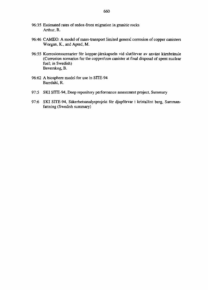
660
96:35 Estimated rates of redox-front migration in granitic rocksArthur, R.
96:46 CAMEO: A model of mass-transport limited general corrosion of copper canistersWorgan, K., and Apted, M.
96:55 Korrosionsscenarier for koppar-jarnkapseln vid slutforvar av anvant karnbransle(Corrosion scenarios for the copper/iron canister at final disposal of spent nuclearfuel; in Swedish)Beverskog, B.
96:62 A biosphere model for use in SITE-94Barrdahl, R.
97:5 SKI SITE-94, Deep repository performance assessment project, Summary
97:6 SKI SITE-94, Sakerhetsanalysprojekt for djupforvar i kristallint berg, Samman-fattning (Swedish summary)
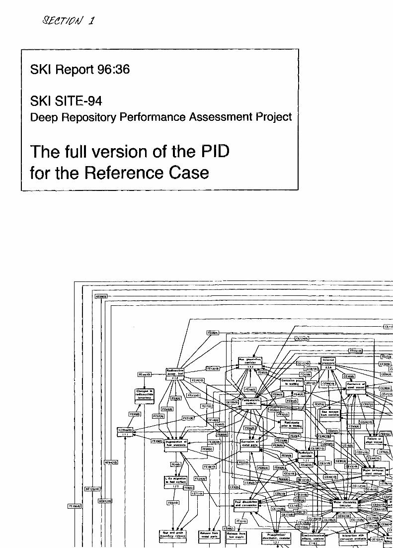
SKI Report 96:36
SKI SITE-94Deep Repository Performance Assessment Project
The full version of the PIDfor the Reference Case
j NEB8(0)
Lcdlliii
-JJFESSII^J-
-j_CETI7
S I

/R»*o«rOv« itocay •< m r t m
nusli^M, back!!!!
- 1M'|IU>| -
EoaiiMcO.. siosay".> ra.,bUe|
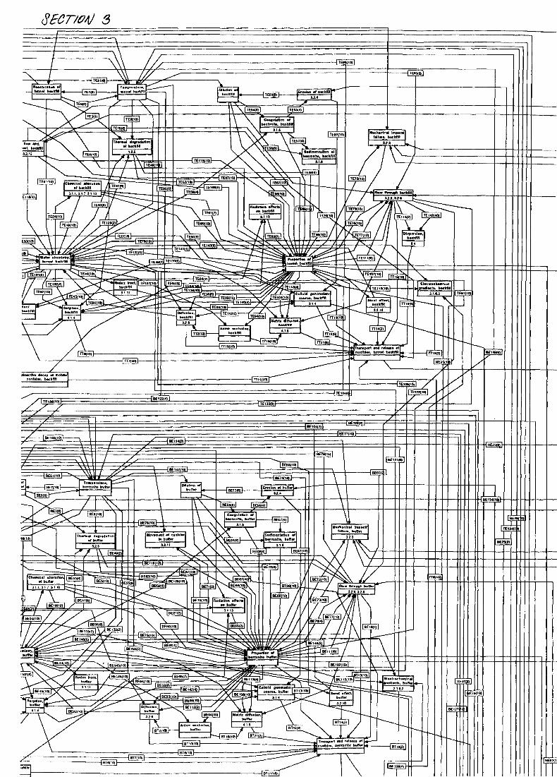
B6<4»(oTl
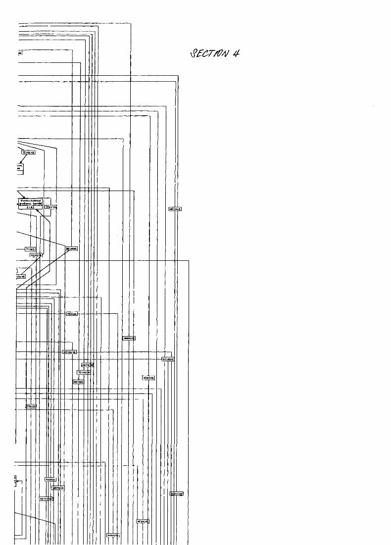
h
\
| xeardot |

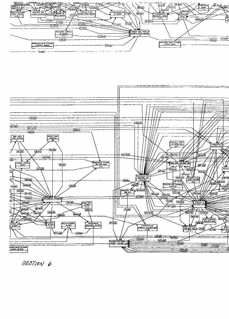
H3E
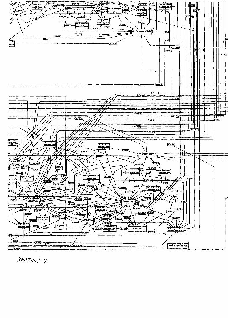
[ IE79OW
I NEe
Bt 129(101
N«!S9J
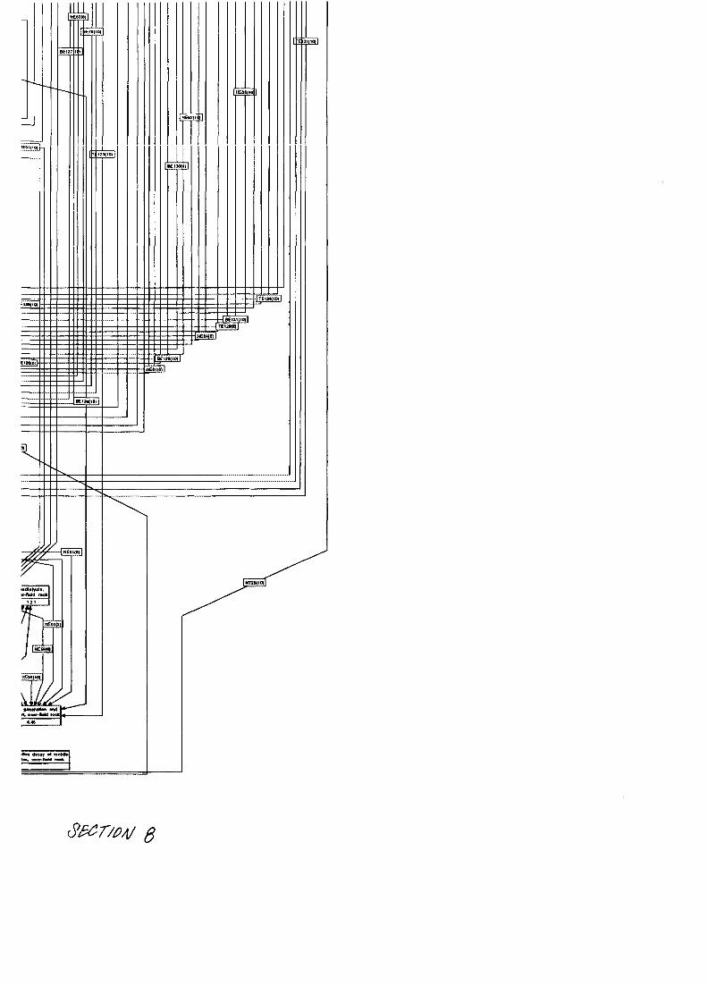
g

STATENS KARNKRAFTINSPEKTIONSwedish Nuclear Power Inspectorate
Postadress/Postal address Telefon/Telephone Telefax
SKIS-106 58 STOCKHOLM
Nat 08-698 84 00Int +46 8 698 84 00
Nat 08-661 90 86Int +46 8 661 90 86
Telex
11961 S WE ATOMS