Sketch-based Querying of Distributed Sliding-WindowData Streams

Odysseas Papapetrou, Minos Garofalakis, Antonios DeligiannakisTechnical University of Crete

{papapetrou,minos,adeli}@softnet.tuc.gr

ABSTRACTWhile traditional data-management systems focus on evaluating single, ad-hoc queries over static data sets in a centralized setting, several emerg-ing applications require (possibly, continuous) answers to queries on dy-namic data that is widely distributed and constantly updated. Furthermore,such query answers often need to discount data that is “stale”, and operatesolely on a sliding window of recent data arrivals (e.g., data updates occur-ring over the last 24 hours). Such distributed data streaming applicationsmandate novel algorithmic solutions that are both time- and space-efficient(to manage high-speed data streams), and also communication-efficient (todeal with physical data distribution). In this paper, we consider the prob-lem of complex query answering over distributed, high-dimensional datastreams in the sliding-window model. We introduce a novel sketching tech-nique (termed ECM-sketch) that allows effective summarization of stream-ing data over both time-based and count-based sliding windows with prob-abilistic accuracy guarantees. Our sketch structure enables point as wellas inner-product queries, and can be employed to address a broad rangeof problems, such as maintaining frequency statistics, finding heavy hit-ters, and computing quantiles in the sliding-window model. Focusing ondistributed environments, we demonstrate how ECM-sketches of individ-ual, local streams can be composed to generate a (low-error) ECM-sketchsummary of the order-preserving aggregation of all streams; furthermore,we show how ECM-sketches can be exploited for continuous monitoringof sliding-window queries over distributed streams. Our extensive experi-mental study with two real-life data sets validates our theoretical claims andverifies the effectiveness of our techniques. To the best of our knowledge,ours is the first work to address efficient, guaranteed-error complex queryanswering over distributed data streams in the sliding-window model.

1. INTRODUCTIONThe ability to process, in real time, continuous high-volume stre-

ams of data is a common requirement in many emerging applica-tion environments. Examples of such applications include, sensornetworks, financial data trackers, and intrusion-detection systems.As a result, in recent years, we have seen a flurry of activity inthe area of data-stream processing. Unlike conventional databasequery processing that requires several passes over a static, archiveddata image, data-stream processing algorithms often rely on build-ing concise, approximate (yet, accurate) sketch synopses of the in-

put streams in real time (i.e., in one pass over the streaming data).Such sketch structures typically require small space and updatetime (both significantly sublinear in the size of the data), and can beused to provide approximate query answers with guarantees on thequality of the approximation. These answers can be more than suf-ficient for typical exploratory analysis of massive data, where thegoal is to detect interesting statistical behavior and patterns ratherthan obtain answers that are precise to the last decimal. Large-scalestream processing applications are also inherently distributed, withseveral remote sites observing their local stream(s) and exchanginginformation through a communication network. This distributionof the data naturally imposes critical communication-efficiency re-quirements that prohibit naıve solutions that centralize all the data,due to its massive volume and/or the high cost of communication(e.g., in sensornets). Communication efficiency is particularly im-portant for distributed event-monitoring scenarios (e.g., monitoringsensor or IP networks), where the goal is real-time tracking of dis-tributed measurements and events, rather than one-shot answers tosporadic queries [25].

Several query models for streaming data have been explored overthe past decade. Streaming data items naturally carry a notionof “time”, and, in many applications, it is important to be ableto downgrade the importance (or, weight) of older items; for in-stance, in the statistical analysis of trends or patterns in financialdata streams, data that is more than a few months old might beconsidered “stale” and irrelevant. Various time-decay models forquerying streaming data have been proposed in the literature, mostlydifferentiating on the relation of an item’s weight to its age (e.g., ex-ponential or polynomial decay [6]). The sliding-window model [12]is one of the most prominent and intuitive time-decay models thatconsiders only a window of the most recent items seen in the streamthus far (i.e., items outside the window are “aged out” or given aweight of zero). The window itself can be either time-based (i.e.,items seen in the last N time units) or count-based (i.e., the lastN items). Several algorithms have been proposed for maintainingdifferent types of statistics over sliding-window data streams whilerequiring time and space that is significantly sublinear (typically,poly-logarithmic) in the window size N [12, 15, 24, 26]. Still, thebulk of existing work on the sliding-window model has focused ontracking basic counts and other simple aggregates (e.g., sums) overone-dimensional streams in a centralized setting. Some recent workhas also considered the case of distributed data, however, no exist-ing techniques can handle flexible, complex aggregate queries overrapid, high-dimensional distributed data streams, e.g., with eachdimension corresponding to the frequency of a distinct key in thestream.

Example: Recent work on effective network-monitoring systems(e.g., for detecting DDoS attacks or network-wide anomalies in

Permission to make digital or hard copies of all or part of this work forpersonal or classroom use is granted without fee provided that copies arenot made or distributed for profit or commercial advantage and that copiesbear this notice and the full citation on the first page. To copy otherwise, torepublish, to post on servers or to redistribute to lists, requires prior specificpermission and/or a fee. Articles from this volume were invited to presenttheir results at The 38th International Conference on Very Large Data Bases,August 27th - 31st 2012, Istanbul, Turkey.Proceedings of the VLDB Endowment, Vol. 5, No. 10Copyright 2012 VLDB Endowment 2150-8097/12/06... $ 10.00.

992

arX

iv:1

207.

0139

v1 [

cs.D

B]

30

Jun

2012

large-scale IP networks) has stressed the importance of an efficientdistributed-triggering functionality [20, 22, 18, 17]. In their earlywork, Jain et al. [20] discuss a generic distributed attack-detectionscheme relying on the ability to maintain frequency statistics forhigh-dimensional data over sliding windows. In particular, eachnode (e.g., a network router implementing Cisco’s Netflow proto-col, a wireless access point, or a peer in a P2P network) maintainsa sliding-window count of all observed messages for each target IPaddress. If this count exceeds a pre-determined threshold, which isdetermined based on the capacity of the target machine (possiblyexpressing the fair share of each client to the target machine), anevent is triggered to a central coordinator as a warning of possibleoverloading. The coordinator then collects network-wide statisticsto monitor overloaded nodes or abnormal behavior. More recentefforts have focused on different variants and extensions of this ba-sic scheme, often requiring more extensive data/statistics collectionand more sophisticated analyses [18, 17]. (Note that such data col-lection mechanisms are supported by commercial products, such asthe Cisco Netflow Collection Engine solution.)

The ability to efficiently summarize high-dimensional data oversliding windows is obviously crucial to such network-monitoringschemes, given the tremendous volume of network-data streamsand their massive domain sizes (e.g., 248 for IPv6 addresses). Thisraises a critical need for synopsis data structures that can compactlycapture accurate frequency statistics for a vast domain space oversliding windows. Furthermore, to enable the coordinator to aggre-gate data coming from different nodes (a requirement for detectingDDoS attacks), we need to be able to compose individually con-structed synopses to a single synopsis which can capture the globalstate of the network and help isolate network-wide abnormalities.Thus, we are faced with the difficult challenge of designing ef-fective, composable synopses that can support potentially complexsliding-window analysis queries over massive, distributed network-data streams.

Note that similar requirements are frequently observed in otherdomains, e.g., for identifying misbehaving nodes in large wirelessnetworks, for training of classifiers with distributed training datathat expires over time, and for ranking products in a cloud-basede-shop, based on the number of recent visits of each product.

Our Contributions. In this paper, we consider the problem of an-swering potentially complex queries over distributed, high-dimen-sional data streams in the sliding-window model. Our contribu-tions can be summarized as follows.

• ECM-Sketches for Sliding-Window Streams. We introduce anovel sketch synopsis (termed ECM-sketch) that allows effectivesummarization of streaming data over both time-based and count-based sliding windows with probabilistic accuracy guarantees. Ina nutshell, our ECM-sketch combines the well-known Count-Minsketch structure [10] for conventional streams with state-of-the-arttools for sliding-window statistics. The end result is a sliding-window sketch synopsis that can provide provable, guaranteed-error performance for point, as well as inner-product, queries, andcan be employed to address a broad range of problems, such asmaintaining frequency statistics, finding heavy hitters, and com-puting quantiles in the sliding-window model.

• Time-based Sliding Windows over Distributed Streams. Fo-cusing on distributed environments, we demonstrate how ECM-sketches summarizing time-based sliding windows of individual,local streams can be composed to generate a guaranteed-error ECM-sketch synopsis of the order-preserving aggregation of all streams.While conventional Count-Min sketches are trivially composable,composing ECM-sketches is more challenging, since it requires

the composition of the sliding-window statistics maintained in thesketch. Compared to earlier work on composable, randomized sli-ding-window statistics [27, 15], our sliding window approximationtechnique is completely deterministic and is much more space ef-ficient (with a linear rather than a quadratic dependence on the ap-proximation error). This increased efficiency comes at the cost ofa slight inflation of the worst-case error guarantee due to composi-tion. Furthermore, we demonstrate how our ECM-sketches can beexploited in the context of the geometric framework of Sharfman etal. [25] for continuous monitoring of sliding-window queries overdistributed streams.

• Experimental Study and Validation. We perform a thoroughexperimental evaluation of our techniques using two real-life datasets, in both centralized and distributed settings. The results of ourstudy verify the efficiency and effectiveness of our ECM-sketchsynopses in a variety of applications, and expose interesting func-tional trade-offs. When compared to algorithms based on random-ized sliding window synopses – which are the only ones that wereconsidered for composition up to now – ECM-sketches reduce thememory and computational requirements by at least one order ofmagnitude with a very small loss in accuracy. Similar savings ap-ply to the network requirements.

2. RELATED WORKCentralized and Distributed Data Streams. Most prior work ondata-stream processing has focused on developing space-efficient,one-pass algorithms for performing a wide range of centralized,one-shot computations on massive data streams; examples includecomputing quantiles [16], estimating distinct values [14], count-ing frequent elements (i.e., “heavy hitters”) [5, 9], and estimatingjoin sizes and stream norms [1, 10]. Out of these efforts, flexi-ble, general-purpose sketch summaries, such as the AMS [1] andthe Count-Min [10] sketch have found wide applicability in a broadrange of stream-processing scenarios. More recent efforts have alsoconcentrated on distributed-stream processing, proposing commu-nication-efficient streaming tools for handling a number of querytasks, including distributed tracking of simple aggregates [23], quan-tiles [8], and join aggregates [7], as well as monitoring distributedthreshold conditions [25]. All the above-referenced works assumea traditional, “full-history” data stream and do not address the is-sues specific to the sliding-window model.

Sliding-Window Stream Queries. As mentioned earlier, the bulkof existing work on the sliding-window model has focused on al-gorithms for maintaining simple statistics, such as basic counts andsums, in space and time that is significantly sub-linear (typically,poly-logarithmic) in the sliding-window size N . Exponential his-tograms [12] are a state-of-the-art deterministic technique for main-taining ǫ-approximate counts and sums over sliding windows, usingO( 1

ǫlog2 N) space. Deterministic waves [15] solve the same ba-

sic counting/summation problem with the same space complexityas exponential histograms, but improve the worst-case update timecomplexity to O(1); on the other hand, randomized waves [15] relyon randomization through hashing to track duplicate-insensitivecounts (i.e., COUNT-DISTINCT aggregates) over sliding windows.While randomized waves can be easily composed (in distributedsettings), they also come with an increased space requirement ofO( log(1/δ)

ǫ2log2 N), where δ is a small probability of failure. Xu

et al. [27] describe a randomized, sampling-based synopsis, verysimilar to randomized waves, for tracking sliding-window countsand sums with out-of-order arrivals (e.g., due to network delays)in a distributed setting. As with randomized waves, their space re-quirements are also quadratic in the inverse approximation error;

993

furthermore, their approach requires knowledge of the maximumnumber of elements in any sliding window (to set up the synopsisdata structure), which could be problematic in dynamic, widely-distributed environments. Cormode et al. [11] also propose ran-domized techniques for handling out-of-order arrivals for trackingduplicate-insensitive sliding-window aggregates. To address thehigh cost associated with randomized data structures, Busch andTirthapura propose a deterministic structure for handling out-of-order arrivals in sliding windows [3]. Similar to the other deter-ministic structures, this structure also does not allow compositionand focuses only on basic counts and sums. Finally, Chan et al. [4]investigate continuous monitoring of exponential-histogram aggre-gates over distributed sliding windows. The main contribution oftheir work lies in the efficient scheduling of the propagation of thelocal exponential-histogram summaries to a coordinator, withoutviolating prescribed accuracy guarantees.

Going beyond counts, sums, and simple aggregates, there is sur-prisingly little work in the more general problem of maintaininggeneral, frequency-distribution synopses over high-dimensionalstreaming data in the sliding-window model. Hung and Ting [19]and Dimitropoulos et al. [13] propose synopses based on Count-Min sketches for tracking heavy hitters and frequency counts oversliding windows; still, their techniques rely on keeping simple equi-width counters within the sketch, and, thus, cannot provide anymeaningful error guarantees, especially for small query ranges. Sim-ilarly, the hybrid histograms of Qiao et al. [24] combine exponen-tial histograms with simplistic equi-width histograms for answer-ing sliding-window range queries; again, these structures cannotgive meaningful bounds on the approximation error and cannot becomposed in a distributed setting.

3. PRELIMINARIESECM-sketches combine the functionalities of Count-Min

sketches [10] and exponential histograms [12]. We now describethe two structures, focusing on the aspect related to our work.

Count-Min Sketches. Count-Min sketches are a widely appliedsketching technique for data streams. A Count-Min sketch is com-posed of a set of d hash functions, h1(·), h2(·), . . ., hd(·), and a 2-dimensional array of counters of width w and depth d. Hash func-tion hj corresponds to row j of the array, mapping stream items tothe range of [1 . . . w]. Let CM [i, j] denote the counter at position(i, j) in the array. To add an item x of value vx in the Count-Minsketch, we increase the counters located at CM [hj(x), j] by vx,for j ∈ [1 . . . d]. A point query for an item q is answered by hash-ing the item in each of the d rows and getting the minimum valueof the corresponding cells, i.e., mind

j=1 CM [hj(q), j]. Note thathash collisions may cause estimation inaccuracies – only overesti-mations. By setting d = ⌈ln(1/δ)⌉ and w = ⌈e/ǫ⌉, where e is thebase of the natural logarithm, the structure enables point queries tobe answered with an error of less than ǫ||a||1, with a probability ofat least 1− δ, where ||a||1 denotes the number of items seen in thestream. Similar results hold for range and inner product queries.

Exponential Histograms. Exponential histograms [12] are a de-terministic structure, proposed to address the basic counting prob-lem, i.e., for counting the number of true bits in the last N streamarrivals. They belong to the family of methods that break the slid-ing window range into smaller windows, called buckets or basicwindows, to enable efficient maintenance of the statistics. Eachbucket contains the aggregate statistics, i.e., number of arrivals andbucket bounds, for the corresponding sub-range. Buckets that nolonger overlap with the sliding window are expired and discardedfrom the structure. To compute an aggregate over the whole (or

Notation DescriptionN Length of the sliding window, in time units or # arrivalshi(·) Hash function i of the Count-Min sketchar , br Substream of stream a, b, within the query range rfa(x, r) Frequency of item x in stream a, within the query range rEa(i, j, r) Estimated value of the ECM-sketch counter for stream a in

position (i, j) for query range r

ar ⊙ br, ar ⊙ br Real and estimated inner product of ar and bru(N,S) Upper bound of number of arrivals on stream S within the

sliding window of length N

Table 1: Frequently used notation.

a part of) sliding window, the statistics from all buckets overlap-ping with the query range are aggregated. For example, for basiccounting, aggregation is a summation of the number of true bits inthe buckets. A possible estimation error can be introduced due tothe oldest bucket inside the query range, which usually has only apartial overlap with the query. Therefore, the maximum possibleestimation error is bounded by the size of the last bucket.

To reduce the space requirements, exponential histograms main-tain buckets of exponentially increasing sizes. Bucket boundariesare chosen such that the ratio of the size of each bucket b with thesum of the sizes of all buckets more recent than b is upper bounded.In particular, the following invariant (invariant 1) is maintained forall buckets j: Cj/(2(1+

∑j−1i=1 Ci)) ≤ ǫ where ǫ denotes the max-

imum acceptable relative error and Cj denotes the size of bucket j(number of true bits arrived in the bucket range), with bucket 1being the most recent bucket. Queries are answered by summingthe sizes of all buckets that fully overlap the query range, and halfof the size of the oldest bucket, if it partially overlaps the query.The estimation error is solely contained in the oldest bucket, and istherefore bounded by this invariant, resulting to a maximum rela-tive error of ǫ.

4. ECM-SKETCHESWe now describe ECM-sketches (short for Exponential Count-

Min sketches), a composable sketch for maintaining data streamstatistics over sliding windows in distributed environments. ECM-sketches combine the functionality of Count-Min sketches and slid-ing windows, and support both time-based and count-based slidingwindows under the cash register model. Therefore, they can beused for compactly summarizing high-dimensional streams oversliding windows, i.e., to maintain the observed frequencies of thestream items within the sliding window range.

The core of the structure is a modified Count-Min sketch. Count-Min sketches alone cannot handle the sliding window requirement.To address this limitation, ECM-sketches replace the Count-Mincounters with sliding window structures. Each counter is main-tained as a sliding window, covering the last N time units, or thelast N arrivals, depending on whether we need time-based or count-based sliding windows.

As discussed in Section 2, there have been several algorithmsproposed for sliding window maintenance. Due to the large ex-pected number of sliding window counters in ECM-sketches, werequire an algorithm with a small memory footprint. Randomizedsliding window synopses are therefore not a good choice. Instead,we employ exponential histograms [12], a compact and efficientdeterministic synopsis. Each of the Count-Min counters is imple-mented as an exponential histogram, configured to provide an ǫapproximation for any query within a sliding window of length N ,i.e., the estimation x of the counter for any query range within thesliding window length is in the range of (1 ± ǫ)x of the true valuex of the counter. We will be discussing our choice for exponentialhistograms again in more detail in the following section, where wewill consider alternative deterministic and randomized algorithms.

994

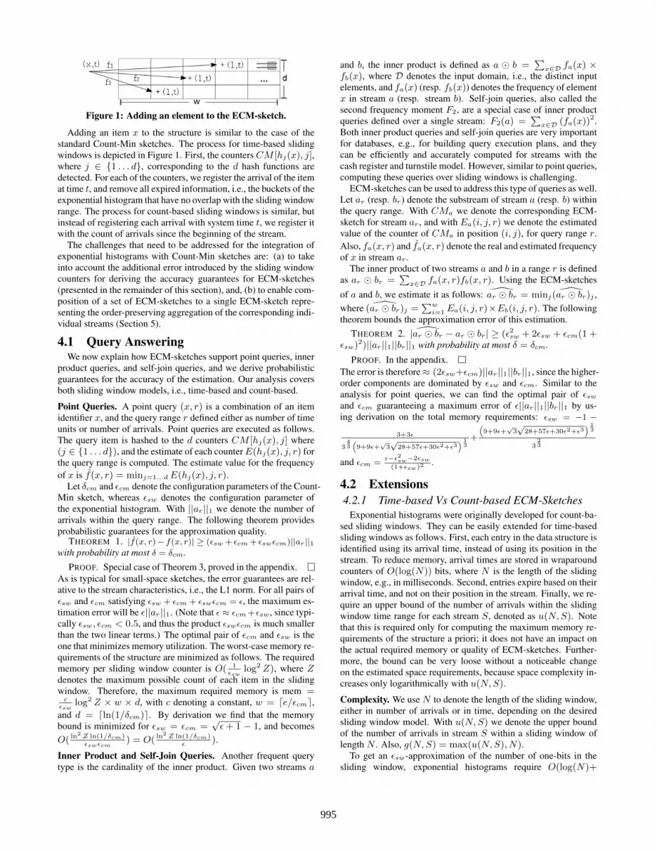
Figure 1: Adding an element to the ECM-sketch.

Adding an item x to the structure is similar to the case of thestandard Count-Min sketches. The process for time-based slidingwindows is depicted in Figure 1. First, the counters CM [hj(x), j],where j ∈ {1 . . . d}, corresponding to the d hash functions aredetected. For each of the counters, we register the arrival of the itemat time t, and remove all expired information, i.e., the buckets of theexponential histogram that have no overlap with the sliding windowrange. The process for count-based sliding windows is similar, butinstead of registering each arrival with system time t, we register itwith the count of arrivals since the beginning of the stream.

The challenges that need to be addressed for the integration ofexponential histograms with Count-Min sketches are: (a) to takeinto account the additional error introduced by the sliding windowcounters for deriving the accuracy guarantees for ECM-sketches(presented in the remainder of this section), and, (b) to enable com-position of a set of ECM-sketches to a single ECM-sketch repre-senting the order-preserving aggregation of the corresponding indi-vidual streams (Section 5).

4.1 Query AnsweringWe now explain how ECM-sketches support point queries, inner

product queries, and self-join queries, and we derive probabilisticguarantees for the accuracy of the estimation. Our analysis coversboth sliding window models, i.e., time-based and count-based.

Point Queries. A point query (x, r) is a combination of an itemidentifier x, and the query range r defined either as number of timeunits or number of arrivals. Point queries are executed as follows.The query item is hashed to the d counters CM [hj(x), j] where(j ∈ {1 . . . d}), and the estimate of each counter E(hj(x), j, r) forthe query range is computed. The estimate value for the frequencyof x is f(x, r) = minj=1...d E(hj(x), j, r).

Let δcm and ǫcm denote the configuration parameters of the Count-Min sketch, whereas ǫsw denotes the configuration parameter ofthe exponential histogram. With ||ar||1 we denote the number ofarrivals within the query range. The following theorem providesprobabilistic guarantees for the approximation quality.

THEOREM 1. |f(x, r)− f(x, r)| ≥ (ǫsw + ǫcm + ǫswǫcm)||ar||1with probability at most δ = δcm.

PROOF. Special case of Theorem 3, proved in the appendix.As is typical for small-space sketches, the error guarantees are rel-ative to the stream characteristics, i.e., the L1 norm. For all pairs ofǫsw and ǫcm satisfying ǫsw + ǫcm + ǫswǫcm = ǫ, the maximum es-timation error will be ǫ||ar||1. (Note that ǫ ≈ ǫcm+ǫsw, since typi-cally ǫsw, ǫcm < 0.5, and thus the product ǫswǫcm is much smallerthan the two linear terms.) The optimal pair of ǫcm and ǫsw is theone that minimizes memory utilization. The worst-case memory re-quirements of the structure are minimized as follows. The requiredmemory per sliding window counter is O( 1

ǫswlog2 Z), where Z

denotes the maximum possible count of each item in the slidingwindow. Therefore, the maximum required memory is mem =c

ǫswlog2 Z × w × d, with c denoting a constant, w = ⌈e/ǫcm⌉,

and d = ⌈ln(1/δcm)⌉. By derivation we find that the memorybound is minimized for ǫsw = ǫcm =

√ǫ+ 1 − 1, and becomes

O( ln2 Z ln(1/δcm)

ǫswǫcm) = O( ln

2 Z ln(1/δcm)ǫ

).

Inner Product and Self-Join Queries. Another frequent querytype is the cardinality of the inner product. Given two streams a

and b, the inner product is defined as a ⊙ b =∑

x∈D fa(x) ×fb(x), where D denotes the input domain, i.e., the distinct inputelements, and fa(x) (resp. fb(x)) denotes the frequency of elementx in stream a (resp. stream b). Self-join queries, also called thesecond frequency moment F2, are a special case of inner productqueries defined over a single stream: F2(a) =

∑x∈D (fa(x))

2.Both inner product queries and self-join queries are very importantfor databases, e.g., for building query execution plans, and theycan be efficiently and accurately computed for streams with thecash register and turnstile model. However, similar to point queries,computing these queries over sliding windows is challenging.

ECM-sketches can be used to address this type of queries as well.Let ar (resp. br) denote the substream of stream a (resp. b) withinthe query range. With CMa we denote the corresponding ECM-sketch for stream ar , and with Ea(i, j, r) we denote the estimatedvalue of the counter of CMa in position (i, j), for query range r.Also, fa(x, r) and fa(x, r) denote the real and estimated frequencyof x in stream ar .

The inner product of two streams a and b in a range r is definedas ar ⊙ br =

∑x∈D fa(x, r)fb(x, r). Using the ECM-sketches

of a and b, we estimate it as follows: ar ⊙ br = minj(ar ⊙ br)j ,where (ar ⊙ br)j =

∑wi=1 Ea(i, j, r)×Eb(i, j, r). The following

theorem bounds the approximation error of this estimation.THEOREM 2. |ar ⊙ br − ar ⊙ br| ≥ (ǫ2sw + 2ǫsw + ǫcm(1 +

ǫsw)2)||ar||1||br||1 with probability at most δ = δcm.

PROOF. In the appendix.The error is therefore ≈ (2ǫsw+ǫcm)||ar||1||br||1, since the higher-order components are dominated by ǫsw and ǫcm. Similar to theanalysis for point queries, we can find the optimal pair of ǫswand ǫcm guaranteeing a maximum error of ǫ||ar||1||br||1 by us-ing derivation on the total memory requirements: ǫsw = −1 −

3+3ǫ

343(9+9ǫ+

√3√

28+57ǫ+30ǫ2+ǫ3) 1

3

+

(9+9ǫ+

√3√

28+57ǫ+30ǫ2+ǫ3) 1

3

323

and ǫcm =ǫ−ǫ2sw−2ǫsw(1+ǫsw)2

.

4.2 Extensions4.2.1 Time-based Vs Count-based ECM-Sketches

Exponential histograms were originally developed for count-ba-sed sliding windows. They can be easily extended for time-basedsliding windows as follows. First, each entry in the data structure isidentified using its arrival time, instead of using its position in thestream. To reduce memory, arrival times are stored in wraparoundcounters of O(log(N)) bits, where N is the length of the slidingwindow, e.g., in milliseconds. Second, entries expire based on theirarrival time, and not on their position in the stream. Finally, we re-quire an upper bound of the number of arrivals within the slidingwindow time range for each stream S, denoted as u(N,S). Notethat this is required only for computing the maximum memory re-quirements of the structure a priori; it does not have an impact onthe actual required memory or quality of ECM-sketches. Further-more, the bound can be very loose without a noticeable changeon the estimated space requirements, because space complexity in-creases only logarithmically with u(N,S).

Complexity. We use N to denote the length of the sliding window,either in number of arrivals or in time, depending on the desiredsliding window model. With u(N,S) we denote the upper boundof the number of arrivals in stream S within a sliding window oflength N . Also, g(N,S) = max(u(N,S), N).

To get an ǫsw-approximation of the number of one-bits in thesliding window, exponential histograms require O(log(N)+

995

Exponential Histogram Deterministic Wave Randomized Wave

Memory O(1ǫln( 1

δ) ln2(g(N,S))

)O

(1ǫln( 1

δ) ln2(g(N,S))

)O

(1ǫ2

ln2(δ) ln2(u(N,S)))

Amort. update O(ln(1/δ)) O(ln(1/δ)) O(ln2(δ))Worst update O(ln(1/δ) ln(u(N,S))) O(ln(1/δ)) O(ln2(δ) ln(u(N,S)))

Query O(ln(1/δ) ln(u(N,S))/√ǫ) O(ln(1/δ) ln(u(N,S))/

√ǫ) O(ln2(δ)(ln(u(N,S)) + 1/ǫ2))

Table 2: Computational and space complexity of ECM-sketches. Function g(N,S) is used as a shortcut for max(u(N,S), N).

log log(u(N,S))) memory per bucket, to store the bucket size andbucket boundaries. The number of buckets is O(log(u(N,S))/ǫsw),yielding a total memory of O(log2(g(N,S))/ǫsw). With respect tocomputational cost, the update cost per element is O(log(u(N,S)))worst-case, and O(1) amortized time. Queries covering the wholesliding window are executed in constant time. For queries withrange N ′ < N , the required time is O(log(u(N,S)/ǫsw)). Theextra time is required for finding the oldest bucket overlapping withthe query, assuming sequential access. If the storage model of thebuckets supports random access, e.g., a fixed-length array, then thistime can be further reduced to O(log(log(u(N,S)/ǫsw))), by em-ploying binary search.

The space complexity of ECM-sketches is as follows. For theCount-Min array, we require an array of width w = ⌈e/ǫcm⌉ anddepth d = ⌈ln(1/δ)⌉. Each cell in the array stores an exponentialhistogram, requiring O(log2(g(N,S))/ǫsw) bits. Therefore, thetotal memory requirements are O( 1

ǫswǫcmlog2(g(N,S)) log(1/δ)).

With respect to the time complexity, adding an element requirescomputing d hash functions, and updating d separate exponentialhistograms. The amortized complexity for each arrival is there-fore O(d) = O(log(1/δ)), whereas the worst-case complexity isO(d log(u(N,S))) = O(log(u(N,S)) log(1/δ)). Finally, queryexecution takes O(log(1/δ)) time for a query of range N ′ equal toN . For N ′ < N , the execution cost is O(d log(u(N,S))/ǫsw) =O(log(1/δ) log(u(N,S))/

√ǫ) with sequential access to buckets,

e.g., using a linked list. With random access support, binary searchcan be used for finding the last relevant bucket for each query, re-ducing the query cost to O(log(1/δ) log(log(u(N,S))/

√ǫ)).

4.2.2 ECM-Sketches based on WavesThe sliding window counters can also be materialized using other

sliding window algorithms. In the literature, two such algorithmsare particularly well-known: (a) deterministic waves, and, (b) ran-domized waves [15]. We now show how ECM-sketches can in-corporate these algorithms, and discuss the positive and negativeaspects of each variant.

Deterministic Waves. Deterministic waves [15] have identicalmemory requirements with exponential histograms, and they out-perform exponential histograms with respect to worst-case com-plexity for updates, requiring always constant time. As such, thespace and computational complexity of ECM-sketches based ondeterministic waves is the same to the one of sketches based onexponential histograms, with the only difference being the worst-case update complexity, which is O(log(1/δ)).

A downside of deterministic waves is that they require knowl-edge of the upper bound of the number of arrivals u(N,S) duringthe initialization of the data structures, to decide on the requirednumber of queues/levels. Any overestimation of u(N,S) is there-fore translated to an increase on the space requirements – logarith-mic with u(N,S). It is important to note that this constraint issubstantially less limiting compared to the constraints of previousalgorithms, e.g., [27], which required an upper bound for the totalnumber of items in all streams, and therefore could not be appliedto dynamic networks, with an unknown number of participatingnodes and streams.

Randomized Waves. Randomized waves [15] provide an (ǫ, δ)

approximation for the basic counting problem, i.e., Pr[|x − x| ≤ǫswx] ≥ 1 − δsw, where x and x denote the estimated and realnumber of true bits in the sliding window range respectively. Thisstructure has substantially higher space complexity compared to thedeterministic counterparts – O(1/ǫ2sw) instead of O(1/ǫsw). How-ever, randomized waves are important for distributed applications,as they enable lossless aggregation of individual summaries to asingle summary corresponding to the aggregated data. Therefore,we also consider randomized waves for integration with the ECM-sketch.

The space complexity of ECM-sketches based on randomizedwaves is derived by multiplying the space complexity of the two ba-sic structures: O (log(δcm) log(δsw) log2(f(N,S))/(ǫcmǫ2sw)

).

Inserting a new element requires O(log(δcm) log(δsw)) amortizedtime, and O(log(δcm) log(δsw) log(f(N,S))) worst-case time. Fi-nally, query execution takes O(log(δcm) log(δsw) (log(f(N,S))+1/ǫ2sw)) with sequential access to buckets and O(log(δcm) log(δsw)(log log(f(N,S)) + log(1/ǫ2sw))) time with random access.

THEOREM 3. |f(x, r)− f(x, r)| ≥ (ǫsw + ǫcm + ǫswǫcm)||ar||1with probability at most δ = δsw + δcm.

PROOF. In the appendix.By derivation on the total memory usage, we can find the combi-nation of ǫsw and ǫcm that minimizes the memory bound: ǫsw =√

ǫ2+10ǫ+9+ǫ−3

4and ǫcm =

3ǫ−√

ǫ2+10ǫ+9+3

ǫ+√

ǫ2+10ǫ+9+1. The optimal space

complexity becomes O(log(δcm) log(δsw) log2(f(N,S))/ǫ2

), and

for δcm = δsw = δ/2 it becomes O(log2(δ) log2(f(N,S))/ǫ2

).

Table 2 summarizes the main results for the combination of ECM-sketches and the three sliding window structures. The results cor-respond to both time-based and count-based sliding windows.

5. ORDER-PRESERVING AGGREGATIONFor many distributed applications, such as the network monitoringapplication described in the introduction, we require aggregatingindividual ECM-sketches CM1, CM2, . . . , CMn, each one cor-responding to stream S1, S2, . . . , Sn, to get a single ECM-sketchCM⊕ that corresponds to the logical stream S⊕ = S1 ⊕ S2 ⊕. . . ⊕ Sn. The ⊕ operator is defined as an aggregation that pre-serves the ordering and arrival time of the events. Standard Count-Min sketches allow this aggregation, as long as all sketches areconstructed with identical dimensions and hash functions. For this,they rely on the linearity of the Count-Min counters, which are sim-ple integers in the general case. However, this does not triviallyhold for ECM-sketches, where the counters are not simple num-bers but complex sliding window structures, since the analysis ofexponential histograms (as well as all other deterministic slidingwindow structures), does not cover linearity. Although random-ized structures cover linearity by default, these are substantiallymore expensive, and not preferable for ECM-sketches. Therefore,we now consider the order-preserving aggregation of deterministicsliding window structures. Note that this problem is interesting byitself, since these data structures are widely used in the literaturefor maintaining statistics over sliding windows. We then extendour results to cover aggregation of the ECM-sketches.

996

5.1 Aggregation of Exponential HistogramsConsider a set of exponential histograms EH1, EH2, . . . , EHn,

summarizing time-based sliding windows. All are configured tocover a sliding window of N time units. The aggregation opera-tion is denoted with ⊕, i.e., EH⊕ = EH1 ⊕ EH2 ⊕ . . .⊕ EHn.With EHj

i we denote bucket j of EHi, and |EHji | denotes the

bucket size (number of true bits). By convention, buckets are num-bered such that bucket 1 is the most recent. The ending time of thebucket is denoted as e(EHj

i ). To ease exposition, we use s(EHji )

to denote the starting time of the bucket, even though this is notexplicitly stored in the buckets. By construction, the starting timeof a bucket is equal to the ending time of the previous bucket, i.e.,s(EHj

i ) = e(EHj−1i ).

To construct EH⊕ our methodology considers the individual ex-ponential histograms as logs. The general idea is to reconstructEH⊕ by assuming that half of the elements arrive at the start-ing time of each bucket, and the other half at the ending time ofthe bucket. Precisely, let B denote the list containing all bucketsof all sliding windows. We initialize an empty time-based expo-nential histogram with error ǫ′, configured to keep the last N timeunits, and a maximum of

∑ni=1 |EHi| elements. For each bucket

B[i] ∈ B, we simulate the insertion in EH⊕ of |B[i]| true bits. Halfof the bits are inserted with timestamp s(B[i]), and the other half attime e(B[i]). The insertions are simulated in the order defined bythe starting and ending timestamps of the buckets.

THEOREM 4. Consider n time-based exponential histogramsEH1, EH2, . . ., EHn, initialized with error parameter ǫ, and cov-ering the same time range. The exponential histogram EH⊕ ini-tialized with error parameter ǫ′, and constructed with the proposedaggregation algorithm answers any query within its time range forthe stream S⊕ with a maximum relative error of (ǫ+ ǫ′ + ǫǫ′).

We will now give the intuition of the proof. The formal proofis presented in the appendix. Each exponential histogram EH ofstream S configured with error parameter ǫ can be used to recon-struct an approximate stream S′, as follows: For each bucket b inEH , add |b|/2 true bits in time s(b), and |b|/2 true bits in timee(b). We argue that answering any query with starting time sqwithin the range of EH using the reconstructed stream S′ willresult to a maximum relative error ǫ. Let bj be the bucket s.t.s(bj) < sq ≤ e(bj). Therefore, the accurate answer x of thequery for stream S is bounded by x ≥ ∑j−1

i=1 |bi| + 1 and x ≤∑j−1i=1 |bi| + |bj |. By construction, the reconstructed stream will

contain a total of∑j−1

i=1 |bi|+ |bj |/2 items with timestamp greaterthan or equal to sq . Therefore, answering the query by countingthe number of true bits in the reconstructed stream with times-tamp after sq will have a maximum error of max(h−∑j−1

i=0 |bi|+|bj |/2,

∑j−1i=0 |bi| + |bj |/2 − l) = |bj |/2. By invariant 1 of expo-

nential histograms, |bj |/2 ≤ ǫ(1 +∑j−1

i=1 |bi|) ≤ ǫx. Therefore,the maximum difference between the answer estimated by streamS′ and the correct answer x will be less than or equal to ǫx.

Our aggregation algorithm is equivalent to reconstructing eachstream S′

i from exponential histogram EHi, and using these torecreate an exponential histogram EH⊕. The reconstruction ofstream S′ introduces a maximum relative error ǫ, as explained above.Summarizing S′ with a new exponential histogram we get an ad-ditional error ǫ′. However, ǫ′ is relative on the answer providedby stream S′, and not by S. Therefore, the absolute error dueto the exponential histogram summarization will be ǫ′x′, wherex′ ∈ (1 ± ǫ)x and x denoting the accurate answer on Si. Sum-ming both errors, we get a total relative error of ǫ+ ǫ′ + ǫǫ′.

For the special case when ǫ′ = ǫ, the maximum relative errorbecomes 2ǫ+ǫ2. Concerning space and computational complexity,

EH⊕ behaves as a standard exponential histogram, and thereforehas the same complexity as presented in [12].

Multi-level Aggregation. It is frequently desired to aggregate slid-ing windows in more than one levels. For example, consider ahierarchical P2P network, where each peer maintains its own ex-ponential histogram, and pushes it to its parent for aggregation atregular intervals. Since the aggregated exponential histograms havethe same properties as the individual exponential histograms (albeitwith a higher ǫ), the above analysis also supports iterative aggrega-tion of exponential histograms.

There are two types of approximation error that influence theestimation of an aggregated exponential histogram. A possible ap-proximation error, denoted as err1, is introduced due to halving ofthe size of the last bucket of the aggregated exponential histogram.This error occurs only at query time, and is independent of the num-ber of performed aggregations. Therefore, at a multi-level aggre-gation scenario this error does not need to be propagated at the in-termediary exponential histograms. A second type of error, termedas err2, occurs due to the inclusion (exclusion) of data that arrivedbefore (after) the query starting time in buckets that are accounted(not accounted) in the query result.

It turns out that the error err2 is additive at the worst case (inabsolute value). For instance, in the lowest level (Level 0) of thehierarchy, aggregating two exponential histograms (all with relativeerror ǫ), having a true number of bits (in a given query range) equalto i1 and i2, will result at a maximum value for err2 ≤ ǫ(i1 + i2).In Level 1, in addition to the previous possible errors, ǫ(i1 + i2) +ǫ(i3 + i4) stream items may be incorrectly registered at the wrongside of the query start time. A recursive repetition for h levelsresults to err2 ≤ hǫi, where i =

∑j ij . The total absolute error

(including err1) then becomes err = err2+err1 ≤ hǫi+ǫ(i+hǫi),resulting to a maximum relative error of hǫ(1 + ǫ) + ǫ.

In many applications, the number of aggregation levels can bepredicted, or even controlled when constructing the network topol-ogy. For example, consider DHT-based or hierarchical P2P topolo-gies, which typically enable a balanced-tree access to the peers ofheight h = log(N), where N is the number of nodes. In such sys-tems, initializing the individual exponential histograms with error√

1+2h+h2+4hǫ−1−h

2hyields an aggregated exponential histogram

of relative error ǫ. Naturally, this causes a slight inflation of thesize of the sliding window, by O(log(N)). However, even with thisinflation, exponential histograms are – even for extremely large net-works – substantially smaller and more efficient than randomizeddata structures that enable error-free aggregation in the expense ofmemory proportional to O(1/ǫ2) (see also Section 5.2).

Deterministic Waves. The aggregation technique trivially extendsfor deterministic waves. Recall that each wave is composed of llevels, each covering a different range. To perform the aggregation,we start from the lowest level l − 1, and switch to a higher levelevery (1/ǫ+ 1)/2 bits, i.e., when the first entry in the higher levelhas arrived before the next entry in the current level. Repeating thecalculation of the error bounds for the aggregation of deterministicwaves becomes straightforward when we notice that invariant 1 ofthe exponential histograms is also true for deterministic waves.

Count-based Exponential Histograms. Although exponential his-tograms cover both time-based and count-based sliding windows,aggregation of exponential histograms is specific for time-basedsliding windows. Count-based sliding windows do not contain suf-ficient information for allowing order-preserving aggregation. Evenstoring the system-wide time of the buckets would not be sufficientto allow such an aggregation. To illustrate this limitation, consider

997

the two count-based exponential histograms depicted in Fig. 2. Foreach bucket we store the bucket id, the size of the bucket, the bucketcompletion time and the total number of arrivals until that time. Anarrival in count-based sliding windows might be a true or a falsebit. An example query can then be: how many true bits arrived inthe last 100 system-wide arrivals. If these 100 system-wide arrivalswere read between time 19 and 20, then the correct answer wouldbe 1. However, it is also possible that the last 100 system-wide ar-rivals have arrived between time 3 and time 20, in which case thecorrect answer could be anything between 2 and 9. The informationcontained in the two exponential histograms is not sufficient to es-timate this type of queries, as it only allows us to preserve the orderof the true bits, but looses the order of the false bits, which is alsoimportant. Therefore, given only the exponential histograms, it isnot possible to aggregate them in a way that preserves the orderingof both true and false bits. Deterministic and randomized wavesalso have the same limitation when it comes to order-preservingaggregation of count-based sliding windows.

5.2 Aggregation of Randomized WavesRandomized waves were proposed in [15] to address the prob-

lem of distributed union counting: counting the number of 1’s inthe position-wise union of t distributed data streams, over a slid-ing window. However, the existing algorithm for utilizing morethan one randomized waves does not consider aggregation of sev-eral waves, to generate a single wave. It assumes that the individualrandomized waves can be stored and accessed any time, which isinconvenient for large networks. To eliminate this assumption wenow propose a slight variation of their algorithm that can producea single randomized wave out of a set of individual waves, with thesame probabilistic accuracy guarantees as the individual waves.

Our algorithm simulates the construction of the aggregate ran-domized wave RW⊕ by using only the information included inthe individual randomized waves. Consider a set R of randomizedwaves RW1, RW2, . . . , RWn, configured to store a sliding win-dow of N time units, with error parameters ǫ and δ. The aggregaterandomized wave RW⊕ is initialized with the same ǫ and δ pa-rameters, for storing a maximum of

∑ni=1 |RWi| events over N

time units. Each level l of RW⊕ is then constructed by concatenat-ing the corresponding level l from all individual randomized waves,sorting all events based on the timestamp, and keeping the last c/ǫ2

events. Recall that the number of levels of individual randomizedwaves is determined based on the maximum number of events inthe sliding window. Therefore, it may happen that RW⊕ has morelevels than individual randomized waves. To populate the lowerlevels of RW⊕, we rehash the events populating the last level ofeach individual randomized wave, as proposed in [15] when merg-ing different levels from randomized waves.

The process of query execution and the accuracy guarantees re-main the same as for the standard randomized waves.

5.3 Composability of ECM-SketchesConsider a set of ECM-sketches CM1, CM2, . . ., CMn with

identical dimensions and hash functions. The ECM-sketch CM⊕with each counter set to the sum of all corresponding counters fromthe individual sketches (as defined by the ⊕ operator), summarizesthe information found in the individual sketches:

CM⊕[j, k] = CM1[j, k]⊕ CM2[j, k]⊕ . . .⊕ CMn[j, k]

To bound the estimation error, we consider the two sources oferror in the aggregated ECM-sketch. The error due to the Count-Min sketch ǫcm does not change, since it only depends on the di-mensionality of the Count-Min array, which is fixed. However,

EH1 EH2

Bucket id 2 1 5 4 3 2 1Size 1 1 8 4 2 1 1

Completion time 3 20 3 5 10 15 19Arrivals 500 1000 900 950 980 990 1000

Figure 2: An example why aggregating count-based exponen-tial histograms is not possible.

the error due to sliding window estimations at each counter mightchange with each aggregation. Let ǫ′sw denote the error producedby the aggregation of the corresponding Count-Min counters, asdiscussed in Sections 5.1 and 5.2. Recall that this error depends onthe data structure used for maintaining the sliding window. Simi-lar to the case of individual ECM-sketches, the total error is ǫ =ǫcm + ǫ′sw + ǫcmǫ′sw, with probability 1− δsw − δcm.

6. OTHER APPLICATIONSIn addition to point and inner product queries, ECM-sketches can

also address more complex requirements. We now briefly discusstwo such cases: (a) finding the frequent items, and, (b) continu-ous monitoring of the value of inner joins or point queries overdistributed streams. Additional problems, such as computing quan-tiles or answering range queries over sliding windows, can also beaddressed, e.g., by adapting the algorithms proposed for Count-Minsketches [10] to employ ECM-sketches instead.

6.1 Finding the Frequent ItemsConsider a stream S containing items from the universe U. The

straightforward solution for finding the frequent items in the slid-ing window is to execute |U| point queries on the ECM-sketch, onefor each item in the universe, and retain only the items above thedesired frequency threshold. However, this approach carries a com-putational complexity of O(|U|×ln(1/δ)) for executing all queriesand detecting the frequent items, which is clearly prohibitive forstreaming algorithms.

A more efficient algorithm based on range sums is proposed byCormode et al. [10], and can be adapted to ECM-sketches for ad-dressing the sliding-window requirements. The algorithm relies ongroup testing, for progressively reducing the domain of candidatefrequent items, until only the truly frequent items remain. The basicidea is to create log(|U|) ECM-sketches, denoted as CM0, CM1,. . .CMlog(|U|)−1, to keep the number of occurrences of ranges ofitems. The i’th ECM sketch is used to maintain the range sum of thenecessary dyadic ranges of length 2i for covering U. A new arrivalx ∈ U is handled by adding ⌊x/2i⌋ to CMi, for 0 ≤ i < log(|U|).To detect the frequent items, we start with CMlog(|U|)−1, estimat-ing the number of occurrences of the contained dyadic ranges. Ifany of the dyadic ranges has an estimated frequency less than thefrequency threshold φ, the whole dyadic range is ignored, as it can-not contain a frequent item. For all ranges with frequency surpass-ing φ, the test continues recursively by breaking the range in two,and using the ECM-sketch of the lower level.

There are some interesting variants of the above problem, mostlyrelating to the way the threshold φ is expressed by the user. If φ isgiven as a minimum number of occurrences of each item, then nofurther computation is needed to determine which dyadic rangesare frequent and which are infrequent. However, it is often usefulto express φ as the ratio of the number of occurrences of each itemto the total number of arrivals within the sliding window. For time-based sliding windows, we can estimate the total number of arrivalsby maintaining an additional sliding window, e.g., a deterministicwave, and using its lower bound. A better alternative that doesnot require additional memory is to use ECM-sketch CM0 to esti-mate the total number of arrivals, by summing all counters in each

998

3

u 4

u 2

u1

Drift Vector u

Global Estimate Vector e

Global Statistics Vector v

ve

Are

a w

here

f(v

) >

T

u

Figure 3: Local constraints using the Geometric Approach.Each node constructs a sphere with diameter the drift vectoru of the node and the estimate vector e. The global statisticsvector v is guaranteed to lie in the convex hull of e, u1, u2,u3, u4. The union of the local spheres covers the convex hull.

row, and getting the average value. Although this approach has thesame error bounds, in practice it offers better estimation accuracythan maintaining a single additional sliding window, since the er-rors coming from all counters in each row are usually canceled out.

This estimation based on ECM-sketches may result to false pos-itives and false negatives. Theorem 5 allows us to bound this error.

THEOREM 5. The proposed algorithm usesO((log |U|/ǫ) log(2 log |U|/(δφ)) log2(g(N,S))) memory andamortized time O(log(2 log |U|/δ) log |U|) per update, for detect-ing every item with frequency at least (φ+ǫ)||a||1. With probability1− δ, no item with frequency less than φ||a||1 is output.

The same algorithm for approximating range sums can also beused for range queries, by noticing that all valid ranges withinU can be expressed by a sum of dyadic ranges [10]. The errorguarantees in this case are identical to the ones for Count-Minsketches, as described in [10], whereas the memory requirementsare O((1/ǫ) log(1/δ) log2(g(N,S)) log |U|) bytes, for maintain-ing the log |U| ECM-sketches.

6.2 Continuous Monitoring of Functions forThreshold Crossing

In many application domains, continuous monitoring of func-tions is required. ECM-sketches can also be used in these scenar-ios to reduce the memory and network requirements. We give themain intuition on how this can be done using self-join queries oversliding windows as an example.

We combine ECM-sketches with the geometric method [25]. Thegeometric method allows the distributed monitoring of complex(non-linear) functions defined over the average of local vectors(termed as local statistics vectors) maintained at sites. The goalis to to drastically reduce the required coordination for monitoringthreshold crossing of such complex functions in a distributed net-work. The main idea is to distributively monitor the domain spacewhere the average vector may lie. Each site monitors a portionof the corresponding subset of the domain space, with the corre-sponding monitoring zone often being expressed as a hypersphere.A common reference point of all such hyperspheres is the globalestimate vector, which is the average vector computed during thelast global communication (often called as a synchronization step)among all sites. Figure 3 depicts this process.

In this context, ECM-sketches are used to represent:• The local statistics vectors at each site. The ECM-sketches are

denoted as −→sv1(t),−→sv2(t), . . . ,

−→svn(t), where n is the numberof sites. All sketches have an identical configuration.

• The global statistics vector. This vector is the current averageover all local statistics vectors. The value of this vector is un-

known to all sites, unless a synchronization takes place. Theglobal statistics sketch is denoted as −→sv(t), and is computed bya linear aggregation of the local statistics sketches. We alsouse −→se(t) to denote the global estimate vector, which is the lastknown value of the global statistics vector.

Out of these two ECM-sketches, we can also compute the fol-lowing two vectors, required by the geometric method:• The statistics delta vectors, denoted using ∆−→sv(t). This vec-

tor is equal to the difference between the local statistics vectorand the corresponding vector that was transmitted in the lastsynchronization.

• The drift vectors, denoted as −→sui(t), where −→sui(t) = −→se(t) +∆−→svi(t). The global statistics vector is guaranteed to lie in theconvex hull of the drift vectors, while this convex hull is cov-ered by the union of hyperspheres monitored by the sites. Eachhypersphere of a site is constructed with diameter the global es-timate vector and the corresponding drift vector of the site [25].

To initialize the monitoring process, all nodes send their localstatistics vectors −→sv1(t),

−→sv2(t), . . . ,−→svn(t) to a coordinator. The

coordinator aggregates all vectors using the algorithm for order-preserving aggregation of ECM-sketches, and computes a singleglobal statistics vector −→sv(t). This global statistics vector is calledthe global estimate vector, and it is propagated to all network nodes,e.g., by using a hierarchy, or a broadcasting technique. This es-timate vector is used by each participating node to extract a setof Count-Min sketches, one for each query range. Without lossof generality, assume that we have only a single query range, and−→se(t) denotes the corresponding extracted Count-Min sketch.

After each new arrival at time t′, node pi updates its local statis-tics vector −→svi, and checks for a local constraint violation. For thischeck, pi extracts the statistics delta vector ∆−→sv(t′) from −→svi(t

′)as a Count-Min sketch, by querying each counter of −→svi(t

′) for itsvalue within the time range (t, t′]. By summing ∆−→sv(t′) with −→se(t)the node can compute the drift vector −→sui(t

′), again as a Count-Min sketch, and construct the sphere of the geometric method. Thesphere is formed with a center κ = (−→se(t)+−→sui(t

′))/2, and radiusα = ||(−→se(t) − −→sui(t

′))||/2. The geometric method guaranteesthat if the maximum and minimum value of the function within thesphere are at the same side of the threshold, then there can be nothreshold crossing caused by this update. For computing the max-imum and minimum value of the function efficiently, we currentlyhave closed form equations for simple functions, like self-joins.Sharfman et al. [25] propose using numerical analysis algorithms,to compute these extrema, e.g., with Matlab. We are still work-ing on this problem, to achieve efficient analytic solutions for morefunction types.

7. EXPERIMENTAL EVALUATIONOur experiments focused on evaluating ECM-sketches with re-

spect to their scalability, effectiveness, and efficiency, as well astheir suitability for distributed setups. The experiments were con-ducted using two frequently used real-life data sets, the world-cup’98 [2] (wc’98) and the Crawdad SNMP Fall 03/04 data set [21](snmp). The wc’98 data set consists of all HTTP requests thatwere directed within a period of 92 days to the web-servers host-ing the official world-cup 1998 website. It contains a total of 1.089billion valid requests, served by 33 server mirrors. Each requestwas indexed using the web-page url as a key, i.e., the ECM-sketchcould be used for estimating the popularity of each web-page. Thesnmp data set contains a total of 134 million records collectedfrom the wireless network of Dartmouth college during the fallof 2003/2003. For this data set, we have used the (anonymised)

999

MAC addresses of the clients as keys for indexing. Therefore,the ECM-sketch enabled estimating the traffic volume generatedby each user.

We have compared three sketch variants, differentiating on theemployed sliding window algorithm: (a) the default variant de-scribed earlier which is based on exponential histograms, denotedas ECM-EH, (b) a variant using deterministic waves (ECM-DW),and, (c) a variant based on randomized waves (ECM-RW). Thecomparison between the variants was performed to demonstrate theinfluence of the sliding window algorithm to the performance ofECM-sketches.

7.1 Implementation DetailsECM-sketches were implemented in Java 1.7 using 32-bit ad-

dressing, and executed on a single idle core of an Intel Xeon 1.6GHz machine. Deterministic and randomized waves were imple-mented as described in [15], including all optimizations. The queueswere implemented as fixed-size deques. The waves were initializedusing one event per millisecond as an upper bound for the num-ber of arrivals within the sliding window. In practice, it is rarelypossible to predict the maximum number of events per sliding win-dow, and therefore conservative estimates, like this one, are oftenthe only option. Concerning exponential histograms, [12] does notprovide sufficient details for the implementation of the list of buck-ets. We therefore considered different possibilities for maintainingthe buckets, including fixed arrays, deques, doubly-linked lists, andtree lists, and their combinations. The most efficient implementa-tion was a combination of fixed arrays with deques, which enabledrandom access to buckets and constant-time bucket merges. Specif-ically, the bucket list was divided to different levels L0, L1, . . . , Ll.Each level Li was initialized as a fixed-length deque, for storingonly the buckets of size 2i. Furthermore, to save memory, all levelswere initially set to null, and initialized on request. The space andcomputational complexity of our implementation is as described inSection 6, for the random-access model.

Unless otherwise noted, all ECM-sketches were set to monitor asliding window of 1 million seconds (11.5 days). Queries were gen-erated with an exponentially increasing range, i.e., query qi coveredthe range [t−10i, t], with t denoting the time of the last arrival. Foreach range, a self-join query, as well as a set of point queries wereconstructed and executed. For thorough evaluation, we constructedone point query for each distinct item in the query range (i.e., es-timating the popularity of each web-page in the wc’98 dataset, orthe number of snmp messages generated by each MAC address inthe snmp dataset).

7.2 Centralized SetupIn the centralized scenario, a single node monitors the whole

stream and maintains an ECM-sketch, which is subsequently usedfor answering the queries. We first consider the tradeoff betweenmemory requirements and estimation error. For this, we vary ǫwithin the range of [0.05, 0.25], keeping δ = 0.1. For each ǫ value,we use the analysis presented in Section 4 to configure the ECM-sketch such that the required memory for the targeted query type isminimized – hence the difference in the cost of point queries andself-join queries for the same ǫ values.

Figures 4(a)-(d) plot the average and maximum observed errorin correlation to the required memory for the two data sets. Thefigures are annotated with indicative ǫ values. The displayed errorat the Y axis is relative to the number of events arriving within thequery range, i.e., for point queries, err = |f(x, r)−f(x, r)|/||ar||1and for self-joins, err = | ar ⊙ ar − ar ⊙ ar|/(||ar||1)2. Recallthat the ECM-RW structure does not allow probabilistic guarantees

for self-join queries, and is therefore not considered for this typeof queries. Table 3 presents sample update rates for the consideredvariants, for ǫ = 0.1.

Our first observation is that, for all variants, both the average andmaximum observed errors are lower than the user-selected value ǫ.However, the memory requirements of ECM-RW are at least an or-der of magnitude higher than the requirements of ECM-sketchesbased on the two deterministic structures for offering the same ac-curacy guarantees. As an example, for the wc’98 experiment witha moderate value of ǫ = 0.1, the cost of maintaining the ECM-RWsketch is already 400 Mbytes, whereas the ECM-sketches based onexponential histograms and deterministic waves require less thana megabyte for satisfying the same guarantees (the simulation ofECM-RW configured with ǫ = 0.05 could not be completed dueto insufficient main memory). This happens because the memoryrequirements of randomized waves grow quadratically with 1/ǫ,whereas the two deterministic sliding window algorithms scale lin-early. Note that this negative result applies to all known random-ized sliding window algorithms, e.g., [27, 11], since they all scalequadratically with 1/ǫ. As such, ECM-sketches based on determin-istic structures are more applicable for scenarios with non-specia-lized hardware, or hardware with less memory, like sensor net-works and network devices. Comparing the two deterministic meth-ods, we see that ECM-EH sketches are faster and more compact,requiring approximately half the space compared to the ones basedon deterministic waves. All results are consistent for both data sets.

Summarizing, these results demonstrate that ECM-EH sketchesare more efficient and compact compared to the other two variants,and that ECM-RW sketches require at least an order of magnitudemore memory to satisfy the accuracy guarantees compared to thetwo variants based on deterministic sliding window structures.

7.3 Distributed SetupThe second series of experiments focused on evaluating the ap-

plicability of ECM-sketches for distributed setups. For this, weconducted simulations of distributed networks using the real-worlddistributions obtained from the two data sets. In particular, wc’98contains the server identification for each of the 33 official world-cup servers answering the HTTP requests, whereas the records inthe snmp data set contain the identification for each of the 535 mon-itored APs. For our simulations, these servers were organized in anarchitecture resembling a balanced binary tree of height ⌈log2(n)⌉,where n is the number of servers. All servers resided at the leafnodes of the tree. Some of these servers were also randomly cho-sen to occupy the internal tree nodes, responsible for aggregation ofthe ECM-sketches coming from the children nodes. At the end ofthe aggregation process, the root node of the hierarchy was holdinga single ECM-sketch, representing the order-preserving aggrega-tion of the n streams generated in ⌈log2(n)⌉ − 1 steps. ECM-DWsketches are not considered in this set of experiments, since they donot offer any advantages compared to ECM-EH sketches.

Figures 5(a)-(b) plot the average observed error for point andself-join queries in correlation to the network requirements for thewhole aggregation to be completed. The results correspondto ǫ ∈ [0.05, 0.25] and δ = 0.1. Note that the simulation withECM-RW sketches did not complete for all ǫ values, due to insuffi-cient memory resources at the machine simulating the n nodes. Toillustrate the accuracy loss due to this aggregation, Table 4 presentsa comparison between the observed error of the centralized and thedistributed ECM-sketches.

As expected, the process of iterative aggregations causes an in-crease of the observed error for ECM-EH sketches. This error how-ever is still substantially lower than the upper bound derived by

1000

0.00

0.01

0.02

0.03

0.04

0.05

0.01 0.1 1 10 100 1000

Ob

se

rve

d e

rro

r

Memory (Mbytes)

ε=0.25

ε=0.05

ε=0.25

ε=0.10.00

0.01

0.02

0.03

0.04

0.05

0.06

0.07

0.01 0.1 1 10 100 1000

Ob

se

rve

d m

axim

um

err

or

Memory (Mbytes)

ε=0.25

ε=0.05

ε=0.25

ε=0.1

0.00

0.01

0.02

0.03

0.04

0.05

0.01 0.1 1 10 100 1000 10000

Ob

se

rve

d e

rro

r

Memory (Mbytes)

ε=0.25

ε=0.25

ε=0.05

ε=0.25

ε=0.05

0.00

0.01

0.02

0.03

0.04

0.05

0.06

0.07

0.08

0.01 0.1 1 10 100 1000 10000

Ob

se

rve

d m

axim

um

err

or

Memory (Mbytes)

ε=0.25

ε=0.05

ε=0.25

ε=0.05

Self-join queries:Point queries: EH: DW:RW: EH:DW:

Figure 4: Average and maximum observed error in correlation to memory requirements for a centralized setup: (a)-(b) wc’98 dataset, (c)-(d) snmp data set. The plots are annotated with indicative ǫ values.

ECM-EH ECM-DW ECM-RWwc’98 1486314 1167704 177149snmp 736595 667036 105825

Table 3: Update rate (updates per sec-ond) for the centralized setup (ǫ = 0.1).

Point queries ECM-EH Self join ECM-EH Point queries ECM-RWǫ Data set Centr.:Distr. Ratio Centr.:Distr. Ratio Centr.:Distr. Ratio0.1 wc’98 0.012:0.015 1.234 0.012:0.015 1.231 0.007:N/A N/A0.2 wc’98 0.027:0.031 1.164 0.026:0.029 1.131 0.016:0.016 1.0080.1 snmp 0.011:0.011 1.042 0.010:0.011 1.021 0.006:0.006 1.0310.2 snmp 0.025:0.026 1.037 0.025:0.025 1.016 0.014:0.014 0.986

Table 4: Observed error – loss is due to the iterative aggregation.

0.00

0.01

0.02

0.03

0.04

0.05

1 10 100 1000 10000

Ob

se

rve

d e

rro

r

Transfer volume (Mbytes)

ε=0.25

ε=0.25

ε=0.05

ε=0.15

0.00

0.01

0.02

0.03

0.04

0.05

1 10 100 1000 10000

Ob

se

rve

d e

rro

r

Transfer volume (Mbytes)

ε=0.25

ε=0.25

ε=0.25

ε=0.05ε=0.05

Self-join queries:Point queries: EH: RW: EH:

Figure 5: Observed error in correlation to the network cost, forvarying ǫ: (a) wc’98 data set, (b) snmp data set.

the analysis. For example, for the case of the wc’98 data set withǫ = 0.1, the error bound is 0.3, whereas the average observed er-ror after aggregation is less than 0.015, i.e., the increase due to theaggregation is less than 1/4 of the experimentally derived error ofthe centralized sketch. Concerning ECM-RW sketches, there is nosystemic variation of the error, since randomized waves enable alossless aggregation at the expense of a larger memory footprint.However, the network required for performing this aggregation us-ing ECM-RW is higher by at least an order of magnitude comparedto the transfer volume for the variant with exponential histograms.This requirement is prohibitive for a large set of application sce-narios, like sensor and mobile networks, where high network usagecauses battery drainage.

To further explore the influence of the network size on the esti-mation accuracy and network cost, we have also simulated an arti-ficial network of i servers, with i = {1, 2, 4, . . . , 256}. The nodeswere again placed as leaf nodes on a balanced binary tree, and therequests were divided uniformly across them. Figure 6(a) and (c)plot the average observed error in correlation to the network size,for ǫ = δ = 0.1. As expected, for ECM-EH sketches, increasingthe number of nodes leads to a small increase on the observed esti-mation error. On the other hand, the aggregation process does notaffect the accuracy of ECM-RW sketches, due to the lossless aggre-gation of randomized waves. However, the network cost for aggre-gating the sketches based on randomized waves (Figure 6(b) and(d)) is at least an order of magnitude higher compared to ECM-EH.This limits the applicability of ECM-sketches based on randomizedwaves to cases where a fast, fixed network is available, and makesthe ability to merge deterministic sliding windows, e.g., based onexponential histograms, a very important contribution of this work.

Summarizing, this set of experiments showed that ECM-sketchesbased on exponential histograms can be aggregated with very smallinformation loss. Compared to the lossless aggregation of ECM-

sketches based on randomized waves, the sketches based on expo-nential histograms are substantially more compact, and are there-fore applicable for a wider range of application scenarios, wherenetwork cost and memory is of the essence, such as P2P networks,sensor networks, and communication between network routers.

8. CONCLUSIONSIn this work we considered the problem of answering complex

queries over distributed and high dimensional data streams, in thesliding window model. Our proposal, ECM-sketches, is a com-pact structure combining the state-of-the-art sketching techniquefor data stream summarization with deterministic sliding windowsynopses. The structure provides probabilistic accuracy guaran-tees for the quality of the estimation, for point queries and self-joinqueries, and can enable a broad range of problems, such as findingheavy hitters, computing quantiles, and answering range queriesover sliding windows.

Focusing on distributed applications, we also showed how a setof ECM-sketches, each one representing an individual stream, canbe aggregated to generate a single ECM-sketch that summarizesthe stream produced by the order-sensitive aggregation of all indi-vidual streams. Interestingly, this is the first result in the literatureenabling such aggregation for sketches that use deterministic slid-ing window synopses, and it is of high importance since determin-istic synopses are generally a factor of O(1/ǫ) more compact thanthe best-known randomized synopsis for delivering an ǫ-accurateapproximation. In the same context, we demonstrated how ECM-sketches can be exploited for detecting frequent items, as well aswithin the geometric method for answering continuous queries.

ECM-sketches were thoroughly evaluated with a set of extensiveexperiments, using two large real-world datasets, and consideringboth centralized and distributed setups. The results verified thehigh performance of the structure. Compared to structures basedon randomized sliding window synopses, ECM-sketches improvethe memory and computational complexity by at least one order ofmagnitude. The same magnitude of improvement is observed withrespect to the network requirements.

Our future work includes further investigation on employingECM-sketches for the geometric method, for handling additionaltypes of continuous queries over distributed sliding window streams.

Acknowledgments. This work was supported by the EuropeanCommission under ICT-FP7- LIFT-255951 (Local Inference inMassively Distributed Systems).

1001

0.004

0.008

0.012

0.016

0.020

1 2 4 8 16 32 64 128 256

Ob

se

rve

d e

rro

r

Number of nodes

0

200

400

600

800

1000

1200

1400

1600

1 2 4 8 16 32 64 128 256

Tra

nsfe

r vo

lum

e (

Mb

yte

s)

Number of nodes

0.004

0.008

0.012

0.016

0.020

1 2 4 8 16 32 64 128 256

Ob

se

rve

d e

rro

r

Number of nodes

0

100

200

300

400

500

1 2 4 8 16 32 64 128 256

Tra

nsfe

r vo

lum

e (

Mb

yte

s)

Number of nodes

Self-join queries:Point queries: EH: RW: EH:

Figure 6: Observed error and network cost for different network sizes: (a)-(b) wc’98, (c)-(d) snmp.

9. REFERENCES[1] N. Alon, Y. Matias, and M. Szegedy. The space complexity of

approximating the frequency moments. J. Comput. Syst. Sci.,58(1):137–147, 1999.

[2] M. Arlitt and T. Jin. A workload characterization study of the 1998world cup web site. Network, 14(3):30 –37, 2000.

[3] C. Busch and S. Tirthapura. A deterministic algorithm forsummarizing asynchronous streams over a sliding window. InSTACS, pages 465–476, 2007.

[4] H.-L. Chan, T.-W. Lam, L.-K. Lee, and H.-F. Ting. Continuousmonitoring of distributed data streams over a time-based slidingwindow. Algorithmica, 62(3-4):1088–1111, 2012.

[5] M. Charikar, K. Chen, and M. Farach-Colton. Finding frequent itemsin data streams. In ICALP, pages 693–703, 2002.

[6] E. Cohen and M. J. Strauss. Maintaining time-decaying streamaggregates. J. Algorithms, 59(1):19–36, 2006.

[7] G. Cormode and M. Garofalakis. Approximate continuous queryingover distributed streams. ACM Trans. Database Syst., 33(2), 2008.

[8] G. Cormode, M. Garofalakis, S. Muthukrishnan, and R. Rastogi.Holistic aggregates in a networked world: Distributed tracking ofapproximate quantiles. In SIGMOD, pages 25–36, 2005.

[9] G. Cormode and S. Muthukrishnan. What’s hot and what’s not:Tracking most frequent items dynamically. In PODS, pages 296–306,2003.

[10] G. Cormode and S. Muthukrishnan. An improved data streamsummary: the count-min sketch and its applications. J. Algorithms,55(1):58–75, 2005.

[11] G. Cormode, S. Tirthapura, and B. Xu. Time-decaying sketches forrobust aggregation of sensor data. SIAM J. Comput.,39(4):1309–1339, 2009.

[12] M. Datar, A. Gionis, P. Indyk, and R. Motwani. Maintaining streamstatistics over sliding windows. SIAM J. Comput., 31(6):1794–1813,2002.

[13] X. A. Dimitropoulos, M. P. Stoecklin, P. Hurley, and A. Kind. Theeternal sunshine of the sketch data structure. Computer Networks,52(17):3248–3257, 2008.

[14] P. B. Gibbons. Distinct sampling for highly-accurate answers todistinct values queries and event reports. In VLDB, pages 541–550,2001.

[15] P. B. Gibbons and S. Tirthapura. Distributed streams algorithms forsliding windows. In SPAA, pages 63–72, 2002.

[16] M. B. Greenwald and S. Khanna. Space-efficient online computationof quantile summaries. In SIGMOD, pages 58–66, 2001.

[17] L. Huang, M. Garofalakis, A. Joseph, and N. Taft. Communicationefficient tracking of distributed cumulative triggers. In ICDCS, 2007.

[18] L. Huang, X. Nguyen, M. Garofalakis, J. Hellerstein, M. Jordan,A. Joseph, and N. Taft. Communication-efficient online detection ofnetwork-wide anomalies. In INFOCOM, pages 134–142, 2007.

[19] R. Y. S. Hung and H.-F. Ting. Finding heavy hitters over the slidingwindow of a weighted data stream. In LATIN, pages 699–710, 2008.

[20] A. Jain, J. M. Hellerstein, S. Ratnasamy, and D. Wetherall. A wakeupcall for internet monitoring systems: The case for distributed triggers.In SIGCOMM Workshop on Hot Topics in Networks (HotNets), 2004.

[21] D. Kotz, T. Henderson, I. Abyzov, and J. Yeo. CRAWDAD trace setdartmouth/campus/snmp (v. 2004-11-09).http://crawdad.cs.dartmouth.edu/dartmouth/campus/snmp.

[22] J. Mirkovic, G. Prier, and P. L. Reiher. Attacking DDoS at the source.In ICNP, pages 312–321, 2002.

[23] C. Olston, J. Jiang, and J. Widom. Adaptive filters for continuousqueries over distributed data streams. In SIGMOD, pages 563–574,2003.

[24] L. Qiao, D. Agrawal, and A. El Abbadi. Supporting sliding windowqueries for continuous data streams. In SSDBM, pages 85–96, 2003.

[25] I. Sharfman, A. Schuster, and D. Keren. A geometric approach tomonitoring threshold functions over distributed data streams. InSIGMOD, pages 301–312, 2006.

[26] S. Tirthapura, B. Xu, and C. Busch. Sketching asynchronous streamsover a sliding window. In PODC, pages 82–91, 2006.

[27] B. Xu, S. Tirthapura, and C. Busch. Sketching asynchronous datastreams over sliding windows. Distributed Computing,20(5):359–374, 2008.

APPENDIXPROOF OF THEOREM 2. We consider the estimation derived by

any single row j of the ECM-sketch. We first check the case ofE((ar ⊙ br)j) > ar ⊙ br:

E((ar ⊙ br)j − ar ⊙ br) =∑

x∈Dfa(x, r)fb(x, r)+

∑

p,q∈D,p 6=qhj(p)=hj(q)

fa(p, r)fb(q, r)−∑

x∈Dfa(x, r)fb(x, r)

≤∑

x∈Dfa(x, r)fb(x, r)(1 + ǫsw)

2+

∑

p,q∈D,p 6=qhj(p)=hj(q)

fa(p, r)fb(q, r)(1 + ǫsw)2 −

∑

x∈Dfa(x, r)fb(x, r) =

(ǫ2sw + 2ǫsw)ar ⊙ br +∑

p,q∈D,p 6=qhj(p)=hj(q)

fa(p, r)fb(q, r)(1 + ǫsw)2 (1)

From [10], we know that E(∑

p,q∈D,p 6=qhj(p)=hj(q)

fa(p, r)fb(q, r)) ≤

ǫcm||ar||1||br||1/e. Furthermore, by Markov inequality,

Pr[∀j :∑

p,q∈D,p 6=qhj(p)=hj(q)

fa(p, r)fb(q, r) ≥ ǫcm||ar||1||br||1/e] ≤ e−d ≤ δ

Combining this with Eqn. 1, we get that with probability at least1− δ,

ar ⊙ br − ar ⊙ br ≤ (ǫ2sw + 2ǫsw)ar ⊙ br + ǫcm(1 + ǫsw)2||ar||1||br||1

Repeating the analysis for the case of E((ar ⊙ br)j) < ar ⊙ brwe get the following probabilistic guarantees:

ar ⊙ br − ar ⊙ br ≤ (ǫ2sw + 2ǫsw)ar ⊙ br

The bounds follow directly by noticing thatar ⊙ br ≤ ||ar||1||br||1.

PROOF OF THEOREM 3. By the estimation algorithm we knowthat there exists at least one row j, for which

1002

E(hj(x), j, r) = f(x, r). Let us focus now on this row. We ini-tially assume that we have an accurate algorithm to maintain thesliding window counters, i.e., errors are only due to hashing colli-sions. With R(hj(x), j, r) we denote the accurate number of bitsthat were added in the counter (hj(x), j), within the query range r.Note that, because of hashing collisions, the value of R(hj(x), j, r)might be greater than the real frequency of x, denoted as f(x, r).In fact, since the counters are assumed to be accurate, the standardanalysis introduced for count-min sketches may be applied. There-fore, Pr[R(hj(x), j, r) − f(x, r) ≤ ǫcm||ar||1] ≥ 1 − δcm ⇒Pr[R(hj(x), j, r) ≤ f(x, r) + ǫcm||ar||1] ≥ 1− δcm.

However, in practice, the sliding window algorithm may intro-duce errors to the computation of R(hj(x), j, r). Since all consid-ered algorithms are (ǫ, δ)-approximate, we know that their estima-tion E(hj(x), j, r) has the following property: Pr[|E(hj(x), j, r)−R(hj(x), j, r) ≤ ǫswR(hj(x), j, r)] ≥ 1− δsw.

For the case that E(hj(x), j, r) > R(hj(x), j, r), we havePr[E(hj(x), j, r) ≤ (1 + ǫsw)R(hj(x), j, r)] ≥ 1 − δsw. Con-sidering the two results together, we get:

Pr[E(hj(x), j, r) ≤ (1 + ǫsw)R(hj(x), j, r)] ≥ 1− δsw ⇒Pr[E(hj(x), j, r) ≤ (1 + ǫsw)(f(x, r) + ǫcm||ar||1)]

≥ 1− δsw − δcm ⇒Pr[f(x, r)− f(x, r) ≤ ǫswf(x, r) + ǫcm||ar||1+

ǫcmǫsw||ar||1] ≥ 1− δ

Note that ǫswf(x, r) + ǫcm||ar||1 + ǫcmǫsw||ar||1 ≤ (ǫsw +ǫcm + ǫcmǫsw)||ar||1. Therefore,

Pr[f(x, r)− f(x, r) ≤ (ǫsw + ǫcm + ǫcmǫsw)||ar||1] ≥ 1− δ (2)

With a similar analysis, the case of E(hj(x), j, r) <R(hj(x), j, r) gives a much tighter constraint:

Pr[f(x, r)− f(x, r) ≤ ǫswf(x, r)] ≥ 1− δsw (3)

Note that the events considered by equations 2 and 3 are mutu-ally exclusive. The proof is completed by taking the minimum ofPr[f(x, r)− f(x, r) ≤ ǫswf(x, r)] and Pr[f(x, r)− f(x, r) ≤(ǫsw + ǫcm + ǫcmǫsw)||ar||1].

PROOF OF THEOREM 4. We argue that EH⊕ approximates the ex-ponential histogram of the logical stream, with a maximum relativeerror of (1 + ǫ)ǫ′ + ǫ, where ǫ is the error parameter of the initialexponential histograms. Consider a query for the last q time units.With sq = t − q we denote the query starting time. Let Q denotethe index of the bucket of EH⊕ which contains sq in its range, i.e.,s(EHQ

⊕ ) ≤ sq ≤ e(EHQ⊕ ). With i and i we denote the accurate

and estimated number of true bits in the query range. According tothe estimation algorithm, the estimation for the number of true bitsin the stream will be i = 1/2|EHQ

⊕ |+∑1≤Y <Q |EHY

⊕ |. This es-timation may be influenced by two types of approximation errors:(a) a possible approximation error of the overlap of bucket EHQ

⊕with the query range, denoted as err1, and, (b) a possible approxi-mation error of i, denoted as err2, because of the inclusion of datathat arrived before sq in buckets Y ≤ Q, or data that arrived aftersq in buckets Y > Q. Let us now look into these two errors inmore details.

With respect to err2, recall that the contents of individual bucketsare inserted to EH⊕ using the starting time and the ending time of

the buckets. Therefore, it may happen that some bits arrive beforesq but are inserted to EH⊕ with a timestamp after sq , creating‘false positives’. The opposite is also possible. These bits are calledout-of-order bits with respect to sq . Clearly, out-of-order bits maylead to underestimation or overestimation of the query answer. Thefollowing lemma allows us to upper bound the number of out-of-order bits, and thereby control the maximum error err2.

LEMMA 1. Consider an (individual) exponential histogramEHz of stream Z, configured with error parameter ǫ. The out-of-order bits with respect to the query starting time sq that EHz

can generate are at most ǫiz , with iz denoting the number of truebits arriving after sq in Z.

PROOF. Due to the non-decreasing nature of bucket timestamps,there can be only one bucket with a start time less than sq and endtime greater than or equal to sq . Let this bucket be EHj

z . All otherbuckets have both starting and ending time at the same side of sq ,and therefore their contents are always inserted with a timestampat the correct side of sq and do not create out-of-order bits.

Since the ending time of EHjz is at or after sq , its most recent

true bit has arrived at or after sq , and should be included in thequery range. Therefore, the number of true bits arriving at or aftersq in stream Z is iz ≥ 1 +

∑j−1b=1 |EHb

z |. Furthermore, sincehalf of the bits of EHj

z are inserted using the ending time and halfusing the starting time of the bucket, the maximum number of out-of-order bits is |EHj

z |/2. By construction (invariant 1):

|EHjz |

2(1 +

j−1∑

b=1

|EHbz |)

≤ ǫ ⇒ |EHjz |

2≤ ǫ(1+

j−1∑

b=1

|EHbz |) ≤ ǫiz

The following lemma extends this result to all exponential his-tograms constituting EH⊕, for computing the total value of err2:

LEMMA 2. Consider the exponential histogram EH⊕, con-structed by aggregating exponential histograms EH1, EH2, . . .,EHn. The maximum value of err2 is ǫi, with i =

∑nx=1 ix de-

noting the number of true bits that arrived in all streams during orafter sq .

PROOF. Let err2(x) denote the number of out-of-order bits ofstream x with respect to sq . Furthermore, jx = max{b|e(EHb

x) ≥sq}.

Notice that err2(x) is upper-bounded by Lemma 1. Due to theaggregation algorithm, err2 =

∑nx=1 err2(x). Observing that ǫ

is the same across all EH, we have: err2 =∑n

x=1 err2(x) ≤ǫ∑n

x=1 ix ≤ ǫi.

Underestimation or overestimation of the overlap may also hap-pen because of the halving of the size of bucket EHQ

⊕ during querytime (err1). As shown in [12], this process may introduce a max-imum relative error of ǫr, where r is the sum of the sizes of allbuckets in EH⊕ with an index lower than Q (i.e., with a startingtime at least equal to sq). Recall that r may also include bits that ar-rived before sq , which can however be upper bounded by Lemma 2.Therefore, the maximum underestimation or overestimation error iserr1 = ǫ′r ≤ ǫ′(i+ ǫi) = ǫ′i+ ǫǫ′i, with i =

∑nx=1 ix.

Summing err1 and err2, we get a maximum relative error of (ǫ+ǫ′ + ǫǫ′). Theorem 4 follows directly.

1003