Prepared for submission to JHEP

A 6D standing-wave Braneworld with normalmatter as source.

L. J. S. Sousa,a,b W. T. Cruz,c and C. A. S. Almeidaa

aDepartamento de Física - Universidade Federal do CearáC.P. 6030, 60455-760 Fortaleza-Ceará-Brazil

bInstituto Federal de Educação, Ciência e Tecnologia do Ceará (IFCE)Campus Canindé

cInstituto Federal de Educação, Ciência e Tecnologia do Ceará (IFCE)Campus Juazeiro do Norte

E-mail: luisjose@fisica.ufc.br, wilami@fisica.ufc.br,carlos@fisica.ufc.br

Abstract: A six dimensional standing-wave braneworld model has been constructed. Itconsists in an anisotropic 4-brane generated by standing gravitational waves whose sourceis normal matter. In this model the compact (on-brane) dimension is assumed to be suffi-ciently small in order to describe our universe (hybrid compactification). The bulk geometryis non-static, unlike most of the braneworld models in the literature. The principal featureof this model is the fact that the source is not a phantom like scalar field, as the originalstanding-wave model that was proposed in five dimensions and its six dimensional exten-sion recently proposed in the literature. Here it was obtained a solution in the presence ofnormal matter what assures that the model is stable. Also our model is the first standingwave brane model in the literature which can be applied successfully to the hierarchy prob-lem. Additionally, we have shown that the zero-mode for the scalar and fermionic fields arelocalized around the brane. Particularly for the scalar field we show that it is localized onthe brane, regardless the warp factor is decreasing or increasing. This is in contrast to thecase of the local string-like defect where the scalar field is localized for a decreasing warpfactor only.

arX

iv:1

311.

5848

v1 [

hep-

th]

22

Nov

201

3

Contents

1 Introduction 1

2 The model 3

3 Standing waves solution 73.1 Case A: the same sign for a and c 83.2 Case B: a and c have opposite signs 10

4 Scalar field localization 11

5 Localization of spin 1/2 fermionic zero mode 14

6 Remarks and conclusions 16

1 Introduction

The so called braneworld models assume the idea that our universe is a membrane, orbrane, embedded in a higher-dimensional space-time. The success of this idea betweenthe physicists can been explained basically because these models have brought solution forsome insoluble problems in the Standard Model (SM) physics, as the hierarchy problem.There are many theories that carry this basic idea, but the main theories in this contextare the one first proposed by Arkani-Hamed, Dimopoulos and Dvali [1–3] and the so-called,Randall-Sundrum (RS) model [4, 5].

In these models it is assumed, a priori, that all the matter fields are restricted topropagate only in the brane. The gravitational field is the only one which is free to propagatein all the bulk. However, some authors have argued that this assumption is not so obviousand it is necessary to look for alternative theoretical mechanisms of field localization in suchmodels [6, 7]. So, before to study the cosmology of a braneworld model, it is convenient toanalyze its capability to localize fields. Therefore, for a braneworld model to be indicatedas a potential candidate of our universe it is necessary to be able to localize the StandardModel fields.

The Randall-Sundrum model was generalized to six dimensions by several interestingworks [6–29]. A great number of the works in six dimensions refer to the scenarios where thebrane has cylindrical symmetry, the so-called string-like braneworlds, which is associatedto topological defects. Some of these six dimensional models are classified as global string[6, 8, 11], the local string [12–14], thick string [16, 17, 19–22] and supersymmetric cigar-universe [23]. The work proposed here is a generalization of the RS model for six dimensionalspace-time also. However we treat the so called standing wave brane model which will bediscussed later.

– 1 –

On the other hand, studies of field localization are very common in the literature in 5D[30–35] and in 6D braneworld [6, 7, 12, 14, 26–28]. In general we find strategies of localiza-tion for all the Standard Model fields but the way that this localization is possible variesin different works. In some of them the localization is possible by means of gravitationalinteractions only [6, 7]. In other works it is necessary to consider the existence of auxiliaryfields, like the dilaton [33, 34]. As far as we know, there is not in the literature a purelyanalytical geometry that localizes all the SM fields by means of the gravitational field inter-action only. Hence, looking for a model which presents the features of to be analytical andto localize all the Standard Model fields through the gravitational interaction only is, in ourpoint of view, an appropriated reason to study localization of fields in different braneworldmodels.

The search for such a model has motivated the appearance of some braneworld scenar-ios with non-standard transverse manifold. Randjbar-Daemi and Shaposhnikov obtainedtrapped massless gravitational modes and chiral fermions as well, in a model that theycalled a Ricci-flat space or an homogeneous space [36]. Kehagias proposed an interestingmodel which drains the vacuum energy, through a conical tear-drop like space which formsa transverse space with a conical singularity. In this way it was possible to explain thesmall value of the cosmological constant [37]. An other non-trivial geometry was proposedby Gogberashvili et al. They have found three-generation for fermions on a 3-brane whosetransverse space has the shape of an apple [38]. It is still possible to cite other examples ofspace used like the torus [39], a space-time geometry with football-shape [40] and smoothversions of the conifold, classified as resolved conifold [41] and deformed conifold [42–44].

The standing wave braneworld was first proposed in five dimensions by Gogberashviliand Singleton [45]. This is a completely anisotropic braneworld model whose source isa phantom-like scalar (a scalar field with a wrong sign in front of the kinetic term in theLagrangian). To avoid problem with instability, normally presented in theory with phantomscalar, the model is embedded in a 5D Weyl geometry in such a way that the phantom-likescalar may be associated with the Weyl scalar [30, 31, 46], which is stable. About theWeyl scalar we may point out their presence also in other braneword scenarios like thepure-gravity, which is an extension of the RS model. In the context of field localizationin the standing wave approach it was possible to localize several fields in five dimensions,albeit the right-handed fermions were not localized neither in increasing nor decreasing warpgeometry [30, 31]. It is worthwhile to mention that the models generated by phantom-likescalar are relevant phenomenologically since this exotic source is useful in different scenarioslike cosmology [25], where the phantom scalar is used to explain dark energy theories andthe accelerated expansion of the universe [47]. An extension for 6D of the standing wave5D model with a phantom like scalar was first proposed by some authors of this article [48].Additionally, the study of massive modes was not addressed in this model neither in fivedimensional nor in its six dimensional versions.

In this article we do not specify a priori the source or the stuff from which the braneis done. We consider a general matter source and look for an standing wave solution. Incontrast to the work of Gogberashvili and collaborators in the 5D model [30], in whichthe source is a phantom-like scalar field, here we have obtained standing gravitational

– 2 –

waves solutions of Einstein equations in the presence of normal matter (we are using theclassification for different types of matter given by M. Visser [49]). Since is done by normalmatter, the model constructed here is stable. Our model with normal matter as source isa first six dimensional one, but quite recently Midodashvili et al. [50] constructed a 5Dstanding wave braneworld model with a real field as source.

The model built here consists of a 6D braneworld with an anisotropic 4-brane, wherethe small compact dimension belongs to the brane. The bulk is completely anisotropic,unless for some points called the AdS islands [30, 31]. Its dynamics, as in the case of theworks of Gogberashvili and collaborators and its extensions, represents a special featurein the sense that both metric and source are time dependent. We present two types ofsolutions: one with an isotropic cosmological constant where the source despite the factthat all its components are positive do not satisfies the dominant energy condition - DEC.This source may be classified as a not normal matter [49]. In the other case we make use ofa recently approach that suggests an extension for the Randall-Sundrum model to higherdimensions in the presence of an anisotropic cosmological constant [51]. In this case we findsolutions in the presence of normal matter.

We have obtained analytical solution for the warp factor, which corresponds to a thinbrane, for both decreasing and increasing warp factor. The bulk is smooth everywhere andconverges asymptotically to an AdS6 manifold. We have considered a minimally coupledscalar field and we have shown that it is localized in this model. Here we have obtainedresults that are more general that those encountered for the string-like defect and the 5Dand 6D versions of the standing wave approach. Indeed, here the scalar field is trapped forboth decreasing and increasing warp factor whereas in the string-like is a localized modefor a decreasing warp factor only. Also in 5D and 6D versions of the standing wave modelsthe scalar field is localized for increasing warp factor only.

Furthermore, our six dimensional standing wave braneworld with physical source is aninteresting scenario in order localize fermions fields. Indeed, we show that right handedfermions can be localized in this kind of brane.

We organize this work as follows: in section (2) the model is described and the Ein-stein equations are solved in order to obtain the general expressions for the source andthe function that characterizes the anisotropy. In section (3) we have found the standingwaves solutions and we have discussed its mainly features. We still show that the energy-momentum components are all positives and in the case of an anisotropic cosmologicalconstant it obey all the energy conditions which characterizes it as normal matter. Thelocalization of the zero mode of scalar and fermionic fields have been done in the sections(4) and (5), respectively. Some remarks and conclusions are outlined in section (6).

2 The model

Our intent is to derive a standing wave solution of the Einstein equations, by consideringnormal matter as source. So, we consider the standard Einstein-Hilbert action in six dimen-

– 3 –

sional space-time added by a matter field action which may be time dependent. Namely,

S =1

2κ26

∫d6x√−g[(R− 2Λ6) + Lm

], (2.1)

where κ6 is the six dimensional gravitational constant, Λ6 is the bulk cosmological constantand Lm is any matter field Lagrangian.

From the action (2.1) we derive the Einstein equations

RMN −1

2gMNR = −ΛgMN + κ2

6TMN , (2.2)

where M, N,... denote D-dimensional space-time indices and the TMN is the energy-momentum tensor defined as

TMN = − 2√−g

δ

δgMN

∫d6x√−gLm. (2.3)

The general ansatz for the metric considered in this work is given as follows

ds2 = eA(−dt2 + eudx2 + eudy2 + e−3udz2

)+ dr2 +R2

0eB+udθ2, (2.4)

where the functions A(r) and B(r) depend only on r and the function u depends on r andt variables. For this metric ansatz, (2.4), the Einstein equations (2.2) may be rewritten as

Gxx = Gyy =

(1

4eA+u

)(

6A′2 +B

′2 + 3A′B

′+ 6A

′′+ 2B

′′+ 6(u

′2 − e−Au2) + 2e−Au− 5A′u

′ − 2u′′)

= κ26Txx − eA+uΛ6, (2.5)

Gzz =

(1

4eA−3u

)(

6A′2 +B

′2 + 3A′B

′+ 6A

′′+ 2B

′′+ 6(u

′2 − e−Au2)− 6e−Au+ (11A′+ 4B

′)u

′+ 6u

′′)

= κ26Tzz − eA−3uΛ6, (2.6)

Gtt =

(1

4eA)

(−6A

′2 −B′2 − 3A′B

′ − 6A′′ − 2B

′′ − 6(u′2 + e−Au2) + (A

′ −B′)u

′)

= κ26Ttt + eAΛ6, (2.7)

Grt =1

4u(A

′ −B′ − 12u′) = κ2

6Trt, (2.8)

Grr =

(1

4

)(

6A′2 + 4A

′B

′ − 6(u′2 + e−Au2) + (A

′ −B′)u

′)

= κ26Trr − Λ6, (2.9)

– 4 –

and

Gθθ =

(1

4R2

0eB+u

)(

10A′2 + 8A

′′+ 6(u

′2 − e−Au2) + 2e−Au− 5A′u

′ − 2u′′)

= κ26Tθθ −R2

0eB+uΛ6. (2.10)

The case A = B = 2ar was treated in a previous work [48]. As a matter of fact, inthis case, it is possible to find a standing gravitational wave solution in the presence of aphantom-like scalar field, similar to the one first found in five dimensions. An other 6Dstanding wave braneworld has been recently proposed [50]. However, in that case the metricis quite different from the one considered here, as given by eq. (2.4). In this last modelthe spatial metric components x, y, z are all multiplied by the same factor, e2ar+u while thecompact extra dimension is multiplied by e2ar−3u. The solution in this case is similar to theone found in Ref. [48] and the source is still a phantom-like scalar field. The two modelsare still similar in the results of field localization.

As was commented above, the two 6D standing wave braneworld models recently pro-posed in the literature have shown interesting results in field localization, but both aregenerated by exotic matter, a phantom like scalar. Here we are interested in studyingthe possibility to have a standing wave braneworld generated by normal matter and whichmaintains the efficiency in localizing fields. So we will consider the case where A 6= B,A(r) = 2cr, and B(r) = c1r. In this case the set of equations (2.5 - 2.16) will be simplifiedto (

1

4

)(

24c2 + c21 + 6cc1 + 6(u

′2 − e−2cru2) + 2e−2cru− 10cu′ − 2u

′′)

= κ26T

xx − Λ6, (2.11)

(1

4

)(

24c2 + c21 + 6cc1 + 6(u

′2 − e−2cru2)− 6e−2cru+ (22c+ 4c1)u′+ 6u

′′)

= κ26T

zz − Λ6, (2.12)

−(

1

4

)(−24c2 − c2

1 − 6cc1 − 6(u′2 + e−2cru2) + (2c− c1)u

′)

= κ26T

tt − Λ6, (2.13)

1

4u(2c− c1 − 12u

′) = Trt, (2.14)

– 5 –

(1

4

)(

24c2 + 8cc1 − 6(u′2 + e−2cru2) + (2c− c1)u

′)

= κ26T

rr − Λ6, (2.15)

and (1

4

)(

40c2 + 6(u′2 − e−2cru2) + 2e−2cru− 10cu

′ − 2u′′)

= κ26T

θθ − Λ6. (2.16)

In order to have standing wave solution we will choose

− e−2cru+1

6(22c+ 4c1)u

′+ u

′′= 0. (2.17)

In this case the energy-momentum components have to satisfy the relations

κ26T

xx = κ2

6Tyy =

1

4

(6(u′2 − e−2cru2)− 4

3(2c− c1)u′ + 6cc1

), (2.18)

κ26T

zz =

1

4

(6(u′2 − e−2cru2)) + 6cc1

), (2.19)

κ26T

tt = −1

4

(−6(u′2 + e−2cru2) + (2c− c1)u′ − 6cc1

), (2.20)

κ26T

rr =

1

4

(−6(u′2 + e−2cru2) + (2c− c1)u′ − c2

1 + 8c1c), (2.21)

and

κ26T

θθ =

1

4

(6(u′2 − e−2cru2)− 4

3(2c− c1)u′ + 16c2 − c2

1

). (2.22)

The component κ26Trt must be equal to Grt. This energy-momentum component, as

will be seen, does not influence in the general results here since we will consider only timeaveraged features of the quantities above. This will be better explained later in section 4.

Finally the bulk cosmological constant will assume the relation

Λ6 = −1

4(24c2 + c2

1). (2.23)

This will imply in Λ6 < 0 which allows us to obtain relations between c, c1, and |Λ6|.Namely,

c1 = ±√

4|Λ6| − 24c2, (2.24)

wherec2 ≤ 1

6|Λ6|. (2.25)

– 6 –

It may be useful to highlight that for the configuration A(r) = 2cr and B(r) = c1r,the metric (2.4) will assume the simpler form

ds2 = e2cr(dt2 − eudx2 − eudy2 − e−3udz2

)− dr2 −R2

0ec1r+udθ2. (2.26)

Here c and c1 ∈ R are real constants. The range of the variables r and θ are 0 ≤ r <∞and 0 ≤ θ < 2π, respectively. The function u = u(r, t) depends on the variables r andt, only. The compact dimension θ, different of the string-like defect model, lives on thebrane, i.e., θ is a brane coordinate for r = 0. This particular feature is called hybridcompactification [52].

The metric ansatz (2.26) is a combination of the 6D warped braneworld model throughthe e2cr and ec1r terms (particularly this is similar to the global string-like defect) [6–8, 25]plus an anisotropic (r, t)-dependent warping of the brane coordinates, x, y, and z, throughthe terms eu(t,r) and e−3u(t,r). This may be seen as a six dimensional generalization ofthe 5D standing wave braneworld model [29–31, 45, 46] and a 6D generalization of the sixdimensional standing wave braneworld [48, 50]. Still we can see our model as an extensionof the global string-like defect [6, 7]. Therefore, for u = 0, the metric (2.26) is the sameof the thin global string-like defects [6, 7]. As will be seen there are more than one pointwhere u = 0. In these points the geometry is the so-called AdS island.

In addition, we can consider the exponential of the function u(r, t) as a correction ofthe string-like models resulting in an anisotropic, time-dependent braneworld.

3 Standing waves solution

In order to obtain a standing wave solution we rewrite here the differential equation for theu(r, t) function (2.17) as

e−2cru(r, t)− au′(r, t)− u′′

(r, t) = 0, (3.1)

where prime and dots mean differentiation with respect to r and t, respectively and a =16(22c + 4c1). In order to solve equation (3.1) we proceed as in Ref. [45] by choosingu(r, t) = sin(ωt)ρ(r). The general solution to the equation for the variable ρ(r) is given by

ρ(r) = D1e−a

2rJ− a

2c(ω

ce−cr) +D2e

−a2rJ a

2c(ω

ce−cr), (3.2)

where D1 = C1(ω/2c)a/2cΓ(1 − a/2c) and D2 = C2(ω/2c)a/2cΓ(1 + a/2c). C1 and C2 areintegration constants. J− a

2cand J a

2care the first kind Bessel functions of orders − a

2c anda2c , respectively, and Γ represents the Gamma function. Now that we found the solution(3.2) we have the so called standing waves solution which generalizes the 5D work [45], andthe 6D works [48, 50]. Depending on the values of c and a one can obtain solutions similarto that in six dimensions. If one has a = 5c and D1 = 0 the solution will depends onthe Bessel function J 5

2which is the case in the works in six dimensions. So these present

solutions are more general then those obtained in the works cited above.Some features of the function u(r, t) can be derived from the solution above. The first

one is the fact that both functions J− a2c

and J a2c

are regular at the origin and at infinity

– 7 –

(r → ∞), given the possibility to maintain the general solution (3.2). Depending on therelation between ω, c and a the functions J− a

2cand J a

2cconverge for both c > 0 or c < 0

enabling solutions with decreasing and increasing warp factor. Furthermore, we require thatthe function u is zero on the brane, i.e., at r = 0 [45]. This assumption may be expressedby

ω

c= X± a

2c,n, (3.3)

where X± a2c,n represents the n-th zero of J− a

2cor J a

2cdepending if we do C1 or C2 equal to

zero in (3.2). The boundary condition (3.3) quantizes the ω frequency.By this consideration the u function will assume the value zero in some specific r values,

namely rm. For these rm values our model may be identified with other 6D braneworldmodels [6–8, 12–14, 23, 25] as one can see in the metric (2.26). For c > 0 the convergenceof the function (3.2) for C1 = 0 or C2 = 0, will depends essentially on the value of the ratioω/c. The quantity of zeros, or AdS island, will depend on the value of c and mainly on thevalue of this ratio. For the case discussed here we have a finite number of zero. For c < 0

(with either C1 = 0 or C2 = 0) the solution will present infinite zeros.Once we know u we may obtain the components of the energy-momentum tensor. This

will be done for the cases where a and c have the same sign and for the case where theyhave opposite sign.

3.1 Case A: the same sign for a and c

In this case we will choose a = 4c which will imply in c1 = c2 . Here we will consider only

the time average of the energy-momentum tensor components. This option will be betterexplained in the section about field localization. In the case a = 4c and D1 = 0 the solution(3.2) will depends on J2, so our energy-momentum components will be done in terms ofthis function.

In the figures below we plot the quantities 〈T xx 〉 = 〈T yy 〉 = 〈T zz 〉, 〈T tt 〉 , 〈T rr 〉 and 〈T θθ 〉 forD2 = κ6 = c = 1; ω = 5.13. In figure (1) the dot-dashed line represents 〈T xx 〉 = 〈T yy 〉 = 〈T zz 〉,the doted one represents 〈T rr 〉, the dashed line represents 〈T θθ 〉 and finally, the filled linerepresents the energy density 〈T tt 〉. As one can see all these quantities are positive (part ofT rr is negative but |〈T rr 〉| < |〈T rr 〉|), what is an advantage when one compares it with theother works in this context [45, 48, 50]. But it is not possible to say that this is a normalmatter once the dominant energy condition (DEC) is violated. However it is not an exoticsource once the null (NEC), strong (SEC) and weak (WEC) energy conditions are satisfied.By following the matter classification given in [49] this is a not normal matter.

But the we are interested in a solution generated by normal matter. In order to have anormal matter solution it is necessary that ρ ≥ p. In order to treat this unique possibilitywe have to consider an anisotropic cosmological constant. As a matter of fact, recently ahigher dimensional Randall-Sundrum toy model was proposed by Archer and Huber [51]which contains a bulk with anisotropic cosmological constant given by

Λ =

ΛηµνΛ5

Λ6

,

– 8 –

1 2 3 4 5r

-1

1

2

3

4

5

6T M

N @rD

Figure 1. 〈TMN 〉 profile.

where ηµν is the metric of the brane.Following this procedure it is possible to find our solution in the presence of nor-

mal matter. For an anisotropic cosmological constant where its brane part is given byΛ = −1

4(c21 + 6cc1), Λ5 = −1

4(8cc1), and Λ6 = −14(16c2), the components of the energy-

momentum tensor (2.18 - 2.22) will assume the form

κ26〈T xx 〉 = κ2

6〈T yy 〉 = κ26〈T zz 〉 = κ2

6〈T θθ 〉 =1

4

(6(u′2 − e−2cru2) + 24c2

), (3.4)

κ26T

tt = −1

4

(−6(u′2 + e−2cru2)− 24c2

), (3.5)

and

κ26〈T rr 〉 =

1

4

(−6(u′2 + e−2cru2) + 24c2

). (3.6)

We plot in figure (2) these quantities as in figure (1) with the same values for theconstants. The dotted line represents the spatial components, except the r componentwhich is represented by the shaded line. The filled line represents the temporal componentof the energy-momentum tensor. As one can see all these quantities are positive and allthe energy conditions (particularly DEC) are satisfied. This is sufficient to assure that oursource is a normal matter and that our model is stable. Of course it is possible to choosethe value of the cosmological constant in a different way and still keep the normal mattersolution.

0 1 2 3 4 5r

4.5

5.0

5.5

6.0

6.5

7.0

7.5T M

N @rD

Figure 2. 〈TMN 〉 profile.

– 9 –

3.2 Case B: a and c have opposite signs

For this case we will consider a = −4c which will give c1 = −232 c. As in the other case if the

cosmological constant is isotropic it is possible to find solution with all energy-momentumtensor components positive, but it would not possible to obey the dominant energy condi-tion, as in the case above. In fact once we choose Λ6 = −1

4(24c2 + 6cc1), which is positivefor a = −4c (meaning that the bulk is asymptotically dS), than we obtain not normal mat-ter as in case A above. But the principal interest consists in a source which correspondsto normal matter. So we will once again look for a solution with an anisotropic cosmo-logical constant. There are several ways to choose the energy-momentum components andcosmological constant in order to have a solution in the presence of normal matter. Herewe assume Λ = −1

4(24c2 + 6cc1), Λ5 = −14(24c2 + 8cc1 − c2

1) and Λθ = −14(40c2 − c2

1).Since we know the relation between c and c1 it is easy to see that the components of theanisotropic cosmological constant are all positive. The time average components of theenergy-momentum tensor are

κ26〈T xx 〉 = κ2

6〈T yy 〉 = κ26〈T zz 〉 = κ2

6〈T θθ 〉 =1

4

(6(u′2 − e−2cru2) + c2

1

), (3.7)

κ26T

tt = −1

4

(−6(u′2 + e−2cru2)− c2

1

), (3.8)

andκ2

6〈T rr 〉 =1

4

(−6(u′2 + e−2cru2) + c2

1

). (3.9)

For D2 = 0 and a = −4c in (3.2) we plot the time averaged components of the energy-momentum tensor (3.8 - 3.9) in figure (3). As in figure (2) the filled line represents theenergy density, the dotted one gives κ2

6〈T xx 〉 = κ26〈T

yy 〉 = κ2

6〈T zz 〉 = κ26〈T θθ 〉 and the dashed

line represents the 〈T rr 〉 component. As one can see all these quantities are positive andρ ≥ p which assures the dominant energy condition. Therefore again we obtained a standingwave solution generated by normal matter.

0 1 2 3 4 5r

30

32

34

36

T MN @rD

Figure 3. 〈TMN 〉 profile.

On the other hand, one important feature of the braneworld models is the possibilityto solve the hierarchy problem. In others standing wave braneworld works this feature wasnot explored. Here we are interested in showing that it is possible to readdress this solutionin this context. The condition to solve the hierarchy problem in this context is that the

– 10 –

integral below be convergent, namely

M24 = 2πM4

6

∫ ∞0

dre(2c+c12

)r. (3.10)

For c1 = c = 2a, where a is a positive constant, as in the two 6D standing wavebraneworld models cited above, the integral is not convergent and the hierarchy problem isnot solvable. The same is valid for the first case presented in this work where c1 = 1

2c andc > 0. But in this second case where c1 = −23

2 c and c is positive we obtain the hierarchyproblem solution. So this is another advantage of the model presented here in relation tothe other ones done in this same context.

After we obtain the solutions for the standing wave braneworld and after we demon-strate that one of our solutions is able to solve the hierarchy problem, we are now interestin the potential of our model in order to localizes the Standard Model (SM) fields.

In the other 6D standing wave braneworld [48, 50] the localization issues of scalar, vectorand fermion fields were already exhaustively studied. Therefore, since from our model wemay obtain these other 6D standing wave braneworld, here it is sufficient to assure thatthe scenario presented here is convenient to localizes standard model fields. But we willbriefly present the study of localization for the scalar and fermion fields. This last one isinteresting because in five dimension it was not possible to localize the right fermion.

4 Scalar field localization

This section is devoted to the study of the localization of the bulk scalar field. We willfollow again the proceedings given in Refs. [30, 31, 45]. Then, considering the generalmetric (2.4) we have that

√−g = R0e

2A+B/2. Therefore, the equation for the scalar fieldmay be written as[

∂2t − e−u

(∂2x + ∂2

y

)− e3u∂2

z −e−u

R20

∂2θ

]Φ = e−A−B/2

(e2A+B/2Φ

′)′

. (4.1)

Next we consider a solution of the form

Φ(xM ) = Ψ(r, t)χ(x, y)ζ(z)eilθ. (4.2)

If one separates the variables r and t by making Ψ(r, t) = eiEtρ(r), the equation forthe r variable will assume the form(

e2A+B/2ρ(r)′)′

− eA+B/2G(r)ρ(r) = 0, (4.3)

where

G(r) =(p2x + p2

y

) (e−u − 1

)+ p2

z

(e3u − 1

)+

l2

R20

e−u. (4.4)

It will be convenient to write (4.3) as an analogue non-relativistic quantum mechanicproblem. So we will assume the change of variable ρ(r) = e−(A+B/4)Ψ(r). With this changewe will find

Ψ′′(r)− V (r)Ψ(r) = 0, (4.5)

– 11 –

where

V (r) =1

2(2A

′′+B

′′

2) +

1

4(2A

′+B

′

2)2 + e−AG(r). (4.6)

From now on we will consider A = 2cr, B = c1r and the simplified metric (2.26).Next, we will obtain the rt-dependent function Ψ, in order to analyze the localization ofthe scalar field. In other words it is necessary to solve equation (4.5), but this will be doneonly for the zero mode scalar and s-wave. This case is obtained when we assume (l = 0)

and E = p2x+p2

y +p2z. Additionally it is considered that ω >> E, which justifies to perform

the time-averaging of V (r) reducing the number of independent variables to one, namely r.By applying this simplification we will find the following expansion

⟨ebu⟩

= 1 ++∞∑n=1

(b)2n

22n(n!)2[D1e

−a2rJ− a

2c(ω

ce−cr) +D2e

−a2rJ a

2c(ω

ce−cr)]2n, (4.7)

or ⟨ebu⟩

= I0(bρ(r)), (4.8)

where I0 is the modified Bessel function of the first kind. It is evident from the expressionabove that our problem is still very complex. As can be seen from the expression (4.7),the approach in order to solve analytically the equation (4.5) is a hard work. Our strategyconsists in consider simplification and asymptotic approximations for the expression above.

Let us begin the approximations by making D1 = 0 in (3.2). Once we do this, theu(r, t) will depends on first kind Bessel function J a

2c. The expansion (4.7) will be given by

⟨ebu⟩

= 1 +

+∞∑n=1

(bD2)2ne−anr

22n(n!)2[J a

2c(ω

ce−cr)]2n. (4.9)

It is evident that our solution is still very general since the order of the function J isa/2c. This give us the advantage to choose the order of the function J more convenientfor our interest, since our choosing is in accordance with the relations (2.24) and (2.25). Ifone choose a = 4c the order of J will be 2, as in the case A discussed above. This solutionis very similar to the one first proposed in five dimensions for the localization of the scalarfield, with the difference that there the authors considered the Bessel function of the secondkind, Y2, rather than J2 [45].

After applying what it was discussed above, let us study (4.5) by considering asymptoticapproximation far from and near the brane. For the first case, r → +∞, the expressionJ a

2c= J2 goes to zero ((ω/c)e−cr → 0) and the relation (4.9) will be approximated as⟨

ebu⟩≈ 1. This will result in the following simpler form for equation (4.5), namely

Ψ′′(r)− 289

64c2Ψ(r) = 0, (4.10)

whose solution is e±178cr. We choose Ψ = e−

178cr and c > 0 which is convergent for all r

values. This solution is similar to that one found in 5D standing wave context in the caseof scalar field localization, for this same asymptotic limit assumed here [31].

– 12 –

The other case to be considered here for asymptotic approximation is the case wherer → 0. In this case the equation (4.5) may be approximated as

Ψ′′(r)−

(8dc2r2 − 6dcr + d

′)

Ψ(r) = 0. (4.11)

This equation is more general that the equivalent equation considered in five dimension[31], once there it was considered only first order approximation. The constants d and d′

are given, respectively, by

d =

(D2

4

)2 (ωc

)4(p2x + p2

y + 9p2z), (4.12)

andd′

=9

4c2 + d. (4.13)

The solution of the equation (4.11) is given by

Ψ(r) = E1Dµ

− 3

27/4

√√d

c+ 2

(√c√

2d

)r

+ E2Dν

−i 3

27/4

√√d

c+ 2i

(√c√

2d

)r

, (4.14)

where D is the parabolic cylinder function, and E1 and E2 are integration constants. Wesee that E2 must be zero in order to have a real solution. The µ, ν indexes are givenrespectively by

µ = −18c2 + 16√

2dc− d32√

2dc, (4.15)

and

ν =18√

2c2 − 32√dc−

√2d

64√dc

. (4.16)

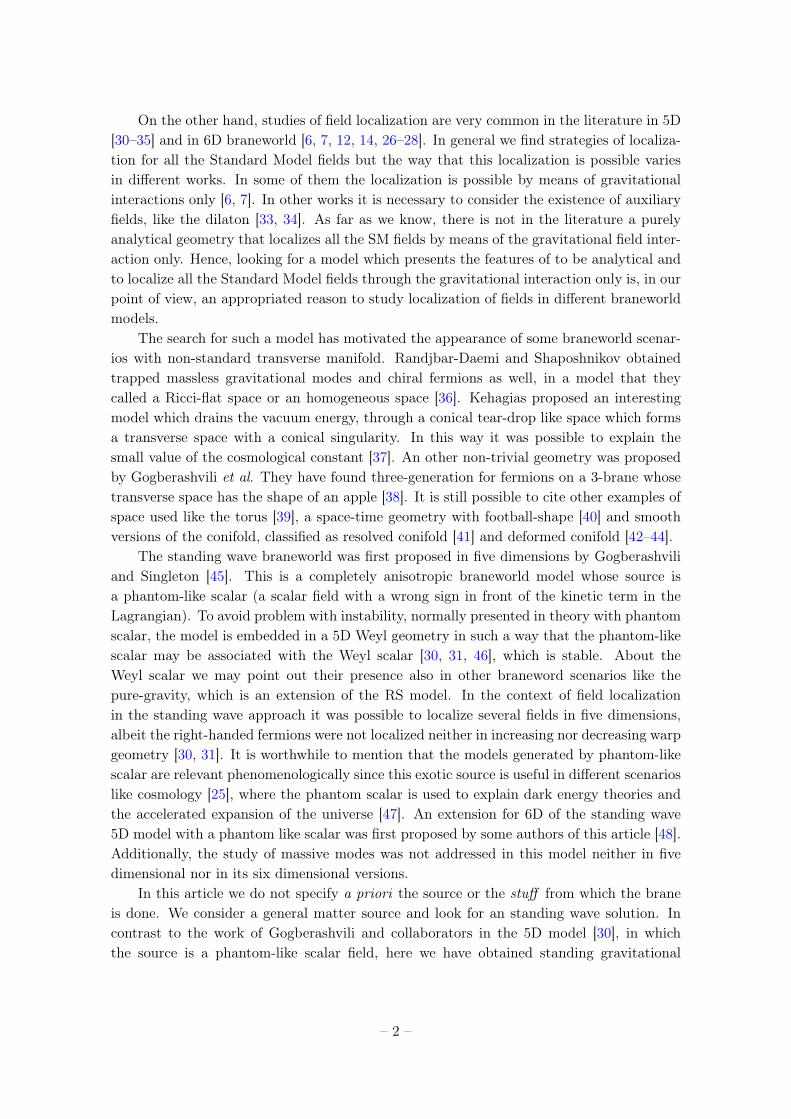
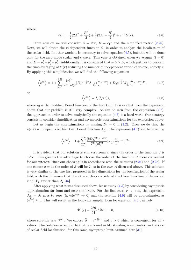
For E2 = 0 and ω/a = 5.13, which corresponds to the first zero of J2, and requiringµ = 0 it is possible to show that this solution is convergent for either c > 0 or c < 0, ascan be seen in the figures below. We see that the extra part of the scalar zero-mode wavefunction ρ(r) has a minimum at r = 0, increases and then fall off, for the case c = 1, as canbe seen in figure (4). For c = −1 the function has a maximum at r = 0 and it rapidly fallsoff as we move away from the brane, as can be seen in figure (5). On the other hand, forr →∞, it assumes the asymptotic form e−(17/8)cr which is in accordance with [31] for c > 0,only. But in general, for other relations between a and c, it is possible to have localizationfor c positive or negative, i.e., for increasing or decreasing warp factor.

The results of this section show that we have the localization of the zero-mode scalarfield in the model considered in this work. This is an expected result since the study oflocalization of the scalar field was performed in simpler 5D and 6D models than the oneconsidered here. It is relevant to stress the fact that the localization here is possible for bothincreasing or decreasing warp factor whereas in the thin string-like brane the localization

– 13 –

0.1 0.2 0.3 0.4 0.5r

0.05

0.10

0.15

0.20

0.25

0.30

Ρ@rD

Figure 4. ρ profile. c = 1

0.1 0.2 0.3 0.4 0.5r

0.005

0.010

0.015

0.020

0.025

0.030

Ρ@rD

Figure 5. ρ profile. c = −1

of the zero-mode scalar field is obtained for a decreasing warp factor, only, and in otherstanding wave braneworld this result was obtained only for the case of an increasing warpfactor [6, 7, 48, 50].

5 Localization of spin 1/2 fermionic zero mode

The study of localization of zero mode spin 1/2 fermion is interesting in this context sincein 5D standing wave braneworld it was not possible to localize the zero mode right fermion.However in the six dimensional models cited above it was demonstrated that this field islocalized. Once the model presented here is more general it is natural that we find the sameresults here. As a matter of fact, our results, as will be seen in this section is very similar tothe one found in Refs. [48, 50], except that there the Bessel function considered is J 5

2and

here we are using J2. Therefore we begin by the action for the massless spin 1/2 fermionin six dimension which may be written as

S =

∫d6x√−gΨiΓMDMΨ. (5.1)

From this action we derive the respective equation of motion, namely(ΓµDµ + ΓrDr + ΓθDθ

)Ψ(xM ) = 0. (5.2)

In this expression ΓM represents the curved gamma matrices which relate to the flat onesas

ΓM = hMMγM , (5.3)

where the vielbein hMM

is defined as follows

gMN = ηMNhMMh

NN . (5.4)

The covariant derivative assumes the classical form

DM = ∂M +1

4ΩMNM γMγN . (5.5)

– 14 –

The spin connection ΩMNM in this case is defined as

ΩMNM =

1

2hNM

(∂Mh

NN − ∂NhNM

)+

−1

2hNN

(∂Mh

MN − ∂NhMM

)− 1

2hPMhQNhRM

(∂PhQR − ∂QhPR

). (5.6)

In order to find the relations between the curved gamma matrices and the flat gammamatrices we refer to the metric ansatz (2.26) and use the relation (5.3), which will give usthe non zero results

Γt = e−crγ t; Γx = e−cr−u2 γx; Γy = e−cr−

u2 γy;

Γz = e−cr+3u2 γ z; Γr = γ r; Γθ = R−1

0 e−c12r−u

2 γ θ. (5.7)

It is still necessary to put in evidence the non-vanishing components of the spin con-nection (5.6), namely

Ωtxx = Ωty

y =1

R0Ωtθθ = − u

2eu/2; Ωtz

z =3u

2e−3u/2;

Ωrxx = Ωry

y =

(c+

u′

2

)ecr+u/2; Ωrz

z =

(c− 3u

′

2

)ecr−3u/2;

1

R0Ωrθθ =

(c1

2+u

′

2

)e

c12r+u/2; Ωrt

t = cecr. (5.8)

On the other hand, in order to solve eq. (5.2) it will be necessary to consider, as inthe last section, the case where ω >> E and to perform time average of the equation ofmotion. Additionally we assume the decomposition Ψ(xA) = ψ(xµ)ρ(r)eilθ for the wavefunction. This will allow us to write the equation of motion (5.2) as[

D + γr(

3c+ c1

2+ ∂r

)− e−crR−1

0 l2⟨e−u/2

⟩]ψ(xµ)ρ(r) = 0, (5.9)

where the operator D is given as

D = e−ar[(⟨

e−u/2⟩− 1)

(γx∂x + γy∂y) +(⟨e3u/2

⟩− 1)γz∂z

]. (5.10)

Once again it is not possible to analytically solve the equation above and then wehave to study this equation in the limits r → 0 and r → ∞. It is relevant to note thatthe operator D may be approximated as D ≈ 0 in this two distinct regions. This is aconsequence of the fact that

⟨ebu⟩≈ 1 for r → 0. This result it is shown schematically

in figure (6) below. The constant b assumes the values b = −0.5 and b = 1.5, representedby filled and dotted line respectively. As one can see from this figure the quantity

⟨ebu⟩is

approximately one for both values of the constant b. Therefore, in both cases, the equation(5.9) for the s-wave (l = 0), may be simplified as(

3c+ c1

2+ ∂r

)ρ(r) = 0. (5.11)

– 15 –

0 1 2 3 4 5r

0.5

1.0

1.5

2.0eb u HrL

Figure 6. 〈ebu〉 profile. The filled line represents b = −0.5 and the dotted line represents b = 1.5

It is very easy to solve this equation resulting in ρ(r) ∝ e−3c+c1

2r. This solution shows

that for r → 0 the function ρ has a maximum at the origin and that it decays as e−3c+c1

2r

for a > 0 when r →∞. To show the localization we insert this solution in the action (5.1).By doing this the resultant integral in variable r will assume the form I ∝

∫∞0 dre−ar. It is

evident that this integral is convergent for a > 0. This is sufficient to assure that the spin1/2 fermion zero mode is localized in this model. Therefore, similar to the other results insix dimension, we show that the geometry is important to localize fields in contrast to 5Dstanding wave braneworld where is not possible to find localization for the fermion. Thisstill shows that the model presented here is more general that the other six dimensionalstanding wave brane world model and allows the localization of fields for different Besselfunction.

6 Remarks and conclusions

In this work we have obtained standing gravitational waves solution for the six dimensionalEinstein equation in the presence of an anisotropic brane generated by normal matter. Thecompact dimension belongs to the brane and is small enough to assure that our model isrealistic. Our metric ansatz is anisotropic and non-static, unlike most models consideredin the braneworld literature. We find solution for the warp factor which represents a thinbrane and in this case the bulk may be seen as a generalization of the string-like defect[6, 7]. Apart from having as source a physical field, our model is more general than otherssix dimensional standing wave braneworld recently considered in the literature [48, 50],since their solutions may be derived from our solution as special cases. Our metric ansatzhas two different warp factors e2cr and e2c1r, similar to the global string-like defect and ithas also general warp factors eu(r,t) and e−3u(r,t) similar to the 6D standing wave braneworldwith an exotic source. The different warp factors permit us to find solution for the functionu for increasing or decreasing warp factor e±cr which is an advantage when compared withits similar model.

We find standing wave solution for the function u(r, t) and we show that this solution ismore general and comprises the others six dimensional standing wave braneworld solutionswhich have recently appeared in the literature [48, 50]. In fact our solutions depend on theBessel function J± a

2cwhich for the special case a = ±5c coincides with the models cited

above.

– 16 –

From the u(r, t) function it was possible to choose the type of matter that generates thebrane. We have found two types of matter depending if we consider isotropic or anisotropiccosmological constant. In the first case, for a negative cosmological constant and a = 4c wehave demonstrated that the energy density and pressure components are all positive andthe energy conditions NEC, WEC and SEC are satisfied, although the dominant energycondition is violated in this case. If one consider a = −4c, similar results are found forthe matter but in this case the cosmological constant is positive which means that in thiscase the bulk is asymptotically dS, while in the first case we have an 6D AdS space-time.It is interesting to note that an asymptotically AdS space-time has been considered in theothers 5D and 6D standing wave braneworld, but a dS geometry was found for the first timehere. For the case of anisotropic cosmological constant we have considered the situationrecently suggested in the literature for higher dimensional Randall-Sundrum model [51].So we consider that the cosmological constant on the brane has a fixed value λ but theextra components Λ5 and Λ6 may assume different values. This is specifically reasonablein our case since we are dealing with an anisotropic bulk. Therefore, for a = 4c all the"components" of the cosmological constant are negative and for a = −4c they are positive,in line with the findings for the case of isotropic cosmological constant discussed above.In the two cases we have obtained the components of the energy-momentum tensor andshowed that all of them are positive and that all the energy conditions are satisfied. Thismeans that we have constructed a 6D standing wave braneworld which is generated bynormal matter and therefore stable.

An important feature of some braneworld models is their ability to solve the so calledhierarchy problem. But in the context of standing wave braneworld this problem was nevertreated. Here we have demonstrated that it is possible to solve the hierarchy problem in thiscontext. This is another advantage of the model proposed in this work over other standingwave braneworld models.

Finally we have considered the localization of fields in our model. Since it generalizesour previous work in this subject [48] it is reasonable to expect that the localization of thefields which was studied there, it is also possible here. Indeed, here we have considereda = 4c and we studied only the zero mode scalar and fermion fields localization and as wasexpected we have shown that there is a zero mode localized for both scalar and fermionfields. The solution found here for the scalar field is in accordance with the ones that wereencountered in five dimensions [31] and six dimensions [48, 50].

Acknowledgments

The authors thank the Fundação Cearense de apoio ao Desenvolvimento Científico e Tec-nológico (FUNCAP), the Coordenação de Aperfeiçoamento de Pessoal de Nível Superior(CAPES), and the Conselho Nacional de Desenvolvimento Científico e Tecnológico (CNPq)for financial support.

– 17 –

References

[1] I. Antoniadis, N. Arkani-Hamed, S. Dimopoulos and G. R. Dvali, Phys. Lett. B 436, 257(1998) [hep-ph/9804398].

[2] N. Arkani-Hamed, S. Dimopoulos and G. R. Dvali, Phys. Lett. B 429, 263 (1998)[hep-ph/9803315].

[3] N. Arkani-Hamed, S. Dimopoulos and G. R. Dvali, Phys. Rev. D 59, 086004 (1999)[hep-ph/9807344].

[4] L. Randall and R. Sundrum, Phys. Rev. Lett. 83, 3370 (1999) [arXiv:hep-ph/9905221].

[5] L. Randall and R. Sundrum, Phys. Rev. Lett. 83, 4690 (1999) [arXiv:hep-th/9906064].

[6] I. Oda, Phys. Lett. B 496, 113 (2000) [arXiv:hep-th/0006203].

[7] I. Oda, Phys. Rev. D 62, 126009 (2000) [hep-th/0008012].

[8] R. Gregory, Phys. Rev. Lett. 84, 2564 (2000) [arXiv:hep-th/9911015].[9]

[9] J. W. Chen, M. A. Luty and E. Ponton, JHEP 0009, 012 (2000) [arXiv:hep-th/0003067].

[10] A. G. Cohen and D. B. Kaplan, Phys. Lett. B 470, 52 (1999) [arXiv:hep-th/9910132].

[11] I. Olasagasti and A. Vilenkin, Phys. Rev. D 62, 044014 (2000) [hep-th/0003300].

[12] T. Gherghetta and M. E. Shaposhnikov, Phys. Rev. Lett. 85, 240 (2000)[arXiv:hep-th/0004014].

[13] E. Ponton and E. Poppitz, JHEP 0102, 042 (2001) [hep-th/0012033].

[14] M. Giovannini, H. Meyer and M. E. Shaposhnikov, Nucl. Phys. B 619, 615 (2001)[hep-th/0104118].

[15] P. Tinyakov and K. Zuleta, Phys. Rev. D 64, 025022 (2001) [hep-th/0103062].

[16] S. Kanno and J. Soda, JCAP 0407, 002 (2004) [hep-th/0404207].

[17] J. Vinet and J. M. Cline, Phys. Rev. D 70, 083514 (2004) [hep-th/0406141].

[18] J. M. Cline, J. Descheneau, M. Giovannini and J. Vinet, JHEP 0306, 048 (2003)[hep-th/0304147].

[19] E. Papantonopoulos, A. Papazoglou and V. Zamarias, Nucl. Phys. B 797, 520 (2008)[arXiv:0707.1396 [hep-th]].

[20] I. Navarro, JCAP 0309, 004 (2003) [hep-th/0302129].

[21] I. Navarro and J. Santiago, JHEP 0502, 007 (2005) [hep-th/0411250].

[22] E. Papantonopoulos and A. Papazoglou, JCAP 0507, 004 (2005) [hep-th/0501112].

[23] B. de Carlos and J. M. Moreno, JHEP 0311, 040 (2003) [arXiv:hep-th/0309259].

[24] M. Gogberashvili and P. Midodashvili, Europhys. Lett. 61, 308 (2003) [hep-th/0111132].

[25] R. Koley and S. Kar, Class. Quant. Grav. 24, 79 (2007) [hep-th/0611074].

[26] R. S. Torrealba, Phys. Rev. D 82, 024034 (2010) [arXiv:1003.4199 [hep-th]].

[27] J. E. G. Silva and C. A. S. Almeida, Phys. Rev. D 84, 085027 (2011) [arXiv:1110.1597[hep-th]].

– 18 –

[28] L. J. S. Sousa, W. T. Cruz and C. A. S. Almeida, Phys. Lett. B 711, 97 (2012)[arXiv:1203.5149 [hep-th]].

[29] Localization of Matter Fields in the 5D Standing Wave Braneworld, M. Gogberashvili,arXiv:1204.2448 [hep-th].

[30] M. Gogberashvili, P. Midodashvili and L. Midodashvili, Phys. Lett. B 707, 169 (2012)[arXiv:1105.1866 [hep-th]].

[31] M. Gogberashvili, P. Midodashvili and L. Midodashvili, Phys. Lett. B 702, 276 (2011)[arXiv:1105.1701 [hep-th]].

[32] A. Kehagias and K. Tamvakis, Phys. Lett. B 504, 38 (2001) [hep-th/0010112].

[33] W. T. Cruz, M. O. Tahim and C. A. S. Almeida, Europhys. Lett. 88, 41001 (2009)[arXiv:0912.1029 [hep-th]].

[34] W. T. Cruz, A. R. Gomes and C. A. S. Almeida, Europhys. Lett. 96, 31001 (2011).

[35] M. O. Tahim, W. T. Cruz and C. A. S. Almeida, Phys. Rev. D 79, 085022 (2009)[arXiv:0808.2199 [hep-th]].

[36] S. Randjbar-Daemi and M. E. Shaposhnikov, Phys. Lett. B 491, 329 (2000)[hep-th/0008087].

[37] A. Kehagias, Phys. Lett. B 600, 133 (2004) [arXiv:hep-th/0406025].

[38] M. Gogberashvili, P. Midodashvili and D. Singleton, JHEP 0708, 033 (2007)[arXiv:0706.0676 [hep-th]].

[39] Y. -S. Duan, Y. -X. Liu and Y. -Q. Wang, Mod. Phys. Lett. A 21, 2019 (2006)[hep-th/0602157].

[40] J. Garriga and M. Porrati, JHEP 0408, 028 (2004) [hep-th/0406158].

[41] J. F. Vazquez-Poritz, JHEP 0209, 001 (2002) [arXiv:hep-th/0111229].

[42] H. Firouzjahi and S. H. Tye, JHEP 0601, 136 (2006) [arXiv:hep-th/0512076].

[43] T. Noguchi, M. Yamaguchi and M. Yamashita, Phys. Lett. B 636, 221 (2006)[arXiv:hep-th/0512249].

[44] F. Brummer, A. Hebecker and E. Trincherini, Nucl. Phys. B 738, 283 (2006)[arXiv:hep-th/0510113].

[45] M. Gogberashvili and D. Singleton, Mod. Phys. Lett. A 25, 2131 (2010) [arXiv:0904.2828[hep-th]].

[46] M. Gogberashvili, A. Herrera-Aguilar and D. Malagon-Morejon, Class. Quant. Grav. 29,025007 (2012) [arXiv:1012.4534 [hep-th]].

[47] R. R. Caldwell, M. Kamionkowski and N. N. Weinberg, Phys. Rev. Lett. 91, 071301 (2003);S. M. Carroll, M Hoffman and M. Trodden, Phys. Rev. D68, 023509 (2003); P. Frampton,Phys Lett. B555 139 (2003); V. Sahni and Y. Shtanov, JCAP 0311, 014 (2003).

[48] A 6D standing wave Braneworld, L. J. S. Sousa, J. E. G. Silva and C. A. S. Almeida,arXiv:1209.2727 [hep-th].

[49] M. Visser, Phys. Rev. D 56, 7578 (1997).

[50] Localization of Matter Fields in the 6D Standing Wave Braneworld, P. Midodashvili,arXiv:1211.0206v1 [hep-th].

– 19 –

[51] P. R. Archer and S. J. Huber JHEP 1103:018,2011.

[52] B. Carter, A. Nielsen and D. Wiltshire, JHEP 07 (2006) 34 [arxiv:0602086 [hep-th]].

– 20 –