arX

iv:1

206.

5832

v1 [

hep-

th]

25

Jun

2012

Prepared for submission to JHEP

Five-dimensional Hořava-like braneworld models

F. S. Bemfica,a M. Dias,b M. Gomesa and J. M. Hoff da Silvac

aInstituto de Física, Universidade de São Paulo,

Caixa Postal 66318, 05315-970, São Paulo, SP, BrazilbDepartamento de Ciências Exatas e da Terra, Universidade Federal de São Paulo,

Diadema, SP, BrazilcUNESP - Campus Guaratinguetá - DFQ,

Av. Dr. Ariberto Pereira da Cunha, 333 CEP 12516-410, Guaratinguetá, SP, Brazil

E-mail: fbemfica@fma.if.usp.br, mafd@cern.ch, mgomes@fma.if.usp.br,

hoff@feg.unesp.br

Abstract: In this work we study a Hořava-like five-dimensional model in the context of

braneworld theory. To begin with, the equations of motion of such model are obtained

and, within the realm of warped geometry, we show that the model is consistent if and

only if λ takes its relativistic value 1. Furthermore, since the first derivative of the warp

factor is discontinuous over the branes, we show that the elimination of problematic terms

involving the square of the warp factor second order derivatives are eliminated by impos-

ing detailed balance condition in the bulk. Afterwards, the Israel’s junction conditions

are computed, allowing the attainment of an effective Lagrangian in the visible brane. In

particular, for a (4+1)-dimensional Hořava-like model defined in the bulk without cosmo-

logical constant, we show that the resultant effective Lagrangian in the brane corresponds

to a (3+1)-dimensional Hořava-like model with an emergent positive cosmological constant

but without detailed balance condition. Now, restoration of detailed balance condition, at

this time imposed over the brane, plays an interesting role by fitting accordingly the sign of

the arbitrary constant β that labels the extra terms in the model, insuring a positive brane

tension and a real energy for the graviton within its dispersion relation. To end up with,

the brane consistency equations are obtained and, as a result, we show that the detailed

balance condition again plays an essential role in eliminating bad behaving terms and that

the model admits positive brane tensions in the compactification scheme if, and only if, β

is negative, what is in accordance with the previous result obtained for the visible brane.

Keywords: braneworld, higher-dimensional gravity, modified theories of gravity, Hořava-

Lifshitz-like models

Contents

1 Introduction 1

2 Hořava-like model in the bulk 3

3 The equations of motion 4

4 Israel’s junction conditions and the detailed balance condition 8

5 Effective Lagrangian on the brane 10

6 Consistency conditions 14

7 Summary and conclusions 16

A Evaluation of Λ 17

1 Introduction

Modified theories of gravity containing higher order terms in curvature have been proposed

in the literature mainly due to the interest in obtaining a renormalizable quantum version

of Einstein gravity. We know that the linearized version of general relativity (GR) has a

propagator that behaves like

∼ 1

−k2, (1.1)

where k2 = −k02+ ~k2 is the square of the graviton four-momentum while k0 and ~k are

its energy and linear 3-momentum, respectively. To improve the ultraviolet behavior, a

modified model containing terms with higher order products of the curvature has been set.

As desired, the modified theory was proven to be renormalizable [1]. However, the presence

of higher order terms in time derivative is known to produce pathologies like ghosts in such

models due to the fact that it introduces “wrong” sign poles in the propagators. Also, in

some situations the theory describes tachyon.

In the context of modified theories of gravity and with the aim of having a unitary

model that, moreover, could improve the ultraviolet behavior of the propagator, Hořava

proposed a model that basically modifies GR by terms involving only products of a 3-

curvature defined on a 3-dimensional space [2]. In other words, by foliating the (3+1)

spacetime (here we will call it Σ) into 3-dimensional hypersurfaces σ of constant time t

(Σ ≈ ℜ× σ), the action may be schematically written as

SH =1

2κ2

∫

ℜ

dt

∫

σd3xN

√q[

KijKij − λK2 + f((3)R, (3)Rij , · · · )]

, (1.2)

– 1 –

where κ2 = 8πG and λ is an arbitrary parameter that may acquire quantum corrections in

the quantum procedure but that must flows to its relativistic value 1 in the limit of large

distances. Also,

Kij =1

2N

(

qij − 2D(iNj)

)

(1.3)

is the extrinsic curvature, N and N i are the lapse function and shift vector, respectively,

known from the ADM formalism, and Di is the metric preserving and torsion free covariant

derivative compatible with the 3-metric qij (q = det(qij)). The 3-curvature of σ is (3)R.

Beyond λ, the main modifications in such theory must come out from f((3)R, (3)Rij, · · · ),what may contain terms like (3)R, (3)R2, (3)Rij (3)Rij, and so on which, in view of its higher

order spatial derivatives in the metric, shall improve the ultraviolet behavior of the prop-

agator. In the original model, Hořava imposed what he called detailed balance condition

on f((3)R, (3)Rij, · · · ) to avoid the spreading of coupling constants.1 However, it was shown

that it is an important ingredient in proving renormalizability of the theory [3]. In fact,

the propagator contains a bad ultraviolet behaving term that spoils renormalizability un-

less a detailed balance condition is imposed on the quadratic terms in curvature (3)R2 and(3)Rij (3)Rij [4, 5].

In this work, we shall investigate a (Hořava-type) braneworld scenario in the context of

a Hořava-like five-dimensional model within warped spacetimes. It is well known that the

study of braneworld models in such geometry leads to very important results as the solution

of the hierarchy problem [6]. As we shall see, the simple exigency of warped geometry en-

forces the relativistic choice for the λ parameter of Eq. (2.1). Moreover, we are particularly

interested in the possibility of setting up only branes endowed with positive tensions. It

is important to remark, for example, that at least for isotropic branes, its tension may be

understood as its vacuum energy. Hence, a negative brane tension (as appearing in the first

Randall-Sundrum model [6]) is certainly a bad feature. Several possible ways to escape from

the necessity of a negative brane tension have appeared. For instance, in a five-dimensional

bulk this requirement is relaxed in scalar-tensorial theories [7], as well as in f(R) gravita-

tional models [8]. Here, we show that the presence of Hořava terms in the bulk action is also

responsible for the existence of only positive tension branes if the β parameter of Eq. (2.1)

has a suitable sign, quite adequate with our other results. The tension sign are studied via

the so-called braneworld sum rules [9, 10], a one parameter family of consistency conditions

giving necessary constraints to be respected by the braneworld scenario to construct a well

defined model from the gravitational point of view. The extra, transverse, dimension is

regarded as a S1/Z2 orbifold, consistent with the sum rules program. Finally, we assume,

somewhat naively, that the distance between the brane is already fixed. However, in our

developments it is always open the possibility of inserting additional scalar fields in the

bulk in order to implement a stabilization mechanism [11].

This paper is structured as follows: in the next section we present a (4+1)-dimensional

Hořava-like gravity. The equations of motion for such model are developed in section 3

and, in the realm of warped geometries, where a position dependent warp factor ensures

the spacetime is not trivially separable, we show that this condition is satisfied if only if

1We will return to this point in a latter time and define detailed balance condition.

– 2 –

λ = 1. Within this regime, and since the first derivative of the warp factor is discontinuous,

section 4 implements the Israel’s junction conditions over the branes and demonstrates that

the detailed balance condition plays an essencial role regarding a bad behaving term arising

from the modified theory. Such junction conditions enable us to calculate, in section 5, an

effective Lagrangian for the visible brane. The resulting effective Lagrangian turns out to

be a (3+1)-dimensional Hořava-like model with an emerging positive cosmological constant.

By exploiting the detailed balance condition again, we show that the theory accepts positive

tension if the model arbitrary constant β is set negative, the correct sign in view of the

graviton dispersion relation. The consistency conditions for the branes are obtained in

section 6 and, again, brane tension positivity requires β < 0, in accordance with previous

results. Summary and conclusions are found in section 7.

2 Hořava-like model in the bulk

The model we will be working with shall be defined in a five dimensional spacetime, the

bulk M (with installed coordinates labeled by XA with A = 0, · · · , 4). As it is usual in

the ADM formalism, we may choose a foliation M ∼= ℜ × Ωt characterized by a function

t(XA) = cte, where the hipersurface Ωt is spacelike and its normal vector field n is timelike

(nAnA = −1 when the spacetime signature is −++++). As originally proposed, Hořava

theory shall be defined in the foliation X0 = t = cte. In this framework, the model we are

interested in is given by the action

S =1

2κ(5)2

∫

ℜ

dt

∫

Ωd4xN

√

q(

KabKab − λK2 + (4)R+ α (4)R2 + β (4)Rab(4)Rab

)

, (2.1)

where

Kab =1

2N

(

˙qab − 2D(aNb)

)

(2.2)

is the extrinsic curvature, κ(5)2 = 8πG5 is the corresponding coupling constant in 5-

dimensions, N and Na (a = 1, · · · , 4) are the lapse function and the four components

of the shift vector, respectively, (4)Rab is the Ricci tensor while (4)R is the scalar curvature

of the foliation Ω and Da is the torsion free metric preserving covariant derivative com-

patible with the spatial metric qab. To fix notation, we are defining, for a generic space,

Rαµνβ = ∂νΓ

αµβ − ∂µΓ

ανβ + · · · , while Rµβ = Rα

µαβ . Since we are in a five dimensional exten-

sion of Hořava-like gravity, the arbitrary parameter λ introduced by Hořava has been kept

initially, despite the problematic behavior introduced by its presence in the four dimensional

case [5, 12, 13]. The metric of the (4+1)-dimensional bulk M is denoted by GAB and may

be decomposed as

GAB =

−N2 + NaNa Na

Na qab

, (2.3)

with inverse

GAB =

− 1N2

Na

N2

Na

N2qab − NaNb

N2

. (2.4)

– 3 –

It will prove interesting to define the first fundamental form

qAB = GAB + nAnB , (2.5)

where nA = (−N , 0, 0, 0, 0) because nA = (1/N ,−Na/N). This enables one to obtain

q00 = NaNa, q0a = Na and qab = Gab while q0A = 0 and qabqbc = δac .

The above considerations together with the identity N√q =

√−G, where q = det(qab)

and G = det(GAB), enable one to rewrite the action (2.1), up to a surface term, as

S =1

2κ(5)2

∫

ℜ

dt

∫

Ωd4x

√−G

[

(4,1)R+ (1− λ)K2 + (4)R+ α (4)R2 + β (4)Rab(4)Rab

]

, (2.6)

where the scalar curvature of the (4+1)-dimensional bulk has been labeled by (4,1)R.

3 The equations of motion

We shall now proceed with the variation of the action given in (2.6) to obtain the equations

of motion. The independent variables are the lapse function N , the four components of the

shift vector Na together with the 10 components of the 4-dimensional spatial metric qab.

It follows that

δS =1

2κ(5)2

∫

ℜ

dt

∫

Ωd4x

√−G

[

MABδGAB + 2(1 − λ)KδK

−2(

α (4)R(4)Rab + β (4)Rd(a(4)Rb)d

)

δqab + fabδ(4)Rab

]

, (3.1)

where

MAB ≡ −(4,1)RAB +GAB

2

[

(4,1)R+ (1− λ)K2 + α (4)R2 + β (4)Rab(4)Rab

]

, (3.2)

while

fab ≡ 2αqab(4)R+ 2β (4)Rab . (3.3)

The process is not over yet since we did not expressed the variation in terms of the inde-

pendent variables N , Na, and qab. We must work out the quantities δK and δ(4)Rab. The

first quantity shall be developed by using the definition of the second fundamental form, or

extrinsic curvature, given by 2

KAB = qCA qDB ∇CnD =⇒ K = ∇An

A , (3.4)

with ∇A being the covariant derivative compatible with the (4 + 1)-metric GAB on M.

Notice that qCA acts as a projector of any vector field defined on M onto a vector field

defined on Ω at that point. It is worth saying that in the specific foliation we are working

in, where X0 = t, K = qABKAB = qabKab and KABKAB = KabKab since q0A = 0. By one

hand, one may show that

δK = ∇AδnA +

1

2GACnB∇BδGAC , (3.5)

2For technical details on those calculations see, for instance, refs. [14, 15].

– 4 –

while

δnA = −nB qACδqBC − nA

NδN , (3.6)

and obtain the result∫

ℜ

dt

∫

Ωd4x

√−GKδK =

∫

ℜ

dt

∫

Ωd4x

√−G

[

DaK

(

δNa

N− N b

Nδqab

)

+∇nK

NδN

−1

2

(

K2 + ∇nK)

GABδGAB

]

, (3.7)

up to surface terms, with ∇n ≡ nA∇A. To obtain an expression only in terms of independent

variables one must consider the identity

GABδGAB =2

NδN + qabδqab (3.8)

in (3.7). On the other hand, remember that [14]

δ (4)Rab = qcdDcD(aqb)d −qcd

2DcDdδqab −

1

2qcdD(aDb)δqcd , (3.9)

enabling one to obtain, neglecting surface terms,∫

Ωd4x√

qNfabδ (4)Rab =

∫

Ωd4x√

qV abδgab . (3.10)

Here,

Vab ≡ D(aDc(

Nfb)c

)

− qcd

2DcDd

(

Nfab

)

− qab2DcDd

(

Nf cd)

. (3.11)

Equations (3.7), (3.8), and (3.11), together with the equality

MABδGAB = −2NM00δN + 2(

M0a + NaM00)

δNa +(

Mab − NaN bM00)

δqab , (3.12)

lead (3.1) to

δS =1

2κ(5)2

∫

ℜ

dt

∫

Ωd4x

√−G

(

−2δN

[

NM00 + (1− λ)K2

N

]

+2δNa

[

M0a + NaM00 + (1− λ)DaK

N

]

+δqab

Mab − NaN bM00 +V ab

N− (1− λ)

[

2N (aDb)K

N+ qab

(

K2 + ∇nK)

]

−2α (4)R(4)Rab − 2β (4)Rd(a (4)Rb)d

)

. (3.13)

The variation of the matter sector may be given by

δSM =1

2

∫

ℜ

dt

∫

Ωd4x

√−GSABδGAB

=1

2

∫

ℜ

dt

∫

Ωd4x

√−G

[

−2NS00δN + 2(

S0a + NaS00)

δNa

+(

Sab − NaN bS00)

δqab

]

, (3.14)

– 5 –

rendering the equations of motion to the final form

NM00 + (1− λ)K2

N= −κ(5)2S00 , (3.15a)

M0a + NaM00 + (1− λ)DaK

N= −κ(5)2

(

S0a + NaS00)

, (3.15b)

Mab − NaN bM00 +V ab

N− (1− λ)

[

2N (aDb)K

N+ qab

(

K2 + ∇nK)

]

−2α (4)R(4)Rab − 2β (4)Rd(a (4)Rb)d = −κ(5)2

(

Sab − NaN bS00)

. (3.15c)

The stress-energy tensor SAB shall be chosen in accordance with the model one is interested

in. In the present model we shall be concerned with the case without cosmological constant

in the bulk. In fact, as we will see, it does not preclude the emergency of a cosmological

constant on the brane as an effect of the Hořava-like bulk.

Warped geometry and its effect on λ

Warped spaces are characterized by the metric

dS2 = w(y)gµν(t, xi)dxµdxν + dy2 , (3.16)

where, from now on, XA = (t, xi, y) with i = 1, 2, 3 and w(y) is the warping factor that

ensures the geometry is not totally separable. Usually, the warp factor is written as W 2

to denote its positivity. However, for further simplicity, in this work we shall use w > 0

instead. From the above equation, one may easily verify that qij(t, xi, y) = w(y)qij(t, x

l),

q44 = 1. It is also interesting to define y independent fields N(t, xi, y) =√

w(y)N(xi, t)

and Na(t, xi, y) = w(y)Na(t, xi). Naturally, N4 = 0. Notice that qij (qilqlj = δij) is the

3-metric of the 3-dimensional space foliation σt,y of constant t and y. By considering all

that, it is straightforward to obtain

(4)R44 =3

4

(∂yw)2

w2− 3

2

∂2yw

w, (3.17a)

(4)Rij = −1

4qij

[

(∂yw)2

w+ 2∂2

yw

]

+ (3)Rij , (3.17b)

(4)R =(3)R

w− 3

∂2yw

w, (3.17c)

(4,1)R44 =(∂yw)

2

w2− 2

∂2yw

w, (3.17d)

(4,1)Rµν = Rµν −1

2gµν

[

(∂yw)2

w+ ∂2

yw

]

, (3.17e)

(4,1)R =R

w− 3

∂2yw

w− (∂yw)

2

w2, (3.17f)

(4)R4i =(4,1)R4µ = 0 , (3.17g)

– 6 –

where Rµν ((3)Rij) is the Ricci tensor defined by the the metric gµν (qij). Moreover, with

such metric the extrinsic curvature turns out to be

K44 = 0 , (3.18a)

K4i = − Ni

4N

∂yw√w

, (3.18b)

Kij =√wKij , (3.18c)

what lead us to K = K/√w. It is worth saying that Kij and K are written in (1.3) and

do not depend on y.

One of the important consequences of the above quoting is that in a region of vacuum

on the bulk and aware of the identity M4µ = N4 = 0, equation (3.15b) for a = 4 goes into

the form

(1− λ)∂yw = 0 . (3.19)

Note that even if we consider the introduction of the cosmological constant in te bulk,

equation (3.15b) will not be affected when a = 4 since in the warped space G04 = 0. The

utmost information obtained from the above equation is that there is a division of two

extreme regimes. On the one hand, one accepts the introduction of an arbitrary parameter

λ 6= 1 and ends up with the fact that w is a constant since λ is a parameter that does not

depend on position, what leads to a geometrically separable spacetime, loosing the advan-

tages provided by the warped formalism. On the other hand, one chooses the relativistic

value λ = 1 and continues with the situation where w is dependent on y, what is the more

interesting case in view of braneworld formalism.

The relativistic choice λ = 1

We claim that a y dependent w is the physical situation we are looking for, so that we must

set λ = 1. In such case, the equations of motion become

(4,1)RAB − GAB

2(4,1)R = ΛAB + κ(5)2SAB , (3.20)

where

Λ0A =G0A

2

(

α (4)R2 + β (4)Rab(4)Rab

)

, (3.21a)

Λab =qab2

(

α (4)R2 + β (4)Rab(4)Rab

)

+Vab

N

−2α (4)R(4)Rab − 2β (4)Rd(a(4)Rd

b) . (3.21b)

As one can observe, the bulk has induced an energy momentum tensor on the brane which

depends on the warping factor w and the curvature of the 4-dimensional space Ω. It is clear

that ∇AΛAB = 0. Within this regime, one may also show that

Rµν −gµν2

R = Λµν + κ(5)2Sµν , (3.22)

– 7 –

what is the conventional Einstein equations of general relativity in (3+1)-dimensions mod-

ified by Λ that, componentwise, reads

Λ0µ = Λµ0 =wg0µ2

(

−3∂2yw

w+ α (4)R2 + β (4)Rab (4)Rab

)

, (3.23a)

Λij =Vij√wN

− 2

w

(

α (3)R (3)Rij + β(3)Rl(i

(3)Rj)l

)

+6α

w∂2yw

(3)Rij

+wqij2

(

−3∂2yw

w+ α (4)R2 + β (4)Rab (4)Rab

)

. (3.23b)

One can also verify that

α (4)R2 + β (4)Rab (4)Rab = 3(∂2

yw)2

w2(3α + β)−

(3)R∂2yw

w2(6α+ β)

+ β

[

3

4

(∂yw)4

w4− 3

2

(∂yw)2∂2

yw

w3−

(3)R

2

(∂yw)2

w3

]

+1

w2

(

α (3)R2 + β (3)Rij (3)Rij

)

. (3.24)

Again, ∇µΛµν = 0, where now ∇µ is compatible with the y independent foliation metric

gµν .

4 Israel’s junction conditions and the detailed balance condition

It would be interesting to insert several branes in our scenario, investigating the physical

outputs of this type of gravitational theory. In order to do so, let us assume a brane

localized, say, at y = yr. In this vein, the spacetime splits in two parts, namely, M =

M+r ∪ M−

r , with a common boundary ∂M+r

⋂

∂M−r = Σr. Due to this separation, we

must obtain the metric junction condition in the region Σ in each brane. This may be

done by integrating Eq. (3.22) from yr − ǫ to yr + ǫ in the limit ǫ → 0 [16]. In fact, the

metric must be continuous in this junction. However, because the branes are foliations of

the spacetime M fixed at a constant y whose direction respect Z2 symmetry, the vector˜n (˜nA ˜nA = 1) normal to the brane must be discontinuous, turning the extrinsic curvature˜KAB = (1/2)L˜n

˜gAB = (1/2)(

˜nC∂C ˜gAB + 2˜gC(A∂B)˜nC)

also discontinuous. In other words,

˜n+ = −˜n− , (4.1)

and, as a consequence, ˜K+AB = − ˜K−

AB. In this foliation

˜gAB ≡ GAB − ˜nA˜nB , (4.2)

G44 = ˜N2 + ˜Nµ ˜Nµ, G4µ = ˜Nµ, and Gµν = ˜gµν = wgµν . By imposing the metric (3.16), the

components µ, ν of the extrinsic curvature can be readily obtained:

˜Kµν =1

2 ˜N

(

∂ygµν − 2∇(µ˜Nν)

)

=gµν2

∂yw(y) . (4.3)

– 8 –

(M, GAB)

(σy,t, qij)

(Σy, ˜gµν)

y

t(Ωt, qab)

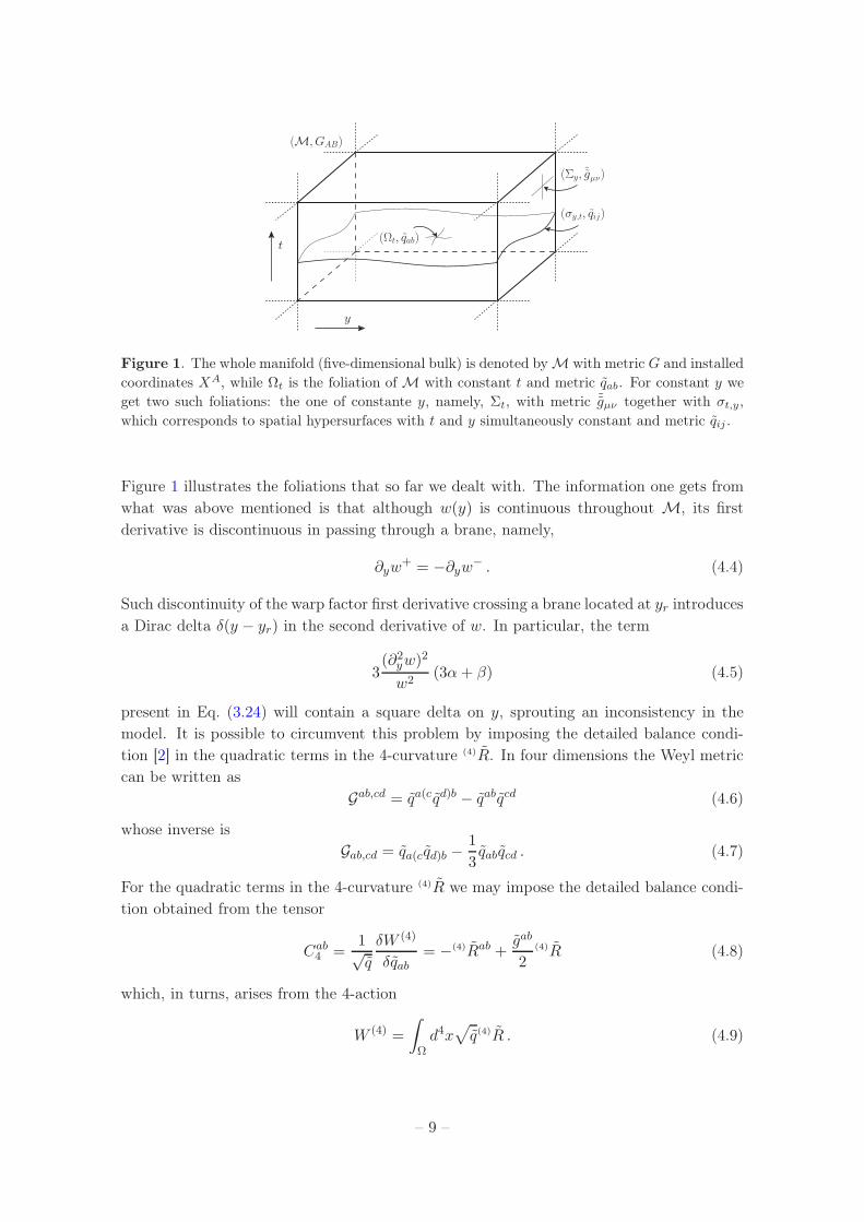
Figure 1. The whole manifold (five-dimensional bulk) is denoted by M with metric G and installed

coordinates XA, while Ωt is the foliation of M with constant t and metric qab. For constant y we

get two such foliations: the one of constante y, namely, Σt, with metric ˜gµν together with σt,y,

which corresponds to spatial hypersurfaces with t and y simultaneously constant and metric qij .

Figure 1 illustrates the foliations that so far we dealt with. The information one gets from

what was above mentioned is that although w(y) is continuous throughout M, its first

derivative is discontinuous in passing through a brane, namely,

∂yw+ = −∂yw

− . (4.4)

Such discontinuity of the warp factor first derivative crossing a brane located at yr introduces

a Dirac delta δ(y − yr) in the second derivative of w. In particular, the term

3(∂2

yw)2

w2(3α+ β) (4.5)

present in Eq. (3.24) will contain a square delta on y, sprouting an inconsistency in the

model. It is possible to circumvent this problem by imposing the detailed balance condi-

tion [2] in the quadratic terms in the 4-curvature (4)R. In four dimensions the Weyl metric

can be written as

Gab,cd = qa(cqd)b − qabqcd (4.6)

whose inverse is

Gab,cd = qa(cqd)b −1

3qabqcd . (4.7)

For the quadratic terms in the 4-curvature (4)R we may impose the detailed balance condi-

tion obtained from the tensor

Cab4 =

1√q

δW (4)

δqab= −(4)Rab +

gab

2(4)R (4.8)

which, in turns, arises from the 4-action

W (4) =

∫

Ωd4x√

q(4)R . (4.9)

– 9 –

The resulting condition then reads

β

∫

dtd4x√GCab

4 Gab,cdCcd4 = β

∫

dtd4x√G

(

(4)Rab(4)Rab −1

3(4)R2

)

. (4.10)

The relation imposed by (4.10) is equivalent of setting

α = −β

3(4.11)

in Eq. (2.1). From now on we are fixing α as (4.11) by imposing detailed balance condition

on quadratic terms in the 4-curvature (4)R. This clearly eliminates the delta squared from

(3.24).

Let us integrate Eq. (3.22) over y from yr − ǫ to yr + ǫ in the limit ǫ → 0. For a model

with the stress-energy tensor

SAB ≡ TBAB +

N−1∑

r=0

δ(y − yr)˜gµA˜gνBS

(r)µν , (4.12)

with TBAB being the energy-momentum tensor of the bulk while

S(r)µν = −˜gµντ

(r) + T (r)µν (4.13)

is the localized stress-energy tensor of the r-th brane written in term of the brane tension

τ (r) together with its energy-momentum tensor T(r)µν . Continuous terms in y will annulate.

The resulting equations are, then,

(−3wr + βR

wr

)

∂y lnw+ − β

2(∂y lnw

+)3 = −κ(5)2˜gµ0S(r)0µ = −κ(5)2S(r)0

0 , (4.14a)

˜giµS(r)µ0 = S(r)i

0 = 0 , (4.14b)∫ +

−

dyVij√wN

− 4β∂y lnw+ (3)Rij = κ(5)2

(

−S(r)ij +wrgij S

(r)00

)

, (4.14c)

where wr stands for w(yr). The equations above not only tell us about the discontinuity

of ∂yw but also impose some conditions on the metric gµν , on the 3-curvature (3)R, and on

the tensor Vij. In particular, although S(r)0µ 6= 0, the combination ˜giµS(r)

0µ must vanish.

5 Effective Lagrangian on the brane

Let us now consider the visible brane, arbitrarily chosen as the r = 0 brane in the position

y = 0.3 By first considering Eq. (4.14a), one must find the solution for A by solving

(−3w0 + β(3)R

w0

)

A− β

2A3 = κ(5)2

(

τ (0) − T (0)00

)

, (5.1)

where

A ≡ ∂y lnw+ . (5.2)

3Remember we are considering Z2 symmetry in the y direction.

– 10 –

Clearly ∂yw+ = w0A and, since we want a decreasing warp factor coming out from the

(visible) brane, the next brane must have a smaller warp factor. In other words,

A < 0 . (5.3)

The equation for A is of third degree and its solution is complicated. Instead of searching

such solution, let us analyze possible values for A in regions in our universe where T (0)00 = 0.

The positivity of the brane tension implies

β

2|A|3 −

(−3w0 + β(3)R

w0

)

|A| > 0 . (5.4)

There are three situations where (5.4) can be valid:

1. β > 0 and −3w0 + |β|(3)R > 0. This combination demands

|A| >√

2

w0|β|(−3w0 + |β|(3)R) . (5.5)

The odd result is that it does not permit solutions as (3)R = 0, what is expected at

large distances due to asymptotic flatness;

2. β > 0 and |β|(3)R < 3w0, implying that there are solutions for all

|A| > 0 ; (5.6)

and

3. β < 0 and 3w0 + |β|(3)R > 0, consisting in solutions of the type

0 < |A| <√

2

w0|β|(3w0 + |β|(3)R) . (5.7)

One may summarize all three possible solutions by setting

A ≡ −γ

√

2s

w0|β|(−s|β|(3)R+ 3w0) , (5.8)

with s ≡ β/|β| = sign(β) and s = ±1. Clearly, solution 1 relies on the choice s = 1

and s = −1 imposing γ > 1, while solution 2 consists of setting s = 1 and s = 1 for any

γ > 0, and, the last possibility, solution 3 corresponds to s = −1 and s = 1 and demands

0 < γ < 1. In terms of the dimensionless γ, (5.1) turns out to be

|β|2

[

2s

w0|β|(

−s|β|(3)R+ 3w0

)

] 3

2(

sγ + sγ3)

= κ(5)2(

τ (0) − T (0)00

)

. (5.9)

So far we still have a complicated equation in γ. However, as well as γ is an unknown, so

is the tension τ (0) on the brane. Instead of finding an expression for γ as a function of τ (0),(3)R, β, and so forth, we will try to limit some values for γ and then express τ (0) in terms

– 11 –

of it. In order to do that we may study the gravity sector of the effective Lagrangian for

the brane that, up to surface terms in y, is written as follows:

LG(t, ~x) ≡ L(5)(t, ~x, y = ±ǫ)

=N√q

2κ(5)2

w0

(

KijKij −K2 + (3)R)

+ 3(∂yw±)2 − β

3(3)R2 + β (3)Rij (3)Rij

+ β

[

1

4

(∂yw±)4

w20

−(3)R

2

(∂yw±)2

w0

]

=N√q

2κ(5)2

w0

[

KijKij −K2 + (3)R(

1− 9ssγ2 − 6γ4)]

− β(3)R2

(

1

3− ssγ2 − γ4

)

+ β (3)Rij (3)Rij +9w2

0γ2

β

(

2ss+ γ2)

, (5.10)

with q ≡ det(qij).

At this point a digression is needed. We recall the results found in refs. [4, 5], where it

was shown that the propagator of the linearized theory given by a Lagrangian like the one

above will get an improvement in its ultraviolet behavior if and only if the quadratic terms

in the 3-curvature (3)R obeys detailed balance condition. Although we have already imposed

detailed balance condition in the quadratic term for the Lagrangian in (4+1)-dimensions,

the proceeding of evaluating the effective (3+1)-dimensional Lagrangian has changed it. To

restore detailed balance condition, the quadratic term in the 3-curvature must derive from

a 3-dimensional action defined in the foliation Σ0∼= ℜ× σ0, namely,

W (3) =

∫

σ0

d3x√q(3)R . (5.11)

In three dimensions the inverse of the Weyl metric is given by

Gij,kl = qi(kql)j −1

2qijqkl . (5.12)

Now, the detailed balance condition will come out from the tensor

Cij3 =

1√q

δW (3)

δqij= −(3)Rij +

qij

2(3)R (5.13)

and the result is

β

∫

ℜ

dt

∫

σ0

d3xN√qCij

3 Gij,klCkl3 = β

∫

ℜ

dt

∫

Σ0

d3xN√q

(

−3

8(3)R2 + (3)Rij (3)Rij

)

. (5.14)

A direct consequence of demanding the detailed balance condition in the (3+1) La-

grangian (5.10) corresponds to set

− 1

3+ ssγ2 + γ4 = −3

8. (5.15)

There is no real solution to the above equation when s = s and, therefore, solution 2 is not

acceptable. For s = −s ⇒ ss = −1 (either solution 1 or solution 3), the positive values for

γ turn out to be

γ± =1

2

√

2±√

10

3> 0 . (5.16)

– 12 –

Since 0 < γ± < 1, the possible solution that leads to τ (0) > 0 is solution 3 and corresponds

to β = −|β| < 0. In fact,

τ (0)

± = T (0)00 +

|β|48κ(5)2w0

(

2√3∓

√10)

√

6±√30

[

2

w0|β|(

|β|(3)R+ 3w0

)

]3

2

. (5.17)

The resulting effective Lagrangian then reads

L±

G(t, ~x) =N√q

2κ(5)2

[

w0

(

KijKij −K2 + σ±(3)R

)

+3|β|8

(3)R2 − |β|(3)Rij (3)Rij + 2w20Λ±

]

, (5.18)

where

σ± ≡ 1

4

(

11±√30)

> 0 , (5.19a)

Λ± ≡ 3

16|β|(

13± 2√30)

> 0 . (5.19b)

One must remember that so far we have calculated the effective Lagrangean for gµν . But

what we really measure in our universe comes from the metric Gµν = wgµν . By considering

again that N =√wN , N i = wN i, qij = wqij ⇒ q = w3/2q and that Kij =

√wKij as one

can see from (3.18c), the effective Lagrangian is

L±

G(t, ~x) =N√q

2κ(5)2

(

KijKij − K2 + σ±(3)R

+3|β|8

(3)R2 − |β|(3)Rij (3)Rij + 2Λ±

)

. (5.20)

Let us define

N± ≡ √σ±N , (5.21a)

κ(4)

±

2 ≡ κ(5)2

√σ±

, (5.21b)

β± ≡ |β|σ±

> 0 , (5.21c)

Λ± ≡ Λ±

σ±=

3

16|β|σ±

(

13± 2√30)

> 0 , (5.21d)

in terms of what the resulting Lagrangian is, then,

L±

G(t, ~x) =N±

√q

2κ(4)

±

2

(

KijKij − K2 + (3)R

+3β±8

(3)R2 − β±(3)Rij (3)Rij + 2Λ±

)

. (5.22)

One important result from the above procedure is that we have obtained a cosmolog-

ical constant on the brane without previously introducing it. The cosmological constant

– 13 –

obtained in (5.21d) has appeared as a result of the Hořava bulk into the brane. Note that

this brane cosmological constant is positive, in agreement with a de Sitter-like universe.

Moreover, one may verify, by comparing the equations (2.1) and (2.24b) in ref. [5] with

equation (5.22), that the dispersion relation for the graviton in the linearized version of

(5.22) is

k02± = ~k2 + β±~k

4 + 2Λ± . (5.23)

It is important that β± > 0 (β < 0) to avoid a limitation in the graviton energy, otherwise

one will get imaginary values for the energy.

6 Consistency conditions

After the previous considerations, it would be interesting to verify whether negative brane

tension is necessary in the compactification scheme. Note that the identity

∂y

(

wξ∂yw)

= wξ+1

[

ξ(∂yw)

2

w2+

∂2yw

w

]

(6.1)

enable us to obtain, for an arbitrary ξ, the consistency equations∮

dywξ+1

[(

ξ +1

2

)(

R

w− (4)Rµ

µ

)

+ (ξ − 1)(4)R44

]

= 0, (6.2)

by considering equations (3.17) and by setting (4)Rµµ ≡ ˜gµν (4)Rµν . We emphasize that the

symbol∮

stands for a integration along the extra dimension y which, by means of the

orbifold symmetry, is compact without boundary in such a way that∮

dy∂y(

wξ∂yw)

= 0.

These consistency equations above may be modified as well by considering

(4)Rµµ = −1

3Λµµ − 4

3Λ44 −

1

3κ(5)2Sµ

µ − 4

3κ(5)2S44 (6.3)

and(4)R44 =

2

3Λ44 −

1

3Λµµ − 1

3κ(5)2Sµ

µ +2

3κ(5)2S44 , (6.4)

where S = GABSAB, as one can see from (3.20). The desired form for the consistency

equations are, then,∮

dywξ+1

[(

ξ +1

2

)

R

w+

1

2κ(5)2 S +

1

2Λ +

(

2ξ − 1

2

)

(

Λ44 + κ(5)2S44

)

]

= 0 . (6.5)

In the above equation, the definitions Λ ≡ ΛAA and S ≡ SA

A were used. Notice that the last

equation must be valid for any point t, ~x in the (3+1)-dimensional spacetime. Since the

space is not full of matter, we choose a point of vacuum (TBAB = 0 = T(r)µν ) so that (6.5)

must be written as

2κ(5)2∑

r

τ (r)ωξ+1r =

(

ξ +1

2

)

R

∮

dy wξ +

∮

dy wξ+1

[

1

2Λ +

(

2ξ − 1

2

)

Λ44

]

. (6.6)

If one chooses α = β = 0, taking ξ > −1/2 and remembering that w > 0, the sum over

the tensions seems to be positive. However, since R does not depend on y, we can consider

– 14 –

our universe where R is practically zero (about 10−120 M2P [9]). This, in turns, lead us to

the necessity of having at least one brane with negative tension. Notice that this problem

has disappeared due to the presence of extra terms coming from the higher order terms in

4-spatial curvature in the Hořava-like model we proposed. Of course, it will depend mostly

on the choice of the signs of α and β. In order to fix them, for simplicity we will evaluate

the consistency condition for ξ = 1/4, namely,

4κ(5)2∑

r

τ (r)ω5

4r =

∮

dy w5

4 Λ . (6.7)

The calculation of Λ is rather intricate and the details are in appendix A. Here we just

quote the result

Λ = − 2

w3/4

qikqjl

NDiDj

N

[

β(3)Rkl +

(

3α+β

2

)

qkl(3)R

]

+

[

(27α+ 7β)(∂yw)

2

w7/4+ 4 (9α+ 2β) ∂y

(

∂yw

w3/4

)]

qij

2NDi∂jN +

β(3)Rij (3)Rij + α(3)R2

2w3/4

+β (3)R

2

[

(∂yw)2

w7/4+ 2∂y

(

∂yw

w3/4

)]

− β

[

5

8

(∂yw)4

w11/4+ ∂y

(

(∂yw)3

w7/4

)]

− 3(3α+ β)

[

3

2

(∂2yw)

2

w3/4− 3

4

(∂yw)2∂2

yw

w7/4− ∂y

(

∂yw∂2yw

w3/4

)

− 2w1/4∂4yw

]

. (6.8)

So far we left α generic again. But notice that Λ contains problematic terms like the square

of ∂2yw, ∂4

yw and so on. However, all those terms may be eliminated again by imposing the

detailed balance condition (4.10). In other words, by again fixing α through the equation

3α+ β = 0. Nothing prevent us from choosing this option, what simplifies last equation as

16κ(5)2

3

∑

r

τ (r)ω5

4r = β

1

2

[

(3)Rij (3)Rij −1

3(3)R2 − 4

N

(

(3)Rij +1

2qij (3)R

)]

Di∂jN I1

+

(

(3)R

2− qijDi∂jN

N

)

I2 −5

8I3

. (6.9)

Above, we defined the integrals

I1 ≡∮

dy

w3/4> 0 , (6.10)

I2 ≡∮

dy(∂yw)

2

w7/4> 0 , (6.11)

and

I3 ≡∮

dy(∂yw)

4

w11/4> 0 . (6.12)

The equation (6.9) is valid for every point in the (3+1)-spacetime Σ. To study the sign of

β we take large radius (r → ∞) in Σ where (3)Rij = 0 and N → 1.4 In this region

16κ(5)2

3

∑

r

τ (r)ω5

4r = −5β

8I3 . (6.13)

4Obviously, it is in accordance with our previous vacuum case particularization.

– 15 –

Since τ (r) is a constant, this result must be independent of point chosen to evaluate it. To

eliminate negative tension in the branes clearly we have to set β = −|β|, being in accordance

with the results obtained in the previous section.

7 Summary and conclusions

In this work we dealt with a (4+1)-dimensional Hořava-like model treated by means of

braneworld models. We have calculated the equation of motion of the model and, by

defining a warped metric characterized by the warp factor w(y) > 0, we showed that

warped geometry requires λ = 1. This is interesting as λ 6= 1 has introduced several illness

in the original Hořava theory such as ghosts [5]. Furthermore, in the context of brane

theory, where ∂yw is discontinuous across the branes, the extra terms labeled by α and β

introduces inconsistencies proportional to (∂2yw)

2 ∼ (δ(y))2. However, those inconsistencies

are cancelled simply by setting α = −β/3, what we verified corresponds exactly to demand

detailed balance condition for the quadratic terms in the 4-curvature (4)R.

The discontinuity of ∂yw also led us to the Israel’s junction condition which, in turns,

enabled us to obtain an effective Lagrangian on the brane. Nonetheless, although the result-

ing Lagrangian corresponded to a (3+1)-dimensional Hořava-like model with an emerging

positive cosmological constant, it failed to obey detailed balance condition. By imposing

then the detailed balance condition in the quadratic terms in the 3-curvature (3)R for this

effective theory, positive brane tension demanded β < 0. The most interesting aspect of this

result is the fact that this sign for β was exactly the expected one for a graviton dispersion

relation that have only real energy k0.

Despite coincidences among detailed balance condition, positive tension and desired

sign for β, it was important to verify whether the theory permits only positive tension

for all branes in the compactification scheme. The response to this task was obtained

by studying the consistency conditions in the last section. Again, the detailed balance

condition played an essential role by eliminating undesired terms like (∂2yw)

2. Moreover,

the answer relied in the sign of β that was shown to be negative, in accordance with the

results above commented.

The mechanism of detailed balance condition has served as a basis not only for avoiding

spreading of constants in the theory, which was one of the arguments used by Hořava, as

well as it was essential for the consistency of the model. It has not only guaranteed the

improvement of the propagator [4, 5], but also eliminated inconsistencies in the present work.

Furthermore, it worked in agreement with the expected sign of β, sometimes imposing it. In

fact, we are not aware of the complete implications of the detailed balance condition and its

relation in particular with the quadratic term in curvature.5 So far we have just analyzed

its consequences. The present results points to the necessity of a deeper understanding of

this mechanism in more general grounds.

5It is worth saying that, at least regarding ultraviolet behavior of the propagator, there is a necessity of

the detailed balance condition only in the quadratic terms in curvature, a soft detailed balance condition,

despite the presence of higher order terms in the action, as shown in ref. [5].

– 16 –

A Evaluation of Λ

From (3.21), it is straightforward to obtain

Λ =1

2

(

α (4)R2 + β (4)Rab(4)Rab

)

+qabVab

N, (A.1)

where the first term in the right hand side of the above equation can be found in (3.24).

The more intricate term is qabVab. By defining vab ≡ Nfab (v ≡ gabvab) and by keeping in

mind that v4i = 0, it can be expressed as [see (3.11)]

qabVab = −1

2qabDaDbv − qacqbdDaDbvcd

= −1

2∂2yv −

1

2qijDiDjv − ∂2

yv44 − qijD4Div4j − qijDiD4v4j − qikqjlDiDjvkl .

(A.2)

We are benefited of the identity

(4)Γ44a = (4)Γa

44 = 0 . (A.3)

Note that(4)Γ4

ij = − gij2

∂yw

w, (A.4)

while

(4)Γi4j =

δij2

∂yw

w. (A.5)

Pure spatial indexes lead us to

(4)Γijk =

qil

2

(

2∂(jqk)l − ∂lqjk)

= (3)Γijk . (A.6)

Although vi4 = 0, this is not true for Dav4i. The important relations one needs at this

point are

Div4j =1

2

∂yw

w(qijv44 − vij) , (A.7)

D4vij = w∂y

(vijw

)

, (A.8)

Divjk = Divjk , (A.9)

together with D4vi4 = 0. With those relations in mind one is able to get

qijDiDjv = qij(

∂i∂jv − (4)Γaij∂av

)

=qij

wDi∂jv +

3

2

∂yw∂yv

w, (A.10)

qijD4Div4j = qij(

∂yDiv4j − (4)Γa4iDav4j − (4)Γa

4jDiv4a

)

=1

2∂y

[

∂yw (4v44 − v)

w

]

, (A.11)

– 17 –

qijDiD4v4j = qij(

−(4)Γli4Dlv4j − (4)Γl

i4D4vlj − (4)Γ4ij∂yv44

)

=1

2

∂yw√w

(

4v44 − v√w

)

, (A.12)

and

qikqjlDiDjvkl = qik qjl(

∂iDjvkl − (4)ΓaijDavkl − (4)Γa

ikDjval − (4)ΓailDjvka

)

=qikqjl

w2DiDjvkl +

1

2

∂yw∂y (v − v44)

w+

(∂yw)2

w2(4v44 − v) . (A.13)

By collecting the results (A.7)–(A.13) into (A.2), dividing it by N =√wN , writing vab =√

wNfab and then inserting it into (A.1) one finally gets the result quoted in (6.8).

Acknowledgments

This work was partially supported by Fundação de Amparo à Pesquisa do Estado de São

Paulo (FAPESP) and Conselho Nacional de Pesquisas (CNPq).

References

[1] K. S. Stelle, Renormalization of higher-derivative quantum gravity, Phys. Rev. D 16 (1977)

953–969.

[2] P. Horava, Quantum gravity at a lifshitz point, Phys. Rev. D 79 (2009) 084008,

[arXiv:0901.3775].

[3] D. Orlando and S. Reffert, On the renormalizability of horava-lifshitz-type gravities,

Class.Quant.Grav. 26 (2009) 155021, [arXiv:0905.0301].

[4] F. Bemfica and M. Gomes, Fourth order spatial derivative gravity, Phys.Rev. D84 (2011)

084022, [arXiv:1108.5979].

[5] F. Bemfica and M. Gomes, Propagator in the horava-lifshitz gravity, arXiv:1111.5779.

[6] L. Randall and R. Sundrum, An Alternative to compactification, Phys.Rev.Lett. 83 (1999)

4690–4693, [hep-th/9906064].

[7] M. Abdalla, M. Guimaraes, and J. Hoff da Silva, Positive tension 3-branes in an AdS5 bulk,

JHEP 1009 (2010) 051, [arXiv:1001.1075].

[8] J. Hoff da Silva and M. Dias, Five Dimensional f(R) Braneworld Models, Phys.Rev. D84

(2011) 066011, [arXiv:1107.2017].

[9] G. W. Gibbons, R. Kallosh, and A. D. Linde, Brane world sum rules, JHEP 0101 (2001)

022, [hep-th/0011225].

[10] F. Leblond, R. C. Myers, and D. J. Winters, Consistency conditions for brane worlds in

arbitrary dimensions, JHEP 0107 (2001) 031, [hep-th/0106140].

[11] W. D. Goldberger and M. B. Wise, Modulus stabilization with bulk fields, Phys.Rev.Lett. 83

(1999) 4922–4925, [hep-ph/9907447].

[12] M. Henneaux, A. Kleinschmidt, and G. L. Gomez, A dynamical inconsistency of horava

gravity, Phys. Rev. D 81 (2010) 064002, [arXiv:0912.0399].

– 18 –

[13] D. Blas, O. Pujolas, and S. Sibiryakov, On the extra mode and inconsistency of horava

gravity, JHEP 10 (2009) 029, [arXiv:0906.3046].

[14] R. M. Wald, General Relativity. The University of Chicaco Press, Chicaco and London, 1984.

[15] T. Thiemann, Modern canonical quantum general relativity. Cambridge University Press,

2007.

[16] W. Israel, Singular hypersurfaces and thin shells in general relativity., Il Nuovo Cimento B

44 (1966) 1.

– 19 –