Simultaneous Stabilization of Power System Using UPFC-Based Controllers

Electric Power Components and Systems, 34:941–959, 2006Copyright © Taylor & Francis Group, LLCISSN: 1532-5008 print/1532-5016 onlineDOI: 10.1080/15325000600596635

Simultaneous Stabilization of Power SystemUsing UPFC-Based Controllers

ALI T. AL-AWAMI

Electrical Engineering DepartmentKing Fahd University of Petroleum and MineralsDhahran, Saudi Arabia

Y. L. ABDEL-MAGID

Electrical Engineering ProgramPetroleum InstituteAbu Dhabi, United Arab Emirates

M. A. ABIDO

Electrical Engineering DepartmentKing Fahd University of Petroleum and MineralsDhahran, Saudi Arabia

This article studies the use of robust UPFC-based stabilizers to damp low frequencyoscillations. The potential of the UPFC-based stabilizers to enhance the dynamicstability is evaluated by singular value decomposition. Particle swarm optimizationtechnique is used to optimize the parameters of each stabilizer, first individually, thenconcurrently. To ensure the robustness of the proposed stabilizers, the design processconsiders a wide range of operating conditions. The effectiveness of the proposedcontrollers is verified through several linear and nonlinear analysis techniques. Thesetechniques prove that the coordinated design of UPFC-based stabilizers is superiorover any of the individual designs.

Keywords FACTS devices, UPFC, particle swarm optimization, simultaneous sta-bilization, power system stability

1. Introduction

As power demand grows rapidly and expansion in transmission and generation is re-stricted, power systems are today much more loaded than before. This causes the powersystems to be operated near their stability limits. In addition, interconnection between

Manuscript received in final form on 24 January 2006.The authors would like to acknowledge King Fahd University of Petroleum and Minerals for

the support of this work under Project # KFUPM EE/Power/282.Address correspondence to Dr. M. A. Abido, Electrical Engineering Dept., KFUPM Box 183,

Dhahran 31261, Saudi Arabia. E-mail: [email protected]

941

942 A. T. Al-Awami et al.

remotely located power systems gives rise to low frequency oscillations in the rangeof 0.1–3.0 Hz. If not well damped, these oscillations may keep growing in magnitude,resulting in loss of synchronism.

Power system stabilizers (PSSs) have been used in the last few decades to serve thepurpose of enhancing power system damping to low frequency oscillations. PSSs haveproved to be efficient in performing their assigned tasks. However, they may adverselyaffect voltage profile and may not be able to suppress oscillations resulting from severedisturbances, especially those that may occur at the generator terminals.

A wide spectrum of PSS tuning approaches has been proposed. These approacheshave included pole placement [1], damping torque concepts [2],H∞ [3], variable structure[4], and the different optimization and artificial intelligence techniques [5–7].

FACTS devices have shown very promising results when used to improve powersystem steady-state performance. Because of the extremely fast control action associatedwith FACTS-device operations, they have been potential candidates for utilization inpower system damping enhancement.

A unified power flow controller (UPFC) is the most versatile device in the FACTSconcept. It has the ability to adjust the three control parameters, i.e., the bus voltage,transmission line reactance, and phase angle between two buses, either simultaneouslyor independently. A UPFC performs this through the control of the in-phase voltage,quadrature voltage, and shunt compensation. Until now, not much research has beendedicated to the analysis and control of UPFCs.

Several trials have been reported in the literature to model a UPFC for steady-state and transient studies. Based on Nabavi-Iravani model [8], Wang developed twoUPFC models [9, 10] that have been linearized and incorporated into the Heffron-Phillipsmodel [11].

A number of control schemes have been suggested to perform the oscillation-dampingtask. Huang et al. [12] attempted to design a conventional fixed-parameter lead-lag con-troller for a UPFC installed in the tie line of a two-area system to damp the interareamode of oscillation. Mok et al. [13] considered the design of an adaptive fuzzy logic con-troller for the same purpose. Dash et al. [14] suggested the use of a radial basis functionNN for a UPFC to enhance system damping performance. Robust control schemes, suchas H∞ and singular value analysis, have also been explored [15, 16]. To avoid pole-zerocancellation associated with the H∞ approach, the structured singular value analysis havebeen utilized in [17] to select the parameters of the UPFC controller to have the robuststability against model uncertainties.

In this work, singular value decomposition (SVD) is used to select the control signalsthat are most suitable for damping the electromechanical (EM) mode oscillations. This isdone as SVD analysis can be readily used to estimate the EM mode controllability of thedifferent UPFC-based stabilizers. A weakly connected system equipped with a UPFC isused in this study. The problem of designing the damping stabilizers is formulated as anoptimization problem to be solved using PSO. The aim of the optimization is to search forthe optimum controller parameter settings that minimize the maximum damping factorof the system complex modes. To ensure the robustness of the proposed stabilizers, thedesign process simultaneously takes into account several loading conditions with andwithout system parameter uncertainties, a process called simultaneous stabilization. Inaddition, a coordinated scheme of the UPFC-based stabilizers is presented. Dampingtorque coefficient, eigenvalue and nonlinear simulation analyses are used to assess theeffectiveness of the proposed stabilizers to damp low frequency oscillations.

Simultaneous Stabilization of Power System 943

2. Problem Statement

2.1. Nonlinear Model of Power System with UPFC

Figure 1 shows a SMIB system equipped with a UPFC. The UPFC consists of an excita-tion transformer (ET), a boosting transformer (BT), two three-phase GTO based voltagesource converters (VSCs), and DC link capacitors. The four input control signals to theUPFC are mE , mB , δE , and δB , where

mE is the excitation amplitude modulation ratio,mB is the boosting amplitude modulation ratio,δE is the excitation phase angle, andδB is the boosting phase angle.

By applying Park’s transformation and neglecting the resistance and transients of theET and BT transformers, the UPFC can be modeled as [8–10]:

[vEtdvEtq

]=

[0 −xExE 0

] [iEdiEq

]+

mE cos δEvdc

2

mE sin δEvdc2

(1)

[vBtdvBtq

]=

[0 −xBxB 0

] [iBdiBq

]+

mB cos δBvdc

2

mB sin δBvdc2

(2)

vdc = 3mE4Cdc

[cos δE sin δE

] [iEdiEq

]+ 3mB

4Cdc

[cos δE sin δB

] [iBdiBq

](3)

where vEt , iE , vBt , and iB are the excitation voltage, excitation current, boosting voltage,and boosting current, respectively; Cdc and vdc are the DC link capacitance and voltage,respectively.

Figure 1. SMIB power system equipped with UPFC.


The nonlinear model of the SMIB system of Figure 1 is

δ = ωb(ω − 1) (4)

ω = (Pm − Pe −D(ω − 1))/M (5)

E′q = [−E′

q + Efd + (xd − x′d)id ]/T ′

do (6)

Ef d = (KA(Vref − v + uPSS)− Efd)/TA (7)

where Pm and Pe are the input and output power, respectively.

Pe = vdid + vqiq, v = (v2d + v2

q)1/2, vd = xqiq, vq = E′

q − x′d id ,

id = iEd + iBd, iq = iEq + iBq(8)

M and D the inertia constant and damping coefficient, respectively; ωb the synchronousspeed; δ and ω the rotor angle and speed, respectively; E′

q , E′f d , and v the generator

internal, field and terminal voltages, respectively; T ′do the open circuit field time constant;

xd , x′d , and xq the d-axis reactance, d-axis transient reactance, and q-axis reactance, re-

spectively; KA and TA the exciter gain and time constant, respectively; Vref the referencevoltage; and uPSS the PSS control signal.

Also from Figure 1, we have

v = jxtEit + vEt (9)

vEt = vBt + jxBV iB + vb (10)

where it and vb, are the armature current and infinite bus voltage, respectively; vEt , vBt ,and iB the ET voltage, BT voltage, and BT current, respectively.

From (9) we have

vd + jvq = xq(iEq + iBq)+ j [E′q − x′

d(iEd + iBd)]= jxtE(iEd + iBd + jiEq + jiBq)+ vEtd + vEtq

(11)

And from (10) we have

vEtd + jvEtq = vBtd + jvBtq + jxBV iBd − xBV iBq + vb sin δ + jvb cos δ (12)

From (1)–(2) and (11)–(12) we can find

iEd = xBB

xd E′q − mE sin δEvdcxBd

2xd + xdE

xd

(vb cos δ + mB sin δBvdc

2

)(13)

iEq = mE cos δEvdcxBq2xq

− xqE

xq

(vb sin δ + mB cos δBvdc

2

)(14)

iBd = xE

xd E′q + mE sin δEvdcxdE

2xd − xdt

xd

(vb cos δ + mB sin δBvdc

2

)(15)

iBq = −mE cos δEvdcxqE2xq

+ xqt

xq

(vb sin δ + mB cos δBvdc

2

)(16)


where

xq = (xq + xtE + xE)(xB + xBV )+ xe(xq + xtE),xBq = xB + xBV + xq + xtE

(17)

xqt = xq + xtE + xE, xqE = xq + xtE (18)

xd = (x′d + xtE + xE)(xB + xBV )+ xE(x′

d + xtE),xBd = xB + xBV + x′

d + xtE(19)

xdt = x′d + xtE + xE, xdE = x′

d + xtE (20)

xBB = xB + xBV (21)

xE and xB are the ET and BT reactances, respectively.

2.2. Linearized Model of Power System with UPFC

The nonlinear dynamic equations can be linearized around a given operating point tohave the linear model given below:

!δ = ωb!ω (22)

!ω = (!Pm −!Pe −D!ω)/M (23)

!E′q = [−!E′

q +!Efd + (xd − x′d)!id ]/T ′

do (24)

!Efd = [−!Efd +KA(!Vref −!v +!upss]/TA (25)

!vdc = K7!δ +K8!E′q −K9!vdc +Kce!mE +Kcδe!δE

+Kcb!mB +Kcδb!δB(26)

where

!Pe = K1!δ +K2!E′q +Kpd!vdc +Kpe!mE +Kpδe!δE

+Kpb!mB +Kpδb!δB(27)

!Eq = K4!δ +K3!E′q +Kqd!vdc +Kqe!mE +Kqδe!δE

+Kqb!mB +Kqδb!δB(28)

!v = K5!δ +K6!E′q +Kvd!vdc +Kve!mE +Kvδe!δE

+Kvb!mB +Kvδb!δB(29)

K1–K9, Kpu, Kqu, and Kvu are linearization constants.


In state-space representation, the power system can be modeled as

x = Ax + Bu (30)

where the state vector x and control vector u are

x = [!δ !ω !E′

q !Efd !vdc]T

(31)

u = [!upss !mE !δE !mb !δb

]T (32)

A =

0 ωb 0 0 0

−K1

M−DM

−K2

M0 −Kpd

M

−K4

T ′do

0 −K3

T ′do

1

T ′do

−KqdT ′do

−KAK5

TA0 −KAK6

TA− 1

TA−KAKvd

TA

K7 0 K8 0 −K9

(33)

B =

0 0 0 0 0

0 −KpeM

−KpδeM

−KpbM

−KpδbM

0 −KqeT ′do

−KqδeT ′do

−KqbT ′do

−KqδbT ′do

KA

TA−KAKve

TA−KAKvδe

TA−KAKvb

TA

KAKvδb

TA

0 Kce Kcδe Kcb Kcδb

(34)

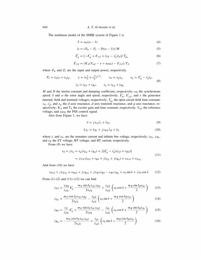
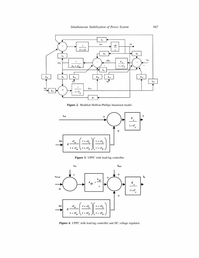
The linearized dynamic model of the state-space representation is shown in Figure 2.Only one UPFC control input is considered in this figure.

2.3. UPFC-Based Stabilizers

The UPFC damping stabilizers are the widely used lead-lag scheme of the structure,shown in Figure 3, where u can be mE , mB , or δB .

In order to maintain the power balance between the series and shunt converters,a DC voltage regulator must be incorporated. The DC voltage is controlled throughmodulating the phase angle of the ET voltage, δE . Therefore, the δE damping controllerto be considered is that shown in Figure 4, where the DC voltage regulator is a PI-controller.

2.4. Objective Function and Stabilizer Design

In this study, several loading conditions, including nominal, light, heavy, and leadingpower factor without and with system parameter uncertainties, are considered simulta-neously to ensure the robustness of the proposed stabilizers. To select the best stabilizer


Figure 2. Modified Heffron-Phillips linearized model.

Figure 3. UPFC with lead-lag controller.

Figure 4. UPFC with lead-lag controller and DC voltage regulator.


parameters that enhance the most power system transient performance, the problem isformulated so as to optimize a selected objective function J subject to some inequalityconstraints, which are the maximum and minimum limits of each controller gain K andtime constants T1–T4.

In this work,

J = max{σi} (35)

where σi is the damping factor corresponding to the least damped complex mode of theith loading condition.

Hence, the design problem can be formulated as:

minimize J

Subject to Kmin ≤ K ≤ Kmax

T min1 ≤ T1 ≤ T max

1


2


3


4

The proposed approach employs PSO to search for the optimum parameter settings ofthe given controllers.

3. Controllability Measure

To measure the controllability of the EM mode by a given input (control signal), thesingular value decomposition (SVD) is employed. Mathematically, if G is an m × n

complex matrix, then there exist unitary matrices W and V with dimensions of m × mand n× n, respectively, such that

G = W V (36)

where

=[ 1 00 0

], 1 = diag(σ1, . . . , σr ) (37)

with σ1 ≥ · · · ≥ σr ≥ 0 where r = min{m, n} and σ1, . . . , σr are the singular valuesof G.

The minimum singular value σr represents the distance of the matrix G from all thematrices with a rank of r−1. This property can be used to quantify modal controllability[18]. The matrix B can be written as B = [b1 b2 b3 b4 b5] where bi is a columnvector corresponding to the ith input. The minimum singular value, σmin, of the matrix[λI −A bi] indicates the capability of the ith input to control the mode associated withthe eigenvalue λ. Actually, the higher the σmin, the higher the controllability of this modeby the input considered. As such, the controllability of the EM mode can be examinedwith all inputs in order to identify the most effective one to control the mode.


4. Particle Swarm Optimizer

A novel population based optimization approach, called particle swarm optimization(PSO) approach, was introduced first in [19]. This new approach features many advan-tages; it is simple, fast and can be coded in few lines. Also, its storage requirement isminimal.

Moreover, this approach is advantageous over evolutionary and genetic algorithms inmany ways. First, PSO has memory. That is, every particle remembers its best solution(local best) as well as the group best solution (global best). Another advantage of PSO isthat the initial population of the PSO is maintained, and so there is no need for applyingoperators to the population, a process that is time and memory storage consuming [19–21].

PSO starts with a population of random solutions “particles” in a D-dimensionspace. The ith particle is represented by Xi = (xi1, xi2, . . . , xiD). Each particle keepstrack of its coordinates in hyperspace, which are associated with the fittest solution ithas achieved so far. The value of the fitness for particle i (pbest) is also stored asPi = (pi1, pi2, . . . , piD). The global version of the PSO keeps track of the overall bestvalue (gbest), and its location, obtained thus far by any particle in the population [20, 21].

PSO consists of, at each step, changing the velocity of each particle toward itspbest and gbest according to Eq. (38). The velocity of particle i is represented as Vi =(vi1, vi2, . . . , viD). Acceleration is weighted by a random term, with separate randomnumbers being generated for acceleration toward pbest and gbest. The position of the ithparticle is then updated according to Eq. (39) [20, 21].

vid = w ∗ vid + c1 ∗ rand() ∗ (pid − xid)+ c2 ∗ Rand() ∗ (pgd − xid) (38)

xid = xid + vid (39)

where

pid = pbest and pgd = gbest (40)

The PSO algorithm can be described as follows:

Step 1: Initialize an array of particles with random positions and their associatedvelocities to satisfy the inequality constraints.

Step 2: Check for the satisfaction of the equality constraints and modify the solutionif required.

Step 3: Evaluate the fitness function of each particle.Step 4: Compare the current value of the fitness function with the particles’ previous

best value (pbest). If the current fitness value is less, then assign the currentfitness value to pbest and assign the current coordinates (positions) to pbestx.

Step 5: Determine the current global minimum fitness value among the current po-sitions.

Step 6: Compare the current global minimum with the previous global minimum(gbest). If the current global minimum is better than gbest, then assignthe current global minimum to gbest and assign the current coordinates(positions) to gbestx.

Step 7: Change the velocities according to Eq. (38).Step 8: Move each particle to the new position according to Eq. (39) and return to

Step 2.Step 9: Repeat Step 2–Step 8 until a stopping criterion is satisfied or the maximum

number of iterations is reached.


5. Simulation Results

5.1. Controllability Measure

First, singular value decomposition is employed to measure the controllability of theEM mode from each of the UPFC input signals: mE , δE , mB , and δB . The minimumsingular value, σmin, is estimated over a wide range of operating conditions. For SVDanalysis, Pe ranges from 0.05 to 1.4 p.u. andQe = [0, 0.4]. At each loading condition, thesystem model is linearized, the EM mode is identified, and the SVD-based controllabilitymeasure is implemented.

For comparison purposes, the minimum singular value for the four inputs at Qe =0.0 p.u. and Qe = 0.4 p.u. are shown in Figures 5 and 6, respectively. From these figures,it is evident that δE and mB are more powerful than δB and mE . Hence, they are theUPFC signals to be considered throughout this study. It can be also concluded that:

• δE capability of controlling the EM mode is almost independent of loading.• The controllability of δE is generally higher than those of the other stabilizers,

especially for low and moderate loading.• At very low loading, all the stabilizers, except the mB -based stabilizer at nominal

loading and the δE-based stabilizer, suffer from poor controllability.

5.2. Stabilizer Design

The objective is to design robust δE- and mB -based stabilizers. Both individual and co-ordinated designs are to be considered. To ensure the stabilizer effectiveness over a widerange of operating conditions, the design process takes into account several loading con-ditions including nominal, light, heavy, and leading Pf conditions. These conditions areconsidered without and with system parameter uncertainties, such as machine inertia, lineimpedance, and field time constant. The total number of operating conditions consideredduring the design process is 16, as given in Table 1.

First, PSO is used to optimize the parameters of each stabilizer individually. Theobjective function is to minimize the maximum damping factors of all the complexeigenvalues associated with the 16 operating points simultaneously. Then, PSO is used tosearch for the optimum parameters of both controllers simultaneously. The final settingsof the optimized parameters for the proposed stabilizers are given in Table 2.

For reference, Table 3 lists the open-loop eigenvalues associated with the EM modes

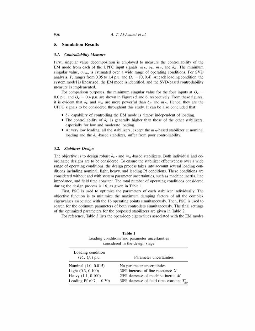
Table 1Loading conditions and parameter uncertainties

considered in the design stage

Loading condition(Pe, Qe) p.u. Parameter uncertainties

Nominal (1.0, 0.015) No parameter uncertaintiesLight (0.3, 0.100) 30% increase of line reactance XHeavy (1.1, 0.100) 25% decrease of machine inertia MLeading Pf (0.7, −0.30) 30% decrease of field time constant T ′

do


Figure 5. Minimum singular value with all stabilizers at Qe = 0.0.

Figure 6. Minimum singular value with all stabilizers at Qe = 0.4.


Table 2The optimal parameter settings of the individual

and coordinated designs

Individual Coordinated

δE mB δE mB

K −100.00 96.862 −66.1817 100T1 5.0000 4.9980 1.5345 5.0000T2 1.0379 2.5728 1.6110 3.0948T3 0.0643 0.1203 4.4207 5.0000T4 1.5452 0.0100 3.9503 3.3213

of all the 16 operating points considered in the robust design process. It is evident thatall these modes are unstable.

To evaluate the performances of the proposed stabilizers, damping torque coefficientanalysis, eigenvalue analysis, and nonlinear time-domain simulations are carried out. It isworth mentioning that all the time domain simulations are carried out using the nonlinearpower system model. The system data is given in the appendix.

5.3. Damping Torque Coefficient

To evaluate the effectiveness of the proposed stabilizers, the damping torque coefficient(Kd ) has been estimated with those stabilizers when designed individually. In addition,the damping torque coefficient of the coordinated design is also estimated. Figures 7and 8 show Kd versus the loading variations with the different schemes at Q = 0.0 andQ = 0.4 p.u., respectively. These figures address the highly effective coordinated design,as compared with δE and mB individual designs, over the different loading conditions.

5.4. Eigenvalue Analysis and Time-Domain Simulations

The system EM modes with the proposed UPFC-based controllers when applied at thefour loading conditions—nominal, light, heavy, and leading Pf—are given in Table 4.

Table 3Open-loop eigenvalues associated with the EM modes of all the

16 points considered in the robust design process

LoadingNo parameteruncertainties

30% increaseof line

reactance X

25% decreaseof machineinertia M

30% decreaseof field timeconstant T ′

do

Nominal (N) 1.5033 ± 5.3328i 1.4191 ± 4.9900i 1.8047 ± 5.9408i 1.5034 ± 5.4025iLight (L) 1.3952 ± 5.0825i 1.3254 ± 4.7414i 1.6730 ± 5.6676i 1.3951 ± 5.0913iHeavy (H) 1.4138 ± 5.0066i 1.2553 ± 4.5295i 1.7027 ± 5.5775i 1.4038 ± 5.0846iLeading Pf (P) 1.4502 ± 5.3584i 1.4092 ± 5.0888i 1.7461 ± 5.9774i 1.4498 ± 5.3952i


Figure 7. Damping coefficient with load variations, Q = 0.0 p.u.

Figure 8. Damping coefficient with load variations, Q = 0.4 p.u.


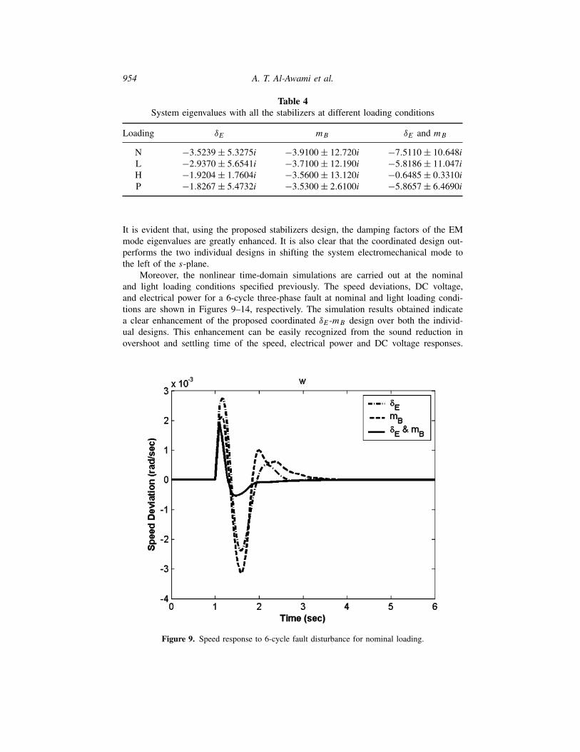
Table 4System eigenvalues with all the stabilizers at different loading conditions

Loading δE mB δE and mB

N −3.5239 ± 5.3275i −3.9100 ± 12.720i −7.5110 ± 10.648iL −2.9370 ± 5.6541i −3.7100 ± 12.190i −5.8186 ± 11.047iH −1.9204 ± 1.7604i −3.5600 ± 13.120i −0.6485 ± 0.3310iP −1.8267 ± 5.4732i −3.5300 ± 2.6100i −5.8657 ± 6.4690i

It is evident that, using the proposed stabilizers design, the damping factors of the EMmode eigenvalues are greatly enhanced. It is also clear that the coordinated design out-performs the two individual designs in shifting the system electromechanical mode tothe left of the s-plane.

Moreover, the nonlinear time-domain simulations are carried out at the nominaland light loading conditions specified previously. The speed deviations, DC voltage,and electrical power for a 6-cycle three-phase fault at nominal and light loading condi-tions are shown in Figures 9–14, respectively. The simulation results obtained indicatea clear enhancement of the proposed coordinated δE-mB design over both the individ-ual designs. This enhancement can be easily recognized from the sound reduction inovershoot and settling time of the speed, electrical power and DC voltage responses.

Figure 9. Speed response to 6-cycle fault disturbance for nominal loading.


Figure 10. Speed response to 6-cycle fault disturbance for light loading.

Figure 11. UPFC DC voltage response to 6-cycle fault disturbance for nominal loading.


Figure 12. UPFC DC voltage response to 6-cycle fault disturbance for light loading.

Figure 13. Electrical power response to 6-cycle fault disturbance for nominal loading.


Figure 14. Electrical power response to 6-cycle fault disturbance for light loading.

The control efforts of the coordinated design are also greatly reduced as compared withthe control efforts of the two individual designs, but are not shown here for space limi-tations.

6. Conclusions

In this article, SVD has been employed to evaluate the EM mode controllability to theUPFC control signals. An optimization technique has been proposed to design the UPFC-based stabilizers individually. PSO has been utilized to search for the optimal controllerparameter settings that optimize an eigenvalue-based objective function. To guarantee therobustness of the proposed controllers, the design process is carried out considering a widerange of operating conditions. A similar approach has been used to design the UPFC-based stabilizers in a coordinated manner. To compare the effectiveness of the proposedstabilizer schemes, damping torque coefficient analysis, eigenvalue analysis, and nonlineartime domain simulation analysis have been carried out. The different analysis resultshave proved that the coordinated scheme of the UPFC-based stabilizers outperforms theindividual schemes.

7. Appendix

The test system parameters are:

Machine: xd = 1, xq = 0.6, x′d = 0.3, D = 0, M = 8.0, T ′

do = 5.044, freq = 60,v = 1.05;


Exciter: KA = 50, TA = 0.05, Efd_ max = 7.3, Efd_ min = −7.3;PSS: Tw = 5; Ti_ min = 0.01; Ti_ max = 5; i = 1, 2, 3, 4; |uPSS| ≤ 0.2; |BSVC | ≤ 0.4;

|XTCSC | < 0.5; |2TCPS| < 15 deg;DC voltage regulator: kdp = −10, kdi = 0;Transmission line: X = 0.7;UPFC: xE = 0.1, xB = 0.1, Ks = 1, Ts = 0.05, Cdc = 3, Vdc = 2.

References

1. C. L. Chen and Y. Y. Hsu, “Coordinated synthesis of multimachine power system stabilizerusing an efficient decentralized modal control (DMC) algorithm,” IEEE Trans. Power Systems,vol. 9, no. 3, pp. 543–551, 1987.

2. M. J. Gibbard, “Co-ordinated design of multimachine power system stabilisers based on damp-ing torque concepts,” IEE Proc. Pt. C, vol. 135, no. 4, pp. 276–284, 1988.

3. M. Klein, L. X. Le, G. J. Rogers, S. Farrokhpay, and N. J. Balu, “H∞ damping controllerdesign in large power systems,” IEEE Trans. Power Systems, vol. 10, no. 1, pp. 158–166,February 1995.

4. V. G. D. C. Samarasinghe and N. C. Pahalawaththa, “Damping of multimodal oscillations inpower systems using variable structure control techniques,” IEE Proc. Gen. Trans. and Distrib.,vol. 144, no. 3, pp. 323–331, 1997.

5. Y. L. Abdel-Magid, M. A. Abido, S. Al-Baiyat, and A. H. Mantawy, “Simultaneous stabiliza-tion of multimachine power systems via genetic algorithms,” IEEE Trans. Power Sys., vol. 14,no. 4, pp. 1428–1439, November 1999.

6. M. A. Abido, “Particle swarm optimization for multimachine power system stabilizer design,”Power Eng. Society Summer Meeting, IEEE, vol. 3, pp. 1346–1351, July 15–19, 2001.

7. M. A. Abido and Y. L. Abdel-Magid, “Radial basis function network based power systemstabilizers for multimachine power systems,” Intl. Conf. Neural Networks, vol. 2, pp. 622–626,June 9–12, 1997.

8. A. Nabavi-Niaki and M. R. Iravani, “Steady-state and dynamic models of unified power flowcontroller (UPFC) for power system studies,” IEEE Trans. Power Systems, vol. 11, no. 4,pp. 1937–1943, November 1996.

9. H. F. Wang, “Damping function of unified power flow controller,” IEE Proc. Gen. Trans. andDistrib., vol. 146, no. 1, pp. 81–87, 1999.

10. H. F. Wang, “Application of modeling UPFC into multi-machine power systems,” IEE Proc.Gen. Trans. and Distrib., vol. 146, no. 3, pp. 306–312, 1999.

11. W. G. Heffron and R. A. Phillips, “Effect of modern amplidyne voltage regulators on under-excited operation of large turbine generator,” AIEE Trans. Power Apparatus and Systems,pp. 692–697, August 1952.

12. H. Zhengyu, N. Yinxin, C. M. Shen, F. F. Wu, C. Shousun, and Z. Baolin, “Application ofunified power flow controller in interconnected power systems—modeling, interface, controlstrategy, and case study,” IEEE Trans. Power Systems, vol. 15, no. 2, pp. 817–824, May 2000.

13. T. K. Mok, Y. Ni, and F. F. Wu, “Design of fuzzy damping controller of UPFC through geneticalgorithm,” IEEE Power Eng. Society Summer Meeting, vol. 3, pp. 1889–1894, July 16–20,2000.

14. P. K. Dash, S. Mishra, and G. Panda, “A radial basis function neural network controller forUPFC,” IEEE Trans. Power Systems, vol. 15, no. 4, pp. 1293–1299, November 2000.

15. M. Vilathgamuwa, X. Zhu, and S. S. Choi, “A robust control method to improve the perfor-mance of a unified power flow controller,” Electric Power System Research, vol. 55, pp. 103–111, 2000.

16. B. C. Pal, “Robust damping of interarea oscillations with unified power flow controller,” IEEProc. Gen. Trans. and Distrib., vol. 149, no. 6, pp. 733–738, 2002.


17. J.-C. Seo, S.-I. Moon, J.-K. Park, J.-W. Choe, “Design of a robust UPFC controller for enhanc-ing the small signal stability in the multi-machine power systems,” IEEE Power Eng. SocietyWinter Meeting, vol. 3, pp. 1197–1202, January 28–February 1, 2001.

18. A. M. A. Hamdan, “An investigation of the significance of singular value decomposition inpower system dynamics,” Int. Journal Electrical Power and Energy Systems, vol. 21, pp. 417–424, 1999.

19. J. Kennedy and R. Eberhart, “Particle swarm optimization,” Proc. IEEE Intl. Conf. NeuralNetworks, vol. 4, pp. 1942–1948, November/December 1995.

20. R. Eberhart and J. Kennedy, “A new optimizer using particle swarm theory,” Proc. the SixthIntl. Symposium on Micro Machine and Human Science (MHS ’95), pp. 39–43, October 4–6,1995.

21. Y. Shi and R. Eberhart, “A modified particle swarm optimizer,” The 1998 IEEE Intl. Conf.on Evolutionary Computation Proc., IEEE World Congress on Computational Intelligence,pp. 69–73, May 4–9, 1998.

Simultaneous Stabilization of Power System Using UPFC-Based Controllers

Documents

Transcript of Simultaneous Stabilization of Power System Using UPFC-Based Controllers