A

ocmcac©

K

1

omTwcoohmtamfiiom

0d

Fisheries Research 83 (2007) 175–184

Simulation-based investigation of the paired-gear methodin cod-end selectivity studies

Bent Herrmann a,∗,1, Rikke P. Frandsen a,1, Rene Holst a,1, Finbarr G. O’Neill b,1

a Danish Institute for Fisheries Research (DIFRES), North Sea Centre, DK-9850 Hirtshals, Denmarkb Fisheries Research Services, Marine Laboratory, PO Box 101, Aberdeen, Scotland, UK

Received 28 June 2006; received in revised form 13 September 2006; accepted 28 September 2006

bstract

In this paper, the paired-gear and covered cod-end methods for estimating the selectivity of trawl cod-ends are compared. A modified versionf the cod-end selectivity simulator PRESEMO is used to simulate the data that would be collected from a paired-gear experiment where the testod-end also had a small mesh cover. Thus, estimates of the selectivity parameters of the test cod-end can be made using both the paired-gearethod and the covered cod-end method. These estimates are compared and, as it is assumed that the covered cod-end method is objective, we

onclude that the paired-gear method is biased. We demonstrate that extreme parameter estimates as well as discrepancies between the paired-gearnd covered cod-end experiments do not necessarily reflect physical or biological mechanisms. We believe that this phenomenon may help explainases in the literature where the covered cod-end and paired-gear methods produce different estimates of cod-end selectivity.

2006 Elsevier B.V. All rights reserved.

aired-

ctc

bzTlttmd(

tb

eywords: Cod-end selectivity; Trouser trawl; Twin trawl; SELECT method; P

. Introduction

A number of experimental and associated statistical method-logies have been developed to estimate the selective perfor-ance of the cod-end of towed gears (Wileman et al., 1996).he two most widely used are (i) the covered cod-end method,here a small mesh cover surrounds the experimental cod-end to

ollect escapees and (ii) the paired-gear method, where a trouserr twin trawl is used and one cod-end is the test cod-end and thether is a ‘non-selective’ small mesh cod-end. Both methodsave their advantages and disadvantages. The covered cod-endethod gives a direct measurement of the total number of fish

hat have entered the test cod-end, however, there are concernss to whether the small mesh cover influences the fishing perfor-ance of the cod-end. The flow regime in the cod-end and thesh behaviour may be affected and, especially where support-

ng hoops have not been used, the cover may mask the meshesf the test cod-end. The paired-gear method only gives an esti-ate of the population that is assumed to have entered the test

∗ Corresponding author. Tel.: +45 3396 3204.E-mail address: bhe@dfu.min.dk (B. Herrmann).

1 These authors contributed equally to this work.

tpo

iptS

165-7836/$ – see front matter © 2006 Elsevier B.V. All rights reserved.oi:10.1016/j.fishres.2006.09.011

gear; Simulations; PRESEMO

od-end and certain assumptions have to be made with regardso the comparative fishing power of the test and small meshod-ends.

In general, the retention probability of fish in a cod-end cane expressed in terms of a logistic type curve that goes fromero retention for small fish to 100% retention for large ones.hese types of curves are often characterised in terms of the

ength at which 50% of fish are retained (L50) and the selec-ion range (SR) which is defined to be the difference betweenhe L75 and L25 points. These two parameters can be esti-

ated from both covered cod-end and paired-gear experimentalata and can be analysed using the SELECT method of Millar1992).

For covered cod-end data, the SELECT method is reducedo a generalized linear model (McCullagh and Nelder, 1989) forinary data, whereas the paired-gear case introduces an addi-ional non-linear parameter. The extra parameter, called the splitarameter (SP), accounts for the potential of unequal numbersf fish entering the two cod-ends.

SP is the probability a fish enters the test cod-end, given that

t enters one of them. Thus, SP = 0.5 corresponds to equal fishingower of the two cod-ends. Compared to the covered cod-endechnique that only estimates the selectivity parameters L50 andR, the extra parameter adds to the uncertainty of the estimating

1 ies Research 83 (2007) 175–184

ppmtb

egttlthtsd2

ttheaathdffMmBthfiS

ac(iorsi(tf

ipCdotto

Fig. 1. PRESEMO simulates the data that would be collected from a paired-gearexperiment where the test cod-end also had a small mesh cover. Thus, for eachsimulation, the selectivity of the test cod-end can be estimated by both the paired-gt

2

sssme(ttfwceem

atoCSmonctf

epu

76 B. Herrmann et al. / Fisher

rocedure and consequently to the estimates of the selectivityroperties of a gear under test. The original form of the SELECTethod assumes that the split is independent of fish length and

ime of catch, and SP is therefore a constant that can be expressedy a single parameter.

Ideally, the employment of two different methodologies tostimate the selective properties of the same fishing gear, wouldive equal estimates of the selective parameters. When applyinghe different methods to data from a large number of hauls fromhe same fishery, distribution of the parameter estimates shouldikewise be equal. It is therefore relevant to investigate whetherhis is the case when cod-end selection is assessed, on the oneand, using the paired-gear methodology and, on the other, usinghe covered cod-end methodology. A number of experimentaltudies have raised concerns that these two methodologies pro-uce different estimates (Dahm et al., 2002; Madsen and Holst,002; Shephard, 1999; Fonteyne, 1991).

Cadigan and Millar (1992) report on a theoretical study ofhe reliability of the paired-gear methodology. They studiedhe performance of three different ways of analysing simulatedaul data including the SELECT methodology. They consid-red different scenarios using parametric simulations assuminglogistic selection curve with predefined (known) parameters

nd a given population structure entering the trouser gear duringhe fishing process. For each scenario, 200 replicated simulatedauls were conducted. The haul data were analysed by the threeifferent methods in order to obtain estimates for L50 and SRor each haul. Due to the predefinition of L50 and SR, biasor these parameters could be directly calculated. Cadigan and

illar (1992) concluded that there was little or no bias in theean selection parameters when using the SELECT method.ut when looking at the distributions of the selection parameters

hey found that results could be seriously biased for individualauls, especially when catches were small (not exceeding 250sh). In particular, some hauls showed very small estimates ofR.

In their simulations Cadigan and Millar (1992) assumed (i)constant split over the duration of the haul and for all length

lasses, (ii) a constant (logistic) selectivity during a haul andiii) constant selectivity between hauls. These assumptions min-mise the within-haul and between-haul variation that are oftenbserved during experiments and which may be due to envi-onmental and biological factors such as fish distribution or fishwimming ability or physical mechanisms such as differencesn fishing efficiency, strong currents or unequal wire lengthsWileman et al., 1996). Furthermore, the 200 simulated haulshey use in their analysis are far in excess of what is usuallyeasible during sea trials.

In this paper, we use a modified version of the selectiv-ty simulator PRESEMO (Herrmann, 2005a,b) to compare theaired-gear and covered cod-end methodologies. In contrast toadigan and Millar’s study we allow the split parameter to varyuring and between hauls and we do not predefine the selectivity

f the cod-end. Furthermore, we include between-haul variationhat is comparable with that obtained experimentally and inves-igate how the number of hauls of an experiment may influenceur results.

mpms

ear method and the covered cod-end method. This allows for a comparison ofhe parameter estimates obtained by the two methods.

. Materials and methods

As part of this study, PRESEMO was further developed toimulate the selection process of a paired-gear experiment. Theplit parameter was allowed to vary for each fish and PRESEMOimulated whether a fish entered the test cod-end or the smallesh control cod-end accordingly. Fish that entered test cod-

nd either escaped or were retained as described in Herrmann2005a,b). Thus, three distinct data sets are simulated (i) of fishhat are retained in the small mesh control cod-end, (ii) of fishhat are retained in the test cod-end and (iii) of fish that escaperom the test cod-end. In effect we are simulating the data thatould be collected from a paired-gear experiment where the test

od-end also had a small mesh cover (Fig. 1). Consequently, forach simulation, we can estimate the selectivity of the test cod-nd by both the paired-gear method and the covered cod-endethod and directly compare these estimates.The covered cod-end method is a direct approach insofar

s we know the length of all fish that enter and escape fromhe test cod-end. In this sense we assume that it provides anbjective and unbiased estimate of the selectivity parameters.onsequently, we assume that paired-gear estimates of L50 andR which differ from those obtained using the covered cod-endethod are biased. We can also directly estimate SP as the sum

f fish in the test cod-end and in the cover divided by the totalumber of fish in the control cod-end, the test cod-end and theover. Similarly, we assume that this is an unbiased estimate ofhe true split and that pair-geared estimates of SP which differrom this are also biased.

PRESEMO requires information on the fish behaviour, thescape process, the fish population structure, and the fish mor-hology. Herrmann and O’Neill (2005) outlined a protocol forsing PRESEMO to simulate selection of haddock in a diamondesh cod-end taking between haul variability into account. This

rocedure ensures that the selection parameters reflect experi-ental values and their variances. We use haddock as the target

pecies for this study and list in Tables 1 and 2 the fish data and

B. Herrmann et al. / Fisheries Research 83 (2007) 175–184 177

Table 1Fish data used in simulations

Population 1 Population 2 Population 3 Population 4 Population 5 Population 6

Species Haddock Haddock Haddock By-catch By-catch By-catchNumber >40 to <4000a >20 to <3200a >20 to <800a >20 to <600a >20 to <400a >20 to <400a

Size of fish distribution Normal Normal Normal Normal Normal NormalMean length (mm) 160.0 298.0 500.0 240.0 290.0 500.0Var length (mm2) 578.0 737.0 5561.0 1600.0 1200.0 1600.0Height factor 0.1720 0.1720 0.1720 0.1750 0.1750 0.1750Height var 0.000027 0.000027 0.000027 0.000011 0.000011 0.000011Width factor 0.1030 0.1030 0.1030 0.1100 0.1100 0.1100Width var 0.000010 0.00001 0.00001 0.000004 0.000004 0.000004Condition factor (g/cm3) 0.0109 0.0109 0.0109 0.0116 0.0116 0.0116Condition var (g2/cm6) 0.0 0.0 0.0 0.0 0.0 0.0Entry interval distribution Random Random Random Random Random RandomEntry interval (% of entry period) >50 to <100a >50 to <100a >50 to <100a >50 to <100a >50 to <100a >50 to <100a

Entry period (min) 240 240 240 240 240 240Time travel down distribution Linear on length Linear on length Linear on length Linear on length Linear on length Linear on lengthTime travel down par A (min/mm) 0.005 0.005 0.005 0.005 0.005 0.005Time travel down par B (min) 0.0 0.0 0.0 0.0 0.0 0.0Exhaustion time distribution Linear on length Linear on length Linear on length Linear on length Linear on length Linear on lengthExhaustion time par A (min/mm) 0.1 0.1 0.1 0.1 0.1 0.1Exhaustion time var par A (min2) 0.03 0.03 0.03 0.03 0.03 0.03Time between distribution Fixed Fixed Fixed Fixed Fixed FixedTime between (min) 1.0 1.0 1.0 1.0 1.0 1.0Catch packing density 1.0 1.0 1.0 1.0 1.0 1.0I 0.5

F d O’

oeud8fgc

2

l

((

TT

THECCIEMPP

Fa

(

(

(

(

n front of packing density 0.5 0.5

or further information on the PRESEMO simulation program see Herrmann ana Random variation of value in interval between hauls.

ther PRESEMO settings used in the simulations (for furtherxplanation see Herrmann and O’Neill, 2005). The test cod-endsed in the simulations was a 100 mm (inside stretched measure)iamond mesh cod-end made of 4 mm double PE twine. It was0 meshes long and had 100 open meshes around the circum-erence. PRESEMO also requires information on the cod-endeometry and how it varies as the catch builds up. This was cal-ulated using the techniques described in O’Neill (1997, 1999).

.1. Simulation of the splitting process

We simulate the splitting process in a number of ways. We

ook at a number of cases where for each fish the split

a) is constant and equal to 0.5 during the entire fishing process;b) is constant and equal to 0.7 during the entire fishing process;

able 2owing time and other settings used in simulations

owing time (min) 200auling time (min) 15.0scapement model Soft distortionatch weight break value (kg) 0.0atch weight zero distortion (kg) 5.0

nfront of factor 0.5scapement during haul factor 0.8ax distortion mesh opening 0.15

opulations in simulation 1, 2, 3, 4, 5 and 6opulations as target 1, 2 and 3

or further information on the PRESEMO simulation program see Herrmannnd O’Neill (2005).

ethotIsaitc

2

hfT

0.5 0.5 0.5

Neill (2005).

c) is chosen randomly from normal distribution with mean 0.5and standard deviation 0.1;

d) increases from 0.3 to 0.7 linearly with time during the fishingprocess;

e) decreases linearly with length from 0.7 at 10 cm to 0.3 at60 cm;

f) varies linearly with length from SP10 at 10 cm to SP60 at60 cm where for each haul SP10 and SP60 are chosen ran-domly from normal distribution with mean 0.5 and standarddeviation 0.1.

Case (a) is closest to the study of Cadigan and Millar (1992)xcept that PRESEMO contains additional between-haul varia-ion that is not present in their study. Case (b) considers whatappens when the split is constant but not equal to 0.5. This canccur, for example, if one trawl of a twin trawl is fishing closero the bottom, has a wider cross section or there are tidal effects.n case (c) we present what is a more realistic reflection of theplitting process and hence, believe that this case gives a moreccurate indication of potential bias. The last three cases arencluded to further test the SELECT method and, in particular,o demonstrate the consequences of assuming a constant split inases when it does not hold.

.2. Statistical analysis

For each split case, 1000 simulations were made, i.e., 1000auls were simulated yielding 1000 comparable sets of dataor the paired-gear method and the covered cod-end method.he L50 and SR for each haul and for both methodologies

1 ies Re

ww(bmi(o

ia(sfldsgcpet

3

ftrtev

apet0ceh(

0cta

f0fsc1

lac1

TM

D

Ccm

Pgm

B

R

Pg

78 B. Herrmann et al. / Fisher

ere calculated using the CC2000 software (ConStat, 1995)hich complies with the recommendations of Wileman et al.

1996) and has built-in facilities to handle data obtained byoth the paired-gear and the covered cod-end methods. Theean and variance of parameter estimates for the 1000 hauls

n each of the different cases were calculated using EC-webhttp://www.constat.dk//ecwebsd) which implements the modelf Fryer (1991).

Mean selectivity estimates are subject to uncertainty depend-ng partly on the number of fish measured within individual haulsnd partly on the number of hauls used in calculating the meanFryer, 1991). To investigate how the number of hauls in theample size influences the bias of the paired-gear method, theollowing analysis was carried out. From the 1000 hauls simu-ated for each case, sub-samples containing 2–100 hauls wererawn (with replacement). For each sub-sample size, 3000 suchub-samples were made and for each of these the mean paired-ear selectivity parameters and the corresponding mean coveredod-end selectivity parameters were estimated. Again, bias of theaired-gear method is defined as the difference between param-ters estimated using the paired-gear method and those usinghe covered cod-end method.

. Results

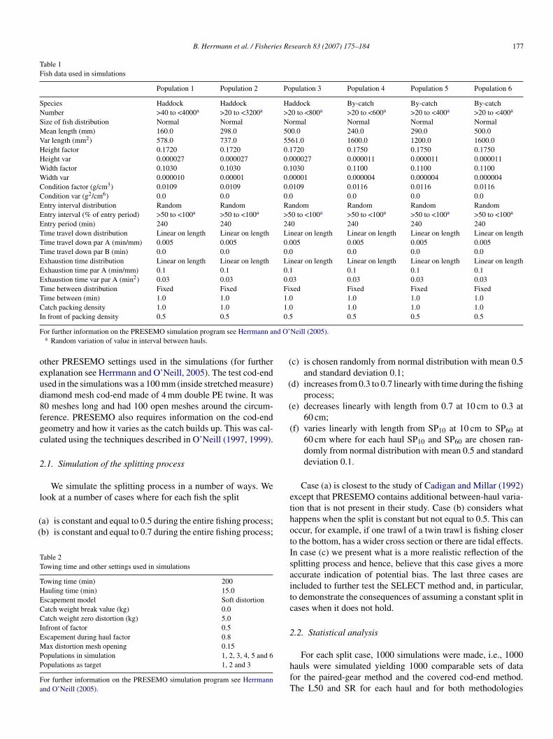
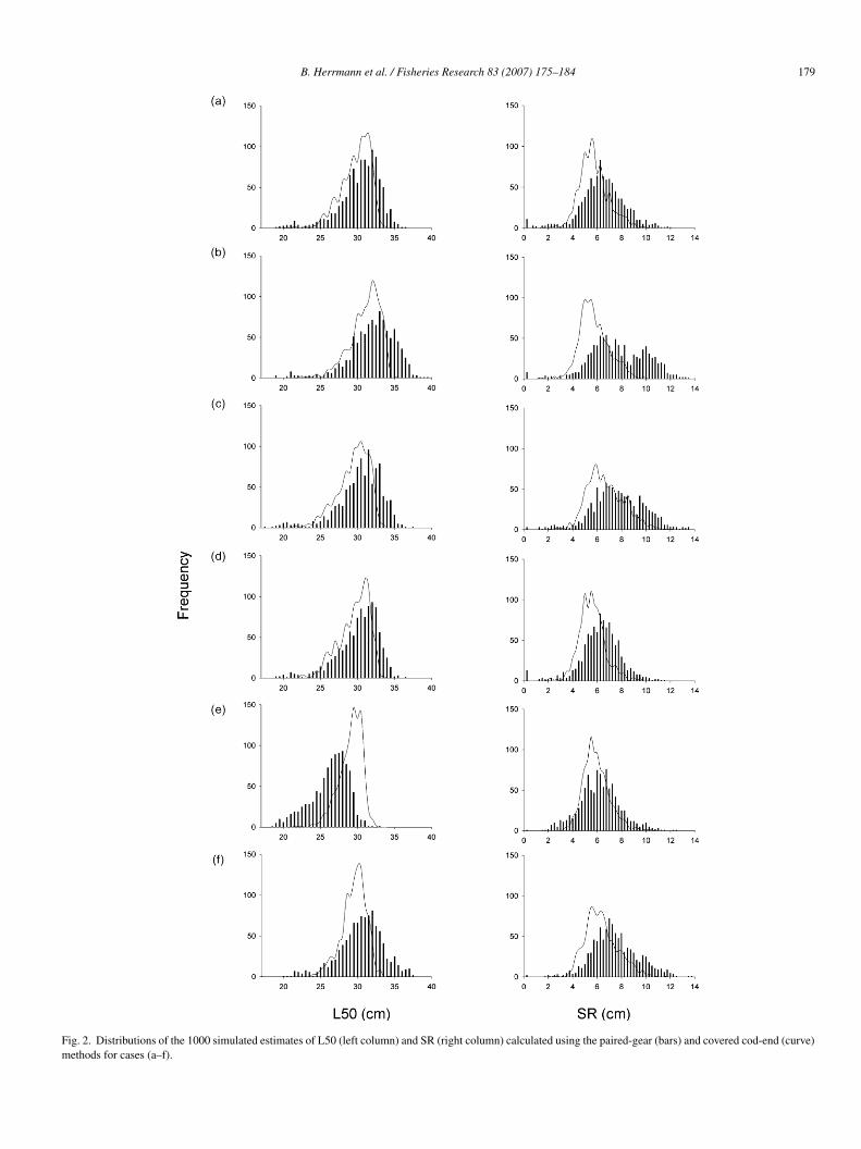
The frequency distribution of the 1000 L50 and SR estimatesor each case are presented in Fig. 2. The continuous curves arehe results from the covered cod-end analysis and the bars are the

esults from the paired-gear analysis. In all cases, the distribu-ions of parameter estimates differ and generally the paired-gearstimates have a higher incidence of both smaller and largeralues.

fiTmm

able 3ean and variance of the 1000 simulated parameter estimates for each case using EC

escription Case a,constantsplit 0.5

Case b,constantsplit 0.7

Case c, split randoselected from normdistribution. ∼N(00.1)

overedod-endethod

Mean L50 (cm) 29.34 30.81 29.23Var L50 (cm2) 3.70 3.98 4.19Mean SR (cm) 5.47 6.48 6.51Var SR (cm2) 1.21 2.32 2.00

airedearethod

Mean L50 (cm) 29.92 31.82 30.09Var L50 (cm2) 6.41 8.16 8.09Mean SR (cm) 6.30 7.65 7.55Var SR (cm2) 2.22 4.41 3.84Mean SP 0.51 0.71 0.52Var SP 1.03E−4 1.9E−4 1.2E−4

iasMean L50 (cm) 0.58 (2.0%) 1.01 (3.3%) 0.86 (2.9%)Mean SR (cm) 0.83 (15.2%) 1.17 (18.1%) 1.04 (16.0%)

atioVar L50 1.73 2.05 1.93Var SR 1.83 1.90 1.92

ercentage deviation from the covered result is shown in brackets. Bias = covered codear estimate.a For each haul SP10 and SP60 are selected independently from normal distribution

search 83 (2007) 175–184

The estimates of the first case, where the split is constantnd equal to 0.5, indicate a bias towards larger values for theaired-gear method compared to the covered cod-end. Meanstimates for the 1000 hauls confirm this (Table 3) wherehe L50 and SR for the paired-gear method are respectively,.58 cm (2.0%) and 0.83 cm (15.2%) greater than that of theovered cod-end method. The variance of the selection param-ters estimated by the paired-gear method was 1.7–1.8 timesigher than the variance in the covered cod-end estimatesTable 3).

The case where the split parameter is constant and equal to.7 is presented in Fig. 2b. A split value that is greater than 0.5orresponds to the fish having a higher probability of enteringhe test cod-end. When SP equals 0.7 the bias is 1.01 cm (3.3%)nd 1.17 cm (18.1%) for L50 and SR, respectively (Table 3).

Fig. 2c presents the case where the split is chosen randomlyrom a normal distribution with mean 0.5 and standard deviation.1. Mean estimates of the selection parameters in the 1000 haulsor the covered cod-end method and the paired-gear method areummarized in Table 3. Mean bias for the paired-gear estimatesompared to the covered cod-end estimates are 2.9% (L50) and6.0% (SR).

Fig. 2d contains the case where the split in each haul increasesinearly with time during the fishing process, starting at SP = 0.3nd ending at SP = 0.7. Mean bias for the paired-gear estimatesompared to the covered cod-end estimates are 2.1% (L50) and5.1% (SR).

The case where the split decreases linearly with length of

sh is plotted in Fig. 2e. The biases in this case are very large.he mean value of L50 is 28.82 cm using the covered cod-endethod and is 25.89 cm using the paired-gear method whileean values of SR are 5.78 and 6.01 cm, respectively.

-web

mlyal

.5,

Case d, split increasinglinearly with tow timefrom 0.3 at start to 0.7at end

Case e, split decreasinglinearly with fishlength from 0.7 at10 cm to 0.3 at 60 cm.

Case f, splitvarying linearlywith fish lengthfrom SP10 at 10 cmto SP60 at 60 cma

29.35 28.82 29.273.92 2.28 2.515.44 5.78 6.210.99 0.94 1.60

29.97 25.89 30.186.65 5.24 7.526.26 6.01 7.301.91 1.74 2.620.53 0.44 0.521.5E−3 8.3E−4 6.7E−3

0.62 (2.1%) −2.93 (−10.2%) 0.91 (3.1%)0.82 (15.1%) 0.23 (4.0%) 1.09 (17.6%)

1.70 2.30 3.01.93 1.85 1.64

-end estimate − paired gear estimate. Ratio = covered cod-end estimate/paired

∼N(0.5, 0.1).

B. Herrmann et al. / Fisheries Research 83 (2007) 175–184 179

Fig. 2. Distributions of the 1000 simulated estimates of L50 (left column) and SR (right column) calculated using the paired-gear (bars) and covered cod-end (curve)methods for cases (a–f).

180 B. Herrmann et al. / Fisheries Research 83 (2007) 175–184

F d using the paired-gear (bars) and covered cod-end (curve) methods for hauls wheret

dTaup7

vwa(homtbc(oWtLia

SrodTobfia

gttLei

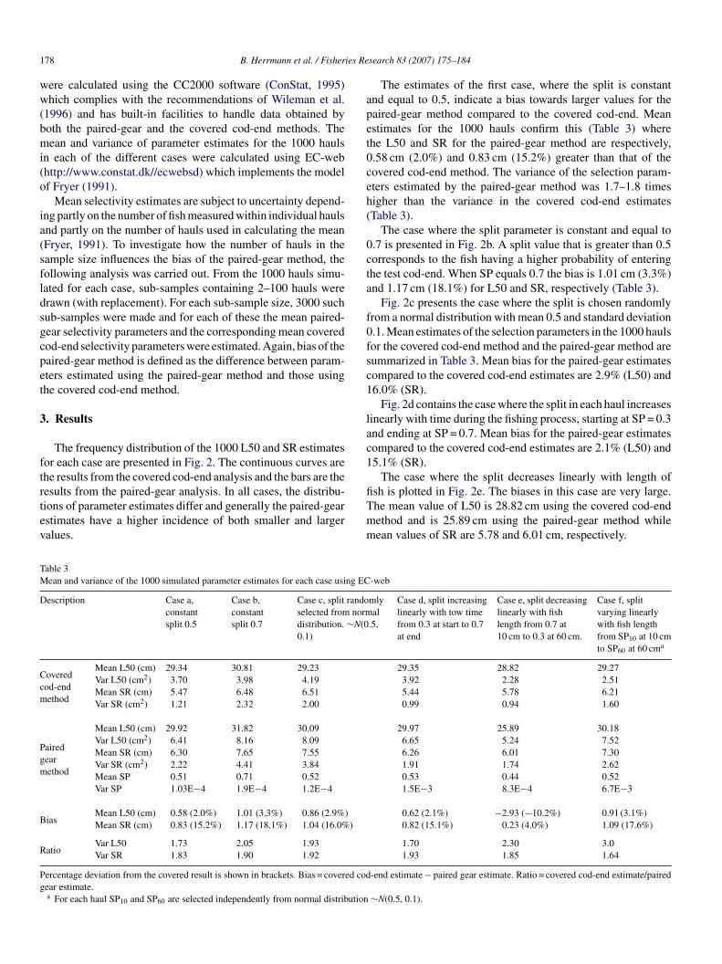
ig. 3. Distributions of the estimates of L50 and SR (for case (a) only) calculatehe total number of fish retained in the test cod-end did not exceed 200.

In case (f) we examine the case where the split is lengthependent but where the dependency varies from haul to haul.his condition may occur if the population distribution is size orge segregated. In this case the mean value of L50 is 29.27 cmsing the covered cod-end method and is 30.18 cm using theaired-gear method while the mean values of SR are 6.21 and.30 cm, respectively.

In the present study, the total number of fish entering the geararied from 125 to 8000. Cadigan and Millar (1992) found thathen the number of fish entering the gear was small there was

n increased likelihood of obtaining very low estimates for SRbelow 1.0 cm). In Fig. 3, we show that we get similar resultsere when we restrict attention to the hauls where the numberf fish retained in the test cod-end is less than 200. Fig. 4 sum-arizes how, on a haul-by-haul basis, the differences between

he estimates calculated using the two methodologies (i.e. theiases) depend on the number of fish that are retained in the testod-end over the full range of catch sizes. All three parametersL50%, SR and SP) display a dependency between variationf the bias and the number of fish entering the test cod-end.hen there are less than 200 fish retained in the test cod-end

he range of bias is approximately 14 cm, 12 cm and 0.25 for50, SR and SP, respectively. When the number of fish retained

n the test cod-end is higher than 400, these values reduce topproximately 2 cm, 2 cm and 0.07.

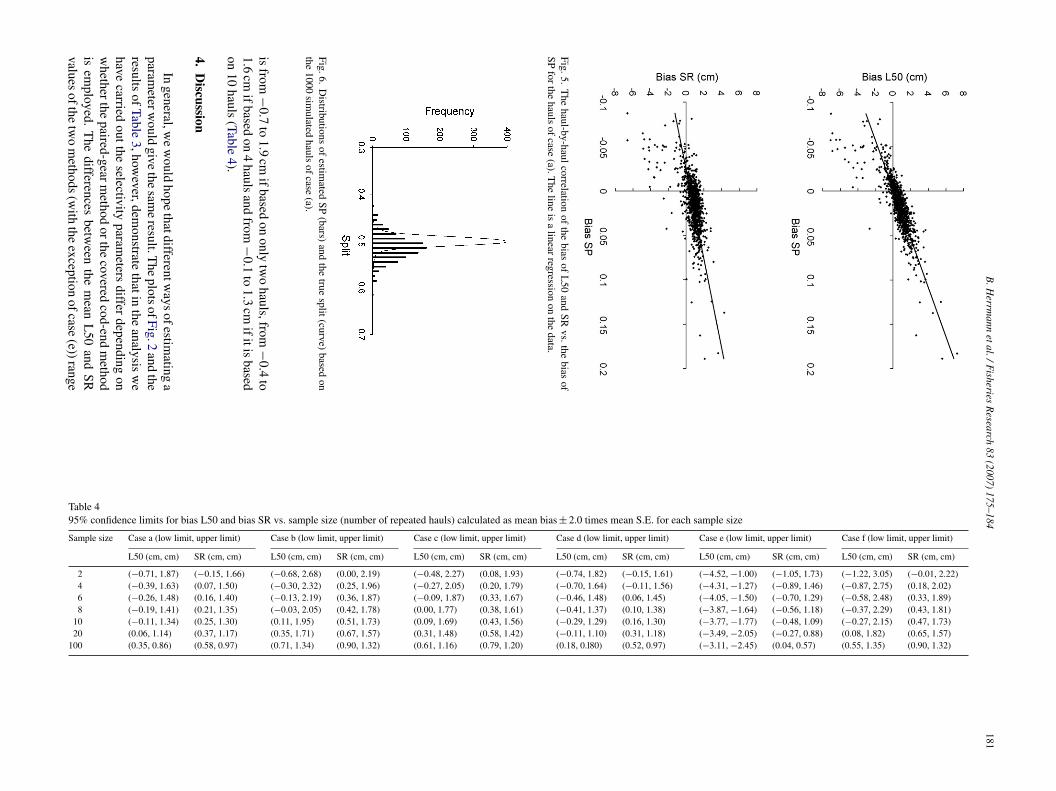
Fig. 5 plots, for case (a), estimates of the bias of L50 andR against the bias of SP. Using a simple linear regression theseesults indicate that with a 0.05 SP bias we should expect a biasf 2.0 cm for L50 and 1.5 cm for SR. In Fig. 6, the frequencyistributions of the estimated SP and the true split are plotted.he true split is distributed narrowly around the simulated valuef 0.5 whereas the estimated paired-gear split has a wider distri-ution that is slightly biased towards higher values. These twogures demonstrate that inaccurate estimates of SP may explainlarge proportion of the observed bias of L50 and SR.

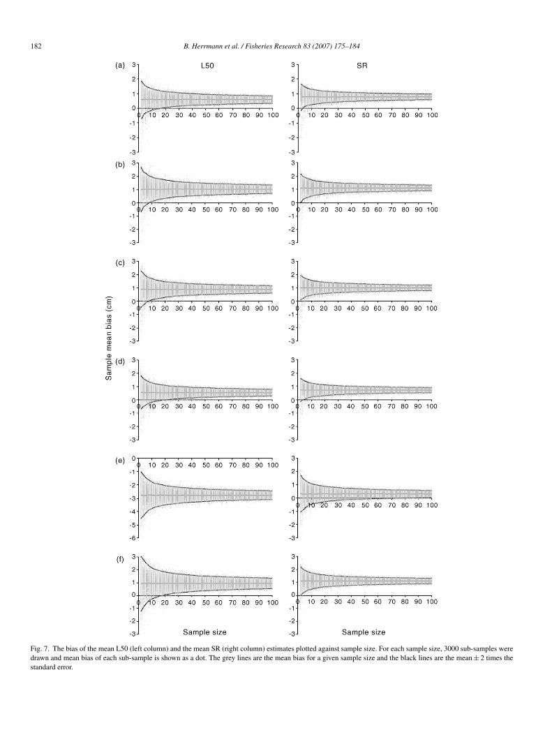
Fig. 7 demonstrates how the mean estimates of the paired-ear sub-samples vary with the sub-sample size. For each casehe mean bias remains constant with sub-sample size, whereas

he ∼95% (2S.E.) confidence range of the mean bias of both50 and SR decreases as the sub-sample size increases. Forxample, in the first case (Fig. 7a), the bias of mean L50 is 0.6 cmrrespective of sample size, whereas its ∼95% confidence range

Ffi

ig. 4. The haul-by-haul bias of L50, SR and SP plotted against the number ofsh retained by the test cod-end for the simulated hauls of case (a).

B.H

errmann

etal./Fisheries

Research

83(2007)

175–184181

Fig.5.T

hehaul-by-haul

correlationof

thebias

ofL

50and

SRvs.the

biasof

SPfor

thehauls

ofcase

(a).The

lineis

alinear

regressionon

thedata.

Fig.6.D

istributionsof

estimated

SP(bars)

andthe

truesplit(curve)

basedon

the1000

simulated

haulsof

case(a).

isfrom

−0.7

to1.9

cmifbased

ononly

two

hauls,from−

0.4to

1.6cm

ifbasedon

4hauls

andfrom

−0.1

to1.3

cmifitis

basedon

10hauls

(Table4).

4.D

iscussion

Ingeneral,w

ew

ouldhope

thatdifferentways

ofestimating

aparam

eterwould

givethe

same

result.The

plotsofFig.2

andthe

resultsof

Table3,how

ever,demonstrate

thatinthe

analysisw

ehave

carriedoutthe

selectivityparam

etersdiffer

dependingon

whetherthe

paired-gearmethod

orthecovered

cod-endm

ethodis

employed.

The

differencesbetw

eenthe

mean

L50

andSR

valuesofthe

two

methods

(with

theexception

ofcase(e))range

Table 495% confidence limits for bias L50 and bias SR vs. sample size (number of repeated hauls) calculated as mean bias ± 2.0 times mean S.E. for each sample size

Sample size Case a (low limit, upper limit) Case b (low limit, upper limit) Case c (low limit, upper limit) Case d (low limit, upper limit) Case e (low limit, upper limit) Case f (low limit, upper limit)

L50 (cm, cm) SR (cm, cm) L50 (cm, cm) SR (cm, cm) L50 (cm, cm) SR (cm, cm) L50 (cm, cm) SR (cm, cm) L50 (cm, cm) SR (cm, cm) L50 (cm, cm) SR (cm, cm)

2 (−0.71, 1.87) (−0.15, 1.66) (−0.68, 2.68) (0.00, 2.19) (−0.48, 2.27) (0.08, 1.93) (−0.74, 1.82) (−0.15, 1.61) (−4.52, −1.00) (−1.05, 1.73) (−1.22, 3.05) (−0.01, 2.22)4 (−0.39, 1.63) (0.07, 1.50) (−0.30, 2.32) (0.25, 1.96) (−0.27, 2.05) (0.20, 1.79) (−0.70, 1.64) (−0.11, 1.56) (−4.31, −1.27) (−0.89, 1.46) (−0.87, 2.75) (0.18, 2.02)6 (−0.26, 1.48) (0.16, 1.40) (−0.13, 2.19) (0.36, 1.87) (−0.09, 1.87) (0.33, 1.67) (−0.46, 1.48) (0.06, 1.45) (−4.05, −1.50) (−0.70, 1.29) (−0.58, 2.48) (0.33, 1.89)8 (−0.19, 1.41) (0.21, 1.35) (−0.03, 2.05) (0.42, 1.78) (0.00, 1.77) (0.38, 1.61) (−0.41, 1.37) (0.10, 1.38) (−3.87, −1.64) (−0.56, 1.18) (−0.37, 2.29) (0.43, 1.81)

10 (−0.11, 1.34) (0.25, 1.30) (0.11, 1.95) (0.51, 1.73) (0.09, 1.69) (0.43, 1.56) (−0.29, 1.29) (0.16, 1.30) (−3.77, −1.77) (−0.48, 1.09) (−0.27, 2.15) (0.47, 1.73)20 (0.06, 1.14) (0.37, 1.17) (0.35, 1.71) (0.67, 1.57) (0.31, 1.48) (0.58, 1.42) (−0.11, 1.10) (0.31, 1.18) (−3.49, −2.05) (−0.27, 0.88) (0.08, 1.82) (0.65, 1.57)

100 (0.35, 0.86) (0.58, 0.97) (0.71, 1.34) (0.90, 1.32) (0.61, 1.16) (0.79, 1.20) (0.18, 0.l80) (0.52, 0.97) (−3.11, −2.45) (0.04, 0.57) (0.55, 1.35) (0.90, 1.32)

182 B. Herrmann et al. / Fisheries Research 83 (2007) 175–184

Fig. 7. The bias of the mean L50 (left column) and the mean SR (right column) estimates plotted against sample size. For each sample size, 3000 sub-samples weredrawn and mean bias of each sub-sample is shown as a dot. The grey lines are the mean bias for a given sample size and the black lines are the mean ± 2 times thestandard error.

ies Re

bMm(pwiobca

wcsttTv(fivttroSttnatS

dbdtsvfdis(acIfis1

thap

oastccshstb(

fdctmratetcvgstthcfpacFLiftti

asfoeo

mbb

B. Herrmann et al. / Fisher

etween 0.58 and 1.01 cm and 0.82 and 1.17 cm, respectively.ore importantly, perhaps, the variances of the paired-gear esti-ates are much larger than those of the covered cod-end method

Table 3). The larger variance is attributable to the paired geararameters having more ‘extreme’ estimates. In Fig. 3, wheree restrict attention to hauls where the number of fish retained

n the test cod-end is less than 200, we see that the proportionf extreme values increases. Similarly, Fig. 4, which plots theias of estimates against the number of fish retained in the testod-end, shows that the bias is more variable when fewer fishre retained in the test cod-end.

Cadigan and Millar (1992) also found that bias increasedhen the sample size is very small. For larger catches, they con-

luded that the SELECT method is close to unbiased. In theirimulations they assume (i) a constant split over the duration ofhe haul and for all length classes, (ii) a constant (logistic) selec-ivity during a haul and (iii) constant selectivity between hauls.hese assumptions minimise the within-haul and between-haulariation that are often observed during experiments. Our casea) is the closest to their study; however, we do not prede-ne the selectivity of the cod-end and include between-haulariation that is comparable with those obtained experimen-ally. These greater levels of variation are likely to explainhe larger mean bias we observe even when the catch size iselatively large. Figs. 5 and 6 may also explain some of thebserved bias. Fig. 5 demonstrates that the biases of L50 andR are correlated with the SP bias, while Fig. 6 shows that

he distribution of the SELECT estimates of SP differs fromhat of the true split. Together these figures indicate that theon-linearity introduced to the estimation procedure by SPnd possible related inaccuracies in estimating this parame-er may be an important contribution to the bias in L50 andR.

Case (c), where the split is chosen randomly from a normalistribution with mean 0.5 and standard deviation 0.1, probablyest reflects the splitting process of a well (or perhaps ideally)esigned experiment. Here, the biases are 0.86 and 1.0 cm forhe L50 and SR, respectively. In general, however, it is not pos-ible to ensure a constant split during a haul, and the bias mayary with time and/or fish length. Such a situation may arise if,or example, tidal conditions change during a tow or the fishistribution is patchy and size/age segregated. Cases (d) to (f)nvestigate these conditions. The results of case (d), where theplit varies linearly with time, are very similar to those of casea). This is probably because over the course of a tow the aver-ge split for any length class will be 0.5. Case (e) demonstrateslearly what happens if the constant split assumption is not valid.n this example where the split decreases linearly with lengthrom 0.7 at 10 cm to 0.3 at 60 cm the difference of mean L50ss almost 3 cm. In case (f) where the linear dependence of theplit varies haul by haul we get a 0.9 cm increase of L50 and a.1 cm increase of SR.

The results of Fig. 2 and Table 3 are based on 1000 simula-

ions and those of Cadigan and Millar (1992) on 200 simulatedauls. Both these numbers of hauls are far in excess of whatre usually carried out during experimental trials at sea. Thelots of Fig. 7, where we present the mean bias of sub-samples

stFt

search 83 (2007) 175–184 183

f paired-gear estimates are probably more informative as theyre a better representation of experimental trials. These plotshow that while the mean bias is more or less independent ofhe number of hauls, the variation of the bias is not. For eachase, the extent to which the paired-gear parameter estimatesan vary from the unbiased covered cod-end estimates is con-iderable when the estimates are based on a small numbers ofauls. In Fig. 7a, bias in the mean L50 is 0.6 cm irrespective ofample size, whereas its ∼95% confidence ranges from −0.7o 1.9 cm if based on only two hauls, from −0.4 to 1.6 cm ifased on 4 hauls and from −0.1 to 1.3 cm if is based on 10 haulsTable 4).

Often, the selectivity of a cod-end is estimated using the datarom less than 8 hauls, so these results may help explain someifferences that have been observed between paired-gear andovered cod-end selectivity studies. It has been suggested thathese differences are due to the cover inhibiting escape, either byasking the cod-end meshes, presenting a further physical bar-

ier, or by modifying the hydrodynamics of the cod-end. Therere only a few studies that permit a direct comparison betweenhe covered cod-end method and the paired-gear method. Dahmt al. (2002) found a substantial difference of about 4.5 cm inhe L50s of cod and haddock between trouser trawl and coveredod-end experiments. Although these trials were on differentessels, they took place at the same time on the same fishingrounds. The authors state that it is not clear why there wereuch large differences as underwater observations made duringhe experiments demonstrated that the cover did not mask theest cod-end. Madsen and Holst (2002) found a tendency forigher estimates of L50 and SR when using the paired-gear inomparison to the covered cod-end method. The parameter dif-erences were not significant for the combined hauls but theaired-gear method showed significantly higher parameter vari-nces of L50. They conclude that such differences may either beaused by the cover or by inaccuracy of the paired-gear method.onteyne (1991) found that the twin trawl method gave higher50 values than the covered cod-end method for sole and dab

n beam trawls. Shephard (1999), on the other hand, found that,or haddock, the paired-gear estimates were significantly lowerhan the covered cod-end ones. Fig. 7 demonstrates that althoughhe results of these authors may differ they are not necessarilynconsistent.

It should be recognised that the results we have obtainedre indicative and the parameter values we have estimated arepecific to the simulation conditions. Hence, it is not possible,or example, to define a generally acceptable minimum numberf fish that should be retained in the test cod-end. However, ifnough is known about a fishery, it should be possible to carryut a similar analysis to at least provide guidelines.

In summary, we have demonstrated that the paired-gearethod contains a certain amount of inherent bias which

ecomes more apparent when we include within haul andetween haul variability. The bias is greater again when there are

mall numbers of fish (in our simulations <400) retained in theest cod-end and when the constant split assumption is invalid.inally, the likelihood of obtaining biased results is greater when

he number of hauls used is small.

1 ies Re

A

tPtiSA

R

C

C

D

F

F

H

H

H

M

M

M

O

O

S

84 B. Herrmann et al. / Fisher

cknowledgements

This paper has been carried out with financial support fromhe Commission of the European Communities, EU projectsREMECS II and NECESSITY. It does not necessarily reflect

he Commission’s view and in no way anticipates its future pol-cy in this area. Financial support was also given from projectELTRA financed by the Directorate for Food, Fisheries andgri Business.

eferences

adigan, N.G., Millar, R.B., 1992. The reliability of selection curves obtainedfrom trouser trawl or alternate haul studies. Can. J. Fish. Aquat. Sci. 49,1624–1632.

onStat, 1995. CC selectivity. Groenspaettevej 10, DK-9800 Hjoerring, Den-mark.

ahm, E., Wienbeck, H., West, C.W., Valdemarsen, J.W., O’Neill, F.G., 2002.

On the influence of towing speed and gear size on the selective properties ofbottom trawls. Fish. Res. 55, 103–119.

onteyne, R., 1991. Comparison between the covered codend method an the twintrawl method in beam trawl selectivity experiments. ICES C.M. 1991/B:52,1–13.

W

search 83 (2007) 175–184

ryer, R., 1991. A model of the between-haul variation in selectivity. ICES J.Mar. Sci. 48, 281–290.

errmann, B., 2005a. Effect of catch size and shape on the selectivity of diamondmesh cod-ends I. Model development. Fish. Res. 71, 1–13.

errmann, B., 2005. Modelling and simulation of size selectivity in diamondmesh trawl cod-ends. Ph.D. Thesis. Aalborg University, Denmark. ISBN87-91200-50-4.

errmann, B., O’Neill, F.G., 2005. Theoretical study of the between-haul vari-ation of haddock selectivity in a diamond mesh cod-end. Fish. Res. 74,243–252.

cCullagh, P., Nelder, J.A., 1989. Generalized Linear Models, 2nd ed. Chapmanand Hall, New York.

adsen, N., Holst, R., 2002. Assessment of the cover effect in trawl codendselectivity experiments. Fish Res. 56, 289–301.

illar, R.B., 1992. Estimating the size-selectivity of fishing gear by conditioningon the total catch. J. Am. Stat. Assoc. 87 (420), 962–968.

’Neill, F.G., 1997. Differential equations governing the geometry of diamondmesh cod-end of a trawl net. J. Appl. Mech. 64/7 (453), 1631–1648.

’Neill, F.G., 1999. Axissymmetrical trawl cod-ends made from netting of gen-eralized mesh shape. IMA J. Appl. Math. 62, 245–262.

hephard, S., 1999. Estimation of selectivity in mobile gears: a comparison

of twin trawl and covered codend. M.Sc. Thesis, University College Cork,Ireland.

ileman, D., Ferro, R.S.T., Fonteyne, R., Millar, R.B. (Eds.), 1996. Manual ofmethods of measuring the selectivity of towed fishing gears. ICES Coop.Res. Rep. No. 215.