Simulation and Planning of a 3D Spray Painting Robotic System
78
FACULDADE DE E NGENHARIA DA UNIVERSIDADE DO P ORTO Simulation and Planning of a 3D Spray Painting Robotic System João Marcelo Casanova Mestrado Integrado em Engenharia Eletrotécnica e de Computadores Supervisor: Paulo Costa (Ph.D.) Co-Supervisor: José Lima (Ph.D.) July 29, 2021
-
Upload
khangminh22 -
Category
Documents
-
view
4 -
download
0
Transcript of Simulation and Planning of a 3D Spray Painting Robotic System
FACULDADE DE ENGENHARIA DA UNIVERSIDADE DO PORTO
Simulation and Planning of a 3D SprayPainting Robotic System
João Marcelo Casanova
Mestrado Integrado em Engenharia Eletrotécnica e de Computadores
Supervisor: Paulo Costa (Ph.D.)
Co-Supervisor: José Lima (Ph.D.)
July 29, 2021

© João Marcelo Casanova, 2021
Resumo
Os sistemas de pintura por spray que utilizam robôs industriais, capazes de seguir trajetórias comprecisão, e realizar trabalhos de alta repetibilidade, têm sido amplamente utilizados na indústria eestão a tornar-se cada vez mais competitivos. Nesta dissertação é proposto um sistema robóticoem 3D de pintura por spray. Este sistema inclui simulação de pulverização e geração de trajetórias.Para a simulação proposta, foram realizadas experiências no mundo real, resultando numa vali-dação realista. Para a calibração da simulação com os parâmetros da pistola de pintura do mundoreal, foi desenvolvida uma ferramenta de processamento de imagem. Os algoritmos de geração detrajetórias, são capazes de pintar peças 3D não triviais e fornecem uma base de comparação paraqualquer futura investigação.
i

ii

Abstract
Spray painting systems that use industrial robots, capable of accurately following trajectories andperform high repeatability jobs, have been widely used in industry and are becoming increasinglymore competitive. In this dissertation a 3D spray painting robotic system is proposed. This sys-tem includes spray simulation and trajectory generation. For the proposed simulation, real worldexperiments were conducted resulting in a realistic validation. In order to calibrate the simulationwith the real world spray gun parameters, an image processing tool was developed. The trajectorygeneration algorithms, are able to paint non trivial 3D designs and provide a baseline for furtherinvestigation.
iii

iv

Acknowledgments
I would like to thank my supervisor Paulo Costa for his constant support, dedication and availabil-ity. Specially for his enthusiasm in sharing his experiences and advises while being receptive tomy ideas. Also to my co-supervisor José Lima for his support and helpful tips.
To the company ALTO Perfis Lda., for making their robot and laboratory always available formy experiments.
I would also like to thank my parents for their full support throughout the work.At last I would like to thanks all my friends that discussed several ideas with me, particularly
to Carlos Pinto for reviewing this document. Also Lília Teixeira for her constant incentive.
João Marcelo Casanova
v

vi

“Any intelligent fool can make things bigger, more complex, and more violent. It takes a touch ofgenius and a lot of courage to move in the opposite direction.”
E.F.Schumacher’s
vii

viii
Contents
1 Introduction 11.1 Context and motivation . . . . . . . . . . . . . . . . . . . . . . . . . . . . . . . 11.2 Objectives . . . . . . . . . . . . . . . . . . . . . . . . . . . . . . . . . . . . . . 2
2 Literature review 32.1 Spray painting simulation . . . . . . . . . . . . . . . . . . . . . . . . . . . . . . 3
2.1.1 CAD models review . . . . . . . . . . . . . . . . . . . . . . . . . . . . 32.1.2 Scanned models review . . . . . . . . . . . . . . . . . . . . . . . . . . . 42.1.3 Painting methods . . . . . . . . . . . . . . . . . . . . . . . . . . . . . . 52.1.4 Computational fluid dynamics (CFD) . . . . . . . . . . . . . . . . . . . 62.1.5 Spray simulation applied to robotics . . . . . . . . . . . . . . . . . . . . 62.1.6 Commercial simulators . . . . . . . . . . . . . . . . . . . . . . . . . . . 7
2.2 Trajectory calculation . . . . . . . . . . . . . . . . . . . . . . . . . . . . . . . . 82.2.1 Path planning algorithms . . . . . . . . . . . . . . . . . . . . . . . . . . 82.2.2 Machine learning systems . . . . . . . . . . . . . . . . . . . . . . . . . 92.2.3 Texture painting . . . . . . . . . . . . . . . . . . . . . . . . . . . . . . 102.2.4 Painting robotic manipulators . . . . . . . . . . . . . . . . . . . . . . . 10
3 Spray painting simulation 133.1 Simulation environment . . . . . . . . . . . . . . . . . . . . . . . . . . . . . . . 133.2 Spray painting simulation . . . . . . . . . . . . . . . . . . . . . . . . . . . . . . 143.3 Occlusion paint culling . . . . . . . . . . . . . . . . . . . . . . . . . . . . . . . 173.4 Parameters initialization . . . . . . . . . . . . . . . . . . . . . . . . . . . . . . 213.5 Paint validation metrics . . . . . . . . . . . . . . . . . . . . . . . . . . . . . . . 233.6 Experimental trials . . . . . . . . . . . . . . . . . . . . . . . . . . . . . . . . . 253.7 Image processing tool . . . . . . . . . . . . . . . . . . . . . . . . . . . . . . . . 283.8 Analysis of the results . . . . . . . . . . . . . . . . . . . . . . . . . . . . . . . . 32
4 Trajectory optimization use cases 374.1 SimTwo scene . . . . . . . . . . . . . . . . . . . . . . . . . . . . . . . . . . . . 374.2 Primitive trajectory generation . . . . . . . . . . . . . . . . . . . . . . . . . . . 384.3 Patched trajectory generation . . . . . . . . . . . . . . . . . . . . . . . . . . . . 404.4 Car bumper use case . . . . . . . . . . . . . . . . . . . . . . . . . . . . . . . . 43
4.4.1 Trajectory’s parameters optimization . . . . . . . . . . . . . . . . . . . . 434.4.2 Results’ comparison and conclusions . . . . . . . . . . . . . . . . . . . 48
4.5 Compressor cover use case . . . . . . . . . . . . . . . . . . . . . . . . . . . . . 484.5.1 Trajectory’s parameters optimization . . . . . . . . . . . . . . . . . . . . 484.5.2 Results’ comparison and conclusions . . . . . . . . . . . . . . . . . . . 52
ix

x CONTENTS
5 Conclusion 535.1 Contributions . . . . . . . . . . . . . . . . . . . . . . . . . . . . . . . . . . . . 535.2 Future work . . . . . . . . . . . . . . . . . . . . . . . . . . . . . . . . . . . . . 53
References 55
List of Figures
2.1 CFD results with the calculated velocity contours colored by magnitude (m/s) inthe plane z = 0 [1]. . . . . . . . . . . . . . . . . . . . . . . . . . . . . . . . . . 6
2.2 On the left side is presented a beta distribution for varying β , with the x axis rep-resenting the distance from the center in mm and the F axis representing the paintthickness in µm [2]. On the right side is presented an asymmetrical model (el-lipse), the x and y axis represent the distance from the center in the two considereddirections [2]. . . . . . . . . . . . . . . . . . . . . . . . . . . . . . . . . . . . . 7
2.3 KUKA ready to spray package [3]. . . . . . . . . . . . . . . . . . . . . . . . . . 112.4 7 DoF Kawasaki robot KJ314 [4]. . . . . . . . . . . . . . . . . . . . . . . . . . 12
3.1 The top image presents the car hood model produced by the modeling software.The image on the bottom presents the same model after the Isotropic ExplicitRemeshing. . . . . . . . . . . . . . . . . . . . . . . . . . . . . . . . . . . . . . 15
3.2 Simulation example with marked Spray gun origin (S), piece Center (C) and ex-ample point (P). . . . . . . . . . . . . . . . . . . . . . . . . . . . . . . . . . . . 16
3.3 Demonstration of the non convex culling algorithm mode. The top image presentsthe result without this algorithm, and the image on the bottom presents the resultwith the culling active. . . . . . . . . . . . . . . . . . . . . . . . . . . . . . . . 19
3.4 Demonstration of the non convex culling algorithm mode with a surface that con-tains both paint and paint that was occluded. . . . . . . . . . . . . . . . . . . . . 20
3.5 Demonstration of the heatmap mode. The top image presents the result in normalmode, and the image on the bottom presents the result in the heatmap mode. . . . 24
3.6 HVLP gravity feed air spray gun used in the experimental trials. . . . . . . . . . 253.7 On the left is the spray gun used during experiments, without the front cover (with
a servo motor to control the trigger). On the right is the technical CAD drawing. . 263.8 Robotic painting system used during experiments on the top image. Simulated
version of the robotic painting system on the bottom image. . . . . . . . . . . . . 273.9 Imaging processing pipeline: original image, converted to grayscale image, thresh-
olded image, eroded image, image with the circle delimiting the region of interest,and an example of the selected lines. . . . . . . . . . . . . . . . . . . . . . . . . 30
3.10 The top plot presents the average paint intensity of the lines and the respectivestandard deviation. The plot on the bottom presents the fitting curve of the Gaus-sian function with the obtained paint distribution. . . . . . . . . . . . . . . . . . 31
3.11 Imaging processing pipeline applied to the simulator: original image, converted tograyscale image, thresholded image, eroded image, image with the circle delimit-ing the region of interest, and an example of the selected lines. . . . . . . . . . . 32
xi
xii LIST OF FIGURES
3.12 Imaging processing plots: average paint intensity of the lines and the respectivestandard deviation and the fitting curve of the Gaussian function with the obtainedpaint distribution. . . . . . . . . . . . . . . . . . . . . . . . . . . . . . . . . . . 33
3.13 3D plot of the paint distribution across the image pixels in the analysis of the realworld, and in the simulation respectively. . . . . . . . . . . . . . . . . . . . . . 34
3.14 Paint distribution curves obtained in the real experiment and in the simulated replica. 35
4.1 Developed SimTwo sheet. . . . . . . . . . . . . . . . . . . . . . . . . . . . . . 384.2 Two examples of the generated trajectory: on the top image with a cube, and on
the bottom image with a car hood. . . . . . . . . . . . . . . . . . . . . . . . . . 394.3 Diagram explaining patched trajectory generation algorithm. . . . . . . . . . . . 404.4 Patched trajectory generated on a sample cube, as the cube faces have the same
size, the trajectory connections are random. . . . . . . . . . . . . . . . . . . . . 414.5 Patched trajectory generated on the car bump model with the respective paint ap-
plied and the result in heatmap mode. . . . . . . . . . . . . . . . . . . . . . . . 444.6 Histogram of the painted car bump with the generated patched trajectory. . . . . 454.7 Painted car bumper after two paint applications by the patched trajectory. . . . . 454.8 Patched trajectory generated on the car bump model with the respective paint ap-
plied and the result in heatmap mode. . . . . . . . . . . . . . . . . . . . . . . . 464.9 Patched trajectory generated on the car bump model with the respective paint ap-
plied and the result in heatmap mode. . . . . . . . . . . . . . . . . . . . . . . . 474.10 Patched trajectory generated on the compressor’s cover model with the respective
paint applied and the result in heatmap mode (α < 20º). . . . . . . . . . . . . . . 494.11 Patched trajectory generated on the compressor’s cover model with the respective
paint applied and the result in heatmap mode (α < 30º). . . . . . . . . . . . . . . 504.12 Patched trajectory generated on the compressor’s cover model with the respective
paint applied and the result in heatmap mode (α < 40º). . . . . . . . . . . . . . . 514.13 Histogram of the painted compressor cover with the generated patched trajectory
(α < 40º). . . . . . . . . . . . . . . . . . . . . . . . . . . . . . . . . . . . . . . 52
List of Tables
3.1 Yaskawa MH50 characteristics . . . . . . . . . . . . . . . . . . . . . . . . . . . 253.2 25-420 C-THANE S400 SAT paint characteristics . . . . . . . . . . . . . . . . . 263.3 Environmental conditions . . . . . . . . . . . . . . . . . . . . . . . . . . . . . . 26
4.1 Car bump trajectory metrics . . . . . . . . . . . . . . . . . . . . . . . . . . . . 484.2 Compressor cover trajectory metrics . . . . . . . . . . . . . . . . . . . . . . . . 52
xiii

xiv LIST OF TABLES

Abbreviations and Symbols
3D Three DimensionalAGV Automated Guided VehicleCAD Computer-Aided DesignCFD Computational Fluid DynamicsCNN Convolutional Neural NetworkDoF Degrees of FreedomFMCW Frequency Modulated Continuous WaveHVLP High Volume Low PressureLiDAR Light Detection And RangingMDP Markov Decision ProcessODE Open Dynamics EnginePPO Proximal Policy OptimizationRGB Red, Green and BlueRL Reinforcement LearningRNN Recurrent Neural NetworkSTL StereolithographyToF Time of FlightXML Extensible Markup Language
xv


Chapter 1
Introduction
In this introductory chapter a description of the context and motivation of the thesis is presented as
well as an overview of the objectives needed to develop an advanced autonomous painting system.
1.1 Context and motivation
Industrial robots are multipurpose manipulators capable of accurately following trajectories and
perform high repeatability tasks. They usually have one (or more) tool(s) attached to the wrist and
a varying reach, payload and degrees of freedom (DoF) according to the application.
Industrial manipulators were first developed in 1959 by George Devol and Joseph Engelberger
[5]. The first robot, Unimate, had hydraulic actuators and rudimentary programming capabilities.
In the last decades the evolution of robotic manipulators has allowed their widespread use across
various industries. Factors such as accuracy, speed, high quality work, low mistakes level, no
breaks, no safety conditions required, and fast return of investment have made them the ideal
factory worker. The main industry using robotic manipulators is the automotive industry [6]. The
car manufacturing process is complex and repetitive hence suited for robot cells. Processes like
assembly, soldering and painting are programmed once at the beginning of production in the car
assembly line, and from there after the factory maintains the line running without reprogramming.
This way most of the engineering is done initially. However, with the increase in processing power
and in the amount of memory available, as well as cloud computing technology, the industrial
manipulators become more flexible in what they can do, becoming also more autonomous.
Robot programming software is always in ongoing development. Nowadays it is still consid-
ered a complex and sophisticated topic. This is mainly due to the fact that different tasks usually
require different methods. Consider a software for pick and place, it should have parameters like
specifications for claws or vacuum-based suction cup grippers as well as initial and final location.
However a soldering software must have the solder location and trajectory speeds. Other signifi-
cant difficulties arise when sensors are to be used: a sanding robot with a wrist force sensor has
a very different algorithm and parameter set than a bin picking robot with a depth camera. One
of the 4.0 industry’s challenges is the replacement of ad hoc robot programming for independent
1

2 Introduction
robots that can adapt to different specifications. Simulation plays a great role in this type of soft-
ware, allowing the user to analyse the robot path, limits, singularities and assess the quality of the
action being performed without additional costs or dangers.
In fact, small business enterprises (SBE) don’t usually employ robotic solutions since they
can’t afford to waste materials, time and hire trained personnel every time a new product needs
to be produced, which in SBEs is frequent as the production is usually flexible. Hence there is a
market demand for software that is easy to use, capable of adapting to different products and can
guarantee a certain level of quality.
1.2 Objectives
In this the dissertation, the following objectives are addressed:
1. Develop a spray painting simulator with enough accuracy to simulate real spray painting;
2. Implement the ability to use designed or scanned 3D models as input pieces;
3. Develop an evaluation metric which evaluates and scores the painting trajectory based on
thickness, uniformity, time and waste of paint;
4. Develop a imaging processing tool that can accurately compare real world and simulated
paintings;
5. Develop an optimized algorithm for path generation capable of painting non trivial 3D de-
signs.

Chapter 2
Literature review
Spray painting systems have been widely used in industry, becoming increasingly more compet-
itive. Throughout the years several technologies have been developed and adopted in order to
improve optimization and quality of the painting process.
This chapter will be divided in two sections: spray painting simulation and trajectory calcu-
lation. Each will focus on describing and reviewing the advances accomplished in the respective
field.
2.1 Spray painting simulation
Spray painting simulation is an important part of automated spray painting systems since it pro-
vides the possibility to predict the end result without any cost. Furthermore, virtual simulations
allow quality metrics such as paint thickness uniformity or paint coverage to be easily measured
and optimized. This section analyses the basis to simulate spray painting, including Computer
Aided Design (CAD) models, scanned models and painting methods. Additionally, several ap-
proaches on the spray simulation will also be reviewed such as computational fluid dynamics
(CFD), spray simulation applied to robotics and commercial simulators.
2.1.1 CAD models review
First and foremost the piece to be painted is the main focus of any painting system. Nowadays
most manufacturing industries use CAD models in the fabrication process. These models are
of extreme importance and convenience as they include diverse information about the design like
stress simulations, utilized materials, assemblies and in some cases even robot paths [7]. Although
CAD files can be stored in standard formats, most of the design tools don’t use them natively,
limiting their usage as a transport format providing export and import functionalities. This can
cause information to be lost. Therefore research has been conducted with the goal of developing
solutions to tackle this issue [8].
There are two types of CAD models: tessellated and parametric [9]. These two types describe
different design/modelling strategies. In tessellated models, a piece is described by a polygon
3
4 Literature review
mesh (a description of polyhedral shapes through vertices, edges and faces). This design process
usually involves the input of points by the user (usually by push and pull operations). In parametric
models however, a piece is described by geometric features and their constraints, such as a sphere
centered in a coordinate with a fixed radius intersected with a circumscribed cube. Nowadays, both
model types are used depending mainly on the properties of the piece. The tessellated models have
the advantage of being simple and easy to use, however lack the information and compression of
parametric models. On the other hand, the latter have higher precision and less errors, but contain
redundant information and have to be discretized for many applications such as calculating the
area of coverage of a spray tool.
2.1.2 Scanned models review
Another method of obtaining 3D information about a piece is through 3D scanning. This is a use-
ful method in situations where the piece to be painted wasn’t designed by 3D modelling, or those
files aren’t easily available, such as in repair work or handcrafted pieces. Real time scanning is
also of interest in every robotics problem, since it provides the possibility to use feedback loops,
thus enabling the establishment of a more robust system with the capability to adapt to different
conditions [10, 11, 12]. There are several ways of object scanning, with its characteristics vary-
ing accordingly. The main used techniques are: Photogrammetry, Light Detection And Ranging
(LiDAR), Infrared/Structured Light Scanning [13].
Photogrammetry is a passive technique (no energy is passed to the object) inspired in the
human vision (stereo vision) where a set of images taken from different angles are used to obtain a
3D space representation. Many solutions have been proposed which can be divided in local, global
and semi-global algorithms [14]. Global algorithms compare all the information in an image with
the remaining images successively, determining the differences by minimizing a global energy
function [15, 16, 17]. This method provides the best results but the computation time is usually
high, greater than a minute per frame [18]. For this reason semi-global and local algorithms may
be of interest in certain applications. The semi-global algorithm consists in comparing 1D sums
of the pixels instead of the pixels themselves [19]. Whereas local algorithms consist of comparing
specific areas that are likely the same in several images [20].
LiDAR is an active scanning technique capable of real time high resolution scans and has
the lowest interference compared with the other described active scanning technologies. There
are two main types of LiDAR scanners: frequency-modulated-continuous-wave (FMCW) LiDAR
and time-of-flight (TOF) LiDAR [21]. The working principle of this technique is a simple but
precise process, where several signals are emitted, resulting in their reflection by the object. The
reflected signals are measured, in order to calculate either the frequency difference or the time
delay (time-of-flight) and obtain a 3D image.
Structured light scanning is also an active technique frequently used in this field, in which a
light pattern is projected by a projector and observed with one or multiple camera for triangula-
tion. There are several low cost structured light scanners with low resolution 3D cameras like Intel

2.1 Spray painting simulation 5
Realsense and Microsoft Kinect which made this technique popular. Modern 3D scanners devel-
oped for industry also use this technique. The advances in computing power allow more complex
patterns, that change over time, as digital fringe projection, in which sinusoidal patterns are used
with frequencies as high as 120 Hz. This allows for high accuracy scans with speeds of at least 24
Hz [22].
2.1.3 Painting methods
Paint application has been used for centuries. For most of this time the main methods consisted in
spreading paint along the desired surface with tools like a brush or a roller. Nowadays however,
their popularity and use are decreasing since they are slow methods with low efficiency, and the
resulting quality highly depends on the quality of the materials and tools. Consequently new tech-
niques were developed such as dipping and flow coating, that are best applied to small components
and protective coatings, and spray painting that is more suitable for industry.
The main industrial painting methods are: air atomized spray application, high volume low
pressure (HVLP) spray application, airless spray application, air-assisted airless spray application,
heated spray application and electrostatic spray application [23].
The conventional spray application method is air atomized spray. In this method the com-
pressed air is mixed with the paint in the nozzle and the atomized paint (i.e. paint that is dispersed
in small droplets) is propelled out of the gun. HVLP is an improvement on the conventional system
and is best suited for finishing operations. The paint is under pressure and the atomization occurs
when it contacts the high volume of low pressure air resulting in the same amount of paint to be
propelled at the same rate but with lower speeds. This way a high precision less wasteful spray
is produced, since the paint doesn’t miss the target and the droplets don’t bounce back. Airless
spray application is a different method, that uses a fluid pump to generate high pressure paint. The
small orifice in the tip atomizes the pressurized paint. The air resistance slows down the droplets
and allows for a good amount to adhere to the surface, but still in a lower extent than HVLP [24].
Air-assisted airless spray application is a mixture of the airless and conventional methods with the
purpose of facilitating the atomization and decreasing the waste of paint. Heated spray application
can be applied to the other methods and it consists in pre-heating the paint, making it less viscous
requiring lower pressures. This also reduces drying time and increases efficiency. Electrostatic
spray application can also be applied with the other techniques and consists in charging the paint
droplets as they pass through an electrostatic field. The surface to be painted is grounded in order
to attract the charged particles [25].
At last, the conditions at which the paint is applied have a direct impact on the paint job quality
and success. This way, painting booths are usually used, because it is easier to control aspects such
as temperature, relative humidity and ventilation. Lower temperatures increase drying time, while
high moisture in the air interferes with adhesion and can cause some types of coating not to cure.
Also the ventilation decreases initial drying time and allows the workspace to be safer for the
workers.

6 Literature review
2.1.4 Computational fluid dynamics (CFD)
In order to simulate the spray painting process as accurately as possible, it is necessary to under-
stand the physical properties that dictate droplets’ trajectories and deposition. Computational fluid
dynamics (CFD) allows for a numerical approach that can predict flow fields using the Navier-
Stokes equations [26]. An important step that CFD still struggles to solve is the atomization
process. It is possible to skip the atomization zone by using initial characteristics that can be
approximated by measures of the spray [27]. Another alternative is to allow some inaccuracies
of the model in the atomization zone by simulating completed formed droplets near the nozzle.
This allows for simpler initialization while maintaining accurate results near the painted surface
[28]. Figure 2.1 shows a CFD result that compared with the experimental process reveals similar
thickness [1].
Despite these advantages, CFD isn’t used in industrial applications [2]. This is due to the fact
that CFD requires a high computation cost and the precision that it produces isn’t a requirement
for many applications. On the other hand, with the current technological advances this seems to
be a promising technique that enables high precision even on irregular surfaces [29].
Figure 2.1: CFD results with the calculated velocity contours colored by magnitude (m/s) in theplane z = 0 [1].
2.1.5 Spray simulation applied to robotics
In robotics, it’s common to use explicit functions to describe the rate of paint deposition at a point
based on the position and orientation of the spray gun. Depending on the functions used, it’s
conceivable to create finite and infinite range models [2]. In infinite range models the output ap-
proaches zero as the distance approaches infinity. The most usually used distributions are Cauchy
and Gaussian. Cauchy is simpler, allowing for faster computation while Gaussian is rounder and
closer to reality [30, 31]. It is also possible to use multiple Gaussian functions in order to obtain
more complex and accurate gun models [32]. If the gun model is considerably asymmetrical, an

2.1 Spray painting simulation 7
1D Gaussian with an offset revolved around an axis summed with a 2D Gaussian provides a 2D
deposition model [33]. In finite range models the value of deposition outside a certain distance is
actually zero. Several models have been developed such as trigonometric, parabolic, ellipsoid and
beta [2]. The most used model is the beta distribution model in which, as beta increases, changes
from parabolic to ellipsoid and even the Gaussian distribution can be modelled, as shown in Figure
2.2 [34]. It is also useful to use two beta distributions that best describe the gun model, as was
done with infinite range models, Figure 2.2 exemplifies an asymmetrical model [35].
Figure 2.2: On the left side is presented a beta distribution for varying β , with the x axis repre-senting the distance from the center in mm and the F axis representing the paint thickness in µm[2]. On the right side is presented an asymmetrical model (ellipse), the x and y axis represent thedistance from the center in the two considered directions [2].
2.1.6 Commercial simulators
The growing necessity of an user friendly software that provides a fast and risk free way of pro-
gramming industrial manipulators led to the development of dedicated software by the manipula-
tors manufacturers and by external software companies. Most of them include essential features
such as support for several robots, automatic detection of axis limits, collisions and singularities
and cell components positioning.
RoboDK [36] is a software developed for industrial robots that works as an offline program-
ming and simulation tool. With some simple configurations it’s possible to simulate and program
a robotic painting system, however the simulation is a simple cone model and the programming
is either entered manually or a program must be implemented [37]. This is a non trivial task for
the end user but a favorable feature for research in paint trajectory generation. The advantages of
this system are the general simulator advantages such as creating a manual program and exper-
iment it without any danger of collisions or without any waste of paint. RobCad paint [38], by
Siemens, also works as an offline programming and simulation tool and also presents features as

8 Literature review
paint coverage analysis and paint databases. It also includes some predefined paths that only re-
quire the user to set a few parameters. This simulator is one of the oldest in the market being used
by many researchers to assess their algorithms. OLP Automatic [39] by Inropa is a system that
uses 3D scanning to automatically produce robot programs. A laser scanner is used to scan parts
that are placed on a conveyor and the system can paint every piece without human intervention.
Although there is no available information about the created paths, the available demonstrations
only paint simple pieces like windows and doors. Delfoi Paint [40] is an offline programming
software that besides the simulation and thickness analysis tools has distinctive features such as
pattern tools that create paths based on surface topology and manual use of the 3D CAD features.
On the other hand RoboGuide PaintPRO [41] by FANUC is specifically designed to generate paths
for FANUC robots. The user selects the area to be painted and chooses the painting method and
the path is generated automatically. Lastly, RobotStudio® Paint PowerPac by ABB is purposely
developed for ABB robots and doesn’t have automatically generated paths. Its main benefit is the
fast development of manual programs for multiple simultaneous robots.
2.2 Trajectory calculation
Generating a robot trajectory is a common task in several industries such as automotive, aerospace
and ship building. Therefore several algorithms have been developed over the years with very
different objectives according to the end use of the painted piece. This section will review path
planning algorithms, machine learning systems and texture painting. Painting robotic manipula-
tors will also be considered as they are the tool to which the trajectories are generated.
2.2.1 Path planning algorithms
Without automation, a human painter follows intuition and usually uses a raster pattern, turning on
and off the tool at the corners. Regarding robotic patterns, there are two which are most explored:
raster and spiral, with raster being the most common and better in terms of material distribution
[42]. Both continuous and discontinuous application of paint have been experimented without
conclusive reports on the literature [9].
For tessellated CAD models, one approach consists in a framework that creates trajectories
considering material uniformity or coverage. The working principle consists basically in estimat-
ing the optimum spray width and velocity, finding a bounding box and generating the path based
on the determined width. An important step that generalizes this method to more complex pieces
involves forming patches by dividing a part into sub-parts. This is accomplished by randomly
placing a seed and to include the seed’s triangle neighbors as long as they follow the conditions
(such as max angle). This process is repeated while there are still triangles that aren’t included in
any of the sub-parts by placing new seeds. Consecutively, a filter is applied and the patches are
created. The bounding box is calculated for each patch and, the box’s orthogonal planes intersec-
tion with the piece create the path. The orientation is based on the geometry of the intersection
and the velocity is determined based on the area of the projected spray cone [43].
2.2 Trajectory calculation 9
For a complex model the patch division approach generates several patches and their connec-
tion sort can lead to varying painting times. Raster patterns used for each created patch [43] have
four possible start and ending points. In order to optimize the problem, integer programming can
be used, where the cost function just needs to be minimized. However path planning is an NP-
hard problem that can be solved using a heuristic method that benefits from the known travelling
salesman problem approaches (nearest neighbor heuristic) [44].
For parametric CAD models, a trajectory can be generated by approximating surfaces to planes
and applying a pattern directly. However, in the approximation step, features are generally lost
which, for complicated pieces, can cause a large deviation resulting in a different trajectory than
the initially intended one, guaranteeing neither coverage nor uniformity [45]. A different approach
uses CAD edges as a base for path generation. First, a starting curve is selected and through
continuously offsetting and intersecting it a path is generated. This has some limitations and only
performs properly for some continuous pieces where all the created curves are geodesics [46].
An optimal approach on the problem that views a piece as a graph is to create Eulerian cycles,
since an Eulerian path visits each edge once (Chinese Postman Problem)[47]. Thus, simple pieces
can be described as sets of edges and surfaces but ad hoc iterative algorithms are necessary in
order to guarantee the existence of Eulerian circuits, since every vertex in the graph must have an
even degree (Euler’s Theorem).
A proposed solution for the lack of CAD files is a scanning method [47]. The piece to be
painted is placed on a conveyor and scanned with barrier sensors which results in a series of
column binary data. A pool of settings are adjusted by the user. These settings include velocity,
spray gun opening/closing phases, spray distance, flux and color of the paint. The determined
speed profiles are trapezoidal or polynomial primitives since they allow the continuity of velocity.
To improve the performance, the arcs are stored as a graph with a B-type matrix of incidence.
2.2.2 Machine learning systems
Machine learning has evolved a lot in recent years and has achieved comparable performance to
other state of the art methods in several areas. However, the amount of data and computational
power required is still significant. This barrier hasn’t been surpassed in industry. Still, algorithms
have been developed in order to tackle the trajectory generation, such as, PaintRL [48, 49] that
uses reinforcement learning (RL) and, specifically, proximal policy optimization (PPO) which is
a family of policy optimization methods that use multiple epochs and stochastic gradient ascent
to perform each policy update. In order to use PPO the painting process should be described as
a Markov decision process (MDP). The used action space consists of four discrete actions (left,
right, up or down), and the state space is composed of the position of the paint gun and the ratio
of paint that several sectors of the work piece have. Another approach is to use genetic algorithms
[34] where the new paint path is based on the thickness of the paint deposited in the last path. The
methodology adopted consists in three steps that are repeated until the entire surface is covered:
firstly the surface is divided in sections, then in points and normals, after this, the points are
connected by linear segments generating a path. Then the thickness, velocity and overlap distance

10 Literature review
are calculated to adjust the next paint pass. Another approach that highly reduces the training time
and the dataset size is the invertion of the simulation, i.e. the simulator transforms the outputs of
the robot such as position, velocity and spray state into an image (texture), it is possible to learn
the reverse problem [50]. The proposed solutions consist in the use of autoencoders [51, 52]. A
convolutional neural network (CNN) acts as an autoencoder and the output of this network is a
spray pattern of a finite set of spray patterns [53].
2.2.3 Texture painting
A less explored theme in robotic painting systems is texture painting, where the painting objective
is to paint a certain pattern or figure with different colors, as opposed to uniform painting. This is
mainly due to the fact that uniform deposition is used in many industrial processes, such as protec-
tive coatings on the automotive industry. However texture painting also has some applications in
architecture, themed events or decorative pieces. In this context, spray painting isn’t as suited as
dipping or direct writing of digital images onto 3D surfaces [54]. Texture painting also becomes
more appealing with larger areas to paint. In this perspective, mobile robots such as drones or
automated guided vehicles (AGVs) are used [55, 56]. These investigations are relatively recent so
they are still being developed. Thus operations with effects like gradients still aren’t implemented.
The main tasks that already suit certain applications are area fill and line painting. Additionally
there is a methodology developed to paint monochromatic textures that uses deep learning and
graphical computing techniques [12]. This approach consists in extracting a 2D representation
(UV mapping, with the "U" and "V" representing the orthogonal axes of the 2D texture) from the
3D model and generate layers that have similar paint intensity, then, a recurrent neural network
(RNN) is used to calculate the paint volume, location and spray pattern. More recent work also
addresses colored textures as a set of single-ink layers [50, 57, 58].
2.2.4 Painting robotic manipulators
The increasing utilization of robotic spray painting systems led to the development of specialized
spray painting robotic manipulators. This type of robotic manipulator separates itself from the
other industrial manipulators in several aspects. One of those is the lesser importance of the
robot payload. Unlike operations like pick and place, sanding or machining, in painting, the
required payload is usually low (less than 15 kg) since only the weight of the equipment requires
force from the robot. Other desired characteristics for painting robots include hollow wrists, that
allow the paint tubes to pass without interfering with the nozzle, and explosion proof robots.
Since the liquid paint is flammable a certification for ATEX EX II is usually required. This sub-
section will analyse some of the distinctive characteristics of the most prominent painting robotic
manipulators, considering that all support the aforementioned features.
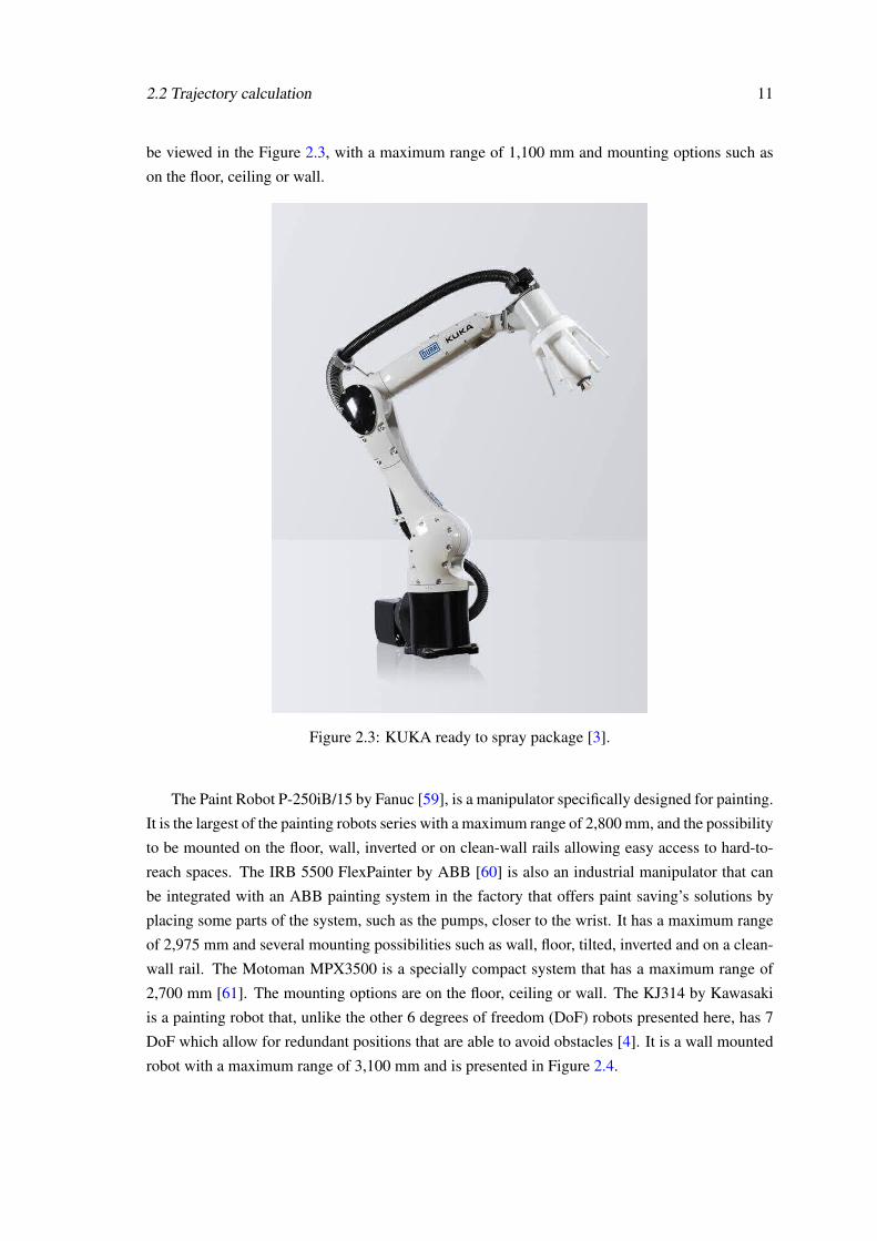
The KR AGILUS KR 10 R1100 [3] is an industrial manipulator sold in a ready2_spray pack-
age that includes the painting system. It is a partnership between two industry expert suppliers
KUKA (robots) and Dürr (painting systems). It has the advantage of being fully integrated, as can
2.2 Trajectory calculation 11
be viewed in the Figure 2.3, with a maximum range of 1,100 mm and mounting options such as
on the floor, ceiling or wall.
Figure 2.3: KUKA ready to spray package [3].
The Paint Robot P-250iB/15 by Fanuc [59], is a manipulator specifically designed for painting.
It is the largest of the painting robots series with a maximum range of 2,800 mm, and the possibility
to be mounted on the floor, wall, inverted or on clean-wall rails allowing easy access to hard-to-
reach spaces. The IRB 5500 FlexPainter by ABB [60] is also an industrial manipulator that can
be integrated with an ABB painting system in the factory that offers paint saving’s solutions by
placing some parts of the system, such as the pumps, closer to the wrist. It has a maximum range
of 2,975 mm and several mounting possibilities such as wall, floor, tilted, inverted and on a clean-
wall rail. The Motoman MPX3500 is a specially compact system that has a maximum range of
2,700 mm [61]. The mounting options are on the floor, ceiling or wall. The KJ314 by Kawasaki
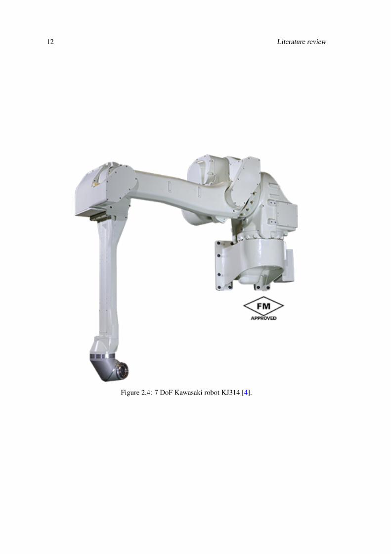
is a painting robot that, unlike the other 6 degrees of freedom (DoF) robots presented here, has 7
DoF which allow for redundant positions that are able to avoid obstacles [4]. It is a wall mounted
robot with a maximum range of 3,100 mm and is presented in Figure 2.4.
12 Literature review
Figure 2.4: 7 DoF Kawasaki robot KJ314 [4].

Chapter 3
Spray painting simulation
This chapter will describe the design process taken into building the spray painting simulation. It
will also include the results of real world experiments and their respective comparison with the
simulated counterparts.
3.1 Simulation environment
Spray paint simulation requires a 3D graphical environment that is capable of containing both
the target piece and the spray gun. In addition to this it is also necessary to be able to modify
the color of the part of the piece that has been painted in order to visually comprehend the sim-
ulation. Besides the fundamental features, several others become useful in order to utilize the
simulation process for as many applications as desired. Some of these optional features include
the possibility of loading different file types of CAD models, allowing a broad range of models
to be used as painting target. Another beneficial feature is the possibility to change spray gun
parameters so that the simulation can easily correspond with the real world. The main application
for spray simulation is the generation of automatic trajectories that a robotic system can perform
autonomously, with this in consideration, another valuable feature is the ability to simulate a di-
verse range of robotic systems as well as the environments they are in, including the containing
obstacles. A simulation system that is capable of most of these features, open source and focused
on educational and research purposes, is SimTwo.
SimTwo is a robot simulation environment that was designed to enable researchers to accu-
rately test their algorithms in a way that reflected the real world. SimTwo uses The Open Dynam-
ics Engine for simulating rigid body dynamics and the virtual world is represented using GLScene
components [62], these provide a simple implementation of OpenGL [63]. SimTwo applications
include robotic manipulators, and mobile robotics lessons, where students can practice inverse
kinematics and Kalman filters, humanoid robot research, where optimization algorithms can learn
in the simulated environment [64] or path planning for pick and place operations [65]. SimTwo
scenes are made up of "robots", "obstacles", "things", "tracks" and "sensors" described in one or
more XML (Extensible Markup Language) files, which allows for easy configuration of the scene
13
14 Spray painting simulation
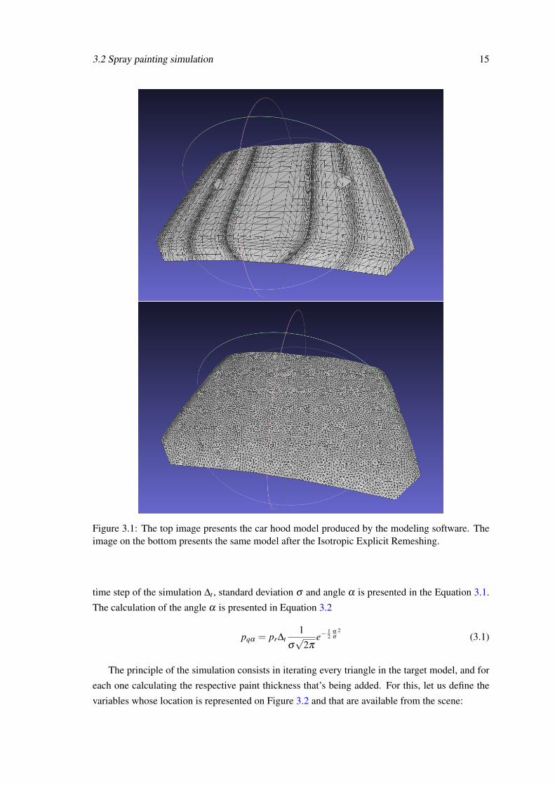
parameters and a scene can rapidly be adapted to match a real life environment. For this thesis,
a paint target element was added to SimTwo so that every other object represented in the simula-
tion doesn’t get painted, this is specially important for large scenes where the computing cost of
calculating the spray painting dispersion is significant. A spray gun element was also added pro-
viding the freedom to place the origin of the spray cone anywhere in the scene, including a fixed
location in the simulated world or attached to already existing motor actuated robotic systems.
This element also supports the configuration of the spray gun parameters, such as paint color in
RGB (Red, Green and Blue) values or paint rate in m3/s. For the experimental part of this work it
was used an already existing robotic machining cell with an Yaskawa MH50 robotic manipulator.
Therefore, it was added a simulated version of this cell to the scene providing easier positioning
and visualization of the simulation.
3.2 Spray painting simulation
In order to simulate spray painting, the color of specific parts of the paint target mesh must be
changed. This can be mainly done by two processes, either the mesh vertex’s color change or the
texture associated with the mesh is altered at the location of the vertex’s texture coordinate. The
primary advantage of using the texture for simulation is the spray resolution that can be achieved
with low poly meshes, however, most industrial application don’t require textures for the CAD
models, and the process of unwrapping the model (generating the texture coordinates) is non
trivial and usually performed by artists in the game or movie industries. Therefore, the vertex’s
color is used to colorize the model, since it is present in every CAD format or 3D scan and every
model can easily be adapted to match the required resolution.
The assumption that the target mesh has regular sized triangles is taken. As this is rarely the
case, a preprocess phase is required, where the CAD model is remeshed using an Isotropic Explicit
Remeshing algorithm that repeatedly applies edge flip, collapse, relax and refine to improve aspect
ratio and topological regularity. This step can be held by the free software MeshLab [66] and the
transformation can be observed in Figure 3.1 with a CAD model of a car hood as an example.
The importance of the preprocess lies in the fact that from thereafter the triangle center de-
scribes a triangle location, since the triangles are approximately equilateral. Another important
result emerges from the fact that every triangle area is identical and small enough so that each
triangle constitutes an identity for the mesh supporting a pixel/voxel like algorithm.
In order to achieve a fast runtime without compromising the realism of the simulation, the paint
distribution model adopted is a Gaussian function limited to the area of a cone. The parameters
that describe the paint distribution as well as the cone’s angle are dependent on the spray gun and
its settings. As the assumed distribution model is circular symmetric, there is no need for a higher-
order Gaussian function since the paint quantity only varies according to the angle difference. In
the center of the cone is the highest concentration of paint and, as the angle increases the paint
quantity also decreases following the Gaussian distribution for any direction of the painted surface.
The general equation that calculates the paint quantity per angle pqα based on the painting rate pr,
3.2 Spray painting simulation 15
Figure 3.1: The top image presents the car hood model produced by the modeling software. Theimage on the bottom presents the same model after the Isotropic Explicit Remeshing.
time step of the simulation ∆t , standard deviation σ and angle α is presented in the Equation 3.1.
The calculation of the angle α is presented in Equation 3.2
pqα = pr∆t1
σ√
2πe−
12
α
σ
2(3.1)
The principle of the simulation consists in iterating every triangle in the target model, and for
each one calculating the respective paint thickness that’s being added. For this, let us define the
variables whose location is represented on Figure 3.2 and that are available from the scene:
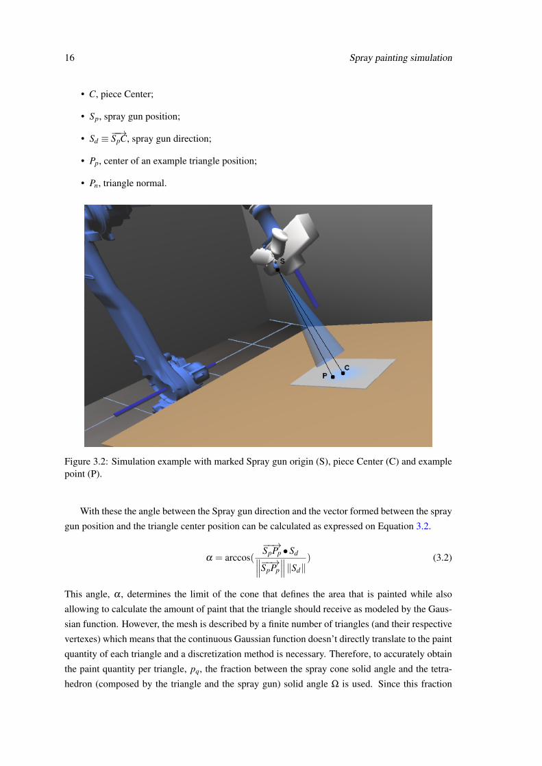
16 Spray painting simulation
• C, piece Center;
• Sp, spray gun position;
• Sd ≡−−→SpC, spray gun direction;
• Pp, center of an example triangle position;
• Pn, triangle normal.
Figure 3.2: Simulation example with marked Spray gun origin (S), piece Center (C) and examplepoint (P).
With these the angle between the Spray gun direction and the vector formed between the spray
gun position and the triangle center position can be calculated as expressed on Equation 3.2.
α = arccos(−−→SpPp •Sd∥∥∥−−→SpPp
∥∥∥‖Sd‖) (3.2)
This angle, α , determines the limit of the cone that defines the area that is painted while also
allowing to calculate the amount of paint that the triangle should receive as modeled by the Gaus-
sian function. However, the mesh is described by a finite number of triangles (and their respective
vertexes) which means that the continuous Gaussian function doesn’t directly translate to the paint
quantity of each triangle and a discretization method is necessary. Therefore, to accurately obtain
the paint quantity per triangle, pq, the fraction between the spray cone solid angle and the tetra-
hedron (composed by the triangle and the spray gun) solid angle Ω is used. Since this fraction
3.3 Occlusion paint culling 17
provides a precise relation between each triangle and the total paint cone, which is dependent on
the distance and angle in relation to the paint gun, it is a valid reproduction of the spray projection
process. The triangle solid angle calculation is presented on Equation 3.3 and the paint quantity
per triangle is presented on Equation 3.4. Considering that the angle of the cone is δ , the vectors
A,B,C are the 3 vertices of the triangle and the vectors a =−−→SpA, b =
−−→SpB and c =−−→SpC.
Ω = 2arctan(|abc|
‖a‖‖b‖‖c‖+(a•b)‖c‖+(a• c)‖b‖+(b• c)‖a‖) (3.3)
pq =pqα
π
Ω
(2π(1− cos( δ
2 ))(3.4)
At last the added paint thickness Pt can be calculated by dividing the paint quantity by the area
of the triangle At , Equation 3.5.
Pt =pq
At(3.5)
3.3 Occlusion paint culling
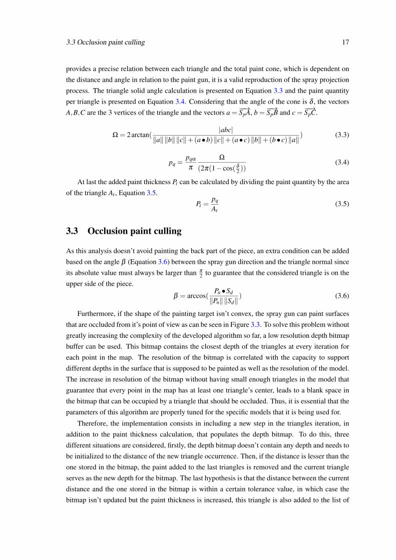
As this analysis doesn’t avoid painting the back part of the piece, an extra condition can be added
based on the angle β (Equation 3.6) between the spray gun direction and the triangle normal since
its absolute value must always be larger than π
2 to guarantee that the considered triangle is on the
upper side of the piece.
β = arccos(Pn •Sd
‖Pn‖‖Sd‖) (3.6)
Furthermore, if the shape of the painting target isn’t convex, the spray gun can paint surfaces
that are occluded from it’s point of view as can be seen in Figure 3.3. To solve this problem without
greatly increasing the complexity of the developed algorithm so far, a low resolution depth bitmap
buffer can be used. This bitmap contains the closest depth of the triangles at every iteration for
each point in the map. The resolution of the bitmap is correlated with the capacity to support
different depths in the surface that is supposed to be painted as well as the resolution of the model.
The increase in resolution of the bitmap without having small enough triangles in the model that
guarantee that every point in the map has at least one triangle’s center, leads to a blank space in
the bitmap that can be occupied by a triangle that should be occluded. Thus, it is essential that the
parameters of this algorithm are properly tuned for the specific models that it is being used for.
Therefore, the implementation consists in including a new step in the triangles iteration, in
addition to the paint thickness calculation, that populates the depth bitmap. To do this, three
different situations are considered, firstly, the depth bitmap doesn’t contain any depth and needs to
be initialized to the distance of the new triangle occurrence. Then, if the distance is lesser than the
one stored in the bitmap, the paint added to the last triangles is removed and the current triangle
serves as the new depth for the bitmap. The last hypothesis is that the distance between the current
distance and the one stored in the bitmap is within a certain tolerance value, in which case the
bitmap isn’t updated but the paint thickness is increased, this triangle is also added to the list of
18 Spray painting simulation
triangles that is being deleted in the last situation (if a closer value is found and the bitmap value of
the current location updated). In order to determine the index of the bitmap in which the triangles
are located, two new angles were calculated. These correspond to the spherical coordinates of
the new triangle from the point of view of the spray gun. Since the max angle is equal in both
coordinates, a simple approximation serves as index of the bitmap, considering the respective
resolution. This algorithm is presented in Algorithm 1 and a second example with a surface that
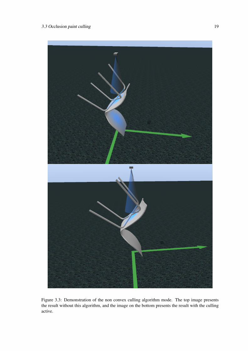
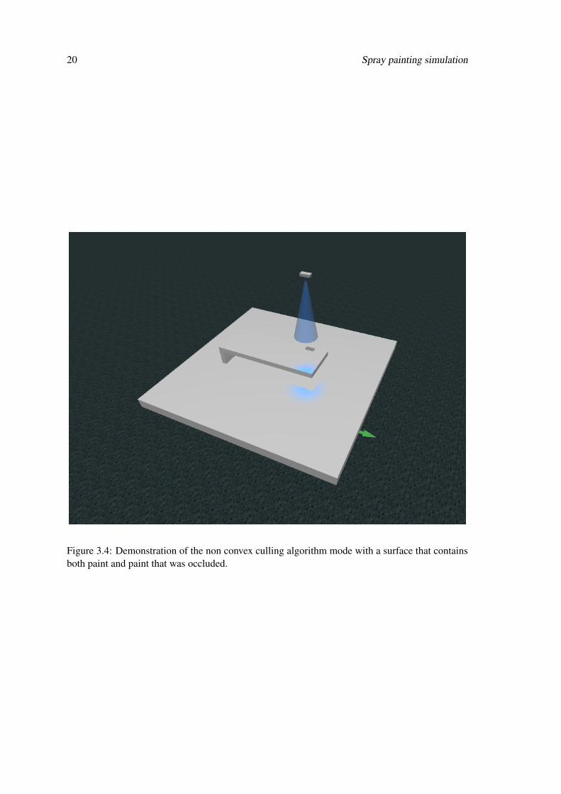
contains both paint and paint that was occluded is presented in Figure 3.4.
Algorithm 1: Occlusion paint culling algorithm
1 // initialize the bitmap with a negative value2 bitmap[bitmapSize][bitmapSize] =−13 // create a dynamic array of lists to store the triangles that
may get removed4 bitmapOldTriangles[bitmapSize][bitmapSize] = []5 for triangle In triangles do6 angleT heta = calculateT heta(triangle,sprayGun)7 anglePhi = calculatePhi(triangle,sprayGun)8 zi = b(bitmapSize/2)∗ (angleT heta/maxAngle)c+(bitmapSize/2)9 z j = b(bitmapSize/2)∗ (anglePhi/maxAngle)c+(bitmapSize/2)
10 dist = calculateDist(triangle, sprayGun)11 if bitmap[zi][z j]< 0 then12 // first time painting this bitmap zone13 calculatePaintT hickness(triangle,sprayGun)14 bitmap[zi][z j] = dist15 bitmapOldTriangles[zi][z j].append(triangle)16 else if abs(bitmap[zi][zj]-dist) <= cavitySize then17 calculatePaintT hickness(triangle,sprayGun)18 bitmapOldTriangles[zi][z j].append(triangle)19 else if dist < bitmap[zi][zj then20 // delete old paint and start over with this triangle21 calculatePaintT hickness(triangle,sprayGun)22 bitmap[zi][z j] = dist23 removePaint(bitmapOldTriangles[zi][z j])24 bitmapOldTriangles[bitmapSize][bitmapSize] = []25 bitmapOldTriangles[zi][z j].append(triangle)26 end for
3.3 Occlusion paint culling 19
Figure 3.3: Demonstration of the non convex culling algorithm mode. The top image presentsthe result without this algorithm, and the image on the bottom presents the result with the cullingactive.
20 Spray painting simulation
Figure 3.4: Demonstration of the non convex culling algorithm mode with a surface that containsboth paint and paint that was occluded.
3.4 Parameters initialization 21
3.4 Parameters initialization
Some calculations such as the area and center of the triangles and which vertices correspond to
each triangle can occur every iteration (as long as the triangle is accumulating paint). As these
values aren’t dynamic, they can be calculated only once, when the paint target CAD is loaded and
stored for faster access during runtime.
The center coordinates of every triangle are calculated by simply averaging the three vertex
coordinates. To calculate the average triangle area, every triangle is considered. The area of a
triangle is calculated according to Equation 3.7.
A =12||(p2− p1)× (p3− p1)| | (3.7)
To determine which vertices correspond to each triangle and what are the neighboring triangles
given the position of the triangles vertices, it’s necessary to iterate the triangles’ list twice. The
results are stored in a way that allow the access of the vertexes from the triangles and the triangles
from the vertexes without accessing the GPU memory which greatly reduces the simulation speed.
In the first iteration of the triangle list it is determined which triangles belong to each vertex. To
achieve this, for every triangle the first occurring vertex in the mesh vertex’s list is stored in the
corresponding triangle index. And in the list of triangles of that vertex, the current triangle is
added. In the second iteration, the neighbors of each triangle are calculated. To achieve this, the
list of triangles that a vertex belong is used, since the 3 vertexes of the triangle are known, every
triangle that also has at least one equal vertex is considered a neighbor and stored that way. This
initialization is presented in Algorithm 2.
In the worst case, this algorithm is O(N2) since every vertex is searched in the list of all ver-
texes. Thus, calculating these values only once, and only accessing them in runtime is a tremen-
dous advantage, specially considering the reduced complexity of the spray simulation algorithm
O(N) (iterates every triangle once).

22 Spray painting simulation
Algorithm 2: Initialization algorithm
1 // initialize the bitmap with a negative value2 meshTriangles[Length(triangles)]3 meshTriangles.vertex[3] = []4 bitmapOldTriangles[bitmapSize][bitmapSize] = []5 for i In triangles do6 meshTriangles[i].vertex[0].append( f indLowestVertexIndex(triangles[i].v0))7 meshTriangles[i].vertex[1].append( f indLowestVertexIndex(triangles[i].v1))8 meshTriangles[i].vertex[2].append( f indLowestVertexIndex(triangles[i].v2))9 updateStatisticalParameters(triangles[i],meshTriangles[i])
10 end for11 for i In triangles do12 for k In [0,1,2] do13 for j In meshTriangles[i].vertex[k].triangles do14 for l In meshTriangles[i].neighbors do15 if meshTriangles[i].vertexs[k].triangles[ j] = i then16 break17 if l = length(meshTriangles[i].neighbors) then18 meshTriangles[i].neighbors.append(meshTriangles[i].vertexs[k].triangles[ j])19 if
meshTriangles[i].vertexs[k].triangles[ j] = meshTriangles[i].neighbors[l]then
20 break21 end for22 end for23 end for24 end for

3.5 Paint validation metrics 23
3.5 Paint validation metrics
In order to determine the paint quality several metrics were implemented. Establishing which
part of the paint target model is indeed supposed to be painted is a problem that is outside of the
scope of this work as it would either involve a development of a graphical tool to select the parts
to be painted or resort to simple plane intersections or even some kind of CAD model coloring
that would limit the format abstraction. For these reasons a compromise solution is to calculate
a dual version of each metric that only considers the painted triangles as triangles to be painted.
These measurements aren’t as accurate as the others and should only be used when the painting
algorithm is clearly doing what it was meant to do and paying close attention to the coverage ratio
(percentage of triangles that contain paint).
In this regard the following functions have been made available for any trajectory or sets of
trajectories:
• average spray thickness;
• standard deviation of the spray thickness;
• positive average of the spray thickness;
• positive standard deviation of the spray thickness;
• max spray thickness;
• minimum spray thickness;
• positive minimum spray thickness;
• histogram of triangle’s paint thickness;
• coverage ratio.
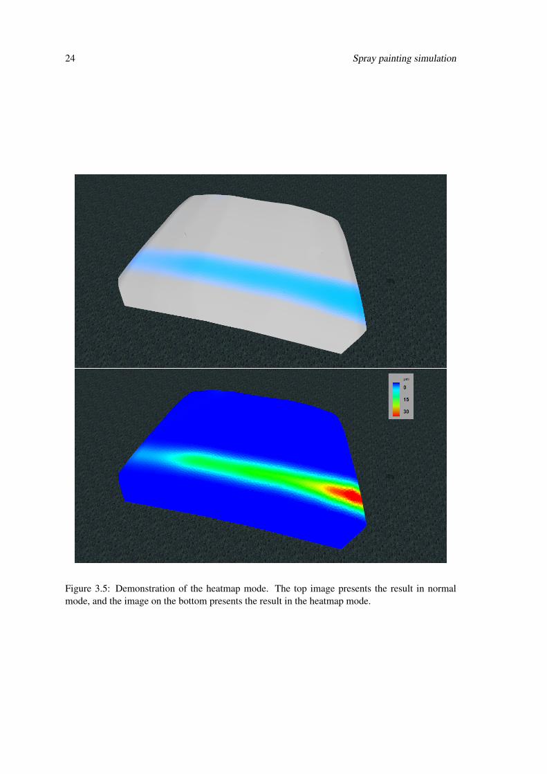
In order to facilitate the visual assessment of the paint quality a heatmap mode was imple-
mented. In this mode the blue color means that there is no paint and as the color goes to yellow
and more reddish tones the paint quantity is increasingly higher, being that a red tone means that
there is too much paint on that face. With this mode a qualitative review can be easily performed,
unlike with the true color prediction where once the paint saturates the color doesn’t change much.
This mode can be seen in Figure 3.5 where the spray gun started on the left and with increasingly
slower velocity moved to the right producing the observed pattern.
24 Spray painting simulation
Figure 3.5: Demonstration of the heatmap mode. The top image presents the result in normalmode, and the image on the bottom presents the result in the heatmap mode.

3.6 Experimental trials 25
3.6 Experimental trials
In order to validate the simulation results, a real life experiment was made. Several trials were
conducted with the cooperation of a local company that made available a machining cell and
the respective industrial manipulator. The Yaskawa MH50 is a powerful robot that’s capable of
reaching high speeds, has a less than 1 mm repeatability and has a horizontal reach of more than
2 m and a vertical reach of more than 3.5 m. Its main applications are material cutting, handling,
dispensing and coating. The main characteristics of the manipulator used can be found in Table
3.1.
Table 3.1: Yaskawa MH50 characteristics
Controlled axes 6Maximum payload 50 kgRepeatability ±0.07 mmHorizontal reach 2061 mmVertical reach 3578 mmWeight 550 kgPower rating 4.0 kVA
After a market survey, the chosen spray gun was a HVLP gravity feed air spray gun, presented
in Figure 3.6. This is a common spray painting gun that is low cost, easily available and allows
for a generic test that is likely to generalize to other spray guns.
Figure 3.6: HVLP gravity feed air spray gun used in the experimental trials.
This HVLP gravity feed air spray gun is designed for being used by human painters, as such,
a modification was necessary that allowed the actuation to be performed by a servo controlling the
trigger position. This was achieved by disassembling the spray gun, removing the handle grip and
drilling a small hole in the trigger so that a metal rod could be placed connecting the trigger with
the servo horn. Both the servo and the spray gun were attached to an angle bracket that served as

26 Spray painting simulation
an easy attach system to the robot. With this procedure the operator’s hand is fully replaced by a
robotic system. The inside of the assembly can be observed in Figure 3.7 along with the assembly
support drawing that also served as a spray gun 3D model included in the simulation.
Figure 3.7: On the left is the spray gun used during experiments, without the front cover (with aservo motor to control the trigger). On the right is the technical CAD drawing.
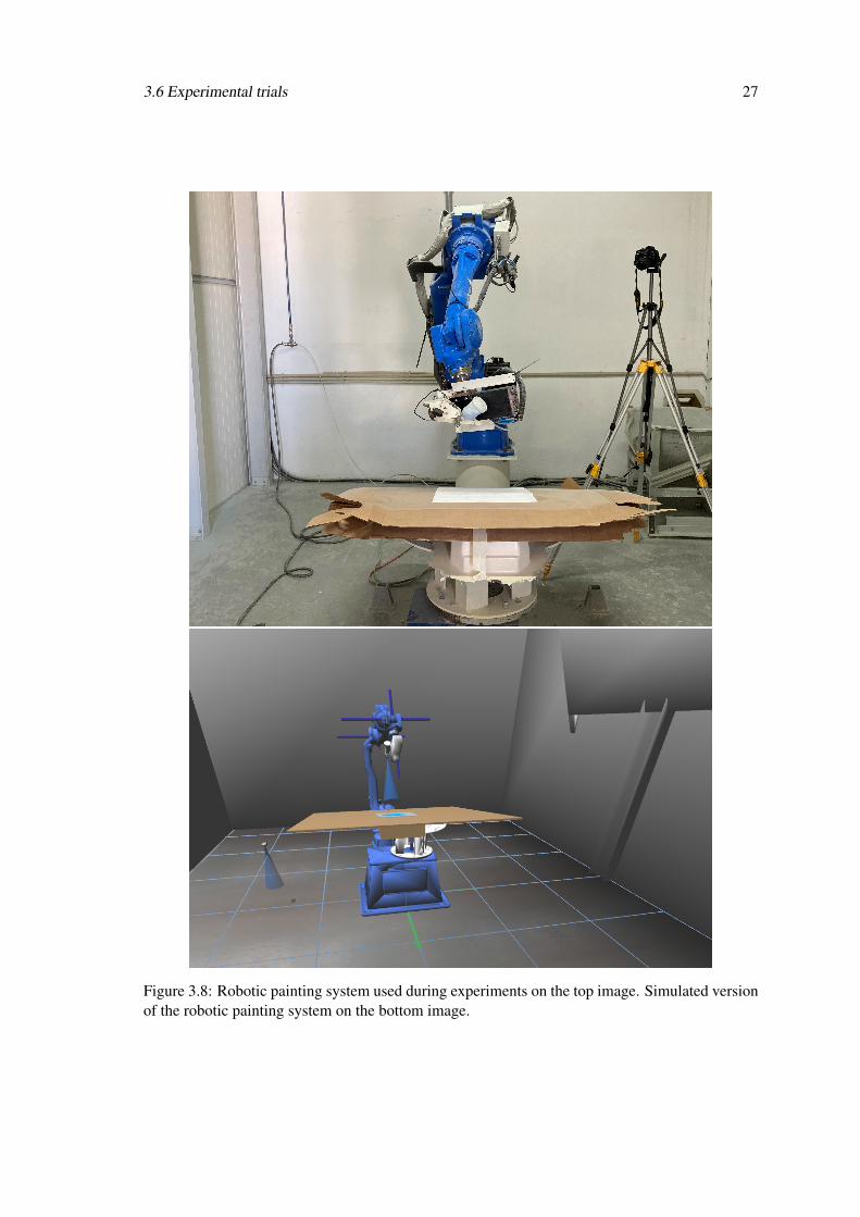
Therefore, the spray gun was mounted in a Yaskawa MH50 machining robot, alongside the
spindle, and several loose paper sheets were used as sample painting targets. The full system is
presented in Figure 3.8.
The chosen paint was 25-420 C-THANE S400 SAT, whose characteristics are in Table 3.2,
for being one of the most used in industrial equipments and machinery providing great exterior
durability allied with excellent superficial finishing.
Table 3.2: 25-420 C-THANE S400 SAT paint characteristics
Viscosity 70-75 UKVolumic mass 1,227 g/mLSolid percentage 42 %Theoretical efficiency 12 m2/LRecommended paint thickness 35 µm
The last preparation step consisted in guaranteeing that the environmental conditions inside
the cell are within the parameters defined by the paint supplier that can be consulted in Table 3.3.
Table 3.3: Environmental conditions
Ambient temperature >15 ºCRelative humidity <75 %Drying time >2 h
3.6 Experimental trials 27
Figure 3.8: Robotic painting system used during experiments on the top image. Simulated versionof the robotic painting system on the bottom image.

28 Spray painting simulation
Before the trials started, in order to determine the paint rate, the gun was activated for 30
seconds. The paint was collected and weighted, obtaining the paint rate value for the chosen
pressure of 6.2 bar (as recommended by the spray gun supplier). This is an inexpensive test
that can be repeated when there is a possibility that the spray gun settings changed. In order to
guarantee coherence among the results the servo actuation was always the maximum amount that
the trigger allowed, and it was chosen a constant active time of 3 seconds. Several tests were
conducted with increasing offsets from the paint target. From the point that no visible saturation
occurred, three locations were chosen for further analysis. Then the painted paper sheets were
scanned in order to obtain a digitized image.
At last, a simulated room and the robot were added to the SimTwo scene, Figure 3.8. The
room was designed using the Fusion 360 program and the normals of the exterior faces of the
walls were switched using Blender, so that it was possible to look inside the cell from anywhere in
the simulation. The robot’s CAD files are made available directly from Yaskawa and the assembly
was made in the SimTwo XML files considering the measured offsets between the joints in the
three axis using the Fusion 360 software. With these upgrades, the real world positions for the
trials were mimicked since the angles in the real robot and in the simulated one were matched.
The spray gun parameters were updated, as will be explained in the following sections, and the
experiments were conducted with the same duration and offset distances as the real ones. Then,
a close screen print was taken and the paper sheet vertices were used as a reference (by manual
selection) for the perspective transformation thus obtaining a scan like image.
3.7 Image processing tool
For the sake of reproducibility and meaningful analysis, an imaging processing pipeline was devel-
oped. The objective of this tool is the extraction of the paint distribution function from the painted
sheets scans. In this regard, the OpenCV [67] library for python was used because it provides
the necessary computer vision algorithms. As the images are obtained with controlled conditions,
such as traditional scanning of a sheet of paper, no extensive preprocessing is necessary to clean
them.
This way, the first step is converting the image to grayscale as can be seen in Equation 3.8.
This conversion reduces the color dependency of the algorithm and also increases the illumination
invariance.
G = 0.299 ·R+0.587 ·G+0.114 ·B (3.8)
Then a simple threshold, where the pixels whose intensities are below the threshold value are
deleted. Following, a single step erosion that segments the majority of the paint is enough to
remove any noise in the image. The erosion operation replaces the anchor pixel (iterates every
pixel) by the local minimum over the area of the kernel, as presented in Equation 3.9.
dst(x,y) = min(x′,y′):element(x′,y′)6=0src(x+ x′,y+ y′) (3.9)

3.7 Image processing tool 29
Since the spray pattern is circular, the center of the segmentation (Cx,Cy) is the same as the
center of the paint. The region of interest is thus defined by a circle, with this center and a slightly
larger radius than half the segmentation bounding box. From this region the image intensity along
several lines is averaged according to Equation 3.10 and the respective standard deviation is cal-
culated to validate the assumption that the pattern is indeed circular symmetric.
i(x) =1L ∑
limg(Cx + x.cos(αl),Cy + x.sin(αl)) (3.10)
The size of the paper sheet used is known, as is the amount of paint P spent during the experi-
ment. Considering that the paint didn’t saturate, we can deem the amount of paint proportional to
the pixel intensity as a reasonable assumption. Thus the image can be normalized so that the mini-
mum intensity pixels (darkest) are transformed in ones and the maximum intensity pixels (whiter)
transformed in zeros. To obtain the paint quantity per pixel, the ratio between paint quantity spent
in the test and the sum of the normalized pixels is multiplied by the normalized pixels. The overall
expression is presented in Equation 3.11, with the img(x,y) being the value of the pixel in the (x,y)
position and the max(img) and min(img) being the maximum and minimum pixel values of the
full image, respectively.
pq(x,y) = P∗max(img)−img(x,y)max(img)−min(img)
∑max(img)−img(x,y)max(img)−min(img)
(3.11)
The last step is to fit the curve to the Gaussian distribution (cf. Equation 3.1) used in the
simulation. The least mean squares is used for optimization, obtaining the optimal values for the
Gaussian function parameters (the sum of the squared residuals is minimized). The pipeline can
be observed in Figure 3.9 and the calculated plots in Figure 3.10.
This tool allows us not only to validate the purposed simulation but also to easily calibrate the
spray parameters. This is a great advantage since every spray painting gun has different parameters
and even the same gun with different configurations can have a variety of spray patterns.

30 Spray painting simulation
Figure 3.9: Imaging processing pipeline: original image, converted to grayscale image, thresh-olded image, eroded image, image with the circle delimiting the region of interest, and an exampleof the selected lines.
3.7 Image processing tool 31
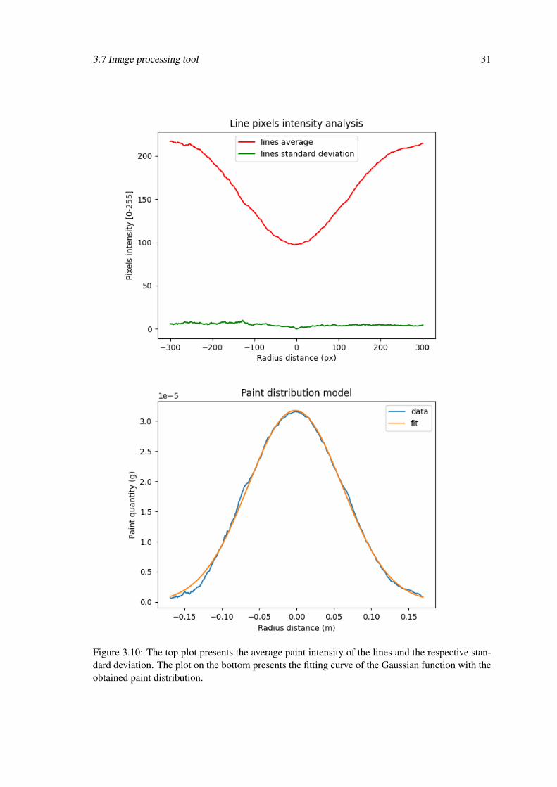
Figure 3.10: The top plot presents the average paint intensity of the lines and the respective stan-dard deviation. The plot on the bottom presents the fitting curve of the Gaussian function with theobtained paint distribution.

32 Spray painting simulation
3.8 Analysis of the results
The analysis of the results enabled to conclude that the spray gun distribution follows indeed a
Gaussian distribution, as can be seen in Figure 3.10 where the curve of a Gaussian function fits
with the measured paint distribution. The low standard deviation among the lines proves that the
spray pattern is truly circular symmetric.
In order to further validate the simulation, the experiment was repeated in the simulator, with
the updated values for the paint distribution. The results were processed with the developed imag-
ing processing tool (cf. Figure 3.11).
Figure 3.11: Imaging processing pipeline applied to the simulator: original image, converted tograyscale image, thresholded image, eroded image, image with the circle delimiting the region ofinterest, and an example of the selected lines.
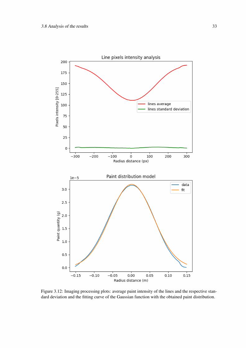
The calculated plots (Figure 3.12) compared with the real life plots (Figure 3.10) are smoother
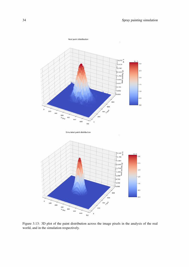
as they present the ideal curve, however, the distribution is the same. Figure 3.13 presents the
calculated paint distribution across the real and simulated images and here again the paint distri-
butions are identical.
3.8 Analysis of the results 33
Figure 3.12: Imaging processing plots: average paint intensity of the lines and the respective stan-dard deviation and the fitting curve of the Gaussian function with the obtained paint distribution.
34 Spray painting simulation
Figure 3.13: 3D plot of the paint distribution across the image pixels in the analysis of the realworld, and in the simulation respectively.
3.8 Analysis of the results 35
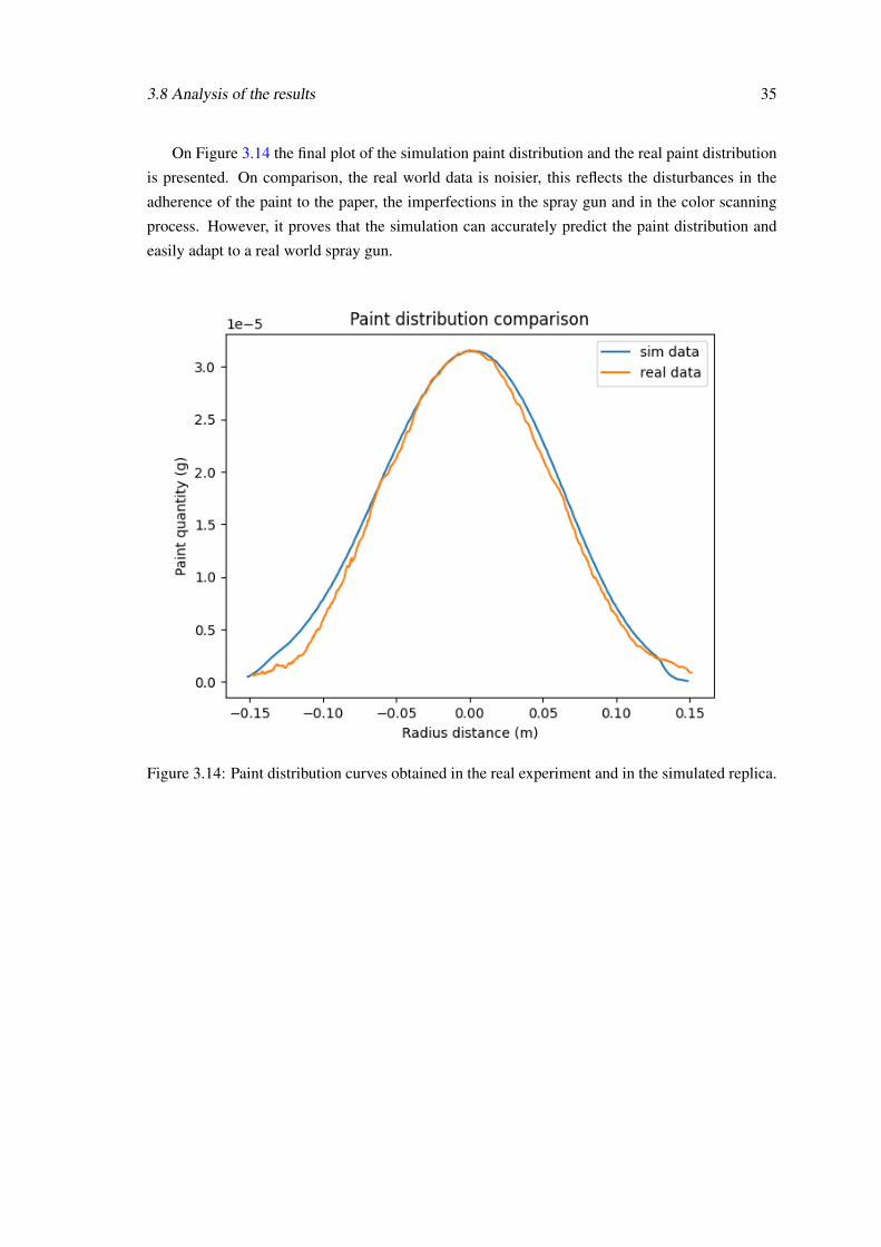
On Figure 3.14 the final plot of the simulation paint distribution and the real paint distribution
is presented. On comparison, the real world data is noisier, this reflects the disturbances in the
adherence of the paint to the paper, the imperfections in the spray gun and in the color scanning
process. However, it proves that the simulation can accurately predict the paint distribution and
easily adapt to a real world spray gun.
Figure 3.14: Paint distribution curves obtained in the real experiment and in the simulated replica.

36 Spray painting simulation

Chapter 4
Trajectory optimization use cases
In this chapter several methods that have been implemented to generate trajectories will be re-
viewed. Their main purpose is to validate the simulation and provide a baseline for further re-
search.
4.1 SimTwo scene
In order to interface with the simulation, a scene containing a spray gun and a target object was
developed along with a control program and a sheet where the main functionalities are easily
accessible as can be seen in Figure 4.1. Several control modes have been implemented, allowing
for different use types, such as:
• Manual mode allows the user to use the arrow keys to move the paint gun in the selected
axis;
• Paint mode allows the simulation of a selected trajectory (included a loaded trajectory);
• UDP server waits for a connection with remote python program and responds to:
– number of triangles requests;
– sending the triangles’ data such as vertex, normals, center and area;
– setting a color for a specific triangle;
– closing the connection.
• Calibration imitates the procedure described in section 3.7.
Other behaviours, that directly interact with the stored paint and visualization, are present in
separate buttons making it possible to reset a scene, reset the paint, change from paint mode to
heatmap mode and turn on and off the spray gun. It is also possible to preview the developed
metrics for the specific instant when the button is pressed.
37

38 Trajectory optimization use cases
Figure 4.1: Developed SimTwo sheet.
4.2 Primitive trajectory generation
An algorithm that is both simple to implement and somewhat useful is a simple raster pattern that
covers a rectangle, with a certain offset of the piece. This type of trajectories is useful when the
part to paint is relatively flat. An example of this algorithm’s application is painting the top of a
car hood, as can be seen in Figure 4.2.
This algorithm doesn’t require a specific knowledge of the vertex’s position, and a simple
bounding box with a face selection (typically the top face) is enough for determining the trajec-
tory waypoints. Since the borders of the rectangular projected piece being painted need to have
the same overlapping passages as the center, the rectangle that is used for the rasterization is an
extension of the original projected rectangle. The step size between two consecutive passages is
dependent on the distance between the paint gun and the piece, and the angle of the spray cone.
It can also be adjusted according to the number of repetitions desired, the amount of paint in each
repetition and the desired paint thickness on the final product. From hereafter the parameters of
this algorithm will be defined as BoxVExtend, the dimension of this extension for each of the four
sides of the rectangle, BoxUstep, the side step between consecutive passages and BoxOffset, the
height of the plane used for rasterization in relation with the top of the piece.
If the selected piece surface isn’t flat then the produced paint dispersion doesn’t have a uniform
thickness, thus limiting the application of this algorithm. However, with the statistical measures
and the heatmap observations presented in the last chapter it is possible to fix a limit and easily
determine if the fast and simplified approach can successfully paint the target piece.

4.2 Primitive trajectory generation 39
Figure 4.2: Two examples of the generated trajectory: on the top image with a cube, and on thebottom image with a car hood.
40 Trajectory optimization use cases
4.3 Patched trajectory generation
When a professional painter works on a piece, usually the trajectory taken is a combination of
raster patterns applied to the different sections of the piece. Unlike a robotic system, a human
approach usually varies the speed and the distance to the piece according to the painter’s experi-
ence and physical limitations. With this process in mind, an upgrade on the primitive trajectory
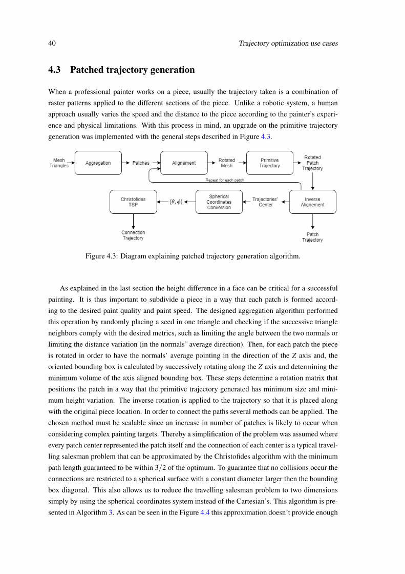
generation was implemented with the general steps described in Figure 4.3.
Figure 4.3: Diagram explaining patched trajectory generation algorithm.
As explained in the last section the height difference in a face can be critical for a successful
painting. It is thus important to subdivide a piece in a way that each patch is formed accord-
ing to the desired paint quality and paint speed. The designed aggregation algorithm performed
this operation by randomly placing a seed in one triangle and checking if the successive triangle
neighbors comply with the desired metrics, such as limiting the angle between the two normals or
limiting the distance variation (in the normals’ average direction). Then, for each patch the piece
is rotated in order to have the normals’ average pointing in the direction of the Z axis and, the
oriented bounding box is calculated by successively rotating along the Z axis and determining the
minimum volume of the axis aligned bounding box. These steps determine a rotation matrix that
positions the patch in a way that the primitive trajectory generated has minimum size and mini-
mum height variation. The inverse rotation is applied to the trajectory so that it is placed along
with the original piece location. In order to connect the paths several methods can be applied. The
chosen method must be scalable since an increase in number of patches is likely to occur when
considering complex painting targets. Thereby a simplification of the problem was assumed where
every patch center represented the patch itself and the connection of each center is a typical travel-
ling salesman problem that can be approximated by the Christofides algorithm with the minimum
path length guaranteed to be within 3/2 of the optimum. To guarantee that no collisions occur the
connections are restricted to a spherical surface with a constant diameter larger then the bounding
box diagonal. This also allows us to reduce the travelling salesman problem to two dimensions
simply by using the spherical coordinates system instead of the Cartesian’s. This algorithm is pre-
sented in Algorithm 3. As can be seen in the Figure 4.4 this approximation doesn’t provide enough
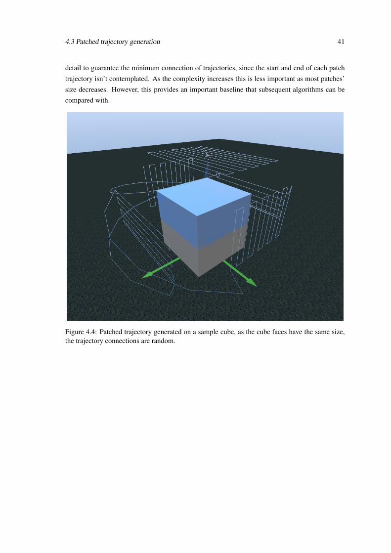
4.3 Patched trajectory generation 41
detail to guarantee the minimum connection of trajectories, since the start and end of each patch
trajectory isn’t contemplated. As the complexity increases this is less important as most patches’
size decreases. However, this provides an important baseline that subsequent algorithms can be
compared with.
Figure 4.4: Patched trajectory generated on a sample cube, as the cube faces have the same size,the trajectory connections are random.
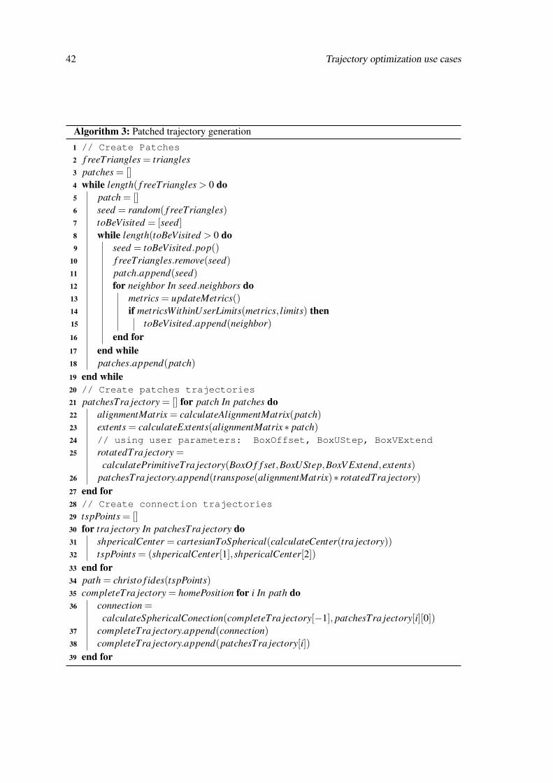
42 Trajectory optimization use cases
Algorithm 3: Patched trajectory generation
1 // Create Patches2 f reeTriangles = triangles3 patches = []4 while length( f reeTriangles > 0 do5 patch = []6 seed = random( f reeTriangles)7 toBeVisited = [seed]8 while length(toBeVisited > 0 do9 seed = toBeVisited.pop()
10 f reeTriangles.remove(seed)11 patch.append(seed)12 for neighbor In seed.neighbors do13 metrics = updateMetrics()14 if metricsWithinUserLimits(metrics, limits) then15 toBeVisited.append(neighbor)16 end for17 end while18 patches.append(patch)19 end while20 // Create patches trajectories21 patchesTra jectory = [] for patch In patches do22 alignmentMatrix = calculateAlignmentMatrix(patch)23 extents = calculateExtents(alignmentMatrix∗ patch)24 // using user parameters: BoxOffset, BoxUStep, BoxVExtend25 rotatedTra jectory =
calculatePrimitiveTra jectory(BoxO f f set,BoxUStep,BoxV Extend,extents)26 patchesTra jectory.append(transpose(alignmentMatrix)∗ rotatedTra jectory)27 end for28 // Create connection trajectories29 tspPoints = []30 for tra jectory In patchesTra jectory do31 shpericalCenter = cartesianToSpherical(calculateCenter(tra jectory))32 tspPoints = (shpericalCenter[1],shpericalCenter[2])33 end for34 path = christo f ides(tspPoints)35 completeTra jectory = homePosition for i In path do36 connection =
calculateSphericalConection(completeTra jectory[−1], patchesTra jectory[i][0])37 completeTra jectory.append(connection)38 completeTra jectory.append(patchesTra jectory[i])39 end for
4.4 Car bumper use case 43
4.4 Car bumper use case
In order to test the developed algorithms, a car bumper piece was chosen since this is a non
trivial piece that can’t be painted uniformly from a single plane. To include the car bumper in
the simulation, the CAD model was first preprocessed in Meshlab where the Isotropic Explicit
Remeshing algorithm was applied with 3 iterations, a edge target length of 24 mm and a crease
angle of 30º. This preprocess results in a model with 3361 vertices and 6261 faces (triangles) with
an average edge length of 17 mm. The model was saved in STL (Stereolithography) format and
the path was added in the XML configuration files with this model marked as a painting target.
4.4.1 Trajectory’s parameters optimization
The generation of trajectories can be optimized by adapting the trajectory generation algorithm’s
parameters according to the simulation results in an iterative process. The patched trajectory
algorithm has parameters for patch aggregation and for the patches’ primitive trajectory. Since
the car bump model doesn’t have any sharp edges or discontinuities in the places that the paint
will be applied, the patch aggregation was set to not limit the normal’s angle, only varying in the
maximum distance difference allowed in the same patch. Each primitive trajectory was set to have
fixed parameters in order to not increase the complexity of the optimization because their effect is
more stable. As such the chosen value for the BoxOffset was 500 mm, 100 mm for the BoxUStep
and 300 mm for the BoxVExtend. The velocity along the trajectory affects the total amount of
paint that is spent in each coat, scaling linearly the paint thickness disregarding the path taken.
For this reason, it was chose a fixed value of 0.3 m/s for the connection paths and for the painting
paths.
4.4.1.1 Maximum distance difference of 100 mm
As can be seen in Figure 4.5, the generated trajectory is quite complex and the end result isn’t
uniform. However, when observing the metrics in Table 4.1 and the histogram presented in Figure
4.6, the resulting trajectory did indeed result in full coverage of the piece and the variations in
paint thickness, although not optimal, have a smaller impact with further layers of paint, as can be
seen in Figure 4.7 where the piece has been painted twice with the same trajectory.
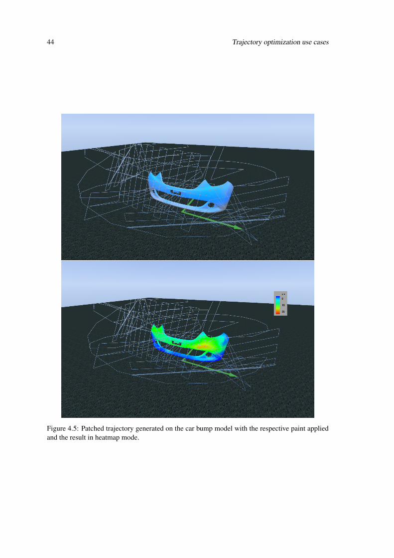
44 Trajectory optimization use cases
Figure 4.5: Patched trajectory generated on the car bump model with the respective paint appliedand the result in heatmap mode.
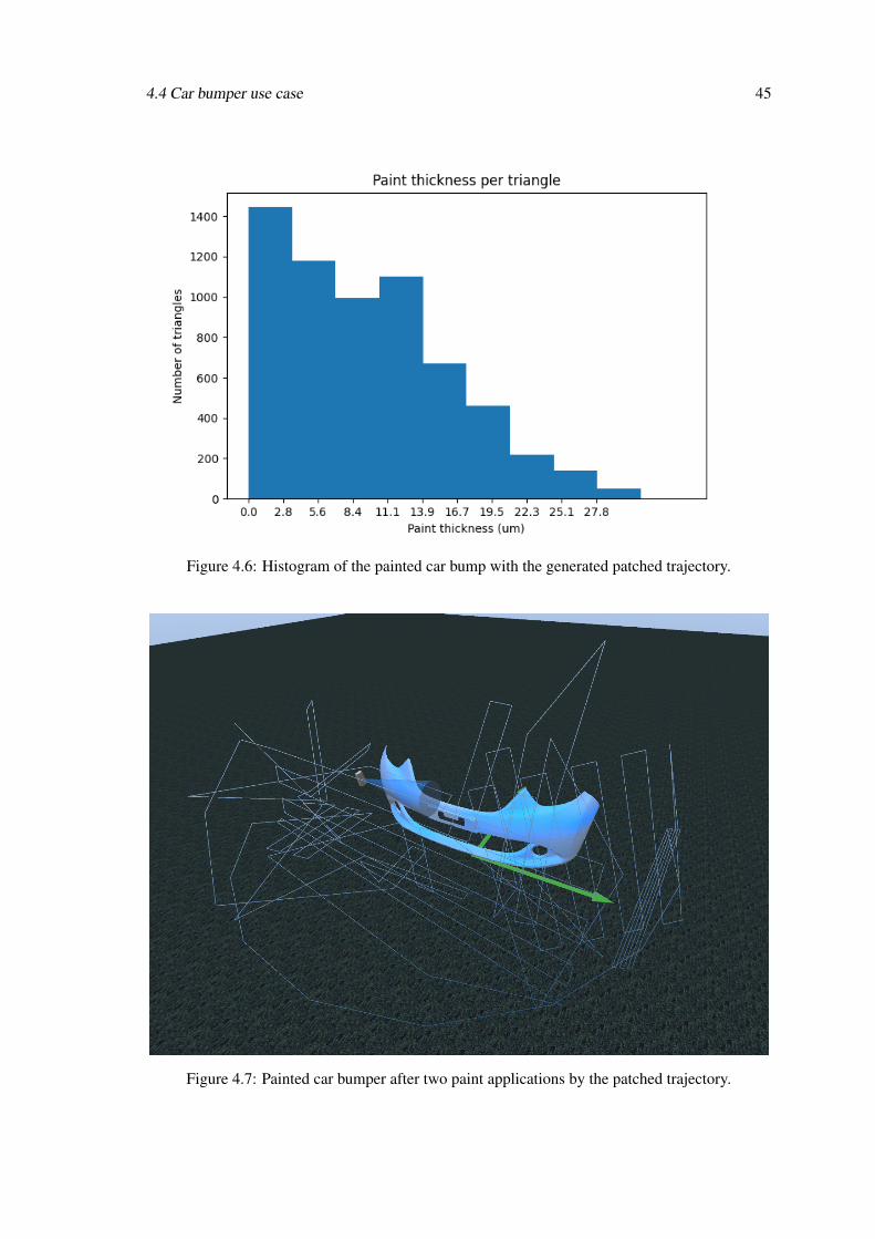
4.4 Car bumper use case 45
Figure 4.6: Histogram of the painted car bump with the generated patched trajectory.
Figure 4.7: Painted car bumper after two paint applications by the patched trajectory.

46 Trajectory optimization use cases
4.4.1.2 Maximum distance difference of 150 mm
With the maximum distance difference of 150 mm, there are less generated patches thus resulting
in longer individual trajectories that aren’t capable of painting curves with the previous level of
detail, as can be seen in Figure 4.8.
Figure 4.8: Patched trajectory generated on the car bump model with the respective paint appliedand the result in heatmap mode.
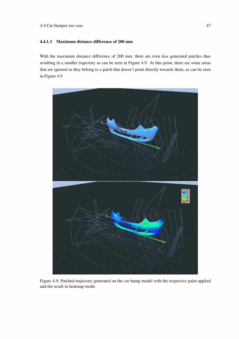
4.4 Car bumper use case 47
4.4.1.3 Maximum distance difference of 200 mm
With the maximum distance difference of 200 mm, there are even less generated patches thus
resulting in a smaller trajectory as can be seen in Figure 4.9. At this point, there are some areas
that are ignored as they belong to a patch that doesn’t point directly towards them, as can be seen
in Figure 4.9
Figure 4.9: Patched trajectory generated on the car bump model with the respective paint appliedand the result in heatmap mode.

48 Trajectory optimization use cases
4.4.2 Results’ comparison and conclusions
In the Table 4.1 the metrics implemented in the simulation are presented for the three chosen
maximum distance differences. The generated paths reached the 100% spray coverage only with
the maximum distance difference of 100 mm this means that the ability to create smaller patches
forces the trajectory to cover every bit of the piece. However, the standard deviation is much
inferior in the case with less patches, with a spray coverage still near 100% (≈99%) and with
less than half the number of waypoints needed to cover the full model. The significantly large
maximum spray thickness and the large standard deviation values that are present in the 100 mm
and 150 mm trajectories, come from the fact that, to paint a small patch, the nearby areas are
also affected, thus leading to locations with a disproportional amount of paint. As the patches are
created by random placed seeds, the generated path is also random and this effect can be more
severe arbitrarily, as can be seen in the 150 mm trajectory.
Table 4.1: Car bump trajectory metrics
Maximum distance difference (mm) 100 150 200Average spray thickness (µm) 7.602 13.951 4.079Standard deviation spray thickness(µm) 5.727 11.700 2.866Minimum spray thickness (µm) 0.006 0 0Maximum spray thickness (µm) 139.211 133.596 12.561Spray coverage (%) 100 99.968 98.977Number of waypoints 260 227 120Duration (min:s) 5:42 6:24 3:18Average spray thickness/duration (nm/s) 22.22 36.33 20.60
In conclusion, with the utilities developed in the simulator it is possible to make an informed
choice about what parameters to use in the algorithm, and what trajectories are the best. In this
case, the trajectory generated by the 200 mm of maximum distance difference provides a simpler
and more uniform trajectory, that can also be visually validated.
4.5 Compressor cover use case
In order to further test the developed algorithms, and to explore different parameters, a second use
case was used. The preprocess procedure was similar to the previous section, with the resulting
model having 5067 faces and 3496 triangles with an average edge length of 18.4 mm.
4.5.1 Trajectory’s parameters optimization
The same fixed parameters used in section 4.4 were set, with the exception of the maximum
distance difference that was now fixed at 300 mm and the normal’s angle varied sequentially. The
normal’s angle is useful in this piece, since it provides a way to deal with the border between the
side and the top, while also helping define the patch’s size on the curved side surface.

4.5 Compressor cover use case 49
4.5.1.1 Maximum normal’s angle difference of 20º
With the maximum normal’s angle difference of 20º, there are specific locations with a lot of
detail, resulting in an excess of paint in those areas, as can be seen in Figure 4.10.
Figure 4.10: Patched trajectory generated on the compressor’s cover model with the respectivepaint applied and the result in heatmap mode (α < 20º).
4.5.1.2 Maximum normal’s angle difference of 30º
With the maximum normal’s angle difference of 30º, there are fewer patches, but in this specific
trajectory, they were mainly concentrated on the top part of the piece, which led to a lack of paint
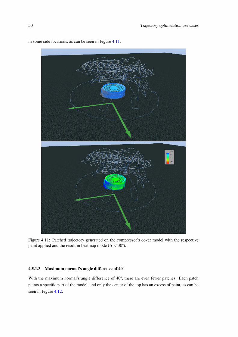
50 Trajectory optimization use cases
in some side locations, as can be seen in Figure 4.11.
Figure 4.11: Patched trajectory generated on the compressor’s cover model with the respectivepaint applied and the result in heatmap mode (α < 30º).
4.5.1.3 Maximum normal’s angle difference of 40º
With the maximum normal’s angle difference of 40º, there are even fewer patches. Each patch
paints a specific part of the model, and only the center of the top has an excess of paint, as can be
seen in Figure 4.12.

4.5 Compressor cover use case 51
Figure 4.12: Patched trajectory generated on the compressor’s cover model with the respectivepaint applied and the result in heatmap mode (α < 40º).

52 Trajectory optimization use cases
4.5.2 Results’ comparison and conclusions
In the Table 4.2 the metrics implemented in the simulation are presented for the three chosen
maximum angle’s normal differences. The generated path reached the 100% with the two smaller
values for the maximum normal’s angle difference. Although the varying parameter is different
than section 4.4, the end result is similar: the ability to create smaller patches forces the trajectory
to cover every bit of the piece. Also, the standard deviation is inferior in the cases with fewer
patches. The trajectory with the least number of waypoints, covered the full model faster and with
relatively low standard deviation, as can also be seen in the histogram presented in Figure 4.13.
This way, the better trajectory to paint the compressor cover is the one generated by the patched
trajectory algorithm with the maximum normal’s angle difference of 40º.
Table 4.2: Compressor cover trajectory metrics
Maximum distance difference (mm) 300 300 300Maximum angle difference (º) 20 30 40Average spray thickness (µm) 24.737 17.589 28.707Standard deviation spray thickness(µm) 20.428 15.203 15.896Minimum spray thickness (µm) 0.036 0.063 0.013Maximum spray thickness (µm) 120.635 101.305 113.156Spray coverage (%) 100 100 99.941Number of waypoints 371 308 234Duration (m:s) 7:04 5:58 4:47Average spray thickness/duration (nm/s) 58.31 49.13 99.93
Figure 4.13: Histogram of the painted compressor cover with the generated patched trajectory(α < 40º).

Chapter 5
Conclusion
This work describes the development of a spray painting system, including a simulation tool and
trajectory generation algorithms for industrial spray painting applications. The advantages of this
simulation tool include fast and easy testing of algorithms in the developing stage, optimization
without paint, energy and pieces being wasted, availability of qualitative and quantitative metrics
without real world hassles. The accuracy and validity of the simulation system was tested with
several real world experiments and an image processing pipeline that facilitates the tuning of the
spray parameters was developed.
The trajectory generation algorithms presented, provide a baseline capable of painting 3D
pieces with varying paint quality levels. For the selected use cases, the trajectory generation
algorithm achieved 99% paint coverage, with a standard deviation of 2.9 µm in paint thickness,
and 99.9% paint coverage with a standard deviation of 17 µm in paint thickness, for the car bumper
and compressor cover models respectively, which proved to be acceptable amounts of uniformity
by visually inspecting the end result.
5.1 Contributions
This new simulation system, provides an open source implementation that is capable of real time
spray simulation with validated experimental results, a calibration tool, qualitative and quantitative
metrics and baseline trajectory generation methods. This work resulted in the accepted paper, "A
simulation tool for optimizing a 3D Spray Painting System", for the conference OL2A, Interna-
tional Conference on Optimization, Learning Algorithms and Applications, 2021 July, regarding
the simulation system and the calibration tool.
5.2 Future work
Future work includes better occlusion algorithms in order to allow the simulation to work with
more complex parts that have cavities of varying sizes. More trajectory generation algorithms are
53

54 Conclusion
also necessary for those pieces with intricate shapes. Another essential feature is the ability to post
process the generated trajectories and test and use them in the real world.

References
[1] Qiaoyan Ye and Karlheinz Pulli. Numerical and experimental investigation on the spraycoating process using a pneumatic atomizer: Influences of operating conditions and targetgeometries. Coatings, 2017. doi:10.3390/coatings7010013.
[2] Yan Chen, Wenzhuo Chen, Bo Li, Gang Zhang, and Weiming Zhang. Paint thick-ness simulation for painting robot trajectory planning: A review, 2017. doi:10.1108/IR-07-2016-0205.
[3] KUKA ready2spray. URL: https://www.kuka.com/en-gb/products/robotics-systems/ready2_solutions/kuka-ready2_spray.
[4] Kawasaki KJ314 Wall Robot-7 Axes. URL: https://robotics.kawasaki.com/en1/products/robots/painting/KJ314/.
[5] Balkeshwar Singh and N Sellappan. Evolution of Industrial Robots and their Applica-tions. International Journal of Emerging Technology and Advanced Engineering Website:www.ijetae.com ISO Certified Journal, 9001(5):1–6, 2013.
[6] Statista Research Department. Industrial robots - statistics & facts | Statista, 2020. URL:https://www.statista.com/topics/1476/industrial-robots/.
[7] J. Norberto Pires, T. Godinho, and P. Ferreira. CAD interface for automatic robot weldingprogramming, 2004. doi:10.1108/01439910410512028.
[8] Anton Jezernik and Gorazd Hren. A solution to integrate computer-aided design (CAD)and virtual reality (VR) databases in design and manufacturing processes, jul 2003. URL:https://link.springer.com/article/10.1007/s00170-003-1604-3, doi:10.1007/s00170-003-1604-3.
[9] Heping Chen, Thomas Fuhlbrigge, and Xiongzi Li. A review of CAD-based robot pathplanning for spray painting. Industrial Robot, 36(1):45–50, 2009. doi:10.1108/01439910910924666.
[10] Kong Meng, Zhang Jie, Gu Fang, and Chen Huabin. Robotic GMAW adaptive weldingbased on linear structured light scanning method. Electric Welding Machine, v 47, n11, 2017. URL: https://www.engineeringvillage.com/share/document.url?mid=inspec_19aa98c1675fe4ee49M480d1017816339&database=ins&view=detailed, doi:10.7512/j.issn.1001-2303.2017.11.08.
[11] Binbin Zhang, Jun Wu, Liping Wang, Zhenyang Yu, and Peng Fu. A Method to Real-ize Accurate Dynamic Feedforward Control of a Spray-Painting Robot for Airplane Wings.IEEE/ASME Transactions on Mechatronics, 23(3):1182–1192, jun 2018. doi:10.1109/TMECH.2018.2817884.
55
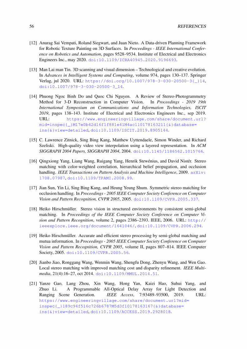
56 REFERENCES
[12] Anurag Sai Vempati, Roland Siegwart, and Juan Nieto. A Data-driven Planning Frameworkfor Robotic Texture Painting on 3D Surfaces. In Proceedings - IEEE International Confer-ence on Robotics and Automation, pages 9528–9534. Institute of Electrical and ElectronicsEngineers Inc., may 2020. doi:10.1109/ICRA40945.2020.9196693.
[13] Man Lai man Tin. 3D scanning and visual dimension – Technological and creative evolution.In Advances in Intelligent Systems and Computing, volume 974, pages 130–137. SpringerVerlag, jul 2020. URL: https://doi.org/10.1007/978-3-030-20500-3_14,doi:10.1007/978-3-030-20500-3_14.
[14] Phuong Ngoc Binh Do and Quoc Chi Nguyen. A Review of Stereo-PhotogrammetryMethod for 3-D Reconstruction in Computer Vision. In Proceedings - 2019 19thInternational Symposium on Communications and Information Technologies, ISCIT2019, pages 138–143. Institute of Electrical and Electronics Engineers Inc., sep 2019.URL: https://www.engineeringvillage.com/share/document.url?mid=inspec_M17e0b42d16f1f881e41M4ac110178163211&database=ins&view=detailed, doi:10.1109/ISCIT.2019.8905144.
[15] C. Lawrence Zitnick, Sing Bing Kang, Matthew Uyttendaele, Simon Winder, and RichardSzeliski. High-quality video view interpolation using a layered representation. In ACMSIGGRAPH 2004 Papers, SIGGRAPH 2004, 2004. doi:10.1145/1186562.1015766.
[16] Qingxiong Yang, Liang Wang, Ruigang Yang, Henrik Stewénius, and David Nistér. Stereomatching with color-weighted correlation, hierarchical belief propagation, and occlusionhandling. IEEE Transactions on Pattern Analysis and Machine Intelligence, 2009. arXiv:1708.07987, doi:10.1109/TPAMI.2008.99.
[17] Jian Sun, Yin Li, Sing Bing Kang, and Heung Yeung Shum. Symmetric stereo matching forocclusion handling. In Proceedings - 2005 IEEE Computer Society Conference on ComputerVision and Pattern Recognition, CVPR 2005, 2005. doi:10.1109/CVPR.2005.337.
[18] Heiko Hirschmüller. Stereo vision in structured environments by consistent semi-globalmatching. In Proceedings of the IEEE Computer Society Conference on Computer Vi-sion and Pattern Recognition, volume 2, pages 2386–2393. IEEE, 2006. URL: http://ieeexplore.ieee.org/document/1641046/, doi:10.1109/CVPR.2006.294.
[19] Heiko Hirschmüller. Accurate and efficient stereo processing by semi-global matching andmutua information. In Proceedings - 2005 IEEE Computer Society Conference on ComputerVision and Pattern Recognition, CVPR 2005, volume II, pages 807–814. IEEE ComputerSociety, 2005. doi:10.1109/CVPR.2005.56.
[20] Jianbo Jiao, Ronggang Wang, Wenmin Wang, Shengfu Dong, Zhenyu Wang, and Wen Gao.Local stereo matching with improved matching cost and disparity refinement. IEEE Multi-media, 21(4):16–27, oct 2014. doi:10.1109/MMUL.2014.51.
[21] Yanze Gao, Lang Zhou, Xin Wang, Hong Yan, Kaizi Hao, Suhui Yang, andZhuo Li. A Programmable All-Optical Delay Array for Light Detection andRanging Scene Generation. IEEE Access, 7:93489–93500, 2019. URL:https://www.engineeringvillage.com/share/document.url?mid=inspec_189c94f516c726b6787M5d3f10178163167&database=ins&view=detailed, doi:10.1109/ACCESS.2019.2928018.
REFERENCES 57
[22] John G. Webster, Tyler Bell, Beiwen Li, and Song Zhang. Structured Light Techniques andApplications. In Wiley Encyclopedia of Electrical and Electronics Engineering, pages 1–24.John Wiley & Sons, Inc., feb 2016. doi:10.1002/047134608x.w8298.
[23] N. R. Whitehouse. Paint application. In Shreir’s Corrosion, pages 2637–2642. Elsevier, jan2010. doi:10.1016/B978-044452787-5.00142-6.
[24] Dick Fleming. AIRLESS SPRAY-PRACTICAL TECHNIQUE FOR MAINTENANCEPAINTING. Plant Engineering (Barrington, Illinois), 31(20):83–86, 1977.
[25] Joel Rupp, Eric Guffey, and Gary Jacobsen. Electrostatic spray processes. Metal Finishing,108(11-12):150–163, dec 2010. doi:10.1016/S0026-0576(10)80225-9.
[26] M. Fogliati, D. Fontana, M. Garbero, M. Vanni, G. Baldi, and R. Dondè. CFD sim-ulation of paint deposition in an air spray process. Journal of Coatings Technologyand Research, 3(2):117–125, 2006. URL: www.coatingstech.org, doi:10.1007/s11998-006-0014-5.
[27] P. G. Hicks and D. W. Senser. Simulation of paint transfer in an air spray process. Journal ofFluids Engineering, Transactions of the ASME, 117(4):713–719, dec 1995. doi:10.1115/1.2817327.
[28] Q Ye, J Domnick, and E Khalifa. Simulation Of The Spray Coating Process Using A Pneu-matic Atomizer. Institute for Liquid Atomization and Spray Systems, 2002.
[29] Q. Ye. Using dynamic mesh models to simulate electrostatic spray-painting. In High Perfor-mance Computing in Science and Engineering 2005 - Transactions of the High PerformanceComputing Center Stuttgart, HLRS 2005, 2006. doi:10.1007/3-540-29064-8-13.
[30] John K. Antonio. Optimal trajectory planning for spray coating. In Proceedings - IEEE In-ternational Conference on Robotics and Automation, 1994. doi:10.1109/robot.1994.351125.
[31] W. Persoons and H. Van Brussel. CAD-based robotic coating of highly curved surfaces.In 24th International Symposium on Industrial Robots, Tokyo, pages 611–618, nov 1993.doi:10.1109/robot.1994.351125.
[32] Bo Zhou, Xi Zhang, Zhengda Meng, and Xianzhong Dai. Off-line programming system ofindustrial robot for spraying manufacturing optimization. In Proceedings of the 33rd ChineseControl Conference, CCC 2014, 2014. doi:10.1109/ChiCC.2014.6896426.
[33] David C. Conner, Aaron Greenfield, Prasad N. Atkar, Alfred A. Rizzi, and Howie Choset.Paint deposition modeling for trajectory planning on automotive surfaces. IEEE Transactionson Automation Science and Engineering, 2005. doi:10.1109/TASE.2005.851631.
[34] Mayur V. Andulkar and Shital S. Chiddarwar. Incremental approach for trajectory generationof spray painting robot. Industrial Robot, 2015. doi:10.1108/IR-10-2014-0405.
[35] Yonggui Zhang, Yumei Huang, Feng Gao, and Wei Wang. New model for air spray gun ofrobotic spray-painting. Jixie Gongcheng Xuebao/Chinese Journal of Mechanical Engineer-ing, 2006. doi:10.3901/JME.2006.11.226.
[36] Examples - RoboDK. URL: https://robodk.com/examples#examples-painting.

58 REFERENCES
[37] Getting Started - RoboDK Documentation. URL: https://robodk.com/doc/en/Getting-Started.html#Station.
[38] Robcad Robotics and automation workcell simulation, validation and off-line programming.URL: www.siemens.com/tecnomatix.
[39] Automatic Scanning and Programming of Robots. URL: https://www.inropa.com/fileadmin/Arkiv/Dokumenter/Produktblade/OLP_automatic.pdf.
[40] Delfoi PAINT - Software for painting and coating. URL: https://www.delfoi.com/delfoi-robotics/delfoi-paint/.
[41] Robust ROBOGUIDE Simulation Software | FANUC America.URL: https://www.fanucamerica.com/products/robots/robot-simulation-software-FANUC-ROBOGUIDE.
[42] Ju-hsien Kao and Fritz B Prinz. Optimal Motion Planning for Deposition in Layered Manu-facturing. 1998 ASME Design Engineering Technical Conferences, 1998.
[43] Heping Chen, Ning Xi, Weihua Sheng, Yifan Chen, Allen Roche, and Jeffrey Danl. Ageneral framework for automatic CAD-guided tool planning for surface manufacturing. InProceedings - IEEE International Conference on Robotics and Automation, 2003. doi:10.1109/robot.2003.1242132.
[44] Heping Chen, Ning Xi, Weihua Sheng, Jeffrey Dahl, and Zhaojie Li. Optimal tooltrajectory integration in surface manufacturing. In IFAC Proceedings Volumes (IFAC-PapersOnline), volume 16, pages 211–216. IFAC Secretariat, 2005. doi:10.3182/20050703-6-cz-1902.01305.
[45] Naoki Asakawa and Yoshimi Takeuchi. Teachingless spray-painting of sculptured surfaceby an industrial robot. In Proceedings - IEEE International Conference on Robotics andAutomation, 1997. doi:10.1109/robot.1997.619061.
[46] Prasad N. Atkar, Aaron Greenfield, David C. Conner, Howie Choset, and Alfred A. Rizzi.Uniform coverage of automotive surface patches. In International Journal of Robotics Re-search, 2005. doi:10.1177/0278364905059058.
[47] Alessandro Gasparetto, Renato Vidoni, Daniele Pillan, and Ennio Saccavini. Automatic pathand trajectory planning for robotic spray painting. 7th German Conference on Robotics,ROBOTIK 2012, pages 211–216, 2012.
[48] Jonas C. Kiemel, Peiren Yang, Pascal Meißner, and Torsten Kröger. PaintRL: Coverage PathPlanning for Industrial Spray Painting with Reinforcement Learning. Workshop on Closingthe Reality Gap in Sim2real Transfer for Robotic Manipulation, Freiburg, June 23, 2019,2019. URL: https://publikationen.bibliothek.kit.edu/1000096523.
[49] J. Schulman, F. Wolski, P. Dhariwal, A. Radford, and O. Klimov. Prox-imal policy optimization algorithms [arXiv]. arXiv, 2018. URL:https://www.engineeringvillage.com/share/document.url?mid=inspec_b53fca615eee43acc3M541c10178163176&database=ins&view=detailed.
REFERENCES 59
[50] Majed El Helou, Stephan Mandt, Andreas Krause, and Paul Beardsley. Mobile robotic paint-ing of texture. In Proceedings - IEEE International Conference on Robotics and Automation,2019. doi:10.1109/ICRA.2019.8793947.
[51] Jeff Heaton. Ian Goodfellow, Yoshua Bengio, and Aaron Courville: Deep learning. GeneticProgramming and Evolvable Machines, 19(1-2):305–307, jun 2018. URL: https://doi.org/10.1007/s10710-017-9314-z, doi:10.1007/s10710-017-9314-z.
[52] Diederik P. Kingma and Max Welling. Auto-encoding variational bayes. In 2nd InternationalConference on Learning Representations, ICLR 2014 - Conference Track Proceedings, 2014.arXiv:1312.6114.
[53] Jonathan Long, Evan Shelhamer, and Trevor Darrell. Fully convolutional networks for se-mantic segmentation. In Proceedings of the IEEE Computer Society Conference on Com-puter Vision and Pattern Recognition, 2015. doi:10.1109/CVPR.2015.7298965.
[54] Raymond C.W. Sung, Jonathan R. Corney, David P. Towers, Ian Black, Duncan P. Hand,Finlay McPherson, Doug E.R. Clark, and Markus S. Gross. Direct writing of digital im-ages onto 3D surfaces. Industrial Robot, 33(1 SPEC. ISS.):27–36, 2006. doi:10.1108/01439910610700702.
[55] Anurag Sai Vempati, Mina Kamel, Nikola Stilinovic, Qixuan Zhang, Dorothea Reusser,Inkyu Sa, Juan Nieto, Roland Siegwart, and Paul Beardsley. PaintCopter: An autonomousUAV for spray painting on three-dimensional surfaces. IEEE Robotics and Automation Let-ters, 3(4):2862–2869, oct 2018. doi:10.1109/LRA.2018.2846278.
[56] Ehsan Asadi, Bingbing Li, and I. Ming Chen. Pictobot: A Cooperative Painting Robot forInterior Finishing of Industrial Developments. IEEE Robotics and Automation Magazine,25(2):82–94, jun 2018. doi:10.1109/MRA.2018.2816972.
[57] William Baxter, Jeremy Wendt, and Ming C. Lin. IMPaSTo: A realistic, interactive modelfor paint. In NPAR Symposium on Non-Photorealistic Animation and Rendering, 2004.
[58] Chet S. Haase and Gary W. Meyer. Modeling pigmented materials for realistic image syn-thesis. ACM Transactions on Graphics (TOG), 1992. doi:10.1145/146443.146452.
[59] FANUC Paint Robot 250iB. URL: https://www.fanuc.eu/se/en/robots/robot-filter-page/paint-series/p-250ib-15.
[60] ABB IRB 5500 FlexPainter. URL: https://library.e.abb.com/public/396b885928754b56867a589c03bd43ab/IRB5500-Flex-RP50010EN-Rev.G.pdf?x-sign=5ezePLvm1fu3W7gOIU46isAIMaOQmRoUNF+Kj98BltOkOAyEpDgy0mf8bomRGXvj.
[61] MOTOMAN MPX3500. URL: https://www.motoman.com/en-us/products/robots/industrial/painting-dispensing/mpx-series/mpx3500.
[62] GLScene. URL: http://glscene.sourceforge.net/wikka/.
[63] OpenGL. URL: https://www.opengl.org/.
[64] José L Lima, José A Gonçalves, Paulo G Costa, and A Paulo Moreira. Humanoid Gait Op-timization Resorting to an Improved Simulation Model Regular Paper. International Jour-nal of Advanced Robotic Systems, 2013. URL: www.intechopen.com, doi:10.5772/54766.

60 REFERENCES
[65] Joáo Sousa e Silva, Pedro Costa, and José Lima. Manipulator path planning forpick-and-place operations with obstacles avoidance: An A* algorithm approach. InCommunications in Computer and Information Science, volume 371, pages 213–224.Springer Verlag, 2013. URL: https://link.springer.com/chapter/10.1007/978-3-642-39223-8_20, doi:10.1007/978-3-642-39223-8_20.
[66] Paolo Cignoni, Marco Callieri, Massimiliano Corsini, Matteo Dellepiane, Fabio Ganovelli,and Guido Ranzuglia. MeshLab: an Open-Source Mesh Processing Tool. In Vittorio Scarano,Rosario De Chiara, and Ugo Erra, editors, Eurographics Italian Chapter Conference. TheEurographics Association, 2008. doi:10.2312/LocalChapterEvents/ItalChap/ItalianChapConf2008/129-136.
[67] opencv. Open source computer vision library. https://github.com/opencv/opencv,2015.