Simulation and Formal Analysis of Visual Attention Tibor Bossea, Peter-Paul van Maanena,b and Jan Treura aVrije Universiteit Amsterdam, Dept. of AI, De Boelelaan 1081a, 1081 HV Amsterdam, The Netherlands bTNO Human Factors, P.O. Box 23, 3769 ZG Soesterberg, The Netherlands

Abstract. In this paper a simulation model for visual attention is discussed and formally analysed. The model is part of the design of an agent-based system that supports a naval officer in its task to compile a tactical picture of the situation in the field. A case study is described in which the model is used to simulate a human subject’s attention. The formal analysis is based on temporal relational specifications for attentional states and for different stages of attentional processes. The model has been automatically verified against these specifications.

Keywords: Visual attention, ambient intelligence, cognitive modeling, simulation, philosophical foundations

1. Introduction

This paper presents a formal model of visual atten-tion, which is part of an agent-based system that sup-ports a user in his task [6, 7, 8]. Being able to for-mally describe human attention opens the opportu-nity to run real-time simulations and apply formal analyses. These can be beneficial for a number of reasons. First of all, on a theoretical level, the attempt can be used to enhance the understanding of human attentional processes. On a more practical level, simulation and formal analysis of attention can be beneficial as well. For example, in the domain of naval warfare, a crucial but complex task is tactical picture compilation. In this task, the naval officer has to compile a tactical picture of the situation in the field, based upon the information he observes on a computer screen. Similar situations occur in other domains, for example, in the area of air traffic control. Since the environment in these situations is often complex and dynamic, the naval officer has to deal with a large number of tasks in parallel. Given the demanding nature of such tasks, in practice, the hu-man is often supported by automated systems (agents) that take over part of these tasks or assist the execution of them. However, a problem is how to determine an appropriate work division between hu-man and agent: due to the rapidly changing environ-ment, such a work division cannot be fixed before-

hand by the designers of the support systems [2]. This results in the need for agent systems that are able to dynamically and at run-time reallocate tasks between human and agent. For this purpose, two ap-proaches exist, namely human-triggered and system-triggered dynamic task allocation [10]. In the former case, the user can decide up to what level the agent should assist him. However, especially in alarming situations, the user does not have enough time to think about task reallocations [20]. In these situations it would be better if the system determines this. Hence a system-triggered dynamic task allocation is desirable. This is where simulation and formal analy-sis comes into play: it could enable agent systems to properly reallocate tasks by adapting to the human’s attentional state and processes.

In order to obtain such a system-triggered dynamic task allocation, the model of visual attention intro-duced and formally analysed in this paper is incorpo-rated within a supporting agent. The idea is to use an estimation of the user’s current allocation of attention to determine which subtasks the agent is best to pay attention to. In this case, it is the agent that adapts its support to the human’s attentional state and processes. For instance, if one of a user´s tasks is to identify a certain track on a computer screen, it is likely that the user desires support concerning this track, whereas the user probably does not desire support concerning those tracks that do not have to be identified. On the

other hand, if a certain track that is not in the focus of the user’s attention clearly requires attention, it is desirable that the supporting agent either takes over the task dealing with this track or notifies the user that he should pay attention to it, or a colleague of the user who can also perform the task. In this paper we assume that, if the user´s attention is allocated to certain objects, he is also committing himself to deal-ing with those in a correct manner. Given this as-sumption, the agent can adjust its support at runtime solely based on the dynamics of the modelled atten-tion, i.e. it does not have to worry about any other problems once the tasks have been properly divided. This is a reasonable assumption, since attention is a prerequisite for conscious action [1] and the applica-tion is aimed at highly trained users, unlikely to make mistakes once their situation awareness is in order.

As mentioned above, this paper introduces a model of visual attention that can be incorporated within a supporting agent [6, 7, 8]. In addition, the model is formally analysed, by using the output of a simula-tion based on an implementation of the model and data from a case study. In this case study, a user exe-cuted a task abstracted from an Air Traffic Control (ATC) task. This ATC task was tailored to a naval radar track identification task, because this suited more the domain of this study. The gathered data from the case study, which is only used for demon-stration purposes, consist of two types of informa-tion: dynamics of tracks on a radar scope; dynamics of the user’s gaze. Based on this information, to-gether with the knowledge of the rules of the task, the cognitive model estimates the distribution of atten-tion over the different locations on the radar scope. Furthermore, based on the characteristics of this at-tention distribution over time, temporal properties are defined that indicate certain attentional subprocesses. These subprocesses are related to the different phases of information processing [27, 32, 33]. The further discrimination of attention is juxtaposed to the as-sumption often made in literature that attention is a single and homogeneous concept (e.g. in [21, 36]).

This paper is structured in the following manner. In Section 2 a brief introduction of the existing litera-ture on visual attention is introduced. The sole pur-pose of this part is to help understand the choices made further on. Next, Section 3 shows a mathemati-cal description of the cognitive model of attention. This description is quite straightforward and the main contribution of the present paper is in the application and the formal analysis of such models in adaptive agent-based systems that assist human users. One of such applications is illustrated in Section 4, which

consists of a description of a case study and the cor-responding simulation results after applying the model to the case study, using human data. Section 5 shows how the model can be further analysed by ve-rifying formal temporal relational specifications for attentional states and subprocesses. Section 6 is a discussion. At the end of this paper an appendix is included that consists of the source code of the im-plemented cognitive model.

2. Visual Attention

Visual attention has been a subject of study in many disciplines and this section is not intended to deliberate on all of these disciplines. It rather dis-cusses a small but dominant part of the literature on attention, in order to bridge between relevant theory on the one hand and the application mentioned in the introduction on the other hand. This bridge helps to explain why certain choices are made later on in the paper.

In Psychology, a dominant view on attention dis-tinguishes two types of attention: exogenous atten-tion and endogenous attention [36]. The former stands for attention by means of triggers by (par-tially) unexpected inputs from the environment, i.e. bottom-up triggers, such as a fierce blow on a horn. The latter stands for attention by means of a slower trigger from within the subject, i.e. top-down triggers, such as searching a friend in a crowd. There are rea-sons to say that exogenous and endogenous attention are closely intertwined. A recent study [33], for in-stance, shows that capture of exogenous attention occurs only if the object that attracts attention has a property that a person is using to find a target.

Another relevant aspect of visual attention for modelling is the effect of so-called inattentional blindness [30]. This is the property that perception does not always result in attending to the important and unexpected events. Attention may also be a based on certain non-visual cognitive activities, such as having deep thoughts on past or future events. Because of the limited amount of attentional re-sources, this can result in a large blind spot for visual stimuli. Attention is therefore often distinguished in at least two types of attention, i.e. perceptual and decisional attention [33]. Some even propose a larger number of functionally different subprocesses of at-tention [27, 32]. This gives rise to the idea that atten-tion is more than of a single homogeneous type, which should be taken into account.

A third important discussion in the psychological literature relevant for computational models of atten-tion addresses the distinction of two definitions of visual attention: the definition of visual attention as a division over space and the definition as a division over objects. The first definition is more traditional and involves continuous locations over 2D or 3D space. There are several space-based theories of at-tention, such as the filter theory [9], spotlight theory [34], and the zoom-lens theory [17]. There are many more, but to mention and discuss them is beyond the scope of the paper. What they all have in common is that attention is subject to whatever is within a cer-tain location in space. The object-based view of at-tention is more ‘recent’ and stresses that attention is allocated to (groups of) perceptual objects, rather than a continuous space [16]. These objects can have various properties, such as shape, speed, colour, etc. Location, in that sense, is treated as just a special property of objects. Computationally this seems in-triguing, but there are downsides of this view, which is treated below.

A fourth important and relevant discussion in psy-chology is sometimes called to be related to the what-where-distinction [29], and combines in some way the space- and object-based views of attention. So-called what-attention prepares a person that some-thing will happen concerning a certain already visible object. Where-attention, on the other hand, prepares the sensory memory for further deliberation. This kind of preparation also happens when a person ex-pects something to happen in a specific region in the search space or from a sensory input, but does not know what exactly will happen. One of the down-sides of the above mentioned object-view is that it is difficult to translate such a kind of where-attention according to that view.

Apart from a more experimental interest, mainly in Psychology, there has also been a growing interest in the development and application of mathematical models of visual attention, mainly in Computer Sci-ence and AI [21]. Such models are for instance used for enhancing encryption techniques in JPEG and MPEG standards [13]. Another example of an appli-cation is usage of such models for making believable virtual humans in artificial environments [26]. Basi-cally one can distinguish two types of questions ad-dressed within the literature on visual attention mod-elling:

− Given certain circumstances and behaviour, to

which attention distribution does this lead?

− Given certain circumstances and an attention distribution, to which behaviour does this lead?

Models addressing the first question are for instance interesting for predicting to what features of an im-age a person is paying attention. Models addressing the second question are for instance interesting for generating realistic behaviour for virtual characters. Answers to both questions help in the construction of cognitive models of visual attention. To construct cognitive models of attention, several types of information can be used as an input. In gen-eral, the following three types of information are dis-tinguished:

− Behavioural cues from the user. Information or cues about the behaviour of the user are depend-ant of the current attentional state. The behav-iour is a result of it and this means that, for ex-ample, gaze duration, gaze frequency, gaze path, head pose, and task performance, are useable as input of the model.

− Properties of objects in the environment. This type of information can lead to clues about when certain stimuli from the environment cause a us-er to attend to an object. Examples of such cues are features of objects, such as shape, texture, colour, size, movement, direction, and centered-ness. Note that this type of information ad-dresses exogenous attention.

− Properties of the human attention mechanism. An example of this kind of information is know-ledge about when a user pays attention to a speaker. For instance only when he expects or wants the speaker to speak, or when he has a certain commitment, interest, or goal, related to the speaker. An estimate of the user´s commit-ments, interests, or goals, can lead to an estimate of an attention distribution and therefore be used as an input of the model. Note that this type of information addresses endogenous attention.

The next section will demonstrate how the above

types of information can be integrated into one ex-ecutable model.

3. A Mathematical Model for Visual Attention

In this section the mathematical model for visual attention is presented. The proposed model is com-posed of formal rules that are related to the psycho-

logical concepts discussed in the previous section. In Section 3.1 a formal definition of attention is given, taking into account the distinction between the two possible informal definitions stated earlier. In Section 3.2 it is described how behavioural cues of the user are derived from gaze characteristics and are used to estimate attention. In Section 3.3 saliency maps are discussed shortly, that translate properties of objects in the environment to a probable attention demand. Saliency maps are not only related to exogenous but also to endogenous attention, since saliency is task related as well. Inattentional blindness is modelled by means of fixing a certain limited amount of total at-tention, which is managed by normalisation, persis-tency, decay, and concentration processes, described in Sections 3.4, 3.5, and 3.6, respectively.

3.1 Attention values, objects and spaces

As described in Section 2, there is a distinction be-tween the definition of attention as a division over space and that as a division over objects. In this paper the first approach is used and it is assumed that one can have attention for multiple spaces at the same time. One of the reasons for using spaces instead of objects is that it is actually possible to pay attention to certain spaces that do not contain any objects (yet).

The model presented in this paper will define dif-ferent (discrete) spaces, which each have a specific ‘quantity’ of attention. One argument for this choice is that certain spaces can contain more relevant in-formation than others. This quantity of attention will be called the attention value. Division of attention is now defined as an instantiation of attention values AV for all attention spaces s. An attentional state is a division of attention at a certain moment in time. Mathematically, given the above, the following is expected to hold:

where A(t) is the total amount of attention at a certain time t and AV(s,t) is the attention value for attention space s at time t. In this study we define attention spaces to be 1 × 1 squares within an M × N grid. In principle it holds that the more attention spaces, the less attention value for each of those spaces. This is reasonable because there is a certain upper limit of total amount of working memory humans have. In the following sections the concept of attention value is further formalised.

3.2 Gaze

As discussed earlier, human behaviour can be used to draw conclusions on a person’s current attentional state. An important aspect of the visual attentional state is human gaze behaviour. The gaze dynamics (saccades) are not random, but say something about what spaces have been attended to [11, 28]. Since people often pay more attention to the centre than to the periphery of their visual space, the relative dis-tance of each space s to the gaze point (the centre) is an important factor in determining the attention value of s. Mathematically this is modelled as follows:

where AVpot(s,t) is the potential attention value of s at time point t. For now, the reader is advised to as-sume that AVnew(s,t) = AV(s,t). The term r(s,t) is taken as the Euclidian distance between the current gaze point and s at time point t (multiplied by an im-portance factor α which determines the relative im-pact of the distance to the gaze point on the atten-tional state):

Other ways for calculating attention degradation as a function of distance is for instance using a Gaussian approximation.

3.3 Saliency maps

Still unspecified is how the potential attention val-ue AVpot(s,t) is to be calculated. The main idea here is to use the properties of the space (i.e., of the types of objects present) at that time. These properties can be for instance features such as colour, intensity, and orientation contrast, amount of movement (move-ment is relatively well visible in the periphery), etc. For each of such a feature a specific saliency map describes its potency of drawing attention [13, 21, 22]. Because not all features are equally highlighting, an additional weight for every map is used. Formally the above can be depicted as:

where for any feature there is a saliency map M, for which M(s,t) is the unweighted potential attention value of s at time point t, and wM(s,t) is the weight for saliency map M, where 1 ≤ M(s,t) and 0 ≤ wM(s,t) ≤ 1. The specific features used and the exact values for the weights depend on the application.

3.4 Normalisation

The total amount of human attention is assumed to be limited. Therefore the attention value for each space s is limited due to the attention values of other attention spaces. This can be written down as fol-lows:

where AVnorm(s,t) is called the normalised attention value for space s at time point t.

3.5 Persistency and decay

On the one hand, visual attention is something that persists over time. If one has a look at a certain space at a certain time, it is probably not the case that the attention value of that space is lowered drastically the next moment [36]. This can be done by persistently keeping the model fed with input from the environ-ment or the user, such as saliency and gaze, respec-tively. But, and this holds especially for gaze, the input is not persistent. Gaze is in general more dy-namic than attention. Consider the following: reading this long sentence does not cause you to just pay at-tention to, and therefore comprehend, merely the characters you read, but instead, while your gaze follows specific positions in this sentence, you pay attention to whole parts of this sentence.

As a final observation, in reality it is impossible to keep one’s attention to everything that one sees. In fact, given the above formulas, this will lead to in-creasingly low attention values (consider the formula in the previous section again).

Based on the above considerations a persistency and decay factor has been added to the model, which allows attention values to persist over time independ-ently of the persistency of the input, but not com-pletely: with a certain decay. Formally this can be described as follows:

where λ is the decay parameter that results in the de-cay of the attention value of s at time point t – 1. Note that higher values for λ results in a higher per-sistency and lower decay and vice versa.

3.6 Concentration

In this document concentration is seen as the total amount of attention one can have. For instance if for all t, A(t) = 1, then the concentration is always the same, i.e., 1. But there may be a variance in concen-tration. Distractions by irrelevant stimuli can be the reason for that, or becoming tired. If the model needs to describe attention dynamics precisely and the task is sensitive for irrelevant distraction, one might con-sider non-fixed A(t) values.

4 Case Study

Now that the model of visual attention has been explained, in this section a case study is briefly set out. The case study involves a human operator exe-cuting a naval officer-like task. For this case study, it is first explained how the data were obtained (Section 4.1). The data were then used as input for the simula-tion model (implemented in Matlab), which is de-scribed in detail in Section 4.2. In Section 4.3 the results of the case study are shown.

4.1 Task

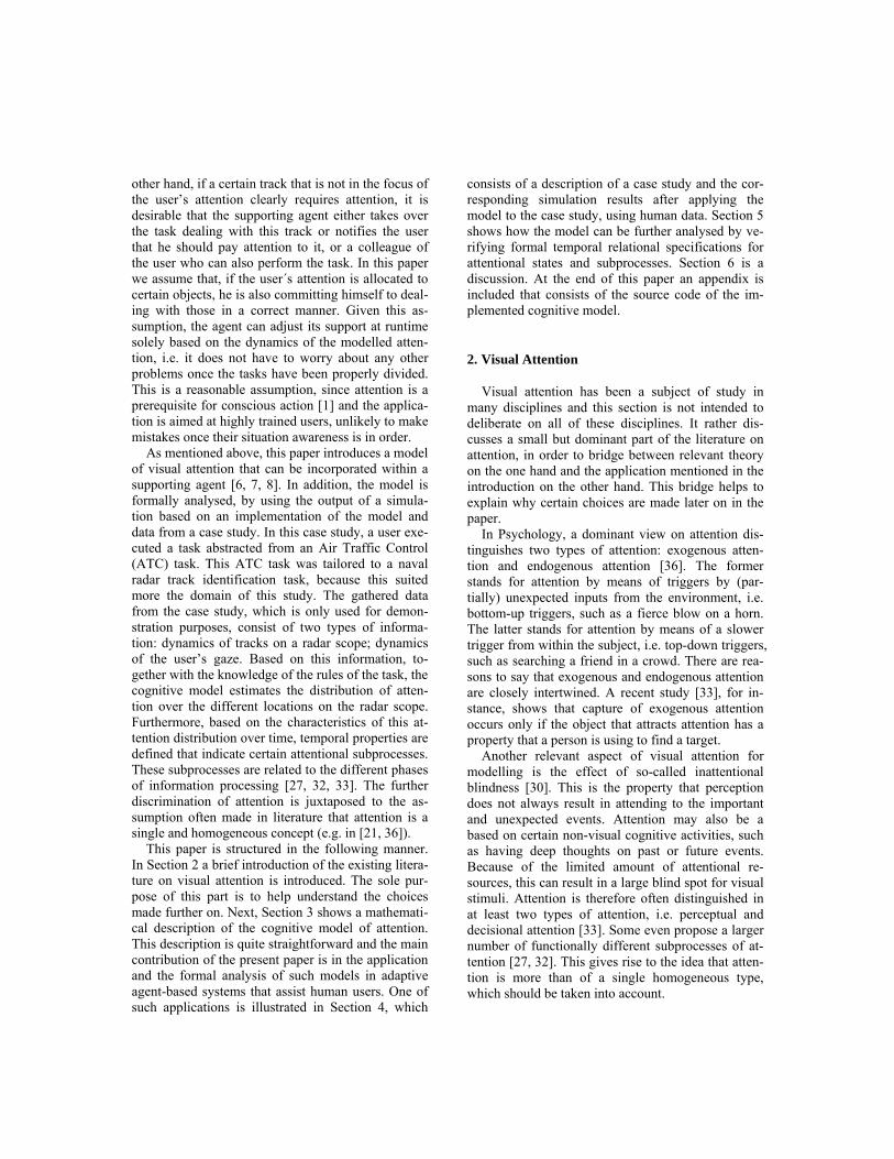
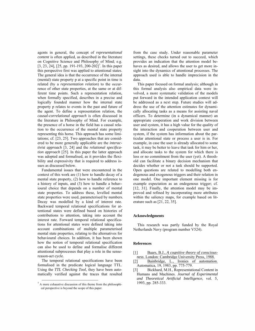
The model of visual attention presented above was used in a simulation run based on ‘real’ data from a human participant executing a naval officer-like task. The software Multitask [14] was altered in order to have it output the proper data as input for the model. This study did not yet deal with altering levels of automation (subject of Clamann et al.’s), and the software environment was momentarily only used for providing relevant data. Multitask was originally meant to be a low fidelity air traffic control (ATC) simulation. In this study it is considered to be an ab-straction of the cognitive tasks concerning the compi-lation of the tactical picture. A snapshot of the task is shown in Figure 1.

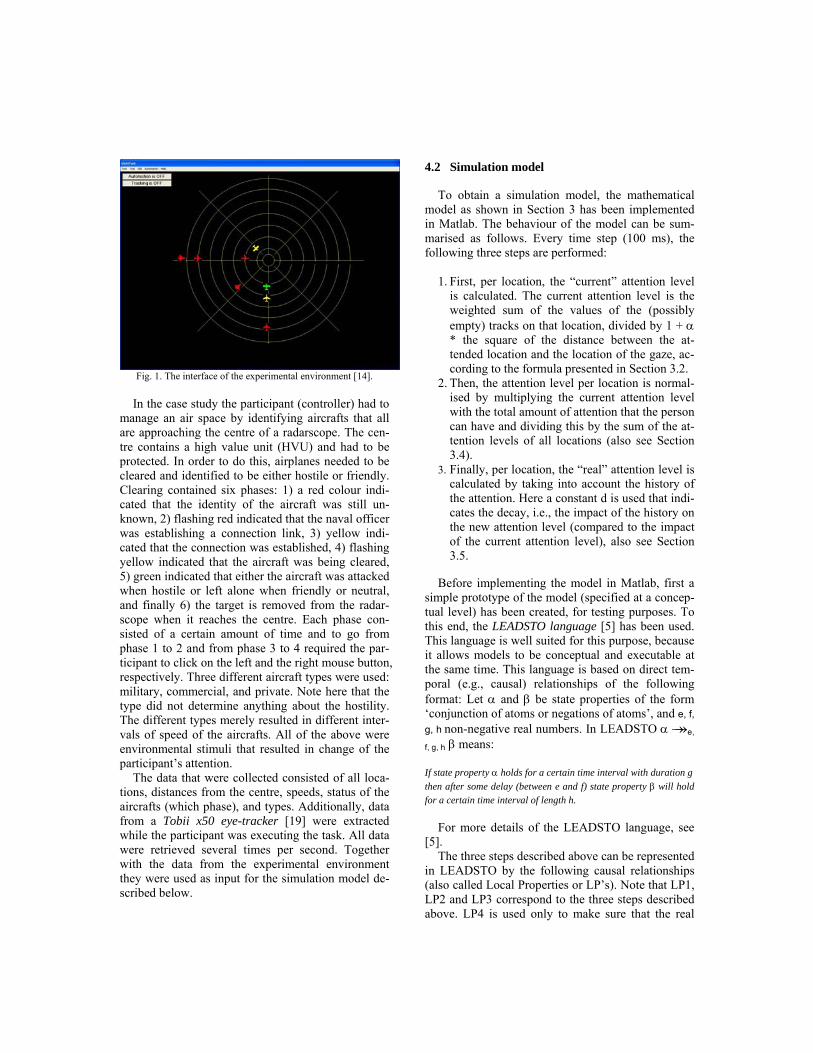
Fig. 1. The interface of the experimental environment [14]. In the case study the participant (controller) had to

manage an air space by identifying aircrafts that all are approaching the centre of a radarscope. The cen-tre contains a high value unit (HVU) and had to be protected. In order to do this, airplanes needed to be cleared and identified to be either hostile or friendly. Clearing contained six phases: 1) a red colour indi-cated that the identity of the aircraft was still un-known, 2) flashing red indicated that the naval officer was establishing a connection link, 3) yellow indi-cated that the connection was established, 4) flashing yellow indicated that the aircraft was being cleared, 5) green indicated that either the aircraft was attacked when hostile or left alone when friendly or neutral, and finally 6) the target is removed from the radar-scope when it reaches the centre. Each phase con-sisted of a certain amount of time and to go from phase 1 to 2 and from phase 3 to 4 required the par-ticipant to click on the left and the right mouse button, respectively. Three different aircraft types were used: military, commercial, and private. Note here that the type did not determine anything about the hostility. The different types merely resulted in different inter-vals of speed of the aircrafts. All of the above were environmental stimuli that resulted in change of the participant’s attention.

The data that were collected consisted of all loca-tions, distances from the centre, speeds, status of the aircrafts (which phase), and types. Additionally, data from a Tobii x50 eye-tracker [19] were extracted while the participant was executing the task. All data were retrieved several times per second. Together with the data from the experimental environment they were used as input for the simulation model de-scribed below.

4.2 Simulation model

To obtain a simulation model, the mathematical model as shown in Section 3 has been implemented in Matlab. The behaviour of the model can be sum-marised as follows. Every time step (100 ms), the following three steps are performed:

1. First, per location, the “current” attention level

is calculated. The current attention level is the weighted sum of the values of the (possibly empty) tracks on that location, divided by 1 + α * the square of the distance between the at-tended location and the location of the gaze, ac-cording to the formula presented in Section 3.2.

2. Then, the attention level per location is normal-ised by multiplying the current attention level with the total amount of attention that the person can have and dividing this by the sum of the at-tention levels of all locations (also see Section 3.4).

3. Finally, per location, the “real” attention level is calculated by taking into account the history of the attention. Here a constant d is used that indi-cates the decay, i.e., the impact of the history on the new attention level (compared to the impact of the current attention level), also see Section 3.5.

Before implementing the model in Matlab, first a

simple prototype of the model (specified at a concep-tual level) has been created, for testing purposes. To this end, the LEADSTO language [5] has been used. This language is well suited for this purpose, because it allows models to be conceptual and executable at the same time. This language is based on direct tem-poral (e.g., causal) relationships of the following format: Let α and β be state properties of the form ‘conjunction of atoms or negations of atoms’, and e, f, g, h non-negative real numbers. In LEADSTO α →→e,

f, g, h β means: If state property α holds for a certain time interval with duration g then after some delay (between e and f) state property β will hold for a certain time interval of length h.

For more details of the LEADSTO language, see [5].

The three steps described above can be represented in LEADSTO by the following causal relationships (also called Local Properties or LP’s). Note that LP1, LP2 and LP3 correspond to the three steps described above. LP4 is used only to make sure that the real

attention level becomes the old attention level after each round. First, some constants and sorts are intro-duced (which correspond to the parameters as used for the formulae as introduced in Section 3) in Table 1.

Table 1. Constants corresponding to the formulae in Section 3.

total duration of the simulation in time steps 500 highest x-coordinate 31 highest y-coordinate 28 wM(stat, t), weight factor of attribute status at time point t

0.8 (for all t)

wM(dist, t), weight factor of attribute distance at time point t

0.5 (for all t)

wM(type, t), weight factor of attribute type at time point t

0.1 (for all t)

wM(spd, t), weight factor of attribute speed at time point t

0.5 (for all t)

concentration A(t), i.e. total amount of attention a person has at time point t

100 (for all t)

impact α of gaze on the current attention level 0.3 (for all t) decay parameter d, i.e., impact of history on the new attention level

0.8 (for all t)

LP1 Calculate Current Attention Level Calculate the current attention level per location. The current at-tention level of a location is based on the values of the attributes of the (possibly empty) tracks on that location, and the distance be-tween the location and the location of the gaze. ∀x1,x2,y1,y2:coordinate ∀v1,v2,v3,v4:integer ∀tr:track is_at_location(tr, loc(x1,y1)) ∧ gaze_at_loc(x2,y2) ∧ has_value_for(tr, v1, status) ∧ has_value_for(tr, v2, distance) ∧ has_value_for(tr, v3, type) ∧ has_value_for(tr, v4, speed) →→ 0,0,1,1 has_current_attention_level(loc(x1, y1), (v1*w1+v2*w2+v3*w3+v4*w4) / 1+ alpha * (x1-x2)^2 + (y1-y2)^2)) LP2 Normalise Attention Level Normalise the attention level per location by multiplying the cur-rent attention level with the total amount of attention, divided by the sum of the attention levels of all locations. ∀x1,y1:coordinate ∀v:real has_current_attention_level(loc(x1,y1), v) ∧ s = Σx2=1

max_x [ Σy2=1max_y

current_attention_level(loc(x2,y2)) ] →→ 0,0,1,1 has_normalised_attention_level(loc(x1,y1), v*a/s) LP3 Calculate Real Attention Level Calculate the real attention level per location. The real attention level of a location is the sum of the old attention level times d and the current (normalised) attention level times 1-d. ∀x,y:coordinate ∀v1,v2:real has_normalised_attention_level(loc(x,y), v1) ∧ has_old_attention_level(loc(x,y), v2) →→ 0,0,1,1 has_real_attention_level(loc(x, y), d*v2 + (1-d)*v1) LP4 Determine Old Attention Level After each round, the real attention level becomes the old attention level. ∀x,y:coordinate ∀v:real

has_real_attention_level(loc(x,y), v) →→ round-2, round-2,1,1 has_old_attention_level(loc(x,y), v)

When this LEADSTO model turned out to show

the expected behaviour, it has been converted to an actual implementation in the mathematical environ-ment Matlab. The Matlab code of the model can be found in Appendix A.

4.3 Simulation results

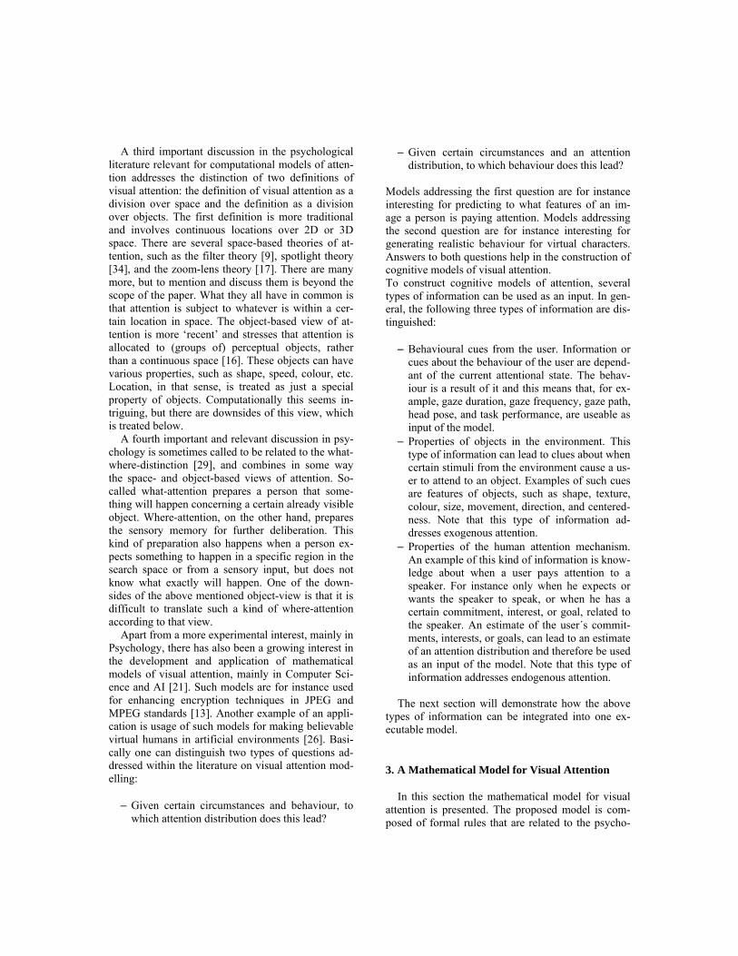
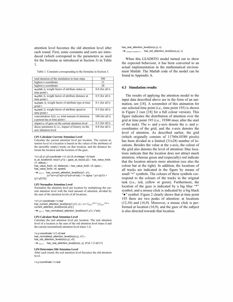
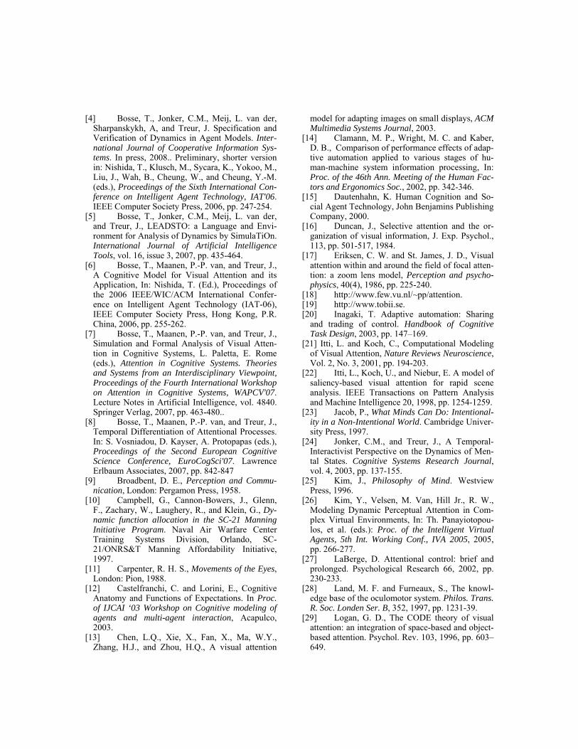
The results of applying the attention model to the input data described above are in the form of an ani-mation, see [18]. A screenshot of this animation for one selected time point (i.e., time point 193) is shown in Figure 2 (see [18] for a full colour version). This figure indicates the distribution of attention over the grid at time point 193 (i.e., 19300 msec after the start of the task). The x- and y-axis denote the x- and y-coordinates of the grid, and the z-axis denotes the level of attention. As described earlier, the grid (which originally consists of 11760x10380 pixels) has been divided in a limited (31x28) number of lo-cations. Besides the value at the z-axis, the colour of the grid also denotes the level of attention: blue loca-tions indicate that the location does not attract much attention, whereas green and (especially) red indicate that the location attracts more attention (see also the colour bar at the right). In addition, the locations of all tracks are indicated in the figure by means of small “•” symbols. The colours of these symbols cor-respond to the colours of the tracks in the original task (i.e., red, yellow or green). Furthermore, the location of the gaze is indicated by a big blue “*” symbol, and a mouse click is indicated by a big black “●” symbol. Figure 2 clearly shows that at time point 193 there are two peaks of attention: at locations (12,10) and (16,9). Moreover, a mouse click is per-formed at location (16,9), and the gaze of the subject is also directed towards that location.

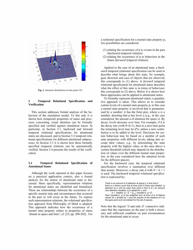
Fig. 2. Attention distribution at time point 193.

5 Temporal Relational Specification and Verification

This section addresses formal analysis of the be-haviour of the simulation model. To this end, it is shown how (temporal) properties of states and proc-esses concerning visual attention can be formally specified and verified against simulation traces. In particular, in Section 5.1, backward and forward temporal relational specifications for attentional states are discussed, and in Section 5.2 temporal rela-tional specifications for different attentional subproc-esses. In Section 5.3 it is shown how these formally specified temporal relations can be automatically verified. Section 5.4 presents the results of the verifi-cation.

5.1 Temporal Relational Specification of Attentional States

Although the work reported in this paper focuses on a practical application context, also a formal analysis for the notion of attentional state is dis-cussed. More specifically, representation relations for attentional states are identified and formalised. These are relationships between the occurrence of a specific mental state and circumstances that occurred in the past or will occur in the future. To express such representation relations, the relational specifica-tion approach from Philosophy of Mind is adopted. This approach indicates how the occurrence of a mental state property relates to properties of states ‘distant in space and time’; cf. [25, pp. 200-202]. For

a relational specification for a mental state property p, two possibilities are considered:

(1) relating the occurrence of p to events in the past

(backward temporal relation) (2) relating the occurrence of p to behaviour in the

future (forward temporal relation) Applied to the case of an attentional state, a back-

ward temporal relational specification can be used to describe what brings about this state, for example, gaze direction and cues of objects that are observed; this corresponds to (1) above. A forward temporal relational specification for attentional states describes what the effect of this state is in terms of behaviour; this corresponds to (2) above. Below it is shown how these approaches can be applied to attentional states.

To formally represent attentional states, a quantita-tive approach is taken. This allows us to consider certain levels of a mental state property p; in this case a mental state property is involved that is parameter-ised by a number: it has the form p(a), where a is a number, denoting that p has level a (e.g., in the case considered, the amount a of attention for space s). By decay, levels decrease over time. For example, if d is the decay rate (with 0<d<1), then at a next time point the remaining level may be d*a, unless a new contri-bution is to be added to the level. Decisions for cer-tain behaviour may be based on a number of such state properties with different levels, taking into ac-count their values; e.g., by determining the state property with the highest value, or the ones above a certain threshold (which may depend on the distribu-tion of values over the different mental state proper-ties, in the case considered here the attention levels for the different spaces).

For the backward case, the temporal relational specification involves a summation over different time points. Moreover, a decay rate d with 0 < d < 1 is used. The backward temporal relational specifica-tion is expressed by:

There is an amount w of attention at space s, if and only if there is a history such that at time point 0 there was initatt(0, s) attention at s, and for each time point k from 0 to t an amount new attention newatt(k, s) is added for s, and

w = initatt(0, s) * dt + ∑k=0t newatt(t-k, s) *dk.

Here newatt(t-k, s) is the weighted sum at time t-k-e of feature values for s divided by 1 plus the square of the distance of s to the gaze point and normalised for the set of spaces.

Note that the logical ‘if and only if’ connective indi-cates that the expression on the past is both a neces-sary and sufficient condition on past circumstances for the attentional state to occur.

The forward case involves a behavioural choice that depends on the relative levels of the multiple mental state properties. This makes that at each choice point the temporal relational specification of the level of one mental state property is not inde-pendent of the level of the other mental state proper-ties involved at the same choice point. Therefore it is only possible to provide a temporal relational specifi-cation for the combined mental state property. For the case considered, this means that it is not possible to consider only one space and the attention level for that space, but that the whole distribution of attention over all spaces has to be taken into account. The for-ward temporal relational specification is expressed in a bidirectional manner as follows:

If at time t1 the amount of attention at space s is above threshold h, then action is undertaken for s at some time t2 ≥ t1 with t2≤t1+e & If at some time t2 an action is undertaken for space s for track 1, then at some time t1 with t2-e≤t1≤t2 the amount of attention at space s was above threshold h.

Note that this statement expresses sufficient and nec-essary conditions for the attentional state to occur: the first clause is the necessary condition, and the second clause the sufficient condition for future cir-cumstances. The threshold h can be determined, for example, as a value such that for 5% of the spaces the attention is above h and for the other spaces it is below h, or such that only three spaces exist with attention value above h and the rest under h.

5.2 Temporal Relational Specification of Attentional Sub-processes

In the previous subsection, temporal relational specifications for attentional states have been defined. In recent years, an increasing amount of work is aimed at identifying different types of attention, and focuses not on attentional states, but on subprocesses of attention. For example, many researchers distin-guish at least two types of attention, i.e. perceptual and decisional attention [33]. Some others even pro-pose a larger number of functionally different sub-processes of attention [27, 32]. Following these ideas, this section provides a (temporal) differentiation of an attentional process into a number of different types of subprocesses. To differentiate the process into subprocesses, a cycle sense – examine – decide – prepare and execute action – assess action effect is used. It is discussed how different types of attention

within these phases can be distinguished and defined by temporal specifications.

5.2.1 Attention allocation This is a subprocess in which attention of a subject

is drawn to an object by certain exogenous (stimuli from the environment) and endogenous (e.g., goals, expectations) factors, see, e.g., [36]. At the end of such an ‘attention catching’ process an attentional state for this object is reached in which gaze and in-ternal focus are directed to this object. The informal temporal specification of this attention allocation process is as follows:

From time t1 to t2 attention has been allocated object O iff at t1 a combination of external and internal triggers related to object O occurs, and at t2 the mind focus and gaze are just di-rected to object O.

Note that in this paper validation only takes place with respect to gaze and not to mind focus, as the empirical data used have no reference to internal states.

5.2.2 Examinational attention Within this subprocess, attention is shared between

or divided over a number of different objects. Atten-tion allocation is switched between these objects, for example, visible in the changing gaze. The informal temporal specification of this examinational atten-tional process is as follows:

During the time interval from t1 to t2 examinational attention occurs iff from t1 to t2, for a number of different objects, atten-tion is allocated alternatively to these objects.

5.2.3 Decision making attention A next subprocess distinguished is one in which a

decision is made on which object to select for an ac-tion on a certain object to be undertaken. Such a de-cision making attentional process may have a more inner-directed or introspective character, as the sub-ject is concentrating on an internal mental process to reach a decision. Temporal specification of this atten-tional subprocess involves a criterion for the decision, which is based on the relevance of the choice made; it is informally defined as follows:

During the time interval from t1 to t2 decision making attention occurs iff at t2 attention is allocated to an object, from which the relevance is higher than a certain threshold.

5.2.4 Action preparation and execution attention Once a decision has been made for an action, an

action preparation and execution attentional process occurs in which the subject concentrates on the ob-ject, but this time on the aspects relevant for action execution. The informal temporal specification is as follows:

During the time interval from t1 to t2 attention on action prepara-tion and execution occurs iff from t1 to t2 the mind focus and gaze is on an object O and at t2 an action a is performed for this object O.

5.2.5 Action assessment attention Finally, after an action has been executed, a retro-

spective action assessment attentional process occurs in which the subject evaluates the outcome of the action. Here the subject focuses on aspects related to goal and effect of the action. For example, Wegner [37] investigates such a process in relation to the ex-perience of conscious will and ownership of action. The informal temporal specification of this atten-tional process is as follows:

During the time interval from t1 to t2 action assessment attention occurs iff at t1 an action a is performed for this an object O and from t1 to t2 the mind focus and gaze is on this object O and from t2 they are not on O.

5.3 Formal Specification and Analysis

The temporal representation relations introduced in the previous sections are expected to apply to dif-ferent parts of attentional processes. In order to verify in detail which of these specifications holds for which part of a given process, automated support is needed. This subsection explains how the representa-tion relations introduced above can be automatically verified against the simulation runs presented in Sec-tion 4.3.

In order to analyse the results of the simulation model in detail, they first are converted into formally specified traces (i.e., sequences of events over time). Moreover, the temporal relational specifications dis-cussed above are logically formalised in the language TTL [4]. This predicate logical language supports formal specification and analysis of dynamic expres-sions, covering both qualitative and quantitative as-pects. TTL is built on atoms referring to states, time points and traces. Traces are time-indexed sequences of states. Here a state S is described by a truth as-signment to the set of basic state properties (ground

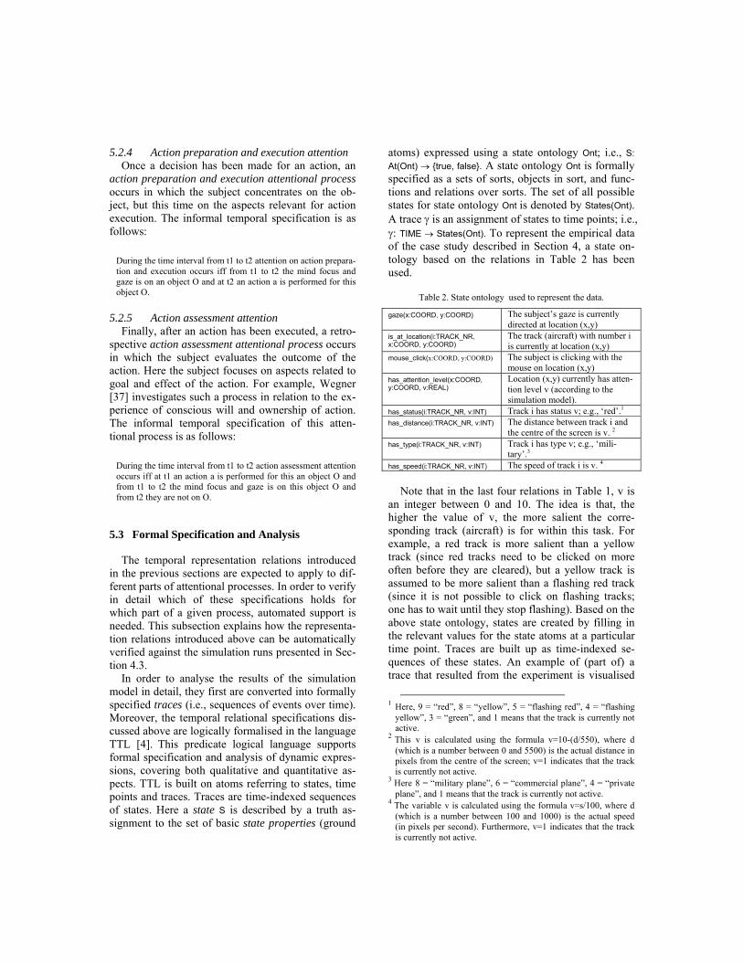
atoms) expressed using a state ontology Ont; i.e., S: At(Ont) → {true, false}. A state ontology Ont is formally specified as a sets of sorts, objects in sort, and func-tions and relations over sorts. The set of all possible states for state ontology Ont is denoted by States(Ont). A trace γ is an assignment of states to time points; i.e., γ: TIME → States(Ont). To represent the empirical data of the case study described in Section 4, a state on-tology based on the relations in Table 2 has been used.

Table 2. State ontology used to represent the data.

gaze(x:COORD, y:COORD) The subject’s gaze is currently directed at location (x,y)

is_at_location(i:TRACK_NR, x:COORD, y:COORD)

The track (aircraft) with number i is currently at location (x,y)

mouse_click(x:COORD, y:COORD) The subject is clicking with the mouse on location (x,y)

has_attention_level(x:COORD, y:COORD, v:REAL)

Location (x,y) currently has atten-tion level v (according to the simulation model).

has_status(i:TRACK_NR, v:INT) Track i has status v; e.g., ‘red’.1 has_distance(i:TRACK_NR, v:INT) The distance between track i and

the centre of the screen is v. 2 has_type(i:TRACK_NR, v:INT) Track i has type v; e.g., ‘mili-

tary’.3 has_speed(i:TRACK_NR, v:INT) The speed of track i is v. 4

Note that in the last four relations in Table 1, v is

an integer between 0 and 10. The idea is that, the higher the value of v, the more salient the corre-sponding track (aircraft) is for within this task. For example, a red track is more salient than a yellow track (since red tracks need to be clicked on more often before they are cleared), but a yellow track is assumed to be more salient than a flashing red track (since it is not possible to click on flashing tracks; one has to wait until they stop flashing). Based on the above state ontology, states are created by filling in the relevant values for the state atoms at a particular time point. Traces are built up as time-indexed se-quences of these states. An example of (part of) a trace that resulted from the experiment is visualised

1 Here, 9 = “red”, 8 = “yellow”, 5 = “flashing red”, 4 = “flashing

yellow”, 3 = “green”, and 1 means that the track is currently not active.

2 This v is calculated using the formula v=10-(d/550), where d (which is a number between 0 and 5500) is the actual distance in pixels from the centre of the screen; v=1 indicates that the track is currently not active.

3 Here 8 = “military plane”, 6 = “commercial plane”, 4 = “private plane”, and 1 means that the track is currently not active.

4 The variable v is calculated using the formula v=s/100, where d (which is a number between 100 and 1000) is the actual speed (in pixels per second). Furthermore, v=1 indicates that the track is currently not active.

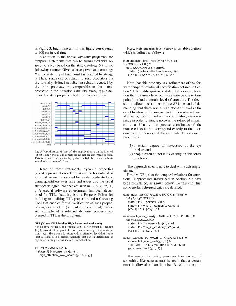
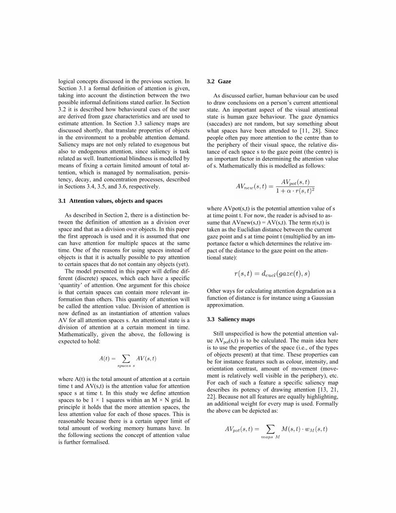
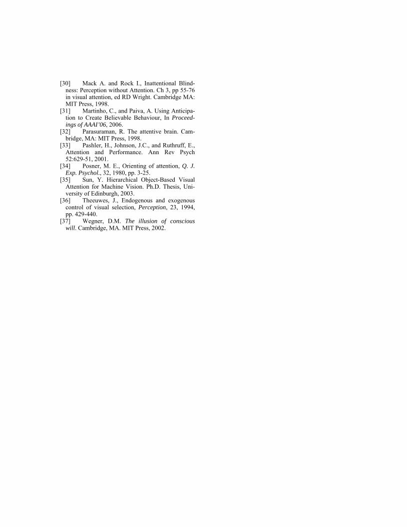
in Figure 3. Each time unit in this figure corresponds to 100 ms in real time.

In addition to the above, dynamic properties are temporal statements that can be formulated with re-spect to traces based on the state ontology Ont in the following manner. Given a trace γ over state ontology Ont, the state in γ at time point t is denoted by state(γ, t). These states can be related to state properties via the formally defined satisfaction relation denoted by the infix predicate |=, comparable to the Holds-predicate in the Situation Calculus: state(γ, t) |= p de-notes that state property p holds in trace γ at time t.

Fig. 3. Visualisation of (part of) the empirical trace on the interval [65,85). The vertical axis depicts atoms that are either true or false. This is indicated, respectively, by dark or light boxes on the hori-zontal axis, in units of 10 ms.

Based on these statements, dynamic properties (about representation relations) can be formulated in a formal manner in a sorted first-order predicate logic, using quantifiers over time and traces and the usual first-order logical connectives such as ¬, ∧, ∨, ⇒, ∀, ∃. A special software environment has been devel-oped for TTL, featuring both a Property Editor for building and editing TTL properties and a Checking Tool that enables formal verification of such proper-ties against a set of (simulated or empirical) traces. An example of a relevant dynamic property ex-pressed in TTL is the following:

GP1 (Mouse Click implies High Attention Level Area) For all time points t, if a mouse click is performed at location {x,y}, then at e time points before t, within a range of 2 locations from {x,y}, there was a location with an attention level that was at least h. Here, h is a certain threshold that can be determined as explained in the previous section. Formalisation:

∀t:T ∀x,y:COORDINATE [ state(γ,t) |= mouse_click(x,y) ⇒ high_attention_level_nearby(γ, t-e, x, y) ]

Here, high_attention_level_nearby is an abbreviation, which is defined as follows:

high_attention_level_nearby(γ:TRACE, t:T, x,y:COORDINATE) ≡ ∃p,q: COORDINATE, ∃i:REAL state(γ,t) |= has_attention_level(p,q,i) &

x-2 ≤ p ≤ x+2 & y-2 ≤ q ≤ y+2 & i > h Note that this property is a refinement of the for-

ward temporal relational specification defined in Sec-tion 5.1. Roughly spoken, it states that for every loca-tion that the user clicks on, some time before (e time points) he had a certain level of attention. The deci-sion to allow a certain error (see GP1: instead of de-manding that there was a high attention level at the exact location of the mouse click, this is also allowed at a nearby location within the surrounding area) was made in order to handle noise in the retrieved empiri-cal data. Usually, the precise coordinates of the mouse clicks do not correspond exactly to the coor-dinates of the tracks and the gaze data. This is due to two reasons:

(1) a certain degree of inaccuracy of the eye

tracker, and (2) people often do not click exactly on the centre

of a track.

The approach used is able to deal with such impre-cision.

Besides GP1, also the temporal relations for atten-tional subprocesses introduced in Section 5.2 have been formalised, as shown below. To this end, first some useful help-predicates are defined: gaze_near_track(γ:TRACE, c:TRACK, t1:TIME) ≡ ∃x1,y1,x2,y2:COORD state(γ, t1) |== gaze(x1, y1) & state(γ, t1) |== is_at_location(c, x2, y2) & |x2-x1| ≤ 1 & |y2-y1| ≤ 1 mouseclick_near_track(γ:TRACE, c:TRACK, t1:TIME) ≡ ∃x1,y1,x2,y2:COORD state(γ, t1) |== mouse_click(x1, y1) & state(γ, t1) |== is_at_location(c, x2, y2) & |x2-x1| ≤ 1 & |y2-y1| ≤ 1 action_execution(γ:TRACE, c:TRACK, t2:TIME) ≡ mouseclick_near_track(γ, c, t2) & ∃t1:TIME t1 < t2 & ∀t3:TIME [t1 ≤ t3 ≤ t2 ⇒ gaze_near_track(γ, c, t3) ]

The reason for using gaze_near_track instead of something like gaze_at_track is again that a certain error is allowed to handle noise. Based on these in-

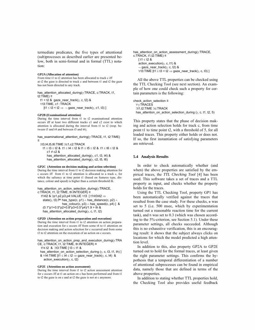
termediate predicates, the five types of attentional (sub)processes as described earlier are presented be-low, both in semi-formal and in formal (TTL) nota-tion:

GP2A (Allocation of attention) From time t1 to t2 attention has been allocated to track c iff at t2 the gaze is directed to track c and between t1 and t2 the gaze has not been directed to any track. has_attention_allocated_during(γ:TRACE, c:TRACK, t1, t2:TIME) ≡ t1 < t2 & gaze_near_track(γ, c, t2) & ∀t3:TIME, c1 :TRACK [t1 ≤ t3 < t2 ⇒ ¬ gaze_near_track(γ, c1, t3) ] GP2B (Examinational attention) During the time interval from t1 to t2 examinational attention occurs iff at least two different tracks c1 and c2 exist to which attention is allocated during the interval from t1 to t2 (resp. be-tween t3 and t4 and between t5 and t6). has_examinational_attention_during(γ:TRACE, t1, t2:TIME) ≡ ∃t3,t4,t5,t6:TIME ∃c1,c2:TRACK t1 ≤ t3 ≤ t2 & t1 ≤ t4 ≤ t2 & t1 ≤ t5 ≤ t2 & t1 ≤ t6 ≤ t2 &

c1 ≠ c2 & has_attention_allocated_during(γ, c1, t3, t4) & has_attention_allocated_during(γ, c2, t5, t6)

GP2C (Attention on decision making and action selection) During the time interval from t1 to t2 decision making attention for c occurs iff from t1 to t2 attention is allocated to a track c, for which the saliency at time point t1 (based on features type, dis-tance, colour and speed) is higher than a certain threshold th. has_attention_on_action_selection_during(γ:TRACE, c:TRACK, t1, t2:TIME, th:INTEGER) ≡ t1≤t2 & ∃p1,p2,p3,p4:VALUE ∀t3 [ t1≤t3≤t2 ⇒ state(γ, t3) |== has_type(c, p1) ∧ has_distance(c, p2) ∧ has_colour(c, p3) ∧ has_speed(c, p4) ] & (0.1*p1+0.5*p2+0.8*p3+0.5*p4)/1.9 > th & has_attention_allocated_during(γ, c, t1, t2) GP2D (Attention on action preparation and execution) During the time interval from t1 to t2 attention on action prepara-tion and execution for c occurs iff from some t4 to t1 attention on decision making and action selection for c occurred and from some t3 to t2 attention on the execution of an action on c occurs. has_attention_on_action_prep_and_execution_during(γ:TRACE, c:TRACK, t1, t2:TIME, th:INTEGER) ≡ t1≤ t2 & ∃t3:TIME [ t3 ≤ t1 & has_attention_on_action_selection_during (γ, c, t3, t1, th) ] & ∀t4:TIME [t1 ≤ t4 ≤ t2 ⇒ gaze_near_track(γ, c, t4) & action_execution(γ, c, t2) GP2E (Attention on action assessment) During the time interval from t1 to t2 action assessment attention for c occurs iff at t1 an action on c has been performed and from t1 to t2 the gaze is on c and at t2 the gaze is not at c anymore.

has_attention_on_action_assessment_during(γ:TRACE, c:TRACK, t1,t2:TIME) ≡ [ t1 ≤ t2 & action_execution(γ, c, t1) & ¬ gaze_near_track(γ, c, t2) & ∀t3:TIME [t1 ≤ t3 < t2 ⇒ gaze_near_track(γ, c, t3) ]

All the above TTL properties can be checked using

the TTL Checking Tool (see next section). An exam-ple of how one could check such a property for cer-tain parameters is the following:

check_action_selection ≡ ∀γ:TRACES ∃t1,t2:TIME ∃c:TRACK has_attention_on_action_selection_during (γ, c, t1, t2, 5) This property states that the phase of decision mak-ing and action selection holds for track c, from time point t1 to time point t2, with a threshold of 5, for all loaded traces. This property either holds or does not. If so, the first instantiation of satisfying parameters are retrieved.

5.4 Analysis Results

In order to check automatically whether (and when) the above properties are satisfied by the em-pirical traces, the TTL Checking Tool [4] has been used. This software takes a set of traces and a TTL property as input, and checks whether the property holds for the traces.

Using the TTL Checking Tool, property GP1 has been automatically verified against the traces that resulted from the case study. For these checks, e was set to 5 (i.e. 500 msec, which by experimentation turned out a reasonable reaction time for the current task), and h was set to 0.3 (which was chosen accord-ing to the 5%-criterion, see Section 5.1). Under these parameter settings, all checks succeeded. Although this is no exhaustive verification, this is an encourag-ing result: it shows that the subject always clicks on locations for which the model predicted a high atten-tion level.

In addition to this, also property GP2A to GP2E turned out to hold for the formal traces, at least given the right parameter settings. This confirms the hy-pothesis that a temporal differentiation of a number of attentional subprocesses can be found in empirical data, namely those that are defined in terms of the above properties.

In addition to stating whether TTL properties hold, the Checking Tool also provides useful feedback

about the exact instantiations of variables for which they hold. For example, suppose that the property check_action_selection holds for a certain trace, the checker will return specific values for time point t1 and t2 and for track c for which that property holds. This approach has been used to identify certain in-stances of attentional processes in the empirical trac-es that resulted from the experiment described earlier.

To illustrate this idea, Figure 3 shows part of such a trace.5 For this trace, the five properties as men-tioned earlier hold for the following parameter val-ues6:

− has_attention_allocated_during holds for track c=9,

for time points t1=0 and t2=6 − has_examinational_attention_during holds for tracks

c1=8 and c2=9, for time points t1=0 and t2=19, because has_attention_allocated_during holds for track c=9, for time points t1=0 and t2=6 and for track c1=8, for time points t1=18 to t2=19 (note that for t=17 the gaze is still on track c=9)

− has_attention_on_action_selection_during holds for track c=9, for time points t1=1 and t2=6, and threshold value th=4. This is due to the fact that has_type(9, 4), has_distance(9, 3), has_colour(9, 5), and has_speed(9, 4), not shown in Figure 2, result in a combined saliency above th=4, for this time period

− has_attention_on_action_prep_and_execution_during holds for track c=9, for time points t1=6 and t2=7, because has_attention_on_action_selec-tion_during holds for track c=9, for time points 1 to 6, and action_execution holds at t2=7, and the gaze is near track c=9 at time point 7

− has_attention_on_action_assessment_during holds for track c=9, for time points t1=7 and t2=9 (note that after t2=9 the gaze is not on c=9 any-more)

Furthermore, the TTL Checking Tool enables addi-

tional analyses, such as counting the number of times a property holds for a given trace, using a built-in operator for summation. Using this mechanism, one can calculate that the property has_attention_allocated_during holds three times for

5 Due to space limitations, in Figure 3 a mere selection of atoms

has been made from the actual empirical trace, i.e., the time in-terval [65,85).

6 Note that the maximum intervals are given for which each prop-erty holds. So, the fact that has_attention_allocated_during holds (for track c=9) between time points 0 and 6, obviously implies that it also holds between time point 2 and 4. However, it does not hold for all time points after time point 6.

track 1, four times for track 7, one time for track 8, and two times for track 9, in the time interval [0,100) of the empirical trace. A similar calculation shows that has_attention_on_action_prep_and_execution_during holds only once in this time interval, namely for track 9. For all other combinations of tracks and time in-tervals, the property does not hold. Comparison be-tween such counts can be used to, for instance, indi-cate different task progresses or workload differences.

All of the formalised dynamic properties shown above have been successfully checked, given reason-able parameter instantiations, against the traces. Al-though an extensive investigation of the results is beyond the scope of this article, we hereby demon-strate the benefits of automated checks to investigate attentional processes. As mentioned above, the checks cannot be seen as an exhaustive validation, but they contribute to a detailed formal analysis of the simulation model. The main contribution of such an analysis is that it allows the user to distinguish different attentional states and subprocesses, which can be compared with the expected behaviour.

6 Discussion

This paper presents a cognitive model as a compo-nent of a socially intelligent supporting agent (cf.[15]). The component allows the agent to adapt to the need for support of its user, for example a naval officer and his or her task to compile a tactical pic-ture. Given two types of input, i.e. user- and context-input, the implemented cognitive model is able to estimate the visual attention distribution within a 2D-space. The user-input was retrieved by an eye-tracker, and the context-input by means of the output of the software for an Air Traffic Control task (ATC), tai-lored to a naval radar track identification task. The first consists of the (x, y)-coordinates of the gaze of the user over time. The latter consists of the variables speed, distance to the centre, type of plane, and status of the plane. In a case study, the model was used to estimate the attention of a human user that executes the task mentioned above. The model was specifi-cally tailored to domain-dependent properties re-trieved from a task environment; nevertheless the method presented remains generic enough to be eas-ily applied to other domains and task environments.

Although the work reported in this paper focuses on a practical application context, as a main contribu-tion, also a formal analysis was given for attentional states and processes. To describe mental states of

agents in general, the concept of representational content is often applied, as described in the literature on Cognitive Science and Philosophy of Mind; e.g. [3, 23, 24], [25, pp. 191-193, 200-202]7. In this paper this perspective first was applied to attentional states. The general idea is that the occurrence of the internal (mental) state property p at a specific point in time is related (by a representation relation) to the occur-rence of other state properties, at the same or at dif-ferent time points. Such a representation relation, when formally specified, describes in a precise and logically founded manner how the internal state property p relates to events in the past and future of the agent. To define a representation relation, the causal-correlational approach is often discussed in the literature in Philosophy of Mind. For example, the presence of a horse in the field has a causal rela-tion to the occurrence of the mental state property representing this horse. This approach has some limi-tations; cf. [23, 25]. Two approaches that are consid-ered to be more generally applicable are the interac-tivist approach [3, 24] and the relational specifica-tion approach [25]. In this paper the latter approach was adopted and formalised, as it provides the flexi-bility and expressivity that is required to address is-sues as discussed below.

Fundamental issues that were encountered in the context of this work are (1) how to handle decay of a mental state property, (2) how to handle reference to a history of inputs, and (3) how to handle a behav-ioural choice that depends on a number of mental state properties. To address these, levelled mental state properties were used, parameterised by numbers. Decay was modelled by a kind of interest rate. Backward temporal relational specifications for at-tentional states were defined based on histories of contributions to attention, taking into account the interest rate. Forward temporal relational specifica-tions for attentional states were defined taking into account combinations of multiple parameterised mental state properties, relating to the alternatives for behavioural choices. In addition, it has been shown how the notion of temporal relational specification can also be used to define and formalise different attentional subprocesses that play a role in the sense-reason-act cycle.

The temporal relational specifications have been formalised in the predicate logical language TTL. Using the TTL Checking Tool, they have been auto-matically verified against the traces that resulted

7 A more exhaustive discussion of this theme from the philosophi-

cal perspective is beyond the scope of this paper.

from the case study. Under reasonable parameter settings, these checks turned out to succeed, which provides an indication that the attention model be-haves as desired, and allows the user to get more in-sight into the dynamics of attentional processes. The approach used is able to handle imprecision in the data.

This paper focused on formal analysis; although in this formal analysis also empirical data were in-volved, a more systematic validation of the models put forward in the intended application context will be addressed as a next step. Future studies will ad-dress the use of the attention estimates for dynami-cally allocating tasks as a means for assisting naval officers. To determine (in a dynamical manner) an appropriate cooperation and work division between user and system, it has a high value for the quality of the interaction and cooperation between user and system, if the system has information about the par-ticular attentional state or process a user is in. For example, in case the user is already allocated to some task, it may be better to leave that task for him or her, and allocate tasks to the system for which there is less or no commitment from the user (yet). A thresh-old can facilitate a binary decision mechanism that decides whether or not a task should be supported. Open questions are related to modelling both en-dogenous and exogenous triggers and their relation in one model. One important element missing is for example expectation as an endogenous trigger; cf. [12, 31]. Finally, the attention model may be im-proved and refined by incorporating more attributes within the saliency maps, for example based on lit-erature such as [21, 22, 35].

Acknowledgments

This research was partly funded by the Royal Netherlands Navy (program number V524).

References

[1] Baars, B.J., A cognitive theory of conscious-ness. London: Cambridge University Press, 1988.

[2] Bainbridge, L., Ironies of automation. Automatica, 19, 1983, pp. 775-779.

[3] Bickhard, M.H., Representational Content in Humans and Machines. Journal of Experimental and Theoretical Artificial Intelligence, vol. 5, 1993, pp. 285-333.

[4] Bosse, T., Jonker, C.M., Meij, L. van der, Sharpanskykh, A, and Treur, J. Specification and Verification of Dynamics in Agent Models. Inter-national Journal of Cooperative Information Sys-tems. In press, 2008.. Preliminary, shorter version in: Nishida, T., Klusch, M., Sycara, K., Yokoo, M., Liu, J., Wah, B., Cheung, W., and Cheung, Y.-M. (eds.), Proceedings of the Sixth International Con-ference on Intelligent Agent Technology, IAT'06. IEEE Computer Society Press, 2006, pp. 247-254.

[5] Bosse, T., Jonker, C.M., Meij, L. van der, and Treur, J., LEADSTO: a Language and Envi-ronment for Analysis of Dynamics by SimulaTiOn. International Journal of Artificial Intelligence Tools, vol. 16, issue 3, 2007, pp. 435-464.

[6] Bosse, T., Maanen, P.-P. van, and Treur, J., A Cognitive Model for Visual Attention and its Application, In: Nishida, T. (Ed.), Proceedings of the 2006 IEEE/WIC/ACM International Confer-ence on Intelligent Agent Technology (IAT-06), IEEE Computer Society Press, Hong Kong, P.R. China, 2006, pp. 255-262.

[7] Bosse, T., Maanen, P.-P. van, and Treur, J., Simulation and Formal Analysis of Visual Atten-tion in Cognitive Systems, L. Paletta, E. Rome (eds.), Attention in Cognitive Systems. Theories and Systems from an Interdisciplinary Viewpoint, Proceedings of the Fourth International Workshop on Attention in Cognitive Systems, WAPCV'07. Lecture Notes in Artificial Intelligence, vol. 4840. Springer Verlag, 2007, pp. 463-480..

[8] Bosse, T., Maanen, P.-P. van, and Treur, J., Temporal Differentiation of Attentional Processes. In: S. Vosniadou, D. Kayser, A. Protopapas (eds.), Proceedings of the Second European Cognitive Science Conference, EuroCogSci'07. Lawrence Erlbaum Associates, 2007, pp. 842-847

[9] Broadbent, D. E., Perception and Commu-nication, London: Pergamon Press, 1958.

[10] Campbell, G., Cannon-Bowers, J., Glenn, F., Zachary, W., Laughery, R., and Klein, G., Dy-namic function allocation in the SC-21 Manning Initiative Program. Naval Air Warfare Center Training Systems Division, Orlando, SC-21/ONRS&T Manning Affordability Initiative, 1997.

[11] Carpenter, R. H. S., Movements of the Eyes, London: Pion, 1988.

[12] Castelfranchi, C. and Lorini, E., Cognitive Anatomy and Functions of Expectations. In Proc. of IJCAI ‘03 Workshop on Cognitive modeling of agents and multi-agent interaction, Acapulco, 2003.

[13] Chen, L.Q., Xie, X., Fan, X., Ma, W.Y., Zhang, H.J., and Zhou, H.Q., A visual attention

model for adapting images on small displays, ACM Multimedia Systems Journal, 2003.

[14] Clamann, M. P., Wright, M. C. and Kaber, D. B., Comparison of performance effects of adap-tive automation applied to various stages of hu-man-machine system information processing, In: Proc. of the 46th Ann. Meeting of the Human Fac-tors and Ergonomics Soc., 2002, pp. 342-346.

[15] Dautenhahn, K. Human Cognition and So-cial Agent Technology, John Benjamins Publishing Company, 2000.

[16] Duncan, J., Selective attention and the or-ganization of visual information, J. Exp. Psychol., 113, pp. 501-517, 1984.

[17] Eriksen, C. W. and St. James, J. D., Visual attention within and around the field of focal atten-tion: a zoom lens model, Perception and psycho-physics, 40(4), 1986, pp. 225-240.

[18] http://www.few.vu.nl/~pp/attention. [19] http://www.tobii.se. [20] Inagaki, T. Adaptive automation: Sharing

and trading of control. Handbook of Cognitive Task Design, 2003, pp. 147–169.

[21] Itti, L. and Koch, C., Computational Modeling of Visual Attention, Nature Reviews Neuroscience, Vol. 2, No. 3, 2001, pp. 194-203.

[22] Itti, L., Koch, U., and Niebur, E. A model of saliency-based visual attention for rapid scene analysis. IEEE Transactions on Pattern Analysis and Machine Intelligence 20, 1998, pp. 1254-1259.

[23] Jacob, P., What Minds Can Do: Intentional-ity in a Non-Intentional World. Cambridge Univer-sity Press, 1997.

[24] Jonker, C.M., and Treur, J., A Temporal-Interactivist Perspective on the Dynamics of Men-tal States. Cognitive Systems Research Journal, vol. 4, 2003, pp. 137-155.

[25] Kim, J., Philosophy of Mind. Westview Press, 1996.

[26] Kim, Y., Velsen, M. Van, Hill Jr., R. W., Modeling Dynamic Perceptual Attention in Com-plex Virtual Environments, In: Th. Panayiotopou-los, et al. (eds.): Proc. of the Intelligent Virtual Agents, 5th Int. Working Conf., IVA 2005, 2005, pp. 266-277.

[27] LaBerge, D. Attentional control: brief and prolonged. Psychological Research 66, 2002, pp. 230-233.

[28] Land, M. F. and Furneaux, S., The knowl-edge base of the oculomotor system. Philos. Trans. R. Soc. Londen Ser. B, 352, 1997, pp. 1231-39.

[29] Logan, G. D., The CODE theory of visual attention: an integration of space-based and object-based attention. Psychol. Rev. 103, 1996, pp. 603–649.

[30] Mack A. and Rock I., Inattentional Blind-ness: Perception without Attention. Ch 3, pp 55-76 in visual attention, ed RD Wright. Cambridge MA: MIT Press, 1998.

[31] Martinho, C., and Paiva, A. Using Anticipa-tion to Create Believable Behaviour, In Proceed-ings of AAAI’06, 2006.

[32] Parasuraman, R. The attentive brain. Cam-bridge, MA: MIT Press, 1998.

[33] Pashler, H., Johnson, J.C., and Ruthruff, E., Attention and Performance. Ann Rev Psych 52:629-51, 2001.

[34] Posner, M. E., Orienting of attention, Q. J. Exp. Psychol., 32, 1980, pp. 3-25.

[35] Sun, Y. Hierarchical Object-Based Visual Attention for Machine Vision. Ph.D. Thesis, Uni-versity of Edinburgh, 2003.

[36] Theeuwes, J., Endogenous and exogenous control of visual selection, Perception, 23, 1994, pp. 429-440.

[37] Wegner, D.M. The illusion of conscious will. Cambridge, MA. MIT Press, 2002.

Appendix A - Source Code

This appendix contains the Matlab code of the simu-lation model presented in Section 4.2. The complete model consists of four separate modules:

1. The Pre-Processing Module, needed to convert the

data resulting from the task described in Section 4.1 and the data from the eye-tracker (which are both stored in an Excel-file) to a format that can be handled by the Main Module.

2. The Main Module, needed to calculate the distri-bution of attention over time and space, according to the three steps described in Section 4.2.

3. The Visualisation Module, needed to plot the out-put of the Main Module in a format as shown in Figure 2.

4. The Matlab to TTL Module, needed to convert the output of the Main Module to traces that can be used to check properties on by the TTL Checking Tool and can be visualised by LEADSTO in the format shown in Figure 3.

In order to replicate the simulation results and

automated verifications one has to do the following:

− Consider the Excel-file “data.xls” (see below) that contains raw experimental data.

− Import the data from the "targets", "gaze", and "actions" tabs in the Excel-file into Matlab and rename them to "inp1", "inp2", and "inp3", re-spectively.

− Load Pre-Processing Module in Matlab and run it. Wait for a while until all Matlab data is gen-erated.

− Load Main Module in Matlab and run it. Wait for a while until all Matlab data is generated.

− Load Visualisation Module in Matlab and run it. Wait until all plots have been processed and the file “movie_new.mpg” has been generated.

− Load Matlab to TTL Module and run it. Wait for a while until “attention.tr” has been generated.

− Install the LEADSTO Simulation Tool and the TTL Checking Tool from http://www.cs.vu.nl/~wai/TTL/.

− Open “attention.tr” in LEADSTO to view the trace. This takes a while.

− Use the TTL Checking Tool to check the proper-ties in “ttl_check.fm” on “attention.tr”.

The Matlab source code of the four modules of the model is provided in the subsections below. The data file “data.xls” and property file “ttl_check.fm” are downloadable from one of the authors’ website [18].

A.1 Pre-Processing Module

% Pre-Processing Module % By Tibor Bosse, Peter-Paul van Maanen, and Jan Treur % ADAPT EXCEL SHEET for i = 1:830 % depends on the time of the experiment for j = 1:4200 % depends on the length of the excel sheet if inp1(j,1) < 100*i & inp1(j+1,1) > 100*1 for n = 1:size(inp1,2) input2(i,n) = inp1(j,n); end end end end for i = 1:830 % depends on the time of the experiment for j = 1:4200 % depends on the length of the excel sheet if inp2(j,3) < 100*i & inp2(j+1,3) > 100*1 input1(i,1) = inp2(j,1); input1(i,2) = inp2(j,2); end end end % CREATE GAZE DATA FROM ADAPTED EXCEL SHEET for i = 1:500 % or: size(input1,1) gaze(i,1) = max(0, ceil((input1(i,1)-220)/25)); gaze(i,2) = max(0, ceil((input1(i,2)-55)/25)); end % CREATE ACTION DATA FROM EXCEL SHEET for i = 1:500 % or: size(input1,1) for j = 1:size(inp3,1) if i == ceil(inp3(j,3)/100) actions(i,1) = max(0, ceil((inp3(j,1)-220)/25)); actions(i,2) = max(0, ceil((inp3(j,2)-55)/25)); end end end % CREATE TRACK LOCATION DATA FROM ADAPTED EXCEL SHEET mx = 31; my = 28; for i = 1:500 % or: size(input2,1) for x = 1:mx for y = 1:my if ceil((input2(i,2)-3240)/380) == x & ceil(input2(i,3)/380) == y tracks(x,y,i) = 1; elseif ceil((input2(i,10)-3240)/380) == x & ceil((input2(i,11)-240)/380) == y tracks(x,y,i) = 2; elseif ceil((input2(i,18)-3240)/380) == x & ceil((input2(i,19)-240)/380) == y tracks(x,y,i) = 3; elseif ceil((input2(i,26)-3240)/380) == x & ceil((input2(i,27)-240)/380) == y tracks(x,y,i) = 4; elseif ceil((input2(i,34)-3240)/380) == x & ceil((input2(i,35)-240)/380) == y tracks(x,y,i) = 5; elseif ceil((input2(i,42)-3240)/380) == x & ceil((input2(i,43)-240)/380) == y tracks(x,y,i) = 6; elseif ceil((input2(i,50)-3240)/380) == x & ceil((input2(i,51)-240)/380) == y tracks(x,y,i) = 7; elseif ceil((input2(i,58)-3240)/380) == x & ceil((input2(i,59)-240)/380) == y tracks(x,y,i) = 8; elseif ceil((input2(i,66)-3240)/380) == x & ceil((input2(i,67)-240)/380) == y tracks(x,y,i) = 9; else tracks(x,y,i) = 0; end end end end % CREATE TRACK ATTRIBUTE DATA FROM ADAPTED EXCEL SHEET

for i = 1:500 % or: size(input2,1) for t = 1:9 % COLOUR colour(t,1,i) = t; if input2(i,4+8*(t-1)) == 1 colour(t,2,i) = 9; elseif input2(i,4+8*(t-1)) == 2 colour(t,2,i) = 5; elseif input2(i,4+8*(t-1)) == 3 colour(t,2,i) = 8; elseif input2(i,4+8*(t-1)) == 4 colour(t,2,i) = 4; elseif input2(i,4+8*(t-1)) == 5 colour(t,2,i) = 3; elseif input2(i,4+8*(t-1)) == 6 colour(t,2,i) = 3; else colour(t,2,i) = 1; end % DISTANCE distance(t,1,i) = t; if input2(i,5+8*(t-1)) < 0 distance(t,2,i) = 1; else distance(t,2,i) = 10 - ceil(input2(i,5+8*(t-1))/550); end % TYPE type(t,1,i) = t; if input2(i,6+8*(t-1)) == 1 type(t,2,i) = 6; elseif input2(i,6+8*(t-1)) == 2 type(t,2,i) = 8; elseif input2(i,6+8*(t-1)) == 3 type(t,2,i) = 4; else type(t,2,i) = 1; end % SPEED speed(t,1,i) = t; if input2(i,7+8*(t-1)) < 0 speed(t,2,i) = 1; else speed(t,2,i) = ceil(input2(i,7+8*(t-1))/100); end end end

A.2 Main Module

% Main Module % By Tibor Bosse, Peter-Paul van Maanen, and Jan Treur % CONSTANTS w1 = 0.8; % COLOUR w2 = 0.5; % DISTANCE w3 = 0.1; % TYPE w4 = 0.5; % SPEED a = 100; d = 0.8; alph = 0.3; % INPUT-SPECIFIC CONSTANTS max_x = size(tracks, 1); max_y = size(tracks, 2); end_time = size(actions, 1); no_tracks = size(colour, 1); % START SIMULATION for i = 1:end_time % CALCULATE CURRENT ATTENTION LEVEL for x = 1:max_x for y = 1:max_y if tracks(x,y,i) == 0 v1 = 1; v2 = 1; v3 = 1; v4 = 1; else for x2 = 1:no_tracks if tracks(x,y,i) == colour(x2,1,i) v1 = colour(x2,2,i);

end end for x3 = 1:no_tracks if tracks(x,y,i) == distance(x3,1,i) v2 = distance(x3,2,i); end end for x4 = 1:no_tracks if tracks(x,y,i) == type(x4,1,i) v3 = type(x4,2,i); end end for x5 = 1:no_tracks if tracks(x,y,i) == speed(x5,1,i) v4 = speed(x5,2,i); end end end current(x,y,i) = (v1*w1+v2*w2+v3*w3+v4*w4)/(1 + alph*((x - gaze(i,1))^2 + (y

- gaze(i,2))^2)); end % note that I added a factor alph in the above formula end % CALCULATE TOTAL CURRENT ATTENTION LEVEL sum = 0; for x = 1:max_x for y = 1:max_y sum = sum + current(x,y,i); end end % NORMALISE ATTENTION LEVEL for x = 1:max_x for y = 1:max_y normalised(x,y,i) = current(x,y,i)*a / sum ; end end % CALCULATE REAL ATTENTION LEVEL for x = 1:max_x for y = 1:max_y if i == 1 real(x,y,i) = normalised(x,y,i)*(1-d); else real(x,y,i) = (real(x,y,i-1)*d) + (normalised(x,y,i)*(1-d)); end end end end

A.3 Visualisation Module

% Visualisation Module % By Tibor Bosse, Peter-Paul van Maanen, and Jan Treur % DISPLAY RESULTS [X,Y] = meshgrid(1:max_y, 1:max_x); for i = 1:end_time hold off; surf(X,Y,real(:,:,i)); axis([0 28 0 31 0 8]); % campos([0 15 55]); % this can be used to modify the camera position % campos([17 14 55]); % from above campos([197 -22 49]); % from aside, viewed from the south alpha(0.5); colorbar; hold on; for x = 1:max_x for y = 1:max_y for x6 = 1:no_tracks if tracks(x,y,i) == colour(x6,1,i) & colour(x6,2,i) == 9 % red plot3(y,x,0,'Color',[1 0 0],'Marker','.','MarkerSize',15); end if tracks(x,y,i) == colour(x6,1,i) & colour(x6,2,i) == 5 % flashing red plot3(y,x,0,'Color',[1 0 0],'Marker','.','MarkerSize',25); end if tracks(x,y,i) == colour(x6,1,i) & colour(x6,2,i) == 8 % yellow plot3(y,x,0,'Color',[1 1 0],'Marker','.','MarkerSize',15); end if tracks(x,y,i) == colour(x6,1,i) & colour(x6,2,i) == 4 % flashing yellow plot3(y,x,0,'Color',[1 1 0],'Marker','.','MarkerSize',25); end if tracks(x,y,i) == colour(x6,1,i) & colour(x6,2,i) == 3 % green plot3(y,x,0,'Color',[0 1 0],'Marker','.','MarkerSize',15);

end if tracks(x,y,i) == colour(x6,1,i) & colour(x6,2,i) == 2 % (or 3) flashing green plot3(y,x,0,'Color',[0 1 0],'Marker','.','MarkerSize',25); end end if actions(i,1) == x & actions(i,2) == y plot3(y,x,0,'Color',[0 0 0],'Marker','.','MarkerSize',35); end if gaze(i,1) == x & gaze(i,2) == y plot3(y,x,0,'Color',[0 0 1],'Marker','*','MarkerSize',35); end end end pause(0.1); end

A.4 Matlab to TTL Module

% Matlab to TTL Module % By Tibor Bosse, Peter-Paul van Maanen, and Jan Treur % July 2006

end_time = size(actions,1);

myfile = fopen('attention.tr', 'wt'); fprintf(myfile, 'times(0, %d, %d).\n', end_time+1, end_time+1);

% GAZE

for i = 1:end_time fprintf(myfile, 'atom_trace(_, gaze(%d, %d), [range(%d, %d, true)]).\n', gaze(i,1), gaze(i,2), i, i+1); end

% ACTIONS

for i = 1:end_time if actions(i,1) > 0 fprintf(myfile, 'atom_trace(_, mouse_click(%d, %d), [range(%d, %d, true)]).\n', actions(i,1), actions(i,2), i, i+1); end end

% TRACKS

for i = 1:end_time for x = 1:size(tracks,1) for y = 1:size(tracks,2)

if tracks(x,y,i) > 0 fprintf(myfile, 'atom_trace(_, is_at_location(%d, %d, %d), [range(%d, %d, true)]).\n', tracks(x,y,i), x, y, i, i+1); end end end end

% ATTENTION

for i = 1:end_time for x = 1:size(real,1) for y = 1:size(real,2) fprintf(myfile, 'atom_trace(_, has_attention_level(%d, %d, %6.6f), [range(%d, %d, true)]).\n', x, y, real(x,y,i), i, i+1); end end end

fclose(myfile);