--

COVER SHEET NOTE: This coversheet is intended for you to list your article title and author(s) name only

—this page will not print with your article.

Title: Simulation and Analysis of an Integrated Device to Simultaneously Characterize Thermal and Thermoelectric Properties for inclusion in the 32nd International Thermal Conductivity Conference and the 20th International Thermal Expansion Symposium

Authors: Collier Miers and Amy Marconnet

PAPER DEADLINE: **An electronic copy is required in advance of the meeting (Deadline: APRIL 16, 2014)**

PAPER LENGTH: **8–10 Pages**

SEND PAPER TO: ThermalConductivity2014@gmail.com

Please submit your paper in Microsoft Word® format or PDF if prepared in a program other than MSWord. We encourage you to read attached Guidelines prior to preparing your paper— this will ensure your paper is consistent with the format of the articles in the BOOK.

NOTE: Sample guidelines are shown with the correct margins. Follow the style from these guidelines for your page format.

Electronic file submission: When making your final PDF for submission make sure the box at “Printed Optimized PDF” is checked. Also—in Distiller—make certain all fonts are embedded in the document before making the final PDF.

Collier Miers, Purdue University, 585 Purdue Mall, West Lafayette, IN, 47907, USA

(FIRST PAGE OF ARTICLE)

ABSTRACT

For many applications, multiple material properties impact device performance and characterization of multiple properties using a single sample is desirable. In this work, we focus on thermoelectric materials characterization, which requires the thermal conductivity, electrical conductivity, and Seebeck coefficient to be quantified. Specifically, we present a design analysis using numerical COMSOL simulations of the 3 technique to optimize a measurement structure for thermoelectric films, while also including the capability for electrical measurements to be performed on the same sample without detachment or repositioning. Thermal optimization of the structure is achieved through investigation of temperature spatial uniformity, the impact of heater line width on the fitted thermal conductivity, and the impact of uncertainty in material properties and geometric parameters on the fitted thermal conductivities for the material of interest. INTRODUCTION

As we move further into the twenty-first century, energy consciousness and environmental awareness have become staples of everyday life; yet, renewed interest in an old technology might hold the key to the problem. The efficiency of thermoelectric materials is governed by the dimensionless figure of merit, ≡ / , where , , , and are the Seebeck coefficient, electrical conductivity, temperature, and thermal conductivity of the material respectively [1]. An ideal thermoelectric material (high ZT) exhibits a high Seebeck coefficient and electrical conductivity, but has a low thermal conductivity. Enhancement of the figure of merit is accomplished by enhancing the power factor, , or by reducing the thermal conductivity of the material; for either approach, the accurate measurement of the material parameters is essential for the proper development of optimized structures for use in energy conversion devices.

The first step in developing high efficiency thermoelectric materials is precisely measuring the performance of each device and accurately comparing the results across different samples. The figure of merit is pivotal for the characterization of thermoelectric materials, and requires knowledge of both thermal and electrical properties at each operating temperature. Electrical

conductivity can be easily measured in various sample configurations, but the measurement of thermal conductivity is often more challenging. Most standard techniques for measuring the thermal conductivity are designed for investigating the cross-plane thermal properties, including the laser flash method, thermoreflectance, and the 3 method. It is important that all properties used to determine ZT be obtained in the same direction in the material. It is not precise to use the in-plane electrical conductivity with the cross-plane thermal conductivity, because then ZT is based upon an assumption of a completely isotropic material. Multi-property characterization can be carried out using proven thermal metrology techniques with the addition of two thin film sensing layers to measure the electrical conductivity and the Seebeck coefficient across the thermoelectric material. This combined measurement strategy ensures that all properties are determined for the same material configuration and orientation. The simultaneous measurement of each property that comprises ZT is not a novel pursuit, and many groups have measured the thermal conductivity and the Seebeck coefficient concurrently [2–5]. Our device is unique because it is designed to accommodate many different types of materials and presently is designed for samples similar in size to the dimension required for application. Evaluating materials at the scale of device integration is important for a better understanding of device operation and performance. Other techniques have already been developed and used to investigate 1-D nanostructures, but those structures cannot be directly implemented at the device scale [6]. The relatively large scale sample also allows easier control of the sample orientation and easier contact with the sample.

In this work, we develop and optimize a measurement structure for thermal and electrical conductivities, as well as the Seebeck coefficient, on a single sample without removal from the test fixture. Specifically, COMSOL is used to simulate the experimental design under different test conditions and mimics the physical experiment, which is based on the 3ω technique for thermal conductivity. Simulated data from 2-D and 3-D numerical COMSOL models are analyzed with the 1-D solutions to the heat diffusion equation, which will also be used to extract the thermal conductivity from the experimental data. In this way, the accuracy and potential limitations of this experimental technique are determined prior to fabrication of the sample. EXPERIMENTAL MEASUREMENT STRUCTURE AND TECHNIQUE

Here we consider square samples with side lengths of 10 mm and a thickness of approximately 3 mm. Although this is relatively large compared to many samples considered in this field, it is close to the scale of the legs that make up conventional thermoelectric devices. Additionally, it is simpler to fabricate materials at the device scale rather than incorporating very small samples (e.g. individual nanowires or nanoscale thin films) for measurement [5]. For this measurement design, 50 nm thick palladium electrodes are deposited, via electron beam (e-beam) evaporation, onto silicon wafers, which have been electrically passivated with a 100 nm layer of silicon dioxide. The thermoelectric material, bismuth telluride, is electrodeposited on the first electrode and subsequently a second palladium electrode is deposited to permit measurement of the electrical conductivity and Seebeck coefficient of the thermoelectric material. For thermal measurements, a double spiral pattern electrical resistance heater trace is patterned on the top surface of the measurement structure. Specifically, 75 nm of palladium is deposited on top of the patterned photoresist, and the heater is formed using the lift-off technique. The upper electrical interface must be separated from the heater by a 300 nm layer of

aluminum oxide to electrically isolate the sensing layer from current that is passed through the top heater pattern and prevent cross-talk [7]. Figure 1 provides a 2-D cross-section of the measurement structure to illustrate the different layers. The heater layer on the top surface of the device is of particular importance, because it is used as both the heater and the temperature sensor. Resistive Thermometry The operating principle of resistance temperature detectors (RTDs) is the variability of the resistance of the sensor film with temperature; therefore, the change in resistance corresponds to a change in temperature of the film. A favorable temperature sensor material is chosen based upon the magnitude and linearity of the response of the electrical resistance to temperature in the measurement range of interest, as well as the stability of the film under operating conditions. The linear temperature dependence of the electrical resistance is described as:

1 , (1)

where is the resistance at reference temperature , and is the temperature coefficient of resistance (TCR). The TCR is a material property; therefore if the material is changed, the behavior of the heater is altered. Additionally, any impurities or physical variations in the tested film compared to the film used for calibration will introduce measurement uncertainty [8]. The calibration of the TCR is generally introduces the most uncertainty into the measurements, and even when carefully considered, it can still introduce errors on the order of 10% [5]. Measuring the resistance at different reference points across the operating range of the device allows the resistance-temperature relationship to be determined for that particular RTD film.

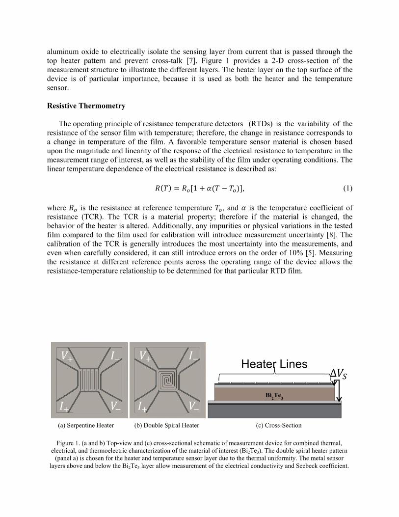
Figure 1. (a and b) Top-view and (c) cross-sectional schematic of measurement device for combined thermal, electrical, and thermoelectric characterization of the material of interest (Bi2Te3). The double spiral heater pattern

(panel a) is chosen for the heater and temperature sensor layer due to the thermal uniformity. The metal sensor layers above and below the Bi2Te3 layer allow measurement of the electrical conductivity and Seebeck coefficient.

(a) Serpentine Heater (b) Double Spiral Heater (c) Cross-Section

Bi2Te

3

Heater Lines Δ

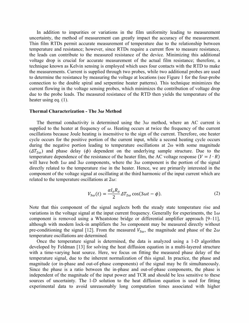
In addition to impurities or variations in the film uniformity leading to measurement uncertainty, the method of measurement can greatly impact the accuracy of the measurement. Thin film RTDs permit accurate measurement of temperature due to the relationship between temperature and resistance; however, since RTDs require a current flow to measure resistance, the leads can contribute to the measured resistance of the device. Minimizing this additional voltage drop is crucial for accurate measurement of the actual film resistance; therefore, a technique known as Kelvin sensing is employed which uses four contacts with the RTD to make the measurements. Current is supplied through two probes, while two additional probes are used to determine the resistance by measuring the voltage at locations (see Figure 1 for the four-probe connection to the double spiral and serpentine heater patterns). This technique minimizes the current flowing in the voltage sensing probes, which minimizes the contribution of voltage drop due to the probe leads. The measured resistance of the RTD then yields the temperature of the heater using eq. (1). Thermal Characterization - The 3 Method The thermal conductivity is determined using the 3 method, where an AC current is supplied to the heater at frequency of . Heating occurs at twice the frequency of the current oscillations because Joule heating is insensitive to the sign of the current. Therefore, one heater cycle occurs for the positive portion of the current input, while a second heating cycle occurs during the negative portion leading to temperature oscillations at 2ω with some magnitude ( ) and phase delay ( ) dependent on the underlying sample structure. Due to the temperature dependence of the resistance of the heater film, the AC voltage response ∙ will have both 1 and 3 components, where the 3 component is the portion of the signal directly related to the temperature rise in the heater. Hence, we are primarily interested in the component of the voltage signal at oscillating at the third harmonic of the input current which are related to the temperature oscillations at 2 :

2

cos 3 . (2)

Note that this component of the signal neglects both the steady state temperature rise and variations in the voltage signal at the input current frequency. Generally for experiments, the 1 component is removed using a Wheatstone bridge or differential amplifier approach [9–11], although with modern lock-in amplifiers the 3ω component may be measured directly without pre-conditioning the signal [12]. From the measured , the magnitude and phase of the 2 temperature oscillations are determined.

Once the temperature signal is determined, the data is analyzed using a 1-D algorithm developed by Feldman [13] for solving the heat diffusion equation in a multi-layered structure with a time-varying heat source. Here, we focus on fitting the measured phase delay of the temperature signal, due to the inherent normalization of this signal. In practice, the phase and magnitude (or in-phase and out-of-phase components) of the signal may be fit simultaneously. Since the phase is a ratio between the in-phase and out-of-phase components, the phase is independent of the magnitude of the input power and TCR and should be less sensitive to these sources of uncertainty. The 1-D solution to the heat diffusion equation is used for fitting experimental data to avoid unreasonably long computation times associated with higher

dimension solutions solved numerically with COMSOL. However, there can be errors in the extracted thermal conductivity due to the heater configuration deviating from 1-D. In this work, we optimize the heater structure for peak performance based on the simplified 1-D solution. This allows the data to be analyzed rather quickly using a MATLAB routine to process the information. Electrical Characterization Beyond thermal conductivity, the figure of merit ZT also depends on electrical and thermoelectric parameters. For accurate thermoelectric material characterization, it is crucial that the electrical parameters be determined at the same temperatures and in the same sample examined for the thermal conductivity. Determining the electrical conductivity of a material is generally accomplished by measuring the electrical resistance of the material. Inclusion of the palladium electrode layers in our sample, both above and below the thermoelectric material permits the in situ measurement of the cross-plane electrical conductivity without needing a separate sample, changing probes, or needing to reposition the sample from the thermal measurements. This allows data to be collected under identical conditions as the thermal data and should provide more accurate characterizations compared to using two separate samples for electrical and thermal characterization. Seebeck Coefficient The final parameter to be determined to compute the figure of merit is the Seebeck coefficient. Determining this parameter does not require additional modifications to the testing system because the Seebeck coefficient is found by measuring the voltage difference across the thermoelectric material at different applied heat fluxes. This allows us to utilize the same electrodes used in determining the electrical conductivity. While this method is straightforward and relatively simple, it cannot be performed simultaneously with the 3 technique because it requires a steady state heat flux. As an alternative to this method, some researchers have had success in using the sensor layers to measure the Seebeck voltage while conducting the 3 measurements in order to determine the Seebeck coefficient [7]. This simultaneous characterization is preferable, because it allows the experiments to be conducted under the exact same conditions. ZT Characterization The figure of merit can either be determined by combining the individual property measurement results or ZT can be measured directly [7,14]. The direct measurement of ZT is attractive for evaluating the performance of existing thermoelectric materials, because it is a single measurement instead of three separate measurements. The downside to a direct measurement of ZT is the lack of specific information about the individual properties, which is necessary for characterization and development of new materials.

NUMERICAL MODELS OF EXPERIMENTAL APPARATUS Simulations provide a valuable tool for investigating the impact of structural design parameters on the experimental results. Parametric analysis via simulation of the experiment provides feedback on the effectiveness of a particular design and permits a quantitative analysis of the sample design prior to fabrication. The primary focus for the simulations is to enhance the thermal characterization capabilities of the measurement structure. This is accomplished first through optimization of heater geometry to achieve better temperature uniformity within the sample layers and then simulating the frequency dependent response and analysis mimicking the 3 technique. The thermoelectric material is simulated with the heat capacity of bulk bismuth telluride and an estimated thermal conductivity of 1.2 W/(m K). Thermal properties of all other materials in the system are taken from the materials library in COMSOL.

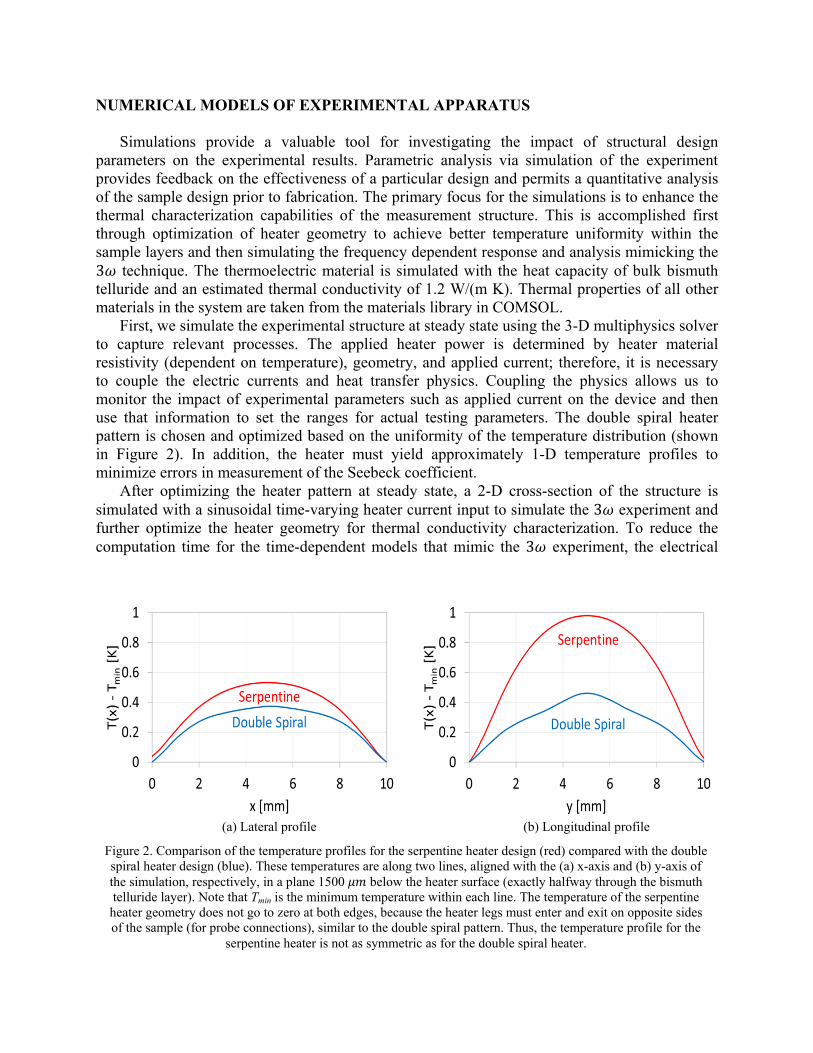
First, we simulate the experimental structure at steady state using the 3-D multiphysics solver to capture relevant processes. The applied heater power is determined by heater material resistivity (dependent on temperature), geometry, and applied current; therefore, it is necessary to couple the electric currents and heat transfer physics. Coupling the physics allows us to monitor the impact of experimental parameters such as applied current on the device and then use that information to set the ranges for actual testing parameters. The double spiral heater pattern is chosen and optimized based on the uniformity of the temperature distribution (shown in Figure 2). In addition, the heater must yield approximately 1-D temperature profiles to minimize errors in measurement of the Seebeck coefficient.

After optimizing the heater pattern at steady state, a 2-D cross-section of the structure is simulated with a sinusoidal time-varying heater current input to simulate the 3 experiment and further optimize the heater geometry for thermal conductivity characterization. To reduce the computation time for the time-dependent models that mimic the 3 experiment, the electrical

(a) Lateral profile (b) Longitudinal profile

Figure 2. Comparison of the temperature profiles for the serpentine heater design (red) compared with the double spiral heater design (blue). These temperatures are along two lines, aligned with the (a) x-axis and (b) y-axis of the simulation, respectively, in a plane 1500 below the heater surface (exactly halfway through the bismuth telluride layer). Note that Tmin is the minimum temperature within each line. The temperature of the serpentine heater geometry does not go to zero at both edges, because the heater legs must enter and exit on opposite sides of the sample (for probe connections), similar to the double spiral pattern. Thus, the temperature profile for the

serpentine heater is not as symmetric as for the double spiral heater.

model is decoupled from the thermal model and the heat generated is applied as a boundary condition:

12 ∙ cos 2 . (3)

Note that the steady state offset in the heat generation term is removed, which allows the system to reach a steady state oscillation in just a few heating cycles. Furthermore, this heat generation term neglects the temperature variation in resistance because it leads to a negligible change in heat generation rate if the temperature rise is small. As described above with regards to the experimental data, the thermal conductivity is extracted from the simulated data by fitting the measured phase delay of the temperature oscillations with a 1-D transient solution to the heat diffusion equation determined by using the Feldman algorithm.

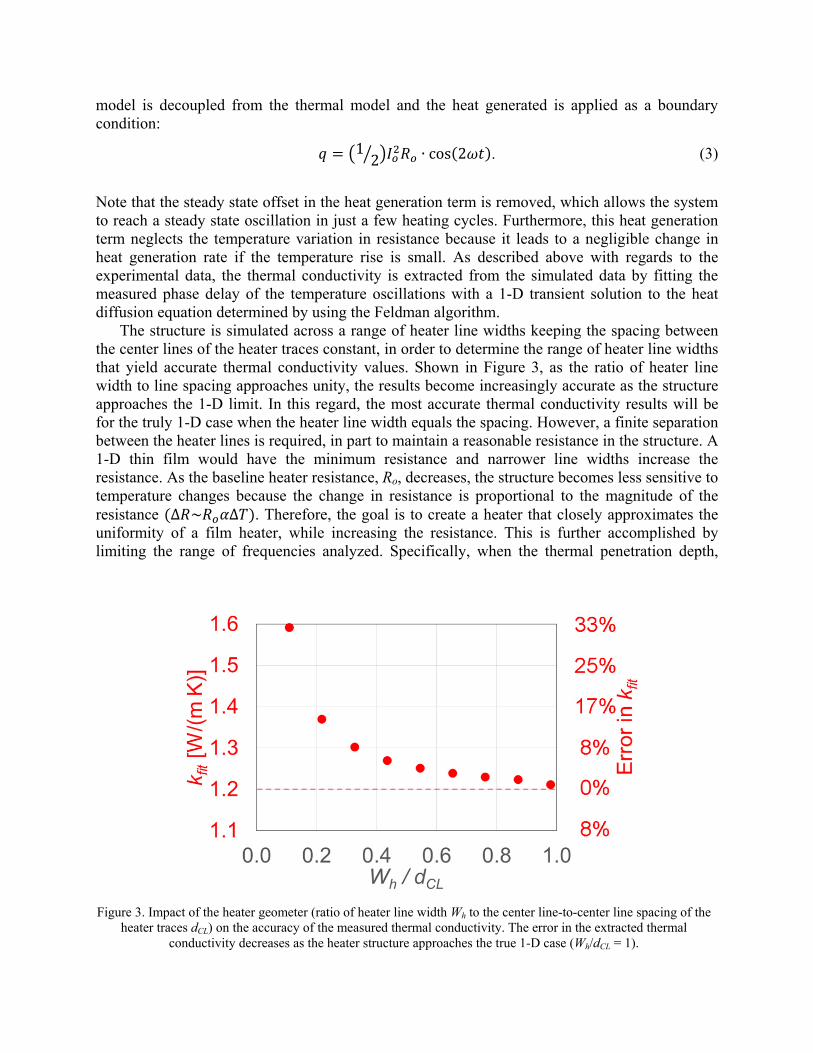
The structure is simulated across a range of heater line widths keeping the spacing between the center lines of the heater traces constant, in order to determine the range of heater line widths that yield accurate thermal conductivity values. Shown in Figure 3, as the ratio of heater line width to line spacing approaches unity, the results become increasingly accurate as the structure approaches the 1-D limit. In this regard, the most accurate thermal conductivity results will be for the truly 1-D case when the heater line width equals the spacing. However, a finite separation between the heater lines is required, in part to maintain a reasonable resistance in the structure. A 1-D thin film would have the minimum resistance and narrower line widths increase the resistance. As the baseline heater resistance, Ro, decreases, the structure becomes less sensitive to temperature changes because the change in resistance is proportional to the magnitude of the resistance Δ ~ Δ . Therefore, the goal is to create a heater that closely approximates the uniformity of a film heater, while increasing the resistance. This is further accomplished by limiting the range of frequencies analyzed. Specifically, when the thermal penetration depth,

Figure 3. Impact of the heater geometer (ratio of heater line width Wh to the center line-to-center line spacing of the heater traces dCL) on the accuracy of the measured thermal conductivity. The error in the extracted thermal

conductivity decreases as the heater structure approaches the true 1-D case (Wh/dCL = 1).

( ~ / , where αth is the thermal diffusivity of the sample) is small compared to the heater line width, the structure approximates the 1-D case despite lateral diffusion from the edge of the heater line.

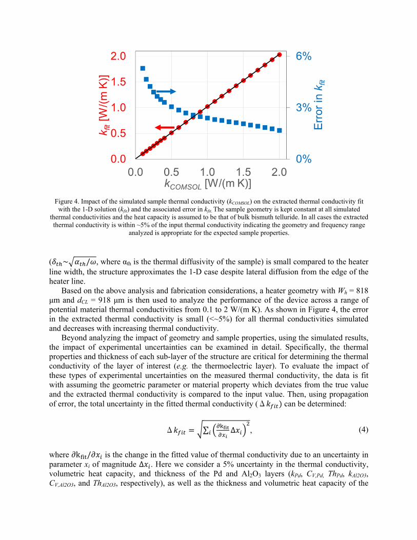
Based on the above analysis and fabrication considerations, a heater geometry with Wh = 818 μm and dCL = 918 μm is then used to analyze the performance of the device across a range of potential material thermal conductivities from 0.1 to 2 W/(m K). As shown in Figure 4, the error in the extracted thermal conductivity is small (<~5%) for all thermal conductivities simulated and decreases with increasing thermal conductivity.

Beyond analyzing the impact of geometry and sample properties, using the simulated results, the impact of experimental uncertainties can be examined in detail. Specifically, the thermal properties and thickness of each sub-layer of the structure are critical for determining the thermal conductivity of the layer of interest (e.g. the thermoelectric layer). To evaluate the impact of these types of experimental uncertainties on the measured thermal conductivity, the data is fit with assuming the geometric parameter or material property which deviates from the true value and the extracted thermal conductivity is compared to the input value. Then, using propagation of error, the total uncertainty in the fitted thermal conductivity (Δ can be determined:

Δ ∑ Δ , (4)

where ∂k / is the change in the fitted value of thermal conductivity due to an uncertainty in parameter xi of magnitude Δ . Here we consider a 5% uncertainty in the thermal conductivity, volumetric heat capacity, and thickness of the Pd and Al2O3 layers (kPd, CV,Pd, ThPd, kAl2O3, CV,Al2O3, and ThAl2O3, respectively), as well as the thickness and volumetric heat capacity of the

Figure 4. Impact of the simulated sample thermal conductivity (kCOMSOL) on the extracted thermal conductivity fit with the 1-D solution (kfit) and the associated error in kfit. The sample geometry is kept constant at all simulated

thermal conductivities and the heat capacity is assumed to be that of bulk bismuth telluride. In all cases the extracted thermal conductivity is within ~5% of the input thermal conductivity indicating the geometry and frequency range

analyzed is appropriate for the expected sample properties.

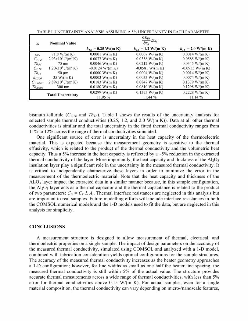
bismuth telluride (CV,TE and ThTE). Table I shows the results of the uncertainty analysis for selected sample thermal conductivities (0.25, 1.2, and 2.0 W/(m K)). Data at all other thermal conductivities is similar and the total uncertainty in the fitted thermal conductivity ranges from 11% to 12% across the range of thermal conductivities simulated.

One significant source of error is uncertainty in the heat capacity of the thermoelectric material. This is expected because this measurement geometry is sensitive to the thermal effusivity, which is related to the product of the thermal conductivity and the volumetric heat capacity. Thus a 5% increase in the heat capacity is reflected by a ~5% reduction in the extracted thermal conductivity of the layer. More importantly, the heat capacity and thickness of the Al2O3 insulation layer play a significant role in the uncertainty in the measured thermal conductivity. It is critical to independently characterize these layers in order to minimize the error in the measurement of the thermoelectric material. Note that the heat capacity and thickness of the Al2O3 layer impact the extracted data in a similar manner because, in this sample configuration, the Al2O3 layer acts as a thermal capacitor and the thermal capacitance is related to the product of two parameters: Cth = CV L As. Thermal interface resistances are neglected in this analysis but are important to real samples. Future modelling efforts will include interface resistances in both the COMSOL numerical models and the 1-D models used to fit the data, but are neglected in this analysis for simplicity. CONCLUSIONS

A measurement structure is designed to allow measurement of thermal, electrical, and thermoelectric properties on a single sample. The impact of design parameters on the accuracy of the measured thermal conductivity, simulated using COMSOL and analyzed with a 1-D model, combined with fabrication consideration yields optimal configurations for the sample structures. The accuracy of the measured thermal conductivity increases as the heater geometry approaches a 1-D configuration; however, for line widths as small as one half the heater line spacing, the measured thermal conductivity is still within 5% of the actual value. The structure provides accurate thermal measurements across a wide range of thermal conductivities, with less than 5% error for thermal conductivities above 0.15 W/(m K). For actual samples, even for a single material composition, the thermal conductivity can vary depending on micro-/nanoscale features,

xi Nominal Value

kTE = 0.25 W/(m K) kTE = 1.2 W/(m K) kTE = 2.0 W/(m K) kPd 71.8 W/(m K) 0.0001 W/(m K) 0.0007 W/(m K) 0.0014 W/(m K)

CV,Pd 2.93x106 J/(m3 K) 0.0077 W/(m K) 0.0358 W/(m K) 0.0585 W/(m K) ThPd 75 nm 0.0046 W/(m K) 0.0212 W/(m K) 0.0345 W/(m K) CV,TE 1.20x106 J/(m3 K) -0.0124 W/(m K) -0.0581 W/(m K) -0.0955 W/(m K) ThTE 50 μm 0.0000 W/(m K) 0.0004 W/(m K) 0.0014 W/(m K) kAl2O3 35 W/(m K) 0.0003 W/(m K) 0.0033 W/(m K) 0.0074 W/(m K)

CV,Al2O3 2.89x106 J/(m3 K) 0.0183 W/(m K) 0.0847 W/(m K) 0.1379 W/(m K) ThAl2O3 300 nm 0.0180 W/(m K) 0.0810 W/(m K) 0.1298 W/(m K)

Total Uncertainty 0.0299 W/(m K) 0.1373 W/(m K) 0.2228 W/(m K)

11.95 % 11.44 % 11.14 %

TABLE I. UNCERTAINTY ANALYSIS ASSUMING A 5% UNCERTAINTY IN EACH PARAMETER

manufacturing processes, and impurities; this analysis shows that comparisons between samples will be accurate.

In this work, we focused on characterization of thermoelectric materials; however, this system is equally suited for investigation of many other materials systems. The robustness of this measurement structure makes it favorable as a standard platform for thermal and electrical characterization of materials across many different applications. Such standardization is beneficial for measurements because it reduces the differences in sources of experimental error, and lends to a more thorough understanding of the performance of the actual material of interest without unknown effects from the measurement structure. The parametric design study presented here should serve as a reference when designing similar measurement structures for other applications. While this study centers primarily on the optimization of the thermal characterization capabilities of the measurement structure, there are additional aspects of the design yet to be considered. Incorporation of radiation and convection losses into the model will further enhance the model and enable quantification of heater powers necessary to minimize thermal losses. Additionally, confining the material of interest to a region directly beneath the heater, while insulating the sides, should reduce spreading effects yielding a more uniform temperature profile. REFERENCES [1] D.M. Rowe, “CRC Handbook of Thermoelectrics,” New York, vol. 16, 1995, pp. 1251–1256. [2] H. Bougrine and M. Ausloos, “Highly sensitive method for simultaneous measurements of thermal

conductivity and thermoelectric power: Fe and Al examples,” Review of Scientific Instruments, vol. 66, 1995, p. 199.

[3] Y. Zhang, C.L. Hapenciuc, E.E. Castillo, T. Borca-Tasciuc, R.J. Mehta, C. Karthik, and G. Ramanath, “A microprobe technique for simultaneously measuring thermal conductivity and Seebeck coefficient of thin films,” Applied Physics Letters, vol. 96, 2010, p. 062107.

[4] B. Yang, J.L. Liu, K.L. Wang, and G. Chen, “Simultaneous measurements of Seebeck coefficient and thermal conductivity across superlattice,” Applied Physics Letters, vol. 80, 2002, p. 1758.

[5] J.S. Sadhu, T. Hongxiang, J. Ma, J. Kim, and S. Sinha, “Simultaneous Measurements of Thermal Conductivity and Seebeck Coefficients of Roughened Nanowire Arrays,” Materials Research Society2, vol. 1456.

[6] L. Shi, D. Li, C. Yu, W. Jang, D. Kim, Z. Yao, P. Kim, and A. Majumdar, “Measuring Thermal and Thermoelectric Properties of One-Dimensional Nanostructures Using a Microfabricated Device,” Journal of Heat Transfer, vol. 125, Oct. 2003, p. 881.

[7] R. Singh, Z. Bian, A. Shakouri, G. Zeng, J.-H. Bahk, J.E. Bowers, J.M.O. Zide, and A.C. Gossard, “Direct measurement of thin-film thermoelectric figure of merit,” Applied Physics Letters, vol. 94, 2009, p. 212508.

[8] J. Fraden, Handbook of Modern Sensors: Physics, Designs, and Applications, Springer, 2004. [9] L.A. Rosenthal, “Thermal Response of Bridgewires used in Electroexplosive Devices,” Review of Scientific

Instruments, vol. 32, Dec. 1961, p. 1033. [10] N.O. Birge and S.R. Nagel, “Wide-frequency specific heat spectrometer,” Review of Scientific Instruments,

vol. 58, Aug. 1987, p. 1464. [11] D.G. Cahill, “Thermal conductivity measurement from 30 to 750 K: the 3ω method,” Review Of Scientific

Instruments, vol. 61, 1990, pp. 802–808. [12] C. Dames, “Measuring the Thermal Conductivity of Thin Films: 3 Omega and Related Electrothermal

Methods,” Annual Review of Heat Transfer, vol. 16, 2013, pp. 7–49. [13] A. Feldman, “Algorithm for solutions of the thermal diffusion equation in a stratified medium with a

modulated heating source,” High Temperatures - High Pressures, vol. 31, 1999, pp. 293–298. [14] T.C. Harman, “Special Techniques for Measurement of Thermoelectric Properties,” Journal of Applied

Physics, vol. 29, 1958, p. 1373.