Simulated pre-industrial climate in Bergen Climate Model (version 2): model description and...

Geosci. Model Dev., 2, 197–212, 2009www.geosci-model-dev.net/2/197/2009/© Author(s) 2009. This work is distributed underthe Creative Commons Attribution 3.0 License.

GeoscientificModel Development

Simulated pre-industrial climate in Bergen Climate Model(version 2): model description and large-scale circulation features

O. H. Otter a1,2, M. Bentsen1,2, I. Bethke1,2, and N. G. Kvamstø2,3

1Nansen Environmental and Remote Sensing Center, Thormøhlensgt. 47, 5006 Bergen, Norway2Bjerknes Centre for Climate Research, Allegt. 55, 5007 Bergen, Norway3Geophysical Institute, University of Bergen, Allegt. 70, 5007 Bergen, Norway

Received: 28 April 2009 – Published in Geosci. Model Dev. Discuss.: 14 May 2009Revised: 9 September 2009 – Accepted: 15 September 2009 – Published: 11 November 2009

Abstract. The Bergen Climate Model (BCM) is a fully-coupled atmosphere-ocean-sea-ice model that provides state-of-the-art computer simulations of the Earth’s past, present,and future climate. Here, a pre-industrial multi-century sim-ulation with an updated version of BCM is described andcompared to observational data. The model is run withoutany form of flux adjustments and is stable for several cen-turies. The simulated climate reproduces the general large-scale circulation in the atmosphere reasonably well, exceptfor a positive bias in the high latitude sea level pressure dis-tribution. Also, by introducing an updated turbulence schemein the atmosphere model a persistent cold bias has been elim-inated. For the ocean part, the model drifts in sea surfacetemperatures and salinities are considerably reduced com-pared to earlier versions of BCM. Improved conservationproperties in the ocean model have contributed to this. Fur-thermore, by choosing a reference pressure at 2000 m andincluding thermobaric effects in the ocean model, a more re-alistic meridional overturning circulation is simulated in theAtlantic Ocean. The simulated sea-ice extent in the NorthernHemisphere is in general agreement with observational dataexcept for summer where the extent is somewhat underesti-mated. In the Southern Hemisphere, large negative biases arefound in the simulated sea-ice extent. This is partly related toproblems with the mixed layer parametrization, causing themixed layer in the Southern Ocean to be too deep, which inturn makes it hard to maintain a realistic sea-ice cover here.However, despite some problematic issues, the pre-industrialcontrol simulation presented here should still be appropriatefor climate change studies requiring multi-century simula-tions.

Correspondence to:O. H. Ottera([email protected])

1 Introduction

The recently published Intergovernmental Panel of ClimateChange report (IPCC AR4) has raised global awareness onclimate change issues considerably. Consequently, there isnow a growing concern over the ongoing and possible futureenvironmental changes depicted in the IPCC reports. Themany different projections of possible future climate changesdescribed in the IPCC reports are made possible by the useof numerical models of the earth system. The improvementsin state-of-the-art climate models have increased our confi-dence in their ability to simulate future climate change. How-ever, the models still show significant differences, both interms of the simulated climate change and more fundamentalaspects of the representation of internal processes and feed-backs. Although, an accurate simulation of the current cli-mate represents an important achievement, it does not guar-antee that a model will correctly simulate climatic conditionsvery different from that of the present, such as, for exam-ple, those due to increasing greenhouse gas concentrations.Past climates may provide useful tests for GCMs by enablinga comparison between model simulations and paleoclimaticreconstructions, and thereby providing a means of assessingtheir capability to simulate past changes of climate.

The original version of Bergen Climate Model (BCM)first described byFurevik et al.(2003), is a global fully-coupled atmosphere-ocean-sea-ice general circulation modelthat has been used for a range of climate change studies in re-cent years (Bentsen et al., 2004; Ottera et al., 2004; Mignotand Frankignoul, 2004; Sorteberg et al., 2005; Bethke et al.,2006; Yu et al., 2008). The main model modules in BCMare the ARPEGE-CLIMAT atmospheric general circulationmodel (Deque et al., 1994) and a modified version of MiamiIsopycnic Coordinate Ocean Model (MICOM,Bleck et al.1992). In the second version of BCM (hereafter referred

Published by Copernicus Publications on behalf of the European Geosciences Union.

http://creativecommons.org/licenses/by/3.0/

198 O. H. Ottera et al.: Simulated pre-industrial climate in BCM

to as BCM2) presented here, MICOM has been coupled tothe GELATO (Salas-Melia, 2002) dynamic and thermody-namic sea-ice model. In addition, MICOM has been mod-ified in a number of ways since the original version of themodel. These changes include among other things a newpressure gradient formulation and the introduction of incre-mental remapping for tracer advection, which has improvedthe ocean circulation in many respects compared to the orig-inal version of the model.

The aim of this paper is to give an overview of BCM2 andpresent results from a multi-century run for pre-industrialtimes. The mean climate states of the atmosphere, oceanand sea-ice for this period are described and validated againstavailable observations. Another multi-century pre-industrialsimulation with BCM2 that incorporates an intermediatecomplexity terrestrial and oceanic carbon cycle model, hasalso been carried out. Results from this simulation will bepresented in a separate paper (Tjiputra et al., 2009). In thisstudy, however, the carbon cycle model has not been in-cluded. The paper is organized as follows: in Sect. 2 thedifferent model components are described in more detail. InSect. 3 the spin-up procedures and design of the experimentare presented. The results are given in Sect. 4. Finally, theresults are discussed and summarized in Sect. 5.

2 Model description

2.1 The atmosphere model

The atmosphere component is the spectral atmospheric gen-eral circulation model ARPEGE-CLIMAT3 from METEOFRANCE (Deque et al., 1994). The ARPEGE version ap-plied in this study is described in detail inFurevik et al.(2003). However, its major features are briefly summarizedhere. In ARPEGE, the representation of most model vari-ables is spectral (i.e. scalar fields are decomposed on a trun-cated basis of spherical harmonic functions). In the presentstudy, ARPEGE is run with a truncation at wave number 63(TL63), and a time step of 1800 s. All the physics and thetreatment of model nonlinear terms require spectral trans-forms to a Gaussian grid. This grid (about 2.8◦ resolutionin longitude and latitude) is reduced near the poles to give anapproximately uniform horizontal resolution (on the targetsphere) and to save computational time. The vertical hybridcoordinate follows the topography in the lower troposphere,but becomes gradually parallel to pressure surfaces with in-creasing height. In this study, a total of 31 vertical levels areemployed, ranging from the surface to 0.01 hPa.

The physical parametrization is divided into several ex-plicit schemes, each calculating the flux of mass, energyand/or momentum due to a specific physical process. Dif-ferences from the model description inDeque et al.(1994)include a convective gravity drag parametrization (Bossuetet al., 1998), a new snow scheme (Douville et al., 1995), a re-

fined orographic gravity wave drag scheme (Lott and Miller,1997; Lott, 1999; Catry et al., 2008) and modifications indeep convection and soil vegetation schemes.

The vertical diffusion scheme is a first order eddy-viscosity scheme (Louis, 1979; Louis et al., 1982; Geleyn,1988), which is popular in global models because of its sim-plicity and physical clarity. In the original version of thescheme a feedback could be activated in the case of a verycold surface. A cooling surface involved an increase in thestability, which in turn would prevent any heating by the at-mosphere. This would accelerate the cooling until reaching aradiative balance which could be very cold in the polar night.This phenomenon led to a significant cold bias in the globaltemperature in earlier versions of BCM. To avoid the phe-nomenon a limitation has been added to the Richardson num-ber:

if Ri>0 then Ri←Ri

1+Ri/Ricrand Uric=

1

Ricr,

whereRicr is an upper limit for positive Richardson num-bers. The standard value forUric is 0, which comes to notapplying the above limitation. In the present version of BCMa value of 1.2 is used forUric.

In ARPEGE there is a mass drift due to the non-conservative form of the discretized continuity equation(M. Deque, personal communication, 2009). In order tocorrect for this the following method has been used: every6 h the partial pressure of dry air averaged over the globeis calculated. This value is then compared with the value983.2 hPa, which is the ERA40 average value. The difference(loss or gain of mass) is then added to the surface pressureuniformly (less than 0.1 hPa per month). With this correctiontotal air mass can have a seasonal cycle or a long-term drift(due to variations in water vapor content), but no drift due tonon-conservation due to the equation. The drawback, how-ever, is the unform correction, since the sources and sinksmay be local.

The ARPEGE model includes the effect of differentkinds of aerosols: continental, marine (due to emissionsof sea salt), desert dust, black carbon, tropospheric sul-phate aerosols and stratospheric aerosols (due to volcaniceruptions). The horizontal distribution of the first four areheld constant at their default values which are defined ac-cording toTanre et al.(1984). The concentrations of sul-phate aerosols are set at pre-industrial 1850 values basedon data provided for byBoucher and Pham(2002) for theIPCC AR4 simulations. The direct effect of all these aerosoltypes has been taken into account, but no indirect effectshave been considered in this version of the model. Vol-canic aerosols have been implemented into the model, andstandard Mount Pinatubo test simulations have been carriedout (Ottera, 2008). These experiments reveal that the at-mospheric circulation in ARPEGE reacts realistically to im-posed volcanic aerosols. In this study, however, the strato-spheric aerosols are kept constant at their default backgroundvalues.

Geosci. Model Dev., 2, 197–212, 2009 www.geosci-model-dev.net/2/197/2009/

O. H. Ottera et al.: Simulated pre-industrial climate in BCM 199

2.2 The ocean model

The numerical methods and thermodynamics of MICOMare documented inBleck and Smith(1990) andBleck et al.(1992). In the version of MICOM used in this study, severalimportant aspects deviate from the original model and theone used in the original version of BCM (i.e.Furevik et al.,2003). The original MICOM uses potential density with ref-erence pressure at 0 db as vertical coordinate (σ0-coordinate).This ensures that the very different flow and mixing char-acteristic in neutral and dia-neutral directions is well repre-sented near the surface since isopycnals and neutral surfacesare similar near the reference pressure. For pressures that dif-fer substantially from the reference pressure, this conditiondoes not hold. In this study, a reference pressure of 2000 db isused. The non-neutrality of the isopycnals in the world oceanis then reduced compared to having the reference pressure atthe surface (McDougall and Jackett, 2005).

Furthermore, for the advection of tracers (potential tem-perature, salinity and passive tracers) and layer thickness,the current version of MICOM uses incremental remapping(Dukowicz and Baumgardner, 2000) adapted to the grid stag-gering of MICOM. The algorithm is computationally ratherexpensive compared to other second order methods with lim-iters for one tracer or age tracer, but the cost of adding addi-tional tracers and age tracers is modest. In contrast to theoriginal transport methods of MICOM, incremental remap-ping ensures monotonicity of the tracers.

Traditionally, MICOM expresses the pressure gradientforce as a gradient of a potential on an isopycnic surface, assuch a formulation has favorable numerical properties (Hsuand Arakawa, 1990). This is only accurate if the density canbe considered as a function of potential density and pressurealone, which is not the case (de Szoeke, 2000). There havebeen several attempts to modify the MICOM pressure gradi-ent formulation in order to incorporate a more accurate rep-resentation of density (Sun et al., 1999; Hallberg, 2005). Theformulation used in the new version of MICOM, is based onthe formulation ofJanic(1977) where the pressure gradientis expressed as a gradient of the geopotential on a pressuresurface. This allows a more accurate representation of den-sity in the pressure gradient formulation.

The treatment of diapycnal mixing follows the standardMICOM approach of a background diffusivity dependent onthe local stability and implemented using the scheme ofMc-Dougall and Dewar(1998). To incorporate shear instabilityand gravity current mixing, a Richardson number dependentdiffusivity has been added to the background diffusivity. Thishas greatly improved the water mass characteristics down-stream of overflow regions. Lateral turbulent mixing of mo-mentum and tracers is parameterized by Laplacian diffusion,and layer interfaces are smoothed with biharmonic diffusion.

With the exception of the equatorial region, the ocean gridis almost regular with horizontal grid spacing approximately2.4◦×2.4◦. In order to better resolve the dynamics near the

Equator, the horizontal spacing in the meridional direction isgradually decreased to 0.8◦ along the Equator. The modelhas a stack of 34 isopycnic layers in the vertical, with po-tential densities ranging from 1029.514 to 1037.800 kg m−3,and a non-isopycnic surface mixed layer on top providing thelinkage between the atmospheric forcing and the ocean inte-rior.

2.3 The sea-ice model

There are currently two dynamic and thermodynamic sea-icemodules available for BCM2, both of which are handled assubroutine calls from MICOM. Originally, the sea-ice modeldeveloped at Nansen Environmental and Remote SensingCenter (NERSC) was used. This model consists of one iceand one snow layer assuming a linear temperature profile ineach layer, and the thermodynamics followsDrange and Si-monsen(1996). The dynamic part of the model is based onthe viscous-plastic rheology ofHibler (1979) with the modi-fications and implementation ofHarder(1996).

The sea-ice model used in this study, however, isGELATO, a sea-ice model that was developed at METEOFRANCE and described in detail bySalas-Melia(2002).As opposed to the original NERSC model, GELATO is amulti-category sea-ice model (thickness dependent), allow-ing a more precise treatment of thermodynamics. Specifi-cally, growth rates of ice slabs of different thicknesses, sub-jected to the same oceanic and atmospheric forcings, canvary considerably from one category to another. Within agrid cell, sea-ice is described as a collection of ice slabs, andeach slab is described by its thickness, the fraction of the gridcell it covers, its enthalpy, and the amount of snow coveringit. For every thickness category the model computes sea-icevelocities solving the stress tensor as described inHunke andDukowicz(1997) and then applies a non-diffusive advectionscheme that conserves the first and second moments of theadvected fields (Prather, 1986). Redistribution of sea-ice dueto rafting and ridging processes is simulated according to thetheory developed byThorndike et al.(1975).

In order to model vertical heat diffusion in an ice-snowslab, a vertical discretization is defined, considering four lay-ers in the ice part of the slab and one level snow. Solving ofthis diffusion scheme is implicit in time. All model equationsare solved on an Arakawa B-grid which shares its grid pointswith the C-grid of the ocean model. A linear interpolationbetween the two grids is performed internally by the sea-icemodel.The rest of the thermodynamics, including snow agingscheme is treated explicitly (Salas-Melia, 2002).

2.4 The coupler

The OASIS coupler (version 2.2) has been used to couple theatmosphere and ocean models. It was developed at the Na-tional centre for climate modeling and global change (CER-FACS), Toulouse, France (Terray and Thual, 1995; Terray

www.geosci-model-dev.net/2/197/2009/ Geosci. Model Dev., 2, 197–212, 2009


Table 1. List of variables that are being exchanged via the coupler,OASIS2.2.

Ocean-Atmosphere Atmosphere-Ocean

sea surface temperature non-solar heat fluxsea ice extent solar heat fluxalbedo total water fluxzonal sea surface velocity runoffmeridional sea surface velocity albedo

zonal wind stressmeridional wind stressnon-solar heat flux derivativeliquid precipitationsolid precipitationsurface temperaturetotal cloud cover

et al., 1995), and is currently in use in many climate centers.The main tasks of OASIS are to synchronize the models, sothe fastest running model can wait for the other model un-til they are both integrated a prescribed time interval (1 day);to read the exchange fields from the source model; to applyweight coefficients for the interpolations; and to finally writethe new fields to the target model. A list of the fields beingexchanged via the coupler is given in Table1.

3 Experimental design

The initialization of coupled atmosphere-ocean climate mod-els for historical simulations has been a long-standing prob-lem in the climate model development communities. In par-ticular, obtaining initial conditions for the ocean is quite achallenge since world-wide observational oceanic measure-ments are only available for near present-day. One techniquethat has often been used to initialize pre-industrial controlsimulations, is to reset the radiative forcing to near 1850 con-ditions using near present day Levitus oceanic initial condi-tions. However, a model coupled in this manner will, in gen-eral, suffer from climate drifts. In this study, we therefore usea method similar to the one outlined inStouffer et al.(2004),where the radiative forcing was run backwards in time fromthe present to pre-industrial (1850) levels, and then held con-stant at this level for 3–5 centuries. One of the advantagesof this method compared to other methods is that it gener-ates internally consistent pre-industrial conditions within theframework of the model (Stouffer et al., 2004).

The initial conditions for the pre-industrial (PI) controlintegration are obtained from the end of a 500 years, four-phase spin-up integration. In the first phase of the spin-upthe ocean and sea-ice model were integrated together for ap-proximately 100 years, forced with two consecutive cyclesof daily NCEP/NCAR reanalysis fields (Kalnay et al., 1996).The ocean was initialized with a climatological present-day

hydrography (Steele et al., 2001) while the sea-ice was ini-tialized with a climatological sea-ice extent and a constantthickness of one meter. The surface salinity was kept closeto observations, while there was no adjustment of sea surfacetemperatures. The purpose of using a restart from an ocean-sea-ice spin-up was to avoid initializing the coupled modelwith an ocean at rest.

In the second phase, the coupled system was initializedwith the final state of the ocean-sea-ice spin-up combinedwith an atmospheric state that was obtained from the endof a multi-year simulation with the atmosphere-only model.The model is not sensitive to the atmospheric initial condi-tion, as the atmosphere equilibrates with the upper oceanon a relatively rapid time scale. Once coupled, the modelwas run without any form of flux adjustment on neitherheat nor freshwater. The coupled system was then inte-grated for 200 years with constant, present-day (2000 AD)radiative conditions and with a solar constant value set at1370 W m−2, which is somewhat higher than what is ob-served (about 1366 W m−2). However, in earlier runs withBCM2 a poor low-level atmospheric circulation (i.e. anoma-lously high pressure in the high northern regions describedbelow) partly contributed to an excessive NH sea-ice extentin the model. In order to remedy this, the default value ofthe solar constant was increased from 1365 to 1370 W m−2.Even though this will likely not change the variability of thesystem, the use of a more physically accepted solar constantvalue is better and will be used in future development of themodel system. Other forcings, such as the ice sheet topogra-phy, coastlines, soil and vegetation fields were all prescribedat present-day values.

In the third phase, following the method outlined inStouf-fer et al.(2004), the radiative forcing conditions were thengradually changed to pre-industrial (1850 AD) values over aperiod of 50 years and then kept constant thereafter. Here,radiative forcings refer to changes in the trace gases only.The orbital parameters were prescribed to the reference val-ues of 1950 AD. In the final spin-up phase the model wasrun for a further 150 years to allow the simulated climate toadjust, at least partially, to the new forcing regime. Theselast 150 years of the spin-up are discarded and not part ofthe analysis shown below. Thus, what is labeled as year 1of the PI control simulation corresponds to a time 200 yearsafter the gradual decrease in the radiative forcings were firstintroduced.

4 Results

A necessary condition for a reliable GCM prediction of re-gional climate change is that the control simulation should befairly realistic. If features are positioned incorrectly, then anysimulated shifts in these features may also be incorrect. Here,the control simulation for pre-industrial climate is assessedby comparison with climatological data. Climatological



estimates are subject to errors due, among other things, toinadequate temporal or spatial sampling, observational bi-ases, and different periods of observation. Thus, there maybe substantial differences between climatologies, particularlyin data-sparse regions.

4.1 Model stability and climate drift

After coupling the model components and starting from theset of initial conditions (see previous section), the climatesystem is typically not in equilibrium, and undergoes a drifttoward a more equilibrated state. The time series of global-mean SST is plotted in Fig.1a. The model experiences driftfor a considerable time during the integration, with a warm-ing trend of about 0.05 degrees per century. As will be shownbelow this warming trend is related to a persistent positive ra-diative imbalance in the model. Thus, time series of global-mean surface air temperature (not shown) show a very similarbehavior.

Another measure of the drift is the top-of-the-atmosphere(TOA) net radiative imbalance (incoming shortwave – outgo-ing longwave) shown in Fig.1b. There is a persistent positiveimbalance of about 2.5 W m−2, indicating a net long-termgain of heat by the system. At the surface there is a net ra-diative imbalance (incoming shortwave – outgoing longwave– sensible heat – latent heat) of about 0.5 W m−2 (Fig. 1c).The radiation values gradually decrease over time as the sys-tem approaches a more equilibrated state. The radiative im-balance values are smaller at the surface than at the TOA(Fig. 1b and c). This is largely due to the fact that the atmo-spheric dynamics in ARPEGE does not conserve energy (seeabove), and loses heat at a rate of approximately 2 W m−2.However, since this loss is quite uniform in time, it is notexpected to be a significant issue in climate change experi-ments.

The heat imbalance at the surface is related to the timeseries of volume-mean ocean temperature averaged over theglobe shown in Fig.1d. There are small subsurface drifts(about 0.03 K per century) throughout the integration, reflect-ing the heat stored in the ocean, and it will likely take manycenturies for the full-depth ocean to come into equilibrium.

The evolution of global sea surface salinity (SSS) overthe 600 year integration period is shown in Fig.2. In themodel the water cycle budget is not entirely closed. Thereis therefore a drift towards higher global-mean salinity dur-ing the whole integration. The overall drift is about 0.01 psuper century for the whole 600 year integration. Over 80% ofthis drift is balanced by growth of the Greenland and Antarc-tic ice sheets due to the absence of a calving scheme in themodel. The remainder is likely due to the non-conservationof mass in the atmospheric model. Both the SST and SSSdrifts are considerably reduced in the new version of BCMcompared to the older version of the model (Furevik et al.,2003), despite the fact the older version used flux adjust-ments on both heat and freshwater. Several factors have con-

18.2

18.4

18.6

18.8

19

19.2

o C

(a) SST

1.5

1.9

2.3

2.7

3.1

3.5

W m

−2

(b) NET RAD TOA

−0.4

0

0.4

0.8

1.2

1.6

W m

−2

(c) Sfc Heat Flux

0 100 200 300 400 500 6003.7

3.8

3.9

4

4.1

4.2

Time (yr)

o C

(d) Ocean Temp

Fig. 1. Time series of annual-mean, global-mean quantities for thePI simulation. (a) SST, (b) TOA net radiative imbalance,(c) netheat flux at the surface, and(d) volume-mean temperature for thefull-depth global ocean. The grey lines are annual-mean values, andthe thick black lines are 10-year running means.

Time (yr)

SS

S (

psu)

Global Mean Sea Surface Salinity

0 100 200 300 400 500 60034.7

34.8

34.9

35

35.1

Fig. 2. Time series of annual-mean global-mean SSS (psu). Theshaded region represents the spread of the monthly-mean data,while the thick black line is the 5-year running mean.

tributed to this, but improved conservation properties in theocean model, MICOM, is probably the most important one.

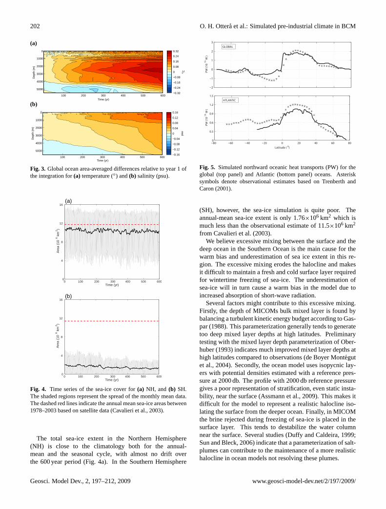
The vertical distribution of the temperature and salinity bi-ases (differences relative to year 1) of the global ocean isshown in Fig.3. Generally the ocean becomes warmer andmore saline during the integration. The radiative imbalanceat the surface is likely the main reason for the warming trend.This imbalance will add heat to the deep ocean through con-vective mixing at high latitudes which will then gradually bespread around the globe by the thermohaline circulation. Be-low 4000 m it is interesting to note a cooling and a fresheningearly in the simulation, possibly indicating a changed stratifi-cation in the very deep ocean. This is not surprising as it willtake many centuries for the deep ocean to reach equilibrium.



(a)

o C

−0.32

−0.24

−0.16

−0.08

0

0.08

0.16

0.24

0.32

Time (yr)

Dep

th (

m)

100 200 300 400 500 600

0

1000

2000

3000

4000

5000

psu

−0.16

−0.12

−0.08

−0.04

0

0.04

0.08

0.12

0.16(b)

Time (yr)

Dep

th (

m)

100 200 300 400 500 600

0

1000

2000

3000

4000

5000

(b)

o C

−0.32

−0.24

−0.16

−0.08

0

0.08

0.16

0.24

0.32(a)

Time (yr)

Dep

th (

m)

100 200 300 400 500 600

0

1000

2000

3000

4000

5000

psu

−0.16

−0.12

−0.08

−0.04

0

0.04

0.08

0.12

0.16

Time (yr)

Dep

th (

m)

100 200 300 400 500 600

0

1000

2000

3000

4000

5000

Fig. 3. Global ocean area-averaged differences relative to year 1 ofthe integration for(a) temperature (◦) and(b) salinity (psu).

16 OTTERA ET AL.: SIMULATED PRE-INDUSTRIAL CLIMATE IN BCM

Time (yr)

Are

a (1

06 k

m2 )

0 100 200 300 400 500 6000

4

8

12

16

Time (yr)

Are

a (1

06 k

m2 )

0 100 200 300 400 500 6000

4

8

12

16

(a)

(b)

Fig. 4. Time series of the sea-ice cover for (a) NH, and (b) SH. The shaded regions represent the spread of the monthly mean data. Thedashed red lines indicate the annual mean sea-ice areas between 1978-2003 based on satellite data (Cavalieri et al., 2003).

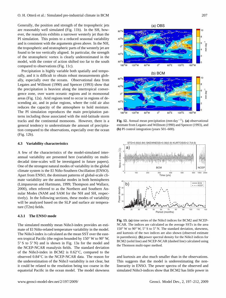
Fig. 4. Time series of the sea-ice cover for(a) NH, and (b) SH.The shaded regions represent the spread of the monthly mean data.The dashed red lines indicate the annual mean sea-ice areas between1978–2003 based on satellite data (Cavalieri et al., 2003).

The total sea-ice extent in the Northern Hemisphere(NH) is close to the climatology both for the annual-mean and the seasonal cycle, with almost no drift overthe 600 year period (Fig.4a). In the Southern Hemisphere

−2

−1

0

1

2

3

PW (1

015

W )

GLOBAL

−80 −60 −40 −20 0 20 40 60 800

0.3

0.6

0.9

1.2

1.5

PW (1

015

W )

Latitude ( o)

ATLANTIC

−2

−1

0

1

2

3

PW (1

015

W )

GLOBAL

−80 −60 −40 −20 0 20 40 60 800

0.3

0.6

0.9

1.2

1.5

PW (1

015

W )

Latitude ( o)

ATLANTIC

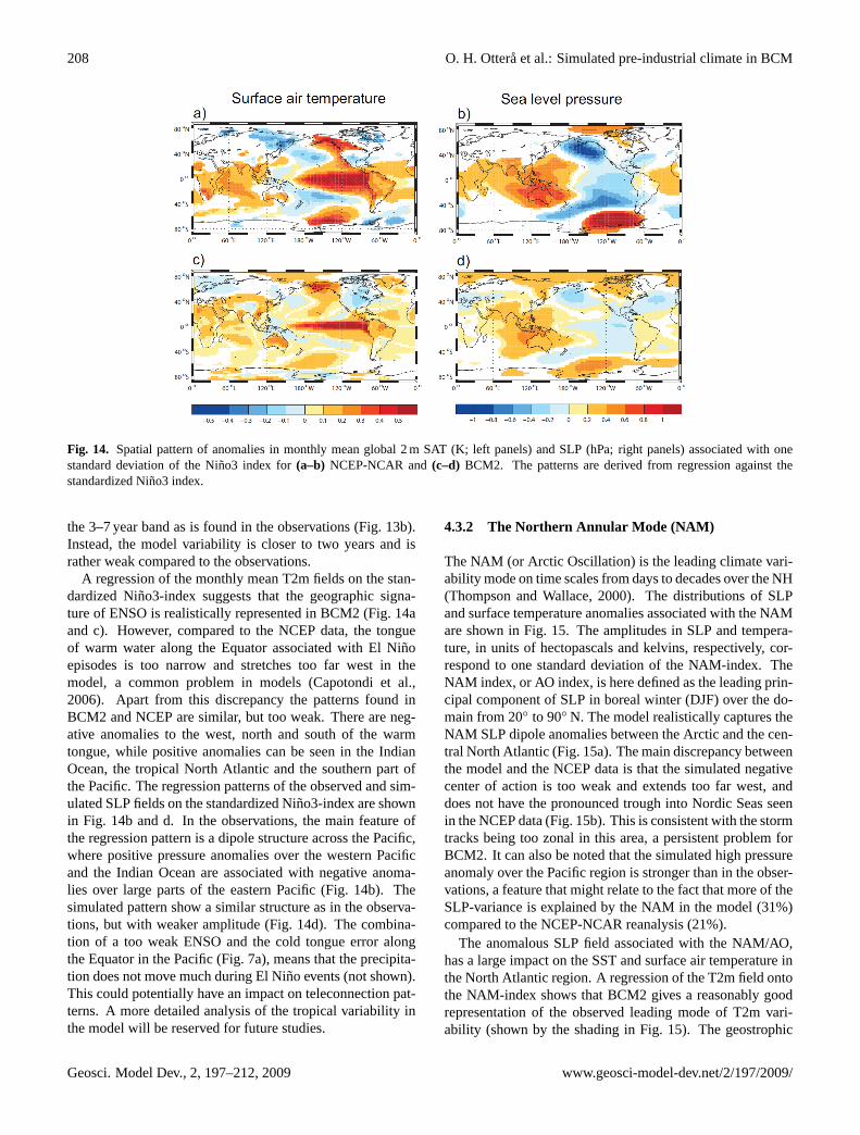
Fig. 5. Simulated northward oceanic heat transports (PW) for theglobal (top panel) and Atlantic (bottom panel) oceans. Asterisksymbols denote observational estimates based onTrenberth andCaron(2001).

(SH), however, the sea-ice simulation is quite poor. Theannual-mean sea-ice extent is only 1.76×106 km2 which ismuch less than the observational estimate of 11.5×106 km2

from Cavalieri et al.(2003).We believe excessive mixing between the surface and the

deep ocean in the Southern Ocean is the main cause for thewarm bias and underestimation of sea ice extent in this re-gion. The excessive mixing erodes the halocline and makesit difficult to maintain a fresh and cold surface layer requiredfor wintertime freezing of sea-ice. The underestimation ofsea-ice will in turn cause a warm bias in the model due toincreased absorption of short-wave radiation.

Several factors might contribute to this excessive mixing.Firstly, the depth of MICOMs bulk mixed layer is found bybalancing a turbulent kinetic energy budget according toGas-par(1988). This parameterization generally tends to generatetoo deep mixed layer depths at high latitudes. Preliminarytesting with the mixed layer depth parameterization ofOber-huber(1993) indicates much improved mixed layer depths athigh latitudes compared to observations (de Boyer Montegutet al., 2004). Secondly, the ocean model uses isopycnic lay-ers with potential densities estimated with a reference pres-sure at 2000 db. The profile with 2000 db reference pressuregives a poor representation of stratification, even static insta-bility, near the surface (Assmann et al., 2009). This makes itdifficult for the model to represent a realistic halocline iso-lating the surface from the deeper ocean. Finally, in MICOMthe brine rejected during freezing of sea-ice is placed in thesurface layer. This tends to destabilize the water columnnear the surface. Several studies (Duffy and Caldeira, 1999;Sun and Bleck, 2006) indicate that a parameterization of salt-plumes can contribute to the maintenance of a more realistichalocline in ocean models not resolving these plumes.



4.2 Time-mean simulation characteristics

4.2.1 Ocean transports of heat and volume

The meridional transport of heat by the oceans is an impor-tant factor in the ability of models to simulate a realistic cli-mate. The total simulated meridional transports of heat bythe ocean, as well as an observational estimate, are shownin Fig. 5. For the entire globe, the northward transport inthe NH poleward of 10◦ is consistent with observational esti-mates fromTrenberth and Caron(2001), but there appears tobe insufficient southward transport of heat out of the Tropicsin the model (Fig.5, upper panel). The heat transport inthe Atlantic is in reasonably good agreement with observa-tional estimates, with just over 1 PW maximum northwardheat transport around 20◦ N (Fig. 5, lower panel). It should,however, be noted that significant uncertainties exist in theobservational estimates of ocean heat transport.

A common diagnostic of the strength of the Atlantic ther-mohaline circulation is the Atlantic Meridional Overturn-ing Circulation (AMOC). The simulated Atlantic meridionaloverturning streamfunction is characterized by a northwardflow close to the surface, sinking at high latitudes and asouthward flow at greater depths (Fig.6a). Due to the choiceof reference pressure at 2000 m and inclusion of thermobariceffects in the new version of MICOM, one can now see indi-cations of a deep circulation cell of Antarctic bottom waterextending into the Atlantic, a feature that was absent in pre-vious versions of BCM. The overturning cell is also moreshallow and realistic than in earlier versions of the model(Furevik et al., 2003; Ottera et al., 2003), and has a maximumvalue between 30 and 40◦N. The time series of the maximumvalue of the AMOC shows both decadal and interannual vari-ability in the strength of the overturning around a mean ofabout 20 Sv (Fig.6b). The mean value for the AMOC overthe last 100 years at 24◦ N is about 16.6 Sv, which is withinthe range of observational estimates of about 15.75±1.6 Sv(Ganachaud and Wunsch, 2000; Lumpkin and Speer, 2003)and other model estimates (Schmittner et al., 2005; Meehlet al., 2007). In the corresponding power spectrum of theAMOC time series peaks are seen at decadal (50–60 years)as well centennial (130–170 years) periods (Fig.6c). Towhat extent the multidecadal AMOC variability simulatedby BCM2 constitutes a true oscillatory mode of the cou-pled ocean-atmosphere system, is a question that will be ad-dressed in future studies.

The mean simulated volume transports in the PI sim-ulation for some key sections in the model are summa-rized and compared to estimates cited in the literaturein Table 2. The simulated poleward transport of At-lantic Water (AW) across the Greenland-Scotland Ridge(GSR) sections amounts to about 10.8 Sv, which is some-what higher than the 8.0 Sv estimate based on observationsfrom Hansen and Østerhus(2000). The southward transportsacross the GSR compare reasonably well with observational

0

250

500

750

1000 Sv

−18 −14 −10 −6 −2 2 6

10 14 18

Latitude (o)

Dep

th (m

)

−30 −20 −10 0 10 20 30 40 50 60 70

2000

3000

4000

5000

0 100 200 300 400 500 60018

20

22

24

Time (yr)

Sv

0 50 100 150 200 250 3000

5

10

15

Period (yr)

Pow

er d

ensi

ty

a)

c)

b)

Fig. 6. (a)Annual-mean streamfunction (Sv) for the Atlantic ocean(years 501–600).(b) time evolution of the maximum of the At-lantic meridional overturning circulation for the PI control integra-tion. (c) power spectrum of the detrended AMOC calculated usingthe Thomson multi-taper method.

estimates, although it should be mentioned that no attempthas been made to distinguish the different water masses inthe simulated transport estimates.

The total northward transport of Atlantic and coastal wa-ters into the Barents Sea is 2.9 Sv which is in good agreementwith earlier estimates fromLoeng et al.(1997) and more re-cent estimates fromSchauer et al.(2002), Ingvaldsen et al.(2002) andDickson et al.(2007). In addition, the polewardflow of Pacific Water through the Bering Strait of 1.5 Svand the southward flow through the Canadian Archipelagoof 1.7 Sv are both in reasonable agreement with observations(Dickson et al., 2007). The simulated northward and south-ward transports for the Fram Strait are 5.6 and 6.7 Sv, re-spectively. Observational estimates of the transport throughthis section have large uncertainties attached to them due tothe highly variable and complex circulation across this sec-tion, but recent estimates fromDickson et al.(2007) (4.5 and6.2 Sv for the northward and southward transports, respec-tively) compare quite well with the model. In the SH, thesimulated net volume transport through the Drake Passage is161.7 Sv, which is larger than the observational estimate of134±11.2 Sv ofWithworth and Peterson(1985). For the In-donesian Throughflow, the model simulates a net transport of18.3 Sv, which is higher than recent observational estimatesof about 8.9±1.7 Sv (Wijffels et al., 2008).

Most of the transport estimates for the high northern lat-itudes are reasonably stable throughout the entire 600 yearintegration period. There are some positive trends in thenorthward transports through the Faroe Shetland Channel



Table 2. Simulated (years 501–600) and observed estimates of ocean volume transports (Sv) through some key sections in the model domain.For the model estimates the trends are given in parentheses (100 yrs−1). 1 Dickson et al.(2007), 2 Blindheim(1989), 3 Hansen and Østerhus(2000), 4 Withworth and Peterson(1985) and5 Wijffels et al. (2008).

PI simulation ObservedN/E S/W Net N/E S/W Net

Ocean transports (Sv)

Bering Strait 1.5 (0.01) 0 1.5 (0.01) 0.81 0 0.8Canadian Arch. 0 1.7 (0.03) 1.7 (0.03) 0 1.51 1.5Fram Strait 5.6 (0.24) 6.7 (0.24) 1.1 (0) 4.51 6.21 1.7Barents Opening 2.9 (0.03) 1.6 (0.01) 1.3 (0.02) 2.21 1.22 1.0Denmark Strait 1.8 (−0.01) 5.1 (0.02) 3.3 (0.03) 1.03 4.33 3.3Iceland-Faroe 3.8 (0) 1.6 (0.03) 2.2 (−0.03) 3.33 1.03 2.3Faroe-Scotland 5.2 (0.14) 4.4 (0.05) 0.8 (0.09) 4.33 4.53

−0.2North Sea Opening 1.9 (0.01) 1.3 (0.02) 0.5 (−0.01) n/a n/a n/aDrake Passage 167.3 (4.3) 5.6 (0.1) 161.7 (4.2) n/a n/a 134.04

Indonesian Arch. 5.9 (0) 24.2 (0.2) 18.3 (0.2) n/a n/a 8.95

and further north through the Fram Strait. However, for theFram Strait this trend is counteracted by a similar positivetrend in the southward transport making the net transportquite stable. The transport through the Drake Passage is,however, not stable. There is a positive drift of about 4 Svper century throughout the integration, which underlines theproblems BCM2 has in the Southern Ocean. This is mostlikely a due to slow oceanic adjustment to the changed sea-ice cover for this region.

4.2.2 Ocean surface

The time-mean errors in the PI simulation of sea surface tem-perature (SST) and sea surface salinity (SSS) are shown inFig. 7 along with their global root mean square values. Thelargest errors in SST compared to the Levitus data (Levitusand Boyer, 1994) are seen in the Southern Ocean (Fig.7a)and are mainly caused by negative sea-ice biases here. Theextratropical northern Pacific is slightly too cold, while thenorthern North Atlantic, including the subpolar gyre, is toowarm. For the SSS, the largest errors compared to the Levi-tus data (Levitus et al., 1994) are found in the poorly sampledArctic Ocean. In the central Arctic Ocean the ocean surfaceis too saline by about 2 psu, while negative salinity anomaliesof 1–2 psu can be found in the Transpolar Drift (Fig.7b). Inthe northern Pacific and Indian Oceans the waters are gener-ally too saline (1–2 psu) compared to the Levitus data, whilea fresh bias (about 1 psu) can be found in the sub-tropicalSouth Atlantic. In the Southern Ocean and the North At-lantic, the errors are relatively small in SSS.

The sea-ice thickness distributions and the surface oceanvelocities for the NH and SH are shown for the PI sim-ulation in Fig. 8. In March, the simulated sea-ice extentcompares well with observations except for the LabradorSea region where there is too little sea-ice (Fig.8a). In

180oW 120oW 60oW 0o 60oE 120oE 180oW

80oS

40oS

0o

40oN

80oN

RMSE value: 2.33(a) SST

o C

−10

−8

−6

−4

−2

0

2

4

6

8

10

180oW 120oW 60oW 0o 60oE 120oE 180oW

80oS

40oS

0o

40oN

80oN

RMSE value: 0.74(b) SSS

psu

−2

−1.6

−1.2

−0.8

−0.4

0

0.4

0.8

1.2

1.6

2

Fig. 7. Errors in simulation of(a) SST and(b) SSS for the PI sim-ulation compared to Levitus data. The root mean square error(RMSE) is indicated in the upper right corner of each panel. Con-tour interval is 1◦C and 0.2 psu for (a) and (b), respectively.

September, the sea-ice extent is generally too small com-pared to the observations (Fig.8b). A general problem forboth seasons, but in particular for the summer season, isthat the sea-ice is quite thin (about 1–1.5 m for the sum-mer). This may adversely affect projections of Arctic sea-icechange under increasing greenhouse gas concentrations andchanges in the orbital configuration. The annual-mean sea-ice extent for the last 100 years is 10.3×106 km2 which issomewhat below the observational estimate of 11.7×106 km2

from Cavalieri et al.(2003).




0.1 m s

0 0.5 1 1.5 2 2.5 3

m -1

(a) NH, March (b) NH, September

(d) SH, September(c) SH, March

Fig. 8. Simulated sea-ice thickness (m) and surface ocean velocity (m s−1) in the PI simulation for (a) NH, March, (b) NH, September, (c)SH, March and (d) SH, September. The observational estimate for sea ice extent (from NCEP) is indicated by the thick red line.

Fig. 8. Simulated sea-ice thickness (m) and surface ocean velocity(m s−1) in the PI simulation for(a) NH, March,(b) NH, September,(c) SH, March and(d) SH, September. The observational estimatefor sea ice extent (from NCEP) is indicated by the thick red line.

For the SH, the simulated sea ice does not compare wellwith observations neither in summer nor in winter (Fig.8cand d). The poor sea ice simulation is likely related to theparametrization of the mixed layer turbulent kinetic energyclosure (see discussion above). The current parametrizationleads to a mixed layer that is too deep in the Southern Ocean,which in turn makes it hard to maintain a realistic sea-icecover here. The sea-ice biases in the SH are a serious prob-lem in the model, and are an important area for further modeldevelopment.

The model manages to capture the major features of theobserved flow fields in the North Atlantic-Arctic region andthe Southern Ocean (Fig.8). In northern North Atlanticthe ocean circulation is dominated by the sub-polar gyre,while the general surface ocean circulation within the NordicSeas is dominated by the warm and saline Norwegian At-lantic Current to the south and east, and the cold and freshEast Greenland Current to the north and west (Fig.8a andb). In the Arctic Ocean, the circulation is dominated by theBeaufort Gyre (a roughly circular current flowing clockwisewithin the surface waters of the Beaufort Sea) and the Trans-polar Drift (the major current flowing into the Atlantic Oceanfrom the eastern Arctic). In the Southern Ocean the oceancirculation is dominated by the Antarctic Circumpolar Cur-rent flowing from west to east around Antarctica (Fig.8c and

OTTERA ET AL.: SIMULATED PRE-INDUSTRIAL CLIMATE IN BCM 21

−80 −70 −60 −50 −40 −30−0.1

−0.05

0

0.05

0.1

0.15

0.2

Latitude (o)

N m−2

ObsBCM

Fig. 9. Zonally averaged wind-stress (N m−2) from observations based on NCEP-NCAR reanalysis (black line) and BCM2 (red line).Fig. 9. Zonally averaged wind-stress (N m−2) from observationsbased on NCEP-NCAR reanalysis (black line) and BCM2 (red line).

d). In addition, two clockwise gyres are seen to swirl in thevicinity of the Weddell and Ross Seas.

The distribution and magnitude of the simulated windstress over the Southern Ocean compares relatively poorlywith observations (Fig.9). The peak zonally averaged windstress is shifted equatorward relative to the observations(from NCEP long-term mean), and is about 30% weaker thanobserved. A recent intercomparison of the Southern Oceancirculations in the IPCC coupled climate models revealedthat many of the models suffers from similar problems asBCM (Russell et al., 2006). In particular, all but a few of themodels show an equatorward shift of the peak westerlies inthe Southern Ocean.

4.2.3 Atmospheric circulation and precipitation

The model successfully reproduces the main features ofthe sea level pressure (SLP) distribution as depicted by theNCEP reanalysis (Kalnay et al., 1996), but there are errors inthe details (Fig.10). In December-January-February (DJF,Fig. 10a, c, and e) the Icelandic low is not deep enoughand the associated trough does not extend far enough east-northeastward due to excessive pressure over the Arctic. Themid-latitude circulation in the Atlantic and Eurasia regionsis generally well reproduced. In the Pacific sector, the Aleu-tian low is somewhat underestimated in the model, while thepressure over North America is overestimated compared tothe NCEP reanalysis. In the SH, the circumpolar trough isshallower than observed leading to anomalously weak sur-face winds there.

In June-July-August (JJA, Fig.10b, d, and f) the SLP dis-tribution is generally well reproduced in the mid-latitudes ex-cept for the North Pacific where the model produces anoma-lously high pressures. As was the case for the winter circula-tion, the simulated pressure north of 60◦ N is much too highcompared to NCEP data. In the SH, the pressure in the cir-cumpolar trough is also higher than observed. The relatively




90 oS

60 oS

30 oS

0 o

30 oN

60 oN

90 oN

150 o W 90 o W 30 o W 30 o E 90 o E 150 o E

90oS

60 o S

30 o S 0 o

30 o N

60 o N

90 o N

hPa980 986 992 998 1004 1010 1016 1022 1028 1034

150 o W 90 o W 30 o W 30 o E 90 o E 150 o E

150 o W 90 oW 30 o W 30 o E 90 o E 150 o E

90oS

60 o S

30 o S 0 o

30 o N

60 o N

90 o N

hPa- 20 -16 -12 -8 -4 0 4 8 12 16 20

150 o W 90 o W 30 o W 30 o E 90 o E 150 o E

(a) NCEP: DJF (b) NCEP: JJA

(c) BCM: DJF (d) BCM: JJA

(e) BCM - NCEP: DJF (f) BCM - NCEP: JJA

Fig. 10. Observed (based on NCEP-NCAR reanalysis) and simulated SLP (hPa). (a) NCEP (DJF), (b) NCEP (JJA), (c) BCM (DJF), (d)BCM (JJA), (e) BCM−NCEP (DJF) and (f) BCM−NCEP (JJA).

Fig. 10. Observed (based on NCEP-NCAR reanalysis) and simulated SLP (hPa).(a) NCEP (DJF),(b) NCEP (JJA),(c) BCM (DJF), (d)BCM (JJA),(e)BCM-NCEP (DJF) and(f) BCM-NCEP (JJA).

poor simulation of SLP at high latitudes in the model hasbeen a persistent problem with the current model system.Part of the problem in the SH is related to the poor sea-icedistribution (see above). A negative zonal bias in the Antarc-tic sea-ice extent during winter will give massive anomalousheat fluxes that produce warm marine air in the Antarctic re-gion. This results in weaker, and poleward shifted tempera-ture gradients. According to the thermal wind balance, thepressure gradients will be reduced and this in turn will con-tribute to a positive bias in the circumpolar Antarctic low,particularly during JJA. As the negative sea-ice bias is largestin winter, the consequences mentioned will also contributeto a reduced seasonal variability in the mass and wind fields.The reasons for the positive SLP anomalies in high northernlatitudes are less clear. It could be noted, however, that theinclusion of the refined gravity wave drag parametrizationfrom version 4 of ARPEGE (see above) has not significantlyimproved the high northern SLP distribution.

Figure11shows the annual zonal-mean zonal wind for thePI simulation compared to NCEP data. In the observations,there are two main jet streams at the polar latitudes, one ineach hemisphere (Fig.11a). The peaks of the jet streamsare found just below the tropopause at about 200 hPa and

Latitude (o)

Pre

ssur

e (h

Pa)

(a)

−80 −60 −40 −20 0 20 40 60 80

10

20

50

100

200

500

1000

m s

−1

−30 −25 −20 −15 −10 −5 0 5 10 15 20 25 30

Latitude (o)

(b)

−80 −60 −40 −20 0 20 40 60 80

m s

−1

−10

−8

−6

−4

−2

0

2

4

6

8

10

Latitude (o)

Pre

ssur

e (h

Pa)

(c)

−80 −60 −40 −20 0 20 40 60 80

10

20

50

100

200

500

1000

Fig. 11. Annual-mean zonal-mean of zonal wind (m s−1). (a) ob-servational estimates from NCEP-NCAR reanalysis,(b) PI controlintegration (years 501–600), and(c) PI-observations.

located around 30–40◦ N for the NH, and around 40–50◦ Nfor the SH. The stratosphere is characterized by an easterlyjet that extends across the Equator, and a westerly jet innorthern high latitudes with a center of action around 60◦ N.



Generally, the position and strength of the tropospheric jetsare reasonably well simulated (Fig.11b). In the SH, how-ever, the reanalysis exhibits a narrower westerly jet than thePI simulation. This points to a reduced seasonal variabilityand is consistent with the arguments given above. In the NH,the tropospheric and stratospheric parts of the westerly jet arefound to be too vertically aligned. In particular, the strengthof the stratospheric vortex is clearly underestimated in themodel, with the center of action shifted too far to the southcompared to observations (Fig.11c).

Precipitation is highly variable both spatially and tempo-rally, and it is difficult to obtain robust measurements glob-ally, especially over the oceans. Observational data fromLegates and Willmott(1990) andSpencer(1993) show thatthe precipitation is heaviest along the intertropical conver-gence zone, over warm oceanic regions and in monsoonalareas (Fig.12a). Arid regions tend to occur in regions of de-scending air, and in polar regions, where the cold air alsoreduces the capacity of the atmosphere to hold moisture.The PI simulation reproduces the main precipitation pat-terns including those associated with the mid-latitude stormtracks and the continental monsoons. However, there is ageneral tendency to underestimate the amount of precipita-tion compared to the observations, especially over the ocean(Fig. 12b).

4.3 Variability characteristics

A few of the characteristics of the model-simulated inter-annual variability are presented here (variability on multi-decadal time-scales will be investigated in future papers).One of the strongest natural modes of variability in the globalclimate system is the El Nino-Southern Oscillation (ENSO).Apart from ENSO, the dominant patterns of global-scale cli-mate variability are the annular modes in both hemispheres(Limpasuvan and Hartmann, 1999; Thompson and Wallace,2000), often referred to as the Northern and Southern An-nular Modes (NAM and SAM for the NH and SH, respec-tively). In the following sections, these modes of variabilitywill be analyzed based on the SLP and surface air tempera-ture (T2m) fields.

4.3.1 The ENSO mode

The simulated monthly mean Nino3-index provides an esti-mate of El Nino-related temperature variability in the model.The Nino3-index is calculated as the mean SST over the east-ern tropical Pacific (the region bounded by 150◦W to 90◦W,5◦ S to 5◦N) and is shown in Fig.13a for the model andthe NCEP-NCAR reanalysis fields. The standard deviationof the Nino3-index in BCM2 is 0.62◦C, compared to theobserved 0.84◦C in the NCEP-NCAR data. The reason forthe underestimation of the Nino3 variability is not clear, butit could be related to the resolution being too coarse in theequatorial Pacific in the ocean model. The model skewness

mm

day

−1

0

2

4

6

8

10

180oW 120oW 60oW 0o 60oE 120oE 180oW 80oS

40oS

0o

40oN

80oN

(a) OBS

mm

day

−1

0

2

4

6

8

10

180oW 120oW 60oW 0o 60oE 120oE 180oW 80oS

40oS

0o

40oN

80oN

(b) BCM

Fig. 12. Annual mean precipitation (mm day−1). (a) observationalestimate fromLegates and Willmott(1990) andSpencer(1993), and(b) PI control integration (years 501–600).

0 100 200 300 400 500 600 1950 2000−4

−2

0

2

4

Time (yrs)

Nin

o−3

inde

x (° C

)

10 20 30 40 50 60 70 80 90 100 110 1200

10

20

30

40

Period (months)

Pow

er d

ensi

ty

BCMNCEP

a)

b)

STD=0.60(0.84) SKEWNESS=0.06(0.9) KURTOSIS=2.7(4.6)

PECNMCB

0 100 200 300 400 500 600 1950 2000−4

−2

0

2

4

Time (yrs)

Nin

o−3

inde

x (° C

)

10 20 30 40 50 60 70 80 90 100 110 1200

10

20

30

40

Period (months)

Pow

er d

ensi

ty

BCMNCEP

a)

b)

STD=0.60(0.84) SKEWNESS=0.06(0.9) KURTOSIS=2.7(4.6)

PECNMCB

Fig. 13. (a)time series of the Nino3 indices for BCM2 and NCEP-NCAR. The indices are calculated as the average SSTs in the area150◦W to 90◦W, 5◦ S to 5◦ N. The standard deviation, skewness,and kurtosis of the two indices are also shown (observed estimatein parenthesis).(b) power spectral density for the Nino3 indices forBCM2 (solid line) and NCEP-NCAR (dashed line) calculated usingthe Thomson multi-taper method.

and kurtosis are also much smaller than in the observations.This suggests that the model is underestimating the non-linerarity in ENSO. The power spectra of the observed andsimulated Nino3-indices show that BCM2 has little power in



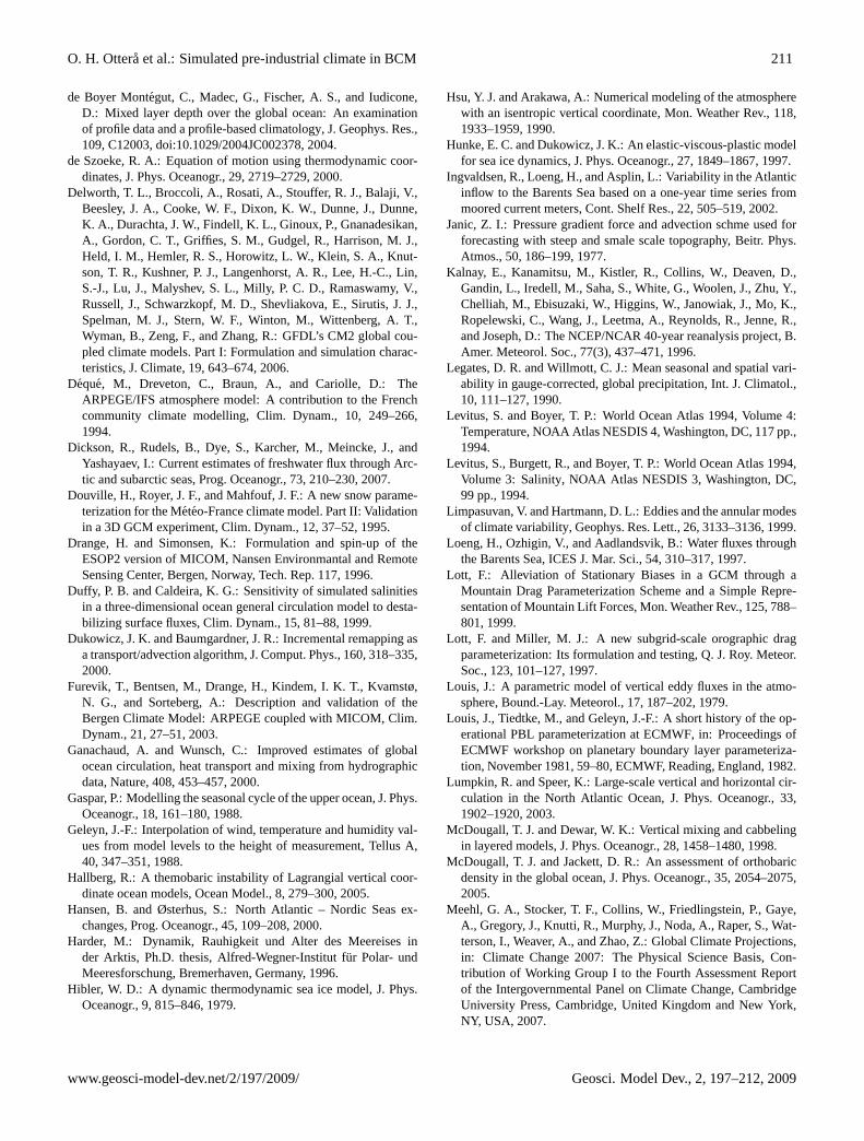
Fig. 14. Spatial pattern of anomalies in monthly mean global 2 m SAT (K; left panels) and SLP (hPa; right panels) associated with onestandard deviation of the Nino3 index for(a–b) NCEP-NCAR and(c–d) BCM2. The patterns are derived from regression against thestandardized Nino3 index.

the 3–7 year band as is found in the observations (Fig.13b).Instead, the model variability is closer to two years and israther weak compared to the observations.

A regression of the monthly mean T2m fields on the stan-dardized Nino3-index suggests that the geographic signa-ture of ENSO is realistically represented in BCM2 (Fig.14aand c). However, compared to the NCEP data, the tongueof warm water along the Equator associated with El Ninoepisodes is too narrow and stretches too far west in themodel, a common problem in models (Capotondi et al.,2006). Apart from this discrepancy the patterns found inBCM2 and NCEP are similar, but too weak. There are neg-ative anomalies to the west, north and south of the warmtongue, while positive anomalies can be seen in the IndianOcean, the tropical North Atlantic and the southern part ofthe Pacific. The regression patterns of the observed and sim-ulated SLP fields on the standardized Nino3-index are shownin Fig. 14b and d. In the observations, the main feature ofthe regression pattern is a dipole structure across the Pacific,where positive pressure anomalies over the western Pacificand the Indian Ocean are associated with negative anoma-lies over large parts of the eastern Pacific (Fig.14b). Thesimulated pattern show a similar structure as in the observa-tions, but with weaker amplitude (Fig.14d). The combina-tion of a too weak ENSO and the cold tongue error alongthe Equator in the Pacific (Fig.7a), means that the precipita-tion does not move much during El Nino events (not shown).This could potentially have an impact on teleconnection pat-terns. A more detailed analysis of the tropical variability inthe model will be reserved for future studies.

4.3.2 The Northern Annular Mode (NAM)

The NAM (or Arctic Oscillation) is the leading climate vari-ability mode on time scales from days to decades over the NH(Thompson and Wallace, 2000). The distributions of SLPand surface temperature anomalies associated with the NAMare shown in Fig.15. The amplitudes in SLP and tempera-ture, in units of hectopascals and kelvins, respectively, cor-respond to one standard deviation of the NAM-index. TheNAM index, or AO index, is here defined as the leading prin-cipal component of SLP in boreal winter (DJF) over the do-main from 20◦ to 90◦ N. The model realistically captures theNAM SLP dipole anomalies between the Arctic and the cen-tral North Atlantic (Fig.15a). The main discrepancy betweenthe model and the NCEP data is that the simulated negativecenter of action is too weak and extends too far west, anddoes not have the pronounced trough into Nordic Seas seenin the NCEP data (Fig.15b). This is consistent with the stormtracks being too zonal in this area, a persistent problem forBCM2. It can also be noted that the simulated high pressureanomaly over the Pacific region is stronger than in the obser-vations, a feature that might relate to the fact that more of theSLP-variance is explained by the NAM in the model (31%)compared to the NCEP-NCAR reanalysis (21%).

The anomalous SLP field associated with the NAM/AO,has a large impact on the SST and surface air temperature inthe North Atlantic region. A regression of the T2m field ontothe NAM-index shows that BCM2 gives a reasonably goodrepresentation of the observed leading mode of T2m vari-ability (shown by the shading in Fig.15). The geostrophic



(a) NCEP (21%)

−3 −2 −1 0 1 2 3

(b) BCM (31%)(a) NCEP (21%)

−3 −2 −1 0 1 2 3

(b) BCM (31%)

Fig. 15. Spatial pattern of anomalies in SLP (hPa; contours) and2 m SAT (K; color shading) associated with one standard deviationof the AO-index. The AO-index is defined as the first principal com-ponent of winter mean SLP (December through February) for allpoints north of 20◦ N. Both SLP and surface temperature patternsare derived from regression against the standardized AO index.(a)Spatial AO patterns for NCEP-NCAR reanalysis from 1950 through2000,(b) similar to (a) but for years 1–600 from BCM2 PI run out-put. The contour interval for the SLP anomalies is 1 hPa.

winds associated with the SLP dipole anomalies induce aquadropole temperature pattern by advecting the mean tem-perature. This pattern is characterized by positive anomaliesover southeastern North America and northern Eurasia, andnegative anomalies over northeastern North America, north-ern Africa and through the Middle East. The main discrep-ancy between simulated and observed anomalies occurs nearAlaska and over Siberia, with larger negative temperatureanomalies than observed. This could be related to the largerSLP anomalies and the associated SLP gradients over theNorth Pacific in the simulation. The warming signal overnorthern Europe and Asia is also somewhat underestimatedin the model compared to the observations, possibly relatedto the negative center of action being too weak over the Arc-tic region in the model.

4.3.3 Southern Annular Mode (SAM)

The SH counterpart of NAM is presented in Fig.16. The cal-culation of the Southern Annular Mode [SAM, or referred toas Antarctic Oscillation (AAO)] is similar to the NAM exceptthat monthly data for all months are used. Overall, the SAMaccounts for a large part of the total variance, 32% and 30%for the NCEP-NCAR data and the BCM2, respectively. TheNCEP-NCAR reanalysis and the PI simulation exhibit sim-ilar SAM patterns, with a strong zonally symmetric compo-nent, showing an out-of-phase relationship of SLP betweenthe Antarctic and mid-latitudes at all longitudes. However,some discrepancies in the spatial structure and amplitudesof SLP and surface temperature associated with the SAMcan be seen. For the SLP, the strength of the low pressureanomalies over Antarctica agrees reasonably well in termsof amplitude, but with weaker gradients. As a result of this

(a) NCEP (32%)

−2 −1.2 −0.4 0.4 1.2 2

(b) BCM (30%)(a) NCEP (32%)

−2 −1.2 −0.4 0.4 1.2 2

(b) BCM (30%)

Fig. 16. Same as in Fig.16, but for the AAO-index. The AAOindex is defined as the first principal component of monthly SLPfor all points south of 20◦ S. (a) same as in Fig.15a, but for AAO.(b) same as Fig.15b, but for years 501–600 from BCM2 PI runoutput.

the associated winds are weaker and shifted somewhat north-wards compared to the NCEP data. Also, the distinct positiveanomalies in the eastern and western parts of the Pacific arenot clearly visible in BCM2. A simulated cooling over thewestern part of Antarctica associated with SAM is in reason-able agreement with the NCEP data. However, neither theclear warming near the Weddell Sea nor the strong coolingsignal over the Ross Sea are captured by the model. Manyof these discrepancies are likely related to the poor sea-icesimulation in the Southern Ocean (see above), an issue thatis an important part of the ongoing model development.

5 Discussion and outlook

In this paper, the formulation and simulation characteristicsof BCM2 have been presented. The current model doesnot employ flux adjustments, unlike the first version of themodel. A multi-century simulation for pre-industrial timeshas been completed, and the simulated climate is stable andreproduces many features of the observed climate quite well.In particular, the introduction of a more adequate turbulencescheme in the very stable cases (i.e. large Richardson num-bers) has eliminated a persistent cold bias in the model. Fur-thermore, the introduction of incremental remapping for theadvection of tracers in the ocean has improved the conserva-tive properties of temperature and salt in the model, and thusreduced the drift significantly compared to earlier versions.By setting the reference pressure in the ocean at 2000 m andintroducing a more accurate representation of density in thepressure gradient formulation, the simulated Atlantic over-turning circulation appears more realistic with a shalloweroverturning cell compared to the first version of the model.Furthermore, the volume transports through some key sec-tions in the model compare quite well with observed esti-mates, which yields further credibility to the model system.



However, several aspects of the climate system are notvery well simulated and need further attention in the fu-ture. For instance, there is a strong bias towards higher thanobserved SLP at the high northern latitudes, a feature thatis shared by other climate models as well (Delworth et al.,2006). In addition, SLP gradients in the northern North At-lantic is too zonal, leading to too few storms entering theNordic Seas region.

In the Southern Ocean, excessive mixing between the sur-face and the deep ocean lead to a strong warm bias and un-derestimation of sea ice extent in this region. The excessivemixing erodes the halocline and makes it difficult to main-tain a fresh and cold surface layer required for wintertimefreezing of sea-ice. The warm bias in the Southern Oceanwill likely lead to less oceanic heat and tracer uptake in fu-ture climate change simulations than would otherwise be thecase. This would lead to a larger transient climate responsedue to less heat going into the ocean. If used as and EarthSystem Model (i.e. including the full carbon cycle) such anerror would also lead to a larger amount of carbon stayingin the model atmosphere. Recently, oceanic and terrestrialcarbon cycle models have been coupled to BCM2 to formthe Bergen Earth System Model (BCM-C). An assessmentof regional climate-carbon cycle feedbacks using this modelsystem is given inTjiputra et al.(2009).

The poor sea-ice simulation in the SH is a serious prob-lem with the model system presented here, and will certainlybe a key area for future model development. The problemwith the sea-ice also makes the PI simulation less suitablefor use in climate change simulations for the SH. However,it should still be applicable for climate change studies focus-ing on the NH, as the climate here is generally well repro-duced. It should be noted, however, that the diagnosed bi-ases not entirely may originate from model deficiencies. Asthe PI simulation employs pre-industrial forcing, a compari-son with NCEP data, which contain a growing anthropogenicforcing, may reveal errors which also stems from differencesin external forcing between the two data sets.

Additional analyses of the simulation presented here are inprogress. In particular, analyses of the multidecadal variabil-ity of the thermohaline circulation in the PI simulation andits possible link to Atlantic Multidecadal Oscillation are un-derway. Furthermore, model simulations for key periods inthe past, such as the Last Glacial Maximum (21 ka) and themid-Holocene (6 ka), are planned. Such simulations will al-low us to carry out detailed model-observation comparisonsfor the North Atlantic region during these times, both from amarine and terrestrial perspective. This will be important forfurthering evaluating the realism of the model.

Finally, this simulation is the basis for a transient climatesimulation of the last 600 years where most relevant forcings(natural and anthropogenic) have been incorporated. Resultsfrom these simulations will be presented in future papers.The comparisons among model results and between modeland paleo data will help to better quantify the many different

feedbacks from ocean, sea-ice and vegetation, and to test theclimate sensitivity of the climate model. This is importantnot only to understand past climate variability, but even moreso to increase our confidence in the models used to provideprojections of future climate.

Acknowledgements.We thank C. Li and M. Deque for helpfuldiscussions, and two anonymous reviewers for valuable commentsthat helped improve the manuscript. This study has been supportedby the Research Council of Norway through a postdoctoral grantto O. H. O. (Project 155957), by the NorKlima project GLOMIX(Project 178399), and by the Program of Supercomputing. Thisis contribution No. A252 from the Bjerknes Centre for ClimateResearch.

Edited by: P. Jockel

References

Assmann, K. M., Bentsen, M., Segschneider, J., and Heinze, C.: Anisopycnic ocean carbon cycle model, Geosci. Model Dev. Dis-cuss., 2, 1023–1079, 2009.

Bentsen, M., Drange, H., Furevik, T., and Zhou, T.: Simulated vari-ability of the Atlantic Meridional Overturning Circulation, Clim.Dynam., 22, 701–720, 2004.

Bethke, I., Furevik, T., and Drange, H.: Towards a more salineNorth Atlantic and a fresher Arctic under global warming, Geo-phys. Res. Lett., 33, L21712, doi:10.1029/2006GL027264, 2006.

Bleck, R. and Smith, L. T.: A wind-driven isopycnic coordinatemodel of the North and Equatorial Atlantic Ocean. 1. Modeldevelopment and supporting experiments, J. Geophys. Res., 95,3273–3285, 1990.

Bleck, R., Rooth, C., Hu, D., and Smith, L. T.: Salinity-driven Ther-mocline Transients in a Wind- and Thermohaline-forced Isopyc-nic Coordinate Model of the North Atlantic, J. Phys. Oceanogr.,22, 1486–1505, 1992.

Blindheim, J.: Cascading of Barents Sea bottom water into the Nor-wegian Sea, Rapports et Proces-Verbaux des Reunions, ConseilInternational pour l’Exploration de la Mer, 188, 49–58, 1989.

Bossuet, C., Deque, M., and Cariolle, D.: Impact of a simple pa-rameterization of convective gravity-wave drag in a stratosphere-troposphere general circulation model and its sensitivity to verti-cal resolution, Ann. Geophys., 16, 238–249, 1998,http://www.ann-geophys.net/16/238/1998/.

Boucher, O. and Pham, M.: History of sulfate aerosolradiative forcings, Geophys. Res. Lett., 29(9), 1308,doi:10.1029/2001GL014048, 2002.

Capotondi, A., Wittenberg, A., and Masina, S.: Spatial and tem-poral structure of tropical Pacific interannual variability in 20thcentury coupled simulations, Ocean Model., 15, 274–298, 2006.

Catry, B., Geleyn, J.-F., Bouyssel, F., Cedilnik, J., Brozkova, R.,Derkova, M., and Mladek, R.: A new sub-grid scale lift formula-tion in a mountain drag parameterisation scheme, Meteorol. Z.,17, 193–208, 2008.

Cavalieri, D. J., Parkinson, C. L., and Vinnikov, K. Y.: 30-year satellite record reveals contrasting Arctic and Antarc-tic decadal variability, Geophys. Res. Lett., 30, 1970,doi:10.1029/2003GL018031, 2003.


http://www.ann-geophys.net/16/238/1998/


de Boyer Montegut, C., Madec, G., Fischer, A. S., and Iudicone,D.: Mixed layer depth over the global ocean: An examinationof profile data and a profile-based climatology, J. Geophys. Res.,109, C12003, doi:10.1029/2004JC002378, 2004.

de Szoeke, R. A.: Equation of motion using thermodynamic coor-dinates, J. Phys. Oceanogr., 29, 2719–2729, 2000.

Delworth, T. L., Broccoli, A., Rosati, A., Stouffer, R. J., Balaji, V.,Beesley, J. A., Cooke, W. F., Dixon, K. W., Dunne, J., Dunne,K. A., Durachta, J. W., Findell, K. L., Ginoux, P., Gnanadesikan,A., Gordon, C. T., Griffies, S. M., Gudgel, R., Harrison, M. J.,Held, I. M., Hemler, R. S., Horowitz, L. W., Klein, S. A., Knut-son, T. R., Kushner, P. J., Langenhorst, A. R., Lee, H.-C., Lin,S.-J., Lu, J., Malyshev, S. L., Milly, P. C. D., Ramaswamy, V.,Russell, J., Schwarzkopf, M. D., Shevliakova, E., Sirutis, J. J.,Spelman, M. J., Stern, W. F., Winton, M., Wittenberg, A. T.,Wyman, B., Zeng, F., and Zhang, R.: GFDL’s CM2 global cou-pled climate models. Part I: Formulation and simulation charac-teristics, J. Climate, 19, 643–674, 2006.

Deque, M., Dreveton, C., Braun, A., and Cariolle, D.: TheARPEGE/IFS atmosphere model: A contribution to the Frenchcommunity climate modelling, Clim. Dynam., 10, 249–266,1994.

Dickson, R., Rudels, B., Dye, S., Karcher, M., Meincke, J., andYashayaev, I.: Current estimates of freshwater flux through Arc-tic and subarctic seas, Prog. Oceanogr., 73, 210–230, 2007.

Douville, H., Royer, J. F., and Mahfouf, J. F.: A new snow parame-terization for the Meteo-France climate model. Part II: Validationin a 3D GCM experiment, Clim. Dynam., 12, 37–52, 1995.

Drange, H. and Simonsen, K.: Formulation and spin-up of theESOP2 version of MICOM, Nansen Environmantal and RemoteSensing Center, Bergen, Norway, Tech. Rep. 117, 1996.

Duffy, P. B. and Caldeira, K. G.: Sensitivity of simulated salinitiesin a three-dimensional ocean general circulation model to desta-bilizing surface fluxes, Clim. Dynam., 15, 81–88, 1999.

Dukowicz, J. K. and Baumgardner, J. R.: Incremental remapping asa transport/advection algorithm, J. Comput. Phys., 160, 318–335,2000.

Furevik, T., Bentsen, M., Drange, H., Kindem, I. K. T., Kvamstø,N. G., and Sorteberg, A.: Description and validation of theBergen Climate Model: ARPEGE coupled with MICOM, Clim.Dynam., 21, 27–51, 2003.

Ganachaud, A. and Wunsch, C.: Improved estimates of globalocean circulation, heat transport and mixing from hydrographicdata, Nature, 408, 453–457, 2000.

Gaspar, P.: Modelling the seasonal cycle of the upper ocean, J. Phys.Oceanogr., 18, 161–180, 1988.

Geleyn, J.-F.: Interpolation of wind, temperature and humidity val-ues from model levels to the height of measurement, Tellus A,40, 347–351, 1988.

Hallberg, R.: A themobaric instability of Lagrangial vertical coor-dinate ocean models, Ocean Model., 8, 279–300, 2005.

Hansen, B. and Østerhus, S.: North Atlantic – Nordic Seas ex-changes, Prog. Oceanogr., 45, 109–208, 2000.

Harder, M.: Dynamik, Rauhigkeit und Alter des Meereises inder Arktis, Ph.D. thesis, Alfred-Wegner-Institut fur Polar- undMeeresforschung, Bremerhaven, Germany, 1996.

Hibler, W. D.: A dynamic thermodynamic sea ice model, J. Phys.Oceanogr., 9, 815–846, 1979.

Hsu, Y. J. and Arakawa, A.: Numerical modeling of the atmospherewith an isentropic vertical coordinate, Mon. Weather Rev., 118,1933–1959, 1990.

Hunke, E. C. and Dukowicz, J. K.: An elastic-viscous-plastic modelfor sea ice dynamics, J. Phys. Oceanogr., 27, 1849–1867, 1997.

Ingvaldsen, R., Loeng, H., and Asplin, L.: Variability in the Atlanticinflow to the Barents Sea based on a one-year time series frommoored current meters, Cont. Shelf Res., 22, 505–519, 2002.

Janic, Z. I.: Pressure gradient force and advection schme used forforecasting with steep and smale scale topography, Beitr. Phys.Atmos., 50, 186–199, 1977.

Kalnay, E., Kanamitsu, M., Kistler, R., Collins, W., Deaven, D.,Gandin, L., Iredell, M., Saha, S., White, G., Woolen, J., Zhu, Y.,Chelliah, M., Ebisuzaki, W., Higgins, W., Janowiak, J., Mo, K.,Ropelewski, C., Wang, J., Leetma, A., Reynolds, R., Jenne, R.,and Joseph, D.: The NCEP/NCAR 40-year reanalysis project, B.Amer. Meteorol. Soc., 77(3), 437–471, 1996.

Legates, D. R. and Willmott, C. J.: Mean seasonal and spatial vari-ability in gauge-corrected, global precipitation, Int. J. Climatol.,10, 111–127, 1990.

Levitus, S. and Boyer, T. P.: World Ocean Atlas 1994, Volume 4:Temperature, NOAA Atlas NESDIS 4, Washington, DC, 117 pp.,1994.

Levitus, S., Burgett, R., and Boyer, T. P.: World Ocean Atlas 1994,Volume 3: Salinity, NOAA Atlas NESDIS 3, Washington, DC,99 pp., 1994.

Limpasuvan, V. and Hartmann, D. L.: Eddies and the annular modesof climate variability, Geophys. Res. Lett., 26, 3133–3136, 1999.

Loeng, H., Ozhigin, V., and Aadlandsvik, B.: Water fluxes throughthe Barents Sea, ICES J. Mar. Sci., 54, 310–317, 1997.

Lott, F.: Alleviation of Stationary Biases in a GCM through aMountain Drag Parameterization Scheme and a Simple Repre-sentation of Mountain Lift Forces, Mon. Weather Rev., 125, 788–801, 1999.

Lott, F. and Miller, M. J.: A new subgrid-scale orographic dragparameterization: Its formulation and testing, Q. J. Roy. Meteor.Soc., 123, 101–127, 1997.

Louis, J.: A parametric model of vertical eddy fluxes in the atmo-sphere, Bound.-Lay. Meteorol., 17, 187–202, 1979.

Louis, J., Tiedtke, M., and Geleyn, J.-F.: A short history of the op-erational PBL parameterization at ECMWF, in: Proceedings ofECMWF workshop on planetary boundary layer parameteriza-tion, November 1981, 59–80, ECMWF, Reading, England, 1982.

Lumpkin, R. and Speer, K.: Large-scale vertical and horizontal cir-culation in the North Atlantic Ocean, J. Phys. Oceanogr., 33,1902–1920, 2003.

McDougall, T. J. and Dewar, W. K.: Vertical mixing and cabbelingin layered models, J. Phys. Oceanogr., 28, 1458–1480, 1998.

McDougall, T. J. and Jackett, D. R.: An assessment of orthobaricdensity in the global ocean, J. Phys. Oceanogr., 35, 2054–2075,2005.

Meehl, G. A., Stocker, T. F., Collins, W., Friedlingstein, P., Gaye,A., Gregory, J., Knutti, R., Murphy, J., Noda, A., Raper, S., Wat-terson, I., Weaver, A., and Zhao, Z.: Global Climate Projections,in: Climate Change 2007: The Physical Science Basis, Con-tribution of Working Group I to the Fourth Assessment Reportof the Intergovernmental Panel on Climate Change, CambridgeUniversity Press, Cambridge, United Kingdom and New York,NY, USA, 2007.



Mignot, J. and Frankignoul, C.: Interannual to interdecadal vari-ations of sea surface salinity in the Atlantic and its link to theatmosphere in a coupled model, J. Geophys. Res., 109, C04005,doi:10.1029/2003JC002005, 2004.

Oberhuber, J. M.: Simulation of the Atlantic Circulation witha Coupled Sea Ice-Mixed Layer-Isopycnal General CirculationModel. Part I: Model Description, J. Phys. Oceanogr., 23, 808–829, 1993.

Ottera, O. H.: Simulating the effects of the 1991 Mount Pinatubovolcanic eruption using the ARPEGE Atmosphere General Cir-culation Model, Adv. Atmos. Sci., 25, 213–226, 2008.

Ottera, O. H., Drange, H., Bentsen, M., Kvamstø, N. G., and Jiang,D.: The sensitivity of the present day Atlantic meridional over-turning circulation to freshwater forcing, Geophys. Res. Lett., 30,1898, doi:101029/2003GL017578, 2003.

Ottera, O. H., Drange, H., Bentsen, M., Kvamstø, N. G., and Jiang,D.: Transient response of the Atlantic Merdional OverturningCirculation to enhanced freshwater input to the Nordic Seas-Arctic Ocean in the Bergen Climate Model, Tellus A, 56, 342–361, 2004.

Prather, M. J.: Numerical advection by conservation of second-order moments, J. Geophys. Res., 91(D6), 6671–6681, 1986.

Russell, J., Stouffer, R. J., and Dixon, K. W.: Intercomparison ofthe Southern Ocean circulations in IPCC coupled model controlsimulations, J. Climate, 19, 4560–4575, 2006.

Salas-Melia, D.: A global coupled sea ice-ocean model, OceanModel., 4, 137–172, 2002.

Schauer, U., Loeng, H., Rudels, B., Ozhigin, V. K., and Dieck, W.:Atlantic Water flow through the Barents and Kara Seas, Deep SeaRes., 49, 2281–2298, 2002.

Schmittner, A., Latif, M., and Schneider, B.: Model projectionsof the North Atlantic thermohaline circulation for the 21st cen-tury assessed by observation, Geophys. Res. Lett., 32, L23710,doi:10.1029/2005GL024368, 2005.

Sorteberg, A., Furevik, T., Drange, H., and Kvamst, N. G.:Effects of simulated natural variability on Arctic tem-perature projections, Geophys. Res. Lett., 32, L18708,doi:10.1029/2005GL023404, 2005.

Spencer, R. W.: Global oceanic precipitation from the MSU during1979-91 and comparisons to other climatologies, J. Climate, 6,1301–1326, 1993.

Steele, M., Morley, R., and Ermold, W.: PHC: A global ocean hy-drography with high-quality Arctic Ocean, J. Climate, 14, 2079–2087, 2001.

Stouffer, R. J., Weaver, A. J., and Eby, M.: A method for obtainingpre-twentieth century initial conditions for use in climate changestudies, Clim. Dynam., 23, 327–339, 2004.

Sun, S. and Bleck, R.: Multi-century simulations with the coupledGISSHYCOM climate model: control experiments, Clim. Dy-nam., 26, 407–428, 2006.

Sun, S., Bleck, R., Rooth, C., Dukowicz, J., Chassignet, E., and Kil-worth, P.: Inclusion of Thermobaricity in Isopycnic-CoordinateOcean Models, J. Phys. Oceanogr., 29, 2719–2729, 1999.

Tanre, D., Geleyn, J.-F., and Slingo, J. M.: First results of theintroduction of an advanced aerosol-radiation interaction in theECMWF low resolution global model, in: Aerosols and TheirClimatic Effects, edited by: Gerber, H. E. and Deepak, A., A.Deepak Publ., Hampton, Virginia, USA, 133–177, 1984.

Terray, L. and Thual, O.: Oasis: le couplage ocean-atmosphere, LaMeteorologie, 10, 50–61, 1995.

Terray, L., Thual, O., Belamari, S., Deque, M., Dandin, P., Levy,C., and Delecluse, P.: Climatology and interannual variabilitysimulated by the arpege-opa model, Clim. Dynam., 11, 487–505,1995.

Thompson, D. W. J. and Wallace, J. M.: Annular modes in the ex-tratropical circulation, part I, Month-to-month variability, J. Cli-mate, 13, 1000–1016, 2000.

Thorndike, A. S., Rothrock, D. A., Maykut, G. A., and Colony, R.:The thikness distribution of sea ice, J. Geophys. Res., 80, 4501–4513, 1975.

Tjiputra, J. F., Assmann, K., Bentsen, M., Bethke, I., Ottera, O. H.,Sturm, C., and Heinze, C.: Bergen earth system model (BCM-C):model description and regional climate-carbon cycle feedbacksassessment, Geosci. Model Dev. Discuss., 2, 845–887, 2009.

Trenberth, K. E. and Caron, J. M.: Estimates of meridional atmo-sphere and ocean transports, J. Climate, 14, 3433–3443, 2001.

Wijffels, S. E., Mayers, G., and Godfrey, J. S.: A 20-yr averageof the Indonesian Throughflow: Regional currents and the inter-basin exchange, J. Phys. Oceanogr., 38, 1965–1978, 2008.

Withworth, T. and Peterson, R.: Volume transport of the AntarcticCircumpolar Current from bottom water measurements, J. Phys.Oceanogr., 15, 810–816, 1985.

Yu, L., Gao, Y., Wang, H., and Drange, H.: Revisiting the effectof ocean diapycnal mixing on the Atlantic Merdional Overturn-ing Circulation recovery in a freshwater perturbation experiment,Adv. Atmos. Sci., 25, 597–609, 2008.


Simulated pre-industrial climate in Bergen Climate Model (version 2): model description and...

Documents

Transcript of Simulated pre-industrial climate in Bergen Climate Model (version 2): model description and...