SIMMS Integrated Mathematics: - Math Montana

SIMMS Integrated Mathematics: A Modeling Approach Using

Technology

Level 2 Volumes 1-3

L E V E L 2 V O L U M E S 1 - 3

Teacher Guide Table of Contents

About Integrated Mathematics:A Modeling Approach Using Technology i 1 Marvelous Matrices 1 2 A New Angle on an Old Pyramid 39 3 When to Deviate from a Mean Task 75 4 Who Gets What and Why 115 5 What Are My Child’s Chances? 149 6 There’s No Place Like Home 187 7 Making Concessions 225 8 Crazy Cartoons 259 9 Hurry! Hurry! Step Right Up! 309 10 Atomic Clocks Are Ticking 343 11 And the Survey Says . . . 373 12 Traditional Design 405 13 If the Shoe Fits . . . 451 14 Take It to the Limit 489 15 Algorithmic Thinking 529

i

About Integrated Mathematics: A Modeling Approach Using Technology

The Need for Change In recent years, many voices have called for the reform of mathematics education in the United States. Teachers, scholars, and administrators alike have pointed out the symptoms of a flawed system. From the ninth grade onwards, for example, about half of the students in this country’s mathematical pipeline are lost each year (National Research Council, 1990, p. 36). Attempts to identify the root causes of this decline have targeted not only the methods used to instruct and assess our students, but the nature of the mathematics they learn and the manner in which they are expected to learn. In its Principles and Standards for School Mathematics, the National Council of Teachers of Mathematics addressed the problem in these terms:

When students can connect mathematical ideas, their understanding is deeper and more lasting. They can see mathematical connections in the rich interplay among mathematical topics, in contexts that relate mathematics to other subjects, and in their own interests and experience. Through instruction that emphasizes the interrelatedness of mathematical ideas, students not only learn mathematics, they also learn about the utility of mathematics. (p. 64)

Some Methods for Change Among the major objectives of the Integrated Mathematics curriculum are:

• offering a 9–12 mathematics curriculum using an integrated inter-disciplinary approach for all students.

• incorporating the use of technology as a learning tool in all facets and at all levels of mathematics.

• offering a Standards-based curriculum for teaching, learning, and assessing mathematics.

The Integrated Mathematics Curriculum An integrated mathematics program “consists of topics chosen from a wide variety of mathematical fields. . . [It] emphasizes the relationships among topics within mathematics as well as between mathematics and other disciplines” (Beal, et al., 1992; Lott, 1991). In order to create innovative, integrated, and accessible materials, Integrated Mathematics: A Modeling Approach Using Technology was written, revised, and reviewed by secondary teachers of mathematics and science. It is a complete, Standards-based mathematics program designed to replace all currently offered secondary mathematics courses, with the possible exception of advanced placement classes, and builds on middle-school reform curricula. The Integrated Mathematics curriculum is grouped into six levels. All students should take at least the first two levels. In the third and fourth years, Integrated Mathematics offers a choice of courses to students and their parents, depending on interests and goals. A flow chart of the curriculum appears in Figure 1. Each year-long level contains 14–16 modules. Some must be presented in

ii

sequence, while others may be studied in any order. Modules are further divided into several activities, typically including an exploration, a discussion, a set of homework assignments, and a research project.

Figure 1: Integrated Mathematics course sequence

Assessment materials—including alter-native assessments that emphasize writing and logical argument—are an integral part of the curriculum. Suggested assessment items for use with a standard rubric are identified in all teacher editions. Level 1: a first-year course for ninth graders (or possibly eighth graders) Level 1 concentrates on the knowledge and understanding that students need to become

mathematically literate citizens, while providing the necessary foundation for those who wish to pursue careers involving mathematics and science. Each module in Level 1, as in all levels of the curriculum, presents the relevant mathematics in an applied context. These contexts include the properties of reflected light, population growth, and the manufacture of cardboard containers. Mathematical content includes data collection, presentation, and interpretation; linear, exponential, and step functions; and three-dimensional geometry, including surface area and volume. Level 2: a second-year course for either ninth or tenth graders Level 2 continues to build on the mathematics that students need to become mathematically literate citizens. While retaining an emphasis on the presentation and interpretation of data, Level 2 introduces trigonometric ratios and matrices, while also encouraging the development of algebraic skills. Contexts include pyramid construction, small business inventory, genetics, and the allotment of seats in the U.S. House of Representatives. Levels 3 and 4: options for students in the third year Both levels build on the mathematics content in Level 2 and provide opportunities for students to expand their mathematical understanding. Most students planning careers in math and science will choose Level 4. While Level 3 also may be suitable for some of these students, it offers a slightly different mixture of context and content. Contexts in Level 4 include launching a new business, historic rainfall patterns, the pH scale, topology, and scheduling. The mathematical content includes rational, logarithmic, and circular functions, proof, and combinatorics.

Level 1

Level 2

Level 3

Level 4

Level 5

Level 6

Local Collegeor AP Course

Entry Point

iii

In Level 3, contexts include nutrition, surveying, and quality control. Mathematical topics include linear programming, curve-fitting, polynomial functions, and sampling. Levels 5 and 6: options for students in the fourth year Level 6 materials continue the presentation of mathematics through applied contexts while embracing a broader mathematical perspective. For example, Level 6 modules explore operations on functions, instantaneous rates of change, complex numbers, and parametric equations. Level 5 focuses more specifically on applications from business and the social sciences, including hypothesis testing, Markov chains, and game theory.

More About Level 2 “Marvelous Matrices” introduces matrix operations in the context of business inventories. “When to Deviate from a Mean Task” and “And the Survey Says…” focus on statistics and sampling, respectively. “A New Angle on an Old Pyramid,” “There’s No Place Like Home,” and “Crazy Cartoons” have primarily geometric themes. “Traditional Design” also explores some geometric topics—this time from perspective of American Indian star quilts. “Who Gets What and Why?” examines the mathematics of apportionment to the U.S. House of Representatives. Other modules explore linear programming, multistage probability, models of exponential decay, curve fitting, and the limits of sequences and series. Some teachers may wish to schedule the genetics module—“What Are My Child’s Chances?”—in coordination with a biology class.

The Teacher Edition To facilitate use of the curriculum, the teacher edition contains these features:

Overview /Objectives/Prerequisites Each module begins with a brief overview of its contents. This overview is followed by a list of teaching objectives and a list of prerequisite skills and knowledge. Time Line/Materials & Technology Required A time line provides a rough estimate of the classroom periods required to complete each module. The materials required for the entire module are listed by activity. The technology required to complete the module appears in a similar list. Assignments/Assessment Items/Flashbacks Assignment problems appear at the end of each activity. These problems are separated into two sections by a series of asterisks. The problems in the first section cover all the essential elements in the activity. The second section provides optional problems for extra practice or additional homework. Specific assignment problems recon-mended for assessment are preceded by a single asterisk in the teacher edition. Each module also contains a Summary Assess-ment in the student edition and a Module Assessment in the teacher edition, for use at the teacher’s discretion. In general, Summary Assessments offer more open-ended questions, while Module Assessments take a more traditional approach. To review prerequisite skills, each module includes brief problem sets called “Flashbacks.” Like the Module Assessment, they are designed for use at the teacher’s discretion.

Technology in the Classroom The Integrated Mathematics curriculum takes full advantage of the appropriate use of technology. In fact, the goals of the curriculum are impossible to achieve without it. Students must have ready access to the functionality of a graphing utility, a spreadsheet, a geometry utility, a statistics

iv

program, a symbolic manipulator, and a word processor. In addition, students should have access to a science interface device that allows for electronic data collection from classroom experiments, as well as a telephone modem. In the student edition, references to technology provide as much flexibility as possible to the teacher. In the teacher edition, sample responses refer to specific pieces of technology, where applicable.

Professional Development A program of professional development is recommended for all teachers planning to use the curriculum. The Integrated Mathematics curriculum encourages the use of cooperative learning, considers mathematical topics in a different order than in a traditional curriculum, and teaches some mathematical topics not previously encountered at the high-school level. In addition to incorporating a wide range of context areas, Integrated Mathematics invites the use of a variety of instructional formats involving heterogeneous classes. Teachers should learn to use alternative assessments, to integrate writing and communication into the mathematics curriculum, and to help students incorporate technology in their own investigations of mathematical ideas. Approximately 30 classroom teachers and 5 university professors are available to present inservice workshops for interested school districts. Please contact Kendall Hunt Publishing Company for more information.

Student Performance During the development of Integrated Mathematics, researchers conducted an annual assessment of student performances in pilot schools. Each year, two basic measures—the PSAT and a selection of open-ended tasks—were administered to

two groups: students in classes using Integrated Mathematics and students in classes using other materials. Students using Integrated Mathematics materials typically had access to technology for all class work. During administration of the PSAT, however, no technology was made available to either group. Student scores on the mathematics portion of this test indicated no significant difference in performance. During the open-ended, end-of-year test, technology was made available to both groups. Analysis of student solutions to these tasks showed that students using Integrated Mathematics were more likely to provide justification for their solutions and made more and better use of graphs, charts, and diagrams. They also demonstrated a greater variety of problem-solving strategies and were more willing to attempt difficult problems.

References Beal, J., D. Dolan, J. Lott, and J. Smith.

Integrated Mathematics: Definitions, Issues, and Implications; Report and Executive Summary. ERIC Clearing-house for Science, Mathematics, and Environmental Education. The Ohio State University, Columbus, OH: ED 347071, January 1990, 115 pp.

Lott, J., and A. Reeves. “The Integrated Mathematics Project,” Mathematics Teacher 84 (April 1991): 334–35.

National Council of Teachers of Mathematics (NCTM). Principles and Standards for School Mathematics. Reston, VA: NCTM, 2000.

National Research Council. A Challenge of Numbers: People in the Mathematical Sciences. Washington, DC: National Academy Press, 1990.

The SIMMS Project. Monograph 1: Philosophies. Missoula, MT: The Montana Council of Teachers of Mathematics, 1993.

Marvelous Matrices

How do businesses—large and small—keep track of their sales, inventory, and profits? In this module, you explore some of the ways that matrices are used to store and analyze information.

Kyle Boyce • Pete Stabio

3

Teacher Edition Marvelous Matrices

Overview In this module, students explore matrices as tools for storing, organizing, and analyzing data. The operations of matrix addition, scalar multiplication, and matrix multiplication are introduced within a business context.

Objectives In this module, students will: • organize and interpret data using matrices • use matrices in business applications • add and subtract two matrices • multiply a matrix by a scalar • multiply two matrices • interpret the meaning of the elements within a product matrix.

Prerequisites For this module, students should know:

• the definition of the mean of two numbers

• how to interpret subscripted variables.

Time Line Activity 1 2 3 Summary

Assessment Total

Days 2 2 3 2 9

Materials Required • none

Technology Software Activity

1 2 3 Summary Assessment

matrix manipulator X X X X

4

Marvelous Matrices

Introduction (page 3) The use of matrices for inventory control is based on ideas from management science, specifically Leontief input-output models.

(page 3)

Activity 1 This activity defines matrices, simple components, composite products, requirement graphs, and total requirement matrices. Students explore matrices as a tool for storing and interpreting data.

Materials List • none

Technology • matrix manipulator (optional)

Exploration (page 5) This exploration demonstrates the usefulness of requirement graphs and requirement matrices for data storage.

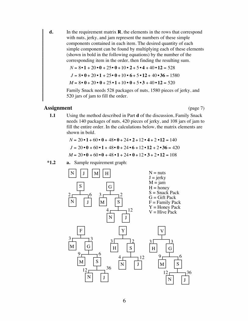
a. Sample requirement graph:

N J M

S

N2 6

J

G

S

N

2

4

3

12M

J

F

G

S

N

3

12

3

9 6

36M

M

J

N= nutsJ = jerkyM = jam

S = Snack PackG = Gift PackF = Family Pack

5

b. 1. A Snack Pack consists of 2 packages of nuts and 6 pieces of jerky.

2. In terms of its simple components and composite products, a Gift Pack consists of 2 Snack Packs and 3 jars of jam.

3. In terms of its simple components only, a Gift Pack consists of 4 packages of nuts, 12 pieces of jerky, and 3 jars of jam.

4. In terms of its simple components and composite products, a Family Pack consists of 3 Gift Packs and 3 jars of jam.

5. In terms of its simple components only, a Family Pack consists of 12 packages of nuts, 36 pieces of jerky, and 12 jars of jam.

c. A total requirement matrix for this product line is shown below. N J M S G F

R =

NJMSGF

1 0 0 2 4 120 1 0 6 12 360 0 1 0 3 120 0 0 1 2 60 0 0 0 1 30 0 0 0 0 1

⎡

⎣

⎢ ⎢ ⎢ ⎢ ⎢

⎤

⎦

⎥ ⎥ ⎥ ⎥ ⎥

Discussion (page 6) a. In this case, it means that there are 5 compasses in a Euclid Set.

b. 1. The elements along the diagonal represent the number of a given product contained in the product itself, which is always 1.

2. An element of 0 indicates that a given product contains none of a specific simple component or composite product.

c. Each element in the requirement matrix can be calculated by adding the numbers in the appropriate product tree which correspond with a particular item. In the product tree for a Family Pack, for example, the two boxes that represent jam are accompanied by the numbers 9 and 3. The sum of these numbers (12) is the element in row M of column F of matrix R. This indicates that there are 12 jars of jam in a Family Pack.

6

d. In the requirement matrix R, the elements in the rows that correspond with nuts, jerky, and jam represent the numbers of these simple components contained in each item. The desired quantity of each simple component can be found by multiplying each of these elements (shown in bold in the following equations) by the number of the corresponding item in the order, then finding the resulting sum. N = 8•1 + 20 •0 + 25• 0 +10 • 2 + 5 •4 + 40 •12 = 528J = 8• 0 + 20 •1 + 25• 0 +10 • 6 + 5 •12 + 40 •36 = 1580M = 8• 0 + 20 • 0 + 25 •1 +10 • 0 + 5 •3 + 40 •12 = 520

Family Snack needs 528 packages of nuts, 1580 pieces of jerky, and 520 jars of jam to fill the order.

Assignment (page 7) 1.1 Using the method described in Part d of the discussion, Family Snack

needs 140 packages of nuts, 420 pieces of jerky, and 108 jars of jam to fill the entire order. In the calculations below, the matrix elements are shown in bold. N = 20 • 1 + 60 • 0 + 48• 0 + 24 • 2 +12 • 4 + 2 •12 = 140J = 20 • 0 + 60 •1 + 48• 0 + 24 •6 +12 •12 + 2 •36 = 420M = 20 • 0 + 60 • 0 + 48 •1 + 24 • 0 +12 • 3 + 2 •12 = 108

*1.2 a. Sample requirement graph:

N MJ H

S

N2 6

J

36

V

3H

3G

S

N12

9 6

36

M

J

F

G

S

N

3

12

3

9 6

M

M

J

G

S

N

2

4

3

12M

J

Y

3H

2S

N4 12

J

H = honey

N = nutsJ = jerkyM = jam

Y = Honey PackV = Hive Pack

S = Snack PackG = Gift PackF = Family Pack

7

b. A total requirement matrix for this product line is shown below. N J M H S G F Y VNJMHSGFYV

1 0 0 0 2 4 12 4 120 1 0 0 6 12 36 12 360 0 1 0 0 3 12 0 90 0 0 1 0 0 0 3 30 0 0 0 1 2 6 2 60 0 0 0 0 1 3 0 30 0 0 0 0 0 1 0 00 0 0 0 0 0 0 1 00 0 0 0 0 0 0 0 1

⎡

⎣

⎢ ⎢ ⎢ ⎢ ⎢ ⎢ ⎢ ⎢

⎤

⎦

⎥ ⎥ ⎥ ⎥ ⎥ ⎥ ⎥ ⎥

c. There are 9 jars of jam in one Hive Pack. *1.3 a. Sample requirement graph:

b. In a column for a simple component, the element 1 occurs once;

the rest of the elements in the column are 0. c. Sample response: Read the number of simple components in the

Ten-Pack column. This tells how many of each are required for each Ten-Pack. Multiply these numbers by 8. You would need 24 shrimp spreads, 24 lobster spreads, and 32 spinach spreads.

* * * * *

Sh L Sp

6P

Sh L Sp2 2 2

Sh = shrimpL = lobster

Sp = spinach6P = Six-Pack

10P = Ten-Pack10P

Sh L Sp2 6P

Sh L Sp2 2 2

3 3 41

8


b. The corresponding total requirement matrix is shown below.

Ch CB SS Sn HO POChCBSSSnHOPO

1 0 0 2 3 80 1 0 0 2 40 0 1 3 0 30 0 0 1 0 10 0 0 0 1 20 0 0 0 0 1

⎡

⎣

⎢ ⎢ ⎢ ⎢ ⎢ ⎢ ⎢ ⎢ ⎢

⎤

⎦

⎥ ⎥ ⎥ ⎥ ⎥ ⎥ ⎥ ⎥ ⎥

c. There are 3 summer sausage logs in one Pig-Out Pack. d. There are 8 cheddar cheese logs in one Pig-Out Pack.

Ch CB SS

Sn

Ch SS2 3

HO

Ch CB3 2

PO

Sn

Ch SS2 3

HO

Ch CB6 4

2

Ch = cheddar cheese logCB = cheese and bacon logSS = summer sausageSn = Snack Pack

HO = Hand-Out PackPO = Pig-Out Pack

9

1.5 a. Sample requirement graph:

b. Sample response: The simple components in matrix T are A, B,

and C. In a column for a simple component, the element 1 occurs once; the rest of the elements in the column are 0.

c. Sample response: Read the number of simple components (As, Bs, and Cs) in the F column. This tells how many of each are required for each F. Multiply these numbers by 10. You would need 200 As, 180 Bs, and 210 Cs.

C

D

A2

B3

C2

E

C23

12 106

F

E

C23

CA B

D

A4

B6

C4

D

A4

B6

C4

D

A4

B6

C4

2

A B

10



c. There are 6 spinach spreads in one Combo Pack. * * * * * * * * * *

(page 9)

Activity 2 In this activity, students are introduced to matrix addition and scalar multiplication in the context of inventory control.

Sh = shrimpL = lobster

Sp = spinach

6P = Six-Pack10P = Ten-Pack

P = pepperoniJ = jalapeno

12P = Twelve-PackC = Combo

SpSh P JL

6P

Sh L Sp2 2 2

P

12P

3 3

6P

Sh L Sp2 2 2

10P

Sh L Sp2 6P

Sh L Sp2 2 2

C

10P P J4 3

J

Sh L Sp2 6P

Sh L Sp2 2 2

3 3 4

33 4

11


Technology • matrix manipulator (optional)

Exploration (page 9) a. 1. The dimensions of this matrix are 3 × 6 .

N J M S G F

S =

KZT

8 12 0 16 28 812 4 24 8 24 1212 0 12 12 36 4

⎡

⎣

⎢ ⎢

⎤

⎦

⎥ ⎥

2. The dimensions of this matrix are 6 ×3 . K Z T

R =

NJ

MSGF

8 12 1212 4 00 24 12

16 8 1228 24 368 12 4

⎡

⎣

⎢ ⎢ ⎢ ⎢ ⎢

⎤

⎦

⎥ ⎥ ⎥ ⎥ ⎥

b. Although they illustrate the same information, the matrices created in Part a are not equal because they have different dimensions.

c. Sample 3 × 6 matrix: N J M S G F

O =

KZT

8 4 24 12 8 3616 8 28 16 20 328 12 4 16 8 0

⎡

⎣

⎢ ⎢

⎤

⎦

⎥ ⎥

d. 1. The matrix T below shows the total of the corresponding elements in matrices S and O.

N J M S G F

T =

KZT

16 16 24 28 36 4428 12 52 24 44 4420 12 16 28 44 4

⎡

⎣

⎢ ⎢

⎤

⎦

⎥ ⎥

12

2. The matrix D below shows the differences between the corresponding elements in matrices O and S.

N J M S G F

D =

KZT

0 −8 24 −4 −20 284 4 4 8 −4 20−4 12 −8 4 −28 −4

⎡

⎣

⎢ ⎢

⎤

⎦

⎥ ⎥

e. The matrix N shows the product of each element in matrix O multiplied by 2.

N J M S G F

N =

KZT

16 8 48 24 16 7232 16 56 32 40 6416 24 8 32 16 0

⎡

⎣

⎢ ⎢ ⎢

⎤

⎦

⎥ ⎥ ⎥

f. 1. This matrix can be determined by matrix addition. N J M S G F

N +O =

KZT

24 12 72 36 24 10848 24 84 48 60 9624 36 12 48 24 0

⎡

⎣

⎢ ⎢

⎤

⎦

⎥ ⎥

2. This matrix can be determined by matrix subtraction. N J M S G F

N −S =

KZT

8 −4 48 8 −12 6420 12 32 24 16 524 24 −4 20 −20 −4

⎡

⎣

⎢ ⎢

⎤

⎦

⎥ ⎥

3. This matrix can be determined by matrix addition. N J M S G F

S +O + N =

KZT

32 24 72 52 52 11660 28 108 56 84 10836 36 24 60 60 4

⎡

⎣

⎢ ⎢ ⎢

⎤

⎦

⎥ ⎥ ⎥

g. 1. This matrix can be determined as follows. N J M S G F

12

(S +O) =

KZT

8 8 12 14 18 2214 6 26 12 22 2210 6 8 14 22 2

⎡

⎣

⎢ ⎢

⎤

⎦

⎥ ⎥

13

2. This matrix can be determined as shown below.

N J M S G F

13

(S +O + N) =

KZT

10 23 8 24 17 1

3 17 13 38 2

3

20 9 13 36 18 2

3 28 3612 12 8 20 20 1 1

3

⎡

⎣

⎢ ⎢ ⎢ ⎢

⎤

⎦

⎥ ⎥ ⎥ ⎥

Discussion (page 11) a. Sample response: The mean sales matrix was found by adding the

matrices for September, October, and November, then multiplying the result by the scalar 1 3 .

b. Only matrices with the same dimensions can be added together. c. The dimensions of the resulting matrix are the same as the dimensions

of the original matrix (or matrices). d. Matrix addition involves adding corresponding elements of matrices

with the same dimensions. Because order does not matter when adding two real numbers, matrix addition is commutative.

Assignment (page 12)

*2.1 a. 5 9−1 4⎡

⎣ ⎢ ⎤

⎦ ⎥ +

−3 31 5

⎡

⎣ ⎢ ⎤

⎦ ⎥ =2 120 9⎡

⎣ ⎢ ⎤

⎦ ⎥

b. Addition is not possible since the matrices do not have the same dimensions.

c. π •

5 711 −43 0

⎡

⎣

⎢ ⎢

⎤

⎦

⎥ ⎥

=

5π 7π11π −4π3π 0π

⎡

⎣

⎢ ⎢

⎤

⎦

⎥ ⎥ ≈

15.7 22.034.6 −12.69.4 0

⎡

⎣

⎢ ⎢

⎤

⎦

⎥ ⎥

d. 4 •2 6 −93 7 11⎡

⎣ ⎢ ⎤

⎦ ⎥ −8 15 2−5 6 0⎡

⎣ ⎢ ⎤

⎦ ⎥ =0 9 −3817 22 44⎡

⎣ ⎢ ⎤

⎦ ⎥

e. 3 41 −7⎡

⎣ ⎢ ⎤

⎦ ⎥ +0 00 0⎡

⎣ ⎢ ⎤

⎦ ⎥ =3 41 −7⎡

⎣ ⎢ ⎤

⎦ ⎥

2.2 a. The element in row 4, column 5 represents the distance from Kansas City to Seattle.

b. In row 5, column 3, 2779 represents the distance from Seattle to Chicago. In row 3, column 5, 2779 represents the distance from Chicago to Seattle.

c. The zeros represent the distance from a city to itself.

14

2.3 a. Sample matrix:

T =

T1 T2 T3 T4E1E2E3E4

8 7 4 1010 4 5 8.56 3.5 4 98 6.5 8 6

⎡

⎣

⎢ ⎢ ⎢

⎤

⎦

⎥ ⎥ ⎥

b. The following assignment requires a minimum of 6 hr to complete all four tasks: Assign task 3 to employee 1, task 2 to employee 2, task 1 to employee 3, and task 4 to employee 4.

c. There is no other set of assignments that completes the day’s tasks in 6 hr. To complete all the tasks in 6 hr, employee 4 must do task 4 (because all the other tasks take this employee more than 6 hr). Likewise, employee 1 must do task 3. Employee 2 must do task 2 or task 1, since tasks 2 and 4 are already taken. Since task 1 requires more than 6 hr for employee 2 to complete, employee 2 must do Task 2. This leaves employee 3 with task 1.

*2.4 a. The dimensions of matrix I are 3 × 4 .

b. This element (22) represents the inventory of large, red sweat pants.

c. The new inventory is shown in matrix A below.

A =

S M L XLBRY

31 45 44 2832 47 42 3029 35 38 32

⎡

⎣

⎢ ⎢

⎤

⎦

⎥ ⎥

d. Using scalar multiplication:

3 • I =

S M L XLBRY

33 75 72 2436 81 66 3027 45 54 36

⎡

⎣

⎢ ⎢

⎤

⎦

⎥ ⎥

e. The sum of the following matrix and matrix I is matrix A. S M L XL

BRY

20 20 20 2020 20 20 2020 20 20 20

⎡

⎣

⎢ ⎢ ⎢

⎤

⎦

⎥ ⎥ ⎥

* * * * *

15

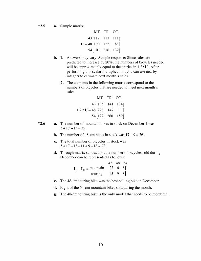
*2.5 a. Sample matrix: MT TR CC

U =

434854

112 117 111190 122 92101 216 132

⎡

⎣

⎢ ⎢

⎤

⎦

⎥ ⎥

b. 1. Answers may vary. Sample response: Since sales are predicted to increase by 20%, the numbers of bicycles needed will be approximately equal to the entries in 1.2 •U . After performing this scalar multiplication, you can use nearby integers to estimate next month’s sales.

2. The elements in the following matrix correspond to the numbers of bicycles that are needed to meet next month’s sales.

MT TR CC

1.2 •U ≈434854

135 141 134228 147 111122 260 159

⎡

⎣

⎢ ⎢

⎤

⎦

⎥ ⎥

*2.6 a. The number of mountain bikes in stock on December 1 was 5 +17 +13 = 35.

b. The number of 48-cm bikes in stock was 17 + 9 = 26 .

c. The total number of bicycles in stock was 5 +17 +13 +11 + 9 +18 = 73.

d. Through matrix subtraction, the number of bicycles sold during December can be represented as follows:

I1 − I31 =

43 48 54mountaintouring

2 6 85 9 8⎡

⎣ ⎢ ⎤

⎦ ⎥

e. The 48-cm touring bike was the best-selling bike in December.

f. Eight of the 54-cm mountain bikes sold during the month.

g. The 48-cm touring bike is the only model that needs to be reordered.

16

2.7 a. 1. Adding matrices C and N results in a matrix T that represents the total inventory after next week.

2. This matrix addition is shown below. MT TR CC

T = C+ N =

whitered

bluegreen

106 112 73133 135 9382 137 40

116 101 149

⎡

⎣

⎢ ⎢ ⎢

⎤

⎦

⎥ ⎥ ⎥

b. To determine the numbers of bicycles required, students should perform the following matrix subtraction:

MT TR CC

S − T =

whiteredbluegreen

10 20 1412 12 1012 15 1414 16 9

⎡

⎣

⎢ ⎢ ⎢

⎤

⎦

⎥ ⎥ ⎥

2.8 a. Sample matrix: A B C D

W1

W2

W3

W4

3 6 7 44 5 5 66 3 4 45 5 3 6

⎡

⎣

⎢ ⎢ ⎢

⎤

⎦

⎥ ⎥ ⎥

b. Answers may vary. Sample response: Worker 1 should knit style C because this is the maximum number of sweaters that can be knitted by any worker. Similarly, worker 2 should knit style D; worker 3 should knit style A; and worker 4 should knit style B. This arrangement allows the production of 24 sweaters per day.

c. The maximum number of sweaters possible is 24.

d. There is more than one possible response. Assigning worker 1 to style C; worker 2 to style B; worker 3 to style A; and worker 4 to style D also results in the production of 24 sweaters per day.

* * * * * * * * * *

17

(page 16)

Activity 3 In this activity, students are introduced to matrix multiplication.


Technology • matrix manipulator

Exploration 1 (page 16) a. 1. Keyes made $860 in sales, while Zhang made $795 in sales.

2. Sample response: To determine the value of the sales made by each person, you must multiply the number of cases of each item sold by the selling price of that item, then add these products. Note: Some students may recognize that each row in the sales matrix W can be multiplied by the column matrix MP , as shown below.

Sales

W•MP =KZ

860.00795.00⎡

⎣ ⎢ ⎤

⎦ ⎥

b. 1. Sample matrix: Com.

MC =

SGF

2.254.207.20

⎡

⎣

⎢ ⎢

⎤

⎦

⎥ ⎥

2. The matrix below illustrates the product W •MC . Com.

W •MC =KZ

52.8051.30⎡

⎣ ⎢ ⎤

⎦ ⎥

c. 1. The product matrix is shown below. Sales Com.

W •M =KZ

860.00 52.80795.00 51.30⎡

⎣ ⎢ ⎤

⎦ ⎥

2. The dimensions of the matrix are 2 × 2 .

18

3. The information in the matrix represents the total value of the sales and commissions for each salesperson.

d. 1. The product matrix is shown below. S G F

M •W =

SGF

184.5 328.5 96.75288.4 515.2 152.6394.4 708.2 211.6

⎡

⎣

⎢ ⎢

⎤

⎦

⎥ ⎥

2. The dimensions of the matrix are 3 × 3 .

3. Sample response: The information in the matrix has no meaning in this context. For example, the entry 184.5 represents the sum of the sales made by Keyes and the commission earned by Zhang on Snack Packs. This information is not of any use to the company.

Discussion 1 (page 18) a. Answers will vary, depending on the methods students used in Part a.

Sample response: Matrix multiplication is the better method because it is more orderly.

b. The number of columns in matrix A must equal the number of rows in matrix B.

c. Sample response: The operation W •M is more efficient because it is a one-step process that includes all of the information in one place.

d. 1. Yes. The entries in the matrix indicate the amount of commission earned by each salesperson.

2. No. The elements in the matrix are not meaningful in this context. (See response to Part d3 of Exploration 1.) Note: The fact that matrix multiplication is not commutative will be examined in Exploration 2. You may wish to emphasize that multiplication of matrices does not guarantee a product matrix which contains useful information. Each product must be evaluated in context.

e. Keyes earned $1.50 more in commissions than Zhang as shown in Part b.2 of Exploration 1.

19

Exploration 2 (page 19) a. Students multiply matrices M and W using technology. They should

observe that the product is the same as that obtained in Exploration 1.

b. Sample matrix: S G F

W2 =

KZTL

4 7 22 6 33 9 16 0 0

⎡

⎣

⎢ ⎢ ⎢

⎤

⎦

⎥ ⎥ ⎥

c. Students should use technology to obtain the 4 × 2 product matrix below. This matrix shows the value of the sales and commissions for each salesperson.

Sales Com.

W2 •M =

KZTL

860.00 52.80795.00 51.30855.00 51.75270.00 13.50

⎡

⎣

⎢ ⎢ ⎢

⎤

⎦

⎥ ⎥ ⎥

d. The product does not exist because the number of columns in M does not equal the number of rows in W2 . When attempting to multiply M •W2 using technology, students will receive an error message.

e. Sample matrix: N J M S G F

W3 =

KZTL

2 3 0 4 7 23 1 6 2 6 33 0 3 3 9 12 4 1 6 0 0

⎡

⎣

⎢ ⎢ ⎢

⎤

⎦

⎥ ⎥ ⎥

f. Sample matrix: Price Com.

S =

NJMSGF

6.00 0.1810.00 0.308.00 0.3245.00 2.2570.00 4.2095.00 7.20

⎡

⎣

⎢ ⎢ ⎢ ⎢ ⎢

⎤

⎦

⎥ ⎥ ⎥ ⎥ ⎥

20

g. Students should use technology to obtain the product below. This matrix shows the value of the sales and commissions for each salesperson on Family Snack’s entire product line.

Sales Com.

W3 •S =

KZTL

902.00 54.06871.00 54.06902.00 53.25330.00 15.38

⎡

⎣

⎢ ⎢ ⎢

⎤

⎦

⎥ ⎥ ⎥

h. The product does not exist because the number of columns in S does not equal the number of rows in W3 .

Discussion 2 (page 20) a. Sample response: To multiply an m × n matrix by a p × q matrix, it is

first necessary to make sure that n equals p. In other words, the number of columns in the first matrix must equal the number of rows in the second matrix. Once that condition has been met, multiplication of the matrices A and B below results in the product matrix C.

A =

a11 a12 … a1na21 a22 … a2n! ! ! !am1 am2 … amn

⎡

⎣

⎢ ⎢ ⎢

⎤

⎦

⎥ ⎥ ⎥

B =

b11 b12 … b1qb21 b22 … b2q! ! ! !bp1 bp2 … bpq

⎡

⎣

⎢ ⎢ ⎢

⎤

⎦

⎥ ⎥ ⎥

C =

a11b11 + a12b21 + a13b31+!+a1nbp1 … a11b1p + a12b2 p + a13b3p +!+a1nbpq" " "

am1b11 + am2b21 + am3b31+!+amnbp1 … am1b1p + am2b2 p + am3b3p +!+amnbpq

⎡

⎣

⎢ ⎢

⎤

⎦

⎥ ⎥

b. Sample response: The product S •W3 cannot be done because the number of columns in S does not equal the number of rows in W3 .

c. Sample response: Matrix multiplication is not commutative because A •B does not always equal B •A . For example, if the dimensions of matrix A are 3 × 4 and the dimensions of B are 4 × 5 , then the product of A •B exists, but the product of B •A is not defined.

If the dimensions of matrix A are 3 × 4 and the dimensions of B are 4 × 3 , then both products exist, but their dimensions are different. Therefore, the two product matrices are not equal.

21

Assignment (page 20) 3.1 a. A •B = 1(−1) + 2(−2) + 3(−3) + 4(−4)[ ] = −30[ ]

b. C • D =3• 3 + (−1) •1 + 4 • 40 • 3 +1•1 + (−2) • 4⎡

⎣ ⎢ ⎤

⎦ ⎥ =24−7⎡

⎣ ⎢ ⎤

⎦ ⎥

c. In this case, matrix multiplication is not possible. Since matrix E is 5 × 3 and matrix B is 4 ×1 , the number of columns in E is not the same as the number of rows in B.

3.2 a. 1. The dimensions of the product matrix are 2 × 2 .

X •Y =25 23−3 7⎡

⎣ ⎢ ⎤

⎦ ⎥

2. The row dimension is the number of rows in X, while the column dimension is the number of columns in Y.

b. 1. The dimensions of the product matrix are 3 × 3 .

Y •X =

20 6 139 4 26−2 0 8

⎡

⎣

⎢ ⎢

⎤

⎦

⎥ ⎥

2. The row dimension is the number of rows in Y, while the column dimension is the number of columns in X.

c. Answers will vary. Students should mention that since the two product matrices have different dimensions and different elements, X •Y ≠ Y •X . Therefore, matrix multiplication is not commutative.

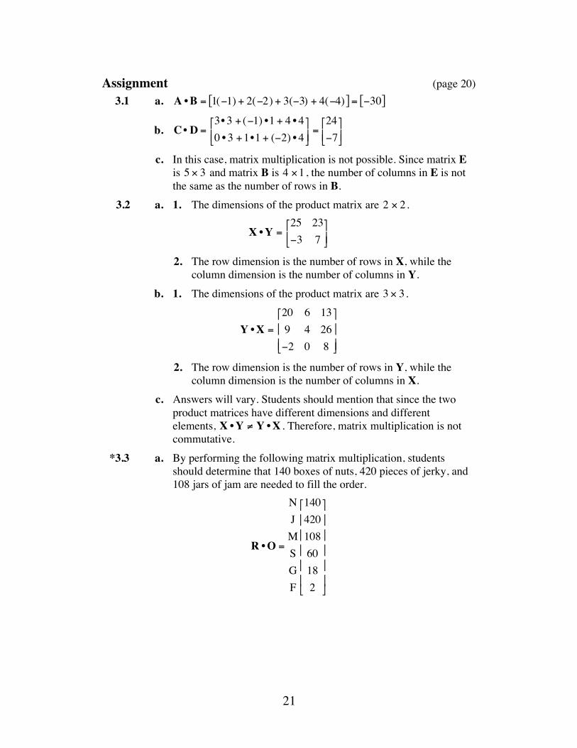
*3.3 a. By performing the following matrix multiplication, students should determine that 140 boxes of nuts, 420 pieces of jerky, and 108 jars of jam are needed to fill the order.

R •O =

NJMSGF

14042010860182

⎡

⎣

⎢ ⎢ ⎢ ⎢ ⎢

⎤

⎦

⎥ ⎥ ⎥ ⎥ ⎥

22

b. By performing the matrix multiplication below, students should find that 318 boxes of nuts, 1104 pieces of jerky, and 84 jars of jam are needed to fill the order.

R •

NJ

MSGF

1506004860120

⎡

⎣

⎢ ⎢ ⎢ ⎢ ⎢

⎤

⎦

⎥ ⎥ ⎥ ⎥ ⎥

=

NJ

MSGF

3181104

8484120

⎡

⎣

⎢ ⎢ ⎢ ⎢ ⎢

⎤

⎦

⎥ ⎥ ⎥ ⎥ ⎥

*3.4 a. Sample matrix:

S =

1234

10643

⎡

⎣

⎢ ⎢ ⎢

⎤

⎦

⎥ ⎥ ⎥

b. The columns of R must match the rows of S in Part a. 1 2 3 4

R =

E1

E2

E3

E4

4 0 4 43 4 0 52 5 5 03 3 3 3

⎡

⎣

⎢ ⎢ ⎢ ⎢ ⎢

⎤

⎦

⎥ ⎥ ⎥ ⎥ ⎥

c. As shown in the product matrix below, employee 3 was first, employees 2 and 4 tied for second, and employee 1 was fourth.

Pts.

R •S =

E1

E2

E3

E4

68697069

⎡

⎣

⎢ ⎢ ⎢ ⎢ ⎢

⎤

⎦

⎥ ⎥ ⎥ ⎥ ⎥

* * * * *

23

3.5 The matrix below is the product of the requirement matrix R and matrix O.

O1 O2 O3 O4 O5

R •O =

NJMSGF

68 104 272 148 32178 270 681 396 7452 72 182 130 1428 42 106 64 1210 16 44 28 22 4 12 8 0

⎡

⎣

⎢ ⎢ ⎢ ⎢ ⎢

⎤

⎦

⎥ ⎥ ⎥ ⎥ ⎥

a. Family Snack needs 272 boxes of nuts to fill O3 . b. Family Snack needs 624 boxes of nuts to fill all five orders. c. Family Snack needs 270 pieces of jerky to fill O2 . d. Family Snack needs 1599 pieces of jerky to fill all five orders. e. Family Snack needs 450 jars of jam to fill all five orders.

*3.6 a. As shown below, the value of the sales for each model can be calculated by matrix multiplication.

MT TR

J •P =MTTR

3570 39606000 6660⎡

⎣ ⎢ ⎤

⎦ ⎥

b. Because it is the product of the first row in J and the first column in P (both of which represent values for mountain bikes), $3570 represents the sales of mountain bikes. Similarly, $6660 represents the sales from touring bikes. The other two elements are not relevant because they involve numbers representing mountain bikes multiplied by numbers representing touring bikes.

c. Yes, it is possible to perform the matrix operation in Part a if the order of the matrices is reversed. In the product matrix below, $1900 is the income from 43-cm bikes, $4320 is the income from the 48-cm bikes, and $4010 is the income from 54-cm bikes. (As in Part b, the only relevant elements are those along the diagonal.)

43 48 54

P •J =

434854

1900 4020 34902040 4320 37502180 4620 4010

⎡

⎣

⎢ ⎢

⎤

⎦

⎥ ⎥

d. The total July sales is less than $15,000. To find the total sales, students should add only the relevant elements in the product matrix: $3570 + $6660 = $10, 230 or $1900 + $4320 + $4010 = $10, 230.

24

3.7 a. The dimensions of A •B are 2 × 4 .

A •B =20 30 −7 2389 104 −78 67⎡

⎣ ⎢ ⎤

⎦ ⎥

Since the column dimension of B does not match the row dimension of A, B •A is not possible.

b. The dimensions of A •C are 2 × 3 .

A •C =40 1 −11131 −14 20⎡

⎣ ⎢ ⎤

⎦ ⎥

Since the column dimension of C does not match the row dimension of A, C • A is not possible.

c. Since the column dimension of B does not match the row dimension of C, B •C is not possible. The dimensions of C • B are 3 × 4 .

C • B =

−55 4 20 4123 −32 61 −5441 30 28 9

⎡

⎣

⎢ ⎢

⎤

⎦

⎥ ⎥

d. The dimensions of both product matrices are 3 × 3 .

C • D =

2 5 −69 −4 09 3 1

⎡

⎣

⎢ ⎢

⎤

⎦

⎥ ⎥ D •C =

2 5 −69 −4 09 3 1

⎡

⎣

⎢ ⎢

⎤

⎦

⎥ ⎥

e. The dimensions of B •E are 3 × 4 .

B •E =

21 −37 −5 −4814 112 −1 114−13 111 −75 132

⎡

⎣

⎢ ⎢

⎤

⎦

⎥ ⎥

Since the column dimension of E does not match the row dimension of B, E • B is not possible.

* * * * * * * * * *

25

Research Project (page 23) a. Multiplication of 2 × 2 matrices is associative, as shown below.

A • B( ) =ae + bg af + bhce + dg cf + dh⎡

⎣ ⎢ ⎤

⎦ ⎥

A •B( ) •C =(ae + bg)i + (af + bh)k (ae + bg) j + (af + bh)l(ce + dg)i + (cf + dh)k (ce + dg) j + (cf + dh)l⎡

⎣ ⎢ ⎤

⎦ ⎥

=a(ei + fl) + b(gi + hk) a(ej + fl ) + b(gj + hl)c(ei + fl ) + d(gi + hk) c(ej + fl) + d(gj + hl)⎡

⎣ ⎢ ⎤

⎦ ⎥

B •C( ) =ei + fk ej + flgi + hk gj + hl⎡

⎣ ⎢ ⎤

⎦ ⎥

A • (B •C) =a(ei + fk ) + b(gi + hk) a(ej + fl) + b(gj + hl)c(ei + fk ) + d(gi + hk) c(ej + fl) + d(gj + hl)⎡

⎣ ⎢ ⎤

⎦ ⎥

Therefore, (A • B)• C = A• (B•C).

b. The distributive property of multiplication over addition is valid for 2 × 2 matrices, as shown below.

A • B +C( ) =a bc d⎡

⎣ ⎢ ⎤

⎦ ⎥ •e + i f + jg + k h + l⎡

⎣ ⎢ ⎤

⎦ ⎥

=a(e + i) + b(g + k ) a( f + j) + b(h + l)c(e + i) + d(g + k) c( f + j) + d(h + l)⎡

⎣ ⎢ ⎤

⎦ ⎥

=ae + ai + bg + bk af + aj + bh + bl)ce + ci + dg + dk cf + cj + dh + dl⎡

⎣ ⎢ ⎤

⎦ ⎥

A •B( ) + A •C( ) =ae + bg af + bhce + dg cf + dh⎡

⎣ ⎢ ⎤

⎦ ⎥ +ai + bk aj + blci + dk cj + dl⎡

⎣ ⎢ ⎤

⎦ ⎥

=ae + bg + ai + bk af + bh + aj + blce + dg + ci + dk cf + dh + cj + dl⎡

⎣ ⎢ ⎤

⎦ ⎥ Therefore, A • (B+C) =A •B+A •C .

c. The identity for multiplication of 2 × 2 matrices is shown below.

I =1 00 1⎡

⎣ ⎢ ⎤

⎦ ⎥

26

d. The Zero Product Matrix for 2 × 2 matrices is shown below. This matrix is unique.

Z =0 00 0⎡

⎣ ⎢ ⎤

⎦ ⎥

27

Answers to Summary Assessment (page 24) 1. a. Sample requirement graph:


N J M C S G F

R =

NJMCSGF

1 0 0 0 1 2 60 1 0 0 10 20 600 0 1 0 1 4 120 0 0 1 1 2 100 0 0 0 1 2 60 0 0 0 0 1 30 0 0 0 0 0 1

⎡

⎣

⎢ ⎢ ⎢ ⎢ ⎢ ⎢

⎤

⎦

⎥ ⎥ ⎥ ⎥ ⎥ ⎥

2. Answers may vary, depending on how students organize their matrices.

a. Sample matrix: one two three

I =fu

10 5 510 10 5⎡

⎣ ⎢ ⎤

⎦ ⎥

CN MJ

N = nutsJ = jerky

M = jamC = crackersS = Snack PackG = Gift PackF = Family Pack

S

N C1 10 1 1

MJ

G

S

N C

2 2

2 20 2 2M

M

J

F

C G

S

N C

4 3

6 6

6 60 6 6M

M

J

28

b. Sample matrix: f u

R =

onetwothree

375 345400 370450 420

⎡

⎣

⎢ ⎢

⎤

⎦

⎥ ⎥

c. The product of the matrices given in Parts a and b can be done in two ways.

one two three

R • I =

onetwothree

7200 5325 36007700 5700 38508700 6450 4350

⎡

⎣

⎢ ⎢ ⎢

⎤

⎦

⎥ ⎥ ⎥

d. The elements along the main diagonal in the product matrix I •R represent the total rents for the furnished ($8000) and unfurnished ($9250) apartments.

The elements along the main diagonal in the product matrix R • I represent the total rents for the one-bedroom ($7200), two-bedroom ($5700) and three-bedroom apartments ($4350).

The other elements in both matrices are irrelevant. The irrelevant elements are the result of combining values from different types of apartments. For example, the rent for a one-bedroom apartment multiplied by the number of two-bedroom apartments is meaningless.

e. Students may use scalar multiplication to determine this matrix, as shown below.

f u

1.1• R =

onetwo

three

412.50 379.50440.00 407.00495.00 462.00

⎡

⎣

⎢ ⎢ ⎢

⎤

⎦

⎥ ⎥ ⎥

f. Students may have to adjust their matrices so that multiplication is defined (and the product is meaningful). Sample response:

I •onetwothree

8095105

⎡

⎣

⎢ ⎢

⎤

⎦

⎥ ⎥

=fu18002275⎡

⎣ ⎢ ⎤

⎦ ⎥

g. Sample response: e s w

e s w

I • onetwothree

80 15 1895 20 26105 30 42

⎡

⎣

⎢ ⎢ ⎢

⎤

⎦

⎥ ⎥ ⎥ =

fu

1800 400 5202275 500 650⎡

⎣ ⎢

⎤

⎦ ⎥

29

Module Assessment

1. Find the values of r and s in each of the following equations.

a. 5 r 3−2 8 s⎡

⎣ ⎢ ⎤

⎦ ⎥ +2 11 46 7 s⎡

⎣ ⎢ ⎤

⎦ ⎥ =7 5 74 15 4⎡

⎣ ⎢ ⎤

⎦ ⎥

b. 5 •−3 4r 0s −2

⎡

⎣

⎢ ⎢

⎤

⎦

⎥ ⎥

=

−15 208 0−11 −10

⎡

⎣

⎢ ⎢

⎤

⎦

⎥ ⎥

c. 2 01 5⎡

⎣ ⎢ ⎤

⎦ ⎥ •rs⎡

⎣ ⎢ ⎤

⎦ ⎥ =

623⎡

⎣ ⎢ ⎤

⎦ ⎥

2. Find the values of the variables in each of the following equations.

a. 3 −4 12−4 6 7⎡

⎣ ⎢ ⎤

⎦ ⎥ +

a b cd e f⎡

⎣ ⎢ ⎤

⎦ ⎥ =

−5 23 8−7 6 15⎡

⎣ ⎢ ⎤

⎦ ⎥

b. 8 •9 −80 g−5 h

⎡

⎣

⎢ ⎢

⎤

⎦

⎥ ⎥

=

72 −640 96−40 −72

⎡

⎣

⎢ ⎢

⎤

⎦

⎥ ⎥

3. Matrix D below shows the distances in kilometers between selected cities.

a. What does the element in row 2, column 3 represent?

b. If you flew from New York to Los Angeles with stops in Kansas City and Chicago, how far would you travel?

c. Create a matrix that shows the flight times between the cities in matrix D if an airplane averages 570 km per hour.

d. What would the values in the matrix 2 • D represent?

MiamiNew York

Chicago

1997 4400 37641765 3875 3944666 2795 2808

⎡

⎣

⎢ ⎢ ⎢

⎤

⎦

⎥ ⎥ ⎥

D =

KansasCity Seattle

LosAngeles

30

4. Describe the steps used to obtain the element in row 1, column 2 of the product matrix below.

3 −4 12−4 6 7⎡

⎣ ⎢ ⎤

⎦ ⎥ •9 −80 −3−5 4

⎡

⎣

⎢ ⎢

⎤

⎦

⎥ ⎥

=−33 36−71 42⎡

⎣ ⎢ ⎤

⎦ ⎥

5. A ski shop sells three different types of skis. The three types—listed in order of quality—are laminate construction, torsion-box construction, and monoblock construction. The shop’s inventory of each type is displayed in the matrix below. The column headings designate the lengths of the skis in centimeters.

160 170 180 190

I =

LTBM

5 11 17 43 16 18 24 13 14 5

⎡

⎣

⎢ ⎢

⎤

⎦

⎥ ⎥

a. The shop pays $1.25 per centimeter for laminate construction, $1.60 per centimeter for torsion-box construction, and $2.15 per centimeter for monoblock construction.

Create a matrix that can be multiplied by matrix I to determine how much the store paid for its inventory.

b. Determine the total cost of all the skis in the store.

6. Family Snack has added two new items to its original product line—the Trail Pack and the Picnic Pack. A Trail Pack consists of 2 boxes of nuts and 3 sticks of jerky, while a Picnic Pack contains 2 Trail Packs plus 5 more sticks of jerky. A total requirement graph for these four products is shown below.

a. Create the corresponding total requirement matrix.

b. Family Snack has received an order for 111 boxes of nuts, 55 pieces of jerky, 46 Trail Packs, and 87 Picnic Packs. Use matrix multiplication to determine the number of each simple component required to fill this order.

2

P

J T

JN

5

4 6

T

N J2 3

JN

J = jerkyN = nuts

T = Trail PackP = Picnic Pack

31

Answers to Module Assessment 1. a. r = −6; s = 2 b. r = 8 5 = 1.6; s = −11 5 = −2.2

c. r = 3; s = 4 2. a. a = −8 , b = 27 , c = −4 , d = −3 , e = 0 , and f = 8

b. g = 12 ; h = −9

3. a. This element represents the distance in kilometers between New York and Los Angeles.

b. The distance from New York to Kansas City is 1765 km; the distance from Kansas City to Chicago is 666 km; and the distance from Chicago to Los Angeles is 2808 km. The total distance traveled is 5239 km.

c. The elements in matrix T below are rounded to the nearest 0.01 hr.

d. Answers may vary. Sample response: The values in the matrix would represent round-trip distances between the cities.

4. Answers will vary. Sample response: First, multiply the number in the first row, first column of the 2 × 3 matrix with the number in the first row, second column of the 3 × 2 matrix as follows: 3 •−8 = −24 .

Then multiply the number in the first row, second column of the 2 × 3 matrix with the number in the second row, second column of the 3 × 2 matrix: −4 •−3 =12 .

Then multiply the number in the first row, third column of the 2 × 3 matrix with the number in the third row, second column of the 3 × 2 matrix: 12 • 4 = 48 .

Finally, find the sum of these three products: −24 +12 + 48 = 36 .

T =1

570•D =

MiamiNew York

Chicago

3.50 7.72 6.603.10 6.80 6.921.17 4.90 4.93

⎡

⎣

⎢ ⎢ ⎢

⎤

⎦

⎥ ⎥ ⎥

KansasCity Seattle

LosAngeles

32

5. a. Matrix C shown below is designed for multiplication on the right side of I. (Multiplication on the left would require the transpose of this matrix.)

L TB M

C =

160170180190

200.00 256.00 344.00212.50 272.00 365.50225.00 288.00 387.00237.50 304.00 408.50

⎡

⎣

⎢ ⎢ ⎢

⎤

⎦

⎥ ⎥ ⎥

b. The total cost is the sum of the elements on the main diagonal in the product matrix below, or $32,612.50.

L TB M

I •C =

LTBM

8112.50 10, 384.00 13, 953.508525.00 10, 912.00 14, 663.007900.00 10,112.00 13, 588.00

⎡

⎣

⎢ ⎢

⎤

⎦

⎥ ⎥

6. a. Sample matrix: N J T P

R =

NJTP

1 0 2 40 1 3 110 0 1 20 0 0 1

⎡

⎣

⎢ ⎢ ⎢

⎤

⎦

⎥ ⎥ ⎥

b. As shown in the product matrix below, 551 boxes of nuts and 1150 pieces of jerky are required to fill the order.

R •

NJTP

111554687

⎡

⎣

⎢ ⎢ ⎢

⎤

⎦

⎥ ⎥ ⎥

=

NJTP

551115022087

⎡

⎣

⎢ ⎢ ⎢

⎤

⎦

⎥ ⎥ ⎥

33

Selected References DeLange, J. Matrices. Utrecht, The Netherlands: Research Group on Mathematics

Education, 1990.

Harshbarger, R. J., and J. J. Reynolds. Mathematical Applications for Management, Life, and Social Sciences. Lexington, MA: D. C. Heath, 1992.

Vazsonyi, A. Finite Mathematics: Quantitative Analysis for Management. Santa Barbara, CA: Wiley/Hamilton, 1977.

34

Flashbacks

Activity 1 1.1 Use the following table for this problem.

Attraction Costs (dollars)

City

Amusement Park

Water Park

Helicopter Tours

San Antonio $50 $15 $125 Orlando $65 $10 $150

San Diego $45 $18 $95 Honolulu $70 $20 $100

a. Which city has the least expensive helicopter tours? b. Which city would be the most expensive if you wanted to include

all three activities? c. Use the row number and column number to identify the location in

the table of the cost of the water park in San Antonio? d. What row number and column number identifies the location of

the entry "70"? 1.2 Evaluate each of the following expressions. a. −23 +10

b. −18 −12 c. 15 − 29 d. −16 + 20 e. −24 − 19

35

Activity 2 2.1 Four circus clowns—Curley, Larry, Moe, and Fred—are selling red,

green, blue, and mauve balloons. The number of balloons each clown has at the beginning of the day are shown in the matrix below.

R G B MCurleyLarryMoeFred

5 3 2 127 5 4 69 7 8 411 9 3 4

⎡

⎣

⎢ ⎢ ⎢ ⎢ ⎢

⎤

⎦

⎥ ⎥ ⎥ ⎥ ⎥

a. What are the dimensions of this matrix?

b. 1. How many green balloons does Moe have at the beginning of the day?

2. How many blue balloons does Larry have at the beginning of the day?

3. How many mauve balloons does Fred have at the beginning of the day?

2.2 The matrix S shown below shows the amount of money in a savings account for the first four months of 1994.

1994

S =

JanFebMarApr

$500$600$750$800

⎡

⎣

⎢ ⎢ ⎢

⎤

⎦

⎥ ⎥ ⎥

a. What are the dimensions of this matrix?

b. What was the average monthly increase in the account during this time?

36

Activity 3 3.1 Consider matrices A and B below.

A =

−2 −2 64 −3 10 4 −1

⎡

⎣

⎢ ⎢

⎤

⎦

⎥ ⎥ B =

4 −2 −20 2 90 −3 −1

⎡

⎣

⎢ ⎢

⎤

⎦

⎥ ⎥

Use these matrices to perform each of the following operations.

a. 6A

b. –2B

c. A + B

d. B − A

3.2 Evaluate each of the following expressions.

a. 2 • 5 +8 • 4

b. 2 • −8 + 4 • 4 + 3 •2 − 4 •10

c. 12 • 25 +18 •24 + 6 •8

d. −2 • −5 + −8 • −4 − 4 •1 + 5• 6

3.3 Consider matrices X, Y, and W below.

X =

2 −1 8−2 4 −310 −4 6

⎡

⎣

⎢ ⎢

⎤

⎦

⎥ ⎥ Y =

5 −14 02 1

⎡

⎣

⎢ ⎢

⎤

⎦

⎥ ⎥

W =3 −7−5 0⎡

⎣ ⎢ ⎤

⎦ ⎥

a. List the dimensions of each matrix.

b. Perform each of the following calculations, if possible. If the operation is not possible, explain why not.

1. X + Y

2. –4X

3. 5W

37

Answers to Flashbacks

Activity 1 1.1 a. San Diego has the least expensive helicopter tours. b. Orlando is the most expensive city if you include all three

activities. c. Row 1, Column 2 is the location of the cost of the water park in

San Antonio. d. Row 4, Column 1 identifies the location of the entry "70". 1.2 a. −23 +10 = −13 b. −18 −12 = −30 c. 15 − 29 = −14 d. −16 + 20 = 4 e. −24 − 19 = −43

Activity 2 2.1 a. 4 × 4 b. 1. Moe starts with 7 green balloons. 2. Larry starts with 4 blue balloons. 3. Fred starts with 4 mauve balloons. 2.2 a. 4 ×1 b. The average monthly increase for the account was $100.

38

Activity 3

3.1 a. 6A =

−12 −12 3624 −18 60 24 −6

⎡

⎣

⎢ ⎢

⎤

⎦

⎥ ⎥

b. −2B =

−8 4 40 −4 −180 6 2

⎡

⎣

⎢ ⎢

⎤

⎦

⎥ ⎥

c. A + B =

2 −4 44 −1 100 1 −2

⎡

⎣

⎢ ⎢

⎤

⎦

⎥ ⎥

d. B − A =

6 0 −8−4 5 80 −7 0

⎡

⎣

⎢ ⎢

⎤

⎦

⎥ ⎥

3.2 a. 10 + 32 = 42

b. −16 + 16 + 6 − 40 = −34

c. 300 + 432 + 48 = 780

d. 10 + 32 − 4 + 30 = 68

3.3 a. The dimensions of matrix X are 3 × 3 , of matrix Y are 3 × 2 , and of matrix W are 2 × 2 .

b. 1. This operation is not possible because the two matrices have different dimensions.

2. −4X =

−8 4 −328 −16 12−40 16 −24

⎡

⎣

⎢ ⎢

⎤

⎦

⎥ ⎥

3. 5W =15 −35−25 0⎡

⎣ ⎢ ⎤

⎦ ⎥

A New Angle on an Old Pyramid

What mathematical skills did the ancient Egyptians use to build the pyramids? In this module, you explore some of the theories regarding the construction of these architectural wonders—and see how modern mathematical knowledge could have made part of the job much simpler.

Clay Burkett • Randy Carspecken

41

Teacher Edition A New Angle on an Old Pyramid

Overview This module reviews similar triangles, the Pythagorean theorem, and triangle notation in the context of Egypt’s Great Pyramid. Students explore the tangent, sine, and cosine ratios and their inverses.

Objectives In this module, students will:

• use similarity to determine unknown measures in triangles

• use the Pythagorean theorem and its converse to solve right-triangle problems

• use technology to develop a table of trigonometric values

• develop and apply the sine, cosine, and tangent ratios

• develop and apply the inverses of sine, cosine, and tangent.


• how to use a protractor

• how to solve proportions

• the sum of the angles of a triangle

• the definition of similarity.

42

Time Line Activity 1 2 3 4 Summary

Assessment Total

Days 2 2 2 2 1 9

Materials Required Materials Activity

1 2 3 4 Summary Assessment

butcher paper X metersticks X

centimeter rulers X protractors X X X

triangle template X puzzle template X

scissors X string X X

graph paper X drinking straws X

paper clips X

Teacher Note Blackline masters of the templates appear at the end of the teacher edition FOR THIS MODULE.



geometry utility X X X spreadsheet X X X

Teacher Note In Activities 3 and 4, students should set the technology to use degree measure (not radian measure).

43

A New Angle on an Old Pyramid

Introduction (page 31) The construction of Egypt’s Great Pyramid provides the context for most of the activities in this module.

(page 32)

Activity 1 In this activity, students review similar triangles and proportional reasoning.

Materials List • butcher paper (one sheet per group; approximately 1 m by 2 m)

• 30-cm rulers (one per group)

• protractors (one per group)

• metersticks (one per group)

• triangle template (one per student; a blackline master appears at the end of the teacher edition for this module)

Exploration (page 32) a. Students use protractors and rulers to construct a 90˚ corner.

b. To illustrate the potential range of error, students mark their locations for point P on a common sheet of paper, as shown in Figure 3.

c. The distance between X and Y may be as large as several centimeters.

d. Students should predict that the distance between R and S will be 100 times the distance between X and Y.

Discussion (page 33) a. Students should discuss the accuracy of their measurements, tools, and

methods.

b. Since CY and CX are congruent, ΔCXY is an isosceles triangle. Because ΔCXY is isosceles, ∠CXY and ∠CYX are congruent.

44

c. It is important to emphasize that this notation indicates corresponding sides and angles. For example, the statement ΔABC ~ ΔEDF indicates that ∠B and ∠D are corresponding angles and must be congruent, among other things. For the similar triangles in Figure 4, this is incorrect.

Note: For the triangles in Figure 4, there is only one correspondence between the angles and sides that results in a similarity relation. For some triangles, however, there can be several different similarity relations. If ∆ABC and ∆DEF are equilateral triangles, for example, then there are six different ways that angles and sides correspond: ΔABC ~ ΔDEF , ΔABC ~ ΔEDF , ΔABC ~ ΔFED , ΔABC ~ ΔDFE , ΔABC ~ ΔEFD, and ΔABC ~ ΔFDE .

d. Students should recognize that ΔCXY and ΔCRS are isosceles triangles with the same vertex angle, as shown below. Therefore, ΔCXY ~ ΔCRS .

e. Since ΔCXY ~ ΔCRS , the corresponding sides are proportional. The

distance RS can be found using the proportion below. XYRS

=CXCR

=1100

Teacher Note Each student will require a copy of the triangle template to complete Problem 1.2.

Assignment (page 34) 1.1 Answers will vary, depending on the class value for XY. For example,

if XY = 5 cm, then by similarity:

10.05

=230x

x =11.5 m

C1 m

1 m

100 m

100 m

D

X

Y

R

S•

•

••

45

1.2 In this problem, students investigate the properties of isosceles triangles.

a–b. The line of symmetry is perpendicular to the base and bisects the base.

c. The line of symmetry contains the altitude of the triangle.

d. When the triangle is folded along the line of symmetry, a right triangle is formed.

e. The line of symmetry bisects the vertex angle.

1.3 Sample response: Since the base of each pyramid is a square, the bases are similar. Each face is an isosceles triangle. Since the sum of the angles in a triangle is 180˚, then m∠ACB =180 − (m∠CAB +m∠CBA) and m∠DFE =180 − (m∠FDE + m∠FED) . Therefore, ∠ACB ≅ ∠DFE . By the AAA Property, ΔACB ~ ΔDFE . Because both the bases and the faces are similar, the pyramids are similar.

1.4 Sample response: The least amount of information needed is that two pairs of corresponding angles are congruent. This is because the sum of the measures of the angles in a triangle is 180˚. Therefore, if two pairs of angles are congruent, then the third pair must also be congruent and the AAA Property would apply.

1.5 a. Since the two right triangles with heights h and k also share another angle, then they have two pairs of congruent, corresponding angles. Therefore, they are similar triangles. Because they are similar, the ratios of corresponding sides are equal.

b. If an acute angle in one right triangle is congruent to an acute angle in another right triangle, then the two triangles are similar by the AAA Property.

*1.6 Sample response: In the following diagram, ΔADE ~ ΔAFB by the AAA Property.

A

B

C

E

D F

h

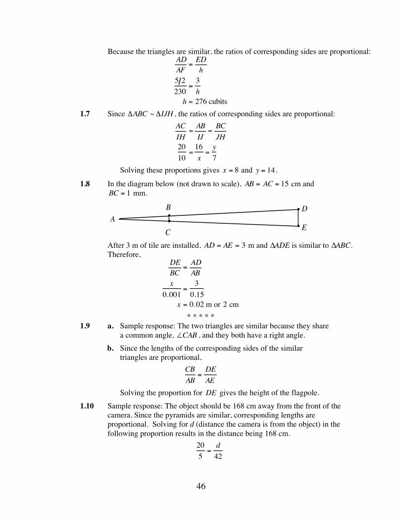
46

Because the triangles are similar, the ratios of corresponding sides are proportional: ADAF

=EDh

5 2230

=3h

h = 276 cubits

1.7 Since ΔABC ~ ΔIJH , the ratios of corresponding sides are proportional: ACIH

=ABIJ

=BCJH

2010

=16x=y7

Solving these proportions gives x = 8 and y = 14 .

1.8 In the diagram below (not drawn to scale), AB = AC = 15 cm and BC = 1 mm.

After 3 m of tile are installed, AD = AE = 3 m and ∆ADE is similar to ∆ABC.

Therefore, DEBC

=ADAB

x0.001

=3

0.15x = 0.02 m or 2 cm

* * * * * 1.9 a. Sample response: The two triangles are similar because they share

a common angle, ∠CAB , and they both have a right angle.

b. Since the lengths of the corresponding sides of the similar triangles are proportional,

CBAB

=DEAE

Solving the proportion for DE gives the height of the flagpole.

1.10 Sample response: The object should be 168 cm away from the front of the camera. Since the pyramids are similar, corresponding lengths are proportional. Solving for d (distance the camera is from the object) in the following proportion results in the distance being 168 cm.

205=d42

•

• D

EA ••

B

C

47

1.11 Yes, if two triangles are similar, then their altitudes are proportional. In the diagram below, for example, ΔLHK ~ ΔQMP . Since ∠LKJ ≅ ∠QPN and ∠LJK ≅ ∠QNP , then ΔLJK ~ ΔQNP . Since these triangles are similar, their corresponding sides LJ and QN are proportional. These segments are also the altitudes of ΔLHK and ΔQMP.

* * * * * * * * * *

(page 39)

Activity 2 In this activity, students review the Pythagorean theorem, then develop its converse using a geometry utility.

Materials List • scissors (one pair per group)

• 30–40 cm lengths of string (one per student)

• puzzle template (one per student; a blackline master appears at the end of the teacher edition for this module)

• graph paper

Technology • geometry utility

• spreadsheet

Exploration (page 40) a. 1. The converse of the Pythagorean theorem may be stated as

follows: “If the square of the length of the longest side equals the sum of the squares of the lengths of the other sides, then the triangle is a right triangle.”

2. Students may or may not believe that the converse is true.

M NP

H

Q

JK

L

48

b. By keeping point C within the given constraints, all obtuse or right triangles generated will have AB as the longest side. Sample data:

!∠! AB AC BC !" ! − [ !" ! + !" !] 62.2˚ 1.59 1.38 1.66 –2.14

135˚ 1.59 0.55 1.16 0.89 90˚ 1.59 0.95 1.27 0

c. 1. obtuse

2. acute

3. right

Discussion (page 41) a. The expression AB( )2 − (AC)2 + (BC)2[ ] represents the difference

between the square of the side opposite ∠C and the sum of the squares of the other two sides. This expression equals 0 when m∠C = 90˚ . At this point, ΔABC is a right triangle, where AB is the hypotenuse and AC and BC are the legs. In this case, the Pythagorean theorem is restated as c2 − (a2 + b2 ) = 0 , where c is the length of the hypotenuse and b and c are the lengths of the legs.

b. Sample response: In obtuse triangles, the square of the length of the side opposite the obtuse angle is greater than the sum of the squares of the lengths of the other two sides. This is shown by a positive value in the right-hand column of Table 1.

c. Sample response: In acute triangles, the square of the length of any side is less than the sum of the squares of the lengths of the other two sides. This is shown by a negative value in the right-hand column of Table 1.

d. From the data in Table 1, students should observe that the converse of the Pythagorean theorem appears to be true. Note: It should be pointed out that the exploration does not constitute a proof.

e. Sample response: Measure the length a and the width b of the corner and consider these the legs of a potential right triangle. Then measure the potential hypotenuse c of the triangle. If these lengths satisfy the equation a2 + b2 = c2 , then the triangle is a right triangle and the angle is a right angle.

Teacher Note Students require string to complete Problem 2.2. The puzzle template is needed for Problem 2.3. Two different puzzles are included at the end of this teacher edition. In Problem 2.4, students explore the triangle inequality property.

49

Assignment (page 42) 2.1 a. Students should verify that, when used as the lengths of the sides of a

triangle, each triple in the table makes the Pythagorean equation true. Since the converse of the Pythagorean theorem is true, these triangles are all right triangles. For example, using the triple in the first row:

1202 +1192 =? 1692

28, 561 = 28, 561

b. Any multiple of a Pythagorean triple is also a Pythagorean triple. For example, suppose a, b, and c are whole numbers and a2 + b2 = c2 . Then 2a, 2b , and 2c are whole numbers and:

2a( )2 + 2b( )2 = 4 a2 + b2( )= 4 c2( )= 2c( )2

In general, if a2 + b2 = c2 , then ma( )2 + mb( )2 = m2 a2 + b2( ) = m2 c2( ) . 2.2 By using the string to form a 3-4-5 triangle, students can create one

right angle for the square. The other right angles may be formed in a similar manner. Students can then verify that their figures are squares by calculating the lengths of the diagonals. The diagonals of a square are congruent, perpendicular, and bisect each other. If the side length of a square is 3 units, the diagonal length is approximately 4.2 units.

2.3 Sample arrangement:

Note: Although this puzzle provides a graphic illustration of the

Pythagorean relationship as a statement about areas, any demonstration of the Pythagorean theorem by the puzzle method

a

b

c

A

B

C

50

should be treated with caution. Many math puzzles ask students to cut up a rectangle with an area of, for example, 80 cm2 , then rearrange the pieces to obtain a rectangle with an area of 81 cm2 . You may wish to emphasize that a visually convincing demonstration does not constitute a proof.

2.4 a. Answers will vary. Sample response: (2, 3, 6); (1, 4, 5); (9, 10, 25).

b. Sample response: The two shorter sides cannot meet to form the third vertex of the triangle.

c. Any three segments whose lengths satisfy the inequality a + b ≤ c will not form a triangle.

2.5. a. Using the Pythagorean theorem, 202 = x2 +102 . Solving for x, x = 300 ≈ 17.3.

b. Using the Pythagorean theorem, x2 =122 +132 . Solving for x, x = 313 ≈17.7.

c. Since this is a square pyramid, the altitude intersects the center of the base. The length of one leg of the right triangle is therefore 50 m. Using the Pythagorean theorem, 1502 = x2 + 502 . Solving for x, x = 20, 000 ≈ 141.4 .

d. From the diagram below, the height of the triangular face can be found as follows: z2 + 502 = 2002 ; z = 37, 500 .

Substituting for z2 in the equation below:

x2 + 502 = z 2

x = 35, 000 ≈187 m

50 50

200

xzzx

50

51

e. From the diagram below, the height of the triangular face can be found as follows: z2 =1472 +1152; z = 34, 834 .

Substituting for z2 in the equation below:

x2 = z2 +1152

x = 48,059 ≈ 219 m

2.6 a. Since 132 = 52 +122 , these lengths form a right triangle.

b. Since 122 > 62 + 82 , these lengths form an obtuse triangle.

c. Since 7 +10 <19 , no triangle is possible. (See Problem 2.4.)

d. Since 132 + 82 >152 , these lengths form an acute triangle.

2.7 a. AC = 2 ; BC = 3 . Since 22 + 32 = 13 , AB = 13 .

b. Since 52 + 42 = 41, DE = 41 .

c. Since 4 −1( )2 + −1− 3( )2 = 25 , the length of the segment is 5.

d. The distance between two points (x1, y1 ) and (x2 ,y2 ) is:

x1 − x2( )2 + y1 − y2( )2

*2.8 Since the Great Pyramid is 147 m tall, the ramp would have had to rise (147 −1) or 146 m above the ground. Therefore, the “run” of the ramp can be found as follows:

146x

=13

x = 3 146( ) = 438 m

Using the Pythagorean theorem, the length of the ramp is 4382 +1462, or approximately 462 m.

* * * * *

115147

115

x

z

462 m146 m

438 m

52

2.9 Sample response: If the corners of the foundation are right angles, the lengths of the diagonals can be determined using the Pythagorean theorem.

Since the sides are 8 m on each side,

82 + 82 = x2

x = 128 ≈ 11.3 m

2.10 a. The triangles formed are isosceles.

b. Since each triangle is isosceles, the altitude is perpendicular to the base and also bisects the base.

Using the Pythagorean theorem,

22 + x2 = 2.52

x =1.5 m

Since x represents half the length of the base of the isosceles triangle, the length of the base is 3 m.

Therefore, the perimeter of the octagon is 3 • 8 = 24 m. Adding the lengths of the diagonals, the total length of the wood necessary for the floor supports is 24 + (4 • 5) = 44 m .

* * * * * * * * * *

8 m

8 mx

2 m2.5 m

x

53

(page 46)

Activity 3 Students are introduced to the tangent (the first of the trigonometric ratios examined in this module) by investigating triangular ratios found in the casing blocks of the Great Pyramid. These casing blocks were cut with great accuracy using a constant slope. Although the ancient Egyptians might not have used trigonometry, they were aware of the ratios of a casing block’s length to its height. This ratio essentially represents our concept of the cotangent of an angle.

Materials List Note: The materials listed below are required for the research project.

• protractors (one per student)

• drinking straws (one per student)

• string

• paper clips (one per student)

Technology • geometry utility (students should set their geometry utility to use degree

measure, not radian measure)

• spreadsheet

Teacher Note You may wish to emphasize that the measure of a dihedral angle is the measure of the angle whose sides are the two rays formed by the intersections of the faces and a plane perpendicular to the edge (as shown in Figure 11).

Students may create paper representations of the cross sections of casing blocks, using various values of a from 10 to 30 cm.

These models can then be used to illustrate the smooth, continuous slope that casing blocks gave to the sides of a pyramid.

a

b52˚

54

Exploration (page 46) a. Students construct a right triangle with an acute angle measure of 52˚.

b. For the angle measure of 52˚, the ratio is approximately 1.28.

c. 1. The ratio remains constant for all these right triangles.

2. Since all these triangles have congruent angle measures of 90˚, 52˚, and 38˚, the triangles are similar by the AAA Property.

d–e. Students should realize that each acute angle measure is associated with a unique ratio. Sample table:

m∠A opposite adjacent tan∠A 52˚ 1.28 1.28 15˚ 0.268 0.268 30˚ 0.577 0.577 45˚ 1.00 1.00 60˚ 1.73 1.73 75˚ 3.73 3.73

f. Sample response: The inverse tangent of each value from Part e is the

measure of the corresponding angle in Table 2.

Discussion (page 50) a. Since the triangles generated are all similar to the first triangle, the

corresponding ratios are equal.

b. Students should realize that since they all started with the same angle measure, the ratio of opposite to adjacent (the tangent) is the same, regardless of the right triangle used.

c. Sample response: As the measure of the angle gets larger, the tangent value gets larger.

d. The tangent of an acute angle measure in a right triangle is the ratio of the opposite to adjacent, while the seqt is the ratio of adjacent to opposite. The tangent is the multiplicative inverse of the seqt.

e. 1. Sample response: I would find the value in the right-hand column of the table. The measure of the angle is the value in the left-hand column of the same row

2. Sample response: The inverse tangent commands reports the angle measure which corresponds to a particular tangent value.

f. Sample response: When the measure of an acute angle in a right triangle is 45˚, the lengths of the two legs are equal. Since the lengths of the legs are equal, the ratio of opposite to adjacent is 1.

55

Assignment (page 51) *3.1 a. Sample response: The right triangle in the casing block and the

right triangle in the Great Pyramid both have angles that measure 52˚ and 90˚. Therefore, the remaining angles in the two triangles also have the same measure. By the AAA Property, the triangles are similar.

b. 1. Using proportions, x

60=

115147

x ≈ 47 cm

2. Using the tangent ratio,

tan 52˚= 60x

x ≈ 47 cm

3.2 a. x 50 = tan 52˚ ; x ≈ 64 cm

b. 120 x = tan 52˚ ; x ≈ 94 cm

c. x2 =1002 +1282 ; x = 26, 384 ≈ 162 cm

*3.3 Sample response:

3.4 In their responses, students should describe the connections among tan 90˚ , dividing by 0, and the results displayed on their calculators.

3.5 a. Using the tangent ratio,

tan 50˚= x94.5

x ≈113 m

cross section of pyramid

x

115 m 115 m71˚

tan 71˚=x

115x ≈ 334 m

56

b. Considering the right triangle formed by the height at which the 50˚ angle was abandoned:

tan 50˚= 73.5x

x ≈ 61.7 m

The width of the pyramid where the angle changes is therefore about 189 − 2 61.7( ) or 65.6 m.

The height of the upper part of the pyramid is:

tan37˚= x32.8

x ≈ 24.7 m

The total height of Bent Pyramid is 73.5 + 24.7 = 98.2 m . 3.6 a. x =10 tan 30˚ ≈ 17 cm

b. x = tan −1 20 20( ) = 45˚

c. y = 125(tan 70˚) ≈ 343 m

d. y = tan−1 150 450( ) ≈ 18˚ ; x = tan −1 450 150( ) ≈ 72˚

3.7 Since the tangent of the dihedral angle is b a , the Egyptians’ ratio can be expressed as 1 tan θ , where θ is the measure of the dihedral angle.

3.8 Sample response: In the diagram below, the clinometer measures the angle of elevation at point A, where the observer is standing. The length of segment AB, the distance from the observer to the center of the pyramid, could be measured. The tangent ratio can then be used to calculate the length of segment BC—which is the height of the pyramid.

* * * * *

3.9 a. x = tan −1 75 183( ) ≈ 22˚ and y = tan−1 183 75( ) ≈ 68˚

b. x =28 −18

2• tan 63˚ ≈ 9.8 cm

3.10 x = tan −1 2 5( ) ≈ 22˚

* * * * * * * * * *

A B

C

pyramidobserver

57

Research Project (page 54) Students may build clinometers like the one shown in Problem 3.8 or develop their own designs. Their responses should include a discussion of possible sources of error.

(page 54)

Activity 4 In this activity, students explore two other right-triangle ratios that are constant for a given acute angle: sine and cosine.

Materials List • protractors (one per student)


• spreadsheet

Exploration (page 54) a–c. Answers will vary. Students list all ratios that they believe will remain

constant for a given acute angle. The six possible ratios are a b , a c , b a , b c , c a , and c b .

d–e. To demonstrate that the ratios do not depend on the triangle used, you may wish to ask students to compare values for Table 3. Sample table:

m∠A opposite hypotenuse adjacent hypotenuse sin∠A cos∠A 5˚ 0.087 0.996 0.087 0.996 15˚ 0.259 0.966 0.259 0.966 30˚ 0.5 0.866 0.5 0.866 45˚ 0.707 0.707 0.707 0.707 60˚ 0.866 0.5 0.866 0.5 75˚ 0.66 0.259 0.966 0.259

f. Students should determine that the minimum and maximum values of

sin∠A and cos∠A are 0 and 1, respectively.

g. Students should observe that the appropriate inverse of each value from Part e is the measure of the corresponding angle in Table 3.

58

Discussion (page 56) a. In a right triangle, sin∠A = opposite hypotenuse and

cos∠A = adjacent hypotenuse .

b. Answers will vary. Some students will observe that, as m∠A increases, sin∠A increases from 0 to 1 and cos∠A decreases from 1 to 0.

c. When m∠A = 45˚ , both the sine and cosine of ∠A are approximately 0.707.

d. 1. Sample response: You would need to know the length of the side of the right triangle opposite the angle and the length of the hypotenuse.

2. Sample response: You would need to know the length of the side of the right triangle adjacent to the angle and the length of the hypotenuse.

e. Students should recognize that the side adjacent to ∠A is opposite ∠B , and vice versa.

sin∠A = BCAB

= cos∠B

Assignment (page 57) 4.1 a. cosine

b. sine

c. tangent

d. cosine

*4.2 a. h = 160 • sin 44˚≈ 111 m ; l = 2(160 •cos 44˚) ≈ 230 m

b. x =120 sin 52˚ ≈ 152 cm

c. The length of the ramp is 100 sin 25˚ ≈ 237 m .

4.3 x = cos−1 75 100( ) ≈ 41˚

4.4 Sample response: sin∠Acos∠A

=opposite hypotenuseadjacent hypotenuse

=oppositehypotenuse

•hypotenuseadjacent

=oppositeadjacent

= tan∠A

59

4.5 x ≈ 30 ; y ≈ 31; z ≈ 53̊

tan 37˚= x50

x ≈ 30

cos50˚= 20y

y ≈ 31

cos z˚= 35

z ≈ 253̊

4.6 a. By the definitions of sine and cosine, sin65˚ and cos25˚ in triangle ABC are both a c , while tan 65˚= a b and tan 25˚= b a .

b. If ∠A and ∠B are the acute angles of a right triangle, then sin∠A = cos∠B and tan ∠A = 1 tan∠B.

In other words, sin∠A = cos 90˚−∠A( ) , cos∠A = sin 90˚−∠A( ) , and tan ∠A = 1 tan 90˚−∠A( ) .

4.7 Using the Pythagorean theorem, the side of the triangular face is approximately 187 m long. Designating one of the base angles as ∠A ,

tan ∠A ≈ 187115

m∠A ≈ 58˚

*4.8 a. tan −1 4 100( ) ≈ 2.3̊

b. The change in elevation is 32 • sin(2.3˚) ≈ 1.3 m. Sample diagram (not drawn to scale):

4.9 Using the diagram, the length (d) of the crosspiece can be calculated

by solving for d in

cos60˚=

4d

d = 8 m

4.10 cos−1 4 4.5( ) ≈ 27˚

4.11 a. The total length of cable is 4 20 sin60˚( ) ≈ 92 m .

b. The distance from the bottom of the tower to each anchor point is: 20

tan 60˚≈ 11.5 m

* * * * * * * * * *

4 m

100 mx32 m

4d60

60

Answers to Summary Assessment (page 61) 1. In the following sample diagram (not drawn to scale), x represents the

width of the Nile and y represents the distance from the observer to the center of the pyramid’s base.

Since tan 1.5̊ = 147 y , y ≈ 5614 m. The width of the Nile, therefore, is

about 999 m.

2. Since F is the center of the square base, DF is 115 m. Given that DE is 77 m, the Pythagorean theorem can be used to find the length of FE (the hypotenuse of right triangle FDE):

1152 + 772 = (FE)2

FE ≈138 m

In right triangle CFE, m∠CEF can be found using the inverse tangent:

m∠CEF = tan−1 147138⎛ ⎝

⎞ ⎠

≈ 47˚

Since the measure of the dihedral angle is 52˚, the angles have different measures. Note: This problem demonstrates the need for a specific definition of the measure of a dihedral angle (see Activity 3).

3. Sample response: Using the inverse tangent, m∠B = tan −1 6 10( ) ≈ 31˚ . Since ∠C is a right angle, m∠A ≈ 59˚ .

In right triangle BEF,

sin31˚=EF5

EF ≈ 2.6 m

In right triangle ACD,

sin59˚= CD6

CD ≈ 5.1 m

115 m 1000 m x 3500 m

147 m

y

1.5˚

61

Using the Pythagorean theorem, AB can be found as follows:

62 +102 = (AB)2

(AB) ≈ 11.7 m

Again using the Pythagorean theorem,

(AD)2 + 5.12 = 62

(AD) ≈ 3.1 m

and

(BE)2 + 2.52 = 52

(BE) ≈ 4.3 m

Therefore, DE is 11.7 − 3.1 − 4.3 = 4.3 m .

Since DE and EF are now known and DEF is a right triangle, DF can be found as follows:

4.32 + 2.62 = DF2

DF ≈ 5 m

62

Module Assessment

1. Determine the value of x in each of the following triangles.

2. In a violent eruption, like that of Washington’s Mount St. Helens in

1980, the peak of a volcano can be blown apart. Estimate the height of the volcano in the diagram below prior to its eruption. Its original profile appeared roughly triangular. Its base measures 2032 m and its sides form an angle of 42˚ with the horizon.

2.3 3.2

x

a. b.

11.7

16.5

x

x5.9

10.6

6.3

c. d.

80˚

x

e. f.

9.830˚

x

31.8

41.2x

2032 m42˚

63

3. The second largest pyramid built at Giza was constructed for Khafra, son of Khufu. Out of respect, Khafra built his pyramid shorter than his father’s. An old Egyptian was curious about the difference in heights. To measure the height of Khafra’s pyramid, he held his staff at a right angle to the ground. He then found the point where the end of the staff’s shadow coincided with the end of the pyramid’s shadow. The height of the staff and the lengths of each shadow are given in the figure below. If Khufu’s pyramid is 147 m high, how much shorter is Khafra’s pyramid?

4. The Egyptians were not the world’s only pyramid builders. The

Mayans constructed a step pyramid, called El Castillo, in Mexico’s Yucatan Peninsula. This pyramid was built as a temple of worship to the sun. It consisted of four sides, each representing one of the four seasons. To represent the number of days in a Mayan year, each side had 91 steps plus a top platform (4 sides • 91 steps +1 top = 365). If each step is 30 cm wide and 26 cm high, as shown in the diagram below, find the angle of ascent of a side of the pyramid.

3 m

2 m

pyramid’s shadow 206 m

staff

pyramid

26 cm

30 cm

x

64

Answers to Module Assessment 1. a. 2.32 + 3.22 = x2 ; x ≈ 3.9

b. x2 +11.72 = 16.52 ; x ≈11.6

c. cos80˚= 5.9 x ; x ≈ 34

d. tan x = 10.6 6.3; x ≈ 59˚

e. sin x = 31.8 41.2 ; x ≈ 51̊

f. sin30˚= x 9.8; x ≈ 4.9

2. The height of the volcano before the eruption can be determined as follows:

tan 42˚= x1016

x ≈ 915 m

3. Using similar triangles, the height of Khafra’s pyramid can be found by solving the following proportion:

23=

x206

x ≈137.3 m

This is approximately 10 m shorter than King Khufu’s pyramid.

4. The angle of ascent can be found using the inverse tangent:

tan x = 2630

x ≈ 41˚

65

Selected References Badawy, A. Architecture in Ancient Egypt and the Near East. Cambridge, MA:

M.I.T. Press, 1966.

Davidovits, J., and M. Morris. The Pyramids. New York: Hippocrene Books, 1988.

Eves, H., and H. Eves. Introduction to the History of Mathematics with Cultural Connections. Philadelphia, PA: Saunders College Publishing, 1990.

Macaulay, D. Pyramid. Boston, MA: Houghton Mifflin, 1975.

66

Flashbacks

Activity 1 1.1 When are two lines perpendicular?

1.2 When are two triangles similar?

1.3 Solve each of the following proportions for a.

a. 12a=306210

b. a9=423

1.4 Determine the m∠S in the diagram below.

102˚42˚S

T

U

67

Activity 2 2.1 Solve for x in each of the following equations.

a. x2 +16 = 25

b. 12 + x2 = 48

2.2 Identify each of the following triangles as acute, obtuse, or right.

2.3 Determine the lengths of AB and BC in the following diagram.

30˚

a. b. c.40˚

130˚

x

y

(2,2)A

B(7,6)C

(2,6)

68

Activity 3 3.1 Solve for x in each of the following equations. a. 36 = x 12

b. 93 = 0.01 x

3.2 Consider the right triangle in the following diagram.

a. Identify the leg opposite ∠A .

b. Identify the leg adjacent to ∠A .

c. Identify the hypotenuse.

3.3 Determine the value of x in the following triangle.

3.4 Determine the value of x in the diagram below.

A

BC

20

40

x

40˚ 60˚80˚ 15

20

x

10

80˚

60˚40˚

69

Activity 4 4.1 Find the tangent of ∠B for each triangle below.

4.2 When are two angles complementary?

4.3 Find the value of y in the following diagram.

4.4 Determine the value of x in the diagram below.

a.

5

12

13A

BC

A

B C

16

45

48

b.

11.9

y32˚

2.1

2.9x

70


Activity 1 1.1 Sample response: Two lines are perpendicular when they intersect at a

right or 90˚ angle.

1.2 Sample response: Two triangles are similar when all corresponding angles are congruent or when all corresponding sides are proportional.

1.3 a. a = 12 • 210306

≈ 8.2

b. a = 126

1.4 m∠S = 180˚−102˚−42˚= 36˚

Activity 2 2.1 a. x = 3 or − 3

b. x = 6 or − 6

2.2 a. right

b. obtuse

c. acute

2.3 AB = 4 and BC = 5

Activity 3 3.1 a. x = 432

b. x ≈ 0.0001

3.2 a. BC

b. AC

c. AB

3.3 x = 402 + 202 ≈ 45

3.4 x =15 •1020

= 7.5

71

Activity 4 4.1 a. tan ∠B = 16 45 ≈ 0.36

b. tan ∠B = 5 12 ≈ 0.42

4.2 Two angles are complementary when the sum of their measures is 90˚.

4.3 y = 11.9tan 32˚

≈ 19

4.4 x = tan −1 2.92.1

⎛ ⎝

⎞ ⎠ ≈ 54˚

72

Isosceles Triangle Template

73

Pythagorean Puzzle Template A

a

b

c

a

b

c

74

Pythagorean Puzzle Template B

a

b

c

When to Deviate from A Mean Task

You can’t argue with statistics. Or can you? In this module, you look at several different strategies for presenting—and interpreting—statistical information.

Randy Carspecken • Pete Stabio

77

Teacher Edition When to Deviate from a Mean Task

Overview This module examines the statistics of a single variable. Students review and extend their knowledge of frequency tables, histograms, pie charts, stem-and-leaf plots, box-and-whisker plots, and measures of central tendency (mean, median, mode). Mean absolute deviation and standard deviation are introduced as measures of spread. Several problems address the potential use of statistics to mislead consumers.


• create a frequency table from raw data

• interpret data displayed in histograms

• interpret data displayed in pie charts

• interpret data displayed in stem-and-leaf plots

• interpret data displayed in box-and-whisker plots

• find measures of central tendency

• determine mean absolute deviation

• determine standard deviation.

Prerequisites For this module, students should be able to:

• find the mean, median, and mode of a set of data

• create histograms and pie charts

• create stem-and-leaf plots

• determine upper and lower quartiles

• create box-and-whisker plots

• work with percentages.

78

Time Line Activity 1 2 3 4 5 Summary

Assessment Total

Days 2 2 2 3 2 1 12


1 2 3 4 5 metric rulers X

stopwatch X

Technology Materials Activity

1 2 3 4 5 spreadsheet X X X

graphing utility X X X X

79

When to Deviate from a Mean Task

Introduction (page 67) The context for much of this module is the analysis and interpretation of statistics gathered by a high school yearbook staff.

(page 67)

Activity 1 This activity reviews frequency tables, histograms, and pie charts (circle graphs).

Teacher Note Some graphing utilities may not allow users to graph histograms with non-integer data entries.


Technology • graphing utility (capable of creating histograms)

• spreadsheet

Exploration (page 68) In this exploration, students create and interpret several histograms using the same set of data. They should begin to recognize some of the payoffs and pitfalls associated with displaying statistical information in graphical form.

a. Sample frequency table:

Class Students on Honor Roll Freshman 21

Sophomore 20 Junior 24 Senior 29 Total 94

80

b. Students should recognize that the break in the vertical axis can visually exaggerate the difference between the number of seniors on the honor roll and the numbers from the other three classes. In the sample graph below, the differences among the classes are less prominent visually than in the original.

c. The sample histogram below shows that the sophomore class had a

larger percentage of its students on the honor roll than the seniors.

Discussion (page 69) a. Sample response: The graph is visually misleading because of the

break in the vertical axis. This makes the differences among classes appear more substantial than they actually are.

b. Since it allows a direct comparison among classes, students may argue that the graph that displays percentages is better. However, the histogram from Part b indicates exactly how many students from each class are on the honor roll, while the percentage histogram does not.

c. Figure 2 suggests that the seniors had the best representation on the honor roll. The graph created in Part b of the exploration supports this same view but in a less exaggerated manner. The graph from Part c suggests that the sophomores had the best representation on the honor roll. The effect of that graph could be increased by adjusting the vertical axis as in Figure 2.

d. Sample response: Round 27.50% down to 27% and round the other percentages to the nearest whole number.

FR SO JR SR05

1015202530

class

First Semester Honor Roll

num

ber o

f stu

dent

s

FR SO JR SR05

10152025

class

First Semester Honor Roll

perc

enta

ge o

f cla

ss

81

Assignment (page 70) *1.1 a. Sample graph:

b. Sample response: The pie chart presents a more accurate picture

of the comparison of classes. It does not exaggerate the number of seniors on the honor roll compared to the number of underclassmen.

Visually, it may be more difficult to compare categories with close percentage values on a pie chart. Because it involves calculating percentages and measuring the number of degrees in a sector, it is also more difficult to construct than a histogram.

c. No. The pie chart represents only the students who made the honor roll. The percentages are calculated with the number of students from each class who made the honor roll divided by the total number who made the honor roll. Since the number of sophomores on the honor roll is unchanged, this percentage remains constant.

d. The pie chart indicates that 31.18% of the students on the honor roll are seniors. This does not mean that 31.18% of all seniors made the honor roll.

1.2 a. Answers will vary. Students may observe that the majority of the students surveyed were male, or that males had a greater tendency to attend more than 4 movies in September.

b. Sample response: It is not easy to compare the males because they do not have a common base line. The heights of the bars for the males takes time to calculate.

22.34% Freshmen

80˚

21.28%25.53%

Honor Roll

Sophomores77˚Juniors

92˚

Seniors111˚

30.85%

82

1.3 a. Sample graph:

b. In the sample graph, the class with the largest number on the

honor roll can be determined by comparing the heights of the lower bars. This would not be as simple if the honor roll bars were displayed on the top.

c. Although the percentages could be calculated, these values are not immediately evident from the sample graph.

*1.4 a. Sample response: Redraw the vertical axis to include a complete scale from 0 to 92.

b. The sample histogram below shows the kilograms of aluminum collected per student (by class). By this measure, the sophomores appear more productive than the seniors.

Aluminum Collected

classFR SO JR SR0

0.20.40.60.81.01.2

kilo

gram

s per

stud

ent

83

1.5 a. 1. The following histogram shows more females (21) were inducted in the Honor Society than males (18).

2. The following histogram shows that 45% of male applicants

to the honor society were successful, while only 42% of female applicants were successful.

3. The following histogram shows that more seniors (22) were

inducted than juniors (17).

84

4. The following histogram shows that almost 57% of junior applicants to the honor society were successful, while only about 37% of the senior applicants were successful.

b. Sample response: Yes. Using only the statistics in the table, it is

possible to create graphs that argue for or against each statement in Part a.

* * * * * 1.6 a. 1. Sample pie chart:

2. Judging from the pie chart, Alaska is about twice as big as

Texas and about four times as big as California or Montana.

Comparative Land Areas of Four States

Alaska180˚

50%

Texas83˚

California50˚

14%

Montana47˚

13%

23%

85

b. 1. Sample pie chart:

2. Sample response: Judging from the chart, the population of

California is about 1.5 times larger than that of Texas. Visually, it is difficult to make this type of comparison with Montana or Alaska.

1.7 a. Jody’s claim is not correct. The population densities for each state are shown in the table below. Rhode Island’s population density is the second largest, after New Jersey.

State Population Density (people km2 ) Connecticut 262 Maryland 189

Massachusetts 296 New Jersey 402

Rhode Island 371 b. Sample histogram:

1.8 Answers will vary. Students create histograms and pie charts that

emphasize a characteristic of their home states.

* * * * * * * * * *

Comparative Populations of Four States

California223˚

62% Texas126˚

35%

Montana7̊

Alaska4̊

2% 1%

86

Research Project (page 73) Students design surveys of no more than 10 questions to be administered to 30 people. You may wish to ask students to plan the survey and select questions as a class. Questions should provoke answers that lend themselves to statistical analysis—including histograms, pie charts, stem-and-leaf plots, box-and-whisker plots, and mean absolute deviation. (page 74)

Activity 2 Students review stem-and-leaf plots, range, and the measures of central tendency.

In the assignment, they examine situations in which measures of central tendency alone do not allow conclusive analysis of data.

Materials List • stopwatch (or other timepiece that displays seconds; one per group)

Technology • graphing utility

Teacher Note The mode is the item that occurs most frequently in a data set. If no item occurs more than once, then the mode does not exist. If two items have the same, highest frequency, then the data set is bimodal. If three items share the highest frequency, the set is trimodal.

Exploration (page 74) Note: If you do not wish to have students collect their own data, some sample data appears at the end of this teacher edition. a–c. Students measure and record their own pulse rates three times during

this exploration: while at rest, immediately after exercise, and after two minutes of recovery. For the second pulse reading, running in place for one minute is sufficient. Good results are obtained if students check the pulse in the neck area, count the rate for 15 sec, then multiply by 4.

87

d. Students should save all data for the assignment. For comparison, you may want to ask students to separate data for males and females. The table below shows some sample data for 10 students.

Heart rate (beats per minute)

Student At Rest Immediately After Exercise

Two Minutes After Exercise

A 72 116 84 B 68 120 92 C 76 112 88 D 80 124 96 E 72 112 88 F 64 116 84 G 68 112 80 H 76 128 92 I 84 120 100 J 72 112 88

Mean 73.2 117.2 89.2 Median 72 116 88 Mode 72 112 88

e. Students should select a representative number for each of the three

pulse rates taken.

Discussion (page 74) a. Students are likely to select the mean as a representative number for the

class. Typical means will range from 70–80 beats min for resting pulses, 115–125 beats min for active pulses, and 85–95 beats min for pulse rates after a two-minute rest.

b. Sample response: The resting pulse rates produced the lowest mean. Exercise increased the mean. A two-minute rest lowered the mean but did not return it to the original resting rate.

c. Height, weight, age, and general health often influence pulse rate.

d. The class statistics are not likely to be representative of the entire school. During the teen years, pulse rates tend to decline with age. Seniors would be expected to have lower pulse rates than sophomores.

Students may also discuss whether or not their class is a representative sample of the entire student body in terms of physical fitness or male/female ratio.

88

Assignment (page 75) 2.1 a. Sample response: Either the median or mode of 2 would serve as a

good representation of the number of siblings because it is a whole number. The mean of approximately 1.89 is not the best because you cannot have a part of a person.

b. Sample frequency table:

Number of Siblings Frequency 0 2 1 2 2 3 3 1 4 0 5 0 6 1

c. Sample histogram:

*2.2 a. Sample table:

Occupation Estimated Salary teacher $25,000

superintendent $50,000 nurse $25,000

custodian $16,000 Mean $29,000

Median $25,000 Mode $25,000

0

number of siblings

Siblings per Student

0 1 2 3 4 6

1

2

3

5

frequ

ency

89

b. Sample table:

Occupation Estimated Salary teacher $25,000

superintendent $50,000 nurse $25,000

custodian $16,000 baseball player $6,000,000

Mean $1,223,200 Median $25,000 Mode $25,000

c. Sample response: The mean is a good representative number for

the salaries in Part a because they are all relatively close in value.

d. Sample response: The mean is not a good representative number for the incomes in the new group. It is distorted by the large difference in the baseball player’s salary relative to the others.

e. When some data items differ from the majority of the data by a large amount, the mean is most affected. In these situations, the median may be a better representative (although it still may not be a good one). In the sample data given above, the mean is greatly affected, while the median and mode are not affected at all.

2.3 If no element occurs more than once in a data set, then the mode does not exist.

2.4 Answers will vary. Some students may mention that the mode may not be representative for sets with multiple occurrences of very high or very low numbers. Neither the mean, the median, nor the mode may be representative when large differences exist within a data set. Measures of central tendency tend to be most useful when the values in a data set are closely grouped.

2.5 a. The range is 66 hr.

b. Since the range is the difference between the greatest data value and the least data value, it cannot be negative.

*2.6 a. The mean is 167.7 cm; the median is 167.5 cm. There is no mode.

b. Sample stem-and-leaf plot:

Heights of Students

15161718

7

0335 93

566

15 3 represents 153 cm

90

c. The range of heights is 185 −153 = 32 cm . d. Sample histogram:

e. Sample back-to-back stem-and-leaf plot:

f. Sample stacked histogram:

2.7 a. Sample response: No. The advertiser could have driven 1000 new

cars 1000 miles each. Most new cars do not break down during the first 1000 miles.

b. Sample response: Knowing the mean or median number of miles driven by each test car would provide a better measure of reliability.

2.8 a. Answers will vary. Students may choose to claim that their class is in good, average, or poor physical condition.

b. Some possible weaknesses may include small sample size, lack of a truly random sample, unreliable measurements, or lack of knowledge about the connection between pulse rate and overall health.

Heights of Students

15161718

7

03359

3

56

6

16 3 represents 163 cm for male 5

malefemale

and 165 cm for female

0123

Heights of Students4

150–159 160–169 170–179 180–189

malefemale

height in centimeters

frequ

ency

91

* * * * * 2.9 a. The following tables show the mean and median for land area,

1990 population, and population density (in people per square kilometer) for the New England states and Mountain states.

New England States Area (km2 ) 1990 Census Population Density

Mean 27,114 2,201,157 169 Median 21,766 1,168,590 155

Mountain States Area (km2 ) 1990 Census Population Density

Mean 277,417 1,707,347 6 Median 276,529 1,358,451 5

b. Answers will vary. Students should use the data to support their

preferences.

2.10 a. In the following stem-and-leaf plot, land areas are rounded to the nearest 1000 km2 .

b. Sample response: The land areas in Region 1 tend to be more

spread out, while the land areas in Region 2 tend to accumulate near 140,000 km2 .

* * * * * * * * * *

Region 1 Region 2789101112131415

1

00

26

8

7

4

3

578

6

1 7 10 6 represents 106,000 and 107,000 km2

2km

State Land Area in 1000 km2

92

(page 79)

Activity 3 In this activity, students determine quartiles and create box-and-whisker plots.

Materials List • metric rulers

Technology • graphing utility (capable of creating box-and-whisker plots)

Teacher Note Some types of technology do not display the outliers on a box-and-whisker plot.

Exploration (page 79) For the following exploration, you may wish to ask the class to collect and compile their own data for hand spans. This process, however, can prove time consuming.

a. 1. 14.8, 15.4, 15.8, 16.4, 17.5, 17.6, 17.6, 18.1, 18.5, 19.3, 19.6, 19.9, 20.0, 20.7, 21.9, 22.3, 23.4, 23.4, 23.9, 24.1, 24.1, 25.2.

2. The median is 19.75 cm.

3. Note: When determining the upper and lower quartiles for a data set, the median is not counted as a data point.

The upper quartile is 23.4 cm.

4. The lower quartile is 17.6 cm.

5. The interquartile range is 23.4 −17.6 = 5.8 cm. 6. Any outliers must be greater than 23.4 + (5.8)(1.5) = 32.1 cm, or

less than 17.6 − (5.8)(1.5) = 8.9 cm. In this case, there are no outliers.

b. In the five-point analysis for all 22 hand spans, the minimum is 14.8 cm, the lower quartile is 17.6 cm, the median is 19.75 cm, the upper quartile is 23.4 cm, and the maximum is 25.2 cm. The interquartile range is 5.8 cm. There are no outliers.

For the girls’ hand spans, the minimum is 14.8 cm, the lower quartile is 16.4 cm, the median is 18.05 cm, the upper quartile is 19.6 cm, and the maximum is 21.9 cm. There are no outliers.

For the boys’ hand spans, the minimum is 15.4 cm, the lower quartile is 19 cm, the median is 22.85 cm, the upper quartile is 24 cm, and the maximum is 25.2 cm. There are no outliers.

93

Sample box plots:

c. A hand span is the distance from the end of the thumb to the end of

the little finger when the two are stretched as far apart as possible.

d. Answers will vary, depending on hand span. In the following sample plot, a hand span of 22.2 cm was added to the Two Eagle data. In this case, only the median changed (increasing from 19.75 cm to 19.9 cm).

e. Answers will vary. As shown in the following sample graph, adding a

hand span of 22.2 cm to the girls’ data increased the median from 18.05 cm to 18.5 cm and the upper quartile from 19.6 cm to 20 cm.

Two Eagle Sophomore Hand Spans

14 16 18 20 22 24 26centimeters

All Students

Boys Only

Girls Only

14 16 18 20 22 24 26centimeters

All Students

All Studentsand 22.2 cm

14 16 18 20 22 24 26centimeters

Girls Only

Girls and22.2 cm

94

Adding a hand span of 22.2 cm to the boys’ data lowered the median from 22.85 cm to 22.3 cm.

Discussion (page 81) a. Because the number of data points would change from odd to even or

vice versa, adding an outlier might affect the median. It might also affect the nearer quartile, since it is determined in the same manner as the median. It is also possible that neither will be affected. If a new outlier has the same value as an existing one, the plot might not change at all. Otherwise, a new outlier would add an asterisk to the plot.

b. Sample response: The median is less affected than the mean by the addition of extreme values.

c. Sample response: No. A box-and-whisker plot only identifies the extreme values, the quartiles, and the median. This is not enough information to determine the mean of the data.

d. The biggest advantage of box-and-whisker plots is that they allow visual comparison of several sets of data on the same graph. They also give a general view of the spread in a set of data. One disadvantage is that very little other information about the data set is readily apparent. Another is that there is no clear picture of the location of individual items within the data set.

e. The five points identified graphically in a box plot are the minimum value, the maximum value, the median, the upper quartile, and the lower quartile.

Assignment (page 81) 3.1 a. Yes. The lengths of the whiskers are determined by the most

extreme data points that are not outliers (in other words, the greatest and least values within 1.5 times the interquartile range of the two quartiles, respectively.)

b. Sample response: It is not possible to tell. It depends on the data set to which the value is added. See the answer to Discussion Part a.

c. The addition of a data point within the interquartile range may or may not affect the median or the nearer quartile.See the answer to Discussion Part a.

14 16 18 20 22 24 26centimeters

Boys Only

Boys and22.2 cm

95

3.2 The following sample responses use a hand span of 22.2 cm.

a. My hand span is between the median (19.8 cm) and the upper quartile (23.4 cm) of the Two Eagle data. It is above the mean (20.0 cm) and below the two modes (23.4 cm and 24.1 cm).

b. My hand span is greater than the largest value (21.9 cm) in the Two Eagle girls’ data. It is above both the mean (18.1 cm) and the median (18.1 cm).

c. My hand span is between the median (22.9 cm) and the lower quartile (19 cm) of the Two Eagle boys’ data. It is above the mean (21.5 cm) and below the two modes (23.4 cm and 24.1 cm).

3.3 Sample response: Yes, this measurement is an outlier for the Two Eagle High data. It is more than 1.5 times the interquartile range greater than the upper quartile. 37 > 23.4 + 5.8( ) 1.5( )

3.4 a. Class III

b. Class I (smallest range)

c. Class III

d. Since box plots give little information about the distribution of individual data points, this cannot be determined from the graph. By assuming that the data is evenly distributed, some students may guess Class II, since its lower quartile has the highest value.

e. Since class size is not displayed on the box plots, it is not possible to identify the largest class.

*3.5 Answers and methods will vary. Sample response: I chose the value that the mean and median would share (83), then picked seven values equidistant on either side of this value: 76, 78, 79, 80, 82, 82, 82, and 84, 84, 84, 86, 87, 88, 90. This guarantees that the middle element is also the mean.

To choose an outlier, I determined the interquartile range for these 15 values, then multiplied the interquartile range by 1.5 and used it to help select the value for one outlier (43). Then I selected a second outlier an equal distance from the mean in the other direction (123).

My final data set has 17 items: 43, 76, 78, 79, 80, 82, 82, 82, 83, 84, 84, 84, 86, 87, 88, 90, 123.

* * * * *

80 90 100 110 120 1307060504030

* *

96

3.6 a. Sample response: The students at university A tend to be older than those at university B. Of those surveyed, about 75% of the students from university A are older than the oldest students at university B.

b. Sample response: The box plots do not show how many people were in the survey. It also doesn’t allow you to see the actual ages of the students.

3.7 a–b. As shown below, the box plots for these two data sets are the same.

c. Sample response: It can be misleading because box plots do not

show information about individual data points. A box plot only gives a general picture of the spread in a data set.

d. A back-to-back stem-and-leaf plot might better represent the data.

* * * * * * * * * *

(page 83)

Activity 4 In this activity, students examine data sets that are not adequately described by measures of central tendency. Note: Because of its ease of calculation and its direct link with distance from the mean, mean absolute deviation is introduced before standard deviation.


80 90 100706050403020100

01

345

2

6789

5 5 5 5 5

0 0 0 0 0

0 0 0 0 0

5 5 5 5 5

7 6 5

871

8 169

5 2

first setsecond set

3 07 represents 30 in the first data set and 37 in the second data set

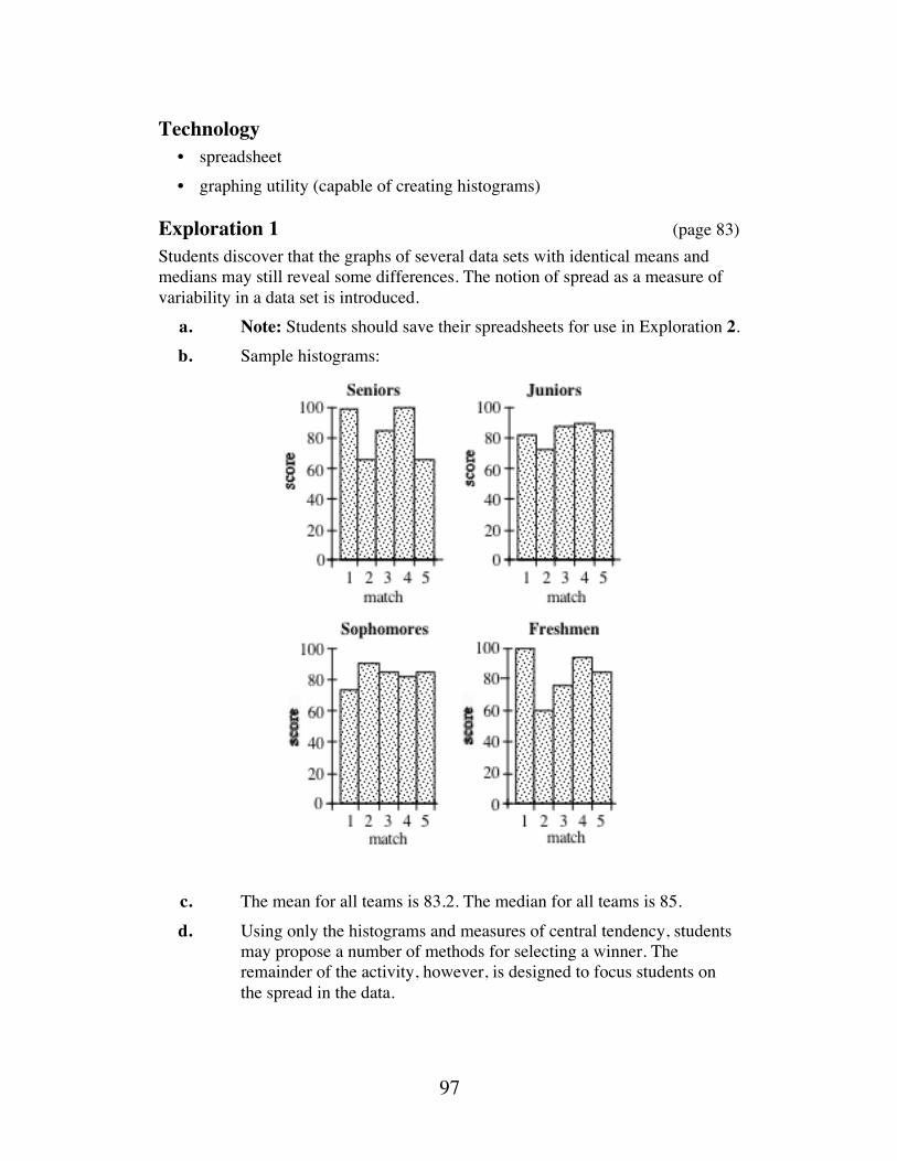
97

Technology • spreadsheet

• graphing utility (capable of creating histograms)

Exploration 1 (page 83) Students discover that the graphs of several data sets with identical means and medians may still reveal some differences. The notion of spread as a measure of variability in a data set is introduced.

a. Note: Students should save their spreadsheets for use in Exploration 2.

b. Sample histograms:

c. The mean for all teams is 83.2. The median for all teams is 85.

d. Using only the histograms and measures of central tendency, students may propose a number of methods for selecting a winner. The remainder of the activity, however, is designed to focus students on the spread in the data.

98

Discussion 1 (page 84) a. Answers will vary. Using measures of central tendency, no clear

winner emerges. Considering other criteria, each team won one match. All—except the seniors—also tied for the lead in one match. The seniors, however, have two of the three highest scores.

b. Judging from the histograms, the ranges in the scores for the juniors and sophomores are less than the ranges for the seniors and freshmen.

c. Sample response: If the variation can be quantified, this might be used as a criterion for selecting a winner. This would reward the team that performed most consistently.

d. Two of the rules might affect the spread of scores—the one that allows teams to work cooperatively, and the one that permits teams to change members after each match.

Exploration 2 (page 84) This exploration introduces students to mean absolute deviation as a measure of spread.

a. Students may use a spreadsheet to determine the mean absolute deviation for each team’s scores. (The mean for all teams was 83.2.)

Seniors’ Scores Distance from Mean

Juniors’ Scores Distance from Mean

99 15.8 82 1.2 66 17.2 72 11.2 85 1.8 88 4.8

100 16.8 89 5.8 66 17.2 85 1.8

Mean Absolute Deviation

13.76 Mean Absolute Deviation

4.96

Sophomores’

Scores Distance from

Mean Freshmen’s

Scores Distance from

Mean 74 9.2 100 16.8 90 6.8 60 23.2 85 1.8 77 6.2 82 1.2 94 10.8 85 1.8 85 1.8


4.16 Mean Absolute Deviation

11.76

b. Any set of five, equal scores will work. For example, the following set has

a mean of 50 and a mean absolute deviation of 0: {50, 50, 50, 50, 50}.

99

c. Two sets of scores produce a mean absolute deviation of 24. These sets are {50, 50, 50, 100, 100} and {50, 50, 100, 100, 100}. In both sets of scores, the distance from each data point to the mean is as great as possible; therefore, the mean absolute deviation is as great as possible.

Discussion 2 (page 85) a. Since distances cannot be negative, the absolute value function is used

to express the difference between each data item and the mean as a non-negative value.

b. The expression xi − µ is the distance from the mean for each data point. The sum of these distances, divided by the number of data points (n), is the average distance from the mean.

c. The distance from the top of each bar to the line is the distance between the data point and the mean. The mean of these distances is the mean absolute deviation.

d. Sample response: The histograms whose bars vary more in height have larger mean absolute deviations.

e. Answers will vary, depending on which team students initially chose as the winner. Adding mean absolute deviation as a criterion would make the sophomores a reasonable selection.

f. Students might reasonably expect the sixth score to fall within a range of values equal to the mean plus or minus the mean absolute deviation.

g. This question encourages students to consider the spread in a data set. Since the scores for the sophomores are clustered more closely around the mean than the scores from the other teams’, a score of 95 seems more unlikely for the sophomores.

Assignment (page 86) 4.1 a. Measures of central tendency are not adequate to differentiate

between these two sets of scores. Although the graphs reveal some differences, the mean (85), median (85), and mode (85) are identical for both teams.

b. The scores for students 3 and 4 on the junior team are 75 and 95, respectively. The distance from the mean score of 85 is 10 for both.

c. The mean absolute deviation would be reduced. The original set of scores has a mean absolute deviation of 5.0; the new set has a mean absolute deviation of 2.5. This occurs because the two revised scores are both closer to the mean.

100

d. Adding another score of 85 increases n in the formula for mean absolute deviation from 4 to 5, without increasing the sum of the distances from the mean. Therefore, the mean absolute deviation would be reduced.

4.2 a. The mean absolute deviation for each team’s scores is shown below.

Class Mean Absolute Deviation Seniors 16.5 Juniors 5

Sophomores 0 Freshmen 8

b. Sample response: All the scores are the same: 85. As a result, the

mean is 85 and the distance from each score to the mean is 0. The mean absolute deviation, therefore, is also 0.

c. Sample response: Since the seniors’ scores are widely spread (mean absolute deviation 16.5), they probably worked independently. The same is likely to be true for the juniors, although the spread in their scores is not as great (mean absolute deviation 5.0). Since the sophomores’ scores are identical, they appear to have worked as a cooperative group. The freshmen may have worked independently, or in two small groups since two pairs of scores are the same (mean absolute deviation 8).

4.3 a. Sample response: The score in match 5 for the seniors and the scores in matches 1 and 2 for the juniors all have a deviation greater than “an average amount.”

b. Sample response: Since mean absolute deviation is the average of the deviations from the mean, I used it to determine the “average amount.”

c. Sample response: The score in match 4 equals the mean score. The “missing” bar is actually a bar with a height of 0.

4.4 a. The upper end of the interval was determined by adding 13.8 to 83.2; the lower end of the interval was found by subtracting 13.8 from 83.2.

b. The mean absolute deviation is 0 when the data point has the same value as the mean.

c. Sample response: The interval that contains scores 2 mean absolute deviations from the mean is [69.4 −13.8, 97 +13.8] or [55.6, 110.8]. As it is not possible to score more than 100 points on the test, the interval would have to be [55.6, 100].

101

*4.5 a. The mean absolute deviation is 11.84 for the seniors and 14 for the juniors.

b. Since the mean absolute deviation for the juniors is higher, the juniors’ scores are spread more widely than the seniors’.

c. The seniors’ score of 51 is more than 2 deviations from the mean. The juniors’ scores of 50 and 100 are more than 1 mean absolute deviation from the mean.

4.6 Sample response: I would select the sophomores because they have the smallest mean absolute deviation and therefore score the most consistently around the mean of 83.2.

* * * * * 4.7 a. Sample response: Since the mean absolute deviation for Rita’s

scoring average is much smaller than Bernard’s, she is the more consistent offensive player.

b. The range of values for Rita is from 20 to 30 points; for Bernard, the range is from 10 to 40 points.

c. Sample response: Rita’s performance in the last game is more impressive because it is out of her range of “typical scores” (established by the mean, plus or minus the mean absolute deviation). Her typical range of points would be between 20 and 30 points per game, so 35 is an outstanding performance. Bernard’s “typical scores” range from 10 points to 40 points. For him, a 35-point game is within the expected range.

d. If both teams average 60 points per game, Bernard’s teammates must score in the range from 20 to 50 points, while Rita’s teammates must score in the range from 30 to 40 points.

4.8 Sample response: Runner 1 should receive the award because her time in the sixth race is the only one more than 1 mean absolute deviation from her mean time for the previous five races.

Runner 1 Runner 2 Runner 3 Race 1 1530 sec 1210 sec 1335 sec Race 2 1425 sec 1190 sec 1520 sec Race 3 1455 sec 1290 sec 1215 sec Race 4 1325 sec 1185 sec 1465 sec Race 5 1270 sec 1120 sec 1210 sec Mean 1401 sec 1199 sec 1349 sec


82.8 sec 40.8 sec 114.8 sec

* * * * * * * * * *

102

(page 89)

Activity 5 In this activity, students investigate a more commonly encountered measure of variance—standard deviation.



Teacher Note Both mean absolute deviation and standard deviation can be treated as functions. If the derivative of the function exists, the deviation can be minimized. However, the absolute value function is not everywhere differentiable. For this reason, statisticians prefer standard deviation rather than mean absolute deviation as a measure of spread.

In this activity, students calculate standard deviation for data sets. The formula given in the mathematics note is for the standard deviation of a population (σ ), not the standard deviation for a sample (s). In the formula for sample standard deviation, the sum of the squared differences is divided by (n −1) , rather than n.

The built-in functions in your technology may handle this calculation in different ways. For example, the TI-82 and TI-83 will determine either sample or population standard deviation. However, Microsoft Excel calculates only sample standard deviation. You may wish to discuss these capabilities with students before assigning Problem 5.2.

Discussion (page 90) a. Sample response: Both formulas use the differences between the mean

and the data points, along with the number of data points in the set, to determine spread. They are different in that mean absolute deviation uses absolute value, while standard deviation uses the squares of the differences, then takes the square root.

b. Sample response: The differences are kept non-negative by squaring them.

c. The square root is taken to eliminate the effect of squaring the differences. It also returns the value of the deviation to its proper units.

d. Sample response: Since standard deviation is a measure of spread, it must be non-negative. A “negative spread” would have no meaning.

103

Assignment (page 90) 5.1 The mean is 83.2. From

σ =99 − 83.2( )2 + 66 − 83.2( )2 + 85 − 83.2( )2 + 100 − 83.2( )2 + 66 − 83.2( )2

5) ,

the standard deviation is approximately 15.01.

5.2 a. Many calculators use x or µ to represent the mean. The mean score for all three teams is 83.2.

b. To represent standard deviation, calculators may use σ, σx, or σ x . The standard deviation for the juniors’ scores is 6.1, for the sophomores’ scores is 5.3, and for the freshmen’s scores is 14.0.

5.3 a. There are 5 audiences more than 1 standard deviation from the mean.

b. Sample response: No. Since the standard deviation is 66, the audience would have to have been less than 18 or greater than 282 to be more than 2 standard deviations from the mean.

* * * * * *5.4 a. The mean mass is 76.96 kg.

b. The standard deviation is 11.3 kg.

c. The interval of values within 1 standard deviation of the mean is [65.66, 88.26]. The masses of 9 of the 25 players, or 36%, fall outside this interval.

d. The mass of 54 kg is more than 2 standard deviations from the mean.

5.5 a. The mean, 340, is the midpoint of the interval [230, 450].

b. From Part a, one standard deviation equals 450 − 340 or 110. The interval of values within 2 standard deviations of the mean is 340 ± 2 110( ) or [120, 560].

c. The interval of values within 3 standard deviations of the mean is 340 ± 3 110( ) or [10, 670].

* * * * * * * * * *

104

Answers to Summary Assessment (page 92) 1. Sample graph:

2. The mean score for the third-period class is approximately 76. The

mean score for the fifth-period class is approximately 86.

3. For the third-period class, the minimum is 52, the maximum is 90, the lower quartile is 71.5, the median is 77.5, and the upper quartile is 84.5. The score of 52 is an outlier.

For the fifth-period class, the minimum is 76, the maximum is 99, the lower quartile is 80, the median is 85, and the upper quartile is 91.

Sample observations: Third-period test results are definitely below

those in fifth period. The range of scores in third period is greater than the range of scores in fifth period.

4. a. The standard deviation for the third-period scores is approximately 9.9. The standard deviation for the fifth-period scores is approximately 6.7.

b. For the third-period class, the interval that contains scores within 1 standard deviation of the mean is [66.1, 86.7]. Eleven of the 16 scores, or about 69%, are in this interval.

For the fifth-period class, the interval that contains scores within 1 standard deviation of the mean is [79.4, 92.8]. Thirteen of the 20 scores, or about 65%, are in this interval.

fifth period third period

represents a score of 76 in fifth period and a score of 71 in third period

56789

20 61 2 3 5 7 80 2 4 5 8 90

9 8 7 68 5 5 4 3 2 0 0 9 6 6 2 2 0 0 0

76 1

50 55 60 65 70 75 80 85 90 95 100

*

fifth period

third period

score

105

Module Assessment

1. An average weekday for a student at Two Eagle High includes

6.5 hr of school, 8.5 hr of sleep, 1.0 hr of travel to and from school, 1.5 hr of television viewing, 0.75 hr of eating, and 5.75 hr of other activities.

a. Determine the measure of the central angle needed for each sector in a pie chart of this data.

b. Display the data in a pie chart.

2. The heights in meters of the 10 tallest buildings in Chicago are 443, 346, 343, 295, 274, 262, 259, 236, 222, and 213.

The heights in meters of the 10 tallest buildings in New York are 419, 381, 319, 290, 279, 274, 259, 248, 246, and 241.

a. Create a histogram that compares the heights of the 10 tallest buildings in each city.

b. Create a histogram that exaggerates the differences in the heights.

3. The heights, in centimeters, of the Two Eagle High girls’ basketball team are 173, 160, 191, 173, 165, 180, 178, 168, 178, 178, and 178.

The heights, in centimeters, of the boys’ basketball team are 170, 201, 175, 193, 178, 193, 180, 191, 180, 188, and 183.

a. Create a back-to-back stem-and-leaf plot of this data.

b. Find the mean, median, mode, range, mean absolute deviation, and standard deviation for the heights of the girls’ team.

c. Find the mean, median, mode, range, mean absolute deviation, and standard deviation for the heights of the boys’ team.

d. 1. To compare the heights of the two teams, create box plots for both sets of data on the same scale.

2. Write a summary of the information displayed in the box plots.

106

4. The box-and-whisker plots shown below represent the starting salaries for three occupations that require a college degree.

a. Which occupation has the greatest range of starting salaries? b. Which occupation has the smallest interquartile range of salaries?

c. If starting salaries were your only concern, which occupation would you choose to prepare for in college? Which occupation would be your second choice? Explain your choices.

*

19 23 27 31 35

I

IIIII

*

17 21 25 29 33

*

salary (in thousands of dollars)

107

Answers To Module Assessment 1. a. In the pie chart shown below, 127.5˚ represents 8.5 hr, 97.5˚

represents 6.5 hr, 86.25˚ represents 5.75 hr, 22.5˚ represents 1.5 hr, 15˚ represents 1 hr, and 11.25˚ represents 0.75 hr.

b. Sample graph:

2. a. Sample graph:

A Day in the Life of a Two Eagle Student

school27%

sleep36%

eating3%

television6%

travel4%

other24%

Tall BuildingsNew York vs. Chicago

050

100150200250300350400450

New York

Chicago

1 2 3 4 5 6 7 8 9 10buildings

heig

ht in

met

ers

108

b. Sample graph:

3. a. Sample graph:

b. For the girls’ team, the mean is 174.7, the median is 178, and the

mode is 178. The range is 31. The mean absolute deviation is 6.3 and the standard deviation is 7.97.

c. For the boys’ team, the mean is 184.7 and the median is 183. The data is bimodal at 180 and 193. The range is 31, the mean absolute deviation is 7.7, and the standard deviation is 8.82.

d. 1. There are no outliers in either data set. Sample graph:

2. Sample response: The data for the boys’ team has a greater

interquartile range, suggesting that their heights vary more than the girls’. The upper 75% of the boys are as tall or taller than the upper 25% of the girls.

1617181920

01

850888833 058

00381331

Girls Boys

17 0 represents a height of 173 cm on the girls’ team and a height of 170 cm on the boys’ team

3

Boys

Girls

160 170 180 190 200height in centimeters

Tall BuildingsNew York vs. Chicago

250

300

350

400

450

New York

Chicago

1 2 3 4 5 6 7 8 9 10buildings

heig

ht in

met

ers

109

4. a. Occupation III b. Occupation I c. Answers will vary. Occupation III has the highest potential

starting salary. Occupation II has the highest median. Occupation I has the least range in salaries.

110

Flashbacks

Activity 1 1.1 One day at the beach, the lifeguard counts 6 red, 10 blue, 5 orange,

and 3 green umbrellas. a. Draw a histogram that shows the frequency of umbrellas of each

color. b. What percentage of the total number of umbrellas is represented

by each color? c. Draw a histogram that shows the percentage of umbrellas of each

color. 1.2 Draw a large circle. Divide and label the circle so that 25% of it is red,

38% is blue, 18% is green and 19% is orange.

Activity 2 2.1 Create a stem-and-leaf plot of the following set of data: 12, 18, 24, 24,

30, 32, 34, 36, 36, 36, 40, 42, 48. 2.2 a. Determine the mean, median, and mode of the data set in

Flashback 2.1. b. 1. What percentage of the data is greater than the mean? 2. What percentage of the data is less than the mean?

Activity 3 3.1 Consider the following set of data: 12.2, 28.6, 29.4, 30.6, 30.8, 32.2,

34.8, 36.2, 36.2, 38.5, 40.8, 48.9, 56.5. a. Determine the mean, median, and mode of the data set. b. Determine the upper and lower quartiles of the data.

111

Activity 4 4.1 a. Create a box-and-whisker plot of the following set of data:

2162, 1118, 2124, 2264, 1230, 1198, 1132, 2284, 2136, 1256, 2106, 2250.

b. What is the interquartile range of the data?

4.2 Simplify each of the following expressions.

a. 12 − 5

b. 12 −15

c. −21 −10

d. −2312 +1355

Activity 5 5.1 Consider the following set of data: 21, 32, 43, 54, 65, 32, 23, 34, 45,

8, 126, 32, 65.

a. Find the mean of the data.

b. Calculate the mean absolute deviation of the data.

112


Activity 1 1.1 a. Sample histogram:

b. The percentages are shown in the table below.

Color Number Percentage red 6 25 blue 10 42

orange 5 21 green 3 12

c. Sample histogram:

1.2 Sample drawing:

red90˚

blue137˚

green65˚

orange68˚

113

Activity 2 2.1 Sample graph:

2.2 a. The mean is approximately 31.7, the median is 34, and the mode is

36.

b. 1. Approximately 62% of the data falls above the mean.

2. Approximately 38% of the data falls below the mean.

Activity 3 3.1 a. The mean is approximately 35.1, the median is 34.8, the mode is 36.2.

b. The upper quartile is 39.7; the lower quartile is 30.

Activity 4 4.1 a. Sample graph:

b. The upper quartile is 2207; the lower quartile is 1214. The

interquartile range is 993.

4.2 a. 7

b. 3

c. 31

d. 957

Activity 5 5.1 a. The mean is 44.6.

b. The mean absolute deviation is 20.3.

1234

2 84 40 2 4 6 6 60 2 8

represents 242 4

800 1200 1600 2000 2400

114

Heart Rate Data (beats per minute)



A 72 116 84 B 68 120 92 C 76 112 88 D 80 124 96 E 72 112 88 F 64 116 84 G 68 112 80 H 76 128 92 I 84 120 100 J 72 112 88

Heart Rate Data (beats per minute)



A 72 116 84 B 68 120 92 C 76 112 88 D 80 124 96 E 72 112 88 F 64 116 84 G 68 112 80 H 76 128 92 I 84 120 100 J 72 112 88

Who Gets What and Why?

Why do some U.S. states have more senators than House representatives? In this module, you examine the process—and the politics—of apportionment.

Patricia Bean • Dean Preble • Teri Willard

117

Teacher Edition Who Gets What and Why?

Overview The mathematics of apportionment is used to assign seats in the U.S. House of Representatives. In this module, students investigate several historical methods of apportionment. As part of their investigations, they round and order decimals, use and interpret inequalities, simplify rational expressions, and apply problem-solving techniques.


• use and interpret inequalities involving rational expressions

• be introduced to geometric mean

• simplify rational expressions.


• how to use scientific notation

• how to use proportions

• rounding techniques

• the greatest integer function

• how to use a spreadsheet

• how to simplify basic algebraic expressions.


Assessment Total

Days 2 2 2 2 2 10

118



map of Antarctica X

Teacher Note A blackline master of the map template appears at the end of the teacher edition for this module.



spreadsheet X X X X symbolic manipulator X

119

Who Gets What and Why?

Introduction (page 97) The introduction presents a scenario in the late 21st century. In this hypothetical situation, Antarctica must be fairly apportioned among seven global regions.

Discussion (page 97) a. Students should recognize that border disputes are a common

occurrence and influence many world events. b–c. Border disputes might involve religious differences, resource

availability, population characteristics, or strategic geographic features.

(page 98)

Activity 1 In the exploration, students consider the apportionment of both land and representatives.

Materials List • map of Antarctica (one copy per student)


Teacher Note A map template appears at the end of this teacher edition. You may wish to obtain a more detailed representation of the Antarctic continent.

Exploration (page 98) Note: Two of the regions listed in Table 1 may be unfamiliar to some students. The Sino-Soviet region contains the countries of the former U.S.S.R. Oceania describes lands of the central and South Pacific, including Micronesia, Australia, and New Zealand.

120

a. Sample response:

Region People km2 Asia 357

Africa 69 North America 55 South America 53

Europe 327 Oceania 10

Sino-Soviet 41 b. Students may use the grid on the map template to estimate area.

Sample response:

c. Methods will vary. If students base the number of delegates on

population, Asia should receive the most delegates, while Oceania should receive the least. Sample response:

Region Delegates Asia 28


Europe 5 Oceania 1

Sino-Soviet 2 Total 49

121

Discussion (page 99) a. Answers will vary. Students may choose to divide the continent based

on population density. For example, since the most densely populated region is Asia, they may give Asia the largest portion of land.

b. Sample response: Land can be divided into fractions of units (such as square kilometers), whereas people cannot be divided into fractional parts.

c. Answers will vary. Students should recognize that there are many ways to divide both land and representatives. In practice, differences often arise due to the needs and ambitions of individual regions. Each region typically would attempt to obtain the most advantageous portion.

Assignment (page 99) 1.1 a. Answers will vary. Sample response: No. Some nations pay more

to support the activities of the United Nations than others, yet all receive one vote.

b. Some students may suggest basing the number of representatives from each member country on its financial contribution. Others may argue that representation should be determined by the ratio of the member country’s population to the world’s population. (You may wish to ask students how the United States would fare under various plans.)

1.2 Sample response: Having two senators from each state helps give each state an equal voice in government. Under this system, a state like Montana—with a relatively small population and only one seat in the House of Representatives—can have the same impact in the Senate as any other state.

* * * * * 1.3 a–b. Sample table:

Region Population Area km2 Asia 6 •109 2 • 107

Africa 1• 109 2 • 107 North America 9 •108 2 • 107 South America 6 •108 1• 107

Europe 1• 109 3 •106 Oceania 5 •107 5 •106

Sino-Soviet 6 •108 1• 107 Total 1.015 •1010 8.7 •107

122

c. Sample table:

Region Fraction of Total Population

Fraction of Total Area

Asia 3 5 2 9 Africa 1 10 2 9

North America 9 100 2 9 South America 3 50 1 9

Europe 1 10 1 30 Oceania 1 200 1 18

Sino-Soviet 3 50 1 9 d. Answers may vary slightly, due to rounding. The sums of both the

population fractions and the area fractions should be approximately 1.

e. 1. The following sample response divides the delegates according to population:

Region Delegates Asia 29


Europe 5 Oceania 1

Sino-Soviet 2 Total 49

2. Answers will vary. The apportionment made in the

exploration also was based on population. 1.4 Answers will vary. Sample response: To find the number of books each

student should receive, divide the total number of books, 957, by the total number of years of post-secondary education, 27. This results in approximately 35.44 books for each year of education. Using this method and rounding to the nearest integer, Elizabeth should receive 354 books, Bill 142 books, Isabella 213 books, and Kareem 248 books.

* * * * * * * * * *

123

(page 100)

Activity 2 Students compare three historical methods of apportionment for the U. S. House of Representatives: the Jefferson method, the Webster method, and Hamilton method.



Exploration (page 100) a. The standard divisor is 2945 10 = 294.5 people representative .

b. Sample table:

Region Population Standard Quota A 813 2.76 B 652 2.21 C 1385 4.70 D 95 0.32

Total 2945 9.99 c. Answers will vary. If students round each quota down to the previous

whole number (assigning 1 to region D), they will assign a total of 9 representatives. If students round to the nearest integer, they may assign a total of 11 representatives (more than the available 10).

d. 1-2. The following table shows the results of rounding each quota down, according to the Jefferson method.

Region Standard Quota Rounded Quota Representatives A 2.76 2 2 B 2.21 2 2 C 4.70 4 4 D 0.32 0 1

Total 9.99 8 9

3. No. Not all 10 representatives were assigned.

124

e. Using the Jefferson method and a divisor between 272 and 277 results in the assignment of all 10 representatives as follows:

Region Rounded Quota Representatives A 2 2 B 2 2 C 5 5 D 0 1

Total 9 10

Discussion (page 102) a. Since the standard divisor in this case is P d , the standard quota for a

region can be expressed as follows: RP d

=R • dP

In other words, the standard quota for a region can be found by multiplying the total number of representatives by the fraction of the population residing in the region.

b. Sample response: The standard quota for a region may not be a whole number. The number of delegates, however, must be a whole number. Depending on the method of rounding, the standard quota may not assign at least one representative to each region.

c. Sample response: Yes. The method was based on population and each region received at least one representative.

d. Sample response: Technology can round each quota down using the greatest integer function.

e. Sample response: Use a spreadsheet to experiment with different values of the divisor until the rounded quotas add up to the exact number of representatives.

Assignment (page 102) 2.1 Because the use of the standard divisor does not assign all

12 representatives, students must modify the divisor. A value of 255 for example, results in the following rounded quotas.

Region Population Rounded Quota Representatives A 813 3 3 B 652 3 3 C 1385 5 5 D 95 0 1

Total 2945 11 12

125

2.2 a–b. Sample table:

Region Standard Quota

Rounded Quota

Representatives

A 2.76 3 3 B 2.21 2 2 C 4.70 5 5 D 0.32 0 1

Total 9.99 10 11 c. Using a strategy similar to that described in Part e of the

discussion, one possible modified divisor is 310.

Region Rounded Quota Representatives A 3 3 B 2 2 C 4 4 D 0 1

Total 9 10 2.3 a. The Hamilton method assigns the first nine representatives as

shown in the table below.

Region Standard Quota

Rounded Quota

Representatives

A 2.76 2 2 B 2.21 2 2 C 4.70 4 4 D 0.32 0 1

Total 9.99 8 9 The remaining seat is assigned by ranking decimal parts of the

standard quota from greatest to least. Since region A has the greatest decimal part, it receives the additional seat.

b. The approximate number of people per delegate in each region is shown below.

Region People per Delegate A 271 B 326 C 346 D 95

126

2.4 a. Sample response: The methods are similar since all three require finding a standard divisor and standard quotas. Each method deals with the decimal portion of the quotas in a different way. The Jefferson method truncates the quotas and modifies the divisor until the exact number of delegates is assigned. The Webster method rounds the quotas to the nearest integer and modifies the divisor until the exact number of delegates is assigned. The Hamilton method truncates the quotas, then assigns any remaining representatives according to a ranking of the decimal portions of the quotas. In all three methods, each region must receive at least one delegate.

b. The following table shows the number of representatives assigned to each region using the three methods. In this case, the Webster and Hamilton methods result in the same apportionment.

Method Number of Representatives Region A Region B Region C Region D

Jefferson 2 2 5 1 Webster 3 2 4 1 Hamilton 3 2 4 1

*2.5 The standard divisor is approximately 2.20 •108 . This results in the

standard quotas shown in the table below.

Region Population Standard Quota Asia 6.32 •109 28.64

Africa 1.35• 109 6.11 North America 8.60 • 108 3.89 South America 6.04 •108 2.73

Europe 1.04 •109 4.71 Oceania 5.40 •107 0.24

Sino-Soviet 5.84 •108 2.64 Total 1.08 •1010 48.96

127

Using the Jefferson method, a possible modified divisor is 2.30 •108 . Using the Webster method, a possible modified divisor is 2.10 •108 . The following table shows the number of delegates assigned to each region using the three methods.

Region Method of Apportionment Jefferson Webster Hamilton

Asia 30 27 28 Africa 6 6 6

North America 4 5 5 South America 4 4 4

Europe 2 3 3 Oceania 1 1 1

Sino-Soviet 2 3 2 Total 49 49 49

* * * * *

*2.6 The following table shows the number of representatives assigned to each region using the three methods. In this case, the Webster and Hamilton methods result in the same apportionment.

Method Number of Representatives Region A Region B Region C Region D

Jefferson 5 4 10 1 Webster 6 4 9 1 Hamilton 6 4 9 1

2.7 a. 1.58 •104 b. The standard divisor is 683,544. c. The corresponding standard quotas are shown in the table below.

Region Standard Quota Asia 9245.93

Africa 1975.00 North America 1258.14 South America 883.63

Europe 1521.48 Oceania 79.00

Sino-Soviet 854.37

128

d. The following table shows an apportionment made using the Jefferson method. The modified divisor must be in the interval [684,131, 684,168].

Region Allotment (1 •106 kL) Asia 9237



Sino-Soviet 853 The table below shows the results using the Webster method.

The modified divisor must be in the interval [684,316, 684,390].

Region Name Allotment (1 •106 kL) Asia 9235



Sino-Soviet 853

* * * * * * * * * *

Research Project (page 104) This research project allows students to explore the relationship between methods of apportionment and the course of U.S. history. In the past, interest groups and political parties have often used the mathematics of apportionment to manipulate the assignment of representatives. In the presidential election of 1876, for example, Samuel L. Tilden (who won the popular vote) was defeated in the electoral college 185 to 184 by Rutherford B. Hayes. Hayes’ one-vote margin of victory may be traced to the assignment of nine seats by political expediency rather than the Hamilton method.

129

(page 105)

Activity 3 In this activity, students simplify rational expressions and are introduced to the geometric mean. They examine a method for minimizing the impact of assigning another representative to a region by comparing “relative differences.”


Technology • symbolic manipulator (optional)

Discussion 1 (page 105) a. The number of people represented by each delegate in Washington

can be expressed as W w , where W is Washington’s population and w its number of representatives.

b. The number of people represented by each delegate in Massachusetts is less than the number of people represented by each delegate in Washington, as shown below. Mm=6, 029, 050

10≈ 602, 905 < W

w=4,887, 945

8≈ 610, 993

Therefore, the people of Massachusetts were better represented in the U.S. House.

c. The relative difference can be calculated as follows: 610, 993 − 602, 905

602, 905≈ 0.013

d. If M m is greater than W w , then the number of people per delegate is higher for Massachusetts than for Washington. The relative difference can be expressed as follows:

Mm−Ww

Ww

130

Exploration (page 106) a. 1. If Massachusetts receives the additional seat, then the number of

people represented by each delegate would be: M

m +1=6, 029, 050

11≈ 548,095

The relative difference would be: 610, 993 − 548, 095

548,095≈ 0.115

2. If Washington receives the additional seat, then the number of people represented by each delegate would be:

Ww +1

=4, 887,945

9= 543,105


543,015≈ 0.110

b. To minimize the effect of adding another representative, Washington should receive the additional seat.

c. 1. If New Jersey receives 14 representatives, then the number of people represented by each delegate would be 7, 748, 634 14 ≈ 553, 474 .


553,474≈ 0.104

2. If New Jersey does not receive an additional seat, the number of people represented by each delegate would be 7, 748, 634 13 ≈ 596, 049 .

The relative difference would be: 596, 049 − 543,105

543,105≈ 0.097

3. The relative difference would be: 602, 905 − 553, 474

553,474≈ 0.089

4. The relative difference would be: 596, 049 − 548,095

548,095≈ 0.087

131

d. Sample response: Using relative difference, Massachusetts would be favored over New Jersey to receive the final representative. However, since Washington is favored over both Massachusetts and New Jersey, Washington should receive the final representative.

e. 1. When determining which of 4 states should receive an additional representative, 12 relative differences would need to be calculated.

2. When determining which of 5 states should receive an additional representative, 20 relative differences would need to be calculated.

Note: In general, when determining which of n states should receive an additional representative, the number of relative differences to be calculated would be nP2 .

Discussion 2 (page 107) a. The expression represents the relative difference between Washington

and Massachusetts if Massachusetts receives an additional seat.

b. In this case, M m is greater than W (w +1) . The relative difference can be expressed as follows:

Mm−

Ww +1Ww + 1

c. 1. 0.115 > 0.110

2. Sample response: Ww−

Mm +1Mm +1

>

Mm−

Ww +1Ww +1

Assignment (page 107) 3.1 a. 21 20

b. 39 80

c. 207 40

d. 4(x +1)6

−1 = 2x −13

132

*3.2 a. 1. Sample response: Subtraction requires fractions with a common denominator. In the original inequality, the difference was written as one fraction with the same denominator.

2. Sample response: When a fraction has the same value in the numerator as the denominator, the fraction is equivalent to 1.

b. The right-hand side of the inequality can be simplified as follows: Mm−

Ww +1Ww + 1

=

Mm

Ww + 1

−1

c. By adding 1 to both sides, the inequality can be written as follows: Ww

Mm +1

>

Mm

Ww +1

d. 1. Since the existing denominators are both positive, their product (the common denominator) also is positive.

2. W2

w(w +1)>

M2

m(m +1)

e. 1. The numerators of both fractions are positive. Since the original denominators and the common denominator are all positive, their products (the resulting denominators) also are positive. Because both numerators and both denominators are positive, both fractions are positive.

2–3. Since the fractions are both positive, the inequality can be written as shown below by taking the principle square root of both sides.

Ww(w +1)

>M

m(m + 1)

4. Sample response: If the fractions were negative, the square root would be undefined.

f. 1. The two inequalities simplify as follows:

Ww−

Mm +1Mm +1

>

Mm−

Ww +1Ww +1

0.115 > 0.110

W

w(w +1)>

Mm(m + 1)

576, 050 > 574, 847

2. Sample response: The inequality that compares priority numbers is easier to use since there are no complex fractions.

133

*3.3 a. The arithmetic mean of two numbers is found by adding the two numbers, then dividing the sum by 2.

b. 1. 8 • 32 = 16

2. 4 • 32 ≈11.31

3.4 a. The geometric mean is found in the denominators of the inequality that compares priority numbers:

Ww(w +1)

>M

m(m + 1)

b. Sample response: The state with the greater priority number would be assigned the additional delegate.

* * * * * 3.5 a. Since ∠BCD and ∠BDA are both complementary to ∠BDC ,

their measures are equal. By the AAA Property, ΔABD is similar to ΔDBC . Since ΔABD ~ ΔDBC , the following proportion is true:

ah=hb

Solving for h yields: h2 = a • b; h = a •b . b. 1. h ≈ 3.27

2. b ≈ 3.11 3. a ≈ 8.70

* * * * * * * * * * (page 110)

Activity 4 In this activity, students are introduced to the Huntington method of apportionment, which uses “priority numbers” to assign representatives. These priority numbers are related to the relative differences developed in Activity 3.



134

Exploration 1 (page 110) a. Sample table:

Region Population Rounded Quota

(Rounded Quota) + 2

A 264 3 5 B 481 5 7 C 330 4 6 D 1652 17 19 E 1442 14 16 F 477 5 7

Total 4646 48 60 b. As shown in the table above, the sum of the values in the right-hand

column is 60. Some students may argue that this means 60 priority numbers must be calculated. However, since each of the 6 regions must receive at least 1 representative, the actual number of priority numbers to be calculated is 60 − 6 = 54 .

Discussion 1 (page 112) a. Column C displays the possible numbers of representatives for the six

regions. In each row, the possible number of representatives is the current number of representatives plus one additional seat.

b. 1. Sample response: The rounded quota for region A is 3. Adding 2 to the rounded quota gives a value of 5. This is the most representatives possible for that region. Since each region must receive at least one representative, priority numbers have to be calculated for the other four possible representatives.

2. Since the rounded quota is 4, the most representatives possible is 4 + 2 = 6. Since no priority number is necessary to award the first representative, 5 priority numbers should be calculated for region C.

c. Students should base the spreadsheet formula on the formula given in the previous historical note. Using Microsoft Excel, for example, the following formula calculates the priority number in cell E2:

=D2/(SQRT(B2*C2))

d. The highest priority number in the portion of the spreadsheet shown is 340.12 for region B. Students may recognize that priority numbers for a given number of representatives are larger for regions with larger populations. Since the priority numbers for regions D, E, and F are not shown on the partial spreadsheet, 340.12 is not the largest priority number among the six regions.

135

Exploration 2 (page 112) a. Sample spreadsheet:

A B C D E 1 Region Current

No. of Reps. Possible

No. of Reps. Pop. Priority

Number 2 A 1 2 264 186.676 3 A 2 3 264 107.778 4 A 3 4 264 76.210 5 A 4 5 264 59.032 6 B 1 2 481 340.118 7 B 2 3 481 196.367 8 B 3 4 481 138.853 9 B 4 5 481 107.555 10 B 5 6 481 87.818 11 B 6 7 481 74.220 12 C 1 2 330 233.345 13 C 2 3 330 134.722 14 C 3 4 330 95.263 15 C 4 5 330 73.790 16 C 5 6 330 60.249 17 D 1 2 1652 1168.140 18 D 2 3 1652 674.426 19 D 3 4 1652 476.891 20 D 4 5 1652 369.398 21 D 5 6 1652 301.613 22 D 6 7 1652 254.909 23 D 7 8 1652 220.758 24 D 8 9 1652 194.690 25 D 9 10 1652 174.136 26 D 10 11 1652 157.512 27 D 11 12 1652 143.788 28 D 12 13 1652 132.266 29 D 13 14 1652 122.454 30 D 14 15 1652 113.999 31 D 15 16 1652 106.636 32 D 16 17 1652 100.167 33 D 17 18 1652 94.439 34 D 18 19 1652 89.330 35 E 1 2 1442 1019.648 36 E 2 3 1442 588.694 37 E 3 4 1442 416.270 38 E 4 5 1442 322.441 39 E 5 6 1442 263.272

136

40 E 6 7 1442 222.505 41 E 7 8 1442 192.695 42 E 8 9 1442 169.941 43 E 9 10 1442 152.000 44 E 10 11 1442 137.489 45 E 11 12 1442 125.510 46 E 12 13 1442 115.452 47 E 13 14 1442 106.888 48 E 14 15 1442 99.507 49 E 15 16 1442 93.081 50 F 1 2 477 337.290 51 F 2 3 477 194.734 52 F 3 4 477 137.698 53 F 4 5 477 106.660 54 F 5 6 477 87.088 55 F 6 7 477 73.603

b. After each region receives one representative, the remaining

39 representatives are assigned by selecting the region with the highest priority number, the region with the next highest priority number, and so on, until all remaining seats have been assigned.

Students may sort the entire spreadsheet according to priority number, greatest to least, then assign representatives to the regions in the first 39 rows. Note: Depending on how the spreadsheets were created, students may lose some cell values when sorting. On some technology, this may be avoided by selecting manual calculation rather than automatic calculation, so that the spreadsheet does not recalculate after sorting.

The table below shows the results of an apportionment by the Huntington method.

Region Population Representatives A 264 3 B 481 5 C 330 3 D 1652 15 E 1442 14 F 477 5

Total 4646 45

137

Discussion 2 (page 113) a. If m and w represent the current number of representatives assigned to

Massachusetts and Washington, respectively, the priority numbers can be expressed as follows:

Mm(m +1)

Ww(w +1)

b. The inequality includes the expressions for both priority numbers. The denominator of each priority number is the geometric mean ab , where a is the current number of representatives and b is the possible number of representatives if one additional seat is assigned.

c. The following table shows the standard quotas for each region along with the number of representatives assigned using the Huntington method.

In this case, region D received fewer representatives (15) than its

standard quota (16). In Fair Representation: Meeting the Ideal of One Man, One Vote, Balinski and Young estimate that the Huntington method will result in some regions not meeting quota in 29 of 10,000 apportionments. On the other hand, the Webster method results in some regions not meeting quota in only 6 out of 10,000 apportionments.

Assignment (page 113) 4.1 a–b. As shown in the table below, the Hamilton method assigns one

more representative to region D, and one less to region A.

Region Number of Representatives Huntington method Hamilton method

A 3 2 B 5 5 C 3 3 D 15 16 E 14 14 F 5 5

Region Population Standard Quota RepresentativesA 264 2.557 3B 481 4.659 5C 330 3.196 3D 1652 16.001 15E 1442 13.967 14F 477 4.620 5

Total 4646 45.000 45

138

4.2 The resulting apportionment is shown in the following table.

Region Representatives A 3 B 5 C 4 D 18 E 15 F 5

Total 50 *4.3 The use of the Huntington method results in the apportionment below.

Region Population Representatives Asia 6.32 •109 27

Africa 1.35• 109 6 North America 8.60 • 108 4 South America 6.04 •108 3

Europe 1.04 •109 5 Oceania 5.40 •107 1

Sino-Soviet 5.84 •108 3

* * * * * 4.4 If one person moves as indicated, region D would gain one

representative, while region F would lose one. * * * * * * * * * *

139

Answers to Summary Assessment (page 115) 1. Canada’s total population in 1991 was 27,296,859. The table below

shows the standard quota for each region and the results of the four apportionment methods.

Province Standard Quota

Jeff. Web. Ham. Hunt.

Alberta 27.510 27 27 27 28 British Columbia 35.470 36 35 35 34

Manitoba 11.801 12 12 12 12 New Brunswick 7.823 7 8 8 8 Newfoundland 6.144 6 6 6 6

Nova Scotia 9.726 9 10 9 10 Ontario 108.988 110 109 109 109 P. E. I. 1.402 1 1 1 1 Quebec 74.525 75 74 75 74

Saskatchewan 10.687 10 11 11 11 N. W. T. 0.623 1 1 1 1 Yukon 0.300 1 1 1 1 Total 295.000 295 295 295 295

Note: None of these apportionments match the actual representation

of each region in the House of Commons, shown in the table below.

Province Delegates Province Delegates Alberta 26 Ontario 99

British Columbia 32 P. E. I. 4 Manitoba 14 Quebec 75

New Brunswick 10 Saskatchewan 14 Newfoundland 7 N. W. T. 2

Nova Scotia 11 Yukon 1 2. Some students may argue that the Hamilton method is best because it

requires the fewest calculations. Others may argue that the Jefferson and Webster methods are better because it is not necessary to consider the ranking of the fractional parts of the standard quotas. Still others may argue that the Huntington method is best because there is no need to modify the divisor. However, this method results in British Columbia receiving one less seat than its standard quota.

140

Module Assessment

Center City is governed by a city council with 12 seats. These seats are shared among five districts, and each district must receive at least one seat. The population of each district is shown in the table below.

District Population North 12,015 East 1512 West 6218 South 5001

Central 4587 1. a. Determine the standard divisor in this situation.

b. Calculate the standard quota for each region.

2. Use either the Jefferson, Webster, or Hamilton method to apportion the 12 seats.

3. a. Use the Huntington method to apportion the 12 seats.

b. Describe how the geometric mean is used to calculate priority numbers. Include an example in your response.

141

Answers to Module Assessment 1. a. The standard divisor is 29, 333 12 ≈ 2444.42 .

b. The following table shows the standard quota for each region.

District Population Standard Quota North 12,015 4.92 East 1512 0.62 West 6218 2.54 South 5001 2.05

Central 4587 1.88 Total 29,333 12.01

2. As shown in the table below, the apportionment is the same for each

of the three methods. For the Jefferson method, one possible modified divisor is 2100. For the Webster method, one possible modified divisor is 2600.

District Number of Representatives Jefferson Webster Hamilton

North 5 5 5 East 1 1 1 West 2 2 2 South 2 2 2

Central 2 2 2 3. a. Using the Huntington method, the apportionment is the same as

shown in the table above.

b. Sample response: The geometric mean, 1 ab , is used to calculate the multiplier for a region’s population. For example, the multiplier for a possible fourth seat is:

13 • 4

142

Selected References Balinski, M. L., and H. P. Young. Fair Representation: Meeting the Ideal of One

Man, One Vote. New Haven, CT: Yale University Press, 1982. Bennett, S., D. De Temple, M. Dirks, B. Newell, J. M. Robertson, and B. Tyus.

“The Apportionment Problem: The Search for a Perfect Democracy.” High School Mathematics and Its Applications (HiMAP) Project. Module 8. Arlington, MA: COMAP, 1986.

Blay, S. K. N. “New Trends in the Protection of the Antarctic Environment: The 1991 Madrid Protocol.” American Journal of International Law 86(April 1992): 377–399.

Huntington, E. V. “The Apportionment of Representatives in Congress.” Transactions of the American Mathematical Society 30 (January 1928): 85–110.

Litwiller, B. H., and D. R. Duncan. “Apportionment Examples: An Application of Decimal Ordering.” The Mathematics Teacher 76 (February 1983): 89–91.

Statistics Canada. The Canada Year Book 1994. Ottawa: Statistics Canada, 1994. Sullivan, J. J. “Apportionment—A Decennial Problem.” The Mathematics

Teacher 75 (January 1982): 20–25. Tannenbaum, P., and R. Arnold. Excursions in Mathematics. Englewood Cliffs,

NJ: Prentice-Hall, 1992. U.S. Congress. House Reports (Public). Vol. 1 (62nd Congress, 1st Session).

Washington, DC: U.S. Government Printing Office, 1911. pp. 43–65. U.S. Department of Commerce. “Strength in Numbers: Your Guide to 1990 Census

Redistricting Data.” Washington, DC: Bureau of the Census, 1990. U.S. Department of State. U.S. Treaties and Other International Agreements.

Vol. 12, Part 1. Washington, DC: U.S. Government Printing Office, 1962.

143

Flashbacks

Activity 1 1.1 Write each of the following numbers in decimal form.

a. 2.54 •106 b. 5.67 •10– 3 c. 7.04 •100 1.2 Write each of the following numbers using scientific notation. a. 0.0045 b. 1,230,000,000 1.3 Calculate each of the following. Express the result in both scientific

notation and decimal notation.

a. 6.34 •105( )3.65 •102( )

b. 2.4 •103( ) • 3.7• 107( ) c. 2.3• 103( ) + 4.5• 103( ) + 6.1•104( )

Activity 2 2.1 Round each of the following numbers down to the previous integer. a. 36.589 b. 6987.34 2.2 Round each of the numbers below to the nearest integer. a. 2.65 b. 0.957 2.3 Rewrite the following expression using multiplication by a fraction

instead of division by a fraction.

A ÷ BC

2.4 Solve for x in each of the following equations.

a. 24x+16x=10

b. 12x+18x+30x= 10

144

Activity 3 3.1 In the expression below, a = 2 , b = 4 , c = 6 , d = 8 , e = 10 , and

f =12 . Write this expression as a fraction in simplest terms. ab−ef

cd

3.2 Calculate each of the following:

a. 234( )2

b. 234( )2

4 • 3

3.3 Solve each of the following inequalities and check your solutions. a. 6x >12 b. − 6x >12 c. 6x > −12

Activity 4 4.1 In Parts a and b below, use estimation to determine which of the two

values is larger.

a. 326 •1

4 • 3 or 1243•

16 • 5

b. 12, 326 •17• 6

or 3246 •1

5 • 4

4.2 A total population of 2564 people in several regions must elect 12 delegates to a governing body.

a. Find the standard divisor in this situation. b. One of the regions has a population of 1052. Determine the

standard quota for this region.

145


Activity 1 1.1 a. 2,540,000

b. 0.00567 c. 7.04

1.2 a. 4.5 •10–3

b. 1.23 •109

1.3 a. 1.74 •103 ; 1740

b. 8.88 •1010; 88,800,000,000

c. 6.78 •104 ; 67,800

Activity 2 2.1 a. 36 b. 6987

2.2 a. 3 b. 1

2.3 A ÷ BC= A • C

B

2.4 a. x = 4 b. x = 6

Activity 3 3.1 −4 9

3.2 a. 234 b. 19.5

3.3 a. x > 2 b. x < −2 c. x > −2

146

Activity 4

4.1 a. 1243 •16 • 5

b. 12, 326 •17• 6

4.2 a. The standard divisor is 213.67.

b. The standard quota for this region is 4.92.

147

Map of Antarctica

What Are My Child’s Chances?

Did you ever wonder why your eyes match your mother’s? Or why you have your father’s chin? In this module, you study the genetics of several inherited traits.

Patricia Bean • Bonnie Eichenberger

151

Teacher Edition What Are My Child’s Chances?

Overview Students examine various probability models and their applications to the study of genetics. They use probability to solve problems involving genetic traits and disorders.


• collect data and calculate experimental probabilities

• use Punnett squares and tree diagrams to determine sample spaces

• determine the theoretical probabilities of events

• compare experimental probabilities and theoretical probabilities

• investigate formulas for determining the probability of two or more events

• identify complementary, independent, dependent, and mutually exclusive events

• simulate a situation involving independent events.


• how to determine sample spaces

• how to make tree diagrams

• how to use the fundamental counting principle

• how to draw Venn diagrams

• how to calculate expected value.


Assessment Total

Days 2 2 2 2 2 1 11

152


1 2 3 4 5 coins X

Teacher Note This module discusses human characteristics from a biological perspective and uses the vocabulary of genetics. You may wish to present this module in coordination with a biology class or with the cooperation of a science teacher.

The science of genetics is extremely complex. To simplify both the mathematical and scientific focuses of this module, the five traits examined in Activity 1 are assumed to be independent of each other. Throughout the module, each allele in each parent’s genotype is assumed to have an equal chance of being passed on to the offspring.

153

What Are My Child’s Chances

Introduction (page 121) The introduction provides an elementary explanation of genetics and genetic disorders.

(page 121)

Activity 1 Students use five inherited characteristics to explore experimental probability.


Exploration (page 121) a–d. Students determine and record their personal numbers. For example, a

personal number of 10 is reached by moving through the rings as shown in the diagram below:

e. Sample data:

Trait No. with Trait No. without Trait mid-digit hair 18 7 widow’s peak 17 8 free earlobes 18 7 rolled tongue 19 6 folded hands 20 5

10

154

f. The experimental probabilities in the table below were calculated using the sample data given in Part e.

Trait Experimental Probability mid-digit hair 18 25 widow’s peak 17 25 free earlobes 18 25 rolled tongue 19 25 folded hands 20 25 = 4 5

Discussion (page 123) a. Answers will vary, depending on the class data. Sample response: No.

Since the probability of having each trait is not the same as the probability of having each of the other traits, the traits are not equally likely.

b. For each of the five traits, there are two possibilities: yes or no. Therefore, the number of possible outcomes is 25 , or 32.

c. Since order is unimportant in this situation, there are 10 different pairs of traits. Using the letters A, B, C, D, and E to designate each trait, the 10 pairs are: AB, AC, AD, AE, BC, BD, BE, CD, CE, and DE.

d. Sample Venn diagram:

e. Given the experimental probability of having a specific trait, the

experimental probability of not having that trait can be calculated by subtracting the known probability from 1. For example, if the experimental probability of having a widow’s peak is 17 25 , the experimental probability of not having this trait is 1 −17 25 = 8 25 .

f. Sample response: If the class is representative of the school population, the product of the school population and the experimental probability of a trait would give a prediction for the number of students with that trait.

E represents event Erepresents event E'

E'

155

Assignment (page 124) *1.1 a. Answers will vary, depending on class data. The probabilities in the

table below were calculated using the sample data given in the exploration.

Trait Experimental Probability of Having Trait

Experimental Probability of Not

Having Trait mid-digit hair 18 25 7 25 widow’s peak 17 25 8 25 free earlobes 18 25 7 25 rolled tongue 19 25 6 25 folded hands 20 25 = 4 5 5 25 =1 5

b. Answers will vary. Students should multiply the experimental

probability of having free earlobes by the number of students in the school population.

c. Because the two events are complementary, the sum of their probabilities is 1.

1.2 Answers will vary. Students may or may not believe that their class is representative of the national population. Some may argue that the sample size is inadequate to make predictions.

1.3 Since the two events are complementary, the probability of not having a widow’s peak in this class is 1 − 0.7 = 0.3 .

*1.4 The event that is complementary to the trait “folded hands” is “not having folded hands,” which means that the right thumb falls naturally on top when hands are folded so that fingers interlace.

* * * * *

1.5 a. 542, 000 + 62, 000 + 36, 0002, 041,000

≈ 0.31

b. 62, 000 + 36, 0002, 041,000

≈ 0.05

c. 1 − 428,0002, 041,000

≈ 0.79

*1.6 a. 46, 07812, 232, 000

≈ 0.004

b. Since the total number of deaths shown in the table is 2,972,965, the percentage was:

1,716, 0562, 972, 965

≈ 0.577

156

c. Since the total number of men represented in the table is 74,253,000, the probability is:

2, 972, 96574, 253, 000

≈ 0.040

d. Sample response:

1 −3278

21,564, 000≈ 0.9998

* * * * * * * * * * (page 126)

Activity 2 Students examine the theoretical probabilities of the inherited traits encountered in Activity 1.


Teacher Note Some students may find it helpful to develop a reference sheet of unfamiliar biological terms, such as allele and genotype. These terms are described in brief in the module summary of the student edition.

Exploration (page 126) a. Answers will vary. The table below shows the possible genotypes for

each cross.

Cross Possible Genotypes FF × FF FF FF × ff Ff FF × Ff FF, Ff Ff × ff Ff, ff Ff × Ff FF, Ff, ff ff × ff ff

b. Some students may have used tree diagrams to show all the

possibilities. Others may have listed the combinations in some pattern in order to consider all possibilities.

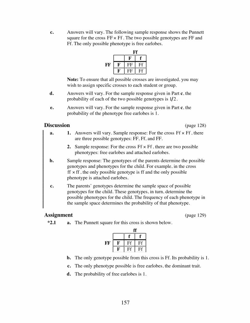
157

c. Answers will vary. The following sample response shows the Punnett square for the cross FF × Ff . The two possible genotypes are FF and Ff. The only possible phenotype is free earlobes.

Note: To ensure that all possible crosses are investigated, you may

wish to assign specific crosses to each student or group. d. Answers will vary. For the sample response given in Part c, the

probability of each of the two possible genotypes is 1 2 .

e. Answers will vary. For the sample response given in Part c, the probability of the phenotype free earlobes is 1.

Discussion (page 128) a. 1. Answers will vary. Sample response: For the cross Ff × Ff , there

are three possible genotypes: FF, Ff, and FF.

2. Sample response: For the cross Ff × Ff , there are two possible phenotypes: free earlobes and attached earlobes.

b. Sample response: The genotypes of the parents determine the possible genotypes and phenotypes for the child. For example, in the cross ff × ff , the only possible genotype is ff and the only possible phenotype is attached earlobes.

c. The parents’ genotypes determine the sample space of possible genotypes for the child. These genotypes, in turn, determine the possible phenotypes for the child. The frequency of each phenotype in the sample space determines the probability of that phenotype.

Assignment (page 129) *2.1 a. The Punnett square for this cross is shown below.

b. The only genotype possible from this cross is Ff. Its probability is 1.

c. The only phenotype possible is free earlobes, the dominant trait.

d. The probability of free earlobes is 1.

FfF f

FF F FF FfF FF Ff

fff f

FF F Ff FfF Ff Ff

158

2.2 a. The Punnett square for this cross is shown below.

b. The two possible genotypes are Ff and ff. Each has a probability of 1 2 .

c. Since F is the dominant trait, the genotype Ff results in the phenotype free earlobes. The genotype ff results in the phenotype attached earlobes.

d. Each phenotype has a probability of 1 2.

2.3 a. As shown in the following Punnett square, the probability of the genotype RR is 1 2 .

b. As shown in the tree diagram below, the probability of the

genotype rr is 0.

c. Because both of the possible genotypes result in the same

phenotype, the probability that a child of these parents has the ability to roll the tongue is 1.

*2.4 a. Since having a widow’s peak is a dominant trait, the father’s genotype is Ww.

b. As shown in the following Punnett square, the two possible genotypes are Ww and ww.

c. Since the genotype ww results in a child with no widow’s peak,

the probability of this phenotype is 2 4 =1 2.

fff f

Ff F Ff Fff ff ff

RRR R

Rr R RR RRr Rr Rr

R

RR

RR

RR

rRr

Rr

R

R

Parent 1 Parent 2 Child

www w

Ww W Ww Www ww ww

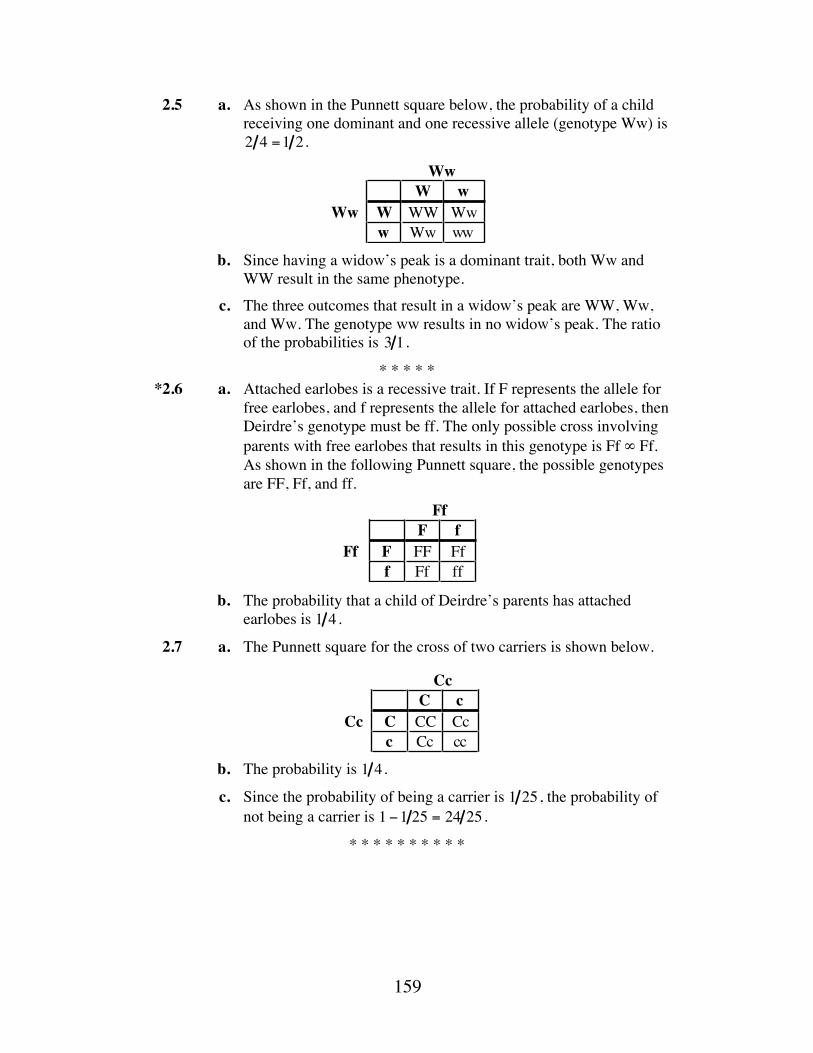
159

2.5 a. As shown in the Punnett square below, the probability of a child receiving one dominant and one recessive allele (genotype Ww) is 2 4 =1 2.

b. Since having a widow’s peak is a dominant trait, both Ww and

WW result in the same phenotype.

c. The three outcomes that result in a widow’s peak are WW, Ww, and Ww. The genotype ww results in no widow’s peak. The ratio of the probabilities is 3 1.

* * * * * *2.6 a. Attached earlobes is a recessive trait. If F represents the allele for

free earlobes, and f represents the allele for attached earlobes, then Deirdre’s genotype must be ff. The only possible cross involving parents with free earlobes that results in this genotype is Ff ∞ Ff. As shown in the following Punnett square, the possible genotypes are FF, Ff, and ff.

b. The probability that a child of Deirdre’s parents has attached

earlobes is 1 4 .

2.7 a. The Punnett square for the cross of two carriers is shown below.

b. The probability is 1 4.

c. Since the probability of being a carrier is 1 25 , the probability of not being a carrier is 1 −1 25 = 24 25 .

* * * * * * * * * *

WwW w

Ww W WW Www Ww ww

FfF f

Ff F FF Fff Ff ff

CcC c

Cc C CC Ccc Cc cc

160

(page 130)

Activity 3 Students explore probabilities for more than one event. The mathematics note introduces a formula for finding the probability of multiple independent events.


Discussion 1 (page 131) a. 1. Since the father has two different alleles, and each has an equal

chance of being passed on, the probability is 1 2.

2. Since the mother has two identical alleles, the probability is 1. 3. The probability that a child of this couple will have the genotype

RR is 1 2.

b. Sample response: No. The probability does not change because the allele passed on by the father is not influenced by the mother’s genotype.

c. Since receiving a particular allele from the father is independent of receiving a particular allele from the mother, the probability of a child receiving a given genotype equals the product of the probabilities for receiving each allele from each parent.

For example, the probability that this child will receive the genotype RR can be calculated as follows:

12• 12=14

Exploration (page 132) Students examine the relationship among P(A) , P(B) , and P(A and B) when A and B are independent events.

a–b. The following table shows sample data for the traits folded hands and rolled tongue.

Trait A: folded hands Trait B: rolled tongue Total Number in Class:

Trait Frequency Experimental Probability A 20 20 25 B 19 19 25

A and B 16 16 25

161

c. Students repeat Part b for each of the 10 possible pairs of two traits.

d. For each pair of traits, students should use experimental probabilities to approximate theoretical probabilities. If P(A) • P(B) ≈ P(A and B) , then they should observe that traits A and B appear to be independent.

Discussion 2 (page 132) a. 1. Answers may vary, depending on class data. 2. If P(A) • P(B) is not approximately equal to P(A and B) ,

students should observe that traits A and B appear to be dependent.

b. 1. Sample response: Having blond hair and being male appear to be independent events. This could be demonstrated by using the experimental probability of each trait to approximate the theoretical probabilities. If P(A) • P(B) ≈ P(A and B), then the traits would appear to be independent.

2. Sample response: Receiving an A in every class and getting on the honor roll are dependent events. This could be demonstrated by using the experimental probability of each event to approximate the theoretical probabilities. If P(A) • P(B) ≠ P(A and B) , then the events would appear to be dependent.

c. Sample response: The product of the probability of that trait and the number of students in the class gives the number of students you could expect to have the trait.

Assignment (page 133) 3.1 Answers may vary, depending on class data. Using the sample data

given in Activity 1, the probability of having free earlobes and the ability to roll the tongue and no widow’s peak is:

1825

•1925

•825

=273615,625

162

*3.2 a. The probability for each branch is shown on the tree diagram below.

b. Since receiving an allele from one parent is independent of receiving an allele from the other parent, the probability for the genotype rr can be found by multiplying the probabilities on the two corresponding branches:

P(r) • P(r) = 12• 12=14

The same method can be used to find the probability for genotype RR:

P(R) • P(R) = 12• 12=14

Similarly, for each occurrence of the genotype Rr:

P(R) • P(r) = 12• 12=14

However, since the genotype Rr occurs twice in the cross, the probabilities of the two occurrences must be added:

14+14=12

c. The Punnett square for this cross is shown below.

Using a Punnett square, the probabilities for rr and RR are 1 4 and

the probability for Rr is 1 2 .

d. The probabilities found for each genotype are the same using either method.

R

r

gene frommother

gene from father

R RR

child

r rr

Rr Rr

Rr

1 2

1 2

1 2

1 21 2

1 2

RrR r

Rr R RR Rrr Rr rr

163

3.3 The cross Mm ∞ Mm yields the outcomes MM, Mm, Mm, and mm. Since 3 of the 4 result in the phenotype mid-digit hair, the probability that a child of these parents has mid-digit hair is 3 4 .

The cross WW ∞ Ww yields the sample space WW, WW, Ww, and Ww. Since all of these outcomes result in a widow’s peak, P(widow ’s peak) = 1.

Therefore, the probability that a child of these parents has both traits is:

34•1 = 3

4

*3.4 a. The experimental probability for type A is 10 26 = 5 13, for type B is 4 26 = 2 13 , for type AB is 1 26 , and for type O is 11 26.

b. The experimental probability for the presence of the Rh factor is 20 26 =10 13; the experimental probability for the absence of the Rh factor is 6 26 = 3 13 .

c. Sample tree diagram:

* * * * *

3.5 Students may use a Punnett square or draw a tree diagram to find the sample space hH, hH, hh, hh. The genotype hH results in curly hair, so the probability of a child having curly hair is 1 2 . The probability that two children of these parents have curly hair is 1 2 •1 2 =1 4 .

*3.6 Assuming that two people chosen at random are unrelated, the probability that both are carriers of cystic fibrosis is:

125• 125

=1625

A+

B+

AB+

O+

A–

B–

AB–

O–

10/13

3/13

5/132/131/26

11/26

5/13

2/131/26

11/26

50/169

20/169

5/169

55/169

15/169

6/169

3/338

33/338

Rh+

Rh–

A

B

AB

O

A

B

AB

O

blood type probability

164

3.7 a. The probability that a person chosen at random prefers cola is 0.30 + 0.25 + 0.10 = 0.65.

b. Assuming that preference for soft drink is independent of preference for snack food, the probability that a person chosen at random prefers cola and pretzels is 0.65 • 0.10 = 0.065 .

c. The probability that a person chosen at random prefers root beer is 0.15. Therefore, the probability that a person chosen at random does not prefer root beer is 1 − 0.15 = 0.85 .

*3.8 a. The Punnett square for this cross is shown below.

b. P(hh) = 1 2

c. Since the births are independent events, the probability that a child is a carrier is the same for each birth: P(Hh) = 1 2 .

d. Since the births are independent events,

P(hh and hh) = 12

• 12=

14

* * * * * * * * * *

Research Project (page 135) Students may contact a local hospital or the March of Dimes Birth Defects Foundation for more information on genetic counseling.

There are more than 2000 diseases with some identifiable genetic component. The following paragraphs briefly describe the diseases listed in the student edition.

• Cystic fibrosis is associated with the failure of the chlorine pump in cell membranes, resulting in a build up of mucous outside cells. The accumulation of mucous in the pancreas, lungs, and digestive tract makes victims susceptible to pneumonia and other infections.

Untreated victims typically die by age 4 or 5. Treatment with special diets low in chlorine and daily doses of antibiotics can increase life expectancy to an average of 27 years.

In the United States, cystic fibrosis occurs in about 1 of every 2500 births. About 1 in every 25 people is a carrier. The disease occurs in individuals with double recessive genotypes.

HhH h

hh h Hh hhh Hh hh

165

• Tay-Sachs disease is caused by the failure of an enzyme that breaks down excess lipids, resulting in a build up of lipids in the brain. Infants develop seizures and blindness, accompanied by a decline in mental and motor skills. There is currently no treatment. Death occurs a few years after birth.

Tay-Sachs occurs in about 1 of every 360,000 births worldwide. It is more frequent (about 1 in every 3600) in Jewish people whose ancestors came from Central Europe. The disease occurs in individuals with double recessive genotypes.

• Huntington’s disease is characterized by a breakdown in the tissues of the nervous system. Victims experience a steady decline in mental and motor skills and typically do not manifest symptoms until middle age (between 35 and 45 years old). There is currently no treatment for the disease.

Huntington’s disease occurs in individuals with one dominant and one recessive allele. Fetuses with double dominant genotypes are spontaneously aborted.

• Sickle-cell anemia is caused by deformed hemoglobin in red blood cells. The malformed red blood cells result in blood clotting, lower blood oxygen levels, and other symptoms of anemia. There is currently no treatment. Although usually not fatal, the disease limits activity and can cause chronic health problems.

In the United States, sickle-cell anemia is most frequent among people of African origins, occurring in about 1 of every 400 births (about 1 in 10 are carriers). Sickle-cell anemia is a co-dominant disease, which means that carriers may have mild symptoms. In tropical regions, carriers have displayed an increased resistance to malaria.

• Phenylketonuria (PKU) is characterized by the inability to metabolize the amino acid, phenylalanine. As a result, phenylpyruvate accumulates in the bloodstream, eventually reaching toxic levels. Maintaining a diet low in phenylalanine has shown to be an effective treatment.

PKU occurs in about 1 of every 15,000 births in the United States. By using a simple blood test, infants can be screened for the disease before they leave the hospital. PKU occurs in individuals with double recessive genotypes.

166

(page 136)

Activity 4 Students identify mutually exclusive events. Given two events A and B, they use appropriate formulas to find the probability of A or B.


Exploration (page 136) a. Sample data:

Trait A: left-handedness Trait B: right-handedness Total Number in Class: 25

Trait Frequency Experimental Probability A 10 10 25 = 2 5 B 15 15 25 = 3 5

A and B 0 0 25 = 0 A or B 25 25 25 =1

b. Students repeat Part a for two other pairs of traits.

Teacher Note You may wish to use the following Venn diagram to help explain the example given in the mathematics note.

deck of cards

black king24 2 2

24

167

c–d. The calculated values for P(A or B) should be equal to those recorded in the tables. For example, using the sample data given in Part a:

P(A or B) = P(A) + P(B) − P(A and B)

=1025

+1525

− 0

=2525

= 1

Discussion (page 137) a. Sample response: Yes. The probabilities determined by the formula

were equal to those observed in the class. b. For all classes, P(A and B) should equal 0 for left-handedness and

right-handedness. Depending on the class data, this also may be true for other pairs of traits.

c. 1. For all classes, the preferences for writing with the left hand or the right hand should be mutually exclusive. Depending on the class data, other pairs of traits also may be mutually exclusive.

2. The preferences for writing with the left hand or the right hand are always mutually exclusive since it is not possible to prefer both at the same time. In the general population, the other pairs of traits are not mutually exclusive.

d. Sample response: Since P(A and B) = 0 for mutually exclusive events, that part of the formula can be omitted without affecting the result.

e. Yes. Since the complement of event E is defined as the event that E does not occur, it is impossible for an event and its complement to occur at the same time.

f. No. On a single roll of a die, for example, a roll of six and a roll of three are mutually exclusive. However, they are not complementary. The probability of rolling a six is 1 6 . The probability of rolling a three is also 1 6. The sum of their probabilities is 1 3 , not 1.

g. When mutually exclusive traits A and B are considered as sets, they do not intersect, as shown in the diagram below. Since there is no intersection, the probability of A and B occurring at the same time is 0.

A B

168

Assignment (page 138) 4.1 a. Because these two events cannot occur at the same time (and are

complementary), they are mutually exclusive. b. Since a person can have both traits at the same time, these two

events are not mutually exclusive. c. Since a person with two blue eyes cannot also have two brown

eyes, these two events are mutually exclusive. *4.2 One way to determine the probability that a child of this couple is

either mildly affected or not affected at all is to use a tree diagram.

Since the genotype Dd occurs twice, the probability that a child is

mildly affected is:

12• 12

⎛ ⎝

⎞ ⎠ +

12• 12

⎛ ⎝

⎞ ⎠ =

12

Since the genotype dd occurs only once, the probability that a child is not affected at all is 1 4 . Using the formula for P(A or B) ,

P(Dd or dd) =12+

14− 0

=34

This probability can also be determined using a Punnett square.

Since Dd occurs twice in a sample space of 4 genotypes, its

probability is 1 2 . Since dd occurs once, its probability is 1 4 . As shown above, P(Dd or dd) = 3 4 .

Erma Hank child

DdDd

dd

DDD

d

d

d

D

D1/2

1/2

1/2

1/2

1/2

1/2

DdD d

Dd D DD Ddd Dd dd

169

4.3 a. For the cross Mm ∞ Mm, the probability of the phenotype mid-digit hair is 3 4 . For the cross WW ∞ Ww, the probability of the phenotype widow’s peak is 1. The probability that a child of these parents has mid-digit hair or a widow’s peak is:

34

+1 −34•1⎛

⎝ ⎞ ⎠ = 1

Note: Students may solve this problem simply by reasoning that since the probability of a widow’s peak is 1, the probability of a widow’s peak or mid-digit hair is also 1.

b. Since the probability of either a widow’s peak or mid-digit hair is 1, all five children would be expected to have one trait or the other.

* * * * *

4.4 Since these events are mutually exclusive, the probability can be calculated as follows:

320

+120

=420

=15

*4.5 a. 0.008

b. 0.008 • 250 = 2

c. 1. 0.008 • 0.008 = 6.4 •10−5 2. 0.008 + 0.008 − (0.008 • 0.008) ≈ 0.016

4.6 a. Since there are 10 digits on each tumbler, the number of possible combinations for a three-tumbler lock is 10 • 10 •10 = 1000 . Therefore, the probability of guessing the right combination on one guess is 1 1000.

b. Sample response: Yes. The number of possible combinations for a five-tumbler lock is 105 = 100, 000 . This lock has 100 times more possible combinations than a three-tumbler lock, which decreases the probability that someone could guess the actual combination.

* * * * * * * * * *

170

(page 140)

Activity 5 In this activity, students discover that the gender of each child in a family is an independent event. They apply this fact to finding the probabilities of specific family combinations of boys and girls. (This presents a somewhat simplified view of the determination of gender. While it is true that the gender of each child is an independent event, the probabilities of having a boy or girl for any particular family may not be exactly 1 2, due to a range of biological and genetic factors.)

Materials List • coins (two per group)

Exploration (page 140) Students use coins to simulate the random selection of the chromosomes that determine gender. (Since the coin that represents the mother’s chromosomes always results in an X, students may realize that only the toss of the coin representing the father’s chromosomes actually determines the gender of the child.) a. Answers may vary. Some students may correctly predict 1 2 .

b. Students simulate the chromosomes by labeling two coins.

c. Students simulate the combination of male and female chromosomes by tossing the two coins. The experimental probability that the combination results in a female child should be approximately 1 2 .

d. As shown below, either method can be used to analyze the cross of genotype XY (male) and genotype XX (female). The sample space from this cross contains four equally likely outcomes: two each of XX and XY. Therefore, the theoretical probability of each outcome is 1 2 .

Sample Punnett square:

XXX X

XY X XX XXY XY XY

171

Sample tree diagram:

e. Answers may vary. Some students may correctly predict 1 2 .

f. The experimental probability that two independent combinations of male and female chromosomes result in one male and one female child should be approximately 1 2.

g. As shown in the following tree diagram, 2 of the 4 possible outcomes result in one male and one female child. The theoretical probability, therefore, is 1 2.

h. The experimental probabilities calculated using the class data should

be approximately 1 2 .

Discussion (page 141) a. Sample response: They are independent events because the outcome

of one coin does not affect the outcome of the other coin.

b. Sample response: Yes. They are equally likely since the chance of getting an X on the father coin is the same as the chance of getting a Y on the father coin: 1 2 . Because the chance of getting an X on the mother coin is 1, the toss of the mother coin does not affect the outcome.

X

X

X

Y

Y

XY

XY

X XX

XX

mother father child

1/2

1/2

1/2

1/21/2

1/2

G

B

B

B

G

G

Child 1 Child 2 FamilyGG

GB

BG

BB

172

c. 1. Answers may vary. As the number of trials increases, the experimental probability is more likely to be close to 1 2 .

2. The experimental probabilities calculated using the class results are more likely to be close to the theoretical probabilities.

d. 1. The sample space contains 4 items: GG, GB, BG, and BB, where G represents girl and B represents boy.

2. Since there are 2 possibilities for each child, the number of possible outcomes for 3 children is 2 • 2 • 2 = 23 = 8 .

3. 2n

Assignment (page 142) *5.1 a. Sample tree diagram:

b. Given that a boy and a girl are equally likely, the probability on

each branch in the tree diagram is 1 2. Therefore, P(GGB) = 1 8.

c. Two of the three children are girls in 3 of the possible outcomes: GGB, GBG, and BGG. Since the probability of each outcome is 1 8 , the total probability is 3 8 .

d. The answers to Parts b and c differ because the event in Part b considers the specific order GGB, while the event in Part c does not. There are 3 different outcomes that satisfy Part c, but only one that satisfies Part b. Therefore, their probabilities are different.

G

B

G

B

G

G

G

B

B

B

GGG

GGBGBG

GBB

BGG

BGB

BBG

BBB

B

B

G

G

Child 1 Child 2 Child 3 Family

173

5.2 Assuming that the probability of having a boy or girl was equally likely for each of the previous four children, the fifth child is as likely to be a boy as a girl.

5.3 If students assume that each birth is an independent event with the same probability, 1 2 , they should agree with this method.

* * * * * 5.4 a. 1 50

b. Assuming that the outcome of one car rental has no effect on the outcome of another, the probability can be calculated as follows:

1 50( )5 = 0.0000000032 ≈ 0

c. They can expect 250 1 50( ) = 5 cars to be involved in accidents.

5.5 a. The probability that the fourth digit is a 7 is 1 10.

b–d. The probability that any one sequence of six digits is the winning number is 1 10( )6 =1 1,000, 000 .

*5.6 a. When rolling two dice, there are 36 equally likely outcomes. Since 6 of them result in a roll of 7 and 2 result in a roll of 11, the probability of winning is:

636

+236

=836

=29

b. Since each roll is an independent event, the probability of winning on three rolls in a row is:

29• 29• 29=8729

* * * * * * * * * *

174

Answers to Summary Assessment (page 143) 1. a. The possible genotypes for each blood type are shown below.

Blood Type A B AB O Possible

Genotype AA, AO BB, BO AB OO

b. Assuming that each genotype is equally likely, the probability of

each phenotype is listed below.

Blood Type A B AB O Probability 2 6 = 1 3 2 6 = 1 3 1 6 1 6

Note: The actual distribution of human blood types varies by

population. 2. Assuming that the genotypes of blood donors are distributed as in

Problem 1, the expected amounts can be found by multiplying each probability by 75 L and rounding to the nearest 0.5 L. The total should not exceed 75 L.

Blood Type A B AB O Expected Amount

(L) 25 25 12.5 12.5

3. Assuming that blood type and Rh factor are independent events, the

expected amount of each blood type can be multiplied by 85% to determine the expected amount of Rh+ blood, and by 15% to determine the amount of Rh– blood, with the results rounded appropriately. As in Problem 2, the total should not exceed 75 L.

Blood Type A+ A– B+ B– AB+ AB– O+ O– Expected Amount

(L) 21 4 21 4 10.5 2 10.5 2

4. As shown in the table in Problem 3, the expected amount for each Rh-

blood type is less than 5 L. The table below shows the amounts needed and the number of donors required for each.

Blood Type A– B– AB– O– Amount Needed (L) 1 1 3 3

Donors Needed 2 2 6 6

175

Module Assessment

The following table shows the frequencies of some inherited traits in a class of 24 students. Use this data to complete Problems 1–6 below.

Trait(s) Number of Students mid-digit hair 18 widow’s peak 14 free earlobes 11

widow’s peak and free earlobes 6 widow’s peak or free earlobes 19

1. In this class, what is the experimental probability of having a widow’s peak?

2. In this class, what is the experimental probability of not having mid-digit hair?

3. Describe the relationship between the events “widow’s peak” and “no widow’s peak.”

4. Determine the sum of the probabilities of having free earlobes and having attached earlobes.

5. a. In this class, what is the experimental probability of having both a widow’s peak and free earlobes?

b. Why can this probability be no more than the experimental probability of having a widow’s peak alone?

6. Explain why the experimental probability of having a widow’s peak or free earlobes does not equal the sum of the probabilities of having each trait.

7. Having curly hair (C) is a dominant trait. Having straight hair (c) is a recessive trait. Consider the cross CC ∞ cc.

a. Use a Punnett square to determine the sample space for this cross.

b. Find the probability that a child of these parents has curly hair.

c. Draw a tree diagram that shows the sample space of this cross.

d. Find the probability that a child of these parents has straight hair.

8. a. A couple plans to have four children. What is the probability that they have a boy, then a girl, then a boy, then a girl?

b. What is the probability that they have two girls and two boys, in any order?

176

9. Carriers of cystic fibrosis have the genotype Cc. If a father and mother who are both carriers decide to have two children, what is the probability that both children will have the genotype cc?

10. Describe an example of each of the following:

a. two independent events

b. two dependent events

c. two mutually exclusive events

d. two events that are not mutually exclusive

e. two complementary events.

177

Answers to Module Assessment 1. 14 24 = 7 12

2. 1 −18 24 = 6 24 =1 4

3. They are complementary events.

4. Since these two traits are complementary events, the sum of their probabilities must be 1:

1124

+1324

=1

5. a. 6 24 = 1 4

b. Sample response: This can be no more than the probability of having a widow’s peak since any student who has a widow’s peak and free earlobes will also be counted in the column for widow’s peak alone.

6. Sample response: Having a widow’s peak and having free earlobes are not mutually exclusive events. In fact, six students in the class have both traits. The probability of having a widow’s peak or free earlobes is calculated by subtracting the probability of having both traits from the sum of the probabilities of having each trait:

1424

+1124

−624

=1924

7. a. Sample Punnett square:

b. Since the genotype Cc results in curly hair, the probability of curly

hair is 4 4 = 1.

c. Sample tree diagram:

ccc c

CC C Cc CcC Cc Cc

1 2

1 2

1 2

1 21 2

1 2

childCc

c

c

C

C

c

cCC cc

CcCc

Cc

178

d. Since only the genotype cc results in straight hair, the probability is 0. 8. a. Assuming that the birth of each child is an independent event and

that the probabilities of having a boy and a girl are the same:

P(BGBG) = 12• 12• 12• 12=116

where B represents boy and G represents girl. b. The total number of outcomes is 16. Of these, 6 include two boys

and two girls: BBGG, BGBG, BGGB, GBBG, GBGB, and GGBB. Therefore, the probability is 6 16 = 3 8 .

9. The following Punnett square shows the possible genotypes for this cross:

The probability of having one child with cystic fibrosis is 1 4 .

Assuming that the birth of each child is an independent event, the probability of having two children with the genotype cc is:

14• 14=116

10. Answers may vary from the following sample responses. a. Two independent events are having a widow’s peak and having

mid-digit hair. b. Two dependent events are being female and being a mother. c. Two mutually exclusive events are being male and being female. d. Two events that are not mutually exclusive are having brown eyes

and having brown hair. e. Two complementary events are being able to roll your tongue and

not being able to roll your tongue.

CcC c

Cc C CC Ccc Cc cc

179

Selected References Goodspeed, J. K. “But My Parents Both Have Brown Eyes.” Science and

Children 22 (January 1985): 9–12. Grollman, S. The Human Body: Its Structure and Physiology. London: The

Macmillan Co., 1969. Ince, S. “Genetic Counseling.” White Plains, NY: March of Dimes Birth Defects

Foundation, 1987. Mange, A. P., and E. J. Mange. Genetics: Human Aspects. Sunderland, MA:

Sinauer Associates, 1990. Rosenberg, N. S. “Genetic Counseling.” Undergraduate Mathematics and Its

Applications (UMAP) Project. Module 456. Arlington, MA: COMAP, 1987.

Schraer, W. D., and H. J. Stoltze. Biology: The Study of Life. Needham, MA: Prentice-Hall, 1991.

Note: To order copies of the March of Dimes pamphlet, call 1-800-367-6630, or write the March of Dimes, P.O. Box 1657, Wilkes-Barre, PA 18703.

180

Flashbacks

Activity 1 1.1 Shade the portion of the Venn diagram below that represents all

elements not in set A.

1.2 Given that b = 1 − a , find the ratio a b for each of the following

values of a.

a. a = 0.76 b. a = 3 8

1.3 A bag contains 20 blue marbles, 16 green marbles, and 12 red marbles. If you select one marble at random from the bag, what is the probability that the marble is:

a. red?

b. green?

c. green or red?

1.4 a. If a fair coin is tossed 40 times, how many times would you expect it to land heads up?

b. If a die is tossed 60 times, how many times would you expect it to show a 5?

A B

181

Activity 2 2.1 A bag contains four marbles: one blue, one red, one green, and one

orange. Consider an experiment which involves drawing the marbles from the bag one at a time and recording the order in which they appear.

a. How many outcomes are there in the sample space for this experiment?

b. In 6 of the possible outcomes, the blue marble is the second one selected. What is the probability that the blue marble will be the second one selected?

2.2 Consider an experiment which involves turning over three cards—an ace, a king, and a queen—one at a time.

a. Describe the sample space for this experiment.

b. What is the probability that the ace is the first card turned over?

c. What is the probability that the king is the second card turned over?

d. What is the probability that the queen is the first card turned over and the ace is the second?

Activity 3 3.1 Consider an experiment in which three coins are tossed, one after the

other.

a. Create a tree diagram of all the possible outcomes. List a probability for each branch.

b. What is the probability that the second coin is heads?

c. What is the probability that the first coin and third coin are heads?

d. What is the probability of obtaining three heads?

3.2 If the experiment in Flashback 3.1 were repeated 80 times, how many times would you expect each of the following events to occur?

a. the second coin is heads

b. the first and third coins are heads

c. all three coins are heads

182

Activity 4 4.1 In a standard deck of 52 playing cards, what is the probability of

randomly selecting each of the following: a. an eight? b. a diamond? 4.2 Consider an experiment in which three cards—an ace, a king, and a

queen—are placed face down. One card is then turned over. At the same time, one marble is drawn from a bag containing four marbles: one blue, one red, one green, and one orange.

a. List the sample space for this experiment. b. What is the probability that the card is a king and the marble is

red? c. What is the probability that the card is a king or the marble is red?

Activity 5 5.1 Evaluate each of the following expressions.

a. 23

b. 510

c. 2 3( )10

5.2 Consider an experiment which involves tossing coins and determining the resulting arrangement of heads and tails. Determine the number of elements in the sample space when tossing each of the following numbers of coins.

a. 2 b. 3 c. 4 d. 5

183


Activity 1 1.1 The shaded region in the diagram below represent the elements not in

set A.

1.2 a. 0.76 0.24 = 19 6

b. 3 85 8

=35

1.3 a. 12 48 = 1 4

b. 16 48 = 1 3

c. 28 48 = 7 12

1.4 a. 40 • 1 2 = 20

b. 60 •1 6 =10

Activity 2 2.1 a. Using the fundamental counting principle, the number of different

orders is 4 • 3• 2 • 1 = 24 . b. 6 24 = 1 4

2.2 a. The sample space consists of the combinations AKQ, AQK, KAQ, KQA, QAK, and QKA.

b. 1 3

c. 2 6 = 1 3

d. 1 6

A B

184

Activity 3 3.1 a. Sample tree diagram:

b. 1 2

c. 1 4

d. 1 8

3.2 a. 12• 80 = 40

b. 14• 80 = 20

c. 18• 80 =10

Activity 4 4.1 a. 4 52 =1 13

b. 13 52 = 1 4

4.2 a. In the following list, A represents ace, K represents king, Q represents queen, b represents blue, r represents red, g represents green, and o represents orange: Ab, Ar, Ag, Ao, Kb, Kr, Kg, Ko, Qb, Qr, Qg, Qo.

b. 1 12

c. 6 12 = 1 2

1/8

1/2

1/21/2

1/2

1/21/2

1/2

1/2 1/2

1/2

1/2

1/2 1/2

1/2

1/81/81/81/8

1/81/81/8

outcome probabilityHHH

HHTHTHHTTTHH

THTTTHTTT

firstcoin

secondcoin

thirdcoin

HH

T

H

HT

T

TH

T

H

HT

T

185

Activity 5 5.1 a. 23 = 8

b. 510 = 9, 765, 625

c. 2 3( )10 = 1024 59, 049

5.2 a. 22 = 4

b. 23 = 8

c. 24 = 16

d. 25 = 32

Wheel of Traits Template

There’s No Place Like Home

What geometric shape does your home resemble? What do you think the houses of the future will look like? In this module, you explore some traditional American Indian housing designs—from the ground up.

Kyle Boyce • Clay Burkett

189

Teacher Edition There’s No Place Like Home

Overview In this module, students use traditional American Indian housing designs to investigate the surface areas and volumes of some common three-dimensional figures. An intuitive understanding of limits is developed by exploring a circle as the limit of a progression of regular polygons with an increasing number of sides inscribed in the circle. Similarly, a cylinder is presented as the limit of a progression of regular polygonal right prisms inscribed in the cylinder, and a cone as the limit of a progression of regular pyramids inscribed in the cone. Students also explore the ratio of surface area to volume as a measure of structural efficiency.

Objectives In this module, students will: • determine the areas of regular polygons and circles • determine the surface areas and volumes of prisms, pyramids, cylinders, and

cones • calculate the surface areas and volumes of spheres • identify a circle as the limiting shape for its inscribed regular polygons, a

cylinder as the limiting shape for its inscribed regular prisms, and a cone as the limiting shape for its inscribed regular pyramids.

Prerequisites For this module, students should know: • how to use the sine, cosine, and tangent ratios to determine unknown

lengths and angle measures in right triangles • how to calculate the perimeter of a regular polygon given the length of a

side • how to express the area of a regular polygon as the sum of the areas of

congruent isosceles triangles with their vertex angle at the center of the polygon

• how to calculate the circumference and area of a circle • the parts of a prism • how to determine the volume of a prism • how to make nets of three-dimensional figures • the Pythagorean theorem.

190


Assessment Total

Days 1 1 2 2 2 1 9


1 2 3 4 5 Summary Assessment

construction paper X X scissors X X

tape X X cubes X

compass X ruler X rice X

Technology Materials Activity


geometry utility X X X graphing utility X

spreadsheet X X

191

There’s No Place Like Home

Introduction (page 149) This module uses traditional American Indian housing designs as a context for studying the surface areas and volumes of prisms, cylinders, pyramids, cones, and spheres. (page 149)

Activity 1 In this activity, students explore the areas of regular polygons. This provides the basis for determining surface area throughout the module. The idea of a circle as the limit of a progression of its inscribed regular polygons is introduced here.


Technology • geometry utility • spreadsheet (optional)

Teacher Note Since the following exploration can be time consuming, you may wish to divide the polygons in Part c among several groups, then ask students to compile their results. (If so, all students should use the same radius when constructing the inscribed polygons.)

Exploration (page 149) a–b. Students use a geometry utility to draw an inscribed regular triangle,

then determine its perimeter and area. c–d. The following sample data was collected using a radius of 5 cm.

Regular Polygon Perimeter (cm) Area (cm2 ) triangle 26.0 32.4 square 28.3 49.9

pentagon 29.4 59.3 hexagon 30.0 64.8 octagon 30.6 70.6 18-gon 31.2 76.8 circle 31.4 78.4

192

Discussion (page 150) a. Sample response: The number of sides in the polygon equals its

number of central angles. Since there are 360˚ in a circle, 360˚ divided by the number of sides (or vertices) determines how many degrees each central angle must have. To find the vertices, locate the points on the circle where each central angle has the desired measure.

b. The congruent central angles form congruent isosceles triangles in each polygon, with the base of each triangle representing a side of the polygon. Since the bases of these triangles are all congruent, the sides of the polygon are congruent. Since the base angles of all the isosceles triangles are congruent, the angles of the polygon are congruent.

c. 1. One method divides the regular polygon into congruent isosceles triangles with vertex angles at the center of the polygon and bases as the sides of the polygon. The area of each of these triangles, where a is the height and b is the length of the base, is

12ab

The area of the polygon is equal to the sum of the areas of these triangles. If the polygon has n sides, then the area of the polygon is

n 12ab⎛

⎝ ⎞ ⎠

Since n • b is the perimeter of the polygon, the generalized form of this method is the formula

A = 12ap

where a is the apothem and p is the perimeter. Note: Students also may suggest using technology, as described in the exploration.

2. Sample response: Each method can be useful, depending on the information given. Using a formula is appropriate when you know the required lengths. Using technology can be faster if you have already drawn a model of the polygon.

d. 1. The shape of the polygon approaches a circle. 2. The area of the polygon approaches the area of the circle. 3. The perimeter of the polygon approaches the circumference of the

circle. e. 1. The shape of the polygon approaches a circle. 2. The area of the polygon approaches the area of the circle. 3. The perimeter of the polygon approaches the circumference of the

circle.

193

f. 1. Sample response: As the number of sides of the polygon increases, the shape of the polygon becomes more and more circular. The apothem approaches a radius (r) of the circle and the perimeter approaches the circumference (2π r ) of the circle.

2. As the number of sides increases, the formula for the area of a regular polygon approaches the formula for the area of a circle:

A = 12r(2π r) = π r 2

Assignment (page 153) 1.1 a. m∠ABC = 20˚ ; m∠ABD = 10˚

b. AD = 5 • sin10˚≈ 0.87 m

c. AC ≈1.74 m

d. Using the Pythagorean theorem, BD ≈ 4.9 m .

e. The area of ΔABC ≈ (4.9 •1.74) 2 ≈ 4.3 m2 .

f. The area of the floor is approximately 18(4.3) ≈ 77 m2 .

*1.2 Student methods may vary. Using the points labeled in the diagram below, AB = 8 m , sin67.5̊ = BD 8 , and cos67.5̊ = AD 8.

The area of the floor, therefore, can be found as follows:

A = 12a • p

=12

(8 • sin67.5˚) • 2(8• cos67.5̊ )8 ≈ 181 m2

1.3 Using the formula for the area of a circle, the area of the floor is π 3.5 2( )2

≈ 9.6 m2 .

* * * * *

B

DA C

194

1.4 Student methods may vary. Using the formula for the area of a regular polygon, the area of the floor is:

A =12a • p

≈12

(0.87 • 6) ≈ 2.6 m2

* * * * * * * * * *

Research Project (page 154) This research project gives students the opportunity to further explore the geometric and cultural aspects of traditional American Indian housing designs. You may wish to encourage students to build models or make sketches. (page 154)

Activity 2 Students examine lateral surface area and total surface area using nets of right prisms and right circular cylinders. (Only right prisms and cylinders are considered in the context of this module.)


Technology • geometry utility (optional)

Discussion (page 155) a. 1. Sample response: The bases of a prism must be parallel. Since the

rectangles are not parallel, the floor cannot be a base. 2. Sample response: It is called a right prism because the bases are

perpendicular to the lateral faces.

b. The length of AD (or BC ) equals the perimeter of the base.

195

c. Sample response: Determine the area of a base by squaring the length of one side of the base. Find the area of the lateral surface by multiplying the perimeter of the base by the height of the prism. Add the area of the two bases to the area of the lateral surface.

d. 1. The length of the rectangle’s longer side is the circumference of the cylinder.

2. The length of the rectangle’s shorter side is the height of the cylinder.

3. The circles represent the two bases of the cylinder.

4. The length of the rectangle’s longer side is 2π r

5. Sample response: Multiply the circumference of the cylinder by the height to find the lateral surface area. Find the area of a base by squaring the radius and then multiplying by π . Add the lateral surface area to two times the area of a base.

Assignment (page 156) 2.1 a–b. Sample response:

c. The lateral surface area is 8 •6 •11 = 528 m2 .

d. Sample response:

A = 2 •n 12ab⎛

⎝ ⎞ ⎠

= 2 • 8 12

• 6 • 3tan 22.5̊

⎛ ⎝

⎞ ⎠

≈ 348 m2

e. The total surface area is 528 + 348 ≈ 876 m2 .

11 m

6 m6 m

196

2.2 a. Sample sketch:

b. Sample response: As the number of sides increases, the base gets

closer and closer to a circle. The shape of the prism approaches a cylinder.

2.3 The lateral surface area, including the floor, is 3 •3.2 • 4.7 ≈ 45 m2 . The height of the triangular base is 1.6 • tan 60˚≈ 2.8 m . The area of each base is

12• 2.8 •3.2 ≈ 4.5 m2

The total surface area is 45 + 2 4.5( ) or approximately 54 m2 .

2.4 The total surface area is 2 • (3.8• 3.4) + 2 • (3.8 +3.4) • 2.2 = 57.5 m2 .

*2.5 a. The area of the floor is 3.7 • 4.9 ≈ 18.1 m2 .

b. The two walls have a total area of π 3.7 2( )2≈ 10.8 m2 .

c. The lateral surface area can be found as follows:

12

• 2π 3.7 2( ) • 4.9 ≈ 28.5 m2

* * * * * 2.6 Sample response: The amount of bark required to cover the Iroquois

house (not including the floor) is the area of the four walls plus the area of the half cylinder that represents the roof:

2 5.5 +18.3( ) •2.75 + π 2.75( )2+

12

(2π • 2.75)• 18.3 ≈ 313 m2

* * * * * * * * * *

197

(page 158)

Activity 3 Students compare the volumes of various American Indian structures. They also consider the ratio of surface area to volume as a measure of a building’s heating (or cooling) efficiency.

Materials List • sets of eight cubes (one or two sets per group)

Exploration (page 159) In this exploration, students investigate the relationship between volume and surface area.

a–b. Students should record each arrangement of the cubes they investigate.

c. In general, the total surface area depends on the number of faces shared by the cubes. The diagram below shows a top view of three sample arrangements with a surface area of 34 units2 .

The following diagram shows the top view of six additional

arrangements of cubes.

The diagram below shows several arrangements in which the cubes

are stacked.

1. 2. 3. 4. 5. 6.

7. 8. 9. 10.

198

The total surface area and ratio of surface area to volume for each arrangement are shown in the table below.

Arrangement Surface Area (units2 ) Surface AreaVolume

1 34 4.25 2 32 4 3 34 4.25 4 32 4 5 30 3.75 6 28 3.5 7 34 4.25 8 30 3.75 9 34 4.25 10 24 3

Discussion (page 159) a. 1. The greatest surface area (34 units2 ) occurs in several different

arrangements.

2. The least surface area (24 units2 ) occurs in a 2 × 2 × 2 arrangement.

3. All the arrangements have the same volume, 8 units3 .

b. Sample response: Given that two designs have the same volume, a design with more surface area (and therefore a higher ratio) would be more in contact with the outside air. While it might receive more sunlight during the day, it would also lose more heat whenever the outside air was colder than the inside air.

c. 1. The greatest ratio (4.25) occurs in the arrangements with the surface area of 34 units2 .

2. The least ratio (3.0) occurs in the arrangement with the surface area of 24 units2 .

d. Sample response: A cube would be a good choice because it has the smallest surface area for a given volume.

e. Sample response: Since more surface area would provide more area for sunlight to strike, one of the shapes with a high ratio of surface area to volume would be a good choice.

199

Assignment (page 160) 3.1 a. The volume inside a Mohave-type house ranges from

62 • 2.2 ≈ 79.2 m3 to about 7.52 • 2.2 ≈ 124 m3 .

b. The ratio of surface area to volume is: 2(6 • 6) + 4(2.2 • 6)

79.2≈1.58

3.2 a. The ratio of surface area to volume is: 2(4 • 3.25 + 2.2 • 3.25 + 2.2 • 4)

2.2(4)3.25≈ 2.02

b. The volume of the Pueblo dwelling is about 13 • 2.2 ≈ 29 m3 . This is about 50 m3 less space than the smallest Yuma dwelling.

3.3 a. The volume of the house is:

(4.1• 3.1•1.7) +3.1• 1

2• 4.1⎛

⎝ ⎞ ⎠ ≈ 28 m3

b. The surface area of the house is:

4.1• 3.1+ 2(1.7• 3.1+1.7 • 4.1) + 2 3.1• 12

⎛ ⎝

⎞ ⎠ + 2(1.84 • 4.1) ≈ 55 m2

The ratio of surface area to volume is 55 28 ≈1.96 .

*3.4 a. Because the floors and side walls are the same sizes, students need only compare those portions of the structures that lie above the side walls. The surface area of this portion of the building with the curved roof is:

2 • π •1.5• 3.82

+ π • (1.5)2 ≈ 25 m2

The surface area of this portion of the other structure is:

2 • 1.5 • 3.02

⎛ ⎝

⎞ ⎠ + 2(1.5 2 • 3.8) ≈ 21 m2

Therefore, the surface area of the building with the curved roof is about 4 m2 greater than that of the other building.

200

b. The volume of the portion of the building with the curved roof that lies above the side walls is:

π •1.52 • 3.82

≈13.4 m3

The volume of the corresponding portion of the other building is: 3.0 • 1.5

2• 3.8 ≈ 8.6 m3

Therefore, the volume of the building with the curved roof is about 5 m3 greater than that of the other building.

c. Sample response: Because heat is lost through surface area, you might expect the building with the curved roof to lose heat more easily. But this structure also has more volume. In fact, the ratio of surface area to volume for the building with the curved roof is 25 13. 4 ≈1.9, while the ratio for the other building is 21 8.6 ≈ 2.4. Judging from these ratios, the building with the curved roof is likely to be more efficient in retaining heat.

3.5 a. Sample response: As the number of sides increases, the volume of the prism approaches the volume of the cylinder.

b. 1. Sample response: Yes, the formula can also be used to find the volume of a cylinder. You just need to find the area of the circular base and multiply it by the height of the cylinder.

2. Since the base of a cylinder is a circle, the formula for its area is A = π r 2 .

* * * * * 3.6 a. The lateral surface area of the cylindrical container is about

1040 cm2 . The total surface area is approximately 1480 cm2 . The volume is approximately 4360 cm3 .

b. The lateral surface area of the container shaped like a rectangular prism is about 1280 cm2 . The total surface area is approximately 1620 cm2 . The volume is approximately 4020 cm3 .

c. Sample response: Since the cylindrical container has less surface area, it should take less material to manufacture each one. Therefore, it should be cheaper to produce.

* * * * * * * * * *

201

(page 162)

Activity 4 Students examine the surface area and volume of both pyramids and cones. Using nets, they also explore the notion of a cone as the limit of a progression of regular polygonal pyramids with the same heights whose bases are inscribed in the same circle.

Materials List • construction paper (one sheet per student)

• tape

• scissors

Technology • geometry utility (optional)

Discussion 1 (page 163) a. The lateral faces are congruent isosceles triangles.

b. 1. The shape of the base becomes more and more circular.

2. The lengths of the bases of the congruent isosceles triangles decrease.

3. The pyramid looks more like a cone.

c. Sample response: To find the surface area of a pyramid, find the area of the polygonal base and the area of all the lateral triangular faces. Add the area of the base to the area of all the triangles.

Exploration (page 163) a. 1. Sample net:

2. Students should fold the net into a pyramid.

202

b. 1–2. The following diagram shows a sample net of the lateral surface (with tape):

Discussion 2 (page 164) a. 1. Sample response: The shape of the net looks like a concave

polygon.

2. Sample response: As the number of faces increases, the net of the lateral surface would look more like a part of a circle.

b. 1. The quantity 2π(10) represents the circumference of the circle.

2. The ratio 40 360 represents the fraction of the circle represented by the shaded sector in Figure 10.

c. The quantity π (10)2 represents the area of the circle.

d. As the number of faces increases, the net of the lateral surface approaches a sector of a circle.

e. 1. The radius of the sector determines the slant height of the cone.

2. The arc length of the sector determines the circumference of the cone’s base.

3. Sample response: Find the arc length of the sector. This is the circumference of the base of the cone. Since the circumference is 2πr , you can then solve for the radius of the base of the cone.

Assignment (page 165) 4.1 To find the area of the base, students must determine the apothem of

the hexagon, 3 3 m . To find the area of each triangular face, they must determine the slant height of the pyramid, 43 m . The total surface area can be found as follows:

66 • 3 3

2⎛

⎝ ⎜ ⎞

⎠ ⎟ + 6 43 • 6

2⎛

⎝ ⎜ ⎞

⎠ ⎟ ≈ 212 m2

203

4.2 a. 1. π(5)2 ≈ 78.5 cm 2

2. 2π • 5 ≈ 31.4 cm

b. 1. The fraction of the circle represented by each unshaded sector is shown below:

270˚360˚

=34

, 240˚360˚

=23

, 300˚360˚

=56

2. The areas of these unshaded sectors are:

34π(5)2 ≈ 58.9 cm2 , 2

3π(5)2 ≈ 52.4 cm 2, 5

6π(5)2 ≈ 65.4 cm2

3. The corresponding arc lengths are:

34

2π( )5 ≈ 23.6 cm, 23

2π( )5 ≈ 20.9 cm, 56

2π( )5 ≈ 26.2 cm

c. 1. The arc length of the sector is the circumference of the base of the cone.

2. From Part b3, the circumference of the base of this cone is 23.6 cm. The radius of the base, therefore, is r = 23.6 2π ≈ 3.8 cm . The slant height of the cone is the radius of the original circle, 5 cm. Using the Pythagorean theorem, the height of the cone can be found as follows:

3.82 + h2 = 52

h = 3.2 cm

3. The area of the base of the cone is π • 3.82 ≈ 45.4 cm2 .

4. The total surface area is: 270360

• π(5)2 + π(3.8)2 ≈ 104.3 cm 2

*4.3 a. Sample sketch:

r

s

204

b. 1. 2π r

2. 2πs

3. By comparing the length of the arc of the curved part of the net with the circumference of the large circle, the fraction of the large circle represented by the cone’s lateral surface is:

2π r2π s

=rs

c. 1. π s 2

2. The area of the lateral surface of the cone is: rsπ s2( ) = π rs

d. Sample response: The total surface area is the sum of the lateral surface area and the area of the base: A = π r 2 + π rs .

e. Using the Pythagorean theorem, h = s2 − r2 . 4.4 a. The circumference of the floor is determined by the length of the

semicircular arc, π (2.5) m. Thus, the diameter of the floor is 2.5 m.

b. Since the radius of the floor is 1.25 m and the slant height of the tipi is 2.5 m, h = 2.52 −1.252 ≈ 2.2 m .

c. Sample response: This is a very small tipi. A person could only stand up in the center, and it could sleep no more than two people.

* * * * * 4.5 a. In order to determine the radius of the template, students must first

recognize that the central angle which defines each funnel, including the tab, measures 120˚. Since the central angle for the tab measures 10˚, the fraction of the circle that actual forms the funnel is 110˚ 360˚ .

Since the length of the arc that forms the larger opening of the funnel is 32 cm, the radius of the circle can be found as follows:

110!

360!• 2πr = 32

r = 322π

•360 !

110!

r ≈ 16.7 cm

205

b. Similarly, the radius of the inner circle can be determined as shown:

110!

360!• 2πr = 5

r = 52π

•360 !

110!

r ≈ 2.6 cm

c. Students should recognize that the height of the funnel is the difference between the height of the cone before the tip is cut off and the height of the small cone which forms the tip.

The slant height of the larger cone is the radius of the larger circle, 16.7 cm. Since the radius of its base is approximately 5.1 cm, its height is 16.72 − 5.12 ≈ 15.9 cm .

The slant height of the smaller cone (the tip) is the radius of the inner circle, 2.6 cm. Since the radius of its base is approximately 0.8 cm, its height is 2.62 − 0.82 ≈ 2.5 cm .

The height of the funnel is 15.9 − 2.5 = 13.4 cm . * * * * * * * * * *

(page 168)

Activity 5 In this activity, students explore cones created from sectors of a circle. They also examine volume, surface area, and the ratio of surface area to volume for various cones and spheres.

Materials List • compass (one per group)

• scissors (one pair per group)

• construction paper (four sheets per group)

• ruler (one per group)

• tape

• rice (about 2 cups per group)


• spreadsheet

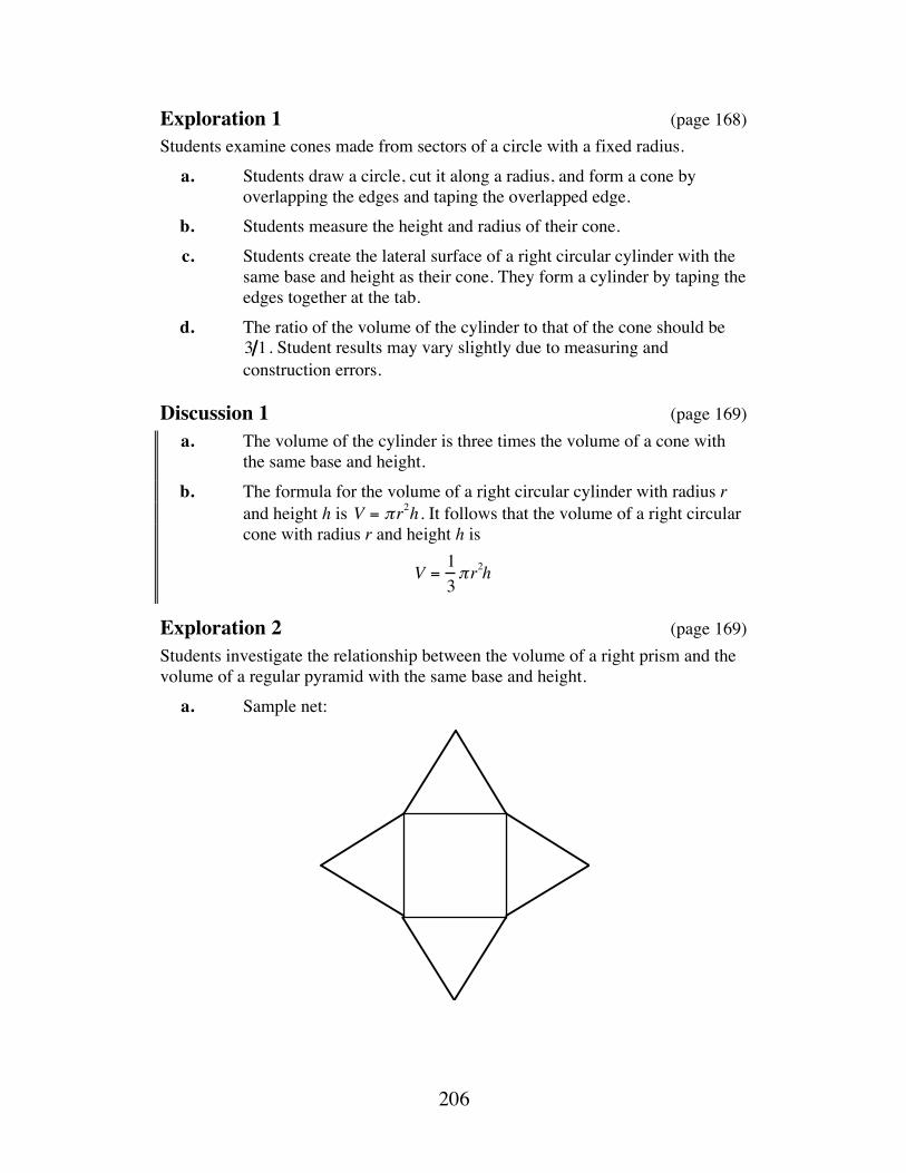
206

Exploration 1 (page 168) Students examine cones made from sectors of a circle with a fixed radius.

a. Students draw a circle, cut it along a radius, and form a cone by overlapping the edges and taping the overlapped edge.

b. Students measure the height and radius of their cone.

c. Students create the lateral surface of a right circular cylinder with the same base and height as their cone. They form a cylinder by taping the edges together at the tab.

d. The ratio of the volume of the cylinder to that of the cone should be 3 1 . Student results may vary slightly due to measuring and construction errors.

Discussion 1 (page 169) a. The volume of the cylinder is three times the volume of a cone with

the same base and height.

b. The formula for the volume of a right circular cylinder with radius r and height h is V = π r2h. It follows that the volume of a right circular cone with radius r and height h is

V =13π r2h

Exploration 2 (page 169) Students investigate the relationship between the volume of a right prism and the volume of a regular pyramid with the same base and height.

a. Sample net:

207

b–c. Students cut the lateral faces from the net and tape them together to form the shape of a pyramid. They then measure the height of the pyramid and a side of the base.

d. Students create a right prism with the same base and height as the pyramid in Parts a–c.

e. The ratio of the volume of the prism to that of the pyramid should be 3 1 . Student results may vary slightly due to measuring and construction errors.

Discussion 2 (page 170) a. The volume of the prism is three times the volume of a pyramid with

the same base and height.

b. The results of the explorations should agree with the formula given in the mathematics note.

c. Sample response: Find the area of the base by squaring s, multiply the area of the base by the height, and multiply that product by 1 3 .

d. 1. Students should rank the figures in the following order: right circular cylinder, hemisphere, right circular cone.

2. The volume of the cylinder is V = B • h = π r2( )r = π r3 . The volume of the cone is:

V =13B • h = 1

3π r3

3. Conjectures will vary. Based on the formulas for the volume of a cone and a cylinder, students will probably guess that the formula involves the product π r 3 . Sample response:

V =23πr3

4. Since the volume of a sphere is twice that of a hemisphere with the same radius, students should suggest multiplying their response to Part d3 of the discussion by 2.

208

Assignment (page 171) 5.1 a. Using the formula for the volume of a cone,

V =13π(10)2 (15) ≈1571 cm3

b. The height of the cylinder must be 1 3 that of the cone, or 5 cm which can be determined by solving for h in 1571 = π 10( )2 • h .

c. Students may solve for h as follows:

1571 = 13π(8)2 h

h ≈ 23.4 cm

5.2 a. The area of the regular dodecagon can be found as follows:

A = 12ap = 1

2tan 75˚(12 • 2) ≈ 45 m2

Using the formula for the volume of a pyramid,

V ≈13• 45 •5 ≈ 75 m3

b. V =13• π 3.75( )2 5 ≈ 74 m3

c. Sample response: The radius of the dodecagon is approximately 7.4 m, which is close to the radius of the base of the cone. Therefore, the areas of the two bases are close in value. Since the pyramid and the cone have the same height, their volumes are also close in value.

*5.3 a. Using the Pythagorean theorem, h = 36 − r2 .

b. Students should substitute for h as shown below:

V =13πr 2h =

13πr 2 36 − r 2

c. The area of the sector is a fraction of the area of the circle with radius 6 m:

A = 2π r12π

• π(62 ) = 6π r

209

d. Sample spreadsheet:

Radius (m) Volume (m3 )

Lateral Surface Area (m2 )

Surface AreaVolume

0.1 0.063 1.884 30.004 0.2 0.251 3.768 15.008 ! ! ! !

4.1 77.114 77.283 1.002 4.2 79.152 79.168 1.000 4.3 81.023 81.053 1.000 4.4 82.701 82.938 1.003 ! ! ! !

5.9 39.765 111.212 2.797 e. Sample response: The smallest ratio of surface area to volume

occurs in a cone with a radius somewhere between 4.2 m and 4.3 m. The corresponding range for the heights is also between approximately 4.2 m and 4.3 m.

Teacher Note The derivation of the formula for the surface area of a sphere requires the use of calculus to find the area of a surface of revolution.

*5.4 a. Students should use the diameter of the pit to approximate the radius of the hemisphere. The total volume of the house can be found as follows:

V = (π •1.752 •1.5) +12

43

• π •1.753⎛ ⎝

⎞ ⎠ ≈ 25.7 m3

b. The total surface area can be found as follows:

A = (π •1.752 ) + (2 •π •1.75 •1.5) + 12

4 • π •1.752( ) ≈ 45.4 m2

c. Sample response: Because part of a pit house is buried—and because the earth provides both insulation and heat storage—it would have less heat loss during cold months, and more moderate indoor temperatures during warm months.

* * * * *

210

5.5 a. The radius of the base of the cone formed by the shaded sector can be determined as shown below:

2πr = 120˚360˚

2π•10( )

r ≈ 3.3 cm

The total surface area can be found as follows:

A ≈ π •3.32 +120˚360˚

• π•102 ≈ 139 cm2

Similarly, the radius of the base of the cone formed by the unshaded sector is:

2πr = 240˚360˚

2π •10( )

r ≈ 6.7 cm

The total surface area of this cone is:

A ≈ π • 6.72 +240˚360˚

• π •102 ≈ 351 cm2

b. For the cone formed by the shaded sector, h ≈ 102 − 3.32 ≈ 9.4 cm . Its volume, therefore, is:

V ≈13• π • 3.32( ) •9.4 ≈107 cm3

For the cone formed by the unshaded sector, h ≈ 102 − 6.72 ≈ 7.4 cm . Its volume is:

V ≈13• π • 6.72( ) •7.4 ≈ 348 cm 3

c. For the cone formed by the shaded sector, the ratio is approximately 1.3. For the cone formed by the unshaded sector, the ratio is approximately 1.0.

5.6 a. Since the inside radius of the hemisphere is 3 m, its volume is:

V =23π (33 ) ≈ 57 m3

b. The volume of snow is about 5.9 m3 .

c. The ratio of surface area to volume is approximately 1. Because this ratio is relatively low, one would expect the efficiency to be fairly good—especially when considering the insulating properties of snow. Although some heat will be lost through the floor (which in the Arctic is also frozen), the temperature of the outside air during the cold months is likely to be much lower than that of the tundra.

211

d. Given a volume of 57 m3 , the length of the half cylinder can be found by solving the following equation for h:

57 = 12(π • 32 • h)

Since h ≈ 4.1 m , the surface area of the half cylinder, not including the floor, is:

π (32 ) + π(3)4.1 ≈ 67 m2

Therefore, the ratio of surface area to volume is approximately 1.2.

e. Answers will vary. Judging only from the calculated ratios of surface area to volume, the hemisphere should be more efficient to heat than the half cylinder of equal volume.

5.7 a. Using the formula for the volume of a sphere,

V =43π(75)3 ≈ 1.8 •106 cm3

b. Subtracting the thickness of the walls,

V =43π(75 − 3.8)3 ≈ 1.5 •106 cm3

c. The surface area of the Bathysphere is A = 4π(75)2 ≈ 71,000 cm2 , while the surface area of a cube with equal volume would be approximately 88,000 cm 2 . Assuming that weight is proportional to surface area, the ratio of the weight of the Bathysphere to the weight of the cube would be approximately 0.8.

* * * * * * * * * *

212

Answers to Summary Assessment (page 175) 1. a. To find the surface area of this structure, students must find the

lateral surface area of a cone and the lateral surface area of a cylinder.

The slant height s of the cone equals r 2 + h2 , where r is the radius of the base and h is the height of the cone. In this case,

s = 5.32 + 2.52 ≈ 5.9 m

The lateral surface area of the cone, therefore, is:

π • r • s = π • 5.3 • 5.9 ≈ 97 m2 The lateral surface area of the cylinder is:

2π • r •h = 2π • 5.3 • 2.1 ≈ 69 m2

Adding the surface area of the floor (π (5.32 ) ≈ 87 m2 ), the total surface area is approximately 97 + 69 + 87 = 253 m2 .

b. The total volume can be found as follows:

V =13π • 5.32 • 2.5 + π • 5.32 • 2.1 ≈ 259 m3

2. The total inside surface area is the surface area of the hemisphere minus the area of the doorway plus the surface area of the entryway. Since the entryway is a half cylinder, its lateral surface area is:

12

(2π • r •h) = π • 0.5 •1 ≈1.6 m2

The surface area of the hemisphere minus the area of the doorway can be found as follows, where ri is the radius of the igloo and re is the radius of the entryway:

12

(4πri2 − πre2 ) = 12

(4π • 2.52 − π • 0.52 )

≈ 39 m2

The total inside surface area, therefore, is about 41 cm2 .

The total volume is the sum of the volume of the half cylinder and the volume of the hemisphere:

V =12π (0.52 )1 +

12

43π2.53⎛

⎝ ⎞ ⎠ ≈ 33 m3

213

3. a. For the Delaware lodge, the total surface area can be found by adding the areas of the floor, four walls, roof, and the two triangular gable ends, respectively.

49 + 4(7• 3) + 2(7 • 3.9) + 212

• 7 •1.7⎛ ⎝

⎞ ⎠ ≈ 200 m2

Its volume is:

3(49) +12

•7 • (1.7)• 7⎛ ⎝

⎞ ⎠ ≈189 m3

The ratio of surface area to volume is approximately 1.

For the Miwok roundhouse, the total surface area can be found by adding the areas of the floor, round side wall, and the conical roof, respectively

49 + 2π •3.9• 3 + π (3.9 • 4.3) ≈ 175 m2

Its volume is:

3(49) +13

• 49 •1.7⎛ ⎝

⎞ ⎠ ≈ 175 m3

The ratio of surface area to volume is approximately 1, the same as that for the Delaware lodge.

b. Answers will vary. Sample response: If materials were limited, I would choose the roundhouse. Although it has slightly less volume, it also has less surface area.

c. Answers will vary. Sample response: Judging from ratio of surface area to volume, the two designs appear to be very close in efficiency. The roundhouse might be slightly easier to heat or cool.

214

Module Assessment

1. Large plank houses were common among the American Indians of the

coastal Northwest. The basic shape of this dwelling resembles that of many modern homes. For example, the floor of the plank house in the diagram below is a rectangle that measures 15 m by 18 m. The height of the side walls is 4 m; the height of the roof’s peak is 7 m.

a. Disregarding the floor, what is the surface area of this house?

b. What is the volume of this house?

2. A canvas shop has received an order for some material to cover a tipi. The height of the tipi is 4.5 m. The base of the tipi is an 18-sided regular polygon. Each side measures 1 m. Describe the dimensions of a piece of canvas shaped like a sector of a circle that will cover the tipi.

3. The Anaconda Company smokestack in Anaconda, Montana, is one of the largest free-standing smokestacks in the world. Its shape approximates a cylinder 178.35 m tall, with an inside diameter of 22.96 m and an outside diameter of 26.21 m.

a. What volume of building material would be required to build a smokestack of this size?

b. How does this amount compare to the volume of concrete required to fill a rectangular classroom 7 m wide, 8 m long, and 3 m high ?

4. Imagine that you are a member of a task force studying the potential colonization of Mars. Since humans cannot survive in the planet’s atmosphere, any living area must be enclosed.

a. Discuss the merits of enclosing living space with a hemisphere compared to a structure of some other shape.

b. If the distance across the proposed colony is 1 km, how much material will be needed to enclose it with a hemispherical dome?

c. How much space will the dome contain?

215

Answers to Module Assessment 1. a. The surface area of the lower portion is about 264 m2 ; the surface

area of the upper portion is about 336 m2 . The total surface area, not including the floor, is approximately 600 m2 .

b. The volume of the lower portion is about 1080 m3 ; the volume of the upper portion is about 405 m3. The total volume is approximately 1485 m3 .

2. In order to determine the size of the canvas needed for the tipi, students must find the tipi’s slant height. Using the Pythagorean theorem, the slant height s equals r 2 + h2 , where r is the radius of the polygonal base (or the circle that circumscribes it) and h is the height of the tipi. The radius can be found using right-triangle trigonometry as follows:

r = 0.5 sin10 ! ≈ 2.9 m

Therefore, the slant height is s = 2.92 + 4.52 ≈ 5.3 m . This value is the radius of the circle from which the sector for the tipi must be cut.

The arc length that bounds this sector is the circumference of the base of the tipi, or 2π(2.9) ≈ 18 m . The circumference of the circle is 2π(5.3) ≈ 33 m . Therefore, the measure of the central angle that defines the sector can be found as follows:

x 360˚ = 18 33x ≈ 196˚

Therefore, the piece of canvas needed for this tipi is a sector of a circle with a radius of 5.3 m whose central angle measures 196˚.

3. a. The volume of building material is approximately 96, 227 − 73,843 = 22, 384 m3 .

b. Since a rectangular classroom with these dimensions has a volume of 168 m3 , the material for the smokestack would completely fill 133 classrooms.

4. a. Sample response: Compared to other building shapes, a hemisphere provides a reasonable living space for a given floor area, as well as a low ratio of surface area to volume. One possibility would be a geodesic dome with many sides, thus approaching the advantages of a hemisphere, yet maintaining angles which are easier to build.

b. The total surface area for this hemisphere (including the floor) is: 12

4π (0.5)2( ) + π (0.5)2 ≈ 2.4 km2

c. The volume of a hemisphere with radius 0.5 km is about 0.26 km3

216

Selected References Blackman, W. Geometry in Architecture. Berkeley, CA: Key Curriculum Press,

1984. Draiver, H. E. Indians of North America. Chicago: University of Chicago Press,

1961. Hall, S. The Fourth World: The Heritage of the Arctic. New York: Alfred A.

Knopf, Inc., 1987. Haskin, F. J. 10,000 Answers to Questions. Detroit, MI: Gale Research Co., 1970. The 1993 Information Please Almanac. Boston, MA: Houghton Mifflin, 1993. Laubin, R., and G. Laubin. The Indian Tipi: Its History, Construction, and Use.

New York: Ballantine Books, 1985. Maletsky, E. M. “Visualization, Estimation, Computation.” Mathematics Teacher

75 (December 1982): 759–64. Maxwell, J., ed. America’s Fascinating Indian Heritage. Pleasantville, NY:

Readers Digest Association, 1978. Nabokov, P., and R. Easton. Native American Architecture. New York: Oxford

University Press, 1989.

217

Flashbacks

Activity 1 1.1 Write the definition of a regular polygon.

1.2 The following diagram shows a regular hexagon inscribed in a circle with a radius of 6 cm. Use this diagram to complete Parts a–d below.

a. Find the measure of ∠AOB .

b. Identify what type of triangle is ΔAOB

c. Find h.

d. Find the area of the hexagon.

e. Find the area of circle O.

A

B

C

D

E

F

O h

218

Activity 2 2.1 Sketch a net for each of the following figures.

2.2 Describe the bases of each figure in Flashback 2.1.

2.3 Find the area of each of the following figures.

a. b. c.

6 cm

b. c.

5 cm

8 cm

a.

219

Activity 3 3.1 Determine the surface area of the right triangular prism shown below.

3.2 Find the surface area of the following right pentagonal prism.

3.3 The diagram below shows half of a right circular cylinder. What is the

surface area of this figure?

3 cm

5 cm5 cm

8 cm

2 cm

2 cm

2 cm2 cm

15 cm

2 cm

6 cm

3 cm 14 cm

220

Activity 4 4.1 Sketch a net for each of the following:

a. a pyramid with a square base

b. a pyramid with a pentagonal base.

4.2 The diagram below shows a square inscribed in a circle with a radius of 4 cm.

a. What is the diameter of the circle?

b. What is the area of the circle?

c. What is the circumference of the circle?

d. What is the perimeter of the square?

e. What is the area of the square?

4 cm

221

Activity 5 5.1 Solve the following equation for a.

42 = a2 + b2 5.2 The diagram below shows a right circular cone with a height of 24 cm.

The radius of the base is 16 cm.

a. What is the lateral surface area of this cone?

b. What is the total surface area of this cone?

5.3 a. Find the surface area, volume, and ratio of surface area to volume for the right square prism shown below.

b. Repeat Part a for the half of the right circular cylinder in the

following diagram.

24 cm

16 cm

4 cm11 cm

4 cm

5 cm

12 cm

222


Activity 1 1.1 Sample response: A regular polygon is a polygon in which all angles

are congruent and all sides are congruent.

1.2 a. m∠AOB = 60˚

b. ΔAOB is an equililateral triangle.

c. h = 3 3 ≈ 5.2 cm

d. The area of the hexagon is six times the area of ΔAOB: 12

(6 • 3 3) • 6 ≈ 94 cm 2

e. The area of the circle is π (62 ) ≈ 113 cm2 .

Activity 2 2.1 Sample sketches:

2.2 a. The bases are triangles.

b. The bases are pentagons.

c. The bases are circles.

a. b. c.

223

2.3 a. Using the formula for the area of a triangle, 12

• 8 • 4 3 ≈ 27.7 cm2

b. π (52 ) ≈ 78.5 cm2

c. Using the formula for the area of a regular polygon, 12

3tan 36˚⎛ ⎝

⎞ ⎠ (6 • 5) ≈ 62 cm2

Activity 3 3.1 The surface area can be found as follows:

4.8• 32

• 2 + (5 + 5 + 3)8 ≈118 cm 2

3.2 The surface area can be found as follows: (1 tan 36˚) • 2

2• 5⎛

⎝ ⎞ ⎠ • 2 +15• 2 • 5 ≈164 cm2

3.3 The surface area can be found as follows:

π • 32 +12

(2π • 3 •14) ≈ 160 cm 2 .

Activity 4 4.1 Sample sketches:

a. b.

224

4.2 a. The diameter of the circle is 8 cm.

b. The area of the circle is approximately π (42 ) ≈ 50 cm2 .

c. The circumference of the circle is approximately 2π(4) ≈ 25 cm .

d. The perimeter of the square is: 82

• 4 ≈ 23 cm

e. The area of the square is: 82

•82≈ 32 cm2

Activity 5 5.1 a = 42 − b2 or a = − 42 − b2

5.2 a. The slant height of the cone is 242 +162 ≈ 29 cm . The lateral surface area of the cone is π •16 • 29 ≈1460 cm2 .

b. The total surface area of the cone is approximately π •16 • 29 + π •162 ≈ 2260 cm2 .

5.3 a. The surface area is 2 • 4 • 4 + 4 •11 • 4 = 208 cm2 and the volume is 4 • 11• 4 = 176 cm3 . The ratio of surface area to volume is 208 176 ≈ 1.2 .

b. The surface area is

π 2.5( )2+

12

(2π • 2.5 •12) ≈ 114 cm 2

and the volume is 12π 2.5( )2 •12 ≈ 118 cm3

The ratio of surface area to volume is 114 118 ≈ 0.97 .

Making Concessions

If there’s going to be a prom this spring, the class needs to raise some cash. What to sell? How much to buy? How much to charge? Unless the class makes good choices, the big spring dance could be doomed.

Bonnie Eichenberger • Paul Swenson

227

Teacher Edition Making Concessions

Overview Students examine linear programming in two dimensions and in three dimensions. To find corner points of figures that enclose feasible solutions, they solve systems of linear equations using substitution and matrices.


• determine constraints for linear programming problems

• write objective functions

• interpret the meaning of points in a feasible region

• find the corner points of a feasible region

• develop the corner principle for optimization

• find solutions to systems of inequalities in two variables

• solve systems of equations in two and three variables graphically, algebraically (by substitution), and by using matrices

• use linear programming to make decisions involving the buying and selling of goods.


• how to graph inequalities on a number line

• how to graph inequalities on a coordinate plane

• how to write the equation of a line

• how to solve a system of linear equations involving two variables using substitution

• how to multiply matrices.

228


Assessment Total

Days 2 3 2 3 1 11



graph paper X X X cardboard box X

scissors X tape X



graphing utility X X X 3-D graphing utility X matrix manipulator X X

Teacher Note In Activity 4, students model feasible regions in three dimensions. This may be treated as an optional activity.

229

Making Concessions

Introduction (page 181) In this module, students use feasibility studies and linear programming to help plan concession sales. (page 181)

Activity 1 This activity focuses on a typical decision-making process in a business setting. Students represent ranges of values on number-line graphs. They then use these ranges to establish feasible regions for linear programming problems.

Materials List • graph paper (several sheets per student; optional)

Technology • graphing utility (optional)

Teacher Note The sample data given in the following exploration will be used to generate sample responses throughout the module.

Exploration (page 181) Students consider some basic questions concerning the planning and start-up of a concession stand. This works well as a group activity.

a–e. Students make decisions based on their own experiences and wishes. The only restriction is the $100 spending limit. The profits shown in the following sample table assume that all items are sold:

Item How Sold

Selling Price

Cost per Item

Quantity Purchased

Amount Spent

Potential Profit

pizza by piece $2.00 $5.00 10 pizzas $50.00 $110.00 pop by can $1.00 $2.00 15 six-packs $30.00 $60.00

nachos by weight $1.50 $10.00 2 kits $20.00 $28.00 Total $100.00 $198.00

f. Students write summaries of their recommendations. Note: Students use

their data on quantity and profit in the assignment.

230

Discussion (page 182) a. Since students have no indication of the potential market or acceptable

selling prices, they may have some difficulty deciding how much of each item to buy and how much to charge.

b. Sample response: It would have helped to know the number of people who would buy concessions, the number interested in each item, the cost to the class for each item, the number of home games left, and the availability of storage for unused products.

c. Questions should reflect student concerns in Parts a and b.

d. Sample response: We assumed that the items could be obtained for a certain price, that we would not have to rent selling space, and that all the food would be sold.

e. 1–2. Answers will vary. Some students may recommend that none of a particular item be bought. The greatest recommended number must keep the total cost below $100.

3. Sample response: The profit ranges from $40 to $600.

f. Since it is possible to spend $100 and not sell anything, the least possible profit is –$100.

Assignment (page 182) 1.1 a. Sample response: The profit could range from –$100 to $600.

b. Sample graph:

c. Answers will vary. The sample response given in Part a can be

written as −$100 ≤ profit ≤ $600 .

d. Sample response: I used the symbols ≤ and ≥ because the endpoints of the interval were part of the range of values.

1.2 a. 1. Point A represents the purchase of 20 pizzas and 30 six-packs.

2. Point B represents the purchase of 20 pizzas and 0 six-packs.

b. Sample response: The x-coordinate of point C is always between 5 and 20. The y-coordinate can take on any real-number value.

0–100 100 200 300 400 500 600 700profit (dollars)

231

c. Sample response: The shaded region below the x-axis has no meaning because it is impossible to buy a negative number of six-packs. Since you can’t buy fractions of pizzas or six-packs, any points with non-integer coordinates also have no meaning.

Because the class has only $100 to spend, the shaded region above the number of six-packs that can be purchased for $100 is not relevant in this setting.

d. Sample graph:

e. Sample graph:

10

20

30

40

pizzas5 10 15 20

y ≤ 40

y ≥10

y

x

six-

pack

s of p

op

10

20

30

40

pizzas5 10 15 20

y ≤ 40

y ≥10

x ≥ 5 x ≤ 20

six-

pack

s of p

op

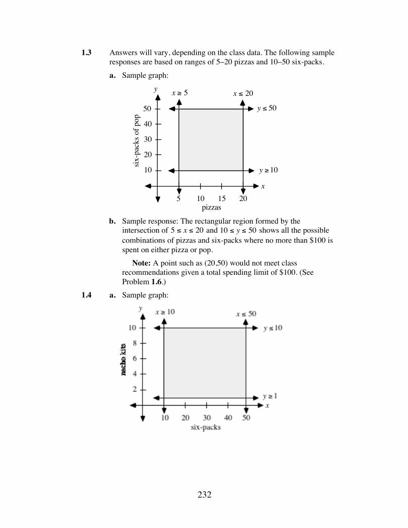
232

1.3 Answers will vary, depending on the class data. The following sample responses are based on ranges of 5–20 pizzas and 10–50 six-packs.

a. Sample graph:

b. Sample response: The rectangular region formed by the intersection of 5 ≤ x ≤ 20 and 10 ≤ y ≤ 50 shows all the possible combinations of pizzas and six-packs where no more than $100 is spent on either pizza or pop.

Note: A point such as (20,50) would not meet class recommendations given a total spending limit of $100. (See Problem 1.6.)


pizzas

y

x

10

20

30

40

50

5 10 15 20

y ≤ 50

x ≥ 5 x ≤ 20

y ≥10

six-

pack

s of p

op

233

b. Sample graph:

1.5 a. For the sample graph given in Problem 1.2e, the intersection is the

set of all ordered pairs such that 5 ≤ x ≤ 20 and 10 ≤ y ≤ 40 .

b. Since the boundary lines represent values that satisfy the constraints, the symbols ≤ and ≥ should be used.

c. Sample response: No. Pizzas, six-packs, and nacho kits can only be bought in whole numbers, so only points whose coordinates are integers [lattice points] should be considered.

*1.6 a. Sample response: Medium pizzas cost $5.00 each and pop costs $2.00 per six-pack. Note: The sample responses given below are based on these costs.

b. 1. 0 ≤ x ≤ 20 2. 0 ≤ y ≤ 50

3. See sample graph given in Part d below.

c. 1. Sample response: 5x + 2y ≤ 100 .

2. See sample graph given in Part d below.

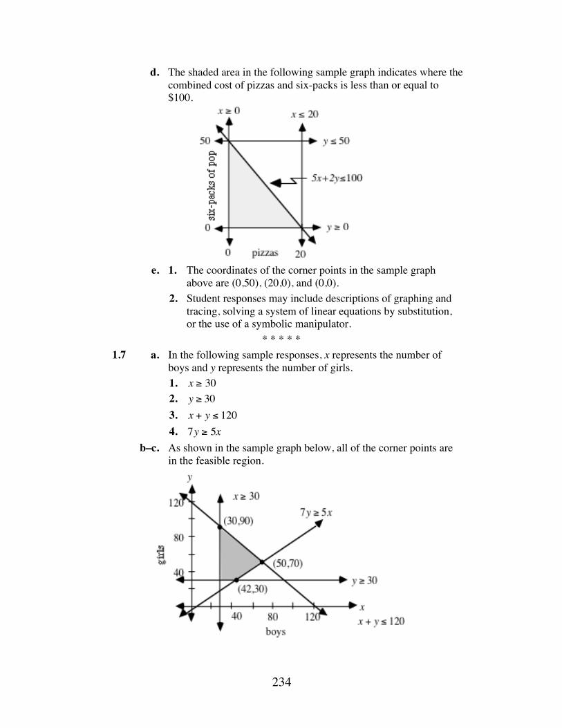
234

d. The shaded area in the following sample graph indicates where the combined cost of pizzas and six-packs is less than or equal to $100.

e. 1. The coordinates of the corner points in the sample graph

above are (0,50), (20,0), and (0,0). 2. Student responses may include descriptions of graphing and

tracing, solving a system of linear equations by substitution, or the use of a symbolic manipulator.

* * * * * 1.7 a. In the following sample responses, x represents the number of

boys and y represents the number of girls. 1. x ≥ 30 2. y ≥ 30 3. x + y ≤ 120 4. 7y ≥ 5x b–c. As shown in the sample graph below, all of the corner points are

in the feasible region.

235

1.8 a. x > 0 , y ≥ 30 , x + y ≤ 70, and y ≥ x .

b. The corner points are (30,30), (35,35), (0,70), and (0,30). Corner points (30,30) and (35,35) lie within the feasible region.

c. Sample response: The constraints indicate that no more than 70 students will be surveyed. Of those surveyed, the number of girls must be greater than or equal to the number of boys. There must be at least 30 girls interviewed.

* * * * * * * * * * (page 186)

Activity 2 Students continue to graph feasible regions and identify the corner points. They then explore the use of the corner principle for solving linear programming problems.

Materials List • graph paper (several sheets per student; optional)


Exploration 1 (page 187) a. Students explore how the graph of an objective function is affected as

the value of the objective (in this case, profit) changes. b. 1. Students should observe that all the lines are parallel. 2. Sample response: As the value of P increases, so does the y-intercept.

Discussion 1 (page 187) a. Sample response: The lines are parallel (they all have the same slope). b. Sample response: All the lines are parallel because the .x-coefficient

and y-coefficient, which deteriorate the slope, remained the same. c. Sample response: For a given profit function, the value of P remains

constant. As the value of x increases, the value of y decreases. d. Sample response: The graph representing the greatest profit is located

above the others. This happens because the value of P affects the y-intercept. The greater the value of P in the objective function, the greater the y-intercept.

e. Sample response: The graph that represents the least profit is the one with the lowest y-intercept in the feasible region. This line is located below the others.

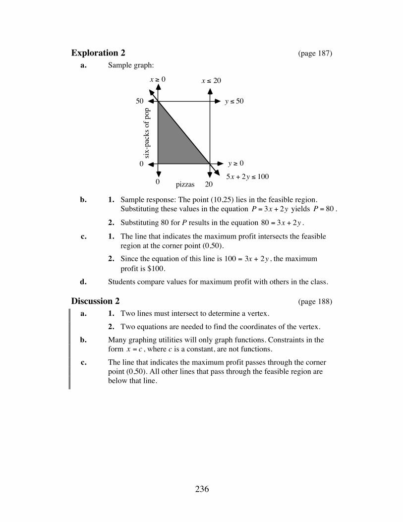
236

Exploration 2 (page 187) a. Sample graph:

b. 1. Sample response: The point (10,25) lies in the feasible region. Substituting these values in the equation P = 3x + 2y yields P = 80 .

2. Substituting 80 for P results in the equation 80 = 3x + 2y .

c. 1. The line that indicates the maximum profit intersects the feasible region at the corner point (0,50).

2. Since the equation of this line is 100 = 3x + 2y , the maximum profit is $100.

d. Students compare values for maximum profit with others in the class.

Discussion 2 (page 188) a. 1. Two lines must intersect to determine a vertex.

2. Two equations are needed to find the coordinates of the vertex.

b. Many graphing utilities will only graph functions. Constraints in the form x = c , where c is a constant, are not functions.

c. The line that indicates the maximum profit passes through the corner point (0,50). All other lines that pass through the feasible region are below that line.

0

50

20

0

pizzas

y ≥ 0

y ≤ 50

x ≥ 0 x ≤ 20

5x + 2y ≤ 100

six-p

acks

of p

op

237

d. Sample response: To find the coordinates of the vertex in the lower right-hand corner of the feasible region, for example, you can use the lines defined by the equations 5x + 2y =100 and x = 20 (the two intersecting boundary lines). Substituting 20 for the value of x in the equation 5x + 2y =100 results in 5(20) + 2y = 100 . Solving this equation for y yields y = 0 . Since the point with coordinates (20,0) satisfies both equations, it is a point of intersection and thus a corner point of the feasible region.

e. Sample response: You could find the coordinates for all the corner points of the feasible region and substitute the values of the coordinates into the objective function until you found the greatest value for P.

f. Sample response: The graph of the objective function that maximizes the objective would coincide with the edge of the feasible region. The maximum value would occur at any point along that border, so there might be more than one way to maximize the objective function.

g. The maximum profit can be found by substituting the coordinates into the objective function.

h. Sample response: Since 5 8 of a six-pack is equivalent to 3 34 cans, this is not a possible amount to buy.

i. Sample response: This means that the maximum value occurs at any point on the segment joining (0,4) and (3,3).

Assignment (page 190) 2.1 Since lines b and c appear to be parallel, they could represent the same

profit function for different values of P.

2.2 a. Sample graph for Parts 1–4:

(1,2)

(2,8)

(3,4)

(4,8)

(6,2)

2

4

6 8

2

4

6

8

10

x

y

P = 15x + yP = 3x + 2y

P = 3x + 2y

P = 15x + y

238

1. 28 = 3(4) + 2(8)

2. 92 = 15(6) + 2

3. 7 = 3(1) + 2(2)

4. 17 = 15(1) + 2

b. Sample response: The slope of the objective function determines which corner point of the feasible region represents a maximum or minimum value of the function.

*2.3 a. The constraints on the problem can be represented by the inequalities 0 ≤ x ≤16 , 0 ≤ y ≤ 22, and 4.96x +1.84y ≤ 100 where x represents the number of pizzas and y represents the number of six-packs of pop.

b. See sample graph given in Part e below.

c. The profit is $11.04 on each pizza and $4.16 on each six-pack. d. Sample response: P = 11.04x + 4.16y , where P is profit, x is the

number of pizzas, and y is the number of six-packs. e. The maximum value of P = 11.04x + 4.16y occurs at the corner

point (12,22). If all items are sold, the maximum profit is 12(11.04) + 22(4.16) or $224.00. The graphs of the two oblique lines nearly coincide. The sample graph distorts that difference. Sample graph:224 = 11.04x + 4.16y

f. Sample response: The class should buy 12 pizzas and 22 six-packs

of pop. Since these are whole number quantities, this seems to be a reasonable answer.

239

2.4 a. Substituting 5.5 for x in each equation yields the following: y1 = 0.8(5.5) + 4= 4.4 + 4= 8.4

y2 = −(5.5) +13.9= 8. 4

Therefore, (5.5,8.4) is a solution to both equations.

b. The coordinates of the corner points are A(0,0), B(0,4), D(8.4,5.5), and E(8.95,0). Students should verify these coordinates by substituting them in the equations defining the corresponding boundaries of the feasible region.


b. The coordinates of the corner points are (0,0), (5,0), (2,9), and (0,10).

c. 1. As shown in the table below, the minimum of –5 occurs at (5,0).

(x,y) P = 2y − x P = 3y + 2x (0,0) 0 0 (5,0) –5 10 (2,9) 16 31 (0,10) 20 30

2. As shown in the table above, the minimum of 0 occurs at

(0,0).

2.6 a. The maximum value of the objective function occurs at the corner point 9 13 ,22( ), where x represents number of pizzas and y represents number of six-packs. Since the value for x is not a whole number, it does represent a reasonable amount of pizza to buy.

b. To find the maximum profit which corresponds to a point with integer coordinates, students may suggest rounding solutions to the nearest integer or substituting the coordinates of points near the corner point into the objective function.

x

y

4 8 12 16 200

4

8

12

0

x + 2y= 20

3x + y = 15

240

In this case, the point (9,22) results in a profit of $244. Although the points (10,22) and (10,21) produce greater profits, they are not in the feasible region. The point (10,20) is in the feasible region but results in a profit of only $240.

Note: Neither of these methods guarantee that the optimum value will be found.

c. Sample response: A businessperson might buy less if the profit is not greatly affected. They may buy slightly more if they believe they could sell the extra or easily absorb the loss.

2.7 Answers will vary. Students should record the quantities of cheese and chips needed to make an appropriate number of nacho servings, the quantity and cost of each item to be purchased, and the selling price of each item. If the corner principle does not give a solution with integer coordinates, they should use an appropriate strategy to determine the quantities to purchase.

* * * * * 2.8 A(0,0), B(0,5), C(4.2,7.1), D(9.3,3.7), E(7.45,0)

2.9 a. 1. D(10,8) 2. A(0,0) b. 1. m = −8 5

2. At both D and E, the value of the objective function is 120.

3. The equation of this line in slope-intercept form is:

y = −85x +

P5

The slope of the objective function is −8 5 .

4. Since the slope of the objective function is the same as the slope of the line that passes through D and E, the value of the function is the same at both D and E (and at any other point on DE ).

5. All three lines would be parallel to DE . c. 1. Sample response: P = 2x + 5y .

2. Sample response: P = x + 5y .

3. Sample response: P = 10x + 2y .

* * * * * * * * * *

241

Research Project (page 194) Students plan a fund-raiser that involves selling two different items. To help determine the feasibility of their plan, they conduct a survey. They then prepare a report designed to persuade their classmates to invest in the venture. This works well as a small-group activity. You may wish to allow students to implement a plan selected by the class. Students then can evaluate the accuracy of their projections. (page 194)

Activity 3 Students use matrices to solve systems of two equations in two unknowns. Matrix equations are then used to find corner points of feasible regions.

Materials • graph paper (several sheets per student)

Technology • graphing utility • matrix manipulator

Exploration (page 194) Students examine the relationship between a system of two equations and two unknowns and the corresponding matrix equation. The concept of inverse matrices is introduced. Students than use technology to solve matrix equations. a. Students should obtain the following equation:

−8x 10y10x 10y⎡

⎣ ⎢ ⎤

⎦ ⎥ =40139⎡

⎣ ⎢ ⎤

⎦ ⎥

b. Sample response: The entries in the matrices are the terms of the equations. The first equation’s terms are in the top rows of the matrices; the second equation’s terms are in the bottom rows of the matrices.

c. One way for students to verify the value of M–1 is to enter matrix M in their technology, then use the multiplicative inverse command. A second approach involves entering both M and M–1, then finding their product—which should be the identity matrix.

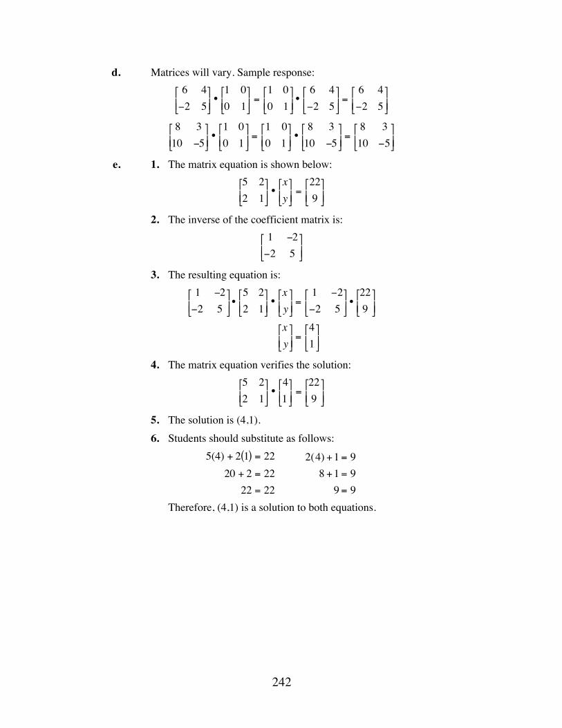
242

d. Matrices will vary. Sample response: 6 4−2 5⎡

⎣ ⎢ ⎤

⎦ ⎥ •1 00 1⎡

⎣ ⎢ ⎤

⎦ ⎥ =1 00 1⎡

⎣ ⎢ ⎤

⎦ ⎥ •6 4−2 5⎡

⎣ ⎢ ⎤

⎦ ⎥ =

6 4−2 5⎡

⎣ ⎢ ⎤

⎦ ⎥

8 310 −5⎡

⎣ ⎢ ⎤

⎦ ⎥ •1 00 1⎡

⎣ ⎢ ⎤

⎦ ⎥ =1 00 1⎡

⎣ ⎢ ⎤

⎦ ⎥ •8 310 −5⎡

⎣ ⎢ ⎤

⎦ ⎥ =8 310 −5⎡

⎣ ⎢ ⎤

⎦ ⎥

e. 1. The matrix equation is shown below: 5 22 1⎡

⎣ ⎢ ⎤

⎦ ⎥ •xy⎡

⎣ ⎢ ⎤

⎦ ⎥ =229

⎡

⎣ ⎢ ⎤

⎦ ⎥

2. The inverse of the coefficient matrix is: 1 −2−2 5⎡

⎣ ⎢ ⎤

⎦ ⎥

3. The resulting equation is: 1 −2−2 5⎡

⎣ ⎢ ⎤

⎦ ⎥ •5 22 1⎡

⎣ ⎢ ⎤

⎦ ⎥ •xy⎡

⎣ ⎢ ⎤

⎦ ⎥ =

1 −2−2 5⎡

⎣ ⎢ ⎤

⎦ ⎥ •229⎡

⎣ ⎢ ⎤

⎦ ⎥

xy⎡

⎣ ⎢ ⎤

⎦ ⎥ =41⎡

⎣ ⎢ ⎤

⎦ ⎥

4. The matrix equation verifies the solution: 5 22 1⎡

⎣ ⎢ ⎤

⎦ ⎥ •41⎡

⎣ ⎢ ⎤

⎦ ⎥ =229⎡

⎣ ⎢ ⎤

⎦ ⎥

5. The solution is (4,1).

6. Students should substitute as follows: 5(4) + 2 1( ) = 22

20 + 2 = 2222 = 22

2(4) +1 = 98 +1 = 99 = 9

Therefore, (4,1) is a solution to both equations.

243

7. Since the graphs of the two lines intersect at (4,1), the graph verifies the solution.

f. 1. The system is inconsistent because the graphs are parallel and do not have a common point.

2. The process fails because the coefficient matrix does not have an inverse.

Discussion (page 197) a. Sample response: You can enter the coefficient matrix M and use the

multiplicative inverse button to find M–1 . Or you can enter M and M–1 , then find their product to see if you get the identity matrix.

b. The coefficient matrix does not have an inverse. c. The coefficient matrix is a 2 × 2 matrix with a y coefficient equal to 0:

3 05 2⎡

⎣ ⎢ ⎤

⎦ ⎥

d. Sample response: Matrix multiplication is not commutative. In matrix multiplication, the number of columns in the first matrix must equal the number of rows in the second matrix. Both the coefficient and the constant matrix must be multiplied by the inverse matrix on the left in order for the dimensions to match.

5x + 2y = 22

x

y

2 4

2468

–2 –2

(4,1)

2x + y = 9

x

y

–2 2 4

2

4

x + 2y = 4

2x + 4y = 13

244

e. Using a process similar to that described for systems of two equations and two unknowns, the system can be represented as a matrix equation in the form M •X =C as shown below:

1 1 12 −1 11 3 −2

⎡

⎣

⎢ ⎢

⎤

⎦

⎥ ⎥ •xyz

⎡

⎣

⎢ ⎢

⎤

⎦

⎥ ⎥

=

615−7

⎡

⎣

⎢ ⎢

⎤

⎦

⎥ ⎥

Assignment (page 198) 3.1 a. The multiplicative inverse of the matrix is shown below:

2 −1−7 4⎡

⎣ ⎢ ⎤

⎦ ⎥

b. Sample response: 2 −1−7 4⎡

⎣ ⎢ ⎤

⎦ ⎥ •4 17 2⎡

⎣ ⎢ ⎤

⎦ ⎥ =1 00 1⎡

⎣ ⎢ ⎤

⎦ ⎥ =4 17 2⎡

⎣ ⎢ ⎤

⎦ ⎥ •2 −1−7 4⎡

⎣ ⎢ ⎤

⎦ ⎥

c. Answers will vary. Sample response: The following matrix does not have an inverse.

2 81 4⎡

⎣ ⎢ ⎤

⎦ ⎥

When the elements of the matrix are used as coefficients, the graphs of the equations (such as 2x + 8y = 1 and x + 4y = 3) are parallel. When I try to find the multiplicative inverse using technology, I get an error message.

3.2 Students can verify their solutions by substituting the values obtained into the original equations.

a. xy⎡

⎣ ⎢ ⎤

⎦ ⎥ =35⎡

⎣ ⎢ ⎤

⎦ ⎥

b. xy⎡

⎣ ⎢ ⎤

⎦ ⎥ =

−17

⎡

⎣ ⎢ ⎤

⎦ ⎥

c. xy⎡

⎣ ⎢ ⎤

⎦ ⎥ =42⎡

⎣ ⎢ ⎤

⎦ ⎥

245

3.3 80 33−20 73⎡

⎣ ⎢ ⎤

⎦ ⎥ •xy⎡

⎣ ⎢ ⎤

⎦ ⎥ =46646

⎡

⎣ ⎢ ⎤

⎦ ⎥

80 33−20 73⎡

⎣ ⎢ ⎤

⎦ ⎥

−1

•80 33−20 73⎡

⎣ ⎢ ⎤

⎦ ⎥ •xy⎡

⎣ ⎢ ⎤

⎦ ⎥ ⎛

⎝ ⎜ ⎞

⎠ ⎟ =

80 33−20 73⎡

⎣ ⎢ ⎤

⎦ ⎥

−1

•46646

⎡

⎣ ⎢ ⎤

⎦ ⎥

xy⎡

⎣ ⎢ ⎤

⎦ ⎥ =52⎡

⎣ ⎢ ⎤

⎦ ⎥


b. (0,0), (8,0), 5 13 , 4( ) , 4 411,4 4

11( ) c. As shown in the table below, the maximum of 24 occurs at two

corner points. Therefore, the maximum occurs at any point on the segment connecting these two points.

(x,y) P = 2y + 3x (0,0) 0 (8,0) 24 5 13 , 4( ) 24 4 411,4 4

11( ) 21 911

*3.5 a. In the following inequalities, x represents number of pizzas and y

represents number of six-packs: 5x + 2y ≤ 1002y ≥ 105x ≤ 805x ≤ 8yx ≥ 0

–

x

y

x + y = 0

3x + 2y = 24

3x + 8y = 48

4 12 16

2

4

6

8

246

b. Sample graph:

c. As shown below, the profit function P = 11x + 2y has its

maximum value at the corner point (16,10). (x,y) P = 11x + 2y (0,5) 10 (8,5) 98

(16,10) 196 (0,50) 100

The maximum potential profit of $196 occurs if the class buys

(and sells) 16 pizzas and 10 six-packs.

* * * * * 3.6 a. In the following inequalities, x represents millions of liters from

the reservoir and y represents millions of liters from the aquifer. x + y ≥ 20

x ≤ 12y ≥ 14y ≤ 20x ≥ 0

247

b. In the following sample graph, units on the axes represent millions of liters. The feasible region is shaded.

c. As shown below, the minimum value of the objective function C = 80x +100y occurs at the corner point (6,14). The maximum occurs at the point (12,20). (x,y) C = 80x +100y (0,20) 2000 (6,14) 1880 (12,14) 2360 (12,20) 2960

1. $1880 2. $2960

* * * * * * * * * * (page 200)

Activity 4 Students extend linear programming concepts into three dimensions by considering the sale of three items instead of two. Note: This may be treated as an optional activity.

Materials List • cardboard boxes (one per group)

• scissors (one pair per group)

• tape

x

y

00

10

20

10 20

y = 20

y = 14

y = 20 − x

x =12

reservoir

aquifer

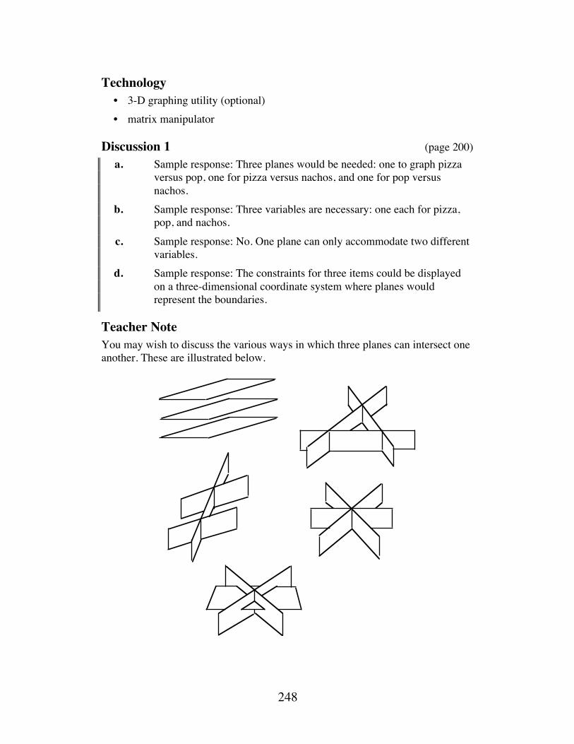
248

Technology • 3-D graphing utility (optional) • matrix manipulator

Discussion 1 (page 200) a. Sample response: Three planes would be needed: one to graph pizza

versus pop, one for pizza versus nachos, and one for pop versus nachos.

b. Sample response: Three variables are necessary: one each for pizza, pop, and nachos.

c. Sample response: No. One plane can only accommodate two different variables.

d. Sample response: The constraints for three items could be displayed on a three-dimensional coordinate system where planes would represent the boundaries.

Teacher Note You may wish to discuss the various ways in which three planes can intersect one another. These are illustrated below.

249

Exploration (page 200) Students build a model of the first octant of a three-dimensional coordinate system. This activity works well in small groups. a–b. Students cut cardboard boxes and label the axes of their coordinate

systems. Note: The leftover cardboard should be saved for use in Part d. c–d. On each plane surface of the first octant, students shade one of three

regions defined by inequalities. They then cut a model of each region from the leftover pieces of cardboard.

e. Students move the model of region A through the various values of the constraint placed on z.

f. Students should tape the model regions to form a rectangular prism in the first octant. This prism defines the set of feasible solutions for the constraints 0 ≤ x ≤ 6 , 0 ≤ y ≤ 4 , and 0 ≤ z ≤ 5 .

g. The coordinates of the eight corner points are: (0,0,0), (0,0,5), (6,0,0), (6,0,5), (0,4,0), (0,4,5), (6,4,0), and (6,4,5).

a. The set of points describes five planes which are parallel to Region A and each measures 4 units by 6 units. The planes are located at z = 1, 2, 3, 4, and 5 .

b. 1. Three planes may intersect in a single point. Two planes may intersect in a line.

2. Each corner point is formed from the intersection of three planes. There are four ways in which three planes can be selected from four planes: ABC, ABD, ACD, and BCD.

3. The maximum number of corner points is 10. Given five planes A, B, C, D, and E, the 10 possible sets of three planes are ABC, ABD, ABE, ACD, ACE, ADE, BCD, BCE, BDE, and CDE.

c. 1. The shape is a rectangular prism. A rectangular prism has eight vertices.

2. Sample response: No. Not all sets of constraints that involve six planes would have three pairs of parallel planes. The parallel planes reduce the number of possible corner points.

d. 1. Sample response: By the corner principle, the maximum will occur at one of the eight corner points. The specific point where the maximum occurs would depend on the objective function.

2. Sample response: The coordinates of each corner point could be substituted into the objective function to determine which represents the maximum value.

e. Sample response: No, this would require four dimensions.

250

Assignment (page 202) 4.1 a. This graph shows the constraints on pizza and pop. The shaded

region is defined by 0 ≤ x ≤10 , 0 ≤ y ≤ 12 , and z = 0 .

b. This graph shows the constraints on pop and nachos. The shaded region is defined by 0 ≤ y ≤ 12 , 0 ≤ z ≤14 , and x = 0 .

c. This graph shows the constraints on pizza and nachos. The shaded region is defined by 0 ≤ x ≤10 , 0 ≤ z ≤14 , and y = 0 .

4.2 Sample response: The class should purchase from 0 to 10 pizzas, from 0 to 12 six-packs of pop, and from 0 to 14 nacho kits.

4.3 a. y = 12 , y = 0 , z = 14 , z = 0

b. x =10 , x = 0 , z = 14 , z = 0

c. Sample response: The points of intersection consist of all the possible combinations of ordered triples formed by the x-values, y-values, and z-values of the equations.

4.4 Sample sketch:

4.5 As shown in the table below, the maximum value of P = x + y + z

occurs at the point (10,12,14). (x,y,z) P = x + y + z (0,0,0) 0 (10,0,0) 10 (0,12,0) 12 (0,0,14) 14 (10,12,0) 22 (10,0,14) 24 (0,12,14 26

(10,12,14) 36

x

y

z

(0,0,0)

(0,12,14)

(0,12,0)

(10,12,14)

(10,12,0)(10,0,0)

(10,0,14)

(0,0,14)

251

4.6 a. (–11,–3,9)

b. This system is inconsistent.

c. 235, −85,−15

⎛ ⎝

⎞ ⎠ or (4.6,–1.6,–0.2)

4.7 a. The profit is $11.00 on each pizza, $4.00 on each six-pack of pop, and $14.00 on each nacho kit.

b. P = 11x + 4y +14z

*4.8 a. The constraints are 0 ≤ x ≤10 , 0 ≤ y ≤ 25, and 0 ≤ z ≤ 5 .

b. Six planes enclose the feasible solutions.

c. Sample response: Eight points must be examined to find the maximum profit. There are eight corner points because the figure formed by the planes is a rectangular prism. Note: Students who do not visualize the prism may respond that 20 points must be examined (the maximum number of ways in which six planes can be chosen three at a time).

4.9 The maximum value of P = 11x + 4y +14z occurs at the corner point (10,25,5). The profit at this point is 11(10) + 4(25) +14(5) = $280 .

* * * * * 4.10 Answers will vary. Students should record the cost and number of

each item to be purchased, the number of servings that can be produced from each one, the selling prices, and the profit.

4.11 The solution may be found as follows:

1 1 12 1 25 2 3

⎡

⎣

⎢ ⎢

⎤

⎦

⎥ ⎥ •xyz

⎡

⎣

⎢ ⎢

⎤

⎦

⎥ ⎥

=

152643

⎡

⎣

⎢ ⎢

⎤

⎦

⎥ ⎥

1 1 12 1 25 2 3

⎡

⎣

⎢ ⎢

⎤

⎦

⎥ ⎥

–1

•1 1 12 1 25 2 3

⎡

⎣

⎢ ⎢

⎤

⎦

⎥ ⎥ •xyz

⎡

⎣

⎢ ⎢

⎤

⎦

⎥ ⎥

=

1 1 12 1 25 2 3

⎡

⎣

⎢ ⎢

⎤

⎦

⎥ ⎥

–1

•152643

⎡

⎣

⎢ ⎢

⎤

⎦

⎥ ⎥

xyz

⎡

⎣

⎢ ⎢

⎤

⎦

⎥ ⎥

=

1410

⎡

⎣

⎢ ⎢

⎤

⎦

⎥ ⎥

* * * * * * * * * *

252

Answers to Summary Assessment (page 204) 1. Sample response: Let x represent the number of double hamburgers

and y represent the number of single hamburgers. The following inequalities are the constraints that define the feasible region: 0.2x + 0.1y ≤ 20 , x ≥ 0 , y ≥ 0, x ≤ 90, y ≤100 , and 8x + 6y ≤ 960 .

The profit function is the equation p = 0.90x + 0.70y .

The graph below shows the feasible region.

Since the maximum profit of $110.50 occurs at the corner point

(45,100), the restaurant should prepare 45 double burgers and 100 singles for the lunch-time rush.

2. Sample response: Using h for the number of hot dogs, c for the number of bags of chips, and p for the number of cans of pop, the three constraints can be expressed as:

0.15h + 0.2c + 0.35 p ≤ 108c ≤ 2hc + h ≤ 3p

The corresponding matrix equation for the boundaries of these constraints is:

0.15 0.2 0.35−2 1 01 1 −3

⎡

⎣

⎢ ⎢

⎤

⎦

⎥ ⎥ •

hcp

⎡

⎣

⎢ ⎢

⎤

⎦

⎥ ⎥

=

10800

⎡

⎣

⎢ ⎢

⎤

⎦

⎥ ⎥

The solution to this system is (120,240,120). The profit equation is P = 0.85h + 0.8c + 0.65p . At this corner point, the profit is $372.

253

Module Assessment

1. Use inequalities to describe the points graphed on the following

number line.

2. Use inequalities to describe the points graphed in the shaded region

below.

3. Which point in the graph below maximizes the value of the objective

function P = 3x + y ? Defend your response.

4. Consider the system of linear equations below:

2x − 3y + z = 2.74x + 2.4y −1.5z =11.712x + 9y + 3.8z = 39.96

a. Write a matrix equation for this system.

b. Solve the system and verify your solution.

c. Determine the value of the objective function P = 3x + 2y − 5z at the point described in Part b.

213

15

20

y

x

A BC

D

EF1 3

1

3

y

x2

2

4

254

Answers to Module Assessment 1. 3 < x ≤ 21 2. 15x + 20y ≤ 300

3. Sample response: According to the corner principle, the maximum value of an objective function occurs at a corner point of the feasible region. As shown in the table below, the maximum of 13.5 occurs at point D.

Point Coordinates P = 3x + y A (0,3) 3 B (2,3) 9 C (3,2.5) 11.5 D (4,1.5) 13.5 E (4,0) 12 F (0,0) 0

4. a. The corresponding matrix equation is shown below:

2 −3 14 2.4 −1.50.5 9 3.8

⎡

⎣

⎢ ⎢

⎤

⎦

⎥ ⎥

•

xyz

⎡

⎣

⎢ ⎢

⎤

⎦

⎥ ⎥

=

2.711.739.96

⎡

⎣

⎢ ⎢

⎤

⎦

⎥ ⎥

b. The solution is (3,2.5,4.2). Students should verify their solutions by substituting into the original equations.

c. P = −7

255

Flashbacks

Activity 1 1.1 Graph each of the following inequalities on a number line:

a. x ≤ 25

b. −16 < x

c. −2 ≤ x < 4

1.2 Graph x ≥ −4 and y < 7 on a two-dimensional coordinate system and name three points in the intersecting region.

1.3. Graph y ≥ −4 , x ≤ 0 , and 2x ≥ y − 4 on a two-dimensional coordinate system and name three points in the intersecting region.

1.4 Identify the inequalities whose intersection is the shaded region on the graph below.

8–8

8

–8

y

x(–2,0)

(0,–4)

256

Activity 2 2.1 Identify the slope and y-intercept of the line represented by each of the

following equations. a. 2y − 4x = 12

b. −y +16 = 3x

2.2 Given the equation w = 3.56a − 4.1b , find w for each of the following values of a and b:

a. a = 2 and b = 6

b. a = −5 and b = 0

2.3 Determine the equation, in slope-intercept form, of the line that passes through (2,4) and (–5,1).

Activity 3 3.1 Complete each of the following matrix multiplications.

a. 2 7−3 6⎡

⎣ ⎢ ⎤

⎦ ⎥ •5−1⎡

⎣ ⎢ ⎤

⎦ ⎥

b. 1 00 1⎡

⎣ ⎢ ⎤

⎦ ⎥ •3 42 −6⎡

⎣ ⎢ ⎤

⎦ ⎥

c. 2 11−7 5⎡

⎣ ⎢ ⎤

⎦ ⎥ •1 02 1⎡

⎣ ⎢ ⎤

⎦ ⎥

Activity 4 4.1 Each of the following ordered triples represents the coordinates of a

point in the form (x,y,z) . Plot and label each point on a three-dimensional coordinate system.

a. (0,3,0)

b. (5,3,2)

c. (8,7,3)

4.2 Find the points of intersection, if any, for each of the following pairs of lines.

a. x + y = 6 and y = 4

b. 2x − y = 4 and x + 3y = −3

c. x = 4 − 2y and y = −3

257



b. Sample graph:

c. Sample graph:

1.2 Sample response: Three points in the intersecting region are (0,0),

(–4,6.9), and (40,–50).

1.3 Sample response: Three points in the intersecting region are: (0,0),

(–4,–4), and (–1,–1).

1.4 y ≥ −2x − 4, y ≤ 2, x ≤ 2

25

–16

4–2

y

x

x = −4

y = 7

y

x

y ≤ 2x + 4

y ≥ −4

x ≤ 0

258

Activity 2 2.1 a. m = 2, b = 6 b. m = −3 , b = 16

2.2 a. w = −17. 48

b. w = −17.8

2.3 Sample response:

(y − 4) =4 −1

2 − (−5)⎛

⎝ ⎜

⎞

⎠ ⎟ (x − 2)

y =37x +

227

Activity 3

3.1 a. 3−21⎡

⎣ ⎢ ⎤

⎦ ⎥

b. 3 42 −6⎡

⎣ ⎢ ⎤

⎦ ⎥

c. 24 113 5⎡

⎣ ⎢ ⎤

⎦ ⎥

Activity 4 4.1 a-c. Sample graph:

4.2 a. (2,4)

b. 97, −107

⎛ ⎝

⎞ ⎠

c. (10,–3)

(0, 3, 0)

x

y

z

(8, 7,3)(5,3,2)

Crazy Cartoons

How are cartoon characters made? How do they change shape? How can you make an inanimate object appear to move? A cartoonist—or a math student—can help answer these questions.

Monty Brekke • John Carter • Janet Kuchenbrod

261

Teacher Edition Crazy Cartoons

Overview Students explore transformations in a plane, including dilations, translations, rotations, reflections, and composite transformations.


• use the properties of similar figures

• calculate distances between points in the Cartesian plane

• explore the geometric relationships in perspective drawings, dilations centered at the origin, translations, rotations about the origin, reflections, and composite transformations

• write matrices for dilations centered at the origin, translations, rotations about the origin, and reflections

• use matrix equations to transform geometric figures on the Cartesian plane.


• how to graph points in the Cartesian plane

• the relationships between similar figures

• how to solve systems of linear equations

• how to perform operations on matrices, including scalar multiplication, matrix addition, and matrix multiplication

• how to find the equation of a line given two points on the line

• how to use trigonometric ratios to determine angle measures

• how to reflect a set of points in a line.


Assessment Total

Days 3 2 2 2 2 1 12

262

Teacher Note Students may use graph paper, tracing paper, MIRAs™, transparent grids, graphing calculators, spreadsheets, or other appropriate graphing utilities to perform transformations. In addition, you may want to use technology to solve matrix equations or simultaneous equations.



rulers X X X X X X graph paper X X X X X X protractors X X X

template for Problem 2.7

X

tracing paper X X X X X decks of playing cards X

Teacher Note A blackline master of the template appears at the end of the teacher edition FOR THIS MODULE.



geometry utility X X X X graphing utility X X X X X

spreadsheet X X X X X matrix manipulator X X X X X

263

Crazy Cartoons

Introduction (page 209) Students describe transformations in general terms, without the use of coordinates.

Discussion (page 209) a. Sample response: The bug in frame B is a reflection of the bug in

frame A with respect to a vertical line. The bug in frame C is a 60˚ clockwise rotation of the bug in frame A. The bug in frame D is a 90˚ counterclockwise rotation of the bug in frame A. The bug in frame E is a scaled-down version of the bug in frame A. The bug in frame F is a scaled-up version of the bug in frame A.

b. Sample response: The bug in frame B can be described as the combination of a 180˚ rotation of the bug in frame A, followed by a reflection with respect to a horizontal line.

(page 210)

Activity 1 In this activity, students explore dilations by graphing shapes in the coordinate plane. They create and measure similar shapes using a geometry utility.

Materials List • graph paper (one sheet per student)

• rulers (one per student)

• protractors (one per student)


264

Teacher Note Point of perspective and dilations are important in both drawing and painting. You may wish to use one or both of the following quotations to initiate a class discussion.

• The optical model, or the visual pyramid, can secure the correctness of the painter’s representation of reality. The painting . . . should be conceived as a “planar representation” of the visual pyramid. All the figures, objects, and spatial distances painted on the artist’s panel are fully proportional to those found in the actual world that the painting represents. Perspective construction, then, makes it provable that a picture is “correct” in its rendering of space. (Barasch, Theories of Art)

• . . . perspective construction begins with a series of arbitrary acts, as the painter selects a visual field of “whatever size I want,” picks a size for the human figures, and places his centric point “wherever I wish.” (Hulse, The Rule of Art)

Exploration (page 211) a–b. Sample graph:

c. In the following sample table, lengths are measured in centimeters and angles are measured in degrees.

Preimage Image AB 1 ʹ A ʹ B 3 BC 5 ≈ 2.2 ʹ B ʹ C 3 5 ≈ 6.6 CA 2 ʹ C ʹ A 6

m∠ABC 63˚ m∠ ʹ A ʹ B ʹ C 63˚ m∠BCA 27˚ m∠ ʹ B ʹ C ʹ A 27˚ m∠CAB 90˚ m∠ ʹ C ʹ A ʹ B 90˚

y

x(0,0)

A(1,1)B(2,1)

C(1,3)ʹ A (3,3)

ʹ B (6,3)

ʹ C (3,9)

265

d. The ratios of corresponding lengths are 3 1 .

e. Sample graph:

f. PA = 2 ≈1.4 , PB = 5 ≈ 2.2 , PC = 10 ≈ 3.2 , P ʹ A = 3 2 ≈ 4.2 , P ʹ B = 3 5 ≈ 6.6 , P ʹ C = 3 10 ≈ 9.5

g–h. As in Part d, the ratios of corresponding lengths are 3 1 .

Discussion (page 212) a. Sample response: The segment connecting two points can be thought

of as the hypotenuse of a right triangle. The length of the horizontal side is x2 − x1 and the length of the vertical side is y2 − y1 . Using the Pythagorean theorem, the distance d between the two points is:

d2 = (x2 − x1)2 + (y2 − y1 )2

d = (x2 − x1)2 + (y2 − y1 )2

b. The ratios of corresponding lengths are equal.

c. Sample response: The point of perspective is the center of dilation. The resulting figures are similar.

d. The corresponding angles are congruent.

e. In a dilation, the corresponding lengths are proportional and the corresponding angles are congruent.

f. 1. ΔABC ~ Δ ʹ A ʹ B ʹ C

2. ΔPAC ~ Δ ʹ P ʹ A ʹ C , ΔPAB ~ Δ ʹ P ʹ A ʹ B , and ΔPBC ~ Δ ʹ P ʹ B ʹ C

y

xA(1,1)B(2,1)

C(1,3)ʹ A (3,3)

ʹ B (6,3)

ʹ C (3,9)

P(0, 0)

266

g. 1. The scale factor equals the ratio of corresponding lengths. 2. The scale factor equals the ratio of perimeters. 3. The ratio of the areas is the square of the scale factor. h. Sample response: Yes, because the two triangles would still be

similar. i. A scale factor x, where −1 < x <1 , reduces the size of the original

shape. j. The ratio is the scale factor.

Assignment (page 214) 1.1 a. Sample response: The center of the dilation can be found by drawing

a line through A and ʹ A and another line through C and ʹ C (or through any two pairs of corresponding points in the image and the preimage). The point of intersection of the two lines is the center of dilation.

b. The scale factor is the ratio of corresponding lengths: 5522

=52=2.51

1.2 Sample response: No. The figures are not similar; therefore, they could not have been produced by a dilation. There is no point of perspective.

1.3 a–c. Sample graph:

d. 1. 2 2. −1 5

3. 2.5

y

x

A (5,10)

B (–5,5)

C (10,–15)

ʹ A (2,4)

ʹ C (4,–6)

ʹ B (–2,2)

267


b. Sample response: The triangle would appear to double in size,

growing like an animated cartoon.

c. Sample response: Assign one figure to represent the preimage and the other to represent the image. Using the origin as the center of dilation, dilate the preimage by a scale factor equivalent to the ratio of the corresponding lengths of the image to the preimage.

*1.5 a. 3 1

b. 1 2

c. 3 2

d. Sample response: They could not have the same center. When you draw lines through corresponding points in the images and preimages, they do not intersect at the same point.

* * * * * 1.6 The center of dilation is the origin and the scale factor is 2 1.

1.7 Sketches will vary. Students should record the coordinates of the point of perspective (which is also the center of dilation). They should also describe how the coordinates of an image point ʹ X and its preimage X can be used to find the scale factor r as follows:

r =P ʹ X PX

–30

–30 30

30

268

1.8 a. See sample graph given in Part d below.

b. Sample response: The ratio of the sides of the image to the sides of the preimage is 2 1 and all the angles are right angles. Since the corresponding sides are proportional and all the angles are congruent, the quadrilaterals are similar.

c. The scale factor is 2.

d. 1. Sample graph:

2. Sample response: The coordinates of the point of perspective

are approximately (–2,–4).

3. Sample response: The equation of the line containing ʹ A and A is:

y −1.2 =6.7 −1.25.3 −1.9⎛ ⎝ ⎜ ⎞

⎠ ⎟ • (x −1.9)

y =5534

x −637340

The equation of the line containing ʹ B and B is:

y −1.2 =6.7 −1.211.3 − 4.9⎛ ⎝ ⎜ ⎞

⎠ ⎟ • (x − 4.9)

y =5564

x −1927640

Their point of intersection is (–1.5,–4.3).

* * * * * * * * * *

y

x–8 16

–6

15

269

(page 217)

Activity 2 In this activity, students use matrices to store the coordinates of points that define a figure. They discover that a dilation with center at the origin can be represented by scalar multiplication of the matrix or by a multiplication on the left by a 2 × 2 matrix.


• ruler (one per student)

• tracing paper (one sheet per student)

• template for Problem 2.7 (one per student; a blackline master appears at the end of the teacher edition for this module)


• spreadsheet

• graphing utility

Teacher Note When using some types of technology (such as spreadsheets, for example) to draw closed figures, it may be necessary to repeat the coordinates of some points in a matrix. For example, a triangle can be defined on a coordinate grid by listing the coordinates of three points (the three vertices) in a 2 × 3 matrix. However, in order to use a spreadsheet to draw the same triangle from a matrix, it may be necessary to list the coordinates of both a starting point and a stopping point (or four points in all).

Alternately, students may simply use the spreadsheet utility to print an unconnected scatterplot, then connect the points by hand.

270

Exploration (page 217) In this exploration, students draw and transform Skip on a coordinate plane.

a. Sample graph:

b. Sample matrix:

M =2 5 4 32 2 1 1⎡

⎣ ⎢ ⎤

⎦ ⎥

c. Sample graph:

d. Sample matrix:

ʹ M =6 15 12 96 6 3 3⎡

⎣ ⎢ ⎤

⎦ ⎥

012345678

1 2 3 4 5 6 7 8 9

y

x

2 4 6 8 10 12 14

2

4

6

8y

x0

271

e. Students may use the following matrix equation to create eight equations with four unknowns.

D• M = ʹ M a bc d⎡

⎣ ⎢ ⎤

⎦ ⎥ •2 5 4 32 2 1 1⎡

⎣ ⎢ ⎤

⎦ ⎥ =6 15 12 96 6 3 3⎡

⎣ ⎢ ⎤

⎦ ⎥

2a + 2b 5a + 2b 4a +1b 3a +1b2c + 2d 5c + 2d 4c +1d 3c +1d⎡

⎣ ⎢ ⎤

⎦ ⎥ =6 15 12 96 6 3 3⎡

⎣ ⎢ ⎤

⎦ ⎥

By solving this system of equations, students can determine the elements of D.

2a + 2b = 6 2c + 2d = 65a + 2b = 15 5c + 2d = 64a +1b =12 4c+ 1d = 33a +1b = 9 3c +1d = 3

⇒D =3 00 3⎡

⎣ ⎢ ⎤

⎦ ⎥

f. Skip can be drawn without lifting a pencil or retracing a segment using the circuit shown below. Because Skip can be drawn with a circuit, students can use a spreadsheet to graph the cartoon without adding additional, unwanted segments. Note: There are several other ways to trace through the figure. Only one possibility is shown here.

In the following sample matrix, the coordinates of some points

have been repeated in order to obtain the graph of a closed figure.

S =0 0 7 7 0 1 2 3 3 4 4 5 6 1 2 5 4 3 2 3 4 7 96 8 7 6 6 4 5 4 3 3 4 5 4 4 2 2 1 1 2 0 0 6 6⎡

⎣ ⎢ ⎤

⎦ ⎥

g. The elements in matrix ʹ S are three times greater than the corresponding elements in matrix S.

stop

start

272

Discussion (page 218) a. Sample response: A dilation by a scale factor of 3, with center at the

origin, can be accomplished by multiplying the preimage matrix by the scalar 3 to obtain the image matrix.

b. In order to multiply matrices, the number of columns in the matrix on the left must equal the number of rows in the matrix on the right.

c. 1. 3 00 3⎡

⎣ ⎢ ⎤

⎦ ⎥

2. 1 4 00 1 4

⎡

⎣ ⎢ ⎤

⎦ ⎥

3. 1 00 1⎡

⎣ ⎢ ⎤

⎦ ⎥

d. As shown in the following equation, when an identity matrix is multiplied by a scalar k, the product is the transformation matrix for a dilation of scale factor k, with center at the origin.

k •1 00 1⎡

⎣ ⎢ ⎤

⎦ ⎥ =

k 00 k⎡

⎣ ⎢ ⎤

⎦ ⎥

e. Sample response: To determine the matrix that represents the image of Skip, you could multiply each entry by n, multiply the matrix that represents Skip’s face by a scalar of n, or multiply on the left by the following matrix:

n 00 n⎡

⎣ ⎢ ⎤

⎦ ⎥

e. Sample response: In a dilation, the image and preimage are similar. They have the same shape and their corresponding angles are congruent. The lengths of the sides of the image are proportional to those of the preimage.

Teacher Note To complete Problem 2.7, each student will require a copy of the template. A blackline master appears at the end of the teacher edition for this module.

273

Assignment (page 219) 2.1 a. Answers may vary. Sample matrix:

P =0 2 5 6 3 03 7 5 2 0 3⎡

⎣ ⎢ ⎤

⎦ ⎥

b. 1. Sample response using scalar multiplication:

ʹ P = 3.5•0 2 5 6 3 03 7 5 2 0 3⎡

⎣ ⎢ ⎤

⎦ ⎥

2. Sample response using multiplication by a 2 × 2 matrix:

ʹ P =3.5 00 3.5

⎡

⎣ ⎢ ⎤

⎦ ⎥ •0 2 5 6 3 03 7 5 2 0 3⎡

⎣ ⎢ ⎤

⎦ ⎥

c. Sample matrix:

ʹ P =0 7 17.5 21 10.5

10.5 24.5 17.5 7 0 0

10.5⎡

⎣ ⎢ ⎤

⎦ ⎥

2.2 a. Sample response: 5 •S = ʹ S or 5 00 5⎡

⎣ ⎢ ⎤

⎦ ⎥ •S = ʹ S

b. Sample response:

ʹ C = 0.75 •9 0 0 7 76 6 8 7 6⎡

⎣ ⎢ ⎤

⎦ ⎥

c. Using matrix M from Part b of the exploration,

M =2 5 4 32 2 1 1⎡

⎣ ⎢ ⎤

⎦ ⎥

then the coordinates for the image of Skip’s mouth under the given dilation are represented in the following matrix:

ʹ M =1.5 3.75 3 2.251.5 1.5 0.75 0.75⎡

⎣ ⎢ ⎤

⎦ ⎥

*2.3 a. Sample matrix:

B =a i g e cb j h f d⎡

⎣ ⎢ ⎤

⎦ ⎥

b. The scale factor from B to A is 1 2 or 0.5. The scale factor from B to C is 3 1.

274

c. Sample response: A = 0.5 •B

=0.5a 0.5i 0.5g 0.5e 0.5c0.5b 0.5j 0.5h 0.5 f 0.5d⎡

⎣ ⎢ ⎤

⎦ ⎥

d. Sample response:

C =6 00 6⎡

⎣ ⎢ ⎤

⎦ ⎥ •0.5a 0.5i 0.5g 0.5e 0.5c0.5b 0.5j 0.5h 0.5 f 0.5d⎡

⎣ ⎢ ⎤

⎦ ⎥

=3a 3i 3g 3e 3c3b 3 j 3h 3 f 3d⎡

⎣ ⎢ ⎤

⎦ ⎥

*2.4 The dilation of Skip by a scale factor of 3 with center at the origin can be accomplished using the matrix operation 3 •S = ʹ S , where S is the matrix representation for Skip and ʹ S is the matrix representation for Skip’s image. Sample graph:

* * * * *

2.5 Sample response: small medium large x-large

bluered

120200⎡

⎣ ⎢ 280320

12080

16040

⎤

⎦ ⎥

2.6 a. Sample response: At 6:00 p.m. on Tuesday, the diameter of the earth’s image appears to be about 0.8 cm. At 1:00 a.m. on Wednesday, the diameter of the earth’s image appears to be about 2.3 cm. The scale factor is about 2.3 0.8 ≈ 2.9 .

b. Sample response: After another 7 hr, the diameter of the earth’s image should appear to be about 6.7 cm, which is 2.9 times larger than 2.3 cm.

x

y

5 10 15 20 25 30

5

10

15

20

25

0

275

2.7 a. As shown in the diagram below, the position of the flashlight can be determined by drawing the lines that connect corresponding vertices.

b. Sample response: Chip should hold the flashlight so that its

distance from the wall is five times its distance from Skip. Then the ratio P ʹ X PX , or the scale factor, will equal 5.

c. Sample response: As Chip moves the flashlight toward Skip, his shadow will grow larger. This is because the ratio of the distance from the flashlight to the wall to the distance from the flashlight to Skip becomes larger.

* * * * * * * * * * (page 222)

Activity 3 In this activity, students explore translations in the coordinate plane.

Materials List • graph paper

• tracing paper


location offlashlight

276


• matrix manipulator


• spreadsheet

Teacher Note As an extension to Activity 3, you may wish to explore dilations with center at C(a,b) . Given a scale factor s, a dilation with center at C(a,b) maps the point P(x,y) onto the point ʹ P s(x − a) + a, s(y − b) + b( ) . For example, a dilation by a scale factor of 0.5 with center at C(5,6) of the triangle defined by matrix S yields matrix ʹ S as follows:

S =3 5 −26 −1 −3⎡

⎣ ⎢ ⎤

⎦ ⎥

ʹ S =0.5 3 − 5( ) + 5 0.5 5 − 5( ) + 5 0.5 −2 − 5( ) + 50.5 6 − 6( ) + 6 0.5 −1− 6( ) + 6 0.5 −3 − 6( ) + 6⎡

⎣ ⎢ ⎤

⎦ ⎥

ʹ S =4 5 1.56 2.5 1.5⎡

⎣ ⎢ ⎤

⎦ ⎥

Exploration (page 222) a. 1–2. Students trace Skip’s movements through the translation vector,

then through this vector’s vertical and horizontal components. In both cases, Skip’s image moves to the same position at the bottom of the slide.

b. Sample graph:

c. Students should observe that every x-value in matrix C is increased by

4 and every y-value is decreased by 3.

2 4 6 8 10 12

2

4

6

8

y

x14

277

d–e. Students should write and verify the following equation: C + T = ʹ C

9 0 0 7 76 6 8 7 6⎡

⎣ ⎢ ⎤

⎦ ⎥ +4 4 4 4 4−3 −3 −3 −3 −3⎡

⎣ ⎢ ⎤

⎦ ⎥ =13 4 4 11 113 3 5 4 3⎡

⎣ ⎢ ⎤

⎦ ⎥

Discussion (page 223) a. Sample response: The two images coincided.

b. Skip’s preimage and image are congruent.

c. Sample response: The image has been moved 4 units to the right and 3 units down from the preimage.

d. The following matrix translates the seven points in matrix C 5 units down and 4 units to the left.

TC, ʹ C =−4 −4 −4 −4 −4−5 −5 −5 −5 −5⎡

⎣ ⎢

⎤

⎦ ⎥

e. Sample response: Since the translation vector and its vertical and horizontal components form a right triangle, you could find the length of the translation vector using the Pythagorean theorem.

f. Sample response: To find the measure of the angle between the vertical component and the translation vector, you could use the inverse tangent.

g. Sample response: The distance between a point in the preimage and the corresponding point in the image is the length of the translation vector.

h. 1. Using the distance formula, the length of the translation vector is (x + h − x)2 + (y + k − y)2 = h2 + k2 .

2. Sample response: The angle between the horizontal component and the translation vector is tan −1 k h( ).

Assignment (page 224) 3.1 Sample response: Skip was translated 5 units in a direction

approximately 37˚ measured counterclockwise from the horizontal.

3.2 a. Sample matrix equation:

1 5 4 01 1 4 4⎡

⎣ ⎢ ⎤

⎦ ⎥ +

4 4 4 4−2 −2 −2 −2⎡

⎣ ⎢ ⎤

⎦ ⎥ =

5 9 8 4−1 −1 2 2⎡

⎣ ⎢ ⎤

⎦ ⎥

278

b. Sample graph:

3.3 a. Sample response: The matrix consists of five columns and two

rows. Each entry in the first row is 7, to represent the horizontal movement. Each entry in the second row is –6, to represent the vertical movement.

b. Sample matrix equation:

1 2 3 4 51 6 4 6 1⎡

⎣ ⎢ ⎤

⎦ ⎥ +7 7 7 7 7−6 −6 −6 −6 −6⎡

⎣ ⎢ ⎤

⎦ ⎥ =

8 9 10 11 12−5 0 −2 0 −5⎡

⎣ ⎢ ⎤

⎦ ⎥

c. The measure of the angle is approximately 49.4˚. d. The length of the translation vector can be found as follows:

(8 −1)2 + (−5 −1)2 = 49 + 36 = 85 ≈ 9.22 .

3.4 a. See diagram given in Problem 3.3 (student edition).

b. Sample response: As you flipped through the cards, the M would appear to move down the page. Note: You may wish to allow students to actually create the flip cards. If so, the origin must be in the same position on each card, and each drawing must be taped in the appropriate location relative to the origin.

c. Sample response: Create a transformation matrix by subtracting the row and column values in the preimage matrix from the corresponding values in the image matrix. Then multiply this matrix by 1 n , where n is the total number of images desired.

*3.5 a. Since students choose their own translations, answers will vary. In each translation matrix, both h and k should be less than 0.

b. To obtain the image matrix ʹ S , h is added to each element in row 1 and k is added to each element in row 2.

2

–1

1

3

2 4 6 8 10

y

x0

4

279

*3.6 a. 1. Sample equation for the translation:

3 2 −1 −2 −1 21 7 7 1 −4 −4⎡

⎣ ⎢ ⎤

⎦ ⎥ +

3 3 3 3 3 3−8 −8 −8 −8 −8 −8⎡

⎣ ⎢ ⎤

⎦ ⎥ =

6 5 2 1 2 5−7 −1 −1 −7 −12 −12⎡

⎣ ⎢ ⎤

⎦ ⎥

Sample equation for the dilation:

2 •

6 5 2 1 2 5−7 −1 −1 −7 −12 −12⎡

⎣ ⎢ ⎤

⎦ ⎥ =

12 10 4 2 4 10–14 –2 –2 –14 –24 –24⎡

⎣ ⎢ ⎤

⎦ ⎥

2. The final image has vertices at (12,–14), (10,–2), (4,–2), (2,–14), (4,–24), and (10,–24). Sample graph:

3. In the sample equation below, P is the matrix representation

of the original preimage:

2 • P +

3 3 3 3 3 3−8 −8 −8 −8 −8 −8⎡

⎣ ⎢ ⎤

⎦ ⎥ ⎡

⎣ ⎢ ⎤

⎦ ⎥ =

12 10 4 2 4 10−14 −2 −2 −14 −24 −24⎡

⎣ ⎢ ⎤

⎦ ⎥

y

–2 2 12 14

–8

–12

–16

–20

4812

–24

86 x

280

b. The final image has vertices at (9,–6), (7,6), (1,6), (–1,–6), (1,–16), and (7,–16). Sample graph:

In the sample equation below, P is the matrix representation of the

original preimage:

2 • P +3 3 3 3 3 3−8 −8 −8 −8 −8 −8⎡

⎣ ⎢ ⎤

⎦ ⎥

=9 7 1 −1 1 7−6 6 6 −6 −16 −16⎡

⎣ ⎢ ⎤

⎦ ⎥

c. Sample response: The transformations are not equivalent. The two figures are congruent but positioned differently. The image in Part a is 3 units to the right and 8 units down from the image in Part b. In other words, it seems to have been translated one additional time. Note: It can be shown algebraically that these two composite transformations are not equivalent using the distributive property of multiplication over addition. The transformation in Part a is 2 P + T( ) = 2P + 2T ; the transformation in Part b is 2P + T .

* * * * * 3.7 a. Sample response: In this translation, the image of quadrilateral

ABCD moves 8 units to the right and 2 units up.

b. 8 8 8 82 2 2 2⎡

⎣ ⎢ ⎤

⎦ ⎥

c. The distance between each point X and its image ʹ X is 82 + 22 = 68 ≈ 8.25.

y

–2 2

–8

–12

–16

4812

86 x104

281

3.8 a. The coordinates are ʹ ́ A (0, 2) , ʹ ́ B (−6, 4) , and ʹ ́ C (−1, −4) .

b. 1. In this translation, the image of triangle ABC moves 2 units to the left and 2 units down.

2. −2 −2 −2−2 −2 −2⎡

⎣ ⎢ ⎤

⎦ ⎥

c. The distance between each point X and its image ʹ X is (−2)2 + (−2)2 = 8 ≈ 2.83.

* * * * * * * * * * (page 227)

Activity 4 Students investigate rotations about the origin for specific degree measures.



• protractor (one per student)

• tracing paper (one sheet per student)

• standard deck of playing cards (for Problem 4.10)



• spreadsheet

Exploration (page 227) Students develop the transformation matrices for 180˚, 360˚, and 90˚ rotations.

a–b. By rotating the tracing paper 180˚ counterclockwise about the origin, students should be able to estimate the coordinates for the image matrix of Chip’s mouth. Sample matrix:

ʹ P =−2 −4 −6−2 0 −2⎡

⎣ ⎢ ⎤

⎦ ⎥

282

c. Sample response: The matrix of the image formed by a 180˚ counterclockwise rotation can be found by multiplying the matrix of the preimage by the scalar –1.

d. When multiplied on the left of a matrix of ordered pairs, the matrix below produces a 180˚ rotation about the origin:

−1 00 −1⎡

⎣ ⎢ ⎤

⎦ ⎥

e. 1. By rotating the tracing paper 360˚ counterclockwise about the origin, students should be able to estimate the coordinates for the following image matrix:

ʹ P =2 4 62 0 2⎡

⎣ ⎢ ⎤

⎦ ⎥

Students may conjecture that multiplication by the scalar 1 is required for a 360˚ counterclockwise rotation. When multiplied on the left of a matrix of ordered pairs, the matrix below produces a 360˚ rotation about the origin:

1 00 1⎡

⎣ ⎢ ⎤

⎦ ⎥

2. By rotating the tracing paper 90˚ counterclockwise about the origin, students should be able to estimate the coordinates for the following image matrix:

ʹ P =−2 0 −22 4 6

⎡

⎣ ⎢ ⎤

⎦ ⎥

When multiplied on the left of a matrix of ordered pairs, the matrix below produces a 90˚ counterclockwise rotation about the origin:

0 −11 0⎡

⎣ ⎢ ⎤

⎦ ⎥

Discussion (page 228) a. Sample response: The image would be the same as the preimage.

b. Sample response: Since multiplication by the identity matrix would not change the preimage matrix, it could be thought of as producing a 0˚ rotation about the origin.

c. In general, a rotation about the origin of any multiple of 360˚ will produce the same result as a rotation of 360˚.

283

d. A clockwise rotation of 270˚ produces the same image as a counterclockwise rotation of 90˚. In general, a clockwise rotation of k˚ is equivalent to a counterclockwise rotation of n • 360˚−k( ) for any integer n.

e. Sample response: Yes. Since the end result is the same, the rotations are equivalent.

f. In a rotation, the image and the preimage are congruent.

Assignment (page 229) 4.1 a. 1. The image matrix is the same as matrix M.

2. −1 00 −1⎡

⎣ ⎢

⎤

⎦ ⎥ •M = ʹ M =

−2 −5 −4 −3−2 −2 −1 −1⎡

⎣ ⎢ ⎤

⎦ ⎥

3. 0 −11 0⎡

⎣ ⎢

⎤

⎦ ⎥ •M = ʹ M =

−2 −2 −1 −12 5 4 3

⎡

⎣ ⎢ ⎤

⎦ ⎥

b. Sample graph:

*4.2 a. The image matrix for Skip’s mouth under a 270˚ counterclockwise

rotation about the origin is:

ʹ M =−2 −2 −1 −12 5 4 3

⎡

⎣ ⎢ ⎤

⎦ ⎥

b. When multiplied on the left of a matrix of ordered pairs, the following matrix produces a 270˚ rotation about the origin:

0 1−1 0⎡

⎣ ⎢ ⎤

⎦ ⎥

x

y

0

5

5

–5

–5

284

4.3 a. 1. a = cos30˚≈ 0.87 2. b = sin30˚= 0.5

3. ʹ P =cos30˚sin 30˚⎡

⎣ ⎢ ⎤

⎦ ⎥ ≈0.870.5

⎡

⎣ ⎢ ⎤

⎦ ⎥

b. 1. ʹ P =2cos30˚2sin30˚⎡

⎣ ⎢ ⎤

⎦ ⎥ ≈1.731

⎡

⎣ ⎢ ⎤

⎦ ⎥

2. ʹ P =c cos30˚( )c sin30˚( )⎡

⎣ ⎢ ⎤

⎦ ⎥ ≈0.87c0.5c

⎡

⎣ ⎢ ⎤

⎦ ⎥

4.4 a. 1. a = sin30˚= 0.5 2. b = cos30˚≈ 0.87

3. ʹ Q =− sin30˚cos30˚

⎡

⎣ ⎢ ⎤

⎦ ⎥ ≈−0.50.87⎡

⎣ ⎢ ⎤

⎦ ⎥

b. 1. ʹ Q =−2 sin30˚2 cos30˚⎡

⎣ ⎢ ⎤

⎦ ⎥ ≈

−11.73⎡

⎣ ⎢ ⎤

⎦ ⎥

2. ʹ Q =−d sin30˚( )d cos30˚( )

⎡

⎣ ⎢ ⎤

⎦ ⎥ ≈−0.5d0.87d⎡

⎣ ⎢ ⎤

⎦ ⎥

4.5 a. cos30˚ − sin30˚sin30˚ cos30˚⎡

⎣ ⎢ ⎤

⎦ ⎥ ≈0.87 −0.50.5 0.87

⎡

⎣ ⎢ ⎤

⎦ ⎥

b. cos20˚ − sin 20˚sin20˚ cos20˚⎡

⎣ ⎢ ⎤

⎦ ⎥ ≈0.94 −0.340.34 0.94⎡

⎣ ⎢ ⎤

⎦ ⎥

c. cos n˚ −sin n˚sin n˚ cosn˚⎡

⎣ ⎢ ⎤

⎦ ⎥

4.6 a. 2 cos30˚ −2sin 30˚2sin 30˚ 2cos30˚⎡

⎣ ⎢ ⎤

⎦ ⎥ ≈1.73 −11 1.73

⎡

⎣ ⎢ ⎤

⎦ ⎥

b. 1. c cos30˚( ) −c sin 30˚( )c sin30˚( ) c cos30˚( )⎡

⎣ ⎢ ⎤

⎦ ⎥ ≈0.87c −0.5c0.5c 0.87c

⎡

⎣ ⎢ ⎤

⎦ ⎥

2. c cosn˚( ) −c sinn˚( )c sinn˚( ) c cos n˚( )⎡

⎣ ⎢ ⎤

⎦ ⎥

285

4.7 Answers will vary, since students choose their own angles of rotation. The following sample equation summarizes a 90˚ rotation about the origin of Skip’s cap: 0 –11 0⎡

⎣ ⎢ ⎤

⎦ ⎥ •9 7 0 0 7 76 6 6 8 7 6⎡

⎣ ⎢ ⎤

⎦ ⎥ =–6 –6 –6 –8 –7 –69 7 0 0 7 7

⎡

⎣ ⎢ ⎤

⎦ ⎥

4.8 a. −1 00 −1⎡

⎣ ⎢ ⎤

⎦ ⎥ •5 0 00 8 2⎡

⎣ ⎢ ⎤

⎦ ⎥ =

−5 0 00 −8 −2

⎡

⎣ ⎢ ⎤

⎦ ⎥

b. 0 −11 0⎡

⎣ ⎢ ⎤

⎦ ⎥ •5 0 00 8 2⎡

⎣ ⎢ ⎤

⎦ ⎥ =0 −8 −25 0 0⎡

⎣ ⎢ ⎤

⎦ ⎥

4.9 Sample response: For each of the following rotations about O, each point in the image coincides with the preimage: 240˚, 360˚, 0˚, –120˚, or –240˚.

4.10 Answers will vary, depending on the particular design of the cards.

4.11 Sample response: Skip’s face does not have rotational symmetry. There is no point about which the face can be rotated to produce an image that coincides with the preimage.

*4.12 a. Sample response: A square has rotational symmetry of 90˚ about its center.

b. a regular octagon

c. 1. 60˚

2. 72˚

3. 36˚ 4. 360˚ n

* * * * *

286

4.13 a. 1. ʹ S =−1 00 −1⎡

⎣ ⎢

⎤

⎦ ⎥ •S =

2 4 0 2 0 −4 0 −20 −3.4 −3.4 0 3.4 −3.4 −3.4 0⎡

⎣ ⎢

⎤

⎦ ⎥

2. ʹ S =1 00 −1⎡

⎣ ⎢

⎤

⎦ ⎥ •S =

−2 −4 0 −2 0 4 0 20 −3.4 −3.4 0 3.4 −3.4 −3.4 0

⎡

⎣ ⎢

⎤

⎦ ⎥

3. ʹ S =1 00 1⎡

⎣ ⎢

⎤

⎦ ⎥ •S =

−2 −4 0 −2 0 4 0 20 3.4 3.4 0 −3.4 3.4 3.4 0

⎡

⎣ ⎢

⎤

⎦ ⎥

4. ʹ S =1 00 1⎡

⎣ ⎢

⎤

⎦ ⎥ •S =

−2 −4 0 −2 0 4 0 20 3.4 3.4 0 −3.4 3.4 3.4 0

⎡

⎣ ⎢

⎤

⎦ ⎥

5. ʹ S =0 −11 0⎡

⎣ ⎢

⎤

⎦ ⎥ •S =

0 −3.4 −3.4 0 3.4 −3.4 −3.4 0−2 −4 0 −2 0 4 0 2⎡

⎣ ⎢

⎤

⎦ ⎥

b. Sample response: The angles which give rotational symmetry about the center are 120˚ and 240˚.

4.14 Sample response: A 90˚ rotation about the origin takes all points in the first quadrant to points in the second quadrant.

* * * * * * * * * * (page 234)

Activity 5 In this activity, students examine reflections in the coordinate plane. The exploration builds on students’ previous experiences with reflections. (See the Level 1 module, “Reflect on This.”)



• MIRA™ (optional)


• spreadsheet

• geometry utility (optional)

287

Exploration (page 234) a. 1–2. Sample graph:

3. Sample matrix:

ʹ P =2 4 5−1 −3 −1⎡

⎣ ⎢ ⎤

⎦ ⎥

4–5. The x-axis is the perpendicular bisector of the segments that connect the corresponding points of the preimage and image.

b. 1–2. Sample graph:

3. Sample matrix:

ʹ H =−1 2 6 80 −3 −4 2

⎡

⎣ ⎢ ⎤

⎦ ⎥

0

y

x

5

P

P´

–5

9

y

x

5

–5

9

288

c. The following sample graph shows the triangle represented by matrix P reflected in the y-axis:

The coordinates of the image can be represented in the matrix below:

ʹ P =−2 −4 −51 3 1

⎡

⎣ ⎢ ⎤

⎦ ⎥

The following sample graph shows the quadrilateral represented by matrix H reflected in the y-axis:


ʹ H =1 −2 −6 −80 3 4 −2⎡

⎣ ⎢ ⎤

⎦ ⎥

P´ P

y

x

4

5–5

y

x

6

–4

10–10

289

d. 1. Sample graph:

2. Sample image matrix:

ʹ P =1 3 12 4 5⎡

⎣ ⎢ ⎤

⎦ ⎥

3. Sample graph:


ʹ H =0 3 4 −2−1 2 6 8⎡

⎣ ⎢ ⎤

⎦ ⎥

y = xy

x

9

90

P

ʹ P

H

y = xy

x

10

10–4

–4

290

e. Sample graph for the triangle represented by matrix P:


ʹ P =−1 −3 −1−2 −4 −5⎡

⎣ ⎢ ⎤

⎦ ⎥

Sample graph for the quadrilateral represented by matrix H:


ʹ H =0 −3 −4 2−1 −2 −6 −8⎡

⎣ ⎢ ⎤

⎦ ⎥

f. Matrix A reflects a set of points with respect to the line y = x . Matrix B reflects a set of points with respect to the y-axis. Matrix C reflects a set of points with respect to the line y = −x . Matrix D reflects a set of points with respect to the x-axis.

ʹ P

y

x

–5

–5

5

5

P

y = −x

y = −x

ʹ H

H

5y

x10

–10

–5

291

Discussion (page 236) a. 1. Sample response: When reflecting in the x-axis, the x-values

remain unchanged but each y-value is the additive inverse of the corresponding y-value in the preimage.

2. Sample response: When reflecting in the y-axis, the y-values remain unchanged but each x-value is the additive inverse of the corresponding x-value in the preimage.

b. 1. Sample response: When reflecting in the line y = x , the x and y-values are switched.

2. Sample response: When reflecting in the line y = −x , the x and y-values are switched and the signs are changed.

c. Sample responses: Both rotations and reflections use multiplication on the left by 2 × 2 matrices. Dilations use scalar multiplication or matrix multiplication. Translations use matrix addition. The number of columns in a translation matrix depends on the number of points being transformed.

d. Sample response: Dilations produce images that are similar to the preimage. Translations, rotations, and reflections produce images that are congruent to the preimage.

Assignment (page 236) 5.1 a. Sample response:

ʹ F = B• F

=−1 00 1

⎡

⎣ ⎢ ⎤

⎦ ⎥ •2 3.5 6.5 7.5 6 34 6 6 4 3 3⎡

⎣ ⎢ ⎤

⎦ ⎥

b. ʹ F =−2 −3.5 −6.5 −7.5 −6 −34 6 6 4 3 3

⎡

⎣ ⎢ ⎤

⎦ ⎥

c. Sample graph:

y

x

292

d. Sample response: No, you can’t. For any preimage, one of the three possible images is the result of two reflections: one in the x-axis and one in the y-axis. Therefore, there is always one image that cannot be created by a single reflection.

*5.2 Answers will vary. The following sample graph shows Skip reflected in the line y = −x , then in the y-axis.

5.3 a–b. The coordinates of the vertices are (–0.5,–2.5), (1,–4), (4,–2.5), and (1,–1). Sample graph:

y

x

y = – x

ʹ M

y

x–4

–5

10

9

M

293

c. The composite transformation can be described by the matrix equation below:

ʹ ́ M = 0.5• D • M

= 0.5•1 00 −1⎡

⎣ ⎢

⎤

⎦ ⎥ •

−1 2 8 25 8 5 2

⎡

⎣ ⎢

⎤

⎦ ⎥

=−0.5 1 4 1−2.5 −4 −2.5 −1⎡

⎣ ⎢

⎤

⎦ ⎥

5.4 a–c. Students should observe that a reflection in the x-axis, followed by a reflection in they-axis, is equivalent to a 180˚ rotation about the origin. Multiplication of the corresponding matrices confirms this result.

*5.5 a. A regular hexagon has six lines of symmetry, as shown below.

b. A line has an infinite number of lines of symmetry, including line

l itself and all lines perpendicular to line l.

c. An ellipse has two lines of symmetry, as shown below.

d. A circle has an infinite number of lines of symmetry, which all

intersect at the center C.

5.6 Sample response: Skip does not have a line of symmetry, unless we exclude his hat.

* * * * * 5.7 a. Matrix Z is a reflection of D in the line y = −x .

b. The matrix that describes this transformation is:

R =0 −1−1 0⎡

⎣ ⎢ ⎤

⎦ ⎥

O

294

c. The following matrix equation verifies the responses given above: R •D = Z

0 −1−1 0⎡

⎣ ⎢ ⎤

⎦ ⎥ •−3 −6 −4 −21 2 4 3

⎡

⎣ ⎢ ⎤

⎦ ⎥ =

−1 −2 −4 −33 6 4 2⎡

⎣ ⎢ ⎤

⎦ ⎥

5.8 a. These do not create equivalent transformations. An example for P(3, 4) is shown below.

4 •34⎡

⎣ ⎢ ⎤

⎦ ⎥ +−25

⎡

⎣ ⎢ ⎤

⎦ ⎥ ≠ 4 •

34⎡

⎣ ⎢ ⎤

⎦ ⎥ +

−25

⎡

⎣ ⎢ ⎤

⎦ ⎥ ⎛

⎝ ⎜ ⎞

⎠ ⎟

1021⎡

⎣ ⎢ ⎤

⎦ ⎥ ≠

436⎡

⎣ ⎢ ⎤

⎦ ⎥

b. These create equivalent transformations, as shown below for P(a,b).

7 •0 11 0⎡

⎣ ⎢

⎤

⎦ ⎥ •

ab⎡

⎣ ⎢ ⎤

⎦ ⎥

⎛

⎝ ⎜ ⎜

⎞

⎠ ⎟ ⎟ =

0 11 0⎡

⎣ ⎢

⎤

⎦ ⎥ • 7 •

ab⎡

⎣ ⎢ ⎤

⎦ ⎥

⎛

⎝ ⎜ ⎜

⎞

⎠ ⎟ ⎟

7b7a⎡

⎣ ⎢

⎤

⎦ ⎥ =

7b7a⎡

⎣ ⎢

⎤

⎦ ⎥

c. These create equivalent transformations, as shown below for P(a,b).

0 −1−1 0⎡

⎣ ⎢ ⎤

⎦ ⎥ •

−1 00 1

⎡

⎣ ⎢ ⎤

⎦ ⎥ •ab⎡

⎣ ⎢ ⎤

⎦ ⎥ ⎛

⎝ ⎜ ⎞

⎠ ⎟ =

0 −11 0⎡

⎣ ⎢ ⎤

⎦ ⎥ •ab⎡

⎣ ⎢ ⎤

⎦ ⎥

−ba

⎡

⎣ ⎢ ⎤

⎦ ⎥ =

−ba

⎡

⎣ ⎢ ⎤

⎦ ⎥

5.9 Answers will vary. Sample response: The following regular heptagon has seven lines of symmetry.

* * * * * * * * * *

295

Research Project (page 239) The flip-card cartoons should demonstrate students’ knowledge of the various transformations and their matrix representations. The following program--plotspt--works on the TI-92 Graphing Calculator. It allows students to "plot points" using the calculator. If they combine that with the program "CyclePic" (found under "catalog" on the TI-92), they can also animate the cartoon.

plotpts(list) Prgm ©Plots a matrix ©The matrix is stored in list Local siz,pts,i ©Defines temporary program variables ©Deleted at end of program execution dim(list) ) siz ©Stores dimensions of matirx in siz siz[2]–1 pts ©Stores 2nd dimension value minus 1 in pts ©This is the number of points minus 1 For i,1,pts Line list[1,i], list[2,i], list[1,i+1], list[2,i+1] EndFor ©Draws lines between points of matrix EndPrgm

Answers to Summary Assessment (page 240) 1. Note: This problem was designed to be completed on a calculator

capable of storing three matrices. It is adaptable to other types of technology and may be done in stages on a spreadsheet.

a. The graph of the triangle should include the vertices (0,0), (16,0), and (16,16).

b. 1. Sample translation matrix:

T =−2 −2 −26 6 6

⎡

⎣ ⎢ ⎤

⎦ ⎥

2. The rotation matrix is shown below.

R =0 −11 0⎡

⎣ ⎢ ⎤

⎦ ⎥

296

3. This dilation may be accomplished through scalar multiplication or through multiplication on the left by the following matrix:

D =3 4 00 3 4

⎡

⎣ ⎢ ⎤

⎦ ⎥

c. Repeating the composite transformation produces a succession of triangles defined by the following matrices:

ʹ A =−9 2 −9 2 −33 2−3 2 21 2 21 2⎡

⎣ ⎢ ⎤

⎦ ⎥

ʹ ́ A =−27 8 −99 8 −99 8−39 8 −39 8 −111 8⎡

⎣ ⎢ ⎤

⎦ ⎥

ʹ ́ ́ A =−27 32 −27 32 182 32−129 32 −345 32 −345 32⎡

⎣ ⎢ ⎤

⎦ ⎥

ʹ ́ ́ ́ A =−189 128 459 128 459 128−273 128 −273 128 395 128⎡

⎣ ⎢ ⎤

⎦ ⎥

Sample graph:

2. Responses will vary. Students should describe their results

mathematically.

y

x

–10

–5

0

5

10

15

20

–20 –5 5 10 15 20–10–15

ʹ A A

ʹ ́ A ʹ ́ ́ A

ʹ ́ ́ ́ A

297

Module Assessment

1. a. Write a matrix equation that describes a dilation, with center at the

origin and a scale factor of 3 4 , of the polygon defined by matrix M below.

M =2 1 −4 −8 −3−1 4 5 1 −3⎡

⎣ ⎢ ⎤

⎦ ⎥

b. Determine the scale factor of the dilation, with center at the origin that, transforms M into ʹ M .

ʹ M =0.5 0.25 −1 −2 −0.75−0.25 1 1.25 0.25 −0.75⎡

⎣ ⎢ ⎤

⎦ ⎥

2. a. Graph the triangles described by matrices H and ʹ H .

H =7 −6 22 −1 8⎡

⎣ ⎢ ⎤

⎦ ⎥ ʹ H =

17 4 121 −2 7⎡

⎣ ⎢ ⎤

⎦ ⎥

b. Identify the transformation of the preimage that occurred in Part a.

c. Use a matrix equation to verify your response to Part b.

3. a. Graph the triangle described by matrix N below and rotate it 180˚ about the origin.

N =−5 5 14 4 0

⎡

⎣ ⎢ ⎤

⎦ ⎥

b. Write a matrix equation that describes this rotation.

4. a. Graph the line segments described by matrices S and ʹ S .

S =−3 27 1

⎡

⎣ ⎢ ⎤

⎦ ⎥ ʹ S =

−10 06 −6

⎡

⎣ ⎢ ⎤

⎦ ⎥

b. Describe a composite transformation that could have generated ʹ S from S. Use a matrix equation to support your response.

298

5. a. Graph a quadrilateral on a coordinate plane.

b. Transform the quadrilateral using three of the four transformations listed below. Graph each image in your composite transformation and write the matrix equation that describes each one.

• a dilation with center at the origin and a scale factor of 2 3

• a translation 8 units to the left and 3 units up

• a 270˚ rotation about the origin • a reflection in the line y = −x

c. Perform the three transformations you selected in Part b in a different order. Graph each image in the composite transformation and write the matrix equation that describes each one.

d. Write a paragraph comparing the final image in Part b with the final image in Part c.

299

Answers to Module Assessment 1. a. Sample matrix equation:

0.75 •2 1 −4 −8 −3−1 4 5 1 −3⎡

⎣ ⎢ ⎤

⎦ ⎥ =

1.5 0.75 −3 −6 −2.25−0.75 3 3.75 0.75 −2.25⎡

⎣ ⎢ ⎤

⎦ ⎥

b. The scale factor that dilates matrix M to matrix ʹ M is 1 4 .

2. a. Sample graph:

b. The transformation is a translation 10 units to the right and 1 unit

down.

c. Sample matrix equation: 7 −6 22 −1 8⎡

⎣ ⎢ ⎤

⎦ ⎥ +10 10 10−1 −1 −1⎡

⎣ ⎢ ⎤

⎦ ⎥ =17 4 121 −2 7⎡

⎣ ⎢ ⎤

⎦ ⎥

3. a. Sample graph:

b. Sample matrix equation:

−1 00 −1⎡

⎣ ⎢ ⎤

⎦ ⎥ •−5 5 14 4 0

⎡

⎣ ⎢ ⎤

⎦ ⎥ =

5 −5 −1−4 −4 0⎡

⎣ ⎢ ⎤

⎦ ⎥

4

2

42

6

8

8–2 4–2

–4–6 6 12 14 16 1810

HH´

y

x

N´

y

x

N

4–4–6 –2–8 2 6

4

2

–2

–4

–6

6

300

4. a. Sample graph:

b. Answers may vary. Sample response: The segment represented by

matrix S was dilated by a scale factor of 2 with center at the origin. The image was then translated 4 units left and 8 units down. A matrix equation describing this composite transformation is:

2S + T = ʹ S

2−3 27 1

⎡

⎣ ⎢ ⎤

⎦ ⎥ +

−4 −4−8 −8⎡

⎣ ⎢ ⎤

⎦ ⎥ =

−10 06 −6

⎡

⎣ ⎢ ⎤

⎦ ⎥

It is also possible that the segment represented by matrix S was translated 2 units left and 4 units down. This image was then dilated by a scale factor of 2 with center at the origin. In this case, the corresponding matrix equation is:

2 S + T( ) = ʹ S

2−3 27 1

⎡

⎣ ⎢ ⎤

⎦ ⎥ +−2 −2−4 −4⎡

⎣ ⎢ ⎤

⎦ ⎥ ⎛

⎝ ⎜ ⎞

⎠ ⎟ =

−10 06 −6

⎡

⎣ ⎢ ⎤

⎦ ⎥

5. Answers will vary. There are 24 possible orders in which the specified transformations could be performed. Some of the orders produce the same result. Note: For assistance in scoring, you may wish to store the following matrices in a calculator or other matrix manipulator. When added to the matrix of ordered pairs, matrix T produces a translation. When multiplied on the left of a matrix of ordered pairs, matrix R produces a 270˚ rotation about the origin, while matrix X produces a reflection in the line y = −x .

T =

−8 −8 −8 −83 3 3 3

⎡

⎣ ⎢ ⎤

⎦ ⎥ R =

0 1−1 0⎡

⎣ ⎢ ⎤

⎦ ⎥ X =

0 −1−1 0⎡

⎣ ⎢ ⎤

⎦ ⎥

y

–6

–2

2

6

–10 –8 –6 –2 2 6

8

4

4

–4

–4

S

S´x

301

Selected References Barasch, M. Theories of Art: From Plato to Winkelman. New York: New York

University Press, 1985.

Hulse, C. The Rule of Art: Literature and Painting in the Renaissance. Chicago: University of Chicago Press, 1990.

Papy, G. Modern Mathematics. London: Collier-Macmillan, 1968.

302

Flashbacks

Activity 1 1.1 a. Use the Pythagorean theorem to find the length of the hypotenuse

of each right triangle in the following diagram.

b. Are these two triangles similar? Explain your response. 1.2. Consider the following points: A(1,2), B(−3, 4) , C(0, 5) , and D(2, 0) .

a. 1. Find the equation of the line that contains A and B.

2. Find the equation of the line that contains C and D.

b. Identify the point of intersection of the two lines in Part a.

Activity 2 2.1. Complete the following operations given matrices A and B below.

A =

2 6 8−9 6 −26 −1 9

⎡

⎣

⎢ ⎢ ⎢

⎤

⎦

⎥ ⎥ ⎥ B =

4 0 −10 1 32 −1 4

⎡

⎣

⎢ ⎢ ⎢

⎤

⎦

⎥ ⎥ ⎥

a. A + B

b. 3A

c. A • B

2.2 Is it possible to perform the matrix multiplication shown below? Explain your response:

2 3 49 2 1⎡

⎣ ⎢ ⎤

⎦ ⎥ •3 4 −94 5 0⎡

⎣ ⎢ ⎤

⎦ ⎥

3 cm

3 cm

5 cm

5 cm

303

Activity 3 3.1 Find the lengths of AB and CD in the diagram below.

3.2 What angle measure corresponds with a tangent of 0.25?

3.3 Determine the measure of ∠A in the following right triangle.

Activity 4 4.1 Graph the figure described by each of the following matrices on a

coordinate plane.

a.−2 51 −6

⎡

⎣ ⎢ ⎤

⎦ ⎥

b. 2 5 6 14 −1 −5 −3⎡

⎣ ⎢ ⎤

⎦ ⎥

4.2 Determine the unknown lengths in the triangle below.

y

x

A(−4, −1)

B(1, −4)

C(−1,1)

D(2, 4)

3

4

A

H E

A

C

1x

yC B30˚

304

Activity 5 5.1 Describe the graphs of y = x and y = −x .

5.2 Complete the following operations given matrices A, B, and C below.

A =2 4 7 4 −67 −1 0 0 −4⎡

⎣ ⎢ ⎤

⎦ ⎥ B =

2 2 2 2 27 7 7 7 7⎡

⎣ ⎢

⎤

⎦ ⎥ C =

0 11 0⎡

⎣ ⎢ ⎤

⎦ ⎥

a. C • A b. C • (A + B)

305


Activity 1 1.1 a. 32 + 32 = 18 ≈ 4.24 cm; 52 + 52 = 50 ≈ 7.07 b. Sample response: Yes, the two triangles are similar. The

corresponding angles are congruent and the corresponding sides are proportional. The ratio of corresponding sides is 3 5 .

1.2 a. 1. Sample response:

y − 4 = 4 − 2−3 − 1

x − (−3)( )

y = −0.5x + 2.5

2. Sample response:

y − 0 = 5 − 00 − 2

(x − 2)

y = −2.5x + 5

b. (1.25,1.875)

Activity 2

2.1 a. A + B =

6 6 7−9 7 18 −2 13

⎡

⎣

⎢ ⎢ ⎢

⎤

⎦

⎥ ⎥ ⎥

b. 3A =

6 18 24−27 18 −618 −3 27

⎡

⎣

⎢ ⎢ ⎢

⎤

⎦

⎥ ⎥ ⎥

c. A •B =

24 −2 48−40 8 1942 −10 27

⎡

⎣

⎢ ⎢ ⎢

⎤

⎦

⎥ ⎥ ⎥

2.2 Sample response: It is not possible to multiply a 2 × 3 matrix by another 2 × 3 matrix. The number of columns in the left-hand matrix must equal the number of rows in the right-hand matrix.

Activity 3 3.1 AB = 32 + 52 = 34 ≈ 5.83 ; CD = 32 + 32 = 18 ≈ 4.24

3.2 tan −1(0.25) ≈14˚

3.3 m∠A = tan −1 43⎛ ⎝ ⎜ ⎞ ⎠ ⎟ ≈ 53̊

306


b. Sample graph:

4.2 y = 3 2 ≈ 0.87 ; x =1 2

Activity 5 5.1 Sample response: Both graphs are lines that pass through the origin.

The slope of y = x is 1; the slope of y = −x is -1.

5.2 a. 7 −1 0 0 −42 4 7 4 −6⎡

⎣ ⎢ ⎤

⎦ ⎥

b. 14 6 7 7 34 6 9 6 −4⎡

⎣ ⎢

⎤

⎦ ⎥

y

x8–8

–6

6

y

x8–8

–6

6

307

Template for Problem 2.7

Hurry! Hurry! Hurry! Step Right Up!

Have you ever played a carnival game? Better yet, have you ever won a big prize? In this module, you use probability to explore the carnival midway.

Bill Chalgren • Mike Trudnowski • Anne Watkins

311

Teacher Edition Hurry! Hurry! Hurry! Step Right Up!

Overview This module uses gaming situations to introduce geometric probability and conditional probability. Students also determine multistage probabilities involving independent events and use expected value to evaluate fair games.


• use geometric models for determining probability

• use expected value to determine fair games

• explore probabilities of multistage experiments

• examine the difference between independent and dependent events

• explore conditional probability.


• how to determine the area of regular polygons and circles

• how to graph inequalities on a coordinate plane

• how to create tree diagrams and use them to determine probabilities

• how to identify the sample space for an experiment

• how to determine theoretical and experimental probabilities

• how to calculate expected value.


Assessment Total

Days 3 2 4 1 10

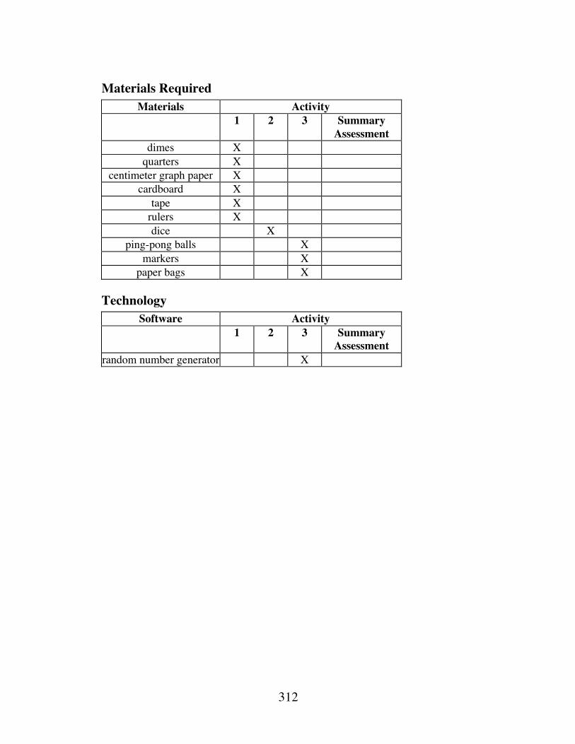
312



dimes X quarters X

centimeter graph paper X cardboard X

tape X rulers X dice X

ping-pong balls X markers X

paper bags X



random number generator X

313

Hurry! Hurry! Hurry! Step Right Up!

Introduction (page 247) This module uses carnival games to introduce geometric models for determining probability.

Discussion (page 247) a. Sample response: The spinner has a better chance because it appears

to win half the time. The dart looks like it has less than a 50% chance of winning.

b. Sample response: It is necessary to use the tip so that a single point determines the part of the board in which the spinner lands. If the entire head of the arrow is considered, the spinner could land in more than one part of the board.

c. 1. Students may mention tossing rings onto the necks of pop bottles, throwing a ball through an opening, shooting at a target with an air rifle, using a sledgehammer to ring a bell, shooting a basketball through a hoop, throwing darts at balloons, knocking over bottles with a ball, playing a raffle, or catching metal disks with a magnet attached to a fishing pole.

2. Some games, such as shooting baskets or throwing darts, involve at least some degree of skill. Others, such as raffles or bingo, are based on chance. Still others involve a mix of chance and skill.

d. Answers will vary. Students may prefer the dart game because at least some skill is involved. Others may choose the spinner game, arguing that the chances of winning seem better. Note: Students are not expected to calculate the probabilities of winning at this time. This situation is revisited in Problem 1.5.

e. Since most carnival games are designed for both entertainment and profit-making, they are usually not fair games in the mathematical sense. Many carnival games allow few winners, or offer inexpensive prizes, to keep the expected value low. Some students may argue that foul play also makes some games unfair (for example, bottles that can’t be knocked over or bent rifle barrels).

314

(page 248)

Activity 1 In this activity, students use geometric models to determine probability.

Materials List • dimes (one per group)

• quarters (one per group)

• centimeter graph paper (one sheet per group)

• rulers (one per group)

• cardboard (four sheets per group)

• tape

Teacher Note This exploration works well for groups of two students. After one student drops the coin onto the grid, the other can judge and record wins or losses.

Exploration (page 248) Students play the coin-drop game and record the experimental outcomes.

a. Students create a game board with four walls around it.

b–c. Note: If dimes are dropped from too great a height, they may bounce over the walls. Placing a notebook under the grid can reduce bouncing.

d. Experimental probabilities will vary. The theoretical probability of winning is approximately 0.16.

e. 1. Answers may vary. Given a dime with a radius of 0.9 cm, the center of the dime must be at least 0.9 cm from each line on the grid.

2. Using the center of the dime as a reference point, the region that models all winning outcomes is a square within the 3 cm ∞ 3 cm square. The following diagram shows eight possible positions for winning dimes, the centers of these dimes, and the square formed by the centers of all winning coins.

315

The area of the region that models winning outcomes is

approximately 3 − (2 • 0.9)( )2=1.44 cm2 .

3. The theoretical probability can be determined by dividing the area of the inner square (representing all winning outcomes) by the area of the outer square (representing all possible outcomes):

area of inner squarearea of outer square

=1.44 cm2

9 cm2 =4

25= 0.16

f. Answers will vary. For a large number of trials, the experimental probability is likely to approximate the theoretical probability.

Discussion (page 250) a. Sample response: If any other point is used, the orientation of the coin

would have to be considered when determining the area that represents a win. This would make the problem very hard to solve.

b. Assuming that the walls are at least 0.9 cm from the grid, the probability of winning is the same for any number of squares (n):

n • area of inner squaren • area of outer square

=1.44n

9n=

1.449

=425

= 0.16

c. Answers will vary. These probabilities may or may not be approximately equal, depending on the class results. For a large number of trials, the experimental probability is likely to be close to the theoretical probability.

d. Sample response: The game could be made impossible to play by using a coin with a diameter that is greater than the dimensions of the squares, or by using squares with dimensions that are less than the diameter of the dime.

0.9 cm

0.9 cm0.9 cm

0.9 cm

316

Assignment (page 251) 1.1 a. The region that models all winning outcomes is the square formed

by the centers of all winning quarters. Since the radius of a quarter is approximately 1.2 cm, the area of this region can be found as follows: 3 − (2 •1.2)( )2

= 0.36 cm2 .

b. The theoretical probability of winning the coin-drop game using a quarter is:


=0.36 cm2

9 cm2 =125

= 0.04

*1.2 a. The region that models all winning outcomes is the square formed by the centers of all winning dimes. Since the radius of a dime is approximately 0.9 cm, the area of this region can be found as follows: 4 − (2 • 0.9)( )2

= 4.84 cm 2 .

b. The theoretical probability of winning this version of the game is:


=4.84 cm2

16 cm 2 =121400

= 0.3025

1.3 a. Using a geometric model, the probability of landing in the yellow ring is the ratio of the area of the yellow ring to the area of the entire target:

π (10)2 − π (7)2

π (13)2=π (51)π (169)

=51169

≈ 0.30

b. Sample response: No. It is not really a random event because players can aim the dart at a particular point.

*1.4 a. As shown in the diagram below, students can consider all the positions of the ball’s center that will knock down the pin:

pin8 cm widebowling ball

20 cm diameterbowling ball

20-cm diameter

length that models a win (pin falls down)

100 cm

28 cm

317

Using this geometric model, the width of all possible paths of the ball’s center down the lane is (100 − 2 •10), or 80 cm. The width of the paths that result in knocking down the pin is 28 cm. The probability of winning is 28 80 = 7 20 = 0.35.

b. As shown in the diagram below, if the pin is placed against one rail, the ball can pass on only one side of the pin. Since the center of the ball can pass no closer than 10 cm from the rail, the width of the paths that result in knocking down the pin is 8 cm. This reduces the probability of winning to 8 80 =1 10 = 0.1 .

1.5 Sample response: I would rather play the spinner game because the

probability of winning is greater. Since each of the four central angles where the spinner is located measure 90˚, the probability that the spinner lands in the unshaded portion of the board is:

90˚+90˚360˚

= 0.5

The probability of a dart landing in the unshaded portion of the board is the sum of areas of the two unshaded rectangles, divided by the total area of the board:

40 • 70 + 40 • 90130 •110

≈ 0.448

* * * * *

100 cmpin

8 cm widebowling ball20-cm diameter

318

*1.6 a. Sample graph:

b. The area of all the possible outcomes is 25 units2 .

c. Sample graph:

The area of the shaded region is 1 2(3)(3) = 4.5 units2 .

d. Using a geometric model, the probability that x + y ≤ 3 is 4.5 25 = 0.18 .

(5,5)

1 2 3 4 5

12

3

4

5

x

y

x + y ≤ 3

1 2 3 4 5

12

3

4

5

x

y

319

e. The following sample graph shows the region bounded by x + y ≥ 6 , 0 ≤ x ≤ 5, and 0 ≤ y ≤ 5 .

The area of the shaded region is 1 2(4)(4) = 8 units2 . Using a geometric model, the probability that x + y ≥ 6 is 8 25 = 0.32.

*1.7 a. Sample sketch:

b. Sample response: The dangerous area is a circle with a radius of

10 m. Therefore, the area of the parking lot in which it is safe to land is: 752 − π102 ≈ 5300 m2 .

c. 1. Using a geometric model, the probability that the parachutist lands safely can be found as follows:

safe areaparking lot area

≈53005625

≈ 0.94

2. The probability that the parachute’s lines get tangled in a security light is:

unsafe areaparking lot area

≈π102

752 ≈3145625

≈ 0.06

d. Sample response: The probabilities in Part c add to 1 because they are complementary events.

1 2 3 4 5

12

3

4

5

x

y

x + y ≥ 6

75 m

75 m

10 m

dangerous areas

320


b. The area of the shaded region in the graph above is 4 units2 .

c. Sample graph:

The area of the shaded region in the graph above is 2 units2 .

d. Using a geometric model, the probability is 2 4 = 0.5 .

e. Using a geometric model, the probability is 2 4 = 0.5 . Note: The events described in Parts d and e are not complementary, since the points on the line y = x are included in both.

* * * * * * * * * * (page 254)

Activity 2 In this activity, students calculate expected value and determine whether or not a game is mathematically fair.

Materials List • dice (one per group)

1 2 3 4

12

3

4

x

y

1 2 3 4

12

3

4

x

y

321

Exploration (page 254) a–b. Students should recognize that the chances of winning each prize are

not equally likely.

c. The theoretical probability of winning each prize is shown below.

Value of Prize Roll of Die Probability $1.50 1 1 6 $1.00 2 1 6 $0.50 3 1 6 $0.00 4 1 6 $0.00 5 1 6 $0.00 6 1 6

Since three of the outcomes result in a prize of $0.00, its theoretical

probability is 1 6 +1 6 +1 6 = 3 6 =1 2 .

d. The experimental probabilities may or may not approximate the theoretical probabilities.

e. The expected value can be found as follows: 16• $1.50 + 1

6• $1.00 + 1

6• $0.50 + 1

2• 0 = $0.50

Discussion (page 255) a. Sample response: No. You are not equally likely to win each prize. A

non-winning roll of 4, 5, or 6 is three times more likely to occur than any single winning roll.

b. Since the cost to play ($1.00) and the expected value ($0.50) are not equal, the game is not mathematically fair. To make the game fair, students may suggest reducing the cost to play, increasing the value of the prizes, or changing the probabilities of winning the prizes.

c. Answers will vary. To pay wages, travel costs, and other expenses, carnival operators must make a profit from their games. It would be unreasonable to expect a mathematically fair game under these circumstances.

322

Assignment (page 256) *2.1 To make this a fair game, the cost to play must equal the expected

value: 12• $0.00 + 1

3• $0.50 + 1

6• $2.00 = $0.50

2.2 a. The expected value can be calculated as follows: 2125• $0.00 + 4

25• $5.00 = $0.80

b. To make the game mathematically fair, the cost to play must be decreased to $0.80.

c. The value of the prize that makes the game mathematically fair can be calculated as follows:

2125• $0.00 + 4

25• x = $1.00

x = $6.25

*2.3 a. The expected value can be calculated as follows: 2425• $0.00 + 1

25• $15.00 = $0.60

b. To make the game mathematically fair, the cost to play must be decreased to $0.60.

c. The value of the prize that makes the game mathematically fair can be calculated as follows:

2425• $0.00 + 1

25• x = $1.00

x = $25.00

2.4 To make this a fair game, the cost to play must equal the expected value:

113• $10 +

313• $1 +

913• $0 = $1.00

* * * * *

323

2.5 a. In the following sample graph, the shaded region represents all the possible pairs of numbers in the interval [0, 5] for which the sum is less than or equal to 3.

The probability of Juan winning is the area of the shaded region

divided by the area of the square: 4.525

= 0.18 =18%

b. Since Juan theoretically wins $0.50 in 18% of the games and loses $0.20 in 82% of the games, the expected value can be calculated as follows: 0.18 •0.50 + 0.82 • −0.20 ≈ −0.07 .

c. Sample response: Juan can expect to lose an average of approximately $0.07 each time he plays. Therefore, he should not play the game.

d. Answers will vary. Sample response: If Joan continues to pay Juan $0.50 each time he wins, then solving the following equation for x gives the amount Juan should pay Joan to make the expected value the same for both players.

0.18 • $0.50 = 0.82x$0.11 ≈ x

If Juan continues to pay Joan $0.20 each time she wins, then solving the following equation for x gives the amount Joan should pay Juan to make the expected value the same for both players.

0.18x = 0.82 • $0.20x ≈ $0.91

* * * * * * * * * *

Research Project (page 257) After students have presented their games to the class, you may wish to ask them to discuss modifications that might make the games profitable at a carnival.

y

x0 1 2 3 4 5

012345

324

(page 257)

Activity 3 In this activity, students examine multistage probabilities.

Materials List • ping-pong balls or other small objects (10 per group)

• red and blue markers (one each per group)

• paper bags or other opaque containers (one per group)

Technology • random number generator

Exploration 1 (page 258) Students simulate the fishing derby by drawing objects from a bag. Note: To ensure random draws, the objects should be indistinguishable by touch.

a–b. Students simulate the fishing derby 10 times, then combine their results with the class. Sample data for 100 trials:

Event Points Number of Occurrences

Experimental Probability

3 red 6 8 0.08 2 red, 1 blue 5 25 0.25 1 red, 2 blue 4 46 0.46

3 blue 3 21 0.21 c. Sample tree diagram:

6 10

4 10

firstdrawR

B

325

d. The eight possible outcomes are RRR, RRB, RBR, RBB, BRR, BRB, BBR, and BBB (where R represents red and B represents blue). Sample tree diagram:

e. Students should calculate the following probabilities:

P(RRR) = 4 10( )3 = 0.064 , P(RRB) = 4 10( )2 • 6 10 = 0.096 , P(RBR) = 4 10( )2 • 6 10 = 0.096 , P(RBB) = 4 10 • 6 10( )2 = 0.144 , P(BRR) = 6 10 • 4 10( )2 = 0.096 , P(BRB) = 6 10( )2 • 4 10 = 0.144 , P(BBR) = 6 10( )2 • 4 10 = 0.144 , and P(BBB) = 6 10( )3 = 0.216 .

f. 1. The probabilities of winning each prize are as follows: P(6) = 0.064, P(5) = 3 • 0.096 = 0.288 , P(4) = 3 • 0.144 = 0.432 , and P(3) = 0.216 .

2. For a large number of trials, the experimental probabilities are likely to be close to the theoretical probabilities.

B

R

R

B

R

B6 10

6 10

6 10

6 10

6 10

6 10

6 10

4 10

4 10

4 10

4 10

4 10

4 10

4 10

firstdraw

second draw

thirddraw

R

R

R

R

B

B

B

B

326

Discussion 1 (page 259) a. There are eight possible outcomes. b. 1. There is one way to get 3 points: BBB. 2. Any combination of 2 blues and 1 red earns 4 points. There are

three possibilities: BBR, BRB, and RBB. 3. Any combination of 2 reds and 1 blue earns 5 points. There are

three possibilities: RRB, RBR, and BRR. 4. There is one way to earn 6 points: RRR. 5. There is no way to earn 7 points. c. Sample response: Because there are fewer rings with red dots than

rings with blue dots, the probability of drawing a red ring is less than that of drawing a blue one.

d. 1. Sample response: No. Since the object is returned to the container and mixed in with the others, the second draw is from the same set of objects as the first.

2. Sample response: No, for the same reasons mentioned above. e. Some students may predict that the rabbit’s foot is the prize most often

won because it requires the fewest points. Considering theoretical probabilities, however, the celebrity poster should be the most frequently awarded prize.

f. 1. Answers may vary. Sample response: Generate random numbers from 1 to 10, inclusive. The numbers from 1 to 4 represent a red ring and earn 2 points. The numbers from 5 to 10 represent a blue ring and earn 1 point.

2. Students may expect the simulations to produce the same results. Since each is repeated a relatively few number of times, however, the results are likely to vary. Over the long run, the simulations should produce similar results because they involve the same theoretical probabilities.

g. Sample response: Because it contains more trials, the class data should better represent the long-term results of the game. The experimental probability should be closer to the theoretical probability as the number of trials increases.

327

Exploration 2 (page 260) In this exploration, students examine conditional probabilities by simulating a version of the fishing derby without replacement.

a. Responses will vary. Some students may observe that the probabilities of scoring 6 points (RRR) or 3 points (BBB) are decreased.

b. The possible outcomes are the same as those in the original version of the game: RRR, RRB, RBR, RBB, BRR, BRB, BBR, and BBB. Sample tree diagram:

c. Students should determine the probabilities of each outcome as follows: P(RRR) = 4 10 • 3 9 • 2 8 = 1 30 ≈ 0.03 , P(RRB) = 4 10 • 3 9 • 6 8 = 1 10 = 0.1, P(RBR) = 4 10 • 6 9 • 3 8 =1 10 = 0.1 , P(RBB) = 4 10 • 6 9 • 5 8 = 1 6 ≈ 0.17 , P(BRR) = 6 10 • 4 9• 3 8 =1 10 = 0.1 , P(BRB) = 6 10 • 4 9 • 5 8 = 1 6 ≈ 0.17 , P(BBR) = 6 10 • 5 9 • 4 8 = 1 6 ≈ 0.17 , and P(BBB) = 6 10 • 5 9 • 4 8 = 1 6 ≈ 0.17 .

Using these probabilities, the theoretical probabilities of obtaining each score are P(6) = 1 30 ≈ 0.03 , P(5) = 3 10 = 0.3 , P(4) = 3 6 = 0.5 , and P(3) =1 6 ≈ 0.17.

firstdraw

thirddraw

6/10

R

R

B

R

B

R

B

B

R

B

R

B

R

B

3/9

2/8

6/9

6/8

3/8

5/8

5/9

3/8

5/8

4/8

4/8

4/10

second draw

4/9

328

d. Students may design their own simulations using either a container of red and blue objects or a random number generator. Sample response: Generate random numbers from 1 to 10, inclusive. The numbers 1 to 4 represent the red rings and are worth 2 points. The numbers 5 to 10 represent the blue rings and are worth 1 point. During a single round of the simulation, any number that comes up more than once is ignored and another number generated.

e. The following table shows some sample data for 100 trials. In this case, the experimental probabilities closely approximate the theoretical probabilities.

Event Points Number of Occurrences

Experimental Probability

3 red 6 3 0.03 2 red, 1 blue 5 31 0.31 1 red, 2 blue 4 45 0.45

3 blue 3 21 0.21

Discussion 2 (page 261) a. Sample response: When using a random number generator, ignoring

any number that comes up more than once in a single round models its removal from the tank. When using red and blue objects, removing them from the container models rings removed from the tank.

b. In the new version of the game, the theoretical probability of getting 6 points decreases from 0.064 to approximately 0.03.

c. Sample response: Although the chances of winning a hat have improved slightly, the chances of winning a bear have decreased. Overall, the chances of winning one or the other has also decreased. In the original game, the chances of winning a hat or a bear are 0.288 + 0.064 = 0.352 . In the new version, the chances of winning a hat or a bear are approximately 0.3 + 0.033 = 0.333 .

d. 1. Sample response: The probabilities are different because the first chip drawn is not replaced in the box. Since the numbers and kinds of chips in the box have changed, the probabilities must be adjusted.

2. Since there is only one blue chip in the game, the probability of drawing two blue chips is 0.

329

Assignment (page 261) *3.1 a. Because all the outcomes result in a prize, and because the sum of

their probabilities is 1, the probability of winning some prize in the fishing derby is 1.

b. Because no combination of three rings adds up to 7 points, the probability of earning 7 points is 0.

c. The expected value, in points, can be determined as follows: 8125

•6 + 36125

•5 + 54125

• 4 + 27125

• 3 = 4.2

*3.2 a. The expected value, in points, is: 130

• 6 + 310

• 5 + 12• 4 + 1

6•3 = 4.2

b. Answers will vary. The probabilities of winning a poster or hat increased slightly in the new version, while the probabilities of winning a key chain or teddy bear decreased.

3.3 a. Sample response: For the game to be fair, the expected value must equal the cost to play. The expected value of the original fishing derby is:

8125

•$2.00 + 36125

• $0.80 + 54125

•$0.60 + 27125

•$0.25 ≈ $0.67

One way to make this a fair game would be to reduce the cost to play to $0.67.

b. Sample response: For the game to be fair, the expected value must equal the cost to play. The expected value of the new version is:

130

• $2.00 + 310

• $0.80 + 12•$0.60 + 1

6• $0.25 ≈ $0.65

One way to make this a fair game would be to reduce the cost to play to $0.65.

*3.4 a. There are four equally likely outcomes when tossing two coins: HH, HT, TH, and TT. Therefore, the probabilities of each result can be determined as follows: P(1 step) = P(HT) + P(TH) =1 2 = 0.5 , P(0 steps) = P(TT) =1 4 = 0.25 , and P(−1 step) = P(HH) =1 4 = 0.25 .

b. The expected value, in number of stairs, is: 14• 0 + 1

2•1 + 1

4• −1 = 1

4= 0.25

330

c. Sample response: Since 10 • 0.25 = 2.5 , Guinn is likely to be 2 or 3 steps up from the starting point.

d. If the game starts on the middle of the 25 stairs (or the 13th stair), a player must move up 12 stairs to win. On average, Guinn would need 48 turns (12 0.25 = 48) to get to the top step.

* * * * * *3.5 a. The following tree diagram shows the probability of each

outcome:

b. 1. 3992 2. 8 3. 994,008 4. 1992 c. Sample response: Of the 1,000,000 people tested, I expect

3992 +1992 = 5984 to test positive. Of these, only 3992 would actually have HIV, so P(HIV|Test +) = 3992 5984 ≈ 0.667 .

* * * * * * * * * *

sample +

sample –

test + correct positive

test – false negative

test – correct negative

test + false positive

1250

= 0.004

0.998

0.002

0.998

0.002

0.003992

0.000008

0.994008

0.001992

249250

= 0.996

331

Answers to Summary Assessment (page 264) 1. Student responses should take the form of a letter and include the

following information.

a. The total area of the board is 30, 000 cm2 . The area of the red zones is 3(30 • 35) = 3150 cm2 . Assuming that the dart is equally likely to land anywhere on the board, the probability of landing in a red zone is 3150 30, 000 = 21 200 = 0.105 .

The area of the blue zone is π (42 ) ≈ 50 cm2 . The probability of landing in the blue zone is approximately 50 30, 000 ≈ 0.002. The probability of not landing in either winning zone is (30, 000 − 3150 − 50.27) 30, 000 ≈ 0.893. Note: This may also be calculated by 1 − P(red zone ) − P(blue zone) .

b. The expected value can be calculated as follows: (0.893• $0) + (0.105 •$25) + (0.002 • $10, 000) ≈ $22.63

c. Assuming no other costs, the lowest price the charity could charge to play, and still hope to earn some profit, is $23.00.

d. For the first 1000 players, the charity should plan to award about 1000 • 0.105 = 105 miniature replicas, and 1000 • 0.002 = 2 full-sized cars.

e. Since each game is an independent event, the probability that two players in a row win full-sized cars is approximately 0.0022 ≈ 0.000004 , or about 4 in 1,000,000.

Student recommendations will vary. At a cost to play of $23.00, the charity could expect to earn an average of approximately $0.37 per player. Based on this small per-player profit, some students may recommend against using this game as fund-raiser. They may also mention the possibility of having to award a full-sized car before earning enough money to pay for it, or suggest that the high cost of playing may discourage potential players.

332

2. Student responses should again take the form of a letter. To determine probabilities, some may construct a tree diagram like the one shown below:

blue

red

green

red

blue

green

red

blue

green

red

blue

green

blue

green

red

blue

green

red

blue

green

red

blue

green

red

blue

green

red

blue

green

red

blue

green

red

blue

green

red

blue

green

red

2/20

1/19

0/18

8/18

8/20

10/20

10/18

8/19

10/19

1/18

7/18

10/18

1/18

8/18

9/18

2/19

7/19

10/19

1/18

7/18

10/18

10/18

2/18

6/18

2/18

7/18

9/18

9/19

8/18

2/19

1/18

8/18

9/18

8/19

2/18

7/18

9/18

2/18

8/18

333

The probabilities and point values for each possible draw of three balls are shown in the following table.

Balls Drawn Point Value Probability 3 red 15 0 6840 = 0.000

2 red, 1 blue 12 48 6840 ≈ 0.007 2 red, 1 green 11 60 6840 ≈ 0.009 1 red, 2 blue 9 336 6840 ≈ 0.049

1 red, 1 blue, 1 green 7 960 6840 ≈ 0.140 1 red, 2 green 8 540 6840 ≈ 0.079

3 blue 6 336 6840 ≈ 0.049 2 blue, 1 green 5 1680 6840 ≈ 0.246 1 blue, 2 green 4 2160 6840 ≈ 0.316

3 green 3 720 6840 ≈ 0.105 The probabilities for winning each prize can be calculated by

adding the probabilities for the appropriate point values. The expected value for the game is shown in the table below.

Points Prize Value Probability Product [12, 15] $3.00 48 6840 ≈ 0.007 $0.02 [9, 11] $1.75 396 6840 ≈ 0.058 $0.10 [6, 8] $0.40 1836 6840 ≈ 0.268 $0.11 [3, 5] $0.00 4560 6840 ≈ 0.667 $0.00

Expected Value $0.23 Over the long term, the carnival can expect to earn an average

profit of $0.77 per player. Based on this relatively large profit, students may recommend that the carnival add the game.

334

Module Assessment

1. In one lottery game, each player purchases a ticket for $5.00, then

selects a three-digit number. Each digit must be between 0 and 9, inclusive, and can appear only once in the number.

Lottery officials then randomly select three digits, one at a time and without replacement. These digits are recorded in the order selected to form a three-digit number.

If the player’s three-digit number matches the number selected by the lottery, the player wins.

a. How many three-digit numbers are possible in this lottery game? b. What is the probability of winning with one ticket? c. If this were a fair game, how much should the lottery pay for

matching the winning number? Justify your response. 2. A local convenience store is having a grand opening celebration. As

part of its promotional activities, the store plans to offer prize tickets to everyone who enters the store. No purchase is necessary to win. The value of each prize and the probability of winning it are shown in the table below. What is the expected value for a prize ticket?

Prize Value Probability soft drink $1 0.05

two lottery tickets $2 0.01 40 L of gasoline $15 0.001

weekend vacation $1000 0.000005 European vacation $10,000 0.00000005

3. Consider a game in which three balls—numbered 1, 2, and 3—are

placed in a paper bag. Player 1 draws a ball, records its number, then replaces it in the bag. Player 2 does the same. For each version of this game described below, determine whether you would want to be player 1 or player 2. Justify your responses.

a. If the sum x of the two numbers is odd, player 1 loses x points while player 2 wins x points. If the sum of the two numbers is even, player 2 loses 4 points, while player 1 wins 4 points.

b. If both players draw the same number, no points are won or lost. If the sum of the two numbers is even, the player with the higher number wins 5 points, while the other player loses 5 points. If the sum of the two numbers is odd, the player with the lower number wins 3 points, while the other player loses 3 points.

335

4. As described in Problem 3.4, Guinn and Ebdul are playing the stair-step game. To reduce the time required to declare a winner, they decide to change the rules of the game.

Ebdul suggests tossing four coins on each turn. If one head or three heads appear on a player’s four coins, the player moves up one stair. If two or four heads appear, the player moves down one stair. If no heads appear, the player remains on the same step.

As before, the game starts on the middle step of a staircase 25 steps long. To win the game, a player must reach the top step.

a. If movement is described in terms of the number of stairs moved upwards, then each player’s turn in the game has three possible results: 1 step, 0 steps, and –1 step.

What is the probability of each of these results?

b. What is the expected value, in number of stairs moved upwards, for each turn in this version of the game?

c. Will Ebdul’s suggestion shorten the stair-step game? Justify your response.

5. In the cube game, players toss a cube with three green faces, one red face, one white face, and one blue face into a bucket. After you toss the cube, the game operator tells you that the green face is not showing. Given this information, what is the probability that the red face is showing? Justify your response.

336

Answers to Module Assessment 1. a. There are 10 • 9 •8 = 720 possible numbers for this game. b. The probability that any one ticket wins is 1 720 ≈ 0.001.

c. If this were a fair game, the expected value should equal the cost to play, or $5.00. Therefore, the prize should be worth $3600.

2. The expected value can be determined as follows:

(0.05 •$1) + (0.01•$2) + (0.001• $15) + (0.000005• $1000) +(0.00000005 •$10, 000) + (0.93899495• $0) ≈ $0.09

3. a. There are five possible sums: 2, 3, 4, 5, and 6. The probability of a 2 is 1 9 , of a 3 is 2 9 , of a 4 is 3 9 =1 3, of a 5 is 2 9 , and of a 6 is 1 9. The expected value for player 1, in points, can be found as follows:

19• 4 + 2

9•−3 + 3

9• 4 + 2

9•−5 + 1

9• 4 = 4

9

The expected value for player 2 is: 19• −4 + 2

9• 3 + 3

9•−4 + 2

9•5 + 1

9• −4 = − 4

9

In this case, player 1 has the advantage. b. The following table shows the number of points associated with

each draw.

Number Drawn Points Received Player 1 Player 2 Player 1 Player 2

1 1 0 0 1 2 3 –3 1 3 –5 5 2 1 –3 3 2 2 0 0 2 3 3 –3 3 1 5 –5 3 2 –3 3 3 3 0 0

Both players have three chances of winning 0 points; two chances

of winning 3 points; two chances of winning –3 points; one chance of winning 5 points; and one chance of winning –5 points. The expected value for both players is:

39• 0 + 2

9• 3 + 2

9• −3 + 1

9•5 + 1

9• −5 = 0

In this case, neither player has an advantage.

337

4. a. There are 16 equally likely outcomes when tossing four coins: HHHH, HHHT, HHTH, HHTT, HTHH, HTHT, HTTH, HTTT, THHH, THHT, THTH, THTT, TTHH, TTHT, TTTH, and TTTT. Therefore, the probabilities of each result can be determined as follows: P(1 step) = 1 2 = 0.5 , P(0 steps) = 1 16 = 0.0625 , and P(−1 step) = 7 16 = 0.4375 .

b. The expected value, in number of stairs, is: 116

• 0 + 12•1 + 7

16• −1 = 1

16= 0.0625

c. Sample response: The rule change would actually slow the game down. The expected movement per turn decreases from 0.25 steps to 0.0625 steps, a factor of 1 4 . Therefore, one would expect the new version to take four times as long as the original game.

5. Sample response: If the result of rolling the cube is not green, the roll must be either red, white, or blue. Each of these three colors appears once, so the probability of a red face is 1 3 ≈ 0.33 .

338

Selected References Dahlke, R., and R. Fakler. “Geometrical Probability—A Source of Interesting and

Significant Applications of High School Mathematics.” In Readings for Enrichment in Secondary School Mathematics, ed. by Max A. Sobel. Reston, VA: National Council of Teachers of Mathematics (NCTM), 1988.

Harshbarger, R. J., and J. J. Reynolds. Finite Mathematics for Management, Life, and Social Sciences. Lexington, MA: D.C. Heath and Co., 1992.

Heintz, R. E. “It’s in the Bag.” Mathematics Teacher 70 (February 1977): 132–36.

“The Laws of Probability.” Time 85 (8 January 1965): 42.

North Carolina School of Science and Mathematics, Department of Mathematics and Computer Science. Geometric Probability. Reston, VA: NCTM, 1988.

“Trial by Mathematics.” Time 91 (26 April 1968): 41.

Zuwaylif, F. H. General Applied Sciences. Reading, MA: Addison-Wesley, 1970.

339

Flashbacks

Activity 1 1.1 Find the area of the shaded region in Parts a–d below.

1.2 Consider an experiment which involves tossing a coin and counting

the number of times that it lands heads up. After 65 tosses, you record 31 heads.

a. What is the experimental probability of the coin landing heads up?

b. What is the theoretical probability of the coin landing heads up?

1.3 Graph the following inequality on a two-dimensional coordinate system: x + y ≥ 1.

15 m

6 m

a. b.

c. d.

5 m

32˚

9 cm

4 cm

2 m

3.5 m

340

Activity 2 2.1 Consider an experiment which involves drawing a card out of a

standard deck of 52 playing cards. Determine the theoretical probability of drawing each of the following:

a. a six b. a heart c. a face card d. a club or a diamond. 2.2 Consider an experiment which involves rolling a six-sided die and

recording the number that appears. a. List all the possible outcomes of this experiment. b. What is the theoretical probability of each outcome? c. What is the expected value of this experiment? 2.3 Solve each of the following equations for x.

a. 23x = 5

b. 113

x = 2

Activity 3 3.1 Consider an experiment in which three cards—an ace, a king and a

queen—are placed face down on a table. The cards are then turned over, one at a time.

a. Draw a tree diagram that shows all the possible sequences in which the cards may be turned over.

b. How many outcomes are there in the sample space for this experiment?

c. What is the probability that the ace is the first card turned over? d. What is the probability that the queen is the first card and the ace

is the second card? 3.2 A bag contains 20 red marbles, 16 green marbles, and 12 blue

marbles. Consider an experiment in which two marbles are drawn from the bag, one at a time and without replacement.

a. What is the probability that the first marble is blue? b. What is the probability that the first marble is red? c. If the first marble is green, what is the probability that the second

marble is red?

341


Activity 1 1.1 a. 328 360 •π • 52 = 205π 9 ≈ 71.56 m2

b. 15 •6 = 90 m2

c. 1 2 •4 •9 = 18 cm2

d. (π •3.52 ) − (π •22 ) ≈ 25.92 m2

1.2 a. 31 65 ≈ 0.48

b. 1 2 ≈ 0.5

1.3 Sample graph:

Activity 2 2.1 a. 4 52 =

113 ≈ 0.08

b. 1352 =14 = 0.25

c. 12 52 =313 ≈ 0.23

d. 26 52 =24 =

12 = 0.5

x + y ≥ 1

1 2 3 4 5

12

3

4

5

x

y

342

2.2 a. There are six possible outcomes: 1, 2, 3, 4, 5, and 6. b. The theoretical probability of each outcome is 1 6 ≈ 0.17 .

c. The expected value is: 16•1+ 1

6• 2 + 1

6•3 + 1

6• 4 + 1

6• 5 + 1

6• 6 = 7

2

2.3 a. x =15 2 = 7.5

b. x = 26

Activity 3 3.1 a. Sample tree diagram:

b. The sample space contains 6 equally likely possibilities: AKQ,

AQK, KAQ, KQA, QAK, and QKA.

c. Since the ace appears first in 2 of the 6 outcomes, the probability is 2 6 ≈ 0.33 .

d. Since the queen appears first and the ace second in 1 of the 6 outcomes, the probability is 1 6 ≈ 0.17 .

3.2 a. 12 48 = 1 4 = 0.25

b. 20 48 = 5 12 ≈ 0.42

c. 20 47 ≈ 0.43

A

K

QK

K

A

A

Q

Q

Q

K

Q

A

A

K

firstdraw

seconddraw

thirddraw

Atomic Clocks Are Ticking

You’ve found the remains of an old cooking fire. How do you tell if that lump of charcoal is 10 years old, or 10,000? In this module, you explore one method that archaeologists use to tell time.

John Freal • Sandy Johnson • Anne Merrifield

345

Teacher Edition Atomic Clocks Are Ticking

Overview This module uses radioactive decay and carbon dating to develop models of exponential decay and examine negative and fractional exponents. Exponential equations are solved graphically and by guess-and-check using a calculator.


• develop models of exponential decay

• examine the relationship between negative and positive exponents

• use equations containing negative exponents as mathematical models

• examine the relationship between rational exponents and roots

• develop properties of exponents.


• how to interpret an exponential expression

• how to model exponential growth using equations of the form y = a •bx

• scientific notation

• how to use a spreadsheet.


Assessment Total

Days 2 3 3 2 10

346



chips X graph paper X X box with lid X

dice (optional) X



graphing utility X X X X spreadsheet X X X

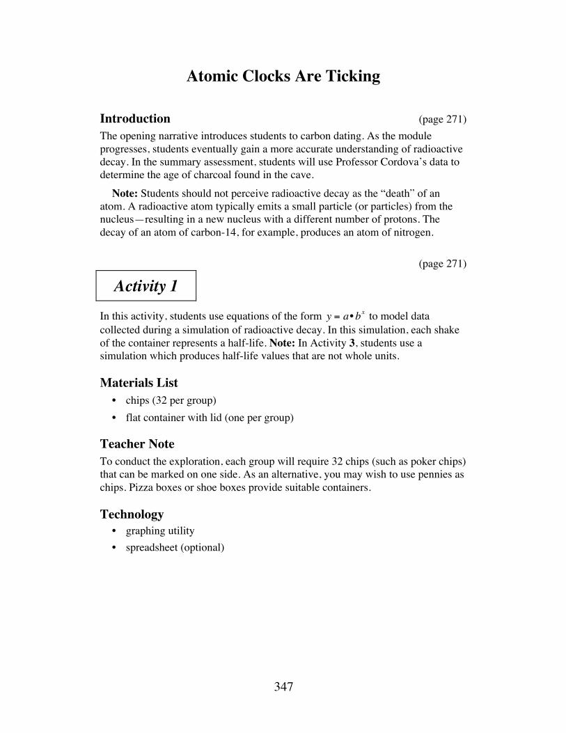
347

Atomic Clocks Are Ticking

Introduction (page 271) The opening narrative introduces students to carbon dating. As the module progresses, students eventually gain a more accurate understanding of radioactive decay. In the summary assessment, students will use Professor Cordova’s data to determine the age of charcoal found in the cave. Note: Students should not perceive radioactive decay as the “death” of an atom. A radioactive atom typically emits a small particle (or particles) from the nucleus—resulting in a new nucleus with a different number of protons. The decay of an atom of carbon-14, for example, produces an atom of nitrogen.

(page 271)

Activity 1 In this activity, students use equations of the form y = a•bx to model data collected during a simulation of radioactive decay. In this simulation, each shake of the container represents a half-life. Note: In Activity 3, students use a simulation which produces half-life values that are not whole units.

Materials List • chips (32 per group) • flat container with lid (one per group)

Teacher Note To conduct the exploration, each group will require 32 chips (such as poker chips) that can be marked on one side. As an alternative, you may wish to use pennies as chips. Pizza boxes or shoe boxes provide suitable containers.

Technology • graphing utility • spreadsheet (optional)

348

Exploration (page 271) Note: Students should save their data for use in the assignment.

a–f. Students simulate the process of radioactive decay. It should take from 4 to 7 shakes to remove all the chips. Sample data:

Shake No. of Chips Remaining 0 32 1 15 2 12 3 8 4 3 5 1 6 1 7 0

g. A graph of the sample data appears below.

Discussion (page 272) a. Sample response: The number of remaining chips appears to decrease

more slowly as the shake number increases.

b. Answers will vary. Sample response: The general shapes of the graphs are the same, with the number of chips decreasing as the shake number increases. However, different numbers of shakes were required to remove all the chips, and the graphs vary in steepness.

c. Since the probability of a chip landing with the mark up is 1 2 , students should expect half of the chips to be removed and half to remain.

d. When a positive number is multiplied by a factor between 0 and 1, the number decreases.

349

e. 1. Sample response: The value of y represents the worth of the machine at the end of half a year, or 6 months.

2. Sample response: The value of y represents the worth of the machine at the end of one-third of a year, or 4 months.

f. Answers will vary, depending on the calculator used.

1. Sample response: Type “0.81^(1/2)” then press the enter button.

2. Sample response: Type “0.81^(1/3)” then press the enter button.

g. Students should realize that the value of (0.81)1 2 is the square root of 0.81, or 0.9.

h. Students should conjecture that since an exponent of 1 2 in the expression (0.81)1 2 represents the square root, an exponent of 1 3 in the expression (0.81)1 3 represents the cube root of 0.81. This can be verified by cubing the value reported by the calculator for (0.81)1 3 .

i. 1. If the equation models exponential growth, b > 1.

2. If the equation models exponential decay, 0 < b <1 .

Assignment (page 274) 1.1 a. 5

b. 3 c. 7

d. 2

1.2 a. The table below shows the percent decrease after each shake for the sample data given in the exploration:

Shake No. of Chips Remaining

Percent Decrease

0 32 1 15 47% 2 12 20% 3 8 33% 4 3 63% 5 1 67% 6 1 0% 7 0 100%

350

b. 1. Answers will vary. The mean of the percents of decrease for the sample data shown above is 47%.

2. Sample response: I would expect the mean of the percents of decrease to be close to 50%, because each chip has a 50% chance of having its mark showing.

c. Sample response: The mean of the percents of decrease can be used as the rate of decay, which is also a percentage, because they measure the same thing.

d. Answers will vary. For the sample data, the rate of decay is –0.47. In this case, b = 1 − 0.47 = 0.53 .

e. Since the initial population is 32, the equation that models the data is y = 32 • 0.53( )x .

1.3 A completed table is shown below.

Initial Population

Rate of Growth or Decay

Model Equation of the Form y = a • bx

a. 500 8% y = 500 • 1.08( )x b. 20,000 –11% y = 20, 000 • (0.89) x c. 100 –32% y = 100 • 0.68( )x

1.4 5.02 •1022 1•1012 ≈ 5 •1010 atoms

1.5 Using an equation of the form y = a •bx , the initial population a is 4 • 1014 chips, b is 0.5, and the number of shakes x is 3. Solving for y gives 5 •1013 or 50 trillion chips.

Students also may solve this problem as follows: After the first shake, the number of chips is (4 •1014) 2 = 2 •1014; after the second shake, the number of chips is (2 • 1014) 2 =1 •1014; after the third shake, the number of chips is (1• 1014) 2 = 5 •1013 .

1.6 Sample response: To find the number of atoms in the previous year, multiply by 2: 3.8 •1013(2) = 7.6 • 1013 atoms. Note: Some students may substitute –1 for x in the equation y = (3.8• 1013)(0.5x ) to calculate an answer. Negative exponents are introduced in Activity 2.

1.7 Sample response: Starting with 1• 1012 and repeatedly multiplying by 0.5 for each decade, it would take 10 decades before the number of atoms was less than 1• 109 (one billion).

351

*1.8 a. Since b > 1, this equation models exponential growth. In this case, 1.055 =1 + r or r = 0.055 . As x increases, the graph increases gradually at first, then dramatically.

b. Since 0 < b <1 , this equation models exponential decay. In this case, 0.50 = 1+ r or r = – 0.50 . As x increases, the graph decreases dramatically at first, then gradually.

c. Since 0 < b <1 , this equation models exponential decay. In this case, 0.75 =1 + r or r = −0.25 . As x increases, the graph decreases dramatically at first, then gradually.

* * * * * 1.9 a. The total amount of money in the account after x years may be

modeled by the equation y = 1000 • (1 + 0.08)x = 1000 • (1.08)x .

b. The account balance after 5 years is y = 1000 • (1.08)5 = $1469.33 .

c. 1. Sample graph:

2. The account balance will reach $2000 in about 9 years. d. Answers may vary. For a 16-year-old student, the account balance

may be calculated as follows: y = 1000 • (1.08)49 ≈ $43,427.42 .

1.10 a. The town’s initial population was 50,000. b. The population decreased to 25,000 between year 6 and year 7. c. The population at year 15 is about 11,000. d. Answers may vary slightly. The rate of decrease is 10% per year.

e. 1. Sample response: y = 50, 000 • (0.90) x .

2. The estimated value from the graph and the approximate value from the equation should be reasonably close. Using the sample equation given above, y = 50, 000 • (0.90)15 ≈10, 295 .

* * * * * * * * * *

Account Balance over 20 Years

years

0500

100015002000250030003500400045005000

0 5 10 15 20

acco

unt b

alan

ce ($

)

352

(page 276)

Activity 2 In this activity, students use negative values for x in equations of the form y = a •bx to represent periods of time before the present. This allows them to explore negative exponents and continue their investigation of carbon dating.




Exploration 1 (page 277) a. Sample spreadsheet:

x 2x 1 2( )x 1 2x 2− x 4 16 0.0625 0.0625 0.0625 3 8 0.125 0.125 0.125 2 4 0.25 0.25 0.25 1 2 0.5 0.5 0.5 0 1 1 1 1

–1 0.5 2 2 2 –2 0.25 4 4 4 –3 0.125 8 8 8 –4 0.0625 16 16 16

b. Sample response: The entries in the 1 2( )x , 1 2 x , and 2− x columns are

the same. Since 1 2 x is the reciprocal of 2 x , then 1 2( )x and 2− x are also reciprocals of 2 x .

353

c. Sample graph:

Discussion 1 (page 277) a. 20 = 1

b. The expressions 1 2( )x , 1 2 x , and 2− x are equal.

c. Sample response: The value of 2 x is the reciprocal of the value of each of the other expressions.

d. Sample response: There is no conflict. Because 1x =1 for any value of x, 1 2( )x = 1x 2 x = 1 2 x .

e. Sample response:

2−3 =123

=12⎛ ⎝ ⎞ ⎠

3

=18

= 0.125

f. Sample response: The graphs are reflections of each other in the y-axis.

g. 1. Using negative exponents, 23 can be expressed as 1 2( )–3 or 1 2–3

.

2. Using negative exponents, a • b2 can be expressed as a • 1 b( )–2 , a • 1 b–2 , or a b−2 .

h. 1. Without using negative exponents, 2−3 can be expressed as 1 2( )3 or 1 23 .

2. Without using negative exponents, a • b–2 can be expressed as a • 1 b( )2 , a • 1 b2 , or a b2 .

32

0–5 5 x

y

1 2 3 4–1–2–3–4

4

812

16

20

24

28

y = 2 xy = 2–x

354

Exploration 2 (page 278) a–c. Students use a spreadsheet to experiment with various values for b, x,

and y in the expressions bx+ y , bx− y , bx •y , bx •by , bx by , and (bx ) y .

They should observe the following relationships: bx •by = bx+ y , (bx ) y = bx•y , and bx by = bx− y .

Discussion 2 (page 279) a. Sample response: Yes, the relationships bx •by = bx+ y , (bx ) y = bx•y ,

and bx by = bx− y appear to be true for all values tested.

b. 1. Sample response: This equation indicates that 4−5 • 4 x = 4−5+ x . This means that −5 + x =10 , so x =15 .

2. Sample response: This equation indicates that 4−5( ) x = 4−5x . This means that −5x = 10 so x = −2 .

c. Sample response: This equation indicates that 53( )x = 53• x . This means that 3x = 1 so x =1 3 .

d. 1. 160. 25 = 1625100 =161 4 = 164 = 2

2. 163 4 = 164( )3 = 40964 = 8

e. Sample response: In this case, 4.3 represents the number of units of time that have passed since the initial level of radioactivity was measured.

f. Sample responses:

b4.3 = b4 • b0.3 = b4 •b3 10 = b4 • b10( )3 or b4.3 = b4310 = b10( )43 g. 1. Sample response:

– 8( )2 6 = –8( )26 = 646 = 2

– 8( )2 6= –86( )2 = undefined

– 8( )2 6 = −8( )2( )1 6= 2

– 8( )2 6= −8( )1 6( )2 = undefined

−8( )1 3 = −8( )13 = −2

−8( )1 3 = – 83( )1 = −2

−8( )1 3 = −8( )1( )1 3= −2

– 8( )1 3 = −8( )1 3( )1 = −2

Note: Some forms of technology may give results that are inconsistent with this sample response. For example, some calculators may report that –8( )2 6 = −2 .

355

2. Sample response: When the rational exponent is not in lowest terms, raising a base to that power may be undefined or may give conflicting values. Note: Another way of approaching this topic is to consider the rational exponent as a decimal. This works well when the decimal is terminating. If the decimal is non-terminating, however, one must consider the corresponding limit.

Assignment (page 280) 2.1 a. 1. In 2 years, 1 4 of the radioactive atoms will remain.

2. Since x = 0 indicates that no time has passed, the number of atoms would remain the same.

3. Two years earlier, the number of radioactive atoms was four times the present number.

b. Sample response: The –2 indicates that you are calculating the number of atoms that were present two years earlier.

2.2 a. Sample response: This represents the number of bacteria present after 4 min.

b. Sample response: This represents the number of bacteria present 4 min before the initial population was counted.

c. The expression can be rewritten as 32 • 1 24( ) or 32 • 1 2( )4 .

2.3 a. Sample response: y = 32 • 2− x .

b. Some students may solve this problem by graphing y = 32 • 1 2( )x and using the trace feature on their graphing utility. Some may write 32 as 25 and use the properties of exponents; others may choose to use a spreadsheet.

1. 2 shakes 2. 4 shakes 3. –1 shakes 4. –2 shakes 5. 0 shakes 2.4 Sample response:

ab⎛ ⎝ ⎞ ⎠

− x

=a− x

b− x=1 ax

1 bx=bx

ax=

ba⎛ ⎝ ⎞ ⎠

x

356

2.5 a. 3−3 b. a− b

c. 32

52=925

d. 5 3( )−2

e. 3 4( )2

*2.6 a. Using 5.12 •1014 for a and 1 − 0.5( ) for b, the equation is: 3.2 • 1013 = 5.12 • 1014 • (0.5)x .

b. Sample response: The equation 3.2 • 1013 = 5.12 • 1014 • (0.5)x can be simplified to 0.0625 = 0.5( )x , or 1 16 = 1 2( )x . In this case, x = 4 . The radioactive atoms in the artifact began decaying 4 intervals of time ago.

2.7 a. Sample response: Changing the initial population changes the value of a, which in turn changes the y-intercept. The graph appears less steep as the value of a approaches 0. Note: Although the graph no longer models decay, it curves downward when the value of a becomes negative and appears steeper as a continues to decrease. When a = 0 , the graph of y = a •bx is the horizontal line y = 0 .

b. Sample response: Since b = 1 + r , changing the rate of decay changes b. For values of b between 0 and 1, the graph becomes less steep for values closer to 0. When b is 0, the graph coincides with the x-axis. When b is 1, the curve coincides with the line y = a . Note: Although the graph no longer models decay, it curves upward and to the right instead of upward and to the left for values of b greater than 1. When b is less than 0, the graph alternates between positive and negative values.

*2.8 Sample response: The equation indicates that the initial number of radioactive atoms in the object was 4000. The rate of decay is −3 20 . This means that 15% of the radioactive material decays in each time interval.

2.9 a. x3( )1 3 = x3•1 3 = x1 = x

b. x = 4

357

2.10 a. Sample response: In this case, x = 3 . This can be found by raising both sides of the equation to a power of 1 6.

x6( )1 6 = 7291 6

x6•1 6 = 7291 6

x = 7291 6 = 3

b. Sample response: In this case, x = 256 . This can be found by raising both sides of the equation to the 8th power.

x0.125 = 2x1 8 = 2

x1 8( )8 = 28

x = 256

c. Sample response:

105 • x =1016

x =1016 105

=1016− 5 = 1011

2.11 a. Since b = 2 , r = 1 . Because r is positive, this equation models a pattern of exponential growth.

b. Since b ≈ 1.1, r ≈ 0.1. Because r is positive, this equation models a pattern of exponential growth.

c. Since b ≈ 0.5 , r ≈ – 0.5 . Because r is negative, this equation models a pattern of exponential decay.

d. Since b ≈ 0.8 , r ≈ – 0.2 . Because r is negative, this equation models a pattern of exponential decay.

* * * * * 2.12 a. Sample scatterplot:

358

b. The mean of the percents of decrease in temperature is approximately 4.1% per 2-min interval.

2-min Interval

Degrees above Room Temperature (˚C)

Percent Decrease

1 74 2 70 5.1% 3 67 4.4% 4 65 3.1% 5 63 3.2% 6 60 5.0% 7 58 3.4% 8 56 3.6%

c. Using the rate of decay from Part b, one equation that could be used

to model the data is y = 77(0.959) x , where x represents the number of 2-min intervals. Students may find the value of a in their models by trial and error or by examining residuals for various values. Note: The regression equation for the data is y ≈ 76 0.962( ) x .

d. Using their model from Part c, students can estimate the room temperature by subtracting the value of the function at x = 0 from 100˚ C. Using the equation y = 77(0.959) x , the approximate room temperature is 23˚ C.

e. Sample response: The exponential equation would not be a good model to predict temperatures before the water is poured because the function increases without bound as x decreases. This would indicate that the water continually increases in temperature as the time prior to pouring the liquid increases.

2.13 The equation y = 5• (1− 0.5)3 is equivalent to y = 5• (2)−3 . The equation y = 5• (2)3 is equivalent to y = 5• (1 2)−3 . The equation y = 5• (2)1 3 is equivalent to y = 5• (0.5)−1 3 .

* * * * * * * * * *

359

(page 284)

Activity 3 This activity focuses on solving equations of the form y = a •bx for x.

Materials List • graph paper

• numbered dice (or other random number generator; one per group)


• spreadsheet (optional)

Exploration (page 284) a–c. The simulation requires students to use an appropriate random number

generator. It should take about four rounds to reach the first half-life. Although students may need more than 10 rounds to remove all the atoms, 10 is sufficient to show the existing patterns. Sample data:

Round Number of Radioactive Atoms 0 32 1 29 2 25 3 19 4 16 5 15 6 12 7 10 8 9 9 8

10 6 d. A graph of the sample data appears in Part e below.

360

e. 1. y = 32 • 5 6( ) x

2. Sample graph:

f. 1. Sample response: The half-life is about 4 rounds. 2. Students may use the graph to find the intersection of y = 16 and

y = 32 • 5 6( )x ,. They may also use the trace feature to estimate the value of x when y = 16 . Students could also use a guess and check method in 16 = 32 • 5 6( )x

Discussion (page 285) a. Sample response: Since the probability of decay in the simulation is

1 6 , about 5 6 of the atoms should remain after each round.

b. The half-life in this exploration is about 4 rounds while the half-life for the simulation in Activity 1 was 1 round (or shake).

c. 1. Since a = 32 and b = 1 − 1 6( ) = 5 6 , an appropriate model is y = 32 5 6( ) x .

2. Sample response: The value of a in both simulations is 32. The value of b in Activity 3 is 5 6 ; it was 1 2 in Activity 1. The value of r in Activity 3 is –1 6; it was –1 2 in Activity 1.

361

Assignment (page 285) 3.1 a. y = 1.05• 1011• (0.99997) x

b. The sample is about 51,000 years old. To find a solution, students may graph the equation or use a guess-and-check method. Sample graph:

3.2 a. 1. x = 2

2. x = 3

b. Sample response: The value of x must be between 2 and 3.

c. x ≈ 2.52

d. x ≈ 3.27

3.3 The half-life is approximately 3.80 rounds. See Exploration Part f2 for solution methods.

3.4 a. In all three cases, the problem can be solved by substituting a 2 for y. The value of x can then be found by guess-and-check using a calculator. Students also may graph each equation, trace until the y-value equals a 2 , then record the corresponding x-value. (Students are not expected to use logarithms.)

In each case, the half-life is about 1.4 time intervals.

b. Sample response: Since all three equations have the same value for b, they must also have the same rate of decay. Since the half-life is the same in all three cases, the initial number of radioactive atoms does not appear to affect the half-life.

*3.5 Note: Radioactive tracers are useful in a number of applications, including engineering, biochemistry, and medicine. Iodine-131 and technetium-99m are two radioactive isotopes used in nuclear medicine. You may wish to consult a local hospital for more details about the use of radioactive tracers.

a. y = 100 • 0.8x

48,000 52,000

2.2 •101 0

2.3• 101 0

2.4 •101 0

50, 615, 2.3 •101 0( )

years

362

b. Sample graph:

c. The half-life occurs when y = 50% . From the graph, this takes place after about 3 days.

d. Sample response: Using the equation y = 100 • (0.8)x and an exponent of –2, the newly manufactured sample’s radioactivity was about 156% of the sample that Kim received.

3.6 a. b = 0.51 1 2.5 ≈ 0.946; r ≈ −5.39% hour

b. b = 0.51 57.3 ≈ 0.988; r ≈ −1.20% century

*3.7 a. b5 = 0.50; b ≈ 0.87 b. r ≈ −0.13 ≈ −13% year

c. Substituting 0.87 for b and 93 for y in the comparative equation y = 100bx gives 93 =100(0.87) x . Solving this equation for x, the sample is about 0.5 years old.

*3.8 a. The percentage of radioactivity remaining after each hour is equal to the value of b in the equation 50 = 100 • (b)6 . Solving this equation for b gives b ≈ 0.89 .

b. y ≈ 100(0.89)x

c. Since 45 min equals 0.75 hours, students should write the equation y = 100(0.89)0.75 . This yields a value of approximately 92% for y.

d. After about 20 hours, 10% of the tracer will remain. This can be calculated by solving the equation 10 = 100(0.89) x for x.

e. The time 3 hours prior to the injection may be represented by x = −3 . Solving the equation y = 100(0.89)−3 for y yields approximately 142. This means that the tracer was 42% more radioactive at the time of manufacture.

2 4 6 8 10

20406080

100

days%

of t

race

r rem

aini

ng

363

3.9 Sample response: Since 5730 years is 57.3 centuries, the comparative equation 50 = 100(b)57.3 can be used to find the rate of decay in centuries. Solving for b yields b = 0.51 57.3 ≈ 0.988 . Since b = 1 + r , the rate of decay is about –0.012 or –1.2% per century.

* * * * * 3.10 x = 0.25 or 1 4

3.11 a. Sample response: Since there are four multiples of 5 in the numbers from 1 to 20, the probability of generating a multiple of 5 is 4 20 or 1 5 . The number of atoms removed should be approximately 1 5 of the atoms remaining in the box from the previous round.

b. 4 5

c. The half-life is about 3 rounds.

d. y = 32 • (0.8)x

3.12 a. Approximately 97.6% of the initial radioactivity remains after 1 year. This can be calculated by finding the value of b using the known half-life of strontium-90:

50 =100 • (b)28

0.51 28 = b0.976 ≈ b

b. Solving the equation 1 = 100 0.976( ) x for x, it will take about 190 years for the level of radioactivity to drop below 1%.

c. Solving the equation y = 100 0.976( )−5 for y yields about 113. This means that the material was approximately 13% more radioactive 5 years ago.

364

d. Note: The labels on the x-axis in the following sample response were generated by adding the year 2002 to the value of x. Students should add the present year to x.

3.13 a. To find the growth rate, students should solve the following

equation for b:

0.65 = 0.25 • b24

b = 2.624

b ≈1.04r ≈ 4%

b. The following sample equation models the price of the candy bar where x represents the number of years after 1972:

y = 0.25• (1.04)x

c. Solving the equation 0.10 = 0.25 • (1.04)x for x yields approximately –23.4. This corresponds with the year 1948.

d. Solving the equation 1.00 = 0.25 • (1.04)x for x yields approximately 35.3. This corresponds with the year 2008.

* * * * * * * * * *

365

Answers to Summary Assessment (page 289) 1. Students can solve this problem efficiently by using the trace function

on a graphing calculator. Professor Cordova’s maximum estimate of 12,000 years (120 centuries) should give students an idea of the appropriate domain. Using the value of b found in Problem 3.6, students may use the equation y = 100(0.988) x .

Layer % Radioactive C-14 Age (in centuries) 1 91.6 7.3 2 83.3 15.1 3 81.6 16.8 4 78.5 20.0 5 75.0 23.8 6 71.2 28.1 7 65.4 35.2 8 47.4 61.8 9 42.9 70.1 10 39.9 76.1 11 32.1 94.1

2. Because 11,500 years is about two half-lives ago, about 25% of the

original carbon-14 should remain. This solution can also be found by substituting 115 for x in the equation y = 100(0.988) x .

3. a. Using the comparative equation y = 100bx and the value of b for carbon-14 found in Problem 3.6, 112 = 100(0.988) x . Solving for x, x ≈ –9.4 centuries. The negative sign indicates that the carbon-14 in the innermost ring has been decaying 940 years longer than the carbon-14 in the outermost ring.

b. The age of the tree using carbon dating is the same as the age determined by counting the rings.

366

Module Assessment

1. The following graph shows the change in radioactivity for a substance

over time. Use the graph to estimate the half-life of the substance.

2. Give an example of a function of the form y = a •bx that models each of

the following situations and explain why your example is appropriate: a. exponential growth b. exponential decay. 3. Find the value of x, to the nearest integer, in each of the following

equations:

a. 48 = 24 0.5( )x

b. 1 2 = 4 5( )x

4. Former U.S. President George Bush was successfully treated for thyroid disease with a radioactive form of iodine. When the thyroid gland absorbs a dose of iodine-131, the process of radioactive decay kills the diseased cells.

a. Iodine-131 has a half-life of 8 days. What percentage of radioactivity in a dose of iodine-131 remains after 1 day? Explain your response.

b. Write an equation of the form y = 100bx that models the decay of iodine-131.

c. Graph the decay of a dose of iodine-131 over 3 weeks. d. What percentage of radioactivity in a dose of iodine-131 remains

after 1 week? e. Iodine therapy can lose its effectiveness when the level of

radioactivity in a dose falls below 20%. After how many days does this occur? Explain your response.

2 4

50

100

25

75

1 3 5years

Radioactive Decay

perce

ntage

rema

ining

367

Answers to Module Assessment 1. The half-life is about 2.5 years. 2. a. Sample response: In exponential growth, the rate is positive. Since

b = 1 + r , the value for b must be greater than 1. One possible equation is y = 100 • 2 x .

b. Sample response: In exponential decay, the rate is negative, so the value of b must be less than 1 (but greater than 0). One possible equation is y = 100(0.5) x .

3. a. x = –1 b. x ≈ 3

4. a. Solving the equation 50 = 100b8 for b gives b ≈ 0.917 . The percentage of radioactivity remaining after 1 day is about 91.7%.

b. y = 100 0.917( )x

c. Sample response:

d. 100 0.917( )7 ≈ 54.5%

e. Using the trace function on a graphing calculator, the graph of y = 100(0.917) x drops below the line y = 20 between the 18th and 19th day.

6 12 18

50

100

3 9 15 21

25

75

days

Decay of Iodine-131

perc

entag

e rem

ainin

g

368

Selected References Libby, W. F. Radiocarbon Dating. Chicago, IL: University of Chicago Press,

1952. Taylor, R. E. Radiocarbon Dating: An Archaeological Perspective. Orlando, FL:

Academic Press, 1987

369

Flashbacks

Activity 1 1.1 When flipping a fair coin, what is the probability of getting tails?

1.2 Simplify each of the following expressions.

a. 6.33•104( ) 5 •102( ) b. 4.18 •1013( ) • 2

1.3 Express each of the following numbers as a power of 10.

a. one hundred

b. one million

c. one

Activity 2 2.1 Solve for x in each equation below.

a. 3 • x = 1

b. 2 • x = 1 2.2 Simplify each of the following expressions.

a. 23

b. 1 2( )3

c. 1 23

2.3 Find the value of x in each of the following equations.

a. 2 x = 4

b. 3x = 27

c. 0.5x = 0.0625

2.4 The equation y = 5• 2 x models the annual growth in a population. In this model, describe what is represented by each of the following:

a. y

b. 5

c. 2

d. x

370

Activity 3 3.1 A jar contains 200 jelly beans. Write an equation that describes the

number of jelly beans remaining in the jar for each of the following situations:

a. 1 3 of the jelly beans are removed each minute

b. 20% of the jelly beans are removed each minute

c. 60% of the jelly beans are removed each minute. 3.2 Write each of the following in the form a b where a and b are

integers:

a. 2−2

b. 3−3 c. 0.6−2

3.3 a. Graph the equation y = 2000 0.35( )x .

b. Find the value of x when y is 100.

371


Activity 1

1.1 50% or 0.5 or 12

1.2 a. 1.266 •102

b. 8.36 •1013 1.3 a. 102 b. 106 c. 100

Activity 2 2.1 a. x =1 3

b. x =1 2

2.2 a. 8

b. 1 8

c. 1 8

2.3 a. x = 2

b. x = 3

c. x = 4

2.4 a. The variable y represents the population after x years.

b. The quantity 5 represents the initial population.

c. The quantity 2 represents 1 + r , where r is the growth rate.

d. The variable x represents the time in years.

372

Activity 3 3.1 a. y = 200 • 2 3( ) x

b. y = 200 • 0.8( )x

c. y = 200 • 0.4( ) x

3.2 a. 1 4

b. 1 27

c. 25 9


b. When y = 100 , x ≈ 2.85 .

2 4 6 8 10

2000

1000

1500

500

y

x

And the Survey Says . . .

How can television newscasters predict the next president of the United States long before the votes are counted? In this module, you explore some of the basics of sampling and surveys.

Staci Auck • Kyle Boyce • Tom Teegarden

375

Teacher Edition And the Survey Says . . .

Overview In this module, students explore methods of sampling. They examine potential sources of bias and experiment with different types of sampling. Histograms are used to represent data and to predict characteristics of a population. Confidence statements and margins of error are introduced as methods for interpreting the results of a survey.


• use a variety of sampling techniques

• predict the characteristics of a population based on samples

• explore the role that biases play in sampling

• use histograms to estimate probabilities and make predictions

• investigate how sample size affects a survey’s reliability

• explore confidence statements and margins of error.


• how to calculate mean and standard deviation

• how to create frequency tables

• how to construct histograms.


Assessment Total

Days 1 2 3 2 2 10

376



graph paper X X paper bags X X dry beans X X

template of town map X




statistics package X X X spreadsheet X X X X

graphing utility X random number generator X programmable calculator

(optional) X X X

377

And the Survey Says . . .

Introduction (page 295) You may wish to ask students to discuss some recent opinion polls.

(page 295)

Activity 1 Using a population of two different kinds of beans, students explore the effects of biased sampling methods on attempts to characterize a population. Note: This activity introduces students to some terms used throughout the module: population, parameter, sample, statistic, census, and bias.

Materials List • two varieties of dry beans that are significantly different in size (about

150 beans per group)

• paper bags or other opaque containers (one per group)

Teacher Note Each population should consist of a total of about 150 beans of two different sizes—for example, kidney beans and lentils. (The actual proportion of the smaller beans to larger beans is unimportant.)

Exploration (page 296) a. When students take samples by the handful, the size difference in the

two kinds of beans creates a bias in favor of the larger beans.

b. The following sample data was collected using a population of 30% kidney beans and 70% lentils.

Sample Kidney Beans Lentils 1 77% 23% 2 60% 40% 3 57% 43% 4 38% 63% 5 64% 36%

Mean 59% 41%

378

c. Answers will vary. Students may use the mean percentages from their five samples to predict the population percentages. (See sample data given in Part b.)

d. This actual proportions of beans in the population may differ considerably from student predictions.

Discussion (page 296) a. 1. The percentages of each type of bean determined in the census are

parameters. 2. The percentages of each type of bean in a sample (as well as the

means of these percentages) are statistics. b. Sample response: The data collected by sampling predicted a higher

percentage of the larger beans and a lower percentage of the smaller beans than are actually in the population.

c. The sampling method—in combination with the difference in the size of the beans—creates bias. When sampling by the handful, larger beans have a better chance of being selected since smaller ones tend to slip through the fingers.

d. Students should suggest sampling techniques that give each bean the same chance of being selected. For example, using a cup to select the sample may help to reduce the bias in favor of the larger beans.

e. Real-life surveys often ignore segments of the population through biased sampling. For example, telephone surveys eliminate anyone who does not own a phone. If conducted during normal business hours, they may also eliminate people who do not work at home. Other polls solicit voluntary responses and therefore count only those people with strong opinions. Since many magazines target specific audiences, their polls are limited to a select readership. Polls taken on downtown streets or in shopping malls exclude large segments of the general population. The wording of questions, especially regarding sensitive topics, may also bias a survey.

f. Because of the descriptive adjectives used to praise the eagle and belittle the bison, this survey question is biased in favor of the eagle. To reduce bias, the question may be rephrased as follows: “Would you prefer the eagle or the bison as the school mascot, or do you have no opinion?”

379

Assignment (page 297) 1.1 Answers will vary. Such surveys do not provide random samples for

several reason. Many dial-in surveys charge a small fee for the call, which creates bias against those unwilling to pay. Often, only those people who have strong opinions about the topic will call. The most significant bias, of course, is against people who are not watching the program.

1.2 Responses may vary. This type of survey does not give everyone in the population an equal chance to be in the sample. The polling method excludes those who do not visit shopping malls. Of those who are questioned, several members of the same household might answer affirmatively, although each individual does not own a separate VCR.

*1.3 a. The population is the 2380 Washington High School students. b. Students should describe methods that survey every student in the

school population. Sample response: Send a person to poll every first-period class in the school. Check records for any students without a first-period class and find them in the next available class.

c. Answers will vary. Three sample responses are listed below. 1. Choose the first person who walks into the cafeteria at lunch

time and every 10th person after that. 2. Select all the sophomores in one homeroom class. 3. Write a computer program to generate random numbers that

correspond with student ID numbers. Sample those students whose ID numbers match the computer-generated numbers.

d. The following list describes some advantages and disadvantages to the sample responses in Part c.

1. This type of sample is easy to administer. However, not all students may eat lunch in the cafeteria. The students who don’t will be excluded from the sample.

2. This type of sample is also easy to administer. But since all students other than sophomores are excluded, as well as all other students not in that homeroom, the sample is extremely biased.

3. Since every student has an equal chance of being selected, this method produces a random sample. It may take some time and effort, however, to write a computer program that will generate appropriate numbers.

380

1.4 a. In 1936, many people did not own a car or a telephone. A significant portion of the voting population was therefore excluded from the survey.

b. The pollsters should have designed a survey that gave every registered voter an equal chance of being selected. (Note: George Gallup did an accurate poll for this election, and his career as a pollster blossomed.)

1.5 Sample response: In a survey on providing housing for the homeless, the following question would be biased in favor of a “yes” response: “If some friends of yours suddenly became homeless, would you want them to be provided with housing?” By including the clause about friends, the question creates bias. Most people would not want to have friends in such a desperate situation. If the question was rewritten as follows—“Would you vote for a bond issue to provide housing for the homeless?”—the number of affirmative answers might change dramatically.

* * * * * 1.6 a. Sample response: No. Jordan’s survey does not necessarily

provide a representative sample of the population, since it contains only his classmates and friends. Note: You may wish to point out that although a random sample also may not necessarily provide a representative sample of a population, the manner in which it was selected is unbiased.

b. Jordan’s survey question appears to be relatively free of bias. Some students may argue, however, that the question is biased towards rock and roll, since this category is listed first.

Since music preferences tend to be similar among friends, his survey technique introduces a bias against the preferences of other students in the school.

c. To minimize bias in the sampling method, students may suggest that Jordan randomly select 50 people from a list of the entire school population.

1.7 a. Sample response: Because of her use of the word confined, Susanne appears to favor the proposal.

b. Sample response: “Do you want to have open campus for the lunch period even though it would lengthen the school day by 15 minutes?”

c. Sample response: “Are you in favor of or against an open campus lunch, or do you have no opinion?”

* * * * * * * * * *

381

Research Project (page 298) a. Student summaries should include a description of the population, the

sample size, and the sampling technique, as well as a discussion of potential bias in the survey.

b. Students may need some guidance on possible topics and on the format of their presentations. You may wish to consult with a history teacher for suggestions.

(page 299)

Activity 2 This activity focuses on different types of sampling techniques, including stratified sampling and systematic sampling.

Materials List • template of town map (one per student; a blackline master appears at the

end of this teacher edition)

Technology • statistics package • random number generator

Exploration (page 299) The exploration provides hands-on activities that allow students to examine different sampling techniques. Note: Students sample from a map of a town divided into districts. This is a much simplified version of an actual district map. Typical voting districts or precincts often have irregular boundaries (and populations that are not multiples of 100). a. Allowing students to select their own samples may illustrate the need

for sampling techniques that eliminate unintentional biases. Students often choose one small, one large, and two medium-sized districts. This creates bias, since after one small district is chosen, for example, the other small districts do not have an equal chance of being selected in the sample. Students may also tend to choose only rectangular districts, which creates bias against those with other shapes.

1. The populations of individual districts vary from 100 to 600 people. 2. Answers will vary. Many students will calculate the mean

population of the four districts in their sample. The actual mean is 207.5.

382

3. Estimates will vary. Students may multiply the mean number of people per district by the total number of districts (40), multiply the number of people in their four samples by 10, or devise other methods.

b. The actual population of the town is 8300. c. Student results will vary. A random sample of districts 25, 40, 39, and

32 results in the following mean population per district: 200 + 300 +100 + 200

4= 200

This corresponds with a population estimate of 200 • 40 = 8000 . d. 1. Answers will vary. Some students may group districts by size and

select one at random from each subgroup. Others may group districts by location or district number. For example, the two highways divide the town into four regions. Each region could be considered a stratum.

2. Using the method in Part 1, the following four districts might be selected: 4, 15, 21, and 37. For this sample, the mean population per district is:

300 + 200 + 300 + 4004

= 300

This corresponds with a population estimate of 300 • 40 =12, 000 e. 1. Sample response: Starting with region 5, select every 10th region

after that. The sample contain regions 5, 15, 25, and 35. 2. The mean population per district for the sample described in Step 1

is: 200 + 200 + 200 + 200

4= 200

This corresponds with a population estimate of 200 • 40 = 8000 . Discussion (page 301) a. Since different samples can be selected using the same method,

identical sampling techniques do not necessarily produce identical results. The class data should illustrate this point.

b. An intuitive sampling method will not guarantee that every district has the same chance of being selected.

Since each district has the same chance of inclusion in a simple random sample, this method has no apparent bias.

Depending on how strata are determined or on how samples are selected from each stratum, bias may or may not appear in a stratified sampling method.

A systematic sampling method might introduce bias through the selection of the starting point and the value of n.

383

c. The sampling method based on intuition allows the most bias. Simple random sampling has the least potential for bias because every district has an equal chance of being selected.

Assignment (page 301) 2.1 a. This method does not produce a simple random sample because

everyone in the school may not eat in the cafeteria and because it selects only those who arrive early.

b. This method produces a simple random sample because every student has an equal chance of selection.

c. This method produces a simple random sample of boys and a simple random sample of girls, but not a simple random sample of students, since selections depend on gender. This is an example of stratified sampling by gender.

d. This method produces a simple random sample because every student has an equal chance of selection.

e. This method does not produce a simple random sample because it is biased against students who do not attend the pep assembly. This is an example of systematic sampling.

f. This method produces a simple random sample only if student ID numbers are randomly issued (and some ID numbers end with 0).

2.2 Since it creates subgroups by gender, the method described in Part c represents stratified sampling. Because it selects every nth unit of the population, starting with the first student, the method described in Part e represents systematic sampling

*2.3 a. 1. Sample response: Write the names of all students on identical slips of paper, put the slips into a bin, mix them thoroughly, and draw out 20 slips.

2. Sample response: Select five names at random from each of the four classes: seniors, juniors, sophomores, and freshmen.

3. Sample response: Select the first person who walks into the next school-wide assembly and every 10th person after that, until you have selected 20 people.

384

b. The following answers correspond with the sample responses given in Part a.

1. Since this is a simple random sample, where each name has the same chance of being selected in the sample, there is little potential for bias.

2. Some bias may occur in the stratified approach since each student is not selected independently. The proportions of students from each class in the sample may not reflect their proportions in the population. Note: When the sample sizes are proportional to the sizes of the strata, this type of stratified sampling is known as proportional sampling.

3. This method selects from only those students who attend the assembly. (Also, if fewer than 200 students attend, it will not provide the desired sample size.)

2.4 Answers will vary. Students should not feel compelled to use simple random samples. Depending on the purposes of the survey, a different method—such as stratified sampling—could eliminate other biases, even though it does not produce a simple random sample. In a survey of dating preferences, for example, it might be appropriate to guarantee equal participation by males and females and by each class.

2.5 Sample response: For a magazine article on public attitudes about hunting, a group that seeks to ban hunting might sample only an urban population. Since many urban residents may have only limited experience with hunting, the sample would not accurately represent the views of the population as a whole.

* * * * * 2.6 a. Sample response: Starting with the 2nd voter on list, select every

14th voter. b. Sample response: Randomly generate 100 integers in the interval

[1, 1400] and select voters corresponding to these numbers. c. Sample response: Since 53% of the population is female,

randomly select 53 female voters and 47 male voters. 2.7 a. The proposed method will not provide a simple random sample,

since only the potential buyers who request a test drive are sampled.

b. Sample response: One advantage of the proposed method is that the sample would be easy to collect. This may make it more cost-effective for the manufacturer. One disadvantage is that the sample is biased against potential buyers who do not ask for a test drive.

* * * * * * * * * *

385

(page 302)

Activity 3 In this activity, students explore sampling as a tool for describing a population. Using frequency histograms, they investigate the distribution of sample proportions.

Materials List • two varieties of dry beans of different colors but similar sizes

(approximately 150 beans per group) • paper bags or other opaque containers (one per group) • markers (optional; one per group)

Teacher Note The two types of beans should be distinguishable by color but not by size—for example, kidney beans and pinto beans. As an alternative, students may place a clearly discernible mark on 40% of the beans. Objects other than beans also may be used as long as they are of similar size and shape and can be divided into two distinct groups.

Technology • statistics package • spreadsheet (optional) • programmable calculator (optional)

Teacher Note In Part f of the exploration, students use technology to simulate sampling. If a statistics package that allows sampling using binomial trials is not available, students may use a spreadsheet or a programmable calculator. For example, the following program was written for the TI-92 calculator. It stores the results of each sample as an element of a list in the variable list1. (Each student should input a different seed number before running the program.)

386

:Sampling( ) :Prgm : ClrIO:DelVar list1 : Input “Known Percentage?”, p : Input “Number of samples?”, n : Input “Sample size?”, s : 0→c : For i,1,n : Disp “Sample number”, i : For j,1,s : rand(100)→r : If r<p Then : c+1→c : EndIf : EndFor : int(100*(c/s)+0.5)→ list1[i] : 0→c : Disp “Percent marked:”, list1[i] : EndFor :EndPrgm

To use a spreadsheet to simulate sampling from a population in which 40% have a particular characteristic, complete the following steps. • Enter “1” in the first 40 rows in column 1. • Enter “0” in the next 60 rows in column 1. • Enter random numbers in each of the first 100 rows of column 2. • Sort the random numbers, allowing each value in column 1 to follow its

corresponding random number. • To select a sample of size n, find the sum of the values in the first n rows of

column 1. This sum represents the number of individuals in the sample with the given characteristic.

The spreadsheet below shows how this method was used to simulate a sample of size 10 from such a population.

0 0.97677807 0 0.94181197 0 0.9394662 sum = 4 1 0.91934078 1 0.91402806 0 0.88979734 0 0.87726297 1 0.85729261 1 0.82452538 0 0.80195173 ! !

387

Exploration (page 303) This exploration is intended for small groups. In Part e, the class will combine their data to obtain a larger pool of samples. a. Students do not need to create a population of 2380 beans.

Approximately 150 beans is sufficient, as long as the population proportion is 40%.

b. Since 40% of 25 is 10, it would be reasonable to expect about 10 beans to be marked.

c–d. Sample data:

Sample Percentage of Marked Beans 1 48 2 32 3 36 4 48 5 48 6 60 7 56 8 48 9 40 10 36

e. 1. Sorting the data should simplify the task of determining the number of sample proportions that fall within a given interval.

2. The mean of the sample proportions should be close to the population proportion of 40%.

3. Sample histogram for class data:

4. In the sample data shown above, 23% of the sample proportions

are less than or equal to 32%. f. The results of a simulation using technology should be reasonably

close to the results obtained using a population of beans.

388

Discussion (page 304) a. Sample response: Both graphs have peaks near the mean of the sample

proportions, then gradually taper off on each side. b. The mean of the sample proportions should be close to 40%, the

population proportion. c. 1. Sample response: The histograms would be similar in shape, but

would be centered about the population proportion of 52%. 2. If twice as many samples were taken, the histogram would still be

centered about the mean and have the same basic shape. d. Students should observe that the percentage of sample proportions less

than or equal to 32% provides an estimate of the probability of obtaining such a sample from a population in which the population proportion is 40%.

1. Responses will vary. In one simulation of 90 samples of size 25, 23% were less than or equal to 32%. In another simulation, 26% were less than or equal to 32%.

2. Sample response: The simulation models a situation in which Amelia is preferred by 40% of student voters. The selected sample showed only 32% support for her candidacy. Since the simulated samples indicate that obtaining a sample with 32% support from a population with 40% support is unlikely, Amelia should not be concerned.

e. To obtain a more accurate characterization of the population, students may suggest increasing the sample size.

Assignment (page 304) *3.1 a. Of those surveyed, 36% (9 of 25) indicated that they would vote

for the pool. b. There are 300 samples in the simulation. c. The mean percentage of “yes” votes may be estimated by dividing

the sum of the products of each frequency and its corresponding percentage by the total number of samples. The mean of the sample proportions in the simulation is about 52%.

d. Sample response: The architect should not be hired. The simulation models a population that would just barely pass the proposal. The town’s single sample of 25 voters revealed only 36% support, which is at the extreme low end of the simulated samples from a population with 51% support. The town’s sample is very unlikely to have come from a population with enough votes to pass the proposal.

389

3.2 a. Sample response: Since 10% of the population will not vote, Amelia must obtain a majority of the remaining 90%. Therefore, she would need approximately 46% to win.

b. The following sample histogram shows the results of 90 samples of size 25 taken from a population with an assumed parameter of 46%.

c. In the histogram in Part b, 8 of the 90 samples, or approximately

9%, have a sample proportion of less than 32%.

d. Sample response: If Amelia actually has 46% support, the probability of selecting a sample of 25 students with 8 or fewer in favor of Amelia is fairly small. Amelia’s chances of winning the election are not encouraging. Since there were a large number of undecided voters in the census, however, Amelia still has a chance of winning.

* * * * *

390

3.3 a–b. The following histogram shows the results for 300 samples of size 5 for a simulation of a fair die.

c. Answers will vary. In the sample data shown in Parts a and b, the

estimated probability is 0 since in the 300 samples four sixes in five rolls never happened. (See graph.) Note: The theoretical probability of rolling a six 4 out of 5 times with a fair die is approximately 0.3%.

d. Sample response: No. The die does not appear to be fair. Although rolling a six 4 out of 5 times is possible, it is very unlikely. It is not clear if the die is fair or not fair. Theoretically (see Part c answer), there would only be approximately one sample in 300 in which four of the 5 people rolled a six. The histogram showed zero.

* * * * * * * * * * (page 306)

Activity 4 In this activity, students determine the maximum standard deviation of all possible sample proportions for samples of any size. They then use this value to describe the interval for a confidence statement.



• spreadsheet

• statistics package

• programmable calculator (optional)

391

Teacher Note To save time in Exploration 1, you may wish to ask some students to complete Parts a and b, some to complete Part c, and some to complete Part d.

Exploration 1 (page 307) a. 1. Using a statistics package that allows binomial simulations,

students should generate 90 samples of size 25, with a probability of success of 0.40. (See teacher note in Activity 3 if this technology is not available.)

2. Sorting the data should simplify the task of determining the percentage of sample proportions that fall within 1 or 2 standard deviations of the population proportion.

3. Sample histogram:

b. 1. Using the formula given in the mathematics note, the standard

deviation of all possible sample proportions is:

0.4(1− 0.4)25

≈ 0.098

or about 9.8%.

In the sample data shown in Part a, 69% of the sample proportions were contained in the interval [30.2, 49.8].

2. In the sample data shown in Part a, 98% of the sample proportions were contained in the interval [20.4, 59.6].

0.15 0.30 0.45 0.60 0.75

5101520

sample proportions

frequ

ency

392

c. The following histogram shows the results of 90 samples of size 50.

Using the formula given in the mathematics note, the standard

deviation of all possible sample proportions is:

0.4(1− 0.4)50

≈ 0.069 = 6.9%

For the sample data shown above, 69% of the sample proportions were contained in the interval [33.1,46.9], and 98% were contained in the interval [26.2,53.8].

d. The following histogram shows the results of 90 samples of size 100.

Using the formula given in the mathematics note, the standard deviation of all possible sample proportions is:

0.4(1− 0.4)100

≈ 0.049 = 4.9%

For the sample data shown above, 68% of the sample proportions were contained in the interval [35.1, 44.9], and 94% were contained in the interval [30.2,49.8].

0.15 0.30 0.45

5

15

25

sample proportions

frequ

ency

90 Samples of Size 100

393

Discussion 1 (page 307) a. The histograms should display approximately the same mean of the

sample proportions (40%), although their shapes may vary. b. 1. As the sample size increases, the sample proportions tend to be

closer to the mean.

2. As the sample size increases, the standard deviation of all possible sample proportions decreases.

3. As the sample size increases, the interval that represents values within 1 standard deviation of the population proportion becomes narrower.

c. 1. For a sample size of 25, the percentages may vary. They should be relatively close—approximately 68% and 95%—for the larger sample sizes.

2. Sample response: They indicate an estimated probability that the sample proportion will be within 1 or 2 standard deviations of the population proportion.

d. Answers will vary. For a sample size of 100, a sample proportion of 32% is more than 1 standard deviation from the population proportion. In the sample data given in Exploration 1, only 5% of the samples yielded a proportion of 32% or less. This suggests that Amelia should be very concerned about her support, since the sample is not likely to have come from a population in which 40% favored her.

Exploration 2 (page 308) In this exploration, students use the formula for the standard deviation of all possible sample proportions to examine the maximum standard deviation for a given sample size. This value is a conservative estimate of the standard deviation of all possible sample proportions for a situation in which the actual population proportion is unknown.

a. 1. Sample graph:

1.00.2 0.4 0.6 0.8population proportion

stand

ard de

viatio

n

394

2. Students may use the trace function on a graphing utility to find that the maximum standard deviation is 0.05.

3. The population proportion that corresponds with the maximum standard deviation is 0.5.

b. After repeating Part a for other sample sizes, students should conjecture that the maximum standard deviation always occurs when the population proportion is 0.5. As the sample size increases, the maximum standard deviation decreases.

c–d. Students add and subtract 5% from each sample proportion to obtain 90 intervals, then determine how many of these intervals contain the known population proportion of 40%.

e. The percentage of intervals that contain the population proportion should be close to 68%.

f. For a sample size of 100, 2 • MSD = 10%. The percentage of intervals that contain the population proportion should be near 95%.

Discussion 2 (page 309) a. The domain of the function is 0 ≤ p ≤ 1, the range is 0 ≤ σ ≤ 0.05 .

b. Sample response: I would be more confident predicting that the population proportion is within 2 MSDs of the sample proportion. According to the results of the simulation, about 95% of those intervals contained the known population proportion.

c. Sample response: It is important to use the maximum standard deviation because this value describes the largest possible interval, thereby reducing the chance of error.

d. Sample response: Since the width of the intervals depends on the MSD, and the MSD is calculated using the formula 0.5 n , increasing the sample size would make the intervals narrower, while decreasing the sample size would make the intervals wider.

e. Sample response: I would be more confident in predicting the population proportion using the larger sample size. For a sample size of 100, the MSD is 5%. This means the sample proportion would be within 10% of the true proportion about 95% of the time.

For a sample size of 400, the MSD is 0.5 400 or 2.5%. The value of 2 MSDs is 2(2.5%) or 5%. This means that the sample proportion would be within 5% of the true proportion about 95% of the time.

395

f. 1. When the margin of error is twice the maximum standard deviation, it decreases as the sample size increases.

2. Since the maximum standard deviation of all possible sample proportions is not affected by the size of the population, neither is the margin of error.

g. Using a value of twice the maximum standard deviation, the margin of error for a sample size of 1500 is approximately 2.6%. Therefore, the pollster can be confident that the statistic is within 2.6% of the parameter.

Assignment (page 310) 4.1 a. For a sample size of 400, the maximum standard deviation of all

possible sample proportions is 2.5%. Therefore, it is highly likely that the proportion of the population that will vote for Amelia is between 44% and 54%.

b. Sample response: Since 10% of the student body does not intend to vote, Amelia only needs the support of 46% of the population in order to win. Since it is very likely (about 95% probability) that the population proportion falls within the 44% to 54% interval, her prospects are very good but not guaranteed.

4.2 Sample response: A confidence statement should not be made about this survey. The ratio of 4 to 5 does not give any indication of sample size.

4.3 Sample response: Although Senator Rodriguez is not assured of reelection, a victory is likely since the poll predicts a majority of at least 51% (54 – 3) with a high level of confidence.

*4.4 The margin of error for a sample of size 1500 is 1 1500 ≈ 0.026 , which is less than 3%.

*4.5 Sample response: The margin of error for a sample of 100 is about 10%. Since Amelia only needs votes from 46% of the population to win, her election is highly likely.

* * * * * 4.6 The value of twice the maximum standard deviation of all possible

sample proportions for n = 40 is:

2 • σ = 2 • 0.5• (1− 0.5)40

=140

≈ 0.16

Using this value to determine the margin of error, the population proportion is likely to fall in the interval [0.67, 0.99].

396

4.7 The value of twice the maximum standard deviation of all possible sample proportions for n = 25 is:

1 25 = 0.2

This value corresponds with a margin of error of 20%.

* * * * * * * * * *

397

Answers to Summary Assessment (page 312) 1. Answers will vary. Sample response: To sample the bulbs, I would

use a systematic sampling method. Assuming about 10,000 bulbs are produced per day, I would select every 250th bulb. This would create an approximate sample size of 40, which would be practical and efficient in terms of time and money.

2. The following histogram shows the results of 100 samples of size 40 from a population in which p = 0.05 :

3. Using the value of twice the maximum standard deviation of all

possible sample proportions, the margin of error for a sample size of 40 is:

140

≈ 0.158

4. Judging from the results of the simulation, the experimental probability of obtaining a sample with at least 6% defective bulbs from a population in which p = 0.05 is about 35%.

Given a sample proportion of 6.2%, the population proportion is highly likely to be contained in the interval [0, 22.0%]. Since this interval is very wide, I would take another sample of the day’s production using a larger sample size. If this sample also resulted in a proportion of defective bulbs greater than 5%, I would check to make sure that the equipment is running properly.

398

Module Assessment

1. The administration at Washington High is reviewing the student dress

code. Before recommending any changes, the principal has agreed to allow the student council to conduct a survey of student opinion. Three members of the council have suggested sampling methods for the poll.

Proposal A involves selecting the first student that walks into the gym at the next school-wide assembly and every 15th student after that.

Proposal B uses a computer program to generate random numbers with the same number of digits as student identification numbers. Those students whose identification numbers match the computer-generated numbers will be selected for the poll.

Proposal C recommends selecting 10 freshmen, 10 sophomores, 10 juniors, and 10 seniors for the poll.

a. Identify the strengths and weaknesses of each proposal. b. Which proposal seems most fair? Justify your choice. c. Describe any bias that might exist in the proposal you chose in Part b. 2. a. Consider an experiment that involves flipping a fair coin 50 times.

Use a simulation to estimate the probability that less than 40% of the flips will be heads.

b. Imagine that you flipped a dime 400 times and recorded 170 heads. Would you conclude that this dime is not a fair coin? Explain your response.

3. Which statistic would you have more confidence in: a proportion from a simple random sample of 200 people or one from a sample of 500 people? Justify your response using the standard deviation of all possible sample proportions.

4. An independent polling company asked a random sample of 588 teenagers the following question: “What brand of court shoes do you prefer?” Of those surveyed, 174 responded “Eagle Wing.” Write a confidence statement describing the results of the poll.

399

Answers to Module Assessment 1. a. Proposal A is an example of systematic sampling. This method

provides an easy way to gather data. However, since all students who do not attend the assembly are automatically excluded, it creates a biased sample. If all students do attend, then it gives a relatively large sample—158 students. Using a value of twice the maximum standard deviation of all possible sample proportions, the margin of error for that sample size is about 8%.

Proposal B is an example of random sampling. Although it may involve some time and effort to create the computer program, it should generate an unbiased sample. However, there is no way to know how many students will be selected for the sample, and no way to estimate the margin of error.

Proposal C is an example of stratified sampling. Although it gives each class equal representation in the sample, it may not generate a sample that is representative of the school population. For example, if the freshman class is substantially larger than the senior class, the sample is biased against freshmen. It also provides a relatively small sample—only 40 students. The margin of error for that sample size is about 16%.

b–c. Answers will vary. Since it has the least potential for bias, some students may select proposal B and specify a sample size. For a large sample, the margin of error will be relatively small.

2. a. Answers will vary. In one simulation, the proportion of heads was less than 40% in 7 of 90 samples. This corresponds with an estimated probability of 8%.

b. Sample response: The sample proportion is 170 400 or 42.5%. Using 1 n to determine a margin of error, it is highly likely that the true proportion is between 37.5% and 47.5%. Therefore, I would guess that either this dime is not a fair coin, or the flipping process is somehow biased.

3. Students should be more confident in the results obtained using a sample size of 500. The value of twice the maximum standard deviation of all possible sample proportions for this sample size is approximately 4.5%. This means that the population proportion is very likely to be within 4.5% of the sample proportion. The corresponding margin of error for a sample size of 200 is about 7.1%.

4. The sample proportion is 174 588 or about 30%. Using 1 n to determine a margin of error, it is highly likely that between 26% and 34% of all teenagers prefer Eagle Wing brand court shoes.

400

Selected References Gallup, G. The Sophisticated Poll Watcher’s Guide. Ephrata, PA: Princeton

Opinion Press, 1972. Landwehr, J. M., J. Swift, and A. E. Watkins. Exploring Surveys and Information

from Samples. Palo Alto, CA: Dale Seymour Publications, 1988. Mizrahi, A., and M. Sullivan. Finite Mathematics with Applications for Business

and Social Sciences. New York: John Wiley & Sons, 1973. Moore, D. S. Statistics: Concepts and Controversies. New York: W. H. Freeman

and Co., 1991. Sincich, T. Statistics by Example. San Francisco, CA: Dellen Publishing

Company, 1982.

401

Flashbacks

Activity 1 1.1 Find the mean and standard deviation of the following set of numbers:

345, 642, 521, 745, 548, 367{ }

1.2 A box contains 100 kidney beans, 64 black beans, and 96 lima beans.

a. What percentage of the beans in the box are black beans?

b. What percentage are kidney beans?

Activity 2 2.1 Describe a method of randomly generating 20 integers from 1 to 10.

402

Activity 3 3.1 What number is 40% of 360?

3.2 Write each of the following percentages as a decimal.

a. 34%

b. 0.4%

3.3 Write each of the following decimals as a percentage.

a. 0.52

b. 0.0334

3.4 The following histogram shows the number of hot dogs sold by a vendor each day for seven days.

a. Find the mean number of hot dogs sold per day.

b. Calculate the percentage of hot dogs sold on or before day 3.

Activity 4 4.1 Terry caught 18 fish on her first day of fishing, 16 on her second day,

22 on her third day, 10 on her fourth day, and 14 on her last day. Create a bar graph that shows the number of fish she caught each day.

4.2 List the integers that are included in the interval [3.1, 7.2].

403


Activity 1 1.1 The mean of the numbers is 528; the standard deviation is approximately

141. 1.2 a. approximately 25% b. approximately 38%

Activity 2 2.1 To randomly generate integers from 1 to 10, students may suggest

drawing numbered slips of paper from a bowl, rolling a 10-sided die, or using technology. On a TI-92 calculator, for example, the command “rand(10)” generates a random integer between 1 and 10.

Activity 3 3.1 144 3.2 a. 0.34 b. 0.004 3.3 a. 52% b. 3.34%

3.4 a. hot dogs

b.

Activity 4 4.1 Sample graph:

4.2 4, 5, 6, 7

37007

≈ 529

1537

=15003700

≈ 41%

1 2 3 4 5

510152025

day

fish

404

Town Map

1

34

5

6 78

910

1112

13 1415 16

17

1819

20

21 22

23 24 25 2627

282930

3132

3334

35 36

37

38

39 40

2

3

Traditional Design

In this module, you examine the geometric properties of some traditional American Indian art forms.

Todd Fife • Anne Merrifield

407

Teacher Edition Traditional Design

Overview This module uses traditional American Indian art to examine basic geometric principles. Students use the lone-star quilts of the Assiniboine and Sioux tribes to explore parallel and perpendicular lines. They then use the medicine wheels of the Northern Cheyenne to explore properties of tangents and secants in relation to a circle. Finally, they use Navajo sandpaintings to explore transformations.


• use paper-folding constructions to examine angle bisectors, perpendicular lines, parallel lines, and midpoints

• explore properties of angles formed by parallel lines and a transversal

• explore geometric rep tiles

• identify relationships between tangents and secants

• examine properties of parallelograms (specifically rhombi)

• examine similar triangles created by dilations.


• the definition of supplementary angles

• line and rotational symmetry

• properties of a square

• properties of reflections, dilations, rotations, and translations.

Time Line Activity Intro. 1 2 3 Summary

Assessment Total

Days 1 2 2 2 1 8

408


Intro. 1 2 3 Summary Assessment

straightedge X X X X X scissors X

protractor X X template A X template B X template C X template D X template E X template F X template G X template H X template I X

Teacher Note Blackline masters of the templates appear at the end of the teacher edition FOR THIS MODULE.


Intro. 1 2 3 Summary Assessment

geometry utility X X X

409

Traditional Design

Introduction (page 319) Students develop paper-folding methods to construct angle bisectors, perpendicular lines, parallel lines, and midpoints.

Materials List • template A (one copy per student)

• straightedge (one per student)


Exploration (page 319) Each student will require a copy of template A to complete the exploration.

a. 1. Student papers should resemble the following diagram:

2. Each bar is divided in half by the crease.

3. The angles appear to be 90˚.

4. Sample response: The line of symmetry is the perpendicular bisector of each bar in the symbol.

b. 1. Students should fold the paper so that the line of symmetry coincides with itself, creating a crease parallel to the bars. Student papers should resemble the following diagram:

a

a

b

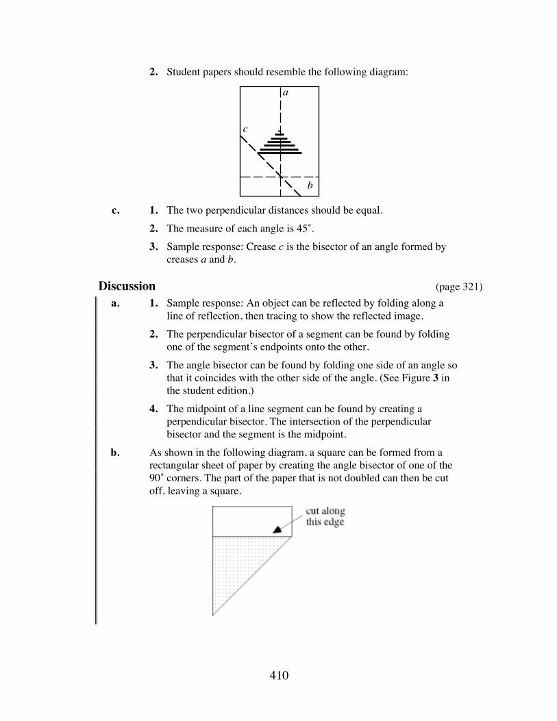
410

2. Student papers should resemble the following diagram:

c. 1. The two perpendicular distances should be equal.

2. The measure of each angle is 45˚.

3. Sample response: Crease c is the bisector of an angle formed by creases a and b.

Discussion (page 321) a. 1. Sample response: An object can be reflected by folding along a

line of reflection, then tracing to show the reflected image.

2. The perpendicular bisector of a segment can be found by folding one of the segment’s endpoints onto the other.

3. The angle bisector can be found by folding one side of an angle so that it coincides with the other side of the angle. (See Figure 3 in the student edition.)

4. The midpoint of a line segment can be found by creating a perpendicular bisector. The intersection of the perpendicular bisector and the segment is the midpoint.

b. As shown in the following diagram, a square can be formed from a rectangular sheet of paper by creating the angle bisector of one of the 90˚ corners. The part of the paper that is not doubled can then be cut off, leaving a square.

a

b

c

411

(page 321)

Activity 1 Students use the design of a star quilt to review the properties of angles formed from parallel lines cut by a transversal. They also examine the properties of a rhombus and explore how to create geometric rep tiles.

Materials List • straightedge (one per student) • pair of scissors (one per student) • copy of template B (one per student) • copy of template C (one per student)

Discussion 1 (page 322) a. Other than the eight-pointed star, students should recognize some

parallelograms—including rhombi—in the design. They may also mention other shapes, such as the octagon that can be made by connecting the star’s eight outer vertices.

b. 1. A parallelogram—specifically, a rhombus—is the basic shape used to construct the star.

2. A rhombus is a parallelogram with congruent sides. Note: You may want students to discuss the properties of parallelograms as well. In the following exploration, students should also discover these properties of a rhombus: opposite angles are congruent, the diagonals are perpendicular bisectors of each other, and the diagonals bisect the angles.

Exploration (page 322) Students use paper folding to form a rhombus and explore some of its properties. Although students also may complete this construction using a geometry utility, this activity is designed to reflect the historical methods used by quiltmakers. a. A square can be formed from a rectangular sheet of paper by creating

the angle bisector of one of the 90˚ corners. The part of the paper that is not doubled is then cut off. (See Part b of the discussion in the introduction.)

b. Student papers should resemble the shape shown in Figure 6b of the student edition.

c. As shown in Figure 7, the resulting shape is a rhombus.

412

d. 1. Students should not have to use protractors to measure these angles. The measure of each of the two smaller angles of the rhombus is the sum of two angles whose measures are:

1212• 90˚⎛

⎝ ⎜ ⎞

⎠ ⎟ = 22.5̊

The sum is therefore 45˚. The adjacent angles of the rhombus are supplementary to these 45˚ angles. Thus, each has a measure of 135˚. Note: Students should recall supplementary angles from middle school. You may wish to remind them of the definition, or to draw and measure a few such angles on a geometry utility.

2. The opposite angles of a rhombus (and, in general, a parallelogram) are congruent.

e. The diagonals of the rhombus are perpendicular bisectors of each other. As seen from the construction of this rhombus, the diagonals also bisect the interior angles.

f. 1. The midpoint of a line segment can be found by folding one of the segment’s endpoints onto the other to create the segment’s perpendicular bisector. The intersection of the perpendicular bisector and the segment is the midpoint.

2. Two congruent parallelograms are formed. Student papers should resemble the diagram below.

3. Student papers should resemble the following diagram.

g. Four smaller congruent rhombi are formed, each similar to the original

rhombus.

h. The measures of the interior angles of the smaller rhombi are the same as those of the original rhombus: 45˚ and 135˚.

Discussion 2 (page 324) a. Sample response: Yes, the shapes are similar to the original rhombus.

The corresponding sides are proportional and the corresponding angles are congruent. Note: You may want to ask students what information is necessary to determine if two rhombi are similar. If one angle of a rhombus is congruent to one angle of another rhombus, then the two rhombi are similar.

413

b. The two parallelograms are congruent. Since they are formed by joining the midpoints of opposite sides of a rhombus, the corresponding sides are congruent and the corresponding angles are congruent.

c. The diagonals of the rhombus are perpendicular bisectors of each other. As seen from the construction of the rhombus, the diagonals also bisect the interior angles.

d. 1. The opposite angles of a rhombus (and, in general, a parallelogram) are congruent. Adjacent angles are supplementary.

2. Sample response: One way to show congruence is to tear off the angles from the paper models and match them. Another way is to measure.

One way to show supplementary angles is to tear off the angles and place them together at the vertices. The non-adjacent sides will form a straight line.

Note: All of these methods are demonstrations. To prove that these relationships are true, students must work with congruent figures.

e. 1. The measures of angles 1 and 3 are equal. 2. The measures of angles 2 and 4 are equal. Angles 2 and 4 also

have the same positional relationship as angles 1 and 3 because they are two non-adjacent angles formed by two intersecting lines.

3. Vertical angles are two non-straight, non-adjacent angles formed by two intersecting lines.

4. Students should identify many pairs of vertical angles. In the diagram below, these pairs include ∠AOB and ∠EOF , ∠BOD and ∠FOH , ∠COD and ∠GOH , ∠AOD and ∠EOH .

f. The result will resemble the diagram below. Each smaller rhombus is

divided into four congruent rhombi. Each of these rhombi is similar to the original rhombus as well as the four intermediate rhombi from which they were formed.

A

B C D

E

FGH

O

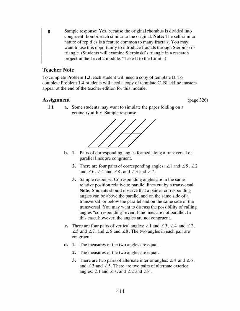
414

g. Sample response: Yes, because the original rhombus is divided into congruent rhombi, each similar to the original. Note: The self-similar nature of rep tiles is a feature common to many fractals. You may want to use this opportunity to introduce fractals through Sierpinski’s triangle. (Students will examine Sierpinski’s triangle in a research project in the Level 2 module, “Take It to the Limit.”)

Teacher Note To complete Problem 1.3, each student will need a copy of template B. To complete Problem 1.4, students will need a copy of template C. Blackline masters appear at the end of the teacher edition for this module.

Assignment (page 326) 1.1 a. Some students may want to simulate the paper folding on a

geometry utility. Sample response:

b. 1. Pairs of corresponding angles formed along a transversal of

parallel lines are congruent.

2. There are four pairs of corresponding angles: ∠1 and ∠5 , ∠2 and ∠6, ∠4 and ∠8 , and ∠3 and ∠7 .

3. Sample response: Corresponding angles are in the same relative position relative to parallel lines cut by a transversal. Note: Students should observe that a pair of corresponding angles can be above the parallel and on the same side of a transversal, or below the parallel and on the same side of the transversal. You may want to discuss the possibility of calling angles “corresponding” even if the lines are not parallel. In this case, however, the angles are not congruent.

c. There are four pairs of vertical angles: ∠1 and ∠3 , ∠4 and ∠2 , ∠5 and ∠7 , and ∠6 and ∠8 . The two angles in each pair are congruent.

d. 1. The measures of the two angles are equal.

2. The measures of the two angles are equal.

3. There are two pairs of alternate interior angles: ∠4 and ∠6 , and ∠3 and ∠5 . There are two pairs of alternate exterior angles: ∠1 and ∠7 , and ∠2 and ∠8 .

415

4. Sample response: Alternate interior angles are between the parallel lines and on opposite sides of a transversal. Alternate exterior angles are outside the parallel lines and on opposite sides of a transversal. With parallel lines, the respective pairs of angles are congruent. Note: You may want to discuss the fact that alternate interior angles formed when two nonparallel lines are cut by a transversal are not congruent. The alternate exterior angles in this situation are also not congruent.

1.2 a. Angle 1 and angle 3 are vertical angles. Angle 1 and angle 2 are supplementary angles. Angles 1 and 4 are also supplementary angles.

b. Sample response: Angles 1 and 5 are congruent because they are corresponding angles of two parallel lines cut by a transversal. Likewise, angles 1 and 13 are corresponding angles.

Angle 1 has the same measure as angle 9 because angle 9 and angle 5 are corresponding angles, or because angle 1 and angle 3 are vertical angles, while angle 3 and angle 9 are opposite angles of the rhombus.

c. Sample response: You only have to measure one angle to determine the measures of all of the angles at one vertex. Given the angles at one vertex, you can then determine the measures of all 16 angles in the diagram. Therefore, the measures of all the angles can be found if you measure just one angle.

d. Sample response: It would be necessary to measure four angles, one angle at each vertex.

*1.3 a. Students should observe that the two pieces are congruent. Some may want to cut the star along the line to compare pieces. Note: Students are not limited to existing lines in the design. They may draw any line that passes through the center of the star.

b. The two pieces have 180˚ rotational symmetry about the center of the star. They may also have symmetry about the line.

c. The two pieces will have 180˚ rotational symmetry about the center of the star for any line that passes through the center. If the line does not pass through the center and one of the outer vertices of the star, the pieces will not have symmetry with respect to the line.

d. Sample response: A line that passes through the center of the lone star design divides the star into two pieces that are the same size and the same shape. The two pieces are identical in design and are related by 180˚ rotational symmetry about the center of the star. Only those lines that pass through the center and one of the outer vertices of the star are lines of symmetry.

416

*1.4 a. Students may use lined notebook paper to help them draw sets of parallel lines. If the lines are perpendicular to the quilt strips, then the figures created are rectangles.

b. If the parallel lines are not perpendicular to the quilt strips, then the figures created are parallelograms.

c. 360˚ 8 = 45˚

d. Sample response: The quilter should draw a set of parallel lines that form 45˚ angles with the strips. To form rombi, these lines must be spaced the same distance apart as the vertical strips.

Cutting along these parallel lines would create strips of rhombi.

These new strips of material could then be shifted up or down one color and sewn to create the desired pattern. The eight large rhombi could then be cut from this new pattern. Note: Students should simulate this process using the paper template, scissors, and tape.

e. Sample response: The stitching may have been neither straight nor parallel. If the lines of stitches are not parallel, there is no guarantee that the corresponding angles will be congruent. As a result, the quilt may start to buckle or curl. To correct this, the seams would have to be taken out and re-sewn.

1.5 Student responses should resemble the following diagram:

Quadrilaterals

RhombiSquaresRectangles

ParallelogramsTrapezoids

417

1.6 a. The diagonals do not bisect each other and are not perpendicular. They are not equal in length unless the trapezoid is isosceles.

b. The diagonals are not perpendicular but they do bisect each other. They are not equal in length.

c. The diagonals are equal in length. They are not perpendicular but they do bisect each other.

d. The diagonals are the perpendicular bisectors of each other. They also bisect the interior angles. The diagonals are not equal in length.

e. The diagonals are equal in length. They are the perpendicular bisectors of each other and also bisect the interior angles.

1.7 a. Sample drawing:

b. Sample response: I started with a triangle, found the midpoints of

the sides, and connected them. This formed segments parallel to the corresponding sides of the original triangle and, in turn, four smaller triangles similar to the original. They are similar using the measures of corresponding and alternate interior angles as well as the sum of the measures of the angles of a triangle.

I then rotated the original triangle 180˚ about the midpoint of a side so

that the original and the image formed a parallelogram. To make the quilt pattern, I used groups of parallelograms in the same way that the rhombus is used in the lone star quilt in Figure 5.

* * * * *

418

1.8 Student responses may include some of the following methods.

1. Show that both pairs of opposite sides are the same length.

2. Show that both pairs of opposite sides are parallel.

3. Show that the diagonals bisect each other.

4 Show that both pairs of opposite angles are congruent.

5. Show that one pair of opposite sides is parallel and congruent.

1.9 Sample response: Measure the sides to determine if opposite sides have the same length. If they do, the quadrilateral is a parallelogram. Measure the diagonals to see if they are the same length. If they do, the parallelogram is a rectangle. Note: Students may also use the Pythagorean theorem to verify that the floor is a rectangle.

1.10 a. parallelogram, rhombus, rectangle, square

b. rhombus, square

c. rhombus, square

* * * * * * * * * * (page 330)

Activity 2 Students use medicine wheel designs to explore properties of tangents and secants. They also use the properties of a circle to create their own medicine wheels.

Materials List • copy of template D (one per student) • copy of template E (one per student)

• copy of template F (one per student)

• straightedge


419

Discussion 1 (page 331) a. The medicine wheel displays rotational and line symmetries.

b. Sample response: Half of the symbol in the center could be constructed and reflected to create the other half. The larger circle is a dilation of the smaller one with center at the center of the circle. The quadrilaterals between the two concentric circles are all rotational images of another about the center. Each feather along the bottom of the wheel might be considered a translated image of the feather on the far right.

Exploration (page 332) Students use a geometry utility to investigate properties of chords, secants, and tangents. (This exploration also can be completed with a compass and straightedge.)

a. For best results, the diameter of the circle should be at least two-thirds the width of the screen.

b. 1. See sample drawing given in Step 3 below.

2. Predictions may vary.

3. Sample drawing:

4–5. Students should observe that the perpendicular bisectors of chords

intersect at the center of the circle.

c. Students should observe that when the angle has a measure of 90˚, the line intersects the circle at a single point and is therefore a tangent line. The final sketch should resemble the following:

A

L

M

420

Teacher Note Before discussing Part d below, you may wish to distribute copies of template D (one per student).

Discussion 2 (page 333) a. 1. 90˚

2. The angle cannot measure 90˚.

b. Sample response: A line tangent to a circle can be created by first folding a circle onto itself through a line containing the center of the circle. This fold represents a secant containing a diameter. Next, without unfolding the first fold, fold the crease onto itself where the first fold intersects the circle. This second fold creates a tangent line perpendicular to a diameter, through the point of tangency.

c. Sample response: The tangents are parallel. Two lines in the same plane perpendicular to the same line must be parallel to each other because alternate interior angles are congruent.

d. Sample response: The center of the circular plate can be found by drawing two chords and their perpendicular bisectors as shown in the sketch below. The intersection of the perpendicular bisectors is the center of the circle.

e. Sample response: Fold to create two chords on the circle. Fold to

create the perpendicular bisector of each chord. The intersection of the perpendicular bisectors is the center of the circle.

f. The point of intersection of the perpendicular bisectors is the point equidistant from the four endpoints of the two chords. The center of a circle is the point that is equidistant from all points on the circle.

g. The altitude of an isosceles triangle is the perpendicular bisector of the base.

421

Teacher Note: Each student will need a copy of template E to complete Problem 2.3 and a copy of template F to complete Problem 2.4.

Assignment (page 334) 2.1 a–b. Student methods will vary, depending on the technology used.

Sample response: To draw each tangent, the radius containing both the point of the tangency and the center of the circle is constructed first. The tangent is then constructed as the line perpendicular to the radius and containing the point of tangency.

*2.2 a. The following sample response refers to the labeled points in the

diagram below: First, I constructed the circle with the larger radius. Then I constructed a point B on the circle. Point F was constructed by transforming B using a rotation of 60˚ around center A. Four more points were constructed using the same type of transformation for a total of six points. These form the vertices of a hexagon.

Next, I constructed the six sides of the hexagon (such as BF ) and the midpoints of each side (such as C). Then I drew the three segments connecting opposite pairs of midpoints (such as CE ). Finally, I constructed the circle with center A and radius CA .

O

AX

W

Y

Z

A

B

C

D

E

F

422

b. 1. The drawing has symmetry with respect to six lines: three that pass through the center of the circles and a pair of opposite vertices of the hexagon (such as B and D in the sample diagram above); and three that pass through the center of the circles and a pair of midpoints of the sides of the hexagon (such as C and E in the diagram above).

2. The drawing has rotational symmetry around the center of the circles for any rotation of n • 60˚ , where n is an integer.

*2.3 a–b. Students should find the center of the circle by constructing the perpendicular bisectors of at least two chords. Sample drawing:

c. Selections will vary. Your school may already have a mascot or

symbol.

d–e. Encourage students to be creative. They may want to display their wheels as a class.

423

2.4 a. Sample response: The center of the circle must be on the perpendicular bisector of C ʹ C because all points contained on it are equidistant from C and ʹ C .

b. Sample response: Draw the perpendicular bisector of C ʹ C and the perpendicular bisector of B ʹ B . Their point of intersection is the center of rotation O.

* * * * *

2.5 a. Since both chords include the center of the circle, they are diameters of the circle.

b. 1. Sample response: Since FI← → ⎯

and GH← → ⎯

are tangent to the circle at B and E, respectively, the measures of ∠JBA and ∠LEA are both 90˚. Since these two angles are congruent, they are alternate interior angles of the two parallel lines FI

← → ⎯

and GH← → ⎯

.

2. Using a similar argument to the one given above, students can show that FG

← → ⎯

and IH← → ⎯

are parallel.

c. Although angle measures may vary among constructions, students should observe that ∠KGP ≅ ∠CGE and ∠KGC ≅ ∠CFB . Sample response: ∠KGP and ∠CGE are vertical angles; ∠KGC and ∠CFB are alternate interior angles; and ∠KGP and ∠KGC are supplements.

d. Sample response:

Vertical Angles Alternate Interior and Exterior Angles

Corresponding Angles

∠BID ≅ ∠NIM ∠BID ≅ ∠IHL ∠NIM ≅ ∠DHL ∠MID ≅ ∠BIN ∠MID ≅ ∠DHE ∠NIB ≅ ∠DHE ∠EHQ ≅ ∠DHL ∠NIB ≅ ∠LHQ ∠MID ≅ ∠LHQ ∠EHD ≅ ∠QHL ∠NIM ≅ ∠EHQ ∠BID ≅ ∠EHQ

e. Sample response: All four segments are congruent. Allowing for

rounding errors, measurement supports this conjecture.

A

B

C

O

ʹ A

ʹ B

ʹ C

424

f. Sample response: Yes, GFIH is a rhombus because the lengths of FI , IH , HG, and GF are the same, FI is parallel to HG , and IH is parallel to GF .

2.6 a. They are congruent isosceles triangles.

b. 1. The two smaller angles are congruent. For example, consider the two angles formed by CB . Since CB is a radius, it is perpendicular to the tangent at B. The incoming angle and outgoing angle are congruent. The sum of the incoming angle and ∠ABC is 90˚, as is the sum of the measures of the outgoing angle and ∠DBC . Therefore, ∠ABC ≅ ∠DBC . A similar argument can be made at each of the other vertices.

2. angle bisector

c. Sample response: The outgoing angle at point B and ∠BDA are alternate interior angles, where BD

← → ⎯

is a transversal. Since both angles measure 60˚, the incoming ray and the tangent at point D must be parallel.

* * * * * * * * * * (page 339)

Activity 3 Students use Navajo sandpaintings—along with similar triangles—to explore dilations.

Materials List • template G (one copy per student) • template H (one copy per student)


Discussion 1 (page 339) a. Sample response: Ignoring the feathers on the head, the design

appears to have a vertical axis of symmetry. Some individual parts of the sandpainting also display line symmetry.

b. This design was constructed using two basic figures: rectangles and trapezoids.

425

c. Many of the geometric shapes which make up the sandpainting are similar to each other. For example, the trapezoids that make up the headdress are similar to each other and to the trapezoids that make up the hands, the arms, and the feet. These trapezoids are also similar to ones that form the garment worn around the waist of the figure, the design on the garment, and the tassels on the edge of the garment. The parallelograms that form the feathers in the headdress are similar to those that are found in the legs.

Exploration (page 340) In this exploration, students use similar triangles to explore the properties of dilations. a. Sample drawing:

b. Because corresponding sides are proportional and corresponding

angles are congruent, ΔPEA ~ ΔP ʹ E ʹ A . c. Students complete a sketch of the image of HEAD under a dilation

with center at P.

d. Dilations of polygons yield similar polygons. Angle measures and

parallelism are preserved. e. Sample response: Only the location of the image changes; its size

stays the same.

H E

D A

P

A'

E'

H E

DA

P

D'

H'A'

E'

426

f. Sample response: The lengths of the sides of the preimage, HEAD, would be reduced by a scale factor of 1 4 in the image, instead of 1 2 .

Discussion 2 (page 341) a. 1. The scale factor is 0.5.

2. The scale factor would be 0.25.

b. Changing the location of the center of dilation changes only the location of the image; it does not change the dimensions of the image.

c. Sample response: The image is larger than the original if the scale factor is greater than 1. For instance, in Part b of the exploration, ʹ E would be on PE but E would be between P and ʹ E .

d. Reflections, rotations, and translations are isometries because congruence is preserved. Although the measures of angles and the ratios between adjacent sides are preserved under dilations, they are not necessarily isometries. The preimage and image are congruent under a dilation only if the scale factor is 1.

Teacher Note To complete Problems 3.1 and 3.2, students will need copies of templates G and H. Blackline masters appear at the end of the teacher edition for this module.

Assignment (page 341) *3.1 Sample response:

427

*3.2 a. The line of reflection can be found by constructing the perpendicular bisector of a segment whose endpoints are corresponding points on the image and preimage (or by paper folding).

b. The center of rotation can be found by determining the

perpendicular bisectors of two segments whose endpoints are corresponding points on the image and preimage. The intersection of the perpendicular bisectors is the center of rotation.

428

c. The vector may be indicated by connecting any point and its image, in the direction from the preimage to the image.

d. The center of dilation can be found at the intersection of two lines connecting corresponding points on the image and preimage. The scale factor is approximately 2.

e. Two possible reflection lines are perpendicular to a line

connecting any point and its image. The distance between the reflection lines is half the distance between the point and its image.

429

3.3 a. To help students consider possible designs, you may wish to provide some reference materials.

b. You may prefer to ask students to give oral presentations.

* * * * *

Research Project (page 343) Students have many choices for both culture and historical period. Besides the examples listed in the student edition, several movements in modern and contemporary art make dramatic use of geometric shapes and lines.

3.4 The following table provides sample descriptions for each figure.

Figure Description of Transformation 2. Not an isometry and not similar. Not an obvious type of

transformation. 3. Not an isometry, but similar. Dilation using C as the

center. Scale factor appears to be 0.5. 4. Not an isometry, but similar. Dilation using A as the

center. Scale factor appears to be 3. 5. An isometry and therefore also similar. A translation by a

vector equivalent to the vector from F to G, with a length of approximately 4.3 cm, in a direction which can described as about 300˚, or a bearing of about 150˚, or approximately southeast.

6. Not an isometry, but similar. Two transformations: first a dilation identical to figure 3, then a reflection in the line containing DE .

7. An isometry and therefore also similar. A rotation of 90˚ about point B.

8. Not an isometry and not similar. Not an obvious type of transformation.

430

Answers to Summary Assessment (page 345) 1. a. Sample response: Parallel lines could be cut as shown in the

sketch below. The resulting strips can be shifted one color and re-sewn.

b. Answers will vary. Cutting the fabric along parallel lines creates

congruent corresponding angles. Re-aligning the new strips along the parallels creates the pattern of parallelograms.

2. a–b. Sample sketch:

c. The following sample response refers to the labeled points in the

diagram above: Since the transformation is a dilation, ΔABC ~ Δ ʹ A ʹ B C . Therefore, ∠BAC ≅ ∠ ʹ B ʹ A C . Since these are corresponding angles, AB is parallel to ʹ A ʹ B . A similar argument could be used for every pair of corresponding sides.

A

B

Cʹ A

ʹ B

431

3. a. The center of rotation can be found by constructing the perpendicular bisectors of segments connecting corresponding points on the image and preimage, as shown below.

b. Sample sketch:

Teacher Note To complete Problem 3 in the module assessment, each student will need one copy of template I.

angle of rotationcenter of

rotation

point of dilation(center of rotation)

432

Module Assessment

1. In the diagram below, line x is parallel to line y. Find the measure of

each labeled angle.

2. Find the center of the circle below. In a paragraph, describe the

procedure that you used.

62˚

58˚a

bc

d

e fgh

ijkl

x

y

433

3. The crossed arrows in the diagram below symbolize friendship in some traditional American Indian artworks.

Use a copy of this diagram to complete the following transformations. a. a dilation with center at point P and a scale factor of 1 4

b. a translation of the image found in Part a using the vector P ʹ P c. a reflection of the image found in Part b in a line containing P and ʹ P .

d. a 45˚ clockwise rotation of the image found in Part c about point P

P

ʹ P

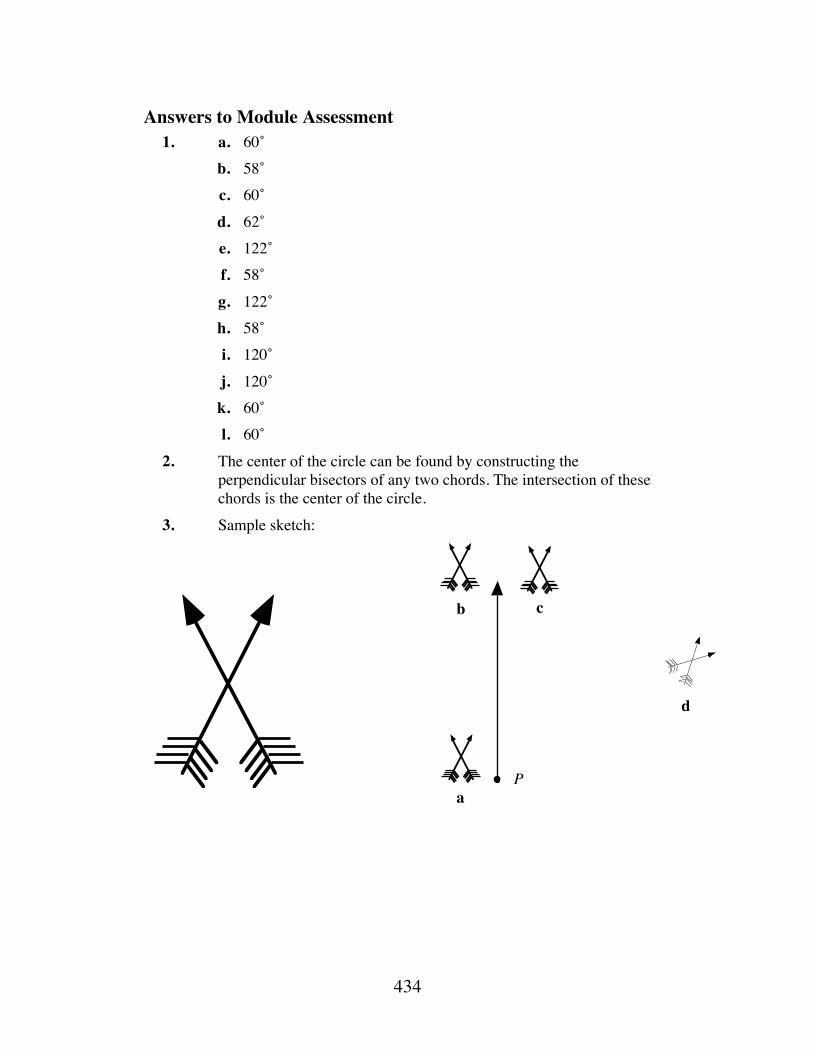
434

Answers to Module Assessment 1. a. 60˚

b. 58˚

c. 60˚

d. 62˚

e. 122˚

f. 58˚

g. 122˚

h. 58˚

i. 120˚

j. 120˚

k. 60˚

l. 60˚

2. The center of the circle can be found by constructing the perpendicular bisectors of any two chords. The intersection of these chords is the center of the circle.

3. Sample sketch:

a

b c

d

P

435

Selected References Better Homes and Gardens. American Patchwork and Quilting. Des Moines, IA:

Meredith Corporation, 1985. Bradkin, C. G. The Seminole Patchwork Book. Westminster, CA: Yours Truly

Inc., 1980. Britton, J., F. Lindstrom, V. Ochiro, and W. Peterson. “Medicine Wheels: the Art

and Culture of the Plains Indian.” Seattle, WA: Seattle Public Schools, 1983. ERIC ED 45 849.

Brown, P. “Native Americans: An Elementary Art Unit.” Washington, DC: U.S. Department of Education, 1978. ERIC ED 241 417.

Cordova, D. “The Navajo Way of Life: A Resource Unit with Activities for Grades 4–6.” Salt Lake City, UT: Salt Lake City School District, 1982. ERIC ED 235 962.

Gale, N. “Strong Tribal Identity Can Protect Native American Youth. How Can We Help?” Washington, DC: Native American Development Corporation, 1985. ERIC ED 329 391.

Lafarge, O. A Pictorial History of the American Indian. New York: Crown Publishers, 1956.

Nabakov, P., and R. Easten. Native American Architecture. New York: Oxford University Press, 1989.

Olson, A. T. Mathematics Through Paper Folding. Reston, VA: National Council of Teachers of Mathematics, 1972.

Storm, H. Seven Arrows. New York: Ballantine Books, 1972.

436

Flashbacks

Activity 1 1.1 Use the parallelogram in the diagram below to complete Parts a–e.

a. Name the interior angles of the parallelogram that are adjacent to

∠SRZ .

b. Name the interior angle of the parallelogram that is opposite ∠SRZ .

c. If ∠RZM ≅ ∠TZM , then ZS is called an .

d. If RM ≅ TM , then ZS is called a .

e. Identify a line of symmetry for the parallelogram.

1.2 Use a protractor to measure the following angles.

R S

TZ

M

a. b.

c. d.

437

Activity 2 2.1 Using the figure below as the preimage, sketch its image for each

transformation listed in Parts a–d.

a. a reflection

b. a rotation

c. a dilation

d. a translation

2.2 a. Draw a triangle ABC inscribed in a circle.

b. Draw a circle inscribed in a triangle ABC.

Activity 3 3.1 When are two objects similar?

3.2 Find the value of x in each of the following proportions.

a. 3x=610

b. 56=x36

3.3 Consider the two similar triangles below.

a. What is the value of the scale factor that creates triangle DEF from triangle

ABC?

b. What is the value of the scale factor that creates triangle ABC from triangle DEF?

24

14

12

A

B C

D

FE

16

21

18

438


Activity 1 1.1 a. ∠RST and ∠TZR

b. ∠ZTS

c. angle bisector

d. perpendicular bisector

e. line SZ or line RT 1.2 a. 30˚ b. 120˚

c. 90˚ d. 75˚

Activity 2 2.1 The diagram below shows a sample response for each transformation.

a.

b.

c.

d.

439

2.2 Sample sketches:

Activity 3 3.1 Sample response: Two objects are similar if the measures of

corresponding angles are equal and the lengths of corresponding sides are proportional.

3.2 a. x = 5

b. x = 30 3.3 a. 2 3

c. 3 2

a.

AB

C

b. AB

C

440

Template A

441

Template B

442

Template C

443

Template D

444

Template E

445

Template F

A

B

C

ʹ A

ʹ B

ʹ C

446

Template G

447

Template H

a

T

b

T

448

Template H (continued)

c

T

d

T

449

Template I

P'

P

If the Shoe Fits . . .

How can you tell when two quantities—like age and heart rate—are related? In this module, you explore methods for finding and evaluating mathematical models of some important relationships.

Byron Anderson • Ruth Brocklebank • Pete Stabio

453

Teacher Edition If the Shoe Fits . . .

Overview In this module, students explore methods of determining linear models for sets of data. Using data from exercise physiology, students are introduced to median-median lines and regression lines. They also use residual plots to evaluate models.


• use the sum of the absolute values of the residuals to compare how well linear models fit a set of data

• model data using the median-median line

• use the least-squares method to find a linear regression equation

• graph and analyze residual plots.


• how to identify graphs with positive or negative associations

• how to create scatterplots

• how to calculate residuals • how to determine the equation of a line in the form y = mx + b

• how to determine the median of a set of data.


Assessment Total

Days 2 3 2 1 8

454



graph paper X X X straightedge X X X

meterstick or measuring tape X



graphing utility X X X X spreadsheet X X X X

455

If the Shoe Fits…

Introduction (page 351) The module uses data from human physiology to introduce relationships that may be modeled mathematically.

Discussion (page 351) a. If the employee is paid by the hour, there is a positive association,

since the more the employee works, the more the employee earns. If the employee is not paid by the hour, there may be no relationship, since earnings are the same regardless of the number of hours worked.

b. Sample response: Since the taller players on the team typically play the forward positions and one of the main objectives of forwards is to score, there may be a positive association between height and the number of points scored. However, individual scoring depends on many factors other than height, so there may not always be a relationship.

c. Unless students are subject to certain travel restrictions, no relationship is likely. However, there is probably a positive association between the distance a student travels and the amount of time it takes the student to arrive at school.

d. The relationship between these two quantities is examined in later activities. Accidents are more likely for younger, novice drivers. They also become more likely for elderly drivers.

e. Sample response: Since students with high GPAs usually study, there may be a positive association between the number of hours spent studying and a student’s GPA. However, a student’s GPA may depend on many factors other than studying, so there may not always be a relationship.

(page 351)

Activity 1 In this activity, students find linear models for a set of data, determine the equations of their models, then calculate the sum of the absolute values of the residuals. Note: Students will examine the least-squares method in Activity 3. Both the sum of the absolute values of the residuals and the sum of the squares of the residuals are reasonable measures of how well a model fits the data. Developed by Carl Friedrich Gauss (1777–1855), the method of least squares is preferred by mathematicians.

456

Materials List • straightedge (one per student) • graph paper (one sheet per student)

Technology • spreadsheet • graphing utility

Exploration (page 352) Students fit lines to a set of data, then determine the equations of these lines. To evaluate their models, students calculate the sum of the absolute values of the residuals.

a. Sample scatterplot and line:

b. The equation of the sample line shown in Part a is y = 0.015x − 0.470

. c. Answers will vary, depending on the line. The following table shows the

sum of the squares of the residuals using the equation y = 0.015x − 0.470 .

x y predicted y residual 60 0.41 0.43 0.02 80 0.71 0.73 0.02

100 0.90 1.03 0.13 120 1.27 1.33 0.06 140 1.62 1.63 0.01 150 1.76 1.78 0.02 160 1.92 1.93 0.01 180 2.24 2.23 0.01 200 2.42 2.53 0.11

Sum 0.39

457

d. Students try to reduce the sum of the absolute values of the residuals by adjusting the slope and y-intercept of the model equation. For example, the equation y = 0.015x − 0.49 results in a lower sum of 0.29.

Discussion (page 353) a. Students should observe that an increase in heart rate is associated with

an increase in oxygen consumption. The relationship appears to be linear.

b. Answers may vary. Students may use residuals, sums of residuals, and visual criteria as justifications. Although a good model may not contain all the points of a scatterplot, it should approximate the general trend of the data.

c. Sample response: Yes, the line comes very close to most of the data points.

d. 1. The equation with the smallest sum of the absolute values of the residuals should have a slope of approximately 0.015 and a y-intercept of approximately –0.49.

2. Answers may vary. Some students may have adjusted either the slope or y-intercept, while others may have adjusted both.

e. 1. Students may suggest determining an estimate from the graph of the line or using the equation to calculate the y-value when x = 168.

2. Students may suggest determining an estimate from the graph of the line or using the equation to calculate the x-value when y = 1.5.

f. Answers will vary. Sample response: It is often dangerous to make predictions for values outside the observed data. For example, the domain and range of the model may be restricted in the real-world setting.

Teacher Note In the following assignment, students are asked to find linear models for data sets. For the sake of comparison, the sample responses given include the linear regression equation for each data set. Students will examine linear regression models in Activity 3. They are not expected to use these models in this assignment.

458

Assignment (page 354) 1.1 a. Sample scatterplot:

b. Answers will vary. Note: The linear regression equation for this data is y = −1.135x + 223.691 .

c. Answers will vary, depending on the equation from Part b. Using the equation y = −1.135x + 223.691 , the sum of the absolute values of the residuals is approximately 8.434.

d. Using the equation y = −1.135x + 223.691 , the suggested maximum heart rate for a person of age 15 would be about 207 beats/min.

e. Sample response: Using the linear model, the suggested maximum heart rate at age 3 is about 220 beats/min. This is the upper limit for the human heart. Therefore, it would probably be wise to use a different model for small children.

*1.2 a. Sample scatterplot:

y = −1.135x + 223.691

10 20 30 40 50 60 70

50

100

150

200

age (years)

Maximum Heart Rate vs. Age

beat

s/min

10

20

30

40

50 100 150 200

Oxygen Consumption vs. Heart Rate

afterbefore

heart rate (beats/min)

mL/

kg/m

in

459

b. Answers may vary. A possible equation for the “after” data is y = 0.186x + 4.128, while a possible equation for the “before” data is y = 0.12x + 9.403 .

c. Answers may vary. Using the equations from Part b, the model for the “before” data has a sum of the absolute values of the residuals of approximately 0.637, while the model for the “after” data has a sum of approximately 1.517. Therefore, the model for the “before” data appears to provide a better fit.

d. Using the sample equations from Part b, the predicted heart rate before an aerobic conditioning program is about 255 beats/min, while the predicted heart rate after an aerobic conditioning program is about 193 beats/min.

* * * * *

Teacher Note In Problems 1.3 and 1.4 (and again in Activities 2 and 3), the sample responses use x = 0 for the initial year. In Problem 1.3, for example, the first data point is (0,1049) rather than (1984,1049). Students may choose to use the actual year. You may wish to point out that, for a linear model, the slope is the same in either case, although the y-intercept is different.

*1.3 a. Sample scatterplot:

b. Answers will vary. Note: The equation of the regression line for

this data is y = 75.881x +1005.167 . A graph of this equation is shown on the scatterplot in Part a.

c. Using the equation from Part b, the sum of the absolute values of the residuals is approximately 260.9.

d. Using the equation from Part b, the predicted mean amount, per person, is approximately $2219.

460

1.4 a. Sample scatterplot:

b. Answers will vary. Note: The equation of the regression line for

this data is y = 0.276x + 60.645 .

c. Using the equation from Part b, approximately 68.9% of the population will participate in the work force in the year 2000.

d. Answers will vary. The sample prediction in Part c is only 0.2% higher than the prediction made by the Bureau of the Census.

* * * * * * * * * * (page 357)

Activity 2 Students explore the median-median line as a tool for modeling linear data.

Materials List • straightedge (one per student)

• graph paper (one sheet per student)

• meterstick or measuring tape (one per pair of students)



Teacher Note Some technology yields a median-median equation different from the one produced through the method described in the Mathematics Note.

461

Exploration (page 358) Students model the relationship between arm span and shoe size using a median-median line. Note: The differences between male and female shoe sizes appear to have little effect on the results of this exploration.

a. The sample data shown in the following table was gathered from a class of 32 students consisting of 17 girls and 15 boys.

Shoe Size Arm Span (cm) Shoe Size Arm Span (cm) 7.5 157 9 173 7.5 165 9 180 7.5 168 9.5 178 7.5 168 9.5 178 8 160 9.5 180 8 165 9.5 183 8 168 10 173 8 170 10 178 8.5 163 10 178 8.5 165 10 183 8.5 175 11 183 8.5 178 11 185 9 165 11.5 183 9 165 12 183 9 168 12 185 9 170 13 188

b. A scatterplot of the sample data is shown below.

462

c. The following table divides the sample data into three groups.

First Group Middle Group Third Group Shoe Size

Arm Span (cm)

Shoe Size

Arm Span (cm)

Shoe Size

Arm Span (cm)

7.5 157 9 165 10 173 7.5 165 9 165 10 178 7.5 168 9 168 10 178 7.5 168 9 170 10 183 8 160 9 173 11 183 8 165 9 180 11 185 8 168 9.5 178 11.5 183 8 170 9.5 178 12 183 8.5 163 9.5 180 12 185 8.5 165 9.5 183 13 188 8.5 175 8.5 178

d. The coordinates of the summary points for the sample data are

(8,166.5) , (9,175.5) , and (11,183) .

e. 1. Using the sample data given in Part a, the equation of the line determined by the first and third summary points is y = 5.5x +122.5.

2. Substituting the x-coordinate of the middle summary point into the equation from Step 1 gives the y-coordinate of the corresponding point on the line. For the sample data, the coordinates of this point are (9,172) .

3. Since the y-coordinate of the middle summary point is 175.5, the vertical distance between these points is 175.5 −172 = 3.5 . The coordinates of the point that is 1 3 the distance from the line are approximately (9,173.2).

4. Students should observe that this line has the same slope as the line in Step 1.

5. For the sample data, the equation of the median-median line is approximately y = 5.5x +123.7 .

Discussion (page 359) a. The median is considered a good representative value for a set of data.

It does not require complicated calculations, and is not as affected by outliers as other measures of central tendency.

b. Sample response: The median-median line provides a reasonable model. Although it does not contain all the points of the scatterplot, it describes the general trend of the data.

463

c. Sample response: The y-intercepts of the two lines differ by 1 3 of the vertical distance between the summary point of the middle group and the line containing the first and third summary points.

d. 1. Answers will vary. Using the median-median line for the sample data, the predicted arm span is 206 cm.

2. Sample response: An arm span of 206 cm is about 6 ft 9 in. This seems reasonable for someone who wears size 15 shoes.

Assignment (page 359) 2.1 a. Answers will vary. Using the sample equation given in the

exploration, Wadlow’s predicted shoe size is 30.

b. The sample prediction is substantially low. Depending on student estimates, this question may illustrate the dangers of making predictions far outside the range of collected data.

2.2 a. Since students may have used estimated values during their calculations for the median-median line, their results may not exactly agree with those reported by technology.

b. Sample response: The two lines are very close. The equation of the median-median line found using technology does not take significant figures into account.


b. Using 1985 as x = 0 , the equation of the median-median line is

approximately y = 24.4x + 21.5.

c. Judging from the scatterplot, the number of HIV-positive patients discharged from hospitals appears to be increasing linearly.

* * * * *

464



approximately y = 171x + 6663 . c. 1. Using the equation given in Part b, the estimated number of

self-employed workers in 1988 is 9741. 2. The estimated value is less than 2% from the actual value. 2.5 a. Sample scatterplot:


approximately y = 27.8x + 417 . c. Sample response: No, the median-median line does not appear to

be a very good model of the data. Many of the data points are relatively far from the line.

d. Sample response: No. After 1987, the scatterplot appears to level off. In fact, from 1988 to 1991, the increase in the annual number of cesarean births was 0.

* * * * * * * * * *

Self-Employed Workers

years after 1970

0

2000

4000

6000

8000

10,000

12,000

self-

empl

oyed

(in

thou

sand

s)

465

(page 361)

Activity 3 In this activity, students determine linear regressions and evaluate linear models using residual plots. Note: The term regression line originated in statistical studies of the heights of children of tall parents because it described how those heights “regressed” toward the mean height of the population.

Materials List • straightedge (one per student)

• graph paper (one sheet per student)



Teacher Note The least-squares method is used to generate equations for regression lines. The equations that students determine in Part d of Exploration 1 using a spreadsheet should approximate the linear regression.

Exploration 1 (page 361) Students use the arm span and shoe size data from Activity 2 to examine a linear regression model. This equation is then compared to the median-median line found in Activity 2.

a–b. Students recreate a scatterplot of the data for arm span vs. shoe size and determine the equation of a line that models the data reasonably well. (See sample graph in given in Part b of the exploration in Activity 2.)

c–d. Students determine the sum of the squares of the residuals for their model. They then adjust the equation until they find the least sum.

For the sample data given in Activity 2, the sum of the squares of the residuals for the regression line is approximately 718.2. In comparison, the sum of the squares of the residuals for the median-median line is about 795.1.

e. Answers will vary. The linear regression equation for the sample data is y = 4.8x +129.1 .

466

Discussion 1 (page 362) a. 1. Depending on the spread of the data, the median-median line may

or may not be close to the linear regression.

2. Students should find that the two equations are quite similar.

b. 1. Sample response: The two models would differ greatly when there are outliers in the data. The median-median line only takes into account the median of each group of data, while the linear regression considers the residuals of all data points. Therefore, the median-median line would tend to reflect only the pattern of the “middle” points.

2. Sample response: The two models would be approximately the same when the data is grouped relatively tightly about the middle data points.

c. Sample response: The linear regression would be better when you wish to consider all the data collected in your interpretation or predictions. Note: It should be pointed out to students that statisticians prefer the linear regression model.

Exploration 2 (page 363) Students investigate the use of residual plots as a tool for evaluating the appropriateness of a model.

a. Sample graph:

467

b. A completed table is shown below.

Heart Rate (beats/min)

Oxygen Consumption

(L/min)

Predicted Oxygen

Consumption

Residual

60 0.41 0.391 0.019 80 0.71 0.691 0.019

100 0.90 0.991 –0.091 120 1.27 1.291 –0.021 140 1.62 1.591 0.029 150 1.76 1.741 0.019 160 1.92 1.891 0.029 180 2.24 2.191 0.049 200 2.42 2.491 –0.071

c. The line y = 0.015x − 0.509 models the data well, as shown by the

graph in Part a.

d. As shown in the following residual plot, the residuals appear to be scattered randomly above and below the x-axis.

e. The following graph shows a scatterplot of the data in Table 5 along

with the line y = 0.02x −1 .

468

The table below shows the residuals that result using the model y = 0.02x −1 .

Heart Rate (beats/min)

Oxygen Consumption

(L/min)

Predicted Oxygen

Consumption

Residual

60 0.41 0.2 0.21 80 0.71 0.6 0.11

100 0.90 1 –0.1 120 1.27 1.4 –0.13 140 1.62 1.8 –0.18 150 1.76 2 –0.24 160 1.92 2.2 –0.28 180 2.24 2.6 –0.36 200 2.42 3 –0.58

The line y = 0.02x −1 does not model the data well. As shown in

the following residual plot, the residuals form a roughly linear pattern with a negative slope.

f. Students compare the residual plots for the two equations. In the

residual plot for the better model, y = 0.015x − 0.509 , the points are located closer to the x-axis and do not seem to form a recognizable pattern. Note: Although the equation y = 0.02x −1 does not model the data well, the shape of the residual plot is linear. This indicates that a linear model is probably a good one for the data.

Discussion 2 (page 365) a. Sample response: The equation y = 0.015x − 0.509 models the data

better. A graph of this line is very close to most of the points on the scatterplot.

b. Sample response: If the points of a residual plot have no definite pattern and are distributed fairly evenly above and below the x-axis, the linear model is probably appropriate for the data.

469

c. 1. The points of this residual plot appear to have a linear pattern. Therefore, another linear model may provide a better fit for the data.

2. The points of this residual plot form a curved pattern. In this case, a linear model is probably not appropriate. Note: Some students may recognize the shape of the residual plot as a parabola and therefore suggest a quadratic model.

3. The points of this residual plot appear to have no definite pattern and are distributed fairly evenly above and below the x-axis.

4. The points of this residual plot appear to form an exponential curve. This suggests that an exponential model may be more appropriate.

Teacher Note The use of some mathematical functions to model data involving time may be reasonable for relatively brief intervals, but may fail when applied to longer periods. For example, many relationships appear approximately linear only over short intervals. You may wish to point out the dangers of using such models to make predictions outside the range of the data.

Assignment (page 366) 3.1 a. Sample scatterplot:

b. Using 1970 as x = 0 , the equation of the regression line is

y = 0.197x + 71.698.

c. Using the equation from Part b, the life expectancy of people born in 1973 is approximately 72.2 years; the life expectancy of people born in 2010 will be approximately 79.6 years.

d. The life expectancy from Part c is 2 years more than that predicted by the U.S. Census Bureau.

470

*3.2 a. The following graph shows a scatterplot of the data as well as the regression line y = 1.129x − 0.655 .

b. Sample residual plot:

c. Sample response: The linear regression equation does not appear

to be an appropriate model for the data. The shape of the scatterplot appears to be curved, not linear. In addition, the residual plot shows a definite pattern. Note: Some students may recognize the shape of the parabola.

*3.3 a. Using 1970 as x = 0 , the equation of the regression line is y = −0.939x + 83.937 .

b. Sample residual plot:

c. Sample response: There is probably a better model for the data

than a line since the points of the residual plot appear to form a curve.

* * * * *

Energy Used while Walking

2 4 6 8

4

810

6

2

walking speed (km/hr)

kcal

/min

471

*3.4 a. Using 1984 as x = 0 , the equation of the regression line is y = 47.345x + 405.917 .

b. Using the equation from Part a, the predicted cost is about $1209. c. Sample residual plot:

d. Sample response: There is probably a better model for the data

than a line since the points of the residual plot appear to form a curve.

3.5 a. Using 1986 as x = 0 , the equation of a regression line that models the data is y = 1279.179x −111,410.893 .

b. Using the equation in Part a, the average yearly increase in the American work force is about 1,279,000 men and women.

c. Sample residual plot: d. Sample response: Since the residual plot appears to show a

pattern, a line is probably not an appropriate model for the data. e. The equation of the regression line for the data for females is

y = 819.429x + 49587.286 . According to this model, the average yearly increase in the number of females in the American work force is approximately 819,000. Since the residual plot appears to show a pattern, a line is probably not the best model for the data.

472

f. The equation of the regression line that models the data for males is y = 459.75x + 61823.607 . According to this model, the average yearly increase in the number of males in the American work force is approximately 460,000. Since the residual plot appears to show a pattern, a line is probably not an appropriate model for the data.

g. Sample response: The average increase in the number of males is

less than half as large as the average increase in the number of females. The average increase in total workers is the sum of the averages for males and females. Note: Students may also recognize that the regression equation for total workers is the sum of the two regression equations for males and females.

* * * * * * * * * *

473

Answers to Summary Assessment (page 369) 1. a. Sample scatterplot:

b. 1. The equation of the linear regression is y = 0.0264x − 0.0642.

2. The equation of the median-median line is y = 0.027x − 0.07 .

c. The sum of the squares of the residuals for the median-median line is 0.0042. The sum of the squares of the residuals for the regression line is 0.0019.

d. The following sample graph shows a residual plot for the median-median line.

The sample graph below shows a residual plot for the regression line.

474

e. Sample response: The equations for the median-median line and the regression line are extremely close. However, the regression line has a smaller sum of the squares of the residuals and a better residual plot. Therefore, the regression line appears to be a better model.

2. Student responses may vary. Some may argue for a linear model since the residuals for the regression line are relatively small. Others may argue against a linear model since the data points appear to follow a power curve and a residual plot reveals a noticeable pattern. In either case, students should support their arguments with graphs, equations, and residuals.

The equation for the regression line is y = −0.229x + 46.798 . The sum of the squares of the residuals for this model is 35.993.

The equation for the median-median line is y = −0.245x + 47.682 . The sum of the squares of the residuals for this model is 37.822.

The following graph shows a scatterplot of the data, along with both the regression line and the median-median line:

The graph below shows residual plots for these linear models:

475

Module Assessment

1. Health professionals often recommend walking as a good way to stay

fit. The table below shows some data for the amount of fat expended per minute of walking time.

Minutes of Walking Fat Expended (kcal/min) 0 0.7 5 1.8

10 1.9 20 2.8 30 3.2 40 3.4 45 3.5

Source: Adapted from Thomas and Londeree, “Calories Expended, Walking vs. Jogging,” The Physician and Sports Medicine 17 (May 1989): 98.

a. Make a scatterplot of the data. b. Find the regression line for the data. c. Find the median-median line for the data. d. Do the models from Parts b and c appear to be appropriate for the

data? Support your response using graphs, equations, and residuals. 2. The table below shows the domestic motor fuel consumption in the

United States for selected years from 1970 to 1991. Year Fuel Consumption (in billions of gallons) 1970 92.3 1975 109.0 1980 115.0 1981 114.5 1982 113.4 1983 116.1 1984 118.7 1985 121.3 1986 125.2 1987 127.5 1988 130.1 1989 131.8 1990 130.8 1991 128.6

Source: U.S. Bureau of the Census, 1995.

476

a. Make a scatterplot of the data. b. Find the regression line for the data. c. Find the median-median line for the data. d. Do the models from Parts b and c appear to be appropriate for the

data? Support your response using graphs, equations, and residuals. e. 1. Use one of your models to predict the motor fuel consumption

in 1993.

2. According to the Bureau of the Census, the actual motor fuel consumption in 1993 was 137.2 billion gallons. How does your prediction compare with this value?

3. The table below shows the annual milk production in the United States for selected years from 1980 to 1992.

Year Milk Production (n billions of pounds) 1980 128.4 1985 143.0 1988 145.2 1989 144.2 1990 148.3 1991 148.5 1992 151.8

Source: U.S. Bureau of the Census, 1995. a. Make a scatterplot of the data. b. Find the regression line for the data. c. Find the median-median line for the data. d. Do the models from Parts b and c appear to be appropriate for the

data? Support your response using graphs, equations, and residuals. e. 1. Use one of your models to predict the U.S. milk production in

1994.

2. According to the Bureau of the Census, the actual milk production in 1994 was 153.6 billion pounds. How does your prediction compare with this value?

477

4. The table below shows the numbers of job-related accidental deaths in the United States for selected years since 1960.

Year Deaths (in thousands) 1960 13.8 1965 14.1 1970 13.8 1975 13.0 1980 13.2 1984 11.5 1985 11.5 1986 11.1 1987 11.3 1988 11.0 1989 10.9 1990 10.6 1991 9.9


data? Support your response using graphs, equations, and residuals. e. 1. Use one of your models to predict the number of job-related

deaths in 1993.

2. According to the Bureau of the Census, the actual number of job-related deaths in 1993 was 9100. How does your prediction compare with this value?

478

5. The cost of health services and supplies has risen dramatically for Americans over the past 30 years. The table below illustrates the increase in total expenditures for medical care since 1970.

Year Total Expenditures for Health Services and Supplies (in billions of dollars)

1970 69.1 1980 238.9 1984 374.2 1985 407.2 1986 438.9 1987 476.9 1988 526.2 1989 583.2 1990 652.4 1991 728.6


data? Support your response using graphs, equations, and residuals.

479

Answers to Module Assessment 1. a. Sample scatterplot:

b. The regression line is y = 0.056x +1.272.

c. The median-median line is y = 0.055x +1.308 .

d. Both models appear to be reasonable for the data. The sum of the squares of the residuals for the regression line is 0.719, while the sum of the squares of the residuals for the median-median line is 0.722. As shown in the sample graph below, the residual plots also are very similar.

480

2. a. Sample scatterplot:

b. Using 1970 as x = 0 , the regression line is y = 1.790x + 95.171 .

c. Using 1970 as x = 0 , the median-median line is y = 1.856x + 94.261 .

d. Neither line appears to be an appropriate model. The sum of the squares of the residuals for the regression line is 91.88, while the sum of the squares of the residuals for the median-median line is 93.825. As shown in the sample graph below, the residual plots show a definite pattern. (The three “turning points” in the plots indicate that a polynomial of higher degree may be a more appropriate model.)

e. 1. Using the linear regression equation, the predicted fuel

consumption is approximately 136.3 billion gallons.

2. The prediction made above is approximately 900 million gallons less than the actual value.

481


b. Using 1980 as x = 0 , the regression line is y = 1.765x +130.335 .

c. Using 1980 as x = 0 , the median-median line is y = 1.606x +131.374 .

d. Both lines appear to be reasonable models. The sum of the squares of the residuals for the regression line is 24.868, while the sum of the squares of the residuals for the median-median line is 27.756. As shown below, the residual plots are similar.

e. 1. Using the linear regression equation, the predicted milk

production is approximately 155 billion pounds.

2. The prediction made above is approximately 1.4 billion pounds more than the actual value.

482


b. Using 1960 as x = 0 , the regression line is y = −0.130x +14.67 .

c. Using 1960 as x = 0 , the median-median line is y = −0.139x + 14.882 .

d. Both lines appear to be reasonable models, although some students may observe that the number of deaths seems to be decreasing more rapidly in the 1990s. The sum of the squares of the residuals for the regression line is 8.054, while the sum of the squares of the residuals for the median-median line is 9.328. As shown in the sample graph below, the residual plots are similar.

e. 1. Using the linear regression equation, the predicted number of

job-related deaths in 1993 is approximately 10,380.

2. The prediction made above is approximately 1280 more than the actual value.

years after 1960

2468

10121416

10 20 30 40

Numbers of Job-Related Deaths

thou

sand

s

483


b. Using 1970 as x = 0 , the regression line is y = 30.212x − 3.620.

c. Using 1970 as x = 0 , the median-median line is y = 41.350x −191.192 .

d. Neither line appears to be an appropriate model. The sum of the squares of the residuals for the regression line is 28,037, while the sum of the squares of the residuals for the median-median line is 74,668. The residual plots both show a definite pattern. Students may observe that an exponential equation may be a more appropriate model.

484

Selected References McArdle, W. D., F. I. Katch, and V. L. Katch. Exercise Physiology. Philadelphia:

Lea & Febiger, 1991. North Carolina School of Science and Mathematics, Department of Mathematics

and Computer Science. Contemporary Precalculus through Applications. Dedham, MA: Janson Publications, 1992.

Rodahl, K. The Physiology of Work. Bristol, PA: Taylor & Francis, 1989. Thomas, T. R., and B. R. Londeree. “Calories Expended, Walking vs. Jogging.”

The Physician and Sports Medicine 17 (May 1989): 98. U.S. Bureau of the Census, Statistical Abstract of the United States: 1995.

Washington, DC: U.S. Government Printing Office, 1995.

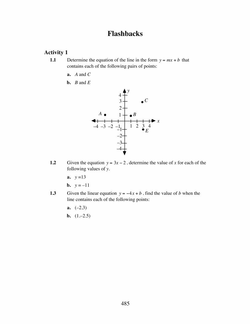
485

Flashbacks

Activity 1 1.1 Determine the equation of the line in the form y = mx + b that

contains each of the following pairs of points:

a. A and C

b. B and E

1.2 Given the equation y = 3x − 2 , determine the value of x for each of the

following values of y.

a. y =13

b. y = –11 1.3 Given the linear equation y = −4x + b , find the value of b when the

line contains each of the following points:

a. (–2,3)

b. (1,–2.5)

y

x 1 2 3 4–4 –3 –2 –1

1234

–1–2–3–4

A B

C

E

486

Activity 2 2.1 Find the median of the following set of numbers: {12, 45, 32, 81, 65,

24, 35, 26, 48, 50}.

2.2 Determine the equation of the line that passes through the points (−3, 4) and (6, −2) .

Activity 3 3.1 Determine the slope of the line that passes through each of the

following pairs of points:

a. (7,–4) and (2,–5)

b. (1,–2) and (4,–6).

3.2 Find the equation of the line in the form y = mx + b that contains each of the following pairs of points:

a. (1,1) and (5,5)

b. (1,–2) and (4,–6).

487


Activity 1

1.1 a. y =13x + 2

b. y = −1x + 2

1.2 a. x = 5 b. x = –3

1.3 a. b = –5 b. b = 1.5

Activity 2 2.1 The median is 40.

2.2 y = −23x + 2

Activity 3 3.1 a. 1 5

b. −4 3

3.2 a. y = x

b. y = −43x −

23

Take It to the Limit

What do hungry chickens, chain letters, and the perimeters of nested triangles have in common? This module introduces you to infinite sequences—and their limits.

Todd Fife • Mark Lutz • Lisa Wood

491

Teacher Edition Take It to the Limit

Overview In this module, students explore arithmetic and geometric sequences and series. They are introduced to limits through infinite geometric sequences and series.


• identify sequences that are arithmetic, geometric, or neither

• develop formulas for finite arithmetic and geometric series

• develop a formula for certain infinite geometric series

• explore limits graphically and geometrically.


• how to interpret subscript notation

• how to find explicit and recursive formulas for arithmetic sequences

• how to find explicit and recursive formulas for geometric sequences.


Assessment Total

Days 3 2 2 2 1 10



graph paper X

492



geometry utility X X graphing utility X

spreadsheet X X X X X symbolic manipulator X X X X X

493

Take It to the Limit

Introduction (page 375) In this introduction, students review arithmetic and geometric sequences along with explicit and recursive formulas.

Discussion (page 375) a. 1. This is an arithmetic sequence. The first term is 7 and the common

difference is 6. The next term is 31.

2. This is a geometric sequence. The first term is 162 and the common ratio is 1 3 . The next term is 2.

3. Sample response: This is a sequence of figures. Each figure is a set of dots forming a right triangle with n dots on each leg and on the hypotenuse, where n is the figure number. The next figure is:

4. This is a geometric sequence. The first term is –7 and the common

ratio is –7. The next term is –16,807.

5. This is a sequence of closed intervals. The left-hand value of the interval is always 2, while the right-hand value is 2 + 1 n( ) , for n = 1, 2, 3, 4, … . The next interval is [2, 2.2].

6. This is a Fibonacci sequence. The first two terms are 4 and 5. Each successive term is the sum of the previous two terms. The next term is 37.

b. A sample formula for each sequence shown below.

1. a1 = 7an = an−1 + 6 for n >1⎧ ⎨ ⎩

2. a1 =162

an = an−1 1 3( ) for n > 1⎧ ⎨ ⎩

3. Although it is not possible to write a recursive formula for the sequence of figures, the number of dots in each figure can be described as follows:

a1 =1an = an−1 + n, n >1⎧ ⎨ ⎩

494

4. a1 = −7an = −7an −1 for n > 1⎧ ⎨ ⎩

5. A recursive formula for the right-hand value in each interval is shown below:

a1 = 3

an = an−1 −1

n(n − 1) for n > 1

⎧ ⎨ ⎩

6. a1 = 4a2 = 5an = an−2 + an−1 for n > 2

⎧

⎨ ⎪

⎩ ⎪

c. A sample formula for each sequence shown below.

1. an = 7 + 6(n −1) for n ≥ 1

2. an =162 1 3( )n−1 for n ≥1

3. Although it is not possible to write an explicit formula for the sequence of figures, the number of dots in each figure can be described as follows:

an =n(n +1)2

4. an = −7 −7( )n−1 for n ≥1

5. An explicit formula for the right-hand value in each interval is shown below:

bn = 2 +1n, n >1

6. Determining an explicit formula for this sequence is beyond the scope of this module.

d. 1. The sequence in Step 1 is arithmetic.

2. The sequences in Steps 2 and 4 are geometric.

e. Sample response: The common difference of an arithmetic sequence can be found by subtracting any term from the following term.

f. Sample response: The common ratio of a geometric sequence can be found by dividing any term by the previous term.

495

(page 376)

Activity 1 This activity continues the review of arithmetic and geometric sequences, as well as recursive and explicit formulas. Note: These concepts were introduced in the Level 1 module “From Rock Bands to Recursion.”


Technology • spreadsheet (optional)

• symbolic manipulator (optional)

Exploration (page 377) This exploration is designed for groups of four students. To ensure equal participation, each student should create a sequence, and each group should pass in a consistent clockwise or counterclockwise rotation.

The following responses describe a sample game.

a. The first student creates an arithmetic sequence with a common difference of –2 and a first term of 20. The student writes down the first five terms—20, 18, 16, 14, 12—and passes the sheet of paper to the second student.

b. The second student identifies the sequence as arithmetic and writes this below the first five terms. The student then writes the following rule: “To make this sequence, start with 20 and add –2 (or subtract 2) every time to get the next term.”

c. The third student uses this algorithm to write the recursive formula a1 = 20an = an−1 + (–2) for n ≥1⎧ ⎨ ⎪

⎩ ⎪

and the explicit formula an = 20 + (−2)(n −1) for n ≥1 .

d. The fourth student uses these formulas to write the first five terms of the sequence: 20, 18, 16, 14, 12.

e. The first student compares the sequence written by the fourth student with the original sequence. (If the terms do not match, the group should examine the paper and identify the source of the mistake.)

496

Discussion (page 377) a. Responses will vary. b. Sample response: For arithmetic sequences, the difference between

consecutive terms must be the same. For geometric sequences, the ratio of any two successive terms must be the same. A sequence that does not have a common ratio or a common difference between successive terms is neither arithmetic nor geometric.

c. 1. If the sequence is arithmetic with a common difference of 1, the next three terms will be 4, 5, 6.

2. If the next term in the sequence is the sum of the two previous terms, then the next three terms will be 5, 8, 13.

3. If the next term in the sequence is the sum of the previous three terms, then the next three terms will be 6, 11, 20.

d. Sample response: Yes. Since the sequence is defined as arithmetic, then there must be a common difference and the next three terms would follow the same pattern.

Assignment (page 378) 1.1 a. The first five terms are 9, 6, 3, 0, –3. b. The first five terms are –5, –6.5, –8.45, –10.985, –14.2805. 1.2 a. 99 = 11+ 2(n −1)⇒ n = 45

b. 6.5536 = 20(0.8)n −1⇒ n = 6

c. 357 = 7 + 3.5(n − 1)⇒ n = 101

d. 3072 = 3(2)n−1 ⇒ n =11

*1.3 a. 1. Two possible terms are 63, 127.

2. The explicit formula is an = 2n −1 for n ≥1 . The recursive formula is:

a1 =1

an = an−1 + 2n−1 for n >1⎧ ⎨ ⎩

3. The sequence is neither arithmetic nor geometric. b. 1. Two possible terms are –2 25, 2 125 .

2. The explicit formula is gn = –50(–1 5)n−1 for n ≥1 . The recursive formula is:

g1 = –50gn = (–1 5)gn−1 for n >1⎧ ⎨ ⎩

3. The sequence is geometric.

497

c. 1. Two possible terms are 13, 16.

2. The explicit formula is an =1 + 3(n −1) for n ≥ 1. The recursive formula is:

a1 =1an = an−1 + 3 for n > 1⎧ ⎨ ⎩

3. This is an arithmetic sequence.

d. 1. Two possible terms are 2 16 , 2 1

7 .

2. The explicit formula is:

an = 2 +1

n +1 for n ≥ 1

The recursive formula is:

a1 = 2 12

an = an−1 −1

n(n +1) for n > 1

⎧

⎨ ⎪

⎩ ⎪

3. This sequence is neither arithmetic nor geometric.

e. 1. Two possible terms are 6, –6.

2. The explicit formula is an = 6(–1)n−1 for n ≥ 1 . The recursive formula is:

a1 = 6an = –1(an −1) for n > 1⎧ ⎨ ⎩

3. This sequence is geometric.

1.4 a. Any geometric sequence with a common ratio of 1 is also an arithmetic sequence with a common difference of 0. For example, the following sequence is both arithmetic and geometric:

π , π , π, π, π , …

b. An explicit formula for the sample sequence given in Part a is an = π + 0(n −1) for n ≥1 .

c. An explicit formula for the sample sequence given in Part a is gn = π • (1)n−1 for n ≥1 .

498

1.5 a. The common difference can be found by solving the following equation:

93 =13 + d(50 −1)d = 80 49

b. The common ratio can be found by solving the equation below:

192 = 12 • r 5−1

r = ±2

c. The common difference is 3 and the number of terms is 18.

d. The common ratio is 5 and the number of terms is 10.

1.6 Sample response: The dog’s mass would be 43.2 kg. If the dog’s loss of mass is actually an arithmetic sequence, then the dog would lose 0.9 kg per month for 12 months—a total of 10.8 kg. Depending on the size of the animal, this might not be reasonable. The veterinarian would not let the dog’s mass fall below a healthy level.

1.7 a. Sample response: If the mass of a chick is 36 g when hatched, and it gains 10% of its mass each day for 8 weeks, then its daily mass is a geometric sequence with the following formula: gn = 36 • 1.1

n−1 . After 56 days, the chick’s mass would be about 6.8 kg.

b. This is probably not reasonable. Students may know from experience that the mass of a broiler chicken is typically under 2 kg. According to most poultry growers, the mass of an 8-week-old chicken should be about 43 times its mass at birth, or about 1548 g.

c. The advertiser should claim a 7% daily mass gain.

1.8 The following sample responses assume that the first term is positive.

a. If the common ratio is between –1 and 0, then the sequence will alternate between positive and negative terms and will get progressively closer to 0.

b. If the common ratio is between 0 and 1, then the sequence will get progressively closer to 0.

c. If the common ratio is less than –1, then the sequence will alternate between positive and negative terms. The absolute value of the terms will get progressively larger.

d. If the common ratio is greater than 1, the terms of the sequence will get progressively larger.

* * * * *

499

*1.9 a–b. Students generate sequences by paper folding.

c. The explicit formula for the area of the top surface (in cm 2 ) is gn =128 • (0.5)n −1 for n ≥ 1. The recursive formula for the area of the top surface is:

g1 =128gn = gn−1 • 0.5 for n >1⎧ ⎨ ⎩

d. The explicit formula for the number of layers is gn = 2 • 2n −1 for n ≥1. The recursive formula for the number of layers is:

g1 = 2gn = gn−1 • 2 for n >1⎧ ⎨ ⎩

e. As the number of folds increases, the area of the top surface appears to approach 0 cm 2 .

f. As the number of folds increases, the number of layers becomes larger and larger.

1.10 a. The sheet of paper would have to have an area of about 5.6 • 101 4 cm 2 . Its dimensions would be about 2.4 •107 cm (or 240 km) on each side.

b. Answers will vary, depending on the thickness of the paper. If a single layer were 0.1 mm thick, the height of the stack after 50 cuts would be about 1.1•108 km.

1.11 a. This is a Fibonacci sequence with the first two terms equal to 1. It is neither arithmetic nor geometric.

b. This is a geometric sequence with a common ratio of 1.05 and a first term of 2.

c. This is an arithmetic sequence with a common difference of –1000 and a first term of 2000.

d. This sequence (0, 1, 3, 6, 10, 15, 21, …) is neither arithmetic nor geometric. The pattern can be described by the recursive formula.

e. This sequence is neither arithmetic nor geometric. The first term is 3 1. In each successive term, the numerator remains constant at 3 and the denominator increases by 1.

1.12 a. The terms increase without bound. b. The terms increase without bound. c. The terms decrease without bound. d. The terms increase without bound. e. The terms approach 0.

* * * * * * * * * *

500

(page 381)

Activity 2 This activity introduces students to finite arithmetic series and their expanded form.


Technology • spreadsheet (optional)


Exploration (page 382) a. 1. Sample response:

S1000 = 1 + 2 + ! + 999 + 1000S1000 = 1000 + 999 + ! + 2 + 1

2S1000 = 1001 + 1001 + ! + 1001 + 1001 Since there are a total of 1000 terms of 1001:

S1000 =1000 • 1001

2= 500, 500

2. Sample response:

Sn = n + (n −1) + ! + 2 + 1Sn = 1 + 2 + ! + (n −1) + n

2Sn = (n +1) + (n +1) + ! + (n +1) + (n +1)

Since there are a total of n terms of (n +1) :

Sn =n • (n +1)

2

b. Sample response:

S5 0 = 2 + 4 + ! + 998 + 100S5 0 = 100 + 998 + ! + 4 + 2

2S5 0 = 102 + 102 + ! + 102 + 102 Since there are a total of 50 terms of 102:

S50 =50 • (102)

2= 2550

501

c. Using the explicit formula for an arithmetic sequence, a75 = 2 + (75 −1) • 4 = 298 . Given this value, students should use a method like the one employed in Parts a and b:

S7 5 = 2 + 6 + ! + 294 + 298S7 5 = 298 + 294 + ! + 6 + 2

2S7 5 = 300 + 300 + ! + 300 + 300

Since there are a total of 75 terms of 300:

S75 =75• (300)

2=11,250

d. 1. a2 = a1 + d, a3 = a1 + 2d , a4 = a1 + 3d

2. an = a1 + (n −1) • d , an−1 = a1 + (n − 2) • d , an− 2 = a1 + (n − 3) •d , an− 3 = a1 + (n − 4) • d

3. Using a method like the one employed in Parts a and b:

Sn = a1 + a1 + d[ ] + ! + a1 + (n − 2)d[ ] + a1 + (n −1)d[ ]Sn = a1 + (n −1)d[ ] + a1 + (n − 2)d[ ] + ! + a1 + d[ ] + a1

2Sn = 2a1 + (n −1)d[ ] + 2a1 + (n −1)d[ ] + ! + 2a1 + (n − 1)d[ ] + 2a1 + (n −1)d[ ]

Since there are a total of n terms of 2a1 + (n −1)d[ ]:

Sn =n • 2a1 + (n −1)d[ ]

2= na1 +

n • (n − 1)d[ ]2

Discussion (page 383) a. The equation below

Sn =n22a1 + (n −1) • d[ ]

can be expanded as follows:

Sn =n2a1 + a1 + (n −1)• d[ ]

Since an = a1 + (n −1) • d , students can make the following substitution:

Sn = n2(a1 + an )

b. The sequences in Parts a and b are arithmetic sequences because there is a common difference between consecutive terms.

502

c. 1. Sample response: The sum of the first 100 even numbers should be twice the sum of the first 100 natural numbers because:

2 + 4 + 6 +!+ 200 = 2(1 + 2 + 3 +!+100) = 2(5050) = 10,100

2. The sum of the first 100 multiples of k can be found as follows:

k + 2k + 3k +!+ 99k +100k = k(1 + 2 + 3 +!+ 99 + 100)

= k100(101)2

= 5050k

d. Sample response: If the common difference is positive, the sum of the infinite arithmetic series will increase without bound. If the common difference is negative, the sum of the infinite arithmetic series will decrease without bound.

Assignment (page 383) 2.1 The sum of the first n even numbers can be found as follows:

Sn =n2(2 + 2n)

=n2• 2(1 + n)

= n(n +1)

2.2 Student methods may vary. Using the formula from Part a of the exploration:

Sn =n(n +1)2

=2000(2000 +1)

2= 2, 001,000

2.3 a. Sample response:

k + 2k + 3k +!+ (n − 1)k + nk = k(1+ 2 + 3 +!+ (n −1) + n)

= kn(n +1)2

b. The sum can be found as follows: 3(600)(600 +1)

2= 540, 900

*2.4 a. The first term of the sequence is 3. b. The common difference is 4.

c. Using the explicit formula for an arithmetic sequence: 451 = 3 + 4(n −1)113 = n

503

d. The sum is the finite arithmetic series 3 + 7 +11+! + 451. Using the formula for an arithmetic series:

S113 =1132(3 + 451) = 25, 561

2.5 Sample response: No, because the sum of each pair of numbers is not constant. For example, given the sequence 32, 16, 8, 4, 2, 1, the sums of the pairs are 33, 18, 12, 18, and 33.

*2.6 a. Sample response: The monthly payments may be considered an arithmetic sequence where the first term is $106.26 and the common difference is $106.26.

b. Sample response: Yes. Since the payments themselves form an arithmetic sequence, their indicated sum forms an arithmetic series.

c. The lessee pays $150.00 + $1,600.00 + (36 • $106.26) or $5575.36, of which $150.00 is refunded at the end of the lease.

d. Sample response: The difference of $3312.64 may be the cost to purchase the car at the end of the lease. Or it may be that the car costs an additional $8,888.00 at the end of the lease.

* * * * * 2.7 The number of newspapers delivered each week forms an arithmetic

sequence where a1 =15, 000 and d = 50. Using the formula for an arithmetic series:

S52 =522(2 •15, 000 + 51• 50) = 846,300

2.8 a. The first three terms are –2, 3, 8. b. a150 = −2 + 5 149( ) = 743

c. S150 =1502(−2 + 743) = 55,575

2.9 a. S41 =412(5 +120) = 2562.5

b. Using the general formula for an arithmetic sequence, solve 120 = 5 + 40d and the common difference is 2.875.

c. The second and third terms of the sequence are 7.875 and 10.75. * * * * * * * * * *

504

(page 385)

Activity 3 In this activity, students develop an algorithm for finding the sum of the terms of a finite geometric sequence.

Materials List • graph paper (two sheets per student)



Exploration (page 385) a. The number of e-mail warnings sent is 6.

b. Since 6 people send 3 e-mail warnings each, the second group consists of 6 • 3 =18 people. If all decide to participate, the number of e-mail warnings sent is 18.

c. The number of e-mail warnings sent at the third stage is 54, at the fourth stage is 162, and at the fifth stage is 486.

d. The number of e-mail warnings sent at each stage forms the following geometric sequence: 6, 18, 54, .. ., 6 • 3199.

e. The following geometric series (equation 1) represents the total number of warnings sent:

S200 = 6 +18 + 54 +!+ 6 • 3197 + 6 • 3198 + 6 • 3199

f. 1. Multiplying both sides of the equation above by 3 yields equation 2:

3S200 = 18 + 54 +162 +!+ 6 • 3198 + 6 • 3199 + 6 • 3200

2. Subtracting equation 1 from equation 2 as shown below:

3. Solving for S200, the number of e-mail warnings sent is:

S200 =6 • 3200 − 6

2≈ 7.96842 •1095

3S200 = 18 + 54 +!+ 6 • 3197 + 6 • 3198 + 6 • 3199 + 6 • 3200

−(S200 = 6 +18 + 54 +!+ 6 • 3197 + 6 • 3198 + 6 • 3199)2S200 = 6 •3200 − 6

505

g. Student answers may vary, but the general formula should appear as follows:

S =g1r n − g1r −1

=g1 (rn −1)r −1

Discussion (page 386) a. Sample response: If every recipient continues to e-mail warnings to

three of their friends, we would expect to send approximately 7.96842 •1095 e-mail warnings. This is not reasonable, since it far exceeds the earth’s population.

b. Sample response: If the virus is a hoax and people e-mail all their friends, the number of e-mail messages can quickly overload servers. This can stop the e-mail or at least slow it down. Whenever you receive an e-mail warning of a computer virus, check with web sources first to insure the warning is legitimate.

c. Answers may vary, but the general formula should appear as follows:

S = g1rn − g1r −1

=g1 (rn −1)r −1

Note: Some students may have obtained the equivalent form shown below (found by multiplying both the numerator and the denominator by –1):

S = g1(1 − rn )

1− r

d. Sample response: If r equals 1, the denominator in the formula is 0. This makes the value of the fraction undefined.

e. 1. Sample response: Sn = 41 + 42 + . . . + 4n −1 + 4n 2. Sample response: If r is 1, then each term is equal to the first term,

and the sequence is arithmetic with a common difference of 0. The sum of n terms can be found as follows: Sn = n • g1 .

f. 1. These are equivalent by using the distributive property and factoring out g1.

2. These are equivalent by factoring out r from g1rn and substituting gn for g1r

n−1 .

g. Sn = g1r 0 + g1r1 + g1r 2 + ... + g1rn −2 + g1r n−1

so

rSn = g1r0 + g1r

2 + g1r3 + ... + g1r

n−1 + g1rn

− Sn = g1r 0 + g1r1 + g1r2 + ... + g1r n−2 + g1rn−1( )rSn − Sn = g1r

n − g1r0

Sn r −1( ) = g1r n − g1

Sn =g1r n − g1r −1

=g1 rn − 1( )r −1

506

Assignment (page 387)

3.1 a. S17 =(3.5)(0.6)17 − 3.5

0.6 −1≈ 8.75

b. S10 =(10)(10)10 − 10

10 −1=11,111,111,110

3.2 a. S = (6.5536)(0.8) − 200.8 −1

≈ 73.79

b. S = (3072)2 − 32 −1

= 6141

3.3 a. This is an arithmetic series.

S45 =45211+ 99( ) = 2475

b. This is an arithmetic series.

S7 =722 + −28( )( ) = −91

c. This series is neither arithmetic nor geometric.

S6 =1903140

≈13.59

d. This is a geometric series.

S5 =

12• 12⎛ ⎝ ⎞ ⎠

5

−12

12−1

=3132

≈ 0.97

*3.4 a. Sample response: When the tortoise has run 1.11111 m, six time intervals have elapsed since 1.11111 = 1 + 0.1+ 0.01 + 0.001 + 0.0001 + 0.00001

b. To determine the total distance Achilles covered, I could multiply the distance covered by the tortoise by 10, or use the formula for a finite geometric series:

S6 =10(0.1)6 −100.1 −1

⎛

⎝ ⎜ ⎞

⎠ =11.1111

c. Sample response: No, with its 10-m head start, the tortoise is 11.11111 m from Achilles’ starting point. After six time intervals, Achilles has only traveled 11.1111 m. He is still 0.00001 m behind.

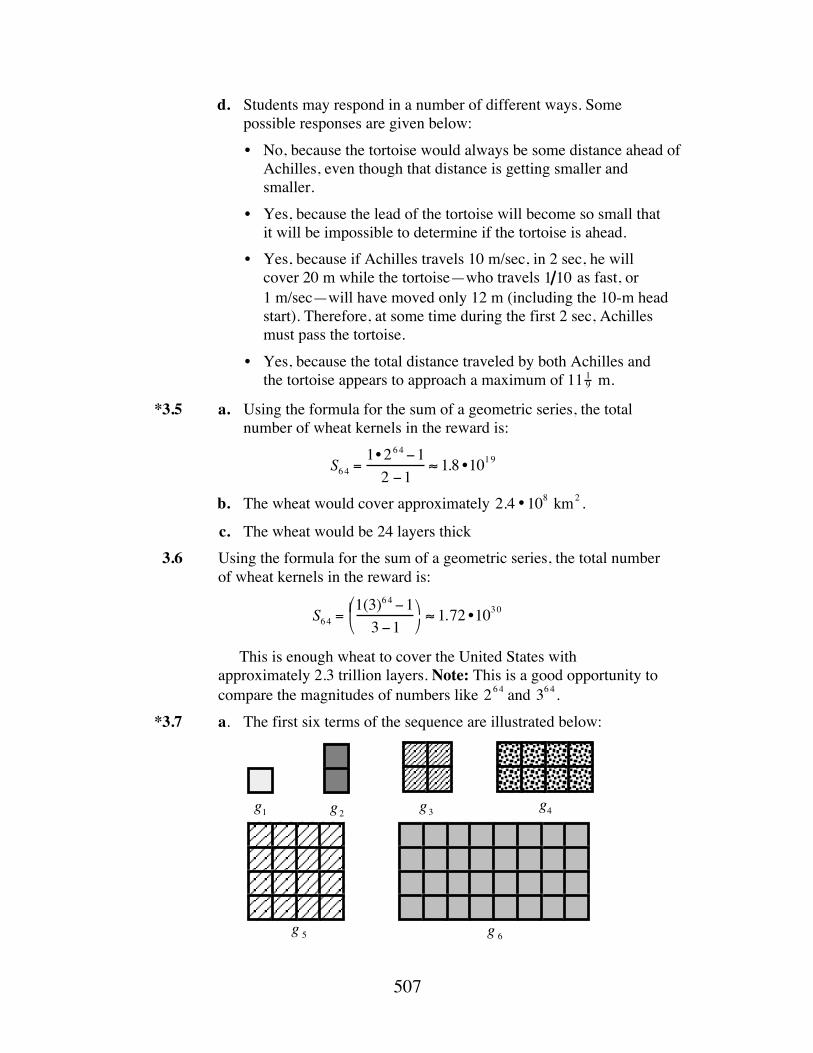
507

d. Students may respond in a number of different ways. Some possible responses are given below:

• No, because the tortoise would always be some distance ahead of Achilles, even though that distance is getting smaller and smaller.

• Yes, because the lead of the tortoise will become so small that it will be impossible to determine if the tortoise is ahead.

• Yes, because if Achilles travels 10 m/sec, in 2 sec, he will cover 20 m while the tortoise—who travels 1 10 as fast, or 1 m/sec—will have moved only 12 m (including the 10-m head start). Therefore, at some time during the first 2 sec, Achilles must pass the tortoise.

• Yes, because the total distance traveled by both Achilles and the tortoise appears to approach a maximum of 11 19 m.

*3.5 a. Using the formula for the sum of a geometric series, the total number of wheat kernels in the reward is:

S64 =1• 264 −12 −1

≈ 1.8 •1019

b. The wheat would cover approximately 2.4 •108 km2 .

c. The wheat would be 24 layers thick

3.6 Using the formula for the sum of a geometric series, the total number of wheat kernels in the reward is:

S64 =1(3)64 −13 −1

⎛

⎝ ⎜ ⎞

⎠ ≈ 1.72 •1030

This is enough wheat to cover the United States with approximately 2.3 trillion layers. Note: This is a good opportunity to compare the magnitudes of numbers like 264 and 364.

*3.7 a. The first six terms of the sequence are illustrated below:

g2 g3g1 g4

g 5 g 6

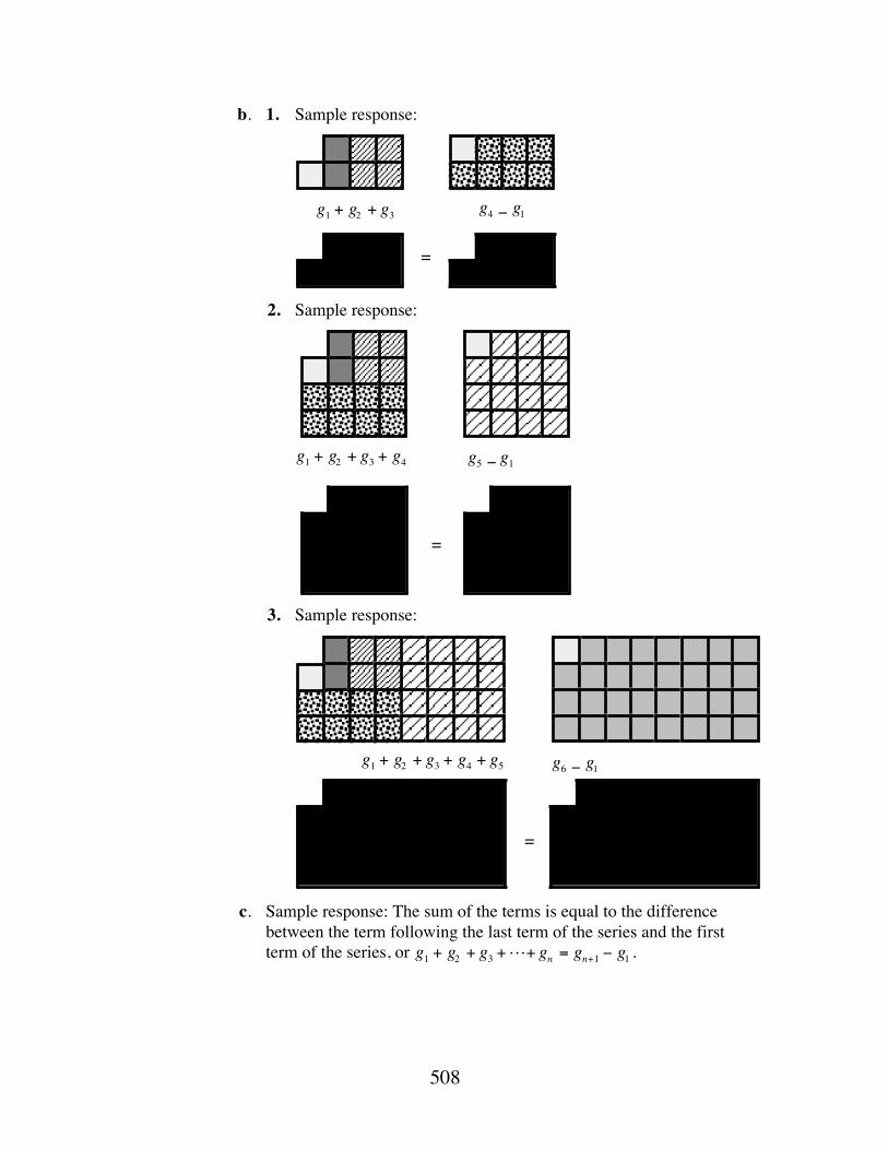
508

b. 1. Sample response:

2. Sample response:

3. Sample response:

c. Sample response: The sum of the terms is equal to the difference

between the term following the last term of the series and the first term of the series, or g1 + g2 + g3 +!+ gn = gn+1 − g1 .

g4 − g1

=

g1 + g2 + g3

g5 − g1

=

g1 + g2 + g3 + g4

g1 + g2 + g3 + g4 + g5 g6 − g1

=

509

d. Sample response: The sum of a geometric series can be found using the formula:

Sn =gnr − g1r −1

In this series r is 2. By substituting 2 for r, the formula becomes:

Sn =gn (2) − g12 −1

or Sn = gn (2) − g1 . Since gnr represents the term following gn , gn+1 can be substituted for gn (2) . The result is Sn = gn+1 − g1.

* * * * * 3.8 a. The geometric sequence is: 6, 4.8, 3.84, …, 6(0.8)n−1 .

b. Sn = 6 + 4.8 + 3.84 +!+ 6(0.8)n−1

c. 1. S10 =6 0.8( )10 − 60.8 −1

≈ 26.78 m

2. S20 =6 0.8( )20 − 60.8 −1

≈ 29.65 m

3. S30 =6 0.8( )30 − 60.8 −1

≈ 29.96 m

4. S40 =6 0.8( )40 − 60.8 −1

≈ 30.00 m

d. 1. The geometric series appears to approach 30 m.

2. Sample response: The number is the sum of all the heights that the ball reaches.

3.9 a. S5 = 9 + 6 + 4 +83+169

or S5 = 9 + 923

⎛ ⎝ ⎞ ⎠

1

+ 923⎛ ⎝ ⎞ ⎠

2

+ 923⎛ ⎝ ⎞ ⎠

3

+ 923⎛ ⎝ ⎞ ⎠

4

b. The common ratio is 2 3 .

c. 1. The height of the tree is:

4 + S10 = 4 +9 23⎛ ⎝ ⎜ ⎞ ⎠ ⎟ 10

− 9

23−1

≈ 30.53 m

510

2. The height of the tree is:

4 + S20 = 4 +923⎛ ⎝ ⎞ ⎠

20

− 9

23−1

≈ 30.99 m

3. The height of the tree is:

4 + S30 = 4 +923⎛ ⎝ ⎞ ⎠

30

− 9

23−1

≈ 31.00 m

4. 4 + S40 = 4 +923⎛ ⎝ ⎜ ⎞ ⎠ ⎟ 40

−1

23−1

≈ 31.00 m

d. 1. The height appears to approach 31 m.

2. The value represents the maximum height of the tree.

* * * * * * * * * * (page 391)

Activity 4 In this activity, students are introduced to limits, sequences that approach limits, and sequences that do not approach limits.

Materials Required • none


• spreadsheet

• geometry utility


Exploration (page 391) a. Students create a sequence by connecting the midpoints of sides of

successive triangles. See Figure 2 in student edition.

511

b. Sample table:

Term No.

Name of Triangle

Area (cm2 )

Perimeter (cm)

Area of ΔArea of

Previous Δ

Perimeter of ΔPerimeter of Previous Δ

1 ∆ABC 100.2 45.7 none none 2 ∆DEF 25.05 22.9 0.25 0.5 3 ∆GHJ 6.3 11.4 0.25 0.5 4 ∆KLM 1.6 5.7 0.25 0.5 5 ! 0.4 2.9 0.25 0.5 6 9.8E–2 1.4 0.25 0.5 7 2.4E–2 7.1E–1 0.25 0.5 8 6.1E–3 3.6E–1 0.25 0.5 9 1.5E–3 1.8E–1 0.25 0.5 10 3.8E–4 8.9E–2 0.25 0.5 11 9.6E–5 4.5E–2 0.25 0.5 12 2.4E–5 2.2E–2 0.25 0.5 13 6.0E–6 1.1E–2 0.25 0.5 14 1.5E–6 5.6E–3 0.25 0.5 15 3.7E–7 2.8E–3 0.25 0.5

c. 1. See table given in Part b.

2. Sample scatterplot:

d. 1. See table given in Part b.

02040

6080

100

0 5 10 15term number

y

x

area

512

2. Sample scatterplot:

e. 1. The following table shows the sums for the sample triangle used

in Parts a and b (rounded to the nearest hundredth).

Sum Area (cm2 ) S1 100.20 S2 125.25 S3 131.51 S4 133.07 S5 133.47 S6 133.57 S7 133.59 S8 133.60 S9 133.60 S10 133.60

2. Sample graph:

term number

20406080

0 1 2 3 4 5 6 7 8 9 10

y

x

140120100

sum

of a

reas

513

f. The following table shows the sums for the sample triangle used in Parts a and b (rounded to the nearest hundredth).

Sum Area (cm2 ) S20 133.60 S30 133.60 S50 133.60 S100 133.60

Discussion (page 392) a. 1. The area of each triangle is 1 4 the area of the previous triangle.

2. The perimeter of each triangle is 1 2 the perimeter of the previous triangle.

b. 1. Sample response: The area would approach 0 but never actually reach it.

2. Sample response: The perimeter would approach 0 but never actually reach it.

c. Sample response: When finding a limit, you can choose a prescribed accuracy however small you wish. This prescribed accuracy sets up boundaries above and below the conjectured limit. If all the terms after a certain term lie within the boundaries we picked, no matter how small, we know what the limit is as the number of terms increases indefinitely.

d. Sample response: My answers are consistent with the graphs. The perimeters and areas appear to approach 0 after only a few terms.

e. 1. Sample response: From the spreadsheet, the perimeter of each triangle after the 13th one is within 1 100 of 0.

2. Sample response: From the spreadsheet, the area of each triangle after the 7th one is within 1 100 of 0.

f. 1. As n increases indefinitely, the value of 1 2( )n approaches 0.

2. As n increases indefinitely, the formula approaches the following expression:

S = g1 • 0 −1( )12−1

=g1 •−1

−12

=g112

= 2g1

514

g. 1. As n increases without bound, the value of r n (for −1 < r < 1) approaches 0.

2. As n increases without bound, the formula approaches the following expression:

S =g1 • 0 −1( )r −1

=g1 •−1r − 1

=g11− r

h. 1. If r ≤ −1 , rn increases indefinitely as n increases, while r n alternates between positive and negative values. If r > 1, r n increases indefinitely as n increases.

2. Sample response: The formula is affected in the same manner as r n .

Assignment (page 395) 4.1. a. Sample response: These terms do not appear to have a limit. As

the term number increases, the value of the term appears to increase without bound.

b. Sample response: These terms appear to have a limit of 0. As the term number increases, the value of the term approaches 0.

c. Sample response: These terms appear to have a limit of 100 because all the terms are the same.

4.2 Sample spreadsheet:

A B C D E 1 1 1 2 10 10 0.1 0.1 3 100 10 0.01 0.1 4 1000 10 0.001 0.1 5 10000 10 0.0001 0.1 6 100000 10 0.00001 0.1 7 1000000 10 0.000001 0.1 8 10000000 10 0.0000001 0.1 9 100000000 10 0.00000001 0.1 10 1000000000 10 1E-09 0.1 ! ! ! ! !

45 1E+44 10 1E-44 0.1 46 1E+45 10 1E-45 0.1 47 1E+46 10 1E-46 0.1 48 1E+47 10 1E-47 0.1 49 1E+48 10 1E-48 0.1 50 1E+49 10 1E-49 0.1

515

a. The values in column B are increasing and do not appear to approach a limit. Note: Some students may respond that they approach infinity. You may wish to remind them that, although we often talk about positive and negative infinity, infinity is not an actual number.

b. The ratio of consecutive terms is 10. c. The limit of the sequence is 10. After the first term, each

successive term is within 0.01 of 10. d. See sample spreadsheet above. e. The terms appear to approach 0. After the fifth term, each

successive term is within 0.005 of 0. f. The ratio of consecutive terms is 0.1. g. The limit of the sequence is 0.1. After the first term, each

successive term is within 0.001 of 0.1. h. 1. Sample graph:

2. Sample graph:

3. Sample response: As the number of terms increases, the

scatterplot of column B is increasing and does not approach a limit. As the number of terms increases, the scatterplot of column D is decreasing and appears to approach a limit of 0.

516

4.3 Sample spreadsheet:

A B C D E 1 –1 –1 2 –10 10 –0.1 0.1 3 –100 10 –0.01 0.1 4 –1000 10 –0.001 0.1 5 –10000 10 –0.0001 0.1 6 –100000 10 –0.00001 0.1 7 –1000000 10 –0.000001 0.1 8 –10000000 10 –0.0000001 0.1 9 –100000000 10 –1E-08 0.1 ! ! ! ! !

48 –1E+47 10 –1E-47 0.1 49 –1E+48 10 –1E-48 0.1 50 –1E+49 10 –1E-49 0.1

a. The terms in column B are decreasing negatively and do not

appear to approach a limit.

b. The ratio of consecutive terms is 10.

c. The limit of the sequence is 10. After the first term, all terms are within 0.01 of 10.

d. See sample spreadsheet above. e. The terms appear to approach 0. After the fourth term, all terms

are within 0.005 of 0.

f. The ratio of consecutive terms is 0.1.

g. The limit of the sequence is 0.1. After the first term, all terms are within 0.001 of 0.1.

h. 1. Sample graph:

517

2. Sample graph:

3. Sample response: As the number of terms increases, the

scatterplot of column B is decreasing and does not approach a limit. As the number of terms increases, the scatterplot of column D is increasing and appears to approach a limit of 0.

*4.4 In the following sample construction, polygon 1 is ABEC, polygon 2 is GHJK, polygon 3 is LMNP and polygon 4 is QRST.

a. Answers may vary. Students should show that the figure is equilateral

and that all angles are right angles.

b. Sample response: Each of the other three figures is a square. The four sides of each one are the same length and the four angles in each are right angles.

BA G

C E

K

J

H

L

P N

MT

S

R

Q

Area(Polygon 1) = 50.28 square cm

Perimeter(Polygon 1) = 28.36 cm







Area(Polygon 4)/Area(Polygon 3) = 0.50Area(Polygon 3)/Area(Polygon 2) = 0.50Area(Polygon 2)/Area(Polygon 1) = 0.50

518

c. Answers will vary, depending on the size of the original square. d. 1. Students should observe the ratio of consecutive areas is 1 2 .

2. The ratio of the areas of consecutive squares is not the same as the ratios of the areas of the consecutive triangles.

e. Sample response: The ratio of the perimeters is 2 2 ≈ 0.707 , which is not the same as the ratios of the perimeters for the triangles.

f. 1. The sequence of areas approaches 0.

2. The sequence of perimeters approaches 0.

4.5 Since r = 0.2 and g1 = 98 , the sum can be found as follows:

S = 981 − 0.2

=122.5

4.6 a. Sample response: [3, 4], [3, 3.5], [3, 3. 3 ] , [3, 3.25].

b. Sample response: As n increases, the limit appears to be the interval [3, 3], which is equivalent to 3.

* * * * * 4.7 a. r = 1 10

b. The limit of the sequence appears to be 0.

c. After the third term, all the following terms are within 0.001 of 0.

d. 610

, 66100

, 6661000

, 666610, 000

, 66, 666100, 000

, 666,6661, 000, 000

e. The limit of the sequence of sums appears to be 2 3 . Note: You may wish to discuss other infinitely repeating decimals whose limits are exact values, such as 0.33 =1 3 .

4.8 Students may wish to use a spreadsheet to investigate this situation. a. 250, 250 + 0.10(250) , 250 + 0.10(250 + 0.10(250)) ,

250 + 0.10(250 + 0.10(250 + 0.10(250))) or 250, 275, 277.5, 277.75

b. 277.5 mg

519

c–d. Sample response: By the middle of the third day (after five tablets), the amount of medication in the body approaches a limit of approximately 277.8 mg.

Number of Tablets Amount of Medication in Body (mg)

0 250 1 275 2 277.5 3 277.75 4 277.775 5 277.7775 6 277.778 7 277.778 8 277.778

4.9

511

= 0.45 = 45100

+45

10, 000+

451,000, 000

+!

4.10 a. g1 = 0.27, g2 = 0.0027, g3 = 0.000027, g4 = 0.00000027

b. The sum of the infinite geometric sequence can be found as follows:

S = 0.271 − 0.01

=0.270.99

=2799

=311

* * * * * * * * * *

Research Project (page 398) a. One good resource for students is Peitgen, et al., Fractals for the

Classroom. The authors provide many references to Sierpinski and describes how to produce these triangles using graphing calculators or dot paper.

b. When students construct these figures, they should observe that the first quadrilateral is a parallelogram (a rhombus), but not a rectangle. The second quadrilateral is a rectangle. This alternating pattern continues. The ratio of the areas of consecutive rectangles is a constant, while the ratio of the areas of consecutive parallelograms is a different constant.

520

Answers to Summary Assessment (page 399) 1. Students may use different methods to analyze this situation. The area

added to the snowflake at each stage after stage 1 can be described by the geometric sequence below, where n is the stage number minus 1:

39

, 39

49⎛ ⎝ ⎞ ⎠ ,

39

49⎛ ⎝ ⎞ ⎠

2

, …, 39

49⎛ ⎝ ⎞ ⎠

n−1

Thus, the area of the snowflake at each stage is:

1 + Sn = 1 +

39

+3949⎛ ⎝ ⎞ ⎠ +

3949⎛ ⎝ ⎞ ⎠

2

+!+3949⎛ ⎝ ⎞ ⎠

n −1

a. 1 unit2

b. Using the expression shown above, where n is the stage number minus 1:

1 + S1 = 1 + 39= 11

3 units2

c. By combining the expression shown above, where n is the stage number minus 1, with the formula for an infinite geometric series in which −1 < r < 1:

1 + S1 4 = 1 +

39⎛ ⎝ ⎜ ⎞ ⎠ ⎟

49⎛ ⎝ ⎜ ⎞ ⎠ ⎟

1 4

−39

49−1

≈ 1.60 units2

2. Sample response: The area of the snowflake approaches 1.6 units2 . The following graph shows how, after stage 5, all of the terms fall within 0.05 units of 1.6.

y = 1.65y = 1.55

1.81.61.41.21.00.80.60.40.2

0 1 2 3 4 5 6 7 8 9 10

y

x

stage

area

of s

now

flake

521

Module Assessment

1. a. Consider an arithmetic sequence in which the 1st term is –4 and

the 11th term is –38.

1. What is the common difference?

2. What are the intermediate 9 terms?

3. What is the sum of the first 11 terms?

b. Consider a geometric sequence in which the 1st term is –4 and the 6th term is 128.

1. What is the common ratio?

2. What are the intermediate four terms?

3. What is the sum of the first 20 terms?

2. In Problem 1.6, you examined the claims of a veterinary diet that promised to “help your pet lose 0.9 kg a month.”

a. If that claim is true, a pet’s continued loss of mass could be represented by a finite arithmetic sequence. How many terms could be in the sequence? Explain your response.

b. Imagine that the ad promised a pet could lose 1 kg the first month, 0.5 kg the second month, 0.25 kg the third month, and so on. If that claim were true, a pet’s continued loss of mass could be represented by a finite geometric sequence. What is the common ratio of this sequence? Explain your response.

c. Could the continued loss of the pet’s mass be represented by an infinite geometric sequence? Explain your response.

3. The sequence 1, 3, 4, 7, 11, 18, 29, 47, 76, ... is credited to the French mathematician Edouard Lucas.

a. Write the next five terms in the sequence.

b. Determine whether the sequence is arithmetic, geometric, or neither.

c. Write a recursive formula for the sequence.

4. a. Write an explicit formula for a geometric sequence with a common ratio of 0.5 and a first term of 40.

b. Create a graph of the first 15 terms of the sequence.

c. If this sequence continued indefinitely, would it approach a limit?

d. Find the sum of the first 15 terms of the sequence.

522

Answers to Module Assessment 1. a. 1. The common difference is –3.4. Solve for d in

−38 = −4 + 11−1( )d .

2. The intermediate terms are –7.4, –10.8, –14.2, –17.6, –21, –24.4, –27.8, –31.2, and –34.6.

3. The sum of the first 11 terms can be found as follows:

S11 =112(−4 + (−38)) = −231

b. 1. The common ratio is –2. Solve for r in 128 = −4 r( )6−1 .

2. The intermediate terms are 8, –16, 32, and –64.

3. The sum of the first 20 terms can be found as follows:

S20 =−4(−2)20 − (−4)

−2 −1= 1,398,100

2. a. Answers will vary. Sample response: If represented as a sequence, the pet’s continued mass loss cannot have more than a few terms. Unless the pet is extremely overweight, it should not take more than a few months to reach a healthy level. Taken literally, losing mass continually at 0.9 kg per month means that a 20-kg dog would have no mass at the end of 22 months.

b. Sample response: If the claim is true, it’s possible that a pet’s mass loss could be represented by a finite geometric sequence with a first term of 1 and a common ratio of 0.5.

c. Sample response: The geometric sequence 1, 0.5, 0.25, … appears to approach a limit of 0. The corresponding series appears to approach a limit of 2. It might be possible for a pet to lose mass according to this geometric sequence—whether finite or infinite. Continuing the pattern, the total mass loss would never be more than 2 kg.

3. a. The next five terms are 123, 199, 322, 521, 843.

b. The sequence is neither arithmetic nor geometric because it has neither a common difference nor a common ratio.

c. Sample response: p1 =1p2 = 3pn = pn −1 + pn− 2 , n > 2

⎧

⎨ ⎪

⎩ ⎪

523

4. a. The explicit formula is gn = 40 • (0.5)n−1 .

b. Sample graph:

c. As n increases, the terms appear to approach 0.

d. Using the formula for the sum of a geometric series:

Sn =g1r n − g1r −1

=40(0.5)15 − 40

0.5 −1≈ 80

524

Selected References Bennett, Jr., A. B. “Visualizing the Geometric Series.” Mathematics Teacher 82

(February 1989): 130–36. Buchanan, O. L. Limits: A Transition to Calculus. Boston: Houghton Mifflin,

1985. Garland, T. H. Fascinating Fibonaccis: Mystery and Magic in Numbers. Palo

Alto: Dale Seymour Publications, 1987. Huntley, H. E. The Divine Proportion: A Study in Mathematical Beauty. New

York: Dover Publications, 1970. Peitgen, H.-O., H. Jürgens, D. Saupe, E. Maletsky, T. Perciante, and L. Yunker.

Fractals for the Classroom. New York: Springer-Verlag, 1991.

525

Flashbacks

Activity 1 1.1 Find a possible next term for each of the following sequences.

a. 10, 5, 0, –5, …

b. 12

, 76

, 116

, 52

, ...

1.2 Consider the following arithmetic sequence:

–2, –5.4, –8.8, …, –53

a. What is the common difference?

b. How many terms are in the sequence?

1.3 If an describes any term in a sequence, which terms are described by each of the following notations?

a. an+1

b. an−1

1.4 Write the first three terms of the sequence defined by the formula below:

xn = 2(n −1)n +1

Activity 2 2.1 What is the sum of the first 10 natural numbers?

2.2 Write both an explicit and a recursive formula for each of the following sequences:

a. 8, 16, 24, 32, ...

b. 1, 4, 16, 64, ...

2.3 Consider the following geometric sequence:

5, –15, 45, ..., –10,935

a. What is the common ratio?

b. How many terms are in the sequence?

526

Activity 3 3.1 Simplify each of the following expressions:

a. x • xn

b. x • xn−1

c. x • xn− 2

3.2 Multiply both sides of the equation below by x:

A = b + bx + bx2 + bx3 +!+ bx m−2 + bx m−1

3.3 Solve the following equation for x:

ax + bx =12 3.4 Find the sum of the arithmetic series below:

6, 8, 10, 12, …, 52

Activity 4 4.1 Consider a geometric sequence in which g1 = 8 3 and r = 1 2 . What is

the sum of the first 5 terms of this sequence?

4.2 Consider an arithmetic sequence in which a1 = 8 3 and d = 1 2 . What is the sum of the first 5 terms of this sequence?

4.3 Is there an integer n for which 1 n = 0 ? Explain your response.

527


Activity 1 1.1 a. Answers may vary. Sample response: –10. b. Answers may vary. Sample response: 19 6 .

1.2 a. The common difference is –3.4. b. The number of terms can be found as follows:

−53 = −2 + (n −1)• −3.4

n = −53 + 2−3.4

+1

= 16

1.3 a. Sample response: The term an+1 is the term following an .

b. Sample response: The term an−1 is the term before an .

1.4 0, 2, 32

Activity 2 2.1 The sum of the first 10 natural numbers is 55. 2.2 a. One possible explicit formula is an = 8 + 8(n −1) for n ≥ 1 . A

possible recursive formula is shown below: a1 = 8an = an−1 + 8 for n > 1⎧ ⎨ ⎩

b. One possible explicit formula is gn =1 4( )n−1 for n ≥ 1. A possible recursive formula is shown below:

g1 =1gn = 4gn−1 for n >1⎧ ⎨ ⎩

2.3 a. The common ratio is –3. b. The number of terms can be found as follows:

−10, 935 = 5(−3)n−1

−10, 9355

= (−3)n−1

n = 8

528

Activity 3 3.1 a. x • xn = xn+1

b. x • xn−1 = x n

c. x • xn− 2 = xn−1

3.2 xA = bx + bx2 + bx3 + bx4 +!+ bx m−1 + bx m

3.3 Sample response: x(a + b) = 12

x =12a + b

3.4 The number of terms can be found as follows: 52 = 6 + (n −1) • 2

n = 52 − 62

+1

= 24

Using the formula for a finite arithmetic series:

S24 =242(6 + 52) = 696

Activity 4 4.1 Using the formula for a finite geometric series:

S5 =

8312

5

−1⎛

⎝ ⎜

⎞

⎠ ⎟

12−1

=316≈ 5.16

4.2 Using the formula for a finite arithmetic series:

S5 =522 • 83

+ (5 −1) • 12

⎛ ⎝ ⎜ ⎞

⎠ ⎟ =

553≈ 18.3

4.3 Sample response: No. If 1 n = 0 , then 1 = n • 0 . This cannot be true.

Algorithmic Thinking

What do baking a cake, programming a VCR, and adding a pair of two-digit numbers have in common? In this module, you explore how algorithms affect everything from cooking to computers.

Wendy Driscoll • Darlene Pugh • Todd Robins

531

Teacher Edition Algorithmic Thinking

Overview In this module, students examine some classic algorithms, create flowcharts, and use recursion in algorithms.


• construct algorithms

• use algorithmic thinking

• examine the efficiency of algorithms

• organize algorithms into flowcharts

• develop algorithms that use recursion.


• the definition of prime numbers

• how to write recursive formulas of sequences.


Assessment Total

Days 2 3 3 1 9



compass X ruler X

protractor X flowchart template X

scissors X tape or glue X

532




geometry utility X

533

Algorithmic Thinking

Introduction (page 405) Students may recall the definition of an algorithm from the Level 1 module “Going in Circuits.” The historical note describes the derivation of the word from the name of an Arabian mathematician, Mohammed ibn-Musa al-Khwarizmi. (The title of another of al-Khwarizmi’s influential works, Al-jabr wa’l muqabalah, is the source of the word algebra.)

(page 405)

Activity 1 Students investigate some characteristics desirable in algorithms.

Materials List • compass (one per student)



Exploration (page 406) Students experiment with writing clear and efficient algorithms.

a. You may wish to encourage students to keep the pictures simple.

b. Student instructions may appear in a list, as a paragraph, or in other forms.

c–d. Each student should follow the partner’s instructions exactly as written, without additions or omissions.

e. Students revise their algorithms based on the results of Part d.

f. The revised algorithms may be more efficient.

Discussion (page 406) a. Answers will vary. In most cases, the two pictures are likely to look

somewhat different.

b–c. The simplest pictures—with the most concise instructions—should take the least amount of time to reproduce. A drawing of three concentric circles of specified radii, for example, should be fairly easy to duplicate.

534

d. Answers will vary. Some students will consider only time when determining efficiency. (This is also the typical measure of efficiency in computer programming.) Others may consider the quality of the writing and the accuracy of the recreated picture as part of the “efficiency” of a set of instructions.

e. Sample response: Yes, it is possible to have more than one set of instructions for the same picture. For example, the two instructions “draw an equilateral triangle with side length of 5 cm” and “draw an equiangular triangle whose sides are 5 cm long” both produce the same figure.

f. Students should reflect on the characteristics of clear, easy-to-follow instructions. Eliminating trivial steps, ordering the steps numerically, and using vocabulary appropriate for the audience all may be factors in making instructions more clear.

g. Sample response: The vocabulary may need to change. For example, an elementary student may not know the meaning of “regular heptagon.”

Assignment (page 407) 1.1 a. Sample response for washing clothes: Jillian packed the machine

full of white cotton shirts, then added a red silk blouse. The load indicator was set on “small,” but she did not adjust it. She poured in half a box of soap, then turned on the machine. Complete disaster!

Sample response for preparing a bath: Jack set the water temperature just right, put the towels by the tub, and sat down to wait. Since he had neglected to put in the plug, however, the tub never filled.

b. Sample response for washing clothes: The instructions do not represent a successful algorithm because they are not precise. The instructions should include directions for sorting clothes by color and fabric, and for setting water temperature, load size, and wash cycle (like permanent press, for example). They should also specify the amount of soap needed.

Sample response for preparing a bath: The instructions are for a task that will not terminate. As written, the instructions do not direct the person to close the drain—or tell when to turn off the water.

c. Sample response: Washing Clothes Sort the clothes into light or dark. If the clothes are light, set the machine on hot or warm. If the clothes are dark, set the machine on cool or cold. Add one scoop of soap. Add the clothes, but do not overfill the washer. Select the load size and wash cycle. Start the machine.

535

1.2 a. Sample response: This recipe will probably not always produce the same results. A difference in the amount of milk may change the consistency of the dough. And different cooks will have different ideas of what is “warm.” The variations in temperature may cause the yeast to act differently. The temperature of the hot grease will also affect the bread.

b. Sample response: There are many decision points in this recipe. For example, “Beat until smooth” demands a decision on the meaning of smoothness. Also “turning the bread until golden brown” creates another decision to be made. In the first case, if the dough is not smooth enough, the bread will have lumps. In the second case, what looks like golden brown to some may mean overcooked—or burned—to others.

1.3 a. The first 20 prime numbers are 2, 3, 5, 7, 11, 13, 17, 19, 23, 29, 31, 37, 41, 43, 47, 53, 59, 61, 67, and 71.

b. Sample response: (1) Is the number 1? If yes, then it is not prime. (2) Is the number divisible by a natural number less than itself, but greater than 1? If yes, then it is not prime. (3) Otherwise, the number is not prime.

*1.4 a. Sample response: 1. Subtract the cost of the item from 100 cents. 2. Divide the difference in step 1 by 25 cents. 3. The integer part of the quotient in step 2 is the number of

quarters in change. 4. Divide the remainder of the quotient in step 2 by 10 cents. 5. The integer part of the quotient in step 4 is the number of

dimes in change. 6. Divide the remainder of the quotient in step 4 by 5 cents. 7. The integer part of the quotient in step 6 is the number of

nickels in change. 8. The remainder of the quotient in step 6 is the number of

pennies in change. b. The following sample response uses an item which costs $0.33. 1. 100 − 33 = 67 2. 67 25 = 2, remainder 17 3. There are two quarters in change. 4. 17 10 = 1, remainder 7 5. There is one dime in change. 6. 7 5 = 1, remainder 2 7. There is one nickel in change. 8. There are two pennies in change.

536

c. The sample algorithm given in Part a requires a knowledge of the arithmetic terms product, quotient, remainder, and integer part.

* * * * * 1.5 a. Students should substitute and solve as shown below:

C =5999 − 32( ) ≈ 37˚

b. The following algorithm will convert temperature in degrees Celsius to degrees Fahrenheit.

• Let F represent the temperature in degrees Fahrenheit and C the temperature in degrees Celsius.

• Substitute the value of C into the following equation.

F = 95C + 32

• Solve the equation for F.

1.6 a. Sample response: It would trace an equilateral triangle with sides 10 m long.

b. Sample response: • Forward(x) • Right(90˚) • Forward(x) • Right(90˚) • Forward(x) • Right(90˚) • Forward(x) • Right(90˚)

c. Answers will vary. Students create an algorithm that will trace a figure and ask another student to follow the algorithm.

* * * * * * * * * * (page 409)

Activity 2 In this activity, students create flowcharts for algorithms.

Materials List • flowchart template (one copy per student; a blackline master appears at the

end of the teacher edition for this module) • scissors (one pair per student) • tape or glue

537

Exploration 1 (page 411) a–b. Students organize the command boxes on the flowchart template into

a usable order and draw the appropriate arrows. Sample response: c. After exchanging flowcharts, students should test the algorithm using

two natural numbers.

Subtract the digits. Record the result directly under the digits being subtracted.

Is the units

digit in the top number greater

than the units digit in the bottom

number?

Is this digit

in the top number greater than the digit

in the bottom number?

Is there a digit

in the top number to the left of the

digit just used?

Reduce the digit one place to the left by 1. Add 10 to the digit to be subtracted from.

Subtract the bottom digit from the sum.

Record the result directly under the digits subtracted.

Output the difference between the two numbers.

Stop.

Yes

Place the greater number above the lesser, aligning corresponding place values.

Input two natural numbers. Start.

Yes

No No

538

Discussion 1 (page 411) a. Sample response: No. Although the order is basically the same in all of

the flowcharts, the arrangement of the command boxes on the page varies.

b. Sample response: I placed the start command at the beginning and the input command next. Then I looked for a processing box that seemed to describe the first step in the subtraction algorithm. After that, I tested each command box to see if it contained the following step.

c. Sample response: To make the flowchart easier to read, the command boxes should be lined up (when possible) and the arrows should be clearly drawn.

Exploration 2 (page 411) Students write an algorithm for adding a pair of two-digit numbers and draw the corresponding flowchart.

a. Students may select any pair of two-digit numbers. The sum of 84 and 39 is 123.

b. Sample response:

1. Add the units digits of the pair of numbers. In this case, 4 + 9 = 13.

2. If the sum of the units digits is greater than 10, separate the sum into two parts, 10 and the rest. If not, the sum of the units digits is the units digit of the final sum. In this case, separate the sum into 10 and 3.

3. Add the tens digits of the pair of numbers. In this case, 8 + 3 =11 . 4. Add the sum of the tens digits and the number of 10s from the

sum of the units digits. If the number is less than 10, this is the tens digit of the final sum. In this case, 11 +1 = 12.

5. If the number is more than 10, then separate this sum into 10 tens and the rest. In this case, separate the sum into 10 and 2. The number of 10 tens becomes the hundreds digit of the final sum; the remainder becomes the tens digit in the final sum. In this case, the hundreds digit is 1 and the tens digit is 2.

6. The sum of the two original numbers has a hundreds digit (if any) from Step 5, a tens digit from Step 4 or Step 5, and a units digit from Step 2. In this case, the sum is 123.

c. Students should use the flowchart symbols from Figure 1. See sample flowchart given in Part e.

d. Students exchange flowcharts and test their partners’ instructions.

539

e. Sample flowchart:

Input a pair oftwo-digit natural

numbers.

Add the units digits.

Yes

No

Separate the sum into tens and units.

Add the tens digits. Add 1 to the tens column.

Start

Write the units digit in the units place of the answer.

Write the sum in the tens place of the answer.

Separate the sum into tens and units.

Write 1 in the hundreds place of the answer.

Write the units digit in the tens place of the answer.

Is thesum greater

than 10?

Write the sum in the units place of the answer.

YesIs thesum greater

than 10?

No

Stop

Output the sum.

540

Discussion 2 (page 411) a. Students should compare the sequence and organization of the steps in

their algorithms, as well as the use of flowchart symbols.

b. When evaluating flowcharts, students may consider precision, ease of interpretation, and time required to complete the algorithm.

c. Sample response: The flowchart could be extended to find the sum of a pair of three-digit numbers by including boxes to find the sum of the hundreds digits and to determine whether or not the sum contains 10 hundreds to see how many thousands (if any) are in the sum.

Assignment (page 412) 2.1 a. 1. $367.50

2. $270.00

b. Sample flowchart:

c. Sample response: Company B would be better to work for because

it pays overtime whenever an employee works more than 8 hours in 1 day. For example, an employee who worked 11 hours on 1 day of the week and 7 hours on each of the remaining 4 days would get paid $303.75 if she worked for Company B, but only $292.50 if she worked for Company A.

Start Input the hoursworked for the day.

Arethe hours greater than 8?

Multiply the total hours worked by $7.50.

Output the pay for the day.

Stop

Subtract 8 from the hours worked.

Multiply the difference by $11.25.

Add $60.00 to this product.

Yes

No

541

2.2 Sample flowchart:

2.3 a. By playing the game several times, students should recognize that a winning algorithm exists.

b. Sample response: The winning algorithm is to allow your partner to play first and control the sum at the end of each round. If your partner plays 1, then you should play 2 to keep the total for the round at 3. If your partner plays 2, then you should play 1. By playing second and continuing to force the total to be a multiple of 3, the total after 7 rounds will be 21 and you will win.

c. Sample response: You could program a computer to win at this game if the human player always goes first. The program would have to instruct the computer to play a 2 every time its opponent played a 1, and a 1 every time its opponent played a 2.

Start

Yes

No

Output “1 is not prime.” Stop

Is the remainder

0?

Yes

No No

Yes

Input any naturalnumber n.

Stop

Doesn = 1?

Let d = 2.

Divide n by d.

Replace d with d + 1.

Doesn = d ?

Output “nis prime.”

Output “nis not prime.”

542

*2.4 a. The insert sort algorithm requires 28 comparisons to sort this list of 10 numbers.


c. Sample response: The merge sort appears to be the most efficient,

since it takes 4 fewer comparisons than the insertion sort and 21 fewer comparisons than the bubble sort.

Start

Move the second number into the storage position,

creating an empty position.

Has the last number in the list been moved to

storage?

Output the sorted list of numbers.

Input a list ofnumbers.

Move the next number into storage.

Stop

Is thenumber to the

left of the empty position greater than the number

in storage?

Arethere any more

numbers to the left of the empty

position?

Move the stored numberinto the empty position.

Yes

YesNo

No

Yes

No

Move the number to the left of the empty position into the empty position.

543


* * * * *

Input a pair of three-digit natural

numbers.

Add the units digits.

Is the sum ≥

10?

YesNo Separate the sum into tens

and units.

Add the tens digits.

Yes

Add 1 to the tens column.

No

Start

Is the sum ≥

10?

Write the sum in the units place of

the answer.

Write the units digit in the units place of

the answer.

Write the sum in the tens place of

the answer.

Separate the sum into tens

and units.

Add 1 to the hundreds column.

Write the units digit in the tens place of

the answer.

Add the hundreds digits.

No Is the sum ≥

10?

Stop

Write the sum in the hundreds place

of the answer.

Yes Separate the sum into tens

and units.

Write the units digit in the hundreds place

of the answer.

Write 1 in the thousands place of the answer.

Output the sum.

544


Teacher Note The algorithm described in Problem 2.7 relies on the fact that the greatest common divisor of two natural numbers a and b is the same as the greatest common divisor of a and b − a . In other words, gcd(a,b) = gcd(a,b − a) . This may be proved as follows: Let d = gcd(a,b) . This means that d divides a or that there is an integer n such that dn = a . This also means that d divides b or that there is an integer m such that dm = b. Furthermore, d is the greatest integer that divides both a and b. Because dn = a and dm = b , then dm − dn = b − a . Thus d(m − n) = b − a , so d divides b − a .

Suppose that an integer x = gcd(a,b − a). This means that x is the greatest integer that divides both a and b − a . This implies that xy = a and xz = b − a for some integers y and z. Thus, xz + xy = b − a + a and x(z + y) = b . Thus x divides b. Now x divides both a and b, but x must be less than d. This contradicts the assumption that x = gcd(a,b − a) , since d is greater than x and divides both.

Therefore, d = gcd(a,b − a) and gcd(a,b) = gcd(a,b − a) .

2.7 a. 1. 6 2. 3 3. 1

Start

Let

Forward( )

Right (90˚)

Let

Is ?No

Stop

Yes

x = 5

x =1.2x

x > 40

x

545


c. Sample response: Yes, the Euclidean algorithm could be adapted to find the greatest common divisor of any two integers. This is because the greatest common divisor of a and b, –a and b, a and –b, and –a and –b are all equal.

2.8 a. Sample response: The Euclidean algorithm consists of a process for finding the greatest common divisor of two natural numbers. To do this using division, divide the greater number by the lesser and consider the remainder. If the remainder is 0, then the divisor is the greatest common divisor of the two numbers. If not, then divide the previous divisor by the remainder and consider the new remainder as described above. Repeat the process until the remainder is 0. The greatest common divisor of the two original numbers is the divisor when the remainder is 0.

Start

Yes

No

Yes

No

Input twonatural numbers.

Stop

Subtract b fromthe remainder.

Let a be thegreater numberand b the lesser.

Store copies of aand b in c and d,

respectively .

Subtract b from a.

Is theremainder

< b?

Let the remainderbe r.

Arec and ddivisible

by r?

Replace a with band b with r.

Output “r is thegreatest common

divisor of b and a . ”

546


* * * * * * * * * *

Research Project (page 416) There are many variations of Nim. Using 1 and n, where n is a natural number, and a target number T, where T is a multiple of 1 + n , the sum can be controlled by the second player as described in Problem 2.3.

If T is not a multiple of 1 + n , then the first player can control the game by using the first turn to reduce the remaining sum to a multiple of 1 + n , then continuing to keep the remaining sum a multiple of 1 + n .

Start

Input two naturalnumbers.

Yes

Stop

Divide a by b.

Does theremainderr = 0?

No

Replace a with band b with r.

Let a be the greaternumber and b be

the lesser.

Output “The divisor isthe greatest commondivisor of the two

numbers.”

547

(page 416)

Activity 3 Students explore the use of recursion in algorithms involving geometric figures.



Exploration (page 416) Students use recursive algorithms to create geometric shapes.

a. Sample construction:

b. Sample algorithm:

Given: A square. Procedure: 1. Make a copy of the polygon. 2. Locate the new polygon so that its center coincides

with the center of the original polygon. 3. Dilate the new polygon by a scale factor of 0.8

with center of dilation at the center of the polygon. 4. Rotate the new polygon clockwise until it is

inscribed in the previous polygon. 5. Repeat the procedure on the new polygon.

548

c. Sample construction:

Discussion (page 417) a. The procedure an = an−1 + 7, n > 1 creates recursion.

b. In the algorithm described in Table 1, step 3 creates recursion.

c. The limit of the perimeters of the inscribed polygons is 0. d. 1. Sample response: Change step 3 to read: “Repeat the procedure

9 times.”

2. Sample response: Change the given information to “a quadrilateral.”

Assignment (page 418) 3.1 a. The first five terms are 3, 12, 48, 192, 768. b. The given information is g1 = 3 .

c. The procedure is defined by gn = 4gn−1, n > 1.

*3.2 Sample algorithm.

Given: A pentagon. Procedure: 1. Make a copy of the polygon to create a new

polygon. 2. Locate the new polygon so that its center coincides

with the center of the original polygon. 3. Dilate the new polygon by a scale factor of 0.8

with center of dilation at the center of the original polygon.

4. Rotate the new polygon clockwise until it is inscribed in the previous polygon.

5. Repeat the procedure on the new polygon.

549

3.3 Sample algorithm.

Given: A circle with a vertical diameter. Procedure: 1. Make a copy of the circle and its diameter to create

a new circle with its corresponding diameter. 2. Dilate the new circle by a scale factor of 0.5. 3. Locate the new circle so that the lower endpoint of

its diameter coincides with the upper endpoint of the diameter of the previous circle.

4. Repeat the procedure on the new circle. 3.4 Answers will vary. Sample response: The geometric sequence 10, 5,

2.5, 1.25, 0.625, … can be created by the following algorithm: g1 = 10gn = (0.5)gn−1, n >1⎧ ⎨ ⎪

⎩ ⎪

* * * * * *3.5 a. The length of the first side is 5 m; the length of the second side is 4

m.

b. Sample response: The robot will go forward and turn indefinitely.

c. Sample response:

• Spiral(x) Forward(x) Right(60˚) • Spiral(0.9x )

3.6 a. A1 = 500 + 500 • 0.08 = $540A2 = 540 + 540 •0.08 = $583.20A3 = 583.20 + 583.20 • 0.08 = $629.86

b. Sample response: Yes, the algorithm is recursive because the same procedure is first used on initial information and then repeatedly used on previously generated information. The initial information is the initial investment of $500 and the annual interest rate of 8%. The previously generated information is the output from the machine, or the account balance. The process is the two steps in the function machine.

c. 1. $2330.48

2. Since the initial investment was $500, the total interest earned is: $2330.48 − $500.00 = $1830.48 .

* * * * * * * * * *

550

Answers to Summary Assessment (page 421) 1. a. Sample algorithm:

Given: A square. Procedure: 1. Make two copies of the figure. 2. Put one copy directly to the right of the original

figure. 3. Put the other copy directly above the original

figure. 4. The three figures now form a new figure. 5. Repeat the procedure on the new figure.

b. The following flowchart illustrates the algorithm given in Part a.

c. Sample response: Yes, the algorithm is recursive because the same

procedure is first used on given information and then used repeatedly on previously generated information.

Start

Create a small square.

Place one of the copies to the right of the original figure.

Make two copies of the figure.

Place the other copy directly above

the original figure.

The three figures now form a new figure.

551

d. The next figure in the sequence is shown below:

2. a. Answers will vary. Sample response:

b. The following table describes an algorithm that could be used to

create the sequence of figures given in Part a.

Given: A square. Procedure: 1. Make four copies of the figure. 2. Put one copy directly to the right of the original

figure. 3. Put one copy directly to the left of the original

figure. 4. Put one copy directly below the original figure. 5. Put one copy directly above the original figure. 6. The five figures now form a new figure. 7. Repeat the procedure on the new figure.

552

Module Assessment

1. Write an algorithm for inscribing a square in a circle, as shown below.

2. The following algorithm can be used to calculate the sample standard

deviation of a data set.

a. Use the flowchart to calculate the sample standard deviation of the

following set: {11, 13, 20, 25}. b. Use technology to confirm your response to Part a. 3. a. Create an algorithm for writing a fraction in lowest terms. b. Draw a flowchart for your algorithm in Part a.

Input a set of data values.

Choose a number from the set. Record the

difference between this number and the mean.

Cross the number off to indicate that it has

already been chosen.

Record the square of the difference.

Arethere any

numbers in the set that have not

been crossedoff?

Record the sum of the squares.

Divide the sum of the squares by this

difference and record the quotient.

Determine the square root of the quotient.

Start

Stop

Determine the sum of the set.

Calculate the mean by dividing the sum by the number of items in the

set.

Subtract 1 from the number of items in the

set. Record this difference.

Output this squareroot as the samplestandard deviation.

yes

no

553

Answers to Module Assessment 1. Sample response: Draw a circle, construct a point on the

circumference, define the center of the circle as the center of rotation and transform the point using a rotation of 90˚. Repeat this transformation twice using the image of the previous transformation as the preimage. Connect the four points consecutively to make a square.

2. a. Sample response: Input {11, 13, 20, 25}. The sum is 69 and the mean is 17.25. The differences are –6.25, –4.25, 2.75, and 7.75. The squares of the differences are 39.0625, 18.0625, 7.5625, and 60.0625. The sum of the squares is 124.75. Subtracting 1 from the number of items in the set yields a difference of 3. The quotient of the sum and this difference is 41.583 . The square root of the quotient is approximately 6.4. This is the sample standard deviation of the set.

b. Technology will confirm that the sample standard deviation of this set is approximately 6.4.

3. a. Sample algorithm: 1. Let a trial divisor of both the numerator and denominator be

d = 2. 2. Check to see if d divides evenly into both the numerator and

denominator. If it does, divide it into both, and find the new denominator and numerator. If it does not, go to Step 4.

3. Using the new numerator and denominator, go back to Step 1. 4. Let d be 1 more than it was before. 5. If d is more than half of the original denominator or more than

half of the original numerator, you have checked far enough. The last denominator and numerator you found are the lowest terms of the original fraction.

6. If d is still too small to fulfill the requirements of Step 5, go back to Step 2.

554

b. The following flowchart describes another possible algorithm for writing a fraction in lowest terms:

Note: Stopping d at n would make a more efficient algorithm. (Students must stop the divisors at some point, otherwise the algorithm will not terminate.)

Start

Input the fraction a b .

Let n be the smallerof a or b.

Doesn = 1?

yes

Stop

Let d = 2.Does d

divide evenlyinto both a

and b?

Doesd = n?

Add 1 to d.

Output fraction a b .

no

yes

Divide d intoboth a and b.

Substitute a d fora and b d for b.

no

yes

no

555

Selected References Coes, L., III. “Building Fractal Models with Manipulatives.” Mathematics

Teacher 86 (November 1993): 646–51. Guy, R. Fair Game. Arlington, MA: Consortium for Mathematics and Its

Applications (COMAP), 1989. Graham, N. Introduction to Computer Science. St. Paul, MN: West Publishing

Co., 1985. Harel, D. Algorithmics. Workingham, England: Addison-Wesley, 1987. Harel, D. The Science of Computing. Reading, MA: Addison-Wesley, 1989. Kenney, M. J., and C. R. Hirsch, eds. Discrete Mathematics Across the

Curriculum K-12. Reston, VA: National Council of Teachers of Mathematics (NCTM), 1991.

Kolman, B., and R. C. Busby. Discrete Mathematical Structures for Computer Science. Englewood Cliffs, NJ: Prentice-Hall, 1984.

Kraus, W. H. “Don’t Give Up!” Mathematics Teacher 86 (February 1993): 111–12. Merris, R. Introduction to Computer Mathematics. Rockville, MD: Computer

Science Press, 1985. Murril, P. W., and C. L. Smith. Introduction to Computer Science. New York:

Intext Education Publishers, 1973. Spencer, D. D. Computers in Number Theory. Rockville, MD: Computer Science

Press, 1982. Stiffarm, N. Unpublished set of recipes. Indian Studies Program. Harlem, MT.

1993.

556

Flashbacks

Activity 1 1.1 Find a rule that describes the following arithmetic sequence.

7, 21, 35, 49, 63, … 1.2 Identify the quotient and remainder in each of the following divisions: a. 37 25

b. 83 5

1.3 Given that a = 1 , b = −8 , and c = 7 , use substitution to find the value of x in each of the following expressions.

a. x =−b + b2 − 4ac

2a

b. x =−b − b2 − 4ac

2a

Activity 2 2.1 Find the greatest common divisor of each of the following pairs of

numbers: a. 59 and 24 b. 42 and 66 2.2 Determine whether each of the following statements is true or false:

a. 164≤ −2 +

366

⎛ ⎝

⎞ ⎠

b. If x is 9, then x +1 < 10 . 2.3 A company pays its employees $10 per hour, plus “time and a half”

for overtime. Only those hours worked in excess of 40 hours per week qualify for overtime pay. Determine the weekly wage of an employee who works each of the following numbers of hours:

a. 30 hours b. 50 hours

557

Activity 3 3.1 Write the first three terms of the sequence described by the following

recursive formula: a1 = 5an = 2 + an−1, n >1⎧ ⎨ ⎩

3.2 Consider the sequence 8, 14, 20, 26, … .

a. Write a recursive formula for the sequence.

b. Write an explicit formula for the sequence.

558


Activity 1 1.1 Sample response: This sequence can be described by the explicit

formula an = 7 +14(n −1), n ≥ 1.

1.2 a. quotient 1, remainder 12

b. quotient 16, remainder 3

1.3 a. x = 7

b. x =1

Activity 2 2.1 a. 1 b. 6 2.2 a. true

b. false

2.3 a. $300

b. $550

Activity 3 3.1 5, 7, 9

3.2 a. Sample response: a1 = 8an = 6 + an−1, n > 1⎧ ⎨ ⎩

b. an = 8 + 6(n −1), n ≥ 1

559

Flowchart Template

Subtract the bottom digit from the sum

Reduce the digit one place to the left by 1. Add 10 to the digit to be subtracted from.

Place the greater number above the

lesser, aligning place values.

Input two natural numbers

Stop

Subtract the digits

Record the result directly under the digits subtracted

Output the difference between the two numbers

Start

Record the result directly under the digits subtracted

Is this digit in the

top number greater than the digit in

the bottom number?

Is there a digit in the

top number to the left of the digit

just used?

Is the units digit in

the top number greater than the units digit in the bottom

number?

SIMMS Integrated Mathematics: - Math Montana

Documents

Transcript of SIMMS Integrated Mathematics: - Math Montana