Master Thesis

Similarity Analysis of Jazz Tunes withVector Space Models

Author:Doris Zahnd

Supervisors:Prof. Thilo Stadelmann, Zürcher

Hochschule für AngewandteWissenschaften, Winterthur

Prof. Ralf Schmid, Hochschulefür Musik, Freiburg

A thesis submitted in fulfillment of the requirementsfor the degree of Master of Advanced Studies in Data Science

January 31, 2022

ii

“Life is a lot like jazz. It’s best when you improvise. ”

George Gershwin

iii

AbstractMaster of Advanced Studies in Data Science

Similarity Analysis of Jazz Tunes with Vector Space Models

by Doris Zahnd

Learning to play jazz can be overwhelming for a beginner and a frequent question ofjazz students is how to learn to improvise, or how to extend the repertoire. For this purpose,this project aims to recommend jazz tunes which are similar in harmonic structure.

The similarity of jazz tunes is evaluated with natural language processing (NLP) methods.Concretely, a chord symbol in the musical context is considered like a word in the textcontext. The vector space models Term Frequency-Inverse Document Frequency (TF-IDF),Latent Semantic Analysis (LSA) and the neural-network-based Doc2Vec are used to trainhigh-dimensional vectors for the tunes in an unsupervised fashion. The chord data aretokenized, normalized, cleaned and simplified ("stemming") in the same way as naturallanguage. The performance is evaluated using a manually labeled reference list. It is shownthat augmenting the data by concatenating multiple chord n-grams improves the accuracyfor all models.

For many tune sections, all models find appropriate similar tunes, therefore it is valid totransfer the document similarity methods from the natural language context to the musicalcontext. Explorative analysis based on the Doc2Vec DBOW model shows that the modelcan catch sections that share the same harmonic structure, or shift temporarily to a differenttonal center. One major challenge is that the models rather recommend tunes based onsimilar microstructures than on more global harmonic movements.

v

AcknowledgementsI would like to thank my supervisors, Prof. Dr. Thilo Stadelmann and Prof. Ralf Schmid,for their enthusiastic encouragement, brainstorming, and guidance. I was honored beingadvised by experts in bothMachine Learning and JazzMusic. Thanks also to Prof. Dr. MartinBraschler, who introduced me to the topic of Relevance Feedback.

I am thankful that the company Sonova, my long-term employer, generously supportedme in doing the continuing education.

Finally, my gratitude goes to jazz pianist Rossano Sportiello, who encouraged me to diveinto this topic and has always been open to share his knowledge, and to my love MarkusBosshard, who is my everything. Thank you.

vii

Contents

Abstract iii

Acknowledgements v

1 Introduction 1

2 Background 32.1 Jazz Vocabulary . . . . . . . . . . . . . . . . . . . . . . . . . . . . . . . . . . 32.2 Common NLP Terminology . . . . . . . . . . . . . . . . . . . . . . . . . . . . 72.3 Vector Space Models . . . . . . . . . . . . . . . . . . . . . . . . . . . . . . . . 72.4 Relevance Feedback . . . . . . . . . . . . . . . . . . . . . . . . . . . . . . . . 10

3 Related Work 11

4 Methods 134.1 Similarity between Jazz Tunes . . . . . . . . . . . . . . . . . . . . . . . . . . 134.2 System Architecture . . . . . . . . . . . . . . . . . . . . . . . . . . . . . . . . 154.3 Data Collection . . . . . . . . . . . . . . . . . . . . . . . . . . . . . . . . . . 164.4 Data Set Overview . . . . . . . . . . . . . . . . . . . . . . . . . . . . . . . . . 184.5 Corpus Pre-Processing . . . . . . . . . . . . . . . . . . . . . . . . . . . . . . 204.6 Experiments . . . . . . . . . . . . . . . . . . . . . . . . . . . . . . . . . . . . 274.7 Performance Evaluation . . . . . . . . . . . . . . . . . . . . . . . . . . . . . . 28

5 Results 315.1 Contrafacts Similarity Results . . . . . . . . . . . . . . . . . . . . . . . . . . 315.2 Chord Analogies for Doc2Vec . . . . . . . . . . . . . . . . . . . . . . . . . . 325.3 Self-Similarity for Doc2Vec . . . . . . . . . . . . . . . . . . . . . . . . . . . . 335.4 Best Hyperparameters . . . . . . . . . . . . . . . . . . . . . . . . . . . . . . . 33

6 Discussion and Outlook 356.1 Discussion of Results . . . . . . . . . . . . . . . . . . . . . . . . . . . . . . . 356.2 Conclusions . . . . . . . . . . . . . . . . . . . . . . . . . . . . . . . . . . . . 426.3 Limitations . . . . . . . . . . . . . . . . . . . . . . . . . . . . . . . . . . . . . 426.4 Future Work . . . . . . . . . . . . . . . . . . . . . . . . . . . . . . . . . . . . 43

A Relevance Feedback, Prove of Concept 45

B List of Contrafacts 49

C Doc2Vec Hyperparameter Tuning 53C.1 Results based on the Contrafacts Metric . . . . . . . . . . . . . . . . . . . . . 53C.2 Chord Analogies Results . . . . . . . . . . . . . . . . . . . . . . . . . . . . . 55

viii

D Web Application 57D.1 Development and Deployment . . . . . . . . . . . . . . . . . . . . . . . . . . 57D.2 Web App Pages . . . . . . . . . . . . . . . . . . . . . . . . . . . . . . . . . . 58D.3 Styled Leadsheet Display . . . . . . . . . . . . . . . . . . . . . . . . . . . . . 58D.4 Web App Screenshots . . . . . . . . . . . . . . . . . . . . . . . . . . . . . . . 60

List of Figures 65

List of Tables 67

Bibliography 69

Declaration of Originality 73

1

Chapter 1

Introduction

Motivation

Jazz musicians rely on leadsheets, an abbreviated notation to describe the basic melodyand the chord structure of a tune. It is then up to the skills of the musicians to create theappropriate accompaniment, bassline and melody improvisation.

The chords are the building blocks for playing a jazz tune, and every jazz musician needsto know them inside out. In jazz, a chord typically consists of four or more notes, resultingin many different chord variations. However, many chord patterns are very common in jazz,or some tunes use an identical chord structure for a part of the tune with a different melody.When a student has mastered a tune, it can be helpful to find a tune with a similar chordstructure to improve the learning experience.

Objectives

The aim of this thesis is to use the chords data of jazz tunes as textual input for vectorspace models that are commonly used in natural language processing (NLP). The chordsdata are retrieved from the iRealPro app in musicXML format, and are transformed and pre-processed using different strategies. Three models are evaluated: Term Frequency-InverseDocument Frequency (TF-IDF), Latent Semantic Analysis (LSA) and the neural-network-based Doc2Vec.

A web application is created for exploring the tune recommendations. For easy com-parison, the tool displays the leadsheet for both the reference tune and the recommendedsimilar tune. It also displays additional information for both tunes such as composers, lyri-cists, publication year, and links to other databases. The user can provide optional feedbackwhether the proposed recommendation is helpful or not. This information can either beused to extend the test data or to directly influence the vectors of the model.

Relating Human and Musical Language

Previous work has shown that the techniques of human language processing can be appliedto musical language. Table 1.1 lists the basic connections between the human and musicallanguage contexts that form the assumption for this work.

Table 1.1: Relationship of terms in the textual and the musical context.

Human Language Musical Context

Word ChordSentence Chord ProgressionParagraph Section (e.g. A, B)Document Tune

3

Chapter 2

Background

This chapter briefly presents background information about jazz tunes that is consideredhelpful in understanding the scope of this project. It also introduces vector space models.

2.1 Jazz Vocabulary

The repertory of jazz consists of many thousand tunes, and any respected jazz musicianis expected to be able to deal with hundreds of these at a moment’s notice. This sectiondescribes common terms that are frequently used in jazz. ([1], [2]).

2.1.1 The Form

In jazz, the vast majority of tunes in the standard repertory have a simple form, consistingoften of 12, 16 or 32 measures, with melodies typically written in 4-bar phrases. Thisbasic form is called a Chorus and is repeated multiple times when performing a jazz piece.The simplicity of the form gives the jazz musician the freedom to create variations to theaccompaniment or invent a melody on the spot, which is called improvisation.

Blues The blues has always had a strong influence on jazz, and a 12-bar chord pattern builtfrom three 4-bar phrases has become standard; however, there is considerable varietyin the chord progressions used.

AABA The classic form of the American popular songs from the 1920s to 1940s is theAABAform. There are two different eight-bar sections in this form, called A and B. The Asection is played twice and typically has first and second endings. The first endingoften contains a turnaround, a passage designed to lead back to the beginning. Thenthe 8 bars of the bridge (B section) follow, often providing tonal contrast to the Asection. Finally, the A section is played again to end the chorus. The vast majority ofjazz tunes are composed in AABA structure (compare to Figure 4.5).Popular tunes with AABA structure: Body and Soul, I Got Rhythm, Misty, Oh, Lady BeGood, Perdido, ’Round Midnight, Someone to Watch Over Me.

ABAC, AABC, ABCD Another song form consists of 3 different 8-bar sections A, B, C, andthe A part is repeated after the B part. Often this structure is also described as two 16bar units, the first unit containing the A and B section and the second unit the A andC section. The structure is then often called AB. Other common forms include ABACand the 4-part form ABCD.Tunes with these forms: ABAC: All Of Me, But Beautiful, Days of Wine and Roses, Teafor Two. AABC: Again, Autumn Leaves, My Funny Valentine, ’S Wonderful. ABCD: Allthe Things You Are, I’ve Got You Under my Skin, My Gal Sal.

4 Chapter 2. Background

Verse Often, the American popular song chorus is introduced with a lead-in section, theverse. Jazz musicians often omit the verse.

Through-Composed These songs consist of one big section that runs from beginningto end, although the melody may still be organized as four 8-bar units (yielding anABCD form). This form does not include thematic repetition. Three well-knownthrough-composed songs are Avalon, Stella by Starlight, and You Do Something to Me.

Ad-hoc A major proportion of jazz tunes composed later than 1940 does not follow thesetraditional forms, but instead exhibits an ad hoc approach to form, sometimes consist-ing of a simple pattern that is repeated over and over.

2.1.2 The Harmony

While the form of most jazz tunes is simple, the harmonies can get much involved, andharmonic changes tend to happen in a short space of time.

Beginning in 1910, we can observe that the harmonic structure of the popular songsbecame more and more sophisticated. By the late 1920s, we find more frequent brief modu-lations to secondary tonal centers. From the early 1930s on, there is an increasingly creativeuse of harmony, applied by composers like George Gershwin, Cole Porter, Jerome Kern andRichard Rodgers. From the mid-1940s onward, new harmonic approaches were exploredand became known as Bebop, Cool Jazz, Modal Jazz or Latin Jazz 1.

Many jazz tunes borrow the harmonic structure from a popular tune published earlieron. Some tunes are almost identical regarding the harmonic structure over the whole form,while others share only a part. A new tune is created by applying a different melody to thechord changes (see Contrafacts, defined in Section 2.1.6 .)

2.1.3 Intervals, Chords and Chord Progressions

An Interval is the distance between two tones, characterized by the number of semi-tones.Table 2.1 lists the intervals with the shorthand name as used in this document.

Table 2.1: Definition of intervals.

Main Intervals Intervals higher by one OctaveInterval Name Short Semitones Interval Name Short Semitones

Perfect unison 1 0 Perfect octave 8 12Minor second b2 1 Minor ninth b9 13Major second 2 2 Major ninth 9 14Minor third b3 3 Augmented ninth #9 15Major third 3 4 Major tenth 10 16Perfect fourth 4 5 Perfect eleventh 11 17Diminished fifth b5 6 Augmented eleventh #11 18Perfect fifth 5 7 Perfect twelfth 12 19Minor sixth b6 8 Minor thirteenth b13 20Major sixth 6 9 Major thirteenth 13 21Minor seventh b7 10Major seventh 7 11

1Source: https://jazzstandards.com/theory/harmony-and-form.htm

2.1. Jazz Vocabulary 5

Figure 2.1: Excerpt of a typical leadsheet.

A Chord is a set of notes, usually three or more, that are played simultaneously or closeto each other. A series of chords is called a Chord Progression.

The majority of jazz chords can be grouped into three main categories: major, minorand dominant-7 chords. These chord types can then be combined to build more complexextended chords (see Table 2.2).

2.1.4 The Leadsheets

A leadsheet is the notation of a jazz tune, consisting of the melodic line and the chordsymbols of one chorus. Figure 2.1 shows an example. The notation is abbreviated in thefollowing sense:

• A chord is usually not played in strict form from root to top, as the notation suggests.Instead, the root might be somewhere other than the bottom (inversion). The tonesof the chord might be spread out or clumped together. It is the accompaniment’s jobto create a chord movement that is functional, pleasant, and swinging.

• The musician may not play every chord or all tones of a chord. On the other hand,the musician will cerainly add more chords, and alter or substitute the chords writtenon the leadsheet.

• There is no indication on the leadsheet where a chord should fall within the range ofan instrument.

2.1.5 Representation of Chords

Chords are described in symbolic notation, which evolved into many different styles. [3]made an attempt to standardize the notation in 1976, but the jazz musician today still has toget used to different notations of the same chord.

In this document, we distinguish between the notation of chords in plain text, and thestyled chord representation.

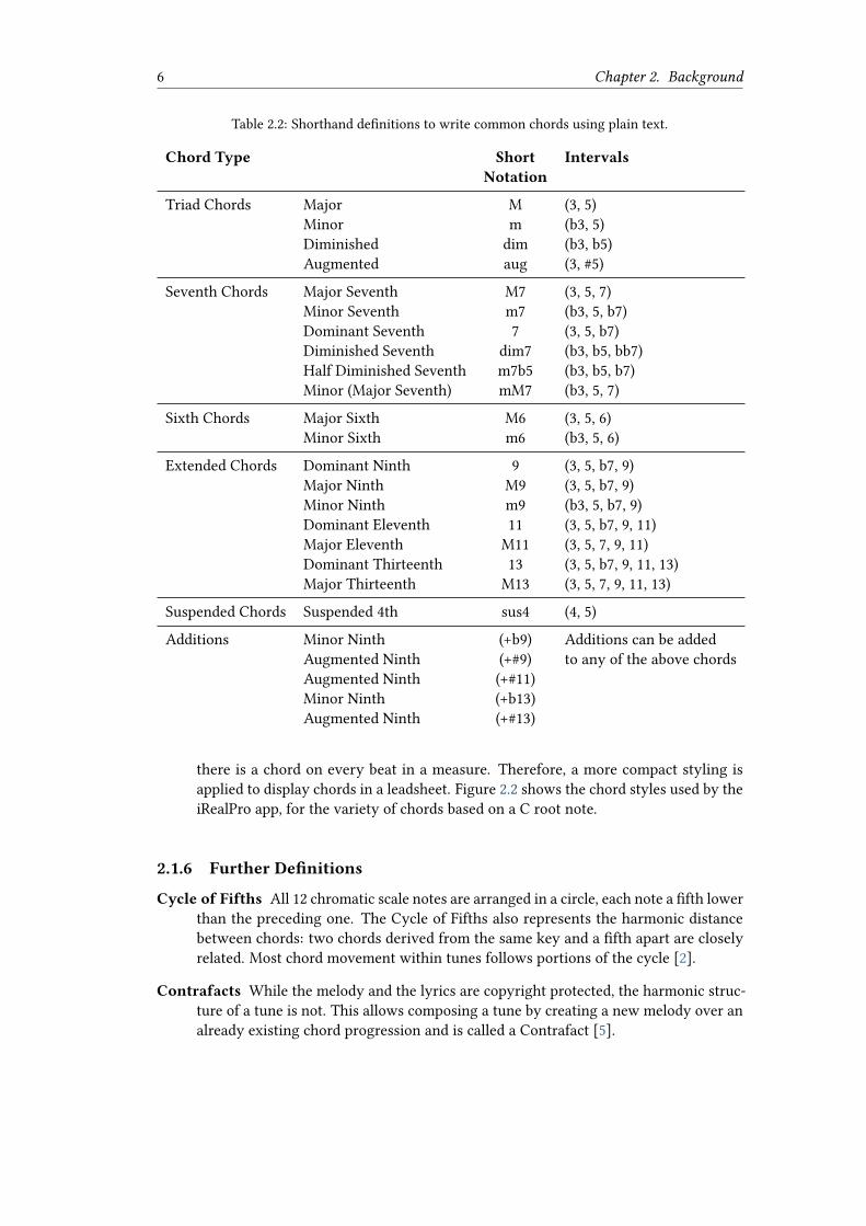
Chords in Plain Text For writing chords in plain text, [4] proposes a shorthand definition.Table 2.2 lists a variation based on this proposal, that is more compact and is used inthis document and in the source code.

Styled Chords for Leadsheets The textual notation for chords symbols is convenient fortext but is confusing in a leadsheet because the notation is too cluttered, mainly if

6 Chapter 2. Background

Table 2.2: Shorthand definitions to write common chords using plain text.

Chord Type Short IntervalsNotation

Triad Chords Major M (3, 5)Minor m (b3, 5)Diminished dim (b3, b5)Augmented aug (3, #5)

Seventh Chords Major Seventh M7 (3, 5, 7)Minor Seventh m7 (b3, 5, b7)Dominant Seventh 7 (3, 5, b7)Diminished Seventh dim7 (b3, b5, bb7)Half Diminished Seventh m7b5 (b3, b5, b7)Minor (Major Seventh) mM7 (b3, 5, 7)

Sixth Chords Major Sixth M6 (3, 5, 6)Minor Sixth m6 (b3, 5, 6)

Extended Chords Dominant Ninth 9 (3, 5, b7, 9)Major Ninth M9 (3, 5, b7, 9)Minor Ninth m9 (b3, 5, b7, 9)Dominant Eleventh 11 (3, 5, b7, 9, 11)Major Eleventh M11 (3, 5, 7, 9, 11)Dominant Thirteenth 13 (3, 5, b7, 9, 11, 13)Major Thirteenth M13 (3, 5, 7, 9, 11, 13)

Suspended Chords Suspended 4th sus4 (4, 5)

Additions Minor Ninth (+b9) Additions can be addedAugmented Ninth (+#9) to any of the above chordsAugmented Ninth (+#11)Minor Ninth (+b13)Augmented Ninth (+#13)

there is a chord on every beat in a measure. Therefore, a more compact styling isapplied to display chords in a leadsheet. Figure 2.2 shows the chord styles used by theiRealPro app, for the variety of chords based on a C root note.

2.1.6 Further Definitions

Cycle of Fifths All 12 chromatic scale notes are arranged in a circle, each note a fifth lowerthan the preceding one. The Cycle of Fifths also represents the harmonic distancebetween chords: two chords derived from the same key and a fifth apart are closelyrelated. Most chord movement within tunes follows portions of the cycle [2].

Contrafacts While the melody and the lyrics are copyright protected, the harmonic struc-ture of a tune is not. This allows composing a tune by creating a new melody over analready existing chord progression and is called a Contrafact [5].

2.2. Common NLP Terminology 7

Figure 2.2: Different chord types based on the root note C, displayed withthe iRealPro app.

2.2 Common NLP Terminology

This section introduces terms commonly used in the field of Natural Language Processing(NLP).

Corpus A corpus is a large and structured collection of machine-readable texts.

N-gram In NLP tasks, an n-gram is a sequence of n words. A 2-gram (also called bigram) isthe sequence of two consecutive words, a 3-gram the sequence of three consecutivewords, and consequently, an n-gram is a sequence of n consecutive words. N-gramsare usually generated by extracting n words from the corpus, then moving on by oneword, and extracting the next n words.Example: n-grams with n=3 for the sentence "Music is the only medicine withoutside effects": Music-is-the, is-the-only, the-only-medicine, only-medicine-without,medicine-without-side, without-side-effects.

Token, Term An element in the vocabulary of a corpus. It can be a word, a processed word,or an n-gram. Token and term are often used synonymously.

2.3 Vector Space Models

Language is unstructured data. To use machine learning algorithms on text, we need anumerical representation to analyze the text. This process is called feature extraction andis an essential first step in natural language processing. A common way to transform thedocuments into vectors is using a Vector Space Model [6].

The Vector Space Model is an algebraic model in high-dimensional space, where eachdimension corresponds to one term in the vocabulary. Vectors in this high-dimensional termspace represent documents and queries. Semantically similar documents are representedclose to each other [7].

While the vector space model is a basic framework for representing documents andhandling similarity queries, it does not define how the terms are actually placed in the space,

8 Chapter 2. Background

i.e., how the term weights or term feature vectors are defined. The vector space model doesalso not address how the similarity between terms is calculated.

The following sections describe actual implementations of the Vector Space Model toretrieve documents based on a query.

2.3.1 Bag-of-Words Models

Count Vectorizing

In Count Vectorizing, also called Bag-of-words model or Term Frequency (TF) model, a textdocument is converted into a vector of counts. Each item of this document vector corre-sponds to a term in the vocabulary and is filled with the counts of that term. For example, ifthe term world occurs 3 times in the document, then the corresponding index in the vectorwill be filled with a 3. If the term world does not appear in the document, it will be filledwith a zero.

TF-IDF

TF-IDF stands for Term Frequency-Inverse Document Frequency and is an extension to theCount Vectorizing model. The calculated TF-IDF weight is a statistical measure to evaluatehow important a word is to a document in a corpus. Instead of looking at the raw counts ofthe words in each document, TF-IDF looks at a normalized count where each word count isdivided by the number of documents this word appears in.

Latent Semantic Analysis

Latent Semantic Analysis (LSA) is also known as Latent Semantic Indexing (LSI). It findsgroups of documents with the same words by building a matrix with documents in columnsand terms in rows. Each value in the matrix corresponds to the frequency with which thegiven term appears in that document. Singular Value Decomposition (SVD) can then beapplied to the matrix M, resulting in three matrices U,Σ and V, representing the term-topics,topic importances, and the topic-documents (Figure 2.3).

Documents Topics

Topics

Topics

Documents

Topics=

Term

s

Term

s

x x

Term-Document Matrix

Topic Importance

Term assignment to Topics

Topic Distributionacross Documents

U Σ VCount Vectors

Figure 2.3: Latent Semantic Analysis (LSA)

Using the derived diagonal topic importance matrix, we can identify the most significanttopics in our corpus, and remove rows that correspond to less important topic terms. Ofthe remaining rows (terms) and columns (documents), we can assign topics based on theirhighest corresponding topic importance weights ([8], [9], [10]).

2.3. Vector Space Models 9

Music is the only medicine without side effects. (Franco Cerri, Italian Guitarist)

only

medicine

side

effects

Single-layer

neuralnetwork

without

ContextWords

TargetWord

only

medicine

side

effects

Single-layer

neuralnetwork

without

TargetWord

ContextWord

Figure 2.4: Word2Vec Continuous Bag-of-Words (left) versus Skip-gramModel (right)

2.3.2 Word Embeddings

A major drawback of bag-of-words models is that they are completely based on the numberof commonwords in two documents when comparing the document similarity. If documentsdo not share any words, their similarity will be zero.

In contrast, Word Embeddings try to capture the semantics of words by using a neuralnetwork. The algorithm tries to find vector representations for the terms in the vocabularysuch that similar terms have similar vectors.

Word2Vec

Since the publication of the Word2Vec model by Tomáš Mikolov at Google [11], Word Em-beddings became popular because they dramatically outperformed previous approaches,especially on analogy tasks.

There are two variants of Word2Vec, the continuous bag-of-words model (CBOW) andthe skip-gram model (see Figure 2.4). Refer to the original paper or [12] for an accuratedescription.

Both variants use a shallow neural network to predict word co-occurrences. The trainingdata is derived from the full text corpus. The major distinction is that the CBOWmodel triesto predict the center word from context words, while the skip-gram model tries to predictthe center word given the context words.

The actual result that we are interested in, namely the vectors for each token in thedictionary (called word embedding), is trained in the neural network’s single hidden layer.The dimension of the word embedding corresponds to the number of nodes in the hiddenlayer.

Doc2Vec

Doc2Vec uses the same concepts as Word2Vec, but also uses the concept of a documentidentity, from which the words are taken ([13]). For Doc2Vec, there are two variants too: theDistributed Memory (DM)model and the Distributed Bag-Of-Words (DBOW)model. Contraryto intuition, the Doc2Vec DM model is analogous to the Word2Vec CBOW model, and theDoc2Vec DBOW is analogous to the word2vec Skip-gram model. [14] finds that DBOWworks best for small data sets, while DM is superior for big datasets.

The Doc2Vec DM model takes the context word as the input and predicts the documentID. In contrast, the DBOWmodel takes the document ID as the input and predicts randomly

10 Chapter 2. Background

Music is the only medicine without side effects. (Franco Cerri, Italian Guitarist)

only

medicine

side

effects

Single-layer

neuralnetwork

without

Context Wordsplus Document

Id

TargetWord

Music

is

the

only

Single-layer

neuralnetwork

DocumentId

DocumentId

ParagraphWords

DocumentIdeffects

Figure 2.5: Doc2Vec Distributed Bag-of-Words DBOW (left) versus Dis-tributed Memory DM model (right)

sampled words from the document (Figure 2.5). The pure DBOW model as presented by[13] does not train any word vectors like the Word2Vec or the Doc2Vec DM models. Also,it does not consider the order of the words, since there is no sliding window that definescontext and target words. However, there is the option to interleave word vector trainingwith document vector training also for the DBOW variant, which [15] observes that it canimprove the document vectors.

2.3.3 Document Similarity

The methods described in the previous sections transform the documents in vectors. Tocalculate the document similarity, usually the cosine similarity is used by calculating thecosine of the angle α beween two vectors. This angle will be small if two documents sharemany features. To compute the cosine of the angle, the scalar product of the two vectors isused, which is normalized by the vector lengths [16].

2.4 Relevance Feedback

Relevance Feedback aims to involve the user in the retrieval process to improve the finalresult. For a particular search query, the user gives feedback on the relevance of documentsthat are presented to him or her.

The procedure for explicit, binary feedback is as follows:

1. The user issues a query.2. The system returns an initial set of retrieval results.3. The user marks some returned documents as relevant or non-relevant.4. The system computes a better representation of the information need based on the

user feedback.5. The system displays a revised set of retrieval results.

The Rocchio algorithm [17] is a classical algorithm to improve the result of step 4. It canbe applied to all vector space models.

11

Chapter 3

Related Work

The application of linguistical techniques to music is not a new topic by any means. It hasbecome even more popular in with the advent of neural networks in text processing. Therehave been quite a few attempts for modeling musical context with semantic vector spacemodels, many based on the foundations ofWord2Vec embeddings ([11]). This section givesan overview of applications that apply the tools of text analysis to musical chords.

One obvious application for using machine learning algorithms is to predict the nextchord based on a given input chord sequence. [18] proposes to use embeddings similar toWord2Vec, resulting in a Chord2Vec model that learns chord embeddings from a corpus ofchord sequences, placing chords nearby when used in similar contexts. [19] uses Word2Vecto propose a next chord for novice composers and provide inspiration for writing a newtune that goes out of the ordinary. [20] uses several public datasets with annotated chordsto evaluate different neural network topologies for chord prediction. Finally, [21] is an-other application of predicting chord sequences based on recurrent neural networks, usingembeddings created by Word2Vec.

Other applications focus on clustering the chord progressions. [22] performs a similarityanalysis of tunes from 18 jazz musicians, based on n-grams of the chords of 218 tunes. Theyexamine different chord simplification strategies and conclude that the bass note of a slashchord is not relevant for their analysis. Depending on the use case, they also conclude thattension notes (e.g., +#11, +b13 etc) can be removed to minimize the vocabulary.

[23] uses annotated polyphonic music from Beethoven Sonatas that are split into shortslices as input to train embeddings usingWord2Vec. Based on visualizations using dimensionreduction techniques, they conclude that the model can capture tonal proximity. Similarly,[24] shows tonal relationships between chords by clustering the embeddings derived byWord2Vec. They found that Classical and Baroque composers use chords similarly, whileModernists and Renaissance composers seem to have a more distinctive style.

[25] provides a database for finding patterns ("licks") that are commonly played duringjazz solo improvisation, based on selected recordings of jazz masters.

13

Chapter 4

Methods

4.1 Similarity between Jazz Tunes

How is the similarity between two tunes defined? Given that the technical mastery ofplaying an instrument is not an obstacle, if I have learned to improvise over one tune, whatother tune would be a good next one to start working on?

There is no clear answer to this question. Table 4.1 lists two different goals that a studentcan have in mind, each resulting in different strategies and consequentially in a differentdefinition of similarity:

Table 4.1: Possible intention and strategy how to select the next tune.

Nr Goal Possible Strategy

1 Memorize a big repertory of tunes. Identify sections or parts of sections thatshare the same basic harmonic move-ment.

2 Build the skills to improvise over differentchord progressions in various keys.

Identify sections that share the chord ma-terial, not necessarily following the samebasic movement.

Figures 4.1 and 4.2 each provide an example for these two goals.

Figure 4.1: Goal 1: The basic harmonic movement for Honeysuckle Rose andSatin Doll (B section) is identical, although the chord types are different.

Figure 4.2: Example for Goal 2: The B sections of Honeysuckle Rose and TeaFor Two share the same blocks, but the basic harmonic structure is different.

14 Chapter 4. Methods

Another aspect to consider when recommending the next tune to learn is the difficultyor complexity of the chords vocabulary. The following characteristics can contribute to howdifficult a tune is perceived to learn:

• Complexity of the chord vocabulary; e.g., root and dominant chords only, versusaltered chords with additions.

• Tonality: a higher number of flats and sharps in the tonality is generally consideredmore challenging.

• Chord density: how frequently does the chord change; e.g., every two bars only versusevery one or two beats.

• Harmonic familiarity: simple harmonic structure with an ear-worm character versusunexpected, hard to remember harmonies.

• Speed: fast tempo can be a technical challenge, versus slow tempo, which can be achallenge for musical expression.

• Technical challenges of playing the instrument (see [26] for Piano sheet music as anexample).

4.1.1 Tasks

Based on these assumptions, I suggest to break down the task of recommending a next tuneto learn into three sub-tasks:

1. Identify similar basic harmonic structures for parts of two tunes.

2. Identify similar chord pattern blocks for parts of two tunes.

3. Identify a similar chords vocabulary difficulty level for two tunes.

4.1.2 Assumptions for this Project

To limit the scope for this thesis, I take the following assumptions for defining the similarityof tunes:

1. Similar tunes contain the same chord progression patterns.• A chord progression pattern typically consists of 2 to 4 chords but can also belonger.

• By chaining multiple chord progression patterns, similarity can be observed ineither part of a section, the whole section, or the whole tune.

2. Similar tunes temporarily shift to the same tonal center for part of that tune.• Indirectly, this is a repetition of the above claim because a shift to a differenttonal center will result in different chord progression patterns.

3. Many tunes share an almost identical section, while the rest can be very different.• The similarity of sections seems to be a good similarity indicator.• As a consequence, I am evaluating similarities on a per-section level insteadof on a per-tune level, i.e., the models receive paragraphs as input instead ofdocuments.

4. The focus is to recommend tunes described by Goal 2 (Table 4.1).

5. The difficulty level of a tune is not evaluated nor considered.

4.2. System Architecture 15

4.2 System Architecture

Figure 4.3 shows the basic framework of the proposed method. The data set consists of thechords sequences and meta information for each tune (Section 4.3.1). The chords data isencoded into a numerical representaton, which also allows transposition (Section 4.3.2).

Then, the chords data is pre-processed to make it suitable as input for the model, bysimplifying the chord types and generating n-grams (Section 4.5). Three different modelmethods are trained with different pre-processing strategies (Section 4.6). The performanceof the models is evaluated according to Section 4.7. For the model which appears to bebest, the trained tune section vectors are reduced to two dimensions and clustered. Next,the tune recommendations and the dimension-reduced visualization are deployed to a webapplication for further explorative evaluation (Appendix D).

The web application provides the possibility to collect feedback about good and badtune recommendations. The user feedback can either be used to directly influence thelearned vectors of the models (Appendix A), or it can be used to improve the test set for theContrafacts accuracy metric (Section 4.7.1).

Data Set

Method 1TF-IDF

Method 2 LSA

Method 3 Doc2Vec

Model 2Model 1 Model 3

Methods

Train and EvaluateModels

RecommendedTunes

WebApplication

Existing Test Samples

User Feedback forRecommendations

Chords Encodingand Pre-

ProcessingPre-Processing

Pre-Processing forStyled Leadsheets

Cluster Vectors,visualize in 2-dimensions

VisualizeClusters

Figure 4.3: Framework of the proposed method.

Amore detailed diagram of the data pipelines used for training the model and generatingthe data for the web application is depicted in Figure D.1 in the Appendix.

16 Chapter 4. Methods

4.3 Data Collection

4.3.1 Data Sources

For the creation of the data set, the following information about jazz tunes are gathered:

• Chord Sequence• Musical information about the tune: default key, time signature, form (sections)• Composer, Lyricist• Publication Date• Relevant links to databases for further information

This information is obtained from the following sources:

• iRealPro app1• musicbrainz database2• wikidata3, wikipedia4• Official Real Books Volumes 1..3 by Hal Leonard5

Data Source for Chord Sequences and Musical Meta-Information

I obtain the chord sequences for the jazz tunes and their musical information from thepopular iRealPro app, exported to musicXML format.

The most popular source for the chords of jazz standards are the Real Books, but they areavailable only in pdf format and are not machine-readable. There are other music datasetsavailable,6 but I could not use them for the scope of this project. They either provide onlymetadata information for tunes but do not have any information about the musical contentor the chords. Or, they consist of MIDI data, but deriving the chord symbols from the MIDInotes is not a trivial task. In addition, these datasets are also not specifically targeted forjazz tunes.

Data Source for Composer, Lyricist

In the iRealPro raw data, the composer and lyricists are available for some tunes. However,this information is very messy because the name of the same composer is often written indifferent ways and has typos. Also, there is no differentiation between the composer andthe lyricist.

The open-source database musicbrainz is a more reliable and consistent source. I usedthe title and composer information by the iRealPro data to query the musicbrainz databaseusing its API, and obtained the composers and lyricists from there.

The composer and lyricist information found in the musicbrainz database is the firstchoice to use for the data set. If the tune is not found in the musicbrainz database, but thecomposer information is available from the iRealPro data, this information is merged to thedata set. Finally, a list of manually curated tunes and their composers was also used andmerged into the data set.

1https://www.irealpro.com/2https://musicbrainz.org/3https://www.wikidata.org/wiki/Wikidata:Main_Page4https://www.wikipedia.org/5https://officialrealbook.com/real-books/6https://fourscoreandmore.org/musoRepo/

4.3. Data Collection 17

Data Source for Publication Year

I obtain the publication year for a tune from the Real Book Volumes 1-3 where available, andwith second priority from the iRealPro data.

The copyright claim on the official Real Book lead sheets is the most reliable informationfor the publication year of a tune because it was edited by a professional publishing company.I created a helper tool to extract the publication year from the Real Book pdf lead sheets in asemi-manual approach: the tool goes through the list of tunes in the data set and opens thecorresponding Real Book pdf file if available. It then asks me to type in the publication yearthat is displayed in the copyright notice. This information is then merged into the data set.

Although the musicbrainz web interface displays the publication year for some tunes,this information is not available for querying using the API. The wikidata interface alsocontains the publication date for a few tunes, but this information proved completely wrongin many cases and was therefore not used.

Data Source for Additional Links

The musicbrainz database provides links to these additional databases:

• allmusic7 provides the relevant recordings for a tune.• secondhandsongs8 provides relevant recordings and also cover versions.• wikidata provides a short description for some tunes.• wikipedia link to a wiki page with background information.

If links are available, they are stored in the data set and displayed in the web applicationas additional information.

4.3.2 Chords Encoding

Numerical Representation of Chords

The chords from the iRealPromusicXML data are encodedwith<harmony> xml elements9.From this representation, I am generating a numerical representation for each chord (basedon the code from [27]), which allows transposing the chords to every musical key, and alsoallows creating a textual representation of the chord.

The numerical representation of each chord consists of three parts [28]:

• A root note, stored as the number of half-tone steps above the root note of the defaultkey of the tune (the tonic). The root note of the tonic is 0.

• The component, which contains a list of degrees. A degree is a note from the chord,represented by the number of half-tone steps above the root.

• A bass note, used for slash chords to indicate a chord inversion.

I extracted the sequence of chords together with the following information from themusicXML raw data :

Measure Number In the musicXML raw data, the measures are numbered without re-specting the repetitions. If first and second endings are available, the resulting chordsequence for both endings is therefore simply concatenated, which is wrong. There-fore, I respected the repetitions when parsing the musicXML data, which assigns thechords to their actual measure number.

7https://www.allmusic.com/8https://secondhandsongs.com/9https://w3c.github.io/musicxml/musicxml-reference/elements/harmony/

18 Chapter 4. Methods

Time Signature e.g., 4/4, 3/4, 5/4: this information is not used for the model but is neededto place the chords to the beats for the styled lead sheet display (Section D.3).

Beat Number used to place the chord on the beat for the lead sheet display in the webapplication (Section D.3).

Key with Mode e.g., F major, D minor: required to encode the chords to the numericalrepresentation. For the model input data, tunes in a major key are transposed to Cmajor, and tunes in a minor key are transposed to A minor.

Section Information is used to partition the chord sequences of a tune into paragraphs,which are fed to the model. The section information in the raw data is very messyand needs much manual cleaning.

Repetitions needed to map the chords to their true measurement number correctly.

4.4 Data Set Overview

After the cleaning step, there are 1240 tunes from the iRealPro jazz1350 playlist and 261tunes from the dixie and trad playlist left, resulting in a total of 1501 tunes. The tunes consistof 3411 unique sections (e.g., for an AABA form, the A section is counted only once), and5168 sections in total.

Figure 4.5 shows the distribution of the 15 most frequent tune forms in the data set.Clearly, most of the tunes are written in an AABA form.

Figure 4.4 shows the top 15 composers that are contributing to the data set.Although this data set is not a gold reference for jazz standards and many tunes had to

be removed in the cleaning step, Figure 4.6 shows the importance of the years between 1925and 1945.

Figure 4.7 shows that most of the tunes are in major keys, namely in the keys that areconsidered as easy like Cmajor, Fmajor, Bbmajor, Ebmajor and Gmajor. Most of the tunesin minor keys are written in Dminor or Cminor.

0 10 20 30 40 50

Jimmy Van HeusenAntônio Carlos Jobim

Miles DavisJohn ColtraneJerome KernHarold Arlen

Horace SilverWayne Shorter

Irving BerlinCharlie Parker

George GershwinDuke Ellington

Cole PorterRichard RodgersThelonious Monk

Number of Tunes per Composer Only Top 15 are shown.

Number of Tunes

Loading [MathJax]/extensions/MathMenu.js

Figure 4.4: Top 15 composers contributing tunes for the data set.

4.4. Data Set Overview 19

0 200 400 600

verseAABAintroAABA

ABABABCA

AABACABAABC

AABCAA

AABAB

ABCDA

ABACAABA

Form of the Tunes Only Top 15 are shown.

Number of Tunes

Loading [MathJax]/extensions/MathMenu.js

Figure 4.5: Top 15 tune form in the data set, the majority of the tunes is inAABA form.

1900 1920 1940 1960 19800

50

100

150

200

Publishing Year of Tunes Year is missing for 200 tunes

Num

ber

of T

unes

Loading [MathJax]/extensions/MathMenu.js

Figure 4.6: The period between 1925 and 1945 clearly dominates the publi-cation year of the tune in the dataset.

0 100 200 300 400

F#

C#

Ab

Eb

Bb

F

C

G

D

A

E

B majorminor

Tonality (major or minor)

Number of Tunes

tune

_key

Loading [MathJax]/extensions/MathMenu.js

Figure 4.7: Distribution of the default keys of the tunes.

20 Chapter 4. Methods

4.5 Corpus Pre-Processing

In every machine learning task, cleaning or preprocessing the data is as important as modelbuilding if not more. For unstructured data like text, this process becomes even moreimportant.

Corpus pre-processing for text analytics models usually involves the following steps:

Tokenization Text tokenization is the process of splitting up the text into chunks (theso-called tokens).

Normalization Text normalization is a text pre-processing step that includes cleaning text,case conversion, correcting spellings, removing stop words and other unnecessaryterms, stemming, and lemmatization.

Cleaning Cleaning describes the process of stripping away unnecessary parts of the textto get better results in downstream tasks due to less ambiguity, which could not beresolved by the computer otherwise.

Stemming Stemming is the process of removing a part of a word, or reducing a word toits stem or root to reduce the size of the vocabulary.

Lemmatization Lemmatization is another approach to derive roots from words next tostemming. Lemmatization uses unlike stemming a mostly human curated dictionaryto look up words and replace it with the correct root or also called lemmas.

Filtering Infrequent Words Depending on the task that has to be fulfilled, cutting off wordsthat do not often appear in the corpus might be beneficial because they blow up thevocabulary without providing much predictive power.

These steps are further described in the next stections.

4.5.1 Assumptions for Chords Pre-Processing

Section 4.1.2 lists different properties that contribute to the similarity of two jazz tunes. Itis possible that different models are needed to capture the variety of these properties. Butwithout appropriate preprocessing of the input data, a model certainly cannot perform well.

These are the assumptions made to decide how to pre-process the input data:• To make chords compareable across tunes:

– Transpose all tunes to C major and A minor respectively.– Use a fixed set of 12 root notes, without enharmonic spelling:

[A, Bb, B, C, C#, D, Eb, E, F, F#, G, Ab]– Simplify the chords vocabulary (Section 4.5.2).– Ignore slash chords if the bass note belongs to the chord.

• To find similar Chord Progression patterns:– Use chord n-grams, concretely a concatenation of unigrams and different n-

grams (Section 4.5.3).• It is easier to find similar sections than similar tunes.

– Split the tunes into their sections and use them as input documents for the model.– Two tunes are considered similar if at least one section was found to be similarwithin the first k matches.

• If a section is repeated multiple times in a tune (e.g., section A in an AABA form), thenonly the first occurrence of the section is considered.

4.5. Corpus Pre-Processing 21

Table 4.2 applies these assumptions to the general corpus pre-processing steps andcompares the differences of using natural language versus chords.

Table 4.2: Comparison of pre-processing steps for natural language andchords.

Natural Language Vocabulary Chords Vocabulary

Normalize Lan-guage

Translate text to same language. Transpose all major tunes to C ma-jor, transpose all minor tunes to Aminor.

Tokenization Split up text in documents, para-graphs, sentences, words.

Split up text in tunes, sections,chords.

Cleaning Removal of stop words; case con-version; removal of punctuationmarks.

Remove tunes with missing orwrong information. Fix tunes orremove them. If multiple sectionswith same label, keep only the firstoccurrence.

Stemming,Lemmatization

Remove word suffix. Use lookup-tables to replace a word with thecorrect root.

Reduce chords to simpler variants.

Generaten-grams

Use n-grams of words or charac-ters.

Use chord n-grams.

Filter infrequentTokens

Remove rare words or n-grams. Remove rare or chord n-grams.

4.5.2 Pre-Processing Steps

Chord Transposition

It is intuitive to transpose all tunes to the same key for comparison. This enables thefunctional role of different roots or pitches to stay consistent across tunes, for example iftransitioning to a different tonal center [23]. I transpose all major tunes to C major, and allminor tunes to A minor.

Cleaning Tunes

The cleaning process of tunes was done manually, so it might be incomplete or biased. Ideleted tunes from the data set for the following reasons:

• A tune is duplicated by the jazz1350 and the trad playlists, using the exact same chordsequences.

• The form is not correctly represented in the musicXML data, namely many tunesmake use of a coda for the ending, but the coda information is missing in musicXML;therefore the coda chords are lumped together with the previous section which iswrong.

• Few tunes have multiple repetitions, which are not handled correctly.• Tunes having very simple harmonic structure, e.g., many spirituals which mostlymake use of the I, IV and V chords only.

22 Chapter 4. Methods

Cleaning Tune Sections

The section labels of the iRealPro musicXML raw data have many issues. Many tunes are notlabeled at all, or labeled wrong. Some tunes are labeled with AB sections, each comprisingof 16 bars, while the form actually corresponds to ABCD or ABAC.

Often, the Verse or Intro is tagged with a text in iRealPro instead of a section label. Texttags are not included in the musicXML file.

Also, there is a bug in the musicXML export such that labels are sometimes visible inthe iRealPro app, but not contained in the musicXML file.

I cleaned and labeled sections according to my best knowledge, but since it was manualwork, some tunes still may have incorrectly labeled sections.

Chord Simplification ("Stemming")

I simplify the chords into a chordsBasic and a chordsSimplified vocabulary to reduce the sizeof the vocabulary and make chords compareable across tunes.

The chordsBasic vocabulary reduces the chord types to major, minor, dominant, dimin-ished, augmented and suspended chords (Table 4.3). All extended chords (9, 11, 13) andadditions (+b9, +#11 etc.) are removed. All major chord types are reduced to major triads,because harmonically spoken, a chord written as CM7 has the same function as a C6 or a Ctriad.

The chordsSimplified vocabulary distinguishes between the different 4-tone major andminor chords, but still removes all extended chords and additions.

Table 4.3: The vocabularies for chordsBasic and chordsSimplified are twodifferent variants of chord simplification.

Chord chordBasic chordSimplified

M7, 6 reduce to triad keepm6, m7 reduce to m keepm7b5, dim keep keepdim7 reduce to dim keepM9, M11, M13 reduce to triad reduce to M79, 11, 13 reduce to 7 reduce to 7mM7 reduce to m keepmM9 reduce to m reduce to mM7sus, sus7 keep keepsus9, sus11, sus13 sus7 sus7aug, aug7 keep keepmaug reduce to m keepMaug reduce to aug keep7alt reduce to aug7 keepdimM7 reduce to dim keep(+b9), (+#9), (+#11), (+b13) remove remove(+b5) keep keep(+b6) keep keep

Simplification of the Bass Note ("Slash Chords")

A Slash Chord is a chord which has the bass note written explicitly to the chord symbol usinga slash, e.g. C7/G means that a C7 chords should be played in second inversion, with the G

4.5. Corpus Pre-Processing 23

in the root. Since the proportion of slash chords in the corpus is small and is not expectedto have a big impact on the similarity between tunes, the bass note is not considered tosimplify the vocabulary [22].

4.5.3 Data Augmentation with Concatenated n-grams

Analogous to n-grams for natural language, chord n-grams are tokens consisting of n consec-utive chords. The chords of the tune sections are augmented by generating chord n-gramswith n in {1. . . 4}. All resulting n-grams are concatenated and represent the input data fortraining the model. As an example, the chords of a tune section with the n-gram con-figuration n=[1,2,3] consist of the chord uni-grams, concatenated by the chord bi-grams,concatenated by the chord tri-grams. An n-gram configuration of n=[1] consists of the chorduni-grams only.

Here is an example of n-grams with n in 1,2,3,4 for a chord sequence:

n Resulting n-grams, chordsBasic vocabulary

1 C, Bbm, Eb7, Ab, Dm7b5, G72 C-Bb, Bb-Eb, Eb7-Ab, Ab-Dm7b5, Dm7b5-G73 C-Bbm-Eb7, Bbm-Eb7-Ab, Eb7-Ab-Dm7b5, Ab-Dm7b5-G74 C-Bbm-Eb7-Ab, Bm-Eb7-Ab-Dm7b5, Eb7-Ab-Dm7b5-G7

4.4 gives an overview about the resulting number of tokens and the average length ofa tune section. With concatenated n-grams=[1,2,3,4], the average length of a section isincreased by factor 3.3 compared to unigrams, while the size of the corpus is increased by afactor 3.5.

Table 4.4: Number of tokens for different n-gram augmentation, for chords-Basic vocabulary.

n-gram Total Tokens Number of Tune Sections Avg Length of Sections

[1] 43832 3411 12.9[1, 2] 84253 3411 24.7[1, 2, 3] 121263 3411 35.6[1, 2, 3, 4] 154862 3411 45.4

Chords and the Zipf Distribution

Natural language follows the Zipf law, which means that a few words occur very often whileother words are rare. [29] provides evidence based on the notes contained in MIDI files, thatthe Zipf distribution of the linguistic context can be applied to the musical context. The Zipfplot shows the number of occurrences n of a token (absolute frequency) versus the token’sfrequency rank, with the most frequent token being in rank 0. A perfect Zipf distributionfollows a straight sinking line.

24 Chapter 4. Methods

Figure 4.8 shows the Zipf plots for different concatenations of n-grams for the chordsBasicvocabulary. For the unigrams, the curve is not straight and therefore the Zipf distributiondoes not fit well. The line gets straighter by concatenating more n-grams.

Figure 4.9 shows the Zipf plots for the chordsSimplified and the unprocessed chordsFullvocabulary. The uni-grams of the chordsFull vocabulary naturally follow the Zipf law betterthan the uni-grams of the chordsBasic because of the bigger vocabulary size.

1 10 100

1

10

100

1000

10k

Zipf Plot for chordsBasic Vocabulary n-grams=[1]

Frequency Rank

Abs

olut

e Fr

eque

ncy

1 10 100 1000

1

10

100

1000

10k

Zipf Plot for chordsBasic Vocabulary n-grams=[1, 2]

Frequency Rank

Abs

olut

e Fr

eque

ncy

(a) n-gram=[1] (b) n-gram=[1,2]

1 10 100 1000 10k

1

10

100

1000

10k

Zipf Plot for chordsBasic Vocabulary n-grams=[1, 2, 3]

Frequency Rank

Abs

olut

e Fr

eque

ncy

1 10 100 1000 10k

1

10

100

1000

10k

Zipf Plot for chordsBasic Vocabulary n-grams=[1, 2, 3, 4]

Frequency Rank

Abs

olut

e Fr

eque

ncy

(c) n-gram=[1,2,3] (d) n-gram=[1,2,3,4]

Figure 4.8: Zipf Plots for chordBasic vocabulary, for different n-grams.

Chord Type Distribution

Figure 4.10 shows the chord type distribution for the vocabularies chordsBasic, chordsSimpli-fied and the unprocessed chordsFull. The root note is removed, which gives an overview ofthe remaining chord types in the vocabularies and also their occurence. The * in the figuredenotes any root note. A * by itself means a major triad.

Figure 4.11 shows the most frequent 50 chord n-grams for the concatenated list of n-grams=[1,2,3,4], for the three vocabularies. For the chordsBasic vocabulary with the strongreduction of major and minor chords to triads, the C, G7, Dm and Am chords (I, V, ii, vi) arethe 4 most frequent tokens in the corpus. The popular ii-V chord progression Dm-G7 is onrank 5. For the chordsSimplified vocabulary, the tonic chord no longer is on rank 0 becauseit is split into CM7, C6 and C chords.

4.5. Corpus Pre-Processing 25

1 10 100

1

10

100

1000

10k

Zipf Plot for chordsSimplified Vocabulary n-grams=[1]

Frequency Rank

Abs

olut

e Fr

eque

ncy

1 10 100 1000 10k

1

10

100

1000

10k

Zipf Plot for chordsSimplified Vocabulary n-grams=[1, 2, 3, 4]

Frequency Rank

Abs

olut

e Fr

eque

ncy

(a) chordsSimplified, n-gram=[1] (b) chordsSimplified, n-gram=[1,2,3,4]

1 10 100

1

10

100

1000

10k

Zipf Plot for chordsFull Vocabulary n-grams=[1]

Frequency Rank

Abs

olut

e Fr

eque

ncy

1 10 100 1000 10k

1

10

100

1000

10k

Zipf Plot for chordsFull Vocabulary n-grams=[1, 2, 3, 4]

Frequency RankAbs

olut

e Fr

eque

ncy

(c) chordsFull, n-gram=[1] (d) chordsFull, n-gram=[1,2,3,4]

Figure 4.9: Zipf Plots for chordSimplified and chordFull, for uni-grams andconcatenated n-grams=[1,2,3,4].

*7 *m * *m7b5*dim

*7sus4*aug7

*7(+b5)

*aug*m(+b6)

*sus4*maug

1

10

100

1000

10k

Distribution of chordsBasic n-grams, Root removed. n-grams=[1]. All chord n-grams are shown.

Abs

olut

e Fr

eque

ncy

(a) chordsBasic

*7 *m7

*M7

* *6 *m7b5

*m *dim7

*7sus4

*m6

*aug7

*dim

*7(+b5)

*aug

*mM

7

*m(+

b6)

*augM7

*sus4

*maug

1

10

100

1000

10k

Distribution of chordsSimplified n-grams, Root removed. n-grams=[1]. All chord n-grams are shown.

Abs

olut

e Fr

eque

ncy

*7 *m7

*M7

* *6 *7(+b9)

*m7b5

*m *dim7

*m6

*9 *7sus4*aug7*7(+

#11)

*13*dim*7(+

#9)

*M7(+

#11)

*m9

*7(+b13)

*m11

*aug*m

M7

*7alt*6(+

9)*9sus4*9(+

#11)

*7(+b5)

*M9

*13(+b9)

5

100

2

5

1000

2

5

10k

Distribution of chordsFull n-grams, Root removed. n-grams=[1]. Only the top 30 chord n-grams are shown.

Abs

olut

e Fr

eque

ncy

(c) chordsFull (d) chordsFull

Figure 4.10: Distribution of the chord types for uni-grams, with the rootnote removed.

26 Chapter 4. Methods

C G7

Dm

Am

Dm

-G7

A7

D7

G7-C

F E7 C7

Em C-CD

m-G

7-CA7-D

mF7 Bb7

Fm B7

E7-Am

Em-A

7A7-D

m-G

7G

mAm

-Am

D7-G

7Am

-D7

C7-F

G7-G

7Bm

7b5Ab7

A7-D

7Am

-Dm

Bm

7b5-E7G

m-C

7Em

-A7-D

mC-D

mG

7-C-CD

7-D7

D7-D

mC-A

mC-A

7Em

-A7-D

m-G

7Cm

C-G7

EbdimAm

-Dm

-G7

Dm

-Dm

F-FF#

m7b5

Eb7

3

4

5

6789

1000

2

3

4

5

67

Distribution of chordsBasic n-grams n-grams=[1, 2, 3, 4]. Only the top 50 chord n-grams are shown.

Abs

olut

e Fr

eque

ncy

(a) chordsBasic

G7

Dm

7D

m7-G

7CM

7A7

D7

Am

7C E7 C7

Em7

C6

FM7

A7-D

m7

F7 Bb7

G7-C

M7

B7

Am

Em7-A

7A7-D

m7-G

7D

7-G7

Gm

7D

m7-G

7-CM

7F Am

7-D7

G7-C

G7-G

7Bm

7b5C-CG

7-C6

Ab7

A7-D

7Fm

7Bm

7b5-E7G

m7-C

7E7-A

m7

Em7-A

7-Dm

7CM

7-CM

7D

7-D7

Am

7-Dm

7D

7-Dm

7Em

7-A7-D

m7-G

7C7-FM

7D

m7-G

7-C6

F#m

7b5Eb7Am

7-Am

7Am

7-Dm

7-G7

D7-D

m7-G

7

3

4

5

6789

1000

2

3

4

5

6

Distribution of chordsSimplified n-grams n-grams=[1, 2, 3, 4]. Only the top 50 chord n-grams are shown.

Abs

olut

e Fr

eque

ncy

(b) chordsSimplified

G7

Dm

7CM

7D

m7-G

7C Am

7D

7A7

C7

Em7

C6

FM7

E7 F7 Am

G7-C

M7

Bb7

A7-D

m7

D7-G

7G

m7

F Dm

7-G7-C

M7

G7-C

E7(+b9)

Bm

7b5Em

7-A7

C-CAm

7-D7

G7-G

7A7-D

m7-G

7B7

Fm7

G7-C

6A7(+

b9)G

m7-C

7A7-D

7CM

7-CM

7Ab7

Am

7-Dm

7D

7-D7

Em7-A

7-Dm

7D

7-Dm

7Bm

7b5-E7(+b9)

F#m

7b5D

m7-G

7-C6

Am

7-Dm

7-G7

C7-FM

7Em

7-A7-D

m7-G

7Bm

7Ebdim

7

3

4

5

6789

1000

2

3

4

5

Distribution of chordsFull n-grams n-grams=[1, 2, 3, 4]. Only the top 50 chord n-grams are shown.

Abs

olut

e Fr

eque

ncy

(c) chordsSimplified

Figure 4.11: Distribution of the chord types for concatenatedngrams=[1,2,3,4] including the root.

4.6. Experiments 27

4.6 Experiments

This section describes the background of the experiments and lists the methods and theirhyperparameters. All models are trained using the gensim10 library.

4.6.1 Split into Train and Test Set

The data is split into a training and a test set for all experiments. The test set consists of thelist of tunes that is manually defined for the Contrafacts accuracy metric (Section 4.7.1).

This approach is questionable; in [14], the authors explain that because the model istrained completely unsupervised, i.e., not given any supervised or annotated information,there is no need to hold out the test data, as it is unlabeled.

4.6.2 Evaluation of Pre-processing Method and Models

Training the 4 models with different pre-processed data results in 32 experiments executedin total.

The TF-IDF and LSA models yield deterministic results and are therefore only executedonce. For the Doc2Vec experiments, 5 runs are executed and the results are averaged. Theresults of the experiments are being tracked using the Weights &Biases11 service.

Model Methods

The following four methods are used to train a model, each model with varied hyperparam-eters according to Section 4.6.3:

• TF-IDF• LSA• Doc2Vec DBOW (with interleaved training of word vectors)• Doc2Vec DM

As a general assumption, I would expect that document embeddings outperform bag-of-words models for finding similar chord progression patterns, while bag-of-word modelsoutperform document embedding methods for finding tunes with similar chords vocabulary.

Pre-processing Strategies

For each model, the input data is provided using different pre-processing strategies, resultingin 8 experiments per model:

• Vocabulary: chordsBasic, chordsSimplified• n-grams: [1], [1,2], [1,2,3], [1,2,3,4]

4.6.3 Model Hyperparameters

This section describes the evaluated hyperparameters of the three model methods.

TF-IDF 12 No hyperparameters tuned.

LSA 13 One hyperparameter:• Number of latent topics.

10https://radimrehurek.com/gensim/11https://wandb.ai/12https://radimrehurek.com/gensim/models/tfidfmodel.html13https://radimrehurek.com/gensim/models/lsimodel.html

28 Chapter 4. Methods

Doc2Vec 14 Most relevant hyperparameters for Doc2Vec:

• dm: DM or DBOW, defines the training variant of Doc2Vec.• vector_size : dimensionality of the feature vectors.• sample: threshold for configuring how much of the higher-frequency tokens torandomly subsample.

• window: size of the window around the center token to consider as contexttokens. window = 2 uses 2 tokens on both sides of the center token.

• negative: if > 0, uses negative sampling specifies how many negative samplesshould be randomly drawn from outside the window.

• dbow_words: if 1, then the word vectors are also trained in addition to thedocument vectors. Only relevant for DBOW.

• hs: if hierarchical softmax should be used.• min_count: ignore all tokens with a total frequency lower than this threshold.

4.7 Performance Evaluation

Since the task of recommending similar tunes is an unsupervised learning problem, we donot have any ground-truth data to assess the performance of the trained model. The trainedchord n-gram vectors and the trained tune vectors are in n-dimensional vector space andare not directly interpretable.

One option that does not rely on supplementary test information is to cluster the resultof the model and evaluate if the clusters are compact and well-separated ([30]). However,it is not clear if the evaluation based on cluster information only is appropriate for the usecase of recommending tunes.

Generally, unsupervised learning cannot be evaluated without any additional label in-formation. Therefore, I am defining the following metrics for the performance evaluation.

4.7.1 Metric 1: Proportion of correctly recommended Contrafact Tunes

I manually created a list of test tunes to compare the different approaches with each other,and to help assess the quality of an embedding (see Appendix B). The test list contains tupleswith a reference tune and an expected similar tune, called the list of contrafact tunes. Fora reference tune, if the trained model reports the expected similar tune within the top-Nrecommendations, it is considered as a success. The accuracy is reported as the proportionof successes with respect to the number of test tunes.

This metric is evaluated for all experiments (TF-IDF, LSA, Doc2Vec).

4.7.2 Metric 2: Self-Similarity

For the self-similarity test15, the model is first trained using the training data. Then thesame training data is used to infer the document vectors again, which are compared to thetrained vectors to determine the similarity. For perfect self-similarity, the model will returnthe inferred training documents in the first rank.

This test is superfluous for the TF-IDF and LSA models, because they are deterministicand will always return first ranks. In contrast, the embedding methods like Doc2Vec arebased on iterative algorithms that make use of drawing randomized samples from the corpus,therefore the resulting vectors will differ with repeated inferences.

This metric is only evaluated for the Doc2Vec model.14https://radimrehurek.com/gensim/models/doc2vec.html15https://radimrehurek.com/gensim/auto_examples/tutorials/run_

Doc2Vec_lee.html#assessing-the-model

4.7. Performance Evaluation 29

4.7.3 Metric 3: Chord Analogies

The original word2vec paper [11] describes that the model is able to solve word analogieslike (a, b) is similar to (c, d), with a, b, c being given and d being solved by the model. Theyprovide the example that the pair of (woman, queen) is similar to (man, king). The sameprinciple can also be applied to musical chords ([31]).

To test the chord analogies, I am generating a total of 1064 test samples for all 12 keys(code is based on [21]), for the following common chord progressions 16:

• minor to dominant, e.g. (Dm D7)�(Cm C7)• major to minor, e.g. (A Am)�(F Fm)• dominant to minor, e.g. (C7 Cm)�(G7 Gm)• dominant to minor, half step down, e.g. (A7 Abm)�(F7 Em)• minor to dominant, half step down, e.g. (Fm E7)�(F#m F7)• subdominant to tonic, V-I, e.g. (A7 D)�(C7 F)• ii to dominant, ii-V, e.g. (Gm C7)�(Fm Bb7)• dominant sequences, V/V-V, e.g. (E7 A7)�(C7 F7)

For the performance evaluation, it is important to consider that the models are trainedon chord input data which is transposed to C major and A minor respectively, so the modelis given input only for a small part of these analogy pairs.

It is not clear however, if the performance evaluation using chord analogies is a goodindicator to decide which model performs best, but it certainly gives insight about whatchords the model considers being close to each other.

This metric is only evaluated for the Doc2Vec model and only for the chordsbasic vocab-ulary.

4.7.4 Manual Evaluation of the Result

Finally, it is definitely instructive to manually explore the similarity results. The web appli-cation eases the task by comparing the lead sheets of selected tunes. See screenshots of theweb application in Appendix D.2.

Assess the List of recommended Tunes The web application displays the recommenda-tions of the most promising model and thus makes it accessible for a broader audienceto give feedback. The user selects a reference tune and a corresponding section ofthe tune, and the web application displays a list of recommended similar sections ofother tunes, along with both lead sheets. The user is given the possibility to providefeedback using a ‘like’ or ‘dislike’ button. This feedback is being stored in a databaseand can extend the existing contrafact test set and therefore contribute to furtherimproving the model performance.

Visual Inspection of the Tunes in Vector Space To evaluate if there are clusters of sim-ilar tune sections found, the trained vector weights are visualized in 2-dimensionalspace using dimensionality reduction techniques like T-SNE or UMAP. Subsequently,the 2-dimensional representation is clustered. The web application displays the scatterplot with the clusters and the user can explore the leadsheets that belong to a samecluster.

16https://www.learnjazzstandards.com/blog/learning-jazz/jazz-theory/3-important-jazz-chord-progressions-need-master/

31

Chapter 5

Results

5.1 Contrafacts Similarity Results

Table 5.1 summarizes the achieved accuracy for the Contrafacts test for the three differentvector space models. The trained models for these summary results use the hyperparametersettings according to Section 5.4.

For a reference tune, if the model lists the similar tune according to the list of Contrafactsin the first n=30 recommendations, the test is counted as success.

If using chord uni-grams only, the Doc2Vec and TF-IDF models achieve a similar accu-racy of around 75%, while the accuracy of the LSA model is almost 10% higher. However,when concatenating multiple n-grams, all models achieve an accuracy of 85..87%, with theexception of Doc2Vec DM.

Table 5.1: Summary of Similarity Results based on the Contrafacts Test, fordifferent model types. The top 30 recommendations are considered.

Doc2Vec DBOW Doc2Vec DM LSA TF-IDFn-gram mean std mean std mean std mean std

chordsBasic[1,2,3,4] 87.13% 0.60% 81.37% 3.46% 84.55% 0.00% 81.82% 0.00%[1,2,3] 84.24% 1.05% 83.63% 1.97% 84.55% 0.00% 85.45% 0.00%[1,2] 84.55% 0.69% 80.53% 2.44% 86.10% 0.00% 82.73% 0.00%[1,4] 85.09% 0.73% 82.73% 0.00% 81.82% 0.00%[1] 75.64% 1.06% 76.45% 0.97% 83.64% 0.00% 73.64% 0.00%

chordsSimplified[1,2,3,4] 73.98% 0.78% 67.82% 0.73% 70.91% 0.00% 70.91% 0.00%[1,2,3] 70.45% 2.73% 70.36% 0.45% 73.64% 0.00% 70.00% 0.00%[1,2] 74.36% 0.68% 67.27% 0.00% 74.66% 0.00% 70.00% 0.00%[1,4] 73.45% 0.68% 70.00% 0.00% 69.09% 0.00%[1] 68.36% 1.34% 64.73% 0.89% 69.09% 0.00% 58.18% 0.00%

Figure 5.1 shows the histogram for the number of common recommendations of twotrained models, for two different experiments. The distribution is slightly left-skewed withthe peak between 12 and 15 common tunes.

32 Chapter 5. Results

0 5 10 15 20 25 30Number of Commmon Tune Sections

0

50

100

150

200

250Common Recommendations

0 5 10 15 20 25 30Number of Commmon Tune Sections

0

50

100

150

200

250

Common Recommendations

(a) chordBasic versus chordSimplified (b) chordBasic; LSA, n-gram=[1,2],Doc2Vec DBOW, ngram=[1,2,3,4] Doc2Vec DBOW, ngram=[1,2,3,4]

Figure 5.1: Histogram with number common recommendations, for twodifferent experiments.

5.2 Chord Analogies for Doc2Vec

Table 5.2 shows the results for the Chord Analogy test for Doc2Vec DBOW and DM. This testis done only for the chordsBasic vocabulary. The Correct Analogy column lists the accuracyfor analogies where the model delivered the correct answer in first rank. The Correct Analogyin Top 5 Match column lists the accuracy for giving the correct answer within the first 5ranks.

Table 5.2: Chord Analogies for Doc2Vec DBOW and DM in comparison.

Correct Analogy Correct Analogy in Top 5n-gram mean std mean std

DBOW[1,2,3,4] 9.97% 0.77% 20.98% 0.93%[1,2,3] 8.93% 0.48% 21.23% 1.08%[1,2] 8.55% 0.52% 20.22% 1.13%[1,4] 7.99% 0.40% 16.63% 1.11%[1] 7.23% 0.39% 15.81% 0.84%

DM[1,2,3,4] 4.38% 0.52% 13.18% 1.12%[1,2,3] 3.87% 0.79% 9.85% 2.87%[1,2] 4.36% 0.75% 8.54% 0.67%[1] 4.36% 0.15% 11.52% 0.25%

Table 5.3 lists the detailed results of the tested chord progression types, for the Doc2VecDBOW model, one test run only.

5.3. Self-Similarity for Doc2Vec 33

Table 5.3: Results for the Doc2Vec DBOW model for guessing the chordanalogies. The model achieves the highest accuracy for the ii-V chord pro-greessions.

Chord Progression Perfect Match Top 5 Match

minor-to-dominant 0.76% 18.18%major-to-minor 7.58% 14.39%dominant-to-minor 5.30% 20.45%dominant-to-minor-half-step-down 4.55% 7.58%minor-to-dominant-half-step-down 0.76% 6.82%subdominant to tonic, V-I 23.48% 36.36%ii to dominant, ii-V 36.36% 43.94%dominant sequences, V/V-V 3.79% 22.73%

Overall 10.3% 21.3%

5.3 Self-Similarity for Doc2Vec

The self-similarity of the inferred tune sections using the Doc2Vec model is consistent andis not clearly impacted by different hyperparameter tunings. Therefore, this value is moreimportant as a crosscheck than as a useful metric to determine the model quality. Table 5.4lists the results for self-similarity.

Table 5.4: Doc2Vec Self-Similarity for tune sections in the training set.

Sections Self-similar in Rank 0 Sections Self-similar in Rank 1n-grams Mean Std Mean Std

DBOW[1,2,3,4] 95.90% 0.16% 98.02% 0.06%[1,2,3] 96.03% 0.21% 98.03% 0.12%[1,2] 95.50% 0.03% 97.80% 0.03%

DM[1,2,3,4] 96.07% 0.04% 98.08% 0.02%[1,2,3] 96.03% 0.06% 98.12% 0.08%[1,2] 95.62% 0.10% 97.74% 0.05%[1] 91.90% 0.15% 95.68% 0.15%

5.4 Best Hyperparameters

The best hyperparameters were evaluated based on the contrafacts test metric.

LSA

[32] describes the use of a coherence score to derive an optimum number of topics. Thiscalculation is conveniently available in the gensim library.1 However, the optimum numberof topics as reported by the coherencemodel is around 30, but in the Contrafacts test, a highernumber of topics performed clearly better. The number of topics is set to the somewhatarbitrary number of 100 topics.

1https://radimrehurek.com/gensim/models/coherencemodel.html

34 Chapter 5. Results

Doc2Vec

Table 5.5 lists the values that contribute to a highest accuracy in the Contrafact test metricfor the Doc2Vec hyperparameters. Each run was repeated at least 5 times to incorparatethe varibility of the probablistic nature of the Doc2Vec model. Detailed results are listed inAppendix C.

Table 5.5: Doc2Vec hyperparameter values resulting in highest Contrafactstest accuray.

Parameter Tested Values n=[1,2,3,4] n=[1] Commentn=[1,2]n=[1,2,3]

vector_size {100, 300} 300 300 not a big influence, but300 performs slightly bet-ter than 100 mainly forthe chordsSimplified vo-cabulary.

sample {0.1, 0.01, 0.001} 0.001 0.01 0.1 is worse for all.window {2, 3, 4} 3 3 Has only an effect if

dbow_words = 1.negative {10, 12, 14} 12 12 No big effect.dbow_words {0, 1} 1 1 Chord Analogy test

can only be done whenword vectors are storedwith dbow_words = 1.Slightly improves theresult.

hs {0, 1} 1 1 Hierarchical softmax im-proves the result for all ex-periments.

min_count {10, 20, 30, 40} 30 20epochs {30, 50, 100, 200} 50 for DBOW, 200 for DM Longer training needed

for DM.

35

Chapter 6

Discussion and Outlook

6.1 Discussion of Results

6.1.1 Contrafact Test Results

The TF-IDF, LSA and the pure Doc2Vec DBOW variant do not consider the input order ofthe chords. They all perform worst with the chords as uni-grams, and clearly benefit fromconcatenating multiple chord n-grams. In fact, concatenating n-grams has a higher effecton the contrafacts test than any hyperparameter tuning.

The contrafact test was useful to start, but then proved to be not accurate enough. Themodels achieve a similar contrafacts test accuracy, therefore it is not possible to determineif a Doc2Vec model delivers better recommendations than the LSA or TF-IDF model. Thelist of contrafacts needs more cleaning and test cases.

6.1.2 Doc2Vec DM versus DBOW

The pure Doc2Vec DBOW variant (dm=0, dbow_words=0) is fast to train (ca. 30s). Withthe same amount of training, Doc2Vec DM performs much worse and requires at least 4times more training epochs to achieve a similar accuracy for the contrafacts test. In [14],the authors found that DBOW performs significantly better than DM for small data sets.

Doc2Vec DBOWwith concurrent skip-gram training (dm=0, dbow_words=1) interleavesthe training of word vectors with the training of document vectors. This mode works as asort of corpus-expansion trick: every sliding window of target to context word predictionacts like training a mini-document, and the neural network is fed with manymore individualtraining examples (by the factor of thewindow parameter), which also multiplies the trainingtime. It is not clear if increasing the number of training epochs by the number of the factorof the window-size would have the same effect1.

Doc2Vec DM naturally considers the input order of the chords. However, as Section6.1.3 describes, the word vectors as learned by the interleaved DBOW method make moresense from a musical context than the word vectors learned by the DM model. Again, wecould conclude that DBOW is better suited for small data sets.

Therefore, the Doc2Vec interleaved DBOWmodel wins over the Doc2Vec DMmodel forthis use case.

6.1.3 Learned Weights for the Chords Vocabulary

This section inspects the vectors learned by the Doc2Vec and LSA model for each token.The high-dimensional vectors are reduced to 2 dimensions and visualized.

1https://groups.google.com/g/gensim/c/4-pd0iA_xW4

36 Chapter 6. Discussion and Outlook

ngram1234

doc2vec Chord n-gram Weights PCA, chordsBasic

PC1

PC2

Figure 6.1: Doc2Vec weights for the chord n-gram vocabulary, visualizedin 2-diensional space using PCA. The n-grams with n=[1,2,3,4] are clearlyseparated. Total variance explained by the two principal components: 11.0%

Visualization of Doc2Vec DBOW Chord Vectors

Figure 6.1 visualizes the 300-dimensional chord vectors learned by Doc2Vec in two dimen-sions by applying PCA. In this exampe, the input data consisted of chord n-grams withn=[1,2,3,4] for each tune section. Each data point in Figure 6.1 corresponds to an n-gram(token) in the vocabulary. The n-grams are clearly separated, the uni-grams being at thetop left, followed by the bi-grams, the tri-grams in the middle, and the 4-grams on the rightside.

The rationale for the separation is that the input data is constructed by concatenatingthe different n-grams. The Doc2Vec model is trained in DBOWmode with interleaved wordtraining, which considers the context tokens around the center token.

Figure 6.2 shows a zoomed-in version of Figure 6.1 for the n-grams with n=1 and n=2.For better clarity, the figure shows only n-grams that contain major chords. Interestingly,the bi-grams that consist of two identical chords are located closest to the uni-grams.

Figure 6.3 shows the 2-dimensional representation of the chord unigrams alone. The C,Dm and F chords (I, ii, IV in the context of C major) are grouped close together in the topleft corner. The dominant chords A7, D7 and G7, which naturally lead to C, are also locatedclose to C. Interestingly, F# and B, which are considered as harmonically far away from C,are also placed far away in this representation.

The major chords Bb, Eb, Ab and C# (Db) are harmonically close and form another groupin this representation. Also the major chords E and A are harmonically close, and are locatedat the bottom of the diagram, while G and D are in the middle.

A speculative interpretation of the first principal component (x-axis) for major chordscould be the likelihood that a tune in C major modulates to another major tonal center.

6.1. Discussion of Results 37

C

G7-C

F

C-C

C7-F

G

F-F

EAb

BbEb

C-FFm-C

A

F-C

C#

D

Bb7-C

B7-E

Bb7-EbD7-G

Eb7-Ab

F#

B

G7sus4-C

F7-CEm-F

Gaug7-CDm-C

C#7-C

Gaug-C

E7-AF7-Bb

Ab7-C#

Eb-EbAm-F

Bb-Bb

E7-F

Ab-Ab

A7-D

E-ED-D

D7-C

G-G

modemajor

doc2vec Chord n-gram Weights PCA, chordsBasic

PC1

PC2

Figure 6.2: Focus on ngrams with n=1 and n=2 and n-grams which containroot chords only. Bi-grams that contain two identical chords are locatedclosest to the uni-grams.

C F

G

E

Ab

BbEb

A

C#

D

F#

B

G7

A7D7

E7

C7

F7

Bb7

B7

Ab7

Eb7

C#7

F#7

Dm

AmEm

FmGm

Cm

Bm

F#m

Ebm

Bbm

C#m

Abm

modemajordom7minor

doc2vec Chord n-gram Weights PCA on unigrams only, chordsBasic

PC1

PC2

Figure 6.3: Representation of learned doc2vec weights for unigrams contain-ing a root major, minor or dominant chord. The model is trained with alltunes transposed to C major and A minor, therefore this representation hasto be analyzed from the C major or A minor point of view. Total varianceexplained: 14.3%.

38 Chapter 6. Discussion and Outlook

Visualization of Doc2Vec DM Chord Vectors

Figure 6.4 shows the dimension-reduced scatter plot for the trained chord vectors for theDoc2Vec DM model. This figure is generated analogue to Figure 6.1 for DBOW, but thetrained chord vectors for Doc2Vec DM do not form any clusters for different n-grams. Theinterpretation of the projected chord unigrams (Figure 6.3) is rather difficult.

ngram1234

doc2vec Chord n-gram Weights PCA, chordsBasic

PC1

PC2

Figure 6.4: Doc2Vec DM weights for chordBasic vocabulary, dimension-reduced with PCA. The n-grams with different sizes of n are inseparable.Total variance explained: 8.19%.

C

F

G

E

Ab

Bb

Eb

AC#D

F#

B

G7 A7

D7

E7

C7

F7

Bb7

B7

Ab7

Eb7

C#7

F#7

Dm

AmEm

FmGm

Cm

Bm

F#m

Ebm

Bbm

C#m

Abm

modemajordom7minor

doc2vec Chord n-gram Weights PCA on unigrams only, chordsBasic

PC1

PC2

Figure 6.5: Doc2Vec DM weights for the uni-grams only, chordBasic vocab-ulary, dimension-reduced with PCA. Total variance explained: 12.17%.

Visualization of LSA Chord Vectors

Figure 6.6 shows the dimension-reduced scatter plot of the LSA chord vectors for concate-nated input data with n-gram=[1,2,3,4]. The resulting points are lumped together. Also, thefirst two principal components can explain only 2% of the variance, while the PCA appliedto Doc2Vec DBOW could explain 11%.

6.1. Discussion of Results 39

ngram1234

LSA Chord n-gram Weights PCA, chordsBasic

PC1

PC2

Figure 6.6: LSA weights for the chord n-gram vocabulary, visualized in 2-diensional space using PCA. The n-gramswith n=[1,2,3] are lumped together.Total variance explained: 2.01%.

6.1.4 Doc2Vec Chord Analogies

The Doc2Vec DBOWmodel is able to answer twice the number of chord analogies correctly,compared to the Doc2Vec DM model. Concretely, the DM model is able to answer only 3.5%of the ii-V chord progression analogies, while the DBOW model answers 36% correctly.

For the DBOW model, the ii-V and the V-I chord progressions achieve the highest pre-diction accuracy, due to the fact that they are frequently used in jazz.

It is important to consider that the chord analogy test contains chord progression analo-gies in all 12 keys, but the model is trained only on tunes in C major and A minor respec-tively. Considering this fact, for Doc2Vec DBOW, the overall accuracy of 10.3% is higherthan 100/12=8.3% and therefore actually quite good.

6.1.5 Explorative Evaluation of Similarity Results

While Section 6.1.3 discussed the learned chord vectors, this section is focusing on thelearned document vectors (for tune sections). We would like to learn if there are sectionswhich are used in a lot of different tunes, and therefore forming clusters.

To explore this, the high-dimensional vectors are reduced to two dimensions usingUMAP (Uniform Manifold Approximation and Projection) [33]. Subsequently, the UMAPresult is clustered using HDBSCAN2 [34]. HDBSCAN is a density-based clustering techniquethat has the ability to refuse to cluster some points and classify them as noise.

Figure 6.7 shows the result of the clustered tune sections. Points that are located closeto each other are supposed to be similar. UMAP has the advantage that it conserves thedata’s global structure fairly well, which means that clusters on the left side of the plot aresupposed to be very different from clusters on the right side. In fact, visual explorationsuggests that sections which use many C major chords are located on the left side, whilesections with many A minor chords are located on the right side.

To conclude whether the clusters are meaningful, the chords of a few clusters (labelledA to M) are listed in Table 6.1.

For example, we can find the bridge of I Got Rhythm in cluster A, the bridge of Honey-suckle Rose in cluster B, and the Blues pattern in cluster C.

Sections that shortly modulate the tonal center a minor third up from C to Eb, are foundin cluster G. Sections that modulate a major third up to E are grouped in cluster I. Otherclusters modulate to Bb (red cluster close to H) or to F (green cluster close to I).

2https://hdbscan.readthedocs.io/en/latest/index.html

40 Chapter 6. Discussion and Outlook

doc2vec Clustered Tune SectionsUMAP, chordsBasic, all sections

UMAP metric: cosine, n_neighbors: 20, min_dist: 0.0001. HDBSCAN: cluster_size: 10, min_samples: 8.

Number of Clusters: 78, Noise proportion: 27.56%

UMAP1

UM

AP2

AB

C

DE

F

GH I

J

K

L

M

Figure 6.7: Clustered tune sections, based on the chordsBasic vocabulary, inthe 2-dimensional UMAP space. Each point in the plot represents a tunesection. Points that could not be assigned to a cluster are omitted. Differentcolors represent different clusters, but have no meaning otherwise.

Other clusters reveal the limitations of the current approach. Cluster K contains sectionswith a C#dim chord, which is used as a passing chord between C and Dm7. Similarly, clusterL contains sections with Ebdim chords. For the global harmonic structure, these diminishedchords are not relevant.

Figure 6.8 shows the same UMAP space as Figure 6.7, but unfiltered and unclustered.Tune sections belonging to a tune in a major key are visualized as orange dots, tune sectionsbelonging to a tune in a minor key are shown in green. We can see that the minor tunesare assembled on the left side. The few green points that are located at the very right sidebelong to tunes which are written in a minor key, but modulate to a major key in the Bsection, e.g., No Moon At All, Close Your Eyes, Caravan.

tune_modemajorminor

Doc2Vec Tunes in Major vs Minor UMAP, chordsBasic, all sections UMAP metric: cosine, n_neighbors: 20, min_dist: 0.0001.

UMAP1

UM

AP2

Figure 6.8: Visualization of tunes in minor and major, in the 2-dimensionalUMAP space. Each point in the plot represents a tune section, the colorrepresents the overall mode of the tune.

6.1. Discussion of Results 41

Table 6.1: Clusters according to Figure 6.7, with typical chord expoonentsand a few examples of tune sections.

Cluster Typical Chords Tune Section Examples

A E7, A7, D7, G7 I Got Rhythm, BAnthropology, BRobbin’s Nest, B

B C7, F, D7, G7 Honeysuckle Rose, BPennies From Heaven, BWhen You’re Smiling, B

C Blues Pattern Blue MonkBlues In the Closet

C C7, F7, D7, G7 Flying Home, BC7, F7, Bb7, Eb7, G7 Fine And Dandy, B

D F, C, D7, G7 Lady Be Good, BSentimental Journey, BMemories, B

E Gm, C7, F, Fm, Bb7 Crazy Rhythm, BMy Shining Hour, C,

E F, Fm, Bb7, Eb Bluesette, BStar Eyes, B

F C7, Bb7 On Broadway, AKiller Joe, A

G Fm7, Bb7, Eb Flamingo, BI’ll Remember April, CA Kiss To Build A Dream On, B

H Bbm7, Eb7, Ab Do You Know What It Means To Miss New Orleans, BThe More I See You, B

I F#m7, B7, E Tea For Two, BA Nightingale Sang In Berkeley Square, BPrelude To A Kiss, BMoonlight In Vermont, BPolkadots And Moonbeams, B

J E7, Am7, D7 All Of Me, BShoe Shine Boy, BMy Gal Sal, B

K C C#dim, Dm7, G7 Makin’ Whopee, AYou Make Me Feel So Young, AStormy Weather, A

L C, Ebdim, Dm7, G7 Pennies From Heaven, AFine And Dandy, A(Hello Dolly, A)

M Am7, Dm7, G7, C People, APolkadots And Moonbeams, AJeepers Creepers, AFlamingo, A

42 Chapter 6. Discussion and Outlook

6.2 Conclusions

In this project, I used vector space models to find similar sections of jazz tunes, and showedthat NLP methods can be applied to the textual chord symbol vocabulary. The bag-of-wordmodels TF-IDF and LSA perform well out-of-the-box for the contrafacts accuracy. Thecontrafacts accuracy for the Doc2Vec DBOW model is slightly higher than for TF-IDF andLSA, but needs hyperparameter tuning.

Trained on chord unigrams only, all models performed worse than if they were trainedon concatenated chord n-grams. One reason for this could be that the models expect the datato follow the Zipf distribution for natural language, but the chord unigrams of the highlysimplified chordsBasic vocabulary does not fit this distribution well. Another reason is thatthe number of training samples is increased by adding chord n-grams. As another advantage,the n-grams introduce the dependency to close chord neighbors, which is otherwise missingwhen using uni-grams and bag-of-word models.

It is instructive to visually explore the high-dimensional tune vectors by reducing themto two dimensions, and subsequently apply clustering. Applied to the Doc2Vec DBOWmodel, this shows that the model can catch sections with similar harmonic structure, andalso a temporary shift to a different tonal center. For example, there are distinct clusters fortunes that share the harmonic structure of the B section of I Got Rhythm, or HoneysuckleRose, or Tea for Two. Other clusters contain sections which shortly modulate to a differentkey, like from C to Bb, Eb or F.

The simplification of the chords vocabulary is a good approach for comparing tunes.A challenge remains to identify the basic harmonic structure of tunes, because the modelcannot distinguish between main chords and passing chords. For example, though a ii-Vchord progression in the input data might not be relevant for the global similarity of a tune,the model recognizes those chord progressions best because they are most frequently used.Chords used as passing chords have too much influence on the similarity, mainly if they areused rather infrequently. Both situations result in recommendations that focus more on thechords’ microstructure than on the global harmonic structure.

It is quite impressive how many of the chord analogies the Doc2Vec DBOW model isable to solve, given the fact that the model was only trained by tunes in one key (C majorand its parallel minor key A minor). However, it is not clear to what extent a high accuracyin the chord analogies test contributes to good recommender results.

The manual inspection of results remains an important step in the evaluation. For this,the created web application is a most valuable tool to explore the leadsheets of clusters andtry to understand why the model considers a group of sections as similar.

6.3 Limitations

Insufficient Metrics The list of contrafacts that I used to test the accuracy of the modelis biased towards tunes that are well known for similarity. The metric was good tostart, but then it was not accurate enough to discriminate which model delivers thebest tune recommendations according to the goals described in Section 4.1.

Section-based Approach Using the tune sections as the input for the models simplifiesfinding similar sections, but also creates a strong dependency on correct section label-ing. Comparing sections with different lengths (e.g. 8 bars versus 16 bars) typicallyresults in asymmetric similarity results.

"Over-jazzed" Lead Sheets For the harmonic structure of jazz tunes, there is no singlesource that defines the "correct" chords. Based on a leadsheet, a jazz musician will

6.4. Future Work 43

enhance or substitute the chords and play more chords than indicated. Therefore, atune is actually characterized by basic chords, butwill certainly be enhancedwithmorepassing chords during a performance. For the iRealPro chords data, the chords forsome tunes are kept rather simple, while other tunes are augmented with additionalchords or reharmonized. With the current approach, the model does not performwell to find similarities between an augmented and a simple tune, even though theharmonic structure is the same.

Messy Input Data The musicXML format of iRealPro omits necessary information, forexample the Coda sign. This makes it impossible to reconstruct the correct form.Also, the section label is visible in the iRealPro app for certain conditions but is notcontained in the exported musicXML file. Another limitation in the musicXML data isthe missing tempo information. Overall, instead of exporting the chords from iRealProto musicXML format, it might have been beneficial to use the custom iRealPro URLformat3 that is used for sharing playlists.

Productization The web application is deployed only as a prototype to a developmentenvironment and is missing a productive web server environment (WSGI server4).The data pipelines are not automated, and new data can only be added by rerunningthe pipelines and re-building the model. The graphical user interface serves as anexploration application for the developer.

6.4 Future Work

Future work could improve the application by considering these aspects:

Improve Performance Evaluation Extend the list of contrafacts for the test set, e.g., byadding tunes where positive user feedback is received. Split up the list in subtests,to identify which parts perform well with different models (e.g., tunes with same Bsection, part of a section, modulation to same tonal center, etc.). This step is essentialbefore it can be decided which model performs best.

More Training Data Generate training data to learn basic harmonic movements. Usetunes with the chord sequences in their most basic harmonic form. Train the Doc2Vecmodel with the tunes transposed to all keys. Consider the duration of a chord toemphasize main chords.

Tune versus Section Similarity Train a Doc2Vec model with both a tune-id and a section-id to find similar tunes and similar sections using the same model.

Difficulty of Tunes Include the chords complexity into the similarity analysis (Section4.1).

Relevance Feedback Evaluate the effect of applying the Rocchio method for user feedback.Evaluate the effect of Pseudo Relevance Feedback (which replaces a tune vector withthe mean of its top-n most similar vectors).

Network Graphs Analyze basic harmonic movements using network graph models ([35],[36]).

User Interface Develop an application with a user-centric interface.

Leadsheets Display the root tone of chords with proper enharmonic spelling.

3https://www.irealpro.com/ireal-pro-file-format/4https://www.fullstackpython.com/wsgi-servers.html

45

Appendix A

Relevance Feedback, Prove ofConcept

Relevance feedback can be used to improve the recommendation quality based on userfeedback. The user is asked to rate a result as relevant or non-relevant. Relevance feedbackcan go through one or more iterations. Naturally, relevance feedback only works if the usersare willing to give feedback.

Rocchio Method

A typical approach for applying user feedback is the Rocchio method, and can used for allvector space models. If the user provides feedback for a tune Q being similar as the tuneA, then the vector q⃗ is rotated towards a⃗. Before applying Rocchio, the vectors have to benormalized to unit length.

Formally, the new vector q⃗′ is obtained as follows (quoted from [16]):

where Drel and Dnon are the sets of known (i.e., those judged by the user) relevantand irrelevant documents, respectively. α, β and γ allow a tuning of the influence of thedifferent components (original query, known relevant documents, known irrelevant docu-ments). Typically, β is chosen to be greater than γ, and γ is often chosen to be 0 (i.e., relevantdocuments have a greater influence on the new vector than irrelevant documents).

Example: Applying Rocchio to a Tune Recommendation

This section describes the effect of the Rocchio method applied to a positive user feedbackfor a tune recommendation. Concretely, we assume that a user gave positive feedback forthe tune If I Had You, B being similar to These Foolish Things, B. The 15 most relevant andirrelevant recommendations for These Foolish Things, B are visualized in two dimensionsusing PCA, before and after applying the Rocchio method. Negative user feedback is notconsidered, i.e., γ = 0.

Figure A.1 shows the initial query and subsequent two steps after applying the Rocchiomethod. The initial query, marked by a big purple dot, consequently moves towards thegreen square. Note that more tunes pop up close to the green square after the first applicationof user feedback. Table A.1 lists the most relevant results for the initial query and afterapplying the Rocchio method. For this configuration, If I Had You, B jumps directly to thefirst rank of recommended tunes after applying Rocchio once. Tunes that are close, likeCome Back To Me, are also influenced and move up higher in rank.

46 Appendix A. Relevance Feedback, Prove of Concept

(a) Original Query−0.4 −0.2 0 0.2 0.4

−0.4

−0.3

−0.2

−0.1

0

0.1

0.2

0.3

0.4relevance

relevantirrelevantpositive feedbackreference

These Foolish Things [jazz1350] Original Query

PC1

PC2

Loading [MathJax]/extensions/MathMenu.js

(b) Rocchio Step 1−0.4 −0.2 0 0.2 0.4

−0.4

−0.3

−0.2

−0.1

0

0.1

0.2

0.3

0.4relevance

relevantirrelevantpositive feedbackreference

These Foolish Things [jazz1350] Rocchio 01 alpha=0.8, beta=0.2

PC1

PC2

(c) Rocchio Step 2−0.4 −0.2 0 0.2 0.4

−0.4

−0.3

−0.2

−0.1

0

0.1

0.2

0.3

0.4relevance

relevantirrelevantpositive feedbackreference

These Foolish Things [jazz1350] Rocchio 02 alpha=0.8, beta=0.2

PC1

PC2

Figure A.1: (a) shows the original recommendationwith the 15most relevantand irrelevant recommendations for the tunemarked by a big dot. (b) appliesthe Rocchio formula for the positive feedback that was received for the tunemarked with a big square. (c) applies the same step again.

Appendix A. Relevance Feedback, Prove of Concept 47

TableA.1:T

he15

mostrelevantresultsforthe

tune

"These

Foolish

Things",SectionB,

with

positiveuser

feedback

appliedforthe

tune

"IfIH

adYo

u",Sectio

nB.

Thescoreisbasedon

thecosin

esim

ilarity.

Rank

Orig

inalRe

commendatio

nRo

cchioStep

1Ro

cchioStep

2Title

Score

Title

Score

Title

Score

0Im

agination

0.575

IfIH

adYo

u0.6

50If

IHad

You

0.772

1Th

eyCa

n’tT

akeTh

atAw

ayFrom

Me

0.573

ComeBa

ckTo

Me

0.649

ComeBa

ckTo

Me

0.768

2Ro

setta

0.572

They

Can’tT

akeTh

atAw

ayFrom

Me

0.626

TooYo

ungTo

GoSteady

0.723

3Isn

’tItAPity

0.570

Imagination

0.623

Am

IBlue

0.711

4MoreTh

anYo

uKn

ow0.5

37Ro

setta

0.621

They

Can’tT

akeTh

atAw

ayFrom

Me

0.655

5Walkin’

MyBa

byBa

ckHom

e0.5

33Isn

’tItAPity

0.612

Imagination

0.647

6Eiderdow

n0.4

98To

oYo

ungTo

GoSteady

0.611

Rosetta

0.646

7Co

meBa

ckTo

Me

0.495

Am

IBlue

0.605

Isn’tItAPity

0.631

8If

IHad

You

0.493

Walkin’

MyBa

byBa

ckHom

e0.5

75AllGo

d’sC

hillu

nGo

tRhy

thm

0.602

9Soultra

ne0.4

90MoreTh

anYo

uKn

ow0.5

67Walkin’

MyBa

byBa

ckHom

e0.5

9510

EmbraceableYo

u0.4

88AllGo

d’sC

hillu

nGo

tRhy

thm

0.551

I’veGo

tMyLo

veTo

Keep

MeWarm

0.591

11I’v

eTo

ldEv

e’ryLittleStar

0.486

Soultra

ne0.5

50FolksW

hoLive

OnTh

eHill,T

he0.5

9012

IMay

BeWrong

(But

IThink

You’re...)

0.484

FolksW

hoLive

OnTh

eHill,T

he0.5

45Haunted

Heart

0.587

13Wou

ldn’tItB

eLo

verly

0.478

I’veTo

ldEv

e’ryLittleStar

0.533

Soultra

ne0.5

8714

AllGo

d’sC

hillu

nGo

tRhy

thm

0.476

Let’s

GetL

ost

0.532

Let’s

CallTh

eWho

leTh

ingOff

0.586

49

Appendix B

List of Contrafacts

The following table lists the tunes that are being used as the reference test standard for theContrafacts metric (see Section 4.7.1). The list of reference tunes forms the test set and isexcluded from the training set. In square brackets the iRealPro playlist source is indicated.

Tunes in this list can either be virtually identical for the whole tune, for a whole sectionor for the major part of a section.

A part of this list is taken from Wikipedia.1

Reference Tune Expected Similar Tune

26-2 [jazz1350] Confirmation [jazz1350]52nd Street Theme [jazz1350] Honeysuckle Rose [jazz1350]A Blossom Fell [jazz1350] Among My Souvenirs [jazz1350]A Night In Tunisia [jazz1350] Alone Together [jazz1350]A Night In Tunisia [jazz1350] Segment [jazz1350]A Weaver Of Dreams [jazz1350] There Will Never Be Another You [jazz1350]Ablution [jazz1350] All The Things You Are [jazz1350]All I Do Is Dream Of You [trad] L-O-V-E [jazz1350]Anthropology [jazz1350] I Got Rhythm [jazz1350]As Long As I Live [trad] Charleston, The [jazz1350]As Long As I Live [trad] I’m Glad There Is You [jazz1350]Baubles, Bangles and Beads [jazz1350] Bossa Antigua [jazz1350]Bei Mir Bist Du Schon (Root Hog Or Die) [trad] Egyptian Fantasy [trad]Bei Mir Bist Du Schon (Root Hog Or Die) [trad] Puttin’ On The Ritz [jazz1350]Bill Bailey [jazz1350] Bourbon Street Parade [jazz1350]Billy Boy [jazz1350] Elora [jazz1350]Broadway [jazz1350] Undecided [jazz1350]C.T.A. [jazz1350] I Got Rhythm [jazz1350]Cheek To Cheek [jazz1350] Violets For Your Furs [jazz1350]Come Back To Me [jazz1350] Am I Blue [jazz1350]Come Back To Me [jazz1350] I Wish I Knew [jazz1350]Coquette [trad] Pretend You’re Happy When You’re Blue [trad]Cottontail [jazz1350] I Got Rhythm [jazz1350]Countdown [jazz1350] Tune Up [jazz1350]Dearly Beloved [jazz1350] We See [jazz1350]Dewey Square [jazz1350] Oh, Lady Be Good [jazz1350]Dexterity [jazz1350] I Got Rhythm [jazz1350]Donna Lee [jazz1350] Indiana (Back Home Again In) [jazz1350]Don’t Be That Way [jazz1350] Long Ago And Far Away [jazz1350]Evidence [jazz1350] Just You, Just Me [jazz1350]Exactly Like You [jazz1350] Jersey Bounce [jazz1350]Exactly Like You [jazz1350] True (You Don’t Love Me ) [trad]Fine And Dandy [jazz1350] I Can’t Give You Anything But Love [jazz1350]Fine And Dandy [jazz1350] Let’s Call The Whole Thing Off [jazz1350]Five Foot Two [trad] Please Don’t Talk About Me When I’m Gone [trad]Flintstones [jazz1350] I Got Rhythm [jazz1350]Flying Home [jazz1350] Down For Double [jazz1350]

1https://en.wikipedia.org/wiki/List_of_jazz_contrafacts

50 Appendix B. List of Contrafacts

Reference Tune (cont.) Expected Similar Tune (cont.)

Four On Six [jazz1350] Summertime [jazz1350]Freight Train [jazz1350] Blues For Alice [jazz1350]Glory Of Love, The [jazz1350] I’ve Got My Fingers Crossed [trad]Good Bait [jazz1350] I Got Rhythm [jazz1350]Hackensack [jazz1350] Oh, Lady Be Good [jazz1350]Hot House [jazz1350] What Is This Thing Called Love [jazz1350]I Like The Likes Of You [jazz1350] Mountain Greenery [jazz1350]I Want To Be Happy [jazz1350] A Beautiful Friendship [jazz1350]If I Had You [jazz1350] Too Young To Go Steady [jazz1350]I’ll Close My Eyes [jazz1350] Bluesette [jazz1350]I’ll Close My Eyes [jazz1350] There Will Never Be Another You [jazz1350]Impressions [jazz1350] So What [jazz1350]In A Mellow Tone (In A Mellotone) [jazz1350] Rose Room [jazz1350]In Walked Bud [jazz1350] Blue Skies [jazz1350]Jeannie’s Song [jazz1350] Shiny Stockings [jazz1350]Killer Joe [jazz1350] Straight Life [jazz1350]Ko Ko [jazz1350] Cherokee [jazz1350]Lennie’s Pennies [jazz1350] Pennies From Heaven [jazz1350]Let’s Fall In Love [jazz1350] At Last [jazz1350]Let’s Fall In Love [jazz1350] Heart And Soul [jazz1350]Little Rootie Tootie [jazz1350] I Got Rhythm [jazz1350]Little Willie Leaps [jazz1350] All God’s Chillun Got Rhythm [jazz1350]Lullaby Of Birdland [jazz1350] Love Me Or Leave Me [jazz1350]Misty [jazz1350] I May Be Wrong [jazz1350]Misty [jazz1350] Portrait Of Jennie [jazz1350]Misty [jazz1350] September In The Rain [jazz1350]Moose The Mooche [jazz1350] I Got Rhythm [jazz1350]Moten Swing [jazz1350] Once In A While (Ballad) [trad]My Heart Stood Still [jazz1350] All Too Soon [jazz1350]My Little Suede Shoes [jazz1350] Jeepers Creepers [jazz1350]My One And Only Love [jazz1350] Am I Blue [jazz1350]My One And Only Love [jazz1350] Folks Who Live On The Hill, The [jazz1350]My Secret Love [jazz1350] Samba De Orfeu [jazz1350]Nancy (With The Laughing Face) [jazz1350] Body And Soul [jazz1350]Oh! Lady Be Good [trad] Sentimental Journey [jazz1350]On The Sunny Side Of The Street [jazz1350] Eclypso [jazz1350]On The Sunny Side Of The Street [jazz1350] I’m Confessin’ That I Love You [jazz1350]On The Sunny Side Of The Street [jazz1350] Mountain Greenery [jazz1350]On The Sunny Side Of The Street [jazz1350] September In The Rain [jazz1350]On The Sunny Side Of The Street [jazz1350] There’s No You [jazz1350]On The Sunny Side Of The Street [jazz1350] You Stepped Out Of A Dream [jazz1350]Ornithology [jazz1350] How High The Moon [jazz1350]Quasimodo (Theme) [jazz1350] Embraceable You [jazz1350]Room 608 [jazz1350] I Got Rhythm [jazz1350]Satellite [jazz1350] How High The Moon [jazz1350]Satin Doll [jazz1350] Undecided [jazz1350]Scrapple From The Apple [jazz1350] Honeysuckle Rose [jazz1350]Scrapple From The Apple [jazz1350] I Got Rhythm [jazz1350]Softly, As In A Morning Sunrise [jazz1350] Segment [jazz1350]Softly, As In A Morning Sunrise [jazz1350] Strode Rode [jazz1350]Subconscious Lee [jazz1350] What Is This Thing Called Love [jazz1350]Sweet Georgia Brown [jazz1350] Bright Mississippi [jazz1350]Sweet Georgia Brown [jazz1350] Dig [jazz1350]Sweet Sue, Just You [jazz1350] Bye Bye Blackbird [jazz1350]Sweet Sue, Just You [jazz1350] Honeysuckle Rose [jazz1350]Take The A Train [jazz1350] Girl From Ipanema, The [jazz1350]Tangerine [jazz1350] Tea For Two [jazz1350]Teach Me Tonight [jazz1350] I May Be Wrong [jazz1350]

Appendix B. List of Contrafacts 51

Reference Tune (cont.) Expected Similar Tune (cont.)

These Foolish Things [jazz1350] Blue Moon [jazz1350]These Foolish Things [jazz1350] Embraceable You [jazz1350]These Foolish Things [jazz1350] Isn’t It A Pity [jazz1350]These Foolish Things [jazz1350] More Than You Know [jazz1350]These Foolish Things [jazz1350] Rosetta [jazz1350]These Foolish Things [jazz1350] Soultrane [jazz1350]These Foolish Things [jazz1350] Why Do I Love You [jazz1350]This Year’s Kisses [jazz1350] My Monday Date [trad]Tour De Force [jazz1350] Jeepers Creepers [jazz1350]Wait Till You See Her [jazz1350] A Certain Smile [jazz1350]Woody’n You [jazz1350] Stella By Starlight [jazz1350]Yardbird Suite [jazz1350] Rosetta [jazz1350]You Can Depend On Me [jazz1350] I Can’t Give You Anything But Love [jazz1350]You Can Depend On Me [jazz1350] Move [jazz1350]You Can Depend On Me [jazz1350] Wow [jazz1350]

53

Appendix C

Doc2Vec Hyperparameter Tuning

This section lists detailed results for different hyperparameters.

C.1 Results based on the Contrafacts Metric

The results below are derived by varying one hyperparameter for different input data whileholding the other hyperparameters constant.

DM versus DBOW: dm

Both models are trained with 50 epochs. Althought the Doc2Vec DM model needs moretraining for higher contrafacts accuracy, the results with 50 epochs are listed here anywayfor comparison.

ChordsBasic ChordsSimplifiedn=1,2,3,4 n=1,2,3 n=1,2,3,4 n=1,2,3

dm=0 Contrafacts mean 0.876 0.847 0.742 0.691std 0.007 0.01 0.011 0.006

Chord Analogy mean 0.0966 0.0848std 0.0037 0.0053

dm=1 Contrafacts mean 0.767 0.76 0.653 0.609std 0.017 0.018 0.015 0.008

Chord Analogy mean 0.0528 0.0504std 0.0056 0.0029

Vector Size: vector_size

ChordsBasic ChordsSimplifiedn=1,2,3,4 n=1,2,3 n=1,2,3,4 n=1,2,3

size=100 Contrafacts mean 0.869 0.840 0.736 0.687std 0.007 0.011 0.006 0.015

Chord Analogy mean 0.099 0.091std 0.006 0.002

size=300 Contrafacts mean 0.873 0.836 0.745 0.727std 0.005 0.000 0.007 0.018

Chord Analogy mean 0.100 0.094std 0.009 0.002

54 Appendix C. Doc2Vec Hyperparameter Tuning

Sample Size: sample

ChordsBasic ChordsSimplifiedsize n=1,2,3,4 n=1,2,3 n=1,2 n=1 n=1,2,3,4 n=1,2,3 n=1,2

0.001 Contrafacts mean 0.866 0.83 0.832 0.741 0.742 0.713 0.755std 0.006 0.013 0.012 0.012 0.011 0.021 0.014

Analogy mean 0.096 0.086 0.08 0.053std 0.008 0.006 0.008 0.007

0.01 Contrafacts mean 0.872 0.856 0.838 0.762 0.752 0.766std 0.006 0.008 0.012 0.011 0.013 0.01

Analogy mean 0.084 0.089 0.073 0.063std 0.011 0.01 0.012 0.011

Window Size: window

ChordsBasic ChordsSimplifiedn=1,2,3,4 n=1,2,3 n=1,2,3,4 n=1,2,3

2 Contrafacts mean 0.866 0.836 0.743std 0.004 0.018 0.019

Chord Analogy mean 0.080 0.082std 0.008 0.005

3 Contrafacts mean 0.870 0.842 0.742 0.722std 0.007 0.016 0.011 0.032

Chord Analogy mean 0.097 0.089std 0.005 0.006

Negative Samples: negative

ChordsBasic ChordsSimplifiedn=1,2,3,4 n=1,2,3 n=1,2,3,4 n=1,2,3

10 Contrafacts mean 0.867 0.843 0.740std 0.006 0.015 0.014

Chord Analogy mean 0.097 0.092std 0.007 0.005

12 Contrafacts mean 0.870 0.742 0.842 0.722std 0.007 0.011 0.016 0.032

Chord Analogy mean 0.097 0.089std 0.005 0.006

14 Contrafacts 0.870 0.838 0.7440.011 0.015 0.004

Chord Analogy 0.098 0.0970.006 0.008

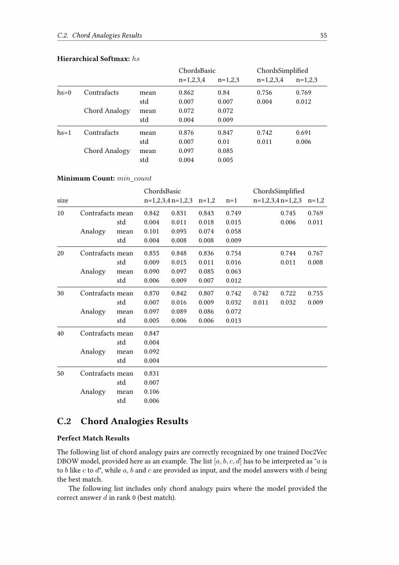
C.2. Chord Analogies Results 55

Hierarchical Softmax: hs

ChordsBasic ChordsSimplifiedn=1,2,3,4 n=1,2,3 n=1,2,3,4 n=1,2,3

hs=0 Contrafacts mean 0.862 0.84 0.756 0.769std 0.007 0.007 0.004 0.012

Chord Analogy mean 0.072 0.072std 0.004 0.009

hs=1 Contrafacts mean 0.876 0.847 0.742 0.691std 0.007 0.01 0.011 0.006

Chord Analogy mean 0.097 0.085std 0.004 0.005

Minimum Count: min_count

ChordsBasic ChordsSimplifiedsize n=1,2,3,4 n=1,2,3 n=1,2 n=1 n=1,2,3,4 n=1,2,3 n=1,2

10 Contrafacts mean 0.842 0.831 0.843 0.749 0.745 0.769std 0.004 0.011 0.018 0.015 0.006 0.011

Analogy mean 0.101 0.095 0.074 0.058std 0.004 0.008 0.008 0.009

20 Contrafacts mean 0.855 0.848 0.836 0.754 0.744 0.767std 0.009 0.015 0.011 0.016 0.011 0.008

Analogy mean 0.090 0.097 0.085 0.063std 0.006 0.009 0.007 0.012

30 Contrafacts mean 0.870 0.842 0.807 0.742 0.742 0.722 0.755std 0.007 0.016 0.009 0.032 0.011 0.032 0.009

Analogy mean 0.097 0.089 0.086 0.072std 0.005 0.006 0.006 0.013

40 Contrafacts mean 0.847std 0.004

Analogy mean 0.092std 0.004

50 Contrafacts mean 0.831std 0.007

Analogy mean 0.106std 0.006

C.2 Chord Analogies Results

Perfect Match Results

The following list of chord analogy pairs are correctly recognized by one trained Doc2VecDBOW model, provided here as an example. The list [a, b, c, d] has to be interpreted as "a isto b like c to d", while a, b and c are provided as input, and the model answers with d beingthe best match.

The following list includes only chord analogy pairs where the model provided thecorrect answer d in rank 0 (best match).

56 Appendix C. Doc2Vec Hyperparameter Tuning

minor-to-dominant:[’Fm’, ’F7’, ’Ebm’, ’Eb7’]

major-to-minor:[’A’, ’Am’, ’D’, ’Dm’][’A’, ’Am’, ’E’, ’Em’][’B’, ’Bm’, ’D’, ’Dm’][’C’, ’Cm’, ’Bb’, ’Bbm’][’C#’, ’C#m’, ’Ab’, ’Abm’][’Eb’, ’Ebm’, ’D’, ’Dm’][’E’, ’Em’, ’D’, ’Dm’][’F’, ’Fm’, ’Eb’, ’Ebm’][’F#’, ’F#m’, ’Eb’, ’Ebm’][’Ab’, ’Abm’, ’F#’, ’F#m’]

dominant-to-minor:[’Bb7’, ’Bbm’, ’Ab7’, ’Abm’][’C7’, ’Cm’, ’D7’, ’Dm’][’C#7’, ’C#m’, ’Eb7’, ’Ebm’][’Eb7’, ’Ebm’, ’D7’, ’Dm’][’F#7’, ’F#m’, ’Ab7’, ’Abm’][’F#7’, ’F#m’, ’D7’, ’Dm’][’Ab7’, ’Abm’, ’F#7’, ’F#m’]

dominant-to-minor-half-step-down:[’A7’, ’Abm’, ’G7’, ’F#m’][’C7’, ’Bm’, ’Bb7’, ’Am’][’D7’, ’C#m’, ’G7’, ’F#m’][’Eb7’, ’Dm’, ’F7’, ’Em’][’F7’, ’Em’, ’Eb7’, ’Dm’][’G7’, ’F#m’, ’A7’, ’Abm’]

minor-to-dominant-half-step-down:[’Bbm’, ’A7’, ’Abm’, ’G7’]

V-I:[’A7’, ’D’, ’Bb7’, ’Eb’][’A7’, ’D’, ’B7’, ’E’][’A7’, ’D’, ’D7’, ’G’][’A7’, ’D’, ’E7’, ’A’][’A7’, ’D’, ’F#7’, ’B’][’Bb7’, ’Eb’, ’D7’, ’G’][’Bb7’, ’Eb’, ’E7’, ’A’][’Bb7’, ’Eb’, ’F#7’, ’B’][’B7’, ’E’, ’Eb7’, ’Ab’][’B7’, ’E’, ’Ab7’, ’C#’][’C7’, ’F’, ’G7’, ’C’][’C#7’, ’F#’, ’F#7’, ’B’][’C#7’, ’F#’, ’G7’, ’C’][’C#7’, ’F#’, ’C7’, ’F’][’D7’, ’G’, ’Eb7’, ’Ab’][’D7’, ’G’, ’Bb7’, ’Eb’][’Eb7’, ’Ab’, ’Ab7’, ’C#’][’E7’, ’A’, ’F#7’, ’B’][’E7’, ’A’, ’G7’, ’C’][’E7’, ’A’, ’Bb7’, ’Eb’][’F7’, ’Bb’, ’F#7’, ’B’][’F7’, ’Bb’, ’G7’, ’C’][’F7’, ’Bb’, ’Bb7’, ’Eb’][’F7’, ’Bb’, ’Eb7’, ’Ab’][’F7’, ’Bb’, ’E7’, ’A’][’F#7’, ’B’, ’G7’, ’C’][’F#7’, ’B’, ’Bb7’, ’Eb’][’F#7’, ’B’, ’C7’, ’F’]

[’F#7’, ’B’, ’F7’, ’Bb’][’G7’, ’C’, ’C7’, ’F’][’G7’, ’C’, ’F#7’, ’B’]

ii-V:[’Am’, ’D7’, ’Dm’, ’G7’][’Am’, ’D7’, ’Ebm’, ’Ab7’][’Am’, ’D7’, ’Gm’, ’C7’][’Bbm’, ’Eb7’, ’Dm’, ’G7’][’Bbm’, ’Eb7’, ’Gm’, ’C7’][’Bm’, ’E7’, ’Dm’, ’G7’][’Bm’, ’E7’, ’F#m’, ’B7’][’Cm’, ’F7’, ’Dm’, ’G7’][’Cm’, ’F7’, ’F#m’, ’B7’][’Cm’, ’F7’, ’Gm’, ’C7’][’Cm’, ’F7’, ’Bm’, ’E7’][’C#m’, ’F#7’, ’Gm’, ’C7’][’C#m’, ’F#7’, ’Bm’, ’E7’][’C#m’, ’F#7’, ’Cm’, ’F7’][’Dm’, ’G7’, ’Ebm’, ’Ab7’][’Dm’, ’G7’, ’Em’, ’A7’][’Dm’, ’G7’, ’Gm’, ’C7’][’Dm’, ’G7’, ’Bbm’, ’Eb7’][’Ebm’, ’Ab7’, ’F#m’, ’B7’][’Ebm’, ’Ab7’, ’Gm’, ’C7’][’Ebm’, ’Ab7’, ’Abm’, ’C#7’][’Ebm’, ’Ab7’, ’Bm’, ’E7’][’Ebm’, ’Ab7’, ’Cm’, ’F7’][’Ebm’, ’Ab7’, ’C#m’, ’F#7’][’Ebm’, ’Ab7’, ’Dm’, ’G7’][’Em’, ’A7’, ’Bbm’, ’Eb7’][’Em’, ’A7’, ’Bm’, ’E7’][’Em’, ’A7’, ’Dm’, ’G7’][’Em’, ’A7’, ’Ebm’, ’Ab7’][’Fm’, ’Bb7’, ’Gm’, ’C7’][’Fm’, ’Bb7’, ’Bbm’, ’Eb7’][’Fm’, ’Bb7’, ’Cm’, ’F7’][’Fm’, ’Bb7’, ’Dm’, ’G7’][’Fm’, ’Bb7’, ’Ebm’, ’Ab7’][’F#m’, ’B7’, ’Bbm’, ’Eb7’][’F#m’, ’B7’, ’Bm’, ’E7’][’F#m’, ’B7’, ’Cm’, ’F7’][’F#m’, ’B7’, ’Dm’, ’G7’][’F#m’, ’B7’, ’Ebm’, ’Ab7’][’Gm’, ’C7’, ’Bbm’, ’Eb7’][’Gm’, ’C7’, ’Cm’, ’F7’][’Gm’, ’C7’, ’Dm’, ’G7’][’Gm’, ’C7’, ’Ebm’, ’Ab7’][’Abm’, ’C#7’, ’Bbm’, ’Eb7’][’Abm’, ’C#7’, ’Bm’, ’E7’][’Abm’, ’C#7’, ’Cm’, ’F7’][’Abm’, ’C#7’, ’Dm’, ’G7’][’Abm’, ’C#7’, ’Gm’, ’C7’]

V/V-V:[’A7’, ’D7’, ’B7’, ’E7’][’A7’, ’D7’, ’D7’, ’G7’][’Bb7’, ’Eb7’, ’D7’, ’G7’][’E7’, ’A7’, ’D7’, ’G7’][’F#7’, ’B7’, ’D7’, ’G7’]

57

Appendix D

Web Application

D.1 Development and Deployment

D.1.1 Data Pipelines

Figure D.1 shows the steps involved to generate the data for the web application. Each boxrepresents a python source code file. Chords data is exported to a mySQL database andconsumed by the web application. Also, the user feedback is stored in a mySQL database.The recommender data and the clustered UMAP scatter plot data are consumed as csv filesby the Web Application.

generate chordcorpus for models

Train Model &calculate similarity

store meta infomerge & clean metainfo

parse tunes,musicXML from

iRealPro

transform meta info totable

query additional metainfo

chords.json

chords.json meta data per tune meta data per tune meta data per tune jazztunes.tunes

generate chords forlead sheet display

jazztunes.chords

chords for each tune section

Visualize TuneSections in Vector

Space

2D coordinates for each tune section

topN similar sections for each tune section

Web Application

Feedback forRecommendations

jazztunes.feedback

Figure D.1: Data Pipelines for data pre-Processing, model training and visu-alization, leadsheet display, storage of user feedback.

D.1.2 Deployment

The Web Application is created with Plotly Dash. It is deployed to a Microsoft Azure WebApplication using a Docker container. For the deployment, the application is first tested onthe local computer, then a docker container is created and uploaded to https://hub.docker.com, and finally attached to the Web Application on Azure. Care must be takenthat the http traffic of the Plotly Dash application is routed to the correct port.

58 Appendix D. Web Application

D.2 Web App Pages

Recommender Page

On the top of the main page (Figure D.6), the user selects a reference tune and a section ofthat tune. The tool displays a list of tunes with the corresponding section, that are consideredas most similar. The leadsheets for both tunes are displayed, both tunes transposed to Cmajor or A minor respectively. Optionally, the user can select to display the leadsheets inthe default key. Below the leadsheets, there are a like and a dislike button to collect userfeedback. At the bottom, additional information regarding the tunes is displayed.

Visualize Clusters

The Visualize Clusters page (Figure D.7) is meant for a deeper investigation of the resultsprovided by the model. The learned vectors for the tune sections are reduced to 2 dimensionsusing UMAP and visualized in a scatter plot. Each point in the scatter plot corresponds to aunique section of a tune. The result is also clustered and points that could not be assignedto a cluster are not displayed.

The user can hover over the points and the corresponding chords are displayed. Tunesthat are recommended on the Recommender page should lie close together also in this scatterplot. As another feature, the user can one or several tune sections with a dropdown box, tohighlight them in the scatter plot. As an example, this can be used to find all the tunes thathave a similar bridge like ’Honeysuckle Rose’.

Tunes Explorer

The Tunes Explorer page (Figure D.8) lists all available tunes with some meta informationin table format. There is a filter function available. Each row in the table is unique per tunename and composer.

Info

The Info page (Figure D.9) provides statistical overview for the tunes. It displays the his-tograms for the number of tunes per composer, the publication year, the tonality and thesection structure.

D.3 Styled Leadsheet Display

.section

.measure

.beat .beat .beat

.measure .measure .measure

.section

.section

Figure D.2: Flexgrid structure used to display leadsheets.

The chords for the web application leadsheets are styled with CSS. The leadsheet isdisplayed as a grid of 4 bars, using Flexgrid, an open-source grid-system based on Flexbox.A new section always starts at a new row (see Figure D.4 for an example). The chords are

D.3. Styled Leadsheet Display 59

aligned according to the appropriate beat within the measure. Figure D.2 illustrates the basicleadsheet grid with the CSS properties.

Figure D.3 shows the 5 parts that a chord is split into. The .root box is mandatory, all otherboxes are optional and depend on the chord type. The .down box contains the major, minor,dominant or diminished symbol. Up to two additions are supported, which are displayedbelow each other in the .alt-up and .alt-down boxes, like in the last bar of Figure D.4.

major,minor,

alterations

.root

.sharp,

.flat,

.natural

.add

.down

alterations

.alt-up

.alt-down

Figure D.3: CSS container names.

The chords data is pre-processed in the data pipeline by identifying and separating the5 chord type parts (Figure D.3) into columns, together with the information about section,measure number and beat. The data is exported to a mySQL database and consumed bythe Plotly Dash web application. The application generates the html code for the styledleadsheet and displays it.

The leadsheet display does not consider correct enharmonic spelling of the root notes.

Figure D.4: Example leadsheet where the number of bars per section is nota multiple of 4.

Figure D.5: Example chord notation with CSS styling applied.

60 Appendix D. Web Application

D.4 Web App Screenshots

Figure D.6: Web Application Recommender Page

D.4. Web App Screenshots 61

Figure D.7: Web Application Visualize Clusters Page

62 Appendix D. Web Application

Figure D.8: Web Application Tunes Explorer Page, with filters to display asubset of the tunes. Here, the list is filtered for composer Jimmy van Heusen.

D.4. Web App Screenshots 63

Figure D.9: Web Application Information Page, with summary statisticsabout the dataset.

65

List of Figures

2.1 Excerpt of a typical leadsheet. . . . . . . . . . . . . . . . . . . . . . . . . . . 52.2 Different chord types based on the root note C, displayed with the iRealPro

app. . . . . . . . . . . . . . . . . . . . . . . . . . . . . . . . . . . . . . . . . . 72.3 Latent Semantic Analysis (LSA) . . . . . . . . . . . . . . . . . . . . . . . . . 82.4 Word2Vec Continuous Bag-of-Words (left) versus Skip-gram Model (right) . 92.5 Doc2Vec Distributed Bag-of-Words DBOW (left) versus Distributed Memory

DM model (right) . . . . . . . . . . . . . . . . . . . . . . . . . . . . . . . . . 10

4.1 Goal 1: The basic harmonic movement for Honeysuckle Rose and Satin Doll(B section) is identical, although the chord types are different. . . . . . . . . 13

4.2 Example for Goal 2: The B sections of Honeysuckle Rose and Tea For Twoshare the same blocks, but the basic harmonic structure is different. . . . . . 13

4.3 Framework of the proposed method. . . . . . . . . . . . . . . . . . . . . . . . 154.4 Top 15 composers contributing tunes for the data set. . . . . . . . . . . . . . 184.5 Top 15 tune form in the data set, the majority of the tunes is in AABA form. 194.6 The period between 1925 and 1945 clearly dominates the publication year

of the tune in the dataset. . . . . . . . . . . . . . . . . . . . . . . . . . . . . . 194.7 Distribution of the default keys of the tunes. . . . . . . . . . . . . . . . . . . 194.8 Zipf Plots for chordBasic vocabulary, for different n-grams. . . . . . . . . . . 244.9 Zipf Plots for chordSimplified and chordFull, for uni-grams and concatenated

n-grams=[1,2,3,4]. . . . . . . . . . . . . . . . . . . . . . . . . . . . . . . . . . 254.10 Distribution of the chord types for uni-grams, with the root note removed. . 254.11 Distribution of the chord types for concatenated ngrams=[1,2,3,4] including

the root. . . . . . . . . . . . . . . . . . . . . . . . . . . . . . . . . . . . . . . 26

5.1 Histogram with number common recommendations, for two different exper-iments. . . . . . . . . . . . . . . . . . . . . . . . . . . . . . . . . . . . . . . . 32

6.1 Doc2Vec weights for the chord n-gram vocabulary, visualized in 2-diensionalspace using PCA. The n-grams with n=[1,2,3,4] are clearly separated. Totalvariance explained by the two principal components: 11.0% . . . . . . . . . . 36

6.2 Focus on ngrams with n=1 and n=2 and n-grams which contain root chordsonly. Bi-grams that contain two identical chords are located closest to theuni-grams. . . . . . . . . . . . . . . . . . . . . . . . . . . . . . . . . . . . . . 37

6.3 Representation of learned doc2vec weights for unigrams containing a rootmajor, minor or dominant chord. The model is trained with all tunes trans-posed to C major and A minor, therefore this representation has to be ana-lyzed from the C major or A minor point of view. Total variance explained:14.3%. . . . . . . . . . . . . . . . . . . . . . . . . . . . . . . . . . . . . . . . . 37

6.4 Doc2Vec DM weights for chordBasic vocabulary, dimension-reduced withPCA. The n-grams with different sizes of n are inseparable. Total varianceexplained: 8.19%. . . . . . . . . . . . . . . . . . . . . . . . . . . . . . . . . . . 38

66 List of Figures

6.5 Doc2VecDMweights for the uni-grams only, chordBasic vocabulary, dimension-reduced with PCA. Total variance explained: 12.17%. . . . . . . . . . . . . . 38

6.6 LSA weights for the chord n-gram vocabulary, visualized in 2-diensionalspace using PCA. The n-grams with n=[1,2,3] are lumped together. Totalvariance explained: 2.01%. . . . . . . . . . . . . . . . . . . . . . . . . . . . . 39

6.7 Clustered tune sections, based on the chordsBasic vocabulary, in the 2-dimensionalUMAP space. Each point in the plot represents a tune section. Points thatcould not be assigned to a cluster are omitted. Different colors representdifferent clusters, but have no meaning otherwise. . . . . . . . . . . . . . . 40

6.8 Visualization of tunes in minor and major, in the 2-dimensional UMAP space.Each point in the plot represents a tune section, the color represents theoverall mode of the tune. . . . . . . . . . . . . . . . . . . . . . . . . . . . . . 40

A.1 (a) shows the original recommendation with the 15 most relevant and irrel-evant recommendations for the tune marked by a big dot. (b) applies theRocchio formula for the positive feedback that was received for the tunemarked with a big square. (c) applies the same step again. . . . . . . . . . . 46

D.1 Data Pipelines for data pre-Processing, model training and visualization,leadsheet display, storage of user feedback. . . . . . . . . . . . . . . . . . . . 57

D.2 Flexgrid structure used to display leadsheets. . . . . . . . . . . . . . . . . . . 58D.3 CSS container names. . . . . . . . . . . . . . . . . . . . . . . . . . . . . . . . 59D.4 Example leadsheet where the number of bars per section is not a multiple of 4. 59D.5 Example chord notation with CSS styling applied. . . . . . . . . . . . . . . . 59D.6 Web Application Recommender Page . . . . . . . . . . . . . . . . . . . . . . 60D.7 Web Application Visualize Clusters Page . . . . . . . . . . . . . . . . . . . . 61D.8 Web Application Tunes Explorer Page, with filters to display a subset of the

tunes. Here, the list is filtered for composer Jimmy van Heusen. . . . . . . . 62D.9 Web Application Information Page, with summary statistics about the dataset. 63

67

List of Tables

1.1 Relationship of terms in the textual and the musical context. . . . . . . . . . 1

2.1 Definition of intervals. . . . . . . . . . . . . . . . . . . . . . . . . . . . . . . 42.2 Shorthand definitions to write common chords using plain text. . . . . . . . 6

4.1 Possible intention and strategy how to select the next tune. . . . . . . . . . . 134.2 Comparison of pre-processing steps for natural language and chords. . . . . 214.3 The vocabularies for chordsBasic and chordsSimplified are two different vari-

ants of chord simplification. . . . . . . . . . . . . . . . . . . . . . . . . . . . 224.4 Number of tokens for different n-gram augmentation, for chordsBasic vo-

cabulary. . . . . . . . . . . . . . . . . . . . . . . . . . . . . . . . . . . . . . . 23

5.1 Summary of Similarity Results based on the Contrafacts Test, for differentmodel types. The top 30 recommendations are considered. . . . . . . . . . . 31

5.2 Chord Analogies for Doc2Vec DBOW and DM in comparison. . . . . . . . . 325.3 Results for the Doc2Vec DBOWmodel for guessing the chord analogies. The

model achieves the highest accuracy for the ii-V chord progreessions. . . . . 335.4 Doc2Vec Self-Similarity for tune sections in the training set. . . . . . . . . . 335.5 Doc2Vec hyperparameter values resulting in highest Contrafacts test accuray. 34

6.1 Clusters according to Figure 6.7, with typical chord expoonents and a fewexamples of tune sections. . . . . . . . . . . . . . . . . . . . . . . . . . . . . 41

A.1 The 15 most relevant results for the tune "These Foolish Things", Section B,with positive user feedback applied for the tune "If I Had You", Section B.The score is based on the cosine similarity. . . . . . . . . . . . . . . . . . . . 47

69

Bibliography

[1] Barry Dean Kernfeld.What to listen for in jazz. 1997. isbn: 978-0300072594.[2] Mark Levine. The Jazz Theory Book. 1995. isbn: 1-883217-04-0.[3] Carl Brandt and Clinton Roemer. Standardized Chord Symbol Notation. Roerick Music

Co., Sherman Oaks, USA, 1976.[4] Carl Brandt and Clinton Roemer. “Standardized chord symbol notation”. In: Sherman

Oakes, Calif.: Roerick Music Co (1976).[5] J. Peter Burkholder. “The Uses of Existing Music: Musical Borrowing as a Field”.

In: Notes 50.3 (1994), pp. 851–870. issn: 00274380, 1534150X. url: http://www.jstor.org/stable/898531.

[6] Gerard Salton, AnitaWong, andChung-Shu Yang. “A vector spacemodel for automaticindexing”. In: Communications of the ACM 18.11 (1975), pp. 613–620.

[7] Stephen McGregor et al. “From distributional semantics to conceptual spaces: A novelcomputational method for concept creation”. In: Journal of Artificial General Intelli-gence 6.1 (2015), p. 55.

[8] Michael W Berry, Zlatko Drmac, and Elizabeth R Jessup. “Matrices, vector spaces, andinformation retrieval”. In: SIAM review 41.2 (1999), pp. 335–362.

[9] Scott Deerwester et al. “Indexing by latent semantic analysis”. In: Journal of the Amer-ican society for information science 41.6 (1990), pp. 391–407.

[10] Thomas K Landauer, Peter W Foltz, and Darrell Laham. “An introduction to latentsemantic analysis”. In: Discourse processes 25.2-3 (1998), pp. 259–284.

[11] TomasMikolov et al. “Distributed representations of words and phrases and their com-positionality”. In: Advances in neural information processing systems. 2013, pp. 3111–3119.

[12] Xin Rong. “word2vec parameter learning explained”. In: arXiv preprint arXiv:1411.2738(2014).

[13] Quoc Le and Tomas Mikolov. “Distributed representations of sentences and docu-ments”. In: International conference on machine learning. PMLR. 2014, pp. 1188–1196.

[14] Jey Han Lau and Timothy Baldwin. “An empirical evaluation of doc2vec with practicalinsights into document embedding generation”. In: arXiv preprint arXiv:1607.05368(2016).

[15] Andrew M Dai, Christopher Olah, and Quoc V Le. “Document embedding with para-graph vectors”. In: arXiv preprint arXiv:1507.07998 (2015).

[16] Carol Peters, Martin Braschler, and Paul Clough. Multilingual information retrieval:From research to practice. Springer Science & Business Media, 2012.

[17] Joseph Rocchio. “Relevance feedback in information retrieval”. In: The Smart retrievalsystem-experiments in automatic document processing (1971), pp. 313–323.

70 Bibliography

[18] Sephora Madjiheurem, Lizhen Qu, and Christian Walder. “Chord2vec: Learning musi-cal chord embeddings”. In: Proceedings of the constructivemachine learning workshop at30th conference on neural information processing systems (NIPS2016), Barcelona, Spain.2016.

[19] Cheng-Zhi Anna Huang, David Duvenaud, and Krzysztof Z Gajos. “Chordripple: Rec-ommending chords to help novice composers go beyond the ordinary”. In: Proceedingsof the 21st International Conference on Intelligent User Interfaces. 2016, pp. 241–250.

[20] Filip Korzeniowski, David RW Sears, and GerhardWidmer. “A large-scale study of lan-guagemodels for chord prediction”. In: 2018 IEEE International Conference on Acoustics,Speech and Signal Processing (ICASSP). IEEE. 2018, pp. 91–95.

[21] Mateusz Waldemar Dorobek. “Generating jazz chords progressions using word em-beddings and recurrent neural networks”. PhD thesis. Wydział Matematyki i NaukInformacyjnych, 2020.

[22] Mitsunori Ogihara and Tao Li. “N-Gram Chord Profiles for Composer Style Represen-tation.” In: ISMIR. 2008, pp. 671–676.

[23] DorienHerremans and Ching-Hua Chuan. “Modelingmusical context withword2vec”.In: arXiv preprint arXiv:1706.09088 (2017).

[24] Elia Anzuoni et al. “A historical analysis of harmonic progressions using chord em-beddings”. In: Proceedings of the 18th Sound and Music Computing Conference. 2021,pp. 284–291.

[25] Martin Pfleiderer and Klaus Frieler. “The Jazzomat project. Issues and methods for theautomatic analysis of jazz improvisations”. In: Concepts, experiments, and fieldwork:Studies in systematic musicology and ethnomusicology (2010), pp. 279–295.

[26] Shih-Chuan Chiu and Min-Syan Chen. “A study on difficulty level recognition ofpiano sheet music”. In: 2012 IEEE International Symposium on Multimedia. IEEE. 2012,pp. 17–23.

[27] Felix Wu. “Data Representations in Neural Network Based Chord Progression Gener-ation Methods”. In: ().

[28] Christopher Harte et al. “Symbolic Representation of Musical Chords: A ProposedSyntax for Text Annotations.” In: ISMIR. Vol. 5. 2005, pp. 66–71.

[29] Damiáan H Zanette. “Zipf’s law and the creation of musical context”. In: MusicaeScientiae 10.1 (2006), pp. 3–18.

[30] Maria Halkidi, Yannis Batistakis, and Michalis Vazirgiannis. “On clustering validationtechniques”. In: Journal of intelligent information systems 17.2 (2001), pp. 107–145.

[31] Allison Lahnala et al. “Chord Embeddings: Analyzing What They Capture and TheirRole for Next Chord Prediction and Artist Attribute Prediction”. In: InternationalConference on Computational Intelligence in Music, Sound, Art and Design (Part ofEvoStar). Springer. 2021, pp. 171–186.

[32] Michael Röder, Andreas Both, and Alexander Hinneburg. “Exploring the space oftopic coherence measures”. In: Proceedings of the eighth ACM international conferenceon Web search and data mining. 2015, pp. 399–408.

[33] Leland McInnes, John Healy, and James Melville. “Umap: Uniform manifold approxi-mation and projection for dimension reduction”. In: arXiv preprint arXiv:1802.03426(2018).

[34] Ricardo JGB Campello, Davoud Moulavi, and Jörg Sander. “Density-based clusteringbased on hierarchical density estimates”. In: Pacific-Asia conference on knowledgediscovery and data mining. Springer. 2013, pp. 160–172.

Bibliography 71

[35] Shalev Itzkovitz et al. “Recurring harmonic walks and network motifs in Westernmusic”. In: Advances in Complex Systems 9.01n02 (2006), pp. 121–132.

[36] Jeff Miller, Vincenzo Nicosia, and Mark Sandler. “Discovering Common Practice: Us-ing Graph Theory to Compare Harmonic Sequences in Musical Audio Collections”.In: 8th International Conference on Digital Libraries for Musicology. 2021, pp. 93–97.

73

Declaration of Originality

Mit der Abgabe dieser Abschlussarbeit versichert der/die Studierende, dass er/sie die Arbeitselbständig und ohne fremde Hilfe verfasst hat. (Bei Teamarbeiten gelten die Leistungen derübrigen Teammitglieder nicht als fremde Hilfe.)

Der/die unterzeichnende Studierende erklärt, dass alle zitierten Quellen (auch Internet-seiten) im Text oder Anhang korrekt nachgewiesen sind, d.h. dass die Abschlussarbeit keinePlagiate enthält, also keine Teile, die teilweise oder vollständig aus einem fremden Text odereiner fremden Arbeit unter Vorgabe der eigenen Urheberschaft bzw. ohne Quellenangabeübernommen worden sind.

Contact: doris.zahnd@gmx.ch

Signed:

Date: