RICE UNIVERSITY

ShuFFLE: Automated Framework for Hardware

Accelerated Iterative Big Data Analysis

by

Ebrahim M. Songhori

A Thesis Submittedin Partial Fulfillment of the

Requirements for the Degree

Master of Science

Approved, Thesis Committee:

Dr. Farinaz Koushanfar, ChairAssociate Professor of Electrical andComputer Engineering

Dr. Richard G. BaraniukVictor E. Cameron Professor of Electricaland Computer Engineering

Dr. Joseph R. CavallaroProfessor of Electrical and ComputerEngineering and Computer Science

Houston, Texas

April, 2014

ABSTRACT

ShuFFLE: Automated Framework for Hardware Accelerated Iterative Big Data

Analysis

by

Ebrahim M. Songhori

This thesis introduces ShuFFLE, a set of novel methodologies and tools for au-

tomated analysis and hardware acceleration of large and dense (non-sparse) Gram

matrices. Such matrices arise in most contemporary data mining; they are hard to

handle because of the complexity of known matrix transformation algorithms and the

inseparability of non-sparse correlations. ShuFFLE learns the properties of the Gram

matrices and their rank for each particular application domain. It then utilizes the

underlying properties for reconfiguring accelerators that scalably operate on the data

in that domain. The learning is based on new factorizations that work at the limit of

the matrix rank to optimize the hardware implementation by minimizing the costly

off-chip memory as well as I/O interactions. ShuFFLE also provides users with a

new Application Programming Interface (API) to implement a customized iterative

least squares solver for analyzing big and dense matrices in a scalable way. This API

is readily integrated within the Xilinx Vivado High Level Synthesis tool to translate

user’s code to Hardware Description Language (HDL). As a case study, we imple-

ment Fast Iterative Shrinkage-Thresholding Algorithm (FISTA) as an l1 regularized

least squares solver. Experimental results show that during FISTA computation using

Field-Programmable Gate Array (FPGA) platform, ShuFFLE attains 1800x iteration

iii

speed improvement compared to the conventional solver and about 24x improvement

compared to our factorized solver on a general purpose processor with SSE4 archi-

tecture for a Gram matrix with 4.6 billion non-zero elements.

Contents

Abstract ii

List of Illustrations vi

List of Tables vii

1 Introduction 1

1.1 Motivating Application . . . . . . . . . . . . . . . . . . . . . . . . . . 3

1.2 Contributions . . . . . . . . . . . . . . . . . . . . . . . . . . . . . . . 4

2 Preliminaries and Related Work 6

2.1 Notation and Basics . . . . . . . . . . . . . . . . . . . . . . . . . . . 6

2.2 Low Rank and Sparse Factorization . . . . . . . . . . . . . . . . . . . 6

2.3 Hardware Accelerated Matrix Computation . . . . . . . . . . . . . . 7

3 ShuFFLE Overview 9

4 Domain Learning 11

4.1 Sparse Matrix Decomposition . . . . . . . . . . . . . . . . . . . . . . 11

4.1.1 Random Sparse Matrix Decomposition (rSMD) . . . . . . . . 12

4.1.2 Adaptive Sparse Matrix Decomposition (aSMD) . . . . . . . . 12

4.1.3 Serial Sparse Matrix Decomposition (sSMD) . . . . . . . . . . 12

4.2 Evolving Dataset . . . . . . . . . . . . . . . . . . . . . . . . . . . . . 13

5 Execution Phase and Hardware Design 15

5.1 Solver Kernel . . . . . . . . . . . . . . . . . . . . . . . . . . . . . . . 15

v

5.2 Parallel Solver . . . . . . . . . . . . . . . . . . . . . . . . . . . . . . . 17

5.3 Case Study: FISTA . . . . . . . . . . . . . . . . . . . . . . . . . . . . 17

6 Evaluation 19

6.1 Experiment Setup . . . . . . . . . . . . . . . . . . . . . . . . . . . . . 19

6.2 FPGA Implementation . . . . . . . . . . . . . . . . . . . . . . . . . . 21

6.3 Domain Learning Results . . . . . . . . . . . . . . . . . . . . . . . . . 22

6.4 Execution Phase Results . . . . . . . . . . . . . . . . . . . . . . . . . 24

7 Conclusion 31

7.1 Future Work . . . . . . . . . . . . . . . . . . . . . . . . . . . . . . . . 31

Bibliography 33

Illustrations

3.1 Global flow of ShuFFLE. . . . . . . . . . . . . . . . . . . . . . . . . . 10

5.1 Solver kernel datapath. . . . . . . . . . . . . . . . . . . . . . . . . . . 16

5.2 Parallel solver datapath. . . . . . . . . . . . . . . . . . . . . . . . . . 17

6.1 Complexity of low rank factorization. . . . . . . . . . . . . . . . . . . 23

6.2 Density of V versus the normilized error. . . . . . . . . . . . . . . . . 24

6.3 Relative computation time versus learning factor l. . . . . . . . . . . 25

6.4 Performance comparison versus dataset size. . . . . . . . . . . . . . . 26

6.5 Effect of l on performance versus dataset size. . . . . . . . . . . . . . 27

6.6 Relative reconstruction error versus time. . . . . . . . . . . . . . . . . 28

6.7 Density of solution vector x versus time. . . . . . . . . . . . . . . . . 29

6.8 Energy performance of different methods. . . . . . . . . . . . . . . . . 30

Tables

6.1 Technical features of the FPGA and CPU platforms. . . . . . . . . . 20

6.2 Memory storage and bandwidth of the FPGA and CPU platforms. . . 20

6.3 Virtex-6 resource utilization. . . . . . . . . . . . . . . . . . . . . . . . 22

1

Chapter 1

Introduction

One of the grand challenges of our time is to find efficient and effective methods for

extracting relevant information from increasingly massive and complex datasets. The

core of several important data analysis and learning algorithms is iterative computa-

tion on the Gram matrix whose elements are the Hamiltonian inner products of data

vectors. Examples of Gram matrix iterative calculation include kernel-based learning

and classification (e.g., spectral clustering, nonlinear dimensionality reduction), sev-

eral regression and regularized least squares methods (e.g., ridge regression [1], and

sparse recovery [2]).

When the Gram matrix is sparse, partitioning the dataset and then using the com-

mon content analysis algorithms can efficiently perform the required learning opera-

tions. Previous studies in hardware acceleration and reconfigurable computing have

already exploited the sparsity in data to perform more efficient data analysis and com-

putations, e.g., [3]. However, when the Gram matrix is large and dense (non-sparse),

none of the currently known mappings are able to handle the iterative updating meth-

ods in a timely and cost-effective way. This is because the overwhelming dependencies

on the content cannot be efficiently partitioned and/or parallel processed.

When performing dense and big matrix computation in hardware, the limit-

ing factor is communications to and from the off-chip memory. In fact, the upper

bound for the performance of most hardware implementation scenarios is often de-

termined by the memory bandwidths. To address this problem, algorithmic solutions

2

have been proposed to trade off communication with computation [4]. For example,

communication-avoiding iterative solver [5] and communication-avoiding QR decom-

position [6] have been proposed to trade-off memory communication with redun-

dant computations. FPGA-based approaches for finding linear algebra kernels were

suggested which optimize the communication/computation trade-off and lower the

costs. However, these optimizations were aimed at generalizing and implementing

non-iterative linear solvers, e.g., QR decompositions which has a high computational

complexity and is not well-suited for large matrix computations.

This thesis proposes Sparse Factorization-based Fast Least squares solvEr (ShuF-

FLE), a novel automated framework for efficient analysis of big and dense datasets.

ShuFFLE devises a domain-specific architecture based on preliminary learning of the

Gram matrix properties for each particular data domain. ShuFFLE exploits the fact

that even dense Gram matrices in big data analysis often admit a low rank structure,

despite their lack of sparsity and large dimension. Learning the pertinent properties

of the Gram matrix and its rank structure are utilized by ShuFFLE for building an

application-specific and accelerator-rich architecture that scalably operates on the

data in the particular domain. The philosophy behind ShuFFLE is consistent with

the current trends in data generation and processing [7]. As an example, more than

50% generated content on the Internet are video and image data; implementing ac-

celerators to efficiently process this content is of great benefit.

The core of ShuFFLE is the set of newly introduced factorizations with linear

complexity that work at the limit of the matrix rank. The new factorizations optimize

the hardware implementation by minimizing the dependencies in data, total off-chip

memory communication, and storage requirements. ShuFFLE provides users with a

new API to implement customized iterative least squares solvers; it uses the domain

3

learning phase knowledge for analyzing big and dense Gram matrices in a scalable way.

This API is readily integrated within the Xilinx Vivado HLS tool to translate user’s

API code to Hardware Description Language (HDL) for direct hardware acceleration.

1.1 Motivating Application

Solving a linear system Ax = y (where A ∈ Rm×n is an overcomplete matrix consist-

ing of m-dimensional vectors of data (m < n), y ∈ Rm×1 is an m-dimensional input

vector, and x ∈ Rn×1 is a solution vector) with the least squares approach appears

in a wide range of algebraic algorithms, machine learning methods, computer vision

computations, and graph processing. Computing the direct solution of this system

involves inversion of the Gram matrix (G = AtA), which is well-known to be very

complex (and even completely impractical) for massively large matrices.

Iterative gradient descent is an alternative approach for solving these linear sys-

tems; it enables reducing the required resources for large scale data analysis while

allowing for additional constraints such as sparsity on the solution. This approach is

typically based upon the following iterative update in each step:

xi = f(xi−1,Gxi−1), (1.1)

where xi is the estimation of solution in iteration i, and f is a linear kernel function.

Various approaches including iterative ridge regression, LASSO [1], power methods

for principal components analysis (PCA) [8], PageRank [9], and high resolution image

reconstruction [10] exploit a similar iterative paradigm often with an added constraint

on f .

The Matrix-Vector Multiplication (MVM) operationGxi−1 in Equation 1.1 carries

almost all of the significant computation and memory interaction load of the execution

4

of the iterative solver. Our observation is that learning to extract the structure of the

data dependencies in A for each particular application domain has the potential to

significantly reduce the complexity of the MVM computations. During the learning

phase, ShuFFLE factorizes A into a product of two smaller matrices D ∈ Rm×l and

V ∈ Rl×n, where A = DV. To make the computations efficient, factorization is

performed such that a sparsity is enforced on the structure of V and we obtain an D

matrix whose size is proportional to the A matrix rank (D is likely dense). Enforcing

sparsity on V allows partitioning of the computations, i.e., the original single MVM

(on G) can be replaced with 4 consecutive MVMs with Vt, Dt, D, and V with lower

total complexity.

Our data analysis in the execution phase leverages the learned structure of the

Gram matrix for the domain to perform its computations in a scalable and cost-

effective way (in terms of energy, storage and speed.) As a case study, we implement

the widely used FISTA [10] method in ShuFFLE API as an iterative solver for ℓ1

regularized least squares. The objective of the ℓ1 problem is to find vector x such

that:

argminx

∥Ax− y∥2 + λ∥x∥1, (1.2)

where λ is a regularization coefficient.

1.2 Contributions

In brief, our contributions are as follows:

• In Chapter 3, 4, and 5, ShuFFLE is proposed as an automated framework for

hardware accelerated analysis of large and dense data.

• Chapter 4 exploits new factorizations with linear complexity for learning the

5

specific structure of the Gram matrices in each particular domain. The new

factorizations optimize the hardware implementation by minimizing the depen-

dencies in data, total off-chip memory communication, and storage require-

ments.

• Chapter 4 introduces two optimization methods for the processing of the low

rank factorizations to improve the robustness to errors and reduce the memory

footprint.

• Chapter 4 presents a case study of SHuFFLE factorization on FISTA that is a

widely used fast linear equation solver kernel.

• Chapter 5 exploits a set of factorizations to provide a domain-specific mapping

of the FISTA into an hardware accelerated architecture. A ShuFFLE API is

introduced for automatic mapping and is readily integrated within the Xilinx

Vivado HLS tool to translate user’s solver code to HDL code for hardware

implementation.

• Chapter 5 creates a further optimized architecture for the ShuFFLE framework

which maximizes the bandwidth of off-chip memory by sequential addressing.

• Chapter 6 compares the conventional (unfactorized iterative calculations using

the full Gram matrix AtA) and the factorized method. The comparison is

performed between a general purpose processor and the ShuFFLE acceleration

on the FPGA platform for the regularized least squares problem. Orders of

magnitude computational efficiency is obtained by the ShuFFLE framework

compared with the conventional CPU.

6

Chapter 2

Preliminaries and Related Work

This chapter provides our notations, relevant background materials of our domain

learning methods, and related work on accelerating matrix computation on hardware.

2.1 Notation and Basics

We write vectors in bold lowercase script, x, and matrices in bold uppercase script,

A. Let At denote the transpose of A. We use ∥x∥p = (∑n

j=1 |x(j)|p)1/p as the

p-norm of a vector where p ≥ 1. The ℓ0-norm of a vector ∥x∥0 is defined as the

number of non-zero coefficients in x. The Frobenius norm of matrix A is defined by

∥A∥F =√

(∑

i,j |A(i, j)|2).

2.2 Low Rank and Sparse Factorization

Singular Value Decomposition (SVD) or Principal Component Analysis (PCA) pro-

vides the exact solution for low rank factorization of a matrix [11]. To enforce specific

structure on the factorized components, alternative minimization approaches can be

employed such as Sparse PCA (SPCA) [12] or K-SVD [13]. However, all these meth-

ods have superlinear computation complexity which makes them impractical for large

datasets.

An alternative scalable and efficient method to find low rank matrix decomposition

is column subset selection [14]. In this approach, a few columns of A are selected to

7

form a projection matrix to factorize data into the subspace spanned by this set of

columns. Another approach to decompose a dataset is the Nystrom method [15]. This

method first learns the best low dimensional subspace, and then projects the entire

dataset into the learned subspace matrix. The result is the compressed Gram matrix

of the dataset. Applications of the Nystrom method can be found in various machine

learning methods such as spectral clustering [16], kernel Support Vector Machines

(SVMs) [17], and large-scale dimensionality reduction [18].

Unfortunately in all the aforementioned methods, the sparsity of the generated

matrices is not guaranteed. Dyer et al., proposed a random Sparse Matrix Decompo-

sition (rSMD) method for low rank sparse factorization with linear complexity [19].

Similar to the Nystrom method, it relies on a small subset of columns of A. However

unlike the Nystrom method, rSMD provides a sparse representations of the data. This

guarantees the reduction of storage and computation overheads.

2.3 Hardware Accelerated Matrix Computation

A number of studies have been devoted to acceleration of matrix computation on

hardware. For example, both dense and sparse MVM operation have been imple-

mented on FPGA using Hardware Description Language (HDL) [20, 21, 22]. Because

MVM consumes the most resources in a linear solver implementation, we focus on

MVM optimization. However, we prefer HLS tools to HDL in order to provide a high

level API for users.

Solving linear system has been also widely studied by the hardware community.

The scope can be roughly divided into direct and iterative methods. In the class of

direct methods, Lower Upper (LU) factorization method is implemented in [23] and

the Cholesky direct solver on FPGA is proposed in [24]. However, the application of

8

direct methods is limited by the complexity of computation.

Recent studies are devoted to iterative methods on sparse matrices. Jacobi solver

is proposed in [25] and enables multiple iteration speedups ranging from 2.8× to 36.8×

on FPGA. Successive over-relaxation method is presented in [26]. In the class of

Krylov methods, conjugate gradient solvers are implemented by [27, 28, 29]. Lanczos

algorithm is implemented in [30]. Unfortunately, most of these implementations are

either done on a sparse dataset, or cannot be scaled properly for large dense matrices.

9

Chapter 3

ShuFFLE Overview

Figure 3.1 demonstrates the global overview of our proposed framework. Steps for

solving a least squares system with ShuFFLE are as follow:

1. ShuFFLE factorized the dataset A into D and V based on user-specified algo-

rithm and parameters in the learning phase (Chapter 4).

2. ShuFFLE sends D and V to the memory on hardware platform.

3. ShuFFLE compiles user’s high level API code for function f using an HLS tool

and embeds it to solver kernel module (Chapter 5).

4. In the execution phase, the host sends inputs y to the ShuFFLE’s solver on

the hardware platform. After computation, it receives back outputs x from

ShuFFLE’s solver.

10

Sampling

Raw

Data

Decomposition

O

M

P

O

M

P

V

D

Execution Phase

Parallel Solver

Domain

Learning Phase

Off-chip Memory

Subspace

Sampling

D

XY

...

Kernel

High level Code

Vivado HLS

Figure 3.1 : Global flow of ShuFFLE.

11

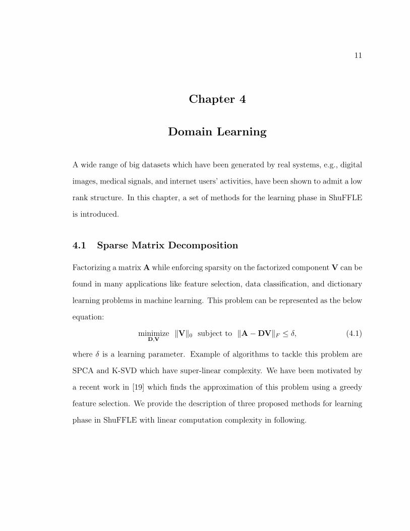
Chapter 4

Domain Learning

A wide range of big datasets which have been generated by real systems, e.g., digital

images, medical signals, and internet users’ activities, have been shown to admit a low

rank structure. In this chapter, a set of methods for the learning phase in ShuFFLE

is introduced.

4.1 Sparse Matrix Decomposition

Factorizing a matrixA while enforcing sparsity on the factorized componentV can be

found in many applications like feature selection, data classification, and dictionary

learning problems in machine learning. This problem can be represented as the below

equation:

minimizeD,V

∥V∥0 subject to ∥A−DV∥F ≤ δ, (4.1)

where δ is a learning parameter. Example of algorithms to tackle this problem are

SPCA and K-SVD which have super-linear complexity. We have been motivated by

a recent work in [19] which finds the approximation of this problem using a greedy

feature selection. We provide the description of three proposed methods for learning

phase in ShuFFLE with linear computation complexity in following.

12

4.1.1 Random Sparse Matrix Decomposition (rSMD)

In rSMD method, matrix D consists of randomly subsampled columns of A. In order

to enforce sparsity on representation matrix V , rSMD uses Orthogonal Matching Pur-

suit (OMP) which is greedy sparse approximation. OMP is used locally to determine

sparse representation of each column of A in the space spanned by D. The detailed

and grantees of this greedy sampling can be found in [19].

4.1.2 Adaptive Sparse Matrix Decomposition (aSMD)

Although the randomized subspace selection reduces the complexity in rSMD, it may

decrease the robustness of factorization. aSMD is an extension of rSMD which, unlike

rSMD, gradually selects column of A and adds them to D. At each step, aSMD calcu-

lates projection errors for all columns and selects new ones based on the distribution

of the errors. This projection error, W , is defined as:

W (Ai) =∥D(DtD)−1DtAi −Ai∥2

∥Ai∥2, (4.2)

where Ai is the ith column of matrix A, D is the current selected columns, and

D(DtD)−1Dt is a projection matrix into the space spanned by D. aSMD selects the

columns in ∆ steps which is learning parameter.

4.1.3 Serial Sparse Matrix Decomposition (sSMD)

Both rSMD and sSMD require access to entire data for subspace sampling. Due to

the massive size of A, their memory footprints can be intolerable for small devices.

sSMD method can locally decide about adding each column of A to D. Thus this

method only requires to store a single column and D matrix. sSMD, like aSMD, uses

the weight function defined in Equation 4.2 to sample columns of A. Algorithm 1

13

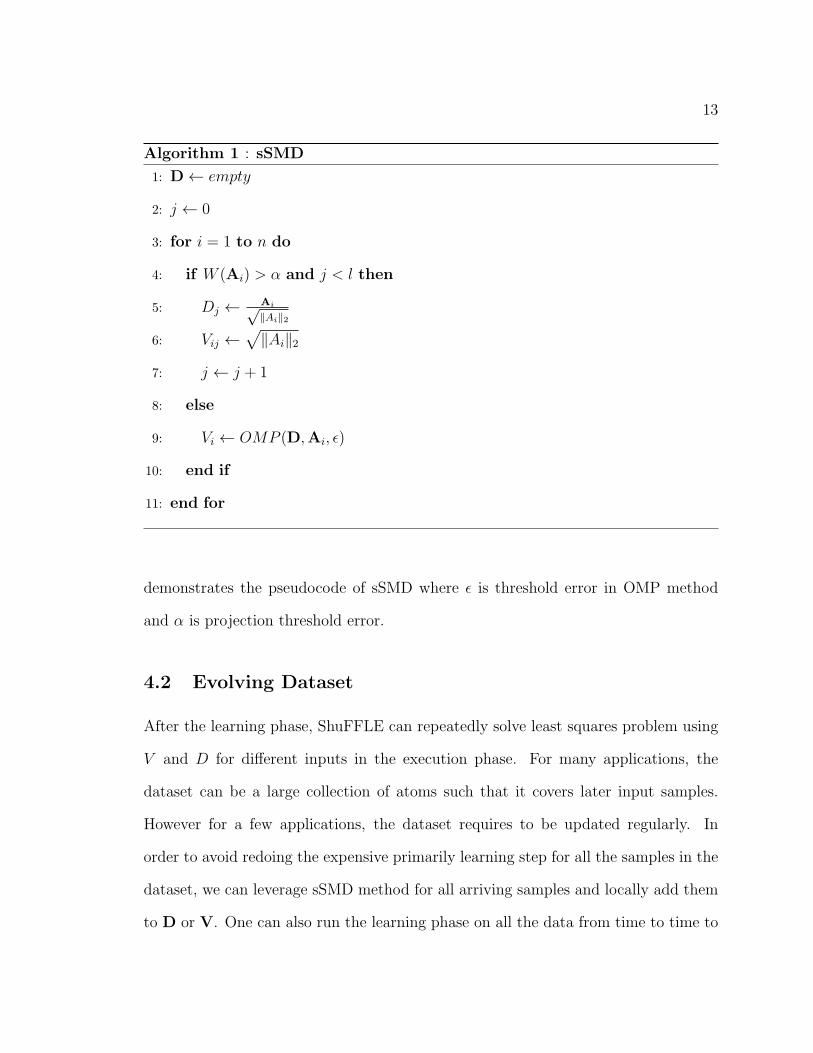
Algorithm 1 : sSMD

1: D← empty

2: j ← 0

3: for i = 1 to n do

4: if W (Ai) > α and j < l then

5: Dj ← Ai√∥Ai∥2

6: Vij ←√∥Ai∥2

7: j ← j + 1

8: else

9: Vi ← OMP (D,Ai, ϵ)

10: end if

11: end for

demonstrates the pseudocode of sSMD where ϵ is threshold error in OMP method

and α is projection threshold error.

4.2 Evolving Dataset

After the learning phase, ShuFFLE can repeatedly solve least squares problem using

V and D for different inputs in the execution phase. For many applications, the

dataset can be a large collection of atoms such that it covers later input samples.

However for a few applications, the dataset requires to be updated regularly. In

order to avoid redoing the expensive primarily learning step for all the samples in the

dataset, we can leverage sSMD method for all arriving samples and locally add them

to D or V. One can also run the learning phase on all the data from time to time to

14

ensure that error and sparsity are in a desirable range. Further research is required

for finding improved strategies to handle such dynamic datasets.

15

Chapter 5

Execution Phase and Hardware Design

We use a combination of HLS and HDL design to implement ShuFFLE’s hardware

iterative solver. The reason for adopting an HLS tool is to allow using high-level

programming in ShuFFLE API. HLS tools enables developers to describe applications

in high level description as well as applying hardware optimization, such as pipelining,

into the design. In this chapter, we provide detailed description of our hardware

architecture and a ℓ1 regularized least squares algorithm as a case study.

5.1 Solver Kernel

As a result of the learning phase, the input dataset A is factorized to a dense and

small matrix D and a sparse and large matrix V. The iterative update changes

accordingly from two MVMs on At and A to four MVMs on Vt, Dt, D, and V. We

designed solver kernel module to handle only a single input y. Algorithm 2 shows the

iterative update in solver kernel. In this algorithm, vectors p ∈ Rl×1 and y ∈ Rm×1

are intermediate vectors. Two MVMs with matrix V, Line 2 and 5, are sparse and

two others with D, Line 3 and 4, are dense MVM operations.

Both matrix D and V are stored in the off-chip memory. Matrix V is stored in

Compressed Sparse Row (CSR) format. In this format, subsequent non-zeros of a

matrix row are stored in contiguous memory addresses. This helps us to enhance the

performance by sequential reading from off-chip memory. Figure 5.1 shows the overall

16

Solver Kernel

P Y’ P Xx + x +x + x +

Y

-

f

Memory

ControllerEthernet

Ethernet

X

Dense MVM

fKernel function

Sparse MVM

Figure 5.1 : Solver kernel datapath.

datapath of solver kernel. In this module, all the vectors x, p, y, and y are stored in

block memories. The module of linear function f is given by user in ShuFFLE API in

high level C/C++ description. ShuFFLE synthesizes it by an HLS tool and embeds

it to solver kernel module.

Algorithm 2 Solver Kernel Algorithm

1: for # of iterations do

2: p← Vx

3: y← Dp

4: p← Dt(y − y)

5: x← f(x,Vtp)

6: end for

17

5.2 Parallel Solver

The pattern of memory accesses is the same for solver kernel regardless of input

vector y. This leads us to use a coarse-grain parallel architecture (parallel solver) by

broadcasting results of memory read to all solver kernels.

CLK3CLK2CLK1

Solver Kernel

Solver Kernel

Solver Kernel

Solver Kernel

Parallel Solver

DDR3

MemoryEthernet

Controller

.

.

.

Memory

Controller

Figure 5.2 : Parallel solver datapath.

Figure 5.2 shows the overall datapath for parallel solver. Input y is directly sent

to a solver kernel through Ethernet from the host. Each solver kernel computes a

single column of the input and sends the result vector x back to the host.

5.3 Case Study: FISTA

Several iterative methods have been proposed to solve ℓ1 regularized least squares,

e.g., gradient descent, stochastic gradient descent, conjugate gradient, Jacobi, ISTA,

FISTA. As a case study, we use ShuFFLE API to implement FISTA method. FISTA

is shown to be a high performance solver with a rapid convergence rate. The iterative

update in FISTA is defined as follows [10]:

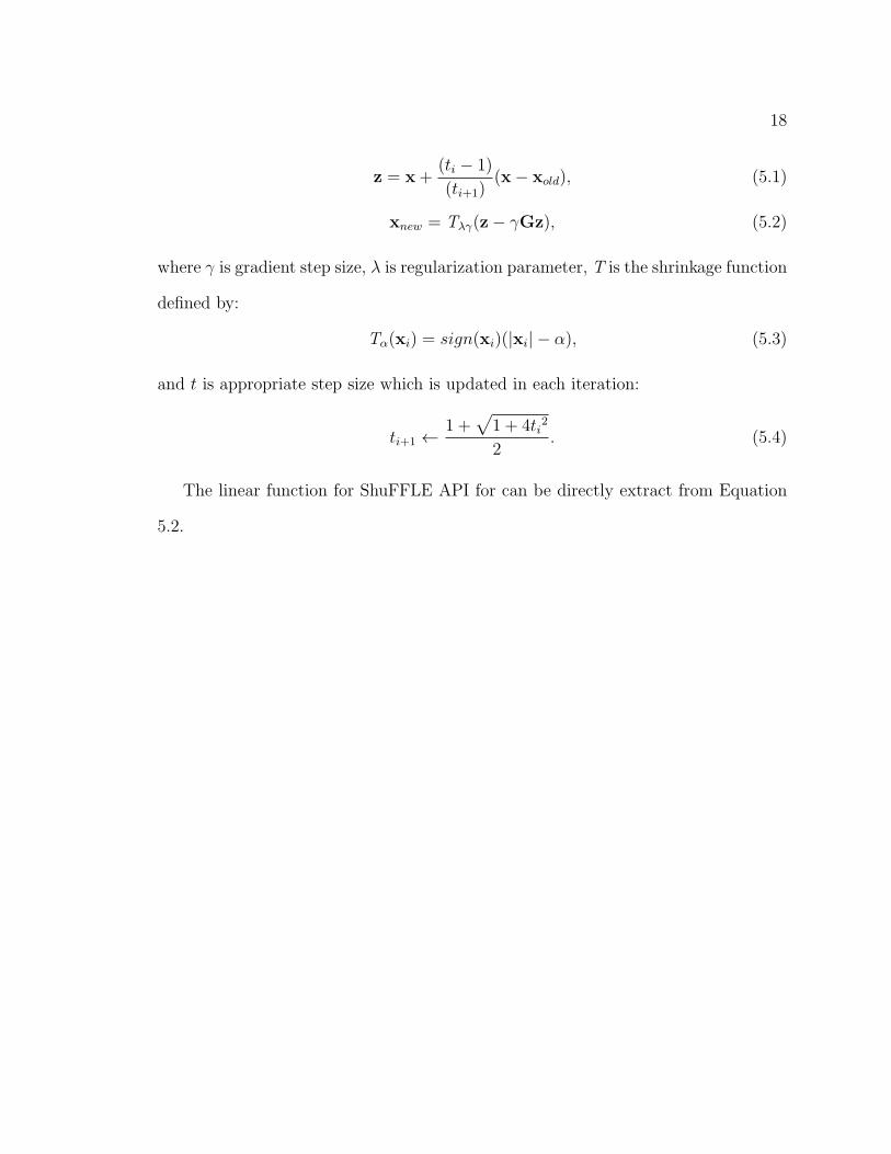
18

z = x+(ti − 1)

(ti+1)(x− xold), (5.1)

xnew = Tλγ(z− γGz), (5.2)

where γ is gradient step size, λ is regularization parameter, T is the shrinkage function

defined by:

Tα(xi) = sign(xi)(|xi| − α), (5.3)

and t is appropriate step size which is updated in each iteration:

ti+1 ←1 +

√1 + 4ti

2

2. (5.4)

The linear function for ShuFFLE API for can be directly extract from Equation

5.2.

19

Chapter 6

Evaluation

6.1 Experiment Setup

We use Xilinx Virtex-6-XC6VLX240T FPGA ML605 Evaluation Kit as our hardware

platform and a system with Linux operating system and Intel core i7-2600K processor

with SSE4 architecture as our general purpose processor platform and also the host of

FPGA board. Table 6.2 provides the detailed features of these two platforms[31, 32].

In our experiments, we use light field dataset from the Stanford Light Field

Archive. Light field data consists of images from an array of cameras taken from

sightly different viewpoints [33]. Light filed images have an application on image

refocusing, denoising, and 3D modeling in computer vision. As an application, we

use high resolution image reconstruction on light field dictionaries problem which is

a form of ℓ1 regularized least-squares [34]. We examine our platform on a light field

dataset with 256k high resolution light field patches. Each patch extracts from 17×17

array of 8 × 8 windows. Thus, the final dataset is a dense 18k × 256k matrix which

has 4.6 billion non-zero coefficients.

We evaluate the performance of ShuFFLE for FISTA API on FPGA by comparing

it to two other methods on general purpose processor platform: (i) Conventional

CPU which is the realization of FISTA using AtA and (ii) CPU Factorized which

is the implementation of factorized FISTA using VtDtDV. We use Eigen library to

implement these methods on a single core of an Intel processor [35].

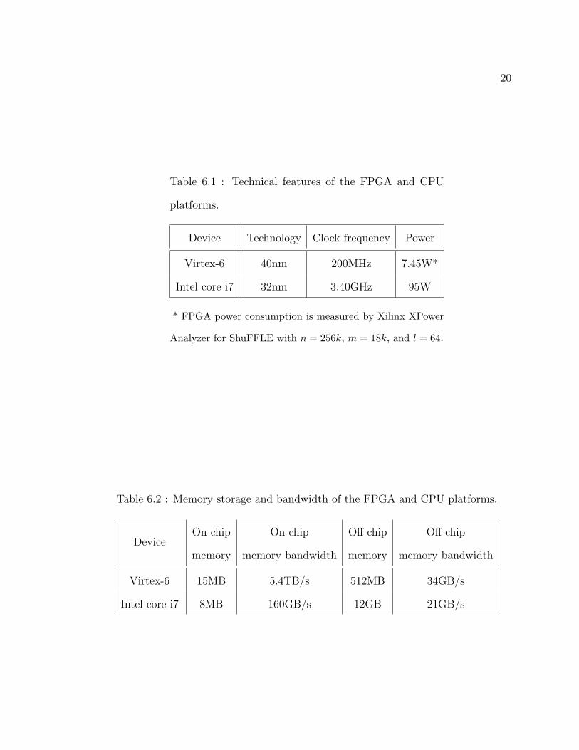
20

Table 6.1 : Technical features of the FPGA and CPU

platforms.

Device Technology Clock frequency Power

Virtex-6 40nm 200MHz 7.45W*

Intel core i7 32nm 3.40GHz 95W

* FPGA power consumption is measured by Xilinx XPower

Analyzer for ShuFFLE with n = 256k, m = 18k, and l = 64.

Table 6.2 : Memory storage and bandwidth of the FPGA and CPU platforms.

DeviceOn-chip

memory

On-chip

memory bandwidth

Off-chip

memory

Off-chip

memory bandwidth

Virtex-6 15MB 5.4TB/s 512MB 34GB/s

Intel core i7 8MB 160GB/s 12GB 21GB/s

21

Intel Stream SIMD Extension (SSE) is an instruction set for modern Intel pro-

cessors designed for Single Instruction Multiple Data (SIMD) computation which is

a parallel computing technology to enhance the performance of wide range of appli-

cation [36]. SSE may promote the performance of intensive matrix computation on

CPU. Many tools and libraries, such as the Eigen library which is used in this thesis,

support SSE programming. In all the experiments on both FPGA and CPU, IEEE

754 single precision floating point format is used to compute and store data.

6.2 FPGA Implementation

In this work, Xilinx Vivado HLS 2013.3 has been used as the HLS tool to translate

C/C++ ShuFFLE API code to Verilog. We also employ Xilinx standard IP cores

for DDR3 memory controller (MIG) and single precision floating point. ShuFFLE

uses Xilinx ISE 14.6 to synthesis, place, route, and program the Virtex 6 FPGA.

The system is successfully placed and routed on three different clock domains with

6 Kernel Solvers on FPGA (Figure 5.2). DDR3 memory and its interface to the

memory controller work on CLK1 domain with 400MHz frequency. Parallel Solver

and the application side of memory and Ethernet controller work on CLK2, with

200MHz frequency. The physical interface of Ethernet controller works on CLK3

with 125Mhz frequency.

Table 6.3 shows Virtex-6 resource utilization for implementing 6 Solver Kernels

and the following sizes: n = 256k, m = 18k, and l = 64. The result includes the

infrastructure overheads such as memory and Ethernet controller.

22

Table 6.3 : Virtex-6 resource utilization.

Used Available Utilization

Slice Registers 40,169 301,440 13%

Slice LUTs 44,049 150,720 29%

RAMB36E1 350 416 84%

DSP48E1s 240 768 31%

6.3 Domain Learning Results

In ShuFFLE framework, the methods in the learning phase are implemented in C++

using Eigen and MPI library and executed on the 4 cores of host core i-7 Intel pro-

cessor. The learning requires to be executed only once to generate D and V. This

process takes about 1 hour for our largest light field dataset with 4.6 billion non-zero

elements. It can be done in parallel with synthesizing HDLs and programming FPGA.

User may also choose between three available factorization methods: rSMD, aSMD,

and sSMD.

Figure 6.1 demonstrates the relative complexity of factorization methods intro-

duced in this thesis including SVD, SPCA, K-SVD, aSMD, rSMD, and sSMD in a

log-log plot. All the computation time is normalized by their time of calculation with

n = 1024, m = 64, l = 16. The OMP error threshold for SMD methods is ϵ = 0.5.

As it appears, the complexity of rSMD and sSMD are close to linear while the one

for aSMD is slightly higher than linear but lower than SVD-based methods.

Figure 6.2 shows the relation between error and sparsity of learning result for

rSMD, aSMD, and sSMD. In order to control the trade-off between error and sparsity,

one can alter ϵ to achieve the desired result. In this experiment, we use a small light

23

105

106

107

108

109

100

102

104

106

108

1010

Low Rank FactorizationComputation Complexity

Matrix Size (n)

Relative Computation Time

aSMD

rSMD

sSMDSVD

K-SVD

SPCA

Figure 6.1 : Complexity of low rank factorization.

filed dataset with n = 10k, m = 1.6k, l = 20. As it appears, larger ∆ in aSMD and

larger α in sSMD result in smaller errors and sparser reperesentation matrices.

Figure 6.3 shows the relative computation time for different learning methods

versus l. In this experiment, we have n = 10k, m = 1.6k, and ϵ = 0.1. These results

is normalized by the time of rSMD at l = 50 As it appears, performance of sSMD

remains steady for large l, while computation time for other two methods increase by

l. As expected, larger ∆ results in slower learning process in aSMD. Furthermore, α

in sSMD does not have a significant contribution to the performance.

24

0.09 0.1 0.11 0.12 0.13 0.14 0.15 0.16

0.1

0.2

0.3

0.4

0.5

0.6

0.7

0.8

0.9

1

Normalized Error

Density of V

SMD Comparison

rSMD

sSMD α=0.90

sSMD α=0.95

aSMD ∆=2

aSMD ∆=5

Figure 6.2 : Density of V versus the normilized error.

6.4 Execution Phase Results

In order to evaluate the performance of ShuFFLE, we use time per iteration metric

to show the speed of solvers in the execution phase. This metric does not include

learning and transferring time.

Figure 6.4 illustrates the performance of ShuFFLE and the CPU realizations ver-

sus matrix size (n) in a log-log plot. In this experiment, we use rSMD with l = 64 and

ϵ = 0.1. The conventional method results in a better performance in comparison with

25

50 100 150 200 250 3000

5

10

15

20

25

30

# of atoms in D (l)

Re

lative

Co

mp

uta

tio

n T

ime

SMD Timing Comparison

rSMD

sSMD α=0.90

sSMD α=0.95

aSMD ∆=2

aSMD ∆=5

Figure 6.3 : Relative computation time versus learning factor l.

the factorized solver and ShuFFLE where the size of A is small due to the overheads

of the two additional MVM operations in both the factorized method and ShuFFLE.

However, by increasing n, the factorized method and ShuFFLE rapidly outperform

the conventional solver. For example, for n = 0.2M , updates in conventional solver is

1800× slower than ShuFFLE and 75× slower than the factorized solver. For n < 32k,

the performance of ShuFFLE is approximately 10× faster than the factorized solver.

However, the performance of the factorized solver drops after n ≥ 64k and ShuFFLE

26

0.2k 1k 4k 16k 64k 0.2M10

-2

10-1

100

101

102

103

104

105

Performance Comparison

Matrix Size (n)

Time (ms) / Iteration

FPGA ShuFFLE

CPU Factorized

CPU Conventional

Figure 6.4 : Performance comparison versus dataset size.

becomes about 24× faster than that. This is caused by the cache misses due to lack

of cache space to store the entire D and V.

The number of selected columns, l, in the factorization has a direct effect on

convergence error rate, as well as system speed (Figure 6.5). l can be interpreted as

learning factor. Increasing l results in smaller convergence error for the least squares.

At the same time, it decreases the performance due to the increase of computation.

As expected, the factorization with l = 256 results in 2× better performance than

l = 512 for both CPU Factorized and ShuFFLE. In this experiment, we use rSMD

27

0.2k 1k 4k 16k 64k 0.2M10

-1

100

101

102

103

104

Matrix Size (n)

Tim

e (

ms

) /

Ite

rati

on

Effect of l on Performance

FPGA ShuFFLE, l= 256

FPGA ShuFFLE, l= 512

CPU Factorized, l= 256

CPU Factorized, l= 512

Figure 6.5 : Effect of l on performance versus dataset size.

for factorization with ϵ = 0.1.

Figure 6.6 shows relative reconstruction error of least squares versus time for

ShuFFLE and the CPU factorized and conventional methods. Relative reconstruction

error is defined as error = ∥y−y∥2∥y∥2 . In this experiment, we use rSMD with l = 128

and ϵ = 0.1 on a light field dataset with n = 16k. ShuFFLE reaches the same

reconstruction error faster than the other methods, for example it achieves error = 0.2

2.9× faster than factorized CPU and 4.4× faster than the conventional method.

The objective of ℓ1 regularized least squares equation is to find a sparser solution

28

0 2 4 6 8 10 12

0.18

0.2

0.22

0.24

0.26

0.28

0.3Relative Error vs. Time

Time (s)

Relative Error

FPGA ShuFFLE

CPU Factorized

CPU Conventional

Figure 6.6 : Relative reconstruction error versus time.

vector x. Figure 6.7 demonstrates the percentage density of x versus time for the same

combination of methods and sizes as the previous experiment. The CPU Factorized

method and ShuFFLE considerably outperform the conventional method because

they go over more iteration for the same period of time due to the better speed. For

example, after 10s, ShuFFLE reaches to 48% density level while CPU factorization

and conventional methods achieve 60% and 90% respectively.

Figure 6.8 shows the energy efficiency for the three methods on both CPU and

FPGA platform. Factorized method on FPGA achieves 2 orders of magnitude com-

29

0 2 4 6 8 1040

50

60

70

80

90

100Density of x vs. Time

Time (s)

Density of x (%)

FPGA ShuFFLE

CPU Factorized

CPU Conventional

Figure 6.7 : Density of solution vector x versus time.

pared to Factorized CPU and 4 orders of magnitude compared to Conventional CPU

better energy efficiency.

30

CPU Conventional CPU Factorized FPGA ShuFFLE10

-1

100

101

102

103

104

Energy Efficiency

Joules per iteration

Figure 6.8 : Energy performance of different methods.

31

Chapter 7

Conclusion

In this thesis, ShuFFLE an automated framework for solving least squares is pre-

sented. ShuFFLE utilizes an offline processing to factorize the original low rank

dataset into its lower dimensional components. As a case study, we use the ShuFFL

API to realize FISTA iterative solver. We use ML605 Virtex-6 board as a hardware

platform. Based on our experimental results, we show that ShuFFLE effectively im-

proves the performance of iterative least squares. ShuFFLE reaches up to 4 orders

of magnitude in joules per iteration efficiency compared to the original matrix opera-

tions using a core-i7 Intel processor with SSE4 architecture. Our proposed framework

achieves up to 2 orders of magnitude energy efficiency than factorized model using

the same CPU on a 4.6 billion non-zeros light field dataset (pre-processing time and

transferring time are excluded from performance measurement for both comparison).

7.1 Future Work

Our Future work will be dedicated to study other platforms like GPU and hetero-

geneous systems. GPU could be a considerable candidate for matrix computation

because of its SIMD architecture. We can also benefit by exploiting heterogeneous

systems, since tasks in our framework have different characteristics. The domain

learning phase has different computation requirements compare to the execution

phase. For example, we may gain speedup by implementing learning phase with

32

rSMD and aSMD on a GPU because of its completely parallel structure. While,

learning phase with sSMD can efficiently implemented on a FPGA platform to at-

tain a high throughput. Furthermore, the execution phase may be efficiently realized

on both GPU and FPGA. Further work is also required for improving strategies to

handle dynamic datasets while updating the factorization.

33

Bibliography

[1] R. Tibshirani, “Regression shrinkage and selection via the lasso,” Journal of the

Royal Statistical Society. Series B (Methodological), pp. 267–288, 1996.

[2] S. S. Chen, D. L. Donoho, and M. A. Saunders, “Atomic decomposition by basis

pursuit,” SIAM, vol. 20, no. 1, pp. 33–61, 1998.

[3] D. Gregg, C. Mc Sweeney, C. McElroy, F. Connor, S. McGettrick, D. Moloney,

and D. Geraghty, “FPGA based sparse matrix vector multiplication using com-

modity dram memory,” in FPL, pp. 786–791, 2007.

[4] A. Rafique, N. Kapre, and G. Constantinides, “Application composition and

communication optimization in iterative solvers using FPGAs,” in FCCM,

pp. 153–160, 2013.

[5] M. Hoemmen, Communication-avoiding Krylov subspace methods. PhD thesis,

University of California, 2010.

[6] M. Anderson, G. Ballard, J. Demmel, and K. Keutzer, “Communication-avoiding

qr decomposition for gpus,” in IPDPS, pp. 48–58, IEEE, 2011.

[7] J. Cong, V. Sarkar, G. Reinman, and A. Bui, “Customizable domain-specific

computing,” IEEE Design and Test of Computers, vol. 28, no. 2, pp. 6–15, 2011.

[8] M. Journee, Y. Nesterov, P. Richtarik, and R. Sepulchre, “Generalized power

method for sparse principal component analysis,” JMLR, vol. 11, pp. 517–553,

34

2010.

[9] L. Page, S. Brin, R. Motwani, and T. Winograd, “The pagerank citation ranking:

bringing order to the web.,” 1999.

[10] A. Beck and M. Teboulle, “A fast iterative shrinkage-thresholding algorithm for

linear inverse problems,” SIAM, vol. 2, no. 1, pp. 183–202, 2009.

[11] G. H. Golub and C. Reinsch, “Singular value decomposition and least squares

solutions,” Numerische Mathematik, vol. 14, no. 5, pp. 403–420, 1970.

[12] H. Zou, T. Hastie, and R. Tibshirani, “Sparse principal component analysis,”

JCGS, vol. 15, no. 2, pp. 265–286, 2006.

[13] M. Aharon, M. Elad, and A. Bruckstein, “k -svd: An algorithm for designing

overcomplete dictionaries for sparse representation,” Signal Processing, IEEE

Transactions on, vol. 54, pp. 4311–4322, Nov 2006.

[14] P. Drineas, A. Frieze, R. Kannan, S. Vempala, and V. Vinay, “Clustering large

graphs via the singular value decomposition,” Machine learning, vol. 56, no. 1-3,

pp. 9–33, 2004.

[15] P. Drineas and M. W. Mahoney, “On the nystrom method for approximating a

gram matrix for improved kernel-based learning,” JMLR, vol. 6, pp. 2153–2175,

2005.

[16] C. Fowlkes, S. Belongie, F. Chung, and J. Malik, “Spectral grouping using the

nystrom method,” TPAMI, vol. 26, no. 2, pp. 214–225, 2004.

[17] C. Williams and M. Seeger, “Using the nystrom method to speed up kernel

machines,” in NIPS, Citeseer, 2001.

35

[18] K. Zhang and J. T. Kwok, “Clustered nystrom method for large scale manifold

learning and dimension reduction,” Neural Networks, IEEE Transactions on,

vol. 21, no. 10, pp. 1576–1587, 2010.

[19] E. L. Dyer, A. C. Sankaranarayanan, and R. G. Baraniuk, “Greedy feature se-

lection for subspace clustering,” J. Mach. Learn. Res., vol. 14, pp. 2487–2517,

Jan. 2013.

[20] H. ElGindy and Y. Shue, “On sparse matrix-vector multiplication with FPGA-

based system,” in FCCM, pp. 273–274, 2002.

[21] S. Qasim, S. Abbasi, and B. Almashary, “A proposed FPGA-based parallel ar-

chitecture for matrix multiplication,” in APCCAS, pp. 1763–1766, 2008.

[22] X. Jiang and J. Tao, “Implementation of effective matrix multiplication on

FPGA,” in IC-BNMT, pp. 656–658, 2011.

[23] W. Zhang, V. Betz, and J. Rose, “Portable and scalable FPGA-based accelera-

tion of a direct linear system solver,” in FPT, pp. 17–24, 2008.

[24] P. Greisen, M. Runo, P. Guillet, S. Heinzle, A. Smolic, H. Kaeslin, and M. Gross,

“Evaluation and FPGA implementation of sparse linear solvers for video process-

ing applications,” TCSVT, vol. 23, no. 8, pp. 1402–1407, 2013.

[25] G. Morris and V. Prasanna, “An FPGA-based floating-point jacobi iterative

solver,” in ISPAN, pp. 8 pp.–, 2005.

[26] B. Di Martino, N. Mazzocca, G. P. Saggese, and A. G. Strollo, “A technique for

FPGA synthesis driven by automatic source code analysis and transformations,”

36

in Field-Programmable Logic and Applications: Reconfigurable Computing Is Go-

ing Mainstream, pp. 47–58, Springer, 2002.

[27] M. deLorimier and A. DeHon, “Floating-point sparse matrix-vector multiply for

FPGAs,” in FPGA, FPGA ’05, (New York, NY, USA), pp. 75–85, ACM, 2005.

[28] G. R. Morris, V. K. Prasanna, and R. D. Anderson, “A hybrid approach for

mapping conjugate gradient onto an FPGA-augmented reconfigurable supercom-

puter,” in FCCM, pp. 3–12, IEEE, 2006.

[29] A. R. Lopes and G. A. Constantinides, “A high throughput FPGA-based floating

point conjugate gradient implementation,” in Reconfigurable Computing: Archi-

tectures, Tools and Applications, pp. 75–86, Springer, 2008.

[30] J. Jerez, G. Constantinides, and E. Kerrigan, “Fixed point lanczos: Sustain-

ing tflop-equivalent performance in FPGAs for scientific computing,” in FCCM,

pp. 53–60, 2012.

[31] Xilinx, “Virtex-6 family overview,” Jan. 2012.

[32] Intel, “Intel core i7-2600 processor,” 2011.

[33] K. Marwah, G. Wetzstein, Y. Bando, and R. Raskar, “Compressive light field

photography using overcomplete dictionaries and optimized projections,” ACM

TG, vol. 32, no. 4, pp. 46:1–46:12, 2013.

[34] B. Wilburn, “High-performance imaging using arrays of inexpensive cameras,”

PhD Dissertation, Stanford University, 2005.

[35] E. Library, “Eigen library website,” April 2014.

37

[36] S. Intel, “Programming reference,” Intels software network, sofwareprojects. in-

tel. com/avx, vol. 2, p. 7, 2007.