
Shreedhar Savant TODKAR
295
THESE DE DOCTORAT DE L'UNIVERSITE DE NANTES COMUE UNIVERSITE BRETAGNE LOIRE ECOLE DOCTORALE N° 601 Mathématiques et Sciences et Technologies de l'Information et de la Communication Spécialité : Signal, Image et Vision Par Shreedhar Savant TODKAR Suivi de l'endommagement des structures de chaussées par technique radar Ultra-large bande Application to debonding detection Thèse présentée et soutenue à Nantes, le 27 Novembre 2019 Unité de recherche : Évaluation Non-Destructive des Structures et des Matériaux (Cerema) Département Composants et Systèmes - Laboratoire Structure et Instrumentation Intégrée (IFSTTAR) Thèse N° : Rapporteurs : M. Pascal LARZABAL Professeur des universités, ENS Cachan – Cachan Mme. Atika MENHAJ Professeur des universités, Université Polytechnique Hauts-de-France Composition du Jury : Président : M. François AUGER Professeur des Universités, Université de Nantes Examinateurs : M. Pascal LARZABAL Professeur des Universités, ENS Cachan – Cachan Mme. Atika MENHAJ Professeur des Universités, Université Polytechnique Hauts-de-France M. Emmanuel TROUVE Professeur des Universités, Université Savoie Mont-Blanc M. Emanuel RADOI Professeur des Universités, Université Bretagne Occidentale M. François AUGER Professeur des Universités, Université de Nantes Dir. de thèse : M. Amine IHAMOUTEN IDTPE – HDR (ENDSUM), Cerema - Angers Invité(s) M. Cédric LE BASTARD Co-directeur de thèse, Chargé de Recherches HDR, Cerema - Angers M. Vincent BALTAZART Co-directeur de thèse, Chargé de Recherches, IFSTTAR – Nantes M. Xavier DEROBERT ITPE – HDR (GERS-GeoEND), IFSTTAR – Nantes
-
Upload
khangminh22 -
Category
Documents
-
view
0 -
download
0
Transcript of Shreedhar Savant TODKAR

THESE DE DOCTORAT DE
L'UNIVERSITE DE NANTES
COMUE UNIVERSITE BRETAGNE LOIRE
ECOLE DOCTORALE N° 601
Mathématiques et Sciences et Technologies
de l'Information et de la Communication
Spécialité : Signal, Image et Vision
Par
Shreedhar Savant TODKAR
Suivi de l'endommagement des structures de chaussées par technique radar Ultra-large bande Application to debonding detection Thèse présentée et soutenue à Nantes, le 27 Novembre 2019 Unité de recherche : Évaluation Non-Destructive des Structures et des Matériaux (Cerema)
Département Composants et Systèmes - Laboratoire Structure et Instrumentation Intégrée (IFSTTAR)
Thèse N° :
Rapporteurs : M. Pascal LARZABAL Professeur des universités, ENS Cachan – Cachan Mme. Atika MENHAJ Professeur des universités, Université Polytechnique Hauts-de-France
Composition du Jury : Président : M. François AUGER Professeur des Universités, Université de Nantes Examinateurs : M. Pascal LARZABAL Professeur des Universités, ENS Cachan – Cachan
Mme. Atika MENHAJ Professeur des Universités, Université Polytechnique Hauts-de-France M. Emmanuel TROUVE Professeur des Universités, Université Savoie Mont-Blanc M. Emanuel RADOI Professeur des Universités, Université Bretagne Occidentale M. François AUGER Professeur des Universités, Université de Nantes
Dir. de thèse : M. Amine IHAMOUTEN IDTPE – HDR (ENDSUM), Cerema - Angers
Invité(s) M. Cédric LE BASTARD Co-directeur de thèse, Chargé de Recherches HDR, Cerema - Angers M. Vincent BALTAZART Co-directeur de thèse, Chargé de Recherches, IFSTTAR – Nantes M. Xavier DEROBERT ITPE – HDR (GERS-GeoEND), IFSTTAR – Nantes


The hardest choices require the strongest wills-Thanos


Acknowledgements
To my life-coach, my beloved father and my life-support, my lovely mother. I owe itall to you.
First of all, I am indebted to my Thesis director, Dr. Amine IHAMOUTEN and my co-director Dr. Vincent BALTAZART for his great support and invaluable advice throughoutthe course of my research. I extend my gratitude to Dr. Cédric LE BASTARD for hisguidance throughout the course of my research and for his invaluable comments thathelped me improve the manuscript.
I am grateful to Dr. LE BASTARD and Dr. BALTAZART for their insights and sharingtheir knowledge and experience in Signal Processing and Machine Learning. I also thankDr. BALTAZART for his crucial remarks that shaped my final dissertation. A specialthanks to Dr. Xavier DEROBERT for sharing his knowledge and experience in GPR andGeophysics.
A very special gratitude goes out to all the members of ‘Comite de Suivi de Thèse’,Prof. Emanuel RADOI and Dr. Christophe BOURLIER for providing me their valuablefeedback and suggestions to improve my work.
A personal note of thanks to my dissertation rapporteurs: Prof. Pascal LARZABALand Prof. Atika MENHAJ for taking their valuable time in providing me a speedy response.I extend my gratitude towards the thesis committee members Prof. Emmanuel TROUVEand Prof. Emanuel RADOI and the president of the jury, Prof. François AUGER for theirpresence during the defense and their comments that helped me improve the final versionof the manuscript.
And at last but by no means least, a special thanks to all my colleagues at Ceremaand IFSTTAR for directly or indirectly sharing their experience with me throughout thecourse of the thesis.
Last but not least, I would like to express my deepest gratitude to my family andfriends. This dissertation would not have been possible without their warm love, continuedpatience, and endless support.
Thanks one and all for your encouragement!
3


Contents
Acknowledgements 3
ABSTRACTANDRÉSUMÉ ÉTENDU 29
I INTRODUCTION 49
1 Introduction 511.1 Introduction . . . . . . . . . . . . . . . . . . . . . . . . . . . . . . . . . . . . 51
1.1.1 Context of the Thesis . . . . . . . . . . . . . . . . . . . . . . . . . . 511.1.2 Problem statement: Monitoring structural pavement conditions . . . 521.1.3 Objectives: GPR data processing for debonding detection . . . . . . 53
1.2 Thesis Structure . . . . . . . . . . . . . . . . . . . . . . . . . . . . . . . . . 541.3 Conclusions . . . . . . . . . . . . . . . . . . . . . . . . . . . . . . . . . . . . 55
2 Debonding Survey in Pavement Structures 572.1 Existing methods for structural pavement survey . . . . . . . . . . . . . . . 582.2 Common methods of Structural health evaluation . . . . . . . . . . . . . . . 59
2.2.1 Destructive Testing . . . . . . . . . . . . . . . . . . . . . . . . . . . . 592.2.2 Non-destructive Testing . . . . . . . . . . . . . . . . . . . . . . . . . 62
2.2.2.1 Mechanical wave . . . . . . . . . . . . . . . . . . . . . . . . 632.2.2.2 Electromagnetic (EM) wave . . . . . . . . . . . . . . . . . . 63
2.3 Radar-based NDT techniques . . . . . . . . . . . . . . . . . . . . . . . . . . 642.3.1 GPR System . . . . . . . . . . . . . . . . . . . . . . . . . . . . . . . 652.3.2 GPR Data Acquisition . . . . . . . . . . . . . . . . . . . . . . . . . . 65
2.3.2.1 Data collection modes . . . . . . . . . . . . . . . . . . . . . 672.3.3 GPR Performance Specifications . . . . . . . . . . . . . . . . . . . . 69
2.3.3.1 Reflections . . . . . . . . . . . . . . . . . . . . . . . . . . . 692.3.3.2 Penetration depth . . . . . . . . . . . . . . . . . . . . . . . 702.3.3.3 Vertical Resolution (or Time Resolution) . . . . . . . . . . 70
2.3.4 Clutter . . . . . . . . . . . . . . . . . . . . . . . . . . . . . . . . . . 702.4 GPR Data formats . . . . . . . . . . . . . . . . . . . . . . . . . . . . . . . . 712.5 Data processing techniques for debonding survey . . . . . . . . . . . . . . . 73
5

CONTENTS
2.5.1 Data-driven methods . . . . . . . . . . . . . . . . . . . . . . . . . . . 732.5.2 Model-based or Model-driven methods . . . . . . . . . . . . . . . . . 742.5.3 Proposed two-step strategy for debonding survey . . . . . . . . . . . 74
2.6 Reference data processing method for debonding detection: Amplitude Ra-tio Test . . . . . . . . . . . . . . . . . . . . . . . . . . . . . . . . . . . . . . 752.6.1 ART Principle . . . . . . . . . . . . . . . . . . . . . . . . . . . . . . 752.6.2 ART Computation . . . . . . . . . . . . . . . . . . . . . . . . . . . . 762.6.3 Decision threshold . . . . . . . . . . . . . . . . . . . . . . . . . . . . 78
2.7 Conclusion . . . . . . . . . . . . . . . . . . . . . . . . . . . . . . . . . . . . 84
II MACHINE LEARNING METHODSAND DATA PREPROCESSING FORDEBONDING DETECTION 85
3 Machine Learning Methods 873.1 Elements of Machine Learning . . . . . . . . . . . . . . . . . . . . . . . . . 89
3.1.1 Unsupervised Machine Learning . . . . . . . . . . . . . . . . . . . . 893.1.2 Supervised Machine Learning . . . . . . . . . . . . . . . . . . . . . . 903.1.3 Implementation of ML algorithms . . . . . . . . . . . . . . . . . . . 92
3.2 Data Clustering method . . . . . . . . . . . . . . . . . . . . . . . . . . . . . 943.2.1 Principle . . . . . . . . . . . . . . . . . . . . . . . . . . . . . . . . . 943.2.2 Modified clustering algorithm . . . . . . . . . . . . . . . . . . . . . . 95
3.3 Parameterized Supervised machine learning: Support Vector Machines . . . 983.3.1 Two-Class SVMs for binary classification . . . . . . . . . . . . . . . 98
3.3.1.1 Linear SVM . . . . . . . . . . . . . . . . . . . . . . . . . . 993.3.1.2 Non-linear SVM . . . . . . . . . . . . . . . . . . . . . . . . 102
3.3.2 One-Class SVMs for anomaly detection . . . . . . . . . . . . . . . . 1043.4 Non-Parameterized Supervised learning: Random Forests . . . . . . . . . . 110
3.4.1 Background . . . . . . . . . . . . . . . . . . . . . . . . . . . . . . . . 1103.4.2 Principle . . . . . . . . . . . . . . . . . . . . . . . . . . . . . . . . . 1103.4.3 Application to binary classification for debonding detection . . . . . 112
3.5 Decision making: Probabilistic estimates . . . . . . . . . . . . . . . . . . . . 1153.5.1 Introduction . . . . . . . . . . . . . . . . . . . . . . . . . . . . . . . 1163.5.2 Probabilistic estimation for SVMs: Platt scaling . . . . . . . . . . . 1163.5.3 Probabilistic estimation for Random forests . . . . . . . . . . . . . . 118
3.6 Synthesis . . . . . . . . . . . . . . . . . . . . . . . . . . . . . . . . . . . . . 1193.7 Conclusions . . . . . . . . . . . . . . . . . . . . . . . . . . . . . . . . . . . . 122
4 Signal Feature Analysis For Debonding Survey 1234.1 Feature engineering . . . . . . . . . . . . . . . . . . . . . . . . . . . . . . . . 1244.2 Signal features for GPR data . . . . . . . . . . . . . . . . . . . . . . . . . . 125
4.2.1 Local signal features . . . . . . . . . . . . . . . . . . . . . . . . . . . 1264.2.2 Global signal features . . . . . . . . . . . . . . . . . . . . . . . . . . 130
6
CONTENTS
4.2.3 Comparison of Local and Global feature sets . . . . . . . . . . . . . 1314.2.4 Feature reduction using Principal Component Analysis (PCA) . . . 1324.2.5 Feature selection methodology . . . . . . . . . . . . . . . . . . . . . 135
4.3 Preliminary tests on machine learning methods using GPR signal features . 1374.3.1 Two-Class SVM . . . . . . . . . . . . . . . . . . . . . . . . . . . . . 1384.3.2 One-Class SVM . . . . . . . . . . . . . . . . . . . . . . . . . . . . . . 1384.3.3 Random forests . . . . . . . . . . . . . . . . . . . . . . . . . . . . . . 139
4.4 Conclusion . . . . . . . . . . . . . . . . . . . . . . . . . . . . . . . . . . . . 140
III DATA PROCESSING FOR DEBONDING DETECTION IN PAVE-MENT STRUCTURES 143
5 Machine Learning Model Selection and Validation For Debonding Sur-vey 1455.1 Methodology . . . . . . . . . . . . . . . . . . . . . . . . . . . . . . . . . . . 1465.2 Method-based model fitting . . . . . . . . . . . . . . . . . . . . . . . . . . . 147
5.2.1 Kernel-based analysis . . . . . . . . . . . . . . . . . . . . . . . . . . 1505.2.2 Cross-validation techniques . . . . . . . . . . . . . . . . . . . . . . . 151
5.2.2.1 Choice of optimal hyper-parameters . . . . . . . . . . . . . 1525.2.2.2 Some results . . . . . . . . . . . . . . . . . . . . . . . . . . 156
5.2.3 Learning data size . . . . . . . . . . . . . . . . . . . . . . . . . . . . 1575.3 Robustness of machine learning methods w.r.t pavement medium . . . . . . 159
5.3.1 Noise vs. permittivity variations . . . . . . . . . . . . . . . . . . . . 1605.3.1.1 Analysis of noisy data . . . . . . . . . . . . . . . . . . . . . 1605.3.1.2 Some results . . . . . . . . . . . . . . . . . . . . . . . . . . 163
5.3.2 Debonding thickness and permittivity variations . . . . . . . . . . . 1645.3.3 Single scattering vs. Multiple scattering effects . . . . . . . . . . . . 167
5.4 Summary . . . . . . . . . . . . . . . . . . . . . . . . . . . . . . . . . . . . . 1695.5 Conclusion . . . . . . . . . . . . . . . . . . . . . . . . . . . . . . . . . . . . 172
6 Application For Decision Support To Detect Debondings 1736.1 Debonding detection on experimental data . . . . . . . . . . . . . . . . . . . 1746.2 Artificial air-void debonding detection in test slabs . . . . . . . . . . . . . . 175
6.2.1 Two-class SVM . . . . . . . . . . . . . . . . . . . . . . . . . . . . . . 1756.2.2 One-class SVM . . . . . . . . . . . . . . . . . . . . . . . . . . . . . . 1756.2.3 Random forests . . . . . . . . . . . . . . . . . . . . . . . . . . . . . . 1766.2.4 Benchmark comparison with reference method . . . . . . . . . . . . 178
6.3 Artificial debonding detection from embedded in pavements . . . . . . . . . 1796.3.1 Two-class SVM . . . . . . . . . . . . . . . . . . . . . . . . . . . . . . 1806.3.2 One-class SVM . . . . . . . . . . . . . . . . . . . . . . . . . . . . . . 1806.3.3 Random forests . . . . . . . . . . . . . . . . . . . . . . . . . . . . . . 1846.3.4 Benchmark comparison with reference method . . . . . . . . . . . . 186
6.4 Conclusion . . . . . . . . . . . . . . . . . . . . . . . . . . . . . . . . . . . . 187
7

CONTENTS
7 Conclusions and Perspectives 1897.1 Conclusions . . . . . . . . . . . . . . . . . . . . . . . . . . . . . . . . . . . . 1897.2 Perspectives . . . . . . . . . . . . . . . . . . . . . . . . . . . . . . . . . . . . 191
Appendices 193
A Simulated Databases 195A.1 Radar pulse . . . . . . . . . . . . . . . . . . . . . . . . . . . . . . . . . . . . 196
A.1.1 Analytic GPR pulse . . . . . . . . . . . . . . . . . . . . . . . . . . . 196A.1.2 Experimental GPR pulse . . . . . . . . . . . . . . . . . . . . . . . . 197
A.2 Analytic GPR modeling . . . . . . . . . . . . . . . . . . . . . . . . . . . . . 198A.2.1 Basics and hypothesis . . . . . . . . . . . . . . . . . . . . . . . . . . 198A.2.2 Non-debonding case . . . . . . . . . . . . . . . . . . . . . . . . . . . 200A.2.3 Debonding case . . . . . . . . . . . . . . . . . . . . . . . . . . . . . . 201
A.2.3.1 Single scattering model . . . . . . . . . . . . . . . . . . . . 202A.2.3.2 Multiple scattering model . . . . . . . . . . . . . . . . . . . 203
A.3 Numeric database: Pavement modeling using MoM . . . . . . . . . . . . . . 204A.4 Numeric database: Pavement modeling using FDTD . . . . . . . . . . . . . 206
A.4.1 Creating a 2D gprMax model of a pavement structure . . . . . . . . 207A.5 Noisy data . . . . . . . . . . . . . . . . . . . . . . . . . . . . . . . . . . . . . 209
A.5.1 SNR definition . . . . . . . . . . . . . . . . . . . . . . . . . . . . . . 209A.5.2 Illustrative results . . . . . . . . . . . . . . . . . . . . . . . . . . . . 210
B Experimental Databases 213B.1 Test slabs database with controlled air-void debondings at Cerema . . . . . 213
B.1.1 Experimental setup . . . . . . . . . . . . . . . . . . . . . . . . . . . . 213B.1.2 Ground-coupled WB GPR: GSSI SIR-3000 . . . . . . . . . . . . . . 215B.1.3 Data Acquisition . . . . . . . . . . . . . . . . . . . . . . . . . . . . . 216
B.2 Fatigue Carousel database over embedded artificial debondings at IFSTTAR218B.2.1 Experimental setup . . . . . . . . . . . . . . . . . . . . . . . . . . . . 219B.2.2 GPR used . . . . . . . . . . . . . . . . . . . . . . . . . . . . . . . . . 220
B.2.2.1 Air-coupled UWB Stepped-frequency GPR . . . . . . . . . 220B.2.3 Data acquisition . . . . . . . . . . . . . . . . . . . . . . . . . . . . . 220
B.2.3.1 Air-coupled UWB Stepped-frequency GPR . . . . . . . . . 221B.2.3.2 Ground-coupled WB GPR: GSSI SIR-3000 . . . . . . . . . 223
C Performance benchmarks and Performance metrics 227C.1 Performance benchmark . . . . . . . . . . . . . . . . . . . . . . . . . . . . . 227
C.1.1 Ground truth (GT) . . . . . . . . . . . . . . . . . . . . . . . . . . . 227C.1.2 Pseudo-ground truth (PGT) . . . . . . . . . . . . . . . . . . . . . . . 229
C.2 Performance assessment of detection methods . . . . . . . . . . . . . . . . . 230C.2.1 Performance assessment for Binary classification . . . . . . . . . . . 230C.2.2 Performance assessment for probabilistic estimation . . . . . . . . . 232
8

CONTENTS
D Time-gating of a GPR A-scan 235
E Additional illustrations for Chapter. 6 239
Abbreviations 255
IV BIBLIOGRAPHY 257
Bibliography 288
9


List of Figures
1 Schéma simplifié d’un décollement entre couches de chaussée . . . . . . . . 31
2 Méthodes END pour l’auscultation des chaussées . . . . . . . . . . . . . . 32
3 Synoptique général des méthodes de traitement de données étudiées danscette thèse pour la détection de décollement entre couches de chaussées . . 33
4 Classification des méthodes de traitement de données étudiées dans cettethèse . . . . . . . . . . . . . . . . . . . . . . . . . . . . . . . . . . . . . . . 34
5 Acquisition de données radar GSSI SIR-3000 sur des dalles de béton bitu-mineux au Cerema-Angers . . . . . . . . . . . . . . . . . . . . . . . . . . . 35
6 Illustration des trois décollements artificiels entre dalles de bétons bitu-mineux. . . . . . . . . . . . . . . . . . . . . . . . . . . . . . . . . . . . . . . 35
7 Zone du manège de fatigue de l’IFSTTAR-Nantes où ont été placés desdéfauts artificiels sur la couche de base. Les zones [A], [B] et [C] représen-tent les zones des trois plus grands défauts (sable, géotextile et non-collé,respectivement) introduits à la construction entre la couche de base et lacouche de roulement. . . . . . . . . . . . . . . . . . . . . . . . . . . . . . . 36
8 Acquisition des deux types de données radar sur le manège de fatigue,IFSTTAR-Nantes . . . . . . . . . . . . . . . . . . . . . . . . . . . . . . . . 36
9 Exemple de résultats de classification des signaux radar SFR méthodes enterme de classification binaire et d’estimation de la probabilité d’apparitiond’un décollement pour le zone non-collé (décollements faible) à 10K dechargements . . . . . . . . . . . . . . . . . . . . . . . . . . . . . . . . . . . 38
10 Illustration of a pavement structure with a debonding between layers . . . 39
11 NDT ascultation methods for pavement evaluation . . . . . . . . . . . . . . 40
12 General synopsis of the processing methods studied in the thesis for thedetection of thinf interlayer debondingd . . . . . . . . . . . . . . . . . . . . 41
13 Classification of data processing methods studied during the thesis . . . . 42
14 GSSI SIR-3000 experimental setup for data acquisition on the bituminoustest bench at Cerema-Angers . . . . . . . . . . . . . . . . . . . . . . . . . . 43
15 Test bench configuration at Cerema-Angers with air-void as debonding layer 43
16 25m track with artificial defects at the fatigue carousel before laying thewearing course layer. Areas ‘A,a’, ‘B,b’ and ‘C,c’ indicate Sand, Geotextileand Tack-free based defects respectively between the base and the top layer 44
17 Data acquisition at the fatigue carousel, IFSTTAR-Nantes . . . . . . . . . 44
11

LIST OF FIGURES
18 Some illustrations of results for the classification of GPR data using ma-chine learning methods as binary classification and probability estimatesfor Tack-free based defects at 10K loading . . . . . . . . . . . . . . . . . . 45
2.1 Representation of debonding occurring in a pavement structure . . . . . . 582.2 Coring equipment in [1]: the core cylinder is up to 200mm in diameter
and the complete setup can weigh up to 110 kg. . . . . . . . . . . . . . . . 602.3 DCPT setup for pavement fatigue evaluation [2] . . . . . . . . . . . . . . . 612.4 An FWD double-mass (KUAB) setup mounted behind a control unit ve-
hicle [3] . . . . . . . . . . . . . . . . . . . . . . . . . . . . . . . . . . . . . . 612.5 Sound wave spectrum [4] . . . . . . . . . . . . . . . . . . . . . . . . . . . . 632.6 Electromagnetic spectrum [4] . . . . . . . . . . . . . . . . . . . . . . . . . . 642.7 Data collection at the fatigue carousel at IFSTTAR using a pair of robot-
controlled bistatic antennas . . . . . . . . . . . . . . . . . . . . . . . . . . . 662.8 An illustration of the three antenna configurations: (a) Mono-static (b)Quasi-
mono static and (c) Bi-static . . . . . . . . . . . . . . . . . . . . . . . . . . 672.9 Illustration of air-launched and ground-coupled GPR systems [5] . . . . . . 682.10 Example of ground coupled GPR [6] . . . . . . . . . . . . . . . . . . . . . . 682.11 Example of a commercial Air-coupled GPR [6] . . . . . . . . . . . . . . . . 692.12 Visualization of GPR signal as (a) A-scan, (b) B-scan, and (c) C-scan [7] . 712.13 Configuration and representation of an A-scan (or 1D signal) [8] . . . . . . 722.14 B-scan (or 2D representation) of a GPR image [8, 9] . . . . . . . . . . . . . 722.15 C-scan (or 3D representation) as a collection of several B-scan images [8, 9] 732.16 Synthetic pavement structure showing the signals received from the healthy
(left) and defective zones (right). On the left, As is the surface echo andAT/H0
is the second echo for non-debonding zone. In case of debonding(right), AT/H1
is the composite signal with multiple scattering accounted for 762.17 Simulated backscattered (noiseless) signal over healthy and debonding in-
terface (top layer: εr1 = 5, t1 = 7 cm, base layer: : εr2 = 7, t2 =
inf; debonding layer: : εr,deb = 6, tdeb = 0.2 cm); the maximum abso-lute amplitude difference (MAAD) and magnitude (MAG) for each echo,namely, AS , AT /H0 and AT /H1, are shown for comparison of amplitudesAS ; AT /H0 (non-debonding case) and AT /H1 (debonding case) . . . . . . 77
2.18 MAG (left) and MAAD (right) as functions of debonding layer thicknessfor εr,deb = 2, 10 using noiseless simulated analytic Fresnel data; parametersfor layers 1 and 2 are as specified in Table. A.1 . . . . . . . . . . . . . . . . 79
2.19 PDF for ARTnorm over defective and healthy areas computed from noisysimulated analytic data with SNR = 30dB (Appendix. A.2), εr1 = 5,εr2 = 7 and tdeb = 0.3 cm. The dashed vertical line depicts the decisionthreshold for debonding detection . . . . . . . . . . . . . . . . . . . . . . . 79
2.20 PDF for ARTnorm over defective and healthy areas computed from ex-perimental data (see Appendix B). The dashed vertical line depicts thedecision threshold for debonding detection . . . . . . . . . . . . . . . . . . 79
12

LIST OF FIGURES
2.21 Results for the detection of debondings on noisy simulated analytical datatwo-class decision classification. Permittivities of top and base layers arerespectively εr1 = 5 and εr2 = 7, fc = 4.2GHz, SNR = 20dB; withεr,deb = 2 . . . . . . . . . . . . . . . . . . . . . . . . . . . . . . . . . . . . . 81
2.22 Results for the detection of debondings on noisy simulated analytical datatwo-class decision classification. Permittivities of top and base layers arerespectively εr1 = 5 and εr2 = 7, fc = 4.2GHz, SNR = 20dB; withεr,deb = 6 . . . . . . . . . . . . . . . . . . . . . . . . . . . . . . . . . . . . . 82
2.23 Results for the detection of debondings on noisy simulated analytical datatwo-class decision classification. Permittivities of top and base layers arerespectively εr1 = 5 and εr2 = 7, fc = 4.2GHz, SNR = 20dB; withεr,deb = 10 . . . . . . . . . . . . . . . . . . . . . . . . . . . . . . . . . . . . 82
2.24 Results for the detection of debondings on noisy simulated analytical dataone-class decision classification. Permittivities of top and base layers arerespectively εr1 = 5 and εr2 = 7, fc = 4.2GHz, SNR = 20dB; withεr,deb = 2 . . . . . . . . . . . . . . . . . . . . . . . . . . . . . . . . . . . . . 83
2.25 Results for the detection of debondings on noisy simulated analytical datausing one-class decision classification. Permittivities of top and base layersare respectively εr1 = 5 and εr2 = 7, fc = 4.2GHz, SNR = 20dB; withεr,deb = 6 . . . . . . . . . . . . . . . . . . . . . . . . . . . . . . . . . . . . . 83
2.26 Results for the detection of debondings on noisy simulated analytical datausing one-class decision classification. Permittivities of top and base layersare respectively εr1 = 5 and εr2 = 7, fc = 4.2GHz, SNR = 20dB; withεr,deb = 10 . . . . . . . . . . . . . . . . . . . . . . . . . . . . . . . . . . . . 83
3.1 Data processing methods which are tested in this thesis . . . . . . . . . . . 883.2 GPR data grouping for supervised ML methods . . . . . . . . . . . . . . . 913.3 GPR data collected over artificial embedded debonding at the IFSTTAR’s
fatigue carousel (Tack-free defect at 10kcycles loading stage); see Ap-pendix. B for more information . . . . . . . . . . . . . . . . . . . . . . . . 92
3.4 Implementation of the unsupervised clustering algorithm to detect debond-ings presenting the difference in the initial seed point w.r.t. conventionalk-means . . . . . . . . . . . . . . . . . . . . . . . . . . . . . . . . . . . . . 96
3.5 Comparison of clustering methods on noisy simulated analytic raw data(with SNR = 20dB) using two signal features, namely, Kurtosis and Skew-ness . . . . . . . . . . . . . . . . . . . . . . . . . . . . . . . . . . . . . . . . 97
3.6 SVM Hyper-planes. x1 and x2 are the the axes of the feature-planes [10] . 993.7 Example of a principal scheme of Soft SVM on a 2-dimensional feature
space. Axes f1 and f2 indicate the feature space . . . . . . . . . . . . . . . 1003.8 Geometrical representation of Figure. 3.7. Axes f1 and f2 indicate the
feature space . . . . . . . . . . . . . . . . . . . . . . . . . . . . . . . . . . . 1023.9 Flowchart for SVM classification . . . . . . . . . . . . . . . . . . . . . . . . 104
13

LIST OF FIGURES
3.10 Binary SVM applied on simulated noisy raw Ascan data (see Appendix A)for the detection of debondings using non-linear RBF kernel. Permittivitiesof top and base layers are respectively εr1 = 5 and εr2 = 7, fc = 4.2GHz,SNR = 20dB. The dashed line differentiates the non-debonding anddebonding zones . . . . . . . . . . . . . . . . . . . . . . . . . . . . . . . . . 105
3.11 Geometrical representation of a One-class SVM . . . . . . . . . . . . . . . 106
3.12 Implementation of One-class SVM to detect a debonding as an anomaly . 108
3.13 OC-SVM applied on simulated noisy raw A-scan data (see Appendix. A)for the detection of debondings. Permittivities of top and base layers arerespectively εr1 = 5 and εr2 = 7, fc = 4.2GHz, SNR = 20dB. The bluedashed box indicates the learning data set. The dashed box indicates thelearning database . . . . . . . . . . . . . . . . . . . . . . . . . . . . . . . . 109
3.14 Random Forests voting approach for classification and regression problems[11] . . . . . . . . . . . . . . . . . . . . . . . . . . . . . . . . . . . . . . . . 111
3.15 Example of randomly splitting the data into three subsets. XL is the learn-ing data set; XLa, XLb and XLc represent one possibility of bootstrappeddata . . . . . . . . . . . . . . . . . . . . . . . . . . . . . . . . . . . . . . . . 111
3.16 Node splitting at a specific node N based on Gini impurity index . . . . . 112
3.17 Illustration of a forest with T trees. The final nodes marked in greenrepresent the ‘leaves’ (i.e. no further splitting possible) . . . . . . . . . . . 113
3.18 Random Forests implementation for the detection of debondings using rawGPR data . . . . . . . . . . . . . . . . . . . . . . . . . . . . . . . . . . . . 114
3.19 RF applied on simulated noisy raw A-scan data (see Appendix. A) forthe detection of debondings. Permittivities of top and base layers arerespectively εr1 = 5 and εr2 = 7, fc = 4.2GHz, SNR = 20dB . . . . . . . . 115
4.1 Categorization of signal features . . . . . . . . . . . . . . . . . . . . . . . . 125
4.2 Automatic time-gating of the second echo used to extract local signal fea-tures (simulated analytic Fresnel data; εr,deb = 6, SNR = 30dB, εr,deb = 6,tdeb = 0.3 cm) . . . . . . . . . . . . . . . . . . . . . . . . . . . . . . . . . . 126
4.3 Representation of local statistical features for simulated data (computedfrom analytic Fresnel data model (Appendix A.2) with added noise (SNR =
30dB, εr,deb = 6, tdeb = 0.3 cm). ‘’ (red) indicate debonding and ‘+’(blue) indicate non-debonding values . . . . . . . . . . . . . . . . . . . . . 127
4.4 Representation of inseparable unused local statistical features for simulateddata (computed from analytic Fresnel data model (Appendix A.2) withadded noise (SNR = 30dB, εr,deb = 6, tdeb = 0.3 cm). Due to the faintseparation, these features are not used . . . . . . . . . . . . . . . . . . . . 128
4.5 PQRST data-points of time-gated debonding and non-debonding A-scansfrom simulated data (analytic Fresnel data) . . . . . . . . . . . . . . . . . . 128
14

LIST OF FIGURES
4.6 Representation of local PQRST features for simulated data (computedfrom analytic Fresnel data model (Appendix A.2) with added noise (SNR =
30dB, εr,deb = 6, tdeb = 0.3 cm). ‘’ (red) indicate debonding and ‘+’(blue) indicate non-debonding values . . . . . . . . . . . . . . . . . . . . . 129
4.7 Representation of inseparable unused local PQRST features for simulateddata (computed from analytic Fresnel data model (Appendix A.2) withadded noise (SNR = 30dB). ‘’ (red) indicate debonding and ‘+’ (blue)indicate non-debonding values . . . . . . . . . . . . . . . . . . . . . . . . . 129
4.8 Representation of local morphological features for simulated data (com-puted from analytic Fresnel data model (Appendix A.2) with added noise(SNR = 30dB, εr,deb = 6, tdeb = 0.3 cm). ‘’ (red) indicate debondingand ‘+’ (blue) indicate non-debonding values . . . . . . . . . . . . . . . . . 130
4.9 Representation of global statistical features for simulated data (computedfrom analytic Fresnel data model (Appendix A.2) with added noise (SNR =
30dB, εr,deb = 6, tdeb = 0.3 cm). ‘’ (red) indicate debonding and ‘+’(blue) indicate non-debonding values . . . . . . . . . . . . . . . . . . . . . 131
4.10 Representation of global morphological features for simulated data (com-puted from analytic Fresnel data model (Appendix A.2) with added noise(SNR = 30dB, εr,deb = 6, tdeb = 0.3 cm). ‘’ (red) indicate debondingand ‘+’ (blue) indicate non-debonding values . . . . . . . . . . . . . . . . . 132
4.11 Comparison of local and global statistical features for noisy simulated data(computed from analytic Fresnel data mode; Appendix A.2) with addednoise (SNR = 30dB, εr,deb = 6, tdeb = 0.3 cm) . . . . . . . . . . . . . . . . 133
4.12 Comparison of normalized local and global statistical features for noisysimulated data (computed from analytic Fresnel data mode; Appendix A.2)with added noise (SNR = 30dB, εr,deb = 6, tdeb = 0.3 cm) . . . . . . . . . 134
4.13 Inertia plot for local and global feature sets on simulated data (analyticFresnel model; Appendix A.2) . . . . . . . . . . . . . . . . . . . . . . . . . 135
4.14 Overall machine learning approach to detect debonding using various inputdata sets (red, blue and green arrows respectively indicate the detectionapproach for raw data, global feature set and local feature set) . . . . . . . 136
4.15 ROC curves obtained using Two-class SVM for simulated analytic Fresneldata model (see Appendix A) at various levels of SNR (tdeb = 0.3 cm) . . . 138
4.16 ROC curves obtained using One-class SVM for simulated analytic Fresneldata model (see Appendix A) at various levels of SNR (tdeb = 0.3 cm) . . . 139
4.17 ROC curves obtained using RF for simulated analytic Fresnel data model(see Appendix A) at various levels of SNR (tdeb = 0.3 cm) . . . . . . . . . . 139
5.1 Variation of DSC score and MCC coefficient at different Nratio values . . 1475.2 Generic machine learning model fitting/parameter tuning approach . . . . 1485.3 Parameter tuning for supervised machine learning methods . . . . . . . . . 1495.4 Categorization of method-based model fitting approaches for supervised
machine learning methods . . . . . . . . . . . . . . . . . . . . . . . . . . . 150
15

LIST OF FIGURES
5.5 DSC score for the Method-based kernel SA for noisy simulated (analyticFresnel) data for various values of εr,deb . . . . . . . . . . . . . . . . . . . . 151
5.6 Variation of Hinge-loss function w.r.t. C and γ parameters for noisy sim-ulated analytic data (εr,deb-specific optimization) for various εr,deb andtdeb = 0.3 cm at 30 dB SNR. The red ‘o’ indicates the optimal hyper-parameter pair chosen during the CV stage . . . . . . . . . . . . . . . . . . 154
5.7 Representation of Hinge-loss function w.r.t. C and γ parameters for noisysimulated analytic data (global optimization approach) over all εr,deb valueswith tdeb = 0.3 cm at 30 dB SNR. The red ‘o’ indicates the optimal hyper-parameter pair chosen during the CV stage . . . . . . . . . . . . . . . . . . 154
5.8 Representation of Hinge-loss function w.r.t. C and γ parameters for noisysimulated analytic data (εr,deb-specific optimization) for all εr,deb valueswith tdeb = 0.3 cm at 30 dB SNR. The solid lines indicate the loss-functioncurves and the dashed lines represent their respective optimal ν values . . 155
5.9 Representation of Hinge-loss function w.r.t ν parameter for noisy simulatedanalytic data (global optimization approach) over all εr,deb and tdeb =
0.3 cm at 30 dB SNR. The solid line indicate the loss-function curve andthe dashed line represent its optimal ν value . . . . . . . . . . . . . . . . . 156
5.10 DSC score vs. Cross validation techniques for noisy simulated analyticFresnel data for various permittivity values on local signal features . . . . 156
5.11 DSC score vs. Learning data size curve for noisy simulated analytic Fresneldata for various permittivity values for local signal features . . . . . . . . . 158
5.12 Characteristics that define the echo for the debonding layer . . . . . . . . . 1595.13 Representation of Hinge-loss function w.r.t. C and γ parameters for noisy
simulated analytic data (see Appendix A) for εr,deb = 2 and tdeb = 0.3 cm
at different SNR levels. The red ‘o’ indicates the optimal hyper-parameterpair chosen during the CV stage . . . . . . . . . . . . . . . . . . . . . . . . 161
5.14 Representation of Hinge-loss function w.r.t ν parameter for noisy simulatedanalytic data (see Appendix A) for εr,deb = 2, 6, 10 and tdeb = 0.3 cm atvarious levels of SNR . . . . . . . . . . . . . . . . . . . . . . . . . . . . . . 162
5.15 Comparison of DSC score vs. Signal-to-noise ratio for simulated analyticFresnel data model (εr,deb = 2, 6, 10 and tdeb = 0.3 cm) using local features 163
5.16 DSC scores for the Material-based debonding layer SA for analytic Fresneldata using SVM. εr1 = 5, εr3 = 7, εr,deb = 2, 6 and 10, tdeb = 0.1 cm, 0.3 cm,0.5 cm, 0.7 cm and 0.9 cm . . . . . . . . . . . . . . . . . . . . . . . . . . . . 165
5.17 Comparison of debonding A-scan signals with single and multiple scatter-ing within the debonding layer for simulated analytic Fresnel data model(εr,deb = 2 and tdeb = 0.3 cm) . . . . . . . . . . . . . . . . . . . . . . . . . . 167
5.18 Comparison of DSC score for single vs. multiple scattering for simulatedanalytic Fresnel data model (tdeb = 0.3 cm) using local features at 30 dB
SNR value . . . . . . . . . . . . . . . . . . . . . . . . . . . . . . . . . . . . 168
6.1 Formulation of machine learning methods for the debonding detection . . . 174
16

LIST OF FIGURES
6.2 Two-class SVM Probabilistic estimate for GSSI-GPR data using local fea-tures for various test bench configurations . . . . . . . . . . . . . . . . . . 176
6.3 One-class SVM Probabilistic estimate for GSSI-GPR data using local fea-tures for various test bench configurations . . . . . . . . . . . . . . . . . . 177
6.4 Random forests Probabilistic estimate for GSSI-GPR data using local fea-tures for various test bench configurations . . . . . . . . . . . . . . . . . . 178
6.5 Two-class SVM debonding detection estimates for SF-GPR data using lo-cal features at initial and final loading stages for Geotextile-based defects(strong debonding permittivity contrast) . . . . . . . . . . . . . . . . . . . 180
6.6 Two-class SVM debonding detection estimates for SF-GPR data using localfeatures at initial and final loading stages for Sand-based defects (averagedebonding permittivity contrast) . . . . . . . . . . . . . . . . . . . . . . . . 181
6.7 Two-class SVM debonding detection estimates for SF-GPR data using localfeatures at initial and final loading stages for Tack free-based defects (weakdebonding permittivity contrast) . . . . . . . . . . . . . . . . . . . . . . . . 181
6.8 One-class SVM debonding detection estimates for SF-GPR data using lo-cal features at initial and final loading stages for Geotextile-based defects(strong debonding permittivity contrast) . . . . . . . . . . . . . . . . . . . 182
6.9 One-class SVM debonding detection estimates for SF-GPR data using localfeatures at initial and final loading stages for Sand-based defects (averagedebonding permittivity contrast) . . . . . . . . . . . . . . . . . . . . . . . . 183
6.10 One-class SVM debonding detection estimates for SF-GPR data using localfeatures at initial and final loading stages for Tack free-based defects (weakdebonding permittivity contrast) . . . . . . . . . . . . . . . . . . . . . . . . 183
6.11 Random forests debonding detection estimates for SF-GPR data usinglocal features at initial and final loading stages for Geotextile-based defects(strong debonding permittivity contrast) . . . . . . . . . . . . . . . . . . . 184
6.12 Random forests debonding detection estimates for SF-GPR data usinglocal features at initial and final loading stages for Sand-based defects(average debonding permittivity contrast) . . . . . . . . . . . . . . . . . . 185
6.13 Random forests debonding detection estimates for SF-GPR data usinglocal features at initial and final loading stages for Tack free-based defects(weak debonding permittivity contrast) . . . . . . . . . . . . . . . . . . . . 185
A.1 Illustration of the Ricker pulse in time and frequency domain used to gen-erate the simulated models with fc = 4.2GHz . . . . . . . . . . . . . . . . 197
A.2 Illustration of the setup used to experimentally extract GPR pulse . . . . . 197A.3 Illustration of the Ricker pulse in time and frequency domain used in ex-
periments . . . . . . . . . . . . . . . . . . . . . . . . . . . . . . . . . . . . . 198A.4 Simplified pavement structure to create the Analytic data model . . . . . . 200A.5 Fresnel coefficients for a two-layered structure . . . . . . . . . . . . . . . . 201A.6 Fresnel coefficients for a three-layered structure (two layers with a sand-
wiched debonding layer as a thin bed structure) . . . . . . . . . . . . . . . 202
17

LIST OF FIGURES
A.7 Fresnel coefficients for a three-layered structure (two layers with a sand-wiched debonding layer as a thin bed structure) with multiple internalreflections within the debonding layer . . . . . . . . . . . . . . . . . . . . . 203
A.8 Example of a noiseless B-scan generated with multiple scattering accountedfor and the following parameters : εr1 = 5, εr2 = 7, εr,deb = 2 and tdeb =
0.3 cm. On the right, the two A-scans represent respectively non-debondingand debonding cases . . . . . . . . . . . . . . . . . . . . . . . . . . . . . . . 204
A.9 EM scattering from a 1-D random rough layer with two rough surfaces i.e.Non-debonding case (top) and scattering from 1-D three rough interfacesi.e. debonding case (bottom) [12] . . . . . . . . . . . . . . . . . . . . . . . 205
A.10 Example of GPILE B-scan generated with εr1 = 5, εr2 = 7, εr,deb = 2 andtdeb = 0.3 cm (left). A-scans representing respectively non-debonding anddebonding cases (right) . . . . . . . . . . . . . . . . . . . . . . . . . . . . . 206
A.11 Two-layered pavement model created using gprMax. Rx, Tx and representthe antenna positioning . . . . . . . . . . . . . . . . . . . . . . . . . . . . . 207
A.12 gprMax B-scan generated using Figure. A.11 . . . . . . . . . . . . . . . . . 209A.13 Example of a noisy analytic B-scan for Figure. A.8 generated with SNR =
20dB (left). A-scans represent respectively non-debonding and debondingcases (right) . . . . . . . . . . . . . . . . . . . . . . . . . . . . . . . . . . . 210
A.14 Example of a noisy GPILE B-scan for Figure. A.9 generated with SNR =
20dB (left). A-scans represent respectively non-debonding and debondingcases (right) . . . . . . . . . . . . . . . . . . . . . . . . . . . . . . . . . . . 210
A.15 Example of a noisy gprMax B-scan for Figure. A.12 generated with SNR =
20dB (left). A-scans represent respectively non-debonding and debondingcases (right) . . . . . . . . . . . . . . . . . . . . . . . . . . . . . . . . . . . 211
B.1 Depiction of the test bench setup [13] . . . . . . . . . . . . . . . . . . . . . 214B.2 A bituminous concrete test slab used during the experiments [13] . . . . . 215B.3 GSSI SIR-3000 trans-receiver system [14] . . . . . . . . . . . . . . . . . . . 215B.4 Experimental Setup for GSSI SIR-3000 [13] . . . . . . . . . . . . . . . . . . 216B.5 Test slab configurations for data acquisition [13]. The unraised slab (Fig-
ure. B.5(a)) is assumed to represent non-debonding case . . . . . . . . . . 217B.6 Radargrams obtained using the WB GSSI-GPR for the artificial air-void
debonding test slabs at Cerema (left) along with each of the A-scans arepresented (right) . . . . . . . . . . . . . . . . . . . . . . . . . . . . . . . . . 217
B.7 Fatigue carousel at IFSTTAR, Nantes site [15, 16] . . . . . . . . . . . . . . 218B.8 Carousel loading arm configurations at the fatigue carousel at IFSTTAR . 218B.9 Fatigue carousel at IFSTTAR, Nantes site [15, 17] . . . . . . . . . . . . . . 219B.10 ETSA antenna configuration . . . . . . . . . . . . . . . . . . . . . . . . . . 220B.11 Experimental setup for data collection (surrounding blue cones are damp-
eners to avoid stray reflections) [10, 18]. The axes ‘X’, ‘Y’ and ‘Z’ respec-tively denote spatial, temporal and axial scanning directions . . . . . . . . 221
18

LIST OF FIGURES
B.12 Radargram obtained for Geotextile based defects using the UWB SF-GPRat the APT site at 50 kcycles loading stage (left) along with each of debond-ing and non-debonding A-scans are presented (right) . . . . . . . . . . . . 222
B.13 Radargram obtained for Sand based defects using the UWB SF-GPR atthe APT site at 50 kcycles loading stage (left) along with each of debondingand non-debonding A-scans are presented (right) . . . . . . . . . . . . . . 222
B.14 Radargram obtained for Tack-free based defects using the UWB SF-GPRat the APT site at 50 kcycles loading stage (left) along with each of debond-ing and non-debonding A-scans are presented (right) . . . . . . . . . . . . 223
B.15 GSSI SIR-3000 for data acquisition at the fatigue carousel, IFSTTAR . . . 223
B.16 Radargram obtained for Geotextile based defects using the WB GSSI-GPR at the APT site at 50K cycles loading stage (left) along with each ofdebonding and non-debonding A-scans are presented (right) . . . . . . . . 224
B.17 Radargram obtained for Sand based defects using the WB GSSI-GPR atthe APT site at 50K cycles loading stage (left) along with each of debond-ing and non-debonding A-scans are presented (right) . . . . . . . . . . . . 224
B.18 Radargram obtained for Tack-free based defects using the WB GSSI-GPRat the APT site at 50K cycles loading stage (left) along with each ofdebonding and non-debonding A-scans are presented (right) . . . . . . . . 225
C.1 Example of the GT assignment for two test slab configurations presentedin Appendix. B.1. ‘0’ indicates non-debonding and ‘1’ indicates debonding 228
C.2 Pseudo-ground truth for experimental data collected at IFSTTAR’s fatiguecarousel; sand-based defects at 50 kcycles loading. The boxed region is thetransition zone and is not assigned a classification label . . . . . . . . . . . 230
C.3 Representation of Confusion matrix in case of binary classification . . . . . 231
C.4 Confusion matrix in case of binary classification . . . . . . . . . . . . . . . 231
D.1 Example of an A-scan from experimental data collected using the UWB SF-GPR at IFSTTAR’s fatigue carousel (Appendix. B.2.1); Tack-free defecttype at 10k cycles loading stage and the time-gating window used to isolatethe second echo . . . . . . . . . . . . . . . . . . . . . . . . . . . . . . . . . 236
D.2 B-scan images for experimental data collected using the UWB SF-GPR atIFSTTAR’s fatigue carousel (Appendix. B.2.1); Geotextile defect type at10K cycles loading stage (left) and its respective the B-scan obtained aftertime gating (right) . . . . . . . . . . . . . . . . . . . . . . . . . . . . . . . . 236
D.3 B-scan images for experimental data collected using the UWB SF-GPR atIFSTTAR’s fatigue carousel (Appendix. B.2.1); Tack-free defect type at10K cycles loading stage (left) and its respective the B-scan obtained aftertime gating (right) . . . . . . . . . . . . . . . . . . . . . . . . . . . . . . . . 237
19

LIST OF FIGURES
D.4 B-scan images for experimental data collected using the UWB SF-GPR atIFSTTAR’s fatigue carousel (Appendix. B.2.1); Sand defect type at 10Kcycles loading stage (left) and its respective the B-scan obtained after timegating (right) . . . . . . . . . . . . . . . . . . . . . . . . . . . . . . . . . . 237
E.1 Two-class SVM debonding detection estimates for SF-GPR data using localfeatures at intermediate loading stages for Geotextile-based defects (strongdebonding permittivity contrast) . . . . . . . . . . . . . . . . . . . . . . . . 240
E.2 Two-class SVM debonding detection estimates for SF-GPR data using localfeatures at intermediate loading stages for Sand-based defects (averagedebonding permittivity contrast) . . . . . . . . . . . . . . . . . . . . . . . . 241
E.3 Two-class SVM debonding detection estimates for SF-GPR data using localfeatures at intermediate loading stages for Tack free-based defects (weakdebonding permittivity contrast) . . . . . . . . . . . . . . . . . . . . . . . . 242
E.4 One-class SVM debonding detection estimates for SF-GPR data using localfeatures at intermediate loading stages for Geotextile-based defects (strongdebonding permittivity contrast) . . . . . . . . . . . . . . . . . . . . . . . . 243
E.5 One-class SVM debonding detection estimates for SF-GPR data using localfeatures at intermediate loading stages for Sand-based defects (averagedebonding permittivity contrast) . . . . . . . . . . . . . . . . . . . . . . . . 244
E.6 One-class SVM debonding detection estimates for SF-GPR data using localfeatures at intermediate loading stages for Tack free-based defects (weakdebonding permittivity contrast) . . . . . . . . . . . . . . . . . . . . . . . . 245
E.7 Random forests debonding detection estimates for SF-GPR data usinglocal features at intermediate loading stages for Geotextile-based defects(strong debonding permittivity contrast) . . . . . . . . . . . . . . . . . . . 246
E.8 Random forests debonding detection estimates for SF-GPR data using lo-cal features at intermediate loading stages for Sand-based defects (averagedebonding permittivity contrast) . . . . . . . . . . . . . . . . . . . . . . . . 247
E.9 Random forests debonding detection estimates for SF-GPR data usinglocal features at intermediate loading stages for Tack free-based defects(weak debonding permittivity contrast) . . . . . . . . . . . . . . . . . . . . 248
20

List of Illustrations
21


List of Tables
3.1 Synthesized comparison of the ML methods . . . . . . . . . . . . . . . . . 1203.1 Synthesized comparison of the ML methods . . . . . . . . . . . . . . . . . 121
4.1 List of the local signal features used obtained by analyzing the PDF sep-arations of debonding and non-debonding data . . . . . . . . . . . . . . . . 137
4.2 List of the global signal features used obtained by analyzing the PDFseparations of debonding and non-debonding data . . . . . . . . . . . . . . 137
4.3 Comparison of DSC scores for machine learning methods with variousinput data sets obtained using noisy simulated analytic data at SNR =30 dB (εr,deb = 2, 6; tdeb = 0.3 cm) . . . . . . . . . . . . . . . . . . . . . . . 140
5.1 MCC coefficient for various kernel functions for noisy simulated (analyticFresnel) data using Two-class SVM at various values of εr,deb . . . . . . . . 151
5.2 MCC coefficient for various kernel functions for noisy simulated (analyticFresnel) data using One-class SVM at various values of εr,deb . . . . . . . . 151
5.3 MCC coefficient for various learning data sizes for noisy simulated (ana-lytic Fresnel) data using Two-class SVM at various values of εr,deb . . . . . 157
5.4 MCC coefficient for various learning data sizes for noisy simulated (ana-lytic Fresnel) data using One-class SVM at various values of εr,deb . . . . . 157
5.5 MCC coefficient for various learning data sizes for noisy simulated (ana-lytic Fresnel) data using Two-class SVM at various values of εr,deb . . . . . 158
5.6 MCC coefficient for various learning data sizes for noisy simulated (ana-lytic Fresnel) data using One-class SVM at various values of εr,deb . . . . . 159
5.7 MCC coefficient for various levels of SNR values for noisy simulated (an-alytic Fresnel) data using Two-class SVM at various values of εr,deb . . . . 163
5.8 MCC coefficient for various levels of SNR values for noisy simulated (an-alytic Fresnel) data using One-class SVM at various values of εr,deb . . . . 164
5.9 MCC coefficient for various levels of SNR for noisy simulated (analyticFresnel) data using Random forests at various values of εr,deb . . . . . . . . 164
5.10 MCC coefficient for various debonding thicknesses at SNR = 30 dB fornoisy simulated (analytic Fresnel) data using Two-class SVM at variousvalues of εr,deb . . . . . . . . . . . . . . . . . . . . . . . . . . . . . . . . . . 166
5.11 MCC coefficient for various debonding thicknesses at SNR = 30 dB fornoisy simulated (analytic Fresnel) data using One-class SVM at variousvalues of εr,deb . . . . . . . . . . . . . . . . . . . . . . . . . . . . . . . . . . 166
23

LIST OF TABLES
5.12 MCC coefficient for various debonding thicknesses at SNR = 30 dB fornoisy simulated (analytic Fresnel) data using Random forests at variousvalues of εr,deb . . . . . . . . . . . . . . . . . . . . . . . . . . . . . . . . . . 166
5.13 MCC coefficient for various levels of SNR for noisy simulated (analyticFresnel) data using Two-class, One-class SVMs and Random forests atvarious values of εr,deb with SNR = 30 dB for tdeb = 0.3 cm . . . . . . . . . 169
5.14 Synthesis of the robustness of supervised machine learning methods . . . . 1705.14 Synthesis of the robustness of supervised machine learning methods . . . . 171
6.1 DPR and NPR coefficients for probability estimation from local signalfeatures for various air-void thicknesses of the test bench using Two-classSVM . . . . . . . . . . . . . . . . . . . . . . . . . . . . . . . . . . . . . . . 175
6.2 DPR and NPR coefficients for probability estimation from local signalfeatures for various air-void thicknesses of the test bench using One-classSVM . . . . . . . . . . . . . . . . . . . . . . . . . . . . . . . . . . . . . . . 176
6.3 DPR and NPR coefficients for probability estimation from local signalfeatures for various air-void thicknesses of the test bench using Randomforests . . . . . . . . . . . . . . . . . . . . . . . . . . . . . . . . . . . . . . 178
6.4 Comparison of DSC ([..]) and MCC ((..)) scores for debonding detectionfrom local signal features for various methods at tdeb = 1.0 cm at two testbench configurations . . . . . . . . . . . . . . . . . . . . . . . . . . . . . . . 179
6.5 DPR and NPR coefficients for probability estimation from local signalfeatures at 10K (initial stage) and 300K (final stage) loading for respec-tively Geotextile, Sand and Tack-free based defects using Two-class SVM . 182
6.6 DPR and NPR coefficients for probability estimation from local signalfeatures at 10K (initial stage) and 300K (final stage) loading for respec-tively Geotextile, Sand and Tack-free based defects using One-class SVM . 182
6.7 DPR and NPR coefficients for probability estimation from local signalfeatures at 10K (initial stage) and 300K (final stage) loading for respec-tively Geotextile, Sand and Tack-free based defects using Random forests . 184
6.8 Comparison of DSC ([..]) and MCC ((..)) coefficients for binary debond-ing detection from local signal features at initial and final loading stagesfor Geotextile based defects . . . . . . . . . . . . . . . . . . . . . . . . . . . 186
6.9 Comparison of DSC ([..]) and MCC ((..)) coefficients for binary debond-ing detection from local signal features at initial and final loading stagesfor Sand based defects . . . . . . . . . . . . . . . . . . . . . . . . . . . . . . 186
6.10 Comparison of DSC ([..]) and MCC ((..)) coefficients for binary debond-ing detection from local signal features at initial and final loading stagesfor Tack-free based defects . . . . . . . . . . . . . . . . . . . . . . . . . . . 186
A.1 Parameters used to create a GPR B-scan using the analytic data model . . 201A.2 Parameters used to create a GPR B-scan using the numerical GPILE model206
B.1 Degrees of freedom for each pavement layer . . . . . . . . . . . . . . . . . . 214
24

LIST OF TABLES
B.2 System settings used for data acquisition during the controlled tests . . . . 216B.3 Debonding zone characteristics at the pavement test site [18, 17] . . . . . . 219
E.1 DPR and NPR coefficients for probability estimation from local signalfeatures at 50K to 250K loading for respectively Geotextile, Sand andTack-free based defects using Two-class SVM . . . . . . . . . . . . . . . . . 249
E.2 DPR and NPR coefficients for probability estimation from local signalfeatures at 50K to 250K loading for respectively Geotextile, Sand andTack-free based defects using One-class SVM . . . . . . . . . . . . . . . . . 249
E.3 DPR and NPR coefficients for probability estimation from local signalfeatures at 50K to 250K loading for respectively Geotextile, Sand andTack-free based defects using Random forests . . . . . . . . . . . . . . . . . 249
E.4 Comparison of DSC ([..]) and MCC ((..)) coefficients for binary debond-ing detection from local signal features at intermediate loading stages forGeotextile based defects . . . . . . . . . . . . . . . . . . . . . . . . . . . . . 250
E.5 Comparison of DSC ([..]) and MCC ((..)) coefficients for binary debond-ing detection from local signal features at intermediate loading stages forSand based defects . . . . . . . . . . . . . . . . . . . . . . . . . . . . . . . 250
E.6 Comparison of DSC ([..]) and MCC ((..)) coefficients for binary debond-ing detection from local signal features at intermediate loading stages forTack-free based defects . . . . . . . . . . . . . . . . . . . . . . . . . . . . . 250
25


List of Algorithms
C.1 Steps to determine the PGT for a B-scan image . . . . . . . . . . . . . . . . 229
27


ABSTRACTANDRÉSUMÉ ÉTENDU
29


Résumé étendu
Le réseau routier français est principalement constitué de routes nationales, dont laplupart a été achevée il y a plus de 30 ans. Les routes se dégradent à l’usage, sous
l’influence du trafic, ainsi que des conditions météorologiques et des phénomènes associés(infiltrations d’eau). La dégradation de la chaussée est visible par le phénomène d’orniérageet de fissuration de surface (voir Figure. 1). Les deux phénomènes peuvent révéler desdéfauts de structure, incluant entre autres, les défauts de collage ou de délaminationaux interfaces entre couches de chaussée. Des fissures peuvent ainsi remonter en surface(reflexive cracks) de chaussée et favoriser l’infiltration d’eau. Dans ce contexte, la détectionprécoce de décollement entre couches permettrait d’améliorer la gestion et l’entretien duréseau routier.
Figure 1: Schéma simplifié d’un décollement entre couches de chaussée
Dans le cadre de cette thèse, nous nous focalisons sur la détection de décollements entreles deux premières couches de la structure de chaussée. Le premier chapitre présente laproblématique de la détection du décollement et les travaux existants dans la littérature surcette problématique. La plupart des travaux utilisent des essais destructifs, qui présententl’inconvénient d’être ponctuels et limités en nombre de mesures. En comparaison, lestraitements développés dans cette thèse sont basés sur des méthodes d’évaluation non-destructive (END ou Non-destructive Testing), qui permettent une auscultation exhaustivede la subsurface.
Au Chapitre 2, nous discutons de l’état de l’art des méthodes END pour l’auscultationdes chaussées. Nous présentons en particulier les travaux destinés à détecter les délami-nations entre les interfaces de la structure de chaussée. Le dépouillement des mesures desméthodes existantes nécessite généralement l’intervention d’opérateurs compétents.
Parmi les méthodes END, les systèmes GPR (Ground Penetrating Radar) sont utilisésdepuis une vingtaine d’années en génie civil pour réaliser des opérations d’auscultationdes chaussées à vitesse de trafic. Ils utilisent les propriétés de propagation des ondes
31

Figure 2: Méthodes END pour l’auscultation des chaussées
électromagnétiques pour sonder la chaussée, et déterminer la géométrie et les propriétésdiélectriques des couches. Le radar présente l’avantage d’être une technique non destruc-tive à grand rendement et sans contact. En outre, des travaux de la littérature ontégalement développé des méthodes de détection de décollements centimétriques. En com-paraison, l’objectif de cette thèse est la détection des décollements millimétriques entre lesdeux premières couches de chaussé par des techniques radar. Pour atteindre cet objectif,nous combinons l’utilisation d’un radar GPR Ultra-Large Bande (ULB) à des techniquesde traitement de données. Nous cherchons à améliorer la détection du décollement parrapport aux autres méthodologies existantes dans la littérature.
Les méthodes par apprentissage (Machine Learning) est une famille de méthodes detraitement de données. Nous la développons dans cette thèse pour la détection de dé-collements à partir de données GPR. En particulier, nous détaillons au Chapitre 3 la miseen œuvre de ces méthodes pour la détection du décollement. Ainsi, pour atteindre cetobjectif, nous avons mené une étude comparative de quatre méthodes par apprentissage.Une méthode non supervisée (k-means) et trois méthodes par apprentissage supervisée(deux méthodes de classification à vaste marge (SVM) et une méthode par forêt d’arbresdécisionnels) ont été étudiées. La Figure 3 présente le synoptique général de la mise enœuvre de ces quatre méthodes de traitement pour la détection de décollement d’interfacesde chaussées.
Dans ce travail, la méthode des rapports d’amplitude (ART pour Amplitude Ra-tio Test) sert de référence pour comparer les performances de méthodes étudiées. Laméthode ART est une méthode opérationnelle utilisée par la communauté GPR pour dé-tecter la présence de défauts d’interfaces dans la chaussée, et tester l’intégrité des chapesd’étanchéité des tabliers de ponts.
Au Chapitre 3, nous présentons les quatre méthodes de traitement de données parapprentissage qui sont utilisées dans la thèse pour détecter les décollements d’interfacede chaussées. La méthode de clustering classique non-supervisée k-means est d’abordprésentée. Une modification de l’initialisation de cette méthode a permis d’améliorer
32

Figure 3: Synoptique général des méthodes de traitement de données étudiées dans cettethèse pour la détection de décollement entre couches de chaussées
ses performances. Nous présentons ensuite deux méthodes par apprentissage supervisée,une méthode paramétrée (séparateur à vaste marge ou Support Vector Machine) et unedernière, non paramétrée (forêts d’arbres décisionnels). La méthode SVM a été utilisée dedeux manières. La méthode SVM conventionnelle consiste à réaliser la détection à partird’une classification binaire (en deux classes) des données (décollement, sans décollement).La variante One-class SVM, que nous introduisons ensuite, cherche à détecter les décolle-ments comme des anomalies (outliers) dans le signal. Enfin, la méthode non-paramétréedes forêts d’arbres décisionnels (Random forests), est introduite. La Figure. 4 présenteune classification des méthodes étudiées.
Le principe de chaque méthode est illustré au Chapitre 3 par le traitement des échan-tillons temporels des signaux radar sans pré-traitement, i.e., donnée brutes. Les signauxcorrespondent à des données radar bruitées simulées avec des hypothèses simplificatrices(le modèle est détaillé en annexe). Chaque méthode supervisée a permis de détecter desdécollements d’interfaces de permittivités différentes à moyen rapport signal à bruit (≈30 dB). La méthode non-supervisée (k-means) se distingue par des résultats de classifica-tion moins précis.
Toutefois, cette mise en œuvre des méthodes par apprentissage, bien qu’immédiateet intuitive, présente quelques inconvénients, qui sont susceptibles d’en limiter les perfor-mances : redondance des informations, base de données volumineuse, temps de calcul etcomplexité calculatoire importantes.
Une alternative consiste à représenter les échantillons temporels des signaux par unnombre réduit d’attributs (ou descripteurs). Le Chapitre 4 présente une sélection d’attributs
33

Figure 4: Classification des méthodes de traitement de données étudiées dans cette thèse
du signal temporel, qui peut être utilisée pour la classification des signatures GPR. Ondistingue les attributs locaux et globaux. Les attributs locaux décrivent le signal sur unefenêtre temporelle localisée à l’interface de la chaussée où le décollement survient. Lesattributs globaux décrivent le signal GPR sur un intervalle temporel plus étendu, incluantles échos des deux premières interfaces de la chaussée. Les attributs les plus sensiblesau décollement sont mis en évidence par la séparation de leurs densités de probabilitérespectives.
Les performances des méthodes sont évaluées quantitativement à partir des résultatsde classification des signaux de chaque A-scan, soit en bonne détection (vrai positif; TP),absence de défauts (ou vrai négatif; TN), fausse alarme (faux positif; FP) et non détection(faux négatif; FN). Ces valeurs permettent d’établir des courbes ROC, et de calculerles indices de performances de type DSC (Dice score) et MCC (Matthew’s correlationcoefficient), dont le principe est rappelé en Annexe C.
En termes de classification, l’influence du type d’attributs (attributs locaux, globauxavec /sans réduction par l’ACP) sur les performances de classification des méthodes detraitement a été mise en évidence à partir de signaux GPR simulés. Dans le cas de laSVM, les meilleures performances de classification sont obtenues à partir des attributslocaux; elles sont très proches de celles obtenues au Chapitre 3 à partir des échantillonstemporels du signal GPR. L’ACP permet de réduire quelque peu le nombre d’attributs,mais sans observer de différence significative sur les performances de classification.
Après le choix du type de données, nous présentons au Chapitre 5, l’optimisation des
34

paramètres des méthodes supervisées paramétrées, i.e., SVM. En résultat du Chapitre 4,les paramètres des deux variantes de la méthode SVM sont optimisés à partir des at-tributs locaux des signaux. L’optimisation est analysée par le biais d’une étude de sensi-bilité des performances des méthodes vis-à-vis de la taille des données d’apprentissage, del’optimisation des hyper-paramètres, du choix du noyau, et des techniques de validationcroisée (Cross Validation ou CV en anglais); cette dernière étant jugée comme la plusimportante. La sensibilité des performances des méthodes de traitement est illustrée surdes données simulées.
Figure 5: Acquisition de données radar GSSI SIR-3000 sur des dalles de bétonbitumineux au Cerema-Angers
(a) Sans décollement
(b) Décollement de tdeb = 0.5 cm (c) Décollement de tdeb = 1 cm
Figure 6: Illustration des trois décollements artificiels entre dalles de bétons bitumineux.
Enfin, les méthodes de traitement présentées dans la thèse sont testées au Chapitre 6sur deux bases de données expérimentales de signaux radar. Les données radar ont étécollectées au-dessus de décollements artificiels respectivement, sur des dalles bitumineuses(Cerema-Angers) et sur une structure de chaussée du manège de fatigue de l’IFSTTAR-Nantes. Le descriptif de ces bases est disponible dans l’Annexe B.
Au Cerema, le radar utilisé est un radar impulsionnel commercial GSSI (modèle SIR-3000), couplé au sol, et de fréquence centrale 2.6GHz. Il a servi à collecter des mesuressur des dalles de béton bitumineux, composées de 2 couches séparées par un vide d’airvariable de 0.5 cm cm à 1.0 cm d’épaisseur (voir Figures B.4 et B.5).
35

Figure 7: Zone du manège de fatigue de l’IFSTTAR-Nantes où ont été placés des défautsartificiels sur la couche de base. Les zones [A], [B] et [C] représentent les zones des trois
plus grands défauts (sable, géotextile et non-collé, respectivement) introduits à laconstruction entre la couche de base et la couche de roulement.
(a) Radar GSSI SIR-3000 (2.6 GHz couplé au sol)
X
Y
Z
(b) Radar ULB à sauts de fréquences (4.5 GHz coupléà l’air)
Figure 8: Acquisition des deux types de données radar sur le manège de fatigue,IFSTTAR-Nantes
36

Le manège de fatigue de l’IFSTTAR-Nantes permet de simuler de manière accéléréel’effet du trafic routier sur la durabilité des infrastructures de chaussée. Pour simuler undécollement entre couches, trois types de défauts artificiels ont été intégrés à la structure dechaussée lors de la construction d’une portion de piste. Comme illustré Figure B.9, il s’agitd’une zone Géotextile (décollement très fort), une Sable (décollement intermédiaire) et unezone non-collée (décollement faible). Les données ont été acquises à plusieurs étapes dechargement (10, 50, 100, 200, 250 et 300 kilo-chargements) à l’aide des deux configurationset technologies radar existantes: le radar GSSI SIR-3000 déjà évoqué, fonctionnant à2.6GHz (voir Figure B.15), et un système experimental de radar à sauts de fréquences(SFR) couplé à l’air, fonctionnant à 4.5 GHz (voir Figure B.11). Seules les résultatsobtenus à l’aide des données radar SFR sont présentés dans cette thèse.
Les résultats de traitement du Chapitre 6 ont été obtenus après optimisation desméthodes par apprentissage pour chacun des jeux de données, selon la procédure explicitéeaux Chapitres 4 et 5. Sur les données GSSI du Cerema (radar couplé au sol, vide d’air), onobserve que la méthode SVM à deux classes et la méthode de forêts d’arbres décisionnelsatteignent le meilleur taux de détection. La méthode SVM à une classe, affiche uneplus faible précision. Pour les données SFR sur le manège de fatigue (défauts artificielsinsérés à la construction entre la couche de roulement et la couche de base), les résultats declassification à chaque cycle de chargement sont rassemblés en Annexe. Les trois méthodesde classification détectent facilement les défauts les plus marqués (géotextile et sable). Misà part les données à 200K et 250K, les trois méthodes détectent également le défaut lemoins marqué (tack free) avec précision.
Finalement, les résultats de classification des méthodes SVM et de forêt d’arbres déci-sionnels sont formulés en termes d’estimation de la probabilité d’apparition d’un décolle-ment (voir Figure 9) par l’intermédiaire des deux indices DPR (debonding prediction rate)et NPR (Non-debonding prediction rate). Les tests expérimentaux semblent montrer queces deux nouveaux indices permettraient de fournir une aide à la décision plus concrèteque les indices de classification binaire DSC et MCC utilisés conventionnellement.
37

(a) [SVM à une classe (b) SVM à deux classes
(c) Forêts d’arbres décisionnels
Figure 9: Exemple de résultats de classification des signaux radar SFR méthodes enterme de classification binaire et d’estimation de la probabilité d’apparition d’undécollement pour le zone non-collé (décollements faible) à 10K de chargements
38

Extended Abstract
The network of French roadways consist mainly of national roads (or auto-routes),most of which were completed over three decades ago. Over the passage of time,
the influence of traffic, weather conditions and various phenomena such as water seepage,the degradation of the pavement structure is inevitable. This degradation is visible onthe pavement surface by cracks. Additionally, surface cracks may also reveal structuraldefects within the pavement, including, among other things, uncoating or delaminationdefects at the interfaces between the pavement layers. Internal delaminations can give riseto surface cracks with time, namely, reflexive cracks. In this context, the early detection ofsuch type of internal defects (debondings) can improve the management and maintenanceof the road network.
Figure 10: Illustration of a pavement structure with a debonding between layers
During the thesis, we primarily focused on the detection of interlayer debondings be-tween the top two layers of the pavement structure. The first chapter presents the problemstatement and the global objectives of the thesis. Various works are already available inthe literature on this issue. However, most of these applications use destructive tests,which are limited to a few number of spatial measurements and also specific to a time oftest. In comparison, in this thesis, we develop data processing methods to detect debond-ings by means of Non-Destructive Testing (NDT) which allow a dense spatial sensing ofthe subsurface.
In Chapter 2, we discuss the State of the Art and the progress made in the field ofNDT with the emphasis on radar imaging of pavement structures. To support the workin this thesis, various research has been found to implement NDT delaminations betweenthe interfaces of the pavement structure. However, most of these methods require specifichuman skills for data interpretation purposes.
In this context, Pulse radar systems, called Ground Penetrating Radar (GPR) havebeen in use for over twenty years in civil engineering to conduct pavement survey at traffic
39

Figure 11: NDT ascultation methods for pavement evaluation
speed. GPR uses the properties of electromagnetic waves to probe the pavement materialin order to determine the characteristics of the structure (e.g, geometry and dielectricproperties). The advantage of GPR is from the fact that it is a non-invasive, contact-lesstechnique with high efficiency. In addition, some research already exist in the literaturethat provide the thickness of layers in the order of a few centimeters. In contrast, theobjective of this thesis is detecting debondings of the order of a few millimeters betweenthe first two layers of pavement by radar techniques. To achieve this goal, it is requiredto improve the time resolution by combining the use of Ultra-Wide Band (UWB) GPRtechnology with suitable data processing techniques. Moreover, we aim to improve thedebonding detection efficiency compared to other existing methodologies in the literature.
To achieve this goal, in this thesis, we develop machine learning methods for debondingdetection from GPR data. In Chapter 3, we detail the implementation of these machinelearning methods for our application. A comparative study of four machine learningmethods is conducted, which included both unsupervised and supervised methods. Anunsupervised method based on clustering technique, namely, k-means, and three super-vised learning methods (Two-class SVM, One-class SVM and Random forests) were stud-ied. Figure 12 presents the global approach of the data processing methods used for thedetection of interlayer debondings.
In this research, a conventional method, namely Amplitude Ratio Test (ART) is usedas a reference to compare the performance of the methods studied. ART is an operational-level method used in the GPR community to detect the presence of defects in the pavementstructure and to probe waterproofing screeds on bridge decks. The following chapters detailthe different data processing methods studied in this thesis.
In Chapter 3, we present the four machine learning methods studied during the thesis todetect interlayer debondings from radar data. An unsupervised classical clustering method(called k-means) is first introduced. The initialization step of the clustering method ismodified to improve its performance. We then present two supervised learning methods, aparametric method namely Support Vector Machines (SVM) and a non-parametric method
40

Figure 12: General synopsis of the processing methods studied in the thesis for thedetection of thinf interlayer debondingd
namely, Random forests. The conventional SVM is used to detect debondings as binarySVM (Two-class SVM) and as an anomaly detection method (One-class SVM). The One-class SVM is a variant that is used to detect debondings as anomalies (outliers) in thesignal. Finally, Random forests was introduced. Figure. 13 presents a classification of thestudied methods.
The implementation of each machine learning method is illustrated in Chapter 3 bydirect processing of the temporal GPR data (i.e, raw GPR data). In the initial phase,the simplified analytic data model presented in Appendix A was used. Each supervisedmethod showed good qualitative results as they were able to detect debondings (of thick-nesses 2mm) of different permittivities with medium signal-to-noise ratio (≈ 30 decibels).Nevertheless, the unsupervised method (k-means) is shown to not perform as well as thesupervised methods (SVM, Random forests).
Although the implementation of machine learning methods using raw GPR data isintuitive and easy, redundant data, computational complexity and burden may likely limitthe performance of said methods.
One possible alternative would be to represent the temporal samples as a reduced num-ber of signal attributes (or signal features). Chapter 4 presents the selection of time signalfeatures, which can be used for the classification of GPR A-scans. Here, we categorizethe GPR data attributes as local and global features. Local signal features describe thesignal within a limited time window located at the interface of the pavement where thedebonding is supposed to occur. As a result, these signal features, which focus on thesought-out information (i.e, second echo) are expected to be optimal for best classifica-
41

Figure 13: Classification of data processing methods studied during the thesis
tion. Global attributes describe the GPR signal over a longer time interval, that includesthe first two echoes (i.e, surface and the interface reflections) of the pavement. The mostsensitive signal features to the debonding are highlighted by using their probability den-sity distributions. Finally, Principal Component Analysis (PCA) attempts to reduce thenumber of signal features by an additional factor.
The performances of the methods are evaluated quantitatively using classification re-sults of each A-scan as one of the four possible outcomes, namely, good detection (TruePositive, TP), absence of defects (or True Negative TN), false alarm (False Positive; FP)and non-detection (False Negative; FN). These values are used to establish ROC curves,and to calculate the Performance indexes namely, DSC (Dice score) and MCC (Matthew’scorrelation coefficient), which are presented in Appendix C.
As part of the initial analyses, the influence of the feature type (local, global featureswith/without PCA reduction) on the classification performance of the data processingmethods was evidenced from simulated GPR signals (Appendix A). The results werecompared with the performances observed in Chapter 3 obtained using the raw GPRdata. In the case of SVM, the best classification performance is obtained from the set oflocal features. Although PCA somewhat reduced the number of global and local features,no significant difference in classification performance was observed.
However, the robustness of machine learning methods also depends on other parame-ters, such as the size of the learning data, method hyper-parameters, method kernels, crossvalidation techniques, etc. It is therefore necessary to identify the ‘best’ parameters thatcan be used to achieve improved efficiency in terms of detecting fine interlayer debondings.
Once the optimal feature data set is chosen, in Chapter 5, we present the optimizationof parameters for the parametrized supervised methods, i.e., SVM. Strictly speaking, theoptimization depends on the type of data processed. Also, from Chapter 4, the parameters
42

of the two variants of SVM are optimized from the local signal features. The CV is seento undoubtedly be the most important step of optimization. The results are illustratedfor simulated analytic data (detailed in Appendix A).
Chapter 5 primarily consists of the approach aimed at optimizing methods that in-cludes the Model-fitting using cross validation techniques and kernel functions. In addition,to make the method more operational, the optimization of the parameters is performedon various debonding permittivity values.
Figure 14: GSSI SIR-3000 experimental setup for data acquisition on the bituminous testbench at Cerema-Angers
(a) Non-debonding
(b) Debonding thickness tdeb = 0.5 cm (c) Debonding thickness tdeb = 1 cm
Figure 15: Test bench configuration at Cerema-Angers with air-void as debonding layer
Finally, the machine learning methods presented in the thesis are tested in Chapter 6on two experimental GPR databases. The radar data were collected over artificial debond-ings respectively on bituminous slabs (Cerema-Angers), and on a test pavement structure(Fatigue carousel at IFSTTAR-Nantes). The description of these databases is available inAppendix B.
At Cerema, a commercial impulse radar, namely GSSI (SIR-3000 model) operating inground-coupled configuration at 2.6 GHz is used. It was used to collect GPR data onasphalt concrete slabs, composed of 2 layers with an air-void acting as a debonding layerof thickness 0.5 cm and 1.0 cm (see Figures 14 and 15).
On the other hand, the IFSTTAR’s fatigue carousel in Nantes is used to simulate road
43

Figure 16: 25m track with artificial defects at the fatigue carousel before laying thewearing course layer. Areas ‘A,a’, ‘B,b’ and ‘C,c’ indicate Sand, Geotextile and
Tack-free based defects respectively between the base and the top layer
traffic in order to carry out accelerated durability tests. Three types of artificial defectswere incorporated into the pavement structure during the construction of a 25m section ofthe track to simulate a separation between layers. As shown in Figure 16, these defects arerespectively Geotextile-based (very strong debondings), sand-based (weaker debondings)and tack-free based (weak debondings). The data was collected at several loading stages(10, 50, 100, 200, 250 and 300 K-loadings) using the two existing configurations of radartechnologies. The ground-coupled GSSI SIR-3000 radar (presented earlier), operating at2.6 GHz (see Figure 17(a)) and an experimental system of air-launched stepped-frequencyradar operating at 4.5 GHz (see Figure 17(b)) were used. Only the results obtained usingthe SFR radar data are presented in this thesis.
(a) Using ground-coupled commercial GSSI SIR-3000
X
Y
Z
(b) Using air-launched UWB radar
Figure 17: Data acquisition at the fatigue carousel, IFSTTAR-Nantes
The results presented in Chapter 6 were obtained after the optimization of the machinelearning methods for each dataset, following the procedures explained in Chapters 4 and5. On the Cerema GSSI data (ground coupled radar, air-void), it is observed that Two-class SVM and Random forest methods achieved the best detection rate. One-class SVM,
44

(a) One-class SVM (b) Two-class SVM
(c) Random forests
Figure 18: Some illustrations of results for the classification of GPR data using machinelearning methods as binary classification and probability estimates for Tack-free based
defects at 10K loading
45

displays a lower precision. For SFR data on the fatigue carousel (artificial defects insertedbetween the wearing course and the base layer), the classification results for each loadingstage are collated in Appendix E. The three classification methods easily detect the strongdefects (Geotextile and Sand). Apart from the data at 200K and 250K, the three methodswere also able to detect the weak defects (Tack-free) with precision.
Finally, the classification results of the three machine learning methods are formulatedin terms of estimating the probability of occurrence of a detachment (see Figure 9) throughthe two indexes: DPR (Debonding Prediction Rate) and NPR (Non-debonding PredictionRate). Experimental tests seem to show that these two new indexes would provide moreconcrete decision support than conventionally used DSC and MCC binary classificationindexes.
46

List of Publications
International Conference Publications
• S. S. Todkar, C. Le Bastard, V. Baltazart, A. Ihamouten, X. Dérobort, C. Fauchard,D. Guilbert and F. Bosc, “Detection of debondings with Ground Penetrating Radarusing a machine learning method”, 2017 9th International Workshop on Ad-vanced Ground Penetrating Radar (IWAGPR), Edinburgh, 2017, pp. 1-6.(DOI: 10.1109/IWAGPR.2017.7996056)
• S. S. Todkar, C. Le Bastard, V. Baltazart, A. Ihamouten and X. Dérobort, “Com-parative Study of Classification Algorithms to Detect Interlayer Debondings withinPavement Structures from Step-Frequency Radar Data”, IGARSS 2018 - 2018 IEEEInternational Geoscience and Remote Sensing Symposium, Valencia, 2018,pp. 6820-6823. (DOI: 10.1109/IGARSS.2018.8518959)
• A. Ihamouten, X. Derobert, F. Bosc, D. Guilbert, J.N. Gaudin, S. S. Todkar, F.Bernardin and J.L. Bicard., ‘Monitoring of water imbibition of a particular porouspavement structure by impulse and step-frequency radar ’. 2018 17th InternationalConference on Ground Penetrating Radar (GPR), June 2018, Rapperswil,France. DOI: 10.1109/ICGPR.2018.8441526
Journal Publications
• Shreedhar Savant Todkar, Cédric Le Bastard, Vincent Baltazart, Amine Ihamouten,Xavier Dérobert, “Performance assessment of SVM-based classification techniquesfor the detection of artificial debondings within pavement structures from stepped-frequency A-scan radar data”, NDT & E International, Volume 107, 2019, 102128,ISSN 0963-8695, DOI: https://doi.org/10.1016/j.ndteint.2019.102128.
• C. Le Bastard, J. Pan, Y. Wang, M. Sun, S. S. Todkar, V. Baltazart, N. Pinel,A. Ihamouten, X. Dérobert and C. Bourlier , ‘A Linear Prediction and SupportVector Regression-Based Debonding Detection Method Using Step-Frequency GroundPenetrating Radar ’, in IEEE Geoscience and Remote Sensing Letters, vol. 16, no.3, pp. 367-371, March 2019. DOI: 10.1109/LGRS.2018.2873045
47

Publications under writing/ready for submission
• Shreedhar Savant Todkar, Cédric Le Bastard, Vincent Baltazart, Amine Ihamoutenand Xavier Dérobert, ‘One-class SVM based outlier detection strategy to detect thininterlayer debondings within pavement structures using Ground Penetrating Radardata’, IEEE Journal Of Selected Topics In Applied Earth ObservationsAnd Remote Sensing (JSTARS); under writing.
• Shreedhar Savant Todkar, Vincent Baltazart, Cédric Le Bastard, Xavier Dérobert,Amine Ihamouten and Jean-Michel Simonon, ‘Performance assessment of supervisedmachine learning methods on GPR data to detect interlayer debondings within pave-ment structures’; accepted at the 6th international conference on AcceleratedPavement Testing (APT); full-text under writing.
Miscellaneous
• Poster presentation at the ‘Journées Téchniques des Routes (JTR) 2018 ’ conductedat Cité des Congres de Nantes in February 2018
• Video presentation of thesis as a part of ‘Ma thèse au Cerema’ on 26th April 2019,published on 24th May 2019 (Video link: https://dai.ly/x797kgp)
• Thesis presentation under 3 minutes: ‘Ma thèse en 180 seconds’ in April 2019(Presentation link: https://www.cerema.fr/fr/actualites/ma-these-au-cerema-suivi-endommagement-structures-chaussees)
• Thesis work presented at IFSTTAR, Site: Marne la Vallée during the ‘Journéesdoctoriales COSYS’ on 4th July 2018
• Oral thesis presentation entitled ‘Suivi de l’endommagement des structures des chausséespar technique radar ultra-large bande’ at the ‘Journées des Doctorants MathSTIC ’conducted at Université de Nantes in May 2018
• Paper presentation entited ‘Detection of debondings with GPR using machine learn-ing methods’ at Cerema, Site: Angers as a part of ECODEM; on 3rd July 2017
48

Part I
INTRODUCTION
49


Chapter 1
Introduction
Contents1.1 Introduction . . . . . . . . . . . . . . . . . . . . . . . . . . . . . . 51
1.1.1 Context of the Thesis . . . . . . . . . . . . . . . . . . . . . . . . 51
1.1.2 Problem statement: Monitoring structural pavement conditions . 52
1.1.3 Objectives: GPR data processing for debonding detection . . . . 53
1.2 Thesis Structure . . . . . . . . . . . . . . . . . . . . . . . . . . . . 54
1.3 Conclusions . . . . . . . . . . . . . . . . . . . . . . . . . . . . . . . 55
1.1 Introduction
1.1.1 Context of the Thesis
This thesis was conducted during the period 2016 - 2019 within both the LaboratoryEvaluation Non-Destructive des Structures et des Matériaux (ENDSUM) at the Centred’Etudes et d’Expertise sur les Risques, l’Environnement, la Mobilité et l’Aménagement(Cerema) and the Laboratory Composants et Systèmes / Structure et InstrumentationIntégrée (COSYS-SII) at the Institut Français des Sciences et Technologies des Transports,de l’Aménagement et des Réseaux (IFSTTAR).
IFSTTAR and Cerema are two recent French public institutes affiliated to the Ministryof Ecology, Sustainable Development and Energy, which have been created in 2011 and2014, respectively. They both collaborate to conduct applied research activities and expertappraisals in the fields of transport, civil engineering infrastructures, natural hazards andurban issues with the aim of improving the living conditions and promoting the sustainabledevelopment of our societies. They support public policies at different scales.
Within this scope, IFSTTAR and Cerema have been both involved in the survey ofcivil engineering structures, namely, road network and bridges mainly, by Non-DestructiveTechniques (NDT) and Structural Health Monitoring (SHM) methods. Such survey con-tributes to minimize the risk of collapse, help at planning, maintenance and repairs, and,at extending the life cycle of civil engineering infrastructures.
51

Chapter 1. Introduction
1.1.2 Problem statement: Monitoring structural pavement conditions
France has a large network of roads that stretch for over a million kilometers reaching toevery part of the country. According to the research conducted by ‘The World Factbook’of the CIA in 2010, France stands 8th in the ranking of the world’s largest network ofroadways. A major portion of these roads are made up of bituminous concrete (alsosometimes referred to as Hot-mix asphalt) and were laid about three decades ago.
Since the beginning of human settlements, one of the major transportation media hasbeen the use of roads. With the change in times, the roadways proved to be one of the mostefficient and convenient means of transportation within a mainland until the invention ofthe airplanes at the beginning of the 20th century.
Today, roads are the most widespread means for transportation. And depending onthe environmental situations, a wide variety of materials have been used to construct thesepavements. Based on the type of material used, roads can be classified as:
• Earthen roads
• Gravel roads
• Water bound Macadam (WBM) and Wet Mix Macadam (WMM) roads
• Bituminous concrete (Hot-Mix asphalt or HMA) roads
• Concrete roads
From the various types of materials mentioned above, bituminous is the most widelyused material for roads. They are low-cost and are excellent for driving conditions overall types of weather conditions. The bituminous pavements are multi-layered (generallytwo or three layers) pavement structures. The thickness of each layer depend on themechanical characteristics to achieve for the pavement structure. According to [19], thepavement surfacing materials (i.e., the top layer) could be as high as half of the entirepavement costs. Thus, the selection of proper materials plays an important role in thelifespan of the pavement and the user comfort.
However irrespective of the material quality, with the passage of time, these pavementsundergo deterioration. The cause can be environmental (rain, weather, erosion etc.), theexcessive use by the traffic or even the use of average quality construction material. Thedamage to the pavement structures can be either external, e.g., visible surface cracks,or internal, e.g., delamination between layers. Be it may, both damages equally pose athreat to the lifespan of the pavement. Additionally, the road surface defects are causedmainly by underground defects that can occur long before visible degradation occurs onthe surface. As a result, the evaluation and monitoring of pavement structure damage isof utmost importance for the sustainable management of roads.
The monitoring of pavement structures has been carried out for over quite a fewdecades. The methods can be broadly classified as Destructive testing (DTs) and Non-destructive testing (NDTs). Under DTs, a small section of the structure is drilled andthe specimen is used to analyze the structure. On the other hand, NDT involves no
52

1.1 Introduction
such disturbance to the structure. It uses various methods to determine the propertiesof the materials without damaging the structure whatsoever. Ground Penetrating Radaris one of the most widely used method under NDT. The use of GPR Systems have beenone of the major achievements in the NDT for roads and bituminous pavements. GPRsystems are used to probe the structural pavement conditions, which include the detectionof subsurface defects and the determination of the geometric subsurface structure.
1.1.3 Objectives: GPR data processing for debonding detection
Pulse radar systems have been used over two decades to perform NDT operations onpavements. They not only provide continuous measurements of pavement layer thickness,but also allow the detection of significant discontinuities (cracks, debondings etc.) be-tween layers providing a large enough dielectric contrast between layers/discontinuities.However, their use depends on the skills of users to perform the interpretation of radarimages. The debonding can be defined as the horizontal delamination or break at theinterface between two pavement layers, as illustrated in Figure 2.1. Debondings may ini-tiate reflexive cracks up to the pavement surface and greatly reduce the lifespan of thestructure. It is thus recommended to detect such defects at an early stage to avoid thedegradation of the structure.
Within this scope, the objective is to map the coating condition at the interface betweenthe top two pavement layers, with the help of both Ground Penetrating Radar (GPR) atmicrowave range and suitable data processing methods. Debonding if any, is assumed to bea few mm in thickness, i.e., to represent a small fraction of the dominant radar wavelength.The objective will then rely on the use of Ultra wide-band (UWB) capabilities at S and Cbands on the one hand, and on the other hand, on advanced data processing techniquesto detect the millimetric debondings within said pavements.
On one hand the UWB systems provide better time resolution, but may reduce thepenetration depth of microwaves within pavement structure in a limited way. Using acombined effort of better time resolution and advanced signal processing techniques, weaim to improve GPRs ability to detect even thinner defects (in the order of a few mm).The heterogeneity of civil engineering materials imposes an upper limit on the frequencythat can be used, where we will attempt to quantify using experimental approaches.
The data processing is integrated within a more general framework including a two-stepstrategy to process radar B-scan images. At first, some data processing techniques willbe used to detect debondings within the radar profiles, then, as a second step, time delayestimation techniques may be performed on the selected A-scans to further characterizethe defects, e.g., thickness and permittivity. However, the PhD will focus on the first-step,namely, the detection, and the results may be used later on for the ongoing ANR researchproject, called ACIMP (https://anr.fr/Projet-ANR-18-CE22-0020).
For debonding detection, the thesis will focus on a specific data processing familytechniques, called Machine Learning Methods (MLMs). In this thesis, a comparativestudy of various MLMs, namely, unsupervised and supervised methods, is carried out.The performance of these methods is compared with the conventional method which is
53

Chapter 1. Introduction
routinely used by the GPR community for the qualitative assessment of the pavementsubsurface conditions and sealing screeds over bridges.
The performance assessment of the studied methods is based on both simulated andfield data. Simulated models are created with the help of analytical models and twonumerical methods, namely, Method of moment (MoM) and Finite Differential Time Do-main (FDTD) methods). Field data are collected using the two main radar technologies,namely, air-coupled step-frequency radar and ground-coupled pulse radars.
1.2 Thesis Structure
The thesis is categorized into six chapters with three parts:In Part-A, Chapter. 2 presents the debonding survey in the pavement structures. It
discusses the state of the art in destructive and non-destructive testing and the process todetect debondings. Finally, a reference debonding detection method namely, AmplitudeRatio Test (ART) is presented with qualitative results from a simulated data model.
Chapter. 3 introduces the concept of Machine Learning. This chapter discusses thefamily of machine learning and its types. An unsupervised methods based on k-means clus-tering is presented along with three supervised methods, namely Support vector machines(Two-class SVMs and One-class SVMs) and Random forests are presented. Qualitativeresults using the raw GPR data obtained from analytic simulated data are also presented.
Under Part-B, beginning with the need for preprocessing and feature selection, Chap-ter. 4 introduces the signal feature analyses and the feature selection. Various approachessuch as A-scan vs. B-scan feature selection, temporal and spectral, and, global and localsignal features are presented. Two major feature selection techniques namely distributionbasesd (PDF) based feature selection and PCA-based feature reduction techniques are pre-sented. A preliminary test is conducted using simulated data to compare the performanceof the machine learning methods using various input feature sets.
Part-C proceeds with the Data processing for debonding detection. In Chapter. 5, theperformance measurement criteria are presented. The chapter also introduces the variousoptimized parameter selection techniques used to in the detection of thin debondings. Therobustness of the machine learning methods w.r.t the input parameters and the pavementmedium are discussed.
Chapter. 6 finally presents the various results using machine learning methods appli-cation for decision support to detect debondings from experimental data. These exper-imental data are acquired at the test sites at both Cerema and IFSTTAR using groundand air-coupled radar configurations. The results presented are in two categories: binarydetection and probabilistic estimation.
The final chapter draws the conclusions of the thesis and provides perspectives to thedirection where the GPR NDT work is heading in the near future.
In addition, five appendices are added at the end of the manuscript. Appendix. Apresents the simulated data modeling using analytic method (Fresnel model), MoM (GPILE)and FDTD (GprMax) methods. These databases are used to qualitatively represent theperformance of the machine learning methods in Chapter. 3. Appendix. B presents the ex-
54

1.3 Conclusions
perimental data collected using two radar configurations (air-coupled and ground-coupled)at IFSTTAR’s fatigue carousel and ground-coupled GSSI at test bench setup at Cerema.Appendix. C presents the various performance indexes that are used throughout themanuscript to indicate the performance of the machine learning methods. Appendix. Dexplains the automatic time gating used to isolate the second echo of the GPR A-scanin order to obtain the local signal features used in Chapter. 4 to Chapter. 6. The finalappendix (Appendix. E) provides additional illustrative results for experimental data fromChapter. 6.
1.3 Conclusions
In this chapter, we presented the problem statement that led us to the objectives topursue this research. The overview of the manuscript was also presented here.
The next chapter discusses the state of the art presented the various research, bothongoing, and completed in the field of NDT&E and their advantages and limitations.
55


Chapter 2
Debonding Survey in Pavement Structures
Contents2.1 Existing methods for structural pavement survey . . . . . . . . 58
2.2 Common methods of Structural health evaluation . . . . . . . . 59
2.2.1 Destructive Testing . . . . . . . . . . . . . . . . . . . . . . . . . . 59
2.2.2 Non-destructive Testing . . . . . . . . . . . . . . . . . . . . . . . 62
2.3 Radar-based NDT techniques . . . . . . . . . . . . . . . . . . . . 64
2.3.1 GPR System . . . . . . . . . . . . . . . . . . . . . . . . . . . . . 65
2.3.2 GPR Data Acquisition . . . . . . . . . . . . . . . . . . . . . . . . 65
2.3.3 GPR Performance Specifications . . . . . . . . . . . . . . . . . . 69
2.3.4 Clutter . . . . . . . . . . . . . . . . . . . . . . . . . . . . . . . . 70
2.4 GPR Data formats . . . . . . . . . . . . . . . . . . . . . . . . . . 71
2.5 Data processing techniques for debonding survey . . . . . . . . 73
2.5.1 Data-driven methods . . . . . . . . . . . . . . . . . . . . . . . . . 73
2.5.2 Model-based or Model-driven methods . . . . . . . . . . . . . . . 74
2.5.3 Proposed two-step strategy for debonding survey . . . . . . . . . 74
2.6 Reference data processing method for debonding detection:Amplitude Ratio Test . . . . . . . . . . . . . . . . . . . . . . . . . 75
2.6.1 ART Principle . . . . . . . . . . . . . . . . . . . . . . . . . . . . 75
2.6.2 ART Computation . . . . . . . . . . . . . . . . . . . . . . . . . . 76
2.6.3 Decision threshold . . . . . . . . . . . . . . . . . . . . . . . . . . 78
2.7 Conclusion . . . . . . . . . . . . . . . . . . . . . . . . . . . . . . . 84
Over the past few decades, several technologies have been developed to survey thesurface and subsurface conditions of the pavement. Additionally, these techniques
have been improved in sensitivity and performance. In this chapter, we present the ex-isting Non-destructive testing techniques for pavement survey with a large focus on thesubsurface radar techniques, namely, GPR-based techniques.
Within this scope, the conventional method, Amplitude Ratio Test (ART) is intro-duced. This method will serve as a reference method to detect debonding within B-scanradar data. It will additionally be used in the subsequent chapters as a performancebenchmark for other data processing methods.
57

Chapter 2. Debonding Survey in Pavement Structures
2.1 Existing methods for structural pavement survey
Roadways are one of the most widely spread network of transportation across theworld. As of 2014, in France alone, roadways stretched over a million kilometers. Mostof these roads are made up of multi-layered bituminous concrete and were laid over threedecades ago.
The condition of the pavement structures depend on the proper mixture, bituminouscontent and its characteristics (such as aggregate size, compaction etc.), the constructionmethod used, traffic and weather conditions en suite [20]. Additionally, the bondingstrength between pavement layers depends on various factors, including emulsion qualityand quantity of tack, grading mixture of each layer etc. [21, 22, 23]. The occurrence offatigue cracking in pavements has been observed due to repeated loading [24] and hasbeen recognized as an important reoccurring issue in pavement structures [25]. In fact,[23] provides a study on the effect of pavement interlayer bonding quality of asphalt layerson the performance of these pavement structures.
Over time, traffic and environmental factors such as water seepage, seismic activities,seasonal temperature variations may lead to sub-surface cracks at the interface betweentwo stratified layers. These horizontal cracks are called debondings. Figure 2.1 presentsan example of one such debonding occurring between the first two layers. Since these pre-carious defects occur sub-superficially, they tend to go unnoticed for some time. However,the defects may continue to grow underneath until being visible on the pavement surfacecondition, e.g., reflexive cracks, and causing further severe degradations. Thus, it is ofgreat importance for early detection of these defects.
Figure 2.1: Representation of debonding occurring in a pavement structure
Over the past decades, different methods have been proposed to monitor the pavementstructures. They can be broadly categorized into Destructive Testing (DT) and Non-destructive Testing (NDT) [7]. In DT, a small section of the structure is extracted andanalyzed for anomalies. Although DT provides accurate information about the structure,it has several disadvantages. To overcome the drawbacks in destructive testing, NDT hasbeen widely adopted to monitor structures. NDT is the process of testing and monitoringthe properties of a material without damaging the material under test (MUT) in any way.
58

2.2 Common methods of Structural health evaluation
Due to its non-damaging ability, NDT is used in numerous applications including (but notrestricted to) monitoring in monument degradation [26, 27], structural integrity tests [28],mechanical equipment testing [29] and pavement monitoring [7, 30, 31].
2.2 Common methods of Structural health evaluation
Structural health evaluation (SHE), sometimes also referred to as Structural healthmonitoring (SHM) is process of implementing a damage detection and characterizationstrategy for civil engineering structures [32]. SHE aims to enhance the performance of anexisting structure by:
• integrating sensors (such as Piezo-ceramic transducers [33] or embedded wirelesssensors [32, 34, 35]), smart materials, data transmission and processing inside thestructure
• monitoring the structures affected by external and internal factors
• development of statistical models to estimate the longevity of the structure
Evaluation and Monitoring of a pavement structure can be broadly categorized as De-structive Testing and Evaluation (DTE or simply DT) and, Non-Destructive Testing andEvaluation (NDT&E or simply NDT).
2.2.1 Destructive Testing
Destructive testing (DT) methods are defined as the methods used to evaluate thecondition of a material, normally, by extracting a small sample of the overall material undertest (MUT) [4]. The MUT is procured through a process wherein the characteristics ofthe material under survey is mostly altered in some way (physical or chemical alterations).Although DTs
DTs have also been used for pavement survey in some cases. These pavement tests canbe performed at regular distance intervals. Three well-known DT methods in pavementsurvey are briefly presented hereafter.
Pavement Coring (PC)
Pavement coring (or simply known as Coring) is a well-known approach of pavementtesting by means of DT. In coring, a cylindrical drill is used to excavate a portion of thepavement structure for further analysis, as shown in Figure 2.2. The objective of coring isto collect information at in-situ conditions [36]. Coring provides vital information aboutthe structure that is unavailable from other tests such as log measurements or productivitytests [36]. With the help of pavement coring, it is possible to determine:
1. Pavement thickness and various layer thicknesses [37]
2. Bonding/debonding between pavement layers [38, 39] and,
59

Chapter 2. Debonding Survey in Pavement Structures
3. Granular material characterization (such as soil, rubble etc.) under the pavementstructure
Figure 2.2: Coring equipment in [1]: the core cylinder is up to 200mm in diameter andthe complete setup can weigh up to 110 kg.
Dynamic cone penetration test (DCPT)
The Dynamic Cone Penetration Test (DCPT) on the other hand is a light-weight,cheaper, considerably faster approach to pavement survey compared to the former method[2, 40]. It was originally developed as an alternative to evaluate the properties of pavements[41] and subgrade soil.
According to [2], DCPT is used to measure the fatigue on a part of the pavementby using an 8 kg ‘hammer’ and a Scala penetrometer (named after its inventor in 1956)[42]. The ‘hammer’ is dropped on the pavement from a specific height. The pavementis then pierced with the penetrometer to estimate the penetration depth and to analyzethe structural pavement condition. Figure. 2.3 shows the DCP test setup for pavementfatigue evaluation used in [2].
60

2.2 Common methods of Structural health evaluation
Figure 2.3: DCPT setup for pavement fatigue evaluation [2]
Falling Weight Deflectometer (FWD)
The Falling Weight Deflectometer (FWD) test is an impulsive load test is applied onthe road surface [43]. The FWD is a device designed to ‘simulateâ the effect of a vehicle ofspecific weight passing over a pavement and it is used to measure the vertical deflection ofthe pavement w.r.t the load [44]. It is used to estimate the elastic moduli of the pavementlayers and the subgrades [45]. In the pavement testing community, the FWD test is now astandard approach to characterize these subsurface properties to estimate the remaininglife of the pavement [44]. Figure.2.4 shows an FWD test mounted behind a vehicle.
Figure 2.4: An FWD double-mass (KUAB) setup mounted behind a control unit vehicle[3]
61

Chapter 2. Debonding Survey in Pavement Structures
Advantages and Drawbacks of Destructive testing
DTs have been in use for over sixty years and they have several advantages. Some ofits key benefits are listed below:
1. Provides reliable and accurate information about the test material
2. Are extremely useful data for design purposes
3. Are useful to predict the durability of the material
4. Provide information of the test material that can be used to create a benchmark forfurther tests
5. Usually provide quantitative results
DTs provide sparse spatial information on the pavement structure through a limited datasamples. To be reliable, it is assumed that the extracted test samples represent the"average" material in terms of condition and characteristics. However, in reality, it cannotbe ascertained that this assumption will hold true. Thus, we now list some of its drawbacks:
1. Provides localized information i.e. specific to the examined zone at a particularinstant of time
2. Most DT samples cannot be reused once the test is complete since it presents asingle-state of the structure [46]
3. DTs sometimes require bulky and expensive equipment
4. Cannot be performed at all places (e.g, pavements cannot be cored that have sub-surface embedded sensors)
To overcome these drawbacks, Non-destructive testing is used. As mentioned in [47], NDTapproaches are also recommended by enterprises as the best technique in the evaluationof pavement structural capacity.
2.2.2 Non-destructive Testing
The concept of Non-destructive testing (NDT), sometimes also referred to as Non-destructive Examination (NDE), Non-destructive Evaluation (NDE) or Non-destructiveInspection (NDI), can be defined as a type of test performed on a material without alteringor changing its physical, chemical and geometrical characteristics in any way. These arethe methods that use indirect means to do the structure health evaluation [4].
Within the scope of the thesis, NDTs are conducted to probe subsurface conditionswithin pavement structures, especially, disbonding. It can be also used to further charac-terizing the pavement structure in thickness and material composition.
NDT has seen significant innovations and growth over the past few years. Today,NDT is considered to be one of the fastest growing technologies from the standpoint ofuniqueness and innovation. A number of NDT methods that are used to inspect the
62

2.2 Common methods of Structural health evaluation
materials has been growing since the past few decades. Researchers continue to find newways of applying physics and other scientific disciplines to either improve existing NDTmethods or to develop new ones.
Several NDT methods are already available depending on the application such asVisual Testing, Magnetic Particle Testing, Eddy Current Testing, Radiography, UltrasonicTesting, Acoustic Testing, Electromagnetics etc.
Within our scope, the structural evaluation was conducted using the wave signal. Thereare primarily two classes of waves: mechanical and electromagnetic [4].
2.2.2.1 Mechanical wave
The mechanical wave is defined as the oscillation of matter that transfers energythrough a medium [4, 48]. Ultrasonics is one such type of mechanical wave used in thefield of NDT. Figure. 2.5 shows the sound wave spectrum used in ultrasonic NDT. Thehuman ear is sensitive to sound frequencies averagely between 20Hz to 20 kHz. Thus, asthe name suggests, ultrasonics use sound frequencies above 20 kHz which has proved to beefficient in various NDT applications [49].
Figure 2.5: Sound wave spectrum [4]
Since its invention in 1943 [4], ultrasonics have been used in various applications suchas: damage detection in asphalt [50, 51], defects in concrete [52], buried object detection[53, 54], welding cracks [55, 56] and several other NDT applications.
2.2.2.2 Electromagnetic (EM) wave
EM waves propagates in straight lines at the speed of light in vacuum. Electromagneticwave consists in both electric and magnetic field components, which synchronously prop-agate perpendicular to each other and perpendicular to the direction of energy and wavepropagation, namely, TEM wave propagation. According to [57], a large group of NDTcommunity uses the EM for non-invasive tests including X-rays (used in radiographic test-ing), Ultraviolet rays (for dye penetrant inspection and liquid penetrant testing), infraredand thermal (for visual/optical testing). The EM frequency band used mainly dependson the application. However, in case of structural evaluation, the commonly chosen bandis microwaves and radio waves [4, 57] which is also the band used by Ground PenetratingRadar.
For illustration, Figure. 2.6 shows the EM spectrum.
63

Chapter 2. Debonding Survey in Pavement Structures
Figure 2.6: Electromagnetic spectrum [4]
Within the scope of the thesis, GPR is used as the means for non-destructive evaluationof pavement structures. GPR has been used in numerous NDT applications. The followingsections and chapters discuss the concept of GPR in detail.
2.3 Radar-based NDT techniques
Radar (or Radio Detection and Ranging) is one of the application of the theory ofelectromagnetism. Radar systems use radio waves to probe any dielectric media andto determine the range of the objects which reflect radio waves back to the receiver.Eventually, the size of the object may be estimated as well as the wave velocity of theprobed media.
Within the scope of the thesis, we focus on Ground Penetrating Radar (GPR), which isalso known as Ground Probing Radar (GPR), Subsurface Radar or Geophysical Radar, is anon-destructive method that uses electromagnetic waves to probe the subsurface structure.GPR provides a cross-sectional profile of subsurface features without drilling, probing, ordigging. As electromagnetic waves can propagation within dielectric materials, GPR isable to find target or interfaces embedded within the subsurface [58].
GPR stands out as one of the most popular electromagnetic NDT&E methods sincethe past few decades. It responds to both metallic and non-metallic objects. Besides, theGPR antennas are easy to be operated and can be moved rapidly above the ground.
Due to this diversity, in the field of civil engineering, GPR has been involved in theestimation of various sub-material characteristics such as its dielectric properties, deter-mination of layer thicknesses and identification of subsurface objects etc. As [4] reiterates,these indicators are important observables linked to the structure evaluation, namely mon-itoring.
Additionally, the applications of GPR evolved as electronic systems gradually improvedin frequency center and frequency bandwidth. While it was initially devoted to probe soilsand large targets for geophysical applications, shorter wavelengths allowed to extend GPRapplications to depth-limited civil engineering structures, such as concrete and pavement
64

2.3 Radar-based NDT techniques
structures.Within the scope of this thesis, to probe the layered pavement structures for thin
interlayer debonding detection, the microwave spectrum from the range of roughly around1GHz to 10GHz was used.
2.3.1 GPR System
A generic GPR system has three main components: a transmitter- receiver (Tx-Rx)and a control unit [58]. When a GPR pulse is emitted a reflected signal is received ateach encounter of dielectric contrast. The velocity (vm) of the pulse within a materialis inversely proportional to the square root of the material permittivity and is given by[59, 60]:
vm =c0√ϵr
(2.1)
where,
- c0 is the velocity of the EM wave in vaccum- ϵr is the dielectric constant of the layer
Let us consider the case of a layered pavement structure. When the EM wave entersthe ground, it travels through the material at a velocity expressed in Equation.2.1. Thewave then spreads out and travels downward until it encounters a layer whose propertiesdiffer from its preceding material. At each such encounter, a part of the signal is reflectedback and the remainder enters the succeeding layer (subject to Fresnel equations; seeAppendix.A.2). This process continues until a certain depth where the signal completelyfades out (the penetration depth being a factor of the frequency of operation and pavementmaterial properties as mentioned before).
Finally, the received signal by the GPR system consists of:
1. Coupling induced by transmitting and receiving antennas (also called direct cou-pling)
2. Reflection from the ground surface (first echo)
3. Interference either from GPR system itself or from environment (clutter, discussedlater)
4. Reflection by subsurface targets and/or pavement interface
5. Reflection by the underground inhomogeneity (roughness etc.).
2.3.2 GPR Data Acquisition
To probe the subsurface structure, the GPR antennas can be pulled over the groundalong a scanning direction. The configuration of the Transmitter (Tx) and Receiver (Rx)antennas will determine the capability to perform different kinds of data collection with
65

Chapter 2. Debonding Survey in Pavement Structures
the radar [61]. Three primary antenna configurations are available for GPR namely, mono-static, quasi-mono static and bi-static configurations.
Mono-static radar is the term given to the radar antenna configuration in which the Txand Rx are collocated, namely, zero-offset configuration. However, radar instruments thathave both transmitting and receiving antenna housed within the same box are normallyconsidered to be coincident and mono-static because they cannot be separated.
On the contrary, a bi-static radar is a configuration where the Tx and Rx are physicallyseparated so that the reflected echo does not take the same path as the transmitted signal[62].
A bi-static radar is one in which the receiver is physically separated from the transmit-ter so that the echo signal does not travel over the same path as the transmitted signal.A setup of bi-static antennas can be set on a frame that allows the operator to control theunit to move over the surface to acquire data (refer Figure. 2.7).
Figure 2.7: Data collection at the fatigue carousel at IFSTTAR using a pair of robot-controlled bistatic antennas
Finally, the quasi-mono static is a configuration where the Tx and Rx antennas havea small offset to each other. Thus, such an antenna configuration can be assumed to actin mono-static at far-field condition and as bi-static in case of near-field conditions.
To summarize, Figure. 2.8 illustrates the three configurations.
66

2.3 Radar-based NDT techniques
Figure 2.8: An illustration of the three antenna configurations: (a) Mono-static (b)Quasi-mono static and (c) Bi-static
Within the scope of the thesis, two radar antenna configurations (bi-static and quasi-mono static) were used. In case of quasi-mono static, the commercial GPR was usedin the acquisition of data over various experimental sites, namely GSSI SIR-3000 (seeAppendix. B.1 for details). On the other hand, an experimental stepped-frequency radar(SFR) in bi-static configuration developed at IFSTTAR is also used to collect the pavementdata over similar experimental sites (see Appendix. B.2 for details). The GSSI SIR-3000was a ground-coupled GPR whereas the experimental SFR was configured to collect datain air-coupled configuration. In the following sections under data collection modes, webriefly present the two radar configurations, namely, ground-coupled and air-coupled.
2.3.2.1 Data collection modes
Figure. 2.9 [5] illustrates the air and ground-coupled GPR modes for data collection.
Ground-coupled radar (GC-GPR)
Ground-coupled systems operate at near-field with either the antennas directly incontact with the pavement or the antennas are a few centimeters above the surface. Thisconfiguration provides better energy coupling than air-coupled antennas, resulting in abetter penetration depth of waves. As a counterpart, the shape of the received signal ismore complex to model and the data interpretation may be more qualitative rather thanquantitative.
The ground-coupled technology has been widely used for a variety of geophysical ap-plications, including mapping and detection of ground water [63, 64], bedrock [65, 66], andsoil layers, detecting pipes [67], buried containers [68] and several other applications.
67

Chapter 2. Debonding Survey in Pavement Structures
Figure 2.9: Illustration of air-launched and ground-coupled GPR systems [5]
For these radar systems, the energy transfer can be further improved by some top-shielding (on both Tx and Rx antennas) to reduce the back lobes of antennas. Theseantennas are available with center frequencies ranging from 80MHz to over 3.0GHz pro-viding a wide range of penetration depths and resolutions. [69]. (see Figure 2.10).
Figure 2.10: Example of ground coupled GPR [6]
Air-coupled radar (AC-GPR)
Most of GPR layer thickness studies have been carried out with air-coupled antenna,since these can be implemented at traffic speed without lane closures. The antennas areusually located in far-field above ground, i.e. the height of antenna above the ground isbeyond the Fraunhoffer limit, defined as (2 ∗D2)/λ, where D is the lateral dimension ofthe antenna and λ is the free space dominant wavelength [70], as shown in Figure 2.11.
68

2.3 Radar-based NDT techniques
Figure 2.11: Example of a commercial Air-coupled GPR [6]
Despite their applications, some GPR experts consider ground-coupled GPR to bemore effective since, by raising the antennas off the surface degrades the lateral spatialresolution of the measured data [5, 71]. However, on the other hand some experts counter-argue that air-coupled GPRs are faster and can be easily deployed on vehicles moving athighway speeds [5, 72]. Nevertheless, the two configurations present their own advantagesand thus, in this thesis, we study both configurations for our application.
2.3.3 GPR Performance Specifications
GPR data are site-specific and vary depending on various factors such as the measure-ment surface and subsurface conditions. The performance specifications that govern thedata acquired over a zone include the requirements for information about reflected signals(from interfaces, objects etc.), depth of penetration, and resolution (which relies on thematerial characteristics and frequency of operation of the GPR) [60, 73].
2.3.3.1 Reflections
Reflection in an electromagnetic wave occurs when a change in the electrical and mag-netic properties of the traveling medium is encountered. However in most situations,magnetic effects are negligible.
In case of layered pavement structures, the GPR reflections are observed due to di-electric contrast (small or large) between layers. Per Fresnel equations (presented inAppendix. A.2), the greater the change in properties, the more is the amplitude of theecho. Additionally, the amplitude also depends on other material characteristics such asthe interface roughness, dispersion and scattering angle.
A decay in frequency of the interface echo is observed due to dispersion and materialroughness. These frequency variations of the radar magnitude introduce some distortionsin the shape and form on the reflected signals [74]. However, as mentioned in [75], the dis-persion can be usually neglected for pavement materials. On the other hand, the influence
69

Chapter 2. Debonding Survey in Pavement Structures
of surface and interface roughness on the reflected signal is studied in Appendix. B.
2.3.3.2 Penetration depth
The penetration depth of GPR waves reduces with increasing electrical conductivityof the ground, higher transmitting frequency, and decreasing transmitting power.
In practice, GPR system designer must make a trade-off between vertical time resolu-tion and penetration depth. A lower frequency (and limited bandwidth) provides greaterpenetration depth but lower resolution, while a higher frequency antenna (and large fre-quency bandwidth) provides less depth penetration but has better time resolution [76].The latter solution is better matched to probe the layered pavement structure.
2.3.3.3 Vertical Resolution (or Time Resolution)
The definition of resolution, as described in [77, 78] is the capability of the GPR todiscriminate individual scatterers in the subsurface. Without any further processing, thetime resolution ∆τ is limited by the bandwidth Bw of the radar system, i.e. ∆τ ≈ 1/Bw
at the most [69]. It corresponds to the minimum time shift for which two successiveechoes can be separated in time. The vertical resolution of GPR, ∆z, is with respect tothe material permittivity, ∆z = co∆τ/2
√ϵr.
Various frequency antennas (i.e, from 25MHz to 2.0GHz or more) can be selected sothat the resulting data can be optimized to the application requirements. In practice,radar geophysical survey requires to reach a trade-off between penetration depth and timeresolution as pointed in the previous section [79, 80, 81, 58].
Within the scope of this thesis, the probing of layered pavement structures requires avertical resolution of a few millimeters. This implies to use ultra wide band GPR systems,and as a result, higher dominant frequency. Better time resolution also provides a largerdynamic range of the isolated echoes [82].
2.3.4 Clutter
The definition of clutter is quite versatile according to the radar configuration and theapplication under consideration. In practice however, clutter is generally considered to beany signal other than the useful one.
Within the scope of the application, useful echoes are the backscattered signals fromthe sub-surface targets one is looking for. Clutter is the direct coupling of the Tx-Rx signalbetween the antennas for air-launched radars. In case of ground-coupled configuration,the clutter is the combination of direct coupling between Tx and Rx overlapping withreflected wave from the surface [83].
Compared to the useful echoes, clutter usually shows different shape and lower dom-inant frequency. Besides, clutter and useful echoes usually overlap to each other on theradar display. As a result, the resolution of images is degraded. Clutter reduction tech-nique have been developed in the literature, e.g., [83, 84, 85].
70

2.4 GPR Data formats
The ability of any radar system to cancel clutter depends on the purity (stability) of thetransmitted waveform. [86]. The clutter may sometimes vary with dielectric characteristicsand/or surface roughness subsequently leading to uncertainty in the measurements [83, 87].
As mentioned previously, in this thesis both air-launched and ground-coupled GPRshave been used. Since the zone-of-interest for processing is limited to the top two pavementlayers, certain clutter removal methods are implemented for the two configurations.
In case of ground-coupled radar, the clutter reduction technique implemented is simplybased on an automatic time gating window (presented in Appendix. D) to process localdata concentrated at the interface of interest where the debonding may occur.
In case of air-coupled GPR, since the direct Tx-Rx coupling is well-separated from thesurface reflection, similar automatic windowing is used to eliminate the clutter and thereflections from the subsequent pavement interfaces which do not require our interest.
2.4 GPR Data formats
The GPR data has three common representation formats namely: A-scan, B-scan andC-scan. They are respectively one (temporal; X-axis), two (spatio-temporal; X-Y plane)and three (spatio-temporal planar; X-Y-Z region) dimensional representations of the GPRdata. Figure. 2.12 from [7] provides a visual representation of the GPR signal in 1,2 and3 dimensions.
Figure 2.12: Visualization of GPR signal as (a) A-scan, (b) B-scan, and (c) C-scan [7]
The first form of GPR data representation is the one dimensional A-scan. It is therepresentation (or vertical profile) display of the backscattered received signal as a functionof time. Reflector depth can be determined by the position of the echoes, i.e, the extremain signal amplitude, on the horizontal sweep. Figure. 2.13 illustrates an example of aone-dimensional A-scan signal.
71

Chapter 2. Debonding Survey in Pavement Structures
Figure 2.13: Configuration and representation of an A-scan (or 1D signal) [8]
A collection of 1D A-scans along the scanning direction (i.e, Y-axis) is used to obtaina two-dimensional image representation called B-scan. To display this data matrix, thetravel time is displayed along the vertical axis, and the scanning direction is displayedalong the horizontal axis. Figure. 2.14 illustrates an example of a B-scan image.
Figure 2.14: B-scan (or 2D representation) of a GPR image [8, 9]
The third type of representation of GPR data is the C-scan (i.e, 3-dimensional datarepresentation). C-scan illustrates the amplitude variation of the radar signal over the X-Y probed surface w.r.t the round-trip time (i.e, B-scans). An ensemble of several parallelB-scans along the plane (i.e, Z-axis) is used to obtain the C-scan. These 3D images anbe useful for interpreting specific targets. Figure. 2.15 illustrates an example of a C-scanimage.
Both B and C-scans are generally represented using gray-scale levels or different col-ors indicating the signal amplitude or intensity. Specific image features characterize thesubsurface situation. For e.g, perfect horizontal features may represent clutter, strati-fied image structure may represent subsurface layered structures, hyperbolas representpoint-like targets or edges of stratified layers.
72
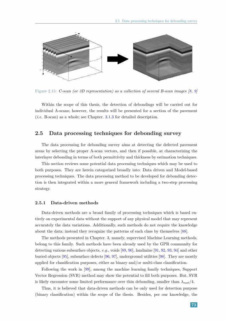
2.5 Data processing techniques for debonding survey
Figure 2.15: C-scan (or 3D representation) as a collection of several B-scan images [8, 9]
Within the scope of this thesis, the detection of debondings will be carried out forindividual A-scans; however, the results will be presented for a section of the pavement(i.e. B-scan) as a whole; see Chapter. 3.1.3 for detailed description.
2.5 Data processing techniques for debonding survey
The data processing for debonding survey aims at detecting the defected pavementareas by selecting the proper A-scan vectors, and then if possible, at characterizing theinterlayer debonding in terms of both permittivity and thickness by estimation techniques.
This section reviews some potential data processing techniques which may be used toboth purposes. They are herein categorized broadly into: Data driven and Model-basedprocessing techniques. The data processing method to be developed for debonding detec-tion is then integrated within a more general framework including a two-step processingstrategy.
2.5.1 Data-driven methods
Data-driven methods are a broad family of processing techniques which is based en-tirely on experimental data without the support of any physical model that may representaccurately the data variations. Additionally, such methods do not require the knowledgeabout the data; instead they recognize the patterns of each class by themselves [88].
The methods presented in Chapter. 3, namely, supervised Machine Learning methods,belong to this family. Such methods have been already used by the GPR community fordetecting various subsurface objects, e.g., voids [89, 90], landmine [91, 92, 93, 94] and otherburied objects [95], subsurface defects [96, 97], underground utilities [98]. They are mostlyapplied for classification purposes, either as binary and/or multi-class classification.
Following the work in [99], among the machine learning family techniques, SupportVector Regression (SVR) method may show the potential to fill both purposes. But, SVRis likely encounter some limited performance over thin debonding, smaller than λmat/4.
Thus, it is believed that data-driven methods can be only used for detection purpose(binary classification) within the scope of the thesis. Besides, per our knowledge, the
73

Chapter 2. Debonding Survey in Pavement Structures
machine learning methods (especially supervised), have not yet been used in the literatureto detect horizontal interface debondings.
2.5.2 Model-based or Model-driven methods
By contrast to the previous subsection, model-driven methods rely on a physicalmodel to process data. As detailed in the next section, the conventional GPR method,namely Amplitude Ratio Test (ART) relies on the thin-bed analytical data model (seeAppendix. A.2). ART has been used for binary classification of A-scan data within theGPR community [100, 18]. However, no attempt has been made to interpret ART valuesin terms of thickness (on the condition that the layer permitivities are known).
Time Delay Estimation (TDE) techniques are data processing techniques that maypotentially fulfill both purposes, namely, detection and characterization of debonding. Ithas been initially developed for GPR pavement survey to control the thickness pavementlayers.
However, TDE tends be more difficult and challenging is GPR pavement applicationswhen: the backscattered echoes from the thin debonding interface are too close to eachother (i.e, overlapping echoes) or, they are highly correlated (which is usually the case forGPR data) [101].
To overcome this issue, super-resolution TDE techniques have been introduced tomeasure thin and ultra thin pavement layers [102], i.e, TAS and UTAS (i.e, Thin andUltra-thin Asphalt Surface), respectively. At medium to high levels of SNR, they canachieve about 10 (resp. 20) times better time resolution than the conventional FFT-based TDE techniques. In other words, they can distinguish between overlapping echoes,which the differential time shift ∆τ is up to (10 × Bw)−1 (resp. (20 × Bw)−1). Thelatter time resolution capability matches to the detection of debonding larger than a fewmillimeter in thickness for the UWB step-frequency radar [103]. This may be not sufficientenough within the scope of the thesis for thin debonding within the range [0, λmat/4].Besides, super-resolution TDE techniques rely on a single scattering signal model (seeAppendix. A.2) which is not always true in practice.
Therefore, model-based TDE techniques are likely not expected to manage the debond-ing survey problem on its own.
2.5.3 Proposed two-step strategy for debonding survey
Following the previous subsections, we can conclude that no unique data processingtechnique exists that can fulfill the two described purposes of debonding survey. Thecharacterization step requires some physical model while the detection step may not.
Therefore, the data processing method to be developed for debonding survey is inte-grated within a more general framework including a two-step strategy to process radarB-scan images. At first, some data-driven processing techniques will be used to select theA-scan data vectors which debondings within the B-scan data. Then, as a second step,super TDE techniques may be performed on the selected A-scans to further characterizethe defects in thickness and permittivity.
74

2.6 Reference data processing method for debonding detection: Amplitude Ratio Test
The thesis will focus on the detection step, namely, the detection, and the results maybe used later within the ongoing ANR research project, called ACIMP (https://anr.fr/Projet-ANR-18-CE22-0020).
2.6 Reference data processing method for debonding detec-tion: Amplitude Ratio Test
ART is a conventional NDT method to detect subsurface delamination from GPR data[100, 18]. The ART method is usually carried out at the operational level for two kinds ofqualitative diagnosis: the debonding detection within pavement structures and the controlof sealing screed over bridge decks. ART allows selecting the areas where some coring isperformed to verify the NDT diagnosis.
In this section, we present the basis of the ART method for debonding detection withina more rigorous framework. This method relies on a simple data modeling of A-scan data,which is detailed in Appendix. A.2. For detection purpose, the decision threshold isdetermined using the conventional likelihood ratio test on the basis of each A-scan datavector.
2.6.1 ART Principle
Any delamination/debonding can be seen as a thin-bed structure []. In case of thinbeds, two reflections from respectively the upper and lower interface are recieved [104, 105,106, 107]. Similarly, in case of a debonding occurring within the top two pavement layers,(as illustrated in Figure 2.16 and Figure. 2.17), two echoes are received: the first echo(As(t)) is the surface echo, and the second one (AT/H0,1
(t)) is the echo from the interfacebetween the top two layers to be monitored by NDT techniques. Healthy and debondingstructures are referred as H0 and H1 assumptions, respectively. The t is simply to indicatethat the signals are in time domain.
According to the data modeling in Appendix. A.2, AT/H0(t) is conventionally assumed
to be a shifted and attenuated copy of the top echo As(t). Whereas in case of debonding,AT/H1
(t) is a composite signal made of the overlapping of two echoes from the upperand the lower interfaces of the debonding along with multiple echoes occurring withinthe debonding region (as shown in Figure. 2.16). As detailed in Appendix A1, the latterechoes interact constructively with each other, assuming limited thickness of the debondinginterface and providing εr,deb > εr,1,2. The resulting composite echo usually shows a largersignal strength compared to the echo over the non-debonding interface.
75

Chapter 2. Debonding Survey in Pavement Structures
Figure 2.16: Synthetic pavement structure showing the signals received from the healthy(left) and defective zones (right). On the left, As is the surface echo and AT/H0
is thesecond echo for non-debonding zone. In case of debonding (right), AT/H1
is thecomposite signal with multiple scattering accounted for
2.6.2 ART Computation
ART is defined as the ratio between the signal strength of the two latter echoes, namely,AS(t) and AT/H0,1
(t). In the following, the signal strengths are labeled AS and AT/H0,1,
respectively. They can be computed from the local extreme values of either the signalmagnitude (MAG) or the Maximum Absolute Amplitude Deviation (MAAD), whereMAAD value of the surface (AS(t)) and second AT/H0,1
echoes are written as follows:
MAAD(AS) = |max(AS(t))−min(AS(t))| (2.2)
MAAD(AT/H0,1) = |max(AT/H0,1
(t))−min(AT/H0,1(t))| (2.3)
where |...| represents the absolute value.Similarly, we express the MAG for the two echoes as:
MAG(AS) = max(|H(AS(t))|) (2.4)
MAG(AT/H0,1) = max(|H(AT/H0,1
(t))|) (2.5)
where H(s(t))) represents the analytical signal of the amplitude signal s(t), which is com-puted by Hilbert transform.For representation, MAAD(AS) and MAAD(AT/H0,1
) are shown in Figure. 2.17(a) andMAG(AS) and MAG(AT/H0,1
) are shown in Figure. 2.17(b) for the debonding and non-debonding A-scans. In practice, an automatic time gating window is used to isolate bothechoes and to compute the MAG and MAAD values as detailed in Appendix. D.
The ART values are usually computed for each A-scan data vector from the MAAD/MAG
76
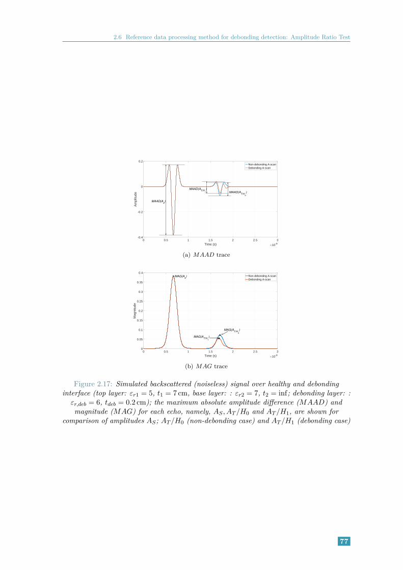
2.6 Reference data processing method for debonding detection: Amplitude Ratio Test
0 0.5 1 1.5 2 2.5 3Time (s) ×10-9
-0.4
-0.2
0
0.2
Am
plitu
de
Non-debonding A-scanDebonding A-scan
MAAD(As)
MAAD(AT/H
1
)MAAD(A
T/H0
)
(a) MAAD trace
0 0.5 1 1.5 2 2.5 3Time (s) ×10-9
0
0.05
0.1
0.15
0.2
0.25
0.3
0.35
0.4
Mag
nitu
de
Non-debonding A-scanDebonding A-scan
o
+*
MAG(As)
MAG(AT/H
0
)
MAG(AT/H
1
)
(b) MAG trace
Figure 2.17: Simulated backscattered (noiseless) signal over healthy and debondinginterface (top layer: εr1 = 5, t1 = 7 cm, base layer: : εr2 = 7, t2 = inf; debonding layer: :
εr,deb = 6, tdeb = 0.2 cm); the maximum absolute amplitude difference (MAAD) andmagnitude (MAG) for each echo, namely, AS , AT /H0 and AT /H1, are shown for
comparison of amplitudes AS; AT /H0 (non-debonding case) and AT /H1 (debonding case)
77

Chapter 2. Debonding Survey in Pavement Structures
values of both echoes, as follows:
ART =AT/H0,1
AS(2.6)
(2.7)
Finally, for classification purposes, the following normalized ratio ARTnorm is introduced:
ARTnorm =ARTtest
ARTref(2.8)
where ARTtest is the ART value over the pavement area to test (under either H0 or H1
hypothesis) and ARTref is the one for a reference data set over the healthy pavement zone(i.e. Non-debonding A-scan or H0 hypothesis).
Following the ART principle in Chapter. 2.6.1, for noiseless condition and limiteddebonding thickness (< λmat/4), we can express ARTnorm as:
ARTnorm
= 1 for Healthy case (H0)
> 1 for Debonding case (H1) if εr,deb > εr,1,2
< 1 for Debonding case (H1) if εr1 < εr,deb < εr2
(2.9)
Then, the debonding detection relies on the decision threshold ηART , which is estab-lished by the likelihood ratio test (presented later in the next section).
The magnitude of echoes (MAG) can be theoretically expressed w.r.t the dielectriccontrast between layers through the Fresnel coefficients as discussed in Appendix. A.2.The latter correspondence is more difficult to establish with MAAD values. However, itcan be shown that both definitions of ARTnorm take larger values when the debondingmaterial shows a larger dielectric contrast compared to the surrounding pavement materiallayers.
In [100], ARTref is theoretically computed using MAG values from the prior knowl-edge of the permittivity attached to the two first underlying layers. By contrast, it isexperimentally established in [15, 108]. In [10], MAAD values were selected to computeART because they provided a slightly larger contrast in ARTnorm values (by a few dB)compared to MAG values, as shown on Figure. 2.18.
2.6.3 Decision threshold
The decision threshold relies on the statistical distribution (i.e, PDF) of ART valuesover both healthy and defective areas. PDFs are established from the collection of ART val-ues, which are computed for each A-scan vector along the scanning direction. Figure. 2.19presents an example of the PDFs for simulated analytic data in Appendix. A.2. As seenin Figure 2.19(a), due to destructive interference, the PDF for debonding case is lowerthan that of non-debonding. Figure. 2.20 presents the ARTnorm for experimental data.As seen, we can say that in practice, destructive interference (as seen in Figure 2.19(a))
78

2.6 Reference data processing method for debonding detection: Amplitude Ratio Test
0 0.1 0.2 0.3 0.4 0.5d/λ
mat
0
0.5
1
1.5
2
2.5
3
3.5
Mag
nitu
de o
f sec
ond
echo
(M
AA
G)
ǫr,deb
= 2
ǫr,deb
= 10
0 0.1 0.2 0.3 0.4 0.5d/λ
mat
0
0.5
1
1.5
2
2.5
3
3.5
Am
plitu
de o
f sec
ond
echo
(M
AD
)
ǫr,deb
= 2
ǫr,deb
= 10
Figure 2.18: MAG (left) and MAAD (right) as functions of debonding layer thickness forεr,deb = 2, 10 using noiseless simulated analytic Fresnel data; parameters for layers 1 and2 are as specified in Table. A.1
0.6 0.7 0.8 0.9 1 1.1 1.2 1.3ART
norm
0
0.25
0.5
0.75
1
Mag
nitu
de
Non-debondingDebonding
(a) εr,deb = 6
0.8 1 1.2 1.4 1.6 1.8 2 2.2ART
norm
0
0.25
0.5
0.75
1
Mag
nitu
de
Non-debonding
Debonding
(b) εr,deb = 2
Figure 2.19: PDF for ARTnorm over defective and healthy areas computed from noisysimulated analytic data with SNR = 30dB (Appendix. A.2), εr1 = 5, εr2 = 7 andtdeb = 0.3 cm. The dashed vertical line depicts the decision threshold for debonding
detection
0.4 0.6 0.8 1 1.2 1.4 1.6 1.8 2ART
norm
0
0.2
0.4
0.6
0.8
1
Mag
nitu
de
Non-debonding
Debonding
(a) Tack-free defects (weak contrast)
0 1 2 3 4 5 6 7 8ART
norm
0
0.2
0.4
0.6
0.8
1
Mag
nitu
de
Non-debonding
Debonding
(b) Sand based defects (strong contrast)
Figure 2.20: PDF for ARTnorm over defective and healthy areas computed fromexperimental data (see Appendix B). The dashed vertical line depicts the decision
threshold for debonding detection
79

Chapter 2. Debonding Survey in Pavement Structures
is not observed.Following Equation. 2.9, for noisy GPR A-scan data, ARTnorm values are expected to
be normally distributed around a mean value, which is different for healthy and debondingareas, as follows:
Hypothesis H0: ARTnorm/H0(x) = 1 + nH0(x)
Hypothesis H1: ARTnorm/H1(x) = µH1 + nH1(x)
where,
- µH0 = 1 and µH1 > 1 are the mean ART values, which is assumed steadyalong the scanning direction x over each area, namely, healthy (H0) and de-fective areas (H1);- nH0(x) and nH1(x) are the noise attached to each case
The noises are assumed to be of zero mean with different standard deviations, namely,σH0 and σH1 . Besides, they are assumed to be decorrelated between A-scans and also toeach other.
The decision threshold for debonding detection depends on the following two classifi-cation strategies: Two-classed and One-classed decision thresholds.
Two-class decision threshold
The conventional approach to distinguish between two classes of data with normaldistribution consists in finding the point of intersection of the two PDFs [10]. The followinglikelihood ratio test (LRT) is used to this aim:
λ(ARTnorm) =p(ARTnorm|µH1 , σH1)
p(ARTnorm|µH0 , σH0)
H1
≷H0
1 (2.10)
where p(x|µ, σ) represent the gaussian PDF with mean µ and standard deviation σ. Itcan be easily shown that the log-Likelihood is expressed as follows:
Λ(ARTnorm) = 2lnσH0/σH1+(ARTnorm − µH0)
2
2σ2H0
− (ARTnorm − µH1)2
2σ2H1
H1
≷H0
0 (2.11)
Finally, the test for debonding detection (H1) becomes :
(ARTnorm − µH0)2
2σ2H0
− (ARTnorm − µH1)2
2σ2H1
H1
≷H0
2lnσH1/σH0 (2.12)
Equation. 2.12 requires to have some estimation (or prior knowledge) of both the meanand standard deviation of the two-class data, that means a collection of ART values overhealthy (H0) and defected areas (H1). This scenario is difficult to hold in practice. Thus,the second approach using one-class decision threshold is proposed.
80

2.6 Reference data processing method for debonding detection: Amplitude Ratio Test
One-class decision threshold
This scenario is better tailored to the operational level, where the operator has noprior information on the location of defective areas. Here, the operator has access to areference non-circulated area, where the interface layer is assumed to be perfectly coating,i.e., healthy with no possible occurrences of debondings.
ART values are then collected over the reference area to compute σH0 (recalling, µH0 =
1). The following decision threshold then serves to detect the outlier ART values over thearea under test:
ARTnorm
H1
≷H0
µH0 +KσH0 (2.13)
where K is a constant value, usually within the interval [2, 3], which allows tuning the truenegative rate (see Chapter. 3.3.2 for One-class SVM for further explanation) and makesthe outlier detection more robust.
Illustration
Figure. 2.21, Figure. 2.22 and Figure. 2.23 present the debonding detection using thetwo-class decision classification on simulated noisy analytic Fresnel data (SNR = 30 dB).Three configurations with debonding thickness tdeb = 0.2 cm and permittivity values ofrespectively εr,deb = 2, 6 and 10. To present detailed information on the false classification(if any), we also present the curve-smoothed PDFs and the threshold observed for eachconfiguration.
10 20 30 40 50 60 70 80 90 100No. of A-scans
0
0.5
1
1.5
2
2.5
3
Tim
e (s
)
×10-9
-0.4 -0.3 -0.2 -0.1 0 0.1 0.2Amplitude
0
0.5
1
1.5
2
2.5
3
Tim
e (s
)
×10-9
10 20 30 40 50 60 70 80 90 100No. of A-scans
0
1
Cla
ss. l
abel
0.8 1 1.2 1.4 1.6 1.8 2MAAD
0
2
4
6
Mag
nitu
de o
f dis
tr.
Non-debondingDebondingThreshold
Figure 2.21: Results for the detection of debondings on noisy simulated analytical datatwo-class decision classification. Permittivities of top and base layers are respectively
εr1 = 5 and εr2 = 7, fc = 4.2GHz, SNR = 20dB; with εr,deb = 2
81

Chapter 2. Debonding Survey in Pavement Structures
10 20 30 40 50 60 70 80 90 100No. of A-scans
0
0.5
1
1.5
2
2.5
3
Tim
e (s
)
×10-9
-0.4 -0.3 -0.2 -0.1 0 0.1 0.2Amplitude
0
0.5
1
1.5
2
2.5
3
Tim
e (s
)
×10-9
10 20 30 40 50 60 70 80 90 100No. of A-scans
0
1
Cla
ss. l
abel
0.7 0.8 0.9 1 1.1 1.2 1.3MAAD
0
2
4
6
8
Mag
nitu
de o
f dis
tr.Non-debonding
DebondingThreshold
Figure 2.22: Results for the detection of debondings on noisy simulated analytical datatwo-class decision classification. Permittivities of top and base layers are respectively
εr1 = 5 and εr2 = 7, fc = 4.2GHz, SNR = 20dB; with εr,deb = 6
10 20 30 40 50 60 70 80 90 100No. of A-scans
0
0.5
1
1.5
2
2.5
3
Tim
e (s
)
×10-9
-0.4 -0.3 -0.2 -0.1 0 0.1 0.2Amplitude
0
0.5
1
1.5
2
2.5
3
Tim
e (s
)
×10-9
10 20 30 40 50 60 70 80 90 100No. of A-scans
0
0.5
1
Cla
ss. l
abel
0.8 1 1.2 1.4 1.6 1.8 2MAAD
0
2
4
6
8
Mag
nitu
de o
f dis
tr.Non-debonding
DebondingThreshold
Figure 2.23: Results for the detection of debondings on noisy simulated analytical datatwo-class decision classification. Permittivities of top and base layers are respectively
εr1 = 5 and εr2 = 7, fc = 4.2GHz, SNR = 20dB; with εr,deb = 10
As done for the two-class decision classification, Figure. 2.24, Figure. 2.25 and Fig-ure. 2.26 present the results for one-class classification for the same simulated data modelconfigurations.
82

2.6 Reference data processing method for debonding detection: Amplitude Ratio Test
10 20 30 40 50 60 70 80 90 100No. of A-scans
0
0.5
1
1.5
2
2.5
3
Tim
e (s
)
×10-9
-0.4 -0.3 -0.2 -0.1 0 0.1 0.2Amplitude
0
0.5
1
1.5
2
2.5
3
Tim
e (s
)
×10-9
10 20 30 40 50 60 70 80 90 100No. of A-scans
0
1
Cla
ss. l
abel
0.8 1 1.2 1.4 1.6 1.8 2MAAD
0
2
4
6
Mag
nitu
de o
f dis
tr.
Non-debondingDebondingThreshold
Figure 2.24: Results for the detection of debondings on noisy simulated analytical dataone-class decision classification. Permittivities of top and base layers are respectively
εr1 = 5 and εr2 = 7, fc = 4.2GHz, SNR = 20dB; with εr,deb = 2
10 20 30 40 50 60 70 80 90 100No. of A-scans
0
0.5
1
1.5
2
2.5
3
Tim
e (s
)
×10-9
-0.4 -0.3 -0.2 -0.1 0 0.1 0.2Amplitude
0
0.5
1
1.5
2
2.5
3
Tim
e (s
)
×10-9
10 20 30 40 50 60 70 80 90 100No. of A-scans
0
1
Cla
ss. l
abel
0.7 0.8 0.9 1 1.1 1.2 1.3MAAD
0
2
4
6
8
Mag
nitu
de o
f dis
tr.Non-debondingDebondingThreshold
Figure 2.25: Results for the detection of debondings on noisy simulated analytical datausing one-class decision classification. Permittivities of top and base layers arerespectively εr1 = 5 and εr2 = 7, fc = 4.2GHz, SNR = 20dB; with εr,deb = 6
10 20 30 40 50 60 70 80 90 100No. of A-scans
0
0.5
1
1.5
2
2.5
3
Tim
e (s
)
×10-9
-0.4 -0.3 -0.2 -0.1 0 0.1 0.2Amplitude
0
0.5
1
1.5
2
2.5
3
Tim
e (s
)
×10-9
10 20 30 40 50 60 70 80 90 100No. of A-scans
0
0.5
1
Cla
ss. l
abel
0.8 1 1.2 1.4 1.6 1.8 2MAAD
0
2
4
6
8
Mag
nitu
de o
f dis
tr.Non-debonding
DebondingThreshold
Figure 2.26: Results for the detection of debondings on noisy simulated analytical datausing one-class decision classification. Permittivities of top and base layers arerespectively εr1 = 5 and εr2 = 7, fc = 4.2GHz, SNR = 20dB; with εr,deb = 10
83
Chapter 2. Debonding Survey in Pavement Structures
2.7 Conclusion
We begin this chapter by presenting the existing techniques for pavement evaluation.These techniques were categorized broadly into Destructive and Non-destructive tech-niques. A review on the various aspects of destructive testing was presented along withits limitations. We then presented the pavement evaluation methods in the field non-destructive testing scopes along with the various existing methods to detect debondings.We then focused on the GPR tool, which is used in the thesis for pavement imaging andsurvey.
A reference method, namely, ART for Amplitude Ratio Test, was then presented.ART is routinely used by the GPR community for qualitative trace debondings withinpavement structures. In this chapter, this method was presented within a more rigorousframework. The ART is selected to serve as a reference method to assess the performanceof the classification methods to be presented in the next chapter for debonding detection.
However, the reference method depends on a single feature of the GPR A-scan signal,namely MAAD or MAG. As such, it may achieve limited performance compared to thedata-driven methods mentioned in section 2.5.
In the next chapter, we study three machine learning methods, namely unsupervised(k-means clustering) and supervised (Support vector machines and Random forests) inthe context of debonding detection.
84

Part II
MACHINE LEARNING METHODS
AND DATA PREPROCESSING FOR
DEBONDING DETECTION
85


Chapter 3
Machine Learning Methods
Contents3.1 Elements of Machine Learning . . . . . . . . . . . . . . . . . . . 89
3.1.1 Unsupervised Machine Learning . . . . . . . . . . . . . . . . . . 89
3.1.2 Supervised Machine Learning . . . . . . . . . . . . . . . . . . . . 90
3.1.3 Implementation of ML algorithms . . . . . . . . . . . . . . . . . 92
3.2 Data Clustering method . . . . . . . . . . . . . . . . . . . . . . . 94
3.2.1 Principle . . . . . . . . . . . . . . . . . . . . . . . . . . . . . . . 94
3.2.2 Modified clustering algorithm . . . . . . . . . . . . . . . . . . . . 95
3.3 Parameterized Supervised machine learning: Support VectorMachines . . . . . . . . . . . . . . . . . . . . . . . . . . . . . . . . 98
3.3.1 Two-Class SVMs for binary classification . . . . . . . . . . . . . 98
3.3.2 One-Class SVMs for anomaly detection . . . . . . . . . . . . . . 104
3.4 Non-Parameterized Supervised learning: Random Forests . . . 110
3.4.1 Background . . . . . . . . . . . . . . . . . . . . . . . . . . . . . . 110
3.4.2 Principle . . . . . . . . . . . . . . . . . . . . . . . . . . . . . . . 110
3.4.3 Application to binary classification for debonding detection . . . 112
3.5 Decision making: Probabilistic estimates . . . . . . . . . . . . . 115
3.5.1 Introduction . . . . . . . . . . . . . . . . . . . . . . . . . . . . . 116
3.5.2 Probabilistic estimation for SVMs: Platt scaling . . . . . . . . . 116
3.5.3 Probabilistic estimation for Random forests . . . . . . . . . . . . 118
3.6 Synthesis . . . . . . . . . . . . . . . . . . . . . . . . . . . . . . . . 119
3.7 Conclusions . . . . . . . . . . . . . . . . . . . . . . . . . . . . . . . 122
The concept of Machine Learning (ML) is a rapidly growing field due to its immenserange of applications. Machine learning is a subset of Artificial Intelligence that fo-
cuses on making predictions based on its experience. The goal of machine learning is to beable to predict and perform classification or regression tasks based on historical relation-ships between data [109]. The ML algorithms can be broadly classified into unsupervisedlearning, semi-supervised learning and Supervised learning family groups [110, 111, 112].
Among the existing ML methods in the literature, we select in this chapter threerelatively mature ML methods that can be used within the scope of the thesis, namely,
87

Chapter 3. Machine Learning Methods
the Support Vector Machine (SVM), Random Forest (RF) and k-means clustering. Themethods based on “deep learning” were not selected in this thesis since the GPR databasesare too limited in size. ML methods are expected to improve the performance of debondingdetection in comparison with the reference ART method which was presented in Chapter. 2(Section. 2.6). It should also be noted that, in contrast to the reference method, the MLmethods do not use the same number of signal features (ART uses only one signal feature).
The ML techniques have been already used by the GPR community for various ap-plications. Among others, SVM methods have been applied for the detection of voidsin concrete [89, 90], landmine detection [91, 92, 93, 94], detection of subsurface defects[96, 97], railway ballast classification [113], underground utilities [98], buried objects [95]etc. One-class SVM has been used to detect landmines [93, 114]. Pavement surface crackshave been investigated using GPR in [115, 116, 117]. However, to the extent of our knowl-edge, ML methods have not yet been used to detect interface debondings.
This chapter provides an overview of three different machine learning families froman applied perspective. We then present the principle of one unsupervised ML method(k-means clustering) and three supervised ML methods (Support Vector Machines, One-class SVM and Random forests). For illustration, the latter methods are used to processsimulated raw A-scan data vectors.
Finally, Figure. 3.1 presents the family of data processing methods studied in thisthesis.
Figure 3.1: Data processing methods which are tested in this thesis
88

3.1 Elements of Machine Learning
3.1 Elements of Machine Learning
Each ML algorithm possesses its own approach towards making predictions. However,a key common element for each algorithm is the use of Learning data and in some cases,the use of feature extraction/transformation step. The learning data is used by the MLto create a prediction (or classification) model [111, 118]. This model is the basis for theprediction. When a new input is introduced to the ML algorithm, it makes a predictionusing the said model.
The ML algorithms can be broadly classified into three major groups amely, unsuper-vised learning, semi-supervised learning and Supervised learning [110, 111, 112]. One un-supervised method, namely k-means clustering [119], and two supervised methods, namelySupport Vector Machines (SVM) [120] and Random Forests [121] are presented hereafter.The semi-supervised learning (SSL) would have practical interest within the scope of thethesis [122, 123]. However, the potential interest is canceled by the drawbacks listed in[124, 125, 126, 127]. Thus, only supervised and unsupervised methods were studied in thethesis.
3.1.1 Unsupervised Machine Learning
As mentioned in [128] (Chap. 5), the unsupervised learning methods do not require anyguidance making them rely only on the data instances [112], namely, data labeling. Suchmethods ‘learn’ through observation and attempt to find structures in the data [128, 112].Here, the prediction model automatically finds the patterns and relationships betweendata and clusters them into individual groups that present similar characteristics and itdoes not require the use of predefined labels [129]. The unsupervised learning aims toassign the data into subsets (also referred to as clusters) which possess certain similaritiesin characteristics.
Various unsupervised machine learning methods have been studied in the literature,including Self-organizing Maps (which is based on unsupervised Neural networks) [130], k-means [131, 130, 132], expectation maximization [132], C-means and hierarchical clustering[131], etc. Additionally, [133] presents and compares the performance of six unsupervisedML methods (k-means, DBSCAN, OPTICS, Agglomerative, Divisive and COBWEB) onthe basis of number of iterations, clusters used, computational time etc.
The motivation behind using k-means as a reference for unsupervised methods is that itis one of the most commonly used unsupervised learning method [131] due to its simplicityin comparison to other clustering approaches [134]. Moreover, for a large number ofvariables, k-means can be computationally faster than other unsupervised methods suchas hierarchical clustering [134].
Unsupervised clustering methods have several advantages:
1. They significantly reduce the computational costs [135]
2. They are flexible to deal with various datatypes: temporal data [135], spectral data[136] (using fuzzy clustering or even time-frequency data) [137] (by means of hierar-chical clustering)
89

Chapter 3. Machine Learning Methods
3. They are known for their simplicity [135], ease of implementation and real-timecapability [138, 139, 140]
4. They do not require the operator intervention for labeling the data (except during theperformance assessment stage). This is also the key difference between supervisedand unsupervised ML methods.
By contrast, the lack of prior information may bring certain drawbacks to unsupervisedmethods:
1. Lower accuracy of the results: this is also because the input data is not known andnot labeled by the operator in advance.
2. Although unsupervised clustering focuses more on being real-time, it is sometimesa time-consuming in case of large data [141]
3. May sometimes result in loss of information conveyed by the original data for clus-tering [135]
4. Different algorithmic approaches may lead to drastic changes in the results [142]
5. Since the numbers of classes are also not known, it could lead to the inability toascertain the results generated by the analysis.
These drawbacks in unsupervised learning approach demands the need of an approachto overcome by the use of supervised machine learning.
3.1.2 Supervised Machine Learning
According to [143, 144], the most common form of ML relies on supervised learning.In contrast to the unsupervised methods, the Supervised learning methods is based on atraining data model to classify and/or perform prediction. It is a two-step method where,the training data is used to create a classification model controlled by various parameters(discussed later). This model is then fed with test data and the model performs theclassification.
In case of supervised learning, the data is divided into two groups namely, learning andtesting data. Figure 3.2 shows the data division. The learning data is sub-divided intoTraining data and Validation data. During the learning stage, a method as for exampleCross validation [145, 146] is used. The training data is used to ‘train’ the model while thevalidation data is used to optimize the model-parameters for the given application (i.e.debonding detection). Once the optimal parameters (for a certain method) are obtained,the testing data uses this model to predict the presence or absence of debondings.
In Section. 3.3, three supervised ML techniques are selected for the application. Theyare categorized into parameterized (SVM-based) and non-parameterized (Random Forest)techniques. The first method requires to adjust its internal parameters on the learningdata set.
Supervised machine learning has many advantages:
90

3.1 Elements of Machine Learning
Figure 3.2: GPR data grouping for supervised ML methods
1. The learning step (which creates the classification model) allows achieving betterclassification performance
2. It allows the user to be very specific: the user has the freedom to set the decisionalboundaries to distinguish between classes (i.e. benchmarking)
3. The results produced by the supervised method are known to be more accurate andreliable in comparison to the results produced by the unsupervised techniques ofmachine learning. This is mainly because the input data in the supervised algorithmis well known and labeled [147]
4. As mentioned in [148, 149], supervised learning method such as decision trees andself-organizing neural networks can be suitable for real-time with very fast testingspeed. SVM has also been readapted to be used in real-time for hyperspectral imageclassification [150], emotion recognition [151], trojan-horse detection [152] etc.
5. Since the number and the type of classes are set at the labeling stage and are includedin the classification model, no ambiguous results can occur.
However, besides all the advantages, supervised ML methods has a few drawbacks:
1. Supervised learning can sometimes be a complex method both in terms of modelingand computational time compared to the unsupervised method.
2. The necessity to label the inputs in supervised learning adds to the overhead and isnot always accurately done
3. It may or may not be applicable in real time since the learning stage demands com-putational time thereby making supervised learning quasi-real time at the most. Onthe other hand, unsupervised learning can be implemented in real-time, constrainedby the data size.
91

Chapter 3. Machine Learning Methods
4. For dynamic and large data sets, it is a huge challenge to pre-define the labels.
Nevertheless, the efficiency and robustness of supervised learning is expected to achievethe detection of thin debondings with high accuracy.
3.1.3 Implementation of ML algorithms
According to Maxwell et al. [153], the implementation of ML methods is not straight-forward, and the literature may provide conflicting advice. The implementation of algo-rithms helps to understand the mathematical approach and the practical considerationsbehind the method. It could supposedly improve the ML method’s efficiency, reduce itscomputational time and perform at low costs.
In this subsection, we explore some practical considerations regarding the use of MLmethods within the perspective of debonding/non-debonding classification of radar data.We then broadly categorize the implementation of ML methods into the feature-spaceselection and reduction, and the possible impact on computer burden and (specific) limi-tation/difficulties reported in the literature.
Signal vs. Image data processing
According to Section. 2.3, the most conventional processing formats for GPR dataare B-scan (2D image) and A-scan (1D data vector). We initially represent each B-scanradar data by a spatio-temporal image, i.e., a N ×M -dimensional matrix, where M is thenumber of data samples in an A-scan, and N is the number of A-scans along the scanningdirection. B-scan radar data matrix are arranged column wise, each column, namely, A-scan, representing 1D time data vector. As an example, Figure. 3.3(a) illustrates two 1DA-scan signals while Figure. 3.3(b) shows the collection of adjacent A-scan signals to formthe 2D GPR B-scan image.
-0.6
-0.4
-0.2
0
0.2
0.4
0.6
0.8
1
Am
plitu
de
2 2.5 3 3.5 4 4.5Time (s) ×10-9
DebondingNon-debonding
(a) 1D signal (A-scan) over debonding and non-debonding areas
10 20 30 40 50Number of A-scans
2
2.5
3
3.5
4
4.5
Tim
e (s
)
×10-9
Non-debonding
Debonding
Transition
(b) 2D GPR image (Bscan)
Figure 3.3: GPR data collected over artificial embedded debonding at the IFSTTAR’sfatigue carousel (Tack-free defect at 10kcycles loading stage); see Appendix. B for more
information
92

3.1 Elements of Machine Learning
ML methods can theoretically process the two data formats in either independentsignal-by-signal 1D analysis basis or in image based 2D analysis. Theoretically, the imagedata brings more information than independent data vectors due to its possible spatialcoherency of the overall data.
Within the GPR community, the choice of the data format to be processed usually de-pends on the application under scope. The 2D image processing are required for detectingpoint-like scatterers within subsurface, provided a dense enough spatial sampling of GPRdata collection is available. In this case, the spatial sampling is required to be smaller thanthe footprint of the antenna beams, introducing some useful spatial overlapping betweensuccessive A-scan profiles.
By contrast, for GPR pavement surveys at traffic speed, the latter condition on spatialsampling does not hold (since the acquisition rate of the electronic system is limited, andthe sampling spatial interval increases with traffic speed). In addition, in case of 2D B-scan data, radar clutter demonstrates a strong spatial coherency, which may disturb theanalysis of the subsequent stratified pavement layers. Thus, in case of GPR pavementsurvey, B-scan data are usually processed on a scan-by-scan basis.
Similarly, in this thesis, radar data are processed on a scan-by-scan (individual A-scanat a time) basis to keep the processing closer to the operational level. (Note: Althoughthe data collection in Appendix. A provides dense enough spatial sampling.)
Raw data vs. Signal features
ML techniques were initially applied to process data in their raw form. However,according to LeCun et al., 2015 [143], this conventional implementation of ML techniquesis supposed to limit their ability to process data. Then, feature extractor have beenintroduced to transform the raw data into a suitable internal representation or featurevector, on which the ML techniques then perform classification.
For the GPR application under scope, the ‘raw’ data is the collected GPR data intime/frequency domain without introducing any alteration or modifications into the data.Feature vector on the other hand refers to some selected signal characteristics extractedfrom the raw data, that well-represent the actual data but with reduced data size. MLsystems required careful engineering to design a feature extractor. The feature set willbe extensively explored in the later chapters and the two implementation ways of MLtechniques will be quantitatively compared.
To implement the machine learning methods using feature sets, an initial preprocessingstep is used wherein the signal features (or characteristics) that strongly represent the dataare extracted. This will be later discussed in detail in Chapter. 4.2 and the performancebetween the two implementations of ML techniques, i.e., raw-based data and features-based processing, will be compared in Chapter. 5.
Limitations and difficulties
Despite of various approaches of ML methods, they have certain limitations. In caseof supervised learning, one such problem is over-fitting. It is generally referred in machine
93

Chapter 3. Machine Learning Methods
learning where a model produced by the method (in the learning stage) is unable to makeproper predictions for the new (test) data [154, 155, 156]. On the other hand, under-fittingis another issue wherein the method is unable to produce a model based on the learningdata [157, 158].
A survey on ML methods is conducted in [159]. It presents a detailed list of individuallimitations of various supervised machine learning methods (such as SVM, Decision trees,k-nearest neighbors etc.) and unsupervised clustering methods. Moreover, the computa-tional burden and complexity may increase due to the large size of the raw data sets.
However, solutions to overcome some of these limitations have already been proposed inthe literature. These include signal feature selection and extraction, feature dimensionalityreduction and cross validation techniques, which are discussed in detail in Chapter. 4 andChapter. 5 respectively.
3.2 Data Clustering method
The clustering algorithm is one of the most simple unsupervised method to categorizedata into N different clusters. Such algorithms are useful in classifying the raw data andpossibly identify any hidden patterns that exist within the datasets. The method presentedthereafter is a modified iterative clustering of the conventional k-means algorithm, whichis explained hereafter.
3.2.1 Principle
The clustering algorithm works on the principle of ‘grouping’ the datasets into variouscategories based on their statistical parameters and distance . In this algorithm, theprimary step is to choose the number of clusters N required by the user. This is auser-defined parameter. Once the number of clusters is decided, an iterative process isconducted until convergence is met or defined by the user.
Within the scope of the thesis, the primary focus of the clustering methods and pro-cesses is to determine the presence (or absence) of debondings occurring at the interfacebetween the first two layers of the pavement structure from GPR A-scan data. Accord-ing to Chapter. 4.2), signal features may be different on Healthy (unbonded) and De-fective (debonded) regions and then, can be used to cluster the data as debonding ornon-debonding groups.
Thus, the value of initial cluster is N = 2. [160] describes the k-means approach usingan algorithm. For the debonding detection applications, the number of clusters k = 2;these initial cluster centroids are chosen at random. We then form 2 clusters by assigningthe remaining points to their nearest cluster.
A proximity measure, namely Euclidean (L2) distance (d), is used to quantify the‘nearest’ points to a cluster defined by:
d(Ci, xj) =√
(si − sj)2 + (ki − kj)2 (3.1)
94

3.2 Data Clustering method
where,
- Ci = (si, ki) is the ith centroid with i ∈ 1, 2 indicating each cluster, andj ∈ 1, 2 . . . N, j = i,- s and k are respectively the skewness and kurtosis computed for each A-scanvector,- xj = (sj , kj) is associated to the jth A-scan
The A-scan xj is then assigned to the cluster based on:
xj ∈
Cdeb if d1,j < d2,j
Cndeb if d1,j > d2,j(3.2)
where d1,j = d(Cdeb, xj) and d2 = d(Cndeb, xj) are the Euclidean distances of xj fromrespectively debonding (Cdeb) and non-debonding (Cndeb) centroids.Iteratively, new centroids are recomputed until no such reassignment is possible (i.e. con-vergence is met) using the now clustered data as follows [128]:
Ci,new =1
card(Ci,old)
∑(sj ,kj)∈Ci,old
[sj
kj
](3.3)
where,
- Ci ∈ Cdeb, Cndeb- [sj kj ]
T is associated to the jth A-scan point in the cluster Ci,old
- card(C) is the cardinality of C
However, since the initial seed step in the conventional approach is chosen at random,the choice of a wrong centroid may lead to a high misclassification rate.
3.2.2 Modified clustering algorithm
By contrast to the conventional method, the modified clustering approach proposed tointroduce an initial seed step wherein the first k centroids are predetermined by the useras follows.
In the modified clustering approach, we select two signal characteristics, namely, signalkurtosis and signal skewness to construct the 2D cluster-space. We modify Equation. 3.1to get the 2 farthest points in this cluster-space as follows:
dmax = maxi,j,i=j
√(si − sj)2 + (ki − kj)2
(3.4)
Each A-scan is then assigned to its nearest centroid (as shown in Equation. 3.3) andthe process is then repeated until convergence is met as done in the conventional k-meansapproach. Figure. 3.4 presents the schematic for the implementation of the modifiedclustering approach and also compares it with the conventional k-means.
95

Chapter 3. Machine Learning Methods
Figure 3.4: Implementation of the unsupervised clustering algorithm to detect debondingspresenting the difference in the initial seed point w.r.t. conventional k-means
96

3.2 Data Clustering method
The conventional k-means approach and the modified clustering approach are used toprocess noisy simulated B-scan radar data (see Appendix. A.2). Figure. 3.5 compares thefinal clustering results using the global skewness and kurtosis computed from raw A-scandata. The proposed modified approach achieves a more relevant data grouping with lessmisclassification.
-2.7 -2.6 -2.5 -2.4 -2.3 -2.2 -2.1Data Skewness
17
18
19
20
21
22
23
Dat
a K
urto
sis
Dataset-1Dataset-2
(a) Clustering by conventional k-means
-2.7 -2.6 -2.5 -2.4 -2.3 -2.2 -2.1Data Skewness
17
18
19
20
21
22
23
Dat
a K
urto
sis
Dataset 1
Dataset 2
Initial seed point-1
Initial seed point-2
(b) Clustering by modified k-means
Figure 3.5: Comparison of clustering methods on noisy simulated analytic raw data (withSNR = 20dB) using two signal features, namely, Kurtosis and Skewness
97

Chapter 3. Machine Learning Methods
3.3 Parameterized Supervised machine learning: SupportVector Machines
Support Vector Machines (SVM) have been extensively researched in the data miningand machine learning communities for the two last decades due to its robustness andeasiness to implement. It actively applied to applications in various domains such ashandwriting recognition [161, 162], facial detection [163], learning of cancer genomics [164].SVM can be typically implemented for both classification (classifying SVM or C-SVM)and regression (Support Vector Regression) problems. In the field of NDT, SVM has beenused for the detection of buried objects [95, 165]. We have also implemented SVM in thedetection of thin inter-layer debondings in pavement structures in [13], [166], [10].
The precursor to SVM was first introduced by Vladimir Vapnik and Alexey Chervo-nenkis in 1963 [167, 168]. In 1992, Boser et al. [169] suggested a way to create nonlinearclassifiers by applying the kernel trick to maximum-margin hyper-planes. The currentstandard incarnation (soft margin) was proposed by Cortes and Vapnik in 1995 [120].
SVM is usually applied for multi-class classification in the literature. However, withinthe scope of the thesis, SVM is first focused on the two-class classification in Section3.3.1 to distinguish between radar A-scan data over debonding and non-debonding areas.Later on in Section 3.3.2, SVM is implemented as an outlier detection methods namely,One-Class SVM to detect debonding A-scan data as an outlier class.
For representation, in this section, each B-scan radar data is represented by an N×M -dimensional matrix X = [x1,x2 . . .xN ], where N is the number of A-scans and M may beeither the number of time samples or the number of signal features. In the following, theconventional way of applying SVMs to data is presented; it consists in processing data intheir raw form, i.e., the time samples of Ascan in our case. By contrast, signal featureswill be used in Chapters 4 and 5 to implement SVMs.
3.3.1 Two-Class SVMs for binary classification
Binary SVMs are classifiers which discriminate data points of two categories. Toclassify data into two classes, we initially represent each B-scan data by an N × M -dimensional matrix, where M is the number of data samples in an A-scan, and N is thenumber of A-scans. Each of the A-scans belongs to only one of two classes (i.e non-debonding or debonding). A classification boundary is used to separate the two classes;such boundaries are called hyper-planes. In theory, to separate the data into two classes,several hyper-planes can be traced. However, in order to avoid misclassifications, anoptimal hyper-plane must be found that provides the maximum separation of the data.In order to achieve this, SVM picks the hyper-plane which has the largest margin [170] asshown in Figure. 3.6.
SVM can be implemented differently depending on the application requirements andthe data. The two general types SVM based on the kernel are linear SVM and non-linear(kernel) based SVM.
98

3.3 Parameterized Supervised machine learning: Support Vector Machines
(a) All possible hyper-planes (b) Optimal hyper-plane for classification
Figure 3.6: SVM Hyper-planes. x1 and x2 are the the axes of the feature-planes [10]
3.3.1.1 Linear SVM
Given a learning data set X = [x1,x2 . . .xN ] of the order M × N (where M is thenumber of time samples and N is the number of A-scans), the aim is to find the maximum-margin hyper-plane that divides the learning data A-scans X into two separate classes,namely, Non-debonding (labeled as -1) or debonding (labeled as +1). Additionally, themargin between the separation is expected to be maximized as much as possible in orderto have a better classification.
Each hyper-plane can be expressed as a linear equation that depends on the learningdata as follows [171]:
wTx+ b = 0 (3.5)
where w is the normal vector to the hyper-plane (the distance between x and the hyper-plane)). The parameter b is the bias (offset from the origin [172]) introduced and b
||w||determines the offset of the hyper-plane from the origin along the normal vector w.
In case of linearly separable data, two parallel hyper-planes to Equation. 3.5 can beselected that separate the two classes of data, so that the distance between them is aslarge as possible. The distance bounded by these two hyper-planes is called the ‘margin’and the maximum-margin hyper-plane is the hyper-plane that lies halfway between thetwo hyper-planes. These hyper-planes can be described by the equations [10]:
wTxi + b = 1 for debonding; yi = 1 (3.6)
wTxi + b = −1 for non-debonding; yi = −1 (3.7)
where xi is the ith learning A-scan and yi is its associated classification label.
The decision function D(x) for linearly separable data is expressed using Equation. 3.6and Equation. 3.7 as [10]:
99

Chapter 3. Machine Learning Methods
D(xi) = sgn(wTxi + b) (3.8)
where, sgn is the sign function.Geometrically speaking, the distance between the two hyper-planes from Equation. 3.6and Equation. 3.7 would be 2/||w||. As mentioned earlier, in order to obtain better clas-sification, the margin must be maximized. Thus, the weight vector should be minimized.Additionally, to prevent the data points from being falsely classified, constraints are addedto ‘force’ each learning data to remain on the designated side of the margin. To do so, wecombine Equation. 3.6 and Equation. 3.7 to obtain a single condition as:
yi.(wTxi + b) ≥ 1, ∀ 1 ≤ i ≤ n (3.9)
Figure 3.7: Example of a principal scheme of Soft SVM on a 2-dimensional feature space.Axes f1 and f2 indicate the feature space
The GPR data in practice are noisy data. So even if there is a linear relationshipbetween the data and their classes, a linear classifier may result in false classifications. Todeal with such cases, it is reasonable to permit a relaxation parameter for such noise. Inthe context of SVM this amounts to release the constraint imposing that all the examplesare many classes. In order to ‘loosen’ the constraint variables, called spring or relaxationdeviations denoted ξi were introduced, as shown in Figure 3.7 To ensure that the numberof outliers is reasonable, the gap variables are included in the objective function. The new
100

3.3 Parameterized Supervised machine learning: Support Vector Machines
formulation of the optimization problem can thus be written as [10]:
Minimize 1
2||w||2 + C
N∑i=1
ξi (3.10)
where C is called the Cost function or compromise constant. The parameter C is importantin the learning model as it controls the tolerance level of the classifier. For larger values ofC, only low ξ values are permitted thereby reducing the margin. Conversely, low C valuesresult in larger margins. Finally, if C is undetermined (i.e. C = inf), the classifier is ahard margin SVM. In short, C is used to indicate the importance given to errors on thetraining set against the attempt to maximize the margin. To express the formulation offlexible margins (i.e, with slack variable ξi), the Lagrangian of the problem of minimizingassociated to the Equation. 3.6 - Equation. 3.10 can be expressed as [173]:
L(w, b, ξ, α, β) =1
2||w||2 + C
N∑i=1
ξi +
N∑i=1
αi
1− ξi − yi(w
Txi + b)
(3.11)
where αi is the Lagrangian associated with the hyperplane and βi is the Lagrangianassociated with slack variable ξi. Next, we use the Karush-Kuhn Tucker (KKT) conditionsin order to obtain the saddle point for Equation. 3.11. These conditions are necessary ingeneral, and sufficient for convex optimization problems [174]. These conditions are definedas the as [171]:
∂L
∂w= w −
N∑i=1
αi yi xi = 0 (3.12)
∂L
∂b=
N∑i=1
αi yi = 0 (3.13)
∂L
∂ξi= C − αi − λi = 0 (3.14)
α(yi(w,xi) + b)− 1 + ξi = 0 ∀ i = 1 . . . N (3.15)
The dual classification problem can thus be written as [171, 175]:
Maximize W (α) =N∑
i,j=1
αi +1
2
N∑i,j=1
yi yj αi αj⟨xi,xj⟩ (3.16)
101

Chapter 3. Machine Learning Methods
constrained by,
N∑i=1
αi yi = 0 (3.17)
0 ≤ αi ≤ C ∀ i = 1 . . . N (3.18)
The decision function D(x) from Equation. 3.8 for a linear kernel can thus be expressedas [10]:
D(x) = sgn
∑i
wTαi⟨xi,x⟩+ b
(3.19)
An advantage of the flexible margins is that the solution of the problem is often ‘hol-low’, i.e. a large proportion of αi is zero. The geometric interpretation is given by theFigure. 3.8:
Figure 3.8: Geometrical representation of Figure. 3.7. Axes f1 and f2 indicate the featurespace
3.3.1.2 Non-linear SVM
When there is no available possibility to classify the data by Linear classification, non-linear methods by applying Kernel tricks can be used. This methodology was suggested byVapnik, Boser and Guyon in 1992 [169]. This method maximizes the hyper-plane marginsthat allow to fit the maximum-margin hyper-plane in a transformed feature space. Thetransformation may be nonlinear and the transformed space high dimensional. Althoughthe classifier is a hyper-plane in the transformed feature space, it may be nonlinear in theoriginal input space [176].
102

3.3 Parameterized Supervised machine learning: Support Vector Machines
The SVM classifier method consists of a maximum margin in which the scalar product(in Equation. 3.19) was replaced by the kernel. Extending the linear SVM from Equa-tion. 3.16, we get [171, 175]:
Maximize W (α) =
N∑i=1
αi −1
2
N∑i,j=1
yi.yj .αi.αjκ(xi,xj) (3.20)
once again under the constraints of Equation. 3.17 and Equation. 3.18.The decision function for a kernel-based non-linear SVM can thus be expressed as [10]:
D(x) = sgn
N∑i=1
αiyiκ(x,xi) + b
(3.21)
It can be seen that the term κ(x,xi) in the latter equation replaces the term ⟨x,xi⟩ inEquation. 3.19 for the Linear SVM.
NOTE: Kernel classifiers were described as early as the 1960s, with the invention of
the kernel perceptron. They rose to great prominence with the popularity of SVMs inthe 1990s, when the SVM was found to be competitive with neural networks on taskssuch as handwriting recognition. Some of the well-known kernel functions include:
1. Gaussian Radial basis function (RBF) [171, 177]:
κ(xi,xj) = exp(−γ||xi − xj ||2) (3.22)
for all positive values of γ.2. Polynomial kernel [171, 177]:
κ(xi,xj) = (xiTxj + 1)d (3.23)
where d is the degree of the polynomial.3. Sigmoid kernel [177]:
κ(xi,xj) = tanh(αxiTxj + c) (3.24)
with α being the degree of the sigmoid and c is the kernel coefficient.
Under Kernel based classification, the Radial Basis Function (or commonly called theRBF kernel) is a popular and most commonly used kernel function in SVM classifications[177, 178].
Figure 3.9 shows the flowchart of SVM classification for our application. The GPRdata is divided into Learning and Testing data sets after initial preprocessing steps. Withthe help of suitable performance indication method, an optimal SVM model is constructedin the learning step. These model parameters are then applied on the Testing data set to
103

Chapter 3. Machine Learning Methods
validate the overall performance of the method.
Figure 3.9: Flowchart for SVM classification
Figure. 3.10 illustrates the application of the binary SVM (with a non-linear RBFkernel) to process noisy simulated A-scan data (see Appendix. A.2) for test data only.A B-scan consisting of 200 A-scan vectors is created (using the analytic Fresnel model;see Appendix. A.2). The desired noise is then added to the B-scan (see Appendix. A.5).One half of the B-scan (i.e. 100 A-scans) is then used for the learning step to create anSVM classification model. The remainder is used for the testing step. We can see thatthe two-class SVM classification is able to identify the presence of debondings of variousinterlayer permittivities.
3.3.2 One-Class SVMs for anomaly detection
One-class SVM was suggested by Schölkopf [179] in the late 1990’s as a method ofadapting SVM to a one-class classification problem (as anomaly detection or outlier de-tection). This approach can be considered as a conventional two-class SVM where thetraining data consists only non-debonding data and the origin is the only member of thedebonding data set (in contrast to the previous method, where, the training data com-prises of both debonding and non-debonding data). It has been used in many applicationssuch as image retrieval [180], document classification [181] etc.Figure 3.11 shows the geometrical interpretation of One-class SVM. It is worth to notingthat the labeling convention is the opposite to the one for the binary SVM: −1 refers todebonding and +1 to non-debonding.
One-class SVM can be obtained using the support vector data description (SVDD)[182] method wherein the data-points are mapped onto a higher dimension circumscribedby a sphere. This sphere acts as the limiting factor and aim would be to find the spherewith minimal radius that encompasses the positive data in the hyper-space.
To begin with, we first define a closed sphere around our data-points in the hyperplane(also referred to as the hyper-sphere). This sphere is defined by its radius R > 0 and
104

3.3 Parameterized Supervised machine learning: Support Vector Machines
10 20 30 40 50 60 70 80 90 100
-1
0
1
Cla
ss. l
abel
1000
2000
3000
4000
Tim
e sa
mpl
es
(a) Config. 1: B-scan with tdeb = 0.3 cm and εr,deb = 2
10 20 30 40 50 60 70 80 90 100
-1
0
1
Cla
ss. l
abel
1000
2000
3000
4000
Tim
e sa
mpl
es
(b) Config. 2: B-scan with tdeb = 0.3 cm and εr,deb = 6
1000
2000
3000
4000
Tim
e sa
mpl
es
0 20 40 60 80 100
-1
0
1
Cla
ss. l
abel
(c) Config. 3: B-scan with tdeb = 0.3 cm and εr,deb = 10
Figure 3.10: Binary SVM applied on simulated noisy raw Ascan data (see Appendix A)for the detection of debondings using non-linear RBF kernel. Permittivities of top and
base layers are respectively εr1 = 5 and εr2 = 7, fc = 4.2GHz, SNR = 20dB. Thedashed line differentiates the non-debonding and debonding zones
105

Chapter 3. Machine Learning Methods
Figure 3.11: Geometrical representation of a One-class SVM
centered at b. As done in the previous section, the training data matrix X strictly consistsof N A-scans of the non-debonding class and is given by : X = [x1,x2 . . .xN ]. The aim isto minimize the volume of this hyper-sphere by minimizing the radius R keeping in mindthat all the training non-debonding points are embedded within this hyper-sphere. Theerror function for minimization, according to the Support vector classifier proposed byVapnik is given by [182]:
f(R, b) = R2 (3.25)
with constraints:
||xi − b||2 ≤ R2 ∀ i; i ∈ 1 . . . N (3.26)
Now, to allow all possibilities of the outliers into the training set, the distance betweenthe data-point xi and the center of the hyper-sphere b should be less than R2. An A-scan where the result goes beyond the radius R should be considered to be an debonding(i.e. outlier). If this condition is not satisfied, the distances larger than this should bepenalized.
To do so, we introduce a slack variable ξi (where ξi ≥ 0). The minimization problemthus becomes:
MinimizeR,ξ,b = f(R, b, ξ) = R2 +1
νN
N∑i=1
ξi (3.27)
such that, ||κ(xi)− b||2 ≤ R2 + ξi, ∀i = 1, 2, . . . N
where ν is a user designed parameter that is used to determine the amount of admitted
106

3.3 Parameterized Supervised machine learning: Support Vector Machines
slack, κ(x) is the kernel function (either linear or non-linear), R is the radius of the hyper-sphere and ξ is the introduced slack variable.
We now introduce the Lagrangian multipliers α and β to obtain the Lagrange function(£) as follows:
£(R, ξ, b, α, β) = R2 +1
νN
N∑i=1
ξi +
N∑i=1
αi(κ(xi)− b)T (κ(xi)− b)−R2 − ξi −N∑i=1
βi
(3.28)
Now, to obtain the values for the saddle point, we partially differentiate w.r.t the La-grangian multipliers and after calculation we obtain:
£(R, ξ, b, α, β) =∑i
αiκ(xi,xi)−∑i
∑j
αiαjκ(xi,xj) (3.29)
such that, 0 ≤ αi , βi ≥ 0 and αi + βi =1
νN
NOTE: For simplicity, henceforth∑N
i=1 and∑N
j=1 are simply written as∑
i and∑
j
respectively.
The boundary condition is defined by the radius R of the hyper-sphere and is givenby:
||κ(xi)− b||2 = R2 (3.30)
where, xi is any support vector with 0 < αi <1
νN
The decision function D(x) is given as : D(x) = sgn(κ(xi)− b)
D(x) =
+1, for f(x)
−1, for f(x) is odd
Substituting the value of b in Equation 3.30, we obtain the optimal radius of the hyper-sphere which is also the boundary condition to separate the anomalous data. It is givenas:
R2 = κ(xi,xi)− 2∑j
αjκ(xi,xj) +∑i
∑j
αiαjκ(xi,xj) (3.31)
Once the boundary conditions are obtained, it is possible to classify the data andidentify if they belong to the class non-debonding (i.e. inliers within the hyper-sphere) orclass debonding (i.e. outliers). However, a major step of optimizing said boundary shouldbe done to increase the efficiency and avoid the false detection of any outliers. The radius
107

Chapter 3. Machine Learning Methods
given in the previous section (Eq. 3.31) provides the boundary condition. To optimize thisboundary, it is necessary to obtain the minimum value for R. The optimization problemis thus presented as:
argminα
∑i
αiκ(xi,xi)−∑i
∑j
αiαjκ(xi,xj)
(3.32)
Considering the Translation Invariant Kernel [183], we get that the kernel function forthe same data is a constant i.e., κ(x, x) = const, and it can be omitted. Similarly, frombefore, we have
∑i αi = 1. Hence we can simplify Equation 3.32 to:
argminα
∑i
∑j
αiαjκ(xi,xj)
(3.33)
Figure. 3.12 presents an overall anomaly detection approach using OCSVM. Duringthe learning stage, the data used is made sure to be of only one type (i.e. non-debondingzone). As done previously in case of two-class SVM, the raw GPR data is used here. Usingthe OCSVM, a classification model is generated. The unknown B-scan is then ‘tested’ toidentify the anomalies (debondings).
Figure 3.12: Implementation of One-class SVM to detect a debonding as an anomaly
Figure. 3.13 illustrates the application of OCSVM (using RBF kernel) to process thesame noisy simulated A-scan data as in Figure. 3.10. The 20 initial non-debonding A-scans are used for the learning step. The remainder part of the B-scan is assumed to bethe unknown data that comprise both debonding and non-debonding A-scans. Comparedto the two-class SVM results in Figure. 3.10, OCSVM provides some false detection (falsealarm) for all cases and misses some true debonding (false negative) rate for the interme-diate interlayer permittivity (Figure. 3.13(b)).
108

3.4 Non-Parameterized Supervised learning: Random Forests
3.4 Non-Parameterized Supervised learning: Random Forests
3.4.1 Background
Decision trees are a class of non-parameterized supervised machine learning methods.They are widely used due to their high execution speed and low complexity [184]. Bydefinition, decision trees are a map (or branching) of all possible outcomes for a set ofdata.
Initially, the decision tree starts at one node and branches into a set of possible out-comes [185, 186, 187]. Each outcome further leads to additional nodes until there is nolonger a possibility of branching (or the user-defined limit is reached).
Over the past two decades, there have been numerous methods studied under decisiontrees. One of the well known type are the Classification and regression trees (CART)which include the Random forests. Random Forests (RF) was first proposed by Tin KamHo [121] in 1995. It is a supervised machine learning algorithm that works on classificationand regression by branching the data into nodes and possible outcomes (decisions). Due toits versatility, RF has been used in several applications including: image segmentation andclassification [188, 189, 190], disease identification [11, 191, 192, 193], facial classifcation[194], crack detection in concrete structures [195, 196], text categorization [197], pavementcrack detection [198] and numerous other applications. Most recently, we have also usedRF to detect debondings [166]. Although RF seems to be underused for binary 1D signalclassification in our application, due to its advantages (listed in Table. 3.6), this methodwas studied during the thesis.
Random Forests gain their strength from the combination of a large number of indi-vidual possibly weak models. Since the models are generated by a random process, withrandom selection of data and partially random selection of predictors, we can be sure ofan adequate supply of substantially different decision trees. These substantially differenttrees are then combined through a voting process. Figure. 3.14 shows the RF approach.
3.4.2 Principle
Before diving into RF, we present two terms widely used with RF namely, Bootstrap-ping and Bagging. Bootstrapping is an approach of drawing subsets at random from alarger dataset. It is mainly used to estimate ‘how good’ the parameters perform in orderto control the complexity of the method. In actuality, bootstrapping is an alternativeto cross-validation technique implemented by other machine learning methods (such asSVM, One-class SVM etc.). Bagging, on the other hand, is the combination of severalestimators/trees obtained after the bootstrapping process.
The main difference between RF and the previous methods is that they are intended todesign and apply good standalone models. Random Forests, on the other hand, is differentin that aspect as it introduces an entirely new way of generating individual componentmodels by combining several weaker standalone models (or trees) to perform together
109

Chapter 3. Machine Learning Methods
1000
2000
3000
4000
Tim
e sa
mpl
es
10 20 30 40 50 60 70 80 90 100Number of A-scans
-1
0
1
Cla
ss. l
abel
(a) Config. 1: B-scan with tdeb = 0.3 cm and εr,deb = 2
1000
2000
3000
4000
Tim
e sa
mpl
es
10 20 30 40 50 60 70 80 90 100Number of A-scans
-1
0
1
Cla
ss. l
abel
(b) Config. 2: B-scan with tdeb = 0.3 cm and εr,deb = 6
1000
2000
3000
4000
Tim
e sa
mpl
es
10 20 30 40 50 60 70 80 90 100Number of A-scans
-1
0
1
Cla
ss. l
abel
(c) Config. 3: B-scan with tdeb = 0.3 cm and εr,deb = 10
Figure 3.13: OC-SVM applied on simulated noisy raw A-scan data (see Appendix. A) forthe detection of debondings. Permittivities of top and base layers are respectively εr1 = 5
and εr2 = 7, fc = 4.2GHz, SNR = 20dB. The blue dashed box indicates the learningdata set. The dashed box indicates the learning database
110

3.4 Non-Parameterized Supervised learning: Random Forests
Figure 3.14: Random Forests voting approach for classification and regression problems[11]
effectively to obtain better results. Random forests uses various performance metrics toperform the classification of data into different nodes. We have, for example: Informationgain, Entropy, Gini Impurity or Gini Index (GI) and Variance reduction.
The Gini impurity or Gini Index (GI) is one the most commonly used metric forclassification in RF. It refers to the probability of ‘dissimilarity’ between two elements thatare chosen at random from a given dataset. In other words, GI is the sum of probabilitiesof an item ‘i’ being chosen multiplied by the sum of the probabilities of the same item ‘i’being misclassified.
Let X be a 2D B-scan matrix of size M ×N , where M is the number of data points(or number of features) and N is the number of A-scans. The GI is computed as follows.Initially, the data is split into learning (XL) and testing data (XT ). the training data isbootstrapped into subsets such that each subset is disjoint (i.e. do not contain the samedata-points or features). An example is as shown in Figure. 3.15.
In general, the GI for a K-class classification is given by []:
GI =K∑i=1
pi(1− pi) (3.34)
where,
- K is the number of classes in which the data is to be classified- pi is the probability of belongingness to class i computed using all the datapoints (or features) randomly chosen from respective subset
Once the split is carried out, a single node can be visualized as shown in Figure. 3.16.After the split, the question now arises if the node can further be split or, it is a leaf.
A leaf is defined as the terminal node which cannot be further split.To verify this, the node is initially split and the GI is once again computed at both
nodes using Equation. 3.34. If the GI after the split is less than the GI before the split, the
111

Chapter 3. Machine Learning Methods
Figure 3.15: Example of randomly splitting the data into three subsets. XL is the learningdata set; XLa, XLb and XLc represent one possibility of bootstrapped data
Figure 3.16: Node splitting at a specific node N based on Gini impurity index
112

3.4 Non-Parameterized Supervised learning: Random Forests
node-splitting is retained; otherwise, it is rejected and the specific node is now consideredas a leaf (further splitting not possible). This is one tree. The process is repeated forT trees with each tree having the same number of subsets obtained randomly. Afterobtaining all the trees in the forest, the forest would resemble somewhat as shown earlierin Figure. 3.14.
The test data is then validated using each of the decision trees. In case of classification,Majority voting (or sometimes called majority ranking [197]) is used. Here, the highestnumber of ‘decisions’ are considered to be the final result.
3.4.3 Application to binary classification for debonding detection
In case of binary classification to classify the data as debonding or a non-debonding,implies that K = 2. Thus Equation. 3.34 can be simplified to get []:
GI(s,N) = 1− p2deb + p2ndeb (3.35)
where, for a particular node,
- pdeb is the probability of belongingness to class debonding given by TP(TP+TN)
- pndeb is the probability of belongingness to class non-debonding given byTN
(TP+TN)
Initially, a bootstrap learning data set sampled from X with replacement [199, 200],and containing p random data samples (p ≤ m) each with n instances (A-scans) aregenerated. Although RF trees can work with even one data point, as described in theliterature by Breiman et al. [201], the optimal data size for each subset is p × n wherep =
√m. The number of trees we thus obtain are T ≈ m
p . The GI is computed then foreach subset as a whole using Equation. 3.35 and the split is obtained.
Iteratively, the GI is computed for each node until either no further splitting is possible,or, the GI of the node before split is less than the GI of the individual nodes after thesplit. The process is then repeated for T trees and majority voting is used to ‘decide’ thepresence or absence of debondings. Figure. 3.17 illustrates an example of a forest. Thenodes marked in green represent the ‘leaves’.
The initial step of RF implementation are similar to the SVM. The B-scan data (eitherraw or feature set) is divided into learning and test data sets. The learning data set isused to generate individual trees (and subsequently, a forest). As mentioned earlier, thenumber of trees is a function of the number of A-scan vectors (or features).
However, as mentioned in [200], there is no such limit on the number of trees; however,by increasing the number of trees, we subsequently increase the computational time. Asmentioned in [200, 202], the optimal number if trees in the forest can be between 64 to128. Thus, in case of raw GPR data, we follow this approach and use T = 100 trees witheach tree having the same number of observation samples. The value for the subset size(p) is fixed as mentioned before.
Figure. 3.18 presents an illustration of the implementation of RF.
113

Chapter 3. Machine Learning Methods
Figure 3.17: Illustration of a forest with T trees. The final nodes marked in green representthe ‘leaves’ (i.e. no further splitting possible)
Figure 3.18: Random Forests implementation for the detection of debondings using rawGPR data
114

3.4 Non-Parameterized Supervised learning: Random Forests
Figure. 3.19 illustrates the application of RF to process the same noisy simulated A-scan data as in Figure. 3.10 and Figure. 3.13. Here, the ratio between learning and testingdata is 1:1 with 4096 time samples in each A-scan. The number of data points in eachsubset p =
√4096 = 64. The number of trees is fixed to T = 100, as mentioned earlier
(the data is bootstrapped with repetitions).
By observing the performance for raw GPR data, we see that RF provided equivalentresults compared to the binary SVM results in Figure. 3.10. It is observed that RF iscapable of identifying debondings of various interlayer permittivities (εr,deb = 2, 6, 10).
In the following chapters, the performance of RF will be tested on experimental datacollected at various test sites.
115

Chapter 3. Machine Learning Methods
10 20 30 40 50 60 70 80 90 100
-1
0
1C
lass
. lab
el
1000
2000
3000
4000T
ime
sam
ples
(a) Config. 1: B-scan with tdeb = 0.3 cm and εr,deb = 2
10 20 30 40 50 60 70 80 90 100
-1
0
1
Cla
ss. l
abel
1000
2000
3000
4000
Tim
e sa
mpl
es
(b) Config. 2: B-scan with tdeb = 0.3 cm and εr,deb = 6
1000
2000
3000
4000
Tim
e sa
mpl
es
0 20 40 60 80 100
-1
0
1
Cla
ss. l
abel
(c) Config. 3: B-scan with tdeb = 0.3 cm and εr,deb = 10
Figure 3.19: RF applied on simulated noisy raw A-scan data (see Appendix. A) for thedetection of debondings. Permittivities of top and base layers are respectively εr1 = 5 and
εr2 = 7, fc = 4.2GHz, SNR = 20dB
3.5 Decision making: Probabilistic estimates
The previous section presented the classification of GPR B-scans into two classes,namely, debonding and non-debonding as binary indicators. While the binary classification
116

3.5 Decision making: Probabilistic estimates
methods can be used to provide a discrete label, by means of probability estimations, itis possible to predict outputs that are continuous. In other words, the prediction is madein terms of quantity rather than being confined to a specific set of labels.
3.5.1 Introduction
Probabilistic estimation is quite interesting as it has quite some advantages. Firstly,many machine learning models are designed with the probabilistic framework. For e.g.,Random forests are primarily used for regression problems via probability estimations asmentioned in Chapter. 3.4. Additionally, probability estimations can be used to simplifythe machine learning model. By providing a flexible range of values rather that rigid (i.e,between 0 and 1 rather than 0 or 1 for example), the model is free to take ambiguous datainto consideration. This could also help the model to reduce the amount of outliers.
Finally, one of the most interesting characteristic of probabilistic estimation is thatthey act as a measure of their own assessment. For e.g., suppose, for an A-scan, themodel predicts a debonding with probability of 0.2. This means that this prediction isonly 20% accurate, thereby indicating that the error rate for the A-scan is 0.8. Therefore,by using probabilities, the operator can express the decisions at various confidence levels,in contrast to binary values 0 and 1 (or +1 and -1) as done by classical classificationtechniques.
All the three machine learning methods studied in this thesis have been used forprobabilistic estimation; as in, Two-class SVM [203, 204, 205, 206, 207], Random Forests[208, 209, 210, 211, 212, 213] and One-class SVM [214, 215, 216].
3.5.2 Probabilistic estimation for SVMs: Platt scaling
Probability estimation using SVM has been implemented for multi-class classification[207], in medicine for leukaemia data [217], risk prediction of rheumatoid arthritis [218]etc. Since standard SVMs do not provide probabilistic estimates, it can be achieved bysimply mapping the outputs of a single SVM into posterior probabilities [219]. Theseestimations for SVMs can be achieved in two ways: by using regression, proposed byDrucker et al. [220] or Platt scaling (similar to logistic regression) introduced by John C.Platt [221, 219].
In case of SVMs for binary classification, one of the commonly used approach forestimating the probability is Platt scaling. Another approach is the Isotonic regressionas presented in [222]. However, as mentioned in [222], a learning curve analysis showedthat Isotonic regression is more prone to over-fitting than Platt scaling and therefore, hasa lower performance. Thus, in the thesis, we implement the probability estimation usingPlatt scaling. The Platt scaling is implemented for both Two-class and One-class SVMs.
In general terms, Platt scaling can be defined as an approach used to transform thebinary outputs of a machine learning classification model into a distribution of probabilityvalues. Platt scaling assumes that the posterior probability of the debonding class giventhe classification scores takes form of a sigmoidal function [223]. Platt scaling for SVMswas first introduced in [221].
117

Chapter 3. Machine Learning Methods
As studied in [217, 218, 224, 225], supervised learning using SVM have also been provento provide consistent probability estimates.
Principle
In case of pavement monitoring, the probabilities can be estimated in two ways,i.e, probability of occurrence of debondings (Pdeb) or probability of occurrence of non-debondings (Pndeb). It should be noted that, for any A-scan, Pdeb + Pndeb = 1. As thefocus is to predict debondings, we focus on the former i.e, debonding probability.
In order to calculate the ‘probability of occurrence of debondings’ (denoted by P (y =
1|f) or Pdeb), the estimation is given using Platt scaling as [221, 222]:
Pdeb = Pi(y = 1|f) = 1
1 + expA.f +B(3.36)
where,
- Pdeb is the probability of occurrence of debonding (i.e, y = 1)- f is the signed distance from the optimal hyperplane H- A and B are two values that are determined during the learning step
The parameters A and B from Equation. 3.36 are computed by maximum likelihood es-timation from the learning data set (fi, yi); where yi is the classification label (∈ −1,+1)for the ith A-scan vector and fi is its signed distance from the optimal hyperplane H [221].
In case of binary classification using labels yi = −1,+1, an intermediate value ti
(called target probability) is introduced in [221] such that:
ti =yi + 1
2
This transforms the binary labels from y = −1,+1 to t = 0,+1. Now, theparameters A and B can be determined as follows [221, 222]:
argminA,B
−∑i
tilog(pi) + (1− ti)log(1− pi)
(3.37)
where,
pi =1
1 + expA.fi +B
NOTE: In cases where the classification label used are positive, i.e, y = 0,+1, ti in
Equation. 3.37 can be replaced by yi (as presented in [222]).
118
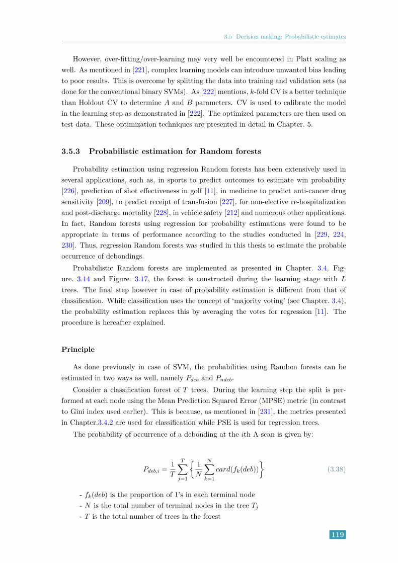
3.5 Decision making: Probabilistic estimates
However, over-fitting/over-learning may very well be encountered in Platt scaling aswell. As mentioned in [221], complex learning models can introduce unwanted bias leadingto poor results. This is overcome by splitting the data into training and validation sets (asdone for the conventional binary SVMs). As [222] mentions, k-fold CV is a better techniquethan Holdout CV to determine A and B parameters. CV is used to calibrate the modelin the learning step as demonstrated in [222]. The optimized parameters are then used ontest data. These optimization techniques are presented in detail in Chapter. 5.
3.5.3 Probabilistic estimation for Random forests
Probability estimation using regression Random forests has been extensively used inseveral applications, such as, in sports to predict outcomes to estimate win probability[226], prediction of shot effectiveness in golf [11], in medicine to predict anti-cancer drugsensitivity [209], to predict receipt of transfusion [227], for non-elective re-hospitalizationand post-discharge mortality [228], in vehicle safety [212] and numerous other applications.In fact, Random forests using regression for probability estimations were found to beappropriate in terms of performance according to the studies conducted in [229, 224,230]. Thus, regression Random forests was studied in this thesis to estimate the probableoccurrence of debondings.
Probabilistic Random forests are implemented as presented in Chapter. 3.4, Fig-ure. 3.14 and Figure. 3.17, the forest is constructed during the learning stage with L
trees. The final step however in case of probability estimation is different from that ofclassification. While classification uses the concept of ‘majority voting’ (see Chapter. 3.4),the probability estimation replaces this by averaging the votes for regression [11]. Theprocedure is hereafter explained.
Principle
As done previously in case of SVM, the probabilities using Random forests can beestimated in two ways as well, namely Pdeb and Pndeb.
Consider a classification forest of T trees. During the learning step the split is per-formed at each node using the Mean Prediction Squared Error (MPSE) metric (in contrastto Gini index used earlier). This is because, as mentioned in [231], the metrics presentedin Chapter.3.4.2 are used for classification while PSE is used for regression trees.
The probability of occurrence of a debonding at the ith A-scan is given by:
Pdeb,i =1
T
T∑j=1
1
N
N∑k=1
card(fk(deb))
(3.38)
- fk(deb) is the proportion of 1’s in each terminal node- N is the total number of terminal nodes in the tree Tj
- T is the total number of trees in the forest
119

Chapter 3. Machine Learning Methods
The probability estimation procedure using Random forests is summarized in Algo-rithm. 1 of [229].
In Chapter. 6, we present the estimation of debondings in two sets of experimentaldata using the various feature sets, namely, local and global features (presented later inChapter. 4), and compare the results with the benchmark obtained using raw GPR data.
3.6 Synthesis
We finally present a concise list of the family of ML methods presented in this chapter.As presented in Table. 3.6, each of the ML methods possess their own advantages.
120
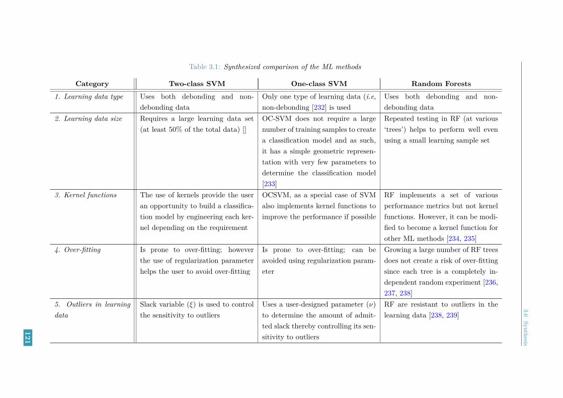
3.6Synthesis
Table 3.1: Synthesized comparison of the ML methods
Category Two-class SVM One-class SVM Random Forests
1. Learning data type Uses both debonding and non-debonding data
Only one type of learning data (i.e,non-debonding [232] is used
Uses both debonding and non-debonding data
2. Learning data size Requires a large learning data set(at least 50% of the total data) []
OC-SVM does not require a largenumber of training samples to createa classification model and as such,it has a simple geometric represen-tation with very few parameters todetermine the classification model[233]
Repeated testing in RF (at various‘trees’) helps to perform well evenusing a small learning sample set
3. Kernel functions The use of kernels provide the useran opportunity to build a classifica-tion model by engineering each ker-nel depending on the requirement
OCSVM, as a special case of SVMalso implements kernel functions toimprove the performance if possible
RF implements a set of variousperformance metrics but not kernelfunctions. However, it can be modi-fied to become a kernel function forother ML methods [234, 235]
4. Over-fitting Is prone to over-fitting; howeverthe use of regularization parameterhelps the user to avoid over-fitting
Is prone to over-fitting; can beavoided using regularization param-eter
Growing a large number of RF treesdoes not create a risk of over-fittingsince each tree is a completely in-dependent random experiment [236,237, 238]
5. Outliers in learningdata
Slack variable (ξ) is used to controlthe sensitivity to outliers
Uses a user-designed parameter (ν)to determine the amount of admit-ted slack thereby controlling its sen-sitivity to outliers
RF are resistant to outliers in thelearning data [238, 239]
121

Chapter
3.M
achineLearning
Methods
Table 3.1: Synthesized comparison of the ML methods
Category Two-class SVM One-class SVM Random Forests
6. Cross validation Uses CV techniques to avoid over-fitting and computation of optimalhyper-parameters
Uses CV techniques to avoid over-fitting and computation of optimalhyper-parameters
Self testing is based on an extensionof cross validation that is repeatedseveral times. This provides highlyreliable assessments of the reliabilityof the RF model [237]
7. Decision making Uses the two-class classificationmodel to predict the presence or ab-sence of debondings (single predic-tion step)
Uses the learning data as reference(single prediction step)
Identifies the best predictor auto-matically through the process ofvoting [236] (several repetitions)
8. Computational Speed Learning step is relatively slower;however it can be sped up using fea-ture selection
Due to its simplistic modeling,OCSVM performs relatively fasterlearning and testing [240]
Trees are grown at high speed be-cause few variables are in use at anyone time [237].
9. Accuracy SVM presents high accuracy bymeans of regularization and the useof proper kernels, the learning stepgenerates a more robust result
OCSVM has a high accuracy pro-vided that the hyper-parameterschosen are optimal
RF models are often considerablymore accurate than a single decisiontree. The accuracy achieved is oftencompetitive with the best alterna-tive methods [236, 237]
10. Estimation of prob-ability
Both two-class and One-class SVMs can be used to estimate probabilityusing Platt scaling
RF has a built-in regression that canbe used for probability estimation[11]
122

3.7 Conclusions
3.7 Conclusions
In this chapter we introduced four Machine Learning methods to detect the debondingswithin pavement structures, namely, Random forests, SVM for binary classification (Two-class SVM) and outlier detection (One-class SVM) and k-means clustering technique.They have been categorized into supervised and unsupervised techniques, respectively.
The principle of each method is illustrated through the straightforward processing oftime data as a whole (i.e raw GPR data). The four methods were applied to process noisysimulated analytic data with simplified assumptions, which are presented in Appendix. A.The methods demonstrated good qualitative results as they were able to detect debondingswith various interlayer permittivities.
Due to the limitations of binary SVM, the anomaly detection method, One-class SVMwas then presented to demonstrate a ML method that is closer to the operational levelmeasurement and detection. Finally, the third ML method, Random forests method wasstudied. This method, although underused (as opposed to its real capability), its advan-tages made it interesting to compare with other supervised machine learning methods.
The conventional binary SVM presented very high debonding detection rate for allnoisy simulated data configurations. However, the need for both debonding and non-debonding data to be present in the learning data limits its implementation at an opera-tional level.
Despite its advantages of being close to the operational level, OCSVM was seen toprovide the lowest accuracy among the three methods with several false detection (in caseof weak dielectric contrast i.e. εr,deb = 6).
Finally, in case of RF, it was observed that once again very high detection rate wasobserved for all cases.
In the final section of this chapter, we introduced the approach of probabilistic estima-tion of the occurrence of debondings using the supervised machine learning methods. Eachmethod, with the help of certain post-processing of the GPR data presented the abilityto provide a probability of debondings. This estimation will be explored in Chapter. 6 forexperimental data.
The processing of raw data is not always acceptable since the raw GPR data maycontain redundant information that could reduce the debonding detection rate. As statedby [143], the machine learning methods could be limited in their processing of raw data.In addition, large data size of the raw data can increase the computational time andcomplexity. To overcome this issue, certain preprocessing techniques can be done.
As observed in Section. 3.2, the unsupervised clustering method presented low detec-tion rate using simulated data. Similar behavior was also observed on experimental SFRdata, which was presented by us in [166]. Thus, the next chapter presents the variouspreprocessing and feature extraction techniques performed to aid the supervised learninglearning methods used for debonding survey.
123


Chapter 4
Signal Feature Analysis For Debonding Survey
Contents4.1 Feature engineering . . . . . . . . . . . . . . . . . . . . . . . . . . 124
4.2 Signal features for GPR data . . . . . . . . . . . . . . . . . . . . 125
4.2.1 Local signal features . . . . . . . . . . . . . . . . . . . . . . . . . 126
4.2.2 Global signal features . . . . . . . . . . . . . . . . . . . . . . . . 130
4.2.3 Comparison of Local and Global feature sets . . . . . . . . . . . 131
4.2.4 Feature reduction using Principal Component Analysis (PCA) . 132
4.2.5 Feature selection methodology . . . . . . . . . . . . . . . . . . . 135
4.3 Preliminary tests on machine learning methods using GPRsignal features . . . . . . . . . . . . . . . . . . . . . . . . . . . . . 137
4.3.1 Two-Class SVM . . . . . . . . . . . . . . . . . . . . . . . . . . . 138
4.3.2 One-Class SVM . . . . . . . . . . . . . . . . . . . . . . . . . . . . 138
4.3.3 Random forests . . . . . . . . . . . . . . . . . . . . . . . . . . . . 139
4.4 Conclusion . . . . . . . . . . . . . . . . . . . . . . . . . . . . . . . 140
In the previous chapter, we presented the various data processing methods, supervisedand unsupervised, that were used in the thesis to detect the presence of thin debond-
ings within pavement structures. These machine learning methods were used in the con-text of detecting thin debondings within pavement structures. Qualitative results werepresented for each ML method using simulated data generated from various models pre-sented in Appendix A.2, Appendix A.3 and Appendix A.4. However these results wereobtained using the raw GPR data (as shown in Chapter 3.3.1 for Two-class SVMs, Chap-ter 3.3.2 for One-class SVMs and Chapter 3.4.3 for Random forests). By using the rawGPR data, the computational complexity may increase leading to increased processingtime. Moreover redundant data may either have no effect on the performance or may alsoreduce the detection rate of a method.
Thus, in order to improve the performance of a method and avoid the effects of re-dundant signal data, preprocessing of the data is necessary. This can include the datatransformation (time to frequency domains and vice-versa) and feature selection/extrac-tion [143]. In the latter case, either a part of the original data are taken, or, new signalcharacteristics (called features or attributes) are derived from the original data. Feature
125

Chapter 4. Signal Feature Analysis For Debonding Survey
extraction aims to remove irrelevant and redundant information leading to better perfor-mance [241]. [242] demonstrate that the performance of machine learning methods can beimproved by the use of signal features.
In this chapter, we present the preprocessing step of GPR data feature selection tech-niques using simulated data. This approach has been also implemented in [10] for debond-ing detection from experimental data. Feature selection for SVM has been extensively usedin the literature for multiple medical applications [243, 244, 245], data classification in datamining [246], facial recognition [247] handwriting character recognition [161], text cate-gorization [248] etc. One-class SVM has been demonstrated to use feature selection fordocument classification [181], image segmentation [249] and also for audio detection andclassification applications [250].
Signal feature selection can be performed on both spectral (frequency-domain) andtemporal (time-domain) data. Temporal features of the signal are studied here as they areeasy to implement and avoid complex preprocessing and computations (such as Fouriertransformations, filtering etc.) [251]. In some cases, as in [252] for the study of EMGsignals, the time-domain features even outperform the spectral features (such as PSD,mean power, mean frequency etc.) for supervised machine learning method (k-nearestneighbor).
In this chapter, signal feature extraction is performed on temporal data to obtainfeatures globally (over the complete A-scan signal) as well as features localized at thepavement interface (i.e. only the second echo of the A-scan). Additionally, a featurereduction technique, namely Principal Component Analysis (PCA) is used. A parametricstudy will be done wherein the machine learning methods are analyzed w.r.t the inputGPR data (in the form of raw GPR data, local signal features, global signal features andPCA reduced local and global signal features).
The motive behind the preprocessing is to study (a) adaptation the ML methods forvarious input data types, (b) reduce the processing data size and complexity, (c) avoidover-learning/over-fitting that may hinder the performance and improve the debondingdetection rate.
4.1 Feature engineering
Most GPR data are very large containing thousands of time samples in each A-scanprofile. From this huge data set, it is highly possible that a part of the data is redundantand presents negligible or no information at all. In the machine learning classificationproblems, the first step is then to perform data reduction by identifying and selecting thedata subset that provides maximum information.
Feature engineering is the concept of using the known knowledge of the data to ex-tract/select the signal features that can help to improve the performance of a machinelearning method. It can be carried out manually based on the experienced understandingof the operator/user, or, automatically by means of certain well-known feature engineeringtechniques. On a broader scale, the feature engineering can be two-fold: feature selectionand feature extraction.
126
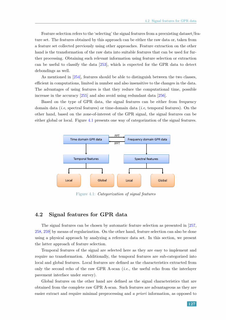
4.2 Signal features for GPR data
Feature selection refers to the ‘selecting’ the signal features from a preexisting dataset/fea-ture set. The features obtained by this approach can be either the raw data or, taken froma feature set collected previously using other approaches. Feature extraction on the otherhand is the transformation of the raw data into suitable features that can be used for fur-ther processing. Obtaining such relevant information using feature selection or extractioncan be useful to classify the data [253], which is expected for the GPR data to detectdebondings as well.
As mentioned in [254], features should be able to distinguish between the two classes,efficient in computations, limited in number and also insensitive to the changes in the data.The advantages of using features is that they reduce the computational time, possibleincrease in the accuracy [255] and also avoid using redundant data [256].
Based on the type of GPR data, the signal features can be either from frequencydomain data (i.e, spectral features) or time-domain data (i.e, temporal features). On theother hand, based on the zone-of-interest of the GPR signal, the signal features can beeither global or local. Figure 4.1 presents one way of categorization of the signal features.
Figure 4.1: Categorization of signal features
4.2 Signal features for GPR data
The signal features can be chosen by automatic feature selection as presented in [257,258, 259] by means of regularization. On the other hand, feature selection can also be doneusing a physical approach by analyzing a reference data set. In this section, we presentthe latter approach of feature selection.
Temporal features of the signal are selected here as they are easy to implement andrequire no transformation. Additionally, the temporal features are sub-categorized intolocal and global features. Local features are defined as the characteristics extracted fromonly the second echo of the raw GPR A-scan (i.e., the useful echo from the interlayerpavement interface under survey).
Global features on the other hand are defined as the signal characteristics that areobtained from the complete raw GPR A-scan. Such features are advantageous as they areeasier extract and require minimal preprocessing and a priori information, as opposed to
127

Chapter 4. Signal Feature Analysis For Debonding Survey
the local features. In case of GPR data, global features are usually dominated by the sur-face clutter and are therefore supposed to be less sensitive to the debonding. Whereas localfeatures are expected to provide more sensitive information about the interface betweenthe first two pavement layers and the debonding that may occur therein.
The two next subsections introduce both local and global temporal features of thesignal which have been used for performing SVM classification. The feature selectionpresented later in Chapter 4.2.5 relies on the prior knowledge about the database (exper-imental or otherwise) under test.
4.2.1 Local signal features
Local features are expected to provide more sensitive information about the interlayerpavement conditions. They are defined as the signal characteristics of the original rawGPR A-scan over a short time window focused at the pavement interface, whose centerand duration are computed using a known non-debonding A-scan as reference. Localfeatures are obtained from this window focused at the second echo only. This approachhas been presented in detail in Appendix D.
Figure 4.2 presents the automatic windowing of the second echo used to extract localsignal features for simulated data. The same approach is used for experimental data.Figure D.2, Figure D.3 and Figure D.4 respectively present the B-scans before and afterthe automatic time-gating for experimental SFR data (Appendix D) for Geotextile, Tack-free and Sand-based defects.
1 1.5 2 2.5 3 3.5 4Time (s) ×10-9
-0.4
-0.3
-0.2
-0.1
0
0.1
0.2
Am
plitu
de
Debonding A-scanNon-debonding A-scanTukey time-gating window
(a) Complete debonding and non-debonding A-scans
1 1.5 2 2.5 3 3.5 4Time (s) ×10-9
-0.08
-0.06
-0.04
-0.02
0
0.02
0.04
0.06
Am
plitu
de o
f sec
ond
echo
Non-debonding A-scanDebonding A-scanTime gating Tukey window
(b) Time-gated second echo
Figure 4.2: Automatic time-gating of the second echo used to extract local signal features(simulated analytic Fresnel data; εr,deb = 6, SNR = 30dB, εr,deb = 6, tdeb = 0.3 cm)
As presented earlier in Chapter 2, the presence of a debonding layer alters the formof the received signal. This alteration of the signal form is expected to differentiate be-tween the debonding and non-debonding cases. A GPR database is used to analyze thevarious feature sets that can aid the data processing methods to detect debondings. Theprobability density functions (PDFs) are then traced for debonding and non-debondingcases for each signal feature. The separation of the distributions is used to decide if thesignal feature can be used. The PDFs are displayed after a curve-smoothing techniquewith moving average is applied to the distributions. We broadly categorize the features
128

4.2 Signal features for GPR data
into three subsets: Statistical, Morphological and PQRST features.The first feature subset, namely statistical feature set, refers to statistical characteris-
tics of the time-gated GPR A-scan. These features have been used in the literature for thedetection of abnormal mammograms [260], character recognition [261] and classify exter-nal stimuli [262]. As in [263, 264, 265], local statistical features used here are: Standarddeviation, Mean absolute deviation (MAD), Kurtosis and Skewness. Standard deviation isthe amount of dispersion of the data of the mean. Skewness is the measure of asymmetrywhile kurtosis measures the ‘peakedness’ of the given data [266]. We have also used theselocal features in [10] to detect debondings using SVM.
Figure 4.3 presents the local statistical signal features (i.e. for the second echo only). It
0 0.2 0.4 0.6 0.8 1Normalized Magnitude
0 10 20 30 40 50 60 70 80 90 100A-scans
1.7
1.8
1.9
2
2.1
2.2
2.3
MA
D
×10-3
(a) Mean Absolute Deviation (MAD)
0 0.2 0.4 0.6 0.8 1Normalized Magnitude
0 10 20 30 40 50 60 70 80 90 100A-scans
6.5
7
7.5
8
8.5
9
9.5
10
Std
. dev
iatio
n
×10-3
(b) Standard deviation
0 0.2 0.4 0.6 0.8 1Normalized Magnitude
0 10 20 30 40 50 60 70 80 90 100A-scans
28
30
32
34
36
38
40
42
44
46
Kur
tosi
s
(c) Kurtosis
0 0.2 0.4 0.6 0.8 1Normalized Magnitude
0 10 20 30 40 50 60 70 80 90 100A-scans
-5
-4
-3
-2
-1
0
1
2
Ske
wne
ss
(d) Skewness
Figure 4.3: Representation of local statistical features for simulated data (computed fromanalytic Fresnel data model (Appendix A.2) with added noise (SNR = 30dB, εr,deb = 6,tdeb = 0.3 cm). ‘’ (red) indicate debonding and ‘+’ (blue) indicate non-debonding values
should be noted that the signal features that do not present sufficient PDF separation arenot used. For e.g, as mentioned in [10], the mean of a GPR A-scan was found to be centredat zero. As such, the two distributions for debonding and non-debonding cases usingmean as the signal feature present very little separation. Additionally, other statisticalfeatures such as entropy [260], median [267] were observed to provide any significantPDF separation. Therefore such features are not considered. As illustrations, Figure 4.4presents the distributions for the rejected statistical features of mean and median.
The second feature subset is named PQRST features. Specific Electrocardiography(ECG) signal features have been used due to the similarity in shape between the GPRA-scan and an ECG signal, namely the PQRST features discussed in [268, 269]. ThePQRST signal is the basic pattern of electrical activity (or one cycle) of the heart [270].
129

Chapter 4. Signal Feature Analysis For Debonding Survey
0 0.2 0.4 0.6 0.8 1Normalized Magnitude
0 10 20 30 40 50 60 70 80 90 100A-scans
-2
-1.5
-1
-0.5
0
0.5
1
1.5
2
2.5
3
Mea
n
×10-4
(a) Mean
0 0.2 0.4 0.6 0.8 1Normalized Magnitude
0 10 20 30 40 50 60 70 80 90 100A-scans
0
0.2
0.4
0.6
0.8
1
1.2
1.4
1.6
Med
ian
×10-3
(b) Median
Figure 4.4: Representation of inseparable unused local statistical features for simulateddata (computed from analytic Fresnel data model (Appendix A.2) with added noise
(SNR = 30dB, εr,deb = 6, tdeb = 0.3 cm). Due to the faint separation, these features arenot used
Its patterns (shape and/or form) are seen to closely resemble the reflected signal at eachinterface of the pavement structure (for comparison, see Figure 1 in [271]).
In our application, we propose to assign the points P and T to respectively the first andthe last breaks of the second echo while the points Q, R and S respectively represent thefirst, second and third alterations of the signal. Figure 4.5 shows the PQRST data-pointsin a GPR signal for debonding and non-debonding for the second echo. The PQRST
0 0.5 1 1.5 2 2.5 3 3.5 4 4.5 5Time (s) ×10-9
-0.08
-0.06
-0.04
-0.02
0
0.02
0.04
0.06
Am
plitu
de
Time-gated Non-debonding A-scanTime-gated Non-debonding A-scanTime-gating window
P
P'
Q
Q'
R
R'
S
S'
T
T'
Figure 4.5: PQRST data-points of time-gated debonding and non-debonding A-scansfrom simulated data (analytic Fresnel data)
features were chosen once again on the PDF separation as done for statistical features.Figure 4.6 presents the distributions of the various PQRST feature sets.
Figure 4.7 presents the amplitude at point ‘Q’ and slope QR from the PQRST features.The PDF for amplitude at point ‘Q’ does not present a good separation; while that ofslope QR is a bimodal PDF as opposed to our assumptions (i.e, normal distribution).
The last subset of local features are the Morphological features. These features arerelated to the ‘form’ and ‘shape’ of the GPR signal. The constructive interference of thereflections within the debonding layer results in an observable increase (or decrease de-pending on the contrast in permittivities) in the characteristics of the second reflectionsuch as amplitude range. As seen in Figure 4.2 the difference between the second echoes of
130

4.2 Signal features for GPR data
0 0.2 0.4 0.6 0.8 1Normalized Magnitude
0 10 20 30 40 50 60 70 80 90 100A-scans
0.04
0.045
0.05
0.055
0.06
0.065
0.07
0.075
0.08A
mpl
itude
P
(a) Amplitude at point ‘P’
0 0.2 0.4 0.6 0.8 1Normalized Magnitude
0 10 20 30 40 50 60 70 80 90 100A-scans
0.05
0.06
0.07
0.08
0.09
0.1
0.11
0.12
Am
plitu
de Q
(b) Amplitude at point ‘Q’
0 0.2 0.4 0.6 0.8 1Normalized Magnitude
0 10 20 30 40 50 60 70 80 90 100A-scans
0.045
0.05
0.055
0.06
0.065
0.07
0.075
0.08
0.085
Am
plitu
de R
(c) Amplitude at point ‘R’
0 0.2 0.4 0.6 0.8 1Normalized Magnitude
0 10 20 30 40 50 60 70 80 90 100A-scans
0.05
0.06
0.07
0.08
0.09
0.1
0.11
0.12
Am
plitu
de S
(d) Amplitude at point ‘S’
0 0.2 0.4 0.6 0.8 1Normalized Magnitude
0 10 20 30 40 50 60 70 80 90 100A-scans
0.04
0.045
0.05
0.055
0.06
0.065
0.07
0.075
Am
plitu
de T
(e) Amplitude at point ‘T’
Figure 4.6: Representation of local PQRST features for simulated data (computed fromanalytic Fresnel data model (Appendix A.2) with added noise (SNR = 30dB, εr,deb = 6,tdeb = 0.3 cm). ‘’ (red) indicate debonding and ‘+’ (blue) indicate non-debonding values
0 0.2 0.4 0.6 0.8 1Normalized Magnitude
0 10 20 30 40 50 60 70 80 90 100A-scans
0.05
0.055
0.06
0.065
0.07
0.075
0.08
0.085
0.09
Am
plitu
de Q
(a) Amplitude at point ‘Q’
0 0.2 0.4 0.6 0.8 1Normalized Magnitude
0 10 20 30 40 50 60 70 80 90 100A-scans
0.4
0.6
0.8
1
1.2
1.4
1.6
1.8
Slo
pe Q
R
(b) Slope QR
Figure 4.7: Representation of inseparable unused local PQRST features for simulateddata (computed from analytic Fresnel data model (Appendix A.2) with added noise
(SNR = 30dB). ‘’ (red) indicate debonding and ‘+’ (blue) indicate non-debondingvalues
131

Chapter 4. Signal Feature Analysis For Debonding Survey
debonding and non-debonding cases can be considered to be used as signal feature. Thus,amplitude range and magnitude of the second echo are used as local features. Addition-ally, the root-mean square (RMS) and inter-quartile range (as in [272]) of the debondingand non-debonding A-scans have been observed to present a significant PDF separation,thereby considered as usable local features. For representation, Figure 4.8 presents thedistributions for the usable morphological features.
0 0.2 0.4 0.6 0.8 1Normalized Magnitude
0 10 20 30 40 50 60 70 80 90 100A-scans
0.1
0.11
0.12
0.13
0.14
0.15
0.16
0.17
Am
plitu
de 2
nd e
cho
(a) Amplitude range of second echo
0 0.2 0.4 0.6 0.8 1Normalized Magnitude
0 10 20 30 40 50 60 70 80 90 100A-scans
0.07
0.075
0.08
0.085
0.09
0.095
0.1
0.105
0.11
0.115
Mag
nitu
de 2
nd e
cho
(b) Magnitude of second echo
0 0.2 0.4 0.6 0.8 1Normalized Magnitude
0 10 20 30 40 50 60 70 80 90 100A-scans
6.5
7
7.5
8
8.5
9
9.5
10
Roo
t-m
ean-
squa
re
×10-3
(c) Root-mean square
Figure 4.8: Representation of local morphological features for simulated data (computedfrom analytic Fresnel data model (Appendix A.2) with added noise (SNR = 30dB,
εr,deb = 6, tdeb = 0.3 cm). ‘’ (red) indicate debonding and ‘+’ (blue) indicatenon-debonding values
4.2.2 Global signal features
Contrary to the local features, the Global signal features are defined as the signalcharacteristics that are obtained from the raw GPR A-scan. In case of experimentaldata, the raw GPR data is described as the data after the elimination of clutter, namelythe straightforward direct antenna-coupling. These features are relatively easier to extractcompared to the local features as they use the raw GPR scans. Additionally, these featuresdo not require any information a priori as is the case for local features.
As done for local features, the global features are categorized into two groups, Statis-tical and Morphological features holding the same definition as for local features.
Each statistical feature was computed for the “raw GPR B-scan”. By observing theseparation of the PDFs for each feature (debonding vs. non-debonding), the best featureswere chosen. Figure 4.9 presents the usable global statistical features that showed well-separated distributions.
132

4.2 Signal features for GPR data
0 0.2 0.4 0.6 0.8 1Normalized Magnitude
0 10 20 30 40 50 60 70 80 90 100A-scans
1.6
1.7
1.8
1.9
2
2.1
2.2
2.3
MA
D
×10-3
(a) Mean Absolute Deviation (MAD)
0 0.2 0.4 0.6 0.8 1Normalized Magnitude
0 10 20 30 40 50 60 70 80 90 100A-scans
6.5
7
7.5
8
8.5
9
9.5
10
Std
. dev
iatio
n
×10-3
(b) Standard deviation
0 0.2 0.4 0.6 0.8 1Normalized Magnitude
0 10 20 30 40 50 60 70 80 90 100A-scans
28
30
32
34
36
38
40
42
44
Kur
tosi
s
(c) Kurtosis
0 0.2 0.4 0.6 0.8 1Normalized Magnitude
0 10 20 30 40 50 60 70 80 90 100A-scans
-5
-4
-3
-2
-1
0
1
2
Ske
wne
ss
(d) Skewness
Figure 4.9: Representation of global statistical features for simulated data (computed fromanalytic Fresnel data model (Appendix A.2) with added noise (SNR = 30dB, εr,deb = 6,tdeb = 0.3 cm). ‘’ (red) indicate debonding and ‘+’ (blue) indicate non-debonding values
The PQRST features are not used in the computation of global features since theyare specific to the second echo. In case of morphological features, the RMS and IQR arethe two features that were suggested. In addition, a new global feature, namely, InterfaceTime-Delay (ITD) is introduced. Due to the presence of an additional (debonding) layerin case of a defective pavement, the second echo is an attenuated composite signal usuallyshifted in time (w.r.t the surface echo). ITD is thus defined as the time delay between themaximum magnitudes of the first (surface) echo and the second echo. Figure 4.10 presentsthe global morphological features that showed well-separated distributions.
4.2.3 Comparison of Local and Global feature sets
Although the signal features chosen in the previous section (local and global) presented‘good’ PDF separation; it is necessary to compare the respective features obtained globallyand locally. This is done to observe the ‘overall goodness of separation’. Since, the rate ofclassification strongly depends on the separation of the signal features in the feature-space,it is necessary to analyze ‘how well are’ the chosen signal features separated w.r.t eachother.
As mentioned in Section 4.2.1, the local features are more accurate than global fea-tures (due to their localization at the pavement interface). Thus, they are expected toprovide a much better separation compared to their respective global counterparts. Forillustration, Figure 4.11(a), Figure 4.11(b), Figure 4.11(c) respectively present the localand global statistical features of standard deviation, signal kurtosis and signal skewness
133

Chapter 4. Signal Feature Analysis For Debonding Survey
0 0.2 0.4 0.6 0.8 1Normalized Magnitude
0 10 20 30 40 50 60 70 80 90 100A-scans
840
850
860
870
880
890
900
910
920
930
ITD
(a) Interface-time delay
0 0.2 0.4 0.6 0.8 1Normalized Magnitude
0 10 20 30 40 50 60 70 80 90 100A-scans
0.0472
0.0474
0.0476
0.0478
0.048
0.0482
0.0484
Roo
t-m
ean-
squa
re
(b) Root-mean square
Figure 4.10: Representation of global morphological features for simulated data (computedfrom analytic Fresnel data model (Appendix A.2) with added noise (SNR = 30dB,
εr,deb = 6, tdeb = 0.3 cm). ‘’ (red) indicate debonding and ‘+’ (blue) indicatenon-debonding values
and Figure 4.12(a), Figure 4.12(b), Figure 4.12(c) respectively present the same normal-ized between [0, 1]. As seen in case of Kurtosis and Skewness, the local features clearlydemonstrate a more clearer separation between the debonding and non-debonding casesthan its counterpart global features.
All signal features listed in Table 4.2 were subsequently analyzed in a similar fashionin order to verify ‘how well’ are the separations for debonding and non-debonding cases.It was observed that the local signal features always provided better separation than theirglobal counterparts.
Feature reduction using PCA, as presented in the following section, is one approachthat can be used to either eliminate the highly correlated features or transform them intouncorrelated features.
4.2.4 Feature reduction using Principal Component Analysis (PCA)
However, in case of both global and local features, since the features were chosen byphysical analysis of the GPR data, a threat of correlation between the features may beencountered. Such features, although tend to be different, are influenced by the sameparameter. Such features are thus redundant [273] and may lead force the method to ‘by-heart’ rather than learn. Feature reduction using PCA, as presented here, is one approachthat can be used to either eliminate the highly correlated features or transform them intouncorrelated features.
Principal component analysis is a non-supervised transformation technique that ismainly used for feature extraction and dimensionality reduction [274, 275]. Using PCA,it is possible to identify correlation patterns within the data that can be used to find thedirections of maximum variance in the higher dimensions and finally project the data ona new space with lesser dimensions than the original one [274]. In other words, PCA isused to transform this larger set of correlated features into a smaller set of uncorrelatedprincipal components [276] while still preserving as much information as possible.
In the literature, PCA has been used for feature extraction with SVM to classifyElectroencephalography (EEG) signals [277], ECG signals [278] and pattern identification
134

4.2 Signal features for GPR data
0.005 0.02 0.035 0.05Standard deviation
0
0.25
0.5
0.75
1
Nor
mal
ized
mag
nitu
de
Stdlocal
(debonding)
Stdlocal
(non-debonding)
Stdglobal
(debonding)
Stdglobal
(non-debonding)
(a) Standard deviation
25 30 35 40 45 50Kurtosis
0
0.25
0.5
0.75
1
Nor
mal
ized
mag
nitu
de
Kulocal
(debonding)
Kulocal
(non-debonding)
Kuglobal
(debonding)
Kuglobal
(non-debonding)
(b) Kurtosis
-5 -4 -3 -2 -1 0 1 2 3Skewness
0
0.25
0.5
0.75
1
Nor
mal
ized
mag
nitu
de
Sklocal
(debonding)
Sklocal
(non-debonding)
Skglobal
(debonding)
Skglobal
(non-debonding)
(c) Skewness
Figure 4.11: Comparison of local and global statistical features for noisy simulated data(computed from analytic Fresnel data mode; Appendix A.2) with added noise
(SNR = 30dB, εr,deb = 6, tdeb = 0.3 cm)
135

Chapter 4. Signal Feature Analysis For Debonding Survey
-0.2 0 0.2 0.4 0.6 0.8 1 1.2Normalized Std. deviation
0
0.25
0.5
0.75
1
Nor
mal
ized
mag
nitu
de
Stdlocal
(debonding)
Stdlocal
(non-debonding)
Stdglobal
(debonding)
Stdglobal
(non-debonding)
(a) Standard deviation
-0.2 0 0.2 0.4 0.6 0.8 1 1.2Normalized Kurtosis
0
0.25
0.5
0.75
1
Nor
mal
ized
mag
nitu
de
Kulocal
(debonding)
Kulocal
(non-debonding)
Kuglobal
(debonding)
Kuglobal
(non-debonding)
(b) Kurtosis
-0.2 0 0.2 0.4 0.6 0.8 1 1.2Normalized Skewness
0
0.25
0.5
0.75
1
Nor
mal
ized
mag
nitu
de
Sklocal
(debonding)
Sklocal
(non-debonding)
Skglobal
(debonding)
Skglobal
(non-debonding)
(c) Skewness
Figure 4.12: Comparison of normalized local and global statistical features for noisysimulated data (computed from analytic Fresnel data mode; Appendix A.2) with added
noise (SNR = 30dB, εr,deb = 6, tdeb = 0.3 cm)
[279].However, here PCA is used to reduce the dimension of the pre-selected local and global
feature data sets. And since we want to reduce the dimensions, a subset of principalcomponents (called Eigenvectors) is selected containing the most information. A variancethreshold is then used to ‘shortlist’ the k prominent features that can be used.
Let Xm×n be a GPR B-scan in time domain (where m is the number of time samples,n is the number of A-scans) whose feature matrix is given by Fp×n (where p is the numberof features). The PCA is computed as follows. In order to assign equal importance to eachfeature, the feature set is normalized [280] for each feature (i.e, row-wise normalization).Then, the covariance matrix S of the 2D feature matrix is estimated.
As mentioned by [281, 282], the ‘importance’ of each principal component (or thequality of measure) is indicated by its inertia (or by the proportion of the total inertia).Hence, for a given principal component, the inertia can be expressed as [283, 282]:
πj =λj∑pj=1 λj
=λj
tr(S)T (4.1)
where tr(S) denotes the trace of the covariance matrix S.The increment nature of the components means that we can express the total variance
of a set of S different principal components as a percentage of total variance accountedfor:
∑j∈S πj × 100% [282].
Figure 4.13 presents the inertia plots for the global (Figure 4.13(a)) and local (Fig-
136

4.2 Signal features for GPR data
ure 4.13(b)) feature sets.
1 2 3 4 5 6 7Principal components
0
0.2
0.4
0.6
0.8
1
Iner
tia o
f the
com
pone
nts
Non-debondingDebonding
(a) Global feature set
1 2 3 4 5 6 7 8 9 10 11 12 13Principal components
0
0.2
0.4
0.6
0.8
1
Iner
tia o
f the
com
pone
nts
Non-debondingDebonding
(b) Local feature set
Figure 4.13: Inertia plot for local and global feature sets on simulated data (analytic Fresnelmodel; Appendix A.2)
The principal components that are to be retained are then chosen by using the pre-determined threshold. This threshold is user-defined (in percentage). Initially, each ofglobal and local feature sets are extracted. Then, PCA is performed separately on localand global feature sets using the same threshold values for both feature sets.
Initially, the threshold value was set to 100% (considering all the components as newfeatures); allowing us to achieve the same performance as for the original feature set.However by doing so, only transformed features are used but the resulting feature set sizeremains of the same. At 90% as well, the use of PCA is unnecessary for both, the scope ofthe application and the feature set as since there is hardly any data/feature reduction. Theaim would be to implement a threshold value that can achieve data reduction, but also,at the same time, maintain information within the reduced data for high performance.
By choosing the value of inertia (I ∈ R0, 1 or 0 to 100%), the number of Eigenvectors(and consequently the number of PCs) are controlled. For eg., in case of local features, ifthreshold = 100%, all 13 components are used; at 80% inertia 10 PCs are used and so on.
As done earlier in our paper [10], PCA is performed independently on local and globalfeature sets. By initial analysis, it was observed that, at first, the whole set of PCAfeatures (i.e. at 100% PC inertia) allows us to achieve the same performance as for theoriginal feature set (as seen for experimental data in our article [10] as well). The inertiawas brought down to 90% and similar performance levels were observed. However at 90%PC inertia, the use of PCA is unnecessary for both, the scope of the application and thefeature set as since there is hardly any data reduction.
The inertia was reduced step-by-step (steps of 10%) and the finally set to 80%, whichgives us 10 components for local signal features and 6 components for global signal features.It should be noted that when the inertia was reduced below 50%, the DSC score drasticallydropped below 0.5.
137

Chapter 4. Signal Feature Analysis For Debonding Survey
4.2.5 Feature selection methodology
The performance of a machine learning method depends on the hyper-parameters,kernel function and also the choice of its input data [284]. As such, a lot of effort isrequired to design the preprocessing steps for data transformation and feature extraction[284]. Figure 4.14 presents the overall debonding detection approach observed throughoutthis manuscript.
Figure 4.14: Overall machine learning approach to detect debonding using various inputdata sets (red, blue and green arrows respectively indicate the detection approach for rawdata, global feature set and local feature set)
Here, we take advantage of the ground truth associated to the data base (see Ap-pendix C.1) to perform the feature selection. The ground truth categorizes the A-scansinto two classes, namely debonding and non-debonding cases. The probability densityfunction (PDF) of the features is computed over each class to determine those which aresensitive enough to the pavement conditions.
Initially, a known B-scan with debonding and non-debonding regions is taken. PDFsare traced for each feature listed in Table 4.1 (Global features) and Table 4.2 (Localfeatures) for debonding and non-debonding cases. Figure 4.3 and Figure 4.4 present someof the features to indicate how each feature is able to distinguish between debonding andnon-debonding cases. For representation only, a curve-smoothing technique using movingaverage is applied to the PDFs in Figure 4.3 and Figure 4.4.
The separation between the two curves is used to choose the best features for our ap-
138

4.3 Preliminary tests on machine learning methods using GPR signal features
plication. For example, the mean of the signal (represented in Figure 4.4(a), Figure 4.7(a)etc.) show minimal/no PDF separation whereas the other features presented in Figure 4.3,Figure 4.6, Figure 4.8, Figure 4.9 and Figure 4.10 provide well-separated distributions andare thus used. The other features are rejected. Additionally, PCA is also used on local andglobal features to further reduce the data. However, as presented later, it was observedthat reduction using PCA did not provide much difference in the detection rate. Finally,
Time domain local signal features• Statistical features: Mean Absolute deviation (MAD), Standard deviation,
Skewness and Kurtosis
• Morphological features: RMS of the signal, Inter-quartile range, Amplitudeof second echo, Magnitude of second echo• PQRST features: Amplitudes at points P, R, S and T, Slope RS
Table 4.1: List of the local signal features used obtained by analyzing the PDF separationsof debonding and non-debonding data
Time domain global signal features• Statistical features: Mean Absolute deviation (MAD), Standard deviation,
Skewness and Kurtosis
• Morphological features: RMS of the signal, Inter-quartile range, Interfacetime-delay of second echo (ITD)
Table 4.2: List of the global signal features used obtained by analyzing the PDF separationsof debonding and non-debonding data
a total of 13 local features and 7 global features were chosen as input data for furtherprocessing by supervised machine learning methods. In case of PCA reduced sets, 10 and6 components respectively were obtained from local and global feature sets.
We now compare the performance of the three supervised machine learning methodsbased on the various input feature sets. The results are compared with the benchmarkresults from Chapter 3 (i.e. performance using raw GPR data). These results are obtainedusing the optimization of each machine learning method (optimization methodologies de-tailed in the next chapter; Chapter 5).
4.3 Preliminary tests on machine learning methods usingGPR signal features
In this section, we perform a preliminary analysis of the supervised machine learningmethods by comparing their performances using various input feature sets (i.e, local andglobal features) from simulated analytic data. Additionally, the performance observed
139

Chapter 4. Signal Feature Analysis For Debonding Survey
using the raw GPR data (see Chapter 3) is used as the performance benchmark referencefor the results.
The analytic Fresnel data model (see Appendix A.2) is used to generate the simulateddata with various levels of SNR (i.e, SNR = 10 dB, 20 dB, 30 dB, 40 dB, 50 dB and 60 dB).Both global and local feature sets are extracted as discussed in Chapter 4.2.1 and 4.2.2respectively.
To represent the results, the ROC is traced at all levels of SNR (10 dB, 20 dB, 30 dB,40 dB, 50 dB and 60 dB) averaged over 100 independent Monte-Carlo realizations.
To illustrate the binary classification of GPR data, we use the ROC curves as thepreliminary form of representation. Although the ROC curve does not provide a diag-nostic tests in terms of gains and losses, they are still considered to be better in termsof representation at a superficial level. To add more meaning to the results, we use theperformance indexes, namely DSC and MCC scores as well.
4.3.1 Two-Class SVM
Figure 4.15 presents the ROC curves to compare the performance of Two-class SVMusing various input data sets discussed in Chapter 4.2 for simulated analytic data at variouslevels of SNR. These results are obtained using 5-fold cross validation (presented in thenext chapter) and non-linear RBF kernel. In case of binary Two-class SVM for simulated
0 0.1 0.2 0.3 0.4 0.5 0.6 0.7 0.8 0.9 1FPR
0
0.2
0.4
0.6
0.8
1
TP
R
Raw GPR data
Global feature set
PCA reduced Global feature set
Local feature set
PCA reduced Local feature set
Random chance
(a) Weak contrast (εr,deb = 6)
0 0.1 0.2 0.3 0.4 0.5 0.6 0.7 0.8 0.9 1FPR
0
0.2
0.4
0.6
0.8
1
TP
R
Raw GPR data
Global feature set
PCA reduced Global feature set
Local feature set
PCA reduced Local feature set
Random chance
(b) Strong contrast (εr,deb = 2)
Figure 4.15: ROC curves obtained using Two-class SVM for simulated analytic Fresneldata model (see Appendix A) at various levels of SNR (tdeb = 0.3 cm)
data, at low SNR levels the detection is low. However, with the increase in SNR, highdetection rate is observed for all types of feature sets, with local features providing resultsbetter than global feature sets.
4.3.2 One-Class SVM
Figure 4.16 presents the ROC curves to compare the performance of One-class SVMusing various input data sets discussed in Chapter 4.2 for simulated analytic data at variouslevels of SNR. Learning data size is Tlearn = 20 A-scan/feature vectors of non-debondingcase. A linear kernel is used with 5-fold cross validation to obtain an optimal value for the
140

4.3 Preliminary tests on machine learning methods using GPR signal features
parameter νopt. In case of εr,deb = 2 (strong contrast), νopt = 0.03 and εr,deb = 6 (weakcontrast), νopt = 0.05.
0 0.2 0.4 0.6 0.8 1FPR
0
0.2
0.4
0.6
0.8
1
TP
R
Raw GPR dataGlobal featuresPCA reduced Global featuresLocal featuresPCA reduced Local features
(a) Weak contrast (εr,deb = 6)
0 0.2 0.4 0.6 0.8 10
0.2
0.4
0.6
0.8
1
Raw GPR dataGlobal featuresPCA reduced Global featuresLocal featuresPCA reduced Local features
(b) Strong contrast (εr,deb = 2)
Figure 4.16: ROC curves obtained using One-class SVM for simulated analytic Fresneldata model (see Appendix A) at various levels of SNR (tdeb = 0.3 cm)
In case of weak contrast (εr,deb = 6), the performance of the global feature set is verylow. However, the local signal features perform well and better than the raw GPR dataas well as global features.
4.3.3 Random forests
Figure 4.17 presents the ROC curves to compare the performance of Random forestsusing various input data sets discussed in Chapter 4.2 for simulated analytic data atvarious levels of SNR. As done in Chapter 3.4.3 for raw GPR data, we use T = 100 treeswith each tree having the same number of observation samples. The value for the subsetsize (p) is fixed as mentioned earlier in Chapter 3.4.3.
0 0.2 0.4 0.6 0.8 1FPR
0
0.2
0.4
0.6
0.8
1
TP
R
Raw GPR dataGlobal featuresPCA reduced Global featuresLocal featuresPCA reduced Local features
(a) Weak contrast (εr,deb = 6)
0 0.2 0.4 0.6 0.8 1FPR
0
0.2
0.4
0.6
0.8
1
TP
R
Raw GPR dataGlobal featuresPCA reduced Global featuresLocal featuresPCA reduced Local features
(b) Strong contrast (εr,deb = 2)
Figure 4.17: ROC curves obtained using RF for simulated analytic Fresnel data model(see Appendix A) at various levels of SNR (tdeb = 0.3 cm)
It can be seen that, for simulated data, both local and global feature sets demonstrateexcellent detection at various levels of SNR.
141

Chapter 4. Signal Feature Analysis For Debonding Survey
Table 4.3: Comparison of DSC scores for machine learning methods with various inputdata sets obtained using noisy simulated analytic data at SNR = 30 dB (εr,deb = 2, 6; tdeb= 0.3 cm)
Input data setTwo-class SVM One-class SVM Random forests
εr,deb = 2 εr,deb = 6 εr,deb = 2 εr,deb = 6 εr,deb = 2 εr,deb = 6
Raw GPR data 1.00 1.00 0.927 0.91 1.00 1.00
Global features 1.00 1.00 0.97 0.0 1.00 1.00
Global features (PCA) 1.00 1.00 0.97 0.842 1.00 1.00
Local features 1.00 0.84 0.964 0.96 1.00 1.00
Local features (PCA) 1.00 1.00 0.962 0.85 1.00 1.00
In summary, Table 4.3 simply compares the DSC similarity index for the three ma-chine learning methods at SNR = 30 dB. It is clear that the Random forests outperformthe SVM approaches over all types of input data sets (feature sets or raw GPR data)thereby establishing it as the best debonding detection method amongst the three for ourapplication.
4.4 Conclusion
We begin this chapter by presenting one of the important preprocessing step in debond-ing detection i.e, signal feature selection. The feature selection was categorized into timedomain local and global signal features. The local features were focused at the pavementinterface where the debonding is expected to occur. These features were expected topresent higher efficiency for the purpose of debonding detection. Global features on theother hand used the complete GPR signal with the top two pavement interfaces. A totalof 13 local features and 7 global features were chosen by physical analysis of the GPRdata. In order to further reduce the data complexity, a well-known data reduction tech-nique (PCA) was introduced. The extracted feature sets were obtained for a simulateddata model (analytic Fresnel; see Appendix A.2) and the experimental data collected atIFSTTAR’s fatigue carousel (for Geotextile and Tack-free defects; see Appendix B.2).
From Chapter 3, the debonding detection from raw GPR data was used as the basisof performance comparison presented on ROC curves. Although the raw GPR data pre-sented very high detection, this approach is quite cumbersome and not efficient in termsof computational time and complexity. As expected, in case of Two-class SVM for sim-ulated data, it was observed that the local feature set presented better detection resultsthan global features. In case of RF, for simulated data, both local and global feature setsdemonstrated very high detection rate inferring that the method is well-suited for varioustypes of input data. Finally, in case of anomaly detection (One-class SVM), the localfeature sets presented better detection rate than its counterparts.
In case of each of the machine learning methods, it was observed that the raw GPR
142
4.4 Conclusion
data provided very similar results to that obtained using the local feature sets. However,the preference of using the local feature set over raw data was its smaller data size thatreduced the computational burden for the machine learning methods.
The motive behind the comparison of the methods using various input data was toanalyze their dependency on the input data for debonding detection and verify if there is anecessity of initial data preprocessing. By observing the results, the overall conclusion is,although the raw GPR data presents high debonding detection rate (in most cases), dueto computational complexity and the burden, it is necessary to perform feature selection.
The preliminary results presented for each machine learning method were obtainedusing optimized hyper-parameters that control the methods. However the optimizationof the machine learning methods can be performed on several parameters such as, thelearning data size, method hyper-parameters, method kernels, cross validation techniquesetc. Moreover, from the operator point-of-view, the objective would be to have robustdetection methods that are able to perform well despite the lack of knowledge (informationregarding pavement permittivity, composition etc).
Thus, in the next chapter, we explore this adaptability of machine learning methodsto these parameters by means of optimization and parameter tuning.
143


Part III
DATA PROCESSING FOR DEBONDING
DETECTION IN PAVEMENT STRUCTURES
145


Chapter 5
Machine Learning Model Selection and Validation
For Debonding Survey
Contents5.1 Methodology . . . . . . . . . . . . . . . . . . . . . . . . . . . . . . 146
5.2 Method-based model fitting . . . . . . . . . . . . . . . . . . . . . 147
5.2.1 Kernel-based analysis . . . . . . . . . . . . . . . . . . . . . . . . 150
5.2.2 Cross-validation techniques . . . . . . . . . . . . . . . . . . . . . 151
5.2.3 Learning data size . . . . . . . . . . . . . . . . . . . . . . . . . . 157
5.3 Robustness of machine learning methods w.r.t pavement medium159
5.3.1 Noise vs. permittivity variations . . . . . . . . . . . . . . . . . . 160
5.3.2 Debonding thickness and permittivity variations . . . . . . . . . 164
5.3.3 Single scattering vs. Multiple scattering effects . . . . . . . . . . 167
5.4 Summary . . . . . . . . . . . . . . . . . . . . . . . . . . . . . . . . 169
5.5 Conclusion . . . . . . . . . . . . . . . . . . . . . . . . . . . . . . . 172
In the previous chapter, we presented the pre-processing of GPR data by means offeature extraction and feature reduction. We also presented an initial performance
analysis of the machine learning methods by comparing the various input feature sets.These results were obtained using optimized hyper-parameters that govern the methods.
The optimization of a machine learning method is an important part since, by identi-fying the ‘best’ parameters, it is possible to achieve high debonding detection rate. In thischapter, we focus on the behavior of various parameters included in the machine learningmethod in the context of detecting interface debondings. Various optimization techniquesfor machine learning methods have already been discussed in the literature [285, 286, 287].
One such approach namely, Sensitivity Analysis [255], is studied here in the contextof detection of interface debonding. The approach namely, method-based model fitting(Chapter 5.2) is used to study the relationship between the performance of the methodsand the input hyper-parameters that control said methods, such as cross-validation tech-niques, kernel functions, learning data size etc). The sensitivity analysis of Two-class SVMwas implemented for GPR data in [10] w.r.t kernel function, learning data size and inputsignal feature sets.
147

Chapter 5. Machine Learning Model Selection and Validation For Debonding Survey
On the other hand, in this chapter, we also perform robustness tests (Chapter 5.3)to observe the effect of pavement medium and configurations (such as variations in thedebonding thickness, permittivity and effect of noisy data) on the performance of themethods. Finally, a concept of global parameter-optimization, which is suited for practicalapplications, is also introduced here.
As seen in the previous chapter (Chapter 4), the local signal features were able toprovide a higher detection rate to its counterparts (i.e. global features). Thus, in thischapter, the optimization of the methods is performed on the local signal features only.The optimization was performed using simulated data (Appendix A) independently oneach machine learning method, but over various pavement configurations (i.e global opti-mization).
5.1 Methodology
The standard methodology for debonding detection as we have presented in [10] isimplemented in this chapter. The GPR B-scan data is initially generated using simulatedanalytic Fresnel model (see Appendix A). Initial pre-processing feature selection steps arethen carried out as presented in Chapter 4.2.5. The data is then ready for processing usingthe machine learning methods.
In case of two-class classification (Two-class SVM and Random forests), the data israndomly divided into two disjoint sets: learning and test data. In this case, learning dataset contains both debonding as well as non-debonding data. One-class SVM, on the otherhand is divides the data in such a way that the learning data contains only one type ofdata, i.e. non-debonding.
In the learning stage, SVM methods then use various cross validation techniques toobtain the optimal hyper-parameters for the specific method. These optimal values arethen used with the test data for validation of results. In case of Random forests, thelearning data is randomly divided into several subsets to generate a ‘forest’ as presentedin Chapter 3.4.3. The classification for Random forests depends on the number of trees(T ) and the number of features (p) in each subset. These values are chosen as mentionedin Chapter 3.4.3.
Representation of results
In the previous chapter, the initial analysis and performance of the machine learningmethods for various input feature sets was presented using ROC curves. In this chapter,the ROC and AUC were found not easy to handle to determine the optimal parametersof the machine learning methods [288, 289, 290, 291]. As established in [292], diagnostictests are better understood when presented in terms of gains and losses, using numericindicators such as accuracy, error rate etc.. We then switch from ROC to performanceindexes.
Numeric indicators such as DSC score and MCC etc. are more representative and canthus be easily understood and interpretive by the operator with minimum knowledge. As
148

5.2 Method-based model fitting
explained in [288], the advantage of MCC coefficient over the other performance indexes isthat it provides a high MCC score iff the machine learning method has high percentageof true positives (in this case, debondings). The other rates (such as Accuracy, DSC
score, Precision, etc.) lack in this aspect and as discussed in [288, 289], they can lead tomisleading results. For illustration, Figure 5.1 compares the DSC and MCC scores forbalanced and imbalanced cases. The value Nratio is the ratio Ndeb/Nndeb where Ndeb andNndeb are respectively number of debonding and non-debonding A-scans.
0 0.2 0.4 0.6 0.8 1MCC coefficient
0
0.2
0.4
0.6
0.8
1
DS
C s
core
Nratio
= 0.25
Nratio
= 0.5
Nratio
= 1.0
Nratio
= 2.0
Nratio
= 4.0
Figure 5.1: Variation of DSC score and MCC coefficient at different Nratio values
It can be observed that in case of imbalanced data, i.e., Nratio < 0.5, DSC scoresaturates at higher values presenting very less variation, while MCC demonstrates to bemore robust. Conversely, for Nratio > 1, DSC would be recommended. Both indicators arealmost equivalent for balanced data, i.e., Nratio ≈ 1. Despite this different behavior, theDSC score is still used for imbalanced data and is widely used to represent the performancein binary classification [293].
However, in this thesis we are dealing with both situations. The tests on simulateddata are performed with balanced data, leading to equivalent interpretation with eitherDSC or MCC. By contrast, we may face the situation of imbalanced experimental datain Chapter 6, for which MCC would lead to a more reliable data interpretation. Toavoid the dilemma of choice, we then use both DSC and MCC scores to present theoptimization results for the methods.
5.2 Method-based model fitting
Machine learning involves predicting and classifying data and to do so, various machinelearning models can be best suited to a given dataset. The machine learning models areparameterized so that they can be ‘tuned’ in order to suit it to a given situation [286]. Eachmachine learning model can have various parameters and the goal would be to find the bestcombination of parameters in order to achieve the highest efficiency and demonstrate itsrobustness. However, the term ‘parameter’ and ‘hyper-parameter’ hold totally differentmeanings in machine learning. Parameters are simply the input settings that make an
149

Chapter 5. Machine Learning Model Selection and Validation For Debonding Survey
algorithm work; whereas hyper-parameters are the settings of an algorithm that can beadjusted to optimize the machine learning performance [287].
For debonding detection using supervised learning methods presented in Chapter 3,various input method-related parameters can be used. However, all these parametersmay or may not yield the desired accuracy solution. So, to decide what are the optimalvalues for each parameter that can provide the highest accuracy, a task most commonlycalled as Model selection [294]. In the field of data analysis, Sensitivity Analysis (SA)refers to the study of relationship of uncertainties between the input and its outputs [255].As mentioned in [295], both model selection and sensitivity analysis are similar as theyboth attempt to analyze the appropriateness of a model. However, while model selectionconcentrates on the assessment of ‘fitting’ specific to an application, SA has a more generalapproach to quantify the uncertainty in a model [295].
Several model-fitting approaches have been discussed in literature [286, 287, 296]. Thiscan be either performed manually by the user or it can also be automatically performedby the machine learning method. In the latter, the machine learning method has thefreedom to perform this parameter exploration and select the optimal model architectureautomatically governed by certain constraints.
Figure 5.2: Generic machine learning model fitting/parameter tuning approach
A model is said to be ‘fit’ if it is capable of identifying the relationship between thedata (or features) and the target detection [297]. In order to fit a model, the inputparameters are adjusted in such a manner that the best predictions can be achieved forthe data set under study. This process is sometimes also referred to as ‘Parameter tuning’.The parameter tuning by the machine learning method is an iterative process wherein themodel is continuously tuned to improve the accuracy of the method as shown in Figure 5.2.
Following the conclusions in Chapter 4, the local features presented better resultsthan the global feature sets. Thus, hyper-parameter optimization for model selection andvalidation in this chapter will be performed using local feature sets.
In this section, we propose the implementation of model-fitting by means of hyper-parameter optimization in the case of pavement debonding detection in two ways: globaloptimization and εr,deb-specific optimization.
150

5.2 Method-based model fitting
In case of the εr,deb-specific optimization, the cross validation techniques (presentedlater in Chapter 5.2.2) is used to find the optimized hyper-parameters for individual casesof pavement configurations that vary in terms of debonding layer permittivity etc. Al-though this approach may present the best hyper-parameters and achieve may very highefficiency, it is not practically possible due to the limited knowledge possessed by theoperators about the pavement configuration.
On the other hand, we define the global approach in which the optimization is per-formed with respect to all εr,deb scenarios. By doing so, the hyper-parameters used in thetesting stage are the same regardless of the debonding material under test. This approachis closer to the operational level than the former, since the operators do not possess allthe information about the pavement layers. The subsequent sections will discuss theseapproaches.
Figure 5.3 presents the parameter tuning during the learning stage to obtain theoptimal machine learning parameters necessary for ‘best-fitting’ the model (i.e. hyper-parameters).
Figure 5.3: Parameter tuning for supervised machine learning methods
In general, the model selection involves optimization of criterion, such as cross valida-tion [298]. Some other model selection techniques include the kernel functions and learningdata sizes. Figure 5.4 presents the categorization of the method based model fitting ap-proaches presented here. In this section, we explore the model selection approach for thethree machine learning methods, SVM, OCSVM and Random forests for noisy analyticsimulated databases. For each model-fitting approach, the two remaining categories areoptimized beforehand.
151
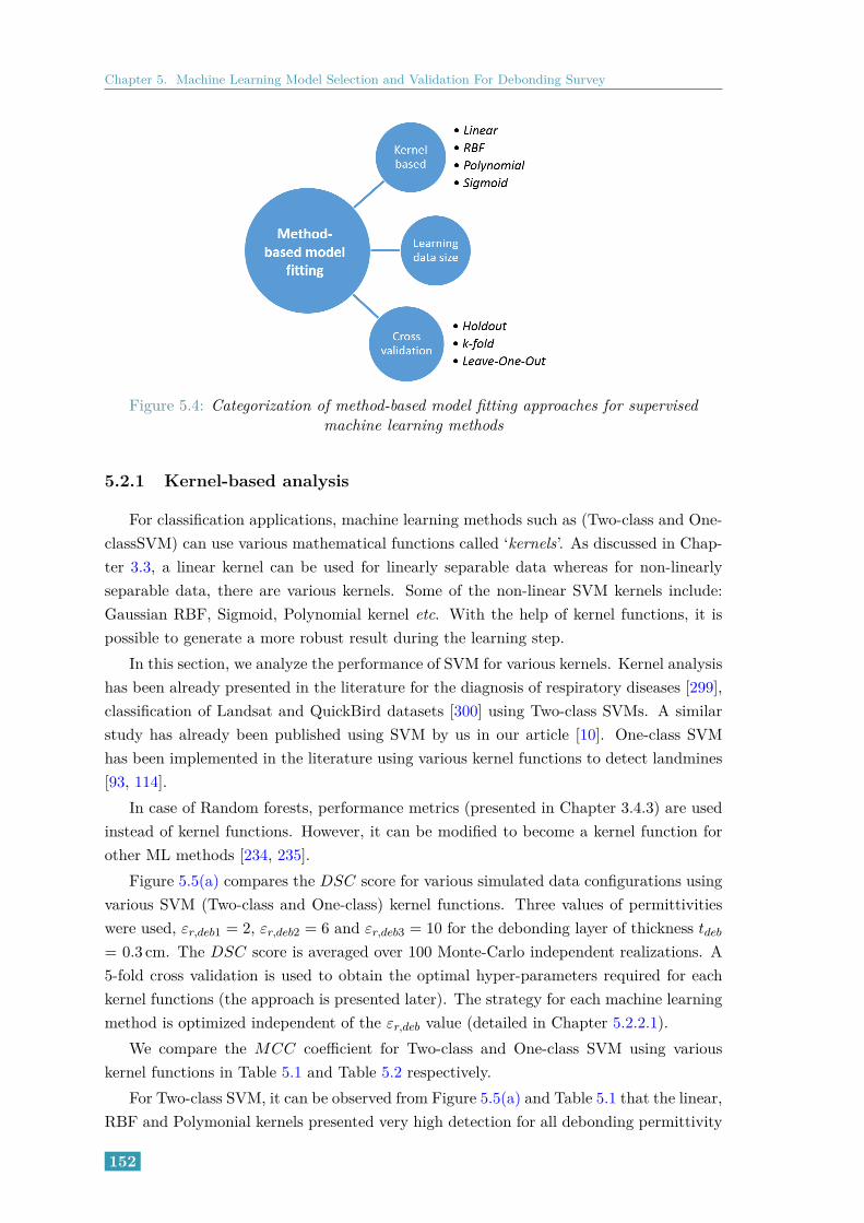
Chapter 5. Machine Learning Model Selection and Validation For Debonding Survey
Figure 5.4: Categorization of method-based model fitting approaches for supervisedmachine learning methods
5.2.1 Kernel-based analysis
For classification applications, machine learning methods such as (Two-class and One-classSVM) can use various mathematical functions called ‘kernels’. As discussed in Chap-ter 3.3, a linear kernel can be used for linearly separable data whereas for non-linearlyseparable data, there are various kernels. Some of the non-linear SVM kernels include:Gaussian RBF, Sigmoid, Polynomial kernel etc. With the help of kernel functions, it ispossible to generate a more robust result during the learning step.
In this section, we analyze the performance of SVM for various kernels. Kernel analysishas been already presented in the literature for the diagnosis of respiratory diseases [299],classification of Landsat and QuickBird datasets [300] using Two-class SVMs. A similarstudy has already been published using SVM by us in our article [10]. One-class SVMhas been implemented in the literature using various kernel functions to detect landmines[93, 114].
In case of Random forests, performance metrics (presented in Chapter 3.4.3) are usedinstead of kernel functions. However, it can be modified to become a kernel function forother ML methods [234, 235].
Figure 5.5(a) compares the DSC score for various simulated data configurations usingvarious SVM (Two-class and One-class) kernel functions. Three values of permittivitieswere used, εr,deb1 = 2, εr,deb2 = 6 and εr,deb3 = 10 for the debonding layer of thickness tdeb
= 0.3 cm. The DSC score is averaged over 100 Monte-Carlo independent realizations. A5-fold cross validation is used to obtain the optimal hyper-parameters required for eachkernel functions (the approach is presented later). The strategy for each machine learningmethod is optimized independent of the εr,deb value (detailed in Chapter 5.2.2.1).
We compare the MCC coefficient for Two-class and One-class SVM using variouskernel functions in Table 5.1 and Table 5.2 respectively.
For Two-class SVM, it can be observed from Figure 5.5(a) and Table 5.1 that the linear,RBF and Polymonial kernels presented very high detection for all debonding permittivity
152

5.2 Method-based model fitting
(a) Two-class SVM (b) One-class SVM
Figure 5.5: DSC score for the Method-based kernel SA for noisy simulated (analyticFresnel) data for various values of εr,deb
Table 5.1: MCC coefficient for various kernel functions for noisy simulated (analyticFresnel) data using Two-class SVM at various values of εr,deb
Kernel type εr,deb = 2 εr,deb = 6 εr,deb = 10
Linear 1.00 0.929 0.993
Polynomial 1.00 0.873 0.998
RBF 1.00 0.933 1.00
Sigmoid 1.00 0.591 0.93
Table 5.2: MCC coefficient for various kernel functions for noisy simulated (analyticFresnel) data using One-class SVM at various values of εr,deb
Kernel type εr,deb = 2 εr,deb = 6 εr,deb = 10
Linear 1.0 0.794 0.48
Polynomial 0.77 0.78 0.38
RBF 0.117 0.12 0.114
Sigmoid 0.74 0.72 0.77
values with RBF providing an edge over the two. This observation was found in case oflocal features for experimental data and published in our article [10]. The sigmoid kernelhowever, in case of εr,deb = 6 has false detection leading to DSC ≈ 0.65.
On the contrary, in case of One-class SVM, it was observed that apart from the RBFkernel, the linear and sigmoid kernels presented better results with DSC ≥ 0.70.
5.2.2 Cross-validation techniques
Cross validation is a model evaluation method that is better than residuals [301]. Theproblem with residual evaluations is that they do not give an indication of how well thelearner will do when it is asked to make new predictions for data it has not already seen.One way to overcome this problem is to not use the entire data set when training a learner.
153

Chapter 5. Machine Learning Model Selection and Validation For Debonding Survey
Some of the data is removed before training begins. Then when training is done, the datathat was removed can be used to test the performance of the learned model on ‘new’ data.This is the basic idea for a whole class of model evaluation methods called cross validation.
Here, we present and compare three principal cross validation approaches for tuningthe machine learning parameters. These CV techniques have been presented in detailin [297], compared in [302] using ROC and AUC curves, in [303, 304] compares the CVtechniques for defect prediction models and in [305] to classify medical images.
1. Holdout CV :The holdout method is one of the simplest approach in cross validation. Here, the learningdata is split equally into two exclusive sets, namely, training and validation. The trainingdataset is used to ‘fit’ the model and then it is tested using the validation data. Errorfunction is then used to evaluate the model performance and the optimal model is definedas the one with lowest error. Since the training and validation sets are mutually exclusive,the performance of the method completely depends in the samples that end up in each ofthe sets, thereby resulting in a high variance.
2. k-fold CV :The k-fold CV is one way to improve the Holdout method. The approach here is to ran-domly split the learning data into k disjoint subsets (namely, training and validation sets)of identical sizes. The goal is to respect the class distribution in each subdivision. Themodel is then fit using the k−1 folds and validated on the kth fold. This is repeated untileach k-fold has served as the validation set. The optimal model is then defined as beingthe one with the highest score (minimum generalization error) of cross validation.
3. Leave-one-out CV (LOO-CV):This is a modified version of the k-fold cross validation stretched to its logical extremesi.e., the k-fold are chosen in such a way that k = N where N is the number of data-points(or A-scans). The model training is then carried out the k−1 sets and validating using theremaining dataset with simply one data-point. The process is repeated until each data-point has participated as validation data-point. The evaluation given by leave-one-outcross validation seems very expensive to compute at first pass but is efficient as it carriesout the modeling with every data-point.
As seen in the literature, the k-fold CV technique is the commonly used method ofcross-validation.
5.2.2.1 Choice of optimal hyper-parameters
In this section, the method to obtain the optimal hyper-parameters is presented. Inorder to have the best classification model and guarantee global optimum, it is necessary toavoid local optimum hyper-parameters as they might seriously affect the learning processof a method [306]. The local optimum is best solution obtained within a small rangeof hyper-parameter values; whereas, the global optimum is obtained over all the hyper-
154

5.2 Method-based model fitting
parameter values.With the help of CV techniques, it is possible to improve the SVM’s performance
(One-class as well as Two-class) in the detection process. These CV techniques can beused to find the optimal hyper-parameters for a machine learning method and by usingsuitable loss-functions, it is possible to avoid the local minima. One such loss function isthe Hinge-loss [307]. For binary classification, Hinge loss function takes values ∈ [0, 2]; i.e.non-zero values for misclassified points (or penalized) and is equal to zero for well-classifiedpoints. Therefore, the Hinge loss function is suited for classification problems; in contrastto the root-mean square error (RMSE), which is suitable for regression problems.
Since Random forests implements a built-in equivalent of cross validation, namelybootstrapping and bagging, we present the optimization of hyper-parameters using CVfor SVM (Two-class and One-class).
Two-class SVM
As seen earlier in Section 5.2.1, the non-linear RBF kernel demonstrated to performbetter than the other kernel functions. Thus, the optimization of kernel hyper-parametersfor RBF kernel using k-fold CV is presented here. It should be noted that this approachcan be used for other kernel functions and the other CV techniques as well. From Equa-tion 3.22, in order to optimize the RBF kernel, two parameters should be controlled,namely, the cost function C and the RBF γ parameter. In addition, a 5-fold CV with thehinge loss function is used.
Two-class SVM model is initially optimized independently for individual pavementconfigurations (in other words, εr,deb-specific optimization). Figure 5.6 presents the Hinge-loss as a function of C and γ parameters for the non-linear RBF kernel averaged over 100independent Monte-Carlo realizations. The optimum hyper-parameters are thus obtainedas a pair [Copt, γopt] which can be used on test data.
From Figure 5.6, it can be seen that γ parameter does not have a huge effect on theloss function. This explains the performance of linear SVM kernel being very similar tothe RBF kernel in Section. 5.2.1.
Additionally, it can be seen that, within the specific range chosen for C and γ parame-ters, all three configurations overlap with similar regions. This results in the same optimalhyper-parameters for all configurations. For illustration, Figure 5.7 presents the Hinge-lossas a function of C and γ parameters for global optimization for the three configurationsfrom Figure 5.6. Additionally, it was observed that both locally optimized (εr,deb-specificoptimization) as well as the global optimized results provided very similar results with theformer narrowly performing better than the latter approach.
One-class SVM
As seen above in Section. 5.2.1, in case of One-class SVM, the linear kernel providesa better performance than the other kernel functions. We thus present the optimizationof this kernel w.r.t its input hyper-parameters. Once again, this approach can be used forother kernel functions as well.
155

Chapter 5. Machine Learning Model Selection and Validation For Debonding Survey
-1 0 1 2 3 4log
10(C)
-4
-3
-2
-1
0
1
log 10
(γ)
Hinge Loss contour plot(C
opt, γ
opt) value
0
0.05
0.1
0.15
0.2
0.25
0.3
0.35
0.4
0.45
0.5
Hin
ge-lo
ss
(a) εr,deb = 2
-1 0 1 2 3 4log
10(C)
-4
-3
-2
-1
0
1
log 10
(γ)
Hinge Loss contour plot(C
opt, γ
opt) value
0
0.05
0.1
0.15
0.2
0.25
0.3
0.35
0.4
0.45
0.5
Hin
ge-lo
ss
(b) εr,deb = 6
-1 0 1 2 3 4log
10(C)
-4
-3
-2
-1
0
1
log 10
(γ)
Hinge Loss contour plot(C
opt, γ
opt) value
0
0.05
0.1
0.15
0.2
0.25
0.3
0.35
0.4
0.45
0.5
Hin
ge-lo
ss
(c) εr,deb = 10
Figure 5.6: Variation of Hinge-loss function w.r.t. C and γ parameters for noisysimulated analytic data (εr,deb-specific optimization) for various εr,deb and tdeb = 0.3 cmat 30 dB SNR. The red ‘o’ indicates the optimal hyper-parameter pair chosen during the
CV stage
-1 0 1 2 3 4log
10(C)
-4
-3
-2
-1
0
1
log 10
(γ)
Hinge Loss contour plotGlobal (C
opt, γ
opt) value
0
0.05
0.1
0.15
0.2
0.25
0.3
0.35
0.4
0.45
0.5
Hin
ge-lo
ss
Figure 5.7: Representation of Hinge-loss function w.r.t. C and γ parameters for noisysimulated analytic data (global optimization approach) over all εr,deb values with
tdeb = 0.3 cm at 30 dB SNR. The red ‘o’ indicates the optimal hyper-parameter pairchosen during the CV stage
156

5.2 Method-based model fitting
Figure 5.8: Representation of Hinge-loss function w.r.t. C and γ parameters for noisysimulated analytic data (εr,deb-specific optimization) for all εr,deb values with
tdeb = 0.3 cm at 30 dB SNR. The solid lines indicate the loss-function curves and thedashed lines represent their respective optimal ν values
As mentioned in [308], the One-class linear kernel requires the optimization of a singleparameter, namely, the user-defined parameter that defines the admitted slack (ν). Thisparameter decides the amount of outliers (in our case, debondings) present in the learningdata [308] and has a value within the range ν ∈ (0, 1] [308].
From Equation 3.27, we can see that, the smaller the value of ν, the greater is thepossibility to encompass all the learning data within the hyper-sphere and vice versa.Thus, it is imperative to optimize ν in order to obtain the best results.
As done for the Two-class SVM, the hinge loss function is used here. In order to deter-mine the optimal value of ν, a 5-fold CV with the hinge loss function is used. Figure 5.8presents the Hinge-loss w.r.t. ν using the linear kernel averaged over 100 independentMonte-Carlo realizations for εr,deb-specific optimization.
It can be confirmed that with higher values of ν-parameter, we tend to increase theloss (i.e Hinge-loss function) thereby reducing the detection efficiency during the testingstage. Additionally, Figure 5.8 shows that the optimal ν values for the three configurationsare very similar to each other (νopt ≈ [0.03− 0.06]).
On the other hand, as seen in case of Two-class SVM, Figure 5.9 shows the globaloptimization approach for ν-parameter. This observation however, is seen for simulateddata. In the next chapter, we aim to test this behavior in experimental data.
By optimizing each set of hyper-parameters globally irrespective of the material con-figuration, we aim to provide a more robust and independent methodology that can beimplemented in the practical scenarios with minimal changes. Thus, in the subsequent sec-tions, we implement the global optimization for various parametric studies on the machinelearning robustness.
NOTE: Since these analyses are averaged over several Monte-Carlo realizations, the
Hinge loss functions in Figures. 5.6, 5.7, 5.8 and 5.9 show fractional loss values ratherthan integer values.
157

Chapter 5. Machine Learning Model Selection and Validation For Debonding Survey
Figure 5.9: Representation of Hinge-loss function w.r.t ν parameter for noisy simulatedanalytic data (global optimization approach) over all εr,deb and tdeb = 0.3 cm at 30 dBSNR. The solid line indicate the loss-function curve and the dashed line represent its
optimal ν value
5.2.2.2 Some results
In this section, we compare the various CV techniques and present the performancefor simulated analytic data. Each CV technique uses the Hinge-loss function to find theoptimal hyper-parameters (global) in the learning stage that are used later on test data.
We implement the CV techniques on both SVMs (Two-class and One-class). However,in case of Random forests, the cross-validation is not implemented here as its process ofbootstrapping and bagging is considered as a built-in CV technique.
Figure 5.10(a) and Figure 5.10(b) present the DSC curve for noisy simulated analyticFresnel data for respectively Two-class and One-class SVMs for various CV techniquesaveraged over 100 independent Monte-Carlo realizations at various permittivity values (εr,deb = 2, εr,deb = 6 and εr,deb = 10).
(a) Two-class SVM (b) One-class SVM
Figure 5.10: DSC score vs. Cross validation techniques for noisy simulated analyticFresnel data for various permittivity values on local signal features
Table 5.3 and Table 5.4 compare the MCC coefficient for respectively Two-class andOne-class SVM methods at various debonding permittivity values.
In case of Two-class SVM, as seen in Table 5.3 and Figure 5.10(a), the Hold-out CV
158

5.2 Method-based model fitting
Table 5.3: MCC coefficient for various learning data sizes for noisy simulated (analyticFresnel) data using Two-class SVM at various values of εr,deb
CV type εr,deb = 2 εr,deb = 6 εr,deb = 10
Holdout 0.07 0.01 0.03
Leave-one out 1.00 0.99 0.97
K-fold 1.00 0.99 0.99
Table 5.4: MCC coefficient for various learning data sizes for noisy simulated (analyticFresnel) data using One-class SVM at various values of εr,deb
CV type εr,deb = 2 εr,deb = 6 εr,deb = 10
Holdout 0.8 0.8 0.62
Leave-one out 0.87 0.87 0.625
K-fold 1.0 0.8 0.68
technique provided very low detection rate and was incapable of detecting debondings.However, k-fold CV presented excellent debonding detection with very few (or none) falsedetection. Since LOO-CV is a special case of k-fold where k = n (number of A-scans),similar results were observed for LOO-CV as well.
In case of One-class SVM (Figure 5.10(b) and Table 5.4), similar conclusions wereobserved for k-fold CV and LOO-CV techniques. Although Holdout CV presented muchbetter detection rate than that for Two-class, finally the performance of k-fold CV andLOO-CV techniques was better.
5.2.3 Learning data size
A supervised machine learning method relies on the learning data to generate a modelthat can be used for classification and/or regression. As such, the data size used duringthe learning step has an impact on the performance of the method. For example, by usinga small learning data size, under-fitting may occur leading to improper model fitting (lowperformance). On the other hand, using a very large learning data set could possibly overfitthe model (where the model ‘learns’ by-heart) which once again affects the performancerate. Thus, it is imperative to find and use an optimal learning to testing data ratio.
In this section, we analyze the effect of learning data size on the debonding detectionefficiency of the machine learning methods. Here, we fix the test data size to 100 A-scans (comprising of respectively 60 and 40 A-scans for non-debonding and debondingcases) while the learning data size is varied from a sum of 5 A-scans to 60 A-scans. Thisimplementation is different from [10] where both the learning and test data st sizes arevaried to maintain a specific learn-to-test ratio.
Figure 5.11(a), Figure 5.11(b) and Figure 5.11(c), present the DSC curves for simu-lated analytic Fresnel data w.r.t various learning data set sizes at various levels of SNR
159

Chapter 5. Machine Learning Model Selection and Validation For Debonding Survey
obtained using respectively Two-class SVM, One-class SVM and Random forests. TheDSC score in each case is averaged over 100 independent Monte-Carlo realizations.
(a) Two-class SVM (b) One-class SVM
(c) Random forests
Figure 5.11: DSC score vs. Learning data size curve for noisy simulated analytic Fresneldata for various permittivity values for local signal features
Table 5.5 and Table 5.6 compare the MCC coefficient for Two-class ans One-classSVMs at various sizes of learning data.
Table 5.5: MCC coefficient for various learning data sizes for noisy simulated (analyticFresnel) data using Two-class SVM at various values of εr,deb
εr,deb 5 10 20 30 40 50 60
2 0.00 0.84 1.00 1.00 1.00 1.00 1.00
6 0.00 0.8 0.99 1.00 1.00 1.00 1.00
10 0.00 0.56 0.94 0.99 1.00 1.00 1.00
As mentioned extensively in the previous chapters, the Two-class SVM requires thedata from both classes (debonding and non-debonding) during the learning step to createa classification model. However, while using a smaller learning data size (e.g. Learn size= 5 A-scans), possibilities arise that insufficient data is available. This leads to under-learning resulting in an incomplete/rigid classification model that is unable to consider allpossibilities. Therefore, we observe low detection rate at lower learning data set size. Asthe learning data size is increased, the performance grows rapidly as seen in Figure 5.11(a)and Table 5.5.
160

5.3 Robustness of machine learning methods w.r.t pavement medium
Table 5.6: MCC coefficient for various learning data sizes for noisy simulated (analyticFresnel) data using One-class SVM at various values of εr,deb
εr,deb 5 10 20 30 40 50 60
2 0.585 0.717 0.796 0.869 0.908 0.916 0.84
6 0.599 0.713 0.815 0.879 0.889 0.918 0.908
10 0.78 0.79 0.8 0.8 0.8 0.84 0.92
In case of One-class SVM, it was observed that the efficiency of detection increases withthe increase in the size of the learning data set size. However, at very large learning datasize, the efficiency gradually reduces indicating the occurrence of over-learning/over-fittingof the One-class model (see Figure 5.11(b) and Table 5.6).
For Random forests, it was observed that the detection rate over various learningdata sizes was excellent with zero false detection. Even by using a larger learning dataset, the detection rate does not reduce supporting the claim that RF is immune to over-learning/over-fitting (see Figure 5.11(c)).
5.3 Robustness of machine learning methods w.r.t pave-ment medium
The parameters that define a debonding layer are its physical characteristics such aslayer thickness and permittivity, or, the signal characteristics such as noise and scatteringeffects occurring within the debonding layer as summarized in Figure 5.12. Permittivityand thickness increase (or decrease subject to the λmat/4 limit) the signal strength, andtherefore have an effect of the detection performance.
Figure 5.12: Characteristics that define the echo for the debonding layer
In this section, we present how well the machine learning methods (SVM, OCSVMand RF) adapt to the changes in characteristics of the medium. To do so, various B-scan configuration images are generated using the analytic Fresnel data model. Sincelocal feature sets presented the detection rate higher (or sometimes closer) than the other
161

Chapter 5. Machine Learning Model Selection and Validation For Debonding Survey
data sets (raw GPR or global), here the robustness of the machine learning methods isperformed on the Local feature set. In addition, as done is the previous sections, the εr,deb-independent (i.e, global) optimization is used by the three machine learning methods.
5.3.1 Noise vs. permittivity variations
5.3.1.1 Analysis of noisy data
Noise plays an important role in the consistency of a signal and as such, the noiselevel of a signal may also limit the performance of the debonding detection methods. Amachine learning method can be said to be robust enough if it can, with high accuracy,be able to detect debondings regardless of the presence of noise. Thus, an initial analysesof the machine learning methods is performed to observe their behavior at various noiselevels.
Two-class SVM
As done in Chapter 5.2.2.1, the non-linear RBF kernel is analyzed here with its twoparameters, C and γ. A 5-fold cross validation. The signal-to-noise ratio is varied from10 dB to 60 dB. The resulting traces for the two hyper-parameters are averaged over 100independent Monte-Carlo realizations.
Figure 5.13 presents the cost function C and γ hyper-parameters w.r.t Hinge-loss atvarious levels of SNR. The variation of the loss function at higher SNR levels is very lowand the hyper-parameters are seen to be stabilized.
At low SNR, the erraticity of the signal and the signal features do not provide the ‘best’optimal hyper-parameters. This can be seen by a larger [Copt, γopt] values in Figure 5.13(a).However, the increase in SNR results the signal features are well-separated leading to thegeneration of ‘stable’ hyper-parameters with very low loss (errors) in the learning step(as seen in Figure 5.13(b), 5.13(c), the increase in SNR gradually displaces the optimal[Copt, γopt] values).
One-class SVM
In case of One-class SVM, we present the effect of noise on the simulated data config-urations with various εr,deb = 2, 6, 10. The methodology is as mentioned in Chapter 5.1.Figure 5.14 presents the optimization of the ν hyper-parameter at various levels of SNRfor εr,deb = 2 (Figure 5.14(a)), εr,deb = 6 (Figure 5.14(b)) and εr,deb = 10 (Figure 5.14(c)).It can be observed that the hinge-loss is slightly dependent on the SNR value, except atSNR = 10 dB, where the loss function is non-zero even at low ν value indicating that dueto low SNR, the optimization of the model is not completely accurate. However as theSNR increases, the loss is reduced to zero.
By using the optimization approaches presented above, we now present some resultsfor the effect of noise on the performance of the machine learning methods.
162

5.3 Robustness of machine learning methods w.r.t pavement medium
-1 0 1 2 3 4log
10(C)
-4
-3
-2
-1
0
1
log 10
(γ)
Hinge Loss contour plotGlobal (C
opt, γ
opt) value
0.05
0.1
0.15
0.2
0.25
0.3
0.35
0.4
0.45
0.5
Hin
ge-lo
ss
(a) SNR = 20 dB
-1 0 1 2 3 4log
10(C)
-4
-3
-2
-1
0
1
log 10
(γ)
Hinge Loss contour plot(C
opt, γ
opt) value
0
0.05
0.1
0.15
0.2
0.25
0.3
0.35
0.4
0.45
0.5
Hin
ge-lo
ss
(b) SNR = 30 dB
-1 0 1 2 3 4log
10(C)
-4
-3
-2
-1
0
1
log 10
(γ)
0
0.05
0.1
0.15
0.2
0.25
0.3
0.35
0.4
0.45
0.5
Hin
ge-lo
ss
Hinge Loss contour plot(C
opt, γ
opt) value
(c) SNR = 50 dB
Figure 5.13: Representation of Hinge-loss function w.r.t. C and γ parameters for noisysimulated analytic data (see Appendix A) for εr,deb = 2 and tdeb = 0.3 cm at different SNRlevels. The red ‘o’ indicates the optimal hyper-parameter pair chosen during the CV stage
163

Chapter 5. Machine Learning Model Selection and Validation For Debonding Survey
0.2 0.4 0.6 0.8ν-parameter
10
20
30
40
50
SNR (in
dB)
0.25
0.50
0.75
1.00
1.25
1.50
1.75Hing
e-loss
(a) εr,deb = 2
0.2 0.4 0.6 0.8ν-parameter
10
20
30
40
50
SNR (in
dB)
0.25
0.50
0.75
1.00
1.25
1.50
1.75
Hing
e-loss
(b) εr,deb = 6
0.2 0.4 0.6 0.8ν-parameter
10
20
30
40
50
SNR (in
dB)
0.25
0.50
0.75
1.00
1.25
1.50
1.75
Hing
e-loss
(c) εr,deb = 10
Figure 5.14: Representation of Hinge-loss function w.r.t ν parameter for noisy simulatedanalytic data (see Appendix A) for εr,deb = 2, 6, 10 and tdeb = 0.3 cm at various levels of
SNR
164

5.3 Robustness of machine learning methods w.r.t pavement medium
5.3.1.2 Some results
Figure 5.15(a), Figure 5.15(b) and Figure 5.15(c) compare the DSC score at variouslevels of SNR ( = 10 dB to 60 dB) for εr,deb = 6 (weak contrast) and εr,deb = 2, 10 (strongcontrast); the debonding thickness is fixed at tdeb = 0.3 cm for respectively Two-class SVM,One-class SVM and Random forests. These results are averaged over 100 independentMonte-Carlo realizations. Table 5.7, Table 5.8 and Table 5.9 present the MCC score forthe same.
(a) Two-class SVM (b) One-class SVM
(c) Random forests
Figure 5.15: Comparison of DSC score vs. Signal-to-noise ratio for simulated analyticFresnel data model (εr,deb = 2, 6, 10 and tdeb = 0.3 cm) using local features
Table 5.7: MCC coefficient for various levels of SNR values for noisy simulated (analyticFresnel) data using Two-class SVM at various values of εr,deb
εr,deb 10 dB 20 dB 30 dB 40 dB 50 dB 60 dB
2 0.61 0.99 1.00 1.00 1.00 1.00
6 0.05 0.18 0.70 0.97 1.00 1.00
10 0.37 0.94 0.97 0.99 1.00 1.00
At lower SNR values, due to the randomness in the signal, the signal features beingunable to provide a good separation between debonding and non-debonding cases led tolow detection rate (≈ 0.4) for Two-class SVMs. However, at stronger signal-to-noise ratios(≥ 30 dB), the efficiency was very high with very less (or none) false detection.
With the increase in SNR, the effect of noise is reduced thereby reducing the erratic
165

Chapter 5. Machine Learning Model Selection and Validation For Debonding Survey
Table 5.8: MCC coefficient for various levels of SNR values for noisy simulated (analyticFresnel) data using One-class SVM at various values of εr,deb
εr,deb 10 dB 20 dB 30 dB 40 dB 50 dB 60 dB
2 0.93 0.94 1.00 1.00 1.00 1.00
6 0.83 0.83 0.89 0.89 1.00 1.00
10 0.55 0.55 0.80 0.86 0.86 1.00
Table 5.9: MCC coefficient for various levels of SNR for noisy simulated (analytic Fresnel)data using Random forests at various values of εr,deb
εr,deb 10 dB 20 dB 30 dB 40 dB 50 dB 60 dB
2 1.00 1.00 1.00 1.00 1.00 1.00
6 0.81 0.98 1.00 1.00 1.00 1.00
10 0.98 1.00 1.00 1.00 1.00 1.00
signal behavior. Thus, an increase in the detection rate is observed. For SNR valuesgreater than 30 dB, the detection rate is excellent. The case of εr,deb = 10 presented lowdetection rate at low SNR values. However, for SNR values ≥ 30 dB, both the DSC andMCC values indicated increased performance.
In case of Random forests, it can be observed that even at very low SNR values,Random forests has a very high detection rate (> 80%) making it the best performingmethod among the three machine learning methods studied here. Random forests can thusbe seen as a robust method that has a very low effect of noise and permittivity variationson debonding detection.
5.3.2 Debonding thickness and permittivity variations
The robustness of the machine learning methods depends on the capability of not onlydetection debondings but also the ability to do so for at different debonding characteristics.One such debonding layer characteristic that may change is the thickness.
Figure 5.16(a), Figure 5.16(b) and Figure 5.16(c) compare the DSC score for variousdebonding thicknesses with respective permittivities εr,deb1 = 2 (strong contrast), εr,deb2 =6 (weak contrast) and εr,deb3 = 10 (strong contrast) obtained using respectively Two-classSVM, One-class SVM and Random forests. The debonding thickness is chosen from tdeb
= 0.1 cm, 0.3 cm, 0.5 cm, 0.7 cm and 0.9 cm, satisfying the λmat/4 condition. As donerepeatedly in this chapter, we present the results averaged over 100 independent Monte-Carlo realizations. Due to the large dielectric contrast, the case of εr,deb1 and εr,deb3 areexpected to provide better detection rates. As done in the previous sections, the global(i.e, εr,deb independent) optimization approach is used here.
Additionally, Tables. 5.10, 5.11 and 5.12 presents the MCC score for the Two-classSVM, One-class SVM and Random forests respectively.
166

5.3 Robustness of machine learning methods w.r.t pavement medium
(a) Two-class SVM (b) One-class SVM
(c) Random forests
Figure 5.16: DSC scores for the Material-based debonding layer SA for analytic Fresneldata using SVM. εr1 = 5, εr3 = 7, εr,deb = 2, 6 and 10, tdeb = 0.1 cm, 0.3 cm, 0.5 cm,
0.7 cm and 0.9 cm
167

Chapter 5. Machine Learning Model Selection and Validation For Debonding Survey
Table 5.10: MCC coefficient for various debonding thicknesses at SNR = 30 dB for noisysimulated (analytic Fresnel) data using Two-class SVM at various values of εr,deb
εr,deb 0.1 cm 0.3 cm 0.5 cm 0.7 cm 0.9 cm
2 0.99 0.99 1.00 1.00 1.00
6 0.96 0.0.99 0.99 1.00 1.00
10 0.98 0.99 0.99 0.99 0.99
From the Figure 5.16(a) and Table 5.10, it can be observed that SVM is able to detectthe presence of debondings of smaller thickness at various configurations with very highaccuracy.
In case of One-class SVM, it was observed that in case of εr,deb = 6 and 10, the detectionof debonding layers with very small thickness (i.e. 0.1 cm) was difficult due to the lowphysical and statistical variations between the debonding and non-debonding signals. Forlarger thickness (tdeb > 0.1 cm), the detection rate gradually increased to reach 100%efficiency for debonding over 0.5 cm thickness. On the other hand, εr,deb = 2 presentedvery high detection for the small thickness with excellent detection for all debondingthicknesses.
Table 5.11: MCC coefficient for various debonding thicknesses at SNR = 30 dB for noisysimulated (analytic Fresnel) data using One-class SVM at various values of εr,deb
εr,deb 0.1 cm 0.3 cm 0.5 cm 0.7 cm 0.9 cm
2 0.96 1.00 1.00 1.00 1.00
6 0.10 0.89 1.00 1.00 1.00
10 0.06 0.48 1.00 1.00 1.00
Table 5.12: MCC coefficient for various debonding thicknesses at SNR = 30 dB for noisysimulated (analytic Fresnel) data using Random forests at various values of εr,deb
εr,deb 0.1 cm 0.3 cm 0.5 cm 0.7 cm 0.9 cm
2 1.00 1.00 1.00 1.00 1.00
6 0.30 1.00 1.00 1.00 1.00
10 0.785 1.00 1.00 1.00 0.94
Random forests presented similar results as those of Two-class SVM. However, at verysmall debonding thickness i.e 0.1 cm, the Two-class SVM performed better than Randomforests. For thicknesses tdeb ≥ 0.3 cm both Two-class SVM and Random forests performedexcellently.
168

5.3 Robustness of machine learning methods w.r.t pavement medium
5.3.3 Single scattering vs. Multiple scattering effects
As presented in Appendix A, the analytic Fresnel data model can be expressed as asingle scattering model as well as a multiple scattering model. While the single scatteredsignal is a sum of simple reflections from the top and bottom interface of the debond-ing layer, in case of multiple scattering the reflected echo from the debonding layer is acomposite signal consisting of several reflections occurring within the layer. Figure 5.17compares two debonding A-scan signals for εr,deb = 2 at tdeb = 0.3 cm with single andmultiple scattering within the debonding layer.
1 1.5 2 2.5 3 3.5 4Time (s) ×10-9
-0.4
-0.3
-0.2
-0.1
0
0.1
0.2
Am
plitu
de
Single scatteringMultiple scattering
Figure 5.17: Comparison of debonding A-scan signals with single and multiple scatteringwithin the debonding layer for simulated analytic Fresnel data model (εr,deb = 2 and tdeb
= 0.3 cm)
Although both single and multiple scattering are theoretical cases, the multiple scat-tering effect is likely closer to the practical situations for roughless interfaces. In thissection, we analyze the effect of signal scattering on the performance of a machine learn-ing method. The methodology is as explained in Chapter 5.1. Local signal feature setwith 5-fold cross validation are used.
In case of the Two-class SVM, the non-linear RBF kernel is used. On the contrary,in case of One-class SVM, a linear kernel is used. Figure 5.18, present the DSC scorevariation for the three noisy simulated data configurations for respectively Two-class SVM(Figure 5.18(a)), One-class SVM (Figure 5.18(b)) and Random forests (Figure 5.18(c)).Table 5.13 presents the MCC score for the three methods.
It can be observed that in case of Random forests and Two-class SVM, similar per-formances were observed in for both single and multiple scattering conditions. For bothmethods, the detection rate observed at SNR = 30 dB was ≈ 1 indicating that the twomethods are insensitive to the scattering effects of the signal within the debonding layer.On the other hand, in case of One-class SVM, the ideal single scattering scenario presentedhigher debonding detection rate in comparison to multiple scattering.
169

Chapter 5. Machine Learning Model Selection and Validation For Debonding Survey
(a) Two-class SVM (b) One-class SVM
(c) Random forests
Figure 5.18: Comparison of DSC score for single vs. multiple scattering for simulatedanalytic Fresnel data model (tdeb = 0.3 cm) using local features at 30 dB SNR value
170

5.4 Summary
Table 5.13: MCC coefficient for various levels of SNR for noisy simulated (analytic Fres-nel) data using Two-class, One-class SVMs and Random forests at various values of εr,debwith SNR = 30 dB for tdeb = 0.3 cm
εr,deb Two-class SVM One-class SVM Random forests
Single Multiple Single Multiple Single Multiple
2 1.00 1.00 0.9 1.00 1.00 1.00
6 1.00 1.00 0.911 0.794 1.00 1.00
10 0.99 1.00 0.92 0.681 1.00 1.00
5.4 Summary
In this chapter, the three supervised machine learning methods were compared andtheir robustness w.r.t, the pavement medium and the model characteristics were studied.Table 5.4 presents a short comparison of the three methods in terms of performance ingeneral.
171

Chapter
5.M
achineLearning
ModelSelection
andV
alidationFor
Debonding
Survey
Table 5.14: Synthesis of the robustness of supervised machine learning methods
Category Two-class SVM One-class SVM Random Forests
1. Kernel functions Overall, for the two-class SVM,all the kernels presented high ef-ficiency
Linear and Polynomial kernelsprovided the best detection effi-ciency
Not applicable
2. Cross validation k-fold and LOO-CV presentedsimilar yet excellent results
k-fold CV provided the best re-sults followed by LOO-CV
Not applicable
3. Learning data size Performance affected at smallerlearning data; very high effi-ciency at larger learning datasizes
Did not require a large number oftraining samples to create a clas-sification model since it dependsonly on one type of data; bet-ter performance at small learningsets
Repeated testing in RF (at var-ious ‘trees’) provided excellentdebonding detection even whileusing a small learning sample set
4. Debonding thickness Was easily able to detect debond-ings of tdeb = 0.1 cm with veryhigh accuracy
One-class SVM was unable todetect smaller defects in somecases. However, debondings oftdeb ≥ 0.1 cm were detected withease
Was easily able to detect debond-ings of tdeb = 0.1 cm with veryhigh accuracy.
5. Debonding permittivity In general, all 3 methods were able to detect the presence of debodings at various permittvityvalues (εr,deb = 2, 6 and 10)
6. Effect of noise At low SNR values, the performance was low with several false detection. However, with theincrease in SNR, all the methods showed increased accuracy with very few (or none) falsedetection
172

5.4Sum
mary
Table 5.14: Synthesis of the robustness of supervised machine learning methods
Category Two-class SVM One-class SVM Random Forests
7. Signal scattering effects No convincing difference ob-served for debonding detectionfor single or multiple scattering
Presented similar results in caseof εr,deb = 2, 6. However, forεr,deb = 10, the multiple scatter-ing effects seem to reduce the de-tection compared to single scat-tering
Similar conclusions as Two-classSVM were seen for RF as well
(Note: This behavior has been seen to be coherent whilst tdeb ≤ λmat/4; beyond which, theperformance is found to vary for the two cases)
173

Chapter 5. Machine Learning Model Selection and Validation For Debonding Survey
5.5 Conclusion
We began this chapter by introducing the optimization of machine learning methodsby various approaches. The first approach to optimize the methods included the model-fitting approach using CV technique and kernel functions. The detection was carried outusing local signal features since, as presented in Chapter 4, these features are focused atthe pavement interface, thus provide more accurate information. The ROC curves (usedpreviously in Chapter 4.3) were replaced with performance indexes of DSC score andMCC (presented in Appendix C.2) since they provided a more representative result. Bythe use of parameter tuning, it was possible to improve the performance of the methodsand also, prevent over-fitting the model. By conducting parameter tuning on simulatedas well as experimental data, analysis of various approaches was done.
It was observed that, in case of Two-class SVM, although Holdout was a simple CVtechnique, the k-fold CV (with k = 5) provided the best debonding detection rate. Thesigmoid and polynomial kernel functions were the least efficient and although linear kernelwas efficient for simulated cases, the RBF kernel function was useful for all types of data.SVM also presented a good robustness to noisy (simulated) data at various levels of SNRand with a suitable learning data size, provided very high detection rate. Finally, theadaptability was tested over various debonding thicknesses. SVM was able to detectdebondings with various thicknesses (subject to the λmat/4 limit).
In case of Random forests, similar conclusions were drawn. RF provided very highdetection rate at SNR over 20 dB for all debonding thickness. Also, it was observed thatthe performance of RF was immune to the problem of over-learning as it presented anexcellent debonding detection for all learning data sizes (simulated data).
In case of the anomaly detection OCSVM method, it was observed that the k-fold CVonce again presented better results compared to its counterparts. However, linear kernelpresented the best results over all the simulated data. At low levels of SNR (= 10dB),OCSVM presented difficulty in the detection; however, the detection rate increased rapidlywith the increase in SNR. Debonding detection with very low false detection was observedfor SNR over 30 dB. OCSVM was able to detect debondings with very high accuracy usingsmaller sets of learning data over various debonding thickness. However, by increasingthe learning data size over a specific value resulted in the decrease in the detection ratesuggesting the occurrence of overlearning.
Due to its immunity to over-learning, adaptability to various material characteristics(permittivity, debonding thickness and noise), Random forests was observed to providethe best debonding detection compared to SVM (both Two-class and One-class).
By performing parameter tuning and analyzing the robustness of the machine learningmethods using analytic data, it is now possible to replicate the similar methodologies onexperimental data. In the next chapter, we implement our methodologies and approachesstudied in Chapter 4 and Chapter 5 on experimental data. These experimental data arecollected using various GPR configurations at two test sites respectively located at Ceremaand IFSTTAR.
174

Chapter 6
Application For Decision Support To Detect Debond-
ings
Contents6.1 Debonding detection on experimental data . . . . . . . . . . . . 174
6.2 Artificial air-void debonding detection in test slabs . . . . . . . 175
6.2.1 Two-class SVM . . . . . . . . . . . . . . . . . . . . . . . . . . . . 175
6.2.2 One-class SVM . . . . . . . . . . . . . . . . . . . . . . . . . . . . 175
6.2.3 Random forests . . . . . . . . . . . . . . . . . . . . . . . . . . . . 176
6.2.4 Benchmark comparison with reference method . . . . . . . . . . 178
6.3 Artificial debonding detection from embedded in pavements . 179
6.3.1 Two-class SVM . . . . . . . . . . . . . . . . . . . . . . . . . . . . 180
6.3.2 One-class SVM . . . . . . . . . . . . . . . . . . . . . . . . . . . . 180
6.3.3 Random forests . . . . . . . . . . . . . . . . . . . . . . . . . . . . 184
6.3.4 Benchmark comparison with reference method . . . . . . . . . . 186
6.4 Conclusion . . . . . . . . . . . . . . . . . . . . . . . . . . . . . . . 187
In Chapter 3, we presented the supervised machine learning methods that were stud-ied throughout this thesis to detect interlayer debondings. Chapter 4 presented the
preprocessing of GPR data by means of signal feature selection. It was observed that thelocal signal features provided the best debonding detection rate. Finally, in Chapter 5, wedemonstrated the optimization of the machine learning methods based on the input pa-rameters (and hyper-parameters) and also the robustness of each method to the pavementmedium characteristics.
This chapter incorporates all the studies and analyses performed in the previous chap-ters to optimize the machine learning methods on real experimental data. Two sets ofexperimental data collected at two independent sites located respectively at Nantes (IF-STTAR) and Angers (Cerema) will be analyzed in this chapter. The first database is acontrolled thickness with air-void debondings of thicknesses 0.5 cm and 1.0 cm using a com-mercial GSSI radar (see Appendix B.2 for detailed description). On the other hand, thesecond database is collected at the fatigue carousel at IFSTTAR with artificially induceddefects of different characteristics (see Appendix B.3 for detailed description).
175

Chapter 6. Application For Decision Support To Detect Debondings
The objective of this chapter is two-fold: firstly, we present the detection of debondingsas a binary result, as presented in the previous chapters for simulated analytic databases.We then introduce the estimation of probability of debonding occurrences in the pave-ment structures. Probability estimates is expected to provide a much more efficient andconvenient information than its counterpart binary values (i.e. -1 or +1). Additionally,these estimates can also be used as a measure of their own errors leading to a morecomprehensible result.
6.1 Debonding detection on experimental data
The detection of debondings using simulated analytic data has been presented in Chap-ter 3 (using raw GPR data) and Chapter 4 (using signal features). In Chapter 5, wepresented the optimization of the machine learning methods and the robustness of themethods was studied. In this section, we implement the optimized machine learning mod-els on experimental data collected at two independent test sites.
Figure 6.1: Formulation of machine learning methods for the debonding detection
The classification results obtained by individual machine learning methods are com-pared to the benchmarked conventional reference method, namely Amplitude Ratio Test(see Chapter 2.6). The formulation of the machine learning methods shown in Figure 6.1presents the overall approach of the formulation of machine learning methods for thedebonding detection. In case of binary detection, the indexes of DSC and MCC are usedto represent the performance numerically, whereas, in case of probabilistic estimation, weuse DPR and NPR rates. The performance using the conventional reference method,namely ART, is presented as a benchmark for binary detection).
In case of SF-GPR data, as presented in our article [10], the selected strategies for themachine learning methods have been optimized for individual type of defects separately,namely, Tack-free, Sand and Geotextile.
176

6.2 Artificial air-void debonding detection in test slabs
On the other hand, in case of air-void test slabs (GC-GPR), the machine learningmethods are combinedly optimized over both debonding thicknesses, i.e, 0.5 cm and 1.0 cm.
6.2 Artificial air-void debonding detection in test slabs
As mentioned in Appendix B, the data collected at the test site in Cerema-Angersusing air-void test slabs at two thicknesses, namely tdeb = 0.5 cm and 1.0 cm. The radarfor data acquisition is a commercial ground-coupled GPR, namely GSSI SIR-3000. Asmentioned in [13], to avoid the edge/border effect, the A-scans from the central zone ofthe test slabs are taken into consideration. The main challenge in this section is indirectlyto test the sensitivity of the classification methods to the slight time overlapping betweenthe clutter and the interlayer interface echoes.
In this section, we present the results for two test bench configurations each consistingof air-void gaps of 0.5 cm and 1.0 cm:
• Configuration 1: Layers in the order (from top to bottom) BBTM, BBSG and GB
• Configuration 2: Layers in the order (from top to bottom) BBTM, GB and BBSG
6.2.1 Two-class SVM
Figure 6.2(a) and Figure 6.2(b) compares the binary detection against the probabilityestimation of the occurrence of debondings from local signal features for two configurationsof the test slabs using Two-class SVM with air-void gaps of thickness tdeb = 1.0 cm. Themethodology is as done previously in Chapter 6.1. The data with air-void gap of thicknesstdeb = 0.5 cm is used as learning data and the data of tdeb = 1.0 cm are used as test data.In case of probability estimation as well, the non-linear RBF kernel is used.
For binary detection, the DSC and MCC coefficients obtained for Configuration 1were respectively 0.96 and 0.95 for Configuration 2 were respectively 1 and 1. Table 6.1presents the DPR and NPR for the two configurations and Table 6.4 presents the DSC
and MCC for the two configurations.
Table 6.1: DPR and NPR coefficients for probability estimation from local signal featuresfor various air-void thicknesses of the test bench using Two-class SVM
Debonding thicknessConfiguration 1 Configuration 2
DPR NPR DPR NPR
tdeb = 1.0 cm 0.88 0.92 0.93 0.98
6.2.2 One-class SVM
Figure 6.3(a), Figure 6.3(b) , Figure 6.3(c) and Figure 6.3(d) compares the binarydetection against the probability estimation of the occurrence of debondings from local
177

Chapter 6. Application For Decision Support To Detect Debondings
0 20 40 60 80
0
100
200
300
400
500
600
Tim
e sa
mpl
es
0 20 40 60 80Number of A-scans
0
1
Clas
sifica
tion
labe
l Bin. estimate (norm)Probabilistic estimate
(a) Configuration 1
0 20 40 60 80
0
100
200
300
400
500
600
Tim
e sa
mpl
es
0 20 40 60 80Number of A-scans
0
1
Clas
sifica
tion
labe
l Bin. estimate (norm)Probabilistic estimate
(b) Configuration 2
Figure 6.2: Two-class SVM Probabilistic estimate for GSSI-GPR data using localfeatures for various test bench configurations
signal features for various test bench configurations and air-void thicknesses using One-class SVM. The vertical dashed lines indicate the learning data set which is devoid ofdebondings. For the sake of comparison, each figure also presents the binary estimationof debondings using One-class SVM.
To have a convenient form of representing the results, Table 6.2 compares the DPR
and NPR coefficients (see Appendix C for details) for the results from Figure 6.2. FromTable 6.2, it can be seen that in both configurations, the DPR and NPR rates are veryhigh. Table 6.4 presents the DSC and MCC for the two configurations using One-classSVM.
Table 6.2: DPR and NPR coefficients for probability estimation from local signal featuresfor various air-void thicknesses of the test bench using One-class SVM
Debonding thicknessConfiguration 1 Configuration 2
DPR NPR DPR NPR
tdeb = 0.5 cm 0.99 0.92 0.99 0.99
tdeb = 1.0 cm 0.98 0.92 0.98 0.88
6.2.3 Random forests
Figure 6.4(a) and Figure 6.4(b) compare the binary detection against the probabilityestimation of the debonding occurrence from local signal features for the two configurationsof the test slabs using Random forests with air-void gaps of thickness tdeb = 1.0 cm. Themethodology is as done previously in Chapter 6.1 for two-class SVM results. The data
178

6.2 Artificial air-void debonding detection in test slabs
0 20 40 60 80 100
0
100
200
300
400
500
600
Time samples
0 20 40 60 80 100Number of A-scans
0
1
Classif
icatio
n labe
l
(a) Configuration 1; tdeb = 0.5 cm
0 20 40 60 80 100
0
100
200
300
400
500
600
Time samples
0 20 40 60 80 100Number of A-scans
0
1
Classif
icatio
n labe
l
(b) Configuration 1; tdeb = 1.0 cm
0 20 40 60 80 100
0
100
200
300
400
500
600
Time samples
0 20 40 60 80 100Number of A-scans
0
1
Classif
icatio
n labe
l
(c) Configuration 2; tdeb = 0.5 cm
0 20 40 60 80 100
0
100
200
300
400
500
600
Time samples
0 20 40 60 80 100Number of A-scans
0
1
Classif
icatio
n labe
l
(d) Configuration 2; tdeb = 1.0 cm
Figure 6.3: One-class SVM Probabilistic estimate for GSSI-GPR data using local featuresfor various test bench configurations
179

Chapter 6. Application For Decision Support To Detect Debondings
with air-void gap of thickness tdeb = 0.5 cm is used as learning data and tdeb = 1.0 cm
are used as test data. In case of probability estimation, Gini impurity is used with thevalues for the optimal data size for each subset (p) and number of trees (T ) as mentionedin Chapter 4 and Chapter 5.
0 20 40 60 80
0
100
200
300
400
500
600
Tim
e sa
mpl
es
0 20 40 60 80Number of A-scans
0
1
Clas
sifica
tion
labe
l Bin. estimate (norm)Probabilistic estimate
(a) Configuration 1
0 20 40 60 80
0
100
200
300
400
500
600
Tim
e sa
mpl
es
0 20 40 60 80Number of A-scans
0
1
Clas
sifica
tion
labe
l
Bin. estimate (norm)Probabilistic estimate
(b) Configuration 2
Figure 6.4: Random forests Probabilistic estimate for GSSI-GPR data using local featuresfor various test bench configurations
For binary detection, the DSC and MCC coefficients obtained for Configuration 1 wererespectively 0.96 and 0.92 for Configuration 2 were respectively 0.94 and 0.92. Table 6.3presents the DPR and NPR rates obtained for Configuration 1 and 2 for the test datai.e, tdeb = 1.0 cm and Table 6.4 presents the DSC and MCC for the same.
Table 6.3: DPR and NPR coefficients for probability estimation from local signal featuresfor various air-void thicknesses of the test bench using Random forests
Debonding thicknessConfiguration 1 Configuration 2
DPR NPR DPR NPR
tdeb = 1.0 cm 0.83 0.82 0.82 0.82
6.2.4 Benchmark comparison with reference method
In order to assess the performance of binary debonding detection of each methodon experimental data from Cerema, we compare the results with the reference method,namely ART. Table 6.4 compares the MCC coefficient and the DSC score of the threemethods w.r.t ART.
180

6.3 Artificial debonding detection from embedded in pavements
Table 6.4: Comparison of DSC ([..]) and MCC ((..)) scores for debonding detection fromlocal signal features for various methods at tdeb = 1.0 cm at two test bench configurations
Method Configuration 1 Configuration 2
ART (reference method) [0.94], (0.97) [0.93], (0.97)
Two-class SVM [0.95], (0.96) [1.00], (1.00)
One-class SVM [0.79], (0.66) [0.87], (0.77)
Random forests [0.96], (0.92) [0.94], (0.92)
We can see that the performance is not as high as observed in simulated databases,specially in case of One-class SVM. It is also seen that the reference method has a goodperformance for both configurations. However, such performance cannot be guaranteedfor all cases of ground coupled GPR since in case of wideband ground-coupled GPR (suchas GSSI-GPR used in our experiments), the second echo almost always overlaps with theclutter/first echo (see Figure B.6) and thus, it is difficult to isolate of second echo (seeFigure B.6). On the other hand, both Two-class SVM and Random forests have very highperformance as well in both configurations despite the difficulty in obtaining the secondecho for local signal features. Besides, we observe that the feature-based results of Two-Class SVM have an improved debonding detection rate compared to the raw-data-basedresults in [13].
6.3 Artificial debonding detection from embedded in pave-ments
In this section, we present the debonding detection from the second experimentaldatabase collected at IFSTTAR’s fatigue carousel (presented in detail in Appendix B).The radar for data acquisition is an experimental air-launched stepped-frequency radaroperating in UWB.
It should be noted that, as mentioned in Appendix B, a certain zone of the data issectioned as ‘transition zone’ since the this zone contains ambiguous data and it is ignoredduring the computation of performance indexes.
In case of Two class SVMs, the initial loading data (i.e, 10K loading) is used as learningdata to create the Two-class model. The remainder of the data are subsequently used fortesting. This approach is already used and has been adapted in [10]. The same approachis used for Random forests as well for coherence. In case of Geotextile defects at 10Kcycles loading, due to the bad quality of the data collected over the pavement, most of thedata is lost in the transition zone. Thus, both Two-class SVM and Random forests use50K cycles loading as learning data and the remaining loading as test data.
On the other hand, in case of One-class SVMs, the approach is as adapted in our article[309]. At each K-loading stage, a known zone of healthy data (consisting of 20 A-scans)is used for learning to generate the One-class model. The remainder of the data is usedfor testing.
181

Chapter 6. Application For Decision Support To Detect Debondings
A transition zone is indicated in each figure for the B-scan images as a blue dashedbox. This zone is excluded while computing the performance indexes for both binary andprobability estimations.
6.3.1 Two-class SVM
Figure 6.5, Figure 6.6 and Figure 6.7 compares the binary detection against the prob-ability estimation of the occurrence of debondings from local signal features at 10K and300K loading stages for respectively Geotextile, Sand and Tack-free based defects usingTwo-class SVM. For intermediate loading stages, the figures (Figure E.1, Figure E.2, Fig-ure E.3) are presented in Appendix E. The methodology is as presented in the article [10].The 10K cycles loading stage data is used as learning data and the remainder of the dataare used as test data. In case of probability estimation as well, the non-linear RBF kernelis used.
(a) 50K loading (learning data) (b) 300K loading
Figure 6.5: Two-class SVM debonding detection estimates for SF-GPR data using localfeatures at initial and final loading stages for Geotextile-based defects (strong debonding
permittivity contrast)
Table 6.5 presents the DPR and NPR rates for the three types of defects over initialand final loading stages using local features for Two-class SVM. Table E.1 in Appendix Epresents the for the intermediate loading stages.
6.3.2 One-class SVM
Figure 6.8, Figure 6.9 and Figure 6.10 present the probability estimation of the oc-currence of debondings from local signal features at 10K and 300K loading stages forrespectively Geotextile, Sand and Tack-free based defects using One-class SVM. For in-termediate loading stages, the figures (Figure E.4, Figure E.5, Figure E.6) are presentedin Appendix E. The vertical dashed lines indicate the learning data set which is devoid of
182

6.3 Artificial debonding detection from embedded in pavements
(a) 10K loading (learning data) (b) 300K loading
Figure 6.6: Two-class SVM debonding detection estimates for SF-GPR data using localfeatures at initial and final loading stages for Sand-based defects (average debonding
permittivity contrast)
(a) 10K loading (learning data) (b) 300K loading
Figure 6.7: Two-class SVM debonding detection estimates for SF-GPR data using localfeatures at initial and final loading stages for Tack free-based defects (weak debonding
permittivity contrast)
183

Chapter 6. Application For Decision Support To Detect Debondings
Table 6.5: DPR and NPR coefficients for probability estimation from local signal featuresat 10K (initial stage) and 300K (final stage) loading for respectively Geotextile, Sand andTack-free based defects using Two-class SVM
Loading stageGeotextile Sand Tack-free
DPR NPR DPR NPR DPR NPR
50K cycles 0.98 0.58 0.99 0.62 0.63 0.51
300K cycles 0.99 0.53 0.74 0.63 0.84 0.82
debondings. For the sake of comparison, each figure also presents the binary estimationof debondings using One-class SVM.
(a) 10K loading (b) 300K loading
Figure 6.8: One-class SVM debonding detection estimates for SF-GPR data using localfeatures at initial and final loading stages for Geotextile-based defects (strong debonding
permittivity contrast)
Table 6.6: DPR and NPR coefficients for probability estimation from local signal featuresat 10K (initial stage) and 300K (final stage) loading for respectively Geotextile, Sand andTack-free based defects using One-class SVM
Loading stageGeotextile Sand Tack-free
DPR NPR DPR NPR DPR NPR
10K cycles 0.99 0.92 0.99 0.99 0.98 0.92
300K cycles 0.98 0.86 0.99 0.93 0.84 0.85
To provide a more convenient from of representation of results, Table 6.6 compares theDPR and NPR coefficients (see Appendix C for details) for the three defects at the initial
184
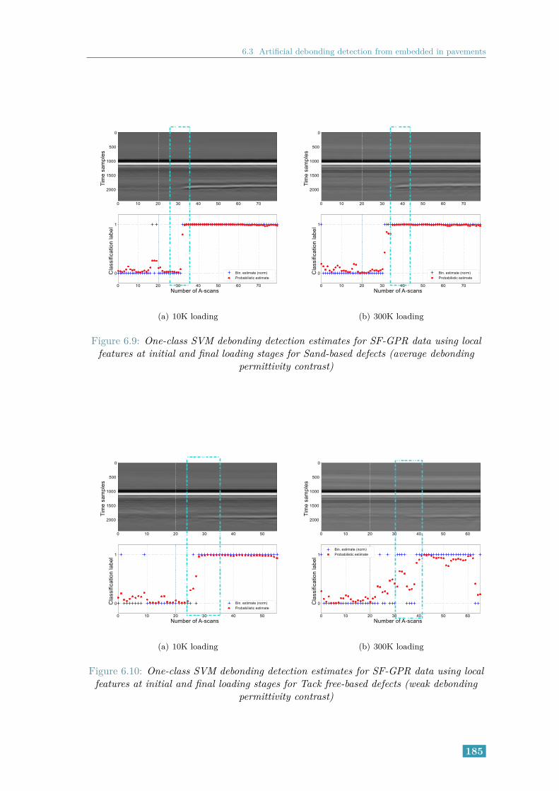
6.3 Artificial debonding detection from embedded in pavements
(a) 10K loading (b) 300K loading
Figure 6.9: One-class SVM debonding detection estimates for SF-GPR data using localfeatures at initial and final loading stages for Sand-based defects (average debonding
permittivity contrast)
(a) 10K loading (b) 300K loading
Figure 6.10: One-class SVM debonding detection estimates for SF-GPR data using localfeatures at initial and final loading stages for Tack free-based defects (weak debonding
permittivity contrast)
185

Chapter 6. Application For Decision Support To Detect Debondings
and final loading stages. Table E.2 in Appendix E presents the same for the intermediateloading stages.
From the tables, it can be seen that, in case of Geotextile and Sand (strong defects),the prediction rates for both debonding and non-debonding (respectively DPR and NPR)are very high. In case of Tack-free defects as well, similar observations are seen.
6.3.3 Random forests
Figure 6.11, Figure 6.12 and Figure 6.13 present the probability estimation of theoccurrence of debondings from local signal features at 10K and 300K loading stages forrespectively Geotextile, Sand and Tack-free based defects using Random forests. Forintermediate loading stages, the figures (Figure E.7, Figure E.8, Figure E.9) are presentedin Appendix E. The methodology is as done previously in Chapter 6.1. The 10K loadingstage data is used as learning data and the remainder of the data are used as test data.
(a) 50K loading (learning data) (b) 300K loading
Figure 6.11: Random forests debonding detection estimates for SF-GPR data using localfeatures at initial and final loading stages for Geotextile-based defects (strong debonding
permittivity contrast)
Table 6.7: DPR and NPR coefficients for probability estimation from local signal featuresat 10K (initial stage) and 300K (final stage) loading for respectively Geotextile, Sand andTack-free based defects using Random forests
Loading stageGeotextile Sand Tack-free
DPR NPR DPR NPR DPR NPR
50K cycles 1.00 0.66 1.00 0.52 0.84 0.91
300K cycles 1.00 0.68 0.98 0.86 0.88 0.68
186

6.3 Artificial debonding detection from embedded in pavements
(a) 10K loading (learning data) (b) 300K loading
Figure 6.12: Random forests debonding detection estimates for SF-GPR data using localfeatures at initial and final loading stages for Sand-based defects (average debonding
permittivity contrast)
(a) 10K loading (learning data) (b) 300K loading
Figure 6.13: Random forests debonding detection estimates for SF-GPR data using localfeatures at initial and final loading stages for Tack free-based defects (weak debonding
permittivity contrast)
187

Chapter 6. Application For Decision Support To Detect Debondings
For qualitative representation of results, Table 6.7 compares the DPR and NPR co-efficients (see Appendix C for details) for the three defects at the initial and final loadingstages. Table E.3 in Appendix E presents the same for the intermediate loading stages.
It can be observed that in case of all the three defects, the debonding detection rateis excellent. However, in case of Tack-free based defects at 200K loading, the DPR ratewas found to be low (DPR ≈ 0.65)
In the following section, we compare the performance of each method against thereference method, namely ART.
6.3.4 Benchmark comparison with reference method
As done previously in Chapter 6.2.4 for GSSI-GPR air-void debondings database, here,we once again compare the performance of SF-GPR data at various loading stages againstthe reference ART method.
Table 6.8, Table 6.9, and Table 6.10 present the DSC and MCC rates for respectivelyTwo-class SVM, One-class SVM and Random forests for various defects at the initial andfinal loading stages. Tables. E.4, Table E.5, and Table E.6 (see Appendix E) provide thesame for intermediate loading levels.
Table 6.8: Comparison of DSC ([..]) and MCC ((..)) coefficients for binary debondingdetection from local signal features at initial and final loading stages for Geotextile baseddefects
Loading stage ART (reference) Two-class SVM One-class SVM Random forests
10K cycles [1.00], (1.00) [1.00], (1.00) [0.88], (0.79) [1.00], (1.00)
300K cycles [0.91], (0.86) [0.99], (0.97) [0.88], (0.74) [1.00], (1.00)
Table 6.9: Comparison of DSC ([..]) and MCC ((..)) coefficients for binary debondingdetection from local signal features at initial and final loading stages for Sand based defects
Loading stage ART (reference) Two-class SVM One-class SVM Random forests
10K cycles [1.00], (1.00) [1.00], (1.00) [0.98], (0.94) [1.00], (1.00)
300K cycles [0.9], (0.86) [1.00], (1.00) [1.00], (1.00) [0.88], (0.78)
Table 6.10: Comparison of DSC ([..]) and MCC ((..)) coefficients for binary debondingdetection from local signal features at initial and final loading stages for Tack-free baseddefects
Loading stage ART (reference) Two-class SVM One-class SVM Random forests
10K cycles [0.98], (0.96) [1.00], (1.00) [0.95], (0.91) [1.00], (1.00)
300K cycles [0.86], (0.8) [0.87], (0.85) [0.85], (0.72) [0.88], (0.85)
188

6.4 Conclusion
It was observed that in case of both Two-class SVMs and Random forests, the perfor-mance rates were very high for all the three types of defects. In case of One-class SVM aswell, similar conclusions were drawn.
6.4 Conclusion
This chapter concentrated on the application of machine learning methods on thedetection of debondings from experimental data. The detection was carried out in twoways: binary detection by representing the results as 0 or 1 and secondly, as a probabilityestimation of the occurrence of debondings.
In the first part, the debonding detection was carried out on the experimental testbench under controlled environment with air-void debondings at Cerema. A widebandcommercial GPR (GSSI SIR-3000) was used here. The debondings were set for thicknesses0.5 cm and 1.0 cm. It was observed that, Two-class SVM and Random forests providedthe best detection rate, both in case of binary as well as probabilistic. One-class SVM onthe other hand performed averagely having the least accuracy among the three.
The second part concentrated on the experimental data collected at the fatigue carouselat IFSTTAR where three defect types were monitored over various loading stages. It wasobserved that, in cases of strong defects (Geotextile and Sand-based), the three methods(Two-class, One-class SVM and Random forests) performed with very high accuracy rate.The estimation of probability of the occurrence of defects was very high as well (DPR ≥0.95) in all cases. In case of Tack-free based defects, apart from 200K and 250K cyclesloading stage, the three methods were once again able to detect debondings with highaccuracy at the same time estimate the occurrence at DPR ≥ 0.8.
The reference method ART, was used as a benchmark for comparison in both experi-mental results and it was observed that ART was able to provide good results for strongdefects; however, its efficiency reduced for weaker defects (such as Tack-free defects). Incase of 100K and 250K loading for Geotextile and Sand defects, DSCART ≈ 0.96; whileTwo-class SVM and Random forests provided near perfect detection with DSC ≈ 1.00
(Table E.4). On the other hand, in case of Tack-free, ART provided very similar results toSVM and Random forests at 50K, 100 and 250K loading i.e, DSC ∈ 0.9− 0.95; however,for 10K and 200K, the DSC for ART was less than that of SVM and Random forests(Table E.6).
In addition, it should be noted that ART relies on the time domain data to obtain itsfeatures (namely MAD or MAAG; refer Chapter 2.6.2). However, the machine learningmethods can process temporal as well as frequential data. The final drawback using ART isthat, unlike the machine learning methods, ART cannot be used for probability estimation.
However, despite its drawbacks, in most cases, ART debonding detection was veryclose to that observed using the machine learning methods. Thus, in perspective, we aimto take advantage of the efficiency of the ART method by including ART as a feature intothe machine learning approach for improved performance.
189


Chapter 7
Conclusions and Perspectives
Contents7.1 Conclusions . . . . . . . . . . . . . . . . . . . . . . . . . . . . . . . 189
7.2 Perspectives . . . . . . . . . . . . . . . . . . . . . . . . . . . . . . . 191
7.1 Conclusions
In this thesis, we primarily focused on the detection of thin interlayer debondings withinpavement structures as described introduction chapter. The first chapter presented an
overview of the thesis by introducing the problem statement and the goals of the thesis.Various research has already been done in the field of debonding and delamination
detection. Most of this research focuses on pavement engineering and monitoring is bymeans of Destructive Testing. Due to the limited capability of destructive testing, we diveinto the field of Non-destructive testing (NDT). In Chapter 2, we discuss the State of theart and the progress in the field of NDT. The focus is on the NDT radar imaging on pave-ment structures. To support the work in this thesis, some available research was found toimplement NDT techniques to detect delaminations within pavement interfaces. The datainterpretation of most of these methods require human skills. In addition, some papersalso presented the detection of interface debondings; however they were limited to thedetection in the order of a few centimeters. The objective in this thesis was the detectionof millimetric interlayer debondings using UWB systems for better time resolution. Toachieve this objective, the 2D GPR imaging technique is carried out to map the pavementsubsurface structure. Besides, we aimed to achieve improved debonding detection withthe help of suitable data processing techniques.
It was also seen that despite their advantages, the implementation of machine learning(ML) methods in the field of interlayer debonding detection has not been explored toits full potential by the NDT community. A comparative study of various ML methods,both unsupervised and supervised methods, was carried out. Finally, the performanceof each method was compared to ART, which is a benchmark technique to assess thepavement subsurface conditions and sealing screeds over bridges in the GPR community.The subsequent chapters discussed in detail the various data processing methods studiedduring the thesis.
191

Chapter 7. Conclusions and Perspectives
In Chapter 3, we introduce the machine learning methods studied during the thesis. Anunsupervised conventional clustering method was modified in order to improve the initialseed-point selection for better performance. A parameterized supervised machine learningmethod, namely SVM was then presented. This method was used to detect debondings intwo ways: as of classification into two classes (Two-class SVM) and as anomaly detection(One-class SVM). Finally a non-parameterized method, Random forests, was introduced.The principle of each method is illustrated through the straightforward processing of timedata in its raw form. The four methods were applied to process noisy analytic data, whichwere presented in the appendices. The methods demonstrated good qualitative results asthey were able to detect debondings with various interlayer permittivities in noisy data.
However, the processing of raw data is not always acceptable since the raw GPRdata may contain redundant information that could reduce the debonding detection rate.Additionally, as stated in the literature, the machine learning methods could be limitedin their processing of raw data signals. The processing of a large databases affect thecomputational time and complexity of a supervised machine learning method. To overcomethis issue, feature engineering techniques were proposed.
Chapter 4 began by presenting one of the important preprocessing step in debondingdetection i.e, signal feature selection. The feature selection was categorized into timedomain local and global signal features. The local features were focused at the pavementinterface where the debonding is expected to occur. These features were expected topresent higher efficiency due to their time localization. Global features on the other handused the complete GPR signal with the top two pavement interfaces. Feature sets wereselected by the ‘goodness of separation’ of their associated PDF distributions for debondingand non-debonding cases. In order to further reduce the data complexity, PCA was alsoused.
As a part of initial tests, the performance of the supervised machine learning methodswere tested using various input feature sets. These results were compared with the per-formance observed in Chapter 3 on temporal raw GPR data as a benchmark. Althoughthe raw GPR data presented very high detection, this approach was seen to be quite cum-bersome and not efficient in terms of computational time and complexity. As expected,in case of SVM for simulated data, it was observed that the local feature set presentedbetter detection results than global features. The PCA reduced global and local featuresets provided little-to-none difference in performance of the unreduced data.
However, the study of robustness of supervised machine learning methods is not justlimited by the input data but several other parameters such as the learning data size,method hyper-parameters, method kernels, cross validation techniques etc. This makes itnecessary to identify the ‘best’ parameters that could be used to achieve high detectionrate in the context of detection of interface debondings.
Therefore, in Chapter 5, we presented the optimization of ML methods by these ap-proaches. Following the conclusions of the previous chapter, the local signal features wereused in Chapter 5 for optimization. The first approach to optimize the methods includedthe model-fitting approach using CV techniques and kernel functions. Optimization ofthe methods was also conducted on the basis of the pavement medium. The parameters
192

7.2 Perspectives
such as debonding thickness, relative permittivity of the debonding layer were used andthe methods were adapted to match various configurations of the pavement medium.
Chapter 6 concentrated on the application of optimized machine learning methods onthe detection of debondings from experimental data. This chapter presented the debondingdetection for experimental data collected at two independent sites located respectively atNantes (IFSTTAR) and Angers (Cerema). The site at Cerema was set up using pavementtest benches and was focused on the detection of artificially induced air-void debondingof thickness 0.5 cm and 1.0 cm using a commercial ground-coupled GPR. The test site atIFSTTAR focused on the detection of artificially induced defects of three types (Geotextile,Sand and Tack-free) using a commercial GPR and an experimental ultra-wide-band air-coupled SF-GPR. The results were presented using the optimized parameters for eachmachine learning method determined in the Chapters 4 and 5. Chapter 6 also presenteda final decision making step wherein the results were presented as an estimate determinedas the probability of occurrence of a defect.
In case of ground-coupled GPR (Cerema test bench), it was observed that, Two-classSVM and Random forests provided the best detection rate, both in case of binary as wellas probabilistic. One-class SVM on the other hand performed averagely having the leastaccuracy among the three.
On the other hand, for the air-coupled radar data from IFSTTAR’s fatigue carousel,it was observed that, in cases of strong defects (Geotextile and Sand-based), the threemethods (Two-class, One-class SVMs and Random forests) performed with very highaccuracy rate. The extimation of probability of the occurrence of defects was very high aswell (DPR ≥ 0.95) in all cases. In case of Tack-free based defects, apart from 200K and250K cycles loading stage, the three methods were once again able to detect debondingswith high accuracy at the same time estimate the occurrence excellently (DPR ≥ 0.8).
Finally, the performance of the machine learning methods was compared to the ARTmethod, which was used as a benchmark in both experimental results. It was observedthat ART, although relying on two signal features, was able to provide equivalent resultsfor strong defects. However, its efficiency was reduced for weaker defects (such as Tack-freedefects).
In conclusion, it was seen that the three machine learning methods, despite certaindrawbacks, presented the ability to detect debondings and also estimate their occurrencewith very high efficiency by means of probability estimates. The use of local signal featuresand optimized hyper-parameter computation proved to improve the performance of themethods.
7.2 Perspectives
The objective of this thesis was to to detect the presence of thin interlayer debondingswithin pavement structures. Although we were able to achieve the goals foreseen as ob-jectives for this thesis, some improvements are open to discussions that we can attempt toanswer by further research in the fields of NDT, GPR and machine learning. Following aresome of the future works from the point of preprocessing for machine learning methods:
193

Chapter 7. Conclusions and Perspectives
Multi-class classification: The study for the detection of thin interface debondings inthis thesis was performed as a binary classification (Two-class SVM, Random forests, k-means clustering) or as an outlier anomaly detection (One-class SVM). The presence ofvarious other types of defects (based on material composing the debonding layer, debond-ing layer thickness etc.) can be explored to perform multi-class classification.
Spectral signal features: As mentioned in Chapter 4, the detection of debondings wascarried out by using various time domain signal features (global and local) extracted fromthe GPR A-scan time signatures. It is proposed to explore in the future the performance offrequency domain signal features, and eventually to mix both domain features for improvedperformance in classification.
In addition, we aim to take advantage of the efficiency of the ART method by includingART as a feature into the machine learning approach for improved performance.
Feature selection: PDF-based feature selection method was implemented in the thesisalong with a feature reduction technique (PCA). However, as presented in the literature,various automatic feature selection methods can be used. Among others, it is proposed tosubstitute the qualitative “goodness of separation” in Chapter 4 by a quantitative index.
Estimation of debonding layer characteristics: This thesis focused mainly on detectingthe presence/absence of debondings in pavements. This however leaves the determinationof other debonding characteristics such as debonding layer thickness, length, permittivityetc.
Exploring Deep learning methods: The use of deep learning methods such as NeuralNetworks has not yet been conducted in the field of NDT for the detection of interlayerdebondings. We aim to explore the possibility to implement deep learning methods inNDT for both classification and regression related problems.
Future work: One of the final goals would be to implement and continue the researchfrom this thesis useful in WP3 of ACIMP project.
194

Appendices
195


Appendix A
Simulated Databases
ContentsA.1 Radar pulse . . . . . . . . . . . . . . . . . . . . . . . . . . . . . . . 196
A.1.1 Analytic GPR pulse . . . . . . . . . . . . . . . . . . . . . . . . . 196
A.1.2 Experimental GPR pulse . . . . . . . . . . . . . . . . . . . . . . 197
A.2 Analytic GPR modeling . . . . . . . . . . . . . . . . . . . . . . . 198
A.2.1 Basics and hypothesis . . . . . . . . . . . . . . . . . . . . . . . . 198
A.2.2 Non-debonding case . . . . . . . . . . . . . . . . . . . . . . . . . 200
A.2.3 Debonding case . . . . . . . . . . . . . . . . . . . . . . . . . . . . 201
A.3 Numeric database: Pavement modeling using MoM . . . . . . 204
A.4 Numeric database: Pavement modeling using FDTD . . . . . . 206
A.4.1 Creating a 2D gprMax model of a pavement structure . . . . . . 207
A.5 Noisy data . . . . . . . . . . . . . . . . . . . . . . . . . . . . . . . . 209
A.5.1 SNR definition . . . . . . . . . . . . . . . . . . . . . . . . . . . . 209
A.5.2 Illustrative results . . . . . . . . . . . . . . . . . . . . . . . . . . 210
The detection methods studied during the thesis were initially validated using the simu-lated data models which are presented in this appendix. Each data model simulates
the noiseless backscattered radar signal from the layered pavement structure assuming(quasi-)vertical incidence. It provides B-scan air-coupled radar data over a simplified syn-thetic layered pavement structure with either k = 2 or k = 3 layers, corresponding tohealthy and debonded areas respectively.
Three techniques were used to create the simulated databases, namely, Analytic Fresneldata model, Numeric 2D FDTD model and Numeric MoM data model. In brief, theanalytic and the numeric MoM data models rely on simplified 1D wave propagation. Bycontrast, the numeric FDTD model accounts for the wave propagation in 2D, e.g., adiffraction hyperbola is visible on simulated data at the frontier between healthy anddebonded areas. Besides, the antenna effect are approximately accounted for in thesethree models. For the FDTD model, antennas are supposed to be dipole antennas. Foranalytic model, the frequency antenna response is accounted for through the radar pulseto be introduced hereafter.
197

Appendix A. Simulated Databases
A.1 Radar pulse
In this section, we present, in brief, the 1D radar pulse used in data modeling to providemore realistic radar vertical profiles using simulations. For the sake of comparison, we alsopresent the experimental radar pulse and the procedure to extract the emitted pulse fromthe GPR data.
A.1.1 Analytic GPR pulse
The radar pulse used for the analytical data models in the ricker (or commonly knownas the Mexican hat) pulse as it is often used in seismic analysis of thin beds [310]. It can bedefined as the negative normalized second derivative of the Gaussian waveform obtainedby solving the Stokes’ differential equation [311, 310].
The ricker wavelet (w(t)) in time domain is defined as [310]:
w(t) =
(1− 1
2ω2c t
2
)exp
− 1
4ω2c t
2
(A.1)
where,
- ωc = 2πfc with fc being the dominant frequency- t is the time (in seconds)
The pulse is symmetric in time domain and has zero mean i.e,∫∞−∞W (t)dt = 0 [310]. In
frequency domain, it is expressed as [310]:
W (ω) =2ω2
√πω3
c
exp
− ω2
ω2c
(A.2)
where ω is the angular frequency at a given frequency f .
Figure. A.1 presents the ricker pulse used to generate the simulated model in timedomain and its respective frequency spectrum.
198

A.1 Radar pulse
0 0.5 1 1.5Time (s) ×10-9
-0.5
0
0.5
1
Am
plitu
de
0 0.5 1 1.5 2 2.5Frequency (Hz) ×1010
0
0.005
0.01
0.015
0.02
Mag
nitu
de
X: 4.199e+09Y: 0.01976
fc
Figure A.1: Illustration of the Ricker pulse in time and frequency domain used togenerate the simulated models with fc = 4.2GHz
This radar pulse will be used subsequently in Appendix. A.2 in the generation ofsimulated databases.
A.1.2 Experimental GPR pulse
In order to extract the GPR pulse from the radar data, the following process is used.The emitted GPR pulse can be recovered by placing the metallic plate (sufficiently large sothat the edge and scattering effects are avoided) underneath the antenna. As mentionedin [312], this plate could be made of copper. The antennas are initially arranged inthe designated form (see Appendix. B.2.3.1 for details) and the metallic plate is placedunderneath as shown in Figure. A.2.
Figure A.2: Illustration of the setup used to experimentally extract GPR pulse
The reflected signal from the plate is an inverted signal (since the reflection coeffi-
199

Appendix A. Simulated Databases
cient of copper is -1). The signal is thus multiplied by -1 and after removing the directcoupling between the transmitter and receiver, the emitted GPR pulse is obtained. Fig-ure. A.3 presents the extracted ricker pulse from experimental data in time domain andits respective frequency spectrum.
0 0.5 1 1.5 2 2.5 3Time (s) ×10-10
-0.02
-0.01
0
0.01
0.02
Am
plitu
de
0 0.5 1 1.5 2 2.5Frequency (Hz) ×1010
0
0.5
1
1.5
2
Mag
nitu
de
X: 4.412e+09Y: 1.713
fc
Figure A.3: Illustration of the Ricker pulse in time and frequency domain used inexperiments
This pulse is used to collect the pavement data using the SF-GPR as detailed inAppendix. B.2.
A.2 Analytic GPR modeling
A.2.1 Basics and hypothesis
The analytic GPR data model has been widely used for processing purpose. It relieson the following conventional assumptions:
1. Wave propagation : Plane waves impinging on the pavement surface (far field as-sumption);
2. Wave interaction vs. medium : single scattering within (thick enough) layers, i.e.,each interface provides a single echo in the data model.
3. Medium: Lateral and vertical homogeneity; roughless layers interfaces; dispersion-free medium, i.e., constant material permittivity w.r.t. frequency; lossless medium.
4. Antenna effects are ignored
Within this scope, the received time signal r(t) which is backscattered by the k layeredpavement structure is the sum of attenuated and shifted copies of the radar pulse, s(t), as
200

A.2 Analytic GPR modeling
follows:
r(t) =
k′∑i=1
Ais(t− Ti) + n(t) (A.3)
where,
• Ai is the amplitude of the received echo from the ith interface,
• Ti is the time delay attached to the ith echo; it is the sum of the propagation timeshift through each layer; it is given by Ti =
∑in=1
2dnνn
where dn is the thickness andνn the wave speed within the nth layer.
• k is the amount of layers; within the scope of the thesis, k = 2 for healthy pavementstructure and k = 3 for disbonded structure.
• k′ is the total amount of echoes accounted for in the data model; it is equal to theamount of layers providing single scattering assumption (see Appendix. A.2.3.1), andlarger in case of multiple scattering (see Appendix. A.2.3.2).
• n(t) is the additive noise, which SNR is discussed in Appendix. A.5.
The amplitude of echoes relies on the well-known Fresnel reflection and transmissioncoefficients. At vertical incidence, the Fresnel coefficients for reflection and transmissionat the interface ij can be expressed in terms of the permittivity of the two materials as:
Rij =
√εr,i −
√εr,j
√εr,i +
√εr,j
(A.4)
Tij =2√εr,j
√εr,i +
√εr,j
(A.5)
where, εr,i is the relative permittivity of the material layer i. Since the materials of eachlayer are considered to be lossless, the transmission and reflection coefficients are relatedas Rij + Tij = 1.
For later use in this Appendix, we also introduce the received signal in the frequencydomain, as follows:
r(f) =
k′∑i=1
Aiz(Ti)
s(f) + n(f) (A.6)
where z(T ) = exp(−2iπfT ) represent the complex phasor associated to the time delayT ; s(f) and n(f) are the Fourier transform of the radar pulse s(t) and the noise n(t),respectively.
Within the scope of the thesis, a two-layered structure is created with each layergoverned by physical parameters such as thickness, material permittivity, antenna heightaccording to the parameters in Table. A.1. To create a defective pavement section, adebonding layer is introduced between the two pavement layers. The debonding layer is
201

Appendix A. Simulated Databases
assumed to be a thin-bed structure satisfying the following condition [313, 314, 315]:
λdeb
4> d (A.7)
where λdeb is the dominant wavelength within the debonding layer of thickness d givenby λdeb = c/fc
√εr,deb. The latter condition limits to π/2 the phase shift between the two
successive echoes, namely, the condition for in-phase summation.
Figure. A.4 presents the simplified pavement model with the defect-free and defectivezones. To create the analytic GPR data model, MATLAB was used.
Figure A.4: Simplified pavement structure to create the Analytic data model
A.2.2 Non-debonding case
For a two-layered structure (k = 2) as shown in Figure. A.5, the received signal ineq. A.3 can be expressed as:
r(t) = A0s(t− T0) +A1s(t− T1) + n(t) (A.8)
where, - A0 is the amplitude of the surface echo defined as A0 ∝ R01 with the timedelay T0 =
2hc as a function of the antenna height (h) in air.
- A1 is the amplitude of the second echo, i.e., the interface to be surveyed; in case ofnon-debonding, A1 ∝ T01 × R12 × T10 with the time delay T1 = T0 +
2d1ν1
as a function ofthe thickness of top layer d1 (where the wave speed is ν1 = c/
√εr1).
202

A.2 Analytic GPR modeling
Figure A.5: Fresnel coefficients for a two-layered structure
Table A.1: Parameters used to create a GPR B-scan using the analytic data model
Layer Label Value
Top layer
εr1 5
t1 5 cm
ρ1 0 Sm−1
Base layer
εr2 7
t2 40 cm
ρ2 0 Sm−1
Debonding layerεr,deb 2 (air-void), 6 (weak contrast), 10 (strong contrast)
tdeb 0.3 cm
ρd 0 Sm−1
Center frequency fc 2GHz
Antenna height hant 46 cm
Observation time Tobs 10 ns
Time resolution ∆t 2.44 ps
Sampling frequency fs 409.6GHz
A.2.3 Debonding case
As indicated in Figure. A.4, in case of a disbonded zone, a thin layer is sandwichedbetween the two pavement layers, namely, a thin-bed structure which thickness d satisfyingthe condition in Eq. A.7.
Two data models have been used in the literature to interpret the backscattering datafrom a thin bed structure. They rely on two opposite assumptions regarding the wave
203

Appendix A. Simulated Databases
interaction within the thin-bed structure, namely, single scattering vs. multiple scattering.
A.2.3.1 Single scattering model
The conventional data model assumes single scattering within the thin-bed structure,e.g., see Chung and Lawton [316]. Then, the signal backscattered from the three-layeredstructure shown in Figure. A.6 can be rewritten following Eq. A.3 as the sum of threeprimary echoes:
r(t) = A0s(t− T0) + A1s(t− T1) +A3s(t− T3)+ n(t) (A.9)
where T3 = T1 + 2d3ν3
is the time delay from the debonding layer as a function ofdebonding layer thickness d3 and the wave speed ν3.
Figure A.6: Fresnel coefficients for a three-layered structure (two layers with asandwiched debonding layer as a thin bed structure)
Using Fresnel coefficients, the respective amplitudes A1 and A3 can be expressed as:
A1 ∝ T01 ×R13 × T10 (A.10)
A3 ∝ T01 × T13 ×R32 × T31 × T10 (A.11)
In the frequency domain, introducing Aeq,s1 for the backscattered signal amplitude by
the interlayer interface to be surveyed, the signal can be written as:
r(f) = s(f)
A0z(T0) +Aeq,s
1 T01T10z(T1)
+ n(f) (A.12)
where: Aeq,s1 = R13 + T13R32T31z(2d3/ν3) (A.13)
and: z(T ) = exp(−2iπfT ) (A.14)
The second and third echoes, i.e., s(t−T1) and s(t−T3) in Equation. A.9, represent thereflected signal from the top and bottom interfaces of the debonding layer, respectively.
204

A.2 Analytic GPR modeling
Providing the thickness condition in Equation. A.7, the two latter echoes overlap to eachother in time and shape as a single composite echo.
A.2.3.2 Multiple scattering model
Figure A.7: Fresnel coefficients for a three-layered structure (two layers with asandwiched debonding layer as a thin bed structure) with multiple internal reflections
within the debonding layer
Multiple scattering is assumed to be limited to the thin-bed structure only. Equa-tion. A.9 then becomes:
r(t) = A0s(t− T0) +
A1s(t− T1) +
∑m
A′3,ms(t− T3 − 2(m− 1)
d3ν3
)
+ n(t) (A.15)
where∑
i operator indicates the sum of all the multiple scattering echoes occurring withinthe thin debonding layer with the following diminishing amplitude A′
3,i:
A′3,m ∝ T01 × T13 ×Rm
32 ×Rm−131 × T31 × T10 (A.16)
In practice, the contribution of multiple scattering to the data model is usually formu-lated in the frequency domain, in order to achieve the analytic solution to the sum inEquation. A.15. The data model in the frequency domain is expressed as:
r(f) = s(f)A0z(T0) + s(f)
A1z(T1) + z(T1)
∑m
A′3,mz(2m
d3ν3
)
+ n(f) (A.17)
with: z(Tm) = exp(−2iπfTm) (A.18)
The backscattered signal from the thin-bed structure with multiple scattering ac-counted for, has been formulated by Rayleigh [317, 318] for seismic waves, and by Annan[72] for GPR waves, providing that layers surrounding the thin-debonding possess thesame material characteristics (i.e. εr1 = εr2). More recent formulation is given by Arosio
205

Appendix A. Simulated Databases
[319] and Shakas [320, 321].Within the scope of the thesis, [322] provides the general solution for the thin-bed
structure with different surrounding permittivity values (i.e. εr1 = εr2 = εr3), as follows:
Aeq,m1 =
A1z(T1) + z(T1)
∑m
A′3,mz(2m
d3ν3
)
=
R13(1−Gz)
1−GR213z
(A.19)
where,
z = z(2d3/ν3) = exp(−4iπfd3/ν3) (A.20)
G =
√εr1 +
√εr3√
εr2 +√εr3
1− R12
R13
√εr1 +
√εr2√
εr1 +√εr3
(A.21)
For a conventional thin-bed structure, for which εr1 = εr2, the parameter G = 1, andEquation. A.19 simplifies to the existing reflection coefficient shown in [319].
Finally, the data model in the frequency domain can be expressed as:
r(f) = s(f)
A0z(T0) +Aeq,m
1 T01T10z(T1)
+ n(f) (A.22)
The data were generated in the frequency domain, and a inverse Fast Fourier Transformallowed to compute the final B-scan data in the time domain. For illustration, Figure. A.8shows the simulated B-scan using the parameters from Table A.1.
20 40 60 80 100 120 140Number of A-scans
0
0.1
0.2
0.3
0.4
0.5
0.6
0.7
0.8
0.9
1
Tim
e (s
)
×10-8
0 0.5 1Amplitude
0
0.1
0.2
0.3
0.4
0.5
0.6
0.7
0.8
0.9
1
Tim
e (s
)
×10-8
Non-debonding zoneDebonding zone
Figure A.8: Example of a noiseless B-scan generated with multiple scattering accountedfor and the following parameters : εr1 = 5, εr2 = 7, εr,deb = 2 and tdeb = 0.3 cm. On the
right, the two A-scans represent respectively non-debonding and debonding cases
A.3 Numeric database: Pavement modeling using MoM
One major drawback of the Fresnel data model is that it assumes a smooth surfaceand smooth interface across the model. To obtain a more realistic model, the numericGPILE was used.
Propagation-Inside-Layer Expansion (PILE) is a 1D numerical approach based on the
206

A.3 Numeric database: Pavement modeling using MoM
Method of Moment (MoM) proposed in [323]. PILE is an efficient numerical model thatcan be used to compute the scattering fields by the rough pavement interfaces for bothreflection and transmission. By introducing the roughness at each interface, the complexityof the model is increased due to the increased number of unknowns.
The major advantage of the PILE method relies on its ability to calculate the echoesscattered by each interface with both the multiple scattering and the accounted inter-layersurface roughness. PILE is also capable of performing faster and efficient computations.Additionally, PILE focuses on rigorous but simple formulation and straightforward phys-ical interpretation of the pavement model.
GPILE or Generalized PILE is the extension of PILE for three or more pavementlayers. The method has been extensively discussed in [12]. Since GPILE can be used tosimulate more than two layers, a three-layered GPILE model can be used to simulate adefective pavement structure as shown in Figure. A.9.
Figure A.9: EM scattering from a 1-D random rough layer with two rough surfaces i.e.Non-debonding case (top) and scattering from 1-D three rough interfaces i.e. debonding
case (bottom) [12]
The 2D GPILE B-scan is generated by repeating the the 1D propagation for Nndeb
times for non-debonding case and Ndeb times for debonding case. This is a 2D imageobtained in frequency domain. Using Inverse Fourier transforms, the B-scan image intime domain is obtained. In addition to the parameters presented in Table. A.1, theadditional parameters used to generate the numerical model are given in Table. A.2.
207

Appendix A. Simulated Databases
Table A.2: Parameters used to create a GPR B-scan using the numerical GPILE model
Layer Label Value
Center frequency fc 2GHz
Bandwidth BW 0.1GHz to 5.1GHz
Antenna height hant 46 cm
Conductivity
Layer − 1 1× 10⁻³ Sm−1
Layer − 2 1× 10⁻³ Sm−1
Debonding 1× 10⁻³ Sm−1
Roughness
topsurface 0× 10−3m
interlayerinterface 0× 10−3m
Figure. A.9 shows the 2D image generated using the parameters from Table. A.1 andTable. A.2.
-1 -0.5 0 0.5 1Amplitude
0
1
2
3
4
5
6
7
8
Tim
e (s
)
×10-9
DebondingNon-debonding
20 40 60 80 100 120 140Number of A-scans
0
1
2
3
4
5
6
7
8
Tim
e (s
)
×10-9
Non-debonding zoneDebonding zone
Figure A.10: Example of GPILE B-scan generated with εr1 = 5, εr2 = 7, εr,deb = 2 andtdeb = 0.3 cm (left). A-scans representing respectively non-debonding and debonding cases
(right)
A.4 Numeric database: Pavement modeling using FDTD
gprMax is an open source tool used to simulate the electromagnetic wave propagationwithin a material (and multiple materials as well). With the help of Maxwell’s equationsprojected in 3D using the Finite-Difference Time-Domain (FDTD) method [324, 325],gprMax is capable of creating various pavement models for different radar configurationsoperating at ultra-wideband frequency.
Developed in 1995 [326, 327], gprMax was first openly distributed by Giannopoulos andGiannakis [328] in 2015. It uses both Python and Cython for background programmingwhereas the user interface is a high-level programming unique to gprMax. Extensive usermanuals on gprMax are available in [329, 328, 330, 331].
208

A.4 Numeric database: Pavement modeling using FDTD
A.4.1 Creating a 2D gprMax model of a pavement structure
A right-handed Cartesian coordinate system is used with the origin of space coordinatesin the lower left corner at (0,0,0). The FDTD approach to the numerical solution ofMaxwells equations is to discretize both the space and time domains. Thus, the spatialdiscretization plays a very important role in the performance of the modeling method.
The 3D gprMax model is discretized in the three axes as ∆x (spatial discretization),∆y (temporal discretization) and ∆z (lateral discretization). In order to observe a goodresolution of the time domain GPR signal, the discretization size (mesh size) in the timeaxis can be defined as:
∆y =λ
10(A.23)
The pavement model created using gprMax consists of: two layers for the healthy zoneand, three layers for the defective zone as depicted in Figure. A.11.
Figure A.11: Two-layered pavement model created using gprMax. Rx, Tx and representthe antenna positioning
Let λ1, λ2 and λdeb be respectively the wavelength of the impulse within the top layer,base layer and debonding layer of permittivities respectively εr1, εr2 and εrdeb. Then, fromEq. A.23, the optimal temporal discretization can be obtained from:
∆y = minλ1
10,λ2
10,λdeb
10
(A.24)
In order to maintain regularity, we use ∆x = ∆y = ∆z.Using the pavement layer parameters presented in Table. A.1, B-scan images were
generated in gprMax. A dipole as a hard-source is used as the signal source.Firstly, the GPR domain is defined along with the total acquisition time and the
domain discretization defined previously (Listing. A.1).
209

Appendix A. Simulated Databases
#domain : 3 . 0 0 .98 0 .002#dx_dy_dz : 0 .001 0 .001 0 .002#time_window : 10e−9
Listing A.1: gprMax modeling: Specifying the domain parameters
The material characteristics of each pavement layer such as permittivity, conductivity andpermeability are defined (Listing. A.2).
#mate r i a l : 5 0 .001 1 0 asphalt_layer_1#mate r i a l : 7 0 .001 1 0 asphalt_layer_2#mate r i a l : 2 0 .001 1 0 debonding_layer
Listing A.2: gprMax modeling: Initializing material characteristics
Each material is assigned a unique identifier that can be used to associate a layer withthe material characteristic. Listing. A.3 presents the code to generate the three pavementlayers with specified thicknesses and are associated to the material defined previously usingthe identifier.
#box : 0 . 0 0 . 4 0 . 0 2 . 0 0 .45 0 .002 asphalt_layer_1#box : 0 .0 0 . 0 0 . 0 2 . 0 0 .4 0 .002 asphalt_layer_2#box : 0 .0 0 .39 0 .0 2 .0 0 .4 0 .002 debonding_layer
Listing A.3: gprMax modeling: Modeling pavement layers
Once the design is complete, the source of the signals is defined. Characterized by thefrequency of operation and the type of waveform used. A voltage source is used as thesignal source that emits the impulse (Listing. A.4). The source is specified to be a ‘hardsource’ (i.e., source internal resistance R = 0Ω). This is done in order to make the sourcecompletely reflecting and prescribe the value of the electric field component.
#waveform : gaussiandotnorm 1 2e9 my_pulse_1#her tz i an_d ipo l e : z 0 .97 0 .92 0 my_pulse_1#rx : 1 .02 0 .92 0
Listing A.4: gprMax modeling: Creating waveform source
In order to acquire data over a zone (in 2D) to create a B-scan image, the antennae aredisplaced spatially step-by-step. Listing. A.5 presents the antenna displacement.
#src_steps : 0 .01 0 0#rx_steps : 0 .01 0 0
Listing A.5: gprMax modeling: Displacing the source and receiver spatially
Using the code presented above, various gprMax data models were created to generate the2D B-scan images. Figure. A.12 presents one such B-scan.
210

A.5 Noisy data
20 40 60 80 100 120 140Number of A-scans
0
0.1
0.2
0.3
0.4
0.5
0.6
0.7
0.8
0.9
1
Tim
e (s
)
×10-8
-200 -100 0 100Amplitude
0
0.1
0.2
0.3
0.4
0.5
0.6
0.7
0.8
0.9
1
Tim
e (s
)
×10-8
Non-debondingDebonding
Debonding zoneNon-debonding zone
Figure A.12: gprMax B-scan generated using Figure. A.11
A.5 Noisy data
In order to test the performance sensitivity of the detection methods against noise, weassociate to each simulated noiseless database noisy datasets at different selected signal-to-noise ratio (SNR) values.
A.5.1 SNR definition
In this section, the conventional additive noise model is assumed, as formulated byEquation. A.25 on each radar profile. The noise is usually a White Gaussian Noise (WGN)with zero mean µ = 0 and standard deviation σ = σn. It is assumed to be decorrelated tothe useful signal, and decorrelated between successive A-scan radar profiles.
The SNR is defined in the time domain with respect to the signal to detect, i.e., thesecond echo from the healthy interlayer interface, according to :
SNRdB = 20log10M
σN(A.25)
where,
- M is the maximum magnitude of the second echo of the non-debonding A-scan,
- σN is the standard deviation of the noise added.
Owing to this definition, a stronger SNR is likely observed over the debonding areas.Inversely, for a selected SNR, the standard deviation of the noise to add to the noiselesssimulated data is given b:
σN = M × 10−SNR20 (A.26)
211

Appendix A. Simulated Databases
A.5.2 Illustrative results
The noise matrix is then added to each simulated B-scan images to obtain the respectivenoisy data. The result is illustrated in this section for the same SNR and the samesubsurface parameters as input for each data model.
Figure. A.13 to A.13 present the noisy B-scans with SNR = 20dB associated to thenoiseless B-scans images from Figure. A.8 to Figure. A.8.
20 40 60 80 100 120 140Number of A-scans
0
0.1
0.2
0.3
0.4
0.5
0.6
0.7
0.8
0.9
1
Tim
e (s
)
×10-8
0 0.5 1Amplitude
0
0.1
0.2
0.3
0.4
0.5
0.6
0.7
0.8
0.9
1
Tim
e (s
)
×10-8
Non-debondingDebonding
Non-debonding zoneDebonding zone
Figure A.13: Example of a noisy analytic B-scan for Figure. A.8 generated withSNR = 20dB (left). A-scans represent respectively non-debonding and debonding cases
(right)
-1 -0.5 0 0.5 1Amplitude
0
0.1
0.2
0.3
0.4
0.5
0.6
0.7
0.8
0.9
1
Tim
e (s
)
×10-8
DebondingNon-debonding
20 40 60 80 100 120 140Number of A-scans
0
0.1
0.2
0.3
0.4
0.5
0.6
0.7
0.8
0.9
1
Tim
e (s
)
×10-8
Debonding zoneNon-debonding zone
Figure A.14: Example of a noisy GPILE B-scan for Figure. A.9 generated withSNR = 20dB (left). A-scans represent respectively non-debonding and debonding cases
(right)
212

A.5 Noisy data
20 40 60 80 100 120 140Number of A-scans
0
0.1
0.2
0.3
0.4
0.5
0.6
0.7
0.8
0.9
1
Tim
e (s
)
×10-8
-200 -100 0 100Amplitude
0
0.1
0.2
0.3
0.4
0.5
0.6
0.7
0.8
0.9
1
Tim
e (s
)
×10-8
Non-debondingDebonding
Debonding zoneNon-debonding zone
Figure A.15: Example of a noisy gprMax B-scan for Figure. A.12 generated withSNR = 20dB (left). A-scans represent respectively non-debonding and debonding cases
(right)
213


Appendix B
Experimental Databases
ContentsB.1 Test slabs database with controlled air-void debondings at
Cerema . . . . . . . . . . . . . . . . . . . . . . . . . . . . . . . . . 213
B.1.1 Experimental setup . . . . . . . . . . . . . . . . . . . . . . . . . . 213
B.1.2 Ground-coupled WB GPR: GSSI SIR-3000 . . . . . . . . . . . . 215
B.1.3 Data Acquisition . . . . . . . . . . . . . . . . . . . . . . . . . . . 216
B.2 Fatigue Carousel database over embedded artificial debond-ings at IFSTTAR . . . . . . . . . . . . . . . . . . . . . . . . . . . 218
B.2.1 Experimental setup . . . . . . . . . . . . . . . . . . . . . . . . . . 219
B.2.2 GPR used . . . . . . . . . . . . . . . . . . . . . . . . . . . . . . . 220
B.2.3 Data acquisition . . . . . . . . . . . . . . . . . . . . . . . . . . . 220
The experimental databases used during the thesis were obtained from the test sites atboth Cerema and IFSTTAR. At Cerema, an artificial test bench was created under
controlled environment to simulate the effect of debondings between the top and the baselayers. At IFSTTAR, on the other hand, a fatigue carousel test track was used to performthe experiments.
B.1 Test slabs database with controlled air-void debondingsat Cerema
The test setup at Cerema uses a commercial ground-coupled GPR, namely, GSSI SIR-3000. This GPR is a hand-held portable radar used extensively in GPR imagery for civilengineering applications.
B.1.1 Experimental setup
The setup was composed of four layers as shown in Figure B.1. The top layer is anultra-thin bituminous layer followed by the debonding layer. The two base layers are madeof either semi-coarse HMA or bituminous gravel.
215

Appendix B. Experimental Databases
Figure B.1: Depiction of the test bench setup [13]
The layer nomenclature is as follows:
• BBTM (Béton Bitumineux Très Mince in French): This is an Ultra-thin AsphaltSurface (UTAS), a very thin Bituminous concrete layer with an average thickness of2.0 cm to 2.5 cm. BBTM is the top layer and is also used to calibrate the GPR.
• Air-void: The second layer is a thickness-controlled air void that acts as a debondinglayer between the top and the subsequent layers. The thickness of this air gap isbetween 0.5 cm to 1.0 cm.
• BBSG (Béton Bitumineux Semi-Grossier in French): The third layer is a semi-coarsehot-mix asphalt (HMA) used for surface layers in roadways with medium to hightraffic. This layer is between 5.5 cm to 6.0 cm thick.
• GB (Gravier Bitumineux in French): The final base layer is the coarse bituminousgravel with average thickness ranging from 10.5 cm to 11.5 cm.
During the experiments, 32 pavement configurations were used. Bituminous concretetest slabs were manufactured under controlled environment for each configuration withvariations in the degrees of freedom (i.e. thickness, aggregate size, compaction levelsetc.) were used. Table. B.1 presents the degrees of freedom and their individual thresholdvalues.
Table B.1: Degrees of freedom for each pavement layer
Degrees of freedom BBTM BBSG GB
Thickness 2.5 cm to 3 cm 5.5 cm to 6 cm 10.5 cm to 11.5 cm
Binder content 5.5% 5.2% 4.0%
Aggregate size fraction 0/10 mm 0/10 mm 0/14 mm
Compaction level 75% - 96%
Emulsion quality 0 gm−2, 200 gm−2, 400 gm−2 and 600 gm−2
One such configuration of the test slab is shown in Figure. B.2 (Config. 28 ). Thetop layer made of BBTM and the bottom layer made of BBSG each having an emulsionquantity of 400 gm−2.
216

B.1 Test slabs database with controlled air-void debondings at Cerema
Figure B.2: A bituminous concrete test slab used during the experiments [13]
B.1.2 Ground-coupled WB GPR: GSSI SIR-3000
The GSSI SIR-3000 is a GPR of the SIR family of antennae that operate at a widerange of frequencies varying between 0.016GHz to 2.6GHz. During the controlled tests, awideband ground-coupled radar, namely, the GSSI SIR-3000 was used, which operates at2.6GHz (bandwidth 0.4GHz to 5.0GHz). The SIR-3000 implements smart antennae witha high-frequency ground-coupled quasi mono-static configuration. The GPR has a maxi-mum time range of 8 ns. Figure. B.3 presents the SIR-3000 transmitter-receiver system.
Figure B.3: GSSI SIR-3000 trans-receiver system [14]
Table. B.2 lists the system settings of the GPR for data acquisition.
217

Appendix B. Experimental Databases
Table B.2: System settings used for data acquisition during the controlled tests
Parameter Value
Samples per scan 512
Time range 8 ns
A-scans per meter 150
Transmission rate 200 kHz
B.1.3 Data Acquisition
The GSSI GPR is coupled to the test slab and the measurements are made longitudi-nally (longer end of the test slab). Six B-scans were collected for each configuration witheach B-scan equidistantly placed (5 cm apart) at the central section of the slabs. EachB-scan further consist of 120 A-scans, of which, 50 A-scans were considered for furtherprocessing. The extremities were discarded as they presented stray reflections from theslab edges. Figure. B.4 shows one such setup with the data acquisition process.
Figure B.4: Experimental Setup for GSSI SIR-3000 [13]
Figures B.5(a), B.5(b) and B.5(c) respectively show the test slab configurations fornon-debonding and debonding with thickness 0.5 cm and 1 cm.
218

B.1 Test slabs database with controlled air-void debondings at Cerema
(a) Non-debonding
(b) Debonding with tdeb = 0.5 cm
(c) Debonding with tdeb = 1 cm
Figure B.5: Test slab configurations for data acquisition [13]. The unraised slab(Figure. B.5(a)) is assumed to represent non-debonding case
To demonstrate the GSSI data, Figure. B.6 presents the B-scan radargram along withthe individual A-scans for non-debonding zone and debonding zone with thickness 0.5 cm
and 1.0 cm.
0 100 200 300 400 500 600 700Number of A-scans
0
0.5
1
1.5
2
2.5
3
3.5
4
4.5
5
Tim
e (s
)
×10-9
2 3 4 5Amplitude ×104
0
0.5
1
1.5
2
2.5
3
3.5
4
4.5
5
Tim
e (s
)
×10-9
Non-debonding
Debonding (0.5 cm)
Debonding (1 cm)
Figure B.6: Radargrams obtained using the WB GSSI-GPR for the artificial air-voiddebonding test slabs at Cerema (left) along with each of the A-scans are presented (right)
219

Appendix B. Experimental Databases
B.2 Fatigue Carousel database over embedded artificial debond-ings at IFSTTAR
The fatigue carousel at IFSTTAR is a unique road traffic simulator that allows Accel-erated Pavement Testing (APT) (Figure. B.7). This test site is composed of a rotatingcarousel and a pavement test track. The 6m wide test pavement track is divided intodifferent sections and subjected to represent an altered pavement design for a comparativestudy of pavement condition. The carousel is off-circular with four arms movable heavyloads up to 65 kN on a single wheel, twin wheel tandem and tridem axles (Figure. B.8).The carousel is capable of rotating at different speeds (up to 100 kmh−1) at different radii(between 15.5m to 19.5m).
Figure B.7: Fatigue carousel at IFSTTAR, Nantes site [15, 16]
Figure B.8: Carousel loading arm configurations at the fatigue carousel at IFSTTAR
220

B.2 Fatigue Carousel database over embedded artificial debondings at IFSTTAR
Table B.3: Debonding zone characteristics at the pavement test site [18, 17]
Defect type Label Length (m) Width (m)
Sanda 0.5 2.0
A 1.5 2.0
Geotextile
b 0.5 2.0
B 1.5 2.0
D 3.0 0.5
Tack-freec 0.5 2.0
C 1.5 2.0
B.2.1 Experimental setup
A quarter section of the track (approximately 25m) is dedicated to study the detectionand monitoring of artificial subsurface defects by NDT methods. The pavement structureconsists of two layers of bituminous concrete. The top layer is of thickness 6 cm and thebase layer is 8 cm thick which is laid on a granular sub-base bed. Rectangular patchesof materials were embedded between the top layer and the base layer to create artificialdebondings as shown in Figure. B.9.
Figure B.9: Fatigue carousel at IFSTTAR, Nantes site [15, 17]
Each patch differs from the other by their size, location, thickness and the materialembedded (namely, Geotextile, Sand and Tack-free). Table. B.3 summarizes the materialcharacteristics based from Figure. B.9.
221

Appendix B. Experimental Databases
B.2.2 GPR used
Two GPR configurations were used for data acquisition. The first GPR is a groundcoupled wideband GPR (GSSI SIR-3000) discussed in Appendix B.1.2. The parametersetting for the GSSI is as given in Table. B.2. The second GPR used during the experimentsis an air-coupled ultra-wideband stepped-frequency GPR.
B.2.2.1 Air-coupled UWB Stepped-frequency GPR
An experimental air-coupled Ultra Wide-Band (UWB) stepped-frequency GPR is usedfor data acquisition. Data are acquired in frequency domain within the bandwidth 0.8GHz
to 10.8GHz using a Vector Network Analyzer (VNA) [332]. Inverse Fourier Transform isconventionally used to provide radar data in time domain.
Figure B.10: ETSA antenna configuration
The transmitter and receiver are exponentially tapered slot antennas (ETSA) [333]positioned in bi-static configuration with distTR = 20 cm, and offset at a height hant =
40 cm above the pavement surface. Fig. B.10 shows the configuration scheme for SFRduring the experiments.
B.2.3 Data acquisition
A small section of the fatigue carousel has been set up to monitor the growth of defectsover time and traffic (aptly referred to as APT). The data is collected repeatedly over aspecific zone; that comprises of a defect-free region and a debonding region (already knownto the operator) at several carousel revolutions.
222

B.2 Fatigue Carousel database over embedded artificial debondings at IFSTTAR
To analyze the ‘state’ of the pavement structure and observe the growth of defects overtime and traffic, the data is collected at several stages. The measurements are taken at var-ious rotations of the carousel, namely, at 10Kcycles, 50Kcycles, 100Kcycles, 200Kcycles,250Kcycles and 300Kcycles (where Kcycles denoting thousands of loading charges) usingtwo radar configurations, namely, Air-coupled UWB SF-GPR and Ground-coupled WBGSSI-GPR. The carousel is controlled by a programmable automatic tool where the num-ber of rotations can be started and stopped automatically. [15] provides an exhaustivedescription of the test site and the mechanical behavior of the bituminous material usingvarious models.
B.2.3.1 Air-coupled UWB Stepped-frequency GPR
The transmitter and receiver are exponentially tapered slot antennas (ETSA) [333]positioned in bi-static configuration with distTR = 20 cm, and offset at a height hant =
40 cm above the pavement surface.In Fig. B.11, an automatic bench which is controlled by a computer can move the Tx
and Rx antennas in both X (scanning direction) and Y axes (elevation). The scanningdirection along the X-axis is about 1.50m at the most. The bench moves the antennas step-wise every 1 cm to 2 cm to collect data vectors, namely, A-scan profiles over the pavement.Dampeners on either sides on the Tx-Rx shield the receiver from the surrounding strayreflections from the bench.
X
Y
Z
Figure B.11: Experimental setup for data collection (surrounding blue cones aredampeners to avoid stray reflections) [10, 18]. The axes ‘X’, ‘Y’ and ‘Z’ respectively
denote spatial, temporal and axial scanning directions
The B-scan images were taken at each loading stage over each defective patch, eachB-scan having 80 to 160 traces (A-scans) per image straddling between the two areas,namely, healthy vs. debonding, to ensure a visual control on data. Finally, the free spaceantenna response is eliminated from the data to provide the radar signal to be analyzed.
223

Appendix B. Experimental Databases
Preprocessing SF-GPR data
The SFR collects the data in frequency domain at limited speed thanks to a vectornetwork analyzer (VNA). The frequency data is then converted to time domain data usinginverse Fourier transform (IFT) for further processing. The temporal data is processed toextract signal features that well express the data without losing any significant informationto perform the detection of debondings using the ML methods presented in Chapter. 3.This process is discussed extensively in Chapter. 4.
10 20 30 40 50 60 70 80Number of A-scans
2
2.5
3
3.5
4
4.5
Tim
e (s
)
×10-9
-1 -0.5 0 0.5 1Amplitude
2
2.5
3
3.5
4
4.5
Tim
e (s
)
×10-9
DebondingNon-debonding
Figure B.12: Radargram obtained for Geotextile based defects using the UWB SF-GPR atthe APT site at 50 kcycles loading stage (left) along with each of debonding and
non-debonding A-scans are presented (right)
10 20 30 40 50 60 70 80Number of A-scans
2
2.5
3
3.5
4
4.5
Tim
e (s
)
×10-9
-1 -0.5 0 0.5 1Amplitude
2
2.5
3
3.5
4
4.5
Tim
e (s
)
×10-9
DebondingNon-debonding
Figure B.13: Radargram obtained for Sand based defects using the UWB SF-GPR at theAPT site at 50 kcycles loading stage (left) along with each of debonding and
non-debonding A-scans are presented (right)
224

B.2 Fatigue Carousel database over embedded artificial debondings at IFSTTAR
10 20 30 40 50 60 70Number of A-scans
2
2.5
3
3.5
4
4.5
Tim
e (s
)
×10-9
-1 -0.5 0 0.5 1Amplitude
2
2.5
3
3.5
4
4.5
Tim
e (s
)
×10-9
DebondingNon-debonding
Figure B.14: Radargram obtained for Tack-free based defects using the UWB SF-GPR atthe APT site at 50 kcycles loading stage (left) along with each of debonding and
non-debonding A-scans are presented (right)
To present the temporal radar data obtained after (IFT), Figure. B.12, Figure. B.13and Figure. B.14 depict the B-scan radargrams along with the individual A-scans for bothdebonding and non-debonding zones for respectively Geotextile, Sand and Tack-free baseddefects.
B.2.3.2 Ground-coupled WB GPR: GSSI SIR-3000
The data is acquired over the debonded zones for each loading stage using the GSSISIR-3000 as done for the UWB SF-GPR. Figure. B.15 shows the data acquisition setupfor the pavement section at the fatigue carousel using GSSI SIR-3000.
Figure B.15: GSSI SIR-3000 for data acquisition at the fatigue carousel, IFSTTAR
Since the GSSI acquires the data in time domain, the initial preprocessing step (i.e,
225

Appendix B. Experimental Databases
IFT) is avoided. The further preprocessing is carried out as discussed extensively inChapter. 4.
To demonstrate the GSSI data, Figure. B.16, Figure. B.17 and Figure. B.18 presentthe B-scan radargrams along with the individual A-scans for both debonding and non-debonding zones for respectively Geotextile, Sand and Tack-free based defects.
10 20 30 40 50 60 70 80Number of A-scans
0
50
100
150
200
250
300
350
400
450
500
Tim
e sa
mpl
es
0
50
100
150
200
250
300
350
400
450
500
Tim
e sa
mpl
es
2 3 4 5Amplitude ×104
DebondingNon-debonding
Figure B.16: Radargram obtained for Geotextile based defects using the WB GSSI-GPRat the APT site at 50K cycles loading stage (left) along with each of debonding and
non-debonding A-scans are presented (right)
10 20 30 40 50 60 70 80Number of A-scans
0
50
100
150
200
250
300
350
400
450
500
Tim
e sa
mpl
es
0
50
100
150
200
250
300
350
400
450
500
Tim
e sa
mpl
es
2 3 4 5Amplitude ×104
DebondingNon-debonding
Figure B.17: Radargram obtained for Sand based defects using the WB GSSI-GPR at theAPT site at 50K cycles loading stage (left) along with each of debonding and
non-debonding A-scans are presented (right)
226

B.2 Fatigue Carousel database over embedded artificial debondings at IFSTTAR
10 20 30 40 50 60 70Number of A-scans
0
50
100
150
200
250
300
350
400
450
500
Tim
e sa
mpl
es
0
50
100
150
200
250
300
350
400
450
500
Tim
e sa
mpl
es
2 3 4 5Amplitude ×104
DebondingNon-debonding
Figure B.18: Radargram obtained for Tack-free based defects using the WB GSSI-GPR atthe APT site at 50K cycles loading stage (left) along with each of debonding and
non-debonding A-scans are presented (right)
227


Appendix C
Performance benchmarks and Performance metrics
ContentsC.1 Performance benchmark . . . . . . . . . . . . . . . . . . . . . . . 227
C.1.1 Ground truth (GT) . . . . . . . . . . . . . . . . . . . . . . . . . 227
C.1.2 Pseudo-ground truth (PGT) . . . . . . . . . . . . . . . . . . . . . 229
C.2 Performance assessment of detection methods . . . . . . . . . . 230
C.2.1 Performance assessment for Binary classification . . . . . . . . . 230
C.2.2 Performance assessment for probabilistic estimation . . . . . . . 232
The performance of a ML method is judged by the amount of accurate predictionsit makes. Higher the right predictions, higher is its performance. However, it is
necessary to have certain benchmark with which the predictions made by the ML methodcan be compared to. Such benchmarks are called Performance benchmarks as they areused to analyze the performance of said methods. In this annexe, we present the variousbenchmarks and their creation. Further, the performance metrics are presented for eachof binary classification, multi-class classification and probabilistic debonding estimation.
C.1 Performance benchmark
The performance of a ML method is judged by the amount of accurate predictions itmakes. Higher the right predictions, higher is its performance. However, it is necessaryto have certain benchmark with which the predictions made by the ML method can becompared to. Such benchmarks are called Performance benchmarks as they are used toanalyze the performance of said methods. Performance benchmarks are estimates that we‘want’ the ML method to predict in an ideal scenario (i.e, 100% efficient method). Twotypes of benchmarks are typically used:
• Ground truth (GT)
• Pseudo-ground truth (PGT)
229

Appendix C. Performance benchmarks and Performance metrics
C.1.1 Ground truth (GT)
In case of controlled tests, the operator mostly possesses complete information aboutthe material under test (MUT); or in this case, bituminous HMA test slabs. As such, theoperator is completely aware of the MUTs containing debondings and those without anysuch defects.
Ground truth (GT) refers to the accurate interpretation and labeling of the pavementconditions under controlled tests. Due to the lack of any misinformation, the GT is almostalways accurate and does not require any special expertise on the operator’s side. Thisinformation can easily be obtained by simple observations of the pavement structure toindicate the debonding and non-debonding regions.
GT can be generated in several ways. Some of them are discussed in [334, 335] as:
1. Synthetically produced: GT generated from computer models
2. Real produced: a video or image sequence is designed and produced
3. Real Selected: real images selected from existing data sources
4. Machine-automated annotation: GT generated from the data using feature analysisand learning methods.
5. Human annotated: GT is defined by an operator based on his observations
The advantage of GT is that it presents a perfect representation of the MUT forbenchmarking. Moreover, GT does not require high expertise. However, such type ofbenchmarking is suitable when the operator has all the information, which, is practicallynot possible.
GT has been used to create the benchmark for the experimental data collected for thetest slabs with controlled air void debondings (presented in Appendix. B.1). Figure. C.1shows two test slab configurations along with the assigned GT.
230

C.1 Performance benchmark
(a) Test bench: Non-debonding (b) Test bench: Debonding with tdeb = 0.5 cm
5 10 15 20 25 30 35 40 45 50Number of A-scans
0
1
Gro
und
trut
h
(c) Ground truth: Non-debonding
5 10 15 20 25 30 35 40 45 50Number of A-scans
0
1
Gro
und
trut
h
(d) Ground truth: Debonding with tdeb = 0.5 cm
Figure C.1: Example of the GT assignment for two test slab configurations presented inAppendix. B.1. ‘0’ indicates non-debonding and ‘1’ indicates debonding
C.1.2 Pseudo-ground truth (PGT)
Pseudo-ground truth (PGT) on the other hand is a roughly estimated benchmark ofthe MUT. In contrast to GT, PGT is an estimate of the image that would have beenacquired without being affected by motion or noise during acquisition.
The primary difference between GT and PGT is that, while GT is generated from theMUT, the PGT is generated using the data collected from the MUT. The efficiency of PGTprimarily depends on the level of expertness of the operator. Nevertheless, [336] presentsa manual and a semi-automatic method to determine the PGT for pavement images.
For the experimental data used during the thesis, the ‘measured’ zone is initiallydivided into sections that are already known by the operator. The acquired data in thespecific zones (namely, debonding and non-debonding) are respectively assigned. In orderto reaffirm the assigned PGT values, the operator uses the signal magnitude as explainedbelow (Algorithm. C.1).
The threshold used in Algorithm. C.1 is manually chosen by the operator based on hisexperience in pavement survey.
231

Appendix C. Performance benchmarks and Performance metrics
Algorithm C.1: Steps to determine the PGT for a B-scan image
if Spectral data thenData: Take Inverse Fourier Transform of the data
elsecontinue;
endwhile Repeat for ‘N ’ A-scans do
Identify the second echo (interface echo)Find the magnitude (magn) of the second echoif magn < threshold then
Assign A-scan ‘0’ (Non-debonding)else
Assign A-scan ‘1’ (Debonding)end
end
2
2.5
3
3.5
4
4.5
Tim
e (s
)
×10-9
10 20 30 40 50 60 70 80Number of A-scans
0
0.5
1
PG
T
Debonding zone Non-debonding zone
Transitionzone
Figure C.2: Pseudo-ground truth for experimental data collected at IFSTTAR’s fatiguecarousel; sand-based defects at 50 kcycles loading. The boxed region is the transition zoneand is not assigned a classification label
Transition zone
The measured pavement is divided into two zones: Healthy (Non-debonding) andDefective (Debonding). In certain pavement conditions, the operator is unable to ‘decide’if a specific zone can be classified as a defective or not. During such cases, the operatordefines a new class of data, namely the ‘Transition zone’ data. This data is ambiguousand is avoided during the classification steps in ML.
Figure. C.2 presents an example of a PGT defined for the experimental data collectedat IFSTTAR’s fatigue carousel (sand-based defects at 50 kcycles loading).
232

C.2 Performance assessment of detection methods
C.2 Performance assessment of detection methods
In order to evaluate the performance of debonding detection methods, certain metricsare used quantitatively. Such metrics are in general termed as Performance metrics. Incase of debonding detection, we propose to use various metrics suitable for each type ofclassification:
• Metrics for Binary classification
• Metrics for Probabilistic estimation
C.2.1 Performance assessment for Binary classification
In case of binary classifications (i.e, 0, 1 or -1, +1), the detection of a ML methodcan result in four possible outcomes namely [10],
1. Debonding detected as a Debonding (or TP)
2. Debonding detected as a Non-debonding (or FN)
3. Non-debonding detected as a Debonding (or FP)
4. Non-debonding detected as a Non-debonding (or TN)
Figure C.3: Representation of Confusion matrix in case of binary classification
Figure C.4: Confusion matrix in case of binary classification
233
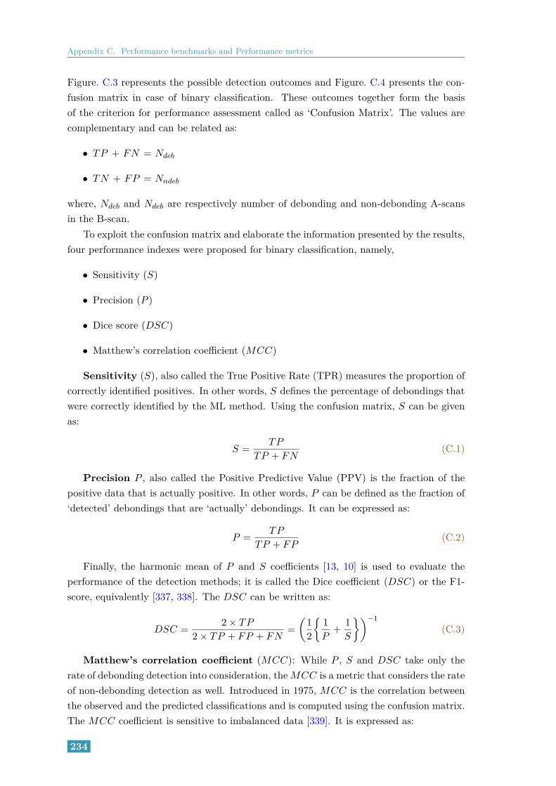
Appendix C. Performance benchmarks and Performance metrics
Figure. C.3 represents the possible detection outcomes and Figure. C.4 presents the con-fusion matrix in case of binary classification. These outcomes together form the basisof the criterion for performance assessment called as ‘Confusion Matrix’. The values arecomplementary and can be related as:
• TP + FN = Ndeb
• TN + FP = Nndeb
where, Ndeb and Ndeb are respectively number of debonding and non-debonding A-scansin the B-scan.
To exploit the confusion matrix and elaborate the information presented by the results,four performance indexes were proposed for binary classification, namely,
• Sensitivity (S)
• Precision (P )
• Dice score (DSC)
• Matthew’s correlation coefficient (MCC)
Sensitivity (S), also called the True Positive Rate (TPR) measures the proportion ofcorrectly identified positives. In other words, S defines the percentage of debondings thatwere correctly identified by the ML method. Using the confusion matrix, S can be givenas:
S =TP
TP + FN(C.1)
Precision P , also called the Positive Predictive Value (PPV) is the fraction of thepositive data that is actually positive. In other words, P can be defined as the fraction of‘detected’ debondings that are ‘actually’ debondings. It can be expressed as:
P =TP
TP + FP(C.2)
Finally, the harmonic mean of P and S coefficients [13, 10] is used to evaluate theperformance of the detection methods; it is called the Dice coefficient (DSC) or the F1-score, equivalently [337, 338]. The DSC can be written as:
DSC =2× TP
2× TP + FP + FN=
(1
2
1
P+
1
S
)−1
(C.3)
Matthew’s correlation coefficient (MCC): While P , S and DSC take only therate of debonding detection into consideration, the MCC is a metric that considers the rateof non-debonding detection as well. Introduced in 1975, MCC is the correlation betweenthe observed and the predicted classifications and is computed using the confusion matrix.The MCC coefficient is sensitive to imbalanced data [339]. It is expressed as:
234

C.2 Performance assessment of detection methods
MCC =(TP × TN)− (FP × FN)√
(TP + FP )(TP + FN)(TN + FP )(TN + FN)(C.4)
These performance metrics are used in Chapter. 4, 5 and 6 for decision support todetect debondings as a binary problem.
C.2.2 Performance assessment for probabilistic estimation
Since the confusion matrix can be implemented from only integral outputs, it is un-suitable for probabilistic outputs. Thus, we introduce two new performance indexes forprobabilistic estimates that use the ground truth (or pseudo ground truth based on theimplementation) and the predicted probabilities.
In the context of pavement monitoring, the probabilities expressed by the machinelearning method can be done in two ways:
• Probability of occurrence of a debonding (Pd)
• Probability of occurrence of a non-debonding (Pn)
In order to assess the probabilistic estimation of debondings, we introduce two new metricsnamely, Debonding Prediction Rate (DPR) and Non-debonding Prediction Rate (NPR)expressed as:
DPR = 1−
1
N
N∑i=1
|pi − di|
(C.5)
NPR = 1−
1
N
N∑i=1
|pi − ni|
(C.6)
where,N is the total number of A-scans,pi is the GT (or PGT) and pi ∈ N0, 1di is the probability of detection of a debonding and di ∈ R0, 1ni is the probability of detection of a non-debonding and ni ∈ R0, 1These metrics are used in Chapter. 6 for decision support to present a probabilistic
estimate of the occurrence of debonding or non-debonding.
235


Appendix D
Time-gating of a GPR A-scan
In this appendix, we present the automatic time gating of the second echo from a GPRA-scan. This windowing step is necessary in order to obtain the information localized
at the interface between the two pavement layers.
The time-gating step is used in Chapter. 2 in the ART and LRT methods to determinethe second amplitude. In addition, it is also used in Chapter. 4 to extract the local signalfeatures in time domain.
Principle
Let x be a non-debonding A-scan signal in time domain with n time samples for thetime interval t. Let the dominant operating frequency of the emitted pulse be fc.
We define the window size (Wx) for the A-scan x as a function of tw (pulse width ofthe emitted pulse) and fsamp as:
Wx = 2× fsamp × tw (D.1)
where tw is related to the fc as: tw = 1fc
.
As discussed extensively throughout the thesis, in case of a debonding, an additionalsignal is observed that interferes constructively with the second echo (of course, limitedby the λmat/4 criteria for constructive interference). Beyond this, the two signals begin toseparate until λmat/2. Thus, the pulse width of the second echo is expected to be greaterthan tw, but, at the same time, less than or equal to 2× tw.
To perform the windowing, the position of a the second maximum (M2) magnitudeis obtained. This is because the first maximum corresponds to the surface echo, and thesecond maximum is expected to occur at the interface of the pavement layers. The windowW is evenly distributed on either sides of M2. A Tukey cosine-tapering window [340] witha taper ratio of 25% is used. The taper ratio is manually chosen by the operator suchthat the unwanted noise and parasitic signal around the second echo is avoided but, at thesame time the important information within the window is preserved. Figure. D.1 showsan example of an A-scan with its designated time-gating window.
237

Appendix D. Time-gating of a GPR A-scan
2 2.5 3 3.5 4 4.5Time (s) ×10-9
-0.6
-0.4
-0.2
0
0.2
0.4
0.6
0.8
1
Am
plitu
de /
Mag
nitu
de
Actual A-scanMagnitude of second echoTukey time-window (25% taper)
Figure D.1: Example of an A-scan from experimental data collected using the UWB SF-GPR at IFSTTAR’s fatigue carousel (Appendix. B.2.1); Tack-free defect type at 10k cyclesloading stage and the time-gating window used to isolate the second echo
Figure. D.2, Figure. D.3 and Figure. D.4 present B-scan image before windowing andcompares it with the time-gated B-scan obtained after windowing for respectively Geotex-tile, Tack-free and Sand based defects at 10K loading.
10 20 30 40 50 60 70 80Number of A-scans
2
2.5
3
3.5
4
4.5
Tim
e (s
)
×10-9
10 20 30 40 50 60 70 80Number of A-scans
2
2.5
3
3.5
4
4.5
Tim
e (s
)×10-9
Figure D.2: B-scan images for experimental data collected using the UWB SF-GPR atIFSTTAR’s fatigue carousel (Appendix. B.2.1); Geotextile defect type at 10K cycles loadingstage (left) and its respective the B-scan obtained after time gating (right)
238

10 20 30 40 50Number of A-scans
2
2.5
3
3.5
4
4.5
Tim
e (s
)
×10-9
10 20 30 40 50Number of A-scans
2
2.5
3
3.5
4
4.5
Tim
e (s
)×10-9
Figure D.3: B-scan images for experimental data collected using the UWB SF-GPR atIFSTTAR’s fatigue carousel (Appendix. B.2.1); Tack-free defect type at 10K cycles loadingstage (left) and its respective the B-scan obtained after time gating (right)
10 20 30 40 50 60 70 80Number of A-scans
2
2.5
3
3.5
4
4.5
Tim
e (s
)
×10-9
10 20 30 40 50 60 70 80Number of A-scans
2
2.5
3
3.5
4
4.5
Tim
e (s
)
×10-9
Figure D.4: B-scan images for experimental data collected using the UWB SF-GPR atIFSTTAR’s fatigue carousel (Appendix. B.2.1); Sand defect type at 10K cycles loadingstage (left) and its respective the B-scan obtained after time gating (right)
239


Appendix E
Additional illustrations for Chapter. 6
In this appendix, we present the debonding detection results for the intermediate loadingstages of the fatigue carousel experiments for Chapter. 6. Each figure indicates the
transition zone in a dashed blue box.
241

Appendix E. Additional illustrations for Chapter. 6
(a) 100K loading
(b) 200K loading (c) 250K loading
Figure E.1: Two-class SVM debonding detection estimates for SF-GPR data using localfeatures at intermediate loading stages for Geotextile-based defects (strong debonding
permittivity contrast)
242

(a) 50K loading (b) 100K loading
(c) 200K loading (d) 250K loading
Figure E.2: Two-class SVM debonding detection estimates for SF-GPR data using localfeatures at intermediate loading stages for Sand-based defects (average debonding
permittivity contrast)
243

Appendix E. Additional illustrations for Chapter. 6
(a) 50K loading (b) 100K loading
(c) 200K loading (d) 250K loading
Figure E.3: Two-class SVM debonding detection estimates for SF-GPR data using localfeatures at intermediate loading stages for Tack free-based defects (weak debonding
permittivity contrast)
244

(a) 50K loading (b) 100K loading
(c) 200K loading (d) 250K loading
Figure E.4: One-class SVM debonding detection estimates for SF-GPR data using localfeatures at intermediate loading stages for Geotextile-based defects (strong debonding
permittivity contrast)
245

Appendix E. Additional illustrations for Chapter. 6
(a) 50K loading (b) 100K loading
(c) 200K loading (d) 250K loading
Figure E.5: One-class SVM debonding detection estimates for SF-GPR data using localfeatures at intermediate loading stages for Sand-based defects (average debonding
permittivity contrast)
246

(a) 50K loading (b) 100K loading
(c) 200K loading (d) 250K loading
Figure E.6: One-class SVM debonding detection estimates for SF-GPR data using localfeatures at intermediate loading stages for Tack free-based defects (weak debonding
permittivity contrast)
247

Appendix E. Additional illustrations for Chapter. 6
(a) 100K loading
(b) 200K loading (c) 250K loading
Figure E.7: Random forests debonding detection estimates for SF-GPR data using localfeatures at intermediate loading stages for Geotextile-based defects (strong debonding
permittivity contrast)
248

(a) 50K loading (b) 100K loading
(c) 200K loading (d) 250K loading
Figure E.8: Random forests debonding detection estimates for SF-GPR data using localfeatures at intermediate loading stages for Sand-based defects (average debonding
permittivity contrast)
249

Appendix E. Additional illustrations for Chapter. 6
(a) 50K loading (b) 100K loading
(c) 200K loading (d) 250K loading
Figure E.9: Random forests debonding detection estimates for SF-GPR data using localfeatures at intermediate loading stages for Tack free-based defects (weak debonding
permittivity contrast)
250

Table E.1: DPR and NPR coefficients for probability estimation from local signal featuresat 50K to 250K loading for respectively Geotextile, Sand and Tack-free based defects usingTwo-class SVM
Loading stageGeotextile Sand Tack-free
DPR NPR DPR NPR DPR NPR
100K cycles 0.99 0.87 0.98 0.76 0.52 0.72
200K cycles 0.98 0.58 0.98 0.71 0.59 0.94
250K cycles 0.98 0.68 0.77 0.75 0.39 0.46
Table E.2: DPR and NPR coefficients for probability estimation from local signal featuresat 50K to 250K loading for respectively Geotextile, Sand and Tack-free based defects usingOne-class SVM
Loading stageGeotextile Sand Tack-free
DPR NPR DPR NPR DPR NPR
50K cycles 0.98 0.92 0.98 0.88 0.97 0.81
100K cycles 0.98 0.87 0.99 0.96 0.83 0.92
200K cycles 0.99 0.87 0.98 0.91 0.82 0.93
250K cycles 0.99 0.81 0.99 0.99 0.89 0.99
Table E.3: DPR and NPR coefficients for probability estimation from local signal featuresat 50K to 250K loading for respectively Geotextile, Sand and Tack-free based defects usingRandom forests
Loading stageGeotextile Sand Tack-free
DPR NPR DPR NPR DPR NPR
100K cycles 1.00 0.78 0.99 0.7 0.62 0.65
200K cycles 0.99 0.58 0.99 0.65 0.66 0.81
250K cycles 0.99 0.68 0.98 0.83 0.73 0.7
251

Appendix E. Additional illustrations for Chapter. 6
Table E.4: Comparison of DSC ([..]) and MCC ((..)) coefficients for binary debond-ing detection from local signal features at intermediate loading stages for Geotextile baseddefects
Loading stage ART (reference) Two-class SVM One-class SVM Random forests
50K cycles [1.00], (1.00) [1.00], (1.00) [1.00], (1.00) [1.00], (1.00)
100K cycles [0.98], (0.96) [1.00], (1.00) [0.85], (0.65) [1.00], (1.00)
200K cycles [1.00], (1.00) [1.00], (1.00) [0.91], (0.79) [1.00]. (1.00)
250K cycles [1.00], (1.00) [1.00], (1.00) [1.00], (1.00) [0.99], (0.97)
Table E.5: Comparison of DSC ([..]) and MCC ((..)) coefficients for binary debondingdetection from local signal features at intermediate loading stages for Sand based defects
Loading stage ART (reference) Two-class SVM One-class SVM Random forests
50K cycles [1.00], (1.00) [1.00], (1.00) [0.94], (0.82) [0.9], (0.8)
100K cycles [1.00], (1.00) [0.98], (0.95) [0.94], (0.82) [0.91], (0.85)
200K cycles [1.00], (1.00) [1.00], (1.00) [1.00], (1.00) [0.95], (0.82)
250K cycles [0.95], (0.91) [1.00], (1.00) [1.00], (1.00) [0.88], (0.77)
Table E.6: Comparison of DSC ([..]) and MCC ((..)) coefficients for binary debondingdetection from local signal features at intermediate loading stages for Tack-free based defects
Loading stage ART (reference) Two-class SVM One-class SVM Random forests
50K cycles [0.96], (0.95) [0.92], (0.89) [0.84], (0.77) [0.90], (0.87)
100K cycles [0.93], (0.89) [0.88], (0.85) [0.96], (0.94) [0.92], (0.88)
200K cycles [0.90], (0.86) [0.9], (0.86) [0.84], (0.81) [0.95], (0.92)
250K cycles [0.95], (0.93) [0.86], (0.82) [0.88], (0.82) [0.88], (0.84)
252

253


Nomenclature
Data processing method related
α, β Lagrangian multipliers
H Hilbert transform
ν Admitted slack (One-class SVM)
y Multi-class classifier labels 0, 1, 2, 3
y Two-class classifier labels −1,+1
ξ Admitted slack (Two-class SVM)
R Radius of the hyper-sphere (One-class SVM)
sgn Sign function −,+
Physical constants
c Speed of the EM wave in air 3× 10⁸ms−1
Material related
ρ Material permeability
σ Material conductivity
εr Relative permittivity
Operators
∗ Convolution
AT Transpose of the matrix A
A−1 Inverse of the matrix A
× Multiplication
card(N) cardinality of a number N
det(A) Determinant of the matrix A
GPR data related
255

Appendix E. Additional illustrations for Chapter. 6
F 2D B-scan feature matrix in time/frequency domain
f 1D A-scan feature vector in time/frequency domain
X 2D B-scan matrix in time/frequency domain
x 1D A-scan vector in time/frequency domain
f One signal feature
M,m Number of time samples; temporal resolution
N,n Number of A-scans; spatial resolution
x Amplitude at an instance t
256

Abbreviations
EMR Electromagnetic RadiationGPR Ground Penetrating RadarMLM Machine Learning MethodsLRT Likelihood Ratio TestART Amplitude Ratio TestRF Random ForestsOC-SVM One-Class Support Vector MachinesSVM Support Vector MachinesAPT Accelerated Pavement TestNDT Non-Destructive TestingDT Destructive testingSHM Structural Health MonitoringFDTD Finite Difference Time DomainMoM Method of MomentGPILE Generalized Propagation Inside Layer ExpansionMCC Matthew’s Correlation CoefficientCV Cross validation techniquesMAG Signal MagnitudeMAAD Maximum Absolute Amplitude DeviationTDE Time Delay EstimationBW BandwidthFFT, IFFT Finite Fourier Transform, Inverse Finite Fourier TransformAC-GPR Air-coupled/Air-launched GPRGC-GPR Ground-coupled GPR
257


Part IV
BIBLIOGRAPHY
259


Bibliography
[1] Q. You, N. Zheng, and J. Ma, “Study of ravelling failure on dense graded asphaltpavement,” Proceedings of the Institution of Civil Engineers - Transport, vol. 171,pp. 1–24, 01 2018.
[2] A. Shaat, “Pavement structural analysis based on non-destructive test measure-ments,” WIT Transactions on Modelling and Simulation, vol. 12, 1970.
[3] K. Chatti, M. E. Kutay, N. Lajnef, I. Zaabar, S. Varma, H. S. Lee et al., “Enhancedanalysis of falling weight deflectometer data for use with mechanistic-empiricalflexible pavement design and analysis and recommendations for improvements tofalling weight deflectometers,” Turner-Fairbank Highway Research Center, Tech.Rep., 2017.
[4] B. Guan, “Characterization of building materials by electromagnetic non-destructivemethods: application to limestone,” Ph.D. dissertation, Nantes, 2018.
[5] N. Diamanti and A. P. Annan, “Air-launched and ground-coupled gpr data,” in 201711th European Conference on Antennas and Propagation (EUCAP), March 2017, pp.1694–1698.
[6] H. Larsen, “Strategic highway research program,” STATENS VEJLAB-ORATORIUM NOTAT, no. 209, 1988. [Online]. Available: http://www.ndtoolbox.org/content/bridge/gpr-equipment
[7] A. Benedetto, F. Tosti, L. B. Ciampoli, and F. D’Amico, “An overview of ground-penetrating radar signal processing techniques for road inspections,” Signal Process-ing, vol. 132, pp. 201–209, 2017.
[8] B. Scheers, “Ultra-wideband ground penetrating radar with application to the de-tection of anti personnel landmines,” Ph.D. dissertation, 2001.
[9] M. Duman and A. C. Gürbüz, “3 d imaging for ground-penetrating radars via dic-tionary dimension reduction,” 2015.
[10] S. S. Todkar, C. L. Bastard, V. Baltazart, A. Ihamouten, and X. Dérobert,“Performance assessment of svm-based classification techniques for the detectionof artificial debondings within pavement structures from stepped-frequency a-scanradar data,” NDT & E International, vol. 107, p. 102128, 2019. [Online]. Available:http://www.sciencedirect.com/science/article/pii/S0963869518306960
261

[11] A. Verikas, E. Vaiciukynas, A. Gelzinis, J. Parker, and M. C. Olsson,“Electromyographic patterns during golf swing: Activation sequence profiling andprediction of shot effectiveness,” Sensors, vol. 16, no. 4, 2016. [Online]. Available:https://www.mdpi.com/1424-8220/16/4/592
[12] C. Bourlier, C. Le Bastard, and V. Baltazart, “Generalization of pile method tothe em scattering from stratified subsurface with rough interlayers: Applicationto the detection of debondings within pavement structure,” IEEE Transactions onGeoscience and Remote Sensing, vol. 53, no. 7, pp. 4104–4115, July 2015.
[13] S. S. Todkar, C. Le Bastard, A. Ihamouten, V. Baltazart, X. Dérobert, C. Fauchard,D. Guilbert, and F. Bosc, “Detection of debondings with ground penetrating radarusing a machine learning method,” in 2017 9th International Workshop on AdvancedGround Penetrating Radar (IWAGPR), June 2017, pp. 1–6.
[14] G. A. Manual, “Geophysical survey systems, inc,” Salem, NH, MN30-903 Rev. E,99ápp, 2014.
[15] J.-M. Simonin and G. Villain, “Detection and survey of interface defects within apavement structure with ultrasonic pulse echo,” in 8th RILEM International Con-ference on Mechanisms of Cracking and Debonding in Pavements, A. Chabot, W. G.Buttlar, E. V. Dave, C. Petit, and G. Tebaldi, Eds. Dordrecht: Springer Nether-lands, 2016, pp. 673–678.
[16] X. Dérobert, C. Fauchard, P. Côte, E. L. Brusq, E. Guillanton, J. Dauvignac, andC. Pichot, “Step-frequency radar applied on thin road layers,” Journal of AppliedGeophysics, vol. 47, no. 3, pp. 317 – 325, 2001, ground Penetrating Radar. [Online].Available: http://www.sciencedirect.com/science/article/pii/S0926985101000751
[17] J. Simonin, V. Baltazart, P. Hornych, X. Dérobert, E. Thibaut, J. Sala, and V. Utsi,“Case study of detection of artificial defects in an experimental pavement struc-ture using 3d gpr systems,” in Proceedings of the 15th International Conference onGround Penetrating Radar, June 2014, pp. 847–851.
[18] J. M. Simonin, V. Baltazart, C. Le Bastard, and X. Dérobert, “Progressin Monitoring the Debonding Within Pavement Structures During AcceleratedPavement Testing on the Fatigue Carousel,” in MCD2016, 8th Internationalconference on Mechanisms of Cracking and Debonding in Pavements, NANTES,France, Jun. 2016, p. 6p, mCD2016, 8th International conference on Mechanismsof Cracking and Debonding in Pavements, NANTES, FRANCE, 07-/06/2016 -09/06/2016. [Online]. Available: https://hal.archives-ouvertes.fr/hal-01364065
[19] A. W.-C. Chan, “Economic and environmental evaluations of life-cycle cost analysispractice: A case study of michigan dot pavement projects,” Ph.D. dissertation, 2007.
[20] K. E. Cooper, P. S. Pell, Transport, and R. R. Laboratory, “The effect of mix vari-ables on the fatigue strength of bituminous materials,” 1974, includes bibliographicreferences.

[21] I. L. Al-Qadi, K. I. Hasiba, A. S. Cortina, H. Ozer, Z. Leng, D. C. Parish, andS. J. Worsfold, “Best practices for implementation of tack coat: Part 1, laboratorystudy,” 2012.
[22] A. Szydo and K. Malicki, “Analysis of the correlation between the static and fatiguetest results of the interlayer bondings of asphalt layers,” Archives of Civil Engineer-ing, vol. 62, 03 2016.
[23] P. Jaskula and D. Rys, “Effect of interlayer bonding quality of asphalt layers onpavement performance,” IOP Conference Series: Materials Science and Engineering,vol. 236, p. 012005, sep 2017. [Online]. Available: https://doi.org/10.1088%2F1757-899x%2F236%2F1%2F012005
[24] E. Özgan, “Determining the stability of asphalt concrete at varying temperaturesand exposure times using destructive and non-destructive methods,” 2007.
[25] R. Y. Liang and J. Zhou, “Prediction of fatigue life of asphalt concrete beams,”International Journal of Fatigue, vol. 19, no. 2, pp. 117 – 124, 1997. [Online].Available: http://www.sciencedirect.com/science/article/pii/S0142112396000667
[26] R. A. Livingston, “Nondestructive testing of historic structures,” Archives andMuseum Informatics, vol. 13, no. 3, pp. 249–271, Sep 1999. [Online]. Available:https://doi.org/10.1023/A:1012416309607
[27] X. Wang, Q. Guo, S. Yang, D. Zhang, and Y. Wang, “Nondestructive testing andassessment of consolidation effects of earthen sites,” Journal of Rock Mechanics andGeotechnical Engineering, vol. 8, no. 5, pp. 726 – 733, 2016. [Online]. Available:http://www.sciencedirect.com/science/article/pii/S1674775516300701
[28] M. Andrzej and M. Marta, “Modern ndt systems for structural integrity examinationof concrete bridge structures,” Procedia Engineering, vol. 91, pp. 418 – 423,2014, xXIII R-S-P Seminar, Theoretical Foundation of Civil Engineering (23RSP)(TFoCE 2014). [Online]. Available: http://www.sciencedirect.com/science/article/pii/S187770581403104X
[29] B. Hankes and D. Couse, “Condition monitoring and non-destructive testing of me-chanical equipment,” in 2007 IEEE Cement Industry Technical Conference Record,April 2007, pp. 160–167.
[30] A. Tedeschi and F. Benedetto, “A real-time automatic pavement crack and pot-hole recognition system for mobile android-based devices,” Advanced EngineeringInformatics, vol. 32, pp. 11–25, 2017.
[31] P. Wang, Y. Hu, Y. Dai, and M. Tian, “Asphalt pavement pothole detection andsegmentation based on wavelet energy field,” Mathematical Problems in Engineering,vol. 2017, pp. 1–13, 02 2017.

[32] A. Dhivya and M. Hemalatha, “Structural health monitoring system - an embeddedsensor approach,” International Journal of Engineering and Technology, vol. 5, pp.273–281, 02 2013.
[33] G. Song, H. Gu, Y. Mo, T. Hsu, and H. Dhonde, “Concrete structural health moni-toring using embedded piezoceramic transducers,” Smart Mater. Struct, vol. 16, pp.959–968, 08 2007.
[34] L. Gallucci, C. Menna, L. Angrisani, D. Asprone, R. S. L. Moriello,F. Bonavolontà, and F. Fabbrocino, “An embedded wireless sensor network withwireless power transmission capability for the structural health monitoring ofreinforced concrete structures,” Sensors, vol. 17, no. 11, 2017. [Online]. Available:https://www.mdpi.com/1424-8220/17/11/2566
[35] M. F. Rad and L. Shafai, “A wireless embedded sensor for structural health moni-toring applications,” in 2009 13th International Symposium on Antenna Technologyand Applied Electromagnetics and the Canadian Radio Science Meeting, Feb 2009,pp. 1–4.
[36] M. Al-Saddique, G. Hamada, and M. N. Al-Awad, “State of the art: Reviewof coring and core analysis technology,” Journal of King Saud University -Engineering Sciences, vol. 12, no. 1, pp. 117 – 137, 2000. [Online]. Available:http://www.sciencedirect.com/science/article/pii/S1018363918307098
[37] L. McGrath, K. Maser, and J. Puccinelli, “Determining asphalt thickness usingground penetrating radar,” in Proceedings of the international conferences on thebearing capacity of roads, railways and airfields, 2013, pp. 199–208.
[38] R. C. West, J. Zhang, J. Moore et al., “Evaluation of bond strength between pave-ment layers.” Auburn University. National Center for Asphalt Technology, Tech.Rep., 2005.
[39] M. Kruntcheva, A. Collop, and N. Thom, “Properties of asphalt concrete layerinterfaces,” Journal of Materials in Civil Engineering, vol. 18, pp. 467–471, 06 2006.
[40] D.-H. Chen, J.-N. Wang, and J. Bilyeu, “Application of dynamic cone penetrometerin evaluation of base and subgrade layers,” Transportation Research Record, vol.1764, pp. 1–10, 01 2001.
[41] R. Salgado and S. Yoon, “Dynamic cone penetration test (dcpt) for subgrade assess-ment,” Joint Transportation Research Program, p. 73, 2003.
[42] S. Shankar and Y. Ravi, “In-situ strength evaluation of pavement layers of lowvolume road using dynamic cone penetrometer (dcp),” 2014.
[43] A. Das, “Interpretation of falling weight deflectometer data,” Indian Institute ofTechnology Kanpur, Kanpur, India, 1994.

[44] R. K. Dhir, J. de Brito, R. V. Silva, and C. Q. Lye, “12 - use of recycledaggregates in road pavement applications,” in Sustainable Construction Materials,ser. Woodhead Publishing Series in Civil and Structural Engineering, R. K. Dhir,J. de Brito, R. V. Silva, and C. Q. Lye, Eds. Woodhead Publishing, 2019, pp.451 – 494. [Online]. Available: http://www.sciencedirect.com/science/article/pii/B9780081009857000121
[45] D. Stolle and F. Peiravian, “Falling weight deflectometer data interpretation usingdynamic impedance,” Canadian Journal of Civil Engineering, vol. 23, pp. 1–8, 022011.
[46] S. Gupta, “Comparison of non-destructive and destructive testing on concrete: Areview,” Trends in Civil Engineering and its Architecture, vol. 3, no. 1, sep 2018.[Online]. Available: https://doi.org/10.32474%2Ftceia.2018.03.000154
[47] A. Quansah and D. Atuah, “Evaluation of pavement structural life using dynamiccone penetrometer,” 08 2017.
[48] J. W. Jewett and R. A. Serway, Physics for scientists and engineers with modernphysics. Cengage Learning EMEA, 2008.
[49] J. F. Mcnulty, “Ultrasonic testing apparatus and method,” Jul. 12 1966, uS Patent3,260,105.
[50] W.-h. Pan, X.-d. Sun, L.-m. Wu, K.-k. Yang, and N. Tang, “Damage detection ofasphalt concrete using piezo-ultrasonic wave technology,” Materials, vol. 12, no. 3,2019. [Online]. Available: https://www.mdpi.com/1996-1944/12/3/443
[51] Y.-c. Cheng, P. Zhang, Y. Jiao, Y.-d. Wang, and J. Tao, “Damage simulationand ultrasonic detection of asphalt mixture under the coupling effects of water-temperature-radiation,” Advances in Materials Science and Engineering, vol. 2013,pp. 1–9, 12 2013.
[52] G. Concu and N. Trulli, “Concrete defects sizing by means of ultrasonicvelocity maps,” Buildings, vol. 8, no. 12, 2018. [Online]. Available: https://www.mdpi.com/2075-5309/8/12/176
[53] V. Krstelj, J. Stepani, and D. Markui, “Ultrasonic method of materials characteri-zation for recognition buried objects,” vol. 3, pp. 6157–129, 01 2000.
[54] T. Sugimoto and T. Abe, “Study on the buried object detection method using op-timum frequency range method in extremely shallow underground,” in 2011 IEEEInternational Ultrasonics Symposium, Oct 2011, pp. 752–755.
[55] T. Arakawa, S. Hirose, and T. Senda, “The detection of weld cracks using ultrasonictesting,” NDT International, vol. 18, no. 1, pp. 9 – 16, 1985. [Online]. Available:http://www.sciencedirect.com/science/article/pii/0308912685900379

[56] S. Djili, F. Boukazouha, R. Halimi, and A. B. Bouda, “Defects detection in weldsusing ultrasonic analysis,” 2006.
[57] H. Hogan, “Non-destructive technology,” Aviation Aftermarket Defence, vol. 11,p. 35, 2015.
[58] Y. Teoh, M. Bruka, N. Idris, N. Ismail, and N. Muztaza, “Introduction of aground penetrating radar system for subsurface investigation in balik pulau, penangisland,” Journal of Physics: Conference Series, vol. 995, p. 012098, apr 2018.[Online]. Available: https://doi.org/10.1088%2F1742-6596%2F995%2F1%2F012098
[59] M. Sato, “Gpr and its application to environmental study,” Center for NortheastAsia Studies (CNEAS), Tohoku University, 2001.
[60] D. J. Daniels, “Ground penetrating radar,” Encyclopedia of RF and MicrowaveEngineering, 2005.
[61] E. Fisher, G. A. McMechan, and A. P. Annan, “Acquisition and processing of wide-aperture ground-penetrating radar data,” Geophysics, vol. 57, no. 3, pp. 495–504,1992.
[62] M. I. Skolnik, “An analysis of bistatic radar,” IRE Transactions on Aerospace andNavigational Electronics, vol. ANE-8, no. 1, pp. 19–27, March 1961.
[63] A. Saintenoy and J. Hopmans, “Ground penetrating radar: Water table detectionsensitivity to soil water retention properties,” Selected Topics in Applied Earth Ob-servations and Remote Sensing, IEEE Journal of, vol. 4, pp. 748–753, 12 2011.
[64] A. P. Annan, S. W. Cosway, and J. D. Redman, Water table detectionwith ground penetrating radar, 2005, pp. 494–496. [Online]. Available: https://library.seg.org/doi/abs/10.1190/1.1888793
[65] M. C. Diallo, L. Z. Cheng, E. Rosa, C. Gunther, and M. Chouteau, “Integratedgpr and ert data interpretation for bedrock identification at cléricy, québec,canada,” Engineering Geology, vol. 248, pp. 230 – 241, 2019. [Online]. Available:http://www.sciencedirect.com/science/article/pii/S0013795218301327
[66] J. Hager and M. Carnevale, “Gpr as a cost effective bedrock mapping tool for largeareas,” 01 2001, pp. GP13–GP13.
[67] S.-H. Ni, Y.-H. Huang, K.-F. Lo, and D.-C. Lin, “Buried pipe detection byground penetrating radar using the discrete wavelet transform,” Computersand Geotechnics, vol. 37, no. 4, pp. 440 – 448, 2010. [Online]. Available:http://www.sciencedirect.com/science/article/pii/S0266352X10000078
[68] J. J. Bowders, R. M. Koerner, and A. E. Lord, “Buried container detectionusing ground-probing radar,” Journal of Hazardous Materials, vol. 7, no. 1, pp. 1– 17, 1982. [Online]. Available: http://www.sciencedirect.com/science/article/pii/0304389482870015

[69] D. J. Daniels, D. J. Gunton, and H. F. Scott, “Introduction to subsurface radar,”IEE Proceedings F - Communications, Radar and Signal Processing, vol. 135, no. 4,pp. 278–320, August 1988.
[70] G. Kino, Acoustic Waves: Devices, Imaging, and Analog Signal Processing, ser.Prentice-Hall Contemporary Topics in Accounting Series. Prentice-Hall, 1987.[Online]. Available: https://books.google.fr/books?id=hcsYAQAAIAAJ
[71] N. Diamanti, A. P. Annan, and J. D. Redman, “Concrete Bridge Deck DeteriorationAssessment Using Ground Penetrating Radar (GPR),” Journal of Environmentaland Engineering Geophysics, vol. 22, no. 2, pp. 121–132, 06 2017. [Online].Available: https://doi.org/10.2113/JEEG22.2.121
[72] P. Annan, N. Diamanti, J. Redman, and S. Jackson, “Ground-penetrating radar forassessing winter roads,” Geophysics, vol. 81, pp. WA101–WA109, 01 2016.
[73] T. Saarenketo and T. Scullion, “Road evaluation with ground penetrating radar,”Journal of Applied Geophysics, vol. 43, no. 2, pp. 119 – 138, 2000. [Online].Available: http://www.sciencedirect.com/science/article/pii/S092698519900052X
[74] M. Sun, N. Pinel, C. Le Bastard, V. Baltazart, A. Ihamouten, and Y. Wang, “Timedelay and interface roughness estimation by gpr for pavement survey,” Near SurfaceGeophysics, 06 2015.
[75] L. Bianchini Ciampoli, F. Tosti, N. Economou, and F. Benedetto, “Signalprocessing of gpr data for road surveys,” Geosciences, vol. 9, no. 2, 2019. [Online].Available: https://www.mdpi.com/2076-3263/9/2/96
[76] GPR modelling applied to vertical and horizontal resolution of buried objects. IEEE,2011.
[77] A. Annan, “Ground penetrating radar principles, procedures, and applications: Sen-sors & software inc,” Mississauga, ON, Canada, 2003.
[78] T. Ziani, D. Teguig, M. A. Takkouche, X. Dérobert, and M. Benslama, “Gpr mod-elling applied to vertical and horizontal resolution of buried objects,” in 2011 Inter-national Conference on Electromagnetics in Advanced Applications, Sep. 2011, pp.1–4.
[79] R. Knight, P. Tercier, and H. Jol, “Multi-frequency ground penetrating radar datato characterize spatial variability,” in SEG Technical Program Expanded Abstracts1999. Society of Exploration Geophysicists, 1999, pp. 559–562.
[80] R. Knight, P. Tercier, and J. Irving, “The effect of vertical measurementresolution on the correlation structure of a ground penetrating radar reflectionimage,” Geophysical Research Letters, vol. 31, no. 21, 2004. [Online]. Available:https://agupubs.onlinelibrary.wiley.com/doi/abs/10.1029/2004GL021112

[81] Lanbo Liu and Lieyuan Zhu, “Gpr signal analysis: can we get deep-penetration andhigh-resolution simultaneously?” in Proceedings of the Tenth International Con-ference on Grounds Penetrating Radar, 2004. GPR 2004., vol. 1, June 2004, pp.263–265.
[82] H. Jol, “Ground penetrating radar antenna frequencies and transmitter powerscompared for penetration depth, resolution and reflection continuity,” GeophysicalProspecting, vol. 43, pp. 693 – 709, 04 2006.
[83] E. Tebchrany, F. Sagnard, V. Baltazart, J. Tarel, and X. Dérobert, “Assessmentof statistical-based clutter reduction techniques on ground-coupled gpr data for thedetection of buried objects in soils,” in Proceedings of the 15th International Con-ference on Ground Penetrating Radar, June 2014, pp. 604–609.
[84] W. Bi, Y. Zhao, C. An, and S. Hu, “Clutter elimination and random-noisedenoising of gpr signals using an svd method based on the hankel matrix inthe local frequency domain,” Sensors, vol. 18, no. 10, 2018. [Online]. Available:https://www.mdpi.com/1424-8220/18/10/3422
[85] X. Song, T. Liu, D. Xiang, and Y. Su, “Gpr antipersonnel mine detection basedon tensor robust principal analysis,” Remote Sensing, vol. 11, no. 8, 2019. [Online].Available: https://www.mdpi.com/2072-4292/11/8/984
[86] J. F. Roulette and K. A. Skrivseth, “Coherent data collection and analysis capabilityfor the an/sps-48e radar,” 1997.
[87] F. Sagnard, E. Tebchrany, and V. Baltazart, “Evaluation of an uwb ground-coupledradar in the detection of discontinuities using polarization diversity: Fdtd modelingand experiments,” in 2013 7th International Workshop on Advanced Ground Pene-trating Radar, July 2013, pp. 1–6.
[88] J. Huh, H. Pham Van, S. Han, H.-J. Choi, and S.-K. Choi, “A data-drivenapproach for the diagnosis of mechanical systems using trained subtractedsignal spectrograms,” Sensors, vol. 19, no. 5, 2019. [Online]. Available:https://www.mdpi.com/1424-8220/19/5/1055
[89] X. Xie, P. Li, and L. Liu, “Gpr identification of voids inside concrete based onsupport vector machine (svm) algorithm,” in 2012 14th International Conference onGround Penetrating Radar (GPR), June 2012, pp. 381–386.
[90] X. Xie, P. Li, H. Qin, L. Liu, and D. C. Nobes, “GPR identification of voidsinside concrete based on the support vector machine algorithm,” Journal ofGeophysics and Engineering, vol. 10, no. 3, 06 2013, 034002. [Online]. Available:https://doi.org/10.1088/1742-2132/10/3/034002
[91] J. Zhang, Q. Liu, and B. Nath, “Landmine feature extraction and classification ofgpr data based on svm method,” in Advances in Neural Networks – ISNN 2004, F.-

L. Yin, J. Wang, and C. Guo, Eds. Berlin, Heidelberg: Springer Berlin Heidelberg,2004, pp. 636–641.
[92] K. Tbarki, S. Ben Said, R. Ksantini, and Z. Lachiri, “Rbf kernel based svm clas-sification for landmine detection and discrimination,” in 2016 International ImageProcessing, Applications and Systems (IPAS), Nov 2016, pp. 1–6.
[93] ——, “Landmine detection improvement using one-class svm for unbalanced data,”in 2017 International Conference on Advanced Technologies for Signal and ImageProcessing (ATSIP), May 2017, pp. 1–6.
[94] K. Tbarki, S. B. Said, R. Ksantini, and Z. Lachiri, “Covariance-guided landminedetection and discrimination using ground-penetrating radar data,” InternationalJournal of Remote Sensing, vol. 39, no. 2, pp. 289–314, 2018. [Online]. Available:https://doi.org/10.1080/01431161.2017.1382746
[95] E. Pasolli, F. Melgani, M. Donelli, R. Attoui, and M. de Vos, “Automatic detectionand classification of buried objects in gpr images using genetic algorithms and sup-port vector machines,” in IGARSS 2008 - 2008 IEEE International Geoscience andRemote Sensing Symposium, vol. 2, July 2008, pp. II–525–II–528.
[96] N. Muniappan, A. Hebsur, E. Rao, G. Venkatachalam, and D. Balasubramani, “3dsubsurface mapping and classification using gpr and support vector machines forcylindrical object identification,” 02 2011.
[97] Q. Lu, J. Pu, and Z. Liu, “Feature extraction and automatic material classificationof underground objects from ground penetrating radar data,” JECE, vol. 2014, pp.28:28–28:28, Jan. 2014. [Online]. Available: http://dx.doi.org/10.1155/2014/347307
[98] M. S. El-Mahallawy and M. Hashim, “Material classification of underground utilitiesfrom gpr images using dct-based svm approach,” IEEE Geoscience and RemoteSensing Letters, vol. 10, no. 6, pp. 1542–1546, Nov 2013.
[99] C. Le Bastard, Y. Wang, V. Baltazart, and X. Derobert, “Time delayand permittivity estimation by ground penetrating radar with support vectorregression,” IEEE Geoscience and Remote Sensing Letters, vol. 11, no. 4, pp.873–877, 2014. [Online]. Available: https://hal.archives-ouvertes.fr/hal-00844482
[100] Z. Dong, S. Ye, Y. Gao, G. Fang, X. Zhang, Z. Xue, and T. Zhang, “Rapid detectionmethods for asphalt pavement thicknesses and defects by a vehicle-mounted groundpenetrating radar (gpr) system,” Sensors, vol. 16, no. 12, 2016. [Online]. Available:https://www.mdpi.com/1424-8220/16/12/2067
[101] J. Pan, C. L. Bastard, Y. Wang, and M. Sun, “Time-delay estimation using ground-penetrating radar with a support vector regression-based linear prediction method,”IEEE Transactions on Geoscience and Remote Sensing, vol. 56, pp. 2833–2840, 2018.

[102] C. Le Bastard, V. Baltazart, Y. Wang, and J. Saillard, “Thin-pavement thickness es-timation using gpr with high-resolution and superresolution methods,” IEEE Trans-actions on Geoscience and Remote Sensing, vol. 45, no. 8, pp. 2511–2519, Aug 2007.
[103] V. Baltazart, J.-M. Moliard, R. Amhaz, L.-M. Cottineau, A. Wright, D. Wright,and M. Jethwa, “Automatic crack detection on pavement images for monitoringroad surface conditions—some results from the collaborative fp7 trimm project,” in8th RILEM International Conference on Mechanisms of Cracking and Debonding inPavements, A. Chabot, W. G. Buttlar, E. V. Dave, C. Petit, and G. Tebaldi, Eds.Dordrecht: Springer Netherlands, 2016, pp. 719–724.
[104] A. Kwietniak, “Spectral decomposition of a seismic signal: Thin bed thickness esti-mation and analysis of attenuating zones,” Ph.D. dissertation, 2016.
[105] N. Grobbe and E. C. Slob, “Seismo-electromagnetic thin-bed responses:Natural signal enhancements?” Journal of Geophysical Research: SolidEarth, vol. 121, no. 4, pp. 2460–2479, 2016. [Online]. Available: https://agupubs.onlinelibrary.wiley.com/doi/abs/10.1002/2015JB012381
[106] C. Duan, R. Wu, and J. Liu, “Estimation of airfield pavement void thickness usinggpr,” in 2011 3rd International Asia-Pacific Conference on Synthetic Aperture Radar(APSAR), Sep. 2011, pp. 1–4.
[107] J. H. Bradford and J. C. Deeds, “Ground-penetrating radar theory and applicationof thin-bed offset-dependent reflectivity,” GEOPHYSICS, vol. 71, no. 3, pp.K47–K57, 2006. [Online]. Available: https://doi.org/10.1190/1.2194524
[108] J.-M. Simonin, C. Fauchard, P. Hornych, V. Guilbert, J.-P. Kerzrého, and S. Trichet,“Detecting unbounded interface with non destructive techniques,” in 7th RILEMInternational Conference on Cracking in Pavements, A. Scarpas, N. Kringos, I. Al-Qadi, and L. A., Eds. Dordrecht: Springer Netherlands, 2012, pp. 179–190.
[109] S. Angra and S. Ahuja, “Machine learning and its applications: A review,” in2017 International Conference on Big Data Analytics and Computational Intelli-gence (ICBDAC), March 2017, pp. 57–60.
[110] R. D. Shirwaikar, N. Mago, Dinesh Acharya U, K. Makkithaya, and GovardhanHegde K, “Supervised learning techniques for analysis of neonatal data,” in 20162nd International Conference on Applied and Theoretical Computing and Commu-nication Technology (iCATccT), July 2016, pp. 25–31.
[111] O. Simeone, “A very brief introduction to machine learning with applications tocommunication systems,” 2018.
[112] T. Wuest, D. Weimer, C. Irgens, and K.-D. Thoben, “Machine learningin manufacturing: advantages, challenges, and applications,” Production &Manufacturing Research, vol. 4, no. 1, pp. 23–45, 2016. [Online]. Available:https://doi.org/10.1080/21693277.2016.1192517

[113] W. Shao, A. Bouzerdoum, S. L. Phung, L. Su, B. Indraratna, and C. Ru-jikiatkamjorn, “Automatic classification of ground-penetrating-radar signals forrailway-ballast assessment,” IEEE Transactions on Geoscience and Remote Sens-ing, vol. 49, no. 10, Oct 2011.
[114] K. Tbarki, S. B. Said, R. Ksantini, and Z. Lachiri, “One-class svm for landminedetection and discrimination,” in 2017 International Conference on Control, Au-tomation and Diagnosis (ICCAD), Jan 2017, pp. 309–313.
[115] L. KrysiÅski and J. Sudyka, “Gpr abilities in investigation of the pavementtransversal cracks,” Journal of Applied Geophysics, vol. 97, pp. 27 – 36, 2013,ground Penetrating Radar. [Online]. Available: http://www.sciencedirect.com/science/article/pii/S0926985113000669
[116] M. Solla, S. LagÃijela, H. GonzÃąlez-Jorge, and P. Arias, “Approach to identifycracking in asphalt pavement using gpr and infrared thermographic methods:Preliminary findings,” NDT & E International, vol. 62, pp. 55 – 65, 2014. [Online].Available: http://www.sciencedirect.com/science/article/pii/S0963869513001515
[117] R. Forest and V. Utsi, “Non destructive crack depth measurements with groundpenetrating radar,” vol. 2, 02 2004, pp. 799 – 802.
[118] P. Louridas and C. Ebert, “Machine learning,” IEEE Software, vol. 33, no. 5, pp.110–115, Sep. 2016.
[119] J. MacQueen, “Some methods for classification and analysis of multivariateobservations,” in Proceedings of the Fifth Berkeley Symposium on MathematicalStatistics and Probability, Volume 1: Statistics. Berkeley, Calif.: University ofCalifornia Press, 1967, pp. 281–297. [Online]. Available: https://projecteuclid.org/euclid.bsmsp/1200512992
[120] C. Cortes and V. Vapnik, “Support-vector networks,” Machine Learning, vol. 20,no. 3, pp. 273–297, Sep 1995. [Online]. Available: https://doi.org/10.1023/A:1022627411411
[121] Tin Kam Ho, “Random decision forests,” in Proceedings of 3rd International Con-ference on Document Analysis and Recognition, vol. 1, Aug 1995, pp. 278–282 vol.1.
[122] A. Oliver, A. Odena, C. Raffel, E. D. Cubuk, and I. J. Goodfellow, “Realistic eval-uation of deep semi-supervised learning algorithms,” 2018.
[123] O. Chapelle, B. Schlkopf, and A. Zien, Semi-Supervised Learning, 1st ed. The MITPress, 2010.
[124] T. T. Lu, “Fundamental limitations of semi-supervised learning,” Master’s thesis,University of Waterloo, 2009.

[125] D. A. J. Amrita Sadarangani *, “A survey of semi-supervised learning,”INTERNATIONAL JOURNAL OF ENGINEERING SCIENCES & RESEARCHTECHNOLOGY, vol. 5, no. 10, pp. 138–143, Oct. 2016. [Online]. Available:https://doi.org/10.5281/zenodo.159333
[126] J. Bagherzadeh and H. Asil, “A review of various semi-supervised learningmodels with a deep learning and memory approach,” Iran Journal ofComputer Science, vol. 2, no. 2, pp. 65–80, Jun 2019. [Online]. Available:https://doi.org/10.1007/s42044-018-00027-6
[127] A. Singh, R. Nowak, and J. Zhu, “Unlabeled data: Now it helps, now it doesn’t,” inAdvances in Neural Information Processing Systems 21, D. Koller, D. Schuurmans,Y. Bengio, and L. Bottou, Eds. Curran Associates, Inc., 2009, pp. 1513–1520.[Online]. Available: http://papers.nips.cc/paper/3551-unlabeled-data-now-it-helps-now-it-doesnt.pdf
[128] P. Wittek, Quantum Machine Learning: What Quantum Computing Means to DataMining, 08 2014.
[129] O. Bousquet, U. Luxburg, and G. Rätsch, “Advanced lectures on machine learn-ing, ml summer schools 2003, canberra, australia, february 2-14, 2003, tübingen,germany, august 4-16, 2003, revised lectures,” 01 2004.
[130] P. Tamilselvi and K. A. Kumar, “Unsupervised machine learning for clustering theinfected leaves based on the leaf-colours,” in 2017 Third International Conferenceon Science Technology Engineering Management (ICONSTEM), March 2017, pp.106–110.
[131] N. Amruthnath and T. Gupta, “A research study on unsupervised machine learningalgorithms for early fault detection in predictive maintenance,” in 2018 5th Interna-tional Conference on Industrial Engineering and Applications (ICIEA), April 2018,pp. 355–361.
[132] A. Wosiak, A. Zamecznik, and K. Niewiadomska-Jarosik, “Supervised and unsuper-vised machine learning for improved identification of intrauterine growth restrictiontypes,” in 2016 Federated Conference on Computer Science and Information Systems(FedCSIS), Sep. 2016, pp. 323–329.
[133] P. Mehta, H. Shah, V. Kori, V. Vikani, S. Shukla, and M. Shenoy, “Survey of unsu-pervised machine learning algorithms on precision agricultural data,” in 2015 Inter-national Conference on Innovations in Information, Embedded and CommunicationSystems (ICIIECS), March 2015, pp. 1–8.
[134] D. Sonagara and S. Badheka, “Comparison of basic clustering algorithms,” 2014.
[135] Y. Yang, “Unsupervised ensemble learning and its application to temporal dataclustering,” Ph.D. dissertation, The University of Manchester (United Kingdom),2011.

[136] I. Bekkouche and F. Hadria, “A new image clustering method based on the fuzzyharmony search algorithm and fourier transform,” JIPS, vol. 12, no. 4, pp. 555–576,2016. [Online]. Available: https://doi.org/10.3745/JIPS.02.0047
[137] G. Amit, N. Gavriely, and N. Intrator, “Cluster analysis and classification ofheart sounds,” Biomedical Signal Processing and Control, vol. 4, no. 1, pp. 26– 36, 2009. [Online]. Available: http://www.sciencedirect.com/science/article/pii/S1746809408000530
[138] Z. Di, M. Chang, P. Guo, Y. Li, and Y. Chang, “Using real-time data andunsupervised machine learning techniques to study large-scale spatiotemporalcharacteristics of wastewater discharges and their influence on surface water qualityin the yangtze river basin,” Water, vol. 11, no. 6, 2019. [Online]. Available:https://www.mdpi.com/2073-4441/11/6/1268
[139] J. Dromard, G. Roudière, and P. Owezarski, “Unsupervised network anomaly detec-tion in real-time on big data,” in New Trends in Databases and Information Systems,T. Morzy, P. Valduriez, and L. Bellatreche, Eds. Cham: Springer InternationalPublishing, 2015, pp. 197–206.
[140] F. Saki and N. Kehtarnavaz, “Real-time unsupervised classification of environmentalnoise signals,” IEEE/ACM Transactions on Audio, Speech, and Language Process-ing, vol. 25, no. 8, pp. 1657–1667, Aug 2017.
[141] T. Maruyama, “Real-time k-means clustering for color images on reconfigurablehardware,” in 18th International Conference on Pattern Recognition (ICPR’06),vol. 2, Aug 2006, pp. 816–819.
[142] S. Theodoridis and K. Koutroumbas, Pattern Recognition, 01 2009.
[143] Y. LeCun, Y. Bengio, and G. Hinton, “Deep learning,” nature, vol. 521, no. 7553, p.436, 2015.
[144] A. E. Maxwell, T. A. Warner, and F. Fang, “Implementation of machine-learningclassification in remote sensing: an applied review,” International Journalof Remote Sensing, vol. 39, no. 9, pp. 2784–2817, 2018. [Online]. Available:https://doi.org/10.1080/01431161.2018.1433343
[145] S. Yadav and S. Shukla, “Analysis of k-fold cross-validation over hold-out valida-tion on colossal datasets for quality classification,” in 2016 IEEE 6th InternationalConference on Advanced Computing (IACC), Feb 2016, pp. 78–83.
[146] J. Hubbard, A. Hund, I. Levin, K. McGraw, M. Wilkins, and R. Safran, “Theimportance of cross-validation, accuracy, and precision for measuring plumage color:A comment on vaquero-alba et al. (2016),” Auk, vol. 134, no. 1, pp. 34–38, 1 2017.
[147] M. Wang, Y. Cui, X. Wang, S. Xiao, and J. Jiang, “Machine learning for networking:Workflow, advances and opportunities,” IEEE Network, vol. 32, no. 2, p. 9299, Mar2018. [Online]. Available: http://dx.doi.org/10.1109/MNET.2017.1700200

[148] W. Yu and Y. Shun-Zheng, “Supervised learning real-time traffic classifiers,” Journalof Networks, vol. 4, 09 2009.
[149] G. A. Carpenter, S. Grossberg, and J. H. Reynolds, “Artmap: Supervisedreal-time learning and classification of nonstationary data by a self-organizingneural network,” Neural Networks, vol. 4, no. 5, pp. 565 – 588, 1991. [Online].Available: http://www.sciencedirect.com/science/article/pii/089360809190012T
[150] D. MadroÃśal, R. Lazcano, R. Salvador, H. Fabelo, S. Ortega, G. Callico, E. Juarez,and C. Sanz, “Svm-based real-time hyperspectral image classifier on a manycorearchitecture,” Journal of Systems Architecture, vol. 80, pp. 30 – 40, 2017. [Online].Available: http://www.sciencedirect.com/science/article/pii/S1383762116302910
[151] W. Swinkels, L. Claesen, F. Xiao, and H. Shen, “Real-time svm-based emotionrecognition algorithm,” in 2017 10th International Congress on Image and SignalProcessing, BioMedical Engineering and Informatics (CISP-BMEI), Oct 2017, pp.1–6.
[152] A. Kulkarni, Y. Pino, and T. Mohsenin, “Svm-based real-time hardware trojandetection for many-core platform,” in 2016 17th International Symposium on QualityElectronic Design (ISQED), March 2016, pp. 362–367.
[153] A. E. Maxwell, T. A. Warner, and F. Fang, “Implementation of machine-learningclassification in remote sensing: an applied review,” International Journalof Remote Sensing, vol. 39, no. 9, pp. 2784–2817, 2018. [Online]. Available:https://doi.org/10.1080/01431161.2018.1433343
[154] G. R. Humphries, D. R. Magness, and F. Huettmann, Machine learning for ecologyand sustainable natural resource management. Springer, 2018.
[155] D. A. Pados and P. Papantoni-Kazakos, “A note on the estimation of the general-ization error and the prevention of overfitting [machine learning],” in Proceedings of1994 IEEE International Conference on Neural Networks (ICNN’94), vol. 1, June1994, pp. 321–326 vol.1.
[156] S. Whiteson, B. Tanner, M. E. Taylor, and P. Stone, “Protecting against evaluationoverfitting in empirical reinforcement learning,” in 2011 IEEE Symposium on Adap-tive Dynamic Programming and Reinforcement Learning (ADPRL), April 2011, pp.120–127.
[157] G. Bonaccorso, Mastering Machine Learning Algorithms: Expert techniques to im-plement popular machine learning algorithms and fine-tune your models. PacktPublishing Ltd, 2018.
[158] ——, Machine learning algorithms. Packt Publishing Ltd, 2017.
[159] O. Obulesu, M. Mahendra, and M. ThrilokReddy, “Machine learning techniquesand tools: A survey,” in 2018 International Conference on Inventive Research inComputing Applications (ICIRCA), July 2018, pp. 605–611.

[160] P. Tan, M. Steinbach, and V. Kumar, “Cluster analysis: Basic concepts and algo-rithms,” Introduction to Data Mining, pp. 487–568, 01 2005.
[161] H. Angadi, “Structural features for recognition of hand written kannada characterbased on svm,” 2015.
[162] N. A. Hamid and N. N. A. Sjarif, “Handwritten recognition using svm, knn andneural network,” 2017.
[163] J. Yeh, Y.-C. Pai, C.-W. Wang, F.-W. Yang, and H.-J. Lin, “Face detection usingsvm-based classification,” Far East Journal of Experimental and Theoretical Artifi-cial Intelligence, vol. 3, 01 2009.
[164] S. HUANG, N. CAI, P. P. PACHECO, S. NARRANDES, Y. WANG, and W. XU,“Applications of support vector machine (svm) learning in cancer genomics,”Cancer Genomics - Proteomics, vol. 15, no. 1, pp. 41–51, 2018. [Online]. Available:http://cgp.iiarjournals.org/content/15/1/41.abstract
[165] L. K. Li, “Classification of ground penetrating radar images using histogram oforiented gradients and support vector mechine,” Ph.D. dissertation, UniversitiTeknologi Malaysia, 2016.
[166] S. S. Todkar, C. Le Bastard, V. Baltazart, A. Ihamouten, and X. Dérobort, “Com-parative study of classification algorithms to detect interlayer debondings withinpavement structures from step-frequency radar data,” in IGARSS 2018 - 2018 IEEEInternational Geoscience and Remote Sensing Symposium, July 2018, pp. 6820–6823.
[167] V. Vapnik, “Pattern recognition using generalized portrait method,” 1963.
[168] V. Vapnik and A. Y. Lerner, “Recognition of patterns with help of generalizedportraits,” Avtomat. i Telemekh, vol. 24, no. 6, pp. 774–780, 1963.
[169] B. E. Boser, I. M. Guyon, and V. N. Vapnik, “A training algorithm for optimalmargin classifiers,” in Proceedings of the Fifth Annual Workshop on ComputationalLearning Theory, ser. COLT ’92. New York, NY, USA: ACM, 1992, pp. 144–152.[Online]. Available: http://doi.acm.org/10.1145/130385.130401
[170] H. Yu and S. Kim, “Svm tutorialclassification, regression and ranking,” in Handbookof Natural computing. Springer, 2012, pp. 479–506.
[171] A. Mammone, M. Turchi, and N. Cristianini, “Support vector machines,” WileyInterdisciplinary Reviews: Computational Statistics, vol. 1, no. 3, pp. 283–289,2009. [Online]. Available: https://onlinelibrary.wiley.com/doi/abs/10.1002/wics.49
[172] A. Ben-Hur and J. Weston, A User’s Guide to Support Vector Machines.Totowa, NJ: Humana Press, 2010, pp. 223–239. [Online]. Available: https://doi.org/10.1007/978-1-60327-241-4_13

[173] M. Jordan, “Advanced topics in learning & decision making,” Course material avail-able at www. cs. berkeley. edu/˜ jordan/courses/281B-spring01, 2004.
[174] M. Welling, “Support vector machines,” A note explaining SVM, 2005.
[175] J. Weston, A. Elisseeff, B. Schölkopf, and M. Tipping, “Use of the zero norm withlinear models and kernel methods,” J. Mach. Learn. Res., vol. 3, pp. 1439–1461,Mar. 2003. [Online]. Available: http://dl.acm.org/citation.cfm?id=944919.944982
[176] K.-R. Muller, S. Mika, G. Ratsch, K. Tsuda, and B. Scholkopf, “An introduction tokernel-based learning algorithms,” IEEE transactions on neural networks, vol. 12,no. 2, pp. 181–201, 2001.
[177] B. Yekkehkhany, A. Safari, S. Homayouni, and M. Hasanlou, “A comparison study ofdifferent kernel functions for svm-based classification of multi-temporal polarimetrysar data,” 2014.
[178] C.-w. Hsu, C.-c. Chang, and C.-J. Lin, “A practical guide to support vector classi-fication chih-wei hsu, chih-chung chang, and chih-jen lin,” 11 2003.
[179] B. Schölkopf, R. Williamson, A. Smola, J. Shawe-Taylor, and J. Platt,“Support vector method for novelty detection,” in Proceedings of the 12thInternational Conference on Neural Information Processing Systems, ser. NIPS’99.Cambridge, MA, USA: MIT Press, 1999, pp. 582–588. [Online]. Available:http://dl.acm.org/citation.cfm?id=3009657.3009740
[180] Yunqiang Chen, Xiang Sean Zhou, and T. S. Huang, “One-class svm for learning inimage retrieval,” in Proceedings 2001 International Conference on Image Processing(Cat. No.01CH37205), vol. 1, Oct 2001, pp. 34–37 vol.1.
[181] L. M. Manevitz and M. Yousef, “One-class svms for document classification,”J. Mach. Learn. Res., vol. 2, pp. 139–154, Mar. 2002. [Online]. Available:http://dl.acm.org/citation.cfm?id=944790.944808
[182] D. M. Tax and R. P. Duin, “Support vector data description,” Machine Learning,vol. 54, no. 1, pp. 45–66, Jan 2004. [Online]. Available: https://doi.org/10.1023/B:MACH.0000008084.60811.49
[183] K. Ghiasi-Shirazi, R. Safabakhsh, and M. Shamsi, “Learning translation invariantkernels for classification,” J. Mach. Learn. Res., vol. 11, pp. 1353–1390, Aug. 2010.[Online]. Available: http://dl.acm.org/citation.cfm?id=1756006.1859896
[184] X. Solé, A. Ramisa, and C. Torras, “Evaluation of random forests on large-scaleclassification problems using a bag-of-visual-words representation,” vol. 269, pp.273–276, 01 2014.
[185] A. Navada, A. N. Ansari, S. Patil, and B. A. Sonkamble, “Overview of use of decisiontree algorithms in machine learning,” in 2011 IEEE Control and System GraduateResearch Colloquium, June 2011, pp. 37–42.

[186] S. Bernard, L. Heutte, and S. Adam, “On the selection of decision trees in randomforests,” in 2009 International Joint Conference on Neural Networks, June 2009, pp.302–307.
[187] P. H. Swain and H. Hauska, “The decision tree classifier: Design and potential,”IEEE Transactions on Geoscience Electronics, vol. 15, no. 3, pp. 142–147, July1977.
[188] B. Xu, Y. Ye, and L. Nie, “An improved random forest classifier for image classi-fication,” in 2012 IEEE International Conference on Information and Automation,June 2012, pp. 795–800.
[189] A. Bosch, A. Zisserman, and X. Munoz, “Image classification using random forestsand ferns,” in 2007 IEEE 11th International Conference on Computer Vision, Oct2007, pp. 1–8.
[190] M. Jin, L. N. Govindarajan, and L. Cheng, “A random-forest random field approachfor cellular image segmentation,” in 2014 IEEE 11th International Symposium onBiomedical Imaging (ISBI), April 2014, pp. 1251–1254.
[191] A. Paul, D. P. Mukherjee, P. Das, A. Gangopadhyay, A. R. Chintha, and S. Kundu,“Improved random forest for classification,” IEEE Transactions on Image Process-ing, vol. 27, no. 8, pp. 4012–4024, Aug 2018.
[192] A. Lebedev, E. Westman, G. V. Westen, M. Kramberger, A. Lundervold,D. Aarsland, H. Soininen, I. KÅoszewska, P. Mecocci, M. Tsolaki, B. Vellas,S. Lovestone, and A. Simmons, “Random forest ensembles for detection andprediction of alzheimer’s disease with a good between-cohort robustness,”NeuroImage: Clinical, vol. 6, pp. 115 – 125, 2014. [Online]. Available:http://www.sciencedirect.com/science/article/pii/S2213158214001326
[193] U. Aprilliani and Z. Rustam, “Osteoarthritis disease prediction based on randomforest,” in 2018 International Conference on Advanced Computer Science and In-formation Systems (ICACSIS), Oct 2018, pp. 237–240.
[194] A. Z. Kouzani, S. Nahavandi, and K. Khoshmanesh, “Face classification by a randomforest,” in TENCON 2007 - 2007 IEEE Region 10 Conference, Oct 2007, pp. 1–4.
[195] Y. Shi, L. Cui, Z. Qi, F. Meng, and Z. Chen, “Automatic road crack detectionusing random structured forests,” IEEE Transactions on Intelligent TransportationSystems, vol. 17, no. 12, pp. 3434–3445, Dec 2016.
[196] P. jo CHUN and A. IGO, “Crack detection from image using random forest,” Journalof Japan Society of Civil Engineers, Ser. F3 (Civil Engineering Informatics), vol. 71,no. 2, pp. I1–I8, 2015.
[197] B. Xu, X. Guo, Y. Ye, and J. Cheng, “An improved random forest classifier for textcategorization,” JCP, vol. 7, pp. 2913–2920, 2012.

[198] S. Patil and M. Ghonge, “Automatic road crack detection techniques: A review,” 052018.
[199] Tin Kam Ho, “The random subspace method for constructing decision forests,”IEEE Transactions on Pattern Analysis and Machine Intelligence, vol. 20, no. 8,pp. 832–844, Aug 1998.
[200] T. M. Oshiro, P. S. Perez, and J. A. Baranauskas, “How many trees in a randomforest?” in Machine Learning and Data Mining in Pattern Recognition, P. Perner,Ed. Berlin, Heidelberg: Springer Berlin Heidelberg, 2012, pp. 154–168.
[201] L. Breiman, “Random forests,” Machine Learning, vol. 45, no. 1, pp. 5–32, Oct2001. [Online]. Available: https://doi.org/10.1023/A:1010933404324
[202] C. Kertész, “Rigidity-based surface recognition for a domestic legged robot,” IEEERobotics and Automation Letters, vol. 1, no. 1, pp. 309–315, Jan 2016.
[203] V. Franc, A. Zien, and B. Schölkopf, “Support vector machines as probabilisticmodels,” in Proceedings of the 28th International Conference on InternationalConference on Machine Learning, ser. ICML’11. USA: Omnipress, 2011, pp.665–672. [Online]. Available: http://dl.acm.org/citation.cfm?id=3104482.3104566
[204] Z. Wen, J. Shi, B. He, J. Chen, and Y. Chen, “Efficient multi-class probabilisticsvms on gpus,” IEEE Transactions on Knowledge and Data Engineering, vol. 31,no. 9, pp. 1693–1706, Sep. 2019.
[205] V. Vapnik, “Svm method of estimating density, conditional probability, and con-ditional density,” in 2000 IEEE International Symposium on Circuits and Systems(ISCAS), vol. 2, May 2000, pp. 749–752 vol.2.
[206] A. Lambrou, H. Papadopoulos, I. Nouretdinov, and A. Gammerman, “Reliable prob-ability estimates based on support vector machines for large multiclass datasets,”in Artificial Intelligence Applications and Innovations, L. Iliadis, I. Maglogiannis,H. Papadopoulos, K. Karatzas, and S. Sioutas, Eds. Berlin, Heidelberg: SpringerBerlin Heidelberg, 2012, pp. 182–191.
[207] T.-F. Wu, C.-J. Lin, and R. C. Weng, “Probability estimates for multi-classclassification by pairwise coupling,” J. Mach. Learn. Res., vol. 5, pp. 975–1005,Dec. 2004. [Online]. Available: http://dl.acm.org/citation.cfm?id=1005332.1016791
[208] M. A. Olson and A. J. Wyner, “Making sense of random forest probabilities: a kernelperspective,” 2018.
[209] R. Rahman, S. Haider, S. Ghosh, and R. Pal, “Design of probabilistic random forestswith applications to anticancer drug sensitivity prediction,” Cancer Informatics, vol.14s5, p. CIN.S30794, 2015. [Online]. Available: https://doi.org/10.4137/CIN.S30794
[210] C. Li, “Probability estimation in random forests,” 2013.

[211] M. Breitenbach, R. D. Nielsen, and G. Z. Grudic, “Probabilistic random forests:Predicting data point specific misclassification probabilities ; cu-cs-954-03,” 2003.
[212] P. Nadarajan and M. Botsch, “Probability estimation for predicted-occupancy gridsin vehicle safety applications based on machine learning,” in 2016 IEEE IntelligentVehicles Symposium (IV), June 2016, pp. 1285–1292.
[213] H. Boström, “Estimating class probabilities in random forests,” 01 2008, pp. 211–216.
[214] V. Leclère, E. Grave, and L. El Ghaoui, “Probabilistic Approach to One-ClassSupport Vector Machine,” Oct. 2016, working paper or preprint. [Online]. Available:https://hal-enpc.archives-ouvertes.fr/hal-01404973
[215] A. Muñoz and J. M. Moguerza, “One-class support vector machines and densityestimation: The precise relation,” in Progress in Pattern Recognition, Image Analysisand Applications, A. Sanfeliu, J. F. Martínez Trinidad, and J. A. Carrasco Ochoa,Eds. Berlin, Heidelberg: Springer Berlin Heidelberg, 2004, pp. 216–223.
[216] K. Hempstalk, E. Frank, and I. H. Witten, “One-class classification by combin-ing density and class probability estimation,” in Machine Learning and KnowledgeDiscovery in Databases, W. Daelemans, B. Goethals, and K. Morik, Eds. Berlin,Heidelberg: Springer Berlin Heidelberg, 2008, pp. 505–519.
[217] J. Wang, X. Shen, and Y. Liu, “Probability estimation for large-marginclassifiers,” Biometrika, vol. 95, no. 1, pp. 149–167, 11 2007. [Online]. Available:https://doi.org/10.1093/biomet/asm077
[218] J. Kruppa, A. Ziegler, and I. R. König, “Risk estimation and risk prediction usingmachine-learning methods,” Human Genetics, vol. 131, no. 10, pp. 1639–1654, Oct2012. [Online]. Available: https://doi.org/10.1007/s00439-012-1194-y
[219] J. Milgram, M. Cheriet, and R. Sabourin, ““One Against One” or “One AgainstAll”: Which One is Better for Handwriting Recognition with SVMs?” in TenthInternational Workshop on Frontiers in Handwriting Recognition, G. Lorette,Ed., Université de Rennes 1. La Baule (France): Suvisoft, Oct. 2006,http://www.suvisoft.com. [Online]. Available: https://hal.inria.fr/inria-00103955
[220] H. Drucker, C. J. C. Burges, L. Kaufman, A. J. Smola, and V. Vapnik, “Supportvector regression machines,” in Advances in Neural Information Processing Systems9, M. C. Mozer, M. I. Jordan, and T. Petsche, Eds. MIT Press, 1997, pp. 155–161.[Online]. Available: http://papers.nips.cc/paper/1238-support-vector-regression-machines.pdf
[221] J. C. Platt, “Probabilistic outputs for support vector machines and comparisons toregularized likelihood methods,” in ADVANCES IN LARGE MARGIN CLASSI-FIERS. MIT Press, 1999, pp. 61–74.

[222] A. Niculescu-Mizil and R. Caruana, “Predicting good probabilities with supervisedlearning,” in Proceedings of the 22Nd International Conference on MachineLearning, ser. ICML ’05. New York, NY, USA: ACM, 2005, pp. 625–632. [Online].Available: http://doi.acm.org/10.1145/1102351.1102430
[223] M. Pakdaman Naeini, “Obtaining accurate probabilities using classifier calibration,”Ph.D. dissertation, University of Pittsburgh, 2017.
[224] J. D. Malley, J. Kruppa, A. Dasgupta, K. G. Malley, and A. Ziegler, “Probabilitymachines: consistent probability estimation using nonparametric learning machines.”Methods of Information in Medicine, vol. 51, no. 1, pp. 74–81, 2012. [Online].Available: https://app.dimensions.ai/details/publication/pub.1071311913andhttps://www.schattauer.de/index.php?id=5236&mid=16692
[225] J. H. Maindonald, “Statistical learning for biomedical data by james d. malley, kareng. malley, sinisa pajevic,” International Statistical Review, vol. 80, no. 3, pp. 476–478,2012. [Online]. Available: https://onlinelibrary.wiley.com/doi/abs/10.1111/j.1751-5823.2012.00196_8.x
[226] L. Dennis and N. Dan, “Using random forests to estimate win probabilitybefore each play of an NFL game,” Journal of Quantitative Analysis inSports, vol. 10, no. 2, pp. 1–9, June 2014. [Online]. Available: https://ideas.repec.org/a/bpj/jqsprt/v10y2014i2p9n10.html
[227] H. S. Gurm, J. Kooiman, T. LaLonde, C. Grines, D. Share, and M. Seth, “A randomforest based risk model for reliable and accurate prediction of receipt of transfusion inpatients undergoing percutaneous coronary intervention,” PLOS ONE, vol. 9, no. 5,pp. 1–9, 05 2014. [Online]. Available: https://doi.org/10.1371/journal.pone.0096385
[228] A. Ragins, P. Scheirer, V. Liu, J. Robles, and P. Kipnis, “Nonelective rehospitaliza-tions and postdischarge mortality,” Medical Care, vol. 53, pp. 916–923, 11 2015.
[229] E. Scornet, G. Biau, and J.-P. Vert, “Consistency of random forests,” TheAnnals of Statistics, vol. 43, no. 4, p. 17161741, Aug 2015. [Online]. Available:http://dx.doi.org/10.1214/15-AOS1321
[230] J. Kruppa, Y. Liu, G. Biau, M. Kohler, I. R. KÃűnig, J. D. Malley, and A. Ziegler,“Probability estimation with machine learning methods for dichotomous andmulticategory outcome: Theory,” Biometrical Journal, vol. 56, no. 4, pp. 534–563,2014. [Online]. Available: https://onlinelibrary.wiley.com/doi/abs/10.1002/bimj.201300068
[231] G. Biau and E. Scornet, “A random forest guided tour,” 2015.
[232] A. Senf, X.-w. Chen, and A. Zhang, “Comparison of one-class svm and two-classsvm for fold recognition,” in Neural Information Processing, I. King, J. Wang, L.-W. Chan, and D. Wang, Eds. Berlin, Heidelberg: Springer Berlin Heidelberg, 2006,pp. 140–149.

[233] N. Shahid, I. H. Naqvi, and S. B. Qaisar, “One-class support vector machines:Analysis of outlier detection for wireless sensor networks in harsh environments,”Artif. Intell. Rev., vol. 43, no. 4, pp. 515–563, Apr. 2015. [Online]. Available:http://dx.doi.org/10.1007/s10462-013-9395-x
[234] E. Scornet, “Random forests and kernel methods,” 2015.
[235] A. Davies and Z. Ghahramani, “The random forest kernel and other kernels for bigdata from random partitions,” 2014.
[236] I. Ahmad, M. Basheri, M. J. Iqbal, and A. Rahim, “Performance comparison ofsupport vector machine, random forest, and extreme learning machine for intrusiondetection,” IEEE Access, vol. 6, pp. 33 789–33 795, 2018.
[237] K. Fawagreh, M. M. Gaber, and E. Elyan, “Random forests: from early developmentsto recent advancements,” Systems Science & Control Engineering, vol. 2, no. 1, pp.602–609, 2014. [Online]. Available: https://doi.org/10.1080/21642583.2014.956265
[238] N. Farnaaz and M. Jabbar, “Random forest modeling for network intrusiondetection system,” Procedia Computer Science, vol. 89, pp. 213 – 217, 2016,twelfth International Conference on Communication Networks, ICCN 2016,August 19â 21, 2016, Bangalore, India Twelfth International Conference onData Mining and Warehousing, ICDMW 2016, August 19-21, 2016, Bangalore,India Twelfth International Conference on Image and Signal Processing,ICISP 2016, August 19-21, 2016, Bangalore, India. [Online]. Available:http://www.sciencedirect.com/science/article/pii/S1877050916311127
[239] J. Ali, R. Khan, N. Ahmad, and I. Maqsood, “Random forests and decision trees,”International Journal of Computer Science Issues(IJCSI), vol. 9, 09 2012.
[240] M. B. Salem and S. J. Stolfo, “A comparison of one-class bag-of-wordsuser behavior modeling techniques for masquerade detection,” Security andCommunication Networks, vol. 5, no. 8, pp. 863–872, 2012. [Online]. Available:https://onlinelibrary.wiley.com/doi/abs/10.1002/sec.311
[241] J. Miao and L. Niu, “A survey on feature selection,” Procedia Computer Science,vol. 91, pp. 919 – 926, 2016, promoting Business Analytics and QuantitativeManagement of Technology: 4th International Conference on InformationTechnology and Quantitative Management (ITQM 2016). [Online]. Available:http://www.sciencedirect.com/science/article/pii/S1877050916313047
[242] J. Suto, S. Oniga, and P. P. Sitar, “Comparison of wrapper and filter feature selectionalgorithms on human activity recognition,” in 2016 6th International Conference onComputers Communications and Control (ICCCC), May 2016, pp. 124–129.
[243] J. Gronsbell, J. Minnier, S. Yu, K. Liao, and T. Cai, “Automated feature selectionof predictors in electronic medical records data,” Biometrics, vol. 75, no. 1,

pp. 268–277, 2019. [Online]. Available: https://onlinelibrary.wiley.com/doi/abs/10.1111/biom.12987
[244] S. Shilaskar and A. Ghatol, “Feature selection for medical diagnosis : Evaluationfor cardiovascular diseases,” Expert Systems with Applications, vol. 40, no. 10,pp. 4146 – 4153, 2013. [Online]. Available: http://www.sciencedirect.com/science/article/pii/S0957417413000456
[245] Q. Liu, Q. Gu, and Z. Wu, “Feature selection method based on supportvector machine and shape analysis for high-throughput medical data,” Computersin Biology and Medicine, vol. 91, pp. 103 – 111, 2017. [Online]. Available:http://www.sciencedirect.com/science/article/pii/S0010482517303281
[246] H.-J. Yu, “Data mining via support vector machines: Scalability, applicability, andinterpretability,” 05 2004.
[247] S.-K. Kim, Y. J. Park, K.-A. Toh, and S. Lee, “Svm-based feature extraction for facerecognition,” Pattern Recognition, vol. 43, no. 8, pp. 2871 – 2881, 2010. [Online].Available: http://www.sciencedirect.com/science/article/pii/S0031320310001287
[248] J. Brank, M. Grobelnik, N. Milic-Frayling, and D. Mladeni, “Feature selection usinglinear support vector machines,” Technical report, Microsoft Research, 01 2002.
[249] X. He, P. Beauseroy, and A. Smolarz, “Feature subspaces selection via one-class svm:Application to textured image segmentation,” in 2010 2nd International Conferenceon Image Processing Theory, Tools and Applications, July 2010, pp. 21–25.
[250] A. Rabaoui, H. Kadri, Z. Lachiri, and N. Ellouze, “One-class svms challenges inaudio detection and classification applications,” EURASIP Journal on Advancesin Signal Processing, vol. 2008, no. 1, p. 834973, May 2008. [Online]. Available:https://doi.org/10.1155/2008/834973
[251] W. Dargie, “Analysis of time and frequency domain features of accelerometer mea-surements,” in 2009 Proceedings of 18th International Conference on ComputerCommunications and Networks, Aug 2009, pp. 1–6.
[252] C. AltÄśn and O. Er, “Comparison of Different Time and Frequency DomainFeature Extraction Methods on Elbow Gestureâs EMG,” European Journal ofInterdisciplinary Studies Articles, vol. 5, May-August 2016. [Online]. Available:https://ideas.repec.org/a/eur/ejisjr/125.html
[253] A. B. Gonzalves, J. S. Souza, G. G. d. Silva, M. P. Cereda, A. Pott, M. H. Naka,and H. Pistori, “Feature extraction and machine learning for the classification ofbrazilian savannah pollen grains,” PLOS ONE, vol. 11, no. 6, pp. 1–20, 06 2016.[Online]. Available: https://doi.org/10.1371/journal.pone.0157044
[254] G. Kumar and P. K. Bhatia, “A detailed review of feature extraction in image pro-cessing systems,” in 2014 Fourth International Conference on Advanced ComputingCommunication Technologies, Feb 2014, pp. 5–12.

[255] F. Samadzadegan, H. Hasani, and T. Partovi, “Sensitivity analysis of support vectormachine in classification of hyperspectral imagery,” in Proceedings of the CanadianGeomatics Conference, Calgary, Canada, 2010.
[256] H. Liu, H. Motoda, R. Setiono, and Z. Zhao, “Feature selection: An ever evolvingfrontier in data mining,” in Proceedings of the Fourth International Workshop onFeature Selection in Data Mining, ser. Proceedings of Machine Learning Research,H. Liu, H. Motoda, R. Setiono, and Z. Zhao, Eds., vol. 10. Hyderabad, India:PMLR, 21 Jun 2010, pp. 4–13.
[257] G. I. Allen, “Automatic feature selection via weighted kernels and regularization,”Journal of Computational and Graphical Statistics, vol. 22, no. 2, pp. 284–299,2013. [Online]. Available: https://doi.org/10.1080/10618600.2012.681213
[258] H. Osman, M. Ghafari, and O. Nierstrasz, “Automatic feature selection by regular-ization to improve bug prediction accuracy,” in 2017 IEEE Workshop on MachineLearning Techniques for Software Quality Evaluation (MaLTeSQuE), Feb 2017, pp.27–32.
[259] A. Y. Ng, “Feature selection, l1 vs. l2 regularization, and rotational invariance,”in Proceedings of the Twenty-first International Conference on Machine Learning,ser. ICML ’04. New York, NY, USA: ACM, 2004, pp. 78–. [Online]. Available:http://doi.acm.org/10.1145/1015330.1015435
[260] Y. Ben Youssef, E. h. Abdelmounim, A. Rabeh, J. Zbitou, and A. Belaguid, “Sta-tistical features and classification of normal and abnormal mammograms,” in 2014International Conference on Multimedia Computing and Systems (ICMCS), April2014, pp. 448–452.
[261] S. Arora, D. Bhattacharjee, M. Nasipuri, D. K. Basu, and M. Kundu, “Applicationof statistical features in handwritten devnagari character recognition,” ArXiv, vol.abs/1006.5911, 2009.
[262] S. K. Chatterjee, S. Das, K. Maharatna, E. Masi, L. Santopolo, S. Mancuso,and A. Vitaletti, “Exploring strategies for classification of external stimuliusing statistical features of the plant electrical response,” Journal of The RoyalSociety Interface, vol. 12, no. 104, p. 20141225, 2015. [Online]. Available:https://royalsocietypublishing.org/doi/abs/10.1098/rsif.2014.1225
[263] M. S. El-Mahallawy and M. Hashim, “Material classification of underground utilitiesfrom gpr images using dct-based svm approach,” IEEE Geoscience and RemoteSensing Letters, vol. 10, no. 6, pp. 1542–1546, Nov 2013.
[264] X. Xie, H. Qin, C. Yu, and L. Liu, “An automatic recognition algorithm for gprimages of rc structure voids,” Journal of Applied Geophysics, vol. 99, pp. 125 – 134,2013.

[265] S. Shihab, W. Al-Nuaimy, Y. Huang, and A. Eriksen, “Neural network target identi-fier based on statistical features of GPR signals,” in Society of Photo-Optical Instru-mentation Engineers (SPIE) Conference Series, vol. 4758, Apr. 2002, pp. 135–138.
[266] H.-Y. Kim, “Statistical notes for clinical researchers: Assessing normal distribution(2) using skewness and kurtosis,” Restorative dentistry & endodontics, vol. 38, pp.52–54, 02 2013.
[267] A. Kar and L. Das, “A technical review on statistical feature extraction of ecg signal,”IJCA Special Issue on 2nd National Conference- Computing, Communication andSensor Network (CCSN), no. 2, pp. 35– 40, 2011.
[268] K. K. Patro and P. R. Kumar, “Effective feature extraction of ecg for biometricapplication,” Procedia Computer Science, vol. 115, pp. 296 – 306, 2017, 7th Interna-tional Conference on Advances in Computing and Communications, ICACC-2017,22-24 August 2017, Cochin, India.
[269] W. Lu, H. Hou, and J. Chu, “Feature fusion for imbalanced ecg data analysis,”Biomedical Signal Processing and Control, vol. 41, pp. 152 – 160, 2018.
[270] S. T. Sanamdikar, S. T. Hamde, and V. G. Asutkar, “Extraction of different featuresof ecg signal for detection of cardiac arrhythmias by using wavelet transformationdb 6,” in 2017 International Conference on Energy, Communication, Data Analyticsand Soft Computing (ICECDS), Aug 2017, pp. 2407–2412.
[271] A. I. Manriquez, Q. Zhang, C. Médigue, Y. Papelier, and M. Sorine, “Multi-leadT wave end detection based on statistical hypothesis testing,” in Modellingand Control in Biomedical Systems, D. D. Feng, O. Dubois, J. Zaytoon, andE. Carson, Eds. Reims, France: IFAC, Sep. 2006, pp. 93–98. [Online]. Available:https://hal.inria.fr/hal-00854838
[272] R. M. G. Tello, T. Bastos-Filho, A. Frizera-Neto, S. Arjunan, and D. K. Kumar,“Feature extraction and classification of semg signals applied to a virtual hand pros-thesis,” in 2013 35th Annual International Conference of the IEEE Engineering inMedicine and Biology Society (EMBC), July 2013, pp. 1911–1914.
[273] R. Chen, N. Sun, X. Chen, M. Yang, and Q. Wu, “Supervised feature selection witha stratified feature weighting method,” IEEE Access, vol. 6, pp. 15 087–15 098, 2018.
[274] A. Widodo and B.-S. Yang, “Application of nonlinear feature extraction andsupport vector machines for fault diagnosis of induction motors,” Expert Systemswith Applications, vol. 33, no. 1, pp. 241 – 250, 2007. [Online]. Available:http://www.sciencedirect.com/science/article/pii/S0957417406001382
[275] V. Kumar, D. Kalitin, and P. Tiwari, “Unsupervised learning dimensionality re-duction algorithm pca for face recognition,” in 2017 International Conference onComputing, Communication and Automation (ICCCA), May 2017, pp. 32–37.
[276] G. Saporta and N. Niang, “Principal component analysis: application to statisticalprocess control,” Data analysis, pp. 1–23, 2009.
[277] A. Subasi and M. Ismail Gursoy, “Eeg signal classification using pca, ica, lda andsupport vector machines,” Expert Syst. Appl., vol. 37, no. 12, pp. 8659–8666, Dec.2010. [Online]. Available: http://dx.doi.org/10.1016/j.eswa.2010.06.065
[278] F. Melgani and Y. Bazi, “Classification of electrocardiogram signals with supportvector machines and particle swarm optimization,” IEEE Transactions on Informa-tion Technology in Biomedicine, vol. 12, no. 5, pp. 667–677, Sep. 2008.
[279] T.-K. Lin, “Pca/svm-based method for pattern detection in a multisensor system,”Mathematical Problems in Engineering, vol. 2018, pp. 1–11, 02 2018.
[280] Y. Jain and S. Bhandare, “Min max normalization based data perturbation methodfor privacy protection,” International Journal of Computer, vol. 2, 01 2011.
[281] H. Abdi and L. J. Williams, “Principal component analysis,” Wiley InterdisciplinaryReviews: Computational Statistics, vol. 2, no. 4, pp. 433–459, 2010. [Online].Available: https://onlinelibrary.wiley.com/doi/abs/10.1002/wics.101
[282] I. T. Jolliffe and J. Cadima, “Principal component analysis: a review and recentdevelopments,” Philosophical Transactions of the Royal Society A: Mathematical,Physical and Engineering Sciences, vol. 374, no. 2065, p. 20150202, 2016. [Online].Available: https://royalsocietypublishing.org/doi/abs/10.1098/rsta.2015.0202
[283] B. A. Kostov, “A principal component method to analyse disconnected frequencytables by means of contextual information,” Ph.D. dissertation, 2015.
[284] S. Rifai, P. Vincent, X. Muller, X. Glorot, and Y. Bengio, “Contractiveauto-encoders: Explicit invariance during feature extraction,” in Proceedingsof the 28th International Conference on International Conference on MachineLearning, ser. ICML’11. USA: Omnipress, 2011, pp. 833–840. [Online]. Available:http://dl.acm.org/citation.cfm?id=3104482.3104587
[285] S. Sun, Z. Cao, H. Zhu, and J. Zhao, “A survey of optimization methods from amachine learning perspective,” 2019.
[286] M. Wimmer, F. Stulp, S. Tschechne, and B. Radig, “Learning robust objectivefunctions for model fitting in image understanding applications,” 01 2006, pp. 1159–1168.
[287] H. Bertrand, “Hyper-parameter optimization in deep learning and transfer learning:applications to medical imaging,” Ph.D. dissertation, 2019.
[288] D. Chicco, “Ten quick tips for machine learning in computational biology,” BioDatamining, vol. 10, no. 1, p. 35, 2017.

[289] R. M. J. Lyra, “Topical subcategory structure in text classification,” Ph.D. disser-tation, University of Sussex, 2019.
[290] S. Halligan, D. G. Altman, and S. Mallett, “Disadvantages of using the area underthe receiver operating characteristic curve to assess imaging tests: A discussionand proposal for an alternative approach,” European Radiology, vol. 25, no. 4, pp.932–939, Apr 2015. [Online]. Available: https://doi.org/10.1007/s00330-014-3487-0
[291] F. E. Harrell Jr and J. C. Slaughter, “Introduction to biostatistics for biomedicalresearch,” Retrieved from data. vanderbilt. edu/biosproj/CI2/handouts. pdf, 2001.
[292] D. Spiegelhalter, M. Pearson, and I. Short, “Visualizing uncertainty about thefuture,” Science, vol. 333, no. 6048, pp. 1393–1400, 2011. [Online]. Available:https://science.sciencemag.org/content/333/6048/1393
[293] L. Fidon, W. Li, L. C. Garcia-Peraza-Herrera, J. Ekanayake, N. Kitchen, S. Ourselin,and T. Vercauteren, “Generalised wasserstein dice score for imbalanced multi-classsegmentation usingÂăholistic convolutional networks,” in Brainlesion: Glioma, Mul-tiple Sclerosis, Stroke and Traumatic Brain Injuries, A. Crimi, S. Bakas, H. Kuijf,B. Menze, and M. Reyes, Eds. Cham: Springer International Publishing, 2018, pp.64–76.
[294] S. Shalev-Shwartz and S. Ben-David, Understanding machine learning: From theoryto algorithms. Cambridge university press, 2014.
[295] J. D. Salciccioli, Y. Crutain, M. Komorowski, and D. C. Marshall, SensitivityAnalysis and Model Validation. Cham: Springer International Publishing, 2016,pp. 263–271. [Online]. Available: https://doi.org/10.1007/978-3-319-43742-2_17
[296] W.-C. Cheung, W. Zhang, Y. Liu, F. Yang, and R.-S.-M. Goh, “Automated hyper-parameter tuning for machine learning models in machine health prognostics,” 2018.
[297] S. Raschka, “Model evaluation, model selection, and algorithm selection in machinelearning,” ArXiv, vol. abs/1811.12808, 2018.
[298] G. C. Cawley and N. L. Talbot, “On over-fitting in model selection and subsequentselection bias in performance evaluation,” J. Mach. Learn. Res., vol. 11, pp.2079–2107, Aug. 2010. [Online]. Available: http://dl.acm.org/citation.cfm?id=1756006.1859921
[299] R. Palaniappan, K. Sundaraj, and S. Sundaraj, “A comparative study of the svmand k-nn machine learning algorithms for the diagnosis of respiratory pathologiesusing pulmonary acoustic signals,” BMC bioinformatics, vol. 15, no. 1, p. 223, 2014.
[300] V. Sharma, D. Baruah, D. Chutia, P. Raju, and D. K. Bhattacharya, “An assessmentof support vector machine kernel parameters using remotely sensed satellite data,” in2016 IEEE International Conference on Recent Trends in Electronics, InformationCommunication Technology (RTEICT), May 2016, pp. 1567–1570.

[301] A. Boubezoul, “Système d’aide au diagnostic par apprentissage: application auxsystèmes microélectroniques,” Ph.D. dissertation, Aix-Marseille 3, 2008.
[302] A. Airola, T. Pahikkala, W. Waegeman, B. D. Baets, and T. Salakoski, “Anexperimental comparison of cross-validation techniques for estimating the areaunder the roc curve,” Computational Statistics & Data Analysis, vol. 55, no. 4,pp. 1828 – 1844, 2011. [Online]. Available: http://www.sciencedirect.com/science/article/pii/S0167947310004469
[303] J. Gardner and C. Brooks, “Statistical approaches to the model comparison task inlearning analytics,” in MLA/BLAC@LAK, 2017.
[304] C. Tantithamthavorn, S. McIntosh, A. E. Hassan, and K. Matsumoto, “An empiri-cal comparison of model validation techniques for defect prediction models,” IEEETransactions on Software Engineering, vol. 43, no. 1, pp. 1–18, Jan 2017.
[305] S. Hegenbart, A. Uhl, and A. Vécsei, “Systematic assessment of performanceprediction techniques in medical image classification: A case study on celiac disease,”in Proceedings of the 22Nd International Conference on Information Processing inMedical Imaging, ser. IPMI’11. Berlin, Heidelberg: Springer-Verlag, 2011, pp.498–509. [Online]. Available: http://dl.acm.org/citation.cfm?id=2029686.2029733
[306] M. Bianchini, M. Gori, and M. Maggini, “On the problem of local minima in re-current neural networks,” IEEE Transactions on Neural Networks, vol. 5, no. 2, pp.167–177, March 1994.
[307] J. D. M. Rennie, “Loss functions for preference levels: Regression with discreteordered labels,” in Proceedings of the IJCAI Multidisciplinary Workshop on Advancesin Preference Handling, 2005, pp. 180–186.
[308] S. Mei, “A novel one-class svm based negative data sampling method for recon-structing proteome-wide htlv-human protein interaction networks,” Scientific Re-ports, vol. 5, p. 8034, 01 2015.
[309] S. S. Todkar, C. Le Bastard, A. Ihamouten, V. Baltazart, and X. Dérobert, “One-class svm based outlier detection strategy to detect thin interlayer debondings withinpavement structures using ground penetrating radar data,” in IEEE Journal OfSelected Topics In Applied Earth Observations And Remote Sensing (JSTARS), vol.under writing, – –, pp. –.
[310] Y. Wang, “Frequencies of the ricker wavelet,” GEOPHYSICS, vol. 80, no. 2, pp.A31–A37, 2015. [Online]. Available: https://doi.org/10.1190/geo2014-0441.1
[311] N. Ricker, “Wavelet functions and their polynomials,” GEOPHYSICS, vol. 9, no. 3,pp. 314–323, 1944. [Online]. Available: https://doi.org/10.1190/1.1445082
[312] S. Lahouar, “Development of data analysis algorithms for interpretation of groundpenetrating radar data,” Ph.D. dissertation, Virginia Tech, 2003.

[313] H. M. Jol and C. S. Bristow, “GPR in sediments: advice on data collection, basicprocessing and interpretation, a good practice guide,” Geological Society of LondonSpecial Publications, vol. 211, pp. 9–27, Jan. 2003.
[314] A. Ruffell, J. McKinley, M. Robinson, and C. Bristow, “Ground penetrating radar.geomorphological techniques,” pp. 1–26, 3 2013.
[315] P. Huggenberger, “Radar facies: recognition of facies patterns and heterogeneitieswithin pleistocene rhine gravels, ne switzerland,” Geological Society, London, SpecialPublications, vol. 75, no. 1, pp. 163–176, 1993.
[316] H.-M. Chung and D. C. Lawton, “Amplitude responses of thin beds; sinusoidalapproximation versus Ricker approximation,” Geophysics, vol. 60, no. 1, pp.223–230, 02 1995. [Online]. Available: https://doi.org/10.1190/1.1443750
[317] P. M. Shearer, Chapter 8 - Surface waves and normal modes, 2nd ed. CambridgeUniversity Press, 2009.
[318] “Chapter 8 - attenuation and scattering of seismic waves,” in An Introduction toMining Seismology, ser. International Geophysics, S. J. Gibowicz and A. Kijko,Eds. Academic Press, 1994, vol. 55, pp. 128 – 175. [Online]. Available:http://www.sciencedirect.com/science/article/pii/B9780122821202500121
[319] D. Arosio, “Rock fracture characterization with gpr by means of deterministicdeconvolution,” Journal of Applied Geophysics, vol. 126, pp. 27 – 34, 2016. [Online].Available: http://www.sciencedirect.com/science/article/pii/S0926985116300064
[320] A. Shakas and N. Linde, “Apparent apertures from ground penetrating radardata and their relation to heterogeneous aperture fields,” Geophysical JournalInternational, vol. 209, no. 3, pp. 1418–1430, 03 2017. [Online]. Available:https://doi.org/10.1093/gji/ggx100
[321] ——, “Effective modeling of ground penetrating radar in fractured media usinganalytic solutions for propagation, thin-bed interaction and dipolar scattering,”Journal of Applied Geophysics, vol. 116, p. 206214, May 2015. [Online]. Available:http://dx.doi.org/10.1016/j.jappgeo.2015.03.018
[322] V. Baltazart, “Signature temps-fréquence théorique : décalage fréquentiel et tem-porel des structures thin-beds,” 2017.
[323] N. Déchamps, N. de Beaucoudrey, C. Bourlier, and S. Toutain, “Fast numericalmethod for electromagnetic scattering by rough layered interfaces: Propagation-inside-layer expansion method,” J. Opt. Soc. Am. A, vol. 23, no. 2, pp. 359–369, Feb2006. [Online]. Available: http://josaa.osa.org/abstract.cfm?URI=josaa-23-2-359
[324] K. S. Kunz and R. J. Luebbers, The finite difference time domain method for elec-tromagnetics. CRC press, 1993.

[325] A. Taflove and S. C. Hagness, Computational electrodynamics: the finite-differencetime-domain method. Artech house, 2005.
[326] A. Giannopoulos, “Modelling ground penetrating radar by gprmax,” Constructionand Building Materials, vol. 19, no. 10, pp. 755–762, 2005.
[327] ——, “The investigation of transmission-line matrix and finite-difference time-domain methods for the forward problem of ground probing radar,” 1998.
[328] C. Warren, A. Giannopoulos, and I. Giannakis, “gprmax: Open source softwareto simulate electromagnetic wave propagation for ground penetrating radar,”Computer Physics Communications, vol. 209, pp. 163 – 170, 2016. [Online].Available: http://www.sciencedirect.com/science/article/pii/S0010465516302533
[329] C. Warren and A. Giannopoulos, “gprmax user guide.”
[330] A. Giannopoulos and N. Diamanti, “Numerical modeling of ground penetrating radarresponse from rough subsurface interfaces,” Near surface geophysics, vol. 6, pp. 357–369, 12 2008.
[331] I. Giannakis, A. Giannopoulos, and C. Warren, “A realistic fdtd numerical modelingframework of ground penetrating radar for landmine detection,” IEEE Journal ofSelected Topics in Applied Earth Observations and Remote Sensing, vol. 9, no. 1,pp. 37–51, Jan 2016.
[332] D. Seyfried and J. Schoebel, “Stepped-frequency radar signal processing,”Journal of Applied Geophysics, vol. 112, pp. 42 – 51, 2015. [Online]. Available:http://www.sciencedirect.com/science/article/pii/S092698511400322X
[333] C. Diakité, N. Fortino, and J.-Y. Dauvignac, “Antenne ETSA ”ExponentialTapered Slot Antenna” miniature pour radar à pénétration de surface,” in19èmes Journées Nationales Microondes (JNM 2015), ser. 19èmes JournéesNationales Microondes (JNM 2015), Bordeaux, France, Jun. 2015, pp. SessionAntennes large bande et multibandes C3L–D, papier 9337. [Online]. Available:https://hal.archives-ouvertes.fr/hal-01149096
[334] S. Krig, Ground Truth Data, Content, Metrics, and Analysis. Berkeley, CA:Apress, 2014, pp. 283–311. [Online]. Available: https://doi.org/10.1007/978-1-4302-5930-5_7
[335] S. Ahmed, M. I. Malik, M. Z. Afzal, K. Kise, M. Iwamura, A. Dengel, and M. Li-wicki, “A generic method for automatic ground truth generation of camera-captureddocuments,” 2016.
[336] V. Baltazart, L. Yang, P. Nicolle, and J. Moliard, “Pseudo-ground truth data col-lection on pavement images,” in 2017 25th European Signal Processing Conference(EUSIPCO), Aug 2017, pp. 2021–2025.

[337] M. P. Sampat, Z. Wang, S. Gupta, A. C. Bovik, and M. K. Markey, “Complexwavelet structural similarity: A new image similarity index,” IEEE Transactions onImage Processing, vol. 18, no. 11, pp. 2385–2401, Nov 2009.
[338] T. Fawcett, “An introduction to roc analysis,” Pattern Recognition Letters, vol. 27,no. 8, pp. 861 – 874, 2006, rOC Analysis in Pattern Recognition. [Online]. Available:http://www.sciencedirect.com/science/article/pii/S016786550500303X
[339] B. Matthews, “Comparison of the predicted and observed secondary structureof t4 phage lysozyme,” Biochimica et Biophysica Acta (BBA) - ProteinStructure, vol. 405, no. 2, pp. 442 – 451, 1975. [Online]. Available:http://www.sciencedirect.com/science/article/pii/0005279575901099
[340] T. K. Roy and M. Morshed, “Performance analysis of low pass fir filters designusing kaiser, gaussian and tukey window function methods,” 2013 2nd InternationalConference on Advances in Electrical Engineering (ICAEE), pp. 1–6, 2013.

Titre : Suivi de l'endommagement des structures de chaussées par technique radar Ultra-large bande
Mots clés : chaussées, l’essai non-destructif (NDT), radar à impulsions (GPR), détection de décollement, l'apprentissage de machine supervisé, Machine à vecteurs de support (SVM), forêt d'arbres aléatoire (RF)
Résumé : Dans le domaine du génie civil, la détection et la caractérisation de défauts (décollements, fissures non-débouchantes) sont des éléments importants de diagnostic qui influencent la mise en œuvre de politique d’entretien et de gestion. Les défauts sont représentatifs d’un état d’altération de la structure. Les caractéristiques géométriques de ces défauts (forme, largeur et longueur) ainsi que l’étendue et les cheminements d’eau induits par ces défauts est un indicateur de durabilité des ouvrages important. Cette détection permet de localiser une éventuelle pathologie, d’évaluer l’état de santé de la structure et de prédire son évolution. Dans ce contexte, les systèmes « radar à impulsions », appelé aussi GPR (Ground Penetrating radar) est utilisé depuis une trentaine d’années pour réaliser des opérations de contrôle non destructif dans le flux du trafic. Ils fournissent une mesure en continu de l’épaisseur de la couche de chaussée, mais permett-
-ent aussi la détection de décollements significatifs (centimétrique) entre couches, et de déterminer ainsi l’emplacement de contrôles structurels destructifs ultérieurs. Néanmoins, la résolution temporelle des GPR conventionnels ne permet pas de détecter directement des décollements d’interface millimétriques. L’objectif de ce travail est donc de réaliser une détection précoce de ce type de défauts. Ainsi, mes travaux se sont focalisés à la fois sur l'utilisation du radar ultra large bande (RSF) et sur le développement de méthodes d’intelligence artificielle (basées sur l’apprentissage supervisé). Des approches théoriques et expérimentales (dalle de chaussée Cerema et manège de fatigue de l’IFSTTAR) ont été réalisées. Elles ont permis de montrer la faisabilité de détecter des décollements fins dans les chaussées.
Title: Monitoring subsurface conditions of pavement structures using Ultra-wideband radar technology
Keywords : pavements, Non-destructive testing (NDT), Ground Penetrating Radar (GPR), debonding detection, Supervised machine learning, Support Vector Machines (SVM), Random Forests (RF)
Abstract: In the field of civil engineering, the detection and characterization of defects (debondings, non-emerging cracks) are important diagnostic elements that influence the maintenance and management of the pavement structure. These defects represent an altered state of the structure. The geometric characteristics of these defects (shape, width and length) as well as their extent and the water seepage induced by these defects are important durability indicators of the structures. This detection makes it possible to locate a possible pathology, to evaluate the state of health of the structure and also predict its evolution. In this context, "pulse radar" systems, also called Ground Penetrating Radar (GPR) have been used for over thirty years to perform non- destructive testing operations in the traffic flow. They not only provide continuous measurement of the thickness of
the pavement layer, but also allow the detection of significant (centimetric) inter-layer detachments, and thus determine the location of subsequent destructive structural controls. However, the temporal resolution of conventional GPRs does not allow direct detection of millimeteric interface debondings. Therefore, the objective of this work is to realize an early detection of such defects. My work is thus focused on both the use of ultra-wideband radar (SFR) and the development of artificial intelligence methods (based on supervised learning) to detect thin debondings. Theoretical and experimental approaches (Cerema test pavement slabs and IFSTTAR's fatigue carousel) were realized which have shown the feasibility of detecting fine debondings in pavements.