This is the author-version of a paper published in 2003 in: Engineering Computation 20(2):pp. 129-151. Published version available at: http://dx.doi.org/10.1108/02644400310465281 Copyright 2003 Emerald Publishing

Shape reconstruction by genetic algorithms and artificial neural networks

Liu Xiyu, Design Technology Research Centre, School of Design, The Hong Kong

Polytechnic University, Hung Hom, Kowloon, Hong Kong Tang Mingxi, Design Technology Research Centre, School of Design, The Hong

Kong Polytechnic University, Hung Hom, Kowloon, Hong Kong John Hamilton Frazer, Design Technology Research Centre, School of Design, The

Hong Kong Polytechnic University, Hung Hom, Kowloon, Hong Kong

Abstract: This paper presents a new surface reconstruction method based on complex form functions, genetic algorithms and neural networks. Surfaces can be reconstructed in an analytical representation format. This representation is optimal in the sense of least-square fitting by predefined subsets of data points. The surface representations are achieved by evolution via repetitive application of crossover and mutation operations together with a back-propagation algorithm until a termination condition is met. The expression is finally classified into specific combinations of basic functions. The proposed method can be used for CAD model reconstruction of 3D objects and free smooth shape modelling. We have implemented the system demonstration with Visual C++ and MatLab to enable real time surface visualisation in the process of design. Introduction In industrial design, determining the shape of products is the primary activity of design process. It is common for designers, especially early in the design process, to start designing a product with a vague image of a shape in mind with reference to existing products. At this stage, they often gather discrete data and sometimes make prototypes to fix their image of a product. In other words, they try to formulate an image of a shape that is derived from existing shapes and designs. Therefore, to support shape design using a computer, it is desirable that the system be able to extract designs from discrete data and reconstruct a shape or combine shapes to stimulate design activities.

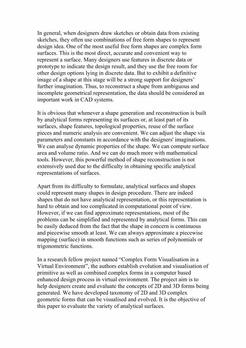
In general, when designers draw sketches or obtain data from existing sketches, they often use combinations of free form shapes to represent design idea. One of the most useful free form shapes are complex form surfaces. This is the most direct, accurate and convenient way to represent a surface. Many designers use features in discrete data or prototype to indicate the design result, and they use the free room for other design options lying in discrete data. But to exhibit a definitive image of a shape at this stage will be a strong support for designers’ further imagination. Thus, to reconstruct a shape from ambiguous and incomplete geometrical representation, the data should be considered an important work in CAD systems. It is obvious that whenever a shape generation and reconstruction is built by analytical forms representing its surfaces or, at least part of its surfaces, shape features, topological properties, reuse of the surface pieces and numeric analysis are convenient. We can adjust the shape via parameters and constants in accordance with the designers' imaginations. We can analyse dynamic properties of the shape. We can compute surface area and volume ratio. And we can do much more with mathematical tools. However, this powerful method of shape reconstruction is not extensively used due to the difficulty in obtaining specific analytical representations of surfaces. Apart from its difficulty to formulate, analytical surfaces and shapes could represent many shapes in design procedure. There are indeed shapes that do not have analytical representation, or this representation is hard to obtain and too complicated in computational point of view. However, if we can find approximate representations, most of the problems can be simplified and represented by analytical forms. This can be easily deduced from the fact that the shape in concern is continuous and piecewise smooth at least. We can always approximate a piecewise mapping (surface) in smooth functions such as series of polynomials or trigonometric functions. In a research fellow project named “Complex Form Visualisation in a Virtual Environment”, the authors establish evolution and visualisation of primitive as well as combined complex forms in a computer based enhanced design process in virtual environment. The project aim is to help designers create and evaluate the concepts of 2D and 3D forms being generated. We have developed taxonomy of 2D and 3D complex geometric forms that can be visualised and evolved. It is the objective of this paper to evaluate the variety of analytical surfaces.

But in applications, the most difficult problem of shape reconstruction and analytical representation lies in the fact that it is hard to obtain an analytical representation for given shapes, especially shapes in design process, which often has discrete nature and varies widely in category. This is partly because the set of analytic functions is too large and has numerous variations from algebraic and differential integral operations. Thus it will be difficult to define a restricted set of a function structure that can represent shapes in concern. There will be other problems apart from the function structure. One of these problems arising accordingly is the size of parameterization of shape data in order to obtain the analytical forms. This size will affect the main processes such as numeric analysis and approximation. In genetic programming, it is well known that convergence of genetic algorithm (GA) depends on the number of parameters. It has been established that the time complexity of serial GAs is of O(N×l) or O(N log N+N×l) depending on the selection scheme used, where N is the population size and l denotes the string length, which is deduced from the number of parameters. The purpose of this paper is to present a general analytic surface reconstruction method using GA combined with artificial neural networks (NNs) for shape design applications. We do not extract geometric primitives; however, a general kind of analytical formed surface can be reconstructed from a set of discrete data taken from the surface. In order to reconstruct the shape by functions, we should first construct a mathematical model which can be used to approximate the desired surfaces. This is done in Section 7. The second problem is to choose an appropriate algorithm for evolution. To do this, we construct a model using artificial NNs and GA together. There are two kinds of models mixing these two algorithms, see Section 3 for detail. The main idea here is to use NNs as a rapid optimizer for local weights, and to use GA for seeking global solutions in a large scope. To simplify the difficulty of restricting the size of large analytical function, we build a function hierarchy using some basic atom functions and operations. Then a relatively small set of data will reduce satisfactory result. Finally, examples of the theory in this paper with implementations are reported.

Related literature review There are some techniques proposed for extracting surfaces from incomplete digitized data (Milroy et al., 1997; Varady et al., 1997). They are grouped into two categories, namely edge-based and face-based (Varady et al., 1997). The first works by trying to find edge curves in the point data, and infer surfaces from the implicit segmentation provided by edge curves (Milroy et al., 1997). Techniques in the second category usually work by finding out points with similar properties, belonging to the same surface, with edges being derived by intersection or other computations from the surfaces. In a recent work on shape reconstruction, Ononye et al., 2001) in his dissertation presented an automatic algorithm which is able to recover surface shape under realistic illumination and surface reflectance conditions from single photographs. And Cheung (2001) gave a direct approach for 3D shape reconstruction from the irradiance data of an object. The direct shape from shading approach requires only three sets of independent iterative equations, which simplifies the implementation of real-time inspection tasks such as integrated circuit (IC) bond-ball shape computation. He used the maximum uphill principle stating that the high intensity value of an image corresponds to high depth level. To achieve this goal, a development of a self-organised NN for parallel implementation of the direct shading approach is presented, where the maximum uphill criteria, the iterative scheme and the momentum factor are mapped to the structure and the learning rules of the NN. Face-based techniques are more widely investigated as they work on a large number of points, in principle using all available data points. Deciding which points belong to which surface is a natural by-product of such techniques, whereas with edge-based techniques, it may not be entirely clear to which surface a given point belongs. Some surface extraction techniques are not aimed at CAD model reconstruction. Oshima and Shirai (1983) proposed a system to recognize stacked objects from range data. The basic idea of Oshima's system is to match the description of the scene (extracted from the range data) to some predefined models one at a time. Oshima's models are much like the conventional templates used for range image processing. Sullivan et al. (1994) proposed a method for constructing algebraic surface models from 2D and 3D images. These models are used in pose computation and object recognition.

In other works, some geometric primitive (straight line, curve, etc.) extraction methods using GA were investigated. Hill and Taylor (1992) proposed one of the earliest GA-based geometric primitive extraction methods. Their method is mainly aimed at extracting geometric primitives for 2D image interpretation. Subsequently, Hill and Taylor (1992) and Roth and Levine (1994) studied further GA-based geometric primitive extraction methods. Roth's method is efficient for geometric primitive extraction. But it requires the explicit expression of each geometric primitive that is to be extracted. In the field of approximating a real or complex function, there are numerous theoretical results. One basic theorem tells us that we can approximate a smooth function by polynomials or trigonometric polynomials, see Guo and Lakshmikantham (1988), Krashosel'skii and Zabreiko (1984) for more results on function approximation. Unfortunately, up to now there are no works relating to contriving analytical forms from discrete data. Usually, the structure of data and the shape represented correspond directly. In some models, see Taura et al. (1998), shapes are represented by a process that consisted of sets of rules which generate the shapes as they are executed, and the design feature of the shapes is indirectly held in the sets of rules. When integrating, two sets of rules combines two shapes represented by this model, the features of the shapes are preserved, and often exaggerated, in the combined shapes. There are already research works such as airfoil shapes (Marco and Lanteri, 2000), where the shape features are created based on the discretization of the shape, that is, parameterization of shapes is a point by point one. In order to obtain accurate results, the shape often has to be defined by a lot of points. The author employs a two-level strategy for the parallelization of a GA coupled to a compressible flow solver designed on unstructured triangular meshes. In some works, several authors have adopted other strategies. A widely used shape parameterization procedure is based on Bezier curves. A few control points are then chosen to represent the whole shape. Since the Bezier curves are smooth, non-smooth shapes will not appear from the crossover operator. On the other hand, Bezier curves have a useful convex hull property that restricts the curve to never leave the bounding polygon of the control points. The convex hull property is derived from the fact that a Bezier curve is a convex combination of the data points.

Although there is hardly any literature in the field of shape reconstruction, the idea of combining GAs and artificial NNs into applications to engineering problems has been a successful approach since many years. In a paper of modelling and controlling dynamical systems, Farag et al. (1998) use the approach combining the merits of the fuzzy logic theory, NNs and (GAs). Their model is presented in a fuzzy-neural network (FNN) form which can handle both quantitative (numerical) and qualitative (linguistic) knowledge. The authors propose a new algorithm and use this new algorithm to extract linguistic-fuzzy rules. Moreover, a multi-resolutional dynamic genetic algorithm (MRD-GA) is proposed and used for optimized tuning of membership functions of the proposed model. We can also find other works in applying GA and ANN in dynamical system. Petridis et al. (1998) introduced a hybrid neural-genetic multi-model parameter estimation algorithm. The main components of the algorithm are: a recurrent incremental credit assignment (ICRA) NN, which computes a credit function for each member of a generation of models, and a GA which uses the credit functions as selection probabilities for producing new generations of models. The NN and GA combination is applied to the task of finding the parameter values which minimize the total square output error. In another paper, Sangbong et al. (1995) investigated a neuro-controller for non-minimum phase system which is trained off-line with GA and is combined in parallel with a conventional linear controller of proportional plus integral plus derivative type. Training of this kind of a neuro-genetic controller provided a solution under a given global evaluation function which is devised based on the desired control performance, during the whole training time interval. Also, Hung and Adeli (1994) proposed an algorithm for the training of multilayer feedforward NNs by integrating a GA with an adaptive conjugate gradient NN learning algorithm. This algorithm has been applied to two different domains, engineering design and image recognition. Angeline et al. (1994), in their paper, argued that GAs are inappropriate for network acquisition and described an evolutionary program that simultaneously acquires both the structure and weights for recurrent networks. Regarding non-linear networks, Chen et al. (1999) presented a two-level learning method for radial basis function (RBF) networks. The key idea of this paper is that the regularization parameter and the RBF width are

optimized using a GA at the upper level. Whitehead (1996) and Whitehead and Choate (1996) applied a cooperative competitive GA to the evolution of RBF centres and widths. The set of genetic strings in one generation of the algorithm represents one RBF network, not a population of computing networks. In other control dynamic researches, Chin-Teng and Chong-Ping (1999) proposed a temporal difference (TD) and GA-based reinforcement (TDGAR) neural learning scheme for controlling chaotic dynamical systems based on the technique of small perturbations. The TDGAR learning scheme is a new hybrid GA, which integrates the TD prediction method and the GA to fulfill the reinforcement learning task. Kodjabachian and Meyer (1998) described the evolution of generating recurrent NNs that control the behaviour of simulated insects. Brill et al. (1992) described experiments using a GA for feature selection in the context of NN classifiers, specifically, counter-propagation network. There are also other works, see Maniezzo (1994), Mitra and Hayashi (2000) and Pattichis and Schizas (1996), for their attempt in providing an exhaustive survey of neuro-fuzzy rule generation algorithms. Moreover, Ngom et al. (2001) considered the problem of synthesizing multiple-valued logic functions by NNs, and the authors described a GA which finds the longest strip in. Most recently, Palaniappan et al. (2002) applied NNs to classify alcoholics and non-alcoholics by features extracted from visual evoked potential (VEP). They again used GAs to select the minimum number of channels that maximise classification performance. 3. Model construction 3.1 Surface geometric models A geometric model is an unambiguous and complete informational representation of a shape in a form that a computer can process. There are two popular solid model representations. One is constructive solid geometry (CSG) and the other is boundary representation. In CSG, an object is described in terms of elementary shapes (half-spaces) or primitives (bounded primitive solids), and complex solids are built by Boolean operations. In boundary representation, the mathematical data for the surface geometry are stored. A solid is represented as unions of faces, bounded by edges, which are bounded by vertices. In representing and reconstructing design models, we use the second model, that is, the boundary representation model. In this representation, surfaces will be represented by the mathematical data of the model

geometry. Changing the surfaces would be simply achieved by adding or subtracting the mathematical data. 3.2 Cell division model Cell division model is another approach and is based on the structure of a living creature. In nature, the shape of a living creature (phenotype) is constructed from the basic genetic information (genotype) to the cells and organisms. The genotype contains information that is the basic construction unit of everything, called the chromosome. Chromosomes form proteins and other large molecules. Chains of molecules form tissues and organs of the whole body. In the natural environment, development begins with the chromosome, which forms the base. Then a number of smaller cells are constructed. Large cells that resulted from joining and other operations form a multicellular structure. Thus the cell division models simply divide the whole into basic units and operations. 3.3 Jelly model Jelly model is derived from the cell model. Another layer called the jelly layer is added to represent a compounded structure. We will use this model to represent functions in various combinations. Basically, the model has three layers, that is, the gene layer, the cell layer and the jelly layer (Figure 1).

The above model is like the molecular structure in biology. Jellies play the role of large molecules, and are composed of cells. In a cell, there are

genes and other small molecules (jellies). The smallest unit in this chain is a gene that forms the base of the three structures. 3.4 Neural structure The neural structure establishes the interconnection of jelly structures. The structure has fitness-based sub-structure for evolutionary purpose, with general mechanisms for processing individuals in parallel, for adaptive individuals of new generation, or NN- based sub-systems for local minimisation of parameters, and for testing the effectiveness of existing population. The neural structure provides a framework in which a population of functions encoded as jelly strings evolves on the discrete data from design system. Fitness scheme in a neural structure form a population of individuals, which evolve over time. There are two basic types of neural structure used in this paper (Figures 2 and 3). One is called the GA-ANN structure, and the other is called the ANN-GA structure. In general, we apply the GA as a function optimiser to the weight space of the NNs system and we use backpropagation to minimize the local properties. Below are two model structures.

4. Geometric definitions and class structure In this section, we will first describe some geometric concepts and definitions for the purpose of representing spatial relations of geometric objects, and then we will describe the class structure used for building the surface reconstruction system. First we list some geometric concepts and definitions. In this paper, we use points to denote data from the design surfaces in the 3D space. A point is represented by its three coordinates x, y and z. Alternatively, we will use a complex number to represent x and y and denote it by (x+iy). We will use P0 to denote a particular point in the sample (data) space, and D to denote this space consisting of all the possible points from the design surface. Some of the important definitions used for this paper are given below.

General complex form surface. A surface in the 3D space represented by a two variable or complex variable function z=f(x,y)=f(x+iy). We will use S: F(x,y,z)=z−f(x,y)=0 to represent such a surface. Algebraic distance. The absolute value of F(P0) for a point P0 is defined as the algebraic distance between the point P0 and a surface S. Geometric distance. Minimum distance of a point P0 to a surface S, that is: ρ(P0,S)=infPSρ(P0,P), where

is the Euclidean distance. Pseudo geometric distance. The minimum Euclidean distance between a point P0 and a surface S along the x, y, z axes, that is,

where

It is clear that the pseudo geometric distance is larger or equal to the geometric distance. Thus we can deduce that if the pseudo geometric distance of a point to a surface is zero, then the point is on the surface. Now we present the class structure of functions used in this paper. First we define a class CGAGene. It is the construction unit of all functions concerned. The main structure of this class is type and chromosome. Data structure will include an unsigned integer and a double number. The unsigned integer will be divided into two units. The first 8 bits will indicate the type of the object, and the last 24 bits (in 32 bits machine) will denote the chromosome. The type of a CGAGene object will be one of the three: constants, operators and atom functions. In our applications, the constants will be a double number, the operators will include +, −, *, /, , and atom functions will include basic mathematical functions.

The second class is CGACell. A cell is an object constructed from genes and jelly that are objects of the third class. A cell is an united object in the function string. In the GA operations, a cell cannot be divided into separate parts. A cell will consist of brackets, atom function with its variable as a jelly. We will take a constant as a cell with num function. If the jelly is just a gene, then the cell will be the simplest cell consisting of a function with variable as a gene, normally a double number. The third class is CGAPoly. This is a stand-alone class for constructing polynomials. Although we can construct a polynomial by class CGAGene and CGACell, it is more convenient to define a class for its special purpose. The poly member variables will include order and coefficients. It will be a sub-type of jelly. The fourth class is CGAJelly. A jelly is a chain of cells joined by operators. Our last function will be in the form of jellys. Other data structures include CDataSample, CErr and CGAError. CGAError has dynamical structure at runtime level. Autotransformation of data coordinates performed in the data class CDataSample. Computation of fitness and error is in the class CGAError. The whole class structure is shown in Figure 4.

5. Genetic algorithms and genetic operators GAs are search algorithms based on the mechanisms of natural selection. They lie on one of the most important principles of Darwin: survival of the fittest. This technique uses a population of potential solutions represented by strings of binary digits, called chromosomes or individuals, that is submitted to many transformations, called genetic operations such as selection, crossover and mutation. The population evolves during the generations according to the fitness value of the individuals; when a stationary state is reached, the population converges to the solution of the given optimisation problem. GAs are different from normal optimisation procedures (e.g. steepest descent methods and artificial NNs) in many ways:

• they work with a coding of the parameter set and not the parameters themselves;

• they work simultaneously with a population of potential binary coded solutions, not only with one solution;

• they use probabilistic rules (the genetic operators are applied with probabilities) and not deterministic ones;

• they investigate in a search space componing a database of the solutions, which implies that they cannot fall into a local optimum.

The main concern related to the use of GAs for shape design is the accurate evaluation of a design instance, while not leading to unacceptable computing time compared with more classical algorithms. In addition, hard problems need bigger populations and long chromosome strings. However, it is a widely accepted position that GAs can be effectively parallelized and can in principle take full advantage of (massively) parallel computer architectures. This is because within a generation (iteration) of the algorithm, the fitness values associated to each individual of the population can be evaluated in parallel. The basic structure of a GA consists of the following steps: (1) initialize randomly a population of individuals; (2) evaluate the individuals following their fitness (cost functional) value; (3) apply genetic operators (crossover and mutation) to the population and go to step (2) until the best individual is reached. The selection process is based on a tournament approach while the crossover operator is needed to increase diversity among the population.

Crossover proceeds in two steps. First, strings of the newly reproduced population are mated at random; this crossover operation is made with a probability. Second, each pair of strings undergoes crossing-over as follows: an integer position k along the string is selected uniformly at random in [1, l−1], where l is the string length of the chromosomes and two new strings are created by swapping all characters between positions (k+1) and l inclusively. These two new strings replace their parents in the population. Now we describe the genetic operators used in this paper. The main genetic operators are crossover and mutation. Crossover operator will be in the following three forms: (1) jelly cross, (2) cell cross, and (3) gene cross. A jelly cross is performed in the jelly string. It swaps two jellies at a certain point. Swapping points of two jellies can be different. Notice that we do not breakdown cells in this kind of cross operation. A simple diagram of this kind of cross is shown in Figure 5.

In Figure 5, the cross over operation takes place in a certain position of the jellies, and they swap the latter part of their bodies. Since the length of the two jellies can be different, the breaking points of the two can vary. The second crossover operation is cell cross. A cell is a function with variable as a jelly. If there is a num function, then the cell becomes a united jelly. If the jelly becomes a gene, then the cell is the simplest cell. Cell operations work in the jelly part as above. In the cell cross operation level, we do not distinguish between jellies and genes, and we always take them as units. By swapping their jellies, a large cell can become a small cell and vice versa (Figure 6).

The third crossover operation is the gene cross. On the gene level, cross operation takes place in three types, namely numbers, atom functions and operators. For real (float, double) numbers cross operation we use binary coding schema and a function type of crossover. One such function can be shown as follows:

In the case of atom functions and operators crossover, a string based coding schema is applied. Then the cross operation swaps the corresponding codes. The last problem is the fitness computation and evaluation. In our applications, the fitness function can be taken as just the pseudo-geometric distance. Then the evaluation is taken by the least pseudo-geometric distance selection. 6. Artificial neural networks NNs which are capable of learning relationships from data, represent a class of robust, non-linear models inspired by the neural architecture of the human brain. This is due to their ability to learn mappings from a set of inputs to a set of outputs based on training examples and to generalize beyond the examples learnt. The process of developing a NN model for a particular application usually involves four basic stages. First, a network developer selects a problem domain, such as contractor prequalification, based on his or her theoretical, empirical, or applied interests. Next, a network architecture is designed for capturing the underlying criteria from the problem domain. This architecture forms the configuration of the network including the

number of units used, their organisation into layers, learning parameters, and error tolerance. Third, given this chosen architecture and a chosen task, a learning paradigm such as backpropagation is applied to train the network and develop the interconnection weights. Finally, the developer evaluates the trained network according to objective performance measures such as its ability to solve the specified task and its ability to predict the outcome of unseen cases. It has been shown that NNs of appropriate structure can be used as a function optimiser or approximator at any accurate level, provided the network has been sufficiently trained. Thus we can use NNs as a searching algorithm in local mode, while we apply GA as a global optimiser. Now we describe the neural structure used in this paper.

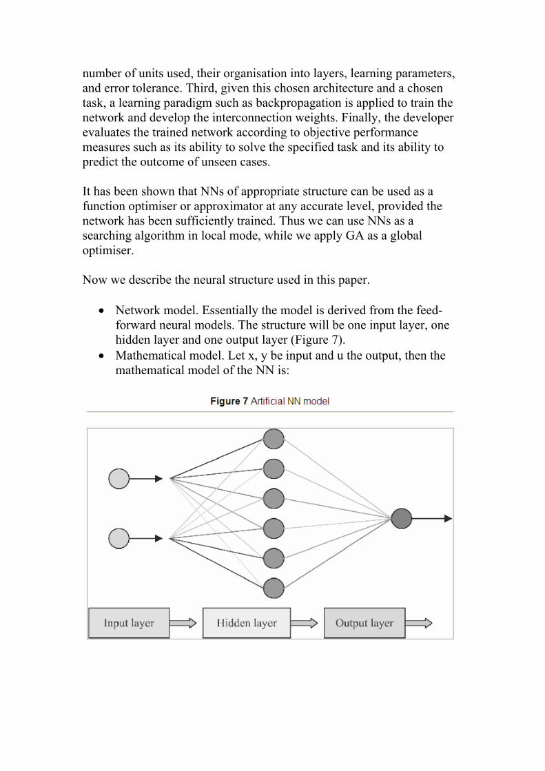
• Network model. Essentially the model is derived from the feed-forward neural models. The structure will be one input layer, one hidden layer and one output layer (Figure 7).

• Mathematical model. Let x, y be input and u the output, then the mathematical model of the NN is:

where FA(x,y) denotes the non-linear mapping, β(x,y) the initial function, δ(x,y) a coefficient multiplier, A the computing (weights) matrix, and f→(x,y) the vector seeds. In some applications, we can take these seeds as the polynomial of order n, or the sine of polynomials, while we take the dimension of matrix A as n×1, that is, f→(x,y) has the following form. Equation 6

In the above expressions, the variable z=x+iy is a complex number, and the operator denotes some operation to change the complex value to real value. The most common of these operations are taking real, imaginary parts or abstract value. Choosing vector seeds f→(x,y) can affect the properties of the networks significantly. In general, the components of this seeds should be orthogonal functions, or linearly independent which can form or generate a standard base of an appropriate function space. Suppose the components of f→(x,y) is ek(z), that is

then we can use the function seeds and NNs to approximate any smooth non-linear mapping. A general result will be as follows.

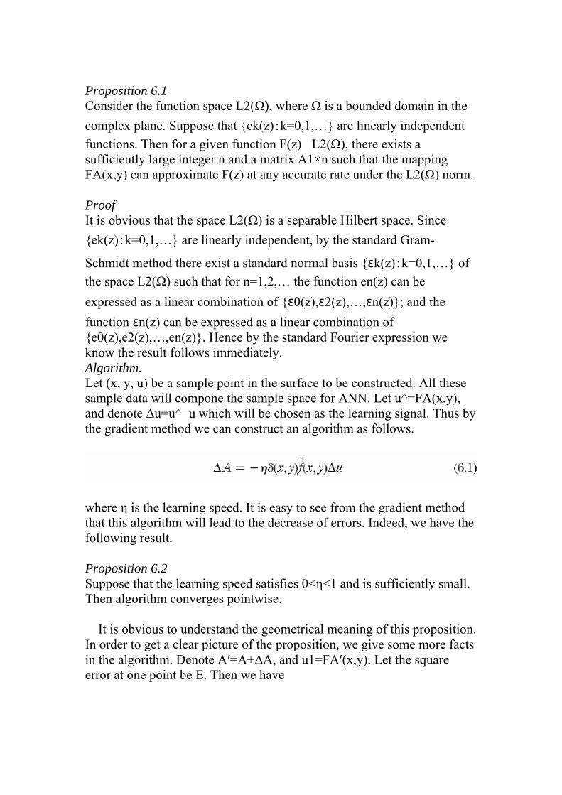
Proposition 6.1 Consider the function space L2(Ω), where Ω is a bounded domain in the complex plane. Suppose that ek(z) : k=0,1,… are linearly independent functions. Then for a given function F(z)L2(Ω), there exists a sufficiently large integer n and a matrix A1×n such that the mapping FA(x,y) can approximate F(z) at any accurate rate under the L2(Ω) norm. Proof It is obvious that the space L2(Ω) is a separable Hilbert space. Since ek(z) : k=0,1,… are linearly independent, by the standard Gram-

Schmidt method there exist a standard normal basis ɛk(z) : k=0,1,… of the space L2(Ω) such that for n=1,2,… the function en(z) can be expressed as a linear combination of ɛ0(z),ɛ2(z),…,ɛn(z); and the function ɛn(z) can be expressed as a linear combination of e0(z),e2(z),…,en(z). Hence by the standard Fourier expression we know the result follows immediately. Algorithm. Let (x, y, u) be a sample point in the surface to be constructed. All these sample data will compone the sample space for ANN. Let u^=FA(x,y), and denote Δu=u^−u which will be chosen as the learning signal. Thus by the gradient method we can construct an algorithm as follows.

where η is the learning speed. It is easy to see from the gradient method that this algorithm will lead to the decrease of errors. Indeed, we have the following result. Proposition 6.2 Suppose that the learning speed satisfies 0<η<1 and is sufficiently small. Then algorithm converges pointwise. It is obvious to understand the geometrical meaning of this proposition. In order to get a clear picture of the proposition, we give some more facts in the algorithm. Denote A′=A+ΔA, and u1=FA′(x,y). Let the square error at one point be E. Then we have

By the gradient method we obtain

Thus we can obtain the following relations by direct computation.

Let Δu′=u1−u be the new error at the point (x,y,u), then we have

It is observed that the new value u1 will change towards the direction of the ideal value u. That is indeed what the proposition says. 7. Application models We build an application model from the above theory. The user interface is shown in Figures 8 and 9. .

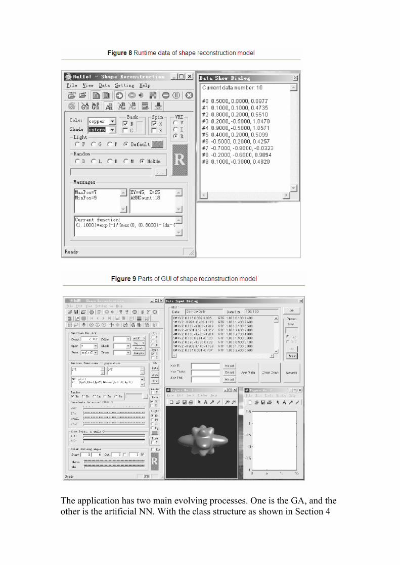
The application has two main evolving processes. One is the GA, and the other is the artificial NN. With the class structure as shown in Section 4

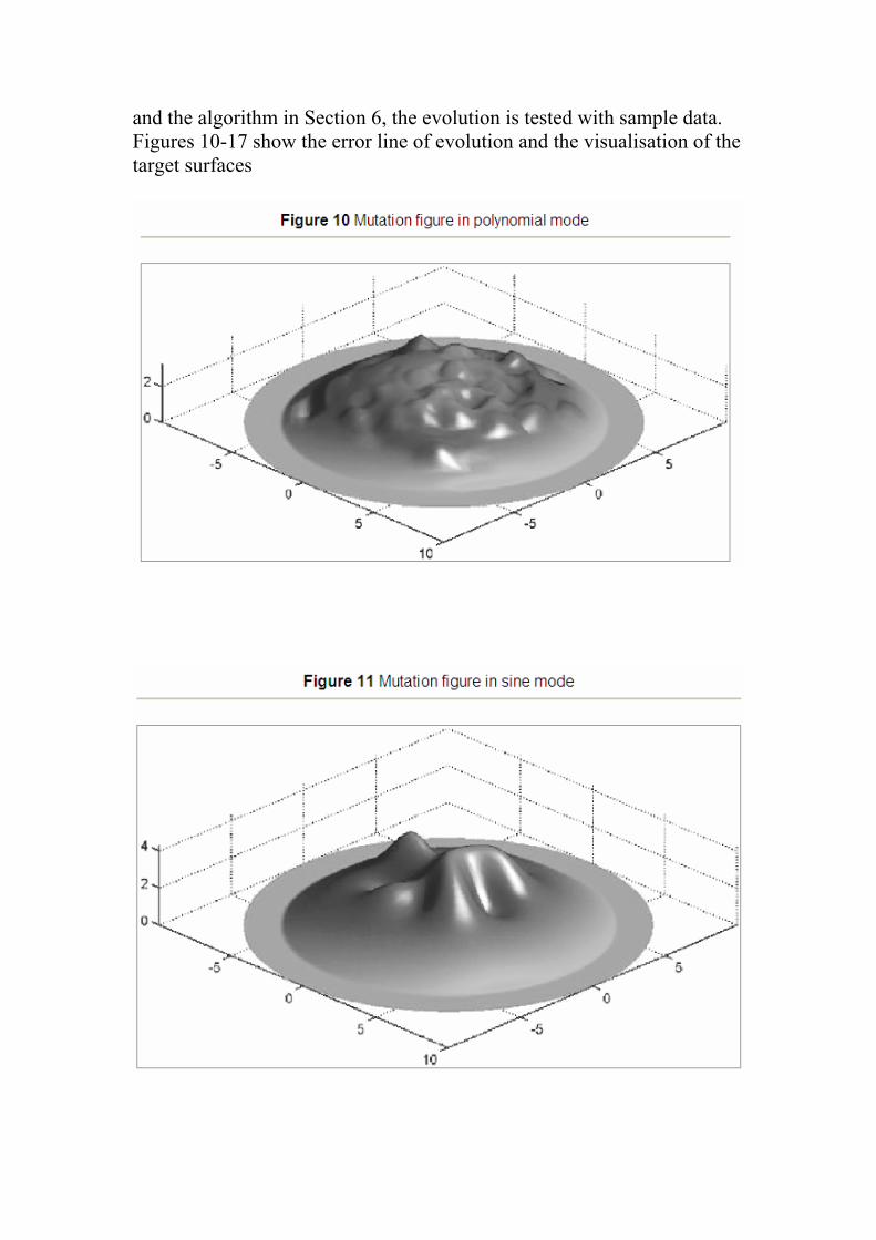
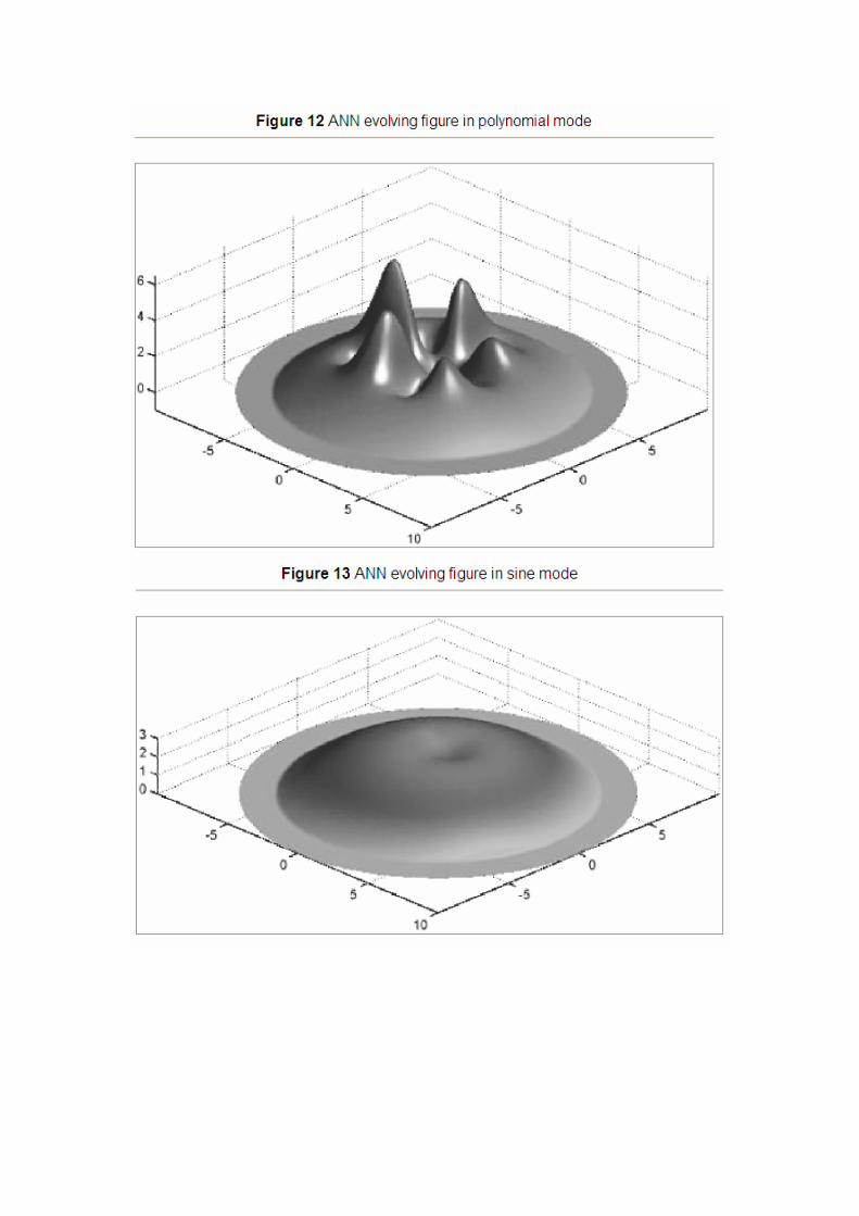
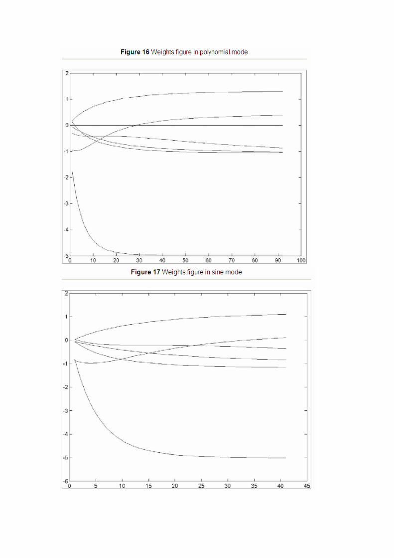
and the algorithm in Section 6, the evolution is tested with sample data. Figures 10-17 show the error line of evolution and the visualisation of the target surfaces

In the above example, we use the following sample population data

We use the following function to construct the target function

Where

and m_fMatrix is the weight matrix of NNs and PowerReal( ) is the polynomial. For more information, please visit http://people.sd.polyu.edu.hk/sdxyliu for visualisation of complex functions and applications in solid modelling. References Angeline, P.J., Saunders, G.M., Pollack, J.B. (1994), "An evolutionary algorithm that constructs recurrent neural networks", IEEE Transactions on Neural Networks, Vol. 5 No.1, pp.54–65. Brill, F.Z., Brown, D.E., Martin, W.N. (1992), "Fast generic selection of features for neural network classifiers", IEEE Transactions on Neural Networks, Vol. 3 No.2, pp.324–8. Chen, S., Wu, Y., Luk, B.L. (1999), "Combined genetic algorithm optimization and regularized orthogonal least squares learning for radial basis function networks", IEEE Transactions on Neural Networks, Vol. 10 No.5, pp.1239–43. Cheung, W. (1992), "Three-dimensional object shape computation based on irradiation data", The Hong Kong Polytechnic University, . Chin-Teng, L., Chong-Ping, J. (1999), "Controlling chaos by GA-based reinforcement learning neural network", IEEE Transactions on Neural Networks, Vol. 10 No.4, pp.846–59.

Farag, W.A., Quintana, V.H., Lambert-Torres, G. (1998), "A genetic-based neuro-fuzzy approach for modeling and control of dynamical systems", IEEE Transactions on Neural Networks, Vol. 9 No.5, pp.756–67. Guo, D., Lakshmikantham (1988), Nonlinear Problems in Abstract Cones, Academic Press, Orlando, FL, . Hill, A., Taylor, C.J. (1992), "Model-based image interpretation using genetic algorithms", Image and Vision Computing, Vol. 10 pp.295–300. Hung, S.L., Adeli, H. (1994), "A parallel genetic/neural network learning algorithm for MIMD shared memory machines", IEEE Transactions on Neural Networks, Vol. 5 No.6, pp.900–9. Kodjabachian, J., Meyer, J.-A. (1998), "Evolution and development of neural controllers for locomotion, gradient-following, and obstacle-avoidance in artificial insects", IEEE Transactions on Neural Networks, Vol. 9 No.5, pp.796–812. Krasnosel'skii, M.A., Zabreiko, P.P. (1984), Geometrical Methods of Nonlinear Analysis, Springer-Verlag, New York, . Maniezzo, V. (1994), "Genetic evolution of the topology and weight distribution of neural networks", IEEE Transactions on Neural Networks, Vol. 5 No.1, pp.39–53. Marco, N., Lanteri, S. (2000), "A two-level parallelization strategy for genetic algorithms applied to optimum shape design", Parallel Computing, Vol. 26 No.4, pp.377–97.

Milroy, M.J., Bradley, C., Vickers, G.W. (1997), "Segmentation of a wrap-around model using an active contour", Computer-Aided Design, Vol. 29 pp.299–320. Mitra, S., Hayashi, Y. (2000), "Neuro-fuzzy rule generation: survey in soft computing framework", IEEE Transactions on Neural Networks, Vol. 11 No.3, pp.748–68. Ngom, A., Stojmenovic, I., Milutinovic, V. (2001), "STRIP - a strip-based neural-network growth algorithm for learning multiple-valued functions", IEEE Transactions on Neural Networks, Vol. 12 No.2, pp.212–27. Ononye, A.H.E. (2001), "Color image-based shape reconstruction of multi-color objects under general illumination conditions", The University of Tennessee, . Oshima, M., Shirai, Y. (1983), "Object recognition using three-dimensional information", IEEE Trans. Pattern Anal. Machine Intell., Vol. 5 No.4, pp.353–61. Palaniappan, R., Raveendran, P., Omatu, S. (2002), "VEP optimal channel selection using genetic algorithm for neural network classification of alcoholics", IEEE Transactions on Neural Networks, Vol. 13 No.2, pp.486–91. Pattichis, C.S., Schizas, C.N. (1996), "Genetics-based machine learning for the assessment of certain neuromuscular disorders", IEEE Transactions on Neural Networks, Vol. 7 No.2, pp.427–39. Petridis, V., Paterakis, E., Kehagias, A. (1998), "A hybrid neural-genetic multimodel parameter estimation algorithm", IEEE Transactions on Neural Networks, Vol. 9 No.5, pp.862–76.

Roth, G., Levine, M.D. (1994), "Geometric primitive extraction using a genetic algorithm", IEEE Trans. Pattern Anal. Machine Intell., Vol. 16 No.9, pp.901–5. Sangbong, P., Lae-Jeong, P., Cheol Hoon, P. (1995), "A neuro-genetic controller for nonminimum phase systems", IEEE Transactions on Neural Networks, Vol. 6 No.5, pp.1297–300. Sullivan, S., Sandford, L., Ponce, J. (1994), "Using geometric distance fits for 3-D object modeling and recognition", IEEE Trans. Pattern Anal. Machine Intel., Vol. 16 No.12, pp.1183–96. Taura, Tl., Nagasaka, I., Yamagishi, A. (1998), "Application of evolutionary programming to shape design", Computer-Aided Design, Vol. 30 No.1, pp.29–35. Varady, T., Martin, R.R., Cox, J. (1997), "Reverse engineering of geometric models – an introduction", Computer-Aided Design, Vol. 29 No.4, pp.255–68. Whitehead, B.A. (1996), "Genetic evolution of radial basis function coverage using orthogonal niches", IEEE Transactions on Neural Networks, Vol. 7 No.6, pp.1525–8. Whitehead, B.A., Choate, T.D. (1996), "Cooperative-competitive genetic evolution of radial basis function centers and widths for time series prediction", IEEE Transactions on Neural Networks, Vol. 7 No.4, pp.869–80. Further Reading Fitzgibbon, A.W., Eggert, D.W., Fisher, R.B. (1997), "High-level CAD model acquisition from range images", Computer-Aided Design, Vol. 29 No.4, pp.321–30.

Goldberg, D.E. (1989), Genetic Algorithms in Search Optimization and Machine Learning, Addison-Wesley, Reading, MA, . Ku, K.W.C., Man, W.M., Wan, C.S. (1999), "Adding learning to cellular genetic algorithms for training recurrent neural networks", IEEE Transactions on Neural Networks, Vol. 10 No.2, pp.239–52. Muhlenbein, H., Schomisch, M., Born, J. (1991), "The parallel genetic algorithm as function optimizer", Parallel Comput., Vol. 17 pp.619–32. Roth, G., Levine, M.D. (1993), "Extracting geometric primitives", CVGIP: Image Understanding, Vol. 58 No.1, pp.1–22. Van Leer, B. (1979), "Towards the ultimate conservative difference scheme V: a second-order sequel to Godunov's method", J. Comp. Phys., Vol. 32 pp.361–70. Zitar, R.A., Hassoun, M.H. (1995), "Neurocontrollers trained with rules extracted by a genetic assisted reinforcement learning system", IEEE Transactions on Neural Networks, Vol. 6 No.4, pp.859–79. Acknowledgements The authors would like to express their gratitude to the School of Design of the Hong Kong Polytechnic University for its support under the Research Fellow Matching Fund Scheme 2001 (No. G.YY.34) and the Young Scientist Award Foundation of Shandong Province. We would also like to thank the Design Technology Research Centre of the Hong Kong Polytechnic University for their help and support in the project.